Data Scientists Guide To Apache Spark
Data-Scientists-Guide-to-Apache-Spark
Data-Scientists-Guide-to-Apache-Spark
Data-Scientists-Guide-to-Apache-Spark
Data-Scientists-Guide-to-Apache-Spark
Data-Scientists-Guide-to-Apache-Spark
User Manual:
Open the PDF directly: View PDF ![]() .
.
Page Count: 100


22
Apache Spark has seen immense growth over the past
several years. The size and scale of Spark Summit 2017 is
a true reflection of innovation aer innovation that has
made itself into the Apache Spark project. Databricks
is proud to share excerpts from the upcoming book,
Spark: The Definitive Guide. Enjoy this free preview copy,
courtesy of Databricks.
Preface

3
Now that we took our history lesson on Apache Spark, it’s time to start using it and applying it! This chapter will
present a gentle introduction to Spark - we will walk through the core architecture of a cluster, Spark Application,
and Spark’s Structured APIs using DataFrames and SQL. Along the way we will touch on Spark’s core terminology
and concepts so that you are empowered start using Spark right away. Let’s get started with some basic background
terminology and concepts.
Spark’s Basic Architecture
Typically when you think of a "computer" you think about one machine sitting on your desk at home or at work. This
machine works perfectly well for watching movies or working with spreadsheet soware. However, as many users
likely experience at some point, there are some things that your computer is not powerful enough to perform. One
particularly challenging area is data processing. Single machines do not have enough power and resources to perform
computations on huge amounts of information (or the user may not have time to wait for the computation to finish).
A cluster, or group of machines, pools the resources of many machines together allowing us to use all the cumulative
resources as if they were one. Now a group of machines alone is not powerful, you need a framework to coordinate
work across them. Spark is a tool for just that, managing and coordinating the execution of tasks on data across a
cluster of computers.
The cluster of machines that Spark will leverage to execute tasks will be managed by a cluster manager like Spark’s
Standalone cluster manager, YARN, or Mesos. We then submit Spark Applications to these cluster managers which will
grant resources to our application so that we can complete our work.
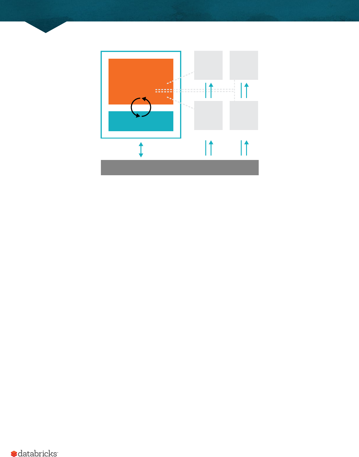
Spark Applications
Spark Applications consist of a driver process and a set of executor processes. The driver process runs your main()
function, sits on a node in the cluster, and is responsible for three things: maintaining information about the Spark
Application; responding to a user’s program or input; and analyzing, distributing, and scheduling work across the
executors (defined momentarily). The driver process is absolutely essential - it’s the heart of a Spark Application and
maintains all relevant information during the lifetime of the application.
The executors are responsible for actually executing the work that the driver assigns them. This means, each
executor is responsible for only two things: executing code assigned to it by the driver and reporting the state of the
computation, on that executor, back to the driver node.
A Gentle Introduction to Spark
4
The cluster manager controls physical machines and allocates resources to Spark Applications. This can be one of
several core cluster managers: Spark’s standalone cluster manager, YARN, or Mesos. This means that there can be
multiple Spark Applications running on a cluster at the same time. We will talk more in depth about cluster managers
in Part IV: Production Applications of this book.
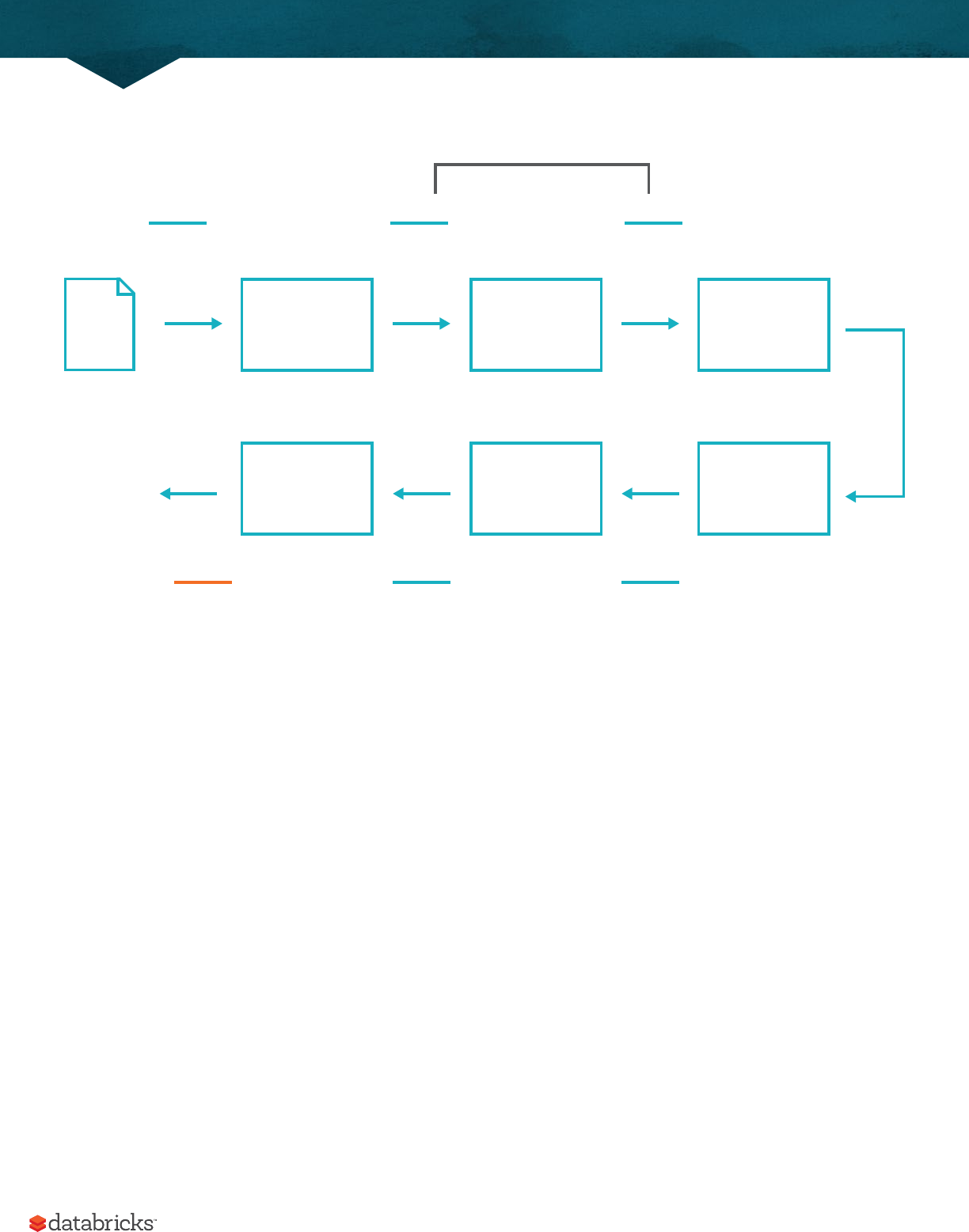
In the previous illustration we see on the le, our driver and on the right the four executors on the right. In this
diagram, we removed the concept of cluster nodes. The user can specify how many executors should fall on each node
through configurations.
NOTE
Spark, in addition to its cluster mode, also has a local mode. The driver and executors are simply processes, this
means that they can live on the same machine or dierent machines. In local mode, these both run (as threads) on
your individual computer instead of a cluster. We wrote this book with local mode in mind, so everything should be
runnable on a single machine.
As a short review of Spark Applications, the key points to understand at this point are that:
• Spark has some cluster manager that maintains an understanding of the resources available.
• The driver process is responsible for executing our driver program’s commands accross the executors in order to
complete our task.
Now while our executors, for the most part, will always be running Spark code. Our driver can be "driven" from a
number of dierent languages through Spark’s Language APIs.
Driver Process Executors
User Code
Spark Session
Cluster Manager
A Gentle Introduction to Spark

5
Spark’s Language APIs
Spark’s language APIs allow you to run Spark code from other langauges. For the most part, Spark presents some core
"concepts" in every language and these concepts are translated into Spark code that runs on the cluster of machines.
If you use the Structured APIs (Part II of this book), you can expect all languages to have the same performance
characteristics.
NOTE
This is a bit more nuanced than we are letting on at this point but for now, it’s the right amount of information for new
users. In Part II of this book, we’ll dive into the details of how this actually works.
Scala
Spark is primarily written in Scala, making it Spark’s "default" language. This book will include Scala code examples
wherever relevant.
Java
Even though Spark is written in Scala, Spark’s authors have been careful to ensure that you can write Spark code in
Java. This book will focus primarily on Scala but will provide Java examples where relevant.
Python
Python supports nearly all constructs that Scala supports. This book will include Python code examples whenever we
include Scala code examples and a Python API exists.
SQL
Spark supports ANSI SQL 2003 standard. This makes it easy for analysts and non-programmers to leverage the big
data powers of Spark. This book will include SQL code examples wherever relevant
R
Spark has two commonly used R libraries, one as a part of Spark core (SparkR) and another as a R community driven
package (sparklyr). We will cover these two dierent integrations in Part VII: Ecosystem.
A Gentle Introduction to Spark
6
Here’s a simple illustration of this relationship.
Each language API will maintain the same core concepts that we described above. There is a SparkSession available to
the user, the SparkSession will be the entrance point to running Spark code. When using Spark from a Python or R, the
user never writes explicit JVM instructions, but instead writes Python and R code that Spark will translate into code
that Spark can then run on the executor JVMs.
Spark’s APIs
While Spark is available from a variety of languages, what Spark makes available in those languages is worth
mentioning. Spark has two fundamental sets of APIs: the low level "Unstructured" APIs and the higher level Structured
APIs. We discuss both in this book but these introductory chapters will focus primarily on the higher level APIs.
Starting Spark
Thus far we covered the basic concepts of Spark Applications. This has all been conceptual in nature. When we
actually go about writing our Spark Application, we are going to need a way to send user commands and data to the
Spark Application. We do that with a SparkSession.
A Gentle Introduction to Spark
JVM
User Code
To Executors
Spark Session
Spark Application

7
NOTE
To do this we will start Spark’s local mode, just like we did in the previous chapter. This means running ./bin/
spark-shell to access the Scala console to start an interactive session. You can also start Python console with
./bin/pyspark. This starts an interactive Spark Application. There is also a process for submitting standalone
applications to Spark called spark-submit where you can submit a precompiled application to Spark. We’ll show
you how to do that in the next chapter.
When we start Spark in this interactive mode, we implicitly create a SparkSession which manages the Spark
Application. When we start it through a job submission, we must go about creating it or accessing it.
The SparkSession
As discussed in the beginning of this chapter, we control our Spark Application through a driver process. This driver
process manifests itself to the user as an object called the SparkSession. The SparkSession instance is the way
Spark executes user-defined manipulations across the cluster. There is a one to one correspondance between a
SparkSession and a Spark Application. In Scala and Python the variable is available as spark when you start up the
console. Let’s go ahead and look at the SparkSession in both Scala and/or Python.
spark
In Scala, you should see something like:
res0: org.apache.spark.sql.SparkSession = org.apache.spark.sql.SparkSession@27159a24
In Python you’ll see something like:
<pyspark.sql.session.SparkSession at 0x7efda4c1ccd0>
Let’s now perform the simple task of creating a range of numbers. This range of numbers is just like a named column
in a spreadsheet.
%scala
val myRange = spark.range(1000).toDF("number")
%python
myRange = spark.range(1000).toDF("number")
You just ran your first Spark code! We created a DataFrame with one column containing 1000 rows with values from
0 to 999. This range of number represents a distributed collection. When run on a cluster, each part of this range of
numbers exists on a dierent executor. This is a Spark DataFrame.
A Gentle Introduction to Spark
8
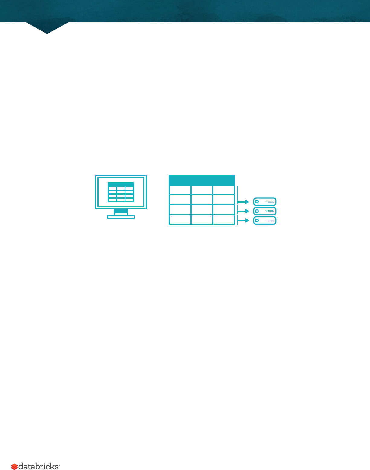
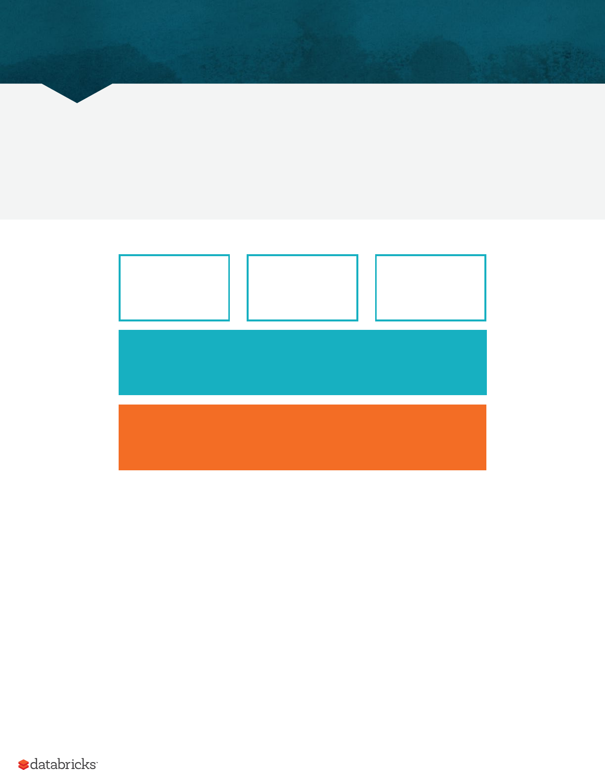
DataFrames
A DataFrame is the most common Structured API and simply represents a table of data with rows and columns. The
list of columns and the types in those columns the schema. A simple analogy would be a spreadsheet with named
columns. The fundamental dierence is that while a spreadsheet sits on one computer in one specific location, a
Spark DataFrame can span thousands of computers. The reason for putting the data on more than one computer
should be intuitive: either the data is too large to fit on one machine or it would simply take too long to perform that
computation on one machine.
The DataFrame concept is not unique to Spark. R and Python both have similar concepts. However, Python/R
DataFrames (with some exceptions) exist on one machine rather than multiple machines. This limits what you can do
with a given DataFrame in python and R to the resources that exist on that specific machine. However, since Spark
has language interfaces for both Python and R, it’s quite easy to convert to Pandas (Python) DataFrames to Spark
DataFrames and R DataFrames to Spark DataFrames (in R).
NOTE
Spark has several core abstractions: Datasets, DataFrames, SQL Tables, and Resilient Distributed Datasets (RDDs).
These abstractions all represent distributed collections of data however they have dierent interfaces for working
with that data. The easiest and most eicient are DataFrames, which are available in all languages. We cover
Datasets at the end of Part II and RDDs in Part III of this book. The following concepts apply to all of the
core abstractions.
Table or DataFrame partitioned
across servers in data center
Spreadsheet on a
single machine
A Gentle Introduction to Spark

9
Partitions
In order to allow every executor to perform work in parallel, Spark breaks up the data into chunks, called partitions. A
partition is a collection of rows that sit on one physical machine in our cluster. A DataFrame’s partitions represent how
the data is physically distributed across your cluster of machines during execution. If you have one partition, Spark
will only have a parallelism of one even if you have thousands of executors. If you have many partitions, but only one
executor Spark will still only have a parallelism of one because there is only one computation resource.
An important thing to note, is that with DataFrames, we do not (for the most part) manipulate partitions manually
(on an individual basis). We simply specify high level transformations of data in the physical partitions and Spark
determines how this work will actually execute on the cluster. Lower level APIs do exist (via the Resilient Distributed
Datasets interface) and we cover those in Part III of this book.
Transformations
In Spark, the core data structures are immutable meaning they cannot be changed once created. This might seem like
a strange concept at first, if you cannot change it, how are you supposed to use it? In order to "change" a DataFrame
you will have to instruct Spark how you would like to modify the DataFrame you have into the one that you want.
These instructions are called transformations. Let’s perform a simple transformation to find all even numbers in our
currentDataFrame.
%scala
val divisBy2 = myRange.where("number % 2 = 0")
%python
divisBy2 = myRange.where("number % 2 = 0")
You will notice that these return no output, that’s because we only specified an abstract transformation and Spark
will not act on transformations until we call an action, discussed shortly. Transformations are the core of how you
will be expressing your business logic using Spark. There are two types of transformations, those that specify narrow
dependencies and those that specify wide dependencies.
Transformations consisting of narrow dependenciess (we’ll call them narrow transformations) are those where each
input partition will contribute to only one output partition. In the preceding code snippet, our where statement
specifies a narrow dependency, where only one partition contributes to at most one output partition.
A Gentle Introduction to Spark

10
A wide dependency (or wide transformation) style transformation will have input partitions contributing to many
output partitions. You will oen hear this referred to as a shule where Spark will exchange partitions across the
cluster. With narrow transformations, Spark will automatically perform an operation called pipelining on narrow
dependencies, this means that if we specify multiple filters on DataFrames they’ll all be performed in-memory. The
same cannot be said for shules. When we perform a shule, Spark will write the results to disk. You’ll see lots of talks
about shule optimization across the web because it’s an important topic but for now all you need to understand are
that there are two kinds of transformations.
We now see how transformations are simply ways of specifying dierent series of data manipulation. This leads us to
a topic called lazy evaluation.
Narrow Transformations
1 to 1
Wide Transformations (shues)
1 to 1
A Gentle Introduction to Spark

11
Lazy Evaluation
Lazy evaulation means that Spark will wait until the very last moment to execute the graph of computation
instructions. In Spark, instead of modifying the data immediately when we express some operation, we build up
a plan of transformations that we would like to apply to our source data. Spark, by waiting until the last minute to
execute the code, will compile this plan from your raw, DataFrame transformations, to an eicient physical plan that
will run as eiciently as possible across the cluster. This provides immense benefits to the end user because Spark
can optimize the entire data flow from end to end. An example of this is something called "predicate pushdown" on
DataFrames. If we build a large Spark job but specify a filter at the end that only requires us to fetch one row from
our source data, the most eicient way to execute this is to access the single record that we need. Spark will actually
optimize this for us by pushing the filter down automatically.
Actions
Transformations allow us to build up our logical transformation plan. To trigger the computation, we run an action. An
action instructs Spark to compute a result from a series of transformations. The simplest action is count which gives
us the total number of records in the DataFrame.
divisBy2.count()
We now see a result! There are 500 number divisible by two from o to 999 (big surprise!). Now count is not the only
action. There are three kinds of actions:
• actions to view data in the console;
• actions to collect data to native objects in the respective language;
• and actions to write to output data sources.
In specifying our action, we started a Spark job that runs our filter transformation (a narrow transformation), then an
aggregation (a wide transformation) that performs the counts on a per partition basis, then a collect with brings our
result to a native object in the respective language. We can see all of this by inspecting the Spark UI, a tool included in
Spark that allows us to monitor the Spark jobs running on a cluster.
Spark UI
During Spark’s execution of the previous code block, users can monitor the progress of their job through the Spark UI.
The Spark UI is available on port 4040 of the driver node. If you are running in local mode this will just be the
http://localhost:4040. The Spark UI maintains information on the state of our Spark jobs, environment, and
A Gentle Introduction to Spark

12
cluster state. It’s very useful, especially for tuning and debugging. In this case, we can see one Spark job with two
stages and nine tasks were executed.
This chapter avoids the details of Spark jobs and the Spark UI, we cover the Spark UI in detail in Part IV: Production
Applications. At this point you should understand that a Spark job represents a set of transformations triggered by an
individual action and we can monitor that from the Spark UI.
An End to End Example
In the previous example, we created a DataFrame of a range of numbers; not exactly groundbreaking big data. In
this section we will reinforce everything we learned previously in this chapter with a worked example and explaining
step by step what is happening under the hood. We’ll be using some flight data available here from the United States
Bureau of Transportation statistics.
Inside of the CSV folder linked above, you’ll see that we have a number of files. You will also notice a number of other
folders with dierent file formats that we will discuss in Part II: Reading and Writing data. We will focus on the CSV
files.
Each file has a number of rows inside of it. Now these files are CSV files, meaning that they’re a semi-structured data
format with a row in the file representing a row in our future DataFrame.
$ head /mnt/defg/ight-data/csv/2015-summary.csv
DEST_COUNTRY_NAME,ORIGIN_COUNTRY_NAME,count
United States,Romania,15
United States,Croatia,1
United States,Ireland,344
A Gentle Introduction to Spark

13
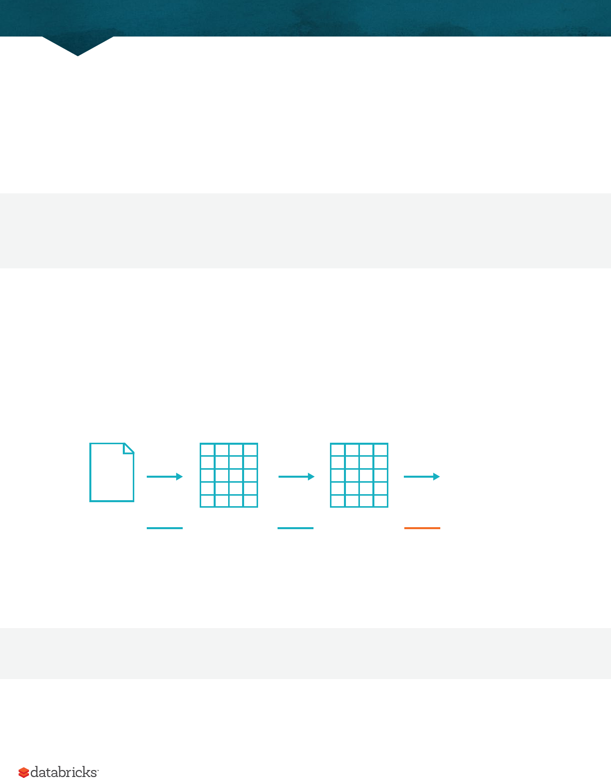
Spark includes the ability to read and write from a large number of data sources. In order to read this data in, we will use
a DataFrameReader that is associated with our SparkSession. In doing so, we will specify the file format as well as any
options we want to specify. In our case, we want to do something called schema inference, we want Spark to take a best
guess at what the schema of our DataFrame should be. The reason for this is that CSV files are not completely structured
data formats. We also want to specify that the first row is the header in the file, we’ll specify that as an option too.
To get this information Spark will read in a little bit of the data and then attempt to parse the types in those rows
according to the types available in Spark. You’ll see that this works just fine. We also have the option of strictly
specifying a schema when we read in data (which we recommend in production scenarios).
%scala
val ightData2015 = spark
.read
.option("inferSchema", "true")
.option("header", "true")
.csv("/mnt/defg/ight-data/csv/2015-summary.csv")
%python
ightData2015 = spark\
.read\
.option("inferSchema", "true")\
.option("header", "true")\
.csv("/mnt/defg/ight-data/csv/2015-summary.csv")
CSV file
Read
DataFrame
Take (N)
Array(Row(...),Row(...))
A Gentle Introduction to Spark
14
Each of these DataFrames (in Scala and Python) each have a set of columns with an unspecified number of rows.
The reason the number of rows is "unspecified" is because reading data is a transformation, and is therefore a lazy
operation. Spark only peeked at a couple of rows of data to try to guess what types each column should be.
If we perform the take action on the DataFrame, we will be able to see the same results that we saw before when we
used the command line.
ightData2015.take(3)
Array([United States,Romania,15], [United States,Croatia...
Let’s specify some more transformations! Now we will sort our data according to the count column which is an
integer type.
NOTE
Remember, the sort does not modify the DataFrame. We use the sort is a transformation that returns a new
DataFrame by transforming the previous DataFrame. Let’s illustrate what’s happening when we call take on that
resulting DataFrame.
Nothing hpapens to the data when we call sort because it’s just a transformation. However, we can see that Spark is
building up a plan for how it will execute this across the cluster by looking at the explain plan. We can call explain
on any DataFrame object to see the DataFrame’s lineage (or how Spark will execute this query).
ightData2015.sort("count").explain()
Congratulations, you’ve just read your first explain plan! Explain plans are a bit arcane, but with a bit of practice
it becomes second nature. Explain plans can be read from top to bottom, the top being the end result and the
A Gentle Introduction to Spark
CSV file
Read
(Narrow) (Wide)
DataFrame DataFrame
Sort
(Wide)
take(3)
Array(...)

15
bottom being the source(s) of data. In our case, just take a look at the first keywords. You will see "sort", "exchange",
and "FileScan". That’s because the sort of our data is actually a wide transformation because rows will have to be
compared with one another. Don’t worry too much about understanding everything about explain plans at this point,
they can just be helpful tools for debugging and improving your knowledge as you progress with Spark.
Now, just like we did before, we can specify an action in order to kick o this plan. However before doing that, we’re
going to set a configuration. By default, when we perform a shule Spark will output two hundred shule partitions. We
will set this value to five in order to reduce the number of the output partitions from the shule from two hundred to five.
spark.conf.set("spark.sql.shule.partitions", "5")
ightData2015.sort("count").take(2)
... Array([United States,Singapore,1], [Moldova,United States,1])
This operation is illustrated in the following image. You’ll notice that in addition to the logical transformations, we
include the physical partition count as well.
The logical plan of transformations that we build up defines a lineage for the DataFrame so that at any given point in
time Spark knows how to recompute any partition by performing all of the operations it had before on the same input
data. This sits at the heart of Spark’s programming model, functional programming where the same inputs always
result in the same outputs when the transformations on that data stay constant.
A Gentle Introduction to Spark
CSV file
Read
(Narrow) (Wide)
DataFrame DataFrame
Sort
(Wide)
take(3)
Array(...)
1 Partition 5 Partitions

16
We do not manipulate the physical data, but rather configure physical execution characteristics through things like
the shule partitions parameter we set above. We got five output partitions because that’s what we changed the
shule partition value to. You can change this to help control the physical execution characteristics of your Spark
jobs. Go ahead and experiment with dierent values and see the number of partitions yourself. In experimenting with
dierent values, you should see drastically dierent run times. Remeber that you can monitor the job progress by
navigating to the Spark UI on port 4040 to see the physical and logical execution characteristics of our jobs.
DataFrames and SQL
We worked through a simple example in the previous example, let’s now work through a more complex example and
follow along in both DataFrames and SQL. Spark the same transformations, regardless of the language, in the exact
same way. You can express your business logic in SQL or DataFrames (either in R, Python, Scala, or Java) and Spark
will compile that logic down to an underlying plan (that we see in the explain plan) before actually executing your
code. Spark SQL allows you as a user to register any DataFrame as a table or view (a temporary table) and query it
using pure SQL. There is no performance dierence between writing SQL queries or writing DataFrame code, they
both "compile" to the same underlying plan that we specify in DataFrame code.
Any DataFrame can be made into a table or view with one simple method call.
%scala
ightData2015.createOrReplaceTempView("ight_data_2015")
%python
ightData2015.createOrReplaceTempView("ight_data_2015")
Now we can query our data in SQL. To execute a SQL query, we’ll use the spark.sql function (remember spark
is our SparkSession variable?) that conveniently, returns a new DataFrame. While this may seem a bit circular in logic
- that a SQL query against a DataFrame returns another DataFrame, it’s actually quite powerful. As a user, you can
specify transformations in the manner most convenient to you at any given point in time and not have to trade any
eiciency to do so! To understand that this is happening, let’s take a look at two explain plans.
A Gentle Introduction to Spark

17
%scala
val sqlWay = spark.sql("""
SELECT DEST_COUNTRY_NAME, count(1)
FROM ight_data_2015
GROUP BY DEST_COUNTRY_NAME
""")
val dataFrameWay = ightData2015
.groupBy(‘DEST_COUNTRY_NAME)
.count()
sqlWay.explain
dataFrameWay.explain
%python
sqlWay = spark.sql("""
SELECT DEST_COUNTRY_NAME, count(1)
FROM ight_data_2015
GROUP BY DEST_COUNTRY_NAME
""")
dataFrameWay = ightData2015\
.groupBy("DEST_COUNTRY_NAME")\
.count()
sqlWay.explain()
dataFrameWay.explain()
== Physical Plan ==
*HashAggregate(keys=[DEST_COUNTRY_NAME#182], functions=[count(1)])
+- Exchange hashpartitioning(DEST_COUNTRY_NAME#182, 5)
+- *HashAggregate(keys=[DEST_COUNTRY_NAME#182], functions=[partial_count(1)])
+- *FileScan csv [DEST_COUNTRY_NAME#182] ...
== Physical Plan ==
*HashAggregate(keys=[DEST_COUNTRY_NAME#182], functions=[count(1)])
+- Exchange hashpartitioning(DEST_COUNTRY_NAME#182, 5)
+- *HashAggregate(keys=[DEST_COUNTRY_NAME#182], functions=[partial_count(1)])
+- *FileScan csv [DEST_COUNTRY_NAME#182] ...
A Gentle Introduction to Spark

18
We can see that these plans compile to the exact same underlying plan!
To reinforce the tools available to us, let’s pull out some interesting statistics from our data. One thing to understand
is that DataFrames (and SQL) in Spark already have a huge number of manipulations available. There are hundreds
of functions that you can leverage and import to help you resolve your big data problems faster. We will use the max
function, to find out what the maximum number of flights to and from any given location are. This just scans each
value in relevant column the DataFrame and sees if it’s bigger than the previous values that have been seen. This is a
transformation, as we are eectively filtering down to one row. Let’s see what that looks like.
spark.sql("SELECT max(count) from ight_data_2015").take(1)
%scala
import org.apache.spark.sql.functions.max
ightData2015.select(max("count")).take(1)
%python
from pyspark.sql.functions import max
ightData2015.select(max("count")).take(1)
Great, that’s a simple example. Let’s perform something a bit more complicated and find out the top five destination
countries in the data? This is a our first multi-transformation query so we’ll take it step by step. We will start with a
fairly straightforward SQL aggregation.
%scala
val maxSql = spark.sql("""
SELECT DEST_COUNTRY_NAME, sum(count) as destination_total
FROM ight_data_2015
GROUP BY DEST_COUNTRY_NAME
ORDER BY sum(count) DESC
LIMIT 5
""")
maxSql.collect()
A Gentle Introduction to Spark

19
%python
maxSql = spark.sql("""
SELECT DEST_COUNTRY_NAME, sum(count) as destination_total
FROM ight_data_2015
GROUP BY DEST_COUNTRY_NAME
ORDER BY sum(count) DESC
LIMIT 5
""")
maxSql.collect()
Now let’s move to the DataFrame syntax that is semantically similar but slightly dierent in implementation and
ordering. But, as we mentioned, the underlying plans for both of them are the same. Let’s execute the queries and see
their results as a sanity check.
%scala
import org.apache.spark.sql.functions.desc
ightData2015
.groupBy("DEST_COUNTRY_NAME")
.sum("count")
.withColumnRenamed("sum(count)", "destination_total")
.sort(desc("destination_total"))
.limit(5)
.collect()
%python
from pyspark.sql.functions import desc
ightData2015\
.groupBy("DEST_COUNTRY_NAME")\
.sum("count")\
.withColumnRenamed("sum(count)", "destination_total")\
.sort(desc("destination_total"))\
.limit(5)\
.collect()
Now there are 7 steps that take us all the way back to the source data. You can see this in the explain plan on those
DataFrames. Illustrated below are the set of steps that we perform in "code". The true execution plan (the one visible
in explain) will dier from what we have below because of optimizations in physical execution, however the llustration
A Gentle Introduction to Spark
20
is as good of a starting point as any. This execution plan is a directed acyclic graph (DAG) of transformations, each
resulting in a new immutable DataFrame, on which we call an action to generate a result.
The first step is to read in the data. We defined the DataFrame previously but, as a reminder, Spark does not actually
read it in until an action is called on that DataFrame or one derived from the original DataFrame.
The second step is our grouping, technically when we call groupBy we end up with a RelationalGroupedDataset
which is a fancy name for a DataFrame that has a grouping specified but needs the user to specify an aggregation
before it can be queried further. We can see this by trying to perform an action on it (which will not work). We basically
specified that we’re going to be grouping by a key (or set of keys) and that now we’re going to perform an aggregation
over each one of those keys.
Therefore the third step is to specify the aggregation. Let’s use the sum aggregation method. This takes as input
a column expression or simply, a column name. The result of the sum method call is a new dataFrame. You’ll see
that it has a new schema but that it does know the type of each column. It’s important to reinforce (again!) that no
computation has been performed. This is simply another transformation that we’ve expressed and Spark is simply
able to trace the type information we have supplied.
The fourth step is a simple renaming, we use the withColumnRenamed method that takes two arguments, the original
column name and the new column name. Of course, this doesn’t perform computation - this is just another transformation!
A Gentle Introduction to Spark
CSV file DataFrame DataFrame
DataFrameDataFrame
SortCollect Limit
Grouped Dataset
DataFrame
Array(...)
Rename
Column
Read GroupBy Sum
One Operation

21
The fih step sorts the data such that if we were to take results o of the top of the DataFrame, they would be the
largest values found in the destination_total column.
You likely noticed that we had to import a function to do this, the desc function. You might also notice that desc
does not return a string but a Column. In general, many DataFrame methods will accept Strings (as column names) or
Column types or expressions. Columns and expressions are actually the exact same thing.
Penultimately, we’ll specify a limit. This just specifies that we only want five values. This is just like a filter except that
it filters by position instead of by value. It’s safe to say that it basically just specifies a DataFrame of a certain size.
The last step is our action! Now we actually begin the process of collecting the results of our DataFrame above and
Spark will give us back a list or array in the language that we’re executing. Now to reinforce all of this, let’s look at the
explain plan for the above query.
%scala
ightData2015
.groupBy("DEST_COUNTRY_NAME")
.sum("count")
.withColumnRenamed("sum(count)", "destination_total")
.sort(desc("destination_total"))
.limit(5)
.explain()
%python
ightData2015\
.groupBy("DEST_COUNTRY_NAME")\
.sum("count")\
.withColumnRenamed("sum(count)", "destination_total")\
.sort(desc("destination_total"))\
.limit(5)\
.explain()
== Physical Plan ==
TakeOrderedAndProject(limit=5, orderBy=[destination_total#16194L DESC], output=[DEST_COUNTRY_NAME#7323,...
+- *HashAggregate(keys=[DEST_COUNTRY_NAME#7323], functions=[sum(count#7325L)])
+- Exchange hashpartitioning(DEST_COUNTRY_NAME#7323, 5)
+- *HashAggregate(keys=[DEST_COUNTRY_NAME#7323], functions=[partial
sum(count#7325L)])
+- InMemoryTableScan [DEST_COUNTRY_NAME#7323, count#7325L]
+- InMemoryRelation [DEST_COUNTRY_NAME#7323, ORIGIN_COUNTRY_NAME#7324, count#7325L]...
+- *Scan csv [DEST_COUNTRY_NAME#7578,ORIGIN_COUNTRY_NAME#7579,count#7580L]...
A Gentle Introduction to Spark

22
While this explain plan doesn’t match our exact "conceptual plan" all of the pieces are there. You can see the limit
statement as well as the orderBy (in the first line). You can also see how our aggregation happens in two phases, in
the partial_sum calls. This is because summing a list of numbers is commutative and Spark can perform the sum,
partition by partition. Of course we can see how we read in the DataFrame as well.
Naturally, we don’t always have to collect the data. We can also write it out to any data source that Spark supports.
For instance, let’s say that we wanted to store the information in a database like PostgreSQL or write them out to
another file.
A Gentle Introduction to Spark
23
In the previous chapter we introduced Spark’s core concepts, like transformations and actions, in the context
of Spark’s Structured APIs. These simple conceptual building blocks are the foundation of Apache Spark’s
vast ecosystem of tools and libraries. Spark is composed of the simple primitives, the lower level APIs and the
Structured APIs, then a series of "standard libraries" included in Spark.
Developers use these tools for a variety of dierent tasks, from graph analysis and machine learning to streaming and
integrations with a host of libraries and databases. This chapter will present a whirlwind tour of much of what Spark
has to oer. Each section in this chapter are elaborated upon by other parts of this book, this chapter is simply here to
show you what’s possible.
This chapter will cover:
• Production applications with spark-submit,
• Datasets: structured and type safe APIs,
• Structured Streaming,
• Machine learning and advanced analytics,
Structured APIs
DataFrames SQL
Datasets
Structured
streaming
Advanced analytics
ML graph
Deep learning
Ecosystem
+
Packages
Low level APIs
Distributed variables RDDs
A Tour of Spark’s Toolset

24
• Spark’s lower level APIs,
• SparkR,
• Spark’s package ecosystem.
The entire book covers these topics in depth, the goal of this chapter is simply to provide a whirlwind tour of Spark.
Once you’ve gotten the tour, you’ll be able to jump to many dierent parts of the book to find answers to your
questions about particular topics. This chapter aims for breadth, instead of depth. Let’s get started!
Production Applications
Spark makes it easy to make simple to reason about and simple to evolve big data programs. Spark also makes it easy
to turn in your interactive exploration into production applications with a tool called spark-submit that is included
in the core of Spark. spark-submit does one thing, it allows you to submit your applications to a currently managed
cluster to run. When you submit this, the application will run until the application exists or errors. You can do this with
all of Spark’s support cluster managers including Standalone, Mesos, and YARN.
In the process of doing so, you have a number of knobs that you can turn and control to specify the resources this
application has as well, how it should be run, and the parameters for your specific application.
You can write these production applications in any of Spark’s supported languages and then submit those
applications for execution. The simplest example is one that you can do on your local machine by running the
following command line snippet on your local machine in the directory into which you downloaded Spark.
./bin/spark-submit \
--class org.apache.spark.examples.SparkPi \
--master local \
./examples/jars/spark-examples_2.11-2.2.0.jar 10
What this will do is calculate the digits of pi to a certain level of estimation. What we’ve done here is specified that we
want to run it on our local machine, specified which class and which jar we would like to run as well as any command
line arguments to that particular class.
We can do this in Python with the following command line arguments.
A Tour of Spark’s Toolset

25
./bin/spark-submit \
--master local \
./examples/src/main/python/pi.py 10
By swapping out the path to the file and the cluster configurations, we can write and run production applications.
Now Spark provides a lot more than just DataFrames that we can run as production applications. The rest of this
chapter will walk through several dierent APIs that we can leverage to run all sorts of production applications.
Datasets: Type-Safe Structured APIs
The next topic we’ll cover is a type-safe version of Spark’s structured API for Java and Scala, called Datasets. This API
is not available in Python and R, because those are dynamically typed languages, but it is a powerful tool for writing
large applications in Scala and Java.
Recall that DataFrames, which we saw earlier, are a distributed collection of objects of type Row, which can hold
various types of tabular data. The Dataset API allows users to assign a Java class to the records inside a DataFrame,
and manipulate it as a collection of typed objects, similar to a Java ArrayList or Scala Seq. The APIs available
on Datasets are type-safe, meaning that you cannot accidentally view the objects in a Dataset as being of another
class than the class you put in initially. This makes Datasets especially attractive for writing large applications where
multiple soware engineers must interact through well-defined interfaces.
The Dataset class is parametrized with the type of object contained inside: Dataset<T> in Java and Dataset[T]
in Scala. As of Spark 2.0, the types T supported are all classes following the JavaBean pattern in Java, and case
classes in Scala. These types are restricted because Spark needs to be able to automatically analyze the type T
and create an appropriate schema for the tabular data inside your Dataset.
The awesome thing about Datasets is that we can use them only when we need or want to. For instance, in the follow
example I’ll define my own object and manipulate it via arbitrary map and filter functions. Once we’ve performed
our manipulations, Spark can automatically turn it back into a DataFrame and we can manipulate it further using the
hundreds of functions that Spark includes. This makes it easy to drop down to lower level, perform type-safe coding
when necessary, and move higher up to SQL for more rapid analysis. We cover this material extensively in the next
part of this book, but here is a small example showing how we can use both type-safe functions and DataFrame-like
SQL expressions to quickly write business logic.
A Tour of Spark’s Toolset

26
%scala
// A Scala case class (similar to a struct) that will automatically
// be mapped into a structured data table in Spark
case class Flight(DEST_COUNTRY_NAME: String, ORIGIN_COUNTRY_NAME: String, count: BigInt)
val ightsDF = spark.read.parquet("/mnt/defg/ight-data/parquet/2010-summary.parquet/")
val ights = ightsDF.as[Flight]
One final advantage is that when you call collect or take on a Dataset, we’re going to collect to objects of
the proper type in your Dataset, not DataFrame Rows. This makes it easy to get type safety and safely perform
manipulation in a distributed and a local manner without code changes.
%scala
ights
.lter(ight_row => ight_row.ORIGIN_COUNTRY_NAME != "Canada")
.take(5)
Structured Streaming
Structured Streaming is a high-level API for stream processing that became production-ready in Spark 2.2. Structured
Streaming allows you to take the same operations that you perform in batch mode using Spark’s structured APIs, and
run them in a streaming fashion. This can reduce latency and allow for incremental processing. The best thing about
Structured Streaming is that it allows you to rapidly and quickly get value out of streaming systems with virtually no
code changes. It also makes it easy to reason about because you can write your batch job as a way to prototype it and
then you can convert it to streaming job. The way all of this works is by incrementally processing that data.
Let’s walk through a simple example of how easy it is to get started with Structured Streaming. For this we will use a
retail dataset. One that has specific dates and times for us to be able to use. We will use the "by-day" set of files where
one file represents one day of data.
We put it in this format to simulate data being produced in a consistent and regular manner by a dierent process.
Now this is retail data so imagine that these are being produced by retail stores and sent to a location where they will
be read by our Structured Streaming job.
A Tour of Spark’s Toolset

27
It’s also worth sharing a sample of the data so you can reference what the data looks like.
InvoiceNo,StockCode,Description,Quantity,InvoiceDate,UnitPrice,CustomerID,Country
536365,85123A,WHITE HANGING HEART T-LIGHT HOLDER,6,2010-12-01 08:26:00,2.55,17850.0,United Kingdom
536365,71053,WHITE METAL LANTERN,6,2010-12-01 08:26:00,3.39,17850.0,United Kingdom
536365,84406B,CREAM CUPID HEARTS COAT HANGER,8,2010-12-01 08:26:00,2.75,17850.0,United Kingdom
Now in order to ground this, let’s first analyze the data as a static dataset and create a DataFrame to do so. We’ll also
create a schema from this static dataset. There are ways of using schema inference with streaming that we will touch
on in the Part V of this book.
%scala
val staticDataFrame = spark.read.format("csv")
.option("header", "true")
.option("inferSchema", "true")
.load("/mnt/defg/retail-data/by-day/*.csv")
staticDataFrame.createOrReplaceTempView("retail_data")
val staticSchema = staticDataFrame.schema
%python
staticDataFrame = spark.read.format("csv")\
.option("header", "true")\
.option("inferSchema", "true")\
.load("/mnt/defg/retail-data/by-day/*.csv")
staticDataFrame.createOrReplaceTempView("retail_data")
staticSchema = staticDataFrame.schema
Now since we’re working with time series data it’s worth mentioning how we might go along grouping and
aggregating our data. In this example we’ll take a look at the largest sale hours where a given customer (identified by
CustomerId) makes a large purchase. For example, let’s add a total cost column and see on what days a customer
spent the most.
The window function will include all data from each day in the aggregation. It’s simply a window over the time
series column in our data. This is a helpful tool for manipulating date and timestamps because we can specify our
requirements in a more human form (via intervals) and Spark will group all of them together for us.
A Tour of Spark’s Toolset

28
%scala
import org.apache.spark.sql.functions.{window, column, desc, col}
staticDataFrame
.selectExpr(
"CustomerId",
"(UnitPrice * Quantity) as total_cost",
"InvoiceDate")
.groupBy(
col("CustomerId"), window(col("InvoiceDate"), "1 day"))
.sum("total_cost")
.show(5)
%python
from pyspark.sql.functions import window, column, desc, col
staticDataFrame\
.selectExpr(
"CustomerId",
"(UnitPrice * Quantity) as total_cost" ,
"InvoiceDate" )\
.groupBy(
col("CustomerId"), window(col("InvoiceDate"), "1 day"))\
.sum("total_cost")\
.show(5)
It’s worth mentioning that we can also run this as SQL code, just as we saw in the previous chapter.
Here’s a sample of the output that you’ll see.
+----------+--------------------+------------------+
|CustomerId| window| sum(total_cost)|
+----------+--------------------+------------------+
| 17450.0|[2011-09-20 00:00...| 71601.44|
| null|[2011-11-14 00:00...| 55316.08|
| null|[2011-11-07 00:00...| 42939.17|
| null|[2011-03-29 00:00...| 33521.39999999998|
| null|[2011-12-08 00:00...|31975.590000000007|
+----------+--------------------+------------------+
A Tour of Spark’s Toolset

29
The null values represent the fact that we don’t have a customerId for some transactions.
That’s the static DataFrame version, there shouldn’t be any big surprises in there if you’re familiar with the syntax.
Now we’ve seen how that works, let’s take a look at the streaming code! You’ll notice that very little actually changes
about our code. The biggest change is that we used readStream instead of read, additionally you’ll notice
maxFilesPerTrigger option which simply specifies the number of files we should read in at once. This is to make
our demonstration more "streaming" and in a production scenario this would be omitted.
Now since you’re likely running this in local mode, it’s a good practice to set the number of shule partitions to
something that’s going to be a better fit for local mode. This configuration simple specifies the number of partitions
that should be created aer a shule, by default the value is two hundred but since there aren’t many executors
on this machine it’s worth reducing this to five. We did this same operation in the previous chapter, so if you don’t
remember why this is important feel free to flip back to the previous chapter to review.
val streamingDataFrame = spark.readStream
.schema(staticSchema)
.option("maxFilesPerTrigger", 1)
.format("csv")
.option("header", "true")
.load("d/mnt/defg/retail-data/by-day/*.csv")
%python
streamingDataFrame = spark.readStream\
.schema(staticSchema)\
.option("maxFilesPerTrigger", 1)\
.format("csv")\
.option("header", "true")\
.load("/mnt/defg/retail-data/by-day/*.csv")
Now we can see the DataFrame is streaming.
streamingDataFrame.isStreaming // returns true
Let’s set up the same business logic as the previous DataFrame manipulation, we’ll perform a summation in the process.
A Tour of Spark’s Toolset

30
%scala
val purchaseByCustomerPerHour = streamingDataFrame
.selectExpr(
"CustomerId",
"(UnitPrice * Quantity) as total_cost",
"InvoiceDate")
.groupBy(
$"CustomerId", window($"InvoiceDate", "1 day"))
.sum("total_cost")
%python
purchaseByCustomerPerHour = streamingDataFrame\
.selectExpr(
"CustomerId",
"(UnitPrice * Quantity) as total_cost" ,
"InvoiceDate" )\
.groupBy(
col("CustomerId"), window(col("InvoiceDate"), "1 day"))\
.sum("total_cost")
This is still a lazy operation, so we will need to call a streaming action to start the execution of this data flow.
NOTE
Before kicking o the stream, we will set a small optimization that will allow this to run better on a single machine.
This simply limits the number of output partitions aer a shule, a concept we discussed in the last chapter. We
discuss this in Part VI of the book.
spark.conf.set("spark.sql.shule.partitions", "5")
Streaming actions are a bit dierent from our conventional static action because we’re going to be populating data
somewhere instead of just calling something like count (which doesn’t make any sense on a stream anyways). The
action we will use will out to an in-memory table that we will update aer each trigger. In this case, each trigger is
based on an individual file (the read option that we set). Spark will mutate the data in the in-memory table such that
we will always have the highest value as specified in our aggregation above.
A Tour of Spark’s Toolset

31
%scala
purchaseByCustomerPerHour.writeStream
.format("memory") // memory = store in-memory table
.queryName("customer_purchases") // counts = name of the in-memory table
.outputMode("complete") // complete = all the counts should be in the table
.start()
%python
purchaseByCustomerPerHour.writeStream\
.format("memory")\
.queryName("customer_purchases")\
.outputMode("complete")\
.start()
Once we start the stream, we can run queries against the stream to debug what our result will look like if we were to
write this out to a production sink.
%scala
spark.sql("""
SELECT *
FROM customer_purchases
ORDER BY `sum(total_cost)` DESC
""")
.show(5)
%python
spark.sql("""
SELECT *
FROM customer_purchases
ORDER BY `sum(total_cost)` DESC
""")\
.show(5)
A Tour of Spark’s Toolset

32
You’ll notice that as we read in more data - the composition of our table changes! With each file the results may or
may not be changing based on the data. Naturally since we’re grouping customers we hope to see an increase in the
top customer purchase amounts over time (and do for a period of time!). Another option you can use is to just simply
write the results out to the console.
purchaseByCustomerPerHour.writeStream
.format("console")
.queryName("customer_purchases_2")
.outputMode("complete")
.start()
Neither of these streaming methods should be used in production but they do make for convenient demonstration of
Structured Streaming’s power. Notice how this window is built on event time as well, not the time at which the data
Spark processes the data. This was one of the shortcoming of Spark Streaming that Structured Streaming as resolved.
We cover Structured Streaming in depth in Part V of this book.
Machine Learning and Advanced Analytics
Another popular aspect of Spark is its ability to perform large scale machine learning with a built-in library of machine
learning algorithms called MLlib. MLlib allows for preprocessing, munging, training of models, and making predictions
at scale on data. You can even use models trained in MLlib to make predictions in Strucutred Streaming. Spark
provides a sophisticated machine learning API for performing a variety of machine learning tasks, from classification
to regression, clustering to deep learning. To demonstrate this functionality, we will perform some basic clustering on
our data using a common algorithm called K-Means.
BOX What is K-Means? K-means is a clustering algorithm where "K" centers are randomly assigned within the
data. The points closest to that point are then "assigned" to a particular cluster. Then a new center for this
cluster is computed (called a centroid). We then label the points closest to that centroid, to the centroid’s
class, and shi the centroid to the new center of that cluster of points. We repeat this process for a finite set
of iterations or until convergence (where our centroid and clusters stop changing.
Spark includes a number of preprocessing methods out of the box. To demonstrate these methods, we will start with
some raw data, build up transformations before getting the data into the right format at which point we can actually
train our model and then serve predictions.
A Tour of Spark’s Toolset
33
staticDataFrame.printSchema()
root
|-- InvoiceNo: string (nullable = true)
|-- StockCode: string (nullable = true)
|-- Description: string (nullable = true)
|-- Quantity: integer (nullable = true)
|-- InvoiceDate: timestamp (nullable = true)
|-- UnitPrice: double (nullable = true)
|-- CustomerID: double (nullable = true)
|-- Country: string (nullable = true)
Machine learning algorithms in MLlib require data to be represented as numerical values. Our current data is
represented by a variety of dierent types including timestamps, integers, and strings. Therefore we need to transform
this data into some numerical representation. In this instance, we will use several DataFrame transformations to
manipulate our date data.
%scala
import org.apache.spark.sql.functions.date_format
val preppedDataFrame = staticDataFrame
.na.ll(0)
.withColumn("day_of_week", date_format($"InvoiceDate", "EEEE"))
.coalesce(5)
%python
from pyspark.sql.functions import date_format, col
preppedDataFrame = staticDataFrame\
.na.ll(0)\
.withColumn("day_of_week", date_format(col("InvoiceDate"), "EEEE"))\
.coalesce(5)
Now we are also going to need to split our data into training and test sets. In this instance we are going to do this
manually by the data that a certain purchase occurred however we could also leverage MLlib’s transformation APIs to
create a training and test set via train validation splits or cross validation. These topics are covered extensively in Part
VI of this book.
A Tour of Spark’s Toolset

34
%scala
val trainDataFrame = preppedDataFrame
.where("InvoiceDate < ‘2011-07-01’")
val testDataFrame = preppedDataFrame
.where("InvoiceDate >= ‘2011-07-01’")
%python
trainDataFrame = preppedDataFrame\
.where("InvoiceDate < ‘2011-07-01’")
testDataFrame = preppedDataFrame\
.where("InvoiceDate >= ‘2011-07-01’")
Now that we prepared our data, let’s split it into a training and test set. Since this is a time-series set of data, we will
split by an arbitrary date in the dataset. While this may not be the optimal split for our training and test, for the intents
and purposes of this example it will work just fine. We’ll see that this splits our dataset roughly in half.
trainDataFrame.count()
testDataFrame.count()
Now these transformations are DataFrame transformations, covered extensively in part two of this book. Spark’s MLlib
also provides a number of transformations that allow us to automate some of our general transformations. One such
transformer is a StringIndexer.
%scala
import org.apache.spark.ml.feature.StringIndexer
val indexer = new StringIndexer()
.setInputCol("day_of_week")
.setOutputCol("day_of_week_index")
A Tour of Spark’s Toolset

35
%python
from pyspark.ml.feature import StringIndexer
indexer = StringIndexer()\
.setInputCol("day_of_week")\
.setOutputCol("day_of_week_index")
This will turn our days of weeks into corresponding numerical values. For example, Spark may represent Saturday
as 6 and Monday as 1. However with this numbering scheme, we are implicitly stating that Saturday is greater than
Monday (by pure numerical values). This is obviously incorrect. Therefore we need to use a OneHotEncoder to
encode each of these values as their own column. These boolean flags state whether that day of week is the relevant
day of the week.
%scala
import org.apache.spark.ml.feature.OneHotEncoder
val encoder = new OneHotEncoder()
.setInputCol("day_of_week_index")
.setOutputCol("day_of_week_encoded")
%python
from pyspark.ml.feature import OneHotEncoder
encoder = OneHotEncoder()\
.setInputCol("day_of_week_index")\
.setOutputCol("day_of_week_encoded")
Each of these will result in a set of columns that we will "assemble" into a vector. All machine learning algorithms in
Spark take as input a Vector type, which must be a set of numerical values.
A Tour of Spark’s Toolset

36
%scala
import org.apache.spark.ml.feature.VectorAssembler
val vectorAssembler = new VectorAssembler()
.setInputCols(Array("UnitPrice", "Quantity", "day_of_week_encoded"))
.setOutputCol("features")
%python
from pyspark.ml.feature import VectorAssembler
vectorAssembler = VectorAssembler()\
.setInputCols(["UnitPrice", "Quantity", "day_of_week_encoded"])\
.setOutputCol("features")
We can see that we have 3 key features, the price, the quantity, and the day of week. Now we’ll set this up into a
pipeline so any future data we need to transform can go through the exact same process.
%scala
import org.apache.spark.ml.Pipeline
val transformationPipeline = new Pipeline()
.setStages(Array(indexer, encoder, vectorAssembler))
%python
from pyspark.ml import Pipeline
transformationPipeline = Pipeline()\
.setStages([indexer, encoder, vectorAssembler])
Now preparing for training is a two step process. We first need to fit our transformers to this dataset. We cover this in
A Tour of Spark’s Toolset

37
depth, but basically our StringIndexer needs to know how many unique values there are to be index. Once those
exist, encoding is easy but Spark must look at all the distinct values in the column to be indexed in order to store
those values later on.
%scala
val ttedPipeline = transformationPipeline.t(trainDataFrame)
%python
ttedPipeline = transformationPipeline.t(trainDataFrame)
Once we fit the training data, we are now create to take that fitted pipeline and use it to transform all of our data in a
consistent and repeatable way.
%scala
val transformedTraining = ttedPipeline.transform(trainDataFrame)
%python
transformedTraining = ttedPipeline.transform(trainDataFrame)
At this point, it’s worth mentioning that we could have included our model training in our pipeline. We chose not to
in order to demonstrate a use case for caching the data. At this point, we’re going to perform some hyperparameter
tuning on the model, since we do not want to repeat the exact same transformations over and over again, we’ll
leverage an optimization we discuss in Part IV of this book, caching. This will put a copy of this intermediately
transformed dataset into memory, allowing us to repeatedly access it at much lower cost than running the entire
pipeline again. If you’re curious to see how much of a dierence this makes, skip this line and run the training without
caching the data. Then try it aer caching, you’ll see the results are significant.
transformedTraining.cache()
Now we have a training set, now it’s time to train the model. First we’ll import the relevant model that we’d like to use
and instantiate it.
A Tour of Spark’s Toolset

38
%scala
import org.apache.spark.ml.clustering.KMeans
val kmeans = new KMeans()
.setK(20)
.setSeed(1L)
%python
from pyspark.ml.clustering import KMeans
kmeans = KMeans()\
.setK(20)\
.setSeed(1L)
In Spark, training machine learning models is a two phase process. First we initialize an untrained model, then we
train it. There are always two types for every algorithm in MLlib’s DataFrame API. They following the naming pattern
of Algorithm, for the untrained version, and AlgorithmModel for the trained version. In our case, this is KMeans
and then KMeansModel.
Predictors in MLlib’s DataFrame API share roughly the same interface that we saw above with our preprocessing
transformers like the StringIndexer. This should come as no surprise because it makes training an entire pipeline
(which includes the model) simple. In our case we want to do things a bit more step by step, so we chose to not do this
at this point.
%scala
val kmModel = kmeans.t(transformedTraining)
%python
kmModel = kmeans.t(transformedTraining)
We can see the resulting cost at this point. Which is quite high, that’s likely because we didn’t necessary scale our data
or transform.
kmModel.computeCost(transformedTraining)
A Tour of Spark’s Toolset

39
%scala
val transformedTest = ttedPipeline.transform(testDataFrame)
%python
transformedTest = ttedPipeline.transform(testDataFrame)
kmModel.computeCost(transformedTest)
Naturally we could continue to improve this model, layering more preprocessing as well as performing
hyperparameter tuning to ensure that we’re getting a good model. We leave that discussion for Part VI of this book.
Lower Level APIs
Spark includes a number of lower level primitives to allow for arbitrary Java and Python object manipulation via
Resilient Distributed Datasets (RDDs). Virtually everything in Spark is built on top of RDDs. As we will cover in the next
chapter, DataFrame operations are built on top of RDDs and compile down to these lower level tools for convenient
and extremely eicient distributed execution. There are some things that you might use RDDs for, especially when
you’re reading or manipulating raw data, but for the most part you should stick to the Structured APIs. RDDs are lower
level that DataFrames because they reveal physical execution characteristics (like partitions) to end users.
One thing you might use RDDs for is to parallelize raw data you have stored in memory on the driver machine. For
instance let’s parallelize some simple numbers and create a DataFrame aer we do so. We can then convert that to a
DataFrame to use it with other DataFrames.
%scala
spark.sparkContext.parallelize(Seq(1, 2, 3)).toDF()
%python
from pyspark.sql import Row
spark.sparkContext.parallelize([Row(1), Row(2), Row(3)]).toDF()
A Tour of Spark’s Toolset

40
RDDs are available in Scala as well as Python. However, they’re not equivalent. This diers from the DataFrame API
(where the execution characteristics are the same) due to some underlying implementation details. We cover lower
level APIs, including RDDs in Part IV of this book. As end users, you shouldn’t need to use RDDs much in order to
perform many tasks unless you’re maintaining older Spark code. There are basically no instances in modern Spark
where you should be using RDDs instead of the structured APIs beyond manipulating some very raw unprocessed and
unstructured data.
SparkR
SparkR is a tool for running R on Spark. It follows the same principles as all of Spark’s other language bindings. To use
SparkR, we simply import it into our environment and run our code. It’s all very similar to the Python API except that it
follows R’s syntax instead of Python. For the most part, almost everything available in Python is available in SparkR.
%r
library(SparkR)
sparkDF <- read.df("/mnt/defg/ight-data/csv/2015-summary.csv",
source = "csv", header="true", inferSchema = "true")
take(sparkDF, 5)
%r
collect(orderBy(sparkDF, "count"), 20)
R users can also leverage other R libraries like the pipe operator in magrittr in order to make Spark transformations a
bit more R like. This can make it easy to use with other libraries like ggplot for more sophisticated plotting.
%r
library(magrittr)
sparkDF %>%
orderBy(desc(sparkDF$count)) %>%
groupBy("ORIGIN_COUNTRY_NAME") %>%
count() %>%
limit(10) %>%
collect()
A Tour of Spark’s Toolset

41
We cover SparkR more in the Ecosystem Part of this book along with short discussion of PySpark specifics (PySpark is
covered heavily through this book), and the new sparklyr package.
Spark’s Ecosystem and Packages
One of the best parts about Spark is the ecosystem of packages and tools that the community has created. Some of
these tools even move into the core Spark project as they mature and become widely used. The list of packages is
rather large at over 300 at the time of this writing and more are added frequently. The largest index of Spark Packages
can be found at https://spark-packages.org/, where any user can publish to this package repository. There are also
various other projects and packages that can be found through the web, for example on GitHub.
A Tour of Spark’s Toolset

42
This part of the book will dive deeper into some of the more cutting edge, machine learning use cases available in
Spark. Beyond large scale SQL analysis and Streaming, Spark also provides support for large scale machine learning
and graph analysis. These are apart of a set of workloads that we frequently call "advanced analytics". This part of the
book will cover the dierent parts of Spark your organization can leverage for advanced analytics including:
• Preprocessing your data (cleaning data and feature engineering)
• Supervised Learning
• Unsupervised Learning
• Recommendation Engines
• Graph Analysis
• Deep Learning
This particular chapter, will cover a basic primer on advanced analytics, some example use cases, and a basic
advanced analytics workflow. Aer which we’ll cover the previous bullets and teaching you how you can apply them.
WARNING
This book is not intended to teach you everything you need to know about machine learning. We won’t go into strict
mathematical definitions and formulations - not for lack of importance but simply because it’s too much information
to include. This part of the book is not an algorithm guide that will teach you the mathematical underpinnings of
every available Spark algorithm nor the in depth implementation strategies of every algorithm. This will be a user
guide for what you’re going to need to know and do to use Spark’s advanced analytics capabilities successfully.
A short primer on Advanced Analytics
Before covering the topics in detail, let’s define advanced analytics more formally and provide a simple crash course
in machine learning.
Gartner defines advanced analytics as follows in their IT Glossary:
Advanced Analytics is the autonomous or semi-autonomous examination of data or content using sophisticated techniques and
tools, typically beyond those of traditional business intelligence (BI), to discover deeper insights, make predictions, or generate
Advanced Analytics and Machine Learning

43
recommendations. Advanced analytic techniques include those such as data/text mining, machine learning, pattern matching,
forecasting, visualization, semantic analysis, sentiment analysis, network and cluster analysis, multivariate statistics, graph analysis,
simulation, complex event processing, neural networks.
In other words, advanced analytics is a grab bag of techniques solving the core problem of deriving insights and
making predictions or recommendations based on data. The best ontology for machine learning is structured based
on the task that you would like to perform. The most common tasks are the following:
1. Supervised learning including classification and regression.
2. Recommendation engines to recommend dierent products based on behavior or preferences.
3. Unsupervised Learning including clustering, anomaly detection, and topic modeling.
4. Graph analysis tasks like discovering and understanding relationship structures in the graph.
Before talking about Spark, let’s review each of these fundamental tasks along with some common use cases before
introducing Spark’s functionality in this problem area. The challenge here is that this information can be quite
challenging. While we will certainly trying to make this introduction as gentle as possible, some times you may need
to reference more examples or other explanations in order to understand the material. O’Reilly also has a number of
books on the folling subjects that serve as excellent references for more detailed material. For the purposes of this
book, we will reference three books throughout the following chapters because they are available for free on the web
(at the linked websites). They are a great resource for those that would like to understand more about the individual
methods.
• An Introduction to Statistical Learning by Gareth James, Daniela Witten, Trevor Hastie, and Robert Tibshirani.
We will refer to this book as "ISL".
• Elements of Statistical Learning by Trevor Hastie, Robert Tibshirani, and Jerome Friedman. We will refer to this
book as "ESL".
• Deep Learning by Ian Goodfellow, Yoshua Bengio, and Aaron Courville. We will refer to this book as "DLB".
Supervised Learning
Supervised learning is probably the type of machine learning that you are most familiar with. The goal is simple; using
historical data that already has labels (oen called the dependent variable), teach an algorithm to predict the value
of that label. If the algorithm predicts it wrong, we adjust the algorithm (not the training data) and try again on the
next row of the data. Then, aer training that algorithm, use it to make predictions on future data that it has never
seen before. There’s a number of dierent things that we’re going to have to do around this, like measuring success of
trained models before using them in the field, but the fundamental principle is simple. Train on historical data, ensure
that it generalizes to data we didn’t train on, then make predictions with that algorithm.
We can further organize supervised learning based on the type of variable we’re hoping to predict.
Advanced Analytics and Machine Learning

44
Classification
A common task for supervised learning is classification. Classification is the act training algorithm to predict a
dependent variable that is categorical (and belongs to a discrete, finite set of values). The most common case is binary
classification, where there are only two groups to choose from. The cononical example is that of email spam. we may
have a number of historical emails that have been organized into two groups: spam or not spam. Using this historical
data, we will train an algorithm to analyze the words in, and any number of properties of, the historical emails and
make a prediction as to its category. One we are satisfied with its performance, we will use that algorithm to make
predictions on future emails that the algorithm has never seen before.
Another example of classification is rather than just predicting whether or not an email is spam or not, we might
want to try and categorize that email further. For example, we may have four dierent categories of email: shopping,
personal, work related, and other and the accompany historical data organized into these categories. We could train
an algorithm to predict the category of an email based on the contents of the email (and who its coming from), then
apply this trained algorithm to new data that it has never seen. If we’ve done things correctly, it could help organize
someones inbox into those dierent groups. This task is commonly referred to as multiclass classification.
Use Cases
There are a number of use cases for classification. Some other examples are:
• Predicting heart disease - A doctor or hospital might have a historical dataset of behavioral and physiological
attributes of a set of patients. They could then train an algorithm on this historical data (and evaluate its
success and ethical implications before applying it) and then leverage that to predict whether or not a patient
has significant heart disease or not. This could be an example of binary classification (healthy heart, unhealthy
heart) or multiclass classification (healthly heart, somewhat healthy heart, unhealthy heart).
• Classifying images - There are a number of applications from companies like Apple, Google, or Facebook that
will predict who is in a given picture by running a classification algorithm on faces that they find in an image
that has been trained on historical images of people in your past photos. A common use case might be to
classify images or label the objects in images.
• Predicting customer churn - A more business applied use case might be predicting customer churn. You can do
this by training a binary classifier on past customers that have churned (and not churned) and using those to try
and predict whether or not current customers will churn or not.
• Buy or won’t buy - A company may want to predict whether an individual on their website will purchase a
given product or not. They might use the information about the user’s browsing habits in order to drive this
prediction.
There are many of dierent use cases for classification and this is just a small sample. The key requirement is that you
have suicient data to train your algorithm on and that you have proper evaluation criteria. We will discuss these in
the classification chapter itself.
Advanced Analytics and Machine Learning

45
Regression
In classification, we saw that there are only a discrete set of values that our dependent variable can be. In regression,
we try to predict a continuous variable (a real number) instead. In simplest terms, rather than predicting a category,
we want to predice a value on a number line. This is a harder task that binary or multiclass classification because our
result can assume any number of values - not just those from a discrete set. The rest is largely the same process (and
hence why they’re both a part of supervised learning), we will train on historical data to predict on data that we have
never seen.
Use Cases
• Predicting sales - A store may want to predict total product sales on a given data using the historical sales data
that they have. The are a number of potential input variables, but a simple example might be using the last
week’s sales data to predict the next day’s data.
• Predicting height - Based on properties of an individual’s parents, we might want to predict the high of their son
or daughter.
• Precting the number of viewers of a show - A company like Netflix might try to predict how many of their
subscribers will watch a particular show in order to judge the overall value of predicting a particular show based
on historical viewership numbers of other shows.
Regression, as we mentioned, is a bit more complicated that classification but quite powerful as well. We’ll cover more
details in the chapter on regression.
Recommendation
The task of recommendation is one of the most intuitive. By studying people’s explicit preferences (through ratings)
or implicit ones (through observed behavior) you can make recommendations on what one user may like by drawing
similarities between the user and other users. Based on this result, we can make a recommendation to another user
based on this information. The is a common use case for Spark and well suited to big data.
Use cases
Recommendation algorithms have a number of applications in the real world. One of the reasons for this is that
building a set historical set of behavioral observations is quite simple. Additionally, serving a trained algorithm is also
quite easy for reasons we will discuss later on in this part of the book.
• Movie Recommendations - Netflix uses Spark, although not necessarily this specific implementation, to make
large scale movie recommendations to their users. They do this by studying what movies users watch and do
not watch when they login to the application. In addition, they likely take into consideration how similar a given
user’s ratings are to other users watch as another way to recommend movies.
Advanced Analytics and Machine Learning

46
• Product Recommendations - Amazon uses product recommendations in order to increase sales. For instance,
based on the items in our shopping cart, Amazon may recommend other items that were added to similar
shopping carts in the past. Another way of performing this task is through a task called collaborative filtering
where item similarities are computed from people’s viewing behavior.
We’ll discuss recommendation further in the chapter on recommendation.
Unsupervised Learning
Unsupervised learning is the act of trying to find patterns or discover the underlying structure in a given set of data.
This diers from supervised learning because there is no dependent variable that we train our algorithm one. This
makes it one of the more diicult advanced analytics tasks because it can be quite diicult to measure success.
Use Cases
As we mentioned above, the goal of unsupervised learning diers from our other tasks because there isn’t always a
simple measure of success that you can leverage to call your analysis a succes. More oen than not, you might run an
unsupervised learning algorithm not to make predictions, but to discover underlying patterns in your data and better
understand the dierent properties that define groups in your data.
• Topic modeling - Given a set of documents, we might analyze the dierent words in these documents to see if
there is some underlying relation between these documents. Taking the structure of this book as an example, by
running a topic modeling algorithm on the chapters, we might find that the streaming chapters dier from the
machine learning chapters because there are words that are unique to these two dierent parts of the book.
• Anomaly Detection - Given some standard event type oen occuring over time, we might want to report
when a non-standard type of event occurs. An example might be that a security oicer would like to receive a
notification when a strange object (think vehicle, skater or bicyclist) is observed on a pathway.
• User segmentation - Given a set of user behaviors, we might want to better understand what attributes certain
users share with other users. For instance, a gaming company might cluster their users based on properties
like number of hours played in each given game. The algorithm might reveal that players of game a oen play
game b as well. Doing so might motivate formalizing this into a recommendation system to provide payers with
recommendatiosn for other games.
As with the other tasks, we will discuss this in the unsupervised learning chapter.
Graph Analysis
While less common than the above tasks, graph analysis is something that we are seeing more and more in advanced
analytics use cases. Graph analysis can provide alternative approaches to the aforementioned tasks. By all means
this does not invalidate or obviate the above approaches, consider it as an alternative or dierent way of framing the
problem. Fundamentally, Graph analysis is the study of relationships where we specify vertices which are objects and
Advanced Analytics and Machine Learning

47
edges which represent relationships between those objects. By looking at the properties of vertices and edges, we can
better study the connections and similarities of dierent vertices and edges.
Use cases
Since graphs are all about relationships, there are a number of dierent use cases for graph analysis.
• Fraud Prediction - Capital One uses Spark’s graph analytics capabilities to better understand fraud networks.
This includes connecting dierent using dierent fraudulent phone numbers, addresses, or other information
and leveraging that new information in order to discover new fraudulent information (or suspicious information)
to try and combat fraud ahead of time.
• Anomaly Detection - By looking at how networks of individuals connect with one another, outliers and
anomalies can be flagged for manual analysis. For instance, if typically in our data a given vertex has ten edges
associated with it and a vertex only has one edge, that might be worth investigating as something strange that
should be studied.
• Classification - Given some facts about certain vertices in the network, you can classify other vertices according
to their connection to that original node. For instance, if a certain individual is labelled as an influencer in a
social network, we could classify other individuals with similar network structures as influencers.
• Recommendation - Google’s original web recommendation algorithm, PageRank, is a graph algorithm that
analyzes web sites relationships in order to provide rank the importance of web pages. As an example, if a web
page has a lot of links to it is ranked as more important that one with no links to it.
We’ll discuss some examples of graph analysis in the upcoming chapters.
The Advanced Analytics Process
We just took a quick review of dierent advanced analytics applications and use cases, from recommendation to
regression. However, this is only a small sliver of the actual advanced analytics process. As you will likely discover,
choosing a task or algorithm is oen the easy part. The primary challenge is everything around the particular
algorithm. This section of the chapter will provide structure to the overall anaytics process and the steps we are
going to have to take to not just perform one of the above tasks, but actually evaulate success objectively in order to
understand whether or not we should or should not use the algorithm we trained in production.
Advanced Analytics and Machine Learning
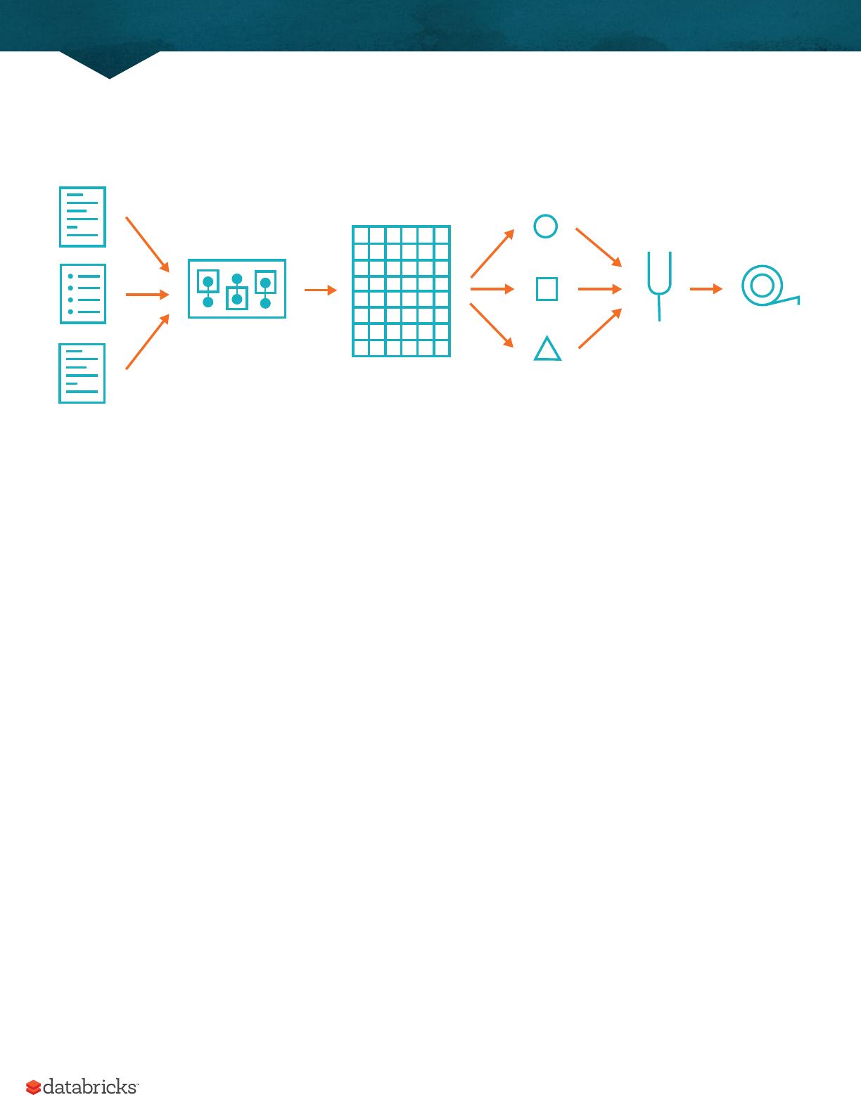
48
The overall process follows some variation of the following process:
• Gathering and collecting the relevant data for your task.
• Cleaning and inspecting the data to better understand it.
• Performing feature engineering to allow the algorithm to leverage more information.
• Using a portion of this data as a training set to train one or more algorithms to generate some candidate models.
• Evaluating and comparing models against your success criteria by objectively measuring results on a subset
of the same data (that was not used for training). This allows you to better understand how your model may
perform in the wild.
• Leveraging the insights from the above process and/or using the model to make predictions, recommndations,
detect anomalies or solve more general business challenges.
As we mentioned, is this going to be the same for every advanced analytics task ever? No, absolutely not. However, it
does serve as a general framework for what you’re going to need to do in order to take an advanced analytics use case
and get value out of it. Just as we did with the various advanced analytics tasks earlier in the chapter, let’s break down
each of these steps in the process to better understand each step’s overall objective.
Data Collection
Naturally it’s hard to create a training set without first collecting data. Typically this means at least gathering the
datasets that you’ll want to leverage to train your algorithm. Spark is, somewhat obviously, an excellent tool for this
because of its ability to speak to a variety of data sources and work with data big and small.
Pre-processing cleaning
& feature engineering
Clean &
Structured
Modeling &
Analytical Techniques
Tuning EvaluationRaw Data
Advanced Analytics and Machine Learning

49
Data Cleaning
Aer you’ve gather the proper data, you’re going to need to clean it and inspect it and perform something along the
lines of exploratory data analysis or EDA. EDA is a suitable technique for this stage of the process as you seek to better
understand your data and EDA has an emphasis on using visual methods in order to better understand distributions,
correlations, and other details in your data. During this process you may notice that you need to remove some values
that may have been misrecorded upstream or that other values may be missing. Whatever the case, it’s always
good have a good understanding and what is in your data to avoid mistakes down the road. The multitude of Spark
functions in the Structured APIs will provide a simple way to clean your data.
Feature Engineering
Now that we have a clean dataset, it’s time to augment it (if necessary) by potentially normalizing data, add variables
to represent the interactions of other variables , manipulating categorical variables and converting them to the proper
format to be input into our machine learning model. In MLlib, Spark’s machine learning library, all variables will have
to be input as doubles (regardless of what they actually represent). This means that you’re likely going to have to do
something like one-hot encode categorical variables and other indexing style techniques. We’re going to cover the
process of feature engineering in great depth in the next chapter but for the most part, Spark provides the essentials
that you’ll leverage to manipulate your data using a variety of machine learning specific statistical techniques.
Training Models
NOTE
The following two steps (training models, model tuning and evaluation) are not relevant to all use cases. This is a
general workflow that can potentially vary significantly based on the end objective you would like to achieve.
At this point in the process we have a dataset that we are ready to train our model on. Now we’ve used this
terminology several times, so let’s be a bit more precise. To train a model means that we will give the model a set
of data and the machine learning model will attempt to perform the task that we specified above. In doing so, the
parameters inside of the model will change according to the loss function in order to try and perform better at the
given task. For instance, if we hope to classify spam emails, our algorithm will likely find that certain words are better
predictors of spam than other words. These will receive higher influence in our model than words that have little
relevance. The output of this algorithm and data is what we call a model. A model is a tuned version of an algorithm
that is simplified version of the world that we can leverage for insights or prediction. We then can give our model new
information and it will manipulate that data accordingly. In the case of the classification example, we now have a
model of what characteristics are associated with a spam email and if we give our model a new email, it will output its
prediction about whether or not the email is spam or not.
Advanced Analytics and Machine Learning

50
However, training an algorithm isn’t the objective - we want to leverage our model to produce insights. Therefore we
must answer the question, how do we know our model is any good at what it’s supposed to do? That’s where model
tuning and evaluation come in.
Model Tuning and Evaluation
You likely noticed in our list above that we mentioned that we usually split our data into multiple portions and use
only one for training. The reason that we create a training set and don’t just train on the entire dataset is so that we
can use the other parts to either tune our model or evaluate it against other models. The reason for this is simple.
When we build a model, we want that model to generalize to new data or data that it hasn’t seen before. The portion
of our cleaned data that we will use to test the eectiveness of our data is what we call a test set. Think of it just like
an exam that you take in school. The objective is to see if your model understands something fundamental about this
data process or whether or not it just noticed the things particular to only the training set. In the process of training
models, we also might take another subset of data and treat that as a miniature test set (called a validation set) in
order to try out dierent hyperparameters or parameters that can aect other parameters - in essense, variations of
the model.
To continue with the classification example we referenced previously. We have three sets of data, we have a training
set for training models, we have a validation set for testing dierent variations of the models that we’re training, and
finally we have a test set that we will use for the final evaluation of our dierent model variations to see which one
performed the best.
Leveraging the model and/or insights
Now we finally get to use our model! This might be to simply better understand customers or perform user
segmentation or predict spam emails. Whatever the case is, this should always be the end objective! Try to solve a
problem and better understand your data!
This quick workflow overview is just an example workflow and doesn’t encompass all use cases or potential
workflows. There are also a lot of details that can have tremendous impact on your results so if this refresher felt a bit
foreign to you but you’d like to learn more there are a multitude of resources across the web that can teach you more.
Spark’s Advanced Analytics Toolkit
Spark includes several core packages and many external packages for performing advanced analytics. The primary
package is MLlib which provides an interface for bulding machine learning pipelines. We elaborate on other packages
in later chapters.
Advanced Analytics and Machine Learning

51
What is MLlib?
MLlib is a package, built on and included in Spark, that provides interfaces for
• gathering and cleaning data,
• feature engineering and feature selection,
• training and tuning large scale supervised and unsupervised machine learning models,
• and using those models in production.
MLlib helps with all three steps of the process although it really shines in steps one and two for reasons that we will
touch on shortly.
WARNING
MLlib consists of two packages that leverage dierent core data structures. The package org.apache.spark.
ml maintains an interface for use with Spark DataFrames. This package also maintains a high level interface for
building machine learning pipelines that help standardize the way in which you perform the above steps. The lower
level package, org.apache.spark.mllib, maintains interfaces for Spark’s Low-Level, RDD APIs. This book will
focus on the DataFrame API. The RDD API is the lower level interface that that is in maintenance mode (meaning it will
only receive bug fixes, not new features) at the time of this writing. It has also been covered fairly extensively in other
books and is therefore omitted from this text.
When and why should you use MLlib (vs scikit learn vs tensorflow vs foo package)?
Now, at a high level, this sounds like a lot of other machine learning packages you have probably heard of like scikit-
learn for Python or the variety of R packages for performing similar tasks. So why should you bother MLlib at all? There
are numerous tools for performing machine learning on a single machine. They do quite well at this and will continue
to be great tools. However, these single machine tools do reach limits either in terms of the size of data you would like
to train on or the processing time. The fact that they hit a limit in terms of scale makes them complementary tools, not
competitive ones. When you do hit those scalability issues, take advantage of Spark’s abilities.
There are two key use cases where you want to leverage Spark’s ability to scale. Firstly, you want to leverage Spark
for preprocessing and feature generation to reduce the amount of time it might take to produce training and test sets
from a large amount of data. You then might leverage single machine learning algorithms to train on those given data
sets. Secondly, when your input data or model size become too diicult or inconvenient to put on one machine, use
Spark to do the heavy liing. Spark makes big data machine learning simple.
Advanced Analytics and Machine Learning
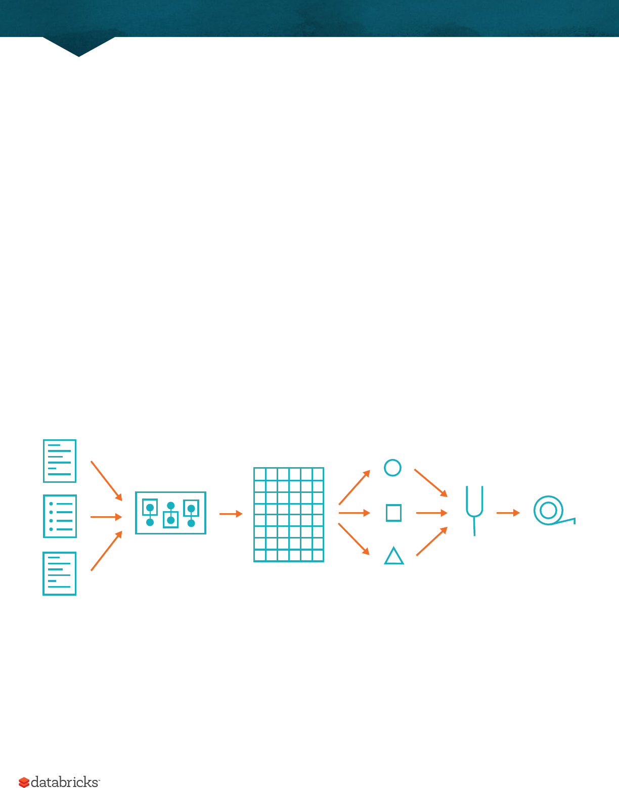
52
WARNING
An important caveat to the previous paragraphs is that while training and data preparation are made simple, there are
still some complexities that you will need to keep in mind. For example, if you train a recommender system on a Spark
cluster, the resulting model will end up being way too large for use on a single machine for prediction, yet we still need
to make predictions to derive value from our model. Another example might be a logistic regression model trained in
Spark. Spark’s execution engine is not a low-latency execution engine and therefore making single predictions quickly
(< 500ms) is still challenging because of the costs of starting up and executing a Spark jobs - even on a single machine.
Some models have good answers to this problem, others are still open questions. We will discuss the state of the art at
the end of this chapter. This is a fruitful research area and likely to change overtime as new systems come out to solve
this problem.
High Level MLlib Concepts
In MLlib there are several fundamental “structural” types: transformers, estimators, evaluator and pipelines.
By structural, we mean that they’ll define the overall architectural choices that you’ll be making. The following
illustration is an example of the overall workflow.
Transformers are functions that convert raw data in some way. This might be to create a new interaction variable (from
two other variables), normalize a column, or simply turn it into a Double to be input into a model. An example of a
transformer is one converts string categorical variables into numerical values that can be used in MLlib. Transformers
are primarily used in preprocessing or feature generation.
Pre-processing cleaning
& feature engineering
Clean &
Structured
Modeling &
Analytical Techniques
Tuning EvaluationRaw Data
Transformers
& Estimators
Estimators
& Models
Pipelines &
Cross-Validations
Evaluators
Metrics
Structured
API’s
Advanced Analytics and Machine Learning
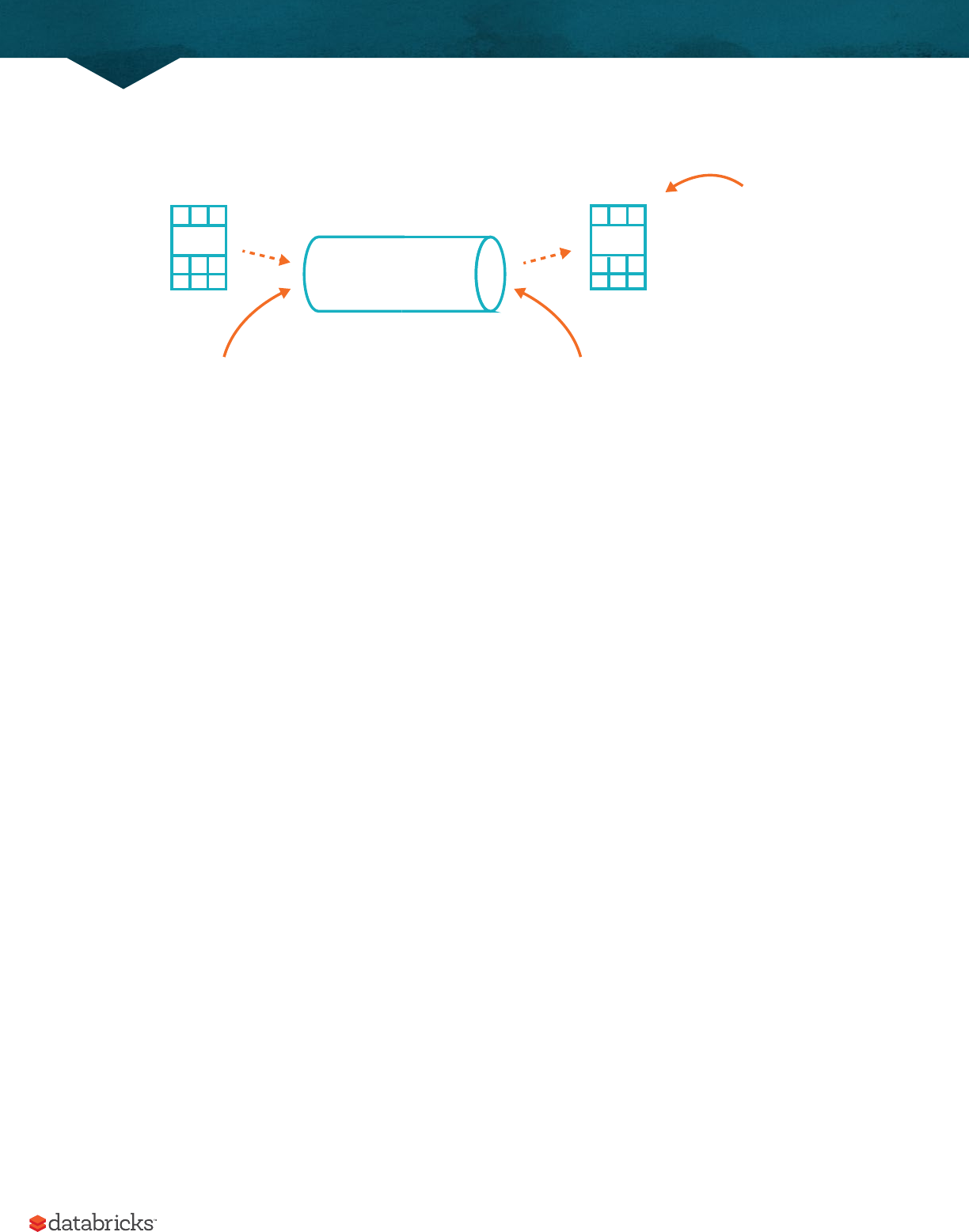
53
Estimators are one of two kinds of things. Firstly, estimators can be a kind of transformer that is initialized with data.
An example would be converting a column into a percentile representation of our column - in order to do this we need
to initialize it based on the values in that column. Lastly, estimators are Spark’s name for the actual models that we
will be training and turning into models so that we can use them to make predictions. Lastly, an evaluator allows us
to see how a given estimator performs according to some criteria that we specify like a ROC curve. Once we select the
best model from the ones that we tested, we can then use it to make predictions.
From a high level we can specify each of the above steps one by one however it is oen more much easier to specify
our steps as stages in a pipeline. This pipeline is similar to Scikit-learn’s Pipeline concept where transformations and
estimators are specified together.
In addition to the high level architectural types, there are also several lower level primitives that you may need to
leverage. The most common that you will come across is the Vector. Whenever we pass a set of features into a
machine learning model, we must do it as a vector that consists of Doubles. This vector can be either sparse (where
most of the elements are zero) or dense (where there are many unique values). These are specified in dierent ways,
one where we specify the exact values(dense) and the other where we specify the total size and which values are
nonzero(sparse). Sparse is appropriate, as you might have guessed, when the majority of the values are zero as this is
a more compressed representation that other formats.
Standard Transformer
input naming
inputCol
DF DF
output naming
outputCol
Transformed
column added
to Data Frame
Advanced Analytics and Machine Learning

54
%scala
import org.apache.spark.ml.linalg.Vectors
val denseVec = Vectors.dense(1.0, 2.0, 3.0)
val size = 3
val idx = Array(1,2) // locations in vector
val values = Array(2.0,3.0)
val sparseVec = Vectors.sparse(size, idx, values)
sparseVec.toDense
denseVec.toSparse
%python
from pyspark.ml.linalg import Vectors
denseVec = Vectors.dense(1.0, 2.0, 3.0)
size = 3
idx = [1, 2] # locations in vector
values = [2.0, 3.0]
sparseVec = Vectors.sparse(size, idx, values)
# sparseVec.toDense() # these two don’t work, not sure why
# denseVec.toSparse() # will debug later
WARNING
Confusingly, there are similar types that refer to ones that can be used in DataFrames and others than can only be used
in RDDs. The RDD implementations fall under the mllib package while the DataFrame implementations under ml.
MLlib in Action
Now that we have described some of the core pieces which we are going to come across, let’s create a simple pipeline
to demonstrate each of the component parts. We’ll use a small synthetic dataset that will help illustrate our point.
Let’s read the data in and see a sample before talking about it further.
%scala
var df = spark.read.json("/mnt/defg/simple-ml")
df.orderBy("value2").show()
Advanced Analytics and Machine Learning

55
%python
df = spark.read.json("/mnt/defg/simple-ml")
df.orderBy("value2").show()
+-----+----+------+------------------+
|color| lab|value1| value2|
+-----+----+------+------------------+
|green|good| 1|14.386294994851129|
|green| bad| 16|14.386294994851129|
| blue| bad| 8|14.386294994851129|
...
| red| bad| 16|14.386294994851129|
|green|good| 12|14.386294994851129|
+-----+----+------+------------------+
This dataset consists of a categorical label with two values, a categorical variable (color), and two numerical variables.
While the data is synthetic, an example of when this data might be used would be to predict customer health at a
company. The label represents their true current health, the color represents a rating before a phone call to determine
their true health and the two values represent some sort of usage metric. You should immediately recognize that this
will be a classification task where we hope to predict our binary output variable based on the inputs.
NOTE
There are some particular data foramts for supervised learning including LIBSVM. These formats have real valued
labels and sparse input data. Spark can read and write for these formats quite easily. For more information on the
LIBSVM format see the documentation.
%scala
val libsvmData = spark.read.format("libsvm")
.load("/mnt/defg/sample_libsvm_data.txt")
%python
libsvmData = spark.read.format("libsvm")\
.load("/mnt/defg/sample_libsvm_data.txt")
Advanced Analytics and Machine Learning

56
Transformers
As we mentioned, transformer will help us manipulate our current columns in one way or another. These columns,
in machine learning terminology, represent features (that we will input into our model) and in our particular case, a
label that represents the correct output. Transformers exist to either cut down on the number of features, add more
features, manipulate current ones or simply help us format our data correctly. In general, transformers add new
columns to DataFrames.
One requirement is that when we are using MLlib, all inputs to machine learning algorithms in Spark must consist of
type Double (for labels) and Vector[Double] for features. Our current data does not meet that requirement and
therefore we need to transform it to the proper format.
To achieve this, we are going to do this by specifying an RFormula. This is a declarative language for specifying
machine learning models and is incredibly simple to use once you understand the syntax. Currently RFormula
supports a limited subset of the R operators that in practice work quite well for simple models. The basic operators
are:
• ~ separate target and terms;
• + concat terms, "+ 0" means removing the intercept (this means that the y-intercept of the line that we will fit
will be 0.);
• - remove a term, "- 1" means removing intercept (this means that the y-intercept of the line that we will fit will
be 0. Yes, this does the same thing as the bullet above.);
• : interaction (multiplication for numeric values, or binarized categorical values);
• . all columns except the target/dependant variable.
In order to specify our transformations with this syntax, we need to import the relevant class.
%scala
import org.apache.spark.ml.feature.RFormula
%python
from pyspark.ml.feature import RFormula
Then we go through the process of defining our formula. In this case we want to use all available variables (the .) and
then specify a interactions between value1 and color and value2 and color.
Advanced Analytics and Machine Learning

57
val supervised = new RFormula()
.setFormula("lab ~ . + color:value1 + color:value2")
%python
supervised = RFormula(formula="lab ~ . + color:value1 + color:value2")
At this point we have declaratively specified how we would like to change out data into what we will train our model
on. The above transformation is a special kind of transformer (called an estimator) that has to be fit on the input data.
Not all transformers have this requirement but because RFormula will automatically handle categorical variables
for us, it needs to figure out which columns are categorical and which are now. For this reason, we have to call the
t method. Once we call t, this returns a "trained" version of our transformer that we can then use to actually
transform our data.
NOTE
We’re using the RFormula because it makes performing several transformations extremely easy to do. We saw in
Chapter 3 another way that we can specify a similar set of transformations and in the next chapter we will see all the
component parts of the RFormula when we cover the specific transformers in MLlib.
Now that we covered those details, let’s continue on and prepare our DataFrame.
%scala
val ttedRF = supervised.t(df)
val preparedDF = ttedRF.transform(df)
%python
ttedRF = supervised.t(df)
preparedDF = ttedRF.transform(df)
preparedDF.show()
Advanced Analytics and Machine Learning

58
+-----+----+------+------------------+--------------------+-----+
|color| lab|value1| value2| features|label|
+-----+----+------+------------------+--------------------+-----+
|green|good| 1|14.386294994851129|(10,[1,2,3,5,8],[...| 1.0|
| blue| bad| 8|14.386294994851129|(10,[2,3,6,9],[8....| 0.0|
...
| red| bad| 1| 38.97187133755819|(10,[0,2,3,4,7],[...| 0.0|
| red| bad| 2|14.386294994851129|(10,[0,2,3,4,7],[...| 0.0|
+-----+----+------+------------------+--------------------+-----+
In the output we can see the result of our transformation, a column called features that has our previously raw data.
What’s happening behind the scenes is actually quite simple. RFormula inspects our data during the t call and
outputs an object that will transform our data according to the specified formula. This "trained" transformer always
has the word Model in the type signature. When we use this transformer, you will notice that Spark automatically
converts our categorical variable to Doubles so that we can input this into a (yet to be specified) machine learning
model. It does this with several calls to the StringIndexer, Interaction, and VectorAssembler
transformers covered in the next chapter. We then call tranform on that object in order to transform our input
data into the expected output data.
Aer preparing our data for out model, we’re know nearing the final stpes in the advanced analytics workflow we
described above. We (pre)processed our data so that it’s clean and tidy and added some features along the way. Now
it comes time to actually train our model (or a set of models on this. In order to do this, we need to prepare a test set
for evaluation.
TIP
Having a good test set is probably the most important thing that you can do to ensure that you train a model that
you can actually use in the real world (in a dependable way). Not creating a representative test set or using your test
set for hyperparameter tuning are surefire ways to create a model that does not perform well in real world scenarios.
Don’t skip creating a test set, it’s a requirement to know how well your model actually does! This is stressed in all of
the books that we mention above so see those books for more information.
%scala
val Array(train, test) = preparedDF.randomSplit(Array(0.7, 0.3))
%python
train, test = preparedDF.randomSplit([0.7, 0.3])
Advanced Analytics and Machine Learning

59
Estimators
Now that we transformed our data into the correct format and created some valuable features. It’s time to actually
fit our model. In this case we will use logistic regression. To create our classifier we instantiate an instance of
LogisticRegression, a method for classification, using the default configuration or hyperparameters(for those
more familiar with machine learning). We then set the label columns and the feature columns. The values we are
setting are actually the default labels for all Estimators in the DataFrame API in Spark MLlib and you will see in later
chapters that we omit them.
%scala
import org.apache.spark.ml.classication.LogisticRegression
val lr = new LogisticRegression()
.setLabelCol("label")
.setFeaturesCol("features")
%python
from pyspark.ml.classication import LogisticRegression
lr = LogisticRegression(
labelCol="label",
featuresCol="features")
Before we actually go about training this model, it can be a best practice to inspect the parameters, this is also a great
way of getting a refresher of the options available for each particular model.
%scala
println(lr.explainParams())
%python
print lr.explainParams()
Here’s the output of calling the above explain command.
Advanced Analytics and Machine Learning

60
aggregationDepth: suggested depth for treeAggregate (>= 2) (default: 2)
elasticNetParam: the ElasticNet mixing parameter, in range [0, 1]. For alpha = 0,
the penalty is an L2 penalty. For alpha = 1, it is an L1 penalty (default: 0.0)
family: The name of family which is a description of the label distribution to
be used in the model. Supported options: auto, binomial, multinomial. (default:
auto) featuresCol: features column name (default: features, current: features)
tIntercept: whether to t an intercept term (default: true) labelCol: label
column name (default: label, current: label) lowerBoundsOnCoeicients: The lower
bounds on coeicients if tting under bound constrained optimization. (undened)
lowerBoundsOnIntercepts: The lower bounds on intercepts if tting under bound
constrained optimization. (undened) maxIter: maximum number of iterations (>=
0) (default: 100) predictionCol: prediction column name (default: prediction)
probabilityCol: Column name for predicted class conditional probabilities. Note:
Not all models output well-calibrated probability estimates! These probabilities
should be treated as condences, not precise probabilities (default: probability)
rawPredictionCol: raw prediction (a.k.a. condence) column name (default:
rawPrediction) regParam: regularization parameter (>= 0) (default: 0.0)
standardization: whether to standardize the training features before tting the
model (default: true) threshold: threshold in binary classication prediction, in
range [0, 1] (default: 0.5) thresholds: Thresholds in multi-class classication
to adjust the probability of predicting each class. Array must have length
equal to the number of classes, with values > 0 excepting that at most one
value may be 0. The class with largest value p/t is predicted, where p is the
original probability of that class and t is the class’s threshold (undened)
tol: the convergence tolerance for iterative algorithms (>= 0) (default: 1.0E-6)
upperBoundsOnCoeicients: The upper bounds on coeicients if tting under bound
constrained optimization. (undened) upperBoundsOnIntercepts: The upper bounds on
intercepts if tting under bound constrained optimization. (undened) weightCol:
weight column name. If this is not set or empty, we treat all instance weights as
1.0 (undened)?
Once we instantiate the model, we can train it. This is done with the t method which returns a
LogisticRegressionModel.
%scala
val ttedLR = lr.t(train)
%python
ttedLR = lr.t(train)
Advanced Analytics and Machine Learning

61
This previous code will kick o a spark job, fitting an ML model is always eagerly performed.
Now that we trained the model, we can use it to make predictions. Logically this represents a transformation of
features into labels. We make predictions with the transform method. For example, we can transform our training
dataset to see what labels our model assigned to the training data and how those compare to the true outputs. This,
again, is just another DataFrame that we can manipulate.
ttedLR.transform(train).select("label", "prediction").show()
+-----+----------+
|label|prediction|
+-----+----------+
| 0.0| 0.0|
| 0.0| 0.0|
...
| 0.0| 0.0|
| 0.0| 0.0|
+-----+----------+
Our next step would be to manually evaluate this model and calculate performance metrics like the true positive rate,
false negative rate, etc. We might then turn around and try a dierent set of parameters to see if those perform better.
This process, while useful, is actually quite tedious and well defined. Spark helps you avoid this by allowing you to
specify your workload as a declarative pipeline of work that includes all your transformations and includes tuning
your hyperparameters.
box: What are hyperparameters?
Hyperparameters are initialization configurations for model. They are parameters that influence other parameters.
Logistic regression is a simple model that doesn’t have that many hyperparameters (we’ll cover the details in a
couple of chapters). However, we could choose to look at dierent interaction variables in our RFormula. In doing
so, we’d eectively be tuning hyperparameters that aect the preprocessing of the data. Pipelines, as you will see
momentarily, allow us to configure the entire data manipulation process from raw data to the model in dierent ways
- allowing us to tune the hyperparameters to the best ones that we try.
Pipelining our Workflow
As you likely noticed above, if you are performing a lot of transformations, writing all the steps and keeping track of
DataFrames ends up being quite tedious. That’s why Spark includes the concept of a Pipeline. A pipeline allows
Advanced Analytics and Machine Learning

62
you to set up a dataflow of the relevant transformations, ending with an estimator that is automatically tuned
according to your specifications resulting a tuned model ready for a production use case. The following diagram
illustrates this process.
One important detail is that it is essential that instances of transformers or models are not reused across pipelines or
dierent models. Always create a new instance of a model before creating another pipeline.
In order to make sure that we don’t overfit, we are going to create a holdout test set and tune our hyperparameters
based on a validation set. Note that this is our raw dataset.
%scala
val Array(train, test) = df.randomSplit(Array(0.7, 0.3))
%python
train, test = df.randomSplit([0.7, 0.3])
Pre-processing cleaning
& feature engineering
Clean &
Structured
Modeling &
Analytical Techniques
Tuning EvaluationRaw Data
Transformers
& Estimators
Estimators
& Models
Pipelines &
Cross-Validations
Evaluators
Metrics
Structured
API’s
All in one pipeline
Advanced Analytics and Machine Learning

63
While in this case we opt for just using the RFormula a common pattern is to set up a pipeline of many dierent
transformations in conjunction with the RFormula (for the simpler features). We cover these preprocessing techniques
in the following chapter, just keep in kind that there can be far more stages than just two. In this case we will not
specify a formula.
%scala
val rForm = new RFormula()
val lr = new LogisticRegression()
.setLabelCol("label")
.setFeaturesCol("features")
%python
rForm = RFormula()
%python
lr = LogisticRegression()\
.setLabelCol("label")\
.setFeaturesCol("features")
Now instead of manually using our transformations and then tuning our model. Now we just make them stages in the
overall pipeline. This makes them just logical transformations, or a specification for chain of commands for Spark to
run in a pipeline.
import org.apache.spark.ml.Pipeline
val stages = Array(rForm, lr)
val pipeline = new Pipeline().setStages(stages)
%python
from pyspark.ml import Pipeline
stages = [rForm, lr]
pipeline = Pipeline().setStages(stages)
Advanced Analytics and Machine Learning

64
Evaluators
At this point we set up a set up our pipeline. The next step will be evaluating the performance of this pipeline.
Spark does this by setting up a parameter grid of all the combinations of the parameters that you specify. You
should immediately notice in the following code snippet that even our RFormula is tuning specific parameters.
In a pipeline, we can modify more than just the model’s hyperparameters, we can even modify the transformer’s
properties.
%scala
import org.apache.spark.ml.tuning.ParamGridBuilder
val params = new ParamGridBuilder()
.addGrid(rForm.formula, Array(
"lab ~ . + color:value1",
"lab ~ . + color:value1 + color:value2"))
.addGrid(lr.elasticNetParam, Array(0.0, 0.5, 1.0))
.addGrid(lr.regParam, Array(0.1, 2.0))
.build()
%python
from pyspark.ml.tuning import ParamGridBuilder
params = ParamGridBuilder()\
.addGrid(rForm.formula, [
"lab ~ . + color:value1",
"lab ~ . + color:value1 + color:value2"])\
.addGrid(lr.elasticNetParam, [0.0, 0.5, 1.0])\
.addGrid(lr.regParam, [0.1, 2.0])\
.build()
In our current grid there are three hyperparameters that will diverge from the defaults.
• two dierent options for the R formula
• three dierent options for the elastic net parameter
• two dierent options for the regularization parameter
Advanced Analytics and Machine Learning

65
This gives us a total of twelve dierent combinations of these parameters, which means we will be training twelve
dierent versions of logistic regression. While we don’t want to go into too much detail in this chapter we explain the
elastic net parameter as well as the regularization options in the Classification Chapter.
With the grid built it is now time to specify our evaluation. There are evaluators for classification and regression, which
we cover in subsequent chapters. In this case, we will be using the BinaryClassicationEvaluator. This
evaluator allows us to automatically optimize our model training according to some specific criteria that we specify.
In this case we will specify areaUnderROC which is the total area under the receiver operating characteristic a very
common measure of classification performance that we cover in the classification chapter.
Now that we have a pipeline that specifies how our data should be transformed. Let’s take it to the next level and
automatically perform model selection by trying out dierent hyper-parameters in our logistic regression model.
We do this by specifying a parameter grid, a splitting measuer, and lastly an Evaluator. An evaluator allows us to
automatically optimize our model training according to some criteria (specified in the evaluator) however in order to
leverage this we need a simple way of trying out dierent model parameters to see which ones perform best. We cover
all the dierent evaluation metrics in each task’s chapter.
%scala
import org.apache.spark.ml.evaluation.BinaryClassicationEvaluator
val evaluator = new BinaryClassicationEvaluator()
.setMetricName("areaUnderROC")
.setRawPredictionCol("prediction")
.setLabelCol("label")
%python
from pyspark.ml.evaluation import BinaryClassicationEvaluator
evaluator = BinaryClassicationEvaluator()\
.setMetricName("areaUnderROC")\
.setRawPredictionCol("prediction")\
.setLabelCol("label")
As you may know, it is a best practice in machine learning to fit your hyperparameters on a validation set (instead of
your test set). The reasons for this are to prevent overfitting. Therefore we cannot use our holdout test set (that we
created before) to tune these parameters. Luckily Spark provides two options for performing this hyperparameter
tuning in an automated way. We can use a TrainValidationSplit, which will simply perform an arbitrary
random split of our data into two dierent groups, or a CrossValidator, which performs K-fold cross validation by
splitting the dataset into k non-overlapping randomly partitioned folds.
Advanced Analytics and Machine Learning

66
%scala
import org.apache.spark.ml.tuning.TrainValidationSplit
val tvs = new TrainValidationSplit()
.setTrainRatio(0.75) // also the default.
.setEstimatorParamMaps(params)
.setEstimator(pipeline)
.setEvaluator(evaluator)
%python
from pyspark.ml.tuning import TrainValidationSplit
tvs = TrainValidationSplit()\
.setTrainRatio(0.75)\
.setEstimatorParamMaps(params)\
.setEstimator(pipeline)\
.setEvaluator(evaluator)
Now we can fit our entire pipeline. This will test out every version of the model against the validation set. You will
notice that the the type of tvsFitted is TrainValidationSplitModel. Any time that we fit a given model, it
outputs a "model" type.
%scala
val tvsFitted = tvs.t(train)
%python
tvsFitted = tvs.t(train)
And naturally evaluate how it performs on the test set!
evaluator.evaluate(tvsFitted.transform(test)) // 0.9166666666666667
Advanced Analytics and Machine Learning

67
We can also see a training summary for particular models. To do this we extract it from the pipeline, cast it to
the proper type and print our results. The metrics available depend on the models which are covered in some of
the following chapters. The only key thing to understand is that an unfitted estimator has the same name as the
estimator, e.g. LogisticRegression.
import org.apache.spark.ml.PipelineModel
import org.apache.spark.ml.classication.LogisticRegressionModel
val trainedPipeline = tvsFitted.bestModel.asInstanceOf[PipelineModel]
val TrainedLR = trainedPipeline.stages(1)
.asInstanceOf[LogisticRegressionModel]
val summaryLR = TrainedLR.summary
SummaryLR.objectiveHistory
The objective history shows how our algorithm performed over each training iteration. This can be helpful because
we can note the progress our algorithm is making towards the best model. Large jumps are typically expected at
the beginning, but over time the values should become smaller and smaller, with only small amounts of variation
between the values.
Persisting and Applying Models
Now that we trained this model, we can persist it to disk to use it in an online predicting fashion later.
tvsFitted.write.overwrite().save("/tmp/modelLocation")
Now that we wrote out the model we can load it back into a program (potentially in a dierent location) in
ordre to make predictions. In order to do this we need to use the companion object to the model, tuning class,
or transformer that we originally used. In this case, we used TrainValidationSplit which outputs a
TrainValidationSplitModel. We will now use the "model" version to load our persisted model. If we were to
use a CrossValidator, we’d have to read in the persisted version as the CrossValidatorModel and if we
were to use LogisticRegression manually we would have to use LogisticRegressionModel.
Advanced Analytics and Machine Learning
68
%scala
import org.apache.spark.ml.tuning.TrainValidationSplitModel
val model = TrainValidationSplitModel.load("/tmp/modelLocation")
model.transform(test)
%python
# not currently available in python but bet it’s coming...
# will remove if not.
# from pyspark.ml.tuning import TrainValidationSplitModel
# model = TrainValidationSplitModel.load("/tmp/modelLocation")
# model.transform(test)
Deployment Patterns
When it comes to Spark there are several dierent deployment patterns for putting machine learning models into
production in Spark. The following diagram illustrates common workflows.
Back End & Oline Training
Recommendation
Portal
exit
Portal
entrance
Model server
program
Key-Value or OCTP
database
Front End & Online Serving
Classification
& regression
Model
persistence
+
Requests
Load
balancer
Advanced Analytics and Machine Learning

69
1. Train your ML algorithm oline and then put the results into a database (usually a key-value store). This works
well for something like recommendation but poorly for something like classification or regression where you
cannot just lookup a value for a given user but must calculate one.
2. Train your ML algorithm oline, persist the model to disk, then use that for serving. This is not a low latency
solution as the overhead of starting up a Spark job can be quite high - even if you’re not running on a cluster.
Additionally this does not parallelize well, so you’ll likely have to put a load balancer in front of multiple model
replicas and build out some REST API integration yourself. There are some interesting potential solutions to
this problem, but nothing quite production ready yet.
3. Manually (or via some other soware) convert your distributed model to one that can run much more quickly
on a single machine. This works well when there is not too much manipulation of the raw data in Spark and
can be hard to maintain over time. Again there are solutions that are working on this specification as well
but nothing production ready. This cannot be found in the previous illustration because it’s something that
requires manual work.
4. Train your ML algorithm online and use it online, this is possible when used in conjunction like streaming but
is quite sophisticated. This landscape will likely continue to mature as Structured Streaming development
continues.
NOTE
These are specific to Spark and don’t apply to many single machine frameworks that don’t have the ability to train on
really large data, but can serve responses more quickly than Spark can.
While these are some of the options, there are more potential ways of performing model deployment and
management. This is a heavy area for development that is certainly likely to change and progress quickly.
Advanced Analytics and Machine Learning
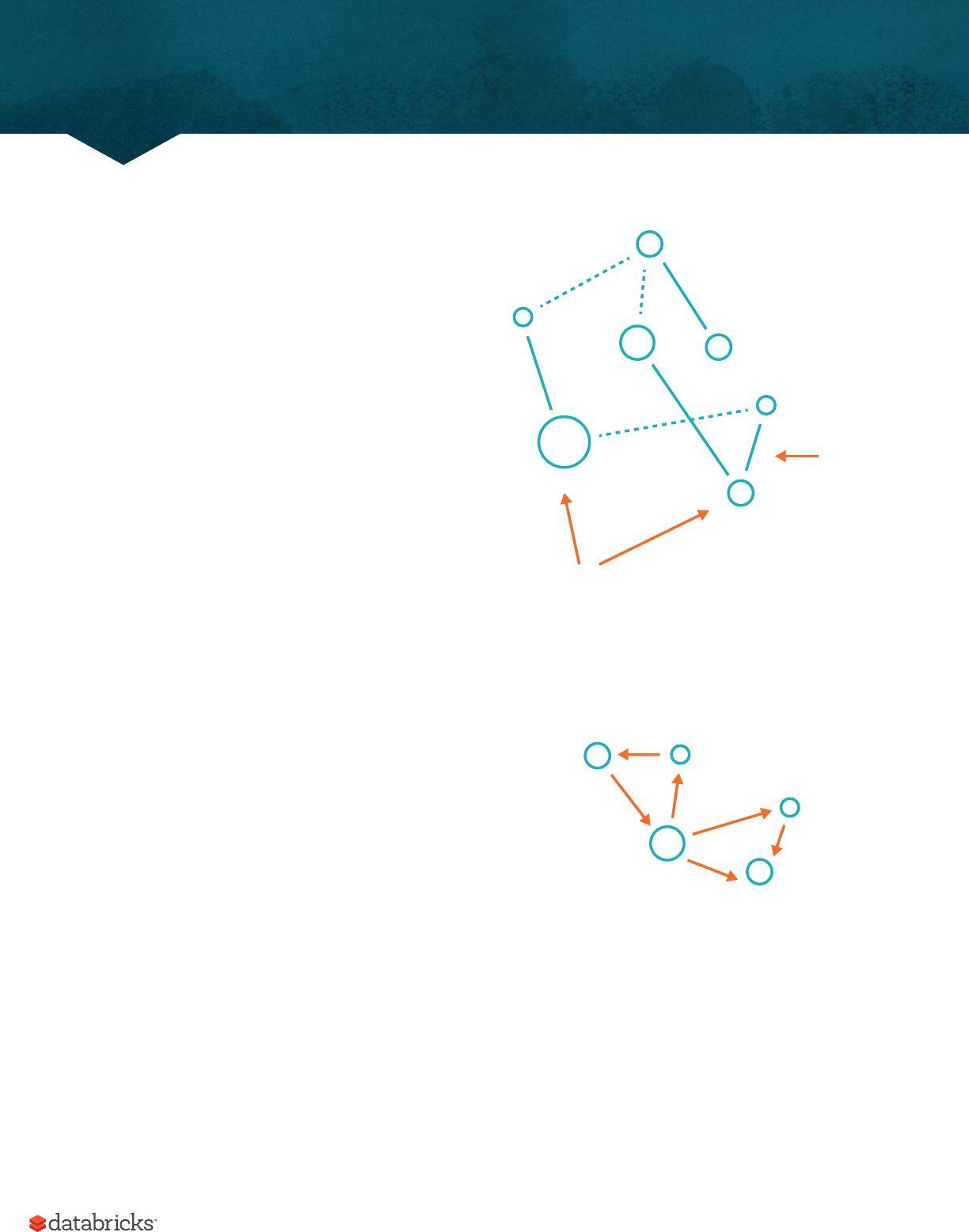
70
The last chapter covered some conventional
unsupervised techniques. This chapter is going to dive
into a more specialized toolset: graph processing. In
the context of graphs, nodes or vertices are the units
while edges define the relationships between those
nodes. The process of graph analysis is the process of
analyzing these relationships. An example graph might
be your friend group, in the context of graph analysis
each vertex or node would represent a person and each
edge would represent a relationship.
You can see the image at the right is a representation
of a directed graph where the edges are directional.
There are also undirected graphs in which there is no
start and beginning for given edges.
Using our example, the weight of the edge might
represent the intimacy between dierent friends;
acquaintances would have low-weight edges between
them while married individuals would have edges
with large weights. We could infer this by looking
at communication frequency between nodes and
weighting the edges accordingly. Graph are a natural
way of describing relationships and many dierent
problem sets and Spark provides several ways of
working in this analytics paradigm. Some business use
cases could be detecting credit card fraud, importance
of papers in bibliographic networks [which papers are
most referenced], and ranking web pages as Google
famously used the PageRank algorithm to do.
When Spark first came out, Spark included a library
for performing graph processing called GraphX. GraphX provides an interface for performing graph analysis on top of
the RDD API. This provided a very low level interface that was extremely powerful but just like RDDs, wasn’t the most
powerful. GraphX is still a core part of Spark. Companies still build production applications on top of it and it still sees
some minor feature development. This API is quite well documented simply because it hasn’t changed much since its
creation. However, some of the developers of Spark (including some of the original authors of GraphX) have recently
created the next generation graph analytics library on Spark called GraphFrames. GraphFrames extends GraphX to
Vertex
or node
Edge
Figure 1:
Directed
Graph
Figure 2:
Graph Analysis

71
provide a DataFrame API as well as support for Spark’s dierent language bindings so that users of Python can take
advantage of the scalability of the tool as well.
GraphFrames is currently available as a Spark Package available here, an external package that you need to load
when you start up your Spark application, but may be merged into the core of Spark in the future. For the the
most part, there should be little dierence in performance between the two (except for a huge user experience
improvement in GraphFrames). There is some small overhead when using GraphFrames but for the most part it
tries to call down to GraphX where appropriate and for most, the user experience gains greatly outweight this minor
overhead.
NOTE
How does GraphFrames compare to Graph Databases? Spark is not a database. Spark is a distributed computation
engine. You can build a graph API on top of Spark but his fundamentally approaches the problem dierently than a
database. GraphFrames can scale to much larger workloads than many graph databases and performs well in the
context of analytics but not transaction data processing and serving.
The goal of this chapter is to show you how to use GraphFrames to perform graph analysis on Spark. We are going to
be doing this with publicly available bike data from the Bay Area Bike Share portal.
NOTE
Over the course of the writing of this book. This map and data have changed dramatically (even the naming!). We
include a copy of the dataset inside of the data folder of this book’s repository. Be sure to use that dataset to replicate
the below results and when you’re feeling adventuous, expand to the whole dataset!
To get setup you’re going to need to point to the proper package. In order to do this from the command line you’ll run.
./bin/spark-shell --packages graphframes:graphframes:0.5.0-spark2.1-s_2.11
%scala
val bikeStations = spark.read
.option("header","true")
.csv("/mnt/defg/bike-data/201508_station_data.csv")
val tripData = spark.read
.option("header","true")
.csv("/mnt/defg/bike-data/201508_trip_data.csv")
Graph Analysis

72
%python
bikeStations = spark.read\
.option("header","true")\
.csv("/mnt/defg/bike-data/201508_station_data.csv")
tripData = spark.read\
.option("header","true")\
.csv("/mnt/defg/bike-data/201508_trip_data.csv")
Building A Graph
The first step is to build the graph, to do this we need to define the vertices and edges. In our case we’re creating
a directed graph. This graph will point from the source to the location. In the context of this bike trip data, this will
point from a trip’s starting location to a trip’s ending location.To define the graph, we use the naming conventions
presented in the GraphFrames library. In the vertices table we define our identifier as id and in the edges table we
label the source id as src and the destination id as dst.
%scala
val stationVertices = bikeStations
.withColumnRenamed("name", "id")
.distinct()
val tripEdges = tripData
.withColumnRenamed("Start Station", "src")
.withColumnRenamed("End Station", "dst")
%python
stationVertices = bikeStations\
.withColumnRenamed("name", "id")\
.distinct()
tripEdges = tripData\
.withColumnRenamed("Start Station", "src")\
.withColumnRenamed("End Station", "dst")
This allows us to build out graph out of the DataFrames we have so far. We will also leverage caching because we’ll be
accessing this data frequently in the following queries.
Graph Analysis

73
%scala
import org.graphframes.GraphFrame
val stationGraph = GraphFrame(stationVertices, tripEdges)
stationGraph.cache()
%python
from graphframes import GraphFrame
stationGraph = GraphFrame(stationVertices, tripEdges)
stationGraph.cache()
Now we can see the basic statistics about data (and query our original DataFrame to ensure that we see the expected
results).
%scala
println(s"Total Number of Stations: ${stationGraph.vertices.count()}")
println(s"Total Number of Trips in Graph: ${stationGraph.edges.count()}")
println(s"Total Number of Trips in Original Data: ${tripData.count()}")
%python
print "Total Number of Stations: " + str(stationGraph.vertices.count())
print "Total Number of Trips in Graph: " + str(stationGraph.edges.count())
print "Total Number of Trips in Original Data: " + str(tripData.count())
This returns the following results.
Total Number of Stations: 70
Total Number of Trips in Graph: 354152
Total Number of Trips in Original Data: 354152
Graph Analysis

74
Querying the Graph
The most basic way of interacting with the graph is simply querying it, performing things like counting trips and
filtering by given destinations. GraphFrames provides simple access to both vertices and edges as DataFrames.
%scala
import org.apache.spark.sql.functions.desc
stationGraph
.edges
.groupBy("src", "dst")
.count()
.orderBy(desc("count"))
.show(10)
%python
from pyspark.sql.functions import desc
stationGraph\
.edges\
.groupBy("src", "dst")
.count()\
.orderBy(desc("count"))\
.show(10)
+--------------------+--------------------+-----+
| src| dst|count|
+--------------------+--------------------+-----+
|San Francisco Cal...| Townsend at 7th| 3748|
|Harry Bridges Pla...|Embarcadero at Sa...| 3145|
...
| Townsend at 7th|San Francisco Cal...| 2192|
|Temporary Transba...|San Francisco Cal...| 2184|
+--------------------+--------------------+-----+
We can also filter by any valid DataFrame expression. In this instance I want to look at one specific station and the
count of trips in and out of that station.
Graph Analysis

75
%scala
stationGraph
.edges
.where("src = ‘Townsend at 7th’ OR dst = ‘Townsend at 7th’")
.groupBy("src", "dst")
.count()
.orderBy(desc("count"))
.show(10)
%python
stationGraph\
.edges\
.where("src = ‘Townsend at 7th’ OR dst = ‘Townsend at 7th’")\
.groupBy("src", "dst")\
.count()\
.orderBy(desc("count"))\
.show(10)
+--------------------+--------------------+-----+
| src| dst|count|
+--------------------+--------------------+-----+
|San Francisco Cal...| Townsend at 7th| 3748|
| Townsend at 7th|San Francisco Cal...| 2734|
...
| Steuart at Market| Townsend at 7th| 746|
| Townsend at 7th|Temporary Transba...| 740|
+--------------------+--------------------+-----+
Subgraphs
Subgraphs are just smaller graphs within the larger one. We saw above how we can query a given set of edges and
vertices. We can use this in order to create subgraphs.
Graph Analysis

76
%scala
val townAnd7thEdges = stationGraph
.edges
.where("src = ‘Townsend at 7th’ OR dst = ‘Townsend at 7th’")
val subgraph = GraphFrame(stationGraph.vertices, townAnd7thEdges)
%python
townAnd7thEdges = stationGraph\
.edges\
.where("src = ‘Townsend at 7th’ OR dst = ‘Townsend at 7th’")
subgraph = GraphFrame(stationGraph.vertices, townAnd7thEdges)
We can then apply the following algorithms to either the original or the subgraph.
Graph Algorithms
A graph is just a logical representation of data. Graph theory provides numerous algorithms for describing data in
this format and GraphFrames allows us to leverage many algorithms out of the box. Development continues as new
algorithms are added to GraphFrames so this list is likely to continue to grow.
PageRank
Arguably one of the most prolific graph algorithms is PageRank. Larry Page, founder of Google, created PageRank as a
research project for how to rank webpages. Unfortunately an in depth explanation of how PageRank works is outside
the scope of this book, however to quote Wikipedia the high level explanation is as follows.
PageRank works by counting the number and quality of links to a page to determine a rough estimate of how important the website
is. The underlying assumption is that more important websites are likely to receive more links from other websites.
However PageRank generalizes quite well outside of the web domain. We can apply this right to our own data and get
a sense for important bike stations. In this example, important bike stations will be assigned large PageRank values.
box: Graph algorithm APIs: parameters and return values Most algorithms in GraphFrames are accessed as methods
which take parameters (e.g., resetProbability in this PageRank example). Most algorithms return either
a new GraphFrame or a single DataFrame. The results of the algorithm are stored as one or more columns in the
GraphFrame’s vertices and/or edges or the DataFrame. For PageRank, the algorithm returns a GraphFrame, and
we can extract the estimated PageRank values for each vertex from the new pagerank column.
Graph Analysis

77
WARNING
Depending on the resources available on your machine, this may take some time. You can always try a smaller set of
data before running this to see the results. On Databricks Community Edition, this takes about twenty seconds to run
although some reviewers found it to take much longer on their personal machines.
%scala
import org.apache.spark.sql.functions.desc
val ranks = stationGraph.pageRank
.resetProbability(0.15)
.maxIter(10)
.run()
ranks.vertices
.orderBy(desc("pagerank"))
.select("id", "pagerank")
.show(10)
%python
from pyspark.sql.functions import desc
ranks = stationGraph.pageRank(resetProbability=0.15, maxIter=10)
ranks.vertices\
.orderBy(desc("pagerank"))\
.select("id", "pagerank")\
.show(10)
+--------------------+------------------+
| id| pagerank|
+--------------------+------------------+
|San Jose Diridon ...| 4.051504835989922|
|San Francisco Cal...|3.3511832964279518|
...
| Townsend at 7th| 1.568456580534273|
|Embarcadero at Sa...|1.5414242087749768|
+--------------------+------------------+
Graph Analysis
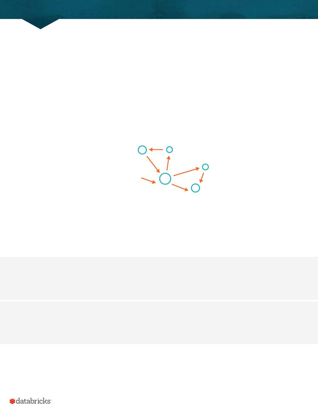
78
Interestingly, we see that Caltrain stations rank quite highly. This makes sense because these are natural connection
points where a lot of bike trips might end up. Either as commuters move from home to the Caltrain station for their
commute or from the Caltrain station to home.
In and Out Degrees
Our graph is a directed graph. This is due to the bike trips being directional, starting in one location and ending in
another. One common task is to count the number of trips into or out of a given station. We counted trips previously,
in this case we want to count trips into and out of a given station. We measure these with in-degree and out-degree
respectively.
This is particularly applicable in the context of social networking because certain users may have many more inbound
connections (say followers) than outbound connections (people they follow). Using the following query, you can find
interesting people in the social network that might have more influence than others. GraphFrames provides a simple
way to query our graph for this information.
%scala
val inDeg = stationGraph.inDegrees
inDeg.orderBy(desc("inDegree")).show(5, false)
%python
inDeg = stationGraph.inDegrees
inDeg.orderBy(desc("inDegree")).show(5, False)
The result of querying for the stations sorted by the highest in-degree.
Directed
Graph
in-degree 1
out-degree 3
Graph Analysis

79
+----------------------------------------+--------+
|id |inDegree|
+----------------------------------------+--------+
|San Francisco Caltrain (Townsend at 4th)|34810 |
|San Francisco Caltrain 2 (330 Townsend) |22523 |
|Harry Bridges Plaza (Ferry Building) |17810 |
|2nd at Townsend |15463 |
|Townsend at 7th |15422 |
+----------------------------------------+--------+
We can query the out degrees in the same fashion.
%scala
val outDeg = stationGraph.outDegrees
outDeg.orderBy(desc("outDegree")).show(5, false)
%python
outDeg = stationGraph.outDegrees
outDeg.orderBy(desc("outDegree")).show(5, False)
+---------------------------------------------+---------+
|id |outDegree|
+---------------------------------------------+---------+
|San Francisco Caltrain (Townsend at 4th) |26304 |
|San Francisco Caltrain 2 (330 Townsend) |21758 |
|Harry Bridges Plaza (Ferry Building) |17255 |
|Temporary Transbay Terminal (Howard at Beale)|14436 |
|Embarcadero at Sansome |14158 |
+---------------------------------------------+---------+
The ratio of these two values is an interesting metric to look at. A higher ratio value will tell us where a large number
of trips end (but rarely begin) while a lower value tells us where trips oen begin (but infrequently end).
Graph Analysis

80
%scala
val degreeRatio = inDeg.join(outDeg, Seq("id"))
.selectExpr("id", "double(inDegree)/double(outDegree) as degreeRatio")
degreeRatio
.orderBy(desc("degreeRatio"))
.show(10, false)
degreeRatio
.orderBy("degreeRatio")
.show(10, false)
%python
degreeRatio = inDeg.join(outDeg, "id")\
.selectExpr("id", "double(inDegree)/double(outDegree) as degreeRatio")
degreeRatio\
.orderBy(desc("degreeRatio"))\
.show(10, False)
degreeRatio\
.orderBy("degreeRatio")\
.show(10, False)
Those queries result in the following data.
+----------------------------------------+------------------+
|id |degreeRatio |
+----------------------------------------+------------------+
|Redwood City Medical Center |1.5333333333333334|
|San Mateo County Center |1.4724409448818898|
...
|Embarcadero at Vallejo |1.2201707365495336|
|Market at Sansome |1.2173913043478262|
+----------------------------------------+------------------+
Graph Analysis

81
+-------------------------------+------------------+
|id |degreeRatio |
+-------------------------------+------------------+
|Grant Avenue at Columbus Avenue|0.5180520570948782|
|2nd at Folsom |0.5909488686085761|
...
|San Francisco City Hall |0.7928849902534113|
|Palo Alto Caltrain Station |0.8064516129032258|
+-------------------------------+------------------+
Breadth-first Search
Breadth-first Search will search our graph for how to connect two given nodes based on the edges in the graph. In
our context, we might want to do this to find the shortest paths to dierent stations. We can specify the maximum of
edges to follow with the maxPathLength and we can also specify an edgeFilter to filter out certain edges that
do not meet a certain requirement like trips during non-business hours.
We’ll choose two fairly close stations so that this does not run too long. However, you can do some pretty interesting
graph traversals when you have some sparse graphs that have some distant connections. Feel free to play around
with the stations (especially those in other cities) to see if you can get some distant stations to connect.
%scala
val bfsResult = stationGraph.bfs
.fromExpr("id = ‘Townsend at 7th’")
.toExpr("id = ‘Spear at Folsom’")
.maxPathLength(2)
.run()
bfsResult.show(10)
%python
bfsResult = stationGraph.bfs(
fromExpr="id = ‘Townsend at 7th’",
toExpr="id = ‘Spear at Folsom’",
maxPathLength=2)
bfsResult.show(10)
Graph Analysis
82
+--------------------+--------------------+--------------------+
| from| e0| to|
+--------------------+--------------------+--------------------+
|[65,Townsend at 7...|[913371,663,8/31/...|[49,Spear at Fols...|
|[65,Townsend at 7...|[913265,658,8/31/...|[49,Spear at Fols...|
|[65,Townsend at 7...|[911919,722,8/31/...|[49,Spear at Fols...|
|[65,Townsend at 7...|[910777,704,8/29/...|[49,Spear at Fols...|
|[65,Townsend at 7...|[908994,1115,8/27...|[49,Spear at Fols...|
|[65,Townsend at 7...|[906912,892,8/26/...|[49,Spear at Fols...|
|[65,Townsend at 7...|[905201,980,8/25/...|[49,Spear at Fols...|
|[65,Townsend at 7...|[904010,969,8/25/...|[49,Spear at Fols...|
|[65,Townsend at 7...|[903375,850,8/24/...|[49,Spear at Fols...|
|[65,Townsend at 7...|[899944,910,8/21/...|[49,Spear at Fols...|
+--------------------+--------------------+--------------------+
Connected Components
A connected component simply defines a graph that has connections to itself but does not connect to the greater
graph. As illustrated in the following image.
Connected components do not directly relate to our current problem because we have a directed graph, however we
can still run the algorithm which just assumes that there are is no directionality associated with our edges. In fact if
we look at the bike share map, we assume that we would get two distinct connected components.
Connected
Component
Graph Analysis
83
WARNING
In order to run this algorithm you will need to set a checkpoint directory which will store the state of the job at every
iteration. This allows you to continue where you le o if for some reason the job crashes. The reason for this is that
this is probably one of the most intensive algorithms so expect this to take some time to complete and potential
instability. This takes approximately three minutes to run on Databricks Community Edition.
One thing you will likely have to do to run this algorithm on your local is take a sample of the data, just as we do
below. This can help you get to a result without crashing the Spark application with garbage collection issues. We’re
also going to clear the cache in order to ensure there’s enough memory to run for our computation.
%scala
spark.sqlContext.clearCache()
spark.sparkContext.setCheckpointDir("/tmp/checkpoints")
%python
spark.sparkContext.setCheckpointDir("/tmp/checkpoints")
%scala
val minGraph = GraphFrame(stationVertices, tripEdges.sample(false, 0.1))
val cc = minGraph.connectedComponents.run()
Graph Analysis

84
%python
minGraph = GraphFrame(stationVertices, tripEdges.sample(False, 0.2))
cc = minGraph.connectedComponents()
From this same we only get two connected components, which does seem a bit strange. Why we get this might be
an opportunity for further analysis. One potential idea is that a friend of a bike renter picked up their friend in a car
and drove them to a distant station, thus connecting two sets of stations that wouldn’t otherwise be connected. Our
sample also may not have all of the correct data or information and we’d probably need more compute resources to
investigate further.
%scala
cc.where("component != 0").show()
%python
cc.where("component != 0").show()
+----------+--------------+---------+-----------+---------------+-------+------------+------------+
|station_id| id| lat| long|dockcount| landmark|installation| component|
+----------+--------------+---------+-----------+---------------+-------+------------+------------+
| 47| Post at Kearney|37.788975|-122.403452| 19|San Francisco| 8/19/2013|317827579904|
| 46|Washington at Kea...|37.795425|-122.404767| 15|San Francisco| 8/19/2013| 17179869184|
+----------+--------------+---------+-----------+---------------+-------+------------+------------+
Strongly Connected Components
However GraphFrames also includes another version of the algorithm that does relate to directed graphs called
strongly connected components. This does the same approximate task as finding connected components but takes
directionality into account. A strongly connected component eectively has one way into a subgraph and no way out.
Graph Analysis

85
WARNING
This takes about thirty seconds to run on Databricks Community Edition, it may take longer on your local machine.
%scala
val scc = minGraph
.stronglyConnectedComponents
.maxIter(3)
.run()
%python
scc = minGraph.stronglyConnectedComponents(maxIter=3)
scc.groupBy("component").count().show()
Motif Finding
Motifs are a way of expresssing structural patterns in a graph. When we specify a motif, we are querying for patterns in
the data instead of actual data. Our current dataset does not suit this sort of querying because our graph consists of
individual trips, not repeated interactions of certain individuals or identifiers. In GraphFrames, we specify our query
in a Domain-Specific Language. We specify combinations of vertices and edges. For example, if we want to specify
a given vertex connects to another vertex we would specify (a)-[ab]->(b). The letters inside of parenthesis or
brackets do not signify values but signify what the columns should be named in the resulting DataFrame. We can omit
the names (e.g., (a)-[]->()) if we do not intend to query the resulting values.
Let’s perform a query. In plain english, let’s find all the round trip rides with two stations in between. We express this
with the following motif using the nd method to query our GraphFrame for that pattern. (a) signifies the starting
station, [ab] represents an edge from (a) to our next station (b). We repeat this for stations (b) to (c) and
then from (c) to (a).
%scala
val motifs = stationGraph
.nd("(a)-[ab]->(b); (b)-[bc]->(c); (c)-[ca]->(a)")
Graph Analysis
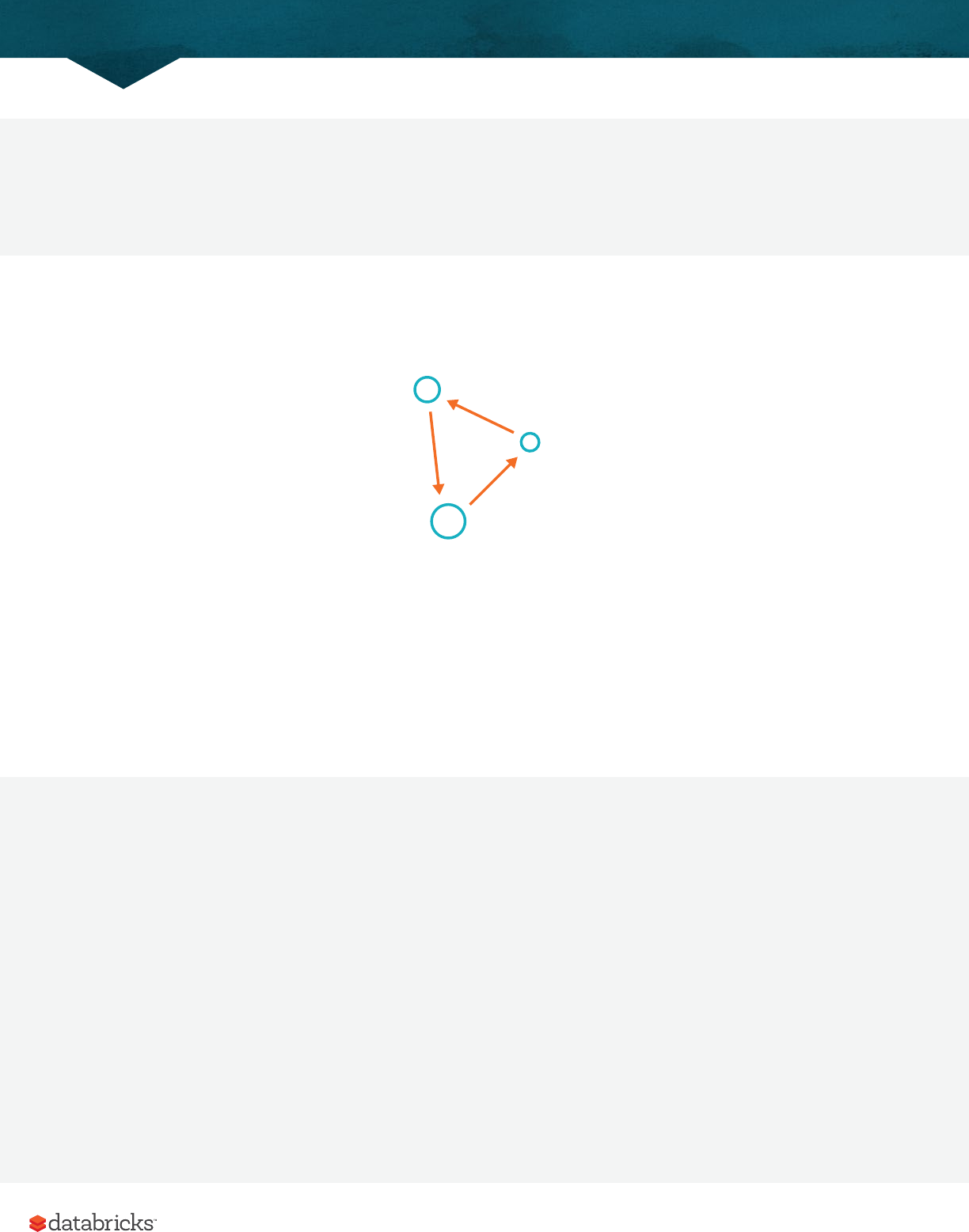
86
%python
motifs = stationGraph\
.nd("(a)-[ab]->(b); (b)-[bc]->(c); (c)-[ca]->(a)")
Here’s a visual representation of this query.
The resulting DataFrame contains nested fields for vertices a, b, and c as well as the respective edges. Now we can
query this data as if it were a DataFrame. Now we can query that to answer a specific question. Given a certain bike
what is the shortest round trip time where that bike is taken from one station (a), ridden to another, dropped o
at (b), ridden to another, dropped o at (c), and then ridden back to the original station, (a). The following logic
will parse our timestamps into Spark timestamps and then we’ll do comparisons to make sure that it’s the same bike,
traveling from station to station, and that the start times for each trip are correct.
%scala
import org.apache.spark.sql.functions.expr
motifs// rst simplify dates for comparisons
.selectExpr("*", """
to_timestamp(ab.`Start Date`, ‘MM/dd/yyyy HH:mm’) as abStart
""",
"""
to_timestamp(bc.`Start Date`, ‘MM/dd/yyyy HH:mm’) as bcStart
""",
"""
to_timestamp(ca.`Start Date`, ‘MM/dd/yyyy HH:mm’) as caStart
""")
.where("ca.`Bike #` = bc.`Bike #`") // ensure the same bike
.where("ab.`Bike #` = bc.`Bike #`")
.where("a.id != b.id") // ensure dierent stations
c
bc
b
ab
a
ca
Graph Analysis

87
.where("b.id != c.id")
.where("abStart < bcStart") // start times are correct
.where("bcStart < caStart")
.orderBy(expr("cast(caStart as long) - cast(abStart as long)")) // order them all
.selectExpr("a.id", "b.id", "c.id",
"ab.`Start Date`", "ca.`End Date`")
.limit(1)
.show(false)
%python
from pyspark.sql.functions import expr
motifs\
.selectExpr("*", """
to_timestamp(ab.`Start Date`, ‘MM/dd/yyyy HH:mm’) as abStart
""",
"""
to_timestamp(bc.`Start Date`, ‘MM/dd/yyyy HH:mm’) as bcStart
""",
"""
to_timestamp(ca.`Start Date`, ‘MM/dd/yyyy HH:mm’) as caStart
""")\
.where("ca.`Bike #` = bc.`Bike #`")\
.where("ab.`Bike #` = bc.`Bike #`")\
.where("a.id != b.id")\
.where("b.id != c.id")\
.where("abStart < bcStart")\
.where("bcStart < caStart")\
.orderBy(expr("cast(caStart as long) - cast(abStart as long)"))\
.selectExpr("a.id", "b.id", "c.id",
"ab.`Start Date`", "ca.`End Date`")\
.limit(1)\
.show(1, False)
+---------------------------------------+---------------+-----------------------+
|id |id |id |Start Date |End Date |
+---------------------------------------+---------------+-----------------------+
|San Francisco Caltrain 2 (330 Townsend)|Townsend at 7th|San Francisco Caltrain (Townsend at 4th)|5/19/2015 16:09|5/19/2015 16:33|
+---------------------------------------+---------------+-----------------------+
We see the fastest trip is approximately 20 minutes. Pretty fast for three dierent people (we assume) using the
same bike!
Graph Analysis

88
Advanced Tasks
This is just a short selection of some of the things GraphFrames allows you to achieve. Development continues as
well and so you will be able to continue to find new algorithms and features being added the library. Some of these
advanced features include writing your own algorithms via a message passing interface, triangle counting, converting
to and from GraphX among other tasks. It is also likely that in the future this library will join GraphX in the core of
Spark.
Graph Analysis

89
One of the most exciting areas of development around Spark is deep learning. Deep learning is rapidly growing into
one of the most powerful techniques for solving machine learning problems, especially those involving unstructured
data such as images, audio and text. This chapter will cover how Spark works in tandem with deep learning, and some
of the dierent approaches that you can take using Spark and deep learning together.
This chapter will not focus on packages that are necessarily core to Spark but rather on the massive amount of
innovation in libraries built on top of Apache Spark. Because deep learning is still a new field, many of the newest
tools are implemented in external libraries. We will start with several high-level ways to use deep learning on Spark,
discuss when to use each one, and discuss the libraries available for them. As usual, we will include end-to-end
examples.
WARNING
If you have little experience with machine learning and/or deep learning, unfortunately this chapter cannot provide a
complete summary of everything you need to know. To be truly successful in this chapter you should know at least the
basics of deep learning as well as the basics of Spark. With that being said, we point to an excellent resource at the
beginning of this part of the book called the Deep Learning Book, by some of the most successful researchers in this
area. We recommend taking some time to learn about the core machine learning methods as well as getting a basic
grasp of deep learning before continuing with this chapter.
What is deep learning?
In order to define deep learning, we must first define neural networks. A neural network is a graph of nodes that
consist of a weight and an activation function. These nodes are organized into layers that are stacked on top of
one another. Each layer is connected, either partially or completely, to the previous layer in the network. Each
node activation’s function will fire when suicient inputs trigger that activation. Together, the network’s layers can
represent progressively more complex functions that oen "learn" a hierarchy of features in the input data (e.g. edges,
circles and textures for image recognition). The goal is to train the network to associate certain inputs with certain
outputs by tuning the weights associated with each connection and the values of each node in the network.
Deep Learning
90
Deep learning, or deep neural networks, just combine many of these layers together in various dierent architectures.
Neural networks themselves have existed for decades, and have waxed and waned in terms of popularity for various
machine learning problems. Recently, however, a combination of much larger datasets (e.g., the ImageNet corpus for
object recognition), parallel infrastructure (clusters and GPUs), and new training algorithms have enabled training
much larger neural networks that outperformed pervious approaches in many machine learning tasks. Deep neural
networks have now become the standard in computer vision, speech processing, and many natural language tasks,
where they oen "learn" better features than previous hand-tuned models. They are also actively being applied in
other areas of machine learning. Apache Spark’s strength as a big data and parallel computing system makes it a
natural framework to use with deep learning.
Ways of Using Deep Learning in Spark
For the most part, regardless of which application you are targeting, there are three major ways to use deep learning
in Spark.
1. Inference: The simplest way to use deep learning is to take a pre-trained model and apply it to large datasets
in parallel using Spark. For example, given an image classification model that can recognized people, trained
using a standard dataset like ImageNet, one might apply it to images from a retail store to track customer flows
within it. Many organizations publish large, pre-trained models on common datasets (e.g., FasterRCNN and
YOLO for object detection), so you can oen take a model from your favorite deep learning framework and apply
it in parallel using a Spark function. In the extreme, simply calling a framework such as TensorFlow or PyTorch
in a map function can get you distributed inference, though some of the libraries we discuss for it make further
optimizations beyond that.
2. Featurization and Transfer Learning: The next level of complexity is to use an existing model as a featurizer
instead of taking its final output. Many deep learning models learn useful feature representations in their
lower layers as they train the network for an end-to-end task. For example, a classifier trained on the ImageNet
dataset (a popular labeled dataset with thousands of object classes) will also learn low-level features present
Input
Units
Hidden
Units
Output
Units
Deep Learning

91
in all natural images, such as edges and textures. We can then use these features to learn models for a new
problem not covered by the original dataset. For example, the ImageNet dataset does not contain any images of
cancer tumors, but several research papers have used models trained on it as featurizers to produce classifiers
for these types of images. This method is called transfer learning, and generally involves cutting o the last few
layers of a pre-trained model and retraining them with the data of interest. Transfer learning is also especially
useful if you do not have a large amount of training data: training a full-blown network from scratch requires a
dataset of hundreds of thousands of images, like ImageNet, to avoid overfitting, which will not be available in
many business contexts. In contrast, transfer learning can work even with a few thousand images because it
updates fewer parameters.
3. Model Training: Spark can also be used to train a new deep learning model from scratch. There are two
common methods here. First, you can use a Spark cluster to parallelize the training of a single model over
multiple servers, communicating updates between them. Alternatively, some libraries let the user train multiple
instances of similar models in parallel to try various model architectures and hyperparameters, accelerating
the model search and tuning process. In both cases, Spark’s deep learning libraries make it simple to pass data
from RDDs and DataFrames to deep learning algorithms. Finally, even if you do not wish to train your model
in parallel, these libraries can be used to extract data from a cluster and export it to a single-machine trainign
script using the native data format of frameworks like TensorFlow.
In all three cases, the deep learning code typically runs as part of a larger application that includes Extract, Transform
and Load (ETL) steps to parse the input data, I/O from various sources, and potentially batch or streaming inference.
For these other parts of the application, you can simply use the DataFrame, RDD and MLlib APIs described earlier in
this book. One of Spark’s strengths is the ease of combining these steps into a single parallel workflow.
Deep Learning Libraries
In this section of the chapter, we’ll survey a few of the most popular libraries available for deep learning in Spark. We
will describe the main use cases of the library and link to references or a small example when possible. This list is not
meant to be exhaustive, because the field is rapidly evolving, so we encourage you to check each library’s website and
the Spark documentation for the latest updates. The Databricks Engineering blog at https://databricks.com/blog also
regularly has articles on deep learning.
MLlib Neural Network Support
Spark’s MLlib currently has native support for one deep learning algorithm, the multilayer perceptron classifier in the
ml.classication.MultilayerPerceptronClassier class. This class is limited to training relatively
shallow networks containing fully connected layers with the sigmoid activation function, and an output layer with
a somax activation function. This class is most useful for training the last few layers of a classification model when
using transfer learning on top of an existing deep learning based featurizer. For example, it can be added on top of the
Deep Learning Pipelines library we describe later in this chapter to quickly perform transfer learning over Keras and
Deep Learning

92
TensorFlow models. However, the MultiLayerPerceptronClassifier alone is not enough to train a deep learning model
from scratch on raw input data.
TensorFrames
TensorFrames is an inference and transfer learning oriented library that makes it easy to pass data between Spark
DataFrames and TensorFlow. It supports Python and Scala interfaces and focuses on providing a simple but optimized
interface to pass data from TensorFlow to Spark and back. In particular, using TensorFrames to apply a model
over Spark DataFrames is generally more eicient than calling a Python map function that directly invokes the
TensorFlow model, due to faster data transfer and amortization of the startup cost. TensorFrames is most useful for
inference, in both streaming and batch settings, and for transfer learning, where you can apply an existing model
over raw data to featurize it, then learn the last layers using a MultilayerPerceptronClassifier or even a simpler logistic
regression or random forest classifier over the data.
https://github.com/databricks/tensorframes
BigDL
BigDL (pronounced "big deal") is a distributed deep learning framework for Apache Spark primarily developed
by Intel. It aims to support distributed training of large models as well as fast applications of these models using
inference. One key advantage of BigDL over the other libraries described here is that it is primiarily optimzied to
use CPUs instead of Graphics Processing Units (GPUs), making it eicient to run on an existing, CPU-based cluster
(e.g. an Apache Hadoop deployment). BigDL provides high-level APIs to build a neural network from scratch and
automatically distributes all operations by default.
https://github.com/intel-analytics/BigDL
TensorFlowOnSpark
TensorFlowOnSpark is a widely used library that can train Google TensorFlow models in a parallel fashion on Spark
clusters. TensorFlow already provides support for distributed training, but it does not come with a cluster manager
or a distributed I/O layer out of the box – instead, users have to manually set up a distributed TensorFlow cluster
and feed data into it. TensorFlowOnSpark launches TensorFlow’s existing distributed mode inside a Spark job, and
automatically feeds data from Spark RDDs or DataFrames into the TensorFlow job. If you already know how to use
TensorFlow’s distributed mode, TensorFlowOnSpark makes it easy to launch your job inside a Spark cluster and
pass it data processed with other Spark libraries (e.g. DataFrame transformations) from any input source that Spark
supports. TensorFlowOnSpark was originally developed at Yahoo! and is also used in production at other large
organizations.
https://github.com/yahoo/TensorFlowOnSpark
Deep Learning

93
CaeOnSpark
Cae is a popular deep learning framework focused on image processing. CaeOnSpark is an open source package
for using Cae on top of Spark that includes parallel model training, testing, and feature extraction. Much like
TensorFlowOnSpark, it aims to run Cae in parallel on an existing Spark cluster and easily pass data into it from
Spark. CaeOnSpark was also developed at Yahoo!
https://github.com/yahoo/CaeOnSpark
DeepLearning4J
DeepLearning4j is an open-source, distributed deep-learning project in Java and Scala that provides both single node
and distributed training options. One of its advantages over the Python-based deep learning frameworks is that it
was primarily designed for the JVM, making it more convenient for groups that do not wish to add Python to their
development process. It includes a wide variety of training algorithms and support for CPUs as well as GPUs.
https://deeplearning4j.org/spark
Deep Learning Pipelines
Deep Learning Pipelines is an open source package from Databricks that integrates deep learning functions into
Spark’s ML Pipelines API. The package calls into existing deep learning frameworks (TensorFlow and Keras at the
time of writing), but focuses on two goals: (1) incorporating these into standard Spark APIs, such as ML Pipelines
and Spark SQL, to make them very easy to use and (2) distributing all computation by default. For example, Deep
Learning Pipelines provides a DeepImageFeaturizer class that acts as a Transformer in the Spark ML Pipeline
API, allowing you to build a transfer learning pipeline in just a few lines of code (e.g., by adding a perceptron or logistic
regression classifier on top). Likewise, the project supports parallel grid search over multiple model parameters using
MLlib’s grid search and cross validation API. Finally, users can export a ML model as a Spark SQL user-defined function
and make it available to analysts using SQL or streaming applications. At the time of writing (summer 2017), Deep
Learning Pipelines is under heavy development, so we encourage you to check its website for the latest updates.
https://github.com/databricks/spark-deep-learning
Here is a summmary table of the various deep learning libraries and the main use cases they support.
Deep Learning

94
Library Underlying DL Framework Use Cases
BigDL BigDL distributed training, inference, ML Pipeline integration
CaeOnSpark Cae distributed training
DeepLearning4J DeepLearning4J inference, transfer learning, distributed training
Deep Learning Pipelines TensorFlow, Keras inference, transfer learning, multi-model training, ML Pipeline
and Spark SQL integration
MLlib Perceptron Spark distributed training, ML Pipeline integration
TensorFlowOnSpark TensorFlow distributed training
TensorFrames TensorFlow inference, transfer learning, DataFrame integration
While there are several approaches dierent companies have taken to integrating Spark and deep learning libraries,
the one currently aiming for the closest integration with MLlib and DataFrames is Deep Learning Pipelines. This
project aims to improve Spark’s support for image and tensor data (which may also be integrated into the core Spark
codebase in the future), and to make all deep learning functionality available in the standard ML Pipeline API. For this
reason, we’ll be covering the project in a bit more detail through the rest of the chapter with simple examples of the
power of the library.
A Simple Example with Deep Learning Pipelines
As we described, Deep Learning Pipelines provides high-level APIs for scalable deep learning by integrating popular
deep learning frameworks with ML Pipelines and Spark SQL.
Deep Learning Pipelines builds on Spark’s ML Pipelines for training, and with Spark DataFrames and SQL for deploying
models. It includes high-level APIs for common aspects of deep learning so they can be done eiciently in a few lines
of code:
• Working with images in Spark DataFrames;
• Applying deep learning models at scale, whether they are your own or standard popular models, to
image and tensor data;
• Transfer learning using common pre-trained deep learning models;
• Exporting models as Spark SQL functions to make it simple for all kinds of users to take advantage of
deep learning;
• Distributed deep learning hyperparameter tuning via ML Pipelines.
• Deep Learning Pipelines currently only oers an API in Python, which is designed to work closely with
existing Python deep learning packages such as TensorFlow and Keras.
Deep Learning

95
WARNING
Readers should be aware that this library, like every Spark related deep learning library, is currently under active
development and may have changed since the time we wrote this chapter. Before getting started, it’s worth checking
on the development of these various projects in order to better understand their current status and new functionality
that may have been added.
Setup
Deep Learning Pipelines is a Spark Package, so we’ll load it just like we loaded GraphFrames. Deep Learning Pipelines
works on Spark 2.x and the package can be found here. You’re going to need to install a couple of dependencies
including tensorframes, TensorFlow, keras, and h5py. Make sure that these are installed across both your driver and
worker machines.
We’ll use the flowers dataset from the TensorFlow retraining tutorial. Now if you’re running this on a cluster of
machines, you’re going to need a way to put these files on a distributed file system once you download them. We
include a sample of these images in the book’s GitHub Repository.
Images and DataFrames
One of the historical challenges when it came to working with images in Spark is that getting them into a DataFrame
was diicult and tedious. Deep Learning Pipelines includes utility functions that making loading and decoding images
in a distributed fashion easy.
TODO: can you say what formats are supported or what image library this uses to load stu?
%python
from sparkdl import readImages
img_dir = ‘/mnt/defg/deep-learning-images/’
image_df = readImages(img_dir)
The resulting DataFrame contains the path, and then the image along with some associated metadata.
%python
image_df.show()
image_df.printSchema()
Deep Learning

96
+--------------------+-----+
| lePath|image|
+--------------------+-----+
|/mnt/defg/de... | null|
+--------------------+-----+
root
|-- lePath: string (nullable = false)
|-- image: struct (nullable = true)
| |-- mode: string (nullable = false)
| |-- height: integer (nullable = false)
| |-- width: integer (nullable = false)
| |-- nChannels: integer (nullable = false)
| |-- data: binary (nullable = false)
Transfer Learning
Now that we have some data, we can get started with some simple transfer learning. Remember, this means
leveraging a model that someone else created and modifying it to better suit our own purposes. First we will load the
data for each type of flower and create a training and a test set.
%python
from sparkdl import readImages
from pyspark.sql.functions import lit
tulips_df = readImages(img_dir + "/tulips").withColumn("label", lit(1))
daisy_df = readImages(img_dir + "/daisy").withColumn("label", lit(0))
tulips_train, tulips_test = tulips_df.randomSplit([0.6, 0.4])
daisy_train, daisy_test = daisy_df.randomSplit([0.6, 0.4])
train_df = tulips_train.unionAll(daisy_train)
test_df = tulips_test.unionAll(daisy_test)
The next step will be to leverage a transformer called the DeepImageFeaturizer. This will allow us to leverage a
pre-trained model called Inception, a powerful neural network successfully used to identify patterns in images. The
version were are using is pre-trained to work well with images. This is a part of the standard pretrained models that
ship with the Keras library. However, this particular neural network is not trained to work with our particular set of
Deep Learning

97
images (involving flowers). Therefore we’re going to use transfer learning in order to make it into something useful for
our own purposes.
One thing that’s quite powerful here is that we can use the same ML pipeline concepts that we saw throughout this
part of the book and leverage them with Deep Learning: DeepImageFeaturizer is just a Spark ML transformer.
Additionally, all that we’ve done to extend this model is add on a logistic regression model in order to facilitate the
training of our end model. We could use another classifier in its place.
WARNING
This next code snippet is unlikely to run successfully on small machines because of the large resource requirements
when using and applying this model.
%python
from pyspark.ml.classication import LogisticRegression
from pyspark.ml import Pipeline
from sparkdl import DeepImageFeaturizer
featurizer = DeepImageFeaturizer(inputCol="image", outputCol="features", modelName="InceptionV3")
lr = LogisticRegression(maxIter=1, regParam=0.05, elasticNetParam=0.3, labelCol="label")
p = Pipeline(stages=[featurizer, lr])
p_model = p.t(train_df)
Once we trained the model, we can use the same classification evaluator that we saw several chapters ago. We can
specify the metric we’d like to test and then test against that.
%python
from pyspark.ml.evaluation import MulticlassClassicationEvaluator
tested_df = p_model.transform(test_df)
evaluator = MulticlassClassicationEvaluator(metricName="accuracy")
print("Test set accuracy = " + str(evaluator.evaluate(tested_df.select("prediction", "label"))))
With our DataFrame of examples, we can inspect the rows and images in which we made mistakes in the previous
training.
Deep Learning

98
%python
from pyspark.sql.types import DoubleType
from pyspark.sql.functions import expr
# a simple UDF to convert the value to a double
def _p1(v):
return oat(v.array[1])
p1 = udf(_p1, DoubleType())
df = tested_df.withColumn("p_1", p1(tested_df.probability))
wrong_df = df.orderBy(expr("abs(p_1 - label)"), ascending=False)
wrong_df.select("lePath", "p_1", "label").limit(10).show()
Applying deep learning models at scale
Spark DataFrames are a natural construct for applying deep learning models to a large-scale dataset. Deep Learning
Pipelines provides a set of (Spark MLlib) Transformers for applying TensorFlow Graphs and TensorFlow-backed Keras
Models at scale. In addition, popular images models can be applied out of the box, without requiring any TensorFlow
or Keras code. The Transformers, backed by the Tensorframes library, eiciently handle the distribution of models and
data to Spark workers.
Applying popular image models
There are many standard deep learning models for images. If the task at hand is very similar to what the models
provide (e.g. object recognition with ImageNet classes), or for pure exploration, one can use the Transformer
DeepImagePredictor by simply specifying the model name. Deep Learning Pipelines supports a variety of
standard models included in Keras, which are listed on its website.
%python
from sparkdl import readImages, DeepImagePredictor
image_df = readImages(img_dir)
predictor = DeepImagePredictor(inputCol="image", outputCol="predicted_labels",
modelName="InceptionV3", decodePredictions=True, topK=10)
predictions_df = predictor.transform(image_df.where("image.mode is not null"))
Deep Learning

99
Notice that the predicted_labels column shows "daisy" as a high probability class for all sample flowers using
this base model. However, as can be seen from the dierences in the probability values, the neural network has the
information to discern the two flower types. Hence our transfer learning example above was able to properly learn the
dierences between daisies and tulips starting from the base model.
df = p_model.transform(image_df)
Applying Custom Keras Models
Spark deep learing also allows for the application of a TensorFlow-backed Keras model in a distributed manner using
Spark. To do this check the user guide on the KerasImageFileTransformer. The way this works by loading the
keras model and then applying that model in the same DataFrame that we’ve seen in the previous sections.
Applying TensorFlow Models
Deep Learning Pipelines, through a deep integration with TensorFlow, can be used to create custom transformers that
manipulate images using TensorFlow. For instance, you could create a transformer to change the size of an image or
modify the color spectrum.
TODO: can you say which class they should use for this?
TODO: Show how to export a function as UDF and call it
Deep Learning
100
The Unified Analytics Platform
The datasets used in the book are also available for you to explore:
Spark: The Definitive Guide Datasets
Try Databricks for free
databricks.com/try-databricks
Contact us for a personalized demo
databricks.com/contact
© Databricks 2017. All rights reserved. Apache Spark and the Apache Spark Logo are trademarks of the Apache Soware Foundation.
