Paralution User Manual
User Manual:
Open the PDF directly: View PDF ![]() .
.
Page Count: 141 [warning: Documents this large are best viewed by clicking the View PDF Link!]
- Introduction
- Installation
- Basics
- Single-node Computation
- Multi-node Computation
- Solvers
- Preconditioners
- Code Structure
- Jacobi
- Multi-colored (Symmetric) Gauss-Seidel and SOR
- Incomplete LU with levels – ILU(p)
- Incomplete Cholesky – IC
- Incomplete LU with threshold – ILUT(t,m)
- Power(q)-pattern method – ILU(p,q)
- Multi-Elimination ILU
- Diagonal Preconditioner for Saddle-Point Problems
- Chebyshev Polynomial
- FSAI(q)
- SPAI
- Block Preconditioner
- Additive Schwarz and Restricted Additive Schwarz – AS and RAS
- Truncated Neumann Series Preconditioner (TNS)
- Variable Preconditioner
- CPR Preconditioner
- MPI Preconditioners
- Backends
- Advanced Techniques
- Plug-ins
- Remarks
- Performance Benchmarks
- Graph Analyzers
- Functionality Table
- Code Examples
- Change Log
- Bibliography

User manual
Version 1.1.0
January 19, 2016

3
PARALUTION - User Manual
This document is licensed under
Creative Commons Attribution-NonCommercial-NoDerivs 3.0 Unported License
http://creativecommons.org/licenses/by-nc-nd/3.0/legalcode
This project is funded by
Imprint:
PARALUTION Labs UG (haftungsbeschr¨ankt) & Co. KG
Am Hasensprung 6, 76571 Gaggenau, Germany
Handelsregister: Amtsgericht Mannheim, HRA 706051
Vertreten durch PARALUTION Labs Verwaltungs UG (haftungsbeschr¨ankt)
Am Hasensprung 6, 76571 Gaggenau, Germany
Handelsregister: Amtsgericht Mannheim, HRB 721277
Gesch¨aftsf¨uhrer: Dimitar Lukarski, Nico Trost
www.paralution.com
Copyright c
2015-2016
4
PARALUTION - User Manual
1 Introduction 9
1.1 Overview ................................................. 9
1.2 PurposeofthisUserManual ...................................... 10
1.3 APIDocumentation ........................................... 10
1.4 DualLicense ............................................... 11
1.4.1 BasicVersions .......................................... 11
1.4.2 CommercialVersions....................................... 11
1.5 VersionNomenclature .......................................... 12
1.6 FeaturesNomenclature.......................................... 12
1.7 Cite .................................................... 12
1.8 Website .................................................. 13
2 Installation 15
2.1 Linux/Unix-likeOS............................................ 15
2.1.1 Makefile.............................................. 15
2.1.2 CMake............................................... 15
2.1.3 SharedLibrary .......................................... 16
2.2 WindowsOS ............................................... 16
2.2.1 OpenMPbackend ........................................ 16
2.2.2 CUDAbackend.......................................... 17
2.2.3 OpenCLbackend......................................... 18
2.3 MacOS .................................................. 18
2.4 SupportedCompilers........................................... 18
2.5 SimpleTest ................................................ 19
2.6 CompilationandLinking ........................................ 19
3 Basics 21
3.1 DesignandPhilosophy.......................................... 21
3.2 OperatorsandVectors.......................................... 21
3.2.1 LocalOperators/Vectors..................................... 22
3.2.2 GlobalOperators/Vectors.................................... 22
3.3 Functionality on the Accelerators . . . . . . . . . . . . . . . . . . . . . . . . . . . . . . . . . . . . 22
3.4 InitializationoftheLibrary ....................................... 22
3.4.1 Thread-coreMapping ...................................... 24
3.4.2 OpenMPThresholdSize..................................... 25
3.4.3 DisabletheAccelerator ..................................... 25
3.4.4 MPI and Multi-accelerators . . . . . . . . . . . . . . . . . . . . . . . . . . . . . . . . . . . 25
3.5 AutomaticObjectTracking ....................................... 26
3.6 VerboseOutput.............................................. 26
3.7 VerboseOutputandMPI ........................................ 26
3.8 DebugOutput .............................................. 26
3.9 FileLogging................................................ 26
3.10Versions.................................................. 26
4 Single-node Computation 27
4.1 Introduction................................................ 27
4.2 CodeStructure .............................................. 27
4.3 ValueType ................................................ 27
4.4 ComplexSupport............................................. 28
4.5 AllocationandFree............................................ 29
5
6PARALUTION - USER MANUAL
4.6 MatrixFormats.............................................. 29
4.6.1 CoordinateFormat–COO ................................... 30
4.6.2 Compressed Sparse Row/Column Format – CSR/CSC . . . . . . . . . . . . . . . . . . . . 30
4.6.3 DiagonalFormat–DIA ..................................... 31
4.6.4 ELLFormat ........................................... 31
4.6.5 HYBFormat ........................................... 31
4.6.6 MemoryUsage .......................................... 32
4.6.7 Backendsupport ......................................... 32
4.7 I/O..................................................... 32
4.8 Access................................................... 33
4.9 RawAccesstotheData ......................................... 34
4.10CopyCSRMatrixHostData ...................................... 35
4.11CopyData ................................................ 35
4.12ObjectInfo ................................................ 35
4.13Copy.................................................... 35
4.14Clone ................................................... 36
4.15Assembling ................................................ 37
4.16Check ................................................... 38
4.17Sort .................................................... 38
4.18Keying................................................... 38
4.19GraphAnalyzers ............................................. 39
4.20 Basic Linear Algebra Operations . . . . . . . . . . . . . . . . . . . . . . . . . . . . . . . . . . . . 40
4.21LocalStencils............................................... 41
5 Multi-node Computation 43
5.1 Introduction................................................ 43
5.2 CodeStructure .............................................. 44
5.3 ParallelManager ............................................. 44
5.4 GlobalMatricesandVectors....................................... 45
5.4.1 ValueTypeandFormats..................................... 45
5.4.2 Matrix and Vector Operations . . . . . . . . . . . . . . . . . . . . . . . . . . . . . . . . . 45
5.4.3 AsynchronousSpMV....................................... 45
5.5 CommunicationChannel......................................... 45
5.6 I/O..................................................... 45
5.6.1 FileOrganization......................................... 45
5.6.2 ParallelManager......................................... 46
5.6.3 Matrices.............................................. 47
5.6.4 Vectors .............................................. 47
6 Solvers 49
6.1 CodeStructure .............................................. 49
6.2 IterativeLinearSolvers ......................................... 51
6.3 StoppingCriteria............................................. 51
6.4 BuildingandSolvingPhase ....................................... 52
6.5 ClearfunctionandDestructor...................................... 53
6.6 NumericalUpdate ............................................ 53
6.7 Fixed-pointIteration........................................... 53
6.8 KrylovSubspaceSolvers......................................... 54
6.8.1 CG................................................. 54
6.8.2 CR................................................. 54
6.8.3 GMRES.............................................. 54
6.8.4 FGMRES ............................................. 55
6.8.5 BiCGStab............................................. 55
6.8.6 IDR ................................................ 55
6.8.7 FCG................................................ 55
6.8.8 QMRCGStab........................................... 56
6.8.9 BiCGStab(l) ........................................... 56
6.9 DeflatedPCG............................................... 56
6.10ChebyshevIteration ........................................... 57
6.11Mixed-precisionSolver.......................................... 57
6.12MultigridSolver ............................................. 58
PARALUTION - USER MANUAL 7
6.12.1 GeometricMultigrid....................................... 58
6.12.2 AlgebraicMultigrid ....................................... 58
6.13DirectLinearSolvers........................................... 61
6.14EigenvalueSolvers ............................................ 61
6.14.1 AMPE-SIRA ........................................... 61
7 Preconditioners 63
7.1 CodeStructure .............................................. 63
7.2 Jacobi ................................................... 63
7.3 Multi-colored (Symmetric) Gauss-Seidel and SOR . . . . . . . . . . . . . . . . . . . . . . . . . . 64
7.4 Incomplete LU with levels – ILU(p) .................................. 65
7.5 IncompleteCholesky–IC ........................................ 65
7.6 Incomplete LU with threshold – ILUT(t,m) .............................. 65
7.7 Power(q)-pattern method – ILU(p,q) .................................. 66
7.8 Multi-EliminationILU.......................................... 66
7.9 Diagonal Preconditioner for Saddle-Point Problems . . . . . . . . . . . . . . . . . . . . . . . . . . 66
7.10ChebyshevPolynomial.......................................... 67
7.11 FSAI(q) .................................................. 67
7.12SPAI.................................................... 68
7.13BlockPreconditioner........................................... 68
7.14 Additive Schwarz and Restricted Additive Schwarz – AS and RAS . . . . . . . . . . . . . . . . . 70
7.15 Truncated Neumann Series Preconditioner (TNS) . . . . . . . . . . . . . . . . . . . . . . . . . . . 71
7.16VariablePreconditioner ......................................... 72
7.17CPRPreconditioner ........................................... 72
7.18MPIPreconditioners........................................... 72
8 Backends 73
8.1 BackendandAccelerators ........................................ 73
8.2 Copy.................................................... 73
8.3 CloneBackend............................................... 73
8.4 Moving Objects To and From the Accelerator . . . . . . . . . . . . . . . . . . . . . . . . . . . . . 74
8.5 AsynchronousTransfers ......................................... 75
8.6 SystemswithoutAccelerators...................................... 76
9 Advanced Techniques 77
9.1 HardwareLocking ............................................ 77
9.2 TimeRestriction/Limit ......................................... 77
9.3 OpenCLKernelEncryption ....................................... 78
9.4 LoggingEncryption ........................................... 78
9.5 Encryption ................................................ 78
9.6 MemoryAllocation............................................ 78
9.6.1 AllocationProblems ....................................... 78
9.6.2 MemoryAlignment........................................ 78
9.6.3 Pinned Memory Allocation (CUDA) . . . . . . . . . . . . . . . . . . . . . . . . . . . . . . 78
10 Plug-ins 79
10.1FORTRAN ................................................ 79
10.2OpenFOAM................................................ 80
10.3Deal.II................................................... 81
10.4Elmer ................................................... 83
10.5Hermes/Agros2D ............................................ 84
10.6Octave/MATLAB ............................................ 84
11 Remarks 87
11.1Performance................................................ 87
11.2Accelerators................................................ 88
11.3Plug-ins .................................................. 88
11.4Correctness ................................................ 88
11.5Compilation................................................ 88
11.6Portability................................................. 89
8PARALUTION - USER MANUAL
12 Performance Benchmarks 91
12.1Single-NodeBenchmarks......................................... 91
12.1.1 HardwareDescription ...................................... 91
12.1.2 BLAS1andSpMV ........................................ 92
12.1.3 CGSolver............................................. 92
12.2Multi-NodeBenchmarks......................................... 95
13 Graph Analyzers 99
14 Functionality Table 103
14.1BackendSupport............................................. 103
14.2 Matrix-Vector Multiplication Formats . . . . . . . . . . . . . . . . . . . . . . . . . . . . . . . . . 103
14.3LocalMatricesandVectors ....................................... 104
14.4GlobalMatricesandVectors....................................... 104
14.5 Local Solvers and Preconditioners . . . . . . . . . . . . . . . . . . . . . . . . . . . . . . . . . . . . 105
14.6 Global Solvers and Preconditioners . . . . . . . . . . . . . . . . . . . . . . . . . . . . . . . . . . . 107
15 Code Examples 109
15.1PreconditionedCG............................................ 109
15.2 Multi-Elimination ILU Preconditioner with CG . . . . . . . . . . . . . . . . . . . . . . . . . . . . 111
15.3 Gershgorin Circles+Power Method+Chebyshev Iteration+PCG with Chebyshev Polynomial . . . 113
15.4Mixed-precisionPCGSolver....................................... 117
15.5PCGSolverwithAMG ......................................... 120
15.6 AMG Solver with External Smoothers . . . . . . . . . . . . . . . . . . . . . . . . . . . . . . . . . 123
15.7 Laplace Example File with 4 MPI Process . . . . . . . . . . . . . . . . . . . . . . . . . . . . . . . 127
16 Change Log 133
Bibliography 139

Chapter 1
Introduction
1.1 Overview
PARALUTION is a sparse linear algebra library with focus on exploring fine-grained parallelism, targeting
modern processors and accelerators including multi/many-core CPU and GPU platforms. The main goal of this
project is to provide a portable library for iterative sparse methods on state of the art hardware. Figure 1.1
shows the PARALUTION framework as middle-ware between different parallel backends and application specific
packages.
Multi-core CPU
OpenMP
GPU
CUDA/OpenCL
Xeon Phi
OpenMP
API: C++
FORTRAN
Plug-ins:
MATLAB/Octave, Deal.II,
OpenFOAM, Hermes, Elmer, ...
Figure 1.1: The PARALUTION library – middleware between hardware and problem specific packages.
The major features and characteristics of the library are:
•Various backends:
–Host – designed for multi-core CPU, based on OpenMP
–GPU/CUDA – designed for NVIDIA GPU
–OpenCL – designed for OpenCL-compatible devices (NVIDIA GPU, AMD GPU, CPU, Intel MIC)
–OpenMP(MIC) – designed for Intel Xeon Phi/MIC
•Multi-node/accelerator support – the library supports multi-node and multi-accelerator configurations
via MPI layer.
•Easy to use – the syntax and the structure of the library provide easy learning curves. With the help of
the examples, anyone can try out the library – no knowledge in CUDA, OpenCL or OpenMP required.
•No special hardware/library required – there are no hardware or library requirements to install and
run PARALUTION. If a GPU device and CUDA, OpenCL, or Intel MKL are available, the library will use
them.
•Most popular operating systems:
–Unix/Linux systems (via cmake/Makefile and gcc/icc)
–MacOS (via cmake/Makefile and gcc/icc)
–Windows (via Visual Studio)
9
10 CHAPTER 1. INTRODUCTION
•Various iterative solvers:
–Fixed-Point iteration – Jacobi, Gauss-Seidel, Symmetric-Gauss Seidel, SOR and SSOR
–Krylov subspace methods – CR, CG, BiCGStab, BiCGStab(l), GMRES, IDR, QMRCGSTAB, Flexible
CG/GMRES
–Deflated PCG
–Mixed-precision defect-correction scheme
–Chebyshev iteration
–Multigrid – geometric and algebraic
•Various preconditioners:
–Matrix splitting – Jacobi, (Multi-colored) Gauss-Seidel, Symmetric Gauss-Seidel, SOR, SSOR
–Factorization – ILU(0), ILU(p) (based on levels), ILU(p,q) (power(q)-pattern method) and Multi-
elimination ILU (nested/recursive), ILUT (based on threshold), IC(0)
–Approximate Inverse - Chebyshev matrix-valued polynomial, SPAI, FSAI and TNS
–Diagonal-based preconditioner for Saddle-point problems
–Block-type of sub-preconditioners/solvers
–Additive Schwarz and Restricted Additive Schwarz
–Variable type of preconditioners
•Generic and robust design – PARALUTION is based on a generic and robust design allowing expansion
in the direction of new solvers and preconditioners, and support for various hardware types. Furthermore,
the design of the library allows the use of all solvers as preconditioners in other solvers, for example you can
easily define a CG solver with a Multi-elimination preconditioner, where the last-block is preconditioned
with another Chebyshev iteration method which is preconditioned with a multi-colored Symmetric Gauss-
Seidel scheme.
•Portable code and results – all code based on PARALUTION is portable and independent of GPU/CUDA,
OpenCL or MKL. The code will compile and run everywhere. All solvers and preconditioners are based on
a single source code, which delivers portable results across all supported backends (variations are possible
due to different rounding modes on the hardware). The only difference which you can see for a hardware
change is the performance variation.
•Support for several sparse matrix formats – Compressed Sparse Row (CSR), Modified Compressed
Sparse Row (MCSR), Dense (DENSE), Coordinate (COO), ELL, Diagonal (DIA), Hybrid format of ELL
and COO (HYB) formats.
•Plug-ins – the library provides a plug-in for the CFD package OpenFOAM [44] and for the finite element
library Deal.II [8, 9]. The library also provides a FORTRAN interface and a plug-in for MATLAB/Octave
[36, 2].
1.2 Purpose of this User Manual
The purpose of this document is to present the PARALUTON library step-by-step. This includes the installation
process, internal structure and design, application programming interface (API) and examples. The change log
of the software is also presented here.
All related documentation (web site information, user manual, white papers, doxygen) follows the Creative
Commons Attribution-NonCommercial-NoDerivs 3.0 Unported License [12]. A copy of the license can be found
in the library package.
1.3 API Documentation
The most important library’s functions are presented in this document. The library’s full API (references)
are documented via the automatic documentation system - doxygen [55]. The references are available on the
PARALUTION web site.

1.4. DUAL LICENSE 11
Basic
GPLv3
version
Single - node/
accelerator
version
Multi - node/
accelerator
version
Basic GPLv3
Single node
Commercial
license
Advanced
solvers
Full complex
support
More ad-
vanced solvers
MPI communi-
cation layer
Figure 1.2: The three PARALUTION versions
1.4 Dual License
The PARALUTION library is distributed within a dual license model. Three different version can be obtained
– a GPLv3 version which is free of charge and two commercial versions.
1.4.1 Basic Versions
The basic version of the code is released under the GPL v3 license [18]. It provides the core components of the
single node functionality of the library. This version of the library is free. Please, note that due to GPLv3 license
model, any code which uses the library must be released as Open Source and it should have compliance to the
GPLv3.
1.4.2 Commercial Versions
The user can purchase a commercial license which will grant the ability to embed the code into a (commercial)
closed binary package. In addition these versions come with more features and with support. The only restriction
imposed to the user is that she/he is not allowed to further distribute the source-code.
Single-node/accelerator Version
In addition to the basic version, the commercial license features:
•License to embed the code into a commercial/non-opensource product
•Full complex numbers support on Host, CUDA and OpenCL
•More iterative solvers - QMRCGStab, BiCGStab(l), FCG
•More AMG schemes - Ruge-St¨uben, Pairwise
•More preconditioners - VariablePreconditioners
Multi-node/accelerator Version
In addition to the commercial basic version, the multi-node license features:
•License to embed the code into a commercial/non-opensource product
•Same functionality as for the single-node/accelerator version
•MPI layer for HPC clusters

12 CHAPTER 1. INTRODUCTION
•Global AMG solver (Pairwise)
Note Please note, that the multi-node version does not support Windows/Visual Studio.
1.5 Version Nomenclature
Please note the following compatibility policy with respect to the versioning. The version number x.y.z repre-
sents: x is the major (increases when modifications in the library have been made and/or a new API has been
introduced), y is the minor (increases when new functionality (algorithms, schemes, etc) has been added, possibly
small/no modification of the API) and z is the revision (increases due to bugfixing or performance improvement).
The alpha and beta versions are denoted with aand b, typically these are pre-released versions.
As mentioned above there are three versions of PARALUTION, each release has the same version numbering
plus an additional suffix for each type. They are abbreviated with ”B” for the Basic version (free under GPLv3),
with ”S” for the single node/accelerator commercial and with ”M” for the multi-node/accelerator commercial
version.
1.6 Features Nomenclature
The functions described in this user manual follows the following nomenclature:
•ValueType – type of values can be double (D), float (F), integer (I), and complex (double and float). The
particular bit representation (8,16,32,64bit) depends on your compiler and operating system.
•Computation – on which backend the computation can be performed, the abbreviation follows: Host backend
with OpenMP (H); CUDA backend (C); OpenCL backend (O); Xeon Phi backend with OpenMP (X).
•Available – in which version this functionality is available: Basic/GPLv3 (B); Single-node/accelerator
commercial version (S); Multi-node/accelerator commercial version (M).
The following example states that the function has double, float, integer and complex support; it can be
performed on Host backend with OpenMP, CUDA backend, OpenCL backend, Xeon Phi backend with OpenMP;
and it is available in all three versions of the library.
ValueType Computation Available
D,F,I,C H,C,O,X B,S,M
Solvers and preconditioners split the computation into a Building phase and Solving phase which can have
different computation backend performance. In the following example the solver/preconditioner support double,
float and complex; the building phase can be performed only on the Host with OpenMP or on CUDA; the solving
phase can be performed on all other backends; it is available only in the commercial versions of the library.
ValueType Building phase Solving phase Available
D,F,C H,C H,C,O,X S,M
Note The full complex support is available only in the commercial version, check Section 4.4.
1.7 Cite
If you like to cite the PARALUTION library you can do it as you like with citing our web site. Please specify
the version of the software or/and date of accessing our web page, like that:
1 @misc{paralution ,
2 author=”{PARALUTION Labs }”,
3 t i t l e=”{PARALUTION vX .Y. Z}”,
4 ye ar=”20XX” ,
5 n ote = {\ u r l {htt p : //www. p a r a l u t i o n . com/}}
6}
1.8. WEBSITE 13
1.8 Website
The official web site of the library (including all (free and commercial) versions) is
http://www.paralution.com
14 CHAPTER 1. INTRODUCTION

Chapter 2
Installation
PARALUTION can be compiled under Linux/Unix, Windows and Mac systems.
Note Please check for additional remarks Sections 11.5.
2.1 Linux/Unix-like OS
After downloading and unpacking the library, the user needs to compile it. We provide two compilation configu-
rations – cmake and Makefile.
2.1.1 Makefile
In this case, the user needs to modify the Makefile which contains the information about the available compilers.
By default PARALUTION will only use gcc [20] compiler (no GPU support). The user can switch to icc [23] with
or without MKL [24] support. To compile with GPU support, the user needs to uncomment the corresponding
CUDA1[43] lines in the Makefile. The same procedure needs to be followed for the OpenCL [29] and for the
OpenMP(MIC) backend.
Note During the compilation only one backend can be selected, i.e. if a GPU is available the user needs to
select either CUDA or OpenCL support.
The default installation process can be summarized in the following lines:
1 wget http : //www. p a r a l u t i o n . com/ download / p a ra l u ti on −x . y . z . t a r . gz
2
3 t a r zx v f p a r a l u t i o n −x . y . z . t a r . g z
4
5 cd paralution−x . y . z / s r c
6
7 make a l l
8 make i n s t a l l
where x.y.z is the version of the library.
Note Please note, that the multi-node version of PARALUTION can only be compiled using CMake.
2.1.2 CMake
The compilation with cmake [30] is easier to handle – all compiler specifications are determined automatically.
The compilation process can be performed by
1 wget http : //www. p a r a l u t i o n . com/ download / p a ra l u ti on −x . y . z . t a r . gz
2
3 t a r zx v f p a r a l u t i o n −x . y . z . t a r . gz
4
5 cd paralution−x . y . z
6
7 mkdir b u i l d
8 cd b u i l d
9
10 cmake . .
11 make
1NVIDIA CUDA, when mentioned also includes CUBLAS and CUSPARSE
15

16 CHAPTER 2. INSTALLATION
where x.y.z is the version of the library. Advanced compilation can be performed with cmake -i .., you need this
option to compile the library with OpenMP(MIC) backend.
The priority during the compilation process of the backends are: CUDA, OpenCL, MIC
You can also choose specific options via the command line, for example CUDA:
1 cd paralution−x . y . z
2
3 mkdir b u i l d
4 cd b u i l d
5
6 cmake −DSUPPORT CUDA=ON −DSUPPORT OMP=ON . .
7 make −j
For the Intel Xeon Phi, OpenMP(MIC) backend:
1 cd paralution−x . y . z
2
3 mkdir b u i l d
4 cd b u i l d
5
6 cmake −DSUPPORT MIC=ON −DSUPPORT CUDA=OFF −DSUPPORT OCL=OFF . .
7 make −j
Note ptk file is generated in the build directory when using cmake.
2.1.3 Shared Library
Both compilation processes produce a shared library file libparalution.so. Ensure that the library object can be
found in your library path. If you do not copy the library to a specific location you can add the path under Linux
in the LD LIBRARY PATH variable.
1export LD LIBRARY PATH=$LD LIBRARY PATH : ˜ / p a r a l u t i o n −x . y . z / b u i l d / l i b /
2.2 Windows OS
This section will introduce a step-by-step guide to compile and use the PARALUTION library in a Windows
based environment. Note Please note, that the multi-node version does not support Windows/Visual Studio.
2.2.1 OpenMP backend
PARALUTION with OpenMP backend comes with Visual Studio Project files that support Visual Studio 2010,
2012 and 2013. PARALUTION is built as a static library during this step-by-step guide.
•Open Visual Studio and navigate to File\Open Project.
Figure 2.1: Open an existing Visual Studio project.
•Load the corresponding PARALUTION project file, located in the visualstudio\paralution omp directory.
The PARALUTION and CG projects should appear.
•Right-click the PARALUTION project, and start to build the library. Once finished, Visual Studio should
report a successful built.
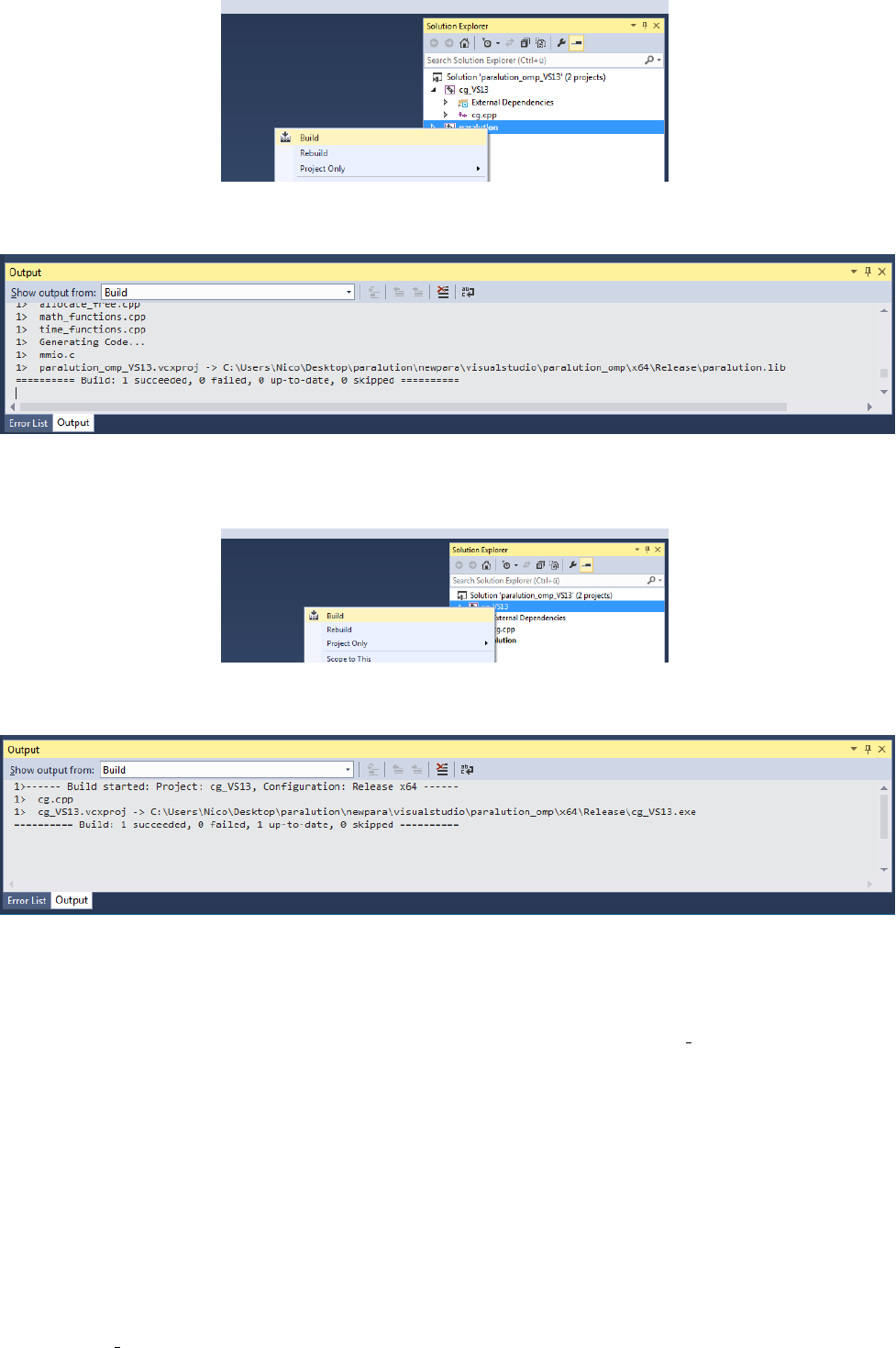
•Next, repeat the building procedure with the CG example project. Once finished, a successful built should
be reported.
2.2. WINDOWS OS 17
Figure 2.2: Build the PARALUTION library.
Figure 2.3: Visual Studio output for a successful built of the static PARALUTION library.
Figure 2.4: Build the PARALUTION CG example.
Figure 2.5: Visual Studio output for a successful built of the PARALUTION CG example.
•Finally, the CG executable should be located within the visualstudio\paralution omp\Release directory.
Note For testing, Windows 7 and Visual Studio Express 2013 has been used.
Note OpenMP support can be enabled/disabled in the project properties. Navigate to C++\Language for
the corresponding switch.
Note The current version of PARALUTION does not support MPI (i.e. the M-version of the library) under
Windows.
2.2.2 CUDA backend
PARALUTION with CUDA backend comes with Visual Studio Project files that support Visual Studio 2010,
2012 and 2013. Please follow the same steps as for the OpenMP backend compilation but using the visualstu-
dio\paralution cuda directory.

18 CHAPTER 2. INSTALLATION
2.2.3 OpenCL backend
PARALUTION with OpenCL backend comes with Visual Studio Project files that support Visual Studio 2010,
2012 and 2013. Please follow the same steps as for the OpenMP backend compilation but using the visualstu-
dio\paralution ocl directory. Additionally, the OpenCL include directory and OpenCL library directory need to
be specified within Visual Studio, as illustrated in Figures 2.6 and 2.7.
Figure 2.6: Setting up Visual Studio OpenCL include directory.
2.3 Mac OS
To compile PARALUTION under Mac, please follow the Linux/Unix-like OS instruction for the CMake compi-
lation.
2.4 Supported Compilers
The library has been tested with the following compilers:
cmake 2.8.12.2; 3.0.2; 3.1.3; 3.2.0 B,S,M
gcc/g++ 4.4.7; 4.6.3; 4.8.2 B,S,M
icc (MKL) 12.0; 13.1; 14.0.4; 15.0.0 B,S,M
CUDA 5.0; 5.5; 6.0; 6.5; 7.0; 7.5 B,S,M
Intel OpenCL 1.2 B,S,M
NVIDIA OpenCL 1.2 B,S,M
AMD OpenCL 1.2; 2.0 B,S,M
Visual Studio 2010, 2012, 2013 B,S
MPICH 3.1.3 M
OpenMPI 1.5.3; 1.6.3; 1.6.5; 1.8.4 M
Intel MPI 4.1.2; 5.0.1 M
Note Please note, that CUDA has limited ICC support.
Note Please note, that Intel MPI >= 5.0.0 is only supported by CMAKE >= 3.2.0.

2.5. SIMPLE TEST 19
Figure 2.7: Setting up Visual Studio OpenCL library directory.
2.5 Simple Test
You can test the installation by running a CG solver on a Laplace matrix [38]. After compiling the library you
can perform the CG solver test by executing:
1 cd paralution−x . y . z
2 cd b u i l d / bi n
3
4 wget f t p : // math . n i s t . gov /pub/ MatrixMarket2 / Har we ll −Boeing / l a p l a c e / g r 3 0 3 0 . mtx . gz
5 g z i p −d g r 3 0 3 0 . mtx . gz
6
7 . / cg g r 3 0 3 0 . mtx
2.6 Compilation and Linking
After compiling the PARALUTION library, the user need to specify the include and the linker path to compile
a program.
1 g++ −O3 −Wall −I / path / to / p a r a l u t i o n −x . y . z / b u i l d / i n c −c main . cpp −o main . o
2 g++ −o main main . o −L/ path / t o / p a r a l u t i o n −x . y . z / b u i l d / l i b / −lparalution
”Compilation and linking”
Before the execution of a program which has been compiled with PARALUTION, the library path need to
be added to the environment variables, similar to
1export LD LIBRARY PATH=$LD LIBRARY PATH : ˜ / p a r a l u t i o n −x . y . z / b u i l d / l i b /
When compiling with MPI, library and program need to be compiled using mpic++ or the corresponding
MPI C++ compiler.
20 CHAPTER 2. INSTALLATION

Chapter 3
Basics
3.1 Design and Philosophy
The main idea of the PARALUTION objects is that they are separated from the actual hardware specification.
Once you declare a matrix, a vector or a solver they are initially allocated on the host (CPU). Then every object
can be moved to a selected accelerator by a simple move-to-accelerator function. The whole execution mechanism
is based on run-time type information (RTTI) which allows you to select where and how you want to perform
the operations at run time. This is in contrast to the template-based libraries which need this information at
compile time.
The philosophy of the library is to abstract the hardware-specific functions and routines from the actual
program which describes the algorithm. It is hard and almost impossible for most of the large simulation software
based on sparse computation to adapt and port their implementation in order to use every new technology. On the
other hand, the new high performance accelerators and devices have the capability to decrease the computational
time significantly in many critical parts.
This abstraction layer of the hardware specific routines is the core of PARALUTION’s design, it is built to
explore fine-grained level of parallelism suited for multi/many-core devices. This is in contrast to most of the
parallel sparse libraries available which are mainly based on domain decomposition techniques. Thus, the design
of the iterative solvers the preconditioners is very different. Another cornerstone of PARALUTION is the native
support of accelerators - the memory allocation, transfers and specific hardware functions are handled internally
in the library.
PARALUTION helps you to use accelerator technologies but does not force you to use them. As you can see
later in this chapter, even if you offload your algorithms and solvers to the accelerator device, the same source
code can be compiled and executed in a system without any accelerators.
3.2 Operators and Vectors
The main objects in PARALUTION are linear operators and vectors. All objects can be moved to an accelerator
at run time – a structure diagram is presented in Figure 3.1. Currently, we support GPUs by CUDA (NVIDIA)
and OpenCL (NVIDIA, AMD) backends, and we provide OpenMP MIC backend for the Intel Xeon Phi.
GPU, Accelerators
OpenCL
Dynamic
Switch
OpenMP
Host Accelerator
GPU
CUDA
Intel MIC
OpenMP
New
Backend
Operators/Vectors
Solvers/Preconditioners
Figure 3.1: Host and backends structure for different hardware
21

22 CHAPTER 3. BASICS
The linear operators are defined as local or global matrices (i.e. on a single node or distributed/multi-node)
and local stencils (i.e. matrix-free linear operations).
Global Vector
Local Vector Vectors
Operators Global Matrix
Local Matrix
Local Stencil
Figure 3.2: Operator and vector classes
The only template parameter of the operators and vectors is the data type (ValueType). The operator data
type could be float or double, while the vector data type can be float,double or int (int is used mainly for the
permutation vectors). In the current version, cross ValueType object operations are not supported.
Each of the objects contains a local copy of the hardware descriptor created by the init platform() function.
This allows the user to modify it according to his needs and to obtain two or more objects with different hardware
specifications (e.g. different amount of OpenMP threads, CUDA block sizes, etc).
3.2.1 Local Operators/Vectors
By Local Operators/Vectors we refer to Local Matrices and Stencils, and to Local Vectors. By Local we mean
the fact they stay on a single system. The system can contain several CPUs via UMA or NUMA memory system,
it can contain an accelerator.
3.2.2 Global Operators/Vectors
By Global Operators/Vectors we refer to Global Matrix and to Global Vectors. By Global we mean the fact they
can stay on a single or multiple nodes in a network. For this this type of computation, the communication is
based on MPI.
3.3 Functionality on the Accelerators
Naturally, not all routines and algorithms can be performed efficiently on many-core systems (i.e. on accelerators).
To provide full functionality the library has internal mechanisms to check if a particular routine is implemented
on the accelerator. If not the object is moved to the host and the routine is computed there. This guarantees
that your code will run (maybe not in the most efficient way) with any accelerator regardless of the available
functionality for it.
3.4 Initialization of the Library
The body of a PARALUTION code is very simple, it should contain the header file and the namespace of the
library. The program must contain an initialization call, which will check and allocate the hardware, and a
finalizing call which will release the allocated hardware.
1#include <paralution .hpp>
2
3using namespace paralution ;
4
5i n t main ( i n t argc , char ∗argv [ ] ) {
6
7 i n i t p a r a l u t i o n ( ) ;
8
9 info paralution () ;
10
11 // . . .
12

3.4. INITIALIZATION OF THE LIBRARY 23
13 s t o p p a r a l u t i o n ( ) ;
14
15 }
”Initialize and shutdown PARALUTION”
1 This v e rs io n o f PARALUTION i s r e l e a s e d under GPL.
2 By downloading t h i s package you f u l l y agree with the GPL l i c e n s e .
3 Number o f CPU c o r e s : 32
4 Host t hrea d a f f i n i t y p o l i c y −th rea d mapping on ev ery cor e
5 Number o f GPU d e v i c e s i n t he system : 2
6 PARALUTION ver B0 . 8 . 0
7 PARALUTION platfo r m i s i n i t i a l i z e d
8 A c c e l e r a t o r backend : GPU(CUDA)
9 OpenMP t h r ea d s : 3 2
10 S e l e c t e d GPU d e v i c e : 0
11 −−−−−−−−−−−−−−−−−−−−−−−−−−−−−−−−−−−−−−−−−−−−−−−−
12 Device number : 0
13 Device name : Tes la K20c
14 totalGlobalMem : 4799 MByte
15 cloc k Rate : 705500
16 compute c a p a b i l i t y : 3 .5
17 ECCEnabled : 1
18 −−−−−−−−−−−−−−−−−−−−−−−−−−−−−−−−−−−−−−−−−−−−−−−−
19 −−−−−−−−−−−−−−−−−−−−−−−−−−−−−−−−−−−−−−−−−−−−−−−−
20 Device number : 1
21 Device name : Tes la K20c
22 totalGlobalMem : 4799 MByte
23 cloc k Rate : 705500
24 compute c a p a b i l i t y : 3 .5
25 ECCEnabled : 1
26 −−−−−−−−−−−−−−−−−−−−−−−−−−−−−−−−−−−−−−−−−−−−−−−−
”An example output for info paralution() on a GPU (CUDA) system”
1 This v e rs io n o f PARALUTION i s r e l e a s e d under GPL.
2 By downloading t h i s package you f u l l y agree with the GPL l i c e n s e .
3 Number o f CPU c o r e s : 32
4 Host t hrea d a f f i n i t y p o l i c y −th rea d mapping on e very c or e
5 Number o f OpenCL d e v i c e s i n th e system : 2
6 PARALUTION ver B0 . 8 . 0
7 PARALUTION platfo r m i s i n i t i a l i z e d
8 A c c e l e r a t o r backend : OpenCL
9 OpenMP t h r ea d s : 3 2
10 S e l e c t e d OpenCL p l at for m : 0
11 S e l e c t e d OpenCL d e v ic e : 0
12 −−−−−−−−−−−−−−−−−−−−−−−−−−−−−−−−−−−−−−−−−−−−−−−−
13 P latform number : 0
14 P latform name : NVIDIA CUDA
15 Device number : 0
16 Device name : Tes la K20c
17 Device type : GPU
18 totalGlobalMem : 4799 MByte
19 cloc k Rate : 705
20 OpenCL v e r s i o n : OpenCL 1 . 1 CUDA
21 −−−−−−−−−−−−−−−−−−−−−−−−−−−−−−−−−−−−−−−−−−−−−−−−
22 −−−−−−−−−−−−−−−−−−−−−−−−−−−−−−−−−−−−−−−−−−−−−−−−
23 P latform number : 0
24 P latform name : NVIDIA CUDA
25 Device number : 1
26 Device name : Tes la K20c
27 Device type : GPU
28 totalGlobalMem : 4799 MByte

24 CHAPTER 3. BASICS
29 cloc k Rate : 705
30 OpenCL v e r s i o n : OpenCL 1 . 1 CUDA
31 −−−−−−−−−−−−−−−−−−−−−−−−−−−−−−−−−−−−−−−−−−−−−−−−
”An example output for info paralution() on a GPU (OpenCL) system”
1 This v e rs io n o f PARALUTION i s r e l e a s e d under GPL.
2 By downloading t h i s package you f u l l y agree with the GPL l i c e n s e .
3 Number o f CPU c o r e s : 16
4 Host t hrea d a f f i n i t y p o l i c y −th rea d mapping on e very c or e
5 MIC backed i s i n i t i a l i z e d
6 PARALUTION ver B0 . 8 . 0
7 PARALUTION platfo r m i s i n i t i a l i z e d
8 A c c e l e r a t o r backend : MIC(OpenMP)
9 OpenMP t h r ea d s : 1 6
10 Number o f MIC d e v i c e s i n the system : 2
11 S e l e c t e d MIC d e v i c e s : 0
”An example output for info paralution() on Intel Xeon Phi (OpenMP) system”
1 This v e rs io n o f PARALUTION i s r e l e a s e d under GPL.
2 By downloading t h i s package you f u l l y agree with the GPL l i c e n s e .
3 Number o f CPU c o r e s : 2
4 Host t hrea d a f f i n i t y p o l i c y −th rea d mapping on e very c or e
5 PARALUTION ver B0 . 8 . 0
6 PARALUTION platfo r m i s i n i t i a l i z e d
7 A c c e l e r a t o r backend : None
8 OpenMP t hre ad s : 2
”An example output for info paralution() on system without accelerator”
The init paralution() function defines a backend descriptor with information about the hardware and its
specifications. All objects created after that contain a copy of this descriptor. If the specifications of the global
descriptor are changed (e.g. set different number of threads) and new objects are created, only the new objects
will use the new configurations.
For control the library provides the following functions
•select device paralution(int dev) – this is a unified function which select a specific device. If you have
compiled the library with a backend and for this backend there are several available cards you can use this
function to select a particular one. This function works for all backends (CUDA, OpenCL, Xeon Phi).
•set omp threads paralution(int nthreads) – with this function the user can set the number of OpenMP
threads. This function has to be called after the init paralution().
•set gpu cuda paralution(int ndevice) – in a multi-GPU system, the user can select a specific GPU by this
function. This function has to be called before the init paralution().
•set ocl paralution(int nplatform, int ndevice) – in a multi-platform/accelerator system, the user can select
a specific platform and device by this function. This function has to be called before the init paralution().
3.4.1 Thread-core Mapping
The number of threads which PARALUTION will use can be set via the set omp threads paralution() function
or by the global OpenMP environment variable (for Unix-like OS this is OMP NUM THREADS). During the
initialization phase, the library provides affinity thread-core mapping based on:
•if the number of cores (including hyperthreading cores) is greater or equal than two times the number of
threads – then all the threads can occupy every second core ID (e.g. 0,2,4, ...). This is to avoid having two
threads working on the same physical core when hyperthreading is enabled.
•if the number of threads is less or equal to the number of cores (including hyperthreading), and the previous
clause is false. Then the threads can occupy every core ID (e.g. 0,1,2,3, ...).
•if non of the above criteria is matched – the default thread-core mapping is used (typically set by the OS).
Note The thread-core mapping is available only for Unix-like OS. For Windows OS, the thread-core mapping
is selected by the operating system.
Note The user can disable the thread affinity by calling set omp affinity(false) (and enable it with set omp affinity(true)),
before initializing the library (i.e. before init paralution()).

3.4. INITIALIZATION OF THE LIBRARY 25
3.4.2 OpenMP Threshold Size
Whenever you want to work on a small problem, you might observe that the OpenMP Host backend is (slightly)
slower than using no OpenMP. This is mainly attributed to the small amount of work which every thread should
perform and the large overhead of forking/joining threads. This can be avoid by the OpenMP threshold size
parameter in PARALUTION. The default threshold is set to 10,000, which means that all matrices under (and
equal) this size will use only one thread (disregarding the number of OpenMP threads set in the system). The
threshold can be modified via the function set omp threshold().
3.4.3 Disable the Accelerator
If you want to disable the accelerator (without recompiling the code), you need to call disable accelerator paralution()
function before the init paralution().
3.4.4 MPI and Multi-accelerators
When initializing the library with MPI, the user need to pass the rank of the MPI process as well as the number
of accelerators which are available on each node. Basically, in this way the user can specify the mapping of MPI
process and accelerators – the allocated accelerator will be rank %num dev per node. Thus the user can run two
MPI process on systems with two GPUs by specifying the number of devices to 2.
1#include <paralution .hpp>
2#include <mpi . h>
3
4using namespace paralution ;
5
6i n t main ( i n t argc , char ∗argv [ ] ) {
7
8 MPI Init (& argc , &argv ) ;
9 MPI Comm comm = MPI COMM WORLD;
10
11 i n t num p roc esses ;
12 i n t rank ;
13 MPI Comm size (comm, &num p roc esse s ) ;
14 MPI Comm rank (comm, &rank ) ;
15
16 i n i t p a r a l u t i o n ( rank , 2) ;
17
18 info paralution () ;
19
20 // . . .
21
22 s t o p p a r a l u t i o n ( ) ;
23
24 }
”Initialize and shutdown PARALUTION with MPI”
1 The default OS t hrea d a f f i n i t y c o n f i g u r a t i o n w i l l be used
2 Number o f GPU d e v i c e s i n t he system : 2
3 The default OS t hrea d a f f i n i t y c o n f i g u r a t i o n w i l l be used
4 PARALUTION ver M0. 8 . 0
5 PARALUTION platfo r m i s i n i t i a l i z e d
6 A c c e l e r a t o r backend : GPU(CUDA)
7 OpenMP t hre ad s : 1
8 S e l e c t e d GPU d e v i c e : 0
9−−−−−−−−−−−−−−−−−−−−−−−−−−−−−−−−−−−−−−−−−−−−−−−−
10 Device number : 0
11 Device name : Tes la K20c
12 totalGlobalMem : 4799 MByte
13 cloc k Rate : 705500
14 compute c a p a b i l i t y : 3 .5
15 ECCEnabled : 1

26 CHAPTER 3. BASICS
16 −−−−−−−−−−−−−−−−−−−−−−−−−−−−−−−−−−−−−−−−−−−−−−−−
17 −−−−−−−−−−−−−−−−−−−−−−−−−−−−−−−−−−−−−−−−−−−−−−−−
18 Device number : 1
19 Device name : Tes la K20c
20 totalGlobalMem : 4799 MByte
21 cloc k Rate : 705500
22 compute c a p a b i l i t y : 3 .5
23 ECCEnabled : 1
24 −−−−−−−−−−−−−−−−−−−−−−−−−−−−−−−−−−−−−−−−−−−−−−−−
25 MPI rank : 0
26 MPI s i z e : 2
”An example output for info paralution() with 2 MPI processes”
3.5 Automatic Object Tracking
By default, after the initialization of the library, it tracks all objects and releasing the allocated memory in them
when the library is stopped. This ensure large memory leaks when the objects are allocated but not freed. The
user can disable the tracking by editing src/utils/def.hpp.
3.6 Verbose Output
PARALUTION provides different levels of output messages. They can be set in the file src/utils/def.hpp before
the compilation of the library. By setting a higher level, the user will obtain more detailed information about
the internal calls and data transfers to and from the accelerators.
3.7 Verbose Output and MPI
To avoid all MPI processes to print information on the screen the default configuration is that only RANK 0
outputs information on the screen. The user can change the RANK or allow all RANK to print by modifying
src/utils/def.hpp. If file logging is enabled, all ranks write into corresponding log files.
3.8 Debug Output
You can also enable debugging output which will print almost every detail in the program, including object
constructor/destructor, address of the object, memory allocation, data transfers, all function calls for matrices,
vectors, solvers and preconditioners. The debug flag can be set in src/utils/def.hpp.
When enabled, additional assert()s are being checked during the computation. This might decrease the
performance of some operations.
3.9 File Logging
All output can be logged into a file, the file name will be paralution-XXXX.log, where XXX will be a counter in
milliseconds. To enable the file you need to edit src/utils/def.hpp.
3.10 Versions
For checking the version in your code you can use the PARALUTION’s pre-defined macros.
1 PARALUTION VER MAJOR −− g i v e s t he v e r s i o n major v a lu e
2 PARALUTION VER MINOR −− g i v e s t he v e r s i o n minor v al ue
3 PARALUTION VER REV −− g i v e s the v e rs i o n r e v i s i o n
4
5 PARALUTION VER PRE −− g i v e s pre−r e l e a s e s ( as ”ALPHA” o r ”BETA” )
The final PARALUTION VER gives the version as 10000major + 100minor +revision.
The different type of versions (Basic/GPLv3; Single-node; Multi-node) are defined as PARALUTION VER TYPE
Bfor Basic/GPLv3; Sfor Single-node; and Mfor Multi-node.

Chapter 4
Single-node Computation
4.1 Introduction
In this chapter we describe all base objects (matrices, vectors and stencils) for computation on single-node
(shared-memory) systems. A typical configuration is presented on Figure 4.1.
Accelerator
(e.g. GPU)
Bus (PCI-E)
Host (CPU)
Figure 4.1: A typical single-node configuration, where gray-boxes represent the cores, blue-boxes represent the
memory, arrows represent the bandwidth
The compute node contains none, one or more accelerators. The compute node could be any kind of shared-
memory (single, dual, quad CPU) system. Note that the memory of the accelerator and of the host can be
physically different.
4.2 Code Structure
The Data is an object, pointing to the BaseMatrix class. The pointing is coming from either a HostMatrix or
an AcceleratorMatrix. The AcceleratorMatrix is created by an object with an implementation in each of the
backends (CUDA, OpenCL, Xeon Phi) and a matrix format. Switching between host or accelerator matrix is
performed in the LocalMatrix class. The LocalVector is organized in the same way.
Each matrix format has its own class for the host and for each accelerator backend. All matrix classes are
derived from the BaseMatrix which provides the base interface for computation as well as for data accessing, see
Figure4.4. The GPU (CUDA backend) matrix structure is presented in Figure 4.5, all other backend follows the
same organization.
4.3 Value Type
The value (data) type of the vectors and the matrices is defined as a template. The matrix can be of type float
(32-bit), double (64-bit) and complex (64/128-bit). The vector can be float (32-bit), double (64-bit), complex
27

28 CHAPTER 4. SINGLE-NODE COMPUTATION
GPU, Accelerators
OpenCL
Dynamic
Switch
OpenMP
Host
Data Data
Data
Data
Data
Accelerator
GPU
CUDA
Intel MIC
OpenMP
New
Backend
Local Matrix/Vector
Figure 4.2: Local Matrices and Vectors
paralution::LocalMatrix< ValueType >
paralution::Operator< ValueType >
paralution::BaseParalution< ValueType >
paralution::ParalutionObj
paralution::LocalVector< ValueType >
paralution::Vector< ValueType >
paralution::BaseParalution< ValueType >
paralution::ParalutionObj
Figure 4.3: LocalMatrix and Local Vector
paralution::BaseMatrix< ValueType >
paralution::AcceleratorMatrix< ValueType > paralution::HostMatrix< ValueType >
paralution::GPUAcceleratorMatrix< ValueType >
paralution::MICAcceleratorMatrix< ValueType >
paralution::OCLAcceleratorMatrix< ValueType >
paralution::HostMatrixBCSR< ValueType >
paralution::HostMatrixCOO< ValueType >
paralution::HostMatrixCSR< ValueType >
paralution::HostMatrixDENSE< ValueType >
paralution::HostMatrixDIA< ValueType >
paralution::HostMatrixELL< ValueType >
paralution::HostMatrixHYB< ValueType >
paralution::HostMatrixMCSR< ValueType >
Figure 4.4: BaseMatrix
(64/128-bit) and int (32/64-bit). The information about the precision of the data type is shown in the Print()
function.
4.4 Complex Support
PARALUTION supports complex computation in all functions due to its internal template structure. The host
implementation is based on the std::complex. In binary, the data is the same also for the CUDA and for the
OpenCL backend. The complex support of the backends with respect to the versions is presented in Table 4.1.

4.5. ALLOCATION AND FREE 29
paralution::GPUAcceleratorMatrix< ValueType >
paralution::AcceleratorMatrix< ValueType >
paralution::BaseMatrix< ValueType >
paralution::GPUAcceleratorMatrixBCSR< ValueType >
paralution::GPUAcceleratorMatrixCOO< ValueType >
paralution::GPUAcceleratorMatrixCSR< ValueType >
paralution::GPUAcceleratorMatrixDENSE< ValueType >
paralution::GPUAcceleratorMatrixDIA< ValueType >
paralution::GPUAcceleratorMatrixELL< ValueType >
paralution::GPUAcceleratorMatrixHYB< ValueType >
paralution::GPUAcceleratorMatrixMCSR< ValueType >
Figure 4.5: GPUAcceleratorMatrix (CUDA)
Host CUDA OpenCL Xeon Phi
B Yes No No No
S Yes Yes Yes No
M Yes Yes Yes No
Table 4.1: Complex support
4.5 Allocation and Free
The allocation functions require a name of the object (this is only for information purposes) and corresponding
size description for vector and matrix objects.
1 Loca lV ector <ValueType>vec ;
2
3 v ec . A l l o c a t e ( ”my v e c t o r ” , 100) ;
4 vec . Cle ar ( ) ;
”Vector allocation/free”
1 LocalMatrix<ValueType>mat ;
2
3 mat . AllocateCSR ( ”my c s r matri x ” , 456 , 1 00 , 100) ; // nnz , rows , columns
4 mat . Cle ar ( ) ;
5
6 mat . AllocateCOO ( ”my coo matrix ” , 2 00 , 10 0 , 100) ; // nnz , rows , columns
7 mat . Cle ar ( ) ;
”Matrix allocation/free”
4.6 Matrix Formats
Matrices where most of the elements are equal to zero are called sparse. In most practical applications the number
of non-zero entries is proportional to the size of the matrix (e.g. typically, if the matrix Ais RN×Nthen the
number of elements are of order O(N)). To save memory, we can avoid storing the zero entries by introducing a
structure corresponding to the non-zero elements of the matrix. PARALUTION supports sparse CSR, MCSR,
COO, ELL, DIA, HYB and dense matrices (DENSE).
To illustrate the different format, let us consider the following matrix in Figure 4.6.
Here the matrix is A∈R5×5with 11 non-zero entries. The indexing in all formats described below are zero
based (i.e. the index values starts at 0, not with 1).

30 CHAPTER 4. SINGLE-NODE COMPUTATION
1 2 11
01234
9 10
3 4
567
8
0
1
2
3
4
Figure 4.6: A sparse matrix example
Note The functionality of every matrix object is different and depends on the matrix format. The CSR format
provides the highest support for various functions. For a few operations an internal conversion is performed,
however, for many routines an error message is printed and the program is terminated.
Note In the current version, some of the conversions are performed on the host (disregarding the actual
object allocation - host or accelerator).
1 mat . ConvertToCSR ( ) ;
2// Perform a matrix−v e c to r m u l t i p l c a t i o n i n CSR f or ma t
3 mat . Apply ( x , &y ) ;
4
5 mat . ConvertToELL ( ) ;
6// Perform a matrix−v e c to r m u l t i p l c a t i o n i n ELL f ormat
7 mat . Apply ( x , &y ) ;
”Conversion between matrix formats”
1 mat . ConvertTo (CSR) ;
2// Perform a matrix−v e c to r m u l t i p l c a t i o n i n CSR f or ma t
3 mat . Apply ( x , &y ) ;
4
5 mat . ConvertTo (ELL) ;
6// Perform a matrix−v e c to r m u l t i p l c a t i o n i n ELL f ormat
7 mat . Apply ( x , &y ) ;
”Conversion between matrix formats (alternative)”
4.6.1 Coordinate Format – COO
The most intuitive sparse format is the coordinate format (COO). It represent the non-zero elements of the
matrix by their coordinates, we need to store two index arrays (one for row and one for column indexing) and
the values. Thus, our example matrix will have the following structure:
row
col
val
0 0 0 1 1 2 2 2 3 4 4
0 1 3 1 2 1 2 3 3 3 4
1 2 11 3 4 5 6 7 8 9 10
Figure 4.7: Sparse matrix in COO format
4.6.2 Compressed Sparse Row/Column Format – CSR/CSC
One of the most popular formats in many scientific codes is the compressed sparse row (CSR) format. In this
format, we do not store the whole row indices but we only save the offsets to positions. Thus, we can easily jump
to any row and we can access sequentially all elements there. However, this format does not allow sequential
accessing of the column entries.

4.6. MATRIX FORMATS 31
row
offset
col
val
0 3 5 8 9 11
0 1 3 1 2 1 2 3 3 3 4
1 2 11 3 4 5 6 7 8 9 10
Figure 4.8: Sparse matrix in CSR format
Analogy to this format is the compressed sparse column (CSC), where we represent the offsets by the column
– it is clear that we can traverse column elements sequentially.
In many finite element (difference/volumes) applications, the diagonal elements are non-zero. In such cases,
we can store them at the beginning of the value arrays. This format is often referred as modified compressed
sparse row/column (MCSR/MCSC).
4.6.3 Diagonal Format – DIA
If all (or most) of the non-zero entries belong to a few diagonals of matrix, we can store them with the responding
offsets. In our example, we have 4 diagonal, the main diagonal (denoted with 0 offset) is fully occupied while the
others contain zero entries.
*1 2 11
-1 0 1 3
0 3 4 0
5 6 7 *
0 8 0 *
9 10 * *
val
dig
Figure 4.9: Sparse matrix in DIA format
Please note, that the values in this format are stored as array with size D×ND, where Dis the number of
diagonals in the matrix and NDis the number of elements in the main diagonal. Since, not all values in this array
are occupied - the not accessible entries are denoted with star, they correspond to the offsets in the diagonal
array (negative values represent offsets from the beginning of the array).
4.6.4 ELL Format
The ELL format can be seen as modification of the CSR, where we do not store the row offsets. Instead, we have
a fixed number of elements per row.
4.6.5 HYB Format
As you can notice the DIA and ELL cannot represent efficiently completely unstructured sparse matrix. To keep
the memory footprint low DIA requires the elements to belong to a few diagonals and the ELL format needs
fixed number of elements per row. For many applications this is a too strong restriction. A solution to this issue
is to represent the more regular part of the matrix in such a format and the remaining part in COO format.
The HYB format, implemented in PARALUTION, is a mix between ELL and COO, where the maximum
elements per row for the ELL part is computed by nnz/num row.

32 CHAPTER 4. SINGLE-NODE COMPUTATION
0 1 3
1 2 3
1 2 *
3 4 *
3* *
1 2 11
3 4 *
9 10 *
8* *
col val
5 6 7
Figure 4.10: Sparse matrix in ELL format
4.6.6 Memory Usage
The memory footprint of the different matrix formats is presented in the following table. Here, we consider a
N×Nmatrix where the number of non-zero entries are denoted with NNZ.
Format Structure Values
Dense – N×N
COO 2 ×NNZ NNZ
CSR N+1+NNZ NNZ
ELL M×N M ×N
DIA D D ×ND
For the ELL matrix Mcharacterizes the maximal number of non-zero elements per row and for the DIA
matrix Ddefines the number of diagonals and NDdefines the size of the main diagonal.
4.6.7 Backend support
Host CUDA OpenCL MIC/Xeon Phi
CSR Yes Yes Yes Yes
COO Yes1Yes Yes Yes1
ELL Yes Yes Yes Yes
DIA Yes Yes Yes Yes
HYB Yes Yes Yes Yes
DENSE Yes Yes Yes2No
BCSR No No No No
4.7 I/O
The user can read and write matrix files stored in Matrix Market Format [37].
1 LocalMatrix<ValueType>mat ;
2 mat . ReadFileMTX ( ” my matrix . mtx” ) ;
3 mat . WriteFileMTX ( ” my matrix . mtx” ) ;
”I/O MTX Matrix”
Matrix files in binary format are also supported for the compressed sparse row storage format.
1 LocalMatrix<ValueType>mat ;
2 mat . ReadFileCSR(” m y matrix . c s r ” ) ;
3 mat . WriteFileCSR ( ” my matrix . c s r ” ) ;
”I/O CSR Binary Matrix”
1Serial version
2Basic version

4.8. ACCESS 33
The binary format stores the CSR relevant data as follows
1 ou t . w r i t e ( ( char ∗) &nrow , sizeof ( IndexType ) ) ;
2 ou t . w r i t e ( ( char ∗) &ncol , sizeof( IndexType ) ) ;
3 ou t . w r i t e ( ( char ∗) &nnz , sizeof( IndexType ) ) ;
4 ou t . w r i t e ( ( char ∗) r o w o f f s e t , ( nrow+1)∗sizeof( IndexType ) ) ;
5 ou t . w r i t e ( ( char ∗) col , nnz∗sizeof( IndexType ) ) ;
6 ou t . w r i t e ( ( char ∗) val , nnz ∗sizeof(ValueType) ) ;
”CSR Binary Format”
The vector can be read or written via ASCII formatted files
1 Loca lV ector <ValueType>vec ;
2
3 vec . ReadFileASCII(” my vecto r . dat ” ) ;
4 vec . WriteFileASCII(” my v ect or . dat ” ) ;
”I/O ASCII Vector”
4.8 Access
ValueType Computation Available
D,F,I,C H B,S,M
The elements in the vector can be accessed via [] operators when the vector is allocated on the host. In the
following example, a vector is allocated with 100 elements and initialized with 1 for all odd elements and −1 for
all even elements.
1 Loca lV ector <ValueType>vec ;
2
3 v ec . A l l o c a t e ( ” v e c t o r ” , 100) ;
4
5 vec . Ones ( ) ;
6
7f o r (i n t i =0; i <100; i=i +2)
8 vec [ i ] = −1;
”Vector element access”
Note Accessing elements via the [] operators is slow. Use this for debugging only.
There is no direct access to the elements of matrices due to the sparsity structure. Matrices can be imported
by a copy function, for CSR matrix this is CopyFromCSR() and CopyToCSR().
1// A l l o c a t e th e CSR ma trix
2i n t ∗r o w o f f s e t s = new i n t [100+1];
3i n t ∗c o l = new i n t [345];
4 ValueType ∗v a l = new ValueType [ 3 4 5 ] ;
5
6// f i l l the CSR matrix
7 . . .
8
9// Create a PARALUTION matrix
10 LocalMatrix<ValueType>mat ;
11
12 // Import matrix to PARALUTION
13 mat . AllocateCSR ( ”my matrix ” , 345 , 100 , 100) ;
14 mat . CopyFromCSR( r o w o f f s e t s , c ol , v al ) ;
15
16 // Export matrix from PARALUTION
17 // the r o w o f f s e t s , col , val have t o be a l l o c a t e d
18 mat . CopyToCSR( r o w o f f s e t s , col , v al ) ;
”Matrix access”

34 CHAPTER 4. SINGLE-NODE COMPUTATION
4.9 Raw Access to the Data
ValueType Computation Available
D,F,I,C H,C B,S,M
For vector and matrix objects, you can have direct access to the raw data via pointers. You can set already
allocated data with the SetDataPtr() function.
1 Loca lV ector <ValueType>vec ;
2
3 ValueType ∗ptr vec = new ValueType [ 2 0 0 ] ;
4
5 v ec . Se tD ata Pt r(& p t r v e c , ”vector” , 200) ;
”Set allocated data to a vector”
1// A l l o c a t e th e CSR ma trix
2i n t ∗r o w o f f s e t s = new i n t [100+1];
3i n t ∗c o l = new i n t [345];
4 ValueType ∗v a l = new ValueType [ 3 4 5 ] ;
5
6// f i l l the CSR matrix
7 . . .
8
9// Create a PARALUTION matrix
10 LocalMatrix<ValueType>mat ;
11
12 // Set the CSR matrix i n PARALUTION
13 mat . SetDataPtrCSR(& r o w o f f s e t s , &c ol , &val ,
14 ”my matrix ” ,
15 345 , 100 , 100) ;
”Set allocated data to a CSR matrix”
With LeaveDataPtr() you can obtain the raw data from the object. This will leave the object empty.
1 Loca lV ector <ValueType>vec ;
2
3 ValueType ∗p t r v e c = NULL;
4
5 v ec . A l l o c a t e ( ” v e c t o r ” , 100) ;
6
7 v ec . LeaveDataPtr(& p t r v e c ) ;
”Get (steal) the data from a vector”
1// Create a PARALUTION matrix
2 LocalMatrix<ValueType>mat ;
3
4// A l l o c a t e and f i l l th e PARALUTION m at rix mat
5 . . .
6
7
8// Defi ne e x t e r n a l CSR s t r u c t u r e
9i n t ∗r o w o f f s e t s = NULL;
10 i n t ∗c o l = NULL;
11 ValueType ∗va l = NULL;
12
13 mat . LeaveDataPtrCSR(& r o w o f f s e t s , &col , &v al ) ;
”Get (steal) the data from a CSR matrix”
After calling the SetDataPtr*() functions (for Vectors or Matrices), the passed pointers will be set to NULL.

4.10. COPY CSR MATRIX HOST DATA 35
Note If the object is allocated on the host then the pointers from the SetDataPtr() and LeaveDataPtr() will
be on the host, if the vector object is on the accelerator then the data pointers will be on the accelerator.
Note If the object is moved to and from the accelerator then the original pointer will be invalid.
Note Never rely on old pointers, hidden object movement to and from the accelerator will make them invalid.
Note Whenever you pass or obtain pointers to/from a PARALUTION object, you need to use the same
memory allocation/free functions, please check the source code for that (for Host src/utils/allocate free.cpp and
for Host/CUDA src/base/gpu/gpu allocate free.cu)
4.10 Copy CSR Matrix Host Data
ValueType Computation Available
D,F,C H,C,O B,S,M
If the CSR matrix data pointers are only accessible as constant, the user can create a PARALUTION matrix
object and pass const CSR host pointers by using the CopyFromHostCSR() function. PARALUTION will then
allocate and copy the CSR matrix on the corresponding backend, where the original object was located at.
4.11 Copy Data
ValueType Computation Available
D,F,I,C H,C B,S,M
The user can copy data to and from a local vector via the CopyFromData() and CopyToData() functions. The
vector must be allocated before with the corresponding size of the data.
4.12 Object Info
Information about the object can be printed with the info() function
1 mat . i n f o ( ) ;
2 vec . i n f o ( ) ;
”Vector/Matrix information”
1 Lo cal Matrix name=G 3 c i r c u i t . mtx ; rows =1585478; c o l s =1585478; nnz =7660826;
pre c=64 b i t ; asm=no ; format=CSR; backends={CPU(OpenMP) , GPU(CUDA) };
c u r r e n t=CPU(OpenMP)
2
3 Loc alVe ctor name=x ; s i z e =900; pre c =64 b i t ; host backend={CPU(OpenMP) };
accelerator backend={No Accelerator }; c u r r e n t=CPU(OpenMP)
”Vector/Matrix information”
In this example, the matrix has been loaded, stored in CSR format, double precision, the library is compiled
with CUDA support and no MKL, and the matrix is located on the host. The vector information is coming from
another compilation of the library with no OpenCL/CUDA/MKL support.
4.13 Copy
ValueType Computation Available
D,F,I,C H,C,O,X B,S,M
All matrix and vector objects provide a CopyFrom() and a CopyTo() function. The destination object should
have the same size or be empty. In the latter case the object is allocated at the source platform.
Note This function allows cross platform copying - one of the objects could be allocated on the accelerator
backend.

36 CHAPTER 4. SINGLE-NODE COMPUTATION
1 Loca lV ector <ValueType>vec1 , vec2 ;
2
3// A l l o c a t e and i n i t vec1 and ve c2
4// . . .
5
6 vec1 . MoveToAccelerator ( ) ;
7
8// now vec1 i s on the a c c e l e r a t o r ( i f any )
9// and vec2 i s on the hos t
10
11 // we can copy v ec 1 to v ec 2 and v i c e v er sa
12
13 vec1 . CopyFrom( vec2 ) ;
”Vector copy”
Note For vectors, the user can specify source and destination offsets and thus copy only a part of the whole
vector into another vector.
Note When copying a matrix - the source and destination matrices should be in the same format.
4.14 Clone
ValueType Computation Available
D,F,I,C H,C,O,X B,S,M
The copy operators allow you to copy the values of the object to another object, without changing the backend
specification of the object. In many algorithms you might need auxiliary vectors or matrices. These objects can
be cloned with the function CloneFrom().
1 Loca lV ector <ValueType>vec ;
2
3// a l l o c a t e and i n i t vec ( h ost or a c c e l e r a t o r )
4// . . .
5
6 Loca lV ector <ValueType>tmp ;
7
8// tmp w i l l have t he same v a l u e s
9// and i t w i l l be on the same backend as vec
10 tmp . CloneFrom ( vec ) ;
”Clone”
If the data of the object needs to be kept, then you can use the CloneBackend() function to copy (clone) only
the backend.
1 Loca lV ector <ValueType>vec ;
2 LocalMatrix<ValueType>mat ;
3
4// a l l o c a t e and i n i t vec , mat ( host or a c c e l e r a t o r )
5// . . .
6
7 Loca lV ector <ValueType>tmp ;
8
9// tmp and vec w i l l have t he same backend as mat
10 tmp . CloneBackend ( mat ) ;
11 v ec . CloneBackend ( mat ) ;
12
13 // the matrix−v e c tor m u l t i p l i c a t i o n w i l l be performed
14 // on the backend s e l e c t e d i n mat
15 mat . Apply ( vec , &tmp) ;
”Clone backend”

4.15. ASSEMBLING 37
4.15 Assembling
ValueType Computation Available
D,F,I,C H (CSR-only) B,S,M
In many codes based on finite element, finite difference or finite volume, the user need to assemble the matrix
before solving the linear system. For this purpose we provide an assembling function – the user need to pass
three arrays, representing the row and column index and the value; similar function is provided for the vector
assembling.
Ai,j =Xvi,j .(4.1)
1 LocalMatrix<ValueType>mat ;
2 Loca lV ector <ValueType>rhs ;
3
4// rows
5i n t i [ 1 1 ] = {0 , 1 , 2 , 3 , 4 , 5 , 1 , 2 , 4 , 3 , 3 };
6
7// c o l s
8i n t j [ 1 1 ] = {0 , 1 , 2 , 3 , 4 , 5 , 2 , 2 , 5 , 2 , 2 };
9
10 // v a l u e s
11 ValueType v [ 1 1 ] = {2 . 3 , 3 . 5 , 4 . 7 , 6 . 3 , 0 . 4 , 4 . 3 , 6 . 2 , 4 . 4 , 4 . 6 , 0 . 7 , 4 . 8 };
12
13 mat . Assemble ( i , j , v , // t u p l e ( i , j , v )
14 11 , // s i z e o f the inp ut arra y
15 ”A” ) ; // name o f t he ma tri x
16
17 rhs . Assemble ( i , a , // a s sembl i n g data
18 11 , // s i z e o f the inp u t array
19 ” rhs ” ) ; // name o f t he v e c t o r
”Matrix assembling”
In this case the function will determine the matrix size, the number of non-zero elements, as well as the
non-zero pattern and it will assemble the matrix in CSR format.
If the size of the matrix is know, then the user can pass this information to the assembling function and thus
it will avoid a loop for checking the indexes before the actual assembling procedure.
1 mat . Assemble ( i , j , a , 11 , ”A” , 6 , 6 ) ;
”Matrix assembling with known size”
The matrix function has two implementations – serial and OpenMP parallel (host only).
In many cases, one might want to assemble the matrix in a loop by modifying the original index pattern –
typically for time-dependent/non-linear problems. In this case, the matrix does not need to be fully assembled,
the user can use the AssembleUpdate() function to provide the new values.
1 Loca lV ector <ValueType>x , r h s ;
2 LocalMatrix<ValueType>mat ;
3
4i n t i [ 1 1 ] = {0 , 1 , 2 , 3 , 4 , 5 , 1 , 2 , 4 , 3 , 3 };
5i n t j [ 1 1 ] = {0 , 1 , 2 , 3 , 4 , 5 , 2 , 2 , 5 , 2 , 2 };
6 ValueType a [ 1 1 ] = {2 . 3 , 3 . 5 , 4 . 7 , 6 . 3 , 0 . 4 , 4 . 3 , 6 . 2 , 4 . 4 , 4 . 6 , 0 . 7 , 4 . 8 };
7
8 mat . Assemble ( i , j , a , 11 , ”A” ) ;
9 rhs . Assemble ( i , a , 11 , ” rhs ” ) ;
10 x . A l l o c a t e ( ”x” , mat . g e t n c o l ( ) ) ;
11
12 mat . MoveToAccelerator ( ) ;
13 r hs . MoveToAccelerator ( ) ;

38 CHAPTER 4. SINGLE-NODE COMPUTATION
14 x . MoveToAccelerator ( ) ;
15
16 GMRES<LocalMatrix<ValueType>, LocalVe ctor<ValueType >, ValueType >l s ;
17
18 l s . S e tO pe ra to r ( mat ) ;
19 l s . B uild ( ) ;
20
21 f o r (i n t k=0; k <10; k++) {
22
23 mat . Z er os ( ) ;
24 x . Z er os ( ) ;
25 r hs . Z er os ( ) ;
26
27 // Modify the asse m b ling data
28 a [ 4 ] = k∗k∗3 . 3 ;
29 a [ 8 ] = k∗k−1.3;
30 a [ 1 0 ] = k∗k / 2 . 0 ;
31 a [ 3 ] = k ;
32
33 mat . AssembleUpdate ( a ) ;
34 rhs . Assemble ( i , a , 1 1 , ” rhs ” ) ;
35
36 l s . R es et Op era to r ( mat ) ;
37 l s . S ol ve ( rhs , &x ) ;
38 }
39
40 x . MoveToHost ( ) ;
”Several matrix assembling with static pattern”
If the information for assembling is available (for calling the AssembleUpdate() function), then in the info()
function will print asm=yes
For the implementation of the assembly function we use an adopted and modified code based on [16]. Per-
formance results for various cases can be found in [17].
4.16 Check
ValueType Computation Available
D,F,I,C H (CSR-only) B,S,M
Checks, if the object contains valid data via the Check() function. For vectors, the function checks if the values
are not infinity and not NaN (not a number). For the matrices, this function checks the values and if the structure
of the matrix is correct.
4.17 Sort
ValueType Computation Available
D,F,I,C H (CSR-only) B,S,M
Sorts the column values in a CSR matrix via the Sort() function.
4.18 Keying
ValueType Computation Available
D,F,I,C H (CSR-only) S,M

4.19. GRAPH ANALYZERS 39
Typically it is hard to compare if two matrices have the same (structure and values) or they just have the same
structure. To do this, we provide a key function which generates three keys, for the row index, column index and
for the values. An example is presented in the following Listing.
1 LocalMatrix<double>mat ;
2
3 mat . ReadFileMTX ( s td : : s t r i n g ( argv [ 1 ] ) ) ;
4
5lon g i n t row key ;
6lon g i n t c o l k e y ;
7lon g i n t v a l k e y ;
8
9 mat . Key ( row key ,
10 c o l k e y ,
11 v a l k e y ) ;
12
13 std : : cou t << ”Row key = ” << row key << s t d : : e n dl
14 << ” Col key = ” << col key << s td : : e ndl
15 << ” Val key = ” << v a l k e y << s t d : : end l ;
”Generating a matrix key”
4.19 Graph Analyzers
ValueType Computation Available
D,F,I,C H (CSR-only) B,S,M
The following functions are available for analyzing the connectivity in graph of the underlying sparse matrix.
•(R)CMK reordering
•Maximal independent set
•Multi-coloring
•ZeroBlockPermutation
•Connectivity ordering
All graph analyzing functions return a permutation vector (int type) which is supposed to be used with the
Permute() and PermuteBackward() functions in the matrix and vector classes.
The CMK (Cuthill–McKee) and RCMK (Reverse Cuthill–McKee) orderings minimize the bandwidth of a
given sparse matrix.
1 Loca lV ector <i nt >cmk ;
2
3 mat .RCMK(&cmk) ;
4 mat . Permute (cmk) ;
”CMK ordering”
The Maximal independent set (MIS) algorithm finds a set with maximal size which contains elements that
do not depend on other elements in this set.
1 Loca lV ector <i nt >mis ;
2i n t s i z e ;
3
4 mat. MaximalIndependentSet( size ,
5 &mis ) ;
6 mat . Permute ( mis ) ;
”MIS ordering”
The Multi-coloring (MC) algorithm builds a permutation (coloring the matrix) in such way that no two
adjacent nodes in the sparse matrix are having the same color.

40 CHAPTER 4. SINGLE-NODE COMPUTATION
1 Loca lV ector <i nt >mc ;
2i n t num colors ;
3i n t ∗b l o c k c o l o r s = NULL;
4
5 mat . M u l t i C o l o ring ( num colors ,
6 &b l o c k c o l o r s ,
7 &mc) ;
8
9 mat . Permute (mc) ;
”MC ordering”
For saddle-point problems (i.e. matrices with zero-diagonal entries) the ZeroBlockPermutation maps all
zero-diagonal elements to the last block of the matrix.
1 Loca lV ector <i nt >zbp ;
2i n t s i z e ;
3
4 mat. ZeroBlockPermutation( size ,
5 &zbp ) ;
6 mat . Permute ( zbp ) ;
”Zero-Block-Permutation”
Connectivity ordering returns a permutation which sorts the matrix by non-zero entries per row.
1 Loca lV ector <i nt >conn ;
2
3 mat . C o nnec t ivit y Orde r (&conn ) ;
4 mat . Permute ( conn ) ;
”Connectivity ordering”
Visualization of the graph analyzers can be found in Chapter 13.
4.20 Basic Linear Algebra Operations
There are more functions and routines which matrix and vector objects can perform - for further specifications
and API, check the doxygen documentation.
Matrix objects can also perform
•Matrix-vector multiplication x:= Ay –Apply()
•Matrix-vector multiplication and addition x:= x+Ay –ApplyAdd()
•Symmetric permutation – Permute();PermuteBackward()
•Sub-matrix / diagonal / L / U extractions – ExtractSubMatrix();ExtractSubMatrices();ExtractDiagonal();
ExtractInverseDiagonal();ExtractU();ExtractL();ExtractColumnVector() ;ExtractRowVector()
•Sparse triangular solvers (L,U,LL,LU) – ; LSolve();LLSolve();LUSolve()
•Factorizations -
–ILU(0) – ILU with no fill-ins – ILU0()
–ILU(p) – based on levels – ILUpFactorize();
–ILU(p,q) – based on power(q)-pattern method – via ILUpFactorize()
–ILUT – based on threshold ILUTFactorize()
–IC0 – Incomplete Cholesky with no fill-ins – ICFactorize()
•FSAI computation – FSAI()
•Symbolic power – compute the pattern of |A|p, where |.|=ai,j –SymbolicPower()
•Sparse matrix-matrix addition (with the same or different sparsity patterns) – MatrixAdd()
•Sparse matrix-matrix multiplication – MatrixMult()
•Sparse matrix multiplication with a diagonal matrix (left and right multiplication) – DiagonalMatrix-
MultL();DiagonalMatrixMultR()

4.21. LOCAL STENCILS 41
•Compute the Gershgorin circles (eigenvalue approximations) – Gershgorin()
•Compress (i.e. delete elements) under specified threshold, this function also updates the structure – Com-
press()
•Transpose – Transpose()
•Create a restriction matrix via restriction map – CreateFromMap()
•Scale with scalar all values / diagonal / off-diagonal – Scale();ScaleDiagonal();ScaleOffDiagonal()
•Add a scalar to all values / diagonal / off-diagonal – AddScalar();AddScalarDiagonal();AddScalarOffDi-
agonal()
Vector objects can also perform
•Dot product (scalar product) – Dot()
•Scaling – Scale()
•Vector updates of types: x:= x+αy,x:= y+αx,x:= αx +βy,x:= αx +βy +γz –ScaleAdd();
AddScale();ScaleAddScale();ScaleAdd2()
•L1,L2and L∞-norm – Asum();Norm();Amax()
•Sum – Reduce()
•Point-wise multiplication of two vector (element-wise multiplication) – PointWiseMult()
•Permutations (forward and backward) – Permute();PermuteBackward()
•Copy within specified permutation – CopyFromPermute();CopyFromPermuteBackward()
•Restriction/prolongation via map – Restriction();Prolongation()
•Initialized the vector with random values – SetRandom()
•Power – Power()
•Copy from double or float vector – CopyFromDouble();CopyFromFloat()
4.21 Local Stencils
Instead of representing the linear operator as a matrix, the user can use stencil operators. The stencil operator
has to be defined manually in each class and backend. This is a necessary step in order to have good performance
in terms of spatial-block technique and compiler optimization.
paralution::LocalStencil< ValueType >
paralution::Operator< ValueType >
paralution::BaseParalution< ValueType >
paralution::ParalutionObj
Figure 4.11: Code structure of a host LocalStencil
1#include <iostream>
2#include <cstdlib>
3
4#include <paralution .hpp>
5
6using namespace paralution ;
7
8i n t main ( i n t argc , char ∗argv [ ] ) {
9
10 i n i t p a r a l u t i o n ( ) ;
11
12 info paralution () ;

42 CHAPTER 4. SINGLE-NODE COMPUTATION
13
14 Loca lV ector <double>x ;
15 Loca lV ector <double>rhs ;
16
17 L o c a l S t e n c i l <double>s t e n c i l ( Laplace2D ) ;
18
19 s t e n c i l . SetGrid ( 1 0 0 ) ; // 100 x100
20
21 x . A l l o c a t e ( ”x” , s t e n c i l . get nr ow ( ) ) ;
22 r hs . A l l o c a t e ( ” rhs ” , s t e n c i l . get nr ow ( ) ) ;
23
24 // L in e a r S o l v e r
25 CG<LocalStencil<double >, L ocalVector<double >,double >l s ;
26
27 r hs . Ones ( ) ;
28 x . Z er os ( ) ;
29
30 l s . S etOpe rator ( s t e n c i l ) ;
31
32 l s . Bu ild ( ) ;
33
34 s t e n c i l . i n f o ( ) ;
35
36 double t i c k , t ac k ;
37 t i c k = p a r a l u t i o n t i m e ( ) ;
38
39 l s . S ol ve ( rhs , &x ) ;
40
41 ta ck = p a r a l u t i o n t i m e ( ) ;
42 std : : cou t << ” S o l v e r e x e c u t i o n : ” << (tack−t i c k ) /1000000 << ” s e c ” << std : : endl ;
43
44 s t o p p a r a l u t i o n ( ) ;
45
46 r e t u r n 0 ;
47 }
”Example of 2D Laplace stencil”

Chapter 5
Multi-node Computation
5.1 Introduction
In this chapter we describe all base objects (matrices and vectors) for computation on multi-node (distributed-
memory) systems. Two typical configurations are presented on Figure 5.1 and Figure 5.2.
Network
Figure 5.1: An example for a multi-node configurations, all nodes are connected via network – single socket
system with a single accelerator.
Network
Figure 5.2: An example for a multi-node configurations, all nodes are connected via network – dual socket systems
with two accelerators attached to each node
To each compute node, one or more accelerators can be attached. The compute node could be any kind of
shared-memory (single, dual, quad CPU) system, details on a single-node can be found in Figure 4.1. Note that
the memory of the accelerator and of the host are physically different. All nodes can communicate with each
other via network.
For the communication channel between the nodes (and between the accelerators on single or multiple nodes)
we use the MPI library. Additional libraries for communication can be added on request.
43

44 CHAPTER 5. MULTI-NODE COMPUTATION
The PARALUTION library supports non-overlapping type of distribution, where the computational domain
is split into several sub-domain with the corresponding information about the boundary and ghost layers. An
example is shown on Figure 5.3. The square box domain is distributed into four sub-domains. Each subdomain
belongs to a process P0, P 1, P 2 and P3.
P0 P1
P2 P3
P0 P1
P2 P3
Figure 5.3: An example for domain distribution
To perform a sparse matrix-vector (SpMV) multiplication, each process need to multiply its own portion of
the domain and update the corresponding ghost elements. For P0 this multiplication reads
Ax =y, (5.1)
AIxI+AGxG=yI,(5.2)
where I stands for interior and G stands for ghost, the xGis a vector with three sections coming from P1, P 2
and P3. The whole ghost part of the global vector is used mainly for the SpMV product and this part of the
vector does not play any role in the computation of all vector-vector operations.
5.2 Code Structure
Each object contains two local sub-objects. The global matrix stores the interior and the ghost matrix via local
objects. The global vector also stores its data via two local objects. In addition to the local data, the global
objects have information about the global communication via the parallel manager – see Figure 5.4.
GPU, Accelerators
OpenCL
Dynamic
Switch
OpenMP
Host
Data/Mapping Data/Mapping
Data/Mapping
Data/Mapping
Data/Mapping
Accelerator
GPU
CUDA
Intel MIC
OpenMP
New
Backend
Local Matrix/Vector
Interior
Local Matrix/Vector
Ghost
Local Matrix/Vector
Data/Mapping
Mapping
Figure 5.4: Global Matrices and Vectors
5.3 Parallel Manager
The parallel manager class handles the communication and the mapping of the global matrix. Each global matrix
and vector need to be initialized with a valid parallel manager in order to perform any operation.
For many distributed simulation, the underlying matrix is already distributed. This information need to be
passed to the parallel manager.

5.4. GLOBAL MATRICES AND VECTORS 45
The required information is:
•Global size
•Local size of the interior/ghost for each rank
•Communication pattern (what information need to be sent to whom)
5.4 Global Matrices and Vectors
The global matrices and vectors store their data via two local objects. For the global matrix, the interior can
be access via the GetInterior() and GetGhost() functions, which point to two valid local matrices. The same
function names exist for the the global vector, which point to two local vector objects.
5.4.1 Value Type and Formats
The value type and the formats can be set in similar manner as in the local matrix. The supported formats are
identical to the local case.
5.4.2 Matrix and Vector Operations
Most functions which are available for the local vectors can be performed on the global vector objects as well.
For the global matrix, only the SpMV function is supported but all other functions can be performed on the
interior of the matrix (without the couplings via the ghost layer).
5.4.3 Asynchronous SpMV
To minimize latency and to increase scalability the PARALUTION library supports asynchronous sparse matrix-
vector multiplication. The implementation of the SpMV starts with asynchronous transfer of the needed ghost
buffers while at the same time it computes the interior matrix. When the computation of the interior SpMV is
done, the ghost transfer is synchronized and the ghost SpMV is performed.
To minimize the PCI-E bus, the OpenCL and CUDA implementation provide a special packaging technique
for transferring all ghost data into a contiguous memory buffer.
5.5 Communication Channel
For the communication channel we use MPI but this can be extended, on request, with some other communication
mechanics.
5.6 I/O
The user can store and load the full data from and to files. For a solver, the needed data would be:
•Parallel manager
•Sparse matrix
•Vector
The reading/writing of the data can be done fully in parallel without any communication.
To visualize the data we use 4 ×4 grid which is distributed on 4 MPI processes (organized in 2 ×2), each
local matrix store the local unknowns (with local index) – see Figure 5.5.
The data associated with RANK 0 is presented on Figure 5.6.
5.6.1 File Organization
When the parallel manager, global matrix or global vector are writing to a file, the main file (passed as a file
name to this function) will contain information for all files on all ranks.
1 pm. dat . rank . 0
2 pm. dat . rank . 1
3 pm. dat . rank . 2
4 pm. dat . rank . 3
”Parallel manager (main) file with 4 MPI ranks”

46 CHAPTER 5. MULTI-NODE COMPUTATION
0 1
4 5
2 3
6 7
8 9
12 13
10 11
14 15
0 1
4 5
2 3
6 7
8 9
12 13
10 11
14 15
Figure 5.5: An example of 4 ×4 grid, distributed in 4 domains (2 ×2)
RANK = 0
GLOBAL_SIZE = 16
LOCAL_SIZE = 4
GHOST_SIZE = 4
BOUNDARY_SIZE = 4
NUMBER_OF_RECEIVERS = 2
NUMBER_OF_SENDERS = 2
RECEIVERS_RANK = {1, 2}
SENDERS_RANK = {1, 2}
RECEIVERS_INDEX_OFFSET = {0, 2, 4}
SENDERS_INDEX_OFFSET = {0, 2, 4}
BOUNDARY_INDEX = {1, 3, 2, 3}
0 1
2 3
0 1
2 3
0 1
2 3
0 1
2 3
Figure 5.6: An example of 4 MPI process and the data associate with RANK 0
1 matrix . mtx . i n t e r i o r . rank . 0
2 matrix . mtx . ghos t . rank .0
3 matrix . mtx . i n t e r i o r . rank . 1
4 matrix . mtx . ghos t . rank .1
5 matrix . mtx . i n t e r i o r . rank . 2
6 matrix . mtx . ghos t . rank .2
7 matrix . mtx . i n t e r i o r . rank . 3
8 matrix . mtx . ghos t . rank .3
”Matrix (main) file with 4 MPI ranks”
1 rhs . dat . rank . 0
2 rhs . dat . rank . 1
3 rhs . dat . rank . 2
4 rhs . dat . rank . 3
”Vector (main) file with 4 MPI ranks”
Example for the data in each file can be found in Section 15.7.
5.6.2 Parallel Manager
The data for each rank can be seen as two type of information – one for receiving data from the neighbors, which
is presented on Figure 5.7. There the RANK0 needs information what type of data will be received, and from
whom. The second needed data is the sending information – RANK0 needs to know where and what to send,
see Figure 5.8.
Receiving data – RANK0 requires:
•Total size of the received information (GHOST SIZE – integer value).
•Number of MPI ranks which will send data to RANK0 (NUMBER OF RECEIVERS – integer value).
•Which are the MPI ranks sending the data (RECEIVERS RANK – integer array).
•How the received data (from each rank) will be stored in the ghost vector (RECEIVERS INDEX OFFSET
– integer array), in this example the first 30 elements will be received from P1 [0,2) and the second 30 from
P2 [2,4)
Sending data – RANK0 requires:

5.6. I/O 47
RANK = 0
GLOBAL_SIZE = 16
LOCAL_SIZE = 4
GHOST_SIZE = 4
BOUNDARY_SIZE = 4
NUMBER_OF_RECEIVERS = 2
NUMBER_OF_SENDERS = 2
RECEIVERS_RANK = {1, 2}
SENDERS_RANK = {1, 2}
RECEIVERS_INDEX_OFFSET = {0, 2, 4}
SENDERS_INDEX_OFFSET = {0, 2, 4}
BOUNDARY_INDEX = {1, 3, 2, 3}
0 1
2 3
0 1
2 3
0 1
2 3
0 1
2 3
Figure 5.7: An example of 4 MPI process, RANK 0 receives data, the associated data is marked in bold)
0 1
2 3
0 1
2 3
0 1
2 3
0 1
2 3
RANK = 0
GLOBAL_SIZE = 16
LOCAL_SIZE = 4
GHOST_SIZE = 4
BOUNDARY_SIZE = 4
NUMBER_OF_RECEIVERS = 2
NUMBER_OF_SENDERS = 2
RECEIVERS_RANK = {1, 2}
SENDERS_RANK = {1, 2}
RECEIVERS_INDEX_OFFSET = {0, 2, 4}
SENDERS_INDEX_OFFSET = {0, 2, 4}
BOUNDARY_INDEX = {1, 3, 2, 3}
Figure 5.8: An example of 4 MPI process, RANK 0 sends data, the associated data is marked in bold
•Total size of the sending information (BOUNDARY SIZE – integer value).
•Number of MPI ranks which will receive data from RANK0 (NUMBER OF SENDERS – integer value).
•Which are the MPI ranks receiving the data (SENDERS RANK – integer array).
•How the sending data (from each rank) will be stored in the sending buffer (SENDERS INDEX OFFSET
– integer array), in this example the first 30 elements will be sent to P1 [0,2) and the second 30 to P2 [2,4)
•The elements which need to be send (BOUNDARY INDEX – integer array). In this example the data
which needs to be send to P1 and to P2 is the ghost layer marked as ghost P0. The vertical stripe needs to
be send to P1 and the horizontal stripe to P2. The numbering of local unknowns (in local indexing) for P1
(the vertical stripes) are 1, 2 (size of 2) and they are stored in the BOUNDARY INDEX. After 2 elements,
the elements for P2 are stored, they are 2, 3 (2 elements).
5.6.3 Matrices
For each rank, two matrices are used – interior and ghost matrix. They can be stored in separate files, one for
each matrix. The file format could be Matrix Market (MTX) or binary.
5.6.4 Vectors
For each rank, the vector object needs only the local (interior) values. They are stored into a single file. The file
could be ASCII or binary.
48 CHAPTER 5. MULTI-NODE COMPUTATION

Chapter 6
Solvers
In this chapter, all linear solvers are presented. Most of the iterative solvers can be performed on linear operators
LocalMatrix,LocalStencil and GlobalMatrix – i.e. the iterative solvers can be performed locally (on a shared
memory system) or in a distributed manner (on a cluster) via MPI. The only exception is the AMG (Algebraic
Multigrid) which has two versions (one for the Local and one for the Global type of computation). The only pure
local solvers (the one which does not support global/MPI operations) are the mixed-precision defect-correction
solver, all direct solvers and the eigenvalue solvers.
All solvers need three template parameters – Operators, Vectors and Scalar type. There are three possible
combinations
•LocalMatrix,LocalVector,float or double
•LocalStencil,LocalVector,float or double
•GlobalMatrix,GlobalVector,float or double
where the Operators/Vectors need to use the same ValueType as the scalar for the solver.
6.1 Code Structure
Iterative Liner
Solvers
Solvers
Deflated PCG
Multigrid
AMG/GMG
Mixed-Precision
Defect-Correction
Chebyshev
Iteration
Fixed-Iteration
Schemes CG, BiCGStab,
GMRES, IDR, CR
MC-GS/SGS/SOR/SSOR
Power(q)-pattern ILU
FSAI/SPAI
Chebyshev
MultiElimination
ILU
Block-Jacobi
AS/RAS
CPR
Preconditioners
Variable Preconditioner
Saddle-point
ILU/IC
Iteration Control
Figure 6.1: Solver’s classes hierarchy
The base class Solver is purely virtual, it provides an interface for:
49

50 CHAPTER 6. SOLVERS
•SetOperator() – set the operator A- i.e. the user can pass the matrix here
•Build() – build the solver (including preconditioners, sub-solvers, etc), the user need to specify the operator
first
•Solve() – solve the system Ax =b, the user need to pass a right-hand-side band a vector xwhere the
solution will be obtained
•Print() – shows solver information
•ReBuildNumeric() – only re-build the solver numerically (if possible),
•MoveToHost() and MoveToAccelerator() – offload the solver (including preconditioners and sub-solvers) to
the host/accelerator.
The computation of the residual can be based on different norms (L1,L2and L∞). This is controlled by the
function SetResidualNorm().
paralution::IterativeLinearSolver< OperatorType, VectorType, ValueType >
paralution::Solver< OperatorType, VectorType, ValueType >
paralution::ParalutionObj
paralution::BaseMultiGrid< OperatorType, VectorType, ValueType >
paralution::BiCGStab< OperatorType, VectorType, ValueType >
paralution::BiCGStabl< OperatorType, VectorType, ValueType >
paralution::CG< OperatorType, VectorType, ValueType >
paralution::Chebyshev< OperatorType, VectorType, ValueType >
paralution::CR< OperatorType, VectorType, ValueType >
paralution::FCG< OperatorType, VectorType, ValueType >
paralution::FGMRES< OperatorType, VectorType, ValueType >
paralution::FixedPoint< OperatorType, VectorType, ValueType >
paralution::GMRES< OperatorType, VectorType, ValueType >
paralution::IDR< OperatorType, VectorType, ValueType >
paralution::QMRCGStab< OperatorType, VectorType, ValueType >
Figure 6.2: Iterative Solvers
paralution::MultiGrid< OperatorType, VectorType, ValueType >
paralution::BaseMultiGrid< OperatorType, VectorType, ValueType >
paralution::IterativeLinearSolver< OperatorType, VectorType, ValueType >
paralution::Solver< OperatorType, VectorType, ValueType >
paralution::ParalutionObj
Figure 6.3: Multi-Grid
paralution::DirectLinearSolver< OperatorType, VectorType, ValueType >
paralution::Solver< OperatorType, VectorType, ValueType >
paralution::ParalutionObj
paralution::Inversion< OperatorType, VectorType, ValueType > paralution::LU< OperatorType, VectorType, ValueType > paralution::QR< OperatorType, VectorType, ValueType >
Figure 6.4: Direct Solvers

6.2. ITERATIVE LINEAR SOLVERS 51
6.2 Iterative Linear Solvers
The iterative solvers are controlled by an iteration control object, which monitors the convergence properties of
the solver - i.e. maximum number of iteration, relative tolerance, absolute tolerance, divergence tolerance. The
iteration control can also record the residual history and store it in an ASCII file.
•Init(),InitMinIter(),InitMaxIter(),InitTol() – initialize the solver and set the stopping criteria
•RecordResidualHistory(),RecordHistory() – start the recording of the residual and store it into a file
•Verbose() – set the level of verbose output of the solver (0 – no output, 2 – detailed output, including
residual and iteration information)
•SetPreconditioner() – set the preconditioning
6.3 Stopping Criteria
All iterative solvers are controlled based on:
•Absolute stopping criteria, when the |rk|Lp< epsABS
•Relative stopping criteria, when the |rk|Lp/|r1|Lp≤epsREL
•Divergence stopping criteria, when the |rk|Lp/|r1|Lp≥epsDIV
•Maximum number of iteration N, when k=N
where kis the current iteration, rkis the residual for the current iteration k(i.e. rk=b−Axk), r1is the
starting residual (i.e. r1=b−Axinitguess). In addition, the minimum number of iteration Mcan be specified.
In this case, the solver will not stop to iterate before k≥M.
1 CG<LocalMatrix<ValueType>, LocalVect or <ValueType >, ValueType >l s ;
2
3 l s . I n i t (1 e −10 , // a b s t o l
4 1e −8, // r e l t o l
5 1 e +8 , // d i v t o l
6 10000) ; // m a x i t e r
7
8 l s . S e tO pe ra to r ( mat ) ;
9
10 l s . B uild ( ) ;
11
12 l s . S ol ve ( rhs , &x ) ;
”Setting different stopping criteria in a CG solver”
The Lpis the norm used for the computation, where pcould be 1, 2 and ∞. The norm computation can be
set via SetResidualNorm() function with 1 for L1, 2 for L2and 3 for L∞. For the computation with the L∞,
the index of maximum value can be obtained via the GetAmaxResidualIndex() function. If this function is called
and the L∞has not been selected then this function will return −1.
The reached criteria can be obtained via GetSolverStatus(), which will return:
•0 – if no criteria has been reached yet
•1 – if absolute tolerance has been reached
•2 – if relative tolerance has been reached
•3 – if divergence tolerance has been reached
•4 – if maximum number of iteration has been reached
1 CG<LocalMatrix<ValueType>, LocalVect or <ValueType >, ValueType >l s ;
2
3 l s . S e tO pe ra to r ( mat ) ;
4 ls . SetResidualNorm (1) ;
5
6 l s . B uild ( ) ;
7
8 l s . S ol ve ( rhs , &x ) ;
”CG solver with L1norm”

52 CHAPTER 6. SOLVERS
1 CG<LocalMatrix<ValueType>, LocalVect or <ValueType >, ValueType >l s ;
2
3 l s . S e tO pe ra to r ( mat ) ;
4 ls . SetResidualNorm (3) ;
5
6 l s . B uild ( ) ;
7
8 l s . S ol ve ( rhs , &x ) ;
9
10 std : : cout << ” Ind ex o f t he L \i n f t y = ” << l s . GetAmaxResidualIndex ( ) << std : : end ;
11
12 std : : cout << ” S o l v e r s t a t u s = ” << ls . GetSolverStatus () << s td : : e ndl ;
”CG solver with L∞norm”
6.4 Building and Solving Phase
Each iterative solver consists of a building step and a solving step. During the building step all necessary auxiliary
data is allocated and the preconditioner is constructed. After that the user can call the solving procedure, the
solving step can be called several times.
When the initial matrix associated with the solver is on the accelerator, the solver will try to build everything
on the accelerator. However, some preconditioners and solvers (such as FSAI and AMG) need to be constructed
on the host and then they are transferred to the accelerator. If the initial matrix is on the host and we want to
run the solver on the accelerator then we need to move the solver to the accelerator as well as the matrix, the
right-hand-side and the solution vector. Note that if you have a preconditioner associate with the solver, it will
be moved automatically to the accelerator when you move the solver. In the following Listing we present these
two scenarios.
1 CG<LocalMatrix<ValueType>, LocalVect or <ValueType >, ValueType >l s ;
2 MultiColoredILU<LocalMatrix<ValueType >, LocalVector <ValueType>, ValueType >p ;
3
4 mat . MoveToAccelerator ( ) ;
5 r hs . MoveToAccelerator ( ) ;
6 x . MoveToAccelerator ( ) ;
7
8
9 l s . S e tO pe ra to r ( mat ) ;
10 l s . S e t P r e c o n d i t i o n e r ( p ) ;
11
12 // The s o l v e r and the p r e c o n d i t i o n e r w i l l be c o ns t r uc ted on the a c c e l e r a t o r
13 l s . B uild ( ) ;
14
15 // The s o l v i n g phase i s performed on t he a c c e l e r a t o r
16 l s . S ol ve ( rhs , &x ) ;
”An example for a preconditioend CG where the building phase and the solution phase are performed on the
accelerator”
1 CG<LocalMatrix<ValueType>, LocalVect or <ValueType >, ValueType >l s ;
2 MultiColoredILU<LocalMatrix<ValueType >, LocalVector <ValueType>, ValueType >p ;
3
4 l s . S e tO pe ra to r ( mat ) ;
5 l s . S e t P r e c o n d i t i o n e r ( p ) ;
6
7// The s o l v e r and the p r e c o n d i t i o n e r w i l l be c o ns t r uc ted on the hos t
8 l s . B uild ( ) ;
9
10 // Now we move a l l o b j e c t s ( i n c l u d i n g the s o l v e r and the p r e c o n d i t i o n e r
11 // to the a c c e l e r a t o r
12
13 mat . MoveToAccelerator ( ) ;
14 r hs . MoveToAccelerator ( ) ;

6.5. CLEAR FUNCTION AND DESTRUCTOR 53
15 x . MoveToAccelerator ( ) ;
16
17 l s . MoveToAccelerator ( ) ;
18
19 // The s o l v i n g phase i s performed on t he a c c e l e r a t o r
20 l s . S ol ve ( rhs , &x ) ;
”An example for a preconditioned CG where the building phase is performed on the host and the solution phase
is performed on the accelerator”
6.5 Clear function and Destructor
The Clear() function clears all the data which is in the solver including the associated preconditioner. Thus,
the solver is not anymore associated with this preconditioner. Note that the preconditioner is not deleted (via
destructor) only a Clear() is called.
When the destructor of the solver class is called, it automatically call the Clear() function. Be careful, when
declaring your solver and preconditioner in different places - we highly recommend to manually call the Clear()
function of the solver and not to relay on destructor of the solver.
6.6 Numerical Update
ValueType Building phase Available
D,F,C H,C S,M
Some preconditioners require two phases in the their construction: an algebraic (e.g. compute a pattern or
structure) and a numerical (compute the actual values). In cases, where the structure of the input matrix is a
constant (e.g. Newton-like methods) it is not necessary to fully re-construct the preconditioner. In this case, the
user can apply a numerical update to the current preconditioner and passed the new operator.
This function is called ReBuildNumeric(). If the preconditioner/solver does not support the numerical update,
then a full Clear() and Build() will be performed.
6.7 Fixed-point Iteration
Fixed-point iteration is based on additive splitting of the matrix as A=M+N, the scheme reads
xk+1 =M−1(b−Nxk).(6.1)
It can also be reformulated as a weighted defect correction scheme
xk+1 =xk−ωM−1(Axk−b).(6.2)
The inversion of Mcan be performed by preconditioners (Jacobi, Gauss-Seidel, ILU, etc) or by any type of
solvers.
ValueType Building phase Solving phase Available
D,F,C H,C,O,X H,C,O,X B,S,M
1 FixedPoint<LocalMatrix<ValueType>, Local Ve ctor<ValueType >, ValueType >l s ;
2 FixedPoint<LocalStencil<ValueType>, LocalStencil<ValueType>, ValueType >l s ;
3 FixedPoint<GlobalMatrix<ValueType>, GlobalVector<ValueType>, ValueType >l s ;
”Fixed-Point declaration”
1 FixedPoint<LocalMatrix<ValueType>, Local Ve ctor<ValueType>, ValueType >f p ;
2 Jacobi<LocalMatrix<ValueType>, LocalVec tor<ValueType>, ValueType >p ;
3
4 f p . S et Op er at or ( mat ) ;

54 CHAPTER 6. SOLVERS
5 f p . S e t P r e c o n d i t i o n e r ( p ) ;
6 fp . S et Relaxation ( 1 . 3 ) ;
7
8 f p . Buil d ( ) ;
9
10 f p . Sol ve ( rhs , &x ) ;
”Fixed-point iteration based on Jacobi preconditioner - Jacobi iteration”
6.8 Krylov Subspace Solvers
Krylov subspace solvers are iterative methods based on projection. The implemented solvers in PARALUTION
are CG, CR, BiCGStab, BiCGStab(l), QMRCGStab, GMRES, as well as Flexible CG and Flexible GMRES.
Details of the methods can be found in [46, 10, 15, 48, 54].
6.8.1 CG
CG (Conjugate Gradient) is a method for solving symmetric and positive definite matrices (SPD). The method
can be preconditioned where the approximation should also be SPD.
ValueType Building phase Solving phase Available
D,F,C H,C,O,X H,C,O,X B,S,M
1 CG<LocalMatrix<ValueType>, LocalVect or <ValueType>, ValueType >l s ;
2 CG<LocalStencil<ValueType>, LocalStencil<ValueType>, ValueType >l s ;
3 CG<GlobalMatrix<ValueType>, GlobalVector<ValueType>, ValueType >l s ;
”CG declaration”
6.8.2 CR
CR (Conjugate Residual) is a method for solving symmetric and semi-positive definite matrices. The method
can be preconditioned where the approximation should also be SPD or semi-SPD.
ValueType Building phase Solving phase Available
D,F,C H,C,O,X H,C,O,X B,S,M
1 CR<LocalMatrix<ValueType>, Local Vector<ValueType>, ValueType >l s ;
2 CR<LocalStencil<ValueType>, LocalStencil<ValueType>, ValueType >l s ;
3 CR<GlobalMatrix<ValueType>, GlobalVector<ValueType>, ValueType >l s ;
”CR declaration”
6.8.3 GMRES
GMRES (Generalized Minimal Residual Method) is a method for solving non-symmetric problems. The pure
GMRES solvers is based on restarting technique. The default size of the Krylov subspace for the GMRES is set
to 30, it can be modify by SetBasisSize() function.
ValueType Building phase Solving phase Available
D,F,C H,C,O,X H,C,O,X B,S,M
1 GMRES<LocalMatrix<ValueType>, LocalVe ctor<ValueType>, ValueType >l s ;
2 GMRES<LocalStencil<ValueType>, LocalStencil<ValueType>, ValueType >l s ;
3 GMRES<GlobalMatrix<ValueType>, GlobalVector<ValueType>, ValueType >l s ;
”GMRES declaration”

6.8. KRYLOV SUBSPACE SOLVERS 55
6.8.4 FGMRES
FGMRES (Flexible Generalized Minimal Residual Method) is a method for solving non-symmetric problems.
The Flexible GMRES solvers is based on a window shifting of the Krylov subspace. The default size of the
Krylov subspace for the GMRES is set to 30, it can be modify by SetBasisSize() function.
ValueType Building phase Solving phase Available
D,F,C H,C,O,X H,C,O,X B,S,M
1 FGMRES<LocalMatrix<ValueType>, LocalVe ctor<ValueType>, ValueType >l s ;
2 FGMRES<LocalStencil<ValueType >, LocalStencil<ValueType >, ValueType >l s ;
3 FGMRES<GlobalMatrix<ValueType >, GlobalVector<ValueType >, ValueType >l s ;
”FGMRES declaration”
6.8.5 BiCGStab
BiCGStab (Bi-Conjugate Gradient Stabilized) is a method for solving non-symmetric problems.
ValueType Building phase Solving phase Available
D,F,C H,C,O,X H,C,O,X B,S,M
1 BiCGStab<LocalMatrix<ValueType>, LocalVector <ValueType>, ValueType >l s ;
2 BiCGStab<LocalStencil<ValueType>, LocalStencil<ValueType>, ValueType >l s ;
3 BiCGStab<GlobalMatrix<ValueType>, GlobalVector<ValueType>, ValueType >l s ;
”BiCGStab declaration”
6.8.6 IDR
IDR (Induced Dimension Reduction) is a method for solving non-symmetric problems. The dimension of the
shadow space for the IDR(s) method can be set by SetShadowSpace() function, the default value is 4.
ValueType Building phase Solving phase Available
D,F,C H,C,O,X H,C,O,X B,S,M
1 IDR<LocalMatrix<ValueType>, LocalVect or<ValueType>, ValueType >l s ;
2 IDR<LocalStencil<ValueType >, LocalStencil<ValueType >, ValueType >l s ;
3 IDR<GlobalMatrix<ValueType >, GlobalVector<ValueType >, ValueType >l s ;
”IDR Solver”
Note The orthogonal system in IDR method is based on random numbers, thus it is normal to obtain slightly
different number of iterations every time you run the program.
6.8.7 FCG
FCG (Flexible Conjugate Gradient) is a method for solving symmetric and positive definite matrices (SPD). The
method can be preconditioned where the approximation should also be SPD. For additional informations see [41].
ValueType Building phase Solving phase Available
D,F,C H,C,O,X H,C,O,X S,M
1 FCG<LocalMatrix<ValueType>, LocalVect or<ValueType>, ValueType >l s ;
2 FCG<LocalStencil<ValueType >, LocalStencil<ValueType >, ValueType >l s ;
3 FCG<GlobalMatrix<ValueType >, GlobalVector<ValueType >, ValueType >l s ;
”FCG declaration”

56 CHAPTER 6. SOLVERS
6.8.8 QMRCGStab
QMRCGStab is a method for solving non-symmetric problems. More details are given in [34].
ValueType Building phase Solving phase Available
D,F,C H,C,O,X H,C,O,X S,M
1 QMRCGStab<LocalMatrix<ValueType>, LocalVector <ValueType>, ValueType >l s ;
2 QMRCGStab<LocalStencil<ValueType >, LocalStencil<ValueType >, ValueType >l s ;
3 QMRCGStab<GlobalMatrix<ValueType >, GlobalVector<ValueType >, ValueType >l s ;
”QMRCGStab declaration”
6.8.9 BiCGStab(l)
BiCGStab(l) (Bi-Conjugate Gradient Stabilized) is a method for solving non-symmetric problems. The degree l
can be set via the function SetOrder(). More details can be found in [19].
ValueType Building phase Solving phase Available
D,F,C H,C,O,X H,C,O,X S,M
1 BiCGStabl<LocalMatrix<ValueType>, LocalVe ct or<ValueType>, ValueType >l s ;
2 BiCGStabl<LocalStencil<ValueType >, LocalStencil<ValueType >, ValueType >l s ;
3 BiCGStabl<GlobalMatrix<ValueType >, GlobalVector<ValueType >, ValueType >l s ;
”BiCGStab(l) declaration”
Example
1 CG<LocalMatrix<ValueType>, LocalVect or <ValueType >, ValueType >l s ;
2 MultiColoredILU<LocalMatrix<ValueType >, LocalVector <ValueType>, ValueType >p ;
3
4 l s . S e tO pe ra to r ( mat ) ;
5 l s . S e t P r e c o n d i t i o n e r ( p ) ;
6
7 l s . B uild ( ) ;
8
9 l s . S ol ve ( rhs , &x ) ;
”Preconditioned CG solver with ILU(0 1)”
6.9 Deflated PCG
The Deflated Preconditioned Conjugate Gradient Algorithm (DPCG) is a two-level preconditioned CG algorithm
to iteratively solve an ill-conditioned linear system, see [51].
ValueType Building phase Solving phase Available
D,F H H,C,O,X B (GPLv3 only)
Deflation attempts to remove the bad eigenvalues from the spectrum of the preconditioned matrix M−1A.
The preconditioned system can be ’deflated’ such that it is transformed into
M−1P Aˆx=M−1P b, (6.3)
where P:= I−AQ,Q:= ZE−1ZTand E:= ZTAZ.Zis called the deflation sub-space matrix. Its columns
are approximations of the eigenvectors corresponding to the bad eigenvalues remaining in the spectrum of the
preconditioned system given in M−1Ax =M−1b.
There can be many choices for Z. In the current implementation, we are using a construction scheme tuned
for matrices arising from discretizing the pressure-correction equation in two-phase flow, details are discussed in
[50].

6.10. CHEBYSHEV ITERATION 57
1 DPCG<LocalMatrix<ValueType >, L ocalVector<ValueType>, ValueType >l s ;
2
3// Set the number o f d e f l a t i o n v e c t or s
4 l s . S et NVe ct ors ( 2 ) ;
5 l s . B uild ( ) ;
6
7 l s . S ol ve ( rhs , &x ) ;
”Deflated PCG”
Note The number of the deflated vectors can be set via SetNVectors() function
Note The dimension of the problem is hard-coded in the MakeZ COO(),MakeZ CSR() function in the solver
code (dpcg.cpp, see function Build())
6.10 Chebyshev Iteration
The Chebyshev iteration (also known as acceleration scheme) is similar to the CG method but it requires the
minimum and the maximum eigenvalue of the matrix. Additional information can be found in [10].
ValueType Building phase Solving phase Available
D,F,C H,C,O,X H,C,O,X B,S,M
1 Chebyshev<LocalMatrix<ValueType>, Local Vector<ValueType>, ValueType >l s ;
2
3 l s . S e tO pe ra to r ( mat ) ;
4 l s . Set ( lambda min , lambda max ) ;
5 l s . B uild ( ) ;
6
7 l s . S ol ve ( rhs , &x ) ;
”Chebyshev iteration”
6.11 Mixed-precision Solver
The library provides mixed-precision solvers based on defect-correction scheme. The current implementation of
the library is based on host correction in double precision and accelerator computation in single precision. The
solver is based on the following scheme:
xk+1 =xk+A−1rk,(6.4)
where the computation of the residual rk=b−Axkand of the update xk+1 =xk+dkare performed on the
host in double precision. The computation of the residual system Adk=rkis performed on the accelerator in
single precision. In addition to the setup functions of the iterative solver, the user need to specify the inner (for
Adk=rk) solver.
ValueType Building phase Solving phase Available
D-F H,C,O,X H,C,O,X B,S,M
1 MixedPrecisionDC<LocalMatrix<double >, Loca lVector <double >,double ,
2 LocalMatrix<float >, LocalVector <float >,float>mp;
3
4 CG<LocalMatrix<float >, LocalVector <float >,float>cg ;
5 MultiColoredILU<LocalMatrix<float >, Lo calVector <float >,float>p ;
6
7// s etup a l ower t o l f o r the i nne r s o l v e r
8 cg . S e t P r e c o n d i t i o n e r ( p ) ;
9 cg . I n i t (1 e −5, 1e −2 , 1 e +20 ,
10 100000) ;

58 CHAPTER 6. SOLVERS
11
12 // s etup the mixed−precision DC
13 mp . Se tO pe ra t or ( mat ) ;
14 mp. Set ( cg ) ;
15
16 mp. Buil d ( ) ;
17
18 mp. S ol ve ( rhs , &x ) ;
”Mixed-precision solver”
6.12 Multigrid Solver
The library provides algebraic multigrid as well as a skeleton for geometric multigrid methods. The BaseMultigrid
class itself is not constructing the data for the method. It contains the solution procedure for V, W, K-cycles,
for details see [53].
The AMG has two different versions for Local (non-MPI) and for Global (MPI) type of computations.
6.12.1 Geometric Multigrid
ValueType Building phase Solving phase Available
D,F,C - H,C,O,X B,S,M
For the geometric multgrid the user need to pass all information for each level and for its construction. This
includes smoothing step, prolongation/restriction, grid traversing and coarsest level solver. This data need to be
passed to the solver:
•Restriction and prolongation operations – they can be performed in two ways, based on Restriction() and
Prolongation() function of the LocalVector class, or by matrix-vector multiplication. This is configured by
a set function.
•Smoothers – they can be of any iterative linear solver’s type. Valid options are Jacobi, Gauss-Seidel, ILU,
etc. using a FixedPoint iteration scheme with pre-defined number of iterations. The smoothers could also
be a solver such as CG, BiCGStab, etc.
•Coarse grid solver – could be of any iterative linear solver type. The class also provides mechanisms to
specify where the coarse grid solver has to be performed on the host or on the accelerator. The coarse grid
solver can be preconditioned.
•Grid scaling – computed based on a L2 norm ratio.
•Operator matrices - the operator matrices need to be passed on each grid level
•All objects need to be passed already initialized to the multigrid class.
6.12.2 Algebraic Multigrid
Plain and Smoothed Aggregation
ValueType Building phase Solving phase Available
D,F,C H H,C,O,X B,S,M
The algebraic multigrid solver (AMG) is based on the Multigrid class. The coarsening is obtained by different
aggregation techniques. Currently, we support interpolation schemes based on aggregation [49] and smoothed
aggregation [56]. The smoothers could be constructed inside or outside of the class. Detailed examples are given
in the examples section.
When building the AMG if not additional information is set, the solver is built based on its default values.
1 AMG<LocalMatrix<ValueType>, LocalVe ct or<ValueType>, ValueType >l s ;
2
3 l s . S e tO pe ra to r ( mat ) ;

6.12. MULTIGRID SOLVER 59
4
5 l s . B uild ( ) ;
6
7 l s . S ol ve ( rhs , &x ) ;
”AMG as a standalone solver”
All parameters can in the AMG can be set externally, including smoothers and coarse-grid solver - any type
of solvers can be used.
1 LocalMatrix<ValueType>mat ;
2
3// L in e a r S o l v e r
4 AMG<LocalMatrix<ValueType>, LocalVe ct or<ValueType>, ValueType >l s ;
5
6 l s . S e tO pe ra to r ( mat ) ;
7
8// c o u p l i n g s t r e n g t h
9 l s . SetC oup li ngS tr eng th ( 0 . 0 0 1 ) ;
10 // number o f unknowns on c o a r s e s t l e v e l
11 l s . S e t C o a r s e s t L e v e l ( 3 00 ) ;
12 // i n t e r p o l a t i o n type f o r g r id t r a n s f e r op er a to r s
13 l s . S e t I n t e r p o l a t i o n ( SmoothedAggregation ) ;
14 // Relaxa ti on parameter f o r smoothed i n t e r p o l a t i o n ag g reg a ti o n
15 l s . S e t I n t e r p R e l ax ( 2 . / 3 . ) ;
16 // Manual smoothers
17 ls . SetManualSmoothers( t r u e ) ;
18 // Manual c ourse g r i d s o l v e r
19 l s . SetManua lSolver ( true) ;
20 // g r id t r a n s f e r s c a l i n g
21 l s . S e t S c a l i n g ( true) ;
22
23 l s . B ui ld Hier arch y ( ) ;
24
25 i n t l e v e l s = l s . GetNumLevels ( ) ;
26
27 // Smoother f o r each l e v e l
28 IterativeLinearSolver<LocalMatrix<ValueType >, LocalVector <ValueType>,
29 ValueType >∗∗sm = NULL;
30 MultiColoredGS<LocalMatrix<ValueType>, LocalVector<ValueType >,
31 ValueType >∗∗ gs = NULL;
32
33 // Co ar se Grid S o l v e r
34 CG<LocalMatrix<ValueType>, LocalVect or <ValueType >, ValueType >c gs ;
35 c g s . Ve rb os e ( 0 ) ;
36
37 sm = new IterativeLinearSolver<LocalMatrix<ValueType>, Local Vector<ValueType>,
38 ValueType >∗[levels −1];
39 g s = new MultiColoredGS<LocalMatrix<ValueType>, LocalVector <ValueType>,
40 ValueType >∗[levels −1];
41
42 // P r e c o n d i t i o n e r f o r the c o a r s e g r i d s o l v e r
43 // MultiColoredILU<LocalMatrix<ValueType>, LocalVector <ValueType >, ValueType >
p ;
44 // cgs−>S e t P r e c o n d i t i o n e r ( p ) ;
45
46 f o r (i n t i =0; i <levels −1; ++i ) {
47 FixedPoint<LocalMatrix<ValueType >, LocalVector <ValueType>, ValueType >∗f p ;
48 fp = new FixedPoint<LocalMatrix<ValueType >, Loc alVector<ValueType>, ValueType
>;
49 fp−>Se tRelaxation ( 1 . 3 ) ;
50 sm [ i ] = fp ;
51

60 CHAPTER 6. SOLVERS
52 gs [ i ] = new MultiColoredGS<LocalMatrix<ValueType>, LocalVector <ValueType >,
ValueType >;
53 gs [ i ]−>SetPrecondMatrixFormat (ELL) ;
54
55 sm [ i ]−>S e t P r e c o n d i t i o n e r ( ∗gs [ i ] ) ;
56 sm [ i ]−>Verbose (0) ;
57 }
58
59 l s . SetOperatorFormat (CSR) ;
60 l s . SetSmoother (sm) ;
61 l s . S e t S o l v e r ( c g s ) ;
62 l s . S et S mo o th er P re I te r ( 1 ) ;
63 l s . S et S mo o t he r Po s tI t er ( 2 ) ;
64 l s . I n i t (1 e −10 , 1e −8, 1 e +8 , 1 000 0) ;
65 l s . Ver bo se ( 2 ) ;
66
67 l s . B uild ( ) ;
68
69 l s . S ol ve ( rhs , &x ) ;
”AMG with manual settings”
The AMG can be used also as a preconditioner within a solver.
1 CG<LocalMatrix<ValueType>, LocalVect or <ValueType >, ValueType >l s ;
2
3// AMG Preconditioner
4 AMG<LocalMatrix<ValueType>, LocalVe ct or<ValueType>, ValueType >p ;
5
6 p . I n i t Ma x I t e r ( 2 ) ;
7 p . Verb os e ( 0 ) ;
8
9 l s . S e t P r e c o n d i t i o n e r ( p ) ;
10 l s . S e tO pe ra to r ( mat ) ;
11 l s . B uild ( ) ;
12
13 l s . S ol ve ( rhs , &x ) ;
”AMG as a preconditioner”
Ruge-Stueben
The classic Ruge-Stueben coarsening algorithm is implemented following the [49].
ValueType Building phase Solving phase Available
D,F,C H H,C,O,X S,M
The solver provides high-efficiency in terms of complexity of the solver (i.e. number of iterations). However,
most of the time it has a higher building step and requires higher memory usage.
Pair-wise
The pairwise aggregation scheme is based on [42].
ValueType Building phase Solving phase Available
D,F,C H H,C,O,X S,M
The pairwise AMG delivers very efficient building phase which is suitable for Poisson-like equation. Most of
the time it requires K-cycle for the solving phase to provide low number of iterations.

6.13. DIRECT LINEAR SOLVERS 61
Global AMG (MPI)
The global AMG is based on a variation of the pairwise aggregation scheme, using the MPI standard for inter-node
communication.
ValueType Building phase Solving phase Available
D,F,C H H,C,O,X M
The building and the solving phase are fully MPI parallel. This solver works well with updating technique
suitable for time-dependent problems (i.e. time-stepping schemes) which decrease significantly the building phase.
6.13 Direct Linear Solvers
The library provides three direct methods – LU, QR and full inversion (based on QR decomposition). The user
can pass a sparse matrix, internally it will be converted to dense and then the selected method will be applied.
These methods are not very optimal and due to the fact that the matrix is converted in a dense format, these
methods should be used only for very small matrices.
1 I n v e r s i o n <LocalMatrix<ValueType>, LocalV ector <ValueType>, ValueType >l s ;
2
3 l s . S e tO pe ra to r ( mat ) ;
4 l s . B uild ( ) ;
5
6 l s . S ol ve ( rhs , &x ) ;
”A direct solver”
Note These methods works only for Local-type of problems (no distributed problems).
6.14 Eigenvalue Solvers
6.14.1 AMPE-SIRA
The Shift Invert Residual Arnoldi (SIRA) is an eigenvalue solver which solves parts of eigenvalues of a matrix.
It computes the closest eigenvalues to zero of a symmetric positive definite (SPD) matrix. Details can be found
in [27, 28, 32, 33].
ValueType Building phase Solving phase Available
D,D-F H,C H,C,O B (GPLv3 only)
1 SIRA<LocalMatrix<double >, LocalV ector <double >,do ub le >s i r a ;
2
3 s i r a . S e tO pe ra to r ( mat ) ;
4// S et the number o f t a r g e t e i g e n v a l u e s
5 s i r a . SetNumberOfEigenvalues ( 3) ;
6
7// S et p r e c o n t i d i o n e r o f i n n e r l i n e a r system
8 MultiColoredILU<LocalMatrix<double >, Lo calVector <double >,double >p ;
9 s i r a . S e t I n n e r P r e c o n d i t i o n e r ( p ) ;
10
11 s i r a . Bu ild ( ) ;
12
13 s i r a . Solv e (& e i g e n v a l u e s ) ;
”SIRA solver with 3 target eigenvalues”
An adaptive mixed precision (AMP) scheme can be performed on the SIRA method, where the stopping
criteria in the inner loop is inspired by Hochstenbach and Notay (HN criteria, see [22]), the declaration takes two
different value type.

62 CHAPTER 6. SOLVERS
1 SIRA<LocalMatrix<double >, LocalV ector <double >,double ,
2 LocalMatrix<float >, LocalVector <float >,f l o a t >a m p e s i ra ;
3
4 a m pe s i ra . S e tO pe ra to r ( mat ) ;
5 a m pe s i ra . S et Num ber Of Eig env alu es ( 3 ) ;
6
7// S et p r e c o n t i d i o n e r o f i n n e r l i n e a r system
8 MultiColoredILU<LocalMatrix<double >, Lo calVector <double >,double >p1 ;
9 MultiColoredILU<LocalMatrix<float >, Lo calVector <float >,f l o a t >p2 ;
10 a mp e s ir a . S e t I n n e r P r e c o n d i t i o n e r ( p1 , p2 ) ;
11
12 a mp e sir a . Bu ild ( ) ;
13 ampe sir a . I n i t (1 e −10 , 200 , 0 . 8 ) ;
14 a mp e sir a . S olv e (& e i g e n v a l u e s ) ;
”SIRA solver with adaptive mixed precision scheme”
The Init(1e−10,200,0.8) after ampe sira.Build() is an optional function to configure the iteration controller
in SIRA solver. All the parameters remain default when the value is set zero. The first argument of Init() sets
the absolute tolerance for eigenvalues, where the default value is 1e−7. The second argument sets the maximun
number of outer loop iteration for solving one eigenvalue. The default value is 300, and the final number would
be value set ×number of target eigenvalues. The third argument sets the maximum number of inner loop
iteration. The default number is 100000. If the value is set on (0,1], then the maximum number would be
val ×dimension of operator, otherwise it would be set directly the value when it is on (1,∞).
If there is a special starting vector for SIRA solver, say vec, one can assign the vector to SIRA in the first
argument in sira.Solve(), that is sira.Solve(vec, &eigenvalues).
Note The stopping criteria of SIRA without mixed precision scheme is by default a constant tolerance. If
one wants to apply the HN criteria, add sira.SetInnerStoppingCriterion(1) before sira.Build().
Note The preconditioner in the inner linear system of SIRA is set by default FSAI level 1.

Chapter 7
Preconditioners
In this chapter, all preconditioners are presented. All preconditioners support local operators. They can be used
as a global preconditioner via block-jacobi scheme which works locally on each interior matrix.
To provide fast application, all preconditioners require extra memory to keep the approximated operator.
7.1 Code Structure
The preconditioners provide a solution to the system Mz =r, where either the solution zis directly computed
by the approximation scheme or it is iterativily obtained with z= 0 initial guess.
Iterative Liner
Solvers
Solvers
Deflated PCG
Multigrid
AMG/GMG
Mixed-Precision
Defect-Correction
Chebyshev
Iteration
Fixed-Iteration
Schemes CG, BiCGStab,
GMRES, IDR, CR
MC-GS/SGS/SOR/SSOR
Power(q)-pattern ILU
FSAI/SPAI
Chebyshev
MultiElimination
ILU
Block-Jacobi
AS/RAS
CPR
Preconditioners
Variable Preconditioner
Saddle-point
ILU/IC
Iteration Control
Figure 7.1: Solver’s classes hierarchy
7.2 Jacobi
The Jacobi preconditioner is the simplest parallel preconditioner, details can be found in [46, 10, 15].
ValueType Building phase Solving phase Available
D,F,C H,C H,C,O,X B,S,M
63

64 CHAPTER 7. PRECONDITIONERS
paralution::Preconditioner< OperatorType, VectorType, ValueType >
paralution::Solver< OperatorType, VectorType, ValueType >
paralution::ParalutionObj
paralution::AIChebyshev< OperatorType, VectorType, ValueType >
paralution::AS< OperatorType, VectorType, ValueType >
paralution::BlockJacobi< OperatorType, VectorType, ValueType >
paralution::BlockPreconditioner< OperatorType, VectorType, ValueType >
paralution::CPR< OperatorType, VectorType, ValueType >
paralution::DiagJacobiSaddlePointPrecond< OperatorType, VectorType, ValueType >
paralution::FSAI< OperatorType, VectorType, ValueType >
paralution::GS< OperatorType, VectorType, ValueType >
paralution::IC< OperatorType, VectorType, ValueType >
paralution::ILU< OperatorType, VectorType, ValueType >
paralution::ILUT< OperatorType, VectorType, ValueType >
paralution::Jacobi< OperatorType, VectorType, ValueType >
paralution::MultiColored< OperatorType, VectorType, ValueType >
paralution::MultiElimination< OperatorType, VectorType, ValueType >
paralution::SGS< OperatorType, VectorType, ValueType >
paralution::SPAI< OperatorType, VectorType, ValueType >
paralution::TNS< OperatorType, VectorType, ValueType >
paralution::VariablePreconditioner< OperatorType, VectorType, ValueType >
Figure 7.2: Preconditioners
1 Jacobi<LocalMatrix<ValueType>, LocalVec tor<ValueType>, ValueType >p ;
2
3 l s . S e t P r e c o n d i t i o n e r ( p ) ;
4 l s . B uild ( ) ;
”Jacobi preconditioner”
7.3 Multi-colored (Symmetric) Gauss-Seidel and SOR
ValueType Building phase Solving phase Available
D,F,C H,C, H,C,O,X B,S,M
The additive preconditioners are based on the splitting of the original matrix. Higher parallelism in solving the
forward and backward substitution is obtained by performing a multi-colored decomposition. Details can be
found in [35, 46].
1 MultiColoredSGS<LocalMatrix<ValueType >, Lo calVector <ValueType>, ValueType >p ;
2
3 l s . S e t P r e c o n d i t i o n e r ( p ) ;
4 l s . B uild ( ) ;
”Multi-colored symmetric Gauss-Seidel preconditioner”

7.4. INCOMPLETE LU WITH LEVELS – ILU(P)65
1 MultiColoredGS<LocalMatrix<ValueType>, LocalVector <ValueType >, ValueType >p ;
2
3 p . SetR e l a x a t i on ( 1 . 6 ) ;
4
5 l s . S e t P r e c o n d i t i o n e r ( p ) ;
6 l s . B uild ( ) ;
”Multi-colored SOR with relaxation parameter 1.6”
7.4 Incomplete LU with levels – ILU(p)
ILU(p) factorization based on p-levels. Details can be found in [46].
ValueType Building phase Solving phase Available
D,F,C H H,C B,S,M
1 ILU<LocalMatrix<ValueType>, LocalVector <ValueType>, ValueType >p ;
2
3 p . S et ( 1 ) ;
4 l s . S e t P r e c o n d i t i o n e r ( p ) ;
5 l s . B uild ( ) ;
”ILU(1) preconditioner - based on levels”
7.5 Incomplete Cholesky – IC
IC factorization without additional fill-ins. Details are given in [46].
ValueType Building phase Solving phase Available
D,F,C H H,C B,S,M
1 IC<LocalMatrix<ValueType>, Local Vector<ValueType >, ValueType >p ;
2
3 l s . S e t P r e c o n d i t i o n e r ( p ) ;
4 l s . B uild ( ) ;
”IC preconditioner”
Note This implementation is still experimental and it is highly recommended to use the ILU preconditioner
instead.
7.6 Incomplete LU with threshold – ILUT(t,m)
Incomplete LU (ILUT(t,m)) factorization based on threshold (t) and maximum number of elements per row (m).
Details can be found in [46]. The preconditioner can be initialized with the threshold value only or with threshold
and maximum number of elements per row.
ValueType Building phase Solving phase Available
D,F,C H H,C B,S,M
1 ILUT<LocalMatrix<ValueType >, LocalVector <ValueType>, ValueType >p ;
2
3 p . Set ( 0 . 0 1 ) ;
4 l s . S e t P r e c o n d i t i o n e r ( p ) ;
5 l s . B uild ( ) ;
”ILUT(0.01) preconditioner”
Note This implementation is still experimental.

66 CHAPTER 7. PRECONDITIONERS
7.7 Power(q)-pattern method – ILU(p,q)
ILU(p,q) is based on the ILU(p) factorization with a power(q)-pattern method, the algorithm can be found
in[35]. This method provides a higher degree of parallelism of forward and backward substitution compared to
the standard ILU(p) preconditioner.
ValueType Building phase Solving phase Available
D,F,C H,C H,C,O,X B,S,M
Note If the preconditioner is initialized with only the first argument (p) then qis taken to be p+ 1.
1 MultiColoredILU<LocalMatrix<ValueType >, LocalVector <ValueType>, ValueType >p ;
2
3 p . S et ( 1 , 2 ) ;
4 l s . S e t P r e c o n d i t i o n e r ( p ) ;
5 l s . B uild ( ) ;
”ILU(1 2) preconditioner - based on power(q)-pattern method”
7.8 Multi-Elimination ILU
The multi-elimination ILU preconditioner is based on the following decomposition
A=D F
E C =I0
ED−1I×D F
0ˆ
A,(7.1)
where ˆ
A=C−ED−1F.
To make the inversion of Deasier, we permute the preconditioning before the factorization with a permutation
Pto obtain only diagonal elements in D. The permutation here is based on a maximal independent set. Details
can be found in [46].
This procedure can be applied to the block matrix ˆ
A, in this way we can perform the factorization recursively.
In the last level of the recursion, we need to provide a solution procedure. By the design of the library, this can
be any kind of solver. In the following example we build a preconditioned CG solver with a multi-elimination
preconditioner defined with 2 levels and without drop-off tolerance. The last block of preconditioner is solved
using a Jacobi preconditioner.
ValueType Building phase Solving phase Available
D,F,C H,C H,C,O B,S,M
1 CG<LocalMatrix<ValueType>, LocalVect or <ValueType >, ValueType >cg ;
2 MultiElimination<LocalMatrix<ValueType>, Local Vector<ValueType >, ValueType >p ;
3 Jacobi<LocalMatrix<ValueType>, LocalVec tor<ValueType>, ValueType >j p ;
4
5 p . Set ( j p , 2 ) ;
6
7 cg . Se tO pe r at or ( mat ) ;
8 cg . S e t P r e c o n d i t i o n e r ( p ) ;
9 cg . Buil d ( ) ;
10
11 cg . Solv e ( rhs , &x ) ;
”PCG solver with multi-elimination ILU preconditioner and Jacobi”
7.9 Diagonal Preconditioner for Saddle-Point Problems
Consider the following saddle-point problem
A=K F
E0.(7.2)

7.10. CHEBYSHEV POLYNOMIAL 67
For such problems we can construct a diagonal Jacobi-like preconditioner of type
P=K0
0S(7.3)
with S=ED−1F, where Dare the diagonal elements of K.
The matrix Sis fully constructed (via sparse matrix-matrix multiplication).
The preconditioner needs to be initialized with two external solvers/preconditioners – one for the matrix K
and one for the matrix S.
ValueType Building phase Solving phase Available
D,F,C H,C H,C,O,X B,S,M
1 GMRES<LocalMatrix<ValueType>, LocalVector <ValueType >, ValueType >gmres ;
2
3 DiagJacobiSaddlePointPrecond<LocalMatrix<ValueType>, LocalVect or<ValueType >,
ValueType >p ;
4 MultiColoredILU<LocalMatrix<ValueType >, LocalVector <ValueType>, ValueType >p k ;
5 MultiColoredILU<LocalMatrix<ValueType >, LocalVector <ValueType>, ValueType >p s ;
6
7 p . Se t ( p k , p s ) ;
8
9 gmres . Se tO pe ra to r ( mat ) ;
10 gmres . S e t B a s i s S i z e ( 5 0) ;
11 gmres . S e t P r e c o n d i t i o n e r ( p ) ;
12 gmres . B uild ( ) ;
13
14 gmres . Sol ve ( rhs , &x ) ;
”GMRES solver with diagonal Jacobi-like preconditioner for Saddle-Point problems”
7.10 Chebyshev Polynomial
The Chebyshev approximate inverse matrix is based on the work [14].
ValueType Building phase Solving phase Available
D,F,C H,C H,C,O,X B,S,M
1 Chebyshev<LocalMatrix<ValueType>, Local Vector<ValueType>, ValueType >l s ;
2
3 l s . S e tO pe ra to r ( mat ) ;
4 l s . Set ( lambda min , lambda max ) ;
5 l s . B uild ( ) ;
6
7 l s . S ol ve ( rhs , &x ) ;
”Chebyshev polynomial preconditioner”
7.11 FSAI(q)
The Factorized Sparse Approximate Inverse preconditioner computes a direct approximation of M−1by mini-
mizing the Frobenius norm ||I−GL||Fwhere Ldenotes the exact lower triangular part of Aand G:= M−1. The
FSAI preconditioner is initialized by q, based on the sparsity pattern of |A|q[35]. However, it is also possible to
supply external sparsity patterns in form of the LocalMatrix class. Further details on the algorithm are given
in [31].

68 CHAPTER 7. PRECONDITIONERS
ValueType Building phase Solving phase Available
D,F,C H H,C,O,X B,S,M
1 FSAI<LocalMatrix<ValueType >, Local Vector<ValueType>, ValueType >p ;
2
3 p . S et ( 2 ) ;
4 l s . S e t P r e c o n d i t i o n e r ( p ) ;
5 l s . B uild ( ) ;
”FSAI(2) preconditioner”
Note The FSAI(q) preconditioner is only suited for SPD matrices.
7.12 SPAI
The SParse Approximate Inverse algorithm is an explicitly computed preconditioner for general sparse linear
systems. In its current implementation, only the sparsity pattern of the system matrix is supported. The SPAI
computation is based on the minimization of the Frobenius norm ||AM −I||F. Details can be found in [21].
ValueType Building phase Solving phase Available
D,F,C H H,C,O,X B,S,M
1 SPAI<LocalMatrix<ValueType >, LocalVector<ValueType>, ValueType >p ;
2
3 l s . S e t P r e c o n d i t i o n e r ( p ) ;
4 l s . B uild ( ) ;
”SPAI preconditioner”
Note The SPAI implementation is still experimental. The current version is based on a original static matrix
pattern (similar to ILU0).
7.13 Block Preconditioner
When handling vector fields, typically one can try to use different preconditioners/solvers for the different blocks.
For such problems, the library provides a block-type preconditioner. This preconditioner builds the following
block-type matrix
P=
Ad0.0
B1Bd.0
. . . .
Z1Z2. Zd
(7.4)
The solution of Pcan be performed in two ways. It can be solved by block-lower-triangular sweeps with
inversion of the blocks Ad...Zdand with a multiplication of the corresponding blocks, this is set by the function
SetLSolver() (which is the default solution scheme). Alternatively, it can be used only with an inverse of the
diagonal Ad...Zd(such as Block-Jacobi type) by using the function SetDiagonalSolver().
ValueType Building phase Solving phase Available
D,F,C H,C H,C,O,X B,S,M
1 GMRES<LocalMatrix<ValueType>, LocalVector <ValueType >, ValueType >l s ;
2
3 BlockPreconditioner<LocalMatrix<ValueType>, LocalVect or<ValueType >,
4 ValueType >p ;
5 Solver<LocalMatrix<ValueType>, LocalVect or<ValueType>, ValueType >∗∗p2 ;
6

7.13. BLOCK PRECONDITIONER 69
7i n t n = 2 ;
8i n t ∗s i z e ;
9 s i z e = new i n t [ n ] ;
10
11 p2 = new Solver<LocalMatrix<ValueType >, LocalVe ct or<ValueType>, ValueType >∗[n ] ;
12
13 f o r (i n t i =0; i <n ; ++i ) {
14 s i z e [ i ] = mat . get nrow ( ) / n ;
15
16 MultiColoredILU<LocalMatrix<ValueType>, LocalVector <ValueType >,
17 ValueType >∗mc ;
18 mc = new MultiColoredILU<LocalMatrix<ValueType>, LocalVector <ValueType >,
19 ValueType >;
20 p2 [ i ] = mc ;
21
22 }
23
24 p . Set ( n , s i z e , p2 ) ;
25
26 l s . S e tO pe ra to r ( mat ) ;
27 l s . S e t P r e c o n d i t i o n e r ( p ) ;
28
29 l s . B uild ( ) ;
30
31 l s . S ol ve ( rhs , &x ) ;
”Block Preconditioner for two MC-ILU”
1 GMRES<LocalMatrix<ValueType>, LocalVector <ValueType >, ValueType >l s ;
2
3 BlockPreconditioner<LocalMatrix<ValueType>, LocalVect or<ValueType >,
4 ValueType >p ;
5 Solver<LocalMatrix<ValueType>, LocalVect or<ValueType>, ValueType >∗∗p2 ;
6
7i n t n = 2 ;
8i n t ∗s i z e ;
9 s i z e = new i n t [ n ] ;
10
11 p2 = new Solver<LocalMatrix<ValueType >, LocalVe ct or<ValueType>, ValueType >∗[n ] ;
12
13
14 // Block 0
15 s i z e [ 0 ] = mat . get n row ( ) / n ;
16 MultiColoredILU<LocalMatrix<ValueType >, LocalVector <ValueType>, ValueType >∗mc ;
17 mc = new MultiColoredILU<LocalMatrix<ValueType >, LocalVect or <ValueType>,
ValueType >;
18 p2 [ 0 ] = mc ;
19
20 // Block 1
21 s i z e [ 1 ] = mat . get n row ( ) / n ;
22 AMG<LocalMatrix<ValueType>, LocalVe ct or<ValueType>, ValueType >∗amg ;
23 amg = new AMG<LocalMatrix<ValueType>, LocalV ector <ValueType>, ValueType >;
24 amg−>InitMaxIter (2) ;
25 amg−>Verbose (0) ;
26 p2 [ 1 ] = amg ;
27
28
29 p . Set ( n , s i z e , p2 ) ;
30 p . S e t D i a g o n a l S o l v e r ( ) ;
31
32 l s . S e tO pe ra to r ( mat ) ;
33 l s . S e t P r e c o n d i t i o n e r ( p ) ;

70 CHAPTER 7. PRECONDITIONERS
34
35 l s . B uild ( ) ;
36
37 l s . S ol ve ( rhs , &x ) ;
”Block Preconditioner for MC-ILU and AMG”
7.14 Additive Schwarz and Restricted Additive Schwarz – AS and
RAS
As a preconditioning technique, we can decompose the linear system Ax =binto small sub-problems based on
Ai=RT
iARi(7.5)
where Riare restriction operators. Thus, we can define:
•Additive Schwarz (AS) – the restriction operators produce sub-matrices which overlap. This leads to
contributions from two preconditioners on the overlapped area, see Figure 7.3 (left). Thus these contribution
sections are scaled by 1/2.
•Restricted Additive Schwarz (RAS) – this is a mixture of the pure block-Jacobi and the additive Schwarz
scheme. Again, the matrix Ais decomposed into squared sub-matrices. The sub-matrices are large as
in the additive Schwartz approach – they include overlapped areas from other blocks. After we solve the
preconditioning sub-matrix problems, we provide solutions only to the non-overlapped area, see Figure 7.3
(right).
ValueType Building phase Solving phase Available
D,F,C H,C H,C,O,X B,S,M
M1
M2
M3
M4
M1
M2
M3
M4
Figure 7.3: Example of a 4 block-decomposed matrix – Additive Schwarz (AS) with overlapping preconditioner
(left) and Restricted Additive Schwarz (RAS) preconditioner (right)
Details can be found in [46, 11, 45, 47, 52].
The library provides Additive Schwarz (called AS ) and Restricted Additive Schwarz (called RAS ) precondi-
tioners. For both preconditioners, the user need to to specify the number of blocks, the size of the overlapping
region and the type of preconditioners which should be used on the blocks.
1// L in e a r S o l v e r
2 GMRES<LocalMatrix<ValueType>, LocalVector <ValueType >, ValueType >l s ;
3
4// Preconditioner
5// AS<LocalMatrix<ValueType>, LocalVector<ValueType>, ValueType >p ;
6 RAS<LocalMatrix<ValueType>, LocalVector <ValueType>, ValueType >p ;
7
8// Second l e v e l p r e c o n d i t i o n e r s
9 Solver<LocalMatrix<ValueType>, LocalVect or<ValueType>, ValueType >∗∗p2 ;

7.15. TRUNCATED NEUMANN SERIES PRECONDITIONER (TNS) 71
10
11 i n t n = 3 ;
12 i n t ∗s i z e ;
13 s i z e = new i n t [ n ] ;
14
15 p2 = new Solver<LocalMatrix<ValueType >,
16 Loca lVector <ValueType >, ValueType >∗[n ] ;
17
18 f o r (i n t i =0; i <n ; ++i ) {
19 s i z e [ i ] = mat . get nrow ( ) / n ;
20
21 MultiColoredILU<LocalMatrix<ValueType>,
22 Loca lVector <ValueType>, ValueType >∗mc ;
23 mc = new MultiColoredILU<LocalMatrix<ValueType >,
24 Loca lVector <ValueType >, ValueType >;
25 p2 [ i ] = mc;
26
27 }
28
29 p . Set (n ,
30 20 ,
31 p2 ) ;
32
33 l s . S e tO pe ra to r ( mat ) ;
34 l s . S e t P r e c o n d i t i o n e r ( p ) ;
35
36 l s . B uild ( ) ;
37
38 l s . S ol ve ( rhs , &x ) ;
”(Restricted) Additive Schwarz defined with 3 blocks and 10 overlapping elements”
7.15 Truncated Neumann Series Preconditioner (TNS)
The Truncated Neumann Series Preconditioner (TNS) is based on
M−1=KTD−1K, (7.6)
where K= (I−LD−1+ (LD−1)2), Dis the diagonal matrix of Aand Lis strictly the lower triangular part
of A.
The preconditioner can be computed in two forms - explicitly and implicitly. In the implicit form, the full
construction of Mis performed via matrix-matrix operations. Whereas in the explicit from, the application of
the preconditioner is based on matrix-vector operations only. The matrix format for the stored matrices can be
specified.
ValueType Building phase Solving phase Available
D,F,C H,C H,C,O,X B,S,M
1 CG<LocalMatrix<double >, LocalVector <double >,double >l s ;
2
3 TNS<LocalMatrix<double >, LocalVect or<double >,double >p ;
4
5// E x p l i c i t or i m p l i c i t
6// p . Set ( f a l s e ) ;
7
8 l s . S et O pe ra to r ( mat ) ;
9 l s . S e t P r e c o n d i t i o n e r ( p ) ;
10
11 l s . B uil d ( ) ;
12

72 CHAPTER 7. PRECONDITIONERS
13 l s . S olve ( rhs , &x ) ;
”Truncated Neumann Series Preconditioner (TNS)”
7.16 Variable Preconditioner
The Variable Preconditioner can hold a selection of preconditioners. In this way any type of preconditioners can
be combined. As example, the variable preconditioner can combine Jacobi, GS and ILU – then, the first iteration
of the iterative solver will apply Jacobi, the second iteration will apply GS and the third iteration will apply ILU.
After that, the solver will start again with Jacobi, GS, ILU. It is important to be used with solvers which can
handle such type of preconditioners.
ValueType Building phase Solving phase Available
D,F H,C,O H,C,O S,M
7.17 CPR Preconditioner
This preconditioner is still under development and it is not part of the official distributions
The CPR (Constrained Pressure Residual) preconditioner is a special type of preconditioner for reservoir
simulations. The preconditioner contains two (or three) stage sub-preconditioners.
ValueType Building phase Solving phase Available
D,F,C H,C,O,X H,C,O,X S,M
The user has the ability to select any combination of the two (or three) sub-preconditioners, as well as to use
the default ILU-like and AMG configuration.
7.18 MPI Preconditioners
The MPI preconditioners are designed to work in parallel on all MPI processes. In this way, any type of
preconditioner can be wrapped in a Block-Jacobi type, where the preconditioner will be applied locally on each
interior matrix.
ValueType Building phase Solving phase Available
D,F,C H,C,O H,C,O M

Chapter 8
Backends
The support of accelerator devices is embedded in the structure of PARALUTION. The primary goal is to use
this technology whenever possible to decrease the computational time.
Note Not all functions are ported and presented on the accelerator backend. This limited functionality is
natural since not all operations can be performed efficiently on the accelerators (e.g. sequential algorithms, I/O
from the file system, etc).
8.1 Backend and Accelerators
Currently, the library supports CUDA GPU [43], OpenCL [29] and MIC [26] devices. Due to its design the library
can be extended to support Cilk [40], Intel TBB [25] backends. The extension of the library will not reflect the
algorithms which are based on it.
If a particular function is not implemented for the used accelerator, the library will move the object to the
host and compute the routine there. In this a case warning message of level 2 will be printed. For example if we
use an OpenCL backend and we want to perform an ILU(0) factorization which is currently not available, the
library will move the object to the host, perform the routine there and print the following warning message:
1∗∗∗ warning : L ocal Mat rix : : ILU 0F ac tori ze ( ) i s perf or me d on th e hos t
”Warning message for performing the ILU(0) factorization on the host”
8.2 Copy
All matrices and vectors have a CopyFrom() function which can be used to transfer data from and to the
accelerator.
1 Loca lV ector <ValueType>vec1 , vec2 ;
2
3// vec1 i s on the h o st
4 vec1 . MoveToHost ( ) ;
5
6// vec2 i s on the a c c e l r a t o r
7 vec2 . MoveToAcclerator ( ) ;
8
9// copy vec2 to vec1
10 vec1 . CopyFrom( vec2 ) ;
11
12 // copy vec1 to vec2
13 vec2 . CopyFrom( vec1 ) ;
”Copying data to and from the accelerator”
8.3 CloneBackend
When creating new objects, often the user has to ensure that it is allocated on the same backend as already
existing objects. This can be achieved via the CloneBackend function. For example, consider a matrix mat and
a vector vec. If a SpMV operation should be performed, both objects need to be on the same backend. This can
73

74 CHAPTER 8. BACKENDS
be achieved by calling vec.CloneBackend(mat). In this way, the vector will have the same backend as the matrix.
Analoguely, mat.CloneBackend(vec) can be called. Then, the matrix will end up with the same backend as the
vector.
8.4 Moving Objects To and From the Accelerator
All object in PARALUTION can be moved to the accelerator and to the host.
1 LocalMatrix<ValueType>mat ;
2 Loca lV ector <ValueType>vec1 , vec2 ;
3
4// Performing the matrix−v ec t or m u l t i p l i c a t i o n on host
5 mat . Apply ( vec1 , &vec2 ) ;
6
7// Move data to the a c c e l e r a t o r
8 mat . MoveToAccelerator ( ) ;
9 vec1 . MoveToAccelerator ( ) ;
10 v ec 2 . MoveToAccelerator ( ) ;
11
12 // Performing the matrix−v ect or m u l t i p l i c a t i o n on a c c e l e r a t o r
13 mat . Apply ( vec1 , &vec2 ) ;
14
15 // Move data t o the host
16 mat . MoveToHost ( ) ;
17 vec1 . MoveToHost ( ) ;
18 vec2 . MoveToHost ( ) ;
”Using an accelerator for sparse matrix-vector multiplication”
1 CG<LocalMatrix<ValueType>, LocalVect or <ValueType >, ValueType >l s ;
2 MultiColoredILU<LocalMatrix<ValueType >, LocalVector <ValueType>, ValueType >p ;
3
4 l s . S e tO pe ra to r ( mat ) ;
5 l s . S e t P r e c o n d i t i o n e r ( p ) ;
6
7 l s . B uild ( ) ;
8
9 mat . MoveToAccelerator ( ) ;
10 r hs . MoveToAccelerator ( ) ;
11 x . MoveToAccelerator ( ) ;
12 l s . MoveToAccelerator ( ) ;
13
14 l s . S ol ve ( rhs , &x ) ;
”Using an accelerator for preconditioned CG solver (building phase on the host)”
1 CG<LocalMatrix<ValueType>, LocalVect or <ValueType >, ValueType >l s ;
2 MultiColoredILU<LocalMatrix<ValueType >, LocalVector <ValueType>, ValueType >p ;
3
4 mat . MoveToAccelerator ( ) ;
5 r hs . MoveToAccelerator ( ) ;
6 x . MoveToAccelerator ( ) ;
7
8 l s . S e tO pe ra to r ( mat ) ;
9 l s . S e t P r e c o n d i t i o n e r ( p ) ;
10
11 l s . B uild ( ) ;
12
13 l s . S ol ve ( rhs , &x ) ;
”Using an accelerator for preconditioned CG solver (building phase on the accelerator)”

8.5. ASYNCHRONOUS TRANSFERS 75
8.5 Asynchronous Transfers
The PARALUTION library also provides asynchronous transfers of data (currently, only for CUDA backend).
This can be done with the CopyFromAsync() function or with the MoveToAcceleratorAsync() and MoveTo-
HostAsync(). These functions return immediately and perform the asynchronous transfer in background mode.
The synchronization is done with the Sync() function.
1 Loca lV ector <ValueType>x , y ;
2 LocalMatrix<ValueType>mat ;
3
4 mat . MoveToAcceleratorAsync ( ) ;
5 x . MoveToAcceleratorAsync () ;
6 y . MoveToAcceleratorAsync () ;
7
8// do some computation
9
10 mat . Sync ( ) ;
11 x . Sync ( ) ;
12 y . Sync ( ) ;
”Asynchronous Transfers with MoveToAcceleratorAsync”
1 Loca lV ector <ValueType>x , y ;
2
3 y . MoveToHost ( ) ;
4 x . MoveToAccelerator ( ) ;
5
6 x . CopyFromAsync ( y ) ;
7
8// do some computation
9
10 x . Sync ( ) ;
”Asynchronous Transfers with CopyFromAsync”
When using the MoveToAcceleratorAsync() and MoveToHostAsync() functions, the object will still point to
its original location (i.e. host for calling MoveToAcceleratorAsync() and accelerator for MoveToHostAsync()).
The object will switch to the new location after the Sync() function is called.
1 Loca lV ector <ValueType>x , y ;
2 LocalMatrix<ValueType>mat ;
3
4// mat , x and y are i n i t i a l l y on t he host
5 . . .
6
7// S tar t async t r a n s f e r
8 mat . MoveToAcceleratorAsync ( ) ;
9 x . MoveToAcceleratorAsync () ;
10
11 // t h i s w i l l be performed on th e h o st
12 mat . Apply ( x , &y ) ;
13
14 mat . Sync ( ) ;
15 x . Sync ( ) ;
16
17 // Move y
18 y . MoveToAccelerator ( ) ;
19
20 // t h i s w i l l be performed on the a c c e l e r a t o r
21 mat . Apply ( x , &y ) ;
”Asynchronous Transfers with MoveToAcceleratorAsync()”
Note The objects should not be modified during an active asynchronous transfer. However, if this happen,
the values after the synchronization might be wrong.

76 CHAPTER 8. BACKENDS
Note CUDA backend – to use the asynchronous transfers you need to enable the pinned memory allocation.
Uncomment #define PARALUTION CUDA PINNED MEMORY in file src/utils/allocate free.hpp
8.6 Systems without Accelerators
PARALUTION provides full code compatibility on systems without accelerators - i.e. the user can take the code
from the GPU systems, re-compile the same code on a machine without a GPU and it will provide the same results.
For example, if one compiles the above matrix-vector multiplication code on a system without GPU support, it
will just perform two multiplications on the host - the MoveToAccelerator() and MoveFromAccelerator() calls
will be ignored.

Chapter 9
Advanced Techniques
9.1 Hardware Locking
PARALUTION also provides a locking mechanism based on keys. Each key is generated by the MAC address of
the network card and the processor’s ID. The library can handle various keys (for running on various comput-
er/nodes). See Figure 9.1 and Figure 9.2.
Available
S,M
Computer
MAC addr
CPU ID
Figure 9.1: Hardware locking based on keys
Computer 2
Key 2
Key 2
Key 1
Computer 1
Key 1
Figure 9.2: Hardware locking based on keys
The user can add the node keys directly in the code by editing src/utils/hw check.cpp file. A detailed descrip-
tion, on the procedure how new keys are added and computed is given in the source file src/utils/hw check.cpp.
Note This feature is available only under Linux OS.
9.2 Time Restriction/Limit
The user can specify also an expiration date. After this date the library cannot be initialized.
Available
S,M
To disable/enable as well as to set the date, edit file src/utils/time check.cpp. In this file, there is a detailed
description, on how to edit this feature.
77

78 CHAPTER 9. ADVANCED TECHNIQUES
9.3 OpenCL Kernel Encryption
The OpenCL kernels are compiled at runtime by the OpenCL compiler. Due to this fact, the source code of the
OpenCl kernels is stored in a readable form in the library. To avoid an easy access to it, PARALUTION provides
encryption of the kernels based on RSA mechanism.
Available
S,M
9.4 Logging Encryption
All logging messages (printed by the library) can be encrypted if the developer needs to ensure limited readability
of logs. The encryption is based on RSA mechanism.
Available
S,M
9.5 Encryption
The encryption (for the OpenCL kernels or for the log files) can be turn on or off by editing src/utils/def.hpp.
The keys for the encryption and for the decryption are based on the RSA mechanism, the user needs to
provide the three of them in the code (encryption, decryption, mask), see file src/utils/enc.cpp
9.6 Memory Allocation
All data which is passed to and from PARALUTION (via SetDataPtr/LeaveDataPtr) is using the memory
handling functions described in the code. By default, the library uses standard new and delete functions for the
host data.
Available
B,S,M
9.6.1 Allocation Problems
If the allocation fails, the library will report an error and exits. If the user requires a special treatment, it has to
be placed in the file src/utils/allocate free.cpp.
Available
B,S,M
9.6.2 Memory Alignment
The library can also handle special memory alignment functions. This feature need to be uncommented before
the compilation process in the file src/utils/allocate free.cpp.
9.6.3 Pinned Memory Allocation (CUDA)
By default, the standard host memory allocation is realized by new and delete. For a better PCI-E transfers
for NVIDIA GPUs, the user can also use pinned host memory. This can be activated by uncommenting the
corresponding macro in src/utils/allocate free.hpp.
Available
B,S,M

Chapter 10
Plug-ins
Note that all plug-ins, except the FORTRAN one, are provided only under GPLv3 license in the Basic version
(B), and there is no MPI support.
10.1 FORTRAN
PARALUTION comes with an easy to use Fortran plug-in. Currently it supports COO and CSR input matrix
formats and uses the intrinsic ISO BIND C to transfer data between Fortran and PARALUTION. The argument
passing for the COO and CSR subroutine calls only differ in the matrix related arrays.
1 c a l l p a r a l u t i o n f o r t r a n s o l v e c o o ( &
2 & n , m, nnz , &
3 & ’GMRES’ // C NULL CHAR, &
4 & ’HYB ’ // C NULL CHAR, &
5 & ’MultiColoredILU ’ // C NULL CHAR, &
6 & ’ELL ’ // C NULL CHAR, &
7 & C LOC( row ) , C LOC( c o l ) , C LOC( val ) , C LOC( r h s ) , &
8 & 1e −10 C DOUBLE, 1e−6 C DOUBLE, 1 e+8 C DOUBLE, 5000 , &
9 & 30 , 0 , 1 , &
10 & C LOC( x ) , i t e r , resnorm , s t a t )
”Example of Fortran subroutine call using COO matrix format”
1 call paralution fortran solve csr( &
2 & n , m, nnz , &
3 & ’CG’ // C NULL CHAR, &
4 & ’CSR ’ // C NULL CHAR, &
5 & ’MultiColoredSGS ’ // C NULL CHAR, &
6 & ’CSR ’ // C NULL CHAR, &
7 & C LOC( r o w o f f s e t ) , C LOC( c o l ) , C LOC( v al ) , C LOC( r hs ) , &
8 & 1e −10 C DOUBLE, 1e−6 C DOUBLE, 1 e+8 C DOUBLE, 2000 , &
9 & 0 , 0 , 1 , &
10 & C LOC( x ) , i t e r , resnorm , s t a t )
”Example of Fortran subroutine call using CSR matrix format”
The arguments include:
•(2) Number of rows, number of columns, number of non-zero elements
•(3) Solver: CG, BiCGStab, GMRES, Fixed-Point
•(4) Operator matrix format: DENSE, CSR, MCSR, COO, DIA, ELL, HYB
•(5) Preconditioner: None, Jacobi, MultiColoredGS, MultiColoredSGS, ILU, MultiColoredILU
•(6) Preconditioner matrix format: DENSE, CSR, MCSR, COO, DIA, ELL, HYB
•(7) Row index (COO) or row offset pointer (CSR), column index, right-hand side
•(8) Absolute tolerance, relative tolerance, divergence tolerance, maximum number of iterations
•(9) Size of the Krylov subspace (GMRES), ILU(p), ILU(q)
•(10) Outputs: solution vector, number of iterations needed to converge, final residual norm, status code
79

80 CHAPTER 10. PLUG-INS
A detailed listing is also given in the header of the PARALUTION Fortran plug-in file.
For a successful integration of PARALUTION into Fortran code a compiled PARALUTION library is necessary.
Furthermore, you need to compile and link the Fortran plug-in (located in src/plug-ins) because it is not included
in the compiled library file. To achieve this, a simple Makefile can be used.
1 CC=g++
2 FC=g f o r t r a n
3 FLAGS=−O3 −l s t d c++ −fopenmp
4 INC=−I . . / . . / . . / b u i ld / i n c
5 LIB = . . / . . / . . / b ui l d / l i b / l i b p a r a l u t i o n . so
6 OBJ=p a r a l u t i o n f o r t r a n . o f o r t ra n c o de . o
7
8d e f a u l t : fortran code
9
10 f o r t r a n c o d e : $ (OBJ)
11 $ (FC) −o f o r t r a n c o d e $ (OBJ) $ ( LIB ) $ (FLAGS)
12
13 f o r t r a n c o d e . o : f o r t r a n c o d e . f 9 0
14 $ (FC) $ (FLAGS) −c f o r t r a n c o d e . f 90
15
16 p a r a l u t i o n f o r t r a n . o : . . / . . / plug−i n s / p a r a l u t i o n f o r t r a n . cpp
17 $ (CC) $ (FLAGS) $ (INC) −c . . / . . / plug−i n s / p a r a l u t i o n f o r t r a n . cpp
18
19 c l e a n :
20 rm −r f ∗.o fortran code
”Example Makefile for PARALUTION integration to Fortran”
Note Examples are in src/examples/fortran.
10.2 OpenFOAM
OpenFOAM [44] is a C++ toolbox for the development of customized numerical solvers, and pre-/post-processing
utilities for the solution of continuum mechanics problems, including computational fluid dynamics (CFD). To
use the PARALUTION solvers in an OpenFOAM application you need to compile the library and include it in
the application:
•Include the chosen solvers in Make/files, for example if you want to add PCG you need to include PARALU-
TION DIR/build/inc/plug-ins/OpenFOAM/matrices/lduMatrix/solvers/paralution PCG/paralution PCG.C
•Add in the Make/options file the path to the include files -IPARALUTION DIR/build/inc in EXE INC
part, and in EXE LIBS the path to the PARALUTION library PARALUTION DIR/build/lib/libparalution.so
needs to be added.
•Include the libraries which you want to use (-fopenmp for OpenMP, -lOpenCL for OpenCL, and -lcudart
-lcublas -lcusparse -L/usr/local/cuda/lib for CUDA).
•Edit the fvSolution configuration file.
•See the example in src/examples/OpenFOAM
1 s o l v e r s
2{
3 va l
4{
5 solver paralution PCG ;
6 p r e c o n d i t i o n e r p ar alut i on M ul tiCol o re dIL U ;
7 ILUp 0 ;
8 ILUq 1 ;
9 MatrixFormat HYB;
10 PrecondFormat ELL ;
11 useAccelerator true ;
12
13 t o l e r a n c e 1e −09;
14 r e l T o l 1e −05;

10.3. DEAL.II 81
15 maxIter 1000 0 0 ;
16 };
17 }
”Example configuration for PARALUTION PCG solver”
1 s o l v e r s
2{
3 va l
4{
5 s o l v e r paralution AMG ;
6 MatrixFormat HYB;
7
8 smoother paralution MultiColoredGS ;
9 SmootherFormat ELL ;
10 nPreSweeps 1 ;
11 nPostSweeps 2 ;
12
13 CoarseGridSolver CG;
14 preconditioner none;
15 PrecondFormat CSR;
16
17 I n t e r p o l a t i o n T y p e Smoo th ed Ag gre ga ti on ;
18 AggrRelax 2 . 0 / 3 . 0 ;
19 n C e l l s I n C o a r s e s t L e v e l 3 0 0 ;
20 c o u p l i n g S t r e n g t h 0 . 0 1 ;
21 R e l axation 1 . 3 ;
22 scaleCorrection true ;
23
24 t o l e r a n c e 1e −09;
25 r e l T o l 1e −05;
26 maxIter 10000 ;
27
28 useAccelerator true ;
29 };
30 }
”Example configuration for PARALUTION AMG solver”
The configuration includes:
•Matrix formats: DENSE, CSR, MCSR, COO, DIA, ELL, HYB.
•Operator matrix format: field MatrixFormat.
•Preconditioner/smoother matrix format: field PrecondFormat and SmootherFormat.
•Solvers: paralution PCG, paralution PBiCG, paralution PGMRES, paralution AMG.
•Preconditioners/smoothers: preconditioners/smoothers are: paralution Jacobi, paralution MultiColoredGS
(Gauss-Seidel), paralution MultiColoredSGS (Symmetric Gauss-Seidel), paralution MultiColoredILU (also
with fields ILUp and ILUq), paralution FSAI, paralution MultiElimination (with fields MEp and Last-
BlockPrecond).
•Using accelerator (GPU): useAccelerator true/false.
Note You need to call the paralution::init paralution() and paralution::stop paralution() function in the Open-
FOAM solver application file.
Note Optimal configuration with respect to the performance could be different for the host and for the
accelerator backends.
Note For details, please check the source files of the solvers.
10.3 Deal.II
Deal.II [8] is a C++ program library targeted at the computational solution of partial differential equations using
adaptive finite elements. It uses state-of-the-art programming techniques to offer you a modern interface to the

82 CHAPTER 10. PLUG-INS
complex data structures and algorithms required. The plug-in for the finite element package Deal.II consists of
3 functions:
•import dealii matrix – imports a sparse Deal.II matrix to PARALUTION, the user also needs to specify
the sparsity pattern of the Deal.II matrix.
•import dealii vector – converts a Deal.II vector into a PARALUTION vector
•export dealii vector – exports a PARALUTION vector to a Deal.II vector. For vector functions both of the
vectors have to be allocated and they need to have the same sizes.
1#include <paralution .hpp>
2#include <plug−i n s / p a r a l u t i o n d e a l i i . hpp>
3
4 ......
5
6// Deal . I I
7 SparseMatrix<double>matrix ;
8 S p a rsi t yPa tt e rn s p a r s i t y p a t t e r n ;
9 Vector<double>rhs ;
10 Vector<double>s o l ;
11
12 . . . . . .
13
14 // PARALUTION
15 p a r a l u t i o n : : Local Ma trix <double>paralution matrix ;
16 p a r a l u t i o n : : Loc al Ve cto r<double>p a r a l u t i o n r h s , p a r a l u t i o n s o l ;
17
18
19 p a r a l u t i o n : : CG<p a r a l u t i o n : : L oc alMatr ix <double >,
20 p a r a l u t i o n : : L oca lVec tor <double >,
21 double>l s ;
22
23 p a r a l u t i o n : : MultiColoredILU<p a r a l u t i o n : : L ocal Matrix <double >,
24 p a r a l u t i o n : : L oca lVec tor <double >,
25 double>paralution precond ;
26
27 . . . . . .
28
29 // A l l o c a t e PARALUTION v e c t o r s
30 p a r a l u t i o n r h s . A l l o c a t e ( ” rhs ” , r h s . s i z e ( ) ) ;
31 p a r a l u t i o n s o l . A ll oc a te ( ” s o l ” , s o l . s i z e ( ) ) ;
32
33
34 // Import th e Deal . I I matrix
35 i m p o r t d e a l i i m a t r i x ( s p ar s i t y p a t t er n ,
36 matrix ,
37 &p a r a l u t i o n m a t r i x ) ;
38
39 p a r a l u t i o n m a t r i x . ConvertToCSR ( ) ;
40
41 // Import th e rhs and the s o l u t i o n v e c to r s
42 i m p o r t d e a l i i v e c t o r ( rhs , &p a r a l u t i o n r h s ) ;
43 i m p o r t d e a l i i v e c t o r ( s ol , &p a r a l u t i o n s o l ) ;
44
45
46 // Setup the l i n e a r s o l v e r
47 l s . Cle ar ( ) ;
48 l s . S et Op erat or ( p a r a l u t i o n m a t r i x ) ;
49 l s . S e t P r e c o n d i t i o n e r ( p a r a l u t i o n p r e c o n d ) ;
50
51 // B ui ld t he p r e c o n d i t i o n e d CG s o l v e r
52 l s . B uild ( ) ;
53

10.4. ELMER 83
54 // S et the matr ix to HYB f o r b e t t e r perfo rma nce on GPUs
55 p a r a l u t i o n m a t r i x . ConvertToHYB ( ) ;
56
57 // Move a l l the data to the a c c e l e r a t o r
58 p a r a l u t i o n m a t r i x . Move ToA cce ler ato r ( ) ;
59 p a r a l u t i o n s o l . MoveToAccelerator ( ) ;
60 p a r a l u t i o n r h s . MoveToAccelerator ( ) ;
61 l s . MoveToAccelerator ( ) ;
62
63
64 // Solv e t he l i n e a r system
65 l s . S ol ve ( p a r a l u t i o n r h s , &p a r a l u t i o n s o l ) ;
66
67 // Get t he r e s u l t s back i n th e Deal . I I v e c t o r
68 e x p o r t d e a l i i v e c t o r ( p a r a l u t io n s o l , &s o l ) ;
”Integration of a PCG solver into Deal.II”
Note Compatibility problems could occur if the Deal.II library has been compiled with TBB support and
the PARALUTION library is with Intel OpenCL (CPU) backend support. Compile the Deal.II code in debug
mode for details.
Note Examples are in src/examples/dealii.
10.4 Elmer
Elmer [13] is an open source multiphysical simulation software. To use PARALUTION within Elmer, several files
need to be added and modified. Please make sure that you have a working and compiled copy of Elmer available.
In the following, a step-by-step guide is introduced to integrate PARALUTION into the Elmer FEM package.
1. Compile the PARALUTION library with flags -m64 -fPIC.
2. Edit elmer/fem/src/SolverUtils.src and search for
IF ( ParEnv % PEs <= 1 ) THEN
SELECT CASE(Method)
where all the iterative solvers are added. Add the PARALUTION solver by inserting the case
CASE(’paralution ’)
CALL ParalutionSolve( A, x, b, Solver )
3. Copy the PARALUTION plug-in files Paralution.src and SolveParalution.cxx into elmer/fem/src.
4. Add PARALUTION to the Makefile. This can be achieved by editing elmer/fem/src/Makefile.in. Here,
you need to add the PARALUTION objects Paralution.$(OBJ EXT) and SolveParalution.$(OBJ EXT) to
the SOLVEROBJS list as well as the rule
P a r a l u t i o n . $ (OBJEXT) : P a r a l u t i o n . f 9 0 Types . $ (OBJEXT)
L i s t s . $ (OBJEXT)
Furthermore, Paralution.$(OBJEXT) need to be added as a dependency to the Solver.$(OBJEXT) and
SolverUtils.$(OBJEXT) rule.
5. In the file elmer/fem/src/Makefile.am the list EXTRA DIST need to be extended with SolveParalution.cxx.
6. Finally, you need to add the library dependencies of PARALUTION (-fopenmp, -lcudart, etc. dependent
on the backends you compiled PARALUTION with) to the Elmer Makefile .
7. Now you should be able to recompile the fem package of Elmer with PARALUTION.
8. Finally, to use the PARALUTION solvers in the supplied Elmer test examples, you will need to change the
ASCII .sif file. Simply modify the solver to Linear System Solver = Paralution.
The PARALUTION solver, preconditioner, etc. can now be modified in the SolveParalution.cxx file using all
available PARALUTION functions and classes.

84 CHAPTER 10. PLUG-INS
10.5 Hermes / Agros2D
Hermes [4, 1] is a C++ library for rapid development of adaptive hp-FEM / hp-DG solvers. Novel hp-adaptivity
algorithms help to solve a large variety of problems ranging from ODE and stationary linear PDE to complex
time-dependent nonlinear multiphysics PDE systems.
How to compile Hermes/Agros2D with PARALUTION (step-by-step):
1. Download Hermes and read the quick description on how to compile it with various features
2. Download PARALUTION
3. Compile, build PARALUTION, and copy headers, and libraries so that Hermes’s CMake system can find
them – On Linux, installing PARALUTION to default install directories is sufficient, on Windows some
paths have to be set
4. In your CMake.vars file (or directly in CMakeLists.txt) in the root of Hermes add set(WITH PARALUTION
YES) – It is on by default, so by default one has to include PARALUTION to build Hermes
5. That is it, build Hermes, it will automatically link to PARALUTION, include headers and make it usable.
How to use PARALUTION:
1. Check the doxygen manual of the classes
(a) Hermes::Algebra::ParalutionMatrix
(b) Hermes::Algebra::ParalutionVector
(c) Hermes::Preconditioners::ParalutionPrecond
(d) Hermes::Solvers::IterativeParalutionLinearMatrixSolver
(e) Hermes::Solvers::AMGParalutionLinearMatrixSolver
(f) and all classes that these inherit from
2. If you want to see Hermes and PARALUTION readily work together, take any test example in the hermes2d
folder in the Hermes root and add one of these lines at the beginning of your main()
(a) HermesCommonApi.set integral param value(matrixSolverType, SOLVER PARALUTION ITERATIVE);
// to use iterative solver
(b) HermesCommonApi.set integral param value(matrixSolverType, SOLVER PARALUTION AMG); //
to use AMG solver
3. Solver classes of Hermes (NewtonSolver, PicardSolver, LinearSolver, ...) will then take this API setting
into account and use PARALUTION as the matrix solver.
10.6 Octave/MATLAB
MATLAB [36] and GNU Octave [2] are computing languages for numerical computations.
How to compile the PARALUTION example for Octave/MATLAB:
1. The Octave/MATLAB example is located in src/plug-ins/MATLAB.
2. To compile the example for Octave, the Octave development environment is required. (Ubuntu: liboctave-
dev)
3. For compilation, open a terminal and run make octave to compile the example for Octave or make matlab
for MATLAB respectively.
4. Once compiled, a file called paralution pcg.mex should be listed.

10.6. OCTAVE/MATLAB 85
1 user@pc : ˜ / p a r a l u t i o n / s r c / plug−i n s /MATLAB$ make o ct av e
2 mkoctfile −−mex −c p a r a l u t i o n p c g . cpp −o o c t a v e p a r a l u t i o n p c g . o
−I . . / . . / . . / bu i l d / i n c
3 mkoctfile −−mex o c t a v e p a r a l u t i o n p c g . o −L . . / . . / . . / b u il d / l i b −lparalution
4 mv o c t a v e p a r a l u t i o n p c g . mex p a r a l u t i o n p c g . mex
5 user@pc : ˜ / p a r a l u t i o n / s r c / plug−i n s /MATLAB$
”The PARALUTION Octave example compile process”
How to run the PARALUTION Octave/MATLAB examples:
1. Start Octave/MATLAB
2. Start the PARALUTION example by the command pcg example.
1 octa v e :1>pcg example
2 pcg : co nverged i n 159 i t e r a t i o n s . the i n i t i a l r e s i d u a l norm was re du ced
1.06 6 6 4 e+06 ti mes .
3 Number o f CPU c o r e s : 8
4 Host t hrea d a f f i n i t y p o l i c y −th rea d mapping on ever y second c o r e ( a v oi d i n g
HyperThreading)
5 Number o f GPU d e v i c e s i n t he system : 2
6 Loca lMatrix name=A; rows =10000; c o l s =10000; nnz =49600; p rec=64 b i t ; asm=no ;
format=CSR; host backend={CPU(OpenMP) }; a c c e l e r a t o r backend={GPU(CUDA) };
c u r r e n t=GPU(CUDA)
7 PCG s o l v e r s t a r t s , with p r e c o n d i t i o n e r :
8 Jacobi preconditioner
9 I t e r a t i o n C o n t r o l c r i t e r i a : abs t o l =0; r e l t o l =1e −06; div t o l =1e +08; max i t e r =500
10 I t e r a t i o n C o n t r o l i n i t i a l r e s i d u a l = 100
11 I t e r a t i o n C o n t r o l RELATIVE c r i t e r i a has been rea ched : r e s norm =9.37523 e −05; r e l
v a l =9.37523 e −07; i t e r =159
12 PCG ends
13 dim = 100
14 L2 norm |x matlab −x paralution |i s
15 1 .9739 e−09
16 octa v e :2>
”The PARALUTION Octave example output”
Create your own solver and preconditioner setup:
1. Open the PARALUTION example file paralution pcg.cpp.
2. Change all PARALUTION relevant structures, similar to the supplied C++ examples.
3. Save paralution pcg.cpp and repeat the compilation steps.
86 CHAPTER 10. PLUG-INS

Chapter 11
Remarks
11.1 Performance
•Solvers – typically the PARALUTION solvers perform better than MKL/CUSPARSE based solvers due to
faster preconditioners and better routines for matrix and vector operations.
•Solvers – you can also build the solvers (via Build()) on the accelerator. In many cases this is faster than
computing it on the host, especially for GPU backends.
•Sizes – small-sized problems tend to perform better on the host (CPU) due to the good caching system,
while large-sized problems typically perform better on GPU devices.
•Vectors – avoid accessing via [] operators, use techniques based on SetDataPtr() and LeaveDataPtr()
instead.
•Host/Threads – by default the host OpenMP backend picks the maximum number of threads available.
However, if your CPU supports HyperThreading, it will allow to run two times more threads than number
of cores. This, in many cases, leads to lower performance. If your system supports HyperThreading, you
may observe a performance increase by setting the number of threads (via the set omp threads paralution
function) equal to the number of physical cores.
•Solving a system with multiple right-hand-sides – if you need to solve a linear system multiple times, avoid
constructing the solver/preconditioner every time.
•Solving similar systems – if you are solving similar linear systems, you might want to consider to use the
same preconditioner to avoid long building phases.
•Matrix formats – in most of the cases, the classical CSR format performs very similar to all other formats
on the CPU. On accelerators with many-cores (like GPU), formats like DIA and ELL typically perform
better. However, for general sparse matrices one could use HYB format to avoid large memory overhead
(e.g. in DIA or ELL formats). The multi-colored preconditioners could be performed in ELL for most of
the matrices.
•Matrix formats - not all matrix conversions are performed on the device, the platform will give you a
warning if the object need to be moved.
•Integration – if you are deploying the PARALUTION library into another software framework try to design
your integration functions to avoid init paralution() and stop paralution() every time you call a solver in
the library.
•Compilation – be sure to compile the library with the correct optimization level (-O3 ).
•Info – check if your solver is really performed on the accelerator by printing the matrix information
(my matrix.info()) just before calling the ls.Solve function.
•Info – check the configuration of the library for your hardware with info paralution().
•Mixed-precision defect correction – this technique is recommended for accelerators (e.g. GPUs) with partial
or no double precision support. The stopping criteria for the inner solver has to be tuned well for good
performance.
•Plug-ins – all plug-ins perform an additional copying of the data to construct the matrix, solver, precon-
ditioner, etc. This results in overhead when calling the PARALUTION solvers/schemes. To avoid this,
adapt the plug-in to your application as much as possible.
•Verbose level – it is a good practice to use the verbose level 2 to obtain critical messages regarding the
performance.
87

88 CHAPTER 11. REMARKS
•Xeon Phi – the allocation of memory on the Xeon Phi is slow, try to avoid unnecessary data allocation
whenever is possible.
11.2 Accelerators
•Old GPUs - PARALUTION requires NVIDIA GPU with minimum compute capability 2.0, if the GPU is
not 2.0 the computation will fall back to the OpenMP host backend.
•Avoid PCI-Express communication – whenever possible avoid extra PCI communication (like copying data
from/to the accelerator), check also the internal structure of the functions.
•GPU init time – if you are running your computation on a NVIDIA GPU card where no X Windows is
running (for Linux OS), you can minimize the initialization time of the GPUs by nvidia-smi -pm 1 which
eliminates reloading the driver every time you launch your GPU program.
•Pinned memory – pinned memory allocation (page-locked) are used for all host memory allocations when
using the CUDA backend. This provides faster transfers over the PCI-Express and allows asynchronous
data movement. By default this option is disabled, to enable the pinned memory allocation uncomment
#define PARALUTION CUDA PINNED MEMORY in file src/utils/allocate free.hpp
•Async transfers – the asynchronous transfers are available only for the CUDA backend so far. If async
transfers are called from other backends they will perform simple sync move or copy.
•Xeon Phi – the Intel MIC architecture could be used also via the OpenCL backend. However the perfor-
mance is not so great due to the fact that most of the kernels are optimize for GPU devices.
•Xeon Phi – you can tune the number OpenCL parameters, after the execution of cmake and before compiling
the library with make edit the OpenCL hardware parameters located in src/utils/HardwareParameters.hpp.
•OpenCL (x86 CPU) – the sparse-matrix vector multiplication in COO format is hanging, we are working
to fix that.
•OpenCL – after calling the cmake you can set the block size and the warp size by editing src/utils/Hard-
wareParameters.hpp. After that you just need to compile the library with make. Alternatively you can
modify the src/utils/ocl check hw.cpp file.
11.3 Plug-ins
•Deal.II – to avoid the initialization time of the accelerator (if used), put the init paralution() and stop paralution()
function in the main application file and include the library in the header.
11.4 Correctness
•Matrix – if you are assembling or modifying your matrix, you can check your matrix in octave/MATLAB
by just writing it into a matrix-market file and read it via mmread() function [39]. You can also input a
MATLAB/octave matrix in such way.
•Solver tolerance – be sure you are setting the correct relative and absolute tolerance values for your problem.
•Solver stopping criteria – check the computation of the relative stopping criteria if it is based on |b−Axk|2
|b−Ax0|2
or |b−Axk|2
|b|2.
•Ill-conditioned problems – solving very ill-conditioned problems by iterative methods without a proper
preconditioning technique might produce wrong results. The solver could stop by showing a low relative
tolerance based on the residual but this might be wrong.
•Ill-conditioned problems – building the Krylov subspace for many ill-conditioned problems could be a tricky
task. To ensure orthogonality in the subspace you might want to perform double orthogonalization (i.e.
re-orthogonalization) to avoid rounding errors.
•I/O files – if you read/write matrices/vectors from files, check the ASCII format of the values (e.g. 34.3434
or 3.43434E+ 01).
11.5 Compilation
•OpenMP backend – the OpenMP support is by default enabled. To disable it you need to specify -
DSUPPORT OMP=OFF in the cmake

11.6. PORTABILITY 89
•CUDA 5.5 and gcc 4.8 – these compiler versions are incompatible (the compilation will report error ”kernel
launches from templates are not allowed in system files”). Please use lower gcc version, you can push the
nvcc compiler to use it by setting a link in the default CUDA installation directory (/usr/local/cuda) - e.g.
by running under root ln -s /usr/bin/gcc-4.4 /usr/local/cuda/bin/gcc. Or try the -ccbin option.
•CUDA backend – be sure that the paths are correctly set (e.g. for Linux export LD LIBRARY PATH=
$LD LIBRARY PATH:/usr/local/cuda/lib64/ and export CPLUS INCLUDE PATH=$CPLUS INCLUDE PATH:
/usr/local/cuda/include/ ). Then you can run cmake with make -DSUPPORT OCL=OFF -DSUPPORT CUDA=ON
..
•OpenCL backend – similar for CUDA backend, you need to set the correct paths for the OpenCL li-
brary and then you can run cmake with Then you can run cmake with make -DSUPPORT OCL=ON
-DSUPPORT CUDA=OFF ..
•OpenCL backend – when compiling the library with OpenCL (with cmake or with Makefile), during the
compilation process you will be asked to select an OpenCL platform and device (if you have more than
one). By doing that, the library will select the optimal number of threads and blocks for your hardware.
Later on, you can change the platform and device, via the set ocl paralution() or select device paralution()
function, but the threads configuration will be not changed.
•MIC backend – the Intel Compiler should be loaded (icc), then run the camke with cmake -DSUPPORT MIC=ON
-DSUPPORT CUDA=OFF -DSUPPORT OCL=OFF ..
11.6 Portability
•Different backends – you do not have to recompile your code if you want to run your program with
different backends. You just need to load the corresponding dynamic library. As an example, if you com-
pile the library with OpenCL support in /usr/local/paralution-ocl/build/lib and with CUDA support in
/usr/local/paralution-cuda/build/lib, you will just need to set the path (i.e. export LD LIBRARY PATH=
$LD LIBRARY PATH:/usr/local/paralution-ocl/build/lib or export LD LIBRARY PATH= $LD LIBRARY PATH:
/usr/local/paralution-cuda/build/lib) and just run your program.
90 CHAPTER 11. REMARKS

Chapter 12
Performance Benchmarks
12.1 Single-Node Benchmarks
12.1.1 Hardware Description
Hardware Cores/SP Memory [GB] Theoretical Bandwidth [GB/s] Backend Notes
2x Xeon E5-2680 2x 8 64 2x 51.2 OpenMP(Host) NUMA
2x Xeon E5620 2x 4 96 2x 25.6 OpenMP(Host) NUMA
Core i7 4770K 4 32 25.6 OpenMP(Host) UMA
Core i7 620M 2 8 17.1 OpenMP(Host) UMA
MIC/Xeon Phi 5110 60 8 320 OpenMP(MIC) ECC
K20X 2688 6 250 CUDA/OpenCL ECC
K20c 2496 5 208 CUDA/OpenCL ECC
GTX Titan 2688 6 288 CUDA/OpenCL no ECC
GTX680 1536 2 192 CUDA/OpenCL no ECC
GTX590 512 1.5 163 CUDA/OpenCL no ECC
GTX560Ti 384 2 128 CUDA/OpenCL no ECC
FirePro (FP) W8000 1792 2 176 OpenCL ECC
Table 12.1: Hardware configurations
The performance values are obtained with the ”benchmark” tool from the PARALUTION package. The tool
is compiled on various systems, no code modification is applied. The operating system (OS) for all hardware
configurations is Linux. All tests are performed in double precision.
The hardware specifications are obtained from Intel 1 2 3 4 5, AMD 6and NVIDIA 7 8 9 10 11 websites.
The configuration is:
•PARALUTION - version 0.4.0
•Host/OpenMP – the number of threads is equal to the number of real cores (no HT), gcc versions 4.4.6,
4.4.7 and 4.6.3
•CUDA – CUDA version 5.0
•OpenCL – NVIDIA OpenCL version 1.1 (comes with CUDA 5.0); AMD OpenCL version 1.2 (comes with
AMD SDK 2.8.1.0)
•MIC/OpenMP – for the Xeon Phi, the number of threads for the OpenMP section is not set (the default
configuration is used), icc version 13.1
1Intel E5620: http://ark.intel.com/de/products/47925/Intel-Xeon-Processor-E5620-12M-Cache-2 40-GHz-5 86-GTs-Intel-QPI
2Intel E5-2680: http://ark.intel.com/de/products/64583
3Intel Core i7 4770K: http://ark.intel.com/products/75123/
4Intel Core i7 620M (Notebook): http://ark.intel.com/products/43560
5Intel Xeon Phi 5110P: http://ark.intel.com/de/products/71992/Intel-Xeon-Phi-Coprocessor-5110P-8GB-1 053-GHz-60-core
6AMD FirePro W8000: http://www.amd.com/us/products/workstation/graphics/ati-firepro-3d/w8000/Pages/w8000.aspx#3
7NVIDIA GTX560 Ti: http://www.geforce.com/hardware/desktop-gpus/geforce-gtx-560ti/specifications
8NVIDIA GTX590: http://www.geforce.com/hardware/desktop-gpus/geforce-gtx-590/specifications
9NVIDIA GTX680: http://www.geforce.com/hardware/desktop-gpus/geforce-gtx-680/specifications
10NVIDIA GTX TITAN: http://www.geforce.com/hardware/desktop-gpus/geforce-gtx-titan/specifications
11NVIDIA K20 and K20X: http://www.nvidia.com/object/tesla-servers.html
91

92 CHAPTER 12. PERFORMANCE BENCHMARKS
12.1.2 BLAS1 and SpMV
The vector-vector routines (BLAS1) are performed with size 4,000,000 – Figure 12.1.
•ScaleAdd is x=αx +y, where x, y ∈Rnand α∈R
•Dot product is α=Pn
i=0 xiyi, where x, y ∈Rnand α∈R
•Reduce is α=Pn
i=0 xi, where x∈Rnand α∈R
•L2Norm is α=pPn
i=0 x2
i, where x∈Rnand α∈R
The backends for all vector-vector routines are CUDA for NVIDIA GPU; OpenCL for AMD GPU; OpenMP
for Host/MIC.
0
50
100
150
200
ScaleAdd Dot Reduce L2 Norm
GB/s
Performance of vector routines
2x Xeon E5620
2x Xeon E5-2680
GTX560Ti
GTX590
GTX680
GTX Titan
K20c
K20X
MIC 5110
FP W8000
Figure 12.1: BLAS1 routines
The SpMV (sparse matrix-vector multiplication) is computed using a 2D Laplace (structured grid, finite
difference) matrix on a grid with 2,000 ×2,000 = 4,000,000 DoFs – Figure 12.2.
All routines are executed 100 times and the average time (in ms resolution) is taken.
12.1.3 CG Solver
Furthermore, a non-preconditioned CG has been performed on a Laplace matrix resulting from a Finite Difference
discretization of the unit square with 4.000.000 unknowns (as for the SpMV tests) on all listed architectures –
Figure 12.3 and Figure 12.4. The right-hand side is set to one, initial guess to zero. A relative tolerance of 1e-6
based on L2 norm is used.
For the speed-up comparison of the CG method, we compare the best configurations for all setups – Fig-
ure 12.5.

12.1. SINGLE-NODE BENCHMARKS 93
0
50
100
150
200
CSR ELL
GB/s
Performance of SpMV (2D Laplace matrix)
2x Xeon E5620
2x Xeon E5-2680
GTX560Ti
GTX590
GTX680
GTX Titan
K20c
K20X
MIC 5110
FP W8000
Figure 12.2: SpMV
0
50
100
150
200
250
300
i7 620M 2x Xeon E5620 i7 4770K2x Xeon E5-2680 MIC 5110
time [sec]
CG - 2D Laplace
OpenMP (CSR)
OpenMP (ELL)
Figure 12.3: CG CPU Performance

94 CHAPTER 12. PERFORMANCE BENCHMARKS
0
5
10
15
20
25
30
35
40
45
GTX560Ti GTX590 GTX680 GTX Titan K20c K20X FP W8000
time [sec]
CG - 2D Laplace
CUDA (CSR)
OpenCL (CSR)
CUDA (ELL)
OpenCL (ELL)
Figure 12.4: CG GPU Performance
0
2
4
6
8
10
12
14
16
GTX560Ti GTX590 GTX680 GTX Titan K20c K20X MIC 5110 FP W8000
speed-up
CG - 2D Laplace
Speedup vs 2x Xeon E5620
Speedup vs 2x Xeon E5-2680
Figure 12.5: CG Speed-up

12.2. MULTI-NODE BENCHMARKS 95
12.2 Multi-Node Benchmarks
For the multi-node benchmark, we use the following setup
•One MPI rank per GPU (1:1 mapping)
•Solver: CG with FSAI preconditioner
•Solver: CG with Pair-wise (global) AMG
Hardware/Compiler/Software Configuration
•PARALUTION 1.0.0 M
•CPU 2×8-core Xeon per node
•GPU 2×K40 per node
•Intel C++ compiler 15.0.0
•Intel MPI compiler 4.1.0.024
•CUDA 6.5
Benchmark Problems
•Pressure solver only
•3D Cavity 27M unknowns
•PitzDaily 16M unknowns (LES)
In the following figures we show strong scalability (i.e. the size of the problem is fixed, the number of
nodes/GPUs varies). The examples represent the solution of the pressure problem of standard benchmarks,
where the data (matrix, right-hand-side, initial guess, normalization factor) is extracted from OpenFOAM [44].
The timings represent the solving phase of the iterative solver.
Figure 12.6: 3D Cavity – CG and FSAI, GPU Scalability

96 CHAPTER 12. PERFORMANCE BENCHMARKS
Figure 12.7: 3D Cavity – Pairwise AMG, CPU and GPU Performances
Figure 12.8: 3D Cavity – Pairwise AMG and CG-FSAI Performances

12.2. MULTI-NODE BENCHMARKS 97
Figure 12.9: Pitzdaily – CG and FSAI, GPU Scalability
Figure 12.10: Pitzdaily – Pairwise AMG, CPU and GPU Performances

98 CHAPTER 12. PERFORMANCE BENCHMARKS
Figure 12.11: Pitzdaily – Pairwise AMG and CG-FSAI Performances

Chapter 13
Graph Analyzers
0
100
200
300
400
500
600
700
800
900
0 100 200 300 400 500 600 700 800 900
0
50
100
150
200
250
300
350
400
450
0 50 100 150 200 250 300 350 400 450
Figure 13.1: gr3030 and nos5 matrices, see [3] and [6]
0
100
200
300
400
500
600
700
800
900
0 100 200 300 400 500 600 700 800 900
0
50
100
150
200
250
300
350
400
450
0 50 100 150 200 250 300 350 400 450
Figure 13.2: CMK permutation of gr3030 and nos5
99

100 CHAPTER 13. GRAPH ANALYZERS
0
100
200
300
400
500
600
700
800
900
0 100 200 300 400 500 600 700 800 900
0
50
100
150
200
250
300
350
400
450
0 50 100 150 200 250 300 350 400 450
Figure 13.3: RCMK permutation of gr3030 and nos5
0
100
200
300
400
500
600
700
800
900
0 100 200 300 400 500 600 700 800 900
0
50
100
150
200
250
300
350
400
450
0 50 100 150 200 250 300 350 400 450
Figure 13.4: Multi-coloring permutation of gr3030 and nos5
0
100
200
300
400
500
600
700
800
900
0 100 200 300 400 500 600 700 800 900
0
50
100
150
200
250
300
350
400
450
0 50 100 150 200 250 300 350 400 450
Figure 13.5: MIS permutation of gr3030 and nos5

101
0
100
200
300
400
500
600
700
800
900
0 100 200 300 400 500 600 700 800 900
0
50
100
150
200
250
300
350
400
450
0 50 100 150 200 250 300 350 400 450
Figure 13.6: Connectivity ordering of gr3030 and nos5
0
20
40
60
80
100
120
0 20 40 60 80 100 120
0
50
100
150
200
250
300
0 50 100 150 200 250 300
Figure 13.7: impcolc and tols340 matrices, see [5] and [7]
0
20
40
60
80
100
120
0 20 40 60 80 100 120
0
50
100
150
200
250
300
0 50 100 150 200 250 300
Figure 13.8: Zero-block permutation of impcolc and tols340
102 CHAPTER 13. GRAPH ANALYZERS

Chapter 14
Functionality Table
14.1 Backend Support
Backend name Host CUDA OpenCL MIC/Xeon Phi
Status Stable Stable Stable Beta
Target Intel/AMD CPU NVIDIA GPU NVIDIA/AMD GPU MIC/Xeon Phi
Parallelism OpenMP CUDA OpenCL OpenMP (offload mode)
Required Lib None CUBLAS, CUSPARSE1None None
Optional Lib Intel MKL None None None
Compiler icc, gcc, VS nvcc NVIDIA/AMD ocl icc
OS Linux,Mac, Windows Linux,Mac, Windows Linux,Mac, Windows Linux
14.2 Matrix-Vector Multiplication Formats
Host CUDA OpenCL MIC/Xeon Phi
CSR Yes Yes Yes Yes
COO Yes2Yes Yes Yes2
ELL Yes Yes Yes Yes
DIA Yes Yes Yes Yes
HYB Yes Yes Yes Yes
DENSE Yes Yes Yes3No
BCSR No No No No
All matrix conversions are performed via the CSR format (either as a source or a destitution – e.g. the user
cannot directly convert a DIA matrix to an ELL matrix). The conversions can be computed on the host or on
the CUDA backend (except back conversions (to a CSR matrix), DENSE, BCSR and MCSR conversions). All
other backends can perform the conversions via the host.
Host CUDA OpenCL MIC/Xeon Phi
B Yes No No No
S Yes Yes Yes No
M Yes Yes Yes No
Table 14.1: Complex support
The base version supports only complex computation on the host.
1CUBLAS and CUSPARSE are delivered with the CUDA package
2Serial version
3Basic version
103

104 CHAPTER 14. FUNCTIONALITY TABLE
14.3 Local Matrices and Vectors
All matrix operations (except the sparse matrix-vector multiplication SpMV) require a CSR matrix. Note that
if the input matrix is not a CSR matrix, an internal conversion will be performed to the CSR format followed
by a back conversion to the current matrix format after the operation. In this case, a warning message on level
2 will be printed.
Host CUDA OpenCL MIC/Xeon Phi
Local Matrices
I/O file Yes via Host via Host via Host
Direct memory access Yes Yes Yes Yes
Extract sub matrix Yes Yes Yes via Host
Extract diagonal Yes Yes Yes via Host
Extract inv diagonal Yes Yes Yes via Host
Assemble Yes via Host via Host via Host
Permutation Yes Yes via Host via Host
Graph Analyzer Yes via Host via Host via Host
Transpose Yes Yes via Host via Host
Sparse Mat-Mat Mult Yes Yes via Host via Host
Local Vectors
I/O file Yes via Host via Host via Host
Direct memory access Yes Yes Yes Yes
Vector updates Yes Yes Yes Yes
Dot product Yes Yes Yes Yes
Dot product (conj/complex) Yes Yes Yes No
Sub copy Yes Yes Yes Yes
Point-wise mult Yes Yes Yes Yes
Scaling Yes Yes Yes Yes
Permutation Yes Yes Yes Yes
14.4 Global Matrices and Vectors
All Local functions (for Vectors or Matrices) can be applied on the interior of each Global Matrix.
Host CUDA OpenCL MIC/Xeon Phi
Global Matrices
I/O file Yes via Host via Host via Host
Direct memory access Yes Yes Yes Yes
Global Vectors
I/O file Yes via Host via Host via Host
Direct memory access Yes Yes Yes Yes
Vector updates Yes Yes Yes Yes
Dot product Yes Yes Yes Yes
Dot product (conj/complex) Yes Yes Yes No
Point-wise mult Yes Yes Yes Yes
Scaling Yes Yes Yes Yes
Note The OpenCL backend supports only GPUs in the multi-node version.

14.5. LOCAL SOLVERS AND PRECONDITIONERS 105
14.5 Local Solvers and Preconditioners
Host CUDA OpenCL MIC/Xeon Phi
Local Solvers
CG – Building Yes Yes Yes Yes
CG – Solving Yes Yes Yes Yes
FCG – Building Yes Yes Yes Yes
FCG – Solving Yes Yes Yes Yes
CR – Building Yes Yes Yes Yes
CR – Solving Yes Yes Yes Yes
BiCGStab – Building Yes Yes Yes Yes
BiCGStab – Solving Yes Yes Yes Yes
BiCGStab(l) – Building Yes Yes Yes Yes
BiCGStab(l) – Solving Yes Yes Yes Yes
QMRCGStab – Building Yes Yes Yes Yes
QMRCGStab – Solving Yes Yes Yes Yes
GMRES – Building Yes Yes Yes Yes
GMRES – Solving Yes Yes Yes Yes
FGMRES – Building Yes Yes Yes Yes
FGMRES – Solving Yes Yes Yes Yes
Chebyshev – Building Yes Yes Yes Yes
Chebyshev – Solving Yes Yes Yes Yes
DPCG – Building Yes Yes via Host via Host
DPCG – Solving Yes Yes via Host via Host
Mixed-Precision DC – Building Yes Yes Yes Yes
Mixed-Precision DC – Solving Yes Yes Yes Yes
Fixed-Point Iteration – Building Yes Yes Yes Yes
Fixed-Point Iteration – Solving Yes Yes Yes Yes
AMG(Plain Aggregation) – Building Yes via Host via Host via Host
AMG(Plain Aggregation) – Solving Yes Yes Yes Yes
AMG(Smoothed Aggregation) – Building Yes via Host via Host via Host
AMG(Smoothed Aggregation) – Solving Yes Yes Yes Yes
AMG(RS) – Building Yes via Host via Host via Host
AMG(RS) – Solving Yes Yes Yes Yes
AMG(Pair-wise) – Building Yes via Host via Host via Host
AMG(Pair-wise) – Solving Yes Yes Yes Yes
Local Direct Solvers (DENSE only)
LU – Building Yes via Host via Host via Host
LU – Solving Yes via Host via Host via Host
QR – Building Yes via Host via Host via Host
QR – Solving Yes via Host via Host via Host
Inversion – Building Yes via Host via Host via Host
Inversion – Solving Yes Yes via Host via Host
Note The building phase of the iterative solver depends also on the selected preconditioner.

106 CHAPTER 14. FUNCTIONALITY TABLE
Host CUDA OpenCL MIC/Xeon Phi
Local Preconditioners
Jacobi – Building Yes Yes Yes Yes
Jacobi – Solving Yes Yes Yes Yes
MC-ILU(0,1) – Building Yes Yes via Host via Host
MC-ILU(0,1) – Solving Yes Yes Yes Yes
MC-ILU(>0,>1) – Building Yes via Host via Host via Host
MC-ILU(>0,>1) – Solving Yes Yes Yes Yes
ME-(I)LU – Building Yes Yes via Host via Host
ME-(I)LU – Solving Yes Yes Yes Yes
ILU(0) – Building Yes Yes via Host via Host
ILU(0) – Solving Yes Yes via Host via Host
ILU(>0) – Building Yes via Host via Host via Host
ILU(>0) – Solving Yes Yes via Host via Host
ILUT – Building Yes via Host via Host via Host
ILUT – Solving Yes Yes via Host via Host
IC(0) – Building Yes Yes via Host via Host
IC(0) – Solving Yes Yes via Host via Host
FSAI – Building Yes via Host via Host via Host
FSAI – Solving Yes Yes Yes Yes
SPAI – Building Yes via Host via Host via Host
SPAI – Solving Yes Yes Yes Yes
Chebyshev – Building Yes Yes via Host via Host
Chebyshev – Solving Yes Yes Yes Yes
MC-GS/SGS – Building Yes Yes via Host via Host
MC-GS/SGS – Solving Yes Yes Yes Yes
GS/SGS – Building Yes Yes via Host via Host
GS/SGS – Solving Yes Yes via Host via Host
AS/RAS – Building Yes Yes Yes via Host
AS/RAS – Solving Yes Yes Yes Yes
Block – Building Yes Yes Yes via Host
Block – Solving Yes Yes Yes Yes
SaddlePoint – Building Yes Yes via Host via Host
SaddlePoint – Solving Yes Yes Yes Yes

14.6. GLOBAL SOLVERS AND PRECONDITIONERS 107
14.6 Global Solvers and Preconditioners
Host CUDA OpenCL MIC/Xeon Phi
Global Solvers
CG – Building Yes Yes Yes Yes
CG – Solving Yes Yes Yes Yes
FCG – Building Yes Yes Yes Yes
FCG – Solving Yes Yes Yes Yes
CR – Building Yes Yes Yes Yes
CR – Solving Yes Yes Yes Yes
BiCGStab – Building Yes Yes Yes Yes
BiCGStab – Solving Yes Yes Yes Yes
BiCGStab(l) – Building Yes Yes Yes Yes
BiCGStab(l) – Solving Yes Yes Yes Yes
QMRCGStab – Building Yes Yes Yes Yes
QMRCGStab – Solving Yes Yes Yes Yes
GMRES – Building Yes Yes Yes Yes
GMRES – Solving Yes Yes Yes Yes
FGMRES – Building Yes Yes Yes Yes
FGMRES – Solving Yes Yes Yes Yes
Mixed-Precision DC – Building Yes Yes Yes Yes
Mixed-Precision DC – Solving Yes Yes Yes Yes
Fixed-Point Iteration – Building Yes Yes Yes Yes
Fixed-Point Iteration – Solving Yes Yes Yes Yes
AMG(Pair-wise) – Building Yes via Host via Host No
AMG(Pair-wise) – Solving Yes Yes Yes No
Note The building phase of the iterative solver depends also on the selected preconditioner.
All local preconditioner can be used on a Global level by Block-Jacobi type of preconditioner, where the local
preconditioner will be applied on each node/process interior matrix.
108 CHAPTER 14. FUNCTIONALITY TABLE

Chapter 15
Code Examples
15.1 Preconditioned CG
1#include <iostream>
2#include <cstdlib>
3
4#include <paralution .hpp>
5
6using namespace paralution ;
7
8i n t main ( i n t argc , char ∗argv [ ] ) {
9
10 i f ( a r gc == 1) {
11 st d : : c e r r << argv [ 0 ] << ”<matrix>[Num thre a d s ] ” << std : : endl ;
12 e x i t ( 1 ) ;
13 }
14
15 i n i t p a r a l u t i o n ( ) ;
16
17 i f ( a r gc >2) {
18 s e t o m p t h r e a d s p a r a l u t i o n ( a t o i ( a rg v [ 2 ] ) ) ;
19 }
20
21 info paralution () ;
22
23 Loca lV ector <double>x ;
24 Loca lV ector <double>rhs ;
25
26 LocalMatrix<double>mat ;
27
28 mat . ReadFileMTX ( s td : : s t r i n g ( argv [ 1 ] ) ) ;
29 mat . MoveToAccelerator ( ) ;
30 x . MoveToAccelerator ( ) ;
31 r hs . MoveToAccelerator ( ) ;
32
33 x . A l l o c a t e ( ”x” , mat . ge t nrow ( ) ) ;
34 r hs . A l l o c a t e ( ” rhs ” , mat . ge t nrow ( ) ) ;
35
36 // L in e a r S o l v e r
37 CG<LocalMatrix<double >, LocalVector <double >,double >l s ;
38
39 // Preconditioner
40 MultiColoredILU<LocalMatrix<double >, Lo calVector <double >,double >p ;
41
42 r hs . Ones ( ) ;
43 x . Z er os ( ) ;
44
109

110 CHAPTER 15. CODE EXAMPLES
45 l s . S et Op er at o r ( mat ) ;
46 l s . S e t P r e c o n d i t i o n e r ( p) ;
47
48 l s . Bu ild ( ) ;
49
50 // l s . Verb ose ( 2 ) ;
51
52 mat . i n f o ( ) ;
53
54 double t i c k , t ac k ;
55 t i c k = p a r a l u t i o n t i m e ( ) ;
56
57 l s . S ol ve ( rhs , &x ) ;
58
59 ta ck = p a r a l u t i o n t i m e ( ) ;
60 std : : cou t << ” S o l v e r e x e c u t i o n : ” << (tack−t i c k ) /1000000 << ” s e c ” << std : : endl ;
61
62 s t o p p a r a l u t i o n ( ) ;
63
64 r e t u r n 0 ;
65 }
”Preconditioned CG solver”
This v er s io n o f PARALUTION i s r e l e a s e d under GPL.
By downloading t h i s package you f u l l y a g ree with th e GPL l i c e n s e .
Number o f CPU c o r e s : 2
Host t hre ad a f f i n i t y p ol ic y −th read mapping on e very c o r e
PARALUTION ve r B0 . 8 . 0
PARALUTION plat f o r m i s i n i t i a l i z e d
A c c e l e r a t o r backend : None
OpenMP t hr e ad s : 2
ReadFileMTX : f i l e n a m e=/home/ d i m i t a r / m a t r i c e s / s m al l /sym/ g r 3 0 3 0 . mtx ; r e a d i n g . . .
ReadFileMTX : f i l e n a m e=/home/ d i m i t a r / m a t r i c e s / s m al l /sym/ g r 3 0 3 0 . mtx ; done
L oc al Ma tr ix name=/home/ d i m i t a r / m a t r i c e s / s m a l l /sym/ g r 3 0 3 0 . mtx ; r ows =900;
c o l s =900; nnz =7744; p rec=64 b i t ; asm=no ; format=CSR; h ost
backend={CPU(OpenMP) }; a c c e l e r a t o r backend={None }; c u r r e n t=CPU(OpenMP)
PCG s o l v e r s t a r t s , with p r e c o n d i t i o n e r :
M u lt i c ol or e d ILU p r e c o n d i t i o n e r ( power ( q )−p at t e rn method ) , ILU ( 0 , 1 )
number o f c o l o r s = 4 ; ILU nnz = 7744
I t e r a t i o n C o n t r o l c r i t e r i a : abs t o l =1e −15; r e l t o l =1e −06; d iv t o l =1e +08; max
iter =1000000
I t e r a t i o n C o n t r o l i n i t i a l r e s i d u a l = 30
I t e r a t i o n C o n t r o l RELATIVE c r i t e r i a has been rea ched : r e s norm=2.532 e −05; r e l
v a l =8.43999 e −07; i t e r =24
PCG ends
S o l v e r e x e c u t i o n : 0 . 0 0 1 9 8 2 s e c
”Output of a preconditioned CG test with matrix gr 30 30.mtx”

15.2. MULTI-ELIMINATION ILU PRECONDITIONER WITH CG 111
15.2 Multi-Elimination ILU Preconditioner with CG
1#include <iostream>
2#include <cstdlib>
3
4#include <paralution .hpp>
5
6using namespace paralution ;
7
8i n t main ( i n t argc , char ∗argv [ ] ) {
9
10 i f ( a r gc == 1) {
11 st d : : c e r r << argv [ 0 ] << ”<matrix>[Num thre a d s ] ” << std : : endl ;
12 e x i t ( 1 ) ;
13 }
14
15 i n i t p a r a l u t i o n ( ) ;
16
17 i f ( a r gc >2) {
18 s e t o m p t h r e a d s p a r a l u t i o n ( a t o i ( a rg v [ 2 ] ) ) ;
19 }
20
21 info paralution () ;
22
23 Loca lV ector <double>x ;
24 Loca lV ector <double>rhs ;
25 LocalMatrix<double>mat ;
26
27 mat . ReadFileMTX ( s td : : s t r i n g ( argv [ 1 ] ) ) ;
28
29 r hs . MoveToAccelerator ( ) ;
30 x . MoveToAccelerator ( ) ;
31 mat . MoveToAccelerator ( ) ;
32
33 x . A l l o c a t e ( ”x” , mat . ge t nrow ( ) ) ;
34 r hs . A l l o c a t e ( ” rhs ” , mat . ge t nrow ( ) ) ;
35
36 x . Z er os ( ) ;
37 r hs . Ones ( ) ;
38
39 double t i c k , t ac k ;
40
41 // Solver
42 CG<LocalMatrix<double >, LocalVector <double >,double >cg ;
43
44 // P r e c o n d i t i o n e r ( main )
45 MultiElimination<LocalMatrix<double >, LocalVector <double >,double >p ;
46
47 // Last block −preconditioner
48 MultiColoredILU<LocalMatrix<double >, Lo calVector <double >,double >mcilu p ;
49
50 m ci l u p . S et ( 0 ) ;
51 p . Se t ( mcilu p , 2 , 0 . 4 ) ;
52
53 cg . S e tO pe ra to r ( mat ) ;
54 cg . S e t P r e c o n d i t i o n e r ( p ) ;
55
56 cg . B uild ( ) ;
57
58 mat . i n f o ( ) ;
59 t i c k = p a r a l u t i o n t i m e ( ) ;

112 CHAPTER 15. CODE EXAMPLES
60
61 cg . S ol ve ( rhs , &x ) ;
62
63 t ac k = p a r a l u t i o n t i m e ( ) ;
64
65 std : : cou t << ” S o l v e r e x e c u t i o n : ” << (tack−t i c k ) /1000000 << ” s e c ” << std : : endl ;
66
67 s t o p p a r a l u t i o n ( ) ;
68
69 r e t u r n 0 ;
70 }
”Multi-Elimination ILU Preconditioner with CG”
This v er s io n o f PARALUTION i s r e l e a s e d under GPL.
By downloading t h i s package you f u l l y a g ree with th e GPL l i c e n s e .
Number o f CPU c o r e s : 2
Host t hre ad a f f i n i t y p ol ic y −th read mapping on e very c o r e
PARALUTION ve r B0 . 8 . 0
PARALUTION plat f o r m i s i n i t i a l i z e d
A c c e l e r a t o r backend : None
OpenMP t hr e ad s : 2
ReadFileMTX : f i l e n a m e=/home/ d i m i t a r / m a t r i c e s / s m al l /sym/ g r 3 0 3 0 . mtx ; r e a d i n g . . .
ReadFileMTX : f i l e n a m e=/home/ d i m i t a r / m a t r i c e s / s m al l /sym/ g r 3 0 3 0 . mtx ; done
L oc al Ma tr ix name=/home/ d i m i t a r / m a t r i c e s / s m a l l /sym/ g r 3 0 3 0 . mtx ; r ows =900;
c o l s =900; nnz =7744; p rec=64 b i t ; asm=no ; format=CSR; h ost
backend={CPU(OpenMP) }; a c c e l e r a t o r backend={None }; c u r r e n t=CPU(OpenMP)
PCG s o l v e r s t a r t s , with p r e c o n d i t i o n e r :
M ul t iE l im i na t io n ( I )LU p r e c o n d i t i o n e r with 2 l e v e l s ; d i ag o n al s i z e = 225 ; drop
t o l = 0 . 4 ; l a s t −b lo ck s i z e = 675 ; l a s t −b lo ck nnz = 4097 ; l a s t −block
solver :
M ul t iE l im i na t io n ( I )LU p r e c o n d i t i o n e r with 1 l e v e l s ; d i ag o n al s i z e = 225 ; drop
t o l = 0 . 4 ; l a s t −b lo ck s i z e = 450 ; l a s t −b lo ck nnz = 1320 ; l a s t −block
solver :
M u lt i c ol or e d ILU p r e c o n d i t i o n e r ( power ( q )−p at t e rn method ) , ILU ( 0 , 1 )
number o f c o l o r s = 2 ; ILU nnz = 1320
I t e r a t i o n C o n t r o l c r i t e r i a : abs t o l =1e −15; r e l t o l =1e −06; d iv t o l =1e +08; max
iter =1000000
I t e r a t i o n C o n t r o l i n i t i a l r e s i d u a l = 30
I t e r a t i o n C o n t r o l RELATIVE c r i t e r i a has been rea ched : r e s norm=2.532 e −05; r e l
v a l =8.43999 e −07; i t e r =24
PCG ends
S o l v e r e x e c u t i o n : 0 . 0 0 1 6 4 1 s e c
”Output of a preconditioned CG (ME-ILU) test with matrix gr 30 30.mtx”

15.3. GERSHGORIN CIRCLES+POWER METHOD+CHEBYSHEV ITERATION+PCG WITH CHEBYSHEV POLYNOMIAL113
15.3 Gershgorin Circles+Power Method+Chebyshev Iteration+PCG
with Chebyshev Polynomial
1#include <iostream>
2#include <cstdlib>
3
4#include <paralution .hpp>
5
6using namespace paralution ;
7
8i n t main ( i n t argc , char ∗argv [ ] ) {
9
10 i f ( a r gc == 1) {
11 st d : : c e r r << argv [ 0 ] << ”<matrix>[Num thre a d s ] ” << std : : endl ;
12 e x i t ( 1 ) ;
13 }
14
15 i n i t p a r a l u t i o n ( ) ;
16
17 i f ( a r gc >2) {
18 s e t o m p t h r e a d s p a r a l u t i o n ( a t o i ( a rg v [ 2 ] ) ) ;
19 }
20
21 info paralution () ;
22
23 Loca lV ector <double>b , b old , ∗b k , ∗b k1 , ∗b tmp ;
24 LocalMatrix<double>mat ;
25
26 mat . ReadFileMTX ( s td : : s t r i n g ( argv [ 1 ] ) ) ;
27
28 // Gers hgo rin spectrum approximation
29 double glambda min , glambda max ;
30
31 // Power method spectrum approxima tion
32 double plambda min , plambda max ;
33
34 // Maximum number o f i t e r a t i o n f o r the power method
35 i n t i t e r m ax = 1 0 0 0 0 ;
36
37 double t i c k , t ac k ;
38
39 // G er sh go ri n a ppr oximatio n o f t he e i g e n v a l u e s
40 mat . G ershgor in ( glambda min , glambda max ) ;
41 std : : cou t << ” Gers hgo rin : Lambda min = ” << glambda min
42 << ” ; Lambda max = ” << glambda max << std : : endl ;
43
44
45 mat . MoveToAccelerator ( ) ;
46 b . MoveToAccelerator ( ) ;
47 b o l d . Move To Ac ce le ra to r ( ) ;
48
49
50 b . A l l o c a t e ( ” b k+1” , mat . g et n row ( ) ) ;
51 b k1 = &b ;
52
53 b o l d . A l l o c a t e ( ” b k ” , mat . g et n row ( ) ) ;
54 b k = &b o l d ;
55
56 b k−>Ones ( ) ;
57

114 CHAPTER 15. CODE EXAMPLES
58 mat . i n f o ( ) ;
59
60 t i c k = p a r a l u t i o n t i m e ( ) ;
61
62 // compute lambda max
63 f o r (i n t i =0; i<=i t e r max ; ++i ) {
64
65 mat . Apply (∗b k , b k1 ) ;
66
67 // st d : : cout << b k1−>Dot ( ∗b k ) << std : : endl ;
68 b k1−>S c a l e ( do uble ( 1 . 0 ) /b k1−>Norm ( ) ) ;
69
70 b tmp = b k1 ;
71 b k1 = b k ;
72 b k = b tmp ;
73
74 }
75
76 // g e t lambda max ( R ay l ei gh q u o t i e n t )
77 mat . Apply ( ∗b k , b k1 ) ;
78 plambda max = b k1−>Dot ( ∗b k ) ;
79
80 t ac k = p a r a l u t i o n t i m e ( ) ;
81 std : : cou t << ” Power method ( lambda max) e x e c u t i o n : ” << (tack−t i c k ) /1000000 <<
” s e c ” << s t d : : endl ;
82
83 mat . AddScalarDiagonal ( double (−1.0) ∗plambda max ) ;
84
85
86 b k−>Ones ( ) ;
87
88 t i c k = p a r a l u t i o n t i m e ( ) ;
89
90 // compute lambda min
91 f o r (i n t i =0; i<=i t e r max ; ++i ) {
92
93 mat . Apply (∗b k , b k1 ) ;
94
95 // st d : : cout << b k1−>Dot ( ∗b k ) + plambda max << std : : endl ;
96 b k1−>S c a l e ( do uble ( 1 . 0 ) /b k1−>Norm ( ) ) ;
97
98 b tmp = b k1 ;
99 b k1 = b k ;
100 b k = b tmp ;
101
102 }
103
104 // g e t lambda min ( R a yl ei g h q u o t i e n t )
105 mat . Apply ( ∗b k , b k1 ) ;
106 plambda min = ( b k1−>Dot (∗b k ) + plambda max ) ;
107
108 // back to th e o r i g i n a l matrix
109 mat . AddScalarDiagon al ( plambda max ) ;
110
111 t ac k = p a r a l u t i o n t i m e ( ) ;
112 std : : cou t << ” Power method ( lambda min ) e x e c u t i o n : ” << (tack−t i c k ) /1000000 <<
” s e c ” << s t d : : endl ;
113
114
115 std : : cou t << ”Power method Lambda min = ” << plambda min
116 << ” ; Lambda max = ” << plambda max

15.3. GERSHGORIN CIRCLES+POWER METHOD+CHEBYSHEV ITERATION+PCG WITH CHEBYSHEV POLYNOMIAL115
117 << ” ; i t e r =2x” << i t e r m a x << std : : endl ;
118
119 Loca lV ector <double>x ;
120 Loca lV ector <double>rhs ;
121
122 x . CloneBackend ( mat ) ;
123 r h s . CloneBackend ( mat ) ;
124
125 x . A l l o c a t e ( ”x” , mat . ge t nrow ( ) ) ;
126 r hs . A l l o c a t e ( ” rhs ” , mat . ge t nrow ( ) ) ;
127
128 // Chebyshev i t e r a t i o n
129 Chebyshev<LocalMatrix<double >, LocalVector <double >,do ub le >l s ;
130
131 r hs . Ones ( ) ;
132 x . Z er os ( ) ;
133
134 l s . S et Op er at o r ( mat ) ;
135
136 l s . Set ( plambda min , plambda max ) ;
137
138 l s . Bu ild ( ) ;
139
140 t i c k = p a r a l u t i o n t i m e ( ) ;
141
142 l s . S ol ve ( rhs , &x ) ;
143
144 t ac k = p a r a l u t i o n t i m e ( ) ;
145 std : : cou t << ” S o l v e r e x e c u t i o n : ” << (tack−t i c k ) /1000000 << ” s e c ” << std : : endl ;
146
147 // PCG + Chebyshev polynomial
148 CG<LocalMatrix<double >, LocalVector <double >,double >cg ;
149 AIChebyshev<LocalMatrix<double >, LocalVect or <double >,double >p ;
150
151 // damping f a c t o r
152 plambda min = plambda max / 7 ;
153 p . S et ( 3 , plambda min , plambda max ) ;
154 r hs . Ones ( ) ;
155 x . Z er os ( ) ;
156
157 cg . S e tO pe ra to r ( mat ) ;
158 cg . S e t P r e c o n d i t i o n e r ( p ) ;
159
160 cg . B uild ( ) ;
161
162 t i c k = p a r a l u t i o n t i m e ( ) ;
163
164 cg . S ol ve ( rhs , &x ) ;
165
166 t ac k = p a r a l u t i o n t i m e ( ) ;
167 std : : cou t << ” S o l v e r e x e c u t i o n : ” << (tack−t i c k ) /1000000 << ” s e c ” << std : : endl ;
168
169 s t o p p a r a l u t i o n ( ) ;
170
171 r e t u r n 0 ;
172 }
”Gershgorin circles + Power method + Chebyshev iteration + PCG with Chebyshev polynomial”
This v er s io n o f PARALUTION i s r e l e a s e d under GPL.
By downloading t h i s package you f u l l y a g ree with th e GPL l i c e n s e .
Number o f CPU c o r e s : 2

116 CHAPTER 15. CODE EXAMPLES
Host t hre ad a f f i n i t y p ol ic y −th read mapping on e very c o r e
PARALUTION ve r B0 . 8 . 0
PARALUTION plat f o r m i s i n i t i a l i z e d
A c c e l e r a t o r backend : None
OpenMP t hr e ad s : 2
ReadFileMTX : f i l e n a m e=/home/ d i m i t a r / m a t r i c e s / s m al l /sym/ g r 3 0 3 0 . mtx ; r e a d i n g . . .
ReadFileMTX : f i l e n a m e=/home/ d i m i t a r / m a t r i c e s / s m al l /sym/ g r 3 0 3 0 . mtx ; done
Ger sh go rin : Lambda min = 0 ; Lambda max = 16
L oc al Ma tr ix name=/home/ d i m i t a r / m a t r i c e s / s m a l l /sym/ g r 3 0 3 0 . mtx ; r ows =900;
c o l s =900; nnz =7744; p rec=64 b i t ; asm=no ; format=CSR; h ost
backend={CPU(OpenMP) }; a c c e l e r a t o r backend={None }; c u r r e n t=CPU(OpenMP)
Power method ( lambda max) e x e c u t i o n : 0 . 3 3 8 0 0 8 s e c
Power method ( lambda min ) e x e c u t i o n : 0 . 3 1 0 9 4 5 s e c
Power method Lambda min = 0 . 0 6 1 4 6 2 8 ; Lambda max = 1 1 . 9 5 9 1 ; i t e r =2x10000
Chebyshev ( non−precond ) l i n e a r s o l v e r s t a r t s
I t e r a t i o n C o n t r o l c r i t e r i a : abs t o l =1e −15; r e l t o l =1e −06; d iv t o l =1e +08; max
iter =1000000
I t e r a t i o n C o n t r o l i n i t i a l r e s i d u a l = 30
I t e r a t i o n C o n t r o l RELATIVE c r i t e r i a has been rea ched : r e s norm =2.98708 e −05; r e l
v a l =9.95692 e −07; i t e r =919
Chebyshev ( non−precond ) ends
S o l v e r e x e c u t i o n : 0 . 0 2 8 3 6 8 s e c
PCG s o l v e r s t a r t s , with p r e c o n d i t i o n e r :
Approximate I n v e r se Chebyshev ( 3 ) p r e c o n d i t i o n e r
AI matrix nnz = 62500
I t e r a t i o n C o n t r o l c r i t e r i a : abs t o l =1e −15; r e l t o l =1e −06; d iv t o l =1e +08; max
iter =1000000
I t e r a t i o n C o n t r o l i n i t i a l r e s i d u a l = 30
I t e r a t i o n C o n t r o l RELATIVE c r i t e r i a has been rea ched : r e s norm =2.55965 e −05; r e l
v a l =8.53216 e −07; i t e r =17
PCG ends
S o l v e r e x e c u t i o n : 0 . 0 0 2 3 0 6 s e c
”Output of the program with matrix gr 30 30.mtx”

15.4. MIXED-PRECISION PCG SOLVER 117
15.4 Mixed-precision PCG Solver
1#include <iostream>
2#include <cstdlib>
3
4#include <paralution .hpp>
5
6using namespace paralution ;
7
8i n t main ( i n t argc , char ∗argv [ ] ) {
9
10 i f ( a r gc == 1) {
11 st d : : c e r r << argv [ 0 ] << ”<matrix>[Num thre a d s ] ” << std : : endl ;
12 e x i t ( 1 ) ;
13 }
14
15 i n i t p a r a l u t i o n ( ) ;
16
17 i f ( a r gc >2) {
18 s e t o m p t h r e a d s p a r a l u t i o n ( a t o i ( a rg v [ 2 ] ) ) ;
19 }
20
21 info paralution () ;
22
23 Loca lV ector <double>x ;
24 Loca lV ector <double>rhs ;
25
26 LocalMatrix<double>mat ;
27
28 // read from f i l e
29 mat . ReadFileMTX ( s td : : s t r i n g ( argv [ 1 ] ) ) ;
30
31 x . A l l o c a t e ( ”x” , mat . ge t nrow ( ) ) ;
32 r hs . A l l o c a t e ( ” rhs ” , mat . ge t nrow ( ) ) ;
33
34 MixedPrecisionDC<LocalMatrix<double >, Lo calVector <double >,double ,
35 LocalMatrix<float >, Loc alVector<float >,float>mp;
36
37 CG<LocalMatrix<float >, LocalVector <float >,float>cg ;
38 MultiColoredILU<LocalMatrix<float >, Lo calVector <float >,float>p ;
39
40 double t i c k , t ac k ;
41
42 r hs . Ones ( ) ;
43 x . Z er os ( ) ;
44
45 // s etup a l ower t o l f o r the i nne r s o l v e r
46 cg . S e t P r e c o n d i t i o n e r ( p ) ;
47 cg . I n i t (1 e −5, 1e −2, 1 e +20 ,
48 100000) ;
49
50 // s etup the mixed−precision DC
51 mp . Se tO pe ra t or ( mat ) ;
52 mp. Set ( cg ) ;
53
54 mp. Buil d ( ) ;
55
56 t i c k = p a r a l u t i o n t i m e ( ) ;
57
58 mp. Solv e ( rhs , &x ) ;
59

118 CHAPTER 15. CODE EXAMPLES
60 t ac k = p a r a l u t i o n t i m e ( ) ;
61
62 std : : cou t << ” S o l v e r e x e c u t i o n : ” << (tack−t i c k ) /1000000 << ” s e c ” << std : : endl ;
63
64 s t o p p a r a l u t i o n ( ) ;
65
66 r e t u r n 0 ;
67 }
”Mixed-precision PCG solver”
This v er s io n o f PARALUTION i s r e l e a s e d under GPL.
By downloading t h i s package you f u l l y a g ree with th e GPL l i c e n s e .
Number o f CPU c o r e s : 2
Host t hre ad a f f i n i t y p ol ic y −th read mapping on e very c o r e
PARALUTION ve r B0 . 8 . 0
PARALUTION plat f o r m i s i n i t i a l i z e d
A c c e l e r a t o r backend : None
OpenMP t hr e ad s : 2
ReadFileMTX : f i l e n a m e=/home/ d i m i t a r / m a t r i c e s / s m al l /sym/ g r 3 0 3 0 . mtx ; r e a d i n g . . .
ReadFileMTX : f i l e n a m e=/home/ d i m i t a r / m a t r i c e s / s m al l /sym/ g r 3 0 3 0 . mtx ; done
MixedPrecisionDC [64 bit −32 b i t ] s o l v e r s t ar t s , with s o l v e r :
PCG s o l v e r , with p r e c o n d i t i o n e r :
M u lt i c ol or e d ILU p r e c o n d i t i o n e r ( power ( q )−p at t e rn method ) , ILU ( 0 , 1 )
number o f c o l o r s = 4 ; ILU nnz = 7744
I t e r a t i o n C o n t r o l c r i t e r i a : abs t o l =1e −15; r e l t o l =1e −06; d iv t o l =1e +08; max
iter =1000000
I t e r a t i o n C o n t r o l i n i t i a l r e s i d u a l = 30
MixedPrecisionDC : s t a r t i n g t he i n t e r n a l s o l v e r [ 32 b i t ]
PCG s o l v e r s t a r t s , with p r e c o n d i t i o n e r :
M u lt i c ol or e d ILU p r e c o n d i t i o n e r ( power ( q )−p at t e rn method ) , ILU ( 0 , 1 )
number o f c o l o r s = 4 ; ILU nnz = 7744
I t e r a t i o n C o n t r o l c r i t e r i a : abs t o l =1e −05; r e l t o l = 0.01 ; div t o l =1e +20; max
i t e r =100000
I t e r a t i o n C o n t r o l i n i t i a l r e s i d u a l = 30
I t e r a t i o n C o n t r o l RELATIVE c r i t e r i a has been rea ched : r e s norm =0.22 7825 ; r e l
va l =0.00 75941 7; i t e r =11
PCG ends
MixedPrecisionDC : d e f e c t c o r r e c t i n g on the hos t [ 64 b i t ]
MixedPrecisionDC : s t a r t i n g t he i n t e r n a l s o l v e r [ 32 b i t ]
PCG s o l v e r s t a r t s , with p r e c o n d i t i o n e r :
M u lt i c ol or e d ILU p r e c o n d i t i o n e r ( power ( q )−p at t e rn method ) , ILU ( 0 , 1 )
number o f c o l o r s = 4 ; ILU nnz = 7744
I t e r a t i o n C o n t r o l c r i t e r i a : abs t o l =1e −05; r e l t o l = 0.01 ; div t o l =1e +20; max
i t e r =100000
I t e r a t i o n C o n t r o l i n i t i a l r e s i d u a l = 0. 22 78 11
I t e r a t i o n C o n t r o l RELATIVE c r i t e r i a has been rea ched : r e s norm =0 .001 543 75; r e l
va l =0.00 67764 6; i t e r =8
PCG ends
MixedPrecisionDC : d e f e c t c o r r e c t i n g on the hos t [ 64 b i t ]
MixedPrecisionDC : s t a r t i n g t he i n t e r n a l s o l v e r [ 32 b i t ]
PCG s o l v e r s t a r t s , with p r e c o n d i t i o n e r :
M u lt i c ol or e d ILU p r e c o n d i t i o n e r ( power ( q )−p at t e rn method ) , ILU ( 0 , 1 )
number o f c o l o r s = 4 ; ILU nnz = 7744
I t e r a t i o n C o n t r o l c r i t e r i a : abs t o l =1e −05; r e l t o l = 0.01 ; div t o l =1e +20; max
i t e r =100000
I t e r a t i o n C o n t r o l i n i t i a l r e s i d u a l = 0. 00 15 4375
I t e r a t i o n C o n t r o l RELATIVE c r i t e r i a has been rea ched : r e s norm =1.46245 e −05; r e l
va l =0.00947 33; i t e r =14
PCG ends
MixedPrecisionDC : d e f e c t c o r r e c t i n g on the hos t [ 64 b i t ]
I t e r a t i o n C o n t r o l RELATIVE c r i t e r i a has been rea ched : r e s norm =1.46244 e −05; r e l

15.4. MIXED-PRECISION PCG SOLVER 119
v a l =4.87482 e −07; i t e r =4
MixedPrecisionDC ends
S o l v e r e x e c u t i o n : 0 . 0 0 2 6 6 1 s e c
”Output of the program with matrix gr 30 30.mtx”

120 CHAPTER 15. CODE EXAMPLES
15.5 PCG Solver with AMG
1#include <iostream>
2#include <cstdlib>
3
4#include <paralution .hpp>
5
6using namespace paralution ;
7
8i n t main ( i n t argc , char ∗argv [ ] ) {
9
10 double t i c k , t ac k , s t a r t , end ;
11
12 s t a r t = p a r a l u t i o n t i m e ( ) ;
13
14 i f ( a r gc == 1) {
15 st d : : c e r r << argv [ 0 ] << ”<matrix>[Num thre a d s ] ” << std : : endl ;
16 e x i t ( 1 ) ;
17 }
18
19 i n i t p a r a l u t i o n ( ) ;
20
21 i f ( a r gc >2)
22 s e t o m p t h r e a d s p a r a l u t i o n ( a t o i ( a rg v [ 2 ] ) ) ;
23
24 info paralution () ;
25
26 Loca lV ector <double>x ;
27 Loca lV ector <double>rhs ;
28
29 LocalMatrix<double>mat ;
30
31 mat . ReadFileMTX ( s td : : s t r i n g ( argv [ 1 ] ) ) ;
32
33 x . A l l o c a t e ( ”x” , mat . ge t nrow ( ) ) ;
34 r hs . A l l o c a t e ( ” rhs ” , mat . ge t nrow ( ) ) ;
35
36 r hs . Ones ( ) ;
37 x . Z er os ( ) ;
38
39 t i c k = p a r a l u t i o n t i m e ( ) ;
40
41 CG<LocalMatrix<double >, LocalVector <double >,double >l s ;
42 l s . Verbo se ( 0 ) ;
43
44 // AMG Preconditioner
45 AMG<LocalMatrix<double >, LocalVector <double >,double >p ;
46
47 p . I n i t M a x It e r ( 1 ) ;
48 p . Verbo se ( 0 ) ;
49
50 l s . S e t P r e c o n d i t i o n e r ( p) ;
51 l s . S et Op er at o r ( mat ) ;
52 l s . Bu ild ( ) ;
53
54 t ac k = p a r a l u t i o n t i m e ( ) ;
55 std : : cou t << ” B u i l d i n g time : ” << (tack−t i c k ) /1000000 << ” s e c ” << std : : endl ;
56
57 // move a f t e r b u i l d i n g s i n c e AMG b u i l d i n g i s not s uppo rted on GPU yet
58 mat . MoveToAccelerator ( ) ;
59 x . MoveToAccelerator ( ) ;

15.5. PCG SOLVER WITH AMG 121
60 r hs . MoveToAccelerator ( ) ;
61 l s . MoveToAccelerator ( ) ;
62
63 mat . i n f o ( ) ;
64
65 t i c k = p a r a l u t i o n t i m e ( ) ;
66
67 l s . I n i t (1 e −10 , 1e −8, 1 e +8 , 1 00 00 ) ;
68 l s . Verbo se ( 2 ) ;
69
70 l s . S ol ve ( rhs , &x ) ;
71
72 t ac k = p a r a l u t i o n t i m e ( ) ;
73 std : : cou t << ” S o l v e r e x e c u t i o n : ” << (tack−t i c k ) /1000000 << ” s e c ” << std : : endl ;
74
75 l s . C le ar ( ) ;
76
77 s t o p p a r a l u t i o n ( ) ;
78
79 end = paralution time () ;
80 std : : cou t << ” Total runtime : ” << ( end−s t a r t ) /1000000 << ” s e c ” << s t d : : e n dl ;
81
82 r e t u r n 0 ;
83 }
”PCG with AMG”
This v er s io n o f PARALUTION i s r e l e a s e d under GPL.
By downloading t h i s package you f u l l y a g ree with th e GPL l i c e n s e .
Number o f CPU c o r e s : 2
Host t hre ad a f f i n i t y p ol ic y −th read mapping on e very c o r e
PARALUTION ve r B0 . 8 . 0
PARALUTION plat f o r m i s i n i t i a l i z e d
A c c e l e r a t o r backend : None
OpenMP t hr e ad s : 2
ReadFileMTX : f i l e n a m e=/home/ d i m i t a r / m a t r i c e s / s m al l /sym/ g r 3 0 3 0 . mtx ; r e a d i n g . . .
ReadFileMTX : f i l e n a m e=/home/ d i m i t a r / m a t r i c e s / s m al l /sym/ g r 3 0 3 0 . mtx ; done
B u il d i ng tim e : 0 . 0 0 1 9 0 1 s e c
L oc al Ma tr ix name=/home/ d i m i t a r / m a t r i c e s / s m a l l /sym/ g r 3 0 3 0 . mtx ; r ows =900;
c o l s =900; nnz =7744; p rec=64 b i t ; asm=no ; format=CSR; h ost
backend={CPU(OpenMP) }; a c c e l e r a t o r backend={None }; c u r r e n t=CPU(OpenMP)
PCG s o l v e r s t a r t s , with p r e c o n d i t i o n e r :
AMG solver
AMG number o f l e v e l s 2
AMG using smoothed a g greg at io n i n t e r p o l a t i o n
AMG coarsest operator s i z e = 100
AMG c o a r s e s t l e v e l nnz = 816
AMG with smoother :
Fixed Point I t e r a t i o n s o l v er , with p r e c o n d i t i o n e r :
M u l t i c o l o r e d Gauss−S e i d e l (GS) p r e c o n d i t i o n e r
number o f c o l o r s = 4
I t e r a t i o n C o n t r o l c r i t e r i a : abs t o l =1e −10; r e l t o l =1e −08; d iv t o l =1e +08; max
i t e r =10000
I t e r a t i o n C o n t r o l i n i t i a l r e s i d u a l = 30
I t e r a t i o n C o n t r o l i t e r =1; r e s i d u a l =13.3089
I t e r a t i o n C o n t r o l i t e r =2; r e s i d u a l =1.50267
I t e r a t i o n C o n t r o l i t e r =3; r e s i d u a l =0.0749297
I t e r a t i o n C o n t r o l i t e r =4; r e s i d u a l =0.00853667
I t e r a t i o n C o n t r o l i t e r =5; r e s i d u a l =0.000410892
I t e r a t i o n C o n t r o l i t e r =6; r e s i d u a l =2.70269 e−05
I t e r a t i o n C o n t r o l i t e r =7; r e s i d u a l =1.81103 e−06
I t e r a t i o n C o n t r o l i t e r =8; r e s i d u a l =2.39013 e−07

122 CHAPTER 15. CODE EXAMPLES
I t e r a t i o n C o n t r o l RELATIVE c r i t e r i a has been rea ched : r e s norm =2.39013 e −07; r e l
v a l =7.96709 e −09; i t e r =8
PCG ends
S o l v e r e x e c u t i o n : 0 . 0 1 0 9 0 4 s e c
To tal r un ti me : 0 . 0 2 4 3 0 3 s e c
”Output of the program with matrix gr 30 30.mtx”

15.6. AMG SOLVER WITH EXTERNAL SMOOTHERS 123
15.6 AMG Solver with External Smoothers
1#include <iostream>
2#include <cstdlib>
3
4#include <paralution .hpp>
5
6using namespace paralution ;
7
8i n t main ( i n t argc , char ∗argv [ ] ) {
9
10 double t i c k , t ac k , s t a r t , end ;
11
12 i f ( a r gc == 1) {
13 st d : : c e r r << argv [ 0 ] << ”<matrix>[Num thre a d s ] ” << std : : endl ;
14 e x i t ( 1 ) ;
15 }
16
17 i n i t p a r a l u t i o n ( ) ;
18
19 i f ( a r gc >2)
20 s e t o m p t h r e a d s p a r a l u t i o n ( a t o i ( a rg v [ 2 ] ) ) ;
21
22 info paralution () ;
23
24 Loca lV ector <double>x ;
25 Loca lV ector <double>rhs ;
26
27 LocalMatrix<double>mat ;
28
29 mat . ReadFileMTX ( s td : : s t r i n g ( argv [ 1 ] ) ) ;
30
31 x . A l l o c a t e ( ”x” , mat . ge t nrow ( ) ) ;
32 r hs . A l l o c a t e ( ” rhs ” , mat . ge t nrow ( ) ) ;
33
34 r hs . Ones ( ) ;
35 x . Z er os ( ) ;
36
37 t i c k = p a r a l u t i o n t i m e ( ) ;
38 s t a r t = p a r a l u t i o n t i m e ( ) ;
39
40 // L in e a r S o l v e r
41 AMG<LocalMatrix<double >, LocalVector <double >,double >l s ;
42
43 l s . S et Op er at o r ( mat ) ;
44
45 // c o u p l i n g s t r e n g t h
46 l s . S et Co up lin gS tre ng th ( 0 . 0 0 1 ) ;
47 // number o f unknowns on c o a r s e s t l e v e l
48 l s . S e t C o a r s e s t L e v e l ( 3 0 0 ) ;
49 // i n t e r p o l a t i o n type f o r g r id t r a n s f e r op er a to r s
50 l s . S e t I n t e r p o l a t i o n ( SmoothedAggregation ) ;
51 // Relaxa ti on parameter f o r smoothed i n t e r p o l a t i o n ag g reg a ti o n
52 l s . S e t I n te r p R e l a x ( 2 . / 3 . ) ;
53 // Manual smoothers
54 ls . SetManualSmoothers( true ) ;
55 // Manual c ourse g r i d s o l v e r
56 l s . SetManualSolver ( true) ;
57 // g r id t r a n s f e r s c a l i n g
58 l s . S e t S c a l i n g ( true) ;
59

124 CHAPTER 15. CODE EXAMPLES
60 l s . B ui ldHi erar chy ( ) ;
61
62 i n t l e v e l s = l s . GetNumLevels ( ) ;
63
64 // Smoother f o r each l e v e l
65 IterativeLinearSolver<LocalMatrix<double >, LocalVector <double >,double >∗∗sm
= NULL;
66 MultiColoredGS<LocalMatrix<double >, LocalVector <double >,double >∗∗ gs = NULL;
67
68 // Co ar se Grid S o l v e r
69 CG<LocalMatrix<double >, LocalVector <double >,double >cgs ;
70 c gs . Ve rb os e ( 0 ) ;
71
72 sm = new IterativeLinearSolver<LocalMatrix<double >, LocalVe ctor<double >,
double >∗[levels −1 ];
73 gs = new MultiColoredGS<LocalMatrix<double >, LocalVe ctor<double >,doubl e
>∗[levels −1 ] ;
74
75 // Preconditioner
76 // MultiColoredILU<LocalMatrix<double >, Lo ca lVector <double >, do ub le >p ;
77 // cgs−>S e t P r e c o n d i t i o n e r ( p ) ;
78
79 f o r (i n t i =0; i <levels −1; ++i ) {
80 FixedPoint<LocalMatrix<double >, Loca lVector <double >,double >∗fp ;
81 fp = new FixedPoint<LocalMatrix<double >, LocalVector <double >,double >;
82 fp−>Se tRelaxation ( 1 . 3 ) ;
83 sm [ i ] = f p ;
84
85 gs [ i ] = new MultiColoredGS<LocalMatrix<double >, LocalVector <double >,double
>;
86 gs [ i ]−>SetPrecondMatrixFormat (ELL) ;
87
88 sm [ i ]−>S e t P r e c o n d i t i o n e r ( ∗gs [ i ] ) ;
89 sm [ i ]−>Verbose (0) ;
90 }
91
92 l s . SetOperatorFormat (CSR) ;
93 l s . SetSmoother (sm) ;
94 l s . S e t S o l v e r ( c g s ) ;
95 l s . S e tS mo o th e rP r eI te r ( 1 ) ;
96 l s . S e tS m oo t he r Po s tI t er ( 2 ) ;
97 l s . I n i t (1 e −10 , 1e −8, 1 e +8 , 1 00 00 ) ;
98 l s . Verbo se ( 2 ) ;
99
100 l s . Bu ild ( ) ;
101
102 mat . MoveToAccelerator ( ) ;
103 x . MoveToAccelerator ( ) ;
104 r hs . MoveToAccelerator ( ) ;
105 l s . MoveToAccelerator ( ) ;
106
107 mat . i n f o ( ) ;
108
109 t ac k = p a r a l u t i o n t i m e ( ) ;
110 std : : cou t << ” B u i l d i n g time : ” << (tack−t i c k ) /1000000 << ” s e c ” << std : : endl ;
111
112 t i c k = p a r a l u t i o n t i m e ( ) ;
113
114 l s . S ol ve ( rhs , &x ) ;
115
116 t ac k = p a r a l u t i o n t i m e ( ) ;

15.6. AMG SOLVER WITH EXTERNAL SMOOTHERS 125
117 std : : cou t << ” S o l v e r e x e c u t i o n : ” << (tack−t i c k ) /1000000 << ” s e c ” << std : : endl ;
118
119 l s . C le ar ( ) ;
120
121 // Free a l l a l l o c a t e d data
122 f o r (i n t i =0; i <levels −1; ++i ) {
123 delete gs [ i ] ;
124 delete sm [ i ] ;
125 }
126 delete [ ] gs ;
127 delete [ ] sm ;
128
129 s t o p p a r a l u t i o n ( ) ;
130
131 end = p a r a l u t i o n t i m e ( ) ;
132 std : : cou t << ” Total runtime : ” << ( end−s t a r t ) /1000000 << ” s e c ” << s t d : : e n dl ;
133
134 r e t u r n 0 ;
135 }
”AMG with external smoothers”
This v er s io n o f PARALUTION i s r e l e a s e d under GPL.
By downloading t h i s package you f u l l y a g ree with th e GPL l i c e n s e .
Number o f CPU c o r e s : 2
Host t hre ad a f f i n i t y p ol ic y −th read mapping on e very c o r e
PARALUTION ve r B0 . 8 . 0
PARALUTION plat f o r m i s i n i t i a l i z e d
A c c e l e r a t o r backend : None
OpenMP t hr e ad s : 2
ReadFileMTX : f i l e n a m e=/home/ d i m i t a r / m a t r i c e s / s m al l /sym/ g r 3 0 3 0 . mtx ; r e a d i n g . . .
ReadFileMTX : f i l e n a m e=/home/ d i m i t a r / m a t r i c e s / s m al l /sym/ g r 3 0 3 0 . mtx ; done
L oc al Ma tr ix name=/home/ d i m i t a r / m a t r i c e s / s m a l l /sym/ g r 3 0 3 0 . mtx ; r ows =900;
c o l s =900; nnz =7744; p rec=64 b i t ; asm=no ; format=CSR; h ost
backend={CPU(OpenMP) }; a c c e l e r a t o r backend={None }; c u r r e n t=CPU(OpenMP)
B u il d i ng tim e : 0 . 0 4 1 7 4 1 s e c
AMG s o l v e r s t a r t s
AMG number o f l e v e l s 2
AMG using smoothed a g greg at io n i n t e r p o l a t i o n
AMG coarsest operator s i z e = 100
AMG c o a r s e s t l e v e l nnz = 816
AMG with smoother :
Fixed Point I t e r a t i o n s o l v er , with p r e c o n d i t i o n e r :
M u l t i c o l o r e d Gauss−S e i d e l (GS) p r e c o n d i t i o n e r
number o f c o l o r s = 4
I t e r a t i o n C o n t r o l c r i t e r i a : abs t o l =1e −10; r e l t o l =1e −08; d iv t o l =1e +08; max
i t e r =10000
I t e r a t i o n C o n t r o l i n i t i a l r e s i d u a l = 30
I t e r a t i o n C o n t r o l i t e r =1; r e s i d u a l =11.9091
I t e r a t i o n C o n t r o l i t e r =2; r e s i d u a l =3.13946
I t e r a t i o n C o n t r o l i t e r =3; r e s i d u a l =0.853698
I t e r a t i o n C o n t r o l i t e r =4; r e s i d u a l =0.232396
I t e r a t i o n C o n t r o l i t e r =5; r e s i d u a l =0.0632451
I t e r a t i o n C o n t r o l i t e r =6; r e s i d u a l =0.0172144
I t e r a t i o n C o n t r o l i t e r =7; r e s i d u a l =0.00468651
I t e r a t i o n C o n t r o l i t e r =8; r e s i d u a l =0.00127601
I t e r a t i o n C o n t r o l i t e r =9; r e s i d u a l =0.000347431
I t e r a t i o n C o n t r o l i t e r =10; r e s i d u a l =9.45946 e −05
I t e r a t i o n C o n t r o l i t e r =11; r e s i d u a l =2.57537 e −05
I t e r a t i o n C o n t r o l i t e r =12; r e s i d u a l =7.01112 e −06
I t e r a t i o n C o n t r o l i t e r =13; r e s i d u a l =1.90858 e −06
I t e r a t i o n C o n t r o l i t e r =14; r e s i d u a l =5.19535 e −07

126 CHAPTER 15. CODE EXAMPLES
I t e r a t i o n C o n t r o l i t e r =15; r e s i d u a l =1.41417 e −07
I t e r a t i o n C o n t r o l RELATIVE c r i t e r i a has been rea ched : r e s norm =1.41417 e −07; r e l
v a l =4.7139 e −09; i t e r =15
AMG ends
S o l v e r e x e c u t i o n : 0 . 0 1 2 1 9 3 s e c
To tal r un ti me : 0 . 0 5 4 0 9 3 s e c
”Output of the program with matrix gr 30 30.mtx”

15.7. LAPLACE EXAMPLE FILE WITH 4 MPI PROCESS 127
15.7 Laplace Example File with 4 MPI Process
1 pm. dat . rank . 0
2 pm. dat . rank . 1
3 pm. dat . rank . 2
4 pm. dat . rank . 3
”Parallel manager (main) file with 4 MPI ranks”
1 %%%%%%%%%%%%%%%%%%%%%%%%%%%%%%%%%%%%%%%%%%%
2 %% PARALUTION MPI P arall e l Manag e r output %%
3 %%%%%%%%%%%%%%%%%%%%%%%%%%%%%%%%%%%%%%%%%%%
4#RANK
5 0
6 %%%%%%%%%%%%%%%%%%%%%%%%%%%%%%%%%%%%%%%%%%%
7#GLOBAL SIZE
8 16
9 %%%%%%%%%%%%%%%%%%%%%%%%%%%%%%%%%%%%%%%%%%%
10 #LOCAL SIZE
11 4
12 %%%%%%%%%%%%%%%%%%%%%%%%%%%%%%%%%%%%%%%%%%%
13 #GHOST SIZE
14 4
15 %%%%%%%%%%%%%%%%%%%%%%%%%%%%%%%%%%%%%%%%%%%
16 #BOUNDARY SIZE
17 4
18 %%%%%%%%%%%%%%%%%%%%%%%%%%%%%%%%%%%%%%%%%%%
19 #NUMBER OF RECEIVERS
20 2
21 %%%%%%%%%%%%%%%%%%%%%%%%%%%%%%%%%%%%%%%%%%%
22 #NUMBER OF SENDERS
23 2
24 %%%%%%%%%%%%%%%%%%%%%%%%%%%%%%%%%%%%%%%%%%%
25 #RECEIVERS RANK
26 1
27 2
28 %%%%%%%%%%%%%%%%%%%%%%%%%%%%%%%%%%%%%%%%%%%
29 #SENDERS RANK
30 1
31 2
32 %%%%%%%%%%%%%%%%%%%%%%%%%%%%%%%%%%%%%%%%%%%
33 #RECEIVERS INDEX OFFSET
34 0
35 2
36 4
37 %%%%%%%%%%%%%%%%%%%%%%%%%%%%%%%%%%%%%%%%%%%
38 #SENDERS INDEX OFFSET
39 0
40 2
41 4
42 %%%%%%%%%%%%%%%%%%%%%%%%%%%%%%%%%%%%%%%%%%%
43 #BOUNDARY INDEX
44 1
45 3
46 2
47 3
”Parallel manager RANK 0 file”
1 %%%%%%%%%%%%%%%%%%%%%%%%%%%%%%%%%%%%%%%%%%%
2 %% PARALUTION MPI P arall e l Manag e r output %%
3 %%%%%%%%%%%%%%%%%%%%%%%%%%%%%%%%%%%%%%%%%%%

128 CHAPTER 15. CODE EXAMPLES
4#RANK
5 1
6 %%%%%%%%%%%%%%%%%%%%%%%%%%%%%%%%%%%%%%%%%%%
7#GLOBAL SIZE
8 16
9 %%%%%%%%%%%%%%%%%%%%%%%%%%%%%%%%%%%%%%%%%%%
10 #LOCAL SIZE
11 4
12 %%%%%%%%%%%%%%%%%%%%%%%%%%%%%%%%%%%%%%%%%%%
13 #GHOST SIZE
14 4
15 %%%%%%%%%%%%%%%%%%%%%%%%%%%%%%%%%%%%%%%%%%%
16 #BOUNDARY SIZE
17 4
18 %%%%%%%%%%%%%%%%%%%%%%%%%%%%%%%%%%%%%%%%%%%
19 #NUMBER OF RECEIVERS
20 2
21 %%%%%%%%%%%%%%%%%%%%%%%%%%%%%%%%%%%%%%%%%%%
22 #NUMBER OF SENDERS
23 2
24 %%%%%%%%%%%%%%%%%%%%%%%%%%%%%%%%%%%%%%%%%%%
25 #RECEIVERS RANK
26 0
27 3
28 %%%%%%%%%%%%%%%%%%%%%%%%%%%%%%%%%%%%%%%%%%%
29 #SENDERS RANK
30 0
31 3
32 %%%%%%%%%%%%%%%%%%%%%%%%%%%%%%%%%%%%%%%%%%%
33 #RECEIVERS INDEX OFFSET
34 0
35 2
36 4
37 %%%%%%%%%%%%%%%%%%%%%%%%%%%%%%%%%%%%%%%%%%%
38 #SENDERS INDEX OFFSET
39 0
40 2
41 4
42 %%%%%%%%%%%%%%%%%%%%%%%%%%%%%%%%%%%%%%%%%%%
43 #BOUNDARY INDEX
44 0
45 2
46 2
47 3
”Parallel manager RANK 1 file”
1 %%%%%%%%%%%%%%%%%%%%%%%%%%%%%%%%%%%%%%%%%%%
2 %% PARALUTION MPI P arall e l Manag e r output %%
3 %%%%%%%%%%%%%%%%%%%%%%%%%%%%%%%%%%%%%%%%%%%
4#RANK
5 2
6 %%%%%%%%%%%%%%%%%%%%%%%%%%%%%%%%%%%%%%%%%%%
7#GLOBAL SIZE
8 16
9 %%%%%%%%%%%%%%%%%%%%%%%%%%%%%%%%%%%%%%%%%%%
10 #LOCAL SIZE
11 4
12 %%%%%%%%%%%%%%%%%%%%%%%%%%%%%%%%%%%%%%%%%%%
13 #GHOST SIZE
14 4
15 %%%%%%%%%%%%%%%%%%%%%%%%%%%%%%%%%%%%%%%%%%%

15.7. LAPLACE EXAMPLE FILE WITH 4 MPI PROCESS 129
16 #BOUNDARY SIZE
17 4
18 %%%%%%%%%%%%%%%%%%%%%%%%%%%%%%%%%%%%%%%%%%%
19 #NUMBER OF RECEIVERS
20 2
21 %%%%%%%%%%%%%%%%%%%%%%%%%%%%%%%%%%%%%%%%%%%
22 #NUMBER OF SENDERS
23 2
24 %%%%%%%%%%%%%%%%%%%%%%%%%%%%%%%%%%%%%%%%%%%
25 #RECEIVERS RANK
26 0
27 3
28 %%%%%%%%%%%%%%%%%%%%%%%%%%%%%%%%%%%%%%%%%%%
29 #SENDERS RANK
30 0
31 3
32 %%%%%%%%%%%%%%%%%%%%%%%%%%%%%%%%%%%%%%%%%%%
33 #RECEIVERS INDEX OFFSET
34 0
35 2
36 4
37 %%%%%%%%%%%%%%%%%%%%%%%%%%%%%%%%%%%%%%%%%%%
38 #SENDERS INDEX OFFSET
39 0
40 2
41 4
42 %%%%%%%%%%%%%%%%%%%%%%%%%%%%%%%%%%%%%%%%%%%
43 #BOUNDARY INDEX
44 0
45 1
46 1
47 3
”Parallel manager RANK 2 file”
1 %%%%%%%%%%%%%%%%%%%%%%%%%%%%%%%%%%%%%%%%%%%
2 %% PARALUTION MPI P arall e l Manag e r output %%
3 %%%%%%%%%%%%%%%%%%%%%%%%%%%%%%%%%%%%%%%%%%%
4#RANK
5 3
6 %%%%%%%%%%%%%%%%%%%%%%%%%%%%%%%%%%%%%%%%%%%
7#GLOBAL SIZE
8 16
9 %%%%%%%%%%%%%%%%%%%%%%%%%%%%%%%%%%%%%%%%%%%
10 #LOCAL SIZE
11 4
12 %%%%%%%%%%%%%%%%%%%%%%%%%%%%%%%%%%%%%%%%%%%
13 #GHOST SIZE
14 4
15 %%%%%%%%%%%%%%%%%%%%%%%%%%%%%%%%%%%%%%%%%%%
16 #BOUNDARY SIZE
17 4
18 %%%%%%%%%%%%%%%%%%%%%%%%%%%%%%%%%%%%%%%%%%%
19 #NUMBER OF RECEIVERS
20 2
21 %%%%%%%%%%%%%%%%%%%%%%%%%%%%%%%%%%%%%%%%%%%
22 #NUMBER OF SENDERS
23 2
24 %%%%%%%%%%%%%%%%%%%%%%%%%%%%%%%%%%%%%%%%%%%
25 #RECEIVERS RANK
26 1
27 2

130 CHAPTER 15. CODE EXAMPLES
28 %%%%%%%%%%%%%%%%%%%%%%%%%%%%%%%%%%%%%%%%%%%
29 #SENDERS RANK
30 1
31 2
32 %%%%%%%%%%%%%%%%%%%%%%%%%%%%%%%%%%%%%%%%%%%
33 #RECEIVERS INDEX OFFSET
34 0
35 2
36 4
37 %%%%%%%%%%%%%%%%%%%%%%%%%%%%%%%%%%%%%%%%%%%
38 #SENDERS INDEX OFFSET
39 0
40 2
41 4
42 %%%%%%%%%%%%%%%%%%%%%%%%%%%%%%%%%%%%%%%%%%%
43 #BOUNDARY INDEX
44 0
45 1
46 0
47 2
”Parallel manager RANK 3 file”
1 matrix . mtx . i n t e r i o r . rank . 0
2 matrix . mtx . ghos t . rank .0
3 matrix . mtx . i n t e r i o r . rank . 1
4 matrix . mtx . ghos t . rank .1
5 matrix . mtx . i n t e r i o r . rank . 2
6 matrix . mtx . ghos t . rank .2
7 matrix . mtx . i n t e r i o r . rank . 3
8 matrix . mtx . ghos t . rank .3
”Matrix file with 4 MPI ranks”
1 %%MatrixMarket m at rix c o o r d i n a t e r e a l g e n e r a l
2 4 4 12
3 1 1 −2.4e −06
4 1 2 4e −07
5 1 3 4e −07
6 2 1 4e −07
7 2 2 −2e−06
8 2 4 4e −07
9 3 1 4e −07
10 3 3 −2e−06
11 3 4 4e −07
12 4 2 4e −07
13 4 3 4e −07
14 4 4 −1.6e −06
”Matrix interior RANK 0 file”
1 %%MatrixMarket m at rix c o o r d i n a t e r e a l g e n e r a l
2 4 4 4
3 2 1 4e −07
4 3 3 4e −07
5 4 2 4e −07
6 4 4 4e −07
”Matrix ghost RANK 0 file”
1 %%MatrixMarket m at rix c o o r d i n a t e r e a l g e n e r a l
2 4 4 12
3 1 1 −2e−06
4 1 2 4e −07

15.7. LAPLACE EXAMPLE FILE WITH 4 MPI PROCESS 131
5 1 3 4e −07
6 2 1 4e −07
7 2 2 −2.4e −06
8 2 4 4e −07
9 3 1 4e −07
10 3 3 −1.6e −06
11 3 4 4e −07
12 4 2 4e −07
13 4 3 4e −07
14 4 4 −2e−06
”Matrix interior RANK 1 file”
1 %%MatrixMarket m at rix c o o r d i n a t e r e a l g e n e r a l
2 4 4 4
3 1 1 4e −07
4 3 2 4e −07
5 3 3 4e −07
6 4 4 4e −07
”Matrix ghost RANK 1 file”
1 %%MatrixMarket m at rix c o o r d i n a t e r e a l g e n e r a l
2 4 4 12
3 1 1 −2e−06
4 1 2 4e −07
5 1 3 4e −07
6 2 1 4e −07
7 2 2 −1.6e −06
8 2 4 4e −07
9 3 1 4e −07
10 3 3 −2.4e −06
11 3 4 4e −07
12 4 2 4e −07
13 4 3 4e −07
14 4 4 −2e−06
”Matrix interior RANK 2 file”
1 %%MatrixMarket m at rix c o o r d i n a t e r e a l g e n e r a l
2 4 4 4
3 1 1 4e −07
4 2 2 4e −07
5 2 3 4e −07
6 4 4 4e −07
”Matrix ghost RANK 2 file”
1 %%MatrixMarket m at rix c o o r d i n a t e r e a l g e n e r a l
2 4 4 12
3 1 1 −1.6e −06
4 1 2 4e −07
5 1 3 4e −07
6 2 1 4e −07
7 2 2 −2e−06
8 2 4 4e −07
9 3 1 4e −07
10 3 3 −2e−06
11 3 4 4e −07
12 4 2 4e −07
13 4 3 4e −07
14 4 4 −2.4e −06
”Matrix interior RANK 3 file”

132 CHAPTER 15. CODE EXAMPLES
1 %%MatrixMarket m at rix c o o r d i n a t e r e a l g e n e r a l
2 4 4 4
3 1 1 4e −07
4 1 3 4e −07
5 2 2 4e −07
6 3 4 4e −07
”Matrix ghost RANK 3 file”
1 rhs . dat . rank . 0
2 rhs . dat . rank . 1
3 rhs . dat . rank . 2
4 rhs . dat . rank . 3
”Vector (main) file with 4 MPI ranks”
1−1.600000e−06
2−8.000000e−07
3−8.000000e−07
4 0.00 0 000 e+00
”Vector RANK 0 file”
1−8.000000e−07
2−1.600000e−06
3 0.00 0 000 e+00
4−8.000000e−07
”Vector RANK 1 file”
1−8.000000e−07
2 0.00 0 000 e+00
3−1.600000e−06
4−8.000000e−07
”Vector RANK 2 file”
1 0.00 0 000 e+00
2−8.000000e−07
3−8.000000e−07
4−1.600000e−06
”Vector RANK 3 file”
Chapter 16
Change Log
1.1.0 - Jan 19, 2016
•New features:
–CSR to COO conversion (GPU)
–CSR to HYB conversion (OpenCL)
–Changeable minimum iteration count for all solvers
•Improvements:
–Fortran plug-in
–Improved debug functionality
–FSAI optimizations
–PairwiseAMG optimizations
–Improved OpenCL backend
–Improvements in matrix conversions
–Renamed vector function PartialSum() to ExclusiveScan()
•Bugfixes:
–File logging
–Fix in Permute
–Fix in extraction of upper matrix
–Fix in RS and PairwiseAMG
–Fix in multicolored preconditioners
–Fix in CSR to HYB conversion
–Minor fixes in LocalMatrix class
1.0.0 - Feb 27, 2015
•New features:
–Dual license model
–Global operations (via MPI)
–Pairwise AMG with global operations (via MPI)
–Hardware/time locking mechanism
•Improvements:
–Function to disable accelerator
•Bugfixes:
–Minor fixes in (S)GS preconditioners
–Residual computation in FixedPoint scheme
133
134 CHAPTER 16. CHANGE LOG
0.9.0 - Jan 30, 2015
•New features:
–Automatic memory PARALUTION object tracking
•Bugfixes:
–CUDA and OpenCL backends
0.8.0 - Nov 5, 2014
•New features:
–Complex support
–Variable preconditioer
–TNS preconditioner
–BiCGStab(l); QMRCGStab, FCG solvers
–RS and PairWise AMG
–SIRA eigenvalue solver
–Replace/Extract column/row functions
–Stencil computation
•Improvements in:
–Support for OpenFOAM 2.3
–FSAI building phase
–Multigrid structure
–Iteration counter
–I/O structure
–Host memory allocation checks
–New user manual structure
•Bugfixes:
–Cmake OpenCL path
0.7.0 - May 19, 2014
•New features:
–Windows support (OpenMP, CUDA, OpenCL backend)
–MATLAB/Octave plugin
–Additive/Restricted Schwarz preconditioner
–Direct solvers LU, QR, inversion (dense)
–Assembling (matrices and vectors)
–OpenMP threshold size (avoid OpenMP for very small problems)
•Improvements in:
–OpenCL backend
–IC0 (OpenMP, CUDA)
•Bugfixes:
–FGMRES

135
0.6.1 - March 2, 2014
•New features:
–Windows support (CUDA backend)
–Mac OS support
–FGMRES in the OpenFOAM plug-in
–FGMRES and FSAI in the FORTRAN plug-in
•Improvements in:
–CSR to DIA conversion (CUDA backend)
•Bugfixes:
–Fixing Init() and Set() functions in the plug-ins
–Using absolute and not relative stopping criteria in the Deal.II example
0.6.0 - Feb 25, 2014
•New features:
–Windows support (OpenMP backend)
–FGMRES (Flexible GMRES)
–(R)CMK ordering
–Thread-core affiliation (for Host OpenMP)
–Async transfers with MoveTo*Async() and with CopyFromAsync() (implemented for CUDA backend)
–Pinned memory allocation on the host when using CUDA backend
–Debug output
–Easy to handle timing functions in the examples
•Improvements in:
–Binary CSR matrix read - now includes also sorting of the CSR
–Better output for the init paralution() and info paralution()
–Better CUDA/OpenCL backend initialization phase
–OpenCL backend - Compress(), MIS, initialization step
•Bugfixes:
–The Init() function in all preconditioners, Chebyshev iteration and mixed-precision DC scheme is
re-named to Set() (due to compiler problems)
–Chebyshev iteration - Linf indexing norm value
–ZeroBlockPermtuation()
0.5.0 - Dec 11, 2013
•New features:
–Deflated PCG method
–CR method
–BlockPreconditioner
–Unique select device paralution() for all backends
–Amax (LocalVector class) also returns index position
–Iterative solvers with Inf norm return also position
–stop paralution() restores the original OpenMP thread configuration
–Invert() function for (small) dense matrices (based on QR decomposition)
136 CHAPTER 16. CHANGE LOG
–ExtractL() and ExtractU() function (LocalMatrix class)
–Write/Read binary CSR files (LocalMatrix class)
–Importing BlockMatrix/Vector from Deal.II
•Improvements in:
–The library is built as a shared-library (.so) file
–Compress (CUDA backend)
–Faster MIS computation (CUDA backend)
–Automatic (different) matrix indexing fixed during compilation (MIC/CUDA/OpenCL/CPU)
–Re-structuring of the MultiGrid class
•Bugfixes:
–DENSE - ApplyAdd
–LLSolve(), ILUT factorization
–IC preconditioner (CUDA backend)
0.4.0 - Oct 3, 2013
•New features:
–MIC/Xeon Phi OpenMP backend
–IDR(s) solver for general sparse systems
–FSAI(q) preconditioner
–SPAI preconditioner
–Incomplete Cholesky preconditioner
–Jacobi-type saddle-point preconditioner
–L1,L2and L∞norms for stopping criteria (Solver class)
–Asum, Amax functions (LocalVector class)
–SetRandom value function (LocalVector class)
–Elmer plug-in
–Hermes / Agros2D plug-in (directly integrated in Hermes)
•Bugfixes:
–DENSE - ApplyAdd
–LLSolve(), ILUT factorization
–ILU preconditioner (CUDA backend),
0.3.0 - June 1, 2013
•New features:
–Select a GPU (CUDA and OpenCL backend) function for multi-GPU systems
–ILUT (Incomplete LU with threshold) - experimental
–OpenFOAM - direct CSR import function
•Improvements in:
–Permute CUDA - L1 cache utilization
–Faster multicoloring with CUDA backend
•Bugfixes:
–HYB, MCSR - ApplyAdd
–CUDA backend manager works on systems without GPU (computation on OpenMP)
–Apple OpenCL include path
–AMG - Operator mismatch backend
137
0.2.0 - May 5, 2013
•New features:
–AMG solver (including OpenFOAM plug-in)
–ELL, DIA, HYB conversion (CUDA)
–ResetOperator function (Solver class)
–SolveZeroSol function (Solver class)
•Improvements in:
–Multigrid class - restructured
–Multicoloring analyzer
–ConvertTo() - internal restructured
–CMake - FindCUDA files included
–OpenFOAM plug-in
•Bugfixes:
–Memory leaks (preconditioners)
–OpenFOAM solvers - absolute stopping criteria
–OpenCL backend - fix in memory allocation
0.1.0 - Apr 6, 2013
•New features:
–GMRES solver
–Mixed-precision solver
–Multi-grid solver (solving phase only/V-cycle)
–Plug-in for Fortran
–Plug-in for OpenFOAM
–Geometric-algebraic multi-grid (GAMG) solver for OpenFOAM
•Improvements in:
–Deal.II plug-in (faster import/export functions)
–ILU(0) CPU factorization
•Bugfixes:
–Preconditioned BiCGStab
–OpenCL ApplyAdd kernel for ELL matrix format
–ExtractSubMatrix()
–Cmake when using Intel compiler
–IterationControl::InitResidual() counter
–Transpose (for non-squared matrices)
0.0.1 - Feb 24, 2013
•Pilot version of the library
•OpenCL support
•OpenMP/CUDA permutation for CSR matrices
•CMake compilation
•Deal.II plug-in
•Internal handling of functions which are not implemented on the accelerator
138 CHAPTER 16. CHANGE LOG
0.0.1b - Jan 23, 2013
•Initial pre-release version of the library

Bibliography
[1] Agros2d — an application for solution of physical fields. http://www.agros2d.org/.
[2] Gnu octave. https://www.gnu.org/software/octave/.
[3] gr3030 matrix. http://math.nist.gov/MatrixMarket/data/Harwell-Boeing/laplace/gr 30 30.html.
[4] Hermes — hp-fem group. http://www.hpfem.org/hermes/.
[5] impcolc matrix. http://math.nist.gov/MatrixMarket/data/Harwell-Boeing/chemimp/impcol c.html.
[6] nos5 matrix. http://math.nist.gov/MatrixMarket/data/Harwell-Boeing/lanpro/nos5.html.
[7] tols340 matrix. http://math.nist.gov/MatrixMarket/data/NEP/mvmtls/tols340.html.
[8] Bangerth, W., Hartmann, R., and Kanschat, G. deal.II – a general purpose object oriented finite
element library. ACM Trans. Math. Softw. 33, 4 (2007), 24/1–24/27.
[9] Bangerth, W., Heister, T., and Kanschat, G. deal.II Differential Equations Analysis Library,
Technical Reference.http://www.dealii.org.
[10] Barrett, R., Berry, M., Chan, T. F., Demmel, J., Donato, J., Dongarra, J., Eijkhout, V.,
Pozo, R., Romine, C., and der Vorst, H. V. Templates for the Solution of Linear Systems: Building
Blocks for Iterative Methods, 2 ed. SIAM, Philadelphia, PA, 1994.
[11] Cai, X., and Sarkis, M. A Restricted Additive Schwarz Preconditioner for General Sparse Linear Systems.
SIAM J. Sci. Comput 21 (1999), 792–797.
[12] Creative Commons. Attribution-noncommercial-noderivs 3.0 unported license.
http://creativecommons.org/licenses/by-nc-nd/3.0/legalcode.
[13] CSC IT Center for Science. Elmer – open source finite element software for multiphysical problems.
http://www.csc.fi/english/pages/elmer.
[14] Dag, H., and Semlyen, A. A new preconditioned conjugate gradient power flow. IEEE Transactions on
Power Systems 18, 4 (2003), 1248–1255.
[15] Demmel, J. W. Applied Numerical Linear Algebra. SIAM, Philadelphia, PA, 1997.
[16] Engblom, S. stenglib: a collection of Matlab packages for daily use, 2014. Multiple software components.
http://user.it.uu.se/∼stefane/freeware.html.
[17] Engblom, S., and Lukarski, D. Fast Matlab compatible sparse assembly on multicore computers. ArXiv
e-prints (June 2014).
[18] Free Software Foundation. GPL v3. http://www.gnu.org/licenses/gpl-3.0.txt.
[19] G, G. L., Sleijpen, G., and Fokkema, D. Bicgstab(l) For Linear Equations Involving Unsymmetric
Matrices With Complex Spectrum, 1993.
[20] GNU Compiler Collection. gcc. http://gcc.gnu.org/.
[21] Grote, M. J., and Huckle, T. Effective parallel preconditioning with sparse approximate inverses. PPSC
(1995), 466–471.
[22] Hochstenbach, M. E., and Notay, Y. Controlling inner iterations in the jacobi-davidson method. SIAM
journal on matrix analysis and applications 31, 2 (2009), 460–477.
[23] Intel. C++ Compiler. http://software.intel.com/en-us/intel-compilers.
139

140 BIBLIOGRAPHY
[24] Intel. Math Kernel Library. http://software.intel.com/en-us/intel-mkl.
[25] Intel. Threading Building Blocks. http://software.intel.com/en-us/intel-tbb.
[26] Intel. Xeon Phi / MIC. http://www.intel.com/content/www/us/en/processors/xeon/xeon-phi-detail.html.
[27] Jia, Z., and Li, C. On Inner Iterations in the Shift-Invert Residual Arnoldi Method and the Jacobi–
Davidson Method. ArXiv e-prints (2011).
[28] Jia, Z., and Li, C. The shift-invert residual arnoldi method and the jacobi–davidson method: Theory and
algorithms. arXiv preprint arXiv:1109.5455 (2011).
[29] Khronos Group. OpenCL. http://www.khronos.org/opencl/.
[30] Kitware. CMake. http://www.cmake.org/.
[31] Kolotilina, L. Y., and Yeremin, A. Y. Factorized sparse approximate inverse preconditionings, 1.
theory. SIAM J. Matrix Anal. Appl. 14 (1993), 45–58.
[32] Lee, C.-R. Residual arnoldi method, theory, package and experiments.
[33] Lee, C.-R., and Stewart, G. Analysis of the residual arnoldi method.
[34] Liu, X., Gu, T., Hang, X., and Sheng, Z. A parallel version of QMRCGSTAB method for large linear
systems in distributed parallel environments. Applied Mathematics and Computation 172, 2 (2006), 744 –
752. Special issue for The Beijing-HK Scientific Computing Meetings.
[35] Lukarski, D. Parallel Sparse Linear Algebra for Multi-core and Many-core Platforms – Parallel Solvers
and Preconditioners. PhD thesis, Karlsruhe Institute of Technology, 2012.
[36] MathWorks. Matlab. http://www.mathworks.se/products/matlab/.
[37] Matrix Market. Format description. http://math.nist.gov/MatrixMarket/formats.html.
[38] Matrix Market. gr 30 30. http://math.nist.gov/MatrixMarket/data/Harwell-
Boeing/laplace/gr 30 30.html.
[39] Matrix Market. Matlab interface. http://math.nist.gov/MatrixMarket/mmio/matlab/mmiomatlab.html.
[40] MIT. Cilk. http://supertech.csail.mit.edu/cilk/.
[41] Notay, Y. Flexible conjugate gradients. SIAM J. Sci. Comput 22 (2000), 1444–1460.
[42] Notay, Y. An aggregation-based algebraic multigrid method, 2010.
[43] NVIDIA. CUDA. http://www.nvidia.com/object/cuda home new.html.
[44] OpenFOAM Foundation. OpenFOAM. http://www.openfoam.org/.
[45] Quarteroni, A., and Valli, A. Domain Decomposition Methods for Partial Differential Equations, 1 ed.
Numerical Mathematics and Scientific Computation. Clarendon Press, Oxford, 1999.
[46] Saad, Y. Iterative Methods for Sparse Linear Systems. Society for Industrial and Applied Mathematics,
Philadelphia, PA, USA, 2003.
[47] Smith, B., Bjrstad, P., and Gropp, W. Domain Decomposition: Parallel Multilevel Methods for Elliptic
Partial Differential Equations. Cambridge Univ. Press, Cambridge, 1996.
[48] Sonneveld, P., and van Gijzen, M. B. IDR(s): A family of simple and fast algorithms for solving large
nonsymmetric systems of linear equations. SIAM J. Scientific Computing 31, 2 (2008), 1035–1062.
[49] Stuben, K. Algebraic multigrid (AMG): An introduction with applications. Journal of Computational and
Applied Mathematics 128 (2001), 281–309.
[50] Tang, J., and Vuik, C. Efficient deflation methods applied to 3-D bubbly flow problems. Electronic
Transactions on Numerical Analysis 26 (2007), 330–349.
[51] Tang, J., and Vuik, C. New variants of deflation techniques for pressure correction in bubbly flow
problems. Journal of Numerical Analysis, Industrial and Applied Mathematics 2 (2007), 227–249.
[52] Toselli, A., and Widlund, O. Domain Decomposition Methods - Algorithms and Theory. Springer Series
in Computational Mathematics ; 34. Springer, Berlin, 2005.
BIBLIOGRAPHY 141
[53] Trottenberg, U., Oosterlee, C., and Schller, A. Multigrid. Academic Press, Amsterdam, 2003.
[54] Van Gijzen, M. B., and Sonneveld, P. Algorithm 913: An elegant IDR(s) variant that efficiently
exploits biorthogonality properties. ACM Trans. Math. Softw. 38, 1 (Dec. 2011), 5:1–5:19.
[55] van Heesch, D. Doxygen. http://www.doxygen.org.
[56] Vanek, P., Mandel, J., and Brezina, M. Algebraic multigrid by smoothed aggregation for second and
fourth order elliptic problems. Computing 56, 3 (1996), 179–196.
