QGIS User Guide Manual 2.8
User Manual: Pdf
Open the PDF directly: View PDF ![]() .
.
Page Count: 346 [warning: Documents this large are best viewed by clicking the View PDF Link!]
- Preámbulo
- Convenciones
- Prólogo
- Características
- Qué es lo nuevo en QGIS 2.8
- Comenzar
- QGIS GUI
- Herramientas generales
- Configuración QGIS
- Working with Projections
- QGIS Browser
- Trabajar con catos vectoriales
- Trabajar con catos raster
- Trabajar con datos OGC
- Trabajar con datos GPS
- GRASS GIS Integration
- Entorno de trabajo de procesamiento de QGIS
- Introducción
- La caja de herramientas
- &Modelador gráfico...
- La interfaz de procesamiento por lotes
- Utilizar algoritmos de procesamiento desde la consola
- El administrador del historial
- Writing new Processing algorithms as python scripts
- Handing data produced by the algorithm
- Communicating with the user
- Documenting your scripts
- Example scripts
- Best practices for writing script algorithms
- Pre- and post-execution script hooks
- Configurar aplicaciones externas
- Los Comandos QGIS
- Diseñadores de impresión
- Complementos
- QGIS Complementos
- Usar complementos núcleo de QGIS
- Complemento Captura de coordenadas
- Complemento administrador de BBDD
- Complemento Conversor DxfaShp
- Complemento Visualización de Eventos
- Complemento fTools
- Complemento Herramientas de GDAL
- Complemento Georreferenciador
- Complemento Mapa de calor
- Complemento de interpolación
- MetaSearch Catalogue Client
- Complemento Edición fuera de linea
- Complemento GeoRaster espacial de Oracle
- Complemento Análisis de Terreno
- Complemento Grafo de rutas
- Complemento Consulta espacial
- Complemento SPIT
- Complemento Comprobador de topología.
- Complemento de Estadísticas de zona
- Ayuda y apoyo
- Apéndice
- Referencias bibliográficas y web
- Índice
"

QGIS User Guide
Publicación 2.8
QGIS Project
07 de August de 2015

Contents
1 Preámbulo 3
2 Convenciones 5
2.1 Convenciones de la Interfaz Gráfica o GUI ............................. 5
2.2 Convenciones de Texto o Teclado .................................. 5
2.3 Instrucciones específicas de cada plataforma ............................ 6
3 Prólogo 7
4 Características 9
4.1 Ver datos ............................................... 9
4.2 Explorar datos y componer mapas .................................. 9
4.3 Crear, editar, gestionar y exportar datos ............................... 10
4.4 Analizar datos ............................................ 10
4.5 Publicar mapas en Internet ...................................... 10
4.6 Extend QGIS functionality through plugins ............................. 10
4.7 Consola de Python .......................................... 11
4.8 Problemas Conocidos ........................................ 12
5 Qué es lo nuevo en QGIS 2.8 13
5.1 Application .............................................. 13
5.2 Proveedor de datos .......................................... 13
5.3 Digitizing ............................................... 14
5.4 Diseñador de impresión de Mapa .................................. 14
5.5 Plugins ................................................ 14
5.6 Servidor QGIS ............................................ 14
5.7 Simbología .............................................. 14
5.8 Interfaz de Usuario .......................................... 14
6 Comenzar 15
6.1 Instalación .............................................. 15
6.2 Datos de ejemplo ........................................... 15
6.3 Sesión de ejemplo .......................................... 16
6.4 Iniciar y cerrar QGIS ......................................... 17
6.5 Opciones de la línea de órdenes ................................... 17
6.6 Proyectos ............................................... 19
6.7 Salida ................................................. 20
7 QGIS GUI 21
7.1 Barra de Menú ............................................ 22
7.2 Barra de herramietas ......................................... 29
7.3 Leyenda del mapa .......................................... 29
7.4 Vista del mapa ............................................ 32
i

7.5 Barra de Estado ............................................ 32
8 Herramientas generales 35
8.1 Teclas de acceso rápido ....................................... 35
8.2 Ayuda de contexto .......................................... 35
8.3 Renderizado ............................................. 35
8.4 Mediciones .............................................. 37
8.5 Identificar objetos espaciales ..................................... 39
8.6 Elementos decorativos ........................................ 40
8.7 Herramientas de anotaciones ..................................... 43
8.8 Marcadores espaciales ........................................ 44
8.9 Anidar proyectos ........................................... 45
9 Configuración QGIS 47
9.1 Paneles y Barras de Herramientas .................................. 47
9.2 Propiedades del proyecto ....................................... 48
9.3 Opciones ............................................... 49
9.4 Personalización ............................................ 57
10 Working with Projections 59
10.1 Overview of Projection Support ................................... 59
10.2 Global Projection Specification ................................... 59
10.3 Define On The Fly (OTF) Reprojection ............................... 61
10.4 Custom Coordinate Reference System ................................ 62
10.5 Default datum transformations .................................... 63
11 QGIS Browser 65
12 Trabajar con catos vectoriales 67
12.1 Supported Data Formats ....................................... 67
12.2 The Symbol Library ......................................... 79
12.3 The Vector Properties Dialog .................................... 82
12.4 Expressions ..............................................112
12.5 Editing ................................................118
12.6 Constructor de consultas .......................................135
12.7 Field Calculator ...........................................136
13 Trabajar con catos raster 139
13.1 Working with Raster Data ......................................139
13.2 Raster Properties Dialog .......................................140
13.3 Calculadora Ráster ..........................................148
14 Trabajar con datos OGC 151
14.1 QGIS como cliente de datos OGC ..................................151
14.2 QGIS como Servidor de Datos OGC .................................161
15 Trabajar con datos GPS 167
15.1 GPS Plugin ..............................................167
15.2 Live GPS tracking ..........................................171
16 GRASS GIS Integration 177
16.1 Starting the GRASS plugin .....................................177
16.2 Loading GRASS raster and vector layers ..............................178
16.3 GRASS LOCATION and MAPSET .................................178
16.4 Importing data into a GRASS LOCATION .............................180
16.5 The GRASS vector data model ...................................181
16.6 Creating a new GRASS vector layer .................................182
16.7 Digitizing and editing a GRASS vector layer ............................182
16.8 The GRASS region tool .......................................185
16.9 The GRASS Toolbox .........................................185
ii

17 Entorno de trabajo de procesamiento de QGIS 195
17.1 Introducción .............................................195
17.2 La caja de herramientas .......................................196
17.3 &Modelador gráfico... ........................................205
17.4 La interfaz de procesamiento por lotes ................................211
17.5 Utilizar algoritmos de procesamiento desde la consola .......................213
17.6 El administrador del historial ....................................218
17.7 Writing new Processing algorithms as python scripts ........................219
17.8 Handing data produced by the algorithm ..............................221
17.9 Communicating with the user ....................................221
17.10 Documenting your scripts ......................................221
17.11 Example scripts ...........................................222
17.12 Best practices for writing script algorithms .............................222
17.13 Pre- and post-execution script hooks .................................222
17.14 Configurar aplicaciones externas ...................................222
17.15 Los Comandos QGIS .........................................229
18 Diseñadores de impresión 231
18.1 Primeros pasos ............................................233
18.2 Modo de representación .......................................237
18.3 Elementos de diseño .........................................238
18.4 Administrar elementos ........................................261
18.5 Revertir y Restaurar herramientas ..................................263
18.6 Generación de Atlas .........................................263
18.7 Ocultar y mostrar paneles ......................................265
18.8 Crear salida ..............................................266
18.9 Administrar el diseñador de impresión ................................267
19 Complementos 269
19.1 QGIS Complementos .........................................269
19.2 Usar complementos núcleo de QGIS ................................275
19.3 Complemento Captura de coordenadas ...............................276
19.4 Complemento administrador de BBDD ...............................276
19.5 Complemento Conversor DxfaShp ..................................278
19.6 Complemento Visualización de Eventos ...............................279
19.7 Complemento fTools .........................................289
19.8 Complemento Herramientas de GDAL ...............................293
19.9 Complemento Georreferenciador ..................................297
19.10 Complemento Mapa de calor .....................................302
19.11 Complemento de interpolación ....................................305
19.12 MetaSearch Catalogue Client ....................................307
19.13 Complemento Edición fuera de linea ................................310
19.14 Complemento GeoRaster espacial de Oracle ............................311
19.15 Complemento Análisis de Terreno ..................................313
19.16 Complemento Grafo de rutas .....................................314
19.17 Complemento Consulta espacial ...................................315
19.18 Complemento SPIT .........................................317
19.19 Complemento Comprobador de topología. .............................317
19.20 Complemento de Estadísticas de zona ................................320
20 Ayuda y apoyo 321
20.1 Listas de correos ...........................................321
20.2 IRC ..................................................322
20.3 Rastreador de Errores ........................................322
20.4 Blog .................................................323
20.5 Plugins ................................................323
20.6 Wiki .................................................323
21 Apéndice 325
iii


QGIS User Guide, Publicación 2.8
.
.
Contents 1

QGIS User Guide, Publicación 2.8
2 Contents
CHAPTER 1
Preámbulo
Este documento es la guía de usuario original del software QGIS que se describe. El software y el hardware
descritos en este documento son el la mayoría de los casos marcas registradas y por lo tanto están sujetos a
requisitos legales. QGIS está sujeto a la Licencia Pública General GNU. Encontrará más información en la página
de QGIS, http://www.qgis.org.
Los detalles, datos y resultados en este documento han sido escritos y verificados con el mejor de los conocimien-
tos y responsabilidad de los autores y editores. Sin embargo, son posibles errores en el contenido.
Por lo tanto, los datos no están sujetos a ningún derecho o garantía. Los autores y editores no aceptan ninguna
responsabilidad u obligación por fallos y sus consecuencias. Siempre será bienvenido a informar posibles errores.
Este documento ha sido compuesto con reStructuredText. Está disponible como código fuente reST vía github y
en línea como HTML y PDF en http://www.qgis.org/en/docs/. También se pueden descargar versiones traducidas
de este documento en varios formatos en el área de documentación del proyecto QGIS. Para mayor información
sobre contribuir a este documento y acerca de la traducción, por favor visite http://www.qgis.org/wiki/.
Enlaces en este documento
Este documento contiene enlaces internos y externos. Pulsando un enlace interno navega dentro del documento,
mientras que pulsando un enlace externo abre una dirección de Internet. En formato PDF, los enlaces internos y
externos son mostrados en azul y son manejados por el navegador del sistema. En formato HTML, el navegador
muestra y maneja ambos de manera idéntica.
Autores y Editores de las Guías de Usuario, Instalación y Programación:
Tara Athan Radim Blazek Godofredo Contreras Otto Dassau Martin Dobias
Peter Ersts Anne Ghisla Stephan Holl N. Horning Magnus Homann
Werner Macho Carson J.Q. Farmer Tyler Mitchell K. Koy Lars Luthman
Claudia A. Engel Brendan Morely David Willis Jürgen E. Fischer Marco Hugentobler
Larissa Junek Diethard Jansen Paolo Corti Gavin Macaulay Gary E. Sherman
Tim Sutton Alex Bruy Raymond Nijssen Richard Duivenvoorde Andreas Neumann
Astrid Emde Yves Jacolin Alexandre Neto Andy Schmid Hien Tran-Quang
Copyright (c) 2004 - 2014 Equipo de desarrollo de QGIS
Internet: http://www.qgis.org
Licencia de este documento
Se permite la copia, distribución y/o modificación de este documento bajo los términos de la Licencia de Docu-
mentación Libre GNU, Versión 1.3 o cualquier versión posterior publicada por la Fundación de Software Libre;
sin Secciones Invariante, ni Texto de Portada ni de Contracubierta. Se incluye una copia de la licencia en el
Apéndice GNU Free Documentation License.
.
3

QGIS User Guide, Publicación 2.8
4 Chapter 1. Preámbulo
CHAPTER 2
Convenciones
Esta sección describe los estilos homogéneos que se utilizarán a lo largo de este manual.
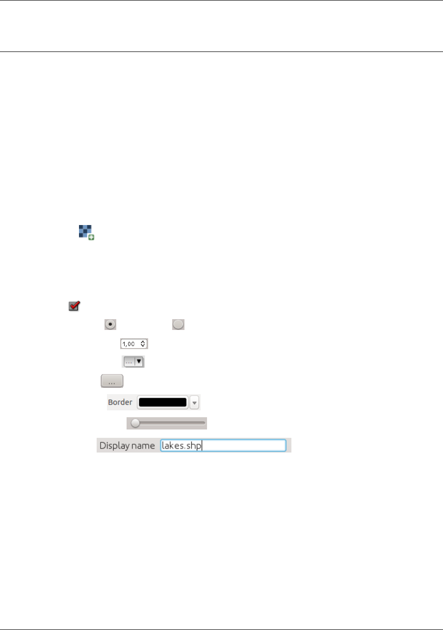
2.1 Convenciones de la Interfaz Gráfica o GUI
Las convenciones de estilo del GUI están destinadas a imitar la apariencia de la interfaz gráfica de usuario. En
general, un estilo reflejará la apariencia simplificada, por lo que un usuario puede escanear visualmente el GUI
para encontrar algo que se parece a lo mostrado en el manual.
• Menú Opciones: Capa →Añadir capa ráster oPreferencias →Barra de Herramientas →Digitalizacion
• Herramienta: Añadir capa ráster
• Boton : [Guardar como]
• Título del Cuadro de Diálogo: Propiedades de capa
• Pestaña: General
• Selección: Renderizar
• Botón de selección: Postgis SRID EPSG ID
• Seleccionar un número:
• Seleccionar una cadena:
• Buscar un archivo:
• Seleccione un color:
• Barra de desplazamiento:
• Texto de Entrada:
El sombreado muestra un componente de la interfaz que el usuario puede pulsar.
2.2 Convenciones de Texto o Teclado
Este manual también incluye estilos relacionadas con el texto, los comandos de teclado y codificación para indicar
diferentes entidades, como las clases o métodos. Estos estilos no se corresponden con la apariencia real de
cualquier texto o codificación dentro QGIS.
• Hiperenlaces: http://qgis.org
• Combinaciones de Teclas: Pulsar Ctrl+B, significa mantener pulsada la tecla Ctrl y pulsar la letra B.
• Nombre de un Archivo: lakes.shp
5
QGIS User Guide, Publicación 2.8
• Nombre de una Clase: NewLayer
• Método: classFactory
• Servidor: myhost.de
• Texto para el Usuario: qgis --help
Las líneas de código se muestran con una fuente de ancho fijo:
PROJCS["NAD_1927_Albers",
GEOGCS["GCS_North_American_1927",
2.3 Instrucciones específicas de cada plataforma
Algunas secuencias GUI y pequeñas cantidades de texto pueden ser formateados en línea : Haga clic
:menuselection: Archivo QGIS →Salir para cerrar QGIS. Esto indica que en Linux , Unix y plataformas
Windows, debe hacer clic en el menú Archivo, y luego en Salir, mientras que en Macintosh OS X, debe hacer clic
en el Menú QGIS primero, y luego en Salir.
Las cantidades mayores de texto se pueden formatear como listas:
• Hacer esto
• Hacer aquello
• Hacer otra cosa
o como párrafos:
Hacer esto y esto y esto. Entonces hacer esto y esto y esto, y esto y esto y esto, y esto y esto y esto.
Hacer eso. Entonces hacer eso y eso y eso, y eso y eso y eso y eso, y eso y eso y eso, y eso y eso y eso, y eso y
eso y eso.
Las capturas de pantalls que aparecen a lo largo de la guía de usuario han sido creadas en diferentes plataformas;
éstas se indicarán por el icono específico para cada una al final del pie de imagen.
.
6 Chapter 2. Convenciones

CHAPTER 3
Prólogo
¡Bienvenido al maravilloso mundo de los Sistemas de Información Geográfica (SIG)!
QGIS es un Sistema de Información Geográfica de código abierto. El proyecto nació en mayo de 2002 y se
estableció como un proyecto en SourceForge en junio del mismo año. Hemos trabajado duro para hacer que el
software SIG (tradicionalmente software propietario caro) esté al alcance de cualquiera con acceso básico a un
ordenador personal. QGIS actualmente funciona en la mayoría de plataformas Unix, Windows y OS X. QGIS se
desarrolla usando el kit de herramientas Qt (http://qt.digia.com) y C++. Esto significa que QGIS es ligero y tiene
una interfaz gráfica de usuario (GUI) agradable y fácil de usar.
QGIS pretende ser un SIG amigable, proporcionando funciones y características comunes. El objetivo inicial
del proyecto era proporcionar un visor de datos SIG. QGIS ha alcanzado un punto en su evolución en el que
está siendo usado por muchos para sus necesidades diarias de visualización de datos SIG. QGIS admite diversos
formatos de datos ráster y vectoriales, pudiendo añadir nuevos formatos usando la arquitectura de complementos.
QGIS se distribuye bajo la Licencia Pública General GNU (GPL). El desarrollo de QGIS bajo esta licencia sig-
nifica que se puede revisar y modificar el código fuente y garantiza que usted, nuestro feliz usuario, siempre
tendrá acceso a un programa de SIG que es libre de costo y puede ser libremente modificado. Debería haber
recibido una copia completa de la licencia con su copia de QGIS, y también podrá encontrarla en el Apéndice
:ref:gpl_appendix.
Truco: Documentación al día
La última versión de este documento siempre se puede encontrar en el área de documentación de la web de QGIS
en http://www.qgis.org/en/docs/.
.
7

QGIS User Guide, Publicación 2.8
8 Chapter 3. Prólogo

CHAPTER 4
Características
QGIS offers many common GIS functionalities provided by core features and plugins. A short summary of six
general categories of features and plugins is presented below, followed by first insights into the integrated Python
console.
4.1 Ver datos
You can view and overlay vector and raster data in different formats and projections without conversion to an
internal or common format. Supported formats include:
• Spatially-enabled tables and views using PostGIS, SpatiaLite and MS SQL Spatial, Oracle Spatial, vector
formats supported by the installed OGR library, including ESRI shapefiles, MapInfo, SDTS, GML and
many more. See section Trabajar con catos vectoriales.
• Raster and imagery formats supported by the installed GDAL (Geospatial Data Abstraction Library) library,
such as GeoTIFF, ERDAS IMG, ArcInfo ASCII GRID, JPEG, PNG and many more. See section Trabajar
con catos raster.
• GRASS raster and vector data from GRASS databases (location/mapset). See section GRASS GIS Integra-
tion.
• Online spatial data served as OGC Web Services, including WMS, WMTS, WCS, WFS, and WFS-T. See
section Trabajar con datos OGC.
4.2 Explorar datos y componer mapas
You can compose maps and interactively explore spatial data with a friendly GUI. The many helpful tools available
in the GUI include:
• Explorador QGIS
• Reproyección al vuelo
• Gestor de Base de Datos
• Diseñador de mapas
• Panel de vista general
• Marcadores espaciales
• Herramientas de anotaciones
• Identify/select features
• Editar/ver/buscar atributos
• Data-defined feature labeling
9

QGIS User Guide, Publicación 2.8
• Data-defined vector and raster symbology tools
• Atlas map composition with graticule layers
• North arrow scale bar and copyright label for maps
• Support for saving and restoring projects
4.3 Crear, editar, gestionar y exportar datos
You can create, edit, manage and export vector and raster layers in several formats. QGIS offers the following:
• Digitizing tools for OGR-supported formats and GRASS vector layers
• Ability to create and edit shapefiles and GRASS vector layers
• Georeferencer plugin to geocode images
• GPS tools to import and export GPX format, and convert other GPS formats to GPX or down/upload directly
to a GPS unit (On Linux, usb: has been added to list of GPS devices.)
• Support for visualizing and editing OpenStreetMap data
• Ability to create spatial database tables from shapefiles with DB Manager plugin
• Improved handling of spatial database tables
• Tools for managing vector attribute tables
• Option to save screenshots as georeferenced images
• DXF-Export tool with enhanced capabilities to export styles and plugins to perform CAD-like functions
4.4 Analizar datos
You can perform spatial data analysis on spatial databases and other OGR- supported formats. QGIS currently
offers vector analysis, sampling, geoprocessing, geometry and database management tools. You can also use the
integrated GRASS tools, which include the complete GRASS functionality of more than 400 modules. (See sec-
tion GRASS GIS Integration.) Or, you can work with the Processing Plugin, which provides a powerful geospatial
analysis framework to call native and third-party algorithms from QGIS, such as GDAL, SAGA, GRASS, fTools
and more. (See section Introducción.)
4.5 Publicar mapas en Internet
QGIS can be used as a WMS, WMTS, WMS-C or WFS and WFS-T client, and as a WMS, WCS or WFS server.
(See section Trabajar con datos OGC.) Additionally, you can publish your data on the Internet using a webserver
with UMN MapServer or GeoServer installed.
4.6 Extend QGIS functionality through plugins
QGIS can be adapted to your special needs with the extensible plugin architecture and libraries that can be used
to create plugins. You can even create new applications with C++ or Python!
10 Chapter 4. Características

QGIS User Guide, Publicación 2.8
4.6.1 Complementos del Núcleo
Los complementos del núcleo incluyen:
1. Coordinate Capture (Capture mouse coordinates in different CRSs)
2. DB Manager (Exchange, edit and view layers and tables; execute SQL queries)
3. Dxf2Shp Converter (Convert DXF files to shapefiles)
4. eVIS (Visualizar eventos)
5. fTools (Analyze and manage vector data)
6. GDALTools (Integrate GDAL Tools into QGIS)
7. Georeferencer GDAL (Add projection information to rasters using GDAL)
8. Herramientas GPS (cargar e importar datos de GPS)
9. GRASS (integrar el SIG GRASS)
10. Heatmap (Generate raster heatmaps from point data)
11. Interpolation Plugin (Interpolate based on vertices of a vector layer)
12. Metasearch Catalogue Client
13. Offline Editing (Allow offline editing and synchronizing with databases)
14. GeoRaster Espacial de Oracle
15. Procesamiento (antiguamente SEXTANTE)
16. Raster Terrain Analysis (Analyze raster-based terrain)
17. Road Graph Plugin (Analyze a shortest-path network)
18. Complemento de consulta espacial
19. SPIT (Import shapefiles to PostgreSQL/PostGIS)
20. Topology Checker (Find topological errors in vector layers)
21. Zonal Statistics Plugin (Calculate count, sum, and mean of a raster for each polygon of a vector layer)
4.6.2 Complementos externos de Python
QGIS offers a growing number of external Python plugins that are provided by the community. These plugins
reside in the official Plugins Repository and can be easily installed using the Python Plugin Installer. See Section
El diálogo de complementos.
4.7 Consola de Python
For scripting, it is possible to take advantage of an integrated Python console, which can be opened from menu:
Plugins →Python Console. The console opens as a non-modal utility window. For interaction with the QGIS en-
vironment, there is the qgis.utils.iface variable, which is an instance of QgsInterface. This interface
allows access to the map canvas, menus, toolbars and other parts of the QGIS application. You can create a script,
then drag and drop it into the QGIS window and it will be executed automatically.
For further information about working with the Python console and programming QGIS plugins and applications,
please refer to PyQGIS-Developer-Cookbook.
4.7. Consola de Python 11

QGIS User Guide, Publicación 2.8
4.8 Problemas Conocidos
4.8.1 Limitación en el número de archivos abiertos
If you are opening a large QGIS project and you are sure that all layers are valid, but some layers are flagged as
bad, you are probably faced with this issue. Linux (and other OSs, likewise) has a limit of opened files by process.
Resource limits are per-process and inherited. The ulimit command, which is a shell built-in, changes the limits
only for the current shell process; the new limit will be inherited by any child processes.
You can see all current ulimit info by typing
user@host:~$ ulimit -aS
You can see the current allowed number of opened files per proccess with the following command on a console
user@host:~$ ulimit -Sn
To change the limits for an existing session, you may be able to use something like
user@host:~$ ulimit -Sn #number_of_allowed_open_files
user@host:~$ ulimit -Sn
user@host:~$ qgis
To fix it forever
On most Linux systems, resource limits are set on login by the pam_limits module according to the settings
contained in /etc/security/limits.conf or /etc/security/limits.d/*.conf. You should be
able to edit those files if you have root privilege (also via sudo), but you will need to log in again before any
changes take effect.
Más información:
http://www.cyberciti.biz/faq/linux-increase-the-maximum-number-of-open-files/ http://linuxaria.com/article/open-
files-in-linux?lang=en
.
12 Chapter 4. Características

CHAPTER 5
Qué es lo nuevo en QGIS 2.8
Esta versión contiene nuevas características y se extiende la interfaz de programación con respecto a versiones
anteriores. Le recomendamos que utilice esta versión sobre las versiones anteriores.
This release includes hundreds of bug fixes and many new features and enhancements
that will be described in this manual. You may also review the visual changelog at
http://qgis.org/en/site/forusers/visualchangelog28/index.html.
5.1 Application
•Map rotation: A map rotation can be set in degrees from the status bar
•Bookmarks: You can share and transfer your bookmarks
•Expressions:
–when editing attributes in the attribute table or forms, you can now enter expressions directly into spin
boxes
–the expression widget is extended to include a function editor where you are able to create your own
Python custom functions in a comfortable way
–in any spinbox of the style menu you can enter expressions and evaluate them immediately
–a get and transform geometry function was added for using expressions
–a comment functionality was inserted if for example you want to work with data defined labeling
•Joins: You can specify a custom prefix for joins
•Layer Legend: Show rule-based renderer’s legend as a tree
•DB Manager: Run only the selected part of a SQL query
•Attribute Table: support for calculations on selected rows through a ‘Update Selected’ button
•Measure Tools: change measurement units possible
5.2 Proveedor de datos
•DXF Export tool improvements: Improved marker symbol export
•WMS Layers: Support for contextual WMS legend graphics
•Temporary Scratch Layers: It is possible to create empty editable memory layers
13

QGIS User Guide, Publicación 2.8
5.3 Digitizing
•Advanced Digitizing:
–digitise lines exactly parallel or at right angles, lock lines to specific angles and so on with the advanced
digitizing panel (CAD-like features)
–simplify tool: specify with exact tolerance, simplify multiple features at once ...
•Snapping Options: new snapping mode ‘Snap to all layers’
5.4 Diseñador de impresión de Mapa
•Composer GUI improvements: hide bounding boxes, full screen mode for composer toggle display of
panels
•Grid improvements: You now have finer control of frame and annotation display
•Label item margins: You can now control both horizontal and vertical margins for label items. You can
now specify negative margins for label items.
• optionally store layer styles
•Attribute Table Item: options ‘Current atlas feature’ and ‘Relation children’ in Main properties
5.5 Plugins
•Python Console: You can now drag and drop python scripts into the QGIS window
5.6 Servidor QGIS
• Python plugin support
5.7 Simbología
• live heatmap renderer creates dynamic heatmaps from point layers
• raster image symbol fill type
• more data-defined symbology settings: the data-defined option was moved next to each data definable
property
• support for multiple styles per map layer, optionally store layer styles
5.8 Interfaz de Usuario
•Projection: Improved/consistent projection selection. All dialogs now use a consistent projection selection
widget, which allows for quickly selecting from recently used and standard project/QGIS projections
.
14 Chapter 5. Qué es lo nuevo en QGIS 2.8
CHAPTER 6
Comenzar
Este capítulo da una vista general rápida sobre la instalación de QGIS, algunos datos de ejemplo de la web de
QGIS y ejecutar una primera sesión sencilla visualizando capas ráster y vectoriales.
6.1 Instalación
La instalación de QGIS es muy sencilla. Hay disponibles paquetes de instalación estándar para MS Windows y
Mac OS X. Se proporcionan paquetes binarios (rpm y deb) o repositorios de software para añadir a su gestor de
paquetes para muchos sabores de GNU/Linux. Consiga la última información sobre paquetes binarios en la web
de QGIS en http://download.qgis.org.
6.1.1 Instalación a partir de las fuentes
Si necesita compilar QGIS a partir de las fuentes, por favor consulte las instrucciones de instalación. Se dis-
tribuyen con el código fuente de QGIS en un archivo llamado INSTALL. También puede encontrarlas en línea en
http://htmlpreview.github.io/?https://raw.github.com/qgis/QGIS/master/doc/INSTALL.html
6.1.2 Instalación en medios extraíbles
QGIS le permite definir una opción --configpath que suplanta la ruta predeterminada para la configuración
de usuario (ej.: ~/.qgis2 bajo Linux) y fuerza a QSettings a usar ese directorio. Esto le permite, por ejemplo,
llevar una instalación de QGIS en una memoria flash junto con todos los complementos y la configuración. Vea la
sección Menú Sistema para información adicional.
6.2 Datos de ejemplo
La guía de usuario contiene ejemplos basados en el conjunto de datos de ejemplo de QGIS.
El instalador de Windows tiene una opción para descargar el conjunto de datos de muestra de QGIS. Si se
marca, los datos se decargarán en su carpeta Mis Documentos y se colocarán en una carpeta llamada GIS
Database. Puede usar el Explorador de Windows para mover esta carpeta a una ubicación adecuada. Si no
marcó la casilla de verificación para instalar el conjunto de datos de muestra durante la instalación inicial de
QGIS, puede hacer algo de lo siguiente:
• Usar datos SIG que ya tenga
• Download sample data from http://qgis.org/downloads/data/qgis_sample_data.zip
• Desinstalar QGIS y volver a instalarlo con la opción de descarga de datos marcada (sólo recomendado si las
soluciones anteriores no funcionaron).
15
QGIS User Guide, Publicación 2.8
For GNU/Linux and Mac OS X, there are not yet dataset installation packages available as rpm,
deb or dmg. To use the sample dataset, download the file qgis_sample_data as a ZIP archive from
http://qgis.org/downloads/data and unzip the archive on your system.
El conjunto de datos de Alaska incluye todos los datos SIG que se usan para los ejemplos y capturas de pantalla
de la guía de usuario; también incluye una pequeña base de datos de GRASS. La proyección del conjunto de datos
de QGIS es Alaska Albers Equal Area con unidades en pies. El código EPSG es 2964.
PROJCS["Albers Equal Area",
GEOGCS["NAD27",
DATUM["North_American_Datum_1927",
SPHEROID["Clarke 1866",6378206.4,294.978698213898,
AUTHORITY["EPSG","7008"]],
TOWGS84[-3,142,183,0,0,0,0],
AUTHORITY["EPSG","6267"]],
PRIMEM["Greenwich",0,
AUTHORITY["EPSG","8901"]],
UNIT["degree",0.0174532925199433,
AUTHORITY["EPSG","9108"]],
AUTHORITY["EPSG","4267"]],
PROJECTION["Albers_Conic_Equal_Area"],
PARAMETER["standard_parallel_1",55],
PARAMETER["standard_parallel_2",65],
PARAMETER["latitude_of_center",50],
PARAMETER["longitude_of_center",-154],
PARAMETER["false_easting",0],
PARAMETER["false_northing",0],
UNIT["us_survey_feet",0.3048006096012192]]
Si pretende usar QGIS como un visor gráfico para GRASS, puede encontrar una selección de lo-
calizaciones de ejemplo (ej.., Spearfish o Dakota de Sur) en la web oficial de GRASS GIS,
http://grass.osgeo.org/download/sample-data/.
6.3 Sesión de ejemplo
Ahora que tiene QGIS instalado y un dispone de un conjunto de datos, nos gustaría mostrarle una sesión
de muestra de QGIS corta y sencilla. Visualizaremos una capa ráster y otra vectorial. Usaremos la
capa ráster landcover,qgis_sample_data/raster/landcover.img y la capa vectorial lakes,
qgis_sample_data/gml/lakes.gml.
6.3.1 Iniciar QGIS
• Arranque QGIS tecleando “QGIS” en la línea de órdenes o si usa un binario precompilado, usando el
menú Aplicaciones.
• Iniciar QGIS usando el menú Inicio o accesos directos en el escritorio o haciendo doble clic en un archivo
de proyecto de QGIS.
• Hacer doble clic en el icono de su carpeta Aplicaciones.
6.3.2 Cargar capas ráster y vectoriales del conjunto de datos de ejemplo
1. Haga clic en el icono Añadir capa ráster
2. Navegue a la carpeta qgis_sample_data/raster/, seleccione el archivo ERDAS IMG
landcover.img y haga clic en [Abrir].
16 Chapter 6. Comenzar
QGIS User Guide, Publicación 2.8
3. Si el archivo no está en la lista, compruebe si el listado Tipo de archivos en la parte inferior del cuadro
de diálogo se encuentra en el tipo correcto, en este caso “Erdas Imagine Images” (*.img, *.IMG)”.
4. Ahora haga clic en el icono Añadir capa vectorial.
5. Archivo debería estar seleccionado como Tipo de origien en el nuevo diálogo Añadir capa vectorial.
Ahora haga clic en [Explorar] para seleccionar la capa vectorial.
6. Navegue a la carpeta qgis_sample_data/gml/, y seleccionar ‘Geography Markup Language [GML]
[OGR] (.gml,.GML)’ de la lista desplegable Filtro , a continuación seleccionar el archivo GML
lakes.gml y haga clic [Abrir]. En el diálogo Añadir capa vectorial, haga clic en [Aceptar]. El diálogo
Selector de Sistema de Referencia de Coordenadas se abrirá con NAD27 / Alaska Alberts seleccionada, haga
clic en [Aceptar].
7. Acerque el zoom un poco a la zona que prefiera con algunos lagos.
8. Haga doble clic en la capa lakes en el panel Capas para abrir el diálogo Propiedades.
9. Clic en la pestaña Estilo y seleccionar un azul como color de relleno.
10. Haga clic en la pestaña Etiquetas‘y marque la casilla |checkbox| :guilabel:‘Etiquetar esta capa con para
habilitar el etiquetado. Seleccione el campo “NAMES” como el campo que contiene las etiquetas.
11. Para mejorar la lectura de las etiquetas, puede añadir una zona blanca a su alrederor haciendo clic en “Már-
gen” en la lista de la izquierda, marcando Dibujar buffer de texto y eligiendo 3 como tamaño de buffer.
12. Haga clik en [Aplicar]. Compruebe si el resultado le gusta y finalmente pulse [Aceptar].
Puede ver lo fácil que es visualizar capas ráster y vectoriales en QGIS. Vayamos a las secciones que siguen para
aprender más sobre las funcionalidades, características y configuración disponibles y cómo usarlas.
6.4 Iniciar y cerrar QGIS
En la sección Sesión de ejemplo ya aprendió como iniciar QGIS. Repetiremos esto aquí y verá que QGIS también
proporciona otras opciones de línea de órdenes.
• Asumiendo que QGIS está instalado en el PATH, puede iniciar QGIS tecleando qgis en la consola
o haciendo doble clic en el enlace (o acceso directo) a la aplicación QGIS en el escritorio o en el menú
Aplicaciones.
• Iniciar QGIS usando el menú Inicio o accesos directos en el escritorio o haciendo doble clic en un archivo
de proyecto de QGIS.
• Haga doble clic en el icono en su carpeta Aplicaciones. Si necesita iniciar QGIS en una consola, ejecute
/path-to-installation-executable/Contents/MacOS/Qgis.
Para detener QGIS, haga clic en la opción de menú Archivo QGIS →Salir, o use use el atajo Ctrl+Q.
6.5 Opciones de la línea de órdenes
QGIS admite diversas opciones cuando se arranca desde la línea de órdenes. Para obteter una lista de las
opciones, introduzca qgis --help en la línea de órdenes. La sentencia de uso para QGIS es:
qgis --help
QGIS - 2.6.0-Brighton ’Brighton’ (exported)
QGIS is a user friendly Open Source Geographic Information System.
Usage: /usr/bin/qgis.bin [OPTION] [FILE]
OPTION:
[--snapshot filename] emit snapshot of loaded datasets to given file
[--width width] width of snapshot to emit
6.4. Iniciar y cerrar QGIS 17

QGIS User Guide, Publicación 2.8
[--height height] height of snapshot to emit
[--lang language] use language for interface text
[--project projectfile] load the given QGIS project
[--extent xmin,ymin,xmax,ymax] set initial map extent
[--nologo] hide splash screen
[--noplugins] don’t restore plugins on startup
[--nocustomization] don’t apply GUI customization
[--customizationfile] use the given ini file as GUI customization
[--optionspath path] use the given QSettings path
[--configpath path] use the given path for all user configuration
[--code path] run the given python file on load
[--defaultui] start by resetting user ui settings to default
[--help] this text
FILE:
Files specified on the command line can include rasters,
vectors, and QGIS project files (.qgs):
1. Rasters - supported formats include GeoTiff, DEM
and others supported by GDAL
2. Vectors - supported formats include ESRI Shapefiles
and others supported by OGR and PostgreSQL layers using
the PostGIS extension
Truco: Ejemplo usando argumentos de la línea de órdenes
Puede iniciar QGIS especificando uno o más archivos de datos en la línea de órdenes. Por ejemplo, asumiendo
que está en el directorio qgis_sample_data, podría iniciar QGIS con una capa vectorial y un archivo ráster
establecidos para que se carguen al inicio usando la siguiente orden: qgis ./raster/landcover.img
./gml/lakes.gml
Opción de la línea de órdenes --snapshot
Esta opción permite crear una captura de pantalla en formato PNG de la vista actual. Esto es práctico cuando tiene
muchos proyectos y quiere generar capturas de pantalla de sus datos.
Actualmente genera un archivo PNG con 800x600 píxeles. Esto se puede ajustar usando los argumentos‘‘–width‘‘
y--height en la línea de órdenes. Se puede añadir un nombre de archivo después de --snapshot.
Opción de la línea de órdenes --lang
Basado en su configuración local, QGIS selecciona el idioma correcto. Si desea cambiar su idioma, se puede
especificar un código de idioma. Por ejemplo, --lang=it inica QGIS en idioma italiano.
Opción de la línea de órdenes --project
También es posible iniciar QGIS con un archivo de proyecto existente. Solamente agregue la opción --project
a la línea de comando, seguida por el nombre de su proyecto y QGIS se abrirá con todas las capas del archivo
indicado cargadas.
Opción de la línea de órdenes --extent
Use esta opción para iniciar con una extensión de mapa específica. Necesita añadir el cuadro delimitador de su
extensión en el siguiente orden, separado por una coma:
--extent xmin,ymin,xmax,ymax
Opción de la línea de órdenes --nologo
Este argumento de línea de órdenes oculta la pantalla de bienvenida cuando inicia QGIS.
Opción de la línea de órdenes --noplugins
Si tiene problemas con los complementos al iniciar, puede evitar cargarlos con ésta opción. Estarán aún disponibles
después en el administrador de complementos.
Opciónde la línea de órdenes --customizationfile
18 Chapter 6. Comenzar
QGIS User Guide, Publicación 2.8
Utilizando este argumento de línea de órdenes puede definir un archivo de personalizacion de la GUI, que se
utilizará al iniciar.
Opción de la línea de órdenes --nocustomization
Utilizando este argumento de línea de órdenes no se aplicará la personalización existente de la GUI.
Opción de la línea de órdenes --optionspath
Puede tener varias configuraciones y decidir cual utilizar al iniciar QGIS con esta opción. Véase Opciones para
confirmar donde almacena los archivos de configuración el sistema operativo. Actualmente, no hay forma de es-
pecificar un archivo para escribir la configuración; por lo tanto puede crear una copia del archivo de configuración
original y cambiarle el nombre. La opción especifica la ruta al directorio con los ajustes. Por ejemplo, para utilizar
el archivo de configuración /path/to/config/QGIS/QGIS2.ini , use la opción.
--optionspath /path/to/config/
Opción de la línea de órdenes --configpath
Esta opción es similar al anterior, pero además anula la ruta predeterminada para la configuración del usuario
(~/.qgis2) y fuerza QSettings para usar también este directorio. Esto permite a los usuarios, por ejemplo,
llevar la instalación de QGIS en una unidad flash junto con todos los complementos y configuraciones.
Opción de línea de comandos --código
Esta opción se puede utilizar para ejecutar un archivo python dado directamente después de que QGIS ha iniciado.
Por ejemplo, cuando se tiene un archivo python llamado load_alaska.py con el siguiente contenido:
from qgis.utils import iface
raster_file ="/home/gisadmin/Documents/qgis_sample_data/raster/landcover.img"
layer_name ="Alaska"
iface.addRasterLayer(raster_file, layer_name)
Suponiendo que esta en el directorio donde el archivo load_alaska.py se encuentra, puede iniciar QGIS,
cargue el archivo raster landcover.img y de a la capa el nombre ‘Alaska’ utilizando el siguiente comando:
qgis --code load_alaska.py
6.6 Proyectos
El estado de su sesión de QGIS es considerado un proyecto. QGIS trabaja en un proyecto cada vez. La con-
figuración está considerada por proyecto o como predeterminada para nuevos proyectos (ver sección Opciones).
QGIS puede guardar el estado de su espacio de trabajo dentro de un archivo de proyecto, usando las opciones de
menú Proyecto →Guardar oProyecto →Guardar como....
Cargar los proyectos guardados en una sesión de QGIS usando Proyecto→Abrir...,Proyecto →Nuevo a
partir de plantilla oProyecto →Abrir reciente →.
Si desea limpiar su sesión e iniciar una fresca, seleccione Proyecto →Nuevo. Cualquiera de estas opciones le
pedirá que guarde el proyecto existente si se han hecho cambios desde que se abrió o se guardó por última vez.
El tipo de información guardada en el archivo de proyecto incluye:
• Las capas añadidas
• Que capas pueden ser consultadas
• Propiedades de la capa, incluyendo simbolización y estilos
• Proyección de la vista del mapa
• Última extensión vista
• Diseñador de impresión
6.6. Proyectos 19
QGIS User Guide, Publicación 2.8
• Elementos de diseñador de impresión con ajustes
• Diseñador de impresión configuración de atlas
• Configuración de digitalización
• Tabla de relaciones
• Proyectos Macros
• Proyecto de estilos predeterminados
• Configuración de complementos
• Configuración de servidor QGIS desde la pestaña de ajustes de OWS en propiedades del proyecto
• Consultas almacenadas en el Administrador de BBDD
El archivo del proyecto se guarda en formato XML, así es posible editarlo fuera de QGIS, si sabe lo que está
haciendo. El formato del archivo ha sido actualizado varias veces comparado con otras versiones de QGIS. Los
archivos de proyecto de versiones anteriores puede que ya no funcionen correctamente. Para estar al tanto de esto,
en la pestaña General bajo Configuración →Opciones se puede seleccionar:
•Preguntar si guardar cambios en el proyecto y la fuente de datos cuando sea necesario
•Avisar al abrir un proyecto guardado con una versión anterior de QGIS
Siempre que guarde un proyecto en QGIS un respaldo del archivo del proyecto se hace con la extensión ~.
6.7 Salida
Hay muchas maneras de generar una salida desde su sesión QGIS. Ya hemos presentado una en la sección Proyec-
tos, guardando como un archivo de proyecto. Aquí hay una muestra de otras formas de producir archivos de
salida:
• La opción del menú Proyecto →Guardar como imagen abre un diálogo de archivo donde se selecciona el
nombre, la ruta y el tipo de imagen (PNG,JPG y muchos otros formatos). Un archivo de mundo con la
extensión PNGW o JPGW guardado en la misma carpeta la georreferencia de la imagen.
• La opción del menú Proyecto →Esportar a DXF ... abre un diálogo donde se puede definir el ‘Modo de
simbología’, la ‘Escala de la simbología’ y las capas vectoriales que se desea exportar a DXF. A través de los
símbolos ‘Modo de simbología’ desde la original simbología QGIS puede ser exportado con alta fidelidad.
• La opción del menú Proyecto →Nuevo diseñador de impresión abre un diálogo en donde se puede
diseñar e imprimir el lienzo de mapa actual (vea sección Diseñadores de impresión).
.
20 Chapter 6. Comenzar
CHAPTER 7
QGIS GUI
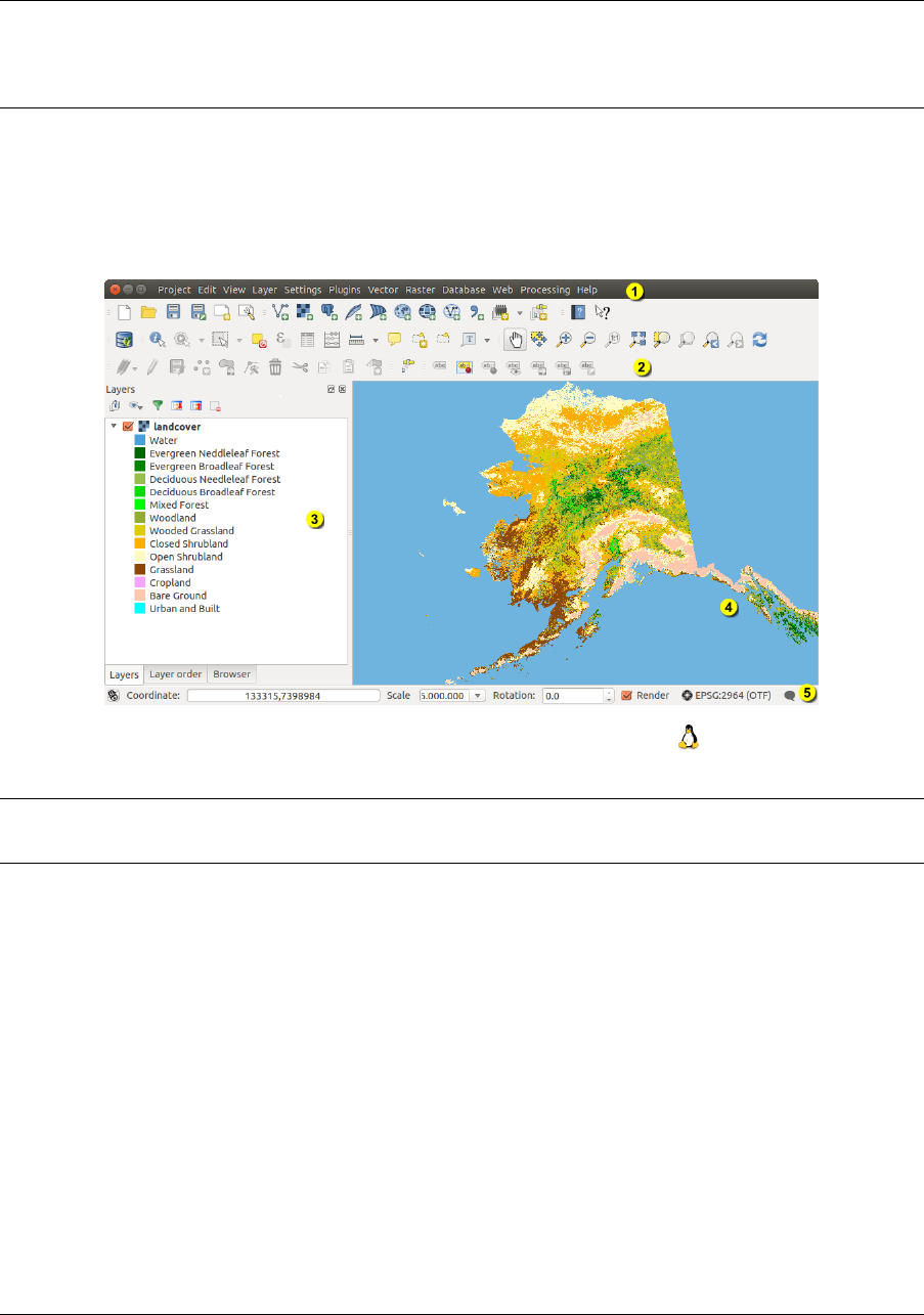
Cuando QGIS inicia, se le presenta la interfaz gráfica de usuario, como se muestra en la figura (los números del 1
al 5 en círculos amarillos se analiza más adelante).
Figure 7.1: QGIS GUI con datos de ejemplo de Alaska
Nota: Las decoraciones de las ventanas (barra de título, etc.) pueden ser distintas dependiendo de su sistema
operativo y su gestor de ventanas.
La GUI QGIS se divide en cinco zonas:
1. Barra de Menú
2. Barra de Herramientas
3. Leyenda del mapa
4. Vista del mapa
5. Barra de Estado
Estos cinco componentes de la interfaz de QGIS se describen con más detalle en la siguiente sección. Dos sec-
ciones más presentan atajos de teclado y ayuda contextual.
21
QGIS User Guide, Publicación 2.8
7.1 Barra de Menú
La barra de menú permite el acceso a varias características de QGIS mediante un menú jerárquico estándar. Los
menús de nivel superior y un resumen de algunas opciones de menú se enumeran a continuación, junto con
los iconos asociados a medida que aparecen en la barra de herramientas, y los atajos de teclado. Los atajos
de teclado presentados en esta sección son los predeterminados; sin embargo, los atajos de teclado también se
pueden configurar manualmente utilizando el diálogo Configurar atajos del teclado, abrir desde Configuración →
Configurar atajos de teclado....
Aunque la mayoría de las opciones tiene una herramienta correspondiente y viceversa, los menús no están orga-
nizados exactamente como las barras de herramientas. La barra de herramientas que contiene la herramienta esta
listada después de cada opción de menú como una entrada de casilla de verificación. Algunas opciones de menú
sólo aparecen si se carga el complemento correspondiente. Para obtener más información acerca de herramientas
y barra de herramientas, ver la sección Barra de herramietas.
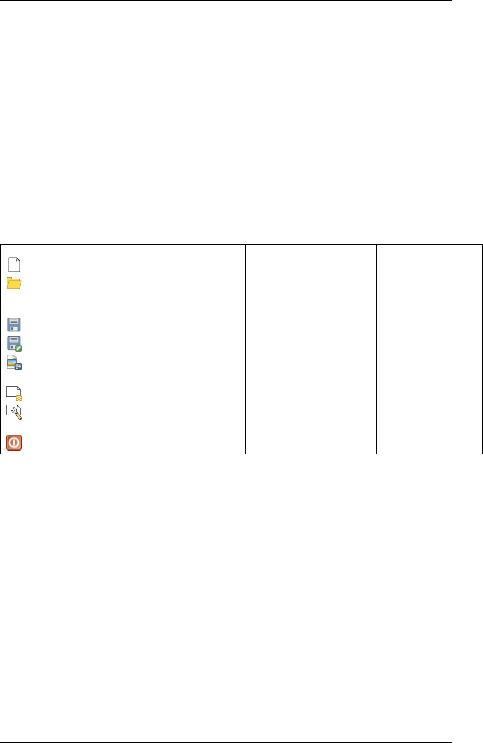
7.1.1 Proyecto
Menú Opción Atajos Referencia Barra de herramietas
Nuevo Ctrl+N ver Proyectos Proyecto
Abrir Ctrl+O ver Proyectos Proyecto
Nuevo a partir de plantilla →ver Proyectos Proyecto
Abrir recientes →ver Proyectos
Guardar Ctrl+S ver Proyectos Proyecto
Guardar como... Ctrl+Shift+S ver Proyectos Proyecto
Guardar como imagen... ver Salida
Exportar DXF ... ver Salida
Nuevo diseñador de impresión Ctrl+P ver Diseñadores de impresión Proyecto
Administrador de diseñadores ... ver Diseñadores de impresión Proyecto
Diseñadores de impresión →ver Diseñadores de impresión
Salir de QGIS Ctrl+Q
22 Chapter 7. QGIS GUI

QGIS User Guide, Publicación 2.8
7.1. Barra de Menú 23
QGIS User Guide, Publicación 2.8
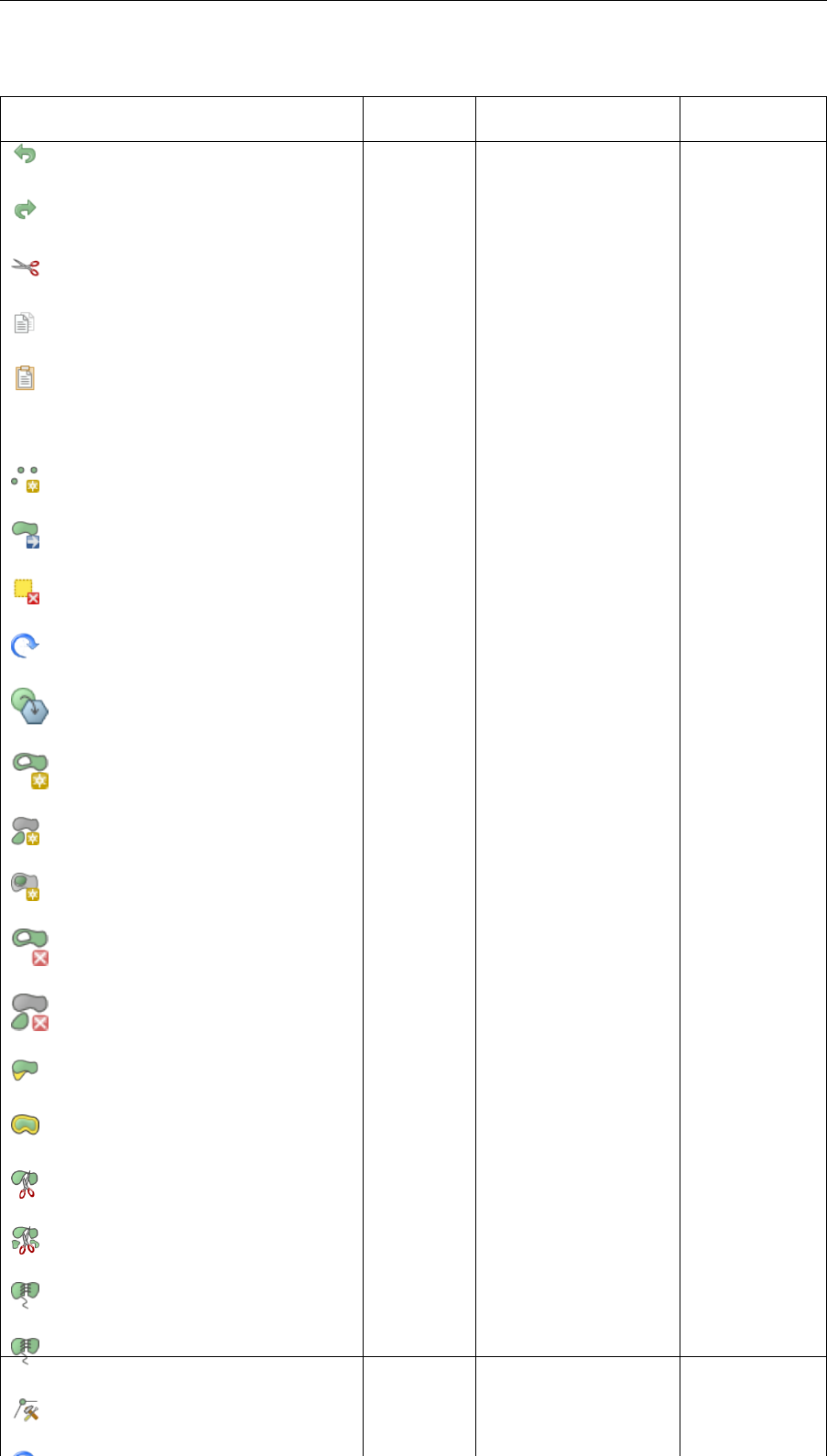
7.1.2 Editar
Menú Opción Atajos Referencia Barra de
herramietas
Deshacer Ctrl+Z ver Advanced digitizing Digitalización
Avanzada
Rehacer Ctrl+Shift+Zver Advanced digitizing Digitalización
Avanzada
Cortar objetos espaciales Ctrl+X ver Digitizing an
existing layer
Digitalización
Copiar objetos espaciales Ctrl+C ver Digitizing an
existing layer
Digitalización
Pegar objetos espaciales Ctrl+V ver Digitizing an
existing layer
Digitalización
Pegar objetos espaciales como →ver Working with the
Attribute Table
Añadir objetos espaciales Ctrl+. ver Digitizing an
existing layer
Digitalización
Mover objeto(s) espaciales ver Digitizing an
existing layer
Digitalización
Borrar seleccionados ver Digitizing an
existing layer
Digitalización
Girar objetos espacial(es) ver Advanced digitizing Digitalización
Avanzada
Simplificar objeto espacial ver Advanced digitizing Digitalización
Avanzada
Añadir anillo ver Advanced digitizing Digitalización
Avanzada
Añadir parte ver Advanced digitizing Digitalización
Avanzada
Rellenar anillo ver Advanced digitizing Digitalización
Avanzada
Borrar anillo ver Advanced digitizing Digitalización
Avanzada
Borrar parte ver Advanced digitizing Digitalización
Avanzada
Remodelar objetos espaciales ver Advanced digitizing Digitalización
Avanzada
Desplazar curva ver Advanced digitizing Digitalización
Avanzada
Dividir objetos espaciales ver Advanced digitizing Digitalización
Avanzada
Dividir partes ver Advanced digitizing Digitalización
Avanzada
Combinar objetos espaciales
seleccionados
ver Advanced digitizing Digitalización
Avanzada
Combinar los atributos de los objetos
espaciales seleccionados
ver Advanced digitizing Digitalización
Avanzada
Herramienta de nodos ver Digitizing an
existing layer
Digitalización
Rotar símbolos de putos ver Advanced digitizing Digitalización
Avanzada
24 Chapter 7. QGIS GUI
QGIS User Guide, Publicación 2.8
Después de activar el modo Conmutar edición de una capa, encontrará el icono Añadir objeto espacial
en el menú Edición dependiendo del tipo de capa (punto, línea o polígono).
7.1.3 Edición (extra)
Menú Opción Atajos Referencia Barra de herramietas
Añadir objetos espaciales ver Digitizing an existing layer Digitalización
Añadir objeto espacial ver Digitizing an existing layer Digitalización
Añadir objeto espacial ver Digitizing an existing layer Digitalización
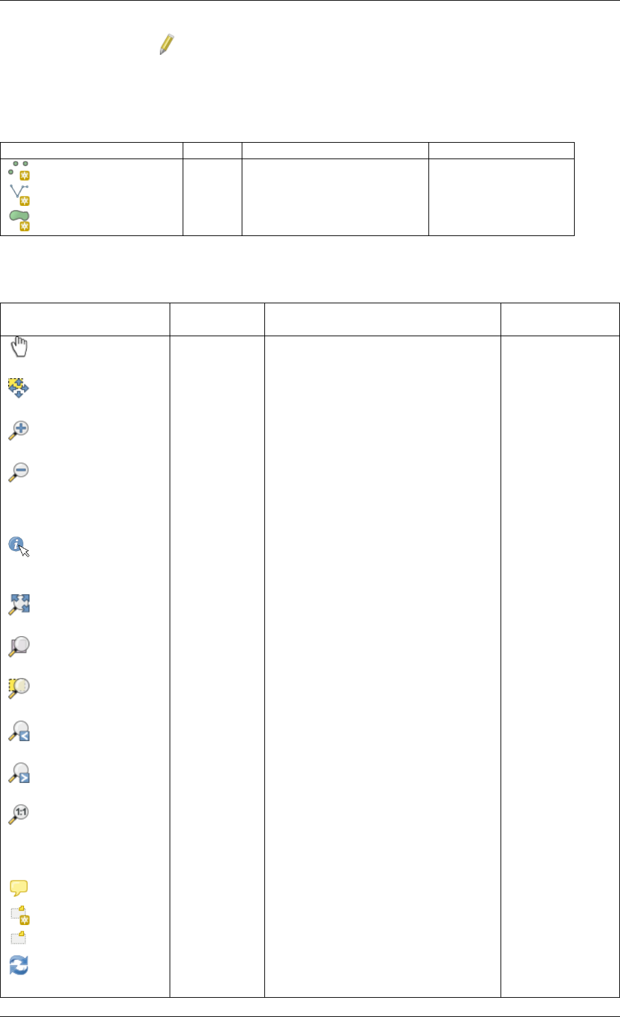
7.1.4 Ver
Menú Opción Atajos Referencia Barra de
herramietas
Desplazar mapa Navegación de
mapas
Desplazar mapa a la
selección
Navegación de
mapas
Acercar zum Ctrl++ Navegación de
mapas
Alejar zum Ctrl+- Navegación de
mapas
Seleccionar →ver Seleccionar y deseleccionar objetos
espaciales
Atributos
Identificar objetos
espaciales
Ctrl+Shift+I Atributos
Medir →ver Mediciones Atributos
Zum General Ctrl+Shift+F Navegación de
mapas
Zum a la capa Navegación de
mapas
Zum a la selección Ctrl+J Navegación de
mapas
Zum anterior Navegación de
mapas
Zum siguiente Navegación de
mapas
Zum al tamaño real Navegación de
mapas
Ilustraciones →ver Elementos decorativos
Modo Vista previa →
Avisos del mapa Atributos
Nuevo marcador Ctrl+B ver Marcadores espaciales Atributos
Mostrar marcadores Ctrl+Shift+Bver Marcadores espaciales Atributos
Actualizar F5 Navegación de
mapas
7.1. Barra de Menú 25
QGIS User Guide, Publicación 2.8
7.1.5 Capa
Menú Opción Atajos Referencia Barra de
herramietas
Crear capa →ver Creating new Vector
layers
Administrar
Capas
Añadir capa →Administrar
Capas
Empotrar capas y grupos ... ver Anidar proyectos
Añadir desde archivo de definición de
capa ...
Copiar estilo ver Style Menu
Pegar estilo ver Style Menu
Abrir Tabla de atributos ver Working with the
Attribute Table
Atributos
Conmutar edición ver Digitizing an existing
layer
Digitalización
Guardar cambios de la capa ver Digitizing an existing
layer
Digitalización
Ediciones actuales →ver Digitizing an existing
layer
Digitalización
Guardar como...
Guardar como archivo de definición
de capa...
Eliminar Capa/Grupo Ctrl+D
Duplicar capa(s)
Establecer escala de visibilidad de
las capas
Establecer el SRC de la capa(s) Ctrl+Shift+C
Establecer SRC del proyecto a partir
de capa
Propiedades ...
Consulta...
Etiquetado
Añadir a la vista general Ctrl+Shift+O Administrar
Capas
Añadir todo a la vista general
Eliminar todo de la vista general
Mostrar todas las capas Ctrl+Shift+U Administrar
Capas
Ocultar todas las capas Ctrl+Shift+H Administrar
Capas
Mostrar capas seleccionadas
Ocultar capas seleccionadas
26 Chapter 7. QGIS GUI
QGIS User Guide, Publicación 2.8
7.1.6 Configuración
Menú Opción Atajos Referencia Barra de
herramietas
Paneles →ver Paneles y Barras de
Herramientas
Barras de herramientas→ver Paneles y Barras de
Herramientas
Alternar el modo de pantalla
completa
F 11
Propiedades del proyecto... Ctrl+Shift+Pver Proyectos
SRC Personalizado ... ver Custom Coordinate Reference
System
Administrador de estilos... ver Presentation
Configurar atajos de teclado
...
Personalización ... ver Personalización
Opciones ... ver Opciones
Opciones de autoensamblado ...
7.1.7 Complementos
Menú Opción Atajos Referencia Barra de
herramietas
Administrar e Instalar
complementos ...
ver El diálogo de
complementos
Consola de Python Ctrl+Alt+P
Cuando inicie QGIS por primera vez no se cargan todos los complementos básicos.
7.1.8 Vectorial
Menú Opción Atajos Referencia Barra de herramietas
menuselection:Open Street Map –> ver Loading OpenStreetMap Vectors
Herramientas de análisis →ver Complemento fTools
Herramientas de investigación →ver Complemento fTools
Herramientas de Geoproceso →ver Complemento fTools
Herramientas de geometría →ver Complemento fTools
Herramientas de gestión de datos →ver Complemento fTools
Cuando inicie QGIS por primera vez no se cargan todos los complementos básicos.
7.1.9 Ráster
Menú Opción Atajos Referencia Barra de herramietas
Calculadora ráster... ver Calculadora Ráster
Cuando inicie QGIS por primera vez no se cargan todos los complementos básicos.
7.1. Barra de Menú 27
QGIS User Guide, Publicación 2.8
7.1.10 Base de datos
Menú Opción Atajos Referencia Barra de herramietas
Base de datos→ver Complemento administrador de BBDD Base de datos
Cuando inicie QGIS por primera vez no se cargan todos los complementos básicos.
7.1.11 Web
Menú Opción Atajos Referencia Barra de herramietas
Metabuscador ver metabuscador Web
Cuando inicie QGIS por primera vez no se cargan todos los complementos básicos.
7.1.12 Procesado
Menú Opción Atajos Referencia Barra de
herramietas
Caja de herramientas de
procesado
ver La caja de herramientas
Modelador gráfico ... ver &Modelador gráfico...
Historial y registro ... ver El administrador del historial
Opciones ... ver Configurar el entorno de trabajo de
procesamiento
Visor de resultador ... ver Configurar aplicaciones externas
Comandos Ctrl+Alt+Mver Los Comandos QGIS
Cuando inicie QGIS por primera vez no se cargan todos los complementos básicos.
7.1.13 Ayuda
Menú Opción Atajos Referencia Barra de herramietas
Contenido de la ayuda F1 Ayuda
¿Qué es esto? Shift+F1 Ayuda
Documentación de la API
¿Necesita soporte comercial?
Página web de QGIS Ctrl+H
Comprobar versión de QGIS
Acerca de
Patrocinadores de QGIS
Tenga en cuenta que para Linux , los elementos de la barra de menú mencionados anteriormente están de
manera predeterminada en la ventada de administrador KDE. En GNOME, el menú Configuración tiene diferente
contenido y los elementos que se encuentran aquí:
28 Chapter 7. QGIS GUI
QGIS User Guide, Publicación 2.8
SRC personalizado Editar
Administrador de estilos Editar
Configurar teclas de atajo Editar
Personalización Editar
Opciones Editar
Opciones de autoensamblado ... Editar
7.2 Barra de herramietas
La barra de herramientas proporciona acceso a la mayoría de las mismas funciones como las de los menús, y
herramientas adicionales para interactuar con el mapa. Cada elemento de la barra de herramientas tiene ayuda
emergente disponible. Mantenga el puntero del ratón sobre el elemento y una breve descripción del propósito de
la herramienta se mostrará.
Cada barra de menú se puede mover de acuerdo a sus necesidades. Además cada barra de menú se puede apagar
utilizando el menú contextual del botón derecho del ratón, sosteniendo el ratón sobre la barra de herramientas
(leer también Paneles y Barras de Herramientas).
Truco: Restauración de barras de herramientas
Si ha ocultado accidentalmente todas las barras de herramientas, puede recuperarlos eligiendo la op-
ción del menú Configuración →Barra de herramientas →. Si una barra de herramientas desaparece
bajo Windows, que parece ser un problema en QGIS de vez en cuando, tiene que quitar la clave
\HKEY_CURRENT_USER\Software\QGIS\qgis\UI\state en el registro. Cuando reinicie QGIS, la
clave se escribirá de nuevo con el estado por defecto y todas las barras de herramientas serán visibles de nuevo.
7.3 Leyenda del mapa
La zona de la leyenda del mapa registra todas las capas en el proyecto. La casilla de verificación de cada entrada
de leyenda se puede utilizar para mostrar u ocultar la capa. La barra de herramientas de leyenda en la leyenda
del mapa esta lista le permite Añadir grupo,Manejo de visibilidad de la capa de todas las capas o manejo
de combinación de capas predefinidas, Filtrar leyenda por contenido de mapa,Expandir todo oComprimir
todo yEliminar capa de grupo. El botón le permite añadir vistas Preestablecidos en la leyenda.
Esto significa que puede elegir por mostrar alguna capa con categorización específica y añadir esta vista a la
lista de Preestablecidos. Para añadir una vista preestablecida simplemente haga clic en , elija Añadir
preestablecido... desde el menú desplegable y de un nombre al preestablecido. Después verá una lista con todos
los preestablecidos que puede llamar pulsando el botón .
Todos los preestablecidos añadidos están presentes en el diseño de impresión con el fin de permitirle crear un
diseño de mapa en base a sus puntos de vista específicos (ver Propiedades principales).
Una capa se puede seleccionar y arrastrar hacia arriba o hacia abajo en la leyenda para cambiar el orden. El orden-
z significa que las capas enlistadas más cerca de la parte superior de la leyenda son dibujadas sobre las capas que
figuran más abajo en la leyenda.
Nota: Este funcionamiento puede ser anulado por el panel ‘Orden de la capa’
Las capas en la ventana de leyenda se pueden organizar en grupos. Hay dos formas de hacer esto:
1. Pulse el icono para añadir un nuevo grupo. Escriba un nombre para el grupo y pulse Enter. Ahora
haga clic en una capa existente y arrástrelo al grupo.
2. Seleccionar algunas capas, al hacer clic derecho en la ventana de la leyenda y elegir Grupo Seleccionado.
Las capas seleccionadas serán colocadas automáticamente en un nuevo grupo.
7.2. Barra de herramietas 29

QGIS User Guide, Publicación 2.8
Para llevar una capa fuera de un grupo, puede arrastrar hacia afuera , o haga clic derecho sobre él y elija Subir
elemento al nivel superior.
La casilla de verificación para un grupo mostrará u ocultará todas las capas en el grupo al hacer clic.
El contenido del menú contextual del botón derecho depende si el elemento de leyenda seleccionada es un ráster
o una capa vectorial. Para las capas vectoriales de GRASS , Botón de edición no está disponible. Vea la sección
Digitizing and editing a GRASS vector layer para obtener información sobre la edición de capas vectoriales de
GRASS.
El menú del boton derecho del raton para capas ráster
•Zum a la capa
•Mostrar en la vista general
•Zum a la mejor escala (100%)
•Eliminar
•Duplicar
•Establecer escala de visibilidad de la capa
•Establecer SRC de la capa
•Establecer SRC del proyecto a partir de capa
•Estilos→
•Guardar como ...
•Guardar como archivo de definición de capa ...
•Propiedades
•Cambiar nombre
Además, de acuerdo con la posición y la selección de la capa
•Mover al nivel superior
•Grupo seleccionado
Menú del botón derecho del ratón para las capas vectoriales
•Zum a la capa
•Mostrar en la vista general
•Eliminar
•Duplicar
•Establecer escala de visibilidad de la capa
•Establecer SRC de la capa
•Establecer SRC del proyecto a partir de capa
•Estilos→
•Abrir tabla de atributos
•Conmutar edición (no disponible para capas GRASS)
•Guardar como ...
•Guardar como Estilo de definición de capa
•Filtrar
•Mostrar el conteo de objetos espaciales
•Propiedades
30 Chapter 7. QGIS GUI
QGIS User Guide, Publicación 2.8
•Cambiar nombre
Además, de acuerdo con la posición y la selección de la capa
•Mover al nivel superior
•Grupo seleccionado
Menú del botón derecho del ratón para grupo de capas
•Zum al grupo
•Eliminar
•Establecer SRC del grupo
•Cambiar nombre
•Añadir grupo
Es posible seleccionar mas de una capa o grupo al mismo tiempo manteniendo presionada la tecla Ctrl mientras
selecciona las capas con el botón izquierdo del ratón. Después puede mover todas las capas a un nuevo grupo al
mismo tiempo.
También puede eliminar más de una capa o un grupo a la vez seleccionando varias capas con la tecla Ctrl y
presionando Ctrl+D después. De esta manera, todas las capas o grupos seleccionados será eliminado de la lista
de capas.
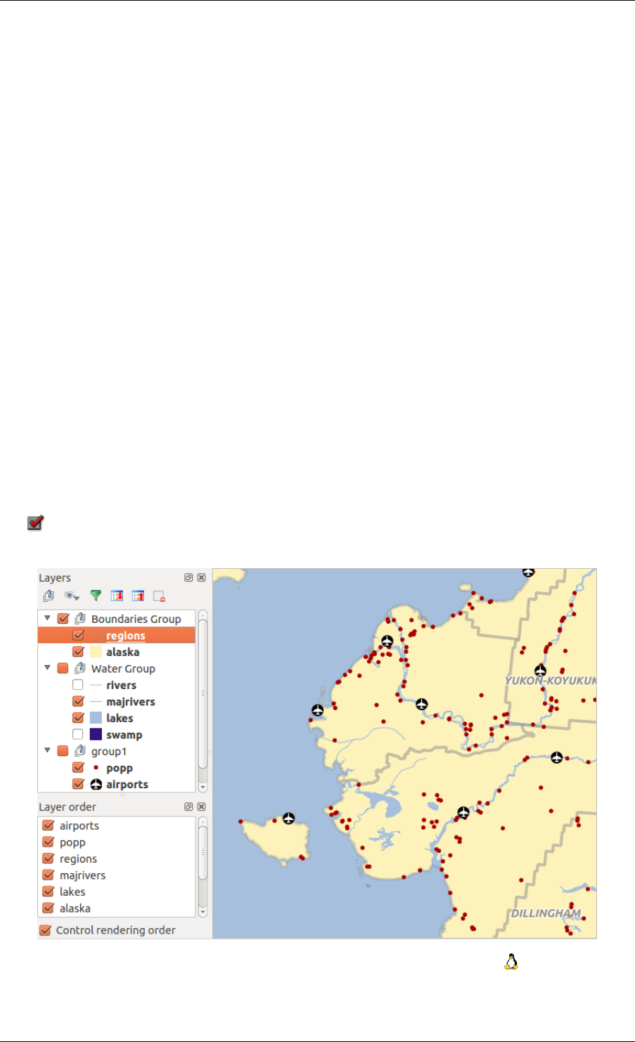
7.3.1 Trabajar con el orden de la leyenda de la capa independiente
Hay un panel que le permite definir un orden dibujo independiente para la leyenda del mapa. Puede activarlo en el
menú Configuración→Paneles →Orden de Capas. Esta característica le permite, por ejemplo, ordenar sus capas
en orden de importancia, pero aún mostrarlas en el orden correcto (ver figure_layer_order) . Comprobación de la
caja Orden de control del renderizado debajo de la lista de capas causará una reversión en el comportamiento
predeterminado .
Figure 7.2: Definir el orden de la leyenda de una capa independiente
7.3. Leyenda del mapa 31
QGIS User Guide, Publicación 2.8
7.4 Vista del mapa
Este es el “final del negocio” de QGIS — ¡los mapas son desplegados en esta zona! El mapa que se muestra
en esta ventana dependerá de las capas vectoriales y ráster que ha elegido cargar (ver secciones siguientes para
obtener más información sobre cómo cargar capas). La vista del mapa se puede desplazar, cambiar el enfoque de
la pantalla del mapa a otra región, y que se puede hacer zum dentro y fuera. Varias otras operaciones se pueden
realizar en el mapa como esta descrito en la descripción de la barra de herramientas anteriormente. La vista del
mapa y la leyenda están estrechamente vinculados entre sí — los mapas en vista reflejan los cambios que realice
en el área de leyenda .
Truco: Zum al mapa con la rueda del ratón
Puede utilizar la rueda del ratón para acercar y alejar zum en el mapa. Coloque el cursor del ratón dentro del mapa
y gire la rueda hacia adelante (hacia la derecha) para acercar y hacia atrás (hacia usted) para alejarlo. El zum se
centra en la posición del cursor del ratón. Puede personalizar el comportamiento del zum de la rueda del ratón
usando la pestaña Herramientas del mapa bajo el menú Configuración→Opciones
Truco: Desplazar el mapa con las teclas de dirección y barra de espaciadora
Puede utilizar las teclas de flechas para desplazar el mapa. Coloque el cursor dentro del mapa y haga clic en la
tecla de flecha a la derecha para desplazarse al este, tecla de flecha izquierda para el oeste, flecha arriba para el
norte y flecha abajo al sur. Puede también desplazar el mapa utilizando la barra espaciadora o al hacer clic en la
rueda del ratón: basta con mover el ratón mientras mantiene pulsada la barra espaciadora o haga clic en la rueda
del ratón.
7.5 Barra de Estado
La barra de estado muestra la posición actual en coordenadas de mapa (por ejemplo, metros o grados decimales)
como el puntero del ratón se mueve a través de la vista del mapa. A la izquierda de la pantalla de coordenadas en
la barra de estado es un botón pequeño que alterna entre mostrar la posición en coordenadas y la extensión del la
vista del mapa como como desplazar, acercar y alejar zum.
Junto a la visualización de coordenadas se encuentra la visualización de la escala. Este muestra la escala de la
vista del mapa. Si acercar o alejar zum, QGIS muestra la escala actual. Hay un selector de escala, lo que le permite
elegir entre las escalas predefinidas de 1:500 a 1:1000000.
A la derecha de la escala desplegada se puede definir una rotación horaria actual de su vista de mapa en grados.
Una barra de progreso en la barra de estado muestra el progreso de representación, ya que cada capa se dibuja a la
vista del mapa. En algunos casos, como en la recopilación de estadísticas en capas ráster, la barra de progreso se
utiliza para mostrar el estado de las operaciones largas.
S un nuevo complemento o una actualizacion de complemento disponible, verá un mensaje en el extremo izquierdo
de la barra de estado. En el lado derecho de la barra de estado, hay una pequeña casilla de verificación que se
puede utilizar para evitar temporalmente capas siendo represtados a la vista del mapa (ver sección Renderizado
abajo). El icono detiene inmediatamente el proceso de representación del mapa actual.
A la derecha de las funciones de representación, vera el código EPSG de la actual proyección SRC y un icono de
proyector. Haga clic en este para abrir las propiedades de proyección del actual proyecto.
Truco: Calcular la escala correcta de su lienzo de mapa
Cuando inicia QGIS, las unidades son grados, y esto significa que QGIS interpretará cualquier coordenada en su
capa como se especifica en grados. Para obtener valores de escala correctos, se puede cambiar esta configuración a
metros manualmente en la pestaña General bajo Configuración→Propiedades del Proyecto, o puede seleccionar
un proyecto SRC al hacer clic en el icono SRC Actual: en la esquina inferior derecha de la barra de estado. En el
último caso, las unidades se establecen en lo que esta especificado en la proyección del proyecto (e.g., ‘+units=m’).
32 Chapter 7. QGIS GUI

QGIS User Guide, Publicación 2.8
.
7.5. Barra de Estado 33

QGIS User Guide, Publicación 2.8
34 Chapter 7. QGIS GUI
CHAPTER 8
Herramientas generales
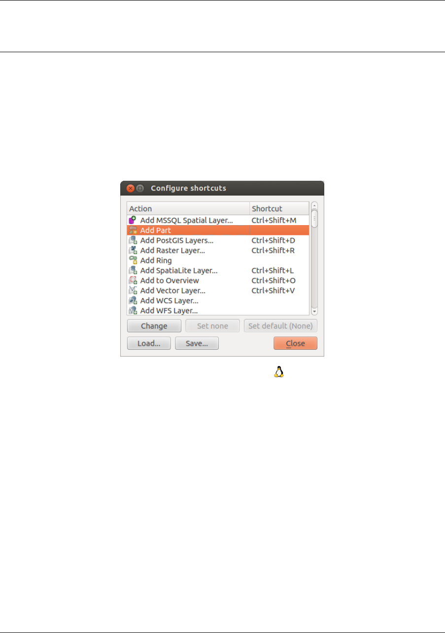
8.1 Teclas de acceso rápido
QGIS proporciona atajos de teclado predeterminados para muchas características. Puede encontrarlos en la sec-
ción Barra de Menú. Además, la opción de menú Configuración →Configurar atajos de teclado... permite
cambiar los atajos de teclado predeterminados y agregar otros nuevos a las características de QGIS .
Figure 8.1: Definir opciones de atajos (Gnome)
La configuración es muy simple. Solo seleccione una entidad de la lista y haga clic en [Cambiar],[Establecer
a ninguno] o[Establecer predeterminado]. Una vez finalizada la configuración, se puede guardar como un
archivo XML y cargarlo en otra instalación de QGIS.
8.2 Ayuda de contexto
Cuando necesite ayuda sobre un tema especifico, puede acceder a la ayuda de contexto mediante el botón [Ayuda]
disponible en la mayoría de diálogos – tenga en cuenta que los complementos de terceros pueden apuntar a paginas
web dedicadas.
8.3 Renderizado
Por omisión, QGIS representa todas las capas visibles siempre que se actualiza la vista del mapa. Los eventos que
desencadena una actualización de la vista del mapa incluyen:
35
QGIS User Guide, Publicación 2.8
• Añadir una capa
• Desplazar o hacer zoom
• Redimensionar la ventana de QGIS
• Cambiar la visibilidad de una o varias capas
QGIS permite controlar el proceso de renderizado de diversas formas.
8.3.1 Renderizado dependiente de la escala
El renderizado dependiente de la escala le permite especificar las escalas mínima y máxima a las que una capa
será visible. Para establecer el renderizado dependiente de la escala, abra el diálogo Propiedades mediante doble
clic en una capa en el panel Capas. En la pestaña General, haga clic en la casilla Visibilidad dependiente de la
escala para activar la característica, luego establezca los valores mínimo y máximo de escala.
Puede determinar los valores de escala haciendo zum primero al nivel que quiera usar y anotanto el valor de escala
en la barra de estado de QGIS.
8.3.2 Controlar el renderizado del mapa
El renderizado del mapa se puede controlar de varias formas, como se describe a continuación.
Suspender el renderizado
Para suspender el renderizado, haga clic en la casilla Representar en la esquina inferior derecha de la barra de
estado. Cuando la casilla Representar no está marcada, QGIS no redibuja el lienzo en respuesta a cualquiera
de los eventos descritos en la sección Renderizado. Ejemplos de cuándo puede querer suspender la representación
incluyen:
• Añadir muchas capas y simbolizarlas antes de dibujar
• Añadir una o más capas grandes y establecer la dependencia de escala antes de dibujar
• Añadir una o más capas grandes y hacer zoom a una vista específica antes de dibujar
• Cualquier combinación de la anteriores
Marcar la casilla Renderizar habilita el renderizado y origina un refresco inmediato del lienzo del mapa.
Configurar la opción de añadir una capa
Puede establecer una opción para cargar siempre las nuevas capas sin dibujarlas. Esto significa que las capas se
añadirán al mapa pero su casilla de visibilidad en el panel Capas no estará marcada de forma predeterminada.
Para establecer esta opción, seleccione la opción de menú Configuración →Opciones y haga clic en la pestaña
Representación. Desmarque la casilla Por omisión, las nuevas capas añadidas al mapa se deben visualizar.
Cualquier capa añadida posteriormente al mapa estará desactivada (invisible) por omisión.
Detener el renderizado
Para detener el dibujado del mapa, presione la tecla ESC. Esto detendrá el refresco del lienzo del mapa y dejará el
mapa parcialmente dibujado. Puede que tarde un poco desde que se presiona la tecla ESC hasta que se detenga el
dibujado del mapa.
Nota: Actualmente no es posible detener la representación — esto se desactivó en el paso a Qt4 debido a
problemas y cuelgues de la Interfaz de Usuario (IU).
36 Chapter 8. Herramientas generales
QGIS User Guide, Publicación 2.8
Actualizar la visualización del mapa durante el renderizado
Se puede establecer una opción para actualizar la visualización del mapa a medida que se dibujan los objetos
espaciales. Por omisión, QGIS no muestra ningún objeto espacial de una capa hasta que toda la capa ha sido
representada. Para actualizar la pantalla a medida que se leen los objetos espaciales desde el almacén de datos,
seleccione la opción de menú Configuración →Opciones y haga clic en la pestaña Representación. Establezca
el número de objetos espaciales a un valor apropiado para actualizar la pantalla durante la representación. Al
establecer un valor de 0 desactiva la actualización durante el dibujado (este es el valor predeterminado). Es-
tablecer un valor demasiado bajo dará como resultado un bajo rendimiento, ya que la vista del mapa se actualiza
continuamente durante la lectura de los objetos espaciales. Un valor sugerido para empezar es 500.
Influir en la calidad del renderizado
Para influir en la calidad de la presentación del mapa, se tienen dos opciones. Elegir la opción de menú Configu-
ración →Opciones, hacer clic en la pestaña Representación y seleccionar o deseleccionar las siguientes casillas
de verificación:
•Hacer que las líneas se muestren menos quebradas a expensas del rendimiento de la representación
•Solucionar problemas con polígonos rellenados incorrectamente
Acelerar renderizado
Hay dos ajustes que le permiten mejorar la velocidad de presentación. Abrir el diálogo de las opciones de QGIS
usando Configuración→Opciones, ir a la pestaña guilabel:Representación y seleccionar o deseleccionar las sigu-
ientes casillas de verificación:
•Activar buffer trasero. Esto proporciona un mejor rendimiento gráficos a costa de perder la posibilidad
de cancelar la representación y dibujar objetos espaciales incrementalmente. Si no esta marcada, se puede
establecer el Número de objetos espaciales a dibujar antes de actualizar la visualización, de lo contrario
esta opción está inactiva.
•Usar cacheado de representación cuando sea posible para acelerar redibujados
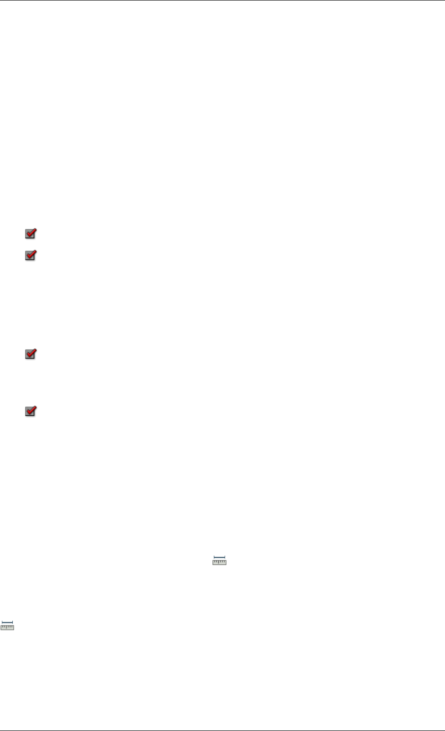
8.4 Mediciones
Las mediciones funcionan en sistemas de coordenadas proyectadas (por ejemplo, UTM) y en datos sin proyectar.
Si el mapa cargado está definido con un sistema de coordenadas geográficas (latitud/longitud), los resultados
de las mediciones de lineas o áreas serán incorrectos. Para solucionar esto, se debe establecer un sistema de
coordenadas del mapa apropiado (ver sección :ref:‘label_projections). Todos los módulos de medición también
usan la configuración de autoensamblado del módulo de digitalización. Esto es útil si se quiere medir a lo largo
de lineas o áreas en una capa vectorial.
Para seleccionar una herramienta de medición, pulsar y seleccione la herramienta que se quiera usar.
8.4.1 Medir longitud, áreas y ángulos
Medir Linea: En QGIS es posible medir distancias reales entre puntos dados conforme a un elipsoide definido.
Para configurar esto, seleccione la opción del menú Configuración →Opciones, haga clic en la pestaña Her-
ramientas del mapa y seleccione el elipsoide apropiado. Ahí, también puede definir un color de banda de medida
y las unidades de medida preferida (metros o pies) y las unidades de ángulos (grados, radianes, grados centesi-
males). La herramienta entonces le permite hacer puntos en el mapa. La longitud de cada segmento, así como el
total, aparecerá en la ventana de medición. Para detener la medición, haga clic en el botón derecho del ratón. Tenga
en cuenta que puede cambiar interactivamente las unidades de medición en el diálogo. Se anula las Unidades de
8.4. Mediciones 37
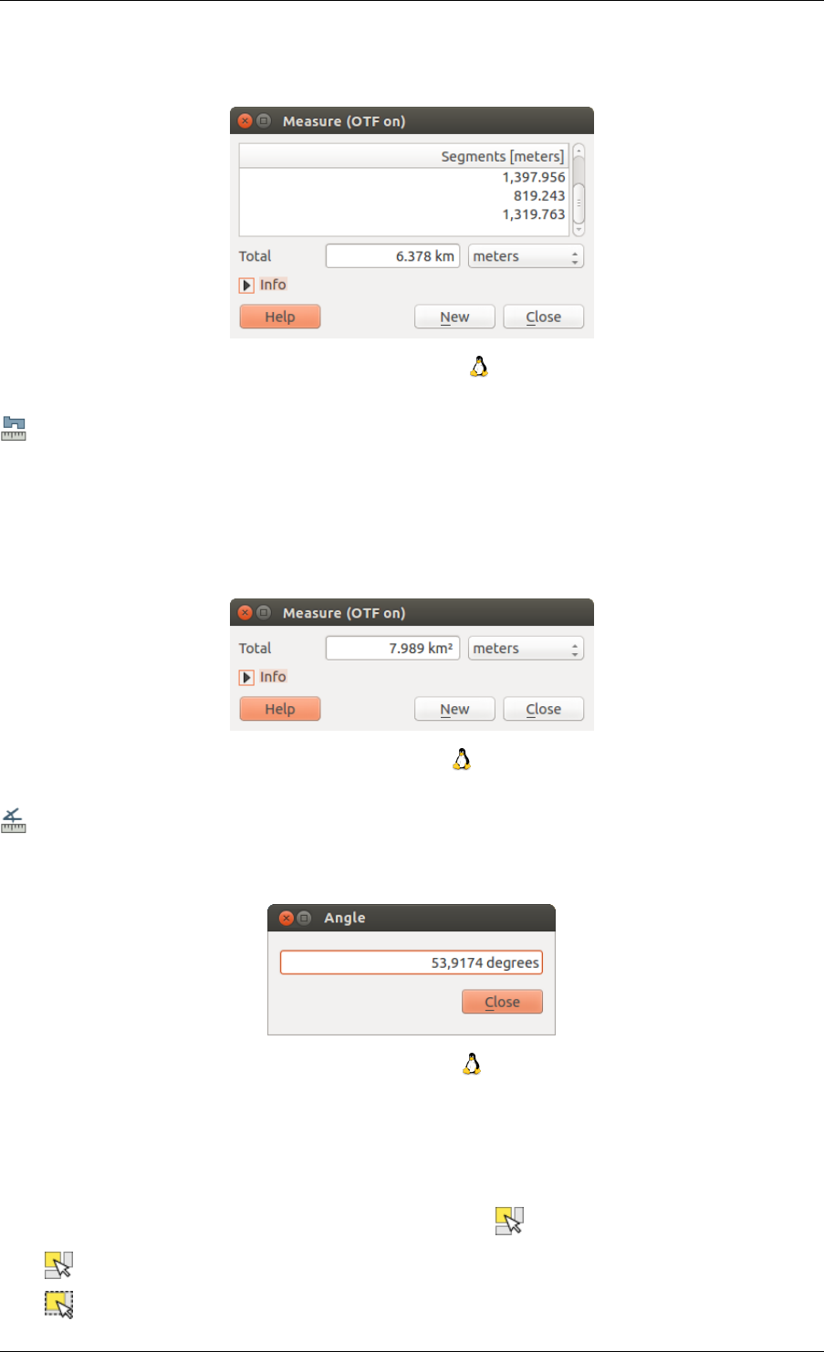
QGIS User Guide, Publicación 2.8
medición preferida en las opciones. Hay una sección de información en el diálogo que muestra que configuración
de SRC se esta utilizando durante los cálculos de medición.
Figure 8.2: Medir distancia (Gnome)
Medir áreas: Las áreas también pueden ser medidas. En la ventana de medición, aparece el tamaño del área
acumulada. Además, la herramienta de medición se autoensamblará a la capa actualmente seleccionada, siempre
que la capa tenga establecida una tolerancia de autoensamblado (ver sección Setting the Snapping Tolerance and
Search Radius). Por lo tanto, si se desea medir con exactitud a lo largo de un objeto espacial lineal, o alrededor
de un objeto poligonal, primero establezca su tolerancia de autoensamblado, luego seleccione la capa. Ahora, al
utilizar las herramientas de medición, cada clic del ratón (dentro de la tolerancia configurada) se ajustará a esa
capa.
Figure 8.3: Medir área (Gnome)
Medir ángulo: Se pueden también medir ángulos. El cursor se convierte en forma de cruz. Se debe hacer clic para
dibujar el primer segmento del ángulo que se desea medir y a continuación mover el cursor para dibujar el ángulo
deseado. La medida se mostrará en el diálogo emergente.
Figure 8.4: Medir ángulo (Gnome)
8.4.2 Seleccionar y deseleccionar objetos espaciales
La barra de herramientas de QGIS provee varias herramientas para seleccionar objetos espaciales en la vista del
mapa. Para seleccionar una o varios objetos, basta con hacer clic en y seleccionar la herramienta:
•Seleccionar objetos espaciales individuales
•Seleccionar objetos espaciales por rectángulo
38 Chapter 8. Herramientas generales
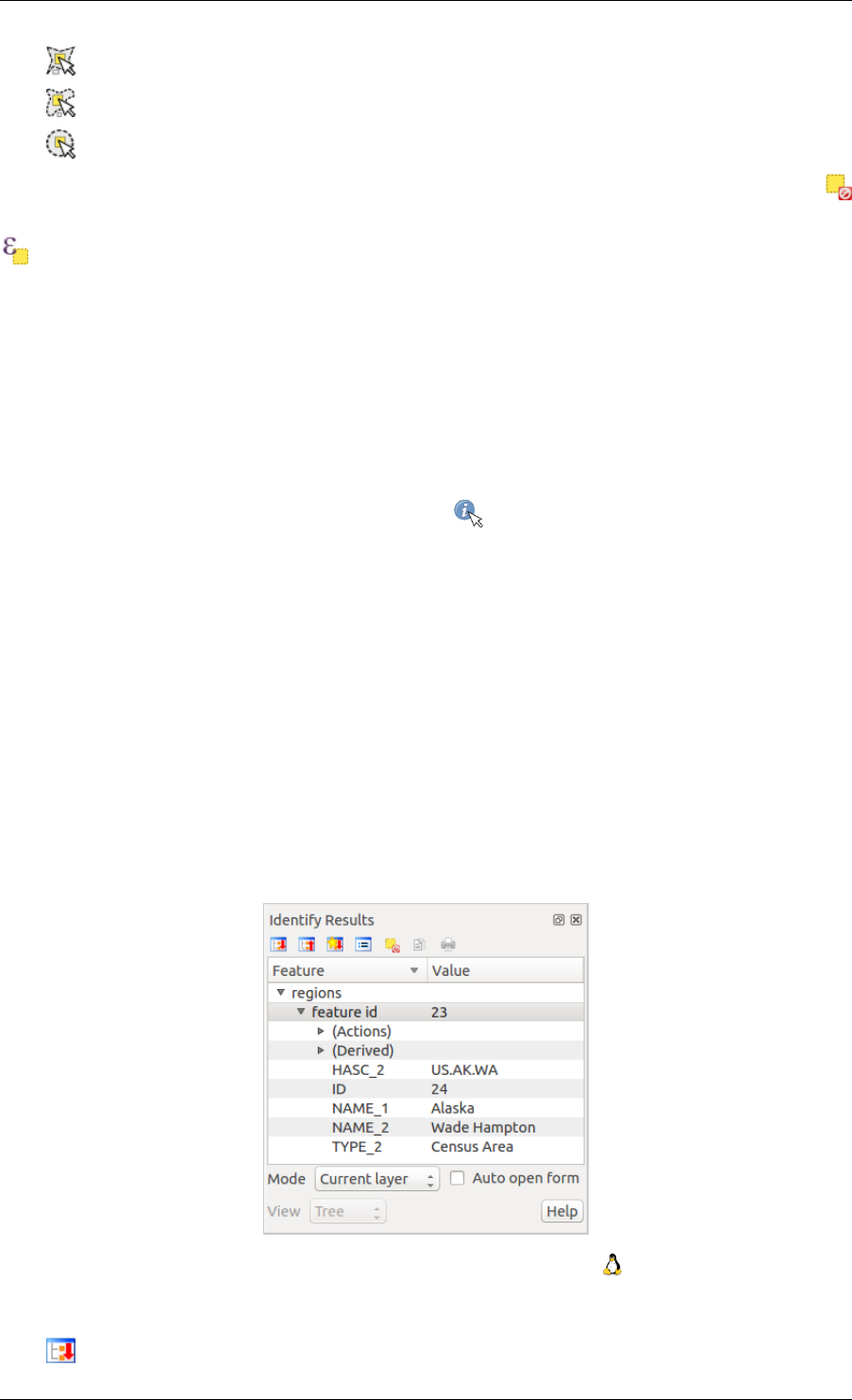
QGIS User Guide, Publicación 2.8
•Seleccionar objetos espaciales por polígono
•Seleccionar objetos espaciales a mano alzada
•Seleccionar objetos espaciales por radio
Para deseleccionar todos los objetos espaciales seleccionados, haga clic en
Deseleccionar objetos espaciales de todas las capas.
Seleccionar un objeto espacial utilizando una expresión‘permite al usuario seleccionar objetos espaciales utilizando un dialogo de expresión. Ver capítulo :ref:‘vector_expressions
para más ejemplos.
Los usuarios pueden guardar objetos espaciales seleccionados en una Nueva capa vectorial en memoria o una
Nueva capa vectorial utilizando Edición →Pegar objetos espaciales como ... y elegir el modo que desea.
8.5 Identificar objetos espaciales
La herramienta de identificar le permite interactuar con la vista del mapa y obtener información de los objetos es-
paciales en una ventana emergente. Para identificar objetos espaciales, se usa Ver →Identificar objetos espaciales
o presionar Ctrl + Shift + I, o hacer clic en el icono Identificar objetos espaciales en la barra de herramientas.
Si hace clic en varios objetos, el diálogo Resultados de la identificación se enumerará la información acerca de
todos los objetos seleccionados. El primer elemento es el numero de la capa en la lista de resultados, seguido por
el nombre. Luego su primer hijo será el nombre de un campo con su valor. El primer campo es la seleccionada en
Propiedades→Visualizar. Al final, toda la información sobre el objeto se mostrará.
Esta ventana puede ser personalizada para mostrar campos personalizados, pero por omisión mostrará tres tipos
de información:
• Acciones: se pueden agregar acciones a la ventana para identificar objetos espaciales. Al hacer clic en la
etiqueta de la acción, ésta se llevará a cabo. Por omisión, sólo se añade una acción, para ver el formulario
del objeto para edición.
• Derivado: esta información se calcula o es derivada de otra información. Se puede encontrar las coordenadas
pulsadas, coordendas X y Y, área y perímetro en unidades del mapa para polígonos, longitud en unidades
del mapa para lineas e ID de los objetos espaciales.
• Atributos de datos: Esta es la lista de campos de atributos de los datos.
Figure 8.5: Diálogo de identificación de objetos espaciales (Gnome)
En la parte superior de la ventana, tiene cinco iconos:
•Expandir árbol
8.5. Identificar objetos espaciales 39
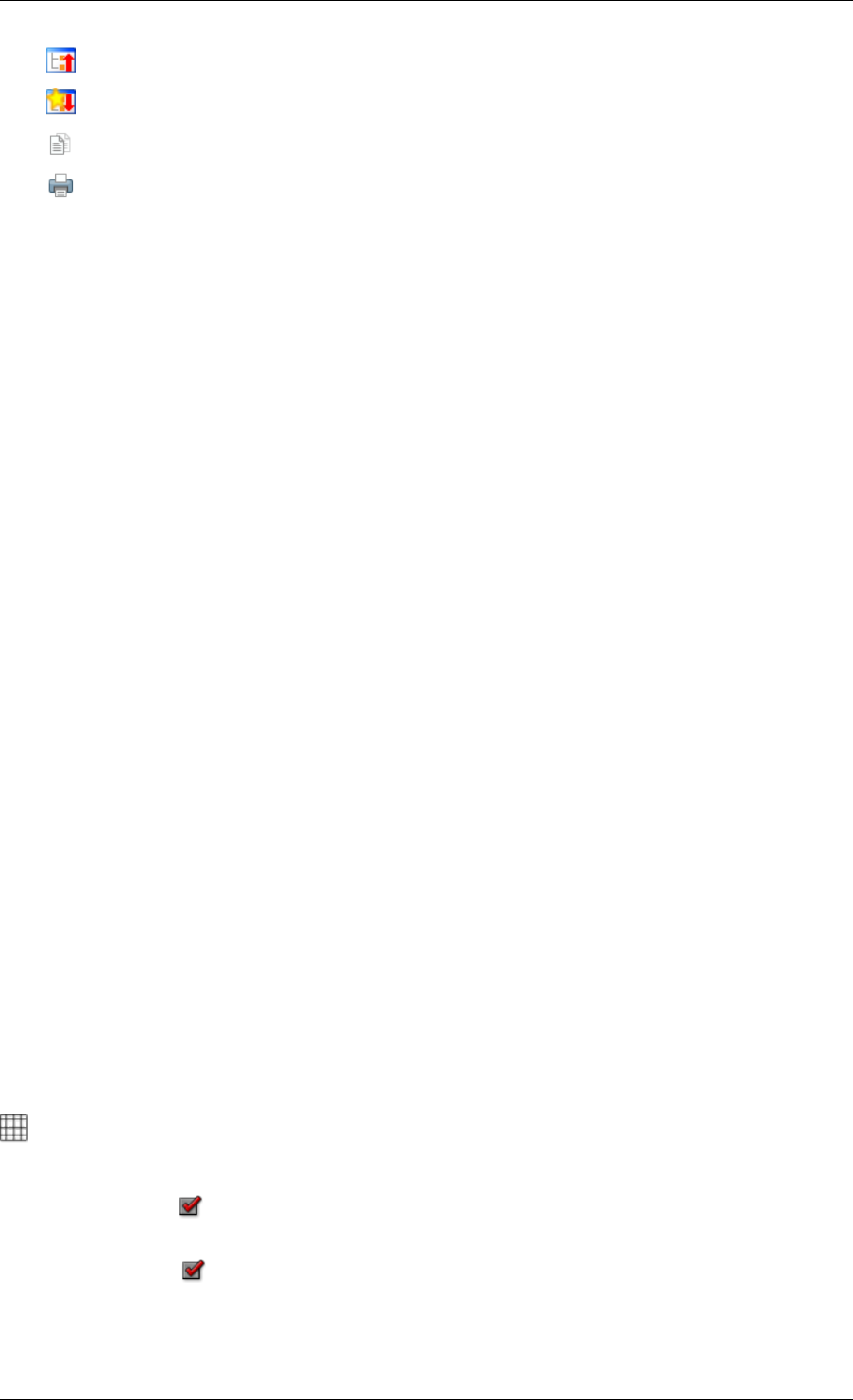
QGIS User Guide, Publicación 2.8
•Comprimir árbol
•Comportamiento predeterminado
•Copiar atributos
•Imprimir respuesta del HTML seleccionado
En la parte inferior de la ventana, se tiene las listas desplegables de Modo yVista. Con la lista desplegable Modo
se puede definir el modo de la identificación: ‘Capa actual’, ‘De arriba a abajo, irse en el primero’, ‘De arriba a
abajo’ y ‘Selección de capa’. La Vista se puede establecer como ‘Árbol’, ‘Tabla’ y ‘Gráfico’.
La herramienta de identificación le permite abrir automáticamente un formulario. En este modo se puede cambiar
los atributos de los objetos espaciales.
Otras funciones se pueden encontrar en el menú contextual del elemento identificado. Por ejemplo, del menú
contextual se puede:
• Ver el formulario del objeto espacial
• Zum a objeto espacial
• Copiar objeto espacial: Copiar toda la geometría y atributos del objeto espacial
• Selección de objetos espaciales: añadir objeto espacial identificado a selección.
• Copiar el valor del atributo: copiar solo el valor del atributo sobre el cual se hizo clic
• Copiar atributos del objeto espacial: Copiar solo atributos
• Limpiar resultados: quitar resultados de la ventana
• Limpiar resaltados: Deseleccionar los objetos espaciales en el mapa
• Resaltar todo
• Resaltar capa
• Activar capa: Elegir una capa para ser activada
• Propiedades de la capa: Abrir la ventana de propiedades de la capa.
• Expandir todo
• Colapsar todo
8.6 Elementos decorativos
Las Ilustraciones de QGIS incluyen la Cuadrícula, Etiqueta de Copyright, Flecha de Norte y Barra de Escala. Se
usan para ‘adornar’ el mapa al agregar elementos cartográficos.
8.6.1 Cuadrícula
Cuadrícula permite agregar una rejilla de coordenadas y anotaciones a la vista del mapa.
1. Seleccione en el menú Ver →Ilustraciones→Cuadrícula. Aparece el díálogo (ver figure_decorations_1).
2. Activar la casilla Activar cuadrícula y establecer la definición de la cuadrícula de acuerdo con las capas
cargadas en la vista del mapa.
3. Activar la casilla Dibujar anotaciones y establecer la definición de las anotaciones de acuerdo con las
capas cargadas en la vista del mapa.
4. Hacer clic en [Aplicar] para verificar que se vea como se esperaba.
40 Chapter 8. Herramientas generales
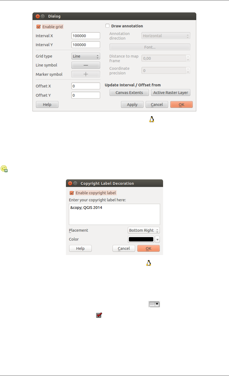
QGIS User Guide, Publicación 2.8
Figure 8.6: El diálogo de cuadrícula
5. Pulse [Aceptar] para cerrar el diálogo.
8.6.2 Etiqueta de derechos de autor
Etiqueta de copyright añade una etiqueta de copyright usando el texto que se prefiera al mapa.
Figure 8.7: Diálogo de copyright
1. Seleccione en el menú Ver →Ilustraciones→Etiqueta de Copyright. Aparece el díálogo (ver fig-
ure_decorations_2).
2. Escribir el texto que se quiera colocar en el mapa. Se puede usar HTML como se muestra en el ejemplo.
3. Elegir la ubicación de la etiqueta en la lista desplegable Ubicación
4. Comprobar que la casilla de verificación Activar etiqueta de copyright este marcada.
5. Hacer clic en [Aceptar]
En el ejemplo anterior, que es el predeterminado, QGIS coloca un símbolo de los derechos de autor seguido de la
fecha en la esquina inferior derecha de la vista del mapa.
8.6. Elementos decorativos 41
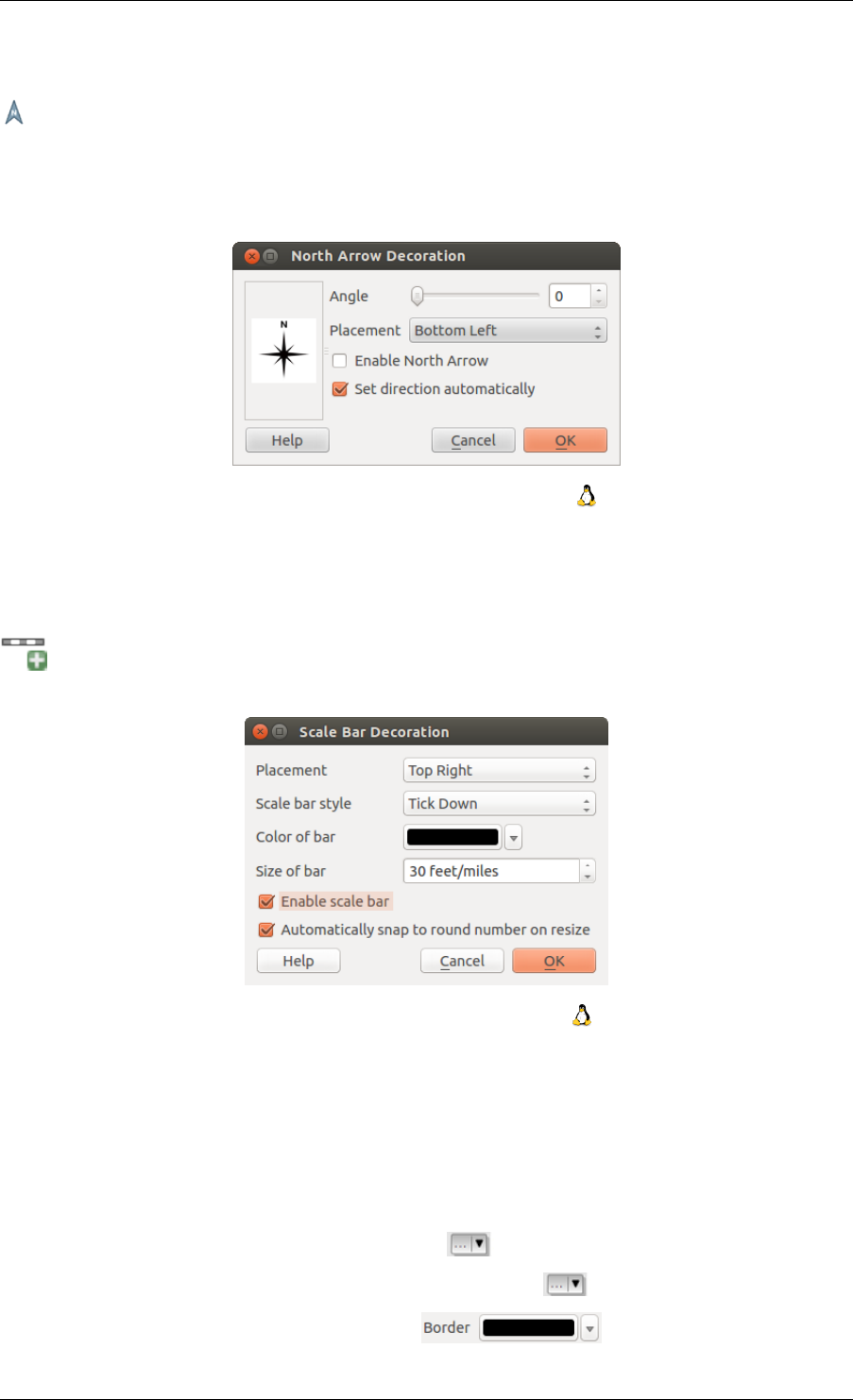
QGIS User Guide, Publicación 2.8
8.6.3 Flecha del Norte
Flecha de Norte coloca una sencilla flecha de norte en la vista del mapa. En la actualidad sólo hay un estilo
disponible. Se puede ajustar el ángulo de la flecha o dejar que QGIS establezca la dirección automáticamente.
Si decide dejar que QGIS determine la dirección, hará su mejor conjetura en cuanto a cómo se debe orientar la
flecha. Para la colocación de la flecha, se tienen cuatro opciones que corresponden a las cuatro esquinas de la vista
del mapa.
Figure 8.8: Diálogo de la flecha del Norte
8.6.4 Barra de escala
Barra de escala añade una barra de escala sencilla a la vista del mapa. Se puede controlar el estilo y la ubicación,
así como el etiquetado de la barra.
Figure 8.9: El diálogo de barra de escala
QGIS sólo es compatible con la visualización de la escala en las mismas unidades que el marco del mapa. Así que
si las unidades de las capas están en metros, no se puede crear una barra de escala en pies. Del mismo modo, si
está usando grados decimales, no se puede crear una barra de escala para mostrar la distancia en metros.
Para añadir una barra de escala:
1. Seleccionar del menú Ver →Ilustraciones →Barra de escala. Se iniciará el diálogo (ver fig-
ure_decorations_4).
2. Elegir la ubicación de la lista desplegable Ubicación .
3. Elegir el estilo de la caja desplegable Estilo de la barra de escala
4. Seleccionar el color de la barra Color de la barra o usar el color negro predetermi-
nado.
42 Chapter 8. Herramientas generales
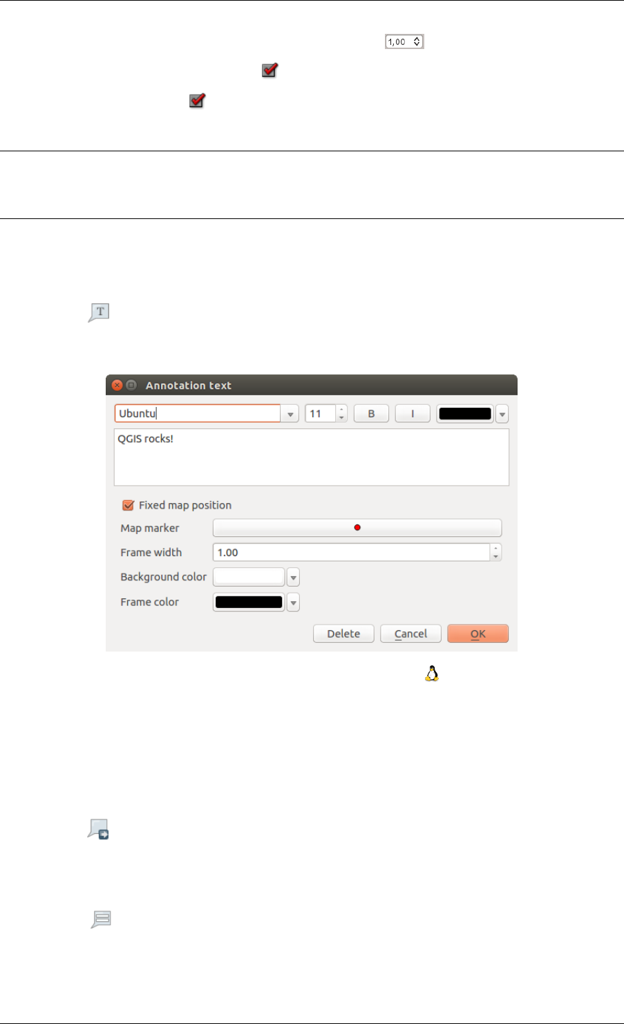
QGIS User Guide, Publicación 2.8
5. Establecer el tamaño de la barra y su etiqueta Tamaño de barra .
6. Comprobar que la casilla de verificación Habilitar barra de escala esté marcada.
7. Opcionalmente, comprobar Redondear números automáticamente al cambiar de tamaño.
8. Hacer clic en [Aceptar]
Truco: Configuración de elementos decorativos
Al guardar un proyecto .qgs, cualquiera de los cambios que se hayan hecho a la cuadrícula, flecha de norte, barra
de escala y copyright se guardarán en el proyecto y se restaurán la próxima vez que cargue el proyecto.
8.7 Herramientas de anotaciones
La herramienta Anotación de texto en la barra de herramientas de atributos provee la posibilidad de colocar texto
con formato en un globo en la vista del mapa de QGIS. Usando la herramienta Anotación de texto haga clic en la
vista del mapa.
Figure 8.10: Diálogo de texto de anotación
Haciendo doble clic sobre el elemento se abre un cuadro de diálogo con varias opciones. Hay un editor de texto
para escribir el texto con formato y otros ajustes de elementos. Por ejemplo, existe la opción de tener el elemento
colocado en una posición del mapa (mostrado por el símbolo del marcador) o tener el elemento en una posición
de la pantalla (no relacionado con el mapa). El elemento se puede mover por la posición del mapa (al arrastrar el
marcador del mapa) o moviendo solo el globo. Los iconos son parte del tema de los SIG, y se utilizan de forma
predeterminada en otros temas también.
La herramienta Mover anotación permite mover la anotación en la vista del mapa.
8.7.1 Anotaciones HTML
La herramienta Anotación HTML de la barra de herramientas de atributos provee la posibilidad de colocar el
contenido de un archivo HTML en un globo en la vista del mapa de QGIS. Utilizando la herramienta Anotación
HTML, haga clic en la vista del mapa y agregue la ruta de acceso al archivo HTML en el diálogo.
8.7. Herramientas de anotaciones 43
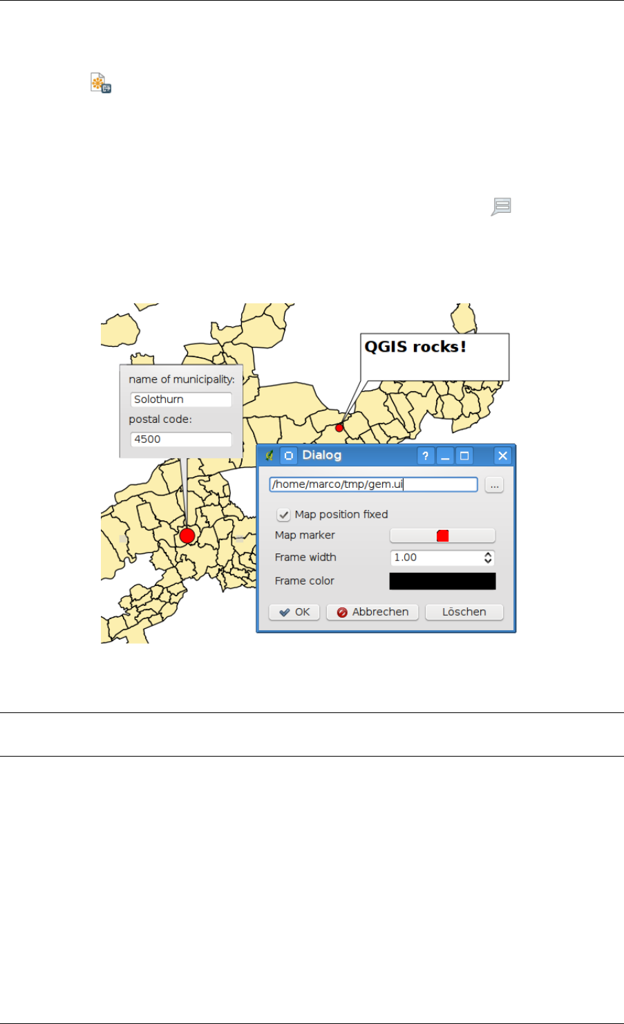
QGIS User Guide, Publicación 2.8
8.7.2 Anotaciones SVG
La herramienta Anotación SVG de la barra de herramientas de atributos provee la posibilidad para colocar un
símbolo SVG en un globo en la vista del mapa de QGIS. Utilizando la herramienta Anotación SVG, haga clic en
la vista del mapa y añada la ruta de acceso al archivo SVG en el diálogo.
8.7.3 Anotaciones de formulario
Además, puede crear sus propios formularios de anotaciones. La herramienta Formulario de anotaciones
es util para mostrar los atributos de una capa vectorial en un formulario Qt Designer personalizado
(ver figure_custom_annotation). Esto es similar al diseñador de formularios para la herramienta Iden-
tificar objetos espaciales, pero mostrado en un elemento de la anotación. Ver también el video
https://www.youtube.com/watch?v=0pDBuSbQ02o de Tim Sutton para más información.
Figure 8.11: Formulario de anotación de diseñador qt personalizado
Nota: Si presiona Ctrl+T mientras está activa una herramienta Anotación (mover anotación, anotación de texto,
anotación de formulario), se invierten los estados de visibilidad de los elementos.
8.8 Marcadores espaciales
Los marcadores espaciales le permiten “marcar” una localización geográfica y volver a ella más tarde.
8.8.1 Crear un marcador
Para crear un marcador:
1. Hacer zoom o desplazarse al área de interés.
2. Seleccione la opción de menú Ver →Nuevo marcador o presione Ctrl-B.
44 Chapter 8. Herramientas generales

QGIS User Guide, Publicación 2.8
3. Introduzca un nombre descriptivo para el marcador (hasta 255 caracteres).
4. Presione Añadir para añadir el marcador o [Borrar] para eliminarlo.
Tenga en cuenta que puede tener múltiples marcadores con el mismo nombre.
8.8.2 Trabajar con marcadores
Para usar o administrar marcadores, seleccionar la opción de menú Ver →Mostrar marcadores. El cuadro de
diálogo Marcadores geoespaciales permite hacer zum a un marcador o eliminarlo. No se pueden editar el nombre
o las coordenadas del marcador.
8.8.3 Hacer zoom a un marcador
En el diálogo Marcadores geoespaciales, seleccione el marcador deseado haciendo clic en él y luego en [Zum a].
También puede hacer zum a un marcador haciendo doble clic en él.
8.8.4 Borrar un marcador
Para eliminar un marcador del cuadro de diálogo Marcadores geospaciales, hacer clic sobre él, después hacer clic
en [Eliminar]. Confirmar la elección pulsando [Si], o cancelar la eliminación pulsando [No].
8.8.5 Importar o exportar un marcador
Para compartir o transferir sus marcadores entre computadoras que puede utilizar el menú desplegable Compartir
en el diálogo Marcadores Geoespaciales.
8.9 Anidar proyectos
Si se quiere incluir contenido de otros proyectos en un proyecto, se puede elegir Capa →Empotrar capas y
grupos.
8.9.1 Empotrar capas
El siguiente cuadro de diálogo le permite incluir capas de otros proyectos. Aquí un pequeño ejemplo:
1. Presione para buscar otro proyecto del conjunto de datos de Alaska.
2. Seleccionar el archivo de proyecto grassland. Puede ver el contenido del proyecto (ver fig-
ure_embed_dialog).
3. Presionar Ctrl y hacer clic sobre las capas file:grassland yregions. Presionar [OK]. Ahora la capa
seleccionada está incrustada en la leyenda del mapa y la vista del mapa.
Si bien las capas incrustadas son editables, no se pueden cambiar sus propiedades como estilo y etiquetado.
8.9.2 Eliminar capas incrustadas
Clic derecho en la capa empotrada y elegir Eliminar.
.
8.9. Anidar proyectos 45
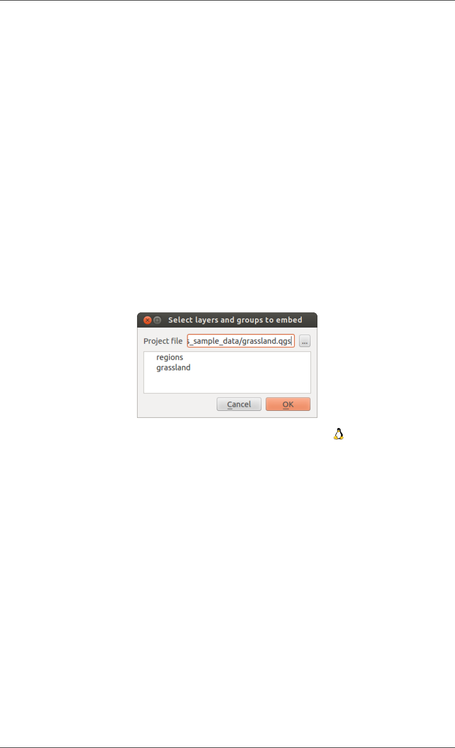
QGIS User Guide, Publicación 2.8
Figure 8.12: Seleccionar capas y grupos para empotrar
46 Chapter 8. Herramientas generales
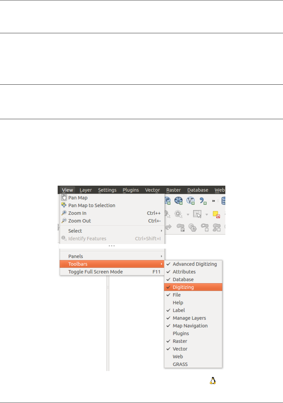
CHAPTER 9
Configuración QGIS
QGIS es altamente configurable a través del menú Configuración. Elegir entre Paneles, Barras de herramientas,
Propiedades del proyecto, Opciones y Personalización.
Nota: QGIS sigue las directrices de escritorio de localización de opciones y elementos de las propiedades del
proyecto. Por consecuencia relacionada a el sistema operativo que utiliza, la ubicación de algunos elementos
descritos anteriormente podrían estar situados en el menú Ver (Paneles y Barra de herramientas) o en Opciones
Proyecto.
9.1 Paneles y Barras de Herramientas
En el menú Paneles→, puede encender o apagar los widgets de QGIS. El menú Barra de herramientas→
proporciona la posibilidad para encender y apagar grupos de iconos en la barra de herramientas (ver fig-
ure_panels_toolbars).
Figure 9.1: El menú de paneles y barras de herramientas
47
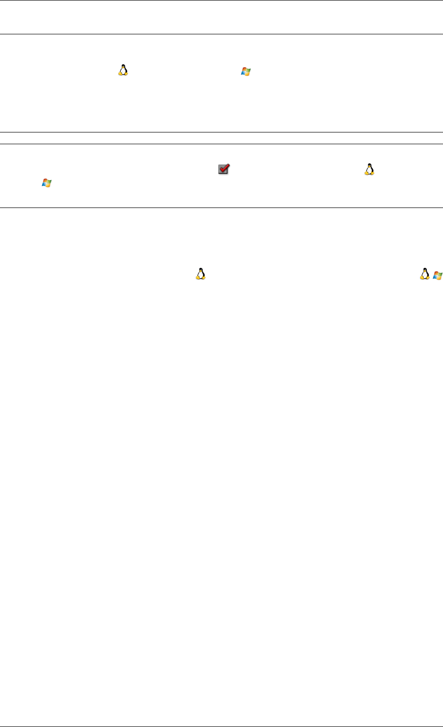
QGIS User Guide, Publicación 2.8
Truco: Activar la información general de QGIS
En QGIS, puede usar un panel de vista general que proporciona una vista completa de las capas añadidas. Se
puede seleccionar en el menú Configuración →Paneles oVer →Paneles. Dentro de la vista un rectangulo
mostrará la vista del mapa actual. Esto le permite determinar rápidamente que área del mapa se ve actualmente.
Tenga en cuenta que las etiquetas no son representadas en la vista general del mapa incluso si las capas en la vista
general del mapa se ha establecido el etiquetado. Al hacer clic y arrastrar el rectángulo rojo en la vista general se
muestra la extensión actual, la vista principal del mapa se actualizará en consecuencia.
Truco: Mostrar el registro de mensajes
Es posible seguir los mensajes de QGIS. Puede activar Registro de mensajes en el menú Configuración→
Paneles oVer →Paneles y seguir los mensajes que aparecen en las diferentes pestañas durante la carga y
funcionamiento.
9.2 Propiedades del proyecto
En la ventana de propiedades del proyecto bajo Configuración →Propiedades del proyecto (kde) o
Proyecto →Propiedades del proyecto (Gnome), puede establecer opciones específicas del proyecto. Estos in-
cluyen:
• En le menú General, el título del proyecto, color de selección y fondo, unidades de la capa, la precisión y
la opción de guardar rutas relativas a las capas se pueden definir. Si la trasformación SRC esta activada,
se puede elegir un elipsoide para cálculos de distancia. Se pueden definir las unidades del lienzo(sólo se
utiliza cuando la transformación SRC está desactivada) y la precisión de decimales se utiliza. También
puede definir una lista de la escala del proyecto, que anula las escalas predefinidas globales.
• El menú SRC habilitado para elegir el Sistema de Referencia de Coordenadas para este proyecto, y para
habilitar la reproyección al vuelo de capas ráster y vector cuando se muestran capas de un diferente SRC.
• Con el tercer menú Identificar capas, se establece (o deshabilitar) las capas que responderán a la herramienta
de identificar objetos espaciales (ver el párrafo de “Herramientas del mapa” de la sección Opciones para
permitir la identificación de múltiples capas)
• El menú Estilos predeterminados le permite controlar cómo las nuevas capas se dibujaran cuando no tienen
un estilo existente .qml definido. También puede establecer el nivel de trasparecía por defecto para nuevas
capas y si los símbolos deben tener colores al azar para asignarlos. También hay una sección adicional
donde puede definir colores específicos para el proyecto en ejecución. Puede encontrar los colores añadidos
en el menú desplegable de la ventana de diálogo de color presente en cada representación.
• La pestaña de Servidor OWS le permite definir información acerca del QGIS servidor WMS y capacidades
WFS, extensión y restricciones SRC.
• El menú Macros es utilizado para editar macros de Python para proyectos. Actualmente, solo tres macros
están disponibles: openProject(),saveProject() and closeProject().
• El menú Relaciones es utilizado para definir relaciones 1:n. Las relaciones están definidas en el diálogo de
propiedades del proyecto. Una vez que existen las relaciones de una capa, un nuevo elemento de la interfaz
de usuario en la vista del formulario (por ejemplo al identificar un elemento espacial y abrir el formulario)
mostrará una lista de las entidades relacionadas. Este proporciona un poderosa forma para expresar, por
ejemplo la inspección de la longitud de una tubería o el segmento de carretera. Se puede encontrar más
información acerca de relaciones 1:n y soporte en la sección Creating one to many relations.
48 Chapter 9. Configuración QGIS
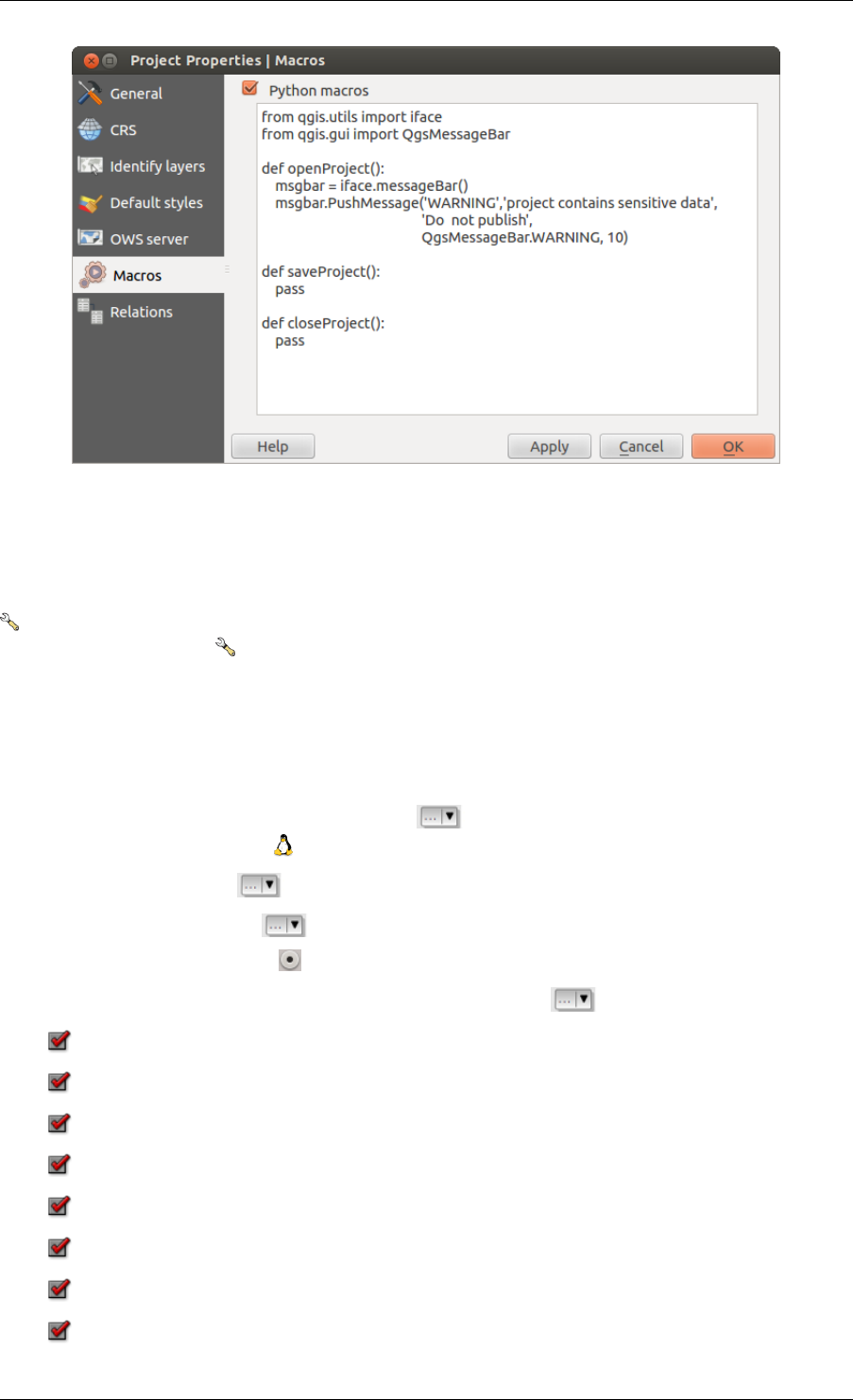
QGIS User Guide, Publicación 2.8
Figure 9.2: Ajustes de la Macro en QGIS
9.3 Opciones
Algunas opciones básicas de QGIS se pueden seleccionar utilizando el diálogo Opciones. Seleccione la opción
del menú Configuración →Opciones. Las pestañas donde puede personalizar las opciones están descritas a
continuación.
9.3.1 Menú General
Aplicación
• Seleccione el Estilo (QGIS requiere reiniciar) y elija entre ‘Oxygen’,’Windows’,’Motif’,’CDE’,
‘Plastique’ and ‘Cleanlooks’ ( ).
• Definir el Tema de icono . Actualmente solo ‘predeterminado’ es posible.
• Definir el Tamaño del icono .
• Definir la Fuente. Elegir entre Qt default y una fuente definida por el usuario.
• Cambiar el Límite de tiempo para mensajes o diálogos con tiempo .
•Ocultar la pantalla de bienvenida al iniciar la aplicación
•Mostrar consejos al iniciar
•Títulos de cajas de grupos en negrita
•Cajas de grupo al estilo QGIS
•Utilizar los diálogos de selección de colores nativos
•Usar diálogos de selección de color actualizadas en vivo
•Estilo de barra lateral personalizado
•Apoyo para rotación del lienzo experimental (requiere reiniciar)
9.3. Opciones 49
QGIS User Guide, Publicación 2.8
Los archivos de proyecto
•Abrir proyecto on launch (elegir entre ‘Nuevo’, Más reciente’ y ‘Específico’). Al elegir ‘Específico’
utilice el para definir un proyecto.
•Crear nuevo proyecto desde el proyecto predeterminado. Tiene la posibilidad de presionar Establecer
el actual proyecto como predeterminado o sobre Restablecer el predeterminado. Puede navegar a través de
sus archivos y definir un directorio donde se encuentra las plantillas definidas por el usuario. Esto se añadirá
aProyecto →Nueva plantilla de formulario. Si activa primero Crear nuevo proyecto desde proyecto
predeterminado y entonces guarde un proyecto en l la carpeta de las plantillas de proyecto.
•Solicitar guardar proyectos y fuentes de datos modificadas cuando sea necesario
•Pedir confirmación cuando se va a eliminar una capa
•Avisar cuando se abra un proyecto guardado con una versión anterior de QGIS
•Habilitar macros . Esta opción fue creada para manejar macros que estén escritos para llevar una
acción en los eventos del proyecto. Puede elegir entre ‘Nunca’, ‘Preguntar’, ‘Sólo para esta sesión’ y
‘Siempre (no recomendado)’.
9.3.2 Menú Sistema
Entorno
Variables de entorno del sistema ahora se puede ver, y muchos lo configuran en el grupo Entorno (ver fig-
ure_environment_variables). Esto es útil para las plataformas, como Mac, donde una aplicación GUI no heredan
necesariamente entorno del casco del usuario. También es útil para configurar y visualizar las variables de en-
torno para los conjuntos de herramientas externas controladas por la caja de herramientas de procesamiento (por
ejemplo, SAGA, GRASS), y para activar la salida de depuración para secciones específicas del código fuente.
•Utilizar variables personalizadas (requiere reiniciar - incluir separadores). Puede [Añadir] y[Borrar]
variables. Las variables de entorno ya definidas se muestran en Variables de entorno actuales, y es posible
filtrarlos activando Mostrar sólo variables de QGIS específicas.
Rutas de complemento
[Añadir] o[Borrar] Ruta(s) para buscar librerías de componentes en C++ adicionales
9.3.3 Menú Fuente de datos
Atributos de entidades espaciales y tabla
•Abrir tabla de atributos en la ventana adosada (requiere reiniciar QGIS)
•Copiar geometría en WKT representación de la tabla de atributos. Al utilizar :sup:‘ Copiar las filas
seleccionadas al portapapeles‘ desde el diálogo Tabla de atributos, este tiene el resultado que las coorde-
nadas de los puntos o vértices también se copian en el portapapeles.
•Funcionamiento de la tabla de atributos . Hay tres posibilidades: ‘Mostrar todos los objetos espa-
ciales’, ‘Mostrar objetos seleccionados’ y ‘Mostrar objetos espaciales visibles en el mapa’.
•Caché de registro de tabla de atributos . Esta fila en caché hace posible guardar la última carga de
N filas de atributos de modo que el trabajo con la tabla de atributos será más rápido. El caché se borrará
cuando cierre la tabla de atributos.
•Representación de valores NULOS. Aquí, puede definir un valor para los datos de campos que tienen un
valor NULO.
Manejo de fuente de datos
50 Chapter 9. Configuración QGIS
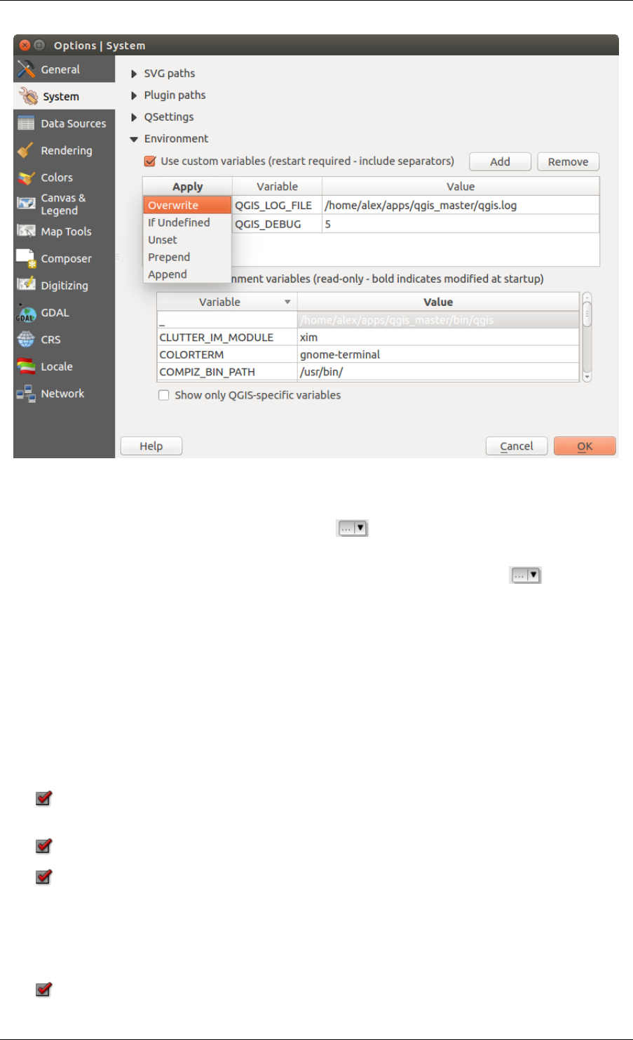
QGIS User Guide, Publicación 2.8
Figure 9.3: Variables de entorno del sistema en QGIS
•Buscar elementos válidos en el dock del explorador . Puede elegir entre ‘Comprobar extensión’ y
‘Comprobar contenido de archivo’.
•Analizar en busca de contenido de archivos comprimidos (zip) en navegador base . ‘No’, ‘Explo-
ración básica’ y ‘Exploración completa’ son posibles.
•Solicitar subcapas raster al abrir. Algunas subcapas raster soportadas — se les llama subdataset en GDAL.
Un ejemplo son los archivos netCDF — si hay muchos variables netCDF, GDAL ve cada variable como un
subconjunto de datos. La opción le permite controlar cómo lidiar con subcapas cuando se abre un archivo
con subcapas. Dispone de las siguientes opciones:
–‘Siempre’: Siempre preguntar (Si hay subcapas existentes)
–‘Si es necesario’: Preguntar si la capa no tiene bandas, pero tiene subcapas
–‘Nunca’: Nunca preguntar, no se cargará nada
–‘Cargar todo’: Nunca preguntar, pero cargar todas las subcapas
•Ignorar la declaración de codificación del archivo shape. Si el archivo shape tiene información de
codificación, Este será ignorado por QGIS.
•Añadir capas PostGIS con doble clic y seleccionar en modo extendido
•Añadir capas de Oracle con doble clic y seleccionar en modo extendido
9.3.4 Menú representación
Comportamiento de presentación
•Por defecto las nuevas capas añadidas al mapa se deben mostrar
9.3. Opciones 51
QGIS User Guide, Publicación 2.8
•Utilizar el cacheo de presentación en lo posible a la velocidad de regeneración
•Representación de capas en paralelo utilizando muchos núcleos CPU
•Máximo de núcleos a utilizar
•Intervalo de actualización del mapa (por defecto 250 ms)
•Habilitar simplificación de objetos espaciales por defecto a las nuevas capas añadidas
•Simplificación del umbral
•Simplifique el lado del proveedor si es posible
•Escala máxima a la que la capa se debe simplificar
Calidad de representación
•Hacer que las líneas se muestren menos quebradas a expensas del rendimiento de la representación
Rásters
• Con Selección de la banda RGB, puede definir el numero para la banda Roja, Verde y Azul.
Mejora de contraste
•Unibanda gris . Una sola banda de gris puede tener ‘Sin realce’, ‘Estirar a MinMax’, ‘Estirar y cortar
a MinMax’ y también ‘Cortar a MinMax’.
•Color de multibanda (byte/band) . Las opciones son ‘Sin realce’, ‘Estirar a MinMax’, ‘Estirar y cortar
a MinMax’ y ‘Cortar a MinMax’.
•Color de multibanda (>byte/band) . Las opciones son ‘No realce’, ‘Estirar a MinMax’, ‘Estirar y
cortar a MinMax’ y ‘Cortar a MinMax’.
•Límites (mínimo/máximo) . Las opciones son ‘Corte del conteo acumulativo’, ‘Min/Máx’, ‘Media +/-
desviación estándar’.
•Límite para corte del conteo acumulativo de píxeles
•Multiplicador de la desviación estándar
Depuración
•Refrescar lienzo de mapa
9.3.5 Menú de Colores
Este menú le permite añadir algunos colores personalizados que puede encontrar en cada ventana de diálogo de
color de la representación. Verá un conjunto de colores predefinidos en la pestaña: se puede eliminar o editar
todos ellos. Por otra parte se puede añadir el color que se desea y realizar algunas operaciones de copiar y pegar.
Finalmente se puede exportar el conjunto de colores como un archivo gpl o importarlos.
9.3.6 Menú Vista del mapa y leyenda
Apariencia del mapa predeterminado (anulado por las propiedades del proyecto)
• Definir un Color de selección y un Color de fondo.
Leyenda de capa
•Acción doble clic en la leyenda . Puede ‘Abrir las propiedades de la capa’ o ‘Abrir la tabla de atributos’
con el doble clic.
• Lo siguiente es posible Estilos de elementos de la leyenda:
52 Chapter 9. Configuración QGIS
QGIS User Guide, Publicación 2.8
–Comenzar el nombre de las capas con mayúsculas
–Poner en negrita los nombres de la capa
–Poner en negrita los nombres de grupo
–Mostrar nombres de atributos de clasificación
–Crear iconos de ráster (puede ser lento)
9.3.7 Menú Herramientas de mapa
Este menú ofrece algunas opciones con respecto al funcionamiento de la Herramienta de Identificación.
•Radio de búsqueda para identificar y visualizar avisos en el mapa es un factor de tolerancia expresada
como un porcentaje del ancho de mapa. Esto significa que la herramienta de identificación representara los
resultados siempre y cuando haga clic dentro de esta tolerancia.
•Color de realce le permite elegir con que color deben ser identificados los objetos espaciales que están
resaltados.
•Buffer expresado como un porcentaje de el ancho del mapa, determina una distancia de separación que se
representa a partir del contorno de lo mas destacado a identificar.
•El ancho mínimo expresado como un porcentaje de la anchura del mapa, determina el grosor del contorno
de cómo debe ser un objeto resaltado.
Herramienta de medición
• Definir Color de la banda de medida para herramienta de medida
• Definir Lugares decimales
•Mantener unidad base
•Unidades de medida preferidas (‘Metros’, ‘Pies’, ‘Millas náuticas’ o ‘Grados’)‘
•Unidades de ángulos preferidas (‘Grados’, ‘Radianes’ o ‘Grados centecimales’)
Mover y zum
• Definir Acción de la rueda del ratón (‘Zum’, ‘Zum y centrar’, ‘Zoom al cursor del ratón’, ‘Nada’)
• Definir Factor de zum para la rueda del ratón
Escalas predefinidas
Aquí, encontrará una liste de escalas predefinidas. Con los botones [+] y[-] puede añadir o eliminar las escalas
individuales.
9.3.8 Menú Diseñador
Predeterminados de la composición
Se puede definir el Tipo de letra predeterminado aquí.
Apariencia de la cuadrícula
• Definir el Estilo de cuadrícula (‘Sólido, ‘Puntos’, ‘Cruces’)
• Definir el Color de la cuadrícula
Valores predeterminados de la cuadrícula y guía
• Definir la Separc
• Definir el Desplazamiento de cuadrícula para x y y
9.3. Opciones 53
QGIS User Guide, Publicación 2.8
• Definir la Tolerancia de Ajuste
9.3.9 Menú Digitalización
Creación de entidades espaciales
•Suprimir formulario emergente de atributos después de crear objetos espaciales
•Reutilizar últimos valores de atributos introducidos
•Validar geometrías. Editar lineas y polígonos complejos con muchos nodos puede resultar a una repre-
sentación muy lenta. Esto se debe a los procesos de validación por defecto en QGIS puede tomar mucho
tiempo. Para acelerar la representación, es posible seleccionar la validación de geometría GEOS (a partir de
GEOS 3.3) o a pagarlo. La validación de geometría GEOS es mucho más rápido, pero la desventaja es que
sólo el primer problema de geometría será reportado.
Banda de medición
• Definir banda elástica Ancho de línea yColor de línea
Autoensamblado
•Abrir opciones de autoensamblado en una ventana adosada(requiere reiniciar QGIS)
• Definir Modo de autoensamblado por omisión (‘A vértice’, ‘A segmento’, ‘A vértice y segmento’,
‘Desconectado’)
• Definir Tolerancia de autoensamblado predeterminado en unidades de mapa o píxeles
• Definir el Radio de búsqueda para edición de vértices en unidades de mapa o píxeles
Marcar vértices
•Mostrar marcadores sólo para los objetos espaciales seleccionados
• Definir vértice Estilo de marcador (‘Cruz’ (predeterminado), ‘Círculo semitransparente’ o ‘Nada’)
• Definir vértice Tamaño de marcador
Herramienta de desplazamiento de curva
Las siguientes 3 opciones se refieren a la herramienta Desplazar curva en Advanced digitizing. A través de las
diversas configuraciones, es posible influir en la forma del desplazamiento de la línea. Estas opciones son posibles
a partir de GEOS 3.3.
•Estilo de la unión
•Segmentos del cuadrante
•Límite Miter
9.3.10 Menú GDAL
GDAL es una biblioteca de intercambio de datos para archivos ráster. Es esta pestaña, puede Editar opciones de
creación yEditar opciones de pirámides de los formatos ráster. Definir que controlador GDAL se va a utilizar
para un formato ráster, como en algunos casos más de un controlador está disponible.
9.3.11 Menú SRC
SRC predeterminado para nuevos proyectos
•No habilitar la reproyección ‘al vuelo’
•Habilitar automáticamente la reproyección al vuelo si las capas tienen un SRC diferente
54 Chapter 9. Configuración QGIS
QGIS User Guide, Publicación 2.8
•Activar reproyección al vuelo por defecto
• Seleccionar un SRC y Empezar siempre nuevos proyectos con este SRC
SRC para nuevas capas
Esta área permite definir la acción a realizar cuando una nueva capa es creada, o cuando una capa sin SRC es
cargada.
•Solicitar SRC
•Usar SRC del proyecto
•Usar el SRC predeterminado
Por defecto transformación de datum
•Preguntar por la trasformación del datum cuando el predeterminado no este definido
• Si ha trabajado con la trasformación de SRC ‘al vuelo’ puede ver el resultado de la transformación en la
ventana de abajo. Puede encontrar información acerca de ‘Origen SRC’ y ‘Destino SRC’ así como también
‘Transformación de datum de origen’ y ‘Trasformación de datum destino’.
9.3.12 Menú Idioma
•Ignorar el idioma del sistema yIdioma a usar en su lugar
• Información acerca del idioma del sistema
9.3.13 Menú Red
General
• Definir Dirección de búsqueda de WMS, por omisión es http://geopole.org/wms/search?search=\%1\&type=rss
• Definir Expiró el tiempo para solicitudes de red - por omisión 60000
• Definir Periodo de expiración predeterminada para teselas WMS-C/WMTS (en horas) - por omisión 24
• Definir Reintentar al máximo en caso de errores en la solicitud de tile
• Definir Agente- Usuario
Configuración de caché
Definir la configuración del caché Directorio y un Tamaño.
•Usar proxy para acceso web y definir ‘Servidor’, ‘Puerto’, ‘Usuario’, y ‘Contraseña’.
• Establecer el Tipo de proxy de acuerdo a sus necesidades.
–Default Proxy: Proxy se determina con base en el proxy de aplicación que establece el uso
–Socks5Proxy: Proxy genérico para cualquier tipo de conexión. Soporta TCP, UDP, unión a un puerto
(conexiones entrantes) y autenticación.
–HttpProxy: Implementado con el comando “CONNECT”, sólo admite conexiones TCP salientes; ad-
mite la autenticación.
–HttpCachingProxy: Implementando el uso de comandos HTTP normales, es útil sólo en el contexto
de peticiones HTTP.
–FtpCachingProxy: Implementar el uso de un proxy FTP, es útil sólo en el contexto de las peticiones
FTP.
9.3. Opciones 55
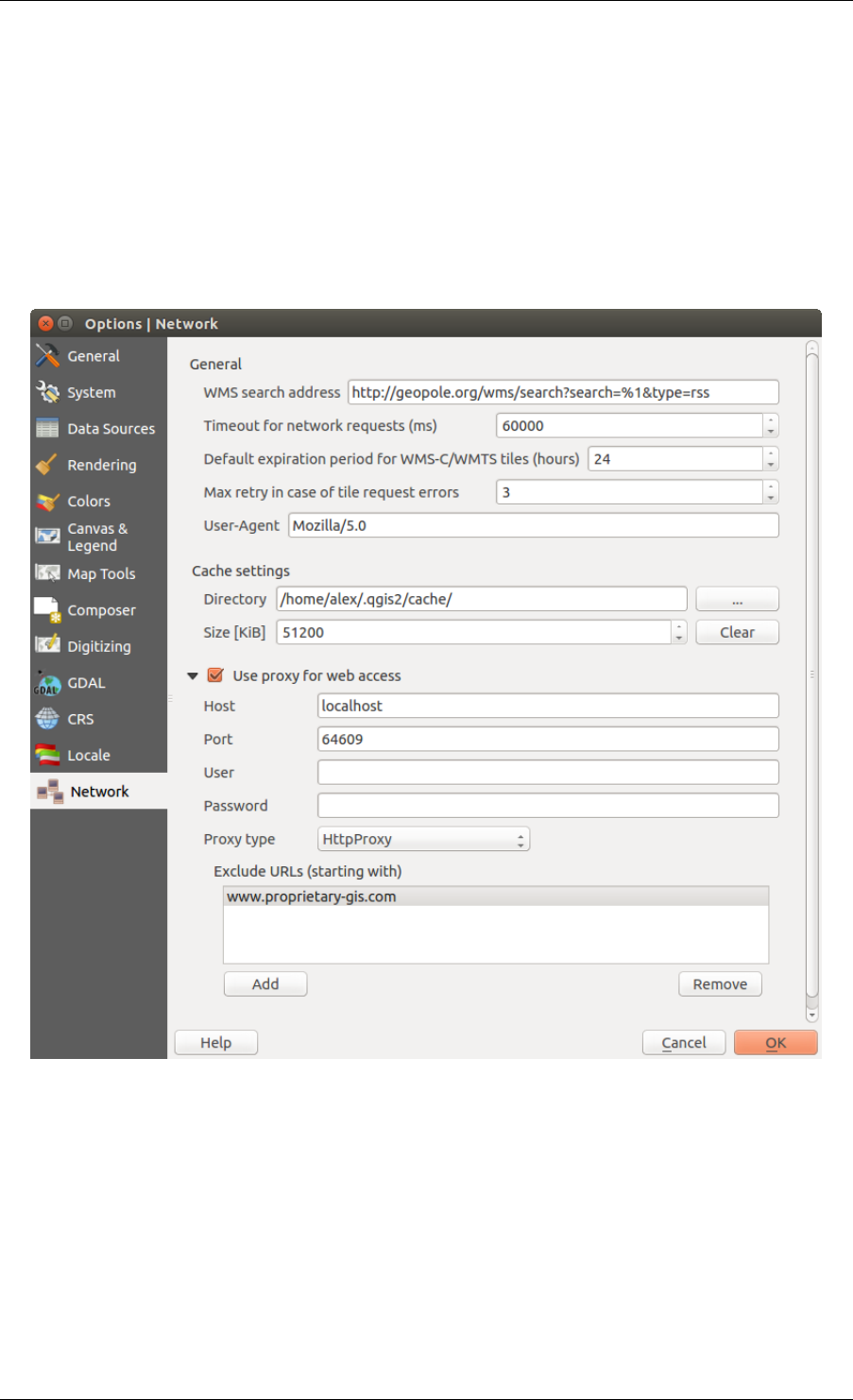
QGIS User Guide, Publicación 2.8
Figure 9.4: Configurar proxy en QGIS
56 Chapter 9. Configuración QGIS
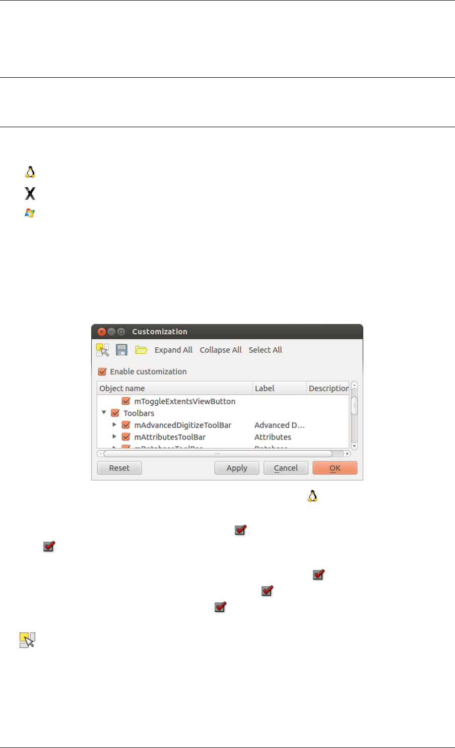
QGIS User Guide, Publicación 2.8
Excluir algunas URLs se puede agregar a la caja de texto debajo los valores del proxy (ver Figure_Network_Tab).
Si necesita más información detallada acerca de las diferentes configuraciones de proxy, consulte el manual de
documentación de la biblioteca QT en http://doc.trolltech.com/4.5/qnetworkproxy.html#ProxyType-enum.
Truco: Utilizar proxies
El uso de proxies a veces puede ser complicado. Es útil para proceder por ‘prueba y error’ con los tipos de proxies
anteriores, comprobar para ver si en su caso tiene éxito.
Puede modificar las opciones de acuerdo a sus necesidades. Alguno de los cambios puede requerir un reinicio de
QGIS antes de hacerse efectivos.
• La configuración se guarda en un archivo de texto: $HOME/.config/QGIS/QGIS2.conf
• Puede encontrar sus ajustes en: $HOME/Library/Preferences/org.qgis.qgis.plist
• Los ajustes se almacenan bajo el registro: HKEY\CURRENT_USER\Software\QGIS\qgis
9.4 Personalización
Las herramientas personalizadas permite que (des)active casi todos los elementos en la interfaz de usuario de
QGIS. Esto puede ser muy útil si se tienen muchos complementos instalados que nunca se utilizan y que esta
llenando su pantalla.
Figure 9.5: El diálogo de Personalización
La personalización de QGIS se divide en cinco grupos. En Menús, se pueden ocultar las entradas en la barra de
Menú. En Paneles se encuentran las ventanas de panel. Las ventanas del panel son aplicaciones que se pueden
iniciar y utilizar como una ventana flotante, de nivel superior o incrustadas en la ventana principal de QGIS como
un widget acoplado (ver también Paneles y Barras de Herramientas). En la Barra de estado, los elementos
como la información de coordenadas se puede desactivar. En las Barra de herramientas se puede (des)activar
los iconos de la barra de herramientas de QGIS, y en Widgets, se puede (des)activar los diálogos así como sus
botones.
Con Cambiar a la captura de widgets en la aplicación principal, puede hacer clic en los elementos en QGIS que desee que se
oculte y busque las entradas correspondientes en la personalización (ver figure_customization). También puede
guardar sus diferentes configuraciones para diferentes casos de uso. Antes de aplicar los cambios es necesario
reiniciar QGIS.
.
9.4. Personalización 57

QGIS User Guide, Publicación 2.8
58 Chapter 9. Configuración QGIS
CHAPTER 10
Working with Projections
QGIS allows users to define a global and project-wide CRS (coordinate reference system) for layers without a
pre-defined CRS. It also allows the user to define custom coordinate reference systems and supports on-the-fly
(OTF) projection of vector and raster layers. All of these features allow the user to display layers with different
CRSs and have them overlay properly.
10.1 Overview of Projection Support
QGIS has support for approximately 2,700 known CRSs. Definitions for each CRS are stored in a SQLite database
that is installed with QGIS. Normally, you do not need to manipulate the database directly. In fact, doing so may
cause projection support to fail. Custom CRSs are stored in a user database. See section Custom Coordinate
Reference System for information on managing your custom coordinate reference systems.
The CRSs available in QGIS are based on those defined by the European Petroleum Search Group (EPSG) and
the Institut Geographique National de France (IGNF) and are largely abstracted from the spatial reference tables
used in GDAL. EPSG identifiers are present in the database and can be used to specify a CRS in QGIS.
In order to use OTF projection, either your data must contain information about its coordinate reference system or
you will need to define a global, layer or project-wide CRS. For PostGIS layers, QGIS uses the spatial reference
identifier that was specified when the layer was created. For data supported by OGR, QGIS relies on the presence
of a recognized means of specifying the CRS. In the case of shapefiles, this means a file containing the well-known
text (WKT) specification of the CRS. This projection file has the same base name as the shapefile and a .prj
extension. For example, a shapefile named alaska.shp would have a corresponding projection file named
alaska.prj.
Whenever you select a new CRS, the layer units will automatically be changed in the General tab of the Project
Properties dialog under the Project (Gnome, OS X) or Settings (KDE, Windows) menu.
10.2 Global Projection Specification
QGIS starts each new project using the global default projection. The global default CRS is EPSG:4326 - WGS 84
(proj=longlat +ellps=WGS84 +datum=WGS84 +no_defs), and it comes predefined in QGIS. This
default can be changed via the [Select...] button in the first section, which is used to define the default coordinate
reference system for new projects, as shown in figure_projection_1. This choice will be saved for use in subsequent
QGIS sessions.
When you use layers that do not have a CRS, you need to define how QGIS responds to these layers. This can be
done globally or project-wide in the CRS tab under Settings →Options.
The options shown in figure_projection_1 are:
•Prompt for CRS
•Use project CRS
59
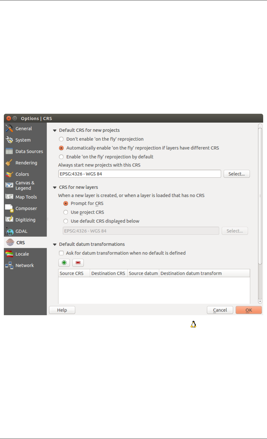
QGIS User Guide, Publicación 2.8
Figure 10.1: CRS tab in the QGIS Options Dialog
60 Chapter 10. Working with Projections
QGIS User Guide, Publicación 2.8
•Use default CRS displayed below
If you want to define the coordinate reference system for a certain layer without CRS information, you can also do
that in the General tab of the raster and vector properties dialog (see General Menu for rasters and General Menu
for vectors). If your layer already has a CRS defined, it will be displayed as shown in Vector Layer Properties
Dialog .
Truco: CRS in the Map Legend
Right-clicking on a layer in the Map Legend (section Leyenda del mapa) provides two CRS shortcuts. Set layer
CRS takes you directly to the Coordinate Reference System Selector dialog (see figure_projection_2). Set project
CRS from Layer redefines the project CRS using the layer’s CRS.
10.3 Define On The Fly (OTF) Reprojection
QGIS supports OTF reprojection for both raster and vector data. However, OTF is not activated by default. To use
OTF projection, you must activate the Enable on the fly CRS transformation checkbox in the CRS tab of the
Project Properties dialog.
There are three ways to do this:
1. Select Project Properties from the Project (Gnome, OSX) or Settings (KDE, Windows) menu.
2. Click on the CRS status icon in the lower right-hand corner of the status bar.
3. Turn OTF on by default in the CRS tab of the Options dialog by selecting Enable ‘on the fly’ reprojection
by default or Automatically enable ‘on the fly’ reprojection if layers have different CRS.
If you have already loaded a layer and you want to enable OTF projection, the best practice is to open the CRS
tab of the Project Properties dialog, select a CRS, and activate the Enable ‘on the fly’ CRS transformation
checkbox. The CRS status icon will no longer be greyed out, and all layers will be OTF projected to the CRS
shown next to the icon.
The CRS tab of the Project Properties dialog contains five important components, as shown in Figure_projection_2
and described below:
1. Enable ‘on the fly’ CRS transformation — This checkbox is used to enable or disable OTF projection.
When off, each layer is drawn using the coordinates as read from the data source, and the components de-
scribed below are inactive. When on, the coordinates in each layer are projected to the coordinate reference
system defined for the map canvas.
2. Filter — If you know the EPSG code, the identifier, or the name for a coordinate reference system, you can
use the search feature to find it. Enter the EPSG code, the identifier or the name.
3. Recently used coordinate reference systems — If you have certain CRSs that you frequently use in your
everyday GIS work, these will be displayed in this list. Click on one of these items to select the associated
CRS.
4. Coordinate reference systems of the world — This is a list of all CRSs supported by QGIS, including
Geographic, Projected and Custom coordinate reference systems. To define a CRS, select it from the list by
expanding the appropriate node and selecting the CRS. The active CRS is preselected.
5. PROJ.4 text — This is the CRS string used by the PROJ.4 projection engine. This text is read-only and
provided for informational purposes.
Truco: Project Properties Dialog
If you open the Project Properties dialog from the Project menu, you must click on the CRS tab to view the CRS
settings.
10.3. Define On The Fly (OTF) Reprojection 61
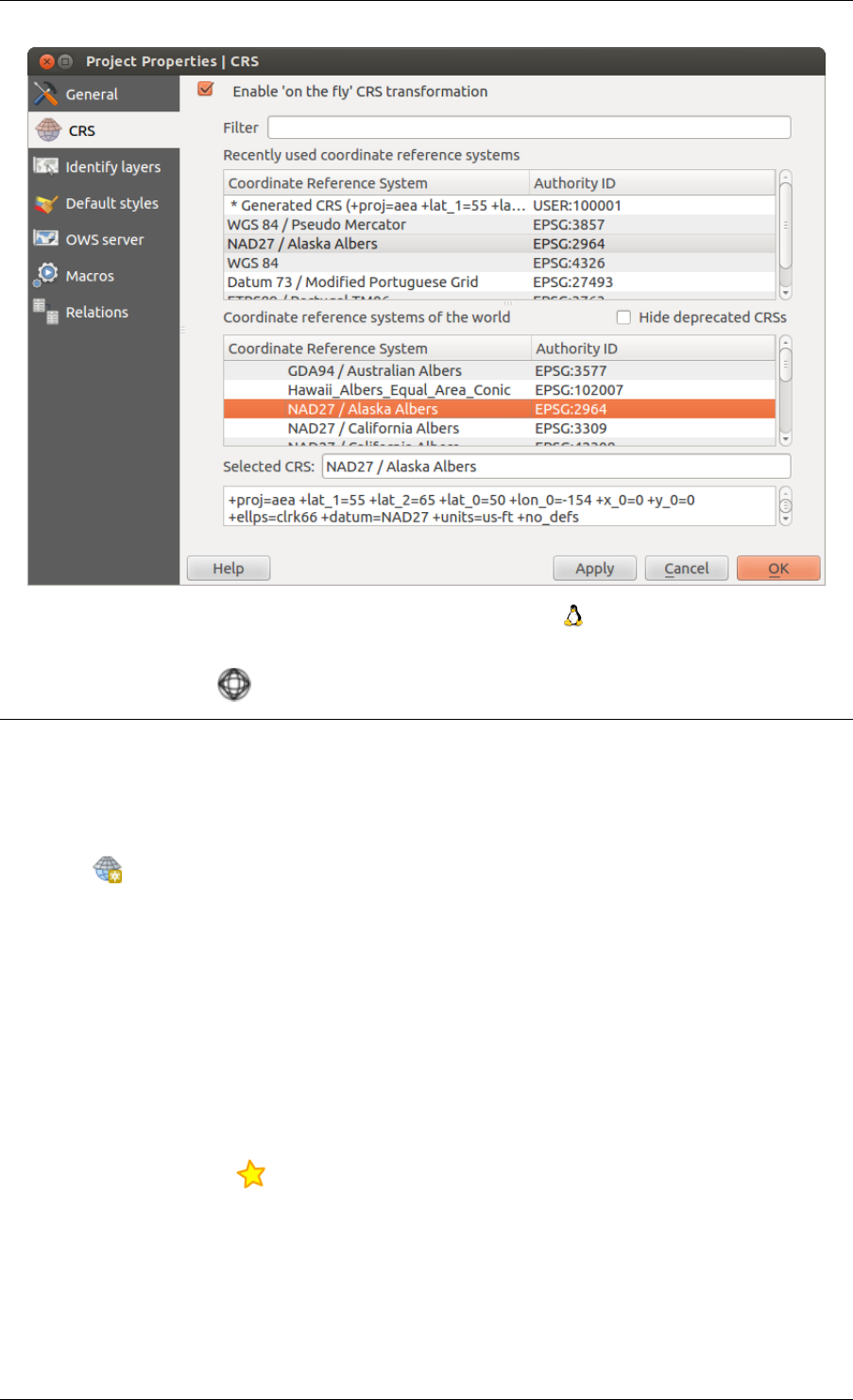
QGIS User Guide, Publicación 2.8
Figure 10.2: Project Properties Dialog
Opening the dialog from the CRS status icon will automatically bring the CRS tab to the front.
10.4 Custom Coordinate Reference System
If QGIS does not provide the coordinate reference system you need, you can define a custom CRS. To define a
CRS, select Custom CRS... from the Settings menu. Custom CRSs are stored in your QGIS user database. In
addition to your custom CRSs, this database also contains your spatial bookmarks and other custom data.
Defining a custom CRS in QGIS requires a good understanding of the PROJ.4 projection library. To begin, refer to
“Cartographic Projection Procedures for the UNIX Environment - A User’s Manual” by Gerald I. Evenden, U.S.
Geological Survey Open-File Report 90-284, 1990 (available at ftp://ftp.remotesensing.org/proj/OF90-284.pdf).
This manual describes the use of the proj.4 and related command line utilities. The cartographic parameters
used with proj.4 are described in the user manual and are the same as those used by QGIS.
The Custom Coordinate Reference System Definition dialog requires only two parameters to define a user CRS:
1. A descriptive name
2. The cartographic parameters in PROJ.4 format
To create a new CRS, click the Add new CRS button and enter a descriptive name and the CRS parameters.
Note that the Parameters must begin with a +proj= block, to represent the new coordinate reference system.
You can test your CRS parameters to see if they give sane results. To do this, enter known WGS 84 latitude and
longitude values in North and East fields, respectively. Click on [Calculate], and compare the results with the
known values in your coordinate reference system.
62 Chapter 10. Working with Projections
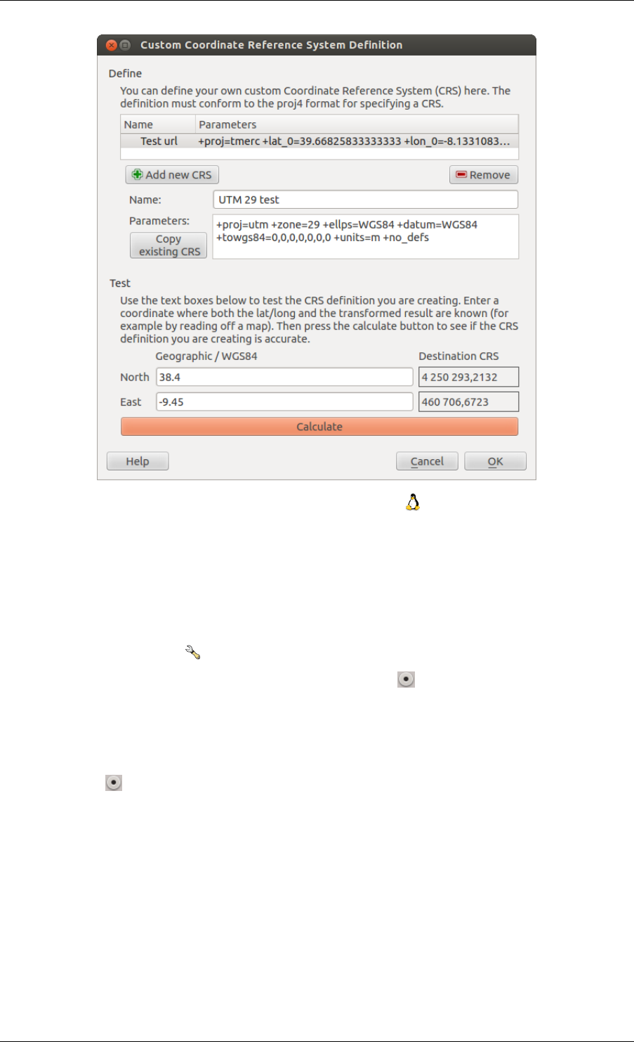
QGIS User Guide, Publicación 2.8
Figure 10.3: Custom CRS Dialog
10.5 Default datum transformations
OTF depends on being able to transform data into a ‘default CRS’, and QGIS uses WGS84. For some CRS there
are a number of transforms available. QGIS allows you to define the transformation used otherwise QGIS uses a
default transformation.
In the CRS tab under Settings →Options you can:
• set QGIS to ask you when it needs define a transformation using Ask for datum transformation when no
default is defined
• edit a list of user defaults for transformations.
QGIS asks which transformation to use by opening a dialogue box displaying PROJ.4 text describing the source
and destination transforms. Further information may be found by hovering over a transform. User defaults can be
saved by selecting Remember selection.
.
10.5. Default datum transformations 63

QGIS User Guide, Publicación 2.8
64 Chapter 10. Working with Projections
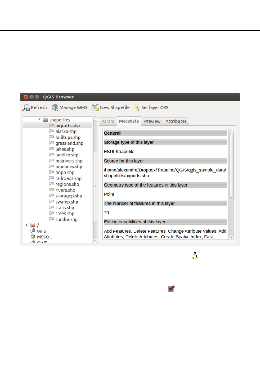
CHAPTER 11
QGIS Browser
The QGIS Browser is a panel in QGIS that lets you easily navigate in your filesystem and manage geodata. You
can have access to common vector files (e.g., ESRI shapefiles or MapInfo files), databases (e.g., PostGIS, Oracle,
SpatiaLite or MS SQL Spatial) and WMS/WFS connections. You can also view your GRASS data (to get the data
into QGIS, see GRASS GIS Integration).
Figure 11.1: QGIS browser as a stand alone application
Use the QGIS Browser to preview your data. The drag-and-drop function makes it easy to get your data into the
map view and the map legend.
1. Activate the QGIS Browser: Right-click on the toolbar and check Browser or select it from Settings →
Panels.
2. Drag the panel into the legend window and release it.
3. Click on the Browser tab.
4. Browse in your filesystem and choose the shapefile folder from qgis_sample_data directory.
5. Press the Shift key and select the airports.shp and alaska.shp files.
6. Press the left mouse button, then drag and drop the files into the map canvas.
65
QGIS User Guide, Publicación 2.8
7. Right-click on a layer and choose Set project CRS from layer. For more information see Working with
Projections.
8. Click on Zoom Full to make the layers visible.
There is a second browser available under Settings →Panels. This is handy when you need to move files or layers
between locations.
1. Activate a second QGIS Browser: Right-click on the toolbar and check Browser (2), or select it from
Settings →Panels.
2. Drag the panel into the legend window.
3. Navigate to the Browser (2) tab and browse for a shapefile in your file system.
4. Select a file with the left mouse button. Now you can use the Add Selected Layers icon to add it into the
current project.
QGIS automatically looks for the coordinate reference system (CRS) and zooms to the layer extent if you work
in a blank QGIS project. If there are already files in your project, the file will just be added, and in the case that
it has the same extent and CRS, it will be visualized. If the file has another CRS and layer extent, you must first
right-click on the layer and choose Set Project CRS from Layer. Then choose Zoom to Layer Extent.
The Filter files function works on a directory level. Browse to the folder where you want to filter files and enter
a search word or wildcard. The Browser will show only matching filenames – other data won’t be displayed.
It’s also possible to run the QGIS Browser as a stand-alone application.
Start the QGIS browser
• Type in “qbrowser” at a command prompt.
• Start the QGIS Browser using the Start menu or desktop shortcut.
• The QGIS Browser is available from your Applications folder.
In figure_browser_standalone_metadata, you can see the enhanced functionality of the stand-alone QGIS Browser.
The Param tab provides the details of your connection-based datasets, like PostGIS or MSSQL Spatial. The
Metadata tab contains general information about the file (see Metadata Menu). With the Preview tab, you can
have a look at your files without importing them into your QGIS project. It’s also possible to preview the attributes
of your files in the Attributes tab.
.
66 Chapter 11. QGIS Browser

CHAPTER 12
Trabajar con catos vectoriales
.
12.1 Supported Data Formats
QGIS uses the OGR library to read and write vector data formats, including ESRI shapefiles, MapInfo and Mi-
croStation file formats, AutoCAD DXF, PostGIS, SpatiaLite, Oracle Spatial and MSSQL Spatial databases, and
many more. GRASS vector and PostgreSQL support is supplied by native QGIS data provider plugins. Vector
data can also be loaded in read mode from zip and gzip archives into QGIS. As of the date of this document, 69
vector formats are supported by the OGR library (see OGR-SOFTWARE-SUITE in Referencias bibliográficas y
web). The complete list is available at http://www.gdal.org/ogr/ogr_formats.html.
Nota: Not all of the listed formats may work in QGIS for various reasons. For example, some require external
commercial libraries, or the GDAL/OGR installation of your OS may not have been built to support the format
you want to use. Only those formats that have been well tested will appear in the list of file types when loading a
vector into QGIS. Other untested formats can be loaded by selecting *.*.
Working with GRASS vector data is described in Section GRASS GIS Integration.
This section describes how to work with several common formats: ESRI shapefiles, PostGIS layers, SpatiaLite
layers, OpenStreetMap vectors, and Comma Separated data (CSV). Many of the features available in QGIS work
the same, regardless of the vector data source. This is by design, and it includes the identify, select, labeling and
attributes functions.
12.1.1 ESRI Shapefiles
The standard vector file format used in QGIS is the ESRI shapefile. Support is provided by the OGR Simple
Feature Library (http://www.gdal.org/ogr/).
A shapefile actually consists of several files. The following three are required:
1. .shp file containing the feature geometries
2. .dbf file containing the attributes in dBase format
3. .shx index file
Shapefiles also can include a file with a .prj suffix, which contains the projection information. While it is very
useful to have a projection file, it is not mandatory. A shapefile dataset can contain additional files. For further
details, see the ESRI technical specification at http://www.esri.com/library/whitepapers/pdfs/shapefile.pdf.
67
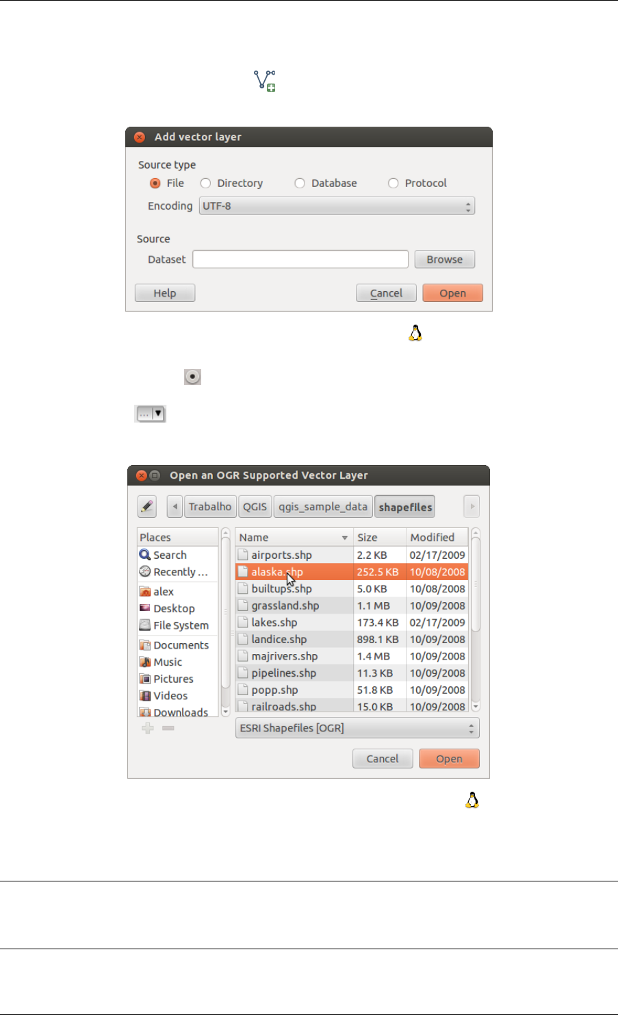
QGIS User Guide, Publicación 2.8
Loading a Shapefile
To load a shapefile, start QGIS and click on the Add Vector Layer toolbar button, or simply press Ctrl+Shift+V.
This will bring up a new window (see figure_vector_1).
Figure 12.1: Add Vector Layer Dialog
From the available options check File. Click on [Browse]. That will bring up a standard open file dialog (see
figure_vector_2), which allows you to navigate the file system and load a shapefile or other supported data source.
The selection box Filter allows you to preselect some OGR-supported file formats.
You can also select the encoding for the shapefile if desired.
Figure 12.2: Open an OGR Supported Vector Layer Dialog
Selecting a shapefile from the list and clicking [Open] loads it into QGIS. Figure_vector_3 shows QGIS after
loading the alaska.shp file.
Truco: Layer Colors
When you add a layer to the map, it is assigned a random color. When adding more than one layer at a time,
different colors are assigned to each layer.
Once a shapefile is loaded, you can zoom around it using the map navigation tools. To change the style of a layer,
open the Layer Properties dialog by double clicking on the layer name or by right-clicking on the name in the
68 Chapter 12. Trabajar con catos vectoriales
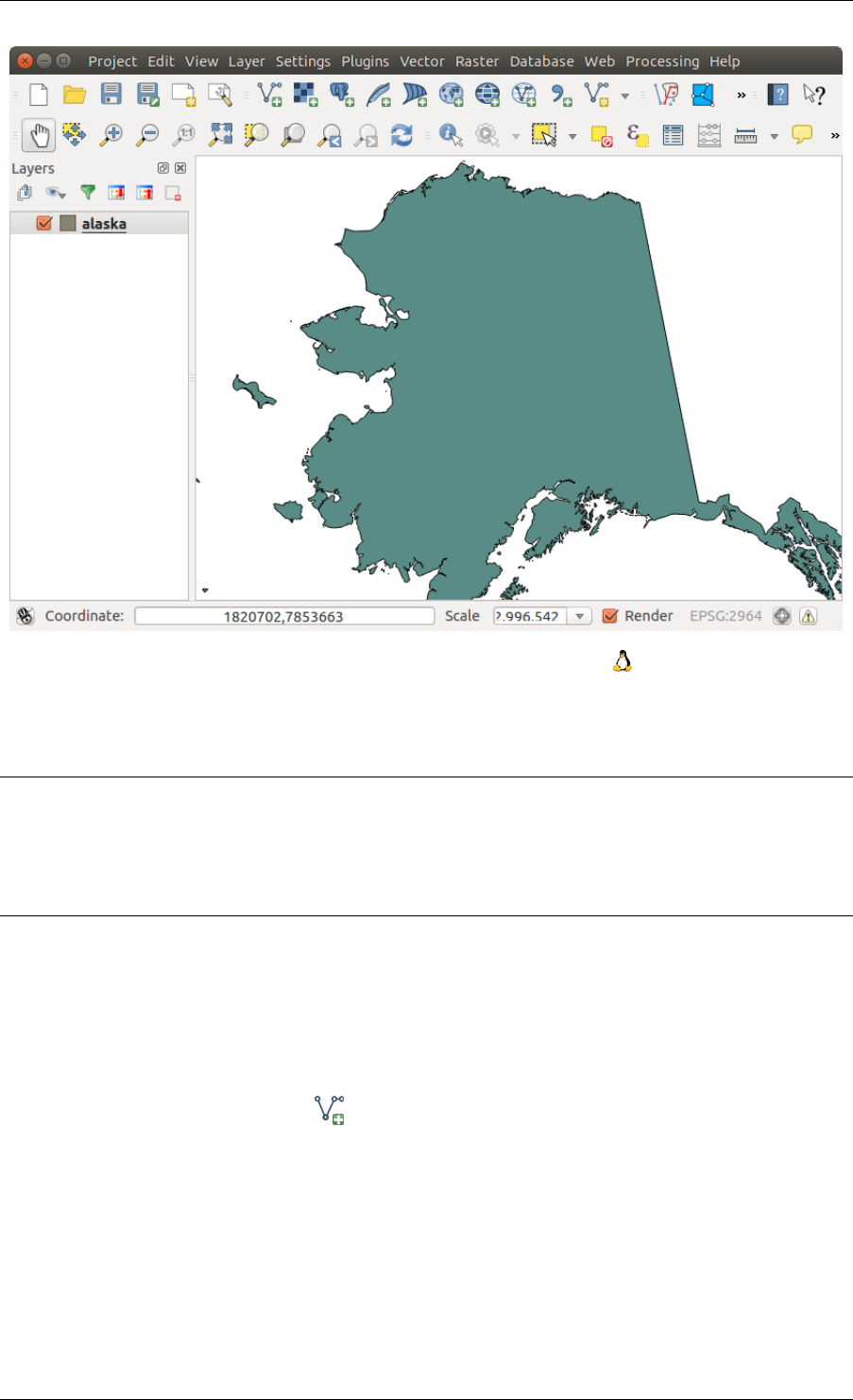
QGIS User Guide, Publicación 2.8
Figure 12.3: QGIS with Shapefile of Alaska loaded
legend and choosing Properties from the context menu. See section Style Menu for more information on setting
symbology of vector layers.
Truco: Load layer and project from mounted external drives on OS X
On OS X, portable drives that are mounted beside the primary hard drive do not show up as expected under File
→Open Project. We are working on a more OSX-native open/save dialog to fix this. As a workaround, you can
type /Volumes in the File name box and press Enter. Then you can navigate to external drives and network
mounts.
Improving Performance for Shapefiles
To improve the performance of drawing a shapefile, you can create a spatial index. A spatial index will improve
the speed of both zooming and panning. Spatial indexes used by QGIS have a .qix extension.
Use these steps to create the index:
• Load a shapefile by clicking on the Add Vector Layer toolbar button or pressing Ctrl+Shift+V.
• Open the Layer Properties dialog by double-clicking on the shapefile name in the legend or by right-clicking
and choosing Properties from the context menu.
• In the General tab, click the [Create Spatial Index] button.
Problem loading a shape .prj file
If you load a shapefile with a .prj file and QGIS is not able to read the coordinate reference system from that
file, you will need to define the proper projection manually within the General tab of the Layer Properties dialog
12.1. Supported Data Formats 69
QGIS User Guide, Publicación 2.8
of the layer by clicking the [Specify...] button. This is due to the fact that .prj files often do not provide the
complete projection parameters as used in QGIS and listed in the CRS dialog.
For the same reason, if you create a new shapefile with QGIS, two different projection files are created: a .prj
file with limited projection parameters, compatible with ESRI software, and a .qpj file, providing the complete
parameters of the used CRS. Whenever QGIS finds a .qpj file, it will be used instead of the .prj.
12.1.2 Loading a MapInfo Layer
To load a MapInfo layer, click on the Add Vector Layer toolbar button; or type Ctrl+Shift+V, change the
file type filter Files of type : to ‘Mapinfo File [OGR] (*.mif *.tab *.MIF *.TAB)’ and select the MapInfo
layer you want to load.
12.1.3 Loading an ArcInfo Binary Coverage
To load an ArcInfo Binary Coverage, click on the Add Vector Layer toolbar button or press Ctrl+Shift+V
to open the Add Vector Layer dialog. Select Directory as Source type. Change the file type filter Files of type
to ‘Arc/Info Binary Coverage’. Navigate to the directory that contains the coverage file, and select it.
Similarly, you can load directory-based vector files in the UK National Transfer Format, as well as the raw TIGER
Format of the US Census Bureau.
12.1.4 Delimited Text Files
Tabular data is a very common and widely used format because of its simplicity and readability – data can be
viewed and edited even in a plain text editor. A delimited text file is an attribute table with each column separated
by a defined character and each row separated by a line break. The first row usually contains the column names. A
common type of delimited text file is a CSV (Comma Separated Values), with each column separated by a comma.
Such data files can also contain positional information in two main forms:
• As point coordinates in separate columns
• As well-known text (WKT) representation of geometry
QGIS allows you to load a delimited text file as a layer or ordinal table. But first check that the file meets the
following requirements:
1. The file must have a delimited header row of field names. This must be the first line in the text file.
2. The header row must contain field(s) with geometry definition. These field(s) can have any name.
3. The X and Y coordinates (if geometry is defined by coordinates) must be specified as numbers. The coor-
dinate system is not important.
As an example of a valid text file, we import the elevation point data file elevp.csv that comes with the QGIS
sample dataset (see section Datos de ejemplo):
X;Y;ELEV
-300120;7689960;13
-654360;7562040;52
1640;7512840;3
[...]
Some items to note about the text file:
1. The example text file uses ;(semicolon) as delimiter. Any character can be used to delimit the fields.
2. The first row is the header row. It contains the fields X,Yand ELEV.
3. No quotes (") are used to delimit text fields.
70 Chapter 12. Trabajar con catos vectoriales
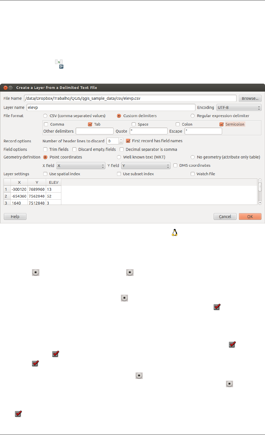
QGIS User Guide, Publicación 2.8
4. The X coordinates are contained in the Xfield.
5. The Y coordinates are contained in the Yfield.
Loading a delimited text file
Click the toolbar icon Add Delimited Text Layer in the Manage layers toolbar to open the Create a Layer from a
Delimited Text File dialog, as shown in figure_delimited_text_1.
Figure 12.4: Delimited Text Dialog
First, select the file to import (e.g., qgis_sample_data/csv/elevp.csv) by clicking on the [Browse]
button. Once the file is selected, QGIS attempts to parse the file with the most recently used delimiter. To
enable QGIS to properly parse the file, it is important to select the correct delimiter. You can specify a delimiter
by activating Custom delimiters, or by activating Regular expression delimiter and entering text into the
Expression field. For example, to change the delimiter to tab, use \t (this is a regular expression for the tab
character).
Once the file is parsed, set Geometry definition to Point coordinates and choose the Xand Yfields from the
dropdown lists. If the coordinates are defined as degrees/minutes/seconds, activate the DMS coordinates
checkbox.
Finally, enter a layer name (e.g., elevp), as shown in figure_delimited_text_1. To add the layer to the map, click
[OK]. The delimited text file now behaves as any other map layer in QGIS.
There is also a helper option that allows you to trim leading and trailing spaces from fields — Trim fields.
Also, it is possible to Discard empty fields. If necessary, you can force a comma to be the decimal separator
by activating Decimal separator is comma.
If spatial information is represented by WKT, activate the Well Known Text option and select the field with the
WKT definition for point, line or polygon objects. If the file contains non-spatial data, activate No geometry
(attribute only table) and it will be loaded as an ordinal table.
Additionaly, you can enable:
•Use spatial index to improve the performance of displaying and spatially selecting features.
12.1. Supported Data Formats 71
QGIS User Guide, Publicación 2.8
•Use subset index.
•Watch file to watch for changes to the file by other applications while QGIS is running.
12.1.5 OpenStreetMap data
In recent years, the OpenStreetMap project has gained popularity because in many countries no free geodata such
as digital road maps are available. The objective of the OSM project is to create a free editable map of the world
from GPS data, aerial photography or local knowledge. To support this objective, QGIS provides suppport for
OSM data.
Loading OpenStreetMap Vectors
QGIS integrates OpenStreetMap import as a core functionality.
• To connect to the OSM server and download data, open the menu Vector →Openstreetmap →Load data.
You can skip this step if you already obtained an .osm XML file using JOSM, Overpass API or any other
source.
• The menu Vector →Openstreetmap →Import topology from an XML file will convert your .osm file into
a SpatiaLite database and create a corresponding database connection.
• The menu Vector →Openstreetmap →Export topology to SpatiaLite then allows you to open the database
connection, select the type of data you want (points, lines, or polygons) and choose tags to import. This
creates a SpatiaLite geometry layer that you can add to your project by clicking on the Add SpatiaLite Layer
toolbar button or by selecting the Add SpatiaLite Layer... option from the Layer menu (see section
SpatiaLite Layers).
12.1.6 PostGIS Layers
PostGIS layers are stored in a PostgreSQL database. The advantages of PostGIS are the spatial indexing, filter-
ing and query capabilities it provides. Using PostGIS, vector functions such as select and identify work more
accurately than they do with OGR layers in QGIS.
Creating a stored Connection
The first time you use a PostGIS data source, you must create a connection to the PostgreSQL database that
contains the data. Begin by clicking on the Add PostGIS Layer toolbar button, selecting the Add PostGIS
Layer... option from the Layer menu, or typing Ctrl+Shift+D. You can also open the Add Vector Layer dialog
and select Database. The Add PostGIS Table(s) dialog will be displayed. To access the connection manager,
click on the [New] button to display the Create a New PostGIS Connection dialog. The parameters required for a
connection are:
•Name: A name for this connection. It can be the same as Database.
•Service: Service parameter to be used alternatively to hostname/port (and potentially database). This can
be defined in pg_service.conf.
•Host: Name of the database host. This must be a resolvable host name such as would be used to open a
telnet connection or ping the host. If the database is on the same computer as QGIS, simply enter ‘localhost’
here.
•Port: Port number the PostgreSQL database server listens on. The default port is 5432.
•Database: Name of the database.
72 Chapter 12. Trabajar con catos vectoriales
QGIS User Guide, Publicación 2.8
•SSL mode: How the SSL connection will be negotiated with the server. Note that massive speedups in
PostGIS layer rendering can be achieved by disabling SSL in the connection editor. The following options
are available:
–Disable: Only try an unencrypted SSL connection.
–Allow: Try a non-SSL connection. If that fails, try an SSL connection.
–Prefer (the default): Try an SSL connection. If that fails, try a non-SSL connection.
–Require: Only try an SSL connection.
•Username: User name used to log in to the database.
•Password: Password used with Username to connect to the database.
Optionally, you can activate the following checkboxes:
•Save Username
•Save Password
•Only look in the geometry_columns table
•Don’t resolve type of unrestricted columns (GEOMETRY)
•Only look in the ‘public’ schema
•Also list tables with no geometry
•Use estimated table metadata
Once all parameters and options are set, you can test the connection by clicking on the [Test Connect] button.
Loading a PostGIS Layer
Once you have one or more connections defined, you can load layers from the PostgreSQL database. Of
course, this requires having data in PostgreSQL. See section Importing Data into PostgreSQL for a discussion on
importing data into the database.
To load a layer from PostGIS, perform the following steps:
• If the Add PostGIS layers dialog is not already open, selecting the Add PostGIS Layer... option from the
Layer menu or typing Ctrl+Shift+D opens the dialog.
• Choose the connection from the drop-down list and click [Connect].
• Select or unselect Also list tables with no geometry.
• Optionally, use some Search Options to define which features to load from the layer, or use the [Build
query] button to start the Query builder dialog.
• Find the layer(s) you wish to add in the list of available layers.
• Select it by clicking on it. You can select multiple layers by holding down the Shift key while clicking.
See section Constructor de consultas for information on using the PostgreSQL Query Builder to further
define the layer.
• Click on the [Add] button to add the layer to the map.
Truco: PostGIS Layers
Normally, a PostGIS layer is defined by an entry in the geometry_columns table. From version 0.9.0 on, QGIS
can load layers that do not have an entry in the geometry_columns table. This includes both tables and views.
Defining a spatial view provides a powerful means to visualize your data. Refer to your PostgreSQL manual for
information on creating views.
12.1. Supported Data Formats 73
QGIS User Guide, Publicación 2.8
Some details about PostgreSQL layers
This section contains some details on how QGIS accesses PostgreSQL layers. Most of the time, QGIS should
simply provide you with a list of database tables that can be loaded, and it will load them on request. However,
if you have trouble loading a PostgreSQL table into QGIS, the information below may help you understand any
QGIS messages and give you direction on changing the PostgreSQL table or view definition to allow QGIS to
load it.
QGIS requires that PostgreSQL layers contain a column that can be used as a unique key for the layer. For tables,
this usually means that the table needs a primary key, or a column with a unique constraint on it. In QGIS, this
column needs to be of type int4 (an integer of size 4 bytes). Alternatively, the ctid column can be used as primary
key. If a table lacks these items, the oid column will be used instead. Performance will be improved if the column
is indexed (note that primary keys are automatically indexed in PostgreSQL).
If the PostgreSQL layer is a view, the same requirement exists, but views do not have primary keys or columns
with unique constraints on them. You have to define a primary key field (has to be integer) in the QGIS dialog
before you can load the view. If a suitable column does not exist in the view, QGIS will not load the layer. If this
occurs, the solution is to alter the view so that it does include a suitable column (a type of integer and either a
primary key or with a unique constraint, preferably indexed).
QGIS offers a checkbox Select at id that is activated by default. This option gets the ids without the attributes
which is faster in most cases. It can make sense to disable this option when you use expensive views.
Truco: Backup of PostGIS database with layers saved by QGIS
If you want to make a backup of your PostGIS database using the pg_dump and pg_restore commands
the default layer styles as saved by QGIS are failing to restore afterwards. You need to set the XML option to
DOCUMENT and the restore will work.
12.1.7 Importing Data into PostgreSQL
Data can be imported into PostgreSQL/PostGIS using several tools, including the SPIT plugin and the command
line tools shp2pgsql and ogr2ogr.
DB Manager
QGIS comes with a core plugin named DB Manager. It can be used to load shapefiles and other data formats, and
it includes support for schemas. See section Complemento administrador de BBDD for more information.
shp2pgsql
PostGIS includes an utility called shp2pgsql that can be used to import shapefiles into a PostGIS-enabled database.
For example, to import a shapefile named lakes.shp into a PostgreSQL database named gis_data, use the
following command:
shp2pgsql -s 2964 lakes.shp lakes_new | psql gis_data
This creates a new layer named lakes_new in the gis_data database. The new layer will have a spatial ref-
erence identifier (SRID) of 2964. See section Working with Projections for more information on spatial reference
systems and projections.
Truco: Exporting datasets from PostGIS
Like the import tool shp2pgsql, there is also a tool to export PostGIS datasets as shapefiles: pgsql2shp. This is
shipped within your PostGIS distribution.
74 Chapter 12. Trabajar con catos vectoriales
QGIS User Guide, Publicación 2.8
ogr2ogr
Besides shp2pgsql and DB Manager, there is another tool for feeding geodata in PostGIS: ogr2ogr. This is part
of your GDAL installation.
To import a shapefile into PostGIS, do the following:
ogr2ogr -f "PostgreSQL" PG:"dbname=postgis host=myhost.de user=postgres
password=topsecret" alaska.shp
This will import the shapefile alaska.shp into the PostGIS database postgis using the user postgres with the
password topsecret on host server myhost.de.
Note that OGR must be built with PostgreSQL to support PostGIS. You can verify this by typing (in )
ogrinfo --formats | grep -i post
If you prefer to use PostgreSQL’s COPY command instead of the default INSERT INTO method, you can export
the following environment variable (at least available on and ):
export PG_USE_COPY=YES
ogr2ogr does not create spatial indexes like shp2pgsl does. You need to create them manually, using the nor-
mal SQL command CREATE INDEX afterwards as an extra step (as described in the next section Improving
Performance).
Improving Performance
Retrieving features from a PostgreSQL database can be time-consuming, especially over a network. You can
improve the drawing performance of PostgreSQL layers by ensuring that a PostGIS spatial index exists on
each layer in the database. PostGIS supports creation of a GiST (Generalized Search Tree) index to speed
up spatial searches of the data (GiST index information is taken from the PostGIS documentation available at
http://postgis.refractions.net).
The syntax for creating a GiST index is:
CREATE INDEX [indexname] ON [tablename]
USING GIST ( [geometryfield] GIST_GEOMETRY_OPS );
Note that for large tables, creating the index can take a long time. Once the index is created, you should perform
aVACUUM ANALYZE. See the PostGIS documentation (POSTGIS-PROJECT Referencias bibliográficas y web)
for more information.
The following is an example of creating a GiST index:
gsherman@madison:~/current$ psql gis_data
Welcome to psql 8.3.0, the PostgreSQL interactive terminal.
Type: \copyright for distribution terms
\h for help with SQL commands
\? for help with psql commands
\g or terminate with semicolon to execute query
\q to quit
gis_data=# CREATE INDEX sidx_alaska_lakes ON alaska_lakes
gis_data-# USING GIST (the_geom GIST_GEOMETRY_OPS);
CREATE INDEX
gis_data=# VACUUM ANALYZE alaska_lakes;
VACUUM
gis_data=# \q
gsherman@madison:~/current$
12.1. Supported Data Formats 75
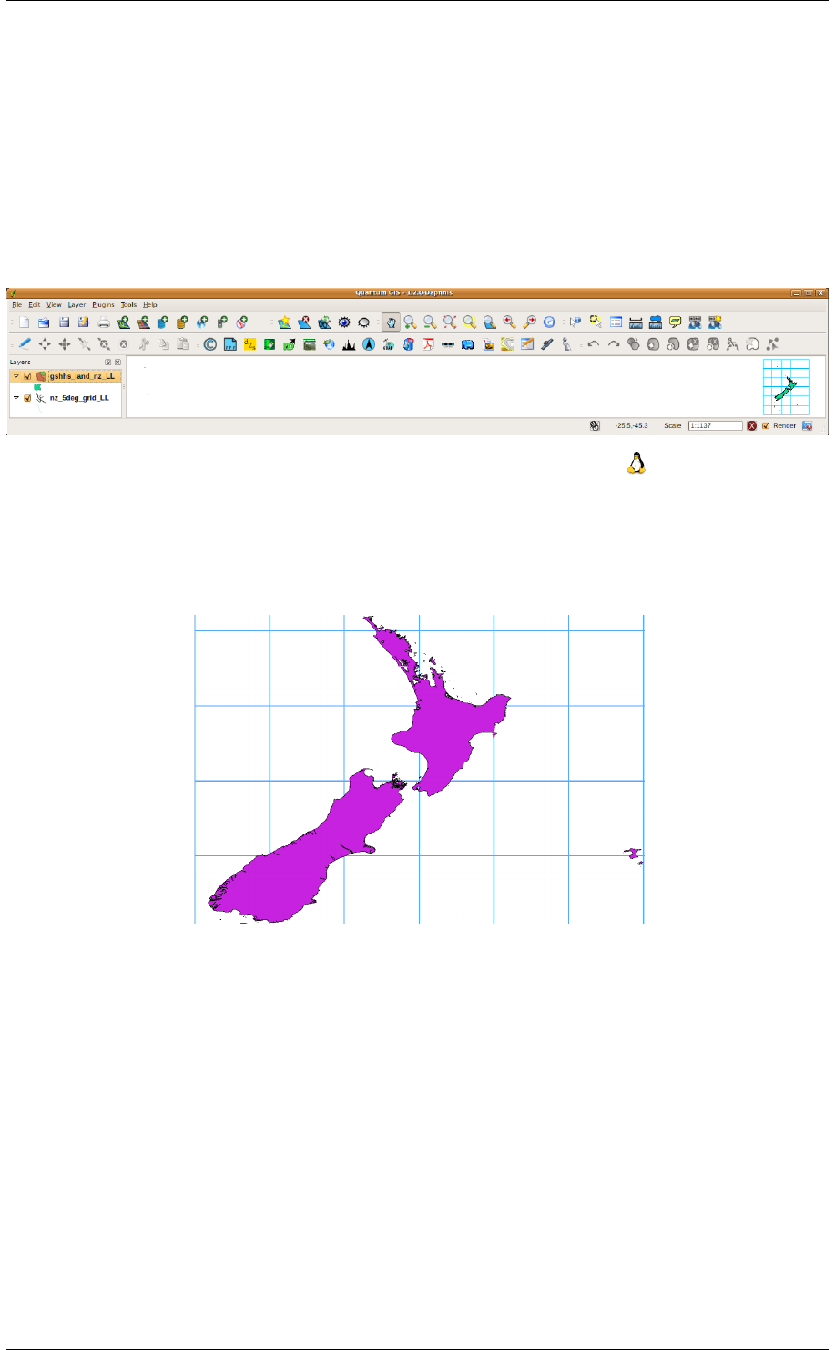
QGIS User Guide, Publicación 2.8
12.1.8 Vector layers crossing 180° longitude
Many GIS packages don’t wrap vector maps with a geographic reference system (lat/lon) crossing the 180 degrees
longitude line (http://postgis.refractions.net/documentation/manual-2.0/ST_Shift_Longitude.html). As result, if
we open such a map in QGIS, we will see two far, distinct locations, that should appear near each other. In
Figure_vector_4, the tiny point on the far left of the map canvas (Chatham Islands) should be within the grid, to
the right of the New Zealand main islands.
Figure 12.5: Map in lat/lon crossing the 180° longitude line
A work-around is to transform the longitude values using PostGIS and the ST_Shift_Longitude function. This
function reads every point/vertex in every component of every feature in a geometry, and if the longitude coordi-
nate is < 0°, it adds 360° to it. The result is a 0° - 360° version of the data to be plotted in a 180°-centric map.
Figure 12.6: Crossing 180° longitude applying the ST_Shift_Longitude function
Usage
• Import data into PostGIS (Importing Data into PostgreSQL) using, for example, the DB Manager plugin.
• Use the PostGIS command line interface to issue the following command (in this example,
“TABLE” is the actual name of your PostGIS table): gis_data=# update TABLE set
the_geom=ST_Shift_Longitude(the_geom);
• If everything went well, you should receive a confirmation about the number of features that were updated.
Then you’ll be able to load the map and see the difference (Figure_vector_5).
76 Chapter 12. Trabajar con catos vectoriales
QGIS User Guide, Publicación 2.8
12.1.9 SpatiaLite Layers
The first time you load data from a SpatiaLite database, begin by clicking on the Add SpatiaLite Layer
toolbar button, or by selecting the Add SpatiaLite Layer... option from the Layer menu, or by typing
Ctrl+Shift+L. This will bring up a window that will allow you either to connect to a SpatiaLite database
already known to QGIS, which you can choose from the drop-down menu, or to define a new connection to a new
database. To define a new connection, click on [New] and use the file browser to point to your SpatiaLite database,
which is a file with a .sqlite extension.
If you want to save a vector layer to SpatiaLite format, you can do this by right clicking the layer in the legend.
Then, click on Save as.., define the name of the output file, and select ‘SpatiaLite’ as format and the CRS. Also,
you can select ‘SQLite’ as format and then add SPATIALITE=YES in the OGR data source creation option field.
This tells OGR to create a SpatiaLite database. See also http://www.gdal.org/ogr/drv_sqlite.html.
QGIS also supports editable views in SpatiaLite.
Creating a new SpatiaLite layer
If you want to create a new SpatiaLite layer, please refer to section Creating a new SpatiaLite layer.
Truco: SpatiaLite data management Plugins
For SpatiaLite data management, you can also use several Python plugins: QSpatiaLite, SpatiaLite Manager or
DB Manager (core plugin, recommended). If necessary, they can be downloaded and installed with the Plugin
Installer.
12.1.10 MSSQL Spatial Layers
QGIS also provides native MS SQL 2008 support. The first time you load MSSQL Spatial data, begin by
clicking on the Add MSSQL Spatial Layer toolbar button or by selecting the Add MSSQL Spatial Layer... option
from the Layer menu, or by typing Ctrl+Shift+M.
12.1.11 Oracle Spatial Layers
The spatial features in Oracle Spatial aid users in managing geographic and location data in a native type within
an Oracle database. QGIS now has support for such layers.
Creating a stored Connection
The first time you use an Oracle Spatial data source, you must create a connection to the database that
contains the data. Begin by clicking on the Add Orcale Spatial Layer toolbar button, selecting the Add Orcale
Spatial Layer... option from the Layer menu, or typing Ctrl+Shift+O. To access the connection manager, click
on the [New] button to display the Create a New Oracle Spatial Connection dialog. The parameters required for
a connection are:
•Name: A name for this connection. It can be the same as Database
•Database: SID or SERVICE_NAME of the Oracle instance.
•Host: Name of the database host. This must be a resolvable host name such as would be used to open a
telnet connection or ping the host. If the database is on the same computer as QGIS, simply enter ‘localhost’
here.
•Port: Port number the Oracle database server listens on. The default port is 1521.
12.1. Supported Data Formats 77
QGIS User Guide, Publicación 2.8
•Username: Username used to login to the database.
•Password: Password used with Username to connect to the database.
Optionally, you can activate following checkboxes:
•Save Username Indicates whether to save the database username in the connection configuration.
•Save Password Indicates whether to save the database password in the connection settings.
•Only look in meta data table Restricts the displayed tables to those that are in the
all_sdo_geom_metadata view. This can speed up the initial display of spatial tables.
•Only look for user’s tables When searching for spatial tables, restrict the search to tables that are owned
by the user.
•Also list tables with no geometry Indicates that tables without geometry should also be listed by default.
•Use estimated table statistics for the layer metadata When the layer is set up, various metadata are
required for the Oracle table. This includes information such as the table row count, geometry type and
spatial extents of the data in the geometry column. If the table contains a large number of rows, determining
this metadata can be time-consuming. By activating this option, the following fast table metadata operations
are done: Row count is determined from all_tables.num_rows. Table extents are always determined
with the SDO_TUNE.EXTENTS_OF function, even if a layer filter is applied. Table geometry is determined
from the first 100 non-null geometry rows in the table.
•Only existing geometry types Only list the existing geometry types and don’t offer to add others.
Once all parameters and options are set, you can test the connection by clicking on the [Test Connect] button.
Truco: QGIS User Settings and Security
Depending on your computing environment, storing passwords in your QGIS settings may be a security risk.
Passwords are saved in clear text in the system configuration and in the project files! Your customized settings for
QGIS are stored based on the operating system:
• The settings are stored in your home directory in ~/.qgis2.
• The settings are stored in the registry.
Loading an Oracle Spatial Layer
Once you have one or more connections defined, you can load layers from the Oracle database. Of course,
this requires having data in Oracle.
To load a layer from Oracle Spatial, perform the following steps:
• If the Add Oracle Spatial layers dialog is not already open, click on the Add Oracle Spatial Layer toolbar
button.
• Choose the connection from the drop-down list and click [Connect].
• Select or unselect Also list tables with no geometry.
• Optionally, use some Search Options to define which features to load from the layer or use the [Build
query] button to start the Query builder dialog.
• Find the layer(s) you wish to add in the list of available layers.
• Select it by clicking on it. You can select multiple layers by holding down the Shift key while clicking.
See section Constructor de consultas for information on using the Oracle Query Builder to further define
the layer.
78 Chapter 12. Trabajar con catos vectoriales
QGIS User Guide, Publicación 2.8
• Click on the [Add] button to add the layer to the map.
Truco: Oracle Spatial Layers
Normally, an Oracle Spatial layer is defined by an entry in the USER_SDO_METADATA table.
.
12.2 The Symbol Library
12.2.1 Presentation
The Symbol Library is the place where users can create generic symbols to be used in several QGIS projects. It
allows users to export and import symbols, groups symbols and add, edit and remove symbols. You can open it
with the Settings →Style Library or from the Style tab in the vector layer’s Properties.
Share and import symbols
Users can export and import symbols in two main formats: qml (QGIS format) and SLD (OGC standard). Note
that SLD format is not fully supported by QGIS.
share item displays a drop down list to let the user import or export symbols.
Groups and smart groups
Groups are categories of Symbols and smart groups are dynamic groups.
To create a group, right-click on an existing group or on the main Groups directory in the left of the library. You
can also select a group and click on the add item button.
To add a symbol into a group, you can either right click on a symbol then choose Apply group and then the group
name added before. There is a second way to add several symbols into group: just select a group and click
and choose Group Symbols. All symbols display a checkbox that allow you to add the symbol into the selected
groups. When finished, you can click on the same button, and choose Finish Grouping.
Create Smart Symbols is similar to creating group, but instead select Smart Groups. The dialog box allow user
to choose the expression to select symbols in order to appear in the smart group (contains some tags, member of
a group, have a string in its name, etc.)
Add, edit, remove symbol
With the Style manager from the [Symbol] menu you can manage your symbols. You can add item,
edit item,remove item and share item. ‘Marker’ symbols, ‘Line’ symbols, ‘Fill’ patterns and ‘colour ramps’
can be used to create the symbols. The symbols are then assigned to ‘All Symbols’, ‘Groups’ or ‘Smart groups’.
For each kind of symbols, you will find always the same dialog structure:
• at the top left side a symbol representation
• under the symbol representation the symbol tree show the symbol layers
• at the right you can setup some parameter (unit,transparency, color, size and rotation)
• under these parameters you find some symbol from the symbols library
12.2. The Symbol Library 79

QGIS User Guide, Publicación 2.8
The symbol tree allow adding, removing or protect new simple symbol. You can move up or down the symbol
layer.
More detailed settings can be made when clicking on the second level in the Symbol layers dialog. You can define
Symbol layers that are combined afterwards. A symbol can consist of several Symbol layers. Settings will be
shown later in this chapter.
Truco: Note that once you have set the size in the lower levels of the Symbol layers dialog, the size of the
whole symbol can be changed with the Size menu in the first level again. The size of the lower levels changes
accordingly, while the size ratio is maintained.
12.2.2 Marker Symbols
Marker symbols have several symbol layer types:
• Ellipse marker
• Font marker
• Simple marker (default)
• SVG marker
• Vector Field marker
The following settings are possible:
•Symbol layer type: You have the option to use Ellipse markers, Font markers, Simple markers, SVG markers
and Vector Field markers.
•colors
•Size
•Outline style
•Outline width
•Angle
•Offset X,Y: You can shift the symbol in the x- or y-direction.
•Anchor point
•Data defined properties ...
12.2.3 Line Symbols
Line marker symbols have only two symbol layer types:
• Marker line
• Simple line (default)
The default symbol layer type draws a simple line whereas the other display a marker point regularly on the line.
You can choose different location vertex, interval or central point. Marker line can have offset along the line or
offset line. Finally, rotation allows you to change the orientation of the symbol.
The following settings are possible:
•colour
•Pen width
•Offset
•Pen style
80 Chapter 12. Trabajar con catos vectoriales
QGIS User Guide, Publicación 2.8
•Join style
•Cap style
•Use custom dash pattern
•Dash pattern unit
•Data defined properties ...
12.2.4 Polygon Symbols
Polygon marker symbols have also several symbol layer types:
• Centroid fill
• Gradient fill
• Line pattern fill
• Point pattern fill
• Raster image fill
• SVG fill
• Shapeburst fill
• Simple fill (default)
• Outline: Marker line (same as line marker)
• Outline: simple line (same as line marker)
The following settings are possible:
•Colors for the border and the fill.
•Fill style
•Border style
•Border width
•Offset X,Y
•Data defined properties ...
Using the color combo box, you can drag and drop color for one color button to another button, copy-paste color,
pick color from somewhere, choose a color from the palette or from recent or standard color. The combo box
allow you to fill in the feature with transparency. You can also just click on the button to open the palettte dialog.
Note that you can import color from some external software like GIMP.
With the ‘Raster image fill’ you can fill polygons with a tiled raster image. Options include (data defined) file
name, opacity, image size (in pixels, mm or map units), coordinate mode (feature or view) and rotation.
‘Gradient Fill’ Symbol layer type allows you to select between a Two color and Color ramp setting. You
can use the Feature centroid as Referencepoint. All fills ‘Gradient Fill‘ Symbol layer type is also available
through the Symbol menu of the Categorized and Graduated Renderer and through the Rule properties menu of
the Rule-based renderer. Other possibility is to choose a ‘shapeburst fill’ which is a buffered gradient fill, where a
gradient is drawn from the boundary of a polygon towards the polygon’s centre. Configurable parameters include
distance from the boundary to shade, use of color ramps or simple two color gradients, optional blurring of the fill
and offsets.
It is possible to only draw polygon borders inside the polygon. Using ‘Outline: Simple line’ select Draw line
only inside polygon.
12.2. The Symbol Library 81
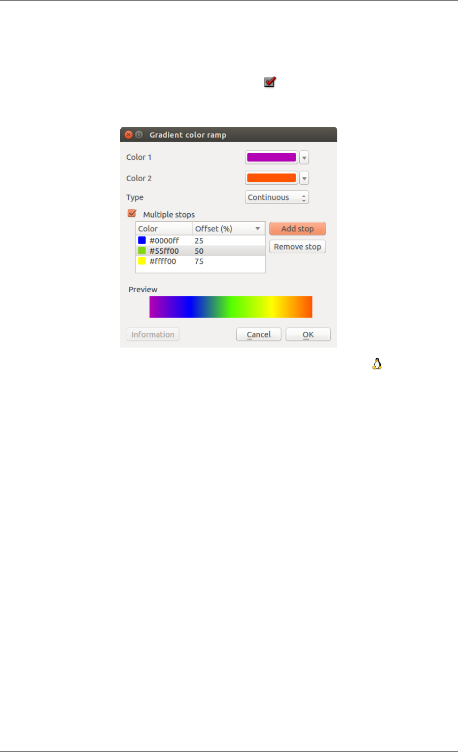
QGIS User Guide, Publicación 2.8
12.2.5 Color ramp
You can create a custom color ramp choosing New color ramp... from the color ramp drop-down menu. A dialog
will prompt for the ramp type: Gradient, Random, colorBrewer, or cpt-city. The first three have options for number
of steps and/or multiple stops in the color ramp. You can use the Invert option while classifying the data with
a color ramp. See figure_symbology_3 for an example of custom color ramp and figure_symbology_3a for the
cpt-city dialog.
Figure 12.7: Example of custom gradient color ramp with multiple stops
The cpt-city option opens a new dialog with hundreds of themes included ‘out of the box’.
.
12.3 The Vector Properties Dialog
The Layer Properties dialog for a vector layer provides information about the layer, symbology settings and
labeling options. If your vector layer has been loaded from a PostgreSQL/PostGIS datastore, you can also alter
the underlying SQL for the layer by invoking the Query Builder dialog on the General tab. To access the Layer
Properties dialog, double-click on a layer in the legend or right-click on the layer and select Properties from the
pop-up menu.
12.3.1 Style Menu
The Style menu provides you with a comprehensive tool for rendering and symbolizing your vector data. You can
use Layer rendering →tools that are common to all vector data, as well as special symbolizing tools that were
designed for the different kinds of vector data.
Renderers
The renderer is responsible for drawing a feature together with the correct symbol. There are four types of
renderers: single symbol, categorized, graduated and rule-based. There is no continuous color renderer, because it
is in fact only a special case of the graduated renderer. The categorized and graduated renderers can be created by
specifying a symbol and a color ramp - they will set the colors for symbols appropriately. For point layers, there
is a point displacement renderer available. For each data type (points, lines and polygons), vector symbol layer
82 Chapter 12. Trabajar con catos vectoriales
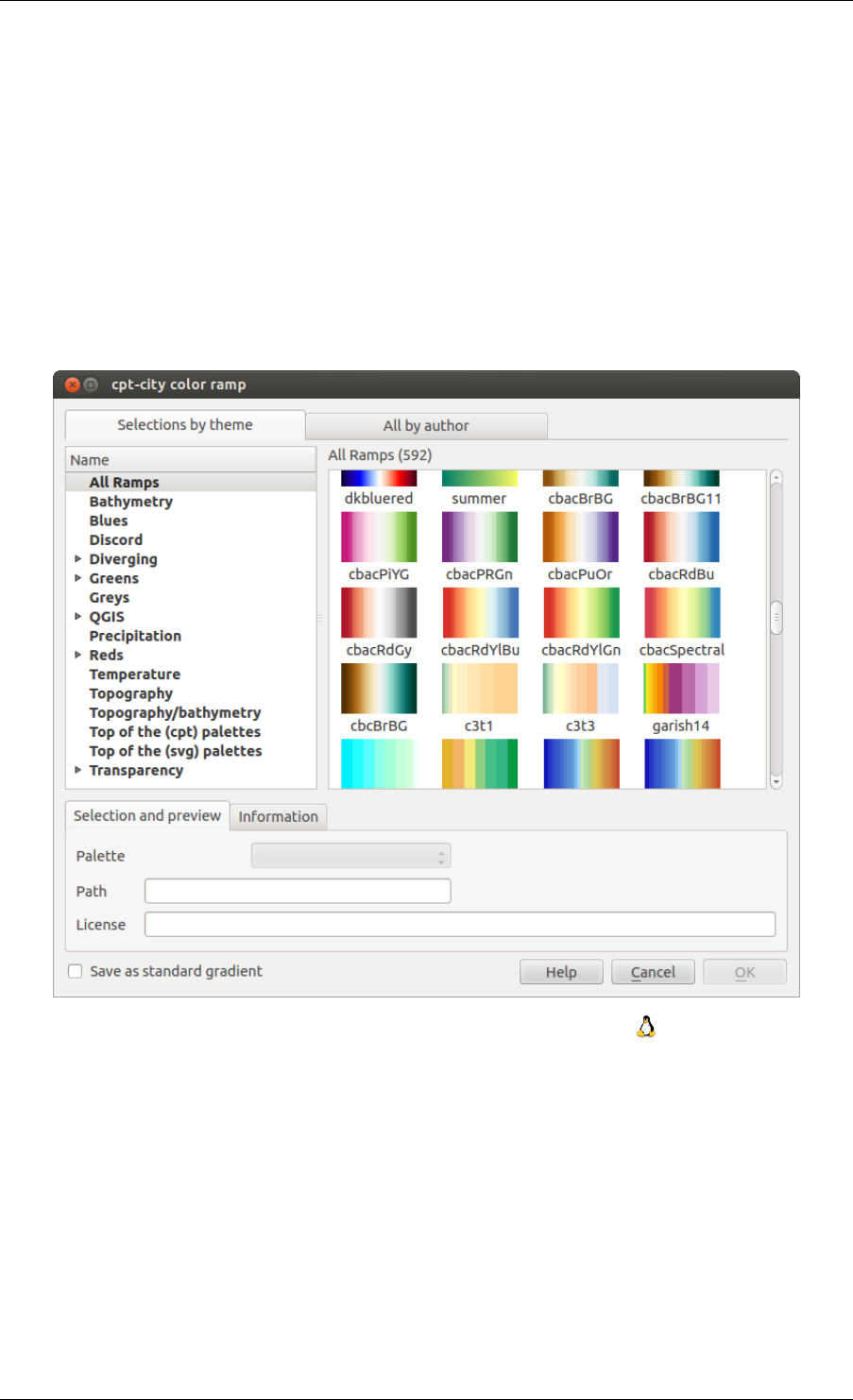
QGIS User Guide, Publicación 2.8
Figure 12.8: cpt-city dialog with hundreds of color ramps
12.3. The Vector Properties Dialog 83
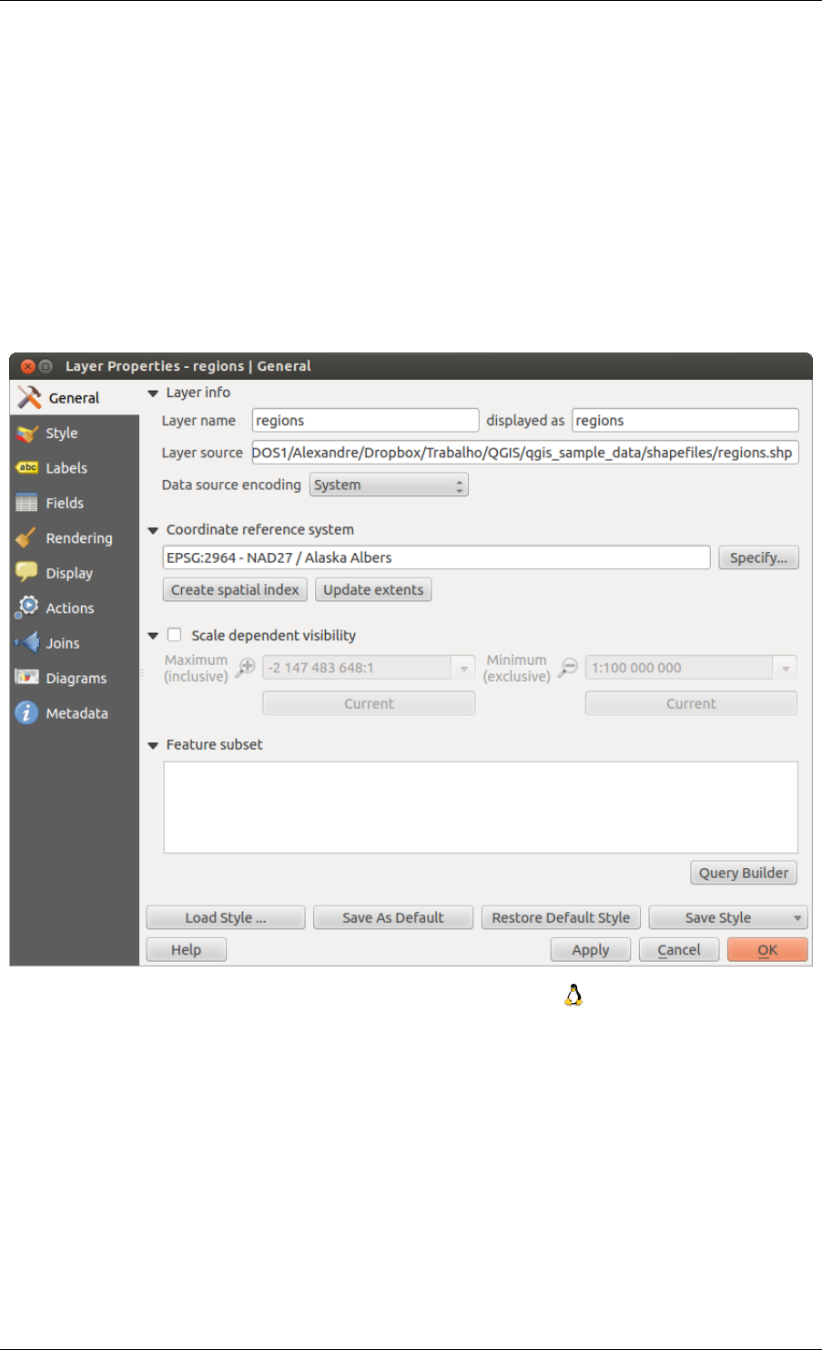
QGIS User Guide, Publicación 2.8
Figure 12.9: Vector Layer Properties Dialog
84 Chapter 12. Trabajar con catos vectoriales
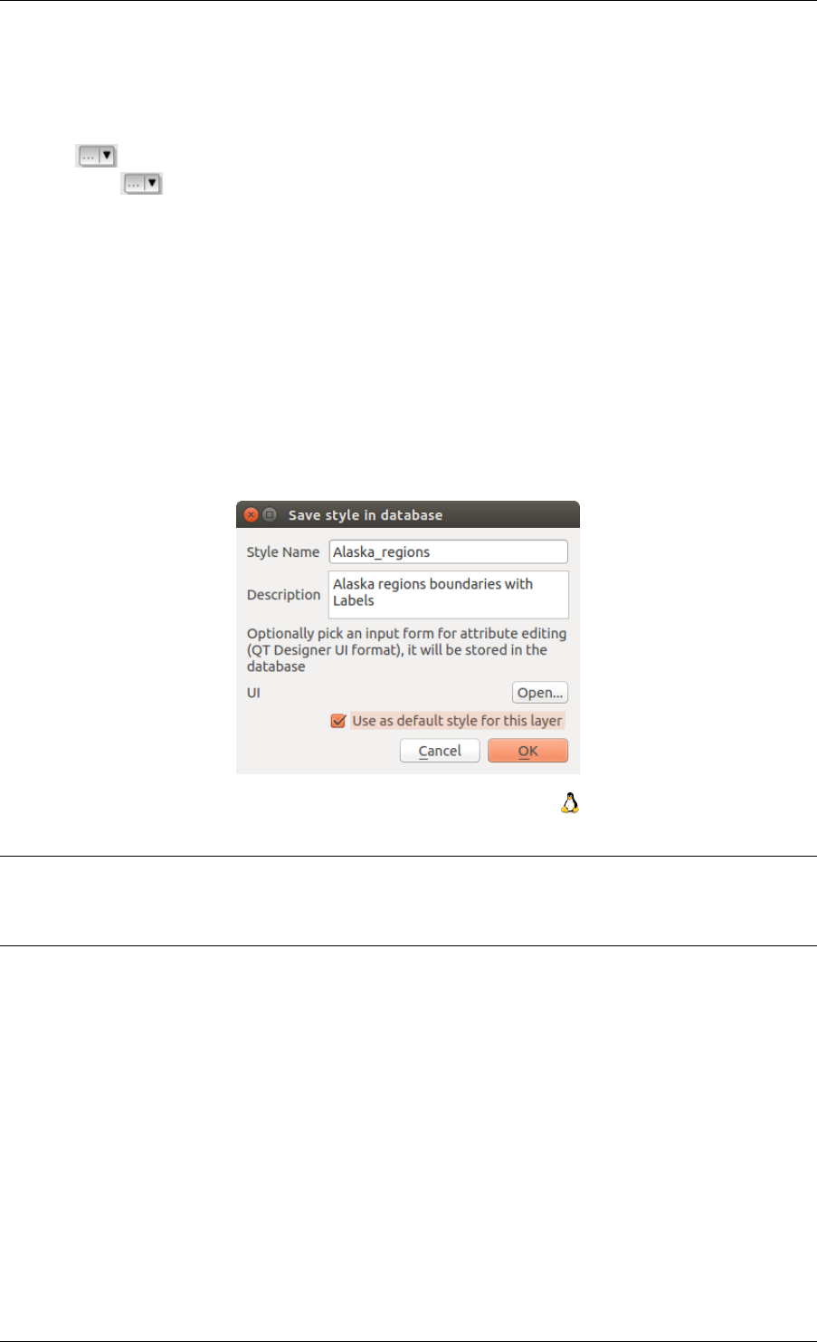
QGIS User Guide, Publicación 2.8
types are available. Depending on the chosen renderer, the Style menu provides different additional sections. On
the bottom right of the symbology dialog, there is a [Symbol] button, which gives access to the Style Manager
(see Presentation). The Style Manager allows you to edit and remove existing symbols and add new ones.
After having made any needed changes, the symbol can be added to the list of current style symbols (using
[Symbol] Save in symbol library), and then it can easily be used in the future. Furthermore, you can use
the [Save Style] button to save the symbol as a QGIS layer style file (.qml) or SLD file (.sld). SLDs can be
exported from any type of renderer – single symbol, categorized, graduated or rule-based – but when importing
an SLD, either a single symbol or rule-based renderer is created. That means that categorized or graduated styles
are converted to rule-based. If you want to preserve those renderers, you have to stick to the QML format. On the
other hand, it can be very handy sometimes to have this easy way of converting styles to rule-based.
If you change the renderer type when setting the style of a vector layer the settings you made for the symbol will
be maintained. Be aware that this procedure only works for one change. If you repeat changing the renderer type
the settings for the symbol will get lost.
If the datasource of the layer is a database (PostGIS or Spatialite for example), you can save your layer style inside
a table of the database. Just click on Save Style comboxbox and choose Save in database item then fill in the
dialog to define a style name, add a description, an ui file and if the style is a default style. When loading a layer
from the database, if a style already exists for this layer, QGIS will load the layer and its style. You can add several
style in the database. Only one will be the default style anyway.
Figure 12.10: Save Style in database Dialog
Truco: Select and change multiple symbols
The Symbology allows you to select multiple symbols and right click to change color, transparency, size, or width
of selected entries.
Single Symbol Renderer
The Single Symbol Renderer is used to render all features of the layer using a single user-defined symbol. The
properties, which can be adjusted in the Style menu, depend partially on the type of layer, but all types share the
following dialog structure. In the top-left part of the menu, there is a preview of the current symbol to be rendered.
On the right part of the menu, there is a list of symbols already defined for the current style, prepared to be used
by selecting them from the list. The current symbol can be modified using the menu on the right side. If you
click on the first level in the Symbol layers dialog on the left side, it’s possible to define basic parameters like Size,
Transparency,color and Rotation. Here, the layers are joined together.
In any spinbox in this dialog you can enter expressions. E.g. you can calculate simple math like multiplying the
existing size of a point by 3 without resorting to a calculator.
If you click on the second level in the Symbol layers dialog a ‘Data-defined override’ for nearly all settings is
possible. When using a data-defined color one may want to link the color to a field ‘budged’. Here a comment
functionality is inserted.
12.3. The Vector Properties Dialog 85
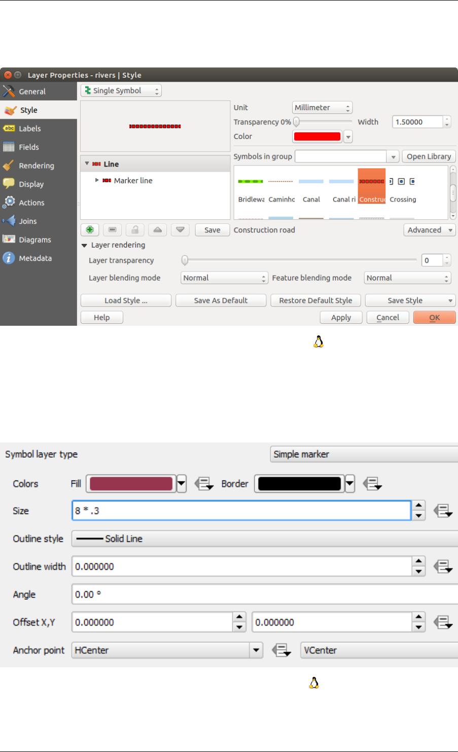
QGIS User Guide, Publicación 2.8
Figure 12.11: Single symbol line properties
Figure 12.12: Expression in Size spinbox
86 Chapter 12. Trabajar con catos vectoriales

QGIS User Guide, Publicación 2.8
/*This expression will return a color code depending on the field value.
*Negative value: red
*0 value: yellow
*Positive value: green
*/
CASE
WHEN value < 0 THEN ’#DC143C’ -- Negative value: red
WHEN value = 0 THEN ’#CCCC00’ -- Value 0: yellow
ELSE ’#228B22’ -- Positive value: green
END
static/user_manual/working_with_vector/symbol_data_defined_edit.png
Figure 12.13: Data-defined symbol with Edit... menu
Categorized Renderer
The Categorized Renderer is used to render all features from a layer, using a single user-defined symbol whose
color reflects the value of a selected feature’s attribute. The Style menu allows you to select:
• The attribute (using the Column listbox or the Set column expression function, see Expressions)
• The symbol (using the Symbol dialog)
• The colors (using the color Ramp listbox)
Then click on Classify button to create classes from the distinct value of the attribute column. Each classes can
be disabled unchecking the checkbox at the left of the class name.
You can change symbol, value and/or label of the class, just double click on the item you want to change.
Right-click shows a contextual menu to Copy/Paste,Change color,Change transparency,Change output unit,
Change symbol width.
The [Advanced] button in the lower-right corner of the dialog allows you to set the fields containing rotation and
size scale information. For convenience, the center of the menu lists the values of all currently selected attributes
together, including the symbols that will be rendered.
The example in figure_symbology_6 shows the category rendering dialog used for the rivers layer of the QGIS
sample dataset.
Graduated Renderer
The Graduated Renderer is used to render all the features from a layer, using a single user-defined symbol whose
color reflects the assignment of a selected feature’s attribute to a class.
Like the Categorized Renderer, the Graduated Renderer allows you to define rotation and size scale from specified
columns.
Also, analogous to the Categorized Renderer, the Style tab allows you to select:
• The attribute (using the Column listbox or the Set column expression function, see Expressions chapter)
• The symbol (using the Symbol Properties button)
• The colors (using the color Ramp list)
Additionally, you can specify the number of classes and also the mode for classifying features within the classes
(using the Mode list). The available modes are:
• Equal Interval: each class has the same size (e.g. values from 0 to 16 and 4 classes, each class has a size of
4);
12.3. The Vector Properties Dialog 87
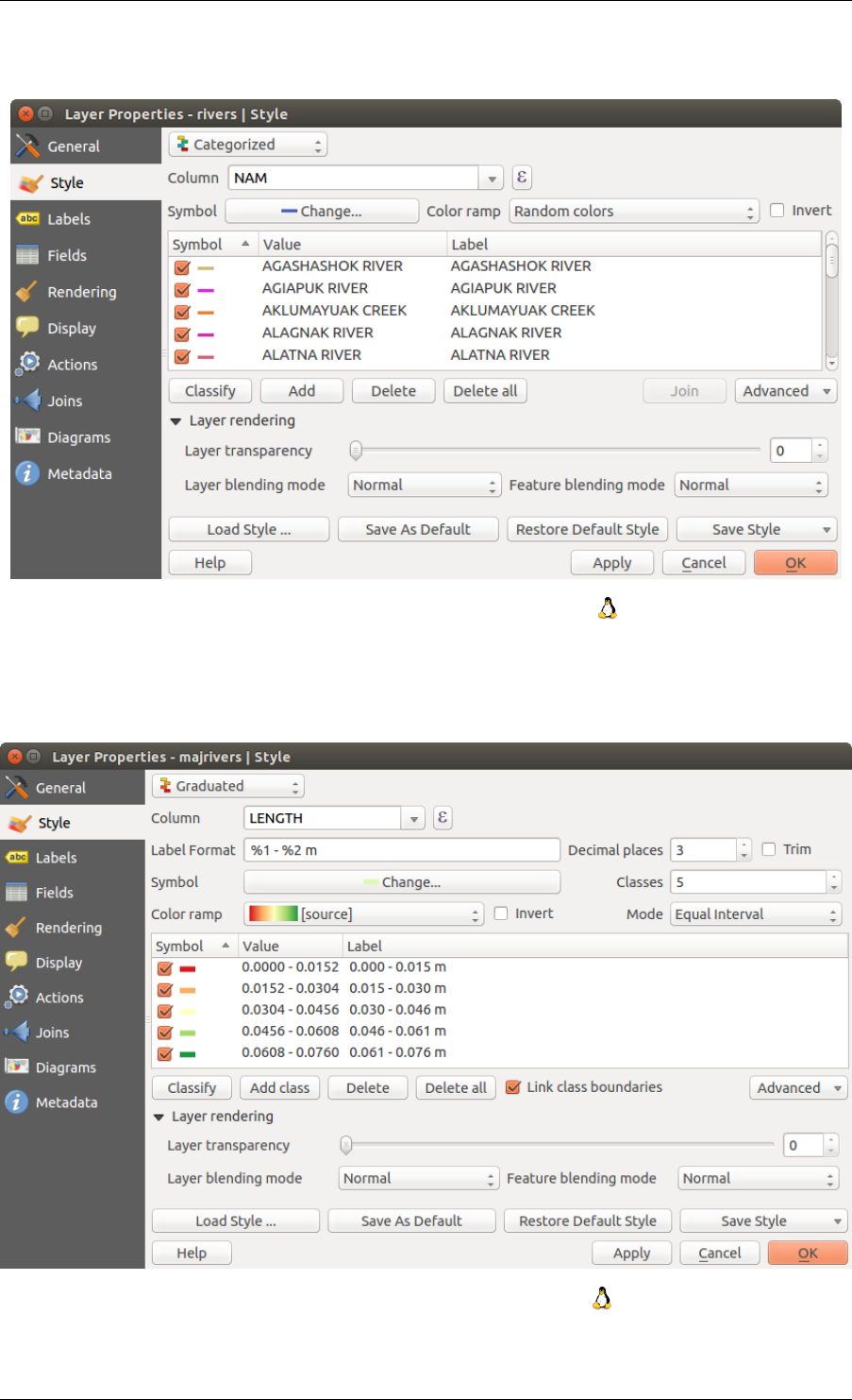
QGIS User Guide, Publicación 2.8
Figure 12.14: Categorized Symbolizing options
Figure 12.15: Graduated Symbolizing options
88 Chapter 12. Trabajar con catos vectoriales
QGIS User Guide, Publicación 2.8
• Quantile: each class will have the same number of element inside (the idea of a boxplot);
• Natural Breaks (Jenks): the variance within each class is minimal while the variance between classes is
maximal;
• Standard Deviation: classes are built depending on the standard deviation of the values;
• Pretty Breaks: the same of natural breaks but the extremes number of each class are integers.
The listbox in the center part of the Style menu lists the classes together with their ranges, labels and symbols that
will be rendered.
Click on Classify button to create classes using the choosen mode. Each classes can be disabled unchecking the
checkbox at the left of the class name.
You can change symbol, value and/or label of the clic, just double clicking on the item you want to change.
Right-click shows a contextual menu to Copy/Paste,Change color,Change transparency,Change output unit,
Change symbol width.
The example in figure_symbology_7 shows the graduated rendering dialog for the rivers layer of the QGIS sample
dataset.
Truco: Thematic maps using an expression
Categorized and graduated thematic maps can now be created using the result of an expression. In the properties
dialog for vector layers, the attribute chooser has been augmented with a Set column expression function. So
now you no longer need to write the classification attribute to a new column in your attribute table if you want the
classification attribute to be a composite of multiple fields, or a formula of some sort.
Rule-based rendering
The Rule-based Renderer is used to render all the features from a layer, using rule based symbols whose color
reflects the assignment of a selected feature’s attribute to a class. The rules are based on SQL statements. The
dialog allows rule grouping by filter or scale, and you can decide if you want to enable symbol levels or use only
the first-matched rule.
The example in figure_symbology_8 shows the rule-based rendering dialog for the rivers layer of the QGIS sample
dataset.
To create a rule, activate an existing row by double-clicking on it, or click on ‘+’ and click on the new rule. In the
Rule properties dialog, you can define a label for the rule. Press the button to open the expression string
builder. In the Function List, click on Fields and Values to view all attributes of the attribute table to be searched.
To add an attribute to the field calculator Expression field, double click its name in the Fields and Values list.
Generally, you can use the various fields, values and functions to construct the calculation expression, or you can
just type it into the box (see Expressions). You can create a new rule by copying and pasting an existing rule with
the right mouse button. You can also use the ‘ELSE’ rule that will be run if none of the other rules on that level
match. Since QGIS 2.8 the rules appear in a tree hierarchy in the map legend. Just double-klick the rules in the
map legend and the Style menu of the layer properties appears showing the rule that is the background for the
symbol in the tree.
Point displacement
The Point Displacement Renderer works to visualize all features of a point layer, even if they have the same
location. To do this, the symbols of the points are placed on a displacement circle around a center symbol.
Truco: Export vector symbology
You have the option to export vector symbology from QGIS into Google *.kml, *.dxf and MapInfo *.tab files. Just
open the right mouse menu of the layer and click on Save selection as →to specify the name of the output file and
its format. In the dialog, use the Symbology export menu to save the symbology either as Feature symbology →
or as Symbol layer symbology →. If you have used symbol layers, it is recommended to use the second setting.
Inverted Polygon
12.3. The Vector Properties Dialog 89
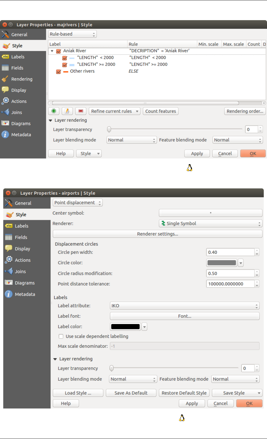
QGIS User Guide, Publicación 2.8
Figure 12.16: Rule-based Symbolizing options
Figure 12.17: Point displacement dialog
90 Chapter 12. Trabajar con catos vectoriales
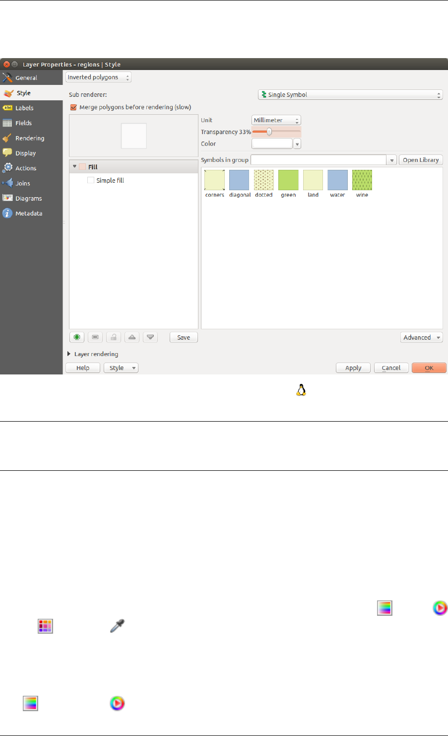
QGIS User Guide, Publicación 2.8
Inverted polygon renderer allows user to define a symbol to fill in outside of the layer’s polygons. As before you
can select subrenderers. These subrenderers are the same as for the main renderers.
Figure 12.18: Inverted Polygon dialog
Truco: Switch quickly between styles
Once you created one of the above mentioned styles you can right-klick on the layer and choose Styles →Add to
save your style. Now you can easily switch between styles you created using the Styles →menu again.
Heatmap
With the Heatmap renderer you can create live dynamic heatmaps for (multi)point layers. You can specify the
heatmap radius in pixels, mm or map units, choose a color ramp for the heatmap style and use a slider for selecting
a tradeoff between render speed and quality. When adding or removing a feature the heatmap renderer updates the
heatmap style automatically.
Color Picker
Regardless the type of style to be used, the select color dialog will show when you click to choose a color - either
border or fill color. This dialog has four different tabs which allow you to select colors by color ramp,
color wheel,color swatches or color picker.
Whatever method you use, the selected color is always described through color sliders for HSV (Hue, Saturation,
Value) and RGB (Red, Green, Blue) values. There is also an opacity slider to set transparency level. On the lower
left part of the dialog you can see a comparison between the current and the new color you are presently selecting
and on the lower right part you have the option to add the color you just tweaked into a color slot button.
With color ramp or with color wheel, you can browse to all possible color combinations. There are other
12.3. The Vector Properties Dialog 91
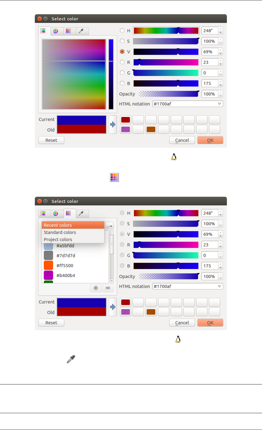
QGIS User Guide, Publicación 2.8
Figure 12.19: Color picker ramp tab
possibilities though. By using color swatches you can choose from a preselected list. This selected list is
populated with one of three methods: Recent colors,Standard colors or Project colors
Figure 12.20: Color picker swatcher tab
Another option is to use the color picker which allows you to sample a color from under your mouse pointer at
any part of QGIS or even from another application by pressing the space bar. Please note that the color picker is
OS dependent and is currently not supported by OSX.
Truco: quick color picker + copy/paste colors
You can quickly choose from Recent colors, from Standard colors or simply copy or paste a color by clicking the
drop-down arrow that follows a current color box.
92 Chapter 12. Trabajar con catos vectoriales
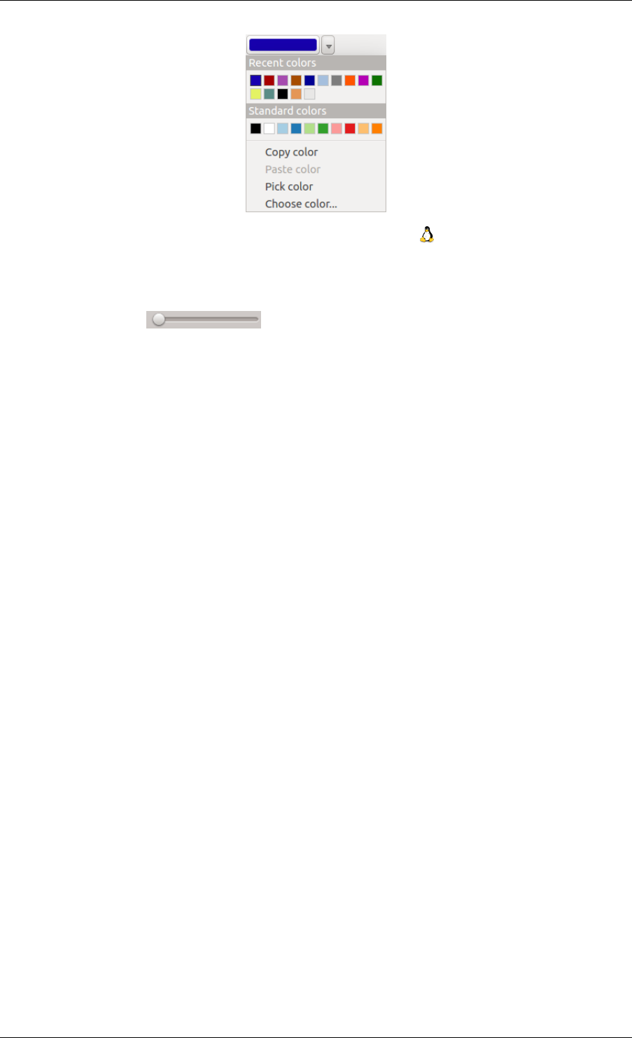
QGIS User Guide, Publicación 2.8
Figure 12.21: Quick color picker menu
Layer rendering
•Layer transparency : You can make the underlying layer in the map canvas visible with
this tool. Use the slider to adapt the visibility of your vector layer to your needs. You can also make a
precise definition of the percentage of visibility in the the menu beside the slider.
•Layer blending mode and Feature blending mode: You can achieve special rendering effects with these tools
that you may previously only know from graphics programs. The pixels of your overlaying and underlaying
layers are mixed through the settings described below.
–Normal: This is the standard blend mode, which uses the alpha channel of the top pixel to blend with
the pixel beneath it. The colors aren’t mixed.
–Lighten: This selects the maximum of each component from the foreground and background pixels.
Be aware that the results tend to be jagged and harsh.
–Screen: Light pixels from the source are painted over the destination, while dark pixels are not. This
mode is most useful for mixing the texture of one layer with another layer (e.g., you can use a hillshade
to texture another layer).
–Dodge: Dodge will brighten and saturate underlying pixels based on the lightness of the top pixel. So,
brighter top pixels cause the saturation and brightness of the underlying pixels to increase. This works
best if the top pixels aren’t too bright; otherwise the effect is too extreme.
–Addition: This blend mode simply adds pixel values of one layer with the other. In case of values
above one (in the case of RGB), white is displayed. This mode is suitable for highlighting features.
–Darken: This creates a resultant pixel that retains the smallest components of the foreground and
background pixels. Like lighten, the results tend to be jagged and harsh.
–Multiply: Here, the numbers for each pixel of the top layer are multiplied with the corresponding
pixels for the bottom layer. The results are darker pictures.
–Burn: Darker colors in the top layer cause the underlying layers to darken. Burn can be used to tweak
and colorise underlying layers.
–Overlay: This mode combines the multiply and screen blending modes. In the resulting picture, light
parts become lighter and dark parts become darker.
–Soft light: This is very similar to overlay, but instead of using multiply/screen it uses color burn/dodge.
This is supposed to emulate shining a soft light onto an image.
–Hard light: Hard light is also very similar to the overlay mode. It’s supposed to emulate projecting a
very intense light onto an image.
–Difference: Difference subtracts the top pixel from the bottom pixel, or the other way around, to
always get a positive value. Blending with black produces no change, as the difference with all colors
is zero.
12.3. The Vector Properties Dialog 93
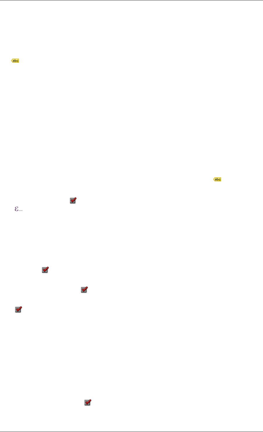
QGIS User Guide, Publicación 2.8
–Subtract: This blend mode simply subtracts pixel values of one layer from the other. In case of negative
values, black is displayed.
12.3.2 Labels Menu
The Labels core application provides smart labeling for vector point, line and polygon layers, and it only
requires a few parameters. This new application also supports on-the-fly transformed layers. The core functions
of the application have been redesigned. In QGIS, there are a number of other features that improve the labeling.
The following menus have been created for labeling the vector layers:
• Text
• Formatting
• Buffer
• Background
• Shadow
• Placement
• Rendering
Let us see how the new menus can be used for various vector layers. Labeling point layers
Start QGIS and load a vector point layer. Activate the layer in the legend and click on the Layer Labeling Options
icon in the QGIS toolbar menu.
The first step is to activate the Label this layer with checkbox and select an attribute column to use for labeling.
Click if you want to define labels based on expressions - See labeling_with_expressions.
The following steps describe a simple labeling without using the Data defined override functions, which are
situated next to the drop-down menus.
You can define the text style in the Text menu (see Figure_labels_1 ). Use the Type case option to influence the text
rendering. You have the possibility to render the text ‘All uppercase’, ‘All lowercase’ or ‘Capitalize first letter’.
Use the blend modes to create effects known from graphics programs (see blend_modes).
In the Formatting menu, you can define a character for a line break in the labels with the ‘Wrap on character’
function. Use the Formatted numbers option to format the numbers in an attribute table. Here, decimal places
may be inserted. If you enable this option, three decimal places are initially set by default.
To create a buffer, just activate the Draw text buffer checkbox in the Buffer menu. The buffer color is variable.
Here, you can also use blend modes (see blend_modes).
If the color buffer’s fill checkbox is activated, it will interact with partially transparent text and give mixed
color transparency results. Turning off the buffer fill fixes that issue (except where the interior aspect of the buffer’s
stroke intersects with the text’s fill) and also allows you to make outlined text.
In the Background menu, you can define with Size X and Size Y the shape of your background. Use Size type to
insert an additional ‘Buffer’ into your background. The buffer size is set by default here. The background then
consists of the buffer plus the background in Size X and Size Y. You can set a Rotation where you can choose
between ‘Sync with label’, ‘Offset of label’ and ‘Fixed’. Using ‘Offset of label’ and ‘Fixed’, you can rotate the
background. Define an Offset X,Y with X and Y values, and the background will be shifted. When applying
Radius X,Y, the background gets rounded corners. Again, it is possible to mix the background with the underlying
layers in the map canvas using the Blend mode (see blend_modes).
Use the Shadow menu for a user-defined Drop shadow. The drawing of the background is very variable. Choose
between ‘Lowest label component’, ‘Text’, ‘Buffer’ and ‘Background’. The Offset angle depends on the orienta-
tion of the label. If you choose the Use global shadow checkbox, then the zero point of the angle is always
oriented to the north and doesn’t depend on the orientation of the label. You can influence the appearance of the
94 Chapter 12. Trabajar con catos vectoriales
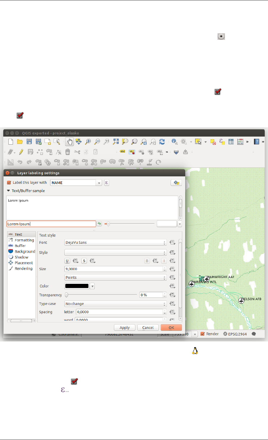
QGIS User Guide, Publicación 2.8
shadow with the Blur radius. The higher the number, the softer the shadows. The appearance of the drop shadow
can also be altered by choosing a blend mode (see blend_modes).
Choose the Placement menu for the label placement and the labeling priority. Using the Offset from point
setting, you now have the option to use Quadrants to place your label. Additionally, you can alter the angle of
the label placement with the Rotation setting. Thus, a placement in a certain quadrant with a certain rotation is
possible. In the priority section you can define with which priority the labels are rendered. It interacts with labels
of the other vector layers in the map canvas. If there are labels from different layers in the same location then the
label with the higher priority will be displayed and the other will be left out.
In the Rendering menu, you can define label and feature options. Under Label options, you find the scale-based
visibility setting now. You can prevent QGIS from rendering only selected labels with the Show all labels for
this layer (including colliding labels) checkbox. Under Feature options, you can define whether every part of a
multipart feature is to be labeled. It’s possible to define whether the number of features to be labeled is limited
and to Discourage labels from covering features.
Figure 12.22: Smart labeling of vector point layers
Labeling line layers
The first step is to activate the Label this layer checkbox in the Label settings tab and select an attribute column
to use for labeling. Click if you want to define labels based on expressions - See labeling_with_expressions.
After that, you can define the text style in the Text menu. Here, you can use the same settings as for point layers.
Also, in the Formatting menu, the same settings as for point layers are possible.
The Buffer menu has the same functions as described in section labeling_point_layers.
12.3. The Vector Properties Dialog 95
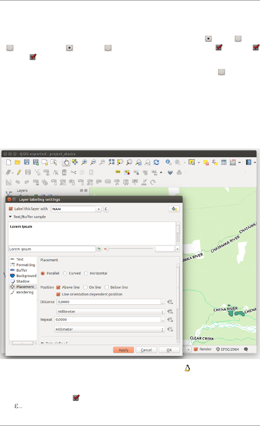
QGIS User Guide, Publicación 2.8
The Background menu has the same entries as described in section labeling_point_layers.
Also, the Shadow menu has the same entries as described in section labeling_point_layers.
In the Placement menu, you find special settings for line layers. The label can be placed Parallel,Curved
or Horizontal. With the Parallel and Curved option, you can define the position Above line,
On line and Below line. It’s possible to select several options at once. In that case, QGIS will look for the
optimal position of the label. Remember that here you can also use the line orientation for the position of the label.
Additionally, you can define a Maximum angle between curved characters when selecting the Curved option
(see Figure_labels_2 ).
You can set up a minimum distance for repeating labels. Distance can be in mm or in map units.
Some Placement setup will display more options, for example, Curved and Parallel Placements will allow the user
to set up the position of the label (above, below or on the line), distance from the line and for Curved, the user can
also setup inside/outside max angle between curved label. As for point vector layers you have the possibility to
define a Priority for the labels.
The Rendering menu has nearly the same entries as for point layers. In the Feature options, you can now Suppress
labeling of features smaller than.
Figure 12.23: Smart labeling of vector line layers
Labeling polygon layers
The first step is to activate the Label this layer checkbox and select an attribute column to use for labeling.
Click if you want to define labels based on expressions - See labeling_with_expressions.
96 Chapter 12. Trabajar con catos vectoriales
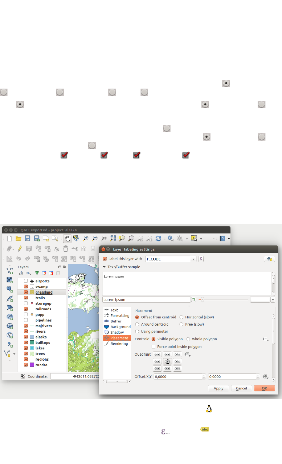
QGIS User Guide, Publicación 2.8
In the Text menu, define the text style. The entries are the same as for point and line layers.
The Formatting menu allows you to format multiple lines, also similar to the cases of point and line layers.
As with point and line layers, you can create a text buffer in the Buffer menu.
Use the Background menu to create a complex user-defined background for the polygon layer. You can use the
menu also as with the point and line layers.
The entries in the Shadow menu are the same as for point and line layers.
In the Placement menu, you find special settings for polygon layers (see Figure_labels_3). Offset from centroid,
Horizontal (slow),Around centroid,Free and Using perimeter are possible.
In the Offset from centroid settings, you can specify if the centroid is of the visible polygon or whole
polygon. That means that either the centroid is used for the polygon you can see on the map or the centroid is
determined for the whole polygon, no matter if you can see the whole feature on the map. You can place your
label with the quadrants here, and define offset and rotation. The Around centroid setting makes it possible to
place the label around the centroid with a certain distance. Again, you can define visible polygon or whole
polygon for the centroid. With the Using perimeter settings, you can define a position and a distance for the
label. For the position, Above line,On line,Below line and Line orientation dependent position
are possible.
Related to the choice of Label Placement, several options will appear. As for Point Placement you can choose the
distance for the polygon outline, repeat the label around the polygon perimeter.
As for point and line vector layers you have the possibility to define a Priority for the polygon vector layer.
The entries in the Rendering menu are the same as for line layers. You can also use Suppress labeling of features
smaller than in the Feature options.Define labels based on expressions
Figure 12.24: Smart labeling of vector polygon layers
QGIS allows to use expressions to label features. Just click the icon in the Labels menu of the properties
dialog. In figure_labels_4 you see a sample expression to label the alaska regions with name and area size, based
12.3. The Vector Properties Dialog 97
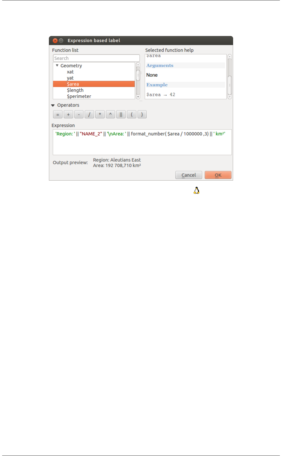
QGIS User Guide, Publicación 2.8
on the field ‘NAME_2’, some descriptive text and the function ‘$area()’ in combination with ‘format_number()’
to make it look nicer.
Figure 12.25: Using expressions for labeling
Expression based labeling is easy to work with. All you have to take care of is, that you need to combine all
elements (strings, fields and functions) with a string concatenation sign ‘||’ and that fields a written in “double
quotes” and strings in ‘single quotes’. Let’s have a look at some examples:
# label based on two fields ’name’ and ’place’ with a comma as separater
"name" || ’, ’ || "place"
-> John Smith, Paris
# label based on two fields ’name’ and ’place’ separated by comma
’My name is ’ || "name" || ’and I live in ’ || "place"
-> My name is John Smith and I live in Paris
# label based on two fields ’name’ and ’place’ with a descriptive text
# and a line break (\n)
’My name is ’ || "name" || ’\nI live in ’ || "place"
-> My name is John Smith
I live in Paris
# create a multi-line label based on a field and the $area function
# to show the place name and its area size based on unit meter.
’The area of ’ || "place" || ’has a size of ’ || $area || ’m²’
-> The area of Paris has a size of 105000000 m²
# create a CASE ELSE condition. If the population value in field
# population is <= 50000 it is a town, otherwise a city.
’This place is a ’ || CASE WHEN "population <= 50000" THEN ’town’ ELSE ’city’ END
-> This place is a town
As you can see in the expression builder, you have hundreds of functions available to create simple and very
complex expressions to label your data in QGIS. See Expressions chapter for more information and examples on
98 Chapter 12. Trabajar con catos vectoriales
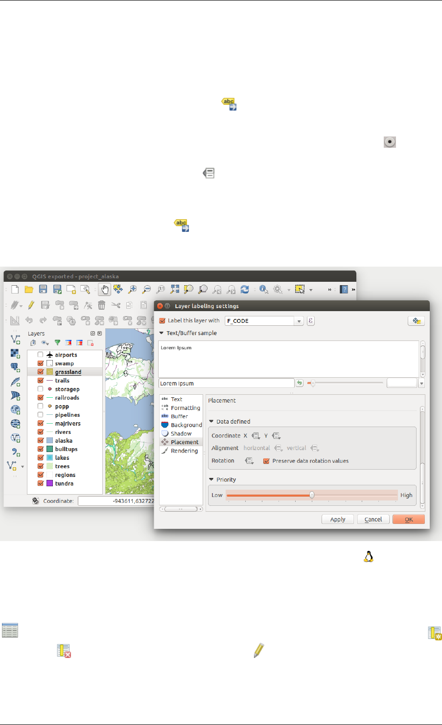
QGIS User Guide, Publicación 2.8
expressions.
Using data-defined override for labeling
With the data-defined override functions, the settings for the labeling are overridden by entries in the attribute
table. You can activate and deactivate the function with the right-mouse button. Hover over the symbol and you
see the information about the data-defined override, including the current definition field. We now describe an
example using the data-defined override function for the Move label function (see figure_labels_5 ).
1. Import lakes.shp from the QGIS sample dataset.
2. Double-click the layer to open the Layer Properties. Click on Labels and Placement. Select Offset from
centroid.
3. Look for the Data defined entries. Click the icon to define the field type for the Coordinate. Choose
‘xlabel’ for X and ‘ylabel’ for Y. The icons are now highlighted in yellow.
4. Zoom into a lake.
5. Go to the Label toolbar and click the icon. Now you can shift the label manually to another position
(see figure_labels_6 ). The new position of the label is saved in the ‘xlabel’ and ‘ylabel’ columns of the
attribute table.
Figure 12.26: Labeling of vector polygon layers with data-defined override
12.3.3 Fields Menu
Within the Fields menu, the field attributes of the selected dataset can be manipulated. The buttons
New Column and Delete Column can be used when the dataset is in Editing mode.
Edit Widget
Within the Fields menu, you also find an edit widget column. This column can be used to define values or a range
of values that are allowed to be added to the specific attribute table column. If you click on the [edit widget]
12.3. The Vector Properties Dialog 99
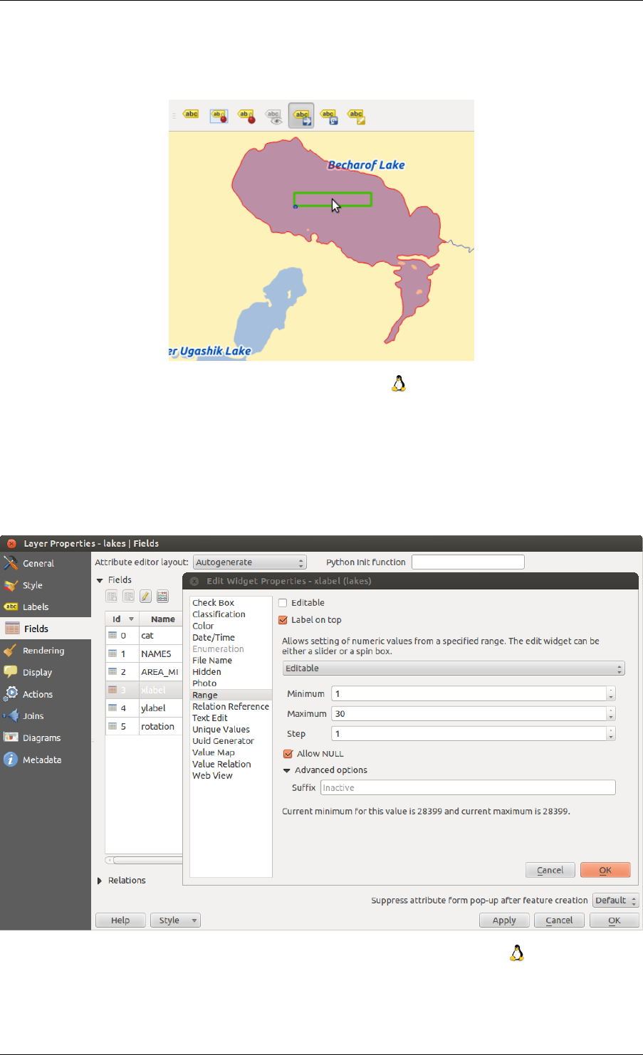
QGIS User Guide, Publicación 2.8
Figure 12.27: Move labels
Figure 12.28: Dialog to select an edit widget for an attribute column
100 Chapter 12. Trabajar con catos vectoriales
QGIS User Guide, Publicación 2.8
button, a dialog opens, where you can define different widgets. These widgets are:
•Checkbox: Displays a checkbox, and you can define what attribute is added to the column when the check-
box is activated or not.
•Classification: Displays a combo box with the values used for classification, if you have chosen ‘unique
value’ as legend type in the Style menu of the properties dialog.
•Color: Displays a color button allowing user to choose a color from the color dialog window.
•Date/Time: Displays a line field which can open a calendar widget to enter a date, a time or both. Column
type must be text. You can select a custom format, pop-up a calendar, etc.
•Enumeration: Opens a combo box with values that can be used within the columns type. This is currently
only supported by the PostgreSQL provider.
•File name: Simplifies the selection by adding a file chooser dialog.
•Hidden: A hidden attribute column is invisible. The user is not able to see its contents.
•Photo: Field contains a filename for a picture. The width and height of the field can be defined.
•Range: Allows you to set numeric values from a specific range. The edit widget can be either a slider or a
spin box.
•Relation Reference: This widged lets you embed the feature form of the referenced layer on the feature
form of the actual layer. See Creating one to many relations.
•Text edit (default): This opens a text edit field that allows simple text or multiple lines to be used. If you
choose multiple lines you can also choose html content.
•Unique values: You can select one of the values already used in the attribute table. If ‘Editable’ is activated,
a line edit is shown with autocompletion support, otherwise a combo box is used.
•UUID Generator: Generates a read-only UUID (Universally Unique Identifiers) field, if empty.
•Value map: A combo box with predefined items. The value is stored in the attribute, the description is
shown in the combo box. You can define values manually or load them from a layer or a CSV file.
•Value Relation: Offers values from a related table in a combobox. You can select layer, key column and
value column.
•Webview: Field contains a URL. The width and height of the field is variable.
Nota: QGIS has an advanced ‘hidden’ option to define your own field widget using python and add it to this
impressive list of widgets. It is tricky but it is very well explained in following excellent blog that explains how
to create a real time validation widget that can be used like described widgets. See http://blog.vitu.ch/10142013-
1847/write-your-own-qgis-form-elements
With the Attribute editor layout, you can now define built-in forms (see figure_fields_2). This is usefull for data
entry jobs or to identify objects using the option auto open form when you have objects with many attributes. You
can create an editor with several tabs and named groups to present the attribute fields.
Choose ‘Drag and drop designer’ and an attribute column. Use the icon to create a category to insert a tab or
a named group (see figure_fields_3). When creating a new category, QGIS will insert a new tab or named group
for the category in the built-in form. The next step will be to assign the relevant fields to a selected category with
the icon. You can create more categories and use the same fields again.
Other options in the dialog are ‘Autogenerate’ and ‘Provide ui-file’.
• ‘Autogenerate’ just creates editors for all fields and tabulates them.
• The ‘Provide ui-file’ option allows you to use complex dialogs made with the Qt-Designer. Us-
ing a UI-file allows a great deal of freedom in creating a dialog. For detailed information, see
http://nathanw.net/2011/09/05/qgis-tips-custom-feature-forms-with-python-logic/.
12.3. The Vector Properties Dialog 101
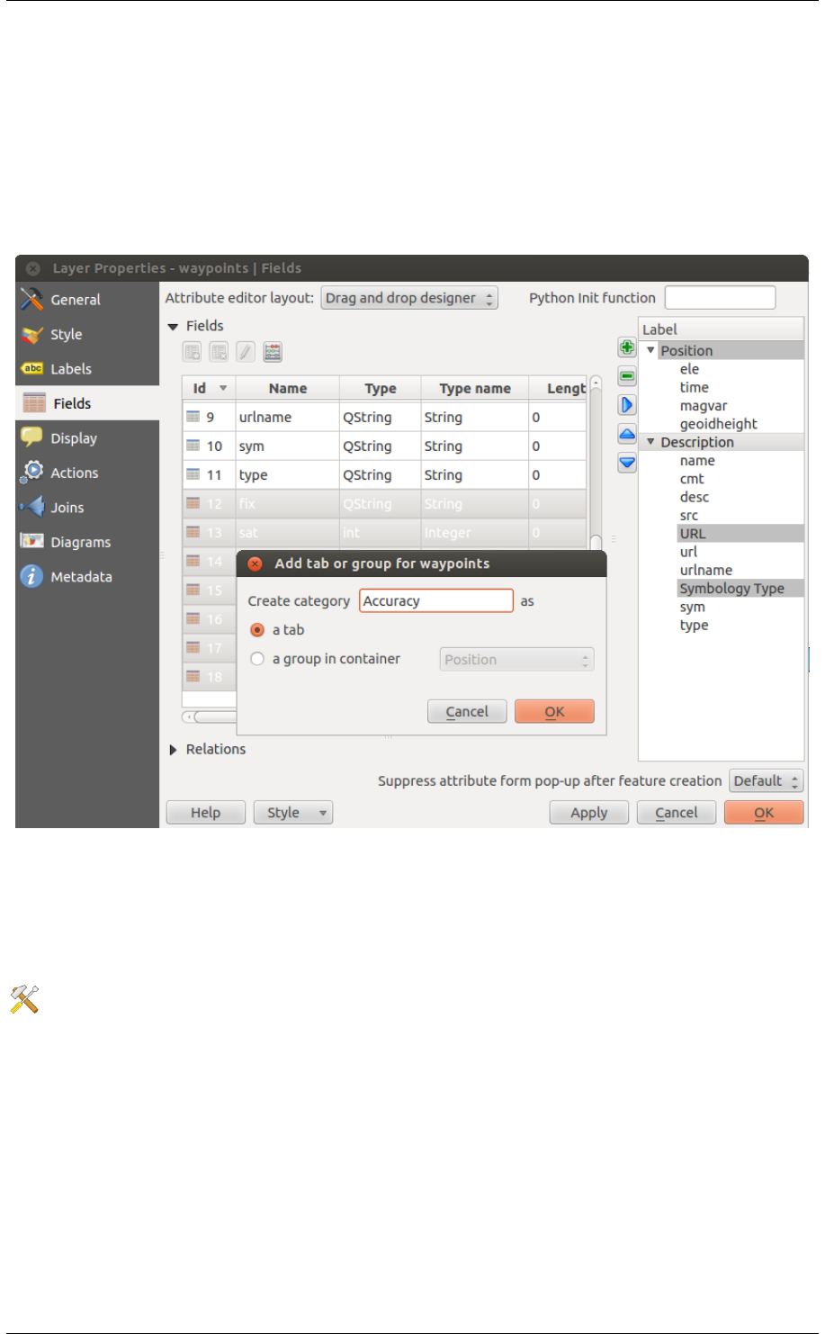
QGIS User Guide, Publicación 2.8
QGIS dialogs can have a Python function that is called when the dialog is opened. Use this function to add extra
logic to your dialogs. An example is (in module MyForms.py):
def open(dialog,layer,feature):
geom = feature.geometry()
control = dialog.findChild(QWidged,"My line edit")
Reference in Python Init Function like so: MyForms.open
MyForms.py must live on PYTHONPATH, in .qgis2/python, or inside the project folder.
Figure 12.29: Dialog to create categories with the Attribute editor layout
12.3.4 General Menu
Use this menu to make general settings for the vector layer. There are several options available:
Layer Info
• Change the display name of the layer in displayed as
• Define the Layer source of the vector layer
• Define the Data source encoding to define provider-specific options and to be able to read the file
Coordinate Reference System
•Specify the coordinate reference system. Here, you can view or change the projection of the specific vector
layer.
• Create a Spatial Index (only for OGR-supported formats)
•Update Extents information for a layer
102 Chapter 12. Trabajar con catos vectoriales
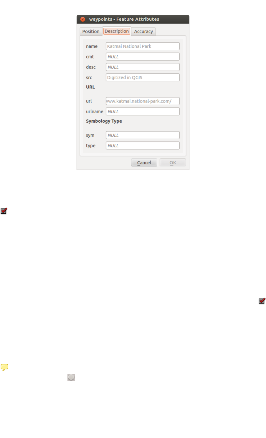
QGIS User Guide, Publicación 2.8
Figure 12.30: Resulting built-in form with tabs and named groups
• View or change the projection of the specific vector layer, clicking on Specify ...
Scale dependent visibility
• You can set the Maximum (inclusive) and Minimum (exclusive) scale. The scale can also be set by the
[Current] buttons.
Feature subset
• With the [Query Builder] button, you can create a subset of the features in the layer that will be visualized
(also refer to section Constructor de consultas).
12.3.5 Rendering Menu
QGIS 2.2 introduces support for on-the-fly feature generalisation. This can improve rendering times when drawing
many complex features at small scales. This feature can be enabled or disabled in the layer settings using the
Simplify geometry option. There is also a new global setting that enables generalisation by default for newly added
layers (see section Opciones). Note: Feature generalisation may introduce artefacts into your rendered output
in some cases. These may include slivers between polygons and inaccurate rendering when using offset-based
symbol layers.
12.3.6 Display Menu
This menu is specifically created for Map Tips. It includes a new feature: Map Tip display text in HTML.
While you can still choose a Field to be displayed when hovering over a feature on the map, it is now possible
to insert HTML code that creates a complex display when hovering over a feature. To activate Map Tips, select
the menu option View →MapTips. Figure Display 1 shows an example of HTML code.
12.3. The Vector Properties Dialog 103
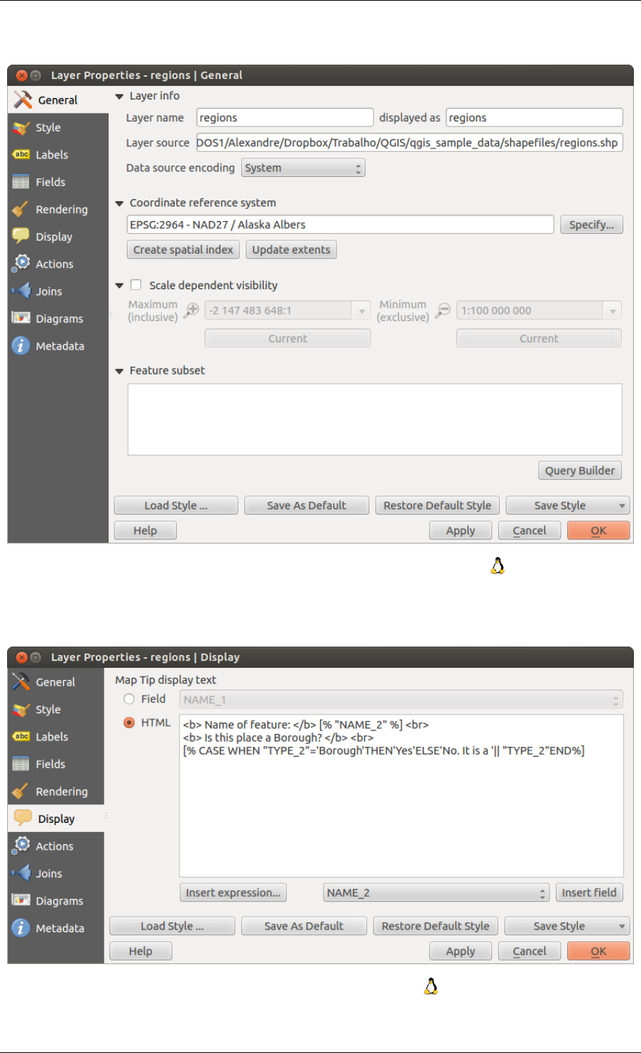
QGIS User Guide, Publicación 2.8
Figure 12.31: General menu in vector layers properties dialog
Figure 12.32: HTML code for map tip
104 Chapter 12. Trabajar con catos vectoriales
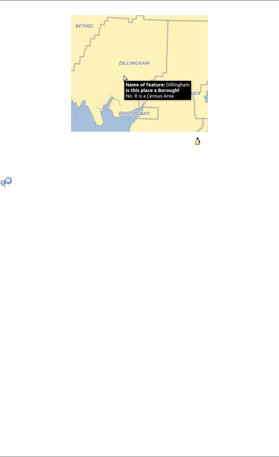
QGIS User Guide, Publicación 2.8
Figure 12.33: Map tip made with HTML code
12.3.7 Actions Menu
QGIS provides the ability to perform an action based on the attributes of a feature. This can be used to
perform any number of actions, for example, running a program with arguments built from the attributes of a
feature or passing parameters to a web reporting tool.
Actions are useful when you frequently want to run an external application or view a web page based on one or
more values in your vector layer. They are divided into six types and can be used like this:
• Generic, Mac, Windows and Unix actions start an external process.
• Python actions execute a Python expression.
• Generic and Python actions are visible everywhere.
• Mac, Windows and Unix actions are visible only on the respective platform (i.e., you can define three ‘Edit’
actions to open an editor and the users can only see and execute the one ‘Edit’ action for their platform to
run the editor).
There are several examples included in the dialog. You can load them by clicking on [Add default actions]. One
example is performing a search based on an attribute value. This concept is used in the following discussion.
Defining Actions
Attribute actions are defined from the vector Layer Properties dialog. To define an action, open the vector Layer
Properties dialog and click on the Actions menu. Go to the Action properties. Select ‘Generic’ as type and provide
a descriptive name for the action. The action itself must contain the name of the application that will be executed
when the action is invoked. You can add one or more attribute field values as arguments to the application. When
the action is invoked, any set of characters that start with a %followed by the name of a field will be replaced by
the value of that field. The special characters %% will be replaced by the value of the field that was selected from
the identify results or attribute table (see using_actions below). Double quote marks can be used to group text into
a single argument to the program, script or command. Double quotes will be ignored if preceded by a backslash.
If you have field names that are substrings of other field names (e.g., col1 and col10), you should indicate that
by surrounding the field name (and the % character) with square brackets (e.g., [%col10]). This will prevent
the %col10 field name from being mistaken for the %col1 field name with a 0on the end. The brackets will be
removed by QGIS when it substitutes in the value of the field. If you want the substituted field to be surrounded
by square brackets, use a second set like this: [[%col10]].
Using the Identify Features tool, you can open the Identify Results dialog. It includes a (Derived) item that contains
information relevant to the layer type. The values in this item can be accessed in a similar way to the other fields
by preceeding the derived field name with (Derived).. For example, a point layer has an Xand Yfield, and
12.3. The Vector Properties Dialog 105
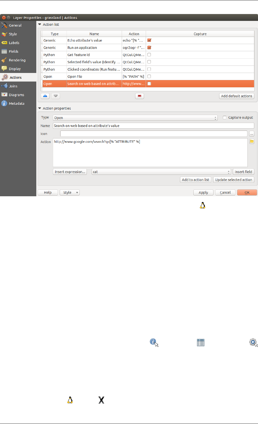
QGIS User Guide, Publicación 2.8
Figure 12.34: Overview action dialog with some sample actions
the values of these fields can be used in the action with %(Derived).X and %(Derived).Y. The derived
attributes are only available from the Identify Results dialog box, not the Attribute Table dialog box.
Two example actions are shown below:
•konqueror http://www.google.com/search?q=%nam
•konqueror http://www.google.com/search?q=%%
In the first example, the web browser konqueror is invoked and passed a URL to open. The URL performs a
Google search on the value of the nam field from our vector layer. Note that the application or script called
by the action must be in the path, or you must provide the full path. To be certain, we could rewrite the first
example as: /opt/kde3/bin/konqueror http://www.google.com/search?q=%nam. This will
ensure that the konqueror application will be executed when the action is invoked.
The second example uses the %% notation, which does not rely on a particular field for its value. When the action
is invoked, the %% will be replaced by the value of the selected field in the identify results or attribute table.
Using Actions
Actions can be invoked from either the Identify Results dialog, an Attribute Table dialog or from Run Fea-
ture Action (recall that these dialogs can be opened by clicking Identify Features or Open Attribute Table or
Run Feature Action). To invoke an action, right click on the record and choose the action from the pop-up menu. Ac-
tions are listed in the popup menu by the name you assigned when defining the action. Click on the action you
wish to invoke.
If you are invoking an action that uses the %% notation, right-click on the field value in the Identify Results dialog
or the Attribute Table dialog that you wish to pass to the application or script.
Here is another example that pulls data out of a vector layer and inserts it into a file using bash and the echo com-
mand (so it will only work on or perhaps ). The layer in question has fields for a species name taxon_name,
latitude lat and longitude long. We would like to be able to make a spatial selection of localities and export
106 Chapter 12. Trabajar con catos vectoriales

QGIS User Guide, Publicación 2.8
these field values to a text file for the selected record (shown in yellow in the QGIS map area). Here is the action
to achieve this:
bash -c "echo \"%taxon_name %lat %long\" >> /tmp/species_localities.txt"
After selecting a few localities and running the action on each one, opening the output file will show something
like this:
Acacia mearnsii -34.0800000000 150.0800000000
Acacia mearnsii -34.9000000000 150.1200000000
Acacia mearnsii -35.2200000000 149.9300000000
Acacia mearnsii -32.2700000000 150.4100000000
As an exercise, we can create an action that does a Google search on the lakes layer. First, we need to determine
the URL required to perform a search on a keyword. This is easily done by just going to Google and doing a
simple search, then grabbing the URL from the address bar in your browser. From this little effort, we see that the
format is http://google.com/search?q=qgis, where QGIS is the search term. Armed with this information, we can
proceed:
1. Make sure the lakes layer is loaded.
2. Open the Layer Properties dialog by double-clicking on the layer in the legend, or right-click and choose
Properties from the pop-up menu.
3. Click on the Actions menu.
4. Enter a name for the action, for example Google Search.
5. For the action, we need to provide the name of the external program to run. In this case, we can use Firefox.
If the program is not in your path, you need to provide the full path.
6. Following the name of the external application, add the URL used for doing a Google search, up to but not
including the search term: http://google.com/search?q=
7. The text in the Action field should now look like this: firefox http://google.com/search?q=
8. Click on the drop-down box containing the field names for the lakes layer. It’s located just to the left of
the [Insert Field] button.
9. From the drop-down box, select ‘NAMES’ and click [Insert Field].
10. Your action text now looks like this:
firefox http://google.com/search?q=%NAMES
11. To finalize the action, click the [Add to action list] button.
This completes the action, and it is ready to use. The final text of the action should look like this:
firefox http://google.com/search?q=%NAMES
We can now use the action. Close the Layer Properties dialog and zoom in to an area of interest. Make sure the
lakes layer is active and identify a lake. In the result box you’ll now see that our action is visible:
When we click on the action, it brings up Firefox and navigates to the URL
http://www.google.com/search?q=Tustumena. It is also possible to add further attribute fields to the ac-
tion. Therefore, you can add a +to the end of the action text, select another field and click on [Insert Field]. In
this example, there is just no other field available that would make sense to search for.
You can define multiple actions for a layer, and each will show up in the Identify Results dialog.
There are all kinds of uses for actions. For example, if you have a point layer containing locations of images or
photos along with a file name, you could create an action to launch a viewer to display the image. You could also
use actions to launch web-based reports for an attribute field or combination of fields, specifying them in the same
way we did in our Google search example.
We can also make more complex examples, for instance, using Python actions.
12.3. The Vector Properties Dialog 107
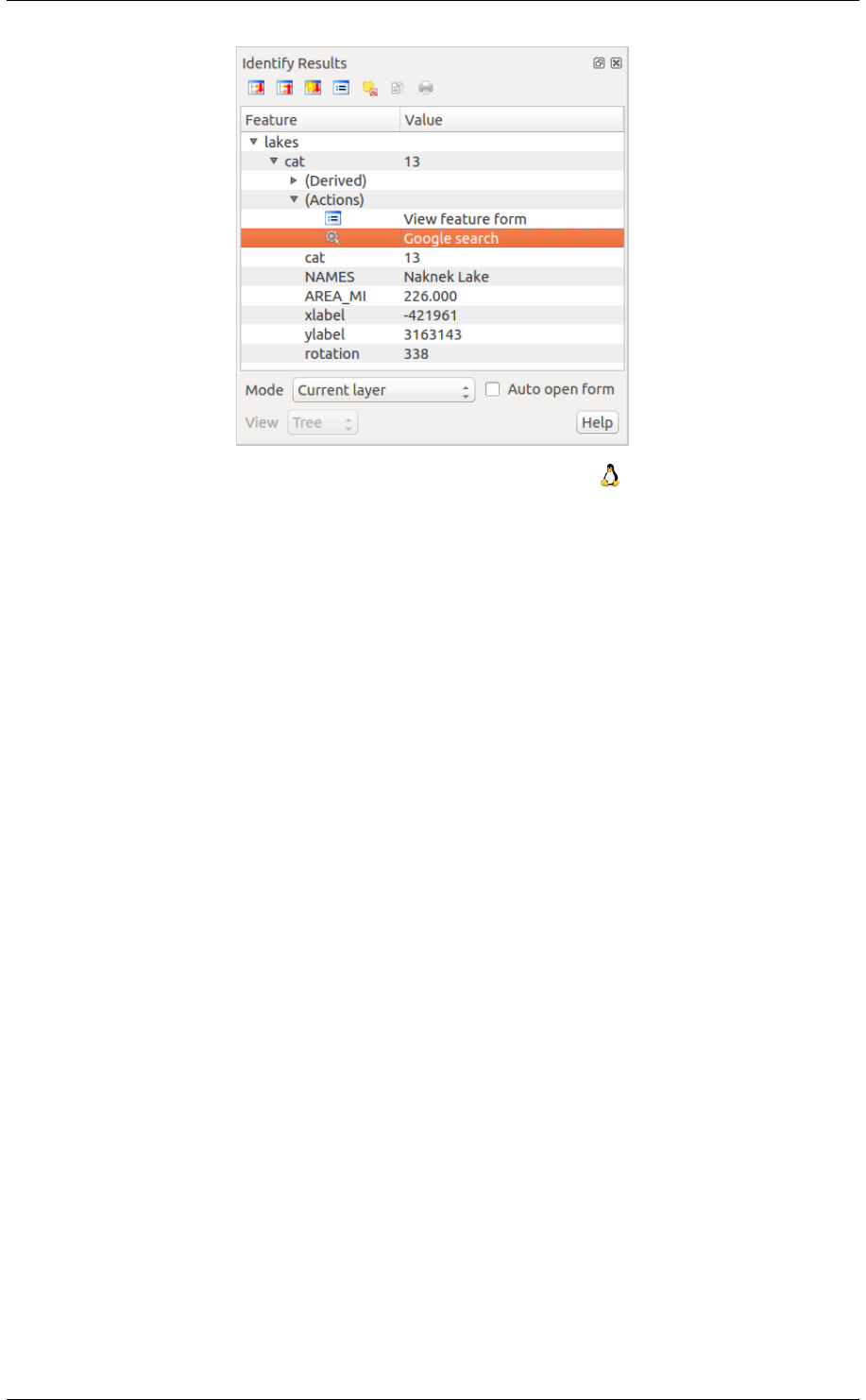
QGIS User Guide, Publicación 2.8
Figure 12.35: Select feature and choose action
Usually, when we create an action to open a file with an external application, we can use absolute paths, or
eventually relative paths. In the second case, the path is relative to the location of the external program executable
file. But what about if we need to use relative paths, relative to the selected layer (a file-based one, like a shapefile
or SpatiaLite)? The following code will do the trick:
command = "firefox";
imagerelpath = "images_test/test_image.jpg";
layer = qgis.utils.iface.activeLayer();
import os.path;
layerpath = layer.source() if layer.providerType() == ’ogr’
else (qgis.core.QgsDataSourceURI(layer.source()).database()
if layer.providerType() == ’spatialite’ else None);
path = os.path.dirname(str(layerpath));
image = os.path.join(path,imagerelpath);
import subprocess;
subprocess.Popen( [command, image ] );
We just have to remember that the action is one of type Python and the command and imagerelpath variables must
be changed to fit our needs.
But what about if the relative path needs to be relative to the (saved) project file? The code of the Python action
would be:
command="firefox";
imagerelpath="images/test_image.jpg";
projectpath=qgis.core.QgsProject.instance().fileName();
import os.path; path=os.path.dirname(str(projectpath)) if projectpath != ’’ else None;
image=os.path.join(path, imagerelpath);
import subprocess;
subprocess.Popen( [command, image ] );
Another Python action example is the one that allows us to add new layers to the project. For instance, the
following examples will add to the project respectively a vector and a raster. The names of the files to be added to
the project and the names to be given to the layers are data driven (filename and layername are column names of
the table of attributes of the vector where the action was created):
qgis.utils.iface.addVectorLayer(’/yourpath/[% "filename" %].shp’,’[% "layername" %]’,
’ogr’)
To add a raster (a TIF image in this example), it becomes:
108 Chapter 12. Trabajar con catos vectoriales
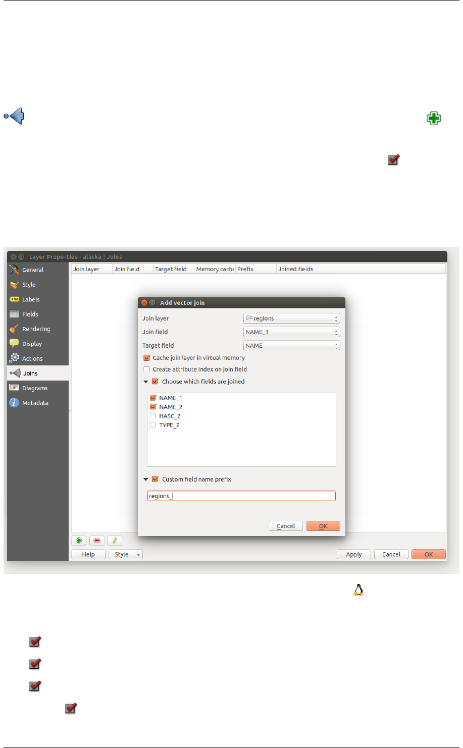
QGIS User Guide, Publicación 2.8
qgis.utils.iface.addRasterLayer(’/yourpath/[% "filename" %].tif’,’[% "layername" %]
’)
12.3.8 Joins Menu
The Joins menu allows you to join a loaded attribute table to a loaded vector layer. After clicking , the
Add vector join dialog appears. As key columns, you have to define a join layer you want to connect with the
target vector layer. Then, you have to specify the join field that is common to both the join layer and the target
layer. Now you can also specify a subset of fields from the joined layer based on the checkbox Choose which
fields are joined. As a result of the join, all information from the join layer and the target layer are displayed in
the attribute table of the target layer as joined information. If you specified a subset of fields only these fields are
displayed in the attribute table of the target layer.
QGIS currently has support for joining non-spatial table formats supported by OGR (e.g., CSV, DBF and Excel),
delimited text and the PostgreSQL provider (see figure_joins_1).
Figure 12.36: Join an attribute table to an existing vector layer
Additionally, the add vector join dialog allows you to:
•Cache join layer in virtual memory
•Create attribute index on the join field
•Choose which fields are joined
• Create a Custom field name prefix
12.3. The Vector Properties Dialog 109

QGIS User Guide, Publicación 2.8
12.3.9 Diagrams Menu
The Diagrams menu allows you to add a graphic overlay to a vector layer (see figure_diagrams_1).
The current core implementation of diagrams provides support for pie charts, text diagrams and histograms.
The menu is divided into four tabs: Appearance,Size,Postion and Options.
In the cases of the text diagram and pie chart, text values of different data columns are displayed one below the
other with a circle or a box and dividers. In the Size tab, diagram size is based on a fixed size or on linear scaling
according to a classification attribute. The placement of the diagrams, which is done in the Position tab, interacts
with the new labeling, so position conflicts between diagrams and labels are detected and solved. In addition,
chart positions can be fixed manually.
Figure 12.37: Vector properties dialog with diagram menu
We will demonstrate an example and overlay on the Alaska boundary layer a text diagram showing temperature
data from a climate vector layer. Both vector layers are part of the QGIS sample dataset (see section Datos de
ejemplo).
1. First, click on the Load Vector icon, browse to the QGIS sample dataset folder, and load the two vector
shape layers alaska.shp and climate.shp.
2. Double click the climate layer in the map legend to open the Layer Properties dialog.
3. Click on the Diagrams menu, activate Display diagrams, and from the Diagram type combo box,
select ‘Text diagram’.
4. In the Appearance tab, we choose a light blue as background color, and in the Size tab, we set a fixed size
to 18 mm.
5. In the Position tab, placement could be set to ‘Around Point’.
110 Chapter 12. Trabajar con catos vectoriales
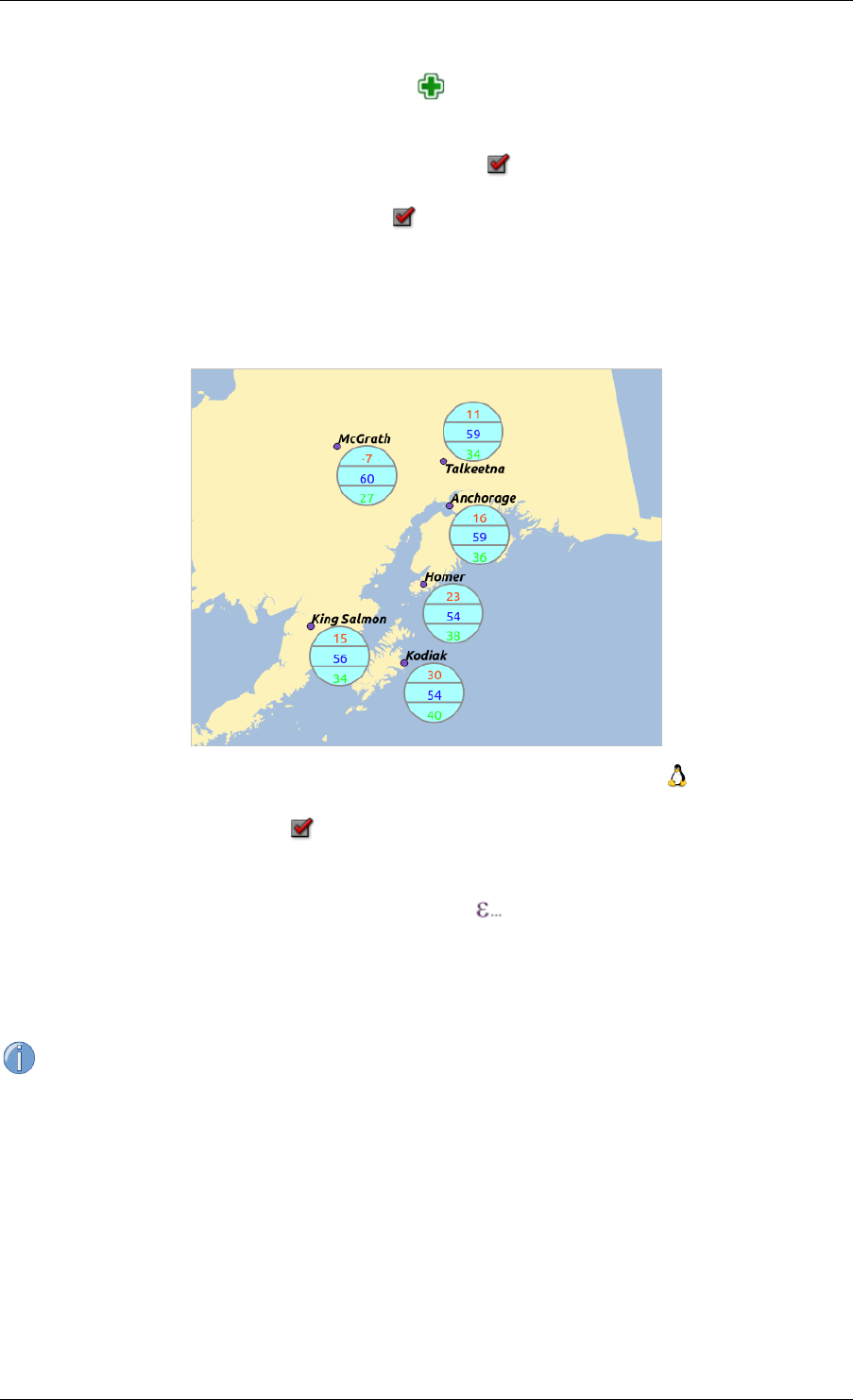
QGIS User Guide, Publicación 2.8
6. In the diagram, we want to display the values of the three columns T_F_JAN,T_F_JUL and T_F_MEAN.
First select T_F_JAN as Attributes and click the button, then T_F_JUL, and finally T_F_MEAN.
7. Now click [Apply] to display the diagram in the QGIS main window.
8. You can adapt the chart size in the Size tab. Deactivate the Fixed size and set the size of the diagrams on
the basis of an attribute with the [Find maximum value] button and the Size menu. If the diagrams appear
too small on the screen, you can activate the Increase size of small diagrams checkbox and define the
minimum size of the diagrams.
9. Change the attribute colors by double clicking on the color values in the Assigned attributes field. Fig-
ure_diagrams_2 gives an idea of the result.
10. Finally, click [Ok].
Figure 12.38: Diagram from temperature data overlayed on a map
Remember that in the Position tab, a Data defined position of the diagrams is possible. Here, you can use
attributes to define the position of the diagram. You can also set a scale-dependent visibility in the Appearance
tab.
The size and the attributes can also be an expression. Use the button to add an expression. See Expressions
chapter for more information and example.
12.3.10 Metadata Menu
The Metadata menu consists of Description,Attribution,MetadataURL and Properties sections.
In the Properties section, you get general information about the layer, including specifics about the type and
location, number of features, feature type, and editing capabilities. The Extents table provides you with layer
extent information and the Layer Spatial Reference System, which is information about the CRS of the layer. This
is a quick way to get information about the layer.
Additionally, you can add or edit a title and abstract for the layer in the Description section. It’s also possible to
define a Keyword list here. These keyword lists can be used in a metadata catalogue. If you want to use a title from
an XML metadata file, you have to fill in a link in the DataUrl field. Use Attribution to get attribute data from an
XML metadata catalogue. In MetadataUrl, you can define the general path to the XML metadata catalogue. This
information will be saved in the QGIS project file for subsequent sessions and will be used for QGIS server.
.
12.3. The Vector Properties Dialog 111
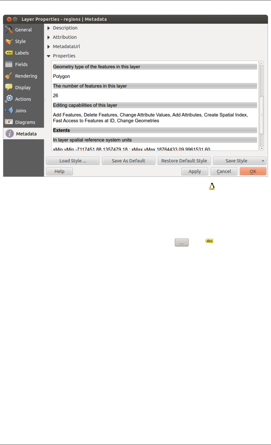
QGIS User Guide, Publicación 2.8
Figure 12.39: Metadata menu in vector layers properties dialog
12.4 Expressions
The Expressions feature are available through the field calculator or the add a new column button in the attribut
table or the Field tab in the Layer properties ; through the graduaded, categorized and rule-based rendering in the
Style tab of the Layer properties ; through the expression-based labeling in the Labeling core application
; through the feature selection and through the diagram tab of the Layer properties as well as the Main properties
of the label item and the Atlas generation tab in the Print Composer.
They are a powerful way to manipulate attribute value in order to dynamically change the final value in order to
change the geometry style, the content of the label, the value for diagram, select some feature or create virtual
column.
12.4.1 Functions List
The Function List contains functions as well as fields and values. View the help function in the Selected Func-
tion Help. In Expression you see the calculation expressions you create with the Function List. For the most
commonly used operators, see Operators.
In the Function List, click on Fields and Values to view all attributes of the attribute table to be searched. To add
an attribute to the Field calculator Expression field, double click its name in the Fields and Values list. Generally,
you can use the various fields, values and functions to construct the calculation expression, or you can just type it
into the box. To display the values of a field, you just right click on the appropriate field. You can choose between
Load top 10 unique values and Load all unique values. On the right side, the Field Values list opens with the
unique values. To add a value to the Field calculator Expression box, double click its name in the Field Values
list.
The Operators,Math,Conversions,String,Geometry and Record groups provide several functions. In Operators,
you find mathematical operators. Look in Math for mathematical functions. The Conversions group contains
functions that convert one data type to another. The String group provides functions for data strings. In the
Geometry group, you find functions for geometry objects. With Record group functions, you can add a numeration
to your data set. To add a function to the Field calculator Expression box, click on the > and then double click the
112 Chapter 12. Trabajar con catos vectoriales

QGIS User Guide, Publicación 2.8
function.
Operators
This group contains operators (e.g., +, -, *).
a + b a plus b
a - b a minus b
a*b a multiplied by b
a / b a divided by b
a % b a modulo b (for example, 7 % 2 = 1, or 2 fits into 7 three
times with remainder 1)
a ^ b a power b (for example, 2^2=4 or 2^3=8)
a = b a and b are equal
a > b a is larger than b
a < b a is smaller than b
a <> b a and b are not equal
a != b a and b are not equal
a <= b a is less than or equal to b
a >= b a is larger than or equal to b
a ~ b a matches the regular expression b
+ a positive sign
- a negative value of a
|| joins two values together into a string ’Hello’ || ’ world’
LIKE returns 1 if the string matches the supplied pattern
ILIKE returns 1 if the string matches case-insensitive the supplied
pattern (ILIKE can be used instead of LIKE to make the match
case-insensitive)
IS returns 1 if a is the same as b
OR returns 1 when condition a or b is true
AND returns 1 when condition a and b are true
NOT returns 1 if a is not the same as b
column name "column name" value of the field column name, take
care to not be confused with simple
quote, see below
’string’ a string value, take care to not be
confused with double quote, see above
NULL null value
a IS NULL a has no value
a IS NOT NULL a has a value
a IN (value[,value]) a is below the values listed
a NOT IN (value[,value]) a is not below the values listed
Some examples:
• Joins a string and a value from a column name:
’My feature’s id is: ’ || "gid"
• Test if the “description” attribute field starts with the ‘Hello’ string in the value (note the position of the %
character):
"description" LIKE ’Hello%’
Conditionals
This group contains functions to handle conditional checks in expressions.
CASE evaluates multiple expressions and returns a
result
CASE ELSE evaluates multiple expressions and returns a
result
12.4. Expressions 113

QGIS User Guide, Publicación 2.8
coalesce returns the first non-NULL value from the
expression list
regexp_match returns true if any part of a string matches
the supplied regular expression
Some example:
• Send back a value if the first condition is true, else another value:
CASE WHEN "software" LIKE ’%QGIS%’ THEN ’QGIS’ ELSE ’Other’
Mathematical Functions
This group contains math functions (e.g., square root, sin and cos).
sqrt(a) square root of a
abs returns the absolute value of a number
sin(a) sine of a
cos(a) cosine of a
tan(a) tangent of a
asin(a) arcsin of a
acos(a) arccos of a
atan(a) arctan of a
atan2(y,x) arctan of y/x using the signs of the two
arguments to determine the quadrant of the
result
exp exponential of a value
ln value of the natural logarithm of the passed
expression
log10 value of the base 10 logarithm of the passed
expression
log value of the logarithm of the passed value
and base
round round to number of decimal places
rand random integer within the range specified by
the minimum
and maximum argument (inclusive)
randf random float within the range specified by
the minimum
and maximum argument (inclusive)
max largest value in a set of values
min smallest value in a set of values
clamp restricts an input value to a specified
range
scale_linear transforms a given value from an input
domain to an output
range using linear interpolation
scale_exp transforms a given value from an input
domain to an output
range using an exponential curve
floor rounds a number downwards
ceil rounds a number upwards
$pi pi as value for calculations
Conversions
This group contains functions to convert one data type to another (e.g., string to integer, integer to string).
toint converts a string to integer number
toreal converts a string to real number
tostring converts number to string
114 Chapter 12. Trabajar con catos vectoriales

QGIS User Guide, Publicación 2.8
todatetime converts a string into Qt data time type
todate converts a string into Qt data type
totime converts a string into Qt time type
tointerval converts a string to an interval type (can be
used to take days, hours, months, etc. off a
date)
Date and Time Functions
This group contains functions for handling date and time data.
$now current date and time
age difference between two dates
year extract the year part from a date, or the number of years from
an interval
month extract the month part from a date, or the number of months
from an interval
week extract the week number from a date, or the number of weeks
from an interval
day extract the day from a date, or the number of days from an
interval
hour extract the hour from a datetime or time, or the number
of hours from an interval
minute extract the minute from a datetime or time, or the number
of minutes from an interval
second extract the second from a datetime or time, or the number
of minutes from an interval
Some example:
• Get the month and the year of today in the format “10/2014”
month($now) || ’/’ || year($now)
String Functions
This group contains functions that operate on strings (e.g., that replace, convert to upper case).
lower convert string a to lower case
upper convert string a to upper case
title converts all words of a string to title
case (all words lower case with leading
capital letter)
trim removes all leading and trailing white
space (spaces, tabs, etc.) from a string
wordwrap returns a string wrapped to a maximum/
minimum number of characters
length length of string a
replace returns a string with the supplied string
replaced
regexp_replace(a,this,that) returns a string with the supplied regular
expression replaced
regexp_substr returns the portion of a string which matches
a supplied regular expression
substr(*a*,from,len) returns a part of a string
concat concatenates several strings to one
strpos returns the index of a regular expression
in a string
left returns a substring that contains the n
leftmost characters of the string
right returns a substring that contains the n
12.4. Expressions 115

QGIS User Guide, Publicación 2.8
rightmost characters of the string
rpad returns a string with supplied width padded
using the fill character
lpad returns a string with supplied width padded
using the fill character
format formats a string using supplied arguments
format_number returns a number formatted with the locale
separator for thousands (also truncates the
number to the number of supplied places)
format_date formats a date type or string into a custom
string format
Color Functions
This group contains functions for manipulating colors.
color_rgb returns a string representation of a color based on its
red, green, and blue components
color_rgba returns a string representation of a color based on its
red, green, blue, and alpha (transparency) components
ramp_color returns a string representing a color from a color ramp
color_hsl returns a string representation of a color based on its
hue, saturation, and lightness attributes
color_hsla returns a string representation of a color based on its
hue, saturation, lightness and alpha (transparency)
attributes
color_hsv returns a string representation of a color based on its
hue, saturation, and value attributes
color_hsva returns a string representation of a color based on its
hue, saturation, value and alpha (transparency) attributes
color_cmyk returns a string representation of a color based on its
cyan, magenta, yellow and black components
color_cmyka returns a string representation of a color based on its
cyan, magenta, yellow, black and alpha (transparency)
components
Geometry Functions
This group contains functions that operate on geometry objects (e.g., length, area).
$geometry returns the geometry of the current feature (can be used
for processing with other functions)
$area returns the area size of the current feature
$length returns the length size of the current feature
$perimeter returns the perimeter length of the current feature
$x returns the x coordinate of the current feature
$y returns the y coordinate of the current feature
xat retrieves the nth x coordinate of the current feature.
n given as a parameter of the function
yat retrieves the nth y coordinate of the current feature.
n given as a parameter of the function
xmin returns the minimum x coordinate of a geometry.
Calculations are in the Spatial Reference System of this
Geometry
xmax returns the maximum x coordinate of a geometry.
Calculations are in the Spatial Reference System of this
Geometry
ymin returns the minimum y coordinate of a geometry.
Calculations are in the Spatial Reference System of this
Geometry
116 Chapter 12. Trabajar con catos vectoriales

QGIS User Guide, Publicación 2.8
ymax returns the maximum y coordinate of a geometry.
Calculations are in the Spatial Reference System of this
Geometry
geomFromWKT returns a geometry created from a well-known text (WKT)
representation
geomFromGML returns a geometry from a GML representation of geometry
bbox
disjoint returns 1 if the geometries do not share any space
together
intersects returns 1 if the geometries spatially intersect
(share any portion of space) and 0 if they don’t
touches returns 1 if the geometries have at least one point in
common, but their interiors do not intersect
crosses returns 1 if the supplied geometries have some, but not
all, interior points in common
contains returns true if and only if no points of b lie in the
exterior of a, and at least one point of the interior
of b lies in the interior of a
overlaps returns 1 if the geometries share space, are of the
same dimension, but are not completely contained by
each other
within returns 1 if geometry a is completely inside geometry b
buffer returns a geometry that represents all points whose
distance from this geometry is less than or equal to
distance
centroid returns the geometric center of a geometry
bounds returns a geometry which represents the bounding box of
an input geometry. Calculations are in the Spatial
Reference System of this Geometry.
bounds_width returns the width of the bounding box of a geometry.
Calculations are in the Spatial Reference System of
this Geometry.
bounds_height returns the height of the bounding box of a geometry.
Calculations are in the Spatial Reference System of
this Geometry.
convexHull returns the convex hull of a geometry (this represents
the minimum convex geometry that encloses all geometries
within the set)
difference returns a geometry that represents that part of geometry
a that does not intersect with geometry b
distance returns the minimum distance (based on spatial ref)
between two geometries in projected units
intersection returns a geometry that represents the shared portion
of geometry a and geometry b
symDifference returns a geometry that represents the portions of a and
b that do not intersect
combine returns the combination of geometry a and geometry b
union returns a geometry that represents the point set union of
the geometries
geomToWKT returns the well-known text (WKT) representation of the
geometry without SRID metadata
geometry returns the feature’s geometry
transform returns the geometry transformed from the source CRS to
the dest CRS
Record Functions
This group contains functions that operate on record identifiers.
$rownum returns the number of the current row
$id returns the feature id of the current row
$currentfeature returns the current feature being evaluated.
12.4. Expressions 117
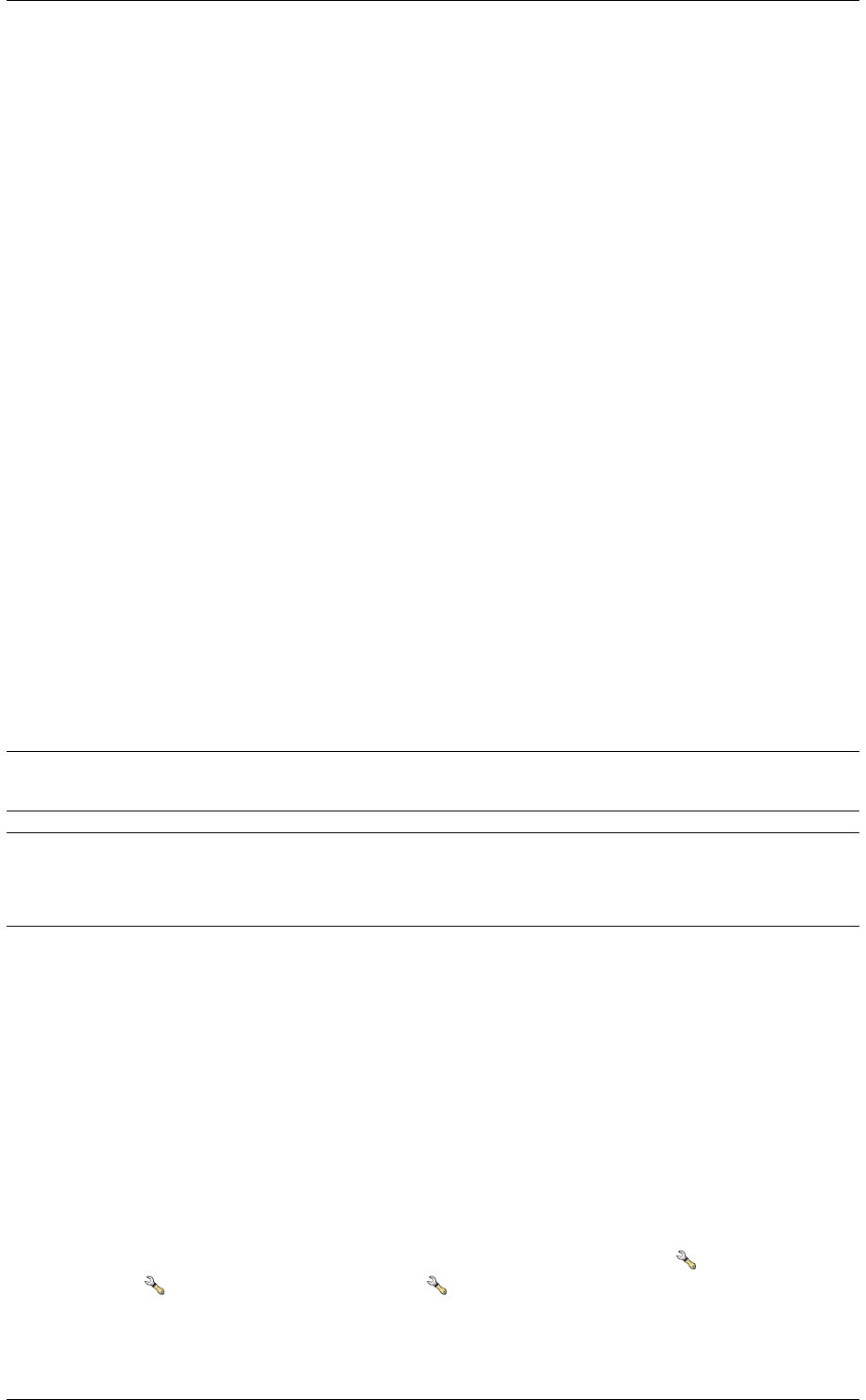
QGIS User Guide, Publicación 2.8
This can be used with the ’attribute’ function
to evaluate attribute values from the current
feature.
$scale returns the current scale of the map canvas
$uuid generates a Universally Unique Identifier (UUID)
for each row. Each UUID is 38 characters long.
getFeature returns the first feature of a layer matching a
given attribute value.
attribute returns the value of a specified attribute from
a feature.
$map returns the id of the current map item if the map
is being drawn in a composition, or "canvas" if
the map is being drawn within the main QGIS
window.
Fields and Values
Contains a list of fields from the layer. Sample values can also be accessed via right-click.
Select the field name from the list, then right-click to access a context menu with options to load sample values
from the selected field.
Fields name should be double-quoted. Values or string should be simple-quoted.
.
12.5 Editing
QGIS supports various capabilities for editing OGR, SpatiaLite, PostGIS, MSSQL Spatial and Oracle Spatial
vector layers and tables.
Nota: The procedure for editing GRASS layers is different - see section Digitizing and editing a GRASS vector
layer for details.
Truco: Concurrent Edits
This version of QGIS does not track if somebody else is editing a feature at the same time as you are. The last
person to save their edits wins.
12.5.1 Setting the Snapping Tolerance and Search Radius
Before we can edit vertices, we must set the snapping tolerance and search radius to a value that allows us an
optimal editing of the vector layer geometries.
Snapping tolerance
Snapping tolerance is the distance QGIS uses to search for the closest vertex and/or segment you are trying to
connect to when you set a new vertex or move an existing vertex. If you aren’t within the snapping tolerance,
QGIS will leave the vertex where you release the mouse button, instead of snapping it to an existing vertex and/or
segment. The snapping tolerance setting affects all tools that work with tolerance.
1. A general, project-wide snapping tolerance can be defined by choosing Settings →Options. On Mac, go
to QGIS →Preferences.... On Linux: Edit →Options. In the Digitizing tab, you can select between
‘to vertex’, ‘to segment’ or ‘to vertex and segment’ as default snap mode. You can also define a default
snapping tolerance and a search radius for vertex edits. The tolerance can be set either in map units or in
pixels. The advantage of choosing pixels is that the snapping tolerance doesn’t have to be changed after
118 Chapter 12. Trabajar con catos vectoriales
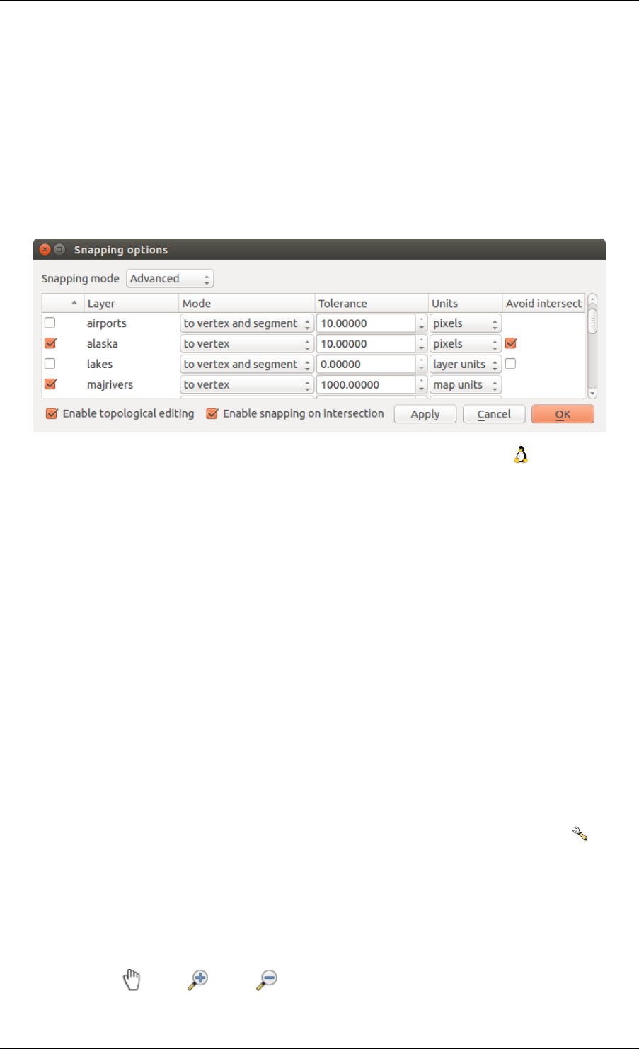
QGIS User Guide, Publicación 2.8
zoom operations. In our small digitizing project (working with the Alaska dataset), we define the snapping
units in feet. Your results may vary, but something on the order of 300 ft at a scale of 1:10000 should be a
reasonable setting.
2. A layer-based snapping tolerance can be defined by choosing Settings →(or File →)Snapping options... to
enable and adjust snapping mode and tolerance on a layer basis (see figure_edit_1 ).
Note that this layer-based snapping overrides the global snapping option set in the Digitizing tab. So, if you need
to edit one layer and snap its vertices to another layer, then enable snapping only on the snap to layer, then
decrease the global snapping tolerance to a smaller value. Furthermore, snapping will never occur to a layer that
is not checked in the snapping options dialog, regardless of the global snapping tolerance. So be sure to mark the
checkbox for those layers that you need to snap to.
Figure 12.40: Edit snapping options on a layer basis (Advanced mode)
The Snapping options enables you to make a quick and simple general setting for all layers in the project so that
the pointer snaps to all existing vertices and/or segments when using the ‘All layers’ snapping mode. In most cases
it is sufficient to use this snapping mode.
It is important to consider that the per-layer tolerance in ‘map units’ was actually in layer units. So if working
with a layer in WGS84 reprojected to UTM, setting tolerance to 1 map unit (i.e. 1 meter) wouldn’t work correctly
because the units would be actually degrees. So now the ‘map units’ has been relabeled to ‘layer units’ and the
new entry ‘map units’ operates with units of the map view. While working with ‘on-the-fly’ CRS transformation
it is now possible to use a snapping tolerance that refers to either the units of the reprojected layer (setting ‘layer
units’) or the units of the map view (setting ‘map units’).
Search radius
Search radius is the distance QGIS uses to search for the closest vertex you are trying to move when you click
on the map. If you aren’t within the search radius, QGIS won’t find and select any vertex for editing, and it will
pop up an annoying warning to that effect. Snap tolerance and search radius are set in map units or pixels, so you
may find you need to experiment to get them set right. If you specify too big of a tolerance, QGIS may snap to the
wrong vertex, especially if you are dealing with a large number of vertices in close proximity. Set search radius
too small, and it won’t find anything to move.
The search radius for vertex edits in layer units can be defined in the Digitizing tab under Settings →Options.
This is the same place where you define the general, project- wide snapping tolerance.
12.5.2 Zooming and Panning
Before editing a layer, you should zoom in to your area of interest. This avoids waiting while all the vertex markers
are rendered across the entire layer.
Apart from using the pan and zoom-in /zoom-out icons on the toolbar with the mouse, navigating can also
be done with the mouse wheel, spacebar and the arrow keys.
12.5. Editing 119
QGIS User Guide, Publicación 2.8
Zooming and panning with the mouse wheel
While digitizing, you can press the mouse wheel to pan inside of the main window, and you can roll the mouse
wheel to zoom in and out on the map. For zooming, place the mouse cursor inside the map area and roll it forward
(away from you) to zoom in and backwards (towards you) to zoom out. The mouse cursor position will be the
center of the zoomed area of interest. You can customize the behavior of the mouse wheel zoom using the Map
tools tab under the Settings →Options menu.
Panning with the arrow keys
Panning the map during digitizing is possible with the arrow keys. Place the mouse cursor inside the map area,
and click on the right arrow key to pan east, left arrow key to pan west, up arrow key to pan north, and down arrow
key to pan south.
You can also use the space bar to temporarily cause mouse movements to pan the map. The PgUp and PgDown
keys on your keyboard will cause the map display to zoom in or out without interrupting your digitizing session.
12.5.3 Topological editing
Besides layer-based snapping options, you can also define topological functionalities in the Snapping options...
dialog in the Settings (or File) menu. Here, you can define Enable topological editing, and/or for polygon
layers, you can activate the column Avoid Int., which avoids intersection of new polygons.
Enable topological editing
The option Enable topological editing is for editing and maintaining common boundaries in polygon mosaics.
QGIS ‘detects’ a shared boundary in a polygon mosaic, so you only have to move the vertex once, and QGIS will
take care of updating the other boundary.
Avoid intersections of new polygons
The second topological option in the Avoid Int. column, called Avoid intersections of new polygons, avoids
overlaps in polygon mosaics. It is for quicker digitizing of adjacent polygons. If you already have one polygon,
it is possible with this option to digitize the second one such that both intersect, and QGIS then cuts the second
polygon to the common boundary. The advantage is that you don’t have to digitize all vertices of the common
boundary.
Enable snapping on intersections
Another option is to use Enable snapping on intersection. It allows you to snap on an intersection of back-
ground layers, even if there’s no vertex on the intersection.
12.5.4 Digitizing an existing layer
By default, QGIS loads layers read-only. This is a safeguard to avoid accidentally editing a layer if there is a
slip of the mouse. However, you can choose to edit any layer as long as the data provider supports it, and the
underlying data source is writable (i.e., its files are not read-only).
In general, tools for editing vector layers are divided into a digitizing and an advanced digitiz-
ing toolbar, described in section Advanced digitizing. You can select and unselect both under View
120 Chapter 12. Trabajar con catos vectoriales
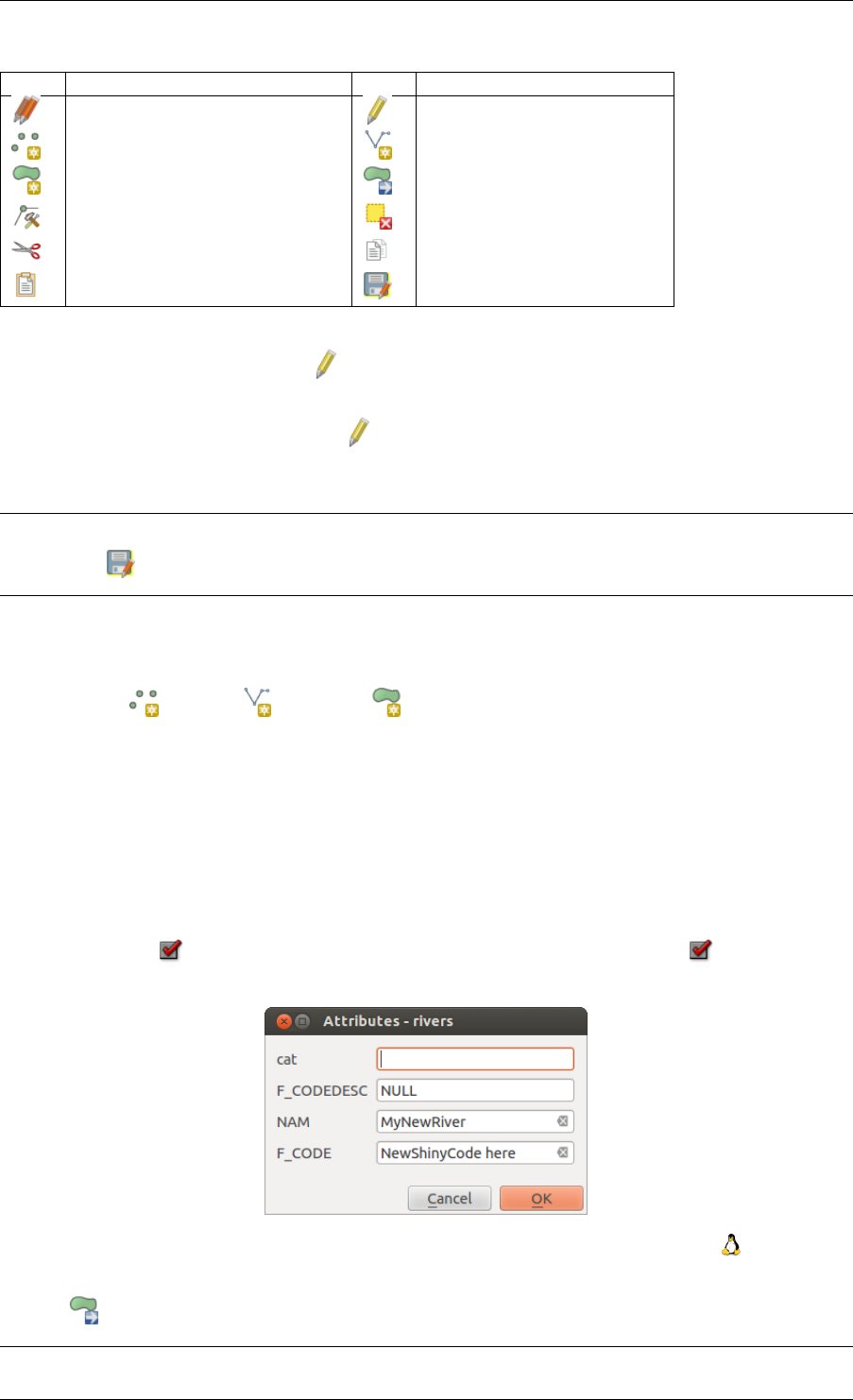
QGIS User Guide, Publicación 2.8
→Toolbars →. Using the basic digitizing tools, you can perform the following functions:
Icon Purpose Icon Purpose
Current edits Toggle editing
Adding Features: Capture Point Adding Features: Capture Line
Adding Features: Capture Polygon Move Feature
Node Tool Delete Selected
Cut Features Copy Features
Paste Features Save layer edits
Table Editing: Vector layer basic editing toolbar
All editing sessions start by choosing the Toggle editing option. This can be found in the context menu after right
clicking on the legend entry for a given layer.
Alternatively, you can use the Toggle Editing Toggle editing button from the digitizing toolbar to start or stop the
editing mode. Once the layer is in edit mode, markers will appear at the vertices, and additional tool buttons on
the editing toolbar will become available.
Truco: Save Regularly
Remember to Save Layer Edits regularly. This will also check that your data source can accept all the changes.
Adding Features
You can use the Add Feature,Add Feature or Add Feature icons on the toolbar to put the QGIS cursor into
digitizing mode.
For each feature, you first digitize the geometry, then enter its attributes. To digitize the geometry, left-click on
the map area to create the first point of your new feature.
For lines and polygons, keep on left-clicking for each additional point you wish to capture. When you have
finished adding points, right-click anywhere on the map area to confirm you have finished entering the geometry
of that feature.
The attribute window will appear, allowing you to enter the information for the new feature. Figure_edit_2 shows
setting attributes for a fictitious new river in Alaska. In the Digitizing menu under the Settings →Options menu,
you can also activate Suppress attributes pop-up windows after each created feature and Reuse last entered
attribute values.
Figure 12.41: Enter Attribute Values Dialog after digitizing a new vector feature
With the Move Feature(s) icon on the toolbar, you can move existing features.
12.5. Editing 121
QGIS User Guide, Publicación 2.8
Truco: Attribute Value Types
For editing, the attribute types are validated during entry. Because of this, it is not possible to enter a number into
a text column in the dialog Enter Attribute Values or vice versa. If you need to do so, you should edit the attributes
in a second step within the Attribute table dialog.
Current Edits
This feature allows the digitization of multiple layers. Choose Save for Selected Layers to save all changes
you made in multiple layers. You also have the opportunity to Rollback for Selected Layers, so that the
digitization may be withdrawn for all selected layers. If you want to stop editing the selected layers, Cancel
for Selected Layer(s) is an easy way.
The same functions are available for editing all layers of the project.
Node Tool
For shapefile-based layers as well as SpatialLite, PostgreSQL/PostGIS, MSSQL Spatial, and Oracle Spatial tables,
the Node Tool provides manipulation capabilities of feature vertices similar to CAD programs. It is possible to
simply select multiple vertices at once and to move, add or delete them altogether. The node tool also works with
‘on the fly’ projection turned on, and it supports the topological editing feature. This tool is, unlike other tools in
QGIS, persistent, so when some operation is done, selection stays active for this feature and tool. If the node tool
is unable to find any features, a warning will be displayed.
It is important to set the property Settings →Options →Digitizing →Search Radius: to a number
greater than zero (i.e., 10). Otherwise, QGIS will not be able to tell which vertex is being edited.
Truco: Vertex Markers
The current version of QGIS supports three kinds of vertex markers: ‘Semi-transparent circle’, ‘Cross’ and ‘None’.
To change the marker style, choose Options from the Settings menu, click on the Digitizing tab and select the
appropriate entry.
Basic operations
Start by activating the Node Tool and selecting a feature by clicking on it. Red boxes will appear at each vertex
of this feature.
•Selecting vertices: You can select vertices by clicking on them one at a time, by clicking on an edge to
select the vertices at both ends, or by clicking and dragging a rectangle around some vertices. When a
vertex is selected, its color changes to blue. To add more vertices to the current selection, hold down the
Ctrl key while clicking. Hold down Ctrl or Shift when clicking to toggle the selection state of vertices
(vertices that are currently unselected will be selected as usual, but also vertices that are already selected
will become unselected).
•Adding vertices: To add a vertex, simply double click near an edge and a new vertex will appear on the
edge near to the cursor. Note that the vertex will appear on the edge, not at the cursor position; therefore, it
should be moved if necessary.
•Deleting vertices: After selecting vertices for deletion, click the Delete key. Note that you cannot use the
Node Tool to delete a complete feature; QGIS will ensure it retains the minimum number of vertices for
the feature type you are working on. To delete a complete feature use the Delete Selected tool.
122 Chapter 12. Trabajar con catos vectoriales
QGIS User Guide, Publicación 2.8
•Moving vertices: Select all the vertices you want to move. Click on a selected vertex or edge and drag in
the direction you wish to move. All the selected vertices will move together. If snapping is enabled, the
whole selection can jump to the nearest vertex or line.
Each change made with the node tool is stored as a separate entry in the Undo dialog. Remember that all operations
support topological editing when this is turned on. On-the-fly projection is also supported, and the node tool
provides tooltips to identify a vertex by hovering the pointer over it.
Cutting, Copying and Pasting Features
Selected features can be cut, copied and pasted between layers in the same QGIS project, as long as destination
layers are set to Toggle editing beforehand.
Features can also be pasted to external applications as text. That is, the features are represented in CSV format,
with the geometry data appearing in the OGC Well-Known Text (WKT) format.
However, in this version of QGIS, text features from outside QGIS cannot be pasted to a layer within QGIS. When
would the copy and paste function come in handy? Well, it turns out that you can edit more than one layer at a
time and copy/paste features between layers. Why would we want to do this? Say we need to do some work on a
new layer but only need one or two lakes, not the 5,000 on our big_lakes layer. We can create a new layer and
use copy/paste to plop the needed lakes into it.
As an example, we will copy some lakes to a new layer:
1. Load the layer you want to copy from (source layer)
2. Load or create the layer you want to copy to (target layer)
3. Start editing for target layer
4. Make the source layer active by clicking on it in the legend
5. Use the Select Single Feature tool to select the feature(s) on the source layer
6. Click on the Copy Features tool
7. Make the destination layer active by clicking on it in the legend
8. Click on the Paste Features tool
9. Stop editing and save the changes
What happens if the source and target layers have different schemas (field names and types are not the same)?
QGIS populates what matches and ignores the rest. If you don’t care about the attributes being copied to the target
layer, it doesn’t matter how you design the fields and data types. If you want to make sure everything - the feature
and its attributes - gets copied, make sure the schemas match.
Truco: Congruency of Pasted Features
If your source and destination layers use the same projection, then the pasted features will have geometry identical
to the source layer. However, if the destination layer is a different projection, then QGIS cannot guarantee the ge-
ometry is identical. This is simply because there are small rounding-off errors involved when converting between
projections.
Truco: Copy string attribute into another
If you have created a new column in your attribute table with type ‘string’ and want to paste values from another
attribute column that has a greater length the length of the column size will be extended to the same amount. This
is because the GDAL Shapefile driver starting with GDAL/OGR 1.10 knows to auto-extend string and integer
fields to dynamically accomodate for the length of the data to be inserted.
12.5. Editing 123
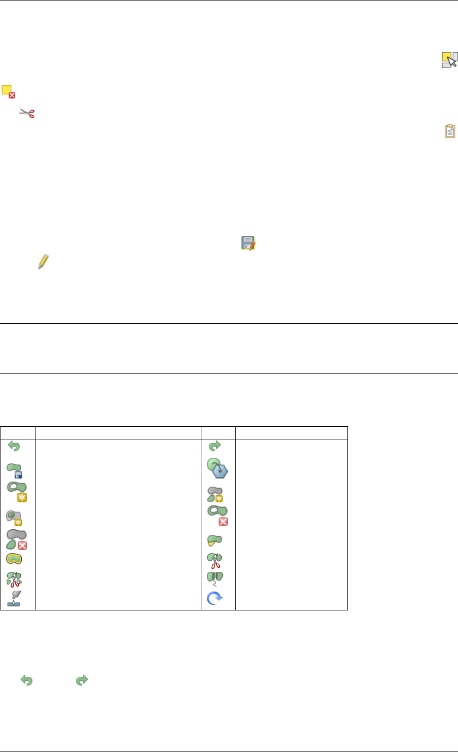
QGIS User Guide, Publicación 2.8
Deleting Selected Features
If we want to delete an entire polygon, we can do that by first selecting the polygon using the regular
Select Single Feature tool. You can select multiple features for deletion. Once you have the selection set, use the
Delete Selected tool to delete the features.
The Cut Features tool on the digitizing toolbar can also be used to delete features. This effectively deletes the
feature but also places it on a “spatial clipboard”. So, we cut the feature to delete. We could then use the
Paste Features tool to put it back, giving us a one-level undo capability. Cut, copy, and paste work on the currently
selected features, meaning we can operate on more than one at a time.
Saving Edited Layers
When a layer is in editing mode, any changes remain in the memory of QGIS. Therefore, they are not commit-
ted/saved immediately to the data source or disk. If you want to save edits to the current layer but want to continue
editing without leaving the editing mode, you can click the Save Layer Edits button. When you turn editing mode
off with Toggle editing (or quit QGIS for that matter), you are also asked if you want to save your changes or
discard them.
If the changes cannot be saved (e.g., disk full, or the attributes have values that are out of range), the QGIS
in-memory state is preserved. This allows you to adjust your edits and try again.
Truco: Data Integrity
It is always a good idea to back up your data source before you start editing. While the authors of QGIS have
made every effort to preserve the integrity of your data, we offer no warranty in this regard.
12.5.5 Advanced digitizing
Icon Purpose Icon Purpose
Undo Redo
Rotate Feature(s) Simplify Feature
Add Ring Add Part
Fill Ring Delete Ring
Delete Part Reshape Features
Offset Curve Split Features
Split Parts Merge Selected Features
Merge Attributes of Selected Features Rotate Point Symbols
Table Advanced Editing: Vector layer advanced editing toolbar
Undo and Redo
The Undo and Redo tools allows you to undo or redo vector editing operations. There is also a dockable
widget, which shows all operations in the undo/redo history (see Figure_edit_3). This widget is not displayed by
default; it can be displayed by right clicking on the toolbar and activating the Undo/Redo checkbox. Undo/Redo
is however active, even if the widget is not displayed.
124 Chapter 12. Trabajar con catos vectoriales
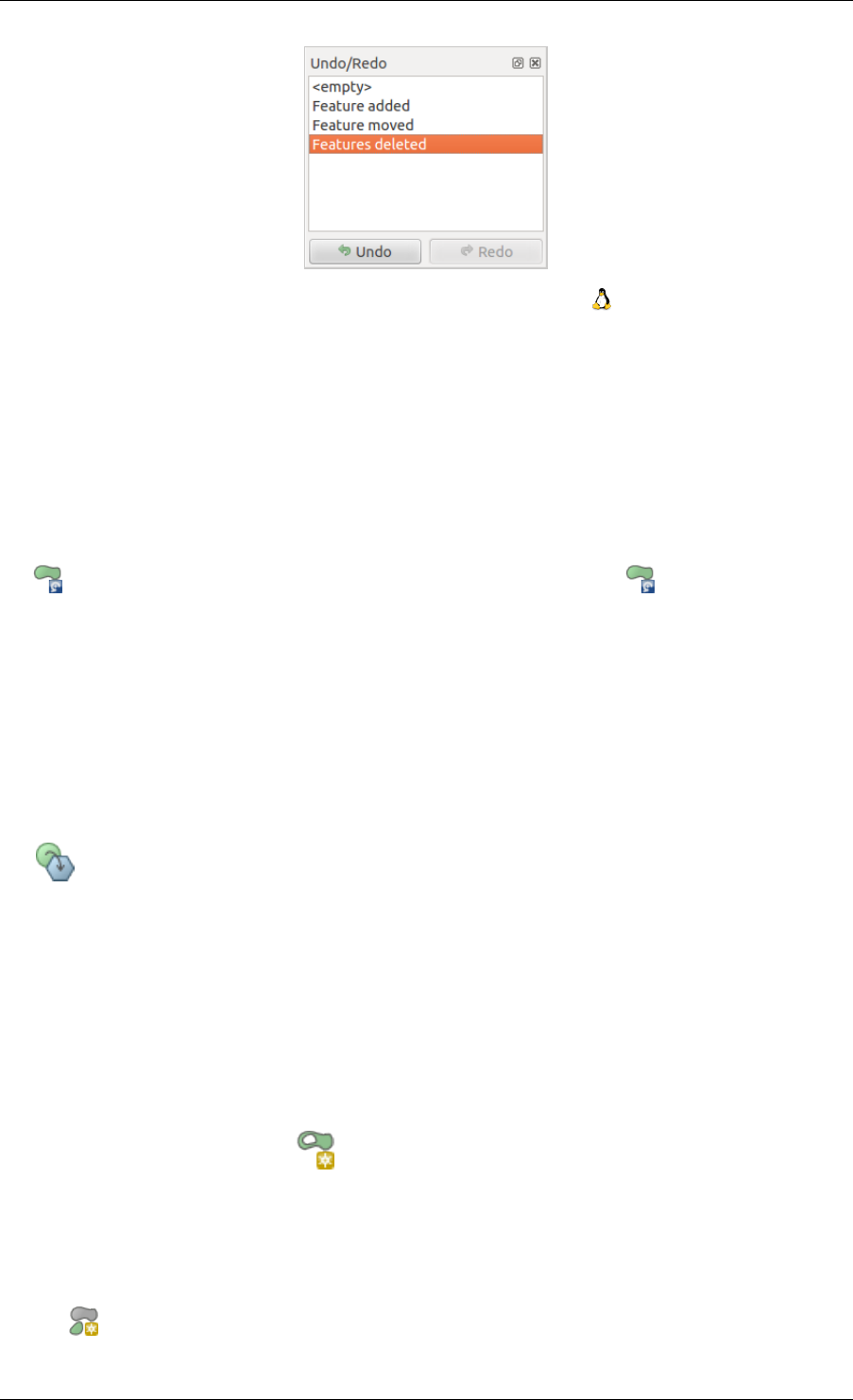
QGIS User Guide, Publicación 2.8
Figure 12.42: Redo and Undo digitizing steps
When Undo is hit, the state of all features and attributes are reverted to the state before the reverted operation
happened. Changes other than normal vector editing operations (for example, changes done by a plugin), may or
may not be reverted, depending on how the changes were performed.
To use the undo/redo history widget, simply click to select an operation in the history list. All features will be
reverted to the state they were in after the selected operation.
Rotate Feature(s)
Use Rotate Feature(s) to rotate one or multiple features in the map canvas. Press the Rotate Feature(s) icon and then
click on the feature to rotate. Either click on the map to place the rotated feature or enter an angle in the user input
widget. If you want to rotate several features, they shall be selected first.
If you enable the map tool with feature(s) selected, its (their) centroid appears and will be the rotation anchor
point. If you want to move the anchor point, hold the Ctrl button and click on the map to place it.
If you hold Shift before clicking on the map, the rotation will be done in 45 degree steps, which can be modified
afterwards in the user input widget.
Simplify Feature
The Simplify Feature tool allows you to reduce the number of vertices of a feature, as long as the geometry
doesn’t change. With the tool you can also simplify multi-part features. First, drag a rectangle over the feature.
The vertices will be highlighted in red while the color of the feature will change and a dialog where you can define
a tolerance in map units or pixels will appear. QGIS calculates the amount of vertices that can be deleted while
maintaining the geometry using the given tolerance. The higher the tolerance is the more vertices can be deleted.
After gaining the statistics about the simplification just klick the OK button. The tolerance you used will be saved
when leaving a project or when leaving an edit session. So you can go back to the same tolerance the next time
when simplifying a feature.
Add Ring
You can create ring polygons using the Add Ring icon in the toolbar. This means that inside an existing area, it
is possible to digitize further polygons that will occur as a ‘hole’, so only the area between the boundaries of the
outer and inner polygons remains as a ring polygon.
Add Part
You can add part polygons to a selected multipolygon. The new part polygon must be digitized outside the
selected multi-polygon.
12.5. Editing 125
QGIS User Guide, Publicación 2.8
Fill Ring
You can use the Fill Ring function to add a ring to a polygon and add a new feature to the layer at the same time.
Thus you need not first use the Add Ring icon and then the Add feature function anymore.
Delete Ring
The Delete Ring tool allows you to delete ring polygons inside an existing area. This tool only works with
polygon layers. It doesn’t change anything when it is used on the outer ring of the polygon. This tool can be used
on polygon and multi-polygon features. Before you select the vertices of a ring, adjust the vertex edit tolerance.
Delete Part
The Delete Part tool allows you to delete parts from multifeatures (e.g., to delete polygons from a multi-polygon
feature). It won’t delete the last part of the feature; this last part will stay untouched. This tool works with all
multi-part geometries: point, line and polygon. Before you select the vertices of a part, adjust the vertex edit
tolerance.
Reshape Features
You can reshape line and polygon features using the Reshape Features icon on the toolbar. It replaces the line or
polygon part from the first to the last intersection with the original line. With polygons, this can sometimes lead
to unintended results. It is mainly useful to replace smaller parts of a polygon, not for major overhauls, and the
reshape line is not allowed to cross several polygon rings, as this would generate an invalid polygon.
For example, you can edit the boundary of a polygon with this tool. First, click in the inner area of the polygon
next to the point where you want to add a new vertex. Then, cross the boundary and add the vertices outside the
polygon. To finish, right-click in the inner area of the polygon. The tool will automatically add a node where the
new line crosses the border. It is also possible to remove part of the area from the polygon, starting the new line
outside the polygon, adding vertices inside, and ending the line outside the polygon with a right click.
Nota: The reshape tool may alter the starting position of a polygon ring or a closed line. So, the point that is
represented ‘twice’ will not be the same any more. This may not be a problem for most applications, but it is
something to consider.
Offset Curves
The Offset Curve tool creates parallel shifts of line layers. The tool can be applied to the edited layer (the
geometries are modified) or also to background layers (in which case it creates copies of the lines / rings and adds
them to the the edited layer). It is thus ideally suited for the creation of distance line layers. The displacement is
shown at the bottom left of the taskbar.
To create a shift of a line layer, you must first go into editing mode and activate the Offset Curve tool. Then click
on a feature to shift it. Move the mouse and click where wanted or enter the desired distance in the user input
widget. Your changes may then be saved with the|mActionSaveEdits|:sup:Save Layer Edits tool.
QGIS options dialog (Digitizing tab then Curve offset tools section) allows you to configure some parameters
like Join style,Quadrant segments,Miter limit.
126 Chapter 12. Trabajar con catos vectoriales
QGIS User Guide, Publicación 2.8
Split Features
You can split features using the Split Features icon on the toolbar. Just draw a line across the feature you want to
split.
Split parts
In QGIS 2.0 it is now possible to split the parts of a multi part feature so that the number of parts is increased. Just
draw a line across the part you want to split using the Split Parts icon.
Merge selected features
The Merge Selected Features tool allows you to merge features. A new dialog will allow you to choose which value
to choose between each selected features or select a function (Minimum, Maximum, Median, Sum, Skip Attribute)
to use for each column. If features don’t have a common boundaries, a multipolygon will be created.
Merge attributes of selected features
The Merge Attributes of Selected Features tool allows you to merge attributes of features with common boundaries
and attributes without merging their boundaries. First, select several features at once. Then press the
Merge Attributes of Selected Features button. Now QGIS asks you which attributes are to be applied to all selected objects.
As a result, all selected objects have the same attribute entries.
Rotate Point Symbols
Rotate Point Symbols allows you to change the rotation of point symbols in the map canvas. You must first define
a rotation column from the attribute table of the point layer in the Advanced menu of the Style menu of the Layer
Properties. Also, you will need to go into the ‘SVG marker’ and choose Data defined properties .... Activate
Angle and choose ‘rotation’ as field. Without these settings, the tool is inactive.
Figure 12.43: Rotate Point Symbols
To change the rotation, select a point feature in the map canvas and rotate it, holding the left mouse button pressed.
A red arrow with the rotation value will be visualized (see Figure_edit_4). When you release the left mouse button
again, the value will be updated in the attribute table.
Nota: If you hold the Ctrl key pressed, the rotation will be done in 15 degree steps.
12.5. Editing 127
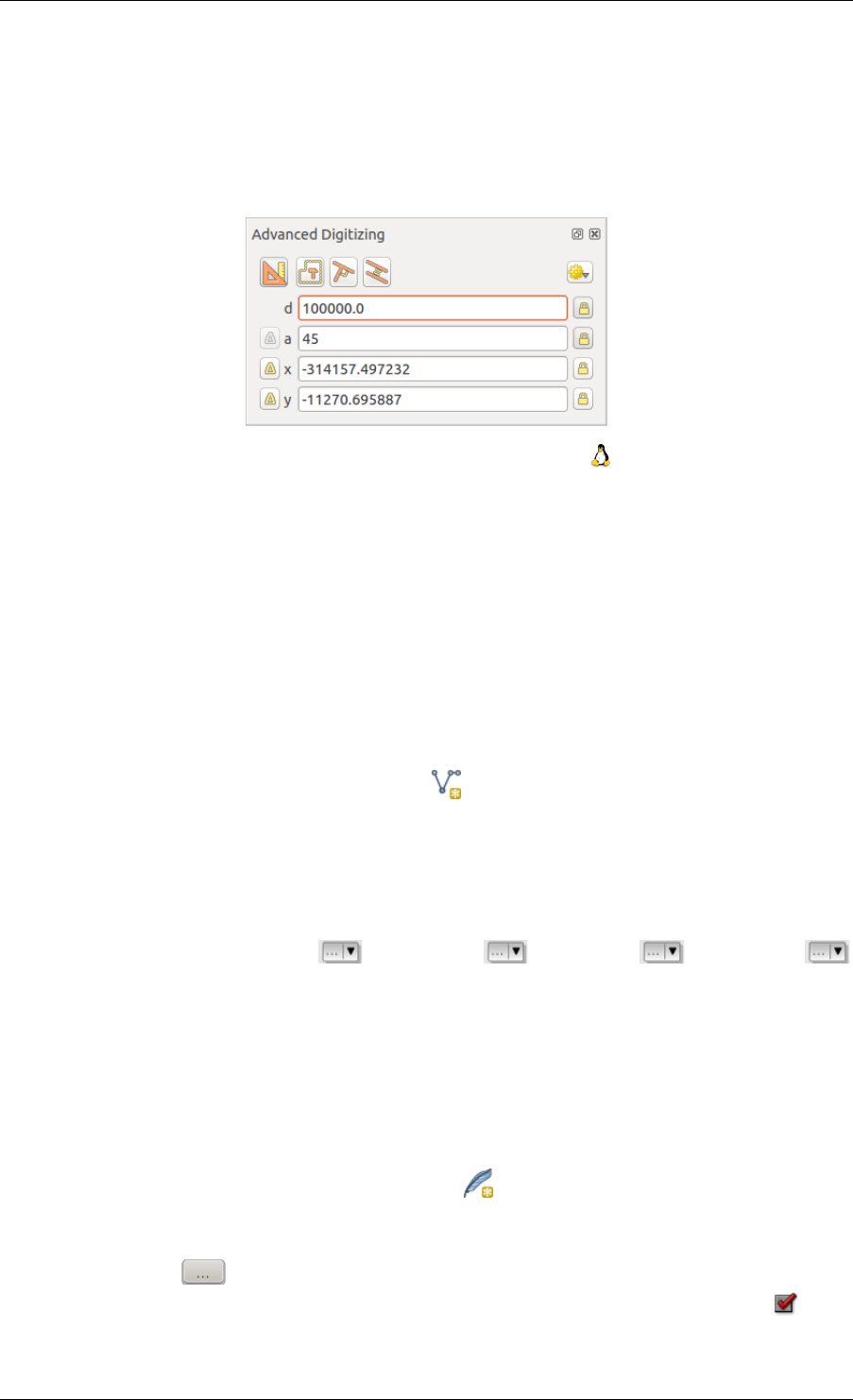
QGIS User Guide, Publicación 2.8
12.5.6 The Advanced Digitizing panel
When capturing new geometries or geometry parts you also have the possibility to use the Advanced Digitizing
panel. You can digitize lines exactly parallel or at a specific angle or lock lines to specific angles. Furthermore
you can enter coordinates directly so that you can make a precise definition for your new geomtry.
_figure_advanced_edit 1:
Figure 12.44: The Advanced Digitizing panel
The tools are not enabled if the map view is in geographic coordinates.
12.5.7 Creating new Vector layers
QGIS allows you to create new shapefile layers, new SpatiaLite layers, new GPX layers and New Temporary
Scratch Layers. Creation of a new GRASS layer is supported within the GRASS plugin. Please refer to section
Creating a new GRASS vector layer for more information on creating GRASS vector layers.
Creating a new Shapefile layer
To create a new shape layer for editing, choose New →New Shapefile Layer... from the Layer menu. The
New Vector Layer dialog will be displayed as shown in Figure_edit_5. Choose the type of layer (point, line or
polygon) and the CRS (coordinate reference system).
Note that QGIS does not yet support creation of 2.5D features (i.e., features with X,Y,Z coordinates).
To complete the creation of the new shapefile layer, add the desired attributes by clicking on the [Add to attributes
list] button and specifying a name and type for the attribute. A first ‘id’ column is added as default but can be
removed, if not wanted. Only Type: real ,Type: integer ,Type: string and Type:date
attributes are supported. Additionally and according to the attribute type, you can also define the width and
precision of the new attribute column. Once you are happy with the attributes, click [OK] and provide a name
for the shapefile. QGIS will automatically add a .shp extension to the name you specify. Once the layer has
been created, it will be added to the map, and you can edit it in the same way as described in section Digitizing an
existing layer above.
Creating a new SpatiaLite layer
To create a new SpatiaLite layer for editing, choose New →New SpatiaLite Layer... from the Layer menu.
The New SpatiaLite Layer dialog will be displayed as shown in Figure_edit_6.
The first step is to select an existing SpatiaLite database or to create a new SpatiaLite database. This can be done
with the browse button to the right of the database field. Then, add a name for the new layer, define the
layer type, and specify the coordinate reference system with [Specify CRS]. If desired, you can select Create
an autoincrementing primary key.
128 Chapter 12. Trabajar con catos vectoriales
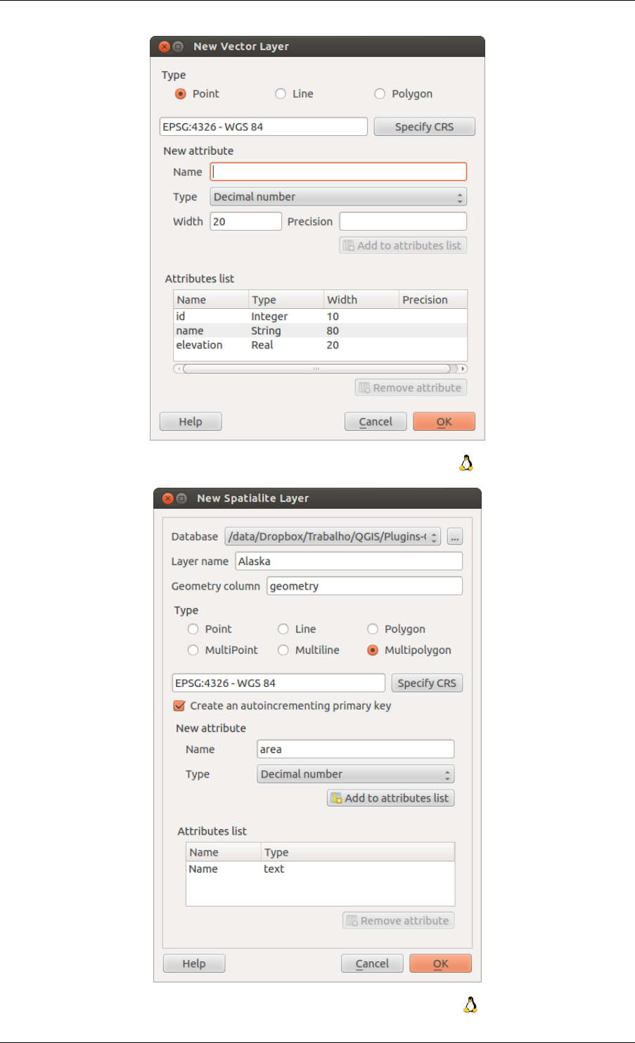
QGIS User Guide, Publicación 2.8
Figure 12.45: Creating a new Shapefile layer Dialog
Figure 12.46: Creating a New SpatiaLite layer Dialog
12.5. Editing 129

QGIS User Guide, Publicación 2.8
To define an attribute table for the new SpatiaLite layer, add the names of the attribute columns you want to create
with the corresponding column type, and click on the [Add to attribute list] button. Once you are happy with the
attributes, click [OK]. QGIS will automatically add the new layer to the legend, and you can edit it in the same
way as described in section Digitizing an existing layer above.
Further management of SpatiaLite layers can be done with the DB Manager. See Complemento administrador de
BBDD.
Creating a new GPX layer
To create a new GPX file, you need to load the GPS plugin first. Plugins →Plugin Manager... opens the
Plugin Manager Dialog. Activate the GPS Tools checkbox.
When this plugin is loaded, choose New →Create new GPX Layer... from the Layer menu. In the Save new
GPX file as dialog, you can choose where to save the new GPX layer.
Creating a new Temporary Scratch Layer
Empty, editable memory layers can be defined using Layer →Create Layer →New Temporary Scratch Layer.
Here you can even create Multipoint,Multiline and Multipolygon Layers beneath Point,Line and
Polygon Layers. Temporary Scratch Layers are not saved and will be discarded when QGIS is closed. See also
paste_into_layer .
12.5.8 Working with the Attribute Table
The attribute table displays features of a selected layer. Each row in the table represents one map feature, and
each column contains a particular piece of information about the feature. Features in the table can be searched,
selected, moved or even edited.
To open the attribute table for a vector layer, make the layer active by clicking on it in the map legend area. Then,
from the main Layer menu, choose Open Attribute Table. It is also possible to right click on the layer and
choose Open Attribute Table from the drop-down menu, and to click on the Open Attribute Table button
in the Attributes toolbar.
This will open a new window that displays the feature attributes for the layer (figure_attributes_1). The number
of features and the number of selected features are shown in the attribute table title.
Figure 12.47: Attribute Table for regions layer
130 Chapter 12. Trabajar con catos vectoriales
QGIS User Guide, Publicación 2.8
Selecting features in an attribute table
Each selected row in the attribute table displays the attributes of a selected feature in the layer. If the set of
features selected in the main window is changed, the selection is also updated in the attribute table. Likewise, if
the set of rows selected in the attribute table is changed, the set of features selected in the main window will be
updated.
Rows can be selected by clicking on the row number on the left side of the row. Multiple rows can be marked by
holding the Ctrl key. A continuous selection can be made by holding the Shift key and clicking on several
row headers on the left side of the rows. All rows between the current cursor position and the clicked row are
selected. Moving the cursor position in the attribute table, by clicking a cell in the table, does not change the row
selection. Changing the selection in the main canvas does not move the cursor position in the attribute table.
The table can be sorted by any column, by clicking on the column header. A small arrow indicates the sort order
(downward pointing means descending values from the top row down, upward pointing means ascending values
from the top row down).
For a simple search by attributes on only one column, choose the Column filter →from the menu in the bottom
left corner. Select the field (column) on which the search should be performed from the drop-down menu, and hit
the [Apply] button. Then, only the matching features are shown in the attribute table.
To make a selection, you have to use the Select features using an Expression icon on top of the attribute table.
Select features using an Expression allows you to define a subset of a table using a Function List like in the Field Calculator
(see Field Calculator). The query result can then be saved as a new vector layer. For example, if you want to find
regions that are boroughs from regions.shp of the QGIS sample data, you have to open the Fields and Values
menu and choose the field that you want to query. Double-click the field ‘TYPE_2’ and also [Load all unique
values] . From the list, choose and double-click ‘Borough’. In the Expression field, the following query appears:
"TYPE_2" =’Borough’
Here you can also use the Function list →Recent (Selection) to make a selection that you used before. The
expression builder remembers the last 20 used expressions.
The matching rows will be selected, and the total number of matching rows will appear in the title bar of the
attribute table, as well as in the status bar of the main window. For searches that display only selected features on
the map, use the Query Builder described in section Constructor de consultas.
To show selected records only, use Show Selected Features from the menu at the bottom left.
The field calculator bar allows you to make calculations on the selected rows only. For example, you can alter the
number of the ID field of the file:regions.shp with the expression
ID+5
as shown in figure_attributes_1 .
The other buttons at the top of the attribute table window provide the following functionality:
•Toggle editing mode to edit single values and to enable functionalities described below (also with Ctrl+E)
•Save Edits (also with Ctrl+S)
•Unselect all (also with Ctrl+U)
•Move selected to top (also with Ctrl+T)
•Invert selection (also with Ctrl+R)
•Copy selected rows to clipboard (also with Ctrl+C)
•Zoom map to the selected rows (also with Ctrl+J)
12.5. Editing 131
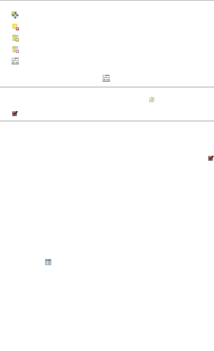
QGIS User Guide, Publicación 2.8
•Pan map to the selected rows (also with Ctrl+P)
•Delete selected features (also with Ctrl+D)
•New Column for PostGIS layers and for OGR layers with GDAL version >= 1.6 (also with Ctrl+W)
•Delete Column for PostGIS layers and for OGR layers with GDAL version >= 1.9 (also with Ctrl+L)
•Open field calculator (also with Ctrl+I)
Below these buttons is the Field Calculator bar, which allows calculations to be quickly applied attributes visible
in the table. This bar uses the same expressions as the Field Calculator (see Field Calculator).
Truco: Skip WKT geometry
If you want to use attribute data in external programs (such as Excel), use the Copy selected rows to clipboard button.
You can copy the information without vector geometries if you deactivate Settings →Options →Data sources
menu Copy geometry in WKT representation from attribute table.
Save selected features as new layer
The selected features can be saved as any OGR-supported vector format and also transformed into another coordi-
nate reference system (CRS). Just open the right mouse menu of the layer and click on Save as to define the name
of the output file, its format and CRS (see section Leyenda del mapa). To save the selection ensure that the
Save only selected features is selected. It is also possible to specify OGR creation options within the dialog.
Paste into new layer
Features that are on the clipboard may be pasted into a new layer. To do this, first make a layer editable. Select
some features, copy them to the clipboard, and then paste them into a new layer using Edit →Paste Features as
and choosing New vector layer or New memory layer.
This applies to features selected and copied within QGIS and also to features from another source defined using
well-known text (WKT).
Working with non spatial attribute tables
QGIS allows you also to load non-spatial tables. This currently includes tables supported by OGR and delimited
text, as well as the PostgreSQL, MSSQL and Oracle provider. The tables can be used for field lookups or just
generally browsed and edited using the table view. When you load the table, you will see it in the legend field. It
can be opened with the Open Attribute Table tool and is then editable like any other layer attribute table.
As an example, you can use columns of the non-spatial table to define attribute values, or a range of values that are
allowed, to be added to a specific vector layer during digitizing. Have a closer look at the edit widget in section
Fields Menu to find out more.
12.5.9 Creating one to many relations
Relations are a technique often used in databases. The concept is, that features (rows) of different layers (tables)
can belong to each other.
As an example you have a layer with all regions of alaska (polygon) which provides some attributes about its name
and region type and a unique id (which acts as primary key).
132 Chapter 12. Trabajar con catos vectoriales
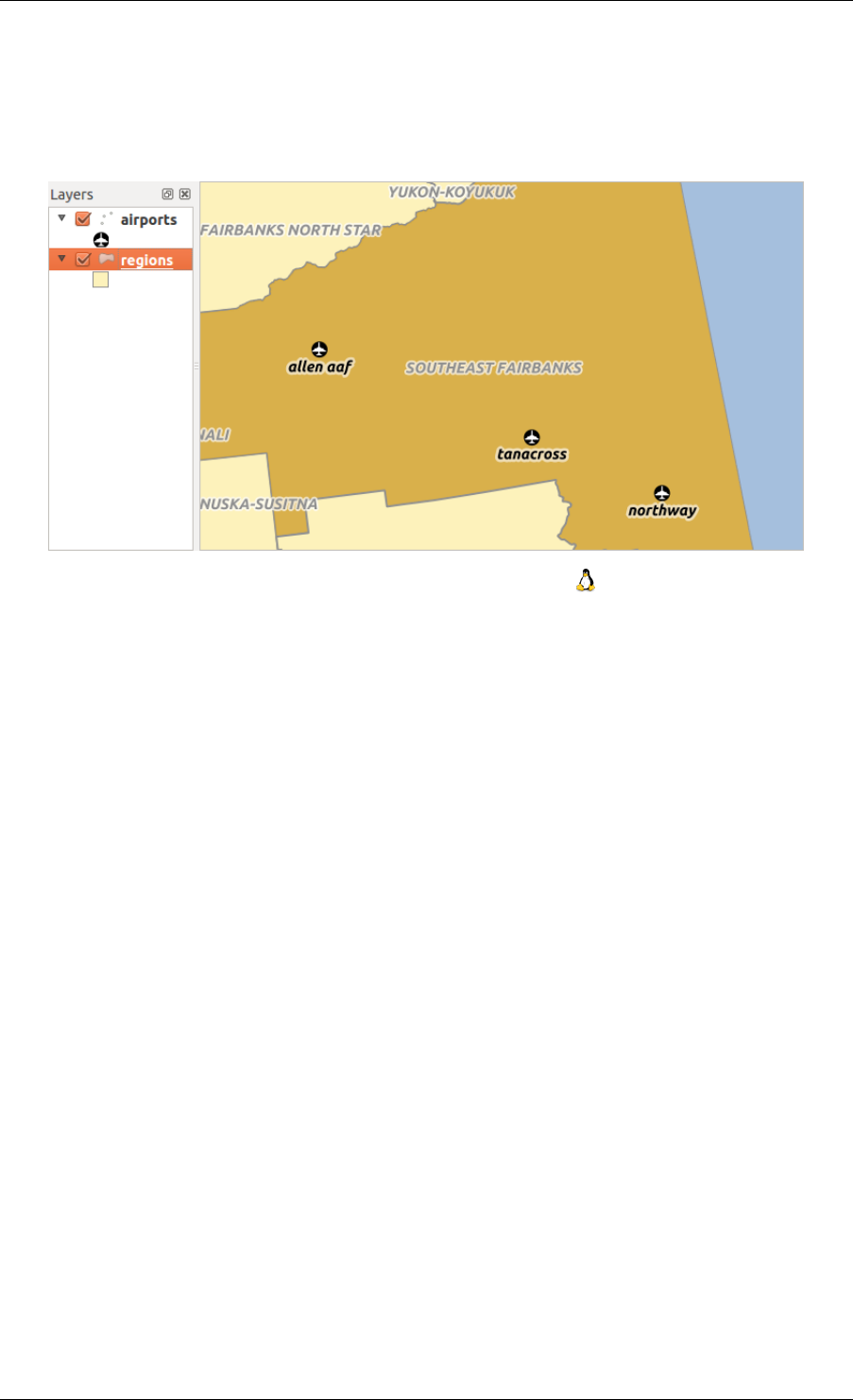
QGIS User Guide, Publicación 2.8
Foreign keys
Then you get another point layer or table with information about airports that are located in the regions and you
also want to keep track of these. If you want to add them to the region layer, you need to create a one to many
relation using foreign keys, because there are several airports in most regions.
Figure 12.48: Alaska region with airports
In addition to the already existing attributes in the airports attribute table another field fk_region which acts as a
foreign key (if you have a database, you will probably want to define a constraint on it).
This field fk_region will always contain an id of a region. It can be seen like a pointer to the region it belongs
to. And you can design a custom edit form for the editing and QGIS takes care about the setup. It works with
different providers (so you can also use it with shape and csv files) and all you have to do is to tell QGIS the
relations between your tables.
Layers
QGIS makes no difference between a table and a vector layer. Basically, a vector layer is a table with a geometry.
So can add your table as a vector layer. To demostrate you can load the ‘region’ shapefile (with geometries) and
the ‘airport’ csv table (without geometries) and a foreign key (fk_region) to the layer region. This means, that
each airport belongs to exactly one region while each region can have any number of airports (a typical one to
many relation).
Definition (Relation Manager)
The first thing we are going to do is to let QGIS know about the relations between the layer. This is done in
Settings →Project Properties. Open the Relations menu and click on Add.
•name is going to be used as a title. It should be a human readable string, describing, what the relation is
used for. We will just call say “Airports” in this case.
•referencing layer is the one with the foreign key field on it. In our case this is the airports layer
•referencing field will say, which field points to the other layer so this is fk_region in this case
•referenced layer is the one with the primary key, pointed to, so here it is the regions layer
•referenced field is the primary key of the referenced layer so it is ID
•id will be used for internal purposes and has to be unique. You may need it to build custom forms once this
is supported. If you leave it empty, one will be generated for you but you can assign one yourself to get one
that is easier to handle.
12.5. Editing 133
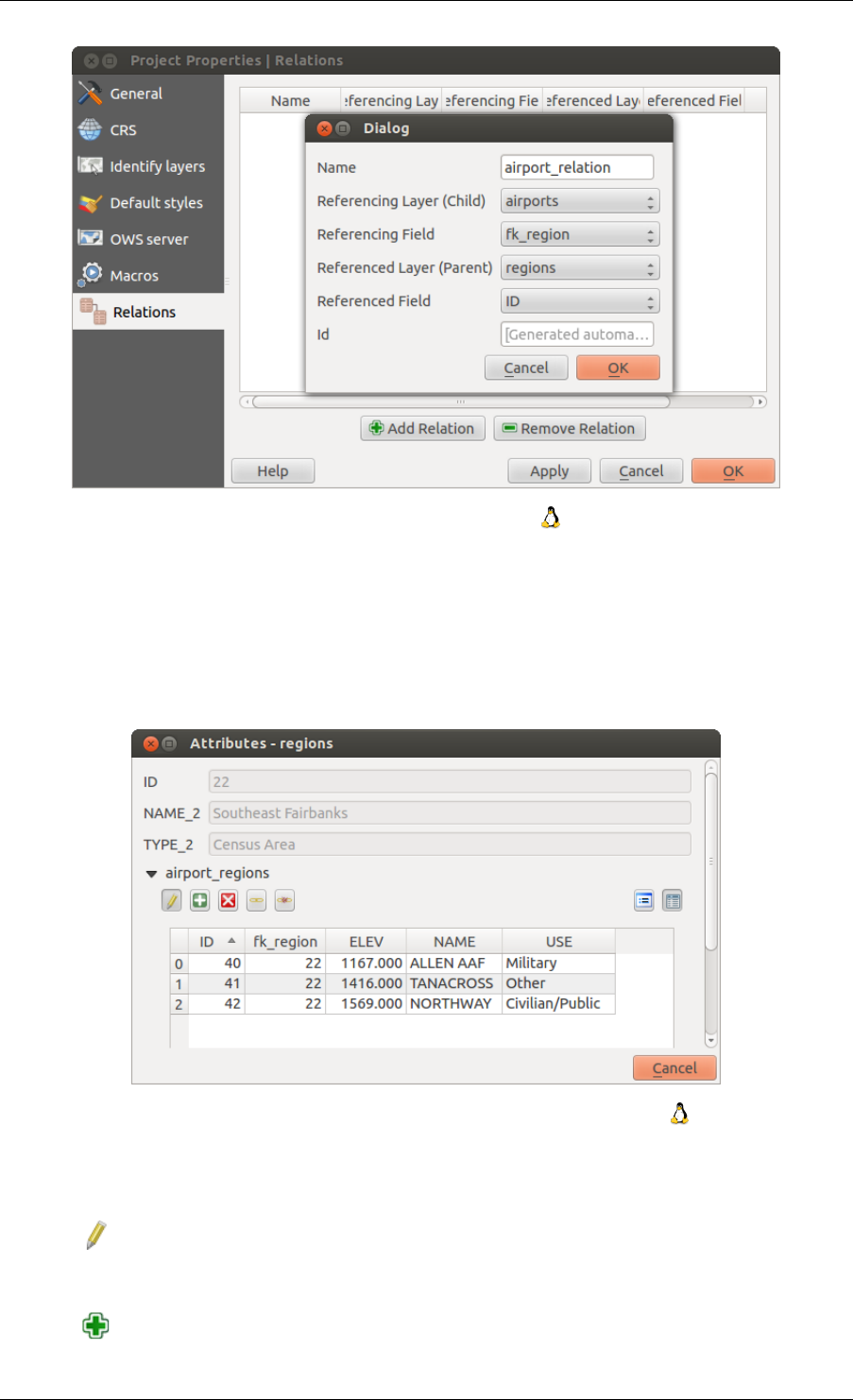
QGIS User Guide, Publicación 2.8
Figure 12.49: Relation Manager
Forms
Now that QGIS knows about the relation, it will be used to improve the forms it generates. As we did not change
the default form method (autogenerated) it will just add a new widget in our form. So let’s select the layer region
in the legend and use the identify tool. Depending on your settings, the form might open directly or you will have
to choose to open it in the identification dialog under actions.
Figure 12.50: Identification dialog regions with relation to airports
As you can see, the airports assigned to this particular region are all shown in a table. And there are also some
buttons available. Let’s review them shortly
• The button is for toggling the edit mode. Be aware that it toggles the edit mode of the airport layer,
although we are in the feature form of a feature from the region layer. But the table is representing features
of the airport layer.
• The button will add a new feature to the airport layer. And it will assign the new airport to the current
region by default.
134 Chapter 12. Trabajar con catos vectoriales
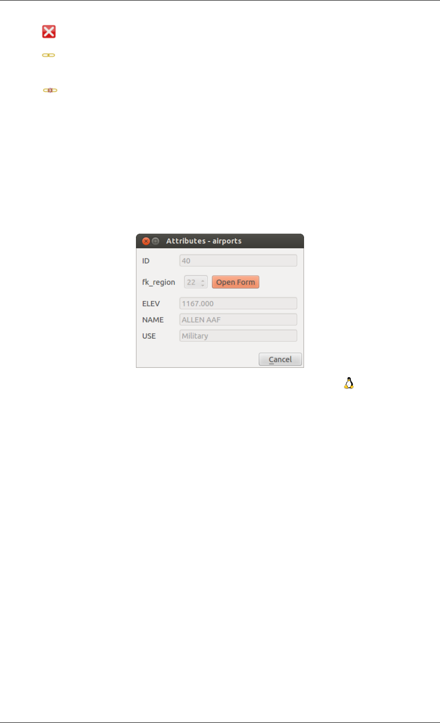
QGIS User Guide, Publicación 2.8
• The button will delete the selected airport permanently.
• The symbol will open a new dialog where you can select any existing airport which will then be assigned
to the current region. This may be handy if you created the airport on the wrong region by accident.
• The symbol will unlink the selected airport from the current region, leaving them unassigned (the
foreign key is set to NULL) effectively.
• The two buttons to the right switch between table view and form view where the later let’s you view all the
airports in their respective form.
If you work on the airport table, a new widget type is available which lets you embed the feature form of the
referenced region on the feature form of the airports. It can be used when you open the layer properties of the
airports table, switch to the Fields menu and change the widget type of the foreign key field ‘fk_region’ to Relation
Reference.
If you look at the feature dialog now, you will see, that the form of the region is embedded inside the airports form
and will even have a combobox, which allows you to assign the current airport to another region.
Figure 12.51: Identification dialog airport with relation to regions
.
12.6 Constructor de consultas
El Constructor de consultas permite definir un sub conjunto de una tabla utilizando SQL- como clausulas WHERE
y visualizar los resultados en la ventana principal. El resultado de la consulta se puede guardar como una nueva
capa vectorial.
12.6.1 Consulta
Abra el Constructor de consultas al abrir las Propiedades de la capa y vaya al menú General. Bajo Subconjunto
de datos espaciales, haga clic en el botón [Constructor de consultas] para abrir el Constructor de consultas.
Por ejemplo, si tiene una capa de regiones con un campo TYPE_2, podría seleccionar sólo regiones que
estén en municipio y la caja Expresión de filtrado específica por el proveedor del Constructor de consultas.
Figure_attributes_2 muestra un ejemplo de Constructor de consultas poblada con la capa regions.shp de los
datos de ejemplo de QGIS. Las secciones de campos, valores y operadores ayudan a construir el SQL- como
consulta.
La Lista de campos contiene todos las columnas de atributos de la tabla de atributos a ser buscados. Para agregar
una columna de atributos al campo de la clausula SQL WHERE, haga doble clic en el nombre de la lista de
campos. En general puede usar varios campos, valores y operadores para construir la consulta, o simplemente
puede escribirlo en la caja SQL.
12.6. Constructor de consultas 135
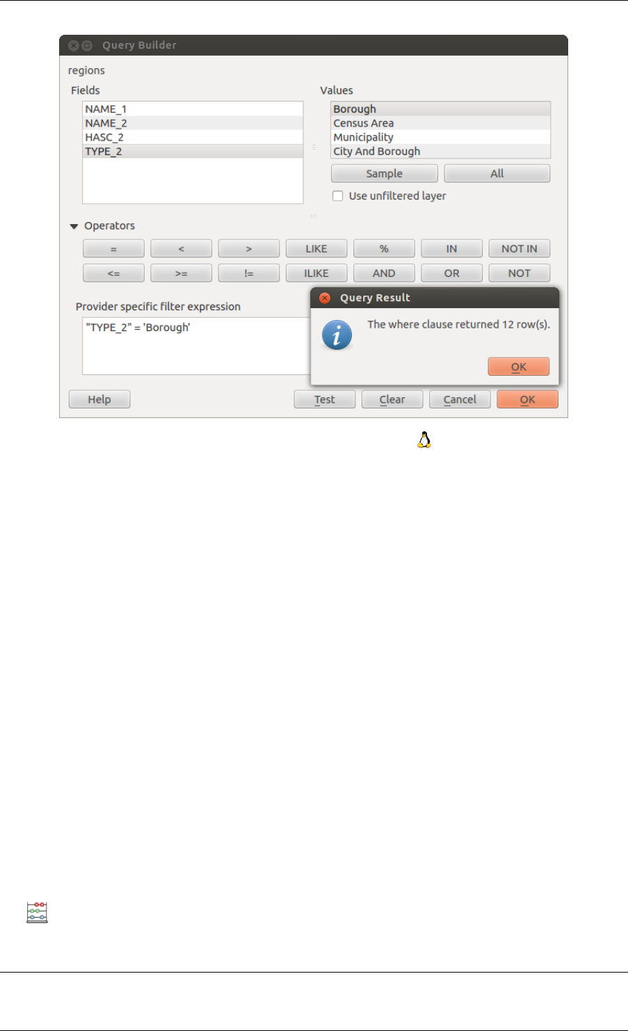
QGIS User Guide, Publicación 2.8
Figure 12.52: Constructor de consultas
La Lista de valores lista los valores de una tabla de atributos. Para listar todos los valores posibles de un atributo,
seleccione el atributo en la lista de campos y haga clic en el botón [Todos]. Para listar los primeros 25 valores
únicos de una columna de atributos, seleccione la columna de atributos en la lista de campos y haga clic en el
botón [Muestra]. Para añadir un valor al campo de la clausula WHERE de SQL, haga doble clic en el nombre en
la lista de valores.
La Sección de Operadores contiene todos los operadores utilizables. Para añadir un operador al campo de la
clausula WHERE, haga clic en el botón correspondiente. Los operadores relacionales ( =,>, ...), operador de
comparación de cadenas (COMO), y los operadores lógicos (Y,O, ...) están disponibles.
El botón [Probar] muestra un cuadro de mensaje con el numero de objetos espaciales que satisfacen la consulta
actual, que es útil en el proceso de construcción de consultas. El botón [Limpiar] limpia el texto en el campo de
texto de la clausula WHERE de SQL. El botón [Aceptar] cierra la ventana y selecciona los objetos espaciales que
satisfacen la consulta. El botón [Cancelar] cierra la ventana sin cambiar la selección actual.
QGIS trata los actos de subconjunto resultantes como si donde toda la capa. Por ejemplo, si aplica el filtro por
encima de ‘Borough’, no se puede desplegar, consultar, guardar o editar Ankorage, porque eso es un ‘Municipality’
y por lo tanto no forma parte del subconjunto.
La única excepción es que a menos que su capa sea parte de una base de datos, utilizar un subconjunto le impedirá
la edición de la capa.
.
12.7 Field Calculator
The Field Calculator button in the attribute table allows you to perform calculations on the basis of existing
attribute values or defined functions, for instance, to calculate length or area of geometry features. The results can
be written to a new attribute field, a virtual field, or they can be used to update values in an existing field.
Truco: Virtual Fields
136 Chapter 12. Trabajar con catos vectoriales
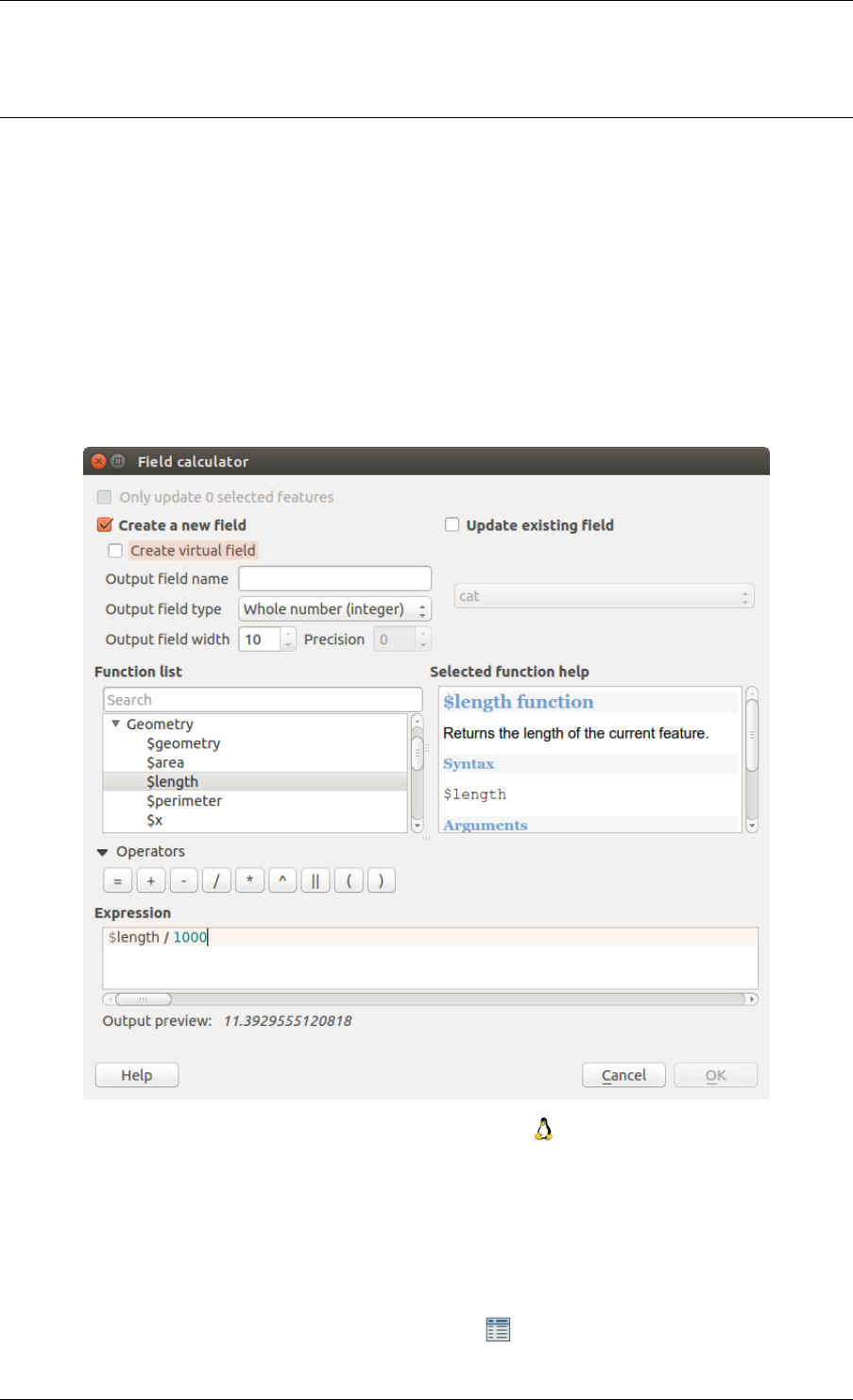
QGIS User Guide, Publicación 2.8
• Virtual fields are not permanent and are not saved.
• To make a field virtual it must be done when the field is made.
The field calculator is now available on any layer that supports edit. When you click on the field calculator icon
the dialog opens (see figure_attributes_3). If the layer is not in edit mode, a warning is displayed and using the
field calculator will cause the layer to be put in edit mode before the calculation is made.
The quick field calculation bar on top of the attribute table is only visible if the layer is editable.
In quick field calculation bar, you first select the existing field name then open the expression dialog to create your
expression or write it directly in the field then click on Update All button.
12.7.1 Expression tab
In the field calculator dialog, you first must select whether you want to only update selected features, create a new
attribute field where the results of the calculation will be added or update an existing field.
Figure 12.53: Field Calculator
If you choose to add a new field, you need to enter a field name, a field type (integer, real or string), the total field
width, and the field precision (see figure_attributes_3). For example, if you choose a field width of 10 and a field
precision of 3, it means you have 6 digits before the dot, then the dot and another 3 digits for the precision.
A short example illustrates how field calculator works when using the Expression tab. We want to calculate the
length in km of the railroads layer from the QGIS sample dataset:
1. Load the shapefile railroads.shp in QGIS and press Open Attribute Table.
12.7. Field Calculator 137

QGIS User Guide, Publicación 2.8
2. Click on Toggle editing mode and open the Field Calculator dialog.
3. Select the Create a new field checkbox to save the calculations into a new field.
4. Add length as Output field name and real as Output field type, and define Output field width to be 10
and Precision, 3.
5. Now double click on function $length in the Geometry group to add it into the Field calculator expression
box.
6. Complete the expression by typing ‘’/ 1000” in the Field calculator expression box and click [Ok].
7. You can now find a new field length in the attribute table.
The available functions are listed in Expressions chapter.
12.7.2 Function Editor tab
With the Function Editor you are able to define your own Python custom functions in a comfortable way. The
function editor will create new Python files in qgis2pythonexpressions and will auto load all functions
defined when starting QGIS. Be aware that new functions are only saved in the expressions folder and not in
the project file. If you have a project that uses one of your custom functions you will need to also share the .py file
in the expressions folder.
Here’s a short example on how to create your own functions:
@qgsfunction(args="auto", group=’Custom’)
def myfunc(value1, value2 feature, parent):
pass
The short example creates a function ‘myfunc’ that will give you a function with two values. When using the
args=’auto’ function argument the number of function arguments required will be calculated by the number of
arguments the function has been defined with in Python (minus 2 - feature, and parent).
This function then can be used with the following expression:
myfunc(’test1’,’test2’)
Your function will be implemented in the ‘Custom’ Functions of the Expression tab after using the Run Script
button.
Further information about creating Python code can be found on http://www.qgis.org/html/en/docs/pyqgis_developer_cookbook/index.html.
The function editor is not only limited to working with the field calculator, it can be found whenever you work
with expressions. See also Expressions.
.
138 Chapter 12. Trabajar con catos vectoriales
CHAPTER 13
Trabajar con catos raster
.
13.1 Working with Raster Data
This section describes how to visualize and set raster layer properties. QGIS uses the GDAL library to read and
write raster data formats, including ArcInfo Binary Grid, ArcInfo ASCII Grid, GeoTIFF, ERDAS IMAGINE, and
many more. GRASS raster support is supplied by a native QGIS data provider plugin. The raster data can also be
loaded in read mode from zip and gzip archives into QGIS.
As of the date of this document, more than 100 raster formats are supported by the GDAL library
(see GDAL-SOFTWARE-SUITE in Referencias bibliográficas y web). A complete list is available at
http://www.gdal.org/formats_list.html.
Nota: Not all of the listed formats may work in QGIS for various reasons. For example, some require external
commercial libraries, or the GDAL installation of your OS may not have been built to support the format you want
to use. Only those formats that have been well tested will appear in the list of file types when loading a raster into
QGIS. Other untested formats can be loaded by selecting the [GDAL] All files (*)filter.
Working with GRASS raster data is described in section GRASS GIS Integration.
13.1.1 What is raster data?
Raster data in GIS are matrices of discrete cells that represent features on, above or below the earth’s surface. Each
cell in the raster grid is the same size, and cells are usually rectangular (in QGIS they will always be rectangular).
Typical raster datasets include remote sensing data, such as aerial photography, or satellite imagery and modelled
data, such as an elevation matrix.
Unlike vector data, raster data typically do not have an associated database record for each cell. They are geocoded
by pixel resolution and the x/y coordinate of a corner pixel of the raster layer. This allows QGIS to position the
data correctly in the map canvas.
QGIS makes use of georeference information inside the raster layer (e.g., GeoTiff) or in an appropriate world file
to properly display the data.
13.1.2 Loading raster data in QGIS
Raster layers are loaded either by clicking on the Add Raster Layer icon or by selecting the Layer →Add
Raster Layer menu option. More than one layer can be loaded at the same time by holding down the Ctrl or
Shift key and clicking on multiple items in the Open a GDAL Supported Raster Data Source dialog.
139

QGIS User Guide, Publicación 2.8
Once a raster layer is loaded in the map legend, you can click on the layer name with the right mouse button to
select and activate layer-specific features or to open a dialog to set raster properties for the layer.
Right mouse button menu for raster layers
•Zoom to Layer Extent
•Zoom to Best Scale (100%)
•Stretch Using Current Extend
•Show in Overview
•Remove
•Duplicate
•Set Layer CRS
•Set Project CRS from Layer
•Save as ...
•Properties
•Rename
•Copy Style
•Add New Group
•Expand all
•Collapse all
•Update Drawing Order
.
13.2 Raster Properties Dialog
To view and set the properties for a raster layer, double click on the layer name in the map legend, or right click on
the layer name and choose Properties from the context menu. This will open the Raster Layer Properties dialog
(see figure_raster_1).
There are several menus in the dialog:
•General
•Style
•Transparency
•Pyramids
•Histogram
•Metadata
13.2.1 General Menu
Layer Info
The General menu displays basic information about the selected raster, including the layer source path, the display
name in the legend (which can be modified), and the number of columns, rows and no-data values of the raster.
140 Chapter 13. Trabajar con catos raster
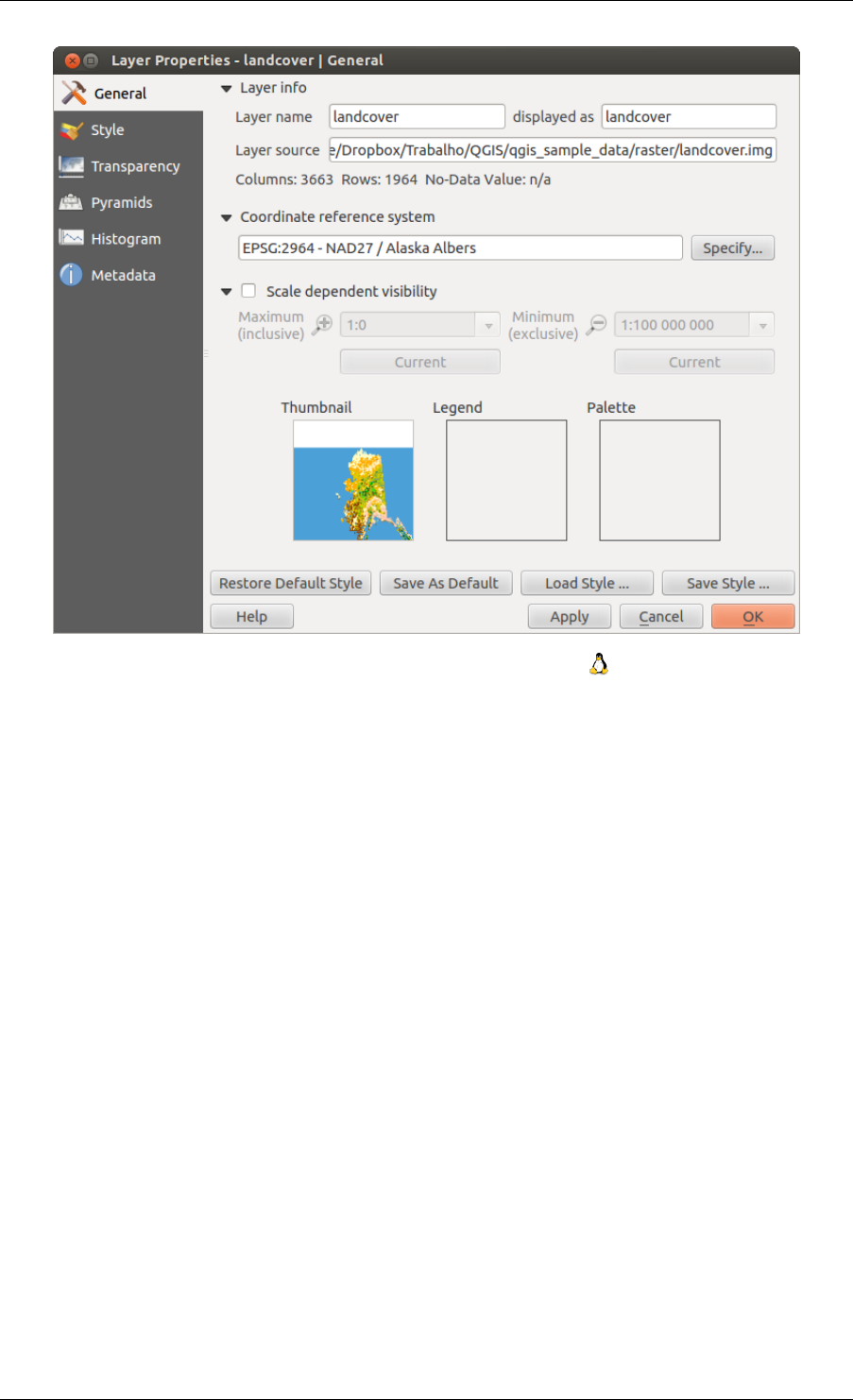
QGIS User Guide, Publicación 2.8
Figure 13.1: Raster Layers Properties Dialog
Coordinate reference system
Here, you find the coordinate reference system (CRS) information printed as a PROJ.4 string. If this setting is not
correct, it can be modified by clicking the [Specify] button.
Scale Dependent visibility
Additionally scale-dependent visibility can be set in this tab. You will need to check the checkbox and set an
appropriate scale where your data will be displayed in the map canvas.
At the bottom, you can see a thumbnail of the layer, its legend symbol, and the palette.
13.2.2 Style Menu
Band rendering
QGIS offers four different Render types. The renderer chosen is dependent on the data type.
1. Multiband color - if the file comes as a multiband with several bands (e.g., used with a satellite image with
several bands)
2. Paletted - if a single band file comes with an indexed palette (e.g., used with a digital topographic map)
3. Singleband gray - (one band of) the image will be rendered as gray; QGIS will choose this renderer if the
file has neither multibands nor an indexed palette nor a continous palette (e.g., used with a shaded relief
map)
4. Singleband pseudocolor - this renderer is possible for files with a continuous palette, or color map (e.g.,
used with an elevation map)
13.2. Raster Properties Dialog 141
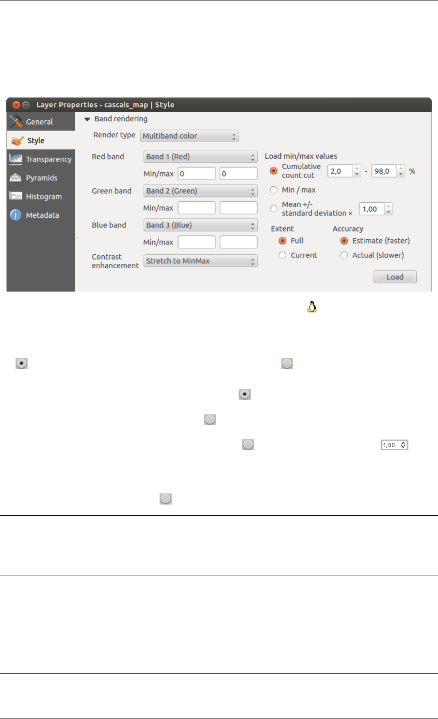
QGIS User Guide, Publicación 2.8
Multiband color
With the multiband color renderer, three selected bands from the image will be rendered, each band representing
the red, green or blue component that will be used to create a color image. You can choose several Contrast
enhancement methods: ‘No enhancement’, ‘Stretch to MinMax’, ‘Stretch and clip to MinMax’ and ‘Clip to min
max’.
Figure 13.2: Raster Renderer - Multiband color
This selection offers you a wide range of options to modify the appearance of your raster layer. First of all, you
have to get the data range from your image. This can be done by choosing the Extent and pressing [Load]. QGIS
can Estimate (faster) the Min and Max values of the bands or use the Actual (slower) Accuracy.
Now you can scale the colors with the help of the Load min/max values section. A lot of images have a few very
low and high data. These outliers can be eliminated using the Cumulative count cut setting. The standard data
range is set from 2% to 98% of the data values and can be adapted manually. With this setting, the gray character
of the image can disappear. With the scaling option Min/max, QGIS creates a color table with all of the data
included in the original image (e.g., QGIS creates a color table with 256 values, given the fact that you have 8
bit bands). You can also calculate your color table using the Mean +/- standard deviation x . Then,
only the values within the standard deviation or within multiple standard deviations are considered for the color
table. This is useful when you have one or two cells with abnormally high values in a raster grid that are having a
negative impact on the rendering of the raster.
All calculations can also be made for the Current extent.
Truco: Viewing a Single Band of a Multiband Raster
If you want to view a single band of a multiband image (for example, Red), you might think you would set the
Green and Blue bands to “Not Set”. But this is not the correct way. To display the Red band, set the image type to
‘Singleband gray’, then select Red as the band to use for Gray.
Paletted
This is the standard render option for singleband files that already include a color table, where each pixel value
is assigned to a certain color. In that case, the palette is rendered automatically. If you want to change colors
assigned to certain values, just double-click on the color and the Select color dialog appears. Also, in QGIS 2.2.
it’s now possible to assign a label to the color values. The label appears in the legend of the raster layer then.
Contrast enhancement
Nota: When adding GRASS rasters, the option Contrast enhancement will always be set automatically to stretch
to min max, regardless of if this is set to another value in the QGIS general options.
142 Chapter 13. Trabajar con catos raster
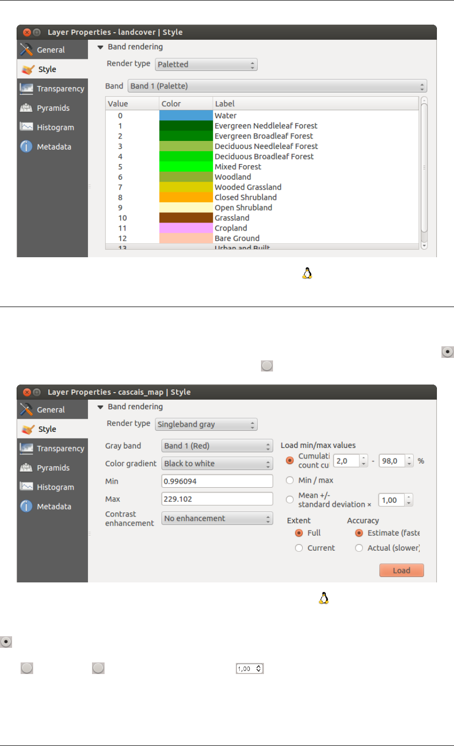
QGIS User Guide, Publicación 2.8
Figure 13.3: Raster Renderer - Paletted
Singleband gray
This renderer allows you to render a single band layer with a Color gradient: ‘Black to white’ or ‘White to black’.
You can define a Min and a Max value by choosing the Extent first and then pressing [Load]. QGIS can
Estimate (faster) the Min and Max values of the bands or use the Actual (slower) Accuracy.
Figure 13.4: Raster Renderer - Singleband gray
With the Load min/max values section, scaling of the color table is possible. Outliers can be eliminated using the
Cumulative count cut setting. The standard data range is set from 2% to 98% of the data values and can be
adapted manually. With this setting, the gray character of the image can disappear. Further settings can be made
with Min/max and Mean +/- standard deviation x . While the first one creates a color table with
all of the data included in the original image, the second creates a color table that only considers values within
the standard deviation or within multiple standard deviations. This is useful when you have one or two cells with
abnormally high values in a raster grid that are having a negative impact on the rendering of the raster.
Singleband pseudocolor
13.2. Raster Properties Dialog 143
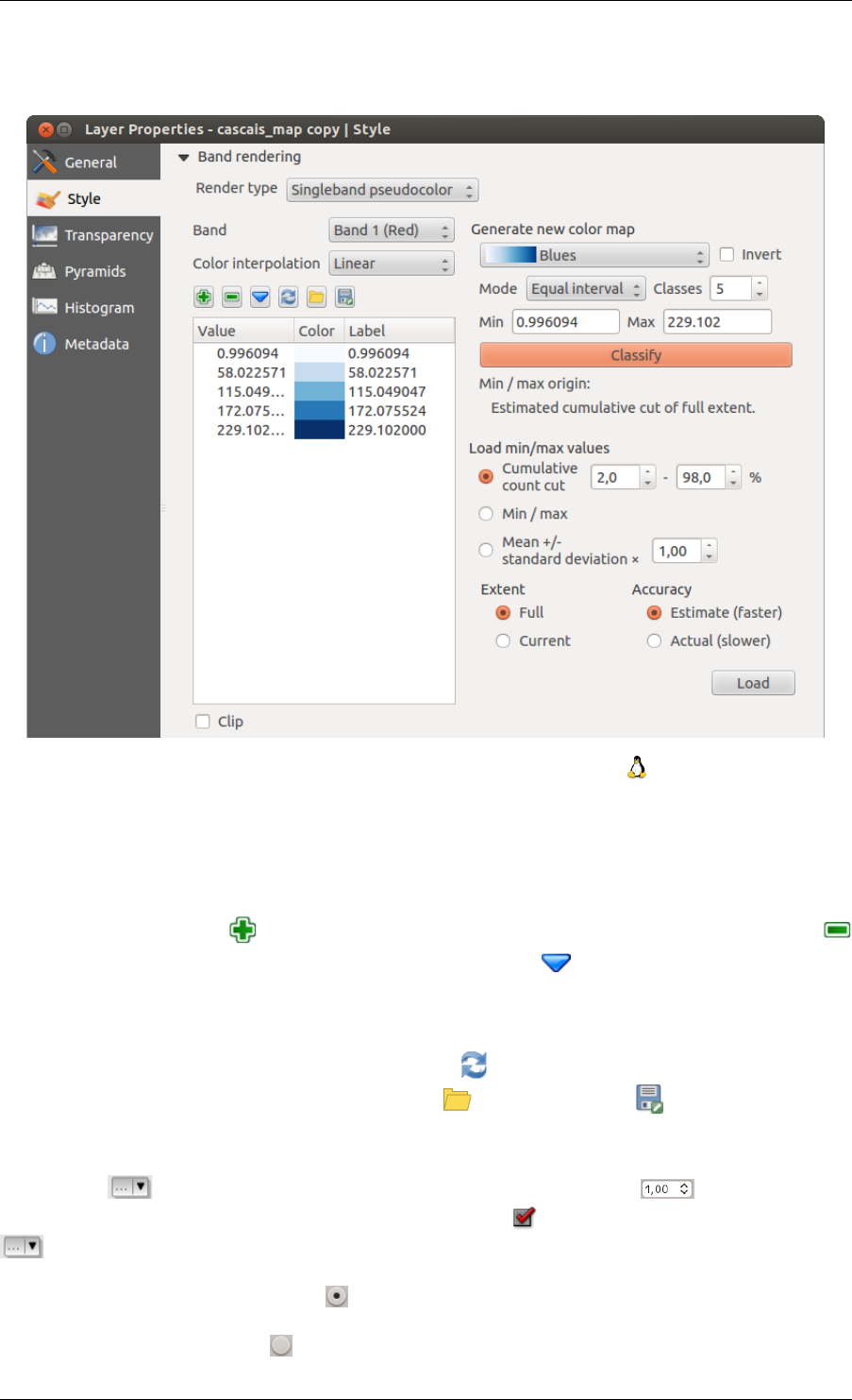
QGIS User Guide, Publicación 2.8
This is a render option for single-band files, including a continous palette. You can also create individual color
maps for the single bands here. Three types of color interpolation are available:
Figure 13.5: Raster Renderer - Singleband pseudocolor
1. Discrete
2. Linear
3. Exact
In the left block, the button Add values manually adds a value to the individual color table. The button
Remove selected row deletes a value from the individual color table, and the Sort colormap items button sorts the color
table according to the pixel values in the value column. Double clicking on the value column lets you insert a
specific value. Double clicking on the color column opens the dialog Change color, where you can select a color
to apply on that value. Further, you can also add labels for each color, but this value won’t be displayed when you
use the identify feature tool. You can also click on the button Load color map from band, which tries to load the table
from the band (if it has any). And you can use the buttons Load color map from file or Export color map to file to load
an existing color table or to save the defined color table for other sessions.
In the right block, Generate new color map allows you to create newly categorized color maps. For the Classi-
fication mode ‘Equal interval’, you only need to select the number of classes and press the button
Classify. You can invert the colors of the color map by clicking the Invert checkbox. In the case of the Mode
‘Continous’, QGIS creates classes automatically depending on the Min and Max. Defining Min/Max values
can be done with the help of the Load min/max values section. A lot of images have a few very low and high data.
These outliers can be eliminated using the Cumulative count cut setting. The standard data range is set from
2% to 98% of the data values and can be adapted manually. With this setting, the gray character of the image can
disappear. With the scaling option Min/max, QGIS creates a color table with all of the data included in the
144 Chapter 13. Trabajar con catos raster
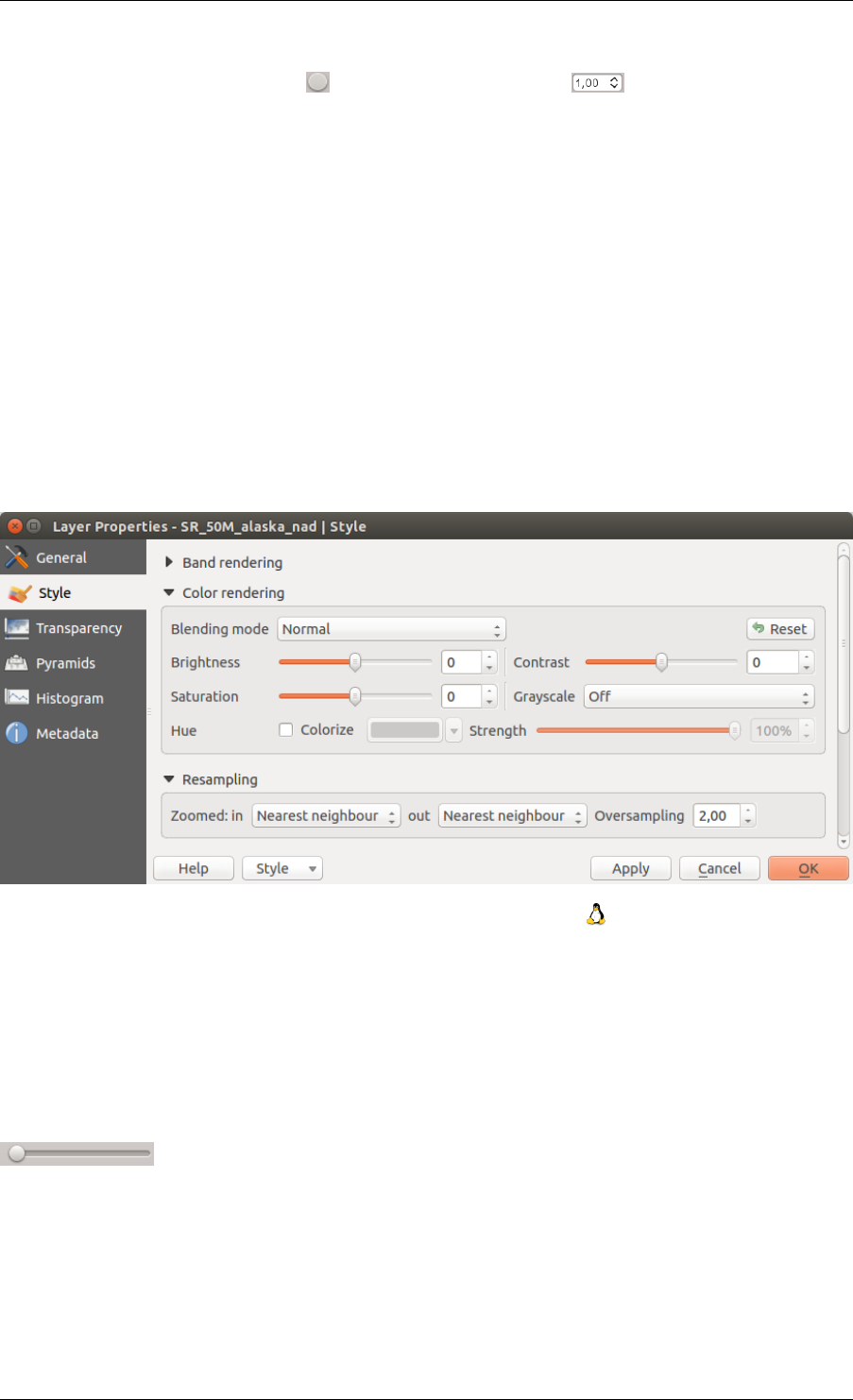
QGIS User Guide, Publicación 2.8
original image (e.g., QGIS creates a color table with 256 values, given the fact that you have 8 bit bands). You can
also calculate your color table using the Mean +/- standard deviation x . Then, only the values within
the standard deviation or within multiple standard deviations are considered for the color table.
Color rendering
For every Band rendering, a Color rendering is possible.
You can also achieve special rendering effects for your raster file(s) using one of the blending modes (see The
Vector Properties Dialog).
Further settings can be made in modifiying the Brightness, the Saturation and the Contrast. You can also use a
Grayscale option, where you can choose between ‘By lightness’, ‘By luminosity’ and ‘By average’. For one hue
in the color table, you can modify the ‘Strength’.
Resampling
The Resampling option makes its appearance when you zoom in and out of an image. Resampling modes can
optimize the appearance of the map. They calculate a new gray value matrix through a geometric transformation.
Figure 13.6: Raster Rendering - Resampling
When applying the ‘Nearest neighbour’ method, the map can have a pixelated structure when zooming in. This
appearance can be improved by using the ‘Bilinear’ or ‘Cubic’ method, which cause sharp features to be blurred.
The effect is a smoother image. This method can be applied, for instance, to digital topographic raster maps.
13.2.3 Transparency Menu
QGIS has the ability to display each raster layer at a different transparency level. Use the transparency slider
to indicate to what extent the underlying layers (if any) should be visible though the current
raster layer. This is very useful if you like to overlay more than one raster layer (e.g., a shaded relief map overlayed
by a classified raster map). This will make the look of the map more three dimensional.
Additionally, you can enter a raster value that should be treated as NODATA in the Additional no data value menu.
An even more flexible way to customize the transparency can be done in the Custom transparency options section.
The transparency of every pixel can be set here.
As an example, we want to set the water of our example raster file landcover.tif to a transparency of 20%.
The following steps are neccessary:
13.2. Raster Properties Dialog 145
QGIS User Guide, Publicación 2.8
1. Load the raster file landcover.tif.
2. Open the Properties dialog by double-clicking on the raster name in the legend, or by right-clicking and
choosing Properties from the pop-up menu.
3. Select the Transparency menu.
4. From the Transparency band menu, choose ‘None’.
5. Click the Add values manually button. A new row will appear in the pixel list.
6. Enter the raster value in the ‘From’ and ‘To’ column (we use 0 here), and adjust the transparency to 20%.
7. Press the [Apply] button and have a look at the map.
You can repeat steps 5 and 6 to adjust more values with custom transparency.
As you can see, it is quite easy to set custom transparency, but it can be quite a lot of work. Therefore, you
can use the button Export to file to save your transparency list to a file. The button Import from file loads your
transparency settings and applies them to the current raster layer.
13.2.4 Pyramids Menu
Large resolution raster layers can slow navigation in QGIS. By creating lower resolution copies of the data (pyra-
mids), performance can be considerably improved, as QGIS selects the most suitable resolution to use depending
on the level of zoom.
You must have write access in the directory where the original data is stored to build pyramids.
Several resampling methods can be used to calculate the pyramids:
• Nearest Neighbour
• Average
• Gauss
• Cubic
• Mode
• None
If you choose ‘Internal (if possible)’ from the Overview format menu, QGIS tries to build pyramids internally.
You can also choose ‘External’ and ‘External (Erdas Imagine)’.
Please note that building pyramids may alter the original data file, and once created they cannot be removed. If
you wish to preserve a ‘non-pyramided’ version of your raster, make a backup copy prior to building pyramids.
13.2.5 Histogram Menu
The Histogram menu allows you to view the distribution of the bands or colors in your raster. The histogram is
generated automatically when you open the Histogram menu. All existing bands will be displayed together. You
can save the histogram as an image with the button. With the Visibility option in the Prefs/Actions menu,
you can display histograms of the individual bands. You will need to select the option Show selected band.
The Min/max options allow you to ‘Always show min/max markers’, to ‘Zoom to min/max’ and to ‘Update style
to min/max’. With the Actions option, you can ‘Reset’ and ‘Recompute histogram’ after you have chosen the
Min/max options.
146 Chapter 13. Trabajar con catos raster
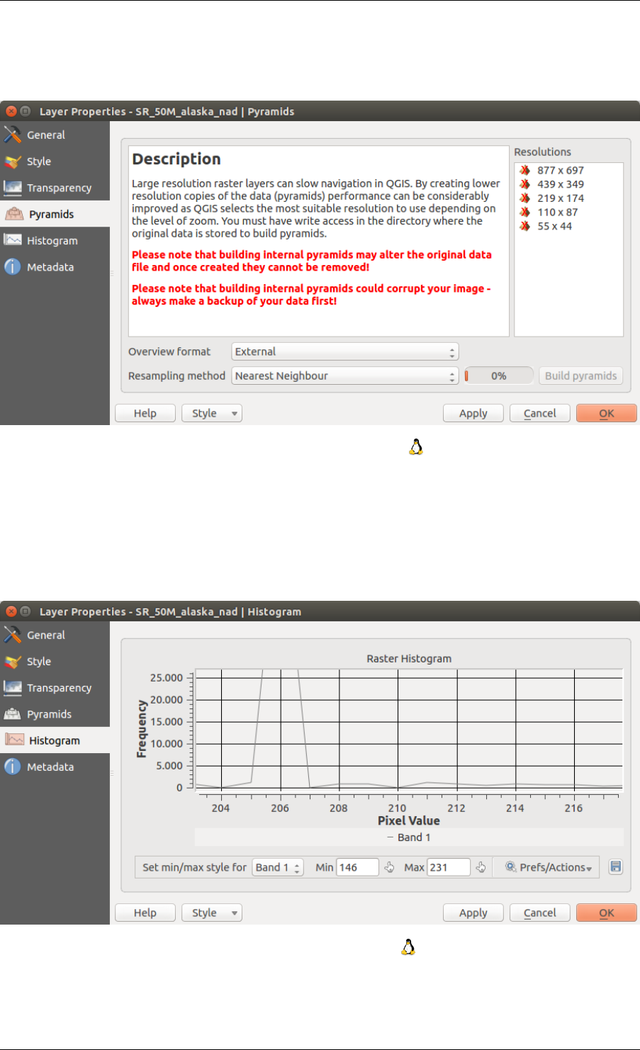
QGIS User Guide, Publicación 2.8
Figure 13.7: The Pyramids Menu
Figure 13.8: Raster Histogram
13.2. Raster Properties Dialog 147
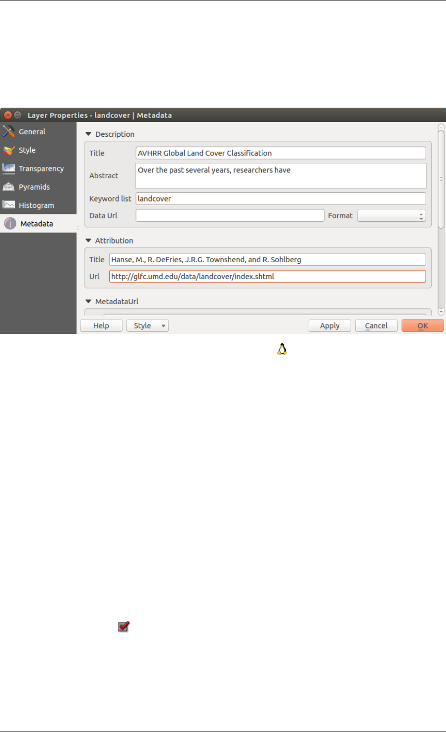
QGIS User Guide, Publicación 2.8
13.2.6 Metadata Menu
The Metadata menu displays a wealth of information about the raster layer, including statistics about each band in
the current raster layer. From this menu, entries may be made for the Description,Attribution,MetadataUrl and
Properties. In Properties, statistics are gathered on a ‘need to know’ basis, so it may well be that a given layer’s
statistics have not yet been collected.
Figure 13.9: Raster Metadata
.
13.3 Calculadora Ráster
La Calculadora ráster en el menú Ráster le permite realizar cálculos en base a los valores de píxel de un ráster ex-
istente (ver figure_raster_10). Los resultados se escriben en una nueva capa ráster con formato GDAL-compatible.
La lista Bandas ráster contiene todas las capas ráster cargadas que pueden ser utilizadas. Para añadir un ráster
a la expresión de la calculadora de campos, haga doble clic en el nombre en la lista de campos. Puede después
utilizar los operadores para construir expresiones de cálculo o simplemente puede escribirlas en el cuadro.
En la sección Capa de resultado, tendrá que definir una capa de salida. A continuación puede definir la extensión
de la zona de cálculo basado en una capa ráster de entrada, o sobre la base de coordenadas X,Y y sobre columnas y
filas, para establecer la resolución de la capa de salida. Si la capa de entrada tiene diferente resolución, los valores
serán remuestreados con el algoritmo del vecino más cercano.
La sección de Operadores contiene todos los operadores disponibles. Para añadir un operador a la caja de expre-
siones de la calculadora ráster, haga clic en el botón apropiado. Cálculos matemáticos (+,-,*, ... ) y funciones
trigonométricas (sin,cos,tan, ... ) están disponibles. ¡Estén atentos a más operadores por venir!
Con la casilla de verificación Añadir resultado al proyecto, La capa de resultado se añadirá automaticamente
a la zona de la leyenda y puede ser visualizado.
13.3.1 Ejemplos
Convertir valores de elevación de metros a pies
148 Chapter 13. Trabajar con catos raster
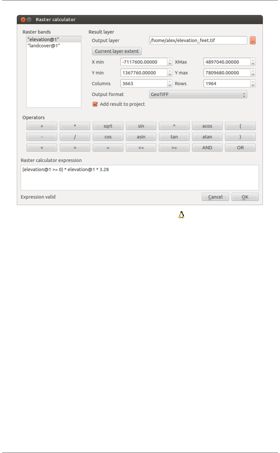
QGIS User Guide, Publicación 2.8
Figure 13.10: Calculadora Ráster
Crear un ráster de elevación en pies de un ráster en metros, es necesario utilizar el factor de conversión de metros
a pies: 3.28. La expresión es:
"elevation@1" *3.28
El uso de una máscara
Si desea enmascarar partes de una ráster- digamos , por ejemplo , porque sólo está interesado en elevaciones por
encima de 0 metros – se puede utilizar la siguiente expresión para crear una máscara y aplicar el resultado a un
ráster en un solo paso.
("elevation@1" >= 0)*"elevation@1"
En otras palabras, por cada celda superior o igual a 0 , establezca su valor en 1. De lo contrario, establecer a 0.
Esto crea la máscara al vuelo.
Si desea clasificar un ráster –digamos, por ejemplo en dos clases de elevación, puede utilizar la siguiente expresión
para crear un ráster con dos valores 1 y 2 en un solo paso.
("elevation@1" <50)*1+("elevation@1" >= 50)*2
En otras palabras, para cada celda menor de 50 establecer el valor a 1. Para cada celda mayor o igual a 50
establecer el valor a 2.
.
13.3. Calculadora Ráster 149

QGIS User Guide, Publicación 2.8
150 Chapter 13. Trabajar con catos raster

CHAPTER 14
Trabajar con datos OGC
.
14.1 QGIS como cliente de datos OGC
El Open Geospatial Consortium (OGC) es una organización internacional con miembros de más de 300 organi-
zaciones comerciales, gubernamentales, sin fines de lucro y de investigación de todo el mundo. Sus miembros
desarrollan e implementan estándares para contenido geoespacial y servicios, procesamiento de datos SIG y el
intercambio.
Al describir un modelo de datos básico para las características geográficas, un número cada vez mayor de las es-
pecificaciones son desarrollados por OGC para atender las necesidades específicas de ubicación interoperable y la
tecnología geoespacial, incluyendo SIG. Más información se puede encontrar en http://www.opengeospatial.org/.
Importantes especificaciones OGC implementadas por QGIS son:
•WMS — Web Map Service (Cliente WMS/WMTS)
•WMTS — Web Map Tile Service (Cliente WMS/WMTS)
•WFS — Web Feature Service (Cliente WFS y WFS-T)
•WFS-T — Web Feature Service - Transactional (Cliente WFS y WFS-T)
•WCS — Web Coverage Service (WCT Cliente)
•SFS — Simple Features for SQL (PostGIS Layers)
•GML — Lenguaje de Marcado Generalizado
Los servicios OGC cada vez más se utilizan para intercambiar datos geoespaciales entre diferentes implementa-
ciones de SIG y almacenes de datos. QGIS puede hacer frente a las especificaciones anteriores como un cliente,
siendo SFS (a través del apoyo del proveedor de datos/PostGIS PostgreSQL, consulte la sección PostGIS Layers).
14.1.1 Cliente WMS/WMTS
Información general de la implementación WMS
Actualmente QGIS puede actuar como un cliente WMS que entiende servidores WMS 1.1, 1.1.1 y 1.3. En
particular, se ha probado contra los servidores de acceso público como DEMIS.
Un servidor WMS actúa sobre las peticiones por parte del cliente (por ejemplo, QGIS) para un mapa ráster con una
extensión dada, conjunto de capas, el estilo de simbolización, y la transparencia. El servidor WMS posteriormente,
consulta a sus fuentes de datos locales, rásteriza el mapa, y lo envía de vuelta al cliente en un formato ráster. Para
QGIS, este formato sería típicamente JPEG o PNG.
WMS es genéricamente un servicio REST (Representational State Transfer) en lugar de un servicio Web en toda
regla. Como tal, puede tomar las URLs generadas por QGIS y utilizarlos en un navegador web para recuperar las
151
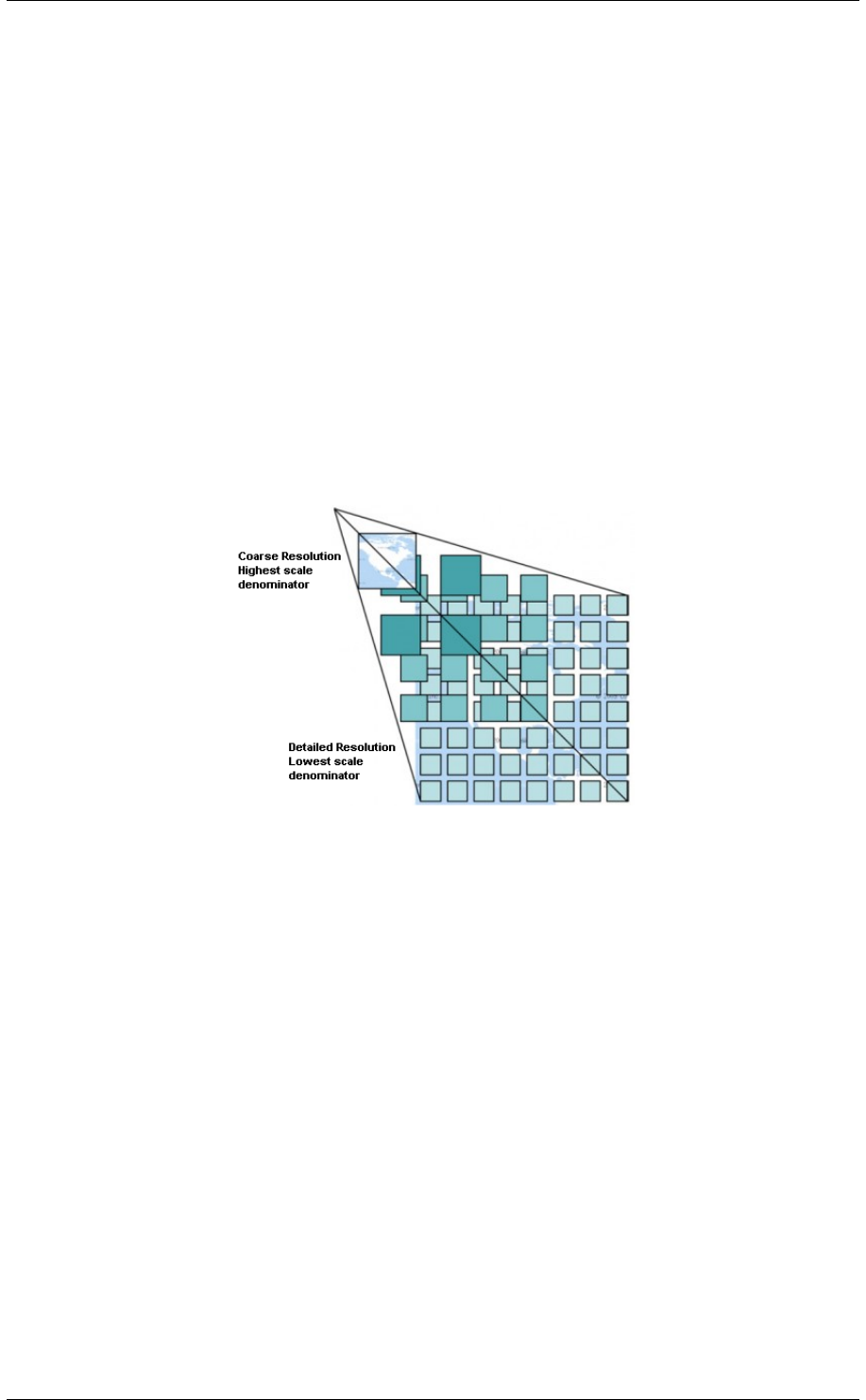
QGIS User Guide, Publicación 2.8
mismas imágenes que QGIS utiliza internamente. Esto puede ser útil para la solución de problemas, ya que hay
varias marcas de servidor WMS en el mercado y todos ellos tienen su propia interpretación de la norma WMS.
Las capas WMS se pueden añadir sencillamente, siempre que conozca la URL para acceder al servidor WMS, si
tiene una conexión útil a ese servidor, y el servidor entiende HTTP como mecanismo de transporte de datos.
Información general de la implementación WMTS
QGIS también puede actuar como un cliente WMTS. WMTS es un estándar OGC para la distribución de conjunto
de fichas de datos geoespaciales. Esta es una forma más rápida y eficiente de distribución de datos que WMS
porque con WMTS, el conjunto de fichas es pre-generado, y el cliente sólo pide a la transmisión de los azulejos,
no su producción. A petición WMS implica típicamente tanto la generación y transmisión de los datos. Un
ejemplo bien conocido de un estándar de no OGC para la visualización de datos geoespaciales de azulejos es
Google Maps.
Para mostrar los datos en una variedad de escalas cercanas a lo que el usuario podría querer, los conjuntos de
teselas WMTS se producen en varios niveles de escala diferentes y están disponibles para el cliente SIG para
pedirlos.
Este diagrama ejemplifica el concepto de conjunto de teselas:
Figure 14.1: Concepto de conjunto de teselas WMTS
Los dos tipos de interfaces de WMTS, que|qg| reconoce son a través de Key-Value-Pairs(KVP) y RESTful. Estas
dos interfaces son diferentes, y hay que especificar a diferente QGIS.
1) In order to access a WMTS KVP service, a QGIS user must open the WMS/WMTS interface and add the
following string to the URL of the WMTS tile service:
"?SERVICE=WMTS&REQUEST=GetCapabilities"
Un ejemplo de este tipo de dirección es
http://opencache.statkart.no/gatekeeper/gk/gk.open_wmts?\
service=WMTS&request=GetCapabilities
Para probar la capa topo2 en este WMTS funciona muy bien. Añadir esta cadena indica que un servicio web
WMTS se va a utilizar en lugar de un servicio WMS.
2. EL servicio RESTful WMTS toma una forma diferente, una URL sencilla. EL formato recomendado por
OGC es:
{WMTSBaseURL}/1.0.0/WMTSCapabilities.xml
Este formato le ayuda a reconocer que es una dirección RESTful. Un WMTS RESTful se accede
en QGIS simplemente añadiendo su dirección en la configuración del WMS en el campo de URL
152 Chapter 14. Trabajar con datos OGC
QGIS User Guide, Publicación 2.8
del formulario. Un ejemplo de este tipo de dirección para un caso de mapa base Austriaco es
http://maps.wien.gv.at/basemap/1.0.0/WMTSCapabilities.xml.
Nota: Se pueden encontrar aun algunos servicios viejos llamados WMS-C. Estos servicios son bas-
tante similares a WMTS (por ejemplo, mismo propósito pero trabaja un poco diferente). Se pueden ad-
ministrar lo mismo que los servicios WMTS hechos. Sólo se añade ?titled=true al final de la url. Vea
http://wiki.osgeo.org/wiki/Tile_Map_Service_Specification para mayor información acerca de esta especificación.
Cuando se lee WMTS, a menudo se puede pensar en WMS-C también.
Seleccionar servidor WMS/WMTS
La primera ves que utiliza el objeto WMS en QGIS, no hay servidores definidos.
Comience haciendo clic en el botón Añadir capa WMS en la barra de herramientas, o seleccionando Capa →
Añadir capa WMS....
El diálogo Añadir capa(s) desde un servidor para añadir capas que aparezcan en el servidor WMS. Se
pueden agregar algunas capas para jugar haciendo clic en el botón [Añadir servidores predetermina-
dos]. Este añadirá dos servidores demo WMS para usar: los servidores WMS de DM Solutions Group y
Lizardtech. Para definir un nuevo servidor WMS en la pestaña Capas, seleccionar el botón [Nuevo]. A con-
tinuación introduzca los parámetros para conectarse a su servidor deseado, como se indica en table_OGC_1:
Nombre Un nombre para esta conexión. Este nombre se utilizará en la lista desplegable de
conexiones a servidor así que se puede distinguir de otros servidores WMS.
URL La URL del servidor provee los datos. Este debe ser un nombre de host soluble – el
mismo formato que usaría para abrir una conexión telnet o ping a un host.
Nombre de
usuario
Nombre de usuario para acceder a un servidor asegurado de WMS. Este parámetro es
opcional.
Contraseña Contraseña para una autentificación básica al servidor WMS. Este parámetro es opcional
Ignorar URI
GetMap
Ignorar URI GetMap reportada en las capacidades. Utilice un URI dado del campo
URL anterior.
Ignorar la URI
GetFeatureInfo
Ignorar la URI GetFeatureInfo reportada en las capacidades. Utilice un URI dado
del campo URL anterior.
Tabla OGC 1: Parámetros de conexión WMS
Si necesita configurar un servidor proxy para poder recibir servicios WMS de internet, se puede añadir el servidor
proxy en las opciones. Elegir Configuración→Opciones y haga clic en la pestaña Red & Proxy. Ahí, podrá añadir
su configuración de proxy y habilitarlos al ajustar el Usar proxy para acceso web. Comprobar que selecciono
el tipo de proxy correcto del menú desplegable Tipo de proxy .
Una vez que la nueva conexión al servidor WMS ha sido creada, será preservado para futuras sesiones QGIS.
Truco: En las direcciones URL del servidor WMS
Asegúrese, al introducir la URL del servidor WMS, que tiene solo la base URL. Por ejemplo, no debe tener
fragmentos como request=GetCapabilities oversion=1.0.0 en su URL.
Cargando capas WMS/WMTS
Una vez que haya llenado exitosamente en sus parámetros, puede utilizar el botón [Conectar] para recuperar
las capacidades del servidor seleccionado. Esto incluye la codificación de la imagen, capas, estilos de capa y
proyecciones. Como es una operación de la red, la velocidad de respuesta depende de la calidad de la conexión de
red al servidor WMS. Mientras descarga los datos desde el servidor WMS, el proceso de descarga se visualizara
en la parte inferior izquierda del dialogo WMS.
Su pantalla debe ahora lucir un poco como figure_OGR_1, que muestra la respuesta proporcionada por el servidor
WMS del European Soil Portal.
14.1. QGIS como cliente de datos OGC 153
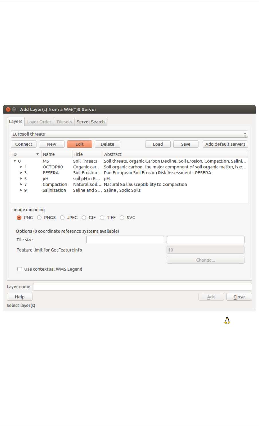
QGIS User Guide, Publicación 2.8
Figure 14.2: El diálogo para añadir un servidor WMs, mostrará las capas disponibles
154 Chapter 14. Trabajar con datos OGC
QGIS User Guide, Publicación 2.8
Codificación de la Imagen
La sección Codificación de la imagen lista los formatos que reconoce por ambos el cliente y el servidor. Elija uno
dependiendo de sus requerimientos de precisión de imagen.
Truco: Codificación de la Imagen
Normalmente, encontrará que un servidor WMS le ofrece la opción de codificación de la imagen en JPEG o PNG.
JPEG es un formato de compresión con pérdida, mientras que PNG reproduce fielmente los datos crudos raster.
Utilizar JPEG si se espera que los datos WMS sean de naturaleza fotográfica y/o no le importa cierta perdida de
calidad de la imagen. Esta disyuntiva típicamente reduce en cinco veces la necesidad de transferencia de datos en
comparación con PNG.
Utilice PNG si desea representaciones precisas de los datos originales y no le importa el incremento de los requi-
sitos de transferencia de datos.
Opciones
La zona Opciones del diálogo provee un campo de texto donde se puede añadir un Nombre de capa para la capa
WMS. Este nombre aparecerá en la leyenda después de cargar la capa.
Debajo del nombre de la capa, se puede definir Tamaño de la tesela, si desea establecer tamaños de tesela (por
ejemplo, 256x256) para dividir la petición WMS en múltiples peticiones.
El Límite del objeto espacial para GetFeatureInfo define los objetos espaciales del servidor a consultar.
Si se selecciona un WMS de la lista, aparece un campo con la proyección predeterminada proporcionada por el
servidor de mapas. Si el botón [Cambiar...] está activo, puede hacer clic en él y cambiar la proyección por defecto
de los WMS a otro SRC proporcionado por el servidor WMS.
Finalmente puede activar Utiliza leyenda-WMS contextual si el servidor WMS admite este objeto. Entonces
sólo la leyenda relevante para su actual extensión de vista de mapa se mostrará y así no incluirá los elementos de
la leyenda por cosas que no puede ver en el mapa actual.
Orden de la capa
La pestaña Orden de Capas lista las capas seleccionadas disponibles de la conexión actual al servidor WMS.
Puede notar que algunas capas son ampliables; esto significa que la capa se puede visualizar en una selección de
estilos de imagen.
Se puede seleccionar varias capas a la vez, pero solo una imagen de estilo por capa. Cuando varias capas son
seleccionadas, estas se combinarán en el servidor WMS y se transmitirán a QGIS una sola vez.
Truco: Ordenar capas WMS
Las capas WMS representadas por un servidor son sobrepuestas en el orden listado en la sección de Capas, desde
la parte superior a la parte inferior de la lista. Si se desea cambiar el orden de la superposición, se puede usar la
pestaña Orden de capas.
Transparencia
En esta versión de QGIS, la configuración de la Transparencia Global de Propiedades de la capa esta codificado
para estar siempre en donde esté disponible
Truco: Transparencia de capa WMS
La disponibilidad de imagen WMS transparente depende de la codificación de la imagen utilizada: PNG y GIF
reconoce la transparencia, mientras JPEG deja sin reconocerlo.
Sistema de referencia de coordenadas
Un sistema de referencia de coordenadas (SRC) es la terminología para un proyección QGIS.
Cada capa WMS se puede representar en múltiples SRC’s, dependiendo de la capacidad del servidor WMS.
14.1. QGIS como cliente de datos OGC 155

QGIS User Guide, Publicación 2.8
Para elegir un SRC, seleccione [Cambiar...] y un cuadro de diálogo similar a Figure Projection 3 en Working with
Projections aparecerá. La principal diferencia con la versión WMS del diálogo es que sólo aquellos SRCs son
reconocidos por el servidor WMS se le mostrarán.
Busqueda del servidor
Dentro QGIS, se puede buscar servidores WMS. Figure_OGC_2 muestra la pestaña Búsqueda de servidor con el
diálogo Añadir capa(s) de un servidor.
Figure 14.3: Diálogo para buscar servidores WMS después de algunas palabras clave
Como se puede ver, es posible ingresar una cadena de búsqueda en el campo de texto y golpear el botón
[Búsqueda]. Después de un rato, el resultado de la búsqueda se completará automáticamente en la lista de abajo
del campo de texto. Examine la lista de resultados e inspeccione los resultados de la búsqueda en la tabla. Para
visualizar los resultados, seleccione una entrada de la tabla, pulse el botón [Añadir la fila seleccionada a la lista
WMS] y cambiar de nuevo a la pestaña Capas. QGIS ha actualizado automáticamente la lista de su servidor, y
el resultado de búsqueda seleccionado ya está habilitado en la lista de servidores WMS guardados en la pestaña
Capas. Sólo tiene que solicitar la lista de capas al hacer clic en el botón [Conectar]. Esta opción es muy útil
cuando se desea buscar mapas por palabras clave específicas.
Básicamente, esta opción es una interfaz del API de http://geopole.org.
Conjunto de teselas
Al utilizar servicios WMTS (Cached WMS) como
http://opencache.statkart.no/gatekeeper/gk/gk.open_wmts?\
service=WMTS&request=GetCapabilities
Son capaces de navegar a través de la pestaña :guilabel: Conjunto de teselas propuesta por el servidor. La in-
formación adicional como el tamaño de la tesela, formatos y SRC compatibles se enumeran en esta tabla. En
156 Chapter 14. Trabajar con datos OGC

QGIS User Guide, Publicación 2.8
combinación con esta característica, puede usar el control deslizante de escala de tesela seleccionando Configu-
ración -> Paneles (KDE y Windows) o Ver -> Paneles (Gnome y MacOSX), a continuación, elegir Escala de
tesela. Esto le da las escalas disponibles desde el servidor de tesela con un buen slider atracado.
Utilizar la herramienta de Identificar objetos espaciales
Una vez que haya añadido un servidor WMS, y si alguna capa de un servidor WMS es consultable, puede entonces
utilizar la herramienta Identificar objetos espaciales para seleccionar un píxel del lienzo del mapa. Una consulta se
hace al servidor WMS por cada selección realizada. El resultado de la consulta se regresara en texto plano. El
formato de este texto es dependiente del servidor WMS particular utilizado. Selección de Formato
Si múltiples formatos de salida son reconocidos por el servidor, una lista desplegable con formatos admitidos se
añade automáticamente al diálogo de resultados identificados y el formato seleccionada puede ser almacenado en
el proyecto para la capa. Usar formato GML
La herramienta Identificar reconoce la respuesta del servidor WMS (GetFeatureInfo) en formato GML (se llama
Objeto espacial en la GUI QGIS en este contexto). Si el formato “Objeto espacial” es admitido por el servidor y
seleccionado, los resultados de la herramienta de identificados son objetos vectoriales, como de una capa vectorial
regular. Cuando un objeto espacial es seleccionado en el árbol, este resalta en el mapa y se puede copiar a la
papelera y pegar a otra capa vectorial. Vea el ejemplo de configuración de UMN Mapserver abajo que admite
GetFeatureInfo en formato GML.
# in layer METADATA add which fields should be included and define geometry (example):
"gml_include_items" "all"
"ows_geometries" "mygeom"
"ows_mygeom_type" "polygon"
# Then there are two possibilities/formats available, see a) and b):
# a) basic (output is generated by Mapserver and does not contain XSD)
# in WEB METADATA define formats (example):
"wms_getfeatureinfo_formatlist" "application/vnd.ogc.gml,text/html"
# b) using OGR (output is generated by OGR, it is send as multipart and contains XSD)
# in MAP define OUTPUTFORMAT (example):
OUTPUTFORMAT
NAME "OGRGML"
MIMETYPE "ogr/gml"
DRIVER "OGR/GML"
FORMATOPTION "FORM=multipart"
END
# in WEB METADATA define formats (example):
"wms_getfeatureinfo_formatlist" "OGRGML,text/html"
Ver propiedades
Una vez que haya añadido un servidor WMS, puede ver sus propiedades haciendo clic derecho sobre el mismo en
la leyenda y la seleccionar Propiedades.Pestaña de Metadatos
La pestaña Metadatos muestra una gran cantidad de información acerca del servidor WMS, generalmente obtenida
de la declaración de capacidades de ese servidor. Muchas definiciones pueden ser extraídas mediante la lectura
del estándar WMS (vea OPEN-GEOSPATIAL-CONSORTIUM en Referencias bibliográficas y web), pero aquí
hay algunas definiciones útiles:
•Propiedades del servidor
– Versión WMS — La versión WMS implementada por el servidor.
– Formatos de Imagen — La lista de MIME-types que el servidor puede responder con la hora de
elaboración del mapa. QGIS reconoce cualquier formato las bibliotecas Qt subyacentes con que fueron
14.1. QGIS como cliente de datos OGC 157

QGIS User Guide, Publicación 2.8
construidas, que es típicamente al menos image/png yimage/jpeg.
– Formato de Identificación — La lista de tipos MIME, el servidor puede responder, cuando utilice la
herramienta de Identificación. Actualmente, QGIS reconoce el tipo texto plano.
•Propiedades de la capa
– Seleccionar — Sea o no esta capa seleccionada cuando su servidor fue añadido a este proyecto.
– Visible — Si la capa seleccionada es o no visible en la leyenda (aun no utilizada en esta versión de
QGIS).
– Poder Identificar — Sea o no esta capa regresará algunos resultados cuando la herramienta de iden-
tificar se utilice en él.
– Puede ser transparente — Si esta capa puede ser representada o no con transparencia. Esta versión de
QGIS siempre usará transparencia si este es Si y la codificación de la imagen admite la transparencia.
–** Puede Acercar zum ** — Si o no esta capa se puede hacer zoom en el servidor. Esta versión de
QGIS asume que todas las capas WMS tienen este conjunto de Yes. Capas deficientes pueden ser
presentadas de manera extraña.
– Conteo en Cascada — Los servidores WMS pueden actuar como proxy para otros servidores WMS
para obtener datos ráster de una capa. Esta entrada muestra el número de veces que se remitió la
solicitud de esta capa para ver a los servidores WMS para obtener un resultado.
–** Ancho fijo, altura fija ** — Si o no esta capa tiene fijos la dimensiones en píxeles de origen. Esta
versión de QGIS asume que todas las capas WMS tienen este conjunto a la nada. Capas deficientes
pueden ser presentadas de manera extraña.
– Recuadro delimitador WGS 84 — El recuadro delimitador de la capa, en coordenadas WGS 84. Al-
gunos servidores WMS no utilizan este valor correctamente (por ejemplo, utilizan coordenadas UTM
en su lugar). Si éste es el caso, la vista inicial de la capa puede aparecer muy ‘lejana’ en QGIS. El web-
master de WMS debería ser informado de este error, que probablemente conocerá como los elementos
XML de WMS LatLonBoundingBox,EX_GeographicBoundingBox o el BoundingBox‘ de
CRS:84.
– Disponible en SRC — Las proyecciones que esta capa puede representar por el servidor WMS. Éstos
se enumeran en el formato nativo de WMS.
– Disponible en estilo — Los estilos de imagen que esta capa puede representar por el servidor WMS.
Mostrar leyenda gráfica WMS en la tabla de contenido y diseñador de impresión
El proveedor de datos WMS de QGIS es capaz de mostrar una leyenda gráfica en la tabla de contendos de la
lista de capas y en el diseñador de mapas. La leyenda WMS se muestra sólo si el servidor WMS tiene capacidad
GetLegendGraphic y la capa especifica una url para getCapability, por lo que, además, es necesario seleccionar
un estilo para la capa.
Si hay definida una legendGraphic, ésta se mostrará debajo de la capa. Es pequeña y hay que hacer clic sobre ella
para abrirla en tamaño real (debido a una limitación de la arquitectura de QgsLegendInterface). Al hacer clic en
la leyenda de la capa se abrirá un cuadro con la leyenda a la máxima resolución.
En el diseñador de impresión, la leyenda se integrará en la dimensión original (descargada). La resolución de
la leyenda se puede configurar en las propiedades del elemento bajo Leyenda->WMS LegendGraphic para que
coincida con los requisitos de impresión
La leyenda mostrará información contextual basada en su escala actual. La leyenda WMS se muestra sólo si el
servidor WMS tiene capacidad GetLegendGraphic y la capa tiene definida una url getCapability, para lo que se
debe seleccionar un estilo.
158 Chapter 14. Trabajar con datos OGC
QGIS User Guide, Publicación 2.8
Limitaciones del cliente WMS
No es posible la funcionalidad de cliente WMS que se había incluido en esta versión de QGIS. Algunas de las
excepciones más notables siguen.
Editar la configuración de la capa WMS
Una vez que hayas completado el procedimiento de :sup: Añadir capa WMS, no se podrá cambiar la configu-
ración. Una solución alternativa es eliminar la capa por completo y empezar de nuevo.
**Autentificación necesaria en servidores WMS **
Actualmente, se admiten servicios WMS públicamente accesibles y garantizados. Los servidores WMS garantiza-
dos se puede acceder mediante autenticación pública. El usuario puede agregar las credenciales (opcional) cuando
agregue un servidor WMS. Vea la sección :ref: ogc-wms-servers para más detalles.
Truco: Acceso garantizado a capas OGC
Si necesita acceder a capas protegidas mediante métodos seguros que no sean la autenticación básica, puede
utilizar InteProxy como un proxy transparente, lo que lo hace compatible con varios métodos de autenticación.
Puede encontrar más información en el manual InteProxy en http://inteproxy.wald.intevation.org.
Truco: QGIS WMS Mapserver
Desde la versión 1.7.0, QGIS tiene su propia implementación de un servidor de mapas WMS 1.3.0. Lea más sobre
esto en el capítulo QGIS como Servidor de Datos OGC.
14.1.2 WCT Cliente
Un Web Coverage Service (WCS) proporciona acceso a los datos ráster en formas que son útiles para la
representación del lado cliente, como datos de entrada en los modelos científicos, y para otros clientes. El WCS
se puede comparar con la WFS y el WMS. Como WMS y WFS instancias de servicios, un WCS permite a los
clientes elegir partes de las explotaciones de información de un servidor basado en restricciones espaciales y otros
criterios de consulta.
QGIS tiene un proveedor WCS nativo y reconocida en ambas versiones 1.0 y 1,1 (que son significativamente
diferentes), pero actualmente se prefiere 1.0, porque 1.1 tiene muchas problemas (por ejemplo, cada servidor
implementa de diferente forma con varias particularidades).
El proveedor de WCS nativo se encarga de todas las solicitudes de red y utiliza las configuraciones de red estándar
de |qgl (especialmente de proxy ). También es posible seleccionar el modo de caché ( ‘siempre caché’, ‘prefer-
entemente caché’, ‘preferentemente red’, ‘siempre red’ ). El proveedor también es compatible con la selección de
tiempo de la posición, si el servidor ofrece dicha información temporal.
14.1.3 Cliente WFS y WFS-T
En QGIS, una capa WFS se comporta prácticamente como cualquier otra capa vectorial. Puede identificar y
seleccionar objetos espaciales, y ver la tabla de atributos. Desde QGIS 1.6, la edición WFS-T está también de
apoyó.
En general, añadir una capa WFS es muy similar al procedimiento utilizado con WMS. La diferencia es que no
hay servidores por defecto definidos, así que tenemos que añadir la nuestra.
Cargar una capa WFS
Como un ejemplo, utilizamos el servidor WFS de DM Solutions y mostramos una capa. La URL es
http://www2.dmsolutions.ca/cgi-bin/mswfs_gmap
14.1. QGIS como cliente de datos OGC 159
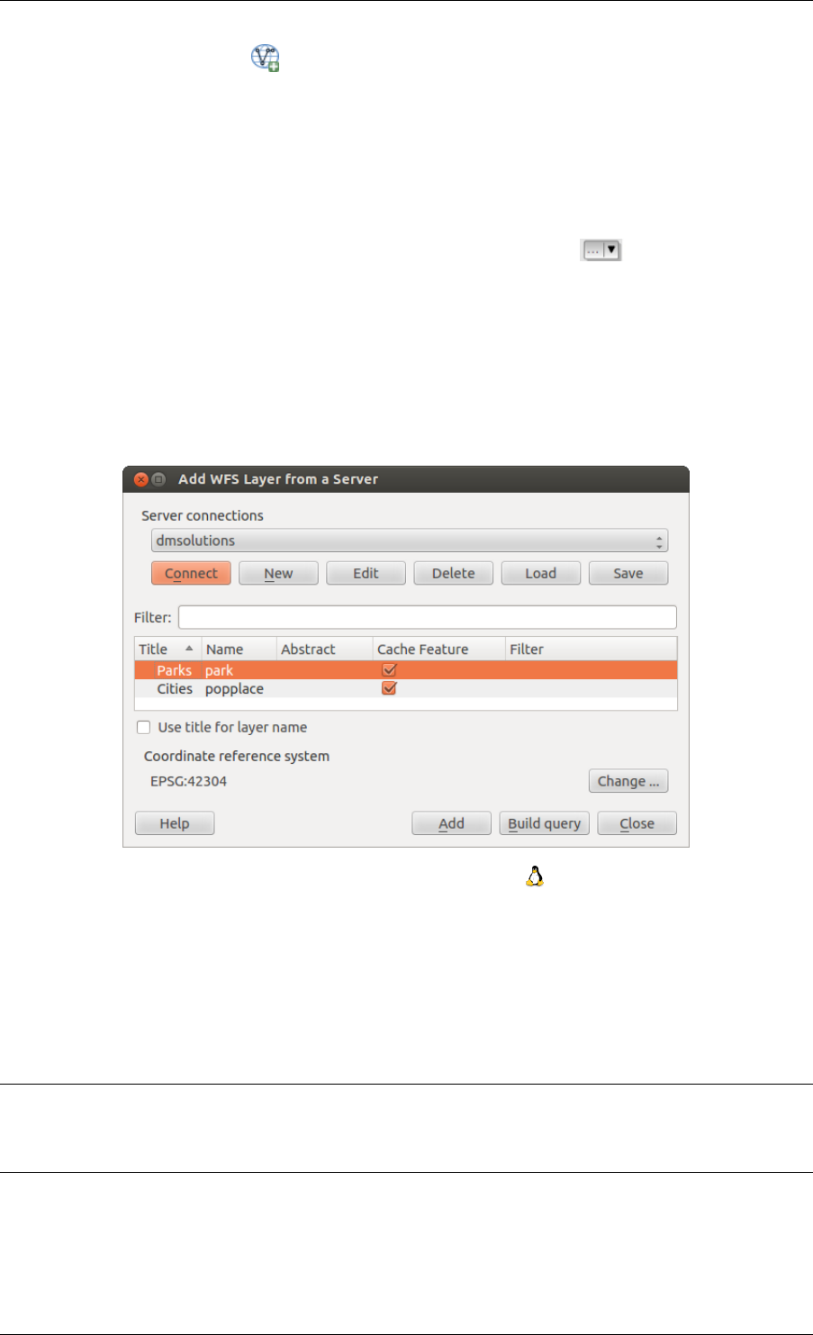
QGIS User Guide, Publicación 2.8
1. Haga clic en la herramienta Añadir capa WFS en la barra de herramientas Capas. El diálogo Añadir capa
WFS de un servidor aparecera.
2. Haga clic en [Nuevo].
3. Ingrese ‘DS Solutions’ como nombre.
4. Introducir la URL (véase más arriba).
5. Haga clic en [Aceptar].
6. Seleccione ‘DM Solutions’ de la lista desplegable Conexiones de servidor .
7. Haga clic en [Conectar]
8. Espere a que la capa de capas este poblada.
9. Seleccione la capa Parks en la lista.
10. Haga clic en [Aplicar] para añadir la capa al mapa.
Tenga en cuenta que cualquier configuración de proxy que pueda haber establecido en sus preferencias también
son reconocidos.
Figure 14.4: Añadir una capa WFS
Se dará cuenta el progreso de la descarga se visualiza en la parte inferior izquierda de la ventana principal de
QGIS. Una vez cargada la capa, puede identificar y seleccionar una provincia o dos y ver la tabla de atributos.
Sólo la versión 1.0.0 de WFS es compatible. Por ahora, no ha habido muchas pruebas contra versiones WFS
implementados en otros servidores de la CMA. Si tiene problemas con cualquier otro servidor WFS, por favor no
dude en ponerse en contacto con el equipo de desarrollo. Por favor, consulte la sección :ref: label_helpsupport
para más información sobre las listas de correo.
Truco: Encontrar servidores WFS
Puede encontrar servidores WFS adicionales al utilizar Google o su buscador favorito. Hay un número de listas
con URLs publicas, algunos de ellos son mantenidos y otro no.
.
160 Chapter 14. Trabajar con datos OGC

QGIS User Guide, Publicación 2.8
14.2 QGIS como Servidor de Datos OGC
QGIS Server es una aplicación de código abierto de WMS 1.3, WFS 1.0.0 y WCS 1 1.1.1, que además im-
plementa características cartográficas avanzadas para la cartografía temática. El QGIS Server es una aplicación
FastCGI/CGI (Common Gateway Interface) escrito en C++ que trabaja junto con un servidor web (por ejemplo,
Apache, Lighttpd). Cuenta con ayuda al complemento Python que permite el desarrollo mas rápido y eficiente
y despliegue de nuevas características. Es financiado por la EU project Orchestra, Sany y la ciudad de Uster en
Suiza
El servidor QGIS utiliza QGIS como back-end para la lógica de los SIG y de mapa de representación. Además,
la biblioteca Qt se utiliza para gráficos y para la plataforma independiente la programación en C++. En contraste
con otro software de WMS, el servidor de QGIS utiliza reglas cartográficos como un lenguaje de configuración,
tanto para la configuración del servidor y de las reglas cartográficas definidas por el usuario.
Como QGIS de escritorio y QGIS servidor utilizan las mismas librerías de visualización, los mapas que se publican
en la web tienen el mismo aspecto que el SIG de escritorio.
En uno de los siguientes manuales, proporcionaremos un ejemplo de configuración para configurar un servidor
QGIS. Por ahora, recomendamos leer una de las siguientes direcciones URLs para obtener más información:
•http://karlinapp.ethz.ch/qgis_wms/
•http://hub.qgis.org/projects/quantum-gis/wiki/QGIS_Server_Tutorial
•http://linfiniti.com/2010/08/qgis-mapserver-a-wms-server-for-the-masses/
14.2.1 Ejemplo de instalación en Debian Squeeze
En este punto, vamos a dar una ejemplo de instalación corta y simple de cómo hacerlo para una configuración de
trabajo mínima utilizando Apache 2 en Debian Squeeze. Muchos otros sistemas operativos proporcionan también
paquetes para QGIS Server. Si usted tiene que construir todo desde el código fuente, por favor, consulte las URLs
anteriores.
En primer lugar, añadir el siguiente repositorio SIG debian añadiendo el siguiente repositorio
$ cat /etc/apt/sources.list.d/debian-gis.list
deb http://qgis.org/debian trusty main
deb-src http://qgis.org/debian trusty main
$ # Add keys
$ sudo gpg --recv-key DD45F6C3
$ sudo gpg --export --armor DD45F6C3 | sudo apt-key add -
$ # Update package list
$ sudo apt-get update && sudo apt-get upgrade
Ahora, instalar QGIS-Server:
$ sudo apt-get install qgis-server python-qgis
La instalación de un complemento de ejemplo HelloWorld para probar los servidores. Se puede crear un direc-
torio para mantener los complementos del servidor. Esto se especificará en la configuración del host virtual y
transmitirlo al servidor a través de una variable de entorno.
$ sudo mkdir -p /opt/qgis-server/plugins
$ cd /opt/qgis-server/plugins
$ sudo wget https://github.com/elpaso/qgis-helloserver/archive/master.zip
$ # In case unzip was not installed before:
$ sudo apt-get install unzip
$ sudo unzip master.zip
$ sudo mv qgis-helloserver-master HelloServer
14.2. QGIS como Servidor de Datos OGC 161

QGIS User Guide, Publicación 2.8
Instalar el servidor Apache en un host virtual separado que escuche en el puerto 80. Habilitar el módulo de
reescritura de pasar encabezados HTTP BASIC de autenticación:
$ sudo a2enmod rewrite
$ cat /etc/apache2/conf-available/qgis-server-port.conf
Listen 80
$ sudo a2enconf qgis-server-port
Esta es la configuración del host virtual, almacenado en /etc/apache2/sites-available/001-qgis-server.conf
:
<VirtualHost *:80>
ServerAdmin webmaster@localhost
DocumentRoot /var/www/html
ErrorLog ${APACHE_LOG_DIR}/qgis-server-error.log
CustomLog ${APACHE_LOG_DIR}/qgis-server-access.log combined
# Longer timeout for WPS... default = 40
FcgidIOTimeout 120
FcgidInitialEnv LC_ALL "en_US.UTF-8"
FcgidInitialEnv PYTHONIOENCODING UTF-8
FcgidInitialEnv LANG "en_US.UTF-8"
FcgidInitialEnv QGIS_DEBUG 1
FcgidInitialEnv QGIS_SERVER_LOG_FILE /tmp/qgis-000.log
FcgidInitialEnv QGIS_SERVER_LOG_LEVEL 0
FcgidInitialEnv QGIS_PLUGINPATH "/opt/qgis-server/plugins"
# ABP: needed for QGIS HelloServer plugin HTTP BASIC auth
<IfModule mod_fcgid.c>
RewriteEngine on
RewriteCond %{HTTP:Authorization} .
RewriteRule .*- [E=HTTP_AUTHORIZATION:%{HTTP:Authorization}]
</IfModule>
ScriptAlias /cgi-bin/ /usr/lib/cgi-bin/
<Directory "/usr/lib/cgi-bin">
AllowOverride All
Options +ExecCGI -MultiViews +FollowSymLinks
# for apache2 > 2.4
Require all granted
#Allow from all
</Directory>
</VirtualHost>
Ahora habilitar el host virtual y reiniciar Apache:
$ sudo a2ensite 001-qgis-server
$ sudo service apache2 restart
Probar el servidor con el complemento HelloWorld:
$ wget -q -O - "http://localhost/cgi-bin/qgis_mapserv.fcgi?SERVICE=HELLO"
HelloServer!
Se puede echar un vistazo al GetCapabilities predeterminado del servidor QGIS en :
http://localhost/cgi-bin/qgis_mapserv.fcgi?SERVICE=WMS&VERSION=1.3.0&REQUEST=GetCapabilities
Truco: Si se trabaja con objetos espaciales que tienen muchos nodos después de modificar y añadir un nuevo
objeto fallará. En este caso, es posible insertar el siguiente código al archivo 001-qgis-server.conf :
<IfModule mod_fcgid.c>
FcgidMaxRequestLen 26214400
FcgidConnectTimeout 60
</IfModule>
162 Chapter 14. Trabajar con datos OGC
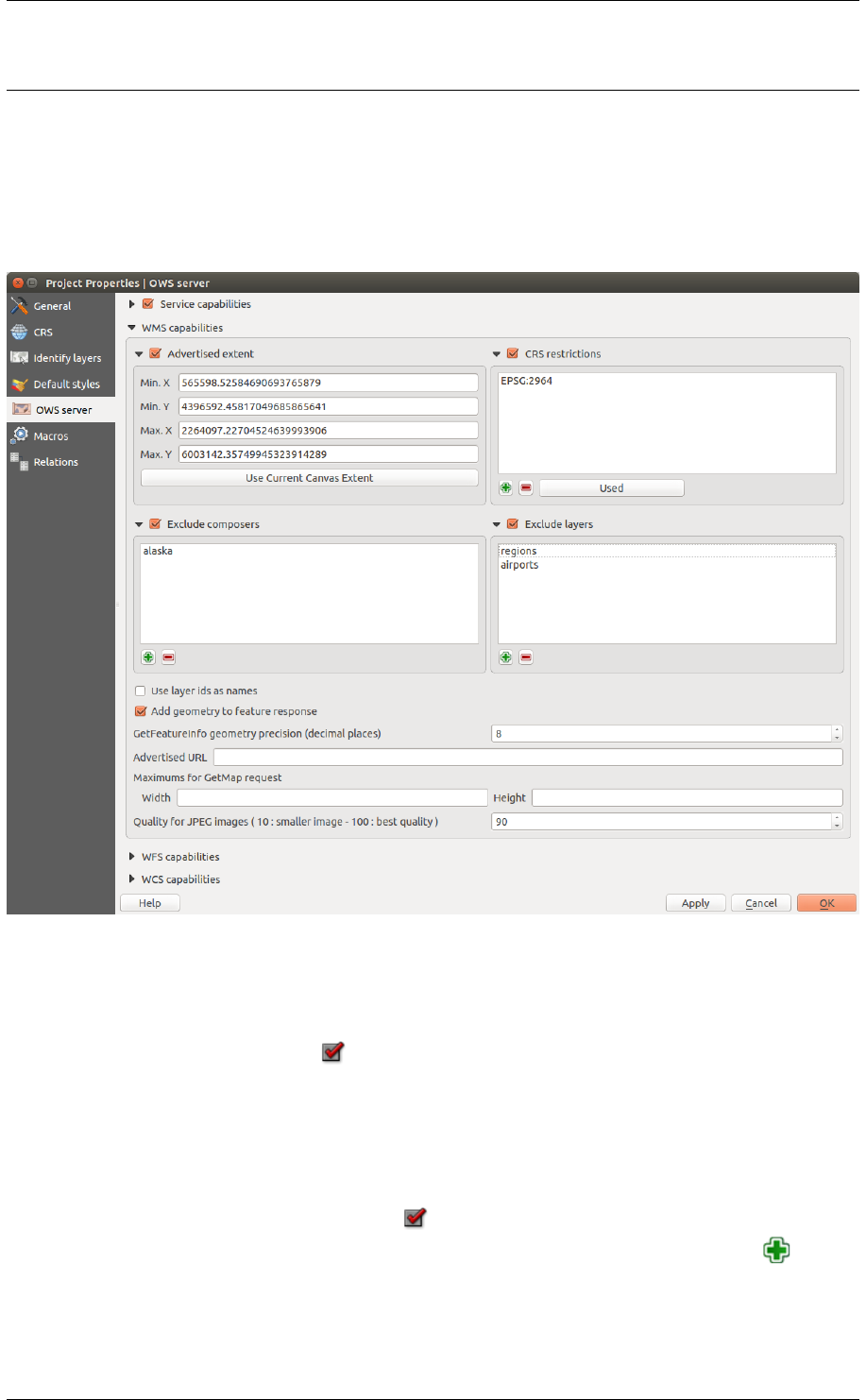
QGIS User Guide, Publicación 2.8
14.2.2 Crear un WMS/WFS/WCS desde un proyecto QGIS
Para proveer un nuevo servidor QGIS WMS, WFS o WCS, tenemos que crear un archivo de proyecto QGIS con
algunos datos. Aquí, utilizamos el archivo shape ‘Alaska’ del conjunto de datos de ejemplo de QGIS. Definir los
colores y estilos de las capas en QGIS y el SRC del proyecto, si aun no se ha definido.
Figure 14.5: Definiciones para un proyecto QGIS de Servidor WMS/WFS/WCS (KDE)
Luego, vaya al menú OWS Server del diálogo Proyecto →Propiedades del Proyecto y proporciona información
acerca del OWS en los campos de abajo Capacidades del Servicio. Esto aparecera en la respuesta de GetCapabili-
ties del WMS, WFS o WCS. Si no marca Capacidades del servicio, el servidor QGIS utilizará la información
dada en el archivo wms_metadata.xml ubicado en la carpeta cgi-bin.
WMS capacidades
En la sección Capacidades WMS, puede definir la extensión anunciada en la respuesta del GetCapabilities del
WMS mediante el ingreso de los valores mínimo y máximo de X y Y en los campos en extensión anunciada.
Al hacer clic en Usar la extensión de la vista del mapa actual establece estos valores de la extensión actual
mostrada en la vista del mapa de QGIS. Al marcar Restricciones SRC, puede restringir en que los sistemas
de coordenadas de referencia (SRC) del servidor QGIS ofrecerá representar mapas. Utilice el botón de abajo
para seleccionar aquellos SRC del selector de Sistemas de Referencia de Coordenadas, o haga clic en Usado y
añada los SRC utilizados en el proyecto QGIS a la lista.
Si usted tiene un diseños de impresión definidas en el proyecto, se enumerarán en la respuesta GetCapabilities, y
pueden ser utilizados por la solicitud GetPrint para crear impresiones, utilizando uno de los diseños de impresión
14.2. QGIS como Servidor de Datos OGC 163
QGIS User Guide, Publicación 2.8
como una plantilla. Esta es una extensión especifica de QGIS de la especificación WMS 1.3.0. Si desea excluir
cualquier diseñador de impresión de ser publicado por el WMS, marque Excluir diseñadores y haga clic en el
botón de abajo . A continuación, seleccione un diseñador de impresión desde el diálogo Seleccionar diseñador
de impresión para añadirlo a la lista de diseñadores excluidos.
Si desea excluir alguna capa o grupo de capas de ser publicadas por el WMS, marque Excluir capas y haga
clic en el botón de abajo . Esto abre el diálogo Seleccionar capas y grupos restringidos, que le permite elegir
las capas y grupos que no desea que sean publicados. Utilice la tecla Shift o la tecla Ctrl si desea seleccionar
múltiples entradas a la vez.
Puede recibir la solicitud de GetFeatureInfo como texto plano, XML y GML. Por omisión el formato es XML,
texto o GML depende del formato de salida seleccionado para la petición GetFeatureInfo.
Si desea, puede marcar Añadir geometría a la repuesta del objeto. Este incluirá en la respuesta GetFeatureInfo
las geometrías de las características en un formato de texto. Si quiere el servidor QGIS para anunciar URLs de
peticiones especificas en la respuesta WMS GetCapabilities, introduzca la URL correspondiente en el campo URL
anunciada. Por otra parte, puede restringir el tamaño máximo de los mapas devueltos en la solicitud GetMap al
introducir el ancho y altura máxima en los campos correspondientes en Máximos para la solicitud GetMap.
Si una de sus capas utiliza Avisos del mapa (por ejemplo, mostrar texto usando expresiones) este será incluido
dentro de la salida GetFeatureInfo. Si la capa utiliza un valor del mapa para uno de sus atributos, también esta
información será mostrada en la salida GetFeatureInfo.
QGIS support the following request for WMS service:
• GetCapabilities
• GetMap
• GetFeatureInfo
• GetLegendGraphic (perfil SLD)
• DescribeLayer (perfil SLD)
• GetStyles (perfil QGIS personalizado)
WFS capacidades
En el área Capacidades WFS, puede seleccionar las capas que desee publicar como WFS, y especificar si permitirá
la actualización, inserción y eliminación de operaciones. Si introduce una URL en el campo URL anunciada de la
sección Capacidades WFS, el Servidor QGIS anunciará esta URL especifica en la respuesta de WFS GetCapabil-
ities.
QGIS support the following request for WFS service:
• GetCapabilities
• DescribeFeatureType
• GetFeature
• Transacción
WCS capacidades
En el área Capacidades WCS, puede seleccionar las capas que desee publicar como WCS. Si introduce una URL
en el campo URL anunciada de la sección Capacidades WCS, el Servidor QGIS anunciará la URL especifica en
la respuesta de WCS GetCapabilities.
Ahora, guardarmos la sesión en un archivo de proyecto alaska.qgs. Para proveer el proyecto como
WMS/WFS, creamos una nueva carpeta /usr/lib/cgi-bin/project con privilegios de administrados y
añadimos el archivo del proyecto alaska.qgs y copiamos del archivo qgis_mapserv.fcgi - eso es todo.
Ahora probaremos nuestro proyecto WMS, WFS y WCS. Añadir el WMS, WFS y WCS como se describe en
Cargando capas WMS/WMTS,Cliente WFS y WFS-T yWCT Cliente a QGIS y cargar los datos. La URL es:
164 Chapter 14. Trabajar con datos OGC

QGIS User Guide, Publicación 2.8
http://localhost/cgi-bin/project/qgis_mapserv.fcgi
QGIS support the following request for WCS service:
• GetCapabilities
• DescribeCoverage
• GetCoverage
Ajuste fino de OWS
Para capas vectoriales, el menú Campos del diálogo Capa→Propiedades permitirá definir cada atributo si será
publicado o no. Por omisión, todos los atributos están publicados por WMS y WFS. Si desea especificar que un
atributo no sea publicado, demarque la casilla de verificación correspondiente en la columna WMS oWFS.
Puede superponer una marca de agua sobre el mapa producido por WMS al añadir anotaciones de texto o anota-
ciones SVG para el archivo del proyecto. Vea la sección Herramientas de Anotación en Herramientas generales
para obtener instrucciones en la creación de anotaciones. Para que las anotaciones sean desplegadas como marca
de agua en el WMS de salida, al marcar la caja Fijar posición del mapa en el diálogo Anotaciones de texto debe
ser desmarcada. Esto se puede acceder al hacer doble clic en la anotación mientras una de las herramientas de
anotación esta activa. Para anotaciones SVG, necesitará configurar el proyecto para guardar rutas absolutas (en
el menú General del diálogo Proyecto→Propiedades del proyecto) o para modificar manualmente la ruta de la
imagen SVG de una manera que representa una ruta relativa válida.
Parámetros extra soportados por la petición GetMap del WMS
En la petición GetMap del WMS, el servidor QGIS acepta un par de parámetros adicionales ademas de los
parámetros estándar de acuerdo a la especificación OGC WMS 1.3.0:
• Parámetro MAP: Similar a MapServer, el parámetro MAP se puede utilizar para especificar la ruta al archivo
del proyecto QGIS. Puede especificar una ruta absoluta o una ruta relativa a la ubicación del ejecutable del
servidor (qgis_mapserv.fcgi). Si no especifica, el Servidor QGIS busca archivos .qgs en el directorio
donde se encuentra el ejecutable del servidor.
Ejemplo:
http://localhost/cgi-bin/qgis_mapserv.fcgi?\
REQUEST=GetMap&MAP=/home/qgis/mymap.qgs&...
• Parámetro DPI: El parámetro DPI se puede utilizar para especificar la resolución de la solicitud de salida.
Ejemplo:
http://localhost/cgi-bin/qgis_mapserv.fcgi?REQUEST=GetMap&DPI=300&...
• Parámetro OPACITIES: La opacidad se puede establecer en una capa o nivel de grupo. Los valores permi-
tidos van de 0 (completamente transparente) a 255 (totalmente opaco).
Ejemplo:
http://localhost/cgi-bin/qgis_mapserv.fcgi?\
REQUEST=GetMap&LAYERS=mylayer1,mylayer2&OPACITIES=125,200&...
Registro del servidor QGIS
Para registrar solicitudes enviadas al servidor, establecer las siguientes variables de entorno:
•QGIS_SERVER_LOG_FILE: Especifica la ruta y el nombre de archivo. Comprobar que el servidor tiene
los permisos apropiados para escritura de archivo. El archivo debe ser creado automáticamente, sólo envié
algunas solicitudes al servidor. Si no está allá, verifique los permisos.
14.2. QGIS como Servidor de Datos OGC 165

QGIS User Guide, Publicación 2.8
•QGIS_SERVER_LOG_LEVEL: Especifica el nivel de registro deseado. los valores disponibles son:
–0 INFO (registrar todas las solicitudes),
–1 ADVERTENCIA,
–2 CRÍTICA (Registrar sólo errores críticos, adecuado para fines de producción)
Ejemplo:
SetEnv QGIS_SERVER_LOG_FILE /var/tmp/qgislog.txt
SetEnv QGIS_SERVER_LOG_LEVEL 0
Nota
• ¡Al usar el módulo Fcgid utilice FcgidInitialEnv en lugar de SetEnv!
• El registro del servidor también está habilitado si el ejecutable está compilado en modo de lanzamiento.
Variables de entorno
•QGIS_OPTIONS_PATH: La variable especifica la ruta al directorio con los ajustes. Funciona de
la misma forma como aplicación QGIS –optionspath. Esta buscando el archivo de configuración en
<QGIS_OPTIONS_PATH>/QGIS/QGIS2.ini. Por ejemplo, para establecer el servidor QGIS en Apache
utilizar el archivo de configuración en /path/to/config/QGIS/QGIS2.ini, añadir a configuración de Apache:
SetEnv QGIS_OPTIONS_PATH "/path/to/config/"
.
166 Chapter 14. Trabajar con datos OGC
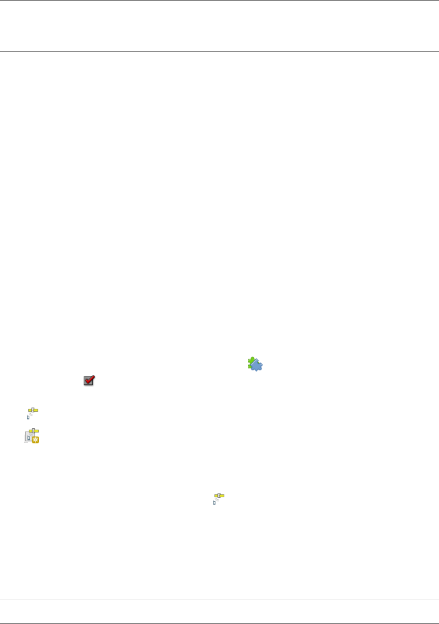
CHAPTER 15
Trabajar con datos GPS
.
15.1 GPS Plugin
15.1.1 What is GPS?
GPS, the Global Positioning System, is a satellite-based system that allows anyone with a GPS receiver to find their
exact position anywhere in the world. GPS is used as an aid in navigation, for example in airplanes, in boats and
by hikers. The GPS receiver uses the signals from the satellites to calculate its latitude, longitude and (sometimes)
elevation. Most receivers also have the capability to store locations (known as waypoints), sequences of locations
that make up a planned route and a tracklog or track of the receiver’s movement over time. Waypoints, routes
and tracks are the three basic feature types in GPS data. QGIS displays waypoints in point layers, while routes
and tracks are displayed in linestring layers.
15.1.2 Loading GPS data from a file
There are dozens of different file formats for storing GPS data. The format that QGIS uses is called GPX (GPS
eXchange format), which is a standard interchange format that can contain any number of waypoints, routes and
tracks in the same file.
To load a GPX file, you first need to load the plugin. Plugins →Plugin Manager... opens the Plugin Manager
Dialog. Activate the GPS Tools checkbox. When this plugin is loaded, a button with a small handheld GPS
device will show up in the toolbar and in Layer →Create Layer →:
•GPS Tools
•Create new GPX Layer
For working with GPS data, we provide an example GPX file available in the QGIS sample dataset:
qgis_sample_data/gps/national_monuments.gpx. See section Datos de ejemplo for more infor-
mation about the sample data.
1. Select Vector →GPS →GPS Tools or click the GPS Tools icon in the toolbar and open the Load GPX file
tab (see figure_GPS_1).
2. Browse to the folder qgis_sample_data/gps/, select the GPX file national_monuments.gpx
and click [Open].
Use the [Browse...] button to select the GPX file, then use the checkboxes to select the feature types you want
to load from that GPX file. Each feature type will be loaded in a separate layer when you click [OK]. The file
national_monuments.gpx only includes waypoints.
167
QGIS User Guide, Publicación 2.8
Figure 15.1: The GPS Tools dialog window
Nota: GPS units allow you to store data in different coordinate systems. When downloading a GPX file
(from your GPS unit or a web site) and then loading it in QGIS, be sure that the data stored in the GPX
file uses WGS 84 (latitude/longitude). QGIS expects this, and it is the official GPX specification. See
http://www.topografix.com/GPX/1/1/.
15.1.3 GPSBabel
Since QGIS uses GPX files, you need a way to convert other GPS file formats to GPX. This can be done for many
formats using the free program GPSBabel, which is available at http://www.gpsbabel.org. This program can also
transfer GPS data between your computer and a GPS device. QGIS uses GPSBabel to do these things, so it is
recommended that you install it. However, if you just want to load GPS data from GPX files you will not need it.
Version 1.2.3 of GPSBabel is known to work with QGIS, but you should be able to use later versions without any
problems.
15.1.4 Importing GPS data
To import GPS data from a file that is not a GPX file, you use the tool Import other file in the GPS Tools dialog.
Here, you select the file that you want to import (and the file type), which feature type you want to import from it,
where you want to store the converted GPX file and what the name of the new layer should be. Note that not all
GPS data formats will support all three feature types, so for many formats you will only be able to choose between
one or two types.
15.1.5 Downloading GPS data from a device
QGIS can use GPSBabel to download data from a GPS device directly as new vector layers. For this we use the
Download from GPS tab of the GPS Tools dialog (see Figure_GPS_2). Here, we select the type of GPS device,
the port that it is connected to (or USB if your GPS supports this), the feature type that you want to download, the
GPX file where the data should be stored, and the name of the new layer.
The device type you select in the GPS device menu determines how GPSBabel tries to communicate with your
GPS device. If none of the available types work with your GPS device, you can create a new type (see section
Defining new device types).
The port may be a file name or some other name that your operating system uses as a reference to the physical port
in your computer that the GPS device is connected to. It may also be simply USB, for USB-enabled GPS units.
• On Linux, this is something like /dev/ttyS0 or /dev/ttyS1.
• On Windows, it is COM1 or COM2.
168 Chapter 15. Trabajar con datos GPS

QGIS User Guide, Publicación 2.8
Figure 15.2: The download tool
When you click [OK], the data will be downloaded from the device and appear as a layer in QGIS.
15.1.6 Uploading GPS data to a device
You can also upload data directly from a vector layer in QGIS to a GPS device using the Upload to GPS tab of
the GPS Tools dialog. To do this, you simply select the layer that you want to upload (which must be a GPX
layer), your GPS device type, and the port (or USB) that it is connected to. Just as with the download tool, you
can specify new device types if your device isn’t in the list.
This tool is very useful in combination with the vector-editing capabilities of QGIS. It allows you to load a map,
create waypoints and routes, and then upload them and use them on your GPS device.
15.1.7 Defining new device types
There are lots of different types of GPS devices. The QGIS developers can’t test all of them, so if you have one
that does not work with any of the device types listed in the Download from GPS and Upload to GPS tools, you
can define your own device type for it. You do this by using the GPS device editor, which you start by clicking
the [Edit devices] button in the download or the upload tab.
To define a new device, you simply click the [New device] button, enter a name, enter download and upload
commands for your device, and click the [Update device] button. The name will be listed in the device menus in
the upload and download windows – it can be any string. The download command is the command that is used to
download data from the device to a GPX file. This will probably be a GPSBabel command, but you can use any
other command line program that can create a GPX file. QGIS will replace the keywords %type,%in, and %out
when it runs the command.
%type will be replaced by -w if you are downloading waypoints, -r if you are downloading routes and -t if
you are downloading tracks. These are command-line options that tell GPSBabel which feature type to download.
%in will be replaced by the port name that you choose in the download window and %out will be replaced by
the name you choose for the GPX file that the downloaded data should be stored in. So, if you create a device
type with the download command gpsbabel %type -i garmin -o gpx %in %out (this is actually the
download command for the predefined device type ‘Garmin serial’) and then use it to download waypoints from
port /dev/ttyS0 to the file output.gpx, QGIS will replace the keywords and run the command gpsbabel
-w -i garmin -o gpx /dev/ttyS0 output.gpx.
The upload command is the command that is used to upload data to the device. The same keywords are used, but
%in is now replaced by the name of the GPX file for the layer that is being uploaded, and %out is replaced by
the port name.
You can learn more about GPSBabel and its available command line options at http://www.gpsbabel.org.
Once you have created a new device type, it will appear in the device lists for the download and upload tools.
15.1. GPS Plugin 169

QGIS User Guide, Publicación 2.8
15.1.8 Download of points/tracks from GPS units
As described in previous sections QGIS uses GPSBabel to download points/tracks directly in the project. QGIS
comes out of the box with a pre-defined profile to download from Garmin devices. Unfortunately there is a bug
#6318 that does not allow create other profiles, so downloading directly in QGIS using the GPS Tools is at the
moment limited to Garmin USB units.
Garmin GPSMAP 60cs
MS Windows
Install the Garmin USB drivers from http://www8.garmin.com/support/download_details.jsp?id=591
Connect the unit. Open GPS Tools and use type=garmin serial and port=usb: Fill the fields Layer
name and Output file. Sometimes it seems to have problems saving in a certain folder, using something like
c:\temp usually works.
Ubuntu/Mint GNU/Linux
It is first needed an issue about the permissions of the device, as described at
https://wiki.openstreetmap.org/wiki/USB_Garmin_on_GNU/Linux. You can try to create a file
/etc/udev/rules.d/51-garmin.rules containing this rule
ATTRS{idVendor}=="091e", ATTRS{idProduct}=="0003", MODE="666"
After that is necessary to be sure that the garmin_gps kernel module is not loaded
rmmod garmin_gps
and then you can use the GPS Tools. Unfortunately there seems to be a bug #7182 and usually QGIS freezes
several times before the operation work fine.
BTGP-38KM datalogger (only Bluetooth)
MS Windows
The already referred bug does not allow to download the data from within QGIS, so it is needed to use GPSBabel
from the command line or using its interface. The working command is
gpsbabel -t -i skytraq,baud=9600,initbaud=9600 -f COM9 -o gpx -F C:/GPX/aaa.gpx
Ubuntu/Mint GNU/Linux
Use same command (or settings if you use GPSBabel GUI) as in Windows. On Linux it maybe somehow common
to get a message like
skytraq: Too many read errors on serial port
it is just a matter to turn off and on the datalogger and try again.
BlueMax GPS-4044 datalogger (both BT and USB)
MS Windows
Nota: It needs to install its drivers before using it on Windows 7. See in the manufacturer site for the proper
download.
Downloading with GPSBabel, both with USB and BT returns always an error like
gpsbabel -t -i mtk -f COM12 -o gpx -F C:/temp/test.gpx
mtk_logger: Can’t create temporary file data.bin
Error running gpsbabel: Process exited unsucessfully with code 1
170 Chapter 15. Trabajar con datos GPS
QGIS User Guide, Publicación 2.8
Ubuntu/Mint GNU/Linux
With USB
After having connected the cable use the dmesg command to understand what port is being used, for example
/dev/ttyACM3. Then as usual use GPSBabel from the CLI or GUI
gpsbabel -t -i mtk -f /dev/ttyACM3 -o gpx -F /home/user/bluemax.gpx
With Bluetooth
Use Blueman Device Manager to pair the device and make it available through a system port, then run GPSBabel
gpsbabel -t -i mtk -f /dev/rfcomm0 -o gpx -F /home/user/bluemax_bt.gpx
.
15.2 Live GPS tracking
To activate live GPS tracking in QGIS, you need to select Settings →Panels GPS information. You will get a
new docked window on the left side of the canvas.
There are four possible screens in this GPS tracking window:
• GPS position coordinates and an interface for manually entering vertices and features
• GPS signal strength of satellite connections
• GPS polar screen showing number and polar position of satellites
• GPS options screen (see figure_gps_options)
With a plugged-in GPS receiver (has to be supported by your operating system), a simple click on [Connect] con-
nects the GPS to QGIS. A second click (now on [Disconnect]) disconnects the GPS receiver from your computer.
For GNU/Linux, gpsd support is integrated to support connection to most GPS receivers. Therefore, you first have
to configure gpsd properly to connect QGIS to it.
Advertencia: If you want to record your position to the canvas, you have to create a new vector layer first
and switch it to editable status to be able to record your track.
15.2.1 Position and additional attributes
If the GPS is receiving signals from satellites, you will see your position in latitude, longitude and altitude
together with additional attributes.
15.2.2 GPS signal strength
Here, you can see the signal strength of the satellites you are receiving signals from.
15.2.3 GPS polar window
If you want to know where in the sky all the connected satellites are, you have to switch to the polar screen.
You can also see the ID numbers of the satellites you are receiving signals from.
15.2. Live GPS tracking 171
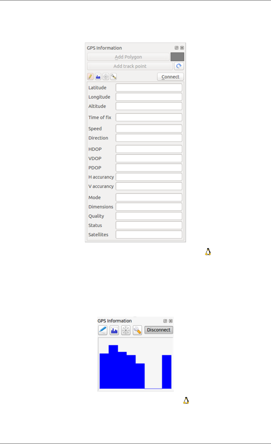
QGIS User Guide, Publicación 2.8
Figure 15.3: GPS tracking position and additional attributes
Figure 15.4: GPS tracking signal strength
172 Chapter 15. Trabajar con datos GPS
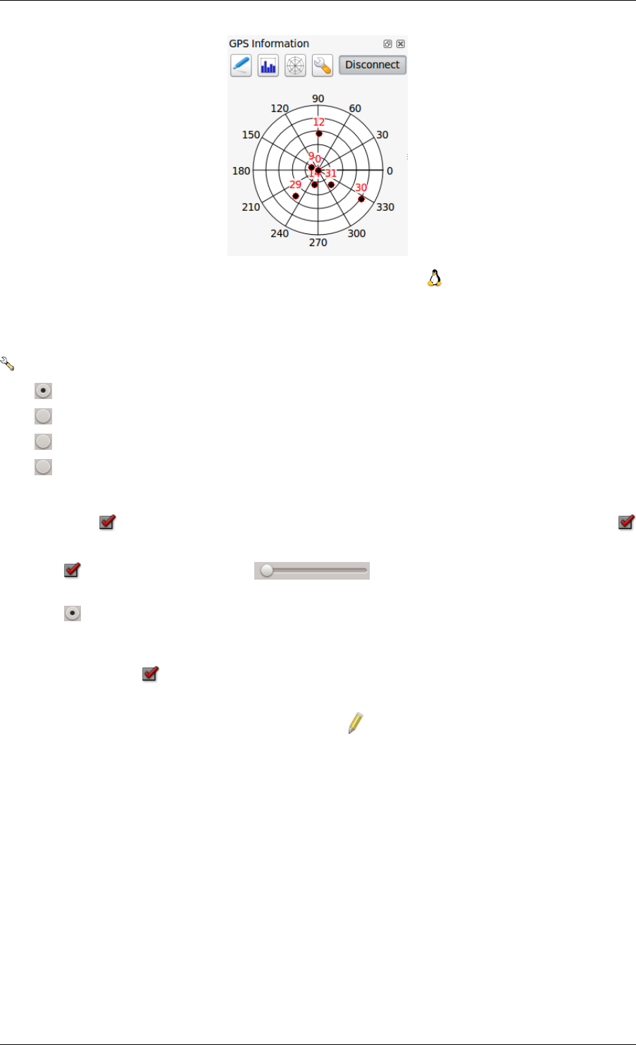
QGIS User Guide, Publicación 2.8
Figure 15.5: GPS tracking polar window
15.2.4 GPS options
In case of connection problems, you can switch between:
•Autodetect
•Internal
•Serial device
•gpsd (selecting the Host, Port and Device your GPS is connected to)
A click on [Connect] again initiates the connection to the GPS receiver.
You can activate Automatically save added features when you are in editing mode. Or you can activate
Automatically add points to the map canvas with a certain width and color.
Activating Cursor, you can use a slider to shrink and grow the position cursor on the
canvas.
Activating Map centering allows you to decide in which way the canvas will be updated. This includes
‘always’, ‘when leaving’, if your recorded coordinates start to move out of the canvas, or ‘never’, to keep map
extent.
Finally, you can activate Log file and define a path and a file where log messages about the GPS tracking are
logged.
If you want to set a feature manually, you have to go back to Position and click on [Add Point] or [Add track
point].
15.2.5 Connect to a Bluetooth GPS for live tracking
With QGIS you can connect a Bluetooth GPS for field data collection. To perform this task you need a GPS
Bluetooth device and a Bluetooth receiver on your computer.
At first you must let your GPS device be recognized and paired to the computer. Turn on the GPS, go to the
Bluetooth icon on your notification area and search for a New Device.
On the right side of the Device selection mask make sure that all devices are selected so your GPS unit will
probably appear among those available. In the next step a serial connection service should be available, select it
and click on [Configure] button.
Remember the number of the COM port assigned to the GPS connection as resulting by the Bluetooth properties.
After the GPS has been recognized, make the pairing for the connection. Usually the autorization code is 0000.
15.2. Live GPS tracking 173
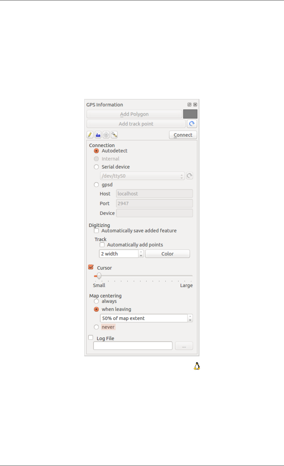
QGIS User Guide, Publicación 2.8
Figure 15.6: GPS tracking options window
174 Chapter 15. Trabajar con datos GPS
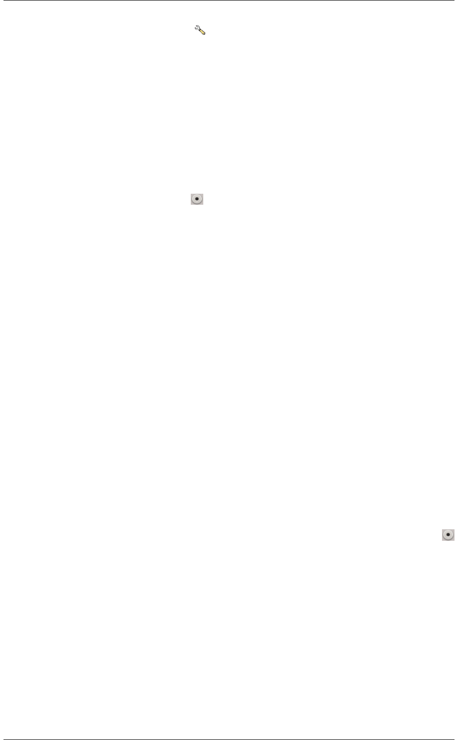
QGIS User Guide, Publicación 2.8
Now open GPS information panel and switch to GPS options screen. Select the COM port assigned to the GPS
connection and click the [Connect]. After a while a cursor indicating your position should appear.
If QGIS can’t receive GPS data, then you should restart your GPS device, wait 5-10 seconds then try to connect
again. Usually this solution work. If you receive again a connection error make sure you don’t have another
Bluetooth receiver near you, paired with the same GPS unit.
15.2.6 Using GPSMAP 60cs
MS Windows
Easiest way to make it work is to use a middleware (freeware, not open) called GPSGate.
Launch the program, make it scan for GPS devices (works for both USB and BT ones) and then in QGIS just click
[Connect] in the Live tracking panel using the Autodetect mode.
Ubuntu/Mint GNU/Linux
As for Windows the easiest way is to use a server in the middle, in this case GPSD, so
sudo apt-get install gpsd
Then load the garmin_gps kernel module
sudo modprobe garmin_gps
And then connect the unit. Then check with dmesg the actual device being used bu the unit, for example
/dev/ttyUSB0. Now you can launch gpsd
gpsd /dev/ttyUSB0
And finally connect with the QGIS live tracking tool.
15.2.7 Using BTGP-38KM datalogger (only Bluetooth)
Using GPSD (under Linux) or GPSGate (under Windows) is effortless.
15.2.8 Using BlueMax GPS-4044 datalogger (both BT and USB)
MS Windows
The live tracking works for both USB and BT modes, by using GPSGate or even without it, just use the
Autodetect mode, or point the tool the right port.
Ubuntu/Mint GNU/Linux
For USB
The live tracking works both with GPSD
gpsd /dev/ttyACM3
or without it, by connecting the QGIS live tracking tool directly to the device (for example /dev/ttyACM3).
For Bluetooth
The live tracking works both with GPSD
15.2. Live GPS tracking 175

QGIS User Guide, Publicación 2.8
gpsd /dev/rfcomm0
or without it, by connecting the QGIS live tracking tool directly to the device (for example /dev/rfcomm0).
.
176 Chapter 15. Trabajar con datos GPS
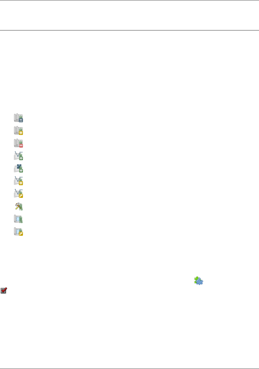
CHAPTER 16
GRASS GIS Integration
The GRASS plugin provides access to GRASS GIS databases and functionalities (see GRASS-PROJECT in Ref-
erencias bibliográficas y web). This includes visualizing GRASS raster and vector layers, digitizing vector layers,
editing vector attributes, creating new vector layers and analysing GRASS 2-D and 3-D data with more than 400
GRASS modules.
In this section, we’ll introduce the plugin functionalities and give some examples of managing and working with
GRASS data. The following main features are provided with the toolbar menu when you start the GRASS plugin,
as described in section sec_starting_grass:
•Open mapset
•New mapset
•Close mapset
•Add GRASS vector layer
•Add GRASS raster layer
•Create new GRASS vector
•Edit GRASS vector layer
•Open GRASS tools
•Display current GRASS region
•Edit current GRASS region
16.1 Starting the GRASS plugin
To use GRASS functionalities and/or visualize GRASS vector and raster layers in QGIS, you must select and load
the GRASS plugin with the Plugin Manager. Therefore, go to the menu Plugins →Manage Plugins, select
GRASS and click [OK].
You can now start loading raster and vector layers from an existing GRASS LOCATION (see section
sec_load_grassdata). Or, you can create a new GRASS LOCATION with QGIS (see section Creating a new
GRASS LOCATION) and import some raster and vector data (see section Importing data into a GRASS LOCA-
TION) for further analysis with the GRASS Toolbox (see section The GRASS Toolbox).
177
QGIS User Guide, Publicación 2.8
16.2 Loading GRASS raster and vector layers
With the GRASS plugin, you can load vector or raster layers using the appropriate button on the toolbar menu.
As an example, we will use the QGIS Alaska dataset (see section Datos de ejemplo). It includes a small sample
GRASS LOCATION with three vector layers and one raster elevation map.
1. Create a new folder called grassdata, download the QGIS ‘Alaska’ dataset
qgis_sample_data.zip from http://download.osgeo.org/qgis/data/ and unzip the file into
grassdata.
2. Start QGIS.
3. If not already done in a previous QGIS session, load the GRASS plugin clicking on Plugins →Manage
Plugins and activate GRASS. The GRASS toolbar appears in the QGIS main window.
4. In the GRASS toolbar, click the Open mapset icon to bring up the MAPSET wizard.
5. For Gisdbase, browse and select or enter the path to the newly created folder grassdata.
6. You should now be able to select the LOCATION alaska and the MAPSET demo.
7. Click [OK]. Notice that some previously disabled tools in the GRASS toolbar are now enabled.
8. Click on Add GRASS raster layer, choose the map name gtopo30 and click [OK]. The elevation layer will
be visualized.
9. Click on Add GRASS vector layer, choose the map name alaska and click [OK]. The Alaska boundary
vector layer will be overlayed on top of the gtopo30 map. You can now adapt the layer properties as
described in chapter The Vector Properties Dialog (e.g., change opacity, fill and outline color).
10. Also load the other two vector layers, rivers and airports, and adapt their properties.
As you see, it is very simple to load GRASS raster and vector layers in QGIS. See the following sections for
editing GRASS data and creating a new LOCATION. More sample GRASS LOCATIONs are available at the
GRASS website at http://grass.osgeo.org/download/sample-data/.
Truco: GRASS Data Loading
If you have problems loading data or QGIS terminates abnormally, check to make sure you have loaded the
GRASS plugin properly as described in section Starting the GRASS plugin.
16.3 GRASS LOCATION and MAPSET
GRASS data are stored in a directory referred to as GISDBASE. This directory, often called grassdata, must
be created before you start working with the GRASS plugin in QGIS. Within this directory, the GRASS GIS
data are organized by projects stored in subdirectories called LOCATIONs. Each LOCATION is defined by its
coordinate system, map projection and geographical boundaries. Each LOCATION can have several MAPSETs
(subdirectories of the LOCATION) that are used to subdivide the project into different topics or subregions, or as
workspaces for individual team members (see Neteler & Mitasova 2008 in Referencias bibliográficas y web). In
order to analyze vector and raster layers with GRASS modules, you must import them into a GRASS LOCATION.
(This is not strictly true – with the GRASS modules r.external and v.external you can create read-only
links to external GDAL/OGR-supported datasets without importing them. But because this is not the usual way
for beginners to work with GRASS, this functionality will not be described here.)
16.3.1 Creating a new GRASS LOCATION
As an example, here is how the sample GRASS LOCATION alaska, which is projected in Albers Equal Area
projection with unit feet was created for the QGIS sample dataset. This sample GRASS LOCATION alaska
178 Chapter 16. GRASS GIS Integration
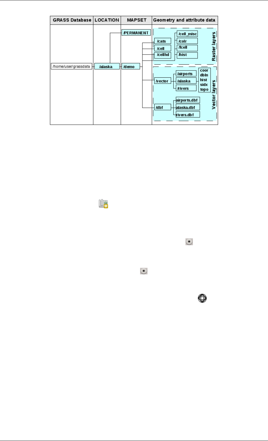
QGIS User Guide, Publicación 2.8
Figure 16.1: GRASS data in the alaska LOCATION
will be used for all examples and exercises in the following GRASS-related sections. It is useful to download and
install the dataset on your computer (see Datos de ejemplo).
1. Start QGIS and make sure the GRASS plugin is loaded.
2. Visualize the alaska.shp shapefile (see section Loading a Shapefile) from the QGIS Alaska dataset (see
Datos de ejemplo).
3. In the GRASS toolbar, click on the New mapset icon to bring up the MAPSET wizard.
4. Select an existing GRASS database (GISDBASE) folder grassdata, or create one for the new
LOCATION using a file manager on your computer. Then click [Next].
5. We can use this wizard to create a new MAPSET within an existing LOCATION (see section Adding
a new MAPSET) or to create a new LOCATION altogether. Select Create new location (see fig-
ure_grass_location_2).
6. Enter a name for the LOCATION – we used ‘alaska’ – and click [Next].
7. Define the projection by clicking on the radio button Projection to enable the projection list.
8. We are using Albers Equal Area Alaska (feet) projection. Since we happen to know that it is represented
by the EPSG ID 2964, we enter it in the search box. (Note: If you want to repeat this process for another
LOCATION and projection and haven’t memorized the EPSG ID, click on the CRS Status icon in the lower
right-hand corner of the status bar (see section Working with Projections)).
9. In Filter, insert 2964 to select the projection.
10. Click [Next].
11. To define the default region, we have to enter the LOCATION bounds in the north, south, east, and west
directions. Here, we simply click on the button [Set current |qg| extent], to apply the extent of the loaded
layer alaska.shp as the GRASS default region extent.
12. Click [Next].
13. We also need to define a MAPSET within our new LOCATION (this is necessary when creating a new
LOCATION). You can name it whatever you like - we used ‘demo’. GRASS automatically creates a special
MAPSET called PERMANENT, designed to store the core data for the project, its default spatial extent and
coordinate system definitions (see Neteler & Mitasova 2008 in Referencias bibliográficas y web).
14. Check out the summary to make sure it’s correct and click [Finish].
15. The new LOCATION, ‘alaska’, and two MAPSETs, ‘demo’ and ‘PERMANENT’, are created. The currently
opened working set is ‘demo’, as you defined.
16.3. GRASS LOCATION and MAPSET 179
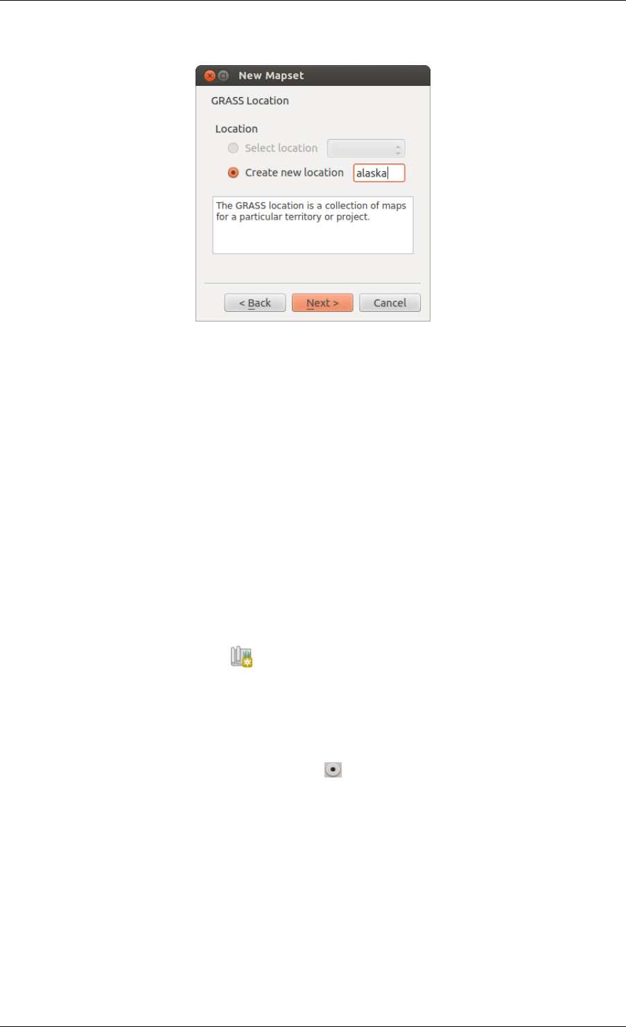
QGIS User Guide, Publicación 2.8
16. Notice that some of the tools in the GRASS toolbar that were disabled are now enabled.
Figure 16.2: Creating a new GRASS LOCATION or a new MAPSET in QGIS
If that seemed like a lot of steps, it’s really not all that bad and a very quick way to create a LOCATION. The
LOCATION ‘alaska’ is now ready for data import (see section Importing data into a GRASS LOCATION). You
can also use the already-existing vector and raster data in the sample GRASS LOCATION ‘alaska’, included in
the QGIS ‘Alaska’ dataset Datos de ejemplo, and move on to section The GRASS vector data model.
16.3.2 Adding a new MAPSET
A user has write access only to a GRASS MAPSET he or she created. This means that besides access to your own
MAPSET, you can read maps in other users’ MAPSETs (and they can read yours), but you can modify or remove
only the maps in your own MAPSET.
All MAPSETs include a WIND file that stores the current boundary coordinate values and the currently selected
raster resolution (see Neteler & Mitasova 2008 in Referencias bibliográficas y web, and section The GRASS region
tool).
1. Start QGIS and make sure the GRASS plugin is loaded.
2. In the GRASS toolbar, click on the New mapset icon to bring up the MAPSET wizard.
3. Select the GRASS database (GISDBASE) folder grassdata with the LOCATION ‘alaska’, where we
want to add a further MAPSET called ‘test’.
4. Click [Next].
5. We can use this wizard to create a new MAPSET within an existing LOCATION or to create a new
LOCATION altogether. Click on the radio button Select location (see figure_grass_location_2) and
click [Next].
6. Enter the name text for the new MAPSET. Below in the wizard, you see a list of existing MAPSETs and
corresponding owners.
7. Click [Next], check out the summary to make sure it’s all correct and click [Finish].
16.4 Importing data into a GRASS LOCATION
This section gives an example of how to import raster and vector data into the ‘alaska’ GRASS LOCATION
provided by the QGIS ‘Alaska’ dataset. Therefore, we use the landcover raster map landcover.img and the
vector GML file lakes.gml from the QGIS ‘Alaska’ dataset (see Datos de ejemplo).
180 Chapter 16. GRASS GIS Integration
QGIS User Guide, Publicación 2.8
1. Start QGIS and make sure the GRASS plugin is loaded.
2. In the GRASS toolbar, click the Open MAPSET icon to bring up the MAPSET wizard.
3. Select as GRASS database the folder grassdata in the QGIS Alaska dataset, as LOCATION ‘alaska’, as
MAPSET ‘demo’ and click [OK].
4. Now click the Open GRASS tools icon. The GRASS Toolbox (see section The GRASS Toolbox) dialog
appears.
5. To import the raster map landcover.img, click the module r.in.gdal in the Modules Tree tab. This
GRASS module allows you to import GDAL-supported raster files into a GRASS LOCATION. The module
dialog for r.in.gdal appears.
6. Browse to the folder raster in the QGIS ‘Alaska’ dataset and select the file landcover.img.
7. As raster output name, define landcover_grass and click [Run]. In the Output tab, you
see the currently running GRASS command r.in.gdal -o input=/path/to/landcover.img
output=landcover_grass.
8. When it says Succesfully finished, click [View output]. The landcover_grass raster layer is now
imported into GRASS and will be visualized in the QGIS canvas.
9. To import the vector GML file lakes.gml, click the module v.in.ogr in the Modules Tree tab. This
GRASS module allows you to import OGR-supported vector files into a GRASS LOCATION. The module
dialog for v.in.ogr appears.
10. Browse to the folder gml in the QGIS ‘Alaska’ dataset and select the file lakes.gml as OGR file.
11. As vector output name, define lakes_grass and click [Run]. You don’t have to care about the other
options in this example. In the Output tab you see the currently running GRASS command v.in.ogr -o
dsn=/path/to/lakes.gml output=lakes\_grass.
12. When it says Succesfully finished, click [View output]. The lakes_grass vector layer is now imported
into GRASS and will be visualized in the QGIS canvas.
16.5 The GRASS vector data model
It is important to understand the GRASS vector data model prior to digitizing.
In general, GRASS uses a topological vector model.
This means that areas are not represented as closed polygons, but by one or more boundaries. A boundary between
two adjacent areas is digitized only once, and it is shared by both areas. Boundaries must be connected and closed
without gaps. An area is identified (and labeled) by the centroid of the area.
Besides boundaries and centroids, a vector map can also contain points and lines. All these geometry elements
can be mixed in one vector and will be represented in different so-called ‘layers’ inside one GRASS vector map.
So in GRASS, a layer is not a vector or raster map but a level inside a vector layer. This is important to distinguish
carefully. (Although it is possible to mix geometry elements, it is unusual and, even in GRASS, only used in
special cases such as vector network analysis. Normally, you should prefer to store different geometry elements
in different layers.)
It is possible to store several ‘layers’ in one vector dataset. For example, fields, forests and lakes can be stored in
one vector. An adjacent forest and lake can share the same boundary, but they have separate attribute tables. It is
also possible to attach attributes to boundaries. An example might be the case where the boundary between a lake
and a forest is a road, so it can have a different attribute table.
The ‘layer’ of the feature is defined by the ‘layer’ inside GRASS. ‘Layer’ is the number which defines if there is
more than one layer inside the dataset (e.g., if the geometry is forest or lake). For now, it can be only a number. In
the future, GRASS will also support names as fields in the user interface.
Attributes can be stored inside the GRASS LOCATION as dBase or SQLite3 or in external database tables, for
example, PostgreSQL, MySQL, Oracle, etc.
16.5. The GRASS vector data model 181
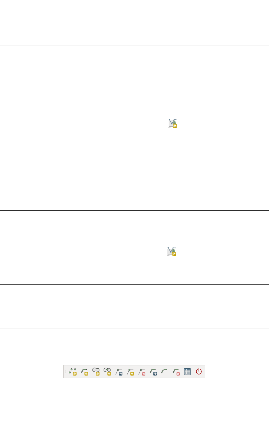
QGIS User Guide, Publicación 2.8
Attributes in database tables are linked to geometry elements using a ‘category’ value.
‘Category’ (key, ID) is an integer attached to geometry primitives, and it is used as the link to one key column in
the database table.
Truco: Learning the GRASS Vector Model
The best way to learn the GRASS vector model and its capabilities is to download one of the many GRASS
tutorials where the vector model is described more deeply. See http://grass.osgeo.org/documentation/manuals/ for
more information, books and tutorials in several languages.
16.6 Creating a new GRASS vector layer
To create a new GRASS vector layer with the GRASS plugin, click the Create new GRASS vector toolbar icon. Enter
a name in the text box, and you can start digitizing point, line or polygon geometries following the procedure
described in section Digitizing and editing a GRASS vector layer.
In GRASS, it is possible to organize all sorts of geometry types (point, line and area) in one layer, because GRASS
uses a topological vector model, so you don’t need to select the geometry type when creating a new GRASS vector.
This is different from shapefile creation with QGIS, because shapefiles use the Simple Feature vector model (see
section Creating new Vector layers).
Truco: Creating an attribute table for a new GRASS vector layer
If you want to assign attributes to your digitized geometry features, make sure to create an attribute table with
columns before you start digitizing (see figure_grass_digitizing_5).
16.7 Digitizing and editing a GRASS vector layer
The digitizing tools for GRASS vector layers are accessed using the Edit GRASS vector layer icon on the toolbar.
Make sure you have loaded a GRASS vector and it is the selected layer in the legend before clicking on the edit
tool. Figure figure_grass_digitizing_2 shows the GRASS edit dialog that is displayed when you click on the edit
tool. The tools and settings are discussed in the following sections.
Truco: Digitizing polygons in GRASS
If you want to create a polygon in GRASS, you first digitize the boundary of the polygon, setting the mode to ‘No
category’. Then you add a centroid (label point) into the closed boundary, setting the mode to ‘Next not used’.
The reason for this is that a topological vector model links the attribute information of a polygon always to the
centroid and not to the boundary.
Toolbar
In figure_grass_digitizing_1, you see the GRASS digitizing toolbar icons provided by the
GRASS plugin. Table table_grass_digitizing_1 explains the available functionalities.
Figure 16.3: GRASS Digitizing Toolbar
182 Chapter 16. GRASS GIS Integration
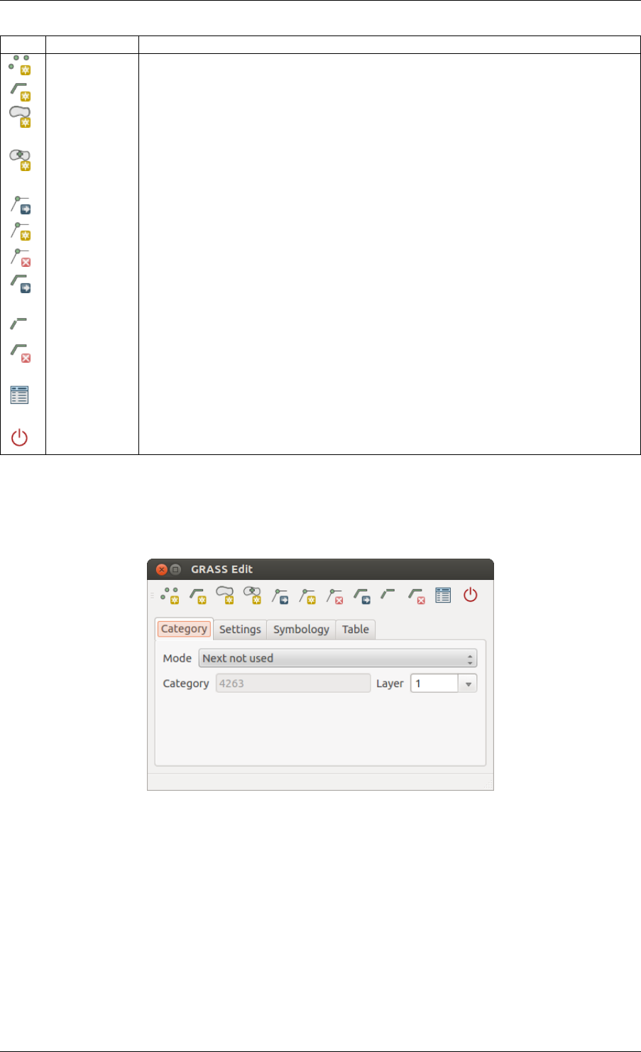
QGIS User Guide, Publicación 2.8
Icon Tool Purpose
New Point Digitize new point
New Line Digitize new line
New
Boundary
Digitize new boundary (finish by selecting new tool)
New
Centroid
Digitize new centroid (label existing area)
Move vertex Move one vertex of existing line or boundary and identify new position
Add vertex Add a new vertex to existing line
Delete vertex Delete vertex from existing line (confirm selected vertex by another click)
Move
element
Move selected boundary, line, point or centroid and click on new position
Split line Split an existing line into two parts
Delete
element
Delete existing boundary, line, point or centroid (confirm selected element by another
click)
Edit
attributes
Edit attributes of selected element (note that one element can represent more features,
see above)
Close Close session and save current status (rebuilds topology afterwards)
Table GRASS Digitizing 1: GRASS Digitizing Tools
Category Tab
The Category tab allows you to define the way in which the category values will be assigned to a new geometry
element.
Figure 16.4: GRASS Digitizing Category Tab
•Mode: The category value that will be applied to new geometry elements.
–Next not used - Apply next not yet used category value to geometry element.
–Manual entry - Manually define the category value for the geometry element in the ‘Category’ entry
field.
–No category - Do not apply a category value to the geometry element. This is used, for instance, for
area boundaries, because the category values are connected via the centroid.
•Category - The number (ID) that is attached to each digitized geometry element. It is used to connect each
geometry element with its attributes.
16.7. Digitizing and editing a GRASS vector layer 183
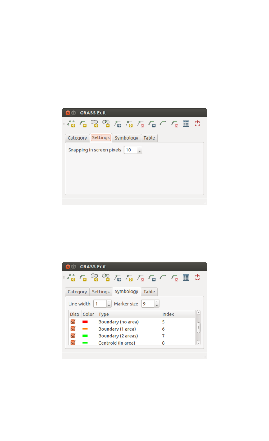
QGIS User Guide, Publicación 2.8
•Field (layer) - Each geometry element can be connected with several attribute tables using different GRASS
geometry layers. The default layer number is 1.
Truco: Creating an additional GRASS ‘layer’ with |qg|
If you would like to add more layers to your dataset, just add a new number in the ‘Field (layer)’ entry box and
press return. In the Table tab, you can create your new table connected to your new layer.
Settings Tab
The Settings tab allows you to set the snapping in screen pixels. The threshold defines at what distance new points
or line ends are snapped to existing nodes. This helps to prevent gaps or dangles between boundaries. The default
is set to 10 pixels.
Figure 16.5: GRASS Digitizing Settings Tab
Symbology Tab
The Symbology tab allows you to view and set symbology and color settings for various geometry types and their
topological status (e.g., closed / opened boundary).
Figure 16.6: GRASS Digitizing Symbology Tab
Table Tab
The Table tab provides information about the database table for a given ‘layer’. Here, you can add new columns
to an existing attribute table, or create a new database table for a new GRASS vector layer (see section Creating a
new GRASS vector layer).
Truco: GRASS Edit Permissions
184 Chapter 16. GRASS GIS Integration
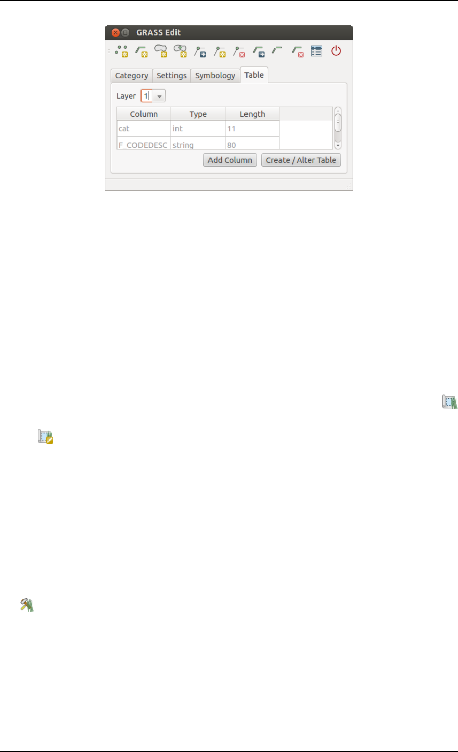
QGIS User Guide, Publicación 2.8
Figure 16.7: GRASS Digitizing Table Tab
You must be the owner of the GRASS MAPSET you want to edit. It is impossible to edit data layers in a MAPSET
that is not yours, even if you have write permission.
16.8 The GRASS region tool
The region definition (setting a spatial working window) in GRASS is important for working with raster layers.
Vector analysis is by default not limited to any defined region definitions. But all newly created rasters will have
the spatial extension and resolution of the currently defined GRASS region, regardless of their original extension
and resolution. The current GRASS region is stored in the $LOCATION/$MAPSET/WIND file, and it defines
north, south, east and west bounds, number of columns and rows, horizontal and vertical spatial resolution.
It is possible to switch on and off the visualization of the GRASS region in the QGIS canvas using the
Display current GRASS region button.
With the Edit current GRASS region icon, you can open a dialog to change the current region and the symbology of
the GRASS region rectangle in the QGIS canvas. Type in the new region bounds and resolution, and click [OK].
The dialog also allows you to select a new region interactively with your mouse on the QGIS canvas. Therefore,
click with the left mouse button in the QGIS canvas, open a rectangle, close it using the left mouse button again
and click [OK].
The GRASS module g.region provides a lot more parameters to define an appropriate region extent and reso-
lution for your raster analysis. You can use these parameters with the GRASS Toolbox, described in section The
GRASS Toolbox.
16.9 The GRASS Toolbox
The Open GRASS Tools box provides GRASS module functionalities to work with data inside a selected GRASS
LOCATION and MAPSET. To use the GRASS Toolbox you need to open a LOCATION and MAPSET that you
have write permission for (usually granted, if you created the MAPSET). This is necessary, because new raster or
vector layers created during analysis need to be written to the currently selected LOCATION and MAPSET.
16.9.1 Working with GRASS modules
The GRASS shell inside the GRASS Toolbox provides access to almost all (more than 300) GRASS modules in
a command line interface. To offer a more user-friendly working environment, about 200 of the available GRASS
modules and functionalities are also provided by graphical dialogs within the GRASS plugin Toolbox.
16.8. The GRASS region tool 185
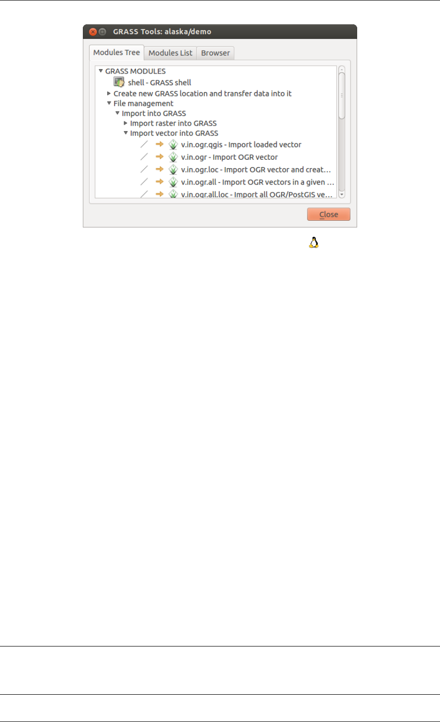
QGIS User Guide, Publicación 2.8
Figure 16.8: GRASS Toolbox and Module Tree
A complete list of GRASS modules available in the graphical Toolbox in QGIS version 2.8 is available in the
GRASS wiki at http://grass.osgeo.org/wiki/GRASS-QGIS_relevant_module_list.
It is also possible to customize the GRASS Toolbox content. This procedure is described in section Customizing
the GRASS Toolbox.
As shown in figure_grass_toolbox_1, you can look for the appropriate GRASS module using the thematically
grouped Modules Tree or the searchable Modules List tab.
By clicking on a graphical module icon, a new tab will be added to the Toolbox dialog, providing three new
sub-tabs: Options,Output and Manual.
Options
The Options tab provides a simplified module dialog where you can usually select a raster or vector layer visualized
in the QGIS canvas and enter further module-specific parameters to run the module.
The provided module parameters are often not complete to keep the dialog clear. If you want to use further module
parameters and flags, you need to start the GRASS shell and run the module in the command line.
A new feature since QGIS 1.8 is the support for a Show Advanced Options button below the simplified module
dialog in the Options tab. At the moment, it is only added to the module v.in.ascii as an example of use, but
it will probably be part of more or all modules in the GRASS Toolbox in future versions of QGIS. This allows you
to use the complete GRASS module options without the need to switch to the GRASS shell.
Output
The Output tab provides information about the output status of the module. When you click the [Run] button, the
module switches to the Output tab and you see information about the analysis process. If all works well, you will
finally see a Successfully finished message.
Manual
The Manual tab shows the HTML help page of the GRASS module. You can use it to check further module
parameters and flags or to get a deeper knowledge about the purpose of the module. At the end of each module
manual page, you see further links to the Main Help index, the Thematic index and the Full index.
These links provide the same information as the module g.manual.
Truco: Display results immediately
If you want to display your calculation results immediately in your map canvas, you can use the ‘View Output’
button at the bottom of the module tab.
186 Chapter 16. GRASS GIS Integration
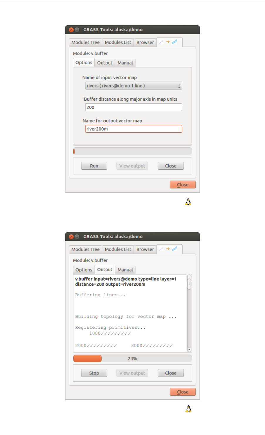
QGIS User Guide, Publicación 2.8
Figure 16.9: GRASS Toolbox Module Options
Figure 16.10: GRASS Toolbox Module Output
16.9. The GRASS Toolbox 187
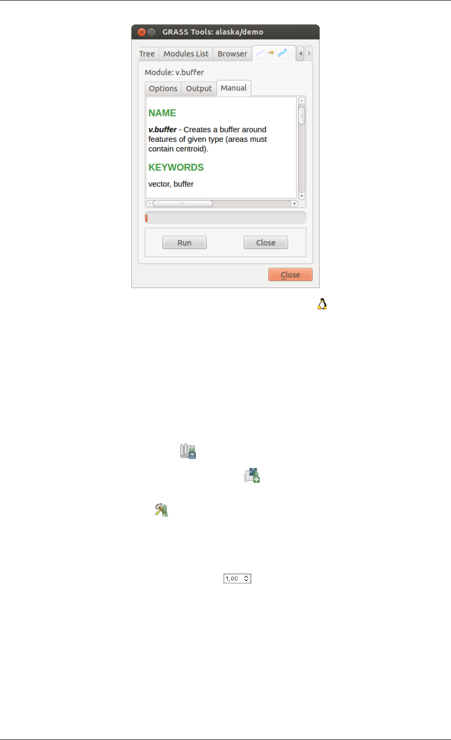
QGIS User Guide, Publicación 2.8
Figure 16.11: GRASS Toolbox Module Manual
16.9.2 GRASS module examples
The following examples will demonstrate the power of some of the GRASS modules.
Creating contour lines
The first example creates a vector contour map from an elevation raster (DEM). Here, it is assumed that you have
the Alaska LOCATION set up as explained in section Importing data into a GRASS LOCATION.
• First, open the location by clicking the Open mapset button and choosing the Alaska location.
• Now load the gtopo30 elevation raster by clicking Add GRASS raster layer and selecting the gtopo30
raster from the demo location.
• Now open the Toolbox with the Open GRASS tools button.
• In the list of tool categories, double-click Raster →Surface Management →Generate vector contour lines.
• Now a single click on the tool r.contour will open the tool dialog as explained above (see Working with
GRASS modules). The gtopo30 raster should appear as the Name of input raster.
• Type into the Increment between Contour levels the value 100. (This will create contour lines at
intervals of 100 meters.)
• Type into the Name for output vector map the name ctour_100.
• Click [Run] to start the process. Wait for several moments until the message Successfully finished
appears in the output window. Then click [View Output] and [Close].
Since this is a large region, it will take a while to display. After it finishes rendering, you can open the layer
properties window to change the line color so that the contours appear clearly over the elevation raster, as in The
Vector Properties Dialog.
Next, zoom in to a small, mountainous area in the center of Alaska. Zooming in close, you will notice that the
contours have sharp corners. GRASS offers the v.generalize tool to slightly alter vector maps while keeping
188 Chapter 16. GRASS GIS Integration
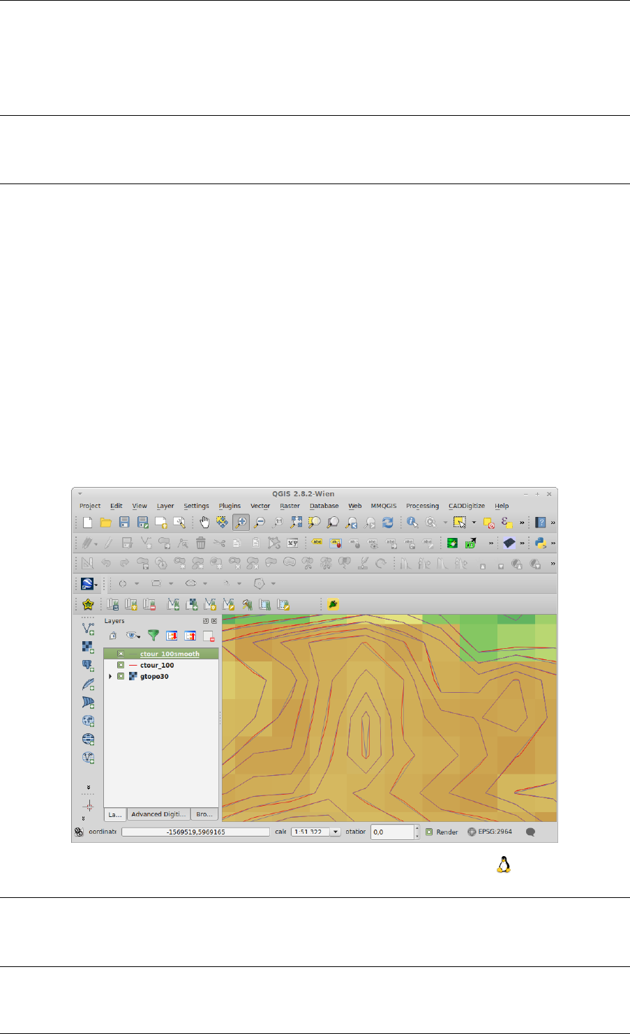
QGIS User Guide, Publicación 2.8
their overall shape. The tool uses several different algorithms with different purposes. Some of the algorithms
(i.e., Douglas Peuker and Vertex Reduction) simplify the line by removing some of the vertices. The resulting
vector will load faster. This process is useful when you have a highly detailed vector, but you are creating a very
small-scale map, so the detail is unnecessary.
Truco: The simplify tool
Note that the QGIS fTools plugin has a Simplify geometries →tool that works just like the GRASS v.generalize
Douglas-Peuker algorithm.
However, the purpose of this example is different. The contour lines created by r.contour have sharp angles
that should be smoothed. Among the v.generalize algorithms, there is Chaiken’s, which does just that (also
Hermite splines). Be aware that these algorithms can add additional vertices to the vector, causing it to load even
more slowly.
• Open the GRASS Toolbox and double-click the categories Vector →Develop map →Generalization, then
click on the v.generalize module to open its options window.
• Check that the ‘ctour_100’ vector appears as the Name of input vector.
• From the list of algorithms, choose Chaiken’s. Leave all other options at their default, and scroll down to
the last row to enter in the field Name for output vector map ‘ctour_100_smooth’, and click [Run].
• The process takes several moments. Once Successfully finished appears in the output windows,
click [View output] and then [Close].
• You may change the color of the vector to display it clearly on the raster background and to contrast with
the original contour lines. You will notice that the new contour lines have smoother corners than the original
while staying faithful to the original overall shape.
Figure 16.12: GRASS module v.generalize to smooth a vector map
Truco: Other uses for r.contour
The procedure described above can be used in other equivalent situations. If you have a raster map of precipitation
data, for example, then the same method will be used to create a vector map of isohyetal (constant rainfall) lines.
16.9. The GRASS Toolbox 189
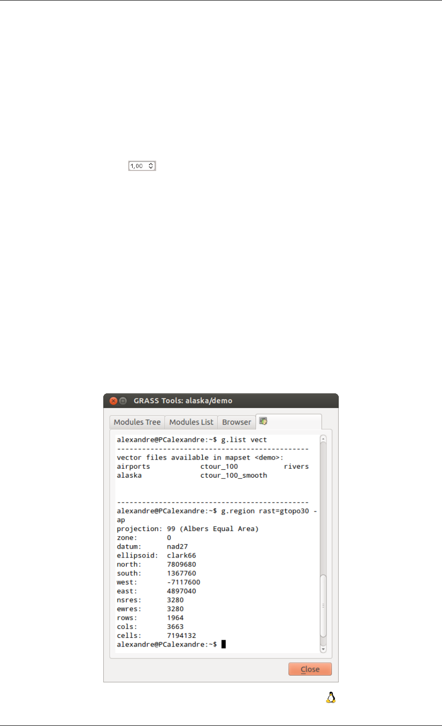
QGIS User Guide, Publicación 2.8
Creating a Hillshade 3-D effect
Several methods are used to display elevation layers and give a 3-D effect to maps. The use of contour lines, as
shown above, is one popular method often chosen to produce topographic maps. Another way to display a 3-D
effect is by hillshading. The hillshade effect is created from a DEM (elevation) raster by first calculating the slope
and aspect of each cell, then simulating the sun’s position in the sky and giving a reflectance value to each cell.
Thus, you get sun-facing slopes lighted; the slopes facing away from the sun (in shadow) are darkened.
• Begin this example by loading the gtopo30 elevation raster. Start the GRASS Toolbox, and under the
Raster category, double-click to open Spatial analysis →Terrain analysis.
• Then click r.shaded.relief to open the module.
• Change the azimuth angle 270 to 315.
• Enter gtopo30_shade for the new hillshade raster, and click [Run].
• When the process completes, add the hillshade raster to the map. You should see it displayed in grayscale.
• To view both the hillshading and the colors of the gtopo30 together, move the hillshade map below the
gtopo30 map in the table of contents, then open the Properties window of gtopo30, switch to the
Transparency tab and set its transparency level to about 25%.
You should now have the gtopo30 elevation with its colormap and transparency setting displayed above the
grayscale hillshade map. In order to see the visual effects of the hillshading, turn off the gtopo30_shade map,
then turn it back on.
Using the GRASS shell
The GRASS plugin in QGIS is designed for users who are new to GRASS and not familiar with all the modules
and options. As such, some modules in the Toolbox do not show all the options available, and some modules do
not appear at all. The GRASS shell (or console) gives the user access to those additional GRASS modules that
do not appear in the Toolbox tree, and also to some additional options to the modules that are in the Toolbox with
the simplest default parameters. This example demonstrates the use of an additional option in the r.shaded.relief
module that was shown above.
Figure 16.13: The GRASS shell, r.shaded.relief module
190 Chapter 16. GRASS GIS Integration
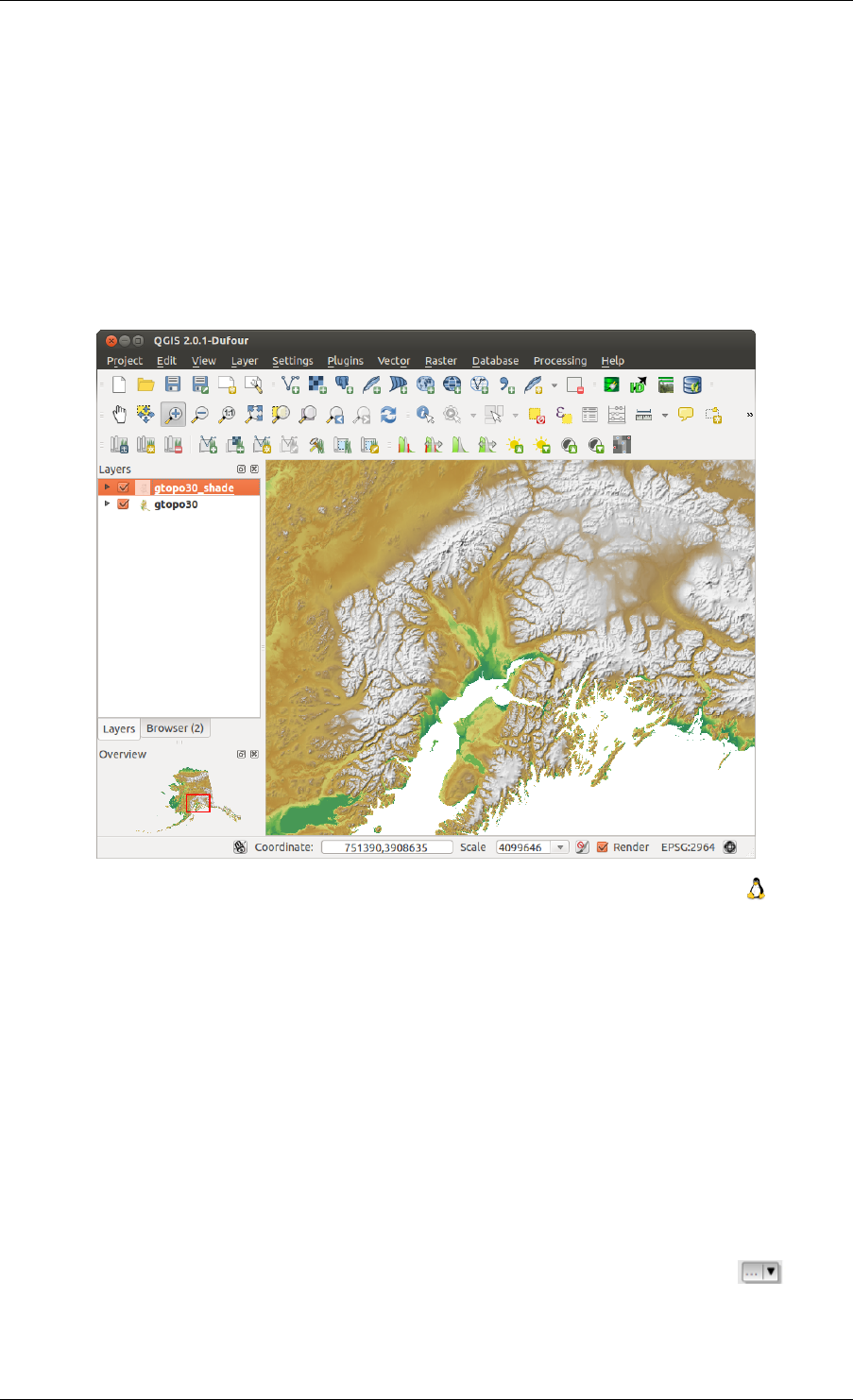
QGIS User Guide, Publicación 2.8
The module r.shaded.relief can take a parameter zmult, which multiplies the elevation values relative to the X-Y
coordinate units so that the hillshade effect is even more pronounced.
• Load the gtopo30 elevation raster as above, then start the GRASS Toolbox and click on the
GRASS shell. In the shell window, type the command r.shaded.relief map=gtopo30
shade=gtopo30_shade2 azimuth=315 zmult=3 and press [Enter].
• After the process finishes, shift to the Browse tab and double-click on the new gtopo30_shade2 raster
to display it in QGIS.
• As explained above, move the shaded relief raster below the gtopo30 raster in the table of contents, then
check the transparency of the colored gtopo30 layer. You should see that the 3-D effect stands out more
strongly compared with the first shaded relief map.
Figure 16.14: Displaying shaded relief created with the GRASS module r.shaded.relief
Raster statistics in a vector map
The next example shows how a GRASS module can aggregate raster data and add columns of statistics for each
polygon in a vector map.
• Again using the Alaska data, refer to Importing data into a GRASS LOCATION to import the trees shapefile
from the shapefiles directory into GRASS.
• Now an intermediate step is required: centroids must be added to the imported trees map to make it a
complete GRASS area vector (including both boundaries and centroids).
• From the Toolbox, choose Vector →Manage features, and open the module v.centroids.
• Enter as the output vector map ‘forest_areas’ and run the module.
• Now load the forest_areas vector and display the types of forests - deciduous, evergreen, mixed - in
different colors: In the layer Properties window, Symbology tab, choose from Legend type ‘Unique
value’ and set the Classification field to ‘VEGDESC’. (Refer to the explanation of the symbology tab in
Style Menu of the vector section.)
• Next, reopen the GRASS Toolbox and open Vector →Vector update by other maps.
16.9. The GRASS Toolbox 191
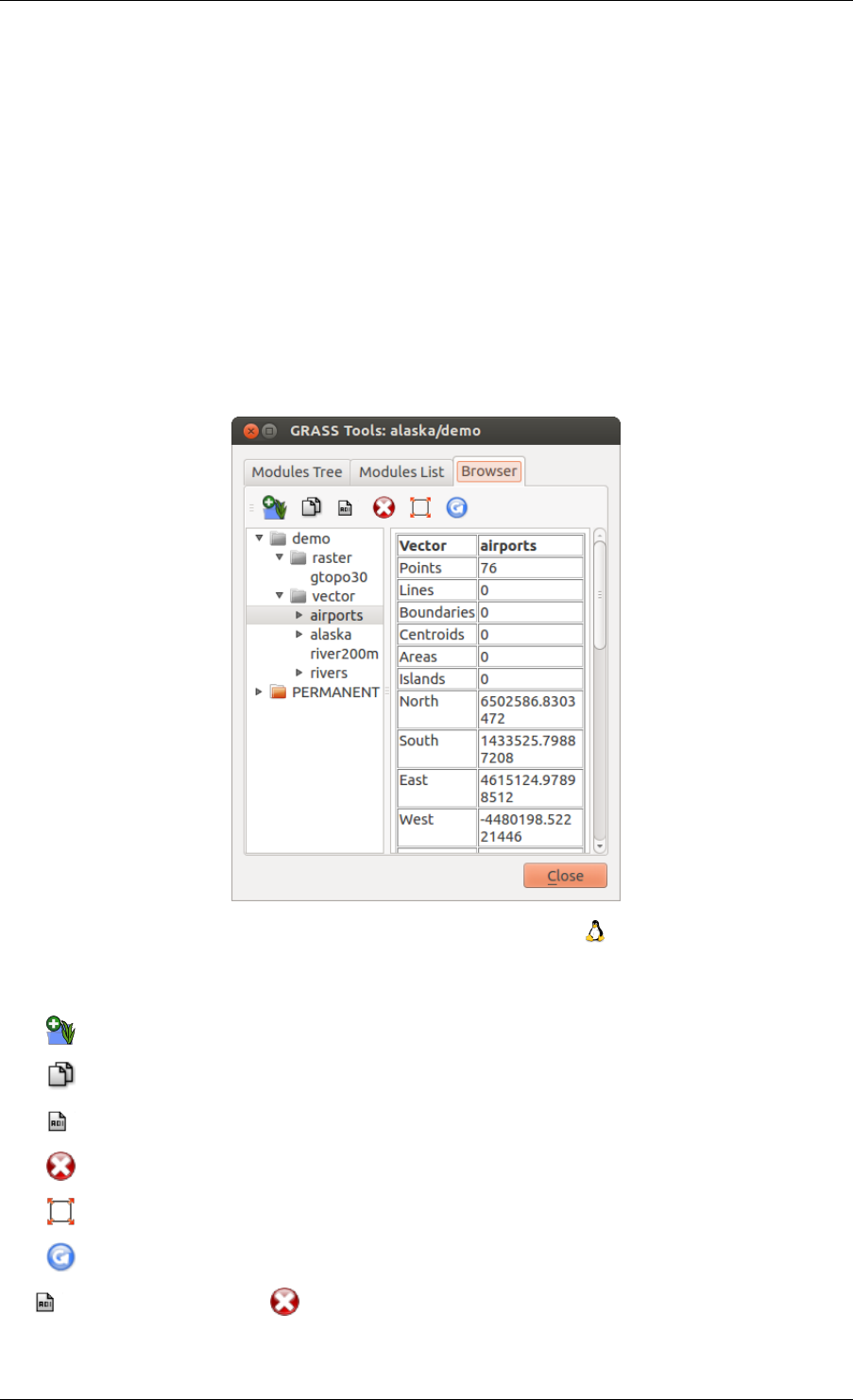
QGIS User Guide, Publicación 2.8
• Click on the v.rast.stats module. Enter gtopo30 and forest_areas.
• Only one additional parameter is needed: Enter column prefix elev, and click [Run]. This is a computa-
tionally heavy operation, which will run for a long time (probably up to two hours).
• Finally, open the forest_areas attribute table, and verify that several new columns have been added,
including elev_min,elev_max,elev_mean, etc., for each forest polygon.
16.9.3 Working with the GRASS LOCATION browser
Another useful feature inside the GRASS Toolbox is the GRASS LOCATION browser. In figure_grass_module_7,
you can see the current working LOCATION with its MAPSETs.
In the left browser windows, you can browse through all MAPSETs inside the current LOCATION. The right
browser window shows some meta-information for selected raster or vector layers (e.g., resolution, bounding box,
data source, connected attribute table for vector data, and a command history).
Figure 16.15: GRASS LOCATION browser
The toolbar inside the Browser tab offers the following tools to manage the selected LOCATION:
•Add selected map to canvas
•Copy selected map
•Rename selected map
•Delete selected map
•Set current region to selected map
•Refresh browser window
The Rename selected map and Delete selected map only work with maps inside your currently selected
MAPSET. All other tools also work with raster and vector layers in another MAPSET.
192 Chapter 16. GRASS GIS Integration

QGIS User Guide, Publicación 2.8
16.9.4 Customizing the GRASS Toolbox
Nearly all GRASS modules can be added to the GRASS Toolbox. An XML interface is provided to parse the
pretty simple XML files that configure the modules’ appearance and parameters inside the Toolbox.
A sample XML file for generating the module v.buffer (v.buffer.qgm) looks like this:
<?xml version="1.0" encoding="UTF-8"?>
<!DOCTYPE qgisgrassmodule SYSTEM "http://mrcc.com/qgisgrassmodule.dtd">
<qgisgrassmodule label="Vector buffer" module="v.buffer">
<option key="input" typeoption="type" layeroption="layer" />
<option key="buffer"/>
<option key="output" />
</qgisgrassmodule>
The parser reads this definition and creates a new tab inside the Toolbox when you select the module. A more
detailed description for adding new modules, changing a module’s group, etc., can be found on the QGIS wiki at
http://hub.qgis.org/projects/quantum-gis/wiki/Adding_New_Tools_to_the_GRASS_Toolbox.
.
16.9. The GRASS Toolbox 193

QGIS User Guide, Publicación 2.8
194 Chapter 16. GRASS GIS Integration
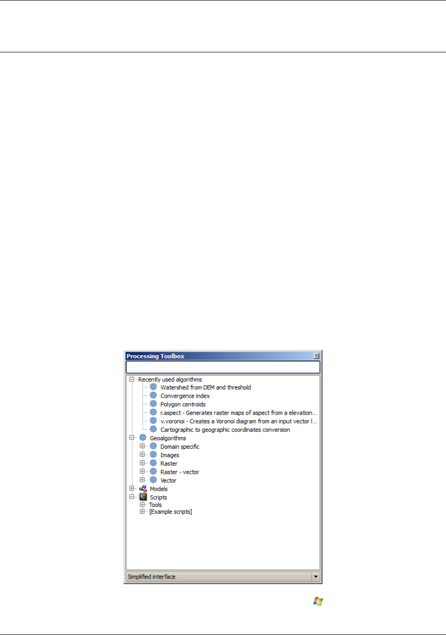
CHAPTER 17
Entorno de trabajo de procesamiento de QGIS
.
17.1 Introducción
Este capítulo introduce al marco de procesamiento de QGIS, un entorno de geoprosesamiento que se puede utilizar
para llamar algoritmos nativos o de terceros de QGIS, haciendo su tarea de análisis espacial más productivo y fácil
de lograr.
En las siguientes secciones, revisaremos cómo usar los elementos gráficos de este sistema y sacar el máximo
provecho de cada uno de ellos.
Hay cuatro elementos básicos en el marco IUG, que se usa para ejecutar algoritmos para diferentes propósitos.
Elegir una u otra herramienta dependerá del tipo de análisis que se va a realizar y de las características particulares
que cada usuario y proyecto. Todos ellos (a excepción de la interfaz de procesamiento por lotes, lo que se llama
desde la caja de herramientas, como veremos más delante) se puede acceder desde el menú Procesado. (Verpa
más de cuatro entradas. Los restantes no se utilizan para ejecutar los algoritmos y se explicarán más adelante en
este capítulo.)
• La caja de herramientas. El elemento principal de la IUG, se usa para ejecutar un solo algoritmo o grupo de
procesos sobre la base de ese algoritmo.
Figure 17.1: Caja de herramientas de procesado
195
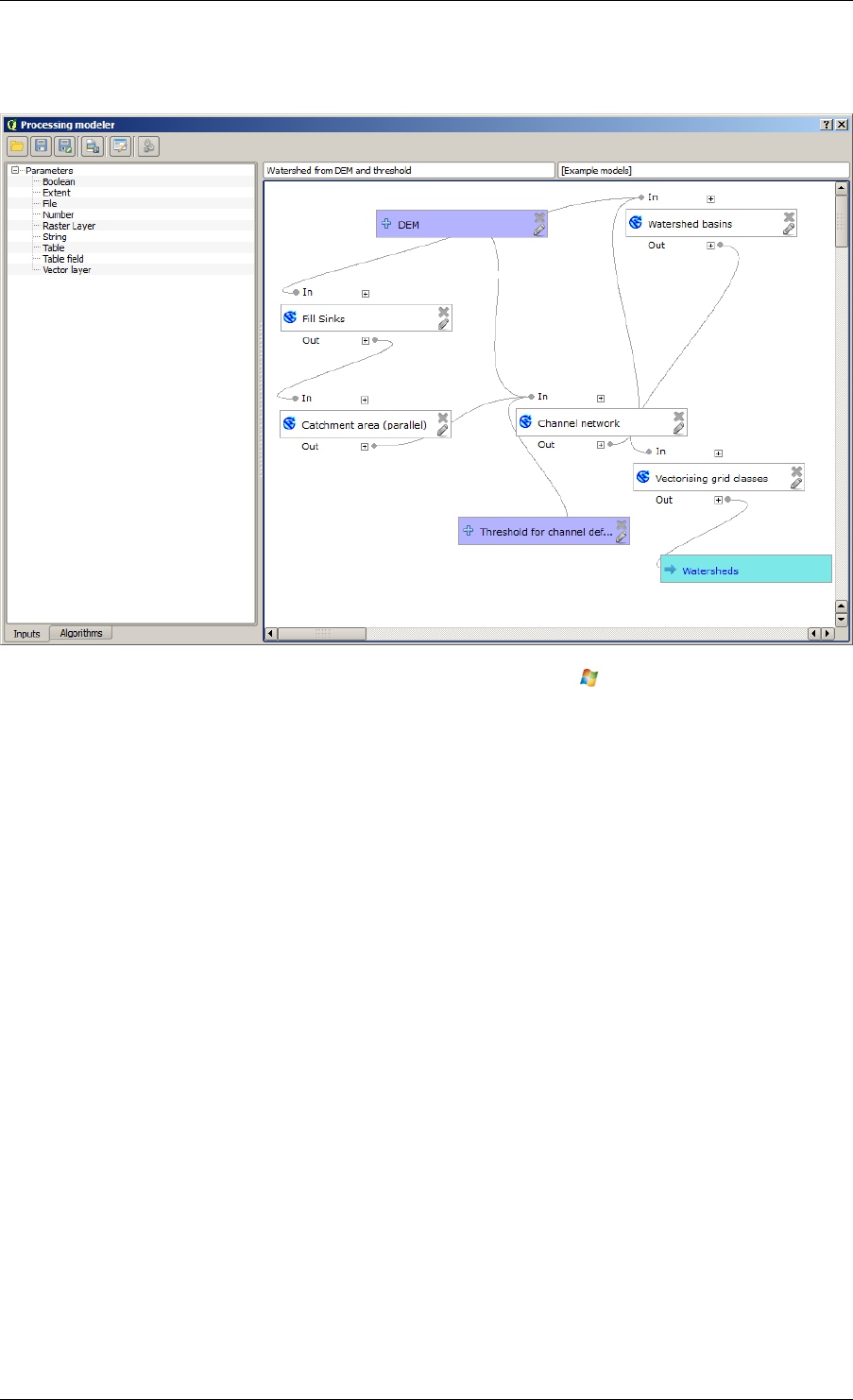
QGIS User Guide, Publicación 2.8
• El modelador gráfico. Varios algoritmos se pueden combinar graficamente usando el modelador para definir
un flujo de trabajo, creando un proceso individual que involucre varios subprocesos.
Figure 17.2: Procesamiento del modelador
• El administrador del historial. Todas las acciones que se llevan acabo mediante cualquiera de los elementos
mencionados se almacenan en un archivo de la historia y puede ser posteriormente producido usando el
administrador del historial.
• La interfaz de procesamiento por lote. Esta interfaz permite que ejecute procesos por lote y automatizar la
ejecución de un solo algoritmo a múltiples conjuntos de datos.
En las siguientes secciones, revisaremos cada uno de los elementos a detalle.
.
17.2 La caja de herramientas
La Caja de herramientas es el principal elemento de procesamiento de la interfaz gráfica de usuario, y el que más
se suele usar en el trabajo diario. Muestra un listado de todos los algoritmos disponibles agrupados en diferentes
bloques, y es el punto de acceso para ejecutarlos, bien haciéndolo como un proceso único o bien como un proceso
por lotes que realice varias ejecuciones del mismo algoritmo con diferentes conjuntos de entradas.
La caja de herramientas contiene todos los algoritmos disponibles, divididos en grupos definidos. Todos estos
grupos se encuentran bajo una sola categoría llamada Geoalgoritmos
Además, hay dos entradas más llamadas Modelos yScripts. Éstas permiten crear algorimtos y definir flujos de
trabajo y tareas de procesamiento personalizados. Más adelante hay uan sección completa dedicada a esto.
En la parte superior de la caja de herramientas, hay una caja de texto. Para reducir el número de algoritmos que
se muestran en la caja de herramientas y que resulte más fácil encontrar el que se necesita, se puede introducir
cualquier palabra o frase en esa caja de texto. Según se va escribiendo, el número de algorimos que se muestra se
va reduciendo a sólo aquellos que contienen el texto introducido en su nombre.
En la parte inferior, hay una caja desplegable en la que se puede elegir entre la lista simplificada (la ya explicada)
y la lista avanzada. Si se cambia a la opción avanzada, la caja de herramientas tendrá este aspecto:
196 Chapter 17. Entorno de trabajo de procesamiento de QGIS
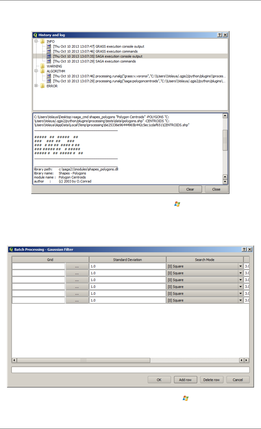
QGIS User Guide, Publicación 2.8
Figure 17.3: Procesamiento de Historial
Figure 17.4: Interfaz de procesamiento por lote
17.2. La caja de herramientas 197
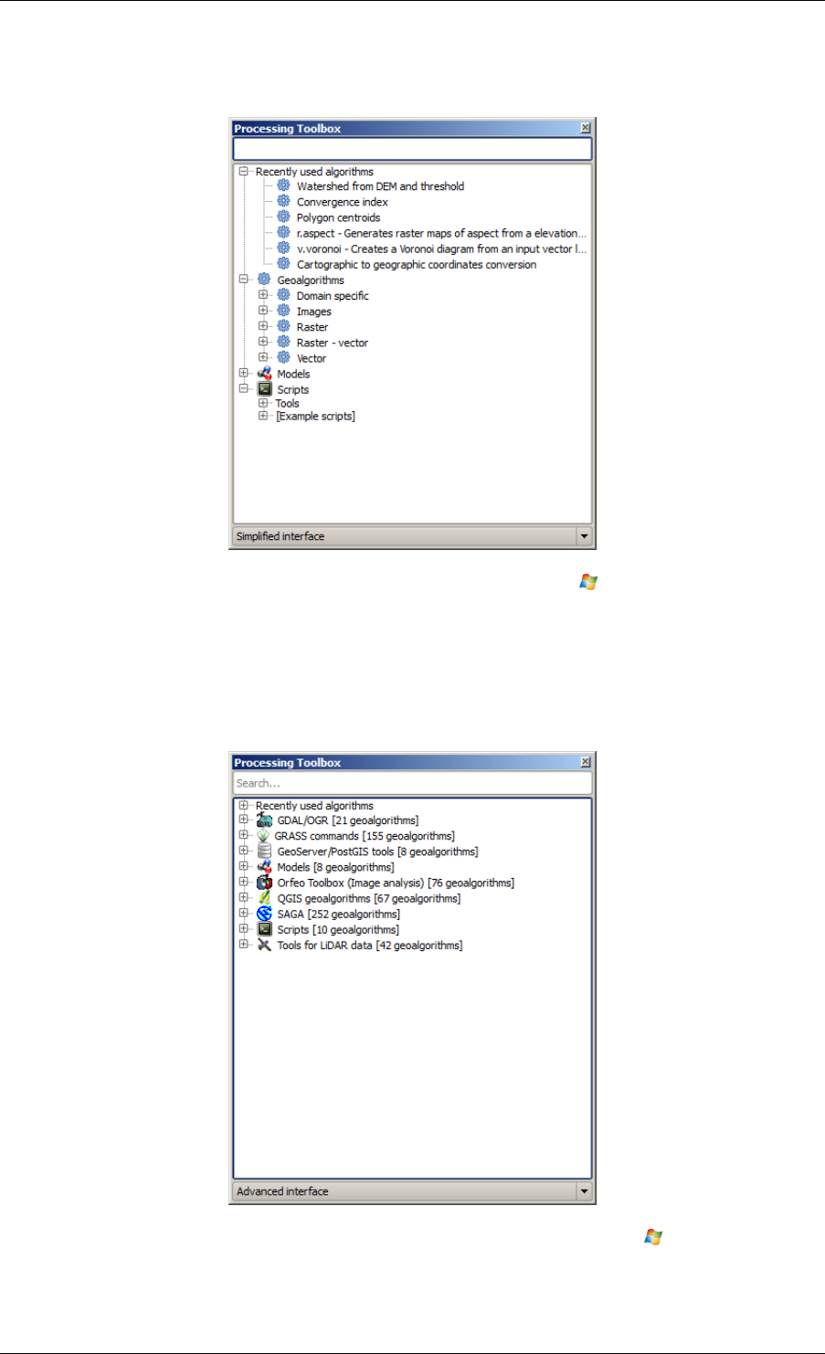
QGIS User Guide, Publicación 2.8
Figure 17.5: Caja de herramientas de procesado
Figure 17.6: Caja de herramientas de procesado (modo avanzado)
198 Chapter 17. Entorno de trabajo de procesamiento de QGIS
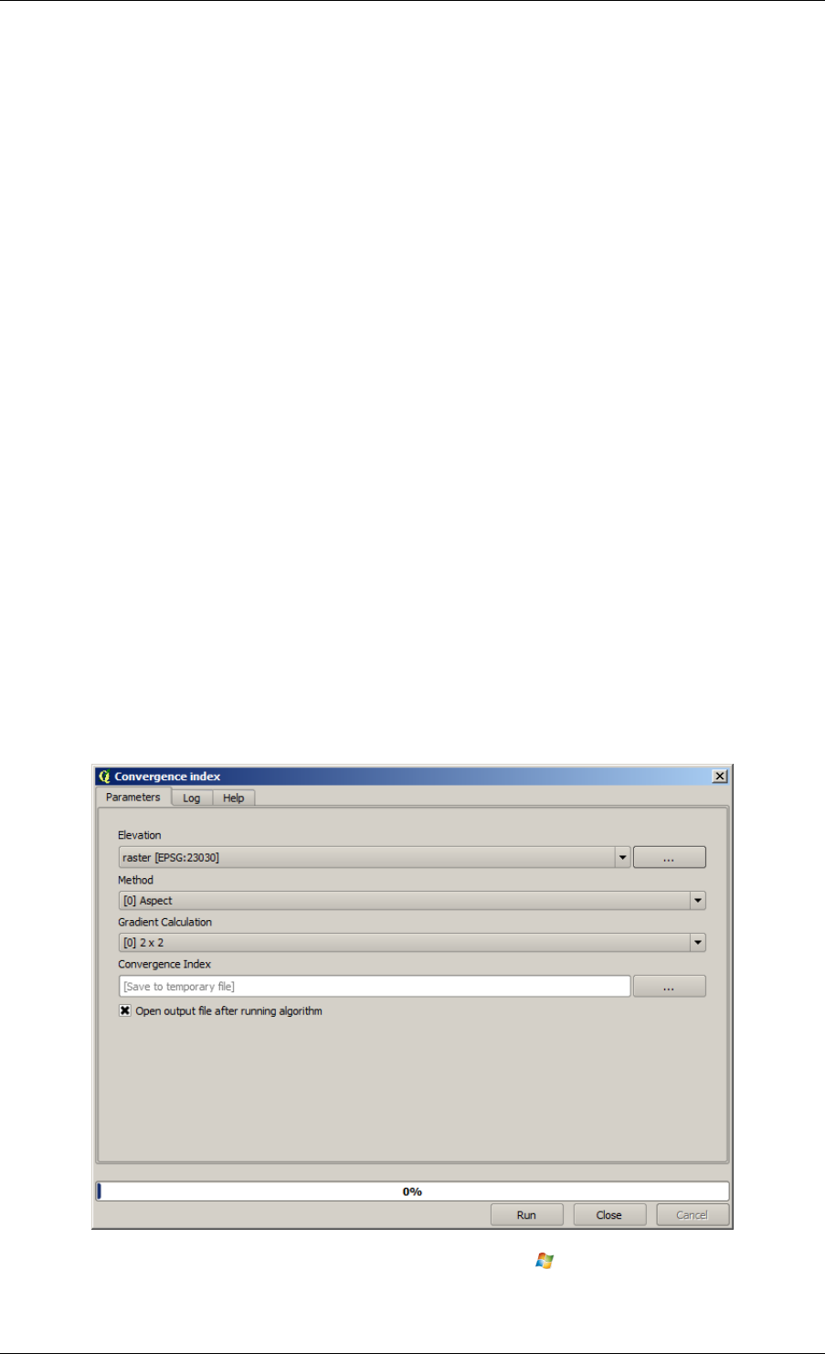
QGIS User Guide, Publicación 2.8
En la vista avanzada, cada grupo representa a un ‘proveedor de algoritmos’, que es un conjunto de algorimos que
tiene el mismo origen, por ejemplo de una aplicación externa con capacidades de geoprocesamiento. Algunos
de estos grupos representan algoritmos de aplicaciones como SAGA, GRASS o R, mientras que otros contienen
algorimos directamente programados usando el complemeto de procesamiento y no pertenecen a ningún otro
programa.
Esta vista se recomienda para los usuarios/as que tienen cierto conocimiento de las aplicaciones de las que
provienen los algoritmos, ya que estos se muestran con sus nombres y grupos originales.
Además, hay algunos algoritmos que sólo están disponibles en la vista avanzada, como las herramientas de LIDAR
y los scripts basados en el software de cálculo estadístico R entre otras. Los plugins de QGIS independientes que
añaden nuevos algoritmos a la caja de herramientas, se muestran también sólo en la vista avanzada.
En concreto, la vista simplificada contiene algoritmos de los siguientes productos:
• GRASS
• SAGA
• OTB
• Algoritmos QGIS nativos
Si se usa QGIS en Windows, estos algorimos están plenamente funcionales desde el principio y pueden ejecu-
tarse sin necesidad de instalaciones adicionales. Además, ejecutarlos no requiere un conocimiento previo de las
aplicaciones externas que usan, haciéndolos más accesibles para usuarios/as sin experiencia.
If you want to use an algorithm not provided by any of the above providers, switch to the advanced mode by
selecting the corresponding option at the bottom of the toolbox.
Para ejecutar un algoritmo, basta con hacer doble click sobre su nombre en la caja de herramientas.
17.2.1 El cuadro de diálogo de algoritmo
Once you double-click on the name of the algorithm that you want to execute, a dialog similar to that in the figure
below is shown (in this case, the dialog corresponds to the SAGA ‘Convergence index’ algorithm).
Figure 17.7: Diálogo de parámetros
17.2. La caja de herramientas 199
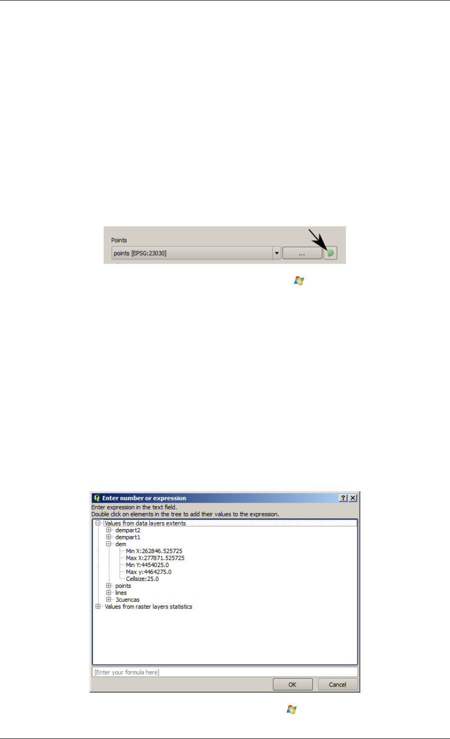
QGIS User Guide, Publicación 2.8
This dialog is used to set the input values that the algorithm needs to be executed. It shows a table where input
values and configuration parameters are to be set. It of course has a different content, depending on the require-
ments of the algorithm to be executed, and is created automatically based on those requirements. On the left side,
the name of the parameter is shown. On the right side, the value of the parameter can be set.
Although the number and type of parameters depend on the characteristics of the algorithm, the structure is similar
for all of them. The parameters found in the table can be of one of the following types.
• A raster layer, to select from a list of all such layers available (currently opened) in QGIS. The selector
contains as well a button on its right-hand side, to let you select filenames that represent layers currently not
loaded in QGIS.
• A vector layer, to select from a list of all vector layers available in QGIS. Layers not loaded in QGIS can
be selected as well, as in the case of raster layers, but only if the algorithm does not require a table field
selected from the attributes table of the layer. In that case, only opened layers can be selected, since they
need to be open so as to retrieve the list of field names available.
Se ve un botón por cada selector de capa vectorial, como se muestra en la figura inferior.
Figure 17.8: Botón iterador vectorial
If the algorithm contains several of them, you will be able to toggle just one of them. If the button corresponding to
a vector input is toggled, the algorithm will be executed iteratively on each one of its features, instead of just once
for the whole layer, producing as many outputs as times the algorithm is executed. This allows for automating the
process when all features in a layer have to be processed separately.
• A table, to select from a list of all available in QGIS. Non-spatial tables are loaded into QGIS like vector
layers, and in fact they are treated as such by the program. Currently, the list of available tables that you will
see when executing an algorithm that needs one of them is restricted to tables coming from files in dBase
(.dbf) or Comma-Separated Values (.csv) formats.
• Una opción, a elegir de una lista de selección de posibles opciones.
• A numerical value, to be introduced in a text box. You will find a button by its side. Clicking on it, you
will see a dialog that allows you to enter a mathematical expression, so you can use it as a handy calculator.
Some useful variables related to data loaded into QGIS can be added to your expression, so you can select
a value derived from any of these variables, such as the cell size of a layer or the northernmost coordinate
of another one.
Figure 17.9: Selector de Número
200 Chapter 17. Entorno de trabajo de procesamiento de QGIS
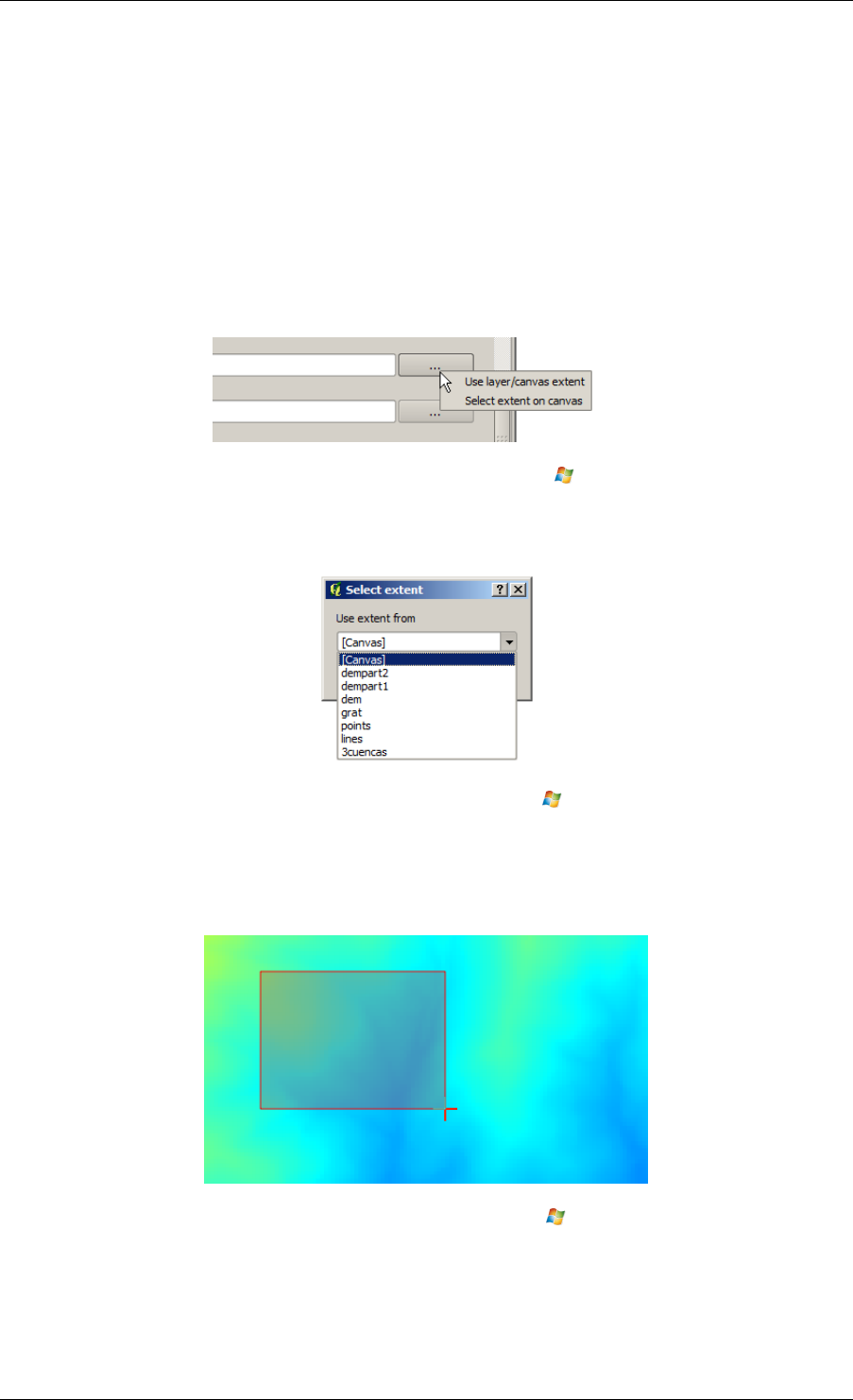
QGIS User Guide, Publicación 2.8
• Un rango, con valores mínimo y máximo que se introducen en dos cuadros de texto.
• Una cadena de texto, que se introduce en un cuadro de texto.
• Un campo, a elegir desde la tabla de atributos de una capa vectorial o una tabla sencilla seleccionada en otro
parámetro.
• A coordinate reference system. You can type the EPSG code directly in the text box, or select it from the
CRS selection dialog that appears when you click on the button on the right-hand side.
• An extent, to be entered by four numbers representing its xmin,xmax,ymin,ymax limits. Clicking on
the button on the right-hand side of the value selector, a pop-up menu will appear, giving you two options:
to select the value from a layer or the current canvas extent, or to define it by dragging directly onto the map
canvas.
Figure 17.10: Selector de Extensión
Si se selecciona la primera opción, se verá una ventana como la siguiente.
Figure 17.11: Lista de Extensión
Si se selecciona la segunda opción, la ventana de parámetros se ocultará, para que se pueda definir el rectán-
gulo haciendo click y arrastrando dentro del lienzo. Una vez hecho esto, el cuadro de diálogo reaparecerá,
con los valores correspondientes ya rellenos en en cuadro de texto.
Figure 17.12: Arrastrar Extensión
• A list of elements (whether raster layers, vector layers or tables), to select from the list of such layers
available in QGIS. To make the selection, click on the small button on the left side of the corresponding row
to see a dialog like the following one.
17.2. La caja de herramientas 201
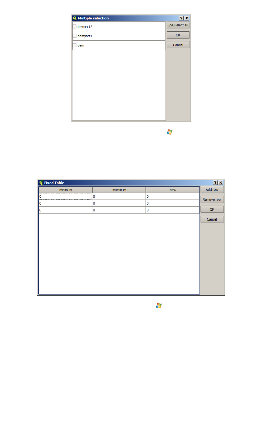
QGIS User Guide, Publicación 2.8
Figure 17.13: Selección múltiple
• Una pequeña tabla para que la edite el usuario. Éstas se usan para definir parámetros como tablas de
búsqueda o matrices de convolución entre otros.
Click en el botón del lado derecho para ver la tabla y editar sus valores.
Figure 17.14: Tabla fija
Depending on the algorithm, the number of rows can be modified or not by using the buttons on the right
side of the window.
You will find a [Help] tab in the the parameters dialog. If a help file is available, it will be shown, giving you
more information about the algorithm and detailed descriptions of what each parameter does. Unfortunately, most
algorithms lack good documentation, but if you feel like contributing to the project, this would be a good place to
start.
Un comentario sobre proyecciones
Algorithms run from the processing framework — this is also true of most of the external applications whose
algorithms are exposed through it. Do not perform any reprojection on input layers and assume that all of them
are already in a common coordinate system and ready to be analized. Whenever you use more than one layer as
202 Chapter 17. Entorno de trabajo de procesamiento de QGIS

QGIS User Guide, Publicación 2.8
input to an algorithm, whether vector or raster, it is up to you to make sure that they are all in the same coordinate
system.
Note that, due to QGIS‘s on-the-fly reprojecting capabilities, although two layers might seem to overlap and
match, that might not be true if their original coordinates are used without reprojecting them onto a common
coordinate system. That reprojection should be done manually, and then the resulting files should be used as input
to the algorithm. Also, note that the reprojection process can be performed with the algorithms that are available
in the processing framework itself.
By default, the parameters dialog will show a description of the CRS of each layer along with its name, making it
easy to select layers that share the same CRS to be used as input layers. If you do not want to see this additional
information, you can disable this functionality in the processing configuration dialog, unchecking the Show CRS
option.
If you try to execute an algorithm using as input two or more layers with unmatching CRSs, a warning dialog will
be shown.
Aún se puede ejecutar el algoritmo, pero en la mayoría de los casos se producirán resultados incorrectos, como
capas vacias debido a que las capas de entrada no se solapan.
17.2.2 Resultados generados por algoritmos
Los tipos de resultados que se pueden generar cor un algoritmo son los siguientes:
• Una capa ráster.
• Una capa vectorial.
• Una tabla
• Un archivo HTML (usado para salidas de texto y salidas gráficas).
These are all saved to disk, and the parameters table will contain a text box corresponding to each one of these
outputs, where you can type the output channel to use for saving it. An output channel contains the information
needed to save the resulting object somewhere. In the most usual case, you will save it to a file, but the architecture
allows for any other way of storing it. For instance, a vector layer can be stored in a database or even uploaded
to a remote server using a WFS-T service. Although solutions like these are not yet implemented, the processing
framework is prepared to handle them, and we expect to add new kinds of output channels in a near feature.
To select an output channel, just click on the button on the right side of the text box. That will open a save file
dialog, where you can select the desired file path. Supported file extensions are shown in the file format selector
of the dialog, depending on the kind of output and the algorithm.
The format of the output is defined by the filename extension. The supported formats depend on what is supported
by the algorithm itself. To select a format, just select the corresponding file extension (or add it, if you are directly
typing the file path instead). If the extension of the file path you entered does not match any of the supported
formats, a default extension (usually .dbf‘ for tables, .tif for raster layers and .shp for vector layers) will
be appended to the file path, and the file format corresponding to that extension will be used to save the layer or
table.
If you do not enter any filename, the result will be saved as a temporary file in the corresponding default file
format, and it will be deleted once you exit QGIS (take care with that, in case you save your project and it contains
temporary layers).
You can set a default folder for output data objects. Go to the configuration dialog (you can open it from the
Processing menu), and in the General group, you will find a parameter named Output folder. This output folder
is used as the default path in case you type just a filename with no path (i.e., myfile.shp) when executing an
algorithm.
When running an algorithm that uses a vector layer in iterative mode, the entered file path is used as the base path
for all generated files, which are named using the base name and appending a number representing the index of
the iteration. The file extension (and format) is used for all such generated files.
Apart from raster layers and tables, algorithms also generate graphics and text as HTML files. These results are
shown at the end of the algorithm execution in a new dialog. This dialog will keep the results produced by any
17.2. La caja de herramientas 203
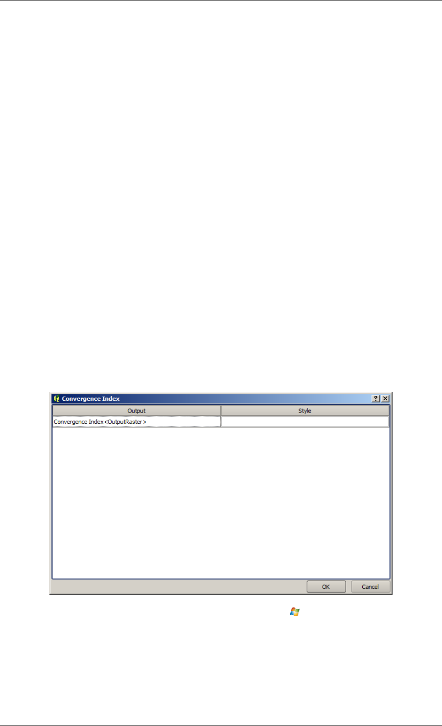
QGIS User Guide, Publicación 2.8
algorithm during the current session, and can be shown at any time by selecting Processing →Results viewer from
the QGIS main menu.
Some external applications might have files (with no particular extension restrictions) as output, but they do not
belong to any of the categories above. Those output files will not be processed by QGIS (opened or included into
the current QGIS project), since most of the time they correspond to file formats or elements not supported by
QGIS. This is, for instance, the case with LAS files used for LiDAR data. The files get created, but you won’t see
anything new in your QGIS working session.
For all the other types of output, you will find a checkbox that you can use to tell the algorithm whether to load
the file once it is generated by the algorithm or not. By default, all files are opened.
Optional outputs are not supported. That is, all outputs are created. However, you can uncheck the corresponding
checkbox if you are not interested in a given output, which essentially makes it behave like an optional output (in
other words, the layer is created anyway, but if you leave the text box empty, it will be saved to a temporary file
and deleted once you exit QGIS).
17.2.3 Configurar el entorno de trabajo de procesamiento
As has been mentioned, the configuration menu gives access to a new dialog where you can configure how algo-
rithms work. Configuration parameters are structured in separate blocks that you can select on the left-hand side
of the dialog.
Al igual que con la ya mencionada Carpeta de salida, el bloque General contienen parámetros para configurar
el estilo de renderizado por defecto para capas de salida (es decir, capas que se generan usando algoritmos desde
cualquiera de los componentes GUI del entorno de trabajo). Hay que crear el estilo deseado usando QGIS, salvarlo
en un archivo, e introducir ela ruta a ese archivo en la configuración para que los algorimos lo puedan usar. Si
SEXTANTE carga una capa y la añade al lienzo de QGIS , se renderizará usando ese estilo.
Los estilos de renderizado se pueden configurar individualmente para cada algoritmo y cada una de sus salidad.
Basta con hacer clic derecho en el nombre del algoritmo en la caja de herramientas y seleccionar Editar estilos de
renderizados para salidas. Aparecerá un cuadro de diálogo como el mostrado a continuación.
Figure 17.15: Estilos de Renderizado
Seleccionar el archivo de estilo (.qml) que se desee para cada salida y presionar [Aceptar].
Otras parámetros de configuración se en listan en el grupo General a continuación:
•Use filename as layer name. The name of each resulting layer created by an algorithm is defined by the
algorithm itself. In some cases, a fixed name might be used, meaning that the same output name will be
used, no matter which input layer is used. In other cases, the name might depend on the name of the input
204 Chapter 17. Entorno de trabajo de procesamiento de QGIS

QGIS User Guide, Publicación 2.8
layer or some of the parameters used to run the algorithm. If this checkbox is checked, the name will be
taken from the output filename instead. Notice that, if the output is saved to a temporary file, the filename
of this temporary file is usually a long and meaningless one intended to avoid collision with other already
existing filenames.
•Use only selected features. If this option is selected, whenever a vector layer is used as input for an al-
gorithm, only its selected features will be used. If the layer has no selected features, all features will be
used.
•Pre-execution script file and Post-execution script file. These parameters refer to scripts written using the
processing scripting functionality, and are explained in the section covering scripting and the console.
Apart from the General block in the settings dialog, you will also find a block for algorithm providers. Each
entry in this block contains an Activate item that you can use to make algorithms appear or not in the toolbox.
Also, some algorithm providers have their own configuration items, which we will explain later when covering
particular algorithm providers.
.
17.3 &Modelador gráfico...
The graphical modeler allows you to create complex models using a simple and easy-to-use interface. When
working with a GIS, most analysis operations are not isolated, but rather part of a chain of operations instead.
Using the graphical modeler, that chain of processes can be wrapped into a single process, so it is as easy and
convenient to execute as a single process later on a different set of inputs. No matter how many steps and different
algorithms it involves, a model is executed as a single algorithm, thus saving time and effort, especially for larger
models.
El modelador puede ser abierto desde el menu de procesamiento
The modeler has a working canvas where the structure of the model and the workflow it represents are shown. On
the left part of the window, a panel with two tabs can be used to add new elements to the model.
Creating a model involves two steps:
1. Definition of necessary inputs. These inputs will be added to the parameters window, so the user can set their
values when executing the model. The model itself is an algorithm, so the parameters window is generated
automatically as it happens with all the algorithms available in the processing framework.
2. Definition of the workflow. Using the input data of the model, the workflow is defined by adding algorithms
and selecting how they use those inputs or the outputs generated by other algorithms already in the model.
17.3.1 Definition of inputs
The first step to create a model is to define the inputs it needs. The following elements are found in the Inputs tab
on the left side of the modeler window:
• Raster layer
• Vector layer
• String
• Table field
• Table
• Extent
• Number
• Boolean
• File
17.3. &Modelador gráfico... 205
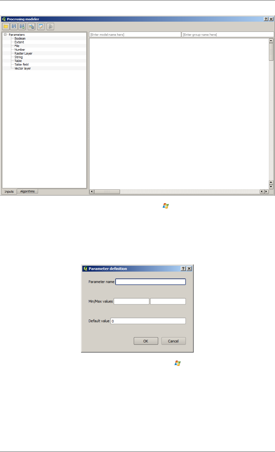
QGIS User Guide, Publicación 2.8
Figure 17.16: Modeler
Double-clicking on any of these elements, a dialog is shown to define its characteristics. Depending on the
parameter itself, the dialog may contain just one basic element (the description, which is what the user will see
when executing the model) or more of them. For instance, when adding a numerical value, as can be seen in the
next figure, apart from the description of the parameter, you have to set a default value and a range of valid values.
Figure 17.17: Model Parameters
For each added input, a new element is added to the modeler canvas.
You can also add inputs by dragging the input type from the list and dropping it in the modeler canvas, in the
position where you want to place it.
206 Chapter 17. Entorno de trabajo de procesamiento de QGIS
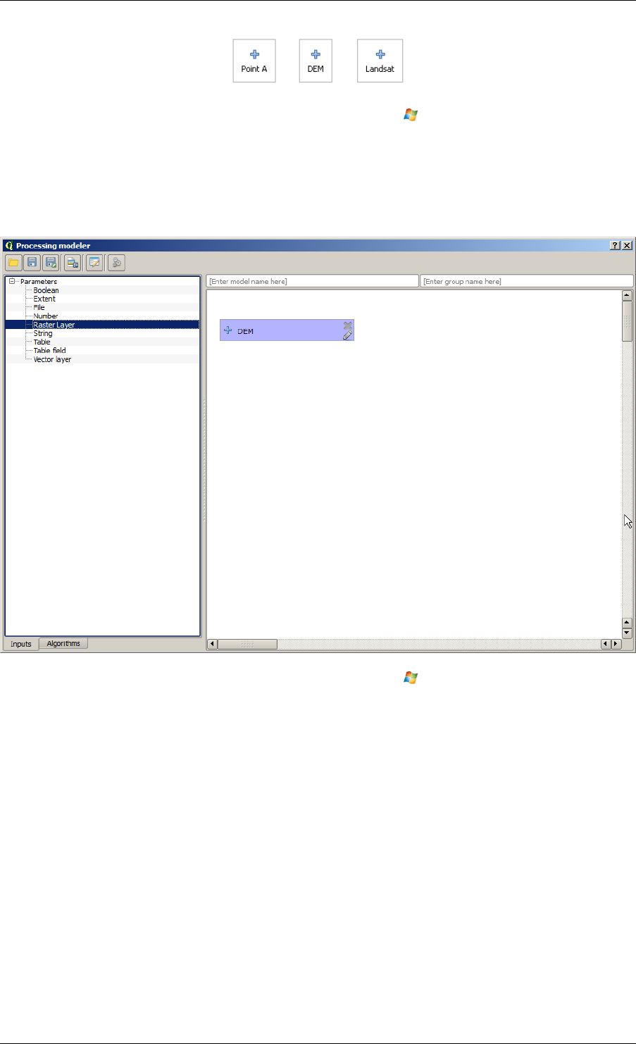
QGIS User Guide, Publicación 2.8
Figure 17.18: Model Parameters
17.3.2 Definition of the workflow
Once the inputs have been defined, it is time to define the algorithms to apply on them. Algorithms can be found
in the Algorithms tab, grouped much in the same way as they are in the toolbox.
Figure 17.19: Model Parameters
The appearance of the toolbox has two modes here as well: simplified and advanced. However, there is no element
to switch between views in the modeler, so you have to do it in the toolbox. The mode that is selected in the toolbox
is the one that will be used for the list of algorithms in the modeler.
To add an algorithm to a model, double-click on its name or drag and drop it, just like it was done when adding
inputs. An execution dialog will appear, with a content similar to the one found in the execution panel that is shown
when executing the algorithm from the toolbox. The one shown next corresponds to the SAGA ‘Convergence
index’ algorithm, the same example we saw in the section dedicated to the toolbox.
As you can see, some differences exist. Instead of the file output box that was used to set the file path for output
layers and tables, a simple text box is used here. If the layer generated by the algorithm is just a temporary result
that will be used as the input of another algorithm and should not be kept as a final result, just do not edit that text
box. Typing anything in it means that the result is final and the text that you supply will be the description for the
output, which will be the output the user will see when executing the model.
Selecting the value of each parameter is also a bit different, since there are important differences between the
context of the modeler and that of the toolbox. Let’s see how to introduce the values for each type of parameter.
• Layers (raster and vector) and tables. These are selected from a list, but in this case, the possible values are
not the layers or tables currently loaded in QGIS, but the list of model inputs of the corresponding type, or
17.3. &Modelador gráfico... 207
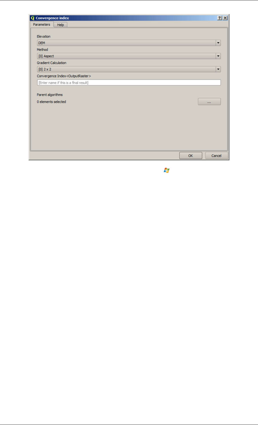
QGIS User Guide, Publicación 2.8
Figure 17.20: Model Parameters
other layers or tables generated by algorithms already added to the model.
• Numerical values. Literal values can be introduced directly in the text box. But this text box is also a list
that can be used to select any of the numerical value inputs of the model. In this case, the parameter will
take the value introduced by the user when executing the model.
• String. As in the case of numerical values, literal strings can be typed, or an input string can be selected.
• Table field. The fields of the parent table or layer cannot be known at design time, since they depend on the
selection of the user each time the model is executed. To set the value for this parameter, type the name of
a field directly in the text box, or use the list to select a table field input already added to the model. The
validity of the selected field will be checked at run time.
In all cases, you will find an additional parameter named Parent algorithms that is not available when calling
the algorithm from the toolbox. This parameter allows you to define the order in which algorithms are executed
by explicitly defining one algorithm as a parent of the current one, which will force the parent algorithm to be
executed before the current one.
When you use the output of a previous algorithm as the input of your algorithm, that implicitly sets the previous
algorithm as parent of the current one (and places the corresponding arrow in the modeler canvas). However,
in some cases an algorithm might depend on another one even if it does not use any output object from it (for
instance, an algorithm that executes an SQL sentence on a PostGIS database and another one that imports a layer
into that same database). In that case, just select the previous algorithm in the Parent algorithms parameter and
the two steps will be executed in the correct order.
Once all the parameters have been assigned valid values, click on [OK] and the algorithm will be added to the
canvas. It will be linked to all the other elements in the canvas, whether algorithms or inputs, that provide objects
that are used as inputs for that algorithm.
Elements can be dragged to a different position within the canvas, to change the way the module structure is
displayed and make it more clear and intuitive. Links between elements are updated automatically. You can zoom
in and out by using the mouse wheel.
You can run your algorithm anytime by clicking on the [Run] button. However, in order to use the algorithm from
the toolbox, it has to be saved and the modeler dialog closed, to allow the toolbox to refresh its contents.
208 Chapter 17. Entorno de trabajo de procesamiento de QGIS
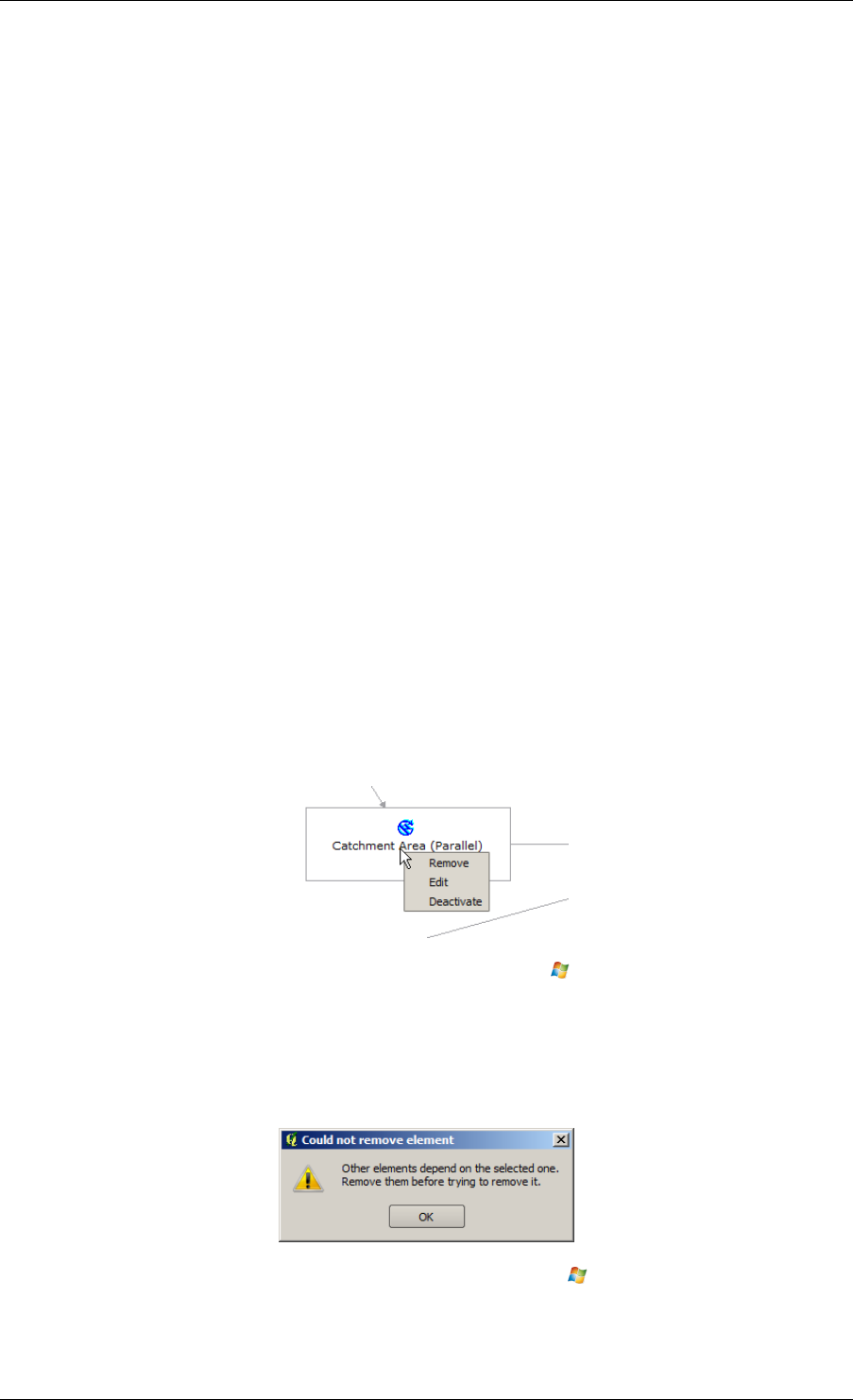
QGIS User Guide, Publicación 2.8
17.3.3 Saving and loading models
Use the [Save] button to save the current model and the [Open] button to open any model previously saved.
Models are saved with the .model extension. If the model has been previously saved from the modeler window,
you will not be prompted for a filename. Since there is already a file associated with that model, the same file will
be used for any subsequent saves.
Before saving a model, you have to enter a name and a group for it, using the text boxes in the upper part of the
window.
Models saved on the models folder (the default folder when you are prompted for a filename to save the model)
will appear in the toolbox in the corresponding branch. When the toolbox is invoked, it searches the models
folder for files with the .model extension and loads the models they contain. Since a model is itself an algorithm,
it can be added to the toolbox just like any other algorithm.
The models folder can be set from the processing configuration dialog, under the Modeler group.
Models loaded from the models folder appear not only in the toolbox, but also in the algorithms tree in the
Algorithms tab of the modeler window. That means that you can incorporate a model as a part of a bigger model,
just as you add any other algorithm.
In some cases, a model might not be loaded because not all the algorithms included in its workflow are available.
If you have used a given algorithm as part of your model, it should be available (that is, it should appear in the
toolbox) in order to load that model. Deactivating an algorithm provider in the processing configuration window
renders all the algorithms in that provider unusable by the modeler, which might cause problems when loading
models. Keep that in mind when you have trouble loading or executing models.
17.3.4 Editing a model
You can edit the model you are currently creating, redefining the workflow and the relationships between the
algorithms and inputs that define the model itself.
If you right-click on an algorithm in the canvas representing the model, you will see a context menu like the one
shown next:
Figure 17.21: Modeler Right Click
Selecting the Remove option will cause the selected algorithm to be removed. An algorithm can be removed only
if there are no other algorithms depending on it. That is, if no output from the algorithm is used in a different one
as input. If you try to remove an algorithm that has others depending on it, a warning message like the one you
can see below will be shown:
Figure 17.22: Cannot Delete Algorithm
Selecting the Edit option or simply double-clicking on the algorithm icon will show the parameters dialog of the
algorithm, so you can change the inputs and parameter values. Not all input elements available in the model will
17.3. &Modelador gráfico... 209
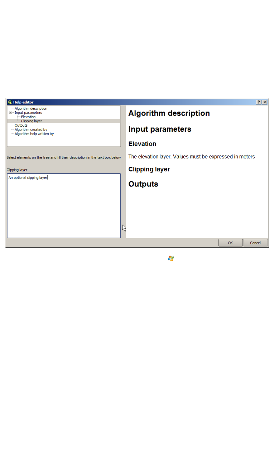
QGIS User Guide, Publicación 2.8
appear in this case as available inputs. Layers or values generated at a more advanced step in the workflow defined
by the model will not be available if they cause circular dependencies.
Select the new values and then click on the [OK] button as usual. The connections between the model elements
will change accordingly in the modeler canvas.
17.3.5 Editing model help files and meta-information
You can document your models from the modeler itself. Just click on the [Edit model help] button and a dialog
like the one shown next will appear.
Figure 17.23: Help Edition
On the right-hand side, you will see a simple HTML page, created using the description of the input parameters
and outputs of the algorithm, along with some additional items like a general description of the model or its author.
The first time you open the help editor, all these descriptions are empty, but you can edit them using the elements
on the left-hand side of the dialog. Select an element on the upper part and then write its description in the text
box below.
Model help is saved in a file in the same folder as the model itself. You do not have to worry about saving it, since
it is done automatically.
17.3.6 About available algorithms
You might notice that some algorithms that can be be executed from the toolbox do not appear in the list of
available algorithms when you are designing a model. To be included in a model, an algorithm must have a
correct semantic, so as to be properly linked to others in the workflow. If an algorithm does not have such a
well-defined semantic (for instance, if the number of output layers cannot be known in advance), then it is not
possible to use it within a model, and thus, it does not appear in the list of algorithms that you can find in the
modeler dialog.
Additionally, you will see some algorithms in the modeler that are not found in the toolbox. These algorithms are
meant to be used exclusively as part of a model, and they are of no interest in a different context. The ‘Calculator’
algorithm is an example of that. It is just a simple arithmetic calculator that you can use to modify numerical
values (entered by the user or generated by some other algorithm). This tool is really useful within a model, but
outside of that context, it doesn’t make too much sense.
210 Chapter 17. Entorno de trabajo de procesamiento de QGIS
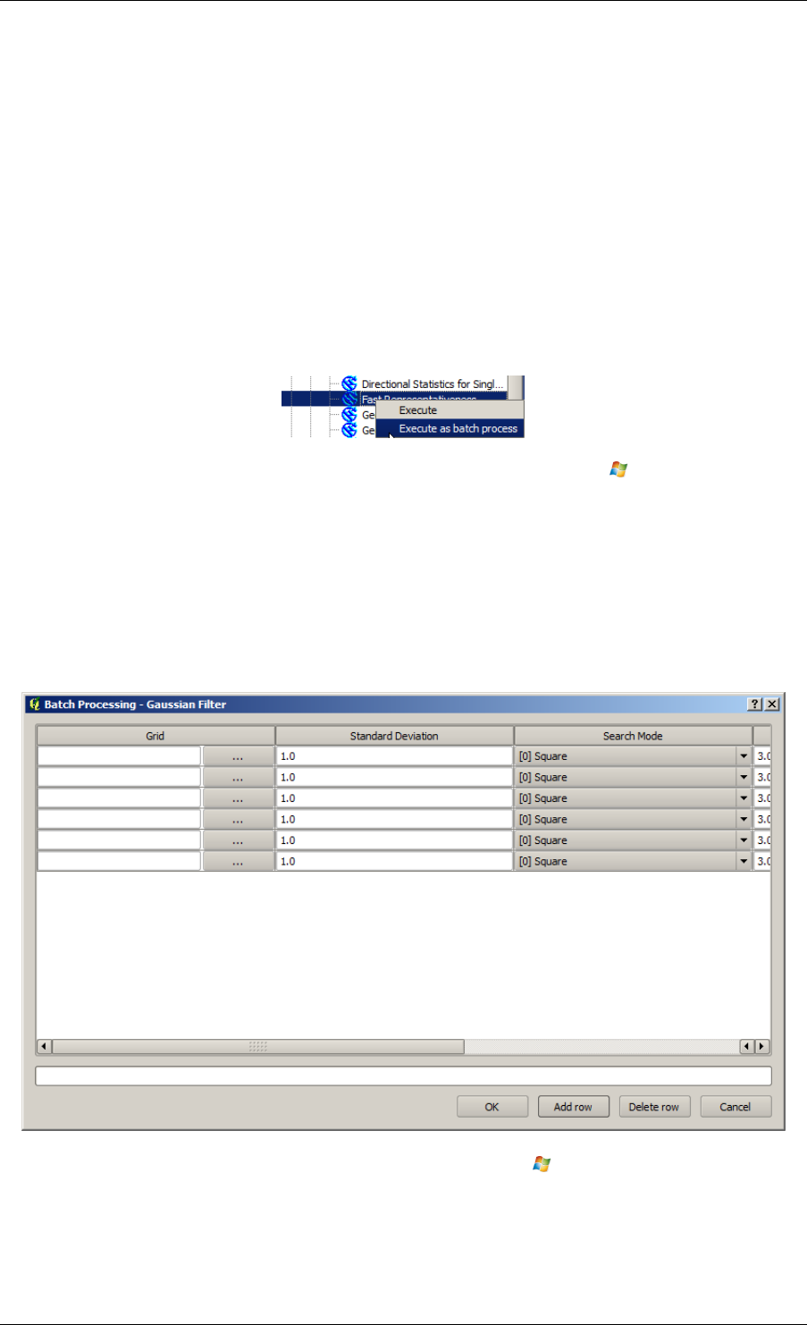
QGIS User Guide, Publicación 2.8
.
17.4 La interfaz de procesamiento por lotes
17.4.1 Introducción
Todos los algoritmos (incluyendo modelos) se pueden ejecutar como un proceso por lotes. Es decir, que se pueden
ejecutar utilizando no sólo un único conjunto de insumos, sino varios de ellos y ejecutar el algoritmo tantas veces
sea necesario. Esto es útil al procesar grandes cantidades de datos, ya que no es necesario poner en marcha el
algoritmo muchas veces desde la caja de herramientas.
Para ejecutar un algoritmo como un proceso por lotes, haga clic en su nombre en la caja de herramientas y
seleccionar la opción Ejecutar como proceso por lotes en el menú emergente que aparecerá.
Figure 17.24: Haga clic derecho en Procesamiento por lotes
17.4.2 La tabla de parámetros
La ejecución de un proceso por lotes es similar a la realización de una sola ejecución de un algoritmo. Los valores
de los parámetros tienen que ser definidos, pero en este caso no sólo necesitan un valor único para cada parámetro,
sino un conjunto de ellos en su lugar, una por cada vez que el algoritmo tiene que ser ejecutado. Los valores se
introducen mediante una tabla como la que se muestra a continuación.
Figure 17.25: Procesamiento por lotes
Cada línea de esta tabla representa una sola ejecución del algoritmo, y cada celda contiene el valor de uno de
los parámetros. Es similar al diálogo de los parámetros que se ve cuando se ejecuta un algoritmo de la caja de
herramientas, pero con una disposición diferente.
17.4. La interfaz de procesamiento por lotes 211
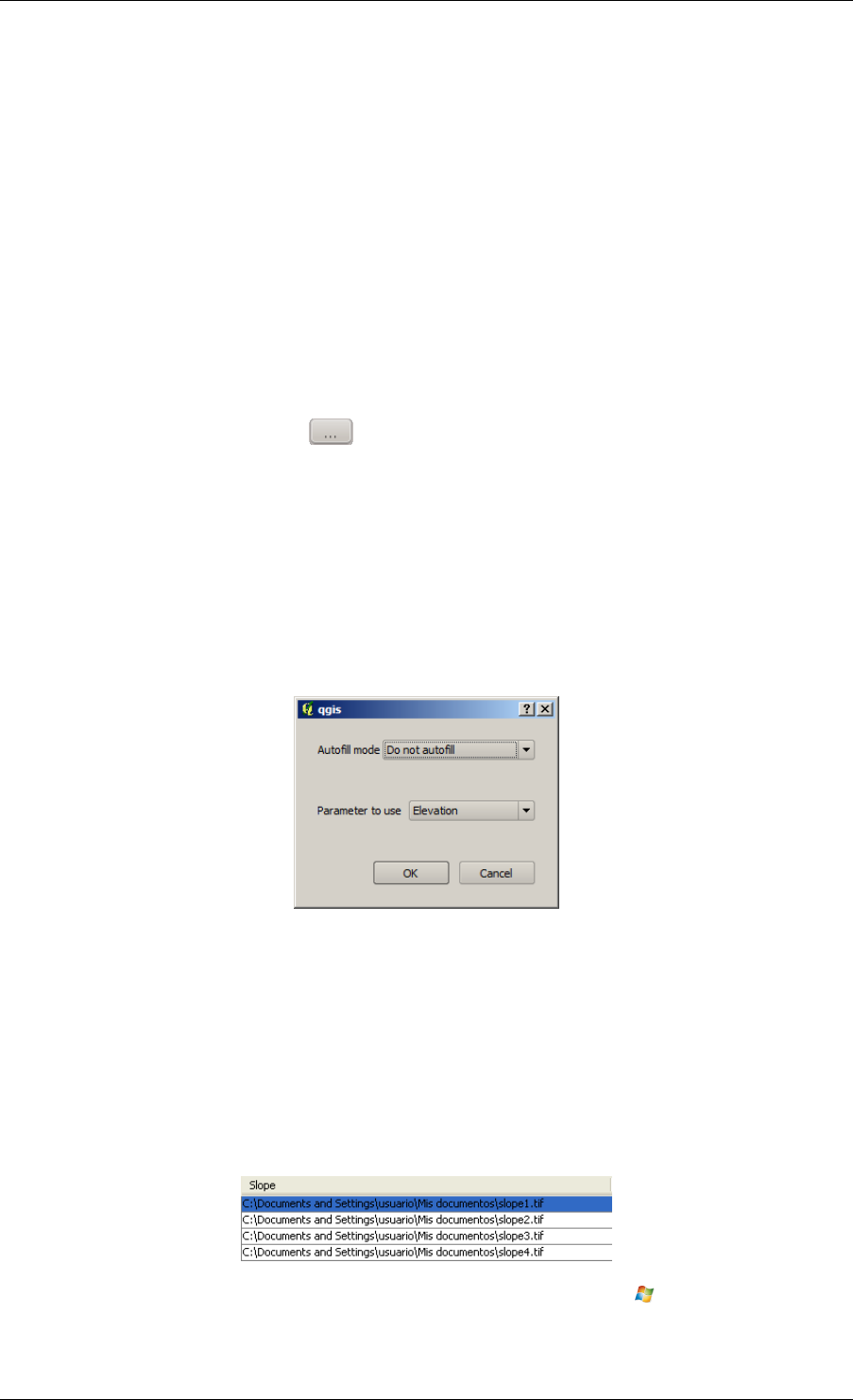
QGIS User Guide, Publicación 2.8
Por defecto, la tabla contiene sólo dos filas. Puede agregar o quitar filas utilizando los botones de la parte inferior
de la ventana.
Una vez que el tamaño de la tabla se ha establecido, este tiene que ser llenado con los valores deseados.
17.4.3 Llenado de la tabla de parámetros
Para la mayoría de los parámetros, establecen el valor es trivial. Sólo tienes que escribir el valor o seleccionarlo
de la lista de opciones disponibles, dependiendo del tipo de parámetro.
Las principales diferencias se encuentran en parámetros que representan capas o tablas, y para las rutas de archivos
de salida. En cuanto a las capas de entrada y tablas, cuando un algoritmo se ejecuta como parte de un proceso por
lotes, los objetos de datos de entrada se toman directamente de los archivos, y no desde el conjunto de ellos ya
abiertos en QGIS. Por esta razón, cualquier algoritmo puede ser ejecutado como un proceso por lotes, incluso si
no hay objetos de datos en absoluto y el algoritmo no se puede ejecutar desde la caja de herramientas.
Los nombres de archivo para los objetos de datos de entrada se introducen escribiendo directamente o, más con-
venientemente, al hacer clic en el botón en la parte derecha de la celda, que muestra un diálogo típico de
selección de archivos. Múltiples archivos se pueden seleccionar a la vez. Si el parámetro de entrada representa
un solo objeto de datos y varios archivos se seleccionan, cada uno de ellos serán puestos en una fila separada,
añadiendo otras nuevas si es necesario. Si el parámetro representa una entrada múltiple, se añadirán todos los
archivos seleccionados a una sola celda, separados por punto y coma (;).
Los objetos de datos de salida siempre se guardan en un archivo y, a diferencia de cuando se ejecuta un algo-
ritmo de la caja de herramientas, guardar en un archivo temporal no está permitido. Puede escribir el nombre
directamente o utilizar el diálogo de selector de archivos que aparece al hacer clic en el botón que lo acompaña.
Una ves que seleccione el archivo, un nuevo diálogo se mostrará para permitir la terminación automática de otras
celdas en la misma columna (mismo parámetro).
Figure 17.26: Guardar Procesamiento por lotes
Si se selecciona el valor por defecto (‘No autocompletar’), se acaba de poner el nombre del archivo seleccionado
en la celda seleccionada de la tabla de parámetros. Si se selecciona cualquiera de las otras opciones, todas las
celdas debajo de la seleccionada será automáticamente llenado basado en un criterio definido. De esta manera, es
mucho más fácil llenar la tabla, y el proceso por lotes se puede definir con menos esfuerzo.
El llenado automático puede hacerse por simple adición de los números correlativos a la ruta del archivo selec-
cionado, o al añadir el valor de otro campo en la misma fila. Esto es particularmente útil para nombrar a los objetos
de datos de salida de acuerdo con los de entrada.
Figure 17.27: Ruta de archivo de procesamiento por lotes
212 Chapter 17. Entorno de trabajo de procesamiento de QGIS

QGIS User Guide, Publicación 2.8
17.4.4 Ejecutar el proceso por lotes
Para ejecutar el proceso por lotes una vez que haya introducido todos los valores necesarios, simplemente haga
clic en [Aceptar]. El progreso de la tarea por lotes global se mostrará en la barra de progreso en la parte inferior
del diálogo
.
17.5 Utilizar algoritmos de procesamiento desde la consola
The console allows advanced users to increase their productivity and perform complex operations that cannot be
performed using any of the other GUI elements of the processing framework. Models involving several algorithms
can be defined using the command-line interface, and additional operations such as loops and conditional sentences
can be added to create more flexible and powerful workflows.
There is not a proccesing console in QGIS, but all processing commands are available instead from the QGIS
built-in Python console. That means that you can incorporate those commands into your console work and connect
processing algorithms to all the other features (including methods from the QGIS API) available from there.
El código se puede ejecutar desde la consola de Python, incluso si no especifica ningún método de procesamiento,
se puede convertir en un nuevo algoritmo que más tarde puede llamar desde la caja de herramientas, el mode-
lador gráfico o algún otro componente, tal como lo hace con cualquier otro algoritmo. De hecho, algunos de los
algoritmos que se pueden encontrar en la caja de herramientas son sencillas secuencias de comandos.
In this section, we will see how to use processing algorithms from the QGIS Python console, and also how to write
algorithms using Python.
17.5.1 Invocando algoritmos desde la consola de Python
Lo primero que tiene que hacer es importar las funciones de procesamiento con la siguiente línea:
>>> import processing
Now, there is basically just one (interesting) thing you can do with that from the console: execute an algorithm.
That is done using the runalg() method, which takes the name of the algorithm to execute as its first parameter,
and then a variable number of additional parameters depending on the requirements of the algorithm. So the first
thing you need to know is the name of the algorithm to execute. That is not the name you see in the toolbox, but
rather a unique command–line name. To find the right name for your algorithm, you can use the algslist()
method. Type the following line in your console:
>>> processing.alglist()
Veras algo como esto:
Accumulated Cost (Anisotropic)---------------->saga:accumulatedcost(anisotropic)
Accumulated Cost (Isotropic)------------------>saga:accumulatedcost(isotropic)
Add Coordinates to points--------------------->saga:addcoordinatestopoints
Add Grid Values to Points--------------------->saga:addgridvaluestopoints
Add Grid Values to Shapes--------------------->saga:addgridvaluestoshapes
Add Polygon Attributes to Points-------------->saga:addpolygonattributestopoints
Aggregate------------------------------------->saga:aggregate
Aggregate Point Observations------------------>saga:aggregatepointobservations
Aggregation Index----------------------------->saga:aggregationindex
Analytical Hierarchy Process------------------>saga:analyticalhierarchyprocess
Analytical Hillshading------------------------>saga:analyticalhillshading
Average With Mask 1--------------------------->saga:averagewithmask1
Average With Mask 2--------------------------->saga:averagewithmask2
Average With Thereshold 1--------------------->saga:averagewiththereshold1
Average With Thereshold 2--------------------->saga:averagewiththereshold2
Average With Thereshold 3--------------------->saga:averagewiththereshold3
17.5. Utilizar algoritmos de procesamiento desde la consola 213

QGIS User Guide, Publicación 2.8
B-Spline Approximation------------------------>saga:b-splineapproximation
...
Esa es una lista de todos los algoritmos disponibles, ordenada alfabéticamente, junto con sus nombres de linea de
comandos correspondientes.
You can use a string as a parameter for this method. Instead of returning the full list of algorithms, it will only
display those that include that string. If, for instance, you are looking for an algorithm to calculate slope from a
DEM, type alglist("slope") to get the following result:
DTM Filter (slope-based)---------------------->saga:dtmfilter(slope-based)
Downslope Distance Gradient------------------->saga:downslopedistancegradient
Relative Heights and Slope Positions---------->saga:relativeheightsandslopepositions
Slope Length---------------------------------->saga:slopelength
Slope, Aspect, Curvature---------------------->saga:slopeaspectcurvature
Upslope Area---------------------------------->saga:upslopearea
Vegetation Index[slope based]----------------->saga:vegetationindex[slopebased]
El resultado podría cambiar dependiendo de los algoritmos que se tienen disponibles.
Ahora es más fácil encontrar el algoritmo que se busca y el nombre de línea de comando, en este caso
saga:slopeaspectcurvature.
Once you know the command-line name of the algorithm, the next thing to do is to determine the right syntax to
execute it. That means knowing which parameters are needed and the order in which they have to be passed when
calling the runalg() method. There is a method to describe an algorithm in detail, which can be used to get a
list of the parameters that an algorithm requires and the outputs that it will generate. To get this information, you
can use the alghelp(name_of_the_algorithm) method. Use the command-line name of the algorithm,
not the full descriptive name.
Calling the method with saga:slopeaspectcurvature as parameter, you get the following description:
>>> processing.alghelp("saga:slopeaspectcurvature")
ALGORITHM: Slope, Aspect, Curvature
ELEVATION <ParameterRaster>
METHOD <ParameterSelection>
SLOPE <OutputRaster>
ASPECT <OutputRaster>
CURV <OutputRaster>
HCURV <OutputRaster>
VCURV <OutputRaster>
Ahora se tiene todo lo necesario para ejecutar cualquier algoritmo. Como ya hemos mencionado, sólo hay un solo
comando para ejecutar algoritmos: runalg(). Su sintaxis es la siguiente:
>>> processing.runalg(name_of_the_algorithm, param1, param2, ..., paramN,
Output1, Output2, ..., OutputN)
La lista de parámetros y salidas para añadir dependen del algoritmo que se desean ejecutar, y es exactamente la
lista que el método alghelp() le da, en el mismo orden que se muestra.
Depending on the type of parameter, values are introduced differently. The next list gives a quick review of how
to introduce values for each type of input parameter:
• Raster Layer, Vector Layer or Table. Simply use a string with the name that identifies the data object to use
(the name it has in the QGIS Table of Contents) or a filename (if the corresponding layer is not opened, it
will be opened but not added to the map canvas). If you have an instance of a QGIS object representing the
layer, you can also pass it as parameter. If the input is optional and you do not want to use any data object,
use None.
• Selección. Si un algoritmo tiene un parámetro de selección, el valor de ese parámetro debe ser intro-
ducido mediante un valor entero. Para conocer las opciones disponibles, se puede utilizar el comando
algoptions(), como se muestra en el siguiente ejemplo
214 Chapter 17. Entorno de trabajo de procesamiento de QGIS

QGIS User Guide, Publicación 2.8
>>> processing.algoptions("saga:slopeaspectcurvature")
METHOD(Method)
0 - [0] Maximum Slope (Travis et al. 1975)
1 - [1] Maximum Triangle Slope (Tarboton 1997)
2 - [2] Least Squares Fitted Plane (Horn 1981, Costa-Cabral & Burgess 1996)
3 - [3] Fit 2.Degree Polynom (Bauer, Rohdenburg, Bork 1985)
4 - [4] Fit 2.Degree Polynom (Heerdegen & Beran 1982)
5 - [5] Fit 2.Degree Polynom (Zevenbergen & Thorne 1987)
6 - [6] Fit 3.Degree Polynom (Haralick 1983)
In this case, the algorithm has one such parameter, with seven options. Notice that ordering is zero-based.
• Multiple input. The value is a string with input descriptors separated by semicolons (;). As in the case of
single layers or tables, each input descriptor can be the data object name, or its file path.
• El campo de la tabla de XXX. Utilice una cadena con el nombre del campo a usar. Este parámetro es
sensible a mayúsculas y minúsculas.
• Fixed Table. Type the list of all table values separated by commas (,) and enclosed between quotes (").
Values start on the upper row and go from left to right. You can also use a 2-D array of values representing
the table.
• SRC. Introduzca el número del código EPSG del SRC deseado.
• Extensión. Se debe utilizar una cadena con valores de xmin,xmax,ymin yymax‘ separados por
comas (,‘‘).
Los parámetros boolean, archivo, cadena y numéricos no necesitan alguna explicación adicional.
Input parameters such as strings, booleans, or numerical values have default values. To use them, specify None
in the corresponding parameter entry.
For output data objects, type the file path to be used to save it, just as it is done from the toolbox. If you want to
save the result to a temporary file, use None. The extension of the file determines the file format. If you enter
a file extension not supported by the algorithm, the default file format for that output type will be used, and its
corresponding extension appended to the given file path.
Unlike when an algorithm is executed from the toolbox, outputs are not added to the map canvas if you execute
that same algorithm from the Python console. If you want to add an output to the map canvas, you have to do it
yourself after running the algorithm. To do so, you can use QGIS API commands, or, even easier, use one of the
handy methods provided for such tasks.
The runalg method returns a dictionary with the output names (the ones shown in the algorithm description)
as keys and the file paths of those outputs as values. You can load those layers by passing the corresponding file
paths to the load() method.
17.5.2 Funciones adicionales para manipular datos
Apart from the functions used to call algorithms, importing the processing package will also import some
additional functions that make it easier to work with data, particularly vector data. They are just convenience
functions that wrap some functionality from the QGIS API, usually with a less complex syntax. These functions
should be used when developing new algorithms, as they make it easier to operate with input data.
Below is a list of some of these commands. More information can be found in the classes under the
processing/tools package, and also in the example scripts provided with QGIS.
•getObject(obj): Returns a QGIS object (a layer or table) from the passed object, which can be a
filename or the name of the object in the QGIS Table of Contents.
•values(layer, fields): Returns the values in the attributes table of a vector layer, for the passed
fields. Fields can be passed as field names or as zero-based field indices. Returns a dict of lists, with the
passed field identifiers as keys. It considers the existing selection.
•features(layer): Returns an iterator over the features of a vector layer, considering the existing
selection.
17.5. Utilizar algoritmos de procesamiento desde la consola 215

QGIS User Guide, Publicación 2.8
•uniqueValues(layer, field): Returns a list of unique values for a given attribute. Attributes can
be passed as a field name or a zero-based field index. It considers the existing selection.
17.5.3 Crear scripts y ejecurarlos desde le Caja de Herramientas
You can create your own algorithms by writing the corresponding Python code and adding a few extra lines to
supply additional information needed to define the semantics of the algorithm. You can find a Create new script
menu under the Tools group in the Script algorithms block of the toolbox. Double-click on it to open the script
editing dialog. That’s where you should type your code. Saving the script from there in the scripts folder (the
default folder when you open the save file dialog) with .py extension will automatically create the corresponding
algorithm.
El nombre del algoritmo (el que podrá ver en la caja de herramientas) se crea a partir del nombre de archivo, la
eliminación su extensión y la sustitución de guiones bajos con espacios en blanco.
Let’s have a look at the following code, which calculates the Topographic Wetness Index (TWI) directly from a
DEM.
##dem=raster
##twi=output
ret_slope = processing.runalg("saga:slopeaspectcurvature", dem, 0, None,
None, None, None, None)
ret_area = processing.runalg("saga:catchmentarea(mass-fluxmethod)", dem,
0, False, False, False, False, None, None, None, None, None)
processing.runalg("saga:topographicwetnessindex(twi), ret_slope[’SLOPE’],
ret_area[’AREA’], None, 1, 0, twi)
As you can see, the calculation involves three algorithms, all of them coming from SAGA. The last one calculates
the TWI, but it needs a slope layer and a flow accumulation layer. We do not have these layers, but since we have
the DEM, we can calculate them by calling the corresponding SAGA algorithms.
La parte del código donde este procesamiento se lleva a cabo no es difícil de entender si ha leído las secciones an-
teriores de este capítulo. Las primeras líneas, sin embargo, necesitan alguna explicación adicional. Proporcionan
la información que se necesita para convertir su código en un algoritmo que se puede ejecutar desde cualquiera de
los componentes GUI, como la caja de herramientas o el modelador gráfico.
These lines start with a double Python comment symbol (##) and have the following structure:
[parameter_name]=[parameter_type] [optional_values]
Here is a list of all the parameter types that are supported in processing scripts, their syntax and some examples.
•raster. A raster layer.
•vector. Una capa vectorial.
•table. Una tabla.
•number. A numerical value. A default value must be provided. For instance, depth=number 2.4.
•string. A text string. As in the case of numerical values, a default value must be added. For instance,
name=string Victor.
•boolean. A boolean value. Add True or False after it to set the default value. For example,
verbose=boolean True.
•ráster múltiple. Un conjunto de capas ráster de entrada.
•Vector múltiple. Un conjunto de capas vectoriales de entrada.
•Campo. Un campo es la tabla de atributos de una capa vectorial. El nombre de la capa se tiene que añadir de-
spués de la etiqueta Campo. Por ejemplo, si ha declarado una vectorial de entrada con mylayer=vector,
podría utilizar myfield=field mylayer para añadir un campo de esa capa como parámetro.
•folder. Una carpeta.
•file. A nombre de archivo.
216 Chapter 17. Entorno de trabajo de procesamiento de QGIS

QGIS User Guide, Publicación 2.8
El nombre del parámetro es el nombre que se mostrará al usuario cuando ejecuta el algoritmo, y también el nombre
de variable a utilizar en la secuencia de código. El valor introducido por el usuario para ese parámetro se asignará
a la variable con ese nombre.
When showing the name of the parameter to the user, the name will be edited to improve its appearance, replacing
low hyphens with spaces. So, for instance, if you want the user to see a parameter named A numerical
value, you can use the variable name A_numerical_value.
Layers and table values are strings containing the file path of the corresponding object. To turn them into a QGIS
object, you can use the processing.getObjectFromUri() function. Multiple inputs also have a string
value, which contains the file paths to all selected object, separated by semicolons (;).
Outputs are defined in a similar manner, using the following tags:
•output raster
•output vector
•output table
•output html
•output file
•output number
•output string
The value assigned to the output variables is always a string with a file path. It will correspond to a temporary file
path in case the user has not entered any output filename.
When you declare an output, the algorithm will try to add it to QGIS once it is finished. That is why, although the
runalg() method does not load the layers it produces, the final TWI layer will be loaded (using the case of our
previous example), since it is saved to the file entered by the user, which is the value of the corresponding output.
Do not use the load() method in your script algorithms, just when working with the console line. If a layer is
created as output of an algorithm, it should be declared as such. Otherwise, you will not be able to properly use
the algorithm in the modeler, since its syntax (as defined by the tags explained above) will not match what the
algorithm really creates.
Hidden outputs (numbers and strings) do not have a value. Instead, you have to assign a value to them. To do so,
just set the value of a variable with the name you used to declare that output. For instance, if you have used this
declaration,
##average=output number
the following line will set the value of the output to 5:
average =5
In addition to the tags for parameters and outputs, you can also define the group under which the algorithm will
be shown, using the group tag.
If your algorithm takes a long time to process, it is a good idea to inform the user. You have a global named
progress available, with two possible methods: setText(text) and setPercentage(percent) to
modify the progress text and the progress bar.
Several examples are provided. Please check them to see real examples of how to create algorithms using the
processing framework classes. You can right-click on any script algorithm and select Edit script to edit its code or
just to see it.
17.5.4 Documenting your scripts
As in the case of models, you can create additional documentation for your scripts, to explain what they do and
how to use them. In the script editing dialog, you will find an [Edit script help] button. Click on it and it will
17.5. Utilizar algoritmos de procesamiento desde la consola 217

QGIS User Guide, Publicación 2.8
take you to the help editing dialog. Check the section about the graphical modeler to know more about this dialog
and how to use it.
Help files are saved in the same folder as the script itself, adding the .help extension to the filename. Notice that
you can edit your script’s help before saving the script for the first time. If you later close the script editing dialog
without saving the script (i.e., you discard it), the help content you wrote will be lost. If your script was already
saved and is associated to a filename, saving the help content is done automatically.
17.5.5 Pre- and post-execution script hooks
Scripts can also be used to set pre- and post-execution hooks that are run before and after an algorithm is run. This
can be used to automate tasks that should be performed whenever an algorithm is executed.
The syntax is identical to the syntax explained above, but an additional global variable named alg is available,
representing the algorithm that has just been (or is about to be) executed.
In the General group of the processing configuration dialog, you will find two entries named Pre-execution script
file and Post-execution script file where the filename of the scripts to be run in each case can be entered.
.
17.6 El administrador del historial
17.6.1 El historial del procesamiento
Cada vez que ejecutas un algoritmo, la información acerca del proceso es almacenado en el administrador de la
historia. Junto con los parámetros usados, la fecha y hora de la ejecución también se guardan.
De esta manera, es fácil rastrear y controlar todo el trabajo que se ha desarrollado usando la caja de herramientas
de procesado, y fácil reproducirlo.
El administrador del historial es un conjunto de entradas de registros agrupados de acuerdo a su fecha de ejecución,
por lo que es más fácil encontrar información sobre un algoritmo ejecutado en cualquier momento en particular.
Información del proceso se mantiene como una expresión de línea de comandos, incluso si el algoritmo fue lanzado
desde la caja de herramientas. Esto hace que sea también útil para aquellos que están aprendiendo cómo utilizar la
interfaz de línea de comandos, ya que se pueden llamar un algoritmo usando la caja de herramientas y compruebe
el administrados del historial para ver cómo ese mismo algoritmo podría ser llamado desde la línea de comandos.
Parte de la navegación por las entradas en el registro, también puede volver a ejecutar los procesos al hacer doble
clic en la entrada correspondiente.
Junto con el registro de algoritmos ejecutados, la caja de herramientas de procesado se comunica con el usuario
por medio de los otros grupos del registro, a saber Errors,WARNING yINFO. En caso de que algo no este
funcionando adecuadamente, echar un vistazo a ERROR que pueden ayudarle a ver lo que está sucediendo. Si se
pone en contacto con un desarrollador para informar de un bug o error, la información en ese grupo va a ser muy
útil para él o ella para averiguar lo que está mal.
Los algoritmos de terceros se ejecutan normalmente llamando su interfaz de linea de comandos, que se comunica
con el usuario vía consola. Aunque la consola no se muestra, una copia completa de la misma se almacena en el
grupo INFO cada vez que se ejecuta uno de estos algoritmos. Si, por ejemplo, se tienen problemas al ejecutar el
algoritmo de SAGA, busque una entrada denominada ‘SAGA execution console output’ para comprobar todos los
mensajes generados por SAGA y tratar de localizar donde esta el problema.
Algunos algoritmos, incluso pueden producir un resultado con los datos de entrada dados , puede añadir comen-
tarios o información adicional para el bloque WARNING si detectan problemas potenciales con los datos, con el
fin de advertirle. Asegúrese de revisar esos mensajes si se esta teniendo resultados inesperados.
218 Chapter 17. Entorno de trabajo de procesamiento de QGIS
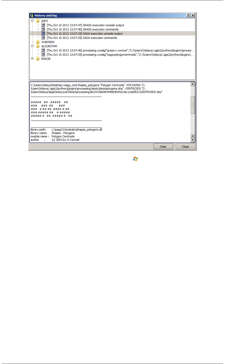
QGIS User Guide, Publicación 2.8
Figure 17.28: Historial
17.7 Writing new Processing algorithms as python scripts
You can create your own algorithms by writing the corresponding Python code and adding a few extra lines to
supply additional information needed to define the semantics of the algorithm. You can find a Create new script
menu under the Tools group in the Script algorithms block of the toolbox. Double-click on it to open the script
edition dialog. That’s where you should type your code. Saving the script from there in the scripts folder (the
default one when you open the save file dialog), with .py extension, will automatically create the corresponding
algorithm.
The name of the algorithm (the one you will see in the toolbox) is created from the filename, removing its extension
and replacing low hyphens with blank spaces.
Let’s have the following code, which calculates the Topographic Wetness Index (TWI) directly from a DEM
##dem=raster
##twi=output raster
ret_slope = processing.runalg("saga:slopeaspectcurvature", dem, 0, None,
None, None, None, None)
ret_area = processing.runalg("saga:catchmentarea", dem,
0, False, False, False, False, None, None, None, None, None)
processing.runalg("saga:topographicwetnessindextwi, ret_slope[’SLOPE’],
ret_area[’AREA’], None, 1, 0, twi)
As you can see, it involves 3 algorithms, all of them coming from SAGA. The last one of them calculates the TWI,
but it needs a slope layer and a flow accumulation layer. We do not have these ones, but since we have the DEM,
we can calculate them calling the corresponding SAGA algorithms.
The part of the code where this processing takes place is not difficult to understand if you have read the previous
chapter. The first lines, however, need some additional explanation. They provide the information that is needed to
turn your code into an algorithm that can be run from any of the GUI components, like the toolbox or the graphical
modeler.
These lines start with a double Python comment symbol (##) and have the following structure
17.7. Writing new Processing algorithms as python scripts 219

QGIS User Guide, Publicación 2.8
[parameter_name]=[parameter_type] [optional_values]
Here is a list of all the parameter types that are supported in processign scripts, their syntax and some examples.
•raster. A raster layer
•vector. A vector layer
•table. A table
•number. A numerical value. A default value must be provided. For instance, depth=number 2.4
•string. A text string. As in the case of numerical values, a default value must be added. For instance,
name=string Victor
•longstring. Same as string, but a larger text box will be shown, so it is better suited for long strings,
such as for a script expecting a small code snippet.
•boolean. A boolean value. Add True or False after it to set the default value. For example,
verbose=boolean True.
•multiple raster. A set of input raster layers.
•multiple vector. A set of input vector layers.
•field. A field in the attributes table of a vector layer. The name of the layer has to be added after the
field tag. For instance, if you have declared a vector input with mylayer=vector, you could use
myfield=field mylayer to add a field from that layer as parameter.
•folder. A folder
•file. A filename
•crs. A Coordinate Reference System
The parameter name is the name that will be shown to the user when executing the algorithm, and also the variable
name to use in the script code. The value entered by the user for that parameter will be assigned to a variable with
that name.
When showing the name of the parameter to the user, the name will be edited it to improve its appearance, replacing
low hyphens with spaces. So, for instance, if you want the user to see a parameter named A numerical
value, you can use the variable name A_numerical_value.
Layers and tables values are strings containing the filepath of the corresponding object. To turn them into a QGIS
object, you can use the processing.getObjectFromUri() function. Multiple inputs also have a string
value, which contains the filepaths to all selected objects, separated by semicolons (;).
Outputs are defined in a similar manner, using the following tags:
•output raster
•output vector
•output table
•output html
•output file
•output number
•output string
•output extent
The value assigned to the output variables is always a string with a filepath. It will correspond to a temporary
filepath in case the user has not entered any output filename.
In addition to the tags for parameters and outputs, you can also define the group under which the algorithm will
be shown, using the group tag.
220 Chapter 17. Entorno de trabajo de procesamiento de QGIS

QGIS User Guide, Publicación 2.8
The last tag that you can use in your script header is ##nomodeler. Use that when you do not want your
algorithm to be shown in the modeler window. This should be used for algorithms that do not have a clear syntax
(for instance, if the number of layers to be created is not known in advance, at design time), which make them
unsuitable for the graphical modeler
17.8 Handing data produced by the algorithm
When you declare an output representing a layer (raster, vector or table), the algorithm will try to add it to QGIS
once it is finished. That is the reason why, although the runalg() method does not load the layers it produces,
the final TWI layer will be loaded, since it is saved to the file entered by the user, which is the value of the
corresponding output.
Do not use the load() method in your script algorithms, but just when working with the console line. If a layer
is created as output of an algorithm, it should be declared as such. Otherwise, you will not be able to properly
use the algorithm in the modeler, since its syntax (as defined by the tags explained above) will not match what the
algorithm really creates.
Hidden outputs (numbers and strings) do not have a value. Instead, it is you who has to assign a value to them. To
do so, just set the value of a variable with the name you used to declare that output. For instance, if you have used
this declaration,
##average=output number
the following line will set the value of the output to 5:
average =5
17.9 Communicating with the user
If your algorithm takes a long time to process, it is a good idea to inform the user. You have a global named
progress available, with two available methods: setText(text) and setPercentage(percent) to
modify the progress text and the progress bar.
If you have to provide some information to the user, not related to the progress of the algorithm, you can use the
setInfo(text) method, also from the progress object.
If your script has some problem, the correct way of propagating it is to raise an exception of type
GeoAlgorithmExecutionException(). You can pass a message as argument to the constructor of the
exception. Processing will take care of handling it and communicating with the user, depending on where the
algorithm is being executed from (toolbox, modeler, Python console...)
17.10 Documenting your scripts
As in the case of models, you can create additional documentation for your script, to explain what they do and
how to use them. In the script editing dialog you will find a [Edit script help] button. Click on it and it will take
you to the help editing dialog. Check the chapter about the graphical modeler to know more about this dialog and
how to use it.
Help files are saved in the same folder as the script itself, adding the .help extension to the filename. Notice that
you can edit your script’s help before saving it for the first time. If you later close the script editing dialog without
saving the script (i.e. you discard it), the help content you wrote will be lost. If your script was already saved and
is associated to a filename, saving is done automatically.
17.8. Handing data produced by the algorithm 221
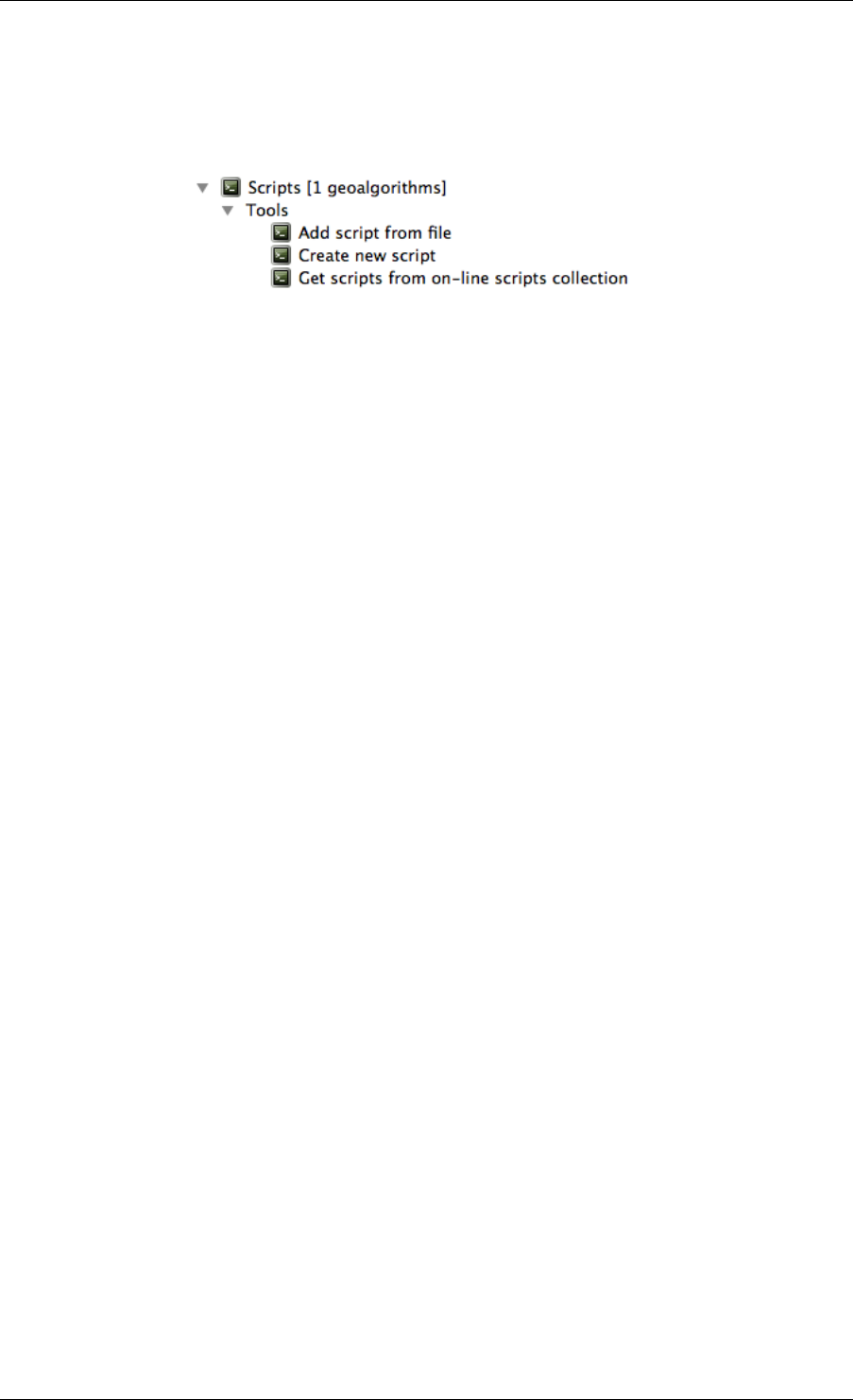
QGIS User Guide, Publicación 2.8
17.11 Example scripts
Several examples are available in the on-line collection of scripts, which you can access by selecting the Get script
from on-line script collection tool under the Scripts/tools entry in the toolbox.
Please, check them to see real examples of how to create algorithms using the processing framework classes. You
can right-click on any script algorithm and select Edit script to edit its code or just to see it.
17.12 Best practices for writing script algorithms
Here’s a quick summary of ideas to consider when creating your script algorithms and, especially, if you want to
share with other QGIS users. Following these simple rules will ensure consistency across the different Processing
elements such as the toolbox, the modeler or the batch processing interface.
• Do not load resulting layers. Let Processing handle your results and load your layers if needed.
• Always declare the outputs your algorithm creates. Avoid things such as declaring one output and then
using the destination filename set for that output to create a collection of them. That will break the correct
semantics of the algorithm and make it impossible to use it safely in the modeler. If you have to write an
algorithm like that, make sure you add the ##nomodeler tag.
• Do not show message boxes or use any GUI element from the script. If you want to communicate with the
user, use the setInfo() method or throw an GeoAlgorithmExecutionException
• As a rule of thumb, do not forget that your algorithm might be executed in a context other than the Processing
toolbox.
17.13 Pre- and post-execution script hooks
Scripts can also be used to set pre- and post-execution hooks that are run before and after an algorithm is run. This
can be used to automate tasks that should be performed whenever an algorithm is executed.
The syntax is identical to the syntax explained above, but an additional global variable named alg is available,
representing the algorithm that has just been (or is about to be) executed.
In the General group of the processing config dialog you will find two entries named Pre-execution script file and
Post-execution script file where the filename of the scripts to be run in each case can be entered.
.
17.14 Configurar aplicaciones externas
El entorno de procesamiento se puede extender el uso de aplicaciones adicionales. Actualmente, SAGA, GRASS,
OTB (Orfeo Toolbox) y R son reconocidos, junto con algunas otras aplicaciones de línea de comandos que pro-
porcionan funcionalidades de análisis de datos espaciales. Los algoritmos que dependen de una aplicación externa
son administrados por su propio proveedor de algoritmos.
Esta sección le mostrará cómo configurar el entorno de procesamiento para incluir estas aplicaciones adicionales,
y le explicará algunas de las características particulares de los algoritmos basados en ellos. Una vez que haya
222 Chapter 17. Entorno de trabajo de procesamiento de QGIS

QGIS User Guide, Publicación 2.8
configurado correctamente el sistema, usted será capaz de ejecutar algoritmos externos de cualquier componente,
como la caja de herramientas o el modelador gráfico, tal como lo hace con cualquier otro geoalgoritmo.
Por defecto, todos los algoritmos que dependen de aplicaciones externas no incluidas con QGIS no estarán habil-
itados. Pueden ser habilitados en el diálogo de configuración. Asegúrese de que la aplicación de la que depende
esté instalada en el sistema. En caso de no hacerlo, los algoritmos aparecerán en la Caja de Herramientas, pero se
emitirá un mensaje de error cuando se intente hacer uso de ellos.
Esto se debe a las descripciones de algoritmos (necesarios para crear el diálogo de parámetros y proporcionar la
información necesaria sobre el algoritmo) no se incluyen con cada aplicación, pero con QGIS en lugar de. Es
decir, que son parte de QGIS, por lo que ellos están en su instalación, incluso si no ha instalado ningún otro
software. La ejecución del algoritmo, sin embargo, necesita de los binarios de la aplicación para ser instalada en
su sistema.
17.14.1 Aclaración para los usuarios de Windows
Si no es un usuario avanzado y está ejecutando QGIS en Windows, podría no estar interesado en leer el resto
de este capítulo. Asegure que la instalación de QGIS en su sistema utiliza el instalador independiente. Esto
instalará automáticamente SAGA, GRASS y OTB en su sistema y configurarlos para que se pueden ejecutar desde
QGIS. Todos los algoritmos de la vista simplificada de la caja de herramientas estarán listas para ser ejecutado
sin necesidad de alguna configuración adicional. Si va a instalar mediante la aplicación OSGeo4W, asegúrese de
seleccionar SAGA, OTB para la instalación.
Si quiere saber más sobre cómo funcionan estos proveedores, o si quiere utilizar algún algoritmo que no se en-
cuentre en la Caja de Herramientas simplificada (como los scripts de R), siga leyendo.
17.14.2 Aclaración respecto a los formatos de archivos
Cuando se utiliza un software externo, la apertura de un archivo en QGIS no significa que se puede abrir y procesar
bien en ese otro software. En la mayoría de los casos, otro software puede leer lo que ha abierto en QGIS, pero
en algunos casos, eso puede no ser cierto. Al utilizar las bases de datos o formatos de archivo poco comunes, ya
sea para capas raster o vectoriales, podrían surgir problemas. Si eso sucede, trate de utilizar formatos de archivo
conocidos que este seguro que ambos programas entiendan, y comprobar la salida de la consola (en el historico y
el diálogo de registro) para saber más acerca de lo que va mal.
Utilizar capas raster de GRASS es, por ejemplo, uno de los casos en los que pueden existir problemas y no
completarse el trabajo si se invoca un algoritmo externo que use dicha capa como entrada. Por este motivo, estas
capas no aparecerán como disponibles para los algoritmos.
Debe, sin embargo, no encontrar ningún problema en absoluto con las capas vectoriales, ya que QGIS convierte
automáticamente desde el formato de archivo original a uno aceptado por la aplicación externa antes de pasar la
capa a la misma. Esto suma tiempo de procesamiento adicional, que podría ser significativo si la capa tiene un
tamaño grande, así que no se sorprenda si se necesita más tiempo para procesar una capa de una conexión de DB
que lo hace para procesar una de un tamaño similar almacenada en un archivo de shape.
Los proveedores que no utilizan aplicaciones externas pueden procesar cualquier capa que se pueda abrir en QGIS,
ya que son abiertas para el análisis mediante QGIS.
En cuanto a formatos de salida, todos los formatos reconocidos por QGIS como salida se pueden utilizar, tanto para
capas ráster y vectoriales. Algunos proveedores no admiten determinados formatos, pero todos pueden exportar
a los formatos de capa raster comunes que luego pueden transformarse con QGIS automáticamente. Al igual que
en el caso de las capas de entrada, si es necesaria esta conversión, podría aumentar el tiempo de procesamiento.
Si la extensión del nombre de archivo especificado cuando se llama a un algoritmo no coincide con la extensión
de cualquiera de los formatos reconocidos por QGIS, entonces se agregará un sufijo para establecer un formato
predeterminado. En el caso de las capas ráster, la extensión .tif se usa, mientras que .shp se utiliza para las
capas vectoriales.
17.14. Configurar aplicaciones externas 223

QGIS User Guide, Publicación 2.8
17.14.3 Nota referente a las seleccion de capas vectoriales
Las aplicaciones externas pueden también ser conscientes de las selecciones que existen en capas vectoriales den-
tro QGIS. Sin embargo, eso requiere reescribir todas las capas vectoriales de entrada, al igual que si originalmente
estuvieran en un formato no compatible con la aplicación externa. Sólo cuando no existe ninguna selección o la
opción *Utilizar sólo objetos espaciales seleccionados * no está activada en la configuración general de proce-
samiento, puede una capa ser directamente pasada a una aplicación externa.
En otros casos sólo es necesario exportar un conjunto de características seleccionadas, lo que hará que los tiempos
de ejecución sean mayores.
SAGA
Los algoritmos de SAGA pueden ser ejecutados desde QGIS si se tiene SAGA instalado en su sistema y se puede
configurar correctamente el entorno de procesamiento para que pueda encontrar ejecutables SAGA. En particular,
se necesita la línea de comandos SAGA ejecutable para ejecutar algoritmos SAGA.
Si ejecuta Windows, tanto el instalador estándar como el de OSGeo4W incluyen SAGA junto con QGIS y la ruta
se configura automáticamente, por lo qu eno es necesrio hacer nada más.
Si ha instalado SAGA usted mismo (recuerde, que necesita la versión 2.1), la ruta del SAGA ejecutable se debe
configurar. Para hacer esto, abrir el diálogo de configuración. En el bloque SAGA, se encontrará un ajuste denom-
inado Directorio SAGA. Ingrese la ruta del directorio donde SAGA está instalado. Cierre el diálogo de configu-
ración, y ahora está listo para ejecutar algoritmos de SAGA desde QGIS.
Si se está ejecutando Linux, los binarios de SAGA no están incluidos con SEXTANTE, así que tiene que descargar
e instalar el software. Por favor, consulte el sitio web de SAGA para mayor información. Se necesita SAGA 2.1.
En este caso, no hay necesidad de configurar la ruta al ejecutable de SAGA, y no se verán esas carpetas. En su
lugar, debe asegurarse de que SAGA está correctamente instalado y se añade su carpeta a la variable de entorno
PATH. Sólo tiene que abrir una consola y escribir saga_cmd para comprobar que el sistema puede encontrar
donde se encuentran los archivos binarios de SAGA.
17.14.4 Sobre las limitaciones del sistema de cuadrícula de SAGA
La mayoría de los algoritmos de SAGA que requieren varias capas ráster de entrada les obligan a tener el mismo
sistema de rejilla. Es decir, deben cubrir la misma área geográfica y tienen el mismo tamaño de la celda, por lo que
sus correspondientes rejillas coinciden. Al llamar a los algoritmos de SAGA desde QGIS, puede utilizar cualquier
capa, independientemente del tamaño de la celda y la extensión. Cuando múltiples capas ráster se utilizan como
entrada para un algoritmo de SAGA, QGIS los vuelve a muestrear a un sistema de rejilla común y luego los pasa
a SAGA (a menos que el algoritmo de SAGA pueda operar con capas de diferentes sistemas de rejilla).
The definition of that common grid system is controlled by the user, and you will find several parameters in the
SAGA group of the settings window to do so. There are two ways of setting the target grid system:
• Setting it manually. You define the extent by setting the values of the following parameters:
–Resampling min X
–Resampling max X
–Resampling min Y
–Resampling max Y
–Resampling cellsize
Nótese que QGIS volverá a muestrear las capas de entrada en dicha medida, incluso si no se solapan con
ésta.
• Setting it automatically from input layers. To select this option, just check the Use min covering grid system
for resampling option. All the other settings will be ignored and the minimum extent that covers all the
input layers will be used. The cell size of the target layer is the maximum of all cell sizes of the input layers.
224 Chapter 17. Entorno de trabajo de procesamiento de QGIS

QGIS User Guide, Publicación 2.8
Para los algoritmos que no utilizan múltiples capas raster, o para aquellos que no necesitan un único sistema de
cuadrícula de entrada, no se realizará un remuestreo antes de invocar SAG y dichos parámetros no son utilizados.
17.14.5 Limitaciones para las capas multibanda
Unlike QGIS, SAGA has no support for multi-band layers. If you want to use a multiband layer (such as an RGB or
multispectral image), you first have to split it into single-banded images. To do so, you can use the ‘SAGA/Grid
- Tools/Split RGB image’ algorithm (which creates three images from an RGB image) or the ‘SAGA/Grid -
Tools/Extract band’ algorithm (to extract a single band).
17.14.6 Limitaciones en el tamaño de celda
SAGA assumes that raster layers have the same cell size in the X and Y axis. If you are working with a layer with
different values for horizontal and vertical cell size, you might get unexpected results. In this case, a warning will
be added to the processing log, indicating that an input layer might not be suitable to be processed by SAGA.
17.14.7 Registro
When QGIS calls SAGA, it does so using its command-line interface, thus passing a set of commands to perform
all the required operations. SAGA shows its progress by writing information to the console, which includes the
percentage of processing already done, along with additional content. This output is filtered and used to update
the progress bar while the algorithm is running.
Both the commands sent by QGIS and the additional information printed by SAGA can be logged along with other
processing log messages, and you might find them useful to track in detail what is going on when QGIS runs a
SAGA algorithm. You will find two settings, namely Log console output and Log execution commands, to activate
that logging mechanism.
La mayoría del resto de proveedores que utilizan una aplicación externa y la invocan a través de la línea de
comandos tienen opciones similares, de forma que las podrá encontrar también en otros lugares de la lista de
ajustes de procesamiento.
R. Creating R scripts
La integración R en QGIS es diferente al de SAGA y es que no hay un conjunto predefinido de algoritmos que
pueda ejecutar (a excepción de algunos ejemplos). En su lugar, debe escribir sus scripts y llamar a los comandos
R, al igual que lo haría desde R, y de una manera muy similar a lo que vimos en la sección dedicada a scripts de
procesamiento. En esta sección se muestra la sintaxis para usar y llamar a los comandos de R QGIS y cómo usar
en QGIS los objetos (capas, tablas) en ellos.
The first thing you have to do, as we saw in the case of SAGA, is to tell QGIS where your R binaries are located.
You can do this using the R folder entry in the processing configuration dialog. Once you have set that parameter,
you can start creating and executing your own R scripts.
De nuevo, esto es diferente en Linux, dónde sólo hay que asegurarse de que el directorio de R está correctamente
incluido en la variable de entorno PATH. Si R puede iniciarse simplemente escribiendo Ren una consola, entonces
la configuración es correcta.
Para añadir un nuevo algoritmo que invoque a una función de R (u otro script de R que se haya creado anterior-
mente y se quiera tener disponible desde QGIS), es necesario crear un archivo de script que indique al entorno de
procesamiento cómo realizar dicha operación y los comandos de R necesarios para ello.
R script files have the extension .rsx, and creating them is pretty easy if you just have a basic knowledge of R
syntax and R scripting. They should be stored in the R scripts folder. You can set this folder in the Rsettings group
(available from the processing settings dialog), just like you do with the folder for regular processing scripts.
Vamos a echar un vistazo a un archivo de script muy simple, que llama al método R spsample para crear una
cuadricula al azar dentro de los límites de los polígonos en una capa de polígono dada. Este método pertenece al
17.14. Configurar aplicaciones externas 225

QGIS User Guide, Publicación 2.8
paquete maptools. Dado que casi todos los algoritmos que pueden gustar incorporar a QGIS utilizará o generará
datos espaciales, el conocimiento de paquetes espaciales como maptools y sobretodo sp es obligatoria.
##polyg=vector
##numpoints=number 10
##output=output vector
##sp=group
pts=spsample(polyg,numpoints,type="random")
output=SpatialPointsDataFrame(pts, as.data.frame(pts))
Las primeras líneas, que comienzan con el símblo doble de comentario en Python (##), indican a QGIS las
entradas del algoritmo descritas en el archivo y las salidas que éste generará. Estas líneas utilizan la misma
sintaxis que los scripts de SEXTANTE que vimos anteriormente por lo que no las describiremos aquí de nuevo.
Cuando se declara un parámetro de entrada, QGIS usa esa información con dos finalidades: crear la interfaz de
usuario que solicita al usuario el valor de dicho parámetro y crear la variable correspondiente en R que se pueda
usar después como entrada para los comandos en R.
In the above example, we are declaring an input of type vector named polyg. When executing the algorithm,
QGIS will open in R the layer selected by the user and store it in a variable also named polyg. So, the name of a
parameter is also the name of the variable that we can use in R for accesing the value of that parameter (thus, you
should avoid using reserved R words as parameter names).
Spatial elements such as vector and raster layers are read using the readOGR() and brick() commands (you
do not have to worry about adding those commands to your description file – QGIS will do it), and they are stored
as Spatial*DataFrame objects. Table fields are stored as strings containing the name of the selected field.
Tables are opened using the read.csv() command. If a table entered by the user is not in CSV format, it will
be converted prior to importing it into R.
Additionally, raster files can be read using the readGDAL() command instead of brick() by using the
##usereadgdal.
Si se es un usuario avanzado y no quiere QGIS para crear el objeto que representado la capa, puede utilizar la
etiqueta ##passfilename para indicar que prefiere una cadena con el nombre de archivo en su lugar. En este
caso, le corresponde abrir el archivo antes de realizar cualquier operación sobre los datos que contiene.
Con la información anterior, se puede comprender la primera línea de nuestro primer script de ejemplo (la primera
línea que no comienza con un comentario de Python).
pts=spsample(polyg,numpoints,type="random")
La variable polygon ya contiene un objeto SpatialPolygonsDataFrame, por lo que se puede utilizar para
llamar al método spsample, al igual que numpoints, que indica el número de puntos a añadir a la rejilla de
ejemplo creada.
Since we have declared an output of type vector named out, we have to create a variable named out and store a
Spatial*DataFrame object in it (in this case, a SpatialPointsDataFrame). You can use any name for
your intermediate variables. Just make sure that the variable storing your final result has the same name that you
used to declare it, and that it contains a suitable value.
En este caso, el resultado obtenido del método spsample ha de ser convertido de forma explícita a un objeto de
tipo SpatialPointsDataFrame, since it is itself an object of class ppp, which is not a suitable class to be
returned to QGIS.
If your algorithm generates raster layers, the way they are saved will depend on whether or not you have used the
#dontuserasterpackage option. In you have used it, layers are saved using the writeGDAL() method.
If not, the writeRaster() method from the raster package will be used.
Si ha utilizado la opción #passfilename, las salidas se generan utilizando el paquete raster (mediante
writeRaster()), incluso cuando no se utiliza para las entradas.
Si el algoritmo no genera ninguna capa, sino más bien en su lugar regresa un texto en la consola, tiene que indicar
lo que desea que la consola mostrará una vez finalizada la ejecución. Para ello, basta con iniciar la línea de
comandos que producen los resultados que desea imprimir con el signo >‘(‘mayor’). La salida de todas las otras
226 Chapter 17. Entorno de trabajo de procesamiento de QGIS

QGIS User Guide, Publicación 2.8
líneas no se mostrará. Por ejemplo, aquí está el archivo de descripción de un algoritmo que realiza una prueba
normalmente en un determinado campo (columna) de los atributos de una capa vectorial:
##layer=vector
##field=field layer
##nortest=group
library(nortest)
>lillie.test(layer[[field]])
The output of the last line is printed, but the output of the first is not (and neither are the outputs from other
command lines added automatically by QGIS).
Si su algoritmo crea algún tipo de gráficos (utilizando el método plot()), añada la siguiente línea:
##showplots
This will cause QGIS to redirect all R graphical outputs to a temporary file, which will be opened once R execution
has finished.
Tanto los resultados gráficos como de consola, se mostrará en el gesto de resultados de procesamiento.
For more information, please check the script files provided with SEXTANTE. Most of them are rather simple and
will greatly help you understand how to create your own scripts.
Nota: Las bibliotecas rgdal ymaptools se cargan por defecto, por lo que no se tiene que añadir el comando
library() correspondiente (sólo hay que asegurarse que los dos paquetes se instalaron en su distribución R).
Sin embargo, otras bibliotecas adicionales que podrían necesitarse tener que cargar de forma explícita. Sólo
tiene que añadir los comandos necesarios al inicio de su script. También tiene que asegurarse que los paquetes
correspondientes se instalen en la distribución R utilizada por QGIS. El marco de procesamiento no se hará cargo
de alguna instalación de paquete. Si se ejecuta un script que requiere un paquete que no está instalado, la ejecución
fallará, y el procesamiento tratará de detectar que paquete hace falta. Se debe instalar las bibliotecas faltantes
manualmente antes de poder ejecutar el algoritmo.
GRASS
Configurar GRASS no es muy diferente de la configuración de SAGA. En primer lugar, la ruta de la carpeta
GRASS debe ser definido, pero solo si se ejecuta en Windows. Adicionalmente, un interprete de comandos
(usualmente msys.exe, que se puede encontrar en la mayoría de distribuciones GRASS para Windows) tiene
que ser definido y establecer la ruta también.
Por defecto, el marco de procesamiento intenta configurar el conector de GRASS para utilizar la distribución
GRASS que se incluye junto con QGIS. Esto debería funcionar sin problemas en la mayoría de los sistemas, pero
si tiene problemas, puede que tenga que configurar el conector GRASS manualmente. Además, si usted desea
utilizar una instalación diferente de GRASS, puede cambiar esta configuración y seleccionar la carpeta donde está
instalada la otra versión. GRASS 6.4 es necesaria para que los algoritmos funcione correctamente.
Si se utiliza Linux, hay que asegurarse de que GRASS está correctamente instalado y que se puede ejecutar sin
problemas desde una consola.
Los algoritmos de GRASS utilizan una región para cálculos. Esta región se puede definir manualmente utilizando
valores similares a los encontrados en la configuración de SAGA, o automáticamente tomara la extensión mínima
que cubre todas las capas de entrada utilizadas para ejecutar el algoritmo cada vez. Si el último enfoque es
el comportamiento que prefiere, simplemente marque la opción Utilizar la región de cobertura mínima en los
parámetros de configuración de GRASS.
El último parámetro que tiene que ser configurado está relacionado al directorio de mapas. Un directorio de mapas
se necesita para ejecutar GRASS, y el marco de procesamiento crea una temporal para cada ejecución. Se tiene
que especificar si los datos se están trabajando con las coordenadas geográficas (lat/lon) o proyectada.
17.14. Configurar aplicaciones externas 227
QGIS User Guide, Publicación 2.8
GDAL
No es necesaria ninguna configuración adicional para ejecutar los algoritmos de GDAL. Al estar estos incluidos
en QGIS, los algoritmos infieren su configuración de forma automática.
Caja de Herramientas de Orfeo
Los algoritmos de la caja de herramientas de Orfeo (OTB) pueden ser ejecutados desde QGIS si se tiene instalado
OTB en su sistema y se tiene configurado QGIS correctamente, por lo que puede encontrar todos los archivos
necesario (herramientas de línea de comandos y bibliotecas).
Al igual que en el caso de SAGA, los binarios de OTB se incluyen en la instalador independiente para Windows,
pero no incluyen si se esta ejecutando en Linux, así que tiene que descargar e instalar el software usted mismo.
Por favor, consulte el sitio web de OTB para más información.
Una vez que OTB está instalado, iniciar QGIS, abrir el diálogo de configuración de procesado y configure el
proveedor del algoritmo OTB. En el bloque Caja de herramientas Orfeo (análisis de imagen), se encontrarán
todos los ajustes relacionados a OTB. Primero asegurar que los algoritmos están habilitados.
Entonces, configurar la ruta al directorio donde las aplicaciones de línea de comandos y las librerías de OTB se
encuentran instaladas:
• Normalmente, el directorio de aplicaciones de OTB apunta a ‘/usr/lib/otb/applications‘‘ y el directorio
con los programas de línea de comandos de OTB es ‘/usr/bin‘‘.
• Si se utiliza el instalador OSGeo4W, entonces instalar el paquete otb-bin e introduzca
C:\OSGeo4W\apps\orfeotoolbox\applications como Carpeta de aplicaciones OTB y
C:\OSGeo4W\bin como Carpeta de herramientas de línea de comando OTB. Estos valores deberían
estar configurados por defecto, pero si se tiene una instalación de OTB diferente, se configuran a los valores
correspondientes en el sistema.
TauDEM
Para utilizar este proveedor, es necesrio instalar las herramientas de linea de comandos de TauDEM.
17.14.8 Windows
Por favor visite la Página principal de TauDEM para instrucciones de instalación y binarios pre-compilados para
sistemas de 32-bit y 64-bit. IMPORTANTE: Se necesita los ejecutables de TauDEM 5.0.6. La versión 5.2
actualmente no es reconocida.
17.14.9 Linux
No hay paquetes para la mayoría de distribuciones de Linux, por lo que debería compilar usted mismo TauDEM.
Como TauDEM utiliza MPICH2, primero instalarlo utilizando su administrador de paquetes favorito. Alternati-
vamente , TauDEM funciona bien con Open MPI por lo que puede utilizar en lugar de MPICH2.
Descargar el código fuente de TauDEM 5.0.6 <http://hydrology.usu.edu/taudem/taudem5.0/TauDEM5PCsrc_506.zip>‘_
y extraer los archivos en algún directorio.
Abrir el archivo linearpart.h , y después de la línea
#include "mpi.h"
añadir una nueva linea con
#include <stdint.h>
y obtendrá
228 Chapter 17. Entorno de trabajo de procesamiento de QGIS
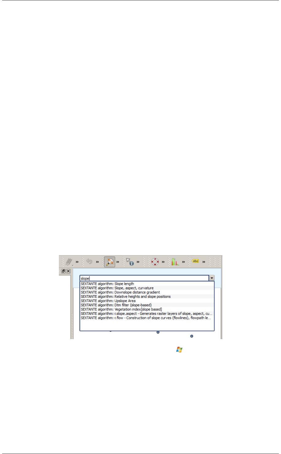
QGIS User Guide, Publicación 2.8
#include "mpi.h"
#include <stdint.h>
Guardar los cambios y cerrar el archivo. Ahora abir tiffIO.h, buscar la línea #include "stdint.h" y
sustituir las comillas ("") con <>, para obtener
#include <stdint.h>
Guardar los cambios y cerrar el archivo. Crear un directorio de compilación y entrar en él
mkdir build
cd build
Configure su construcción con el comando
CXX=mpicxx cmake -DCMAKE_INSTALL_PREFIX=/usr/local ..
y entonces compilar
make
Finalmente, para instalar TauDEM en /usr/local/bin, ejecutar
sudo make install
.
17.15 Los Comandos QGIS
El procesado incluye una herramienta practica que le permite ejecutar algoritmos sin tener que utilizar la caja de
herramientas, pero tan solo escribir el nombre del algoritmo que se desee ejecutar.
Esta herramienta es conocida como Comandos GQIS, y esto es solo una sencilla caja de texto con autocompletado
donde se escribe el nombre del comando que se desee ejecutar.
Figure 17.29: Comandos QGIS
Comandos se inicia del menú Análisis o, mas practico, al presionar Shift + Ctrl + M (puede cambiar ese
atajo de teclado en la configuración de QGIS si prefiere definir uno diferente). Ademas de la ejecución de algorit-
mos de procesado, Comandos da acceso a la mayoría de las funcionalidades en QGIS, lo que significa que le da
una forma práctica y eficaz de ejecutar tareas QGIS y le permite controlar QGIS con un uso reducido de botones
y menús .
Además, el comandante es configurable, así que puede agregar sus comandos personalizados y ellos tienen sólo
unas pocas teclas de distancia, por lo que es una herramienta de gran alcance para ayudarle a ser más productivo
en su trabajo diario con QGIS.
17.15. Los Comandos QGIS 229

QGIS User Guide, Publicación 2.8
17.15.1 Comandos disponibles
Los comandos disponibles en el Comandante caen en la siguiente categoría:
• Algoritmos de procesado. Estos se muestran como Algoritmo de procesamiento: <nombre
del algoritmo>.
• Los elementos del menú. Estos se muestran como Menu item: <Texto de entrada del
menú>. Todos los elementos de los menús disponibles desde la interfaz QGIS están disponibles, incluso si
se incluyen en un submenú.
• Funciones Python. Puede crear funciones cortas en Python que serán entonces incluidas en la lista de
comandos disponibles. Ellos se muestran como Function: <nombre de la función>.
Para ejecutar cualquiera de los anteriores, inicie escribiendo y a continuación, seleccione el elemento de la lista de
comandos disponibles que aparecen después de filtrar toda la lista de comandos con el texto que ha introducido.
En caso de llamar a una función de Python, puede seleccionar la entrada en la lista, que tiene
el prefijo Function: (por ejemplo, Command: removeall), o simplemente escribir
directamente el nombre de la función (‘‘removeall en el ejemplo anterior). No hay necesi-
dad de añadir espacios después del nombre de la función.
17.15.2 Crear funciones personalizadas
Las funciones personalizadas se añaden al introducir el código correspondiente de Python en el archivo
commands.py que se encuentra en el directorio .qgis/sextante/commander en su carpeta de usuario.
Es solo un archivo Python simple donde puede añadir las funciones que necesite.
Se crea el archivo con unas pocas funciones de ejemplo la primera vez que se abre Comandos. Si no ha lanzado
Comandos, puedes crear el archivo usted mismo. Para editar el archivo de comandos, utilice su editor de texto
favorito. También se puede utilizar un editor incorporado llamando al comando edit de Comandos. Se abrirá el
editor con el archivo de comandos, y se puede editar directamente y luego guardar los cambios.
Por ejemplo, puede añadir la siguiente función, la cual borre todas las capa:
from qgis.gui import *
def removeall():
mapreg =QgsMapLayerRegistry.instance()
mapreg.removeAllMapLayers()
Una vez que se haya añadido la función, estará disponible en Comandos, y puede invocarlo escribiendo
removeall. No hay necesidad de hacer algo más aparte de escribir la función en sí.
Las funciones pueden recibir parámetros. Añadir *args a la definición de su función para recibir argumentos.
Cuando llame a la función desde Comandos, los parámetros tienen que ser pasados separados por espacios.
Aquí esta un ejemplo de una función que carga una capa y toma un parámetro con el nombre del archivo de la
capa cargada.
import processing
def load(*args):
processing.load(args[0])
Si desea cargar la capa en /home/myuser/points.shp, tipo load /home/myuser/points.shp en
la caja de texto de Comandos.
.
230 Chapter 17. Entorno de trabajo de procesamiento de QGIS

CHAPTER 18
Diseñadores de impresión
Con el diseñador de impresión se pueden crear buenos mapas y atlas que se pueden imprimir o guardar como
archivo PDF, una imagen o un archivo SVG. Esta es una manera potente para compartir información geográfica
producida con QGIS que se puede incluir en reportes o publicado.
El diseño de impresión ofrece crecientes capacidades de diseño e impresión. Se le permite añadir elementos a la
vista del QGIS como, etiquetas de texto, imágenes, leyendas, barras de escala, formas básicas, flechas, tablas de
atributos y marcos HTML. Puede cambiar el tamaño, grupo, alineación y posición y rotación de cada elemento
y ajustar las propiedades para crear su diseño. El diseño se puede imprimir o exportar a formatos de imagen,
PostScript, PDF o SVG (la exportación a SVG no funciona correctamente con algunas versiones recientes Qt4,
debe intentarlo y comprobar de forma individual en el sistema). Puede guardar el diseño como una plantilla y
cargarla de nuevo en otra sesión. Por último, la generación de varios mapas basados en una plantilla se puede
hacer a través del generador de atlas. Ver una lista de herramientas en table_composer_1:
231
QGIS User Guide, Publicación 2.8
Icono Propósito Icono Propósito
Guardar Proyecto Nuevo diseñador de impresión
Duplicar diseñador de impresión Administrador de diseñadores
Cargar de plantilla Guardar como plantilla
Imprimir o exportar a PostScript Exportar a un formato de imagen
Exportar como SVG Exportar como PDF
Revertir el último cambio Restaurar el último cambio
Zum general Zum a 100%
Acercar Zum Alejar Zum
Actualizar vista
Desplazar diseñador Zum a una región específica
Seleccionar/Mover elementos Mover contenido dentro de un elemento
Añadir nuevo mapa de QGIS a la vista del
mapa
Añadir imagen a diseño de impresión
Añadir etiqueta al diseño de impresión Añadir nueva leyenda a diseño de impresión
Añadir barra de escala a diseño de
impresión
Añadir figura básica al diseño de impresión
Añadir flecha Añadir tabla de atributos
Añadir un marco HTML
Agrupar elementos Desagrupar elementos
Bloquear elementos seleccionados Desbloquear todos los elementos
Subir los elementos seleccionados Bajar elementos seleccionados
Mover elementos seleccionados arriba Mover elementos seleccionados abajo
Alinear a la izquierda elementos
seleccionados
Alinear a la derecha elementos seleccionados
Alinear al centro elementos seleccionados Alinear al centro vertical los elementos
seleccionados
Alinear arriba los elementos
seleccionados
Alinear abajo los elementos seleccionados
Vista previa del Atlas Primer objeto espacial
Anterior objeto espacial Siguiente objeto espacial
Último objeto espacial Imprimir Atlas
Exportar Atlas como imagen Configuración de atlas
Tabla Diseñador 1: Herramientas del Diseñador de Impresión
Todas las herramientas del diseñador de impresión estan disponibles en los menús y como iconos en la barra de
herramientas. La barra de herramientas se puede prender y apagar utilizando el botón derecho del ratón sobre la
barra de herramientas.
232 Chapter 18. Diseñadores de impresión

QGIS User Guide, Publicación 2.8
18.1 Primeros pasos
18.1.1 Abrir una plantilla del diseñador de impresión
Antes de comenzar a trabajar con el Diseñador de impresión, debe cargar algunas capas ráster y vectoriales a la
vista del del mapa de QGIS y adaptar sus propiedades para ajustar a su propia conveniencia. Después de todo lo
que se representa y simboliza a su gusto, haga clic en el icono Nuevo diseño de impresión en la barra de herramientas
o seleccione :menuselection:‘ Proyecto-> Nuevo diseñador de impresión‘. Se le pedirá que elija un título para la
nuevo diseño.
18.1.2 Perspectiva general del Diseñador de impresión
Al abrir el Diseñador de impresión le proporciona un lienzo en blanco que representa la superficie del papel al usar
la opción de impresión . Inicialmente se encuentra botones del lado izquierdo del lienzo para añadir elementos
al mapa del diseño; el lienzo del mapa actual de QGIS, etiquetas de texto, imágenes, leyendas, barras de escala,
formas básicas, flechas, tablas de atributos y marcos HTML. En esta barra de herramientas también se encuentran
los botones de barra de herramientas para navegar, acercar zum sobre un área y desplazar la vista y los botones de
la barra de herramientas para seleccionar un elemento del diseñador del mapa y mover el contenido del elemento
del mapa.
Figure_composer_overview shows la vista inicial del Diseño de impresión se añade antes que cualquier otro
elemento.
Figure 18.1: Diseñador de impresión
18.1. Primeros pasos 233
QGIS User Guide, Publicación 2.8
Del lado derecho del lienzo encontrará dos paneles. El panel superior tiene las pestañas Elementos eHistoria de
la orden y el panel inferior tiene las pestañas Diseño,Propiedades del elemento yGeneración de atlas.
• La pestaña Elementos proporciona una lista de todos los elementos del diseño añadidos al lienzo.
• La pestaña Historia de la orden muestra una historia de todos los cambios aplicados al diseño. Con hacer
un clic, es posible deshacer y rehacer pasos de ida y de vuelta a un cierto estatus
• La pestaña Diseño le permite establecer el tamaño del papel, orientación, fondo de la página, número de
páginas y calidad de impresión para el archivo de salida en dpi. Además, también se puede activar la casilla
Imprimir como ráster. Esto significa que todos los elementos serán convertidos a ráster antes de im-
primirse o guardarse como PostScript o PDF. En esta pestaña, también puede personalizar la configuración
de la cuadrícula o guías inteligentes.
• La pestaña Propiedades del elemento muestra las propiedades del elemento seleccionado. Haga clic en el
icono Seleccionar/Mover elemento para mover un elemento (por ejemplo, la leyenda, la barra de escala o eti-
queta) en el lienzo. Después haga clic en la pestaña Propiedades del elemento y personalice la configuración
del elemento seleccionado.
• La pestaña Generación de atlas le permite habilitar la generación de un atlas del diseño actual y da acceso
a sus parámetros.
• Por último, puede guardar su diseño de impresión con el botón Guardar proyecto.
En la parte inferior de la ventana del Diseñador de impresión, puede encontrar una barra de estado con la posición
del ratón, número de página actual y una lista desplegable para establecer el nivel de zum.
Puede añadir múltiples elementos al diseño de impresión. También es posible tener más de una vista de mapa o
leyenda o barra de escala en el lienzo, en una o varias páginas. Cada elemento tiene sus propias propiedades y, en
caso del mapa, su extensión. Si quiere borrar algún elemento del lienzo, puede hacerlo con Eliminar o la tecla
Retroceso.
Herramientas de navegación
Para navegar en el lienzo del diseño, el Diseñador de impresión proporciona algunas herramientas generales:
•Acercar zum
•Alejar zum
•Zum general
•Zum al 100%
•Actualizar la vista (Si se encontró la vista en un estado inconsistente)
•Desplazar diseño
•Zum (zum a una región específica del Diseñador de impresión)
Puede también cambiar el nivel de zum con la rueda del ratón o en la lista desplegable de la barra de estado. Si
necesita cambiar a modo de panorama mientras se trabaja en el área del diseñador, puede mantenerlo con la Barra
espaciadora o la rueda del ratón. Con Ctrl+Barra espaciadora, puede cambiar temporalmente al
modo de zum, y con Ctrl+Shift+Barra espaciadora, para el modo alejar.
18.1.3 Ejemplo de sesión
Para demostrar cómo crear un mapa, por favor siga las siguientes instrucciones.
234 Chapter 18. Diseñadores de impresión
QGIS User Guide, Publicación 2.8
1. En el lado izquierdo, seleccione el botón de la barra de herramientas Añadir un nuevo mapa y dibuje un
rectángulo en el lienzo manteniendo pulsado el botón izquierdo del ratón. Dentro del rectángulo dibujado
la vista de mapa de QGIS al lienzo.
2. Seleccione el botón de la barra de herramientas Añadir nueva barra de escala y ubicar el elemento del mapa
con el botón izquierdo del ratón en el lienzo del diseñador de impresión. Una barra de escala se añadirá al
lienzo.
3. Seleccione el botón de la barra de herramientas Añadir nueva leyenda y dibuje un rectángulo en el lienzo
manteniendo pulsado el botón izquierdo del ratón. Dentro del rectángulo dibujado se dibujará la leyenda.
4. Elija el icono Seleccionar/Mover elemento para seleccionar el mapa en el lienzo y moverlo un poco.
5. Mientras el elemento del mapa aun esta seleccionado, también se puede cambiar el tamaño del elemento
mapa. Haga clic mientras mantiene pulsado el botón izquierdo del ratón, en un pequeño rectángulo blanco
en una de las esquinas del elemento mapa y arrástrelo a una nueva ubicación para cambiar su tamaño.
6. Haga clic en la pestaña Propiedades del elemento en el panel inferior izquierdo y encuentre el ajuste para la
orientación. Cambie el valor del ajuste Orientación del mapa a ‘15.00|grados| ‘. Se debe ver el cambio en
la orientación del elemento mapa.
7. Por último, puede guardar su diseño de impresión con el botón Guardar proyecto.
18.1.4 Opciones del diseñador de impresión
De Configuración →Opciones del Diseñador se pueden establecer algunas opciones que se utilizarán por defecto
durante su trabajo.
•Predeterminados de la Composición le permite especificar la fuente predeterminada a utilizar.
• Con Apariencia de cuadrícula, se puede establecer el estilo y el color. Hay tres tipos de cuadrícula: Puntos,
Sólido líneas y Cruz.
•La cuadrícula y las guías predeterminadas define el espaciamiento, compensar y la tolerancia de la
cuadrícula.
18.1.5 Pestaña de Diseño — Configuración general de diseño
En la pestaña Diseño, puede definir la configuración global de su diseño.
• Puede elegir uno de los Preestablecidos para su hoja de papel, o ingrese su Anchura yAltura personalizado.
• La composición ahora se puede dividir en varias páginas. Por ejemplo, una primer página puede mostrar
una vista del mapa, y una segunda página puede mostrar la tabla de atributos asociada a la capa, mientras
que una tercera página muestra un marco HTML enlazado a su página web de su organización. Establecer
el Número de páginas al valor deseado. Puede elegir la página Orientación y su Resolución de exportación.
Cuando se activa, Imprimir como ráster significa que todos los elementos serán rásterizados antes de
imprimir o guardar como PostScript o PDF.
•Cuadrícula y guías le permite personalizar la configuración de la cuadrícula como Separación,Desplaza-
miento yTolerancia a su necesidad. La tolerancia es la distancia máxima bajo la cual un elemento es
ensamblado a las guías inteligentes.
Ajustar a la cuadrícula y/o Guías inteligentes se pueden habilitar desde el menú Ver. En este menú, también se
puede ocultar o mostrar la cuadrícula o guías inteligentes.
18.1. Primeros pasos 235
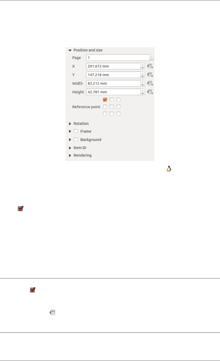
QGIS User Guide, Publicación 2.8
18.1.6 Opciones comunes en los elementos del diseñador
Los elementos del diseñador tienen un conjunto de propiedades comunes que se encontrará en la parte inferior de la
pestaña Propiedades del elemento: Posición y tamaño, Rotación, Marco, Fondo, ID del elemento y Representación
(Ver figure_composer_common_1).
Figure 18.2: Diálogo de propiedades de elementos comunes
• El diálogo Posición y tamaño le permite definir tamaño y posición del marco que contiene los elementos.
También puede optar por Punto de referencia para establecer las coordenadas XyYpreviamente definidas.
• La Rotación establece la rotación del elemento (en grados).
• El Marco muestra u oculta el marco alrededor de la etiqueta. Utilice los menús Color de marco yGrosor
para ajustar esas propiedades.
• Use the Background color menu for setting a background color. With the dialog you can pick a color (see
Color Picker ).
• Utilice el ID del elemento para crear una relación a otros elementos del Diseñador de impresión. Esto se
utiliza con el servidor QGIS y algunos clientes web potenciales. Puede establecer un ID a un elemento (por
ejemplo, un mapa y una etiqueta), y después el cliente web puede enviar datos para establecer una propiedad
(por ejemplo, etiqueta de texto) para ese elemento especifico. El comando GetProjectSettings listará que
elementos y que ID’s están disponibles en un diseño.
• Modo Representación se puede seleccionar en el campo de opción. Ver Rendering_Mode.
Nota:
• Si checa Utilice diálogo seleccionador de color en las opciones generales de QGIS, el botón de color se
actualizará tan pronto como elija un nuevo color desde la ventana Diálogo de Color. Si no, debe cerrar el
Diálogo de color.
• El de a lado icono Anular datos definidos de campo significa que se puede asociar el campo con datos en el
elemento del mapa o utilizar expresiones. Estos son particularmente útiles con la generación de atlas (vea
atlas_data_defined_overrides)
236 Chapter 18. Diseñadores de impresión
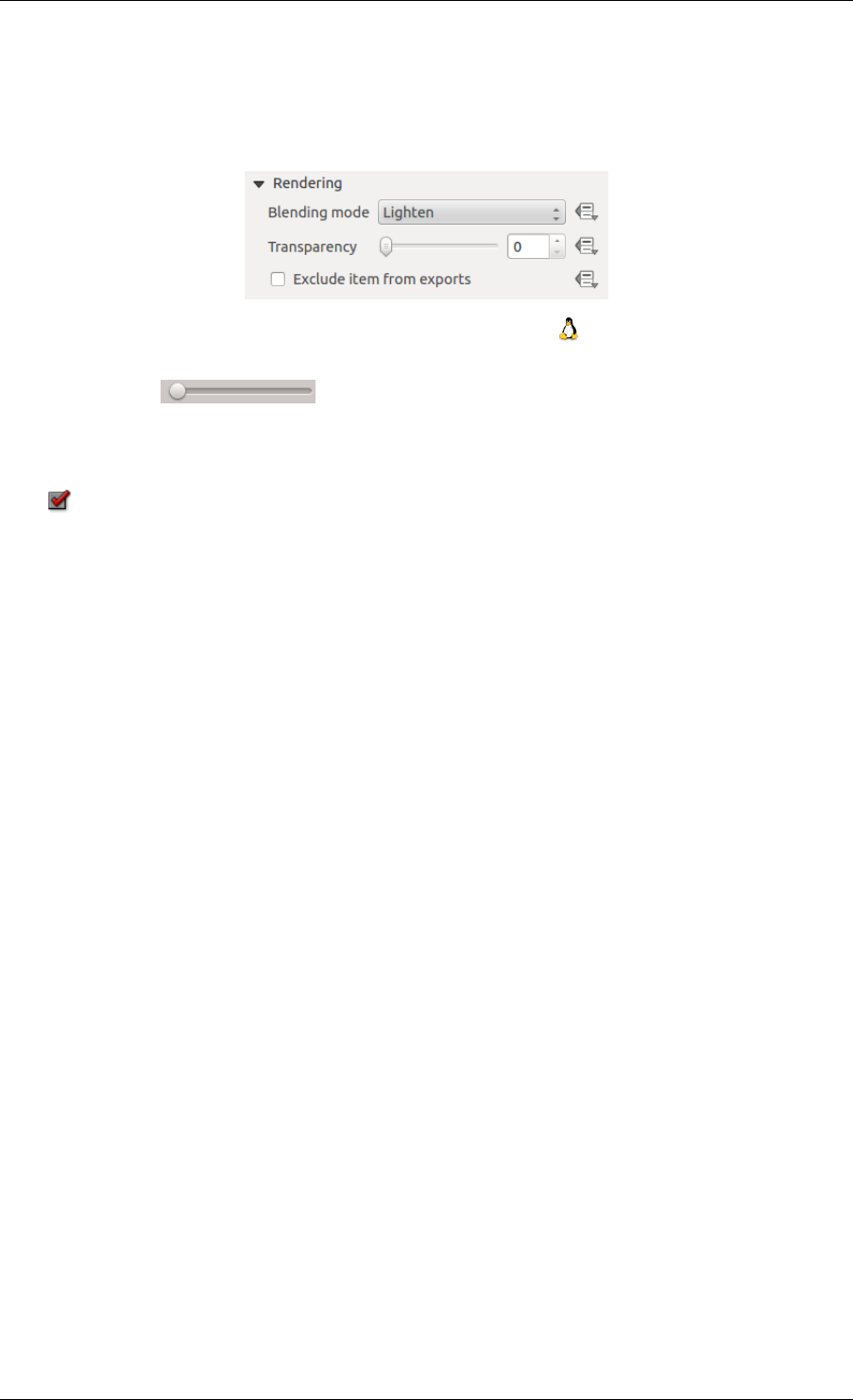
QGIS User Guide, Publicación 2.8
18.2 Modo de representación
Ahora QGIS permite representación avanzada para elementos del Diseñador al igual que capas vectoriales y
rásters.
Figure 18.3: Modo de representación
•Transparencia : Puede hacer que el elemento subyacente este visible en el Diseñador
con esta herramienta. Utilice el control deslizante para adaptar la visibilidad de sus elementos a sus necesi-
dades. También puede hacer una definición precisa del porcentaje de visibilidad en el menú al lado de la
barra de desplazamiento.
•Excluir elementos de las exportaciones: Puede decidir hacer un elemento no visible en todas las ex-
portaciones. Después de activar esta casilla, el elemento no se incluirá en PDF’s, impresiones, etc.
•Modo de mezcla: Puede lograr efectos de representación especial con estas herramientas que antes solo se
puede saber de programas de gráficos. Los píxeles de sus elementos sobrepuestos y subyacentes se mezclan
a través de los ajustes descritos anteriormente.
–Normal: Este es el modo de mezcla estándar, que utiliza el canal alfa del píxel superior para mezclarse
con los pixeles debajo de el; los colores no se mezclan.
–Iluminado: Este selecciona el máximo de cada componente del primer y segundo plano de píxeles.
Tenga en cuenta que los resultados tienden a ser irregulares y rigurosos.
–Pantalla: píxeles de luz de la fuente se pintan sobre el destino, mientras que los píxeles oscuros no
lo son. Este modo es muy útil para la mezcla de la textura de una capa con otra (por ejemplo, puede
utilizar un sombreado para texturizar otra capa).
–Esquivar: aclarará y saturar píxeles subyacentes en base a la ligereza del punto de imagen superior.
Así, los píxeles superiores más brillantes provocan la saturación y el brillo de los píxeles subyacentes
a aumentar. Esto funciona mejor si los píxeles superiores no son demasiado brillantes; de lo contrario
el efecto sera demasiado extremo.
–Suma: Este modo de mezcla simplemente añade valores de píxeles de una capa con valores de píxeles
de otra. En caso de que los valores superiores a 1 (como en el caso de RGB), mientras es mostrado.
Este modo es adecuado para resaltar objetos.
–Oscurecido: Este crea un píxel resultante que conserva el componente mas pequeño del primero y
segundo plano de pixeles. Como el iluminado, los resultados tienden a ser irregulares y rigurosos.
–Multiplicar: Aquí los números de cada píxel de la capa superior están multiplicados con los números
del píxel correspondiente de la capa inferior. Los resultados son imágenes más oscuras.
–Quemar: Los colores más oscuros en la capa superior hacen que las capas subyacentes para oscurecer.
Quemar se pueden utilizar para ajustar y colorear las capas subyacentes.
–Superposición: Este modo combina los modos de mescla multiplicar y pantalla. En la imagen resul-
tante, partes de la luz se vuelven más ligeras y partes oscuras se oscurecen.
–Luz suave: Esto es muy similar a superponer, pero en lugar de utilizar multiplicar/pantalla que utiliza
el color quemar/esquivar. Este modo se supone que debe emular el brillo de una luz suave en una
imagen.
–Iluminar fuerte: Ilumina fuerte es muy similar a la del modo de superposición. Se supone que es
emular a la proyección de una luz muy intensa en una imagen.
18.2. Modo de representación 237
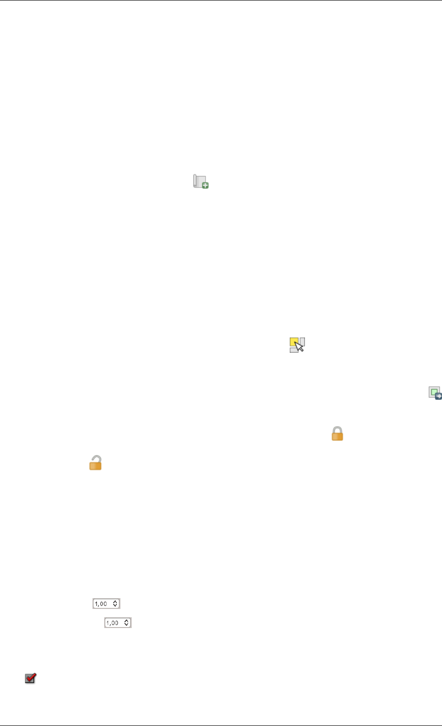
QGIS User Guide, Publicación 2.8
–Diferencia: Diferencia resta el píxel superior de la parte inferior de píxeles, o al revés, para obtener
siempre un valor positivo. La mezcla con negro no produce ningún cambio, ya que la diferencia con
todos los colores es cero.
–Restar: Este modo de mezcla simplemente resta valores de los píxeles de una capa con valores de píxel
de otra. En caso de valores negativos, el negro se muestra.
18.3 Elementos de diseño
18.3.1 El elemento del mapa
Haga clic en el botón de la barra de herramientas Añadir nuevo mapa en la barra de herramientas del Diseñador de
impresión para agregar una vista del mapa de QGIS. Ahora, arrastre un rectángulo sobre el lienzo del Diseñador
con el botón izquierdo del ratón para añadir el mapa. Para mostrar el mapa actual, se puede elegir entre tres modos
diferentes en el mapa, la pestaña Propiedades del elemento:
•Rectángulo es la configuración predeterminada. Solo muestra una caja vacía con un mensaje ‘El mapa será
impreso aquí’.
•Cache representa el mapa en la resolución de la pantalla actual. Si se acerca o aleja el zum en la ventana
del Diseñado, el mapa no representara de nuevo pero la imagen será escalada.
•Representar quiere decir que si se acerca o aleja el zum en la ventana del Diseñador, el mapa será repre-
sentado de nuevo, pero por razones de espacio sólo hasta una resolución máxima.
Cache es el modo de vista previa predeterminado para añadir los recientes mapas al Diseñador de impresión.
Puede cambiar el tamaño del elemento del mapa al hacer clic en el botón Seleccionar/Mover elemento, seleccione el
elemento, y arrastre una de las asas de color azul en la esquina del mapa. Con el mapa seleccionado, ahora se
puede ajustar más propiedades en el mapa, en la pestaña Propiedades del elemento.
Para desplazar capas dentro del elemento del mapa, seleccione el mapa, haga clic en el icono
Mover contenido del elemento y mueva las capas dentro del marco del elemento mapa con el botón izquierdo del ratón.
Después de encontrar el lugar apropiado para un elemento, puede bloquear la posición dentro del lienzo del Dis-
eñador de impresión. Seleccione el elemento mapa y utilice la barra de herramientas Bloquear elementos seleccionados
o la pestaña Elementos. Una vez seleccionado puede utilizar la pestaña Elementos para desbloquear elementos
individuales. El icono Desbloquear todos los elementos desbloqueará todos los elementos del diseñador bloqueados.
Propiedades principales
El diálogo Propiedades principales del mapa, la pestaña Propiedades del mapa proporciona las siguientes fun-
cionalidades (vea figure_composer_map_1)
• La zona Vista preliminar le permite definir los modos de vista previa ‘Rectángulo’, ‘Caché’, y ‘Represen-
tar’, como se describió antes. Si se cambia la vista en la vista del mapa QGIS al cambiar las propiedades
del vector o ráster, puede actualizar la vista del Diseñador de impresión al seleccionar el elemento mapa en
el Diseñador y al hacer clic en el botón [Actualizar vista preliminar]
• El campo Escala establece una escala manual
• El campo Rotación le permite rotar el contenido del elemento del mapa hacia las manecillas del
reloj en grados. La rotación de la vista del mapa puede ser imitado aquí. Tenga en cuenta que un marco
de coordenadas correcta sólo se puede añadir con el valor predeterminado 0 y que una vez que defina una
Rotación en ese momento no se puede cambiar.
•Dibujar elementos de la vista del mapa le deja mostrar anotaciones que se pueden ubicar en la vista del
mapa en la ventana principal de QGIS.
238 Chapter 18. Diseñadores de impresión
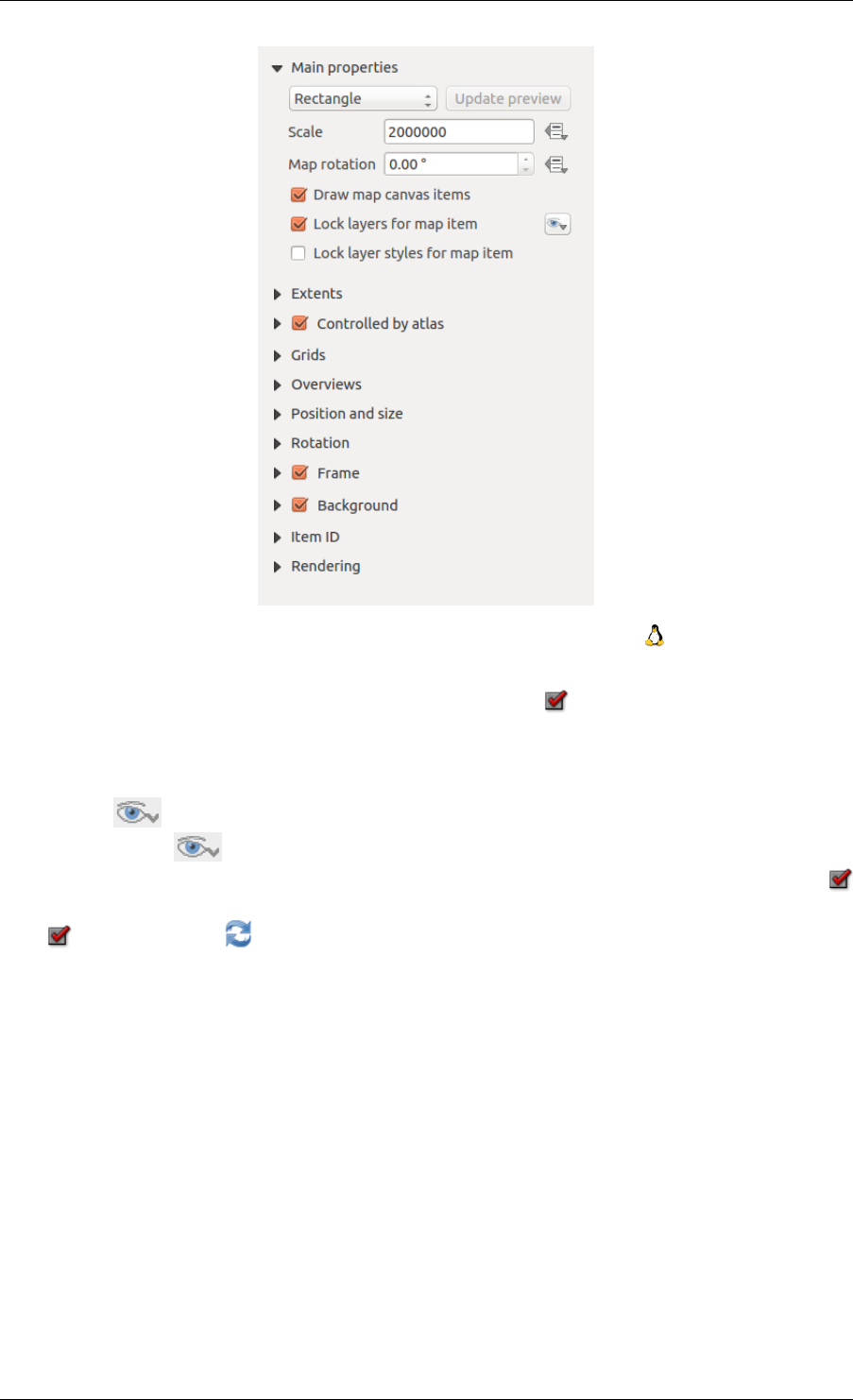
QGIS User Guide, Publicación 2.8
Figure 18.4: Pestaña de propiedades de elementos del mapa
• You can choose to lock the layers shown on a map item. Check Lock layers for map item. After this
is checked, any layer that would be displayed or hidden in the main QGIS window will not appear or be
hidden in the map item of the Composer. But style and labels of a locked layer are still refreshed according
to the main QGIS interface. You can prevent this by using Lock layer styles for map item.
• El botón le permite añadir más rápido las vistas predeterminadas que ha preparado en QGIS. Al Hacer
clic en el botón verá la lista de todas las vistas preestablecidas: sólo seleccione el preestablecido
que se desea mostrar. La vista del mapa automáticamente bloqueará la capa preestablecida al activar
Bloquear las capas para el elemento del mapa: si se desea deseleccionar el preestablecido, sólo desactive
y presione el botón . Vea Leyenda del mapa para averiguar cómo crear vistas preestablecidas.
Extensión
El diálogo Extensión de la pestaña del elemento mapa proporciona las funcionalidades siguientes (ver fig-
ure_composer_map_2):
• La zona Extensión del Mapa le permite especificar la extensión del mapa utilizando los valores X y Y
máximos y mínimos al hacer clic en el botón [Establecer a la extensión de la vista del mapa]. Este botón
establece la extensión del elemento mapa del diseñador a la extensión de la vista del mapa actual en la
aplicación principal QGIS. El botón [Extender vista en la vista del mapa] hace exactamente lo opuesto,
actualiza la extensión de la vista del mapa en la aplicación QGIS a la extensión del elemento mapa del
diseñador.
Si se cambia la vista en la vista del mapa QGIS al cambiar al cambiar las propiedades vectoriales o ráster.
se puede actualizar la vista del Diseñador de impresión seleccionando el elemento mapa en el Diseñador y al
hacer clic en el botón **[Actualizar vista preliminar]**en la pestaña del mapa Propiedades del elemento (ver
figure_composer_map_1).
18.3. Elementos de diseño 239
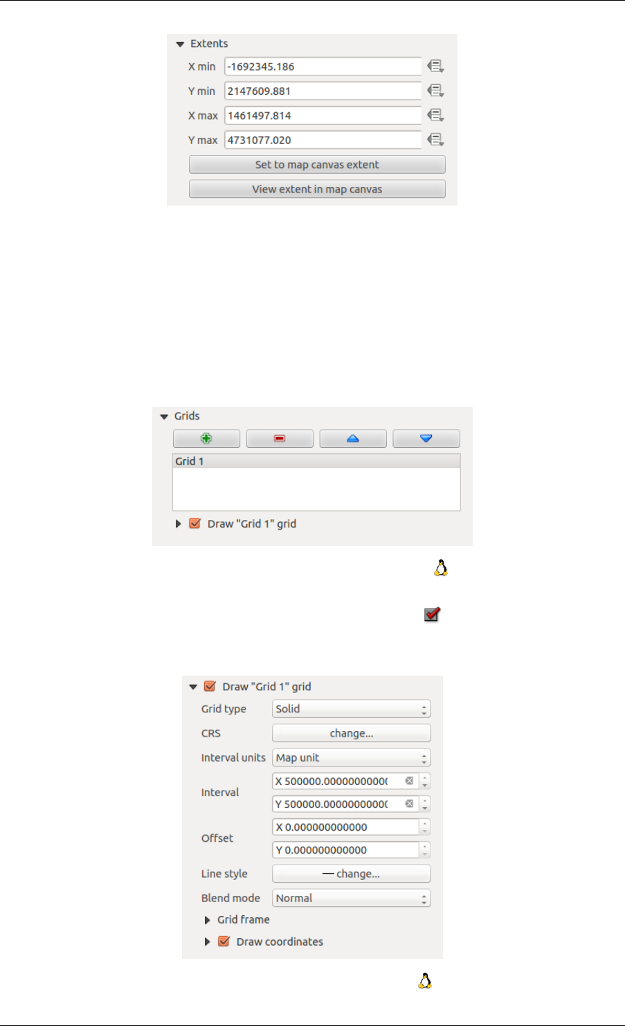
QGIS User Guide, Publicación 2.8
Figure 18.5: Diálogo de Extensión de Mapa
Cuadrículas
The Grids dialog of the map Item Properties tab provides the possibility to add several grids to a map item.
• Con los botón de más y menos se puede añadir o eliminar una rejilla seleccionada
• Con el botón de arriba y abajo se puede mover una rejilla en la lista y establecer la prioridad del dibujo
Al hacer doble clic sobre la rejilla seleccionada se le puede dar otro nombre.
Figure 18.6: Diálogo de cuadrículas del mapa
Después de añadir una rejilla, se puede activar la casilla de verifificación Show grid para superponer una
rejilla al elemento de mapa. Expande esta opción para obtener un montón de opciones de configuración, ver
Figura_composer_map_4.
Figure 18.7: Diálogo para dibujar rejilla
240 Chapter 18. Diseñadores de impresión
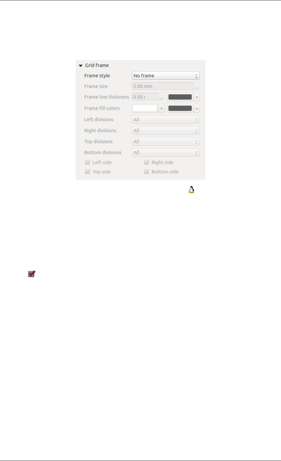
QGIS User Guide, Publicación 2.8
As grid type, you can specify to use a ‘Solid’, ‘Cross’, ‘Markers’ or ‘Frame and annotations only’. ‘Frame and
annotations only’ is especially useful when working with rotated maps or reprojected grids. In the devisions
section of the Grid Frame Dialog mentioned below you then have a corresponding setting. Symbology of the grid
can be chosen. See section Rendering_Mode. Furthermore, you can define an interval in the X and Y directions,
an X and Y offset, and the width used for the cross or line grid type.
Figure 18.8: Diálogo de marco de rejilla
• Hay diferentes opciones para estilos del marco que sostiene el mapa. Las siguientes opciones están
disponibles: Sin marco, Zebra, ticks interiores, ticks exteriores, Stick interior y exterior, línea de borde.
• With ‘LatitudeY/ only’ and ‘Longitude/X only’ setting in the devisions section you have the possibility to
prevent a mix of latitude/y and longitude/x coordinates showing on a side when working with rotated maps
or reprojected grids.
• Modo de representación avanzada también esta disponible para cuadriculas (consulte sección Render-
ing_mode).
• The Draw coordinates checkbox allows you to add coordinates to the map frame. You can choose
the annotation numeric format, the options range from decimal to degrees, minute and seconds, with or
without suffix, and aligned or not. You can choose which annotation to show. The options are: show all,
latitude only, longitude only, or disable(none). This is useful when the map is rotated. The annotation can
be drawn inside or outside the map frame. The annotation direction can be defined as horizontal, vertical
ascending or vertical descending. In case of map rotation you can Finally, you can define the annotation
font, the annotation font color, the annotation distance from the map frame and the precision of the drawn
coordinates.
Vistas generales
The Overviews dialog of the map Item Properties tab provides the following functionalities:
You can choose to create an overview map, which shows the extents of the other map(s) that are available in the
composer. First you need to create the map(s) you want to include in the overview map. Next you create the map
you want to use as the overview map, just like a normal map.
• Con el botón más y menos se puede añadir o borrar una vista general.
• Con el botón arriba y abajo se puede mover una vista general en el listado y establecer la prioridad del
dibujo.
Open Overviews and press the green plus icon-button to add an overview. Initially this overview is named
‘Overview 1’ (see Figure_composer_map_7). You can change the name when you double-click on the overview
item in the list named ‘Overview 1’ and change it to another name.
18.3. Elementos de diseño 241
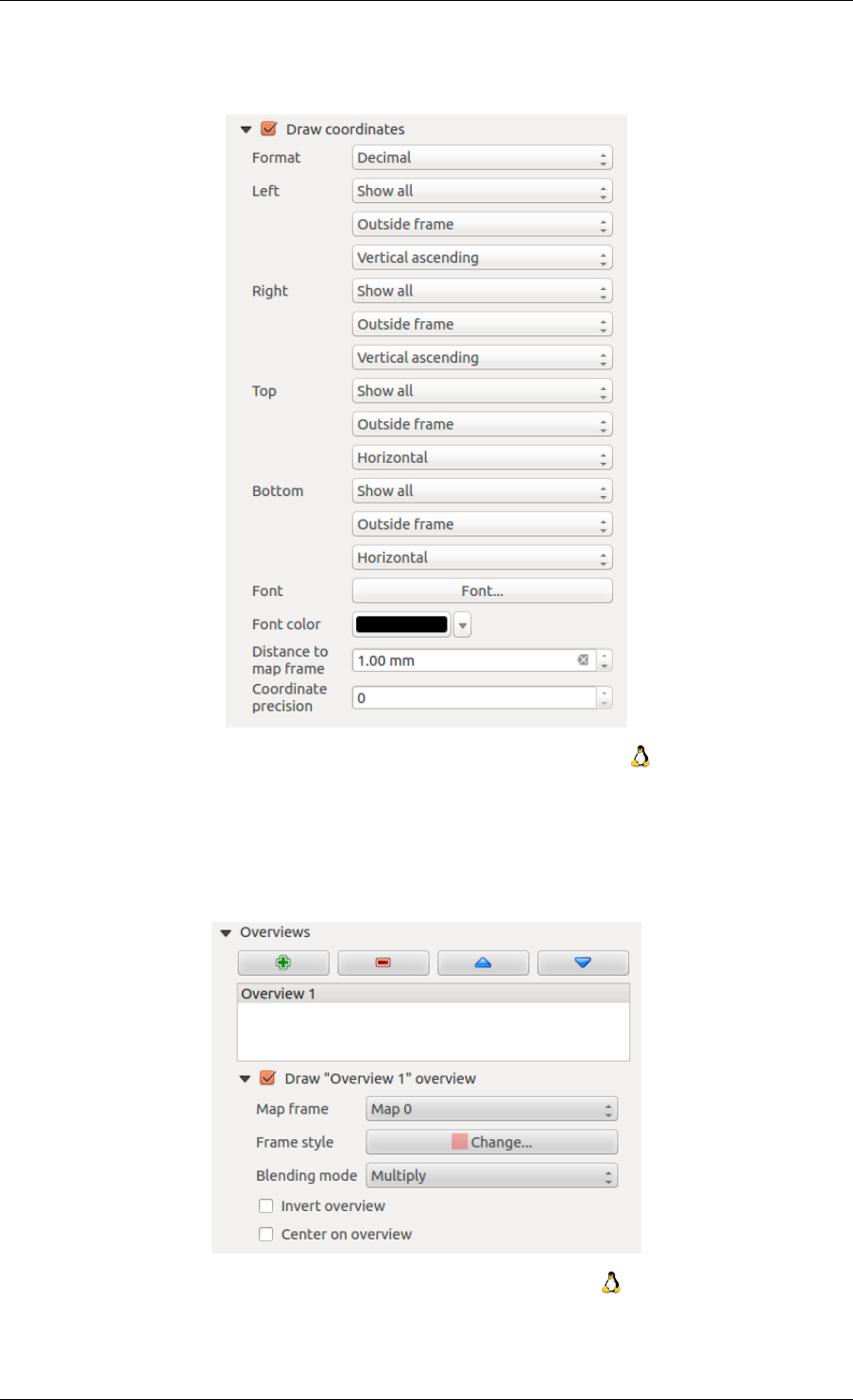
QGIS User Guide, Publicación 2.8
Figure 18.9: Diálogo Coordenadas para dibujo de rejilla
Figure 18.10: Diálogo de vista general del mapa
242 Chapter 18. Diseñadores de impresión
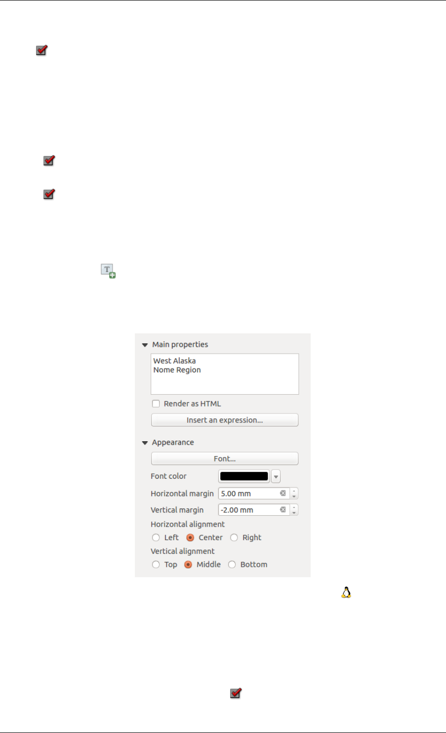
QGIS User Guide, Publicación 2.8
Cuando seleccione el elemento de vista general en la lista se puede personalizar.
• El Dibujar”<name_overview>” vista general necesita estar activado para dibujar la extensión del marco
de mapa seleccionado.
• La lista desplegable Marco de mapa se puede utilizar para seleccionar el elemento mapa, cuya extensión
será dibujada en el elemento de mapa presente.
• El Estilo de marco le permite cambiar el estilo de del marco de vista general.
• El Modo de mezcla le permite establecer diferentes modos de mezcla de transparencia. Consulte Render-
ing_Mode.
• The Invert overview creates a mask around the extents when activated: the referenced map extents are
shown clearly, whereas everything else is blended with the frame color.
• The Center on overview puts the extent of the overview frame in the center of the overview map. You
can only activate one overview item to center, when you have added several overviews.
18.3.2 El elemento etiqueta
To add a label, click the Add label icon, place the element with the left mouse button on the Print Composer
canvas and position and customize its appearance in the label Item Properties tab.
The Item Properties tab of a label item provides the following functionality for the label item (see Fig-
ure_composer_label):
Figure 18.11: Pestaña de propiedades de elemento de etiqueta
Propiedades principales
• The main properties dialog is where the text (HTML or not) or the expression needed to fill the label is
added to the Composer canvas.
• Labels can be interpreted as HTML code: check Render as HTML. You can now insert a URL, a
clickable image that links to a web page or something more complex.
18.3. Elementos de diseño 243
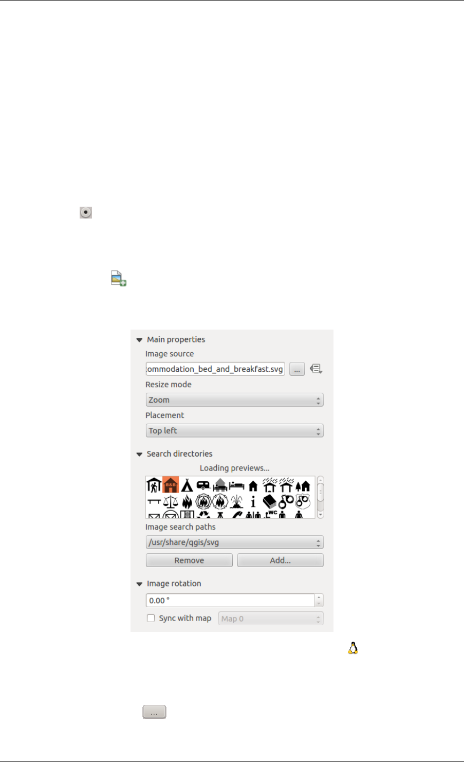
QGIS User Guide, Publicación 2.8
• You can also insert an expression. Click on [Insert an expression] to open a new dialog. Build an ex-
pression by clicking the functions available in the left side of the panel. Two special categories can be
useful, particularly associated with the atlas functionality: geometry functions and records functions. At the
bottom, a preview of the expression is shown.
Apariencia
• Define Font by clicking on the [Font...] button or a Font color selecting a color using the color selection
tool.
• You can specify different horizontal and vertical margins in mm. This is the margin from the edge of the
composer item. The label can be positioned outside the bounds of the label e.g. to align label items with
other items. In this case you have to use negative values for the margin.
• Using the Alignment is another way to position your label. Note that when e.g. using the Horizontal
alignment in Center Position the Horizontal margin feature is disabled.
18.3.3 El elemento imagen
To add an image, click the Add image icon, place the element with the left mouse button on the Print Composer
canvas and position and customize its appearance in the image Item Properties tab.
The picture Item Properties tab provides the following functionalities (see figure_composer_image_1):
Figure 18.12: Pestaña de propiedades de elemento imagen
Primero se tiene que seleccionar la imagen que se desee para mostrar. Hay varias formas para establecer la Origen
de la imagen en el área Propiedades principales.
1. Utilice el botón de explorar de Origen de la imagen para seleccionar un archivo de su computadora
utilizando el diálogo del explorador. El explorador iniciará en la biblioteca SVG proporcionado por QGIS.
Además SVG, también puede seleccionar otro formato de imagen como .png o.jpg.
244 Chapter 18. Diseñadores de impresión
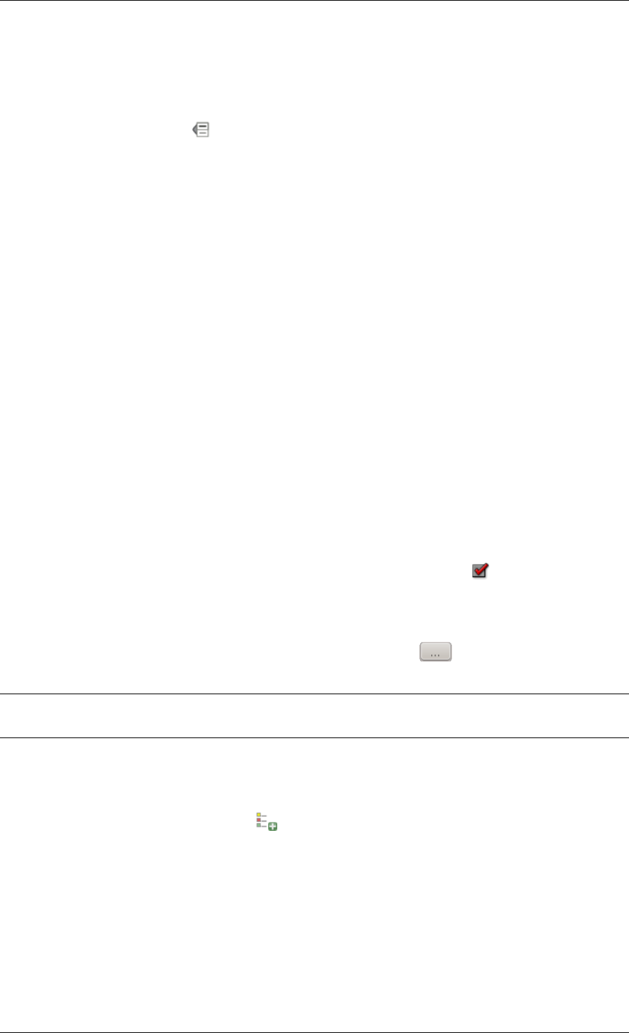
QGIS User Guide, Publicación 2.8
2. Se puede introducir el origen directamente en el campo de texto Origen de la imagen. Incluso puede
proporcionar una dirección URL remota de una imagen.
3. Desde el área Directorios de búsqueda se puede seleccionar también una imagen de Cargando vistas
previas ... para establecer la fuente de la imagen.
4. Utilice el botón definir datos para establecer el origen de la imagen de un registro o utilizar una expresión
regular
Con la opción Modo de redimensionado, se puede establecer cómo se muestra la imagen cuando se cambia el
marco, o elegir el cambiar el tamaño del marco del elemento imagen para que coincida con el tamaño original de
la imagen.
Se puede seleccionar uno de los siguientes modos:
• Zum: Amplia la imagen al marco mientras se mantiene la relación del aspecto de la imagen.
• Estirar: Estira la imagen para que quepa dentro del marco, ignorar la relación del aspecto.
• Cortar: Utilice este modo sólo para imágenes ráster, se establece el tamaño de la imagen al tamaño de la
imagen original sin escalar y el marco suele cortar la imagen, así sólo la parte de la imagen dentro del marco
es visible.
• El zum y el marco de redimensionado: Amplia la imagen para que se adapte al marco, entonces cambia el
tamaño del marco para adaptarse a la imagen resultante.
• Redimensionar marco a tamaño de la imagen: Establecer el tamaño del marco para que coincida con el
tamaño original de la imagen si escala.
Modo de redimensionar seleccionado puede inhabilitar el elemento opciones ‘Ubicación’ y ‘Rotación de imagen’.
La Rotación de imagen está activo para el modo de cambio de tamaño ‘Zum’ y ‘Cortar’.
Con Ubicación se puede seleccionar la posición de la imagen dentro del marco. El área Directorios de búsqueda
le permite añadir o eliminar directorios con imágenes en formato SVG a la base de datos de imágenes. Una vista
previa de las imágenes encontradas en los directorios seleccionados se muestra en un panel y se puede utilizar
para seleccionar y establecer el origen de la fuente.
La imagen se puede rotar con el campo Rotación de imagen. Activando la casilla de Sincronizar con el mapa
sincroniza la rotación de una imagen en el área del mapa de QGIS (por ejemplo, una flecha del norte rotada) con
la imagen apropiada del Diseñador de Impresión.
También es posible seleccionar una flecha de norte directamente. Si primero se selecciona una imagen flecha de
norte desde Directorios de búsqueda y entonces utiliza el botón de explorar del campo Origen de la imagen,
ahora se puede seleccionar una de las flechas de norte desde la lista mostrada en figure_composer_image_2.
Nota: Muchas de las flechas del norte no tienen una ‘N’ añadida, esto se hace a propósito para los idiomas que
no utilizan una ‘N’ para Norte, para que pueda utilizar otra letra.
18.3.4 El elemento leyenda
Para añadir una leyenda, haga clic en el icono Añadir leyenda nueva, colocar el elemento con el botón izquierdo del
ratón en el lienzo del Diseñador de Impresión y posicionar y personalizar la apariencia en la pestaña Propiedades
del elemento de la leyenda.
Las Propiedades del elemento de la pestaña del elemento leyenda proporciona las siguientes funcionalidades (ver
figure_composer_legend_1):
Propiedades principales
El diálogo Propiedades principales de la pestaña de leyenda Item Properties proporciona las siguientes funcional-
idades (ver figure_composer_legend_2):
18.3. Elementos de diseño 245
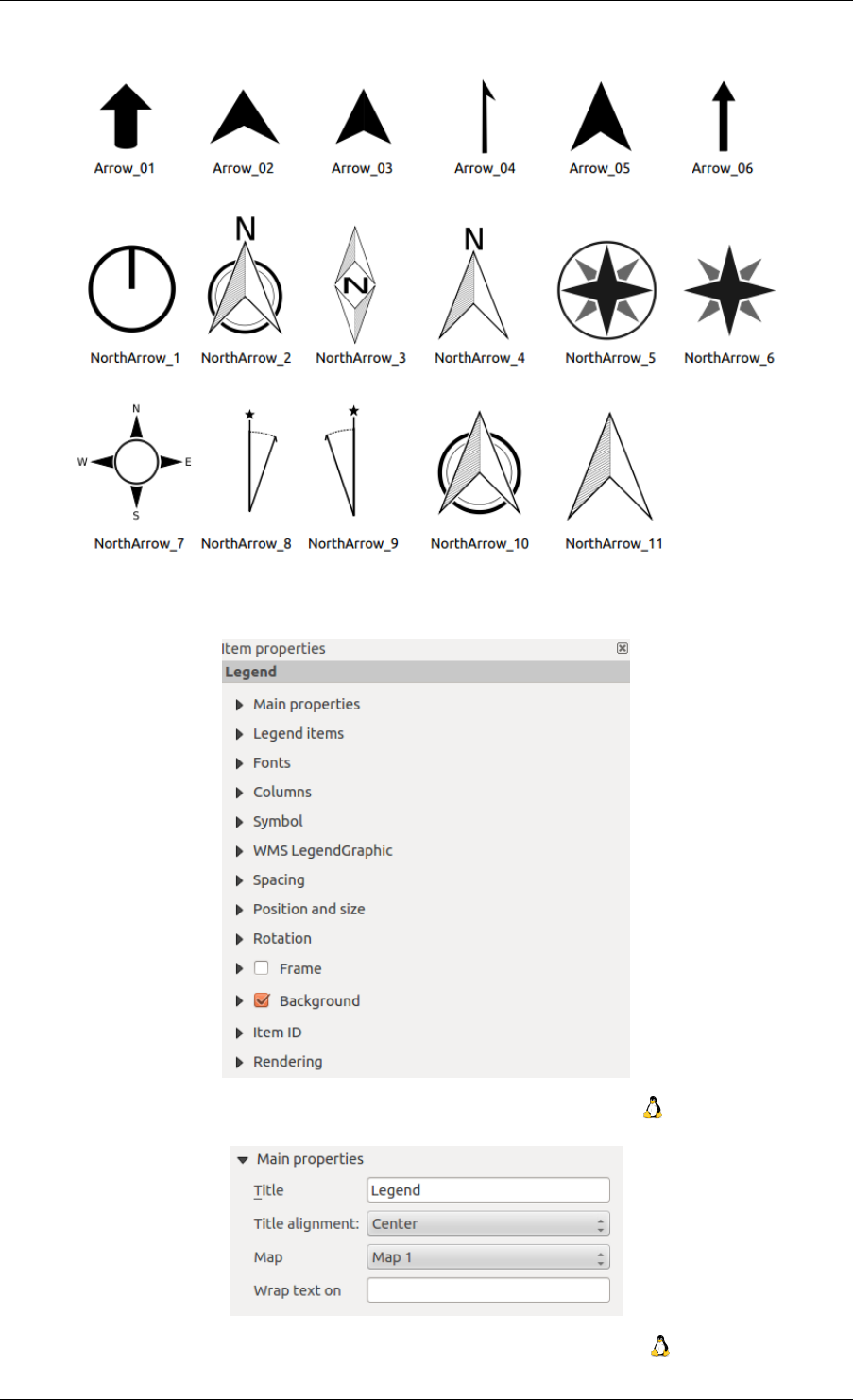
QGIS User Guide, Publicación 2.8
Figure 18.13: Las flechas de norte disponibles para la selección en la biblioteca SVG proporcionada.
Figure 18.14: Pestaña de propiedades del elemento leyenda
Figure 18.15: Diálogo de Propiedades de la leyenda principal
246 Chapter 18. Diseñadores de impresión
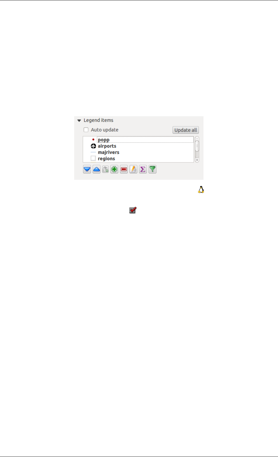
QGIS User Guide, Publicación 2.8
En propiedades principales se puede:
• Cambiar el título de la leyenda.
• Establecer la alineación del título a la Izquierda, Centro o Derecha
• Puede elegir que elemento Mapa de la leyenda actual se referirá a la lista de selección.
• Se puede envolver el texto del título de la leyenda sobre un carácter determinado.
Elementos de la leyenda
El diálogo Elementos de la leyenda de la pestaña de leyenda Propiedades de la leyenda proporciona las siguientes
funcionalidades (ver figure_composer_legend_3):
Figure 18.16: Diálogo de elementos de la leyenda
• La leyenda se actualizará automáticamente si Auto actualizar es activado. Cuando guilabel:Auto actu-
alizar es desactivado este le dará más control sobre los elementos de la leyenda. Los iconos debajo de los
elementos de la leyenda se activarán.
• La ventana de los elementos de la leyenda lista todos los elementos y le permite cambiar el orden, capas de
grupos, eliminar y restaurar elementos en la lista, editar nombres de capas y añadir un filtro.
–El orden de los elementos se puede cambiar utilizando los botones [Arriba] y[Abajo] con la fun-
cionalidad de ‘arrastrar y soltar’. El orden no se puede cambiar para las gráficas de leyenda WMS.
–Utilice el botón [Añadir grupo] para añadir un grupo a la leyenda.
–Utilice los botones [más] y[menos] para añadir o eliminar capas.
–El botón [Editar] se utiliza para editar la capa-, nombre de grupo o título, primero se necesita selec-
cionar el elemento leyenda.
–El botón [Sigma] añade un característica de recuento para cada capa vectorial.
–Utilizar el botón [filtrar] para filtrar la leyenda por el contenido del mapa, sólo los elementos de la
leyenda visibles en el mapa se enlistarán en la leyenda.
Después de cambiar la simbología en la ventana principal de QGIS se puede hacer clic en [Actualizar todo]
para adaptar los cambios en el elemento leyenda del Diseñador de Impresión.
Fuentes, Columnas, Símbolo
Los diálogos Fuente,Columnss and Símbolos de la pestaña Item Properties proporcionan las siguientes funcional-
idades (ver figura_composer_legend_4):
• Se puede cambiar la fuente del título de la leyenda, grupo, subgrupo y elementos (capa) en la leyenda. Haga
clic en un botón de categoría para abrir un diálogo Seleccionar fuente.
• Con el selector de color se dota a las etiquetas de Color, se dará el color seleccionado a todos los elementos
de la leyenda.
18.3. Elementos de diseño 247
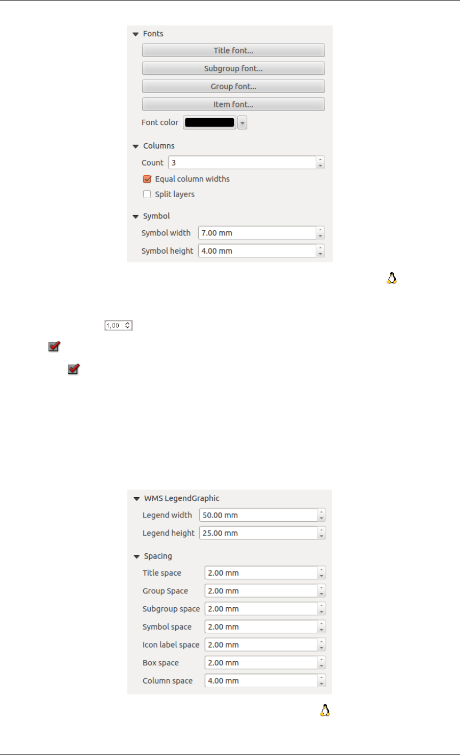
QGIS User Guide, Publicación 2.8
Figure 18.17: Diálogo de Fuentes de leyenda, Columnas, Símbolo y Espaciado
• Los elementos de la leyenda pueden ser organizados en varias columnas. Establece el número de columnas
en el campo Count .
–Anchura de columnas igual controla cómo deberían ser ajustadas las columnas de la leyenda.
–The Split layers option allows a categorized or a graduated layer legend to be divided between
columns.
• Se puede cambiar el ancho y alto del símbolo de la leyenda en este diálogo.
WMS LegendGraphic y espaciamiento
The WMS LegendGraphic and Spacing dialogs of the legend Item Properties tab provide the following function-
alities (see figure_composer_legend_5):
Figure 18.18: Diálogos WMS LegendGraphic
248 Chapter 18. Diseñadores de impresión
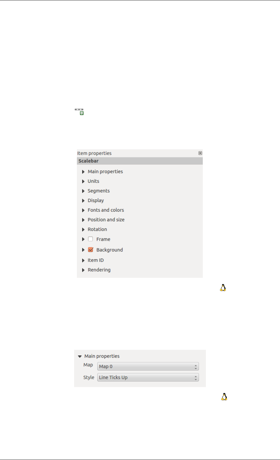
QGIS User Guide, Publicación 2.8
When you have added a WMS layer and you insert a legend composer item, a request will be send to the WMS
server to provide a WMS legend. This Legend will only be shown if the WMS server provides the GetLegend-
Graphic capability. The WMS legend content will be provided as a raster image.
WMS LegendGraphic is used to be able to adjust the Legend width and the Legend height of the WMS legend
raster image.
Spacing around title, group, subgroup, symbol, icon label, box space or column space can be customized through
this dialog.
18.3.5 El elemento de barra de escala
To add a scale bar, click the Add new scalebar icon, place the element with the left mouse button on the Print
Composer canvas and position and customize the appearance in the scale bar Item Properties tab.
The Item properties of a scale bar item tab provides the following functionalities (see fig-
ure_composer_scalebar_1):
Figure 18.19: Pestaña de propiedades del elemento barra de escala
Propiedades principales
The Main properties dialog of the scale bar Item Properties tab provides the following functionalities (see fig-
ure_composer_scalebar_2):
Figure 18.20: Diálogo propiedades principales de la barra de escala
• En primer lugar, se elegirá la barra de escala que se adjuntará al mapa.
• A continuación, seleccione el estilo de la barra de escala. Seis estilos están disponibles:
–Los estilos Recuadro simple yRecuadro doble, contienen uno o dos lineas de recudadros alternando
colores.
18.3. Elementos de diseño 249
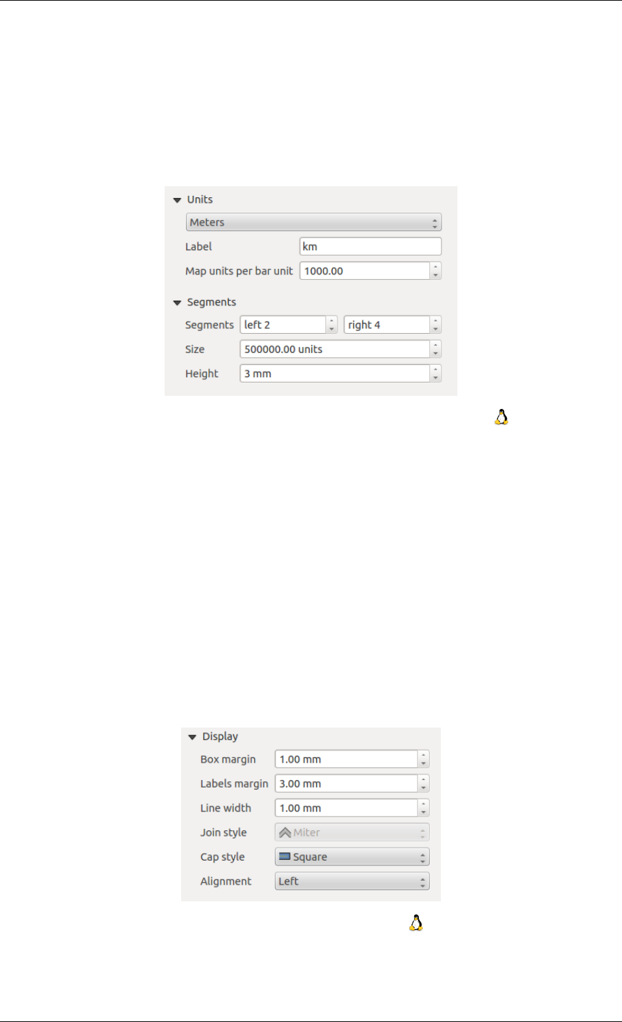
QGIS User Guide, Publicación 2.8
–Linea de marcas en el centro,arriba oabajo.
– Numérico, donde se imprime la relación de escala (por ejemplo, 1:50000).
Unidades y Segmentos
Los diálogos Unidades ySegmentos de la pestaña de barra de escala Propiedades del elemento proporcionan las
siguientes funcionalidades (ver figure_composer_scalebar_3):
Figure 18.21: Unidades de la barra de escala y diálogo de segmentos
En estos dos diálogos, se puede establecer cómo será representada la barra de escala.
• Seleccionar las unidades del mapa a utilizar. Hay cuatro opciones posibles: Unidades del mapa es la unidad
automáticamente seleccionada; Metros,Pies oMillas náuticas conversiones de unidades de fuerza.
• El campo Etiqueta define el texto utilizado para describir las unidades de la barra de escala.
• Las Unidades de mapa por unidad de barra le permite fijar la relación entre una unidad de mapa y su
representación en la barra de escala.
• Se puede definir cuantos Segmentos se dibujarán a la izquierda y derecha de la barra de escala, y cuánto
tiempo será cada segmento (campo Tamaño). Altura pueden ser también definidos.
Mostrar
El diálogo Visualizar de la barra de escala de la pestaña Propiedades del elemento proporciona las siguientes
funcionalidades (ver figure_composer_scalebar_4):
Figure 18.22: Mostrar barra de escala
Se puede definir como la barra de escala se mostrará en un marco.
•Margen de caja : espacio entre texto y bordes del marco
250 Chapter 18. Diseñadores de impresión
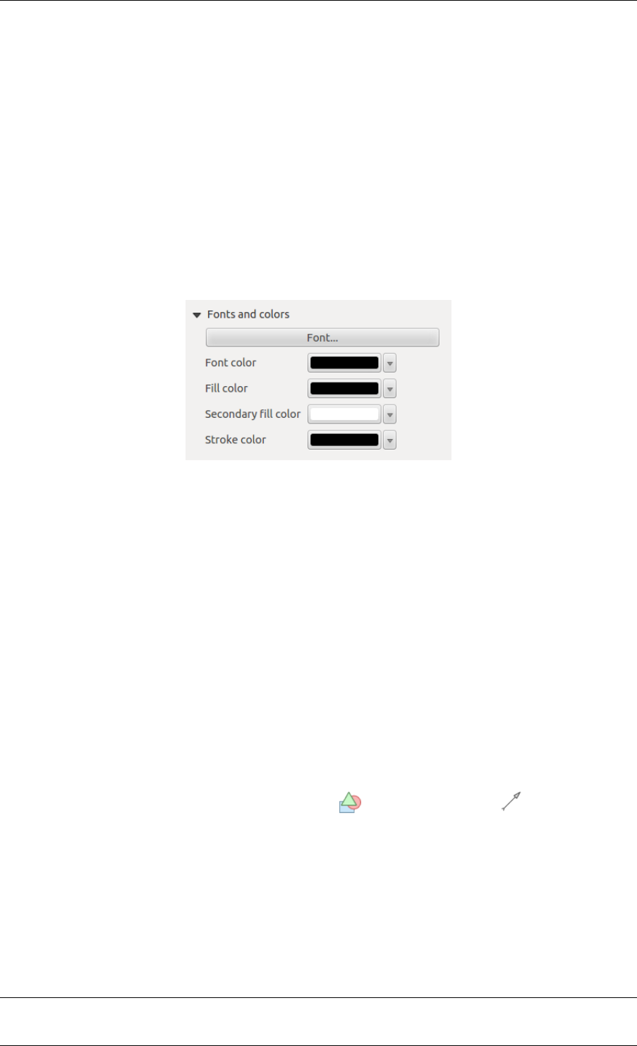
QGIS User Guide, Publicación 2.8
•Margen de etiquetas : espacio entre texto y dibujo de la barra de escala
•Ancho de línea : ancho de línea del dibujo de la barra de escala
•Estilo de unión : Esquinas al final de barra de escala en estilo biselado, redondeado o cuadrado (sólo
disponible para el estilo de barra de escala de Recuadro simple & Recuadro doble)
•Estilo de mayúsculas : El final de todas las lineas en estilo cuadrado, redondo o plana (sólo disponible para
el estilo de barra de escala Linea con marcas Arriba, Abajo y en el centro)
•Alignment : Puts text on the left, middle or right side of the frame (works only for Scale bar style Numeric)
Fuentes y colores
The Fonts and colors dialog of the scale bar Item Properties tab provide the following functionalities (see fig-
ure_composer_scalebar_5):
Figure 18.23: Diálogos de tipo de letra y colores de la barra de escala
Se puede definir el tipo de letra y los colores utilizados para la barra de escala.
• Utilice el botón [Tipo de letra] para establecer el tipo de letra
•Color de letras: establecer color de letras
•Color de relleno: establecer el color de relleno primero
•Secondary fill color: set the second fill color
•Stroke color: set the color of the lines of the Scale Bar
Fill colors are only used for scale box styles Single Box and Double Box. To select a color you can use the list
option using the dropdown arrow to open a simple color selection option or the more advanced color selection
option, that is started when you click in the colored box in the dialog.
18.3.6 El elemento de forma básica
To add a basic shape (ellipse, rectangle, triangle), click the Add basic shape icon or the Add Arrow icon, place
the element holding down the left mouse. Customize the appearance in the Item Properties tab.
When you also hold down the Shift key while placing the basic shape you can create a perfect square, circle or
triangle.
The Shape item properties tab allows you to select if you want to draw an ellipse, rectangle or triangle inside the
given frame.
You can set the style of the shape using the advanced symbol style dialog with which you can define its outline
and fill color, fill pattern, use markers etcetera.
For the rectangle shape, you can set the value of the corner radius to round of the corners.
Nota: Unlike other items, you can not style the frame or the background color of the frame.
18.3. Elementos de diseño 251
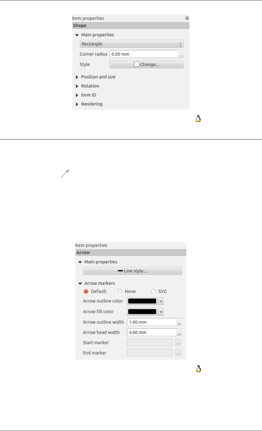
QGIS User Guide, Publicación 2.8
Figure 18.24: Pestaña de propiedades del elemento figura
18.3.7 El elemento flecha
To add an arrow, click the Add Arrow icon, place the element holding down the left mouse button and drag a line
to draw the arrow on the Print Composer canvas and position and customize the appearance in the scale bar Item
Properties tab.
When you also hold down the Shift key while placing the arrow, it is placed in an angle of exactly 45° .
The arrow item can be used to add a line or a simple arrow that can be used, for example, to show the relation
between other print composer items. To create a north arrow, the image item should be considered first. QGIS
has a set of North arrows in SVG format. Furthermore you can connect an image item with a map so it can rotate
automatically with the map (see the_image_item).
Figure 18.25: Pestaña de propiedades del elemento flecha
Propiedades del elemento
The Arrow item properties tab allows you to configure an arrow item.
252 Chapter 18. Diseñadores de impresión
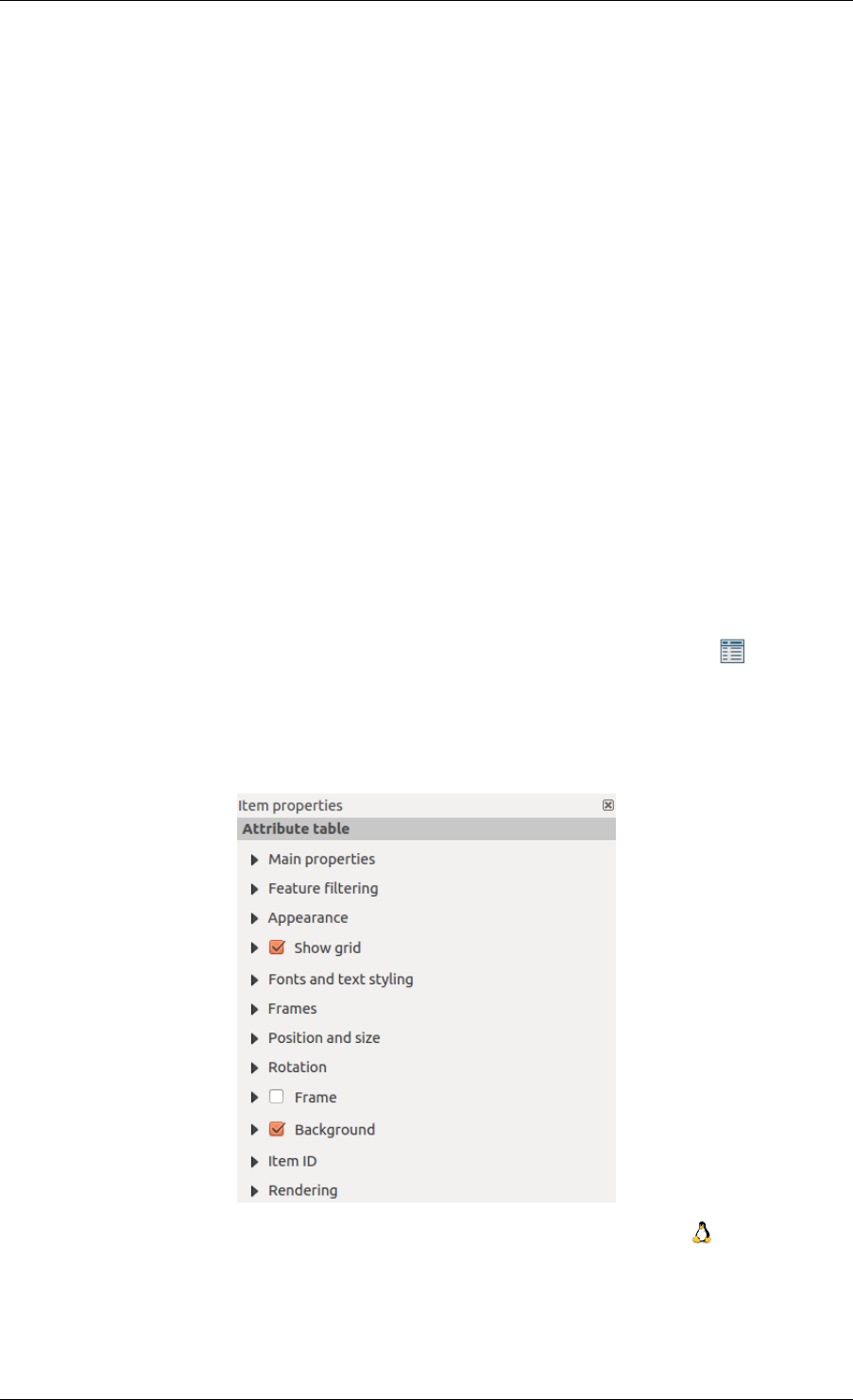
QGIS User Guide, Publicación 2.8
The [Line style ...] button can be used to set the line style using the line style symbol editor.
In Arrows markers you can select one of three radio buttons.
•Default : To draw a regular arrow, gives you options to style the arrow head
•None : To draw a line without arrow head
•SVG Marker : To draw a line with an SVG Start marker and/or End marker
For Default Arrow marker you can use following options to style the arrow head.
•Arrow outline color : Set the outline color of the arrow head
•Arrow fill color : Set the fill color of the arrow head
•Arrow outline width : Set the outline width of the arrow head
•Arrow head width: Set the size of the arrow head
For SVG Marker you can use following options.
•Start marker : Choose an SVG image to draw at the beginning of the line
•End marker : Choose an SVG image to draw at the end of the line
•Arrow head width: Sets the size of Start and/or End marker
SVG images are automatically rotated with the line. The color of the SVG image can not be changed.
18.3.8 El elemento de Tabla de Atributos
It is possible to add parts of a vector attribute table to the Print Composer canvas: Click the Add attribute table
icon, place the element with the left mouse button on the Print Composer canvas, and position and customize the
appearance in the Item Properties tab.
The Item properties of an attribute table item tab provides the following functionalities (see fig-
ure_composer_table_1):
Figure 18.26: Pestaña de propiedades del elemento de Tabla de atributos
18.3. Elementos de diseño 253
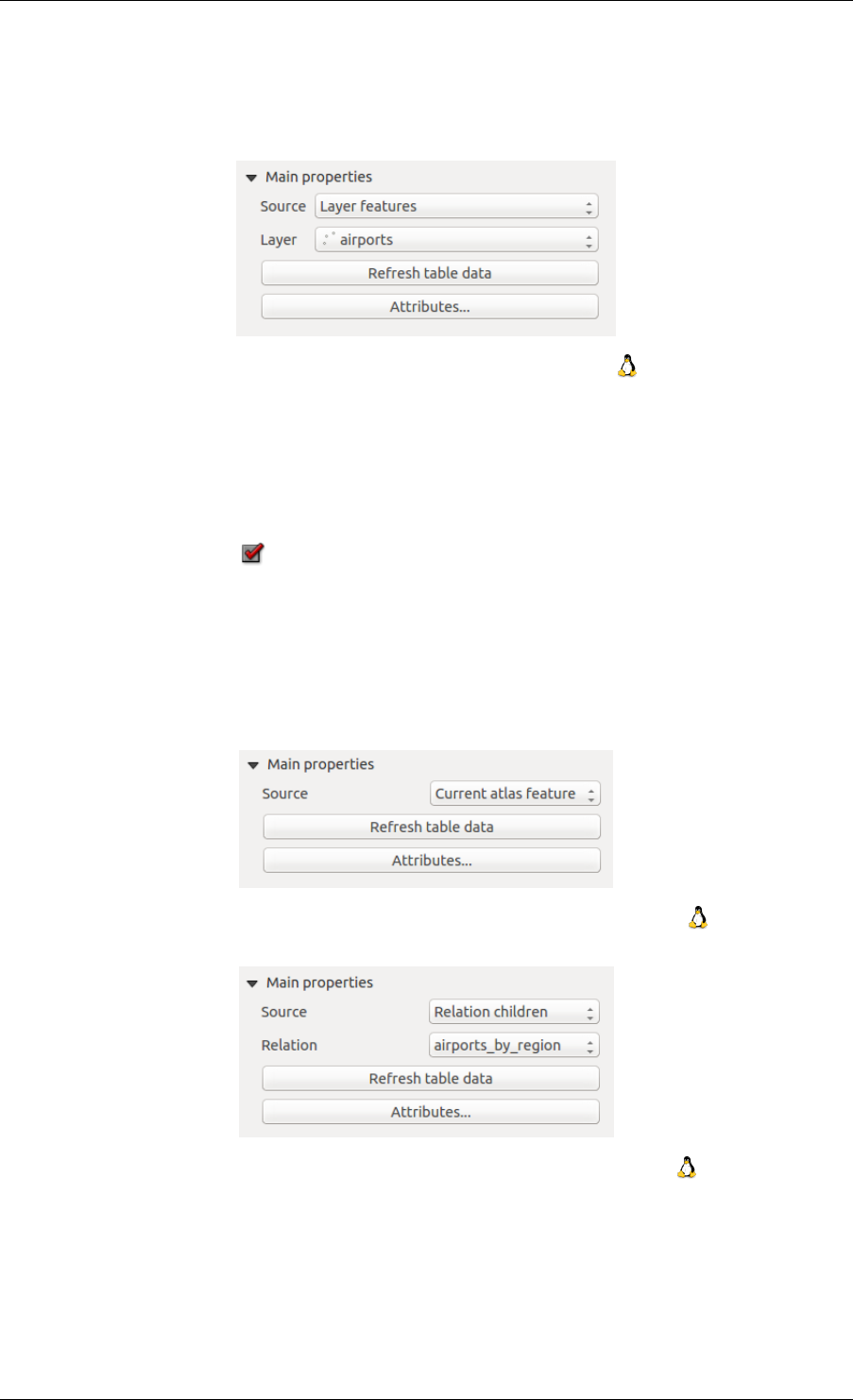
QGIS User Guide, Publicación 2.8
Propiedades principales
The Main properties dialogs of the attribute table Item Properties tab provide the following functionalities (see
figure_composer_table_2):
Figure 18.27: Attribute table Main properties Dialog
• For Source you can normally select only ‘Layer features’.
• With Layer you can choose from the vector layers loaded in the project.
• The button [Refresh table data] can be used to refresh the table when the actual contents of the table has
changed.
• In case you activated the Generate an atlas option in the Atlas generation tab, there are two additional
Source possible: ‘Current atlas feature’ (see figure_composer_table_2b) and ‘Relation children’ (see fig-
ure_composer_table_2c). Choosing the ‘Current atlas feature’ you won’t see any option to choose the layer,
and the table item will only show a row with the attributes from the current feature of the atlas coverage
layer. Choosing ‘Relation children’, an option with the relation name will show up. The ‘Relation children’
option can only be used if you have defined a relation using your atlas coverage layer as parent, and it will
show the children rows of the atlas coverage layer’s current feature (for further information about the atlas
generation see atlasgeneration).
Figure 18.28: Attribute table Main properties for ‘Current atlas feature’
Figure 18.29: Attribute table Main properties for ‘Relation children’
• The button [Attributes...] starts the Select attributes menu, see figure_composer_table_3, that can be used
to change the visible contents of the table. After making changes use the [OK] button to apply changes to
the table.
En la sección Columnas se puede:
–Remove an attribute, just select an attribute row by clicking anywhere in a row and press the minus
button to remove the selected attribute.
254 Chapter 18. Diseñadores de impresión
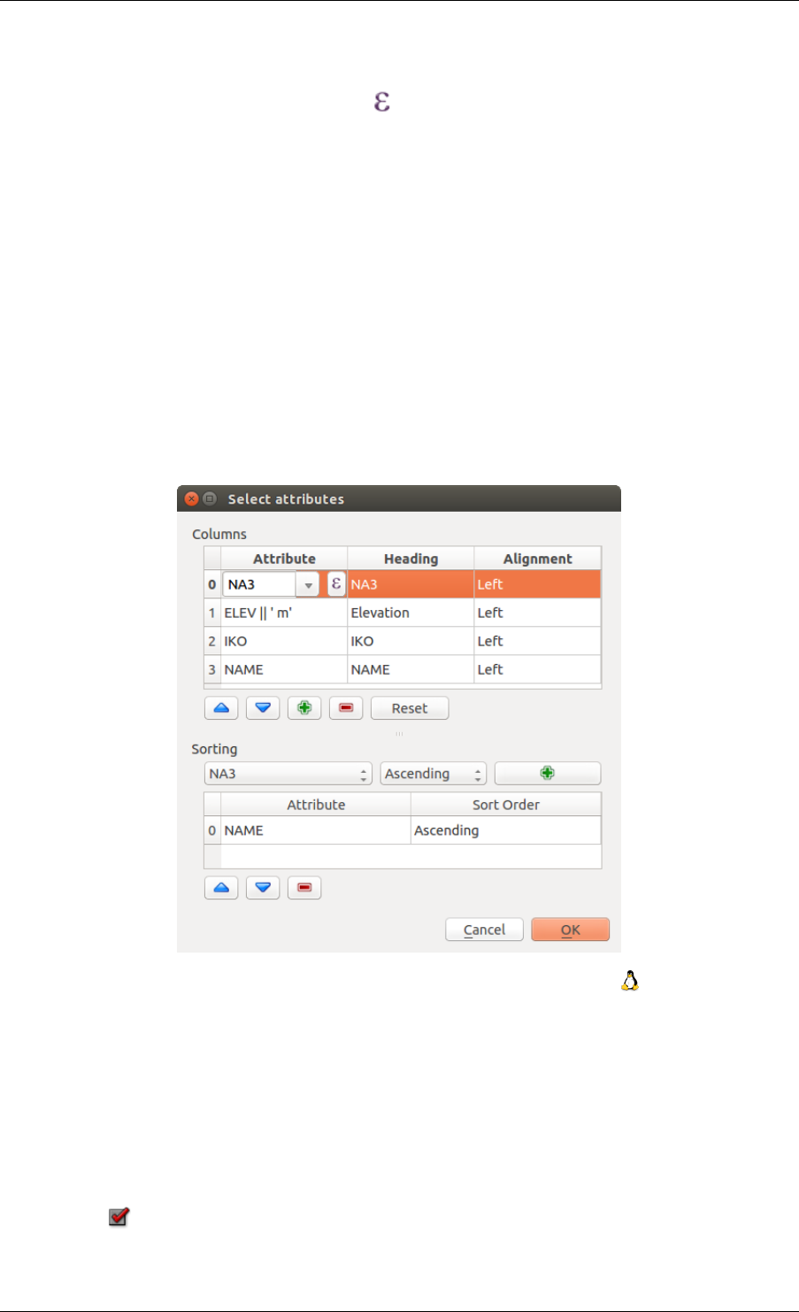
QGIS User Guide, Publicación 2.8
–Add a new attribute use the plus button. At the end a new empty row appears and you can select empty
cell of the column Attribute. You can select a field attribute from the list or you can select to build a
new attribute using a regular expression ( button). Of course you can modify every already existing
attribute by means of a regular expression.
–Use the up and down arrows to change the order of the attributes in the table.
–Select a cel in the Headings column to change the Heading, just type in a new name.
–Select a cel in the Alignment column and you can choose between Left, Center or Right alignment.
–Select a cel in the Width column and you can change it from Automatic to a width in mm, just type a
number. When you want to change it back to Automatic, use the cross.
–The [Reset] button can always be used to restore it to the original attribute settings.
En la sección Ordenar se puede:
–Add an attribute to sort the table with. Select an attribute and set the sorting order to ‘Ascending’ or
‘Descending’ and press the plus button. A new line is added to the sort order list.
–select a row in the list and use the up and down button to change the sort priority on attribute level.
–use the minus button to remove an attribute from the sort order list.
Figure 18.30: Seleccionar tabla de atributos Diálogo de atributos
Feature filtering
The Feature filtering dialogs of the attribute table Item Properties tab provide the following functionalities (see
figure_composer_table_4):
Puede:
• Define the Maximum rows to be displayed.
• Activate Remove duplicate rows from table to show unique records only.
18.3. Elementos de diseño 255
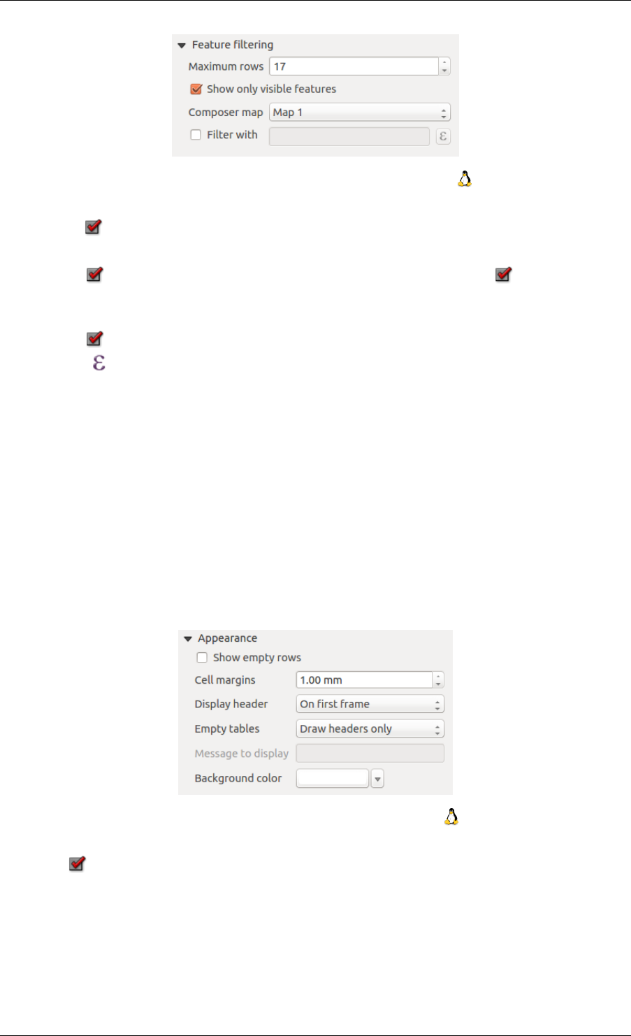
QGIS User Guide, Publicación 2.8
Figure 18.31: Attribute table Feature filtering Dialog
• Activate Show only visible features within a map and select the corresponding Composer map to display
the attributes of features only visible on selected map.
• Activate Show only features intersecting Atlas feature is only available when Generate an atlas is
activated. When activated it will show a table with only the features shown on the map of that particular
page of the atlas.
• Activate Filter with and provide a filter by typing in the input line or insert a regular expression using
the given expression button. A few examples of filtering statements you can use when you have loaded
the airports layer from the Sample dataset:
–ELEV > 500
–NAME = ’ANIAK’
–NAME NOT LIKE ’AN%
–regexp_match( attribute( $currentfeature, ’USE’ ) , ’[i]’)
The last regular expression will include only the arpoirts that have a letter ‘i’ in the attribute field ‘USE’.
Apariencia
The Appearance dialogs of the attribute table Item Properties tab provide the following functionalities (see fig-
ure_composer_table_5):
Figure 18.32: Attribute table appearance Dialog
• Click Show empty rows to make empty entries in the attribute table visible.
• With Cell margins you can define the margin around text in each cell of the table.
• With Display header you can select from a list one of ‘On first frame’, ‘On all frames’ default option, or
‘No header’.
• The option Empty table controls what will be displayed when the result selection is empty.
– Draw headers only, will only draw the header except if you have choosen ‘No header’ for Display
header.
256 Chapter 18. Diseñadores de impresión
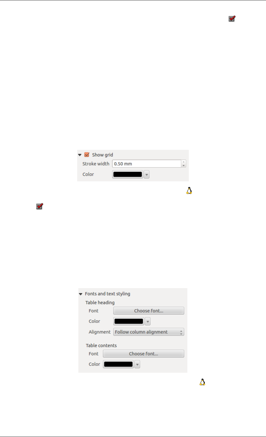
QGIS User Guide, Publicación 2.8
– Hide entire table, will only draw the background of the table. You can activate Don’t draw
background if frame is empty in Frames to completely hide the table.
– Draw empty cells, will fill the attribute table with empty cells, this option can also be used to provide
additional empty cells when you have a result to show!
– Show set message, will draw the header and adds a cell spanning all columns and display a message
like ‘No result’ that can be provided in the option Message to display
• The option Message to display is only activated when you have selected Show set message for Empty table.
The message provided will be shown in the table in the first row, when the result is an empty table.
• With Background color you can set the background color of the table.
Mostrar cuadrícula
The Show grid dialog of the attribute table Item Properties tab provide the following functionalities (see fig-
ure_composer_table_6):
Figure 18.33: Attribute table Show grid Dialog
• Activate Show grid when you want to display the grid, the outlines of the table cells.
• With Stroke width you can set the thickness of the lines used in the grid.
• The Color of the grid can be set using the color selection dialog.
Fuente y estilo de texto
The Fonts and text styling dialog of the attribute table Item Properties tab provide the following functionalities
(see figure_composer_table_7):
Figure 18.34: Attribute table Fonts and text styling Dialog
• You can define Font and Color for Table heading and Table contents.
• For Table heading you can additionally set the Alignment and choose from Follow column align-
ment,Left,Center or Right. The column alignment is set using the Select Attributes dialog (see Fig-
ure_composer_table_3 ).
18.3. Elementos de diseño 257
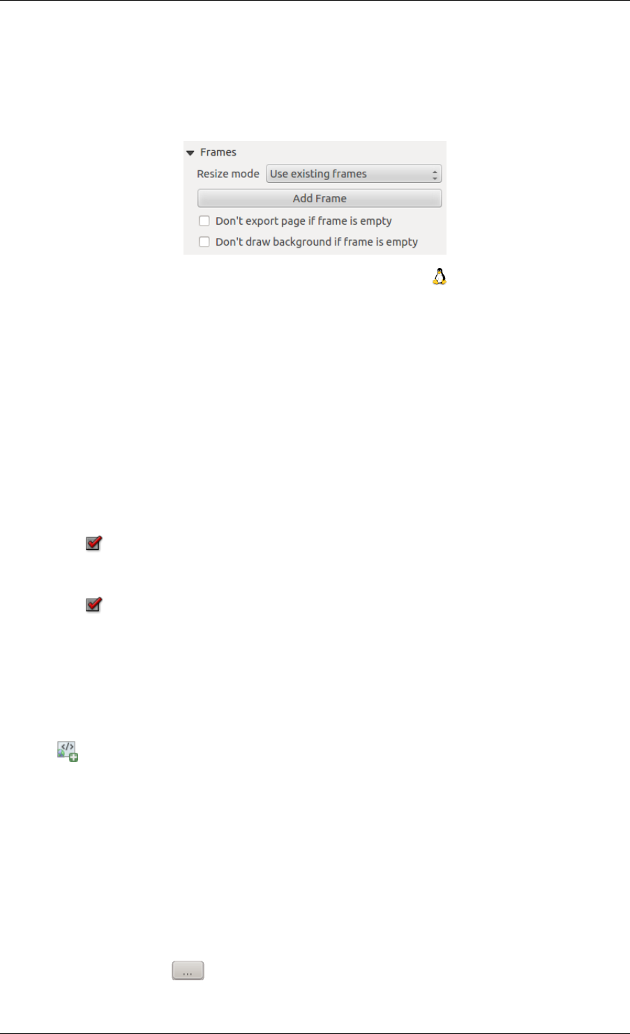
QGIS User Guide, Publicación 2.8
Frames
The Frames dialog of the attribute table Item Properties tab provide the following functionalities (see fig-
ure_composer_table_8):
Figure 18.35: Attribute table Frames Dialog
• With Resize mode you can select how to render the attribute table contents:
–Use existing frames displays the result in the first frame and added frames only.
–Extent to next page will create as many frames (and corresponding pages) as necessary to display the
full selection of attribute table. Each frame can be moved around on the layout. If you resize a frame,
the resulting table will be divided up between the other frames. The last frame will be trimmed to fit
the table.
–Repeat until finished will also create as many frames as the Extend to next page option, except all
frames will have the same size.
• Use the [Add Frame] button to add another frame with the same size as selected frame. The result of the
table that will not fit in the first frame will continue in the next frame when you use the Resize mode Use
existing frames.
• Activate Don’t export page if frame is empty prevents the page to be exported when the table frame has
no contents. This means all other composer items, maps, scalebars, legends etc. will not be visible in the
result.
• Activate Don’t draw background if frame is empty prevents the background to be drawn when the table
frame has no contents.
18.3.9 El elemento del marco HTML
It is possible to add a frame that displays the contents of a website or even create and style your own HTML page
and display it!
Click the Add HTML frame icon, place the element by dragging a rectangle holding down the left mouse but-
ton on the Print Composer canvas and position and customize the appearance in the Item Properties tab (see
figure_composer_html_1).
Fuente HTML
As an HTML source, you can either set a URL and activate the URL radiobutton or enter the HTML source
directly in the textbox provided and activate the Source radiobutton.
The HTML Source dialog of the HTML frame Item Properties tab provides the following functionalities (see
figure_composer_html_2):
• In URL you can enter the URL of a webpage you copied from your internet browser or select an HTML file
using the browse button . There is also the option to use the Data defined override button, to provide
an URL from the contents of an attribute field of a table or using a regular expression.
258 Chapter 18. Diseñadores de impresión
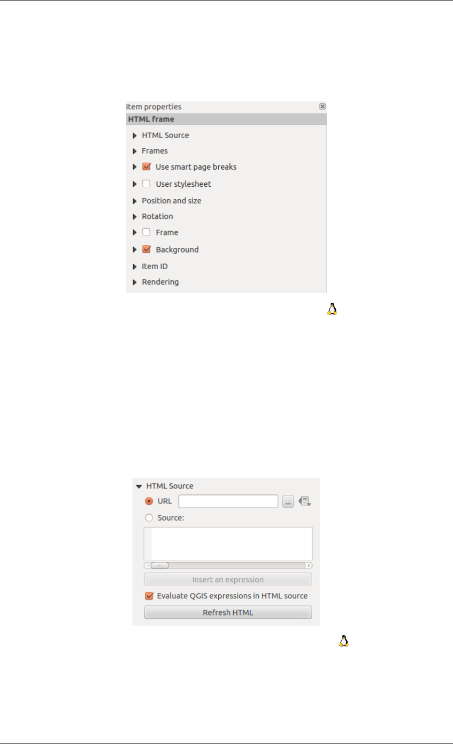
QGIS User Guide, Publicación 2.8
Figure 18.36: HTML frame, the item properties Tab
Figure 18.37: HTML frame, the HTML Source properties
18.3. Elementos de diseño 259
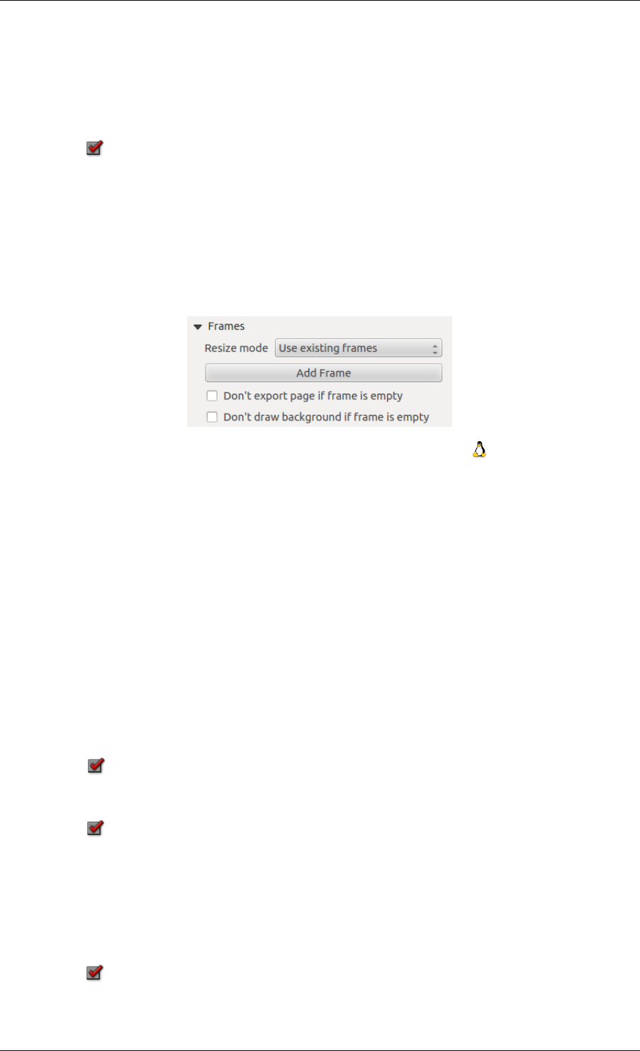
QGIS User Guide, Publicación 2.8
• In Source you can enter text in the textbox with some HTML tags or provide a full HTML page.
• The [insert an expression] button can be used to insert an expression like [%Year($now)%] in the
Source textbox to display the current year. This button is only activated when radiobutton Source is selected.
After inserting the expression click somewhere in the textbox before refreshing the HTML frame, otherwise
you will lose the expression.
• Activate Evaluate QGIS expressions in HTML code to see the result of the expression you have included,
otherwise you will see the expression instead.
• Utilice el botón [Actualizar HTML] para actualizar los marco(s) para ver los resultados de los cambios.
Frames
El diálogo Marcos de la pestaña marco HTML Propiedades del elemento proporciona las siguientes funcionali-
dades (ver figure_composer_html_3):
Figure 18.38: Marco HTML, las propiedades del marco
• Con Modo cambio de tamaño se puede seleccionar cómo renderizar el contenido HTML:
–Use existing frames displays the result in the first frame and added frames only.
–Extender a la página siguiente crear tantos marcos sean necesarios (y páginas corresponedientes) para
renderizar el alto de la página web. Cada marco se puede mover alrededor del diseño. Si cambia el
tamaño de un marco, la página web se dividirá entre los otros marcos. El último cuadro se recortará
para ajustarse a la página web.
–Repeat on every page will repeat the upper left of the web page on every page in frames of the same
size.
–Repeat until finished will also create as many frames as the Extend to next page option, except all
frames will have the same size.
• Utilice el botón [Añadir marco] para añadir otros marcos con el mismo tamaño como el marco selec-
cionado. Si la página HTML no cabe en el primer marco, continuará en el siguiente marco cuando se utilice
modo cambiar tamaño oUtilice marcos existentes.
• Activate Don’t export page if frame is empty prevents the map layout from being exported when the
frame has no HTML contents. This means all other composer items, maps, scalebars, legends etc. will not
be visible in the result.
• Activate Don’t draw background if frame is empty prevents the HTML frame being drawn if the frame
is empty.
Use smart page breaks and User style sheet
The Use smart page breaks dialog and Use style sheet dialog of the HTML frame Item Properties tab provides the
following functionalities (see figure_composer_html_4):
• Activate Use smart page breaks to prevent the html frame contents from breaking mid-way a line of text
so it continues nice and smooth in the next frame.
260 Chapter 18. Diseñadores de impresión
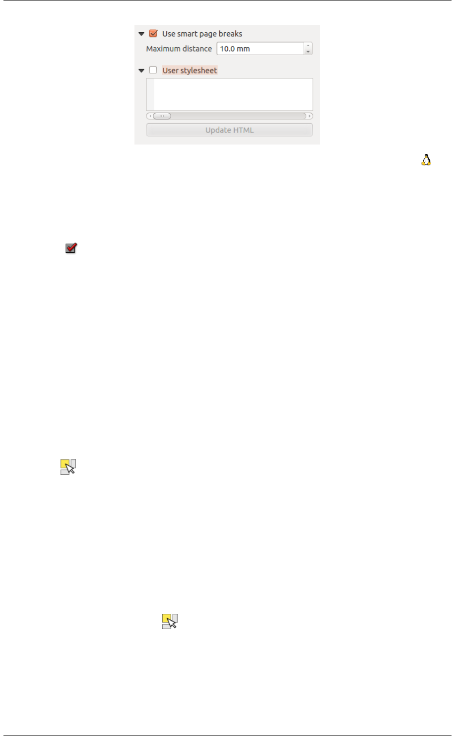
QGIS User Guide, Publicación 2.8
Figure 18.39: Marco HTML, Utilice saltos de página inteligentes y propiedades de estilo de usuario
• Set the Maximum distance allowed when calculating where to place page breaks in the html. This distance
is the maximum amount of empty space allowed at the bottom of a frame after calculating the optimum
break location. Setting a larger value will result in better choice of page break location, but more wasted
space at the bottom of frames. This is only used when Use smart page breaks is activated.
• Activate User stylesheet to apply HTML styles that often is provided in cascading style sheets. An
example of style code is provide below to set the color of <h1> header tag to green and set the font and
fontsize of text included in paragraph tags <p>.
h1 {color:#00ff00;
}
p{font-family:"Times New Roman",Times,serif;
font-size:20px;
}
• Utilice el botón [Actualizar HTML] para ver el resultado de la configuración de la hoja de estilo.
18.4 Administrar elementos
18.4.1 Tamaño y posición
Each item inside the Composer can be moved/resized to create a perfect layout. For both operations the first step is
to activate the Select/Move item tool and to click on the item; you can then move it using the mouse while holding
the left button. If you need to constrain the movements to the horizontal or the vertical axis, just hold the Shift
while moving the mouse. If you need a better precision, you can move a selected item using the Arrow keys
on the keyboard; if the movement is too slow, you can speed up it by holding Shift.
A selected item will show squares on its boundaries; moving one of them with the mouse, will resize the item
in the corresponding direction. While resizing, holding Shift will maintain the aspect ratio. Holding Alt will
resize from the item center.
The correct position for an item can be obtained using snapping to grid or smart guides. Guides are set by clicking
and dragging in the rulers. Guides are moved by clicking in the ruler, level with the guide and dragging to a new
place. To delete a guide move it off the canvas. If you need to disable the snap on the fly just hold Ctrl while
moving the mouse.
You can choose multiple items with the Select/Move item button. Just hold the Shift button and click on all the
items you need. You can then resize/move this group just like a single item.
Once you have found the correct position for an item, you can lock it by using the items on the toolbar or ticking
the box next to the item in the Items tab. Locked items are not selectable on the canvas.
Locked items can be unlocked by selecting the item in the Items tab and unchecking the tickbox or you can use
the icons on the toolbar.
Para cancelar la selección de un elemento, basta con hacer clic en él sosteniendo el botón Shift.
18.4. Administrar elementos 261
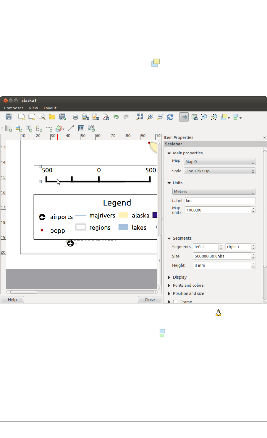
QGIS User Guide, Publicación 2.8
Inside the Edit menu, you can find actions to select all the items, to clear all selections or to invert the current
selection.
18.4.2 Alineación
Raising or lowering functionalities for elements are inside the Raise selected items pull-down menu. Choose an
element on the Print Composer canvas and select the matching functionality to raise or lower the selected element
compared to the other elements (see table_composer_1). This order is shown in the Items tab. You can also raise
or lower objects in the Items tab by clicking and dragging an object’s label in this list.
Figure 18.40: Líneas auxiliares de alineación en el diseño de impresión
There are several alignment functionalities available within the Align selected items pull-down menu (see ta-
ble_composer_1). To use an alignment functionality, you first select some elements and then click on the matching
alignment icon. All selected elements will then be aligned within to their common bounding box. When moving
items on the Composer canvas, alignment helper lines appear when borders, centers or corners are aligned.
18.4.3 Elementos Copiar/Cortar y Pegar
The print composer includes actions to use the common Copy/Cut/Paste functionality for the items in the layout.
As usual first you need to select the items using one of the options seen above; at this point the actions can be
found in the Edit menu. When using the Paste action, the elements will be pasted according to the current mouse
position.
262 Chapter 18. Diseñadores de impresión
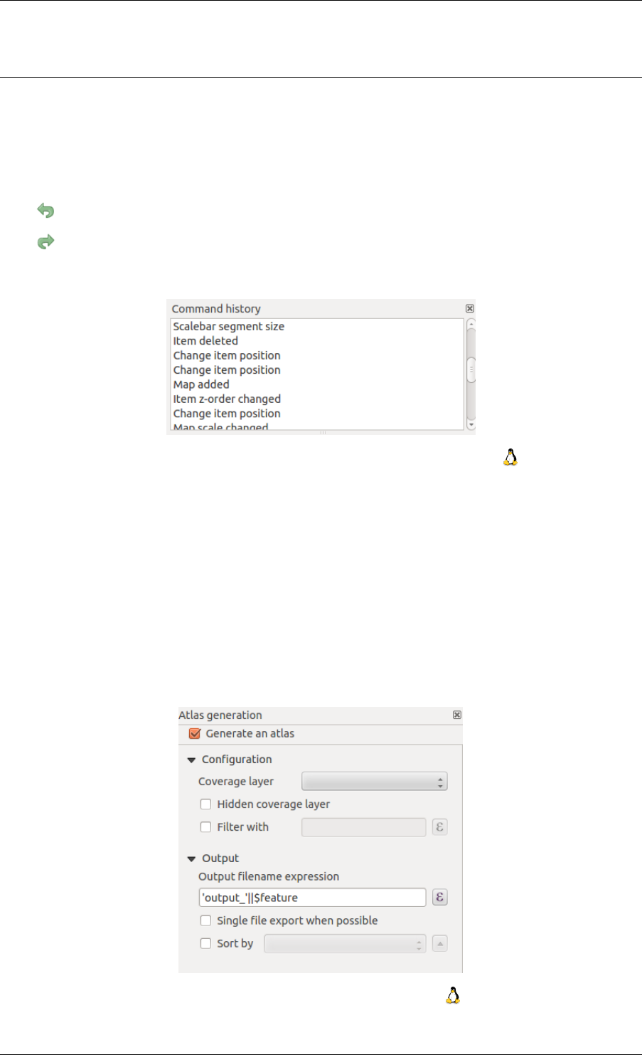
QGIS User Guide, Publicación 2.8
Nota: HTML items can not be copied in this way. As a workaround, use the [Add Frame] button in the Item
Properties tab.
18.5 Revertir y Restaurar herramientas
During the layout process, it is possible to revert and restore changes. This can be done with the revert and restore
tools:
•Revertir el último cambio
•Restaurar el último cambio
This can also be done by mouse click within the Command history tab (see figure_composer_29).
Figure 18.41: Historial de comandos en el diseñador de impresión
18.6 Generación de Atlas
The Print Composer includes generation functions that allow you to create map books in an automated way. The
concept is to use a coverage layer, which contains geometries and fields. For each geometry in the coverage layer,
a new output will be generated where the content of some canvas maps will be moved to highlight the current
geometry. Fields associated with this geometry can be used within text labels.
Every page will be generated with each feature. To enable the generation of an atlas and access generation
parameters, refer to the Atlas generation tab. This tab contains the following widgets (see Figure_composer_atlas):
Figure 18.42: Pestaña de Generación de Atlas
18.5. Revertir y Restaurar herramientas 263
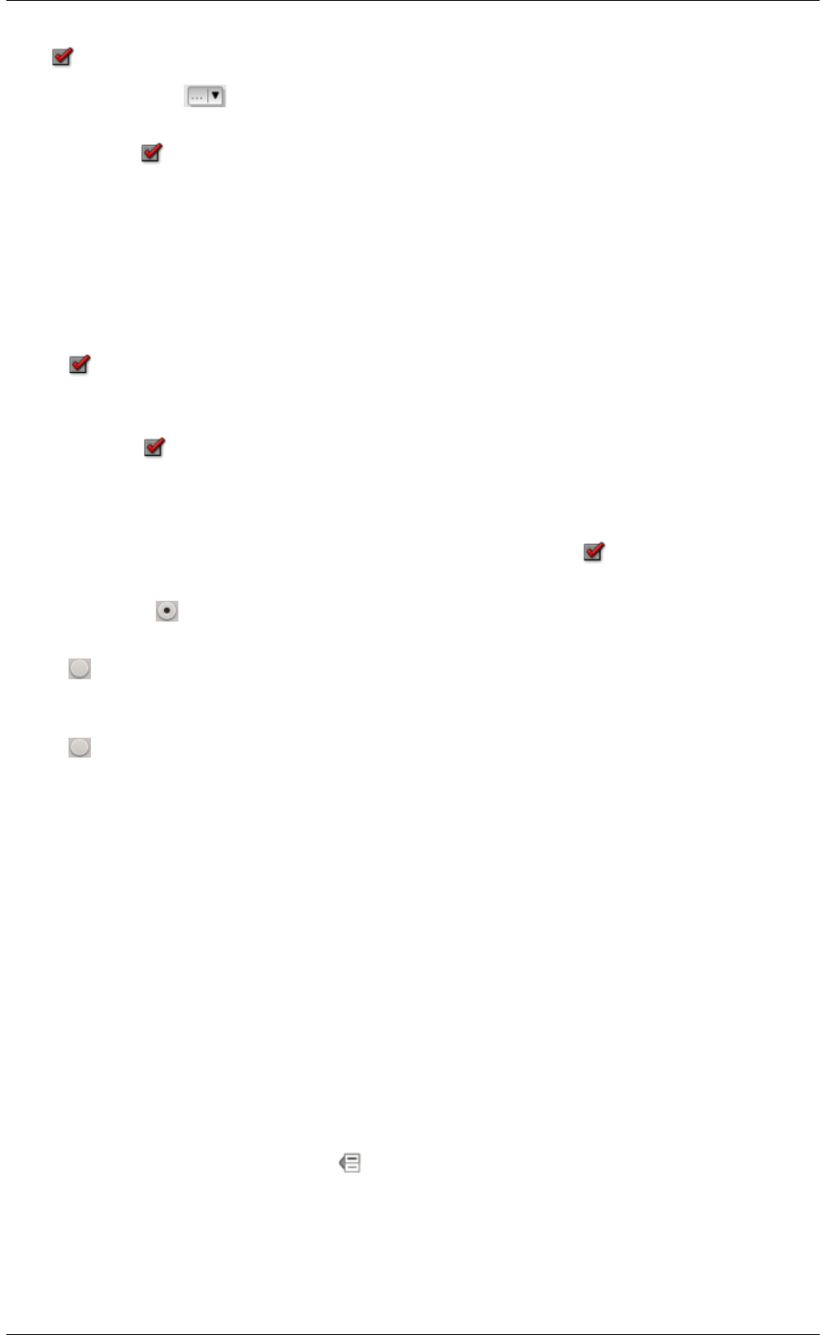
QGIS User Guide, Publicación 2.8
•Generar un atlas, que activa o desactiva la generación del atlas.
• A Coverage layer combo box that allows you to choose the (vector) layer containing the geometries
on which to iterate over.
• An optional Hidden coverage layer that, if checked, will hide the coverage layer (but not the other ones)
during the generation.
• An optional Filter with text area that allows you to specify an expression for filtering features from the
coverage layer. If the expression is not empty, only features that evaluate to True will be selected. The
button on the right allows you to display the expression builder.
• Una caja de texto Expresión de nombre de archivo de salida que se utiliza para generar un nombre de archivo
para cada geometría si es necesario. Se basa en expresiones. Este campo es significativo solo para presentar
múltiples archivos.
• A Single file export when possible that allows you to force the generation of a single file if this is possible
with the chosen output format (PDF, for instance). If this field is checked, the value of the Output filename
expression field is meaningless.
• An optional Sort by that, if checked, allows you to sort features of the coverage layer. The associated
combo box allows you to choose which column will be used as the sorting key. Sort order (either ascending
or descending) is set by a two-state button that displays an up or a down arrow.
You can use multiple map items with the atlas generation; each map will be rendered according to the coverage
features. To enable atlas generation for a specific map item, you need to check Controlled by Atlas under the
item properties of the map item. Once checked, you can set:
• A radiobutton Margin around feature that allows you to select the amount of space added around each
geometry within the allocated map. Its value is meaningful only when using the auto-scaling mode.
• A Predefined scale (best fit). It will use the best fitting option from the list of predefined scales in your
project properties settings (see Project –> Project Properties –> General –> Project Scales to configure
these predefined scales).
• A Fixed scale that allows you to toggle between auto-scale and fixed-scale mode. In fixed-scale mode,
the map will only be translated for each geometry to be centered. In auto-scale mode, the map’s extents are
computed in such a way that each geometry will appear in its entirety.
18.6.1 Etiquetas
In order to adapt labels to the feature the atlas plugin iterates over, you can include expressions. For example, for
a city layer with fields CITY_NAME and ZIPCODE, you could insert this:
The area of [% upper(CITY_NAME) || ’,’ || ZIPCODE || ’ is ’ format_number($area/1000000,2) %] km2
The information [% upper(CITY_NAME) || ‘,’ || ZIPCODE || ‘ is ‘ format_number($area/1000000,2) %] is an
expression used inside the label. That would result in the generated atlas as:
The area of PARIS,75001 is 1.94 km2
18.6.2 Data Defined Override Buttons
There are several places where you can use a Data Defined Override button to override the selected setting. These
options are particularly usefull with Atlas Generation.
For the following examples the Regions layer of the QGIS sample dataset is used and selected for Atlas Generation.
We also assume the paper format A4 (210X297) is selected in the Composition tab for field Presets.
264 Chapter 18. Diseñadores de impresión
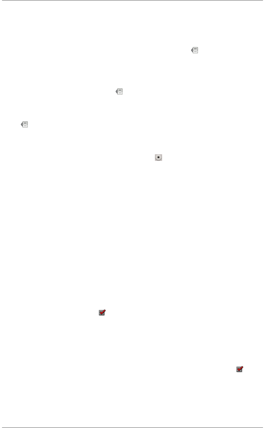
QGIS User Guide, Publicación 2.8
With a Data Defined Override button you can dynamically set the paper orientation. When the height (north-
south) of the extents of a region is greater than it’s width (east-west), you rather want to use portrait instead of
landscape orientation to optimize the use of paper.
In the Composition you can set the field Orientation and select Landscape or Portrait. We want to set the orienta-
tion dynamically using an expression depending on the region geometry. press the button of field Orientation,
select Edit ... so the Expression string builder dialog opens. Give following expression:
CASE WHEN bounds_width($atlasgeometry) > bounds_height($atlasgeometry) THEN ’Landscape’ ELSE ’Portrait’ END
Now the paper orients itself automatically for each Region you need to reposition the location of the composer
item as well. For the map item you can use the button of field Width to set it dynamically using following
expression:
(CASE WHEN bounds_width($atlasgeometry) > bounds_height($atlasgeometry) THEN 297 ELSE 210 END) - 20
Use the button of field Heigth to provide following expression:
(CASE WHEN bounds_width($atlasgeometry) > bounds_height($atlasgeometry) THEN 210 ELSE 297 END) - 20
When you want to give a title above map in the center of the page, insert a label item above the map. First use the
item properties of the label item to set the horizontal alignment to Center. Next activate from Reference point
the upper middle checkbox. You can provide following expression for field X:
(CASE WHEN bounds_width($atlasgeometry) > bounds_height($atlasgeometry) THEN 297 ELSE 210 END) / 2
For all other composer items you can set the position in a similar way so they are correctly positioned when page
is automatically rotated in portrait or landscape.
Information provided is derived from the excellent blog (in english and portugese) on the Data Defined Override
options Multiple_format_map_series_using_QGIS_2.6 .
Este es sólo un ejemplo de cómo se puede utilizar Anulaciones de datos definidos.
18.6.3 Vista previa
Once the atlas settings have been configured and map items selected, you can create a preview of all the pages by
clicking on Atlas →Preview Atlas and using the arrows, in the same menu, to navigate through all the features.
18.6.4 Generación
The atlas generation can be done in different ways. For example, with Atlas →Print Atlas, you can directly print
it. You can also create a PDF using Atlas →Export Atlas as PDF: The user will be asked for a directory for saving
all the generated PDF files (except if the Single file export when possible has been selected). If you need to
print just a page of the atlas, simply start the preview function, select the page you need and click on Composer
→Print (or create a PDF).
18.7 Ocultar y mostrar paneles
Para maximizar el espacio disponible para interactuar con una composición que pueda utilizar Ver –> Ocultar
paneles o presionar F10.
:: nota:
It’s also possible to switch to a full screen mode to have more space to interact by pressing
:kbd:‘F11‘ or using :guilabel:‘View --> |checkbox| :guilabel:‘Toggle full screen‘.
18.7. Ocultar y mostrar paneles 265
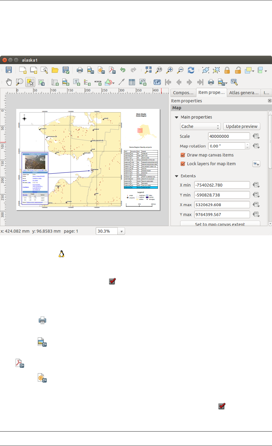
QGIS User Guide, Publicación 2.8
18.8 Crear salida
Figure_composer_output shows el diseñador de impresión con un diseño de ejemplo de impresión, incluyendo
cada tipo de elemento del mapa descrito en los apartados anteriores.
Figure 18.43: Diseñador de impresión con vista de mapa, leyenda, imagen, barra de escala, coordenadas, texto y
marco HTML agregado
Antes de imprimir un diseño tiene la posibilidad de ver su composición sin cuadros delimitadores. Esto de puede
activar mediante la desactivación de Ver –> Mostrar cuadros delimitadores o presionando el acceso directo
Ctrl+Shift+B.
El diseñador de impresión le permite crear varios formatos de salida, y es posible definir la resolución (calidad de
impresión) y tamaño de papel:
• El icono Imprimir le permite imprimir el diseño en una impresora conectada o un archivo PostScript,
dependiendo de los controladores de impresora instalados.
• El icono Exportar como imagen exporta el lienzo del diseñador en varios formatos de imagen, como PNG,
BPM, TIF, JPG,...
•Exportar como PDF guarda el lienzo definido en el diseñador de impresión directamente como PDF.
• El icono Exportar como SVG guarda el lienzo del diseñador de impresión como un SVG (Scalable Vector
Graphic).
Si necesita exportar su diseño como una imagen georeferenciada (por ejemplo, para cargarlo de nuevo dentro de
QGIS), se necesita habilitar esta característica bajo la pestaña Composición. Compruebe Archivo de mundo
activado y seleccione el elemento del mapa a utilizar. Con esta opción, la acción ‘Exportar como imagen’ también
creará un archivo de mundo.
266 Chapter 18. Diseñadores de impresión
QGIS User Guide, Publicación 2.8
Nota:
• Actualmente, la salida SVG es muy básica. Este no es un problema en QGIS, pero un problema con la
biblioteca Qt subyacente. Esperamos que esto se solucione en futuras versiones.
• Exportar grandes ráster algunas veces puede fallar, incluso si parece haber suficiente memoria. Este es
también un problema con la administración Qt subyacente de los rásters.
18.9 Administrar el diseñador de impresión
Con los iconos Guardar como plantilla yAñadir elementos de plantilla, se puede guardar el estado actual de una sesión
del diseñador de impresión como una plantilla .qpt y cargar la plantilla de nuevo en otra sesión.
El botón Administrador de diseñadores en la barra de herramientas de QGIS y en Diseñador→Administrador de
diseñadores le permite añadir una nueva plantilla de diseñador, se crea una nueva composición basada en una
platilla guardada previamente o para administrar las plantillas ya existentes.
Figure 18.44: EL Administrador de diseñadores
Por defecto, el administrador de diseño de impresión busca plantillas de usuario en ~/.qgis2/composer_template.
Los botones Nuevo diseñador de impresión yDuplicar diseñador en la barra de herramientas de QGIS y en Diseñador→
Nuevo diseñador de impresión yDiseñador→Duplicar diseñador le permite abrir un nuevo diálogo de diseñador,
o duplica una composición existente de una previamente creada.
Por último, puede guardar su diseño de impresión con el botón Guardar proyecto. Esta es la misma característica
como en la ventana principal de QGIS. Todos los cambios se guardarán en un archivo de proyecto de QGIS.
.
18.9. Administrar el diseñador de impresión 267

QGIS User Guide, Publicación 2.8
268 Chapter 18. Diseñadores de impresión
CHAPTER 19
Complementos
.
19.1 QGIS Complementos
QGIS ha sido diseñado con una arquitectura de complementos. Esto permite que sea fácil añadir muchas carac-
terísticas y funciones nuevas a la aplicación. Muchas de las características de QGIS están en realidad implemen-
tadas como complementos.
Puede administrar sus complementos en el diálogo de complementos que se puede abrir con Complementos >
Administrar e instalar complementos....
Cuando un complemento necesita ser actualizado, y si la configuración ha sido establecida en consecuencia, la
interfaz principal de QGIS podría mostrar un enlace en la barra de estado para decirle que hay algunas actualiza-
ciones de complementos esperando ser aplicadas.
19.1.1 El diálogo de complementos
Los menús en el diálogo Complementos permiten al usuario instalar, desinstalar y actualizar complementos en
diferentes formas. Cada complemento tiene algunos metadatos desplegados en el panel derecho:
• información si el complemento es experimental
• descripción
• voto(s) puntuación (¡puede votar por su complemento preferido!)
• etiquetas
• algunos enlaces útiles como página de inicio, rastreador y código del repositorio.
• autor(es)
• versión disponible
Puede utilizar el filtro para encontrar un complemento específico.
Todos
Aquí, todos los complementos disponibles están listados, incluyendo los complementos base y externos. Use [Ac-
tualizar todo] para buscar nuevas versiones de los complementos. Además, puede usar [Instalar complemento],
si un complemento esta listado pero no instalado, y [Desinstalar complemento] así como [Reinstalar comple-
mento], si un complemento esta instalado. Si uno esta instalado, puede ser desactivado o activado utilizando la
casilla de verificación.
Instalado
269
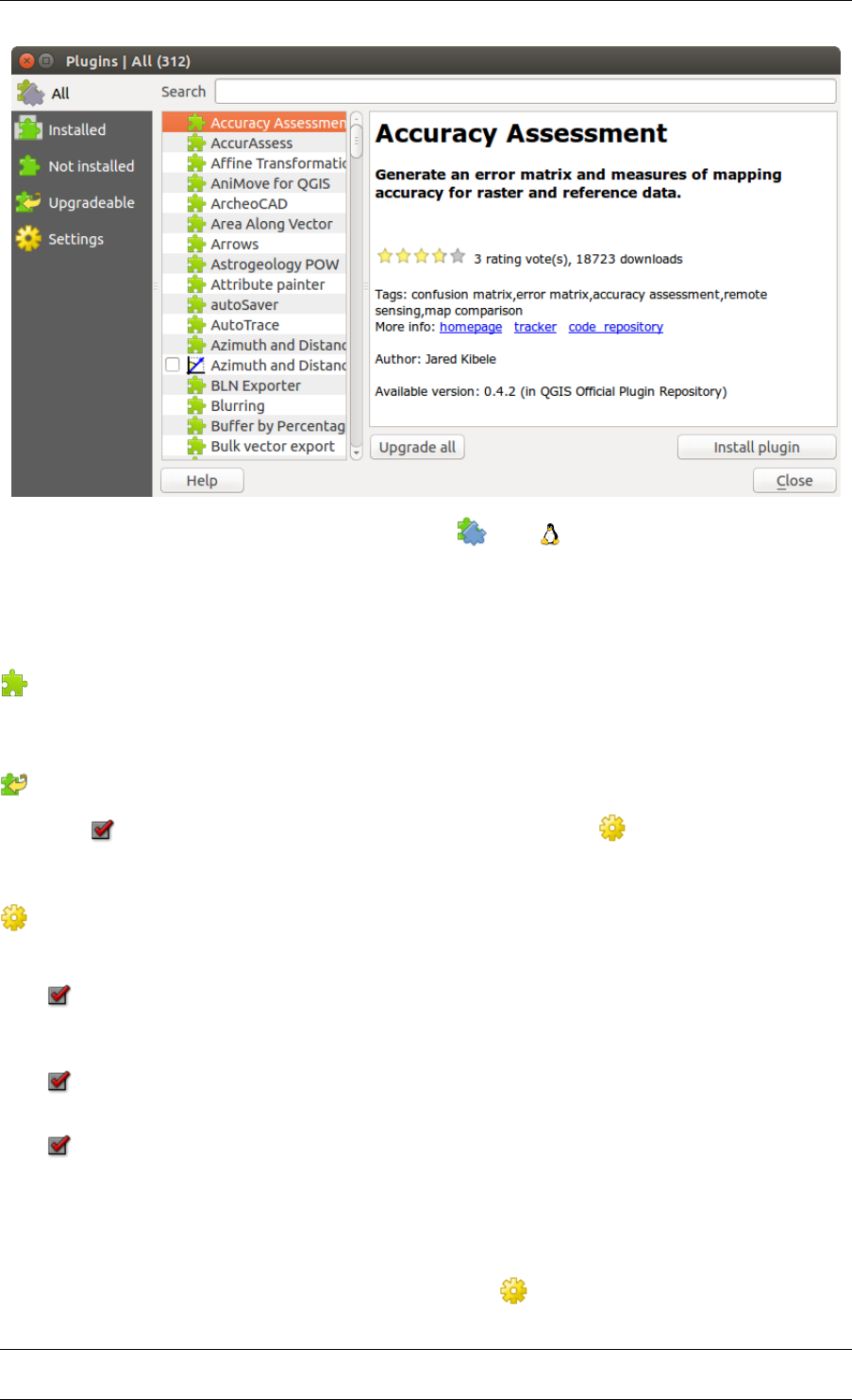
QGIS User Guide, Publicación 2.8
Figure 19.1: El menú Todos
En este menú, se pueden encontrar solo los complementos instalados. Los complementos instalados pueden ser
desinstalados y reinstalados usando los botones [Desinstalar complemento] y[Reinstalar complemento]. Se
puede [Actualizar todo] aquí también.
No instalado
Este menú lista todos los complementos disponibles que no están instalados. Se puede usar el botón [Instalar
complemento] para ejecutar un complemento en QGIS.
Actualizable
Si se activa Mostrar también los complementos experimentales en el menú Configuración, se puede usar
el menú para buscar versiones de complementos más recientes. Esto se puede hacer con los botones [Actualizar
complementos] o[Actualizar todos].
Configuración
Este menú, puede utilizar las siguientes opciones:
•Comprobar actualizaciones al inicio. Siempre que un nuevo complemento o actualización de comple-
mento esta disponible, QGIS informará ‘cada vez que se inicia QGIS’, ‘una vez al día’, ‘cada 3 días’, ‘cada
semana’, ‘cada 2 semanas’ o ‘cada mes’.
•Mostrar también los complementos experimentales. QGIS mostrará complementos en etapas tempranas
de desarrollo, que son generalmente inadecuados para su uso en producción.
•Mostrar también complementos obsoletos. Estos complementos están en desuso y generalmente no
aptos para uso en producción.
Para añadir un repositorio de un autor externo, haga clic [Añadir...] en la sección Repositorios de complementos.
Si no desea uno o más de los repositorios añadidos, se pueden deshabilitar con el botón [Editar...], o eliminar
completamente con el botón [Borrar]
La función Buscar esta disponible en casi cada menú (excepto Configuración). Aquí, se pueden buscar
complemento específicos.
270 Chapter 19. Complementos
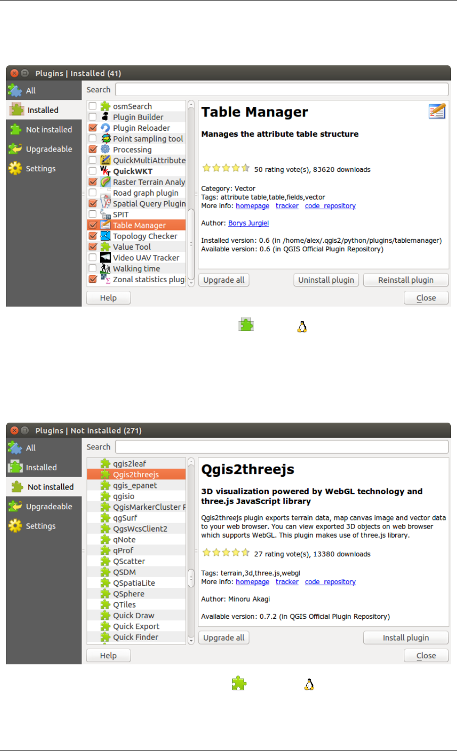
QGIS User Guide, Publicación 2.8
Figure 19.2: El menú Instalado
Figure 19.3: El menú No instalado
19.1. QGIS Complementos 271
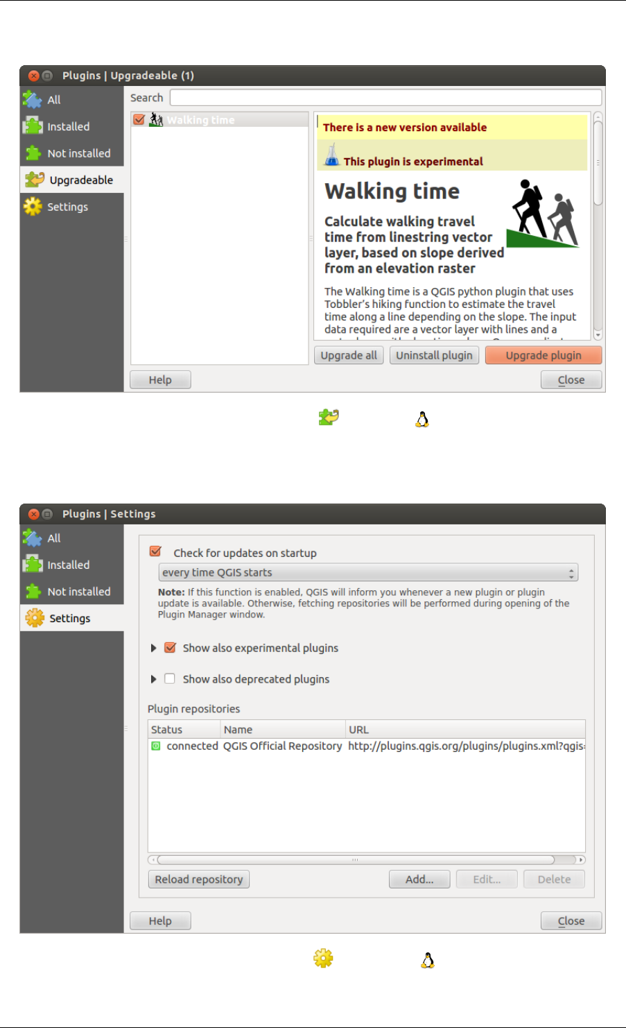
QGIS User Guide, Publicación 2.8
Figure 19.4: El menú Actualizable
Figure 19.5: El menú Configuración
272 Chapter 19. Complementos

QGIS User Guide, Publicación 2.8
Truco: Complementos base y externos
Los complementos de QGIS se ejecutan, ya sea como Complementos base oComplementos Externos. Los
Complementos Base son mantenidos por el equipo de desarrollo QGIS y son automáticamente parte de cada
distribución de QGIS. Están escritas en uno de los dos lenguajes: C++ o Python. Los Complementos Externos
actualmente todo esta escrito en Python. Se almacenan en repositorios externos y son mantenidos por autores
individuales.
La documentación detallada sobre el uso, mínimo de la versión de QGIS, página de inicio, autores, y otra infor-
mación importante se proporcionan para el repositorio ‘Oficial’ de QGIS en http://plugins.qgis.org/plugins/. Para
otros repositorios externos, puede haber documentación en los propios complementos externos. En general, no se
incluye en este manual.
.
19.1. QGIS Complementos 273

QGIS User Guide, Publicación 2.8
274 Chapter 19. Complementos
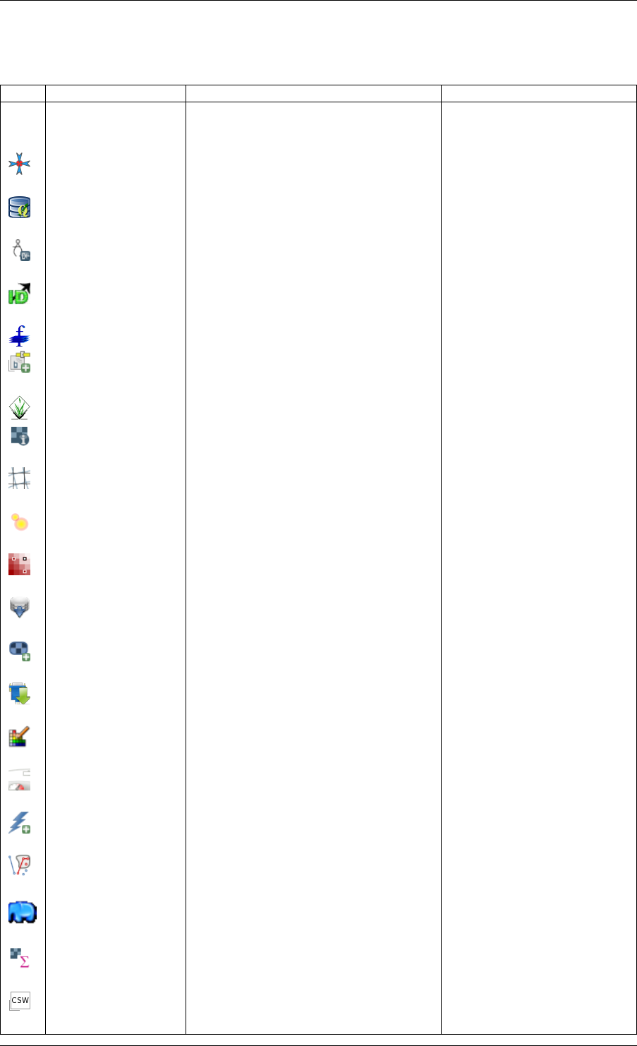
QGIS User Guide, Publicación 2.8
19.2 Usar complementos núcleo de QGIS
Icono Complemento Descripción Manual de referencia
Valoración de
medición
Generar una matriz de error accuracy
CadTools Realizar funciones CAD como en QGIS cadtools
Captura de
coordenadas
Captura de coordenadas del ratón en
diferentes SRC
Complemento Captura de
coordenadas
DB Manager Administrar la base de datos dentro de
QGIS
Complemento administrador
de BBDD
Conversor DXF2Shp Convertir de archivo DXF a formato SHP Complemento Conversor
DxfaShp
eVis Herramienta de visualización de eventos Complemento Visualización de
Eventos
fTools Un conjunto de herramientas vectoriales Complemento fTools
Herramientas de GPS Herramientas para cargar e importar datos
GPS
GPS Plugin
GRASS Funcionalidad GRASS GRASS GIS Integration
Herramientas GDAL Funcionalidad ráster GDAL Complemento Herramientas de
GDAL
Georreferenciador
GDAL
Georeferenciación de rásteres con GDAL Complemento
Georreferenciador
Mapa de calor Crear mapa de calor de un capa de puntos
de entrada.
Complemento Mapa de calor
Complemento de
interpolación
Interpolación en base a vétices de una
capa vectorial
Complemento de interpolación
Edición fuera de línea Edición fuera de línea y sincronización
con la base de datos
Complemento Edición fuera de
linea
Georaster Espacial de
Oracle
Acceso a Georasters Espaciales de Oracle Complemento GeoRaster
espacial de Oracle
Administrar
complementos
Administrar complementos núcleo y
externos
El diálogo de complementos
Análisis del terreno
ráster
Calcular entidades geomorfológica de un
DEMs
Complemento Análisis de
Terreno
Complemento Grafo
de rutas
Análisis de la ruta más corta Complemento Grafo de rutas
Complemento SQL
Anywhere
Acceso a BD SQL anywhere sqlanywhere
Consulta espacial Consulta espacial en vectores Complemento Consulta
espacial
SPIT Herramienta para importar archivo shape
a PostGIS
Complemento SPIT
Estadísticas de zona Calcular estadísticas de ráster para
polígonos.
Complemento de Estadísticas
de zona
MetaSearch Interactuar con metadata catalogue
services (CSW)
MetaSearch Catalogue Client
19.2. Usar complementos núcleo de QGIS 275
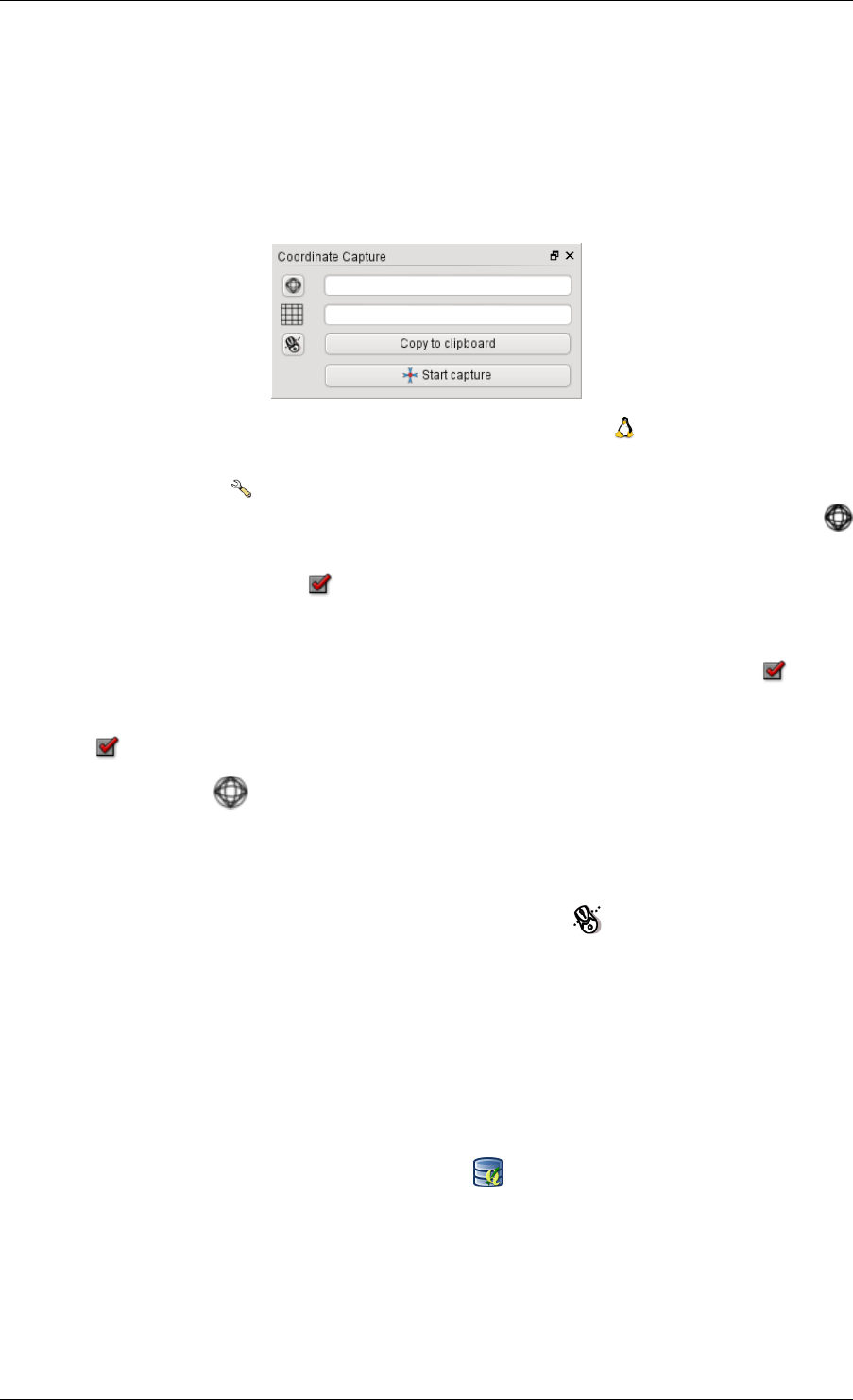
QGIS User Guide, Publicación 2.8
.
19.3 Complemento Captura de coordenadas
El complemento de captura de coordenadas es fácil de usar y proporciona la capacidad de mostrar coordenadas en
la vista del mapa para dos sistemas de referencia de coordenadas (SRC).
Figure 19.6: Complemento Captura de coordenadas
1. Inicie QGIS, seleccione Propiedades del proyecto del menú Configuración (KDE, Windows) o Archivo
(Gnome, OSX) y pulse la pestaña Proyección. Como alternativa, también puede pulsar el icono
Estado del SRC en la esquina inferior derecha de la barra de estado.
2. Pulse en la casilla de verificación Activar transformación de SRC al vuelo y seleccione un sistema de
coordenadas proyectadas de su elección (vea también Working with Projections)
3. Activar el complemento de Captura de coordenadas en el Administrador de complementos (vea El diálogo
de complementos) y asegúrese que el diálogo es visible, vaya a Ver →Paneles y y asegúrese que Captura
de coordenadas está habilitada. El diálogo de captura de coordenadas aparece como se muestra en la Figura
figure_coordinate_capture_1. Alternativamente, también puede ir a Vectorial →Captura de coordenadas y
vea si Captura de coordenadas está habilitada.
4. Haga clic en el icono Pulse para seleccionar el SRC a usar para la visualización de coordenadas y elija un SRC diferente al
que seleccionó anteriormente.
5. Para empezar a capturar coordenadas, pulse [Comenzar captura]. Ahora puede hacer clic en cualquier
lugar de la vista del mapa y el complemento mostrará las coordenadas en ambos SRC seleccionados.
6. Para habilitar el seguimiento de coordenadas del ratón, pulse el icono Seguimiento del ratón.
7. También se pueden copiar las coordenadas seleccionadas al portapapeles.
.
19.4 Complemento administrador de BBDD
El complemento de Administrador de BBDD es oficialmente parte del núcleo de QGIS y tiene la intención de
sustituir el complemento de SPIT y además, para integrar todos los demás formatos de base de datos recono-
cidos por QGIS en una interfaz de usuario. El complemento Admistrador de BBDD ofrece varias características.
Puede arrastrar las capas del navegador de |qg | en el Administrador BBDD, e importará su capa en su base de
datos espacial. Usted puede arrastrar y soltar tablas entre bases de datos espaciales y conseguirá importado. ..
_figure_db_manager:
El menú Base de datos permite conectar a una base de datos existente, para iniciar la ventana de SQL y para
finalizar el componente de Administrador de BBDD. Una vez que este conectado a la base de datos existente, los
menús Esquema yTabla aparecerá de forma adicional.
276 Chapter 19. Complementos
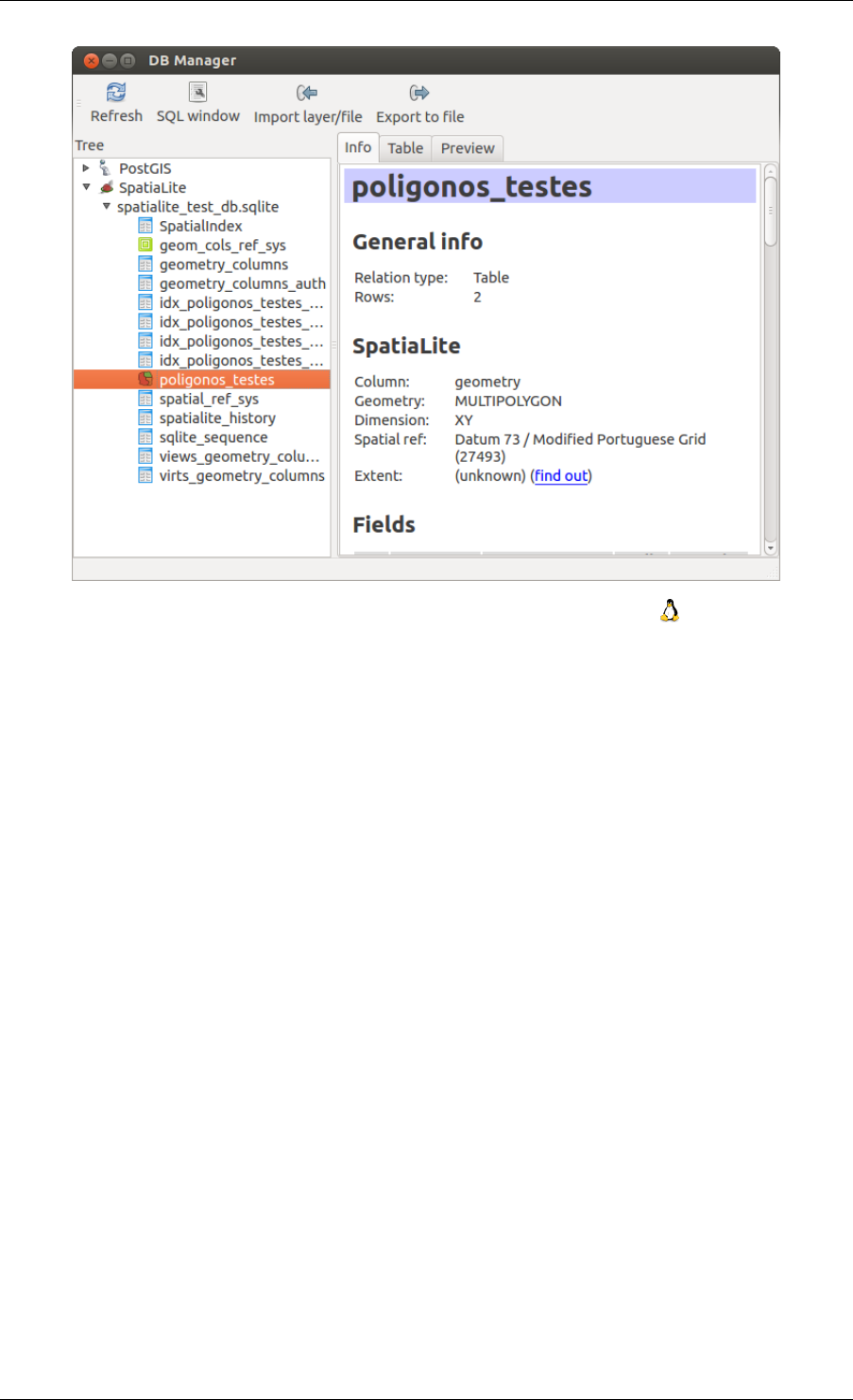
QGIS User Guide, Publicación 2.8
Figure 19.7: Diálogo del complemento administrador de BBDD
EL menú Esquema incluye herramientas para crear y eliminar (vaciar) esquemas y, si la topología esta disponible
(e.j., PostGIS 2), iniciar un TopoViewer.
El menú Tabla permite crear y editar tablas y eliminar tablas y vistas. También es posible vaciar tablas y moverlas
de un esquema a otro. Como función adicional, se puede realizar un VACUUM y luego un ANALYZE para cada
tabla seleccionada. VACUUM simplemente recupera espacio y hace que este disponible para reusarlo. ANALYZE
actualiza las estadisticas para determinar la forma más eficiente de ejecutar una consulta. Finalmente, se pueden
importar capas/archivos, si estan cargados en QGIS o existen en el sistema de archivos. Y se puede exportar tablas
de la base de datos a archivo vectorial con la función “Exportar archivo”.
La ventana Árbol muestra todas las bases de datos soportadas por QGIS. Con un doble-clic, se puede conectar a
la base de datos. Con el botón derecho del ratón, se puede cambiar el nombre y eliminar las tablas y esquemas
existentes. Las tablas también se pueden agregar al lienzo de QGIS con el menú contextual.
Si se está conectado a una base de datos, la ventana principal del Administrador de BBDD ofrece tres pestañas.
La pestaña Info proporciona información acerca de la tabla y su geometría, así como de los campos existentes,
limitaciones e índices. También permite que ejecute Vacuum Analyze y crear índices espaciales en una tabla
seleccionada, si no está ya hecho. La pestaña de Tabla muestra todos los atributos y la pestaña Vista preliminar
representa las geometrías como vista previa.
19.4.1 Trabajar con la ventana SQL
También se puede utilizar el Administrador de BBDD al ejecutar consultas SQL contra la base de datos y luego
visualizar la salida espacial para las consultas al añadir los resultados a QGIS como una capa de consulta. Es
posible para destacar una parte de SQL y sólo esa parte se ejecutara al hacer clic en el botón Ejecutar (F5).
.
19.4. Complemento administrador de BBDD 277
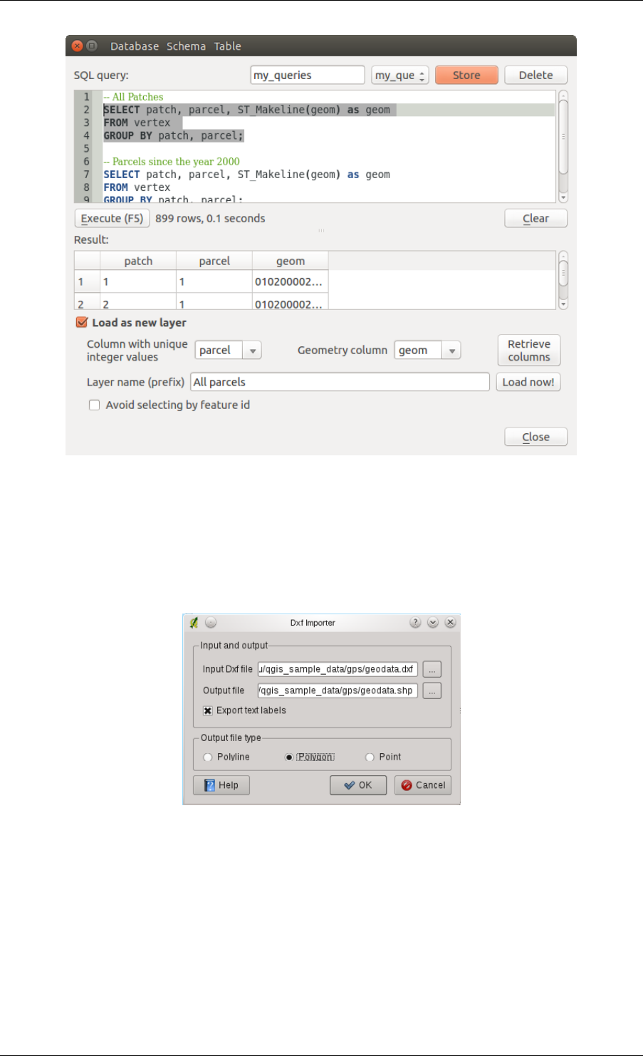
QGIS User Guide, Publicación 2.8
Figure 19.8: Ejecutar consultas SQL en la ventana SQL del Administrador de BBDD
19.5 Complemento Conversor DxfaShp
El complemento Conversor DxfaShp se puede usar para convertir datos vectoriales del formato DXF a archivo
shape. Requiere que se especifiquen los siguientes parámetros antes de ejecutarlo:
Figure 19.9: Complemento Conversor DxfaShp
•Archivo DXF de entrada: Introduzca la ruta al archivo DXF a convertir.
•Archivo shp de salida: Introduzca el nombre deseado para el archivo shape a crear.
•Tipo de archivo de salida: Especificar el tipo de geometría del archivo de salida. Actualmente los tipos
soportados son polilíneas, polígonos y puntos.
•Exportar etiquetas de texto: Cuando esta casilla de verificación esta habilitada, se creará una capa de
puntos adicional, y la tabla DBF asociada contendrá información sobre los campos “texto” que se encuentran
en el archivo DXF y las cadenas de texto en sí.
278 Chapter 19. Complementos
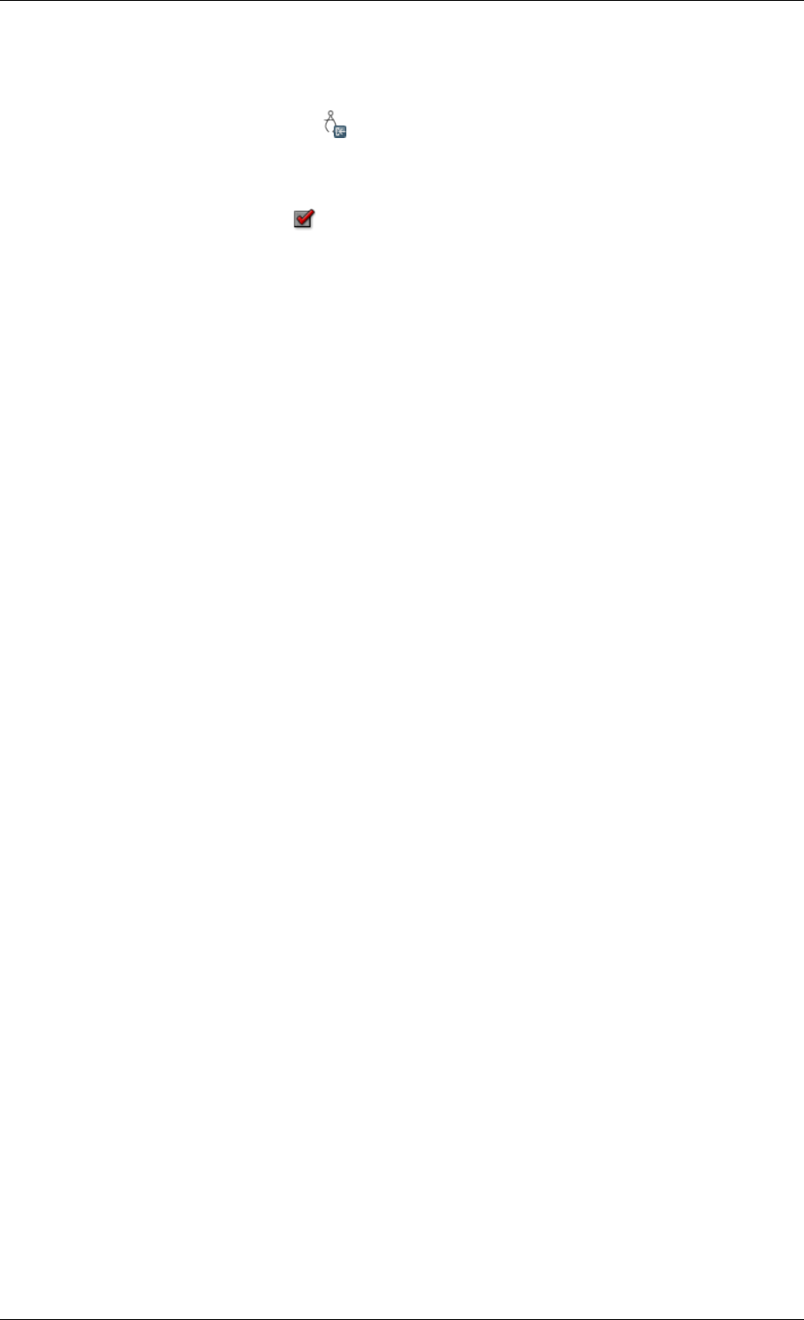
QGIS User Guide, Publicación 2.8
19.5.1 Usar el complemento
1. Iniciar QGIS, cargar el complemento DxfaShape en el Administrador de complementos (vea El diálogo de
complementos) y hacer clic en el icono Conversor DxfaShp, que aparece en el menú de barras de herramientas
de QGIS. El diálogo del complemento Dxf2Shape aparece, como se muestra en Figure_dxf2shape_1.
2. Introduzca el archivo DXF de entrada, un nombre para el archivo shape de salida y el tipo de archivo shape.
3. Habilitar la casilla de verificación Exportar etiquetas de texto si desea crear una capa extra de puntos
con etiquetas.
4. Hacer clic en [Aceptar]
.
19.6 Complemento Visualización de Eventos
(En esta sección se deriva de Horning, N., K, Koy, P. Ersts. 2009. eVis (v1.1.0) Guía de Usuario.
Museo Americano de Historia Natural, Centro para la Biodiversidad y Conservación. Disponible de
http://biodiversityinformatics.amnh.org/, y realizado bajo GNU FDL.)
El mecanismo de información sobre biodiversidad en el Museo Americano de Historia Natural(AMNH) Centro
para la Biodiversidad y la Conservación (CBC) ha desarrollado la herramienta de visualización de eventos (eVis),
otra herramienta de software para añadir al suite de monitoreo de conservación y herramienta de apoyo a las
decisiones para guiar un área protegida y la planificación del paisaje. Este complemento permite a los usuarios
enlazar fácilmente la geocodificación (es decir., se hacer referencia con latitud y longitud o coordenadas X y Y)
de fotografías, y otros documentos de apoyo, a los datos vectoriales en QGIS.
eVis ahora esta automáticamente instalado y habilitado en nuevas versiones de QGIS, y como todos los demás
complementos, se puede habilitar y deshabilitar utilizando el Administrador de Complementos (ver El diálogo de
complementos).
El complemento de visualización de eventos se compone de tres módulos: la ‘Herramienta para conexión a la base
de datos’, ‘Herramienta de ID evento’, y el ‘Eventos del navegador’. Estos trabajan juntos para permitir la visual-
ización de fotografías geocodificadas y otros documentos que están vinculados a objetos espaciales almacenados
en archivo de vectores, base de datos o hojas de cálculo.
19.6.1 Explorador de Eventos
El módulo de Explorador de eventos proporciona la funcionalidad de desplegar fotografías geocodificadas que
están vinculadas con un objetos espacial vectorial desplegado en la ventana de mapa de QGIS. Datos específicos,
por ejemplo, puede ser desde un archivo vectorial que se puede ingresar mediante QGIS o puede ser a partir del
resultado de una consulta de base de datos. El vector del objeto espacial debe tener información del atributo
asociado con él para describir la ubicación y el nombre del archivo que contiene la fotografía y, opcionalmente, la
dirección de la brújula de la cámara fue indicado cuando fue adquirida la imagen. Su capa vectorial se debe cargar
en QGIS antes de ejecutar el explorador de eventos.
Iniciar el módulo de Explorador de eventos
Para poner en marcha el modulo Explorador de Eventos, haga clic en Base de datos→eVis →Explorador de
Eventos eVis. Esto abrirá la ventana Explorador de Eventos Genérico.
La ventana Explorador de eventos tiene tres pestañas desplegadas en la parte superior de la ventana. La pestaña Vi-
sualizar se utiliza para ver las fotografías y los datos de sus atributos asociados. La pestaña Opciones proporciona
un número de ajustes para controlar el funcionamiento del complemento eVis. Por último, la pestaña Config-
uración de aplicaciones externas se utiliza para mantener una tabla de extensiones de archivos y su aplicación
asociada para permitir a eVis desplegar documentos que no sean imágenes.
19.6. Complemento Visualización de Eventos 279
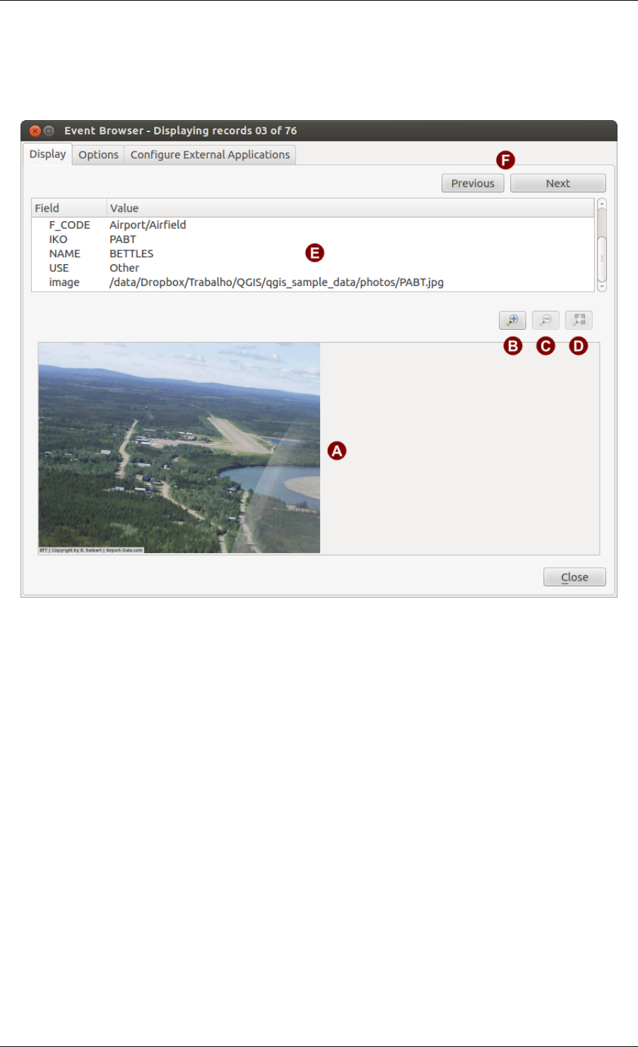
QGIS User Guide, Publicación 2.8
Comprender la ventana Visualizar
Para ver la ventana Visualizar, haga clic en la pestaña Visualizar en la ventana Explorador de Eventos. La ventana
Visualizar se utiliza para visualizar las fotografías geocodificadas y los atributos asociados a ellas.
Figure 19.10: La ventana de eVis visualizar
1. Ventana de Visualizar: Una ventana donde la fotografía aparece.
2. Botón de Acercar zoom: Acercar zoom para ver más detalle. Si la imagen completa no puede ser visual-
izada en la ventana de visualizar, las barras de desplazamiento aparecerán en del lado izquierdo e inferior
de la ventana para permitirle desplazarse por la imagen.
3. Botón de Alejar zoom: Alejar zoom para ver más área.
4. Botón Zum general: Despliega la fotografía completa.
5. Ventana de información de atributos: Toda la información de atributos del punto asociado con la foto que
se está viendo se muestra aquí. Si el tipo de archivo al que hace referencia del registro mostrado no es una
imagen sino un tipo de archivo definido en la pestaña Configurar aplicaciones externas cuando haga doble
clic en el valor del campo que contiene la ruta al archivo se abrirá la aplicación para ver u oír el contenido
del archivo. Si se reconoce la extensión del archivo los datos de los atributos se mostrarán en verde.
6. Botones de Navegación: Utiliza el botón anterior y siguiente para cargar el objeto anterior o siguiente
cuando mas de un objeto espacial esta seleccionado.
Comprender la ventana de Opciones
1. Ruta del archivo: Una lista desplegable para especificar el campo de atributo que contiene la ruta del
directorio o URL para las fotografías u otros documentos que se muestran. Si la ubicación es una ruta
280 Chapter 19. Complementos
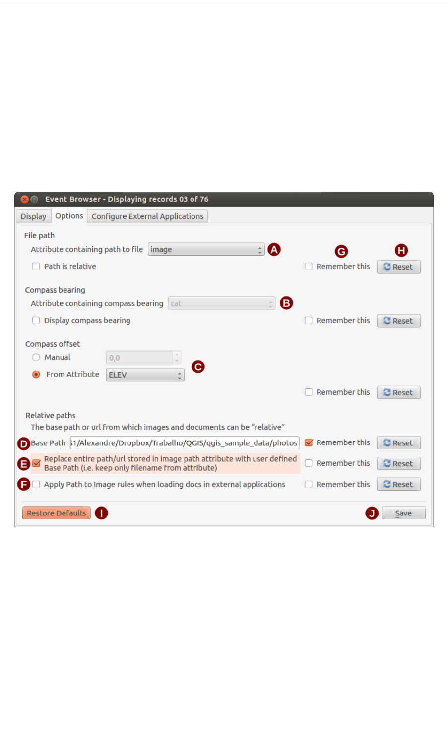
QGIS User Guide, Publicación 2.8
Figure 19.11: La ventana de eVis Opciones
19.6. Complemento Visualización de Eventos 281
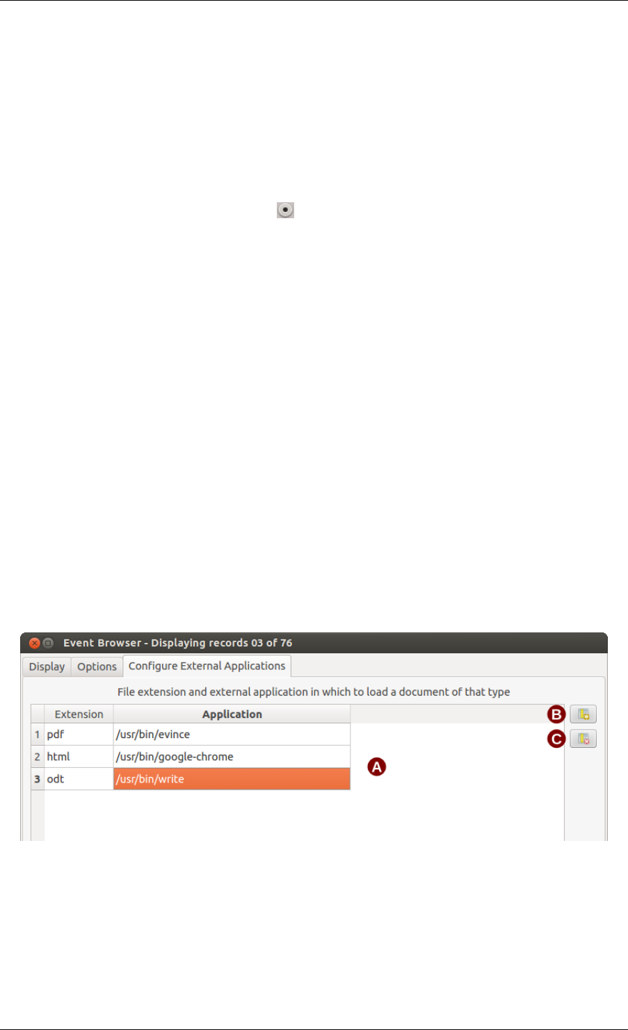
QGIS User Guide, Publicación 2.8
relativa, entonces la casilla de verificacion debe hacer clic. LA ruta base para una ruta relativa puede ser
introducida en la caja de texto Ruta Base a continuación. La información sobre las diferentes opciones
para especificar la ubicación del archivo se indica en la sección Especificar la ubicación y nombre de la
fotografía a continuación.
2. Rumbo de la brújula: Una lista desplegable para especificar el campo de atributo que contiene el rumbo
de la brújula asociado con las fotografías que se muestran. Si la información del rumbo de la brújula esta
disponible, es necesario hacer clic en casilla de verificación a continuación el título del menú desplegable.
3. Desplazamiento de la brújula: El desplazamiento de la brújula se puede utilizar para compensar la de-
clinación (para ajustar los rodamientos recolectados usando cojinetes magnéticos para el rumbo del norte
verdadero). Haga clic en el botón de radio Manual para ingresar el desplazamiento en la caja de texto
o haga clic en el botón de radio De atributo para seleccionar el campo del atributo que contiene los de-
splazamientos. Para ambas opciones, declinaciones del este deben introducirse utilizando valores positivos,
y declinaciones al oeste deben utilizar valores negativos.
4. Ruta del archivo: La ruta de la base sobre la que se añadirá la ruta relativa se define en Figure_eVis_2 (A).
5. Sustituir la ruta: Si esta casilla de verificación esta marcada, solo el nombre del archivo de A se anexará a
la ruta base.
6. Aplicar regla a todos los documentos: Si se marco, las mismas reglas de ruta que están definidas para
las fotografías se utilizarán para los documentos sin imagen, tales como películas, documentos de texto
y archivos de sonido. Si no se marca, las reglas de ruta sólo se aplicarán a las fotografías, y los otros
documentos ignorarán el parámetro de la ruta base.
7. Recordar ajustes: Si la casilla de verificación es marcada, los valores de los parámetros asociados se
guardarán para la siguiente sesión cuando la ventana se cierra o cuando el botón [Guardar] de abajo sea
presionado.
8. Restablecer: Restablecer los valores en esta línea a la configuración predeterminada.
9. Restaurar los valores predeterminados: Esto restablecerá todos los campos a su configuración predeter-
minada. Tiene el mismo efecto hacer clic en todos los botones de [Restablecer].
10. Guardar: Esto guardará los ajustes sin cerrar el panel Opciones.
Comprender la ventana de Configurar aplicaciones externas
Figure 19.12: La ventana de eVis Aplicaciones externas
1. Tabla de referencia de archivo: Una tabla contiene los tipos de archivo que se pueden abrir utilizando
eVis. Cada tipo de archivo necesita una extensión de archivo y la ruta de una aplicación que pueda abrir ese
tipo de archivo. Esto proporciona la capacidad de abrir una amplia gama de archivos tales como películas,
grabaciones sonoras y documentos de texto en lugar de solo imágenes.
2. Añadir nuevo tipo de archivo: Añadir un nuevo tipo de archivo con una única extensión y la ruta para la
aplicación que puede abrirlo.
282 Chapter 19. Complementos

QGIS User Guide, Publicación 2.8
3. Borrar la fila actual: Borrar el tipo de archivo destacado en la tabla y definido por una extensión de archivo
y una ruta a una aplicación asociada.
19.6.2 Especificar la ubicación y nombre de la fotografía
La ubicación y nombre de la fotografía se pueda almacenar utilizando una ruta relativa o absoluta, o una URL,
si la fotografía esta disponible en el servidor web. Ejemplos de los diferentes enfoques están listados en la tabla
evis_examples.
X Y FILE BEARING
780596 1784017 C:\Workshop\eVis_Data\groundphotos\DSC_0168.JPG 275
780596 1784017 /groundphotos/DSC_0169.JPG 80
780819 1784015 http://biodiversityinformatics.amnh.org/\
evis_testdata/DSC_0170.JPG 10
780596 1784017 pdf:http://www.testsite.com/attachments.php?\
attachment_id-12 76
19.6.3 Especificar la ubicación y nombre de otros documentos soportados
Los documentos de apoyo tales como documentos de texto, videos, y clips de sonido también se pueden visualizar
o reproducir por eVis. Para ello, es necesario añadir una entrada en el archivo de tabla de referencia que se puede
acceder desde la ventana Configurar Aplicaciones Externas ‘ en el :guilabel:‘Generic Event Browser que coincide
con la extensión de archivo a una aplicación que se puede utilizar para abrir el archivo. También es necesario
disponer de la ruta o URL para el archivo en la tabla de atributos de la capa vectorial. Una regla adicional que
puede ser utilizada para las direcciones URL que no contienen una extensión de archivo para el documento que
desea abrir es especificar la extensión del archivo antes de la URL. El formato es — file extension:URL.
La URL es precedida por la extensión de archivo y dos puntos; esto es particularmente útil para el acceso a los
mismos a partir de los wikis y otros sitios web que utilizan una base de datos para gestionar las páginas web (véase
Table evis_examples).
19.6.4 Utilizar el Explorador de eventos
Cuando la ventana :guilabel: Navegador de Eventos se abre, una fotografía aparecerá en la pantalla si el documento
se hace referencia en la tabla de atributos de archivo vectorial es una imagen y si la información de la ubicación
del archivo en la ventana Opciones es correctamente establecida. Si se espera una fotografía y no aparece, será
necesario ajustar los parámetros en la ventana :guilabel: Opciones.
Si un documento de apoyo (o una imagen que no tiene una extensión de archivo reconocido por eVis) se hace
referencia en la tabla de atributos, el campo que contiene la ruta del archivo se resaltará en verde en la ventana de
información de atributos si esa extensión de archivo se define en el archivo de la tabla de referencia se encuentra
en la ventana Configurar Aplicaciones Externas. Para abrir el documento, haga doble clic en la línea verde
resaltado en la ventana de información de atributos. Si un documento de apoyo se hace referencia en la ventana
de información de atributos y la ruta del archivo no está resaltado en verde, entonces será necesario añadir una
entrada para la extensión de nombre de archivo del archivo en la ventana Configurar Aplicaciones Externas. Si la
ruta del archivo se resalta en verde, pero no se abre al hacer doble clic, será necesario ajustar los parámetros en la
ventana :guilabel: Opciones por lo que el archivo puede ser localizado por eVis.
Si no se proporciona una brújula en la ventana :guilabel: Opciones, un asterisco rojo se mostrará en la parte
superior de la característica de vector que se asocia con la fotografía que se muestra. Si se proporciona una
brújula, a continuación, aparecerá una flecha apuntando en la dirección indicada por el valor en el campo de
visualización de brújula en la ventana :guilabel: Navegador de Eventos. La flecha estará centrado sobre el punto
que se asocia con la fotografía u otro documento.
Para cerrar la ventana Explorador de eventos, haga clic en el botón [Cerrar] de la ventana Visualizar.
19.6. Complemento Visualización de Eventos 283
QGIS User Guide, Publicación 2.8
19.6.5 Herramienta ID evento
El módulo ‘Evento ID’ le permite mostrar una fotografía al hacer clic en un objeto espacial mostrado en la ventana
de mapa de QGIS. El objeto espacial vectorial debe tener información de atributos asociada a él para describir la
ubicacion y nombre del archivo que contiene la fotografía y, opcionalmente, la dirección de la brújula de la camara
se señalo cuando fue adquirida la imagen. Esta capa debe cargar QGIS antes de ejecutar la herramienta ‘Evento
ID’
Iniciar el módulo ID evento
Para iniciar el módulo ‘Evento ID’, haga clic en el icono Evento ID o bien haga clic en Base de datos→eVis →
Herramienta de ID de evento eVis. Esto hará que el cursor cambie a una flecha con una ‘i’ en la parte superior de
la misma que significa que la herramienta de ID de evento está activa.
Para ver las fotografías vinculadas con entidades vectoriales en la capa vectorial activa se muestra en la ventana
de mapa de QGIS, mova el cursor del Evento ID sobre el objeto espacial y hacer clic en el ratón. Después de hacer
clic en el objeto, la ventana Explorador de eventos se abrirá y las fotografías sobre o cerca de la ubicación donde
se ha hecho clic están disponibles para su visualización en el navegador. Si más de una fotografía está disponible,
se puede rotar entre las distintas entidades utilizando los botones ** [Anterior] ** y ** [Siguiente] **. Los otros
controles se describen en la sección ref:evis_browser de esta guía.
19.6.6 Conexión a base de datos
El módulo ‘Conexión a base de datos’ proporciona herramientas para conectar a y consultar una base de datos u
otros recursos ODBC, tales como una hoja de cálculo.
eVis puede conectar directamente a los siguientes tipos de base de datos: PostgreSQL, MySQL, y SQLite; también
puede leer desde conexiones ODBC (por ejemplo, MS Access). Al leer desde una base de datos ODBC (por
ejemplo una hoja de Excel), es necesario configurar su driver ODBC para el sistema operativo que esté utilizando
Iniciar el módulo de Conexión a base de datos
Para iniciar el módulo ‘Conexión a base de datos’, haga clic en el icono apropiado Conexión a base de datos eVis o
bien se hace clic en Base de datos →eVis →Conexión a base de datos eVis. Esto abrirá la ventana Conexión a
base de datos. La ventana tiene tres pestañas: Consultas predefinidas,Conexión a base de datos, y Consulta SQL.
La ventana Consola de salida en la parte inferior de la ventana, muestra el estado de las acciones iniciadas por las
diferentes secciones de este módulo.
Conectar a una base de datos
Haga clic en la pestaña Conexión a la base de datos para abrir la interfaz de conexión a base de datos. A contin-
uación, utilice la lista desplegable Tipo de base de datos para seleccionar el tipo de base de datos al que
desea conectarse. Si una contraseña o nombre de usuario es necesario, esa información puede ser ingresada en las
cajas de texto Nombre de usuario yContraseña
Introduzca el host de base de datos en el cuadro de texto :guilabel: Host de Base de Datos. Esta opción no está
disponible si ha seleccionado ‘MS Access’ como el tipo de base de datos. Si la base de datos reside en su equipo,
usted debe seleccionar “localhost”.
Introducir el nombre de la base de datos en la caja de texto Nombre de la base de datos. Si seleccionó ‘ODBC’
como el tipo de base de datos, es necesario introducir el nombre de la fuente de datos.
Cuando todos los parámetros están llenos, haga clic en el botón [Conectar]. Si la conexión es satisfactoria, un
mensaje se escribirá en la ventana Consola de salida, inicia que la conexión fue establecida. Si una conexión no
se establece, se necesita comprobar los parámetros correctos fueron insertados anteriormente.
1. Tipo de base de datos: Una lista desplegable para especificar el tipo de base de datos que se utilizará.
284 Chapter 19. Complementos
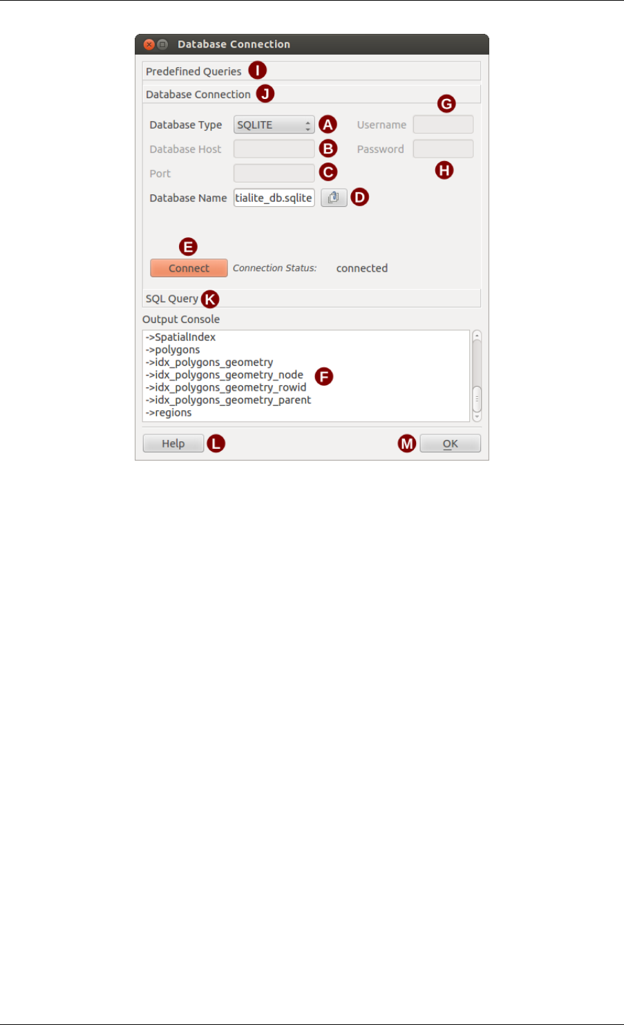
QGIS User Guide, Publicación 2.8
Figure 19.13: La ventana de conexión a base de datos eVis
2. Host de la base de datos: El nombre del host de la base de datos.
3. Puerto: El numero de puerto si una un tipo de base de datos MySQL o PostgreSQL es seleccionado.
4. Nombre de la base de datos: EL nombre de la base de datos.
5. Conectar: Un botón para conectar a la base de datos utilizando los parámetros definidos anteriormente.
6. Salidas a la Consola: La ventana de consola donde los mensajes relacionados a procesos son mostrados.
7. Nombre del Usuario: Nombre del usuario para utilizar cuando una base de datos este protegida con con-
traseña.
8. Contraseña: Para usar cuando la base de datos esta protegida con contraseña.
9. Consultas predefinidas: Pestaña para abrir la ventana “Consultas Predefinidas”.
10. Conexión a base de datos: Pestaña para abrir la ventana “Conexión a base de datos”.
11. Consulta SQL: Pestaña para abrir la ventana “Consulta SQL”.
12. Ayuda: Muestra la ayuda en línea.
13. Aceptar: Cierra la ventana principal “Conexión a Base de datos”
Ejecutar consultas SQL
Se utilizan consultas SQL para extraer información de una base de datos o un recurso ODBC. En eVis, la salida
de estas consultas es una capa vectorial añadida a la ventana de mapa QGIS. Haga clic en la pestaña Consulta
SQL para mostrar la interfaz de Consulta SQL. Los comandos SQL se pueden introducir en esta ventana de texto.
Un tutotial útil sobre comandos SQL está disponible en http://www.w3schools.com/sql. Por ejemplo, para extraer
todos los datos de una hoja de cálculo de un archivo Excel, select *from [sheet1$] donde sheet1 es
el nombre de la hoja de cálculo.
19.6. Complemento Visualización de Eventos 285
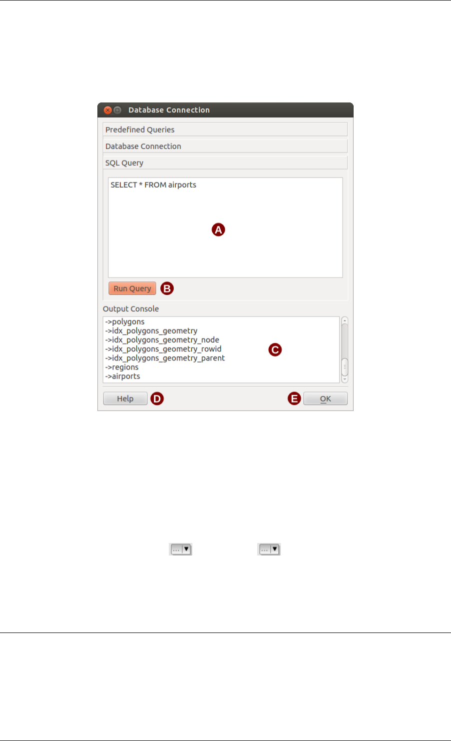
QGIS User Guide, Publicación 2.8
Haga clic en el botón [Ejecutar Consulta] para ejecutar el comando. Si la consulta es satisfactoria, una ventana
Selección de archivo de base de datos se mostrará. Si la consulta no es satisfactoria, aparecerá un mensaje de error
en la ventana Consola de salida.
En la ventana Selección de archivo de base de datos, introduzca el nombre de la capa que será creada de los
resultados de la consulta en la caja de texto Nombre de la nueva capa
Figure 19.14: La pestaña Consulta SQL de eVis
1. Ventana de texto de consulta SQL: Una pantalla para consultas tipo SQL.
2. Ejecutar consulta: El botón para ejecutar la consulta introducida en la Consulta SQL.
3. Consola de salida: La consola de salida donde se muestran los mensajes relacionados con el procesamiento.
4. Ayuda: Muestra la ayuda en línea.
5. Aceptar: Cierra la ventana principal Conexión a base de datos.
Utilice la lista desplegable Coordenada X Coordenada Y para seleccionar los campos de la base de
datos que almacena las coordenadas X(o longitud) y Y(o latitud). Hacer clic en el botón [Aceptar] hace que la
capa vectorial creada a partir de la consulta SQL se mostrará en la ventana de mapa QGIS.
Para guardar este archivo vectorial para usarlo en el futuro, se puede utilizar el comando de QGIS ‘Guardar
como...’ que se accede al hacer clic derecho sobre el nombre de la capa en la leyenda del mapa de QGIS y después
seleccione ‘Guardar como...’
Truco: Crear una capa vectorial de una Hoja de cálculo de Microsoft Excel
Al crear una capa vectorial de una hoja de cálculo Microsoft Excel, es posible ver que los ceros no deseados (“0”)
han sido insertados en las filas de la tabla de atributos debajo de datos válidos. Esto puede ser causado por la
supresión de los valores de estas celdas en Excel utilizando la tecla Espacio. Para corregir este problema, es
necesario abrir el archivo de Excel (que necesita para cerrar QGIS si está conectado con el archivo, que le permite
editar el archivo) y luego usar Edición →Borrar para eliminar las filas en blanco del archivo. Para evitar este
286 Chapter 19. Complementos
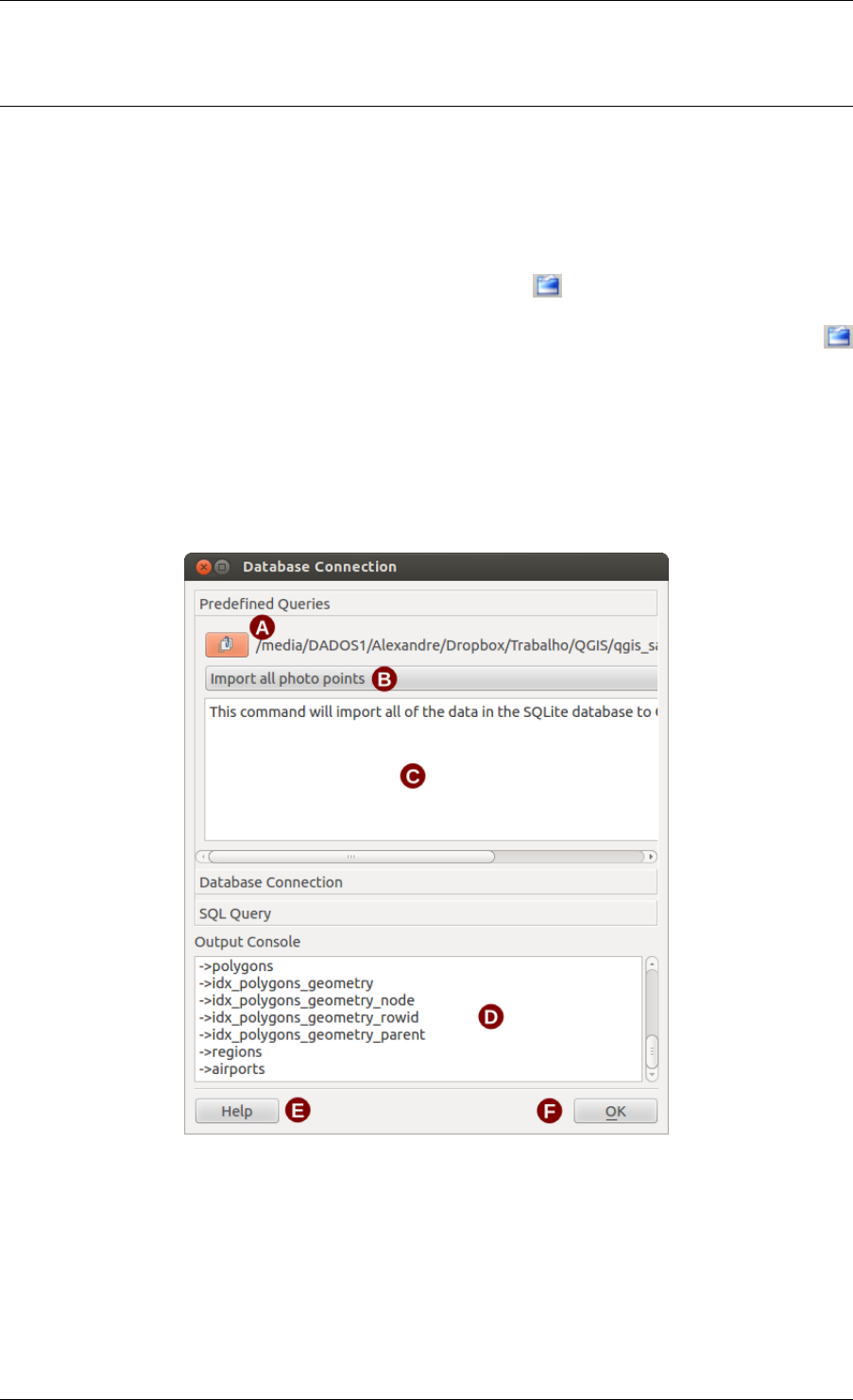
QGIS User Guide, Publicación 2.8
problema, puede simplemente eliminar varias filas en la hoja de Excel usando Edición →Borrar antes de guardar
el archivo.
Ejecutar consultas predefinidas
Con las consultas predefinidas, se pueden seleccionar consultas escritas previamente almacenadas en un archivo
de formato XML. Esto es particularmente útil, si no esta familiarizado con comandos SQL. Haga clic en la pestaña
Consultas predefinidas para visualizar la interfaz de consultas predefinidas.
Para cargar un conjunto de consultas predefinidas, haga clic en el icono Abrir archivo. Este abrirá la ventana Abrir
archivo, que se utiliza para localizar el archivo que contiene las consultas SQL. Cuando se cargan las consultas,
sus títulos definidos en el archivo XML aparecerán en el menú desplegable situado justo debajo del icono
Abrir archivo. La descripción completa de la consulta se mostrará en la ventana de texto en el menú desplegable.
Seleccione la consulta que desee ejecutar del menú desplegable y después haga clic en la pestaña Consulta SQL
para ver las consultas que se han estado cargando en la ventana de consultas. Si es la primera vez puede ejecutar
una consulta predefinida o esta cambiando a base de datos, necesita estar seguro para conectarse a la base de datos.
Haga clic en el botón [Ejecutar consulta] en la pestaña Consulta SQL para ejecutar el comando. Si la consulta
es satisfactoria, una ventana Selección de archivo de base de datos se mostrará. Si la consulta no es satisfactoria,
aparecerá un mensaje de error en la ventana Consola de salida
Figure 19.15: La pestaña de eVis Consultas predefinidas
1. Abrir Archivo: Iniciar el archivo “Abrir Archivo” navegar para buscar el archivo XML manteniendo las
consultas predefinidas.
2. Consultas predefinidas: Una lista desplegable con todas las consultas definidas por el archivo XML de
consultas predefinidas.
3. Descripción de consulta: Una descripción corta de la consulta. Esta descripción es del archivo XML de
consultas predefinidas.
19.6. Complemento Visualización de Eventos 287
QGIS User Guide, Publicación 2.8
4. Consola de salida: La consola de salida donde se muestran los mensajes relacionados con el procesamiento.
5. Ayuda: Muestra la ayuda en línea.
6. Aceptar: Cierra la ventana principal “Conexión a Base de datos”
El formato XML para consultas predefinidas eVis
Las etiquetas XML leídas por eVis
Etiquetas Descripción
Consulta Definir el inicio y fin de una sentencia de consulta.
Descripción
corta
Una descripción corta de la consulta que aparece en el menú desplegable de eVis.
Descripción Una descripción más detallada de la consulta desplegada en la ventana de texto de consulta
predefinida.
Tipo de base
de datos
El tipo de la base de datos, definido en el menú desplegable de Tipo de base de datos en la
pestaña de Conexión a base de datos.
Puerto El puerto como se define en el cuadro de texto Puerto en la pestaña de Conexión a base de
datos.
Nombre de la
base de datos
El nombre de la base de datos como se define en el cuadro de texto en la pestaña de
Conexión a base de datos.
Nombre de
usuario
El nombre de usuario de la base de datos como se define en el cuadro de texto Nombre de
usuario en la pestaña de Conexión a base de datos.
databasepass-
word
La contraseña de la base de datos como se define en el cuadro de texto Contraseña en la
pestaña Conexión a base de datos.
Sentencia sql El comando SQL
autoconectar Una bandera (“verdadero” o “falso”) para especificar si las etiquetas anteriores deben
utilizarse para conectarse automáticamente a la base de datos sin ejecutar la rutina de
conexión de base de datos en la solapa Conexión de Base de Datos.
Se muestra un archivo XML de ejemplo completo con tres preguntas a continuación:
<?xml version="1.0"?>
<doc>
<query>
<shortdescription>Import all photograph points</shortdescription>
<description>This command will import all of the data in the SQLite database to QGIS
</description>
<databasetype>SQLITE</databasetype>
<databasehost />
<databaseport />
<databasename>C:\textbackslash Workshop/textbackslash
eVis\_Data\textbackslash PhotoPoints.db</databasename>
<databaseusername />
<databasepassword />
<sqlstatement>SELECT Attributes.*, Points.x, Points.y FROM Attributes LEFT JOIN
Points ON Points.rec_id=Attributes.point_ID</sqlstatement>
<autoconnect>false</autoconnect>
</query>
<query>
<shortdescription>Import photograph points "looking across Valley"</shortdescription>
<description>This command will import only points that have photographs "looking across
a valley" to QGIS</description>
<databasetype>SQLITE</databasetype>
<databasehost />
<databaseport />
<databasename>C:\Workshop\eVis_Data\PhotoPoints.db</databasename>
<databaseusername />
<databasepassword />
<sqlstatement>SELECT Attributes.*, Points.x, Points.y FROM Attributes LEFT JOIN
Points ON Points.rec_id=Attributes.point_ID where COMMENTS=’Looking across
288 Chapter 19. Complementos

QGIS User Guide, Publicación 2.8
valley’</sqlstatement>
<autoconnect>false</autoconnect>
</query>
<query>
<shortdescription>Import photograph points that mention "limestone"</shortdescription>
<description>This command will import only points that have photographs that mention
"limestone" to QGIS</description>
<databasetype>SQLITE</databasetype>
<databasehost />
<databaseport />
<databasename>C:\Workshop\eVis_Data\PhotoPoints.db</databasename>
<databaseusername />
<databasepassword />
<sqlstatement>SELECT Attributes.*, Points.x, Points.y FROM Attributes LEFT JOIN
Points ON Points.rec_id=Attributes.point_ID where COMMENTS like ’%limestone%’
</sqlstatement>
<autoconnect>false</autoconnect>
</query>
</doc>
.
19.7 Complemento fTools
El objetivo del complemento fTools Python es proporcionar un recurso integral para muchas tareas comunes de
SIG basados en vectores, sin necesidad de software adicional, bibliotecas, o complejas soluciones temporales.
Proporciona un conjunto cada vez mayor de las funciones de gestión y análisis de datos espaciales que son a la
vez rápidos y funcionales.
fTools esta instalado automáticamente y habilitado en nuevas versiones de QGIS, y como con todos los comple-
mentos, se puede deshabilitar y habilitar utilizando el Administrador de complementos (vea El diálogo de comple-
mentos). Cuando está activado, el complemento de fTools agrega un Vectorial a QGIS, proporcionando funciones
que van desde Herramientas de Análisis, de Investigación, de Geometría y herramientas de geoprocesamiento, así
como varias útiles herramientas de gestión de datos.
19.7. Complemento fTools 289
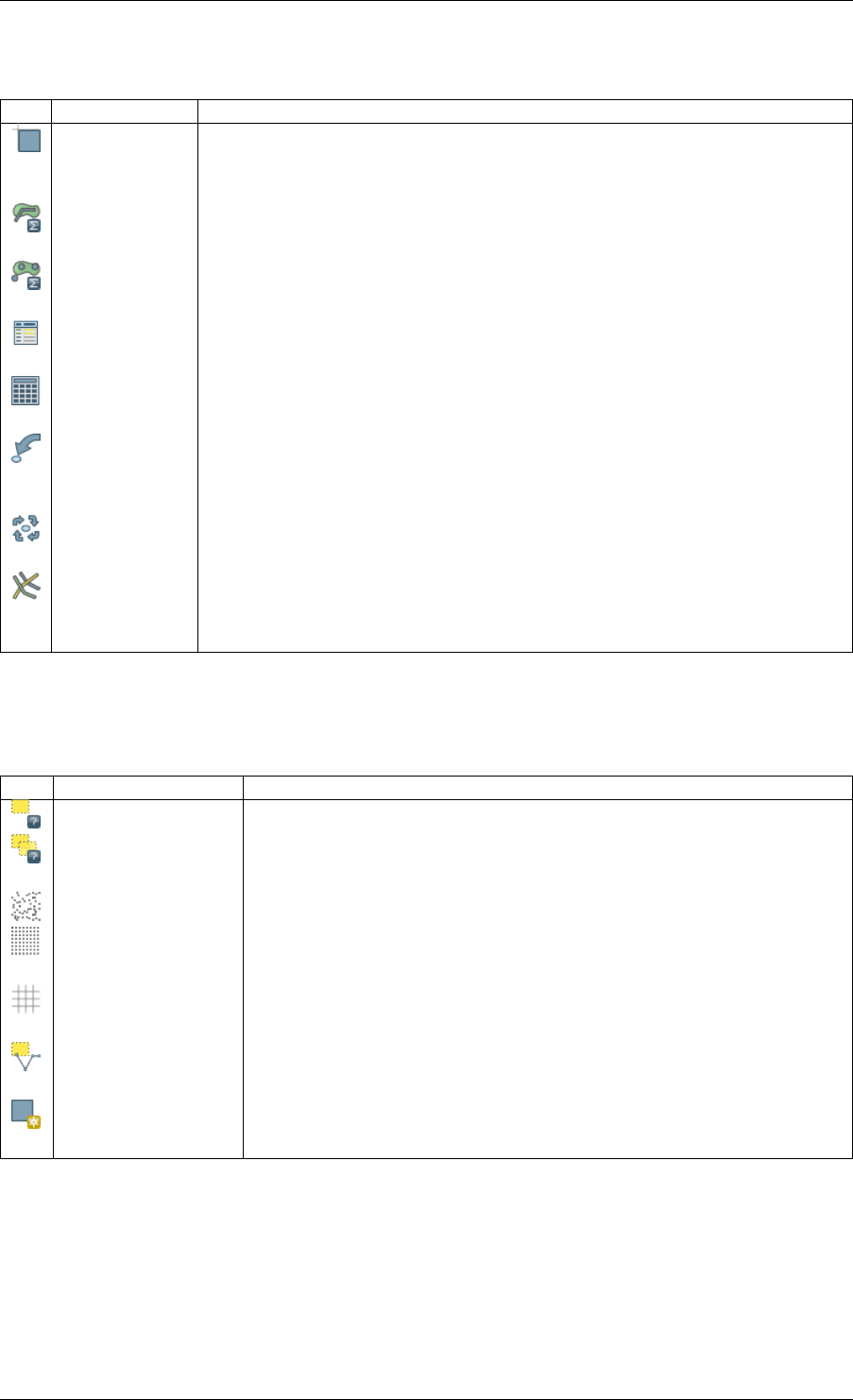
QGIS User Guide, Publicación 2.8
19.7.1 Herramientas de Análisis
IconoHerramienta Propósito
Matriz de
distancia
Medida de distancias entre dos puntos en la capa, y el resultado de salida como a)
Matriz de distancia cuadrada, b) Matriz de distancia lineal, o c) Matriz de distancia
resumen. Puede limitar las distancias de las entidades k más cercanas.
Sumar longitud
de líneas
Calcular la suma total de la longitudes de linea para cada polígono de una capa
vectorial de poligonos.
Puntos en
polígonos
Contar el número de puntos que se encuentran en cada polígono de una capa
vectorial de polígonos de entrada.
Listar valores
únicos
Lista de todos los valores únicos en un campo de la capa vectorial de entrada.
Estadísticas
básicas
Estadísticas básicas (media, desviación estándar, N, suma, CV)en un campo de
entrada.
Análisis del
vecino más
próximo
Calcular estadísticas del vecino más cercano para evaluar el nivel de agregación en
una capa vectorial de puntos.
Coordenada(s)
media
Calcular el centro medio normal o ponderado de una capa vectorial completa, o
múltiples entidades basadas en un campo ID único.
Intersecciones
de líneas
Localizar intersecciones entre líneas, y los resultados de salida como un archivo
shape de puntos. Útil para localizar calles o intersecciones de corrientes, ignora
intersecciones de línea con longitud > 0.
Tabla Ftools 1: Herramientas de Análisis fTools
19.7.2 Herramientas de investigación
Icono Herramienta Propósito
Selección aleatoria Selección aleatoria de un número n de entidades, o n porcentaje de entidades.
Selección aleatoria
dentro de subconjutos
Selección aleatoria de entidades dentro de subconjuntos basado en un campo
ID único
Puntos aleatorios Generar puntos pseudo-aleatorios más de una capa de entrada.
Puntos regulares Generar una cuadrícula regular de puntos sobre una región específica y
exportarlos como un archivo shape de puntos.
Cuadrícula vectorial Generar una cuadrícula de línea o polígono en base aun espaciado de
cuadrícula especificada.
Seleccionar por
localización
Seleccionar entidades en función de su ubicación con respecto a otra capa
para formar una nueva selección, o sumar o restar de la selección actual.
Polígono de la
extensión de la capa
Crear un rectángulo sencillo en la capa de polígono de extensión de una capa
de entrada ráster o vectorial.
Tabla Ftools 2: Herramientas de investigación fTools
290 Chapter 19. Complementos
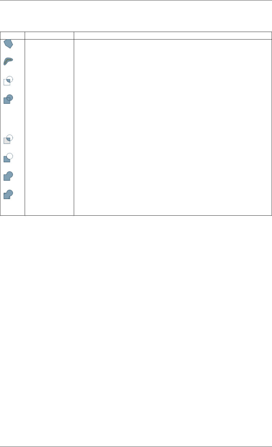
QGIS User Guide, Publicación 2.8
19.7.3 Herramientas de geoproceso
Icono Herramienta Propósito
Envolvente(s)
convexa(s)
Crear un envolvente convexo para una capa de entrada, o en función de un
campo ID.
Buffer(s) Crear buffer(s) en torno a las entidades basado en la distancia, o un campo de
distancia.
Intersección Sobrepone capas de manera que la salida contenga áreas donde ambas capas se
cruzan.
Unión sobreponer capas de manera que la salida contenga las áreas intersectadas y las
no intersectadas.
inter-
sec-
tadas
Diferencia
Simétrica
Sobreponer capas de manera que la salida contenga esas zonas de las capas de
entrada y diferencia que no se intersectan.
Cortar Sobreponer capas de tal manera que la salida contenga zonas que cruzo la capa
de corte.
Deferencia Sobreponer capas de tal manera que la salida contenga las zonas que no
intersectó la capa de corte.
Disolver Combinar entidades basadas en el campo de entrada. Todas los rasgos con
valores de entrada idénticos se combinan para formar una solo rasgo.
Eliminar
polígonos
<<astilla>>
Combinar las entidades seleccionadas con el polígono vecino con el área más
grande o el límite mas grande en común.
Tabla Ftools3: Herramientas de geoproceso fTools
19.7. Complemento fTools 291
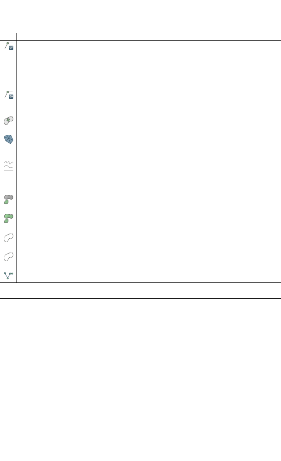
QGIS User Guide, Publicación 2.8
19.7.4 Herramientas de geometría
IconoHerramienta Propósito
Comprobar validez
de geometría
Comprobar intersección de polígonos, cerrado de agujeros y fijar el orden de
nodo. Usted puede elegir el motor utilizado en el cuadro de diálogo Opciones,
digitalizar la pestaña Cambiar el valor de las geometrías validas. Hay dos
motores: QGIS y GEOS que tienen un comportamiento bastante diferente. Otras
herramientas existes que muestran resultados diferentes así: Complemento para
revisar Topología y la regla ‘no debe tener geometrías no válidas’.
Exportar/Añadir
columnas de
geometría
Añadir a capa vectorial información de geometría de la capa de punto
(XCOORD, YCOORD), línea(LONGITUD), o polígono (ÁREA, PERÍMETRO)
.
Centroides de
polígonos
Calcular los verdaderos centroides de cada polígono en una capa de polígonos de
entrada.
Triangulación de
Delaunay
Calcular y salida (como polígonos) de la triangulación Delaunay de una capa
vectorial de puntos de entrada.
Polígonos Voronoi Calcular polígonos Voronoi de una capa vectorial de puntos de entrada.
Simplificar
geometrías
Generalizar líneas o polígonos con un algoritmo Douglas-Peucker modificado.
Densificar
geometrías
Densificar líneas o polígonos al añadir vértices.
Multipartes a
partes sencillas
Convertir entidad multiparte a entidades múltiples de partes sencillas. Crear
polígonos y líneas sencillas
Partes sencillas a
multiparte
Unir múltiples entidades a una sencilla multiparte en base a un campo ID único.
Polígonos a líneas Convertir polígonos a líneas, polígonos multiparte a líneas multiple de parte
sencilla
Líneas a polígonos Convertir líneas a polígonos, líneas multiparte a polígonos de múltiple parte
sencilla.
Extraer nodos Extraer nodos de las capas de líneas y polígonos y la salida de ellos como puntos.
Tabla Ftools 4: Herramientas de geometría fTools
Nota: La herramienta de Simplificar geometría se puede utilizar para borrar nodos duplicados en geometrías de
líneas y polígonos. Solo tiene que establecer el parámetro de Tolerancia de simplificado a 0 y esto hará el truco.
292 Chapter 19. Complementos
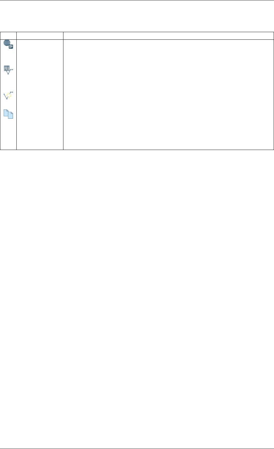
QGIS User Guide, Publicación 2.8
19.7.5 Herramientas de gestión de datos
IconoHerramienta Propósito
Definir la
proyección
actual
Especificar el SRC para archivos shape cuyo SRC no ha sido definido.
Unir atributos
por localización
Unir atributos adicionales a la capa de vectorial en función de su relación espacial.
Los atributos de una capa vectorial se adjunta a la tabla de atributo de otra capa y se
exporta como un archivo shape.
Dividir capa
vectorial
Dividir la capa de entrada en varias capas separadas basadas en el campo de entrada.
Combinar
archivos shape
en uno
Combinar varios archivos shape dentro de una carpeta en un nuevo archivo shape
basándose en el tipo de capa (punto, linea, polígono)
Crear índice
espacial
Crear un índice espacial para formatos OGR soportados.
Tabla Ftools 5: Herramientas de gestión de datos
.
19.8 Complemento Herramientas de GDAL
19.8.1 ¿Qué son las herramientas GDAL?
El complemento de herramientas GDAL ofrece una GUI para la colección de herramientas en Geospatial Data
Abstraction Library, http://gdal.osgeo.org. Estas son las herramientas de gestión ráster para consultar, re-proyecto,
urdimbre y combinar una amplia variedad de formatos ráster. También se incluyen herramientas para crear una
capa (vector) del contorno, o un relieve sombreado de un ráster MDT, y para hacer una VRT (Virtual Raster Tile
en formato XML) a partir de una colección de uno o más archivos ráster. Estas herramientas están disponibles
cuando se instala el complemento y es activado.
La biblioteca GDAL
La librería GDAL consiste en un conjunto de programas de línea de comandos, cada uno con una larga lista
de opciones. Los usuarios cómodos con la ejecución de comandos desde la terminal pueden preferir la línea
de comandos, con acceso a todo el conjunto de opciones. El complemento de Herramientas GDAL ofrece una
interfaz fácil de las herramientas, exponiendo las opciones más populares.
19.8. Complemento Herramientas de GDAL 293
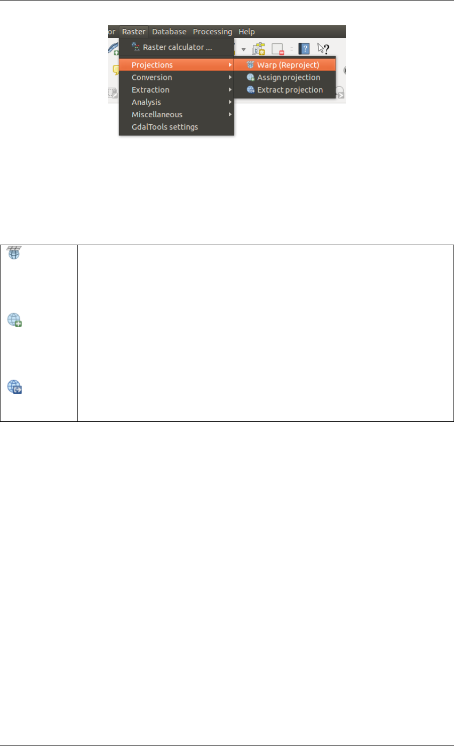
QGIS User Guide, Publicación 2.8
Figure 19.16: La lista del menú Herramientas GDAL
19.8.2 Lista de Herramientas GDAL
Projecciones
Warp
(Reproject)
Esta utilidad es una imagen de mosaicos, reproyección y utilidad deformación. El
programa puede reproyectar a cualquier proyección apoyada, y también se puede aplicar
GCPs almacenados con la imagen si la imagen es “crudo” con información de control.
Para obtener más información, se puede leer en el sitio web GDAL
http://www.gdal.org/gdalwarp.html
Asignación
de proyección
Esta herramienta le permite asignar proyección a rásters que ya tengan una referencia
geográfica, que le falte la información de la proyección. También con su ayuda, es posible
alterar las definiciones de proyección existentes. Ambos archivos simples y el modo por
lotes son compatibles. Para obtener más información, por favor visite la página de utilidad
en el sitio GDAL http://www.gdal.org/gdalwarp.html.
Extraer
proyección
Esta utilidad te ayuda a extraer información de la proyección de un archivo de entrada. Si
desea extraer información de un directorio completo, puede usar el modo por lotes. Este
crea ambos archivos .prj and .wld
294 Chapter 19. Complementos
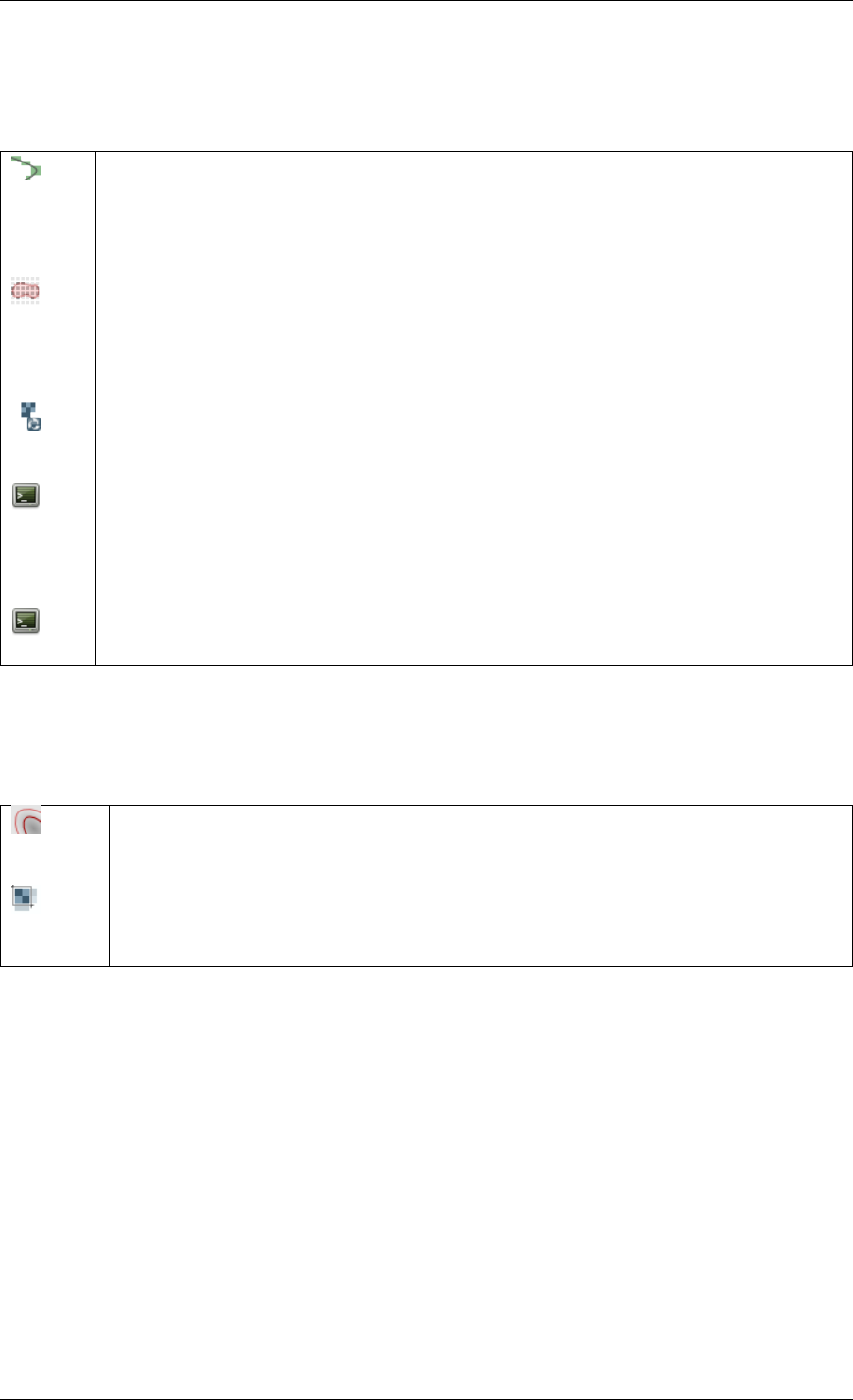
QGIS User Guide, Publicación 2.8
Conversión
Ras-
terizar
Este programa fusiona geometrías vectoriales (puntos, líneas y polígonos) en la banda(s) ráster de
una imagen raster. Los vectores se leen de formatos vectoriales reconocidos por OGR. Tenga en
cuenta que los datos vectoriales debe estar en el mismo sistema de coordenadas como los datos
ráster; en la reproyección al vuelo no se proporciona. Para obtener más información, consulte
http://www.gdal.org/gdal_rasterize.html.
Poligo-
nizar
Esta utilidad crea polígonos vectoriales para todas las regiones conectadas de píxeles del ráster
que comparte un valor de píxel en común. Cada polígono se crea con un atributo que indica el
valor de píxel de dicho polígono. La utilidad crea el vector de salida de origen de datos si no
existe ya, predeterminado a el formato de archivo shape de ESRI. Ver también
http://www.gdal.org/gdal_polygonize.html.
Traducir
Esta utilidad se puede utilizar para convertir los datos ráster entre diferentes formatos, lo que
podría llevar a cabo algunas operaciones como subconjuntos, remuestreo, y reescalar píxeles en el
proceso. Para obtener más información se puede leer en http://www.gdal.org/gdal_translate.html.
RGB
a PCT
Esta utilidad calculará una tabla de pseudocolor óptima para una imagen RGB determinada,
utilizando un algoritmo de corte medio de un histograma RGB downsampled. Luego se convierte
la imagen en una imagen pseudocoloreada usando la tabla de colores. Esta conversión utiliza
Floyd-Steinberg (difusión de errores) para maximizar la imagen de salida de calidad visual. La
utilidad también se describe en http://www.gdal.org/rgb2pct.html.
PCT
a RGB
Esta utilidad convertirá una banda pseudocolor en el archivo de entrada en un archivo RGB de
salida del formato deseado. Para mayor información, vea http://www.gdal.org/pct2rgb.html.
Extracción
Curvas de
nivel
Este programa genera un archivo vectorial de curvas de nivel del modelo del terreno ráster
(MDT). En http://www.gdal.org/gdal_contour.html, se puede encontrar más información.
Clipper
Esta utilidad le permite que acorte rásteres (extraer un subconjunto) utilizando una extensión
seleccionada o en base a límites de la capa de máscara.. Más información se puede encontrar en
http://www.gdal.org/gdal_translate.html.
19.8. Complemento Herramientas de GDAL 295
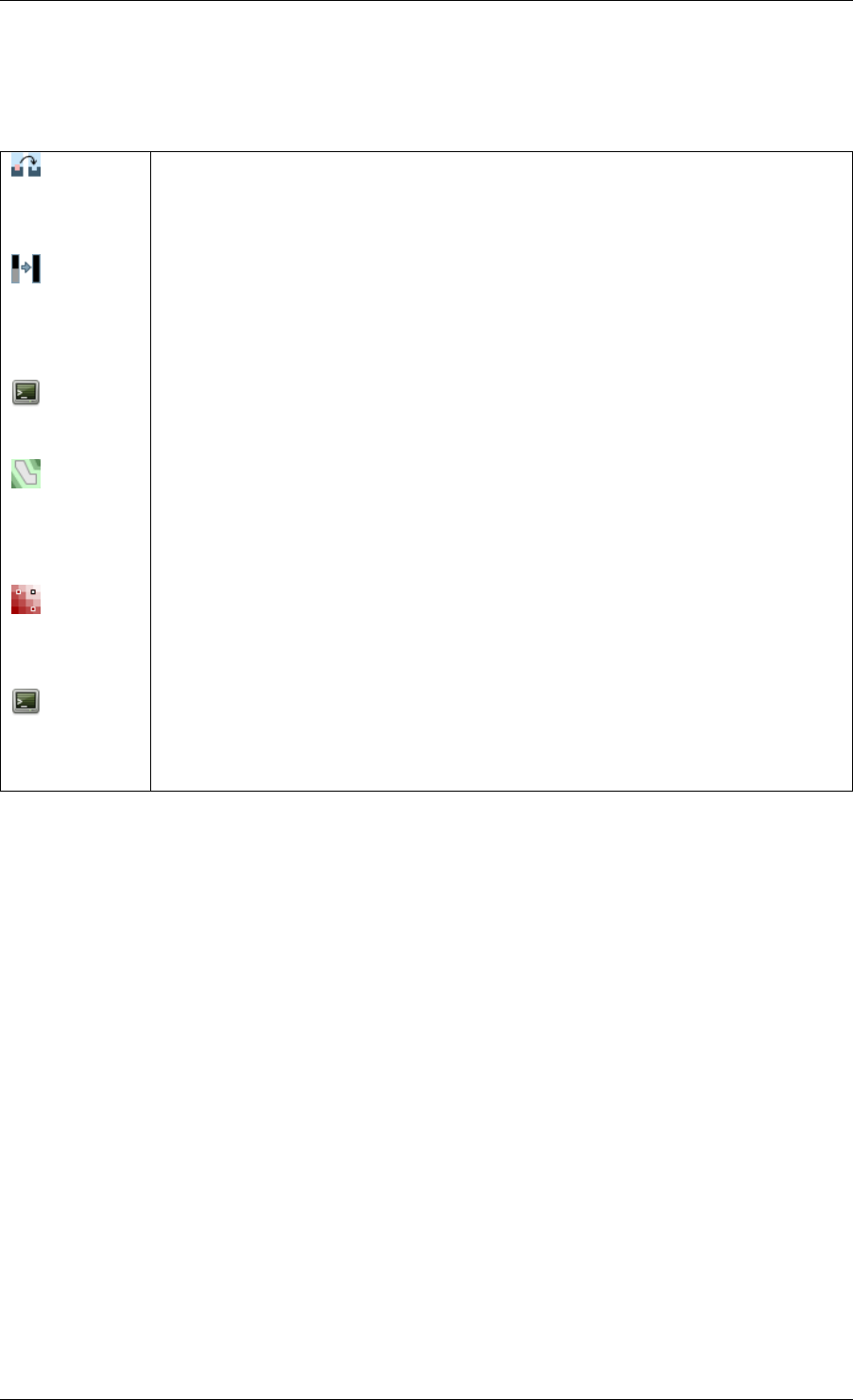
QGIS User Guide, Publicación 2.8
Análisis
Filtrado Esta utilidad elimina polígonos ráster más pequeños que un tamaño umbral previsto (en
píxeles) y los reemplaza con el valor del píxel del polígono vecino más grande. El
resultado se puede escribir de nuevo a la banda del ráster existente, o copiado en un nuevo
archivo. Para mayor información, vea http://www.gdal.org/gdal_sieve.html.
Casi Negro Esta utilidad escaneará una imagen y tratar de establecer todos los píxeles que son casi
negros (o casi blancos) alrededor del borde para exactamente negro (o blanco). Esto se
utiliza a menudo para “arreglar” comprimir pérdidas de fotos aéreas de modo que los
píxeles de color se pueden tratar como transparentes cuando se hace el mosaico. También
vea http://www.gdal.org/nearblack.html.
Rellenar sin
datos
Esta utilidad rellena regiones de ráster seleccionadas (generalmente áreas sin datos) por
interpolación de píxeles válidos alrededor de los bordes de las áreas. En
http://www.gdal.org/gdal_fillnodata.html, se puede encontrar más información.
Proximidad Esta utilidad genera un mapa ráster de proximidad que indica la distancia desde el centro
de cada píxel al centro del píxel más cercano identificado como un píxel objetivo. Los
pixeles objetivo son los del ráster fuente para la cual el valor de píxel del ráster está en el
conjunto de valores de píxel objetivo. Para obtener más información, consulte
http://www.gdal.org/gdal_proximity.html.
Cuadrícula
(Interpolación)
Esta utilidad crea una cuadrícula regular (ráster) a partir de los datos dispersos leídos
desde la fuente de datos OGR. Los datos de entrada serán interpolados para rellenar nodos
de la cuadrícula con los valores, y puede elegir entre varios métodos de interpolación. La
utilidad también se describe en el el sitio web GDAL, http://www.gdal.org/gdal_grid.html.
MDT(Modelos
de Terreno)
Herramientas para analizar y visualizar DEMs. Esto puede crear un relieve sombreado,
pendiente, orientación, color de relieve y un indice de irregularidad del terreno, un indice
de posición topográfica y un mapa de irregularidad de algún ráster de elevación
reconocido GDAL. Para mayor información , vea http://www.gdal.org/gdaldem.html.
296 Chapter 19. Complementos
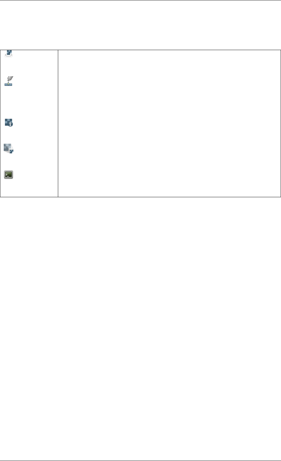
QGIS User Guide, Publicación 2.8
Miscelánea
Construir
ráster virtual
(Catálogo)
Este programa crea un VRT (Conjunto de datos virtual) que es un mosaico de la lista
de conjunto de datos GDAL de entrada. Vea también
http://www.gdal.org/gdalbuildvrt.html.
Combinar Esta utilidad automáticamente hará el mosaico un conjunto de imágenes. Todas las
imágenes deben estar en el mismo sistema de coordenadas y tener un número
correspondiente de bandas, pero pueden ser superpuestas, y en diferentes resoluciones.
En áreas de superposición, la última imagen se copiará en las anteriores. La utilidad
también se describe en http://www.gdal.org/gdal_merge.html.
Información Esta utilidad muestra diversa información acerca de un conjunto de datos ráster
GDAL-implementado. En http://www.gdal.org/gdalinfo.html, puede encontrar más
información.
Generar vistas
generales
La utilidad gdaladdo se puede utilizar para construir o reconstruir las vistas generales
para los formatos más compatibles con un de varios algoritmos de disminución de
resolución. Para obtener más información, vea http://www.gdal.org/gdaladdo.html.
Tile Index Esta utilidad crea un archivo shape con un registro para cada archivo de entrada ráster,
un atributo contiene el nombre del archivo y una geometría de polígono delineando el
ráster. Vea también http://www.gdal.org/gdaltindex.html.
Configuración de herramientas GDAL
Utilice este diálogo para integrar las variables GDAL.
.
19.9 Complemento Georreferenciador
El complemento Georreferenciador es una herramienta para generar archivos de referencia de ráster. Permite
referenciar los ráster a sistemas de coordenadas geográficas o proyectadas mediante la creación de un nuevo
GeoTiff o añadiendo un archivo de referencia a la imagen existente. El enfoque básico para georreferenciar un
ráster es localizar puntos del ráster para los que se puedan determinar con precisión las coordenadas.
Características
19.9. Complemento Georreferenciador 297
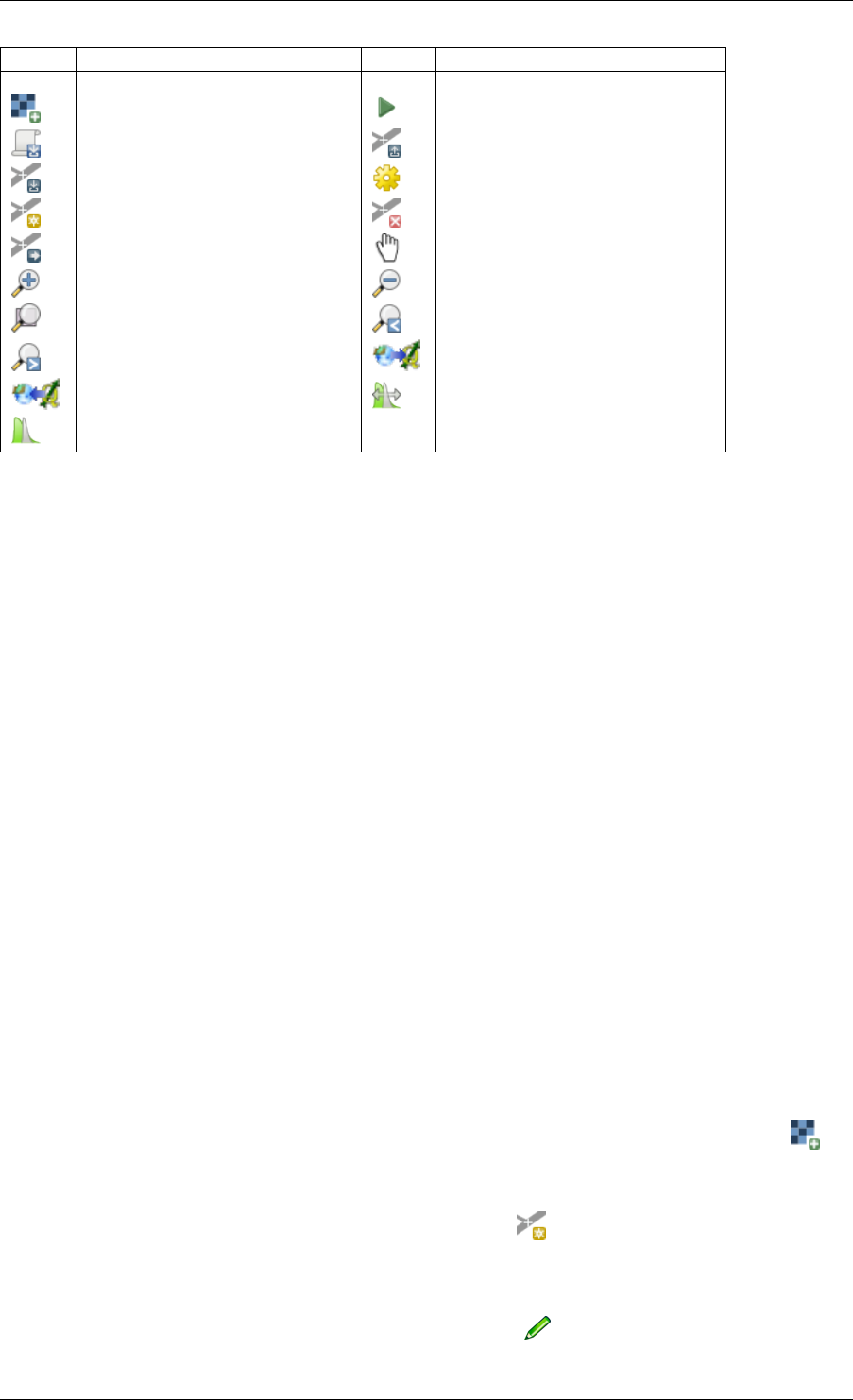
QGIS User Guide, Publicación 2.8
Icono Propósito Icono Propósito
Abrir ráster Comenzar georreferenciado
Generar script de GDAL Cargar puntos PCT
Guardar puntos PCT como Configuración de la transformación
Añadir punto Borrar punto
Mover punto PCT Desplazar
Acercar zum Alejar zum
Zum a la capa Zum anterior
Zum siguiente Enlazar Georreferenciador a QGIS
Enlazar QGIS a Georreferenciador Estiramiento total del histograma
Estiramiento local del histograma
Tabla Georreferenciador 1: Herramientas de Georreferenciador
19.9.1 Procedimiento habitual
Como coordenadas X e Y (GMS (gg mm ss.ss), GG (gg.gg) o coordenadas proyectadas (mmmm.mm)), que
correspondan al punto seleccionado en la imagen, se pueden usar dos procedimientos alternativos:
• El propio ráster a veces proporciona cruces con coordenadas “escritas” sobre la imagen. En este caso se
pueden introducir las coordenadas manualmente.
• Usando capas ya georreferenciadas. Esto pueden ser datos vectoriales o ráster que contengan los mismos
objetos/entidades que tenga en la imagen que desea georreferenciar y con la proyección que desee para su
imagen. En este caso puede introducir las coordenadas haciendo clic en el conjunto de datos de referencia
cargado en el lienzo del mapa de QGIS.
El procedimiento habitual para georreferenciar una imagen consiste en seleccionar múltiples puntos en el ráster,
especificando sus coordenadas, y elegir un tipo de transformación adecuado. Sobre la base de los parámetros y
datos de entrada, el complemento calculará los parámetros del archivo de referencia. Cuantas más coordenadas
suministre, mejor será el resultado.
El primer paso es iniciar QGIS, cargar el complemento Georreferenciador (vea El diálogo de complementos) y
hacer clic en Ráster →Georeferenciador, el cual aparece en la barra de menú de QGIS. El diálogo del comple-
mento Georreferenciador aparece como se muestra en figure_georeferencer_1.
Para este ejemplo usaremos una hoja topográfica de Dakota del Sur del SDGS. Más tarde se puede visualizar
junto con los datos de la localización spearfish60 de GRASS. Puede descargar la hoja topográfica aquí:
http://grass.osgeo.org/sampledata/spearfish_toposheet.tar.gz.
Introducir puntos de control sobre el terreno (PCT)
1. Para empezar a georreferenciar un ráster no referenciado, debemos cargarlo utilizando el botón . El
ráster aparecerá en la zona de trabajo principal del diálogo. Una vez que el ráster esté cargado, podemos
empezar a introducir los puntos de referencia.
2. Añada puntos a la zona principal de trabajo usando el botón Añadir punto e introduzca sus coordenadas
(vea la Figura figure_georeferencer_2). Para este procedimiento tiene tres opciones:
• Hacer clic en un punto de la imagen ráster e introducir las coordenadas X e Y manualmente.
• Haga clic en un punto de la imagen ráster y elija el botón Desde lienzo del mapa para añadir las coorde-
nadas X e Y con la ayuda de un mapa ya georreferenciado cargado en el lienzo del mapa de QGIS.
298 Chapter 19. Complementos
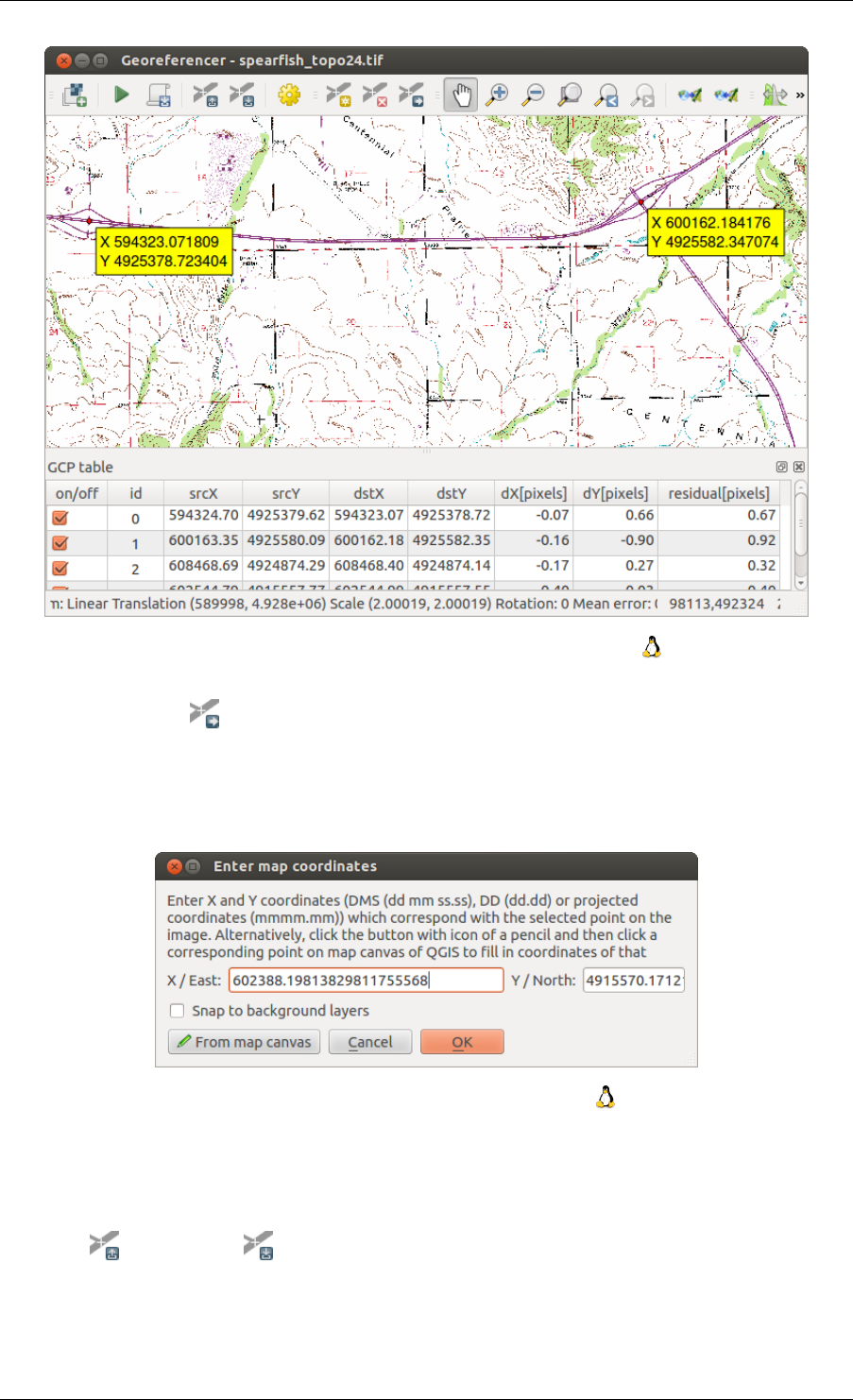
QGIS User Guide, Publicación 2.8
Figure 19.17: Diálogo del complemento Georreferenciador
• Con el botón puede mover los PCT en ambas ventanas, si están en un lugar incorrecto.
3. Continuar introduciendo puntos. Debe tener por lo menos cuatro puntos y cuantas más coordenadas pueda
proporcionar mejor será el resultado. Existen herramientas adicionales en el cuadro de diálogo del comple-
mento para hacer zum o desplazar la zona de trabajo con el fin de localizar un conjunto relevante de puntos
PCT.
Figure 19.18: Añadir puntos a la imagen ráster
Los puntos que se agregan al mapa se almacenarán en un archivo de texto separado ([nombre de
archivo].points) generalmente junto con la imagen ráster. Esto nos permite reabrir el complemento Georef-
erenciador en una fecha posterior y añadir nuevos puntos o eliminar los ya existentes para optimizar el resultado.
El archivo contiene los valores de los puntos de la forma: mapX, mapY, pixelX, pixelY. Puede utilizar
los botones Cargar puntos PCT yGuardar puntos PCT como para gestionar los archivos.
19.9. Complemento Georreferenciador 299
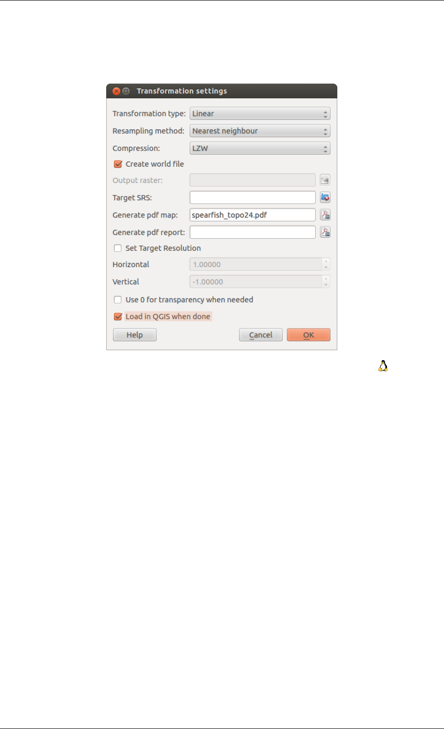
QGIS User Guide, Publicación 2.8
Definir la configuración de la transformación
Después de añadir los PCT a la imagen ráster, debe definir la configuración de la transformación para el proceso
de georreferenciación.
Figure 19.19: Definir la configuración de la transformación del georreferenciador
Algoritmos de transformación disponibles
Dependiendo del número de puntos de control sobre el terreno que haya capturado, es posible que desee utilizar
diferentes algoritmos de transformación. La elección del algoritmo de transformación también depende del tipo
y la calidad de los datos de entrada y la cantidad de distorsión geométrica que está dispuesto a introducir en el
resultado final.
Actualmente están disponibles los siguientes Tipos de transformación:
• El algoritmo Lineal se utiliza para crear un archivo de referencia y es diferente de los otros algoritmos, ya
que realmente no trasforma el ráster. Este algoritmo probablemente no será suficiente si se trata de material
escaneado.
• La trasformación Helmert realiza un escalado sencillo y trasformaciones de rotación.
• Los algoritmos Polinomial 1-3 son algunos de los algoritmos más utilizados introducidas para que coinci-
dan los puntos de control sobre el terreno de origen y destino. El algoritmo polinomial más ampliamente
usado es la transformación polinomial de segundo orden, que permite cierta curvatura. La transformación
polinomial de primer orden (afín) preserva la colinealidad y permite escalado, traslación y rotación sola-
mente.
• El algoritmo Thin Plate Spline (TPS) es un método de georreferenciación más moderno, que es capaz de
introducir deformaciones locales en los datos. Este algoritmo es útil cuando se georreferencian originales
de muy baja calidad.
• La trasformación Proyectiva es una rotación lineal y traducción de coordenadas.
300 Chapter 19. Complementos

QGIS User Guide, Publicación 2.8
Definir el método de remuestreo
El tipo de remuestreo que elija probablemente dependerá de los datos de entrada y el objetivo último del ejercicio.
Si no se desea cambiar las estadísticas de la imagen, es posible que desee elegir “Vecino más próximo”, mientras
que un ‘Remuestreo cúbico’ probablemente proporcionará un resultado más suavizado.
Es posible elegir entre cinco diferentes métodos de remuestreo:
1. Vecino más próximo
2. Lineal
3. Cúbica
4. Spline cúbica
5. Lanczos
Definir la configuración de la trasformación
Hay varias opciones que deben definirse para el ráster de salida georreferenciado.
• La casilla de verificación checkbox| Crear archivo de referencia esta disponible solo si se decide utilizar
la transformación lineal, porque esto quiere decir que la imagen ráster no será transformada realmente. En
este caso, el campo Ráster de salida no se activa, porque solo se creará el nuevo archivo de referencia.
• Para todos los otros tipos de transformación hay que definir un Ráster de salida. Por omisión se creará un
nuevo archivo ([nombre de archivo] _modificado) en la misma carpeta junto con la imagen ráster original.
• Como siguiente paso, tiene que definir el SRE de destino (Sistema de Referencia Espacial) para la imagen
georeferenciada (vea Working with Projections).
• Si lo desea, puede generar un mapa en pdf y también un informe en pdf. El informe incluye información
acerca de los parámetros de trasformación utilizados, una imagen de los residuos y una lista con todos los
PCT y sus errores RMS.
• Además, puede activar la casilla de verificación Establecer resolución de destino y definir la resolución
del píxel del archivo de salida. Por omisión la resolución horizontal y vertical es 1.
• Se puede activar la casilla Usar 0 para transparencia cuando sea necesario, si los píxeles con valor
0 deben visualizarse trasparentes. En nuestra hoja topográfica de ejemplo todas las áreas blancas serían
transparentes.
• Finalmente, la casilla Cargar en QGIS cuando esté hecho carga el ráster de salida automáticamente en
el lienzo del mapa de QGIS cuando la transformación está hecha.
Mostrar y adaptar las propiedades del ráster
Al hacer clic en el diálogo Propiedades del ráster en el menú Configuración se abren las propiedades del ráster
de la capa que desea georreferenciar.
Configurar el georreferenciador
• Puede definir si quiere mostrar las coordenadas y/o las ID de los PCT.
• Como unidades residuales se pueden elegir píxeles y unidades del mapa.
• Para el informe PDF puede definir un margen izquierdo y derecho y también puede establecer el tamaño del
papel para el mapa PDF.
• Finalmente, puede activar Mostrar la ventana del Georeferenciador adosada.
19.9. Complemento Georreferenciador 301
QGIS User Guide, Publicación 2.8
Ejecutar la transformación
Una vez se hayan recopilado todos los PCT y se hayan definido todos los ajustes de transformación, basta con
pulsar el botón Comenzar gerreferenciado para crear el nuevo ráster georreferenciado.
.
19.10 Complemento Mapa de calor
El complemento Mapa de calor usa Estimación de Densidad de Kernel para crear un ráster de densidad (mapa de
calor) de una capa de puntos de entrada. La densidad se calcula en base al número de puntos en una ubicación, de
forma que un mayor número de puntos agrupados resulta en valores mayores. Los mapas de calor permiten una
fácil identificación de los “puntos calientes” y la agrupación de los puntos.
19.10.1 Activar el complemento Mapa de calor
En primer lugar este complemento núcleo necesita ser activado utilizando el Administrador de Complementos
(véase El diálogo de complementos). Después de activarlo, el icono de mapa de calor se puede encontrar en
la barra de herramientas de Ráster, y bajo el menú Ráster →Mapa de calor.
Seleccione el menú Ver →Barras de herramientas →Ráster para mostrar la barra de herramientas Ráster, si no
está visible.
19.10.2 Usar el complemento de Mapa de calor
Haga clic en el botón de la herramienta Mapa de calor para abrir el diálogo del complemento Mapa de calor
(vea figure_heatmap_2).
El diálogo tiene las siguientes opciones:
•Capa de puntos de entrada: Lista todas las capas vectoriales de puntos del proyecto actual y se usa para
seleccionar la capa a analizar.
•Ráster de salida: Permite usar el botón para seleccionar la carpeta y el nombre de archivo del ráster
de salida que genera el complemento Mapa de calor. La extensión del archivo no es necesaria.
•Formato de salida: Selecciona el formato de salida. Aunque se pueden elegir todos los formatos soportados
por GDAL, en la mayoría de los casos GeoTIFF es el mejor formato para elegir.
•Radio: Se usa para especificar el radio de búsqueda del mapa de calor (o ancho de banda del kernel) en
metros o unidades del mapa. El radio especifica la distancia alrededor de un punto a la que se notará la
influencia del punto. Los valores más altos dan lugar a un mayor suavizado, mientras que los valores más
pequeños pueden mostrar detalles y variación más finos en la densidad de puntos.
Cuando la casilla de verificación Avanzado está marcada, hay disponibles opciones adicionales:
•Filas yColumnas: Utilizado para cambiar las dimensiones del ráster de salida. Estos valores también
están ligados a los valores de Tamaño X de celda yTamaño Y de celda. Incrementar el número de
filas y columnas disminuirá el tamaño de la celda e incrementará el tamaño del archivo de salida. Los
valores en Filas y Columnas también están vinculados, por lo que duplicar el número de filas duplicará
automáticamente el número de columnas y el tamaño de las celdas también se reducirá a la mitad. ¡El área
geográfica del ráster de salida seguirá siendo el mismo!
•Tamaño X de celda yTamaño Y de celda: Controlan el tamaño geográfico de cada píxel en el ráster de
salida. Cambiar estos valores también cambiará el número de filas y columnas en el ráster de salida.
302 Chapter 19. Complementos
QGIS User Guide, Publicación 2.8
•Forma del kernel: La forma del kernel controla la proporción en la que la influencia de un punto disminuye
a medida que aumenta la distancia desde el punto. Los diferentes kernels disminuyen en distintas propor-
ciones, por lo que un kernel triweight da mayor peso a las entidades más próximas al punto de lo que hace
el kernel Epanechnikov. En consecuencia, triweight de como resultado puntos calientes “más afilados” y
Epanechnikov da puntos calientes “más suaves”. Hay disponible una serie de funciones estándar del kernel
en QGIS, que se describen e ilustran en Wikipedia.
•Relación de decadencia: Se puede utilizar con kernel Triangulares para un mayor control de cómo dismin-
uye el calor de una entidad con la distancia a la misma.
–Un valor de 0 (= mínimo) indica que el calor estará concentrado en el centro del radio dado y se
extinguirá por completo en el borde.
–Un valor de 0.5 indica que a los píxeles del borde del radio se les dará la mitad del calor que a los
píxeles del centro del radio de búsqueda.
–Un valor de 1 significa que el calor se distribuye uniformemente por todo el círculo del radio de
búsqueda. (Esto es equivalente al kernel ‘Uniforme’.)
–Un valor mayor que 1 indica que el calor es mayor hacia el borde del radio de búsqueda que en el
centro.
La capa de puntos de entrada también puede tener campos de atributos que pueden afectar la forma en que influyen
en el mapa de calor:
•Usar radio a partir de campo: Establece el radio de búsqueda para cada entidad a partir de un campo de
atributos de la capa de entrada.
•Usar peso a partir de campo: Permite ponderar las entidades de entrada por un campo de atributos. Esto
se puede utilizar para aumentar la influencia que ciertas entidades tienen en el mapa de calor resultante.
Cuando se especifica un nombre para el archivo ráster de salida se puede utilizar el botón [Aceptar] para crear el
mapa de calor.
19.10.3 Tutorial: crear un mapa de calor
Para el siguiente ejemplo usaremos la capa vectorial de puntos airports del conjunto de datos de ejemplo de
QGIS (vea Datos de ejemplo). Otro excelente tutorial de QGIS sobre hacer mapas de calor se puede encontrar en
http://qgis.spatialthoughts.com.
En Figure_Heatmap_1, se muestran los aeropuertos de Alaska.
1. Seleccione el botón de la herramienta Mapa de calor para abrir el diálogo de Mapa de calor (vea
Figure_Heatmap_2).
2. En el campo Capa de puntos de entrada , seleccione airports de la lista de capas de puntos
cargadas en el proyecto actual.
3. Especifique un nombre para el archivo de salida haciendo clic en el botón próximo al campo Ráster
de salida. Escriba el nombre del archivo heatmap_airports (no es necesaria extensión de archivo).
4. Deje el Formato de salida como el formato predeterminado, GeoTIFF.
5. Cambie el Radio a1000000 metros.
6. Haga clic en [Aceptar] para crear y cargar el mapa de calor de aeropuertos (vea Figure_Heatmap_3).
QGIS generará el mapa de calor y añadirá el resultado a la ventana del mapa. Por omisión, el mapa de calor está
sombreado en escala de grises, con las zonas más claras mostrando una mayor concentración de aeropuertos. Al
mapa de calor se le puede aplicar ahora un estilo en QGIS para mejorar su apariencia.
1. Abra el diálogo de propiedades de la capa heatmap_airports (seleccione la capa
heatmap_airports, abra el menú contextual con el botón derecho del ratón y seleccione Propiedades).
2. Seleccione la pestaña Estilo.
19.10. Complemento Mapa de calor 303
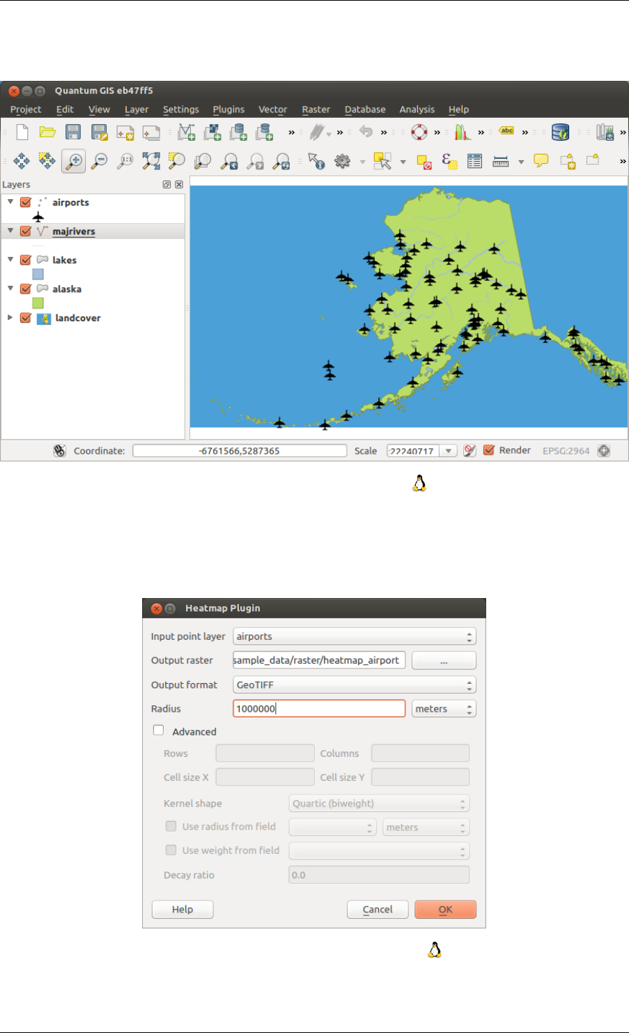
QGIS User Guide, Publicación 2.8
Figure 19.20: Aeropuertos de Alaska
Figure 19.21: El diálogo de Mapa de calor
304 Chapter 19. Complementos
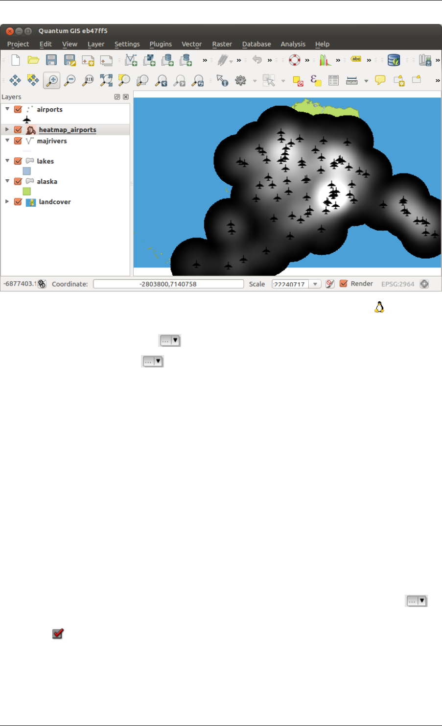
QGIS User Guide, Publicación 2.8
Figure 19.22: Después de cargar el mapa de calor se ve como una superficie gris
3. Cambie el Tipo de representación a ‘Pseudocolor de una sola banda’.
4. Seleccione un Mapa de color adecuado, por ejemplo YlOrRed.
5. Haga clic en el botón [Cargar] para recabar los valores mínimo y máximo del ráster, después pulse el botón
[Clasificar].
6. Pulse [Aceptar] para actualizar la capa.
El resultado final se muestra en Figure_Heatmap_4.
.
19.11 Complemento de interpolación
El complemento de interpolación se puede utilizar para generar una interpolación TIN o IDW de una capa vectorial
de puntos. Es muy fácil de usar y proporciona una interfaz gráfica de usuario intuitiva para crear capas ráster
interpoladas (ver Figure_interpolation_1). El complemento requiere que se especifiquen los siguientes parámetros
antes de ejecutarlo:
•Capas vectoriales de entrada: Especificar la(s) capa(s) vectorial(es) de puntos de entrada a partir de una
lista de capas de puntos cargadas. Si se especifican varias capas, entonces se usarán los datos de todas ellas
para la interpolación. Nota: es posible insertar lineas o polígonos como restricción para la triangulación,
especificando “puntos”, “líneas de estructura” o “líneas de ruptura” en el cuadro combinado Tipo
•Atributo de interpolación: Seleccionar la columna de atributos a usar para la interpolación o habilitar la
casilla Usar coordenada-Z para usar los valores Z almacenados en la capa.
•Método Interpolación: Seleccionar el método de interpolación. Esto puede ser ‘ Red Irregular triangulada
(TIN)’ o ‘Distancia Inversa Ponderada (IDW)’. Con el método TIN puede crear una superficie formada por
triángulos de puntos vecinos más cercanos. Para ello, circunferencias circunscritas alrededor de puntos de
muestra seleccionados se crean y sus intersecciones están conectados a una red de no superposición y tan
compacto como sea posibles de triángulos. Las superficies resultantes no son lisas. Cuando se utiliza el
19.11. Complemento de interpolación 305
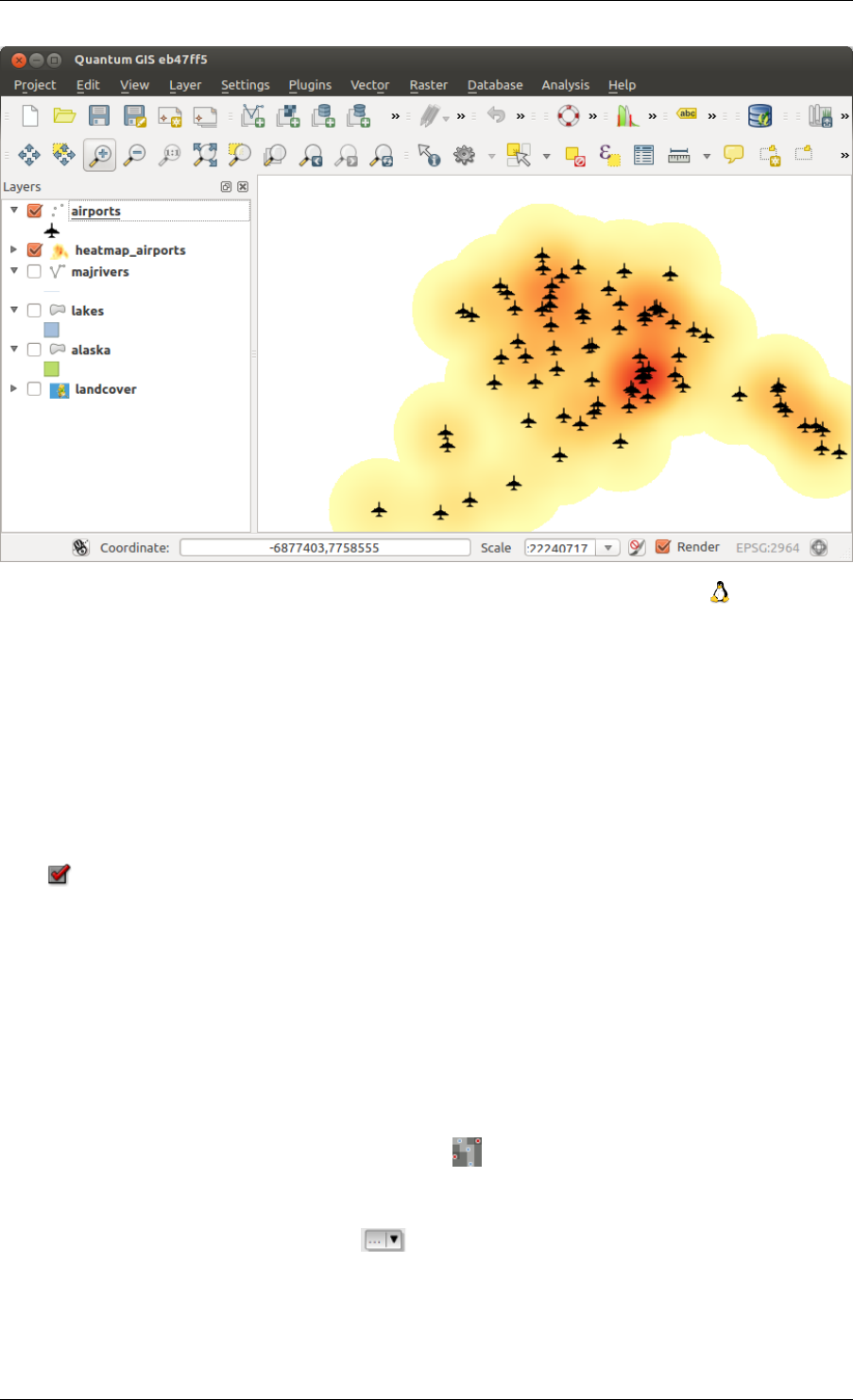
QGIS User Guide, Publicación 2.8
Figure 19.23: Mapa de calor de los aeropuertos de Alaska con estilo aplicado
método IDW los puntos de muestreo se ponderan durante la interpolación de tal manera que la influencia de
un punto en relación con otros disminuye con la distancia desde el punto desconocido que desea crear. El
método de interpolación IDW también tiene algunas desventajas: la calidad del resultado de la interpolación
puede disminuir, si la distribución de puntos de datos de la muestra es desigual. Por otra parte, los valores
máximos y mínimos en la superficie interpolada sólo pueden ocurrir en los puntos de datos de la muestra.
Esto a menudo resulta en pequeños picos y pozos alrededor de los puntos de datos de la muestra.
•Número de columnas/filas: Especificar el número de filasy columnas para el archivo ráster de salida.
•Archivo de salida: Especifica un nombre para el fichero ráster de salida.
•Añadir el resultado al proyecto para cargar el resultado en la vista del mapa.
Tenga en cuenta que el uso de líneas como las limitaciones para la interpolación de la triangulación (método TIN).
También se puede usar ‘líneas de estructura’ o ‘líneas de rotura’. Al usar ‘líneas de rotura’ se producen roturas en
la superficie mientras utiliza ‘líneas de estructura’ se producen roturas continuas. La triangulación es modificada
por ambos métodos tales que no cruza una línea de borde de línea de rotura o estructura.
19.11.1 Usar el complemento
1. Comenzar QGIS y cargar una capa vectorial de puntos (ej. elevp.csv).
2. Cargar el Complemento de interpolación en el Administrador de complementos (ver El diálogo de comple-
mentos) y dar clic sobre Ráster →Interpolación →Interpolación, que aparece en la barra de menú
de QGIS. La ventana de diálogo del complemento de interpolación aparece como se muestra en la Fig-
ure_interpolation_1.
3. Seleccione una capa de entrada (ej. elevp ) y una columna (ej. ELEV) para interpolación.
4. Seleccionar un método de interpolación( ej. ‘Red Irregular Triangulada (Triangulated Irregular Network-
TIN)’) y especificar un tamaño de celda de 5000 así como el nombre del archivo ráster de salida
(ej.:file:elevation_tin).
5. Pulse [Aceptar].
306 Chapter 19. Complementos
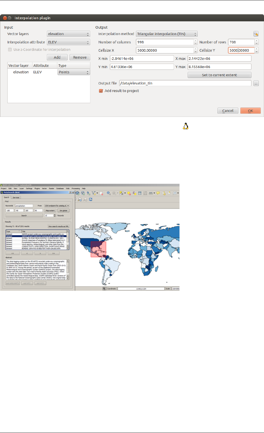
QGIS User Guide, Publicación 2.8
Figure 19.24: Complemento de Interpolación
.
19.12 MetaSearch Catalogue Client
19.12.1 Introduction
MetaSearch is a QGIS plugin to interact with metadata catalogue services, supporting the OGC Catalogue Service
for the Web (CSW) standard.
MetaSearch provides an easy and intuitive approach and user-friendly interface to searching metadata catalogues
within QGIS.
19.12.2 Installation
MetaSearch is included by default with QGIS 2.0 and higher. All dependencies are included within MetaSearch.
Install MetaSearch from the QGIS plugin manager, or manually from http://plugins.qgis.org/plugins/MetaSearch.
19.12. MetaSearch Catalogue Client 307
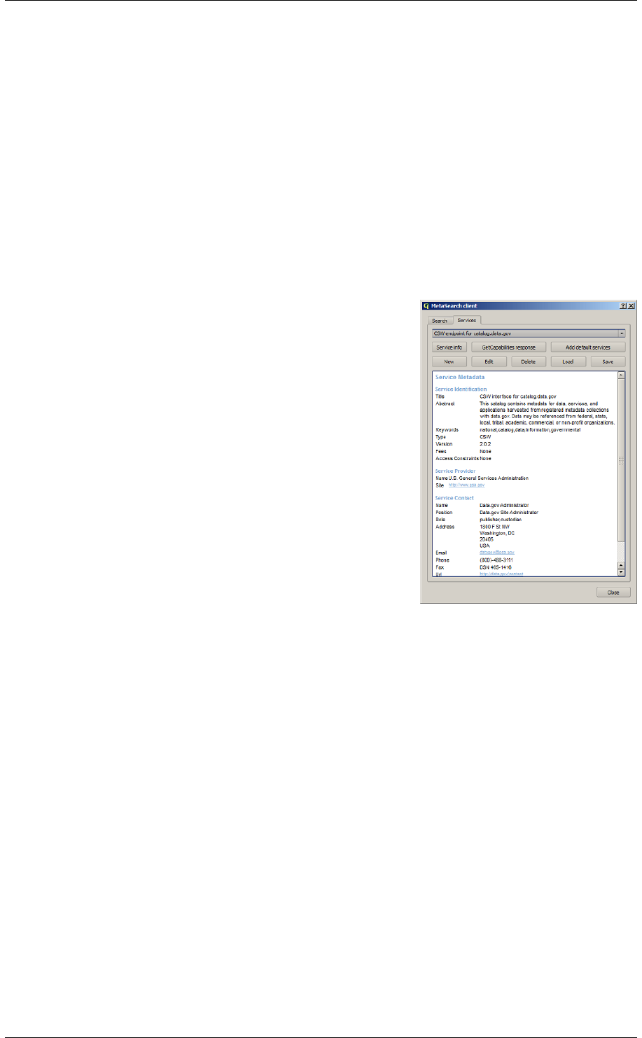
QGIS User Guide, Publicación 2.8
19.12.3 Working with Metadata Catalogues in QGIS
CSW (Catalogue Service for the Web)
CSW (Catalogue Service for the Web) is an OGC (Open Geospatial Consortium) specification, that defines com-
mon interfaces to discover, browse, and query metadata about data, services, and other potential resources.
Startup
To start MetaSearch, click the MetaSearch icon or select Web / MetaSearch / MetaSearch via the QGIS main
menu. The MetaSearch dialog will appear. The main GUI consists of two tabs: ‘Services’ and ‘Search’.
Managing Catalogue Services
The ‘Services’ tab allows the user to manage all available catalogue services. MetaSearch provides a default list
of Catalogue Services, which can be added by pressing ‘Add default services’ button.
To all listed Catalogue Service entries, click the dropdown select box.
To add a Catalogue Service entry, click the ‘New’ button, and enter a Name for the service, as well as the
URL/endpoint. Note that only the base URL is required (not a full GetCapabilities URL). Clicking ok will add
the service to the list of entries.
To edit an existing Catalogue Service entry, select the entry you would like to edit and click the ‘Edit’ button, and
modify the Name or URL values, then click ok.
To delete a Catalogue Service entry, select the entry you would like to delete and click the ‘Delete’ button. You
will be asked to confirm deleting the entry.
MetaSearch allows for loading and saving connections to an XML file. This is useful when you need to share
settings between applications. Below is an example of the XML file format.
<?xml version="1.0" encoding="UTF-8"?>
<qgsCSWConnections version="1.0">
<csw name="Data.gov CSW" url="http://catalog.data.gov/csw-all"/>
<csw name="Geonorge - National CSW service for Norway" url="http://www.geonorge.no/geonetwork/srv/eng/csw"/>
<csw name="Geoportale Nazionale - Servizio di ricerca Italiano" url="http://www.pcn.minambiente.it/geoportal/csw"/>
<csw name="LINZ Data Service" url="http://data.linz.govt.nz/feeds/csw"/>
<csw name="Nationaal Georegister (Nederland)" url="http://www.nationaalgeoregister.nl/geonetwork/srv/eng/csw"/>
<csw name="RNDT - Repertorio Nazionale dei Dati Territoriali - Servizio di ricerca" url="http://www.rndt.gov.it/RNDT/CSW"/>
<csw name="UK Location Catalogue Publishing Service" url="http://csw.data.gov.uk/geonetwork/srv/en/csw"/>
308 Chapter 19. Complementos
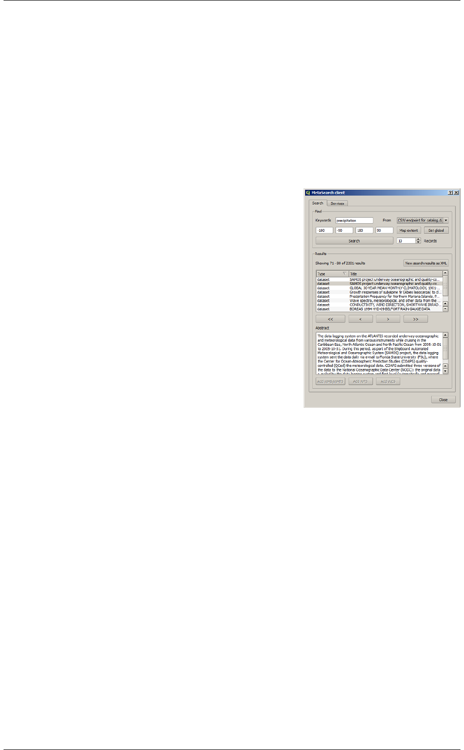
QGIS User Guide, Publicación 2.8
<csw name="UNEP/GRID-Geneva Metadata Catalog" url="http://metadata.grid.unep.ch:8080/geonetwork/srv/eng/csw"/>
</qgsCSWConnections>
To load a list of entries, click the ‘Load’ button. A new window will appear; click the ‘Browse’ button and
navigate to the XML file of entries you wish to load and click ‘Open’. The list of entries will be displayed. Select
the entries you wish to add from the list and click ‘Load’.
The ‘Service info’ button displays information about the selected Catalogue Service such as service identification,
service provider and contact information. If you would like to view the raw XML response, click the ‘GetCapa-
bilities response’ button. A separate window will open displaying Capabilities XML.
Searching Catalogue Services
The ‘Search’ tab allows the user to query Catalogue Services for data and services, set various search parameters
and view results.
The following search parameters are available:
•Keywords: free text search keywords
•From: the Catalogue Service to perform the query against
•Bounding box: the spatial area of interest to filter on. The default bounding box is the map view / canvas.
Click ‘Set global’ to do a global search, or enter custom values as desired
•Records: the number of records to return when searching. Default is 10 records
Clicking the ‘Search’ button will search the selected Metadata Catalogue. Search results are displayed in a list and
are sortable by clicking on the column title. You can navigate through search results with the directional buttons
below the search results. Clicking the ‘View search results as XML’ button opens a window with the service
response in raw XML format.
Clicking a result will show the record’s abstract in the ‘Abstract’ window and provides the following options:
• if the metadata record has an associated bounding box, a footprint of the bounding box will be displayed on
the map
• double-clicking the record displays the record metadata with any associated access links. Clicking the links
opens the link in the user’s web browser
• if the record is an OGC web service (WMS/WMTS, WFS, WCS), the appropriate ‘Add to
WMS/WMTS|WFS|WCS’ buttons will be enabled for the user to add to QGIS. When clicking this but-
ton, MetaSearch will verify if this is a valid OWS. The OWS will then be added to the appropriate QGIS
connection list, and the appropriate WMS/WMTS|WFS|WCS connection dialogue will then appear
19.12. MetaSearch Catalogue Client 309
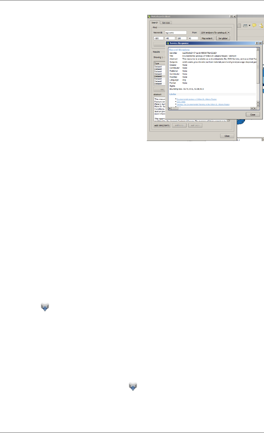
QGIS User Guide, Publicación 2.8
Settings
You can fine tune MetaSearch with the following settings:
•Connection naming: when adding an OWS connection (WMS/WMTS|WFS|WCS), the connection is
stored with the various QGIS layer provider. Use this setting to set whether to use the name provided
from MetaSearch, whether to overwrite or to use a temporary name
•Results paging: when searching metadata catalogues, the number of results to show per page
•Timeout: when searching metadata catalogues, the number of seconds for blocking connection attempt.
Default value is 10
.
19.13 Complemento Edición fuera de linea
Para la recolección de datos, es una situación común para trabajar con un ordenador portátil o una línea de teléfono
celular en el campo. A su regreso a la red, los cambios tienen que ser sincronizados con el origen de datos principal
(ej., una base de datos PostGIS). Si varias personas están trabajando simultáneamente en los mismos conjuntos de
datos, es difícil fusionar los cambios a mano, incluso si la gente no cambia los mismo elementos.
El complemento Edición fuera de linea automatiza la sincronización al copiar el contenido de una fuente de datos
(en general PostGIS o WFS-T) a una base de datos SpatialLite y almacena la edición fuera de linea en tablas
dedicadas, Después ser conectado a la red de nuevo, es posible aplicar la edición fuera de linea al conjunto de
datos maestro.
19.13.1 Usar el complemento
• Abrir algunas capas vectoriales (e.j. de una fuente de datos PostGIS o WFS-T).
• Guardarlo como un proyecto.
• Ir a Base de datos →Edición fuera de linea →Convertir en proyecto fuera de linea y seleccionar las
capas a guardar. El contenido de las capas se guarda en tablas SpatiaLite.
• Editar las capas fuera de linea.
310 Chapter 19. Complementos
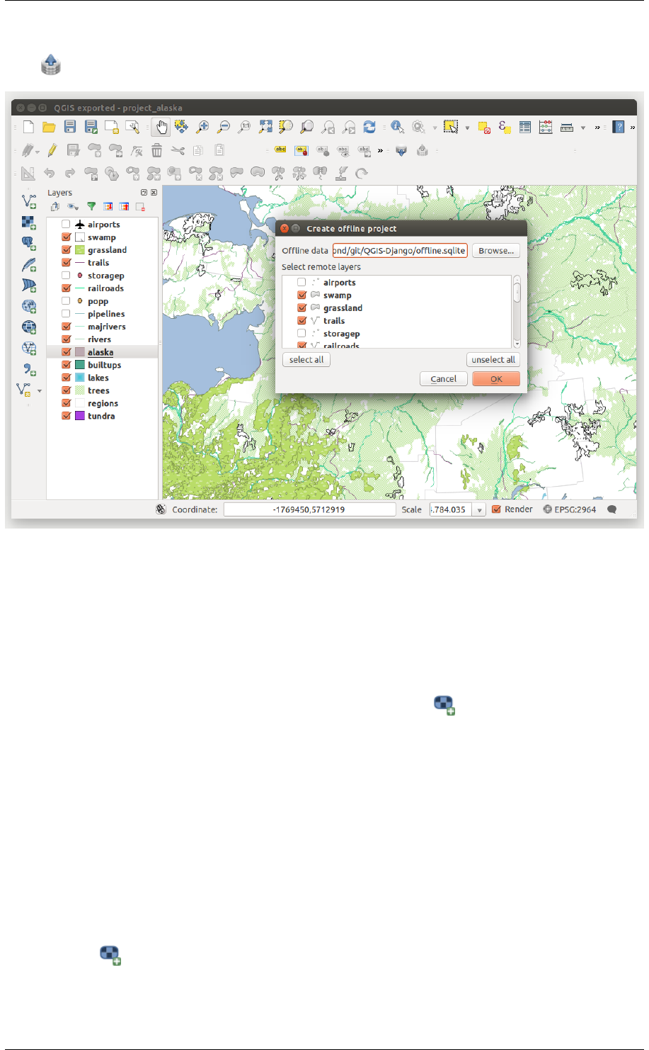
QGIS User Guide, Publicación 2.8
• Después de ser conectado de nuevo, cargar los cambios usando Base de datos →Edición fuera de linea→
Sincronizar.
Figure 19.25: Crear un proyecto fuera de linea de capas PostGIS o WFS
.
19.14 Complemento GeoRaster espacial de Oracle
En las bases de datos de Oracle, los datos raster se pueden almacenar como objetos SDO_GEORASTER
disponibles con la extensión de Oracle Spatial. En QGIS, el complemento GeoRaster espacial de Oracle Spatial es ad-
mitido por GDAL y depende de que tenga instalado y funcionando en su equipo el producto de bases de datos de
Oracle. Aunque Oracle es software propietario, proporciona de forma gratuita su software con fines de desarrollo
y prueba. Aquí hay un ejemplo de cómo cargar imágenes raster a GeoRaster:
$ gdal_translate -of georaster input_file.tif geor:scott/tiger@orcl
Esto cargará el raster en la tabla predeterminada GDAL_IMPORT, como una columna llamada “RASTER”
19.14.1 Administrar conexiones
En primer lugar, se debe habilitar el complemento GeoRaster de Oracle, usando el Administrador de complemen-
tos (ver El diálogo de complementos). La primera vez que cargue un GeoRaster in QGIS, debe crear una conexión
a la base de datos de Oracle que contiene los datos. Para hacer esto, inicie con clic sobre el botón de la barra
de herramientas Añadir capa GeoRaster de Oracle –esto abrirá la ventana de diálogo Seleccionar GeoRaster espacial
de Oracle. Clic sobre [Nuevo] para abrir la ventana de dialogo y especificar los parámetros de conexión (Ver
Figure_oracle_raster_1_1):
•Nombre: Introduzca un nombre para al conexión a la base de datos.
19.14. Complemento GeoRaster espacial de Oracle 311
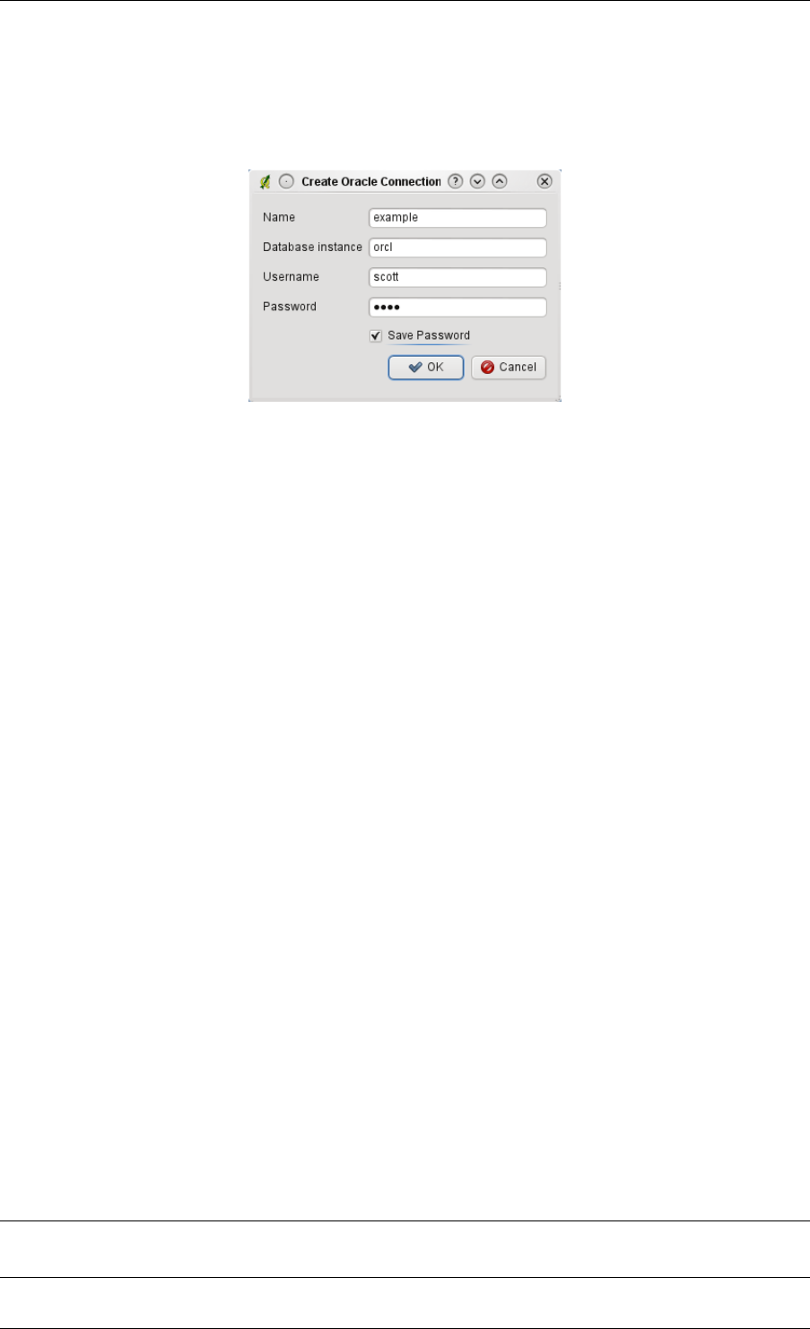
QGIS User Guide, Publicación 2.8
•Instancia de la base de datos: Introduzca el nombre de la base de datos a la que desea conectarse.
•Nombre de usuario: Especificar su nombre de usuario que usará para acceder a la base de datos.
•Contraseña: Proporcionar la contraseña asociada con su usuario que es requerida para el acceso a la base
de datos.
Figure 19.26: Crear dialogo de conexión de Oracle
Ahora, de vuelta en la ventana principal de GeoRaster espacial de Oracle (vea la Figure_oracle_raster_2), utilice
la lista desplegable para elegir una conexión y utilice el botón [Conectar] para establecer la conexión. También
puede [Editar] la conexión abriendo el dialogo previo y haciendo cambios en la información de la conexión, o
usar el botón [Borrar] para eliminar la conexión desde la lista desplegable.
19.14.2 Seleccionar un GeoRaster
Una vez que la conexión se ha establecido, la ventana de subconjuntos de datos mostrará los nombres de todas las
tablas que contengan columnas GeoRaster en esa base de datos en el formato de un nombre del subconjunto de
datos GDAL.
Haga clic en uno de los subconjuntos de datos listados y después haga en [Seleccionar] para elegir el nombre de
la tabla. Ahora se mostrará otra lista de subconjuntos de datos con los nombres de las columnas del GeoRaster en
la tabla. Normalmente es una lista corta, ya que la mayoría de los usuarios no tendrán mas de una o dos columnas
de GeoRaster en la misma tabla.
Clic sobre uno de los subconjuntos de datos en listados y después sobre [Seleccionar] para elegir una de las
combinaciones tabla/columna. El dialogo mostrará ahora todos los registros que contengan objetos GeoRaster.
Note que la lista de subconjunto de datos mostrará ahora las parejas de tablas de datos raster e Id de raster.
En cualquier momento, la entrada seleccionada se puede ser editar para ir directamente a un GeoRaster conocido
o para regresar al inicio y seleccionar otro nombre de tabla.
La entrada de datos seleccionados también puede usarse para introducir una cláusula WHERE al final de
la cadena de identificación (ej. geor:scott/tiger@orcl,gdal_import,raster,geoid=). Vea
http://www.gdal.org/frmt_georaster.html para mayor información.
19.14.3 Mostrar GeoRaster
Finalmente, al seleccionar un GeoRaster de la lista de tablas de datos raster e Id raster, la imagen raster se cargará
en QGIS.
El dialogo Seleccionar GeoRaster espacial de Oracle puede cerrarse ahora y la siguiente ocasión en que se abra
mantendrá la misma conexión y mostrará la misma lista previa de subconjuntos de datos, haciendo muy fácil abrir
otra imagen del mismo contexto.
Nota: Los GeoRaster que contienen pirámides se mostrarán mucho más rápido, pero las pirámides se deben
generar fuera de QGIS usando PL/SQL o gdaladdo.
312 Chapter 19. Complementos
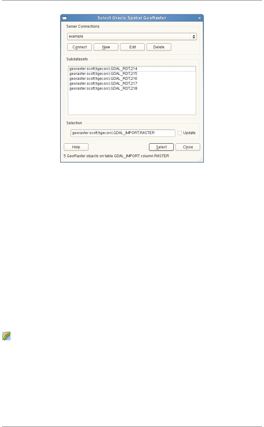
QGIS User Guide, Publicación 2.8
Figure 19.27: Diálogo de selección de GeoRaster de Oracle
Lo siguiente es un ejemplo usando gdaladdo:
gdaladdo georaster:scott/tiger@orcl,georaster\_table,georaster,georid=6 -r
nearest 2 4 6 8 16 32
Este es un ejemplo usando PL/SQL:
$ sqlplus scott/tiger
SQL> DECLARE
gr sdo_georaster;
BEGIN
SELECT image INTO gr FROM cities WHERE id = 1 FOR UPDATE;
sdo_geor.generatePyramid(gr, ’rLevel=5, resampling=NN’);
UPDATE cities SET image = gr WHERE id = 1;
COMMIT;
END;
.
19.15 Complemento Análisis de Terreno
El complemento de Análisis de Terreno se puede utilizar para calcular la pendiente, orientación, mapa de
sombras, índice de irregularidad y relieve para un modelo digital de elevación (DEM). Es muy sencillo el manejo
y proporciona una interfaz de usuario gráfica intuitiva para crear nuevas capas ráster (vea Figure_raster_terrain_1).
Descripción del análisis:
•Pendiente: Calcula el ángulo de la pendiente de cada celda en grados (basado en primer orden estimación
derivada).
•Orientación: Exposición (iniciar con 0 para la dirección norte, en grados antihorario).
•Mapa de sombras: Crea un mapa de sombra utilizando luz y sombra para proveer un aspecto más tridi-
mencional para un mapa de relieve sombreado. El mapa de salida es una banda gris individual que refleja
el valor gris de los píxeles.
19.15. Complemento Análisis de Terreno 313
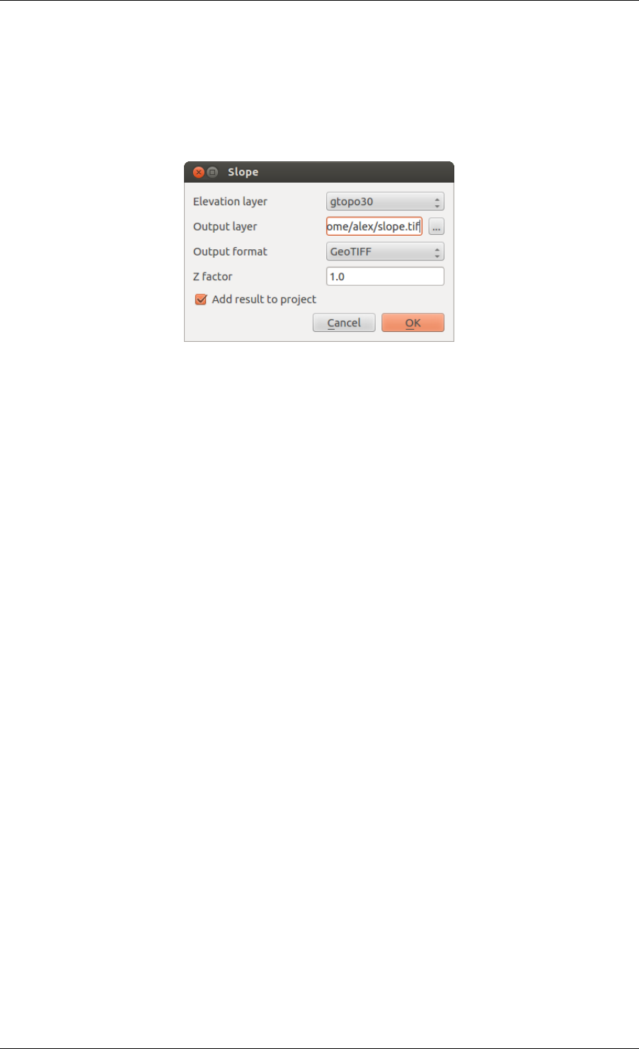
QGIS User Guide, Publicación 2.8
•Índice de irregularidad: Una medición cuantitativa de la heterogeneidad del terreno tal como se describe
por Riley et al. (1999). Se calcula para cada lugar con un resumen de los cambios en la elevación dentro de
la cuadrícula de 3x3 píxeles.
•Relieve: Crea un mapa de relieve sombreado de los datos digitales de elevación. Implementado es un
método para elegir los colores de elevación mediante el análisis de distribución de frecuencia. EL mapa de
salida es una color multibanda con tres bandas que reflejan los valores RGB del relieve sombreado.
Figure 19.28: Complemento de Modelado de Terreno (Cálculo de la pendiente)
19.15.1 Usar el complemento
1. Inicie QGIS y cargue las capas raster gtopo30 de la ubicación de ejemplo de GRASS.
2. Cargar el complemento de Análisis de Terreno en el Administrador de Complementos (vea El diálogo de
complementos).
3. Seleccione un método de análisis del menú (e.j., Ráster →Análisis de Terreno →Pendiente). El diálogo
Pendiente aparece como se muestra en Figure_raster_terrain_1.
4. Especificar una ruta , y un tipo de archivo de salida
5. Haga clic en [Aceptar].
.
19.16 Complemento Grafo de rutas
Grafo de rutas es un complemento en C++ para QGIS que calcula la ruta más corta entre dos puntos de una capa
de polilíneas y traza esta ruta sobre la red de carreteras.
Características principales:
• Calcula la ruta, así como la longitud y el tiempo de viaje.
• Optimiza la longitud o el tiempo de viaje.
• Exporta la ruta a una capa vectorial.
• Resalta la dirección de las carreteras (esto es lento y se utiliza principalmente para fines de depuración y
para pruebas de configuración)
Como una capa de carreteras, se puede usar cualquier capa vectorial de polilíneas en cualquier formato admitido
por QGIS. Dos líneas con un punto en común se consideran conectadas. Tenga en cuenta que es necesario usar
el SRC de la capa como SRC del proyecto mientras edita una capa de carreteras. Esto es debido al hecho de que
recalcular las coordenadas entre diferentes SRC introduce algunos errores que pueden resultar en discontinuidades,
incluso cuando se utiliza el ‘autoensamblado’.
En la tabla de atributos de la capa, se pueden usar los siguientes campos:
• Velocidad en una sección de la carretera (campo numérico).
314 Chapter 19. Complementos
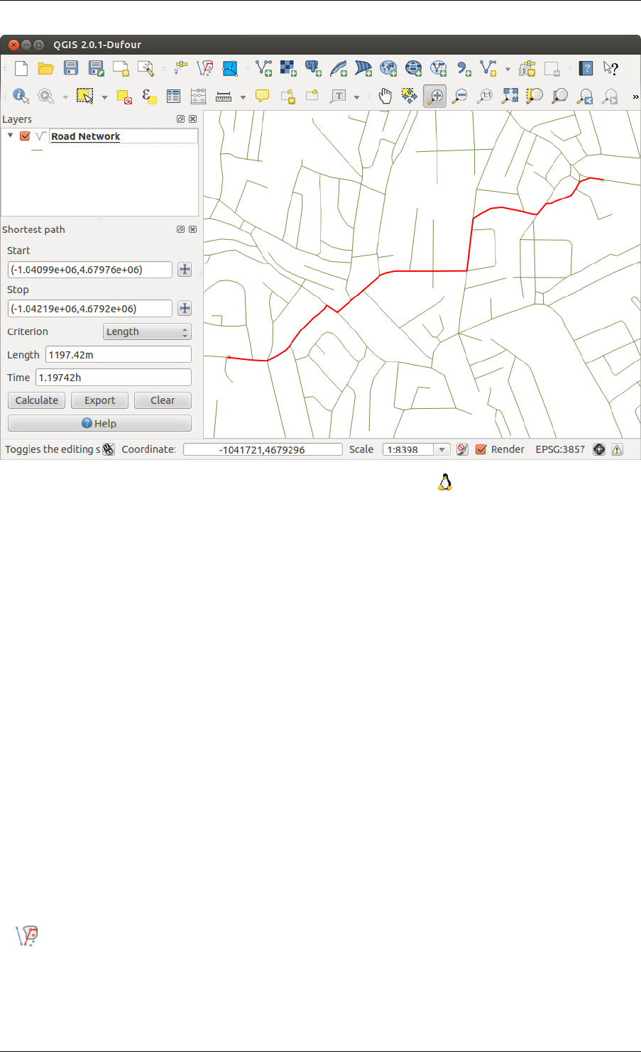
QGIS User Guide, Publicación 2.8
Figure 19.29: Complemento Grafo de rutas
• Dirección (cualquier tipo que se pueda convertir en texto). Las direcciones de avance y retroceso correspon-
den a una carretera de un solo sentido, ambas direcciones indican una carretera de doble sentidos.
Si algunos campos no tienen ningún valor o no existen, se usan los valores predeterminados. Puede cambiar lo
predeterminado y algunas configuraciones del complemento en el diálogo de configuración del complemento.
19.16.1 Usar el componente
Después de activar el complemento verá un panel adicional en el lado izquierdo de la ventana principal de QGIS.
Ahora, escriba algunos parámetros en el diálogo Configuración del complemento Grafos de rutas en el menú
Vectorial →Grafo de rutas (vea figure_road_graph_2).
Después de configurar Unidad de tiempo,Unidad de distancia yTolerancia de topología, puede seleccionar la
capa vectorial en la pestaña Capa de transporte. Aquí también puede seleccionar el Campo de sentido y el Campo
de velocidad. En la pestaña Configuración predeterminada, puede establecer el Sentido para el calculo.
Finalmente, en el panel Ruta más corta, seleccione un punto de Inicio y un punto Final en la capa de red de
carreteras y pulse [Calcular].
.
19.17 Complemento Consulta espacial
El Complemento Consulta espacial permite hacer una consulta espacial (ej., seleccionar rasgos) en una capa de destino
con referencia a otra capa. La funcionalidad se basa en la librería de GEOS y depende de la capa de rasgos de
origen seleccionado.
Operadores posibles son:
19.17. Complemento Consulta espacial 315
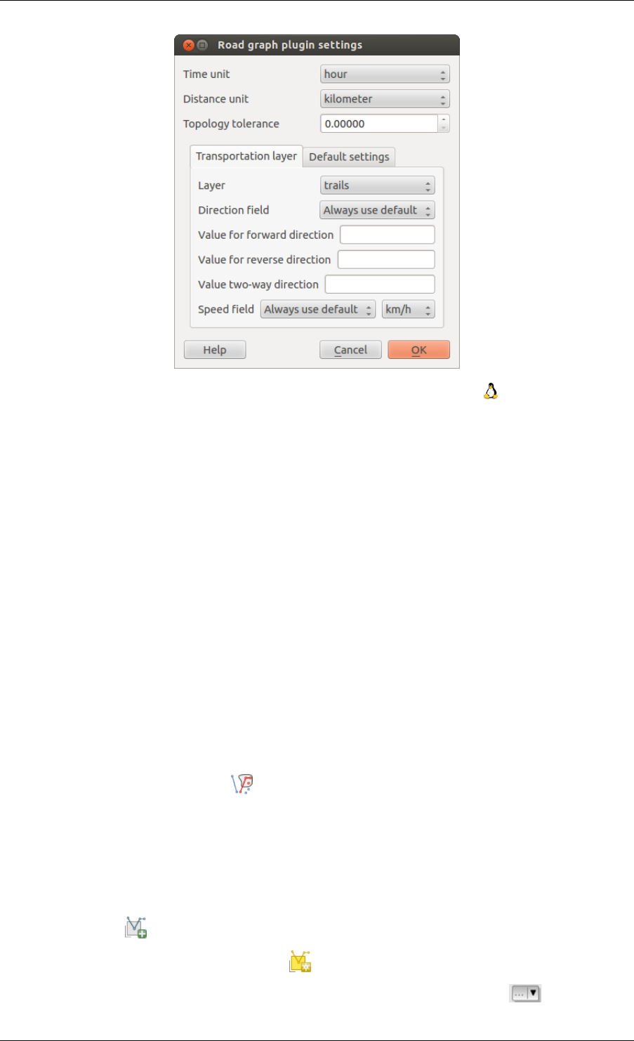
QGIS User Guide, Publicación 2.8
Figure 19.30: Configuración del complemento Grafo de rutas
• Contiene
• Igual
• Solapa
• Cruzar
• Intersecta
• Está inconexo
• Toca
• Dentro
19.17.1 Usar el complemento
Como un ejemplo, queremos encontrar regiones en el conjunto de datos de Alaska que contenga aeropuertos. Los
siguientes pasos son necesarios:
1. Iniciar QGIS y cargar las capas vectoriales regions.shp yairports.shp.
2. Cargue el complemento de Consulta espacial en el Administrador de Complementos (vea El diálogo de com-
plementos) y haga clic en el icono Consulta espacial, que aparecerá en el menú de la barra de herramientas
de QGIS. El diálogo de complemento aparece.
3. Seleccione la capa regions como la capa origen y airports como la capa de entidades de referencia.
4. Seleccione ‘Contiene’ como operador y haga clic en [Aplicar].
Ahora obtiene una lista de IDs de entidades de la consulta y tiene varias opciones, como se muestra en fig-
ure_spatial_query_1.
• Haga clic sobre Crear capa con lista de elementos.
• Seleccione un ID de la lista y haga clic sobre Crear capa selección.
• Seleccione ‘Eliminar de la selección actual’ en el campo Y utilizar el resultado para .
316 Chapter 19. Complementos

QGIS User Guide, Publicación 2.8
• Se puede Zum al elemento o desplegar Registro de mensajes.
• Además en ID’s de los objetos de resultado con las opciones ‘Origen inválido’ y ‘Referencia inválida’ se
puede tener una vista de los objetos espaciales con errores geométricos. Estos objetos no se utilizan para la
consulta.
Figure 19.31: Análisis de consulta espacial - las regiones contienen aeropuertos QGIS
.
19.18 Complemento SPIT
QGIS viene con un complemento llamado SPIT (Herramienta para importar archivos shape a PostGIS). SPIT se
puede usar para cargar multiples archivos shape en una sola vez e incluye soporte para esquemas. Para usar SPIT,
abra el Administrador de complementos desde el menú Complementos, en el menú Instalado marque la casilla
junto a SPIT y pulse [Aceptar].
Para importar un archivo shape, use de la barra de menú Base de datos →Importar (SPIT) →Importar archivos
shape a PostgreSQL para abrir el diálogo SPIT - Herramienta para importar archivos shape a PostGIS. Seleccione
la base de datos PostGIS a la que quiera conectar y haga clic en [Conectar]. Si desea puede definir o cambiar
algunas opciones de importación. Ahora puede agregar uno o más archivos a la cola haciendo clic en el botón
[Añadir]. Para procesar los archivos, haga clic en el botón [Aceptar]. El proceso de importación, así como
cualquier error/advertencia, se mostrará a medida que se procesa cada archivo shape. .
19.19 Complemento Comprobador de topología.
La topología describe las relaciones entre puntos, líneas y polígonos que representa los objetos espaciales de una
región geográfica. Con el complemento de Comprobador de Topología, puede revisar sus archivos vectoriales y
19.18. Complemento SPIT 317
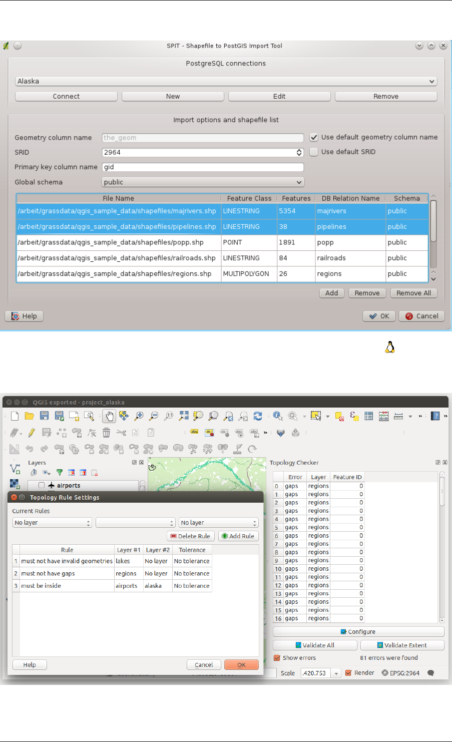
QGIS User Guide, Publicación 2.8
Figure 19.32: Usar el complemento SPIT para importar archivos shape a PostGIS
Figure 19.33: El complemento de Comprobador de Topología
318 Chapter 19. Complementos

QGIS User Guide, Publicación 2.8
verificar la topología con varias reglas topológicas. Estas reglas comprueban con relaciones espaciales si su objeto
espacial es ‘Equal’, ‘Contain’, ‘Cover’, ‘CoveredBy’, ‘Cross’, o son ‘Disjoint’, ‘Intersect’, ‘Overlap’, ‘Touch’
o ‘Within’ el uno al otro. Depende de sus preguntas individuales que reglas topológicas que se aplican a los
datos vectoriales (por ejemplo, normalmente no aceptará overshoots en capas de líneas, pero si ellos representan
callejones sin salida que no eliminará de su capa vectorial).
QGIS tiene una característica integrada de edición topológica, que es ideal para la creación de nuevas funciones
sin errores. Pero los errores de datos existentes y los errores inducidos por el usuario son difíciles de encontrar.
Este complemento te ayuda a encontrar este tipo de errores a través de una lista de reglas.
Es muy simple crear reglas topológicas con el complemento Comprobador de topología.
En capa de puntos las siguientes reglas están disponibles:
•Must be covered by: Aquí puede elegir una capa vectorial de su proyecto. Los puntos que no están
cubiertos por la capa vectorial dada se produce en el campo ‘Error’.
•Must be covered by endpoints of: Aquí puede elegir una capa de líneas de su proyecto.
•Must be inside: Aquí puede elegir una capa de polígonos de su proyecto. Los puntos deben estar dentro
del polígono. De lo contrario, QGIS escribe un ‘Error’ del punto.
•Must not have duplicates: Siempre que un punto se representa dos o más veces, se producirá el campo
‘Error’.
•Must not have invalid geometries: Comprobar si las geometrías son validas.
•Must not have multi-part-geometries: Todos los puntos multi-parte se escriben en el campo ‘Error’.
En Capas de líneas, las siguientes reglas están disponibles:
•End points must be covered by: Aquí se puede seleccionar una capa de puntos de su proyecto.
•Must not have dangles: Este mostrará los overshoots en la capa de líneas.
•Must not have duplicates: Siempre que un objeto línea es representado una o dos veces, se producirá en el
campo ‘Error’.
•Must not have invalid geometries: Comprobar si las geometrías son validas.
•Must not have multi-part geometries: A veces, una geometría es en realidad una colección de simples
(una sola pieza) geometrías. Una geometría de este tipo se denomina de geometría multiparte. Si contiene
sólo un tipo de geometría simple, lo llamamos multi-punto, multi-línea o multi-polígono. Todas las líneas
de multi-partes se escriben en el campo ‘Error’.
•Must not have pseudos: Un punto final de geometría de línea debe estar conectado a los extremos de otras
dos geometrías. Si el punto final está conectado al punto final de otra geometría, el punto final se denomina
un nodo psuedo.
En capas de polígonos, las siguientes reglas están disponibles:
•Must contain: La capa de polígonos debe contener al menos un punto de la geometría de la segunda capa.
•Must not have duplicates: Los polígonos de la misma capa no deben tener geometrías idénticas. Cada vez
que una entidad de polígono se represente dos veces o más se producirá en el campo ‘Error’.
•Must not have gaps: Los polígonos adyacentes no deben formar espacios entre ellos. Los límites adminis-
trativos podrían mencionarse como ejemplo (polígonos de los estados de Estados Unidos no tienen espacios
entre ellos ...).
•Must not have invalid geometries: Comprobar si las geometrías con validas. Algunas de las reglas que
definen si una geometría es valida son:
–Anillos de polígonos deben cerrarse.
–Los anillos que definen agujeros deben estar dentro de los anillos que definen los límites exteriores.
–Los anillos no deben intersectarse (Ni pueden tocarse o cruzarse entre si)
–Los anillos no puede tocar otros anillos, excepto en un punto.
19.19. Complemento Comprobador de topología. 319
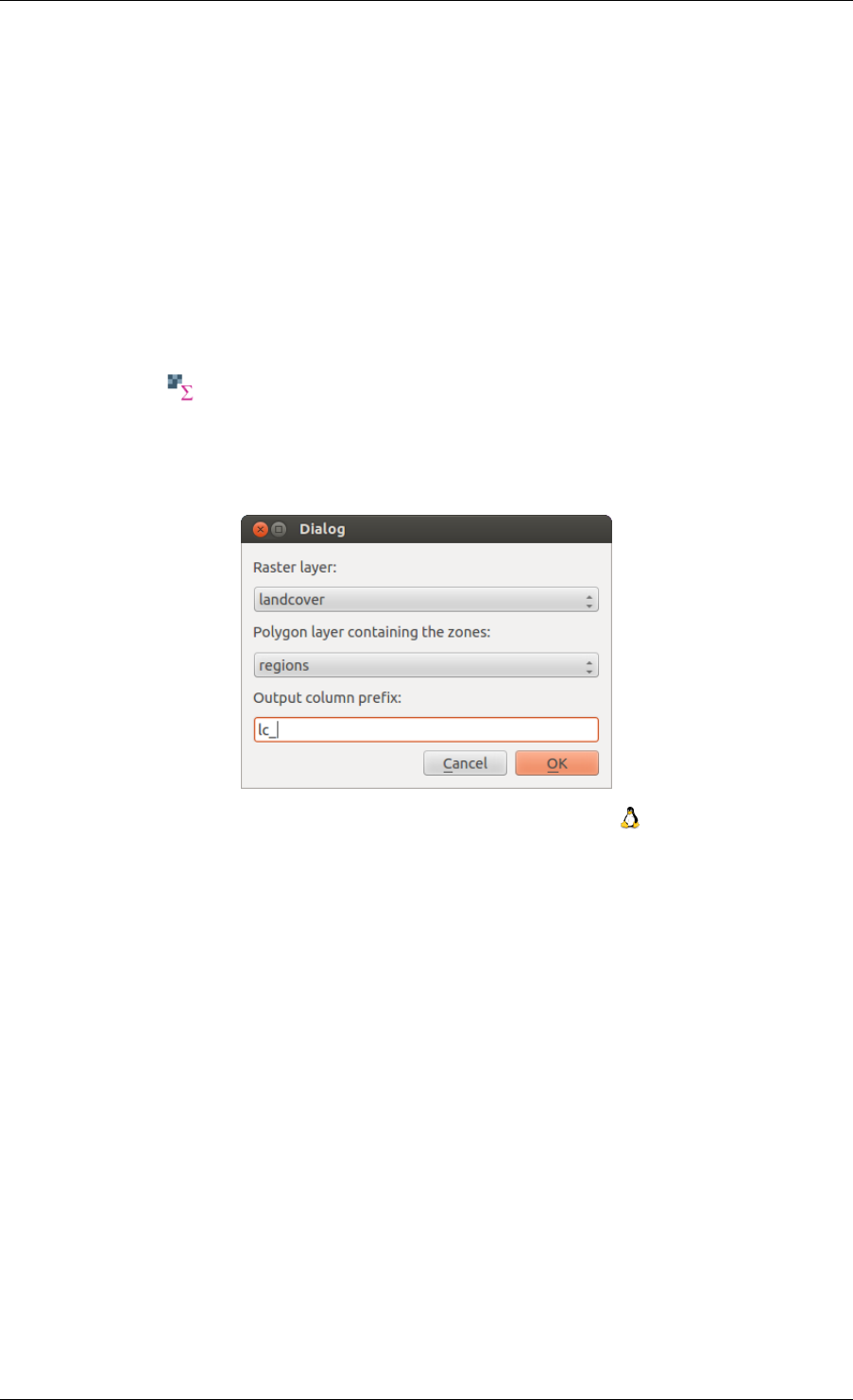
QGIS User Guide, Publicación 2.8
•Must not have multi-part geometries: A veces, una geometría es en realidad una colección geometrías
sencillas (parte sencilla). Una geometría de este tipo se denomina de geometría multi-parte. Si contiene
sólo un tipo de geometría simple, lo llamamos multi-punto, multi-líneas o multi-polígono. Por ejemplo, un
país que consta de múltiples islas se puede representar como un multi-polígono.
•Must not overlap: Los polígonos adyacentes no deben de compartir un área en común.
•Must not overlap with: Los polígonos adyacentes de una capa no deben compartir un área con los polí-
gonos de otra.
.
19.20 Complemento de Estadísticas de zona
Con el complemento Estadísticas de zona, se pueden analizar los resultados de una clasificación temática.
Esto permite calcular varios valores de los píxeles de una capa ráster con la ayuda de una capa vectorial de
polígonos (vea figure_zonal_statistics). Puede calcular la suma, el valor medio y el total de los píxeles que están
dentro de un polígono. El complemento genera columnas de salida en la capa vectorial con un prefijo definido por
el usuario.
Figure 19.34: Diálogo de Estadísticas de zona (KDE)
.
320 Chapter 19. Complementos

CHAPTER 20
Ayuda y apoyo
20.1 Listas de correos
QGIS se encuentra en un desarrollo activo y como tal no siempre funcionará como se espera. La mejor manera de
conseguir ayuda es entrando en la lista de correo de los usuarios qgis. Las preguntas llegan a mayor audiencia y
las preguntas benefician a los demás.
20.1.1 usuarios-qgis
La lista de correo se utiliza para discutir sobre QGIS en general además de otras cuestiones relacionadas con su
instalación y utilización. Puedes suscribirte a la lista de correos de usuarios qgis al visitar el siguiente enlace:
http://lists.osgeo.org/mailman/listinfo/qgis-user
20.1.2 fossgis-talk-liste
Para los de habla alemana, FOSSGIS e.V. ofrece la lista de correos fossgis-talk-liste. Esta lista de correo se utiliza
para discutir sobre QGIS de código abierto en general, incluyendo QGIS. Puedes suscribirte a la lista de correos
fossgis-talk-liste al visitar el siguiente enlace: https://lists.fossgis.de/mailman/listinfo/fossgis-talk-liste
20.1.3 desarrollador-qgis
SI eres un desarrollador con algunos problemas de naturaleza técnica, puede que quieras apuntarte a la lista de
correos de desarrollador-qgis en el siguiente enlace: http://lists.osgeo.org/mailman/listinfo/qgis-developer
20.1.4 qgis-commit
Cada vez que algo se ejecuta en el repositorio de código del QGIS, se publica un email en esta lista.
Si quieres estar al día de cada cambio en el código base actual, puedes suscribirte a esta lista en:
http://lists.osgeo.org/mailman/listinfo/qgis-commit
20.1.5 qgis-trac
Esta lista proporciona notificaciones por email relacionadas con gestión de proyectos, incluyendo
informes de errores, tareas y solicitudes de funciones. Puedes suscribirte a esta lista en:
http://lists.osgeo.org/mailman/listinfo/qgis-trac
321

QGIS User Guide, Publicación 2.8
20.1.6 equipo-de-la-comunidad-qgis
Esta lista se ocupa de temas como la documentación, ayuda de contexto, guía para el usuario, páginas
web. blog, listas de correos, foros y trabajos de traducción. Si además quisieras trabajar en la guía
para el usuario, esta lista es un buen punto de partida para preguntar. Puedes suscribirte a esta lista en:
http://lists.osgeo.org/mailman/listinfo/qgis-community-team
20.1.7 equipo-de-publicación-qgis
Esta lista se ocupa de temas como el proceso de publicación, paquetes de datos binario para var-
ios OSS y anuncios de nuevas publicaciones a nivel mundial. Puedes suscribirte a esta lista en:
http://lists.osgeo.org/mailman/listinfo/qgis-release-team
20.1.8 tr-qgis
Esta lista está relacionada con los trabajos de traducción. Si quieres trabajar en la traducción de los manuales o de
la interfaz gráfica de usuario (GUI), esta lista es un buen punto de partida para responder a tus preguntas. Puedes
suscribirte a esta lista en: http://lists.osgeo.org/mailman/listinfo/qgis-tr
20.1.9 edu-qgis
Esta lista se encarga de los trabajos de educación de QGIS. Si quisieras trabajar en los materiales de ed-
ucación QGIS, esta lista es un buen punto de partida para preguntar. Puedes suscribirte a esta lista en:
http://lists.osgeo.org/mailman/listinfo/qgis-edu
20.1.10 psc-qgis
Se utiliza esta lista para discutir los asuntos del Comité Directivo relacionados con la gestión y dirección general
de QGIS. Puedes suscribirte a esta lista en: http://lists.osgeo.org/mailman/listinfo/qgis-psc
Te invitamos a suscribirte a cualquier lista. Por favor contribuye a la lista respondiendo a preguntas y compartiendo
tus experiencias. Recuerda que las listas de qgis-commit y qgis-trac estñan diseñadas para dar notificaciones
solamente y no para publicaciones de usuarios.
20.2 IRC
También mantenemos una presencia en IRC - visítenos uniéndose al canal #qgis en irc.freenode.net. Por favor,
espere una respuesta a su pregunta, la mayoría de gente en el canal están haciendo otras cosas y puede tomar un
tiempo para que noten su pregunta. Si se ha perdido una discusión en IRC, ¡no hay problema! Registramos toda
discusión, así que puede fácilmente ponerse al día. Sólo tiene que ir a http://qgis.org/irclogs y leer los IRC-logs.
Apoyo comercial para QGIS también esta disponible. Revisar la página web http://qgis.org/en/commercial-
support.html para mayor información.
20.3 Rastreador de Errores
Mientras que la lista de correo de usuarios de QGIS es útil en general para el tipo de preguntas “¿Cómo hago
XYZ en QGIS?, puede que desee notificarnos sobre errores en QGIS. Puede enviar informes de errores utilizando
el gestor de fallos de QGIS en http://hub.qgis.org/projects/quantum-gis/issues. Al crear una nueva entrada de un
error, por favor proporcione una dirección de correo electrónico donde podamos comunicarnos con usted para
obtener información adicional.
322 Chapter 20. Ayuda y apoyo

QGIS User Guide, Publicación 2.8
Por favor, tenga en cuenta que su error no siempre puede disfrutar de la prioridad que podría esperar (depende de
su gravedad). Algunos errores pueden requerir de significativo esfuerzo por parte del desarrollador para remediar,
y la mano de obra no siempre está disponible para esto.
Se pueden presentar las solicitudes de funciones utilizando el mismo sistema de ticket de errores. Asegúrate de
seleccionar el tipo «Función».
Si ha encontrado un error y lo corrige usted mismo, puede enviar este parche también. Una vez más, el encantador
sistema de entradas http://hub.qgis.org/wiki/quantum-gis/issues también tiene este tipo. Compruebe la casilla
Parche suministrado y adjuntar el parche antes de enviar su error . Uno de los desarrolladores lo revisará
y lo aplicará a QGIS. Por favor, no se alarme si su parche no se aplica de inmediato - los desarrolladores pueden
estar vinculados con otros compromisos.
20.4 Blog
La comunidad QGIS también corre un weblog en http://planet.qgis.org/planet/, que tiene algunos artículos in-
teresantes para usuarios y desarrolladores así proporcionados por otros blogs de la comunidad. ¡Se le invita a
contribuir con su propio blog QGIS!
20.5 Plugins
La página web http://plugins.qgis.org a disposición del portal web de complementos QGIS oficial. Aquí, encon-
trará una lista de todos los complementos de QGIS estables y experimentales disponibles vía el ‘Repositorio de
complementos de QGIS oficial” .
20.6 Wiki
Por último, mantenemos un sitio web en WIKI http://hub.qgis.org/projects/quantum-gis/wiki donde se puede en-
contrar una variedad de información útil relacionada con el desarrollo de QGIS, planes de lanzamiento, los enlaces
para descargar sitios, mensaje- consejos de traducción y más. ¡Compruébelo, hay algunas cosas en el interior!
.
20.4. Blog 323

QGIS User Guide, Publicación 2.8
324 Chapter 20. Ayuda y apoyo

CHAPTER 21
Apéndice
21.1 GNU General Public License
Versión 2, Junio de 1991
Copyright (C) 1989, 1991 Free Software Foundation, Inc. 59 Temple Place - Suite 330, Boston, MA 02111-1307,
USA
Everyone is permitted to copy and distribute verbatim copies of this license document, but changing it is not
allowed.
Preámbulo
The licenses for most software are designed to take away your freedom to share and change it. By contrast,
the GNU General Public License is intended to guarantee your freedom to share and change free software–to
make sure the software is free for all its users. This General Public License applies to most of the Free Software
Foundation’s software and to any other program whose authors commit to using it. (Some other Free Software
Foundation software is covered by the GNU Library General Public License instead.) You can apply it to your
programs, too.
When we speak of free software, we are referring to freedom, not price. Our General Public Licenses are designed
to make sure that you have the freedom to distribute copies of free software (and charge for this service if you
wish), that you receive source code or can get it if you want it, that you can change the software or use pieces of
it in new free programs; and that you know you can do these things.
To protect your rights, we need to make restrictions that forbid anyone to deny you these rights or to ask you to
surrender the rights. These restrictions translate to certain responsibilities for you if you distribute copies of the
software, or if you modify it.
For example, if you distribute copies of such a program, whether gratis or for a fee, you must give the recipients
all the rights that you have. You must make sure that they, too, receive or can get the source code. And you must
show them these terms so they know their rights.
We protect your rights with two steps: (1) copyright the software, and (2) offer you this license which gives you
legal permission to copy, distribute and/or modify the software.
Also, for each author’s protection and ours, we want to make certain that everyone understands that there is no
warranty for this free software. If the software is modified by someone else and passed on, we want its recipients
to know that what they have is not the original, so that any problems introduced by others will not reflect on the
original authors’ reputations.
Finally, any free program is threatened constantly by software patents. We wish to avoid the danger that redis-
tributors of a free program will individually obtain patent licenses, in effect making the program proprietary. To
prevent this, we have made it clear that any patent must be licensed for everyone’s free use or not licensed at all.
The precise terms and conditions for copying, distribution and modification follow. TERMS AND CONDITIONS
FOR COPYING, DISTRIBUTION AND MODIFICATION
0. This License applies to any program or other work which contains a notice placed by the copyright holder
saying it may be distributed under the terms of this General Public License. The “Program”, below, refers to
325

QGIS User Guide, Publicación 2.8
any such program or work, and a “work based on the Program” means either the Program or any derivative
work under copyright law: that is to say, a work containing the Program or a portion of it, either verbatim
or with modifications and/or translated into another language. (Hereinafter, translation is included without
limitation in the term “modification”.) Each licensee is addressed as “you”.
Activities other than copying, distribution and modification are not covered by this License; they are outside
its scope. The act of running the Program is not restricted, and the output from the Program is covered only
if its contents constitute a work based on the Program (independent of having been made by running the
Program). Whether that is true depends on what the Program does.
1. You may copy and distribute verbatim copies of the Program’s source code as you receive it, in any medium,
provided that you conspicuously and appropriately publish on each copy an appropriate copyright notice
and disclaimer of warranty; keep intact all the notices that refer to this License and to the absence of any
warranty; and give any other recipients of the Program a copy of this License along with the Program.
You may charge a fee for the physical act of transferring a copy, and you may at your option offer warranty
protection in exchange for a fee.
2. You may modify your copy or copies of the Program or any portion of it, thus forming a work based on the
Program, and copy and distribute such modifications or work under the terms of Section 1 above, provided
that you also meet all of these conditions:
(a) You must cause the modified files to carry prominent notices stating that you changed the files and the
date of any change.
(b) You must cause any work that you distribute or publish, that in whole or in part contains or is derived
from the Program or any part thereof, to be licensed as a whole at no charge to all third parties under
the terms of this License.
(c) If the modified program normally reads commands interactively when run, you must cause it, when
started running for such interactive use in the most ordinary way, to print or display an announcement
including an appropriate copyright notice and a notice that there is no warranty (or else, saying that
you provide a warranty) and that users may redistribute the program under these conditions, and telling
the user how to view a copy of this License. (Exception: if the Program itself is interactive but does
not normally print such an announcement, your work based on the Program is not required to print an
announcement.)
These requirements apply to the modified work as a whole. If identifiable sections of that work are not
derived from the Program, and can be reasonably considered independent and separate works in themselves,
then this License, and its terms, do not apply to those sections when you distribute them as separate works.
But when you distribute the same sections as part of a whole which is a work based on the Program, the
distribution of the whole must be on the terms of this License, whose permissions for other licensees extend
to the entire whole, and thus to each and every part regardless of who wrote it.
Thus, it is not the intent of this section to claim rights or contest your rights to work written entirely by you;
rather, the intent is to exercise the right to control the distribution of derivative or collective works based on
the Program.
In addition, mere aggregation of another work not based on the Program with the Program (or with a work
based on the Program) on a volume of a storage or distribution medium does not bring the other work under
the scope of this License.
3. You may copy and distribute the Program (or a work based on it, under Section 2) in object code or exe-
cutable form under the terms of Sections 1 and 2 above provided that you also do one of the following:
(a) Accompany it with the complete corresponding machine-readable source code, which must be dis-
tributed under the terms of Sections 1 and 2 above on a medium customarily used for software inter-
change; or,
(b) Accompany it with a written offer, valid for at least three years, to give any third party, for a charge no
more than your cost of physically performing source distribution, a complete machine-readable copy
of the corresponding source code, to be distributed under the terms of Sections 1 and 2 above on a
medium customarily used for software interchange; or,
326 Chapter 21. Apéndice

QGIS User Guide, Publicación 2.8
(c) Accompany it with the information you received as to the offer to distribute corresponding source
code. (This alternative is allowed only for noncommercial distribution and only if you received the
program in object code or executable form with such an offer, in accord with Subsection b above.)
The source code for a work means the preferred form of the work for making modifications to it. For an
executable work, complete source code means all the source code for all modules it contains, plus any
associated interface definition files, plus the scripts used to control compilation and installation of the ex-
ecutable. However, as a special exception, the source code distributed need not include anything that is
normally distributed (in either source or binary form) with the major components (compiler, kernel, and
so on) of the operating system on which the executable runs, unless that component itself accompanies the
executable.
If distribution of executable or object code is made by offering access to copy from a designated place, then
offering equivalent access to copy the source code from the same place counts as distribution of the source
code, even though third parties are not compelled to copy the source along with the object code.
4. You may not copy, modify, sublicense, or distribute the Program except as expressly provided under this
License. Any attempt otherwise to copy, modify, sublicense or distribute the Program is void, and will
automatically terminate your rights under this License. However, parties who have received copies, or
rights, from you under this License will not have their licenses terminated so long as such parties remain in
full compliance.
5. You are not required to accept this License, since you have not signed it. However, nothing else grants you
permission to modify or distribute the Program or its derivative works. These actions are prohibited by law
if you do not accept this License. Therefore, by modifying or distributing the Program (or any work based
on the Program), you indicate your acceptance of this License to do so, and all its terms and conditions for
copying, distributing or modifying the Program or works based on it.
6. Each time you redistribute the Program (or any work based on the Program), the recipient automatically
receives a license from the original licensor to copy, distribute or modify the Program subject to these terms
and conditions. You may not impose any further restrictions on the recipients’ exercise of the rights granted
herein. You are not responsible for enforcing compliance by third parties to this License.
7. If, as a consequence of a court judgment or allegation of patent infringement or for any other reason (not
limited to patent issues), conditions are imposed on you (whether by court order, agreement or otherwise)
that contradict the conditions of this License, they do not excuse you from the conditions of this License.
If you cannot distribute so as to satisfy simultaneously your obligations under this License and any other
pertinent obligations, then as a consequence you may not distribute the Program at all. For example, if a
patent license would not permit royalty-free redistribution of the Program by all those who receive copies
directly or indirectly through you, then the only way you could satisfy both it and this License would be to
refrain entirely from distribution of the Program.
If any portion of this section is held invalid or unenforceable under any particular circumstance, the balance
of the section is intended to apply and the section as a whole is intended to apply in other circumstances.
It is not the purpose of this section to induce you to infringe any patents or other property right claims or
to contest validity of any such claims; this section has the sole purpose of protecting the integrity of the
free software distribution system, which is implemented by public license practices. Many people have
made generous contributions to the wide range of software distributed through that system in reliance on
consistent application of that system; it is up to the author/donor to decide if he or she is willing to distribute
software through any other system and a licensee cannot impose that choice.
This section is intended to make thoroughly clear what is believed to be a consequence of the rest of this
License.
8. If the distribution and/or use of the Program is restricted in certain countries either by patents or by copy-
righted interfaces, the original copyright holder who places the Program under this License may add an
explicit geographical distribution limitation excluding those countries, so that distribution is permitted only
in or among countries not thus excluded. In such case, this License incorporates the limitation as if written
in the body of this License.
9. The Free Software Foundation may publish revised and/or new versions of the General Public License from
time to time. Such new versions will be similar in spirit to the present version, but may differ in detail to
address new problems or concerns.
21.1. GNU General Public License 327

QGIS User Guide, Publicación 2.8
Each version is given a distinguishing version number. If the Program specifies a version number of this
License which applies to it and “any later version”, you have the option of following the terms and conditions
either of that version or of any later version published by the Free Software Foundation. If the Program
does not specify a version number of this License, you may choose any version ever published by the Free
Software Foundation.
10. If you wish to incorporate parts of the Program into other free programs whose distribution conditions are
different, write to the author to ask for permission. For software which is copyrighted by the Free Software
Foundation, write to the Free Software Foundation; we sometimes make exceptions for this. Our decision
will be guided by the two goals of preserving the free status of all derivatives of our free software and of
promoting the sharing and reuse of software generally.
NO WARRANTY
11. BECAUSE THE PROGRAM IS LICENSED FREE OF CHARGE, THERE IS NO WARRANTY FOR
THE PROGRAM, TO THE EXTENT PERMITTED BY APPLICABLE LAW. EXCEPT WHEN OTH-
ERWISE STATED IN WRITING THE COPYRIGHT HOLDERS AND/OR OTHER PARTIES PROVIDE
THE PROGRAM “AS IS” WITHOUT WARRANTY OF ANY KIND, EITHER EXPRESSED OR IM-
PLIED, INCLUDING, BUT NOT LIMITED TO, THE IMPLIED WARRANTIES OF MERCHANTABIL-
ITY AND FITNESS FOR A PARTICULAR PURPOSE. THE ENTIRE RISK AS TO THE QUALITY AND
PERFORMANCE OF THE PROGRAM IS WITH YOU. SHOULD THE PROGRAM PROVE DEFEC-
TIVE, YOU ASSUME THE COST OF ALL NECESSARY SERVICING, REPAIR OR CORRECTION.
12. IN NO EVENT UNLESS REQUIRED BY APPLICABLE LAW OR AGREED TO IN WRITING WILL
ANY COPYRIGHT HOLDER, OR ANY OTHER PARTY WHO MAY MODIFY AND/OR REDIS-
TRIBUTE THE PROGRAM AS PERMITTED ABOVE, BE LIABLE TO YOU FOR DAMAGES, IN-
CLUDING ANY GENERAL, SPECIAL, INCIDENTAL OR CONSEQUENTIAL DAMAGES ARISING
OUT OF THE USE OR INABILITY TO USE THE PROGRAM (INCLUDING BUT NOT LIMITED TO
LOSS OF DATA OR DATA BEING RENDERED INACCURATE OR LOSSES SUSTAINED BY YOU
OR THIRD PARTIES OR A FAILURE OF THE PROGRAM TO OPERATE WITH ANY OTHER PRO-
GRAMS), EVEN IF SUCH HOLDER OR OTHER PARTY HAS BEEN ADVISED OF THE POSSIBIL-
ITY OF SUCH DAMAGES.
QGIS Qt excepciones para GPL
In addition, as a special exception, the QGIS Development Team gives permission to link the code
of this program with the Qt library, including but not limited to the following versions (both free
and commercial): Qt/Non-commerical Windows, Qt/Windows, Qt/X11, Qt/Mac, and Qt/Embedded
(or with modified versions of Qt that use the same license as Qt), and distribute linked combinations
including the two. You must obey the GNU General Public License in all respects for all of the code
used other than Qt. If you modify this file, you may extend this exception to your version of the file,
but you are not obligated to do so. If you do not wish to do so, delete this exception statement from
your version.
21.2 GNU Free Documentation License
Version 1.3, 3 November 2008
Copyright 2000, 2001, 2002, 2007, 2008 Free Software Foundation, Inc
<http://fsf.org/>
Everyone is permitted to copy and distribute verbatim copies of this license document, but changing it is not
allowed.
Preamble
The purpose of this License is to make a manual, textbook, or other functional and useful document “free” in the
sense of freedom: to assure everyone the effective freedom to copy and redistribute it, with or without modifying
it, either commercially or noncommercially. Secondarily, this License preserves for the author and publisher a
way to get credit for their work, while not being considered responsible for modifications made by others.
328 Chapter 21. Apéndice

QGIS User Guide, Publicación 2.8
This License is a kind of “copyleft”, which means that derivative works of the document must themselves be free
in the same sense. It complements the GNU General Public License, which is a copyleft license designed for free
software.
We have designed this License in order to use it for manuals for free software, because free software needs free
documentation: a free program should come with manuals providing the same freedoms that the software does.
But this License is not limited to software manuals; it can be used for any textual work, regardless of subject
matter or whether it is published as a printed book. We recommend this License principally for works whose
purpose is instruction or reference.
1. APPLICABILITY AND DEFINITIONS
This License applies to any manual or other work, in any medium, that contains a notice placed by the copyright
holder saying it can be distributed under the terms of this License. Such a notice grants a world-wide, royalty-free
license, unlimited in duration, to use that work under the conditions stated herein. The Document, below, refers
to any such manual or work. Any member of the public is a licensee, and is addressed as “you”. You accept the
license if you copy, modify or distribute the work in a way requiring permission under copyright law.
A “Modified Version” of the Document means any work containing the Document or a portion of it, either copied
verbatim, or with modifications and/or translated into another language.
A “Secondary Section” is a named appendix or a front-matter section of the Document that deals exclusively
with the relationship of the publishers or authors of the Document to the Document’s overall subject (or to related
matters) and contains nothing that could fall directly within that overall subject. (Thus, if the Document is in part
a textbook of mathematics, a Secondary Section may not explain any mathematics.) The relationship could be
a matter of historical connection with the subject or with related matters, or of legal, commercial, philosophical,
ethical or political position regarding them.
The “Invariant Sections” are certain Secondary Sections whose titles are designated, as being those of Invariant
Sections, in the notice that says that the Document is released under this License. If a section does not fit the
above definition of Secondary then it is not allowed to be designated as Invariant. The Document may contain
zero Invariant Sections. If the Document does not identify any Invariant Sections then there are none.
The “Cover Texts” are certain short passages of text that are listed, as Front-Cover Texts or Back-Cover Texts, in
the notice that says that the Document is released under this License. A Front-Cover Text may be at most 5 words,
and a Back-Cover Text may be at most 25 words.
A “Transparent” copy of the Document means a machine-readable copy, represented in a format whose specifi-
cation is available to the general public, that is suitable for revising the document straightforwardly with generic
text editors or (for images composed of pixels) generic paint programs or (for drawings) some widely available
drawing editor, and that is suitable for input to text formatters or for automatic translation to a variety of formats
suitable for input to text formatters. A copy made in an otherwise Transparent file format whose markup, or ab-
sence of markup, has been arranged to thwart or discourage subsequent modification by readers is not Transparent.
An image format is not Transparent if used for any substantial amount of text. A copy that is not “Transparent” is
called Opaque.
Examples of suitable formats for Transparent copies include plain ASCII without markup, Texinfo input format,
LaTeX input format, SGML or XML using a publicly available DTD, and standard-conforming simple HTML,
PostScript or PDF designed for human modification. Examples of transparent image formats include PNG, XCF
and JPG. Opaque formats include proprietary formats that can be read and edited only by proprietary word pro-
cessors, SGML or XML for which the DTD and/or processing tools are not generally available, and the machine-
generated HTML, PostScript or PDF produced by some word processors for output purposes only.
The “Title Page” means, for a printed book, the title page itself, plus such following pages as are needed to hold,
legibly, the material this License requires to appear in the title page. For works in formats which do not have any
title page as such, “Title Page” means the text near the most prominent appearance of the work’s title, preceding
the beginning of the body of the text.
The “publisher” means any person or entity that distributes copies of the Document to the public.
A section “Entitled XYZ” means a named subunit of the Document whose title either is precisely XYZ or contains
XYZ in parentheses following text that translates XYZ in another language. (Here XYZ stands for a specific
section name mentioned below, such as “Acknowledgements”, “Dedications”, “Endorsements”, or “History”.)
21.2. GNU Free Documentation License 329

QGIS User Guide, Publicación 2.8
To “Preserve the Title” of such a section when you modify the Document means that it remains a section “Entitled
XYZ” according to this definition.
The Document may include Warranty Disclaimers next to the notice which states that this License applies to the
Document. These Warranty Disclaimers are considered to be included by reference in this License, but only as
regards disclaiming warranties: any other implication that these Warranty Disclaimers may have is void and has
no effect on the meaning of this License.
2. VERBATIM COPYING
You may copy and distribute the Document in any medium, either commercially or noncommercially, provided
that this License, the copyright notices, and the license notice saying this License applies to the Document are
reproduced in all copies, and that you add no other conditions whatsoever to those of this License. You may not
use technical measures to obstruct or control the reading or further copying of the copies you make or distribute.
However, you may accept compensation in exchange for copies. If you distribute a large enough number of copies
you must also follow the conditions in section 3.
You may also lend copies, under the same conditions stated above, and you may publicly display copies.
3. COPIADO EN CANTIDAD
If you publish printed copies (or copies in media that commonly have printed covers) of the Document, numbering
more than 100, and the Document’s license notice requires Cover Texts, you must enclose the copies in covers
that carry, clearly and legibly, all these Cover Texts: Front-Cover Texts on the front cover, and Back-Cover Texts
on the back cover. Both covers must also clearly and legibly identify you as the publisher of these copies. The
front cover must present the full title with all words of the title equally prominent and visible. You may add other
material on the covers in addition. Copying with changes limited to the covers, as long as they preserve the title
of the Document and satisfy these conditions, can be treated as verbatim copying in other respects.
If the required texts for either cover are too voluminous to fit legibly, you should put the first ones listed (as many
as fit reasonably) on the actual cover, and continue the rest onto adjacent pages.
If you publish or distribute Opaque copies of the Document numbering more than 100, you must either include
a machine-readable Transparent copy along with each Opaque copy, or state in or with each Opaque copy a
computer-network location from which the general network-using public has access to download using public-
standard network protocols a complete Transparent copy of the Document, free of added material. If you use the
latter option, you must take reasonably prudent steps, when you begin distribution of Opaque copies in quantity, to
ensure that this Transparent copy will remain thus accessible at the stated location until at least one year after the
last time you distribute an Opaque copy (directly or through your agents or retailers) of that edition to the public.
It is requested, but not required, that you contact the authors of the Document well before redistributing any large
number of copies, to give them a chance to provide you with an updated version of the Document.
4. MODIFICACIONES
You may copy and distribute a Modified Version of the Document under the conditions of sections 2 and 3 above,
provided that you release the Modified Version under precisely this License, with the Modified Version filling the
role of the Document, thus licensing distribution and modification of the Modified Version to whoever possesses
a copy of it. In addition, you must do these things in the Modified Version:
1. Use in the Title Page (and on the covers, if any) a title distinct from that of the Document, and from those of
previous versions (which should, if there were any, be listed in the History section of the Document). You
may use the same title as a previous version if the original publisher of that version gives permission.
2. List on the Title Page, as authors, one or more persons or entities responsible for authorship of the modifi-
cations in the Modified Version, together with at least five of the principal authors of the Document (all of
its principal authors, if it has fewer than five), unless they release you from this requirement.
3. State on the Title page the name of the publisher of the Modified Version, as the publisher.
4. Preserve all the copyright notices of the Document.
5. Add an appropriate copyright notice for your modifications adjacent to the other copyright notices.
6. Include, immediately after the copyright notices, a license notice giving the public permission to use the
Modified Version under the terms of this License, in the form shown in the Addendum below.
330 Chapter 21. Apéndice

QGIS User Guide, Publicación 2.8
7. Preserve in that license notice the full lists of Invariant Sections and required Cover Texts given in the
Document’s license notice.
8. Include an unaltered copy of this License.
9. Preserve the section Entitled “History”, Preserve its Title, and add to it an item stating at least the title, year,
new authors, and publisher of the Modified Version as given on the Title Page. If there is no section Entitled
“History” in the Document, create one stating the title, year, authors, and publisher of the Document as
given on its Title Page, then add an item describing the Modified Version as stated in the previous sentence.
10. Preserve the network location, if any, given in the Document for public access to a Transparent copy of the
Document, and likewise the network locations given in the Document for previous versions it was based
on. These may be placed in the “History” section. You may omit a network location for a work that was
published at least four years before the Document itself, or if the original publisher of the version it refers
to gives permission.
11. For any section Entitled “Acknowledgements” or “Dedications”, Preserve the Title of the section, and pre-
serve in the section all the substance and tone of each of the contributor acknowledgements and/or dedica-
tions given therein.
12. Preserve all the Invariant Sections of the Document, unaltered in their text and in their titles. Section
numbers or the equivalent are not considered part of the section titles.
13. Delete any section Entitled “Endorsements”. Such a section may not be included in the Modified Version.
14. Do not retitle any existing section to be Entitled “Endorsements” or to conflict in title with any Invariant
Section.
15. Preserve any Warranty Disclaimers.
If the Modified Version includes new front-matter sections or appendices that qualify as Secondary Sections and
contain no material copied from the Document, you may at your option designate some or all of these sections
as invariant. To do this, add their titles to the list of Invariant Sections in the Modified Version’s license notice.
These titles must be distinct from any other section titles.
You may add a section Entitled “Endorsements”, provided it contains nothing but endorsements of your Modified
Version by various parties—for example, statements of peer review or that the text has been approved by an
organization as the authoritative definition of a standard.
You may add a passage of up to five words as a Front-Cover Text, and a passage of up to 25 words as a Back-Cover
Text, to the end of the list of Cover Texts in the Modified Version. Only one passage of Front-Cover Text and one
of Back-Cover Text may be added by (or through arrangements made by) any one entity. If the Document already
includes a cover text for the same cover, previously added by you or by arrangement made by the same entity you
are acting on behalf of, you may not add another; but you may replace the old one, on explicit permission from
the previous publisher that added the old one.
The author(s) and publisher(s) of the Document do not by this License give permission to use their names for
publicity for or to assert or imply endorsement of any Modified Version.
5. COMBINACIÓN DE DOCUMENTOS
You may combine the Document with other documents released under this License, under the terms defined in
section 4 above for modified versions, provided that you include in the combination all of the Invariant Sections
of all of the original documents, unmodified, and list them all as Invariant Sections of your combined work in its
license notice, and that you preserve all their Warranty Disclaimers.
The combined work need only contain one copy of this License, and multiple identical Invariant Sections may be
replaced with a single copy. If there are multiple Invariant Sections with the same name but different contents,
make the title of each such section unique by adding at the end of it, in parentheses, the name of the original author
or publisher of that section if known, or else a unique number. Make the same adjustment to the section titles in
the list of Invariant Sections in the license notice of the combined work.
In the combination, you must combine any sections Entitled “History” in the various original documents, forming
one section Entitled “History”; likewise combine any sections Entitled “Acknowledgements”, and any sections
Entitled “Dedications”. You must delete all sections Entitled “Endorsements”.
6. COLECCIONES DE DOCUMENTOS
21.2. GNU Free Documentation License 331

QGIS User Guide, Publicación 2.8
You may make a collection consisting of the Document and other documents released under this License, and
replace the individual copies of this License in the various documents with a single copy that is included in the
collection, provided that you follow the rules of this License for verbatim copying of each of the documents in all
other respects.
You may extract a single document from such a collection, and distribute it individually under this License,
provided you insert a copy of this License into the extracted document, and follow this License in all other respects
regarding verbatim copying of that document.
7. AGREGACIÓN CON TRABAJOS INDEPENDIENTES
A compilation of the Document or its derivatives with other separate and independent documents or works, in
or on a volume of a storage or distribution medium, is called an “aggregate” if the copyright resulting from the
compilation is not used to limit the legal rights of the compilation’s users beyond what the individual works permit.
When the Document is included in an aggregate, this License does not apply to the other works in the aggregate
which are not themselves derivative works of the Document.
If the Cover Text requirement of section 3 is applicable to these copies of the Document, then if the Document
is less than one half of the entire aggregate, the Document’s Cover Texts may be placed on covers that bracket
the Document within the aggregate, or the electronic equivalent of covers if the Document is in electronic form.
Otherwise they must appear on printed covers that bracket the whole aggregate.
8. TRADUCCIÓN
Translation is considered a kind of modification, so you may distribute translations of the Document under the
terms of section 4. Replacing Invariant Sections with translations requires special permission from their copyright
holders, but you may include translations of some or all Invariant Sections in addition to the original versions of
these Invariant Sections. You may include a translation of this License, and all the license notices in the Document,
and any Warranty Disclaimers, provided that you also include the original English version of this License and the
original versions of those notices and disclaimers. In case of a disagreement between the translation and the
original version of this License or a notice or disclaimer, the original version will prevail.
If a section in the Document is Entitled “Acknowledgements”, “Dedications”, or “History”, the requirement (sec-
tion 4) to Preserve its Title (section 1) will typically require changing the actual title.
9. TERMINACIÓN
You may not copy, modify, sublicense, or distribute the Document except as expressly provided under this License.
Any attempt otherwise to copy, modify, sublicense, or distribute it is void, and will automatically terminate your
rights under this License.
However, if you cease all violation of this License, then your license from a particular copyright holder is reinstated
(a) provisionally, unless and until the copyright holder explicitly and finally terminates your license, and (b)
permanently, if the copyright holder fails to notify you of the violation by some reasonable means prior to 60 days
after the cessation.
Moreover, your license from a particular copyright holder is reinstated permanently if the copyright holder notifies
you of the violation by some reasonable means, this is the first time you have received notice of violation of this
License (for any work) from that copyright holder, and you cure the violation prior to 30 days after your receipt
of the notice.
Termination of your rights under this section does not terminate the licenses of parties who have received copies
or rights from you under this License. If your rights have been terminated and not permanently reinstated, receipt
of a copy of some or all of the same material does not give you any rights to use it.
10. REVISIONES FUTURAS DE ESTA LICENCIA
The Free Software Foundation may publish new, revised versions of the GNU Free Documentation License from
time to time. Such new versions will be similar in spirit to the present version, but may differ in detail to address
new problems or concerns. See http://www.gnu.org/copyleft/.
Each version of the License is given a distinguishing version number. If the Document specifies that a particular
numbered version of this License “or any later version” applies to it, you have the option of following the terms
and conditions either of that specified version or of any later version that has been published (not as a draft) by the
Free Software Foundation. If the Document does not specify a version number of this License, you may choose
any version ever published (not as a draft) by the Free Software Foundation. If the Document specifies that a
332 Chapter 21. Apéndice

QGIS User Guide, Publicación 2.8
proxy can decide which future versions of this License can be used, that proxy’s public statement of acceptance
of a version permanently authorizes you to choose that version for the Document.
11. RENOVACIÓN DE LICENCIAS
“Massive Multiauthor Collaboration Site” (or “MMC Site”) means any World Wide Web server that publishes
copyrightable works and also provides prominent facilities for anybody to edit those works. A public wiki that
anybody can edit is an example of such a server. A “Massive Multiauthor Collaboration” (or “MMC”) contained
in the site means any set of copyrightable works thus published on the MMC site.
“CC-BY-SA” means the Creative Commons Attribution-Share Alike 3.0 license published by Creative Commons
Corporation, a not-for-profit corporation with a principal place of business in San Francisco, California, as well as
future copyleft versions of that license published by that same organization.
“Incorporate” means to publish or republish a Document, in whole or in part, as part of another Document.
An MMC is “eligible for relicensing” if it is licensed under this License, and if all works that were first published
under this License somewhere other than this MMC, and subsequently incorporated in whole or in part into the
MMC, (1) had no cover texts or invariant sections, and (2) were thus incorporated prior to November 1, 2008.
The operator of an MMC Site may republish an MMC contained in the site under CC-BY-SA on the same site at
any time before August 1, 2009, provided the MMC is eligible for relicensing.
APÉNDICE: Cómo usar esta Licencia para sus documentos
To use this License in a document you have written, include a copy of the License in the document and put the
following copyright and license notices just after the title page:
Copyright © YEAR YOUR NAME. Permission is granted to copy, distribute and/or modify this
document under the terms of the GNU Free Documentation License, Version 1.3 or any later version
published by the Free Software Foundation; with no Invariant Sections, no Front-Cover Texts, and no
Back-Cover Texts. A copy of the license is included in the section entitled “GNU Free Documentation
License”.
If you have Invariant Sections, Front-Cover Texts and Back-Cover Texts, replace the “with ... Texts.” line with
this:
with the Invariant Sections being LIST THEIR TITLES, with the Front-Cover Texts being LIST, and
with the Back-Cover Texts being LIST.
If you have Invariant Sections without Cover Texts, or some other combination of the three, merge those two
alternatives to suit the situation.
If your document contains nontrivial examples of program code, we recommend releasing these examples in
parallel under your choice of free software license, such as the GNU General Public License, to permit their use
in free software.
.
21.2. GNU Free Documentation License 333

QGIS User Guide, Publicación 2.8
334 Chapter 21. Apéndice

CHAPTER 22
Referencias bibliográficas y web
GDAL-SOFTWARE-SUITE. Geospatial data abstraction library. http://www.gdal.org, 2013.
GRASS-PROJECT. Geographic ressource analysis support system. http://grass.osgeo.org , 2013.
NETELER, M., AND MITASOVA, H. Open source gis: A grass gis approach, 2008.
OGR-SOFTWARE-SUITE. Geospatial data abstraction library. http://www.gdal.org/ogr , 2013.
OPEN-GEOSPATIAL-CONSORTIUM. Web map service (1.1.1) implementation specification.
http://portal.opengeospatial.org, 2002.
OPEN-GEOSPATIAL-CONSORTIUM. Web map service (1.3.0) implementation specification.
http://portal.opengeospatial.org, 2004.
POSTGIS-PROJECT. Spatial support for postgresql. http://postgis.refractions.net/ , 2013.
335

QGIS User Guide, Publicación 2.8
336 Chapter 22. Referencias bibliográficas y web

Índice
%%, 105
Actions, 105
actualización del renderizado durante el dibujado, 37
anidar proyectos, 45
anotación, 43
apache, 161
apache2, 161
Arc/Info_ASCII_Grid, 139
Arc/Info_Binary_Grid, 139
ArcInfo_Binary_Coverage, 70
Atlas_Generation, 263
attribute table, 130
Attribute_Actions, 105
Attribute_Table_Selection, 130
Avoid_Intersections_Of_Polygons, 120
Ayuda de contexto, 35
Barra de escala
Map_Scalebar, 249
barra de herramientas, 29
barra de herramientas de diseño, 29
Browse_Maps, 65
calcular escala, 32
Calculator_Field, 136
calidad de renderizado, 37
CAT, 151
Categorized_Renderer, 87
CGI, 161
Colliding_labels, 95
Color_interpolation, 144
color_Ramp, 82
colorBrewer, 82
Colormap, 144
Comma Separated Values, 70
Common_Gateway_Interface, 161
complementos, 269
Compose_Maps, 231
Composer_Manager, 267
Composer_Template, 232
Contrast_enhancement, 142
Coordinate_Reference_System, 59,155
Create_Maps, 231
Create_New_Layers, 128
crossing the 180 degrees longitude line, 76
CRS, 59
CSV, 70,123
Cuadrícula
Cuadrículas
Map_Grid, 239
Current_Edits, 122
Custom_color_Ramp, 82
Custom_CRS, 62
Datum_transformation, 63
DB_Manager, 77
Debian_Squeeze, 161
default_CRS, 59
define an action, 105
Derived_Fields, 136
Desplazar con teclas de flechas, 32
Detener el renderizado, 36
Digitizing, 120
Discrete, 144
Displacement_plugin, 89
documentación, 7
editing, 118
Elements_Alignment, 261
EPSG, 59
Equal_Interval, 87
Erdas Imagine, 139
Escala, 36
ESRI, 67
European_Petroleom_Search_Group, 59
example actions, 106
Export_as_image, 266
Export_as_PDF, 266
Export_as_SVG, 266
Expressions, 111
FastCGI, 161
Field_Calculator, 136
Field_Calculator_Functions, 113
GDAL, 139
GeoTIFF, 139
GeoTiff, 139
GiST (Generalized Search Tree) index, 75
GML, 151
337

QGIS User Guide, Publicación 2.8
GNU General Public License, 325
Gradient_color_Ramp, 82
Graduated_Renderer, 87
GRASS, 177,see Creating new vectors;editing;creating
a new layer
attribute linkage, 182
attribute storage, 181
category settings, 183
digitizing tools, 182
display results, 186,189
region, 185
region display, 185
region editing, 185
snapping tolerance, 184
symbology settings, 184
table editing, 184
toolbox, 189
GRASS toolbox, 185
Browser, 192
customize, 193
GRASS vector data model, 181
Heatmap Renderer, 91
Herramienta_de_Importación_de_archivos_Shape_a_Postgis,
317
Herramientas de Análisis, 289
Herramientas de investigación, 290
Herramientas del georreferenciador, 297
Histogram, 146
HTML_Frame, 258
Identificar objetos espaciales, 39
IGNF, 59
Import_Maps, 65
impresión rápida del diseñador de impresión, 20
Imprimir
Export_Map, 265
Institut_Geographique_National_de_France, 59
InteProxy, 159
Inverted_Polygon_Renderer, 89
join, 109
join layer, 109
Layout_Maps, 231
leyenda, 29
license document, 325
load a shapefile, 68
loading_raster, 139
Map_Legend, 245
Map_Navigation, 119
Map_Scalebar, 253
Map_Template, 232
MapInfo, 70
marcdores, 44
marcdores espaciales
ver marcadores, 44
medición, 37
ángulos, 37
áreas, 37
longitud de línea, 37
menús, 22
merge attributes of features, 127
Merge_Attributes_of_Selected_Features, 127
Merge_Selected_Features, 127
Metadata, 146
MSSQL Spatial, 77
Multi_Band_Raster, 141
multipolygon, 125
Natural_Breaks_(Jenks), 87
New_GPX_Layer, 128,130
New_Shapefile_Layer, 128
New_SpatiaLite_Layer, 128
New_Spatialite_Layer, 128
New_Temporary_Scratch_Layer, 130
Node_Tool, 122
Nodes, 122
Non_Spatial_Attribute_Tables, 132
OGC, 151
OGR, 67
OGR Simple Feature Library, 67
ogr2ogr, 75
opciones de línea de órdenes, 17
Open_Geospatial_Consortium, 151
OpenStreetMap, 72
Oracle Spatial, 77
OSM, 72
Pan, 119
pgsql2shp, 74
Picture_database, 244
Point_Displacement_Renderer, 89
PostGIS, 72
PostGIS spatial index, 75
PostgreSQL, 72
Pretty_Breaks, 87
print_composer
herramientas, 231
Proj.4, 62
Proj4, 61
Proj4_text, 61
Projections, 59
Proxy, 153
Pyramids, 146
QGIS_mapserver, 159
QGIS_Server, 161
QSpatiaLite, 77
Quantile, 87
Query_Builder, 135
Raster, 139
Raster_Calculator, 148
Relations, 132
Renderer_Categorized, 87
338 Índice

QGIS User Guide, Publicación 2.8
Renderer_Graduated, 87
Renderer_Point_Displacement, 89
Renderer_Single_Symbol, 85
Rendering_Mode, 236
Rendering_Rule-based, 89
Renderizado, 35
Renderizado dependiente de la escala, 36
Revert_Layout_Actions, 262
ring polygons, 125
Rotate_Point_symbols, 127
Rotated_North_Arrow, 244
Rule-based_Rendering, 89
salida guardar como imagen, 20
Search_Radius, 119
Secured_OGC_Authentication, 159
Select_using_Query, 136
servidor-proxy, 153
SFS, 151
Shapefile, 67
Shared_Polygon_Boundaries, 120
shp2pgsql, 74
Single_Band_Raster, 141
Single_Symbol_Renderer, 85
SLD, 161
SLD/SE, 161
Snapping, 118
Snapping_On_Intersections, 120
Snapping_Tolerance, 118
Spatialite, 76
Spatialite_Manager, 77
SPIT, 317
Split_Features, 126
SQLite, 76
SRC, 155
SRS, 155
ST_Shift_Longitude, 76
Symbology, 94,141
Teclas de acceso rápido, 35
Three_Band_Color_Raster, 141
Tiger_Format, 70
Toggle Editing, 121
Topological_Editing, 120
Transparency, 145
UK_National_Transfer_Format, 70
US_Census_Bureau, 70
ventana principal, 21
Vertex, 122
Vertices, 122
visibilidad de la capa, 29
Vista general del mapa, 48
WCS, 151,159
Web Coverage Service, 159
WFS, 151,159
WFS-T, 159
WFS_Transactional, 159
WKT, 59,123
WMS, 151
WMS-C, 156
WMS_1.3.0, 159
WMS_client, 151
WMS_identify, 157
WMS_layer_transparency, 155
WMS_metadata, 157
WMS_properties, 157
WMS_tiles, 156
WMTS, 156
WMTS_client, 151
Work_with_Attribute_Table, 130
Zoom_In Zoom_Out, 119
zum con rueda del ratón, 32
Índice 339
