Casio ALGEBRA FX 2.0 PLUS_FX 1.0 PLUS_Eng_Users Guide ALGEBRA_FX2.0_FX1.0_PLUS FX2.0 FX1.0 PLUS EN
User Manual: Casio ALGEBRA_FX2.0_FX1.0_PLUS ALGEBRA FX 2.0 PLUS, ALGEBRA FX 1.0 PLUS | Calculators | Manuals | CASIO
Open the PDF directly: View PDF ![]() .
.
Page Count: 592 [warning: Documents this large are best viewed by clicking the View PDF Link!]
- BEFORE USING THE CALCULATOR FOR THE FIRST TIME...
- Quick-Start
- Handling Precautions
- Contents
- Getting Acquainted — Read This First!
- Chapter 1 Basic Operation
- Chapter 2 Manual Calculations
- Chapter 3 List Function
- Chapter 4 Equation Calculations
- Chapter 5 Graphing
- 5-1 Sample Graphs
- 5-2 Controlling What Appears on a Graph Screen
- 5-3 Drawing a Graph
- 5-4 Storing a Graph in Picture Memory
- 5-5 Drawing Two Graphs on the Same Screen
- 5-6 Manual Graphing
- 5-7 Using Tables
- 5-8 Dynamic Graphing
- 5-9 Graphing a Recursion Formula
- 5-10 Changing the Appearance of a Graph
- 5-11 Function Analysis
- Chapter 6 Statistical Graphs and Calculations
- Chapter 7 Computer Algebra System and Tutorial Modes (ALGEBRA FX 2.0 PLUS only)
- Chapter 8 Programming
- Chapter 9 System Settings Menu
- Chapter 10 Data Communications
- Appendix
- Additional Functions


GUIDELINES LAID DOWN BY FCC RULES FOR USE OF THE UNIT IN THE U.S.A. (not appli-
cable to other areas).
NOTICE
This equipment has been tested and found to comply with the limits for a Class B digital device,
pursuant to Part 15 of the FCC Rules. These limits are designed to provide reasonable protec-
tion against harmful interference in a residential installation. This equipment generates, uses
and can radiate radio frequency energy and, if not installed and used in accordance with the
instructions, may cause harmful interference to radio communications. However, there is no
guarantee that interference will not occur in a particular installation. If this equipment does
cause harmful interference to radio or television reception, which can be determined by turning
the equipment off and on, the user is encouraged to try to correct the interference by one or more
of the following measures:
•Reorient or relocate the receiving antenna.
•Increase the separation between the equipment and receiver.
•Connect the equipment into an outlet on a circuit different from that to which the receiver is
connected.
•Consult the dealer or an experienced radio/TV technician for help.
FCC WARNING
Changes or modifications not expressly approved by the party responsible for compliance could
void the user’s authority to operate the equipment.
Proper connectors must be used for connection to host computer and/or peripherals in order to
meet FCC emission limits.
Connector SB-62 Power Graphic Unit to Power Graphic Unit
Connector FA-123 Power Graphic Unit to PC for IBM/Macintosh Machine
IBM is a registered trademark of International Business Machines Corporation.
Macintosh is a registered trademark of Apple Computer, Inc.
Declaration of Conformity
Model Number: ALGEBRA FX 2.0 PLUS / FX 1.0 PLUS
Trade Name: CASIO COMPUTER CO., LTD.
Responsible party: CASIO AMERICA, INC.
Address: 570 MT. PLEASANT AVENUE, DOVER, NEW JERSEY 07801
Telephone number: 973-361-5400
This device complies with Part 15 of the FCC Rules. Operation is subject to the
following two conditions: (1) This device may not cause harmful interference, and
(2) this device must accept any interference received, including interference that may
cause undesired operation.
FOR CALIFORNIA USA ONLY
Perchlorate Material – special handling may apply. See
www.dtsc.ca.gov/hazardouswaste/perchlorate.

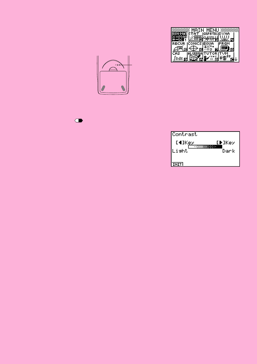
BEFORE USING THE CALCULATOR
FOR THE FIRST TIME...
This calculator does not contain any main batteries when you purchase it. Be sure to
perform the following procedure to load batteries, reset the calculator, and adjust the
contrast before trying to use the calculator for the first time.
1. Making sure that you do not accidently press the o key, slide the case onto the
calculator and then turn the calculator over. Remove the back cover from the calculator
by pulling with your finger at the point marked 1.
2. Load the four batteries that come with calculator.
•Make sure that the positive (+) and negative (–) ends of the batteries are facing cor-
rectly.
3. Remove the insulating sheet at the location marked “BACK UP” by pulling in the direc-
tion indicated by the arrow.
4. Replace the back cover, making sure that its tabs enter the holes marked 2 and turn
the calculator front side up. The calculator should automatically turn on power and
perform the memory reset operation.
P
1
BACK UP
BACK UP
2
19990401
P button
5. Press m.
•If the Main Menu shown to the right is not on the display,
press the P button on the back of the calculator to
perform memory reset.
6. Use the cursor keys (f, c, d, e) to select the SYSTEM icon and press
w, then press 2( ) to display the contrast adjustment screen.
7. Adjust the contrast.
• The e cursor key makes display contrast darker.
• The d cursor key makes display contrast lighter.
•1(INIT) returns display contrast to its initial default.
8. To exit display contrast adjustment, press m.
* The above shows the ALGEBRA
FX 2.0 PLUS screen.
20010102

19990401
Quick-Start
Welcome to the world of graphing calculators.
Quick-Start is not a complete tutorial, but it takes you through many of the most common
functions, from turning the power on, and on to graphing complex equations. When
you’re done, you’ll have mastered the basic operation of this calculator and will be ready
to proceed with the rest of this user’s guide to learn the entire spectrum of functions
available.
Each step of the examples in Quick-Start is shown graphically to help you follow along
quickly and easily. When you need to enter the number 57, for example, we’ve indi-
cated it as follows:
Press fh
Whenever necessary, we’ve included samples of what your screen should look like.
If you find that your screen doesn’t match the sample, you can restart from the begin-
ning by pressing the “All Clear” button o.
TURNING POWER ON AND OFF
To turn power on, press o.
To turn power off, press !
o
OFF
.
Calculator power turns off automatically if you do not perform any operation within the
Auto Power Off trigger time you specify. You can specify either six minutes or 60
minutes as the trigger time.
USING MODES
This calculator makes it easy to perform a wide range of calculations by simply
selecting the appropriate mode. Before getting into actual calculations and operation
examples, let’s take a look at how to navigate around the modes.
To select the RUN • MAT Mode
1. Press m to display the Main Menu.
1
Quick-Start
* The above shows the ALGEBRA
FX 2.0 PLUS screen.
20010102
19990401
2. Use defc to highlight RUN • MAT
and then press w.
This is the initial screen of the RUN • MAT Mode,
where you can perform manual calculations,
matrix calculations, and run programs.
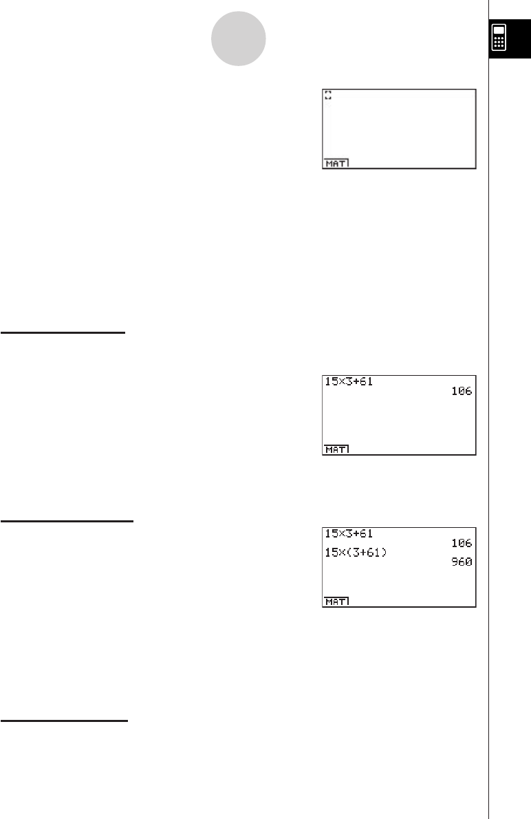
BASIC CALCULATIONS
With manual calculations, you input formulas from left to right, just as they are written
on paper. With formulas that include mixed arithmetic operators and parentheses, the
calculator automatically applies true algebraic logic to calculate the result.
Example:
15 × 3 + 61
1. Press o to clear the calculator.
2. Press bf*d+gbw.
Parentheses Calculations
Example:
15 × (3 + 61)
1. Press bf*(d
+gb)w.
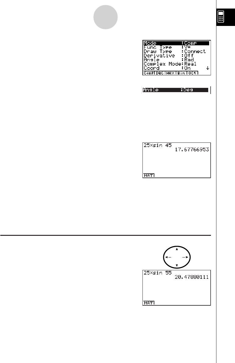
Built-In Functions
This calculator includes a number of built-in scientific functions, including trigonometric
and logarithmic functions.
Example:
25 × sin 45˚
Important!
Be sure that you specify Deg (degrees) as the angle unit before you try this
example.
2
Quick-Start
19990401
1. Pressu3
SET UP
to display the SET UP screen.
2. Press cccc1 (Deg) to specify
degrees as the angle unit.
3. Press i to clear the menu.
4. Press o to clear the unit.
5. Press cf*sefw.
REPLAY FEATURE
With the replay feature, simply press d or e to recall the last calculation that
was performed so you can make changes or re-execute it as it is.
Example:
To change the calculation in the last example from (25 × sin 45˚) to
(25 × sin 55˚)
1. Press d to display the last calculation.
2. Press d twice to move the cursor (t) to 4.
3. Press D to delete 4.
4. Press f.
5. Press w to execute the calculation again.
3
Quick-Start
REPLAY
19990401
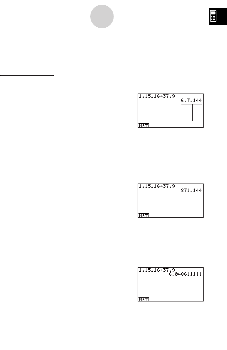
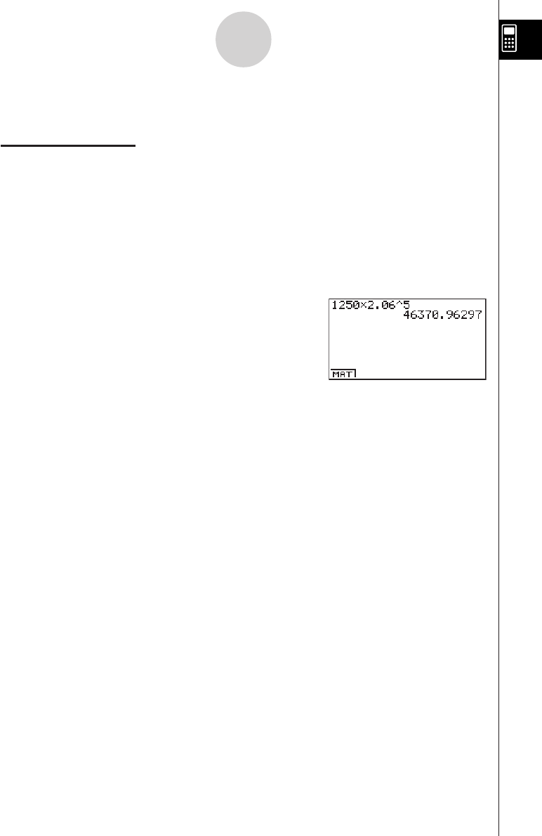
FRACTION CALCULATIONS
You can use the $ key to input fractions into calculations. The symbol “ { ” is used
to separate the various parts of a fraction.
Example:
1 15/16 + 37/9
1. Press o.
2. Press b$bf$
bg+dh$
jw.
Converting a Mixed Fraction to an Improper Fraction
While a mixed fraction is shown on the display, press !
d/c
$
to convert it to an
improper fraction.
Press !
d/c
$again to convert back to a mixed fraction.
Converting a Fraction to Its Decimal Equivalent
While a fraction is shown on the display, press $ to convert it to its decimal
equivalent.
Press $ again to convert back to a fraction.
Indicates 6 7/144
4
Quick-Start
19990401
EXPONENTS
Example:
1250 × 2.065
1. Press o.
2. Press bcfa*c.ag.
3. Press M and the ^ indicator appears on the display.
4. Press f. The ^5 on the display indicates that 5 is an exponent.
5. Press w.
5
Quick-Start
19990401
GRAPH FUNCTIONS
The graphing capabilities of this calculator makes it possible to draw complex graphs
using either rectangular coordinates (horizontal axis: x ; vertical axis: y) or polar
coordinates (angle:
θ
; distance from origin: r).
All of the following graphing examples are performed starting from the calculator setup
in effect immediately following a reset operation.
Example
1: To graph Y = X(X + 1)(X – 2)
1. Press m.
2. Use defc to highlight
GRPH • TBL, and then press w.
3. Input the formula.
v(v+b)
(v-c)w
4. Press 5(DRAW) or w to draw the graph.
Example
2: To determine the roots of Y = X(X + 1)(X – 2)
1. Press 4(G-SLV) to display the pull-up menu.
6
Quick-Start
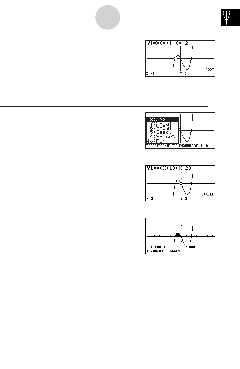
19990401
2. Press b(Root).
Press e for other roots.
Example
3: Determine the area bounded by the origin and the X = –1 root obtained
for Y = X(X + 1)(X – 2)
1. Press i4(G-SLV)c.
2. Press i(∫dx).
3. Use d to move the pointer to the location where
X = –1, and then press w. Next, use e to
move the pointer to the location where X = 0, and
then press w to input the integration range,
which becomes shaded on the display.
7
Quick-Start
19990401
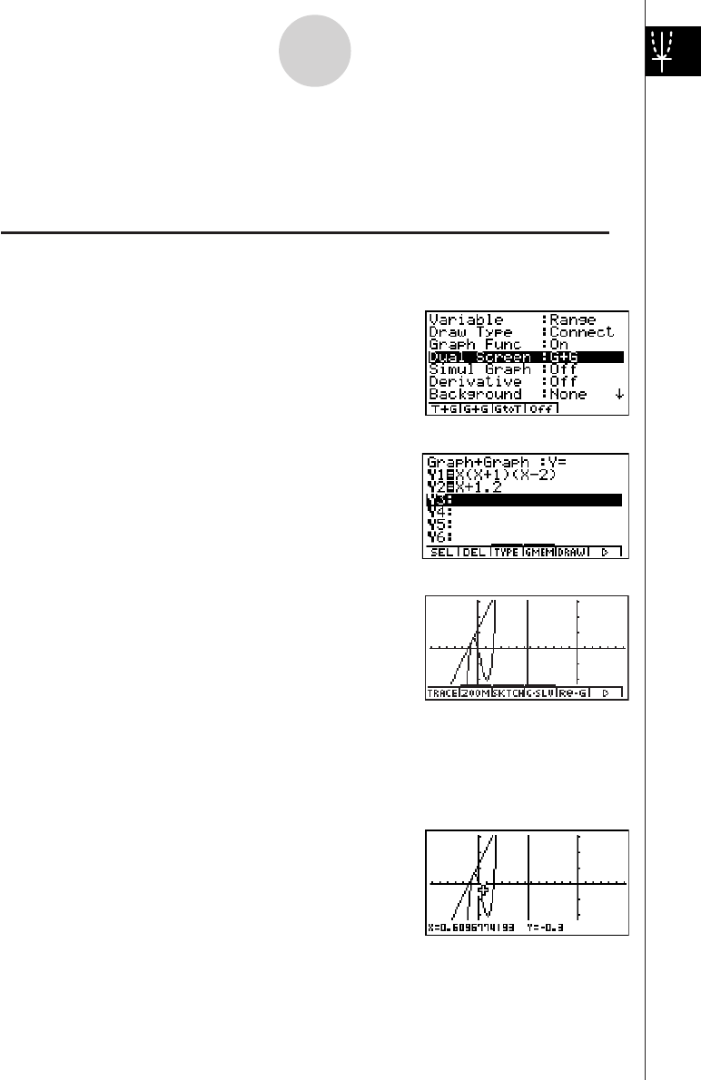
DUAL GRAPH
With this function you can split the display between two areas and display two graphs
on the same screen.
Example:
To draw the following two graphs and determine the points of intersection
Y1 = X(X + 1)(X – 2)
Y2 = X + 1.2
1. Press u
3
SET UP
ccc2(G+G)
to specify “G+G” for the Dual Screen setting.
2. Press i, and then input the two functions.
v(v+b)
(v-c)w
v+b.cw
3. Press 5(DRAW) or w to draw the graphs.
BOX ZOOM
Use the Box Zoom function to specify areas of a graph for enlargement.
1. Press 2(ZOOM) b(Box).
2. Use d e f c to move the pointer
to one corner of the area you want to specify and
then press w.
8
Quick-Start
19990401
3. Use d e f c to move the pointer
again. As you do, a box appears on the display.
Move the pointer so the box encloses the area
you want to enlarge.
4. Press w, and the enlarged area appears in the
inactive (right side) screen.
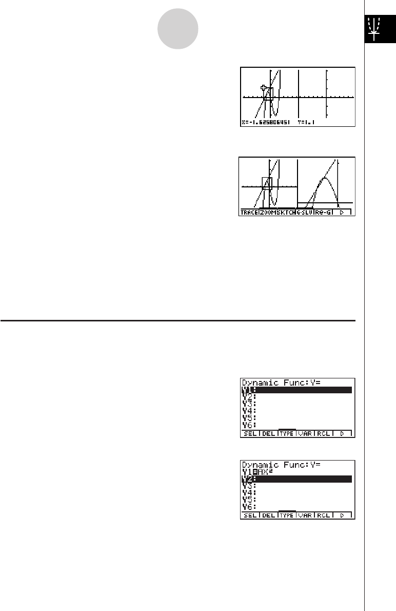
DYNAMIC GRAPH
Dynamic Graph lets you see how the shape of a graph is affected as the value
assigned to one of the coefficients of its function changes.
Example:
To draw graphs as the value of coefficient A in the following function changes
from 1 to 3
Y = AX2
1. Press m.
2. Use d e f c to highlight DYNA,
and then press w.
3. Input the formula.
a
v
A
vxw
12356
9
Quick-Start
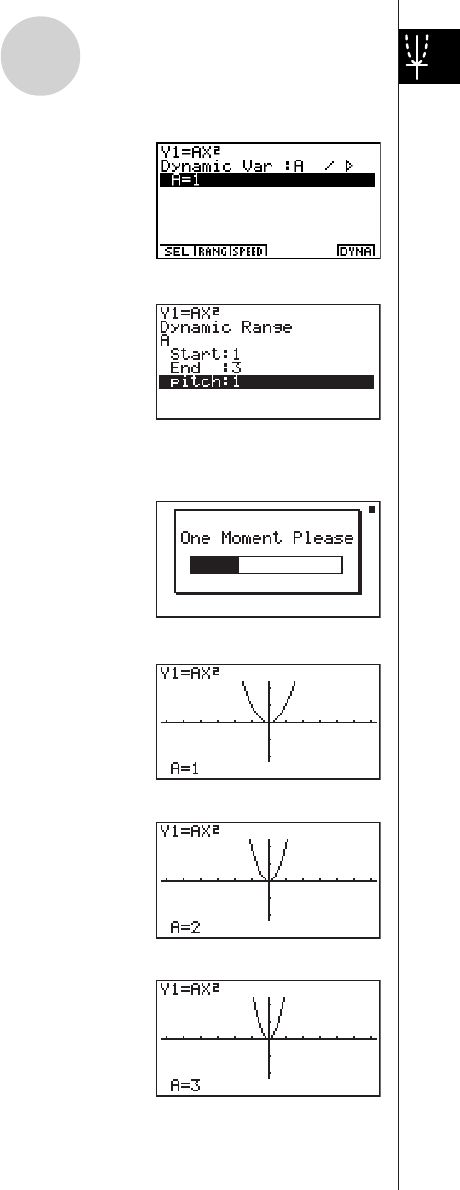
19990401
4. Press 4(VAR) bw to assign an initial value
of 1 to coefficient A.
5. Press 2(RANG) bwdwb
wto specify the range and increment of change
in coefficient A.
6. Press i.
7. Press 6(DYNA) to start Dynamic Graph drawing.
The graphs are drawn 10 times.
↓
↓↑
↓↑
10
Quick-Start
19990401
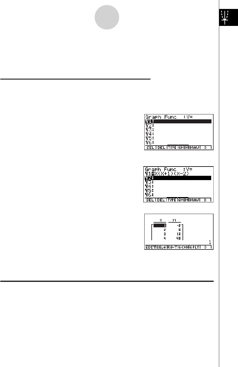
TABLE FUNCTION
The Table Function makes it possible to generate a table of solutions as different
values are assigned to the variables of a function.
Example:
To create a number table for the following function
Y = X (X+1) (X–2)
1. Press m.
2. Use defc to highlight
GRPH • TBL, and then press w.
3. Input the formula.
v(v+b)
(v-c)w
4. Press 6(g)5(TABL) to generate the number
table.
To learn all about the many powerful features of this calculator, read on and explore!
11
Quick-Start

19990401
Handling Precautions
•Your calculator is made up of precision components. Never try to take it apart.
•Avoid dropping your calculator and subjecting it to strong impact.
•Do not store the calculator or leave it in areas exposed to high temperatures or humidity, or
large amounts of dust. When exposed to low temperatures, the calculator may require more time
to display results and may even fail to operate. Correct operation will resume once the calculator
is brought back to normal temperature.
•The display will go blank and keys will not operate during calculations. When you are operating
the keyboard, be sure to watch the display to make sure that all your key operations are being
performed correctly.
•Replace the main batteries once every 2 years regardless of how much the calculator is used
during that period. Never leave dead batteries in the battery compartment. They can leak and
damage the unit.
•Keep batteries out of the reach of small children. If swallowed, consult a physician immediately.
•Avoid using volatile liquids such as thinner or benzine to clean the unit. Wipe it with a soft, dry
cloth, or with a cloth that has been moistened with a solution of water and a neutral detergent
and wrung out.
•Always be gentle when wiping dust off the display to avoid scratching it.
•In no event will the manufacturer and its suppliers be liable to you or any other person for any
damages, expenses, lost profits, lost savings or any other damages arising out of loss of data
and/or formulas arising out of malfunction, repairs, or battery replacement. It is up to you to
prepare physical records of data to protect against such data loss.
•Never dispose of batteries, the liquid crystal panel, or other components by burning them.
•When the “Low Main Batteries!” message or the “Low Backup Battery!” message appears on the
display, replace the main power supply batteries or the back up battery as soon as possible.
•Be sure that the power switch is set to OFF when replacing batteries.
•If the calculator is exposed to a strong electrostatic charge, its memory contents may be
damaged or the keys may stop working. In such a case, perform the Reset operation to clear the
memory and restore normal key operation.
•If the calculator stops operating correctly for some reason, use a thin, pointed object to press
the P button on the back of the calculator. Note, however, that this clears all the data in
calculator memory.
•Note that strong vibration or impact during program execution can cause execution to stop or
can damage the calculator’s memory contents.
•Using the calculator near a television or radio can cause interference with TV or radio reception.
•Before assuming malfunction of the unit, be sure to carefully reread this user’s guide and ensure
that the problem is not due to insufficient battery power, programming or operational errors.

19990401
Be sure to keep physical records of all important data!
Low battery power or incorrect replacement of the batteries that power the unit can cause the
data stored in memory to be corrupted or even lost entirely. Stored data can also be affected by
strong electrostatic charge or strong impact. It is up to you to keep back up copies of data to
protect against its loss.
In no event shall CASIO Computer Co., Ltd. be liable to anyone for special, collateral, incidental,
or consequential damages in connection with or arising out of the purchase or use of these
materials. Moreover, CASIO Computer Co., Ltd. shall not be liable for any claim of any kind
whatsoever against the use of these materials by any other party.
•The contents of this user’s guide are subject to change without notice.
•No part of this user’s guide may be reproduced in any form without the express written
consent of the manufacturer.
•The options described in Chapter 10 of this user’s guide may not be available in certain
geographic areas. For full details on availability in your area, contact your nearest CASIO
dealer or distributor.

19990401
•••••••••••••••••••
•••••••••••••••••••
•••••••••••••••••••
•••••••••••••••••••
•••••••••••••••••••
•••••••••••••••••••
•••••••••••••••••••
•••••••••••••••••••
•••••••••••••••••••
•••••••••••••••••••
•••••••••••••••••••
•••••••••••••••••••
•••••••••••••••••••
•••••••••••••••••••
•••••••••••••••••••
•••••••••••••••••••
•••••••••••••••••••
•••••••••••••••••••
ALGEBRA FX 2.0 PLUS
FX 1.0
PLUS
20010102

19990401
Contents
Getting Acquainted — Read This First!
Chapter 1 Basic Operation
1-1 Keys ................................................................................................. 1-1-1
1-2 Display .............................................................................................. 1-2-1
1-3 Inputting and Editing Calculations .................................................... 1-3-1
1-4 Option (OPTN) Menu ....................................................................... 1-4-1
1-5 Variable Data (VARS) Menu ............................................................. 1-5-1
1-6 Program (PRGM) Menu ................................................................... 1-6-1
1-7 Using the Set Up Screen .................................................................. 1-7-1
1-8 When you keep having problems… ................................................. 1-8-1
Chapter 2 Manual Calculations
2-1 Basic Calculations ............................................................................ 2-1-1
2-2 Special Functions ............................................................................. 2-2-1
2-3 Specifying the Angle Unit and Display Format ................................. 2-3-1
2-4 Function Calculations ....................................................................... 2-4-1
2-5 Numerical Calculations ..................................................................... 2-5-1
2-6 Complex Number Calculations ......................................................... 2-6-1
2-7 Binary, Octal, Decimal, and Hexadecimal Calculations
with Integers ..................................................................................... 2-7-1
2-8 Matrix Calculations ........................................................................... 2-8-1
Chapter 3 List Function
3-1 Inputting and Editing a List ............................................................... 3-1-1
3-2 Manipulating List Data ...................................................................... 3-2-1
3-3 Arithmetic Calculations Using Lists .................................................. 3-3-1
3-4 Switching Between List Files ............................................................ 3-4-1
Chapter 4 Equation Calculations
4-1 Simultaneous Linear Equations ........................................................ 4-1-1
4-2 Higher Degree Equations ................................................................. 4-2-1
4-3 Solve Calculations ............................................................................ 4-3-1
4-4 What to Do When an Error Occurs ................................................... 4-4-1
1
Contents
20011101

19990401
Chapter 5 Graphing
5-1 Sample Graphs ................................................................................ 5-1-1
5-2 Controlling What Appears on a Graph Screen ................................. 5-2-1
5-3 Drawing a Graph .............................................................................. 5-3-1
5-4 Storing a Graph in Picture Memory .................................................. 5-4-1
5-5 Drawing Two Graphs on the Same Screen ...................................... 5-5-1
5-6 Manual Graphing .............................................................................. 5-6-1
5-7 Using Tables ..................................................................................... 5-7-1
5-8 Dynamic Graphing ............................................................................ 5-8-1
5-9 Graphing a Recursion Formula ........................................................ 5-9-1
5-10 Changing the Appearance of a Graph ............................................ 5-10-1
5-11 Function Analysis ........................................................................... 5-11-1
Chapter 6 Statistical Graphs and Calculations
6-1 Before Performing Statistical Calculations ....................................... 6-1-1
6-2 Calculating and Graphing Single-Variable Statistical Data ............... 6-2-1
6-3 Calculating and Graphing Paired-Variable Statistical Data .............. 6-3-1
6-4 Performing Statistical Calculations ................................................... 6-4-1
Chapter 7 Computer Algebra System and Tutorial Modes
(ALGEBRA FX 2.0 PLUS only)
7-1 Using the CAS (Computer Algebra System) Mode .......................... 7-1-1
7-2 Algebra Mode ................................................................................... 7-2-1
7-3 Tutorial Mode .................................................................................... 7-3-1
7-4 Algebra System Precautions ............................................................ 7-4-1
Chapter 8 Programming
8-1 Basic Programming Steps ................................................................ 8-1-1
8-2 Program Mode Function Keys .......................................................... 8-2-1
8-3 Editing Program Contents ................................................................ 8-3-1
8-4 File Management .............................................................................. 8-4-1
8-5 Command Reference ....................................................................... 8-5-1
8-6 Using Calculator Functions in Programs .......................................... 8-6-1
8-7 Program Mode Command List ......................................................... 8-7-1
8-8 Program Library ................................................................................ 8-8-1
Chapter 9 System Settings Menu
9-1 Using the System Settings Menu ..................................................... 9-1-1
9-2 Memory Operations .......................................................................... 9-2-1
9-3 System Settings ............................................................................... 9-3-1
9-4 Reset ................................................................................................ 9-4-1
9-5 Tutorial Lock (ALGEBRA FX 2.0 PLUS only) ................................... 9-5-1
2
Contents
20010102

19990401
3
Contents
Chapter 10 Data Communications
10-1 Connecting Two Units .................................................................. 10-1-1
10-2 Connecting the Unit with a CASIO Label Printer .......................... 10-2-1
10-3 Connecting the Unit to a Personal Computer ............................... 10-3-1
10-4 Performing a Data Communication Operation ............................. 10-4-1
10-5 Data Communications Precautions .............................................. 10-5-1
10-6 Sending a Screen Shot ................................................................ 10-6-1
10-7 Add-ins ......................................................................................... 10-7-1
10-8 MEMORY Mode ........................................................................... 10-8-1
Appendix
1Error Message Table ...........................................................................
α
-1-1
2Input Ranges .......................................................................................
α
-2-1
3 Specifications .......................................................................................
α
-3-1
4 Index ....................................................................................................
α
-4-1
5Key Index .............................................................................................
α
-5-1
6P Button (In case of hang up) .............................................................
α
-6-1
7Power Supply .......................................................................................
α
-7-1

19990401
4
Contents
20010101
Additional Functions
Chapter 1 Advanced Statistics Application
1-1 Advanced Statistics (STAT) .............................................................. 1-1-1
1-2 Tests (TEST) .................................................................................... 1-2-1
1-3 Confidence Interval (INTR) ............................................................... 1-3-1
1-4 Distribution (DIST) ............................................................................ 1-4-1
Chapter 2 Financial Calculation (TVM)
2-1 Before Performing Financial Calculations ........................................ 2-1-1
2-2 Simple Interest ................................................................................. 2-2-1
2-3 Compound Interest ........................................................................... 2-3-1
2-4 Cash Flow (Investment Appraisal) .................................................... 2-4-1
2-5 Amortization ..................................................................................... 2-5-1
2-6 Interest Rate Conversion .................................................................. 2-6-1
2-7 Cost, Selling Price, Margin ............................................................... 2-7-1
2-8 Day/Date Calculations ...................................................................... 2-8-1
2-9 Depreciation ..................................................................................... 2-9-1
2-10 Bonds ............................................................................................. 2-10-1
2-11 TVM Graph ..................................................................................... 2-11-1
Chapter 3 Differential Equations
3-1 Using the DIFF EQ Mode ................................................................. 3-1-1
3-2 Differential Equations of the First Order ........................................... 3-2-1
3-3 Linear Differential Equations of the Second Order ........................... 3-3-1
3-4 Differential Equations of the Nth Order ............................................ 3-4-1
3-5 System of First Order Differential Equations .................................... 3-5-1
Chapter 4 E-CON
4-1 E-CON Overview .............................................................................. 4-1-1
4-2 EA-100 Setup ................................................................................... 4-2-1
4-3 Setup Memory .................................................................................. 4-3-1
4-4 Program Converter ........................................................................... 4-4-1
4-5 Starting a Sampling Operation ......................................................... 4-5-1
Index (Additional Functions)

19990401
Getting Acquainted
— Read This First!
About this User’s Guide
u!
x( )
The above indicates you should press ! and then x, which will input a symbol. All
multiple-key input operations are indicated like this. Key cap markings are shown, followed
by the input character or command in parentheses.
uFunction Keys and Menus
•Many of the operations performed by this calculator can be executed by pressing function
keys 1 through 6. The operation assigned to each function key changes according to
the mode the calculator is in, and current operation assignments are indicated by function
menus that appear at the bottom of the display.
•This user’s guide shows the current operation assigned to a function key in parentheses
following the key cap for that key. 1(Comp), for example, indicates that pressing 1
selects {Comp}, which is also indicated in the function menu.
•When (g) is indicated in the function menu for key 6, it means that pressing 6 displays
the next page or previous page of menu options.
uu
uu
uMenu Titles
•Menu titles in this user’s guide include the key operation required to display the menu
being explained. The key operation for a menu that is displayed by pressing K and then
{MAT} would be shown as: [OPTN]-[MAT].
•6(g) key operations to change to another menu page are not shown in menu title key
operations.
0
19990401
0-1-1
Getting Acquainted
uGraphs
As a general rule, graph operations are shown on
facing pages, with actual graph examples on the right
hand page. You can produce the same graph on your
calculator by performing the steps under the Procedure
above the graph.
Look for the type of graph you want on the right hand
page, and then go to the page indicated for that graph.
The steps under “Procedure” always use initial RESET
settings.
The step numbers in the “SET UP” and “Execution” sections on the left hand page
correspond to the “Procedure” step numbers on the right hand page.
Example:
Left hand page Right hand page
3. Draw the graph. 35(DRAW)(or w)
uu
uu
uCommand List
The Program Mode Command List (page 8-7) provides a graphic flowchart of the various
function key menus and shows how to maneuver to the menu of commands you need.
Example: The following operation displays Xfct: [VARS]-[FACT]-[Xfct]
uu
uu
uPage Contents
Three-part page numbers are centered at the top of
each page. The page number “1-2-3”, for example,
indicates Chapter 1, Section 2, page 3.
uu
uu
uSupplementary Information
Supplementary information is shown at the bottom of each page in a “ (Notes)” block.
*indicates a note about a term that appears in the same page as the note.
# indicates a note that provides general information about topic covered in the same section
as the note.
1-2-2
Display
1-2-3
Display
19981001 19981001
Use this mode for arithmetic calculations and function
calculations, and for calculations involving binary, octal,
decimal, and hexadecimal values and matrices.
Use this mode to perform single-variable (standard
deviation) and paired-variable (regression) statistical
calculations, to perform tests, to analyze data and to draw
statistical graphs.
Use this mode to store functions, to generate a numeric
table of different solutions as the values assigned to
variables in a function change, and to draw graphs.
Use this mode to store graph functions and to draw
multiple versions of a graph by changing the values
assigned to the variables in a function.
Use this mode to store recursion formulas, to generate a
numeric table of different solutions as the values assigned
to variables in a function change, and to draw graphs.
Use this mode to draw graphs of implicit functions.
Use this mode to solve linear equations with two through
six unknowns, quadratic equations, and cubic equations.
Use this mode to store programs in th program area and
to run programs.
Use this mode to perform algebraic calculations.
Use this mode for step-by-step solution of expressions.
Use this mode to determine the expression type and
solve mode, and for interactive equation solutions.
Use this mode for step-by-step solution of expressions.
Use this mode to manage data stored in memory.
Use this mode to initialize memory, adjust contrast, and
to make other system settings.
The following explains the meaning of each icon.
Description
Icon Mode Name
RUN
STATistics
GRaPH-TaBLe
DYNAmic graph
RECURsion
CONICS
EQUAtion
PRoGraM
Computer Algebra
Syetem
ALGEBRA
TUTORial
LINK
MEMORY
SYSTEM
k About the Function Menu
Use the function keys (1 to 6) to access the menus and commands in the menu bar
along the bottom of the display screen. You can tell whether a menu bar item is a menu or a
command by its appearance.
• Command (Example: )
Pressing a function key that corresponds to a menu bar command executes the command.
• Pull-up Menu (Example: )
Pressing a function key that corresponds to a pull-up menu opens the menu.
You can use either of the following two methods to select a command from a pull-up menu.
k About Display Screens
This calculator uses two types of display screens: a text screen and a graphic screen. The
text screen can show 21 columns and 8 lines of characters, with the bottom line used for the
function key menu. The graph screen uses an area that measures 127 (W) × 63 (H) dots.
• Input the key to the left of the command on the pull-up menu.
• Use the f and c cursor keys to move the highlighting to the command you want, and then
press w.
The symbol ' to the right of a command indicates that executing the command displays a
submenu.
To cancel the pull-up menu without inputting the command, press i.
Text Screen Graph Screen
The contents of each type of screen are stored in independent memory areas.
The contents of each type of screen are stored in independent memory areas.
#The contents of each type of screen
are stored in independent memory
areas.
#The contents of each type of screen
are stored in independent memory
5-1-1
Sample Graphs
5-1-2
Sample Graphs
Set Up
1. From the Main Menu, enter the GRPH • TBL Mode.
Execution
2. Input the function you want to graph.
Here you would use the V-Window to specify the range and other parameters of the
graph. See 5-3-1.
3. Draw the graph.
k How to draw a simple graph (1)
Description
To draw a graph, simply input the applicable function.
Procedure
1 m GRPH-TBL
2 dvxw
35(DRAW) (or w)
Example To graph
y
= 3
x
2
Result Screen
19990401 19990401
5-1 Sample Graphs

19990401
1-1 Keys
1-1-1
Keys
REPLAY
COPY PASTE CAT/CAL
H-COPY
PRGM
List Mat
i
19990401
Page Page Page Page Page Page
1-3-5
Page Page Page Page Page
1-3-5 1-7-1
1-6-1 2-4-4
1-1-3 1-5-1 2-4-4
1-3-5 5-3-6 10-6-1
5-2-1
1-1-3 1-3-4 1-4-1 1-2-1
2-4-4 2-4-4
2-4-4 2-4-4
2-4-3 2-4-3
2-4-3 2-4-3
1-3-3
1-3-1
2-1-1
2-1-1
2-1-1
2-1-1
2-2-5
2-1-12-1-1
2-4-6
2-1-1
2-4-10
2-4-10
3-1-2 2-8-11
2-4-3
2-4-6 2-4-6
2-1-1
2-4-3
2-4-3
2-2-1
2-4-6
COPY PASTE
CAT/CAL
H-COPY
PRGM
List Mat
i
REPLAY
1-1-2
Keys
kk
kk
kKey Table
20010102
19990401
1-1-3
Keys
kk
kk
kKey Markings
Many of the calculator’s keys are used to perform more than one function. The functions
marked on the keyboard are color coded to help you find the one you need quickly and
easily.
Function Key Operation
1log l
210x!l
3Bal
The following describes the color coding used for key markings.
Color Key Operation
Orange Press ! and then the key to perform the marked function.
Red Press a and then the key to perform the marked function.
# Alpha Lock
Normally, once you press a and then a key
to input an alphabetic character, the keyboard
reverts to its primary functions immediately.
If you press ! and then a, the keyboard
locks in alpha input until you press a again.
19990401
1-2-1
Display
1-2 Display
kSelecting Icons
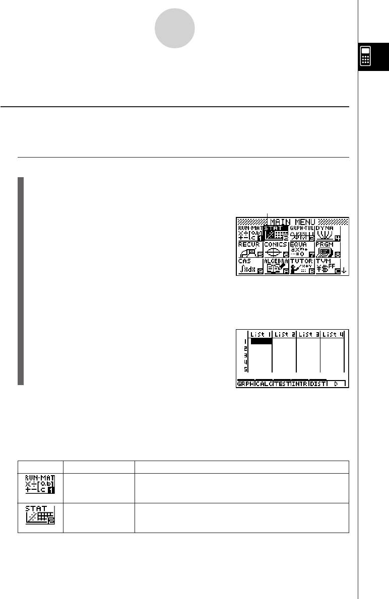
This section describes how to select an icon in the Main Menu to enter the mode you want.
uu
uu
uTo select an icon
1. Press m to display the Main Menu.
2. Use the cursor keys (d, e, f, c) to move the highlighting to the icon you want.
3. Press w to display the initial screen of the mode whose icon you selected.
Here we will enter the STAT Mode.
•You can also enter a mode without highlighting an icon in the Main Menu by inputting
the number or letter marked in the lower right corner of the icon.
Currently selected icon
* The above shows the ALGEBRA
FX 2.0 PLUS screen.
Icon Mode Name Description
RUN • MATrix Use this mode for arithmetic calculations and function
calculations, and for calculations involving binary, octal,
decimal, and hexadecimal values and matrices.
STATistics Use this mode to perform single-variable (standard deviation)
and paired-variable (regression) statistical calculations, to
analyze data and to draw statistical graphs.
The following explains the meaning of each icon.
20010102
19990401
1-2-2
Display
Icon Mode Name Description
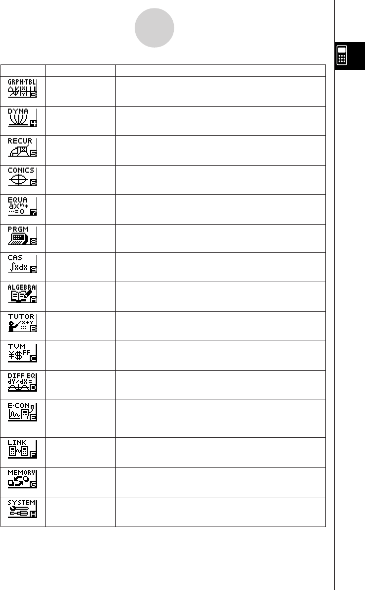
GRaPH-TaBLe Use this mode to store functions, to generate a numeric table
of different solutions as the values assigned to variables in a
function change, and to draw graphs.
DYNAmic graph Use this mode to store graph functions and to draw multiple
versions of a graph by changing the values assigned to the
variables in a function.
RECURsion Use this mode to store recursion formulas, to generate a
numeric table of different solutions as the values assigned to
variables in a function change, and to draw graphs.
CONICS Use this mode to draw graphs of conic sections.
EQUAtion Use this mode to solve linear equations with 2 to 30
unknowns, and higmh degree (2 to 30) equations.
PRoGraM Use this mode to store programs in th program area and to
run programs.
Computer Algebra Use this mode to perform algebraic calculations.
System (ALGEBRA FX 2.0 PLUS only)
ALGEBRA Use this mode for step-by-step solution of expressions.
(ALGEBRA FX 2.0 PLUS only)
TUTORial Use this mode to determine the expression type and solve
mode, and for interactive equation solutions.
(ALGEBRA FX 2.0 PLUS only)
TVM Use this mode to perform financial calculations.
(Financial) (On the FX 1.0 PLUS menu, the icon has the number 9 in the
lower right corner.) to make other system settings.
DIFFerential Use this mode to solve differential equations.
EQuation (On the FX 1.0 PLUS menu, the icon has the letter A in the
lower right corner.)
E-CON Use this mode when you want to control a CASIO EA-100
unit from this calculator.
(On the FX 1.0 PLUS menu, the icon has the letter B in the
lower right corner.)
LINK Use this mode to transfer memory contents or back-up data
to another unit. (On the FX 1.0 PLUS menu, the icon has the
letter C in the lower right corner.)
MEMORY Use this mode to manage data stored in memory.
(On the FX 1.0 PLUS menu, the icon has the letter D in the
lower right corner.)
SYSTEM Use this mode to initialize memory, adjust contrast, and to
make other system settings. (On the FX 1.0 PLUS menu, the
icon has the letter E in the lower right corner.)
20011101
19990401
kk
kk
kAbout the Function Menu
Use the function keys (1 to 6) to access the menus and commands in the menu bar
along the bottom of the display screen. You can tell whether a menu bar item is a menu or a
command by its appearance.
• Command (Example: )
Pressing a function key that corresponds to a menu bar command executes the command.
• Pull-up Menu (Example: )
Pressing a function key that corresponds to a pull-up menu opens the menu.
You can use either of the following two methods to select a command from a pull-up menu.
•Input the key to the left of the command on the pull-up menu.
•Use the f and c cursor keys to move the highlighting to the command you want, and
then press w.
The symbol ' to the right of a command indicates that executing the command displays a
submenu.
To cancel the pull-up menu without inputting the command, press i.
kk
kk
kAbout Display Screens
This calculator uses two types of display screens: a text screen and a graphic screen. The
text screen can show 21 columns and 8 lines of characters, with the bottom line used for the
function key menu. The graph screen uses an area that measures 127 (W) × 63 (H) dots.
Text Screen Graph Screen
The contents of each type of screen are stored in independent memory areas.
Press u5(G↔T) to switch between the graphic screen and text screen.
1-2-3
Display
#The symbol ↑ in the upper left corner of a pull-
up menu indicates that there are more
commands running off the top of the menu.
Use the cursor keys to scroll the menu contents to
view the commands running off the top.
19990401
kk
kk
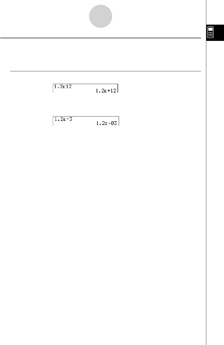
kNormal Display
The calculator normally displays values up to 10 digits long. Values that exceed this limit are
automatically converted to and displayed in exponential format.
uHow to interpret exponential format
1.2E+12 indicates that the result is equivalent to 1.2 × 10¹². This means that you should move
the decimal point in 1.2 twelve places to the right, because the exponent is positive. This
results in the value 1,200,000,000,000.
1.2E–03 indicates that the result is equivalent to 1.2 × 10⁻³. This means that you should move
the decimal point in 1.2 three places to the left, because the exponent is negative. This
results in the value 0.0012.
You can specify one of two different ranges for automatic changeover to normal display.
Norm 1 .................. 10–2 (0.01) > |x|, |x| > 1010
Norm 2 .................. 10–9 (0.000000001) > |x|, |x| > 1010
All of the examples in this manual show calculation results using Norm 1.
See page 2-3-2 for details on switching between Norm 1 and Norm 2.
1-2-4
Display
19990401
kk
kk
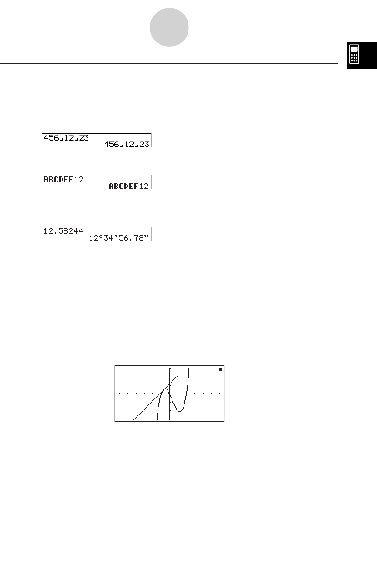
kSpecial Display Formats
This calculator uses special display formats to indicate fractions, hexadecimal values, and
degrees/minutes/seconds values.
uFractions
................. Indicates: 456
uHexadecimal Values
................. Indicates: ABCDEF12(16), which
equals –1412567278(10)
uDegrees/Minutes/Seconds
................. Indicates: 12° 34’ 56.78”
•In addition to the above, this calculator also uses other indicators or symbols, which are
described in each applicable section of this manual as they come up.
kk
kk
kCalculation Execution Indicator
Whenever the calculator is busy drawing a graph or executing a long, complex calculation or
program, a black box “k” flashes in the upper right corner of the display. This black box tells
you that the calculator is performing an internal operation.
1-2-5
Display
12
––––
23
19990401
1-3 Inputting and Editing Calculations
kk
kk
kInputting Calculations
When you are ready to input a calculation, first press A to clear the display. Next, input
your calculation formulas exactly as they are written, from left to right, and press w to
obtain the result.
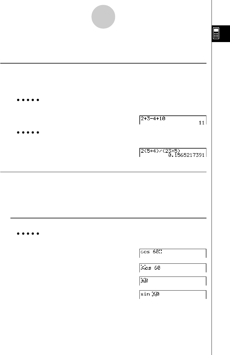
Example 1 2 + 3 – 4 + 10 =
Ac+d-e+baw
Example 2 2(5 + 4) ÷ (23 × 5) =
Ac(f+e)/
(cd*f)w
kEditing Calculations
Use the d and e keys to move the cursor to the position you want to change, and then
perform one of the operations described below. After you edit the calculation, you can
execute it by pressing w. Or you can use e to move to the end of the calculation and input
more.
uTo change a step
Example To change cos60 to sin60
Acga
ddd
D
s
1-3-1
Inputting and Editing Calculations
19990401
uTo delete a step
Example To change 369 × × 2 to 369 × 2
Adgj**c
ddD
uTo insert a step
Example To change 2.362 to sin2.362
Ac.dgx
ddddd
s
uTo change the last step you input
Example To change 396 × 3 to 396 × 2
Adgj*d
D
c
1-3-2
Inputting and Editing Calculations
19990401
kk
kk
kUsing Replay Memory
The last calculation performed is always stored into replay memory. You can recall the
contents of the replay memory by pressing d or e.
If you press e, the calculation appears with the cursor at the beginning. Pressing d
causes the calculation to appear with the cursor at the end. You can make changes in the
calculation as you wish and then execute it again.
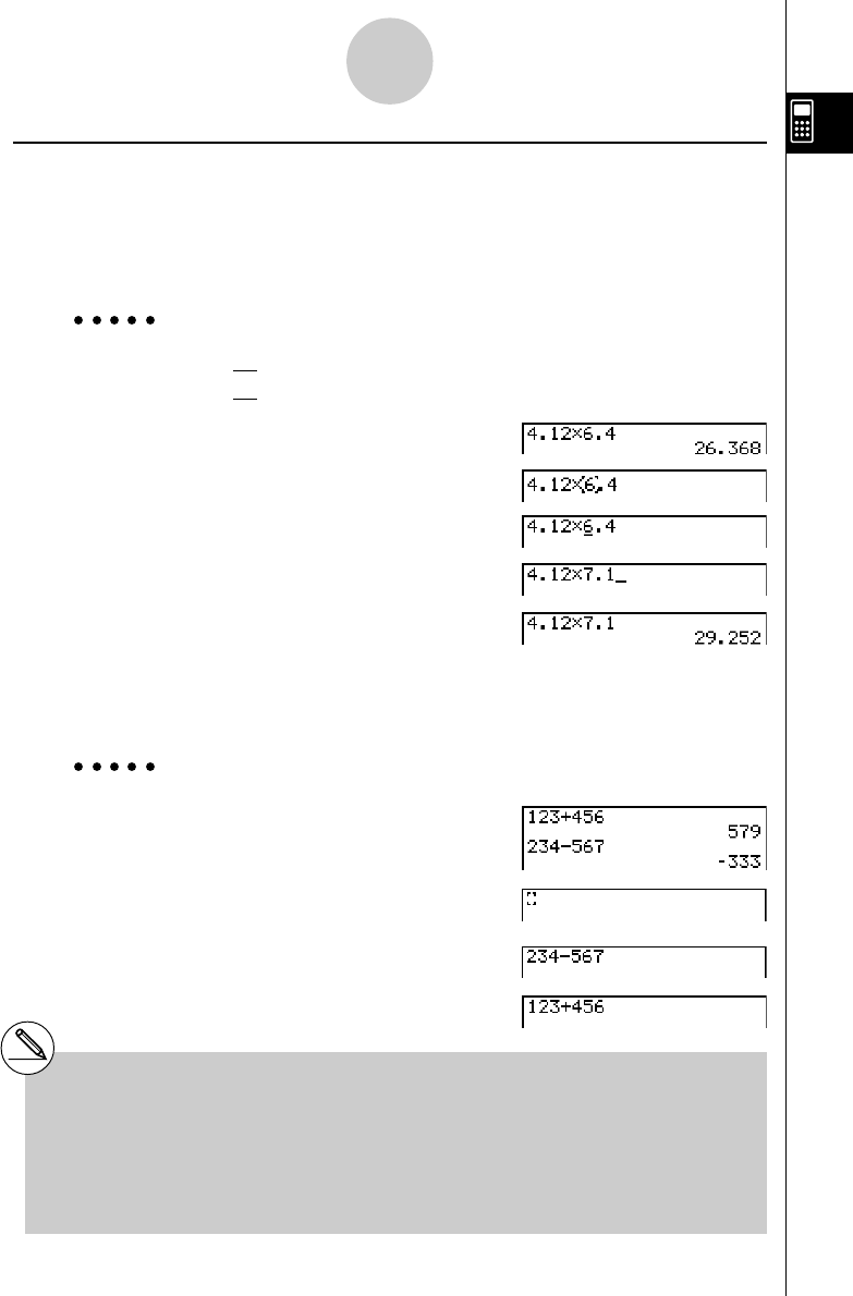
Example 1 To perform the following two calculations
4.12 × 6.4 = 26.368
4.12 × 7.1 = 29.252
Ae.bc*g.ew
dddd
!D(INS)
h.b
w
After you press A, you can press f or c to recall previous calculations, in sequence
from the newest to the oldest (Multi-Replay Function). Once you recall a calculation, you can
use e and d to move the cursor around the calculation and make changes in it to create
a new calculation.
Example 2
Abcd+efgw
cde-fghw
A
f (One calculation back)
f (Two calculations back)
1-3-3
Inputting and Editing Calculations
# Pressing !D(INS) changes the cursor to
‘‘_’’. The next function or value you input is
overwritten at the location of ‘‘_’’. To abort this
operation, press !D(INS) again.
#A calculation remains stored in replay memory
until you perform another calculation or
change modes.
#The contents of replay memory are not cleared
when you press the A key, so you can recall a
calculation and execute it even after performing
the all clear operation.
19990401
1-3-4
Inputting and Editing Calculations
kMaking Corrections in the Original Calculation
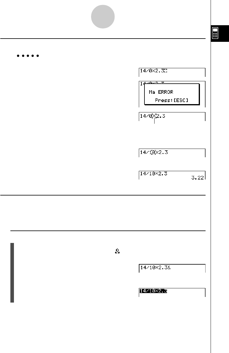
Example 14 ÷ 0 × 2.3 entered by mistake for 14 ÷ 10 × 2.3
Abe/a*c.d
w
Press i.
Make necessary changes.
db
Execute again.
w
kk
kk
kCopy and Paste
You can temporarily copy commands, programs, and other text data you input to a memory
area called “the clipboard,” and then paste it to another location on the display.
uTo specify the copy range
1. Move the cursor (t) the beginning or end of the range of text you want to copy and
then press u. This changes the cursor to “ ”.
2. Use the cursor keys to move the cursor and highlight the range of text you want to copy.
Cursor is positioned automatically at the
location of the cause of the error.
19990401
3. Press u1 (COPY) to copy the highlighted text to the clipboard, and exit the copy
range specification mode.
To cancel text highlighting without performing a copy operation, press i.
uPasting Text
Move the cursor to the location where you want to paste the text, and then press u
2(PASTE). The contents of the clipboard are pasted at the cursor position.
A
u2(PASTE)
kk
kk
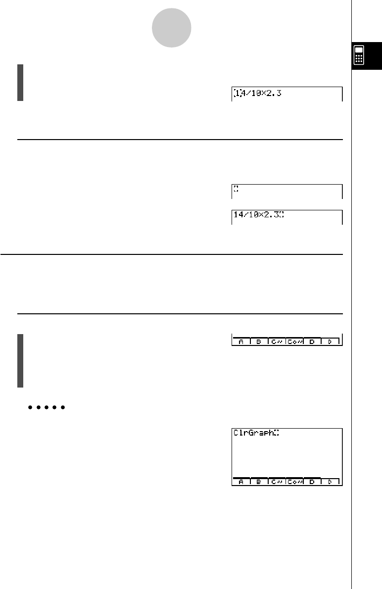
kCatalog Function
The Catalog is an alphabetic list of all the commands available on this calculator. You can
input a command by calling up the Catalog and then selecting the command you want.
uTo use the Catalog to input a command
1. Press u4(CAT/CAL) to display the Catalog at
the bottom of the screen.
2. Press the function key that matches the first letter of the command you want to input.
3. Select the command from the pull-up menu.
Example 1 To use the Catalog to input the ClrGraph command
Au4(CAT/CAL)3(C~)h(CLR)
b(Graph)
1-3-5
Inputting and Editing Calculations

19990401
Example 2 To use the Catalog to input the Prog command
Au4(CAT/CAL)6(g)6(g)
5(P)I(Prog)
Pressing i or !i(QUIT) closes the Catalog.
1-3-6
Inputting and Editing Calculations

19990401
1-4 Option (OPTN) Menu
The option menu gives you access to scientific functions and features that are not marked on
the calculator’s keyboard. The contents of the option menu differ according to the mode you
are in when you press the K key.
See “8-7 Program Mode Command List” for details on the option (OPTN) menu.
uOption Menu in the RUN • MAT or PRGM Mode
•{LIST} ... {list function menu}
•{MAT} ... {matrix operation menu}
•{CPLX} ... {complex number calculation menu}
•{CALC} ... {functional analysis menu}
•{NUM} ... {numeric calculation menu}
•{PROB} ... {probability/distribution calculation menu}
•{HYP} ... {hyperbolic calculation menu}
•{ANGL} ... {menu for angle/coordinate conversion, DMS input/conversion}
•{STAT} ... {paired-variable statistical estimated value menu}
•{FMEM} ... {function memory menu}
•{ZOOM} ... {zoom function menu}
•{SKTCH} ... {sketch function menu}
•{PICT} ... {picture memory menu}
•{SYBL} ... {symbol menu}
•{° ’ ”} … {DMS}
•{ ° ’ ”} … {DMS conversion}
•{ENG}/{ ENG} … {ENG conversion}
1-4-1
Option (OPTN) Menu
#The option (OPTN) menu does not appear
during binary, octal, decimal, and hexadecimal
calculations.

19990401
The following shows the function menus that appear under other conditions.
uOption Menu when a number table value is displayed in the GRPH • TBL or
RECUR Mode
•{LMEM} … {list memory menu}
•{ ° ’ ”}/{ENG}/{ ENG}
uOption Menu in the CAS or ALGEBRA or TUTOR Mode
(ALGEBRA FX 2.0 PLUS only) t
•{∞} … {infinity}
•{Abs} … {absolute value}
•{x!} … {factorial}
•{sign} … {signum function}
•{HYP}/{FMEM}
The meanings of the option menu items are described in the sections that cover each mode.
1-4-2
Option (OPTN) Menu
1999120120010102

19990401
1-5 Variable Data (VARS) Menu
To recall variable data, press J to display the variable data menu.
{V-WIN}/{FACT}/{STAT}/{GRPH}/{DYNA}/
{TABL}/{RECR}/{EQUA*1}
See “8-7 Program Mode Command List” for details on the variable data (VARS) menu.
u V-WIN — Recalling View Window values
•{Xmin}/{Xmax}/{Xscale}/{Xdot}
…X-axis {minimum value}/{maximum value}/{scale}/{dot value*2}
•{Ymin}/{Ymax}/{Yscale}
…Y-axis {minimum value}/{maximum value}/{scale}
•{T
θ
min}/{T
θ
max}/{T
θ
ptch}
…T, θ {minimum value}/{maximum value}/{pitch}
•{R-Xmin}/{R-Xmax}/{R-Xscl}/{R-Xdot}
…Dual Graph right graph X-axis {minimum value}/{maximum value}/{scale}/
{dot value*2}
•{R-Ymin}/{R-Ymax}/{R-Yscl}
…Dual Graph right graph Y-axis {minimum value}/{maximum value}/{scale}
•{R-Tmin}/{R-Tmax}/{R-Tpch}
…Dual Graph right graph T,
θ
{minimum value}/{maximum value}/{pitch}
u FACT — Recalling zoom factors
•{Xfact}/{Yfact}
... {x-axis factor}/{y-axis factor}
1-5-1
Variable Data (VARS) Menu
*1The EQUA item appears only when you
access the variable data menu from the
RUN
•
MAT or PRGM Mode.
#The variable data menu does not appear if
you press J while binary, octal, decimal, or
hexadecimal is set as the default number
system.
*2The dot value indicates the display range (Xmax
value – Xmin value) divided by the screen dot
pitch (126).
The dot value is normally calculated automati-
cally from the minimum and maximum values.
Changing the dot value causes the maximum to
be calculated automatically.

19990401
u STAT — Recalling statistical data
• {n} … {number of data}
• {X} … {single-variable, paired-variable x-data}
•{
oo
oo
o}/{Σx}/{Σx2}/{x
σ
n}/{x
σ
n–1}/{minX}/{maxX}
…{mean}/{sum}/{sum of squares}/{population standard deviation}/{sample
standard deviation}/{minimum value}/{maximum value}
• {Y} ... {paired-variable y-data}
•{
pp
pp
p
}/{Σ
y}/{Σ
y2}/{Σ
xy}/{
y
σ
n}/{
y
σ
n–1}/{minY}/{maxY}
…{mean}/{sum}/{sum of squares}/{sum of products of x-data and y-data}/
{population standard deviation}/{sample standard deviation}/{minimum value}/
{maximum value}
•{GRAPH} ... {graph data menu}
•{a}/{b}/{c}/{d}/{e}
... {regression coefficient and polynomial coefficients}
•{r}/{r2}
... {correlation coefficient}
•{Q1}/{Q3}
... {first quartile}/{third quartile}
•{Med}/{Mod}
... {median}/{mode} of input data
•{H-Strt}/{H-ptch}
... histogram {start division}/{pitch}
•{PTS} ... {summary point data menu}
•{x1}/{y1}/{x2}/{y2}/{x3}/{y3} ... {coordinates of summary points}
1-5-2
Variable Data (VARS) Menu
20011101

19990401
u GRPH — Recalling Graph Functions
•{Yn}/{rn}
... {rectangular coordinate or inequality function}/{polar coordinate function}
•{Xtn}/{Ytn}
... parametric graph function {Xt}/{Yt}
•{Xn} ... {X=constant graph function}
(Press these keys before inputting a value to specify a storage area.)
u DYNA — Recalling Dynamic Graph Set Up Data
•{Start}/{End}/{Pitch}
... {coefficient range start value}/{coefficient range end value}/{coefficient value
increment}
u TABL — Recalling Table & Graph Set Up and Content Data
•{Start}/{End}/{Pitch}
... {table range start value}/{table range end value}/{table value increment}
•{Result*1}
... {matrix of table contents}
1-5-3
Variable Data (VARS) Menu
*1 The Result item appears only when the TABL
menu is displayed in the RUN
•
MAT or PRGM
Mode.

19990401
u RECR — Recalling Recursion Formula*1, Table Range, and Table Content Data
• {FORM}... {recursion formula data menu}
• {an}/{an+1}/{an+2}/{bn}/{bn+1}/{bn+2}/{cn}/{cn+1}/{cn+2}
... {an}/{an+1}/{an+2}/{bn}/{bn+1}/{bn+2}/{cn}/{cn+1}/{cn+2} expressions
• {RANGE} ... {table range data menu}
• {R-Strt}/{R-End}
... table range {start value}/{end value}
• {a0}/{a1}/{a2}/{b0}/{b1}/{b2}/{c0}/{c1}/{c2}
... {a0}/{a1}/{a2} {b0}/{b1}/{b2}/{c0}/{c1}/{c2} value
• {anStrt}/{bnStrt}/{cnStrt}
... origin of {an
}/{bn}/{cn} recursion formula convergence/divergence graph (WEB
graph)
• {Result*2} ... {matrix of table contents*3}
u EQUA — Recalling Equation Coefficients and Solutions*4 *5
•{S-Rslt}/{S-Coef}
... matrix of {solutions}/{coefficients} for linear equations*6
•{P-Rslt}/{P-Coef}
... matrix of {solution}/{coefficients} for a high degree equation
1-5-4
Variable Data (VARS) Menu
*1An error occurs when there is no function or
recursion formula numeric table in memory.
*2 “Result” is available only in the RUN
•
MAT and
PRGM Modes.
*3Table contents are stored automatically in
Matrix Answer Memory (MatAns).
*4Coefficients and solutions are stored
automatically in Matrix Answer Memory
(MatAns).
*5 The following conditions cause an error.
—When there are no coefficients input for the
equation
—When there are no solutions obtained for the
equation
*6 Coefficient and solution memory data for a
linear equation cannot be recalled at the same
time.

19990401
1-6 Program (PRGM) Menu
To display the program (PRGM) menu, first enter the RUN • MAT or PRGM Mode from the
Main Menu and then press !J(PRGM). The following are the selections available in the
program (PRGM) menu.
• {Prog}........ {program recall}
• {JUMP}...... {jump command menu}
• {?}.............. {input prompt}
• {^}............. {output command}
• {I/O}............ {I/O control/transfer command menu}
• {IF}............. {conditional jump command menu}
• {FOR}......... {loop control command menu}
• {WHLE}...... {conditional loop control command menu}
• {CTRL}....... {program control command menu}
• {LOGIC}..... {logical operation command menu}
• {CLR}......... {clear command menu}
• {DISP}........ {display command menu}
• {:}............... {multistatement connector}
The following function key menu appears if you press !J(PRGM) in the RUN • MAT
Mode or the PRGM Mode while binary, octal, decimal, or hexadecimal is set as the default
number system.
• {Prog}/{JUMP}/{?}/{^}/{:}
• {= GG
GG
G <}....... {relational operator menu}
The functions assigned to the function keys are the same as those in the Comp Mode.
For details on the commands that are available in the various menus you can access from
the program menu, see “8. Programming”.
1-6-1
Program (PRGM) Menu
19990401
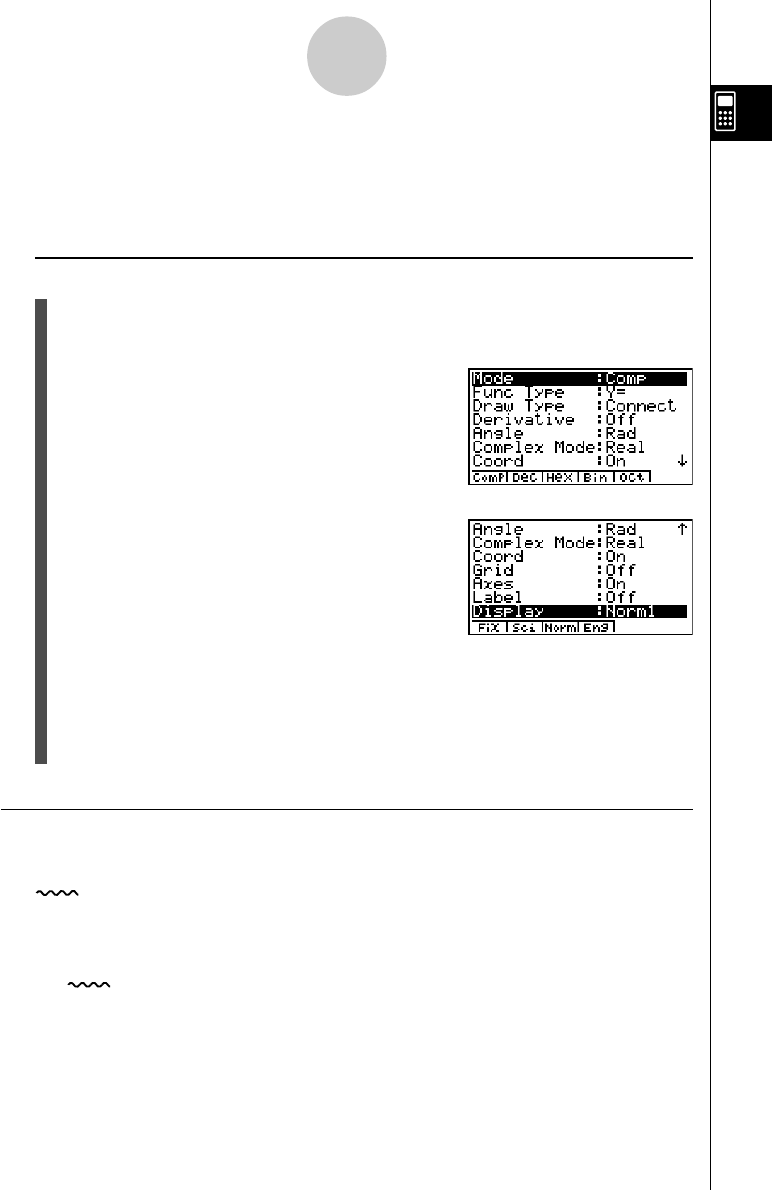
1-7 Using the Set Up Screen
The mode’s set up screen shows the current status of mode settings and lets you make any
changes you want. The following procedure shows how to change a set up.
uTo change a mode set up
1. Select the icon you want and press w to enter a mode and display its initial screen.
Here we will enter the RUN • MAT Mode.
2. Press u3(SET UP) to display the mode’s
SET UP screen.
•This SET UP screen is just one possible example.
Actual SET UP screen contents will differ
according to the mode you are in and that mode’s
current settings.
3. Use the f and c cursor keys to move the highlighting to the item whose setting you
want to change.
4. Press the function key (1 to 6) that is marked with the setting you want to make.
5. After you are finished making any changes you want, press i to return to the initial
screen of the mode.
kSET UP Screen Function Key Menus
This section details the settings you can make using the function keys in the SET UP display.
indicates default setting.
uMode (calculation/binary, octal, decimal, hexadecimal mode)
•{Comp}... {arithmetic calculation mode}
•{Dec}/{Hex}/{Bin}/{Oct}
... {decimal}/{hexadecimal}/{binary}/{octal}
1-7-1
Using the Set Up Screen
...
20011101

19990401
uFunc Type (graph function type)
Pressing one of the following function keys also switches the function of the v key.
•{Y=}/{r=}/{Parm}/{X=c}
... {rectangular coordinate}/{polar coordinate}/{parametric coordinate}/
{X = constant} graph
•{Y>}/{Y<}/{Yt}/{Ys}
... {y>f(x)}/{y<f(x)}/{y≥f(x)}/{y≤f(x)} inequality graph
uDraw Type (graph drawing method)
•{Con}/{Plot}
... {connected points}/{unconnected points}
uDerivative (derivative value display)
•{On}/{Off}
... {display on}/{display off} while Graph-to-Table, Table & Graph, and Trace are
being used
uAngle (default angle unit)
•{Deg}/{Rad}/{Gra}
... {degrees}/{radians}/{grads}
uComplex Mode
•{Real}... {calculation in real number range only}
•{a + bi}/{r
·
e^
θ
i}
... {rectangular format}/{polar format} display of a complex calculation
uCoord (graph pointer coordinate display)
•{On}/{Off}
... {display on}/{display off}
uGrid (graph gridline display)
•{On}/{Off}
... {display on}/{display off}
uAxes (graph axis display)
•{On}/{Off}
... {display on}/{display off}
uLabel (graph axis label display)
•{On}/{Off}
... {display on}/{display off}
1-7-2
Using the Set Up Screen

19990401
uDisplay (display format)
•{Fix}/{Sci}/{Norm}/{Eng}
... {fixed number of decimal places specification}/{number of significant digits
specification}/{normal display setting}/{Engineering Mode}
uStat Wind (statistical graph view window setting method)
•{Auto}/{Man}
... {automatic}/{manual}
uReside List (residual calculation)
•{None}/{LIST}
... {no calculation}/{list specification for the calculated residual data}
uList File (list file display settings)
•{FILE}... {settings of list file on the display}
uVariable (table generation and graph draw settings)
•{Rang}/{LIST}
... {use table range}/{use list data}
uGraph Func (function display during graph drawing and trace)
•{On}/{Off}
... {display on}/{display off}
uDual Screen (Dual Screen Mode status)
•{T+G}/{G+G}/{GtoT}/{Off}
... {graph on one side and numeric table on the other side of Dual Screen}/
{graphing on both sides of Dual Screen}/{graph on one side and numeric table
on the other side of Dual Screen}/{Dual Screen off}
uSimul Graph (simultaneous graphing mode)
•{On}/{Off}
... {simultaneous graphing on (all graphs drawn simultaneously)}/{simultaneous
graphing off (graphs drawn in area numeric sequence)}
uBackground (graph display background)
•{None}/{PICT}
... {no background}/{graph background picture specification}
1-7-3
Using the Set Up Screen

19990401
uDynamic Type (Dynamic Graph locus setting)
•{Cnt}/{Stop}
... {non-stop (continuous)}/{automatic stop after 10 draws}
uΣ Display (Σ value display in recursion table)
•{On}/{Off}
... {display on}/{display off}
uSlope (display of derivative at current pointer location in conic section
graph)
•{On}/{Off}
... {display on}/{display off}
uAnswer Type (result range specification) (ALGEBRA FX 2.0 PLUS only)
•{Real}/{Cplx}
... {real number}/{complex number} range result
uH-Copy (screen shot settings)
•{Dirct}/{Mem}
... {direct send}/{store in memory}
1-7-4
Using the Set Up Screen
20011101

19990401
1-8 When you keep having problems…
If you keep having problems when you are trying to perform operations, try the following
before assuming that there is something wrong with the calculator.
kk
kk
kGetting the Calculator Back to its Original Mode Settings
1. From the Main Menu, enter the SYSTEM Mode.
2. Press 5(Reset).
3. Press 1(S/U), and then press w(Yes).
4. Press m to return to the Main Menu.
Now enter the correct mode and perform your calculation again, monitoring the results on the
display.
kk
kk
kIn Case of Hang Up
•Should the unit hang up and stop responding to input from the keyboard, press the P
button on the back of the calculator to reset the calculator to its initial defaults (see
page α-6-1). Note, however, that this may clear all the data in calculator memory.
1-8-1
When you keep having problems…
19990401
kk
kk
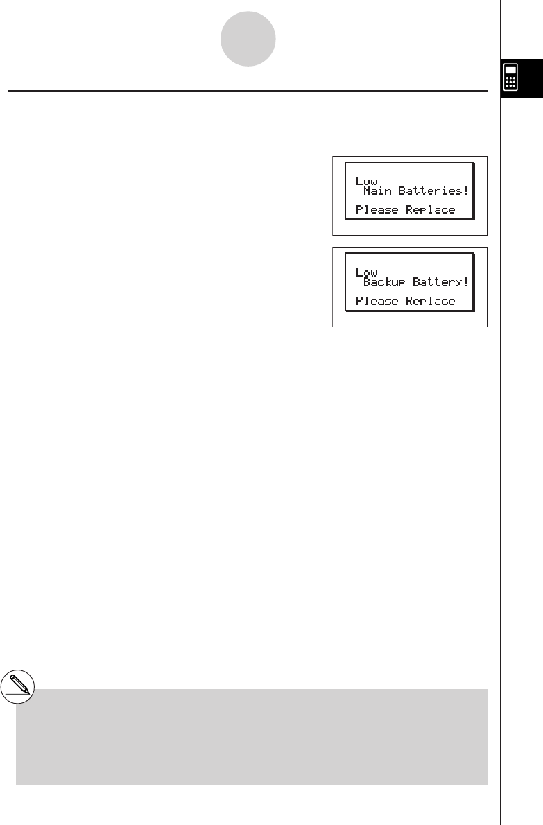
kLow Battery Message
If either of the following messages appears on the display, immediately turn off the calculator
and replace main batteries or the back up battery as instructed.
If you continue using the calculator without replacing main batteries, power will automatically
turn off to protect memory contents. Once this happens, you will not be able to turn power
back on, and there is the danger that memory contents will be corrupted or lost entirely.
#You will not be able to perform data
communications operations after the low
battery message appears.
1-8-2
When you keep having problems…
#If main batteries and the back up battery go
low at the same time (indicated when both of
the messages described above appear),
replace the back up battery first and then
replace the main batteries.

19990401
2-1-1
Basic Calculations
2-1 Basic Calculations
kk
kk
kArithmetic Calculations
•Enter arithmetic calculations as they are written, from left to right.
•Use the - key to input the minus sign before a negative value.
•Calculations are performed internally with a 15-digit mantissa. The result is rounded to a
10-digit mantissa before it is displayed.
•For mixed arithmetic calculations, multiplication and division are given priority over
addition and subtraction.
Example Operation
23 + 4.5 – 53 = –25.5 23+4.5-53w
56 × (–12) ÷ (–2.5) = 268.8 56*-12/-2.5w
(2 + 3) × 102 = 500 (2+3)*1E2w*1
1 + 2 – 3 × 4 ÷ 5 + 6 = 6.6 1+2-3*4/5+6w
100 – (2 + 3) × 4 = 80 100-(2+3)*4w
2 + 3 × (4 + 5) = 29 2+3*(4+5w*2
(7 – 2) × (8 + 5) = 65 (7-2)(8+5)w*3
6= 0.3 6 /(4*5)w*4
4×5
(1 + 2i) + (2 + 3i) = 3 + 5i(b+c!a(i))+(c+
d!a(i))w
(2 + i) × (2 – i) = 5 (c+!a(i))*(c-!a(i)
)w
*1(2+3)E2 does not produce the correct
result. Be sure to enter this calculation as shown.
*2Final closed parentheses (immediately before
operation of the w key) may be omitted, no
matter how many are required.
*3A multiplication sign immediately before an open
parenthesis may be omitted.
*4This is identical to 6 / 4 / 5 w.

19990401
2-1-2
Basic Calculations
*1Displayed values are rounded off to the place
you specify.
kk
kk
kNumber of Decimal Places, Number of Significant Digits, Normal
Display Range [SET UP]- [Display] -[Fix] / [Sci] / [Norm]
•Even after you specify the number of decimal places or the number of significant digits,
internal calculations are still performed using a 15-digit mantissa, and displayed values
are stored with a 10-digit mantissa. Use Rnd of the Numeric Calculation Menu (NUM)
(page 2-4-1) to round the displayed value off to the number of decimal place and
significant digit settings.
•Number of decimal place (Fix) and significant digit (Sci) settings normally remain in effect
until you change them or until you change the normal display range (Norm) setting.
Example 100 ÷ 6 = 16.66666666...
Condition Operation Display
100/6w16.66666667
4 decimal places u3(SET UP)
cccccccccc
*1
1(Fix)ewiw16.6667
5 significant digits u3(SET UP)
cccccccccc
*1
2(Sci)fwiw1.6667E+01
Cancels specification u3(SET UP)
cccccccccc
3(Norm)iw16.66666667
20011101
1999040120011101
2-1-3
Basic Calculations
Example 200 ÷ 7 × 14 = 400
Condition Operation Display
200/7*14w400
3 decimal places u3(SET UP)
cccccccccc
1(Fix)dwiw400.000
Calculation continues 200/7w28.571
using display capacity *Ans ×
of 10 digits 14w400.000
• If the same calculation is performed using the specified number of digits:
200/7w28.571
The value stored K5(NUM)e(Rnd)w28.571
internally is rounded *Ans ×
off to the number of 14w399.994
decimal places you
specify.
kk
kk
kCalculation Priority Sequence
This calculator employs true algebraic logic to calculate the parts of a formula in the following
order:
1Coordinate transformation Pol (x, y), Rec (r,
θ
)
Differentials, quadratic differentials, integrations, Σ calculations
d/dx, d2/dx2, ∫dx, Σ, Mat, Solve, FMin, FMax, List→Mat, Seq, Min, Max, Median, Mean,
Augment, Mat →List, P(, Q(, R(, t(, List
Composite functions*1 fn, Yn, rn, Xtn, Ytn, Xn
2Type A functions
With these functions, the value is entered and then the function key is pressed.
x2, x–1, x !, ° ’ ”, ENG symbols, angle unit o, r, g
*1You can combine the contents of multiple
function memory (fn) locations or graph
memory (Yn, rn, Xtn, Ytn, Xn) locations into
composite functions. Specifying fn1(fn2),
for example, results in the composite function
fn1°fn2 (see page 5-3-3).
A composite function can consist of up to five
functions.
1999040120011101
2-1-4
Basic Calculations
3Power/root ^(xy), x
4Fractions ab/c
5Abbreviated multiplication format in front of π, memory name, or variable name.
2π, 5A, Xmin, F Start, etc.
6Type B functions
With these functions, the function key is pressed and then the value is entered.
, 3, log, In, ex, 10x, sin, cos, tan, sin–1, cos–1, tan–1, sinh, cosh, tanh, sinh–1, cosh–1,
tanh–1, (–), d, h, b, o, Neg, Not, Det, Trn, Dim, Identity, Sum, Prod, Cuml, Percent, AList,
Abs, Int, Frac, Intg, Arg, Conjg, ReP, ImP
7Abbreviated multiplication format in front of Type B functions
2, A log2, etc.3
8Permutation, combination nPr, nCr
9× , ÷
0+, –
!Relational operators >, <, ≥, ≤
@Relational operators =, G
#and (bitwise operation)
$xnor, xor (bitwise operations)
%or (bitwise operation)
^And (logical operation)
Or (logical operation)
Example 2 + 3 × (log sin2π2 + 6.8) = 22.07101691 (angle unit = Rad)
1
2
3
4
5
6
#When functions with the same priority are used
in series, execution is performed from right to
left.
exIn → ex{In( )}
120 120
Otherwise, execution is from left to right.
#Compound functions are executed from right to
left.
#Anything contained within parentheses receives
highest priority.

19990401
2-1-5
Basic Calculations
# Other errors can occur during program
execution. Most of the calculator’s keys
are inoperative while an error message is
displayed.
Press i to clear the error and display
the error position (see page 1-3-4).
# See the “Error Message Table” on page α-1-1
for information on other errors.
kMultiplication Operations without a Multiplication Sign
You can omit the multiplication sign (×) in any of the following operations.
•Before coordinate transformation and Type B functions (1 on page 2-1-3 and 6 on page
2-1-4), except for negative signs
Example 2sin30, 10log1.2, 2 , 2Pol(5, 12), etc.
•Before constants, variable names, memory names
Example 2π, 2AB, 3Ans, 3Y1, etc.
•Before an open parenthesis
Example 3(5 + 6), (A + 1)(B – 1), etc.
kOverflow and Errors
Exceeding a specified input or calculation range, or attempting an illegal input causes an
error message to appear on the display. Further operation of the calculator is impossible
while an error message is displayed. The following events cause an error message to appear
on the display.
•When any result, whether intermediate or final, or any value in memory exceeds
±9.999999999 × 1099 (Ma ERROR).
•When an attempt is made to perform a function calculation that exceeds the input range
(Ma ERROR).
•When an illegal operation is attempted during statistical calculations (Ma ERROR). For
example, attempting to obtain 1VAR without data input.
• When an improper data type is specified for the argument of a function calculation
(Ma ERROR).
•When the capacity of the numeric value stack or command stack is exceeded (Stack
ERROR). For example, entering 25 successive ( followed by 2 + 3 * 4 w.
•When an attempt is made to perform a calculation using an illegal formula (Syntax
ERROR). For example, 5 ** 3 w.
20010102

19990401
•When you try to perform a calculation that causes memory capacity to be exceeded
(Memory ERROR).
•When you use a command that requires an argument, without providing a valid argument
(Argument ERROR).
•When an attempt is made to use an illegal dimension during matrix calculations (Dimension
ERROR).
• When you are in the real mode and an attempt is made to perform a calculation that
produces a complex number solution. Note that “Real” is selected for the Complex Mode
setting on the SET UP Screen (Non-Real ERROR).
kMemory Capacity
Each time you press a key, either one byte or two bytes is used. Some of the functions that
require one byte are: b, c, d, sin, cos, tan, log, In, , and π. Some of the functions that
take up two bytes are d/dx(, Mat, Xmin, If, For, Return, DrawGraph, SortA(, PxIOn, Sum, and
an+1.
2-1-6
Basic Calculations
#As you input numeric values or commands,
they appear flush left on the display.
Calculation results, on the other hand, are
displayed flush right.
#The allowable range for both input and output
values is 15 digits for the mantissa and two
digits for the exponent. Internal calculations
are also performed using a 15-digit mantissa
and two-digit exponent.
20011101
19990401
2-2 Special Functions
kk
kk
kCalculations Using Variables
Example Operation Display
193.2aav(A)w193.2
193.2 ÷ 23 = 8.4 av(A)/23w8.4
193.2 ÷ 28 = 6.9 av(A)/28w6.9
kk
kk
kMemory
uVariables
This calculator comes with 28 variables as standard. You can use variables to store values
you want to use inside of calculations. Variables are identified by single-letter names, which
are made up of the 26 letters of the alphabet, plus r and
θ
. The maximum size of values that
you can assign to variables is 15 digits for the mantissa and 2 digits for the exponent.
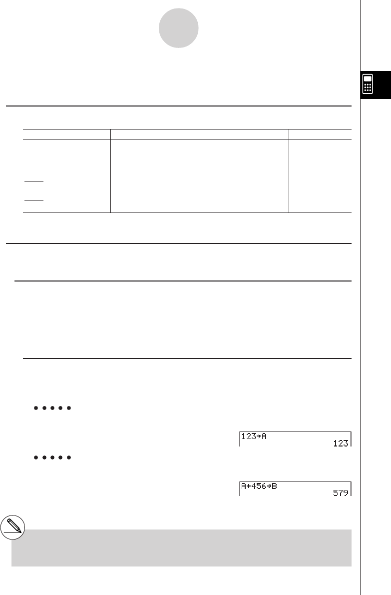
uTo assign a value to a variable
[value] a [variable name] w
Example To assign 123 to variable A
Abcdaav(A)w
Example To add 456 to variable A and store the result in variable B
Aav(A)+efgaa
l(B)w
2-2-1
Special Functions
# Variable contents are retained even when
you turn power off.
19990401
uTo display the contents of a variable
Example To display the contents of variable A
Aav(A)w
uTo clear a variable
Example To clear variable A
Aaaav(A)w
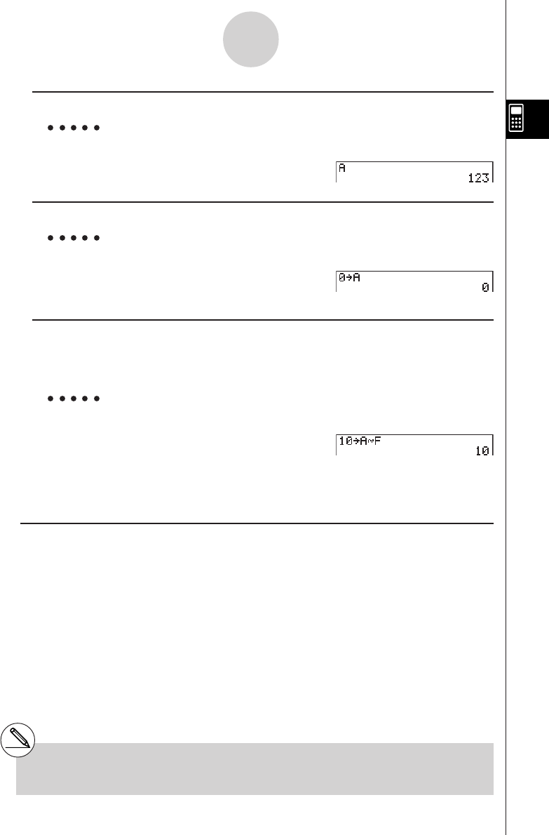
uTo assign the same value to more than one variable
[value]a [first variable name*1]K6(g)6(g)4(SYBL)d(~) [last variable
name*1]w
Example To assign a value of 10 to variables A through F
Abaaav(A)
K6(g)6(g)4(SYBL)d(~)
at(F)w
uFunction Memory [OPTN]-[FMEM]
Function memory (f1~f20) is convenient for temporary storage of often-used expressions. For
longer term storage, we recommend that you use the GRPH • TBL Mode for expressions and
the PRGM Mode for programs.
•{Store}/{Recall}/{fn}/{SEE} ... {function store}/{function recall}/{function area specification
as a variable name inside an expression}/{function list}
2-2-2
Special Functions
*1 You cannot use “r” or “
θ
” as a variable name.
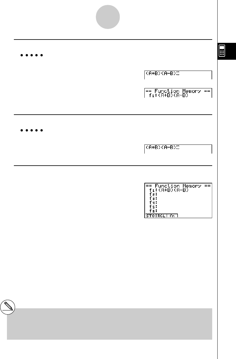
19990401
uTo store a function
Example To store the function (A+B) (A–B) as function memory number 1
(av(A)+al(B))
(av(A)-al(B))
K6(g)5(FMEM)
b(Store)bw
uTo recall a function
Example To recall the contents of function memory number 1
K6(g)5(FMEM)
c(Recall)bw
uTo display a list of available functions
K6(g)5(FMEM)
e(SEE)
2-2-3
Special Functions
#If the function memory number to which you
store a function already contains a function, the
previous function is replaced with the new one.
#The recalled function appears at the current
location of the cursor on the display.
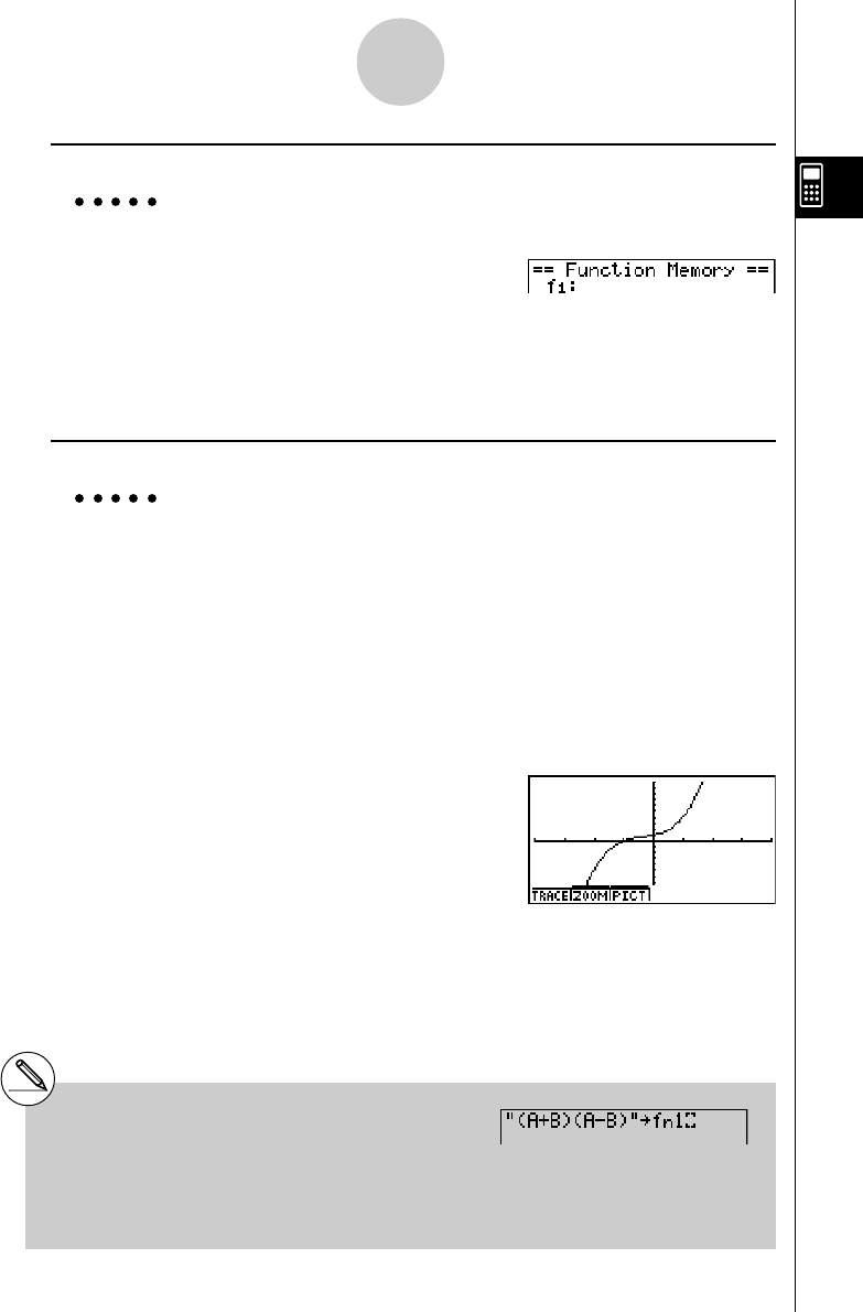
19990401
2-2-4
Special Functions
uTo delete a function
Example To delete the contents of function memory number 1
AK6(g)5(FMEM)
b(Store)bw
•Executing the store operation while the display is blank deletes the function in the
function memory you specify.
uTo use stored functions
Example To store x3 + 1, x2 + x into function memory, and then graph:
y = x3 + x2 + x + 1
Use the following View Window settings.
Xmin = – 4, Xmax = 4, Xscale = 1
Ymin = –10, Ymax = 10, Yscale = 1
u3(SET UP)c1(Y=)i
AvMd+bK6(g)5(FMEM)b(Store)bw(stores (x3 + 1))
iAvx+v5(FMEM)b(Store)cw(stores (x2 + x))
iAK6(g)6(g)2(SKTCH)b(Cls)w
2(SKTCH)e(GRAPH)b(Y=)
K6(g)5(FMEM)d(fn)b+
5(FMEM)d(fn)cw
•For full details about graphing, see “5. Graphing”.
#You can also use a to store a function in
function memory in a program.
In this case, you must enclose the function
inside of double quotation marks.
The maximum size of the function you can
store is 255 bytes.
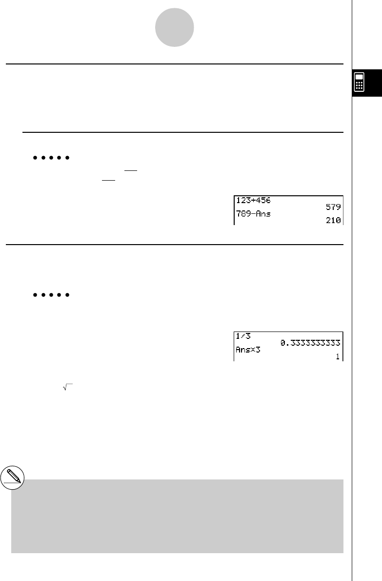
19990401
kk
kk
kAnswer Function
The Answer Function automatically stores the last result you calculated by pressing
w(unless the wkey operation results in an error). The result is stored in the answer
memory.
uTo use the contents of the answer memory in a calculation
Example 123 + 456 = 579
789 – 579 = 210
Abcd+efgw
hij-!-(Ans)w
kk
kk
kPerforming Continuous Calculations
Answer memory also lets you use the result of one calculation as one of the arguments in
the next calculation.
Example 1 1 ÷ 3 =
1 ÷ 3 × 3 =
Ab/dw
(Continuing)*dw
Continuous calculations can also be used with Type A functions (x2, x-1, x!, page 2-1-3), +,
–, ^(xy), x, ° ’ ”, etc.
2-2-5
Special Functions
#The largest value that the answer memory
can hold is 15 digits for the mantissa and 2
digits for the exponent.
# Only numeric values and calculation results
can be stored in answer memory.
# Answer memory contents are not cleared
when you press the A key or when you
switch power off.
#Answer memory contents are not changed
by an operation that assigns values to value
memory (such as: faav(A)w).
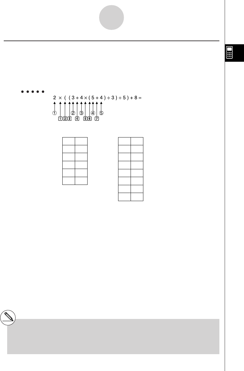
19990401
kStacks
The unit employs memory blocks, called
stacks
, for storage of low priority values and
commands. There is a 10-level
numeric value stack
, a 26-level
command stack
, and a 10-
level
program subroutine stack
. An error occurs if you perform a calculation so complex that it
exceeds the capacity of available numeric value stack or command stack space, or if
execution of a program subroutine exceeds the capacity of the subroutine stack.
Example
2-2-6
Special Functions
1
2
3
4
5
b
c
d
e
f
g
h
2
3
4
5
4
×
(
(
+
×
(
+
...
...
Numeric Value Stack Command Stack
#Calculations are performed according to the pri-
ority sequence. Once a calculation is executed,
it is cleared from the stack.
#Storing a complex number takes up two numeric
value stack levels.
#Storing a two-byte function takes up two
command stack levels.
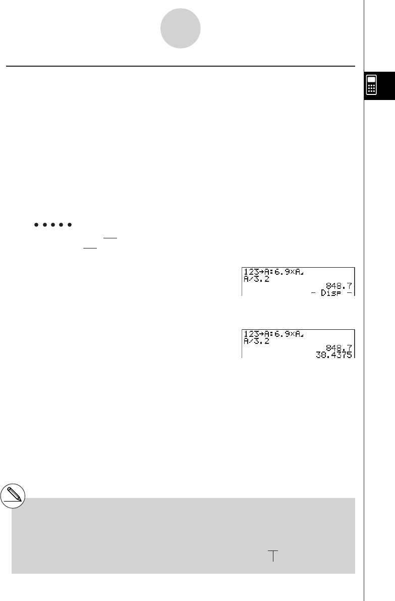
19990401
kUsing Multistatements
Multistatements are formed by connecting a number of individual statements for sequential
execution. You can use multistatements in manual calculations and in programmed calcula-
tions. There are two different ways that you can use to connect statements to form
multistatements.
•Colon (:)
Statements that are connected with colons are executed from left to right, without stopping.
•Display Result Command (^^
^^
^)
When execution reaches the end of a statement followed by a display result command, execu-
tion stops and the result up to that point appears on the display. You can resume execution by
pressing the w key.
Example 6.9 × 123 = 848.7
123 ÷ 3.2 = 38.4375
Abcdaav(A)
!J(PRGM)6(g)6(g)3(:)g.j
*av(A)!J(PRGM)4(^)
av(A)/d.cw
w
2-2-7
Special Functions
#The final result of a multistatement is always
displayed, regardless of whether the
calculation ends with a display result
command. Example : 123 × 456: × 5
Invalid
#You cannot construct a multistatement in
which one statement directly uses the result
of the previous statement.

19990401
2-3 Specifying the Angle Unit and Display
Format
Before performing a calculation for the first time, you should use the SET UP screen to
specify the angle unit and display format.
kk
kk
kSetting the Angle Unit [SET UP]- [Angle]
1. On the Set Up screen, highlight “Angle”.
2. Press the function key for the angle unit you want to specify, then press i.
•{Deg}/{Rad}/{Gra} ... {degrees}/{radians}{grads}
•The relationship between degrees, grads, and radians is shown below.
360° = 2π radians = 400 grads
90° = π/2 radians = 100 grads
kk
kk
kSetting the Display Format [SET UP]- [Display]
1. On the Set Up screen, highlight “Display”.
2. Press the function key for the item you want to set, then press i.
•{Fix}/{Sci}/{Norm}/{Eng} ... {fixed number of decimal places specification}/
{number of significant digits specification}/{normal display}/{Engineering Mode}
uTo specify the number of decimal places (Fix)
Example To specify two decimal places
1(Fix) cw
Press the function key that corresponds to the
number of decimal places you want to specify
(
n
= 0 to 9).
2-3-1
Specifying the Angle Unit and Display Format
#Displayed values are rounded off to the
number of decimal places you specify.
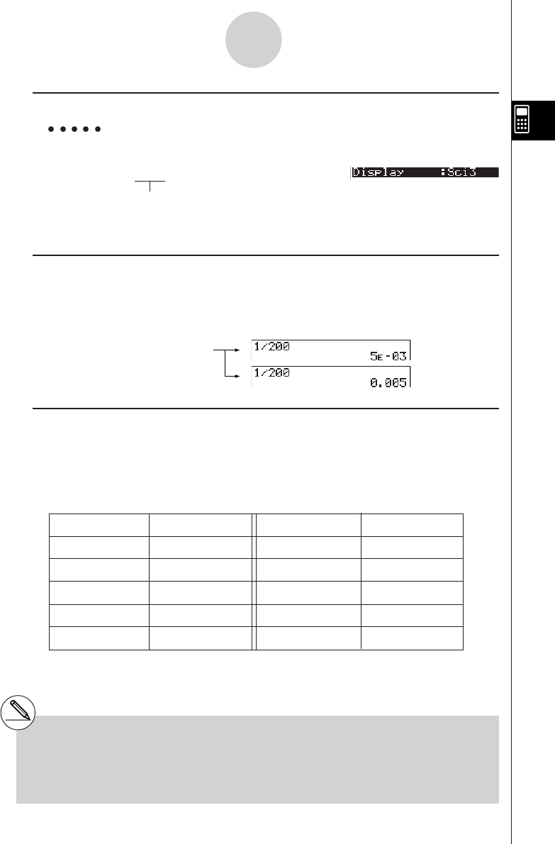
19990401
uTo specify the number of significant digits (Sci)
Example To specify three significant digits
2(Sci) dw
Press the function key that corresponds
to the number of significant digits you
want to specify (
n
= 0 to 9).
uTo specify the normal display (Norm 1/Norm 2)
Press 3(Norm) to switch between Norm 1 and Norm 2.
Norm 1: 10–2 (0.01)>|x|, |x| >1010
Norm 2: 10–9 (0.000000001)>|x|, |x| >1010
Ab/caaw(Norm 1)
(Norm 2)
uTo specify the engineering notation display (Eng Mode)
Press 4(Eng) to switch between engineering notation and standard notation. The
indicator “/E” is on the display while engineering notation is in effect.
You can use the following symbols to convert values to engineering notation, such as
2,000 (= 2 × 10³) → 2k.
E (Exa) × 1018 m (milli) × 10–3
P (Peta) × 1015 µ (micro) × 10–6
T (Tera) × 1012 n (nano) × 10–9
G (Giga) × 109p (pico) × 10–12
M (Mega) × 106f (femto) × 10–15
k (kilo) × 103
2-3-2
Specifying the Angle Unit and Display Format
#Displayed values are rounded off to the number
of significant digits you specify.
#Specifying 0 makes the number of significant
digits 10.
#The engineering symbol that makes the
mantissa a value from 1 to 1000 is automatically
selected by the calculator when engineering
notation is in effect.

20010101
2-4 Function Calculations
kFunction Menus
This calculator includes five function menus that give you access to scientific functions not
printed on the key panel.
•The contents of the function menu differ according to the mode you entered from the Main
Menu before you pressed the K key. The following examples show function menus that
appear in the RUN • MAT Mode.
uu
uu
uNumeric Calculations (NUM) [OPTN]-[NUM]
•{Abs} ... {select this item and input a value to obtain the absolute value of the value.}
•{Int}/{Frac} ... select the item and input a value to extract the {integer}/{fraction} part.
•{Rnd} ... {rounds off the value used for internal calculations to 10 significant digits
(to match the value in the Answer Memory), or to the number of decimal places (Fix)
and number of significant digits (Sci) specified by you.}
•{Intg} ... {select this item and input a value to obtain the largest integer that is not greater
than the value.}
•{E-SYM} ... {engineering symbol}
•{m}/{µ}/{n}/{p}/{f} ... {milli (10–3)}/{micro (10–6)}/{nano (10–9)}/{pico (10–12)}/{femto
(10–15)}
•{k}/{M}/{G}/{T}/{P}/{E} ... {kilo (103)}/{mega (106)}/{giga (109)}/{tera (1012)}/{peta
(1015)}/{exa (1018)}
uu
uu
uProbability/Distribution Calculations (PROB) [OPTN]-[PROB]
•{x!} ... {press after inputting a value to obtain the factorial of the value.}
•{nPr}/{nCr} ... {permutation}/{combination}
•{Ran#}... {pseudo random number generation (0 to 1)}
•{P(}/{Q(}/{R(} ... normal probability {P(t)}/{Q(t)}/{R(t)}
•{t(} ... {value of normalized variate t(x)}
2-4-1
Function Calculations
20011101

20010101
uu
uu
uHyperbolic Calculations (HYP) [OPTN]-[HYP]
•{sinh}/{cosh}/{tanh} ... hyperbolic {sine}/{cosine}/{tangent}
•{sinh–1}/{cosh–1}/{tanh–1} ... inverse hyperbolic {sine}/{cosine}/{tangent}
uu
uu
uAngle Units, Coordinate Conversion, Sexagesimal Operations (ANGL)
[OPTN]-[ANGL]
•{°}/{r}/{g} ... {degrees}/{radians}/{grads} for a specific input value
•{° ’ ”} ... {specifies degrees (hours), minutes, seconds when inputting a degrees/minutes/
seconds value}
•{'DMS} ... {converts decimal value to sexagesimal value}
•{Pol(}/{Rec(} ... {rectangular-to-polar}/{polar-to-rectangular} coordinate conversion
uu
uu
uInstant Functions
•{ ° ’ ”} ... {converts decimal value to degrees/minutes/seconds value}
•{ENG}/{ENG} ... shifts the decimal place of the displayed value three digits to
the {left}/{right} and {decreases}/{increases} the exponent by three.
When you are using engineering notation, the engineering symbol is also changed
accordingly.
•The { ° ’ ” }, {ENG} and { ENG} menu operations are available only when there is a
calculation result on the display.
kk
kk
kAngle Units
To change the angle unit of an input value, first press K3(ANGL). On the pull-up
menu that appears, select “°”, “r”, or “g”.
•Be sure to specify Comp for Mode in the SET UP screen.
Example Operation
To convert 4.25 rad to degrees:
u3(SET UP)cccc1(Deg)i
243.5070629 4.25K6(g)3(ANGL)c(r)w
47.3° + 82.5rad = 4774.20181°
47.3+82.5K6(g)3(ANGL)c(r)w
2-4-2
Function Calculations
# Once you specify an angle unit, it remains
in effect until you specify a different one.
The specification is retained even if you turn
power off.

20010101
kk
kk
kTrigonometric and Inverse Trigonometric Functions
•Be sure to set the angle unit before performing trigonometric function and inverse
trigonometric function calculations.
•Be sure to specify Comp for Mode in the SET UP screen.
Example Operation
sin 63° = 0.8910065242 u3(SET UP)cccc1(Deg)i
s63w
π
cos (–– rad) = 0.5 u3(SET UP)cccc2(Rad)i
3c(!E(π)/d)w
tan (– 35gra) = – 0.6128007881
u3(SET UP)cccc3(Gra)i
t-35w
2 • sin 45° × cos 65° = 0.5976724775
u3(SET UP)cccc1(Deg)i
2*s45*c65w*1
cosec 30° = 1
= 2 1/s30w
sin30°
sin-10.5 = 30°!s(sin–1)0.5*2w
(x when sinx = 0.5)
2-4-3
Function Calculations
*1* can be omitted. *2Input of leading zero is not necessary.
π
(90° = ––– radians = 100 grads)
2
20010101
kLogarithmic and Exponential Functions
•Be sure to specify Comp for Mode in the SET UP screen.
Example Operation
log 1.23 (log101.23) = 8.990511144 × 10⁻² l1.23w
In 90 (loge90) = 4.49980967 I90w
101.23 = 16.98243652
(To obtain the antilogarithm of common !l(10x)1.23w
logarithm 1.23)
e4.5 = 90.0171313
(To obtain the antilogarithm of natural !I(ex)4.5w
logarithm 4.5)
(–3)4 = (–3) × (–3) × (–3) × (–3) = 81 (-3)M4w
–34 = –(3 × 3 × 3 × 3) = –81 -3M4w
1
7 (= 1237) = 1.988647795 7!M(x )123w
2 + 3 × 3 – 4 = 10 2+3*3!M(x )64-4w*1
2-4-4
Function Calculations
123
64
*1^ (xy) and x take precedence over
multiplication and division.
20011101

20010101
kHyperbolic and Inverse Hyperbolic Functions
•Be sure to specify Comp for Mode in the SET UP screen.
Example Operation
sinh 3.6 = 18.28545536 K6(g)2(HYP)b(sinh)3.6w
cosh 1.5 – sinh 1.5 K6(g)2(HYP)c(cosh)1.5-
= 0.2231301601 2(HYP)b(sinh)1.5w
= e–1.5 (Display: –1.5) I!-(Ans)w
(Proof of cosh x ± sinh x = e±x)
cosh
–1
20 = 0.7953654612
K6(g)2(HYP)f(cosh–1)(20/15)w
15
Determine the value of x
when tanh 4 x = 0.88
x = tanh–1 0.88 K6(g)2(HYP)g(tanh–1)0.88/4w
4
= 0.3439419141
2-4-5
Function Calculations

20010101
kOther Functions
•Be sure to specify Comp for Mode in the SET UP screen.
Example Operation
+ = 3.65028154 !x( )2+!x( )5w
25
= 1.755317302 !x( )(d+!a(i))w
(3 + i)
+0.2848487846i
(–3)2 = (–3) × (–3) = 9 (-3)xw
–32 = –(3 × 3) = –9 -3xw
(3!)(x–1)-4!)(x–1))!)(x–1)w
8! (= 1 × 2 × 3 × .... × 8) 8K6(g)1(PROB)b(x!)w
= 40320
3 = 42
!(
(3 )
(36*42*49
)w36 × 42 × 49
What is the absolute value of
the common logarithm of
|
log
|
= 0.1249387366 K5(NUM)b(Abs)l(3/4)w
What is the integer part of K5(NUM)c(Int)-3.5w
– 3.5? – 3
What is the decimal part of K5(NUM)d(Frac)-3.5w
– 3.5? – 0.5
What is the nearest integer K5(NUM)f(Intg)-3.5w
not exceeding – 3.5? – 4
2-4-6
Function Calculations
3
4?
3
4
1
–––––– = 12
11
–– – ––
34

20010101
kRandom Number Generation (Ran#)
This function generates a 10-digit truly random or sequentially random number that is greater
than zero and less than 1.
•A truly random number is generated if you do not specify anything for the argument.
Example Operation
Ran # (Generates a random number.) K6(g)1(PROB)e(Ran#)w
(Each press of w generates a new random w
number.) w
•Specifying an argument from 1 to 9 generates random numbers based on that sequence.
•Specifying an argument of 0 initializes the sequence.*1
Example Operation
Ran# 1 (Generates the first random number in sequence 1.) 1(PROB)e(Ran#)bw
(Generates the second random number in sequence 1.) w
Ran# 0 (Initializes the sequence.) 1(PROB)e(Ran#)aw
Ran# 1 (Generates the first random number in sequence 1.) 1(PROB)e(Ran#)bw
2-4-7
Function Calculations
*1Changing to a different sequence or
generating a totally random number (without
an argument) initializes the sequence.
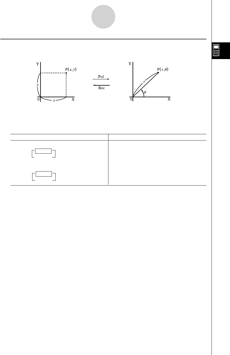
20010101
2-4-8
Function Calculations
kCoordinate Conversion
uu
uu
u Rectangular Coordinates uu
uu
u Polar Coordinates
•With polar coordinates,
θ
can be calculated and displayed within a range of
–180°<
θ
< 180° (radians and grads have same range).
•Be sure to specify Comp for Mode in the SET UP screen.
Example Operation
Calculate r and
θ
° when x = 14 and y = 20.7 u3(SET UP)cccc1(Deg)i
K6(g)3(ANGL)g(Pol()
14,20.7)w
Calculate x and y when r = 25 and
θ
= 56°u3(SET UP)cccc1(Deg)i
K6(g)3(ANGL)h(Rec()
25,56)w
124.989 →24.98979792 (r)
255.928 →55.92839019 (
θ
)
113.979 →13.97982259 (x)
220.725 →20.72593931 (y)

20010101
2-4-9
Function Calculations
n!n!
nPr = ––––– nCr = –––––––
(n – r)! r! (n – r)!
kPermutation and Combination
uu
uu
u Permutation uu
uu
u Combination
•Be sure to specify Comp for Mode in the SET UP screen.
Example To calculate the possible number of different arrangements using 4
items selected from among 10 items
Formula Operation
10P4 = 5040 10K6(g)1(PROB)c(nPr)4w
Example To calculate the possible number of different combinations of 4 items
that can be selected from among 10 items
Formula Operation
10C4 = 210 10K6(g)1(PROB)d(nCr)4w

20010101
kk
kk
kFractions
•Fractional values are displayed with the integer first, followed by the numerator and then
the denominator.
•Be sure to specify Comp for Mode in the SET UP screen.
Example Operation
(Display: 3{13{20) 2$5+3$1$4w
= 3.65 $(Conversion to decimal)
$(Conversion to fraction)
1$2578+1$4572w
1$2*.5w
$
1.5+2.3!a(i)w
$$*3
1$(1$3+1$4)w*4
2-4-10
Function Calculations
2113
–– + 3 –– = 3 –––
5420
11
––––– + –––––
2578 4572 = 6.066202547 × 10⁻⁴
1
–– × 0.5 = 0.25*2
2
(Display: )
6.066202547E–04*1
(Norm 1 display format)
1
= ––
4
(Display: 1{5{7)
15
–––––– = 1––
11 7
–– + ––
34
*1When the total number of characters,
including integer, numerator, denominator
and delimiter marks exceeds 10, the input
fraction is automatically displayed in decimal
format.
*2Calculations containing both fractions and
decimals are calculated in decimal format.
*3Pressing $ once when converting the decimal
part of a complex number to a fraction first
displays the real part and imaginary part on
separate lines.
*4You can include fractions within the numerator
or denominator of a fraction by putting the
numerator or denominator in parentheses.
13
1.5 + 2.3i = 1–– + 2––i
210
Display:
1{1{2
+2{3{10i
20010101
2-4-11
Function Calculations
kEngineering Notation Calculations
Input engineering symbols using the engineering notation menu.
•Be sure to specify Comp for Mode in the SET UP screen.
Example Operation
u3(SET UP)cccccccccc
4(Eng)i
999k (kilo) + 25k (kilo) 999K5(NUM)g(E-SYM)g(k)+255(NUM)
= 1.024M (mega) g(E-SYM)g(k)w
9 ÷ 10 = 0.9 = 900m (milli) 9/10w
= 0.9 K6(g)6(g)6(g)3(ENG)*1
= 0.0009k (kilo) 3(ENG)*1
= 0.9 2(ENG)*2
= 900m 2(ENG)*2
*1Converts the displayed value to the next higher
engineering unit, by shifting the decimal point
three places to the right.
*2Converts the displayed value to the next lower
engineering unit, by shifting the decimal point
three places to the left.

20010101
2-5 Numerical Calculations
The following describes the items that are available in the menus you use when performing
differential/ quadratic differential, integration, Σ, maximum/minimum value, and Solve
calculations.
When the option menu is on the display, press 4(CALC) to display the function analysis
menu. The items of this menu are used when performing specific types of calculations.
•{d/dx}/{d2/dx2}/{∫dx}/{Σ}/{FMin}/{FMax}/{Solve} ... {differential}/{quadratic differential}/
{integration}/{Σ (sigma)}/{minimum value}/{maximum value}/{solve} calculations
Solve calculations
The following is the syntax for using the Solve function in a program.
Solve( f(x), n, a, b) (a: lower limit,
b: upper limit,
n: initial estimated value)
•There are two different input methods that can be used for Solve calculations: direct
assignment and variable table input.
With the direct assignment method (the one described here), you assign values directly
to variables. This type of input is identical to that used with the Solve command used in
the PRGM Mode.
Variable table input is used with the Solve function in the EQUA Mode. This input
method is recommend for most normal Solve function input.
An Error (Iteration ERROR) occurs when there is no convergence of the solution.
2-5-1
Numerical Calculations

20010101
kDifferential Calculations [OPTN]-[CALC]-[d
/dx]
To perform differential calculations, first display the function analysis menu, and then input
the values shown in the formula below.
K4(CALC)b(d/dx) f(x),a,tol)
The differentiation for this type of calculation is defined as:
In this definition,
infinitesimal
is replaced by a
sufficiently small
Ax, with the value in the
neighborhood of f ' (a) calculated as:
In order to provide the best precision possible, this unit employs central difference to perform
differential calculations.
Using Differential Calculation in a Graph Function
• Omitting the tolerance (tol) value when using the differential command inside of a graph
function simplifies the calculation for drawing the graph. In such a case, precision is
sacrificed for the sake of faster drawing. The tolerance value is specified, the graph is
drawn with the same precision obtained when you normally perform a differential
calculation.
• You can also omit input of the derivative point by using the following format for the
differential graph: Y2=d/dx(Y1). In this case, the value of the X variable is used as the
derivative point.
2-5-2
Numerical Calculations
d
d/dx ( f (x), a) ⇒ ––– f (a)
dx
f (a + Ax) – f (a)
f '(a) = lim –––––––––––––
Ax
Ax→0
f (a + Ax) – f (a)
f '(a) –––––––––––––
Ax
(a: point for which you want to determine the
derivative, tol: tolerance)
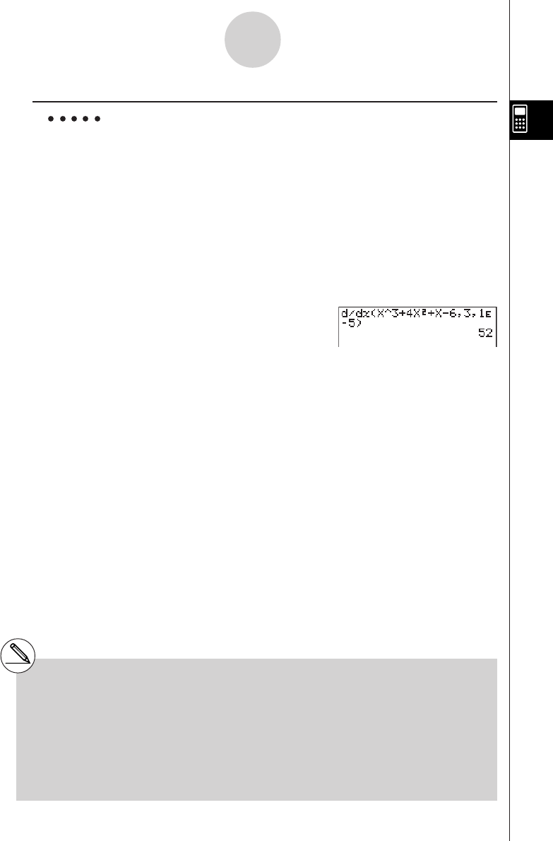
20010101
Example To determine the derivative at point x = 3 for the function
y = x3 + 4x2 + x – 6, with a tolerance of “tol” = 1E – 5
Input the function f(x).
AK4(CALC)b(d/dx)vMd+evx+v-g,
Input point x = a for which you want to determine the derivative.
d,
Input the tolerance value.
bE-f)
w
#In the function f(x), only X can be used as a
variable in expressions. Other variables (A
through Z, r,
θ
) are treated as constants, and
the value currently assigned to that variable is
applied during the calculation.
# Input of the tolerance (tol) value and the
closing parenthesis can be omitted. If you omit
tolerance (tol) value, the calculator automati-
cally uses a value for tol as 1E-10.
# Specify tolerance (tol) value of 1E-14 or less.
An error (Iteration ERROR) occurs whenever
no solution that satisfies the tolerance value
can be obtained.
#Discontinuous points or sections with drastic
fluctuation can adversely affect precision or
even cause an error.
2-5-3
Numerical Calculations

20010101
uApplications of Differential Calculations
•Differentials can be added, subtracted, multiplied or divided with each other.
Therefore:
•Differential results can be used in addition, subtraction, multiplication, and division, and in
functions.
2 × f '(a), log ( f '(a)), etc.
•Functions can be used in any of the terms ( f (x), a, tol) of a differential.
2-5-4
Numerical Calculations
#You cannot use a differential, quadratic
differential, integration, Σ, maximum/minimum
value or solve calculation expression inside a
differential calculation term.
#Pressing A during calculation of a differential
(while the cursor is not shown on the display)
interrupts the calculation.
#Always use radians (Rad Mode) as the angle
unit when performing trigonometric differentials.
dd
––– f (a) = f '(a), ––– g (a) = g'(a)
dx dx
f '(a) + g'(a), f '(a) × g'(a), etc.
d
––– (sinx + cosx, sin0.5, 1E - 8), etc.
dx
20011101

20010101
kk
kk
kQuadratic Differential Calculations [OPTN]-[CALC]-[d2/dx2]
After displaying the function analysis menu, you can input quadratic differentials using either of
the two following formats.
K4(CALC)c(d2/dx2) f(x),a,tol)
Quadratic differential calculations produce an approximate differential value using the following
second order differential formula, which is based on Newton’s polynomial interpretation.
2 f (a + 3h) – 27 f(a + 2h) + 270 f (a + h) – 490 f (a)+270 f(a – h) – 27 f (a – 2h) +2 f (a – 3h)
f''(a) = –––––––––––––––––––––––––––––––––––––––––––––––––––––––––––––––––––––––
180h2
In this expression, values for “sufficiently small increments of h” are used to obtain a value that
approximates f ”(a).
Example To determine the quadratic differential coefficient at the point where
x = 3 for the function y = x3 + 4x2 + x – 6
Here we will use a tolerance tol = 1E – 5
Input the function f(x).
AK4(CALC)c(d2/dx2) vMd+
evx+v-g,
Input 3 as point a, which is the differential coefficient point.
d,
Input the tolerance value.
bE-f)
w
2-5-5
Numerical Calculations
#In the function f(x), only X can be used as a
variable in expressions. Other variables (A
through Z, r,
θ
) are treated as constants, and
the value currently assigned to that variable is
applied during the calculation.
#Input of the tolerance (tol) value and the closing
parenthesis can be omitted.
#Discontinuous points or sections with drastic
fluctuation can adversely affect precision or
even cause an error.
(a: differential coefficient point , tol: tolerance)
d
2
d
2
––– (f (x), a) ⇒ ––– f (a)
dx
2
dx
2
20011101

20010101
uQuadratic Differential Applications
• Arithmetic operations can be performed using two quadratic differentials.
Therefore:
f ''(a) + g''(a), f ''(a) × g''(a), etc.
•The result of a quadratic differential calculation can be used in a subsequent arithmetic
or function calculation.
2 × f ''(a), log ( f ''(a) ), etc.
•Functions can be used within the terms ( f(x), a, tol ) of a quadratic differential expression.
2-5-6
Numerical Calculations
d2d2
––– f (a) = f ''(a), ––– g (a) = g''(a)
dx2dx2
d2
––– (sin x + cos x, sin 0.5, 1E - 8), etc.
dx2
#You cannot use a differential, quadratic
differential, integration, Σ, maximum/minimum
value or Solve calculation expression inside of
a quadratic differential calculation term.
# Specify tolerance (tol) value of 1E-14 or less.
An error (Iteration ERROR) occurs whenever
no solution that satisfies the tolerance value
can be obtained.
#You can interrupt an ongoing quadratic
differential calculation by pressing the A key.
#Always use radians (Rad Mode) as the angle
unit when performing trigonometric quadratic
differentials.
# Using Quadratic Differential Calculation in a
Graph Function (see page 2-5-2)
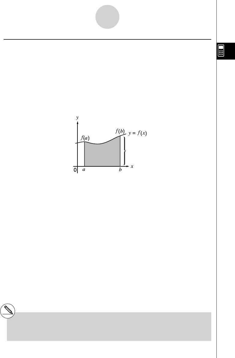
20010101
kk
kk
kIntegration Calculations [OPTN]-[CALC]-[
∫
dx]
To perform integration calculations, first display the function analysis menu and then input
the values in the formula shown below.
K4(CALC)d (
∫
dx) f(x) , a , b , tol )
∫
( f(x), a, b, tol) ⇒
∫
a
b f(x)dx
As shown in the illustration above, integration calculations are performed by calculating
integral values from a through b for the function y = f (x) where a < x < b, and f (x) > 0. This
in effect calculates the surface area of the shaded area in the illustration.
2-5-7
Numerical Calculations
Area of
∫
a
b f(x)dx is calculated
(a: start point, b: end point, tol: tolerance)
#If f (x) < 0 where a a < x < b, the surface area
calculation produces negative values (surface
area × – 1).

20010101
Example To perform the integration calculation for the function shown
below, with a tolerance of “tol” = 1E - 4
∫
1
5 (2x2 + 3x + 4) dx
Input the function f (x).
AK4(CALC)d(∫dx)cvx+dv+e,
Input the start point and end point.
b,f,
Input the tolerance value.
bE-e)
w
uu
uu
uApplication of Integration Calculation
•Integrals can be used in addition, subtraction, multiplication or division.
∫
a
b f(x) dx +
∫
c
d g(x) dx, etc.
•Integration results can be used in addition, subtraction, multiplication or division, in
functions.
2 ×
∫
a
b f(x) dx, etc. log (
∫
a
b f(x) dx), etc.
•Functions can be used in any of the terms (f(x), a, b, tol) of an integral.
∫
cos 0.5
(sin x + cos x) dx =
∫
(sin x + cos x, sin 0.5, cos 0.5, 1E - 4)
sin 0.5
2-5-8
Numerical Calculations
#In the function f(x), only X can be used as a
variable in expressions. Other variables (A
through Z, r,
θ
) are treated as constants, and
the value currently assigned to that variable is
applied during the calculation.
#Input of “tol” and closing parenthesis can be
omitted. If you omit “tol,” the calculator
automatically uses a default value of 1E-5.
# Integration calculations can take a long time to
complete.
#You cannot use a differential, quadratic
differential, integration, Σ, maximum/minimum
value or Solve calculation expression inside of
an integration calculation term.
20011101
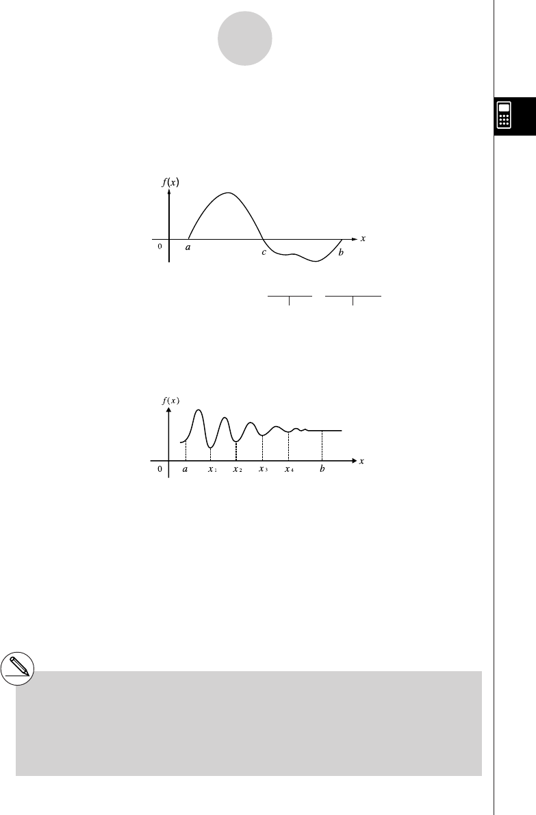
20010101
Note the following points to ensure correct integration values.
(1) When cyclical functions for integration values become positive or negative for different
divisions, perform the calculation for single cycles, or divide between negative and
positive, and then add the results together.
∫
a
b f(x)dx =
∫
a
c f(x)dx + (–
∫
c
b f(x)dx)
Positive part (
S
)Negative part (
S
)
(2) When minute fluctuations in integration divisions produce large fluctuations in integration
values, calculate the integration divisions separately (divide the large fluctuation areas
into smaller divisions), and then add the results together.
∫
a
b f(x)dx =
∫
a
x1 f(x)dx +
∫
x1
x2 f(x)dx +.....+
∫
x4
b
f(x)dx
2-5-9
Numerical Calculations
Negative part (S)
Positive
part (S)
#Pressing A during calculation of an integral
(while the cursor is not shown on the display)
interrupts the calculation.
#Always use radians (Rad Mode) as the angle
unit when performing trigonometric
integrations.
# An error (Iteration ERROR) occurs whenever
no solution that satisfies the tolerance value
can be obtained.
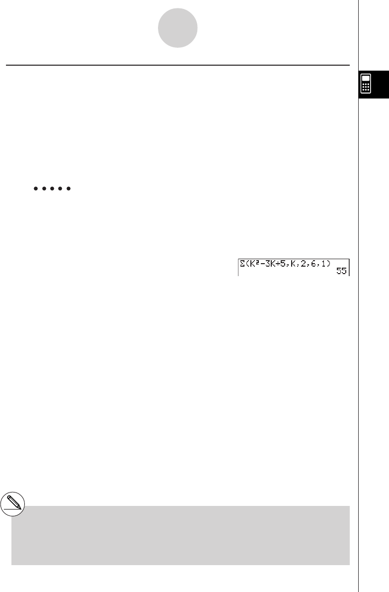
20010101
kk
kk
kΣ Calculations [OPTN]-[CALC]-[Σ ]
To perform Σ calculations, first display the function analysis menu, and then input the values
shown in the formula below.
K4(CALC)e(Σ) ak , k ,
α
,
β
, n )
Example To calculate the following:
Use n = 1 as the distance between partitions.
AK4(CALC)e(Σ)a,(K)x
-da,(K)+f,
a,(K),c,g,b)w
2-5-10
Numerical Calculations
6
Σ (k2 – 3k + 5)
k = 2
#You can use only one variable in the function for
input sequence ak.
#Input integers only for the initial term (
α
) of
sequence ak and last term (
β
) of sequence ak .
#Input of n and the closing parentheses can be
omitted. If you omit n, the calculator automati-
cally uses n = 1.
β
Σ (ak, k,
α
,
β
, n) = Σ ak = a
α
+ a
α
+1 +........+ a
β
k = α(n: distance between partitions)

20010101
uΣ Calculation Applications
•Arithmetic operations using Σ calculation expressions
Expressions:
Possible operations: Sn + Tn, Sn – Tn, etc.
•Arithmetic and function operations using Σ calculation results
2 × Sn, log (Sn), etc.
•Function operations using Σ calculation terms (ak, k)
Σ (sink, k, 1, 5), etc.
2-5-11
Numerical Calculations
nn
Sn = Σ ak, Tn = Σ bk
k = 1k = 1
#You cannot use a differential, quadratic
differential, integration, Σ, maximum/minimum
value or Solve calculation expression inside of
a Σ calculation term.
#Make sure that the value used as the final term
β
is greater than the value used as the initial
term
α
. Otherwise, an error will occur.
#To interrupt an ongoing Σ calculation (indicated
when the cursor is not on the display), press the
A key.
20010101
2-5-12
Numerical Calculations
kk
kk
kMaximum/Minimum Value Calculations [OPTN]-[CALC]-[FMin]/[FMax]
After displaying the function analysis menu, you can input maximum/minimum calculations
using the formats below, and solve for the maximum and minimum of a function within
interval a < x < b. (a: start point of interval, b: end point of interval, n: precision (n = 1 to 9))
uu
uu
uMinimum Value
K4(CALC)f(FMin) f(x) , a , b , n )
uu
uu
uMaximum Value
K4(CALC)g(FMax) f(x), a , b , n )
Example 1 To determine the minimum value for the interval defined by start
point a = 0 and end point b = 3, with a precision of n = 6 for the
function y = x2 – 4x + 9
Input f(x).
AK4(CALC)f(FMin) vx-ev+j,
Input the interval a = 0, b = 3.
a,d,
Input the precision n = 6.
g)
w
20010101
2-5-13
Numerical Calculations
#In the function f(x), only X can be used as a
variable in expressions. Other variables (A
through Z, r,
θ
) are treated as constants, and
the value currently assigned to that variable is
applied during the calculation.
#Input of n and the closing parenthesis can be
omitted.
#Discontinuous points or sections with drastic
fluctuation can adversely affect precision or
even cause an error.
#You cannot use a differential, quadratic
differential, integration, Σ, maximum/minimum
value or Solve calculation expression inside of
a maximum/minimum calculation term.
#Inputting a larger value for n increases the
precision of the calculation, but it also increases
the amount of time required to perform the
calculation.
#The value you input for the end point of the
interval (b) must be greater than the value you
input for the start point (a). Otherwise an error
occurs.
#You can interrupt an ongoing maximum/
minimum calculation by pressing the A key.
#You can input an integer in the range of 1 to 9
for the value of n. Using any value outside this
range causes an error.
Example 2 To determine the maximum value for the interval defined by start
point a = 0 and end point b = 3, with a precision of n = 6 for the
function y = –x2 + 2x + 2
Input f(x).
AK4(CALC)g(FMax) -vx+cv+c,
Input the interval a = 0, b = 3.
a,d,
Input the precision n = 6.
g)
w

20010101
2-6 Complex Number Calculations
You can perform addition, subtraction, multiplication, division, parentheses calculations,
function calculations, and memory calculations with complex numbers just as you do with the
manual calculations described on pages 2-1-1 and 2-4-6.
You can select the complex number calculation mode by changing the Complex
Mode item on the SET UP screen to one of the following settings.
• {Real} ... Calculation in the real number range only*1
• {a+bi} ... Performs complex number calculation and displays results in rectangular
form
• {re^
θ
i} ...Performs complex number calculation and displays results in polar form*2
Press K3(CPLX) to display the complex calculation number menu, which contains the
following items.
• {Abs}/{Arg} ... obtains {absolute value}/{argument}
• {Conjg} ... {obtains conjugate}
• {ReP}/{ImP} ... {real}/{imaginary} part extraction
• {'re^
θ
i}/{'a+bi} ... converts the result to {polar}/{linear}
2-6-1
Complex Number Calculations
*1 When there is an imaginary number in the
argument, however, complex number
calculation is performed and the result is
displayed using rectangular form.
Examples:
ln 2i= 0.6931471806 + 1.570796327i
ln 2i + ln (- 2 ) = (Non-Real ERROR)
*2 The display range of
θ
depends on the angle
unit set for the Angle item on the SET UP
screen.
• Deg ... –180 <
θ
< 180
• Rad ... – π <
θ
< π
• Gra ... –200 <
θ
< 200
# Solutions obtained by the Real and a+bi / re^
θ
i
modes are different for power root (xy)
calculations when x < 0 and y = m/n when n is
an odd number.
Example:
3x (- 8) = – 2 (Real)
= 1 + 1.732050808i(a+bi / re ^θi)
20011101
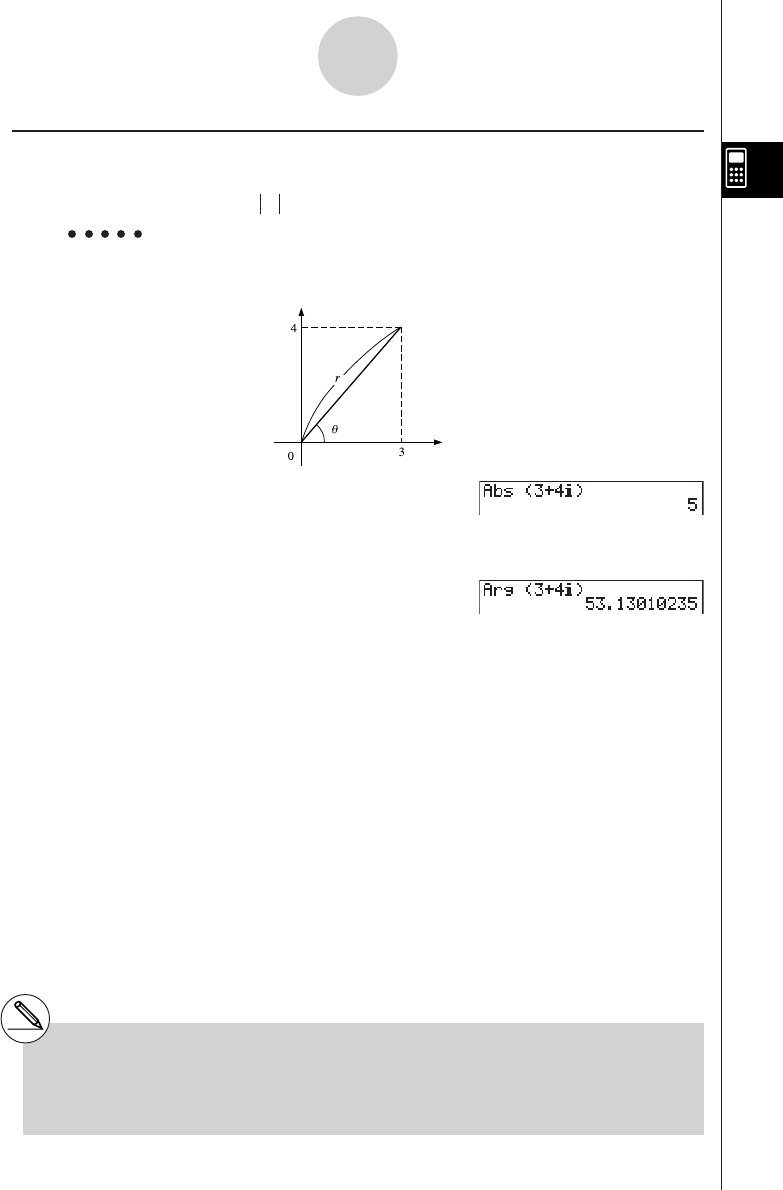
20010101
2-6-2
Complex Number Calculations
kk
kk
kAbsolute Value and Argument [OPTN]-[CPLX]-[Abs]/[Arg]
The unit regards a complex number in the form a + bi as a coordinate on a Gaussian plane,
and calculates absolute value Z and argument (arg).
Example To calculate absolute value (r) and argument (
θ
) for the complex
number 3 + 4i, with the angle unit set for degrees
AK3(CPLX)b(Abs)
(d+e!a(i))w
(Calculation of absolute value)
AK3(CPLX)c(Arg)
(d+e!a(i))w
(Calculation of argument)
#The result of the argument calculation differs
in accordance with the current angle unit
setting (degrees, radians, grads).
Imaginary axis
Real axis
20011101
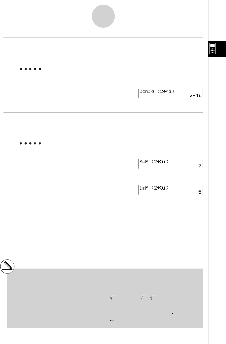
20010101
kk
kk
kConjugate Complex Numbers [OPTN]-[CPLX]-[Conjg]
A complex number of the form a + bi becomes a conjugate complex number of the form
a – bi.
Example To calculate the conjugate complex number for the complex number 2
+ 4i
AK3(CPLX)d(Conjg)
(c+e!a(i))w
kk
kk
kExtraction of Real and Imaginary Parts [OPTN]-[CPLX]-[ReP]/[lmP]
Use the following procedure to extract the real part a and the imaginary part b from a
complex number of the form a + bi.
Example To extract the real and imaginary parts of the complex number 2 + 5i
AK3(CPLX)e(ReP)
(c+f!a(i))w
(Real part extraction)
AK3(CPLX)f(ImP)
(c+f!a(i))w
(Imaginary part extraction)
2-6-3
Complex Number Calculations
#The input/output range of complex numbers is
normally 10 digits for the mantissa and two
digits for the exponent.
#When a complex number has more than 21
digits, the real part and imaginary part are
displayed on separate lines.
#When either the real part or imaginary part of
a complex number equals zero, that part is not
displayed in rectangular form.
#18 bytes of memory are used whenever you
assign a complex number to a variable.
#The following functions can be used with
complex numbers.
, x2, x–1, ^(xy), 3, x, In, log, 10x, ex, sin,
cos, tan, sin–1, cos–1, tan–1, sinh, cosh, tanh,
sinh–1, cosh–1, tanh–1
Int, Frac, Rnd, Intg, Fix, Sci, ENG, ENG, ° ’ ”,
° ’ ”, a b/c, d/c
20011101
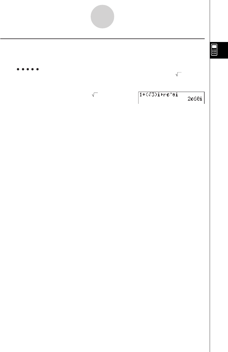
20010101
kk
kk
kPolar Form and Rectangular Transformation [OPTN]-[CPLX]-[''
''
're^
θ
i]
Use the following procedure to transform a complex number displayed in rectangular form to
polar form, and vice versa.
Example To transform the rectangular form of complex number 1 + 3
i to its
polar form
Ab+(!x( )d)!a(i)
K3(CPLX)g('re^
θ
i)w
2-6-4
Complex Number Calculations
20010101
2-7 Binary, Octal, Decimal, and Hexadecimal
Calculations with Integers
You can use the RUN • MAT Mode and binary, octal, decimal, and hexadecimal settings to
perform calculations that involve binary, octal, decimal and hexadecimal values. You can also
convert between number systems and perform bitwise operations.
•You cannot use scientific functions in binary, octal, decimal, and hexadecimal calcula-
tions.
•You can use only integers in binary, octal, decimal, and hexadecimal calculations, which
means that fractional values are not allowed. If you input a value that includes a decimal
part, the unit automatically cuts off the decimal part.
•If you attempt to enter a value that is invalid for the number system (binary, octal,
decimal, hexadecimal) you are using, the calculator displays an error message. The
following shows the numerals that can be used in each number system.
Binary: 0, 1
Octal: 0, 1, 2, 3, 4, 5, 6, 7
Decimal: 0, 1, 2, 3, 4, 5, 6, 7, 8, 9
Hexadecimal: 0, 1, 2, 3, 4, 5, 6, 7, 8, 9, A, B, C, D, E, F
•Negative binary, octal, and hexadecimal values are produced using the two’s complement
of the original value.
•The following are the display capacities for each of the number systems.
Number System Display Capacity
Binary 16 digits
Octal 11 digits
Decimal 10 digits
Hexadecimal 8 digits
2-7-1
Binary, Octal, Decimal, and Hexadecimal Calculations with Integers
#The alphabetic characters used in the
hexadecimal number appear differently on
the display to distinguish them from text
characters.
Normal Text
Hexadecimal Values
Keys
ABCDEF
uvwx y z
20011101

20010101
•The following are the calculation ranges for each of the number systems.
Binary Values
Positive: 0 < x < 111111111111111
Negative: 1000000000000000 < x < 1111111111111111
Octal Values
Positive: 0 < x < 17777777777
Negative: 20000000000 < x < 37777777777
Decimal Values
Positive: 0 < x < 2147483647
Negative: –2147483648 < x < –1
Hexadecimal Values
Positive: 0 < x < 7FFFFFFF
Negative: 80000000 < x < FFFFFFFF
uu
uu
u To perform a binary, octal, decimal, or hexadecimal calculation
1. In the main menu, select RUN • MAT.
[SET UP]- [Mode] -[Dec]/[Hex]/[Bin]/[Oct]
2. Press u3(SET UP) and then specify the default number system by pressing
2(Dec), 3(Hex), 4(Bin), or 5(Oct).
3. Press i to change to the screen for calculation input. This causes a function menu
with the following items to appear.
•{d~o}/{LOGIC}/{DISP}/{SYBL} ... {number system specification}/{bitwise operation}/
{decimal/hexadecimal/binary/octal conversion}/{symbol} menu
2-7-2
Binary, Octal, Decimal, and Hexadecimal Calculations with Integers
20011101

20010101
kk
kk
kSelecting a Number System
You can specify decimal, hexadecimal, binary, or octal as the default number system using
the set up screen. After you press the function key that corresponds to the system you want
to use, press w.
uu
uu
u To specify a number system for an input value
You can specify a number system for each individual value you input. Press 1(d~o) to
display a menu of number system symbols. Press the function key that corresponds to the
symbol you want to select and then input the value.
•{d}/{h}/{b}/{o} ... {decimal}/{hexadecimal}/{binary}/{octal}
uu
uu
u To input values of mixed number systems
Example To input 12310 or 10102, when the default number system is
hexadecimal
u3(SET UP)3(Hex)i
A1(d~o)b(d)bcdw
1(d~o)d(b)babaw
kk
kk
kArithmetic Operations
Example 1 To calculate 101112 + 110102
u3(SET UP)4(Bin)i
Ababbb+
bbabaw
2-7-3
Binary, Octal, Decimal, and Hexadecimal Calculations with Integers
20011101
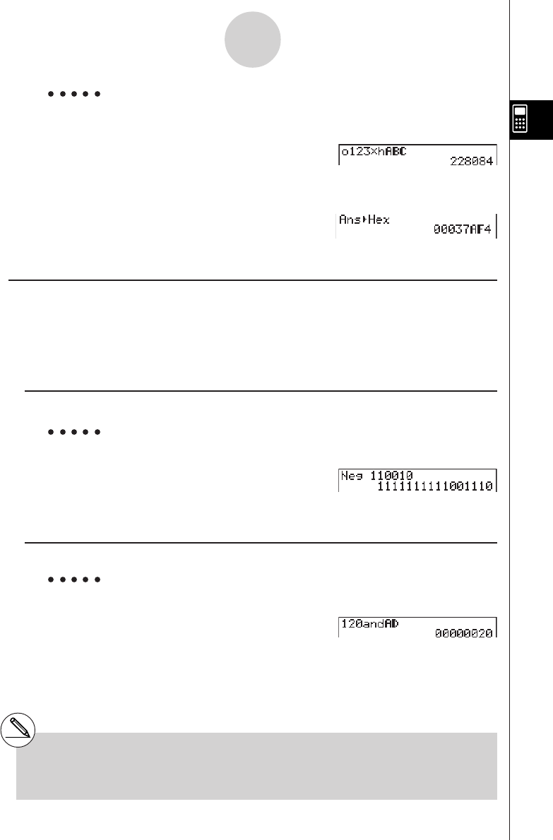
20010101
Example 2 To input and execute 1238 × ABC16, when the default number system is
decimal or hexadecimal
u3(SET UP)2(Dec)i
A1(d~o)e(o)bcd*
1(d~o)c(h)ABC*1w
3(DISP)c(Hex)w
kk
kk
kNegative Values and Bitwise Operations
Press 2(LOGIC) to display a menu of negation and bitwise operators.
•{Neg} ... {negation}*2
•{Not}/{and}/{or}/{xor}/{xnor} ... {NOT}*3/{AND}/{OR}/{XOR}/{XNOR}*4
u Negative Values
Example To determine the negative of 1100102
u3(SET UP)4(Bin)i
A2(LOGIC)b(Neg)
bbaabaw
uBitwise Operations
Example 1 To input and execute “12016 and AD16”
u3(SET UP)3(Hex)i
Abca2(LOGIC)
d(and)AD*1w
2-7-4
Binary, Octal, Decimal, and Hexadecimal Calculations with Integers
*1See page 2-7-1.
*2two’s complement
*3one’s complement (bitwise complement)
20011101
*4bitwise AND, bitwise OR, bitwise XOR,
bitwise XNOR

20010101
Example 2 To display the result of “368 or 11102” as an octal value
u3(SET UP)5(Oct)i
Adg2(LOGIC)
e(or)1(d~o)d(b)
bbbaw
Example 3 To negate 2FFFED16
u3(SET UP)3(Hex)i
A2(LOGIC)c(Not)
cFFFED*1w
uNumber System Transformation
Press 3(DISP) to display a menu of number system transformation functions.
• {''
''
'Dec}/{''
''
'Hex}/{''
''
'Bin}/{''
''
'Oct} ... transformation of displayed value to its {decimal}/
{hexadecimal}/{binary}/{octal} equivalent
u To convert a displayed value from one number system to another
Example To convert 2210 (default number system) to its binary or octal value
Au3(SET UP)2(Dec)i
1(d~o)b(d)ccw
3(DISP)d(''
''
'Bin)w
3(DISP)e(''
''
'Oct)w
2-7-5
Binary, Octal, Decimal, and Hexadecimal Calculations with Integers
*1See page 2-7-1.
20011101

20010101
2-8-1
Matrix Calculations
2-8 Matrix Calculations
From the Main Menu, enter the RUN • MAT Mode, and press 1(MAT) to perform Matrix
calculations.
26 matrix memories (Mat A through Mat Z) plus a Matrix Answer Memory (MatAns), make it
possible to perform the following matrix operations.
•Addition, subtraction, multiplication
•Scalar multiplication calculations
•Determinant calculations
•Matrix transposition
•Matrix inversion
•Matrix squaring
•Raising a matrix to a specific power
•Absolute value, integer part extraction, fractional part extraction, maximum integer
calculations
•Matrix modification using matrix commands
•Absolute value, argument, complex conjugate calculation for a matrix with complex
number components
•Real part and complex number part extraction of a matrix with complex number
components
The maximum number of rows that can be specified for a matrix is 255, and the maximum
number of columns is 255.
# About Matrix Answer Memory (MatAns)
The calculator automatically stores matrix
calculation results in Matrix Answer
Memory. Note the following points about
Matrix Answer Memory.
•Whenever you perform a matrix calculation, the
current Matrix Answer Memory contents are
replaced by the new result. The previous
contents are deleted and cannot be recovered.
•Inputting values into a matrix does not affect
Matrix Answer Memory contents.
20011101
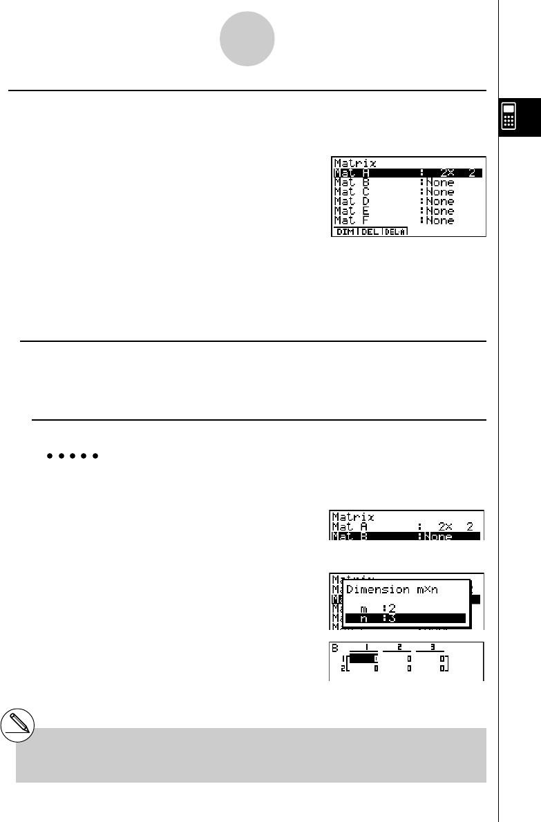
20010101
k Inputting and Editing Matrices
Pressing 1(MAT) displays the matrix editor screen. Use the matrix editor to input and edit
matrices.
• {DIM} ... {specifies the matrix dimensions (number of cells)}
• {DEL}/{DEL·A} ... deletes {a specific matrix}/{all matrices}
u Creating a Matrix
To create a matrix, you must first define its dimensions (size) in the Matrix list. Then you can
input values into the matrix.
u To specify the dimensions (size) of a matrix
Example To create a 2-row × 3-column matrix in the area named Mat B
Highlight Mat B.
c
1(DIM)
Specify the number of rows.
cw
Specify the number of columns.
dw
w
•All of the cells of a new matrix contain the value 0.
2-8-2
Matrix Calculations
#If “Memory ERROR” remains next to the matrix
area name after you input the dimensions, it
means there is not enough free memory to create
the matrix you want.
m × n … m (row) × n (column) matrix
None… no matrix preset
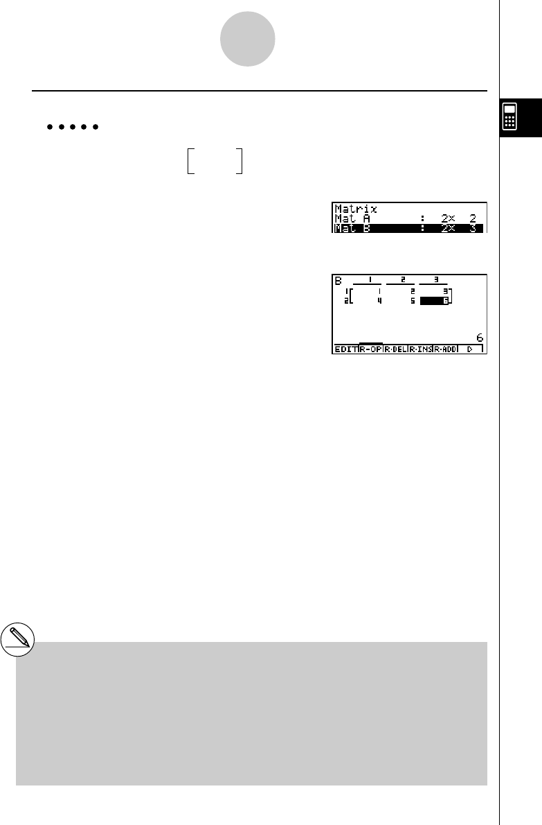
20010101
u To input cell values
Example To input the following data into Matrix B :
123
456
c (Selects Mat B.)
w
bwcwdw
ewfwgw
(Data is input into the highlighted cell.
Each time you press w, the highlighting
moves to the next cell to the right.)
# You can input complex numbers into the
cell of a matrix.
# Displayed cell values show positive
integers up to six digits, and negative
integers up to five digits (one digit used for
the negative sign). Exponential values are
shown with up to two digits for the
exponent. Fractional values are not
displayed.
# You can see the entire value assigned to a cell
by using the cursor keys to move the highlight-
ing to the cell whose value you want to view.
# The amount of memory required for a matrix is 9
bytes per cell. This means that a 3 × 3 matrix
requires 81 bytes of memory (3 × 3 × 9 = 81).
Inputting complex numbers into a matrix
doubles the amount of memory used.
2-8-3
Matrix Calculations
20011101

20010101
uDeleting Matrices
You can delete either a specific matrix or all matrices in memory.
u To delete a specific matrix
1. While the Matrix list is on the display, use f and c to highlight the matrix you want
to delete.
2. Press 2(DEL).
3. Press w(Yes) to delete the matrix or i(No) to abort the operation without deleting
anything.
u To delete all matrices
1. While the Matrix list is on the display, press 3(DEL·A).
2. Press w(Yes) to delete all matrices in memory or i(No) to abort the operation
without deleting anything.
2-8-4
Matrix Calculations
#The indicator “None” replaces the
dimensions of the matrix you delete.
#Inputting the format or changing the dimensions
of a matrix deletes its current contents.
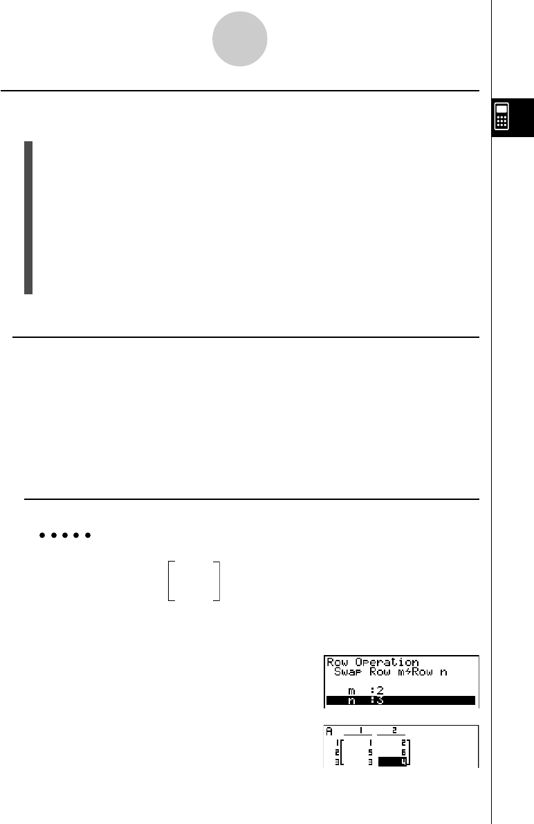
20010101
kMatrix Cell Operations
Use the following procedure to prepare a matrix for cell operations.
1. While the Matrix list is on the display, use f and c to highlight the name of the
matrix you want to use.
You can jump to a specific matrix by inputting the letter that corresponds to the matrix
name. Inputting ai(N), for example, jumps to Mat N.
Pressing !-(Ans) jumps to the Matrix current Memory.
2. Press w and the function menu with the following items appears.
• {EDIT} ... {cell editing screen}
• {R-OP} ... {row operation menu}
• {R • DEL}/{R • INS}/{R • ADD} ... row {delete}/{insert}/{add}
• {C • DEL}/{C • INS}/{C • ADD} ... column {delete}/{insert}/{add}
All of the following examples use Matrix A.
u Row Calculations
The following menu appears whenever you press 2(R-OP) while a recalled matrix is on the
display.
• {Swap} ... {row swap}
• {×Row} ... {product of specified row and scalar}
• {×Row+} ... {addition of one row and the product of a specified row with a scalar}
• {Row+} ... {addition of specified row to another row}
u To swap two rows
Example To swap rows two and three of the following matrix :
12
Matrix A = 34
56
2(R-OP)b(Swap)
Input the number of the rows you want to swap.
cwdw
6(EXE) (orw)
2-8-5
Matrix Calculations
20011101
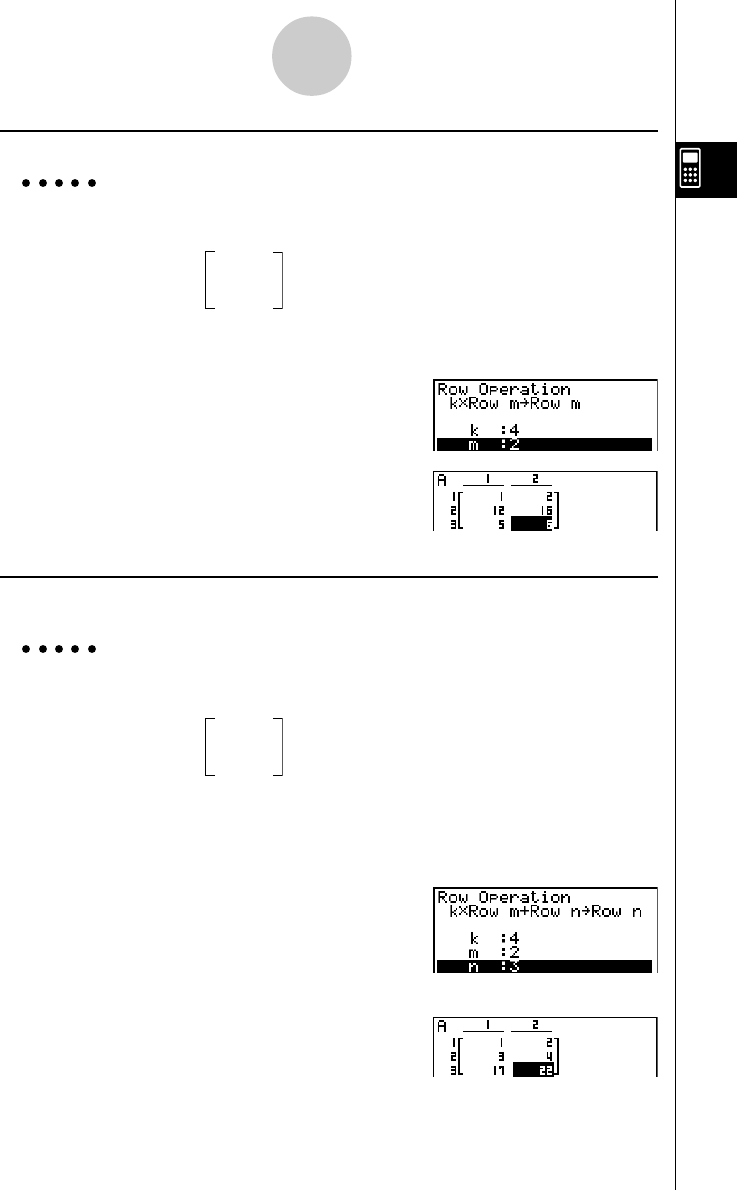
20010101
uu
uu
u To calculate the scalar multiplication of a row
Example To calculate the product of row 2 of the following matrix and the scalar
4 :
12
Matrix A = 34
56
2(R-OP)c(×Row)
Input multiplier value.
ew
Specify row number.
cw
6(EXE) (orw)
uu
uu
u To calculate the scalar multiplication of a row and add the result to another
row
Example To calculate the product of row 2 of the following matrix and the scalar
4, then add the result to row 3 :
12
Matrix A = 34
56
2(R-OP)d(×Row+)
Input multiplier value.
ew
Specify number of row whose product should be
calculated.
cw
Specify number of row where result should be added.
dw
6(EXE) (orw)
2-8-6
Matrix Calculations
20011101
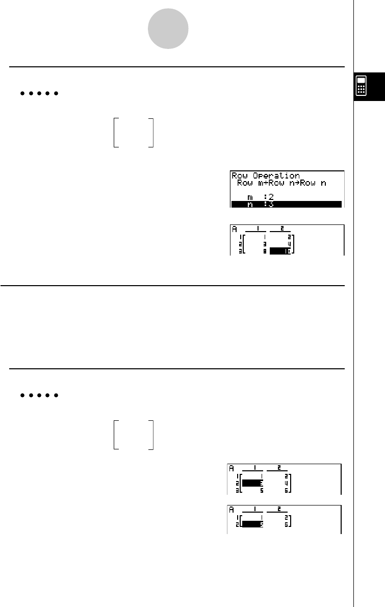
20010101
u To add two rows together
Example To add row 2 to row 3 of the following matrix :
12
Matrix A = 34
56
2(R-OP)e(Row+)
Specify number of row to be added.
cw
Specify number of row to be added to.
dw
6(EXE) (orw)
u Row Operations
• {R • DEL} ... {delete row}
• {R • INS} ... {insert row}
• {R • ADD} ... {add row}
u To delete a row
Example To delete row 2 of the following matrix :
12
Matrix A = 34
56
c
3(R • DEL)
2-8-7
Matrix Calculations
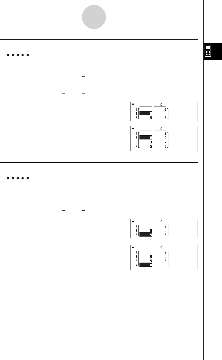
20010101
u To insert a row
Example To insert a new row between rows one and two of the following
matrix :
12
Matrix A = 34
56
c
4(R • INS)
u To add a row
Example To add a new row below row 3 of the following matrix :
12
Matrix A = 34
56
cc
5(R • ADD)
2-8-8
Matrix Calculations

20010101
2-8-9
Matrix Calculations
uColumn Operations
• {C • DEL} ... {delete column}
• {C • INS} ... {insert column}
• {C • ADD} ... {add column}
u To delete a column
Example To delete column 2 of the following matrix :
12
Matrix A = 34
56
e
6(g)1(C • DEL)
u To insert a column
Example To insert a new column between columns 1 and 2 of the following
matrix :
12
Matrix A = 34
56
e
6(g)2(C • INS)
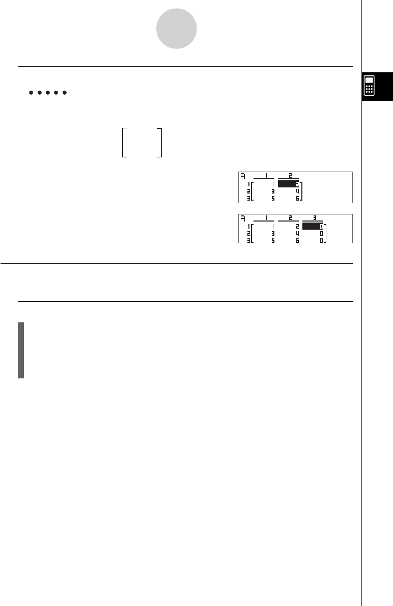
20010101
u To add a column
Example To add a new column to the right of column 2 of the following
matrix :
12
Matrix A = 34
56
e
6(g)3(C • ADD)
kModifying Matrices Using Matrix Commands [OPTN]-[MAT]
u To display the matrix commands
1. From the Main Menu, enter the RUN • MAT Mode.
2. Press K to display the option menu.
3. Press 2(MAT) to display the matrix command menu.
The following describes only the matrix command menu items that are used for creating
matrices and inputting matrix data.
• {Mat} ... {Mat command (matrix specification)}
• {Dim} ... {Dim command (dimension check)}
• {Augmnt} ... {Augment command (link two matrices)}
• {Ident} ... {Identity command (identity matrix input)}
• {Fill} ... {Fill command (identical cell values)}
• {M→List} ... {Mat→List command (assign contents of selected column to list file)}
2-8-10
Matrix Calculations
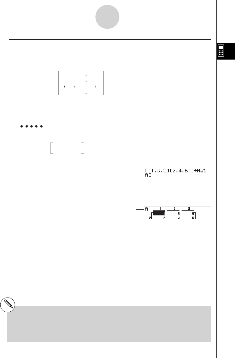
20010101
u Matrix Data Input Format [OPTN]-[MAT]-[Mat]
The following shows the format you should use when inputting data to create a matrix using
the Mat command.
a11 a12 a1n
a21 a22 a2n
am1am2amn
= [ [a11, a12, ..., a1n] [a21, a22, ..., a2n] .... [am1, am2, ..., amn] ]
→ Mat [letter A through Z]
Example 1 To input the following data as Matrix A :
135
246
!+( [ )!+( [ )b,d,f
!-( ] )!+( [ )c,e,g
!-( ] )!-( ] )aK2(MAT)
b(Mat)av(A)
w
2-8-11
Matrix Calculations
# You can also use !c(Mat) in place of
K2 (MAT)b(Mat).
# The maximum value of both m and n is 255.
# An error occurs if memory becomes full as you
are inputting data.
# You can also use the above format inside a
program that inputs matrix data.
Matrix name
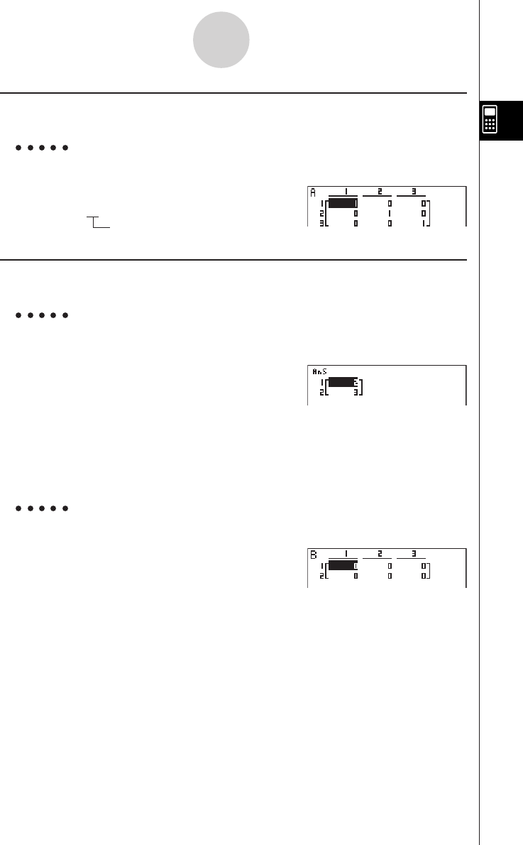
20010101
u To input an identity matrix [OPTN]-[MAT]-[Ident]
Use the Identity command to create an identity matrix.
Example 2 To create a 3 × 3 identity matrix as Matrix A
K2(MAT)g(Ident)
da2(MAT)b(Mat)av(A)w
Number of rows/columns
u To check the dimensions of a matrix [OPTN]-[MAT]-[Dim]
Use the Dim command to check the dimensions of an existing matrix.
Example 3 To check the dimensions of Matrix A, which was input in
Example 1
K2(MAT)c(Dim)
2(MAT)b(Mat)av(A)w
The display shows that Matrix A consists of two rows and three columns.
You can also use {Dim} to specify the dimensions of the matrix.
Example 4 To specify dimensions of 2 rows and 3 columns for Matrix B
!*( )c,d!/( )a
K2(MAT)c(Dim)
2(MAT)b(Mat)al(B)w
2-8-12
Matrix Calculations
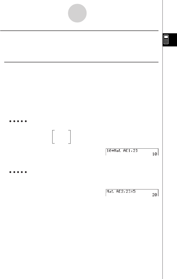
20010101
uModifying Matrices Using Matrix Commands
You can also use matrix commands to assign values to and recall values from an existing
matrix, to fill in all cells of an existing matrix with the same value, to combine two matrices
into a single matrix, and to assign the contents of a matrix column to a list file.
u To assign values to and recall values from an existing matrix
[OPTN]-[MAT]-[Mat]
Use the following format with the Mat command to specify a cell for value assignment and
recall.
Mat X [m, n]
X.................................. matrix name (A through Z, or Ans)
m ................................ row number
n ................................. column number
Example 1 Assign 10 to the cell at row 1, column 2 of the following matrix :
12
Matrix A = 34
56
baaK2(MAT)b(Mat)
av(A)!+( )b,c
!-( )w
Example 2 Multiply the value in the cell at row 2, column 2 of the above
matrix by 5
K2(MAT)b(Mat)
av(A)!+( )c,c
!-( )*fw
2-8-13
Matrix Calculations
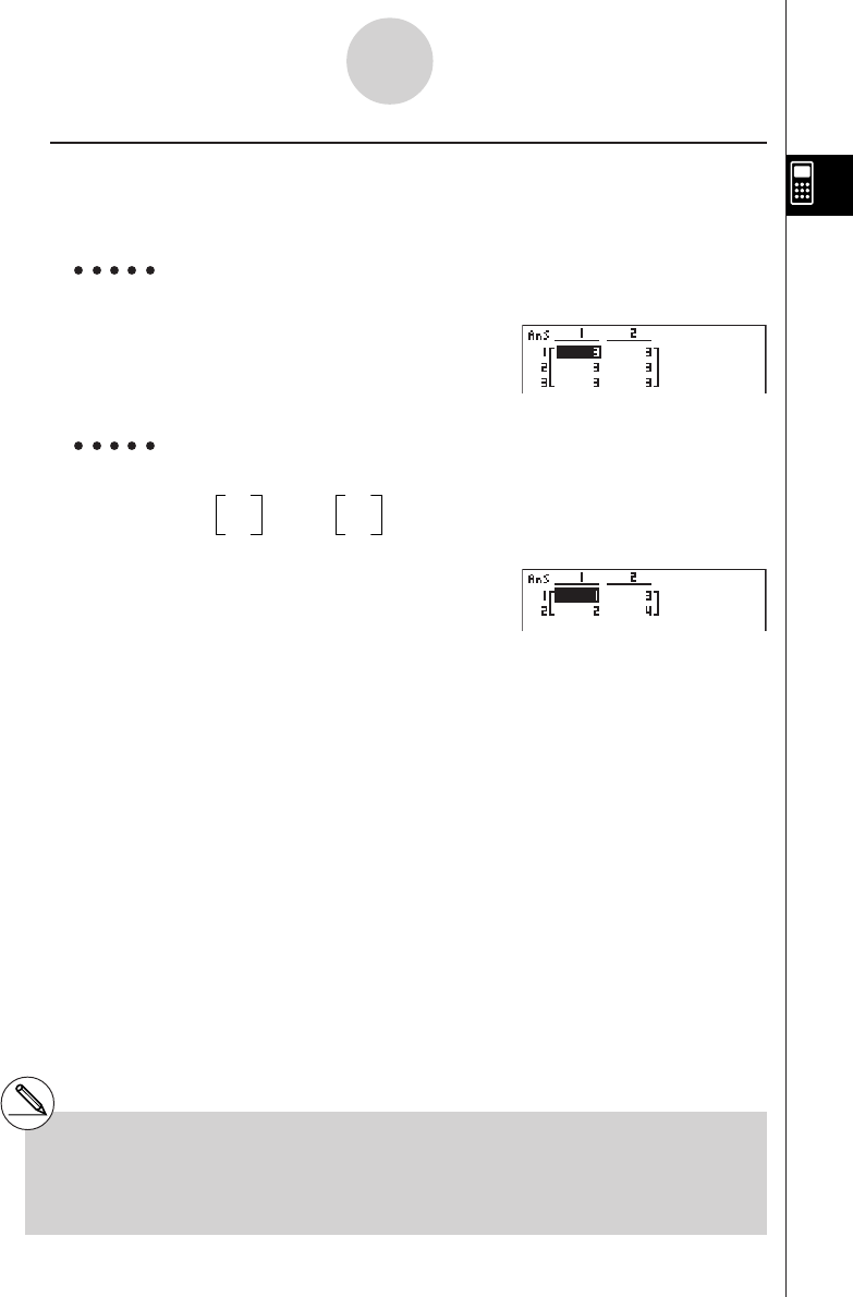
20010101
uu
uu
uTo fill a matrix with identical values and to combine two matrices into a
single matrix [OPTN]-[MAT]-[Fill]/[Augmnt]
Use the Fill command to fill all the cells of an existing matrix with an identical value and the
Augment command to combine two existing matrices into a single matrix.
Example 1 To fill all of the cells of Matrix A with the value 3
K2(MAT)h(Fill)
d,2(MAT)b(Mat)av(A)w
2(MAT)b(Mat)av(A)w
Example 2 To combine the following two matrices :
A = 1B = 3
24
K2(MAT)f(Augmnt)
2(MAT)b(Mat)av(A),
2(MAT)b(Mat)al(B)w
2-8-14
Matrix Calculations
# The two matrices you combine must have the
same number of rows. An error occurs if you
try to combine two matrices that have
different numbers of rows.
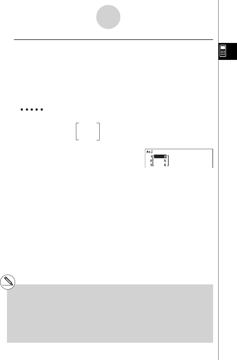
20010101
uu
uu
uTo assign the contents of a matrix column to a list
[OPTN]-[MAT]-[M→List]
Use the following format with the Mat→List command to specify a column and a list.
Mat → List (Mat X, m) → List n
X = matrix name (A through Z, or Ans)
m = column number
n = list number
Example To assign the contents of column 2 of the following matrix to list 1 :
12
Matrix A = 34
56
K2(MAT)i(M→List)
2(MAT)b(Mat)av(A),c)
aK1(LIST)b(List)bw
K1(LIST)b(List)bw
# You can also use !b(List) in place of
K1(LIST)b(List).
#You can use Matrix Answer Memory to assign
the results of the above matrix input and edit
operations to a matrix variable. To do so, use
the following syntax.
•Fill (n, Mat
α
) → Mat
β
•Augment (Mat
α
, Mat
β
) → Mat
γ
2-8-15
Matrix Calculations
In the above,
α
,
β
, and
γ
are any variable
names A through Z, and n is any value.
The above does not affect the contents of Matrix
Answer Memory.

20010101
kMatrix Calculations [OPTN]-[MAT]
Use the matrix command menu to perform matrix calculation operations.
u To display the matrix commands
1. From the Main Menu, enter the RUN • MAT Mode.
2. Press K to display the option menu.
3. Press 2(MAT) to display the matrix command menu.
The following describes only the matrix commands that are used for matrix arithmetic
operations.
• {Mat} ... {Mat command (matrix specification)}
• {Det} ... {Det command (determinant command)}
• {Trn} ... {Trn command (transpose matrix command)}
• {Ident} ... {Identity command (identity matrix input)}
All of the following examples assume that matrix data is already stored in memory.
2-8-16
Matrix Calculations
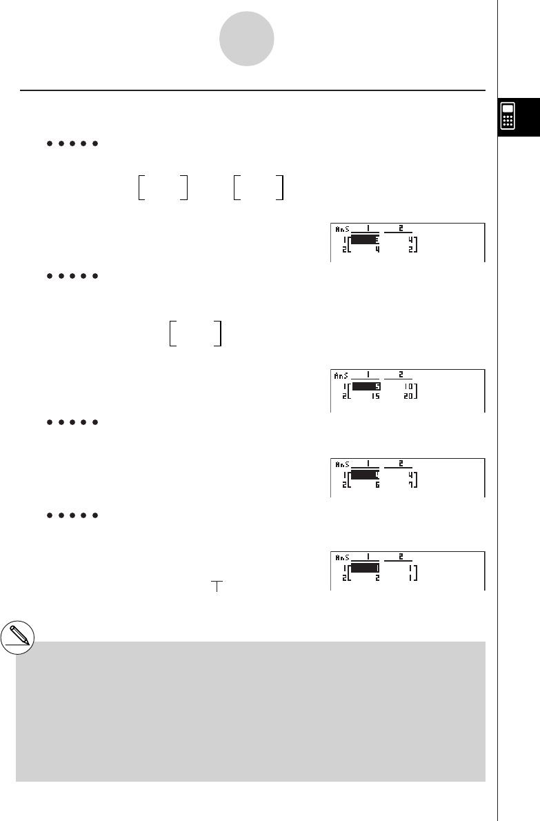
20010101
uMatrix Arithmetic Operations [OPTN]-[MAT]-[Mat]
Example 1 To add the following two matrices (Matrix A + Matrix B) :
A = 11 B = 23
21 21
AK2(MAT)b(Mat)av(A)+
2(MAT)b(Mat)al(B)w
Example 2 Calculate the product to the following matrix using a multiplier value
of 5 :
Matrix A = 12
34
AfK2(MAT)b(Mat)
av(A)w
Example 3 To multiply the two matrices in Example 1 (Matrix A × Matrix B)
AK2(MAT)b(Mat)av(A)*
2(MAT)b(Mat)al(B)w
Example 4 To multiply Matrix A (from Example 1) by a 2 × 2 identity matrix
AK2(MAT)b(Mat)av(A)*
2(MAT)g(Ident)cw
Number of rows and columns
# The two matrices must have the same
dimensions in order to be added or
subtracted. An error occurs if you try to
add or subtract matrices of different
dimensions.
# For multiplication (Matrix 1 × Matrix 2), the
number of columns in Matrix 1 must match
the number of rows in Matrix 2. Otherwise,
an error occurs.
2-8-17
Matrix Calculations
# When performing matrix arithmetic operations,
inputting the Identity command at the location
of a matrix command (such as Mat A) makes it
possible to perform identity matrix
calculations.
20011101
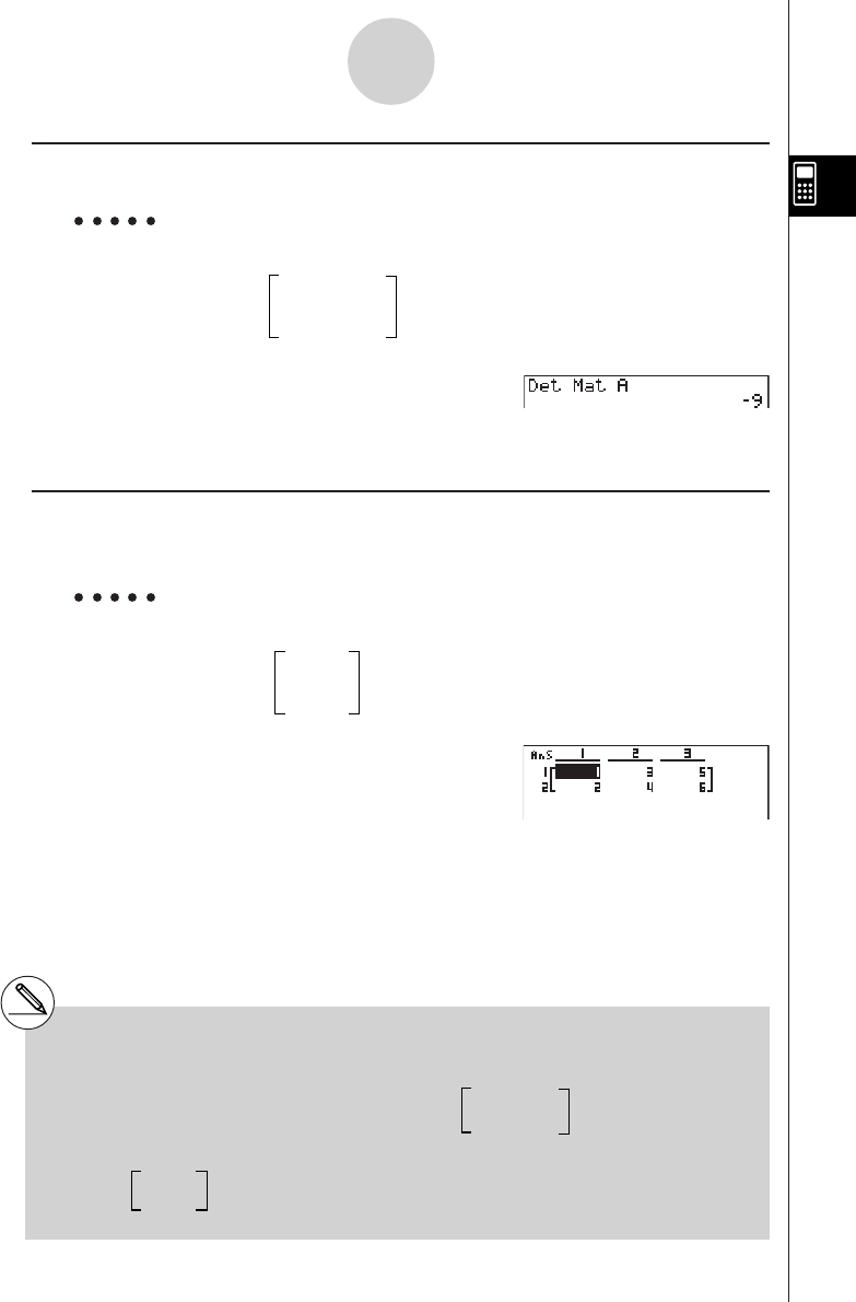
20010101
uDeterminant [OPTN]-[MAT]-[Det]
Example Obtain the determinant for the following matrix :
123
Matrix A = 456
–1 –2 0
K2(MAT)d(Det)2(MAT)b(Mat)
av(A)w
uMatrix Transposition [OPTN]-[MAT]-[Trn]
A matrix is transposed when its rows become columns and its columns become rows.
Example To transpose the following matrix :
12
Matrix A = 34
56
K2(MAT)e(Trn)2(MAT)b(Mat)
av(A)w
2-8-18
Matrix Calculations
#Determinants can be obtained only for square
matrices (same number of rows and
columns). Trying to obtain a determinant for a
matrix that is not square produces an error.
# The determinant of a 2 × 2 matrix is
calculated as shown below.
# The determinant of a 3 × 3 matrix is calculated
as shown below.
|A| = a11 a12 = a11a22 – a12a21
a21 a22
= a11a22a33 + a12a23a31 + a13a21a32
– a11a23a32 – a12a21a33 – a13a22a31
a11 a12 a13
a21 a22 a23
a31 a32 a33
|A| =
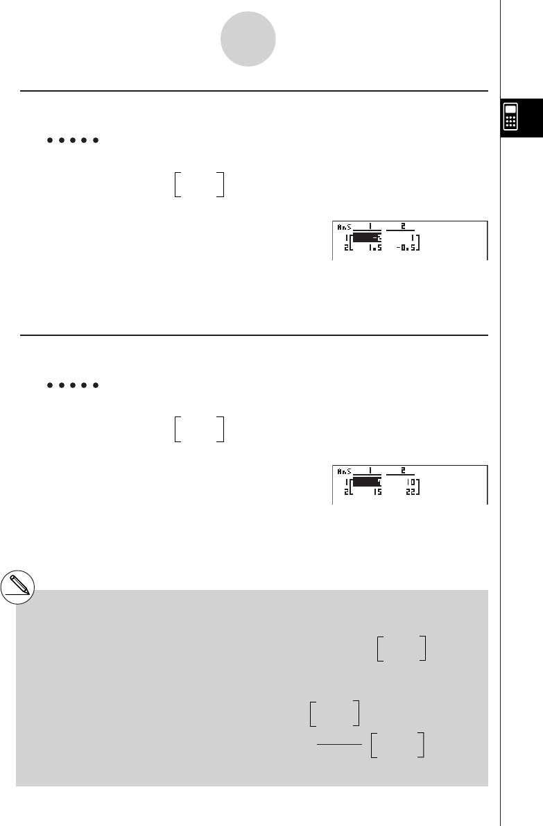
20010101
uMatrix Inversion [OPTN]-[MAT]-[x–1]
Example To invert the following matrix :
Matrix A = 12
34
K2(MAT)b(Mat)
av(A)!) (x–1) w
uSquaring a Matrix [OPTN]-[MAT]-[x2]
Example To square the following matrix :
Matrix A = 12
34
K2(MAT)b(Mat)av(A)xw
2-8-19
Matrix Calculations
#Only square matrices (same number of rows
and columns) can be inverted. Trying to invert
a matrix that is not square produces an error.
#A matrix with a determinant of zero cannot be
inverted. Trying to invert a matrix with
determinant of zero produces an error.
#Calculation precision is affected for matrices
whose determinant is near zero.
#A matrix being inverted must satisfy the
conditions shown below.
The following shows the formula used to
invert Matrix A into inverse matrix A–1.
A A–1 = A–1 A = E = 1 0
0 1
A = a b
c d
Note that ad – bc G 0.
A–1=1
ad – bc
d–b
–c a
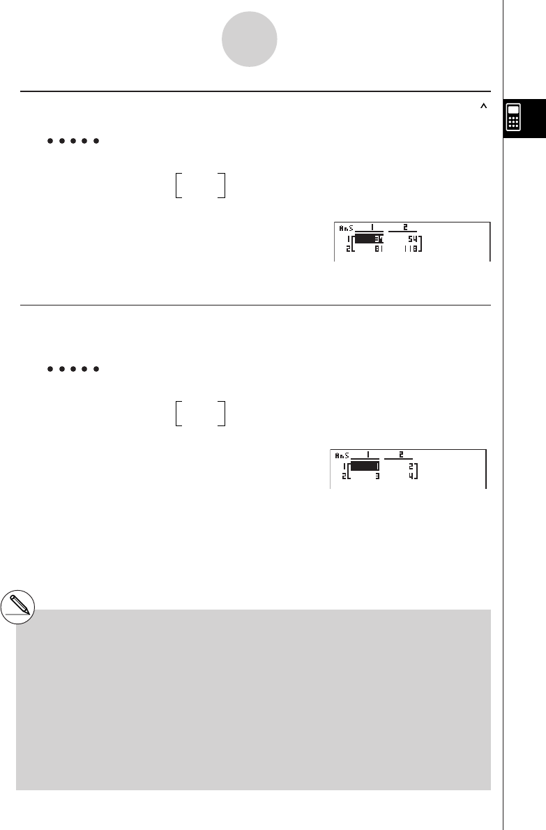
20010101
uRaising a Matrix to a Power [OPTN]-[MAT]-[
]
Example To raise the following matrix to the third power :
Matrix A = 12
34
K2(MAT)b(Mat)av(A)
Mdw
uDetermining the Absolute Value, Integer Part, Fraction Part, and
Maximum Integer of a Matrix [OPTN]-[NUM]-[Abs]/[Frac]/[Int]/[Intg]
Example To determine the absolute value of the following matrix :
Matrix A = 1–2
–3 4
K5(NUM)b(Abs)
K2(MAT)b(Mat)av(A)w
2-8-20
Matrix Calculations
# Determinants and inverse matrices are
subject to error due to dropped digits.
# Matrix operations are performed
individually on each cell, so calculations
may require considerable time to complete.
# The calculation precision of displayed
results for matrix calculations is ± 1 at the
least significant digit.
# If a matrix calculation result is too large to
fit into Matrix Answer Memory, an error
occurs.
# You can use the following operation to transfer
Matrix Answer Memory contents to another
matrix (or when Matrix Answer Memory
contains a determinant to a variable).
MatAns → Mat
α
In the above,
α
is any variable name A through
Z. The above does not affect the contents of
Matrix Answer Memory.
19990401
List Function
A list is a storage place for multiple data items.
This calculator lets you store up to 20 lists in a single file, and
you can store up to six files in memory. Stored lists can be used
in arithmetic and statistical calculations, and for graphing.
3-1 Inputting and Editing a List
3-2 Manipulating List Data
3-3 Arithmetic Calculations Using Lists
3-4 Switching Between List Files
Chapter
3
List 1 List 2 List 3 List 4 List 5 List 20
156 1 107 3.5 4 0
237 2 75 600
321 4 122 2.1 0 0
469 8 87 4.4 2 0
540 16 298 3 0 0
648 32486.8 3 0
793 64 338 2 9 0
830 128 49 8.7 0 0
••••••
••••••
••••••
•
•
•
•
••••••
Element number Display range Cell
Row
List name
Column
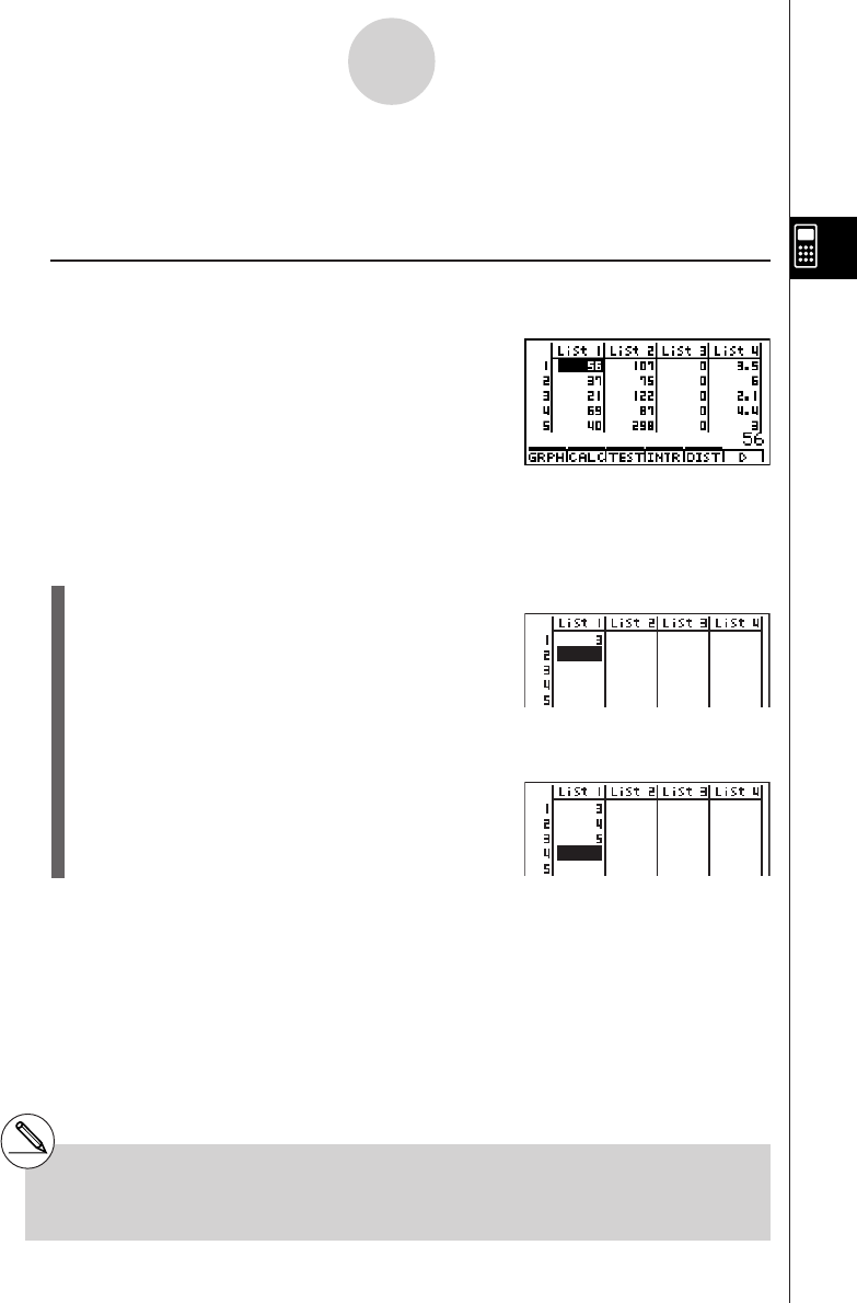
1999040120011101
3-1 Inputting and Editing a List
Enter the STAT Mode from the Main Menu to input data into a list and to manipulate list data.
uu
uu
u To input values one-by-one
Use the cursor keys to move the highlighting to the list name or cell you want to select.
The screen automatically scrolls when the highlighting is located at either edge of the
screen.
The following example is performed starting with the highlighting located at Cell 1 of List 1.
1. Input a value and press w to store it in the list.
dw
•The highlighting automatically moves down to the
next cell for input.
2. Input the value 4 in the second cell, and then input the result of 2 + 3 in the next cell.
ewc+dw
3-1-1
Inputting and Editing a List
#You can also input the result of an expres-
sion or a complex number into a cell.
#You can input values up to 255 cells in a single list.
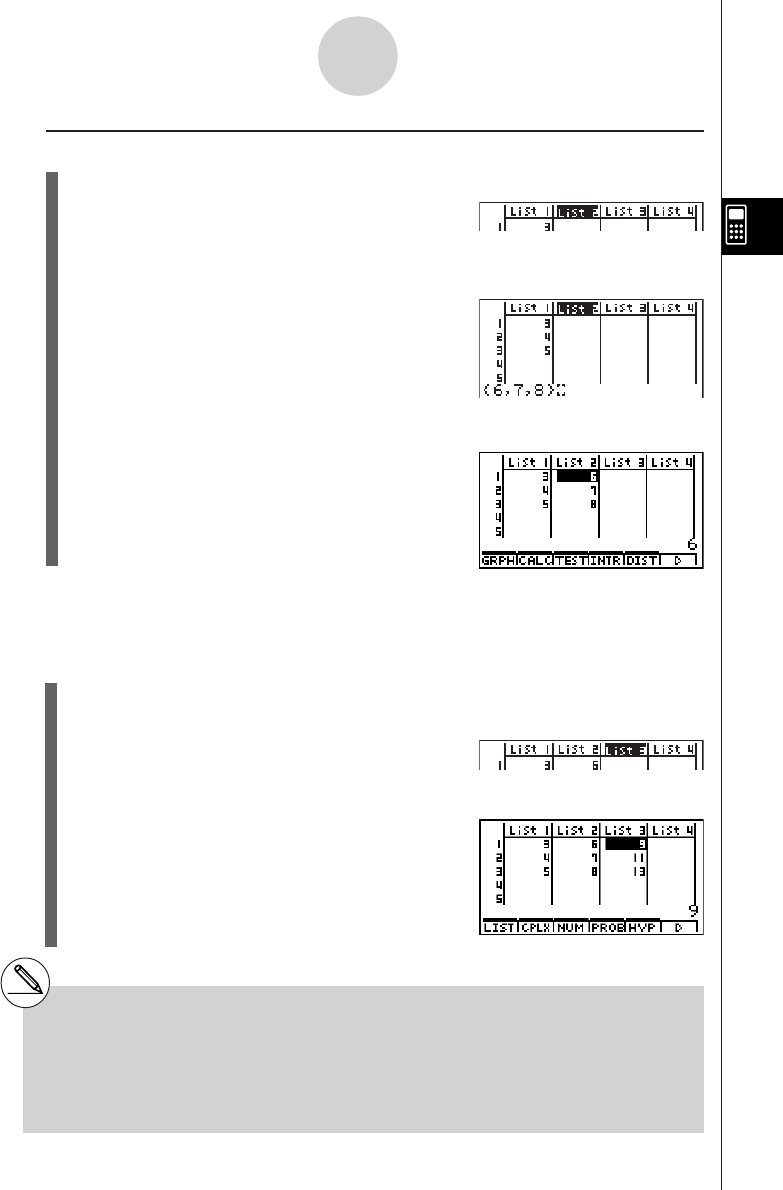
1999040120010102
uu
uu
u To batch input a series of values
1. Use the cursor keys to move the highlighting to another list.
2. Press !*( { ), and then input the values you want, pressing , between each one.
Press !/( } ) after inputting the final value.
!*( { )g,h,i!/( } )
3. Press w to store all of the values in your list.
w
You can also use list names inside of a mathematical expression to input values into another
cell. The following example shows how to add the values in each row in List 1 and List 2, and
input the result into List 3.
1. Use the cursor keys to move the highlighting to the name of the list where you want the
calculation results to be input.
2. Press K and input the expression.
K1(LIST)b(List)b+
K1(LIST)b(List)cw
3-1-2
Inputting and Editing a List
#You can also use !b(List) in place of
K1(LIST)b(List).
# Remember that a comma separates values, so
you should not input a comma after the final
value of the set you are inputting.
Right: {34, 53, 78}
Wrong: {34, 53, 78,}
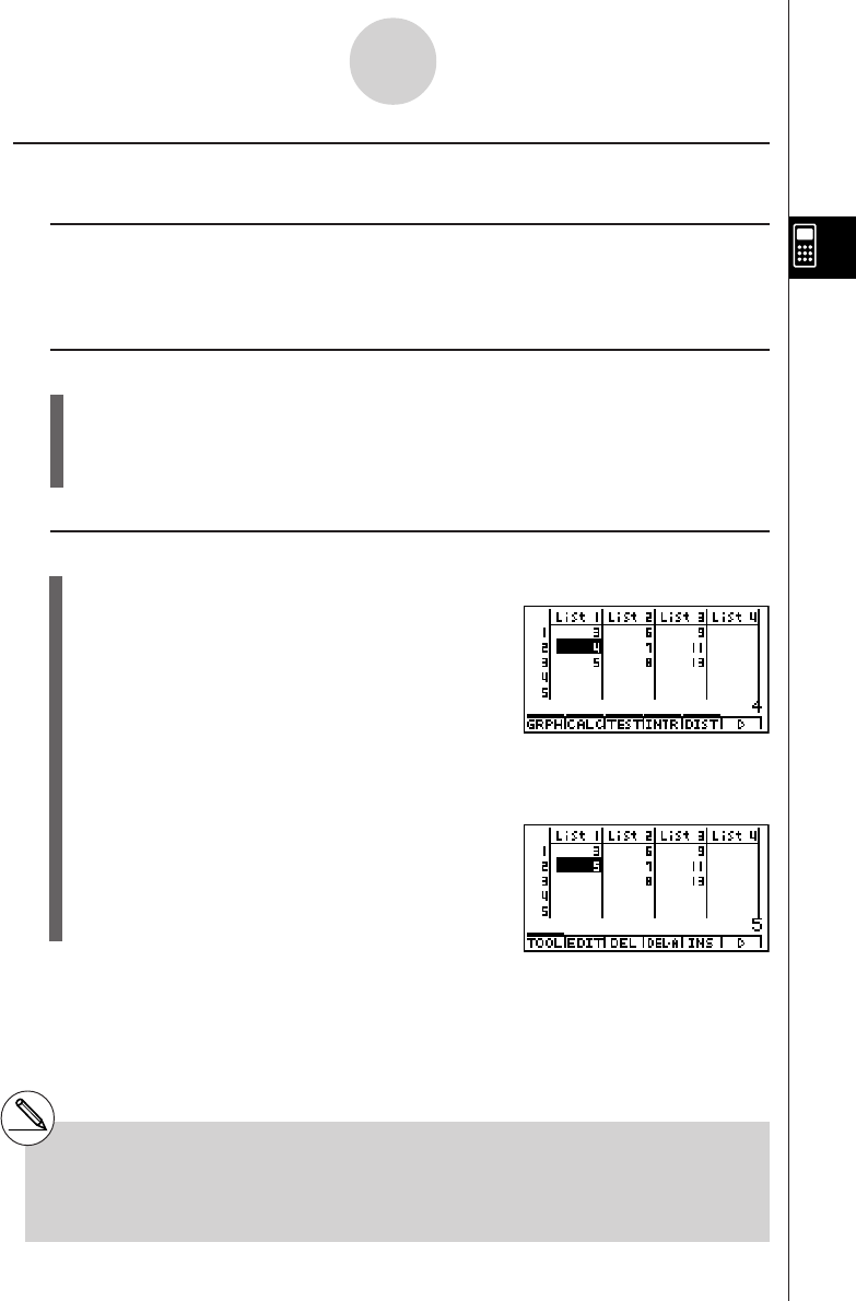
1999040120010102
kk
kk
kEditing List Values
uu
uu
u To change a cell value
Use d or e to move the highlighting to the cell whose value you want to change. Input the
new value and press w to replace the old data with the new one.
uu
uu
u To edit the contents of a cell
1. Use the cursor keys to move the highlighting to the cell whose contents you want to
edit.
2. Press 6(䉯)2(EDIT) to display the contents of the cell at the bottom of the screen.
3. Make any changes in the data you want.
uu
uu
u To delete a cell
1. Use the cursor keys to move the highlighting to the cell you want to delete.
2. Press 6(䉯)3(DEL) to delete the selected cell and cause everything below it to be
shifted up.
3-1-3
Inputting and Editing a List
# The cell delete operation does not affect cells
in other lists. If the data in the list whose cell
you delete is somehow related to the data in
neighboring lists, deleting a cell can cause
related values to become misaligned.
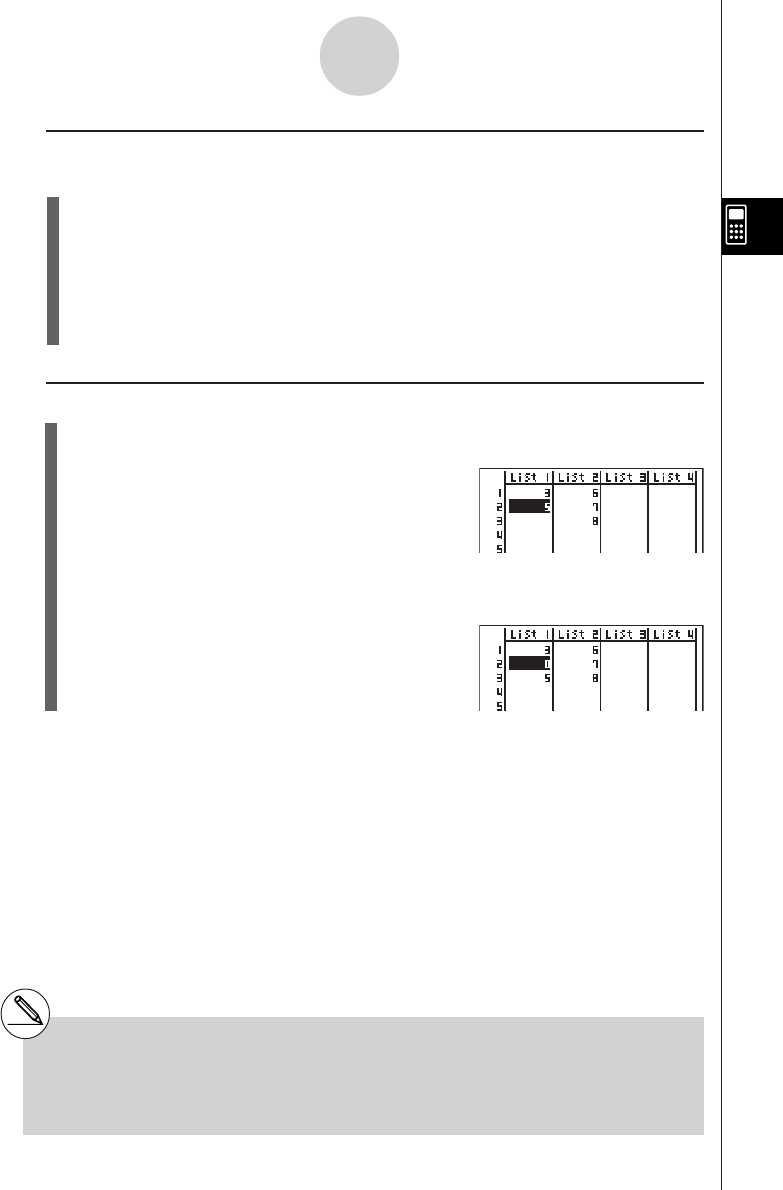
1999040120010102
uu
uu
u To delete all cells in a list
Use the following procedure to delete all the data in a list.
1. Use the cursor key to move the highlighting to any cell of the list whose data you want
to delete.
2. Pressing 6(䉯)4(DEL
•
A) causes a confirmation message to appear.
3. Press w(Yes) to delete all the cells in the selected list or i(No) to abort the delete
operation without deleting anything.
uu
uu
u To insert a new cell
1. Use the cursor keys to move the highlighting to the location where you want to insert
the new cell.
2. Press 6(䉯)5(INS) to insert a new cell, which contains a value of 0, causing
everything below it to be shifted down.
#The cell insert operation does not affect cells in
other lists. If the data in the list where you insert
a cell is somehow related to the data in
3-1-4
Inputting and Editing a List
neighboring lists, inserting a cell can cause
related values to become misaligned.
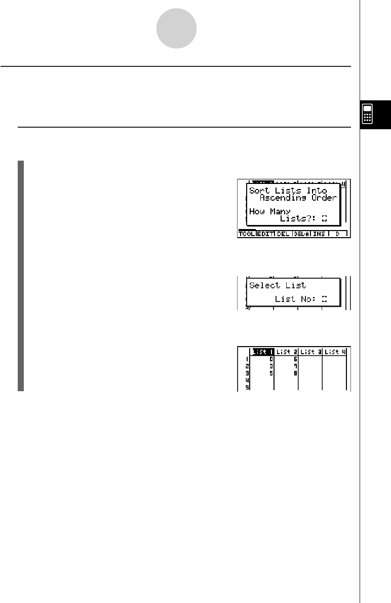
19990401
kk
kk
kSorting List Values
You can sort lists into either ascending or descending order. The highlighting can be located
in any cell of the list.
uu
uu
u To sort a single list
Ascending order
1. While the lists are on the screen, press 6(䉯)1(TOOL)b(SortA).
2. The prompt “How Many Lists?: ” appears to ask how many lists you want to sort. Here
we will input 1 to indicate we want to sort only one list.
bw
3. In response to the “Select List List No: ” prompt, input the number of the list you want
to sort.
bw
Descending order
Use the same procedure as that for the ascending order sort. The only difference is that
you should press c(SortD) in place of b(SortA).
3-1-5
Inputting and Editing a List
20010102
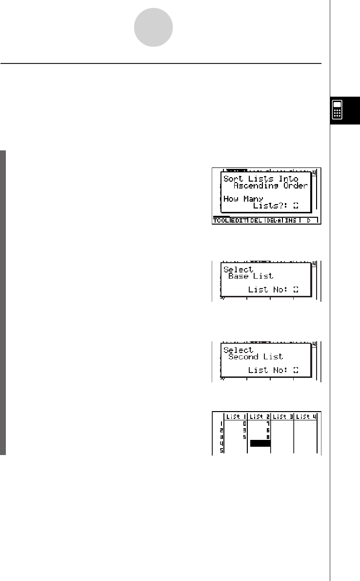
19990401
uu
uu
u To sort multiple lists
You can link multiple lists together for a sort so that all of their cells are rearranged in
accordance with the sorting of a base list. The base list is sorted into either ascending order
or descending order, while the cells of the linked lists are arranged so that the relative
relationship of all the rows is maintained.
Ascending order
1. While the lists are on the screen, press 6(䉯)1(TOOL)b(SortA).
2. The prompt “How Many Lists?: ” appears to ask how many lists you want to sort. Here
we will sort one base list linked to one other list, so we should input 2.
cw
3. In response to the “Select Base List List No: ” prompt, input the number of the list you
want to sort into ascending order. Here we will specify List 1.
bw
4. In response to the “Select Second List List No:” prompt, input the number of the list
you want to link to the base list. Here we will specify List 2.
cw
3-1-6
Inputting and Editing a List
20010102

19990401
3-1-7
Inputting and Editing a List
Descending order
Use the same procedure as that for the ascending order sort. The only difference is that
you should press c(SortD) in place of b(SortA).
#You can specify a value from 1 to 6 as the
number of lists for sorting.
#If you specify a list more than once for a single
sort operation, an error occurs.
An error also occurs if lists specified for sorting
do not have the same number of values (rows).
#Specifying a value of 0 for the number of lists
causes all the lists in the file to be sorted. In
this case you specify a base list on which all
other lists in the file are sorted.

19990401
3-2 Manipulating List Data
List data can be used in arithmetic and function calculations. In addition, various list data
manipulation functions make manipulation of list data quick and easy.
You can use list data manipulation functions in the RUN
•
MAT, STAT, GRPH
•
TBL, EQUA and
PRGM Modes.
kk
kk
k Accessing the List Data Manipulation Function Menu
All of the following examples are performed after entering the RUN
•
MAT Mode.
Press K and then 1(LIST) to display the list data manipulation menu, which contains the
following items.
•{List}/{Dim}/{Seq}/{Min}/{Max}/{Mean}/{Median}/{Sum}/{Prod}/{Cuml}/{%}/{AA
AA
AList}/
{Augmnt}/{Fill}/{L→Mat}
Note that all closing parentheses at the end of the following operations can be omitted.
u To count the number of data items in a list [OPTN]-[LIST]-[Dim]
K1(LIST)c(Dim)1(LIST)b(List) <list number 1-20> w
•The number of cells a list contains is its “dimension.”
Example To count the number of values in List 1 (36, 16, 58, 46, 56)
AK1(LIST)c(Dim)
1(LIST)b(List)bw
u To create a list or matrix by specifying the number of data items
[OPTN]-[LIST]-[Dim]
Use the following procedure to specify the number of data in the assignment statement
and create a list.
<number of data n>aK1(LIST)c(Dim)1(LIST)b(List)
<list number 1-20>w
n = 1 ~ 255
3-2-1
Manipulating List Data
20011101
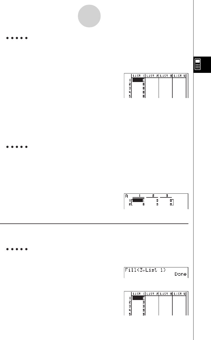
19990401
Example To create five data items (each of which contains 0) in List 1
AfaK1(LIST)c(Dim)
1(LIST)b(List) bw
You can view the newly created list by entering
the STAT Mode.
Use the following procedure to specify the number of data rows and columns, and the matrix
name in the assignment statement and create a matrix.
!*( { )<number of row m> ,<number of column n> !/( } )a
K1(LIST)c(Dim)2(MAT)b(Mat)a<matrix name>w
m, n = 1 ~ 255, matrix name; A ~ Z
Example To create a 2-row × 3-column matrix (each cell of which
contains 0) in Matrix A
A!*( { )c,d!/( } )a
K1(LIST)c(Dim)
2(MAT)b(Mat)av(A)w
The following shows the new contents of Mat A.
u To replace all data items with the same value [OPTN]-[LIST]-[Fill]
K1(LIST)c(Fill) <value>,1(LIST)b(List) <list number 1-20>)w
Example To replace all data items in List 1 with the number 3
AK1(LIST)c(Fill)
d,1(LIST)b(List)b)w
The following shows the new contents of List 1.
3-2-2
Manipulating List Data
20011101
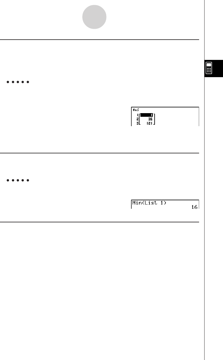
19990401
3-2-3
Manipulating List Data
u To generate a sequence of numbers [OPTN]-[LIST]-[Seq]
K1(LIST)d(Seq) <expression> , <variable name> , <start value>
, <end value> , <increment> ) w
•The result of this operation is stored in ListAns Memory.
Example To input the number sequence 12, 62, 112, into a list, using the function
f(x) = X2. Use a starting value of 1, an ending value of 11, and an
increment of 5
AK1(LIST)d(Seq)vx,
v,b,bb,f)w
Specifying an ending value of 12, 13, 14, or 15 produces the same result as shown above,
because all of them are less than the value produced by the next increment (16).
u To find the minimum value in a list [OPTN]-[LIST]-[Min]
K1(LIST)e(Min)1(LIST)b(List) <list number 1-20> )w
Example To find the minimum value in List 1 (36, 16, 58, 46, 56)
AK1(LIST)e(Min)
1(LIST)b(List)b)w
u To find the maximum value in a list [OPTN]-[LIST]-[Max]
Use the same procedure as when finding the minimum value (Min), except press f(Max) in
place of e(Min).
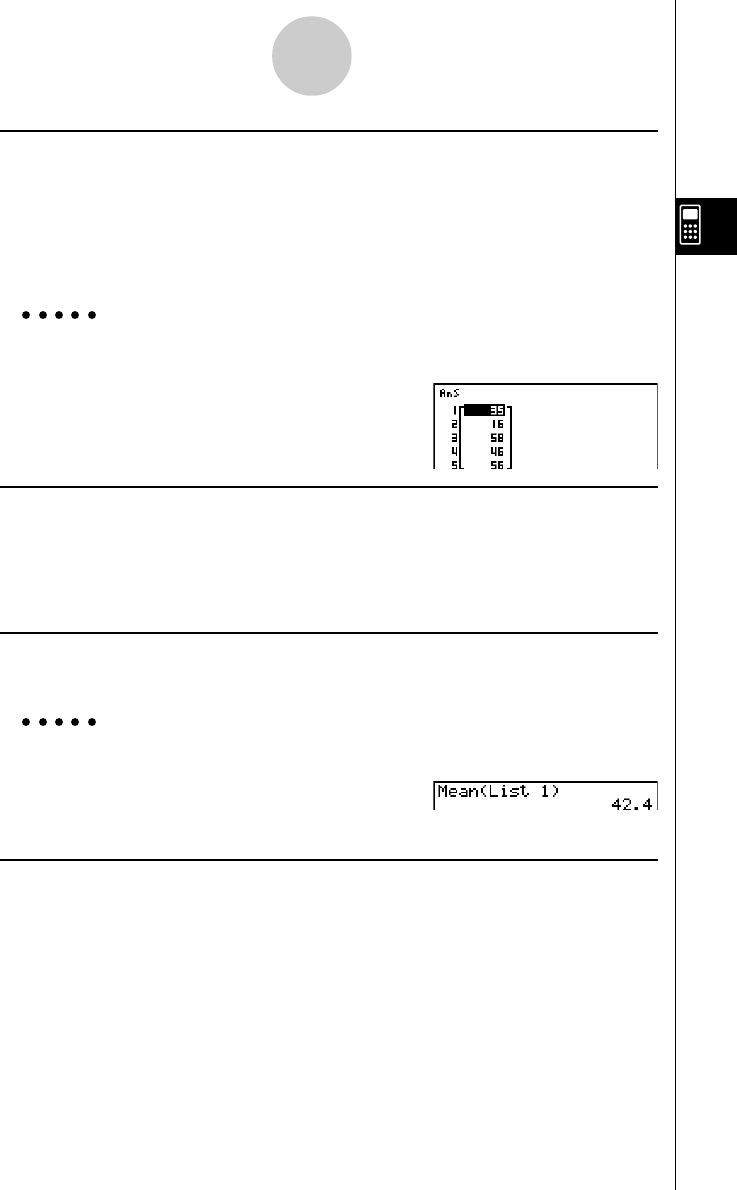
19990401
3-2-4
Manipulating List Data
u To find which of two lists contains the smallest value [OPTN]-[LIST]-[Min]
K1(LIST)e(Min)1(LIST)b(List) <list number 1-20>
,1(LIST)b (List) <list number 1-20>)w
•The two lists must contain the same number of data items. If they don’t, an error occurs.
•The result of this operation is stored in ListAns Memory.
Example To find whether List 1 (75, 16, 98, 46, 56) or List 2 (35, 59, 58, 72, 67)
contains the smallest value
K1(LIST)e(Min)
1(LIST)b(List)b,
1(LIST)b(List)c)w
u To find which of two lists contains the greatest value [OPTN]-[LIST]-[Max]
Use the same procedure as that for the smallest value, except press f(Max) in place of
e(Min).
•The two lists must contain the same number of data items. If they don’t, an error occurs.
u To calculate the mean of data items [OPTN]-[LIST]-[Mean]
K1(LIST)g(Mean)1(LIST)b(List) <list number 1-20>)w
Example To calculate the mean of data items in List 1 (36, 16, 58, 46, 56)
AK1(LIST)g(Mean)
1(LIST)b(List)b)w
u To calculate the mean of data items of specified frequency
[OPTN]-[LIST]-[Mean]
This procedure uses two lists: one that contains values and one that indicates the frequency
(number of occurrences) of each value. The frequency of the data in Cell 1 of the first list is
indicated by the value in Cell 1 of the second list, etc.
•The two lists must contain the same number of data items. If they don’t, an error occurs.
K1(LIST)g(Mean)1(LIST)b(List)<list number 1-20 (data)>
,1(LIST)b(List)<list number 1-20 (frequency)>)w
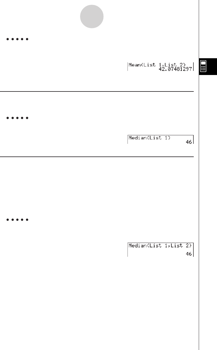
19990401
Example To calculate the mean of data items in List 1 (36, 16, 58, 46, 56), whose
frequency is indicated by List 2 (75, 89, 98, 72, 67)
AK1(LIST)g(Mean)
1(LIST)b(List)b,
1(LIST)b(List)c)w
u To calculate the median of data items in a list [OPTN]-[LIST]-[Med]
K1(LIST)h(Median)1(LIST)b(List)<list number 1-20>)w
Example To calculate the median of data items in List 1 (36, 16, 58, 46, 56)
AK1(LIST)h(Median)
1(LIST)b(List)b)w
u To calculate the median of data items of specified frequency
[OPTN]-[LIST]-[Med]
This procedure uses two lists: one that contains values and one that indicates the frequency
(number of occurrences) of each value. The frequency of the data in Cell 1 of the first list is
indicated by the value in Cell 1 of the second list, etc.
•The two lists must contain the same number of data items. If they don’t, an error occurs.
K1(LIST)h(Median)1(LIST)b(List) <list number 1-20 (data)>
,1(LIST)b(List) <list number 1-20 (frequency)>)w
Example To calculate the median of values in List 1 (36, 16, 58, 46, 56), whose
frequency is indicated by List 2 (75, 89, 98, 72, 67)
AK1(LIST)h(Median)
1(LIST)b(List)b,
1(LIST)b(List)c)w
3-2-5
Manipulating List Data
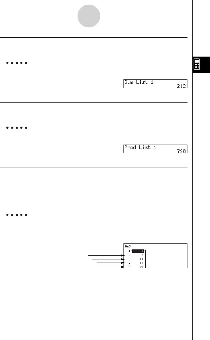
19990401
u To calculate the sum of data items in a list [OPTN]-[LIST]-[Sum]
K1(LIST)i(Sum)1(LIST)b(List)<list number 1-20>w
Example To calculate the sum of data items in List 1 (36, 16, 58, 46, 56)
AK1(LIST)i(Sum)
1(LIST)b(List)bw
u To calculate the product of values in a list [OPTN]-[LIST]-[Prod]
K1(LIST)j(Prod)1(LIST)b(List)<list number 1-20>w
Example To calculate the product of values in List 1 (2, 3, 6, 5, 4)
AK1(LIST)j(Prod)
1(LIST)b(List)bw
u To calculate the cumulative frequency of each data item
[OPTN]-[LIST]-[Cuml]
K1(LIST)v(Cuml)1(LIST)b(List) <list number 1-20>w
•The result of this operation is stored in ListAns Memory.
Example To calculate the cumulative frequency of each data item in List 1
(2, 3, 6, 5, 4)
AK1(LIST)v(Cuml)
1(LIST)b(List)bw
3-2-6
Manipulating List Data
2+3=
2+3+6=
2+3+6+5=
2+3+6+5+4=
20011101
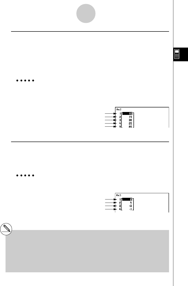
19990401
u To calculate the percentage represented by each data item
[OPTN]-[LIST]-[%]
K1(LIST)l(%)1(LIST)b(List)<list number 1-20>w
•The above operation calculates what percentage of the list total is represented
by each data item.
•The result of this operation is stored in ListAns Memory.
Example To calculate the percentage represented by each data item in List 1
(2, 3, 6, 5, 4)
AK1(LIST)l(%)
1(LIST)b(List)bw
u To calculate the differences between neighboring data inside a list
[OPTN]-[LIST]-[AA
AA
AList]
K1(LIST)I(AList)<list number 1-20>w
•The result of this operation is stored in ListAns memory.
Example To calculate the difference between the data items in List 1
(1, 3, 8, 5, 4)
AK1(LIST)I(AList)
bw
3-2-7
Manipulating List Data
# You can specify the location of the new list (List 1
through List 20) with a statement like: A List 1 →
List 2. You cannot specify another memory or
ListAns as the destination of the A List operation.
An error also occurs if you specify a A List as the
destination of the results of another A List
operation.
# The number of cells in the new A List is one
less than the number of cells in the original list.
#An error occurs if you execute A List for a list
that has no data or only one data item.
2/(2+3+6+5+4)
×
100 =
3/(2+3+6+5+4)
×
100 =
6/(2+3+6+5+4)
×
100 =
5/(2+3+6+5+4)
×
100 =
4/(2+3+6+5+4)
×
100 =
3 – 1 =
8 – 3 =
5 – 8 =
4 – 5 =
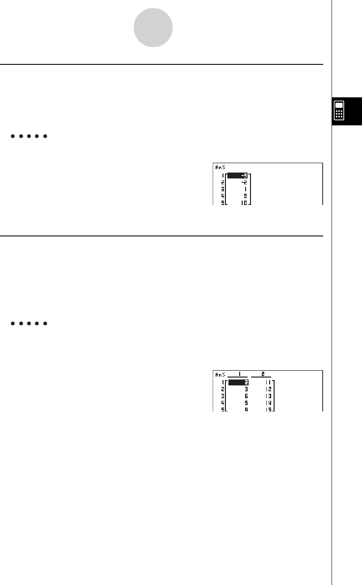
19990401
uu
uu
u To combine lists [OPTN]-[LIST]-[Augmnt]
• You can combine two different lists into a single list. The result of a list combination
operation is stored in ListAns memory.
K1(LIST)s(Augmnt)1(LIST)b(List) < list number 1-20 >
,1(LIST)b(List) < list number 1-20 >)w
Example To combine the List 1 (–3, –2) and List 2 (1, 9, 10)
AK1(LIST)s(Augmnt)
1(LIST)b(List)b,
1(LIST)b(List)c)w
u To transfer list contents to Matrix Answer Memory [OPTN]-[LIST]-[L→Mat]
K1(LIST)t(L→Mat)1(LIST)b(List) <list number 1-20>
,1(LIST)b(List) <list number 1-20> )w
•You can skip input 1(LIST)b(List) in the part of the above operation.
Example: List → Mat (1, 2)w
Example To transfer the contents of List 1 (2, 3, 6, 5, 4) to column 1, and the
contents of List 2 (11, 12, 13, 14, 15) to column 2 of Matrix Answer
Memory
AK1(LIST)t(L→Mat)
1(LIST)b(List)b,
1(LIST)b(List)c)w
3-2-8
Manipulating List Data
20011101
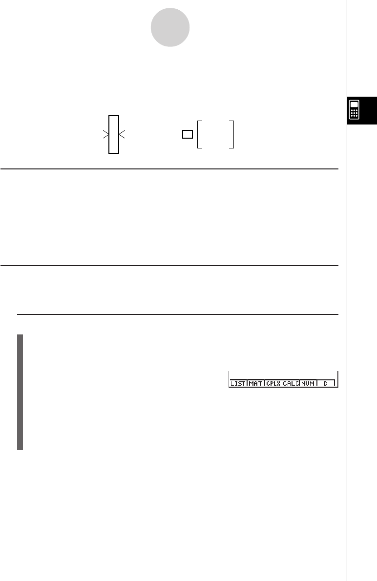
19990401
3-3 Arithmetic Calculations Using Lists
You can perform arithmetic calculations using two lists or one list and a numeric value.
Calculation results are
stored in ListAns Memory.
kError Messages
•A calculation involving two lists performs the operation between corresponding cells.
Because of this, an error occurs if the two lists do not have the same number of values
(which means they have different “dimensions”).
•An error occurs whenever an operation involving any two cells generates a mathematical
error.
kInputting a List into a Calculation
There are two methods you can use to input a list into a calculation.
u To input a specific list by name
1. Press K to display the first Operation Menu.
• This is the function key menu that appears in the RUN
•
MAT Mode when you press K.
2. Press 1(LIST) to display the List Data Manipulation Menu.
3. Press b(List) to display the “List” command and input the number of the list you want
to specify.
3-3-1
Arithmetic Calculations Using Lists
List
Numeric Value
List
Numeric Value
+
−
×
÷
=List
ListAns Memory
19990401
u To directly input a list of values
You can also directly input a list of values using {, }, and ,.
Example 1 To input the list: 56, 82, 64
!*( { )fg,ic,
ge!/( } )
41 6
Example 2 To multiply List 3
(
= 65
)
by the list 0
22 4
K1(LIST)b(List)d*!*( { )g,a,e!/( } )w
246
The resulting list 0 is stored in ListAns Memory.
88
uTo assign the contents of one list to another list
Use a to assign the contents of one list to another list.
Example 1 To assign the contents of List 3 to List 1
K1(LIST)b(List)da1(LIST)b(List)bw
In place of K1(LIST)b(List)d operation in the above procedure, you could input
!*( { )eb,gf,cc!/( } ).
Example 2 To assign the list in ListAns Memory to List 1
K1(LIST)b(List)!-(Ans)a1(LIST)b(List)bw
3-3-2
Arithmetic Calculations Using Lists

19990401
u To recall the value in a specific list cell
You can recall the value in a specific list cell and use it in a calculation. Specify the cell
number by enclosing it inside square brackets.
Example To calculate the sine of the value stored in Cell 3 of List 2
sK1(LIST)b(List)c!+( [ )d!-( ] )w
u To input a value into a specific list cell
You can input a value into a specific list cell inside a list. When you do, the value that was
previously stored in the cell is replaced with the new value you input.
Example To input the value 25 into Cell 2 of List 3
cfaK1(LIST)b(List)d!+( [ )c!-( ] )w
kRecalling List Contents
Example To recall the contents of List 1
K1(LIST)b(List)bw
• The above operation displays the contents of the list you specify and also stores them
in ListAns Memory. You can then use the ListAns Memory contents in a calculation.
u To use list contents in ListAns Memory in a calculation
Example To multiply the list contents in ListAns Memory by 36
K1(LIST)b(List)!-(Ans)*dgw
•The operation K1(LIST)b(List)!-(Ans) recalls ListAns Memory contents.
• This operation replaces current ListAns Memory contents with the result of the above
calculation.
3-3-3
Arithmetic Calculations Using Lists

19990401
kGraphing a Function Using a List
When using the graphing functions of this calculator, you can input a function such as Y1 =
List 1 X. If List 1 contains the values 1, 2, 3, this function will produces three graphs: Y = X,
Y = 2X, Y = 3X.
There are certain limitations on using lists with graphing functions.
kInputting Scientific Calculations into a List
You can use the numeric table generation functions in the Table & Graph Menu to input
values that result from certain scientific function calculations into a list. To do this, first
generate a table and then use the list copy function to copy the values from the table to the
list.
kPerforming Scientific Function Calculations Using a List
Lists can be used just as numeric values are in scientific function calculations. When the
calculation produces a list as a result, the list is stored in ListAns Memory.
41
Example To use List 3 65 to perform sin (List 3)
22
Use radians as the angle unit.
sK1(LIST)b(List)dw
–0.158
The resulting list 0.8268 is stored in ListAns Memory.
–8E–3
In place of the K1(LIST)b(List)d operation in the above procedure, you could input
!*( { ) eb,gf,cc!/( } ).
3-3-4
Arithmetic Calculations Using Lists

19990401
14
Example To use List 1 2 and List 2 5 to perform List 1List 2
36
This creates a list with the results of 14, 25, 36.
K1(LIST)b(List)bM1(LIST)b(List)cw
1
The resulting list 32 is stored in ListAns Memory.
729
3-3-5
Arithmetic Calculations Using Lists
19990401
3-4-1
Switching Between List Files
3-4 Switching Between List Files
You can store up to 20 lists (List 1 to List 20) in each file (File 1 to File 6). A simple operation
lets you switch between list files.
u To switch between list files
1. From the Main Menu, enter the STAT Mode.
Press u3(SET UP) to display the STAT Mode SET UP screen.
2. Press 1(FILE) and then input the number of the list file you want to use.
Example To select File 3
1(FILE)d
w
All subsequent list operations are applied to the lists contained in the file you select (List File
3 in the above example).

19990401
Chapter
Equation Calculations
Your graphic calculator can perform the following three types of
calculations:
•Simultaneous linear equations
•Higher degree equations
•Solve calculations
From the Main Menu, enter the EQUA Mode.
• {SIML} ... {linear equation with 2 to 30 unknowns}
• {POLY} ... {degree 2 to 30 equations}
• {SOLV} ... {solve calculation}
4-1 Simultaneous Linear Equations
4-2 Higher Degree Equations
4-3 Solve Calculations
4-4 What to Do When an Error Occurs
4
20011101

19990401
4-1-1
Simultaneous Linear Equations
4-1 Simultaneous Linear Equations
Description
You can solve simultaneous linear equations with two to thirty unknowns.
•Simultaneous Linear Equation with Two Unknowns:
a1x1 + b1x2 = c1
a2x1 + b2x2 = c2
•Simultaneous Linear Equation with Three Unknowns:
a1x1 + b1x2 + c1x3 = d1
a2x1 + b2x2 + c2x3 = d2
a3x1 + b3x2 + c3x3 = d3
Set Up
1. From the Main Menu, enter the EQUA Mode.
Execution
2. Select the SIML (simultaneous equation) Mode, and specify the number of unknowns
(variables).
You can specify from 2 to 30 unknowns. To specify more than six unknowns, press
6(n) and then input a value.
3. Sequentially input the coefficients.
The cell that is currently selected for input is highlighted. Each time you input a
coefficient, the highlighting shifts in the sequence:
a1 → b1 → c1 → … an → bn → cn → (n = 2 to 30)
You can also input fractions, complex numbers, and values assigned to variables as
coefficients.
You can cancel the value you are inputting for the current coefficient by pressing i at
any time before you press w to store the coefficient value. This returns to the
coefficient to what it was before you input anything. You can then input another value if
you want.
To change the value of a coefficient that you already stored by pressing w, move the
cursor to the coefficient you want to edit. Next, input the value you want to change to or
press 1(EDIT).
Pressing 3(CLR) clears all coefficients to zero.
4. Solve the equations.
…
20011101
19990401
4-1-2
Simultaneous Linear Equations
Example To solve the following simultaneous linear equations for x, y, and z
4x+y–2z=– 1
x+6y+3z= 1
– 5x+4y+z=– 7
Procedure
1m EQUA
21(SIML)
2(3)
3ewbw-cw-bw
bwgwdwbw
-fwewbw-hw
46(SOLV)
Result Screen
#Internal calculations are performed using a 15-
digit mantissa, but results are displayed using
a 10-digit mantissa and a 2-digit exponent.
#Simultaneous linear equations are solved by
inverting the matrix containing the coefficients
of the equations. For example, the following
shows the solution (x1, x2, x3) of a simultane-
ous linear equation with three unknowns.
x1a1b1c1–1 d1
x2=a2b2c2d2
x3a3b3c3d3
Because of this, precision is reduced as the
value of the determinant approaches zero. Also,
simultaneous equations with three or more
unknowns may take a very long time to solve.
#An error occurs if the calculator is unable to find
a solution.
#After calculation is complete, you can press
1 (REPT), change coefficient values, and then
re-calculate.

19990401
4-2-1
Higher Degree Equations
# Internal calculations are performed using a
15-digit mantissa, but results are displayed
using a 10-digit mantissa and a 2-digit
exponent.
#High degree equations of third degree or
higher may take a very long time to solve.
#An error occurs if the calculator is unable to find
a solution.
# After calculation is complete, you can press
1(REPT), change coefficient values, and then
re-calculate.
4-2 Higher Degree Equations
Description
You can use this calculator to solve higher degree equations such as quadratic equations
and cubic equations.
•Quadratic Equation:
ax2 + bx + c = 0 (a ≠ 0)
•Cubic Equation:
ax3 + bx2 + cx + d = 0(a ≠ 0)
Set Up
1. From the Main Menu, enter the EQUA Mode.
Execution
2. Select the POLY (higher degree equation) Mode, and specify the degree of the
equation.
You can specify a degree from 2 to 30. To specify a degree greater than three, press
3(n) and then input a value.
3. Sequentially input the coefficients.
The cell that is currently selected for input is highlighted. Each time you input a
coefficient, the highlighting shifts in the sequence:
a → b → c → …
You can also input fractions, complex numbers, and values assigned to variables as
coefficients.
You can cancel the value you are inputting for the current coefficient by pressing i at
any time before you press w to store the coefficient value. This returns to the
coefficient to what it was before you input anything. You can then input another value if
you want.
To change the value of a coefficient that you already stored by pressing w, move the
cursor to the coefficient you want to edit. Next, input the value you want to change to or
press 1(EDIT).
Pressing 3(CLR) clears all coefficients to zero.
4. Solve the equations.
…
20011101
19990401
4-2-2
Higher Degree Equations
Example To solve the cubic equation
x3 – 2x2 – x + 2 = 0
Procedure
1m EQUA
22(POLY)
2(3)
3bw-cw-bwcw
46(SOLV)
Result Screen
(Multiple Solutions) (Complex Number Solution)
20011101

19990401
4-3-1
Solve Calculations
4-3 Solve Calculations
Description
The Solve Calculation Mode lets you determine the value of any variable in a formula without
having to solve the equation.
Set Up
1. From the Main Menu, enter the EQUA Mode.
Execution
2. Select the SOLV (Solver) Mode, and input the equation as it is written.
If you do not input an equals sign, the calculator assumes that the expression is to the
left of the equals sign, and there is a zero to the right. *1
3. In the table of variables that appears on the display, input values for each variable.
You can also specify values for Upper and Lower to define the upper and lower limits of
the range of solutions. *2
4. Select the variable for which you want to solve to obtain the solution.
“Lft” and “Rgt” indicate the left and right sides that are calculated using the solution.*3
*1An error occurs if you input more than one equals
sign.
*2An error occurs if the solution falls outside the
range you specify.
*3Solutions are approximated using Newton’s
method. Lft and Rgt values are displayed for
confirmation, because Newton’s method may
produce results that are the real solution.
The closer the difference between the Lft and
Rgt values is to zero, the lower degree of error
in the result.
#The message “Retry” appears on the display
when the calculator judges that convergence is
not sufficient for the displayed results.
20011101
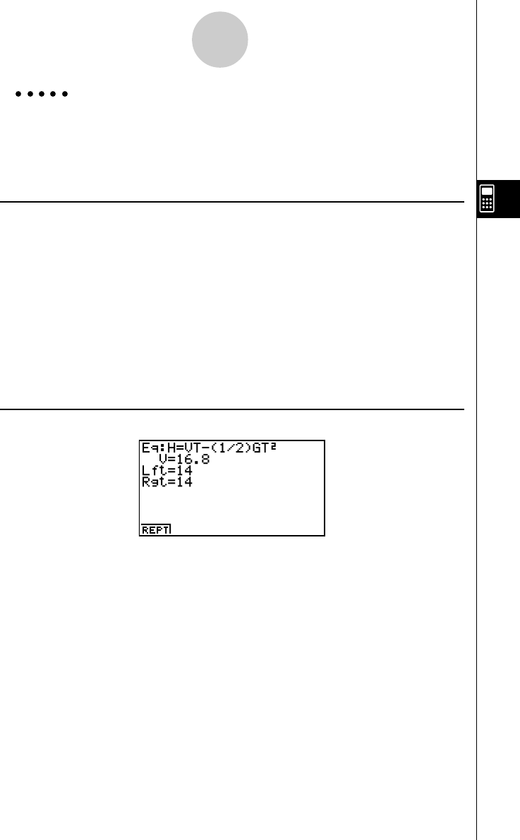
19990401
4-3-2
Solve Calculations
Example An object thrown into the air at initial velocity V takes time T to reach
height H. Use the following formula to solve for initial velocity V when
H = 14 (meters), T = 2 (seconds) and gravitational acceleration is G =
9.8 (m/s2).
H = VT – 1/2 GT2
Procedure
1m EQUA
23(SOLV)
ax(H)!.(=)ac(V)a/(T)-(b/c)
a$(G)a/(T)xw
3bew(H = 14)
aw(V = 0)
cw(T = 2)
j.iw(G = 9.8)
4Press f to highlight V = 0, and then press 6(SOLV).
Result Screen

19990401
4-4 What to Do When an Error Occurs
uError during coefficient value input
Press the i key to clear the error and return to the value that was registered for the
coefficient before you input the value that generated the error. Try inputting a new value
again.
uError during calculation
Press the i key to clear the error and display the coefficient. Try inputting values for the
coefficients again.
4-4-1
What to Do When an Error Occurs
kk
kk
kClearing Equation Memories
1. Enter the equation calculation mode (SIML or POLY) you want to use and
perform the function key operation required for that mode.
•In the case of the SIML Mode (1), use number keys to specify the number of
unknowns.
•In the case of the POLY Mode (2), use number keys to specify the degree of
the polynomial.
•If you pressed 3(SOLV), advance directly to step 2.
2. Press 2(DEL • A).
3. Press w(Yes) to delete the applicable equation memories or i(No) to abort
the operation without deleting anything.
20011101

19990401
Graphing
Sections 5-1 and 5-2 of this chapter provide basic information
you need to know in order to draw a graph. The remaining
sections describe more advanced graphing features and functions.
Select the icon in the Main Menu that suits the type of graph you
want to draw or the type of table you want to generate.
•GRPH
·
TBL … General function graphing or number table generation
•CONICS …Conic section graphing
(5-1-5 ~ 5-1-6, 5-11-17~5-11-21)
•RUN
·
MAT … Manual graphing (5-6-1 ~ 5-6-4)
•DYNA … Dynamic Graph (5-8-1 ~ 5-8-6)
•RECUR … Recursion graphing or number table generation
(5-9-1 ~ 5-9-8)
5-1 Sample Graphs
5-2 Controlling What Appears on a Graph Screen
5-3 Drawing a Graph
5-4 Storing a Graph in Picture Memory
5-5 Drawing Two Graphs on the Same Screen
5-6 Manual Graphing
5-7 Using Tables
5-8 Dynamic Graphing
5-9 Graphing a Recursion Formula
5-10 Changing the Appearance of a Graph
5-11 Function Analysis
Chapter
5
20011101

19990401
5-1-1
Sample Graphs
5-1 Sample Graphs
kk
kk
kHow to draw a simple graph (1)
Description
To draw a graph, simply input the applicable function.
Set Up
1. From the Main Menu, enter the GRPH • TBL Mode.
Execution
2. Input the function you want to graph.
Here you would use the V-Window to specify the range and other parameters of the
graph. See 5-2-1.
3. Draw the graph.
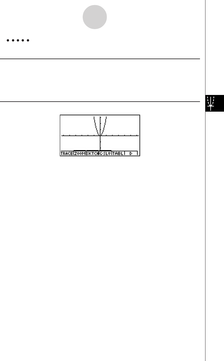
19990401
5-1-2
Sample Graphs
Example To graph y = 3x2
Procedure
1m GRPH • TBL
2dvxw
35(DRAW) (or w)
Result Screen

19990401
5-1-3
Sample Graphs
kk
kk
kHow to draw a simple graph (2)
Description
You can store up to 20 functions in memory and then select the one you want for graphing.
Set Up
1. From the Main Menu, enter the GRPH • TBL Mode.
Execution
2. Specify the function type and input the function whose graph you want to draw.
You can use the GRPH • TBL Mode to draw a graph for the following types of expres-
sions: rectangular coordinate expression, polar coordinate expression, parametric
function, X = constant expression, inequality.
3(TYPE) b(Y =) ... rectangular coordinates
c(r =) ... polar coordinates
d(Param) ... parametric function
e(X = c) ... X = constant function
f(INEQUA)b(Y>)~e(Y<) ... inequality
g(CONV)b('Y=)~f('Y<) ... changes the function type
Repeat this step as many times as required to input all of the functions you want.
Next you should specify which of the functions among those that are stored in memory
you want to graph (see 5-3-6). If you do not select specific functions here, the graph
operation will draw graphs of all the functions currently stored in memory.
3. Draw the graph.
20011101
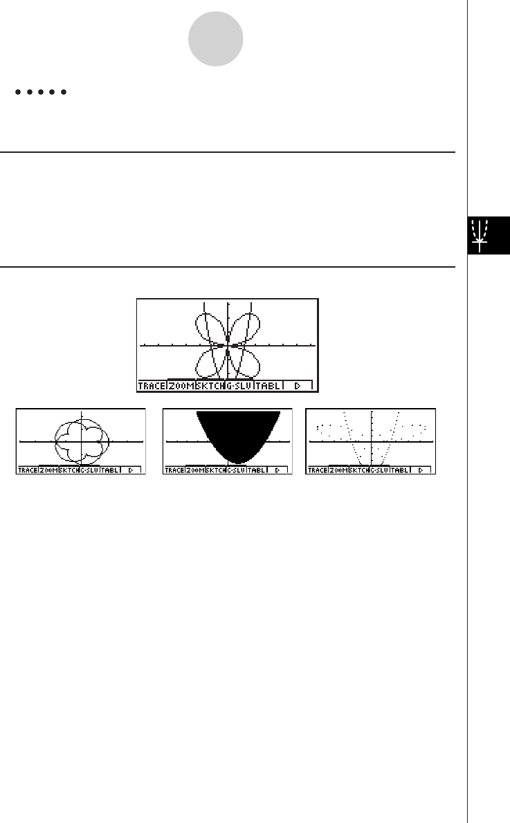
19990401
5-1-4
Sample Graphs
Example Input the functions shown below and draw their graphs
Y1 = 2x2 – 3, r2 = 3sin2
θ
Procedure
1m GRPH • TBL
23(TYPE)b(Y=)cvx-dw
3(TYPE)c(r=)dscvw
35(DRAW)
Result Screen
(Param) (INEQUA) (Plot)

19990401
5-1-5
Sample Graphs
kk
kk
kHow to draw a simple graph (3)
Description
Use the following procedure to graph the function of a parabola, circle, ellipse, or hyperbola.
Set Up
1. From the Main Menu, enter the CONICS Mode.
Execution
2. Use the cursor fc keys to specify one of the function type as follows.
3. Input values for the required variables.
4. Graph the function.
Graph Type Function
Parabola X = A (Y – K)2 + H
X = AY2 + BY + C
Y = A (X – H)2 + K
Y = AX2 + BX + C
Circle (X – H)2 + (Y – K)2 = R2
AX2 + AY2 + BX + CY + D = 0
Ellipse (X – H)2(Y – K)2
–––––––– + –––––––– = 1
A2B2
Hyperbola (X – H)2(Y – K)2
–––––––– – –––––––– = 1
A2B2
(Y – K)2(X – H)2
–––––––– – –––––––– = 1
A2B2
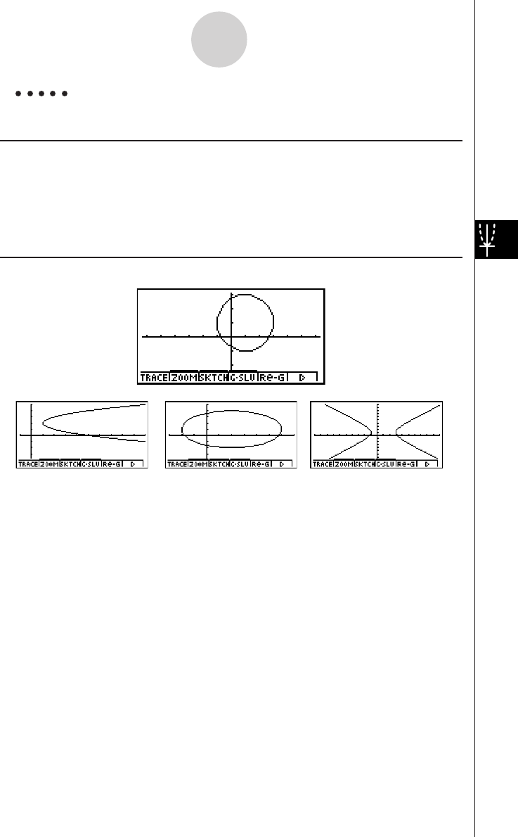
19990401
5-1-6
Sample Graphs
Example Graph the circle (X–1)2 + (Y–1)2 = 22
Procedure
1m CONICS
2ccccw
3bwbwcw
46(DRAW)
Result Screen
(Parabola) (Ellipse) (Hyperbola)
19990401
5-2 Controlling What Appears on a Graph Screen
kk
kk
kV-Window (View Window) Settings
Use the View Window to specify the range of the x- and y-axes, and to set the spacing
between the increments on each axis. You should always set the V-Window parameters you
want to use before graphing.
uTo make V-Window settings
1. From the Main Menu, enter the GRPH • TBL Mode.
2. Press !K(V-Window) to display the V-Window setting screen.
Rectangular coordinate parameter
Xmin … Minimum x-axis value
Xmax … Maximum x-axis value
Xscale … Spacing of x-axis increments
Xdot … Value that corresponds to one x-axis dot
Ymin … Minimum y-axis value
Ymax … Maximum y-axis value
Yscale … Spacing of y-axis increments
Polar coordinate parameter
T
θ
min ... T,
θ
minimum values
T
θ
max ... T,
θ
maximum values
T
θ
ptch ... T,
θ
pitch
3. Press c to move the highlighting and input an appropriate value for each parameter,
pressing w after each.
• {INIT}/{TRIG}/{STD} … V-Window {initial settings}/{initial settings using specified
angle unit}/{standardized settings}
•{STO}/{RCL} … V-Window setting {store}/{recall}
After settings are the way you want them, press i or !i(QUIT) to exit the V-Window
setting screen.*1
5-2-1
Controlling What Appears on a Graph Screen
*1Pressing w without inputting anything while k
is displayed exits the View Window setting
screen.
20011101

19990401
5-2-2
Controlling What Appears on a Graph Screen
uV-Window Setting Precautions
•Inputting zero for T
θ
ptch causes an error.
•Any illegal input (out of range value, negative sign without a value, etc.) causes an error.
•An error occurs when Xmax is less than Xmin, or Ymax is less than Ymin. When T
θ
max
is less than T
θ
min, T
θ
ptch becomes negative.
•You can input expressions (such as 2π) as V-Window parameters.
•When the V-Window setting produces an axis that does not fit on the display, the scale
of the axis is indicated on the edge of the display closest to the origin.
•Changing the V-Window settings clears the graph currently on the display and
replaces it with the new axes only.
•Changing the Xmin or Xmax value causes the Xdot value to be adjusted automatically.
Changing the Xdot value causes the Xmax value to be adjusted automatically.
•A polar coordinate (r =) or parametric graph will appear coarse if the settings you
make in the V-Window cause the T,
θ
pitch value to be too large, relative to the
differential between the T,
θ
min and T,
θ
max settings. If the settings you make cause
the T,
θ
pitch value to be too small relative to the differential between the T,
θ
min and
T,
θ
max settings, on the other hand, the graph will take a very long time to draw.
•The following is the input range for V-Window parameters.
–9.999999999E 97 to 9.999999999E 97

19990401
kk
kk
kInitializing and Standardizing the V-Window
uTo initialize the V-Window
1. From the Main Menu, enter the GRPH • TBL Mode.
2. Press !K(V-Window).
This displays the V-Window setting screen.
3. Press 1(INIT) to initialize the V-Window.
Xmin = –6.3, Xmax = 6.3, Xscale = 1 Xdot = 0.1
Ymin = –3.1, Ymax = 3.1, Yscale = 1
T
θ
min = 0, T
θ
max = 2π (rad), T
θ
ptch = 2π /60 (rad)
uTo initialize the V-Window in accordance with an angle unit
In step 3 of the procedure under “To initialize the V-Window” above, press 2(TRIG) to
initialize the V-Window in accordance with an angle unit.
Xmin = –3π (rad), Xmax = 3π (rad), Xscale = π /2 (rad), Xdot = π /21 (rad),
Ymin = –1.6, Ymax = 1.6, Yscale = 0.5
uTo standardize the V-Window
The following are the standard V-Window settings of this calculator.
Xmin = –10, Xmax = 10, Xscale = 1, Xdot = 0.15873015,
Ymin = –10, Ymax = 10, Yscale = 1,
T
θ
min = 0, T
θ
max = 2π (rad), T
θ
ptch = 2π /60 (rad)
In step 3 of the procedure under “To initialize the V-Window” above, press 3(STD) to
standardize V-Window settings in accordance with the above.
5-2-3
Controlling What Appears on a Graph Screen
#Initialization and standardization cause T
θ
min, T
θ
max, T
θ
ptch values to change
automatically in accordance with the current
angle unit setting as shown below.
Deg Mode:
T
θ
min = 0, T
θ
max = 360, T
θ
ptch = 6
Gra Mode:
T
θ
min = 0, T
θ
max = 400, T
θ
ptch = 400/60
20011101

19990401
kk
kk
kV-Window Memory
You can store up to six sets of V-Window settings in V-Window memory for recall when you
need them.
uTo store V-Window settings
1. From the Main Menu, enter the GRPH • TBL Mode.
2. Press !K(V-Window) to display the V-Window setting screen, and input the values
you want.
3. Press 4(STO) to display the pop-up window.
4. Press a number key to specify the V-Window memory where you want to save the
settings, and then press w. Pressing bw stores the settings in V-Window Memory
1 (V-Win1).
uTo recall V-Window memory settings
1. From the Main Menu, enter the GRPH • TBL Mode.
2. Press !K(V-Window) to display the V-Window setting screen.
3. Press 5(RCL) to display the pop-up window.
4. Press a number key to specify the V-Window memory number for the settings you want
to recall, and then press w. Pressing bw recalls the settings in V-Window Memory
1 (V-Win1).
5-2-4
Controlling What Appears on a Graph Screen
#Storing V-Window settings to a memory that
already contains setting data replaces the
previous data with the new settings.
#Recalling settings causes the current V-Window
settings to be replaced with those recalled from
memory.

19990401
kk
kk
kSpecifying the Graph Range
Description
You can define a range (start point, end point) for a function before graphing it.
Set Up
1. From the Main Menu, enter the GRPH • TBL Mode.
2. Make V-Window settings.
Execution
3. Specify the function type and input the function. The following is the syntax for function
input.
Function ,!+( [ )Start Point , End Point !-( ] )
4. Draw the graph.
5-2-5
Controlling What Appears on a Graph Screen
19990401
5-2-6
Controlling What Appears on a Graph Screen
Example Graph y = x2 + 3x – 2 within the range – 2 < x < 4
Use the following V-Window settings.
Xmin = –3, Xmax = 5, Xscale = 1
Ymin = –10, Ymax = 30, Yscale = 5
Procedure
1m
GRPH • TBL
2!K(V-Window) -dwfwbwc
-bawdawfwi
33(TYPE)b(Y=)vx+dv-c,
!+( [ )-c,e!-( ] )w
45(DRAW)
Result Screen
#You can specify a range when graphing
rectangular expressions, polar expressions,
parametric functions, and inequalities.

19990401
5-2-7
Controlling What Appears on a Graph Screen
kk
kk
kZoom
Description
This function lets you enlarge and reduce the graph on the screen.
Set Up
1. Draw the graph.
Execution
2. Specify the zoom type.
2(ZOOM)b(Box) ... Box zoom
Draw a box around a display area, and that area is enlarged to
fill the entire screen.
c(Factor)
d(In)/e(Out) ... Factor zoom
The graph is enlarged or reduced in accordance with the factor
you specify, centered on the current pointer location.
f(Auto)
... Auto zoom
V-Window y-axis settings are automatically adjusted so the
graph fills the screen along the y-axis.
g(Orig) ...Original size
Returns the graph to its original size following a zoom opera-
tion.
h(Square) ... Graph correction
V-Window x-axis values are corrected so they are identical to
the y-axis values.
i(Rnd) ... Coordinate rounding
Rounds the coordinate values at the current pointer location.
j(Intg) ... Integer
Each dot is given a width of 1, which makes coordinate values
integers.
v(Pre)
... Previous
V-Window parameters are returned to what they were prior to
the last zoom operation.
l(QUICK) ... Quick zoom
Redraws the graph in accordance with the settings stored in a
selected V-Window memory.
Box zoom range specification
3. Use the cursor keys to move the pointer ( ) in the center of the screen to the location
where you want one corner of the box to be, and then press w.
4. Use the cursor keys to move the pointer. This causes a box to appear on the screen.
Move the cursor until the area you want to enlarge is enclosed in the box, and then
press w to enlarge it.

19990401
5-2-8
Controlling What Appears on a Graph Screen
#You must specify two different points for box
zoom, and the two points cannot be on a straight
line vertically or horizontally from each other.
Example Graph y = (x + 5)(x + 4)(x + 3), and then perform a box zoom.
Use the following V-Window settings.
Xmin = –8, Xmax = 8, Xscale = 2
Ymin = – 4, Ymax = 2, Yscale = 1
Procedure
1m
GRPH • TBL
!K(V-Window) -iwiwcwc
-ewcwbwi
3(TYPE)b(Y=)(v+f)(v+e)
(v+d)w
5(DRAW)
22(ZOOM)b(Box)
3d~dw
4d~d,f~fw
Result Screen

19990401
5-2-9
Controlling What Appears on a Graph Screen
kk
kk
kFactor Zoom
Description
With factor zoom, you can zoom in or out, centered on the current cursor position.
Set Up
1. Draw the graph.
Execution
2. Press 2(ZOOM)c(Factor) to open a pop-up window for specifying the x-axis and
y-axis zoom factor. Input the values you want and then press i.
3. Press 2(ZOOM)d(In) to enlarge the graph, or 2(ZOOM)e(Out) to reduce it. The
graph is enlarged or reduced centered on the current pointer location.
4. Use the cursor keys to move the cursor to the point upon which you want the zoom
operation to be centered, and then press w to zoom.
19990401
5-2-10
Controlling What Appears on a Graph Screen
Example Enlarge the graphs of the two expressions shown below five times on
both the x-and y-axis to see if they are tangent.
Y1 = (x + 4)(x + 1)( x – 3), Y2 = 3x + 22
Use the following V-Window settings.
Xmin = –8, Xmax = 8, Xscale = 1
Ymin = –30, Ymax = 30, Yscale = 5
Procedure
1m
GRPH • TBL
!K(V-Window) -iwiwbwc
-dawdawfwi
3(TYPE)b(Y=)(v+e)(v+b)
(v-d)w
dv+ccw
5(DRAW)
22(ZOOM)c(Factor)fwfwi
32(ZOOM)d(In)
4f~f,d~dw
Result Screen
#You can repeat factor zoom to enlarge or
reduce a graph even further.
19990401
kk
kk
kTurning Function Menu Display On and Off
Press ua to toggle display of the menu at the bottom of the screen on and off.
Turning off the function menu display makes it possible to view part of a graph hidden behind
it. When you are using the trace function or other functions during which the function menu is
normally not displayed, you can turn on the menu display to execute a menu command.
5-2-11
Controlling What Appears on a Graph Screen
#If a pull-up menu is open when you press u
a to turn off menu display, the pull-up menu
remains on the screen.
20011101
19990401
kk
kk
kAbout the Calc Window
Pressing u4(CAT/CAL) while a graph or number table is on the display opens the Calc
Window. You can use the Calc Window to perform calculations with values obtained from
graph analysis, or to change the value assigned to variable A in Y = AX and other
expressions and then redraw the graph.
Press i to close the Calc Window.
5-2-12
Controlling What Appears on a Graph Screen
#After using the Calc Window to change the
value of a variable connected with a graph or
table, be sure to always execute Re-G (re-
graph) or Re-T (re-calculate table). Doing so
ensures that the displayed graph or table is
current.
#Calc Window cannot be used in the RUN •
MAT Mode while a program is running, or in
combination with Dynamic Graph.
#Calc Window cannot be used in combination
with V-Window or the table range setting screen.
#Complex number calculations cannot be
performed on the Calc Window.
20011101

19990401
5-3-1
Drawing a Graph
5-3 Drawing a Graph
You can store up to 20 functions in memory. Functions in memory can be edited, recalled,
and graphed.
kk
kk
kSpecifying the Graph Type
Before you can store a graph function in memory, you must first specify its graph type.
1. While the Graph function list is on the display, press 6(g)3(TYPE) to display the
graph type menu, which contains the following items.
•{Y=}/{r=}/{Param}/{X=c} ... {rectangular coordinate}/{polar coordinate}/{parametric}/
{X=constant}*1 graph
•{INEQUA}
•{Y>}/{Y<}/{Ytt
tt
t}/{Yss
ss
s} ... {Y>f(x)}/{Y<f(x)}/{Y>f(x)}/{Y<f(x)} inequality graph
•{CONV}
•{'Y=}/{'Y>}/{'Y<}/{'Ytt
tt
t}/{'Yss
ss
s} ... changes the function type
2. Press the number key that corresponds to the graph type you want to specify.
kk
kk
kStoring Graph Functions
uTo store a rectangular coordinate function (Y =) *2
Example To store the following expression in memory area Y1 : y = 2x2 – 5
3(TYPE)b(Y =) (Specifies rectangular coordinate expression.)
cvx-f(Inputs expression.)
w (Stores expression.)
uTo store a polar coordinate function (r =) *2
Example To store the following expression in memory area r2 :
r = 5 sin3
θ
3(TYPE)c(r =) (Specifies polar coordinate expression.)
fsdv(Inputs expression.)
w(Stores expression.)
*1 Attempting to draw a graph for an expression
in which X is input for an X = constant
expression results in an error.
*2A function cannot be stored into a memory area that
already contains a function of a different type from
the one you are trying to store. Select a memory
area that contains a function that is the same type
as the one you are storing, or delete the function in
the memory area to which you are trying to store.
20011101

19990401
5-3-2
Drawing a Graph
uTo store a parametric function *1
Example To store the following functions in memory areas Xt3 and Yt3 :
x = 3 sin T
y = 3 cos T
3(TYPE)d(Param) (Specifies parametric expression.)
dsvw(Inputs and stores x expression.)
dcvw(Inputs and stores y expression.)
uTo store an X = constant expression *2
Example To store the following expression in memory area X4 :
X = 3
3(TYPE)e(X = c) (Specifies X = constant expression.)
d(Inputs expression.)
w(Stores expression.)
•Inputting X, Y, T, r, or
θ
for the constant in the above procedures causes an error.
uTo store an inequality *2
Example To store the following inequality in memory area Y5 :
y > x2 – 2x – 6
3(TYPE)f(INEQUA)b(Y>) (Specifies an inequality.)
vx-cv-g(Inputs expression.)
w(Stores expression.)
*1You will not be able to store the expression in
an area that already contains a rectangular
coordinate expression, polar coordinate
expression, X = constant expression or
inequality. Select another area to store your
expression or delete the existing expression
first.
*2A function cannot be stored into a memory area
that already contains a function of a different type
from the one you are trying to store. Select a
memory area that contains a function that is the
same type as the one you are storing, or delete
the function in the memory area to which you are
trying to store.
19990401
5-3-3
Drawing a Graph
uTo create a composite function
Example To register the following functions as a composite function:
Y1= (X + 1), Y2 = X2 + 3
Assign Y1°Y2 to Y3, and Y2°Y1 to Y4.
(Y1°Y2 = ((x2 + 3) +1) = (x2 + 4) Y2°Y1 = ( (X + 1)) 2 + 3 = X + 4 (X ⭌ –1))
3(TYPE)b(Y=)
J4(GRPH)b(Yn)b
(1(Yn)c)w
4(GRPH)b(Yn)c
(1(Yn)b)w
• A composite function can consist of up to five functions.
uTo assign values to the coefficients and variables of a graph function
After you combine functions or equations into a composite function, you can assign values to
the coefficients and variables of the expression and draw a graph.
Example Assign the values –1, 0, and 1 to the expression Y = AX2 –1, which is in
memory area A
3(TYPE)b(Y=)
av(A)vx-bw
J4(GRPH)b(Yn)b
(av(A)!.(=)-b)w
4(GRPH)b(Yn)b
(av(A)!.(=)a)w
4(GRPH)b(Yn)b
(av(A)!.(=)b)w
20011101
19990401
ffffi1(SEL)5(DRAW)
The above three screens are produced using the Trace function.
See “5-11 Function Analysis” for more information.
• If you do not specify a variable name (variable A in the above key operation), the calculator
automatically uses one of the default variables listed below. Note that the default variable
used depends on the memory area type where you are storing the graph function.
Memory Area Type Default Variable
YnX
rn
θ
Xtn T
Ytn T
fn X
Example Y1 (3) and Y1 (X = 3) are identical values.
•You can also use Dynamic Graph for a look at how changes in coefficients alter the
appearance of a graph. See “5-8 Dynamic Graphing” for more information.
5-3-4
Drawing a Graph
20010102

1999040120011101
kk
kk
kEditing and Deleting Functions
uTo edit a function in memory
Example To change the expression in memory area Y1 from y = 2x2 – 5 to
y = 2x2 – 3
e (Displays cursor.)
eeeeDd(Changes contents.)
w(Stores new graph function.)
uTo change the type of a function*1
1. While the Graph function list is on the display, press f or c to move the highlighting
to the area that contains the function whose type you want to change.
2. Press 3(TYPE)g(CONV).
3. Select the function type you want to change to.
Example To change the function in memory area Y1 from y = 2x2 – 3 to
y < 2x2 – 3
3(TYPE)g(CONV)d(''
''
'Y<) (Changes the function type to “Y<”.)
uTo delete a function
1. While the Graph function list is on the display, press f or c to move the highlighting
to the area that contains the function you want to delete.
2. Press 2(DEL) or D.
3. Press w(Yes) to delete the function or i(No) to abort the procedure without deleting
anything.
*1The function type can be changed for
rectangular coordinate functions and
inequalities only.
#Parametric functions come in pairs (Xt and Yt).
When editing a parametric function, clear the graph
functions and re-input from the beginning.
5-3-5
Drawing a Graph
1999040120011101
kk
kk
kSelecting Functions for Graphing
uTo specify the draw/non-draw status of a graph
Example To select the following functions for drawing :
Y1 = 2x2 – 5, r2 = 5 sin3
θ
Use the following V-Window settings.
Xmin = –5, Xmax = 5, Xscale = 1
Ymin = –5, Ymax = 5, Yscale = 1
T
θ
min = 0, T
θ
max =
π
,T
θ
ptch = 2
π
/ 60
cc (Select a memory area that contains a function
for which you want to specify non-draw.)
1(SEL) (Specifies non-draw.)
5(DRAW) or w (Draws the graphs.)
•Each press of 1(SEL) toggles a graph between draw and non-draw.
•Pressing u5(G↔T) or i returns to the Graph function list.
•You can use the SET UP screen settings to alter the appearance of the graph screen as
shown below.
•Grid: On (Axes: On Label: Off)
This setting causes dots to appear at the grid
intersects on the display.
•Axes: Off (Label: Off Grid: Off)
This setting clears the axis lines from the display.
•Label: On (Axes: On Grid: Off)
This setting displays labels for the x- and y-axes.
5-3-6
Drawing a Graph

1999040120010102
kk
kk
kGraph Memory
Graph memory lets you store up to 20 sets of graph function data and recall it later when you
need it.
A single save operation saves the following data in graph memory.
•All graph functions in the currently displayed Graph function list (up to 20)
•Graph types
•Draw/non-draw status
•View Window settings (1 set)
uTo store graph functions in graph memory
1. Press 4(GMEM)b(Store) to display the pop-up window.
2. Press a number key to specify the Graph memory where you want to save the graph
function, and then press w. Pressing bw stores the graph function to Graph
Memory 1 (G-Mem1).
•There are 20 graph memories numbered G-Mem1 to G-Mem20.
uTo recall a graph function
1. Press 4(GMEM)c(Recall) to display the pop-up window.
2. Press a number key to specify the Graph memory for the function you want to recall,
and then press w. Pressing bw recalls the graph function in Graph Memory 1
(G-Mem1).
5-3-7
Drawing a Graph
#Storing a function in a memory area that
already contains a function replaces the
existing function with the new one.
#If the data exceeds the calculator’s remaining
memory capacity, an error occurs.
#Recalling data from graph memory causes any
data currently on the Graph function list to be
deleted.

19990401
5-4 Storing a Graph in Picture Memory
You can save up to 20 graphic images in picture memory for later recall. You can overdraw
the graph on the screen with another graph stored in picture memory.
uTo store a graph in picture memory
1. After graphing in GRPH
•
TBL Mode, press 6(g)1(PICT)b(Store) to display the
pop-up window.
2. Press a number key to specify the Picture memory where you want to save the picture,
and then press w. Pressing bw stores the picture function to Picture Memory 1
(Pict 1).
•There are 20 picture memories numbered Pict 1 to Pict 20.
uTo recall a stored graph
1. After graphing in GRPH
•
TBL Mode, press 6(g)1(PICT)c(Recall) to display the
pop-up window.
2. Press a number key to specify the Picture memory for the picture you want to recall,
and then press w. Pressing bw recalls the picture function in Picture Memory 1
(Pict 1).
5-4-1
Storing a Graph in Picture Memory
#Storing a graphic image in a memory area that
already contains a graphic image replaces the
existing graphic image with the new one.
#A dual Graph screen or any other type of graph
that uses a split screen cannot be saved in
picture memory.

19990401
5-5 Drawing Two Graphs on the Same Screen
kk
kk
kCopying the Graph to the Sub-screen
Description
Dual Graph lets you split the screen into two parts. Then you can graph two different
functions in each for comparison, or draw a normal size graph on one side and its enlarged
version on the other side. This makes Dual Graph a powerful graph analysis tool.
With Dual Graph, the left side of the screen is called the “main screen,” while the right side is
called the “sub-screen.”
uu
uu
uMain Screen
The graph in the main screen is actually drawn from a function.
uu
uu
uSub-screen
The graph on the sub-screen is produced by copying or zooming the main screen graph.
You can even make different V-Window settings for the sub-screen and main screen.
Set Up
1. From the Main Menu, enter the GRPH • TBL Mode.
2. On the SET UP screen, select G+G for Dual Screen.
3. Make V-Window settings for the main screen.
Press 6(RIGHT) to display the sub-graph settings screen. Pressing 6(LEFT)
returns to the main screen setting screen.
Execution
4. Store the function, and draw the graph in the main screen.
5. Perform the Dual Graph operation you want.
4(COPY) ... Duplicates the main screen graph in the sub-screen
5(SWAP) ... Swaps the main screen contents and sub-screen contents
5-5-1
Drawing Two Graphs on the Same Screen
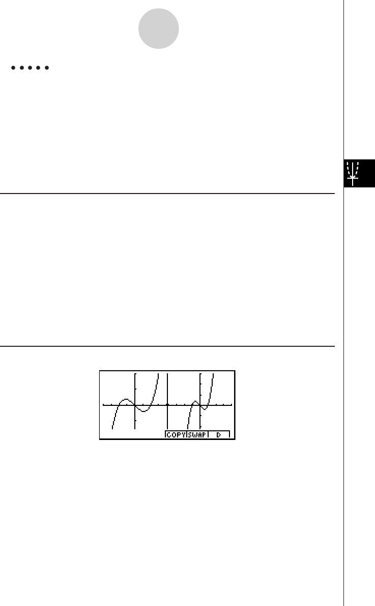
19990401
Example Graph y = x(x + 1)(x – 1) in the main screen and sub-screen.
Use the following V-Window settings.
(Main Screen)
Xmin = –2, Xmax = 2, Xscale = 0.5
Ymin = –2, Ymax = 2, Yscale = 1
(Sub-screen)
Xmin = –4, Xmax = 4, Xscale = 1
Ymin = –3, Ymax = 3, Yscale = 1
Procedure
1m GRPH • TBL
2u3(SET UP)ccc2(G+G)i
3!K(V-Window) -cwcwa.fwc
-cwcwbw
6(RIGHT)-ewewbwc
-dwdwbwi
43(TYPE)b(Y=)v(v+b)(v-b)w
5(DRAW)
56(g)4(COPY)
Result Screen
5-5-2
Drawing Two Graphs on the Same Screen

19990401
kk
kk
kGraphing Two Different Functions
Description
Use the following procedure to graph different functions in the main screen and sub-screen.
Set Up
1. From the Main Menu, enter the GRPH • TBL Mode.
2. On the SET UP screen, select G+G for Dual Screen.
3. Make V-Window settings for the main screen.
Press 6(RIGHT) to display the sub-graph settings screen. Pressing 6(LEFT)
returns to the main screen setting screen.
Execution
4. Store the functions for the main screen and sub-screen.
5. Select the function of the graph that you want to eventually have in the sub-screen.
6. Draw the graph in the main screen.
7. Swap the main screen and sub-screen contents.
8. Return to the function screen.
9. Select the function of the next graph you want in the main screen.
10. Draw the graph in the main screen.
5-5-3
Drawing Two Graphs on the Same Screen
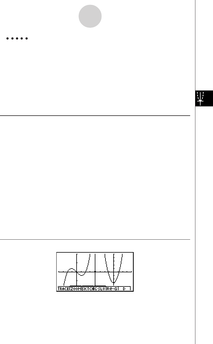
19990401
Example Graph y = x(x + 1)(x – 1) in the main screen, and y = 2x2 – 3 in the sub-
screen.
Use the following V-Window settings.
(Main Screen)
Xmin = –4, Xmax = 4, Xscale = 1
Ymin = –5, Ymax = 5, Yscale = 1
(Sub-screen)
Xmin = –2, Xmax = 2, Xscale = 0.5
Ymin = –2, Ymax = 2, Yscale = 1
Procedure
1m GRPH • TBL
2u3(SET UP)ccc2(G+G)i
3!K(V-Window) -ewewbwc
-fwfwbw
6(RIGHT)-cwcwa.fwc
-cwcwbwi
43(TYPE)b(Y=)v(v+b)(v-b)w
cvx-dw
5ff1(SEL)
65(DRAW)
76(g)5(SWAP)
8i
91(SEL)
05(DRAW)
Result Screen
5-5-4
Drawing Two Graphs on the Same Screen

19990401
kk
kk
kUsing Zoom to Enlarge the Sub-screen
Description
Use the following procedure to enlarge the main screen graph and then move it to the sub-
screen.
Set Up
1. From the Main Menu, enter the GRPH • TBL Mode.
2. On the SET UP screen, select G+G for Dual Screen.
3. Make V-Window settings for the main screen.
Execution
4. Input the function and draw the graph in the main screen.
5. Use Zoom to enlarge the graph, and then move it to the sub-screen.
5-5-5
Drawing Two Graphs on the Same Screen
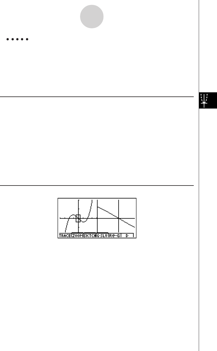
19990401
Example Draw the graph y = x(x + 1)(x – 1) in the main screen, and then use
Box Zoom to enlarge it.
Use the following V-Window settings.
(Main Screen)
Xmin = –2, Xmax = 2, Xscale = 0.5
Ymin = –2, Ymax = 2, Yscale = 1
Procedure
1m GRPH • TBL
2u3(SET UP)ccc2(G+G)i
3!K(V-Window) -cwcwa.fwc
-cwcwbwi
43(TYPE)b(Y=)v(v+b)(v-b)w
5(DRAW)
52(ZOOM)b(BOX)
c~ce~ew
f~fd~dw
Result Screen
5-5-6
Drawing Two Graphs on the Same Screen

19990401
5-6-1
Manual Graphing
5-6 Manual Graphing
kk
kk
kRectangular Coordinate Graph
Description
Inputting the Graph command in the RUN • MAT Mode enables drawing of rectangular
coordinate graphs.
Set Up
1. From the Main Menu, enter the RUN • MAT Mode.
2. Make V-Window settings.
Execution
3. Input the commands for drawing the rectangular coordinate graph.
4. Input the function.
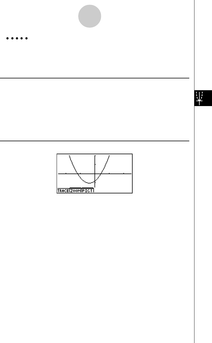
19990401
5-6-2
Manual Graphing
Example Graph y = 2x2 + 3x – 4
Use the following V-Window settings.
Xmin = –5, Xmax = 5, Xscale = 2
Ymin = –10, Ymax = 10, Yscale = 5
Procedure
1m
RUN • MAT
2!K(V-Window) -fwfwcwc
-bawbawfwi
3K6(g)6(g)2(SKTCH)b(Cls)w
2(SKTCH)e(GRAPH)b(Y=)
4cvx+dv-ew
Result Screen
19991201

19990401
5-6-3
Manual Graphing
kk
kk
kIntegration Graph
Description
Inputting the Graph command in the RUN • MAT Mode enables graphing of functions
produced by an integration calculation.
The calculation result is shown in the lower left of the display, and the calculation range is
blackened in the graph.
Set Up
1. From the Main Menu, enter the RUN • MAT Mode.
2. Make V-Window settings.
Execution
3. Input graph commands for the integration graph.
4. Input the function.
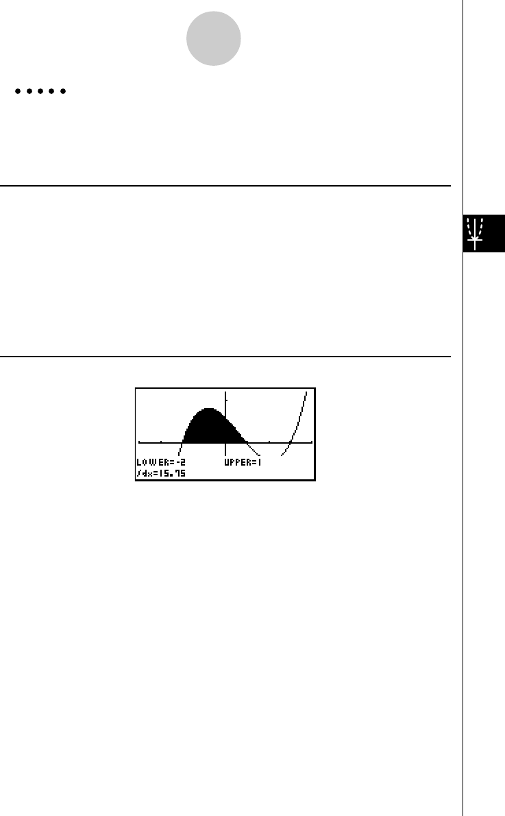
19990401
5-6-4
Manual Graphing
Example Graph the integration
∫
(x + 2)(x – 1)(x – 3) dx.
Use the following V-Window settings.
Xmin = –4, Xmax = 4, Xscale = 1
Ymin = –8, Ymax = 12, Yscale = 5
Procedure
1m
RUN • MAT
2!K(V-Window) -ewewbwc
-iwbcwfwi
3K6(g)6(g)2(SKTCH)b(Cls)w
2(SKTCH)e(GRAPH)c(∫ dx)
4(v+c)(v-b)(v-d),
-c,bw
Result Screen
1
–2
20011101

19990401
5-6-5
Manual Graphing
kk
kk
kDrawing Multiple Graphs on the Same Screen
Description
Use the following procedure to assign various values to a variable contained in an expres-
sion and overwrite the resulting graphs on the screen.
Set Up
1. From the Main Menu, Enter GRPH • TBL Mode.
2. Make V-Window settings.
Execution
3. Specify the function type and input the function. The following is the syntax for function
input.
Expression containing one variable ,!+( [ ) variable !.(=)
value , value , ... , value !-( ] )
4. Draw the graph.
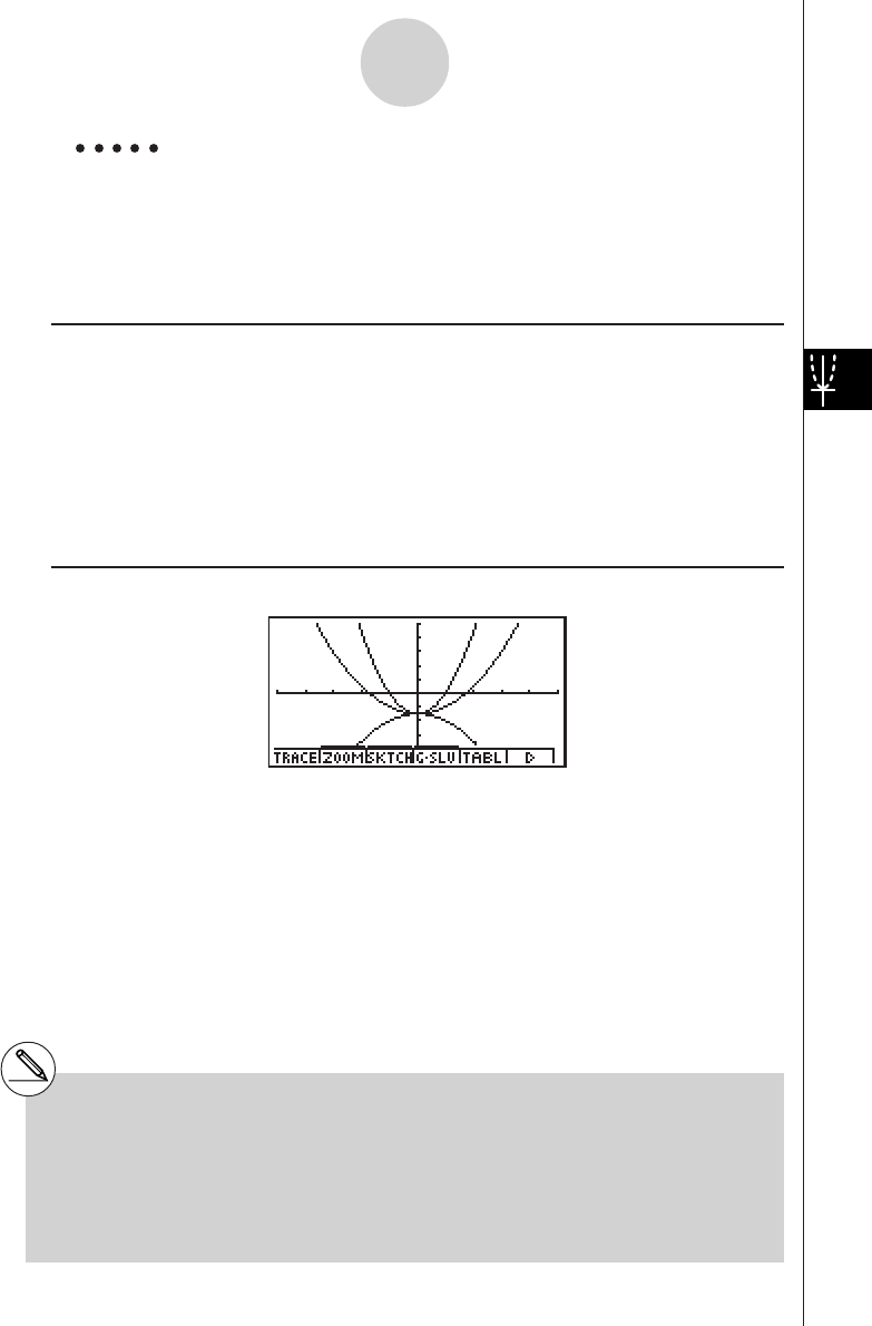
19990401
5-6-6
Manual Graphing
Example To graph y = Ax2 – 3 as the value of A changes in the sequence 3, 1,
–1.
Use the following V-Window settings.
Xmin = –5, Xmax = 5, Xscale = 1
Ymin = –10, Ymax = 10, Yscale = 2
Procedure
1m
GRPH • TBL
2!K(V-Window) -fwfwbwc
-bawbawcwi
33(TYPE)b(Y=)av(A)vx-d,
!+( [ )av(A)!.(=)d,b,-b!-( ] )w
45(DRAW)
Result Screen
#The value of only one of the variables in the
expression can change.
#Any of the following cannot be used for the
variable name: X, Y, r,
θ
, T.
#You cannot assign a variable to the variable
inside the function.
#When Simul Graph is turned on, all of the
graphs for the specified variable values are
drawn simultaneously.
#Overwrite can be used when graphing
rectangular expressions, polar expressions,
parametric functions, X = constant functions,
and inequalities.
20011101
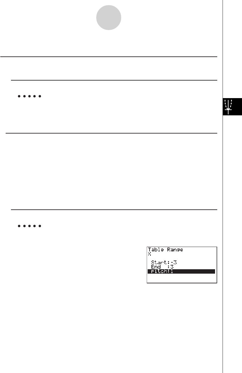
19990401
5-7 Using Tables
kk
kk
kStoring a Function and Generating a Number Table
uTo store a function
Example To store the function y = 3x2 – 2 in memory area Y1
Use f and c to move the highlighting in the Graph function list to the memory area
where you want to store the function. Next, input the function and press w to store it.
uVariable Specifications
There are two methods you can use to specify value for the variable x when generating a
numeric table.
• Table range method
With this method, you specify the conditions for the change in value of the variable.
• List
With this method, the data in the list you specify is substituted for the x-variable to
generate a number table.
uTo generate a table using a table range
Example To generate a table as the value of variable x changes from –3 to 3, in
increments of 1
6(g)2(RANG)
-dwdwbw
The numeric table range defines the conditions under which the value of variable x changes
during function calculation.
Start ........... Variable x start value
End ............. Variable x end value
pitch ............ Variable x value change (interval)
After specifying the table range, press i to return to the Graph function list.
5-7-1
Using Tables
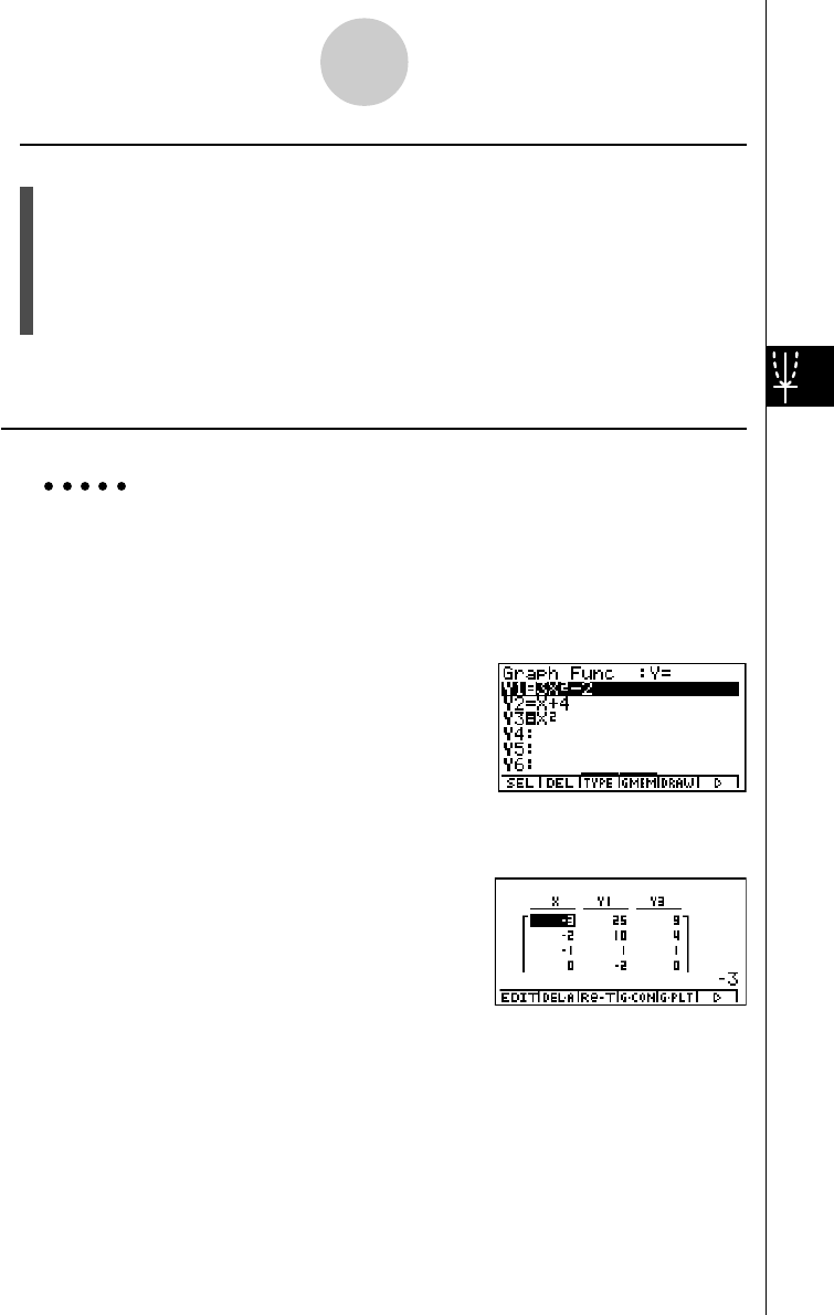
19990401
uTo generate a table using a list
1. While the Graph function list is on the screen, display the SET UP screen.
2. Highlight Variable and then press 2(LIST) to display the pop-up window.
3. Select the list whose values you want to assign for the x-variable.
• To select List 6, for example, press gw. This causes the setting of the Variable item
of the SET UP screen to change to List 6.
4. After specifying the list you want to use, press i to return to the previous screen.
• Note that the {RANG} item does not appear when a list name is specified for the Variable
item of the SET UP screen.
uGenerating a Table
Example To generate a table of values for the functions stored in memory areas
Y1 and Y3 of the Graph function list
Use f and c to move the highlighting to the function you want to select for table genera-
tion and press 1(SEL) to select it.
The “=” sign of selected functions is highlighted on the screen. To deselect a function, move
the cursor to it and press 1(SEL) again.
Press 5(TABL) to generate a number table using the functions you selected. The value of
variable x changes according to the range or the contents of the list you specified.
The example screen shown here shows the results
based on the contents of List 6 (– 3, –2, –1, 0, 1, 2, 3).
Each cell can contain up to six digits, including negative sign.
5-7-2
Using Tables
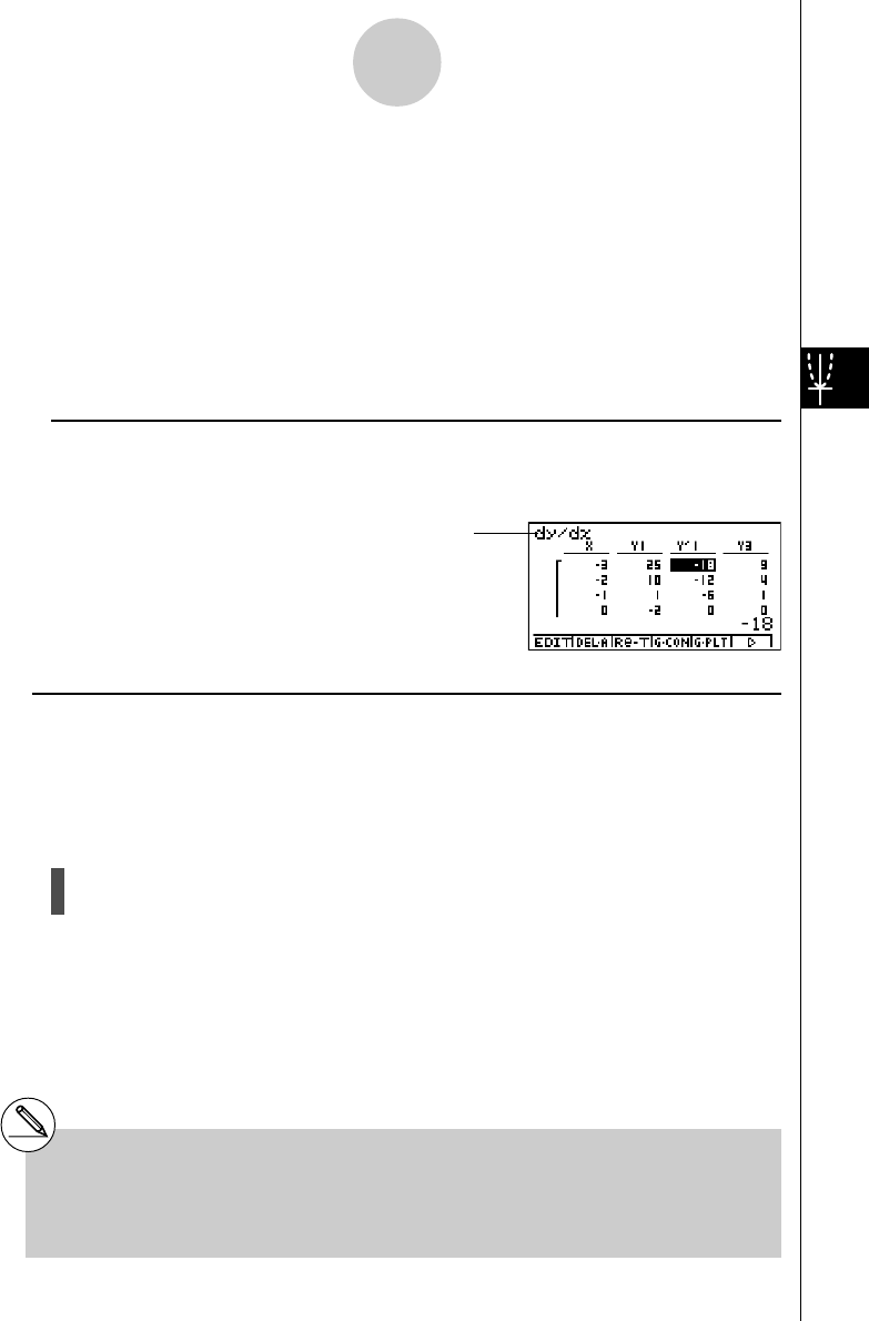
19990401
You can use cursor keys to move the highlighting around the table for the following purposes.
•To display the selected cell’s value at the bottom of the screen, using the calculator’s
current number of decimal place, number of significant digit, and exponential display
range settings
•To scroll the display and view parts of the table that do not fit in the display
•To display at the top of the screen the scientific function that produced the value in the
selected cell (in columns Y1, Y2, etc.)
•To change x variable values by replacing values in column X
Press i to return to the Graph function list.
uTo generate a differential number table *1
Changing the setting of SET UP screen’s Derivative item to On causes a number table that
includes the derivative to be displayed whenever you generate a number table.
uSpecifying the function type
You can specify a function as being one of three types.*2
•Rectangular coordinate (Y=)
•Polar coordinate (r
=)
•Parametric (Param)
1. Press 3(TYPE) while the function list is on the screen.
2. Press the number key that corresponds to the function type you want to specify.
5-7-3
Using Tables
Locating the cursor at a differential
coefficient displays “
dy/dx
” in the top line,
which indicates differential.
*1An error occurs if a graph for which a range is
specified or an overwrite graph is included
among the graph expressions.
*2The number table is generated only for the
function type specified on the function list
(Graph Func). You cannot generate a number
table for a mixture of different function types.
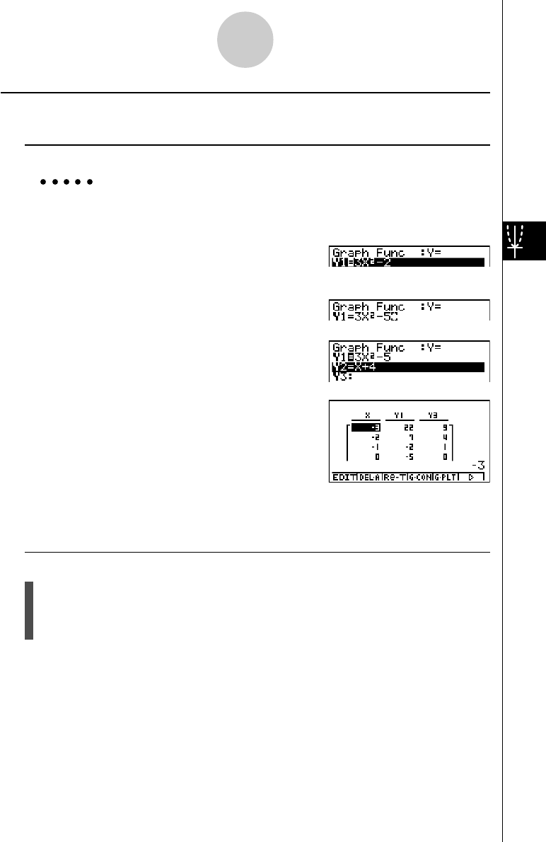
19990401
kk
kk
kEditing and Deleting Functions
uTo edit a function
Example To change the function in memory area Y1 from y = 3x2 – 2 to
y = 3x2 – 5
Use f and c to move the highlighting to the function you want to edit.
Use d and e to move the cursor to the location of the change.
eeeeeDf
w
6(g)5(TABL)
•The Function Link Feature automatically reflects any changes you make to functions in
the GRPH • TBL Mode list, and DYNA Mode list.
uTo delete a function
1. Use f and c to move the highlighting to the function you want to delete and then
press 2(DEL) or D.
2. Press w(Yes) to delete the function or i(No) to abort the operation without deleting
anything.
5-7-4
Using Tables
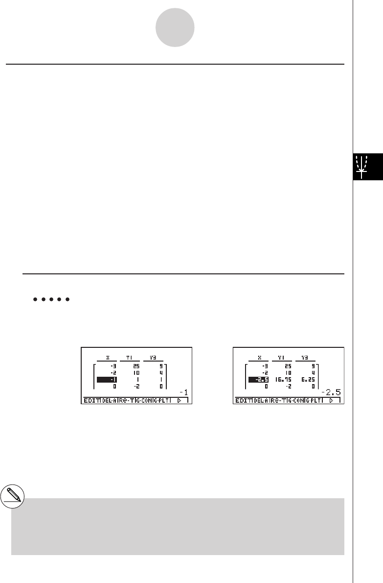
19990401
5-7-5
Using Tables
kk
kk
kEditing Tables
You can use the table menu to perform any of the following operations once you generate a
table.
•Change the values of variable x
•Edit (delete, insert, and append) rows
•Delete a table and regenerate table
•Draw a connect type graph
•Draw a plot type graph
While the Table & Graph menu is on the display, press 5(TABL) to display the table menu.
• {EDIT} ... {edit value of x-variable}
• {DEL·A} ... {delete table}
•{Re-T} ... {regenerate table from function}
•{G·CON}/{G·PLT} ... {connected type}/{draw plot type} graph draw
•{R·DEL}/{R·INS}/{R·ADD} ... {delete}/{insert}/{add} row
uTo change variable values in a table
Example To change the value in Column x, Row 3 of the table generated on
page 5-7-2 from – 1 to – 2.5
cc -c.fw
•When you change a variable value in Column x, all values in the columns to the right are
recalculated and displayed.
#If you try to replace a value with an illegal
operation (such as division by zero), an error
occurs and the original value remains
unchanged.
#You cannot directly change any values in the
other (non-x) columns of the table.
20040901
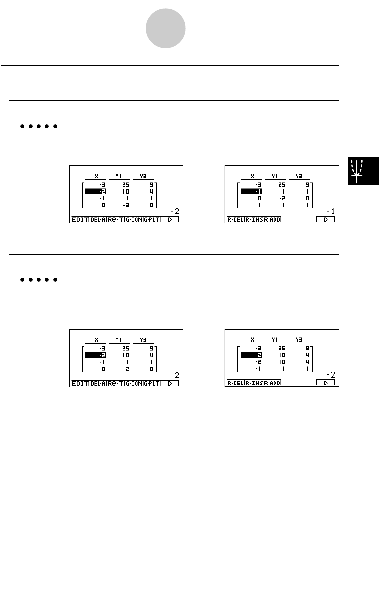
19990401
5-7-6
Using Tables
uRow Operations
uTo delete a row
Example To delete Row 2 of the table generated on page 5-7-2
c6(g)1(R·DEL)
uTo insert a row
Example To insert a new row between Rows 1 and 2 in the table generated on
page 5-7-2
c6(g)2(R·INS)
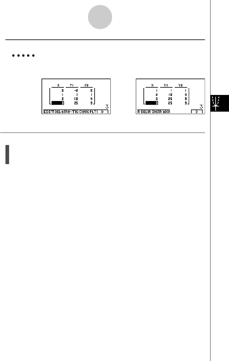
19990401
5-7-7
Using Tables
uTo add a row
Example To add a new row below Row 7 in the table generated on page 5-7-2
cccccc 6(g)3(R·ADD)
uDeleting a Table
1. Display the table and then press 2(DEL·A).
2. Press w(Yes) to delete the table or i(No) to abort the operation without deleting
anything.
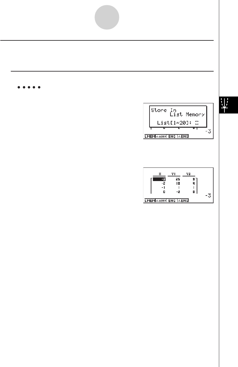
19990401
kk
kk
kCopying a Table Column to a List
A simple operation lets you copy the contents of a numeric table column into a list.
uTo copy a table to a list
Example To copy the contents of Column x into List 1
K1(LMEM)
•You can select any row of the column you want to copy.
Input the number of the list you want to copy and then press w.
bw
5-7-8
Using Tables

19990401
kk
kk
kDrawing a Graph from a Number Table
Description
Use the following procedure to generate a number table and then draw a graph based on the
values in the table.
Set Up
1. From the Main Menu, enter the GRPH • TBL Mode.
2. Make V-Window settings.
Execution
3. Store the functions.
4. Specify the table range.
5. Generate the table.
6. Select the graph type and draw it.
4(G • CON) ... line graph*1
5(G • PLT) ... plot type graph*1*2
5-7-9
Using Tables
*1After drawing the graph, pressing u
5(G ↔ T) or i returns to the function
storage screen. To return to the number table
screen, press 5(TABL).
*2Pressing 6(g) 4(G • PLT) on the function
storage screen generates the number table
and plots the graph simultaneously.
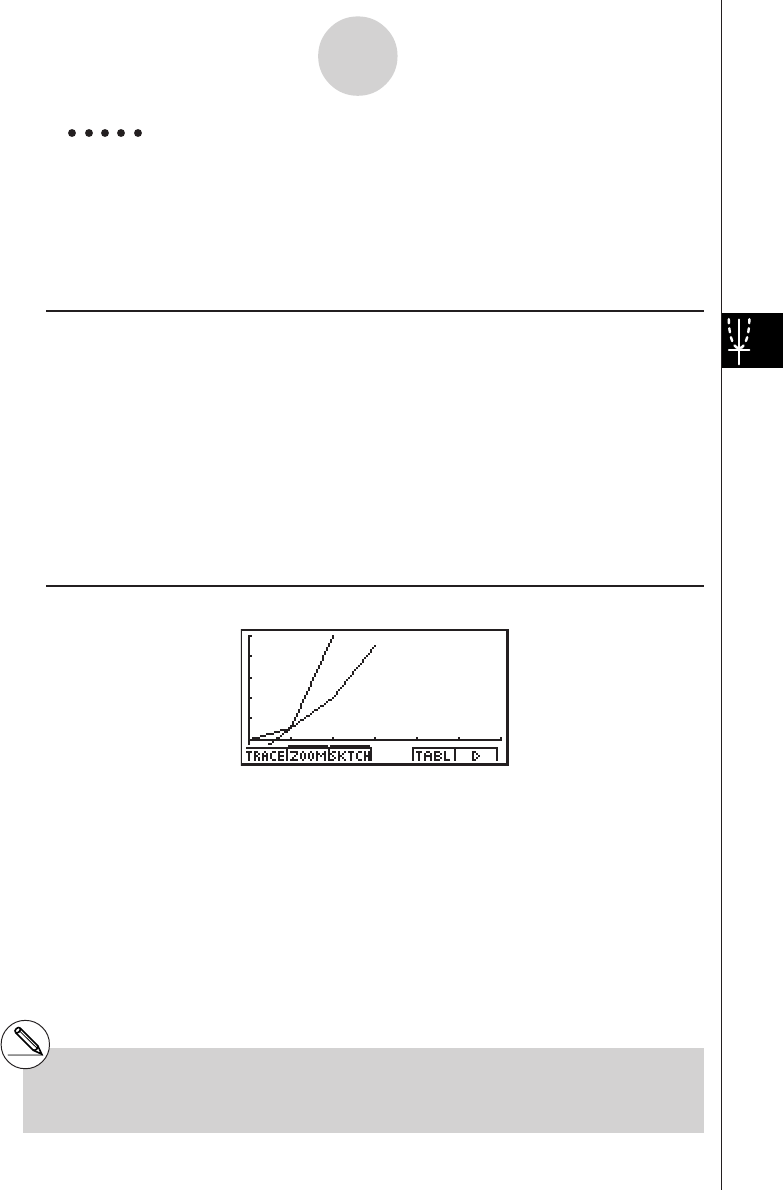
19990401
Example Store the two functions below, generate a number table, and then draw
a line graph. Specify a range of –3 to 3, and an increment of 1.
Y1 = 3x2 – 2, Y2 = x2
Use the following V-Window settings.
Xmin = 0, Xmax = 6, Xscale = 1
Ymin = –2, Ymax = 10, Yscale = 2
Procedure
1m GRPH • TBL
2!K(V-Window) awgwbwc
-cwbawcwi
33(TYPE)b(Y=)dvx-cw
vxw
46(g)2(RANG)-dwdwbwi
55(TABL)
64(G • CON)
Result Screen
5-7-10
Using Tables
#You can use Trace, Zoom, or Sketch after
drawing a graph.
20011101

19990401
kk
kk
kSpecifying a Range for Number Table Generation
Description
Use the following procedure to specify a number table range when calculating scatter data
from a function.
Set Up
1. From the Main Menu, enter the GRPH • TBL Mode.
Execution
2. Store the functions.
3. Specify the table range.
4. Select the functions for which you want to generate a table.
The “=” sign of selected functions is highlighted on the screen.
5. Generate the table.
5-7-11
Using Tables

19990401
Example Store the three functions shown below, and then generate a table for
functions Y1 and Y3. Specify a range of –3 to 3, and an increment of 1.
Y1 = 3x2 – 2, Y2 = x + 4, Y3 = x2
Procedure
1m GRPH • TBL
23(TYPE)b(Y=)dvx-cw
v+ew
vxw
36(g)2(RANG)-dwdwbwi
4ff1(SEL)
55(TABL)
Result Screen
5-7-12
Using Tables
#You can generate number tables from
rectangular coordinate, polar coordinate, and
parametric functions.
#You can include derivatives in generated
number tables by specifying On for the
Derivative item on the SET UP screen.
20011101

19990401
kk
kk
kSimultaneously Displaying a Number Table and Graph
Description
Specifying T+G for Dual Screen on the SET UP makes it possible to display a number table
and graph at the same time.
Set Up
1. From the Main Menu, enter the GRPH • TBL Mode.
2. Make V-Window settings.
3. On the SET UP screen, select T+G for Dual Screen.
Execution
4. Input the function.
5. Specify the table range.
6. The number table is displayed in the sub-screen on the right.
7. Specify the graph type and draw the graph.
4(G • CON) ... line graph
5(G • PLT) ... plot type graph*1
5-7-13
Using Tables
*1Pressing 6(g) 4(G • PLT) on the function
storage screen generates the number table
and plots the graph simultaneously.

19990401
Example Store the function Y1 = 3x2 – 2 and simultaneously display its number
table and line graph. Use a table range of –3 to 3 with an increment of 1.
Use the following V-Window settings.
Xmin = 0, Xmax = 6, Xscale = 1
Ymin = –2, Ymax = 10, Yscale = 2
Procedure
1m GRPH • TBL
2!K(V-Window) awgwbwc
-cwbawcwi
3u3(SET UP)ccc1(T+G)i
43(TYPE)b(Y=)dvx-cw
56(g)2(RANG)
-dwdwbwi
65(TABL)
74(G • CON)
Result Screen
5-7-14
Using Tables
20011101

19990401
5-7-15
Using Tables
kk
kk
kUsing Graph-Table Linking
Description
With Dual Graph, you can use the following procedure to link the graph and table screens so
the pointer on the graph screen jumps to the location of the currently selected table value.
Set Up
1. From the Main Menu, enter the GRPH • TBL Mode.
2. Make the required V-Window settings.
Display the SET UP screen, select the Dual Screen item, and change its setting to
“T+G”.
Execution
3. Input the function of the graph and make the required table range settings.
4. With the number table on the right side of the display, draw the graph on the left side.
4(G • CON) ... connect type graph
5(G • PLT) ... plot type graph
5. Turn on G • Link.
6. Now when you use c and f to move the highlighting among the cells in the table,
the pointer jumps to the corresponding point on the graph screen.
If there are multiple graphs, pressing d and e causes the pointer to jump between
them.
To turn off G • Link, press i or !i(QUIT).
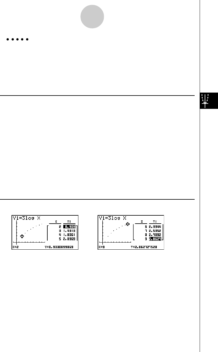
19990401
5-7-16
Using Tables
Example Store the function Y1 = 3logx and simultaneously display its number
table and plot-type graph. Use a table range of 2 through 9, with an
increment of 1.
Use the following V-Window settings.
Xmin = –1, Xmax = 10, Xscale = 1
Ymin = –1, Ymax = 4, Yscale = 1
Procedure
1m GRPH • TBL
2!K(V-Window) -bwbawbwc
-bwewbwi
u3(SET UP)ccc1(T+G)i
33(TYPE)b(Y=)dlvw
6(g)2(RANG)
cwjwbwi
45(TABL)
5(G • PLT)
56(g)4(G • Link)
6c ~ c, f ~ f
Result Screen
…→
←…

19990401
5-8 Dynamic Graphing
kk
kk
kUsing Dynamic Graph
Description
Dynamic Graph lets you define a range of values for the coefficients in a function, and then
observe how a graph is affected by changes in the value of a coefficient. It helps to see how
the coefficients and terms that make up a function influence the shape and position of a
graph.
Set Up
1. From the Main Menu, enter the DYNA Mode.
2. Make V-Window settings.
Execution
3. On the SET UP screen, specify the Dynamic Type.
1(Cont) ... Continuous
2(Stop) ... Automatic stop after 10 draws
4. Use the cursor keys to select the function type on the built-in function type list.*1
5. Input values for coefficients, and specify which coefficient will be the dynamic vari-
able.*2
6. Specify the start value, end value, and increment.
7. Specify the drawing speed.
3(SPEED)1( ) ..... Pause after each draw (Stop & Go)
2( ) ....... Half normal speed (Slow)
3( ) ....... Normal speed (Normal)
4( ) ...... Twice normal speed (Fast)
8. Draw the Dynamic Graph.
5-8-1
Dynamic Graphing
*1The following are the seven built-in function
types.
•Y=AX+B
•Y=A(X–B)2+C
•Y=AX2+BX+C
•Y=AX^3+BX2+CX+D
•Y=Asin(BX+C)
•Y=Acos(BX+C)
•Y=Atan(BX+C)
After you press 3(TYPE) and select the
function type you want, you can then input the
actual function.
b ... rectangular coordinate expression
c ... polar coordinate expression
d ... parametric function
*2You could also press w here and display the
parameter setting menu.
#The message “Too Many Functions” appears
when more than one function is selected for
Dynamic Graphing.
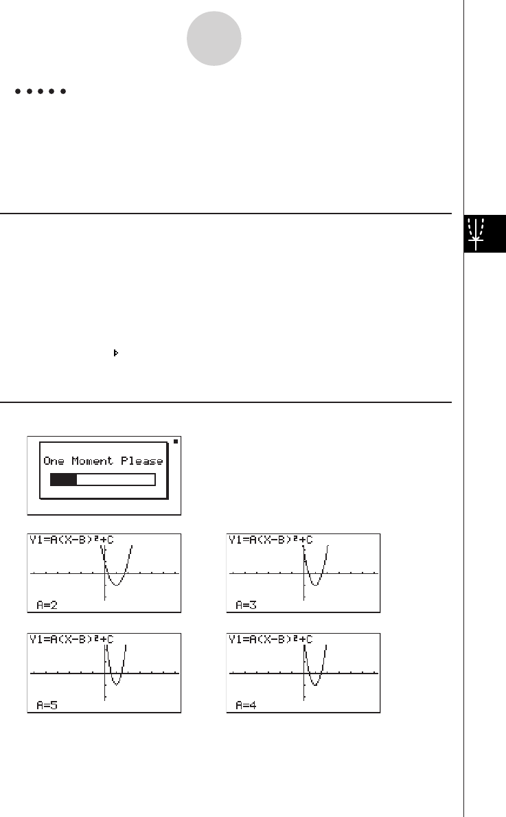
19990401
Example Use Dynamic Graph to graph y = A (x – 1)2 – 1, in which the value of
coefficient A changes from 2 through 5 in increments of 1. The Graph
is drawn 10 times.
Use the following V-Window settings.
Xmin = –6.3, Xmax = 6.3, Xscale = 1
Ymin = –3.1, Ymax = 3.1, Yscale = 1 (initial defaults)
Procedure
1m
DYNA
2!K(V-Window)1(INIT)i
3u3(SET UP)2(Stop)i
46(g)3(B-IN)c1(SEL)
56(g)4(VAR)cwbw-bw
62(RANG)cwfwbwi
73(SPEED)3() i
86(DYNA)
Result Screen
↓
→
←
↓↑
→
←
5-8-2
Dynamic Graphing
1
4
2
3
Repeats from 1 through 4.

19990401
kk
kk
kDynamic Graph Application Examples
Description
You can also use Dynamic Graph to simulate simple physical phenomena.
Set Up
1. From the Main Menu, enter the DYNA Mode.
2. Make V-Window settings.
Execution
3. On the SET UP screen, specify Stop for Dynamic Type and Deg for Angle.
4. Specify Param (parametric function) as the function type, and input a function that
contains a dynamic variable.
5. Specify the dynamic coefficient.
6. Specify the start value, end value, and increment.
7. Specify Normal for the draw speed.
8. Start the Dynamic Graph operation.
5-8-3
Dynamic Graphing
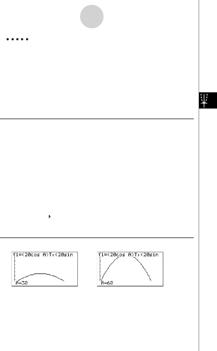
19990401
Example The path over time T of a ball thrown in the air at initial velocity V and
an angle of
θ
degrees from horizontal can be calculated as follows.
X = (Vcos
θ
)T, Y = (Vsin
θ
)T – (1/2)gT2 (g = 9.8m/s2)
Use Dynamic Graph to plot the path of a ball thrown at an initial
velocity of 20 meters per second, at horizontal angles of 30, 45, and 60
degrees (Angle: Deg).
Use the following V-Window settings.
Xmin = –1, Xmax = 42, Xscale = 5
Ymin = –1, Ymax = 16, Yscale = 2
T
θ
min = 0, T
θ
max = 6, T
θ
ptch = 0.1
Procedure
1m DYNA
2!K(V-Window) -bwecwfwc
-bwbgwcw
awgwa.bwi
3u3(SET UP)2(Stop)
cccc1(Deg)i
43(TYPE)d(Param)
(cacav(A))vw
(casav(A))v-e.jvxw
54(VAR)
62(RANG)dawgawbfwi
73(SPEED)3() i
86(DYNA)
Result Screen
···→
←···
5-8-4
Dynamic Graphing
2001100120011101
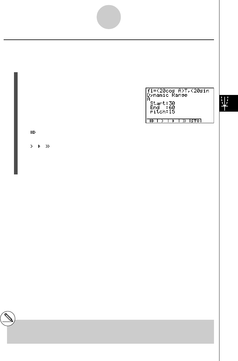
19990401
kAdjusting the Dynamic Graph Speed
You can use the following procedure to adjust the Dynamic Graph speed while the draw
operation is taking place.
1. While a Dynamic Graph draw operation is being performed, press A to change to the
speed adjustment menu.
•{ } ... {Each step of the Dynamic Graph draw operation is performed each time you
press w.}
•{ }/{ }/{} ... {slow (1/2 speed)}/{normal (default speed)}/{fast (double speed)}
•{STO} ... {stores graph conditions and screen data in Dynamic Graph memory}
2. Press the function key (1 to 4) that corresponds to the speed you want to change
to.
5-8-5
Dynamic Graphing
#To clear the speed adjustment menu without
changing anything, press w.
# Press u5 (G↔T) to return to the graph
screen.

19990401
kk
kk
kUsing Dynamic Graph Memory
You can store Dynamic Graph conditions and screen data in Dynamic Graph memory for
later recall when you need it. This lets you save time, because you can recall the data and
immediately begin a Dynamic Graph draw operation. Note that you can store one set of data
in memory at any one time.
The following is all of the data that makes up a set.
•Graph functions (up to 20)
•Dynamic Graph conditions
•SET UP screen settings
•V-Window contents
•Dynamic Graph screen
uu
uu
uTo save data in Dynamic Graph memory
1. While a Dynamic Graph draw operation is being performed, press A to change to the
speed adjustment menu.
2. Press 6(STO). In response to the confirmation dialog that appears, press w(Yes) to
save the data.
uu
uu
uTo recall data from Dynamic Graph memory
1. Display the Dynamic Graph function list.
2. Press 6(RCL) to recall all the data stored in Dynamic Graph memory.
5-8-6
Dynamic Graphing
#If there is already data stored in Dynamic
Graph memory, the data save operation
replaces it with the new data.
#Data recalled from Dynamic Graph memory
replaces the calculator’s current graph functions,
draw conditions, and screen data. The previous
data is lost when it is replaced.
20040901

19990401
5-9 Graphing a Recursion Formula
kk
kk
kGenerating a Number
Table from a Recursion Formula
Description
You can input up to three of the following types of recursion formulas and generate a number
table.
•General term of sequence {an}, composed of an, n
•Linear two-term recursion composed of an+1, an, n
•Linear three-term recursion composed of an+2, an+1, an, n
Set Up
1. From the Main Menu, enter the RECUR Mode.
Execution
2. Specify the recursion type.
3(TYPE)b(an=) ... {general term of sequence an}
c(an+1=) ... {linear two-term recursion}
d(an+2=) ... {linear three-term recursion}
3. Input the recursion formula.
4. Specify the table range. Specify a start point and end point for n. If necessary, specify a
value for the initial term, and a pointer start point value if you plan to graph the formula.
5. Display the recursion formula number table.
5-9-1
Graphing a Recursion Formula
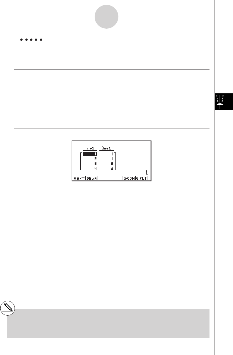
19990401
Example Generate a number table from recursion between three terms as
expressed by an+2 = an+1 + an, with initial terms of a1 = 1, a2 = 1
(Fibonacci sequence), as n changes in value from 1 to 6.
Procedure
1m RECUR
23(TYPE)d(an+2=)
34(n. an ··)d(an+1)+2(an)w
45(RANG)2(a1)bwgwbwbwi
56(TABL)
Result Screen
5-9-2
Graphing a Recursion Formula
#Specifying On for the Σ Display of the SET UP
screen causes the sum of each term to be
included in the table.
*The first two values correspond to
a1 = 1 and a2 = 1.
20011101

19990401
kk
kk
kGraphing a Recursion Formula (1)
Description
After generating a number table from a recursion formula, you can graph the values on a line
graph or plot type graph.
Set Up
1. From the Main Menu, enter the RECUR Mode.
2. Make V-Window settings.
Execution
3. Specify the recursion formula type and input the formula.
4. Specify the table range, and start and ending values for n. If necessary, specify the
initial term value and pointer start point.
5. Display the recursion formula number table.
6. Specify the graph type and draw the graph.
5(G • CON) ... line graph
6(G • PLT) ... plot type graph
5-9-3
Graphing a Recursion Formula
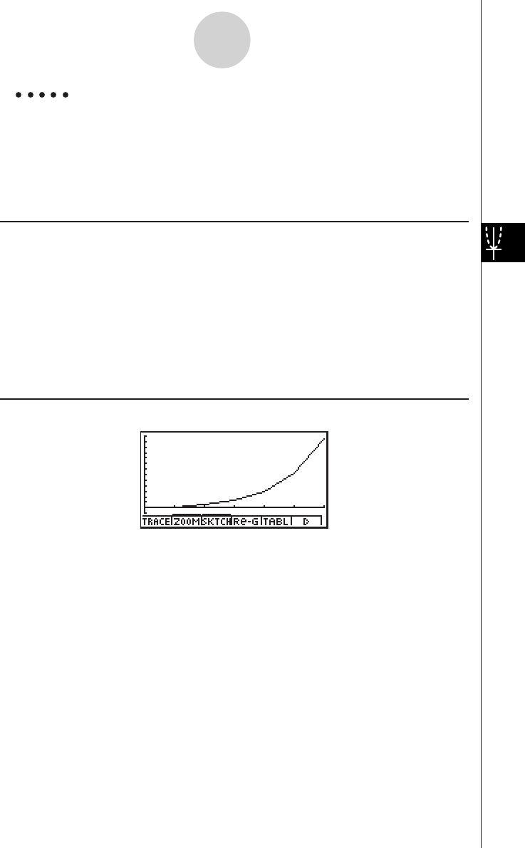
19990401
Example Generate a number table from recursion between two terms as
expressed by an+1 = 2an+1, with an initial term of a1 = 1, as n changes
in value from 1 to 6. Use the table values to draw a line graph.
Use the following V-Window settings.
Xmin = 0, Xmax = 6, Xscale = 1
Ymin = –15, Ymax = 65, Yscale = 5
Procedure
1m
RECUR
2!K(V-Window) awgwbwc
-bfwgfwfwi
33(TYPE)c(an+1=)c2(an)+bw
45(RANG)2(a1)bwgwbwi
56(TABL)
65(G • CON)
Result Screen
5-9-4
Graphing a Recursion Formula

19990401
kk
kk
kGraphing a Recursion Formula (2)
Description
The following describes how to generate a number table from a recursion formula and graph
the values while Σ Display is On.
Set Up
1. From the Main Menu, enter the RECUR Mode.
2. On the SET UP screen, specify On for Σ Display.
3. Make V-Window settings.
Execution
4. Specify the recursion formula type and input the recursion formula.
5. Specify the table range, and start and ending values for n. If necessary, specify the
initial term value and pointer start point.
6. Display the recursion formula number table.
7. Specify the graph type and draw the graph.
5(G • CON)b(an) ... Line graph with ordinate an, abscissa n
c(Σan) ... Line graph with ordinate Σan, abscissa n
6(G • PLT) b(an) ... Plot type graph with ordinate an, abscissa n
c(Σan) ... Plot type graph with ordinate Σan, abscissa n
5-9-5
Graphing a Recursion Formula

19990401
Example Generate a number table from recursion between two terms as
expressed by an+1 = 2an+1, with an initial term of a1 = 1, as n changes
in value from 1 to 6. Use the table values to draw a plot line graph with
ordinate Σan, abscissa n.
Use the following V-Window settings.
Xmin = 0, Xmax = 6, Xscale = 1
Ymin = –15, Ymax = 65, Yscale = 5
Procedure
1m
RECUR
2u3(SET UP)1(On)i
3!K(V-Window) awgwbwc
-bfwgfwfwi
43(TYPE)c(an+1=)c2(an)+bw
55(RANG)2(a1)bwgwbwi
66(TABL)
76(G • PLT)c(Σan)
Result Screen
5-9-6
Graphing a Recursion Formula

19990401
kk
kk
kWEB Graph (Convergence, Divergence)
Description
y = f(x) is graphed by presuming an+1 = y, an = x for linear two-term regression an+1 = f(an)
composed of an+1, an. Next, it can be determined whether the function is convergent or
divergent.
Set Up
1. From the Main Menu, enter the RECUR Mode.
2. Make V-Window settings.
Execution
3. Select 2-term recursion as the recursion formula type, and input the formula.
4. Specify the table range, n start and end points, initial term value, and pointer start
point.
5. Display the recursion formula number table.
6. Draw the graph.
7. Press w, and the pointer appears at the start point you specified.
Press w several times.
If convergence exists, lines that resemble a spider web are drawn on the display.
Failure of the web lines to appear indicates either divergence or that the graph is
outside the boundaries of the display screen. When this happens, change to larger
View Window values and try again.
You can use fc to select the graph.
5-9-7
Graphing a Recursion Formula
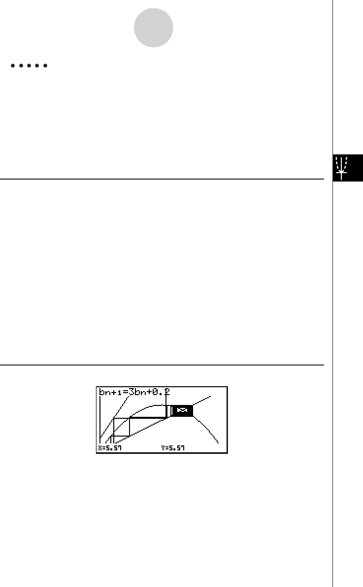
19990401
Example To draw the WEB graph for the recursion formula an+1 = –3(an)2 + 3an,
bn+1 = 3bn + 0.2, and check for divergence or convergence. Use the
following table range and V-Window Settings.
Table Range
Start = 0, End = 6, a0 = 0.01, anStr = 0.01, b0 = 0.11, bnStr = 0.11
V-Window Settings
Xmin = 0, Xmax = 1, Xscale = 1
Ymin = 0, Ymax = 1, Yscale = 1
Procedure
1m RECUR
2!K(V-Window) awbwbwc
awbwbwi
33(TYPE)c(an+1=)-d2(an)x+d2(an)w
d3(bn)+a.cw
45(RANG)1(a0)
awgwa.abwa.bbwc
a.abwa.bbwi
56(TABL)
64(WEB)
71(TRACE)w~w(an is convergence)
cw~w(bn is divergence)
Result Screen
5-9-8
Graphing a Recursion Formula

19990401
5-10-1
Changing the Appearance of a Graph
5-10 Changing the Appearance of a Graph
kk
kk
kDrawing a Line
Description
The sketch function lets you draw points and lines inside of graphs.
Set Up
1. Draw the graph.
Execution
2. Select the sketch function you want to use.*1
3(SKTCH)b(Cls) ... Screen clear
c(PLOT)
{On}/{Off}/{Change}/{Plot} ... Point {On}/{Off}/{Change}/{Plot}
d(LINE)
{F-Line}/{Line} ... {Freehand line}/{Line}
e(Text) ... Text input
f(Pen) ... Freehand
g(Tangnt) ... Tangent line
h(Normal) ... Line normal to a curve
i(Invrse) ... Inverse function*2
j(Circle) ... Circle
v(Vert) ... Vertical line
l(Horz) ... Horizontal line
3. Use the cursor keys to move the pointer ( ) to the location where you want to draw,
and press w.*3
*1The above shows the function menu that
appears in the GRPH • TBL Mode. Menu items
may differ somewhat in other modes.
*2In the case of an inverse function graph,
drawing starts immediately after you select
this option.
*3Some sketch functions require specification of
two points. After you press w to specify the
first point, use the cursor keys to move the
pointer to the location of the second point and
press w.
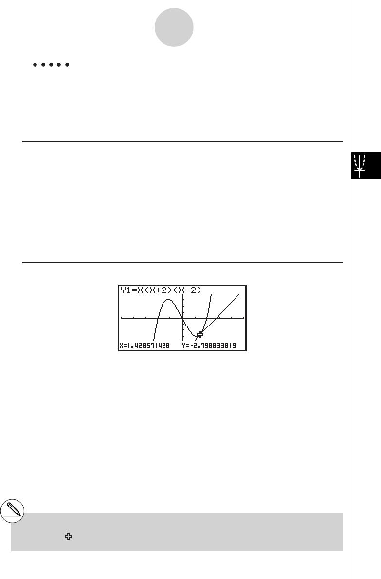
19990401
Example Draw a line that is tangent to point (2, 0) on the graph for
y = x (x + 2)(x – 2).
Use the following V-Window settings.
Xmin = –5, Xmax = 5, Xscale = 1
Ymin = –5, Ymax = 5, Yscale = 1
Procedure
1m
GRPH • TBL
!K(V-Window) -fwfwbwc
-fwfwbwi
3(TYPE)b(Y=)v(v+c)(v-c)w
5(DRAW)
23(SKTCH)g(Tangnt)
3e~ew*1
Result Screen
5-10-2
Changing the Appearance of a Graph
*1You can draw a tangent line in succession by
moving the “ ” pointer and pressing w.

19990401
kk
kk
kInserting Comments
Description
You can insert comments anywhere you want in a graph.
Set Up
1. Draw the graph.
Execution
2. Press 3(SKTCH)e(Text), and a pointer appears in the center of the display.
3. Use the cursor keys to move the pointer to the location where you want the text to be,
and input the text.
5-10-3
Changing the Appearance of a Graph
#You can input any of the following characters as
comment text: A~Z, r,
θ
, space, 0~9, ., +, –, ×,
÷, (–), EXP, π, Ans, (, ), [, ], {, }, comma, →,
x2, ^, log, In, , x, 10x, ex, 3, x–1, sin, cos,
tan, sin–1, cos–1, tan–1, i, List, Mat
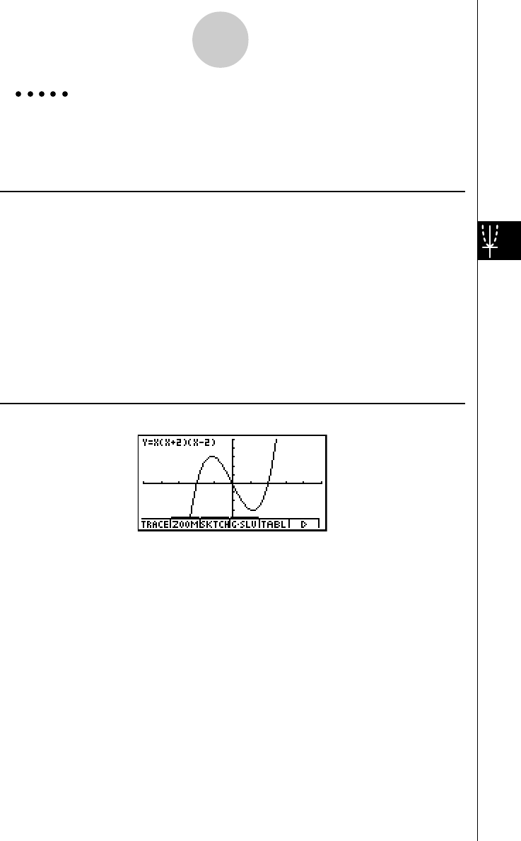
19990401
Example Insert text into the graph y = x (x + 2)(x – 2).
Use the following V-Window settings.
Xmin = –5, Xmax = 5, Xscale = 1
Ymin = –5, Ymax = 5, Yscale = 1
Procedure
1m
GRPH • TBL
!K(V-Window) -fwfwbwc
-fwfwbwi
3(TYPE)b(Y=)v(v+c)(v-c)w
5(DRAW)
23(SKTCH)e(Text)
3f~f d~d
a-(Y)!.(=)v(v+c)(v-c)
i
Result Screen
5-10-4
Changing the Appearance of a Graph
19991201

19990401
kk
kk
kFreehand Drawing
Description
You can use the pen option for freehand drawing in a graph.
Set Up
1. Draw the graph.
Execution
2. Press 3(SKTCH)f(Pen), and a pointer appears in the center of the screen.
3. Use the cursor keys to move the pointer to the point from which you want to start
drawing, and then press w.
4. Use the cursor keys to move the pointer. A line is drawn wherever you move the pointer.
To stop the line, press w.
Repeat step 3 and 4 to draw other lines.
After you are finished drawing, press i.
5-10-5
Changing the Appearance of a Graph
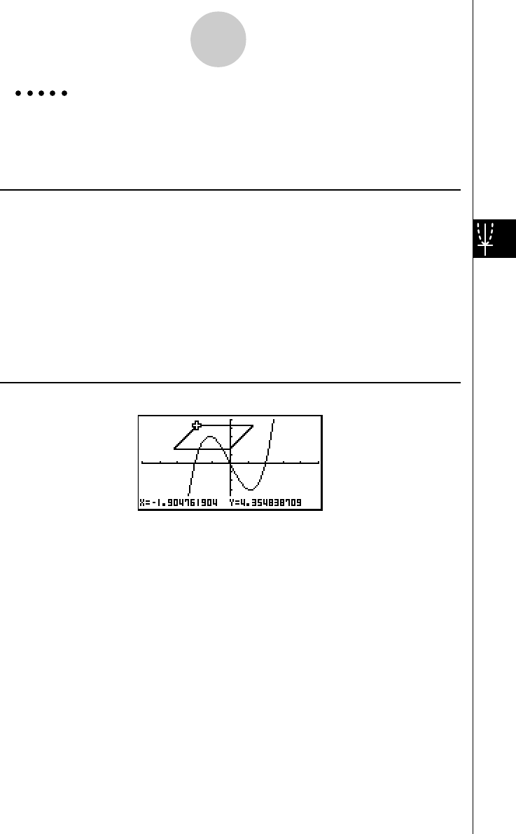
19990401
Example Use the pen to draw on the graph y = x (x + 2)(x – 2).
Use the following V-Window settings.
Xmin = –5, Xmax = 5, Xscale = 1
Ymin = –5, Ymax = 5, Yscale = 1
Procedure
1m
GRPH • TBL
!K(V-Window) -fwfwbwc
-fwfwbwi
3(TYPE)b(Y=)v(v+c)(v-c)w
5(DRAW)
23(SKTCH)f(Pen)
3f~f d~dw
4cd…, e~e, ef…, d~dw
Result Screen
5-10-6
Changing the Appearance of a Graph
19991201
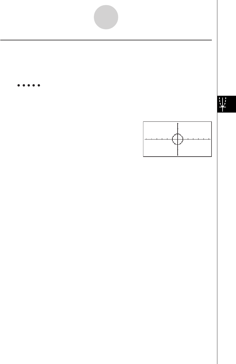
19990401
5-10-7
Changing the Appearance of a Graph
kk
kk
kChanging the Graph Background
You can use the set up screen to specify the memory contents of any picture memory area
(Pict 1 through Pict 20) as the Background item. When you do, the contents of the
corresponding memory area is used as the background of the graph screen.
Example 1 With the circle graph X2 + Y2 = 1 as the background, use Dynamic
Graph to graph Y = X2 + A as variable A changes value from –1 to 1 in
increments of 1.
Recall the background graph.
(X2 + Y2 = 1)
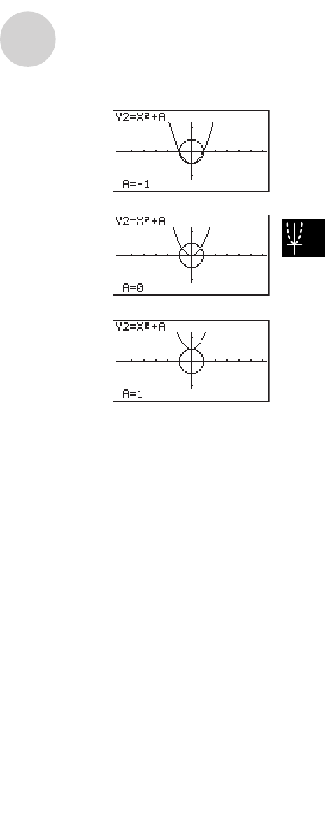
19990401
5-10-8
Changing the Appearance of a Graph
Draw the dynamic graph.
(Y = X2 – 1)
↓↑
(Y = X2)
↓↑
(Y = X2 + 1)
•See “5-8-1 Dynamic Graphing” for details on using the Dynamic Graph feature.

19990401
5-11 Function Analysis
kk
kk
kReading Coordinates on a Graph Line
Description
Trace lets you move a pointer along a graph and read out coordinates on the display.
Set Up
1. Draw the graph.
Execution
2. Press 1(TRACE), and a pointer appears in the center of the graph.*1
3. Use d and e to move the pointer along the graph to the point at which you want to
display the derivative.
When there are multiple graphs on the display, press f and c to move between
them along the x-axis of the current pointer location.
4. You can also move the pointer by pressing v to display the pop-up window, and then
inputting coordinates.
The pop-up window appears even when you input coordinates directly.
To exit a trace operation, press i.
*1The pointer is not visible on the graph when
it is located at a point outside the graph
display area or when an error of no value
occurs.
#You can turn off display of the coordinates at the
pointer location by specifying “Off” for the “Coord”
item on the SET UP screen.
19991201
5-11-1
Function Analysis
20011101
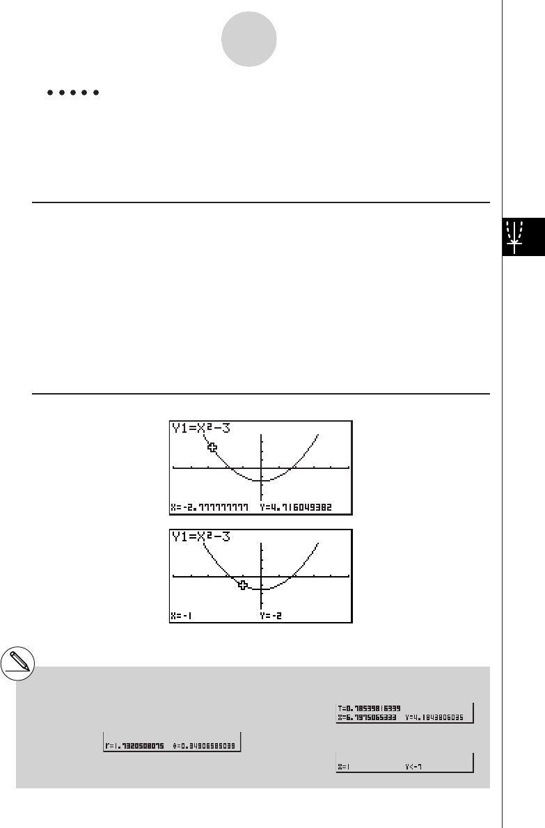
19990401
Example Read coordinates along the graph of the function shown below.
Y1 = x2 – 3
Use the following V-Window settings.
Xmin = –5, Xmax = 5, Xscale = 1
Ymin = –10, Ymax = 10, Yscale = 2
Procedure
1m GRPH • TBL
!K(V-Window) -fwfwbwc
-bawbawcwi
3(TYPE)b(Y=)vx-dw
5(DRAW)
21(TRACE)
3d~d
4-bw
Result Screen
5-11-2
Function Analysis
#The following shows how coordinates are
displayed for each function type.
•Polar Coordinate Graph
•Parametric Graph
•Inequality Graph
19991201

19990401
kk
kk
kDisplaying the Derivative
Description
In addition to using Trace to display coordinates, you can also display the derivative at the
current pointer location.
Set Up
1. On the SET UP screen, specify On for Derivative.
2. Draw the graph.
Execution
3. Press 1(TRACE), and the pointer appears at the center of the graph. The current
coordinates and the derivative also appear on the display at this time.
4. Use d and e to move the pointer along the graph to the point at which you want to
display the derivative.
When there are multiple graphs on the display, press f and c to move between
them along the x-axis of the current pointer location.
5. You can also move the pointer by pressing v to display the pop-up window, and then
inputting coordinates.
The pop-up window appears even when you input coordinates directly.
5-11-3
Function Analysis
20011101
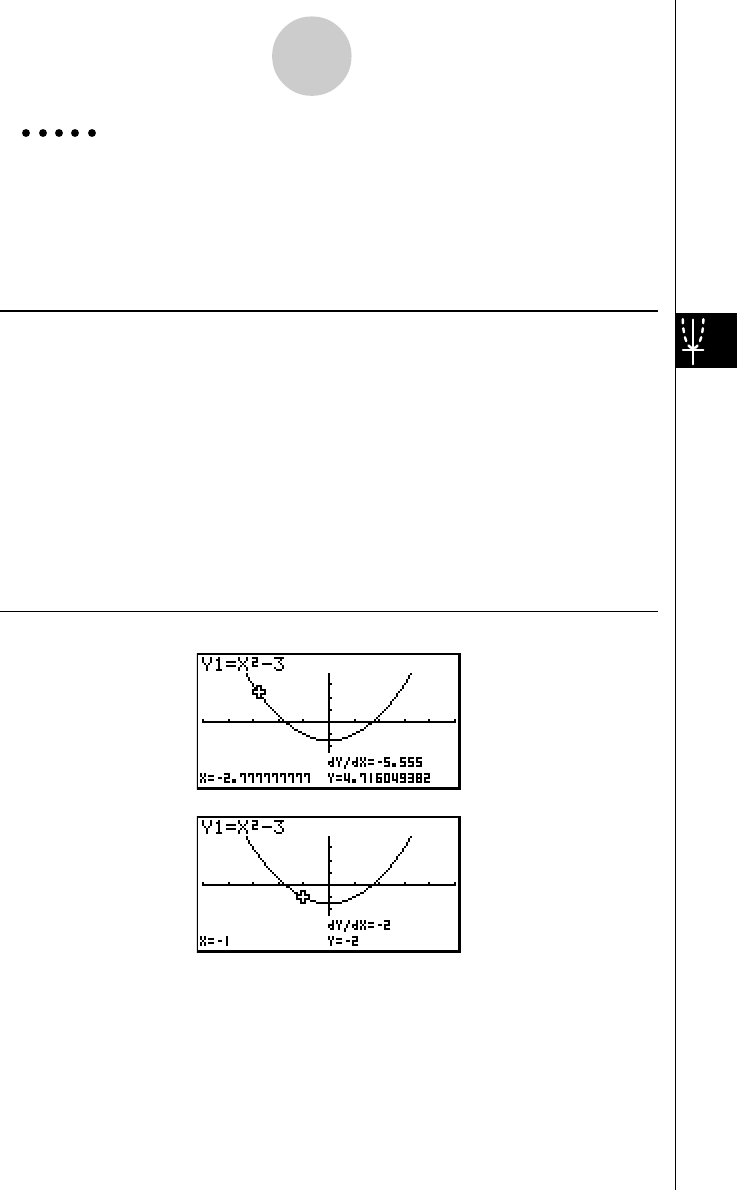
19990401
Example Read coordinates and derivatives along the graph of the function
shown below.
Y1 = x2 – 3
Use the following V-Window settings.
Xmin = –5, Xmax = 5, Xscale = 1
Ymin = –10, Ymax = 10, Yscale = 2
Procedure
1m
GRPH • TBL
u3(SET UP)ccccc1(On)i
2!K(V-Window) -fwfwbwc
-bawbawcwi
3(TYPE)b(Y=)vx-dw
5(DRAW)
31(TRACE)
4d~d
5-bw
Result Screen
5-11-4
Function Analysis
19991201

19990401
kk
kk
kGraph to Table
Description
You can use trace to read the coordinates of a graph and store them in a number table. You
can also use Dual Graph to simultaneously store the graph and number table, making this an
important graph analysis tool.
Set Up
1. From the Main Menu, enter the GRPH • TBL Mode.
2. On the SET UP screen, specify GtoT for Dual Screen.
3. Make V-Window settings.
Execution
4. Save the function and draw the graph on the active (left) screen.
5. Activate Trace. When there are multiple graphs on the display, press f and c to
select the graph you want.
6. Use d to move the pointer and press w to store coordinates into the number table.
Repeat this step to store as many values as you want.
7. Press 6(CHNG) to switch the number table side.
8. From the pop-up window, input the list number you want to save.
5-11-5
Function Analysis
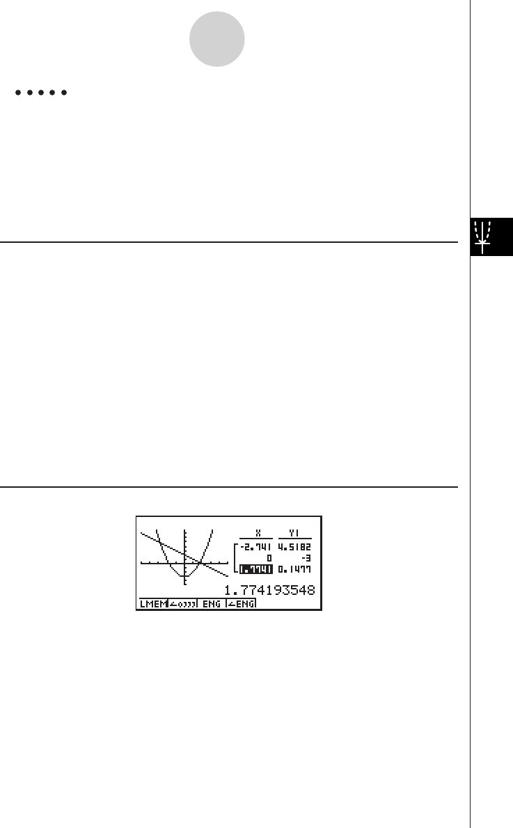
19990401
Example Save, in a table, the coordinates in the vicinity of the points of
intersection at X = 0 for the two graphs shown below, and store the
table contents in List 1.
Y1 = x2 – 3, Y2 = – x + 2
Use the following V-Window settings.
Xmin = –5, Xmax = 5, Xscale = 1
Ymin = –10, Ymax = 10, Yscale = 2
Procedure
1m GRPH • TBL
2u3(SET UP)ccc3(GtoT)i
3!K(V-Window) -fwfwbwc
-bawbawcwi
43(TYPE)b(Y=) vx-dw
-v+cw
5(DRAW)
51(TRACE)
6d~dwe~ewi
76(CHNG)
8K1(LMEM)bw
Result Screen
5-11-6
Function Analysis
20011101

19990401
kk
kk
kCoordinate Rounding
Description
This function rounds off coordinate values displayed by Trace.
Set Up
1. Draw the graph.
Execution
2. Press 2(ZOOM)i(Rnd). This causes the V-Window settings to be changed
automatically in accordance with the Rnd value.
3. Press 1(TRACE), and then use the cursor keys to move the pointer along the graph.
The coordinates that now appear are rounded.
5-11-7
Function Analysis
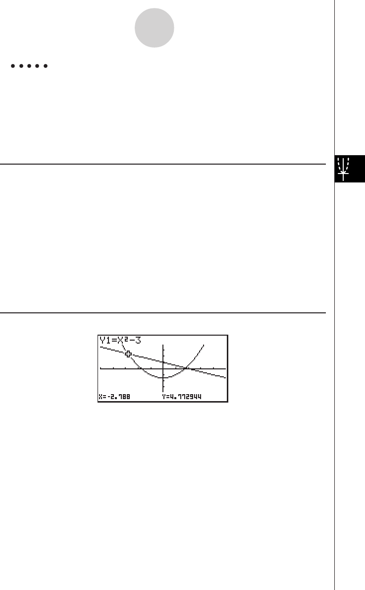
19990401
Example Use coordinate rounding and display the coordinates in the vicinity of
the points of intersection for the two graphs produced by the
functions shown below.
Y1 = x2 – 3, Y2 = – x + 2
Use the following V-Window settings.
Xmin = –5, Xmax = 5, Xscale = 1
Ymin = –10, Ymax = 10, Yscale = 2
Procedure
1m
GRPH • TBL
!K(V-Window) -fwfwbwc
-bawbawcwi
3(TYPE)b(Y=)vx-dw
-v+cw
5(DRAW)
22(ZOOM)i(Rnd)
31(TRACE)
d~d
Result Screen
5-11-8
Function Analysis

19990401
kk
kk
kCalculating the Root
Description
This feature provides a number of different methods for analyzing graphs.
Set Up
1. Draw the graphs.
Execution
2. Select the analysis function.
4(G-SLV) b(Root) ... Calculation of root
c(Max) ... Local maximum value
d(Min) ... Local minimum value
e(Y-lcpt) ... y-intercept
f(Isect) ... Intersection of two graphs
g(Y-Cal) ... y-coordinate for given x-coordinate
h(X-Cal) ... x-coordinate for given y-coordinate
i(∫dx) ... Integral value for a given range
3. When there are multiple graphs on the screen, the selection cursor (k) is located at
the lowest numbered graph. Use the cursor keys to move the cursor to the graph you
want to select.
4. Press w to select the graph where the cursor is located and display the value
produced by the analysis.
When an analysis produces multiple values, press e to calculate the next value.
Pressing d returns to the previous value.
5-11-9
Function Analysis
20011101
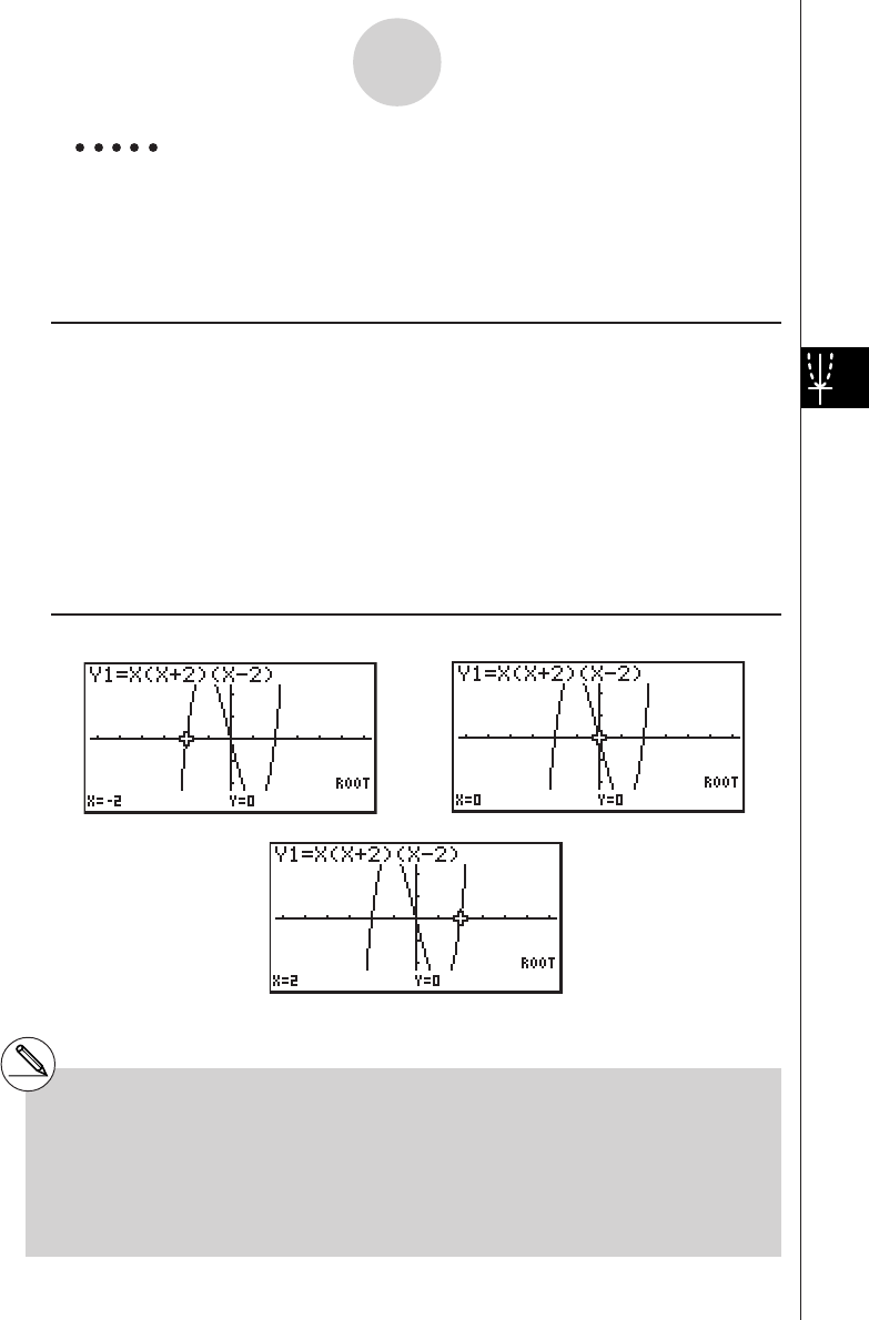
19990401
Example Draw the graph shown below and calculate the root for Y1.
Y1 = x(x + 2)(x – 2)
Use the following V-Window settings.
Xmin = –6.3, Xmax = 6.3, Xscale = 1
Ymin = –3.1, Ymax = 3.1, Yscale = 1 (initial defaults)
Procedure
1m GRPH • TBL
!K(V-Window) 1(INIT)i
3(TYPE)b(Y=)v(v+c)(v-c)w
5(DRAW)
24(G-SLV)b(Root)
4e
e
Result Screen
5-11-10
Function Analysis
#When analyzing a single graph, results appear
as soon as you select an analysis function in
step 2, so step 3 is not necessary.
#Root, local maximum value, local minimum
value, and y-intercept can be calculated for
rectangular coordinate graphs and inequality
graphs only.
#The y-intercept is the point where the graph
crosses the y-axis.
…
20011101

19990401
kk
kk
kCalculating the Point of Intersection of Two Graphs
Description
Use the following procedure to calculate the point of intersection of two graphs.
Set Up
1. Draw the graphs.
Execution
2. Press 4(G-SLV)5(Isect). When there are three or more graphs, the selection cursor
(k) appears at the lowest numbered graph.
3. Use the cursor keys to move the cursor to the graph you want to select.
4. Press w to select the first graph, which changes the shape of the cursor from k to
쏆.
5. Use the cursor keys to move the cursor to the second graph.
6. Press w to calculate the point of intersection for the two graphs.
When an analysis produces multiple values, press e to calculate the next value.
Pressing d returns to the previous value.
5-11-11
Function Analysis
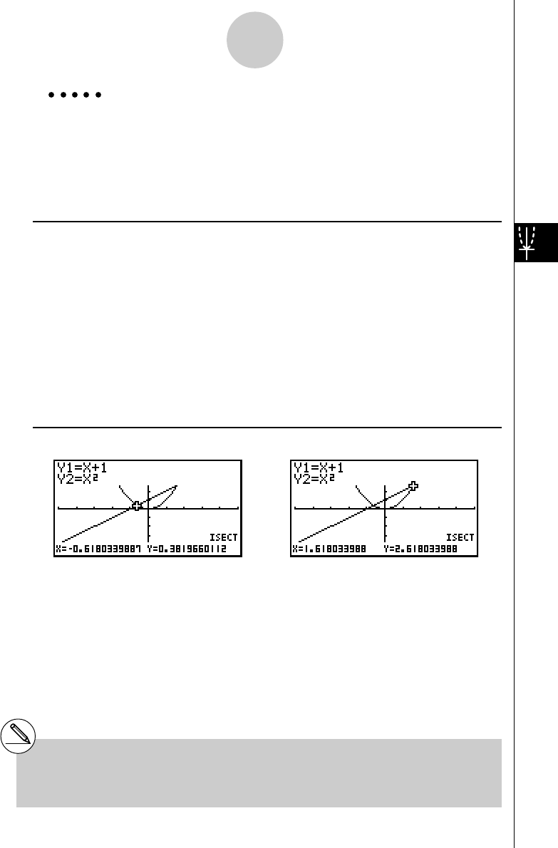
19990401
Example Graph the two functions shown below, and determine the point of
intersection between Y1 and Y2.
Y1 = x + 1, Y2 = x2
Use the following V-Window settings.
Xmin = –5, Xmax = 5, Xscale = 1
Ymin = –5, Ymax = 5, Yscale = 1
Procedure
1m
GRPH • TBL
!K(V-Window) -fwfwbwc
-fwfwbwi
3(TYPE)b(Y=)v+bw
vxw
5(DRAW)
24(G-SLV)f(Isect)
6e
Result Screen
5-11-12
Function Analysis
#In the case of two graphs, the point of
intersection is calculated immediately after you
press 4f in step 2.
#You can calculate the point of intersection for
rectangular coordinate graphs and inequality
graphs only.
…

19990401
kDetermining the Coordinates for Given Points
Description
The following procedure describes how to determine the y-coordinate for a given x, and the
x-coordinate for a given y.
Set Up
1. Draw the graph.
Execution
2. Select the function you want to perform. When there are multiple graphs, the selection
cursor (k) appears at the lowest numbered graph.
4(G-SLV)g(Y-Cal) ... y-coordinate for given x
h(X-Cal) ... x-coordinate for given y
3. Use fc to move the cursor (k) to the graph you want, and then press w to select
it.
4. Input the given x-coordinate value or y-coordinate value.
Press w to calculate the corresponding y-coordinate value or x-coordinate value.
5-11-13
Function Analysis
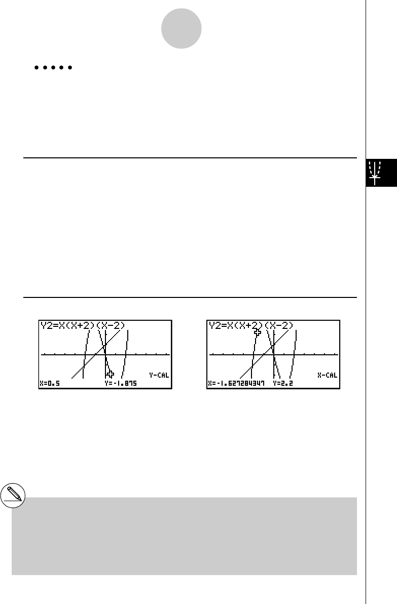
19990401
Example Graph the two functions shown below and then determine the y-
coordinate for x = 0.5 and the x-coordinate for y = 2.2 on graph Y2.
Y1 = x + 1, Y2 = x(x + 2)(x – 2)
Use the following V-Window settings.
Xmin = –6.3, Xmax = 6.3, Xscale = 1
Ymin = –3.1, Ymax = 3.1, Yscale = 1 (initial defaults)
Procedure
1m GRPH • TBL
!K(V-Window) 1(INIT)i
3(TYPE)b(Y=)v+bw
v(v+c)(v-c)w
5(DRAW)
24(G-SLV)g(Y-Cal) 24(G-SLV)h(X-Cal)
3cw3cw
4a.fw4c.cw
Result Screen
5-11-14
Function Analysis
#When there are multiple results for the above
procedure, press e to calculate the next
value. Pressing d returns to the previous
value.
#Step 3 of the above procedure is skipped
when there is only one graph on the display.
#The X-Cal value cannot be obtained for a
parametric function graph.
#After obtaining coordinates with the above
procedure, you can input different coordinates
by first pressing v.

19990401
kk
kk
kCalculating the lntegral Value for a Given Range
Description
Use the following procedure to obtain integration values for a given range.
Set Up
1. Draw the graph.
Execution
2. Press 4(G-SLV)i(∫dx). When there are multiple graphs, this causes the selection
cursor (k) to appear at the lowest numbered graph.
3. Use fc to move the cursor (k) to the graph you want, and then press w to select
it.
4. Use d to move the lower limit pointer to the location you want, and then press w.
You can also move the pointer by pressing v to display the pop-up window, and then
inputting coordinates.
5. Use e to move the upper limit pointer to the location you want.
You can also move the pointer by pressing v to display the pop-up window, and then
inputting the upper limit and lower limit values for the integration range.
6. Press w to calculate the integral value.
5-11-15
Function Analysis
#You can also specify the lower limit and upper
limit by inputting them on the 10-key pad.
#When setting the range, make sure that the lower
limit is less than the upper limit.
#Integral values can be calculated for rectangular
coordinate graphs only.
19991201
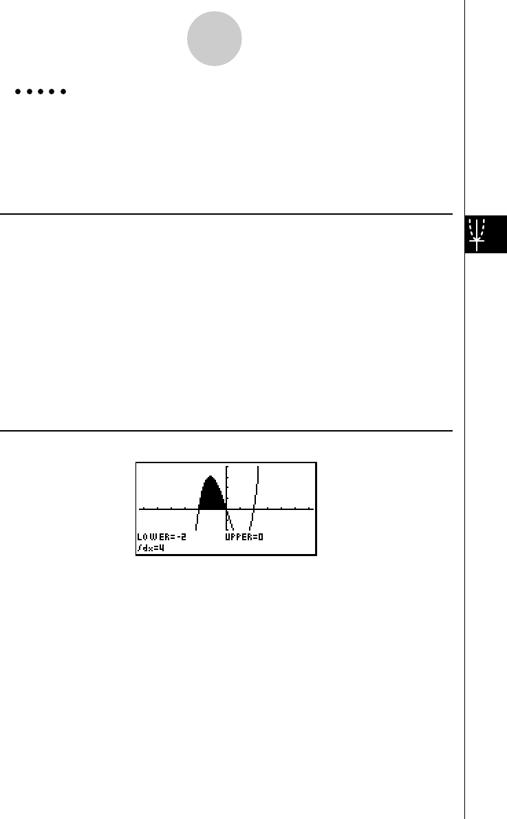
19990401
Example Graph the function shown below, and then determine the integral value
at (–2, 0).
Y1 = x(x + 2)(x – 2)
Use the following V-Window settings.
Xmin = –6.3, Xmax = 6.3, Xscale = 1
Ymin = –4, Ymax = 4, Yscale = 1
Procedure
1m
GRPH • TBL
!K(V-Window) -g.dwg.dwbwc
-ewewbwi
3(TYPE)b(Y=)v(v+c)(v-c)w
5(DRAW)
24(G-SLV)i(∫dx)
4d~dw
5e~e(Upper limit; x = 0)
6w
Result Screen
5-11-16
Function Analysis
…

19990401
kk
kk
kConic Section Graph Analysis
You can determine approximations of the following analytical results using conic section
graphs.
•Focus/vertex/eccentricity
•Latus rectum
•Center/radius
•x-/y-intercept
•Directrix/axis of symmetry drawing and analysis
•Asymptote drawing and analysis
After graphing a conic section, press 4(G-SLV) to display the following graph analysis
menus.
uParabolic Graph Analysis
•{Focus}/{Vertex}/{Length}/{e} ... {focus}/{vertex}/{latus rectum}/{eccentricity}
•{Dirtrx}/{Sym} ... {directrix}/{axis of symmetry}
•{X-Icpt}/{Y-Icpt} ... {x-intercept}/{y-intercept}
uCircular Graph Analysis
•{Center}/{Radius} ... {center}/{radius}
•{X-Icpt}/{Y-Icpt} ... {x-intercept}/{y-intercept}
uElliptical Graph Analysis
•{Focus}/{Vertex}/{Center}/{e} ... {focus}/{vertex}/{center}/{eccentricity}
•{X-Icpt}/{Y-Icpt} ... {x-intercept}/{y-intercept}
uHyperbolic Graph Analysis
•{Focus}/{Vertex}/{Center}/{e} ... {focus}/{vertex}/{center}/{eccentricity}
•{Asympt} ... {asymptote}
•{X-Icpt}/{Y-Icpt} ... {x-intercept}/{y-intercept}
The following examples show how to use the above menus with various types of conic
section graphs.
5-11-17
Function Analysis
20011101
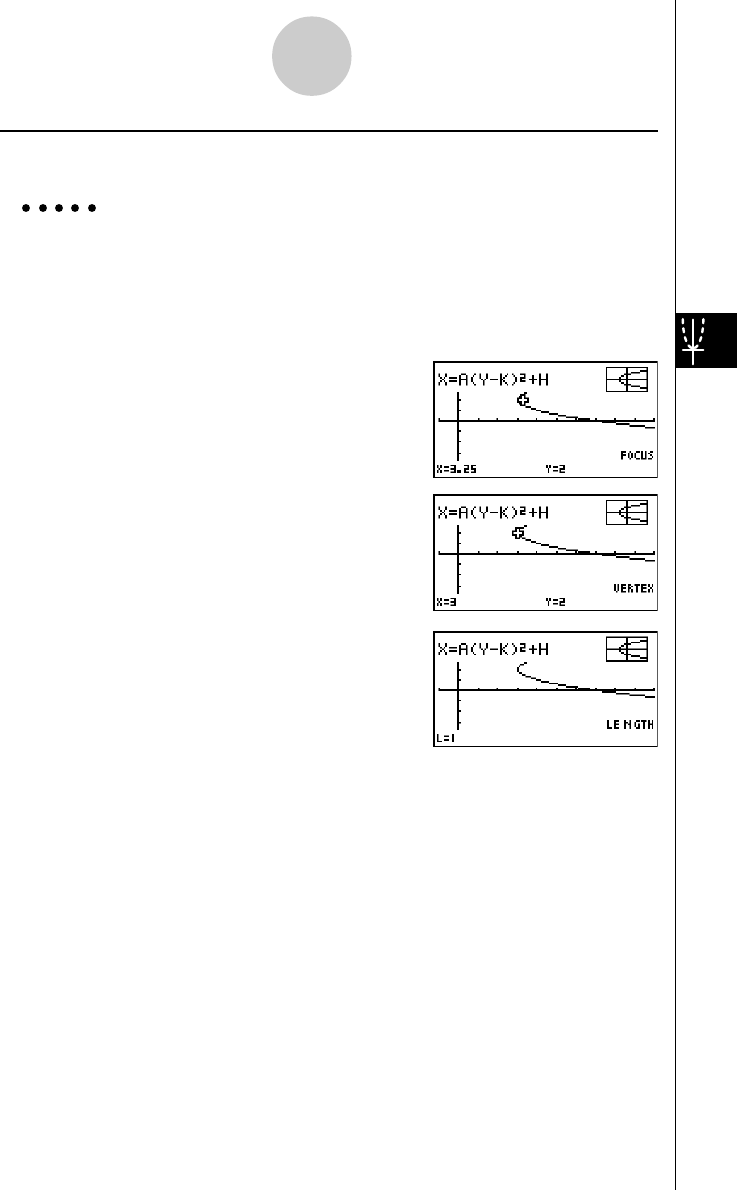
19990401
uTo calculate the focus, vertex and latus rectum
[G-SLV]-[Focus]/[Vertex]/[Length]
Example To determine the focus, vertex and latus rectum for the parabola
X = (Y – 2)2 + 3
Use the following V-Window settings.
Xmin = –1, Xmax = 10, Xscale = 1
Ymin = –5, Ymax = 5, Yscale = 1
4(G-SLV)
b(Focus)
(Calculates the focus.)
i
4(G-SLV)
d(Vertex)
(Calculates the vertex.)
i
4(G-SLV)
f(Length)
(Calculates the latus rectum.)
•When calculating two foci for an ellipse or hyperbolic graph, press e to calculate the
second focus. Pressing d returns to the first focus.
•When calculating two vertexes for an ellipse or hyperbolic graph, press e to calculate
the second vertex. Pressing d returns to the first vertex.
5-11-18
Function Analysis
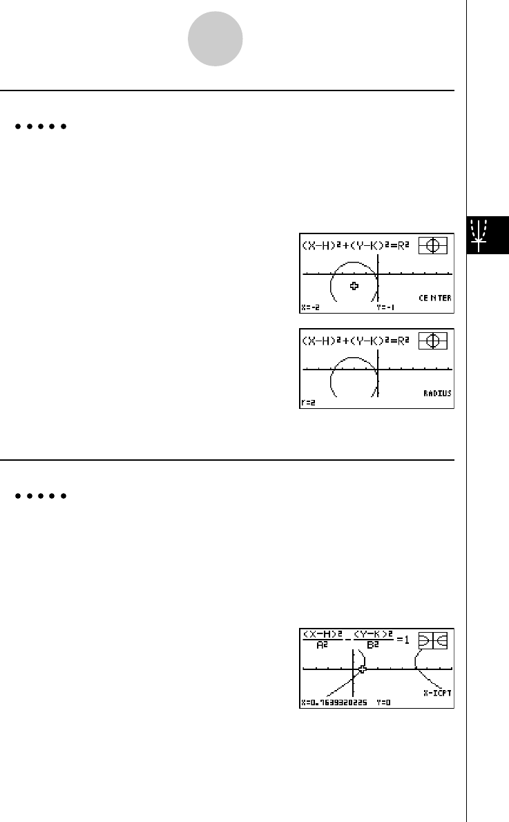
19990401
uTo calculate the center and radius [G-SLV]-[Center]/[Radius]
Example To determine the center and radius for the circle
(X + 2)2 + (Y + 1)2 = 22
Use the following V-Window settings.
Xmin = –6.3, Xmax = 6.3, Xscale = 1
Ymin = –3.1, Ymax = 3.1, Yscale = 1
4(G-SLV)
b(Center)
(Calculates the center.)
i
4(G-SLV)
c(Radius)
(Calculates the radius.)
uTo calculate the x- and y-intercepts [G-SLV]-[X-Icpt]/[Y-Icpt]
Example To determine the x- and y-intercepts for the hyperbola
(X – 3)2(Y – 1)2
–––––––– – –––––––– = 1
2222
Use the following V-Window settings.
Xmin = –4, Xmax = 8, Xscale = 1
Ymin = –5, Ymax = 5, Yscale = 1
4(G-SLV)
g(X-Icpt)
(Calculates the x-intercept.)
5-11-19
Function Analysis
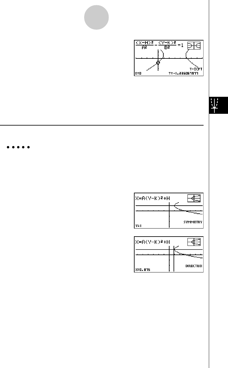
19990401
i
4(G-SLV)
h(Y-Icpt)
(Calculates the y-intercept.)
• Press e to calculate the second set of x-/y-intercepts. Pressing d returns to the first
set of intercepts.
uTo draw and analyze the axis of symmetry and directrix
[G-SLV]-[Sym]/[Dirtrx]
Example To draw the axis of symmetry and directrix for the parabola
X = 2(Y – 1)2 + 1
Use the following V-Window settings.
Xmin = –6.3, Xmax = 6.3, Xscale = 1
Ymin = –3.1, Ymax = 3.1, Yscale = 1
4(G-SLV)
e(Sym)
(Draws the axis of symmetry.)
i
4(G-SLV)
c(Dirtrx)
(Draws the directrix.)
5-11-20
Function Analysis
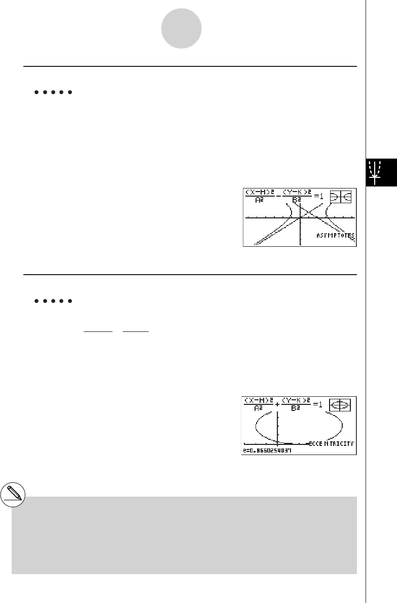
19990401
uTo draw and analyze the asymptotes [G-SLV]-[Asympt]
Example To draw the asymptotes for the hyperbola
(X – 1)2(Y – 1)2
–––––––– – –––––––– = 1
2222
Use the following V-Window settings.
Xmin = –6.3, Xmax = 6.3, Xscale = 1
Ymin = –5, Ymax = 5, Yscale = 1
4(G-SLV)
e(Asympt)
(Draws the asymptotes.)
uTo calculate eccentricity [G-SLV]-[e]
Example To determine the eccentricity of the graph for ellipse
(X – 2)2 + (Y – 2)2 = 1
4222
Use the following V-Window settings.
Xmin = –3, Xmax = 7, Xscale = 1
Ymin = –1, Ymax = 5, Yscale = 1
4(G-SLV)
e(e)
(Calculates eccentricity.)
5-11-21
Function Analysis
#Certain V-Window parameters can produce
errors in values produced as graph analysis
results.
#The message ”Not Found” appears on the
display when graph analysis is unable to
produce a result.
#The following can result in inaccurate analysis
results or may even make it impossible to obtain
a solution at all.
—When the solution is tangent to the x-axis.
—When the solution is a point of tangency
between two graphs.

19990401
Chapter
Statistical Graphs and
Calculations
This chapter describes how to input statistical data into lists, and
how to calculate the mean, maximum and other statistical values.
It also tells you how to perform regression calculations.
6-1 Before Performing Statistical Calculations
6-2 Calculating and Graphing Single-Variable Statistical
Data
6-3 Calculating and Graphing Paired-Variable Statistical
Data
6-4 Performing Statistical Calculations
6-5 Distribution
Important!
•This chapter contains a number of graph screen shots. In each case, new
data values were input in order to highlight the particular characteristics of
the graph being drawn. Note that when you try to draw a similar graph, the
unit uses data values that you have input using the List function. Because of
this, the graphs that appear on the screen when you perform a graphing
operation will probably differ somewhat from those shown in this manual.
6
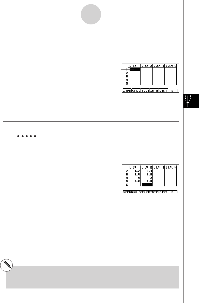
19990401
6-1 Before Performing Statistical Calculations
From the Main Menu, enter the STAT Mode and display the statistical data lists.
Use the statistical data lists to input data and to perform statistical calculations.
Use
f, c, d
and
e
to move
the highlighting around the lists.
Once you input data, you can use it to produce a graph and check for tendencies. You can
also use a variety of different regression calculations to analyze the data.
kInputting Data into Lists
Example To input the following two data groups
0.5, 1.2, 2.4, 4.0, 5.2
–2.1, 0.3, 1.5, 2.0, 2.4
a.fwb.cw
c.ewewf.cw
e
-c.bwa.dw
b.fwcwc.ew
Once data is input, you can use it for graphing and statistical calculations.
6-1-1
Before Performing Statistical Calculations
# Except for complex numbers, calculation
results can be input as statistical data.
#You can use the f, c, d and e keys
to move the highlighting to any cell in the lists
for data input.

19990401
kChanging Graph Parameters
Use the following procedures to specify the graph draw/non-draw status, the graph type, and
other general settings for each of the graphs in the graph menu (GPH1, GPH2, GPH3).
While the statistical data list is on the display, press 1(GRPH) to display the graph menu,
which contains the following items.
•{S-Gph1}/{S-Gph2}/{S-Gph3} ... graph {1}/{2}/{3} drawing*1
•{Select} ... {simultaneous graph (GPH1, GPH2, GPH3) selection} (You can specify the
multiple graphs.)
•{Set} ... {graph settings (graph type, list assignments)}
1. General graph settings [GRPH]-[Set]
This section describes how to use the general graph settings screen to make the following
settings for each graph (GPH1, GPH2, GPH3).
• Graph Type
The initial default graph type setting for all the graphs is scatter graph. You can select one of
a variety of other statistical graph types for each graph.
• List
The initial default statistical data is List 1 for single-variable data, and List 1 and List 2 for
paired-variable data. You can specify which statistical data list you want to use for x-data and
y-data.
• Frequency
Normally, each data item or data pair in the statistical data list is represented on a graph as a
point. When you are working with a large number of data items however, this can cause
problems because of the number of plot points on the graph. When this happens, you can
specify a frequency list that contains values indicating the number of instances (the
frequency) of the data items in the corresponding cells of the lists you are using for x-data
and y-data. Once you do this, only one point is plotted for the multiple data items, which
makes the graph easier to read.
6-1-2
Before Performing Statistical Calculations
*1 The initial default graph type setting for all the
graphs (Graph 1 through Graph 3) is scatter
diagram, but you can change to one of a
number of other graph types.
#You can specify the graph draw/non-draw
status, the graph type, and other general
settings for each of the graphs in the graph
menu (GPH1, GPH2, GPH3).
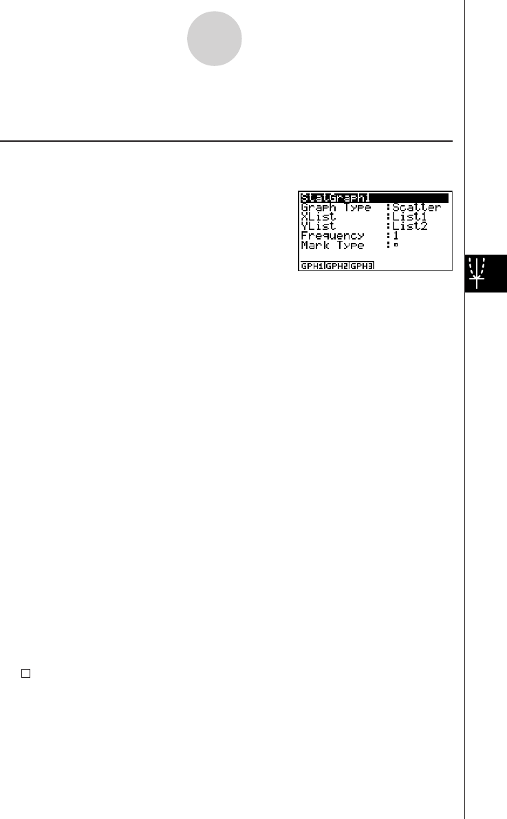
19990401
• Mark Type
This setting lets you specify the shape of the plot points on the graph.
uTo display the general graph settings screen [GRPH]-[Set]
Pressing 1(GRPH)f(Set) displays the general graph settings screen.
•The settings shown here are examples only. The settings on your general graph settings
screen may differ.
• StatGraph (statistical graph specification)
•{GPH1}/{GPH2}/{GPH3} ... graph {1}/{2}/{3}
• Graph Type (graph type specification)
•{Scat}/{xy}/{NPP} ... {scatter diagram}/{xy line graph}/{normal probability plot}
•{Hist}/{Box}/{ModB}/{N·Dis}/{Brkn} ... {histogram}/{med-box graph}/{modified-box
graph}/{normal distribution curve}/{broken line graph}
•{X}/{Med}/{X^2}/{X^3}/{X^4} ... {linear regression graph}/{Med-Med graph}/{quadratic
regression graph}/{cubic regression graph}/{quartic regression graph}
•{Log}/{Exp}/{Pwr}/{Sin}/{Lgst} ... {logarithmic regression graph}/{exponential regression
graph}/{power regression graph}/{sinusoidal regression graph}/{logistic regression graph}
• XList (x-axis data list)
•{LIST} ... {List 1 to 20}
• YList (y-axis data list)
•{LIST} ... {List 1 to 20}
• Frequency (number of times a value occurs)
•{1} ... {1-to-1 plot}
•{LIST} ... contents of this list indicates the frequency of XList and YList data
• Mark Type (plot mark type)
•{ }/{×}/{•} ... scatter diagram plot points
6-1-3
Before Performing Statistical Calculations
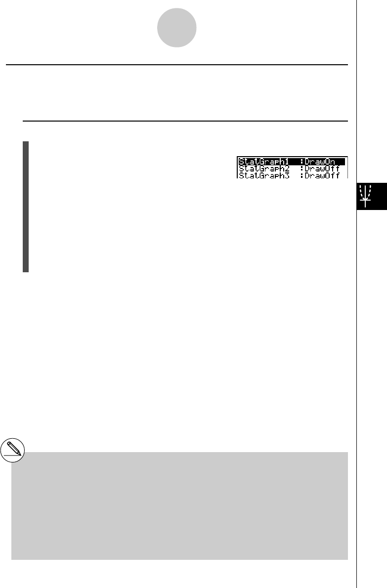
19990401
2. Graph draw/non-draw status [GRPH]-[Select]
The following procedure can be used to specify the draw (On)/non-draw (Off) status of each of
the graphs in the graph menu.
uTo specify the draw/non-draw status of a graph
1. Pressing 1(GRPH) e(Select) displays the graph On/Off screen.
•Note that the StatGraph1 setting is for Graph 1 (GPH1 of the graph menu), StatGraph2
is for Graph 2, and StatGraph3 is for Graph 3.
2. Use the cursor keys to move the highlighting to the graph whose status you want to
change, and press the applicable function key to change the status.
•{On}/{Off} ... {On (draw)}/{Off (non-draw)}
•{DRAW} ... {draws all On graphs}
3. To return to the graph menu, press i.
6-1-4
Before Performing Statistical Calculations
#View Window parameters are normally set
automatically for statistical graphing. If you
want to set View Window parameters
manually, you must change the Stat Wind item
to “Manual”.
While the statistical data list is on the display,
perform the following procedure.
u3(SET UP)2(Man)
i(Returns to previous menu.)
#The default setting automatically uses List 1
data as x-axis (horizontal) values and List 2
data as y-axis (vertical) values. Each set of x/y
data is a point on the scatter diagram.
# Pressinguadoes not hide the menu while a
statistical graph is on the display.
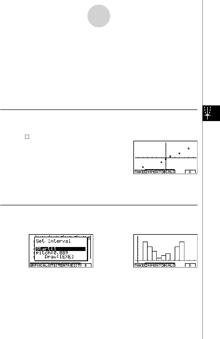
19990401
6-2 Calculating and Graphing Single-Variable
Statistical Data
Single-variable data is data with only a single variable. If you are calculating the average
height of the members of a class for example, there is only one variable (height).
Single-variable statistics include distribution and sum. The following types of graphs are
available for single-variable statistics.
You can also use the procedures under “Changing Graph Parameters” on page 6-1-2 to make
the settings you want before drawing each graph.
kk
kk
kNormal Probability Plot (NPP)
This plot compares the data accumulated ratio with a normal distribution accumulated ratio.
XList specifies the list where data is input, and Mark Type is used to select from among the
marks { / × / • }you want to plot.
Press i or !i(QUIT) to return to the statistical data list.
kk
kk
kHistogram (Bar Graph) (Hist)
XList specifies the list where the data is input, while Freq specifies the list where the data
frequency is input. 1 is specified for Freq when frequency is not specified.
6-2-1
Calculating and Graphing Single-Variable Statistical Data
⇒
w(Draw)
The display screen appears as shown above before the graph is drawn. At this point, you
can change the Start and pitch values.
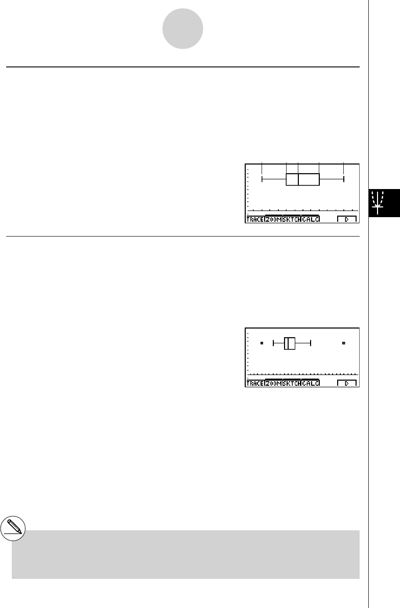
19990401
kMed-box or Box and Whisker Graph (Box)
This type of graph lets you see how a large number of data items are grouped within specific
ranges. A box encloses all the data in an area from the first quartile (Q1) to the third quartile
(Q3), with a line drawn at the median (Med). Lines (called whiskers) extend from either end
of the box up to the minimum (minX) and maximum (maxX) of the data.
XList specifies the list where the data is input, while Freq specifies the list where the data
frequency is input. 1 is specified for Freq when frequency is not specified.
kModified Box Graph (ModB)
The modified box graph omits everything in the range past 1.5 × IQR (IQR = Q3 – Q1,
Q3: 3rd quartile, Q1: 1st quartile) from the med-box 4th quartile and draws whiskers.
Outliers are displayed as plot points.
XList specifies the list where the data is input, while Freq specifies the list where the data
frequency is input. 1 is specified for Freq when frequency is not specified.
6-2-2
Calculating and Graphing Single-Variable Statistical Data
#Input a positive integer for frequency data.
Other types of values (decimals, etc.) cause
an error.
minX Q1 Med Q3 maxX
#Dimension ERROR usually occurs when two
lists contain a different number of elements.
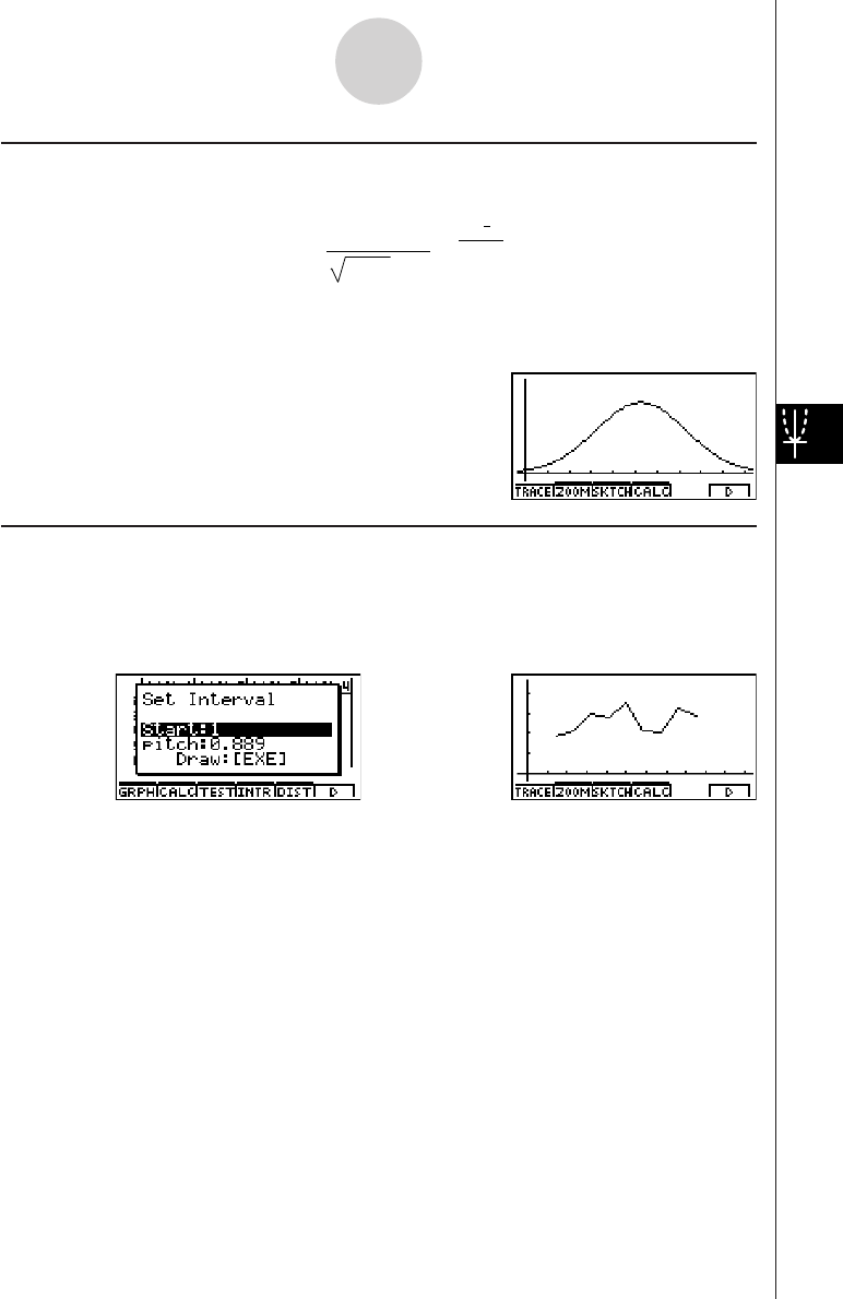
19990401
kNormal Distribution Curve (N • Dis)
The normal distribution curve is graphed using the following normal distribution function.
y
= 1
(2 π)xσ
n
e
–2xσ
n
2
(x–x)2
XList specifies the list where the data is input, while Freq specifies the list where the data
frequency is input. 1 is specified for Freq when frequency is not specified.
kBroken Line Graph (Brkn)
Lines connect center points of a histogram bar.
XList specifies the list where the data is input, while Freq specifies the list where the data
frequency is input. 1 is specified for Freq when frequency is not specified.
6-2-3
Calculating and Graphing Single-Variable Statistical Data
⇒
w(Draw)
The display screen appears as shown above before the graph is drawn. At this point, you
can change the Start and pitch values.
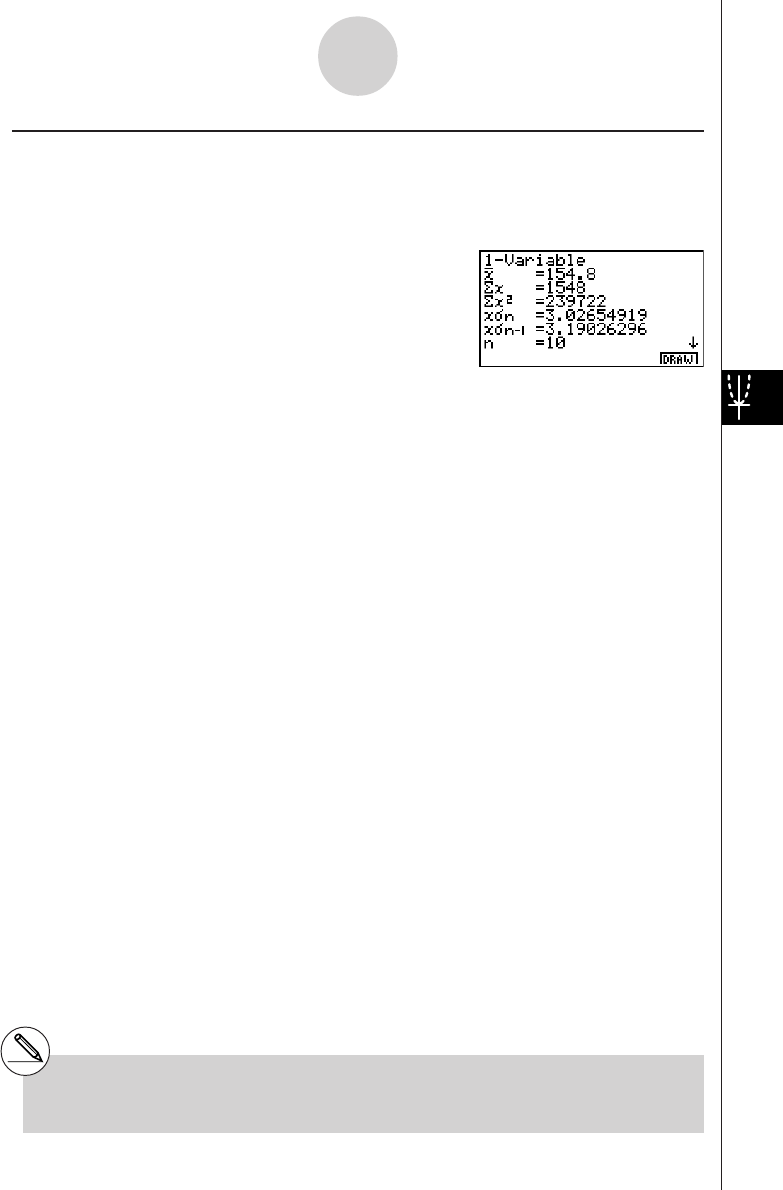
19990401
kDisplaying the Calculation Results of a Drawn Single-Variable Graph
Single-variable statistics can be expressed as both graphs and parameter values. When
these graphs are displayed, the single-variable calculation results appear as shown below
when you press 4(CALC)b(1VAR).
•Use c to scroll the list so you can view the items that run off the bottom of the screen.
The following describes the meaning of each of the parameters.
o............. mean
Σx........... sum
Σx2.......... sum of squares
xσn.......... population standard deviation
xσn–1 ........ sample standard deviation
n............. number of data items
minX ....... minimum
Q1 .......... first quartile
Med ........ median
Q3 .......... third quartile
maxX ...... maximum
Mod ........ mode
Mod : n ... number of data mode items
Mod : F ... data mode frequency
•Press 6(DRAW) to return to the original single-variable statistical graph.
6-2-4
Calculating and Graphing Single-Variable Statistical Data
#When Mod has multiple solutions, they are all
displayed.

19990401
6-3-1
Calculating and Graphing Paired-Variable Statistical Data
6-3 Calculating and Graphing Paired-Variable
Statistical Data
k Drawing a Scatter Diagram and xy Line Graph
Description
The following procedure plots a scatter diagram and connects the dots to produce an xy line
graph.
Set Up
1. From the Main Menu, enter the STAT Mode.
Execution
2. Input the data into a list.
3. Specify Scat (scatter diagram) or xy (xy line graph) as the graph type, and then execute
the graph operation.
Press i or !i(QUIT) to return to the statistical data list.
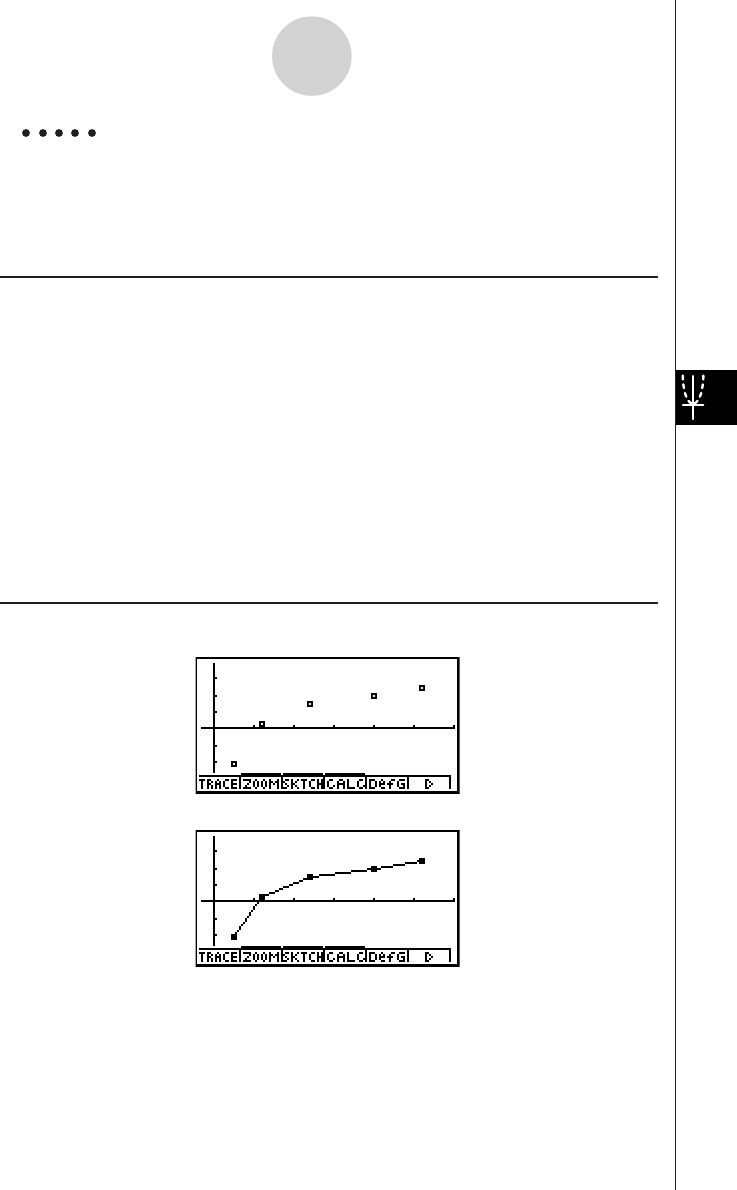
19990401
Example Input the two sets of data shown below. Next, plot the data on a
scatter diagram and connect the dots to produce an xy line graph.
0.5, 1.2, 2.4, 4.0, 5.2, (xList)
–2.1, 0.3, 1.5, 2.0, 2.4 (yList)
Procedure
1m STAT
2a.fwb.cw
c.ewewf.cw
e
-c.bwa.dw
b.fwcwc.ew
3(Scatter diagram)1(GRPH)f(Set)c1(Scat)i
1(GRPH)b(S-Gph1)
3(xy line graph)1(GRPH)f(Set)c2(xy)i
1(GRPH)b(S-Gph1)
Result Screen
(Scatter diagram)
(xy line graph)
6-3-2
Calculating and Graphing Paired-Variable Statistical Data

19990401
k Drawing a Regression Graph
Description
Use the following procedure to input paired-variable statistical data, perform a regression
calculation using the data, and then graph the results.
Set Up
1. From the Main Menu, enter the STAT Mode.
Execution
2. Input the data into a list, and plot the scatter diagram.
3. Select the regression type, execute the calculation, and display the regression
parameters.
4. Draw the regression graph.
6-3-3
Calculating and Graphing Paired-Variable Statistical Data
#You can perform trace on a regression graph.
You cannot perform trace scroll.
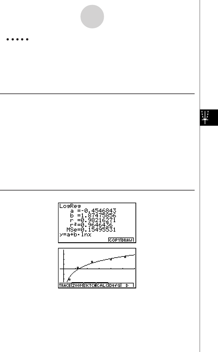
19990401
Example Input the two sets of data shown below and plot the data on a scatter
diagram. Next, perform logarithmic regression on the data to display
the regression parameters, and then draw the corresponding
regression graph.
0.5, 1.2, 2.4, 4.0, 5.2, (xList)
–2.1, 0.3, 1.5, 2.0, 2.4 (yList)
Procedure
1m STAT
2a.fwb.cw
c.ewewf.cw
e
-c.bwa.dw
b.fwcwc.ew
1(GRPH)f(Set)c1(Scat)i
1(GRPH)b(S-Gph1)
34(CALC)h(Log)
46(DRAW)
Result Screen
6-3-4
Calculating and Graphing Paired-Variable Statistical Data
2001010220011101

19990401
kk
kk
kSelecting the Regression Type
After you graph paired-variable statistical data, press 4(CALC). Then you can use the
function menu at the bottom of the display to select from a variety of different types of
regression.
•{2VAR} ... {paired-variable statistical results}
•{Linear}/{MedMed}/{Quad}/{Cubic}/{Quart}/{Log}/{Exp}/{Power}/{Sin}/{Lgstic}
... {linear regression}/{Med-Med}/{quadratic regression}/{cubic regression}/{quartic
regression}/{logarithmic regression}/{exponential regression}/{power regression}/
{sinusoidal regression}/{logistic regression} calculation and graphing
kk
kk
kDisplaying Statistical Calculation Results
Whenever you perform a regression calculation, the regression formula parameter (such as a
and b in the linear regression y = ax + b) calculation results appear on the display. You can
use these to obtain statistical calculation results.
Regression parameters are calculated as soon as you press a function key to select a
regression type, while a graph is on the display.
kk
kk
kGraphing Statistical Calculation Results
While the parameter calculation result is on the display, you can graph the displayed
regression formula by pressing 6(DRAW).
6-3-5
Calculating and Graphing Paired-Variable Statistical Data
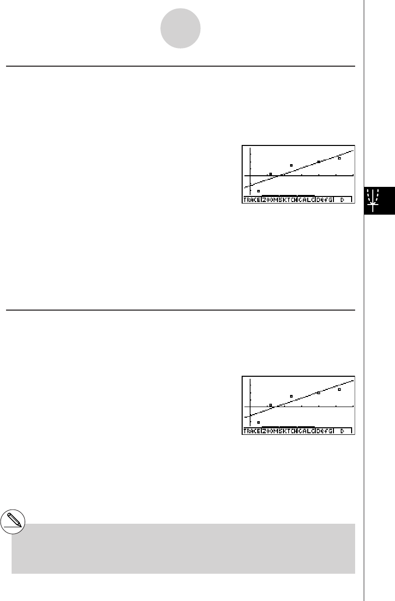
19990401
kk
kk
kLinear Regression Graph
Linear regression uses the method of least squares to plot a straight line that passes close to
as many data points as possible, and returns values for the slope and y-intercept
(y-coordinate when x = 0) of the line.
The graphic representation of this relationship is a linear regression graph.
4(CALC)c(Linear)
6(DRAW)
The following is the linear regression model formula.
y = ax + b
a............. regression coefficient (slope)
b............. regression constant term (y-intercept)
r............. correlation coefficient
r2............ coefficient of determination
MSe ........ mean square error
kk
kk
kMed-Med Graph
When it is suspected that there are a number of extreme values, a Med-Med graph can be
used in place of the least squares method. This is similar to linear regression, but it
minimizes the effects of extreme values.
4(CALC)d(MedMed)
6(DRAW)
The following is the Med-Med graph model formula.
y = ax + b
a ............. Med-Med graph slope
b ............. Med-Med graph y-intercept
6-3-6
Calculating and Graphing Paired-Variable Statistical Data
#Input a positive integer for frequency data.
Other types of values (decimals, etc.) cause
an error.
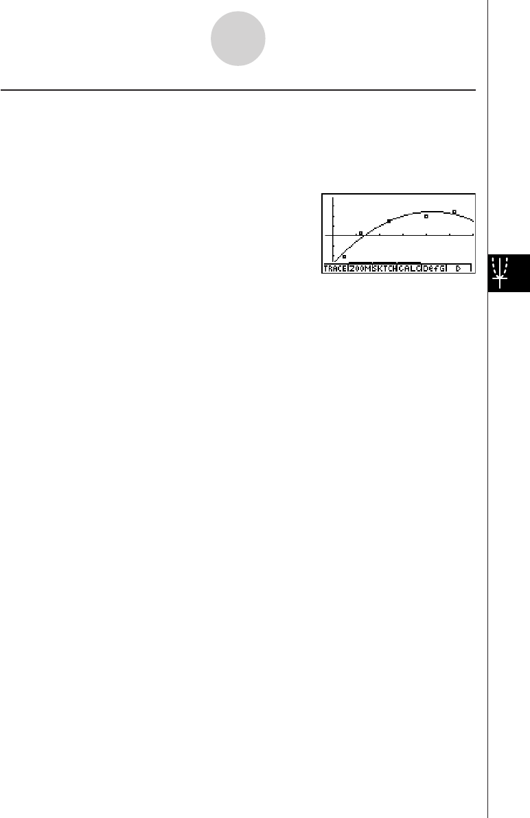
19990401
kk
kk
kQuadratic/Cubic/Quartic Regression Graph
A quadratic/cubic/quartic regression graph represents connection of the data points of a
scatter diagram. It uses the method of least squares to draw a curve that passes close to as
many data points as possible. The formula that represents this is quadratic/cubic/quartic
regression.
Ex. Quadratic regression
4(CALC)e(Quad)
6(DRAW)
Quadratic regression
Model formula ..... y = ax2 + bx + c
a ............. regression second coefficient
b ............. regression first coefficient
c ............. regression constant term (y-intercept)
r2............ coefficient of determination
MSe ........ mean square error
Cubic regression
Model formula ..... y = ax3 + bx2 + cx + d
a ............. regression third coefficient
b ............. regression second coefficient
c ............. regression first coefficient
d ............. regression constant term (y-intercept)
r2............ coefficient of determination
MSe ........ mean square error
Quartic regression
Model formula ..... y = ax4 + bx3 + cx2 + dx + e
a ............. regression fourth coefficient
b ............. regression third coefficient
c ............. regression second coefficient
d ............. regression first coefficient
e ............. regression constant term (y-intercept)
r2............ coefficient of determination
MSe ........ mean square error
6-3-7
Calculating and Graphing Paired-Variable Statistical Data

19990401
kLogarithmic Regression Graph
Logarithmic regression expresses y as a logarithmic function of x. The standard logarithmic
regression formula is y = a + b × In x, so if we say that X = In x, the formula corresponds to
linear regression formula y = a + bX.
4(CALC)h(Log)
6(DRAW)
The following is the logarithmic regression model formula.
y = a + b • ln x
a ............. regression constant term
b ............. regression coefficient
r .............. correlation coefficient
r2............ coefficient of determination
MSe ........ mean square error
kExponential Regression Graph
Exponential regression expresses y as a proportion of the exponential function of x. The
standard exponential regression formula is y = a × ebx, so if we take the logarithms of both
sides we get In y = In a + bx. Next, if we say Y = In y, and A = In a, the formula corresponds
to linear regression formula Y = A + bx.
4(CALC)i(Exp)
6(DRAW)
The following is the exponential regression model formula.
y = a • ebx
a ............. regression coefficient
b ............. regression constant term
r .............. correlation coefficient
r2............ coefficient of determination
MSe ........ mean square error
6-3-8
Calculating and Graphing Paired-Variable Statistical Data
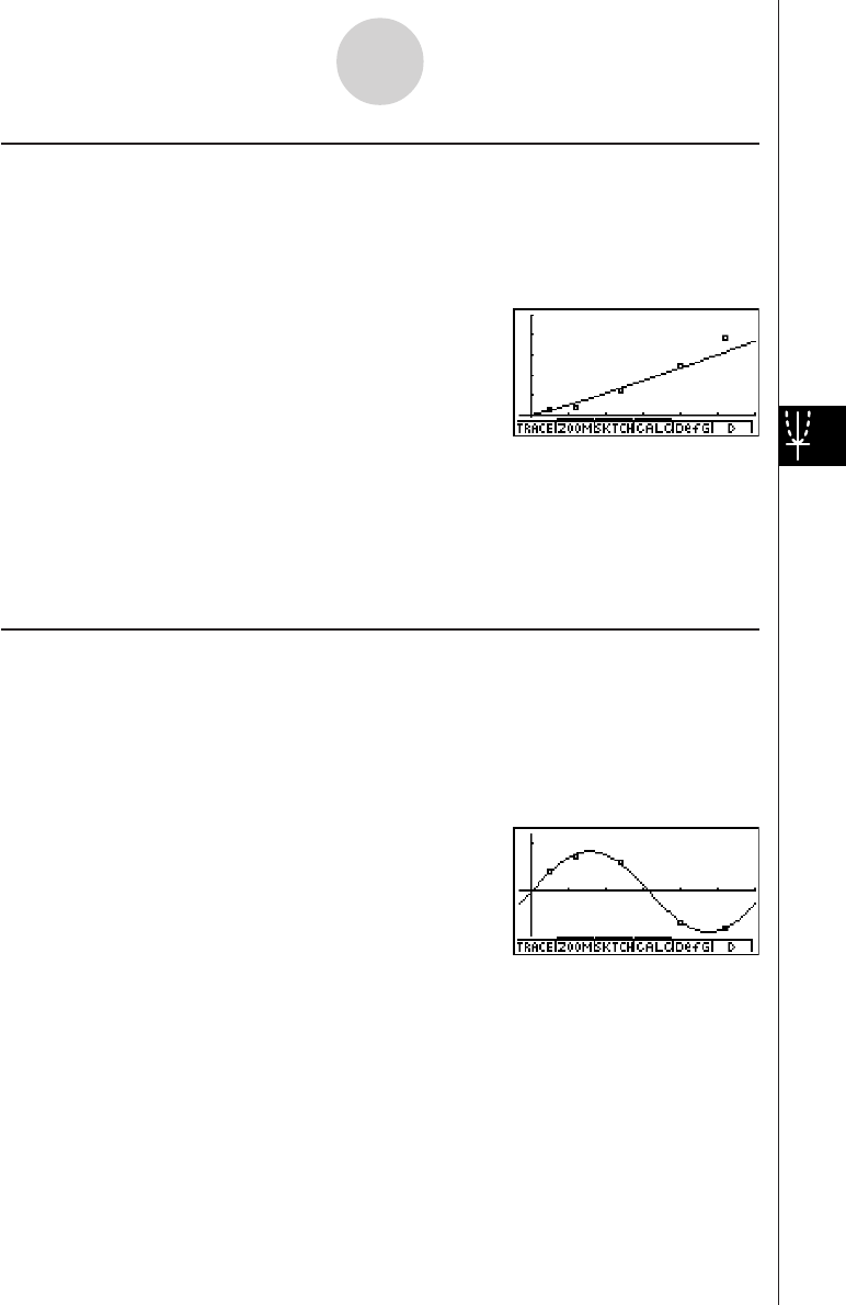
19990401
kk
kk
kPower Regression Graph
Power regression expresses y as a proportion of the power of x. The standard power
regression formula is y = a × xb, so if we take the logarithm of both sides we get In y = In a +
b × In x. Next, if we say X = In x, Y = In y, and A = In a, the formula corresponds to linear
regression formula Y = A + bX.
4(CALC)j(Power)
6(DRAW)
The following is the power regression model formula.
y = a • xb
a ............. regression coefficient
b ............. regression power
r .............. correlation coefficient
r2............. coefficient of determination
MSe ........ mean square error
kk
kk
kSinusoidal Regression Graph
Sinusoidal regression is best applied for cyclical data.
The following is the sinusoidal regression model formula.
y = a·sin(bx + c) + d
While the statistical data list is on the display, perform the following key operation.
4(CALC)v(Sin)
6(DRAW)
Drawing a sinusoidal regression graph causes the angle unit setting of the calculator to
automatically change to Rad (radians). The angle unit does not change when you perform a
sinusoidal regression calculation without drawing a graph.
• Certain types of data may take a long time to calculate. This does not indicate malfunction.
6-3-9
Calculating and Graphing Paired-Variable Statistical Data

19990401
kk
kk
kLogistic Regression Graph
Logistic regression is best applied for time-based phenomena in which there is a continual
increase until a saturation point is reached.
The following is the logistic regression model formula.
y = c
1 + ae
–bx
4(CALC)l(Lgstic)
6(DRAW)
• Certain types of data may take a long time to calculate. This does not indicate malfunction.
kk
kk
kResidual Calculation
Actual plot points (y-coordinates) and regression model distance can be calculated during
regression calculations.
While the statistical data list is on the display, recall the SET UP screen to specify a LIST
(“List 1” through “List 20”) for “Resid List”. Calculated residual data is stored in the specified
list.
The vertical distance from the plots to the regression model will be stored in the list.
Plots that are higher than the regression model are positive, while those that are lower are
negative.
Residual calculation can be performed and saved for all regression models.
6-3-10
Calculating and Graphing Paired-Variable Statistical Data
#Any data already existing in the selected list is
cleared. The residual of each plot is stored in
the same precedence as the data used as the
model.
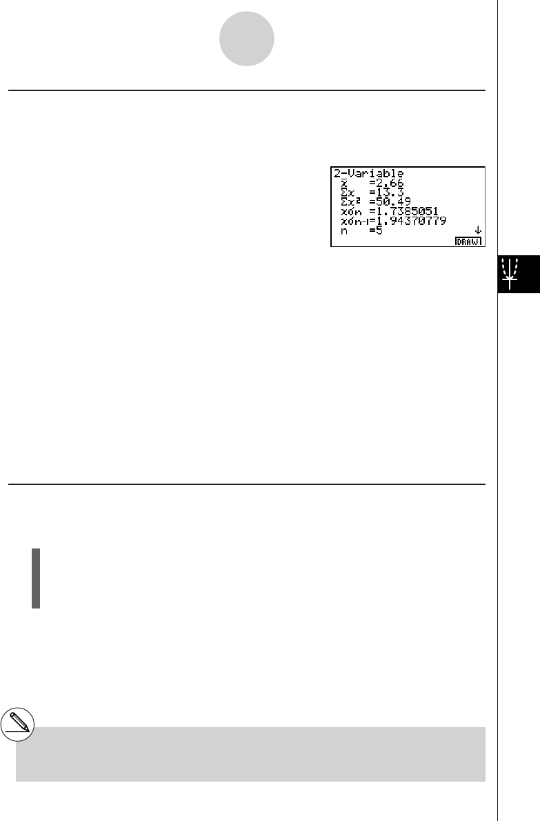
19990401
kk
kk
kDisplaying the Calculation Results of a Drawn Paired-Variable Graph
Paired-variable statistics can be expressed as both graphs and parameter values. When
these graphs are displayed, the paired-variable calculation results appear as shown below
when you press 4(CALC)b(2VAR).
•Use c to scroll the list so you can view the items that run off the bottom of the screen.
o............... mean of data stored in xList
Σx............. sum of data stored in xList
Σx2........... sum of squares of data
stored in xList
xσn............ population standard
deviation of data stored in
xList
xσn-1 .......... sample standard deviation
of data stored in xList
n............... number of data
p............... mean of data stored in yList
Σy............. sum of data stored in yList
kk
kk
kCopying a Regression Graph Formula to the GRPH
•
TBL Mode
You can copy regression formula calculation results to the GRPH • TBL Mode graph formula
area, and store and compare.
1. Press 5(COPY) to copy the regression formula that produced the displayed data to
the GRPH • TBL Mode graph formula area*1.
2. Press w to save the copied graph formula and return to the previous regression
calculation result display.
6-3-11
Calculating and Graphing Paired-Variable Statistical Data
Σy2...... sum of squares of data stored in yList
yσn...... population standard deviation of data
stored in yList
yσn-1 .... sample standard deviation of data
stored in yList
Σxy ..... sum of the product of data stored in
xList and yList
minX ... minimum of data stored in xList
maxX .. maximum of data stored in xList
minY ... minimum of data stored in yList
maxY .. maximum of data stored in yList
*1You cannot edit regression formulas for graph
formulas in the GRPH
•
TBL Mode.
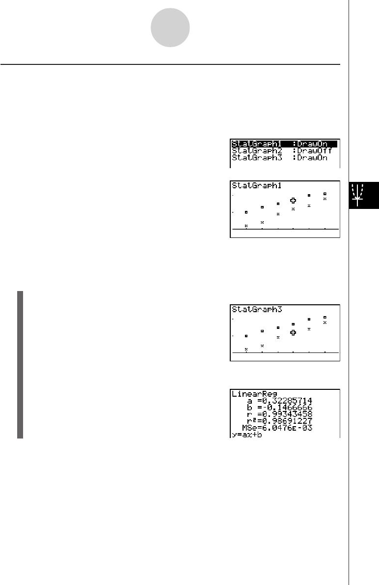
19990401
kk
kk
kMultiple Graphs
You can draw more than one graph on the same display by using the procedure under
“Changing Graph Parameters” to set the graph draw (On)/non-draw (Off) status of two or all
three of the graphs to draw On, and then pressing 6(DRAW)(see page 6-1-4). After
drawing the graphs, you can select which graph formula to use when performing single-
variable statistic or regression calculations.
4(CALC)
c(Linear)
•The text at the top of the screen indicates the currently selected graph (StatGraph1 =
Graph 1, StatGraph2 = Graph 2, StatGraph3 = Graph 3).
1. Press c. The graph name at the top of the screen changes when you do.
2. When the graph you want to use is selected, press w.
Now you can use the procedure under “Displaying the Calculation Results of a Drawn
Paired-Variable Graph” on page 6-3-11 to perform statistical calculations.
6-3-12
Calculating and Graphing Paired-Variable Statistical Data

19990401
k Overlaying a Function Graph on a Statistical Graph
Description
You can overlay a paired-variable statistical graph with any type of function graph you want.
Set Up
1. From the Main Menu, enter the STAT Mode.
Execution
2. Input the data into a list, and draw the statistical graph.
3. Display the Graph Function menu, and input the function you want to overlay on the
statistical graph.
4. Graph the function.
6-3-13
Calculating and Graphing Paired-Variable Statistical Data
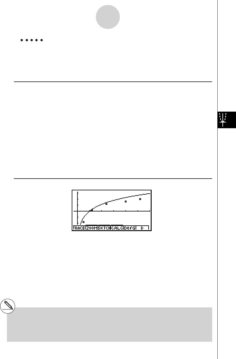
19990401
Example Input the two sets of data shown below. Next, plot the data on a
scatter diagram and overlay a function graph y = 2ln x.
0.5, 1.2, 2.4, 4.0, 5.2,
–2.1, 0.3, 1.5, 2.0, 2.4
Procedure
1m STAT
2a.fwb.cw
c.ewewf.cw
e
-c.bwa.dw
b.fwcwc.ew
1(GRPH)b(S-Gph1)
35(DefG)
cIvw(Register Y1 = 2In x)
46(DRAW)
Result Screen
6-3-14
Calculating and Graphing Paired-Variable Statistical Data
# You can also perform trace, etc. for drawn
function graphs.
# Graphs of types other than rectangular
coordinate graphs cannot be drawn.
# Pressing i while inputting a function returns
the expression to what it was prior to input.
Pressing !i(QUIT) clears the input
expression and returns to the statistical data list.
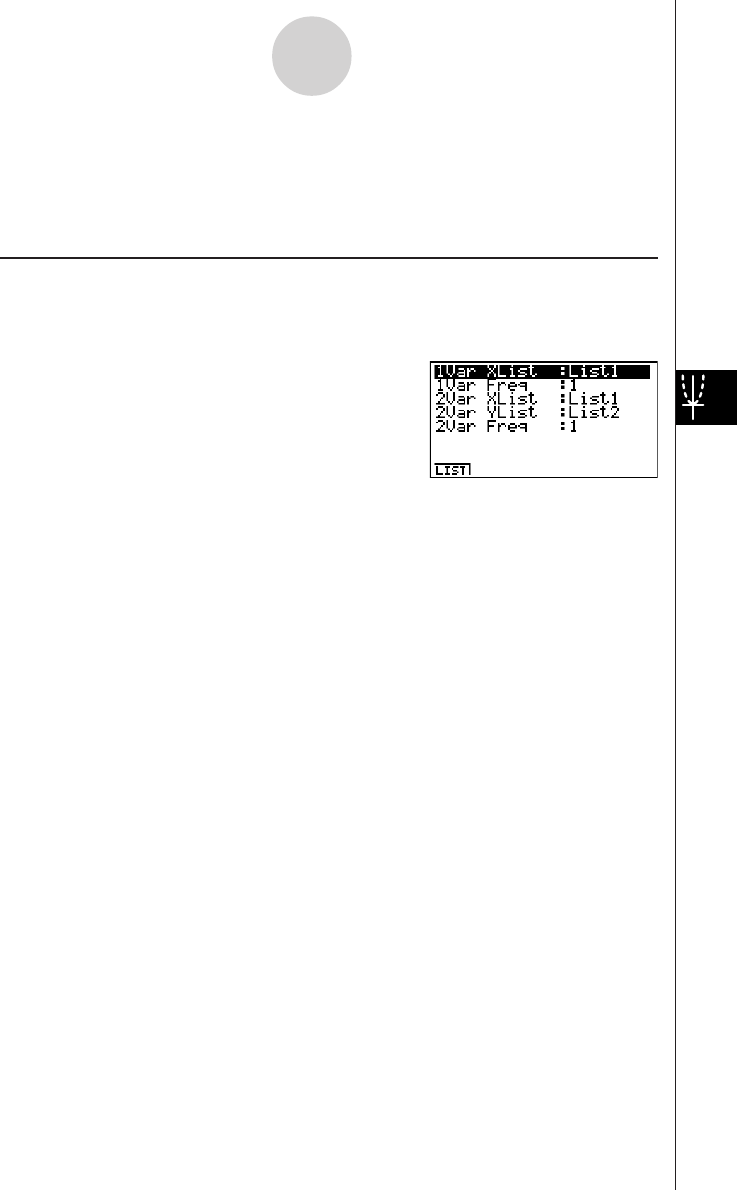
19990401
6-4 Performing Statistical Calculations
All of the statistical calculations up to this point were performed after displaying a graph. The
following procedures can be used to perform statistical calculations alone.
uu
uu
uTo specify statistical calculation data lists
You have to input the statistical data for the calculation you want to perform and specify
where it is located before you start a calculation. Display the statistical data and then press
2(CALC)e(Set).
The following is the meaning for each item.
1Var XList ............ location of single-variable statistic x values (XList)
1Var Freq ............ location of single-variable frequency values (Frequency)
2Var XList ............ location of paired-variable statistic x values (XList)
2Var YList ............ location of paired-variable statistic y values (YList)
2Var Freq ............ location of paired-variable frequency values (Frequency)
•Calculations in this section are performed based on the above specifications.
6-4-1
Performing Statistical Calculations
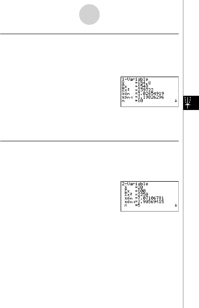
19990401
kk
kk
kSingle-Variable Statistical Calculations
In the previous examples from “Normal Probability Plot” and “Histogram (Bar Graph)” to
“Line Graph,” statistical calculation results were displayed after the graph was drawn. These
were numeric expressions of the characteristics of variables used in the graphic display.
These values can also be directly obtained by displaying the statistical data list and pressing
2(CALC)b(1VAR).
After this, pressing f or c scrolls the statistical calculation result display so you can view
variable characteristics.
For details on the meanings of these statistical values, see “Displaying the Calculation
Results of a Drawn Single-Variable Graph” (page 6-2-4).
kk
kk
kPaired-Variable Statistical Calculations
In the previous examples from “Linear Regression Graph” to “Logistic Regression Graph,”
statistical calculation results were displayed after the graph was drawn. These were numeric
expressions of the characteristics of variables used in the graphic display.
These values can also be directly obtained by displaying the statistical data list and pressing
2(CALC)c(2VAR).
After this, pressing f or c scrolls the statistical calculation result display so you can view
variable characteristics.
For details on the meanings of these statistical values, see “Displaying the Calculation
Results of a Drawn Paired-Variable Graph” (page 6-3-11).
6-4-2
Performing Statistical Calculations
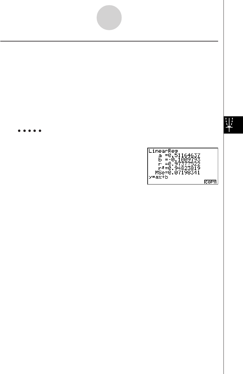
19990401
kRegression Calculation
In the explanations from “Linear Regression Graph” to “Logistic Regression Graph,”
regression calculation results were displayed after the graph was drawn. Here, each
coefficient value of the regression line and regression curve is expressed as a number.
You can directly determine the same expression from the data input screen.
Pressing 2(CALC)d(REG) displays the pull-up menu, which contains the following items.
•{Linear}/{MedMed}/{Quad}/{Cubic}/{Quart}/{Log}/{Exp}/{Power}/{Sin}/{Lgstic} ...
{linear regression}/{Med-Med}/{quadratic regression}/{cubic regression}/
{quartic regression}/{logarithmic regression}/{exponential regression}/
{power regression}/{sinusoidal regression}/{logistic regression} parameters
Example To display single-variable regression parameters
2(CALC)d(REG)b(Linear)
The meanings of the parameters that appear on this screen are the same as those for
“Linear Regression Graph” to “Logistic Regression Graph”.
6-4-3
Performing Statistical Calculations
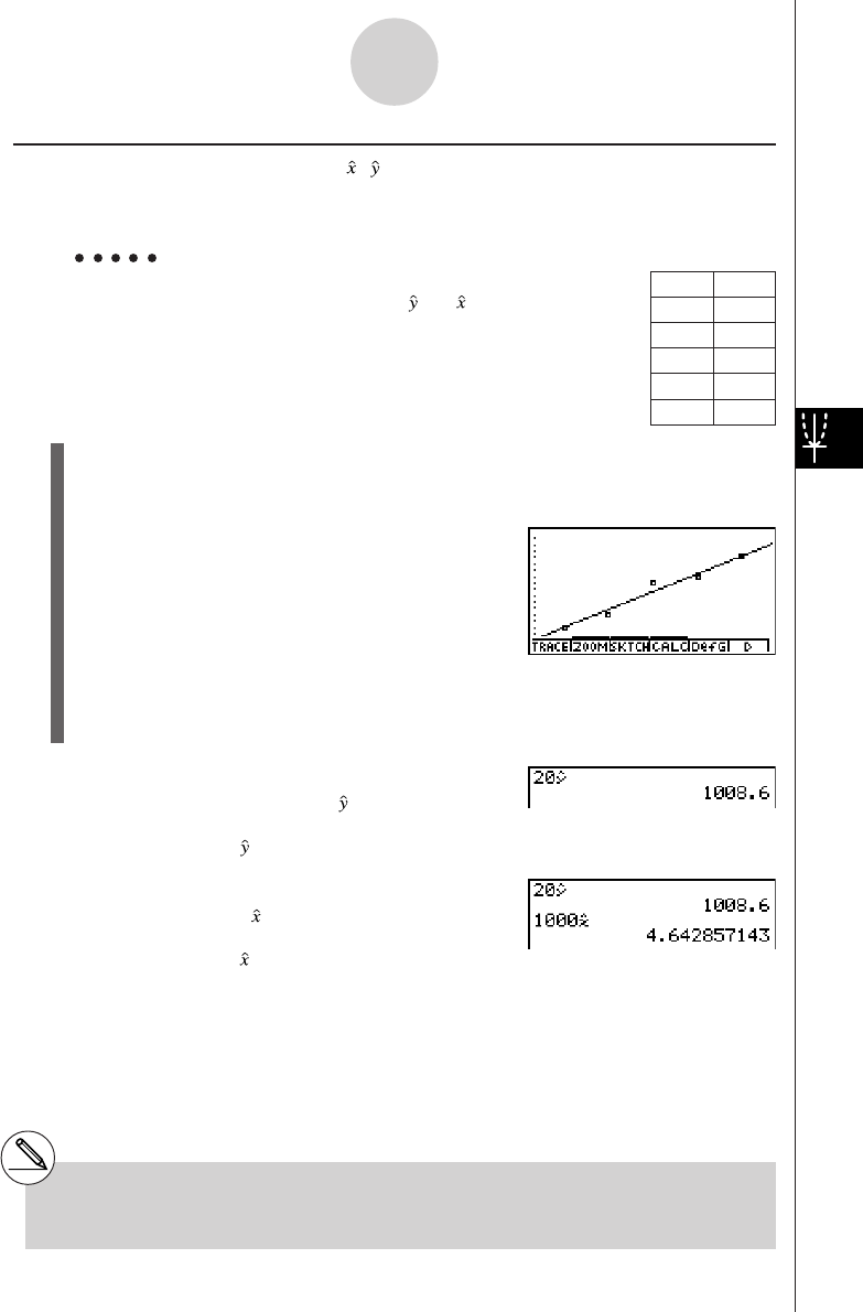
19990401
kEstimated Value Calculation ( , )
After drawing a regression graph with the STAT Mode, you can use the RUN • MAT Mode to
calculate estimated values for the regression graph's x and y parameters.
Example To perform a linear regression using the nearby data
and estimate the values of and when xi = 20 and
yi = 1000
1. From the Main Menu, enter the STAT Mode.
2. Input data into the list and draw the linear regression graph.
3. From the Main Menu, enter the RUN • MAT Mode.
4. Press the keys as follows.
ca(value of xi)
K6(g)4(STAT)c( )w
The estimated value is displayed for xi = 20.
baaa(value of yi)
4(STAT)b( )w
The estimated value is displayed for yi = 1000.
6-4-4
Performing Statistical Calculations
xi yi
10 1003
15 1005
20 1010
25 1011
30 1014
#You cannot obtain estimated values for a Med-
Med, quadratic regression, cubic regression,
quartic regression, sinusoidal regression, or
logistic regression graph.
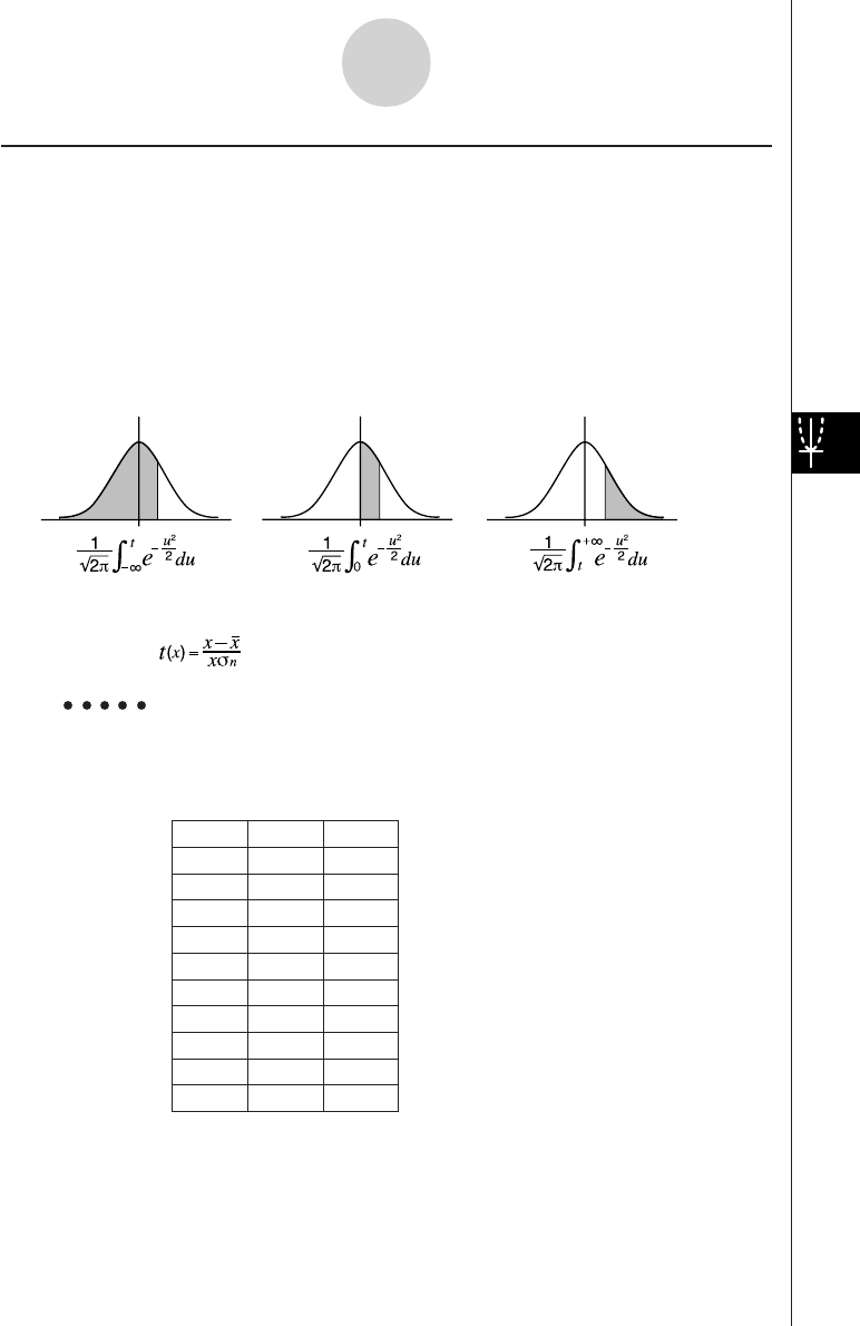
19990401
kNormal Probability Distribution Calculation
You can calculate normal probability distributions for single-variable statistics with the
RUN • MAT Mode.
Press K6(g)1(PROB) to display a function menu, which contains the following items.
•{P(}/{Q(}/{R(} ... obtains normal probability {P(t)}/{Q(t)}/{R(t)} value
•{t(} ... {obtains normalized variate t(x) value}
•Normal probability P(t), Q(t), and R(t), and normalized variate t(x) are calculated using
the following formulas.
P
(
t
)Q
(
t
)R
(
t
)
Example The following table shows the results of measurements of the height
of 20 college students. Determine what percentage of the students fall
in the range 160.5 cm to 175.5 cm. Also, in what percentile does the
175.5 cm tall student fall?
Class no. Height (cm) Frequency
1158.5 1
2160.5 1
3163.3 2
4167.5 2
5170.2 3
6173.3 4
7175.5 2
8178.6 2
9180.4 2
10 186.7 1
6-4-5
Performing Statistical Calculations
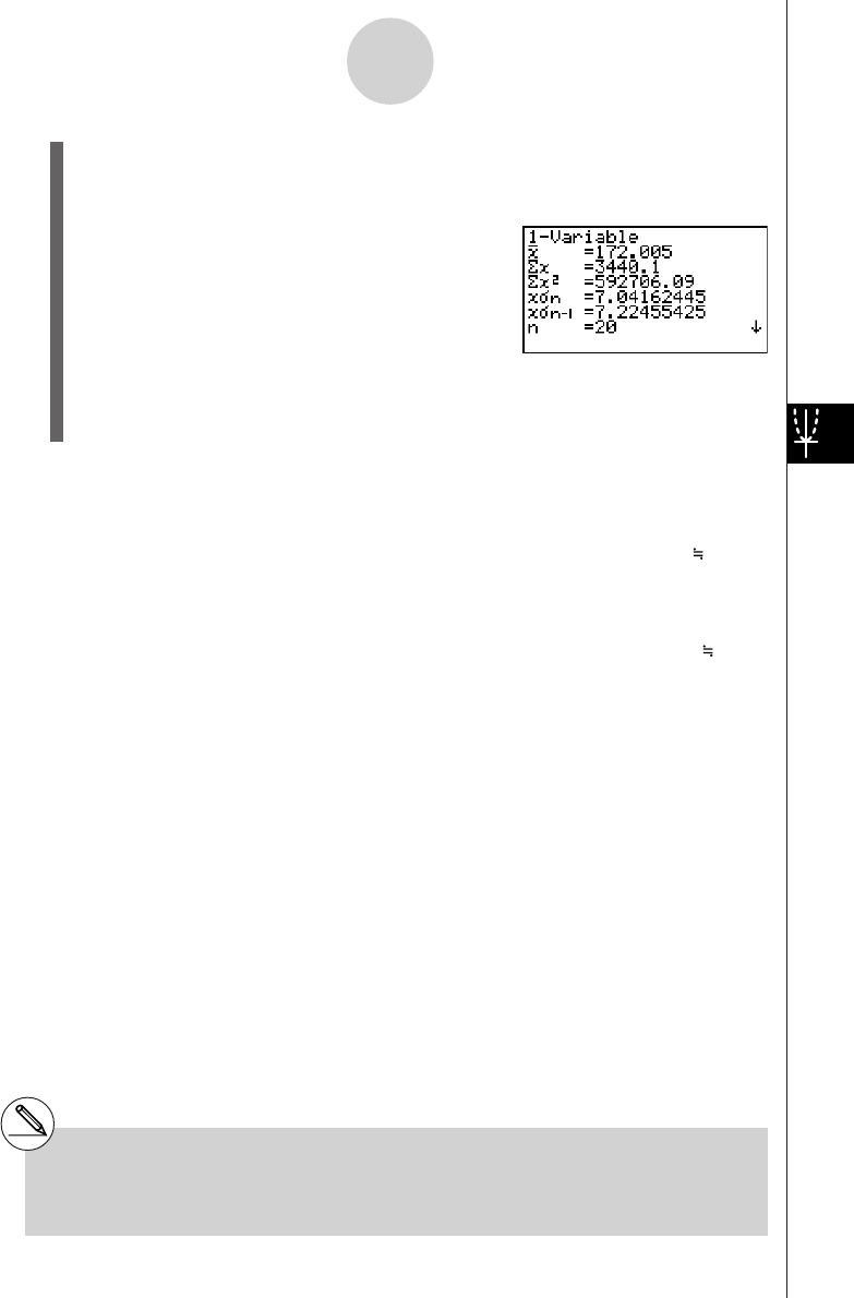
19990401
1. Input the height data into List 1 and the frequency data into List 2.
2. Perform the single-variable statistical calculations.*1
2(CALC)e(Set)
1(LIST)bw
c2(LIST)cwi
2(CALC)b(1VAR)
3. Press m, select the RUN • MAT Mode, press K6(g)1(PROB) to recall the
probability calculation (PROB) menu.
1(PROB)i(t() bga.f)w
(Normalized variate t for 160.5cm) Result: –1.633855948
( –1.634)
1(PROB)i(t() bhf.f)w
(Normalized variate t for 175.5cm) Result: 0.4963343361
( 0.496)
1(PROB)f(P()a.ejg)-
1(PROB)f(P()-b.gde)w
(Percentage of total) Result: 0.638921
(63.9% of total)
1(PROB)h(R()a.ejg)w
(Percentile) Result: 0.30995
(31.0 percentile)
6-4-6
Performing Statistical Calculations
*1 You can obtain the normalized variate
immediately after performing single-variable
statistical calculations only.

19990401
k Drawing a Normal Probability Distribution Graph
Description
You can draw a normal probability distribution graph using manual graphing with the
RUN • MAT Mode.
Set Up
1. From the Main Menu, enter the RUN • MAT Mode.
Execution
2. Input the commands to draw a rectangular coordinate graph.
3. Input the probability value.
6-4-7
Performing Statistical Calculations
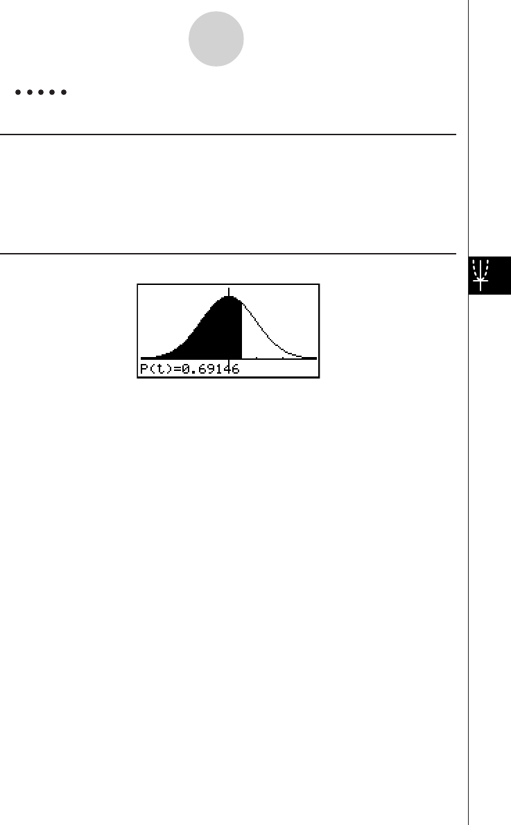
19990401
Example To draw a normal probability P (0.5) graph.
Procedure
1m RUN • MAT
2K6(g)6(g)2(SKTCH)b(Cls)w
2(SKTCH)e(GRPH)b(Y=)
3K6(g)1(PROB)f(P()a.fw
Result Screen
6-4-8
Performing Statistical Calculations

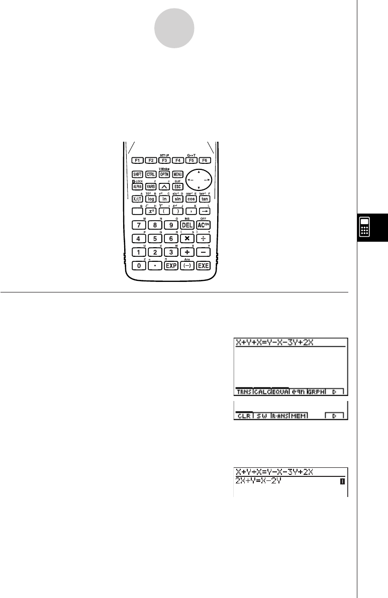
20010102
7-1-1
Using the CAS (Computer Algebra System) Mode
7-1 Using the CAS (Computer Algebra System)
Mode
On the Main Menu, select the CAS icon to enter the CAS Mode.
The following table shows the keys that can be used in the CAS Mode.
kk
kk
k Inputting and Displaying Data
Input in the Algebra Mode is performed in the upper part of the display, which is called the
“input area.” You can input commands and expressions at the current cursor location.
Calculation results appear in the lower part of the display, which is called the “output area.”
When a calculation produces an equation or inequality, the lower part of the display is
divided between a “natural result display area” for the result, and a “formula number area” for
the formula number as shown below.
REPLAY
COPY PASTE
H-COPY
i
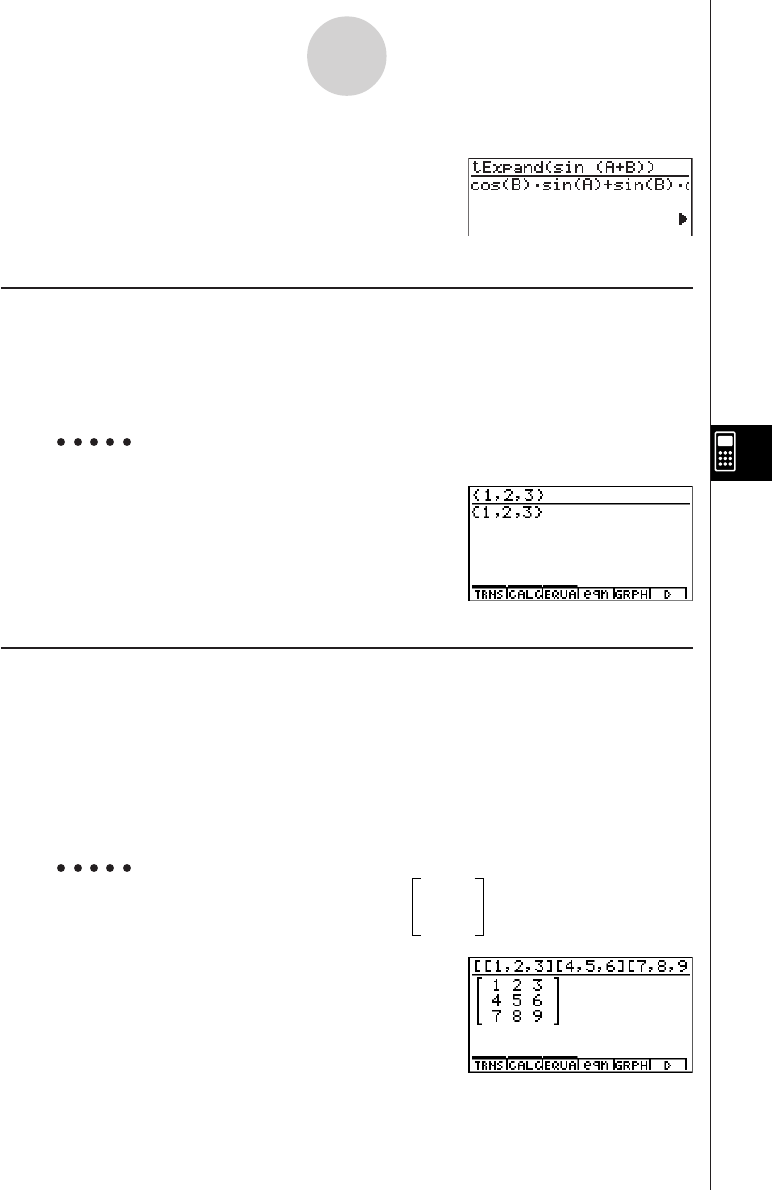
20010102
If all the result does not fit on the display, use the cursor keys to scroll it.
k Inputting List Data
List: {element, element, ..., element}
•Elements should be separated by commas, and the entire set of elements should be
enclosed within {curly braces}.
•You can input numeric values and expressions, equations, and inequalities as list elements.
Example To input List {1, 2, 3}
!*( { )b,c,d
!/( } )w
kInputting Matrix Data
Matrix (m × n): [[(1,1) entry, (1,2) entry, ..., (1,m) entry] [(2,1) entry, ......, (2,n) entry]...
[(m, n) entry, ..., (m, n) entry]]
•The above input is arranged to show the relative positions of entries in the matrix. Actual
input is an unbroken line, from left to right.
•Entries should be separated by commas, and the entire set of elements should be enclosed
within [square brackets]. And each line also should be enclosed within [square brackets].
•You can input numeric values and expressions as matrix entries.
Example To input the matrix shown below 1 2 3
4 5 6
7 8 9
!+( [ )!+( [ )b,c,d
!-( ] )!+( [ )e,f,g
!-( ] )!+( [ )h,i,j
!-( ] )!-( ] )w
7-1-2
Using the CAS (Computer Algebra System) Mode
20011101

20010102
7-1-3
Using the CAS (Computer Algebra System) Mode
kInputting Vector Data
Vector: [component, component, ..., component]
•Components should be separated by commas, and the entire set of components should be
enclosed within [square brackets].
•You can input numeric values and expressions as vector component entries.
Example To input Vector (1 2 3)
!+( [ )b,c,d
!-( ] )w
kk
kk
k Performing an Algebra Mode Operation
There are two methods that you can use for input in the Algebra Mode.
•Function menu command input
•Manual formula and parameter input
kk
kk
k Menu Command Input
Press a function menu key to display the menu of functions for the type of operation you are
trying to perform.
•TRNS ... {formula transformation menu}
•CALC ... {formula calculation menu}
•EQUA ... {equation, inequality menu}
•eqn ... {calls up an equation stored in Equation Memory in accordance with a specified
input value}
•CLR ... {variable/formula delete menu}
Pressing the K key displays the menu shown below.
•LIST ... {list calculation menu}
•MAT ... {matrix calculation menu}
•VECT ... {vector calculation menu}
For details on commands and their formats, see the “Algebra Command Reference” on
page 7-1-11.
20011101
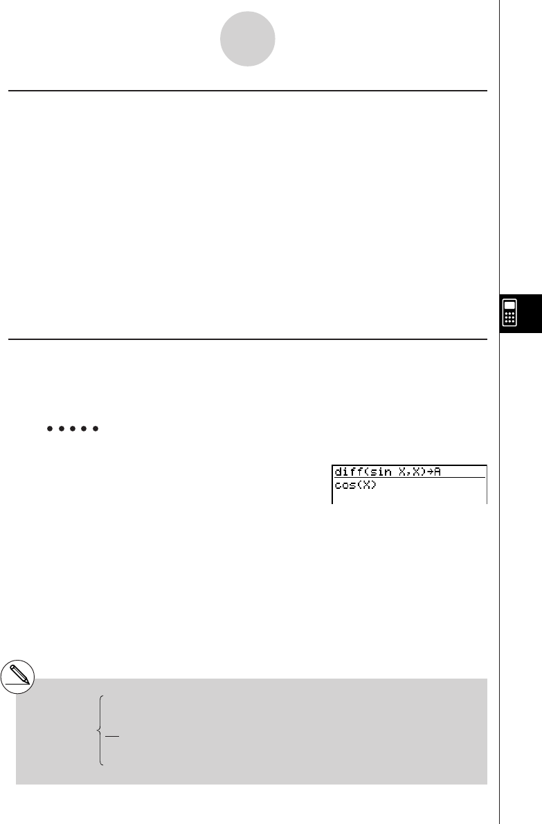
20010102
kk
kk
k Manual Formula and Parameter Input
You can use the function menus, K key, and J key in combination to input formulas and
parameters as described below.
•3(EQUA)b(INEQUA)
•{>}/{<}/{tt
tt
t}/{ss
ss
s} ... {inequality}
•Kkey
•{∞}/{Abs}/{x!}/{sign} ... {infinity}/{absolute value}/{factorial}/{signum function*1}
•{HYP} ... {hyperbolic}/{inverse hyperbolic} functions
•{sinh}/{cosh}/{tanh}/{sinh–1}/{cosh–1}/{tanh–1}
•Jkey
•{Yn}/{rn}/{Xtn}/{Ytn}/{Xn} ... input of graph memory {Yn}/{rn}/{Xtn}/{Ytn}/{Xn}
k Formula Memory
The CAS Mode has 28 formula variables. Variable names are the letters A through Z, plus r,
and
θ
. CAS Mode formula variables are independent of standard value variables.
Example To assign a formula that differentiates sin(X) at X (cos(X)) to variable A
2(CALC)b(diff)sv,
v)aav(A)w
7-1-4
Using the CAS (Computer Algebra System) Mode
1 (real number, A > 0)
–1 (real number, A < 0)
*1signum (A) A (A= imaginary number)
|A|
Undefined (A = 0)
20011101
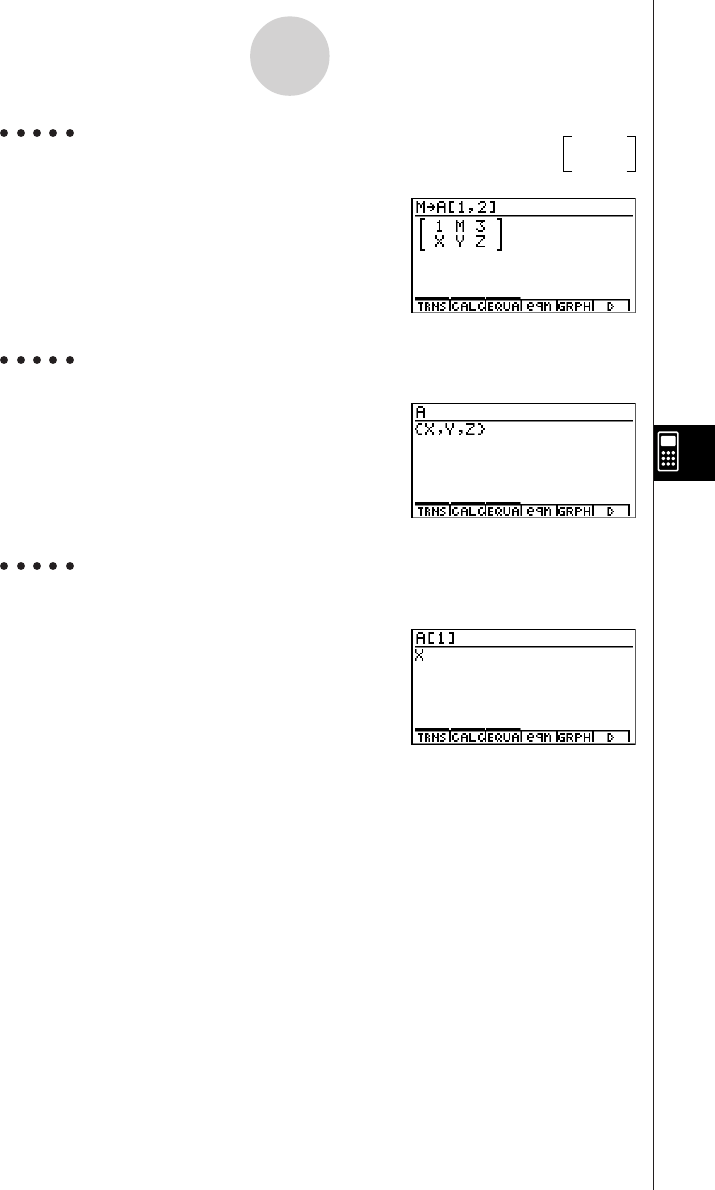
20010102
Example To assign M to row 1 column 2 of variable A when the matrix
is assigned to it
ah(M)aav(A)
!+( [ )b,c!-( ] )w
Example To recall the value of variable A when the list {X, Y, Z} is assigned to it
av(A)w
Example To recall the first component (A [1]) of variable A when vector (X Y Z) is
assigned to it
av(A)!+( [ )b
!-( ] )w
7-1-5
Using the CAS (Computer Algebra System) Mode
123
XYZ
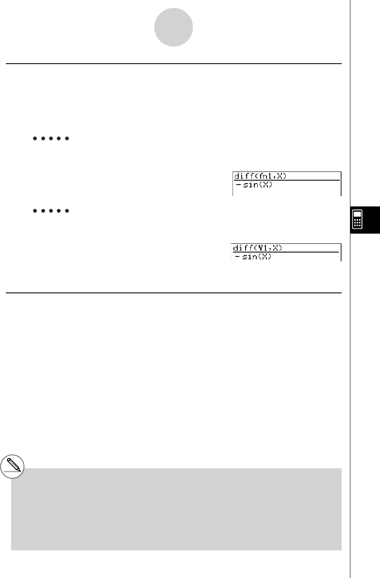
20010102
k Function Memory and Graph Memory
Function memory lets you store functions for later recall when you need them.
With graph memory, you can store graphs in memory. Press the J key and then input the
name of the graph.
Example To differentiate f1 = cos(X), which is assigned to function memory f1,
at X
2(CALC)b(diff)K6(g)4(FMEM)
d(fn)b,v)w
Example To differentiate Y1 = cos(X), which is assigned to graph memory Y1,
at X
2(CALC)b(diff)
J1(Yn) b,v)w
k Eqn Memory
When a calculation result is an equation or inequality, its formula number is displayed in the
formula number area, and the equation is stored in Eqn memory.*1 Stored equations can be
recalled with the eqn command, rclEqn command or rclAllEqn command.
7-1-6
Using the CAS (Computer Algebra System) Mode
*1Up to 99 formulas can be stored in Eqn
memory.
The error message “Memory ERROR” when
you try to store an equation when there are
already 99 equations in Eqn memory. When
this happens, execute the ALLEQU (Delete
All Equations) from the CLR menu.
20011101
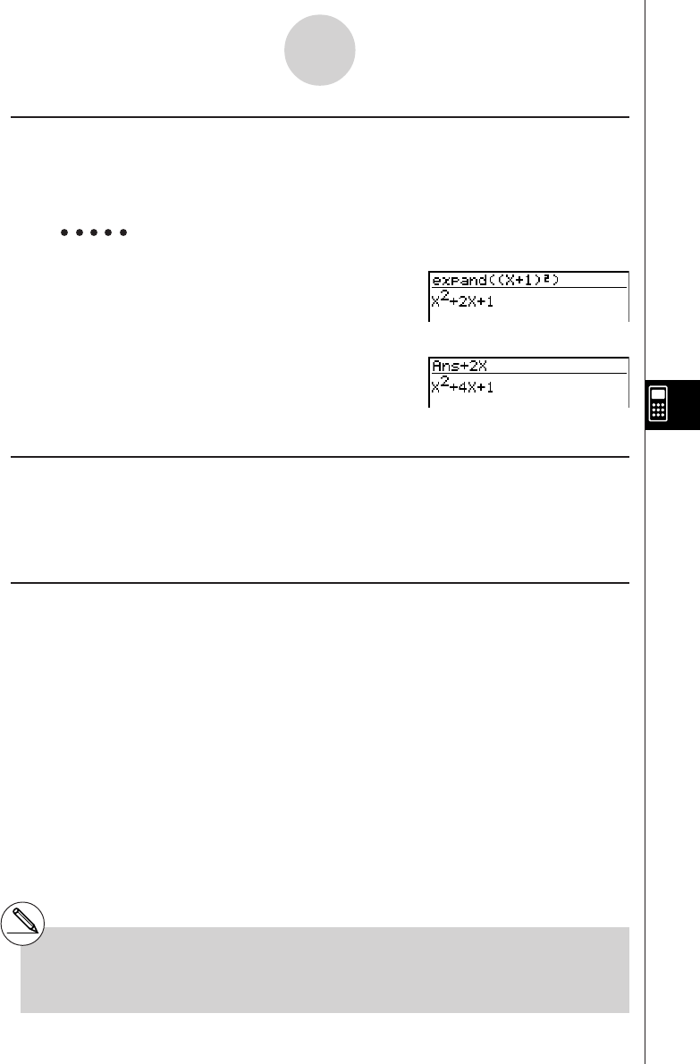
20010102
k Answer (Ans) Memory and Continuous Calculation
Answer (Ans) memory and continuous calculation can be used just as with standard
calculations. In the Algebra Mode, you can even store formulas in Ans memory.
Example To expand (X+1)2 and add the result to 2X
1(TRNS)b(expand)
(v+b)x)w
Continuing:
+cvw
k Replay Contents
Replay memory can be used in the input area. After a calculation is complete, pressing d
or e in the input area recalls the formula of the last calculation performed. After a
calculation or after pressing A, you can press f or c to recall previous formulas.
k Moving the Cursor Between Display Areas
When ] ' ` $ indicates a calculation result that does not fit on the display, the cursor
keys perform output area scrolling. To use the Replay Function from this condition, press
6(g)2(SW). ] ' ` $ change to a dotted line display to indicate that cursor key
operations control the input area.
Pressing 2(SW) again moves the cursor back to the output area.
7-1-7
Using the CAS (Computer Algebra System) Mode
# Pressing 6(g)1(CLR)d(ALLEQU)
deletes Eqn memory, Ans memory, and
Replay memory contents.
#You can input up to 255 bytes of data into the
input area.
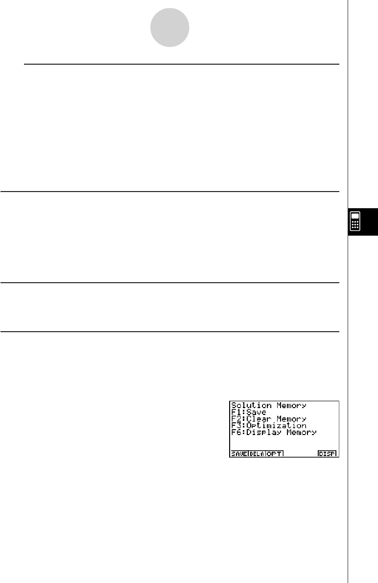
20010102
SET UP Items
uu
uu
uAngle ... Unit of angular measurement specification
•{Deg}/{Rad} ... {degrees}/{radians}
uu
uu
uAnswer Type ... Result range specification
•{Real}/{Cplx} ... {real number}/{complex number}
uu
uu
uDisplay ... Display format specification (for approx only)
•{Fix}/{Sci}/{Norm} ... {number of decimal places}/{number of significant digits}/
{normal display format}
k Graph Function
Pressing 5(GRPH) displays the graph formula screen, which you can use to input a graph
formula. Press 4(G
•
VAR) if you want to input a graph memory.
You can also use the 1(SEL), 2(DEL), and 3(TYPE) functions while the graph formula
screen is on the display.
Press 6(DRAW) to draw a graph.
k RECALL ANS Function
Pressing 6(g)3(R
•
ANS) recalls Ans Memory contents.
k Solution Memory
In the CAS Mode or ALGEBRA Mode, you can save the history of a calculation you perform
(replay memory contents) into solution memory. This section describes how you can access
and work with the contents of solution memory. Pressing 6(g)4(MEM) on the CAS Mode
or ALGEBRA Mode main menu display the initial solution memory screen shown below.
7-1-8
Using the CAS (Computer Algebra System) Mode
•{SAVE} ... {saves the calculation history to solution memory}
•{DEL
•
A}... {deletes solution memory contents}
•{OPT} ... {optimizes solution memory}
•{DISP} ... {displays solution memory contents}
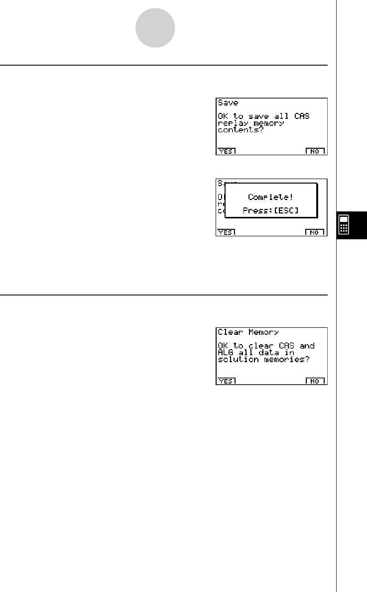
20010102
7-1-9
Using the CAS (Computer Algebra System) Mode
u To save a calculation history to solution memory (Save)
On the initial solution memory screen, press 1(SAVE).
Press 1(YES) to save the calculation history to solution memory.
Pressing i returns to the solution memory initial screen.
•Pressing 6(NO) in place of 1(YES) returns to the solution memory initial screen without
saving anything.
u To clear solution memory contents (Clear Memory)
On the initial solution memory screen, press 2(DEL
•
A).
Press 1(YES) to clear solution memory contents.
Pressing i returns to the solution memory initial screen.
•Pressing 6(NO) in place of 1(YES) returns to the solution memory initial screen without
clearing anything.
•This clears both CAS Mode and ALGEBRA Mode memory contents. You cannot select the
mode shows memory contents you want to delete.
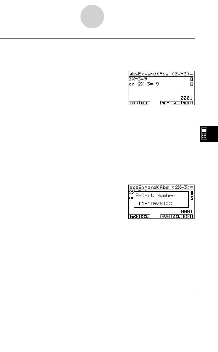
20010102
•6(DISP) is disabled when there is no data in Solution memory.
•To display the next record
Press 6(NEXT).
•To display the previous record
Press 1(BACK).
•Pressing 1(BACK) while the oldest record is on the display returns to the solution
memory initial screen.
•To display a particular record
Press 5(SEL) and then input the number of the record you want to display.
Pressing w displays the record whose number you input.
•To delete a single solution memory record
Display the record you want to delete, and then press 2(DEL).
In response to the confirmation message that appears, press w(Yes) to delete the record
you displayed.
To clear the above screen without deleting anything, press i(No).
•To toggle record number display on and off
Press 4(NUM) to toggle display of the record number on and off.
uTo optimize solution memory (Optimization)
On the initial solution memory screen, press 3(OPT).
Pressing i returns to the solution memory initial screen.
Optimizing solution memory rearranges data and can free up more storage space. Perform
the above procedure when solution memory capacity starts running low.
7-1-10
Using the CAS (Computer Algebra System) Mode
u To display solution memory contents (Display Memory)
On the initial solution memory screen, press 6(DISP).
This displays the oldest expression and result in solution memory. The bottom line shows the
record number.

20010102
7-1-11
Using the CAS (Computer Algebra System) Mode
Algebra Command Reference
The following are the abbreviations used in this section.
•Exp ... Expression (value, formula, variable, etc.)
•Eq ... Equation
•Ineq ... Inequality
•List ... List
•Mat ... Matrix
•Vect ... Vector
Anything enclosed within square brackets can be omitted.
u expand
Function: Expands an expression.
Syntax: expand (
{Exp/Eq/Ineq/List/Mat/Vect} [ ) ]
Example To expand (X+2)2
1(TRNS)b(expand)(v+c)xw X2 + 4X + 4
u rFactor (rFctor)
Function: Factors an expression up to its root.
Syntax: rFactor (
{Exp/Eq/Ineq/List/Mat/Vect} [ ) ]
Example To factor the X2– 3
1(TRNS)c(rFctor)vx-dw(X – 3) (X + 3)
u factor
Function: Factors an expression.
Syntax: factor (
{Exp/Eq/Ineq/List/Mat/Vect} [ ) ]
Example To factor X2– 4X + 4
1(TRNS)d(factor)vx-ev+ew (X – 2)2

20010102
usolve
Function: Solves an equation.
Syntax: solve( Eq [,variable] [ ) ]
solve( {Eq-1,..., Eq-n}, {variable-1,...,variable-n} [ ) ]
Example To solve AX + B = 0 for X
1(TRNS)e(solve)av(A)v+
al(B)!.(=)aw
Example To solve simultaneous linear equation 3X + 4Y = 5, 2X – 3Y = – 8
1(TRNS)e(solve)!*( { )
da+(X)+ea-(Y)!.(=)f,
ca+(X)-da-(Y)!.(=)-i
!/( } ),!*( { )a+(X),X = – 1
a-(Y)!/( } )wY = 2
• X is the default when no variable is specified.
utExpand (tExpnd)
Function: Employs the addition theorem to expand a trigonometric function.
Syntax: tExpand( {Exp/List/Mat/Vect} [ ) ]
Example To employ the addition theorem to expand sin(A+B)
1(TRNS)f(TRIG)b(tExpnd)
s(av(A)+al(B)wcos(B) • sin(A) + sin(B) • cos(A)
utCollect (tCollc)
Function: Employs the addition theorem to transform the product of a trigonometric
function to a sum.
Syntax: tCollect( {Exp/List/Mat/Vect} [ ) ]
Example To employ the addition theorem to transform sin(A)cos(B) to
trigonometric sum
1(TRNS)f(TRIG)c(tCollc)
sav(A)cal(B)w
7-1-12
Using the CAS (Computer Algebra System) Mode
sin (A + B)
2
sin (A – B)
2
+
– B
A
X =
20011101

20010102
7-1-13
Using the CAS (Computer Algebra System) Mode
u trigToExp (trigToE)
Function: Transforms a trigonometric or hyperbolic function to an exponential function.
Syntax: trigToExp( {Exp/List/Mat/Vect} [ ) ]
Example To convert cos(iX) to an exponential function
1(TRNS)f(TRIG)d(trigToE)c!a(i)vw
uexpToTrig (expToT)
Function: Converts an exponential function to a trigonometric or hyperbolic function.
Syntax: expToTrig( {Exp/List/Mat/Vect} [ ) ]
Example To convert eix to a trigonometric function
1(TRNS)f(TRIG)e(expToT)
!I(ex)(!a(i)vw cos(X) + sin(X) • i
u simplify (smplfy)
Function: Simplifies an expression.
Syntax: simplify( {Exp/Eq/Ineq/List/Mat/Vect} [ ) ]
Example To simplify 2X + 3Y – X + 3 = Y + X – 3Y + 3 – X
1(TRNS)g(smplfy)ca+(X)+da-(Y)
-a+(X)+d!.(=)a-(Y)
+a+(X)-da-(Y)+d-
a+(X)wX + 3Y + 3 = –2Y + 3
ex+ e
—
x
2

20010102
u combine (combin)
Function: Adds and reduces rational expressions.
Syntax: combine( {Exp/Eq/Ineq/List/Mat/Vect} [ ) ]
Example To reduce the fraction (X + 1)
/
(X + 2) + X (X + 3)
1(TRNS)h(combin)(v+b)/
(v+c)+v(v+dw
ucollect (collct)
Function: Rearranges an expression, focusing on a particular variable.
Syntax: collect( {Exp/Eq/Ineq/List/Mat/Vect} [,{Exp/variable}] [ ) ]
Example To rearrange X2 + AX + BX, focusing on the variable X
1(TRNS)i(collct)vx+av(A)v+
al(B)vw X2 + (A + B)X
• X is the default when nothing is specified for [,{Exp/variable}].
u substitute (sbstit)
Function: Assigns an expression to a variable.
Syntax: substitute( {Exp/Eq/Ineq/List/Mat/Vect}, variable=expression
[,..., variable=expression] [ ) ]
Example To assign 5 to X in 2X – 1
1(TRNS)j(sbstit)cv-b,
v!.(=)fw9
7-1-14
Using the CAS (Computer Algebra System) Mode
X3 + 5X2 + 7X + 1
X + 2
20011101

20010102
ucExpand (cExpnd)
Function: Expands xth root of imaginary number.
Syntax: cExpand( {Exp/Eq/Ineq/List/Mat/Vect} [ ) ]
Example To expand 2i
1(TRNS)v(cExpnd)!x( )c!a(i)w1 + i
uapprox
Function: Produces a numerical approximation for an expression.
Syntax: approx( {Exp/Eq/Ineq/List/Mat/Vect} [ ) ]
Example To obtain a numerical value for 2
1(TRNS)l(approx)!x( )cw1.414213562
Example 920
Normal:jMcaw12157665459056928801
approx: 1(TRNS)l(approx)jMcaw1. 215766546E+19 (Display: Norm1)
7-1-15
Using the CAS (Computer Algebra System) Mode
#About approx
With normal calculations (when approx is not
used) in the CAS Mode, calculation results are
displayed in full, without using exponents.
When you use approx in the CAS Mode,
however, results are displayed using the
exponential format range specified by the Display
item of the SET UP screen.
This means approx displays results in the CAS
Mode the same way they are displayed in the
RUN•MAT Mode.

20010102
u diff
Function: Differentiates an expression.
Syntax: diff( {Exp/List} [, variable, order, derivative] [ ) ]
diff( {Exp/List}, variable [, order, derivative] [ ) ]
diff( {Exp/List}, variable, order [, derivative] [ ) ]
Example To differentiate X6 with respect to X
2(CALC)b(diff)vMgw6X5
• X is the default when no variable is specified.
• 1 is the default when no order is specified.
u∫
Function: Integrates an expression.
Syntax: ∫( {Exp/List} [, variable, integration constant] [ ) ]
∫( {Exp/List}, variable [, integration constant] [ ) ]
∫( {Exp/List}, variable, lower limit, upper limit [ ) ]
Example To integrate X2 with respect to X
2(CALC)c( ∫ )vxw
• X is the default when no variable is specified.
u lim
Function: Determines the limits of a function expression.
Syntax: lim( {Exp/List}, variable, point [, direction] [ ) ]
Example To determine the limits of sin(X)/X when X = 0
2(CALC)d(lim)sv/v,v,aw1
• Direction can be positive (from right) or negative (from left).
7-1-16
Using the CAS (Computer Algebra System) Mode
X3
3

20010102
uΣ
Function: Calculates a sum.
Syntax: Σ( {Exp/List}, variable, start value, end value [ ) ]
Example To calculate the sum as the value of X in X2 changes from X = 1
through X = 10
2(CALC)e(Σ)vx,v,b,baw385
uΠ
Function: Calculates a product.
Syntax: Π( {Exp/List}, variable, start value, end value [ ) ]
Example To calculate the product as the value of X in X2 changes from X = 1
through X = 5
2(CALC)f(Π)vx,v,b,fw14400
u taylor
Function: Finds a Taylor polynomial.
Syntax: taylor( {Exp/List}, variable, order [, center point] [ ) ]
Example To find a 5th order Taylor polynomial for sin(X) with respect to X = 0
2(CALC)g(taylor)sv,v,f,aw
•The default center point is zero.
u arcLen
Function: Returns the arc length.
Syntax: arcLen( {Exp/List}, variable, start value, end value [ ) ]
Example To determine the arc length for X2 from X = 0 to X = 1
2(CALC)h(arcLen)
vx,v,a,bw
7-1-17
Using the CAS (Computer Algebra System) Mode
X5
–X3
+ X
120 6
In (4
5 + 8) –In(2) + 5
422

20010102
u tanLine (tanLin)
Function: Returns the expression for a tangent line.
Syntax: tanLine( {Exp/List}, variable, variable value at point of tangency [ ) ]
Example To determine the expression for a line tangent with X3 when X = 2
2(CALC)i(tanLin)vMd,v,cw12X – 16
u denominator (den)
Function: Extracts the denominator of a fraction.
Syntax: denominator( {Exp/List} [ ) ]
Example To extract the denominator of the fraction (X + 2)/(Y – 1)
2(CALC)j(EXTRCT)b(den)
(a+(X)+c)/(a-(Y)-bwY – 1
u numerator (num)
Function: Extracts the numerator of a fraction.
Syntax: numerator( {Exp/List} [ ) ]
Example To extract the numerator of the fraction (X + 2)/(Y – 1)
2(CALC)j(EXTRCT)c(num)
(a+(X)+c)/(a-(Y)-bwX + 2
u gcd
Function: Returns the greatest common divisor.
Syntax: gcd( {Exp/List}, {Exp/List} [ ) ]
Example To determine the greatest common divisor of X + 1 and X2 – 3X – 4
2(CALC)v(gcd)v+b,vx-
dv-ewX + 1
7-1-18
Using the CAS (Computer Algebra System) Mode
20011101

20010102
u lcm
Function: Obtains the least common multiple of two expressions
Syntax: lcm( {Exp/List}, {Exp/List} [ ) ]
Example To obtain the least common multiple of X2 – 1 and X2 + 2X – 3
2(CALC)l(lcm)vx-b,
vx+cv-dwX3 + 3X2 – X – 3
u rclEqn
Function: Recalls multiple eqn memory contents.
Syntax: rclEqn( memory number [, ..., memory number] [ ) ]
Example To recall the contents of equation memory 2 and equation memory 3
3(EQUA)c(rclEqn)c,dw3X – Y = 7
3X + 6Y = 63
•The memory numbers of equations produced as the result of a recall are not updated.
u rclAllEqn (rclAll)
Function: Recall all eqn memory contents.
Syntax: rclAllEqn
•The memory numbers of equations produced as the result of a recall are not updated.
u rewrite (rewrit)
Function: Moves the right side expression to the left side.
Syntax: rewrite( {Eq/Ineq/List} [ ) ]
Example To move the right side expression of X + 3 = 5X – X2 to the left side
3(EQUA)e(rewrit)v+d!.(=)
fv-vxw X2 – 4X + 3 = 0
7-1-19
Using the CAS (Computer Algebra System) Mode
20011101

20010102
u exchange (exchng)
Function: Exchanges the right-side and left-side expressions.
Syntax: exchange( {Eq/Ineq/List} [ ) ]
Example To exchange the left-side and right-side expressions of 3 > 5X – 2Y
3(EQUA)f(exchng)d3(EQUA)b(INEQUA)b(>)
fa+(X)-ca-(Y)w5X – 2Y < 3
u eliminate (elim)
Function: Assigns an expression to a variable.
Syntax: eliminate( {Eq/Ineq/List} -1, variable, Eq-2 [ ) ]
Example To transform Y = 2X + 3 to X= and then substitute into 2X + 3Y = 5
3(EQUA)g(elim)ca+(X)+da-(Y)!.(=)
f,a+(X),a-(Y)!.(=)
ca+(X)+dw4Y – 3 = 5
u getRight (getRgt)
Function: Gets the right-side element.
Syntax: getRight( {Eq/Ineq/List} [ ) ]
Example To extract the right side element of Y = 2X2 + 3X + 5
3(EQUA)h(getRgt)a-(Y)!.(=)
ca+(X)x+da+(X)+fw2X2 + 3X + 5
u invert
Function: Inverts two variables.
Syntax: invert( {Exp/Eq/Ineq/List} [,variable name 1, variable name 2] [ ) ]
If you omit the variable names, variables X and Y are inverted.
Example To invert X and Y in the expression 2X = Y
3(EQUA)i(invert)cv!.(=)a-(Y)w2Y = X
7-1-20
Using the CAS (Computer Algebra System) Mode
20011101

20010102
u absExpand (absExp)
Function: Divides an expression that contains an absolute value into two expressions.
Syntax: absExpand( {Eq/Ineq} [ ) ]
Example To strip the absolute value from | 2X – 3 | = 9
3(EQUA)j(absExp)K5(Abs)(
cv-d)!.(=)jw
u andConnect (andCon)
Function: Connects two inequalities into a single expression.
Syntax: andConnect( Ineq-1, Ineq-2 [ ) ]
Example To combine X > – 1 and X < 3 into a single inequality
3(EQUA)v(andCon)v3(EQUA)b(INEQUA)b(>)
-b,v3(EQUA)b(INEQUA)c(<)dw–1 < X < 3
u eqn
Function: Recalls eqn memory contents.
Syntax: eqn( memory number [ ) ]
Example To add 15 to both sides of the equation 6X – 15 = X – 7, which is stored
in equation memory 3
4(eqn)d)+bfw6X = X + 8
2X – 3 = 9
or 2X – 3 = – 9 2
1
7-1-21
Using the CAS (Computer Algebra System) Mode
20010102
uclear (clrVar)
Function: Clears the contents of specific equation (A to Z, r,
θ
).*1
Syntax: clear( variable [ ) ]
clear( {variable list} [ ) ]
Example To clear the contents of variable A
6(g)1(CLR)b(clrVar)av(A)w{ }
Example To clear the contents of variables X, Y, and Z
6(g)1(CLR)b(clrVar)!*( { )a+(X),
a-(Y),aa(Z)!/( } )w{ }
uclearVarAll (VarAll)
Function: Clears the contents of all 28 variables (A to Z, r,
θ
).
Syntax: clearVarAll { }
7-1-22
Using the CAS (Computer Algebra System) Mode
*1When you start out with memories A, B, C,
and D, for example, and delete memories A
and B, the display shows only C,D because
they are the only memories remaining.

20010102
kList Calculation Commands [OPTN]-[LIST]
uDim
Function: Returns the dimension of a list.
Syntax: Dim List
Example To determine the dimension of list {1, 2, 3}
K1(LIST)b(CALC)b(Dim)!*( { )b,c,d
!/( } )w3
uMin
Function: Returns the minimum value of an expression or the elements in a list.
Syntax: Min( {List/Exp} [ ) ]
Min( {List/Exp}, {List/Exp} [ ) ]
Example To determine the minimum value of the elements in list {1, 2, 3}
K1(LIST)b(CALC)c(Min)!*( { )b,c,d
!/( } )w1
Example To compare each element of list {1, 2, 3} with the value 2, and produce
a list whose elements are the minimum value resulting from each
comparison
K1(LIST)b(CALC)c(Min)!*( { )b,c,d
!/( } ),cw{
1, 2, 2
}
Example To compare the elements of list {1, 2, 3} and list {3, 1, 2}, and produce
a list whose elements are the minimum value resulting from each
comparison
K1(LIST)b(CALC)c(Min)!*( { )b,c,d
!/( } ),!*( { )d,b,c!/( } )w{1, 1, 2
}
7-1-23
Using the CAS (Computer Algebra System) Mode

20010102
7-1-24
Using the CAS (Computer Algebra System) Mode
uMax
Function: Returns the maximum value of an expression or the elements of a list.
Syntax: Max( {List/Exp} [ ) ]
Max( {List/Exp}, {List/Exp} [ ) ]
Example To determine the maximum value of the elements in list {1, 2, 3}
K1(LIST)b(CALC)d(Max)!*( { )b,c,d
!/( } )w3
Example To compare each element of list {1, 2, 3} with the value 2, and produce
a list whose elements are the maximum value resulting from each
comparison
K1(LIST)b(CALC)d(Max)!*( { )b,c,d
!/( } ),cw{
2, 2, 3
}
Example To compare the elements of list {1, 2, 3} and list {3, 1, 2}, and produce
a list whose elements are the maximum value resulting from each
comparison
K1(LIST)b(CALC)d(Max)!*( { )b,c,d
!/( } ),!*( { )d,b,c!/( } )w{
3, 2, 3
}
u Mean
Function: Returns the mean of the elements in a list.
Syntax: Mean( List [ ) ]
Mean( List, List [ ) ]
The list must contain values or mathematical expressions only. Equations and inequalities
are not allowed.
Example To determine the mean of the elements in list {1, 2, 3}
K1(LIST)b(CALC)e(Mean)!*( { )b,c,d
!/( } )w2

20010102
Example To determine the mean of the elements in list {1, 2, 3} when their
frequencies are {3, 2, 1}
K1(LIST)b(CALC)e(Mean)!*( { )b,c,d
!/( } ),!*( { )d,c,b!/( } )w
uMedian
Function: Returns the median of the elements in a list.
Syntax: Median( List [ ) ]
Median( List, List [ ) ]
The list must contain values or mathematical expressions only. Equations and inequalities
are not allowed.
Example To determine the median of the elements in list {1, 2, 3}
K1(LIST)b(CALC)f(Median)!*( { )b,c,d
!/( } )w2
Example To determine the median of the elements in list {1, 2, 3} when their
frequencies are {3, 2, 1}
K1(LIST)b(CALC)f(Median)!*( { )b,c,d
!/( } ),!*( { )d,c,b!/( } )w
u Sum
Function: Returns the sum of the elements in a list.
Syntax: Sum List
The list must contain values or mathematical expressions only. Equations and inequalities
are not allowed.
Example To determine the sum of the elements in list {1, 2, 3}
K1(LIST)b(CALC)g(Sum)!*( { )b,c,d
!/( } )w6
7-1-25
Using the CAS (Computer Algebra System) Mode
5
3
3
2

20010102
u Prod
Function: Returns the product of the elements in a list.
Syntax: Prod List
The list must contain values or mathematical expressions only. Equations and inequalities
are not allowed.
Example To determine the product of the elements in list {2, 3, 4}
K1(LIST)b(CALC)h(Prod)!*( { )c,d,e
!/( } )w24
uCuml
Function: Returns the cumulative frequency of the elements in a list.
Syntax: Cuml List
The list must contain values or mathematical expressions only. Equations and inequalities
are not allowed.
Example To determine the cumulative frequency of the elements in list {1, 2, 3}
K1(LIST)b(CALC)i(Cuml)!*( { )b,c,d
!/( } )w{
1, 3, 6
}
u Percent (%)
Function: Returns the percentage of each element in a list, the sum of which is assumed
to be 100.
Syntax: Percent List
The list must contain values or mathematical expressions only. Equations and inequalities
are not allowed.
Example To determine the percentage of each element in the list {1, 2, 3}
K1(LIST)b(CALC)j(%)!*( { )b,c,d
!/( } )w
7-1-26
Using the CAS (Computer Algebra System) Mode
3
50
3
100 50
,,
{
{

20010102
uA List
Function: Returns a list whose elements are the differences between the elements of
another list.
Syntax: AA
AA
A List List
The list must contain values or mathematical expressions only. Equations and inequalities
are not allowed.
Example To generate a list whose elements are the differences between the
elements of list {1, 2, 4}
K1(LIST)b(CALC)v(AList)!*( { )b,c,e
!/( } )w{
1, 2
}
uStdDev
Function: Returns the sample standard deviation of the elements in a list.
Syntax: StdDev List
The list must contain values or mathematical expressions only. Equations and inequalities
are not allowed.
Example To determine the sample standard deviation of the elements in list
{1, 2, 4}
K1(LIST)b(CALC)l(StdDev)!*( { )b,c,e
!/( } )w
u Variance (Vari)
Function: Returns the variance of the elements in a list.
Syntax: Variance List
The list must contain values or mathematical expressions only. Equations and inequalities
are not allowed.
Example To determine the variance of the elements in list {1, 2, 4}
K1(LIST)b(CALC)I(Vari)!*( { )b,c,e
!/( } )w
7-1-27
Using the CAS (Computer Algebra System) Mode
7
3
3
21
20011101

20010102
uSeq
Function: Generates a list in accordance with a numeric sequence expression.
Syntax: Seq( Exp, variable, start value, end value, [increment] [ ) ]
If you do not specify an increment, an increment of 1 is used.
Example To generate a list in accordance with the expression: value A, end
value 3A, increment A
K1(LIST)c(CREATE)b(Seq)v,v,av(A),d
av(A),av(A)w{
A, 2A, 3A
}
u Augment (Augmnt)
Function: Returns a new list that appends List 2 to List 1.
Syntax: Augment( List, List [ ) ]
Example To combine list {1, 2} and list {3, 4}
K1(LIST)c(CREATE)c(Augmnt)!*( { )b,c
!/( } ),!*( { )d,e!/( } )w{
1, 2, 3, 4
}
uFill
Function: Replaces the elements of a list with a specified value or expression.
This command can also be used to create a new list whose elements all
contain the same value or expression.
Syntax: Fill( {Exp/Eq/Ineq}, List [ ) ]
Fill( Exp, numeric value [ ) ]
Example To replace the elements of list {3, 4} with X
K1(LIST)c(CREATE)d(Fill)v,!*( { )
d,e!/( } )w{
X, X
}
Example To create a list with eight elements, all of which are X
K1(LIST)c(CREATE)d(Fill)v,iw{
X, X, X, X, X, X, X, X
}
7-1-28
Using the CAS (Computer Algebra System) Mode
20011101

20010102
uSortA
Function: Sorts the elements of a list into ascending order.
Syntax: SortA( List [ ) ]
The list must contain values or mathematical expressions only. Equations and inequalities
are not allowed.
Example To sort the elements of list {1, 5, 3} into ascending order
K1(LIST)c(CREATE)e(SortA)!*( { )b,f,d
!/( } )w{
1, 3, 5
}
u SortD
Function: Sorts the elements of a list into descending order.
Syntax: SortD( List [ ) ]
The list must contain values or mathematical expressions only. Equations and inequalities
are not allowed.
Example To sort the elements of list {1, 5, 3} into descending order
K1(LIST)c(CREATE)f(SortD)!*( { )b,f,d
!/( } )w{
5, 3, 1
}
u SubList (SubLst)
Function: Extracts a specific section of a list into a new list.
Syntax: SubList( List, start number [, end number] [ ) ]
Example To extract element 2 through element 3 from list {1, 2, 3, 4}
K1(LIST)c(CREATE)g(SubLst)!*( { )b,c,d
,e!/( } ),c,dw{
2, 3
}
•If you do not specify an end number, all the elements from the start number to the end of
the list are extracted.
7-1-29
Using the CAS (Computer Algebra System) Mode

20010102
u List→Mat (L→Mat)
Function: Converts lists into a matrix.
Syntax: List→Mat( List [ , ... ,List ] [ ) ]
Example To convert list {3, 5} and list {2, 4} into a matrix
K1(LIST)d(LIST→)b(L→Mat)!*( { )d,f 32
!/( } ),!*( { )c,e!/( } )w54
u List→Vect (L→Vect)
Function: Converts a list into a vector.
Syntax: List→Vect List
Example To convert list {3, 2} into a vector
K1(LIST)d(LIST→)c(L→Vect)!*( { )d,c
!/( } )w[
3, 2
]
7-1-30
Using the CAS (Computer Algebra System) Mode

20010102
kMatrix Calculation Commands [OPTN]-[MAT]
uDim
Function: Returns the dimensions of a matrix.
Syntax: Dim Mat
Example To determine the dimensions of the matrix below
123
456
K2(MAT)b(CALC)b(Dim)!+( [ )!+( [ )
b,c,d!-( ] )!+( [ )e,f,g
!-( ] )!-( ] )w{
2, 3
}
u Det
Function: Returns the determinant of a matrix.
Syntax: Det Mat
Example To determine the determinant of the matrix below
12
45
K2(MAT)b(CALC)c(Det)!+( [ )!+( [ )
b,c!-( ] )!+( [ )e,f
!-( ] )!-( ] )w– 3
u Norm
Function: Returns the norm of a matrix.
Syntax: Norm Mat
Example To determine the norm of the matrix below
12
45
K2(MAT)b(CALC)d(Norm)!+( [ )!+( [ )
b,c!-( ] )!+( [ )e,f
!-( ] )!-( ] )w 46
7-1-31
Using the CAS (Computer Algebra System) Mode
20011101
20010102
u EigVc
Function: Returns the eigenvector of a matrix.
Syntax: EigVc Mat
Example To determine the eigenvector of the matrix below
34
13
K2(MAT)b(CALC)e(EigVc)
!+( [ )!+( [ )d,e
!-( ] )!+( [ ) [
0.894427191 – 0.894427191
]
b,d!-( ] )!-( ] )w[
0.4472135955 0.4472135955
]
Eigenvectors are stacked vertically on the display.
In this example, (0.894427191 0.4472135955) are the eigenvectors that correspond to 5,
while (–0.894427191 0.4472135955) are the eigenvectors that correspond to 1.
An eigenvector has an infinite number of solutions. The eigenvector displayed by this
command is the one with a size of 1.
u EigVl
Function: Returns the eigenvalue of a matrix.
Syntax: EigVl Mat
Example To determine the eigenvalue of the matrix below
34
13
K2(MAT)b(CALC)f(EigVl)!+( [ )!+( [ )
d,e!-( ] )!+( [ )b,d
!-( ] )!-( ] )w{
5, 1
}
7-1-32
Using the CAS (Computer Algebra System) Mode
20011101

20010102
u Rref
Function: Returns the reduced row echelon form of a matrix.
Syntax: Rref Mat
Example To determine the reduced row echelon form of the matrix below
–
2–
20–
6
1–
19–
9
–
524–
4
K2(MAT)b(CALC)g(Rref)!+( [ )!+( [ )
-c,-c,a,-g!-( ] )!+( [ )
b,-b,j,-j!-( ] )
!+( [ )-f,c,e,-e
!-( ] )!-( ] )w
u Ref
Function: Returns the row echelon form of a matrix.
Syntax: Ref Mat
Example To determine the row echelon form of the matrix below
–
2–
20–
6
1–
19–
9
–
524–
4
K2(MAT)b(CALC)h(Ref)!+( [ )!+( [ )
-c,-c,a,-g!-( ] )!+( [ )
b,-b,j,-j!-( ] )
!+( [ )-f,c,e,-e
!-( ] )!-( ] )w
7-1-33
Using the CAS (Computer Algebra System) Mode
71
66
71
147
71
62
–
1 0 0
0 1 0
0 0 1
71
62
–
1 1 0
0 1
3
6
0 0 1
2
9
–

20010102
u LU
Function: Returns the LU resolution of a matrix.
Syntax: LU( Mat, lower memory, upper memory)
Example To determine the LU resolution of the matrix below
61218
51431
3818
The lower matrix is assigned to variable A, while the upper matrix is assigned to variable B.
K2(MAT)b(CALC)i(LU)!+( [ )!+( [ )
g,bc,bi!-( ] )!+( [ )
f,be,db!-( ] )!+( [ ) 61218
d,i,bi!-( ] )!-( ] ),04 16
av(A),al(B)w00 1
The upper matrix is displayed as the calculation result.
To display the lower matrix, recall the lower matrix variable (A in this example) specified
by the command.
av(A)w
To display the upper matrix, recall the upper matrix variable (B in this example) specified
by the command.
u Trn
Function: Transposes a matrix.
Syntax: Trn Mat
Example To transpose the matrix below
12
34
K2(MAT)c(CREATE)b(Trn)!+( [ )!+( [ )
b,c!-( ] )!+( [ )d,e 13
!-( ] )!-( ] )w24
7-1-34
Using the CAS (Computer Algebra System) Mode
100
01
1
6
5
2
1
2
1

20010102
u Augment (Augmnt)
Function: Combines two matrices.
Syntax: Augment( Mat, Mat [ ) ]
Example To combine the two matrices below
12 56
34 78
K2(MAT)c(CREATE)c(Augmnt)!+( [ )!+( [ )
b,c!-( ] )!+( [ )d,e
!-( ] )!-( ] ),!+( [ )!+( [ )
f,g!-( ] )!+( [ )h,i 1256
!-( ] )!-( ] )w3478
u Identify (Ident)
Function: Creates an identity matrix
Syntax: Ident numeric value
Example To create a 2 × 2 identity matrix
K2(MAT)c(CREATE)d(Ident)cw10
01
u Fill
Function: Replaces the elements of a matrix with a specified value or expression.
This command can also be used to create a new matrix whose elements all
contain the same value or expression.
Syntax: Fill( Exp, Mat [ ) ]
Fill( Exp, number of lines, number of rows [ ) ]
Example To replace the elements of the matrix below with X
34
12
K2(MAT)c(CREATE)e(Fill)v,!+( [ )
!+( [ )d,e!-( ] )!+( [ ) XX
b,c!-( ] )!-( ] )wXX
7-1-35
Using the CAS (Computer Algebra System) Mode

20010102
Example To create a 2 × 3 matrix, all of whose entries are X
K2(MAT)c(CREATE)e(Fill)v,c,dwXXX
XXX
u SubMat
Function: Extracts a specific section of a matrix into a new matrix.
Syntax: SubMat( Mat [, start row] [, start column] [, end row] [, end column] [ ) ]
Example To extract the section from row 2, column 2 to row 3, column 3 from
the following matrix
123
456
789
K2(MAT)c(CREATE)f(SubMat)!+( [ )!+( [ )
b,c,d!-( ] )!+( [ )e,f,g
!-( ] )!+( [ )h,i,j!-( ] ) 56
!-( ] ),c,c,d,dw89
•If you do not specify an end row and column, all the entries from the start row/column to the
end of the matrix are extracted.
7-1-36
Using the CAS (Computer Algebra System) Mode

20010102
uDiag
Function: Extracts the diagonal elements of a matrix.
Syntax: Diag Mat
Example To extract the diagonal elements of the matrix below
12
34
K2(MAT)c(CREATE)g(Diag)!+( [ )!+( [ )
b,c!-( ] )!+( [ )d,e
!-( ] )!-( ] )w[
1, 4
]
uMat→List (M→List)
Function: Converts a specific column of a matrix into a list.
Syntax: Mat→List( Mat, column number [ ) ]
Example To convert column 2 of the matrix below to a list
12
34
K2(MAT)d(MAT→)b(M→List)!+( [ )!+( [ )
b,c!-( ] )!+( [ )d,e
!-( ] )!-( ] ),cw{
2, 4
}
uMat→Vect (M→Vect)
Function: Converts a specific column of a matrix into a vector.
Syntax: Mat→Vect( Mat, column number [ ) ]
Example To convert column 2 of the matrix below to a vector
12
34
K2(MAT)d(MAT→)c(M→Vect)!+( [ )!+( [ )
b,c!-( ] )!+( [ )d,e
!-( ] )!-( ] ),cw[
2, 4
]
7-1-37
Using the CAS (Computer Algebra System) Mode
20011101

20010102
uSwap
Function: Swaps two rows of a matrix.
Syntax: Swap Mat, row number 1, row number 2
Example To swap row 1 with row 2 of the following matrix
12
34
K2(MAT)e(ROW)b(Swap)!+( [ )!+( [ )
b,c!-( ] )!+( [ )d,e 34
!-( ] )!-( ] ),b,cw12
u`Row
Function: Returns the scalar product of a row of a matrix.
Syntax: `Row( Exp, Mat, row number [ ) ]
Example To multiply row 1 of the matrix below by X
12
34
K2(MAT)e(ROW)c(`Row)v,!+( [ )
!+( [ )b,c!-( ] )!+( [ ) X2X
d,e!-( ] )!-( ] ),bw34
u`Row+
Function: Calculates the scalar product of one row of a matrix and adds the result to
another row.
Syntax: `Row+( Exp, Mat, line number 1, line number 2 [ ) ]
Example To multiply row 1 of the matrix below by X, and add the result to row 2
12
34
K2(MAT)e(ROW)d(`Row+)v,!+( [ )
!+( [ )b,c!-( ] )!+( [ ) 12
d,e!-( ] )!-( ] ),b,cwX + 3 2X + 4
7-1-38
Using the CAS (Computer Algebra System) Mode

20010102
uRow+
Function: Adds one row of a matrix and to another row.
Syntax: Row+( Mat, row number 1, row number 2 [ ) ]
Example To add row 1 of the matrix below to row 2
12
34
K2(MAT)e(ROW)e(Row+)!+( [ )
!+( [ )b,c!-( ] )!+( [ ) 12
d,e!-( ] )!-( ] ),b,cw46
7-1-39
Using the CAS (Computer Algebra System) Mode

20010102
kVector Calculation Commands [OPTN]-[VECT]
uDim
Function: Returns the dimension of a vector.
Syntax: Dim Vect
Example To determine the dimension of the vector (1 2 3)
K3(VECT)b(CALC)b(Dim)!+( [ )b,c,d
!-( ] )w3
uCrossP
Function: Returns the cross product of two vectors.
Syntax: CrossP( Vect, Vect [ ) ]
Example To determine the cross product of vector (1 2 3) and vector (4 5 6)
K3(VECT)b(CALC)c(CrossP)!+( [ )b,c,d
!-( ] ),!+( [ )e,f,g!-( ] )w[ – 3, 6, – 3 ]
uDotP
Function: Returns the dot product of two vectors.
Syntax: DotP( Vect, Vect [ ) ]
Example To determine the dot product of vector (1 2 3) and vector (4 5 6)
K3(VECT)b(CALC)d(DotP)!+( [ )b,c,d
!-( ] ),!+( [ )e,f,g!-( ] )w32
uNorm
Function: Returns the norm of a vector.
Syntax: Norm Vect
Example To determine the norm of the vector (1 2 3)
K3(VECT)b(CALC)e(Norm)!+( [ )b,c,d
!-( ] )w 14
7-1-40
Using the CAS (Computer Algebra System) Mode
20011101

20010102
uUnitV
Function: Normalizes a vector.
Syntax: UnitV Vect
Example To normalize a vector (1 2 3)
K3(VECT)b(CALC)f(UnitV)
!+( [ )b,c,d
!-( ] )w
uAngle
Function: Returns the angle formed by two vectors.
Syntax: Angle( Vect, Vect [ ) ]
Example To determine the angle formed by vector (1 2) and vector (3 4)
(Unit Angle: Rad)
K3(VECT)b(CALC)g(Angle)!+( [ )b,c
!-( ] ),!+( [ )d,e!-( ] )w
uAugment (Augmnt)
Function: Combines two vectors.
Syntax: Angle( Vect, Vect [ ) ]
Example To combine vector (1 2) and vector (3 4)
K3(VECT)c(CREATE)b(Augmnt)!+( [ )b,c
!-( ] ),!+( [ )d,e!-( ] )w[
1, 2, 3, 4
]
uFill
Function: Replaces the elements of a vector with a specified value or expression.
Syntax: Fill( Exp, Vect [ ) ]
Example To replace the components of the vector below with X
K3(VECT)c(CREATE)c(Fill)v,!+( [ )
d,e!-( ] )w[
X, X
]
7-1-41
Using the CAS (Computer Algebra System) Mode
,, 14
3 14
14
14
7
14
25
11 5
cos
–1
20011101

20010102
uVect→List (V→List)
Function: Converts a vector into a list.
Syntax: Vect→List Vect
Example To convert vector (3 2) into a list
K3(VECT)d(VECT→)b(V→List)!+( [ )d,c
!-( ] )w{
3, 2
}
uVect→Mat (V→Mat)
Function: Converts vectors into a matrix.
Syntax: Vect→Mat( Vect [, ... ,Vect ] ( ] )
Example To convert vector (3 5) and (2 4) into a matrix
K3(VECT)d(VECT→)c(V→Mat)!+( [ )d,f 32
!-( ] ),!+( [ )c,e!-( ] )w54
7-1-42
Using the CAS (Computer Algebra System) Mode

19990401
7-2 Algebra Mode
The CAS Mode automatically provides you with the final result only. The Algebra Mode, on
the other hand, lets you obtain intermediate results at a number of steps along the way.
On the Main Menu, select the ALGEBRA icon to enter the Algebra Mode. The screens in this
mode are the same as those in the CAS Mode.
Operations in the Algebra Mode are identical to those in the CAS Mode, except for a number
of limitations. Also, the following commands are available in the Algebra Mode only.
u arrange (arrang)
Function: Collects like terms and arranges them in order, starting with the term that
contains the smallest coefficient.
Syntax: arrange( {Exp/Eq/Ineq} [ ) ]
Example To arrange 2X + 3 – 5X + 8Y in sequence of its variables
1(TRNS)j(arrang)ca+(X)+d-
fa+(X)+ia-(Y)w – 5X + 2X + 8Y + 3
u replace (replac)
Function: Replaces a variable with the expression assigned to the corresponding
expression variable.
Syntax: replace( {Exp/Eq/Ineq} [ ) ]
Example To replace S in the expression 3X + 2S, when the expression 2X + 1 is
assigned to S
1(TRNS)v(replac)dv+ca*(S)w3X + 2 (2X + 1)
7-2-1
Algebra Mode
20011101

19990401
7-3 Tutorial Mode
On the Main Menu, select the TUTOR icon to enter the Tutorial Mode.
k Tutorial Mode Flow
1. Specify the expression type.
2. Define the expression.
3. Specify the solve mode.
k Specifying the Expression Type
Entering the Tutorial Mode displays a menu of the following expression types.
•Linear Equation
•Linear Inequality
•Quadratic Equation
•Simul (Simultaneous) Equation
Use the cursor keys to highlight the expression type you want to specify, and then press w.
This displays a list of formulas for the expression type you select. Move the cursor to the
formula you want to use.
In the case of Linear Inequality, press 4(TYPE) to select the inequality type.
7-3-1
Tutorial Mode

19990401
The following shows the formulas available for each type of expression.
Linear Equation — 6 Types
• AX = B • X + A = B
• AX + B = C • AX + B = CX + D
• A(BX + C) = D(EX + F) •AX + B= C
Linear Inequality — 6 × 4 Types
• AX { > < ><} B • X + A { > < ><} B
• AX + B { > < ><} C • AX + B { > < ><} CX + D
• A(BX + C) { > < ><} D(EX + F) •AX + B{ > < ><} C
Quadratic Equation — 5 Types
• AX2 = B • (AX + B)2 = C
• AX2 + BX + C = 0 • AX2 + BX + C = D
• AX2 + BX + C = DX2 + EX + F
Simul Equation — 10 Types
•AX + BY = C • Y = AX + B
DX + EY = F Y = CX + D
•AX + BY + C = 0 • AX + BY + C = DX + EY + F
DX + EY + F = 0 GX + HY + I = JX + KY + L
•AX + BY = C • AX + BY = C
Y = DX + E DX + EY + F = 0
•AX + BY = C • AX + BY + C = 0
DX + EY + F = GX + HY + I Y = DX + E
•AX + BY + C = DX + EY + F • AX + BY + C = 0
Y = GX + H DX + EY + F = GX + HY + I
Pressing 6(EXCH) reverses the left side and right side elements of the expression.
7-3-2
Tutorial Mode
19990401
kDefining the Expression
In this step, you specify coefficients and define the expression. You can select any of the
three following methods for specifying coefficients.
•{RAND} ... {random generation of coefficients}
•{INPUT} ... {key input of coefficients}
•{SMPL} ... {selection of coefficients from samples}
•{SEED} ... {selection of a number from 1 to 99 (specification of the same number
displays the same expression)}
1(RAND) or w generates random coefficients and defines the expression.
2(INPUT) displays the coefficient input screen. Input coefficients, pressing w after each.
After you finish inputting all the coefficients, press 6(EXE) to define the coefficient.
3(SMPL) displays a number of preset sample expressions. Highlight the one you want to
use and then press w to define it.
Pressing4(SEED) displays a number selection screen. When you want to create the same
problem on another calculator, specify an appropriate matching number and press w.
No matter what method you use, the expression you define is displayed in the output area.
You can copy an expression to the Graph Mode as a graph function*1.
•{L•COP}/{R•COP} ... copy {left side element}/{right side element} as a graph function
(Simultaneous Equation Mode*2)
•{1•COP}/{2•COP} ... copy {first}/{second} expression as a graph function
7-3-3
Tutorial Mode
*1In the case of an inequality, the inequality
symbols are also copied.
*2Simultaneous equations are transformed to the
format Y = AX + B when copied.

19990401
k Specifying the Solve Mode
You can select one of the following three solve modes for the displayed expression.
•{VRFY} ... {Verify Mode}
In this mode, you input a solution for verification of whether or not it is correct. It provides
a good way to check solutions you arrive at manually.
•{MANU} ... {Manual Mode}
In this mode, you manually input algebra commands, transform the expression, and
calculate a result.
•{AUTO} ... {Auto Mode}
In this mode, the solution is produced automatically, one step at a time.
k Verify Mode
Press 4(VRFY) to enter the Verify Mode.
The expression is shown in the top line of the display. Input the solution underneath it, and
then press6(JUDG) to determine whether the solution is correct.
The verification result screen shows the left side and right side verification result (except for
a linear equation).
•However, in the case where a linear equation or quadratic equation has two solutions, the
left side and right side are obtained for the value where the pointer is located.
•In the case of simultaneous equations where the left side and right side of the second
equation are dissimilar even though the left side and right side of the first equation match,
the left side and right side of the second equation only are obtained. In other cases, the left
side and right side of the first equation are obtained.
The type of solution input screen that appears is selected according to the expression type.
To input a different type, press 1(TYPE) and then select the solution type you want to want
to use. Available solution types depend on the mode.
•{X = a} ... X has one solution (X = a) (linear equation default)
•{X = a, b} ... X has two solutions (X = a, X = b) (quadratic equation default)
•{X = a,
Y=} ... X and Y have one solution each (X = a, Y = b) (simultaneous equation
default)
•{X > a} ... X { > < ><} a (linear inequality default)
•{X < a, b <} ... X < a, b < X or X < a, b < X
•{a < X < b} ... a < X< b, a < X < b or X = a
•{Identi} (Identity) ... identity of left side and right side
•{Many} (Many Solutions) ... many solutions
•{No sol} (No Solution) ... no solution
7-3-4
Tutorial Mode
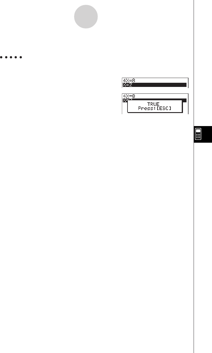
19990401
7-3-5
Tutorial Mode
You can press 4(MANU) to change to the Manual Mode or 5(AUTO) to change to the
Auto Mode.
Example To solve 4X = 8 in the Verify Mode
(Linear Equation)(AX = B)
2(INPUT)ewiw6(EXE)
4(VRFY)cw
6(JUDG)
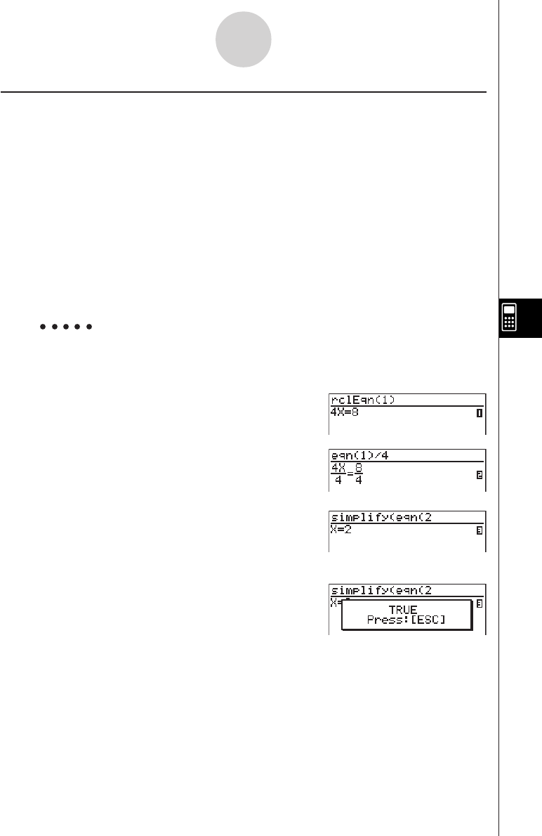
19990401
7-3-6
Tutorial Mode
k Manual Mode
Press 5(MANU) to enter the Manual Mode.
As with the Algebra Mode, the screen is divided between an input area and a display area.
This means you can select Algebra Mode commands from the function menu, transform the
expression, and solve it.
Operation is the same as that in the Algebra Mode.
After you obtain a result, you can press 5(JUDG) to determine whether or not it is correct.
•{DISP} ... Determines whether the expression in the display area is a correct solution.
•{Identi} ... identity of left side and right side
•{Many} ... many solutions
•{No sol} ... no solution
You can press 6(AUTO) to change to the Auto Mode.
Example Solve 4X = 8 in the Manual Mode
(Linear Equation)(AX=B)
2(INPUT)ewiw6(EXE)
5(MANU)
4(eqn)b)/e
w
1(TRNS)b(smplfy)
4(eqn)c
w
5(JUDG)b(DISP)
20010102
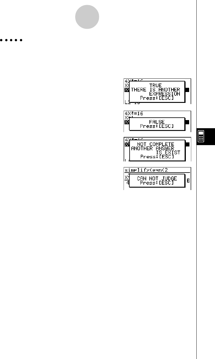
19990401
7-3-7
Tutorial Mode
Example 4X2 = 16
True (X = 2, X = – 2)
Besides “TRUE” the messages shown below can also appear as the result of verification.
“CAN NOT JUDGE” appears in the Manual Mode, while the other messages appear in both
the Verify Mode and Manual Mode.
20010102
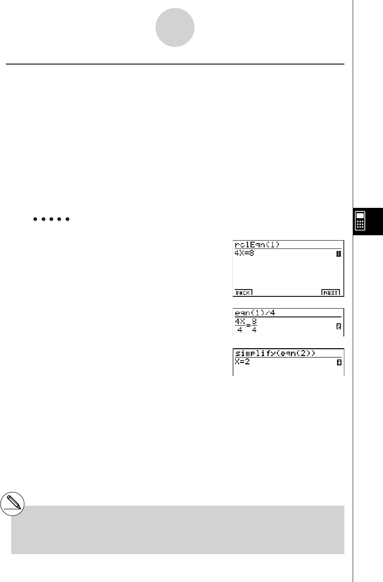
1999040120011101
7-3-8
Tutorial Mode
k Auto Mode
Press 6(AUTO) to enter the Auto Mode.
In the Simultaneous Equation Mode, you must also select SBSTIT (Substitution Method) or
ADD-SU (Addition/Subtraction Method).
The Substitution Method first transforms the equation to the format Y = aX + b, and
substitutes aX + b for Y*1 in the other equation.
The Addition/Subtraction Method multiplies both sides of the expression by the same value
to isolate the coefficient X (or Y).
As with the Algebra Mode, the screen is divided between an input area and a display area.
Each press of 6(NEXT) advances to the next step. 6(NEXT) is not shown on the display
when the solution is obtained.
You can scroll back through the steps by pressing 1(BACK).
Example To solve 4X = 8 in the Auto Mode
(Linear Equation)(AX = B)
2(INPUT)ewiw6(EXE)
6(AUTO)
6(NEXT)
6(NEXT)
*1You can press 5(ADD SU) at any time to
switch from Substitution Method to Addition /
Subtraction Method.
#See 7-1-8 for information about graph functions.

19990401
∫
a
b f(x)dx = F(b) – F(a)
7-4-1
Algebra System Precautions
7-4 Algebra System Precautions
•If an algebraic operation cannot be performed for some reason, the original expression
remains on the display.
•It may take considerable time to perform an algebraic operation. Failure of a result to
appear immediately does not indicate malfunction of the computer.
•Any expression can be displayed in various different formats. Because of this, you
should not assume that an expression is wrong just because it does not appear as you
expected.
•This calculator performs integration calculations under the assumption that integrals are
always positive, even when the integrals switch between positive and negative.
f(x)
F(x): primitive function of f(x)
20011101

19990401
Programming
8-1 Basic Programming Steps
8-2 Program Mode Function Keys
8-3 Editing Program Contents
8-4 File Management
8-5 Command Reference
8-6 Using Calculator Functions in Programs
8-7 Program Mode Command List
8-8 Program Library
Chapter
This unit comes with approximately 144 kbytes of memory.
•You can check how much memory has been used and how much remains
by entering the SYSTEM Mode from the Main Menu, and then pressing
1(Mem). See “9-2 Memory Operations” for details.
8
19990401
8-1 Basic Programming Steps
Description
Commands and calculations are executed sequentially, just like manual calculation
multistatements.
Set Up
1. From the Main Menu, enter the PRGM Mode. When you do, a program list appears on
the display.
Selected program area
(use
f
and
c
to move)
Files are listed in the alphabetic sequence of their
names.
Execution
2. Register a file name.
3. Input the program.
4. Run the program.
8-1-1
Basic Programming Steps
#If there are no programs stored in memory
when you enter the PRGM Mode, the
message “No Programs” appears on the
display and only the NEW item (3) is shown
in the function menu.
#The values to the right of the program list
indicate the number of bytes used by each
program.
#A file name can be up to eight characters
long.
#The following are the characters you can use in
a file name:
A through Z, r,
θ
, spaces, [, ], {, }, ’, ”, ~,
0 through 9, ., +, –, ×, ÷
#Registering a file name uses 24 bytes of
memory.
#The file name input screen remains on the
display if you press w without inputting a file
name.
#To exit the file name input screen and return to
the program list without registering a file name,
press i.
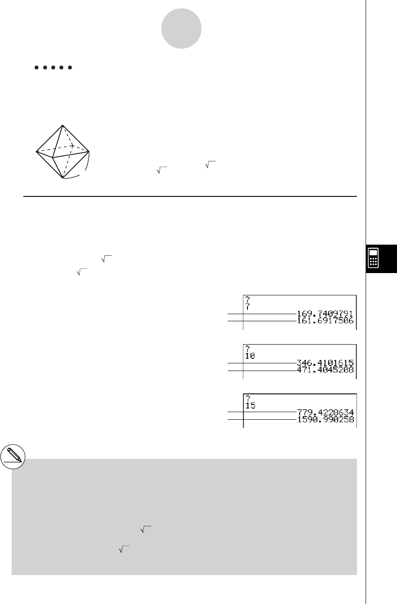
19990401
Example 1 To calculate the surface area (cm2) and volume (cm3) of three regular
octahedrons when the length of one side is 7, 10, and 15 cm,
respectively.
Store the calculation formula under the file name OCTA.
A
The following are the formulas used for calculating surface area S
and volume V of a regular octahedron for which the length of one side
A is known.
Procedure
1m PRGM
23(NEW)OCTAw*1
3!J(PRGM)3(?)aav(A)6(g)6(g)3(:)*2
c*!x( )d*av(A)x6(g)4(^)
!x( )c/d*av(A)Md
ii
41(EXE) or w
hw(Value of A)
w
w
wbaw
w
w
wbfw
w*3
8-1-2
Basic Programming Steps
2
S = 2 3 A2,V = –––– A3
3
*1Press 3(NEW) and the cursor changes form
to indicate alpha character input.
*2The following shows how the calculation of the
surface area and volume of a regular
octahedron would be calculated using a
manual calculation.
Surface Area S ... c*!x()d*
<value of A> xw
Volume V ............ !x()c/d*
<value of A> Mdw
*3Pressing w while the final result of a program
is on the display changes to the program list.
#You can also run a program while in the RUN
•
MAT Mode by inputting: Prog ”<file name>” w.
# Pressing w while the final result of a program
executed using this method is on the display
re-executes the program.
#An error occurs if the program specified by Prog
”<file name>” cannot be found.
S when A = 7
V when A = 7
S when A = 10
V when A = 10
S when A = 15
V when A = 15
20011101

19990401
8-2 Program Mode Function Keys
•{NEW} ... {new program}
u When you are registering a file name
•{RUN}/{BASE} ... {general calculation}/{number base} program input
•{
QQ
QQ
Q} ... {password registration}
•{SYBL} ... {symbol menu}
uWhen you are inputting a program —— 1(RUN) … default
•{JUMP} ... {top}/{bottom} of program
•{SRC} ... {search}
•{MAT}/{STAT}/{LIST}/{GRPH}/{DYNA}/{RECR}
... {matrix}/{statistic}/{list}/{graph}/ {Dynamic Graph}/{recursion} menu
•Pressing !J(PRGM) displays the following PRGM (PROGRAM) menu.
•{Prog} ... {program recall}
•{JUMP} ... {jump command menu}
•{?}/{^^
^^
^} ... {input}/{output} command
•{I/O} ... {I/O control/transfer command menu}
•{IF}/{FOR}/{WHLE}/{CTRL}/{LOGIC}
... {conditional jump}/{loop control}/{conditional loop control}/{program control}/
{logical operation} command menu
•{CLR}/{DISP} ... {clear}/{display} command menu
•{
:} ......... {separator for expressions and commands}
See “8-5 Command Reference” for full details on each of these commands.
•Pressing u3(SET UP) displays the mode command menu shown below.
•{ANGL}/{DISP}/{CPLX}/{GRPH}/{STAT}/{DERIV}/{T-VAR}/{Σ DSP}
See “SET UP Screen Function Key Menus” on page 1-7-1 for details about each of these
commands.
8-2-1
Program Mode Function Keys

19990401
u When you are inputting a program —— 2(BASE)*1
•{JUMP}/{SRC}
•{d~o} ... {decimal}/{hexadecimal}/{binary}/{octal} value input
•{LOG} ... {logical operators}
•{DISP} ... conversion of displayed value to {decimal}/{hexadecimal}/{binary}/{octal}
•{SYBL} ... {symbol menu}
•Pressing !J(PRGM) displays the following PRGM (PROGRAM) menu.
•{Prog}/{JUMP}/{?}/{^^
^^
^}
•{= ≠ <} ... {logical operator menu}
•{
:} ......... {separator for expressions and commands}
•Pressing u3(SET UP) displays the mode command menu shown below.
•{Dec}/{Hex}/{Bin}/{Oct}
•{EXE}/{EDIT}
... program {execute}/{edit}
•{NEW} ... {new program}
•{DEL}/{DEL·A}
... {specific program}/{all program} delete
•{SRC}/{REN}
... file name {search}/{change}
8-2-2
Program Mode Function Keys
*1Programs input after pressing 2(BASE) are
indicated by
B
to the right of the file name.
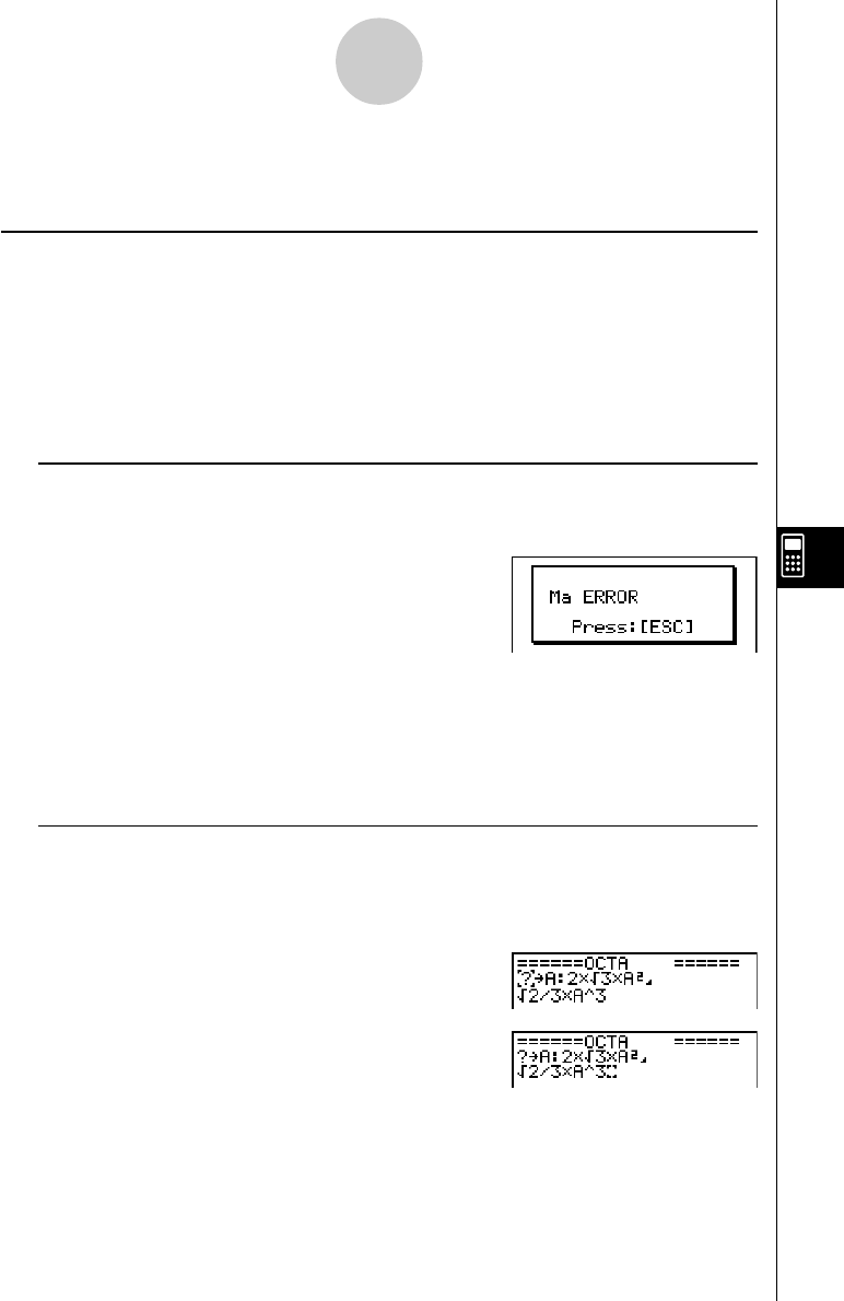
19990401
8-3-1
Editing Program Contents
8-3 Editing Program Contents
kDebugging a Program
A problem in a program that keeps the program from running correctly is called a “bug,” and
the process of eliminating such problems is called “debugging.” Either of the following
symptoms indicates that your program contains bugs that require debugging.
•Error messages appearing when the program is run
•Results that are not within your expectations
uu
uu
uTo eliminate bugs that cause error messages
An error message, like the one shown below, appears whenever something illegal occurs
during program execution.
When such a message appears, press i to display the place in the program where the error
was caused. The cursor will be flashing at the location of the problem. Check the “Error
Message Table” (page
α
-1-1) for steps you should take to correct the situation.
•Note that pressing i does not display the location of the error if the program is
password protected. Instead, it returns to the program list screen.
uu
uu
uTo eliminate bugs that cause bad results
If your program produces results that are not what you normally expect, check the
contents of the program and make necessary changes.
The 1(JUMP) key is also useful when editing program contents.
1(JUMP)b(Top) ....... Moves the cursor to the
top of the program
1(JUMP)c(Bottom)…Moves the cursor to the
bottom of the program
19990401
kUsing an Existing Program to Create a New Program
Sometimes you can input a new program by using a program already in memory as a base.
Simply recall the existing program, make the changes you need, and then execute it.
Example 2 To use the OCTA program (page 8-1-2) to create a program that
calculates the surface area (cm2) and volume (cm3) of regular
tetrahedrons when the length of one side is 7, 10, and 15 cm
Use TETRA as the file name.
The following are the formulas used for calculating surface area S
and volume V of a regular tetrahedron for which the length of one
side A is known.
Use the following key operations when inputting the program.
Length of One Side A .. !J(PRGM)3(?)aav(A)6(g)6(g)3(:)
Surface Area S ............ !x( )d*av(A)x6(g)4(^)
Volume V ..................... !x( )c/bc*av(A)Md
Compare this with the program for calculating the surface area and volume of a regular
octahedron.
Length of One Side A .. !J(PRGM)3(?)aav(A)6(g)6(g)3(:)
Surface Area S ............ c*!x( )d*av(A)x6(g)4(^)
Volume V ..................... !x( )c/d*av(A)Md
As you can see, you can produce the TETRA program by making the following changes in
the OCTA program.
•Deleting c * (underlined using a wavy line above)
•Changing d to b c (underlined using a solid line above)
A
8-3-2
Editing Program Contents
2
S = 3 A2,V = –––– A3
12
19990401
8-3-3
Editing Program Contents
Now edit OCTA to produce the TETRA program.
1. Edit the program name.
6(g)2(REN)ATETRAw
2. Edit the program contents.
2(EDIT)
eeeeDD
cdDbc
i
3. Try running the program.
1(EXE) or w
hw(Value of A)
w
w
wbaw
w
w
wbfw
w
19990401
8-3-4
Editing Program Contents
kSearching for Data Inside a Program
Example To search for the letter “A” inside the program named OCTA
1. Recall the program.
2. Press 2(SRC) or w and input the data you want to find.
2(SRC)
av(A)
3. Press w to begin the search. The contents of the program appear on the screen with
the cursor located at the first instance of the data you specified.*1
4. Each press of w or 1(SRC) causes the cursor to
jump to the next instance of the data you specified.*2
*1The message “Not Found” appears when the
search data you specify cannot be found in
the program.
*2If there are no more instances of the data you
specified, the search operation ends and the
cursor returns to the point from which you
started your search.
#You cannot specify the newline symbol (_) or
display command (^) for the search data.
# Once the contents of the program are on the
screen, you can use the cursor keys to move
the cursor to another location before searching
for the next instance of the data. Only the part of
the program starting from the current cursor
location is searched when you press w.
#Once the search finds an instance of your data,
inputting characters or moving the cursor
causes the search operation to be cancelled.
#If you make a mistake while inputting characters
to search for, press A to clear your input and
re-input from the beginning.
20011101
19990401
8-4-1
File Management
8-4 File Management
kSearching for a File
uTo find a file using initial character search
Example To use initial character search to recall the program named OCTA
1. While the program list is on the display, press 6(g)1(SRC) and input the initial
characters of the file you want to find.
6(g)1(SRC)
OCT
2. Press w to search.
•The name that starts with the characters you input highlights.
#If there is no program whose file name starts
with the characters you input, the message
“Not Found” appears on the display. If this
happens, press i to clear the error message.
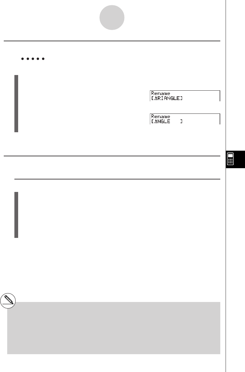
19990401
8-4-2
File Management
kk
kk
kEditing a file name
Example To change the name of a file from TRIANGLE to ANGLE
1. While the program list is on the display, use f and c to move the highlighting to the
file whose name you want to edit and then press 6(g)2(REN).
2. Make any changes you want.
DDD
3. Press w to register the new name and return to the program list.
The program list is resorted according to the changes you made in the file name.
kk
kk
kDeleting a Program
uTo delete a specific program
1. While the program list is on the display, use f and c to move the highlighting to the
name of the program you want to delete.
2. Press 4(DEL).
3. Press w(Yes) to delete the selected program or i(No) to abort the operation
without deleting anything.
#If the modifications you make result in a file
name that is identical to the name of a
program already stored in memory, the
message “Already Exists” appears. When this
happens, you can perform either of the
following two operations to correct the
situation.
•Press i to clear the error and return to the file
name editing screen.
•Press A to clear the input file name and input
a new one.
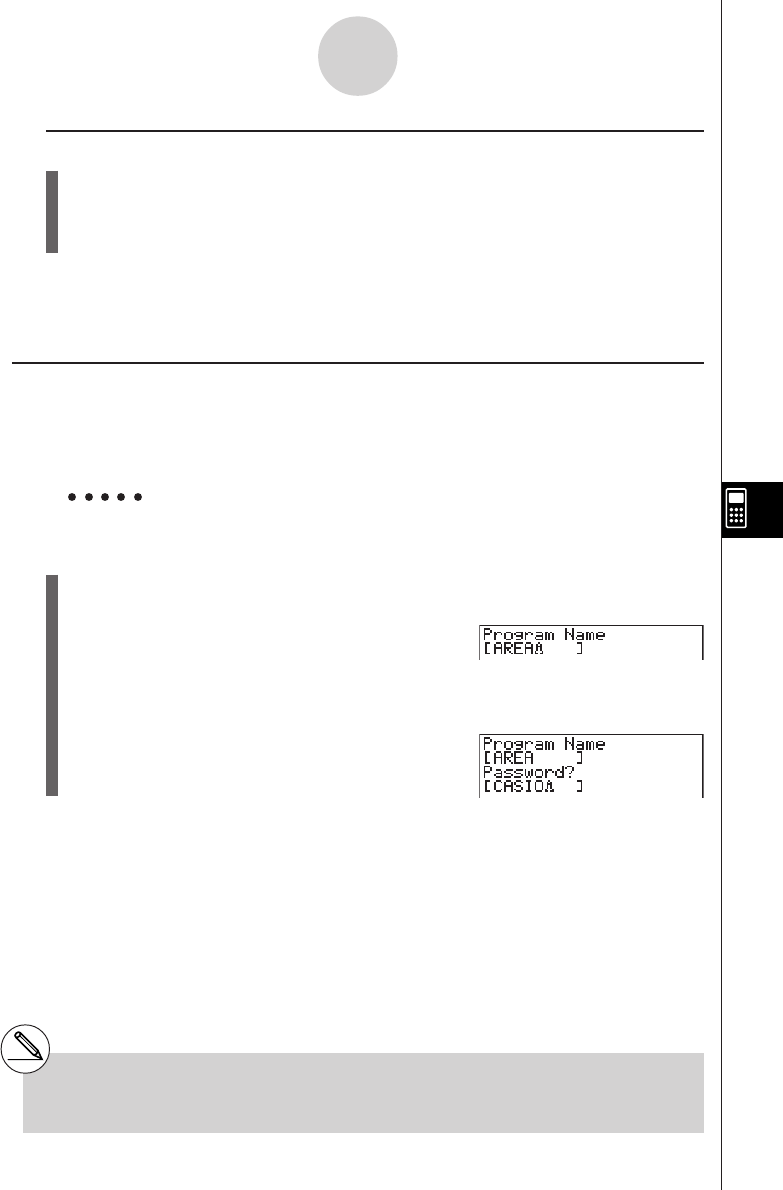
19990401
8-4-3
File Management
uTo delete all programs
1. While the program list is on the display, press 5(DEL·A).
2. Press w(Yes) to delete all the programs in the list or i(No) to abort the operation
without deleting anything.
•You also can delete all programs by entering the SYSTEM Mode from the Main Menu, and
then pressing 1(Mem) to display the memory management screen.
See “9-2 Memory Operations” for details.
kk
kk
kRegistering a password
When inputting a program, you can protect it with a password that limits access to the
program contents to those who know the password.
•You do not need to input the password to run a program.
Example To create a program file under the name AREA and protect it with the
password CASIO
1. While the program list is on the display, press 3(NEW) and input the file name of the
new program file.
3(NEW)
AREA
2. Press 5(Q) and then input the password.
5(Q)
CASIO
#The password input procedure is identical to
that used for file name input.
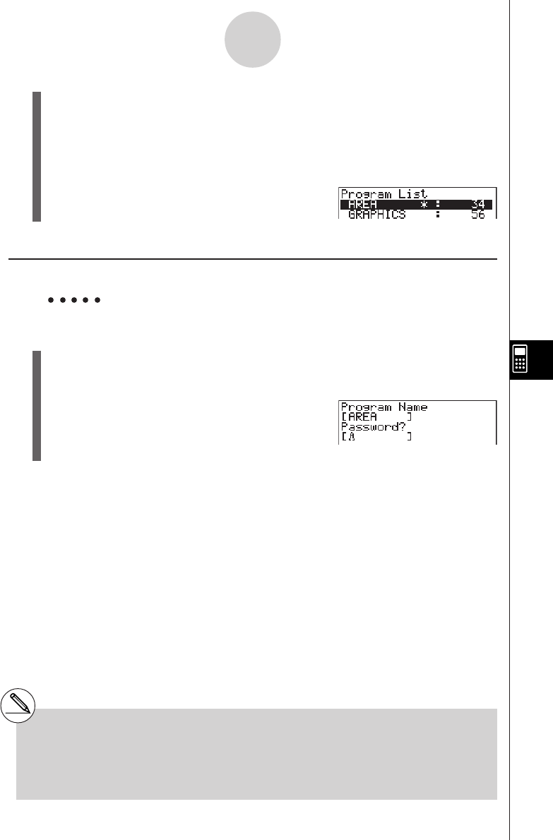
19990401
8-4-4
File Management
3. Press w to register the file name and password. Now you can input the contents of
the program file.
4. After inputting the program, press !i(QUIT) to exit the program file and return to
the program list. Files that are password protected are indicated by an asterisk to the
right of the file name.
kk
kk
kRecalling a Password Protected Program
Example To recall the file named AREA which is protected by the password
CASIO
1. In the program list, use f and c to move the highlighting to the name of the
program you want to recall.
2. Press 2(EDIT).
3. Input the password and press w to recall the program.
#Pressing w without inputting a password
while saving a new program causes the file to
be saved without a password. Pressing w
without inputting a password registers the file
name only, without a password.
#Inputting the wrong password when recalling a
password protected program causes the
message "Mismatch" to appear. Press i to
return to the password input screen.

19990401
8-5-1
Command Reference
8-5 Command Reference
kCommand Index
Break ...............................................................................................................8-5-6
ClrGraph ....................................................................................................... 8-5-11
ClrList ............................................................................................................8-5-11
ClrText ........................................................................................................... 8-5-12
ClrMat ............................................................................................................8-5-12
DispF-Tbl, DispR-Tbl .....................................................................................8-5-12
Do~LpWhile .....................................................................................................8-5-5
DrawDyna ..................................................................................................... 8-5-12
DrawFTG-Con, DrawFTG-Plt ........................................................................8-5-13
DrawGraph ................................................................................................... 8-5-13
DrawR-Con, DrawR-Plt ................................................................................. 8-5-13
DrawRΣ-Con, DrawRΣ-Plt .............................................................................8-5-14
DrawStat ....................................................................................................... 8-5-14
DrawWeb .......................................................................................................8-5-14
Dsz ..................................................................................................................8-5-9
For~To~(Step~)Next ........................................................................................ 8-5-4
Getkey ...........................................................................................................8-5-15
Goto~Lbl ....................................................................................................... 8-5-10
If~Then~(Else~)IfEnd ......................................................................................8-5-4
Isz ..................................................................................................................8-5-11
Locate ............................................................................................................8-5-16
Prog ................................................................................................................ 8-5-7
Receive ( / Send ( ..........................................................................................8-5-17
Return .............................................................................................................8-5-8
Stop ................................................................................................................ 8-5-8
While~WhileEnd ..............................................................................................8-5-6
? (Input Command) ......................................................................................... 8-5-2
^ (Output Command) .....................................................................................8-5-3
: (Multi-statement Command) ..........................................................................8-5-3
_ (Carriage Return) .......................................................................................8-5-3
’ (Comment Text Delimiter) .............................................................................. 8-5-3
=,
GG
GG
G
, >, <, ≥, ≤ (Relational Operators) ........................................................... 8-5-18

19990401
8-5-2
Command Reference
The following are conventions that are used in this section when describing the various
commands.
Boldface Text ............... Actual commands and other items that always must be
input are shown in boldface.
{Curly Brackets} ........... Curly brackets are used to enclose a number of items,
one of which must be selected when using a command.
Do not input the curly brackets when inputting a com-
mand.
[Square Brackets] ........ Square brackets are used to enclose items that are
optional. Do not input the square brackets when inputting
a command.
Numeric Expressions ... Numeric expressions (such as 10, 10 + 20, A) indicate
constants, calculations, numeric constants, etc.
Alpha Characters ......... Alpha characters indicate literal strings (such as AB).
kk
kk
kBasic Operation Commands
? (Input Command)
Function: Prompts for input of values for assignment to variables during program execution.
Syntax: ? → <variable name>, ”<prompt>” ? → <variable name>
Example: ? → A
Description:
•This command momentarily interrupts program execution and prompts for input of a value
or expression for assignment to a variable. If you do not specify a prompt, execution of this
command causes “?” to appear indicating the calculator is standing by for input. If a prompt
is specified, “<prompt>?” appears to prompt input. Up to 255 bytes of text can be used for a
prompt.
•Input in response to the input command must be a value or an expression, and the
expression cannot be a multi-statement.
•You can specify a list name, matrix name, function memory (fn), graph (Yn), etc. as a
variable name.
19991201

19990401
8-5-3
Command Reference
^^
^^
^ (Output Command)
Function: Displays an intermediate result during program execution.
Description:
•This command momentarily interrupts program execution and displays alpha character text
or the result of the calculation immediately before the command.
•The output command should be used at locations where you would normally press the w
key during a manual calculation.
: (Multi-statement Command)
Function: Connects two statements for sequential execution without stopping.
Description:
•Unlike the output command (^), statements connected with the multi-statement command
are executed non-stop.
•The multi-statement command can be used to link two calculation expressions or two
commands.
•You can also use a carriage return indicated by _ in place of the multi-statement
command.
__
__
_ (Carriage Return)
Function: Connects two statements for sequential execution without stopping.
Description:
•Operation of the carriage return is identical to that of the multi-statement command.
•You can create a blank line in a program by inputting a carriage return only. Using a carriage
return in place of the multi-statement command makes the displayed program easier to read.
’ (Comment Text Delimiter)
Function: Indicates comment text inserted inside a program.
Description: Anything following the apostrophe is treated as non-executable comment text.
19991201
19990401
kProgram Commands (COM)
If~Then~(Else~)IfEnd
Function: The Then-statement is executed only when the If-condition is true
(non-zero). The Else-statement is executed when the If-condition is false (0). The IfEnd-
statement is always executed following either the Then-statement or Else-statement.
Syntax:
Parameters: condition, numeric expression
Description:
(1) If ~ Then ~ IfEnd
• When the condition is true, execution proceeds with the Then-statement and then
continues with the statement following IfEnd.
• When the condition is false, execution jumps to the statement following IfEnd.
(2) If ~ Then ~ Else ~ IfEnd
• When the condition is true, execution proceeds with the Then-statement and then jumps
to the statement following IfEnd.
• When the condition is false, execution jumps to the Else-statement and then continues
with the statement following IfEnd.
For~To~(Step~)Next
Function: This command repeats everything between the For-statement and the Next-
statement. The starting value is assigned to the control variable with the first execution, and
the value of the control variable is changed according to the step value with each execution.
Execution continues until the value of the control variable exceeds the ending value.
Syntax:
Parameters:
•control variable name: A to Z
•starting value: value or expression that produces a value (i.e. sin x, A, etc.)
•ending value: value or expression that produces a value (i.e. sin x, A, etc.)
•step value: numeric value (default: 1)
8-5-4
Command Reference
If <condition>
_
:
^
Then <statement>
_
:
^
<statement>
numeric expression
_
:
^
Else <statement>
_
:
^
<statement>
_
:
^
IfEnd
_
For
<starting value> → <control variable name>
To
<ending value>
Step
<step value>
:
^
Next

19990401
8-5-5
Command Reference
Description:
•The default step value is 1.
•Making the starting value less than the ending value and specifying a positive step value
causes the control variable to be incremented with each execution. Making the starting
value greater than the ending value and specifying a negative step value causes the control
variable to be decremented with each execution.
Do~LpWhile
Function: This command repeats specific commands as long as its condition is true (non-
zero).
Syntax:
Parameters: expression
Description:
•This command repeats the commands contained in the loop as long as its condition is true
(non-zero). When the condition becomes false (0), execution proceeds from the statement
following the LpWhile-statement.
•Since the condition comes after the LpWhile-statement, the condition is tested (checked)
after all of the commands inside the loop are executed.
__
Do :<statement> : LpWhile <condition>
^^
numeric expression

19990401
8-5-6
Command Reference
While~WhileEnd
Function: This command repeats specific commands as long as its condition is true (non-
zero).
Syntax:
Parameters: expression
Description:
•This command repeats the commands contained in the loop as long as its condition is true
(non-zero). When the condition becomes false (0), execution proceeds from the statement
following the WhileEnd-statement.
•Since the condition comes after the While-statement, the condition is tested (checked)
before the commands inside the loop are executed.
kk
kk
kProgram Control Commands (CTL)
Break
Function: This command breaks execution of a loop and continues from the next command
following the loop.
Syntax: Break
Description:
•This command breaks execution of a loop and continues from the next command following
the loop.
•This command can be used to break execution of a For-statement, Do-statement, and
While-statement.
_
:
^
_
:
^
While <condition> <statement> WhileEnd
numeric expression
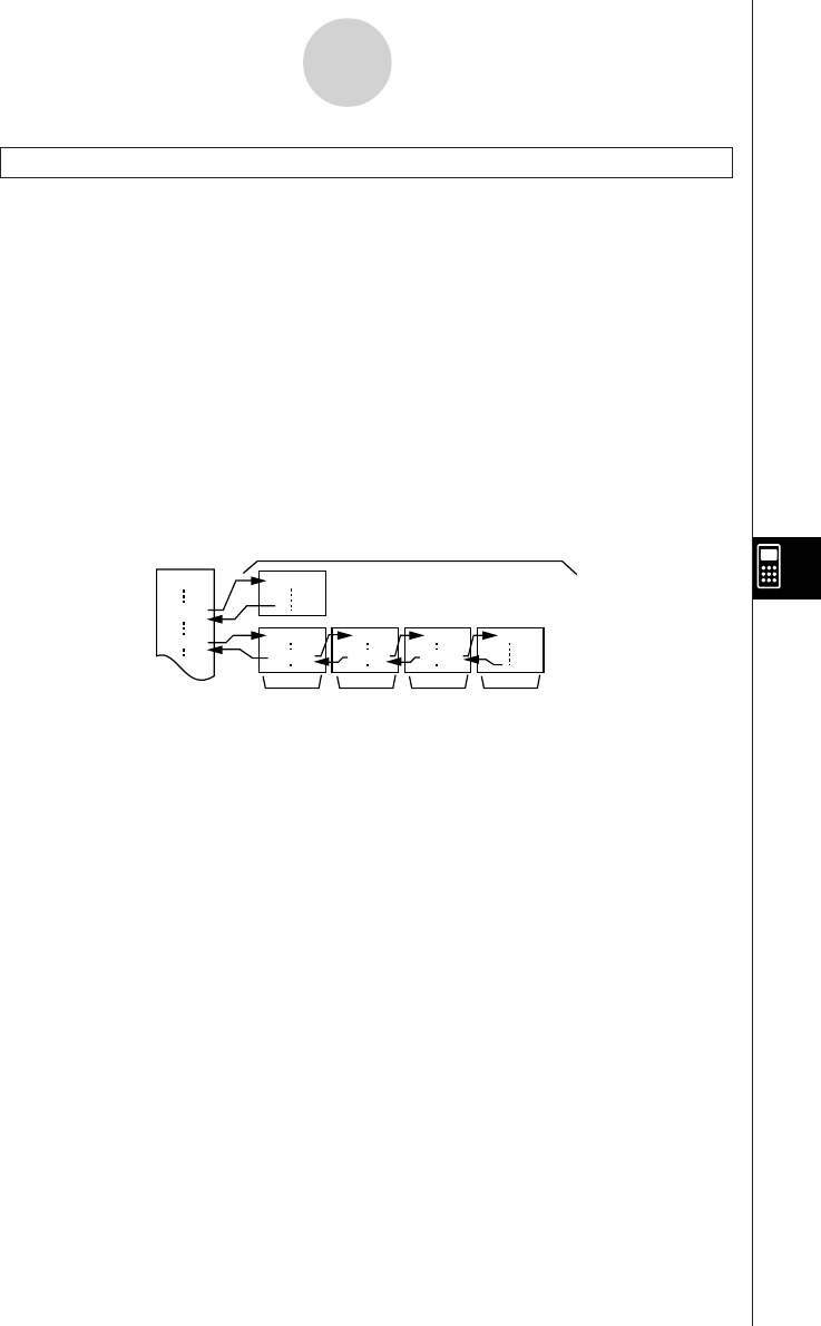
19990401
8-5-7
Command Reference
Prog
Function: This command specifies execution of another program as a subroutine. In the
RUN
•
MAT Mode, this command executes a new program.
Syntax: Prog ”file name”
Example: Prog ”ABC”
Description:
•Even when this command is located inside of a loop, its execution immediately breaks the
loop and launches the subroutine.
•This command can be used as many times as necessary inside of a main routine to call up
independent subroutines to perform specific tasks.
•A subroutine can be used in multiple locations in the same main routine, or it can be called
up by any number of main routines.
Main Routine Subroutines
D
CEIJ
Prog ”E” Prog ”I” Prog ”J”
A
Prog ”D”
Prog ”C”
Level 1 Level 2 Level 3 Level 4
•Calling up a subroutine causes it to be executed from the beginning. After execution of the
subroutine is complete, execution returns to the main routine, continuing from the state-
ment following the Prog command.
•A Goto~Lbl command inside of a subroutine is valid inside of that subroutine only. It cannot
be used to jump to a label outside of the subroutine.
•If a subroutine with the file name specified by the Prog command does not exist, an error
occurs.
•In the RUN
•
MAT Mode, inputting the Prog command and pressing w launches the
program specified by the command.

19990401
8-5-8
Command Reference
Return
Function: This command returns from a subroutine.
Syntax: Return
Description:
Execution of the Return command inside a main routine causes execution of the program to
stop. Execution of the Return command within a subroutine terminates the subroutine and
returns to the program from which the subroutine was jumped to.
Stop
Function: This command terminates execution of a program.
Syntax: Stop
Description:
•This command terminates program execution.
•Execution of this command inside of a loop terminates program execution without an error
being generated.
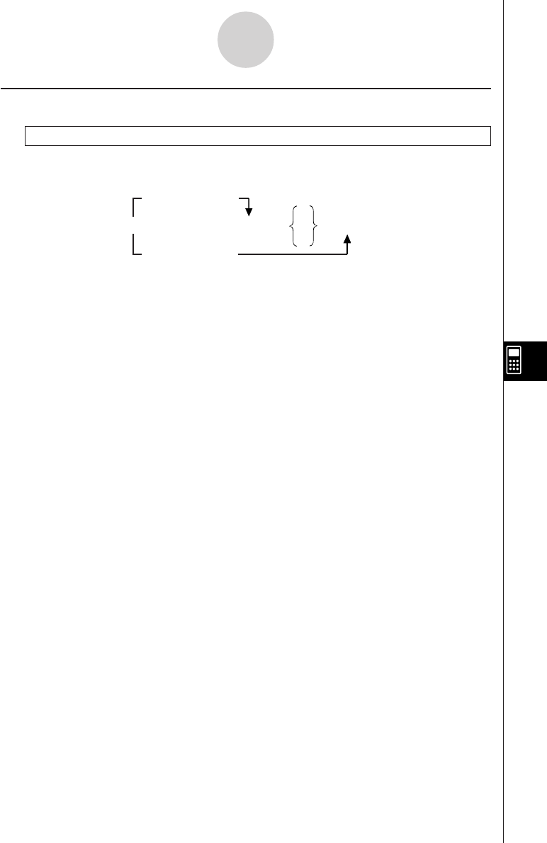
19990401
8-5-9
Command Reference
kJump Commands (JUMP)
Dsz
Function: This command is a count jump that decrements the value of a control variable by
1, and then jumps if the current value of the variable is zero.
Syntax:
Parameters: variable name: A to Z, r,
θ
[Example] Dsz B : Decrements the value assigned to variable B by 1.
Description:
This command decrements the value of a control variable by 1, and then tests (checks) it. If
the current value is non-zero, execution continues with the next statement. If the current
value is zero, execution jumps to the statement following the multi-statement command (:),
display command (^), or carriage return (_).
Variable Value GG
GG
G 0
_
Dsz <variable name> : <statement> :<statement>
^
Variable Value = 0

19990401
8-5-10
Command Reference
Goto~Lbl
Function: This command performs an unconditional jump to a specified location.
Syntax: Goto <label name> ~ Lbl <label name>
Parameters: label name: value (0 to 9), variable (A to Z, r,
θ
)
Description:
•This command consists of two parts: Goto n (where n is a parameter as described above)
and Lbl n (where n is the parameter referenced by Goto n). This command causes program
execution to jump to the Lbl-statement whose n parameter matches that specified by the
Goto-statement.
•This command can be used to loop back to the beginning of a program or to jump to any
location within the program.
•This command can be used in combination with conditional jumps and count jumps.
•If there is no Lbl-statement whose value matches that specified by the Goto-statement, an
error occurs.
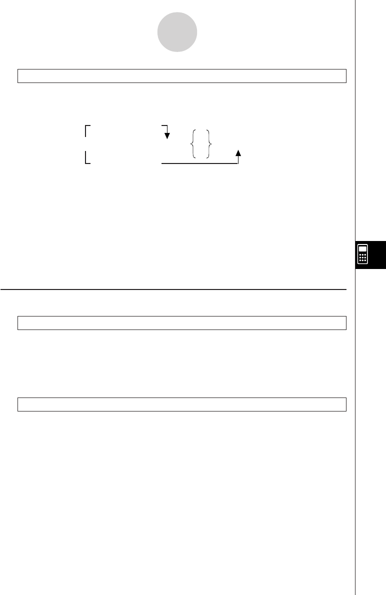
19990401
Isz
Function: This command is a count jump that increments the value of a control variable by
1, and then jumps if the current value of the variable is zero.
Syntax:
Parameters: variable name: A to Z, r,
θ
[Example] Isz A : Increments the value assigned to variable A by 1.
Description:
This command increments the value of a control variable by 1, and then tests (checks) it. If
the current value is non-zero, execution continues with the next statement. If the current
value is zero, execution jumps to the statement following the multi-statement command (:),
display command (^), or carriage return (_).
kk
kk
kClear Commands (CLR)
ClrGraph
Function: This command clears the graph screen and returns View Window settings to their
INIT values.
Syntax: ClrGraph
Description: This command clears the graph screen during program execution.
ClrList
Function: This command deletes list data.
Syntax: ClrList <list name>
ClrList
Parameters: list name: 1 to 20, Ans
Description: This command deletes the data in the list specified by “list name”. All list data is
deleted if nothing is specified for “list name”.
8-5-11
Command Reference
Variable Value GG
GG
G 0
_
Isz <variable name> : <statement> :<statement>
^
Variable Value = 0
20011101

19990401
8-5-12
Command Reference
ClrText
Function: This command clears the text screen.
Syntax: ClrText
Description: This command clears text from the screen during program execution.
ClrMat
Function: This command deletes matrix data.
Syntax: ClrMat <matrix name>
ClrMat
Parameters: matrix name: A to Z, Ans
Description: This command deletes the data in the matrix specified by “matrix name”. All
matrix data is deleted if nothing is specified for “matrix name”.
kk
kk
kDisplay Commands (DISP)
DispF-Tbl, DispR-Tbl No parameters
Function: These commands display numeric tables.
Description:
•These commands generate numeric tables during program execution in accordance with
conditions defined within the program.
•DispF-Tbl generates a function table, while DispR-Tbl generates a recursion table.
DrawDyna No parameters
Function: This command executes a Dynamic Graph draw operation.
Description: This command draws a Dynamic Graph during program execution in
accordance with current Dynamic Graph parameters.

19990401
8-5-13
Command Reference
DrawFTG-Con, DrawFTG-Plt No parameters
Function: This command uses values in a generated table to graph a function.
Description:
•This command draws a function graph in accordance with current conditions.
•DrawFTG-Con produces a connect type graph, while DrawFTG-Plt produces a plot type
graph.
DrawGraph No parameters
Function: This command draws a graph.
Description:
•This command draws a graph in accordance with current conditions.
DrawR-Con, DrawR-Plt No parameters
Function: These commands use values in a generated table to graph a recursion
expression with an(bn or cn) as the vertical axis and n as the horizontal axis.
Description:
•These commands graph recursion expressions in accordance with current conditions, with
an(bn or cn) as the vertical axis and n as the horizontal axis.
•DrawR-Con produces a connect type graph, while DrawR-Plt produces a plot type graph.

19990401
8-5-14
Command Reference
DrawRΣ-Con, DrawRΣ-Plt No parameters
Function: These commands use values in a generated table to graph a recursion
expression with Σan(Σbn or Σcn) as the vertical axis and n as the horizontal axis.
Description:
•These commands graph recursion expressions in accordance with current conditions, with
Σan(Σbn or Σcn) as the vertical axis and n as the horizontal axis.
•DrawRΣ-Con produces a connect type graph, while DrawRΣ-Plt produces a plot type graph.
DrawStat
Function: This draws a statistical graph.
Syntax: See “8-6-9 Using Statistical Calculations and Graphs in a Program”.
Description:
This command draws a statistical graph in accordance with current statistical graph
conditions.
DrawWeb
Function: This command graphs convergence/divergence of a recursion expression (WEB
graph).
Syntax: DrawWeb <recursion type>, <number of lines>
Example: DrawWeb an+1 (bn+1 or cn+1), 5
Description:
•This command graphs convergence/divergence of a recursion expression (WEB graph).
•Omitting the number of lines specification automatically specifies the default value 30.
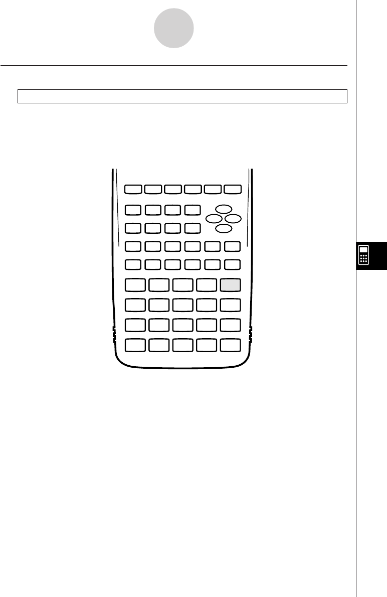
19990401
8-5-15
Command Reference
kInput/Output Commands (I/O)
Getkey
Function: This command returns the code that corresponds to the last key pressed.
Syntax: Getkey
Description:
•This command returns the code that corresponds to the last key pressed.
64
79
78 68 58 48
77 67 57 47
76 66 56 46
75
74 54 44
6373 53 43 33
6272 52 42 32
6171 51 41 31
65 55 45
36
35
26
25
69 59 49 39 29
28
38 27
37
•A value of zero is returned if no key was pressed previous to executing this command.
•This command can be used inside of a loop.
19990401
8-5-16
Command Reference
Locate
Function: This command displays alpha-numeric characters at a specific location on the text
screen.
Syntax: Locate <column number>, <line number>, <value>
Locate <column number>, <line number>, <numeric expression>
Locate <column number>, <line number>, ”<string>”
[Example] Locate 1, 1, ”AB”_
Parameters:
•line number: number from 1 to 7
•column number: number from 1 to 21
•value and numeric expression
•string: character string
Description:
•This command displays values (including variable contents) or text at a specific location on
the text screen. If there is a calculation input, that calculation result is displayed.
•The line is designated by a value from 1 to 7, while the column is designated by a value
from 1 to 21.
(1, 1) → ← (21, 1)
(1, 7) → ← (21, 7)
Example: Cls_
Locate 7, 1, ”CASIO FX”
This program displays the text “CASIO FX” in the center of the screen.
•In some cases, the ClrText command should be executed before running the above program.
20011101

19990401
8-5-17
Command Reference
Receive ( / Send (
Function: This command receives data from and sends data to a connected device.
Syntax: Receive (<data>) / Send (<data>)
Description:
•This command receives data from and sends data to a connected device.
•The following types of data can be received (sent) by this command.
•Individual values assigned to variables
•Matrix data (all values - individual values cannot be specified)
•List data (all values - individual values cannot be specified)

19990401
8-5-18
Command Reference
kConditional Jump Relational Operators (REL)
=,
GG
GG
G
, >, <, ≥, ≤
Function: These relational operators are used in combination with the conditional jump
command.
Syntax:
Parameters:
left side/right side: variable (A to Z, r,
θ
), numeric constant, variable expression (such as: A ×
2)
relational operator: =,
GG
GG
G
, >, <, ≥, ≤
<left side> <relational operator> <right side>

19990401
8-6 Using Calculator Functions in Programs
kText Display
You can include text in a program by simply enclosing it between double quotation marks.
Such text appears on the display during program execution, which means you can add labels
to input prompts and results.
Program Display
”CASIO” CASIO
? → X?
”X =” ? → XX = ?
•If the text is followed by a calculation formula, be sure to insert a display command (^)
between the text and calculation.
•Inputting more than 21 characters causes the text to move down to the next line. The
screen scrolls automatically if the text exceeds 21 characters.
•You can specify up to 255 bytes of text for a comment.
kUsing Matrix Row Operations in a Program
These commands let you manipulate the rows of a matrix in a program.
•For this program, enter the RUN • MAT Mode and then use the MAT Editor to input the
matrix, and then enter the PRGM Mode to input the program.
uTo swap the contents of two rows (Swap)
Example 1 To swap the values of Row 2 and Row 3 in the following matrix:
12
Matrix A = 34
56
The following is the syntax to use for this program.
Swap A, 2, 3_
Mat A
Executing this program produces the following result.
8-6-1
Using Calculator Functions in Programs
Rows to be swapped
Matrix name
1999120120011101
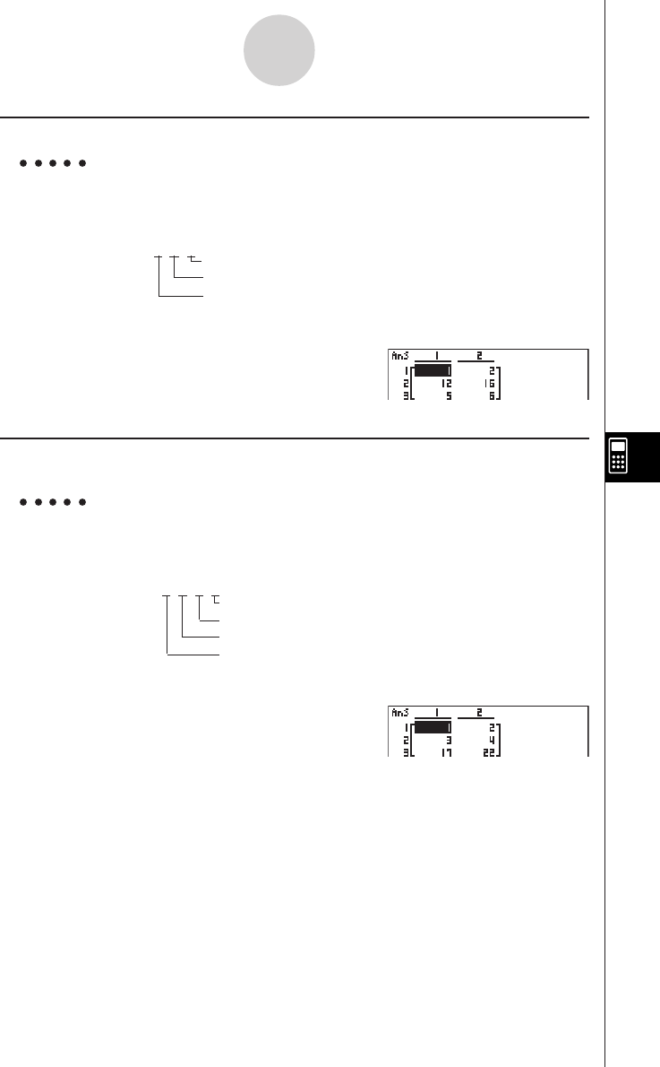
19990401
uTo calculate a scalar multiplication (``
``
`Row)
Example 2 To calculate the product of Row 2 of the matrix in Example 1 and the
scalar 4
The following is the syntax to use for this program.
`Row 4, A, 2_
Mat A
Executing this program produces the following result.
uTo calculate a scalar multiplication and add the results to another row
(``
``
`Row+)
Example 3 To calculate the product of Row 2 of the matrix in Example 1 and the
scalar 4, then add the result to row 3
The following is the syntax to use for this program.
`Row+ 4, A, 2, 3_
Mat A
Executing this program produces the following result.
8-6-2
Using Calculator Functions in Programs
Row
Matrix name
Multiplier
Matrix name
Multiplier
Rows to be added
Row for which scalar multiplication is to be calculated.
20011101
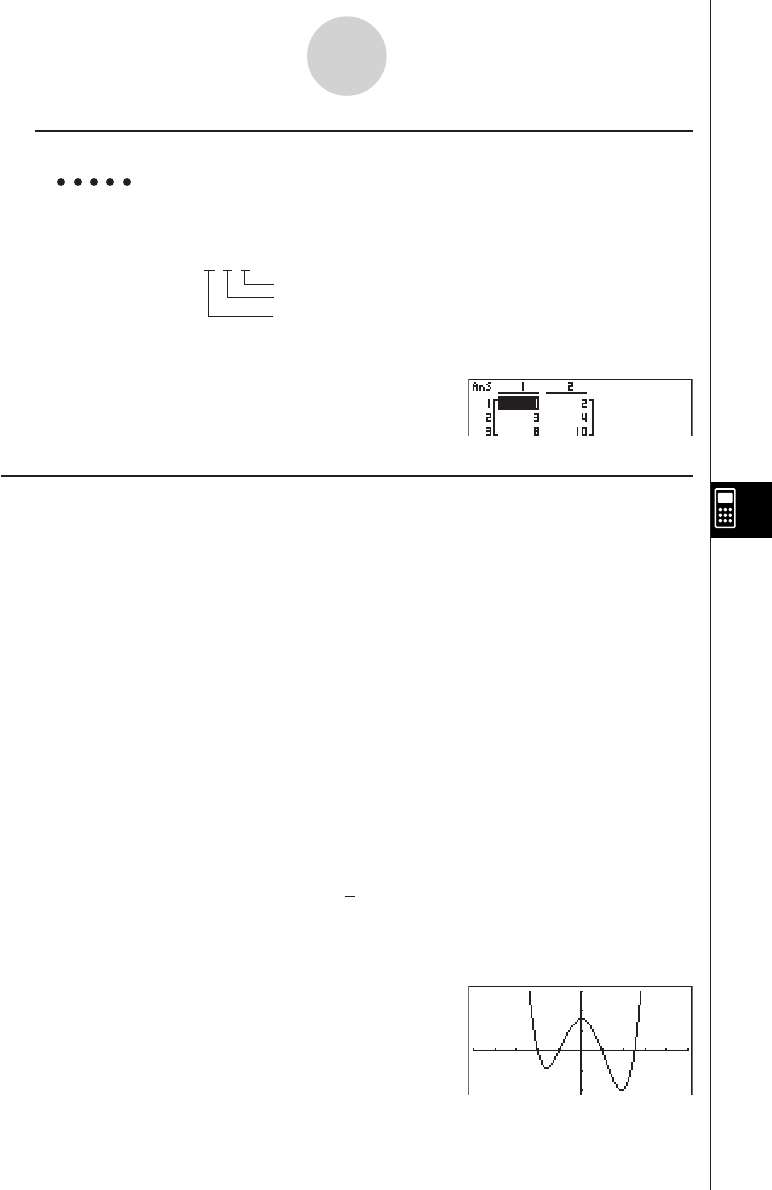
19990401
uTo add two rows (Row+)
Example 4 To add Row 2 to Row 3 of the matrix in Example 1
The following is the syntax to use for this program.
Row+ A, 2, 3_
Mat A
Executing this program produces the following result.
kk
kk
kUsing Graph Functions in a Program
You can incorporate graph functions into a program to draw complex graphs and to overlay
graphs on top of each other. The following shows various types of syntax you need to use when
programming with graph functions.
• View Window
View Window –5, 5, 1, –5, 5, 1_
• Graph function input
Y = Type_..................... Specifies graph type.
”X2 – 3” → Y1_
• Graph draw operation
DrawGraph_
Example Program
1ClrGraph_1 !J661ci
2View Window –10, 10, 2, –120, 150, 50_2 !K1i
3Y = Type_3 61db
”X^4–X^3–24X2 + 4X + 80” @ Y1_4 J4bi
4
5G SelOn 1_5 61b
6DrawGraph 6 !J662c
Executing this program produces the result
shown here.
8-6-3
Using Calculator Functions in Programs
20011101
Matrix name
the row number to be added to
the row number to be added

19990401
8-6-4
Using Calculator Functions in Programs
uSyntax of other graphing functions
• V-Window
View Window <Xmin>, <Xmax>, <Xscale>, <Ymin>, <Ymax>, <Yscale>,
<T
θ
min>, <T
θ
max>, <T
θ
pitch>
StoV-Win <area of V-Win> .............. area: 1 to 6
RclV-Win <area of V-Win> .............. area: 1 to 6
• Zoom
Factor <X factor>, <Y factor>
ZoomAuto ........... Non-parameter
• Pict
StoPict <area of picture> ................ area: 1 to 20
RclPict <area of picture> ................ area: 1 to 20
• Sketch
PlotOn <X-coordinate>, <Y-coordinate>
PlotOff <X-coordinate>, <Y-coordinate>
PlotChg <X-coordinate>, <Y-coordinate>
PxlOn<line number>, <column number>
PxlOff<line number>, <column number>
PxlChg<line number>, <column number>
PxlTest( <line number>, <column number>[)]
F-Line <X-coordinate 1>, <Y-coordinate 1>, <X-coordinate 2>, <Y-coordinate 2>
Text <line number>, <column number>, ”<text>”
Text <line number>, <column number>, <expression>
Tangent <function>, <X-coordinate>
Normal <function>, <X-coordinate>
Inverse <function>
Circle <center point X-coordinate>, <center point Y-coordinate>,
<radius R value>
Vertical <X-coordinate>
Horizontal <Y-coordinate>
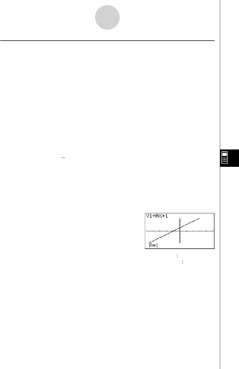
19990401
kk
kk
kUsing Dynamic Graph Functions in a Program
Using Dynamic Graph functions in a program makes it possible to perform repeated Dynamic
Graph operations. The following shows how to specify the Dynamic Graph range inside a
program.
• Dynamic Graph range
1 → DStart_
5 → DEnd_
1 → D pitch_
Example Program
ClrGraph_
View Window –5, 5, 1, –5, 5, 1_
Y = Type_
”AX + 1” → Y1_1 J4bi
1
2D SelOn 1_2 62b
3D Var A_3 2d
1 → 4 DStart_4 J5b
5 → 5 DEnd_5 5c
1 → 6 Dpitch_6 5d
7DrawDyna 7 !J662d
Executing this program produces the result
shown here.
↑
↓
8-6-5
Using Calculator Functions in Programs
20011101
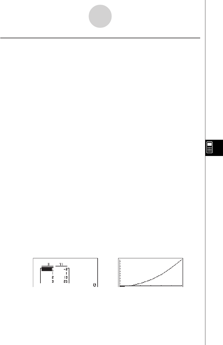
19990401
kk
kk
kUsing Table & Graph Functions in a Program
Table & Graph functions in a program can generate numeric tables and perform graphing
operations. The following shows various types of syntax you need to use when programming
with Table & Graph functions.
• Table range setting
1 → FStart_
5 → FEnd_
1 → F pitch_
• Numeric table generation
DispF-Tbl_
• Graph draw operation
Connect type: DrawFTG-Con_
Plot type: DrawFTG-Plt_
Example Program
ClrGraph_
ClrText_
View Window 0, 6, 1, –20, 106, 10_
Y = Type_
”3X2 – 2” → Y1_
1G SelOn 1_1 61b
0 → 2 FStart_2 J61b
6 → 3 FEnd_3 1c
1 → 4 Fpitch_4 1d
5DispF-Tbl^5 !J662eb
6DrawFTG-Con 6 !J662ec
Executing this program produces the results shown here.
Numeric Table Graph
8-6-6
Using Calculator Functions in Programs

19990401
kk
kk
kUsing Recursion Table & Graph Functions in a Program
Incorporating Recursion Table & Graph functions in a program lets you generate numeric
tables and perform graphing operations. The following shows various types of syntax you
need to use when programming with Recursion Table & Graph functions.
• Recursion formula input
an+1 Type_..... Specifies recursion type.
”3an + 2” → an+1_
”4bn + 6” → bn+1_
• Table range setting
1 → RStart_
5 → REnd_
1 → a0_
2 → b0_
1 → an Start_
3 → bn Start_
• Numeric table generation
DispR-Tbl_
• Graph draw operation
Connect type: DrawR-Con_, DrawRΣ-Con_
Plot type: DrawR-Plt_, DrawRΣ-Plt_
• Statistical convergence/divergence graph (WEB graph)
DrawWeb an+1, 10_
8-6-7
Using Calculator Functions in Programs
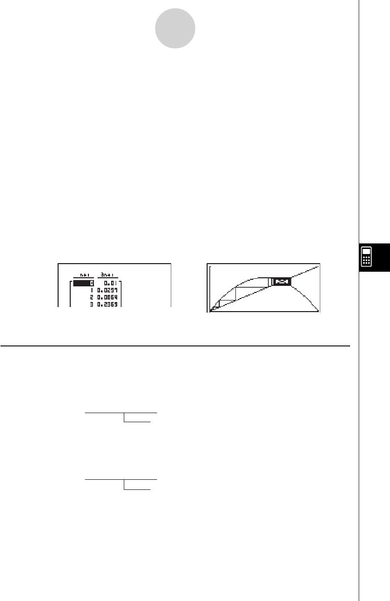
19990401
8-6-8
Using Calculator Functions in Programs
Example Program
View Window 0, 1, 1, –0.2, 1, 1_
1an+1 Type_
23
”–3an2 + 3an” → an+1_
0 → RStart_
6 → REnd_
0.01 → a0_
0.01 → an Start_
8DispR-Tbl^
0
9DrawWeb an+1, 30
Executing this program produces the results shown here.
Numeric Table Recursion graph
kk
kk
kUsing List Sort Functions in a Program
These functions let you sort data in lists into ascending or descending order.
• Ascending order
12
SortA (List 1, List 2, List 3)
Lists to be sorted (up to six can be specified)
1 5b 2 4e
• Descending order
3
SortD (List 1, List 2, List 3)
Lists to be sorted (up to six can be specified)
3 5c
4
5
6
1 63gc
2 3bc
3 3bd
4 J62cb
5 2cc
6 2cd
7 2cC
8 !J662fb
9 2fci
0 63bd
7
20011101

19990401
kk
kk
kUsing Solve Calculation Function in a Program
The following is the syntax for using the Solve function in a program.
Solve( f(x), n, a, b)
Upper limit
Lower limit
Initial estimated value
Example Program
1Solve( 2X2 + 7X – 9, 1, 0, 1) 1K4h
•In the function f(x), only X can be used as a variable in the expression. Other variables (A
through Z, r,
θ
) are treated as constants, and the value currently assigned to that variable is
applied during the calculation.
•Input of the closing parenthesis, lower limit a and upper limit b can be omitted.
kk
kk
kUsing Statistical Calculations and Graphs in a Program
Including statistical calculations and graphing operations in a program lets you calculate and
graph statistical data.
u To set conditions and draw a statistical graph
Following “StatGraph”, you must specify the following graph conditions:
• Graph draw/non-draw status (DrawOn/DrawOff)
• Graph Type
• x-axis data location (list name)
• y-axis data location (list name)
• Frequency data location (list name)
• Mark Type
8-6-9
Using Calculator Functions in Programs
#Solutions obtained using Solve may include
errors.
#You cannot use a differential, quadratic
differential, integration, Σ , maximum/
minimum value or Solve calculation
expressions inside of a Solve calculation
term.
20011101

19990401
The graph conditions that are required depends on the graph type. See “Changing Graph
Parameters” (page 6-1-2).
•The following is a typical graph condition specification for a scatter diagram or xyLine
graph.
S-Gph1 DrawOn, Scatter, List 1, List 2, 1, Square _
In the case of an xy line graph, replace “Scatter” in the above specification with “xyLine”.
•The following is a typical graph condition specification for a normal probability plot.
S-Gph1 DrawOn, NPPlot, List 1, Square _
•The following is a typical graph condition specification for a single-variable graph.
S-Gph1 DrawOn, Hist, List 1, List 2 _
The same format can be used for the following types of graphs, by simply replacing “Hist” in
the above specification with the applicable graph type.
Histogram: ..................................... Hist
Median Box: ................................... MedBox
Modified Box: ................................. Modified
Normal Distribution: ....................... N-Dist
Broken Line: .................................. Broken
•The following is a typical graph condition specification for a regression graph.
S-Gph1 DrawOn, Linear, List 1, List 2, List 3 _
The same format can be used for the following types of graphs, by simply replacing “Linear” in
the above specification with the applicable graph type.
Linear Regression: ........................ Linear
Med-Med: ...................................... Med-Med
Quadratic Regression: ................... Quad
Cubic Regression: ......................... Cubic
Quartic Regression: ....................... Quart
Logarithmic Regression: ................. Log
Exponential Regression: ................ Exp
Power Regression: ........................ Power
8-6-10
Using Calculator Functions in Programs
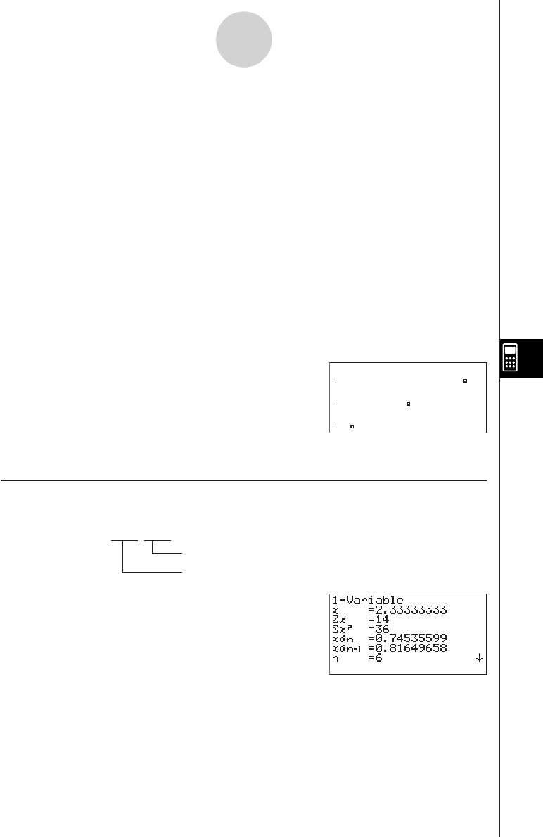
19990401
•The following is a typical graph condition specification for a sinusoidal regression graph.
S-Gph1 DrawOn, Sinusoidal, List 1, List 2 _
•The following is a typical graph condition specification for a logistic regression graph.
S-Gph1 DrawOn, Logistic, List 1, List 2 _
Example Program
ClrGraph_
1
S-Wind Auto_
{1, 2, 3} → List 1_
{1, 2, 3} → List 2_
23 4 5
S-Gph1 DrawOn, Scatter, List 1, List 2, 1, Square _
6
DrawStat
Executing this program produces the scatter
diagram shown here.
kPerforming Statistical Calculations
• Single-variable statistical calculation
11-Variable List 1, List 2
Frequency data (Frequency)
x
-axis data (XList)
14gb
8-6-11
Using Calculator Functions in Programs
1u35bbi
24bb
34cb
44db
54fb
6!J662b
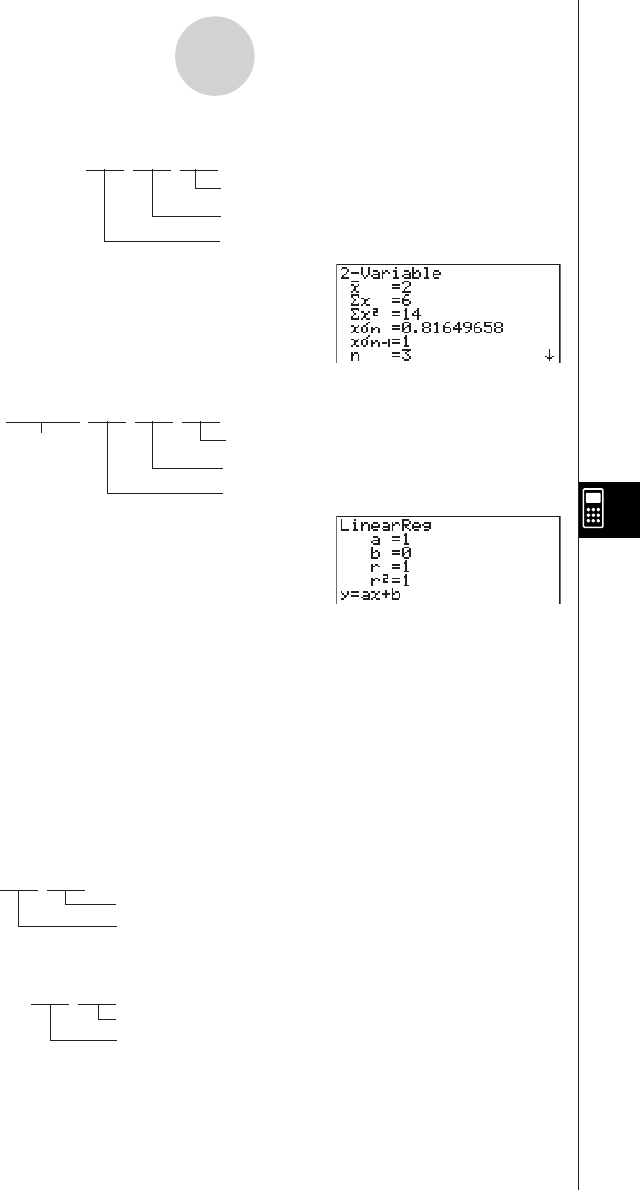
19990401
• Paired-variable statistical calculation
12-Variable List 1, List 2, List 3
Frequency data (Frequency)
y
-axis data (YList)
x
-axis data (XList)
14gc
• Regression statistical calculation
1LinearReg List 1, List 2, List 3
Calculation Frequency data (Frequency)
type*
y
-axis data (YList)
x
-axis data (XList)
14gd
*Any one of the following can be specified as the calculation type.
LinearReg .......... linear regression
Med-MedLine .... Med-Med calculation
QuadReg ........... quadratic regression
CubicReg ........... cubic regression
QuartReg ........... quartic regression
LogReg .............. logarithmic regression
ExpReg ............. exponential regression
PowerReg .......... power regression
8-6-12
Using Calculator Functions in Programs
•Sinusoidal regression statistical calculation
SinReg List 1, List 2
•Logistic regression statistical calculation
LogisticReg List 1, List 2
y
-axis data (YList)
x
-axis data (XList)
y
-axis data (YList)
x
-axis data (XList)
19990401
8-7-1
Program Mode Command List
8-7 Program Mode Command List
G_SelOn_
G_SelOff_
Y=TYPE
r=TYPE
ParamTYPE
X=cTYPE
Y>Type
Y<Type
Y≥Type
Y≤Type
StoGMEM
RclGMEM
D_SelOn_
D_SelOff_
D_Var_
Y=Type
r=Type
ParamType
n
an
an+
1
bn
bn+
1
cn
cn+
1
R_SelOn_
R_SelOff_
Sel_a
0
Sel_a
1
anType
an+
1
Type
an+
2
Type
SelOn
SelOff
TYPE
GMEM
SelOn
SelOff
Var
TYPE
n,an..
SelOn
SelOff
Sel a
0
Sel a
1
TYPE
Y=
r=
Param
X=c
Y>
Y<
Y>
Y<
Store
Recall
Y=
r=
Param
n
an
an+
1
bn
bn+
1
cn
cn+
1
an
an+
1
an+
2
Level 1
Level 2 Level 3 Command
θθ
MAT
STAT
LIST
Swap
*Row
*Row+
Row+
S-GPH
DRAW
GRAPH
List
MARK
CALC
SortA
SortD
Swap_
*Row_
*Row+_
Row+_
S-Gph1_
S-Gph2_
S-Gph3_
DrawOn
DrawOff
Scatter
xyLine
NPPlot
Hist
MedBox
ModifiedBox
N-Dist
Broken
Linear
Med-Med
Quad
Cubic
Quart
Log
Exp
Power
Sinusoidal
Logistic
List_
Square
Cross
Dot
1-Variable_
2-Variable_
LinearReg_
Med-MedLine_
QuadReg_
CubicReg_
QuartReg_
LogReg_
ExpReg_
PowerReg_
SinReg_
LogisticReg_
SortA(
SortD(
S-Gph1
S-Gph2
S-Gph3
On
Off
Scat
xyLine
NPPlot
Hist
Box
ModBox
N-Dist
Broken
Linear
MedMed
Quad
Cubic
Quart
Log
Exp
Power
Sin
Lgstic
•
1VAR
2VAR
Linear
MedMed
Quad
Cubic
Quart
Log
Exp
Power
Sin
Lgstic
x!
nPr
nCr
Ran#
P(
Q(
R(
t(
sinh
cosh
tanh
sinh
–1
cosh
–1
tanh
–1
°
r
g
° ’ ”
'
DMS
Pol(
Rec(
m
n
fn
Factor
Auto
Cls
PLOT
LINE
GRAPH
Text
PIXEL
Tangnt
Normal
Invrse
Circle
Vert
Horz
Store
Recall
’
”
~
*
#
On
Off
Change
Plot
F-Line
Line
Y=
dx
On
Off
Change
Test
!
P
C
Ran#_
P(
Q(
R(
t(
sinh_
cosh_
tanh_
sinh
–1
_
cosh
–1
_
tanh
–1
_
°
r
g
° ’ ”
'
DMS
Pol(
Rec(
m
n
fn
Factor_
ZoomAuto
Cls
PlotOn_
PlotOff_
PlotChg_
Plot_
F-Line_
Line
Graph_Y=
Graph_
Text_
PxlOn_
PxlOff_
PxlChg_
PxlTest(
Tangent_
Normal_
Inverse_
Circle_
Vertical_
Horizontal_
StoPict_
RclPict_
’
”
~
*
#
Level 1
Level 2 Level 3 Command
[OPTN] key
PROB
HYP
ANGL
STAT
FMEM
ZOOM
SKTCH
PICT
SYBL
° ’ ”
LIST
MAT
CPLX
CALC
NUM
List
Dim
Seq
Min
Max
Mean
Median
Sum
Prod
Cuml
%
AList
Augmnt
Fill
L→Mat
Mat
Dim
Det
Trn
Augmnt
Ident
Fill
M→List
Abs
Arg
Conjg
ReP
ImP
'
re^
i
'
a+bi
d/dx
d
2
/dx
2
dx
Σ
FMin
FMax
Solve
Abs
Int
Frac
Rnd
Intg
E-SYM
List_
Dim_
Seq(
Min(
Max(
Mean(
Median(
Sum_
Prod_
Cuml_
Percent_
AList_
Augment(
Fill(
List→Mat(
Mat_
Dim_
Det_
Trn_
Augment(
Identity_
Fill(
Mat→List(
Abs_
Arg_
Conjg_
ReP_
ImP_
'
re^ i
'
a+bi
d/dx(
d
2
/dx
2
(
(
Σ (
FMin(
FMax(
Solve(
Abs_
Int_
Frac_
Rnd
Intg_
m
n
p
f
k
M
G
T
P
E
m
n
p
f
k
M
G
T
P
E
RUN Program
∫∫
∫
∫∫
µµ
GRPH
DYNA
RECR
19990401
Level 1
V-WIN
FACT
STAT
Level 2
Xmin
Xmax
Xscale
Xdot
Ymin
Ymax
Yscale
T min
T max
T ptch
R-Xmin
R-Xmax
R-Xscl
R-Xdot
R-Ymin
R-Ymax
R-Yscl
R-Tmin
R-Tmax
R-Tpch
Xfact
Yfact
n
X
Y
GRAPH
Level 3
x
Σx
Σx2
xσn
xσn–
1
minX
maxX
y
Σy
Σy2
Σxy
y
σ
n
y
σ
n–1
minY
maxY
a
b
c
d
e
r
r2
Q1
Med
Q3
Mod
H-Strt
H-ptch
Command
[VARS] key
GRPH
DYNA
TABL
RECR
EQUA
PTS
Yn
rn
Xtn
Ytn
Xn
Start
End
Pitch
Start
End
Pitch
Result
FORM
RANGE
Result
S-Rslt
S-Coef
P-Rslt
P-Coef
x1
y1
x2
y2
x3
y3
an
an+1
an+2
bn
bn+1
bn+2
cn
cn+1
cn+2
R-Strt
R-End
a0
a1
a2
b0
b1
b2
c0
c1
c2
anStrt
bnstrt
cnStrt
x1
y1
x2
y2
x3
y3
Y
r
Xt
Yt
X
D_Start
D_End
D_pitch
F_Start
F_End
F_pitch
F_Result
an
an+1
an+2
bn
bn+1
bn+2
cn
cn+1
cn+2
R_Start
R_End
a0
a1
a2
b0
b1
b2
c0
c1
c2
anStart
bnStart
cnStart
R_Result
Sim_Result
Sim_Coef
Ply_Result
Ply_Coef
Level 1
Prog
JUMP
?
^
I/O
IF
FOR
WHLE
CTRL
LOGIC
CLR
DISP
:
Level 2
Lbl
Goto
lsz
Dsz
Locate
Getkey
Send
Receiv
If
Then
Else
IfEnd
For
To
Step
Next
While
WhlEnd
Do
LpWhle
Prog
Return
Break
Stop
= G <
And
Or
Not
Text
Graph
List
Matrix
Stat
Graph
Dyna
F-TBL
R-TBL
Level 3
=
G
>
<
>
<
Table
G-Con
G-Plot
Table
Web
R-Con
RΣ-Con
R-Plot
RΣ-Plt
Command
Prog_
Lbl_
Goto_
lsz_
Dsz_
?
^
Locate_
Getkey
Send(
Receive(
If_
Then_
Else_
IfEnd
For_
_To_
_Step_
Next
While_
WhileEnd
Do
LpWhile_
Prog_
Return
Break
Stop
=
G
>
<
>
<
_And_
_Or_
Not_
ClrText
ClrGraph
ClrList_
ClrMat_
DrawStat
DrawGraph
DrawDyna
DispF-Tbl
DrawFTG-Con
DrawFTG-Plt
DispR-Tbl
DrawWeb_
DrawR-Con
DrawR
Σ
-Con
DrawR-Plt
DrawR
Σ
-Plt
:
[SHIFT][VARS](PRGM) key
θ
θ
θ
θ
θ
θ
Xmin
Xmax
Xscl
Xdot
Ymin
Ymax
Yscl
T min
T max
T ptch
RightXmin
RightXmax
RightXscl
RightXdot
RightYmin
RightYmax
RightYscl
RightT min
RightT max
RightT ptch
Xfct
Yfct
n
x
Σx
Σx2
xσn
xσn–1
minX
maxX
y
Σy
Σy2
Σxy
yσn
yσn–1
minY
maxY
a
b
c
d
e
r
r2
Q1
Med
Q3
Mod
H_Start
H_pitch
θ
θ
θ
Level 1
ANGL
DISP
CPLX
GRPH
STAT
DERIV
T-VAR
Σ•DSP
Level 2
Deg
Rad
Gra
Fix
Sci
Norm
EngOn
EngOff
Real
a+bi
re^ i
G-FUNC
D-TYPE
BG
SIMUL
COORD
GRID
AXES
LABEL
S-WIN
File
RESID
On
Off
Range
List
On
Off
Level 3
On
Off
G-Con
G-Plot
None
Pict
On
Off
On
Off
On
Off
On
Off
On
Off
Auto
Manual
None
List
Command
Deg
Rad
Gra
Fix_
Sci_
Norm
EngOn
EngOff
Real
a+bi
re^ i
FuncOn
FuncOff
G-Connect
G-Plot
BG-None
BG-Pict_
SimulOn
SimulOff
CoordOn
CoordOff
GridOn
GridOff
AxesOn
AxesOff
LabelOn
LabelOff
S-WindAuto
S-WindMan
File_
Resid-None
Resid-List_
DerivOn
DerivOff
VarRange
VarList_
ΣdispOn
ΣdispOff
[CTRL][F3](SET UP) key
θθ
θ
8-7-2
Program Mode Command List
19990401
Level 1
d~o
LOG
DISP
Level 2
d
h
b
o
Neg
Not
and
or
xor
xnor
'
Dec
'
Hex
'
Bin
'
Oct
Level 3 Command
d
h
b
o
Neg_
Not_
and
or
xor
xnor
'
Dec
'
Hex
'
Bin
'
Oct
Level 1
Dec
Hex
Bin
Oct
Level 2 Level 3
Command
Dec
Hex
Bin
Oct
[CTRL][F3](SETUP) key
Level 1
V-Win
Sto
Rcl
Level 2 Level 3
Command
ViewWindow_
StoV-Win_
RclV-Win_
[SHIFT][OPTN](V-Window)key
BASE Program
Level 1
Prog
JUMP
?
^
= G <
:
Level 2
Lbl
Goto
lsz
Dsz
=
G
>
<
>
<
Level 3 Command
Prog_
Lbl_
Goto_
lsz_
Dsz_
?
^
=
G
>
<
>
<
:
[SHIFT][VARS](PRGM) key
8-7-3
Program Mode Command List
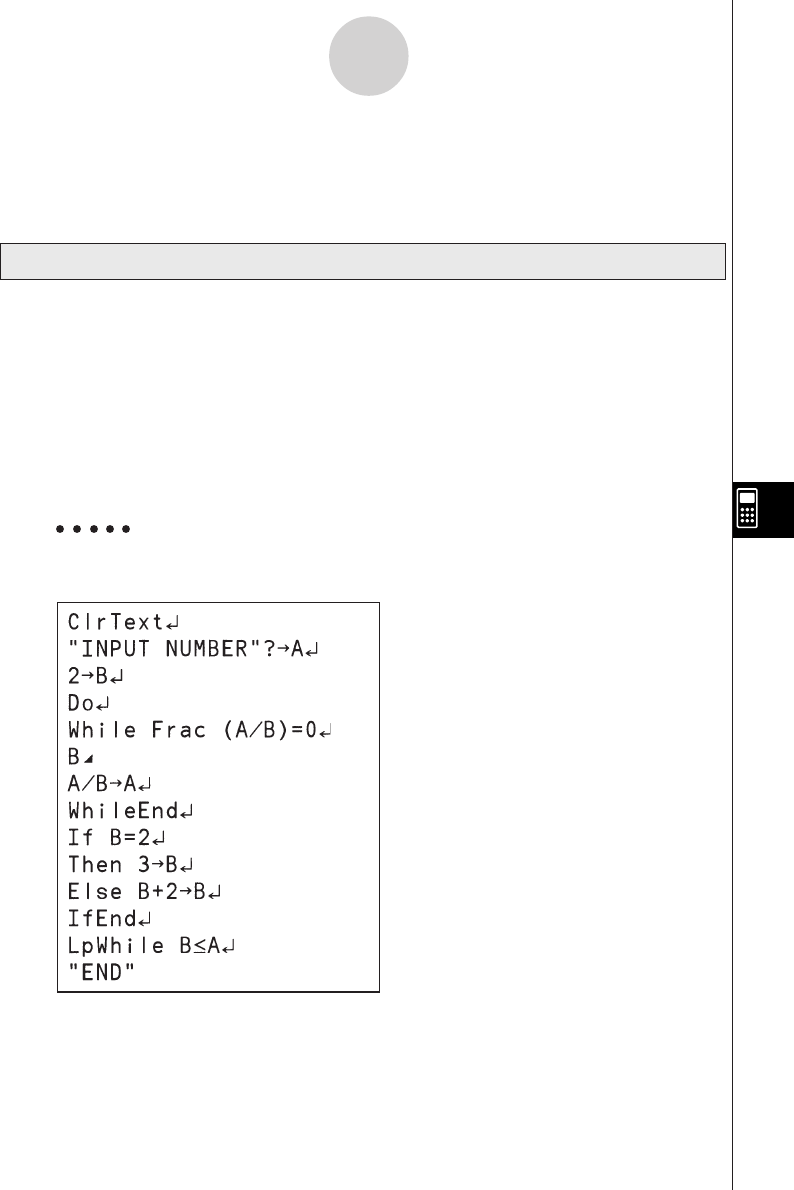
19990401
8-8-1
Program Library
Description
This program continually divides a natural number by factors until all its prime factors are
produced.
Purpose
This program accepts input of natural number A, and divides it by B (2, 3, 5, 7....) to find the
prime factors of A.
•If a division operation does not produce a remainder, the result of the operation is
assigned to A.
•The above procedure is repeated until B > A.
Example
440730 = 2 × 3 × 3 × 5 × 59 × 83
Program Name Prime Factorization
8-8 Program Library
•Be sure to check how many bytes of unused memory are remaining before attempting to
perform any programming.
20011101
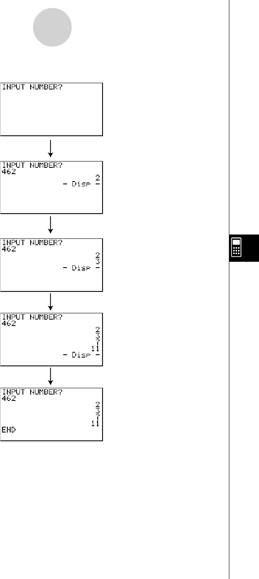
19990401
8-8-2
Program Library
egcw
w
ww
w
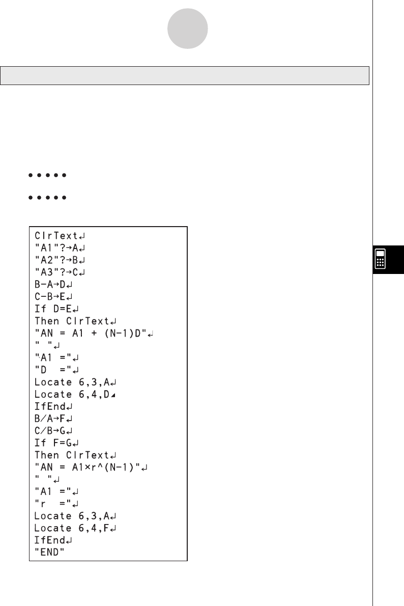
19990401
Description
After inputting sequence terms 1, 2, and 3, this program determines whether it is an arithmetic
sequence or geometric sequence based on the differences and ratios of the terms.
Purpose
This program determines whether a specific sequence is an arithmetic sequence or
geometric sequence.
Example 1 5, 10, 15, ... Arithmetic sequence
Example 2 5, 10, 20, ... Geometric sequence
Program Name Arithmetic-Geometric Sequence Differentiation
8-8-3
Program Library
20011101
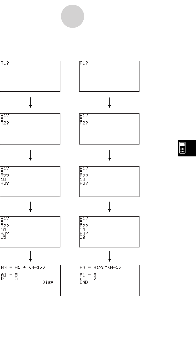
19990401
8-8-4
Program Library
Example 1 Example 2
fw
baw
bf
w
fw
baw
ca
w
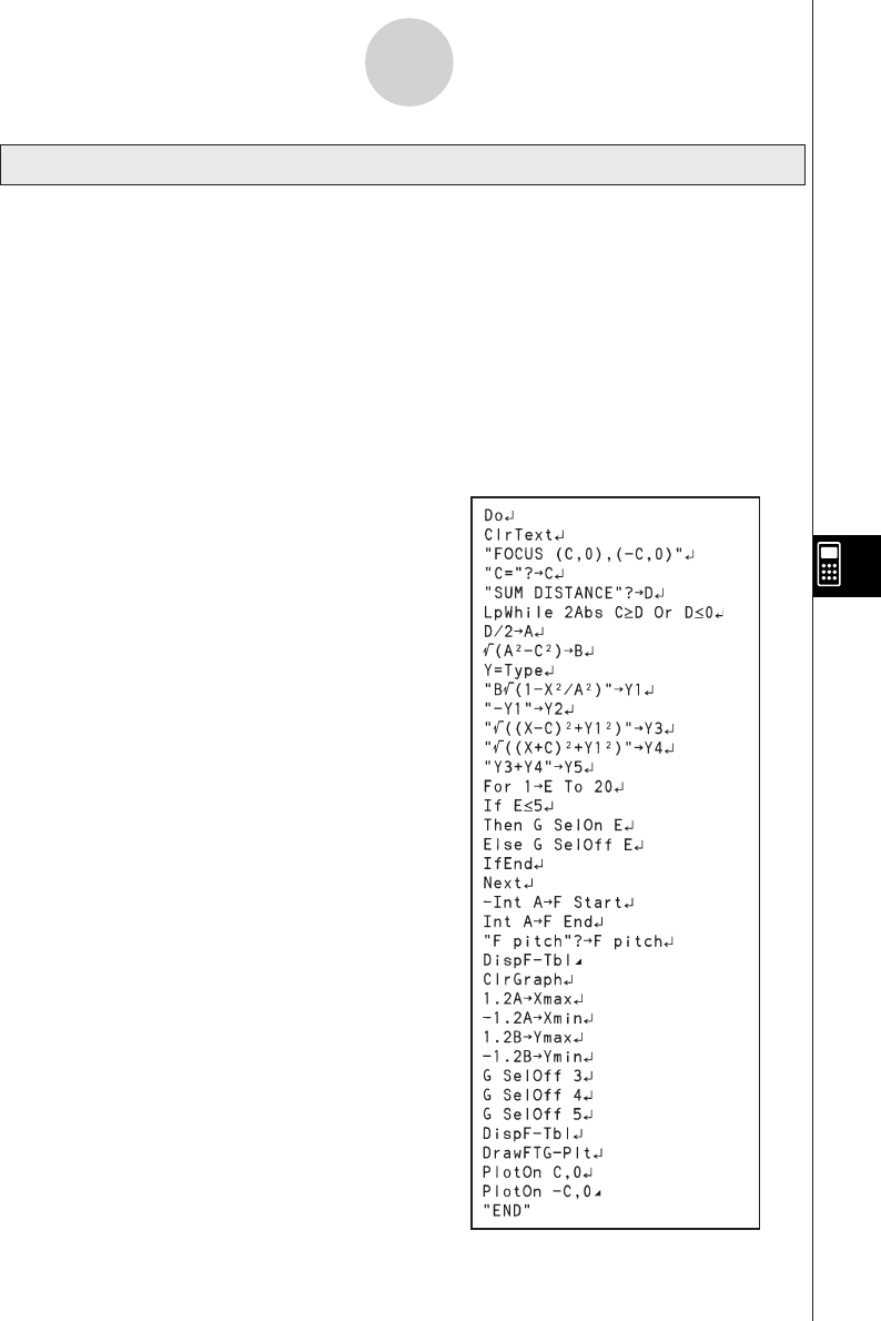
19990401
8-8-5
Program Library
Description
This program displays a number table of the following values based on input of the foci of an
ellipse, the sum of the distance between the loci and foci, and the pitch (step size) of X.
Y1: Coordinate values of upper half of ellipse
Y2: Coordinate values of lower half of ellipse
Y3: Distances between right focus and loci
Y4: Distances between left focus and loci
Y5: Sum of Y3 and Y4
Next, the program plots the foci and values in Y1 and Y2.
Purpose
This program shows that the sums of the
distances between the loci and two foci of an
ellipse are equal.
Program Name Ellipse
19990401
8-8-6
Program Library
wba
wb
w
wua
d
19991201
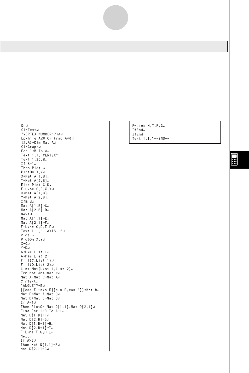
19990401
Description
This program draws an angle at the coordinate defined by an input vertex, and then rotates it
to a specified angle around the vertex.
Purpose
This program demonstrates coordinate transformation using a matrix.
Important!
Deg must be set as the angle unit for this program.
Program Name Rotation
8-8-7
Program Library
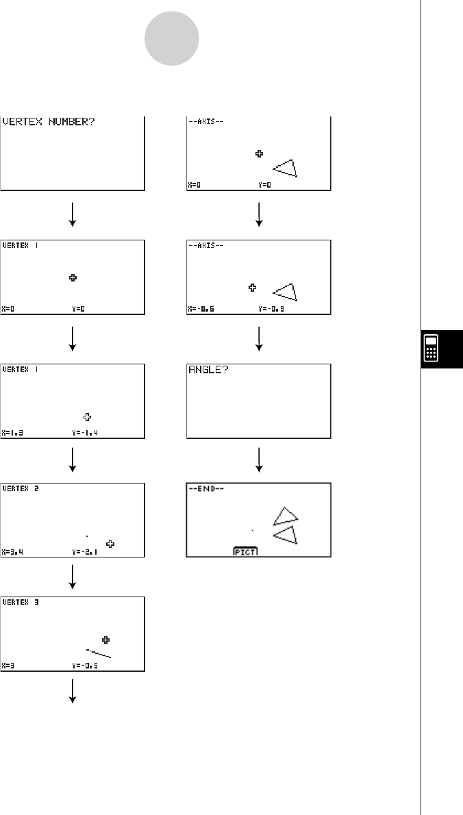
19990401
8-8-8
Program Library
dw
fcde
wwfcde
wwfcde
fcde
ww
daw
ww
19991201
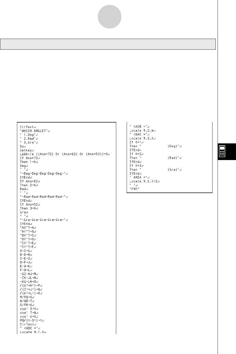
19990401
Description
This program calculates the interior angles and surface area of a triangle defined by input
coordinates for angles A, B, and C.
Purpose
This program calculates the interior angles and surface area of a triangle defined by
coordinates for angles A, B, and C.
Important!
Inputting the same coordinates for any two angles (A, B, C) causes an error.
Program Name Interior Angles and Surface Area of a Triangle
8-8-9
Program Library
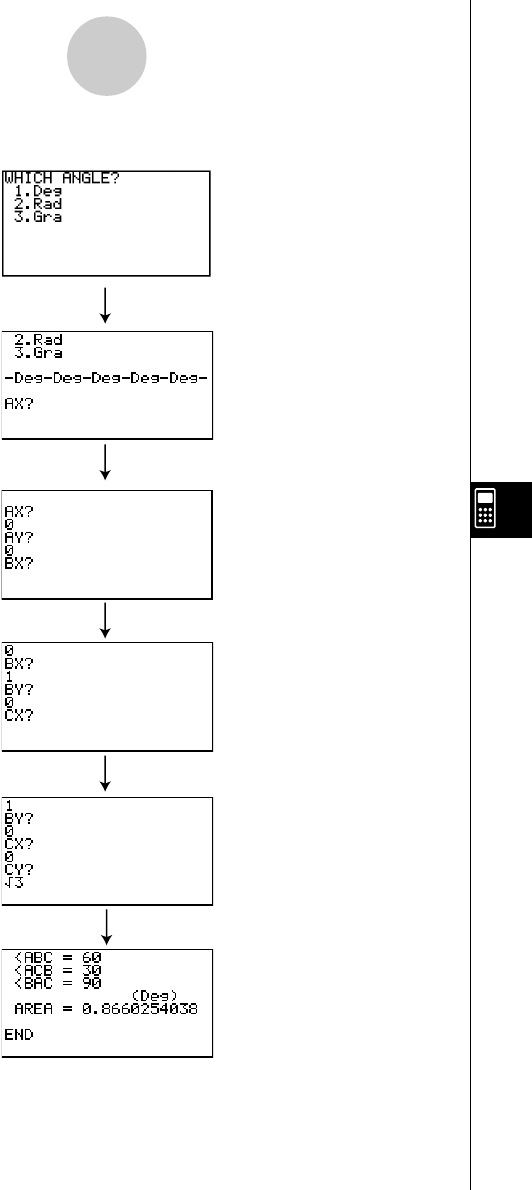
19990401
8-8-10
Program Library
b
awaw
bwaw
aw9d
w

19990401
Chapter
System Settings Menu
Use the system settings menu to view system information and
make system settings. The system settings menu lets you do the
following.
•View memory usage information
•Make contrast settings
•Make Auto Power Off settings
•Specify the system language
•Reset the calculator
•Tutorial Lock (ALGEBRA FX 2.0 PLUS only)
9-1 Using the System Settings Menu
9-2 Memory Operations
9-3 System Settings
9-4 Reset
9-5 Tutorial Lock (ALGEBRA FX 2.0 PLUS only)
9
20010102
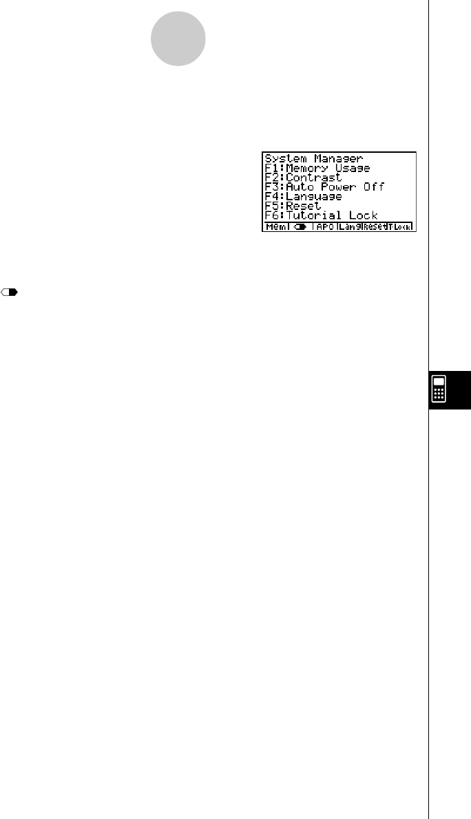
19990401
9-1-1
Using the System Settings Menu
9-1 Using the System Settings Menu
From the Main Menu, enter the SYSTEM Mode and display the following menu items.
• 1(Mem) ... {display current memory status and delete data stored in memory}
• 2() ... {display contrast adjustment}
• 3(APO) ... {Auto Power Off time setting}
• 4(Lang) ... {system language}
• 5(Reset) ... {system reset operations}
• 6(T-Lock) ... {Tutorial Lock}
• The T-Lock menu does not appear on the FX 1.0 PLUS.
20010102
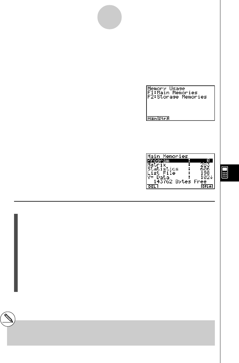
19990401
9-2 Memory Operations
Use the Mem (Memory Usage) item to view current memory status and to delete certain data
stored in memory.
While the initial System Settings Mode screen is displayed, press 1(Mem) to display the
Memory Usage screen.
• 1(Main) ... {display the Main Memories screen}
• 2(Strg) ... {display the Storage Memories screen.}
Pressing 1(Main) displays data currently assigned to Main Memories.
• To delete data
1. Use the f and c cursor keys to move the highlighting to the memory item whose
data you want to delete.
2. Depending on the screen that is on your display, press the function key assigned to the
DEL function.
• From the Main Memories screen, press 1(DEL).*1
• From the Storage Memories screen, press 6(DEL).
3. If you selected List File, Graph Memory, V-Win Memory, Picture or H-Copy Memory in
step 1, a menu appears so you can select which data you want to delete.
Input a number to specify the data and then press w.
4. In response to the confirmation message that appears, press w(Yes) to delete the
data you specified, or i(No) to cancel.
Pressing i or !i(QUIT) returns to the initial System Settings Mode screen.
9-2-1
Memory Operations
20011101
*1Pressing 6(DEL • A) deletes all the data in
the currently selected memory item.
#Performing the procedure to delete add-in
applications clears all currently installed add-ins.
You cannot delete add-ins individually.

19990401
9-2-2
Memory Operations
• To view memory usage information
Use f and c to move the highlighting and view the amount of memory (in bytes) used for
storage of each type of data.
The following table shows all of the data types that appear on the memory status screen.
Main Memories
Data Type Meaning
Program Program data
Matrix Matrix memory data
Statistics Statistical calculations and graphs
List File List data
Y=Data Graph functions
Draw Memory Graph drawing conditions (View Window,
enlargement/reduction factor)
Graph Memory Graph memory data
V-Win Memory View Window memory data
Picture Picture memory data
Table Function Table & Graph data
Dynamic Graph Dynamic Graph data
Recursion Recursion Table & Graph data
Equation Equation calculation data
Algebra Algebra variable data (ALGEBRA FX 2.0 PLUS only)
Financial Financial data
Diff Eq Differential equation and graphing conditions
E-Con E-CON setup memory, custom probe list
Alpha Memory Alpha memory data
Function Mem Function memory data
H-Copy Memory Screen shot transfer memory
System System Variable data
Others Other data
Storage Memories*1
Data Type Meaning
ADD-IN APP. Add-in applications
[B]~ Backup data
Pressing 1(Ver) displays the application names and versions of all currently installed add-
ins.
199912012001010120010102
*1Any item that does not contain any data does
not appear on the screen.
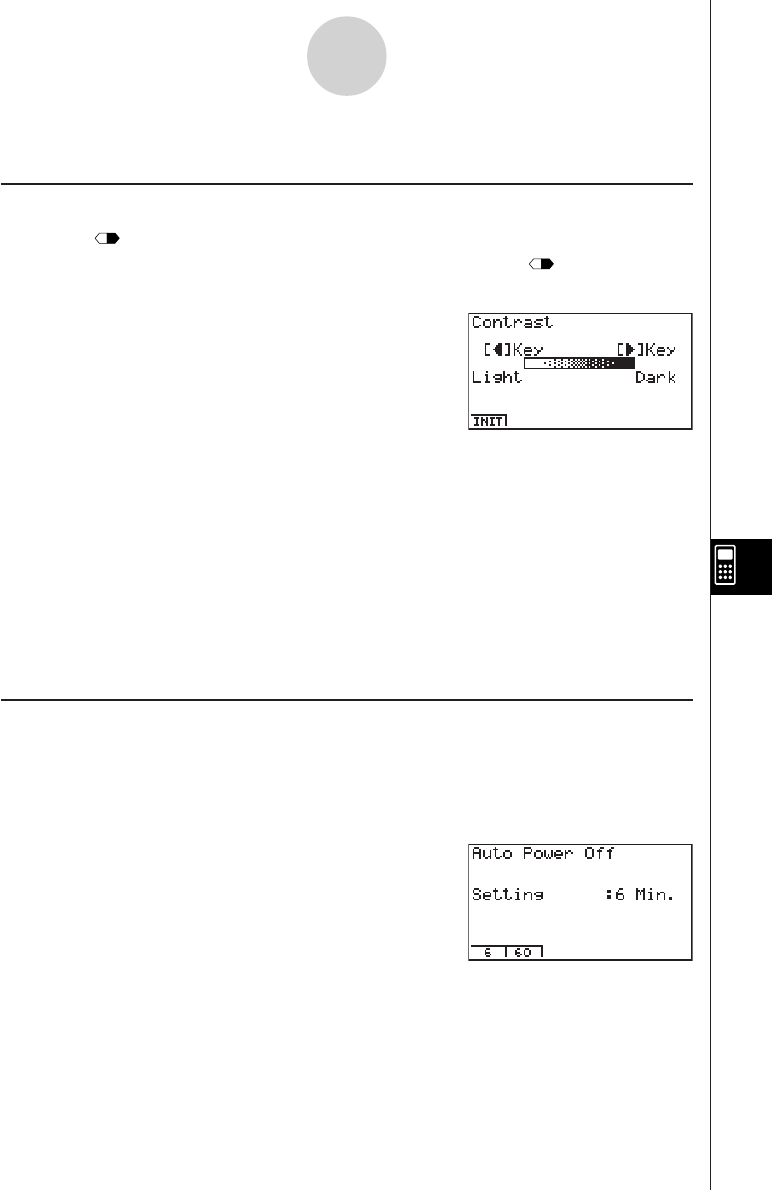
19990401
9-3 System Settings
kk
kk
kContrast Adjustment
Use the (Contrast) item to adjust display contrast.
While the initial System Settings Mode screen is displayed, press 2() to display the
Contrast Adjustment screen.
• The e cursor key makes display contrast darker.
• The d cursor key makes display contrast lighter.
• 1(INIT) returns display contrast to its initial default.
Pressing i or !i(QUIT) returns to the initial System Settings Mode screen.
You can adjust contrast while any screen besides the Main Menu is on the display by
pressing ! and then e or d. To exit contrast adjustment, press ! again.
kk
kk
kAPO Settings
You can specify either six minutes or 60 minutes as the Auto Power Off trigger time. The
initial default setting is six minutes.
While the initial System Settings Mode screen is displayed, press 3(APO) to display the
APO Setting screen.
• 1(6) ... 6 minutes
• 2(60) ... 60 minutes
Pressing i or !i(QUIT) returns to the initial System Settings Mode screen.
9-3-1
System Settings
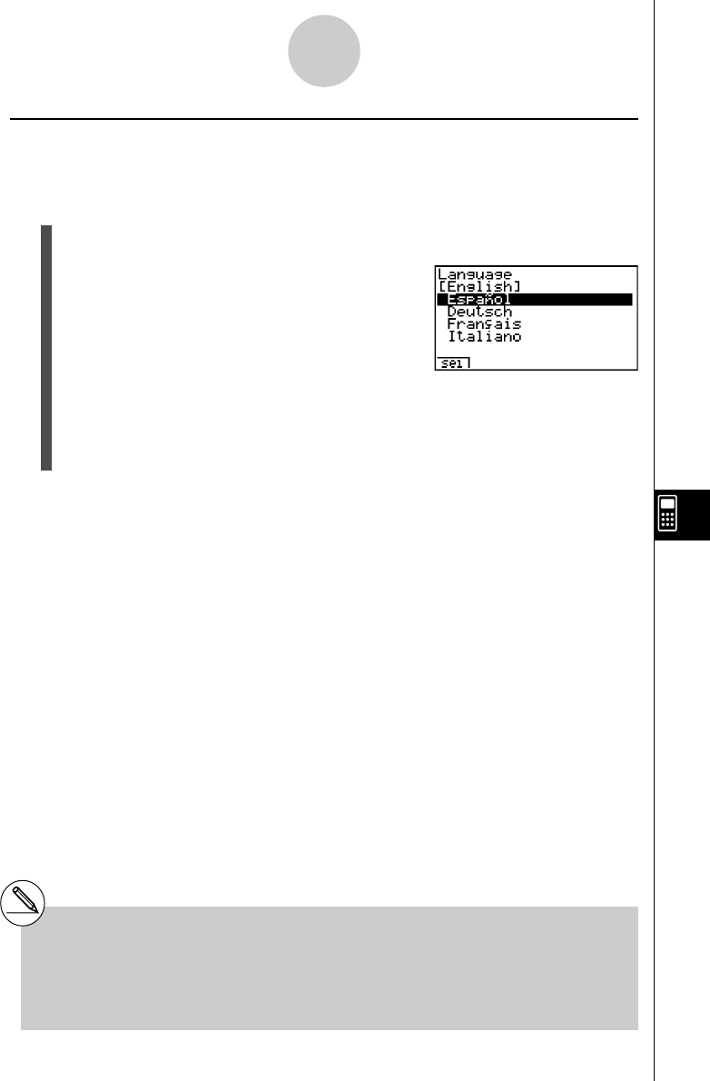
19990401
kk
kk
kSystem Language Setting
Use Lang to specify the display language for built-in applications. You can also use add-ins
to install various other languages.
1. From the initial System Setting Mode screen, press 4(Lang) to display the system
language setting screen.
2. Use the f and c cursor keys to select the language you want, and then press
1(Sel).
3. The pop up window appears using the language you selected. Check the contents and
then press i.
Press i or !i(QUIT) to return to the initial System Setting Mode screen.
9-3-2
System Settings
# Installing a language with an add-in causes
the installed language to be selected as the
system language automatically.
#English display only is supported for the
following functions.
• Differential equations
• E-CON
This means that all displays are in English, even
if another display language is selected.
20011101
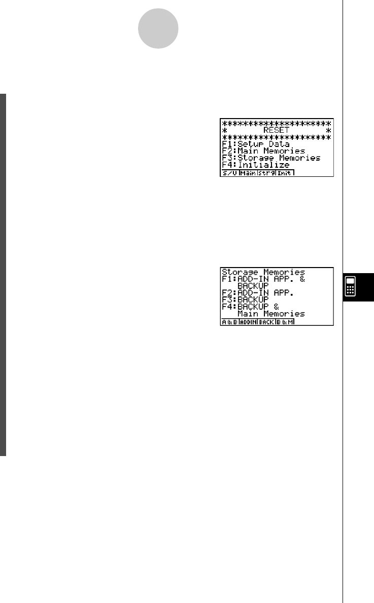
19990401
9-4 Reset
1. While the initial System Settings Mode screen is displayed, press 5(Reset) to display
the Reset Menu screen.
• 1(S/U) ... {set up initialization}
• 2(Main) ... {main memory data clear}
• 4(Init) ... {all memory clear}
Pressing 3(Strg) on the above screen displays the Storage Memories screen shown
below.
• 1(A&B) ... {Add-in application and backup data clear}
• 2(ADDIN) ... {Add-in application clear}
• 3(BACK) ... {Backup data clear}
• 4(B&M) ... {Backup data and Main Memories data clear}
2. Press the function key that corresponds to the reset operation you want to perform.
3. In response to the confirmation message that appears, press w(Yes) to perform the
reset operation you specified, or i(No) to cancel.
4. A message appears to let you know when the reset operation is complete.
Press m to return to the Main Menu.
9-4-1
Reset
20010102
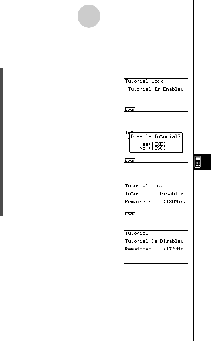
19990401
9-5-1
Tutorial Lock
9-5 Tutorial Lock (ALGEBRA FX 2.0 PLUS only)
You can temporarily disable the Tutorial Mode (for 180 minutes).
1. From the initial System Setting Mode screen, press 6(T-Lock) to display the Tutorial
Lock screen.
2. Pressing 1(Lock) displays the pop-up menu.
3. Pressing w(Yes) locks the Tutorial Mode so it cannot be used for 180 minutes.
Pressing i or !i(QUIT) returns to the initial System Settings Mode screen.
Attempting to enter the Tutorial Mode while Tutorial Lock
is enabled displays a screen that shows the remaining
Tutorial Lock time.
Press i to return to the Main Menu.
20010102

19990401
Data Communications
This chapter tells you everything you need to know to transfer
programs between two CASIO Power Graphic calculators
connected using the cable that is equipped as a standard
accessory.
You can also use the cable to connect the calculator to a CASIO
Label Printer to print screen data.
To transfer data between a calculator and a personal computer,
you need to purchase the separately available CASIO FA-123
Connection Kit.
10-1 Connecting Two Units
10-2 Connecting the Unit with a CASIO Label Printer
10-3 Connecting the Unit to a Personal Computer
10-4 Performing a Data Communication Operation
10-5 Data Communications Precautions
10-6 Sending a Screen Shot
10-7 Add-ins
10-8 MEMORY Mode
Chapter
10
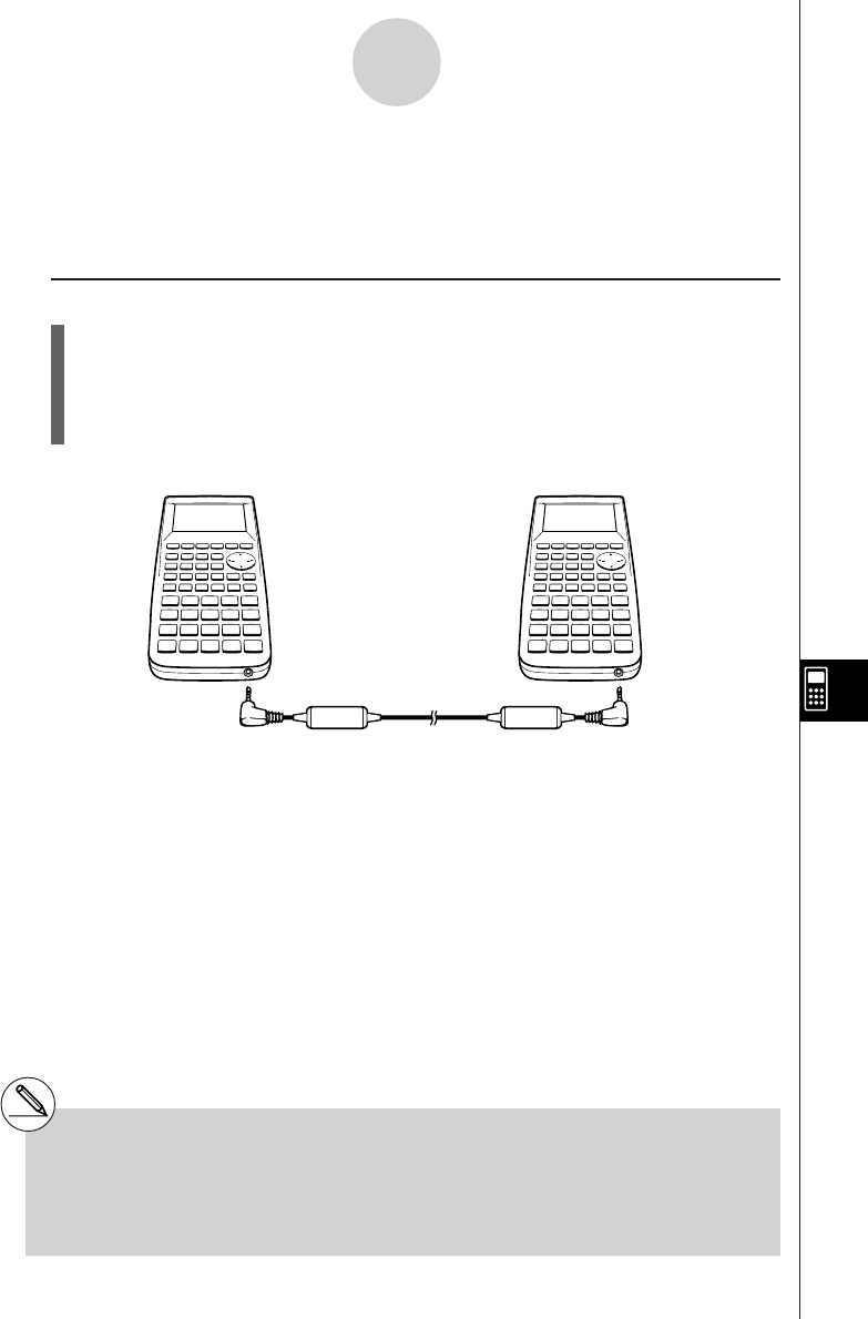
19990401
10-1-1
Connecting Two Units
10-1 Connecting Two Units
The following procedure describes how to connect two units with the connecting cable that
comes equipped as a standard accessory.
uu
uu
uTo connect two units
1. Check to make sure that the power of both units is off.
2. Remove the covers from the connectors of the two units.
3. Connect the two units using the cable.
Cable
#Models that are supported for this configura-
tion are shown below.
ALGEBRA FX 2.0/FX 2.0 PLUS
FX 1.0/FX 1.0 PLUS
#Be sure you keep the connector covers in a safe
place so you can replace them after you finish
your data communications.
#Keep the connectors covered when you are not
using them.
2001100120011101
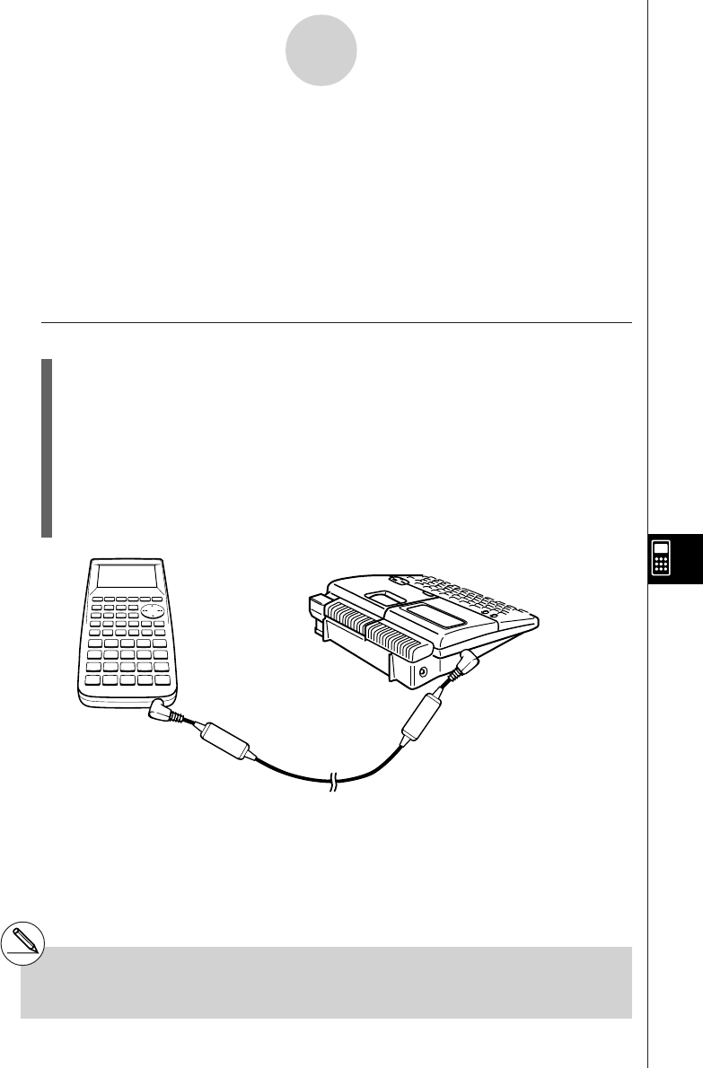
19990401
10-2-1
Connecting the Unit with a CASIO Label Printer
10-2 Connecting the Unit with a CASIO Label
Printer
After you connect the unit to a CASIO Label Printer with cable, you can use the Label Printer
to print screen shot data from the unit (see 10-6 Sending a Screen Shot). See the user’s
guide that comes with your Label Printer for details on how to perform this operation.
•The operation described above can be performed using the following Label Printer
models: KL-2000, KL-2700, KL-8200, KL-8700 (as of February 1999).
uTo connect the unit to a Label Printer
1. Check to make sure that the power of the unit and the Label Printer is off.
2. Connect the cable to the Label Printer.
3. Remove the cover from the connector of the unit.
4. Connect the other end of the cable to the unit.
5. Turn on the power of the unit, followed by the Label Printer.
•After you finish data communications, turn off power in the sequence: the unit first, and
then the Label Printer. Finally, disconnect the equipment.
Label Printer
Cable
#Be sure you keep the connector cover in a
safe place so you can replace it after you
finish your data communications.

19990401
10-3 Connecting the Unit to a Personal
Computer
To transfer data and screen shots between the unit and a personal computer, you must
connect them through a separately available CASIO FA-123 Connection Kit.
For details on operation, the types of computer that can be connected, and hardware
limitations, see the user’s manual that comes with the FA-123.
Some types of data may not be able to be exchanged with a personal computer.
uTo connect the unit to a personal computer
1. Check to make sure that the power of the unit and the personal computer is off.
2. Connect the personal computer to the FA-123 Connection Kit.
3. Remove the cover from the connector of the unit.
4. Connect the unit to the FA-123 Connection Kit.
5. Turn on the power of the unit, followed by the personal computer.
10-3-1
Connecting the Unit to a Personal Computer
#The ALGEBRA calculator also supports to PC
transfer of programs created with a CASIO
CFX-9850 Series calculator.
#Be sure you keep the connector cover in a safe
place so you can replace it after you finish your
data communications.
•After you finish data communications, turn off power in the sequence: the unit first, and
then the personal computer. Finally, disconnect the equipment.
2001100120011101
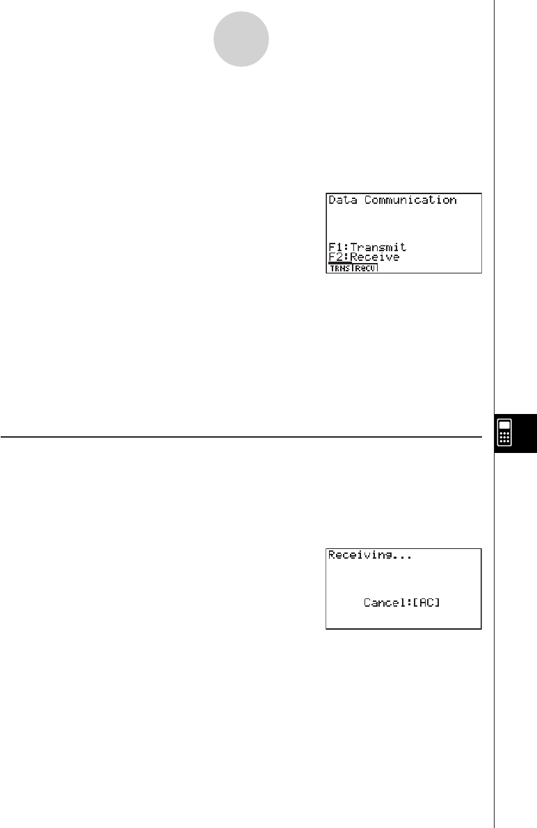
19990401
10-4 Performing a Data Communication
Operation
From the Main Menu, enter the LINK Mode. The following data communication main menu
appears on the display.
•{TRNS}/{Recv} ... menu of {send settings}/{receive settings}
Communication parameters are fixed at the following settings.
•Speed (BPS): 38.4 kbps (sending a data)
9,600bps (sending a screen shot)
•Parity (PARITY): NONE
kk
kk
kPerforming a Data Transfer Operation
Connect the two units and then perform the following procedures.
Receiving unit
To set up the calculator to receive data, press 2(Recv) while the data communication main
menu is displayed.
The calculator enters a data receive standby mode and waits for data to arrive. Actual data
receive starts as soon as data is sent from the sending unit.
10-4-1
Performing a Data Communication Operation
20011101
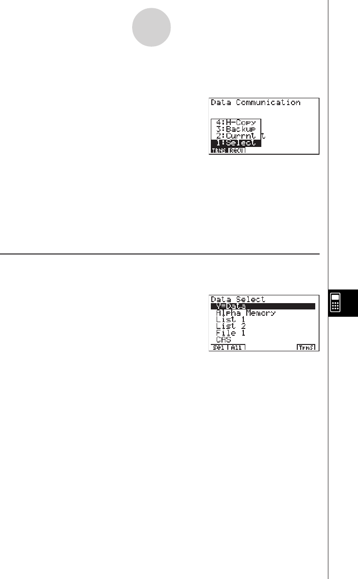
19990401
Sending unit
To set up the calculator to send data, press 1(TRNS) while the data communication main
menu is displayed.
Press the number key that corresponds to the type of data you want to send.
• {Select} ... {selects data items and sends them}
• {Currnt} ... {selects data items from among previously selected data items and sends
them}
• {Backup} ... {sends all memory contents, including mode settings}
• {H-Copy} ... {selects H-Copy screen shot data and sends it}
uTo send selected data items
Press b(Select) or c(Currnt) to display a data item selection screen.
• {Sel} ... {selects data item where cursor is located}
• {All} ... {selects all data}
• {Trns} ... {sends selected data items}
Use the f and c cursor keys to move the cursor to the data item you want to select and
press 1(Sel) to select it. Currently selected data items are marked with “'”. Pressing
6 (Trns) sends all the selected data items.
•To deselect a data item, move the cursor to it and press 1(Sel) again.
Only items that contain data appear on the data item selection screen. If there are too many
data items to fit on a single screen, the list scrolls when you move the cursor to the bottom
line of the items on the screen.
10-4-2
Performing a Data Communication Operation
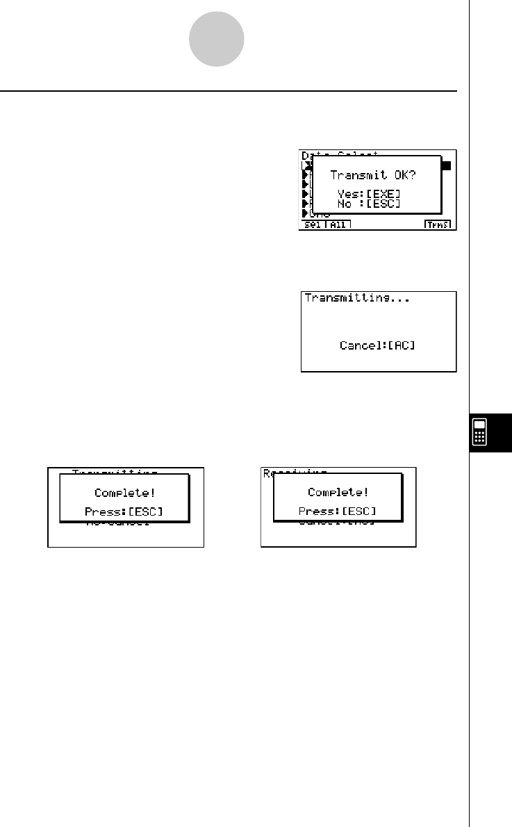
19990401
uTo execute a send operation
After selecting the data items to send, press 6(Trns). A message appears to confirm that
you want to execute the send operation.
•w(Yes) ... sends data
•i(No) ... returns to data selection screen
Press w(Yes) to send the data.
•You can interrupt a data operation at any time by pressing A.
The following shows what the displays of the sending and receiving units look like after the
data communication operation is complete.
Sending Unit Receiving Unit
Press i to return to the data communication main menu.
10-4-3
Performing a Data Communication Operation
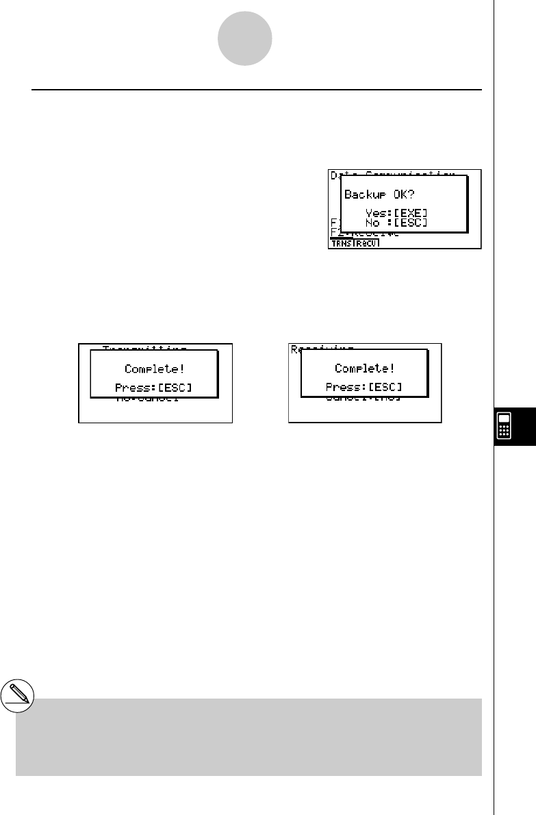
19990401
uTo send backup data
This operation allows you to send all memory contents, including mode settings.
While the transmit data type selection menu is on the screen, press d(Backup), to display
the screen shown below.
Press w(Yes) to start the send operation.
The following shows what the displays of the sending and receiving units look like after the
data communication operation is complete.
Sending Unit Receiving Unit
Press i to return to the data communication main menu.
10-4-4
Performing a Data Communication Operation
#Data can become corrupted, necessitating a
RESET of the receiving unit, should the
connecting cable become disconnected during
data transfer.
Make sure that the cable is securely connected to
both units before performing any data communi-
cation operation.
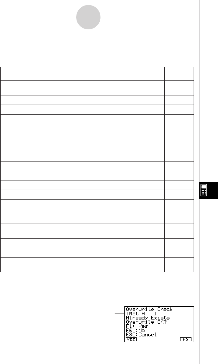
19990401
10-5 Data Communications Precautions
The following are the types of data items that can be sent.
Data Item Contents Overwrite Password
Check*1Check*2
Program names Program contents Yes Yes
(All programs are listed.)
Mat nMatrix memory (A to Z) contents Yes
List nList memory (1 to 20) contents Yes
File nList file memory (1 to 6) contents Yes
Y=Data
Graph expressions, graph write/
non-write status, V-Window contents, No
zoom factors
G-Mem nGraph memory (1 to 20) contents Yes
V-Win nV-Window memory contents No
Picture nPicture (graph) memory (1 to 20) data No
DynaMem Dynamic Graph functions Yes
Equation Equation calculation coefficient values No
Alpha Memory Variable memory contents No
F-Mem nFunction memory contents No
CAS CAS formula data contents
(ALGEBRA FX 2.0 PLUS only) No
Algebra Algebra data contents
(ALGEBRA FX 2.0 PLUS only) No
DIFF Equation Differencial Equation data No
E-CON Data E-CON data No
Add-in application Add-in application data No
names (All add-in applications are listed.)
*1No overwrite check: If the receiving unit already contains the same type of data, the
existing data is overwritten with the new data.
With overwrite check: If the receiving unit already contains the same type of data, a
message appears to ask if the existing data should be overwritten with the new data.
10-5-1
Data Communications Precautions
Data item name
20010102

19990401
•1(YES) ... {replaces the receiving unit’s existing data with the new data}
•6(NO) ... {skips to next data item}
*2With password check: If a file is password protected, a message appears asking for input
of the password.
2
After inputting the password, press w.
Note the following precautions whenever you perform data communications.
•An error occurs whenever you try to send data to a receiving unit that is not yet standing
by to receive data. When this happens, press i to clear the error and try again, after
setting up the receiving unit to receive data.
•An error occurs whenever the receiving unit does not receive any data approximately six
minutes after it is set up to receive data. When this happens, press i to clear the error.
•An error occurs during data communications if the cable becomes disconnected, if the
parameters of the two units do not match, or if any other communications problem
occurs. When this happens, press i to clear the error, then correct the problem before
trying data communications again. If data communications are interrupted by the i key
operation or an error, any data successfully received up to the interruption will be in the
memory of the receiving unit.
•An error occurs if the receiving unit memory becomes full during data communications.
When this happens, press i to clear the error and delete unneeded data from the
receiving unit to make room for the new data, and then try again.
•The E-CON item contains the following data.
1. Current Setup Data
2. Setup Memory Data
3. Custom Probe Memory Data
The corresponding data is overwritten on the receiver. Setup Memory data and Custom
Probe Memory data overwrites the data for the same memory number on the receiver. If
you want to keep data from being overwritten on the receiver, change its memory number.
10-5-2
Data Communications Precautions
20010102
Name of password protected file
Password input field
20011101

19990401
10-6 Sending a Screen Shot
Use the following procedures to send a hardcopy of the screen directly to a connected
personal computer (or CASIO Label Printer) or to save a screen shot in memory to send
later. Screen shots can also be sent to a CASIO Label Printer.
Use the LINK Mode set up (u3(SET UP)) to specify whether you want to send the
screen shot now or save it in memory.
u H-Copy
•{Dirct}/{Mem}............. {direct send}/{save}
uu
uu
uTo send a screen shot directly to a connected computer (or CASIO Label
Printer) (Direct)
1. Connect the unit to the computer (or CASIO Label Printer).
On the computer (or CASIO Label Printer), perform the procedures required to set it up
to receive data.
2. Display the screen you want to send.
3. Press u6(H-COPY).
uu
uu
uTo save a screen shot in memory (Memory)
1. Display the screen you want to save.
2. Press u6(H-COPY).
• You can store up to 20 screen shots in memory. Saved screen shots are automatically
assigned file names from Hcopy1 to Hcopy20.
10-6-1
Sending a Screen Shot
#You cannot send the following types of
screens to a computer or a Label Printer.
•The screen that appears while a data
communication operation is in progress.
•A screen that appears while a calculation is
in progress.
•The screen that appears following the reset
operation.
•The low battery message.
#The flashing cursor is not included in the screen
image that is sent from the unit.
#You cannot use 6mm wide tape to print a screen
shot of a graph.
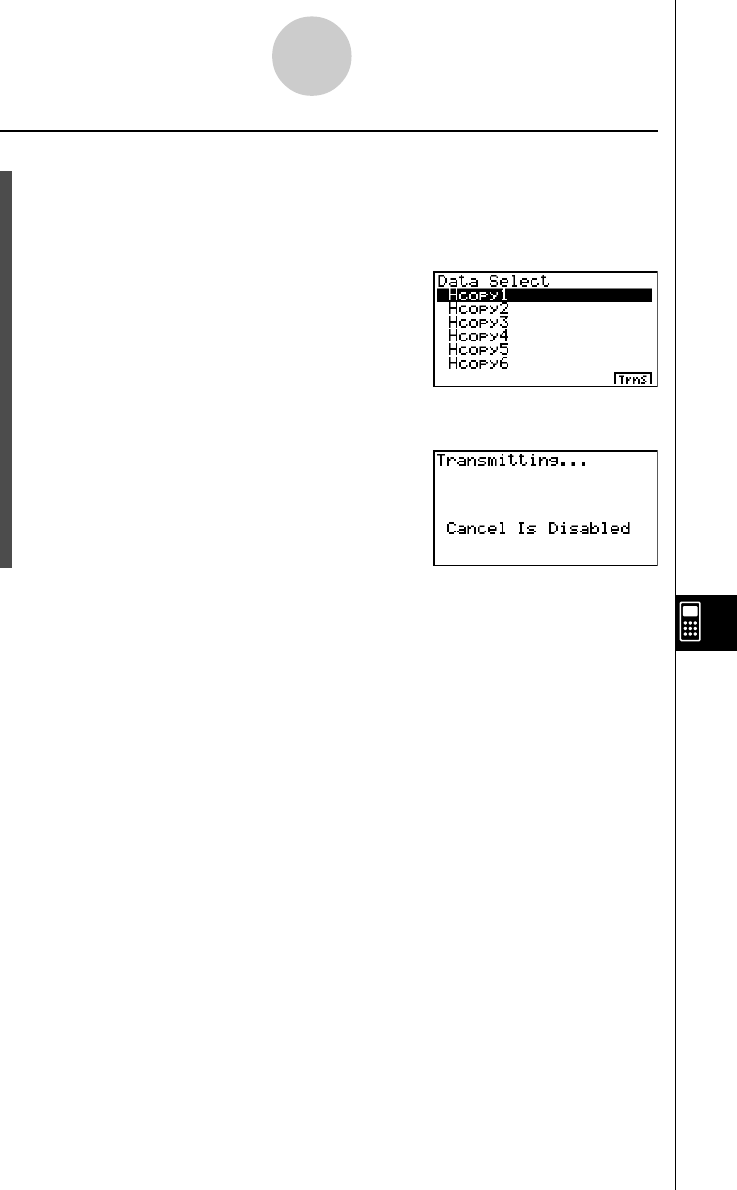
19990401
uu
uu
uTo send a saved screen shot to a computer or CASIO Label Printer
1. Connect the unit to the computer (or CASIO Label Printer). On the computer (or CASIO
Label Printer), perform the procedures required to set it up to receive data.
2. In the LINK Mode, press 1(TRNS)e(H-Copy) to display the list of screen shots in
memory.
3. Use the f and c cursor keys to highlight the name of the screen shot you want to
send, and then press 6(Trns).
10-6-2
Sending a Screen Shot
20011101

19990401
10-7-1
Add-ins
10-7 Add-ins
Add-in capabilities let you install separately available applications and other software to tailor
the calculator to suit your particular needs.
Add-ins are installed from a computer using the data communication described on page
10-4-1.
The following are the types of software that can be installed as add-ins.
uu
uu
uAdd-in Application
After you install an application, its icon appears in the Main Menu, and you can run it just as
you would a built-in application.
uu
uu
uBuilt-in Application Upgrades
These are upgrades for the applications that are pre-programmed in the calculator’s ROM.
uu
uu
uOn-screen Message Language Data
This data is required to display on-screen messages in other languages. Installing this data
causes all on-screen messages to appear in the corresponding language.
2001010220011101
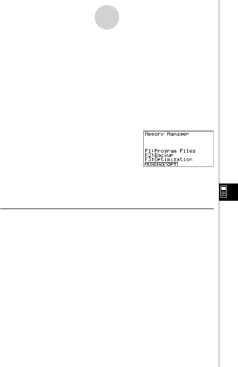
19990401
10-8-1
MEMORY Mode
10-8 MEMORY Mode
This calculator has two separate memory areas: a “current area” and a “storage area.” The
current area is a work area where you can perform input data, perform calculations and run
programs. Data in the current area is relatively safe, but it can be deleted when batteries go
dead or when you perform a full reset.
The storage area uses “flash memory,” so data is safe even when power is interrupted.
Normally, you would use the storage area for data you need to store securely for long periods
and load it into the current area only when you need it.
Use the MEMORY Mode to transfer data between the current area and storage area, and to
perform other memory management operations.
From the Main Menu, select the MEMORY icon to enter the MEMORY Mode and display its
initial screen.
•{PROG}...... {program file save, load, delete, search}
•{BACK}...... {current area data backup and restore}
•{OPT}......... {optimization of the storage area}
kStoring and Loading Program Files
Use the following procedures to store a current area program file into the storage area, and
to load a file from the storage area into the current area.
20011101
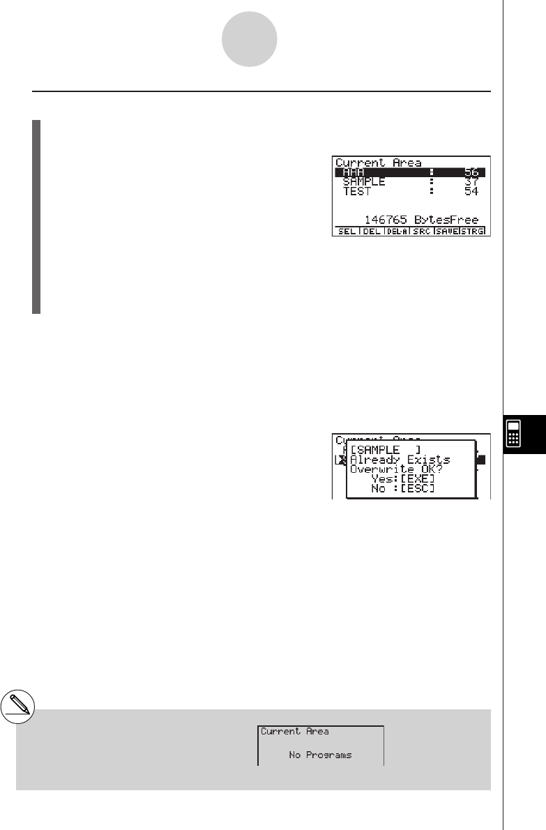
19990401
uTo store a program file into the storage area
1. On the initial MEMORY Mode screen press 1(PROG).
•This displays a list of program files that are in the current area.*1
2. Select the program file you want to store.
•Use the cursor f and c keys to highlight the name of the program file you want to
store, and then press 1(SEL).
3. Press 5(SAVE).
The message “Complete!” appears when the store operation is finished.
Press i to return to the screen displayed in step 1.
A “Memory ERROR” occurs and the store operation is terminated if the storage area
becomes full.
The following message appears if there is already a program file in the storage area with the
same name as the program file you are trying to save.
Press w(Yes) to save the new program file, or i(No) to cancel the save operation.
10-8-2
MEMORY Mode
*1This screen appears as shown to the right if
there are no program files in the current area
when you start the save operation.
20011101
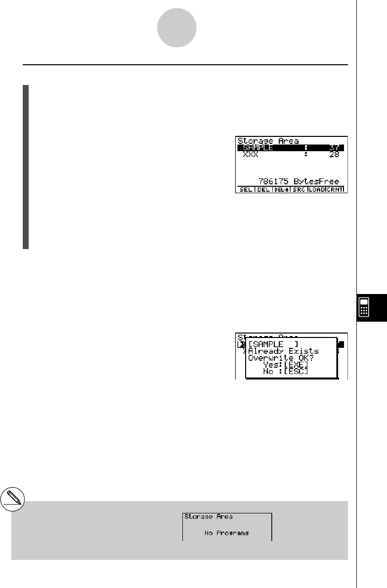
19990401
u To load a program file from the storage area
1. On the initial MEMORY Mode screen press 1(PROG).
2. Press 6(STRG).
• This displays a list of program files that are in the storage area. *1
3. Select the program file you want to load.
•Use the cursor f and c keys to highlight the name of the program file you want to
load, and then press 1(SEL).
4. Press 5(LOAD).
The message “Complete!” appears when the load operation is finished.
Press i to return to the screen displayed in step 1.
A “Memory ERROR” occurs and the load operation is terminated if the current area becomes
full.
The following message appears if there is already a program file in the current area with the
same name as the program file you are trying to load.
Press w(Yes) to load the new program file, or i(No) to cancel the load operation.
*1The screen appears as shown below if there
are no program files in the storage area when
you start the load operation.
10-8-3
MEMORY Mode
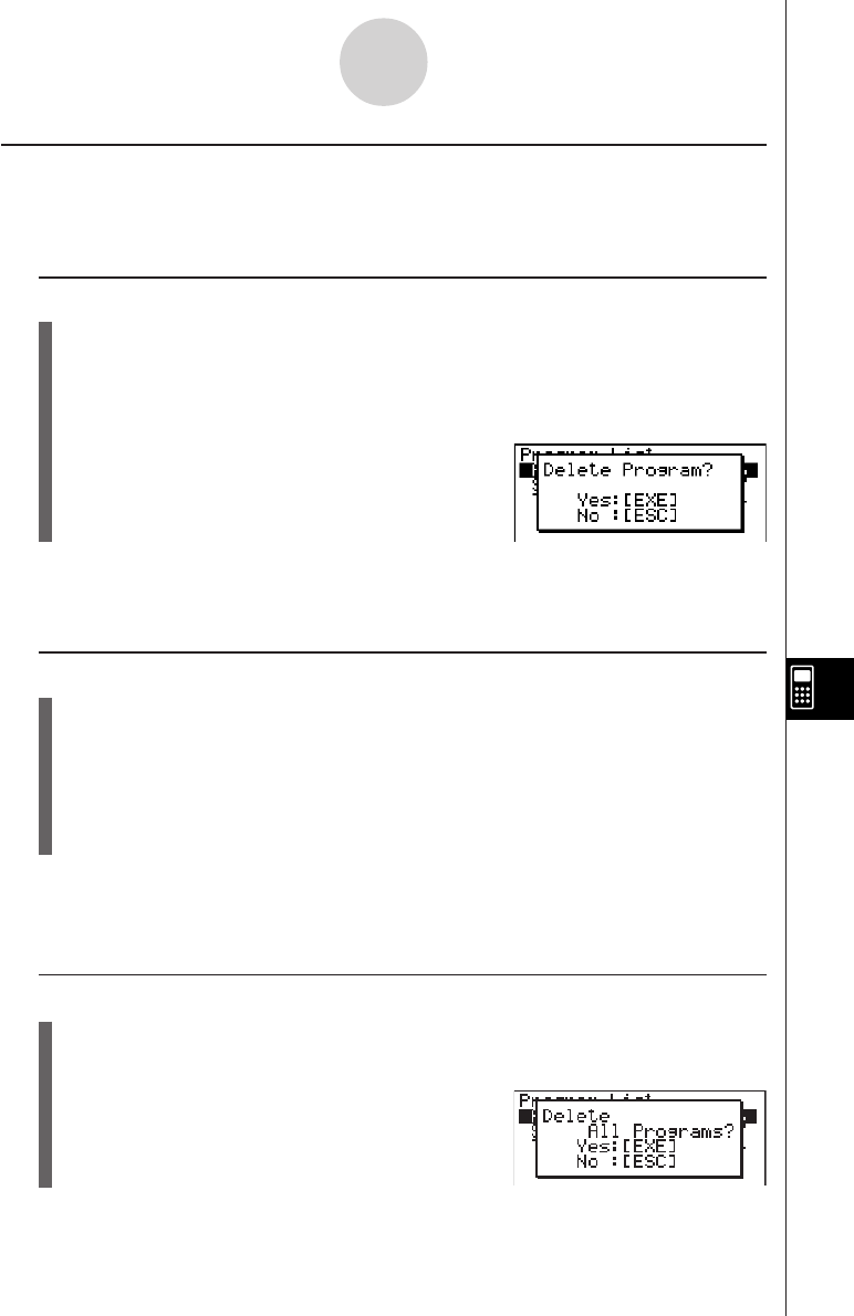
19990401
kDeleting Program Files
Use the following procedures to delete individual files or all files in the current area or
storage areas.
uTo delete a current area program file
1. On the initial MEMORY Mode screen press 1(PROG).
•This displays a list of program files that are in the current area.
2. Use the cursor f and c keys to highlight the name of the program file you want to
delete, and then press 2(DEL).
• Press w(Yes) to delete the program file.
• Press i(No) to cancel the delete operation.
uTo delete a storage area program file
1. On the initial MEMORY Mode screen press 1(PROG).
2. Press 6(STRG).
• This displays a list of program files that are in the storage area.
3. Use the cursor f and c keys to highlight the name of the program file you want to
delete, and then press 2(DEL).
• Press w(Yes) to delete the program file.
• Press i(No) to cancel the delete operation.
uTo delete all the program files in the current area
1. On the initial MEMORY Mode screen press 1(PROG).
•This displays a list of program files that are in the current area.
2. Press 3(DEL•A).
• Press w(Yes) to delete all the program files in the current area.
• Press i(No) to cancel the delete operation.
10-8-4
MEMORY Mode
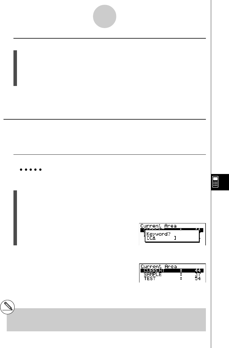
19990401
uTo delete all the program files in the storage area
1. On the initial MEMORY Mode screen press 1(PROG).
2. Press 6(STRG).
• This displays a list of program files that are in the storage area.
3. Press 3(DEL•A).
• Press w(Yes) to delete all the program files in the storage area.
• Press i(No) to cancel the delete operation.
kSearching for a Program File
Use the following procedures to search for a specific program file in the current area or in the
storage area.
u To search for a program file in the current area *1
Example To search for all program files in the current area whose names begin
with the letter “C”
1. On the initial MEMORY Mode screen press 1(PROG).
•This displays a list of program files that are in the current area.
2. Press 4(SRC).
•Input the letter “C” for the keyword.
• The first program file name that begins with the letter “C” appears highlighted on display.
10-8-5
MEMORY Mode
*1 You can input up to eight characters for the
keyword.
The message “Not Found” appears if there are no
program file names that match your keyword.
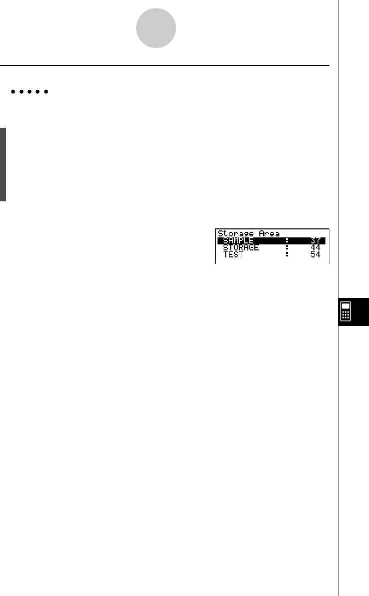
19990401
uTo search for a program file in the storage area
Example To search for all program files in the storage area whose names begin
with the letter “S”
1. On the initial MEMORY Mode screen press 1(PROG).
2. Press 6(STRG).
• This displays a list of program files that are in the storage area.
3. Press 4(SRC).
•Input the letter “S” for the keyword.
•The first program file name that begins with the letter “S” appears highlighted on display.
Press c or 1(SRC) to highlight the next file name that matches your keyword.
Press f to highlight the previous file name that matches your keyword.
The message “Not Found” appears if there are no program file names that match your
keyword.
Press i to exit the search.
10-8-6
MEMORY Mode
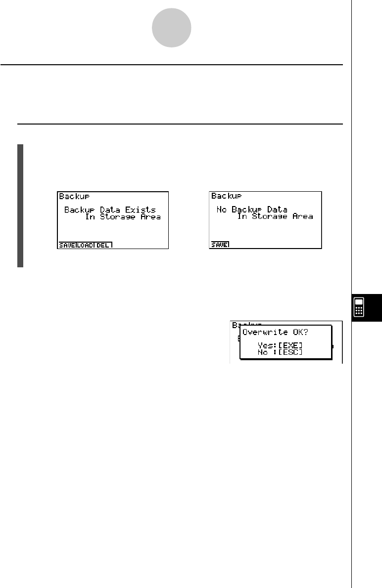
19990401
kBacking Up Current Area Data
You can back up all the data in the current area and store it in the storage area. Later you
can restore the backed up data to the current area when necessary.
uTo back up current area data
1. On the initial MEMORY Mode screen press 2(BACK).
•Screen A appears if there is already backup data in the storage area. Screen B
appears if there is no backup data in the storage area.
Screen A Screen B
2. Press 1(SAVE) to backup the data.
The message “Complete!” appears when the backup operation is finished.
Press i to return to the screen displayed in step 1.
The following message appears if there is already backup data in the storage area.
Press w(Yes) to back up the data, or i(No) to cancel the backup operation.
A “Memory ERROR” occurs when there is not enough space available in the storage area to
complete the backup operation.
10-8-7
MEMORY Mode
20011101
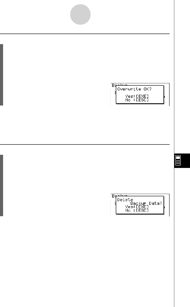
19990401
uTo restore backup data to the current area
1. On the initial MEMORY Mode screen press 2(BACK).
•On the screen that appears, you can confirm whether or not there is backup data in
the storage area.
2. Press 2(LOAD).
•A message appears to confirm whether or not you really want to restore the backed
up data.
Press w(Yes) to restore the data and delete any data currently in the area.
Press i(No) to cancel the data backup operation.
The message “Complete!” appears when the restore operation is finished.
Press i to return to the screen displayed in step 1.
uTo delete backup data from the storage area
1. On the initial MEMORY Mode screen press 2(BACK).
•On the screen that appears, you can confirm whether or not there is backup data in
the storage area.
2. Press 3(DEL).
•A message appears to confirm whether or not you really want to delete the backed
up data.
Press w(Yes) to delete the backed up data from the storage area.
Press i(No) to cancel the backup data delete operation.
The message “Complete!” appears when the delete operation is complete.
Press i to return to the screen displayed in step 1, which now contains the message “No
Backup Data.”
10-8-8
MEMORY Mode
20011101
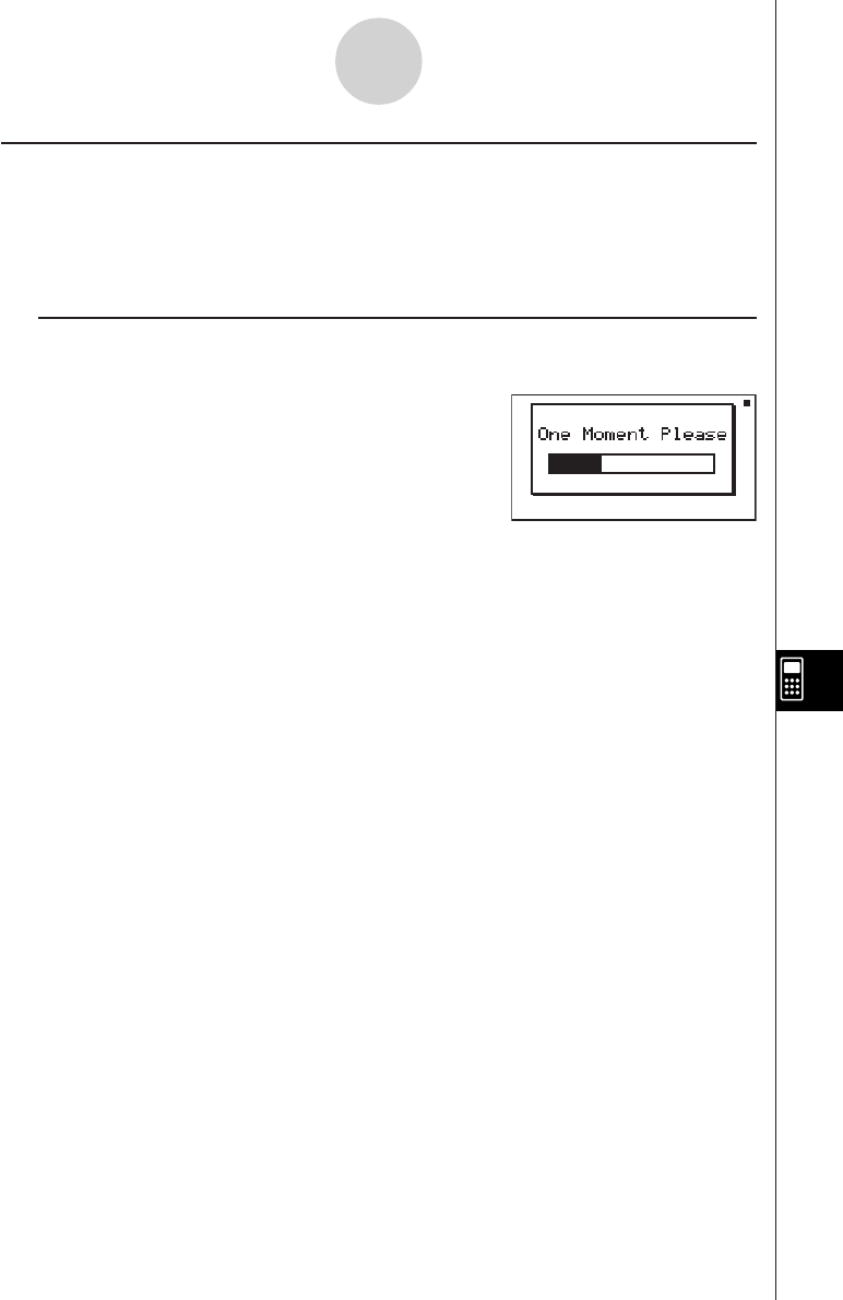
19990401
kOptimizing the Storage Area
Storage area memory can become fragmented after many store and load operations.
Fragmentation can cause blocks of memory to become unavailable for data storage.
Because of this, you should periodically perform the storage area optimization procedure,
which rearranges the data in the storage area and makes memory usage more economical.
uTo optimize the storage area
On the initial MEMORY Mode screen press 3(OPT) to start storage area optimization.
The message “Complete!” appears when the optimize operation is complete.
Press i to return to the initial MEMORY Mode screen.
10-8-9
MEMORY Mode


19990401
Meaning
•Illegal syntax
•Attempt to input an illegal
command
•Calculation result exceeds the
display range.
•Calculation is outside the input
range of a function.
•Mathematical error (division by
zero, etc.)
•Sufficient precision could not be
obtained for Σ calculation,
differential calculation, etc.
•Solution could not be obtained
for equation calculation, etc.
1No corresponding Lbl n for
Goto n.
2No program stored in program
area Prog ”file name”.
•Nesting of subroutines by Prog
”file name” exceeds 10 levels.
•Execution of calculations that
exceed the capacity of the
stack for numeric values or
stack for commands.
Message
Syntax ERROR
Ma ERROR
Go ERROR
Nesting ERROR
Stack ERROR
Countermeasure
•Press i to display the error
and make necessary correc-
tions.
•Check input values and make
corrections to ensure that
values are within allowable
limits.
1Correctly input a Lbl n to corres-
pond to the Goto n , or delete
the Goto n if not required.
2Store a program in program
area Prog ”file name”, or delete
the Prog ”file name” if not
required.
•Ensure that Prog ”file name” is
not used to return from
subroutines to main routine. If
used, delete any unnecessary
Prog ”file name”.
•Trace the subroutine jump
destinations and ensure that no
jumps are made back to the
original program area. Ensure
that returns are made correctly.
•Simplify the formulas to keep
stacks within 10 levels for the
numeric values and 26 levels
for the commands.
•Divide the formula into two or
more parts.
α
-1-1
Error Message Table
1Error Message Table

19990401
Meaning
Message Countermeasure
α
-1-2
Error Message Table
Memory
ERROR
Argument
ERROR
Dimension
ERROR
Range ERROR
Condition
ERROR
Non-Real
ERROR
•Operation or memory storage
operation exceeds remaining
memory capacity.
•Incorrect argument specification
for a command that requires an
argument.
•Illegal dimension or list used
during matrix calculations.
1Input of an improper V-Window
value.
2V-Window range settings
exceeded when a graph is
redrawn.
3Input of an improper value on the
range screen and use of that
value for execution.
•Execution of a calculation or
function before all conditions
required for execution are met.
1Calculation that produces a
complex number when Real is
specified for the Complex Mode
setting on the SET UP screen,
even though the argument is a
real number.
2Calculation that produces a
complex number when Real is
specified for the Answer Type
setting on the SET UP screen,
even though the argument is a
real number. (ALGEBRA FX 2.0
PLUS only)
•Keep the number of variables
you use for the operation within
the number of variables
currently available.
•Simplify the data you are trying
to store to keep it within the
available memory capacity.
•Delete no longer needed data
to make room for the new data.
•Correct the argument.
•Check the matrix or list
dimension.
1Change the V-Window value so
it is within range.
2Redraw using the proper
settings.
3Input a proper range value.
•Check the conditions and make
any necessary corrections.
1Change the Complex Mode
setting to something other than
Real.
2Change the Answer Type
setting to something other than
Real. (ALGEBRA FX 2.0 PLUS
only)
20010102

19990401
α
-1-3
Error Message Table
MeaningMessage Countermeasure
Complex
Number In List
Complex
Number In
Matrix
Can’t Solve!
Adjust Initial
Value Or
Bounds. Then
Try Again
No Variable
Iteration
ERROR
Com ERROR
Transmit
ERROR
Receive
ERROR
Memory Full
•List containing complex number
used in a calculation or
operation for which complex
number data is invalid.
•Matrix containing complex
number used in a calculation or
operation for which complex
number data is invalid.
•Solve could not obtain a
solution within the specified
range.
•No variable specified within a
graph function being used for
Dynamic Graph.
•No variable within a Solve
equation.
1No convergence of Solve
solutions.
2No integration or differential
calculation solution that
satisfies operation ending
condition (tol value).
•Problem with cable connection
or parameter setting during
program data communications.
•Problem with cable connection
or parameter setting during data
communications.
•Problem with cable connection
or parameter setting during data
communications.
•Memory of receiving unit
became full during program
data communications.
•Change all data in the list to
real numbers.
•Change all data in the matrix to
real numbers.
•Change the specified range.
•Correct the input expression.
•Specify a variable for the graph
function.
1Change the initial estimated
value to one that is nearer to
the solution.
2Increase the tol value to reduce
precision.
•Check the cable connection.
•Check the cable connection.
•Check the cable connection.
•Delete some data stored in the
receiving unit and try again.
19991201

19990401
α
-1-4
Error Message Table
MeaningMessage Countermeasure
Download
ERROR
Model
Mismatch
Overflow
ERROR *
Domain
ERROR *
•Data communication cable
disconnect during add-in
installation, or incorrect
data transfer conditions.
•Attempt to perform back up
between two different models.
•Overflow of the calculation
range in the Algebre Mode.
•Overflow of the input element
range in the Algebre Mode.
•Press w and try again.
•Press i and try again.
•Use two identical models.
•Correct the input expression.
•Correct the input expression.
20010102
* ALGEBRA FX 2.0 PLUS only
19990401
α
-2-1
Input Ranges
2Input Ranges
sinx
cosx
tanx
sin–1x
cos–1x
tan–1x
sinhx
coshx
tanhx
sinh–1x
cosh–1x
tanh–1x
logx
Inx
10x
ex
x
x2
1/x
3x
x
!
nPr
nCr
As a rule,
precision is
±1 at the
10th digit.*
"
"
"
"
"
"
"
"
"
However, for tanx:
|x|
GG
GG
G
90(2n+1):DEG
|x|
GG
GG
G
π/2(2n+1):RAD
|x|
GG
GG
G
100(2n+1):GRA
*Complex numbers can be
used as arguments.
*Complex numbers can be
used as arguments.
*Complex numbers can be
used as arguments.
*Complex numbers can be
used as arguments.
*Complex numbers can be
used as arguments.
*Complex numbers can be
used as arguments.
*Complex numbers can be
used as arguments.
*Complex numbers can be
used as arguments.
(DEG) |x| < 9 × (109)°
(RAD) |x| < 5 × 10⁷πrad
(GRA) |x| < 1 × 10¹⁰grad
|x| < 1
|x| < 1 × 10100
|x| < 230.2585092
|x| < 1 ×10100
|x| < 5 × 1099
1< x < 5 × 1099
|x| < 1
1 × 10–99 < x < 1 × 10100
–1 × 10100 < x < 100
–1 × 10100
< x < 230.2585092
0 < x < 1 × 10100
|x| <1 × 1050
|x| < 1 × 10100, x
GG
GG
G
0
|x| < 1 × 10100
0 < x < 69
(x is an integer)
Result < 1 × 10100
n, r (n and r are integers)
0 < r < n,
n < 1 × 10¹⁰
15 digits
"
"
"
"
"
"
"
"
"
Function Input range for real
number solutions
Internal
digits Precision Notes
20011101

19990401
α
-2-2
Input Ranges
Pol (x, y)
Rec
(r ,
θ
)
° ’ ”
←
° ’ ”
^(xy)
xy
ab/c
15 digits
"
"
"
"
"
As a rule,
precision is
±1 at the
10th digit.*
"
"
"
"
"
However, for tan
θ
:
|
θ
|
GG
GG
G
90(2n+1):DEG
|
θ
|
GG
GG
G
π/2(2n+1):RAD
|
θ
|
GG
GG
G
100(2n+1):GRA
|r| < 1 × 10100
(DEG) |
θ
| < 9 × (109)°
(RAD) |
θ
| < 5 × 10⁷π rad
(GRA) |
θ
| < 1 × 10¹⁰grad
|a|, b, c < 1 × 10100
0 < b, c
|x| < 1 × 10100
Sexagesimal display:
|x| < 1 × 10⁷
x > 0:
–1 × 10100 < ylogx < 100
x = 0 : y > 0
x < 0 :
1
y = n,–––– (n is an integer
2n+1 or a fraction)
However;
–1 × 10100 < y log |x| < 100
y > 0 : x
GG
GG
G
0
1
–1 × 10100 < –– logy < 100
x
y = 0 : x > 0 1
y < 0 : x = 2n +1, ––
n
(n
GG
GG
G
0, n is an integer or a
fraction)
However;
1
–1 × 10100 < –– log |y| < 100
x
Total of integer, numerator
and denominator must be
within 10 digits (includes
division marks).
*For a single calculation, calculation error is ±1 at the 10th digit. (In the case of exponential display,
calculation error is ±1 at the last significant digit.) Errors are cumulative in the case of consecutive
calculations, which can also cause them to become large. (This is also true of internal consecutive
calculations that are performed in the case of ^(xy), xy, x!, 3x, nPr, nCr, etc.)
In the vicinity of a function’s singular point and point of inflection, errors are cumulative and may
become large.
Function Input range for real
number solutions
Internal
digits Precision Notes
< 1 × 10100
x2 + y2
*Complex numbers can be
used as arguments.
*Complex numbers can be
used as arguments.
20011101

19990401
α
-2-3
Input Ranges
Function
Binary,
octal,
decimal,
hexadecimal
calculation
Input range
Values fall within following ranges after conversion:
DEC: –2147483648 < x < 2147483647
BIN: 1000000000000000 < x
< 1111111111111111 (negative)
0 < x < 0111111111111111 (0, positive)
OCT: 20000000000 < x < 37777777777 (negative)
0 < x < 17777777777 (0, positive)
HEX: 80000000 < x < FFFFFFFF (negative)
0 < x < 7FFFFFFF (0, positive)

19990401
α
-3-1
Specifications
3Specifications
Variables: 28
Calculation range:
±1 × 10–99 to ±9.999999999 × 1099 and 0. Internal operations use 15-digit mantissa.
Exponential display range: Norm 1: 10–2 > |x|, |x| > 1010
Norm 2: 10–9 > |x|, |x| > 1010
Program capacity: 144 kbytes (max.)
Power supply:
Main: Four AAA-size batteries (LR03 (AM4) or R03 (UM-4))
Back-up: One CR2032 lithium battery
Power consumption: 0.2 W
Approximate battery life
Main (ALGEBRA FX 2.0 PLUS):
LR03 (AM4): 230 hours (continuous display of main menu)
150 hours continuous operation (5 minutes calculation, 55 minutes display)
R03 (UM-4): 140 hours (continuous display of main menu)
90 hours continuous operation (5 minutes calculation, 55 minutes display)
Main (FX 1.0 PLUS):
LR03 (AM4): 200 hours (continuous display of main menu)
140 hours continuous operation (5 minutes calculation, 55 minutes display)
R03 (UM-4): 120 hours (continuous display of main menu)
80 hours continuous operation (5 minutes calculation, 55 minutes display)
Back-up: 2 years
Auto power off:
Power is automatically turned off approximately six minutes or 60 minutes after last
operation.
Ambient temperature range: 0 °C to 40 °C
Dimensions: 19.5 mm (H) × 82 mm (W) × 178 mm (D)
3/4" (H) × 3 1/4" (W) × 6 7/8" (D)
Weight: Approx. 213 g (including batteries)
20010102

19990401
α
-3-2
Specifications
Data Communications
Method: Start-stop (asynchronous), half-duplex
Transmission speed (BPS): 38400 bits/second (normal)
9600 bits/second (H-Copy & Send/Receive)
Parity: None
Bit length: 8 bits
Stop bit:
Send: 3 bits
Receive: 2 bits
Includes parity (None) 1-bit
X ON/X OFF Control: None

19990401
Symbols
AList .................................................. 3-2-7
Σ calculation ..................................... 2-5-10
A
Absolute value .................................. 2-6-2
Add-ins ........................................... 10-7-1
Algebra Mode ................................... 7-2-1
Algebra Mode operation ................... 7-1-3
Angle unit ................................ 2-3-1, 2-4-2
Ans ................................................... 2-2-5
Answer function ................................ 2-2-5
Answer memory ...................... 2-2-5, 7-1-7
APO settings ..................................... 9-3-1
Argument ...........................................2-6-2
Arithmetic calculations ...................... 2-1-1
Asymptotes ................................... 5-11-21
Auto Mode ........................................ 7-3-8
Auto power off ......................... 9-3-1, α-7-5
Axis of symmetry .......................... 5-11-20
B
Backing up data .............................. 10-8-7
Backup data, sending ..................... 10-4-4
Bar graph ...........................................6-2-1
Binary calculation ..............................2-7-1
Bitwise operation .............................. 2-7-4
Box zoom ...........................................5-2-7
Broken line graph .............................. 6-2-3
C
Calc window ..................................... 5-2-12
Calculation execution indicator ......... 1-2-5
Calculation priority sequence ........... 2-1-3
Calculation results of a paired-variable
graph ............................... 6-3-11, 6-4-2
Calculation results of a single-variable
graph ................................ 6-2-4, 6-4-2
CAS Mode ........................................ 7-1-1
Catalog ............................................. 1-3-5
Cell, editing ....................................... 3-1-3
Center ............................................ 5-11-19
Circle ................................................ 5-1-5
Clipboard ...........................................1-3-4
Column operations ........................... 2-8-9
Combination ..................................... 2-4-9
Comments ...................................... 5-10-3
Complex number calculations .......... 2-6-1
Composite function ................. 2-1-3, 5-3-3
Conic section ................................ 5-11-17
CONICS Mode .................................. 5-1-5
Conjugate complex number .............. 2-6-3
Connecting the unit to a personal
computer ................................... 10-3-1
Connecting the unit with a CASIO Label
Printer ....................................... 10-2-1
Connecting two units ...................... 10-1-1
Continuous calculations .......... 2-2-5, 7-1-7
Contrast adjustment ......................... 9-3-1
Coordinate conversion ............ 2-4-2, 2-4-8
Coordinate rounding ........................ 5-11-7
Coordinates for given points .......... 5-11-13
Coordinates on a grah line .............. 5-11-1
Copy range ....................................... 1-3-4
Copying a regression graph formula
................................................... 6-3-11
Copying a table column to a list ........ 5-7-8
Corrections ....................................... 1-3-4
Cubic regression graph ..................... 6-3-7
α
-4-1
Index
4Index
20011101

1999040120011101
α
-4-2
Index
Current area ................................... 10-8-1
D
Data communication operation ........ 10-4-1
DATA ERROR message ................... α-6-1
Debugging ........................................ 8-3-1
Decimal calculations ......................... 2-7-1
Decimal places ....................... 2-1-2, 2-3-1
Degrees/minutes/seconds ...... 1-2-5, 2-4-2
Derivative item ...................... 5-7-3, 5-11-3
Determinant .....................................2-8-18
Differential calculations ..................... 2-5-2
Directrix ......................................... 5-11-20
Display format ................................... 2-3-1
Display screens ................................ 1-2-3
Draw/non draw status of a graph ...... 5-3-6
Drawing a line ..................................5-10-1
Dual graph ........................................ 5-5-1
DYNA Mode ...................................... 5-8-1
Dynamic graph ..................................5-8-1
Dynamic graph functions in a program
.................................................... 8-6-5
Dynamic graph memory ................... 5-8-6
E
Eccentricity .................................... 5-11-21
Editing calculations ........................... 1-3-1
Ellipse ............................................... 5-1-5
Eng ....................................... 2-3-2, 2-4-11
Eqn memory ..................................... 7-1-6
EQUA Mode ...................................... 4-1-1
Error message ........................ 2-1-5, α-1-1
Estimated value ................................ 6-4-4
Exponential function ......................... 2-4-4
Exponential regression graph ........... 6-3-8
F
Factor zoom ...................................... 5-2-9
File name, editing .............................. 8-4-2
File name, registering ............. 8-1-1, 8-1-2
Flash memory ..................................10-8-1
FMEM ............................................... 2-2-2
Focus ............................................. 5-11-18
Formula memory .............................. 7-1-4
Formula number area ....................... 7-1-1
Fraction ................................. 1-2-5, 2-4-10
Freehand drawing ............................5-10-5
Function analysis ............................. 5-11-1
Function memory .................... 2-2-2, 7-1-6
Function menu ...................... 1-2-3, 5-2-11
Function, edit/change/delete ............ 5-3-5
G
Generating a table ............................ 5-7-2
Graph background .......................... 5-10-7
Graph function, recall ....................... 5-3-7
Graph functions in a program ........... 8-6-3
Graph functions, store ...................... 5-3-7
Graph memory ........................ 5-3-7, 7-1-6
Graph parameters, changing ............ 6-1-2
Graph screen .................................... 1-2-3
Graph to table .................................. 5-11-5
Graph type, specifying ...................... 5-3-1
Graph, store/recall ............................ 5-4-1
Graph-Table linking ......................... 5-7-15
GRPH
•
TBL Mode .............................. 5-1-1
H
Hexadecimal calculation ......... 1-2-5, 2-7-1
Higher degree equations .................. 4-2-1

19990401
α
-4-3
Index
Histogram ......................................... 6-2-1
Hyperbola ......................................... 5-1-5
Hyperbolic function (HYP) ...... 2-4-2, 2-4-5
I
Icon ................................................... 1-2-1
Imaginary part ................................... 2-6-3
Inequality ...........................................5-3-2
Input area ......................................... 7-1-1
Input ranges ...................................... α-2-1
Inputting calculations ........................ 1-3-1
Integral value for a given range ..... 5-11-15
Integration calculation ....................... 2-5-7
Integration graph .............................. 5-6-3
Intercepts ....................................... 5-11-19
Inverse hyperbolic function ..... 2-4-2, 2-4-5
Inverse trigonometric function .......... 2-4-3
K
Key markings .................................... 1-1-3
Key table ........................................... 1-1-2
L
Latus rectum .................................. 5-11-18
Linear equation .................................. 7-3-2
Linear inequality ............................... 7-3-2
Linear regression graph .................... 6-3-6
LINK Mode ...................................... 10-4-1
List data, manipulating ...................... 3-2-1
List data in the CAS Mode ................. 7-1-2
List files, switching ............................ 3-4-1
List sort functions in a program ........ 8-6-8
List, arithmetic calculations ............... 3-3-1
List, inputting and editing .................. 3-1-1
Logarithmic function ......................... 2-4-4
Logarithmic regression graph ........... 6-3-8
Logistic regression graph ................ 6-3-10
Low battery message ............. 1-8-2, α-7-1
M
Main Memories ..................................9-2-1
Main screen ...................................... 5-5-1
Manual graphing ............................... 5-6-1
Manual Mode .................................... 7-3-6
MatAns ............................................. 2-8-1
Matrices using matrix commands
...................................... 2-8-10, 2-8-13
Matrix arithmetic operation ............. 2-8-17
Matrix Data in the CAS Mode ........... 7-1-2
Matrix inversion .............................. 2-8-19
Matrix row operations in a program .. 8-6-1
Matrix transposition ......................... 2-8-18
Matrix, dimension ................. 2-8-2, 2-8-12
Matrix, inputting and editing .............. 2-8-2
Maximum/minimum value calculation
...................................................2-5-12
Med-box graph .................................. 6-2-2
Med-Med graph ................................ 6-3-6
Memory ............................................. 2-2-1
Memory capacity .............................. 2-1-6
Memory Mode ..................................10-8-1
Memory operations ........................... 9-2-1
Memory Usage .................................. 9-2-1
Menu bar command .......................... 1-2-3
Mode set up ...................................... 1-7-1
Modified box graph ........................... 6-2-2
Multi-Replay ...................................... 1-3-3
Multiple graphs ................................ 6-3-12
Multiplication sign .............................. 2-1-5
Multistatements ................................ 2-2-7
20011101

19990401
α
-4-4
Index
N
Natural result display area ................. 7-1-1
Negative value .................................. 2-7-4
Norm 1/2 mode ....................... 1-2-4, 2-3-2
Normal display .............. 1-2-4, 2-1-2, 2-3-2
Normal distribution curve .................. 6-2-3
Normal probability distribution
calculation ................................... 6-4-5
Normal probability plot ...................... 6-2-1
Number system ................................ 2-7-3
Number system transformation......... 2-7-5
Numeric calculations (NUM) ............. 2-4-1
O
Octal calculations ..............................2-7-1
Optimizing the storage area............ 10-8-9
Option (OPTN) menu ........................ 1-4-1
Output area ....................................... 7-1-1
Overflow ............................................ 2-1-5
Overwrite the graphs ........................ 5-6-5
P
P button ............................................ α-6-1
Paired-variable statistical graph ........ 6-3-1
Parabola ........................................... 5-1-5
Parametric function .......................... 5-3-2
Parentheses ...................................... 2-1-1
Password ...........................................8-4-3
Pasting text ....................................... 1-3-5
Permutation ...................................... 2-4-9
Picture memory ................................ 5-4-1
Plot ................................................... 5-1-4
Point of intersection of two graphs
................................................ 5-11-11
Polar coordinate function .................. 5-3-1
Polar form transformation ................. 2-6-4
POLY ................................................. 4-2-1
Power regression graph .................... 6-3-9
Power supply .................................... α-7-1
PRGM Mode ..................................... 8-1-1
Probability distribution graph ............ 6-4-7
Probability/distribution calculations
(PROB) ....................................... 2-4-1
Program (PRGM) menu .................... 1-6-1
Program file, load .............................10-8-3
Program file, searching ......... 8-4-1, 10-8-5
Program file, store .......................... 10-8-2
Program files, deleting .....................10-8-4
Program library ..................................8-8-1
Program mode command ................. 8-7-1
Program, BASE Mode ...................... 8-2-2
Program, deleting .............................. 8-4-2
Program, editing ............................... 8-3-1
Program, inputting ............................ 8-2-1
Program, running .............................. 8-1-1
Program, searching for data ............. 8-3-4
Pull-up menu ..................................... 1-2-3
Q
Quadratic differential calculation ....... 2-5-5
Quadratic equation ........................... 7-3-2
Quadratic regression graph .............. 6-3-7
Quartic regression graph .................. 6-3-7
R
Radius ...........................................5-11-19
Raising a matrix to a power ............ 2-8-20
Random number ............................... 2-4-7
Real part ........................................... 2-6-3
Rectangular coordinate function ....... 5-3-1
Rectangular transformation .............. 2-6-4
RECUR Mode ................................... 5-9-1
20011101

1999040120011101
α
-4-5
Index
Recursion formula number table ...... 5-9-1
Recursion Table & Graph functions in a
program ...................................... 8-6-7
Regression calculation ..................... 6-4-3
Regression graph ..............................6-3-3
Replay .................................... 1-3-3, 7-1-7
Reset ................................................ 9-4-1
Residual calculation .........................6-3-10
Root ................................................. 5-11-9
Row calculations ............................... 2-8-5
RUN
•
MAT Mode ............................... 2-1-1
S
Scalar multiplication .......................... 2-8-6
Scatter diagram ................................ 6-3-1
Screen shot, saving .........................10-6-1
Screen shot, sending ...................... 10-6-1
Set up screen ................................... 1-7-1
Sexagesimal operations ......... 1-2-5, 2-4-2
Significant digits ...................... 2-1-2, 2-3-2
SIML ................................................. 4-1-1
Simultaneous linear equations
.......................................... 4-1-1, 7-3-1
Single-variable statistical graph ........ 6-2-1
Sinusoidal regression graph ............. 6-3-9
Sketch ..............................................5-10-1
Solution Memory ............................... 7-1-8
Solve calculation ..................... 2-5-1, 4-3-1
Solve calculation function in a program
.................................................... 8-6-9
Solve Mode ....................................... 7-3-4
Sorting list values ..............................3-1-5
Squaring a matrix ............................ 2-8-19
Stacks ............................................... 2-2-6
STAT Mode ....................................... 6-1-1
Statistical calculation data lists ......... 6-4-1
Statistical calculations and graphs in a
program ...................................... 8-6-9
Statistical data list ..............................6-1-1
Storage area ................................... 10-8-1
Storage Memories ............................ 9-2-1
Sub-screen ....................................... 5-5-1
Submenu ...........................................1-2-3
System language setting .................. 9-3-2
SYSTEM Mode ..................................9-1-1
System setting menu ........................ 9-1-1
T
Table & Graph functions in a program
.................................................... 8-6-6
Table range ....................................... 5-7-1
Table, deleting .................................. 5-7-7
Tables ............................................... 5-7-1
Tables, editing ................................... 5-7-5
Text display ....................................... 8-6-1
Text screen ....................................... 1-2-3
Trace ................................................ 5-11-1
Trigonometric function ...................... 2-4-3
TUTOR ............................................. 7-3-1
Tutorial lock ...................................... 9-5-1
Tutorial Mode .................................... 7-3-1
V
V-Window ......................................... 5-2-1
V-Window memory ........................... 5-2-4
Variable ............................................. 2-2-1
Variable data (VARS) menu .............. 1-5-1
Vector Data in the CAS Mode ........... 7-1-2
Verify Mode ....................................... 7-3-4
Vertex ............................................ 5-11-18
W
WEB graph ....................................... 5-9-7

19990401
X
X = constant expression ................... 5-3-2
xy line graph ..................................... 6-3-1
Z
Zoom ................................................ 5-2-7
α
-4-6
Index
20010102

1999040120010102
α
-4-7
Index
CAS, ALGEBRA, TUTOR
Command Index
∫
........................................................7-1-16
Σ.......................................................7-1-17
Π......................................................7-1-17
absExpand ...................................... 7-1-21
andConnect .....................................7-1-21
approx ..............................................7-1-15
arcLen ..............................................7-1-17
arrange ............................................. 7-2-1
cExpand ...........................................7-1-15
clear ................................................ 7-1-22
clearVarAll ....................................... 7-1-22
collect ..............................................7-1-14
combine ...........................................7-1-14
denominator .....................................7-1-18
diff ................................................... 7-1-16
eliminate ..........................................7-1-20
eqn ...................................................7-1-21
exchange .........................................7-1-20
expand ............................................. 7-1-11
expToTrig .........................................7-1-13
factor ................................................ 7-1-11
gcd ...................................................7-1-18
getRight ...........................................7-1-20
invert ............................................... 7-1-20
lcm ...................................................7-1-19
lim ................................................... 7-1-16
numerator ....................................... 7-1-18
rclAllEqn ..........................................7-1-19
rclEqn ..............................................7-1-19
replace ...............................................7-2-1
rewrite ..............................................7-1-19
rFactor ............................................. 7-1-11
simplify .............................................7-1-13
solve ............................................... 7-1-12
substitute .........................................7-1-14
tanLine .............................................7-1-18
taylor ............................................... 7-1-17
tCollect .............................................7-1-12
tExpand ...........................................7-1-12
trigToExp .......................................... 7-1-13
(List Commands)
AList .................................................... 7-1-27
Augment .............................................. 7-1-28
Cuml .................................................... 7-1-26
Dim ...................................................... 7-1-23
Fill ........................................................ 7-1-28
List → Mat ........................................... 7-1-30
List → Vect .......................................... 7-1-30
Max ...................................................... 7-1-24
Mean .................................................... 7-1-24
Median ................................................. 7-1-25
Min ....................................................... 7-1-23
Percent ................................................ 7-1-26
Prod ..................................................... 7-1-26
Seq ...................................................... 7-1-28
SortA .................................................... 7-1-29
SortD ................................................... 7-1-29
StdDev ................................................. 7-1-27
SubList ................................................ 7-1-29
Sum ..................................................... 7-1-25
Variance ............................................... 7-1-27
(Matrix Commands)
`Row .................................................. 7-1-38
`Row+ ................................................ 7-1-38
Augment .............................................. 7-1-35
Det ....................................................... 7-1-31
Diag ..................................................... 7-1-37
Dim ...................................................... 7-1-31

19990401
EigVc ................................................... 7-1-32
EigVl .................................................... 7-1-32
Fill ........................................................ 7-1-35
Identify ................................................. 7-1-35
LU ........................................................ 7-1-34
Mat → List ........................................... 7-1-37
Mat → Vect .......................................... 7-1-37
Norm .................................................... 7-1-31
Ref ....................................................... 7-1-33
Row+ ................................................... 7-1-39
Rref ...................................................... 7-1-33
SubMat ................................................ 7-1-36
Swap .................................................... 7-1-38
Trn ....................................................... 7-1-34
(Vector Commands)
Angle ................................................... 7-1-41
Augment .............................................. 7-1-41
CrossP ................................................. 7-1-40
Dim ...................................................... 7-1-40
DotP .................................................... 7-1-40
Fill ........................................................ 7-1-41
Norm .................................................... 7-1-40
UnitV .................................................... 7-1-41
Vect → List .......................................... 7-1-42
Vect → Mat .......................................... 7-1-42
α
-4-8
Index
20010102

19990401
α
-4-90
Index
PRGM Command Index
Break ................................................ 8-5-6
ClrGraph .......................................... 8-5-11
ClrList............................................... 8-5-11
ClrMat ..............................................8-5-12
ClrText ............................................. 8-5-12
DispF-Tbl, DispR-Tbl ...................... 8-5-12
Do~LpWhile ...................................... 8-5-5
DrawDyna ....................................... 8-5-12
DrawFTG-Con, DrawFTG-Plt ......... 8-5-13
DrawGraph ......................................8-5-13
DrawR-Con, DrawR-Plt....................8-5-13
DrawRΣ-Con, DrawRΣ-Plt ............... 8-5-14
DrawStat ..........................................8-5-14
DrawWeb .........................................8-5-14
Dsz ................................................... 8-5-9
For~To~(Step~)Next ......................... 8-5-4
Getkey .............................................8-5-15
Goto~Lbl ..........................................8-5-10
If~Then~(Else~)IfEnd ....................... 8-5-4
Isz .................................................... 8-5-11
Locate ..............................................8-5-16
Prog .................................................. 8-5-7
Receive ( /Send ( ............................. 8-5-17
Return ............................................... 8-5-8
Stop .................................................. 8-5-8
While~WhileEnd ............................... 8-5-6
? (Input Command) ........................... 8-5-2
^ (Output Command) ...................... 8-5-3
: (Multi-statement Command) ........... 8-5-3
_ (Carriage Return) ......................... 8-5-3
’ (Comment Text Delimiter) ............... 8-5-3
=,
GG
GG
G
, >, <, ≥, ≤
(Relational Operators) .....................8-5-18
20010102
19990401
α
-5-1
Key Index
5Key Index
H-COPY
6
a
Key Primary Function Combined withuCombined with
Key Primary Function Combined with Combined with
a
!a
COPY
1
PASTE
2
SET UP
CAT/CAL
3Selects 3rd function menu item. Shows the set up display.
Enters number 0. Toggles function menu
display on and off.
Shows the Catalog or opens
the Calc Window.
Displays View Window
parameter input screen.
4Selects 4th function menu item.
G ↔ T
5Switches display between
graph and text screens.
Selects 5th function menu item.
Selects 6th function menu item. Sends a shot of the current
screen to a connected device.
!Activates shift functions of other
keys and function menus.
u
V-Window
K
PRGM
J
Displays option menu.
Activates functions marked above
function keys.
mReturns to the Main Menu.
A -LOCK
a
Allows entry of alphanumeric
characters shown in red.
Locks/Unlocks entry of
alphanumeric characters.
r
x
Displays the variable data menu. Displays program command
menu.
Enters
character r.
θ
M
Press between two values to
make second value exponent of
first.
Press between entering
values for X & Y to show xth
root of y.
Enters
character .
θ
QUIT
iBack steps to the previous screen
without making any changes.
Returns directly to initial
screen of the mode.
Selects 1st function menu item. Performs copy operation.
Selects 2nd function menu item. Performs paste operation.

19990401
α
-5-2
Key Index
H
x
Key Primary Function Combined with!Combined with
a
e
Moves cursor to right. Scrolls
screen. Press after w to display
calculation from beginning.
A
v
Allows input of variable X,
θ
, and
T. Enters letter A.
10
x
B
l
Press before entering value to
calculate common logalithm.
Press before entering
exponent value of 10. Enters letter B.
e
x
C
sin
–1
D
cos
–1
E
tan
–1
F
I
Press before entering value to
calculate natural logarithm.
Press before entering
exponent value of e. Enters letter C.
s
Press before entering value to
calculate sine.
Press before entering value
to calculate inverse sine. Enters letter D.
c
Press before entering value to
calculate cosine.
Press before entering value
to calculate inverse cosine. Enters letter E.
t
Press before entering value to
calculate tangent.
Press before entering value
to calculate inverse tangent. Enters letter F.
d/c
G
$
Press between entering fraction
values.
Converts fraction to decimal.
Displays improper fractions. Enters letter G.
Enters letter H.
I
(
Enters open parenthesis in
formula.
Press before entering value
to calculate cube root. Enters letter I.
x
–1
J
)
Enters close parenthesis in
formula.
Press after entering value to
calculate reciprocal. Enters letter J.
K
,Enters comma. Enters letter K.
L
a
Assigns value to a value memory
name. Enters letter L.
M
hEnters number 7. Enters letter M.
N
iEnters number 8. Enters letter N.
3
Press after entering value to
calculate square.
Press before entering value
to calculate square root.
d
Moves cursor to left. Scrolls
screen. Press after w to display
calculation from end.
f
Moves cursor upward. Scrolls screen.
Switches to previous function in
trace mode.
c
Moves cursor downward. Scrolls
screen. Switches to next function in
trace mode.

19990401
α
-5-3
Key Index
Key Primary Function Combined with!Combined with
a
INS
D
Deletes character at current
cursor location.
Allows insertion of
characters at cursor
location.
OFF
o
Turns power on.
Clears the display. Turns power off.
P
e
Enters number 4. Enters letter P.
Q
f
Enters number 5. Enters letter Q.
R
g
Enters number 6. Enters letter R.
{ S
*
Multiplication function. Enters open curly bracket. Enters letter S.
} T
/
Division function. Enters close curly bracket.
Inputs List command.
Inputs Mat command.
Enters letter T.
UList
Mat
b
Enters number 1. Enters letter U.
V
c
Enters number 2. Enters letter V.
W
d
Enters number 3. Enters letter W.
[ X
+
Addition function.
Specifies positive value. Enters open bracket. Enters letter X.
] Y
-
Subtraction function.
Specifies negative value. Enters close bracket.
Inputs imaginary number
unit.
Enters letter Y.
i Z
a
Enters number 0. Enters letter Z.
=
SPACE
.
Enters decimal point. Enters character =. Enters a blank
Enters double
quotation mark.
space.
π”
E
Enables entry of exponent. Inputs value of pi.
Enters pi symbol.
Ans
-
Enter before value to specify as
negative.
Recalls most recent
calculation result.
_
w
Displays result of calculation. Inputs a new line.
O
j
Enters number 9. Enters letter O.
19990401
α
-6-1
P Button (In case of hang up)
6P Button (In case of hang up)
Pressing the P button resets the calculator to its initial defaults.
Warning!
Never perform this operation unless you want to totally clear the memory of the calculator. If
you need the data currently stored in memory, be sure to write it down somewhere before
performing the P button operation.
• Pressing the P button while a calculation operation is being performed (while the
calculator is performing a calculation internally) deletes all data in memory.
• You can also reset the calculator using front panel key operations (see 9-4 Reset). Use
the P button to reset only while the front panel keys are disabled for some reason.
uDATA ERROR Message
A data error indicates that data in calculator memory is seriously corrupted. This can be
due to exposure of the calculator to strong electrostatic charge, temperature extremes,
high humidity, etc. A data error is indicated by appearance of the screen shown below.
Press the w key to reset the calculator.
• The data error screen appears when you press the P button to reset the calculator or
when you turn on calculator power.
Warning!
Pressing w deletes all data in calculator memory.
If a data error occurs when you press w, it could mean that your calculator is malfunctioning.
If the data error screen keeps appearing, press i to turn off power. Next, take the calculator
to the retailer where you purchased it or to your local CASIO service provider.
P button
19990401
α
-7-1
Power Supply
7Power Supply
This calculator is powered by four AAA-size (LR03 (AM4) or R03 (UM-4)) batteries. In
addition, it uses a single CR2032 lithium battery as a back up power supply for the memory.
If either of the following messages appears on the display, immediately turn off the calculator
and replace main batteries or the back up battery as instructed.
If you try to continue using the calculator, it will automatically turn off in order to protect
memory contents. You will not be able to turn power back on until you replace batteries.
Be sure to replace the main batteries at least once every two years, no matter how much
you use the calculator during that time.
The batteries that come with this calculator discharge slightly during shipment and storage.
Because of this, they may require replacement sooner than the normal expected battery life.
Warning!
All memory contents will be deleted if you remove both the main power supply and the
memory back up batteries at the same time. If you ever remove both batteries, correctly
reload them and then perform the reset operation.
19990401
kReplacing Batteries
Precautions:
Incorrectly using batteries can cause them to burst or leak, possibly damaging the interior of
the calculator. Note the following precautions:
•Be sure that the positive (+) and negative (–) poles of each battery are facing in the proper
directions.
•Never mix batteries of different types.
•Never mix old batteries and new ones.
•Never leave dead batteries in the battery
compartment.
•Remove the batteries if you do not plan
to use the calculator for long periods.
•Never try to recharge the batteries
supplied with the calculator.
•Do not expose batteries to direct heat,
let them become shorted, or try to take
them apart.
(Should a battery leak, clean out the battery compartment of the calculator immediately,
taking care to avoid letting the battery fluid come into direct contact with your skin.)
Keep batteries out of the reach of small children. If swallowed, consult with a physician
immediately.
uTo replace the main power supply batteries
*Before replacing the main power supply batteries, turn on the calculator and check to see if
the “Low Backup Battery!” message appears on the display. If it does, replace the memory
back up battery before replacing the main power supply batteries.
*Never remove the main power supply and the memory back up batteries from the calcula-
tor at the same time.
*Never turn on the calculator while the main power supply batteries are removed or not
loaded correctly. Doing so can cause memory data to be deleted and malfunction of the
calculator. If mishandling of batteries causes such problems, correctly load batteries and
then perform the RESET operation to resume normal operation.
*Be sure to replace all four batteries with new ones.
α
-7-2
Power Supply
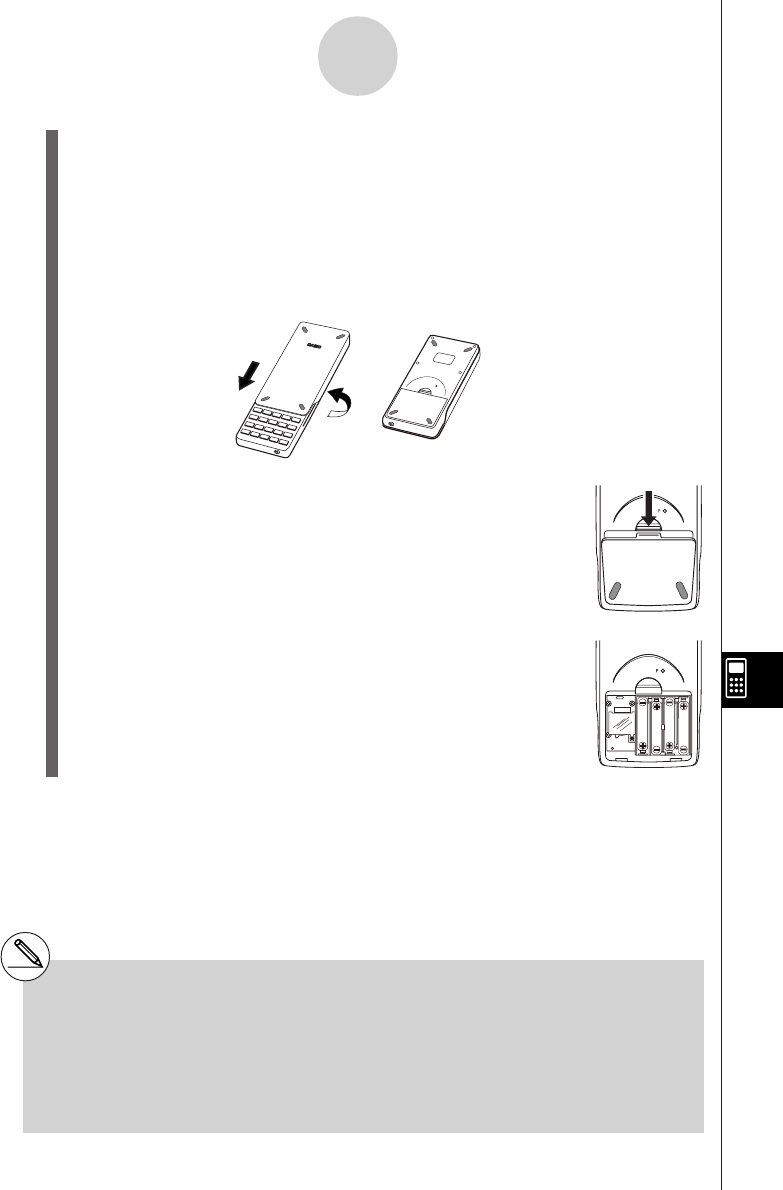
19990401
1. Press !o(OFF) to turn off the calculator.
Warning!
*Be sure to turn the calculator off before replacing batteries. Replacing batteries with
power on will cause data in memory to be deleted.
2. Making sure that you do not accidently press the o key, slide the case onto the
calculator and then turn it over.
P
3. Remove the back cover from the calculator by
1
pulling with your finger at the point marked 1.
4. Remove the four old batteries.
5. Load a new set of four batteries, making sure that
their positive (+) and negative (–) ends are facing in
the proper directions.
BACK UP
6. Replace the back cover.
7. Turn the calculator front side up and slide off its case.
Next, press o to turn on power.
α
-7-3
Power Supply
#Power supplied by memory back up battery
while the main power supply batteries are
removed for replacement retains memory
contents.
#Do not leave the calculator without main power
supply batteries loaded for long periods.
Doing so can cause deletion of data stored in
memory.
#If the figures on the display appear too light and
hard to see after you turn on power, adjust the
tint.
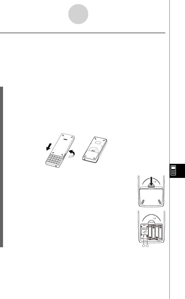
19990401
uTo replace the memory back up battery
*Before replacing the memory back up battery, check to make sure the main batteries
are not dead.
*Never remove the main power supply and the memory back up batteries from the
calculator at the same time.
*Be sure to replace the back up power supply battery at least once 2 years, regardless
of how much you use the calculator during that time. Failure to do so can cause data in
memory to be deleted.
1. Press !o(OFF) to turn off the calculator.
Warning!
*Be sure to turn the calculator off before replacing battery. Replacing battery with power
on will cause data in memory to be deleted.
2. Making sure that you do not accidently press the o key, slide the case onto the
calculator and then turn it over.
3. Remove the back cover from the calculator by
1
pulling with your finger at the point marked 1.
4. Remove screw i on the back of the calculator, and
remove the back up battery compartment cover.
5. Insert a thin, pointed non-metal object (such as a
toothpick) into the hole maked j and remove the old
battery.
α
-7-4
Power Supply
P
A
B
BACK UP

19990401
6. Wipe off the surfaces of a new battery with a soft,
dry cloth. Load it into the calculator so that its positive
(+) side is facing up.
7. Install the memory protection battery cover onto the
calculator and secure it in place with the screw.
Next, replace the back cover.
8. Turn the calculator front side up and slide off its case.
Next, press o to turn on power.
kAbout the Auto Power Off Function
Calculator power turns off automatically if you do not perform any operation within the Auto
Power Off trigger time you specify. You can specify either six minutes or 60 minutes as the
trigger time (see “APO Settings” on page 9-3-1). To restore power, press o.
α
-7-5
Power Supply
BACK UP
20010101
•••••••••••••••••••
•••••••••••••••••••
•••••••••••••••••••
•••••••••••••••••••
•••••••••••••••••••
•••••••••••••••••••
•••••••••••••••••••
•••••••••••••••••••
•••••••••••••••••••
•••••••••••••••••••
•••••••••••••••••••
•••••••••••••••••••
•••••••••••••••••••
•••••••••••••••••••
•••••••••••••••••••
•••••••••••••••••••
•••••••••••••••••••
•••••••••••••••••••
ALGEBRA FX 2.0 PLUS
FX 1.0
PLUS
(Additional Functions)

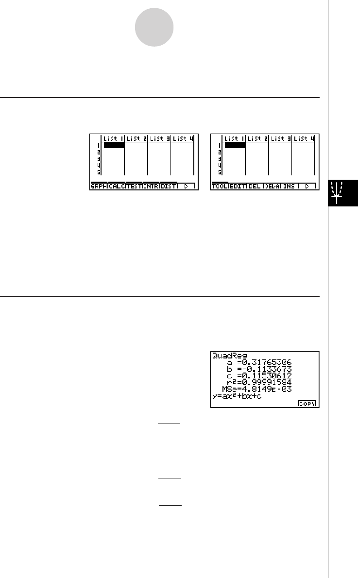
20010101
1-1 Advanced Statistics (STAT)
uu
uu
uFunction Menu
The following shows the function menus for the STAT Mode list input screen.
Pressing a function key that corresponds to the added item displays a menu that lets you
select one of the functions listed below.
•3(TEST) ... Test (page1-2-1)
•4(INTR) ... Confidence interval (page1-3-1)
•5(DIST) ... Distribution (page1-4-1)
SORT and JUMP functions are located in the TOOL menu (6(g)1(TOOL)).
uu
uu
uCalculation of the Coefficient of Determination (r2) and MSE
You can use the STAT Mode to calculate the coefficient of determination (r2) for quadratic
regression, cubic regression, and quartic regression. The following types of MSE
calculations are also available for each type of regression.
•Linear Regression ...
MSE =
Σ
1
n – 2
i=1
n
(y
i
– (ax
i
+ b))
2
•Quadratic Regression ...
MSE =
Σ
1
n – 3 i=1
n
(yi – (axi + bxi+ c))2
2
•Cubic Regression ...
MSE =
Σ
1
n – 4 i=1
n
(yi – (axi3+ bxi + cxi +d ))2
2
•Quartic Regression ...
MSE =
Σ
1
n – 5
i=1
n
(y
i
– (ax
i4
+ bx
i3
+ cx
i
+ dx
i
+ e))
2
2
1-1-1
Advanced Statistics (STAT)
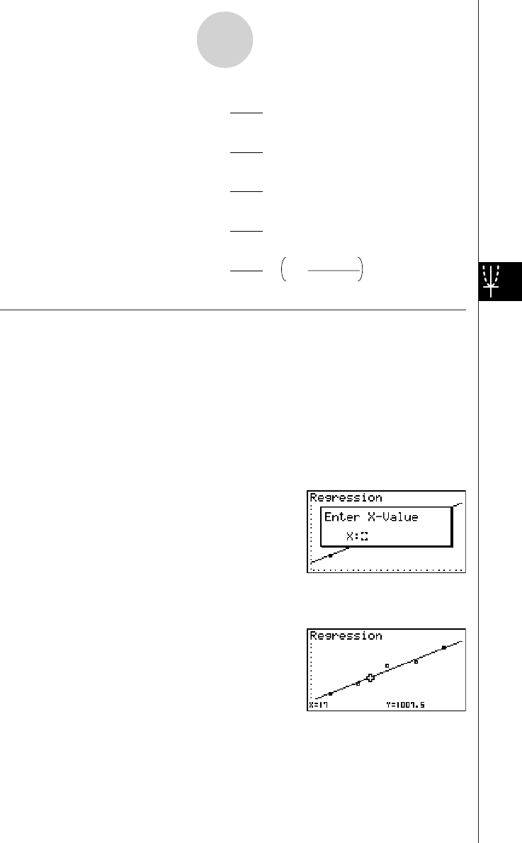
20010101
•Logarithmic Regression ...
MSE =
Σ
1
n – 2 i=1
n
(yi – (a + b ln xi ))2
•Exponential Repression ...
MSE =
Σ
1
n – 2 i=1
n
(ln yi – (ln a + bxi ))2
•Power Regression ...
MSE =
Σ
1
n – 2
i=1
n
(ln y
i
– (ln a + b ln x
i
))
2
•Sin Regression ...
MSE =
Σ
1
n – 2
i=1
n
(y
i
– (a sin (bx
i
+ c) + d ))
2
•Logistic Regression ...
MSE =
Σ
1
n – 2 1 + ae
-bx
i
C
i=1
n
y
i
–
2
uu
uu
uEstimated Value Calculation for Regression Graphs
The STAT Mode also includes a Y-CAL function that uses regression to calculate the
estimated y-value for a particular x-value after graphing a paired-variable statistical
regression.
The following is the general procedure for using the Y-CAL function.
1. After drawing a regression graph, press 6(g)2(Y-CAL) to enter the graph selection mode,
and then press w.
If there are multiple graphs on the display, use f and c to select the graph you want, and
then press w.
•This causes an x-value input dialog box to appear.
2. Input the value you want for x and then press w.
•This causes the coordinates for x and y to appear at the bottom of the display, and moves the
pointer to the corresponding point on the graph.
3. Pressing v or a number key at this time causes the x-value input dialog box to reappear
so you can perform another estimated value calculation if you want.
1-1-2
Advanced Statistics (STAT)
20011101
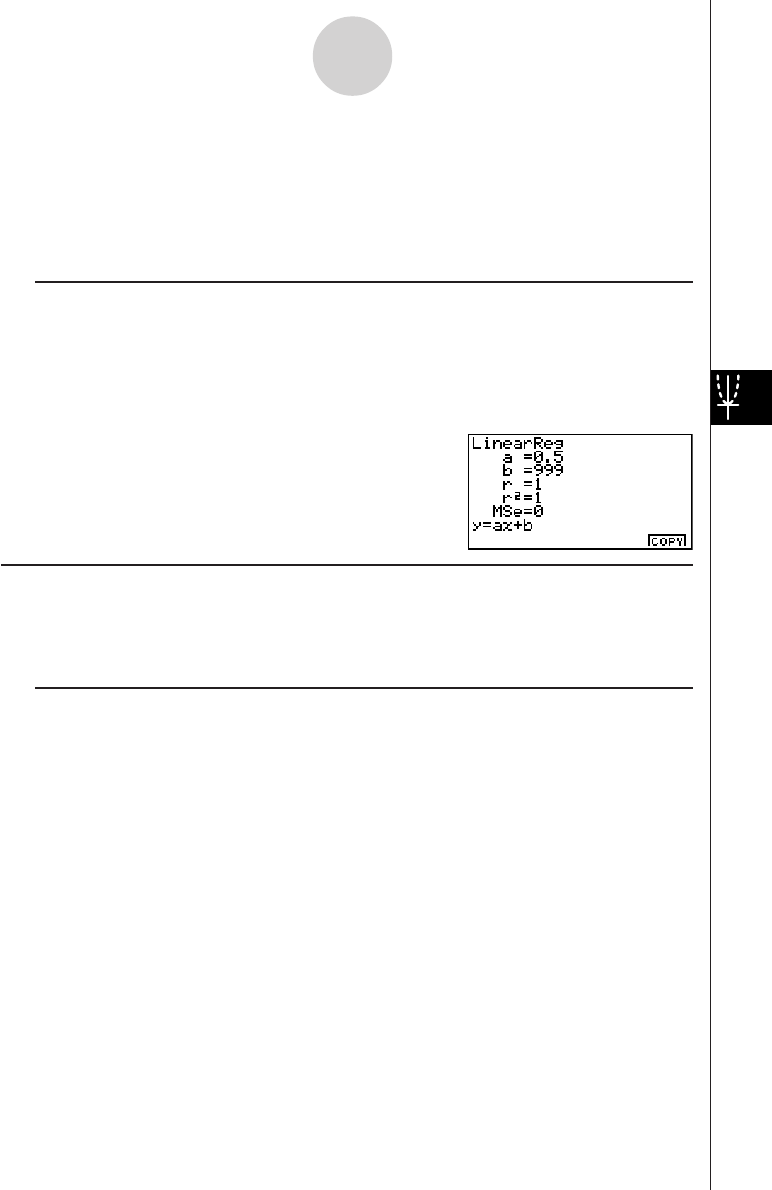
20010101
4. After you are finished, press i to clear the coordinate values and the pointer from the
display.
·The pointer does not appear if the calculated coordinates are not within the display range.
·The coordinates do not appear if [Off] is specified for the [Coord] item of the [SETUP] screen.
·The Y-CAL function can also be used with a graph drawn by using DefG feature.
uu
uu
uRegression Formula Copy Function from a Regression Calculation Result
Screen
In addition to the normal regression formula copy function that lets you copy the regression
calculation result screen after drawing a statistical graph (such as Scatter Plot), the STAT Mode
also has a function that lets you copy the regression formula obtained as the result of a regression
calculation. To copy a resulting regression formula, press 6(COPY).
kk
kk
kTests, Confidence Interval, and Distribution Calculations
The STAT Mode includes functions for performing tests, and confidence interval and distribution
calculations. You can find explanations of each of these functions in the following sections: 1-2
Tests, 1-3 Confidence Interval, and 1-4 Distribution.
uu
uu
uParameter Settings
The following describes the two methods you can use to make parameter settings for test,
confidence interval, and distribution calculations.
• Selection
With this method, you press the function key that corresponds to the setting you want to
select from the function menu.
• Value Input
With this method, you directly input the parameter value you want to input. In this case,
nothing appears in the function menu.
·Pressing i returns to the list input screen, with the cursor in the same position it was at
before you started the parameter setting procedure.
· Pressing ! i(QUIT) returns to the top of list input screen.
· Pressing w without pressing 1(CALC) under “Execute” item advances to calculation
execution. To return to the parameter setting screen, press i, A, or w.
1-1-3
Advanced Statistics (STAT)

20010101
uu
uu
uCommon Functions
• The symbol “■” appears in the upper right corner of the screen while execution of a
calculation is being performed and while a graph is being drawn. Pressing A during this
time terminates the ongoing calculation or draw operation (AC Break).
• Pressing i or w while a calculation result or graph is on the display returns to the
parameter setting screen. Pressing ! i(QUIT) returns to the top of list input screen.
· Pressing A while a calculation result is on the display returns to the parameter setting screen.
• Pressing u 5(G↔T) after drawing a graph switches to the parameter setting screen
(G↔T function). Pressing u 5(G↔T) again returns to the graph screen.
· The G↔T function is disabled whenever you change a setting on the parameter setting screen, or
when you perform a u 3(SET UP) or ! K(V-Window) operation.
• You can perform the PICT menu's screen save or recall functions after drawing a graph.
· The ZOOM function and SKETCH function are disabled.
The TRACE function is disabled, except for the graph display of two-way ANOVA.
The graph screen cannot be scrolled.
• After drawing a graph, you can use a Save Result feature to save calculation results to a
specific list. Basically, all items are saved as they are displayed, except for the first line title.
·Each time you execute Save Result, any existing data in the list is replaced by the new results.
1-1-4
Advanced Statistics (STAT)
20011101

20010101
1-2 Tests (TEST)
The Z Test provides a variety of different standardization-based tests. They make it possible
to test whether or not a sample accurately represents the population when the standard
deviation of a population (such as the entire population of a country) is known from previous
tests. Z testing is used for market research and public opinion research, that need to be
performed repeatedly.
1-Sample Z Test tests for the unknown population mean when the population standard
deviation is known.
2-Sample Z Test tests the equality of the means of two populations based on independent
samples when both population standard deviations are known.
1-Prop Z Test tests for an unknown proportion of successes.
2-Prop Z Test tests to compare the proportion of successes from two populations.
The t Test tests the hypothesis when the population standard deviation is unknown. The
hypothesis that is the opposite of the hypothesis being proven is called the
null hypothesis
,
while the hypothesis being proved is called the
alternative hypothesis
. The t-test is normally
applied to test the null hypothesis. Then a determination is made whether the null hypothesis
or alternative hypothesis will be adopted.
1-Sample t Test tests the hypothesis for a single unknown population mean when the
population standard deviation is unknown.
2-Sample t Test compares the population means when the population standard deviations
are unknown.
LinearReg t Test calculates the strength of the linear association of paired data.
χ
2 Test tests hypothesis concerning the proportion of samples included in each of a number
of independent groups. Mainly, it generates cross-tabulation of two categorical variables
(such as yes, no) and evaluates the independence of these variables. It could be used, for
example, to evaluate the relationship between whether or not a driver has ever been involved
in a traffic accident and that person’s knowledge of traffic regulations.
2-Sample F Test tests the hypothesis for the ratio of sample variances. It could be used, for
example, to test the carcinogenic effects of multiple suspected factors such as tobacco use,
alcohol, vitamin deficiency, high coffee intake, inactivity, poor living habits, etc.
ANOVA tests the hypothesis that the population means of the samples are equal when there
are multiple samples. It could be used, for example, to test whether or not different
combinations of materials have an effect on the quality and life of a final product.
One-Way ANOVA is used when there is one independent variable and one dependent
variable.
Two-Way ANOVA is used when there are two independent variables and one dependent
variable.
1-2-1
Tests (TEST)
20011101

20010101
The following pages explain various statistical calculation methods based on the principles
described above. Details concerning statistical principles and terminology can be found in
any standard statistics textbook.
On the initial STAT Mode screen, press 3(TEST) to display the test menu, which contains
the following items.
•3(TEST)b(Z) ... Z Tests (p. 1-2-2)
c(T) ... t Tests (p. 1-2-10)
d(χ2) ... χ2 Test (p. 1-2-18)
e(F) ... 2-Sample F Test (p. 1-2-20)
f(ANOVA) ... ANOVA (p. 1-2-22)
kk
kk
kZ Tests
uu
uu
uZ Test Common Functions
You can use the following graph analysis functions after drawing a graph.
•1(Z) ... Displays z score.
Pressing 1 (Z) displays the z score at the bottom of the display, and displays the pointer at
the corresponding location in the graph (unless the location is off the graph screen).
Two points are displayed in the case of a two-tail test. Use d and e to move the pointer.
Press i to clear the z score.
•2(P) ... Displays p-value.
Pressing 2 (P) displays the p-value at the bottom of the display without displaying the
pointer.
Press i to clear the p-value.
uu
uu
u1-Sample Z Test
This test is used when the population standard deviation is known to test the hypothesis. The
1-Sample Z Test is applied to the normal distribution.
Z = o –
0
σ
µ
n
o: mean of sample
µ
o: assumed population mean
σ
: population standard deviation
n: size of sample
# The following V-Window settings are used for
drawing the graph.
Xmin = –3.2, Xmax = 3.2, Xscale = 1,
Ymin = –0.1, Ymax = 0.45, Yscale = 0.1
#Executing an analysis function automatically
stores the z and p values in alpha variables Z
and P, respectively.
1-2-2
Tests (TEST)
20011101
20010101
Perform the following key operations from the statistical data list.
3(TEST)
b(Z)
b(1-Smpl)
The following shows the meaning of each item in the case of list data specification.
Data ............................ data type
µ
.................................. population mean value test conditions (“G
µ
0” specifies
two-tail test, “<
µ
0” specifies lower one-tail test, “>
µ
0”
specifies upper one-tail test.)
µ
0................................. assumed population mean
σ
.................................. population standard deviation (
σ
> 0)
List .............................. list whose contents you want to use as data (List 1 to 20)
Freq ............................. frequency (1 or List 1 to 20)
Save Res ..................... list for storage of calculation results (None or List 1 to 20)
Execute ....................... executes a calculation or draws a graph
The following shows the meaning of parameter data specification items that are different
from list data specification.
o.................................. mean of sample
n.................................. size of sample (positive integer)
After setting all the parameters, align the cursor with [Execute] and then press one of the
function keys shown below to perform the calculation or draw the graph.
•1(CALC) ... Performs the calculation.
•6(DRAW) ... Draws the graph.
1-2-3
Tests (TEST)
20011101
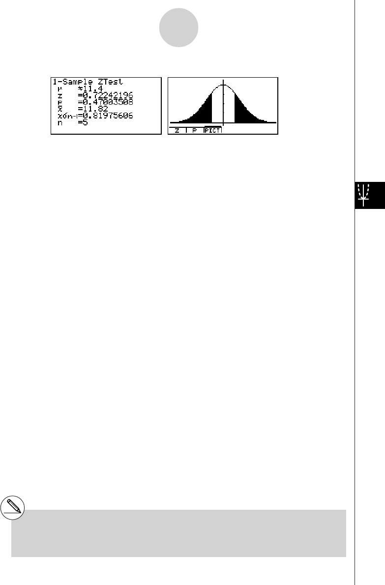
20010101
Calculation Result Output Example
µ
G11.4
........................
direction of test
z.................................. z score
p.................................. p-value
o.................................. mean of sample
x
σ
n-1 ............................. sample standard deviation
(Displayed only for Data: List setting.)
n.................................. size of sample
# [Save Res] does not save the
µ
condition in
line 2.
1-2-4
Tests (TEST)
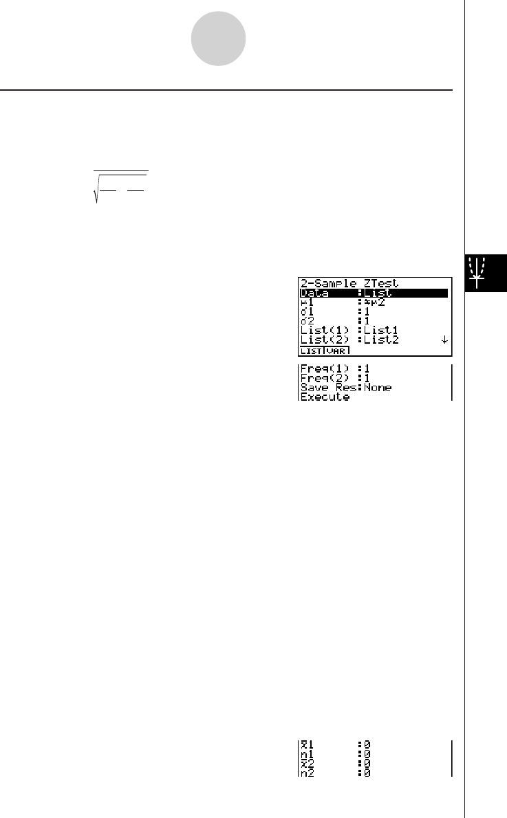
20010101
uu
uu
u2-Sample Z Test
This test is used when the standard deviations for two populations are known to test the
hypothesis. The 2-Sample Z Test is applied to the normal distribution.
Z = o
1
– o
2
σ
n
1
1
2
σ
n
2
2
2
+
o1: mean of sample 1
o2: mean of sample 2
σ
1: population standard deviation of sample 1
σ
2: population standard deviation of sample 2
n1: size of sample 1
n2: size of sample 2
Perform the following key operations from the statistical data list.
3(TEST)
b(Z)
c(2-Smpl)
The following shows the meaning of each item in the case of list data specification.
Data ............................ data type
µ
1................................. population mean value test conditions (“G
µ
2” specifies two-
tail test, “<
µ
2” specifies one-tail test where sample 1 is
smaller than sample 2, “>
µ
2” specifies one-tail test where
sample 1 is greater than sample 2.)
σ
1................................. population standard deviation of sample 1 (
σ
1 > 0)
σ
2................................. population standard deviation of sample 2 (
σ
2 > 0)
List(1) .......................... list whose contents you want to use as sample 1 data
(List 1 to 20)
List(2) .......................... list whose contents you want to use as sample 2 data
(List 1 to 20)
Freq(1) ........................ frequency of sample 1 (1 or List 1 to 20)
Freq(2) ........................ frequency of sample 2 (1 or List 1 to 20)
Save Res ..................... list for storage of calculation results (None or List 1 to 20)
Execute ....................... executes a calculation or draws a graph
The following shows the meaning of parameter data specification items that are different
from list data specification.
1-2-5
Tests (TEST)
20011101
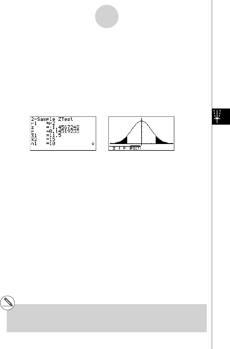
20010101
o1................................. mean of sample 1
n1................................. size (positive integer) of sample 1
o2................................. mean of sample 2
n2................................. size (positive integer) of sample 2
After setting all the parameters, align the cursor with [Execute] and then press one of the
function keys shown below to perform the calculation or draw the graph.
•1(CALC) ... Performs the calculation.
•6(DRAW) ... Draws the graph.
Calculation Result Output Example
µ
1G
µ
2........................... direction of test
z ................................... z score
p.................................. p-value
o1................................. mean of sample 1
o2................................. mean of sample 2
x1
σ
n-1 ............................ standard deviation of sample 1
(Displayed only for Data: List setting.)
x2
σ
n-1 ............................ standard deviation of sample 2
(Displayed only for Data: List setting.)
n1................................. size of sample 1
n2................................. size of sample 2
# [Save Res] does not save the
µ
1 condition in
line 2.
1-2-6
Tests (TEST)
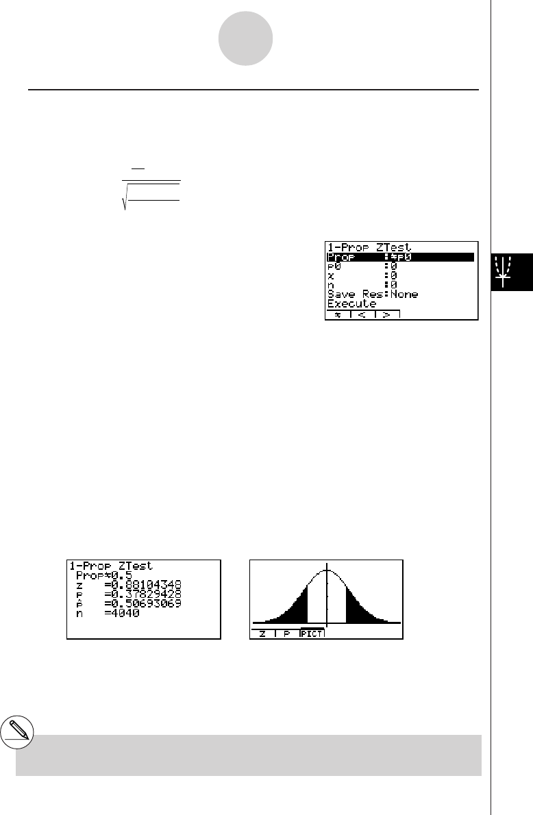
20010101
uu
uu
u1-Prop Z Test
This test is used to test for an unknown proportion of successes. The 1-Prop Z Test is
applied to the normal distribution.
Z = n
x
n
p
0
(1– p
0
)
– p
0
p0: expected sample proportion
n: size of sample
Perform the following key operations from the statistical data list.
3(TEST)
b(Z)
d(1-Prop)
Prop ............................ sample proportion test conditions (“G p0” specifies two-tail
test, “< p0” specifies lower one-tail test, “> p0” specifies upper
one-tail test.)
p0................................. expected sample proportion (0 < p0 < 1)
x.................................. sample value (x > 0 integer)
n.................................. size of sample (positive integer)
Save Res ..................... list for storage of calculation results (None or List 1 to 20)
Execute ....................... executes a calculation or draws a graph
After setting all the parameters, align the cursor with [Execute] and then press one of the
function keys shown below to perform the calculation or draw the graph.
•1(CALC) ... Performs the calculation.
•6(DRAW) ... Draws the graph.
Calculation Result Output Example
PropG0.5 .................... direction of test
z ................................... z score
p .................................. p-value
ˆp .................................. estimated sample proportion
n .................................. size of sample
# [Save Res] does not save the Prop condition
in line 2.
1-2-7
Tests (TEST)
20011101
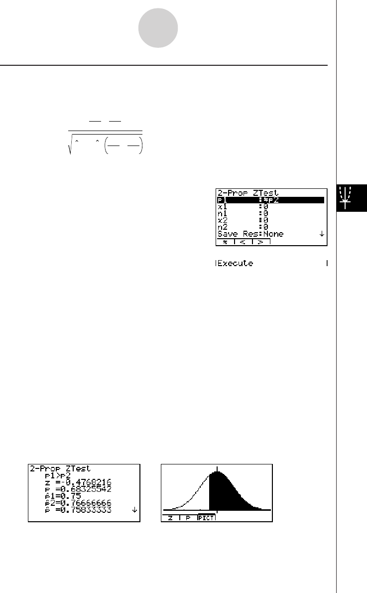
20010101
uu
uu
u2-Prop Z Test
This test is used to compare the proportion of successes. The 2-Prop Z Test is applied to the
normal distribution.
Z = n1
x1
n2
x2
–
p(1 – p )n1
1
n2
1
+
x1: data value of sample 1
x2: data value of sample 2
n1: size of sample 1
n2: size of sample 2
ˆp : estimated sample proportion
Perform the following key operation from the statistical data list.
3(TEST)
b(Z)
e(2-Prop)
p1................................. sample proportion test conditions (“G p2” specifies two-tail
test, “< p2” specifies one-tail test where sample 1 is smaller
than sample 2, “> p2” specifies one-tail test where sample 1
is greater than sample 2.)
x1................................. data value (x1 > 0 integer) of sample 1
n1................................. size (positive integer) of sample 1
x2................................. data value (x2 > 0 integer) of sample 2
n2................................. size (positive integer) of sample 2
Save Res ..................... list for storage of calculation results (None or List 1 to 20)
Execute ....................... executes a calculation or draws a graph
After setting all the parameters, align the cursor with [Execute] and then press one of the
function keys shown below to perform the calculation or draw the graph.
•1(CALC) ... Performs the calculation.
•6(DRAW) ... Draws the graph.
Calculation Result Output Example
1-2-8
Tests (TEST)
20011101

20010101
p1>p2............................ direction of test
z.................................. z score
p.................................. p-value
ˆp 1................................. estimated proportion of sample 1
ˆp 2................................. estimated proportion of sample 2
ˆp .................................. estimated sample proportion
n1................................. size of sample 1
n2................................. size of sample 2
# [Save Res] does not save the p1 condition in
line 2.
1-2-9
Tests (TEST)

20010101
kk
kk
kt Tests
uu
uu
u t Test Common Functions
You can use the following graph analysis functions after drawing a graph.
•1(T) ... Displays t score.
Pressing 1 (T) displays the t score at the bottom of the display, and displays the pointer at the
corresponding location in the graph (unless the location is off the graph screen).
Two points are displayed in the case of a two-tail test. Use d and e to move the pointer.
Press i to clear the t score.
•2(P) ... Displays p-value.
Pressing 2 (P) displays the p-value at the bottom of the display without displaying the pointer.
Press i to clear the p-value.
# The following V-Window settings are used for
drawing the graph.
Xmin = –3.2, Xmax = 3.2, Xscale = 1,
Ymin = –0.1, Ymax = 0.45, Yscale = 0.1
#Executing an analysis function automatically
stores the t and p values in alpha variables T
and P, respectively.
1-2-10
Tests (TEST)
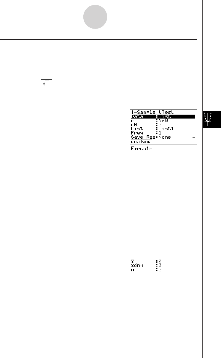
20010101
uu
uu
u1-Sample t Test
This test uses the hypothesis test for a single unknown population mean when the population
standard deviation is unknown. The 1-Sample t Test is applied to t-distribution.
t = o – 0
µ
σ
x
n–1
n
o: mean of sample
µ
0: assumed population mean
x
σ
n-1 : sample standard deviation
n: size of sample
Perform the following key operations from the statistical data list.
3(TEST)
c(T)
b(1-Smpl)
The following shows the meaning of each item in the case of list data specification.
Data ............................ data type
µ
.................................. population mean value test conditions (“G
µ
0” specifies two-
tail test, “<
µ
0” specifies lower one-tail test, “>
µ
0” specifies
upper one-tail test.)
µ
0................................. assumed population mean
List .............................. list whose contents you want to use as data (List 1 to 20)
Freq ............................. frequency (1 or List 1 to 20)
Save Res ..................... list for storage of calculation results (None or List 1 to 20)
Execute ....................... executes a calculation or draws a graph
The following shows the meaning of parameter data specification items that are different
from list data specification.
o.................................. mean of sample
x
σ
n-1 ............................. sample standard deviation (x
σ
n-1 > 0)
n.................................. size of sample (positive integer)
After setting all the parameters, align the cursor with [Execute] and then press one of the
function keys shown below to perform the calculation or draw the graph.
• 1(CALC) ... Performs the calculation.
• 6(DRAW) ... Draws the graph.
1-2-11
Tests (TEST)
20011101
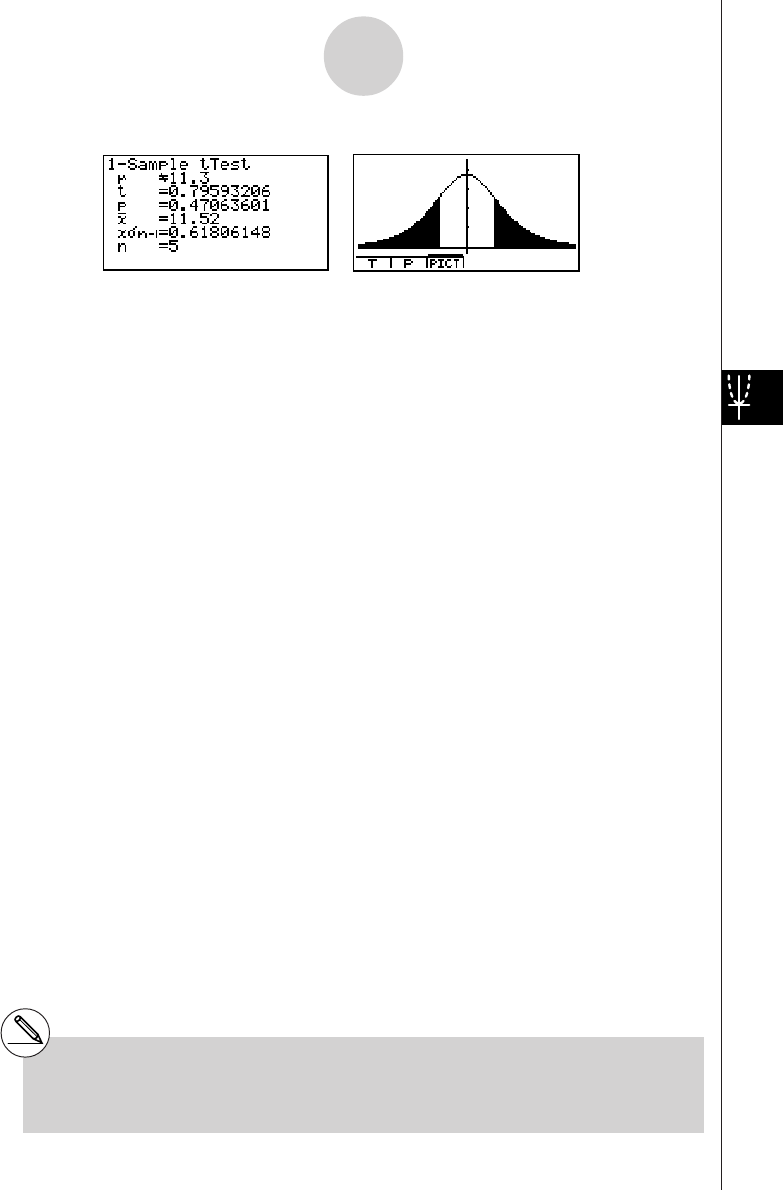
20010101
Calculation Result Output Example
µ
G 11.3 ...................... direction of test
t
...................................
t score
p.................................. p-value
o.................................. mean of sample
x
σ
n-1 ............................. sample standard deviation
n.................................. size of sample
# [Save Res] does not save the
µ
condition in
line 2.
1-2-12
Tests (TEST)
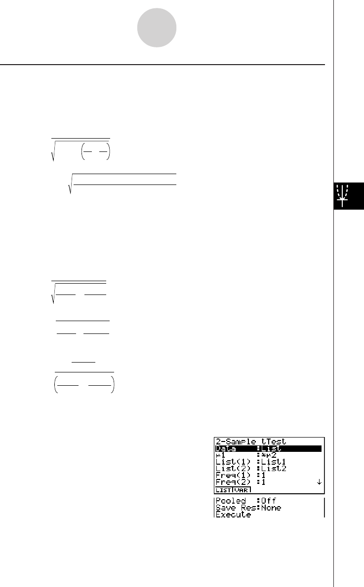
20010101
uu
uu
u2-Sample t Test
2-Sample t Test compares the population means when the population standard deviations
are unknown. The 2-Sample t Test is applied to t-distribution.
The following applies when pooling is in effect.
t
= o
1
– o
2
n
1
1+n
2
1
x
p
n–12
σ
x
p n–1
=
σ
n
1
+ n
2
– 2
(n
1
–1)x
1 n–12
+(n
2
–1)x
2 n–12
σσ
df
= n1 + n2 – 2
The following applies when pooling is not in effect.
t = o
1
– o
2
x
1 n–1
2
σ
n
1
+x
2 n–1
2
σ
n
2
df = 1
C
2
n
1
–1 +(1–C )
2
n
2
–1
C =
x1 n–12
σ
n1+x2 n–12
σ
n2
x1 n–12
σ
n1
Perform the following key operations from the statistical data list.
3(TEST)
c(T)
c(2-Smpl)
1-2-13
Tests (TEST)
o1:mean of sample 1
o2:mean of sample 2
x1
σ
n-1 :standard deviation of
sample 1
x2
σ
n-1 :standard deviation of
sample 2
n1:size of sample 1
n2:size of sample 2
xp
σ
n-1 :pooled sample standard
deviation
df :degrees of freedom
o1:mean of sample 1
o2:mean of sample 2
x1
σ
n-1 :standard deviation of
sample 1
x2
σ
n-1 :standard deviation of
sample 2
n1:size of sample 1
n2:size of sample 2
df :degrees of freedom
20011101

20010101
The following shows the meaning of each item in the case of list data specification.
Data ............................ data type
µ
1................................. sample mean value test conditions (“G
µ
2” specifies two-tail
test, “<
µ
2” specifies one-tail test where sample 1 is smaller
than sample 2, “>
µ
2” specifies one-tail test where sample 1 is
greater than sample 2.)
List(1) .......................... list whose contents you want to use as data of sample 1
(List 1 to 20)
List(2) .......................... list whose contents you want to use as data of sample 2
(List 1 to 20)
Freq(1) ........................ frequency of sample 1 (1 or List 1 to 20)
Freq(2) ........................ frequency of sample 2 (1 or List 1 to 20)
Pooled ......................... pooling On (in effect) or Off (not in effect)
Save Res ..................... list for storage of calculation results (None or List 1 to 20)
Execute ....................... executes a calculation or draws a graph
The following shows the meaning of parameter data specification items that are different
from list data specification.
o1................................. mean of sample 1
x1
σ
n-1 ............................ standard deviation (x1
σ
n-1 > 0) of sample 1
n1................................. size (positive integer) of sample 1
o2................................. mean of sample 2
x2
σ
n-1 ............................ standard deviation (x2
σ
n-1 > 0) of sample 2
n2................................. size (positive integer) of sample 2
After setting all the parameters, align the cursor with [Execute] and then press one of the
function keys shown below to perform the calculation or draw the graph.
•1(CALC) ... Performs the calculation.
•6(DRAW) ... Draws the graph.
1-2-14
Tests (TEST)
20011101
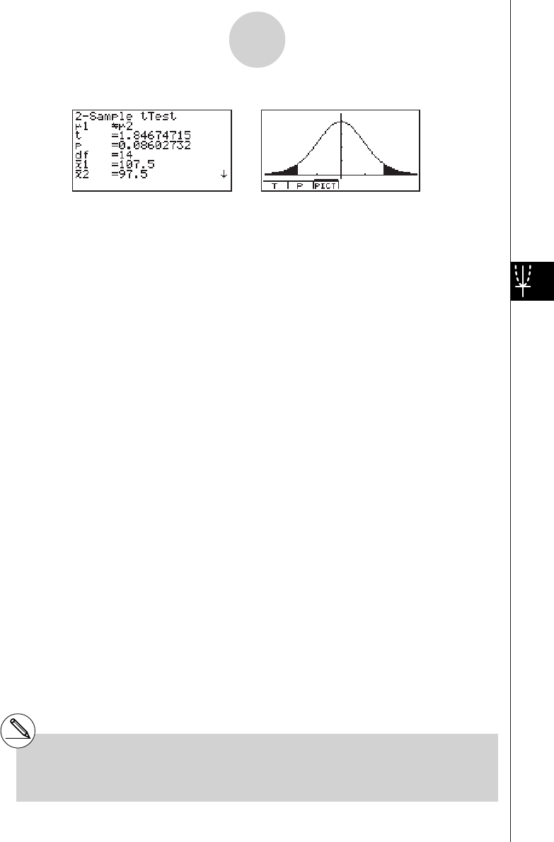
20010101
Calculation Result Output Example
µ
1G
µ
2........................... direction of test
t
...................................
t score
p.................................. p-value
df ................................. degrees of freedom
o1................................. mean of sample 1
o2................................. mean of sample 2
x1
σ
n-1 ............................ standard deviation of sample 1
x2
σ
n-1 ............................ standard deviation of sample 2
xp
σ
n-1 ............................ pooled sample standard deviation (Displayed only when Pooled:
On setting.)
n1................................. size of sample 1
n2................................. size of sample 2
# [Save Res] does not save the
µ
1
condition in
line 2.
1-2-15
Tests (TEST)
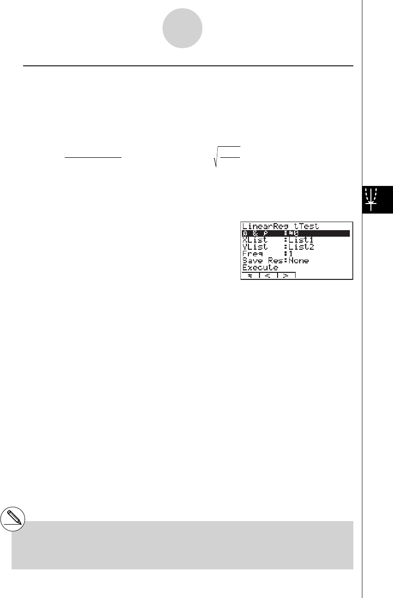
20010101
uu
uu
uLinearReg t Test
LinearReg t Test treats paired-variable data sets as (x, y) pairs, and uses the method of
least squares to determine the most appropriate a, b coefficients of the data for the
regression formula y = a + bx. It also determines the correlation coefficient and t value, and
calculates the extent of the relationship between x and y.
b =
Σ
( x – o)( y – p)
i=1
n
Σ
(x – o)
2
i=1
n
a = p – bot = r n – 2
1 – r
2
a:intercept
b:slope of the line
n:size of sample (n > 3)
r:correlation coefficient
r2:coefficient of
determination
Perform the following key operations from the statistical data list.
3(TEST)
c(T)
d(LinReg)
The following shows the meaning of each item in the case of list data specification.
β
&
ρ
............................ p-value test conditions (“G 0” specifies two-tail test, “< 0”
specifies lower one-tail test, “> 0” specifies upper one-tail
test.)
XList ............................ list for x-axis data (List 1 to 20)
YList ............................ list for y-axis data (List 1 to 20)
Freq ............................. frequency (1 or List 1 to 20)
Save Res ..................... list for storage of calculation results (None or List 1 to 20)
Execute ....................... executes a calculation
After setting all the parameters, align the cursor with [Execute] and then press the function key
shown below to perform the calculation.
• 1(CALC) ... Performs the calculation.
# You cannot draw a graph for LinearReg t
Test.
1-2-16
Tests (TEST)
20011101
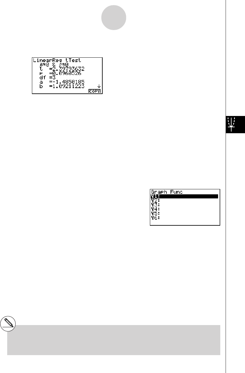
20010101
Calculation Result Output Example
β
G 0 &
ρ
G 0 .............. direction of test
t................................... t score
p.................................. p-value
df ................................. degrees of freedom
a.................................. constant term
b.................................. coefficient
s.................................. standard error
r.................................. correlation coefficient
r2................................. coefficient of determination
Pressing 6 (COPY) while a calculation result is on the display copies the regression formula
to the graph formula editor.
When there is a list specified for the [Resid List] item on the SET UP screen, regression formula
residual data is automatically saved to the specified list after the calculation is finished.
# [Save Res] does not save the
β
&
ρ
conditions in line 2.
#When the list specified by [Save Res] is the
same list specified by the [Resid List] item on
the SET UP screen, only [Resid List] data is
saved in the list.
1-2-17
Tests (TEST)
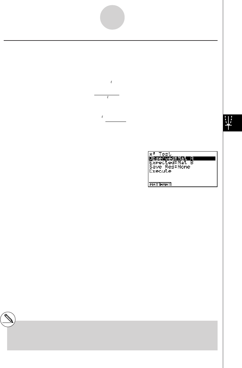
20010101
kk
kk
kχ2 Test
χ2 Test sets up a number of independent groups and tests hypothesis related to the
proportion of the sample included in each group. The χ2 Test is applied to dichotomous
variables (variable with two possible values, such as yes/no).
Expected counts
F
ij
=
Σx
ij
i=1
k
×Σx
ij
j=1
k
ΣΣ
i=1 j=1
x
ij
χ
2
= ΣΣ F
ij
i=1
k
(x
ij
– F
ij
)
2
j
=1
Perform the following key operations from the statistical data list.
3(TEST)
d(χ2)
Next, specify the matrix that contains the data. The following shows the meaning of the
above item.
Observed .................... name of matrix (A to Z) that contains observed counts (all cells
positive integers)
Expected ..................... name of matrix (A to Z) that is for saving expected frequency
Save Res ..................... list for storage of calculation results (None or List 1 to 20)
Execute ....................... executes a calculation or draws a graph
# The matrix must be at least two lines by two
columns. An error occurs if the matrix has
only one line or one column.
1-2-18
Tests (TEST)
20011101
#Pressing 2 ('MAT) while setting
parameters enters the MATRIX editor, which
you can use to edit and view the contents of
matrices.
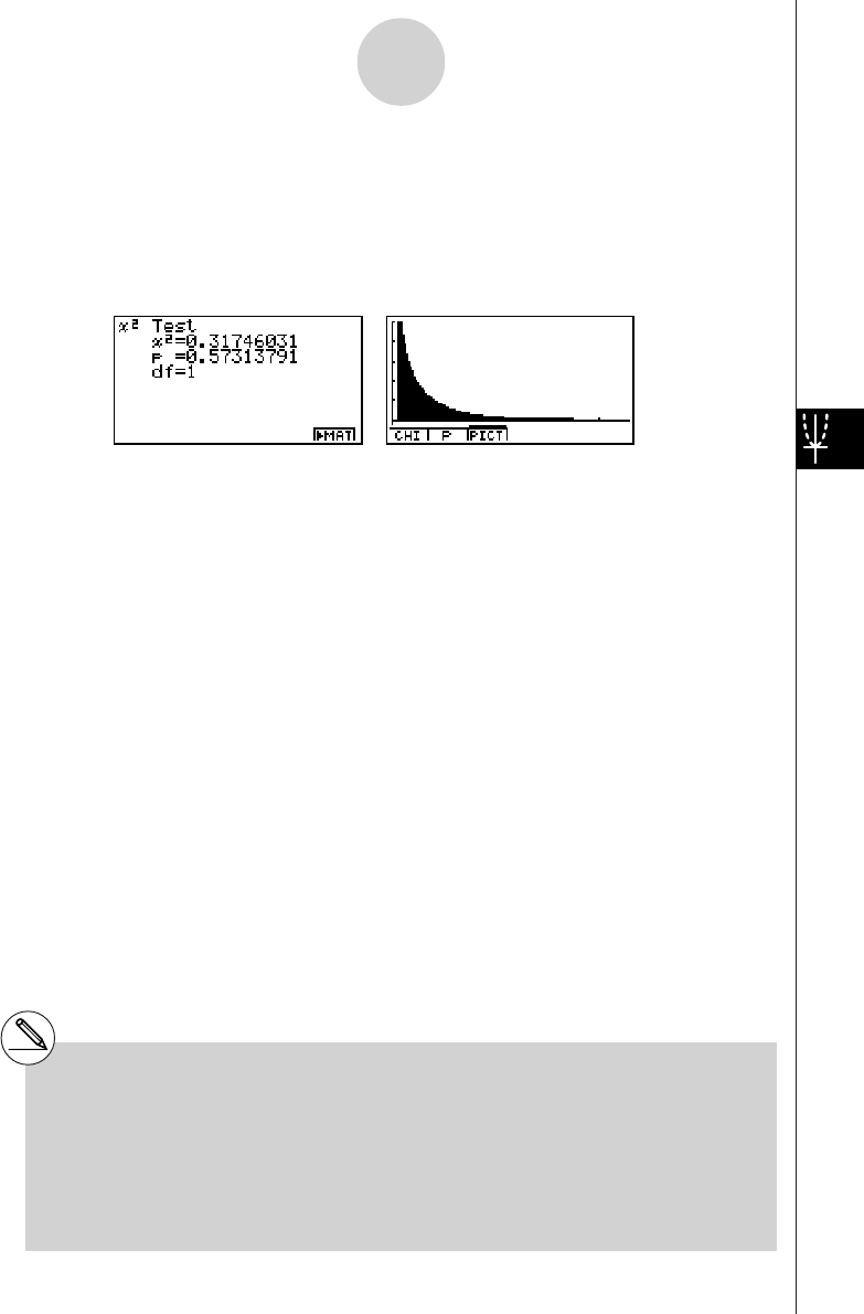
20010101
After setting all the parameters, align the cursor with [Execute] and then press one of the
function keys shown below to perform the calculation or draw the graph.
•1(CALC) ... Performs the calculation.
•6(DRAW) ... Draws the graph.
Calculation Result Output Example
χ
2................................. χ2 value
p.................................. p-value
df ................................. degrees of freedom
You can use the following graph analysis functions after drawing a graph.
•1(CHI) ... Displays
χ
2 value.
Pressing 1 (CHI) displays the
χ
2 value at the bottom of the display, and displays the pointer at
the corresponding location in the graph (unless the location is off the graph screen).
Press i to clear the
χ
2 value.
•2(P) ... Displays p-value.
Pressing 2 (P) displays the p-value at the bottom of the display without displaying the pointer.
Press i to clear the p-value.
# Pressing 6('MAT) while a calculation
result is displayed enters the MATRIX editor,
which you can use to edit and view the
contents of matrices.
# The following V-Window settings are used for
drawing the graph.
Xmin = 0, Xmax = 11.5, Xscale = 2,
Ymin = –0.1, Ymax = 0.5, Yscale = 0.1
#Executing an analysis function automatically
stores the
χ
2 and p values in alpha variables
C and P, respectively.
1-2-19
Tests (TEST)
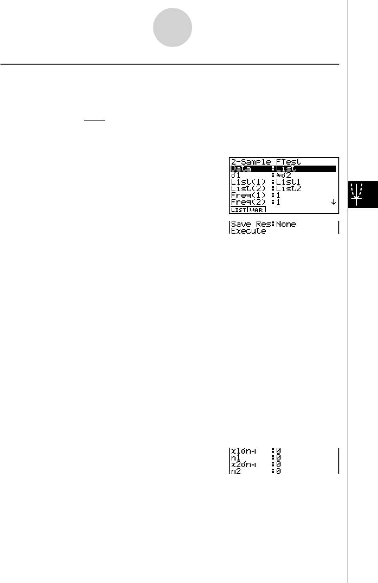
20010101
kk
kk
k2-Sample F Test
2-Sample F Test tests the hypothesis for the ratio of sample variances. The F Test is applied
to the F distribution.
F = x1 n–12
σ
x2 n–12
σ
Perform the following key operations from the statistical data list.
3(TEST)
e(F)
The following is the meaning of each item in the case of list data specification.
Data ............................ data type
σ
1................................. population standard deviation test conditions (“G
σ
2”
specifies two-tail test, “<
σ
2” specifies one-tail test where
sample 1 is smaller than sample 2, “>
σ
2” specifies one-tail
test where sample 1 is greater than sample 2.)
List(1) .......................... list whose contents you want to use as data of sample 1
(List 1 to 20)
List(2) .......................... list whose contents you want to use as data of sample 2
(List 1 to 20)
Freq(1) ........................ frequency of sample 1 (1 or List 1 to 20)
Freq(2) ........................ frequency of sample 2 (1 or List 1 to 20)
Save Res ..................... list for storage of calculation results (None or List 1 to 20)
Execute ....................... executes a calculation or draws a graph
The following shows the meaning of parameter data specification items that are different
from list data specification.
x1
σ
n-1 ............................ standard deviation (x1
σ
n-1
>
0) of sample 1
n1................................. size (positive integer) of sample 1
x2
σ
n-1 ............................ standard deviation (x2
σ
n-1
>
0) of sample 2
n2................................. size (positive integer) of sample 2
1-2-20
Tests (TEST)
20011101
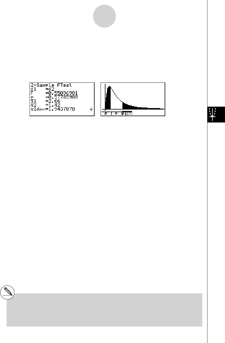
20010101
After setting all the parameters, align the cursor with [Execute] and then press one of the
function keys shown below to perform the calculation or draw the graph.
• 1(CALC) ... Performs the calculation.
• 6(DRAW) ... Draws the graph.
Calculation Result Output Example
σ
1G
σ
2.......................... direction of test
F.................................. F value
p.................................. p-value
o1................................. mean of sample 1 (Displayed only for Data: List setting.)
o2................................. mean of sample 2 (Displayed only for Data: List setting.)
x1
σ
n-1 ............................ standard deviation of sample 1
x2
σ
n-1 ............................ standard deviation of sample 2
n1................................. size of sample 1
n2................................. size of sample 2
You can use the following graph analysis functions after drawing a graph.
•1(F) ... Displays F value.
Pressing 1 (F) displays the F value at the bottom of the display, and displays the pointer at
the corresponding location in the graph (unless the location is off the graph screen).
Two points are displayed in the case of a two-tail test. Use d and e to move the pointer.
Press i to clear the F value.
•2(P) ... Displays p-value.
Pressing 2 (P) displays the p-value at the bottom of the display without displaying the pointer.
Press i to clear the p-value.
# [Save Res] does not save the
σ
1 condition in
line 2.
# V-Window settings are automatically
optimized for drawing the graph.
#Executing an analysis function automatically
stores the F and p values in alpha variables
F and P, respectively.
1-2-21
Tests (TEST)
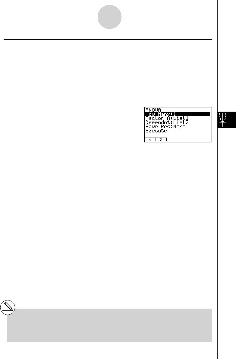
20010101
kk
kk
kANOVA
ANOVA tests the hypothesis that the population means of the samples are equal when there
are multiple samples.
One-Way ANOVA is used when there is one independent variable and one dependent
variable.
Two-Way ANOVA is used when there are two independent variables and one dependent
variable.
Perform the following key operations from the statistical data list.
3(TEST)
f(ANOVA)
The following is the meaning of each item in the case of list data specification.
How Many ................... selects One-Way ANOVA or Two-Way ANOVA (number of
levels)
Factor A ....................... category list (List 1 to 20)
Dependnt .................... list to be used for sample data (List 1 to 20)
Save Res ..................... first list for storage of calculation results (None or List 1 to
16)*1
Execute ....................... executes a calculation or draws a graph (Two-Way ANOVA only)
The following item appears in the case of Two-Way ANOVA only.
Factor B ....................... category list (List 1 to 20)
After setting all the parameters, align the cursor with [Execute] and then press one of the
function keys shown below to perform the calculation or draw the graph.
• 1(CALC) ... Performs the calculation.
• 6(DRAW) ... Draws the graph (Two-Way ANOVA only).
Calculation results are displayed in table form, just as they appear in science books.
*1 [Save Res] saves each vertical column of the
table into its own list. The leftmost column is
saved in the specified list, and each
subsequent column to the right is saved in
the next sequentially numbered list. Up to five
lists can be used for storing columns. You
can specify an first list number in the range of
1 to 16.
1-2-22
Tests (TEST)
20011101
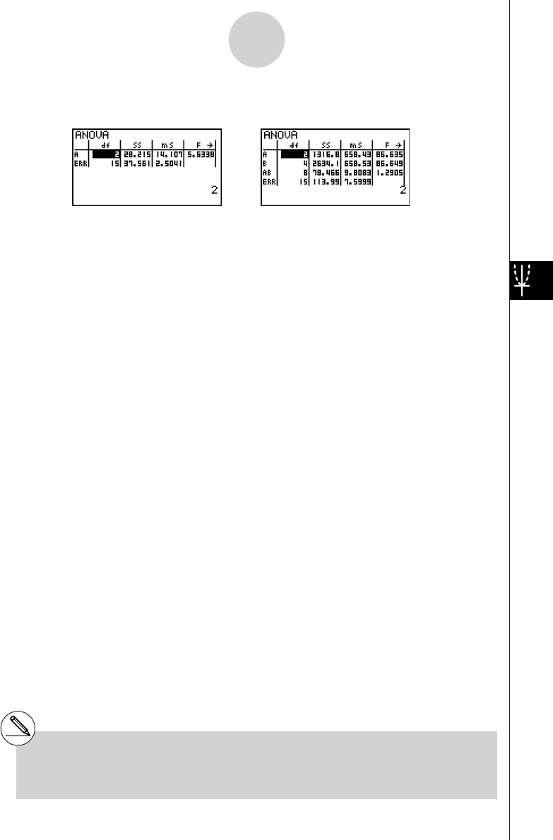
20010101
Calculation Result Output Example
One-Way ANOVA
Line 1 (A) .................... Factor A df value, SS value, MS value, F value, p-value
Line 2 (ERR) ............... Error df value, SS value, MS value
Two-Way ANOVA
Line 1 (A) .................... Factor A df value, SS value, MS value, F value, p-value
Line 2 (B) .................... Factor B df value, SS value, MS value, F value, p-value
Line 3 (AB) .................. Factor A × Factor B df value, SS value, MS value, F value,
p-value
*Line 3 does not appear when there is only one observation
in each cell.
Line 4 (ERR) ............... Error df value, SS value, MS value
F.................................. F value
p.................................. p-value
df ................................. degrees of freedom
SS ................................ sum of squares
MS ............................... mean squares
With Two-Way ANOVA, you can draw Interaction Plot graphs. The number of graphs depends
on Factor B, while the number of X-axis data depends on the Factor A. The Y-axis is the average
value of each category.
You can use the following graph analysis function after drawing a graph.
•1(TRACE) ... Trace function
Pressing d or e moves the pointer on the graph in the corresponding direction. When there
are multiple graphs, you can move between graphs by pressing f and c.
Press i to clear the pointer from the display.
# Graphing is available with Two-Way ANOVA
only. V-Window settings are performed
automatically, regardless of SET UP screen
settings.
# Using the TRACE function automatically
stores the number of conditions to alpha
variable A and the mean value to variable M,
respectively.
1-2-23
Tests (TEST)

20010101
kk
kk
kANOVA (Two-Way)
uu
uu
uDescription
The nearby table shows measurement results for a metal product produced by a heat
treatment process based on two treatment levels: time (A) and temperature (B). The
experiments were repeated twice each under identical conditions.
Perform analysis of variance on the following null hypothesis, using a significance level of
5%.
Ho : No change in strength due to time
Ho : No change in strength due to heat treatment temperature
Ho : No change in strength due to interaction of time and heat treatment temperature
uu
uu
uSolution
Use two-way ANOVA to test the above hypothesis.
Input the above data as shown below.
List1={1,1,1,1,2,2,2,2}
List2={1,1,2,2,1,1,2,2}
List3={113,116,139,132,133,131,126,122}
Define List 3 (the data for each group) as Dependent. Define List 1 and List 2 (the factor
numbers for each data item in List 3) as Factor A and Factor B respectively.
Executing the test produces the following results.
•Time differential (A) level of significance P = 0.2458019517
The level of significance (p = 0.2458019517) is greater than the significance level (0.05),
so the hypothesis is not rejected.
•Temperature differential (B) level of significance P = 0.04222398836
The level of significance (p = 0.04222398836) is less than the significance level (0.05), so
the hypothesis is rejected.
•Interaction (A × B) level of significance P = 2.78169946e-3
The level of significance (p = 2.78169946e-3) is less than the significance level (0.05), so
the hypothesis is rejected.
The above test indicates that the time differential is not significant, the temperature
differential is significant, and interaction is highly significant.
B (Heat Treatment Temperature) B1 B2
A1 113 , 116
133 , 131
139 , 132
126 , 122
A2
A (Time)
1-2-24
Tests (TEST)
20011101
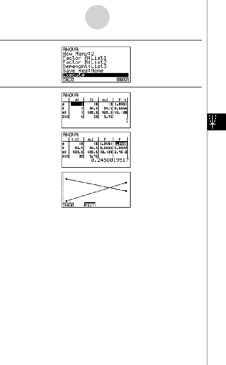
20010101
uu
uu
uInput Example
uu
uu
uResults
1-2-25
Tests (TEST)

20010101
1-3 Confidence Interval (INTR)
A confidence interval is a range (interval) that includes a statistical value, usually the
population mean.
A confidence interval that is too broad makes it difficult to get an idea of where the population
value (true value) is located. A narrow confidence interval, on the other hand, limits the
population value and makes it difficult to obtain reliable results. The most commonly used
confidence levels are 95% and 99%. Raising the confidence level broadens the confidence
interval, while lowering the confidence level narrows the confidence level, but it also
increases the chance of accidently overlooking the population value. With a 95% confidence
interval, for example, the population value is not included within the resulting intervals 5% of
the time.
When you plan to conduct a survey and then t test and Z test the data, you must also
consider the sample size, confidence interval width, and confidence level. The confidence
level changes in accordance with the application.
1-Sample Z Interval calculates the confidence interval for an unknown population mean
when the population standard deviation is known.
2-Sample Z Interval calculates the confidence interval for the difference between two
population means when the population standard deviations of two samples are known.
1-Prop Z Interval calculates the confidence interval for an unknown proportion of
successes.
2-Prop Z Interval calculates the confidence interval for the difference between the propotion
of successes in two populations.
1-Sample t Interval calculates the confidence interval for an unknown population mean
when the population standard deviation is unknown.
2-Sample t Interval calculates the confidence interval for the difference between two
population means when both population standard deviations are unknown.
On the initial STAT Mode screen, press 4 (INTR) to display the confidence interval menu,
which contains the following items.
•4(INTR)b(Z) ... Z intervals (p. 1-3-3)
c(T) ... t intervals (p. 1-3-8)
# There is no graphing for confidence interval
functions.
1-3-1
Confidence Interval (INTR)
20011101

20010101
uu
uu
uGeneral Confidence Interval Precautions
Inputting a value in the range of 0 < C-Level < 1 for the C-Level setting sets you value you
input. Inputting a value in the range of 1 < C-Level < 100 sets a value equivalent to your input
divided by 100.
# Inputting a value of 100 or greater, or a
negative value causes an error (Ma ERROR).
1-3-2
Confidence Interval (INTR)
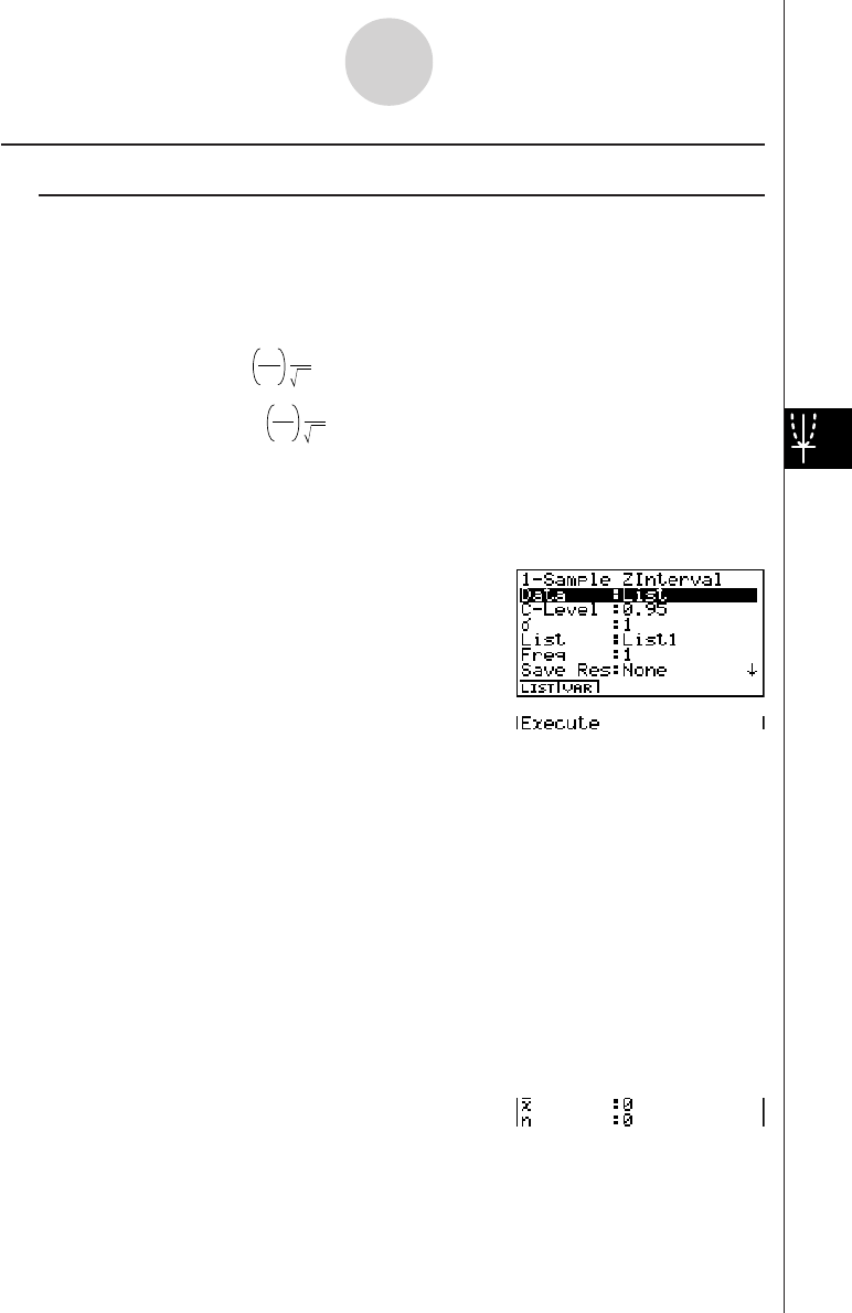
20010101
kk
kk
kZ Interval
uu
uu
u1-Sample Z Interval
1-Sample Z Interval calculates the confidence interval for an unknown population mean
when the population standard deviation is known.
The following is the confidence interval.
Left = o – Zα
2
σ
n
Right = o + Z α
2
σ
n
However,
α
is the level of significance. The value 100 (1 –
α
) % is the confidence level.
When the confidence level is 95%, for example, inputting 0.95 produces 1 – 0.95 = 0.05 =
α
.
Perform the following key operations from the statistical data list.
4(INTR)
b(Z)
b(1-Smpl)
The following shows the meaning of each item in the case of list data specification.
Data ............................ data type
C-Level ........................ confidence level (0 < C-Level < 1)
σ
.................................. population standard deviation (
σ
> 0)
List .............................. list whose contents you want to use as sample data
(List 1 to 20)
Freq ............................. sample frequency (1 or List 1 to 20)
Save Res ..................... list for storage of calculation results (None or List 1 to 20)
Execute ....................... executes a calculation
The following shows the meaning of parameter data specification items that are different
from list data specification.
o.................................. mean of sample
n.................................. size of sample (positive integer)
1-3-3
Confidence Interval (INTR)
20011101
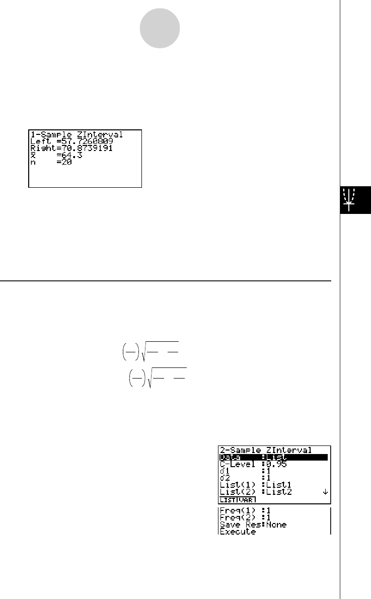
20010101
After setting all the parameters, align the cursor with [Execute] and then press the function
key shown below to perform the calculation.
• 1(CALC) ... Performs the calculation.
Calculation Result Output Example
Left .............................. interval lower limit (left edge)
Right ............................ interval upper limit (right edge)
o.................................. mean of sample
x
σ
n-1 ............................. sample standard deviation
(Displayed only for Data: List setting.)
n.................................. size of sample
uu
uu
u 2-Sample Z Interval
2-Sample Z Interval calculates the confidence interval for the difference between two
population means when the population standard deviations of two samples are known.
The following is the confidence interval. The value 100 (1 –
α) % is the confidence level.
Left = (o
1
– o
2
) – Zα
2
Right = (o
1
– o
2
) + Zα
2
n
1
1
2
σ
+n
2
2
2
σ
n
1
1
2
σ
+n
2
2
2
σ
o1:mean of sample 1
o2:mean of sample 2
σ
1:population standard deviation
of sample 1
σ
2:population standard deviation
of sample 2
n1:size of sample 1
n2:size of sample 2
Perform the following key operations from the statistical data list.
4(INTR)
b(Z)
c(2-Smpl)
1-3-4
Confidence Interval (INTR)
2001010120011101
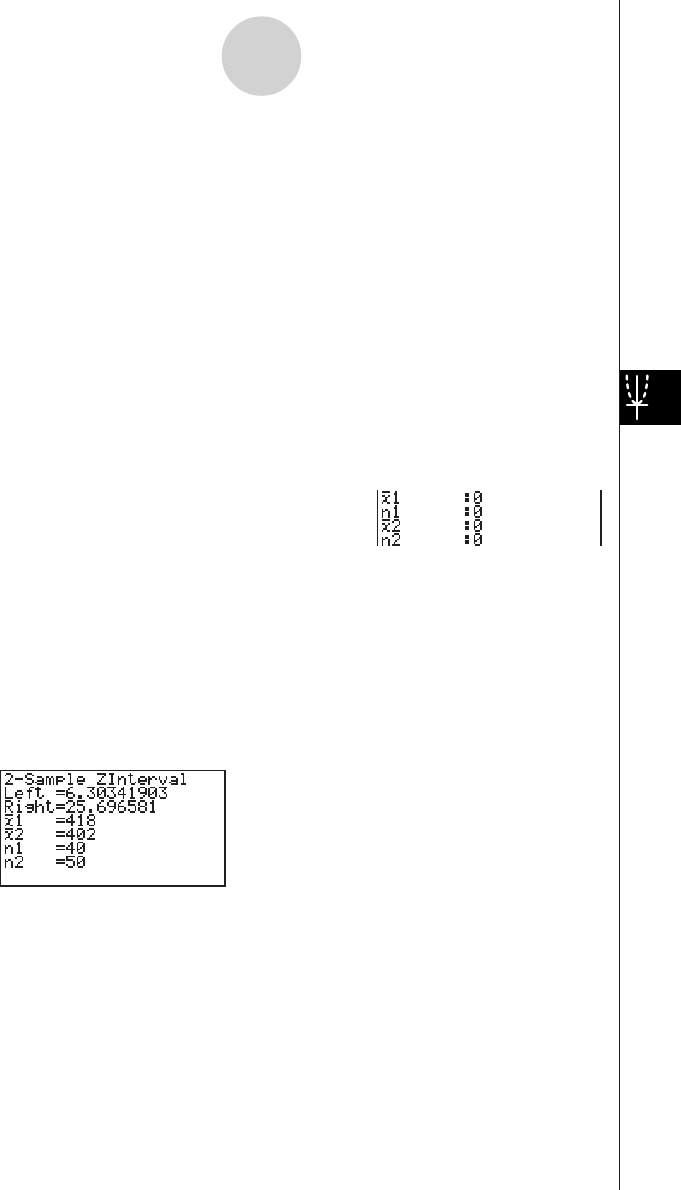
20010101
The following shows the meaning of each item in the case of list data specification.
Data ............................ data type
C-Level ........................ confidence level (0 < C-Level < 1)
σ
1................................. population standard deviation of sample 1 (
σ
1 > 0)
σ
2................................. population standard deviation of sample 2 (
σ
2 > 0)
List(1) .......................... list whose contents you want to use as data of sample 1
(List 1 to 20)
List(2) .......................... list whose contents you want to use as data of sample 2
(List 1 to 20)
Freq(1) ........................ frequency of sample 1 (1 or List 1 to 20)
Freq(2) ........................ frequency of sample 2 (1 or List 1 to 20)
Save Res ..................... list for storage of calculation results (None or List 1 to 20)
Execute ....................... executes a calculation
The following shows the meaning of parameter data specification items that are different
from list data specification.
o1................................. mean of sample 1
n1................................. size (positive integer) of sample 1
o2................................. mean of sample 2
n2................................. size (positive integer) of sample 2
After setting all the parameters, align the cursor with [Execute] and then press the function
key shown below to perform the calculation.
•1(CALC) ... Performs the calculation.
Calculation Result Output Example
Left .............................. interval lower limit (left edge)
Right ............................ interval upper limit (right edge)
o1................................. mean of sample 1
o2................................. mean of sample 2
x1
σ
n-1 ............................ standard deviation of sample 1
(Displayed only for Data: List setting.)
x2
σ
n-1 ............................ standard deviation of sample 2
(Displayed only for Data: List setting.)
n1................................. size of sample 1
n2................................. size of sample 2
1-3-5
Confidence Interval (INTR)
20011101
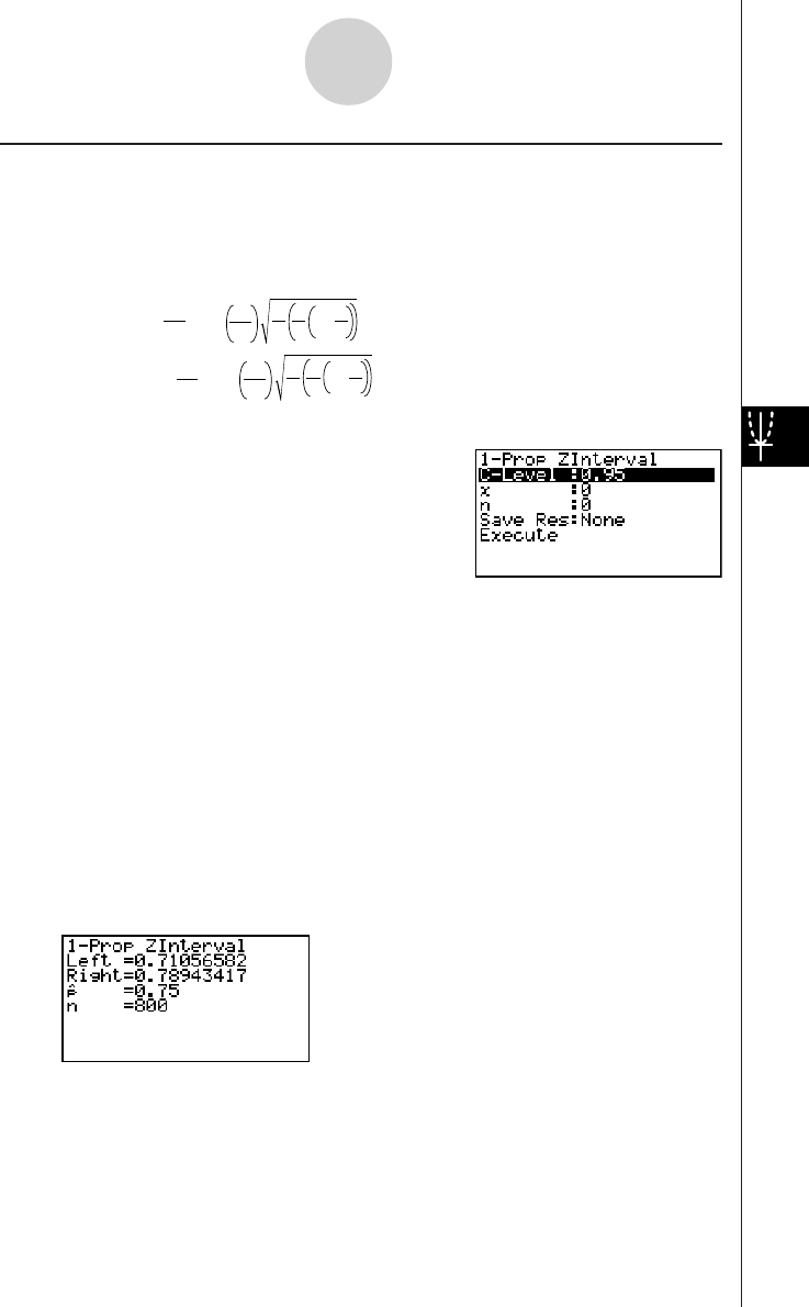
20010101
uu
uu
u1-Prop Z Interval
1-Prop Z Interval uses the number of data to calculate the confidence interval for an
unknown proportion of successes.
The following is the confidence interval. The value 100 (1 –
α) % is the confidence level.
Left = – Zα
2
Right = + Z
x
nn
1n
xn
x
1–
x
n
α
2n
1n
xn
x
1–
n:size of sample
x:data
Perform the following key operations from the statistical data list.
4(INTR)
b(Z)
d(1-Prop)
Data is specified using parameter specification. The following shows the meaning of each
item.
C-Level ........................ confidence level (0 < C-Level < 1)
x.................................. data (0 or positive integer)
n.................................. size of sample (positive integer)
Save Res ..................... list for storage of calculation results (None or List 1 to 20)
Execute ....................... executes a calculation
After setting all the parameters, align the cursor with [Execute] and then press the function
key shown below to perform the calculation.
•1(CALC) ... Performs the calculation.
Calculation Result Output Example
Left .............................. interval lower limit (left edge)
Right ............................ interval upper limit (right edge)
ˆp .................................. estimated sample proportion
n.................................. size of sample
1-3-6
Confidence Interval (INTR)
20011101
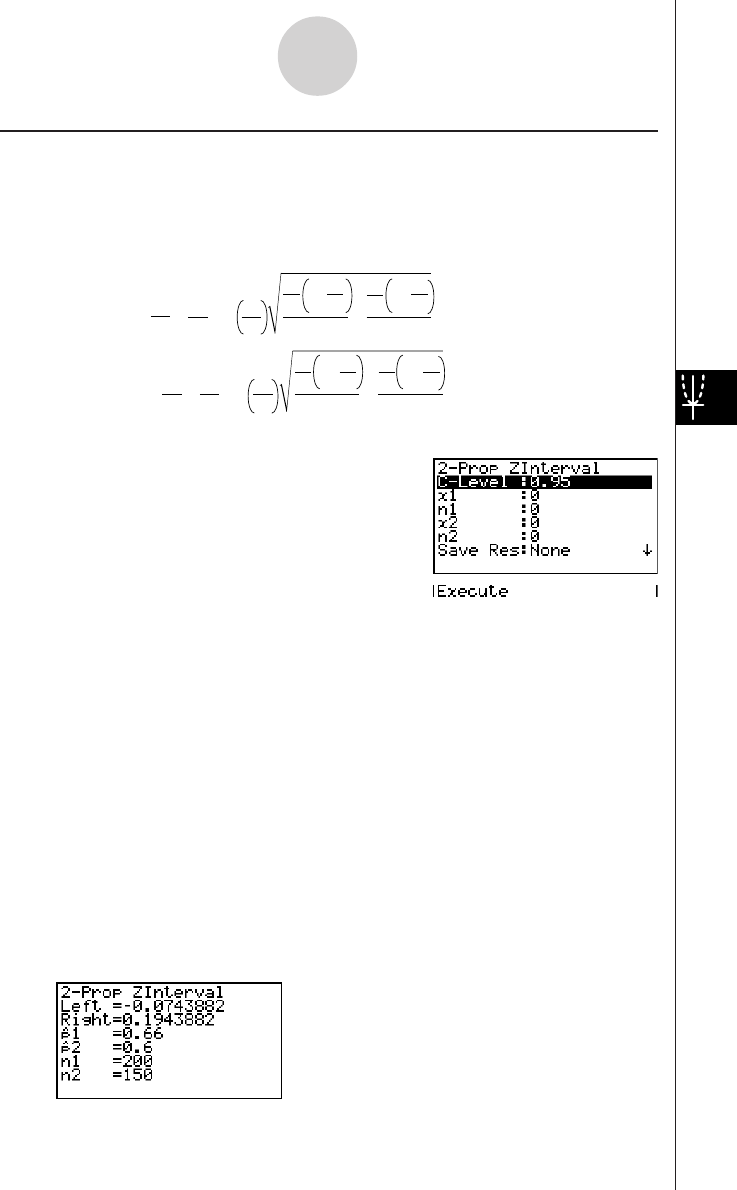
20010101
uu
uu
u 2-Prop Z Interval
2-Prop Z Interval uses the number of data items to calculate the confidence interval for the
defference between the proportion of successes in two populations.
The following is the confidence interval. The value 100 (1 –
α) % is the confidence level.
Left = – – Zα
2
x1
n1
x2
n2n1
n1
x11– n1
x1
+n2
n2
x21– n2
x2
Right = – + Zα
2
x1
n1
x2
n2n1
n1
x11– n1
x1
+n2
n2
x21– n2
x2
n1, n2: size of sample
x1, x2: data
Perform the following key operations from the statistical data list.
4(INTR)
b(Z)
e(2-Prop)
Data is specified using parameter specification. The following shows the meaning of each
item.
C-Level ........................ confidence level (0 < C-Level < 1)
x1................................. data value (x1 > 0) of sample 1
n1................................. size (positive integer) of sample 1
x2................................. data value (x2 > 0) of sample 2
n2................................. size (positive integer) of sample 2
Save Res ..................... list for storage of calculation results (None or List 1 to 20)
Execute ....................... executes a calculation
After setting all the parameters, align the cursor with [Execute] and then press the function
key shown below to perform the calculation.
•1(CALC) ... Performs the calculation.
Calculation Result Output Example
1-3-7
Confidence Interval (INTR)
20011101
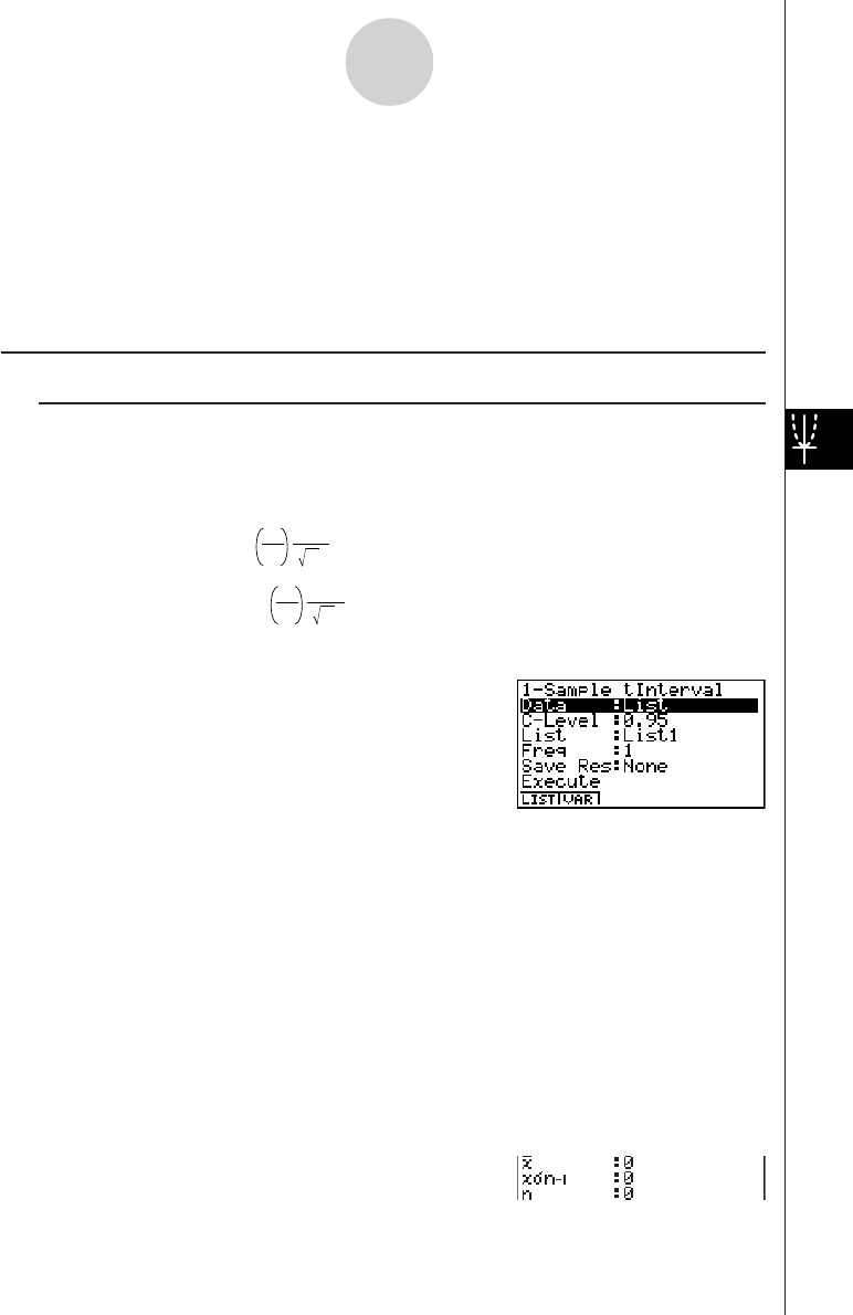
20010101
Left .............................. interval lower limit (left edge)
Right ............................ interval upper limit (right edge)
ˆp 1................................. estimated sample propotion for sample 1
ˆp 2................................. estimated sample propotion for sample 2
n1................................. size of sample 1
n2................................. size of sample 2
kk
kk
kt Interval
uu
uu
u 1-Sample t Interval
1-Sample t Interval calculates the confidence interval for an unknown population mean
when the population standard deviation is unknown.
The following is the confidence interval. The value 100 (1 –
α) % is the confidence level.
Left = o– tn
–
1
α
2
Right = o+tn
–
1
α
2
x n–1
σ
n
x n–1
σ
n
Perform the following key operations from the statistical data list.
4(INTR)
c(T)
b(1-Smpl)
The following shows the meaning of each item in the case of list data specification.
Data ............................ data type
C-Level ........................ confidence level (0 < C-Level < 1)
List .............................. list whose contents you want to use as sample data
(List 1 to 20)
Freq ............................. sample frequency (1 or List 1 to 20)
Save Res ..................... list for storage of calculation results (None or List 1 to 20)
Execute ....................... executes a calculation
The following shows the meaning of parameter data specification items that are different
from list data specification.
1-3-8
Confidence Interval (INTR)
20011101
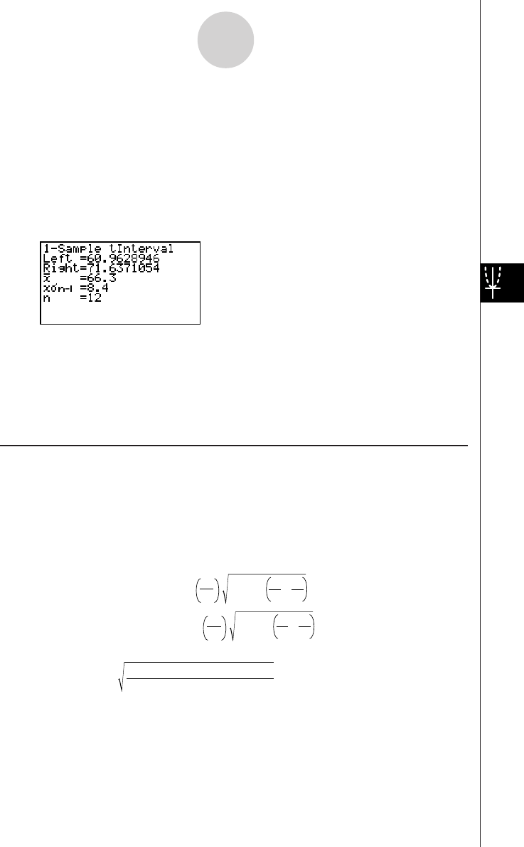
20010101
o.................................. mean of sample
x
σ
n-1 ............................. sample standard deviation (x
σ
n-1 > 0)
n.................................. size of sample (positive integer)
After setting all the parameters, align the cursor with [Execute] and then press the function
key shown below to perform the calculation.
•1(CALC) ... Performs the calculation.
Calculation Result Output Example
Left .............................. interval lower limit (left edge)
Right ............................ interval upper limit (right edge)
o.................................. mean of sample
x
σ
n-1 ............................. sample standard deviation
n.................................. size of sample
uu
uu
u 2-Sample t Interval
2-Sample t Interval calculates the confidence interval for the difference between two
population means when both population standard deviations are unknown. The t interval is
applied to t distribution.
The following confidence interval applies when pooling is in effect. The value 100 (1 –
α) % is
the confidence level.
Left = (o1 – o2)– tα
2
Right = (o1 – o2)+ tα
2
n
1
+n
2
–2 n1
1+n2
1
xp n–12
σ
n
1
+n
2
–2 n1
1+n2
1
xp n–12
σ
x
p n–1
=
σ
n
1
+ n
2
– 2
(n
1
–1)x
1 n–12
+(n
2
–1)x
2 n–12
σσ
1-3-9
Confidence Interval (INTR)
20011101
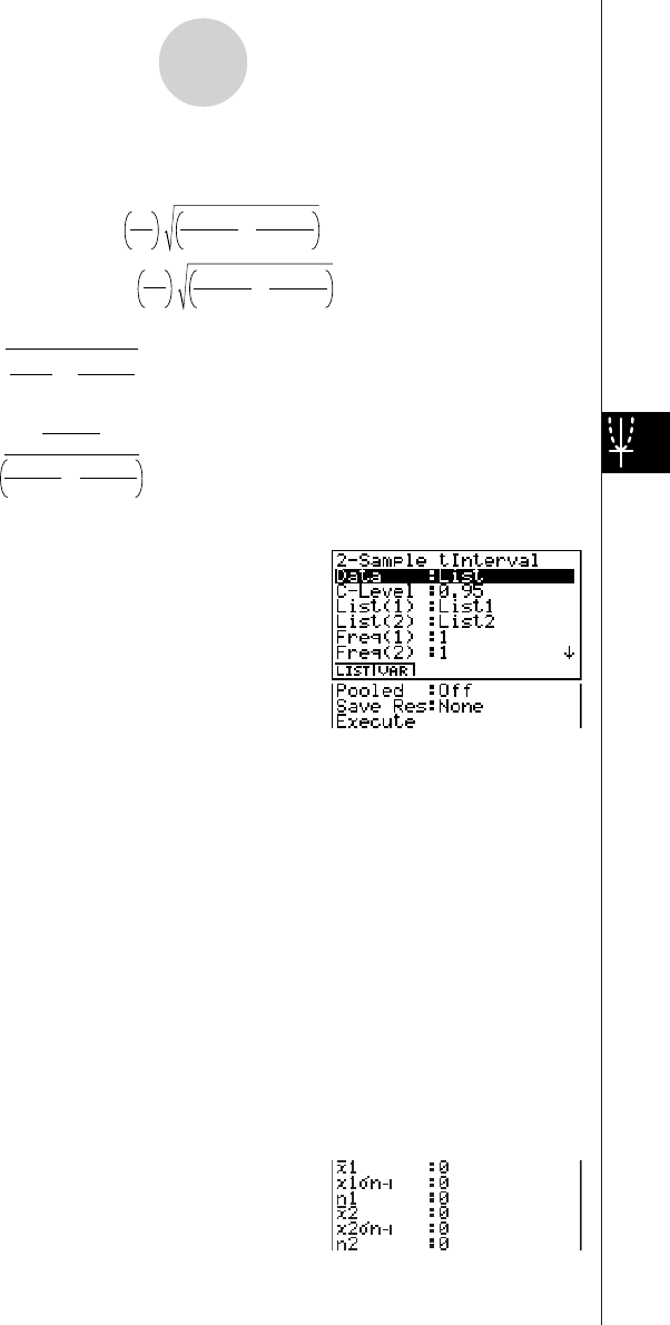
20010101
The following confidence interval applies when pooling is not in effect. The value
100 (1 –
α) % is the confidence level.
Left = (o
1
– o
2
)– t
df
α
2
Right = (o
1
– o
2
)+ t
df
α
2
+
n
1
x
1 n–12
σ
n
2
x
2 n–12
σ
+
n
1
x
1 n–12
σ
n
2
x
2 n–12
σ
C =
df = 1
C
2
n1–1 +(1–C)2
n2–1
+
n1
x1 n–12
σ
n1
x1 n–12
σ
n2
x2 n–12
σ
Perform the following key operations from the statistical data list.
4(INTR)
c(T)
c(2-Smpl)
The following shows the meaning of each item in the case of list data specification.
Data ............................ data type
C-Level ........................ confidence level (0 < C-Level < 1)
List(1) .......................... list whose contents you want to use as data of sample 1
(List 1 to 20)
List(2) .......................... list whose contents you want to use as data of sample 2
(List 1 to 20)
Freq(1) ........................ frequency of sample 1 (1 or List 1 to 20)
Freq(2) ........................ frequency of sample 2 (1 or List 1 to 20)
Pooled ......................... pooling On (in effect) or Off (not in effect)
Save Res ..................... list for storage of calculation results (None or List 1 to 20)
Execute ....................... executes a calculation
The following shows the meaning of parameter data specification items that are different
from list data specification.
1-3-10
Confidence Interval (INTR)
20011101
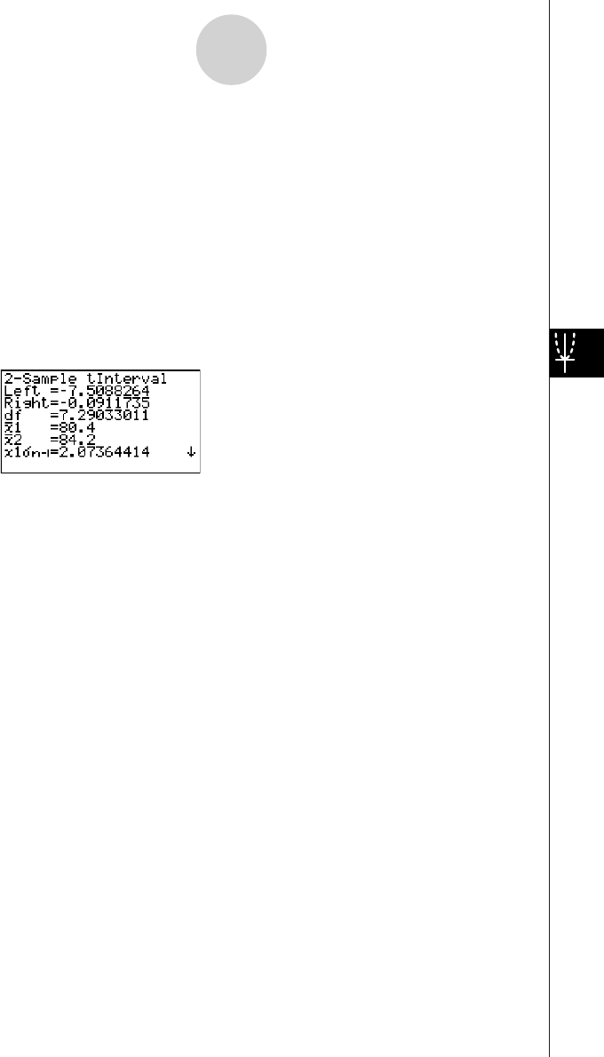
20010101
o1................................. mean of sample 1
x1
σ
n-1 ............................ standard deviation (x1
σ
n-1 > 0) of sample 1
n1................................. size (positive integer) of sample 1
o2................................. mean of sample 2
x2
σ
n-1 ............................ standard deviation (x2
σ
n-1 > 0) of sample 2
n2................................. size (positive integer) of sample 2
After setting all the parameters, align the cursor with [Execute] and then press the function
key shown below to perform the calculation.
•1(CALC) ... Performs the calculation.
Calculation Result Output Example
Left .............................. interval lower limit (left edge)
Right ............................ interval upper limit (right edge)
df ................................. degrees of freedom
o1................................. mean of sample 1
o2................................. mean of sample 2
x1
σ
n-1 ............................ standard deviation of sample 1
x2
σ
n-1 ............................ standard deviation of sample 2
xp
σ
n-1 ............................ pooled sample standard deviation
(Displayed only when Pooled: On setting.)
n1................................. size of sample 1
n2................................. size of sample 2
1-3-11
Confidence Interval (INTR)

20010101
1-4 Distribution (DIST)
There is a variety of different types of distribution, but the most well-known is “normal
distribution,” which is essential for performing statistical calculations. Normal distribution is a
symmetrical distribution centered on the greatest occurrences of mean data (highest
frequency), with the frequency decreasing as you move away from the center. Poisson
distribution, geometric distribution, and various other distribution shapes are also used,
depending on the data type.
Certain trends can be determined once the distribution shape is determined. You can
calculate the probability of data taken from a distribution being less than a specific value.
For example, distribution can be used to calculate the yield rate when manufacturing some
product. Once a value is established as the criteria, you can calculate normal probability
when estimating what percent of the products meet the criteria. Conversely, a success rate
target (80% for example) is set up as the hypothesis, and normal distribution is used to
estimate the proportion of the products will reach this value.
Normal probability density calculates the probability density of normal distribution from a
specified x value.
Normal distribution probability calculates the probability of normal distribution data falling
between two specific values.
Inverse cumulative normal distribution calculates a value that represents the location
within a normal distribution for a specific cumulative probability.
Student- t probability density calculates t probability density from a specified x value.
Student- t distribution probability calculates the probability of t distribution data falling
between two specific values.
Like t distribution, distribution probability can also be calculated for χ2, F, Binomial, Poisson,
and Geometric distributions.
On the initial STAT Mode screen, press 5 (DIST) to display the distribution menu, which
contains the following items.
•5(DIST)b(Norm) ... Normal distribution (p. 1-4-3)
c(T) ... Student-t distribution (p. 1-4-7)
d(χ2) ... χ2 distribution (p. 1-4-9)
e(F) ... F distribution (p. 1-4-12)
f(Binmal) ... Binomial distribution (p. 1-4-16)
g(Poissn) ... Poisson distribution (p. 1-4-19)
h(Geo) ... Geometric distribution (p. 1-4-21)
1-4-1
Distribution (DIST)

20010101
uu
uu
uCommon Distribution Functions
After drawing a graph, you can use the P-CAL function to calculate an estimated p-value for
a particular x value.
The following is the general procedure for using the P-CAL function.
1. After drawing a graph, press 1 (P-CAL) to display the x value input dialog box.
2. Input the value you want for x and then press w.
• This causes the x and p values to appear at the bottom of the display, and moves the
pointer to the corresponding point on the graph.
3. Pressing v or a number key at this time causes the x value input dialog box to reappear
so you can perform another estimated value calculation if you want.
4. After you are finished, press i to clear the coordinate values and the pointer from the
display.
# Executing an analysis function automatically
stores the x and p values in alpha variables X
and P, respectively.
1-4-2
Distribution (DIST)
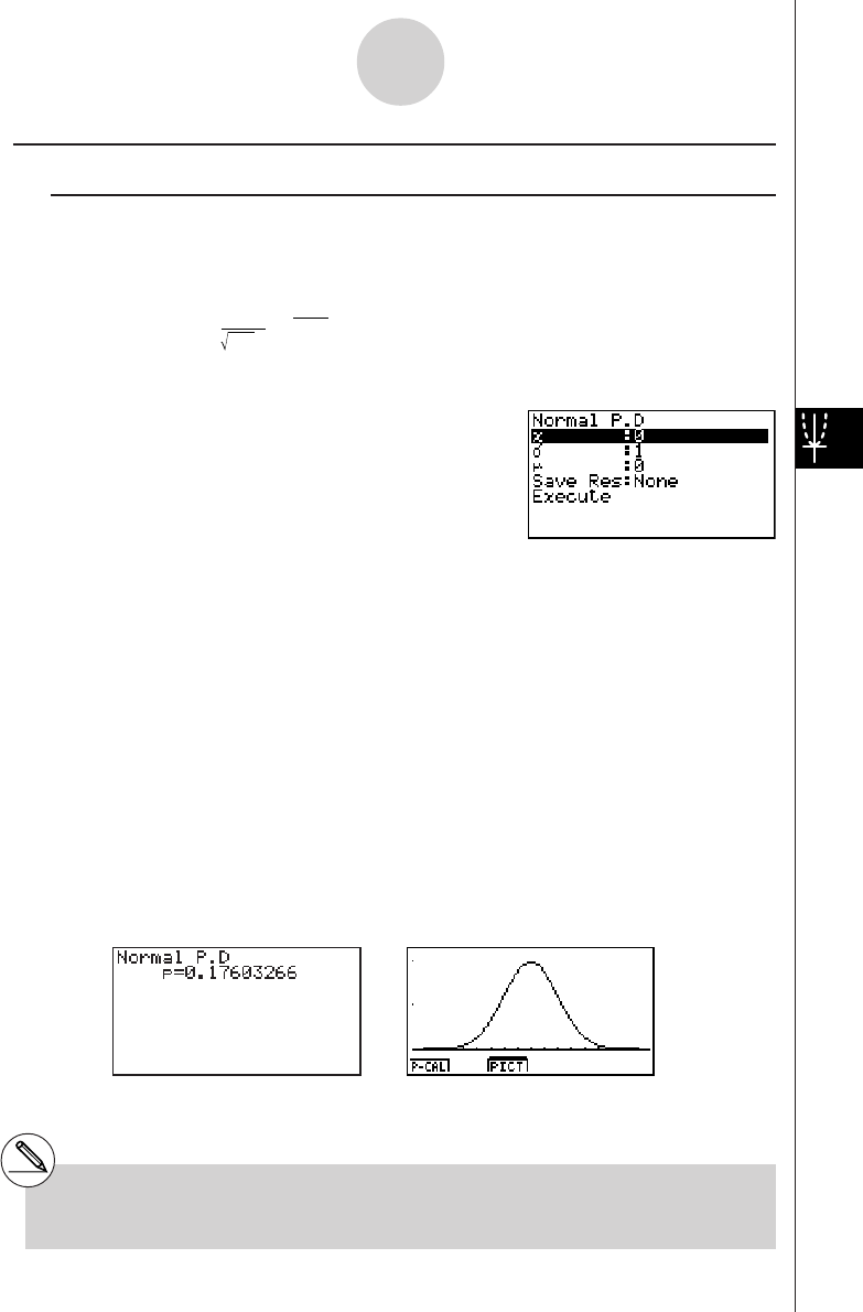
20010101
kk
kk
kNormal Distribution
uu
uu
uNormal Probability Density
Normal probability density calculates the probability density of nomal distribution from a
specified x value. Normal probability density is applied to standard normal distribution.
πσ
2
f(x) = 1e–2
2
σ
(x – µ)
2
µ
(σ > 0)
Perform the following key operations from the statistical data list.
5(DIST)
b(Norm)
b(P.D)
Data is specified using parameter specification. The following shows the meaning of each
item.
x.................................. data
σ
.................................. standard deviation (
σ
> 0)
µ
.................................. mean
Save Res ..................... list for storage of calculation results (None or List 1 to 20)
Execute ....................... executes a calculation or draws a graph
•Specifying
σ
= 1 and
µ
= 0 specifies standard normal distribution.
After setting all the parameters, align the cursor with [Execute] and then press one of the
function keys shown below to perform the calculation or draw the graph.
•1(CALC) ... Performs the calculation.
•6(DRAW) ... Draws the graph.
Calculation Result Output Example
p.................................. normal probability density
# V-Window settings for graph drawing are set
automatically when the SET UP screen's
[Stat Wind] setting is [Auto]. Current V-
Window settings are used for graph drawing
when the [Stat Wind] setting is [Manual].
1-4-3
Distribution (DIST)
20011101
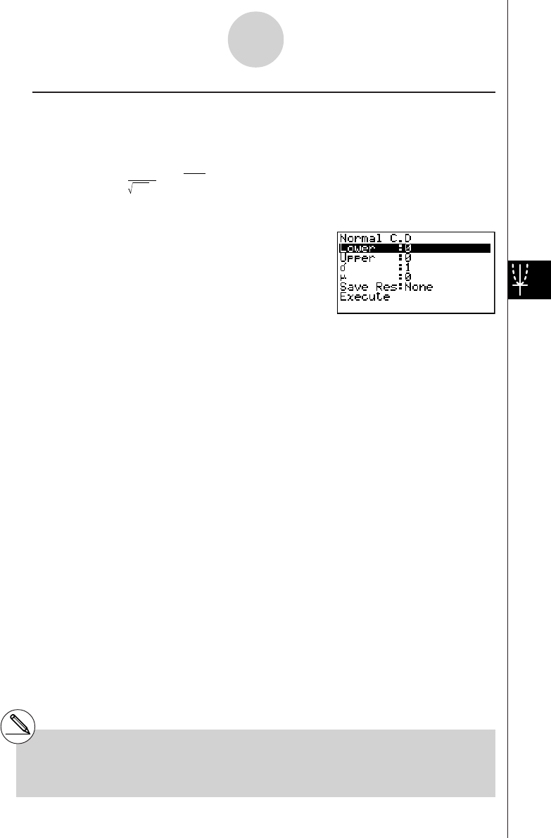
20010101
uu
uu
uNormal Distribution Probability
Normal distribution probability calculates the probability of normal distribution data falling
between two specific values.
πσ
2
p = 1e
–
dx
2 2
σ
(x – µ)2
µ
a
b
∫
a: lower boundary
b: upper boundary
Perform the following key operations from the statistical data list.
5(DIST)
b(Norm)
c(C.D)
Data is specified using parameter specification. The following shows the meaning of each
item.
Lower .......................... lower boundary
Upper .......................... upper boundary
σ
.................................. standard deviation (
σ
> 0)
µ
.................................. mean
Save Res ..................... list for storage of calculation results (None or List 1 to 20)
Execute ....................... executes a calculation
After setting all the parameters, align the cursor with [Execute] and then press the function
key shown below to perform the calculation.
•1(CALC) ... Performs the calculation.
# There is no graphing for normal distribution
probability.
1-4-4
Distribution (DIST)
20011101
20010101
Calculation Result Output Example
p.................................. normal distribution probability
z:Low ........................... z:Low value (converted to standardize z score for lower
value)
z:Up ............................. z:Up value (converted to standardize z score for upper value)
uu
uu
uInverse Cumulative Normal Distribution
Inverse cumulative normal distribution calculates a value that represents the location within a
normal distribution for a specific cumulative probability.
f (x)dx = p
−∞
∫
f (x)dx = p
+∞
∫
f (x)dx = p
∫
Specify the probability and use this formula to obtain the integration interval.
Perform the following key operations from the statistical data list.
5(DIST)
b(Norm)
d(Invrse)
Data is specified using parameter specification. The following shows the meaning of each
item.
Tail ............................... probability value tail specification (Left, Right, Central)
Area ............................ probability value (0 < Area < 1)
σ
.................................. standard deviation (
σ
> 0)
µ
.................................. mean
Save Res ..................... list for storage of calculation results (None or List 1 to 20)
Execute ....................... executes a calculation
Tail: Left
upper
boundary of
integration
interval
α = ?
Tail: Right
lower
boundary of
integration
interval
α = ?
Tail: Central
upper and
lower
boundaries
of integration
interval
α = ? β = ?
1-4-5
Distribution (DIST)
20011101
20010101
After setting all the parameters, align the cursor with [Execute] and then press the function
key shown below to perform the calculation.
•1(CALC) ... Performs the calculation.
Calculation Result Output Examples
x....................................... inverse cumulative normal distribution
(Tail:Left upper boundary of integration interval)
(Tail:Right lower boundary of integration interval)
(Tail:Central upper and lower boundaries of integration
interval)
# There is no graphing for inverse cumulative
normal distribution.
1-4-6
Distribution (DIST)
20010101
kk
kk
kStudent-t Distribution
uu
uu
uStudent-t Probability Density
Student-t probability density calculates t probability density from a specified x value.
f
(x) =
Γ
Γ
df
π
–
df+1
2
2
df
2
df + 1
df
x
2
1+
Perform the following key operations from the statistical data list.
5(DIST)
c(T)
b(P.D)
Data is specified using parameter specification. The following shows the meaning of each
item.
x.................................. data
df ................................. degrees of freedom (df > 0)
Save Res ..................... list for storage of calculation results (None or List 1 to 20)
Execute ....................... executes a calculation or draws a graph
After setting all the parameters, align the cursor with [Execute] and then press one of the
function keys shown below to perform the calculation or draw the graph.
•1(CALC) ... Performs the calculation.
•6(DRAW) ... Draws the graph.
Calculation Result Output Example
p.................................. Student-t probability density
# Current V-Window settings are used for
graph drawing when the SET UP screen's
[Stat Wind] setting is [Manual]. The V-
Window settings below are set automatically
when the [Stat Wind] setting is [Auto].
Xmin = –3.2, Xmax = 3.2, Xscale = 1,
Ymin = –0.1, Ymax = 0.45, Yscale = 0.1
1-4-7
Distribution (DIST)
20011101
20010101
uu
uu
uStudent-t Distribution Probability
Student-t distribution probability calculates the probability of t distribution data falling
between two specific values.
p =
Γ
Γ
df
π
2
df
2
df + 1
–
df+1
2
df
x
2
1+ dx
a
b
∫
a:lower boundary
b:upper boundary
Perform the following key operations from the statistical data list.
5(DIST)
c(T)
c(C.D)
Data is specified using parameter specification. The following shows the meaning of each
item.
Lower .......................... lower boundary
Upper .......................... upper boundary
df ................................. degrees of freedom (df > 0)
Save Res ..................... list for storage of calculation results (None or List 1 to 20)
Execute ....................... executes a calculation
After setting all the parameters, align the cursor with [Execute] and then press the function
key shown below to perform the calculation.
•1(CALC) ... Performs the calculation.
# There is no graphing for Student-t distribution
probability.
1-4-8
Distribution (DIST)
20011101
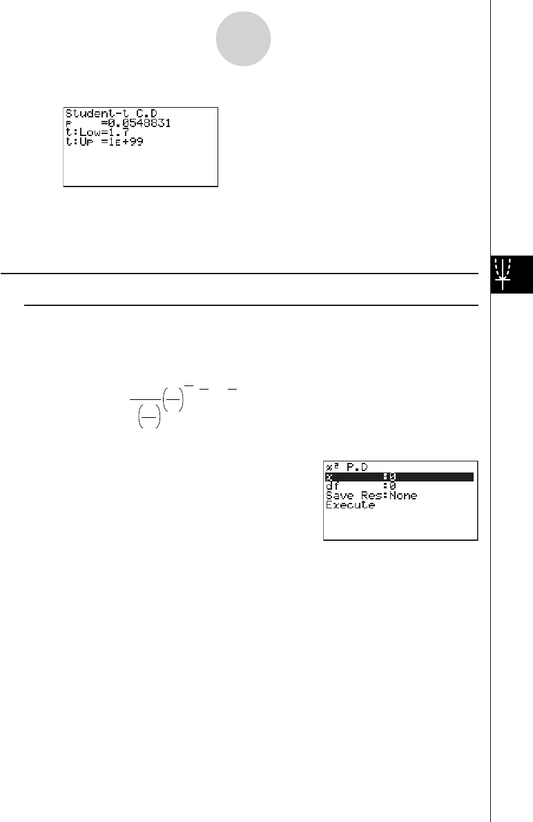
20010101
Calculation Result Output Example
p.................................. Student-t distribution probability
t:Low ........................... t:Low value (input lower value)
t:Up ............................. t:Up value (input upper value)
kk
kk
kχ2 Distribution
uu
uu
uχ2 Probability Density
χ2 probability density calculates the probability density function for the χ2 distribution at a
specified x value.
f
(x) =
Γ
1
2
df
df
2
x e
2
1
df
2–1 x
2
–
Perform the following key operations from the statistical data list.
5(DIST)
d(χ2)
b(P.D)
Data is specified using parameter specification. The following shows the meaning of each
item.
x.................................. data
df ................................. degrees of freedom (positive integer)
Save Res ..................... list for storage of calculation results (None or List 1 to 20)
Execute ....................... executes a calculation or draws a graph
After setting all the parameters, align the cursor with [Execute] and then press one of the
function keys shown below to perform the calculation or draw the graph.
•1(CALC) ... Performs the calculation.
•6(DRAW) ... Draws the graph.
1-4-9
Distribution (DIST)
20011101
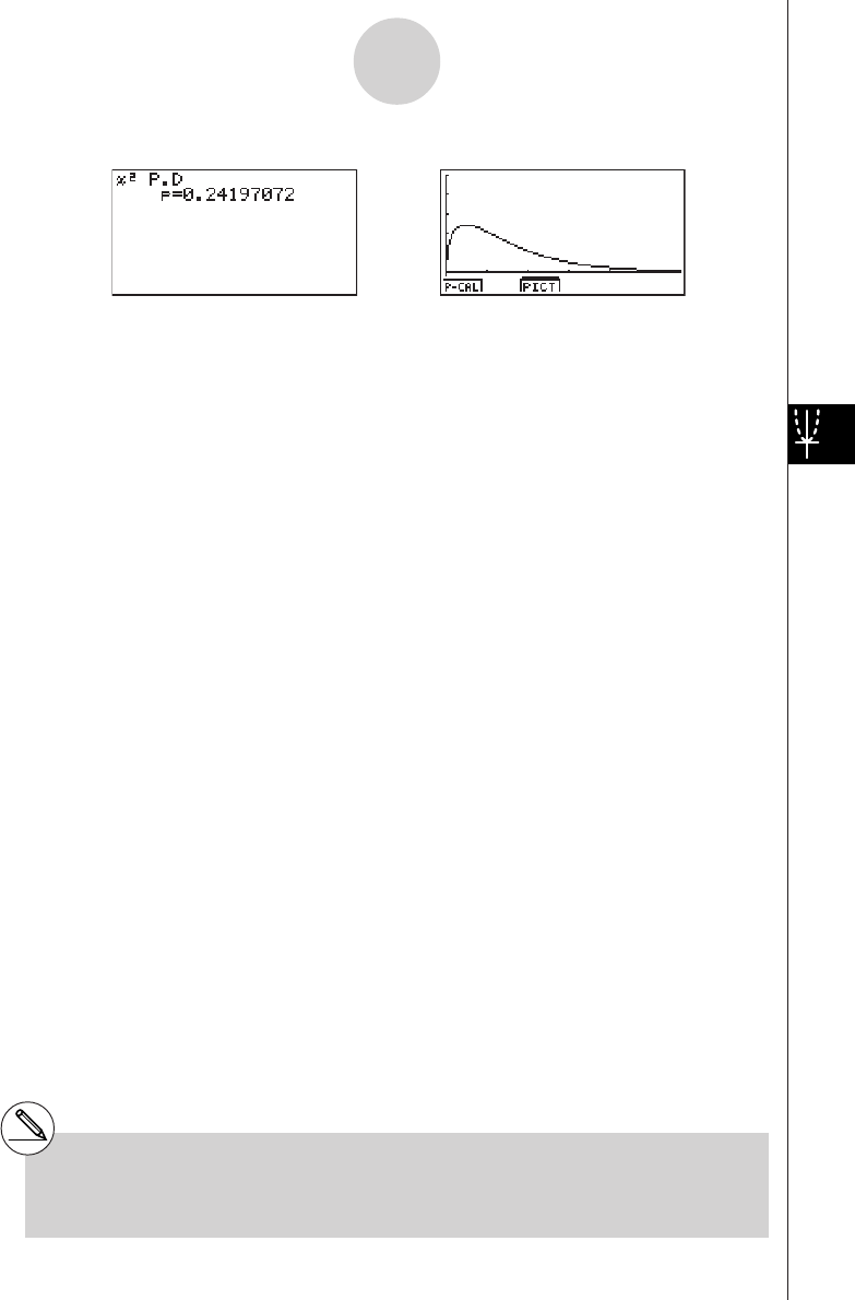
20010101
Calculation Result Output Example
p.................................. χ2 probability density
# Current V-Window settings are used for
graph drawing when the SET UP screen's
[Stat Wind] setting is [Manual]. The V-
Window settings below are set automatically
when the [Stat Wind] setting is [Auto].
Xmin = 0, Xmax = 11.5, Xscale = 2,
Ymin = -0.1, Ymax = 0.5, Yscale = 0.1
1-4-10
Distribution (DIST)
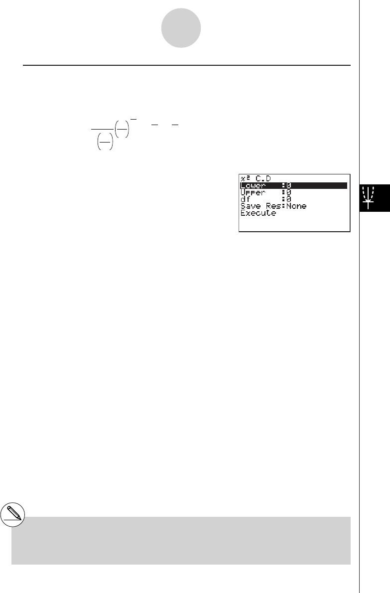
20010101
uu
uu
uχ2 Distribution Probability
χ2 distribution probability calculates the probability of χ2 distribution data falling between two
specific values.
p =
Γ
1
2
df
df
2
x e dx
2
1
df
2–1 x
2
–
a
b
∫
a:lower boundary
b:upper boundary
Perform the following key operations from the statistical data list.
5(DIST)
d(χ2)
c(C.D)
Data is specified using parameter specification. The following shows the meaning of each
item.
Lower .......................... lower boundary
Upper .......................... upper boundary
df ................................. degrees of freedom (positive integer)
Save Res ..................... list for storage of calculation results (None or List 1 to 20)
Execute ....................... executes a calculation
After setting all the parameters, align the cursor with [Execute] and then press the function
key shown below to perform the calculation.
•1(CALC) ... Performs the calculation.
# There is no graphing for χ2 distribution
probability.
1-4-11
Distribution (DIST)
20011101
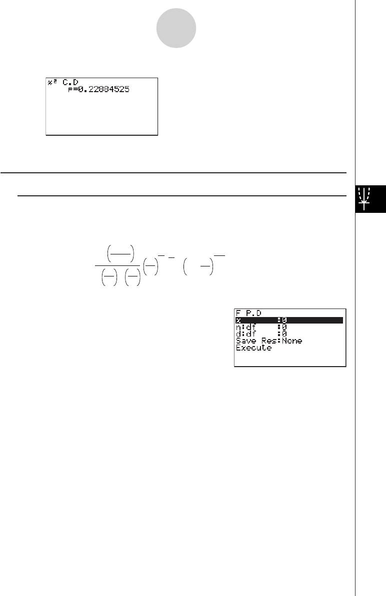
20010101
Calculation Result Output Example
p.................................. χ2 distribution probability
kk
kk
kF Distribution
uu
uu
u F Probability Density
F probability density calculates the probability density function for the F distribution at a
specified x value.
Γ
n
2
x
d
n
n
2–1
2
n
Γ2
n + d
Γ2
dd
nx
1 +
n + d
2
f
(x) =
–
Perform the following key operations from the statistical data list.
5(DIST)
e(F)
b(P.D)
Data is specified using parameter specification. The following shows the meaning of each
item.
x.................................. data
n:df .............................. numerator degrees of freedom (positive integer)
d:df .............................. denominator degrees of freedom (positive integer)
Save Res ..................... list for storage of calculation results (None or List 1 to 20)
Execute ....................... executes a calculation or draws a graph
After setting all the parameters, align the cursor with [Execute] and then press one of the
function keys shown below to perform the calculation or draw the graph.
•1(CALC) ... Performs the calculation.
•6(DRAW) ... Draws the graph.
1-4-12
Distribution (DIST)
20011101

20010101
Calculation Result Output Example
p.................................. F probability density
# V-Window settings for graph drawing are set
automatically when the SET UP screen's
[Stat Wind] setting is [Auto]. Current V-
Window settings are used for graph drawing
when the [Stat Wind] setting is [Manual].
1-4-13
Distribution (DIST)

20010101
uu
uu
u F Distribution Probability
F distribution probability calculates the probability of F distribution data falling between two
specific values.
p =
Γ
n
2
dx
x
d
nn
2–1
2
n
Γ2
n + d
Γ2
dd
nx
1 +
n + d
2
–
a
b
∫
a: lower boundary
b: upper boundary
Perform the following key operations from the statistical data list.
5(DIST)
e(F)
c(C.D)
Data is specified using parameter specification. The following shows the meaning of each
item.
Lower .......................... lower boundary
Upper .......................... upper boundary
n:df .............................. numerator degrees of freedom (positive integer)
d:df .............................. denominator degrees of freedom (positive integer)
Save Res ..................... list for storage of calculation results (None or List 1 to 20)
Execute ....................... executes a calculation
After setting all the parameters, align the cursor with [Execute] and then press the function
key shown below to perform the calculation.
•1(CALC) ... Performs the calculation.
# There is no graphing for F distribution
probability.
1-4-14
Distribution (DIST)
20011101
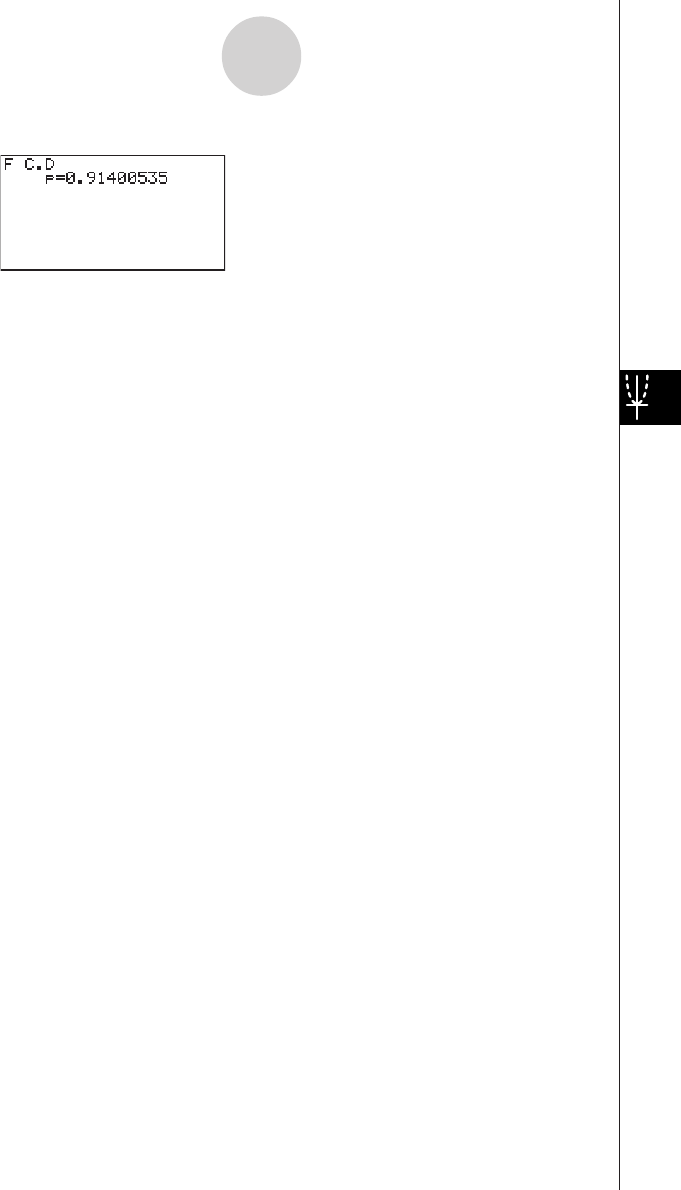
20010101
Calculation Result Output Example
p.................................. F distribution probability
1-4-15
Distribution (DIST)
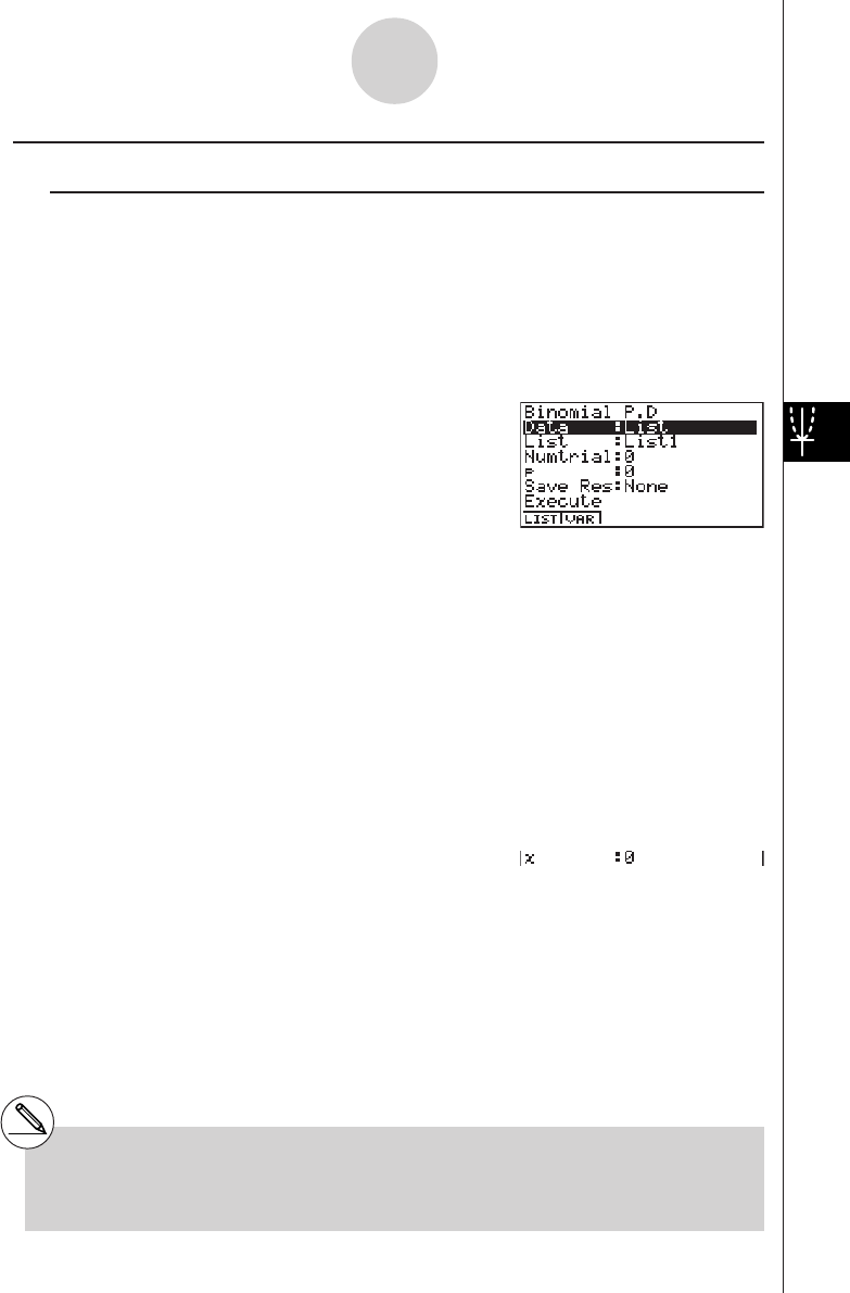
20010101
kk
kk
kBinomial Distribution
uu
uu
u Binomial Probability
Binomial probability calculates a probability at a specified value for the discrete binomial
distribution with the specified number of trials and probability of success on each trial.
f
(x) =
n
C
x
p
x
(1–p)
n – x
(x = 0, 1, ·······, n)p:success probability
(0 < p < 1)
n:number of trials
Perform the following key operations from the statistical data list.
5(DIST)
f(Binmal)
b(P.D)
The following shows the meaning of each item when data is specified using list specification.
Data ............................ data type
List .............................. list whose contents you want to use as specified data
(List 1 to 20)
Numtrial ....................... number of trials
p.................................. success probability (0 < p < 1)
Save Res ..................... list for storage of calculation results (None or List 1 to 20)
Execute ....................... executes a calculation
The following shows the meaning of a parameter data specification item that is different from
list data specification.
x.................................. integer from 0 to n
After setting all the parameters, align the cursor with [Execute] and then press the function
key shown below to perform the calculation.
•1(CALC) ... Performs the calculation.
# There is no graphing for binomial distribution.
1-4-16
Distribution (DIST)
20011101
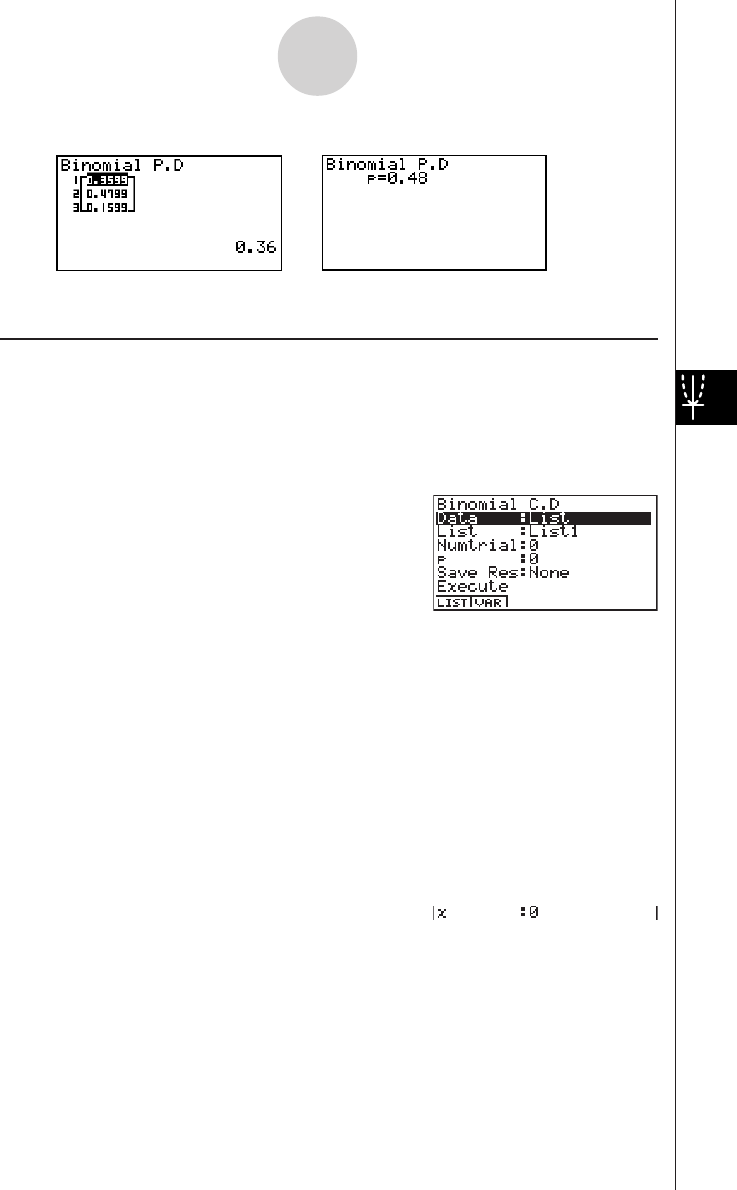
20010101
Calculation Result Output Example
p.................................. binomial probability
uu
uu
uBinomial Cumulative Density
Binomial cumulative density calculates a cumulative probability at a specified value for the
discrete binomial distribution with the specified number of trials and probability of success on
each trial.
Perform the following key operations from the statistical data list.
5(DIST)
f(Binmal)
c(C.D)
The following shows the meaning of each item when data is specified using list specification.
Data ............................ data type
List .............................. list whose contents you want to use as specified data
(List 1 to 20)
Numtrial ....................... number of trials
p.................................. success probability (0 < p < 1)
Save Res ..................... list for storage of calculation results (None or List 1 to 20)
Execute ....................... executes a calculation
The following shows the meaning of a parameter data specification item that is different from
list data specification.
x.................................. integer from 0 to n
1-4-17
Distribution (DIST)
20011101
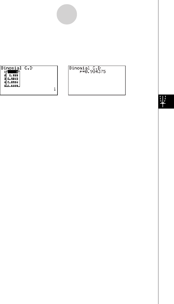
20010101
After setting all the parameters, align the cursor with [Execute] and then press the function
key shown below to perform the calculation.
•1(CALC) ... Performs the calculation.
Calculation Result Output Example
p......................................... probability of success
1-4-18
Distribution (DIST)
20011101
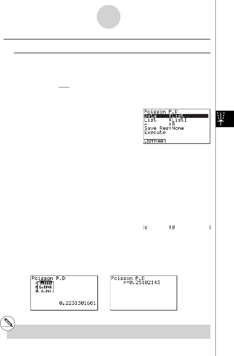
20010101
kk
kk
kPoisson Distribution
uu
uu
uPoisson Probability
Poisson probability calculates a probability at a specified value for the discrete Poisson
distribution with the specified mean.
f(x)
= x!
e
–
x
µ
µ
(x = 0, 1, 2, ···)
µ
:mean (
µ
> 0)
Perform the following key operations from the statistical data list.
5(DIST)
g(Poissn)
b(P.D)
The following shows the meaning of each item when data is specified using list specification.
Data ............................ data type
List .............................. list whose contents you want to use as specified data
(List 1 to 20)
µ
.................................. mean (
µ
> 0)
Save Res ..................... list for storage of calculation results (None or List 1 to 20)
Execute ....................... executes a calculation
The following shows the meaning of a parameter data specification item that is different from
list data specification.
x.................................. ( x
> 0)
After setting all the parameters, align the cursor with [Execute] and then press the function
key shown below to perform the calculation.
•1(CALC) ... Performs the calculation.
Calculation Result Output Example
p.................................. Poisson probability
# There is no graphing for Poisson distribution.
1-4-19
Distribution (DIST)
20011101
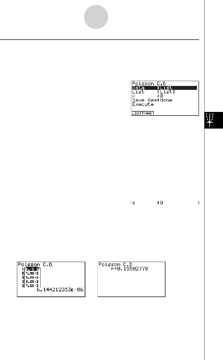
20010101
uu
uu
u Poisson Cumulative Density
Poisson cumulative density calculates a cumulative probability at specified value for the
discrete Poisson distribution with the specified mean.
Perform the following key operations from the statistical data list.
5(DIST)
g(Poissn)
c(C.D)
The following shows the meaning of each item when data is specified using list specification.
Data ............................ data type
List .............................. list whose contents you want to use as specified data
(List 1 to 20)
µ
.................................. mean (
µ
> 0)
Save Res ..................... list for storage of calculation results (None or List 1 to 20)
Execute ....................... executes a caluculation
The following shows the meaning of a parameter data specification item that is different from
list data specification.
x.................................. ( x
> 0)
After setting all the parameters, align the cursor with [Execute] and then press the function
key shown below to perform the calculation.
•1(CALC) ... Performs the calculation.
Calculation Result Output Example
p.................................. Poisson cumulative probability
1-4-20
Distribution (DIST)
20011101
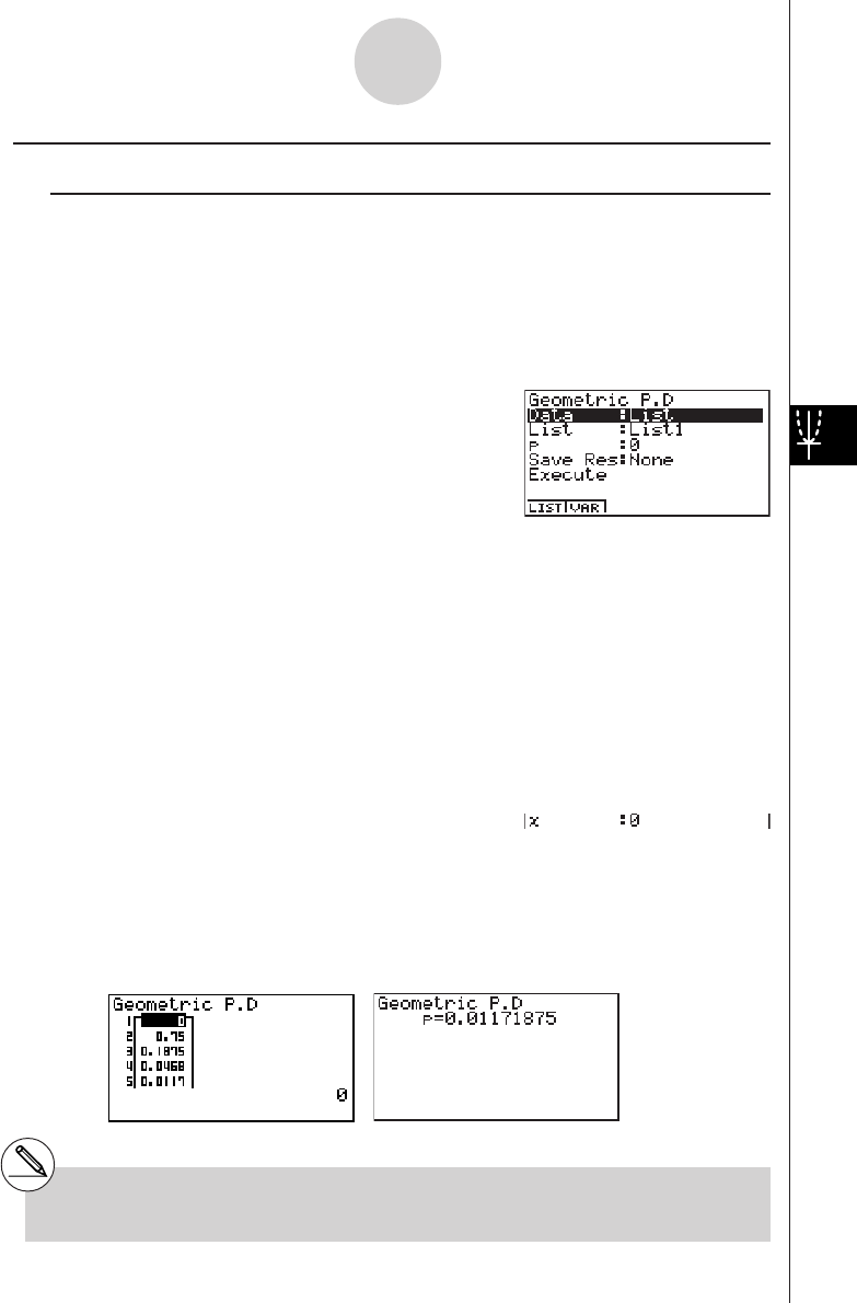
20010101
kk
kk
kGeometric Distribution
uu
uu
uGeometric Probability
Geometric probability calculates the probability at a specified value, and the number of the
trial on which the first success occurs, for the geometric distribution with a specified
probability of success.
f
(x) = p(1– p)x – 1
(x = 1, 2, 3, ···)
Perform the following key operations from the statistical data list.
5(DIST)
h(Geo)
b(P.D)
The following shows the meaning of each item when data is specified using list specification.
Data ............................ data type
List .............................. list whose contents you want to use as specified data
(List 1 to 20)
p.................................. success probability (0 < p < 1)
Save Res ..................... list for storage of calculation results (None or List 1 to 20)
Execute ....................... executes a calculation
The following shows the meaning of a parameter data specification item that is different from
list data specification.
x.................................. positive integer (x > 1)
After setting all the parameters, align the cursor with [Execute] and then press the function
key shown below to perform the calculation.
•1(CALC) ... Performs the calculation.
Calculation Result Output Example
p.................................. geometric probability
1-4-21
Distribution (DIST)
# There is no graphing for geometric distribu-
tion.
# Positive integer number is calculated whether
list data (Data:List) or x value (Data:variable)
is specified.
20011101
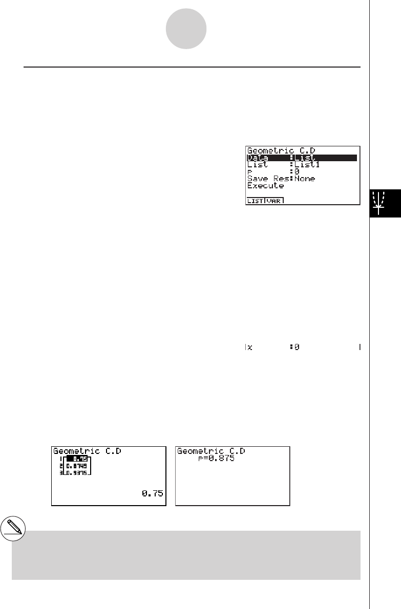
20010101
uu
uu
uGeometric Cumulative Density
Geometric cumulative density calculates a cumulative probability at specified value, the
number of the trial on which the first success occurs, for the discrete geometric distribution
with the specified probability of success.
Perform the following key operations from the statistical data list.
5(DIST)
h(Geo)
c(C.D)
The following shows the meaning of each item when data is specified using list specification.
Data ............................ data type
List .............................. list whose contents you want to use as specified data
(List 1 to 20)
p.................................. success probability (0 < p < 1)
Save Res ..................... list for storage of calculation results (None or List 1 to 20)
Execute ....................... executes a calculation
The following shows the meaning of a parameter data specification item that is different from
list data specification.
x.................................. positive integer (x > 1)
After setting all the parameters, align the cursor with [Execute] and then press the function
key shown below to perform the calculation.
• 1(CALC) ... Performs the calculation.
Calculation Result Output Example
p.................................. geometric cumulative probability
# Positive integer number is calculated whether
list data (Data:List) or x value (Data:variable)
is specified.
1-4-22
Distribution (DIST)
20011101

Financial Calculation (TVM)
2-1 Before Performing Financial Calculations
2-2 Simple Interest
2-3 Compound Interest
2-4 Cash Flow (Investment Appraisal)
2-5 Amortization
2-6 Interest Rate Conversion
2-7 Cost, Selling Price, Margin
2-8 Day/Date Calculations
2-9 Depreciation
2-10 Bonds
2-11 TVM Graph
2
Chapter
20010101
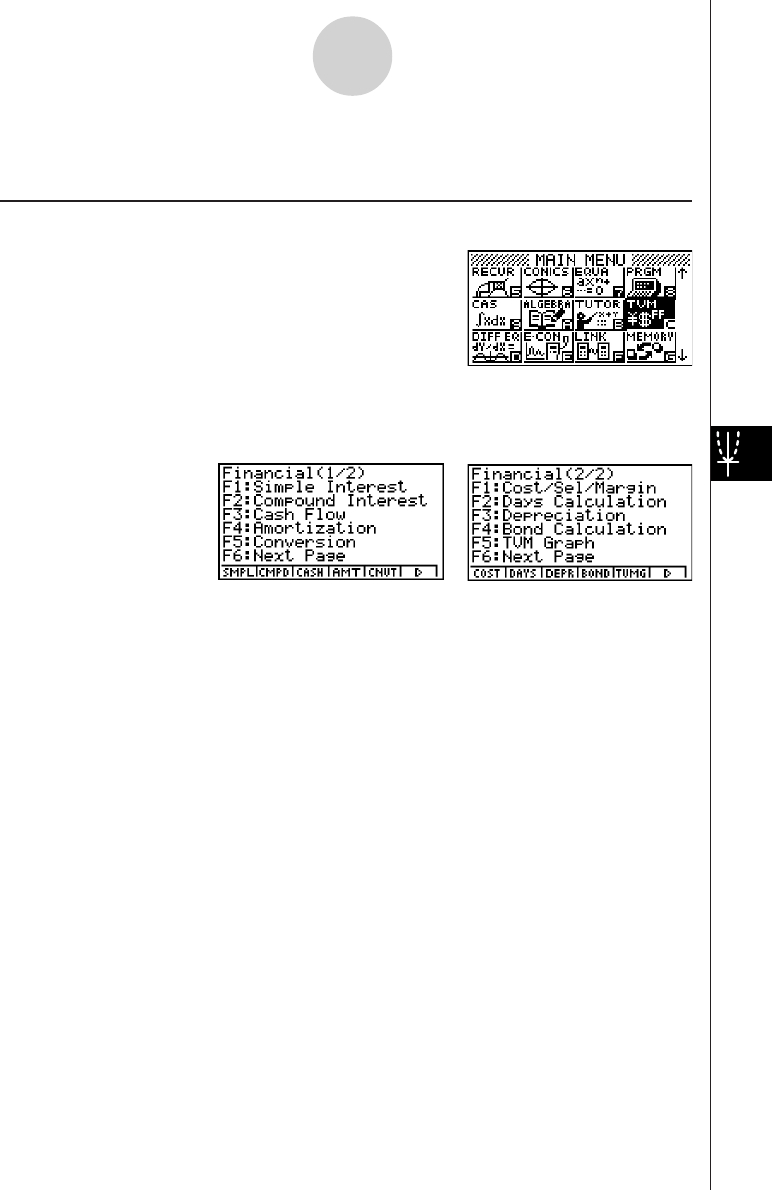
20010101
2-1 Before Performing Financial Calculations
kk
kk
kTVM Mode
On the Main Menu, select the TVM icon.
Entering the TVM Mode displays the Financial screen like the one shown below.
Financial 1 screen Financial 2 screen
•1(SMPL) .... Simple interest
•2(CMPD) ... Compound interest
•3(CASH) .... Cash flow (investment appraisal)
•4(AMT) ...... Amortization
•5(CNVT) .... Interest rate conversion
•6(g)1(COST) ... Cost, selling price, margin
2(DAYS) ... Day/date calculations
3(DEPR) ... Depreciation
4(BOND) ... Bonds
5(TVMG) ... TVM (compound interest simulation) graph
2-1-1
Before Performing Financial Calculations
* The above shows the ALGEBRA
FX 2.0 PLUS screen.
20010101
kk
kk
k SET UP Items
uu
uu
u Payment
•{BGN}/{END}........ Specifies {beginning of the period} / {end of the period} payment
uu
uu
u Date Mode
•{365}/{360}......... Specifies calculation according to a {365-day} / {360-day} year
uu
uu
u Periods/YR. (Bond)
•{Annual}/{SEMI}... Indicates an {annual} / {semi-annual} period
Note the following points regarding SET UP screen settings whenever using the Financial
Mode.
•Drawing a financial graph while the Label item is turned on, displays the label CASH for the
vertical axis (deposits, withdrawals), and TIME for the horizontal axis (frequency). Axis
labels do not appear on the TVM graph.
•The number of display digits applied in the Financial Mode is different from the number of
digits used in other modes. The calculators automatically reverts to Norm 1 whenever you
enter the Financial Mode, which cancels a Sci (number of significant digits) or Eng
(engineering notation) setting made in another mode.
kk
kk
k Graphing in the TVM Mode
After performing a financial calculation, you can use 6 (GRPH) to graph the results as shown
below.
•Pressing 1 (TRACE) while a graph is on the display activates Trace, which can be used to
look up other financial values. In the case of simple interest, for example, pressing e
displays PV, SI, and SFV. Pressing d displays the same values in reverse sequence.
•Zoom, Scroll, and Sketch cannot be used in the Financial Mode.
•Whether you should use a positive or a negative value for the present value (PV) or the
purchase price (PRC) depends on the type of calculation you are trying to perform.
• Note that graphs should be used only for reference purposes when viewing TVM Mode
calculation results.
•Note that calculation results produced in this mode should be regarded as reference values
only.
•Whenever performing an actual financial transaction, be sure to check any calculation results
obtained using this calculator with against the figures calculated by your financial institution.
2-1-2
Before Performing Financial Calculations
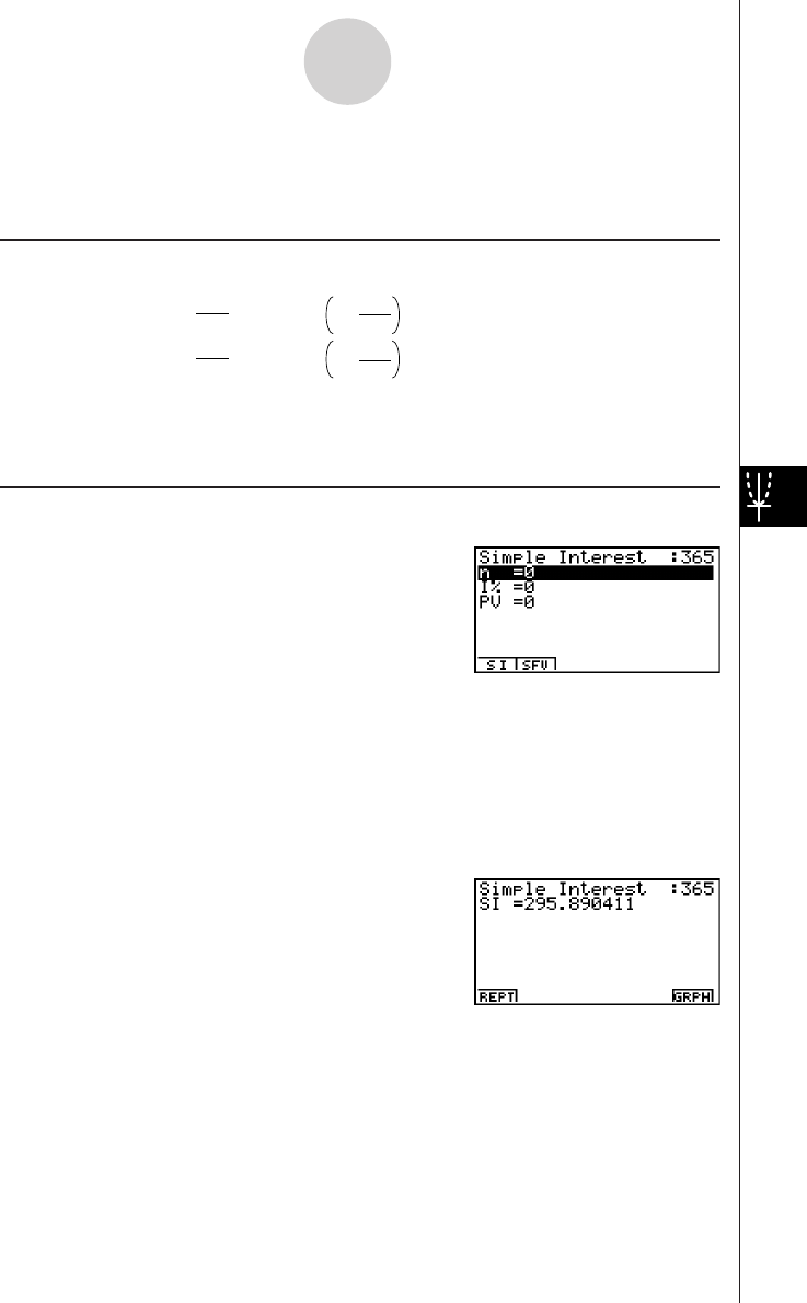
20010101
2-2 Simple Interest
This calculator uses the following formulas to calculate simple interest.
uu
uu
uFormula
365-day Mode
SI' = n
365 × PV × i
SI' = n
360 × PV × i
I%
100
i =
I%
100
i =
SI :interest
n:number of interest
360-day Mode periods
PV :principal
I%:annual interest
SFV :principal plus interest
SI = –SI'
SFV = –(PV + SI')
Press 1(SMPL) from the Financial 1 screen to display the following input screen for simple
interest.
1(SMPL)
n.................................. number of interest periods (days)
I%............................... annual interest rate
PV ............................... principal
After configuring the parameters, press one of the function keys noted below to perform the
corresponding calculation.
•1(SI) ....... Simple interest
•2(SFV) ... Simple future value
2-2-1
Simple Interest

20010101
• An error (Ma ERROR) occurs if parameters are not configured correctly.
Use the following function keys to maneuver between calculation result screens.
•1(REPT) ... Parameter input screen
•6(GRPH) ... Draws graph
After drawing a graph, you can press 1(TRACE) to turn on trace and read calculation
results along the graph.
Each press of e while trace is turned on cycles the displayed value in the sequence:
present value (PV) → simple interest (SI) → simple future value (SFV). Pressing d cycles
in the reverse direction.
Press i to turn off trace.
Press i again to return to the parameter input screen.
2-2-2
Simple Interest
20010101
2-3 Compound Interest
This calculator uses the following standard formulas to calculate compound interest.
uu
uu
uFormula I
PV+PMT ×+ FV
i(1+ i)
n
(1+ i)
n
(1+ i ×
S)[(1+ i)
n
–1]1 = 0
i = 100
I %
Here:
PV= –(PMT × + FV × )
β
α
FV= –
β
PMT × + P
V
α
PMT= –
β
PV
+ FV ×
α
n =
log
{ }
log(1+ i)
(1+ i S ) PMT+PVi
(1+ i S ) PMT–FVi
i
(
1+ i
)
n
(1+ i × S)[(1+ i)n–1]
=
α
(1+ i)n
1
=
β
F(i) = Formula I
+ (1+ i S)[n(1+ i)
–n–1
]+S
[
–
nFV(1+ i)
–n–1
ii
PMT (1+ i S)[1– (1+ i)
–n
]
F(i) = –
[
+S [1–(1+ i)
–n
]
]
uu
uu
uFormula II (I% = 0)
PV + PMT × n + FV = 0
Here:
PV = – (PMT × n + FV )
PV :present value
FV :future value
PMT :payment
n:number of compound periods
I
%
:annual interest rate
i is calculated using Newton’s Method.
S = 0 assumed for end of term
S = 1 assumed for beginning of term
2-3-1
Compound Interest
20011201

20010101
FV = – (PMT × n + PV )
n
PMT = – PV + FV
PMT
n = – PV + FV
• A deposit is indicated by a plus sign (+), while a withdrawal is indicated by a minus sign (–).
uu
uu
uConverting between the nominal interest rate and effective interest rate
The nominal interest rate (I% value input by user) is converted to an effective interest rate
(I%') when the number of installments per year (P/Y ) is different from the number of
compound interest calculation periods (C/Y ). This conversion is required for installment
savings accounts, loan repayments, etc.
P/Y :installment
periods per year
C/Y:compounding
periods per year
When calculating n, PV, PMT, FV
The following calculation is performed after conversion from the nominal interest rate to the
effective interest rate, and the result is used for all subsequent calculations.
i = I%'÷100
When calculating I%
After I% is obtained, the following calculation is performed to convert to I%'.
I%' = I%
(1+ ) –1
[C / Y ]
[P / Y ]
100
{ }
×[C / Y ]×100
P/Y :installment
periods per year
C/Y:compounding
periods per year
The value of I%' is returned as the result of the I% calculation.
2-3-2
Compound Interest
I%' = I%
(1+ ) –1
[C / Y ]
[P / Y ]
100 × [C / Y ]
{ }
×100
20011101
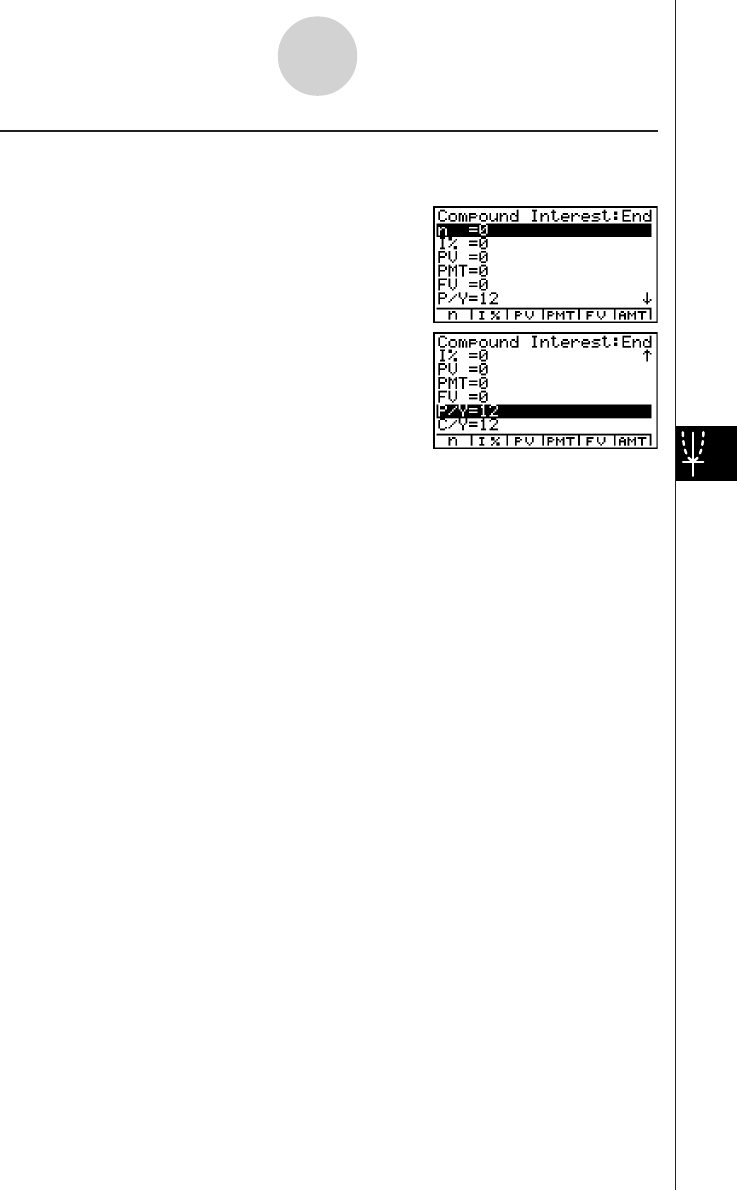
20010101
Press 2(CMPD) from the Financial 1 screen to display the following input screen for
compound interest.
2(CMPD)
n.................................. number of compound periods
I%............................... annual interest rate
PV ............................... present value (loan amount in case of loan; principal in case
of savings)
PMT ............................ payment for each installment (payment in case of loan;
deposit in case of savings)
FV ............................... future value (unpaid balance in case of loan; principal plus
interest in case of savings)
P/Y.............................. installment periods per year
C/Y.............................. compounding periods per year
Important!
Inputting Values
A period (n) is expressed as a positive value. Either the present value (PV ) or future value
(FV ) is positive, while the other (PV or FV ) is negative.
Precision
This calculator performs interest calculations using Newton’s Method, which produces
approximate values whose precision can be affected by various calculation conditions.
Because of this, interest calculation results produced by this calculator should be used
keeping the above limitation in mind or the results should be verified.
2-3-3
Compound Interest
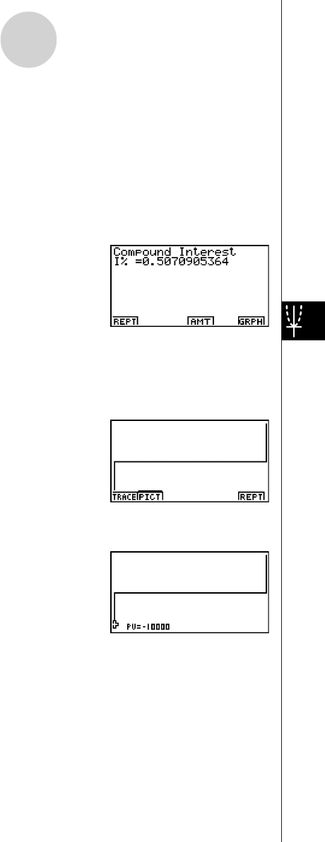
20010101
After configuring the parameters, press one of the function keys noted below to perform the
corresponding calculation.
•1(n) ............ Number of compound periods
•2(I%) .......... Annual interest rate
•3(PV) ......... Present value (Loan: loan amount; Savings: balance)
•4(PMT) ....... Payment (Loan: installment; Savings: deposit)
•5(FV) .......... Future value (Loan: unpaid balance; Savings: principal plus interest)
•6(AMT) ....... Amortization screen
•An error (Ma ERROR) occurs if parameters are not configured correctly.
Use the following function keys to maneuver between calculation result screens.
•1(REPT) ..... Parameter input screen
•4(AMT) ....... Amortization screen
•6(GRPH) .... Draws graph
After drawing a graph, you can press 1(TRACE) to turn on trace and read calculation
results along the graph.
Press i to turn off trace.
Press i again to return to the parameter input screen.
2-3-4
Compound Interest

20010101
2-4 Cash Flow (Investment Appraisal)
This calculator uses the discounted cash flow (DCF) method to perform investment appraisal
by totalling cash flow for a fixed period. This calculator can perform the following four types
of investment appraisal.
•Net present value (NPV)
•Net future value (NFV)
•Internal rate of return (IRR)
•Pay back period (PBP)
A cash flow diagram like the one shown below helps to visualize the movement of funds.
CF
0
CF
1
CF
2
CF
3
CF
4
CF
5
CF
6
CF
7
With this graph, the initial investment amount is represented by CF0. The cash flow one year
later is shown by CF1, two years later by CF2, and so on.
Investment appraisal can be used to clearly determine whether an investment is realizing
profits that were originally targeted.
uNPV
NPV = CF0 + + + + … +
(1+ i)
CF1
(1+ i)2
CF2
(1+ i)3
CF3
(1+ i)n
CFn
i = 100
I %
n: natural number up to 254
uNFV
NFV = NPV × (1 + i )n
uIRR
0 = CF0 + + + + … +
(1+ i)
CF1
(1+ i)2
CF2
(1+ i)3
CF3
(1+ i)n
CFn
In this formula, NPV = 0, and the value of IRR is equivalent to i × 100. It should be noted,
however, that minute fractional values tend to accumulate during the subsequent
calculations performed automatically by the calculator, so NPV never actually reaches
exactly zero. IRR becomes more accurate the closer that NPV approaches to zero.
2-4-1
Cash Flow (Investment Appraisal)
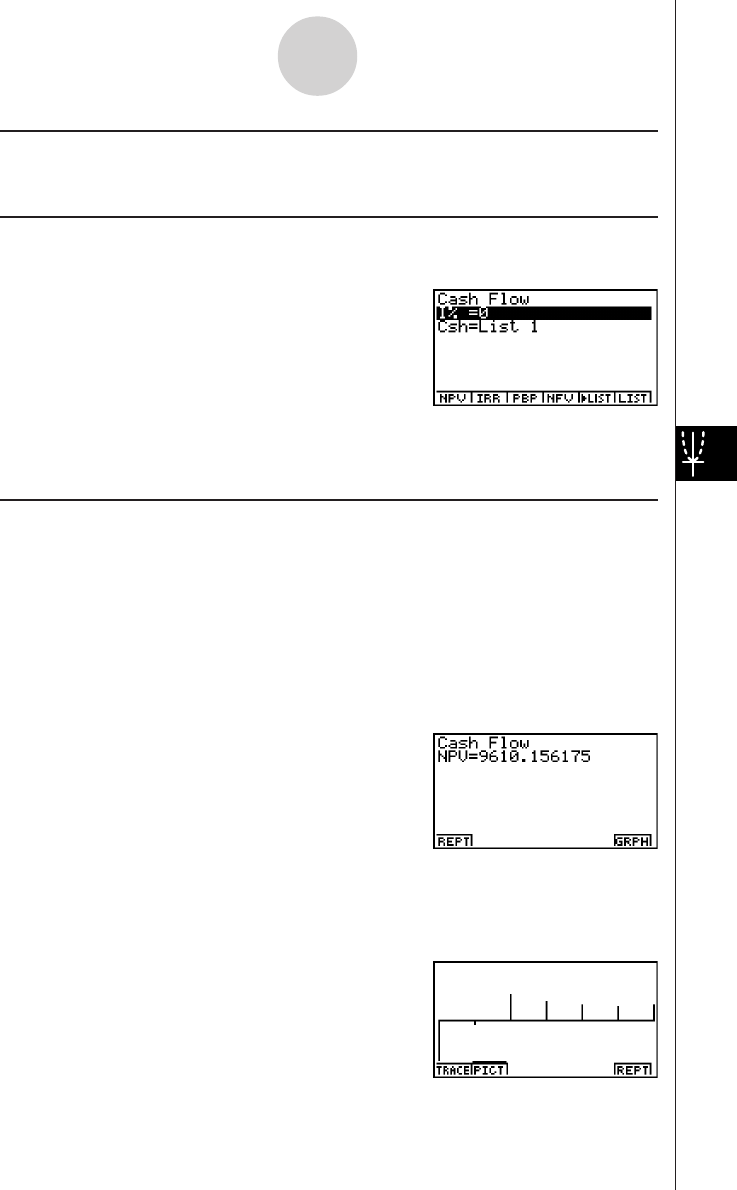
20010101
uu
uu
uPBP
PBP is the value of n when NPV > 0 (when investment can be recovered).
• Press 3(CASH) from the Financial 1 screen to display the following input screen for Cash
Flow.
3(CASH)
I%............................... interest rate (%)
Csh .............................. list for cash flow
If you have not yet input data into a list, press 5('LIST) and input data into a list.
After configuring the parameters, press one of the function keys noted below to perform the
corresponding calculation.
•1(NPV) ......... Net present value
•2(IRR) .......... Internal rate of return
•3(PBP) ......... Pay back period
•4(NFV) ......... Net future value
•5('LIST) ..... Inputs data from a list
•6(LIST) ......... Specifies a list for data input
• An error (Ma ERROR) occurs if parameters are not configured correctly.
Use the following function keys to maneuver between calculation result screens.
•1(REPT) ...... Parameter input screen
•6(GRPH) ..... Draws graph
2-4-2
Cash Flow (Investment Appraisal)
20011101
20010101
After drawing a graph, you can press 1(TRACE) to turn on trace and read calculation
results along the graph.
Press i to turn off trace.
Press i again to return to the parameter input screen.
2-4-3
Cash Flow (Investment Appraisal)
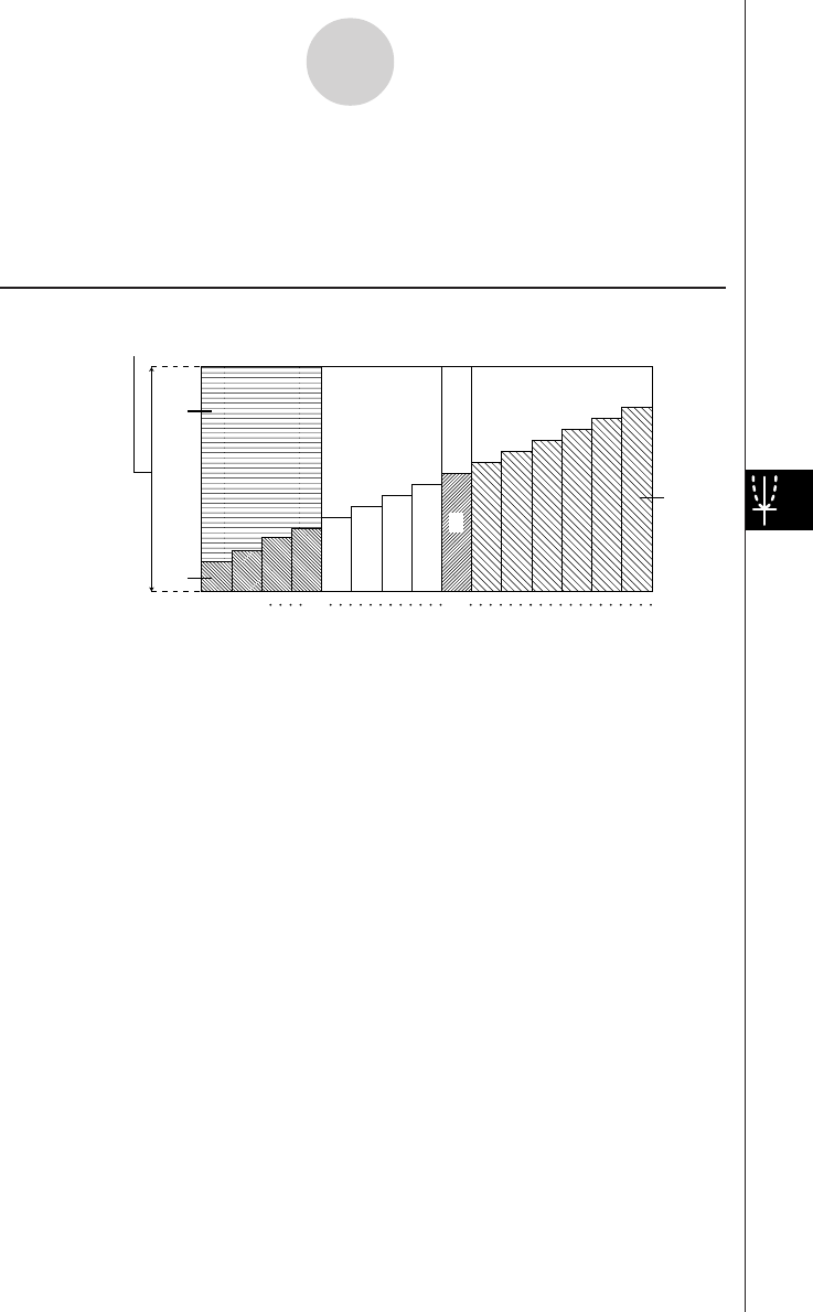
20010101
2-5 Amortization
This calculator can be used to calculate the principal and interest portion of a monthly
installment, the remaining principal, and amount of principal and interest repaid up to any
point.
uu
uu
uFormula
b
a
d
e
c
12 mn
a: interest portion of installment PM1 (INT)
b: principal portion of installment PM1 (PRN)
c: balance of principal after installment PM2 (BAL)
d: total principal from installment PM1 to payment of installment PM2 (ΣPRN)
e: total interest from installment PM1 to payment of installment PM2 (ΣINT)
*a + b = one repayment (PMT)
a : INT
PM1
= I BAL
PM1–1
× i I × (PMT sign)
b : PRN
PM1
= PMT + BAL
PM1–1
× i
c : BAL
PM2
= BAL
PM2–1
+ PRN
PM2
d : Σ PRN = PRN
PM1
+ PRN
PM1+1
+ … + PRN
PM2
e : Σ INT = INT
PM1
+ INT
PM1+1
+ … + INT
PM2
PM2
PM1
PM2
PM1
BAL0 = PV (INT1 = 0 and PRN1 = PMT at beginning of installment term)
(Number of payments)
Amount of single payment
2-5-1
Amortization
20010101
uu
uu
uConverting between the nominal interest rate and effective interest rate
The nominal interest rate (I% value input by user) is converted to an effective interest rate
(I%') for installment loans where the number of installments per year is different from the
number of compound interest calculation periods.
I%' = I%
(1+ ) –1
[C / Y ]
[P / Y ]
100 × [C / Y ]
{ }
×100
The following calculation is performed after conversion from the nominal interest rate to the
effective interest rate, and the result is used for all subsequent calculations.
i = I%'÷100
Press 4(AMT) from the Financial 1 screen to display the following input screen for interest
rate conversion.
4(AMT)
PM1 ............................. first installment of installments 1 through n
PM2 ............................. second installment of installments 1 through n
n.................................. installments
I%............................... interest rate
PV ............................... principal
PMT ............................ payment for each installment
FV ............................... balance following final installment
P/Y.............................. installments per year
C/Y.............................. compoundings per year
2-5-2
Amortization
20010101
After configuring the parameters, press one of the function keys noted below to perform the
corresponding calculation.
•1(BAL) ......... Balance of principal after installment PM2
•2(INT) .......... Interest portion of installment PM1
•3(PRN) ......... Principal portion of installment PM1
•4(Σ INT) ....... Total interest paid from installment PM1 to installment PM2
•5(Σ PRN) ...... Total principal paid from installment PM1 to installment PM2
•6(CMPD) ...... Compound interest screen
• An error (Ma ERROR) occurs if parameters are not configured correctly.
Use the following function keys to maneuver between calculation result screens.
•1(REPT) ....... Parameter input screen
•4(CMPD) ...... Compound interest screen
•6(GRPH) ...... Draws graph
After drawing a graph, you can press 1(TRACE) to turn on trace and read calculation
results along the graph.
The first press of 1(TRACE) displays INT and PRN when n = 1. Each press of e shows
INT and PRN when n = 2, n = 3, and so on.
Press i to turn off trace.
Press i again to return to the parameter input screen.
2-5-3
Amortization
20010101
2-6 Interest Rate Conversion
The procedures in this section describe how to convert between the annual percentage rate
and effective interest rate.
uu
uu
uFormula
EFF = n
APR/100
1+ –1 × 100
n
APR = 100
EFF
1+ –1 × n ×100
1
n
Press 5(CNVT) in the Financial 1 screen to display the following input screen for interest
rate conversion.
5(CNVT)
n....................................... number of compoundings
I%............................... interest rate
After configuring the parameters, press one of the function keys noted below to perform the
corresponding calculation.
•1('EFF) ... Converts annual percent rate to effective interest rate
•2('APR) ... Converts effective interest rate to annual percent rate
• An error (Ma ERROR) occurs if parameters are not configured correctly.
Use the following function key to maneuver between calculation result screens.
•1(REPT) ... Parameter input screen
APR :annual percentage rate (%)
EFF :effective interest rate (%)
n:number of compoundings
2-6-1
Interest Rate Conversion
20011101

20010101
2-7 Cost, Selling Price, Margin
Cost, selling price, or margin can be calculated by inputting the other two values.
uu
uu
uFormula
CST = SEL 100
MRG
1–
SEL =
100
MRG
1–
CST
M
RG(%) = SEL
CST
1– × 100
Press 1(COST) from the Financial 2 screen to display the following input screen.
6(g)1(COST)
Cst ............................... cost
Sel ............................... selling price
Mrg .............................. margin
After configuring the parameters, press one of the function keys noted below to perform the
corresponding calculation.
•1(COST) .... Cost
•2(SEL) ....... Selling price
•3(MRG) ...... Margin
• An error (Ma ERROR) occurs if parameters are not configured correctly.
Use the following function key to maneuver between calculation result screens.
•1(REPT) ... Parameter input screen
CST :cost
SEL :selling price
MRG :margin
2-7-1
Cost, Selling Price, Margin
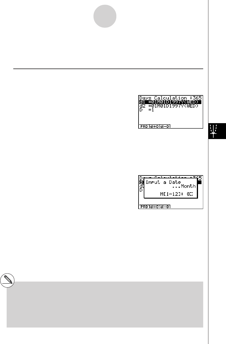
20010101
2-8 Day/Date Calculations
You can calculate the number of days between two dates, or you can determine what date
comes a specific number of days before or after another date.
Press 2(DAYS) from the Financial 2 screen to display the following input screen for day/
date calculation.
6(g)2(DAYS)
d1 ................................ date 1
d2 ................................ date 2
D................................. number of days
To input a date, first highlight d1 or d2. Pressing a number key to input the month causes an
input screen like the one shown below to appear on the display.
2-8-1
Day/Date Calculations
#The set up screen can be used to specify
either a 365-day or 360-day year for financial
calculations. Day/date calculations are also
performed in accordance with the current
setting for number of days in the year, but the
following calculations cannot be performed
when the 360-day year is set. Attempting to do
so causes an error.
(Date) + (Number of Days)
(Date) – (Number of Days)
#The allowable calculation range is January 1,
1901 to December 31, 2099.
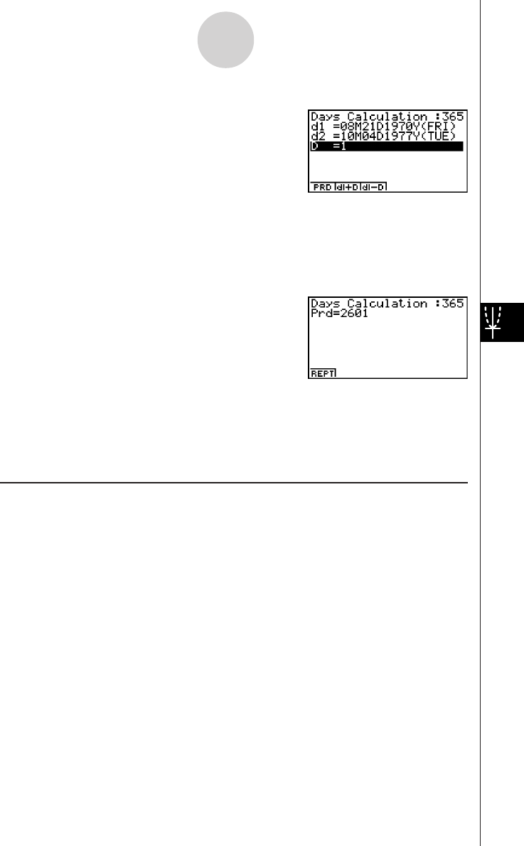
20010101
Input the month, day, and year, pressing w after each.
After configuring the parameters, press one of the function keys noted below to perform the
corresponding calculation.
•1(PRD) ........ Number of days from d1 to d2 (d2 – d1)
•2(d1+D) ....... d1 plus a number of days (d1 + D)
•3(d1 – D) ..... d1 minus a number of days (d1 – D)
• An error (Ma ERROR) occurs if parameters are not configured correctly.
Use the following function key to maneuver between calculation result screens.
•1(REPT) ...... Parameter input screen
360-day Date Mode Calculations
The following describes how calculations are processed when 360 is specified for the Date
Mode item in the SET UP screen.
• If d1 is day 31 of a month, d1 is treated as day 30 of that month is used.
• If d2 is day 31 of a month, d2 is treated as day 1 of the following month, unless d1 is day
30.
2-8-2
Day/Date Calculations

20010101
2-9 Depreciation
Any of the following four methods can be used to calculated depreciation.
uu
uu
uStraight-Line Method
The straight-line method calculates depreciation for a given period.
{Y–1}(PV–FV )
SL1 = n12
u
(PV–FV )
SLj = n
12–{Y–1}
({Y–1}G12)
(PV–FV )
n12
u
SLn+1 =
Depreciation for an item acquired part way through a year can be calculated by month.
uu
uu
uFixed Percentage Method
Fixed percentage method can be used to calculate depreciation for a given period, or to
calculate the depreciation rate.
100
I%
FP
j
= (RDV
j–1
+ FV ) ×
100
{Y–1}I%
FP
1
= PV × 12
×
FP
n+1
= RDV
n
({Y–1}G12)
RDV
1
= PV – FV – FP
1
RDV
j
= RDV
j–1
– FP
j
RDV
n+1
= 0 ({Y–1}G12)
Depreciation for an item acquired part way through a year can be calculated by month.
SL j:depreciation charge for the jth
year
n:useful life in years
PV :original cost (basis)
FV :scrap value (salvage value)
j:year
Y–1:number of depreciable months
in first year
FPj:depreciation charge for the jth year
RDVj:remaining depreciable value at the
end of jth year
I
%
:depreciation rate
2-9-1
Depreciation

20010101
uu
uu
uSum-of-the-Year's Digits Method
The sum-of-the-year's-digits method calculates depreciation for a given period.
12
{Y–1}
n' = n –
n (n +1)
Z = 2
2
(n' integer part +1)(n' integer part + 2*n' fraction part )
Z' =
SYD1 = {Y–1}
12
n
Z×(PV – FV )
n'– j+2
Z' )(PV – FV – SYD1)( jG1)SYDj = (
RDV1 = PV – FV – SYD1
RDVj = RDVj –1 – SYDj
n'– (n +1)+2
Z' )(PV – FV – SYD1)({Y–1}G12)
12–{Y–1}
12
×SYDn+1 = (
Depreciation for an item acquired part way through a year can be calculated by month.
uu
uu
uDeclining Balance Method
The declining balance method calculates depreciation for a given period.
RDV1 = PV – FV – DB1
({Y–1}G12)
({Y–1}G12)
100n
Y–1I%
DB1 = PV ×
100n
I%
12
×
×
DBj = (RDVj–1 + FV )
RDVj = RDVj–1 – DBj
DBn +1 = RDVn
RDVn+1 = 0
Depreciation for an item acquired part way through a year can be calculated by month.
SYDj:depreciation charge for the jth year
RDVj:remaining depreciable value at the
end of jth year
DBj:depreciation charge for the
jth year
RDVj:remaining depreciable
value at the end of jth year
I
%
:factor (%)
2-9-2
Depreciation
20011101
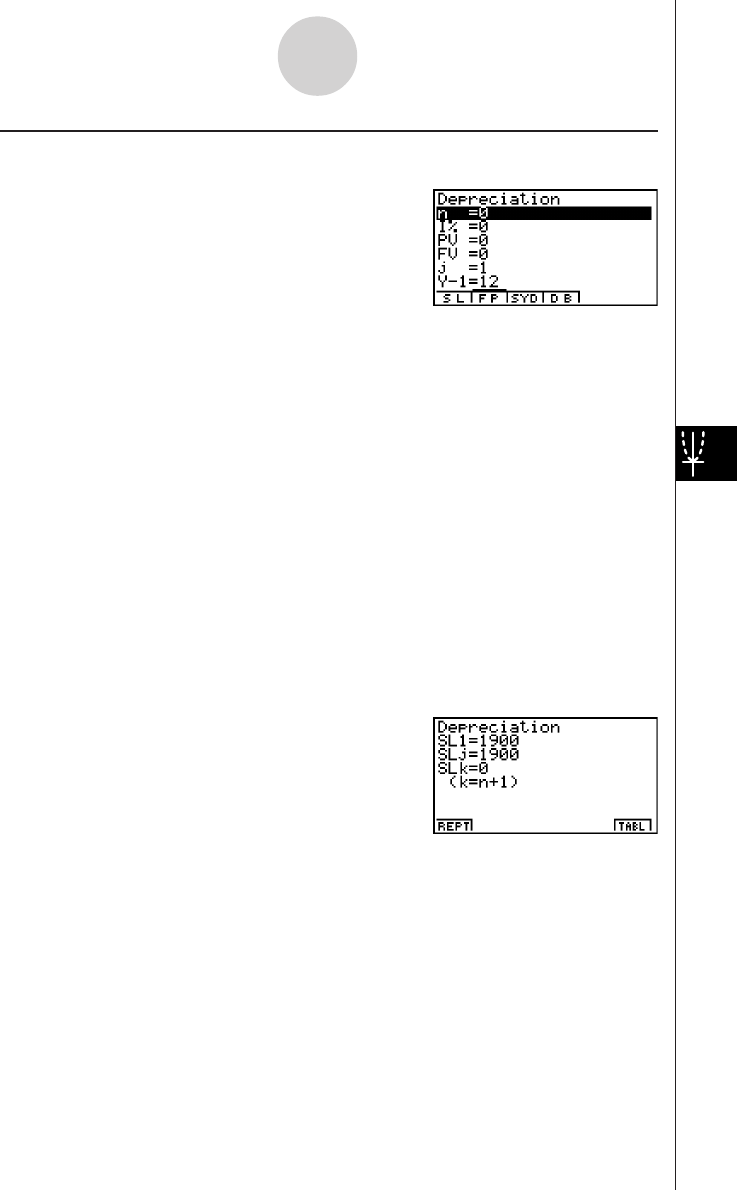
20010101
Press 3(DEPR) from the Financial 2 screen to display the following input screen for
depreciation.
6(g)3(DEPR)
n.................................. useful life in years
I%............................... depreciation rate/factor
PV ............................... original cost (basis)
FV ............................... scrap value (salvage value)
j................................... year
Y–1 .............................. number of depreciable months in first year
• Parameters can be displayed as integer or decimal values only. Inputting a fraction causes
it to be converted to a decimal value.
After configuring the parameters, press one of the function keys noted below to perform the
corresponding calculation.
•1(SL) ........... Straight-Line Method
•2(FP) ........... 1.Fixed Percentage Method
........... 2.Depreciation ratio
•3(SYD) ........ Sum-of-the-Year's Digits Method
•4(DB) .......... Declining Balance Method
2-9-3
Depreciation
20011101
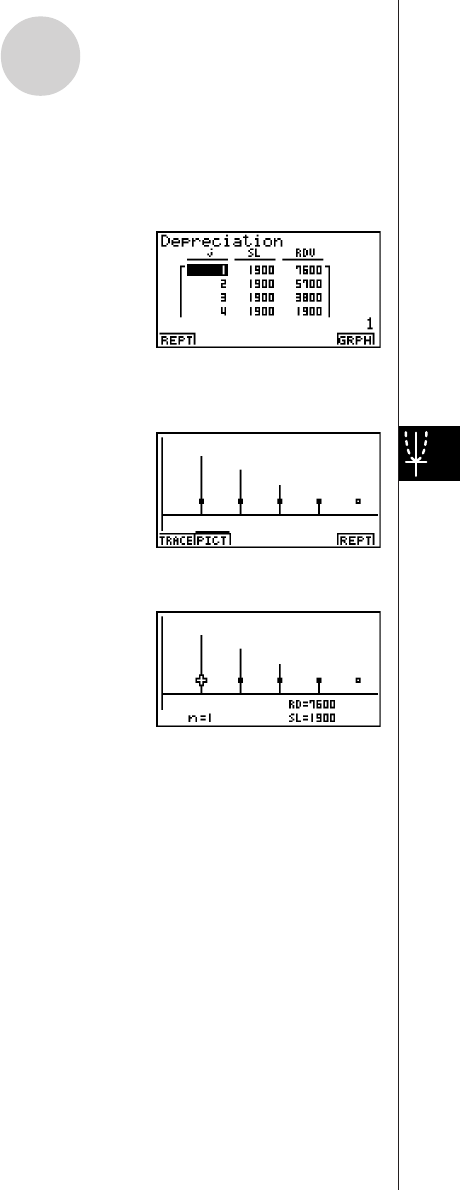
20010101
• An error (Ma ERROR) occurs if parameters are not configured correctly.
Use the following function keys to maneuver between calculation result screens.
•1(REPT) ...... Parameter input screen
•6(TABL) ....... Calculation result table
The following function keys are on the calculation result table screen.
•1(REPT) ...... Parameter input screen
•6(GRPH) ..... Draws graph
After drawing a graph, you can press 1(TRACE) to turn on trace and read calculation results
along the graph.
Press i to turn off trace.
Press i again to return to the parameter input screen.
2-9-4
Depreciation
20011101
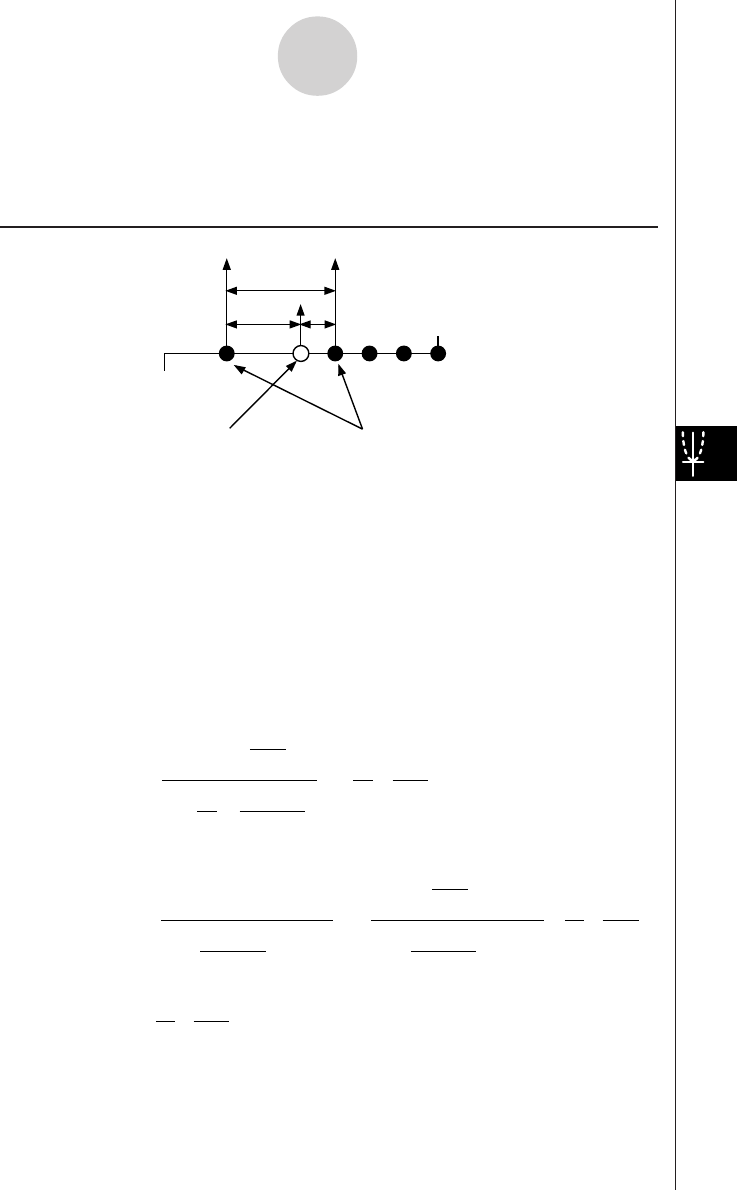
20010101
2-10 Bonds
The bond calculation function calculates the price and yield of a bond.
uu
uu
uFormula
PRC :price per $100 of face value
CPN :annual coupon rate (%)
YLD :yield to maturity (%)
A:accrued days
M:number of coupon payments per year (1=annual, 2=semi annual)
N:number of coupon payments between settlement date and maturity date
RDV :redemption price or call price per $100 of face value
D:number of days in coupon period where settlement occurs
B:number of days from settlement date until next coupon payment date = D – A
INT :accrued interest
CST :price including interest
• Less than six months to redemption
PRC = – ( )
RDV + M
CPN
1+ ( ×)
D
B
M
YLD/100 ×
D
A
M
CPN
• Six months or more to redemption
–×
D
A
M
CPN
PRC = +
RDV
(1+ )
M
YLD/100 (1+ )
M
YLD/100
M
CPN
Σ
N
k=1
(N–1+B/D )
(K–1+B/D )
×
D
A
M
CPN
I
NT =
CST = PRC + IN
T
D
Issue date
Redemption date
Purchase date Coupon Payment dates
A B
2-10-1
Bonds
20011101
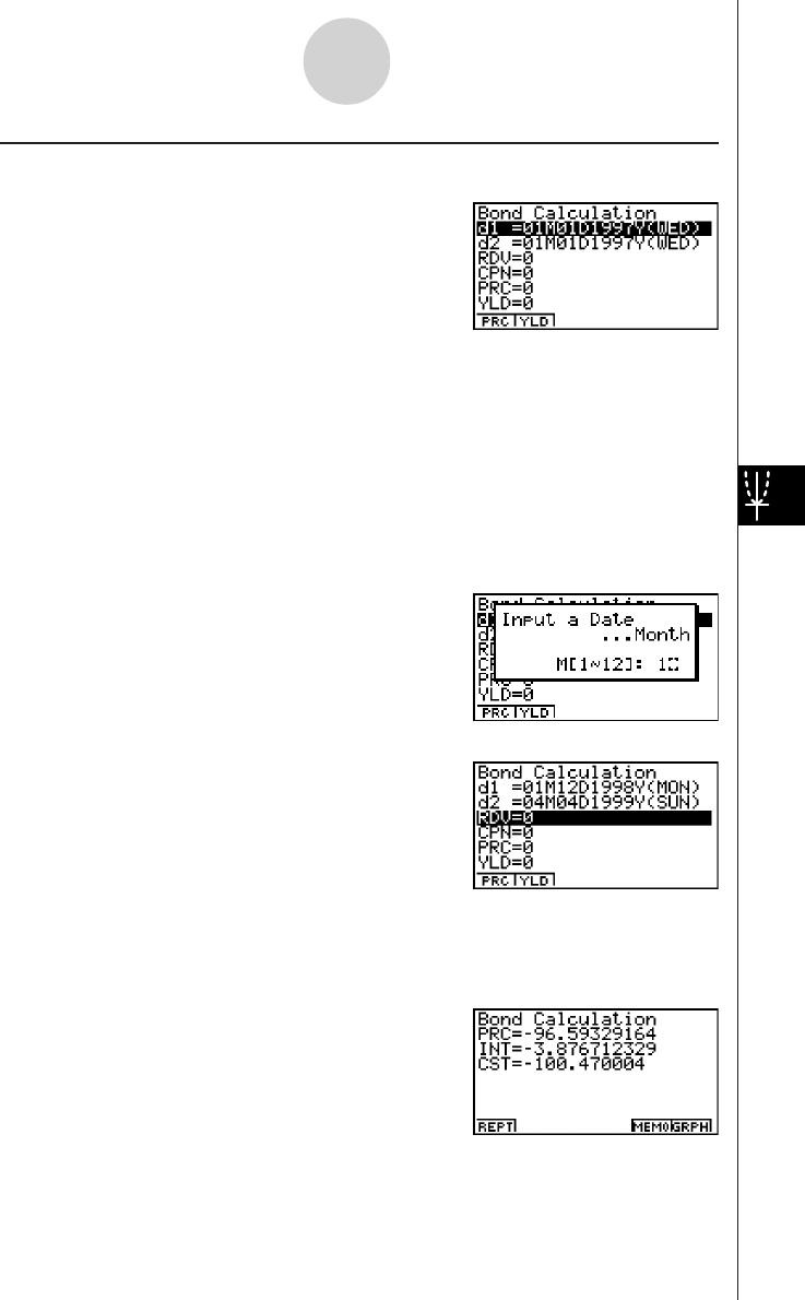
20010101
Press 4(BOND) from the Financial 2 screen to display the following input screen for band
calculation.
6(g)4(BOND)
d1 ................................ purchase date
d2 ................................ redemption date
RDV ............................ redemption price or call price per $100 of face value
CPN ............................ annual coupon rate (%)
PRC ............................ price per $100 of face value
YLD ............................. yield to maturity (%)
To input a date, first highlight d1 or d2. Pressing a number key to input the month causes an
input screen like the one shown below to appear on the display.
Input the month, day, and year, pressing w after each.
After configuring the parameters, press one of the function keys noted below to perform the
corresponding calculation.
•1(PRC) ..... Price per $100 of face value
•2(YLD) ..... Yield to maturity
2-10-2
Bonds
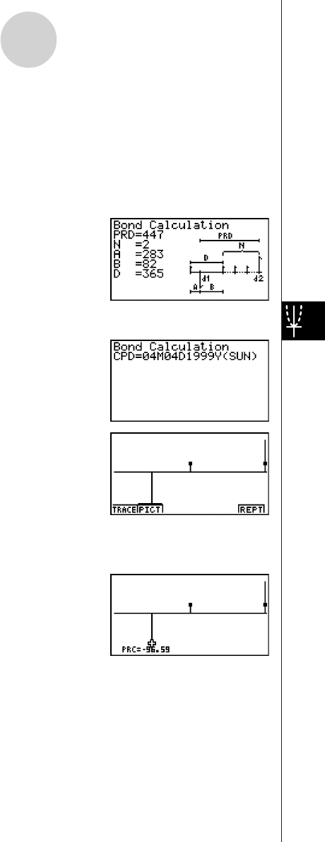
20010101
• An error (Ma ERROR) occurs if parameters are not configured correctly.
Use the following function keys to maneuver between calculation result screens.
•1(REPT) .......Parameter input screen
•5(MEMO) ..... Screen of various bond calculation values*
•6(GRPH) ......Draws Graph
Pressing 5(MEMO) displays various bond calculation values, like those shown here.
*The interest payment date is calculated from d2 when 365 is specified for the Date Mode
item in the SET UP screen.
w~w
6(GRPH)
After drawing a graph, you can press 1(TRACE) to turn on trace and read calculation results
along the graph.
Press i to turn off trace.
Press i again to return to the parameter input screen.
2-10-3
Bonds
20011101
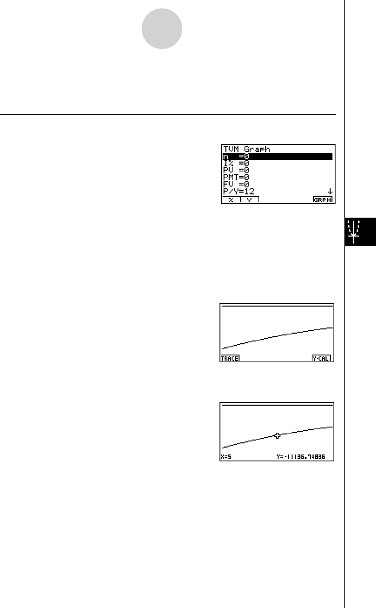
20010101
2-11 TVM Graph
The TVM Graph lets you assign two of the five parameters (n, I%, PV, PMT, FV) to the
x-axis and y-axis of a graph, and plot changes in y as the value of x changes.
Press 5(TVMG) from the Financial 2 screen to display the following input screen for TVM
Graph.
6(g)5(TVMG)
After configuring the parameters, press the function keys noted below to assign parameters
to the x-axis and y-axis.
•1(X) ... Assigns highlighted parameter to the x-axis
•2(Y) ... Assigns highlighted parameter to the y-axis
After making the required settings, draw the graph.
•6(GRPH) ... Draws graph
After drawing a graph, you can press 1(TRACE) to turn on trace and read calculation
results along the graph.
Press i to turn off trace.
2-11-1
TVM Graph
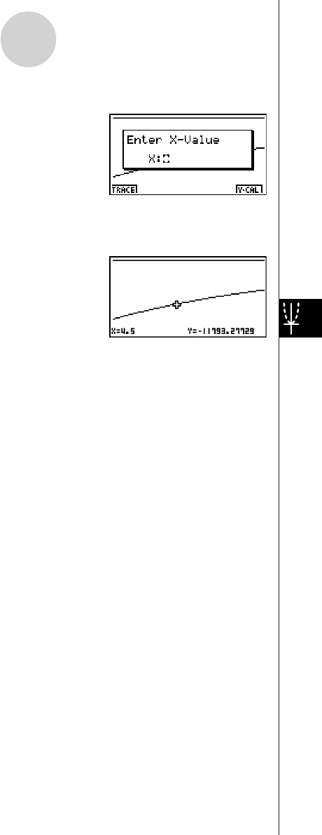
20010101
Pressing 6(Y-CAL) after drawing a graph displays the screen shown below.
Inputting an x-axis value on this screen and pressing w displays the corresponding
y-axis value.
Press i again to return to the parameter input screen.
•Calculation may take some time to perform when you specify I% as the y-axis
parameter.
2-11-2
TVM Graph

Chapter
This chapter explains how to solve the four types of differential
equations listed below.
•Differential equations of the first order
•Linear differential equations of the second order
•Differential equations of the Nth order
•System of first order differential equations
3-1 Using the DIFF EQ Mode
3-2 Differential Equations of the First Order
3-3 Linear Differential Equations of the Second Order
3-4 Differential Equations of the Nth Order
3-5 System of First Order Differential Equations
Differential Equations 3
2001010120011101
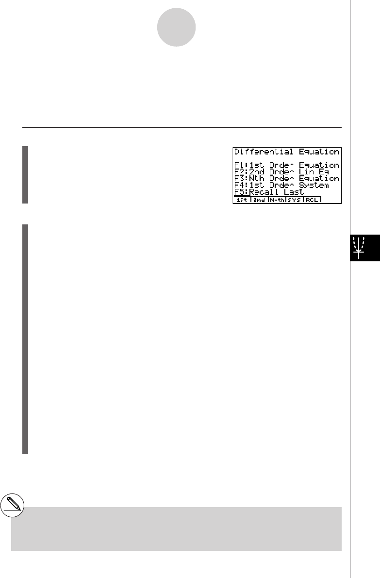
20010101
3-1-1
Using the DIFF EQ Mode
3-1 Using the DIFF EQ Mode
You can solve differential equations numerically and graph the solutions. The general
procedure for solving a differential equation is described below.
Set Up
1. From the Main Menu, enter the DIFF EQ Mode.
Execution
2. Select the differential equation type.
•1(1st) ........ Four types of first order differential equations
•2(2nd) ...... Second order linear differential equations
•3(N-th) ...... Differential equations of the first order through ninth order
•4(SYS) ..... System of the first order differential equations
•5(RCL) ..... Displays a screen for recalling a previous differential equation.
•With 1(1st), you need to make further selections of differential equation type. See
“Differential equations of the first order” for more information.
•With 3(N-th), you also need to specify the order of the differential equation, from 1
to 9.
•With 4(SYS), you also need to specify the number of unknowns, from 1 to 9.
3. Enter the differential equation.
4. Specify the initial values.
5. Press 5(SET) and select b(Param) to display the Parameter screen. Specify the
calculation range. Make the parameter settings you want.
•h ................... Step size for the classical Runge-Kutta method (fourth order)
•Step ............. Number of steps for graphing*1 and storing data in LIST.
•SF................ The number of slope field columns displayed on the screen (0 – 100).
The slope fields can be displayed only for differential equations of the
first order.
*1When graphed for the first time, a function is
always graphed with every step. When the
function is graphed again, however, it is
graphed according to a value of Step. For
example, when Step is set to 2, the function is
graphed with every two steps.
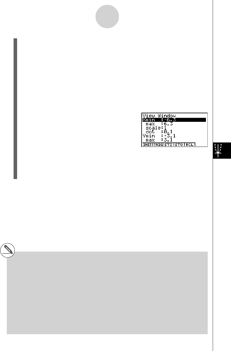
20010101
3-1-2
Using the DIFF EQ Mode
6. Specify variables to graph or to store in LIST.
Press 5(SET) and select c(Output) to display the list setting screen.
x, y, y(1), y(2), ....., y(8) stand for the independent variable, the dependent variable, the
first order derivative, the second order derivative, ....., and the eighth order derivative,
respectively.
1st, 2nd, 3rd, ...., 9th stand for the initial values in order.
To specify a variable to graph, select it using the cursor keys (f, c) and press
1(SEL).
To specify a variable to store in LIST, select it using the cursor keys (f, c) and
press 2(LIST).
7. Press !K(V-Window) to display the V-Window setting screen. Before you solve a
differential equation, you need to make V-Window settings.
Xmin … x-axis minimum value
max … x-axis maximum value
scale … x-axis value spacing
dot … value corresponding to one x-axis dot
Ymin … y-axis minimum value
max … y-axis maximum value
scale … y-axis value spacing
8. Press 6(CALC) to solve the differential equation.
•The calculated result is graphed or stored in the list.
#Only the slope fields are displayed if you do
not input initial values or if you input the wrong
type of initial values.
#An error occurs if you set SF to zero and you
do not input the initial values, or if you input
the initial values inappropriately.
#You are advised to input parentheses and a
multiplication sign between a value and an
expression in order to prevent calculation
errors.
#Do not confuse the - key and the - key.
A syntax error occurs if you use the - key
as the subtraction symbol.
#An error occurs if you input variable y in the
function f(x). Variable x is treated as a
variable. Other variables (A through Ζ, r,
θ
,
excluding X and Y) are treated as constants
and the value currently assigned to that
variable is applied during the calculation.
#An error occurs if you input variable x in the
function g(y). Variable y is treated as a
variable. Other variables (A through Ζ, r,
θ
,
excluding X and Y) are treated as constants
and the value currently assigned to that
variable is applied during the calculation.

20010101
3-2-1
Differential Equations of the First Order
3-2 Differential Equations of the First Order
kSeparable Equation
Description
To solve a separable equation, simply input the equation and specify the initial values.
dy/dx = f(x)g(y)
Set Up
1. From the Main Menu, enter the DIFF EQ Mode.
Execution
2. Press 1(1st) to display the menu of first order differential equations, and then select
b(Separ).
3. Specify f(x) and g(y).
4. Specify the initial value for x0, y0.
5. Press 5(SET)b(Param).
6. Specify the calculation range.
7. Specify the step size for h.
8. Press 5(SET)c(Output).
Select the variable you want to graph, and then select a list for storage of the
calculation results.
9. Make V-Window settings.
10. Press 6(CALC) to solve the differential equation.
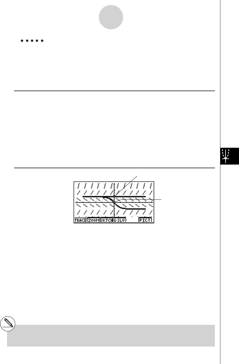
20010101
3-2-2
Differential Equations of the First Order
Example To graph the solutions of the separable equation dy/dx = y2 –1,
x0 = 0, y0 = {0, 1}, –5 <<
<<
< x <<
<<
< 5, h = 0.1.
Use the following V-Window settings.
Xmin = –6.3, Xmax = 6.3, Xscale = 1
Ymin = –3.1, Ymax = 3.1, Yscale = 1 (initial defaults)
Procedure
1m DIFF EQ
21(1st)b(Separ)
3bw
a-(Y)Mc-bw
4aw
!*( { )a,b!/( } )w
55(SET)b(Param)
6-fw
fw
7a.bwi
85(SET)c(Output)4(INIT)i
9!K(V-Window)1(INIT)i
06(CALC)
Result Screen
#To graph a family of solutions, enter a list of
initial conditions.
(x0, y0) = (0,0)
(x0, y0) = (0,1)
20011101

20010101
3-2-3
Differential Equations of the First Order
kLinear Equation
To solve a linear equation, simply input the equation and specify initial values.
dy/dx + f(x)y = g(x)
Set Up
1. From the Main Menu, enter the DIFF EQ Mode.
Execution
2. Press 1(1st) to display the menu of differential equations of the first order, and then
select c(Linear).
3. Specify f(x) and g(x).
4. Specify the initial value for x0, y0.
5. Press 5(SET)b(Param).
6. Specify the calculation range.
7. Specify the step size for h.
8. Press 5(SET)c(Output).
Select the variable you want to graph, and then select a list for storage of the
calculation results.
9. Make V-Window settings.
10. Press 6(CALC) to solve the differential equation.
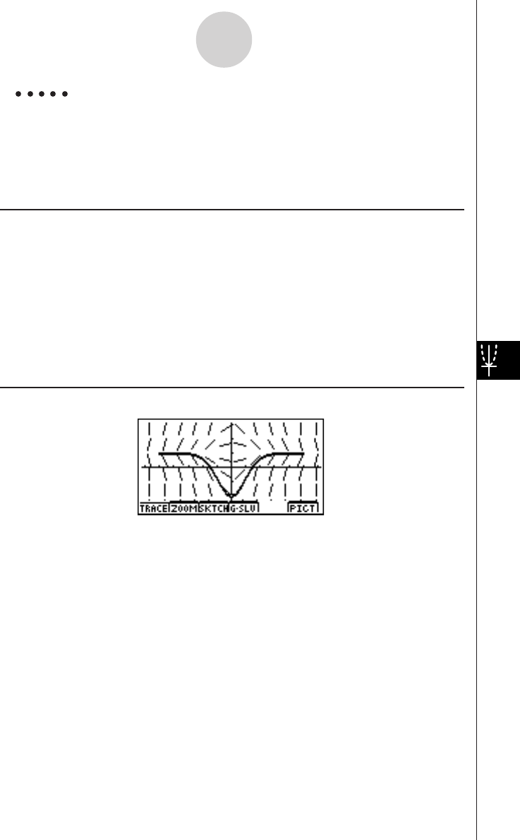
20010101
3-2-4
Differential Equations of the First Order
Example To graph the solution of the linear equation dy/dx + xy = x,
x0 = 0, y0 = –2, –5 <<
<<
< x <<
<<
< 5, h = 0.1.
Use the following V-Window settings.
Xmin = –6.3, Xmax = 6.3, Xscale = 1
Ymin = –3.1, Ymax = 3.1, Yscale = 1 (initial defaults)
Procedure
1m DIFF EQ
21(1st)c(Linear)
3vw
vw
4aw
-cw
55(SET)b(Param)
6-fw
fw
7a.bwi
85(SET)c(Output)4(INIT)i
9!K(V-Window)1(INIT)i
06(CALC)
Result Screen
20011101

20010101
3-2-5
Differential Equations of the First Order
kBernoulli equation
To solve a Bernoulli equation, simply input the equation and specify the power of y and the
initial values.
dy/dx + f(x)y = g(x)y
n
Set Up
1. From the Main Menu, enter the DIFF EQ Mode.
Execution
2. Press 1(1st) to display the menu of differential equations of the first order, and then
select d(Bern).
3. Specify f(x), g(x), and n.
4. Specify the initial value for x0, y0.
5. Press 5(SET)b(Param).
6. Specify the calculation range.
7. Specify the step size for h.
8. Press 5(SET)c(Output).
Select the variable you want to graph, and then select a list for storage of the
calculation results.
9. Make V-Window settings.
10. Press 6(CALC) to solve the differential equation.
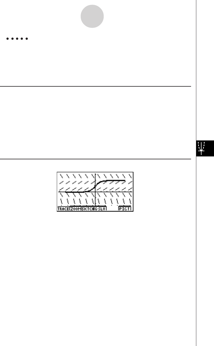
20010101
3-2-6
Differential Equations of the First Order
Example To graph the solution of the Bernoulli equation dy/dx – 2y = –y2,
x0 = 0, y0 = 1, –5 <<
<<
< x <<
<<
< 5, h = 0.1.
Use the following V-Window settings.
Xmin = –6.3, Xmax = 6.3, Xscale = 1
Ymin = –3.1, Ymax = 3.1, Yscale = 1 (initial defaults)
Procedure
1m DIFF EQ
21(1st)d(Bern)
3-cw
-bw
cw
4aw
bw
55(SET)b(Param)
6-fw
fw
7a.bwi
85(SET)c(Output)4(INIT)i
9!K(V-Window)1(INIT)i
06(CALC)
Result Screen
20011101

20010101
3-2-7
Differential Equations of the First Order
kOthers
To solve a general differential equation of the first order, simply input the equation and
specify the initial values. Use the same procedures as those described above for typical
differential equations of the first order.
dy/dx = f(x, y)
Set Up
1. From the Main Menu, enter the DIFF EQ Mode.
Execution
2. Press 1(1st) to display the menu of differential equations of the first order, and then
select e(Others).
3. Specify f(x, y).
4. Specify the initial value for x0, y0.
5. Press 5(SET)b(Param).
6. Specify the calculation range.
7. Specify the step size for h.
8. Press 5(SET)c(Output).
Select the variable you want to graph, and then select a list for storage of the
calculation results.
9. Make V-Window settings.
10. Press 6(CALC) to solve the differential equation.
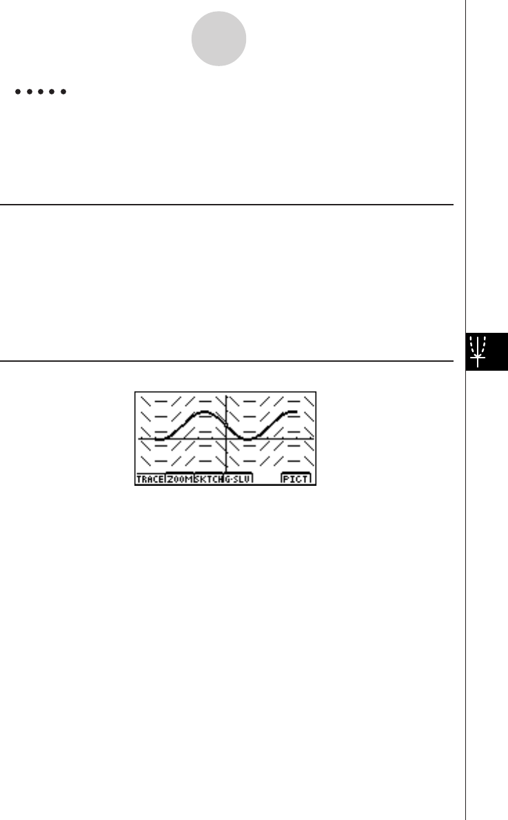
20010101
3-2-8
Differential Equations of the First Order
Example To graph the solution of the first order differential equation
dy/dx = –cos x, x0 = 0, y0 = 1, –5 <<
<<
< x <<
<<
< 5, h = 0.1.
Use the following V-Window settings.
Xmin = –6.3, Xmax = 6.3, Xscale = 1
Ymin = –3.1, Ymax = 3.1, Yscale = 1 (initial defaults)
Procedure
1m DIFF EQ
21(1st)e(Others)
3-cvw
4aw
bw
55(SET)b(Param)
6-fw
fw
7a.bwi
85(SET)c(Output)4(INIT)i
9!K(V-Window)1(INIT)i
06(CALC)
Result Screen
20011101

20010101
3-3-1
Linear Differential Equations of the Second Order
3-3 Linear Differential Equations of the Second
Order
Description
To solve a linear differential equation of the second order, simply input the equation and
specify the initial values. Slope fields are not displayed for a linear differential equation of the
second order.
y앨 + f(x) y쎾 + g(x)y = h(x)
Set Up
1. From the Main Menu, enter the DIFF EQ Mode.
Execution
2. Press 2(2nd).
3. Specify f(x), g(x), and h(x).
4. Specify the initial value for x0, y0, y쎾0.
5. Press 5(SET)b(Param).
6. Specify the calculation range.
7. Specify the step size for h.
8. Press 5(SET)c(Output).
Select the variable you want to graph, and then select a list for storage of the
calculation results.
9. Make V-Window settings.
10. Press 6(CALC) to solve the differential equation.
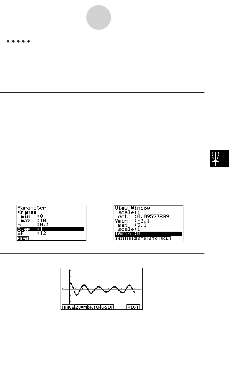
20010101
3-3-2
Linear Differential Equations of the Second Order
Example To graph the solution of the linear differential equation of the second
order y앨 + 9y = sin 3x, x0 = 0, y0= 1, y쎾0 = 1, 0 <<
<<
< x <<
<<
< 10, h = 0.1.
Use the following V-Window settings.
Xmin = –1, Xmax = 11, Xscale = 1
Ymin = –3.1, Ymax = 3.1, Yscale = 1
Procedure
1m DIFF EQ
22(2nd)
3aw
jw
sdvw
4aw
bw
bw
55(SET)b(Param)
6aw
baw
7a.bw*1i
85(SET)c(Output)4(INIT)i
9!K(V-Window)
-bw
bbw
bwc
-d.bw
d.bw
bw*2i
06(CALC)
Result Screen
*1*2

20010101
3-4-1
Differential Equations of the Nth Order
3-4 Differential Equations of the Nth Order
You can solve differential equations of the first through ninth order. The number of initial
values required to solve the differential equation depends on its order.
•Enter dependent variables y, y쎾, y앨, y(3), ....., y(9) as follows.
y.................... a-(Y)
y쎾................... 3(y(n))b(Y1)
y앨................... 3(y(n))c(Y2)
y(3)(=y쎾앨 )......... 3(y(n))d(Y3)
y(8) ................. 3(y(n))i(Y8)
y(9) ................. 3(y(n))j(Y9)
kDifferential Equation of the Fourth Order
The following example shows how to solve a differential equation of the fourth order.
y(4) = f(x, y, ...... , y(3))
Set Up
1. From the Main Menu, enter the DIFF EQ Mode.
Execution
2. Press 3(N-th).
3. Press 3(n)e to select a differential equation of the fourth order.
4. Specify y(4).
5. Specify the initial value for x0, y0, y’0, y”0, and y(3)0.
6. Press 5(SET)b(Param).
7. Specify the calculation range.
8. Specify the step size for h.
9. Press 5(SET)c(Output).
Select the variable you want to graph, and then select a list for storage of the
calculation results.
10. Make V-Window settings.
11.Press 6(CALC) to solve the differential equation.
…
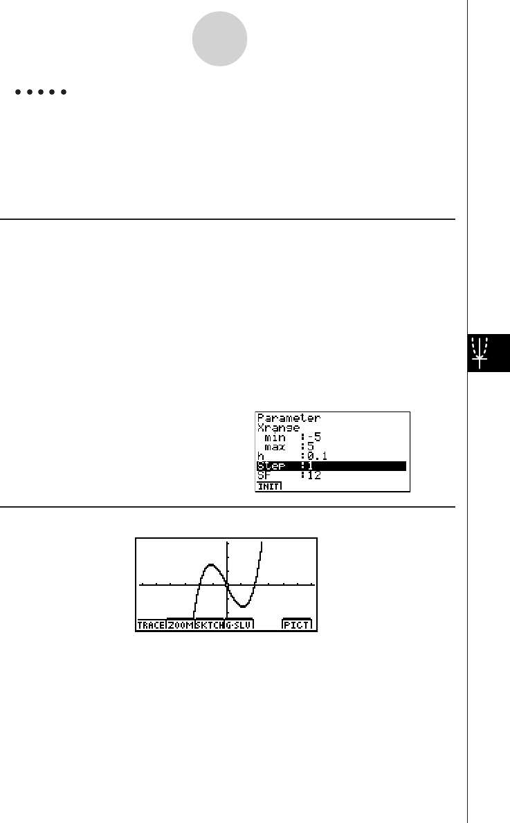
20010101
3-4-2
Differential Equations of the Nth Order
Example To graph the solution of the differential equation of the fourth order
below
y(4) = 0, x0 = 0, y0 = 0, y쎾0 = –2, y앨0 = 0, y(3)0 = 3, –5 <<
<<
< x <<
<<
< 5, h = 0.1.
Use the following V-Window settings.
Xmin = –6.3, Xmax = 6.3, Xscale = 1
Ymin = –3.1, Ymax = 3.1, Yscale = 1 (initial defaults)
Procedure
65(SET)b(Param)
7-fw
fw
8a.bw*1i
95(SET)c(Output)4(INIT)i
0!K(V-Window)1(INIT)i
!6(CALC)
1m DIFF EQ
23(N-th)
33(n)ew
4aw
5aw
aw
-cw
aw
dw
Result Screen
*1
20011101

20010101
3-4-3
Differential Equations of the Nth Order
kConverting a High-order Differential Equation to a System of First Order
Differential Equations
You can convert a single N-th order differential equation to a system of n first order
differential equations.
Set Up
1. From the Main Menu, enter the DIFF EQ Mode.
Execution (N = 3)
2. Press 3(N-th).
3. Press 3(n)d to select a differential equation of the third order.
4. Perform substitutions as follows.
y쎾→Y1 (3(y(n))b)
y앨→Y2 (3(y(n))c)
5. Specify the initial value for x0, y0, y쎾0, and y앨0.
6. Press 2(→SYS).
7. Press w(Yes).
•The entered differential equation is converted to a system of three first order
differential equations. Initial values are also converted accordingly.
20011101
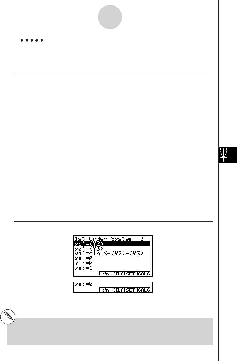
20010101
Example Express the differential equation below as a set of first order
differential equations.
y(3) = sinx – y쎾 – y앨, x0 = 0, y0 = 0, y쎾0 = 1, y앨0 = 0.
Procedure
1m DIFF EQ
23(N-th)
33(n)dw
4sv-3(y(n)) b-3(y(n))cw
5aw
aw
bw
aw
62(→SYS)
7w(Yes)
The differential equation is converted to a set of first order differential equations as shown
below.
(y1)쎾 = dy/dx = (y2)
(y2)쎾 = d2y/dx2 = (y3)
(y3)쎾 = sin x – (y2) – (y3).
Initial values are also converted to (x0 = 0), ((y1)0 = 0), ((y2)0 = 1), and ((y3)0 = 0)).
#On the system of first order differential
equations screen, dependent valuables are
expressed as follows.
(y1)→(Y1)
(y2)→(Y2)
(y3)→(Y3)
Result Screen
3-4-4
Differential Equations of the Nth Order

20010101
3-5 System of First Order Differential Equations
A system of first order differential equations, for example, has dependent variables (y1), (y2),
....., and (y9), and independent variable x. The example below shows a system of first order
differential equations.
(y1)쎾= (y2)
(y2)쎾= – (y1) + sin x
Set Up
1. From the Main Menu, enter the DIFF EQ Mode.
Execution
2. Press 4(SYS).
3. Enter the number of unknowns.
4. Enter the expression as shown below.
(y1)→Y1 (3(yn)b)
(y2)→Y2 (3(yn)c)
(y9)→Y9 (3(yn)j)
5. Specify the initial value for x0, (y1)0, (y2)0 and so on, if necessary.
6. Press 5(SET)b(Param).
7. Specify the calculation range.
8. Specify the step size for h.
9. Press 5(SET)c(Output).
Select the variable you want to graph, and then select a list for storage of the
calculation results.
10. Make V-Window settings.
11.Press 6(CALC) to solve the system of first order equations for y1, y2, and so on.
…
3-5-1
System of First Order Differential Equations
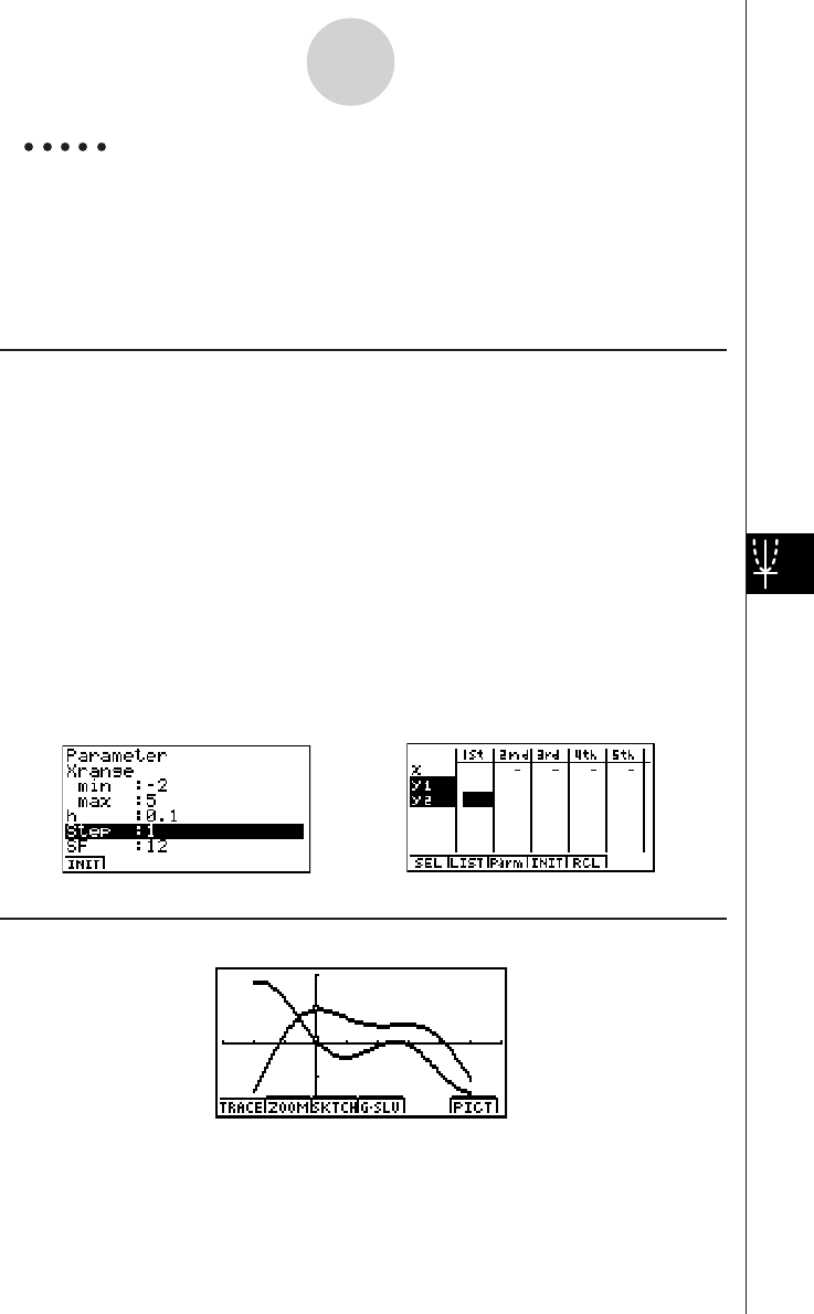
20010101
Example 1 To graph the solution of first order differential equations with two
unknowns below.
(y1)쎾= (y2), (y2)쎾 = – (y1) + sin x, x0 = 0, (y1)0 = 1, (y2)0 = 0.1, –2 < x < 5, h = 0.1.
Use the following V-Window settings.
Xmin = –3, Xmax = 6, Xscale = 1
Ymin = –2, Ymax = 2, Yscale = 1
Procedure
1m DIFF EQ
24(SYS)
32(2)
43(yn)cw
-3(yn)b+svw
5aw
bw
a.bw
65(SET)b(Param)
7-cw
fw
8a.bw*1i
95(SET)c(Output)4(INIT)
cc1(SEL)
(Select (y1) and (y2) to graph)*2
i
0!K(V-Window)
-dw
gw
bwc
-cw
cw
bwi
!6(CALC)
Result Screen
3-5-2
System of First Order Differential Equations
*1*2
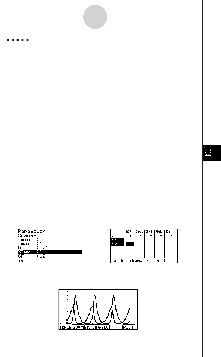
20010101
Example 2 To graph the solution of the system of first order differential equations
below.
(y1)쎾 = (2 – (y2)) (y1)
(y2)쎾 = (2 (y1) – 3) (y2)
x0 = 0, (y1)0 = 1, (y2)0 = 1/4, 0 <<
<<
< x <<
<<
< 10, h = 0.1.
Use the following V-Window settings.
Xmin = –1, Xmax = 11, Xscale = 1
Ymin = –1, Ymax = 8, Yscale = 1
Procedure
1m DIFF EQ
24(SYS)
32(2)
4(c-3(yn)c)*3(yn)
bw
(c*3(yn)b-d
)*3(yn)cw
5aw
bw
b/ew
65(SET)b(Param)
7aw
baw
8a.bw*1i
95(SET)c(Output)4(INIT)
cc1(SEL)
(Select (y1) and (y2) to graph.)
ff2(LIST)bw(Select LIST1
to store the values for x in LIST1)
c2(LIST)cw (Select LIST2 to
store the values for (y1) in LIST2)
c2(LIST)dw (Select LIST3 to
store the values for (y2) in LIST3)*2
i
0!K(V-Window)
-bwbbwbwc
-bwiwbwi
!6(CALC)
3-5-3
System of First Order Differential Equations
*1*2
Result Screen
(y2)
(y1)
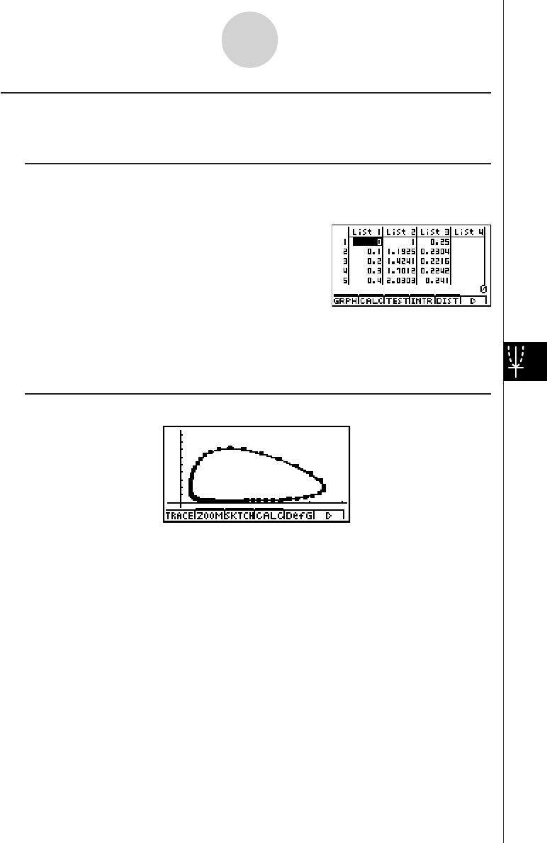
20010101
kFurther Analysis
To further analyze the result, we can graph the relation between (y1) and (y2).
Procedure
1m STAT
2List 1, List 2, and List 3 contain values
for x, (y1), and ( y2), respectively.
31(GRPH)f(Set)
41(GPH1)
5c2(xy)
6c1(LIST)cw (XLIST = LIST2: (y1))
7c1(LIST)dw (YLIST = LIST3: (y2))
i
81(GRPH)b(S-Gph1)
Result Screen
3-5-4
System of First Order Differential Equations
(y1)
(y2)

20010101
Important!
•This calculator may abort calculation part way through when an overflow occurs part way
through the calculation when calculated solutions cause the solution curve to extend into
a discontinuous region, when a calculated value is clearly false, etc.
•The following steps are recommended when the calculator aborts a calculation as
described above.
1. If you are able to determine beforehand the point where the solution curve overflows,
stop the calculation before the point is reached.
2. If you are able to determine beforehand the point where the solution curve extends into
a discontinuous region, stop the calculation before the point is reached.
3. In other cases, reduce the size of the calculation range and the value of h (step size)
and try again.
4. When you need to perform a calculation using a very wide calculation range, store
intermediate results in a list and perform a new calculation starting from step 3 using
the stored results as initial values. You can repeat this step multiple times, if necessary.
kSET UP Items
G-Mem {G-Mem 20}/{1 – 20} ...... Specifies a memory location {G-Mem No.} for storage of
the latest graph functions.
Note the following regarding SET UP screen settings whenever using the DIFF EQ Mode.
The DIFF EQ Mode temporarily stores data into Graph Memory whenever a differential
equation calculation is performed. Before the calculation, DIFF EQ stores the latest graph
functions into the currently specified Graph Memory (G-Mem) location. After the calculation,
it recalls the graph functions from the specified G-Mem location, without deleting the G-Mem
data. Because of this, you should specify the G-Mem location (number) where the DIFF EQ
Mode stores the graph functions.
3-5-5
System of First Order Differential Equations

Chapter
4-1 E-CON Overview
4-2 EA-100 Setup
4-3 Setup Memory
4-4 Program Converter
4-5 Starting a Sampling Operation
E-CON
4
All of the explanations provided here assume that you are already familiar
with the operating precautions, terminology, and operational procedures of
the calculator and the EA-100.
20010101
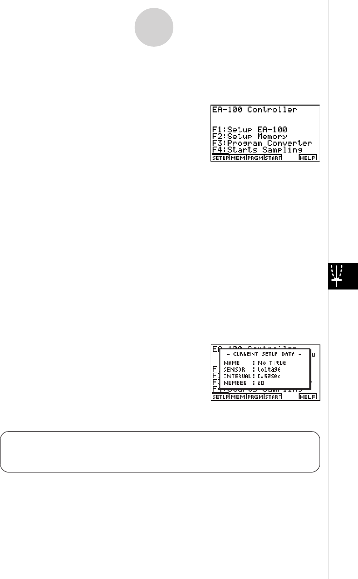
20010101
4-1-1
E-CON Overview
4-1 E-CON Overview
•From the Main Menu, select E-CON to enter the E-CON Mode.
•The E-CON provides the functions listed below for simple and more efficient data
sampling using the CASIO EA-100.
•1(SETUP) ... Displays a screen for setting up the EA-100.
•2(MEM) ....... Displays a screen for saving EA-100 setup data under a file name.
•3(PRGM) ..... Performs program conversion.
•This function converts EA-100 setup data created by E-CON to a
program.
•It can also be used to convert data to a program that can be run on
a CFX-9850 Series/fx-7400 Series calculator, and to transfer the
data to the calculator.
•4(START) .... Starts data collection.
•6(HELP) ...... Displays E-CON help.
•Pressing the K key (Setup Preview) or a cursor key while the E-CON main menu is on
the screen displays a preview dialog box that shows the contents of the setup in the
current setup memory area.
To close the preview dialog box, press i.
About online help
Pressing the 6(HELP) key displays online help about the E-CON Mode.

20010101
4-2 EA-100 Setup
You can use the E-CON Mode to set up the EA-100 for sampling and then start sampling
immediately or save the setup in calculator memory. You can use either of the following two
methods to set up the EA-100.
Setup Wizard: With this method, you set up the EA-100 simply by replying to
questions as they appear.
Advanced Setup: Advanced setup gives you control over a variety of sampling
parameters, which means you can set up the EA-100 for exactly the
type of sampling you want.
kUsing Setup Wizard to Create an EA-100 Setup
With Setup Wizard, you set up the EA-100 simply by replying to questions as they appear.
uSetup Wizard parameters
Setup Wizard lets you make changes to the following three EA-100 basic sampling
parameters using an interactive wizard format.
•Sensor (Select Sensor)
Specify a CASIO or VERNIER*1 sensor from a menu of choices.
•Sampling Interval (Sampling Time)
When you have Photogate specified as the sensor type, you can specify the sampling
timing (Gate Status) and sampling time recording method (Record Time) with this
parameter.
•Number of Samples (Number of Samples)
You can specify a value from 1 to 255.
Note the following limitations that apply to a setup made using Setup Wizard.
•You can use Setup Wizard only when the EA-100 sampling channel is CH1 or SONIC.
•The trigger for a Setup Wizard setup is always the w key.
•Sampling results are always stored in List 1 (for the sampling time) and List 2 (for
sample values).
4-2-1
EA-100 Setup
*1Vernier Software & Technology
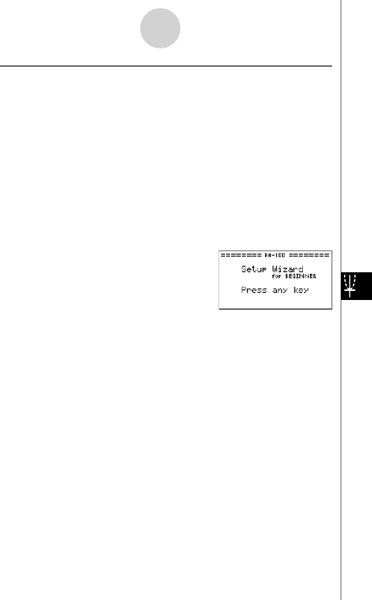
20010101
uTo create an EA-100 setup using Setup Wizard
Before getting started...
•Before starting the procedure below, make sure you first decide if you want to start
sampling immediately using the setup you create with Setup Wizard, or if you want to
store the setup for later sampling.
•See sections 4-3, 4-4, and 4-5 of this manual for information about procedures required to
start sampling and to store a setup. We recommend that you read through the entire
procedure first, referencing the other sections and pages as noted, before actually trying
to perform it.
•To terminate Setup Wizard part way through and cancel the setup, press !i(QUIT).
1. Display the E-CON main menu.
2. Press 1(SETUP). This displays the “Setup EA-100” sub-menu.
3. Press b(Wizard). This displays the Setup Wizard initial screen.
4-2-2
EA-100 Setup
4. Press any key to start Setup Wizard and display the sensor specification screen.
•Press 1 to specify a CASIO sensor, or 2 to specify a VERNIER sensor. From the
menu of supported sensors that appears, select the one you want.
5. The screen that appears after you select a sensor in step 4 depends on whether or not
you specified “Photogate” as the sensor.
• If you did not specify “Photogate,” a screen for setting the sampling interval appears after
step 4.
1. Use the number keys to input the sampling interval.
•Inputting a value in the range of 0.52 to 300 enables real-time sampling. Inputting
a value outside this range enables non-real-time sampling.
2. Press w.
•If you specified “Photogate” as the sensor, a screen for setting the sampling timing
appears after step 4.
1. Press either 1(Open) or 2(Close) to specify the sampling timing. Pressing either
key advances to a screen for setting the time recording method.
•See online help (GATE TRIGGER STATUS HELP) for details about the Open and
Close settings.
2. Press 1(Abs) or 2(Rel) to specify the sampling time recording method.

20010101
6. After you complete step 5, a screen for setting the number of samples appears on the
display.
•Use the number keys to input the number of samples, and then press w.
7. After you complete step 6, a screen like the one shown below appears on the display.
•Press one of the function keys described below to specify what you want to do with the
setup you have created with the above steps.
•1(YES) ........ Starts sampling using the setup (page 4-5-1).
•2(NO) .......... Returns to the E-CON main menu (page 4-1-1).
•3(SAVE) ...... Saves the setup (page 4-3-1).
•4(PRGM) ..... Converts the setup to a program (page 4-4-1).
•Pressing 2(NO) in step 7 returns to the E-CON main menu and stores the setup in the
E-CON Mode’s current setup memory area. You can use the following function key
operations from the E-CON main menu to manipulate the contents of the current setup
memory area.
•2(MEM), then 2(SAVE)
....................... Saves the current setup memory area setup (page 4-3-1).
•3(PRGM) ..... Converts the setup in the current setup memory area to a program
(page 4-4-1).
•4(START) .... Starts sampling using the setup in the current setup memory area
(page 4-5-1).
•Pressing 1(SETUP) and then c(Advan) displays an Advanced Setup screen for more
detailed control over the parameters that make up the setup in the current setup memory
area. See “Creating an EA-100 Setup Using Advanced Setup” for more information
about changing advanced setup parameters.
4-2-3
EA-100 Setup
20011101
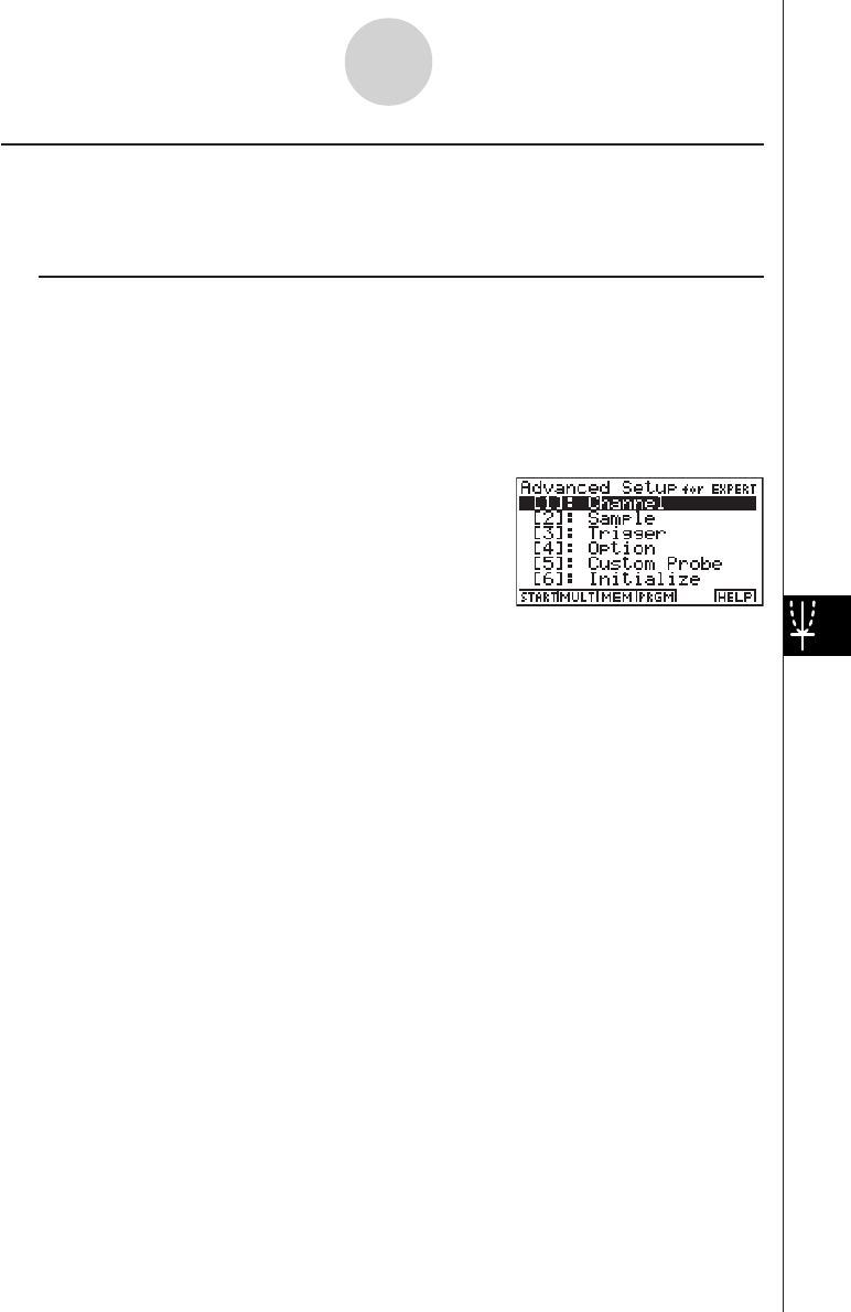
20010101
kCreating an EA-100 Setup Using Advanced Setup
Advanced Setup provides you with total control over a number of parameters that you can
adjust to create the EA-100 setup that suits your particular needs.
uTo create an EA-100 setup using Advanced Setup
The following procedure describes the general steps for using Advanced Setup. Refer to the
pages as noted for more information.
1. Display the E-CON main menu.
2. Press 1(SETUP). This displays the “Setup EA-100” sub-menu.
3. Press c(Advan). This displays the Advanced Setup menu.
4. If you want to configure a custom probe at this point, press f(Custom Probe). Next,
follow the steps under “To configure a custom probe starting from the Advanced Setup
menu” on page 4-2-12.
•You can also configure a custom probe during the procedure under “To change Channel
parameter settings” on page 4-2-6.
•Custom probe configurations you have stored in memory can be selected using Channel
in step 5, below.
5. Use the Advanced Setup function keys described below to set other parameters.
•b(Channel) .... Displays a screen for setting the following parameters: sampling
channel, sensor, sensor configuration, and storage location for
sample data (page 4-2-5).
•c(Sample) ..... Displays a screen for setting the following parameters: real-time
settings, sampling interval, number of samples, measurement time
recording method, and storage location for measurement time
records (page 4-2-7).
•d(Trigger) ...... Displays a screen for setting sampling start (trigger) conditions
(page 4-2-8).
•e(Option) ....... Displays a screen for making View Window settings, real-time
settings (channel for real-time sampling), and filter settings (page
4-2-10).
4-2-4
EA-100 Setup
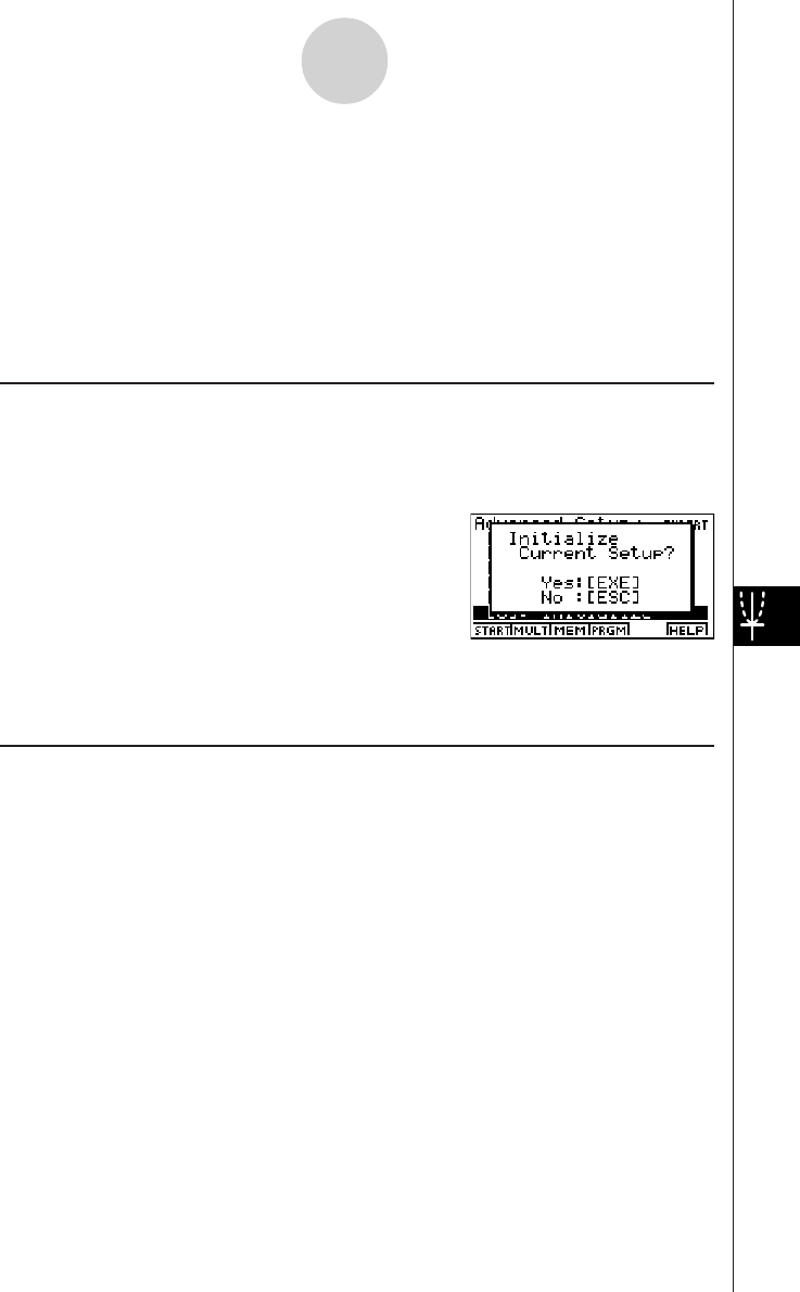
20010101
•You can return the settings on the above setup screens (b through e) using the
procedure described under “To return setup parameters to their initial defaults”.
6. After you create a setup, you can use the function key operations described below to start
sampling or perform other operations.
•1(START) .... Starts sampling using the setup (page 4-5-1).
•2(MULT) ...... Starts MULTIMETER Mode sampling using the setup (page 4-2-14).
•3(MEM) ....... Saves the setup (page 4-3-1).
•4(PRGM) ..... Converts the setup to a program (page 4-4-1).
uTo return setup parameters to their initial defaults
Perform the following procedure when you want to return the parameters of the setup in the
current setup memory area to their initial defaults.
1. While the Advanced Setup menu is on the display, press g(Initialize).
2. In response to the confirmation message that appears, press w to initialize the setup.
•To clear the confirmation message without initializing the setup, press i.
uAdvanced setup parameters
This section provides detailed information about the parameters you can change in step 5 of
the procedure under “To create an EA-100 setup using Advanced Setup” on page 4-2-4.
Channel
Selecting this parameter displays a screen where you can specify the EA-100 channel to be
used for sampling, the type of sensor used for each channel, and the storage location for
saving sample data.
4-2-5
EA-100 Setup
20011101
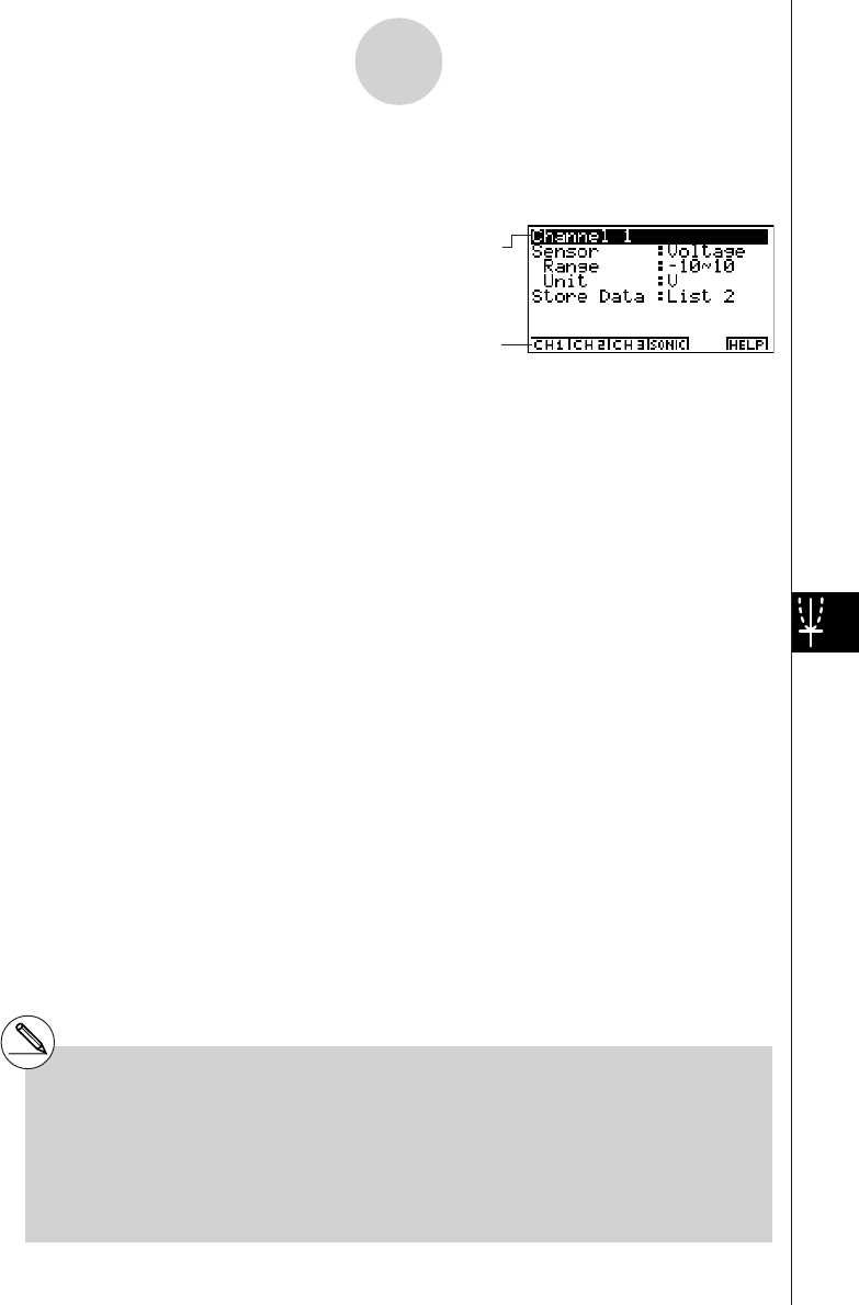
20010101
• To change Channel parameter settings
1. While the Advanced Setup menu is on the display, press b(Channel).
•This displays the Channel parameter setting screen.
4-2-6
EA-100 Setup
#If the list you specify for the Sample Data
Storage Location (Store Data) in step 2 is
already being used, data is overwritten
according to the priority sequence shown
below.
1. (Highest) SONIC 4. CH1
2. CH3 5. (Lowest) Record Time
3. CH2
Example: Specifying the same list number for
CH3 sample data and SONIC
sample data causes the CH3 data to
be overwritten by the SONIC data.
2. Use the function key operations described below to change Channel parameter settings.
(1) Selected Channel
•1(CH1) ........ Channel 1
•2(CH2) ........ Channel 2
•3(CH3) ........ Channel 3
•4(SONIC) .... Sonic channel
(2) Selected Sensor (Sensor)
•1(CASIO) .... CASIO sensor
•2(VERN) ..... VERNIER sensor
•3(CSTM) ..... Custom probe
•4(None) ....... No sensor
(3) Sample Data Storage Location (Store Data)
•1(LIST) ........ Displays a dialog box for specifying the list for storage of
measurement data. Specify a list number from 1 to 20.
•To change the setting of an item, first use the f and c cursor keys to move the
highlighting to the item. Next, use the function keys to select the setting you want. Note
that the Channel parameter settings you make affect the Selected Channel only. You
need to make separate settings for each channel you plan to use for sampling.
•Specifying a sensor causes its sampling range (Range) and measurement unit (Unit) to
appear on the display.
3. After all the settings are the way you want, press w to return to the Advanced Setup
menu.
Current setting of selected item
Selected item
20011101
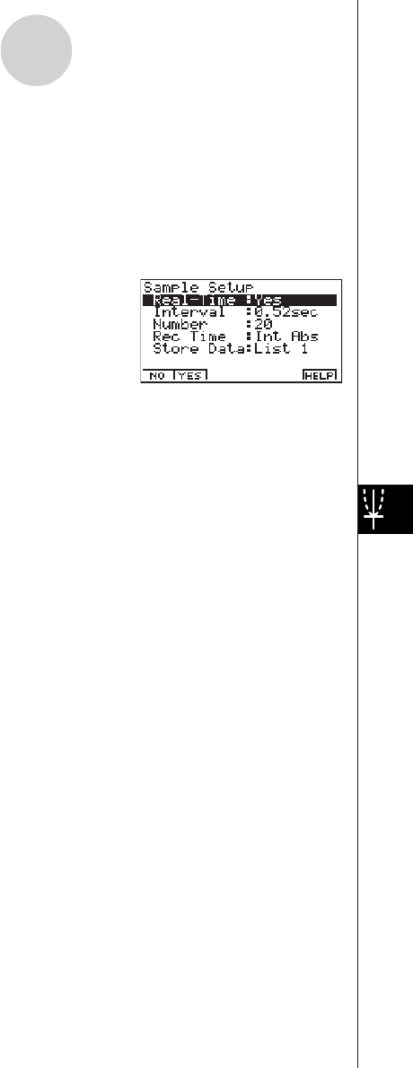
20010101
Sample
Selecting this parameter displays a screen for making real-time settings, and for specifying
the sampling interval, number of samples, measurement time recording method, and storage
location for measurement time records.
• To change Sample Setup settings
1. While the Advanced Setup menu is on the display, press c(Sample).
•This displays the Sample Setup screen.
2. Use the function key operations described below to change Sample Setup settings.
•To change the setting of an item, first use the f and c cursor keys to move the
highlighting to the item. Next, use the function keys to select the setting you want.
(1) Real-time Settings (Real-Time)
•1(NO) .......... Disables real-time sampling.
•2(YES) ........ Enables real-time sampling.
(2) Sampling Interval (Interval)
•1(TIMER) .... Displays a dialog box for specifying a timer value, and enables fixed-
interval sampling.
•2(KEY) ........ Starts sampling operation that uses the EA-100 [TRIGGER] key. The
[TRIGGER] key must be pressed the number of times specified for
the number of samples.
•3(GATE) ...... Starts sampling in accordance with the Photogate Gate Status trigger
timing. Press 1, 2, or 3 to specify the channel of the Photogate
sensor. Photogate is assigned to the sensor of the specified channel.
(3) Number of Samples (Number)
•1(NUM) ....... Displays a dialog box for specifying the number of samples by
inputting a value from 1 to 255.
4-2-7
EA-100 Setup
20011101

20010101
(4) Measurement Time Recording Method (Rec Time)
•1(None) ....... No time recorded.
•2(Abs) ......... Absolute time in seconds from start of sampling
•3(Rel) .......... Relative time (interval between samples) in seconds
•4(Int A) ........ Absolute time calculated from sampling interval and number of
samples
•5(Int R) ........ Relative time calculated from sampling interval and number of
samples
(5) Sample Data Storage Location (Store Data)
•1(LIST) ........ Displays a dialog box for specifying the list (1 to 20) for storing
sample data.
3. After all the settings are the way you want, press w to return to the Advanced Setup
menu.
Trigger
Use the Trigger Setup screen to specify the following measurement start (trigger) conditions:
trigger source, trigger threshold, trigger edge.
• To change Trigger Setup settings
1. While the Advanced Setup menu is on the display, press d(Trigger).
•This displays the Trigger Setup screen.
4-2-8
EA-100 Setup
Current setting of selected item
Selected item

20010101
2. Use the function key operations described below to change Trigger Setup settings.
•To change the setting of an item, first use the f and c cursor keys to move the
highlighting to the item. Next, use the function keys to select the setting you want.
(1) Trigger Source (Source)
•1(KEY)
b([EXE]) .......... Calculator w key press starts sampling.
c(TRIGER) ...... EA-100 [TRIGGER] key press starts sampling.
•2(CH1) ........ Channel 1
•3(CH2) ........ Channel 2
•4(CH3) ........ Channel 3
•Specifying CH1, CH2, or CH3 as the trigger source displays the specified channel’s
sensor name, trigger threshold initial value, measurement unit, and trigger edge initial
value.
(2) Trigger Threshold (Threshold)
•1(EDIT) ....... Displays a dialog box for inputting the trigger threshold. This option is
available only when CH1, CH2, or CH3 is specified as the trigger
source.
(3) Trigger Edge (Edge)
•1(Rise) ........ Rising edge triggers sampling
•2(Fall) .......... Falling edge triggers sampling
3. After all the settings are the way you want, press w to return to the Advanced Setup
menu.
4-2-9
EA-100 Setup
20011101
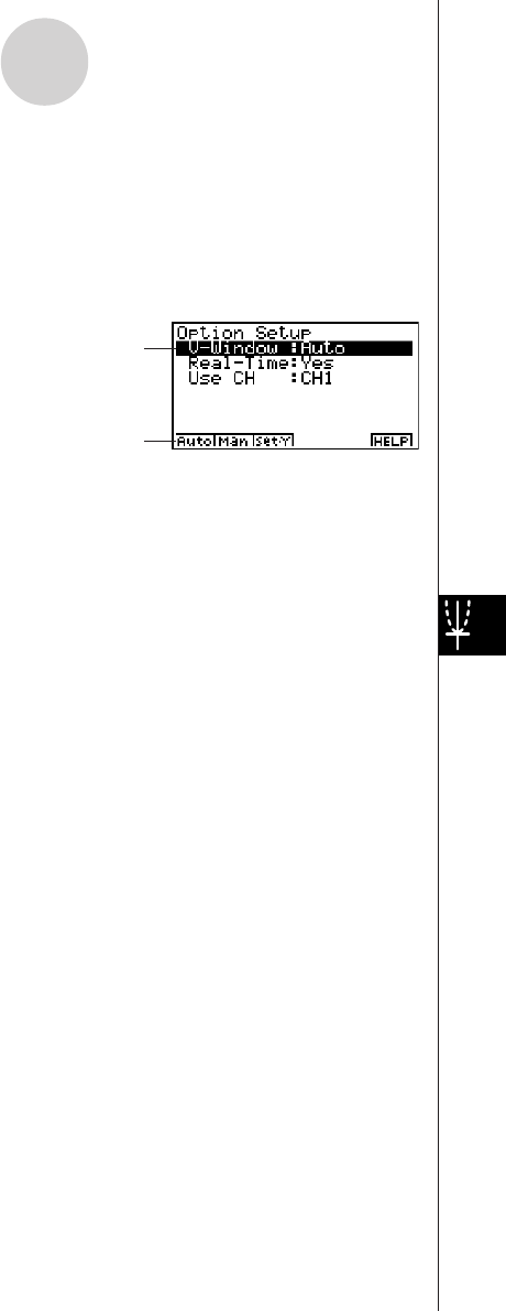
20010101
Option
Use the Option Setup screen to make View Window settings, to specify the channel for real-
time sampling, and to make filter settings.
• To change Option Setup settings
1. While the Advanced Setup menu is on the display, press e(Option).
•This displays the Option Setup screen.
2. Use the function key operations described below to change Option Setup settings.
•To change the setting of an item, first use the f and c cursor keys to move the
highlighting to the item. Next, use the function keys to select the setting you want.
(1) View Window Settings (V-Window)
•1(Auto) ........ Makes View Window settings automatically.
•2(Man) ........ Enables manual View Window settings.
•3(Set•Y) ...... Displays screens for specifying the Y-axis (sample data) minimum
value (Ymin) and maximum value (Ymax).
(2) Real-time Settings (Real-Time)
•1(NO) .......... Disables real-time sampling.
•2(YES) ........ Enables real-time sampling.
•Note that this item is linked with the Real-Time item of the Sample Setup on page
4-2-7.
4-2-10
EA-100 Setup
Current setting of selected item
Selected item

20010101
(3) Real-time Sampling Channel (Use CH)
•1(CH1) ........ Channel 1
•2(CH2) ........ Channel 2
•3(CH3) ........ Channel 3
•4(SONIC) .... Sonic channel
•Note that the above options appear only when real-time sampling is turned on (by
pressing 1(YES) for the Real-Time item).
(4) Filter Settings (Filter)
•1(None) ....... No setting
•2(S-G) ......... S-G Smoothing
b(5-p): 5-point c(9-p): 9-point
d(17-p): 17-point e(25-p): 25-point
•3(MED) ....... Median Filter
b(3-p): 3-point c(5-p): 5-point
•Note that the above options appear only when real-time sampling is turned off (by
pressing 2(NO) for the Real-Time item).
3. After all the settings are the way you want, press w to return to the Advanced Setup
menu.
uTo configure a custom probe
You can use the procedures in this section to configure a custom probe*1 for use with the
EA-100.
Creating a New Custom Probe Configuration
To configure a custom probe, you must input values for the constants of the fixed linear
transformation formula (ax + b). The required constants are slope (a) and intercept (b).
x in the above expression (ax + b) is the sampled voltage value (sampling range: 0 to 5
volts).
You can use either of the two following procedures to create a new custom probe
configuration while creating an EA-100 setup using Advanced Setup.
4-2-11
EA-100 Setup
*1The term “custom probe” means any sensor
other than the CASIO or VERNIER sensors
specified as standard for the E-CON Mode.
20011101

20010101
• To configure a custom probe starting from the Advanced Setup menu
1. From the E-CON main menu, press 1(SETUP) and then c(Advan) to display the
Advanced Setup menu.
•See “Creating an EA-100 Setup Using Advanced Setup” on page 4-2-4 for more
information.
2. On the Advanced Setup menu, press f(Custom Probe) to display the Custom Probe List.
• The message “No Custom Probe” appears if the Custom Probe List is empty.
3. Press 2(NEW).
•This displays the screen for inputting the name of the new custom probe.
4. Input up to 18 characters for the custom probe name, and then press w.
•This displays the screen for configuring a new custom probe.
5. Use the function key operations described below to make custom probe configuration
settings.
•To change the setting of an item, first use the f and c cursor keys to move the
highlighting to the item. Next, use the function keys to select the setting you want.
(1) Slope
Press 1(EDIT) to display a dialog box for inputting the slope for the linear
transformation formula.
(2) Intercept
Press 1(EDIT) to display a dialog box for inputting the intercept for the linear
transformation formula.
(3) Unit Name
Press 1(EDIT) to display a dialog box for inputting up to eight characters for the unit
name.
6. Press wand then input a memory number (1 to 99).
•This saves the custom probe configuration and returns to the Custom Probe List, which
should now contain the new custom probe you configured.
4-2-12
EA-100 Setup
20011101

20010101
• To configure a custom probe starting from the Channel parameter setting screen
1. From the E-CON main menu, press 1(SETUP) and then c(Advan) to display the
Advanced Setup menu.
•See “Creating an EA-100 Setup Using Advanced Setup” on page 4-2-4 for more
information.
2. On the Advanced Setup menu, press b(Channel).
3. On the Channel parameter setting screen, press the function key (1, 2, or 3) for the
channel whose parameter settings you want to change.
4. Next press c 3(CSTM) to display the Custom Probe List.
5. Perform steps 3 through 6 under “To configure a custom probe starting from the Advanced
Setup menu” on page 4-2-12.
Editing an Existing Custom Probe Configuration
Use the following procedure when you want to edit the configuration of an existing custom
probe.
1. Display the Custom Probe List.
2. Select the custom probe whose configuration you want to edit.
•Use the f and c cursor keys to highlight the name of the custom probe you want.
3. Press 3(EDIT).
•This displays the screen for configuring a custom probe.
•To edit the custom probe settings, perform the procedure starting from step 5 under “To
configure a custom probe starting from the Advanced Setup menu” on page 4-2-12.
Deleting a Custom Probe Configuration
Use the following procedure when you want to delete the configuration of a custom probe.
1. Display the Custom Probe List.
2. Select the custom probe whose configuration you want to delete.
•Use the f and c cursor keys to highlight the name of the custom probe you want.
3. Press 4(DEL).
4. In response to the confirmation message that appears, press w to delete the custom
probe configuration.
•To clear the confirmation message without deleting anything, press i.
4-2-13
EA-100 Setup
20011101

20010101
uTo use the MULTIMETER Mode
You can use the Channel parameter settings of Advanced Setup to configure a channel so
that EA-100 MULTIMETER Mode sampling is triggered by a calculator operation.
1. Use the Channel parameter setting Sensor item to configure a sensor.
•See “To create an EA-100 setup using Advanced Setup” on page 4-2-4 for more
information.
2. After making the required settings, press w to display the Advanced Setup menu and
then press 2(MULT).
•This displays the channel selection screen for MULTIMETER Mode sampling.
3. Specify a channel for sampling.
•Pressing a function key to specify a channel causes the EA-100 to enter the
MULTIMETER Mode and start sampling over the specified channel.
4. To stop MULTIMETER Mode sampling, first press the A key. After the Break screen
appears, press i.
•Sample data is updated at intervals of 0.52 second.
•Do not have sensors connected to channels other than the one you specify in step 3.
However, it is not necessary to specify “None” for the Channel parameter Sensor item for
the unused channels.
•Sample data is not stored in memory.
4-2-14
EA-100 Setup
20011101
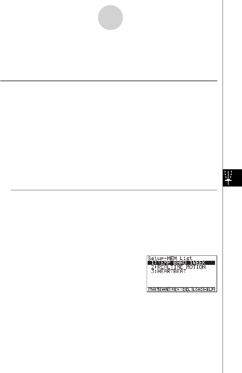
20010101
4-3-1
Setup Memory
4-3 Setup Memory
You can use setup memory to save EA-100 setups you create using Setup Wizard or
Advanced Setup in calculator memory for later recall when you need them.
kSaving a Setup
A setup can be saved when any one of the following conditions exist.
•After creating a new setup with Setup Wizard
See step 7 under “To create an EA-100 setup using Setup Wizard” on page 4-2-2.
•After creating a new setup with Advanced Setup
See step 6 under “To create an EA-100 setup using Advanced Setup” on page 4-2-4 for
more information.
•While the E-CON main menu is on the display
Performing the setup save operation while the E-CON main menu is on the display saves
the contents of the current setup memory area (which were created using Setup Wizard or
Advanced Setup).
Details on saving a setup are listed below.
uTo save a setup
1. Start the save operation by performing one of the function key operations described
below.
•If the final Setup Wizard screen is on the display, press 3(SAVE).
•If the Advanced Setup menu screen is on the display, press 3(MEM).
•If the E-CON main menu screen is on the display, press 2(MEM).
•Performing any one of the above operations causes the setup memory list to appear.
•The message “No Setup-MEM” appears if setup memory is empty.
20011101
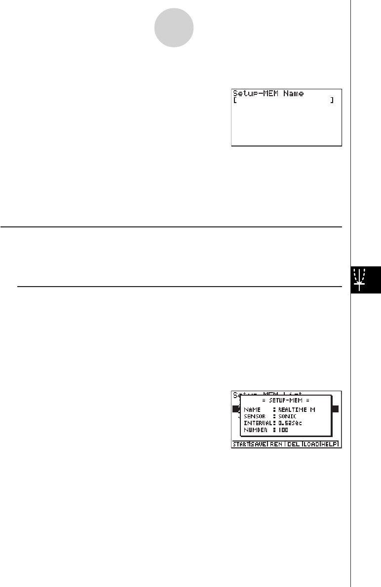
20010101
2. Press 2(SAVE).
•This displays the screen for inputting the setup name.
4-3-2
Setup Memory
3. Press w and then input a memory number (1 to 99).
•If you start from the final setup screen, this saves the setup and the message
“Complete!” appears. Press w to return to the final setup screen.
•If you start from the Advanced Setup menu or the E-CON main menu, this saves the
setup and returns to the setup memory list which includes the name you assigned it.
kUsing and Managing Setups in Setup Memory
All of the setups you save are shown in the setup memory list. After selecting a setup in the
list, you can use it to sample data or you can edit it.
uTo preview saved setup data
You can use the following procedure to check the contents of a setup before you use it for
sampling.
1. On the E-CON main menu, press 2(MEM) to display the setup memory list.
2. Use the f and c cursor keys to highlight the name of the setup you want.
3. Press K(Setup Preview).
•This displays the preview dialog box.
4. To close the preview dialog box, press i.
20011101
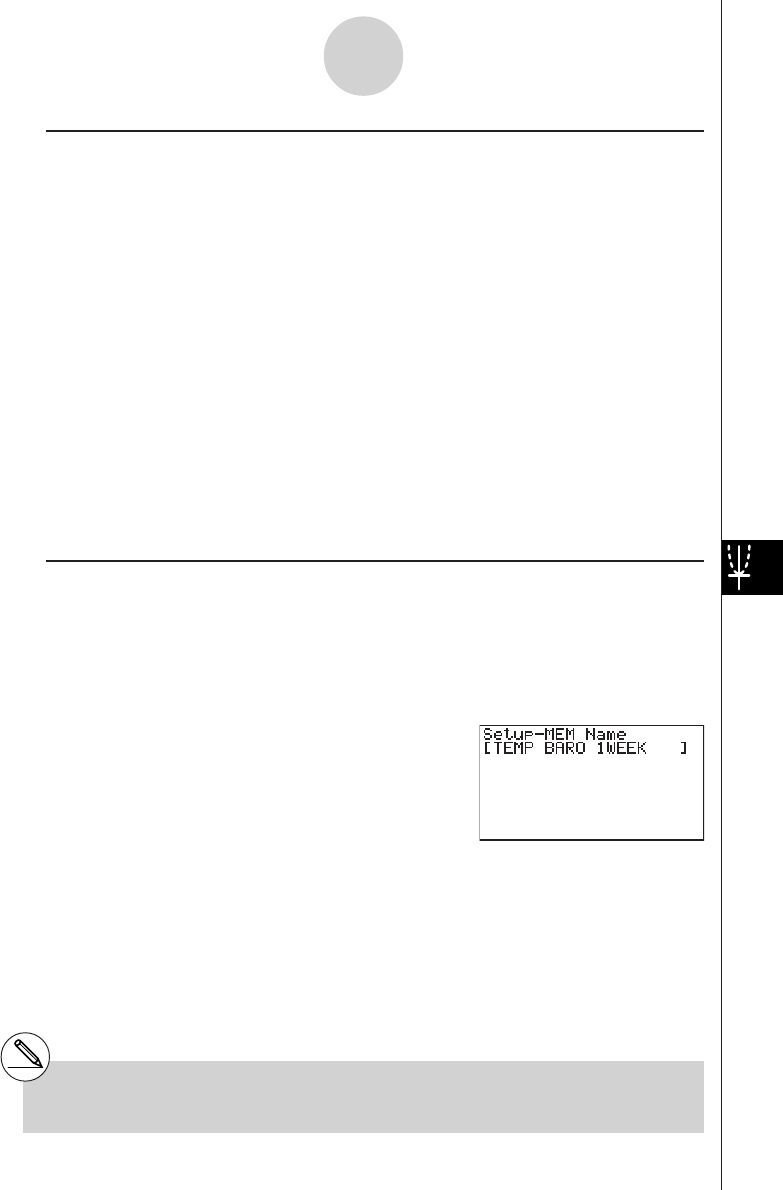
20010101
uTo recall a setup and use it for sampling
Be sure to perform the following steps before starting sampling with the EA-100.
1. Connect the calculator to the EA-100.
2. Turn on EA-100 power.
3. In accordance with the setup you plan to use, connect the proper sensor to the
appropriate EA-100 channel.
4. Prepare the item whose data is to be sampled.
• To recall a setup and use it for sampling
1. On the E-CON main menu, press 2(MEM) to display the setup memory list.
2. Use the f and c cursor keys to highlight the name of the setup you want.
3. Press 1(START).
4. In response to the confirmation message that appears, press w.
•Pressing w sets up the EA-100 and then starts sampling.
•To clear the confirmation message without sampling, press i.
uTo change the name of setup data
1. On the E-CON main menu, press 2(MEM) to display the setup memory list.
2. Use the f and c cursor keys to highlight the name of the setup you want.
3. Press 3(REN).
•This displays the screen for inputting the setup name.
4-3-3
Setup Memory
4. Input up to 18 characters for the setup name, and then press w.
•This changes the setup name and returns to the setup memory list.
#See “Operations during a sampling operation”
on page 4-5-2 for information about
operations you can perform while a sampling
operation is in progress.

20010101
uTo delete setup data
1. On the E-CON main menu, press 2(MEM) to display the setup memory list.
2. Use the f and c cursor keys to highlight the name of the setup you want.
3. Press 4(DEL).
4. In response to the confirmation message that appears, press w to delete the setup.
•To clear the confirmation message without deleting anything, press i.
uTo recall setup data
Recalling setup data stores it in the current setup memory area. You can then use Advanced
Setup to edit the setup. This capability comes in handy when you need to perform a setup
that is slightly different from one you have stored in memory.
1. On the E-CON main menu, press 2(MEM) to display the setup memory list.
2. Use the f and c cursor keys to highlight the name of the setup you want.
3. Press 5(LOAD).
4. In response to the confirmation message that appears, press w to recall the setup.
•To clear the confirmation message without recalling the setup, press i.
4-3-4
Setup Memory
#Recalling setup data replaces any other data
currently in the current setup memory area.

20010101
4-4 Program Converter
Program Converter converts an EA-100 setup you created using Setup Wizard or Advanced
Setup to a program that can run on the calculator. You can also use Program Converter to
convert a setup to a CFX-9850 Series/fx-7400 Series-compatible program and transfer it to a
calculator.*1 *2
kConverting a Setup to a Program
A setup can be converted to a program when any one of the following conditions exists.
•After creating a new setup with Setup Wizard
See step 7 under “To create an EA-100 setup using Setup Wizard” on page 4-2-2.
•After creating a new setup with Advanced Setup
See step 6 under “To create an EA-100 setup using Advanced Setup” on page 4-2-4 for
more information.
•While the E-CON main menu is on the display
Performing the program converter operation while the E-CON main menu is on the display
converts the contents of the current setup memory area (which were created using Setup
Wizard or Advanced Setup).
The program converter procedure is identical in all of the above cases.
uTo convert a setup to a program
1. Start the converter operation by performing one of the function key operations described
below.
•If the final Setup Wizard screen is on the display, press 4(PRGM).
•If the Advanced Setup menu screen is on the display, press 4(PRGM).
•If the E-CON main menu screen is on the display, press 3(PRGM).
•This displays the program name input screen.
4-4-1
Program Converter
*1See the documentation that came with your
scientific calculator or EA-100 for information
about how to use a converted program.
*2See online help (PROGRAM CONVERTER
HELP) for information about supported CFX-
9850 Series and fx-7400 Series models.
2. Input the name you want to assign to the program.
20010101
3. Press w.
•This starts conversion of the setup data to a program.
•The message “Complete!” appears when conversion is complete.
uTo convert setup data to a program and transfer it to a CFX-9850 Series/
fx-7400 Series calculator
1. Connect the scientific calculator (CFX-9850 Series or fx-7400 Series) to the ALGEBRA
calculator.
• Perform the necessary procedure on the scientific calculator to set it up to receive data.
2. Perform steps 1 and 2 of the procedure under “To convert a setup to a program” on page
4-4-1.
3. Press 1 (TRNS). On the sub-menu that appears, specify the type of scientific calculator
(b: FX9850 or c: fx7400) for which you want to create a program.
•Program conversion and transfer starts as soon as you specify a calculator model.
•The message “Complete!” appears when conversion is complete.
4-4-2
Program Converter
#When you convent setup data to a CFX-9850
Series or fx-7400 Series program, any sample
value storage list number greater than 5 is
changed to 5.
#CFX-9850 Series or fx-7400 Series calculators
support up to six lists only.
#List 6 is used for EA-100 setup.

20010101
4-5 Starting a Sampling Operation
The section describes how to use a setup created using the E-CON Mode to start an EA-100
sampling operation.
kBefore getting started...
Be sure to perform the following steps before starting sampling with the EA-100.
1. Connect the calculator to the EA-100.
2. Turn on EA-100 power.
3. In accordance with the setup you plan to use, connect the proper sensor to the
appropriate EA-100 channel.
4. Prepare the item whose data is to be sampled.
kStarting a Sampling Operation
A sampling operation can be started when any one of the following conditions exist.
•After creating a new setup with Setup Wizard
See step 7 under “To create an EA-100 setup using Setup Wizard” on page 4-2-2.
•After creating a new setup with Advanced Setup
See step 6 under “To create an EA-100 setup using Advanced Setup” on page 4-2-4.
•While the E-CON main menu is on the display
Starting a sampling operation while the E-CON main menu is on the display performs
sampling using the contents of the current setup memory area (which were created using
Setup Wizard or Advanced Setup).
•While the setup memory list is on the display
You can select the setup you want on the setup memory list and then start sampling.
The following procedures explain the first three conditions described above. See “To recall a
setup and use it for sampling” on page 4-3-3 for information about starting sampling from the
setup memory list.
4-5-1
Starting a Sampling Operation
20011101
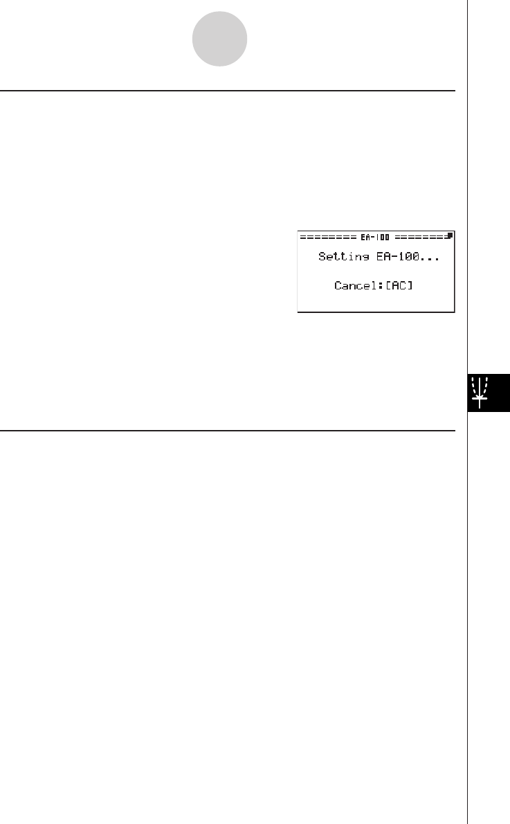
20010101
uTo start sampling
1. Start the sampling operation by performing one of the function key operations described
below.
•If the final Setup Wizard screen is on the display, press 1(YES).
•If the Advanced Setup menu screen is on the display, press 1(START).
•If the E-CON main menu screen is on the display, press 4(START).
•This sets up the EA-100 using the setup data in the current setup memory area.
•To interrupt a setup while the above screen is on the display, press A.
2. The sampling start dialog box appears after setup of the EA-100 is complete.
•The content of the sampling start dialog box depends on the settings contained in the
setup. See “Operations during a sampling operation” below for information about this
dialog box and other display screens.
uOperations during a sampling operation
Sending a sample start command from the calculator to the EA-100 causes the following
sequence to be performed.
Setup Data Transfer → Sampling Start → Sampling End →
Transfer of Sample Data from the EA-100 to the Calculator
The table on the next page shows how the trigger conditions and sensor type specified in the
setup data affects the above sequence.
4-5-2
Starting a Sampling Operation
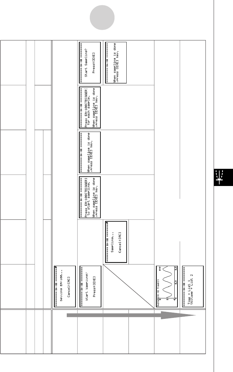
20010101
4-5-3
Starting a Sampling Operation
Real-Time Normal Sampling Normal Sampling Trigg er Start [TRIGGER] Key Photogate
Sampling Type Sampling
Press [EXE] to start. Press [TRIGGER]
Sampling Sampling measurement
to start.
Real-Time Y
es No
Sampling Interval
Timer
Start Trigger
[EXE] key [TRIGGER] Sampled Value
[TRIGGER] Gate Status
key press
Starts Sampling
1. EA-100 Setup
2. Trigger
Conditions
3. Sampling
4. Data Receive
Trigger
5. Graph
Drawing
6. Data Store
Lists
Data is not graphed under the
following conditions.
1. Interval: [TRIGGER]
Rec Time: None
2. Motion Detector
0.02⬉Sampling Interval (sec) ⬍0.065
Rec Time: None
3. Only when Photogate sensor is used
Sampled
values received
automatically.
20010101
4-5-4
Starting a Sampling Operation
#Conductivity, heart rate, and pH sensors
Sample values produced by these types of
sensors lose accuracy unless the sensors are
allowed to warm up. Perform the following
procedure to ensure better sampling accuracy.
Using a Heart Rate Sensor
1. Select [TRIGGER] as the Trigger Source
item of Advanced Setup’s Trigger
parameter.
2. When the EA-100 is in the Ready state
prior to sampling, hold down the EA-100’s
[TRIGGER] key for about 20 to 30
seconds, and then release it.
3. Press the EA-100’s [TRIGGER] key when
you want to start sampling.
Using a Conductivity or pH Sensor
1. Select [Yes] for the [Real-Time] setting on the
Sample Setup screen of the Advanced Setup
menu.
#Initial samples using conductivity, heart rate,
and pH sensors are always inaccurate when
starting from Setup Wizard.
#For detailed information about a sensor, see
the documentation that comes with it.
20011101

20010101
20010101
Symbols
χ2 Distribution .................................... 1-4-9
χ2 Test ................................... 1-2-1, 1-2-18
A
Advanced Setup ............................... 4-2-4
Advanced Statistics .......................... 1-1-1
Amortization ...................................... 2-5-1
ANOVA ................................. 1-2-1, 1-2-22
B
Bernoulli equation ..............................3-2-5
Binomial Distribution ........................ 1-4-16
Bonds ..............................................2-10-1
C
Calculation range .............................. 3-1-1
Cash Flow ......................................... 2-4-1
Channel ............................................ 4-2-5
Compound Interest ........................... 2-3-1
Confidence Interval ........................... 1-3-1
Copy ................................................. 1-1-3
Cost .................................................. 2-7-1
Custom Probe .................................. 4-2-11
D
Date Calculation ............................... 2-8-1
Days Calculation ............................... 2-8-1
Dependent variable .......................... 3-1-2
Depreciation .................................... 2-9-1
Derivative ...........................................3-1-2
DIFF EQ Mode .................................. 3-1-1
Differential equation .......................... 3-1-1
Differential equation of the first
order ........................................... 3-2-1
Differential equation of the fourth
order ........................................... 3-4-1
Differential equation of the Nth
order ........................................... 3-4-1
Distribution ....................................... 1-4-1
E
E-CON HELP .................................... 4-1-1
E-CON Mode .................................... 4-1-1
EA-100 Setup ................................... 4-2-1
F
F Distribution .................................. 1-4-12
F Test .................................... 1-2-1, 1-2-20
Financial Calculations ....................... 2-1-1
G
Geometric Distribution .....................1-4-21
Graph Memory .................................. 3-5-5
H
h (step size) ...................................... 3-1-1
I
Independent variable ........................ 3-1-2
Initial value .............................. 3-1-1, 3-1-2
Interest Rate Conversion .................. 2-6-1
Investment Appraisal ........................ 2-4-1
1
Index
Index (Additional Functions)

2001010120010101
2
Index
L
Linear differential equation of the
second order ............................... 3-3-1
Linear equation .................................. 3-2-3
List setting screen ..............................3-1-2
M
Margin ............................................... 2-7-1
MSE .................................................. 1-1-1
MULTIMETER Mode........................ 4-2-14
N
Normal Distribution ........................... 1-4-3
O
Option Setup ................................... 4-2-10
P
Parameter screen ..............................3-1-1
Poisson Distribution .........................1-4-19
Program Converter ........................... 4-4-1
R
Runge-Kutta method ........................ 3-1-1
S
Sample Setup ................................... 4-2-7
Selling Price ...................................... 2-7-1
Separable equation .......................... 3-2-1
Setup Memory .................................. 4-3-1
Setup Wizard .................................... 4-2-1
SF (slope field) ....................... 3-1-1, 3-1-2
Simple Interest .................................. 2-2-1
Slope field ............................... 3-1-1, 3-1-2
Starting a Sampling Operation ......... 4-5-1
STAT Mode ....................................... 1-1-1
Step .................................................. 3-1-1
Step size ........................................... 3-1-1
Student-t Distribution ........................ 1-4-7
System of the first order differential
equations .......................... 3-4-3, 3-5-1
T
t Interval .................................. 1-3-1, 1-3-8
t Tests ................................... 1-2-1, 1-2-10
Tests ................................................. 1-2-1
Trigger Setup .................................... 4-2-8
TVM Graph ...................................... 2-11-1
TVM Mode ........................................ 2-1-1
V
V-Window ......................................... 3-1-2
Y
Y-CAL ............................................... 1-1-2
Z
Z Interval ................................. 1-3-1, 1-3-3
Z Tests .................................... 1-2-1, 1-2-2

CASIO ELECTRONICS CO., LTD.
Unit 6, 1000 North Circular Road,
London NW2 7JD, U.K.
Important!
Please keep your manual and all information handy for
future reference.

SA0801-E
CASIO COMPUTER CO., LTD.
6-2, Hon-machi 1-chome
Shibuya-ku, Tokyo 151-8543, Japan
G350-11, G352-11
