Casio ClassPad II _fx CP400 Graphing Calculator FXCP400 Class Pad UG EN
User Manual: Casio Casio Graphing Calculator FXCP400 FXCP400
Open the PDF directly: View PDF ![]() .
.
Page Count: 316 [warning: Documents this large are best viewed by clicking the View PDF Link!]
- Contents
- Chapter 1: Basics
- Chapter 2:
Main Application
- 2-1 Basic Calculations
- 2-2 Using the Calculation History
- 2-3 Function Calculations
- 2-4 List Calculations
- 2-5 Matrix and Vector Calculations
- 2-6 Specifying a Number Base
- 2-7 Using the Action Menu
- 2-8 Using the Interactive Menu
- 2-9 Using the Main Application in Combination with Other Applications
- 2-10 Using Verify
- 2-11 Using Probability
- 2-12 Running a Program in the Main Application
- Chapter 3: Graph & Table Application
- Chapter 4: Conics Application
- Chapter 5: Differential Equation Graph Application
- Chapter 6: Sequence Application
- Chapter 7: Statistics Application
- Chapter 8: Geometry Application
- Chapter 9: Numeric Solver Application
- Chapter 10: eActivity Application
- Chapter 11: Financial Application
- Chapter 12: Program Application
- Chapter 13: Spreadsheet Application
- Chapter 14: 3D Graph Application
- Chapter 15: Picture Plot Application
- Chapter 16: Interactive Differential Calculus Application
- Chapter 17: Physium Application
- Chapter 18: System Application
- Chapter 19: Performing Data Communication
- Appendix
- Exam Mode


2
Be sure to keep physical records of all important data!
Low battery power or incorrect replacement of the batteries that power the ClassPad can cause the data stored
in memory to be corrupted or even lost entirely. Stored data can also be affected by strong electrostatic charge
or strong impact. It is up to you to keep backup copies of data to protect against its loss.
Backing Up Data
ClassPad data can be converted to a VCP file or XCP file and transferred to a computer for storage. For details,
see “19-2 Performing Data Communication between the ClassPad and a Personal Computer”.
• Be sure to keep all user documentation handy for future reference.
• The sample screens shown in this manual are for illustrative purposes only, and may not be exactly the
same as the screens actually produced by the ClassPad.
• The contents of this manual are subject to change without notice.
• No part of this manual may be reproduced in any form without the express written consent of the
manufacturer.
• In no event shall CASIO Computer Co., Ltd. be liable to anyone for special, collateral, incidental, or
consequential damages in connection with or arising out of the purchase or use of these materials.
Moreover, CASIO Computer Co., Ltd. shall not be liable for any claim of any kind whatsoever against the
use of these materials by any other party.
• Windows® is a registered trademark or trademark of Microsoft Corporation in the United States and/or
other countries.
• Mac OS, OS X and macOS are registered trademarks or trademarks of Apple Inc. in the United States
and/or other countries.
• Fugue © 1999 – 2012 Kyoto Software Research, Inc. All rights reserved.
• Company and product names used in this manual may be registered trademarks or trademarks of their
respective owners.
• Note that trademark ™ and registered trademark ® are not used within the text of this manual.

3
Contents
About This User’s Guide ..........................................................................................................................11
Chapter 1: Basics ................................................................................................................ 12
1-1 General Guide .........................................................................................................................12
ClassPad at a Glance...............................................................................................................................12
Turning Power On or Off .......................................................................................................................... 13
1-2 Power Supply ..........................................................................................................................13
1-3 Built-in Application Basic Operations ..................................................................................14
Using the Application Menu......................................................................................................................14
Built-in Applications ..................................................................................................................................14
Add-in Applications...................................................................................................................................15
Application Window ..................................................................................................................................16
Using the O Menu ...................................................................................................................................17
Interpreting Status Bar Information ..........................................................................................................17
Pausing and Terminating an Operation ....................................................................................................17
1-4 Input .........................................................................................................................................18
Using the Soft Keyboard ..........................................................................................................................18
Soft Keyboard Key Sets ........................................................................................................................... 18
Input Basics ..............................................................................................................................................19
Various Soft Keyboard Operations ...........................................................................................................22
1-5 ClassPad Data .........................................................................................................................27
Data Types and Storage Locations (Memory Areas) ............................................................................... 27
Main Memory Data Types ........................................................................................................................ 28
Main Memory Folders ...............................................................................................................................28
Using Variable Manager ...........................................................................................................................29
Managing Application Files ......................................................................................................................32
1-6 Creating and Using Variables ................................................................................................33
Creating a New Variable ..........................................................................................................................33
Variable Usage Example ..........................................................................................................................34
“library” Folder Variables ..........................................................................................................................34
Rules Governing Variable Access ............................................................................................................35
1-7 Configuring Application Format Settings .............................................................................36
Application Format Settings .....................................................................................................................36
Initializing All Application Format Settings ................................................................................................42
1-8 When you keep having problems… ......................................................................................43
Chapter 2: Main Application ............................................................................................... 44
Main Application-Specific Menus and Buttons ......................................................................................... 44
2-1 Basic Calculations ..................................................................................................................44
Arithmetic Calculations and Parentheses Calculations ............................................................................44
Using the e Key ..................................................................................................................................45
Omitting the Multiplication Sign ................................................................................................................45
Using the Answer Variable (ans) .............................................................................................................. 45
Assigning a Value to a Variable ...............................................................................................................45
Calculation Priority Sequence .................................................................................................................. 46
Calculation Modes .................................................................................................................................... 46
2-2 Using the Calculation History ................................................................................................48
2-3 Function Calculations ............................................................................................................48
2-4 List Calculations .....................................................................................................................57
Inputting List Data in the Work Area .........................................................................................................57
LIST Variable Element Operations ........................................................................................................... 57

4
Using a List in a Calculation .....................................................................................................................57
Using a List to Assign Different Values to Multiple Variables ................................................................... 57
2-5 Matrix and Vector Calculations .............................................................................................58
Inputting Matrix Data ................................................................................................................................ 58
Performing Matrix Calculations ................................................................................................................58
Using a Matrix to Assign Different Values to Multiple Variables ...............................................................59
2-6 Specifying a Number Base ....................................................................................................59
Binary, Octal, Decimal, and Hexadecimal Calculation Ranges ................................................................ 59
Selecting a Number Base.........................................................................................................................60
Arithmetic Operations ............................................................................................................................... 60
Bitwise Operations ...................................................................................................................................60
Using the baseConvert Function (Number System Transform) ............................................................... 61
2-7 Using the Action Menu ...........................................................................................................61
Abbreviations and Punctuation Used in This Section ...............................................................................61
Example Screenshots ..............................................................................................................................62
Using the Transformation Submenu .........................................................................................................62
Using the Advanced Submenu ................................................................................................................. 64
Using the Calculation Submenu ...............................................................................................................67
Using the Complex Submenu ...................................................................................................................70
Using the List-Create Submenu ............................................................................................................... 71
Using the List-Statistics and List-Calculation Submenus ......................................................................... 72
Using the Matrix-Create Submenu ...........................................................................................................75
Using the Matrix-Calculation and Matrix-Row&Column Submenus .........................................................76
Using the Vector Submenu ......................................................................................................................79
Using the Equation/Inequality Submenu ................................................................................................. 81
Using the Assistant Submenu .................................................................................................................. 84
Using the Distribution/Inv.Dist Submenu .................................................................................................. 85
Using the Financial Submenu ..................................................................................................................90
Using the Command Submenu ................................................................................................................ 90
2-8 Using the Interactive Menu ...................................................................................................91
Interactive Menu Example ........................................................................................................................ 91
Using the “apply” Command .....................................................................................................................91
2-9 Using the Main Application in Combination with Other Applications ...............................92
Using Another Application’s Window ........................................................................................................92
Using the Stat Editor Window ...................................................................................................................93
Using the Geometry Window ....................................................................................................................93
2-10 Using Verify ...........................................................................................................................94
2-11 Using Probability ..................................................................................................................95
2-12 Running a Program in the Main Application ......................................................................96
Chapter 3: Graph & Table Application ............................................................................... 97
Graph & Table Application-Specific Menus and Buttons ..........................................................................97
3-1 Storing Functions ...................................................................................................................99
Using Graph Editor Sheets.......................................................................................................................99
Storing a Function .................................................................................................................................... 99
Graphing a Stored Function ................................................................................................................... 100
Shading the Region Bounded by Two Expressions ............................................................................... 101
Overlaying Two Inequalities in an Intersection Plot / Union Plot ............................................................101
Saving Graph Editor Data to Graph Memory .........................................................................................102
3-2 Using the Graph Window .....................................................................................................102
Configuring View Window Parameters for the Graph Window ............................................................... 102
Using View Window Memory ..................................................................................................................104
Panning the Graph Window ...................................................................................................................104

5
Scrolling the Graph Window ................................................................................................................... 105
Zooming the Graph Window ...................................................................................................................105
Using Quick Zoom .................................................................................................................................. 106
Using Built-in Functions for Graphing .....................................................................................................106
Saving a Screenshot of a Graph ............................................................................................................ 107
Adjusting the Lightness (Fade I/O) of the Graph Window Background Image ....................................... 107
3-3 Using Table & Graph.............................................................................................................108
Generating a Number Table ................................................................................................................... 108
Showing Linked Displays of Number Table Coordinates and Graph Coordinates (Link Trace) .............109
Generating Number Table Values from a Graph ....................................................................................110
Generating a Summary Table ................................................................................................................ 110
3-4 Using Trace ........................................................................................................................... 111
Using Trace to Read Graph Coordinates ...............................................................................................111
3-5 Using the Sketch Menu ........................................................................................................ 112
Using Sketch Menu Commands ............................................................................................................. 112
3-6 Analyzing a Function Used to Draw a Graph ..................................................................... 114
What You Can Do Using the G-Solve Menu Commands ....................................................................... 114
Using G-Solve Menu Commands ........................................................................................................... 114
3-7 Modifying a Graph ................................................................................................................ 115
Modifying a Single Graph (Direct Modify) ...............................................................................................115
Modifying Multiple Graphs Simultaneously (Dynamic Modify) ............................................................... 115
Chapter 4: Conics Application ..........................................................................................118
Conics Application-Specific Menus and Buttons ....................................................................................118
4-1 Inputting an Equation ........................................................................................................... 119
4-2 Drawing a Conics Graph ...................................................................................................... 119
Drawing a Parabola ................................................................................................................................ 119
Drawing a Circle .....................................................................................................................................120
Drawing an Ellipse..................................................................................................................................120
Drawing a Hyperbola .............................................................................................................................. 120
Drawing a General Conics .....................................................................................................................120
4-3 Using G-Solve to Analyze a Conics Graph .........................................................................120
What You Can Do Using the G-Solve Menu Commands ....................................................................... 120
Using G-Solve Menu Commands ........................................................................................................... 121
4-4 Modifying a Graph (Dynamic Modify) .................................................................................121
Chapter 5: Differential Equation Graph Application....................................................... 122
Differential Equation Editor Window-Specific Menus and Buttons .........................................................122
Differential Equation Graph Window-Specific Menus and Buttons ........................................................122
5-1 Graphing a Differential Equation .........................................................................................123
Graphing a First Order Differential Equation ..........................................................................................123
Graphing a Second Order Differential Equation ..................................................................................... 124
Graphing an Nth-order Differential Equation ..........................................................................................124
Configuring and Modifying Initial Conditions .......................................................................................... 125
Configuring Differential Equation Graph View Window Parameters ...................................................... 126
5-2 Drawing f ( x) Type Function Graphs and Parametric Function Graphs ...........................127
5-3 Using Trace to Read Graph Coordinates ............................................................................127
5-4 Graphing an Expression or Value by Dropping It into the Differential Equation Graph
Window ..................................................................................................................................128
Chapter 6: Sequence Application .................................................................................... 129
Sequence Application-Specific Menus and Buttons ............................................................................... 129
6-1 Recursive and Explicit Form of a Sequence ......................................................................130
Generating a Number Table ................................................................................................................... 130

6
Determining the General Term of a Recursion Expression .................................................................... 131
Calculating the Sum of a Sequence .......................................................................................................131
6-2 Graphing a Recursion ..........................................................................................................131
Chapter 7: Statistics Application ..................................................................................... 132
7-1 Using Stat Editor ...................................................................................................................132
Basic List Operations .............................................................................................................................132
Menus and Buttons Used for List Editing ............................................................................................... 133
Using CSV Files ..................................................................................................................................... 134
7-2 Drawing a Statistical Graph .................................................................................................135
Operation Flow Up to Statistical Graphing ............................................................................................. 135
Graphing Single-Variable Statistical Data .............................................................................................. 136
Graphing Paired-Variable Statistical Data .............................................................................................. 137
Overlaying a Regression Graph on a Scatter Plot .................................................................................139
Overlaying a Function Graph on a Statistical Graph ..............................................................................140
Stat Graph Window Menus and Buttons ................................................................................................ 140
7-3 Performing Basic Statistical Calculations ..........................................................................141
Calculating Statistical Values ................................................................................................................. 141
Performing Regression Calculations ......................................................................................................143
Viewing the Results of the Last Statistical Calculation Performed (DispStat) ........................................ 145
7-4 Performing Advanced Statistical Calculations ..................................................................145
Performing Test, Confidence Interval and Distribution Calculations Using the Wizard .......................... 145
Tests.......................................................................................................................................................146
Confidence Intervals...............................................................................................................................149
Distributions............................................................................................................................................151
Input and Output Terms .........................................................................................................................154
Chapter 8: Geometry Application .................................................................................... 156
Geometry Application-Specific Menus and Buttons ............................................................................... 156
Configuring Geometry View Window Settings ........................................................................................157
About the Geometry Format Dialog Box ................................................................................................157
8-1 Drawing Figures ....................................................................................................................157
Drawing a Figure ....................................................................................................................................157
Inserting Text Strings into the Screen .................................................................................................... 161
Attaching an Angle Measurement to a Figure ........................................................................................161
Displaying the Measurements of a Figure .............................................................................................. 161
Displaying the Result of a Calculation that Uses On-screen Measurement Values ............................... 162
Using the Special Polygon Submenu .....................................................................................................162
Using the Construct Submenu ...............................................................................................................163
8-2 Editing Figures ......................................................................................................................167
Selecting and Deselecting Figures ......................................................................................................... 167
Moving and Copying Figures ..................................................................................................................168
Pinning an Annotation on the Geometry Window ...................................................................................168
Specifying the Number Format of a Measurement .................................................................................168
Specifying the Color and Line Type of a Displayed Object .................................................................... 169
Changing the Display Priority of Objects ................................................................................................ 169
8-3 Using the Measurement Box ...............................................................................................170
Viewing the Measurements of a Figure .................................................................................................. 170
Specifying and Constraining a Measurement of a Figure ......................................................................171
Using Sliders .......................................................................................................................................... 172
Changing a Label or Adding a Name to an Element ..............................................................................174
8-4 Working with Animations .....................................................................................................174
Using Animation Commands .................................................................................................................. 174

7
8-5 Using the Geometry Application with Other Applications ................................................177
Drag and Drop ........................................................................................................................................ 177
Copy and Paste ......................................................................................................................................177
Chapter 9: Numeric Solver Application ........................................................................... 178
Numeric Solver Application-Specific Menus and Buttons ......................................................................178
Inputting an Equation .............................................................................................................................178
Solving an Equation ...............................................................................................................................178
Chapter 10: eActivity Application .................................................................................... 180
eActivity Application-Specific Menus and Buttons ..................................................................................180
10-1 Creating an eActivity ..........................................................................................................180
Basic Steps for Creating an eActivity ..................................................................................................... 180
Inserting Data into an eActivity ............................................................................................................... 181
Inserting an Application Data Strip .........................................................................................................182
Inserting a Geometry Link Row ..............................................................................................................184
10-2 Transferring eActivity Files ................................................................................................185
File Compatibility ....................................................................................................................................185
Transferring eActivity Files between a ClassPad Unit and a Computer ................................................. 185
Transferring eActivity Files between Two ClassPad Units ..................................................................... 185
Chapter 11: Financial Application .................................................................................... 186
11-1 Financial Application Basic Operations ...........................................................................186
Page Operations ....................................................................................................................................187
Configuring Financial Application Settings .............................................................................................188
11-2 Performing Financial Calculations ....................................................................................189
11-3 Calculation Formulas .........................................................................................................189
Simple Interest .......................................................................................................................................189
Compound Interest ................................................................................................................................. 190
Cash Flow ..............................................................................................................................................190
Amortization ...........................................................................................................................................191
Interest Conversion ................................................................................................................................ 191
Cost/Sell/Margin .....................................................................................................................................192
Depreciation ...........................................................................................................................................192
Bond Calculation .................................................................................................................................... 192
Break-Even Point ...................................................................................................................................193
Margin of Safety ..................................................................................................................................... 193
Financial Leverage .................................................................................................................................193
Operating Leverage................................................................................................................................193
Combined Leverage ...............................................................................................................................193
Quantity Conversion ............................................................................................................................... 193
11-4 Financial Calculation Functions ........................................................................................194
11-5 Input and Output Field Names ...........................................................................................195
Chapter 12: Program Application .................................................................................... 196
Program Application-Specific Menus and Buttons ................................................................................. 196
12-1 Creating and Running Program ........................................................................................197
Creating a Program ................................................................................................................................197
Running a Program ................................................................................................................................ 199
Terminating Program Execution ............................................................................................................. 200
Creating a Text File ................................................................................................................................200
Using Text Files......................................................................................................................................201
Converting a Text File to a Program File ................................................................................................201
Converting a Program File to an Executable File ................................................................................... 201

8
12-2 Debugging a Program ........................................................................................................202
Debugging After an Error Message Appears .........................................................................................202
Debugging a Program Following Unexpected Results ........................................................................... 202
Editing a Program...................................................................................................................................202
12-3 User-defined Functions ......................................................................................................203
Creating a New User-defined Function .................................................................................................. 203
Executing a User-defined Function ........................................................................................................ 204
Editing a User-defined Function .............................................................................................................204
12-4 Program Command Reference ..........................................................................................205
Using This Reference ............................................................................................................................. 205
Syntax Conventions ...............................................................................................................................205
Command List ........................................................................................................................................ 206
12-5 Including ClassPad Functions in Programs ....................................................................225
Including Graphing Functions in a Program ...........................................................................................225
Including Table & Graph Functions in a Program ..................................................................................225
Including Recursion Table and Recursion Graph Functions in a Program ............................................ 225
Including Statistical Graphing and Calculation Functions in a Program ................................................. 225
Including Financial Calculation Functions in a Program .........................................................................225
Chapter 13: Spreadsheet Application .............................................................................. 226
Spreadsheet Window-Specific Menus and Buttons ...............................................................................226
Changing the Width of a Column ...........................................................................................................227
Option Settings .......................................................................................................................................228
13-1 Inputting and Editing Cell Contents ..................................................................................228
Selecting Cells........................................................................................................................................228
Inputting Data into a Cell ........................................................................................................................229
Inputting a Formula ................................................................................................................................229
Inputting a Cell Reference ...................................................................................................................... 230
Cell Data Types (Text Data and Calculation Data) ................................................................................231
Inputting a Constant into a Calculation Data Type Cell .......................................................................... 231
Using the Cell Viewer Window ............................................................................................................... 233
Changing the Text Color and Fill Color of Specific Cells ........................................................................233
Copying or Cutting Cells and Pasting Them to Another Location .......................................................... 234
Recalculating Spreadsheet Expressions ................................................................................................ 234
Transferring Data between a Spreadsheet and CSV Files ....................................................................235
Importing and Exporting Variable Values ...............................................................................................235
13-2 Graphing ..............................................................................................................................237
Basic Graphing Steps ............................................................................................................................237
Column Series and Row Series .............................................................................................................237
Graph Colors and Color Link .................................................................................................................. 238
Spreadsheet Graph Window-Specific Menus and Buttons ....................................................................239
Graph Menu and Graph Examples .........................................................................................................239
Regression Graph Operations (Curve Fitting) ........................................................................................ 242
Other Graph Window Operations ...........................................................................................................243
13-3 Statistical Calculations ......................................................................................................244
Single-variable, Paired-variable and Regression Calculations ...............................................................245
Test and Interval Calculations ................................................................................................................246
Distribution Calculations ......................................................................................................................... 248
About DispStat Command ...................................................................................................................... 248
13-4 Cell and List Calculations ..................................................................................................249
Using the Cell Calculation Functions ......................................................................................................249
Using the List Calculation Functions ...................................................................................................... 249

9
Chapter 14: 3D Graph Application ................................................................................... 250
3D Graph Application-Specific Menus and Buttons ...............................................................................250
14-1 Inputting an Expression .....................................................................................................251
Using 3D Graph Editor Sheets ...............................................................................................................251
Storing a Function .................................................................................................................................. 251
Graphing a Stored Function ................................................................................................................... 252
14-2 Using the 3D Graph Window .............................................................................................253
Configuring 3D Graph View Window Parameters .................................................................................. 253
Showing and Hiding Axes and Labels .................................................................................................... 254
Rotating the Graph .................................................................................................................................255
3D Graph Example ................................................................................................................................. 255
Using Trace to Read Graph Coordinates ...............................................................................................255
Inserting Text into a 3D Graph Window .................................................................................................256
Calculating a z-value for Particular x- and y-values, or s- and t-values .................................................256
Chapter 15: Picture Plot Application ............................................................................... 257
Picture Plot Application-Specific Menus and Buttons .............................................................................258
15-1 Using the Plot Function .....................................................................................................259
Starting a Picture Plot Operation ............................................................................................................ 259
Plotting Points on a c2p File Image ........................................................................................................ 259
Plotting Points on a c2b File Image ........................................................................................................ 260
Editing Plots on a Background Image .................................................................................................... 261
Overlaying a Graph on Background Image Plots ...................................................................................261
G-Solve ..................................................................................................................................................263
Scrolling the Picture Plot Window ..........................................................................................................263
15-2 Using the Plot List ..............................................................................................................264
Using the Plot List Window to Edit Plots ................................................................................................264
Saving Data to and Importing Data from a Spreadsheet ........................................................................264
Exporting Plot Data to and Importing Plot Data from a Variable ............................................................ 265
15-3 Displaying Plots on t-y or t-x Coordinates ........................................................................265
15-4 Picture Plot Application Files ............................................................................................266
Chapter 16: Interactive Differential Calculus Application.............................................. 267
DiffCalc Table Window-Specific Menus and Buttons ............................................................................. 267
16-1 Learning about Tangents Using the [Tangent] Tab .........................................................268
16-2 Deriving the Derivative Using the [Deriv] Tab ..................................................................269
16-3 Generating a Number Table and Graphing the First Derivative and Second Derivative
Using the [D Trace] Tab ......................................................................................................271
Chapter 17: Physium Application .................................................................................... 273
Physium Application Menus and Buttons ...............................................................................................273
17-1 Periodic Table......................................................................................................................274
17-2 Fundamental Physical Constants .....................................................................................275
17-3 Precautions .........................................................................................................................277
Chapter 18: System Application ...................................................................................... 279
18-1 Managing Memory Usage ..................................................................................................279
Using the Storage Sheet ........................................................................................................................ 279
Using the Main Memory Sheet and eActivity Sheet ............................................................................... 280
18-2 Configuring System Settings ............................................................................................281
System Application Menus and Buttons ................................................................................................. 281
Configuring System Settings ..................................................................................................................281

10
Chapter 19: Performing Data Communication ................................................................ 285
19-1 Data Communication Overview .........................................................................................285
Using the ClassPad Communication Application ................................................................................... 285
Select Connection Mode Dialog Box ...................................................................................................... 286
19-2 Performing Data Communication between the ClassPad and a Personal Computer ..286
Connecting and Disconnecting with a Computer in the USB Flash Mode .............................................287
Transferring Data between the ClassPad and a Personal Computer ....................................................288
Installing an Add-in Application .............................................................................................................. 289
Auto Import of VCP Files ........................................................................................................................ 289
Rules for ClassPad Files and Folders ....................................................................................................289
VCP and XCP File Operations ............................................................................................................... 289
19-3 Performing Data Communication between Two ClassPads ...........................................291
Connecting to Another ClassPad Unit .................................................................................................... 291
Transferring Data between Two ClassPads ........................................................................................... 291
Communication Standby ........................................................................................................................ 293
Interrupting an Ongoing Data Communication Operation ...................................................................... 293
19-4 Connecting the ClassPad to a Data Logger .....................................................................293
Connecting a ClassPad to a Data Logger ..............................................................................................293
19-5 Connecting the ClassPad to a Projector ..........................................................................294
Projecting ClassPad Screen Contents from a Projector .........................................................................294
Precautions when Connecting................................................................................................................294
Appendix ............................................................................................................................ 295
Character Code Table ..................................................................................................................295
System Variable Table .................................................................................................................299
Graph Types and Executable Functions....................................................................................302
Error and Warning Message Tables ...........................................................................................303
Error Message Table ............................................................................................................................. 303
Warning Message Table ........................................................................................................................307
Low Memory Error Processing ...............................................................................................................307
Resetting and Initializing the ClassPad .....................................................................................307
Number of Digits and Precision .................................................................................................308
Number of Digits.....................................................................................................................................308
Precision.................................................................................................................................................308
Display Brightness and Battery Life ..........................................................................................309
Display Brightness..................................................................................................................................309
Battery Life ............................................................................................................................................. 309
Specifications ..............................................................................................................................309
Exam Mode ..........................................................................................................................311
Communication Application - Exam Mode Menu ...................................................................................311
Entering the Exam Mode ........................................................................................................................ 311
ClassPad Operation in the Exam Mode ................................................................................................. 312
Exiting the Exam Mode ..........................................................................................................................313
Displaying Exam Mode Help .................................................................................................................. 314

11
About This User’s Guide
• The four digit boldface example numbers (such as 0201 ) that appear in Chapters 2 through 14 indicate
operation examples that can be found in the separate “Examples” booklet. You can use the “Examples”
booklet in conjunction with this manual by referring to the applicable example numbers.
• In this manual, cursor key operations are indicated as f, c, d, e (1-1 General Guide).

Chapter 1: Basics 12
Chapter 1:
Basics
This chapter provides a general overview of the ClassPad and application operations, as well as information
about input operations, the handling of data (variables and folders), file operations, and how to configure
application format settings.
1-1 General Guide
ClassPad at a Glance
3-pin data communication port
See Chapter 19 for details.
4-pin mini USB port
See Chapter 19 for details.
Touch screen
Icon panel
See “1-3 Built-in Application
Basic Operations”.
Cursor key*1
k key
f key*2
Stylus
K key
c key
Keypad
*1 In this manual, cursor key operations are indicated as f, c, d, e.
*2 Certain functions (cut, paste, undo, etc.) or key input operations can be assigned to key combinations that
consist of pressing the f key and a keypad key. For more information, see “18-2 Configuring System
Settings”.
Chapter 1: Basics 13
Turning Power On or Off
While the ClassPad is turned off, press c to turn it on.
To turn off the ClassPad, press f and then c.
Auto Power Off
The ClassPad also has an Auto Power Off feature. This feature automatically turns the ClassPad off when it is
idle for a specified amount of time. For details, see “To configure power properties” on page 282.
Note
Any temporary information in ClassPad RAM (graphs drawn on an application’s graph window, a dialog box
displayed, etc.) is retained for approximately 30 seconds whenever power is turned off manually or by Auto
Power Off. This means you will be able to restore the temporary information in RAM if you turn ClassPad back
on within about 30 seconds after it is turned off. After about 30 seconds, the temporary information in RAM is
cleared automatically, so turning ClassPad back on will display the startup screen of the application you were
using when you last turned it off, and the previous information in RAM will no longer be available.
1-2 Power Supply
Your ClassPad is powered by four AAA-size batteries LR03 (AM4), or four nickel-metal hydride batteries.
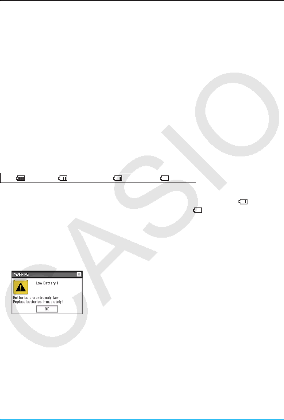
The battery level indicator is displayed in the status bar.
full medium low dead
Important!
• Be sure to replace batteries as soon as possible whenever the battery level indicator shows (low).
• Replace batteries immediately whenever the battery level indicator shows (dead). At this level, you will
not be able to perform data communication or other functions.
• For information about initial setup operations required after replacing batteries, see “Loading Batteries and
Setting Up the ClassPad” in the separate Quick Start Guide.
• When battery power is very low, your ClassPad may not turn back on when you press its c key. If this
happens, immediately replace its batteries.
• The following message indicates that batteries are about to go dead. Replace batteries immediately whenever
this message appears.
If you try to continue using the ClassPad, it will automatically turn off. You will not be able to turn power back
on until you replace batteries.
• Be sure to replace batteries at least once a year, no matter how much you use the ClassPad during that time.
Note: The batteries that come with the ClassPad discharge slightly during shipment and storage. Because of
this, they may require replacement sooner than the normal expected battery life.
Backing Up Data
ClassPad data can be converted to a VCP file or XCP file and transferred to a computer for storage. For details,
see “19-2 Performing Data Communication between the ClassPad and a Personal Computer”.
Chapter 1: Basics 14
1-3 Built-in Application Basic Operations
This section explains basic information and operations that are common to all of the built-in applications.
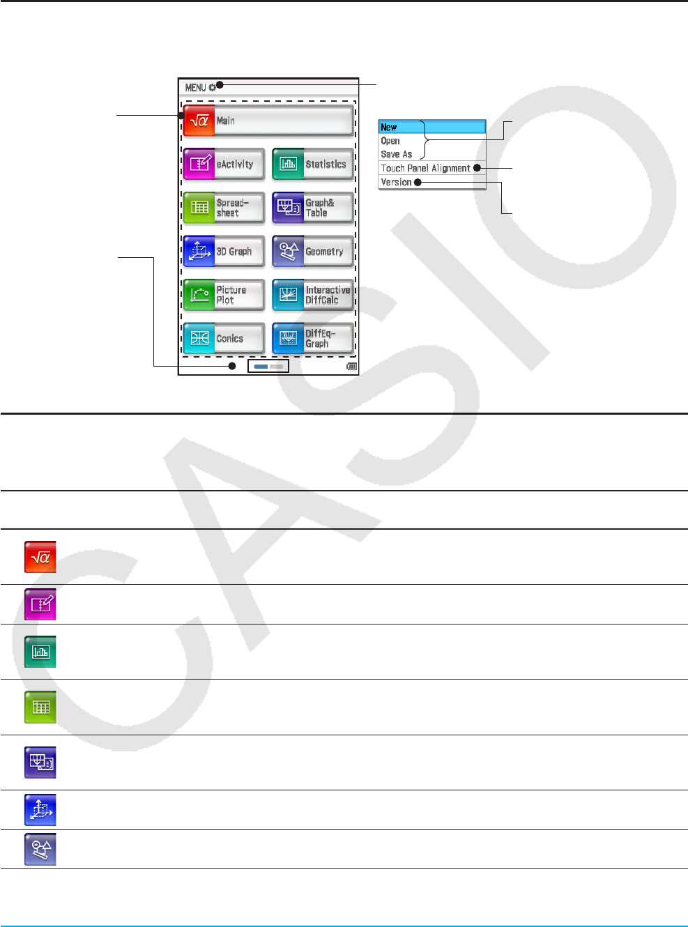
Using the Application Menu
Tapping m on the icon panel displays the application menu. You can perform the operations below with the
application menu.
Tap a button to start up an
application. See “Built-in
Applications” below.
Tapping here scrolls
between application menu
pages.
The application menu page
can also be changed by
swiping the screen left or
right with the stylus or your
finger.
Tap here (or tap s on the icon panel) to display the
next menu.
VCP file operations.
See page 289.
Starts touch panel alignment.
See page 284.
Displays version information.
See page 284.
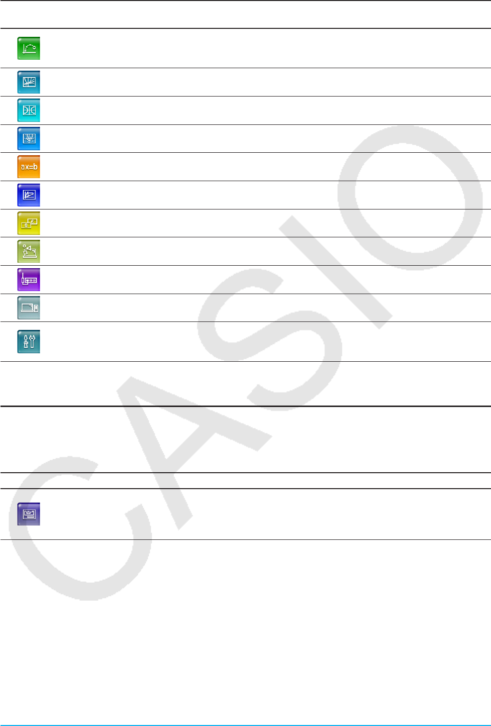
Built-in Applications
The table below shows the application icons displayed on the application menu, and explains what you can do
with each application.
Tap this
icon:
To start this
application: To perform this type of operation:
Main
• General calculations, including function calculations
• Matrix calculations
• Computer Algebra System
eActivity • Create an eActivity file that can be used for input of formulas, text,
and other ClassPad application data
Statistics
• Create a list
• Perform statistical calculations
• Draw a statistical graph
Spreadsheet
• Input data into a spreadsheet
• Manipulate and/or graph spreadsheet data
• Perform statistical calculations and/or draw a statistical graph
Graph & Table
• Draw a graph
• Register a function and create a table of solutions by substituting
different values for the function’s variables
3D Graph • Draw a 3-dimensional graph of an equation in the form z = f ( x, y) or of
a parametric equation
Geometry • Draw geometric figures
• Build animated figures
Chapter 1: Basics 15
Tap this
icon:
To start this
application: To perform this type of operation:
Picture Plot
• Plot points (that represent coordinates) on a photograph, illustration,
or other graphic and perform various types of analysis based on the
plotted data (coordinate values)
Interactive Differential
Calculus
• Learn about the differential coefficients and/or derivative formulas that
are the foundation of differentiation
Conics • Draw the graph of a conics section
Differential Equation
Graph • Draw vector fields and solution curves to explore differential equations
Numeric Solver • Obtain the value of any variable in an equation, without transforming
or simplifying the equation
Sequence • Perform sequence calculations
• Solve recursion expressions
Financial • Perform simple interest, compound interest, and other financial
calculations
Program • Input a program or run a program
• Create a user-defined function
E-CON3 • Control the optionally available Data Logger
(See the separate E-CON3 User’s Guide.)
Communication • Exchange data with another ClassPad, a computer, or another device
System
• Manage ClassPad memory (main memory, eActivity area, storage
area)
• Configure system settings
Tip: You can also start up the Main application by tapping M on the icon panel.
Add-in Applications
You can download add-in applications (as c2a files) from the CASIO website, install them on your ClassPad,
and use them the same way you use built-in applications. The table below shows the add-in applications that
are currently available.
Icon Application Description
Physium
• Find elements and display the atomic number, chemical symbol,
atomic weight and other information from the periodic table of
elements
• Display various physical constants
Note
You can delete all add-in applications using one of the procedures below.
• Reset - Storage Memory or Reset - All (“To batch delete specific data (Reset)”, page 281)
• Initialize (“To initialize your ClassPad”, page 282)
After deleting add-in applications, you can use the procedure under “Installing an Add-in Application” (page 289) to
re-install them.
Chapter 1: Basics 16
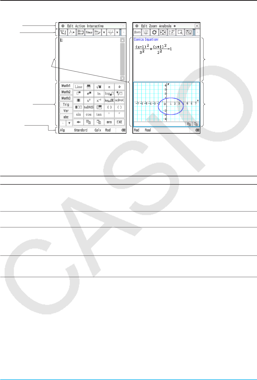
Application Window
The following shows the basic configuration of a built-in application window.
Menu bar
Tool bar
Application window(s)
Soft keyboard
See page 18.
Status bar
See page 17.
Upper window
Lower window
Many applications split the display between an upper window and a lower window, each of which shows
different information. When using two windows, the currently selected window (the one where you can perform
operations) is called the “active window”. The menu bar, toolbar, and status bar contents are all applicable to
the active window. The active window is indicated by a thick boundary around it.
You can perform the operations below on an Application window.
To do this: Perform this operation:
Switch the active window While a dual window is on the display, tap anywhere inside the window that does
not have a thick boundary around it to make it the active window. Note that you
cannot switch the active window while an operation is being performed in the
current active window.
Resize the active window
so it fills the display
While a dual window is on the display, tap r. This causes the active window to
fill the display. To return to the dual window display, tap r again.
Swap the upper and
lower windows
While a dual window is on the display, tap S. This causes the upper window
to become the lower window, and vice versa. Swapping windows does not have
any effect on their active status. If the upper window is active when you tap S
for example, that window will remain active after it becomes the lower window.
Close the active windows While a dual window is on the display, tap C at the top right corner of the
window to close the active window. This will cause the other (inactive) window to
fill the display.
Tip: When you tap the r icon while a dual window is on the display, the currently active window will fill the display, but
the other (inactive) window does not close. It remains open, hidden behind the active window. This means you can
tap S to bring the hidden window forward and make it the active window, and send the current active window to the
background.
u Changing the Display Orientation (Application Menu and Some Applications Only)
You can change the display orientation to horizontal while any one of the following is displayed: application
menu, or the Main, Graph & Table, Conics, or Physium application. Tap g to switch to horizontal (landscape)
display orientation. To return to vertical (portrait) display orientation, tap g again.
Chapter 1: Basics 17
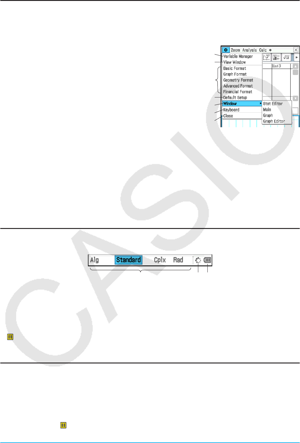
Using the O Menu
The O menu appears at the top left of the window of each application, except for the System application. You
can access the O menu by tapping m on the icon panel, or by tapping the menu bar’s O menu.
The following describes all of the items that appear on the O menu.
1 Tapping [Variable Manager] starts up Variable Manager. See “Using
Variable Manager” (page 29) for details.
2 Tapping [View Window] displays a dialog box for configuring
the display range and other graph settings. For details, see the
explanations for the various applications with graphing capabilities
(Graph & Table, Differential Equation Graph, Statistics, etc.)
3 Tapping a menu selection displays a dialog box for configuring the
corresponding setup settings. See “1-7 Configuring Application Format
Settings” for details.
4 Tapping [Default Setup] returns all settings to their initial defaults
(except for the current folder setting). See “1-7 Configuring Application
Format Settings” for details.
5 Tapping [Window] displays a list of all of the windows that can be accessed from the current application
(Statistics application in this example). Tapping a menu selection displays the corresponding window and
makes it active.
6 Tap [Keyboard] to toggle display of the soft keyboard on or off.
7 Tapping [Close] closes the currently active window, except in the following cases.
• When only one window is on the display
• When the currently active window cannot be closed by the application being used
You cannot, for example, close the Graph Editor window from the Graph & Table application.
Interpreting Status Bar Information
The status bar appears along the bottom of the window of each application.
123
1 Information about the currently running application
You can change the configuration of a setting indicated in the status bar by tapping it. Tapping “Cplx”
(indicating complex number calculations) while the Main application is running will toggle the setting to “Real”
(indicating real number calculations). Tapping again will toggle back to “Cplx”. For more details about the
current application information, see “1-7 Configuring Application Format Settings”.
2 This indicator rotates while processing in progress.
appears here to indicate when an operation is paused.
3 Battery level indicator (See “1-2 Power Supply”.)
Pausing and Terminating an Operation
Many of the built-in applications provide operations to pause and terminate (break) expression processing,
graphing, and other operations.
uTo pause an operation
Pressing the K key while an expression processing, graphing, or other operation is being performed
pauses the operation. appears on the right side of the status bar to indicate when an operation is paused.
Pressing K again resumes the operation.
1
2
4
5
6
7
3
Chapter 1: Basics 18
uTo terminate an operation
Pressing the c key while an expression processing, graphing, or other
operation is being performed terminates the operation and displays a “Break”
dialog box like the one shown nearby.
Tap the [OK] button on the dialog box to exit the Break state.
1-4 Input
You can input data on the ClassPad using its keypad or by using the on-screen soft keyboard.
Virtually all data input required by your ClassPad can be performed using the soft keyboard. The keypad keys
are used for input of frequently used data like numbers, arithmetic operators, etc.
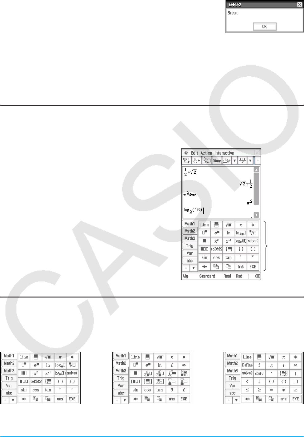
Using the Soft Keyboard
The soft keyboard is displayed in the lower part of the touch screen.
uTo display the soft keyboard
When the soft keyboard is not on the touch screen, press the
k key, or tap the O menu and then tap [Keyboard]. This
causes the soft keyboard to appear.
• The soft keyboard has a number of different key sets such
as [Math1], [abc], and [Catalog], which you can use to input
of functions and text. To select a key set, tap one of the tabs
along the left side of the soft keyboard.
• Pressing the k key or tapping the O menu, and then
[Keyboard] again hides the soft keyboard.
Soft keyboard
Soft Keyboard Key Sets
The soft keyboard has a variety of different key sets that support various data input needs. Each of the
available key sets is shown below.
[Math1], [Math2], [Math3], [Trig] (trigonometric), [Advance] key sets
These key sets include keys for inputting functions, operators, and symbols required for numerical formulas.
Math1 Math2 Math3
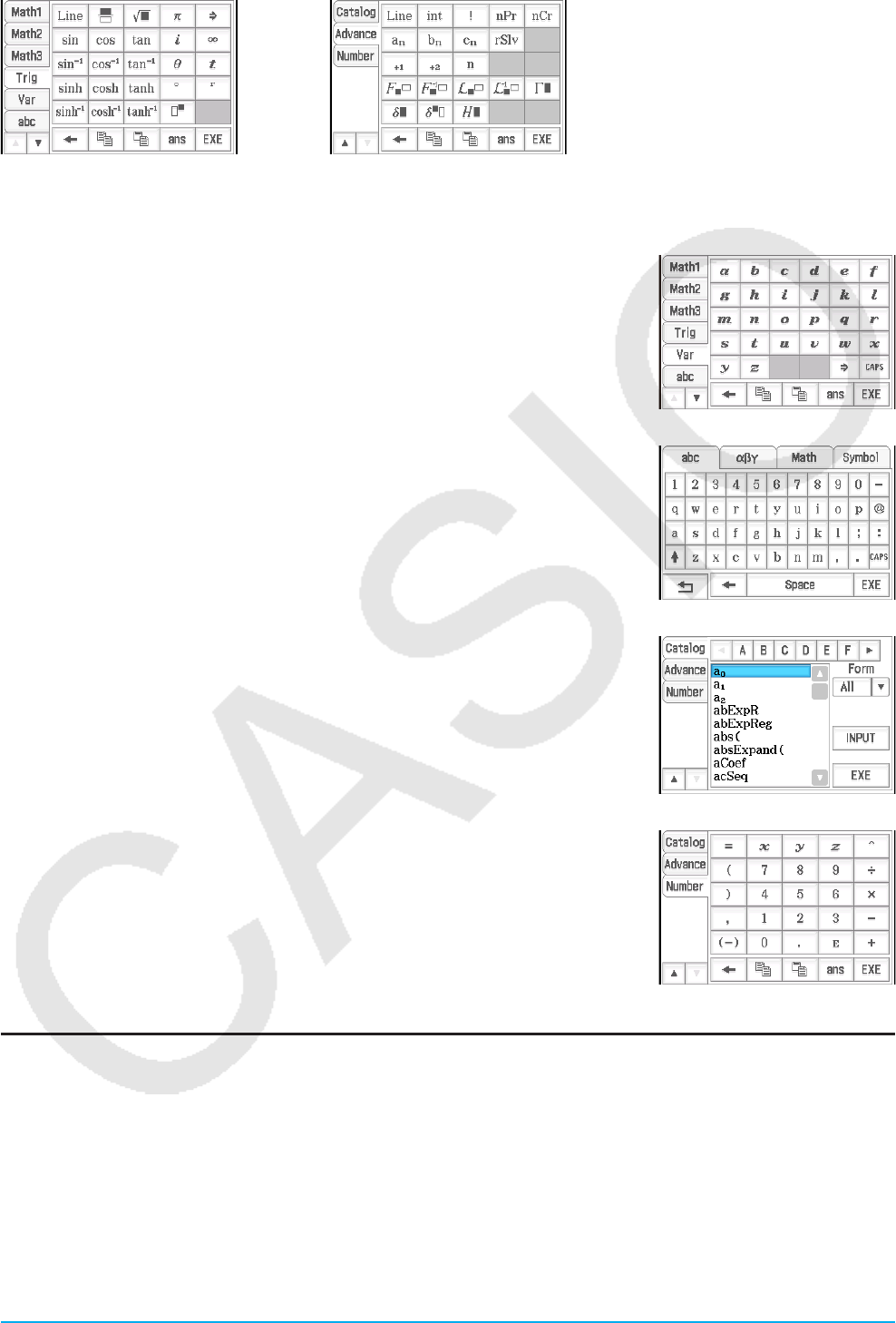
Chapter 1: Basics 19
Trig Advance
For details above the above key sets, see “Using Math, Trig, and Advance Key Sets” (page 23).
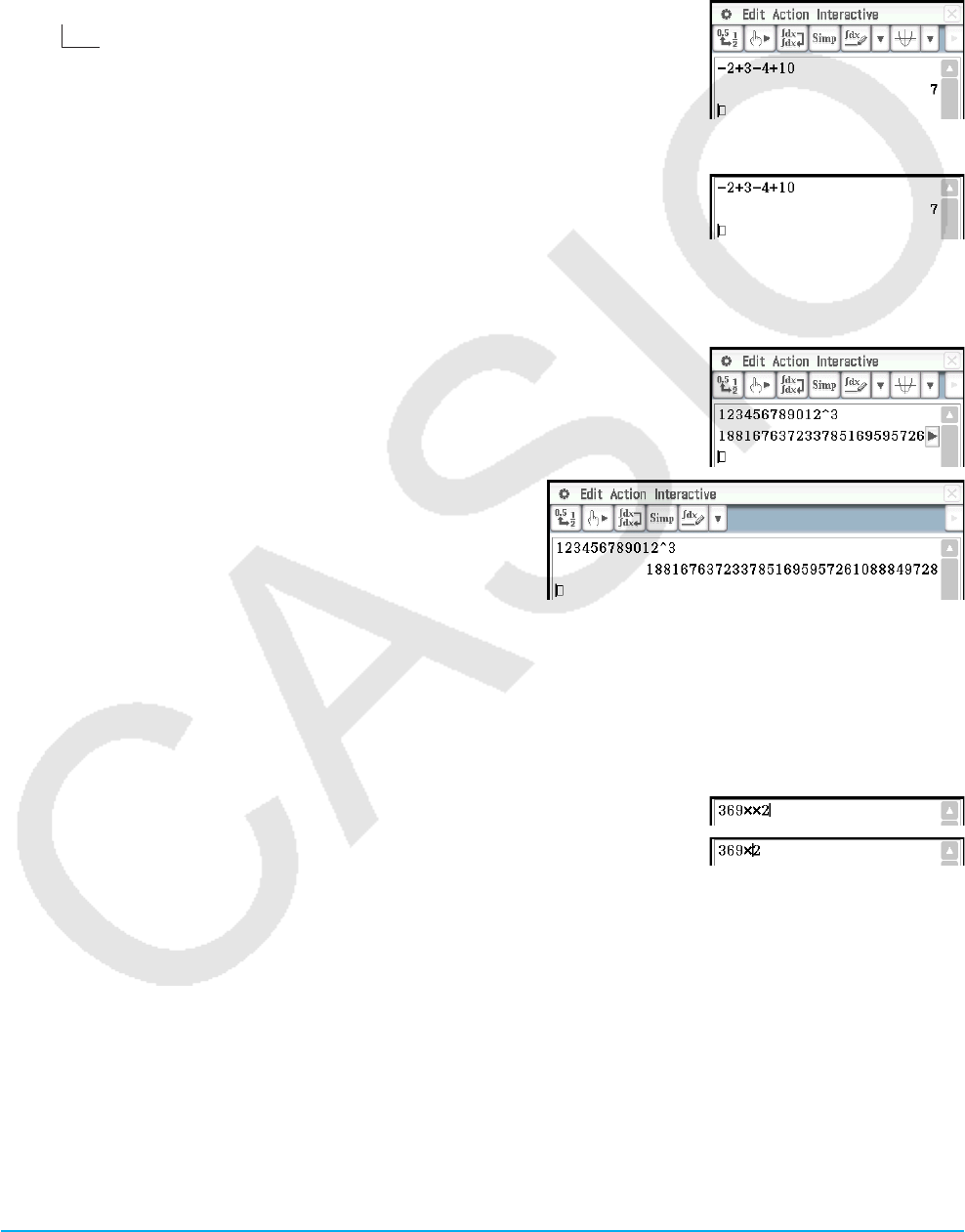
[Var] (variable) key set
This key set includes only keys for the input of single-character variables. For
more information, see “Using Single-character Variables” (page 25).
[abc] key set
Use this key set to input alphabetic characters. Tap one of the tabs along the
top of the keyboard (along the right when using horizontal display orientation)
to see additional characters, for example, tap [Math]. For more information, see
“Using the Alphabet Keyboard” (page 26).
[Catalog] key set
This key set provides a scrollable list that can be used to input built-in
functions, built-in commands, system variables, and user-defined functions.
Tap a command to select it and then tap it again to insert it. Selecting an item
from the Form list changes the available commands. For more information, see
“Using the Catalog Keyboard” (page 27).
[Number] key set
This key set provides the same keys as those on the keypad. Use this key set
when you want to use only the touch screen for input or in place of the keypad
while using horizontal (landscape) display orientation.
Input Basics
This section includes a number of examples that illustrate how to perform basic input procedures. All of the
procedures assume the following.
• The Main application is running. See “Built-in Applications” (page 14).
• The soft keyboard is displayed. See “Using the Soft Keyboard” (page 18).
Chapter 1: Basics 20
kInputting a Calculation Expression
You can input a calculation expression just as it is written, and press the E key to execute it. The
ClassPad automatically determines the priority sequence of addition, subtraction, multiplication, division, and
parenthetical expressions.
Example: To simplify −2 + 3 − 4 + 10
uUsing the keypad keys
cz2+3-4+10E
If the line where you want to input the calculation expression already
contains input, be sure to press c to clear it.
uUsing the soft keyboard
Tap the keys of the [Number] keyboard to input the calculation expression.
c4-c+d-e+baw
As shown in the above Example, you can input simple arithmetic calculations using either the keypad keys
or the soft keyboard. Input using the soft keyboard is required to input higher level calculation expressions,
functions, variables, etc. See Chapter 2 for more information about inputting expressions.
Tip: In some cases, the input expression and output expression (result) may not fit in
the display area. If this happens, tap the left or right arrows that appear on the
display to scroll the expression screen and view the part that does not fit.
You can also change the display orientation to horizontal
(landscape) for easier-to-read display of long input formulas
and calculation results. See “Changing the Display
Orientation” (page 16).
kEditing Input
uTo delete a single character
Move the cursor so it is directly to the right of the character you want to delete, and then press K. Each
press of K deletes one character to the left of the cursor.
Example: To change the expression 369 × × 2 to 369 × 2
1. c369**2
2. dK
After you make all of the changes you want, press E to calculate the result. To add more characters to the
calculation, press e to move the cursor to the end of the calculation, and input what you want.
Tip: You can move the cursor without using the cursor key by tapping at the destination with the stylus. This causes the
cursor to jump to the location where you tap.
uTo insert new input into the middle of an existing calculation expression
Use d or e to move the cursor to the location where you want to insert new input, and then input what you
want.
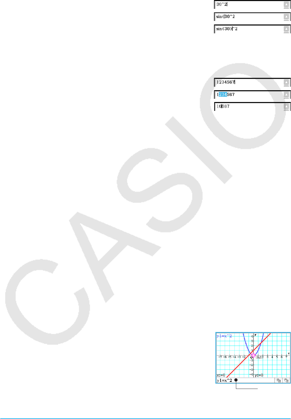
Chapter 1: Basics 21
Example: To change 302 to sin(30)2 (For input, use the keypad and the [Math1] soft keyboard set.)
1. c30x
2. dddds
3. ee)
uTo replace a range of input with new input
After you drag the stylus across the range of input that you want to replace, enter the new input.
Example: To change “1234567” to “10567”
1. c1234567
2. Drag the stylus across “234” to select it.
3. 0
k Using the Clipboard for Copy and Paste
You can copy (or cut) a function, command, or other input to the ClassPad’s clipboard, and then paste the
clipboard contents at another location. Performing a copy or cut operation causes the current clipboard
contents to be replaced by the newly copied or cut characters.
uTo copy characters
1. Drag the stylus across the characters you want to copy to select them.
2. On the soft keyboard, tap p. Or tap the [Edit] menu and then tap [Copy].
• This puts a copy of the selected characters onto the clipboard.
uTo cut characters
1. Drag the stylus across the characters you want to cut to select them.
2. Tap the [Edit] menu and then tap [Cut].
• This causes the selected characters to be deleted, and moves them onto the clipboard.
uTo paste the clipboard contents
1. Move the cursor to the location where you want to paste the clipboard contents.
2. On the soft keyboard, tap q. Or tap the [Edit] menu and then tap [Paste].
• This pastes the clipboard contents at the current cursor location.
Tip: The clipboard contents remain on the clipboard after you paste them. This means you can paste the current contents
as many times as you like.
Copying and pasting in the message box
The “message box” is a 1-line input and display area under the Graph window
(see Chapter 3).
You can use the two buttons to the right of the message box to copy the
message box contents (p button), or to paste the clipboard contents to the
message box (q button). Copy and paste are performed the same way as the
copy and paste operations using the soft keyboard.
Message box
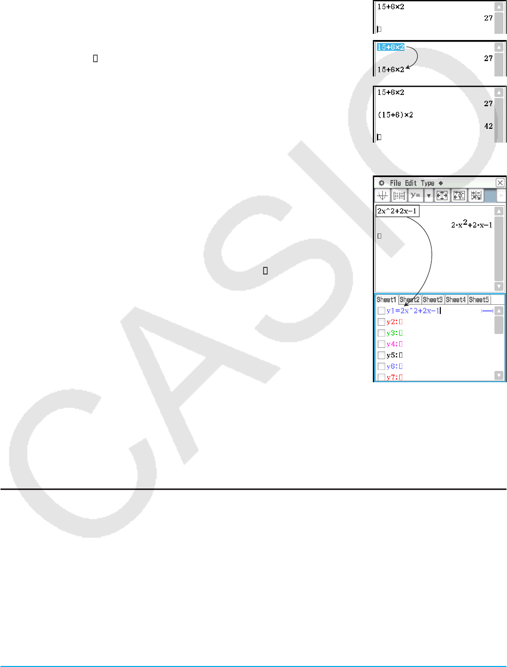
Chapter 1: Basics 22
kCopying with Drag and Drop
You can also copy a string of text by simply selecting it and then dragging it to another location that allows text
input.
Example 1: To use the Main application to perform the calculation 15 + 6 × 2, edit to (15 + 6) × 2, and then
re-calculate
1. In the Main application work area, perform the calculation below.
c15+6*2E
2. Drag across the 15 + 6 × 2 expression to select it, and then drag the
expression to the .
• This will copy 15 + 6 × 2 to the location where you dropped it.
3. Add parentheses before and after 15 + 6 and then press E.
Tip: You can use drag and drop to copy both input formulas and calculation results.
Example 2: To copy an expression you input with the Main application to the Graph Editor window
1. In the Main application work area, input: 2x^2 + 2x − 1.
c2x{2+2x-1E
2. On the right end of the toolbar, tap the down arrow button. On the button
palette that appears, tap !.
• This will display the Graph Editor window in the bottom half of the screen.
3. Select the 2x^2 + 2x − 1 expression you input with the Main application by
dragging across it, and then drag the expression to the located to the right
of y1: on the Graph Editor window.
• This will copy 2x^2 + 2x − 1 to the location where you dropped it.
Tip
• An expression you copy using the operation above is registered to the Graph Editor
window of the Graph & Table application. For information about Graph Editor window
operations, see Chapter 3.
• Depending on the destination to which you drag a character string or an expression,
the drop operation may cause it to be converted automatically to a graph or a
figure. For example, dropping the expression in Example 2 into the Graph window will graph the expression. Refer to the
locations provided below to see examples using drag and drop.
- “2-9 Using the Main Application in Combination with Other Applications” (Chapter 2, page 92)
- “5-4 Graphing an Expression or Value by Dropping It into the Differential Equation Graph Window” (Chapter 5, page 128)
- “8-5 Using the Geometry Application with Other Applications” (Chapter 8, page 177)
- “13-1 Inputting and Editing Cell Contents” (Chapter 13, page 228), “13-2 Graphing” (Chapter 13, page 237)
Various Soft Keyboard Operations
This section explains how to use each of the soft keyboard key sets. For information about key set types and a
general overview of key sets, see “Soft Keyboard Key Sets” (page 18). All of the examples in this section assume
the following conditions.
• The Main application is running. See “Built-in Applications” (page 14).
• The soft keyboard is displayed. See “Using the Soft Keyboard” (page 18).

Chapter 1: Basics 23
k Using Math, Trig, and Advance Key Sets
The [Math1], [Math2], [Math3], [Trig] (trigonometric), and [Advance] key sets
contain keys for inputting numeric expressions.
The L key in the upper left corner and all of the keys in the bottom row are
common to all key sets. Their functions are described below.
L Switches between template input and line input. See “Template Input
and Line Input” (page 24).
h Performs the same operation as the keypad’s K key. Deletes the
character to the left of the current cursor position.
pq See “Using the Clipboard for Copy and Paste” (page 21).
D Inputs “ans”. See “Using the Answer Variable (ans)” (page 45).
w Performs the same operation as the keypad’s E key, which executes calculations.
The keys in the following table are found on different key sets and are used to input functions and commands
for performing particular calculations and operations.
Key set Key Description
Math1, Math2,
Math3, Trig
N5 “Template Input and Line Input” (page 24), “Other Functions”
(page 50)
pInputs pi (π).
WInputs the substitution symbol (⇒). “Creating a New Variable”
(page 33)
Math1, Math2,
Trig
m“Logarithmic Functions and Exponential Functions” (page 49)
sct “Trigonometric and Inverse Trigonometric Functions” (page 49)
Math1, Math2 QI“Logarithmic Functions and Exponential Functions” (page 49)
Math1, Math2 4Inputs the absolute value symbol (| |) or function (abs().
Math1, Math3 .“solve [Action][Equation/Inequality][solve]” (page 81)
Math1, Math3 (Inputs parentheses (( )).
Math1, Math3 )Inputs brackets ({ }). “2-4 List Calculations” (page 57)
Math1, Trig *R “Angle Conversion (°, r)” (page 48)
Math1 V"% “Logarithmic Functions and Exponential Functions” (page 49)
Math1 wE “Other Functions” (page 50)
Math1 /“dms [Action][Transformation][DMS][dms]” (page 64)
Math1 a“toDMS [Action][Transformation][DMS][toDMS]” (page 64)
Math1 #“solve [Action][Equation/Inequality][solve]” (page 81)
Math2, Math3,
Trig
iInputs the imaginary unit (i).
eInputs the infinity symbol (∞).
Math2, Trig 8Inputs the
θ
variable.
Math2, Trig [Inputs the single-character variable (page 25) t.

Chapter 1: Basics 24
Key set Key Description
Math2 `*7
]_) “Using the Calculation Submenu” (page 67)
Math2 678 “2-5 Matrix and Vector Calculations” (page 58)
Math3 d“To create a user-defined function using the Define command”
(page 203)
Math3 fg Inputs the “f” of f(x), or the “g” of g(x).
Math3 '“Derivative Symbol (’)” (page 54)
Math3 +“dSolve [Action][Equation/Inequality][dSolve]” (page 82)
Math3 1“piecewise Function” (page 54)
Math3 U“with Operator ( | )” (page 55)
Math3 [Inputs square brackets ([ ]). “2-5 Matrix and Vector Calculations”
(page 58)
Math3 <>;:=/ “Equal Symbols and Unequal Symbols” (page 55)
Math3 ~“Angle Symbol (∠)” (page 54)
Trig SCT “Trigonometric and Inverse Trigonometric Functions” (page 49)
Trig 123
!@# “Hyperbolic and Inverse Hyperbolic Functions” (page 49)
Advance :!“Other Functions” (page 50)
Advance PN “Permutation (nPr) and Combination (nCr)” (page 53)
Advance NM<
hin“Chapter 6: Sequence Application”
Advance r“About rSolve” (page 131)
Advance 5%(^ “Using the Advanced Submenu” (page 64)
Advance 7“Gamma Function” (page 57)
Advance 6“Dirac Delta Function” (page 56)
Advance l“nth-Delta Function” (page 56)
Advance '“Heaviside Unit Step Function” (page 56)
k Template Input and Line Input
ClassPad supports two different input methods: template input and line input. Template input lets you input
fractions, powers, and other functions using formats that are the same as those in textbooks. Line input uses a
linear format for inputting expressions.
2+
( )
2'
2
'
2+ 1
2
2+ (2 (2) / ( (2) + 1))^2
Template Input Line Input
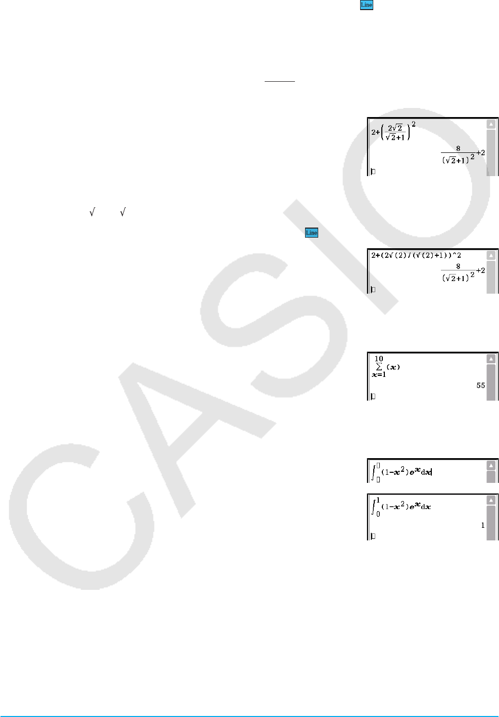
Chapter 1: Basics 25
uSwitching between Template Input and Line Input
Tap the L key. Each toggles the key color between white (L) and light blue ( ).
A white key indicates the template input mode, while a light blue key indicates the line input mode.
In the template input mode, you can perform template input using keys with or marked on their key tops,
such as N and !. Other keys input the same functions or commands as they do in the line mode.
Example 1: To use the template input mode to input
1. Tap the [Math1] tab and then enter the template input mode (white L key).
2. Perform the key operation below:
2+(N2!2c!2e+1
eem2E
Example 2: To use the line input mode to input the same expression as in Example 1
(2+ (2 (2) / ( (2) + 1))^2)
1. Tap the [Math1] tab and then enter the line input mode (light blue key).
2. Perform the key operation below:
2+(d2!2)N
(!2)+1)ewE
Example 3: To use the template input mode to input
1. Tap the [Math2] tab and then enter the template input mode (white L key).
2. Perform the key operation below:
Oxe1f10exE
Example 4: To use the template input mode to input
1. Tap the [Math2] tab and then enter the template input mode (white L key).
2. Perform the key operation below:
7(1-xm2e)Qxeex
3. Tap the upper right input box of
∫
and then press 1. Next, tap the lower
right input box of
∫
and then press 0.
4. To execute the calculation, press E.
Tip: For information about the contents and input formats of the functions in Example 3 and Example 4, see “2-7 Using
the Action Menu” (page 61).
k Using Single-character Variables
As its name suggests, a single-character variable is a variable name that consists of a single character like
“a” or “x”. Input of single-character variable names is subject to different rules than input of a series of multiple
characters (like “abc”).
2+
( )
2'
2
'
2+ 1
2
Y()
∫
1
0(1 − 2)
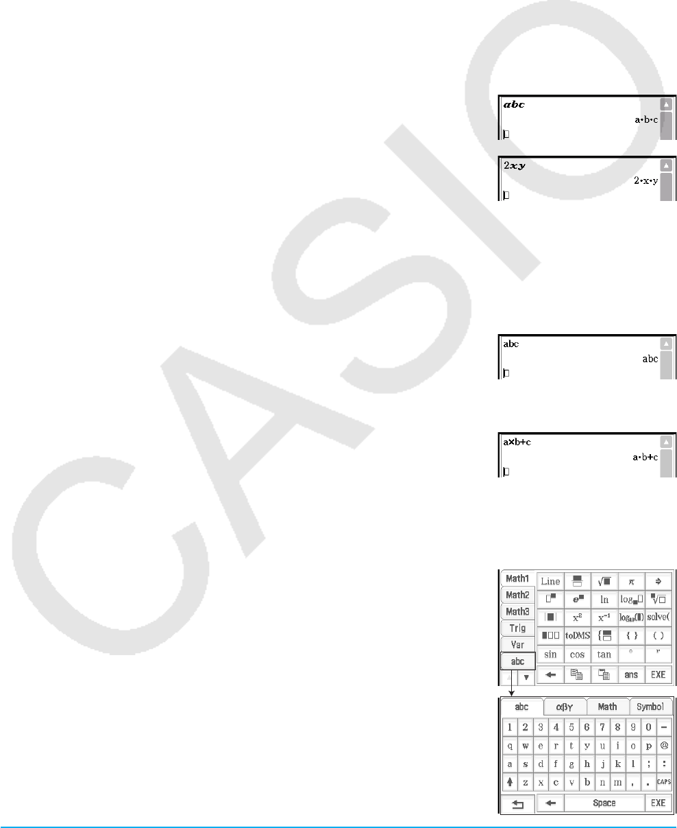
Chapter 1: Basics 26
uTo input a single-character variable name
Any character you input using any one of the following techniques is always treated as a single-character
variable.
• Tapping any key in the [Var] (variable) key set (page 19)
• Tapping the X, Y, or Z key of the [Number] key set
• Tapping the [ key of the [Math2] key set
• Pressing the x, y, or Z keypad key
If you use the above key operations to input a series of characters, each one is treated as a single-character
variable. Inputting A, B, C using the [Var] key set, for example, is treated as the mathematical expression
a × b × c, and not as the characters “abc”.
Tip: The single-character variables described above make it possible for you to perform calculations as they appear in
your textbook.
Example 1: ABCw
Example 2: 2xyE
Tip: When you input a single-character variable, its name appears on the display as an italicized character. This is simply
to let you know that the letter is a single-character variable name.
uTo input a series of multiple characters
A series of multiple characters (like “list1”) can be used for variable names, program commands, comment text,
etc. Always use the [abc] key set when you want to input a series of characters.
Example: abcE
You can also use the [abc] key set to input single-character variable names. To do so, simply input a single
character, or follow a single character with a mathematical operator.
Example: a*b+cE
Tip: A single-character variable you input using the [abc] key set is identical to a single-character variable you input using
the [Var] key set.
k Using the Alphabet Keyboard
Tap the [abc] tab to the left of the soft keyboard to display the alphabet
keyboard [abc] key set. In addition to the [abc] key set, you can also select
from among three other key sets named [αβγ] (character symbols), [Math]
(mathematics symbols), and [Symbol] (extra symbols).
Use the tabs above the alphabet keyboard (to the right of the keyboard when
using horizontal screen orientation) to select a key set. To return to the [Math1]
key set from the alphabet keyboard, tap the I key in the lower left corner.
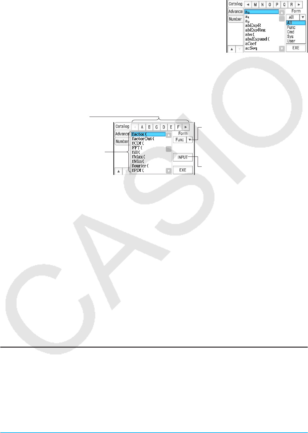
Chapter 1: Basics 27
k Using the Catalog Keyboard
The “Form” menu of the catalog keyboard lets you select one of the five categories described below.
Func ........ built-in functions (pages 48 and 61)
Cmd ........ built-in commands and operators (page 206)
Sys .......... system variables (page 299)
User ........ user-defined functions (page 203)
All ............ all commands, functions, etc.
After selecting a category, you can choose the item you want from the alphabetized list that appears on the
catalog keyboard.
Tip: Note that user-defined variables and user-defined programs cannot be input using the catalog keyboard. Use
Variable Manager (page 29) instead.
Catalog keyboard configuration
Tapping a letter button displays the
commands, functions, or other items that
begin with that letter.
This is an alphabetized list of commands,
functions, and other items available in the
category currently selected with “Form”.
Tap the down arrow button and then
select the category you want ([Func],
[Cmd], [Sys], [User], or [All]) from the list
that appears.
Tap this key to input the item that is
currently selected in the alphabetized list.
uTo use the catalog keyboard
Example: To input the built-in command “Plot”
1. On the catalog keyboard, tap the “Form” down arrow button and then select [Cmd] from the list of categories
that appears.
2. Tap the + button in the upper right corner until the P button is visible.
3. Tap P.
4. In the alphabetized list, tap “Plot” and then tap [INPUT] to input the command.
• Instead of tapping [INPUT], you could also tap the command a second time to input the command.
1-5 ClassPad Data
This section provides information about the various types of data that can be stored in ClassPad memory, and
the location where each type of data is stored. It also explains how to use Variable Manager, which is a tool for
managing stored data, as well as file operations (file save, recall, delete, rename, etc.) that are common to a
number of different applications.
Data Types and Storage Locations (Memory Areas)
ClassPad uses a “main memory” memory area to store various types of data.
Examples:
• Executing “10⇒x” (which assigns a value of 10 to variable x) in the Main application or eActivity application
causes variable x to be stored in main memory as “EXPR” (expression) type data.
• Creating a user-defined function (page 203) causes the function to be stored in main memory as “FUNC”
(function) type data.

Chapter 1: Basics 28
• Saving a spreadsheet to a file (by executing [File] - [Save] with the Spreadsheet application) saves the file in
main memory as “MEM” (memory) type data.
An eActivity file created with the eActivity is stored in a separate eActivity memory area in order to keep it
separate from other application data.
Accessing Data
Besides the application that originally created it, data in main memory can also be accessed by any other
application. It can also be deleted, renamed, copied, moved and otherwise accessed using Variable Manager
(page 29). eActivity files can be accessed from the eActivity application only.
Main Memory Data Types
Data stored in main memory has a data type attribute that is assigned in accordance with the application that
created the data and the actual content of the data. The data type is indicated by a data type name. Data type
names are shown on the Variable Manager variable list, and on the Select Data dialog box that appears when
you are specifying a variable in any ClassPad application. The following table lists all of the data type names
and explains the meaning of each.
Data Type Name Data Type
EXPR Real number, complex number or expression data
STR String data
LIST List data created using the Statistics application, Main application, etc.
MAT Matrix data created using the Main application, etc.
PRGM* General program
EXE* Edit prohibited program
TEXT* Text data
FUNC* User-defined function
GMEM* Graph memory data saved using the Graph & Table application
For more information, see “Saving Graph Editor Data to Graph Memory” (page 102).
GEO* Geometry application data
MEM* Data saved to a file using one of the following applications: Spreadsheet, Geometry,
Verify (page 94), Probability (page 95).
OTHR Data other than that described above
Protected variable types
Some data types are protected. A variable whose data type is protected cannot be overwritten with another
variable, which protects variable contents from being inadvertently altered. Data types whose names are
marked with an asterisk in the above table are protected. Note that whether or not a data type is protected is
determined by the system. You cannot change the protection status of a data type.
Tip: Even when a variable is a protected data type, you can rename, delete, or move it. To disable these operations, you
need to lock the variable. See “Variable Manager operations” on page 30.
Main Memory Folders
Your ClassPad stores data in one of the following types of folders described below.
“main” folder: The “main” folder is a ClassPad reserved folder, and acts as the default current folder (see
“Current Folder” below).
“library” folder: Also a ClassPad reserved folder, the “library” folder can be used for storing user-created data
(variables, programs, user functions, etc.). Data stored in the “library” folder can be accessed without specifying
a path, regardless of the current folder setting.
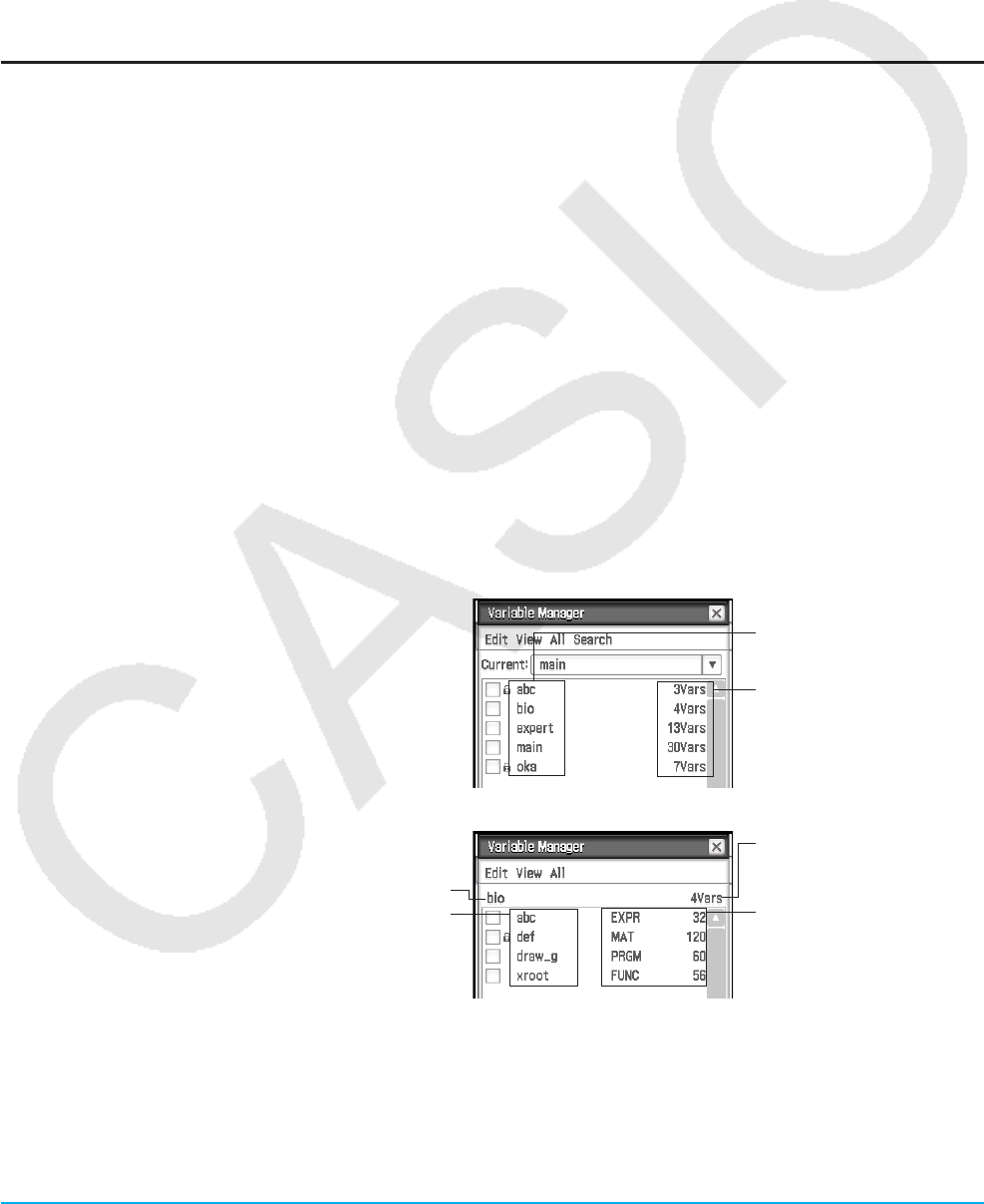
Chapter 1: Basics 29
User folder: This is a folder created and named by you. You can make a user folder the current folder, move
data to a user folder, etc. You can also delete and rename a user folder as required. You can have up to 87
user folders in main memory at one time.
Tip: You cannot put a folder inside of another folder.
Current Folder
The current folder is the folder where the data (excluding eActivity files) created by applications are stored
and from which such data can be accessed. The initial default current folder is the “main” folder. You can also
select a user folder you created as the current folder. For more information about how to do this, see “Variable
Manager operations” on page 30.
Using Variable Manager
Variable Manager is a tool for managing user variables, programs, user functions, and other types of data.
Though this section uses only the term “variables”, the explanations provided here also refer to the other types
of data that can be managed by Variable Manager.
With Variable Manager you can:
• Create, delete, rename, lock, and unlock folders, and configure current folder settings.
• Delete, copy, rename, move, lock, unlock, search for variables, and view the contents of variables.
About Variable Types
A variable with a letter name like x and y can be a user-created user variable, a system variable, or a local
variable.
• System variables are pre-defined reserved variables, and cannot be renamed. For the names of and detailed
information about system variables, see the “System Variable Table” on page 299.
• A local variable is a variable that is temporarily created by a defining function, program, or other operation for
a particular purpose. For more information about local variables, see the “Local” command under the “12-4
Program Command Reference”.
uTo start up Variable Manager
1. While any application (except for the System
application) is running, tap O and then tap
[Variable Manager].
• This displays the folder list. The folder list
always appears first whenever you start up
Variable Manager.
Folder list
Folder name
Number of variables
contained in the folder
2. Tap a folder name twice to open the folder
contents; a variable list.
Folder name
Variable name
• To close the variable list and return to the
folder list, tap [Close].
Variable list
Number of variables
contained in the folder
Data types (page 28) and
sizes (bytes)
3. To exit Variable Manager, tap [Close] on the folder list.

Chapter 1: Basics 30
u Variable Manager operations
The operations described in the table below can be performed while Variable Manager is displayed.
To do this: Do this:
Specify the current folder On the folder list, tap the [Current] down arrow button. On the list that appears,
select the folder that you want to specify as the current folder.
Create a folder On the folder list, tap [Edit] - [Create Folder]. On the dialog box that appears,
enter the name you want to assign to the folder and then tap [OK].
Open a folder On the folder list, tap the name of the folder you want to open so it is
highlighted, and then tap it again.
Open the “library” folder Tap [View] and then [“library” Folder]. This opens the “library” folder and
displays a variable list showing its contents.
Select a folder or variable Select the check box next to the folder or variable name. To select all the
folders or variables in the list, tap [All] and then [Select All].
Deselect a folder or
variable
Clear the check box next to the folder or variable name. To deselect all the
folders or variables in the list, tap [All] and then [Deselect All].
Delete a folder See “To delete a folder” (page 31).
Delete a variable Select the check box next to the variable you want to delete, and then tap [Edit]
- [Delete]. In response to the confirmation dialog box that appears, tap [OK] to
delete the selected variable.
Rename a folder or
variable
Highlight the folder or variable you want to rename and then tap [File] -
[Rename]. On the dialog box that appears, enter the name you want to assign
to it and then tap [OK].
Lock a folder or variable Select the check box next to the folder or variable you want to lock, and then
tap [Edit] - [Lock]. This locks the currently selected folder or variable, and adds
a b icon to the left of its name to indicate that it is locked.
Unlock a folder or variable Select the check box next to the folder or variable you want to unlock, and then
tap [Edit] - [Unlock].
Display a list of a
particular type of variable
On the variable list, tap [View] - [Variable Type]. On the dialog box that appears,
tap the down arrow button and then select the data type from the list that
appears and then tap [OK].
Copy or move a variable On the variable list, tap [Edit] and then [Copy] or [Move]. On the dialog box that
appears, tap the down arrow button and then select the destination folder from
the list that appears and then tap [OK].
Tip
• If a variable with the same name already exists in the destination folder, the variable in
the destination folder is replaced with the one that you are copying or moving.
• A variable that is locked cannot be moved.
View the contents of a
variable
On the variable list, tap the name of the variable whose contents you want to
view so it is highlighted, and then tap it again. This displays a dialog box that
shows the contents of the variable.
Input a folder name or
variable name into an
application
See “To input a folder name or variable name into an application” (page 31).
Search for a variable On the folder list, tap [Search]. On the dialog box that appears, enter the
variable name you want to find and then tap [OK].
An exclamation point (!) appears in front of all folders containing a variable
name that matches the name in your search.
Note: You can use the above procedure to search the “main” folder or a user
defined folder for a particular variable name. Note that you cannot search the
“library” folder.

Chapter 1: Basics 31
Selecting a Folder
• If no check box is selected on the folder list, any folder operation that is performed affects the folder whose
name is currently highlighted on the list. If any folder check box is selected, only that folder is affected by a
folder operation, and the folder whose name is highlighted on the list is not affected.
• Selecting the check box of a folder causes the check boxes of all of the variables inside of it also to become
selected.
• When renaming a folder, only the folder whose name is highlighted on the folder list is renamed. Other folders
whose check boxes are selected are not affected.
Selecting a Variable
• If no check box is selected on the variable list, any variable operation that is performed affects the variable
whose name is currently highlighted on the list. If any variable check box is selected, only that variable is
affected by a variable operation, and the variable whose name is highlighted on the list is not affected.
• When renaming a variable, only the variable whose name is highlighted on the variable list is renamed. If
other variables are selected (checked), they will not be affected.
Folder and Variable Name Rules
The following are the rules that apply to folder and variable names.
• Folder or variable names can be up to 8 bytes long.
• The following characters are allowed in a folder or variable name: Upper-case and lower-case characters,
subscript characters, numbers, underscore (_).
• Folder or variable names are case-sensitive. For example, each of the following is treated as a different
folder/variable name: abc, Abc, aBc, ABC.
• A reserved word (system variable names, built-in function names, command names, etc.) cannot be used as
a folder or variable name.
• A number, subscript characters or the underscore (_) cannot be used as the first character of a folder or
variable name.
u To delete a folder
Important!
Before deleting a folder, make sure you no longer need any of the variables contained inside it. It is probably
a good idea to first delete the variables you don’t need, move the variables you do need to another folder, and
then delete the empty folder.
1. Open the folder you want to delete and check its contents.
• Make sure you no longer need any of the variables in the folder. If any of the variables are locked, unlock
them.
• After checking the contents of the folder, close it to return to the folder list.
2. Select the check box next to the folder you want to delete.
• You can select and delete multiple folders, if you want.
3. On the folder list, tap [Edit] and then [Delete].
4. In response to the confirmation dialog box that appears, tap [OK] to delete the folder.
Tip: You cannot delete the “library” folder or the “main” folder.
u To input a folder name or variable name into an application
1. In the Main application, Graph & Table application, or some other application, move the cursor to the location
where you want to input the variable name.
2. Start up Variable Manager to display the folder list.
3. If you want to input a variable name, double-tap the folder that includes the variable whose name you want to
input. If you want to input a folder name, advance to the next step.

Chapter 1: Basics 32
4. Tap the folder or variable whose name you want to input, so its name is highlighted.
5. Tap [INPUT].
• This exits Variable Manager and inputs the name of the folder or variable you selected in step 4 into the
application at the current cursor position.
Managing Application Files
The applications below can save data to files.
Geometry (Chapter 8), eActivity (Chapter 10), Spreadsheet (Chapter 13), Verify (page 94), Probability (page 95),
Picture Plot (Chapter 15)
This section explains the common operations that can be performed on data files created with these
applications.
Tip: The eActivity file save dialog box is slightly different from the save dialog box of the other applications, but operations
are basically the same.
uTo save a file
1. Tap [File] and then [Save].
2. On the dialog box that appears, tap the name of the folder where you want to save the file so it is selected.
3. Input up to 8 bytes for the file name in the file name edit box, and then tap [Save].
uTo open an existing file
1. Tap [File] and then [Open].
2. On the dialog box that appears, open the folder that contains the file you want to open.
3. Tap the name of the file you want to open so it is selected, and then tap [Open].
uTo search for a file
1. Tap [File] and then [Open].
2. On the dialog box that appears, tap [Search]. This displays the Search dialog box.
3. Enter the file name you want to find and then tap [Search].
• File names that match the one you enter become highlighted on the display. Tapping [Open] opens the
highlighted file.
• To search for the next occurrence of the file name, tap [Search] again and then tap [Next] on the Search
dialog box.
uTo delete a folder or file
Important!
Deleting a folder also deletes all files inside of it. Please double-check to make sure you no longer need the
contents of a folder before deleting it.
1. Tap [File] and then [Open].
2. On the dialog box that appears, select the check box next to the folder or file you want to delete.
• You can select multiple folders/files for deletion, if you want.
• Selecting a check box next to a folder name automatically checks the boxes for all files inside that folder.
3. Tap [File] and then [Delete].
4. In response to the confirmation dialog box that appears, tap [OK] to delete the folder(s) or file(s).
Tip: Selecting a folder in the above procedure deletes the folder and all of its contents. Note, however, that the “main”
folder cannot be deleted, even if you check it.

Chapter 1: Basics 33
uTo rename a folder or file
1. Tap [File] and then [Open].
2. On the dialog box that appears, tap the name of the folder or file you want to rename so it is selected.
3. Tap [File] and then [Rename]. This displays the Rename dialog box.
4. Enter the name you want to assign to it and then tap [OK].
uTo move a file to another folder
1. Tap [File] and then [Open].
2. On the dialog box that appears, select the check box next to the file you want to move.
• To move multiple files, select all of their check boxes.
3. Tap [File] and then [Move].
• This causes a dialog box for selecting the destination folder to appear.
4. On the dialog box, tap the down arrow button and then select the destination folder from the list that appears.
5. Tap [OK] to move the files.
uTo switch the file menu view between List View and Detail View (eActivity application only)
1. Tap [File] and then [Open].
2. On the dialog box that appears, open the folder that contains the files you want to list.
3. To display both the file name and file size, tap [View] - [Detail View]. To display file names only, tap [View] -
[List View].
uTo create a new folder
1. Tap [File] and then [Open].
2. On the dialog box that appears, tap [File] and then [Create Folder], or tap {.
• This displays the Create Folder dialog box.
3. Enter up to 8 bytes for the folder name, and then tap [OK] to create a folder.
1-6 Creating and Using Variables
This section explains how to create a new variable (user variable), and provides a simple sample calculation
that illustrates how to use a variable.
Creating a New Variable
The most common way to create a new variable is assigning a value or expression to the applicable variable
name. Use the variable assignment key (W) to assign data to a variable.
The following is an example of assignment to a variable while “main” is specified as the current folder.
Example: To create a new variable named “eq1” and assign the expression 2x + 1 to it
The following assumes that there are no variables named “eq1” or “x” currently in the “main” folder.
uClassPad Operation
1. Start the Main application.
2. Press k to display the soft keyboard, and then perform the following key operation.
2x+11W0eqbw

Chapter 1: Basics 34
• This creates a variable named “eq1” in the current folder (the “main” folder
in this example), and assigns the expression 2x + 1 to it.
Tip
• If a variable with the specified name already exists in the current folder, the contents of the existing variable are replaced
with the newly assigned data, unless the existing variable is locked or protected. For more information, see “Variable
Manager operations” (page 30) and “Protected variable types” (page 28).
• To store the newly created variable in a folder other than the current folder, specify the variable name as follows:
<folder name>\<variable name>.
• You can use Variable Manager to view the contents of a variable you create. For more information, see “Variable Manager
operations” (page 30).
• For information about rules for naming variables, see “Folder and Variable Name Rules” (page 31).
Variable Usage Example
The following example uses the variable we created in the example under “Creating a New Variable” above.
Example: To assign values of 5 and 10 to x and check the results of eq1 (= 2x + 1)
uClassPad Operation
1. Assign 5 to x.
51WxE
2. Check the contents of variable “eq1”.
0eqbw
• This displays the calculation result of 2x + 1 when x = 5.
3. Assign 10 to x.
101WxE
4. Check the contents of variable “eq1”.
0eqbw
“library” Folder Variables
Variables in the “library” folder can be accessed without specifying a path name, regardless of the current folder.
Example: To create and access two variables, one located in the “library” folder and one located in another
folder
uClassPad Operation
1. With “main” specified as the current folder, perform the following operation to create a variable named “eq1”
and assign the indicated list data to it.
{1, 2, 3} W eq1w
2. Keeping “main” specified as the current folder, perform the following operation to create a variable named
“eq2” in the “library” folder, and assign the indicated list data to it.
{4, 5, 6} W library\eq2w
3. Check the contents of the two variables.
eq1w
eq2w
(Since variable “eq2” is stored in the “library” folder, you do not need to
indicate a path to access it.)

Chapter 1: Basics 35
4. Change the current folder specification to “Test”.
• Use Variable Manager (page 29) to create a folder named “Test” and change the current folder specification.
5. Perform the following operations to view the contents of variables “eq1” and “eq2”.
eq1E
(Since this key operation does not access the “main” folder, the variable
name (“eq1”) is displayed without showing the variable contents.)
main\eq1E
(Specifying the path to the “main” folder where “eq1” is located displays
the contents of the variable.)
eq2E
(Since variable “eq2” is stored in the “library” folder, you do not need to
indicate a path to access it.)
Tip: Specifying a variable name that exists in both the current folder and the “library” folder causes the variable in the
current folder to be accessed. For details about the variable access priority sequence and how to access variables in
particular folders, see “Rules Governing Variable Access” below.
Rules Governing Variable Access
Normally, you access a variable by specifying its variable name. The rules in this section apply when you need
to reference a variable that is not located in the current folder or to access a variable that has the same name
as one or more variables located in other folders.
kVariable Search Priority Sequence
Specifying a variable name to access a variable causes variables to be searched in the sequence below.
(1) Local variables (2) Current folder variables (3) “library” folder variables
• Multiple variables with the same name can exist simultaneously as a local variable, as a variable in the
current folder, and as a variable in the “library” folder. In this case, the ClassPad searches folders according
to the sequence shown above and accesses the first instance of the variable that it finds. If you want to
access such a variable when it occurs lower in the above sequence, you need to specify the folder name
along with the variable name as shown in “Specifying a Variable in a Particular Folder” below.
• If a variable you specify cannot be found, it is treated as an “undefined variable”.
• Note that “system” variables are not included in the above variable search. When accessing a system
variable, you need to specify the variable name only, without specifying the folder name.
Tip: Only local variables and current folder variables are searched in the case of an operation that stores variable data
or a command that performs an operation on a variable (like “DelVar”). Normally, “library” folder variables are not
searched. If you want to include “library” folders in the search, you need to specify the “library” folder as the variable
location as explained below.
kSpecifying a Variable in a Particular Folder
You can access a variable located inside the “main” folder, “library” folder, or a particular user folder by
specifying the folder name along with the variable name.
Use the following syntax when specifying a folder name:
<folder name>\<variable name>
Example: To specify variable “abc” located in the “main” folder
main\abc
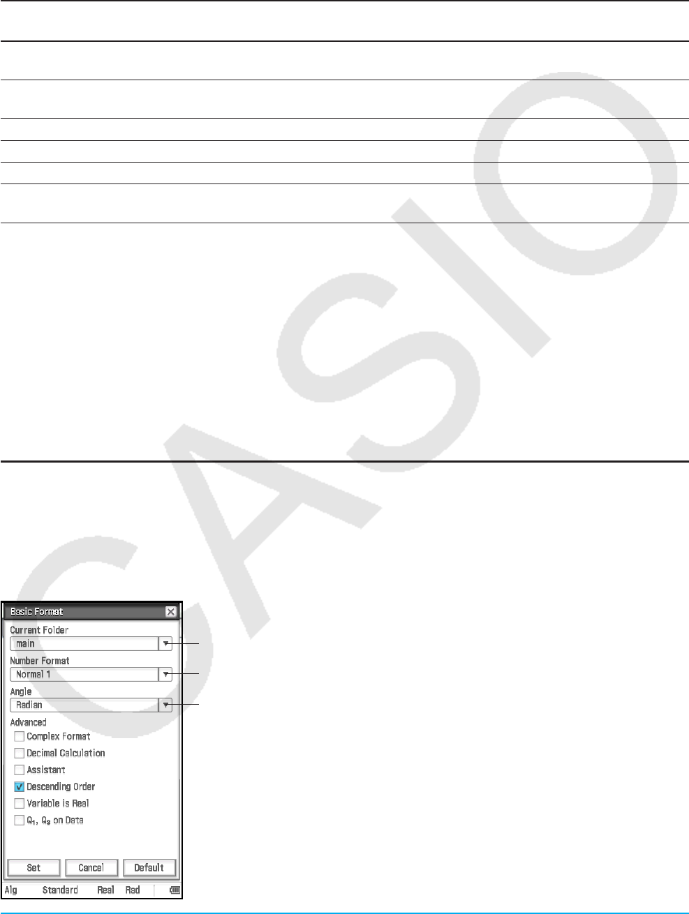
Chapter 1: Basics 36
1-7 Configuring Application Format Settings
The O menu includes format settings for configuring the number of calculation result display digits and
the angle unit, as well as application-specific commands. The following describes each of the settings and
commands that are available on the O menu.
To do this: Select this O
menu command:
Specify folder for variables, and to configure number format, angle, and other basic
settings for all built-in applications
Basic Format
Configure Graph window and graph drawing settings for Graph & Table, Conics, and
other graphing applications
Graph Format
Configure number format, angle, and other settings for Geometry application Geometry Format
Configure Fourier transform and FFT settings Advanced Format
Configure Financial application settings Financial Format
Return all the above menu settings to their initial default values (except for the current
folder setting specified on Basic Format dialog box)
Default Setup
uTo configure application format settings
1. Open any application (except the System application).
2. Tap O. Next, tap the menu command you want: Basic Format, Graph Format, Geometry Format, Advanced
Format, or Financial Format.
3. Use the dialog box to configure the settings you want.
• For details about the settings you can configure on each of the dialog boxes, see “Application Format
Settings” below.
4. To close a dialog box and apply its settings, tap [Set]. To close a dialog box without applying its settings, tap
[Cancel] or the C button in the upper right corner of the dialog box.
Application Format Settings
This section provides details about all of the settings you can configure using the application format settings.
Settings marked with an asterisk (*) in the following explanations are ClassPad initial default settings.
k Basic Format Dialog Box
Use the Basic Format dialog box to configure basic settings for calculations, cells, and other parameters.
1
2
3
To specify the current folder
Tap 1 and then tap the name of the folder (main*) you want.
To specify the numeric value display format
Tap 2 and then tap one of the settings described below.
Normal 1*: Automatically uses exponential display format when calculation
result x is: 10−2 > |x| or |x| t 1010.
Normal 2: Automatically uses exponential display format when calculation
result x is: 10−9 > |x| or |x| t 1010.
Fix 0 – Fix 9: Fixed number of decimal places
Sci 0 – Sci 9: Fixed number of significant digits
To specify the angle unit
Tap 3, and then tap “Radian*”, “Degree”, or “Grad”.
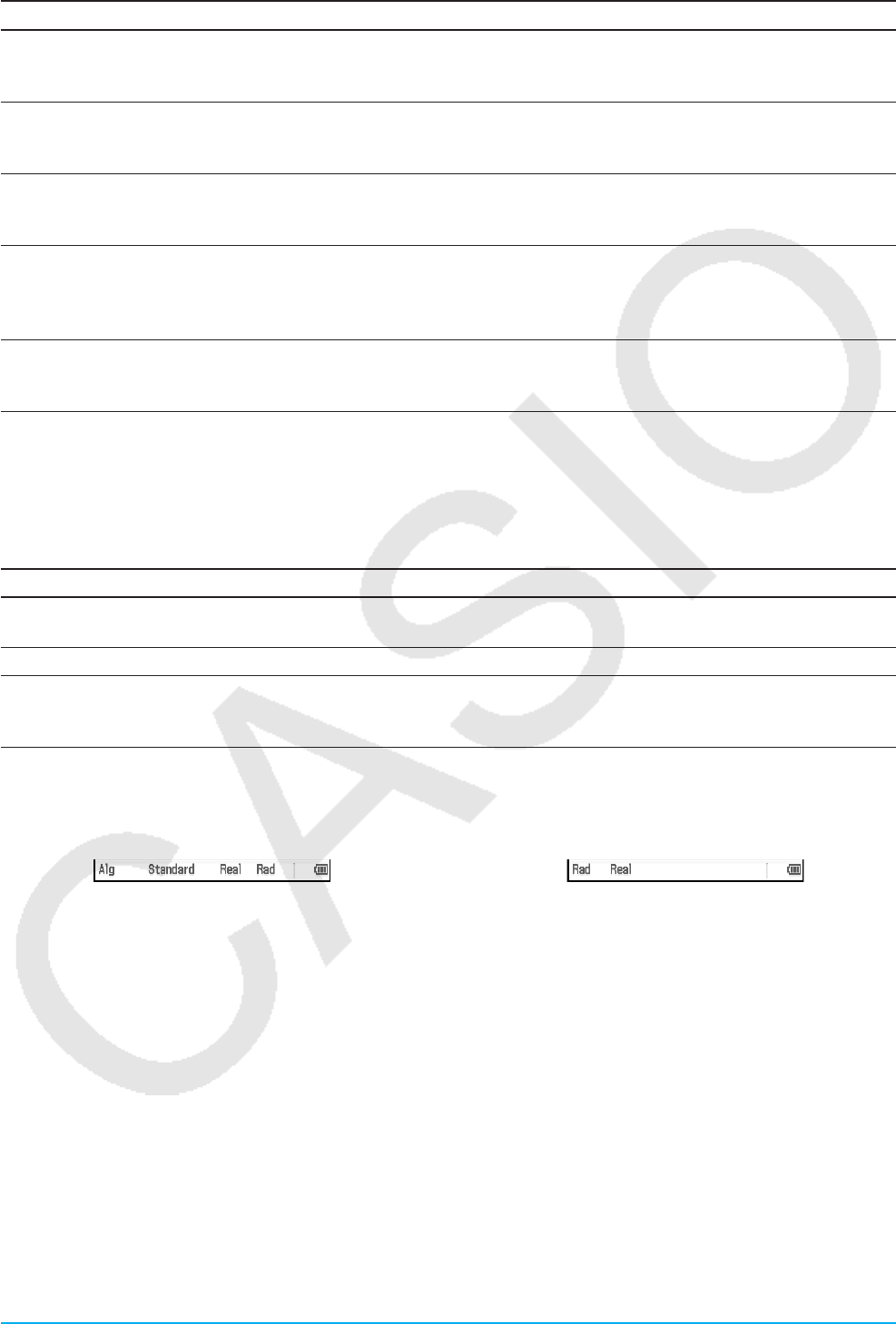
Chapter 1: Basics 37
To do this: Do this:
Switch between complex number calculations
(Complex mode) and real number calculations (Real
mode)
Select the “Complex Format” check box to enter the
Complex mode, or clear the check box* to enter the
Real mode*.
Display results as a decimal value (Decimal mode)
or leave calculation results as expressions (Standard
mode)
Select the “Decimal Calculation” check box to enter
the Decimal mode, or clear the check box* to enter
the Standard mode.
Turn auto simplification of expressions on (Algebra
mode) or off (Assistant mode)
Select the “Assistant” check box to enter the
Assistant mode, or clear the check box* to enter the
Algebra mode. See page 47 for details.
Specify descending order or ascending order for the
calculation result expression
Select the “Descending Order” check box* to display
calculation result expressions in descending order
(like x2 + x + 1), or clear the check box to display in
ascending order (like 1 + x + x2).
Specify whether variables in Complex Mode
calculation should be treated as real numbers or
complex numbers
Select the “Variable is Real” check box to treat
variables as real numbers, or clear the check box* to
treat variables as complex numbers.
Tip: For information about the “Q1, Q3 on Data” check box, see “Calculation Methods for Q1, Q3 and Median” (page 141).
Using Status Bar to Change Application Format Settings
With the applications listed in the table below, you can use the status bar to check and modify a number of
Basic Format dialog box settings.
For this application: You can check and change these settings:
Main, eActivity Algebra mode/Assistant mode setting, Standard mode/Decimal mode
setting, Complex mode/Real mode setting, angle unit setting
Statistics Standard mode/Decimal mode setting, angle unit setting
Graph & Table, Conics,
Differential Equation Graph,
Numeric Solver, Sequence
Complex mode/Real mode setting, angle unit setting
uTo use the status bar to change application format settings
On the status bar, tap the text of the setting you want to change.
Main application Graph & Table application
Each tap changes the tapped item as described below.
• “Alg” ↔ “Assist” ... Toggles between the Algebra mode and Assistant mode.
• “Standard” ↔ “Decimal” ... Toggles between the Standard mode and Decimal mode.
• “Real” ↔ “Cplx” ... Toggles between the Real mode and Complex mode.
• “Rad” → “Deg” → “Gra” ... Cycles the angle unit setting between Radian, Degree, and Grad.
Tip: Changing a setting using the status bar has the same effect as changing the corresponding setting on the Basic
Format dialog box. This means the setting will be changed for all applications.
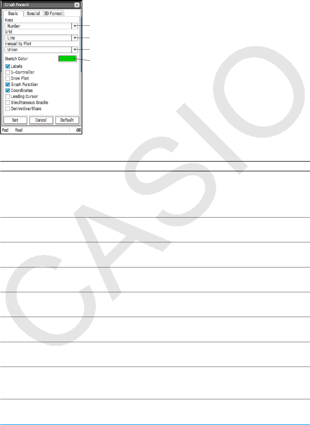
Chapter 1: Basics 38
k Graph Format Dialog Box
Use the Graph Format dialog box to configure settings for the Graph window and for drawing graphs.
[Basic] tab
1
2
3
4
To specify display of Graph window axes
Tap 1 and then tap one of the settings described below.
On: show axis Off: hide axis
Number*: show axis along with maximum and minimum value of each axis
To specify display of Graph window grid
Tap 2 and then tap one of the settings described below.
On: show grid as dots Off: hide grid
Line*: show grid as lines
To select inequality fill specification (Inequality Plot)
Tap 3 and then tap one of the settings described below.
Union*: fill areas where all inequality conditions are satisfied when
graphing multiple inequalities
Intersection: fill areas where each inequality condition is satisfied when
graphing multiple inequalities
To specify the color of figures and graphs drawn with the Sketch function (page 112)
Tap 4. On the dialog box that appears, select the color you want and then tap [OK].
To do this: Do this:
Turn display of Graph
window axis labels on
or off
Select the “Labels” check box* to show labels, or clear the check box to hide
labels.
Tip: Regardless of the “Labels” setting, labels are never displayed on the Sequence
application Graph window. Also, labels are not displayed for the following types
of graph drawn with the Statistics application: NPPlot, Histogram, MedBox, NDist
Broken.
Turn display of graph
controller arrows on
or off
Select the “G-Controller” check box to show graph controller arrows (page 105), or
clear the check box* to hide graph controller arrows.
Specify plotted points
or solid lines for graph
drawing
Select the “Draw Plot” check box to specify plotted points, or clear the check box*
to specify solid lines for graphing.
Turn display of the
function name and
function on or off
Select the “Graph Function” check box* to show the function name and function on
the graph, or clear the check box to hide the function name and function.
Turn display of Graph
window pointer
coordinates on or off
Select the “Coordinates” check box* to show Graph window pointer coordinates, or
clear the check box to hide the coordinates.
Turn display of the
leading cursor during
graphing on or off
Select the “Leading Cursor” check box to show the leading cursor, or clear the
check box* to hide the leading cursor.
Specify the draw
method when drawing
multiple graphs
Select the “Simultaneous Graphs” check box to draw multiple graphs
simultaneously, or clear the check box* to draw graphs in sequence, one at a time.
Show or hide
derivative values on
the Graph window and
Table window
Select the “Derivative/Slope” check box to show derivative values in the Graph
window and Table window, or clear the check box* to hide derivative values. For
details about display contents, see “Using Trace to Read Graph Coordinates”
(page 111) and “Generating a Number Table” (page 108).
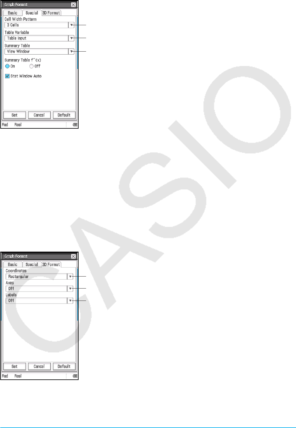
Chapter 1: Basics 39
[Special] tab
1
2
3
To specify the row width for Stat Editor and data table displays
Tap 1 and then select a cell width pattern: 2 Cells, 3 Cells*, or 4 Cells for
vertical display orientation, or 4 Cells, 5 Cells*, or 6 Cells for horizontal
orientation (see “Changing the Display Orientation” on page 16).
To specify a source for table data
Tap 2 and then tap one of the settings described below.
Table Input*: Uses the data input in a Table Input dialog box as the source
for number table generation.
list1 through list6: Uses list data in list1 through list6 as the source for
number table generation.
<list name>: Uses the list data in a selected list as the source for number
table generation.
For details about how to generate a number table using each setting, see
“Generating a Number Table” (page 108).
To specify a source for summary table data
Tap 3 and then tap one of the settings described below.
View Window*: Uses View Window settings as the source for summary table generation.
list1 through list6: Uses list data in list1 through list6 as the source for summary table generation.
<list name>: Uses the list data in a selected list as the source for summary table generation.
For details about how to generate a summary table using each setting, see “Generating a Summary Table”
(page 110).
To show or hide the second derivative for summary tables
Select the On button* under “Summary Table f (x)” to show the second derivative, or the Off button to hide it.
To specify auto setting or manual setting of Statistics application View Window settings
Select the “Stat Window Auto” check box* to specify automatic setting configuration, or clear the check box for
manual settings.
[3D Format] tab
1
2
3
To specify display of coordinate values
Tap 1, and then select “Rectangular*” (display rectangular coordinate
values), “Polar” (display polar coordinate values), or “Off” (turn off display
of coordinates).
To specify display of axes
Tap 2 and then select “On” (display axes normally), “Box” (display box
type coordinate axes), or “Off*” (turn off display of axes).
To turn display of Graph window axis labels on or off
Tap 3 and then select “On” or “Off*”.
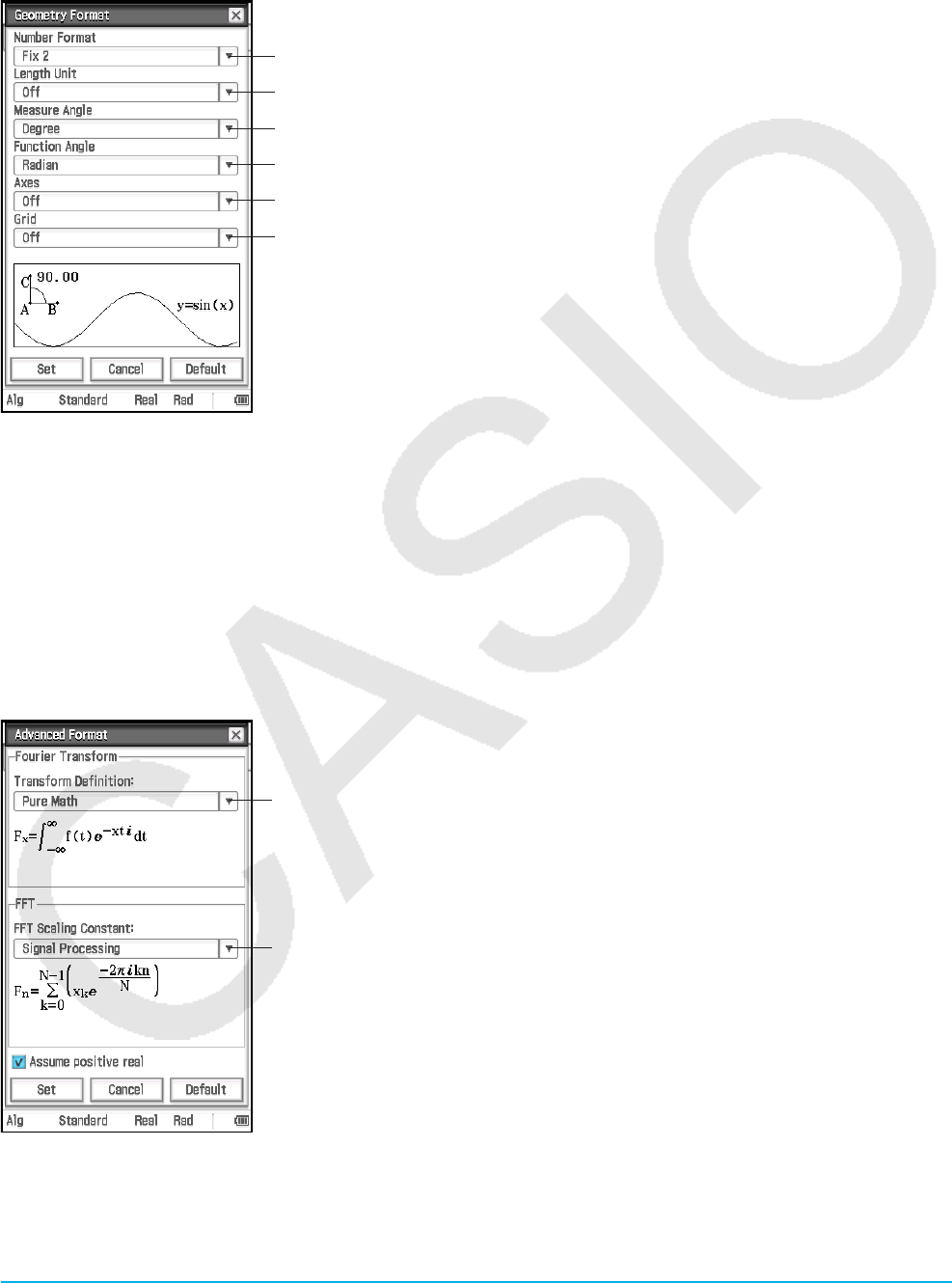
Chapter 1: Basics 40
k Geometry Format Dialog Box
Use the Geometry Format dialog box to configure settings for the Geometry application.
Tip: The information that appears in the preview area at the bottom of the dialog box shows a preview of the Geometry
application window, based on the settings configured in upper part of the dialog box.
1
2
3
4
5
6
To specify the Geometry window numeric value display format
Tap 1 and then select the format you want. The initial default Number
Format setting is Fix2. For more information, see “To specify the numeric
value display format” (page 36).
To specify the unit of the displayed length value
Tap 2 and then tap one of the settings described below.
Off*: Length value unit not displayed.
mm, cm, m, km, in, ft, yd, mi: Displays the length value in the selected
unit.
To specify the angle unit for the measurement box
Tap 3, and then tap “Radian”, “Degree*”, or “Grad”.
To specify the angle unit for graphing
Tap 4, and then tap “Radian*”, “Degree”, or “Grad”.
To specify the initial status of Graph window axes when the Geometry application is started up
Tap 5 and then tap one of the settings described below.
On: Show the axes Off*: Hide the axes
Number: Show the axes along with the maximum and minimum value of each
To specify the initial status of the grid when the Geometry application is started up
Tap 6 and then tap one of the settings described below.
On: Show the grid as dots Off*: Hide the grid Line: Show the grid as lines
k Advanced Format Dialog Box
Use the Advanced Format dialog box to configure settings for Fourier transform and FFT settings.
1
2
To specify the Fourier transform formula
Tap 1 and then tap “Modern Physics”, “Pure Math*”, “Probability”,
“Classical Physics”, or “Signal Processing”.
To specify the FFT scaling constant
Tap 2 and then tap “Pure Math”, “Signal Processing*”, or “Data Analysis”.
To specify how Fourier calculation variables are treated
Select the “Assume positive real” check box* to specify that Fourier
calculation variables should be treated as positive reals only. Clear
the check box to specify that complex numbers are allowed for Fourier
calculation variables.
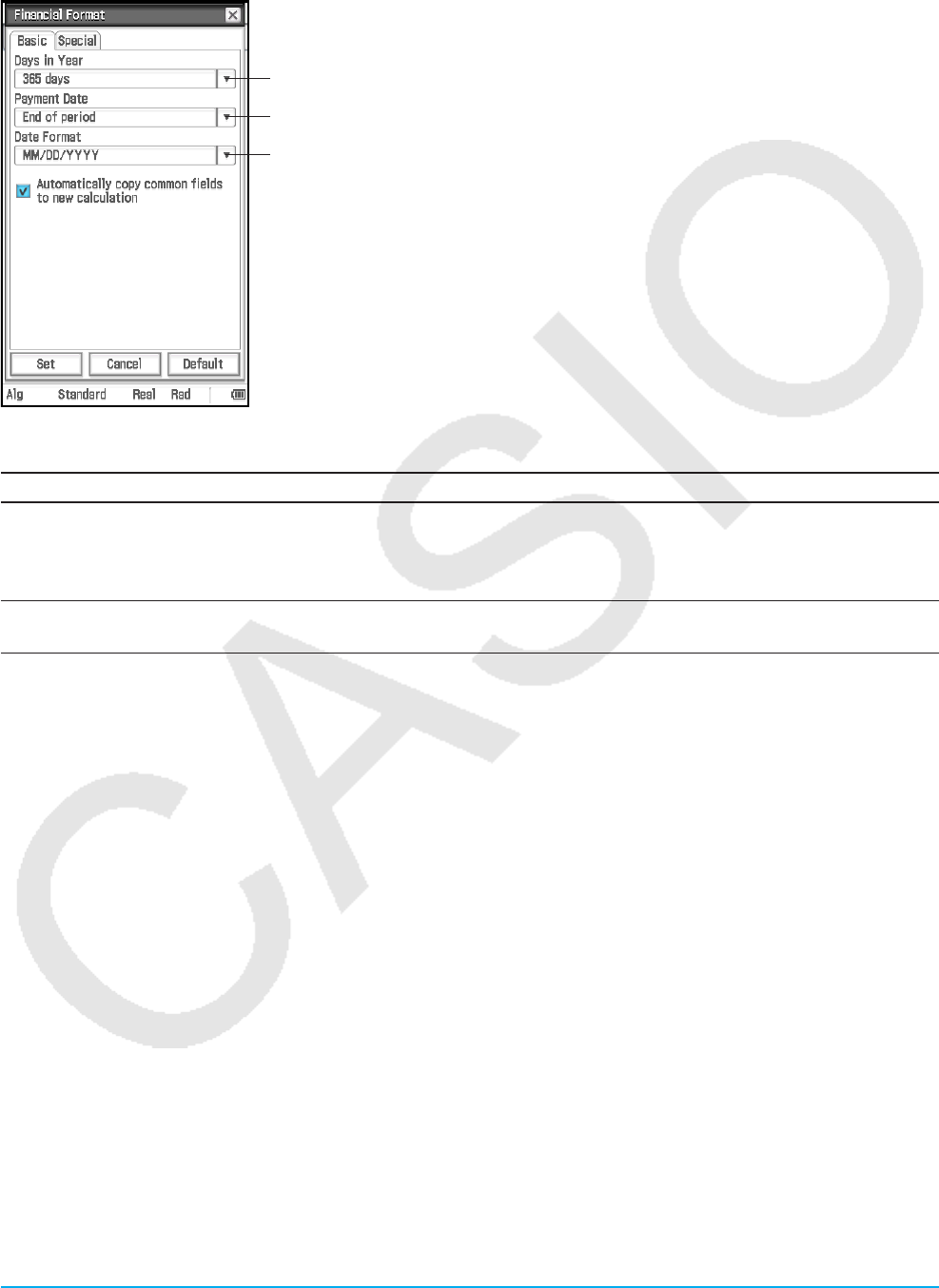
Chapter 1: Basics 41
k Financial Format Dialog Box
Use the Financial Format dialog box to configure settings for the Financial application.
[Basic] tab
1
2
3
To specify the number of days in a year
Tap 1, and then tap “360 days” or “365 days*”.
To specify the beginning or the period or the end of the period as the
payment date
Tap 2 and then tap “Beginning of period” or “End of period*”.
To specify the date format
Tap 3 and then tap one of the settings described below.
MM/DD/YYYY*: month/day/year
DD/MM/YYYY: day/month/year
YYYY/MM/DD: year/month/day
To specify the status of input fields when starting a new calculation
To do this: Do this:
When changing to another calculation type,
automatically copy the contents of all fields in the
current calculation whose names match the names
of fields in the new calculation.
Select the [Automatically copy common fields to new
calculation] check box*.
When changing to another calculation type, clear all
fields.
Clear the [Automatically copy common fields to new
calculation] check box.

Chapter 1: Basics 42
[Special] tab
1
2
3
4
5
To specify odd period handling
Tap 1 and then tap one of the settings described below.
Compound (CI): Apply compound interest to the odd period when
performing a Compound Interest calculation
Simple (SI): Apply simple interest to the odd period when performing a
Compound Interest calculation
Off*: Apply no interest to the odd period when performing a Compound
Interest calculation
To specify the compounding frequency
Tap 2, and then tap “Annual*” (once a year) or “Semi-annual” (twice a
year).
To specify the bond interval
Tap 3 and then tap one of the settings described below.
Term*: Specifies use of the number of payments as the duration for bond
calculation.
Date: Specifies use of a date as the duration for bond calculation.
To specify whether to use the amount (PRF) or profit ratio (r%) when performing break-even point
calculations
Tap 4, and then tap “Amount (PRF)*” or “Ratio (r%)”.
To specify whether to calculate sales quantity ([QBE]) or sales amount ([SBE]) first when performing
break-even point calculations
Tap 5, and then tap “Quantity*” or “Sales”. When “Quantity” is selected, sales quantity can be calculated
before calculating the sales amount. When “Sales” is selected, sales amount can be calculated before
calculating the sales quantity.
Tip: When performing a financial calculation, you can change settings using the Financial application status bar and
[Format] tab. For more information, see “Configuring Financial Application Settings” (page 188).
Initializing All Application Format Settings
Perform the following procedure when you want to return all application format settings to their initial defaults.
uClassPad Operation
1. Tap O and then tap [Default Setup].
2. In response to the “Reset Setup Data?” message that appears, tap [OK] to initialize all settings.
• The settings are initialized except for the current folder setting specified on Basic Format dialog box.

Chapter 1: Basics 43
1-8 When you keep having problems…
If you keep having problems when you are trying to perform operations, try the following before assuming that
there is something wrong with the ClassPad.
1. Initialize all application format settings.
Perform the procedure under “Initializing All Application Format Settings” (page 42).
2. Perform the RAM reset (RESTART) operation.
Perform RAM reset when the ClassPad freezes up or otherwise fails to perform as expected for some
reason.
To perform the RAM reset operation
Important!
• The RAM reset operation deletes all data that is temporarily stored in ClassPad RAM. Performing the RAM
reset operation while a calculation is in progress will cause any data stored in RAM by the calculation to be
lost.
• Perform the RAM reset operation only when your ClassPad freezes up or when it begins to operate
abnormally for some reason.
1. Use the stylus to press the RESTART button on the back of the
ClassPad.
• Following the RAM reset operation, the ClassPad restarts
automatically.
RESTART
Button
2. After the ClassPad restarts, perform the ClassPad setup operation. For more information about the
procedures you need to perform here, see “Loading Batteries and Setting Up the ClassPad” in the
separate Quick Start Guide.
• The application menu appears after you finish the setup operation.
3. Reset the ClassPad.
Before performing the reset operation, first make a written copy of all important data.
For details, see “To batch delete specific data (Reset)” (page 281).

Chapter 2: Main Application 44
Chapter 2:
Main Application
The Main application is a general-purpose numerical and mathematical calculation application that you can use
to study mathematics and solve mathematical problems. You can use the Main application to perform general
operations from basic arithmetic calculations, to calculations that involve lists, matrices, etc.
Starting up the Main application displays a large white work
area. Use this area for inputting operations and commands.
ClassPad also uses this area to output calculation results.
Basic Main application operations consist of inputting a
calculation expression into the work area and pressing
E. This performs the calculation and then displays its
result on the right side of the work area.
Input expression
Calculation result
Work area
Main Application-Specific Menus and Buttons
• Clear variables that contain numbers, list and matrices ...........................................Edit - Clear All Variables
• Insert a command into the work area (page 61) ....................................................................................Action
• Execute an Interactive command for the expression selected in the work area (page 91) ............. Interactive
• Toggle calculation result display between the Standard mode and Decimal mode ....................................u
• Recalculate the equation just for the current line where the cursor is currently located .............................7
• Output an input expression as-is ................................................................................................................0
• Insert and execute the Simplify command ..................................................................................................S
• Switch between binary, octal, decimal or hexadecimal number bases
during normal calculation (page 60).......................................................................................................<
• Access ClassPad application windows from the Main application (page 92) .............................................$
2-1 Basic Calculations
This section explains how to perform basic mathematical operations in the Main application.
Arithmetic Calculations and Parentheses Calculations
You can perform arithmetic calculations by inputting expressions as they are written. The ClassPad
automatically judges the calculation priority sequence for addition, subtraction, multiplication, and division,
functions, and parentheses.
0201 Calculation examples

Chapter 2: Main Application 45
• All of the example calculations shown in 0201 are performed using the keypad or the soft keyboard [Number]
key set, unless noted otherwise.
• The example calculations are all performed using the Decimal mode (page 46).
Using the e Key
Use the e key to input exponential values. You can also input exponential values using the E key on the
soft keyboard [Number] key set.
0202 Calculation examples
Omitting the Multiplication Sign
You can omit the multiplication sign in any of the following cases.
• In front of a function… 2sin (30), 10log (1.2), etc.
• In front of a constant or variable… aπ, 2ab, 3ans, etc.
• In front of an open parenthesis… 3(5 + 6), (a + 1)(b – 1), etc.
Note that you must use a multiplication sign when the expression directly in front of the open parenthesis is a
literal variable. Example: ab (3 + b) must be written ab × (3 + b). Otherwise, your input is considered to be in
function notation (
f ( x )).
• In front of the e key or E key (See “Using the e Key” above.)
• In front of a matrix or list… a {1, 2, 3}, 3 [[1, 2] [3, 4]], etc.
Using the Answer Variable (ans)
Any time you execute a calculation in the Main application work area, the last result is assigned automatically
to a variable named “ans” (answer). You can even recall current “ans” variable contents and input them into
another calculation by tapping the D key on the soft keyboard.
0203 Calculation examples
Tip: Starting a calculation expression with +, −, ×, ÷, or ^ operator will cause the “ans” variable to be inserted automatically
to the left of the operator, even if you do not tap the D key.
Assigning a Value to a Variable
Besides using the variable assignment key (W, page 33), you can also use the syntax shown below in the Main
application and eActivity application to assign a value to a variable.
Syntax: Variable: = value
0204 Assign 123 to variable
x
Important!
“:=” can be used only in Main and eActivity. It can NOT be used in a program. In the Program application, you
must use W to store a value to a variable.
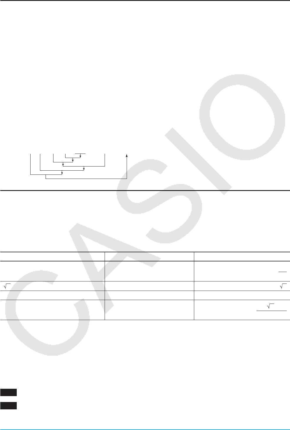
Chapter 2: Main Application 46
Calculation Priority Sequence
Your ClassPad automatically performs calculations in the following sequence.
1 Commands with parentheses (sin(, diff(, etc.)
2 Factorials (
x! ), degree specifications (o, r ),
percents (%)
3 Powers
4 π, memory, variable multiplication operations
that omit the multiplication sign (2π, 5A, etc.),
command with parentheses multiplication
operations that omit the multiplication sign (2'3,
etc.), ×, ÷
5 +, –, (–)
6 Relational operators (=, , <, >, s, t)
7 and
8 or, xor
9 with ( | )
Tip
• Expressions in parentheses are given priority.
• In cases where a series of calculations in the same expression includes more than one of the operators 4 through 9
that are the same priority sequence level, the same level operations are performed from left to right. A series of power
calculations 3 (example: 5^2^3) is performed from right to left (5^(2^3)).
Example: 2 + 3 × (log (sin( 2π2)) + 6.8) = 22.07101691 (In Algebra mode, Decimal mode, Radian mode)
Calculation Modes
All of the following calculation examples are shown using the Algebra mode only.
Standard Mode and Decimal Mode
The Standard mode displays calculation results in mathematical expression format whenever possible, while
the Decimal mode converts calculation results to a decimal form.
Expression Decimal Mode Result Standard Mode Result
50 ÷ 4 = 12.5 12.5 25
2
2 + 2 = 3.414213562... 3.414213562 2 +
2
π = 3.1415926535... 3.141592654 π
sin (2.1π) × 5 = 1.5450849718... 1.545084972 5
·
( − 1)
4
5
• The Decimal mode results in the above table show what would appear on the display when “Normal 1” is
selected for the [Number Format] setting on the Basic Format dialog box.
uUsing the u Button to Toggle between the Standard Mode and Decimal Mode
You can tap u to toggle a displayed value between Standard mode and Decimal mode format.
Note that tapping u toggles the format of a displayed value. It does not change the current Standard mode
and Decimal mode setting.
0205 Tapping u while the ClassPad is configured for Standard mode (Normal 1) display
0206 Tapping u while the ClassPad is configured for Decimal mode (Normal 1) display

Chapter 2: Main Application 47
u Number of Decimal Places, Number of Significant Digits, Normal Display Settings
The [Number Format] settings on the Basic Format dialog box specify the number of decimal places, the
number of significant digits, and the normal display setting for Main application Decimal mode calculation
results. The following shows how calculation results appear under each setting.
Expression Normal 1 Normal 2 Fix 3 Sci 3
50 ÷ 4 = 12.5 12.5 12.5 12.500 1.25E + 1
100 ÷ 6 = 16.6666666... 16.66666667 16.66666667 16.667 1.67E + 1
1 ÷ 600 = 0.00166666... 1.666666667E –3 0.00166666666 0.002 1.67E – 3
1011 ÷ 4 = 2.5E + 10 2.5E + 10 2.5E + 10 2.5E + 10 2.50E + 10
The allowable range for the number of decimal places is Fix 0 to Fix 9, and the range for the number of
significant digits is Sci 0 to Sci 9. For details about the [Number Format] settings, see “Basic Format Dialog
Box” on page 36.
Complex Mode and Real Mode
The Complex mode is for complex number calculations, while the Real mode is limited to calculations within
the range of real numbers. Performing a calculation in the Real mode that produces a result that is outside the
range of real numbers causes an error (Non-Real in Calc).
0207 (Complex mode and Real mode calculation results)
Tip
• You can select “ i ” or “ j ” for the imaginary unit. See “To specify the complex number imaginary unit” on page 283.
• If the expression includes ⬔(
r , ), calculation results should be ⬔( r , ) form.
Radian Mode, Degree Mode and Grad Mode
You can specify radians, degrees or grads as the angle unit for display of trigonometric calculation results.
uExamples of Radian mode, Degree mode and Grad mode calculation results
Expression Radian Mode Degree Mode Grad Mode
sin (π/4) sin π
4
( )
sin π
4
( )
sin (45) sin (45) sin (45)
sin (50) sin (50) sin (50)
Important!
Regardless of the currently selected angle unit setting, a calculation that includes an imaginary number power
exponent (such as: eπi) is performed using radians as the angle unit (eπi = −1).
Assistant Mode and Algebra Mode
The Algebra mode automatically simplifies mathematical expressions produced by calculations. No
simplification is performed in the Assistant mode. In the Assistant mode, you can view intermediate results as
well, which allows you to see the steps that lead to a particular result as shown in 0208 (see the “expand”
example).
0208 (Assistant mode and Algebra mode calculation results)
Important!
The Assistant mode is available in the Main application and eActivity application only.
'
'
'

Chapter 2: Main Application 48
2-2 Using the Calculation History
The Main application work area calculation history can contain up to 30 expression/result pairs. You can look
up a previous calculation, edit, and then re-calculate it, if you want.
• Use the scroll bar or scroll buttons to scroll the work area window up and down. This brings current calculation
history contents into view.
• You can edit a calculation expression in the calculation history and then re-calculate the resulting expression.
Pressing E re-calculates the expression where the cursor is currently located, and also re-calculates all of
the expressions below the current cursor location.
0209 To change the expression “ans × 2” to “ans × 3” in the example, and then re-calculate
Tip
• To re-calculate only a single specific line, tap 7. Tapping 7 re-calculates the calculation where the cursor is currently
located only. It does not affect anything in calculation history that comes before or after the line.
• To re-calculate all of the expressions in the calculation history, locate the cursor in the top line, and then press E.
uTo delete part of the calculation history contents
1. Move the cursor to the expression line or result line of the two-line unit you want to delete.
2. Tap [Edit] and then [Delete].
Important!
Even if the result of the deleted two-line unit has an effect on subsequent calculations, the affected calculations
are not updated automatically following the deletion. When you want to update everything in the calculation
history following the deleted unit, move the cursor to a line that is above the one you deleted and then press
E.
uTo clear all calculation history contents
Tap [Edit] and then [Clear All]. In response to the confirmation message that appears, tap [OK].
2-3 Function Calculations
This section explains how to perform function calculations in the Main application work area.
• You do not need to input the closing parenthesis that comes immediately before an E key operation. All of
the calculation examples in this section omit the closing parentheses before E.
• The following example calculations are all performed using the Decimal mode. Using the Standard mode
causes results to be displayed as fractions.
Angle Conversion (°, r)
The first two examples use “Degree” (indicated by “Deg” in the status bar) as the angle unit setting. The final
example uses “Radian” (indicated by “Rad” in the status bar) as the angle unit setting. Note that using the
wrong angle unit setting will make it impossible to produce correct calculation results.
uTo change the angle unit setting
1. On the O menu, tap [Basic Format].
2. Tap the [Angle] down arrow button, and then select [Radian], [Degree] or [Grad].
• You can also change the angle unit setting by tapping the current setting (Rad, Deg, or Gra) on the status
bar. Each tap will cycle through the available settings.

Chapter 2: Main Application 49
Problem Operation
Convert 4.25 radians to degrees.
= 243.5070629
4.25 Rw
47.3° + 82.5rad = 4774.20181° 47.3 + 82.5 Rw
How many radians is 243.5070629°?
= 4.249999999
Change the [Angle] setting to “Radian”, and then
input 243.5070629 *w.
Trigonometric and Inverse Trigonometric Functions
Problem Operation
cos(( 3
π) rad) = 0.5 Change the [Angle] setting to “Radian”.
c7/ 3 w or cN7c 3 w
2
·
sin45° × cos65° = 0.5976724775 Change the [Angle] setting to “Degree”.
2*s 45 )*c 65 w
Can be omitted.
sin–10.5 =30°
(Determine x for sin x = 0.5.)
S 0.5 w
“.5” can also be used.
Logarithmic Functions and Exponential Functions
Problem Operation
log1.23 (log101.23) = 0.08990511144 " 1.23 w or V 10 e 1.23 w
ln90 (loge90) = 4.49980967 I 90 w or V`e 90 w
log39 = 2 V 3 e 9 w or LV 3 , 9 w
e4.5 = 90.0171313 Q 4.5 w
(–3)4 = (–3) × (–3) × (–3) × (–3) = 81 (- 3 ){ 4 w
7 123 (= 123 7
1
) = 1.988647795 123 {( 1 / 7 w or % 7 e 123 w
Hyperbolic and Inverse Hyperbolic Functions
Problem Operation
sinh3.6 = 18.28545536 1 3.6 w
cosh–1 (
) = 0.7953654612 @ 20 / 15 w or @N 20 c15 w

Chapter 2: Main Application 50
Other Functions (%, ', x2, x
–1, x!, abs, ⬔, signum, int, frac, intg, fRound, sRound)
Problem Operation
What is 12% of 1500? (180) 1500 * 12 &w
What percent of 880 is 660? (75%) 660 / 880 &w
What value is 15% greater than 2500? (2875) 2500 *( 1 + 15 &
What value is 25% less than 3500? (2625) 3500 *( 1 - 25 &
'2 + '5 = 3.65028154 5 2 e+5 5 w
(3 + i ) = 1.755317302 + 0.2848487846 i Change to the Complex mode (“Cplx” indicated on
the status bar).
5 3 +0w
(–3)2 = (–3) × (–3) = 9 (- 3 )xw
–32 = –(3 × 3) = –9 - 3 xw
–
1= 12
3
1
4
1
( 3 X- 4 X)Xw
or
N 1 cN 1 c 3 e-N 1 c 4 w
8! (= 1 × 2 × 3 × … × 8) = 40320 8 !w
What is the absolute value of the common
logarithm of 4
3 ?
⎜log ( 4
3)⎟ = 0.1249387366
4V 10 eN 3 c 4 w
or L4V 3 / 4 w
8⬔40° × 5⬔35°
⬔(8,40) × ⬔(5,35) = ⬔(40,75)
Change to the Degree mode (“Deg” indicated on the
status bar).
~ 8 , 40 )*~ 5 , 35 )w
What is the sign of –3.4567? (–1)
(signum returns –1 for a negative value, 1 for a
positive value, “Undefined” for 0, and $
²$´ for an
imaginary number.)
[signum] - 3.4567 w
What is the integer part of –3.4567? (–3) :- 3.4567 w
What is the decimal part of –3.4567? (–0.4567) [frac] - 3.4567 w
What is the greatest integer less than or equal to
–3.4567? (–4)
[intg] - 3.4567 w
What is –3.4567 rounded to two decimal places?
(–3.46)
[fRound] - 3.4567 , 2 w
What is –34567 rounded to four significant digits?
(–34570)
[sRound] - 34567 , 4 w*
* To round to 10 digits, specify “0” for the second argument.
Random Number Generator (rand, randList, randNorm, randBin, RandSeed)
The ClassPad random number generator can generate truly random numbers (non-sequential random
numbers) and random numbers that follow a particular pattern (sequential random numbers).
uTo switch between non-sequential and sequential random number generation
1. Use the “RandSeed” command to configure random number generation settings. See “RandSeed
Command” on page 52.
2. Use the “rand”, “randList”, “randNorm”, or “randBin” function to generate the random numbers.

Chapter 2: Main Application 51
u“rand” Function
The “rand” function generates random numbers. If you do not specify an argument, “rand” generates 10-digit
decimal values 0 or greater and less than 1.
Specifying two integer values for the argument generates random numbers between them.
Problem Operation
Generate random numbers between 0 and 1. [rand] w
Generate random integers between 1 and 6. [rand] 1 , 6 w
u“randList” Function
Syntax: randList( n [, a, b])
Function:
• Omitting arguments “a” and “b” returns a list of
n elements that contain decimal random values.
• Specifying arguments “a” and “b” returns a list of
n elements that contain integer random values in the range
of “a” through “b”.
Description:
• “
n ” must be a positive integer.
• The random numbers of each element are generated in accordance with “RandSeed” specifications, as with
the “rand” function.
Problem Operation
Generate a list of three elements that contain
decimal random values.
[randList] 3 w
Generate a list of five elements that contain random
values in the range of 1 through 6.
[randList] 5 , 1 , 6 w
u“randNorm” Function
The “randNorm” function generates a 10-digit normal random number based on a specified mean and
standard deviation values.
Syntax: randNorm(
, [, n ])
Function:
• Omitting a value for “
n ” (or specifying 1 for “ n ”) returns the generated random number as-is.
• Specifying a value for “
n ” returns the specified number of random values in list format.
Description:
• “
n ” must be a positive integer, and “ ” must be greater than 0.
Problem Operation
Randomly produce a body length value obtained in
accordance with the normal distribution of a group
of infants less than one year old with a mean body
length of 68 cm and standard deviation of 8.
[randNorm] 8 , 68 w
Randomly produce the body lengths of five infants in
the above example, and display them in a list.
[randNorm] 8 , 68 , 5 w
u“randBin” Function
The “randBin” function generates binomial random numbers based on values specified for the number of trials
n and probability P.
Syntax: randBin( n , P [, m ])

Chapter 2: Main Application 52
Function:
• Omitting a value for “
m ” (or specifying 1 for “ m ”) returns the generated random number as-is.
• Specifying a value for “
m ” returns the specified number of random values in list format.
Description:
• “
n ” and “ m ” must be positive integers.
Problem Operation
Randomly produce the number of heads that can be
expected in accordance with binomial distribution for
five coin tosses where the probability of heads is 0.5.
[randBin] 5 , 0.5 w
Perform the same coin toss sequence described
above three times and display the results in a list.
[randBin] 5 , 0.5 , 3 w
u “RandSeed” Command
• You can specify an integer from 0 to 9 for the argument of this command. 0 specifies non-sequential random
number generation. An integer from 1 to 9 uses the specified value as a seed for specification of sequential
random numbers. The initial default argument for this command is 0.
• The numbers generated by the ClassPad immediately after you specify sequential random number generation
always follow the same random pattern.
Problem Operation
Generate sequential random numbers using 3 as the
seed value.
[RandSeed] 3 w
Generate the first value.
Generate the second value.
Generate the third value.
[rand] w
[rand] w
[rand] w
Tip
• Random values generated by these commands are pseudo random values.
• The arguments a and b of “rand(a,b)” and “randList(n,a,b)” must be integers, subject to the following conditions.
a < b ⎟ a
⎟ , ⎟ b
⎟ < 1E10 b – a < 1E10
Integer Functions
These functions take integers only as their arguments and return integers.
u“iGcd” Function
Syntax: iGcd(Exp-1, Exp-2[, Exp-3…Exp-10)]
(Exp-1 through Exp-10 all are integers.)
iGcd(List-1, List-2[, List-3…List-10)]
(All elements of List-1 through List-10 are integers.)
Function:
• The first syntax above returns the greatest common divisor for two to ten integers.
• The second syntax returns, in list format, the greatest common divisor (GCD) for each of the elements in two
to ten lists. When the arguments are {
a , b }, { c , d }, for example, a list will be returned showing the GCD for a
and c , and for b and d .
Description:
• All of the lists must have the same number of elements.
• When using the “iGcd(List-1, List-2[, List-3…List-10)]” syntax, one (and only one) expression (Exp) can be
include as an argument in place of a list.

Chapter 2: Main Application 53
Problem Operation
Determine the greatest common divisors of {4, 3},
{12, 6}, and {36, 9}.
[iGcd] { 4 , 3 },{ 12 , 6 },{ 36
, 9 })w
u“iLcm” Function
Syntax: iLcm(Exp-1, Exp-2[, Exp-3…Exp-10)]
(Exp-1 through Exp-10 all are integers.)
iLcm(List-1, List-2[, List-3…List-10)]
(All elements of List-1 through List-10 are integers.)
Function:
• The first syntax above returns the least common multiple for two to ten integers.
• The second syntax returns, in list format, the least common multiple (LCM) for each of the elements in two to
ten lists. When the arguments are {
a , b }, { c , d }, for example, a list will be returned showing the LCM for a and c ,
and for b and d .
Description:
• All of the lists must have the same number of elements.
• When using the “iLcm(List-1, List-2[, List-3…List-10)]” syntax, one (and only one) expression (Exp) can be
include as an argument in place of a list.
Problem Operation
Determine the least common multiples of {4, 3},
{12, 6}, and {36, 9}.
[iLcm] { 4 , 3 },{ 12 , 6 },{ 36
, 9 })w
u“iMod” Function
Syntax: iMod(Exp-1/List-1, Exp-2/List-2[)]
Function:
• This function divides one or more integers by one or more other integers and returns the remainder(s).
Description:
• Exp-1 and Exp-2, and all of the elements of List-1 and List-2 must be integers.
• You can use Exp for one argument and List for the other argument (Exp, List or List, Exp) if you want.
• If both arguments are lists, both lists must have the same number of elements.
Problem Operation
Divide 21 by 6 and 7, and determine the remainder
of both operations. (iMod(21, {6, 7})
[iMod] 21 ,{ 6 , 7 })w
Permutation (nPr) and Combination (nCr)
uTotal Number of Permutations
uTotal Number of Combinations
Problem Operation
To determine the number of permutations and combinations
possible when selecting four people from a group of 10
10P4 = 5040 } 10 , 4 w
10C4 = 210 { 10 , 4 w
3 ²²²²²
²
& ²²²²²²²
²

Chapter 2: Main Application 54
Condition Judgment (judge, piecewise)
u“judge” Function
The “judge” function returns TRUE when an expression is true, and FALSE when it is false.
Problem Operation
Is the following expression true or false?
1 = 1 TRUE
[judge] 1 = 1 w
Is the following expression true or false?
1 < 0 FALSE
[judge] 1 < 0 w
u “piecewise” Function
The “piecewise” function returns one value when an expression is true, and another value when the expression
is false.
The syntax of the “piecewise” function is shown below.
piecewise(<condition expression>, <return value when true>, <return value when false or indeterminate> [ ) ]
or
piecewise(<condition expression>, <return value when true>, <return value when false>, <return value when
indeterminate> [ ) ]
Use the soft keyboard (1) to input “piecewise” function according to the syntax shown below.
or
<return value when true>, <condition expression>
<return value when false or indeterminate>
<return value when condition 1 is true>, <condition 1 expression>
<return value when condition 2 is true>, <condition 2 expression>
Problem Operation
For the expression 0 t
x ( x = variable), return 1
when x is 0 or less, and 2 when x is greater than 0
or undefined.
[piecewise] 0 :X, 1 , 2 w
or
1 1 c 2 ef 0 :X w
For the expression 1 t
x ( x = variable), return 1
when x is 1 or less, and 2 when x is greater than 1. 1 1 c 2 ef 1 :X c 1 <Xw
Angle Symbol (∠)
Use this symbol to specify the coordinate format required by an angle in a vector.
You can use this symbol for a vector only.
Problem Operation
Convert the polar coordinates
r = '2 ,
θ
= π /4 to
rectangular coordinates. [1, 1]
Change the [Angle] setting to “Radian”.
[toRect] [5 2 e,~7/ 4 )]w
Derivative Symbol (’)
A single derivative symbol indicates the first derivative of an equation in the format: <variable name>’.
Problem Operation
Solve the differential equation
y ’ = x .
{ y = 0.5 · x
2 + const (1)} +Y'=X,X,Yw
Important!
The “dSolve” function can solve differential equations up to three degrees, so a maximum of three derivative
symbols ( y ’’’) can be used. Executing a “dSolve” calculation that has more than three derivative symbols will
result in an Invalid Syntax error.

Chapter 2: Main Application 55
Primality Test (isPrime)
The “isPrime” function determines whether the number provided as the argument is prime (returns TRUE) or
not (returns FALSE). The syntax of the “isPrime” function is shown below.
isPrime(Exp/List[ ) ]
• Exp or all of the elements of List must be integers.
Problem Operation
Determine whether the numbers 51 and 17 are
prime.
(isPrime({51, 17})
[isPrime] { 51 , 17 })w
Equal Symbols and Unequal Symbols (=, ≠, <, >, s, t)
You can use these symbols to perform a number of different basic calculations.
Problem Operation
To add 3 to both sides of
x = 3. x + 3 = 6 (X= 3 )+ 3 w
Subtract 2 from both sides of
y s 5. y – 2 s 3 (Y; 5 )- 2 w
Tip
• In the “Syntax” explanations of each command under “2-7 Using the Action Menu”, the following operators are indicated
as “Eq/Ineq”: =, ≠, <, >, s, t. Whether or not the “Eq/Ineq” operators include the “≠” operator is specified for each
command by a separate note.
• An expression that contains multiple equation or inequality operators cannot be input as a single expression. For output
expressions, an expression can be output with multiple operators only in the case of inequality operators that are facing in
the same direction (example: –1 <
x < 1).
Example: solve( x
2 – 1 < 0, x ) w {–1 < x < 1}
“with” Operator ( | )
The “with” ( I ) operator temporarily assigns a value to a variable. You can use the “with” operator in the
following cases.
• To assign the value specified on the right side of | to the variable on the left side of |
• To limit or restrict the range of a variable on the left side of | in accordance with conditions provided on the
right side of |
The following is the syntax for the “with” ( I ) operator.
Exp/Eq/Ineq/List/Mat|Eq/Ineq/List/(and operator)
You can put plural conditions in a list or connected with the “and” operator on the right side.
“” can be used on the left side or the right side of |.
Problem Operation
Evaluate
x
2 + x + 1 when x = 3. 13 X{ 2 +X+ 1 UX= 3 w
For
x
2 – 1 = 0, determine the value of x when x > 0.
{ x = 1}
.X{ 2 - 1 = 0 ,X)UX> 0 w
Determine the value of abs (
x ) when x > 0. x 4XeUX> 0 w

Chapter 2: Main Application 56
Solutions Supported by ClassPad (TRUE, FALSE, Undefined, No Solution, ∞, const, constn)
Solution Description Example
TRUE Output when a solution is true. judge (1 = 1) w
FALSE Output when a solution is false. judge (1 < 0) w
Undefined Output when a solution is undefined. 1/0 w
No Solution Output when there is no solution. solve (abs (
x ) = –1, x ) w
∞Infinity lim (1/
x
2, x , 0) w
const Constant displayed as const(1) when any value that is a
constant is included in the solution. In the case of multiple
constants, they are indicated as const(1), const(2), and
so on.
dSolve (
y = x , x , y ) w
{ y = 0.5· x
2 + const (1)}
constn Constant displayed as constn(1) when the solution
includes any integer value that is a constant. In the case
of multiple constants, they are indicated as constn(1),
constn(2), and so on.
Change the [Angle] setting to
“Degree”.
solve (sin (
x ) = 0, x ) w
{ x = 180·constn (1)}
Dirac Delta Function
“delta” is the Dirac Delta function. The delta function evaluates numerically as shown below.
b
^
b
Non-numeric expressions passed to the delta function are left unevaluated. The integral of a linear delta
function is a Heaviside function.
Syntax: delta(
x )
x : variable or number
0210 (Calculation example screenshot)
n th-Delta Function
The n th-delta function is the n th differential of the delta function.
Syntax: delta( x , n )
x : variable or number
n : number of differentials
0211 (Calculation example screenshot)
Heaviside Unit Step Function
“heaviside” is the command for the Heaviside function, which evaluates only to numeric expressions as shown
below.
H
!
Any non-numeric expression passed to the Heaviside function will not be evaluated, and any numeric
expression containing complex numbers will return undefined. The derivative of the Heaviside function is the
Delta function.
Syntax: heaviside(
x )
x : variable or number
0212 (Calculation example screenshot)

Chapter 2: Main Application 57
Gamma Function
The Gamma function is called “gamma” on the ClassPad.
∫
+∞
0tx–1e–t d
t
Γ(x) =
For an integer n the gamma is evaluated as shown below.
²!
K
^
s
The gamma is defined for all real numbers excluding zero and negative integers. It is also defined for all
complex numbers where either the real or imaginary part of the complex number is not an integer.
Gamma of a symbolic expression returns unevaluated.
Syntax: gamma(
x )
x : variable or number
0213 (Calculation and graph example screenshots)
2-4 List Calculations
This section explains how to input list data, and how to perform basic list calculations.
Inputting List Data in the Work Area
0214 To input the list {1, 2, 3} and assign it to LIST variable “lista” in the Main application work area
LIST Variable Element Operations
You can recall the value of any element of a LIST variable. You can also assign a value to any element in a list.
0215 To recall the second element of the “lista” list variable of example 0214
0216 To assign 5 to the second element of “lista”
Using a List in a Calculation
You can perform arithmetic operations between two lists, between a list and a numeric value, or between a list
and an expression, equation, or inequality.
Important!
• When you perform an arithmetic operation between two lists, both of the lists need to have the same number
of cells. An error will occur if they do not.
• An error will also occur whenever an operation between any two cells of the two lists results in an error.
0217 Perform the operation list3 × {6, 0, 4} when list3 contains {41, 65, 22}
Using a List to Assign Different Values to Multiple Variables
Use the procedure in this section when you want to use a list to assign various different values to multiple variables.
Syntax: List with Numbers S List with Variables
0218 Assign the values 10, 20, and 30, to variables x, y, and z respectively

Chapter 2: Main Application 58
2-5 Matrix and Vector Calculations
This section explains how to create matrices, and how to perform basic matrix calculations.
Tip: Since a vector can be viewed as 1-row by n -column matrix or n -row by 1-column matrix, this section does not include
explanations specifically about vectors. For more information about vector-specific calculations, see the explanations
about the applicable [Action] menu items in “2-7 Using the Action Menu”.
Inputting Matrix Data
You can input matrix values in a single line in the work area, or input matrix values using an actual on-screen
matrix.
Inputting Matrix Values in a Single Line
0219 To input the matrix 1 2
3 4 and assign it to the variable “mat1” in the Main application work area
Matrix Variable Element Operations
You can recall the value of any element of a matrix variable. You can also assign a value to any element in a
matrix.
0220 To recall the value in row 2, column 1 of the matrix variable “mat1” of example 0219
0221 To assign 5 to the element at row 1, column 2 of “mat1”
Inputting Matrix Values Using an Actual On-Screen Matrix
• Create a new 1-row × 2-column matrix ...................................................................................................... 6
• Create a new 2-row × 1-column matrix ...................................................................................................... 7
• Create a new 2-row × 2-column matrix ..................................................................................................... 8
• Add a column to the currently displayed matrix ......................................................................................... 6
• Add a row to the currently displayed matrix ............................................................................................... 7
• Add both a row and column to the currently displayed matrix ................................................................... 8
0222 To input the matrix 1 2 3
4 5 6 and assign it to the variable “mat2”
Performing Matrix Calculations
This section provides examples of how to perform the most basic types of matrix calculations.
Matrix Addition, Subtraction, Multiplication, and Division
0223 To calculate 1 1
2 1 + 2 3
2 1 in a single line
0224 To calculate 1 1
2 1 × 2 3
2 1 using an actual on-screen matrix
0225 To multiply the matrix 1 2
3 4 by 5

Chapter 2: Main Application 59
Raising a Matrix to a Specific Power
Example: To raise 1 2
3 4 to the power of 3
0226 Input in a single line
0227 Input using an actual on-screen matrix
Tip: You can raise only a square matrix to a specific power. An error occurs when you try to raise a non-square matrix to a
specific power.
Using a Matrix to Assign Different Values to Multiple Variables
Use the procedure in this section when you want to use a matrix to assign various different values to multiple
variables.
Syntax: Matrix with Numbers ⇒ Matrix with Variables
(The matrix can be one line with multiple columns, or multiple lines with one column.)
0228 Assign the values 10, 20, and 30, to variables
x , y , and z respectively
2-6 Specifying a Number Base
While using the Main application, you can specify a default number base (binary, octal, decimal, hexadecimal).
You can also convert between number bases and perform bitwise operations using logical operators (not, and,
or, xor).
Note the following limitations, which all apply while a default number base (binary, octal, decimal, hexadecimal)
is specified in the Main application.
• You cannot use scientific functions, or [Action] or [Interactive] menu commands.
• Except for Ans (Answer Memory variable), you cannot use variables.
• You can input integers only. An error (Invalid Syntax) will occur if you try to input a non-integer value (like 1.5
or '2 ).
• If a calculation produces a non-integer result (with a decimal part), the ClassPad will cut off the decimal part
automatically. For example, the calculation 5 ÷ 2 while decimal is selected as the number base is 2.
• An error message is displayed if you try to enter a value that is invalid for the speicfied number base. The
following shows the numerals that can be used in each number system.
Binary: 0, 1 Octal: 0 to 7 Decimal: 0 to 9 Hexadecimal: 0 to 9, A, B, C, D, E, F
Binary, Octal, Decimal, and Hexadecimal Calculation Ranges
• The following are the display capacities and calculation ranges for each of the number bases.
Number Base Display Capacity Calculation Range (Positive ; Negative)
Binary 32 digits 0 s x s 01111111111111111111111111111111 ;
10000000000000000000000000000000 s x s
11111111111111111111111111111111
Octal 11 digits 0 s x s 17777777777 ; 20000000000 s x s 37777777777
Decimal 10 digits 0 s x s 2147483647 ; −2147483648 s x s −1
Hexadecimal 8 digits 0 s x s 7FFFFFFF ; 80000000 s x s FFFFFFFF
• Negative binary, octal, and hexadecimal values are produced using the two’s complement of the original
value.

Chapter 2: Main Application 60
Selecting a Number Base
Specifying a default number base in the Main application will apply to the current line (expression/result pair),
and to all subsequent lines until you change the default number base setting.
uTo select the number base for the line where the cursor is located
1. Tap the down arrow button next to the < button.
2. Tap the button that corresponds to the number base you want to use:
1 (binary), 2 (octal), 3 (decimal), 4 (hexadecimal).
• The currently selected number base is indicated in the status bar.
3. Execute the calculation.
Important!
• A line for which a number base is not specified is called a “normal calculation line”. To return a line to a
normal calculation line, tap < in step 2 of the above procedure.
• Calculation results produced by a line for which a number base is specified are followed by one of the suffixes
listed below, to indicate its number system.
Number System Binary Octal Decimal Hexadecimal
Suffix bodh
uTo specify a number base for an input value
You can input the following suffixes to specify the number base of a value as you input it: [b] (binary), [o] (octal),
[d] (decimal), and [h] (hexadecimal). You can specify a number base for an input value only when a default
number base (besides normal) is selected
Arithmetic Operations
You can use the following operators when performing binary, octal, decimal and hexadecimal values: +, −, ×, ÷,
^. You can also use parenthetical expressions.
0229 To calculate 101112 + 110102
0230 To calculate (118 + 78)2
0231 Perform the calculation 12310 + 10102 so it produces a hexadecimal result
Bitwise Operations
The logical operators (and, or, xor, not) can be used in calculations.
and ...Returns the result of a bitwise product.
or ......Returns the result of a bitwise sum.
xor ....Returns the result of a bitwise exclusive logical sum.
not ....Returns the result of a complement (bitwise inversion).
0232 Calculation examples

Chapter 2: Main Application 61
Using the baseConvert Function (Number System Transform)
The baseConvert function lets you convert a number in one base (number system) to its equivalent in another
base.
Important!
• The baseConvert function works for positive integers only.
• The baseConvert function cannot be used in a line for which a particular number base is specified. It can be
used in a normal calculation line only.
Syntax: baseConvert (Number, Current base, Expected base)
• Number must be a positive integer consisting of digits 0 to 9 and/or A to F.
• The current base and expected base can be any whole number from 2 to 16.
0233 Calculation examples
2-7 Using the Action Menu
The [Action] menu helps to make transformation and expansion functions, calculus functions, statistical
functions, and other frequently used mathematical menu operations easier to use. Simply select the function
you want, and then enter expressions or variables in accordance with the syntax of the function.
Tip
• Unless specifically indicated otherwise, all of the explanations in this section are performed using the following modes:
Algebra mode, Standard mode, Complex mode, Radian mode, Descending Order.
• You can use the [Interactive] menu to select most of the commands that are included on the [Action] menu. For details
about using the [Interactive] menu, see page 91.
Abbreviations and Punctuation Used in This Section
The following are the meanings of the abbreviations and punctuation used in the syntax descriptions in this section.
Exp: Expression (Value, Variable, etc.) List: List
Eq: Equation Mat: Matrix
Ineq: All types of inequalities (a>b, atb, a<b, asb, ab)
Ineqⴝ: Inequality ab only
[ ]: You can omit the item(s) inside the brackets.
{ }: Select one of the items inside the braces.
Some of the syntaxes in the following explanations indicate the following for parameters:
Exp/Eq/Ineq/List/Mat
These abbreviations mean that you can use any of the following as a parameter: expression, equation,
inequality, list, or matrix.
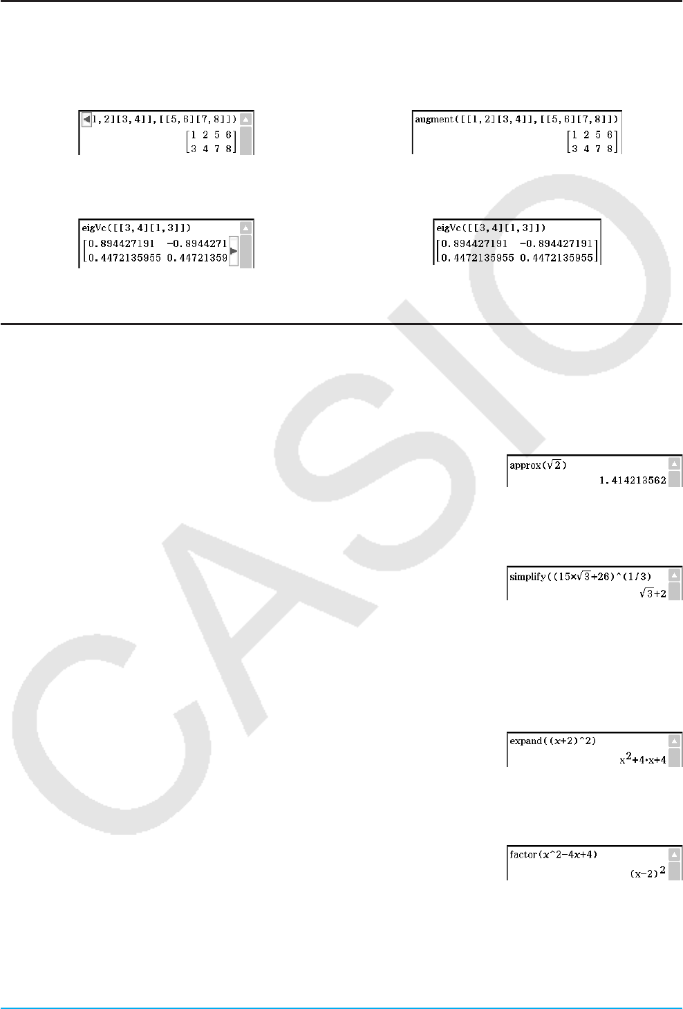
Chapter 2: Main Application 62
Example Screenshots
The screenshots below show examples of how input and output expressions appear on the ClassPad display.
All of the screenshots in this section show the “complete expression” version.
When the input expression does not fit:
Displayed expression Complete expression
When the output expression does not fit:
Displayed expression Complete expression
Using the Transformation Submenu
The [Transformation] submenu contains commands for expression transformation, like “expand” and “factor”.
uapprox [Action][Transformation][approx]
Function: Transforms an expression into a numerical approximation.
Syntax: approx (Exp/Eq/Ineq/List/Mat [
)
]
Example: To obtain the numerical value of '2
usimplify [Action][Transformation][simplify]
Function: Simplifies an expression.
Syntax: simplify (Exp/Eq/Ineq/List/Mat [ ) ]
Example: To simplify (15'3 + 26)^(1/3)
uexpand [Action][Transformation][expand]
Function: Expands an expression.
Syntax: expand (Exp/Eq/Ineq/List/Mat [
)
]
expand (Exp,variable [
)
]
• If you specify a variable, Exp is decomposed into partial fractions, with
respect to the variable.
Example: To expand (
x + 2)2
ufactor [Action][Transformation][factor][factor]
Function: Factors an expression.
Syntax: factor (Exp/Eq/Ineq/List/Mat [ ) ]
Example: To factor
x
2 4 x + 4

Chapter 2: Main Application 63
urFactor [Action][Transformation][factor][rFactor]
Function: Factors an expression up to its roots, if any.
Syntax: rFactor (Exp/Eq/Ineq/List/Mat [ ) ]
Example: To factor
x
2 3
ufactorOut [Action][Transformation][factor][factorOut]
Function: Factors out an expression with respect to a specified factor.
Syntax: factorOut (Exp/Eq/Ineq/List/Mat, Exp [ ) ]
Example: To factor “a” out a
x
2 + b x + c
ucombine [Action][Transformation][combine]
Function: Transforms multiple fractions into their common denominator equivalents and reduces them, if
possible.
Syntax: combine (Exp/Eq/Ineq/List/Mat [ ) ]
Example: To transform and reduce (
x + 1)/( x + 2) + x ( x + 3)
ucollect [Action][Transformation][collect]
Function: Rearranges an expression with respect to a specific variable.
Syntax: collect (Exp/Eq/Ineq/List/Mat[,Exp] [ ) ]
• “
x ” is the default when you omit “[,Exp]”.
Example: To rearrange
x
2 + a x + b x with respect to x
utExpand [Action][Transformation][tExpand]
Function: Employs the sum and difference formulas to expand a trigonometric function.
Syntax: tExpand(Exp/Eq/Ineq/List/Mat [ ) ]
Example: To expand sin (a + b)
utCollect [Action][Transformation][tCollect]
Function: Employs the product to sum formulas to transform the product of a trigonometric function into an
expression in the sum form.
Syntax: tCollect (Exp/Eq/Ineq/List/Mat [ ) ]
Example: To transform cos(a) × cos(b) into an expression in the sum form
uexpToTrig [Action][Transformation][expToTrig]
Function: Transforms an exponent into a trigonometric or hyperbolic function.
Syntax: expToTrig (Exp/Eq/Ineq/List/Mat [ ) ]
Example: To transform
e
ix into a trigonometric function (Radian mode)
utrigToExp [Action][Transformation][trigToExp]
Function: Transforms a trigonometric or hyperbolic function into exponential form.
Syntax: trigToExp (Exp/Eq/Ineq/List/Mat [ ) ]
Example: To transform cosh
x into exponential form
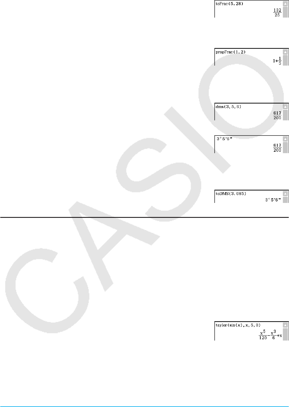
Chapter 2: Main Application 64
utoFrac [Action][Transformation][Fraction][toFrac]
Function: Transforms a decimal value into its equivalent fraction value.
Syntax: toFrac (Exp/Eq/Ineq/List/Mat [ ) ]
Example: To transform 5.28 into its equivalent fraction value
upropFrac [Action][Transformation][Fraction][propFrac]
Function: Transforms a decimal value into its equivalent proper fraction value.
Syntax: propFrac (Exp/Eq/Ineq/List/Mat [ ) ]
Example: To transform 1.2 into its equivalent proper fraction value
u dms [Action][Transformation][DMS][dms]
Function: Transforms a DMS format value into its equivalent degrees-only
value.
Syntax: dms (Exp/List-1 [,Exp/List-2][,Exp/List-3] [ ) ]
Example: To transform 3° 5’ 6” into its equivalent degrees-only value
• Zero is the default when you omit [,Exp/List-2] or [,Exp/List-3][ ) ].
Tip: You can input 3° 5’ 6” using the / key on the soft keyboard.
/e 3 e 5 e 6 E
u toDMS [Action][Transformation][DMS][toDMS]
Function: Transforms a degrees-only value into its equivalent DMS format value.
Syntax: toDMS (Exp/List [ ) ]
Example: To transform 3.085 degrees into its equivalent DMS format value
Using the Advanced Submenu
usolve [Action][Advanced][solve]
For information about solve, see page 81.
udSolve [Action][Advanced][dSolve]
For information about dSolve, see page 82.
utaylor [Action][Advanced][taylor]
Function: Finds a Taylor polynomial for an expression with respect to a specific variable.
Syntax: taylor (Exp/List, variable, order [,center point] [
)
]
Example: To find a 5th order Taylor polynomial for sin(x) with respect to x = 0
(in the Radian mode)
• Zero is the default when you omit “[,center point]”.
ulaplace [Action][Advanced][laplace], invLaplace [Action][Advanced][invLaplace]
Function: “laplace” is the command for the Laplace transform, and
“invLaplace” is the command for the inverse of Laplace transform.
∫
∞
0()–L[ ()] ()=
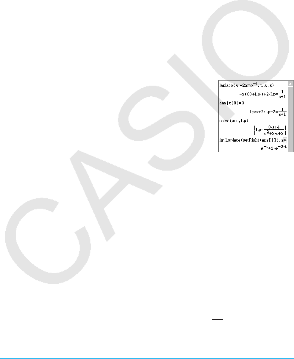
Chapter 2: Main Application 65
Syntax:
laplace( f ( t), t, s)
f ( t): expression ;
t: variable with respect to which the expression is
transformed ;
s: parameter of the transform
invLaplace(L(s), s, t)
L(s): expression ;
s: variable with respect to which the expression is
transformed ;
t: parameter of the transform
ClassPad supports transform of the following functions.
sin(x), cos(x), sinh(x), cosh(x), xn, 'x, ex, heaviside(x), delta(x), delta(x, n)
ClassPad does not support transform of the following functions.
tan(x), sin– 1(x), cos– 1(x), tan– 1(x), tanh(x), sinh– 1(x), cosh– 1(x), tanh– 1(x), log(x), ln(x), 1/x, abs(x), gamma(x)
Laplace Transform of a Differential Equation
The laplace command can be used to solve ordinary differential equations. ClassPad does not support System
of Differential Equations for laplace.
Syntax: laplace(diff eq,
x , y , t )
diff eq: differential equation to solve ; x : independent variable in the diff eq ;
y : dependent variable in the diff eq ; t : parameter of the transform
Example: To solve a differential equation
x ’ + 2 x = e
−t where x (0) = 3 using the
Laplace transform
Lp means F ( s ) = L [ f ( t )] in the result of transform for a differential equation.
ufourier [Action][Advanced][fourier], invFourier [Action][Advanced][invFourier]
Function: “fourier” is the command for the Fourier Transform, and “invFourier” is the command for the inverse
Fourier Transform.
Syntax: fourier( f ( x), x, w, n) invFourier(F ( w), w, x, n)
x : variable with respect to which the expression is transformed with ; w : parameter of the transform ;
n : 0 to 4, indicating Fourier parameter to use (optional)
ClassPad supports transform of the following functions.
sin(t), cos(t), log(t), ln(t), abs(t), signum(t), heaviside(t), delta(t), delta(t,n), eti
ClassPad does not support transform of the following functions.
tan(t), sin– 1(t), cos– 1(t), tan– 1(t), sinh(t), cosh(t), tanh(t), sinh– 1(t), cosh– 1(t), tanh– 1(t), gamma(t), 't , et
The Fourier Transform is defined as the following:
∫
∞
–∞()2π
() =
∫
∞
–∞()–2π
() =
Some authors (especially physicists) prefer to write the transform in terms of angular frequency ω ≡ 2π
instead of the oscillation frequency .
However, this destroys the symmetry, resulting in the transform pair shown below.
∫
∞
–∞()–ω
(ω) = [()] =
∫
∞
–∞(ω)ωω
() = –1[(ω)] = 1
2π

Chapter 2: Main Application 66
To restore the symmetry of the transforms, the convention shown below is sometimes used.
∫
∞
–∞()–
() = [ ()] = 1
2π
∫
∞
–∞()
() = –1[()] = 1
2π
In general, the Fourier transform pair may be defined using two arbitrary constants a and b as shown below.
∫
∞
–∞()ω
(ω) = ⏐⏐
(2π)1–
∫
∞
–∞(ω)–ωω
() = ⏐⏐
(2π)1+
The values of a and b depend on the scientific discipline, which can be specified by the value of n (optional
fourth parameter of fourier and invFourier) as shown below.
Unfortunately, a number of conventions are in widespread use for a and b . For example, (0, 1) is used in
modern physics, (1, –1) is used in pure mathematics and systems engineering, (1, 1) is used in probability
theory for the computation of the characteristic function, (–1, 1) is used in classical physics, and (0, –2π) is
used in signal processing.
Transform Definition n (optional) a b
Modern Physics 0 0 1
Pure Math 1 1 –1
Probability 2 1 1
Classical Physics 3 –1 1
Signal Processing 4 0 –2π
Tip: The Advanced Format dialog box can be used to configure settings related to the Fourier Transform, such a Fourier
Transform definition, etc. For details, see “Advanced Format Dialog Box” on page 40.
uFFT [Action][Advanced][FFT], IFFT [Action][Advanced][IFFT]
Function: “FFT” is the command for the fast Fourier Transform, and “IFFT” is the command for the inverse fast
Fourier Transform. 2n data values are needed to perform FFT and IFFT. On the ClassPad, FFT and
IFFT are calculated numerically.
Syntax: FFT(list) or FFT(list, m ) IFFT(list) or IFFT(list, m )
• Data size must be 2n for n = 1, 2, 3, ...
• The value for
m is optional. It can be from 0 to 2, indicating the FFT parameter to use:
0 (Signal Processing), 1 (Pure Math), 2 (Data Analysis).
The FTT and IFFT are defined as the following:
=0
−1
()–——
() = 2π
∑=0
−1
()——
() = 2π
∑
1
Tip: The Advanced Format dialog box can be used to configure Fast Fourier Transform settings. For details, see
“Advanced Format Dialog Box” on page 40.
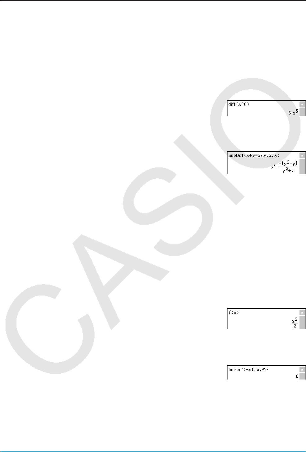
Chapter 2: Main Application 67
Using the Calculation Submenu
The [Calculation] submenu contains calculus related commands, such as “diff” (differentiation) and “ ”
(integration).
udiff [Action][Calculation][diff]
Function: Differentiates an expression with respect to a specific variable.
Syntax: diff(Exp/List[,variable] [ ) ]
diff(Exp/List,variable,order[,a] [ ) ]
• “a” is the point for which you want to determine the derivative.
• “order” = 1 when you use the following syntax: diff(Exp/List[,variable][ ) ]. The default variable is “
x ” when
“variable” is omitted.
Example: To differentiate
x
6 with respect to x
uimpDiff [Action][Calculation][impDiff]
Function: Differentiates an equation or expression in implicit form with respect
to a specific variable.
Syntax: impDiff(Eq/Exp/List, independent variable, dependent variable)
Example: To find
y ’ using implicit differentiation
Important!
The derivative symbol (’) cannot be used in the argument of “impDiff(”. Trying to use a derivative symbol
would result in a Wrong Argument Type error.
u
∫
[Action][Calculation][ ]
Function: Integrates an expression with respect to a specific variable.
Syntax:
(Exp/List[,variable] [ ) ]
(Exp/List, variable, lower limit, upper limit [,tol ] [ ) ]
• “x” is the default when you omit [,variable].
• “tol” represents the allowable error range.
• This command returns an approximate value when a range is specified for “tol ”.
• This command returns the true value of a definite interval when nothing is specified for “tol”. If a true
value cannot be obtained, this command performs approximate calculation using tol = 1E – 5. If an
approximate value can be obtained, that value is returned. An error message is returned if an approximate
value cannot be obtained or if the calculation itself is not possible for some
reason.
Example: To integrate x with respect to x
ulim [Action][Calculation][lim]
Function: Determines the limit of an expression.
Syntax: lim (Exp/List, variable, point [,direction] [
)
]
Example: To determine the limit of
e
−
x
as x approaches ∞
• This function returns the limit from the left when “direction” < 0, the limit from the right when “direction” > 0,
and the limit from both sides (left and right) when “direction” = 0 or when the direction is omitted.
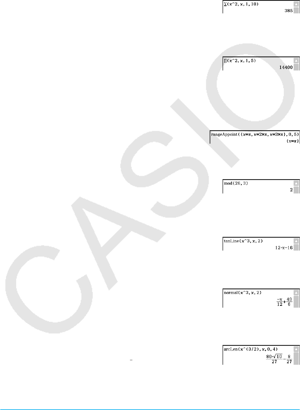
Chapter 2: Main Application 68
u
Σ
[Action][Calculation][Σ]
Function: Evaluates an expression at discrete variable values within a range, and then calculates a sum.
Syntax: Σ(Exp/List, variable, lower value, upper value [ ) ]
Example: To calculate the sum of
x
2 as the value of x changes from x = 1
through x =10
u
Π
[Action][Calculation][Π]
Function: Evaluates an expression at discrete variable values within a range, and then calculates a product.
Syntax: Π(Exp/List, variable, lower value, upper value [ ) ]
Example: To calculate the product of
x
2 as the value of x changes from x = 1
through x = 5
urangeAppoint [Action][Calculation][rangeAppoint]
Function: Finds an expression or value that satisfies a condition in a specified range.
Syntax: rangeAppoint (Exp/Eq/List, start value, end value [ ) ]
• When using an equation (Eq) for the first argument, input the equation using the syntax Var = Exp.
Evaluation will not be possible if any other syntax is used.
Example: To find the expression(s) in the list {
x = π, x = 2π,
x = 3π} that belong(s) to the closed range 0 s x s 5
umod [Action][Calculation][mod]
Function: Returns the remainder when one expression is divided by another expression.
Syntax: mod ({Exp/List} -1, {Exp/List} -2 [ ) ]
Example: To determine the remainder when 26 is divided by 3 (26mod3)
utanLine [Action][Calculation][line][tanLine]
Function: Returns the right side of the equation for the tangent line ( y = ‘expression’) to the curve at the
specified point.
Syntax: tanLine (Exp/List, variable, variable value at point of tangency [ ) ]
Example: To determine the function of the line tangent to
y = x
3 at x = 2
unormal [Action][Calculation][line][normal]
Function: Returns the right side of the equation for the line normal ( y = ‘expression’) to the curve at the
specified point.
Syntax: normal (Exp/List, variable, variable value at point of normal [ ) ]
Example: To determine the function of the line normal to
y = x
3 at x = 2
uarcLen [Action][Calculation][line][arcLen]
Function: Returns the arc length of an expression from a start value to an end value with respect to a
specified variable.
Syntax: arcLen (Exp/List, variable, start value, end value [ ) ]
Example: To determine the arc length for y = x 3
2 from x = 0 to x = 4
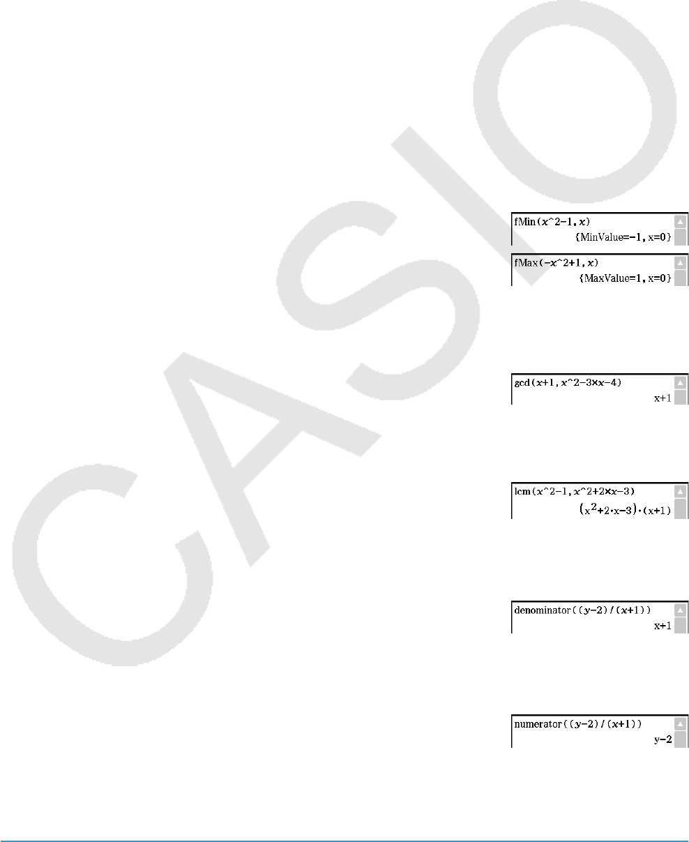
Chapter 2: Main Application 69
ufMin [Action][Calculation][fMin/fMax][fMin], fMax [Action][Calculation][fMin/fMax][fMax]
Function: Returns the minimum (fMin) / the maximum (fMax) point in a specific range of a function.
Syntax: fMin(Exp[,variable] [ ) ]
fMin(Exp, variable, start value, end value[,n] [ ) ]
fMax(Exp[,variable] [ ) ]
fMax(Exp, variable, start value, end value[,n] [ ) ]
• “
x ” is the default when you omit “[,variable]”.
• Negative infinity and positive infinity are the default when the syntax fMin(Exp[,variable] [ ) ] or
fMax(Exp[,variable] [ ) ] is used.
• “ n ” is calculation precision, which you can specify as an integer in the range of 1 to 9. Using any value
outside this range causes an error.
• This command returns an approximate value when calculation precision is specified for “
n ”.
• This command returns a true value when nothing is specified for “
n ”. If the true value cannot be obtained,
however, this command returns an approximate value along with n = 4.
• Discontinuous points or sections that fluctuate widely can adversely affect precision or even cause an error.
• Inputting a larger number for “
n ” increases the precision of the calculation, but it also increases the amount
of time required to perform the calculation.
• The value you input for the end point of the interval must be greater than the value you input for the start
point. Otherwise an error occurs.
Example: To find the minimum point of
x
2 – 1 with respect to x
Example: To find the maximum point of – x
2 + 1 with respect to x
ugcd [Action][Calculation][gcd/lcm][gcd]
Function: Returns the greatest common denominator of two expressions.
Syntax: gcd (Exp/List-1, Exp/List-2 [
)
]
Example: To obtain the greatest common denominator of
x + 1 and x
2 – 3 x – 4
ulcm [Action][Calculation][gcd/lcm][lcm]
Function: Returns the least common multiple of two expressions.
Syntax: lcm (Exp/List-1, Exp/List-2 [ ) ]
Example: To obtain the least common multiple of
x
2 – 1 and x
2 + 2 x – 3
udenominator [Action][Calculation][fraction][denominator]
Function: Extracts the denominator of a fraction.
Syntax: denominator (Exp/List [ ) ]
Example: To extract the denominator of the fraction (
y – 2)/( x + 1)
unumerator [Action][Calculation][fraction][numerator]
Function: Extracts the numerator of a fraction.
Syntax: numerator (Exp/List [ ) ]
Example: To extract the numerator of the fraction (
y – 2)/( x + 1)
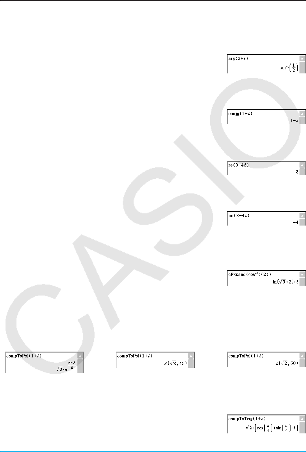
Chapter 2: Main Application 70
Using the Complex Submenu
The [Complex] submenu contains commands that relate to calculations that involve complex numbers.
uarg [Action][Complex][arg]
Function: Returns the argument of a complex number.
Syntax: arg (Exp/Eq/List/Mat [ ) ]
Example: To obtain the argument of complex 2 + i (in the Radian mode)
uconjg [Action][Complex][conjg]
Function: Returns the conjugate complex number.
Syntax: conjg (Exp/Eq/Ineq/List/Mat [ ) ] (Ineq: Real mode only)
Example: To obtain the conjugate of complex number 1 + i
ure [Action][Complex][re]
Function: Returns the real part of a complex number.
Syntax: re (Exp/Eq/Ineq/List/Mat [ ) ] (Ineq: Real mode only)
Example: To obtain the real part of complex number 3 – 4i
uim [Action][Complex][im]
Function: Returns the imaginary part of a complex number.
Syntax: im (Exp/Eq/Ineq/List/Mat [ ) ] (Ineq: Real mode only)
Example: To obtain the imaginary part of complex number 3 – 4i
ucExpand [Action][Complex][cExpand]
Function: Expands a complex expression to rectangular form (a + bi).
Syntax: cExpand (Exp/Eq/List/Mat [ ) ]
• The variables are regarded as real numbers.
Example: To expand cos–1(2) (in the Radian mode)
ucompToPol [Action][Complex][compToPol]
Function: Transforms a complex number into its polar form.
Syntax: compToPol (Exp/Eq/List/Mat [ ) ]
• When the argument is Mat (Matrices), calculation can be performed using the Radian angle unit only.
Example: To transform 1 + i into its polar form
Radian mode Degree mode Grad mode
ucompToTrig [Action][Complex][compToTrig]
Function: Transforms a complex number into its trigonometric/hyperbolic form.
Syntax: compToTrig (Exp/Eq/List/Mat [ ) ]
Example: To transform 1 + i into its trigonometric form (in the Radian mode)
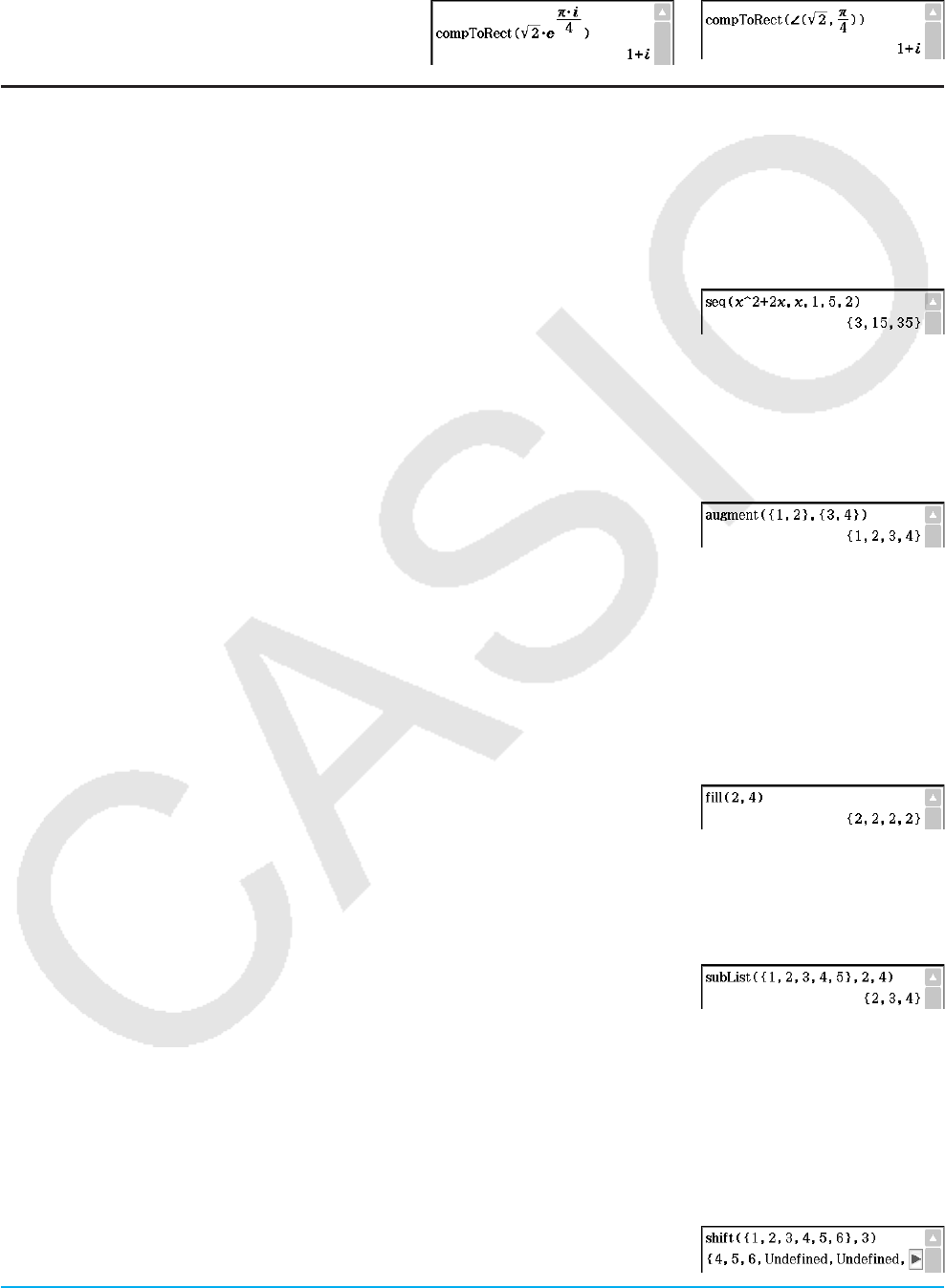
Chapter 2: Main Application 71
ucompToRect [Action][Complex][compToRect]
Function: Transforms a complex number into its rectangular form.
Syntax: compToRect (⬔(
r , ) or r · e^( · i ) form [ ) ]
Example: To transform a complex number
into its rectangular form
Using the List-Create Submenu
The [List][Create] submenu contains commands that are related to creating lists.
useq [Action][List][Create][seq]
Function: Generates a list in accordance with a numeric sequence expression.
Syntax: seq (Exp, variable, start value, end value [,step size] [ ) ]
Example: To generate a list in accordance with the expression x2 + 2x
when the start value is 1, the end value is 5, and the step size is 2
• “1” is the default when you omit “[,step size]”.
• The step size must be a factor of the difference between the start value and the end value.
uaugment [Action][List][Create][augment]
Function: Creates a new list by appending one list to another.
Syntax: augment (List-1, List-2 [ ) ]
Example: To combine list {1, 2} and list {3, 4}
ufill [Action][List][Create][fill]
Function: Replaces the elements of a list with a specified value or expression. This command can also be
used to create a new list whose elements all contain the same value or expression, or a new list in
which the frequency of each element in the first list is determined by the corresponding element in
the second list.
Syntax: fill (Exp/Eq/Ineq, number of elements [ ) ]
fill (Exp/Eq/Ineq, List [ ) ]
fill (List, List [ ) ]
Example: To create a list consisting of four identical elements (2)
usubList [Action][List][Create][subList]
Function: Extracts a specific section of a list into a new list.
Syntax: subList (List [,start number] [,end number] [
)
]
Example: To extract the second through the fourth elements of the list
{1, 2, 3, 4, 5}
• The leftmost element is the default when you omit “[,start number]”, and the rightmost element is the default
when you omit “[,end number]”.
ushift [Action][List][Create][shift]
Function: Returns a list in which elements have been shifted to the right or left by a specific amount.
Syntax: shift (List [,number of shifts] [ ) ]
• Specifying a negative value for “[,number of shifts]” shifts to the right, while a positive value shifts to the left.
• Right shift by one (–1) is the default when you omit “[,number of shifts]”.
Example: To shift the elements of the list {1, 2, 3, 4, 5, 6} to the left by three
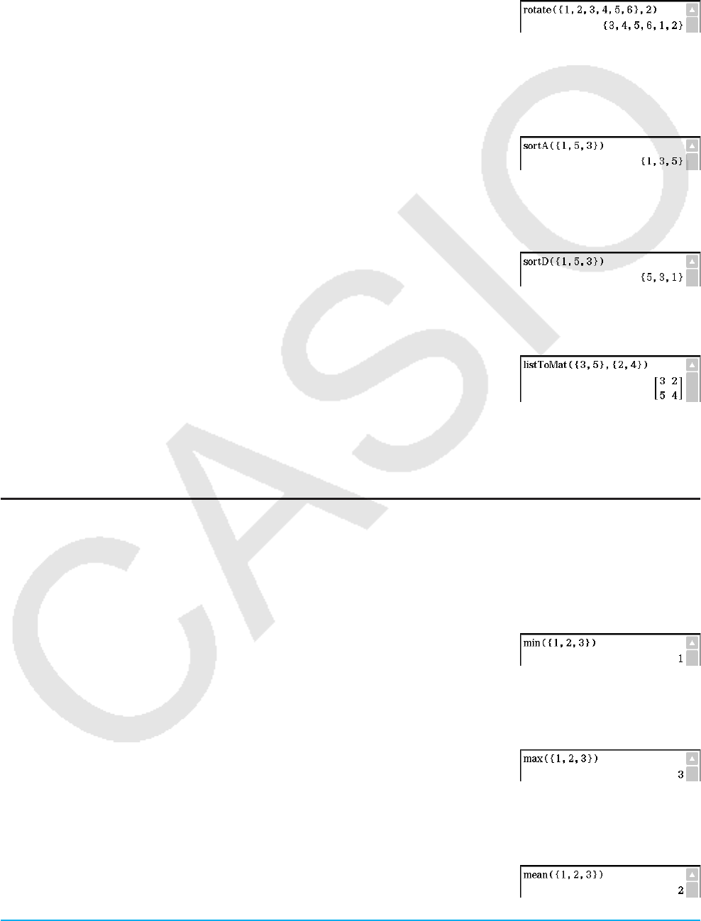
Chapter 2: Main Application 72
urotate [Action][List][Create][rotate]
Function: Returns a list in which the elements have been rotated to the right or to the left by a specific
amount.
Syntax: rotate (List [,number of rotations] [ ) ]
• Specifying a negative value for “[,number of rotations]” rotates to the right, while a positive value rotates to
the left.
Example: To rotate the elements of the list {1, 2, 3, 4, 5, 6} to the left by two
• Right rotation by one (–1) is the default when you omit “[,number of rotations]”.
usortA [Action][List][Create][sortA]
Function: Sorts the elements of the list into ascending order.
Syntax: sortA (List [ ) ]
Example: To sort the elements of the list {1, 5, 3} into ascending order
usortD [Action][List][Create][sortD]
Function: Sorts the elements of the list into descending order.
Syntax: sortD (List [ ) ]
Example: To sort the elements of the list {1, 5, 3} into descending order
u listToMat [Action][List][Create][listToMat]
Function: Transforms lists into a matrix.
Syntax: listToMat (List-1 [, List-2, ..., List-N] [ ) ]
Example: To transform the lists {3, 5} and {2, 4} into a matrix
u matToList [Action][List][Create][matToList]
• For information about matToList, see page 76.
Using the List-Statistics and List-Calculation Submenus
The [List][Statistics] and [List][Calculation] submenus contain commands related to list calculations.
umin [Action][List][Statistics][min]
Function: Returns the minimum value of an expression or the elements in a list.
Syntax: min (Exp/List-1[, Exp/List-2] [ ) ]
Example: To determine the minimum values of the elements in list {1, 2, 3}
umax [Action][List][Statistics][max]
Function: Returns the maximum value of an expression or the elements of a list.
Syntax: max (Exp/List-1[, Exp/List-2] [
)
]
Example: To determine the maximum value of the elements in list {1, 2, 3}
umean [Action][List][Statistics][mean]
Function: Returns the mean of the elements in a list.
Syntax: mean (List-1[, List-2] [ ) ] (List-1: Data, List-2: Freq)
Example: To determine the mean of the elements in list {1, 2, 3}
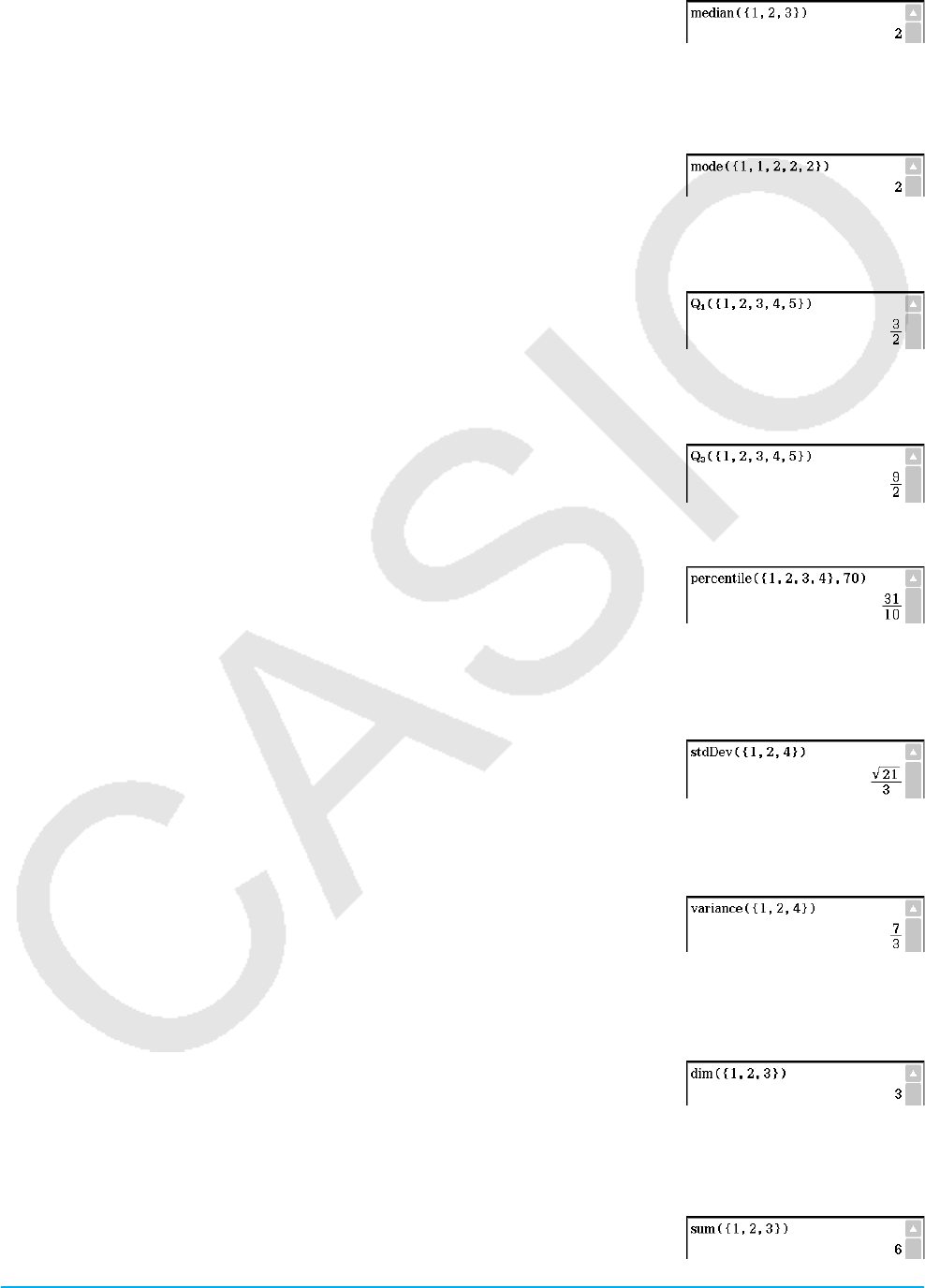
Chapter 2: Main Application 73
umedian [Action][List][Statistics][median]
Function: Returns the median of the elements in a list.
Syntax: median (List-1[, List-2] [ ) ] (List-1: Data, List-2: Freq)
Example: To determine the median of the elements in the list {1, 2, 3}
umode [Action][List][Statistics][mode]
Function: Returns the mode of the elements in a list. If there are multiple modes, they are returned in a list.
Syntax: mode (List-1[, List-2] [
)
] (List-1: Data, List-2: Freq)
Example: To determine the mode of the elements in the list {1, 1, 2, 2, 2}
uQ1 [Action][List][Statistics][Q1]
Function: Returns the first quartile of the elements in a list.
Syntax: Q1 (List-1[, List-2] [ ) ] (List-1: Data, List-2: Freq)
Example: To determine the first quartile of the elements in the list {1, 2, 3, 4, 5}
uQ3 [Action][List][Statistics][Q3]
Function: Returns the third quartile of the elements in a list.
Syntax: Q3 (List-1[, List-2] [
)
] (List-1: Data, List-2: Freq)
Example: To determine the third quartile of the elements in the list {1, 2, 3, 4, 5}
upercentile [Action][List][Statistics][percentile]
Function: Finds the n th percentile point in a list.
Syntax: percentile (list, number)
ustdDev [Action][List][Statistics][stdDev]
Function: Returns the sample standard deviation of the elements in a list.
Syntax: stdDev (List [
)
]
Example: To determine the sample standard deviation of the elements in the
list {1, 2, 4}
uvariance [Action][List][Statistics][variance]
Function: Returns the sample variance of the elements in a list.
Syntax: variance (List [ ) ]
Example: To determine the sample variance of the elements in the list {1, 2, 4}
udim [Action][List][Calculation][dim]
Function: Returns the dimension of a list.
Syntax: dim (List [ ) ]
Example: To determine the dimension of the list {1, 2, 3}
usum [Action][List][Calculation][sum]
Function: Returns the sum of the elements in a list.
Syntax: sum (List-1[, List-2] [ ) ] (List-1: Data, List-2: Freq)
Example: To determine the sum of the elements in the list {1, 2, 3}
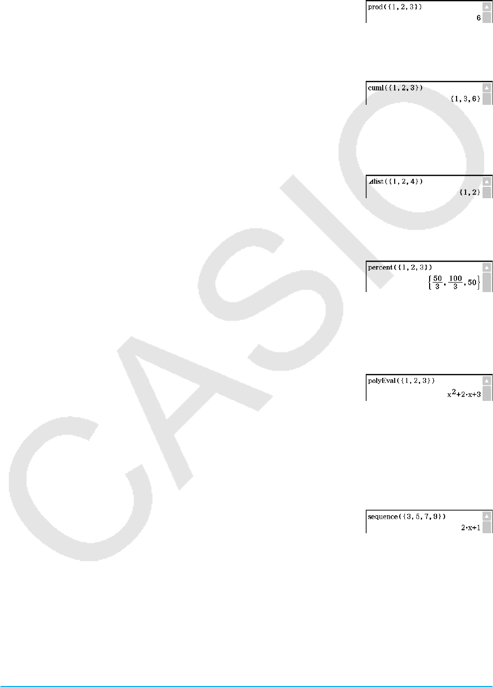
Chapter 2: Main Application 74
uprod [Action][List][Calculation][prod]
Function: Returns the product of the elements in a list.
Syntax: prod (List-1[, List-2] [
)
] (List-1: Data, List-2: Freq)
Example: To determine the product of the elements in the list {1, 2, 3}
ucuml [Action][List][Calculation][cuml]
Function: Returns the cumulative sums of the elements in a list.
Syntax: cuml (List [ ) ]
Example: To determine the cumulative sums of the elements in the list {1, 2, 3}
uAlist [Action][List][Calculation][Alist]
Function: Returns a list whose elements are the differences between two adjacent elements in another list.
Syntax: Alist (List [
)
]
Example: To generate a list whose elements are the differences between two
adjacent elements in the list {1, 2, 4}
upercent [Action][List][Calculation][percent]
Function: Returns the percentage of each element in a list, the sum of which
is assumed to be 100.
Syntax: percent (List [
)
]
Example: To determine the percentage of each element in the list {1, 2, 3}
upolyEval [Action][List][Calculation][polyEval]
Function: Returns a polynomial arranged in the descending order of powers, so coefficients correspond
sequentially to each element in the input list.
Syntax: polyEval (List [,Exp/List] [
) ]
• “
x ” is the default when you omit “[,Exp/List]”.
Example: To create a second degree polynomial with the coefficients {1, 2, 3}
usequence [Action][List][Calculation][sequence]
Function: Returns the lowest-degree polynomial that represents the sequence expressed by the input list.
When there are two lists, this command returns a polynomial that maps each element in the first list
to its corresponding element in the second list.
Syntax: sequence (List-1[, List-2] [,variable] [ ) ]
• “
x ” is the default when you omit “[,variable]”.
Example: To determine a polynomial for a sequence expressed by the list
{3, 5, 7, 9}
usumSeq [Action][List][Calculation][sumSeq]
Function: Finds the lowest-degree polynomial that represents the sequence expressed by the input list and
returns the sum of the polynomial. When there are two lists, this command returns a polynomial that
maps each element in the first list to its corresponding element in the second list, and returns the
sum of the polynomial.
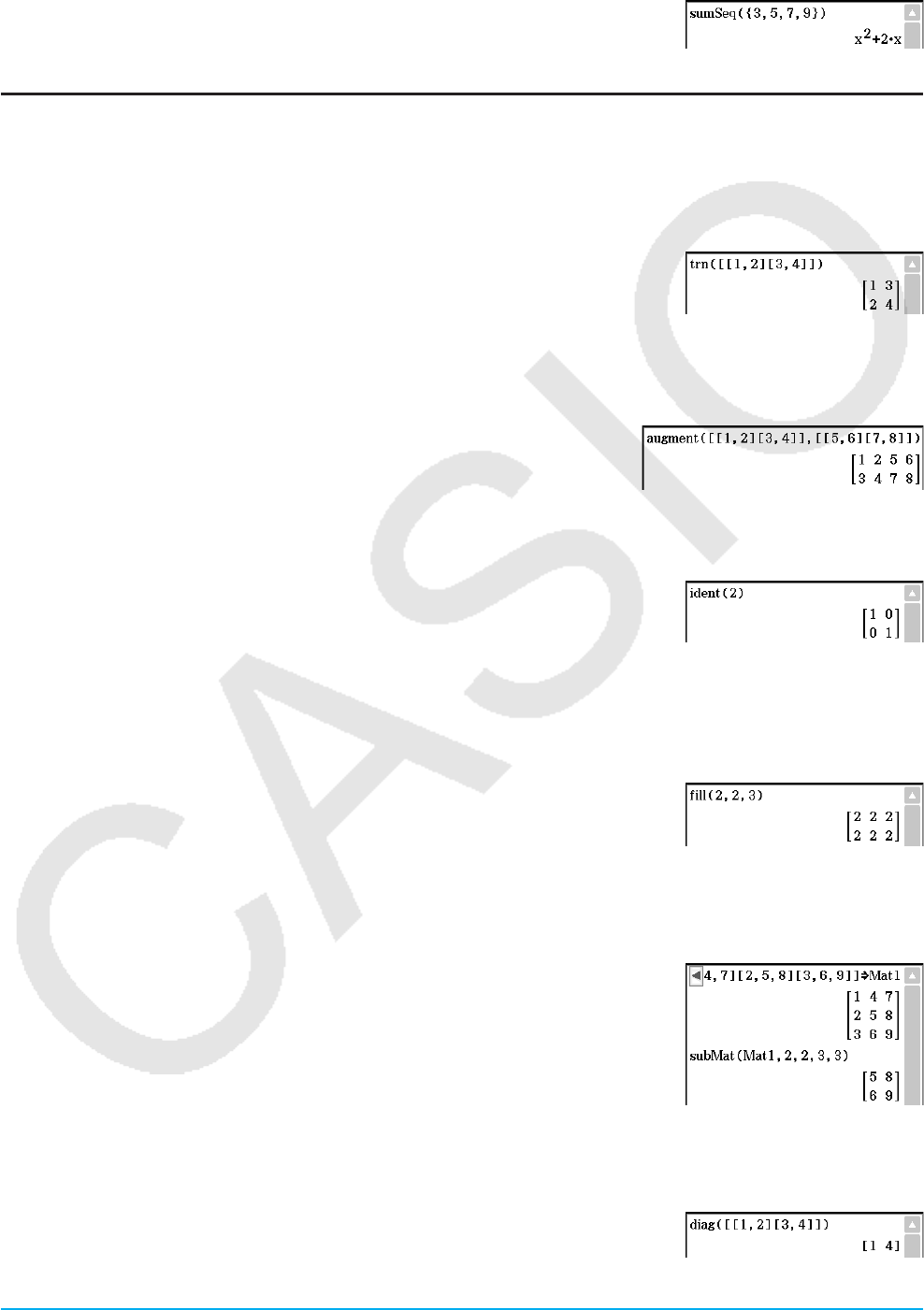
Chapter 2: Main Application 75
Syntax: sumSeq (List-1[, List-2] [,variable] [ ) ]
• “
x ” is the default when you omit “[,variable]”.
Example: To determine the sum of a polynomial for a sequence expressed by
the list {3, 5, 7, 9}
Using the Matrix-Create Submenu
The [Matrix][Create] submenu contains commands related to creation of matrices.
utrn [Action][Matrix][Create][trn]
Function: Returns a transposed matrix.
Syntax: trn (Mat [ ) ]
Example: To transpose the matrix [[1, 2] [3, 4]]
uaugment [Action][Matrix][Create][augment]
Function: Returns a matrix that combines two other matrices.
Syntax: augment (Mat-1, Mat-2 [ ) ]
Example: To combine the two matrices [[1, 2] [3, 4]] and [[5, 6]
[7, 8]]
uident [Action][Matrix][Create][ident]
Function: Creates an identity matrix.
Syntax: ident (natural number [ ) ]
Example: To create a 2 × 2 identity matrix
ufill [Action][Matrix][Create][fill]
Function: Creates a matrix with a specific number of rows and columns, or replaces the elements of a matrix
with a specific expression.
Syntax: fill (Exp, number of rows, number of columns [ ) ]
fill (Exp, Mat [ ) ]
Example: To create a 2 × 3 matrix, all whose elements are 2
usubMat [Action][Matrix][Create][subMat]
Function: Extracts a specific section of a matrix into a new matrix.
Syntax: subMat (Mat [,start row] [,start column] [,end row] [,end column] [ ) ]
• “1” is the default when you omit “[, start row]” and “[, start column]”.
• The last row number is the default when you omit “[, end row]”.
• The last column number is the default when you omit “[, end column]”.
Example: To extract the section from row 2, column 2, to row 3, column
3 from the matrix [[1, 4, 7] [2, 5, 8] [3, 6, 9]]
udiag [Action][Matrix][Create][diag]
Function: Returns a one-row matrix containing the elements from the main diagonal of a square matrix.
Syntax: diag (Mat[ ) ]
Example: To extract the diagonal elements of the matrix [[1, 2] [3, 4]]
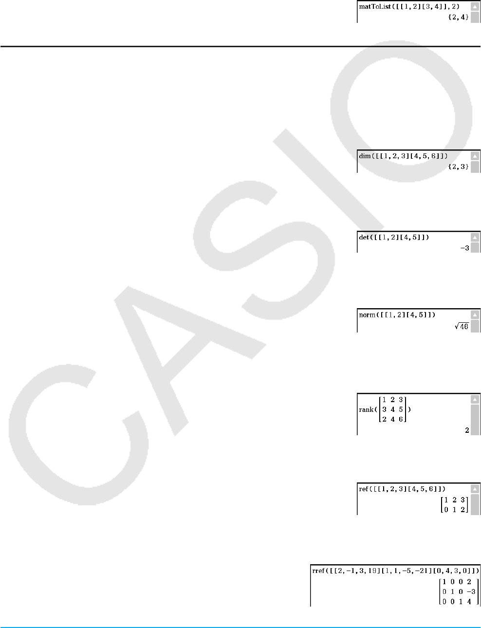
Chapter 2: Main Application 76
ulistToMat [Action][Matrix][Create][listToMat]
• For information about listToMat, see page 72.
u matToList [Action][Matrix][Create][matToList]
Function: Transforms a specific column of a matrix into a list.
Syntax: matToList (Mat, column number [ ) ]
Example: To transform column 2 of the matrix [[1, 2] [3, 4]] into a list
Using the Matrix-Calculation and Matrix-Row&Column Submenus
The [Matrix][Calculation] and [Matrix][Row&Column] submenus contain commands that are related to matrix
calculations.
udim [Action][Matrix][Calculation][dim]
Function: Returns the dimensions of a matrix as a two-element list {number of rows, number of columns}.
Syntax: dim (Mat [
)
]
Example: To determine the dimensions of the matrix [[1, 2, 3] [4, 5, 6]]
udet [Action][Matrix][Calculation][det]
Function: Returns the determinant of a square matrix.
Syntax: det (Mat [ ) ]
Example: To obtain the determinant of the matrix [[1, 2] [4, 5]]
unorm [Action][Matrix][Calculation][norm]
Function: Returns the Frobenius norm of the matrix.
Syntax: norm (Mat [ ) ]
Example: To determine the norm of the matrix [[1, 2] [4, 5]]
urank [Action][Matrix][Calculation][rank]
Function: Finds the rank of matrix.
The rank function computes the rank of a matrix by performing Gaussian
elimination on the rows of the given matrix. The rank of matrix A is the
number of non-zero rows in the resulting matrix.
Syntax: rank (Matrix)
uref [Action][Matrix][Calculation][ref]
Function: Returns the row echelon form of a matrix.
Syntax: ref (Mat [ ) ]
Example: To obtain the row echelon form of the matrix [[1, 2, 3] [4, 5, 6]]
urref [Action][Matrix][Calculation][rref]
Function: Returns the reduced row echelon form of a matrix.
Syntax: rref (Mat [ ) ]
Example: To obtain the reduced row echelon form of the matrix
[[2, –1, 3, 19] [1, 1, –5, –21] [0, 4, 3, 0]]
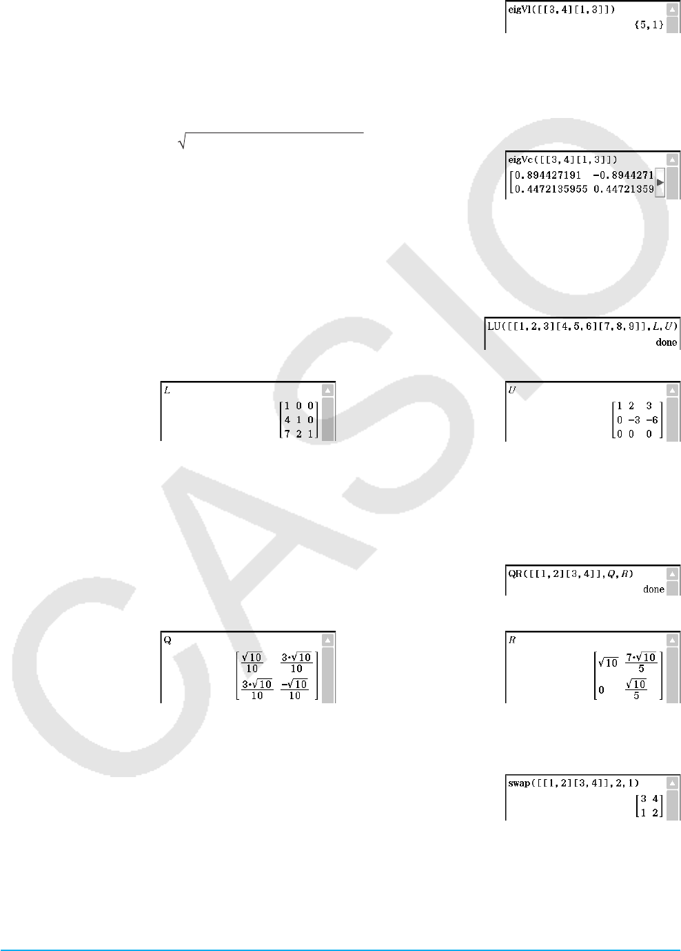
Chapter 2: Main Application 77
ueigVl [Action][Matrix][Calculation][eigVl]
Function: Returns a list that contains the eigenvalue(s) of a square matrix.
Syntax: eigVl (Mat [ ) ]
Example: To obtain the eigenvalue(s) of the matrix [[3, 4] [1, 3]]
ueigVc [Action][Matrix][Calculation][eigVc]
Function: Returns a matrix in which each column represents an eigenvector of a square matrix.
• Since an eigenvector usually cannot be determined uniquely, it is standardized as follows to its norm, which
is 1:
When V = [
x 1, x 2, ..., xn ], (⎥ x 1⎥ 2 + ⎥ x 2⎥ 2 + .... + ⎥ xn ⎥ 2 ) = 1.
Syntax: eigVc (Mat [ ) ]
Example: To obtain the eigenvector(s) of the matrix [[3, 4] [1, 3]]
uLU [Action][Matrix][Calculation][LU]
Function: Returns the LU decomposition of a square matrix.
Syntax: LU (Mat, lVariableMem, uVariableMem [ ) ]
Example: To obtain the LU decomposition of the matrix [[1, 2, 3] [4, 5, 6] [7, 8, 9]]
• The lower matrix is assigned to the first variable L, while the upper
matrix is assigned to the second variable U.
To display the lower matrix To display the upper matrix
LwUw
uQR [Action][Matrix][Calculation][QR]
Function: Returns the QR decomposition of a square matrix.
Syntax: QR (Mat, qVariableMem, rVariableMem [ ) ]
Example: To obtain the QR decomposition of the matrix [[1, 2] [3, 4]]
• The unitary matrix is assigned to variable Q, while the upper triangular
matrix is assigned to variable R.
To display the unitary matrix To display the upper triangular matrix
QwRw
uswap [Action][Matrix][Row&Column][swap]
Function: Swaps two rows of a matrix.
Syntax: swap (Mat, row number-1, row number-2 [ ) ]
Example: To swap row 1 with row 2 of the matrix [[1, 2] [3, 4]]
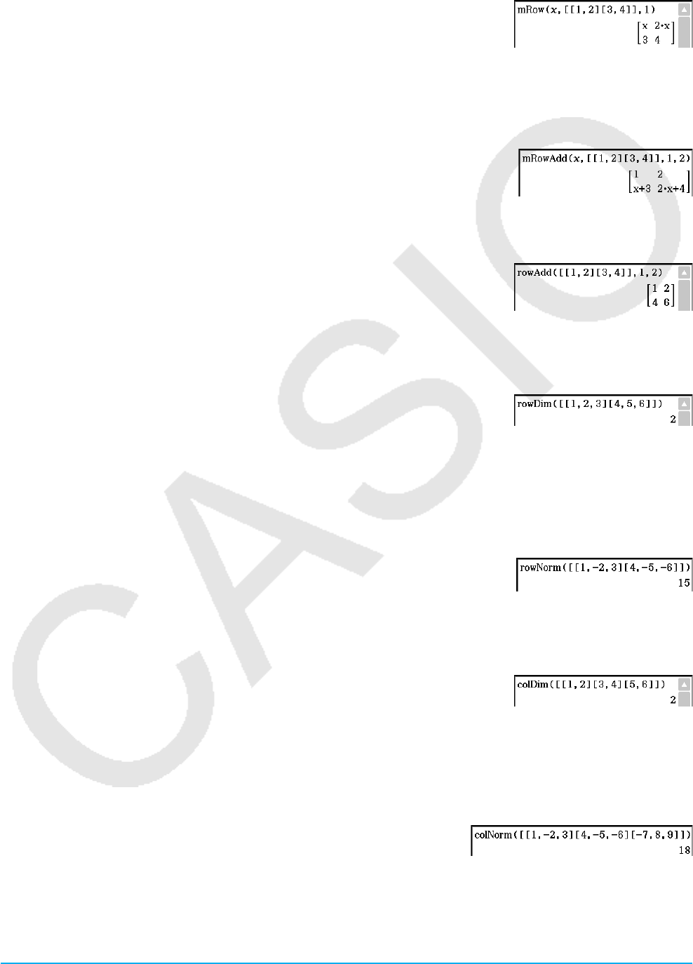
Chapter 2: Main Application 78
umRow [Action][Matrix][Row&Column][mRow]
Function: Multiplies the elements of a specific row in a matrix by a specific
expression.
Syntax: mRow (Exp, Mat, row number [ ) ]
Example: To multiply row 1 of the matrix [[1, 2] [3, 4]] by
x
umRowAdd [Action][Matrix][Row&Column][mRowAdd]
Function: Multiplies the elements of a specific row in a matrix by a specific expression, and then adds the
result to another row.
Syntax: mRowAdd (Exp, Mat, row number-1, row number-2 [ ) ]
Example: To multiply row 1 of the matrix [[1, 2] [3, 4]] by
x , and then add the
result to row 2
urowAdd [Action][Matrix][Row&Column][rowAdd]
Function: Adds a specific matrix row to another row.
Syntax: rowAdd (Mat, row number-1, row number-2 [ ) ]
Example: To add row 1 of the matrix [[1, 2] [3, 4]] to row 2
urowDim [Action][Matrix][Row&Column][rowDim]
Function: Returns the number in rows in a matrix.
Syntax: rowDim (Mat [ ) ]
Example: To obtain the number of rows in the matrix [[1, 2, 3] [4, 5, 6]]
urowNorm [Action][Matrix][Row&Column][rowNorm]
Function: Calculates the sums of the absolute values of the elements of each row of a matrix, and returns the
maximum value of the sums.
Syntax: rowNorm (Mat [ ) ]
Example: To calculate the sums of the absolute values of the elements
in each row of the matrix [[1, –2, 3] [4, –5, –6]], and obtain the
maximum value of the sums
ucolDim [Action][Matrix][Row&Column][colDim]
Function: Returns the number of columns in a matrix.
Syntax: colDim (Mat [ ) ]
Example: To obtain the number of columns in the matrix [[1, 2] [3, 4] [5, 6]]
ucolNorm [Action][Matrix][Row&Column][colNorm]
Function: Calculates the sums of the absolute values of the elements of each column of a matrix, and returns
the maximum value of the sums.
Syntax: colNorm (Mat [ ) ]
Example: To calculate the sums of the absolute values of the elements
in each column of the matrix [[1, –2, 3][4, –5, –6][–7, 8, 9]],
and obtain the maximum value of the sums
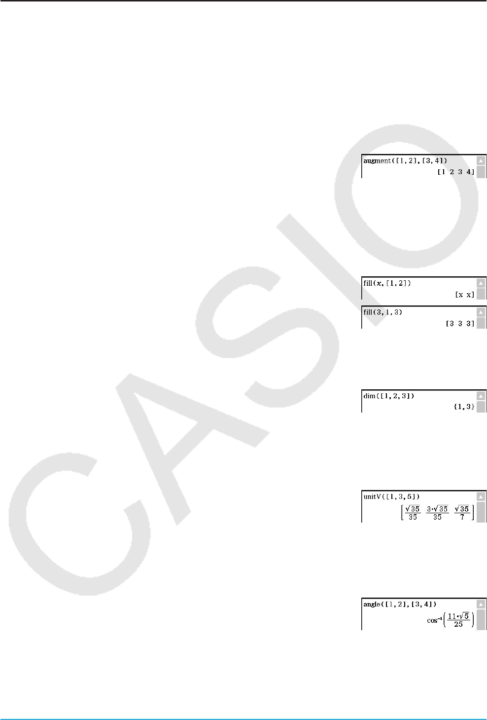
Chapter 2: Main Application 79
Using the Vector Submenu
The [Vector] submenu contains commands that are related to vector calculations.
• A vector is handled as a 1 × N matrix or N × 1 matrix.
• A vector in the form of 1 × N can be entered as [……] or [[……]].
Example: [1, 2], [[1, 2]]
• Vectors are considered to be in rectangular form unless ∠() is used to indicate an angle measure.
uaugment [Action][Vector][augment]
Function: Returns an augmented vector [Mat-1 Mat-2].
Syntax: augment (Mat-1, Mat-2 [ ) ]
Example: To augment vectors [1, 2] and [3, 4]
ufill [Action][Vector][fill]
Function: Creates a vector that contains a specific number of elements, or replaces the elements of a vector
with a specific expression.
Syntax: fill (Exp, Mat [ ) ]
fill (Exp, 1, number of columns [ ) ]
Example: To replace the elements of the vector [1, 2] with x
Example: To create a 1 × 3 (1 row, 3 columns) vector, all of whose elements
are “3”
udim [Action][Vector][dim]
Function: Returns the dimension of a vector.
Syntax: dim (Mat [ ) ]
Example: To determine the dimension of the vector [1, 2, 3]
• The vector [1, 2, 3] is handled as a 1 × 3 matrix.
uunitV [Action][Vector][unitV]
Function: Normalizes a vector.
Syntax: unitV (Mat [ ) ]
• This command can be used with a 1 × N or N × 1 matrix only.
Example: To normalize the vector [1, 3, 5]
uangle [Action][Vector][angle]
Function: Returns the angle formed by two vectors.
Syntax: angle (Mat-1, Mat-2 [ ) ]
• This command can be used with a 1 × N or N × 1 matrix only.
Example: To determine the angle formed by vectors [1, 2] and [3, 4] (in the
Radian mode)
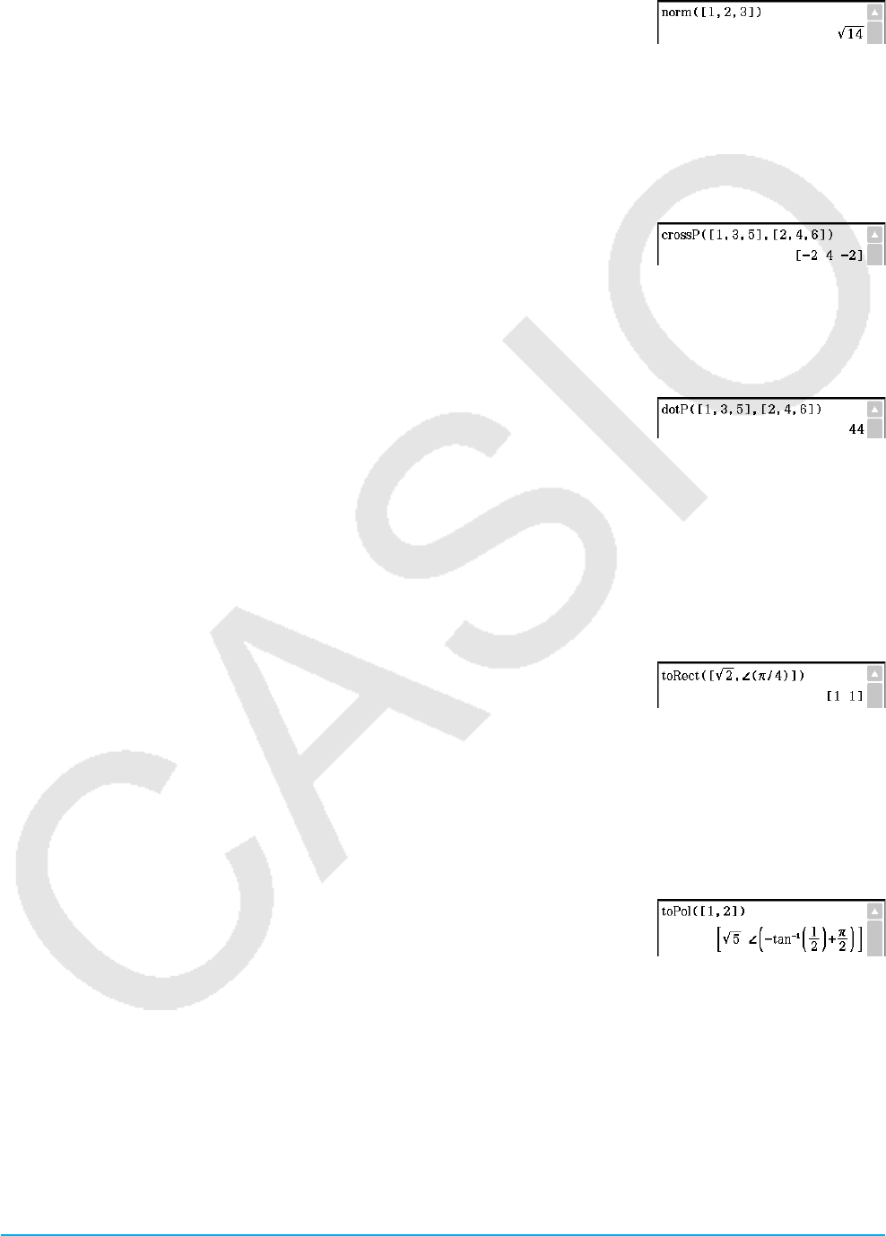
Chapter 2: Main Application 80
unorm [Action][Vector][norm]
Function: Returns the norm of a vector.
Syntax: norm (Mat [ ) ]
Example: To obtain the norm of the vector [1, 2, 3]
ucrossP [Action][Vector][crossP]
Function: Returns the cross product of two vectors.
Syntax: crossP (Mat-1, Mat-2 [ ) ]
• This command can be used with a 1 × N or N × 1 matrix only (N = 2, 3).
• A two-element matrix [a, b] or [[a], [b]] is automatically converted into a three-element matrix [a, b, 0] or
[[a], [b], [0]].
Example: To obtain the cross product of the two vectors [1, 3, 5] and [2, 4, 6]
udotP [Action][Vector][dotP]
Function: Returns the dot product of two vectors.
Syntax: dotP (Mat-1, Mat-2 [ ) ]
• This command can be used with a 1 × N or N × 1 matrix only.
Example: To obtain the dot product of the two vectors [1, 3, 5] and [2, 4, 6]
utoRect [Action][Vector][toRect]
Function: Returns an equivalent rectangular form [ x y ] or [ x y z ].
Syntax: toRect (Mat [,natural number] [ ) ]
• This command can be used with a 1 × N or N × 1 matrix only (N = 2, 3).
• This command returns “x” when “natural number” is 1, “y” when “natural number” is 2, and “z” when “natural
number” is 3.
• This command returns a rectangular form when you omit “natural number”.
Example: To transform the polar form ['2 , ∠(π/4)] into an equivalent
rectangular form (in the Radian mode)
utoPol [Action][Vector][toPol]
Function: Returns an equivalent polar form [ r ∠ ].
Syntax: toPol (Mat [,natural number] [ ) ]
• This command can be used with a 1 × 2 or 2 × 1 matrix only.
• This command returns “r” when “natural number” is 1, and “ ” when “natural number” is 2.
• This command returns a polar form when you omit “natural number”.
Example: To transform the rectangular form [1, 2] into its equivalent polar
form
utoSph [Action][Vector][toSph]
Function: Returns an equivalent spherical form [
ρ
∠ ∠
φ
].
Syntax: toSph (Mat [,natural number] [ ) ]
• This command can be used with a 1 × 3 or 3 × 1 matrix only.
• This command returns “
ρ
” when “natural number” is 1, “ ” when “natural number” is 2, and “
φ
” when “natural
number” is 3.
• This command returns a spherical form when you omit “natural number”.
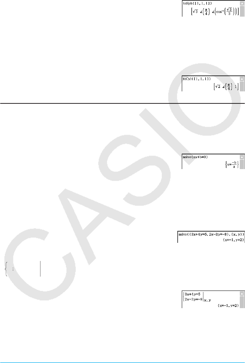
Chapter 2: Main Application 81
Example: To transform the rectangular form [1, 1, 1] into its equivalent
spherical form (in the Radian mode)
utoCyl [Action][Vector][toCyl]
Function: Returns an equivalent cylindrical form [ r ∠ z ].
Syntax: toCyl (Mat [,natural number] [ ) ]
• This command can be used with a 1 × 3 or 3 × 1 matrix only.
• This command returns “r” when “natural number” is 1, “ ” when “natural number” is 2, and “z” when “natural
number” is 3.
• This command returns a cylindrical form when you omit “natural number”.
Example: To transform the rectangular form [1, 1, 1] into an equivalent
cylindrical form (in the Radian mode)
Using the Equation/Inequality Submenu
The [Equation/Inequality] submenu contains commands that are related to equations and inequalities.
u solve [Action][Equation/Inequality][solve]
Function: Returns the solution of an equation or inequality.
Syntax 1: solve(Exp/Eq/Ineq [,variable] [
)
]
• “
x ” is the default when you omit “[,variable]”.
Example: To solve
ax + b = 0 for x
Syntax 2: solve(Exp/Eq/Ineq,variable[, value, lower limit, upper limit] [
)
]
• “value” is an initially estimated value.
• This command is valid only for equations and expressions when “value” and the items following it are
included. In that case, this command returns an approximate value.
• A true value is returned when you omit “value” and the items following it. When, however, a true value
cannot be obtained, an approximate value is returned for equations only based on the assumption that value
= 0, lower limit = –
∞, and upper limit = ∞.
Syntax 3: solve({Exp-1/Eq-1, ..., Exp-N/Eq-N}, {variable-1, ..., variable-N} [
)
]
• When “Exp” is the first argument, the equation Exp = 0 is presumed.
Example: To solve simultaneous linear equations 3
x + 4 y = 5, 2 x – 3 y = –8
You also could input the simultaneous equations shown in this example using the soft keyboard # key. The
following shows the required input syntax.
Exp-1/Eq-1
Exp-N/Eq-N variable-1, ..., variable-N
• The following shows the required key operation to input this example using the # key.
#dX+eY=fccX-dY=-ieX,Yw
• To input simultaneous equations with three or more unknowns, tap the # key when the cursor is in the
Exp-N/Eq-N input field. Each tap of # will add one more line for input of an equation.
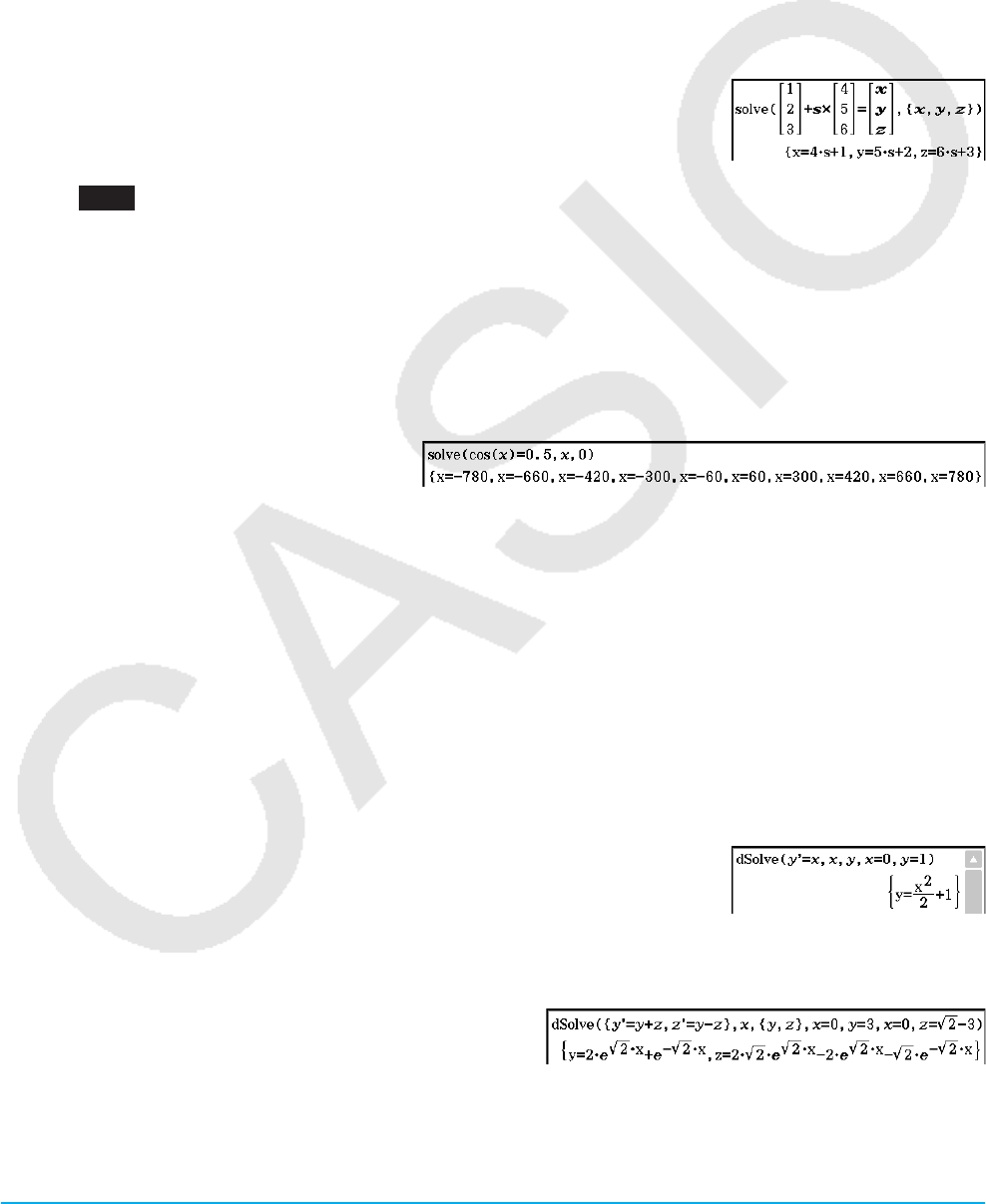
Chapter 2: Main Application 82
Syntax 4: You can solve for the relationship between two points, straight lines, planes, or spheres by entering
a vector equation inside the solve( command. Here we will present four typical syntaxes for solving
a vector equation using the solve( command.
In the syntaxes below, Vct-1 through Vct-6 are column vectors with three (or two) elements, and s,
t, u and v are parameters.
solve(Vct-1 + s * Vct-2 [= Vct-3, {variable-1}])
• If the right side of the equation (= Vct-3) is omitted in the above syntax, it is assumed that all of the
elements on the right side are 0 vectors.
solve(Vct-1 + s * Vct-2 = Vct-3 + t * Vct-4, {variable-1, variable-2})
solve(Vct-1 + s * Vct-2 + t * Vct-3 = Vct-4 – u * Vct-5, {variable-1, variable-2, variable-3})
solve(Vct-1 + s * Vct-2 + t * Vct-3 = Vct-4 – u * Vct-5 + v * Vct-6, {variable-1, variable-2, variable-3,
variable-4})
• Variables (variable 1 through variable 4) can be input into the
elements of each vector (Vct-1 through Vct-6) in the above four
syntaxes to solve for those variables.
0234 To prove whether point P (5, 7, 9) and point Q (5, 7, 8) each exist on straight line l, which is an
orientation vector (4, 5, 6) that passes through point A (1, 2, 3)
Note
For the solution, the solve function returns an expression or value for the expression (Exp/Eq) input as its
argument. The message “More solutions may exist” will appear on the display when a value is returned as the
solution, because there may be multiple solutions.
The solve function can return a maximum of 10 solutions in the case of values.
Example: To solve cos (
x ) = 0.5 for x (initial value: 0)
(Angle unit setting: Deg)
u dSolve [Action][Equation/Inequality][dSolve]
Function: Solves first, second or third order ordinary differential equations, or a system of first order
differential equations.
Syntax: dSolve(Eq, independent variable, dependent variable [, initial condition-1, initial condition-2][, initial
condition-3, initial condition-4][, initial condition-5, initial condition-6] [ ) ]
dSolve({Eq-1, Eq-2}, independent variable, {dependent variable-1, dependent variable-2} [, initial
condition-1, initial condition-2, initial condition-3, initial condition-4] [ ) ]
• If you omit the initial conditions, the solution will include arbitrary constants.
• Input all initial conditions equations using the syntax Var = Exp. Any initial condition that uses any other
syntax will be ignored.
Example: To solve a differential equation
y ’ = x , where y = 1 when x = 0
Example: To solve the system of first order differential equations
y ’ = y + z , z ’ = y – z , where “ x ” is the
independent variable, “ y ” and “ z ” are the dependent variables, and the initial conditions are y = 3
when x = 0, and z = '2 – 3 when x = 0
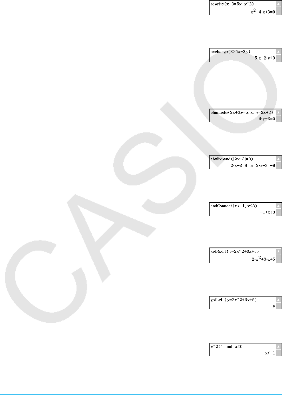
Chapter 2: Main Application 83
urewrite [Action][Equation/Inequality][rewrite]
Function: Moves the right side elements of an equation or inequality to the left side.
Syntax: rewrite(Eq/Ineq/List [ ) ]
Example: To move the right side elements of
x + 3 = 5 x – x
2 to the left side
uexchange [Action][Equation/Inequality][exchange]
Function: Swaps the right-side and left-side elements of an equation or inequality.
Syntax: exchange(Eq/Ineq/List [ ) ]
Example: To swap the left-side and right-side elements of 3 > 5
x – 2 y
ueliminate [Action][Equation/Inequality][eliminate]
Function: Solves one equation with respect to a variable, and then replaces the same variable in another
expression with the obtained result.
Syntax: eliminate(Eq/Ineq/List-1, variable, Eq-2 [ ) ]
Example: To transform
y = 2 x + 3 to x =, and substitute the result into
2 x + 3 y = 5
uabsExpand [Action][Equation/Inequality][absExpand]
Function: Divides an absolute value expression into formulas without absolute value.
Syntax: absExpand(Eq/Ineq [
)
]
Example: To remove the absolute value from ⎜2
x – 3 ⎜ = 9
uandConnect [Action][Equation/Inequality][andConnect]
Function: Combines two equations or inequalities into a single expression.
Syntax: andConnect(Eq/Ineq-1, Eq/Ineq-2 [ ) ]
Example: To rewrite
x > –1 and x < 3 into a single inequality
ugetRight [Action][Equation/Inequality][getRight]
Function: Extracts the right-side elements of an equation or inequality.
Syntax: getRight(Eq/Ineq/List [ ) ]
Example: To extract the right side elements of
y = 2 x
2 + 3 x + 5
ugetLeft [Action][Equation/Inequality][getLeft]
Function: Extracts the left-side elements of an equation or inequality.
Syntax: getLeft(Eq/Ineq/List [ ) ]
Example: To extract the left side elements of
y = 2 x
2 + 3 x + 5
uand [Action][Equation/Inequality][Logic][and]
Function: Returns the result of the logical AND of two expressions.
Syntax: Exp/Eq/Ineq/List-1 and Exp/Eq/Ineq/List-2
Example: To obtain the result of the logical AND of
x
2 > 1 and x < 0
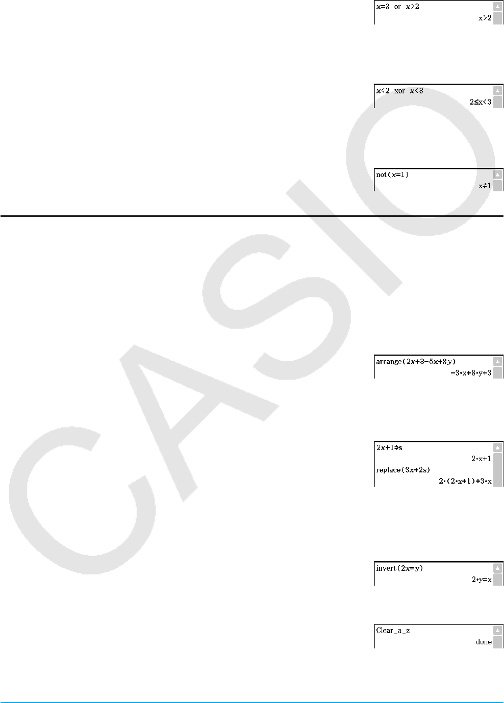
Chapter 2: Main Application 84
uor [Action][Equation/Inequality][Logic][or]
Function: Returns the result of the logical OR of two expressions.
Syntax: Exp/Eq/Ineq/List-1 or Exp/Eq/Ineq/List-2
Example: To obtain the result of the logical OR of
x = 3 or x > 2
uxor [Action][Equation/Inequality][Logic][xor]
Function: Returns the logical exclusive OR of two expressions.
Syntax: Exp/Eq/Ineq/List-1 xor Exp/Eq/Ineq/List-2
Example: To obtain the logical exclusive OR of
x < 2 xor x < 3
unot [Action][Equation/Inequality][Logic][not]
Function: Returns the logical NOT of an expression.
Syntax: not(Exp/Eq/Ineq/List [ ) ]
Example: To obtain the logical NOT of
x = 1
Using the Assistant Submenu
The [Assistant] submenu contains four commands related to the Assistant mode.
Note that the following commands are valid in the Assistant mode only. For more information on the Assistant
mode see “Assistant Mode and Algebra Mode” on page 47.
uarrange [Action][Assistant][arrange]
Function: Collects like terms and arranges them in descending order, starting with the term that contains the
smallest coefficient.
Syntax: arrange (Exp/Eq/Ineq/List/Mat [ ) ]
Example: To arrange 2
x + 3 – 5 x + 8 y in the sequence of its variables
ureplace [Action][Assistant][replace]
Function: Replaces the variable in an expression, equation or inequality with the value assigned to a variable
using the “store” command.
Syntax: replace (Exp/Eq/Ineq/List/Mat [ ) ]
Example: To replace s in the expression 3x + 2s, when the expression 2x + 1
is assigned to s
uinvert [Action][Assistant][invert]
Function: Inverts two variables in an expression.
Syntax: invert (Exp/Eq/Ineq/List [,variable-1, variable-2] [ ) ]
• x and y are inverted when variables are not specified.
Example: To invert x and y in the expression 2 x = y
u Clear_a_z
Function: Clears all single-character variable names (a–z and A–Z) in the
current folder.

Chapter 2: Main Application 85
Using the Distribution/Inv.Dist Submenu
The [Distribution/Inv.Dist] submenu includes functions related to each type of statistical calculation distribution
probability. The functions on this submenu perform the same calculations as the Distribution commands that
are available in the Statistics application and the Main, eActivity, and Program applications.
For information about the numeric expressions used in calculations, see “Distributions” on page 151.
For information about the meanings of the variables used in the syntaxes of the functions presented in this
section, and the system variables that store the values obtained as calculation results, see “Input and Output
Terms” on page 154.
Specifying Arguments within the Distribution Function
You can specify either values or list data for any of the arguments within the Distribution function. The normPDf
function (page 85) syntax (normPDf( x , , )) that returns normal probability density can be used to perform the
calculations shown below. The “Number Format” setting is “Fix 2” for all calculation results.
normPDf(1, 1, 0) = 0.24
normPDf({1, 2}, 1, 0) = {0.24, 0.05}
normPDf(1, {1, 2}, 0) = {0.24, 0.18}
normPDf({1, 2},{1, 2}, 0) = {0.24, 0.12}
normPDf({1, 2},{1, 2},{1, 0}) = {0.40, 0.12}
The following explains how to specify list data in arguments and how calculation results are output.
(a) Specifying list data for a single argument
• Basically, you can specify any list you like, but the each of the elements in the list must be in accordance
with the conditions required by the argument of the function being used.
• Calculation is performed on each element within the list and results are output as shown below.
normPDf(
x , {
1,
2}, )
= {<normPDf(
x ,
1, ) calculation result>, <normPDf( x ,
2, ) calculation result>}
(b) Specifying list data for multiple arguments
• In this case, all of the lists must have the same number of elements. Otherwise an Invalid Dimension error
will occur.
• Calculation is performed on each element within the list and results are output as shown below.
normPDf({
x
1, x
2}, {
1,
2}, )
= {<normPDf(
x
1,
1, ) calculation results>, <normPDf( x
2,
2, ) calculation results>}
Assignment of List Data Calculation Results to Variables
Using the list data in the argument of the Distribution function causes calculation results to be output as list
data, which is assigned as-is to the “ans” variable.
In addition to the “ans” variable, calculations that use the Distribution function causes calculation results also
to be assigned to certain system variables. For example, the normal probability density variable returned by
normPDf is assigned to system variable
prob . Only the last element of the list data will be assigned to a system
variable as a calculation result.
In the distribution function explanations below, the names of the functions to which calculation results are
assigned are shown under “Calculation Result Output”.
u normPDf [Action][Distribution/Inv.Dist][Continuous][normPDf]
Function: Returns the normal probability density for a specified value.
Syntax: normPDf(
x [,
σ
,
μ
)]
• When
σ
and
μ
are skipped,
σ
= 1 and
μ
= 0 are used.
Calculation Result Output:
prob
Example: To determine the normal probability density when x = 37.5,
σ
= 2,
μ
= 35
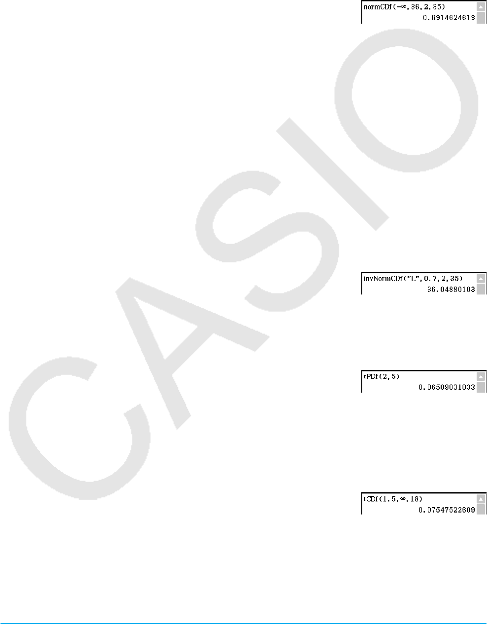
Chapter 2: Main Application 86
unormCDf [Action][Distribution/Inv.Dist][Continuous][normCDf]
Function: Returns the cumulative probability of a normal distribution between a lower bound and an upper
bound.
Syntax: normCDf(lower value, upper value[,
σ
,
μ
)]
• When
σ
and
μ
are skipped,
σ
= 1 and
μ
= 0 are used.
Calculation Result Output:
prob , z Low, z Up
Example: To determine the normal probability density when lower bound
value = −∞, upper bound value = 36,
σ
= 2,
μ
= 35
uinvNormCDf [Action][Distribution/Inv.Dist][Inverse][invNormCDf]
Function: Returns the boundary value(s) of a normal cumulative distribution probability for specified values.
Syntax: invNormCDf([tail setting, ]area value[,
σ
,
μ
)]
• When
σ
and
μ
are skipped,
σ
= 1 and
μ
= 0 are used.
• “tail setting” displays the probability value tail specification, and Left, Right, or Center can be specified. Enter
the following values or letters to specify:
Left: −1, “L”, or “l”
Center: 0, “C”, or “c”
Right: 1, “R”, or “r”
When input is skipped, “Left” is used.
• When one argument is omitted (resulting in three arguments), Tail=Left.
• When two arguments are omitted (resulting in two arguments), Tail=Left,
μ
=0.
• When three arguments are omitted (resulting in one argument), Tail=Left,
σ
=1,
μ
=0.
• When “tail setting” is Center, the lower bound value is returned.
Calculation Result Output: x1InvN, x2InvN
Example: To determine the upper bound value when tail setting = Left, area
value = 0.7,
σ
= 2,
μ
= 35
utPDf [Action][Distribution/Inv.Dist][Continuous][tPDf]
Function: Returns the Student’s t probability density for a specified value.
Syntax: tPDf(x, df [ ) ]
Calculation Result Output: prob
Example: To determine the Student’s t probability density when x = 2, df = 5
utCDf [Action][Distribution/Inv.Dist][Continuous][tCDf]
Function: Returns the cumulative probability of a Student’s t distribution between a lower bound and an upper
bound.
Syntax: tCDf(lower value, upper value, df [ ) ]
Calculation Result Output:
prob, tLow, tUp
Example: To determine the Student’s t distribution probability when
lower value = 1.5, upper value = ∞, df = 18
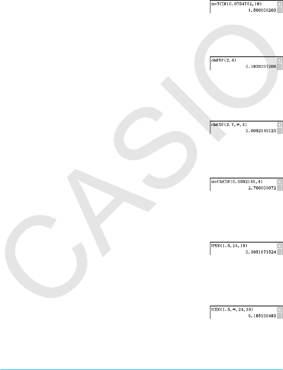
Chapter 2: Main Application 87
uinvTCDf [Action][Distribution/Inv.Dist][Inverse][invTCDf]
Function: Returns the lower bound value of a Student’s t cumulative distribution probability for specified
values.
Syntax: invTCDf(prob, df [ ) ]
Calculation Result Output:
xInv
Example: To determine the lower bound value when prob = 0.0754752,
df = 18
uchiPDf [Action][Distribution/Inv.Dist][Continuous][chiPDf]
Function: Returns the χ2 probability density for specified values.
Syntax: chiPDf(x, df [ ) ]
Calculation Result Output: prob
Example: To determine the χ2 probability density when x = 2, df = 4
uchiCDf [Action][Distribution/Inv.Dist][Continuous][chiCDf]
Function: Returns the cumulative probability of a χ2 distribution between a lower bound and an upper bound.
Syntax: chiCDf(lower value, upper value, df [ ) ]
Calculation Result Output:
prob
Example: To determine the χ2 probability when lower value = 2.7,
upper value = ∞, df = 4
uinvChiCDf [Action][Distribution/Inv.Dist][Inverse][invChiCDf]
Function: Returns the lower bound value of a χ2 cumulative distribution probability for specified values.
Syntax: invChiCDf(prob, df [ ) ]
Calculation Result Output:
xInv
Example: To determine the lower bound value when prob = 0.6092146, df = 4
ufPDf [Action][Distribution/Inv.Dist][Continuous][fPDf]
Function: Returns the F probability density for a specified value.
Syntax: fPDf(
x , n : df , d : df [ ) ]
Calculation Result Output:
prob
Example: To determine the F probability density when x = 1.5, n : df = 24,
d : df = 19
ufCDf [Action][Distribution/Inv.Dist][Continuous][fCDf]
Function: Returns the cumulative probability of an F distribution between a lower bound and an upper bound.
Syntax: fCDf(lower value, upper value,
n : df , d : df [ ) ]
Calculation Result Output: prob
Example: To determine the F distribution probability when lower value = 1.5,
upper value = ∞, n : df = 24, d : df = 19
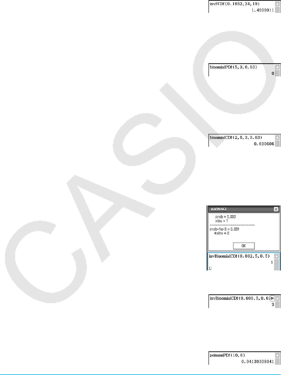
Chapter 2: Main Application 88
uinvFCDf [Action][Distribution/Inv.Dist][Inverse][invFCDf]
Function: Returns the lower bound value of an F cumulative distribution probability for specified values.
Syntax: invFCDf(
prob , n : df , d : df [ ) ]
Calculation Result Output:
x Inv
Example: To determine the lower bound value when
prob = 0.1852, n : df = 24,
d : df = 19
ubinomialPDf [Action][Distribution/Inv.Dist][Discrete][binomialPDf]
Function: Returns the probability in a binomial distribution that the success will occur on a specified trial.
Syntax: binomialPDf(
x , numtrial value, pos [ ) ]
Calculation Result Output:
prob
Example: To determine the binomial probability when x = 5, numtrial value = 3,
pos = 0.63
ubinomialCDf [Action][Distribution/Inv.Dist][Discrete][binomialCDf]
Function: Returns the cumulative probability in a binomial distribution that the success will occur between
specified lower value and upper value.
Syntax: binomialCDf(lower value, upper value, numtrial value,
pos [ ) ]
Calculation Result Output:
prob
Example: To determine the binomial cumulative probability when lower value
= 2, upper value = 5, numtrial value = 3, pos = 0.63
u invBinomialCDf [Action][Distribution/Inv.Dist][Inverse][invBinomialCDf]
Function: Returns the minimum number of trials of a binomial cumulative probability distribution for specified
values.
Syntax: invBinomialCDf(
prob , numtrial value, pos [ ) ]
Calculation Result Output:
x Inv, ½ x Inv
Important!
When executing the invBinomialCDf, invPoissonCDf, invGeoCDf, or
invHypergeoCDf function, the ClassPad uses the specified prob value and
the value that is one less the prob value minimum number of significant digits
(½ prob value) to calculate minimum number of trials values. The results
are assigned to the system variables xInv (calculation result using prob )
and ½ xInv (calculation result using ½ prob ). The function always returns the
xInv value only. However, when the xInv and ½ xInv values are different, the
warning message shown nearby appears showing both values.
The calculation results of the function are integers. Accuracy may be reduced
when the first argument has 10 or more digits. Note that even a slight difference in calculation accuracy
affects calculation results. If a warning message appears, check the displayed values.
Example: To determine the minimum number of trials when prob = 0.609,
numtrial value = 5, pos = 0.63
upoissonPDf [Action][Distribution/Inv.Dist][Discrete][poissonPDf]
Function: Returns the probability in a Poisson distribution that the success will occur on a specified trial.
Syntax: poissonPDf(
x , [ ) ]
Calculation Result Output: prob
Example: To determine the Poisson probability when x = 10, = 6
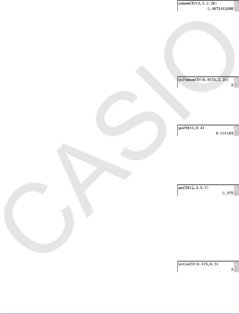
Chapter 2: Main Application 89
upoissonCDf [Action][Distribution/Inv.Dist][Discrete][poissonCDf]
Function: Returns the cumulative probability in a Poisson distribution that the success will occur between
specified lower value and upper value.
Syntax: poissonCDf(lower value, upper value, [ ) ]
Calculation Result Output:
prob
Example: To determine the Poisson cumulative probability when lower
value = 2, upper value = 3, = 2.26
uinvPoissonCDf [Action][Distribution/Inv.Dist][Inverse][invPoissonCDf]
Function: Returns the minimum number of trials of a Poisson cumulative probability distribution for specified
values.
Syntax: invPoissonCDf(
prob , [ ) ]
Calculation Result Output:
x Inv, ½ x Inv
Important!
See “Important!” under “invBinomialCDf” on page 88.
Example: To determine the minimum number of trials when prob = 0.8074,
= 2.26
ugeoPDf [Action][Distribution/Inv.Dist][Discrete][geoPDf]
Function: Returns the probability in a geometric distribution that the success will occur on a specified trial.
Syntax: geoPDf(
x , pos [ ) ]
Calculation Result Output:
prob
Example: To determine the geometric probability when x = 6, pos = 0.4
ugeoCDf [Action][Distribution/Inv.Dist][Discrete][geoCDf]
Function: Returns the cumulative probability in a geometric distribution that the success will occur between
specified lower value and upper value.
Syntax: geoCDf(lower value, upper value,
pos [ ) ]
Calculation Result Output:
prob
Example: To determine the geometric probability when lower value = 2,
upper value = 3, pos = 0.5
uinvGeoCDf [Action][Distribution/Inv.Dist][Inverse][invGeoCDf]
Function: Returns the minimum number of trials of a geometric cumulative probability distribution for specified
values.
Syntax: invGeoCDf(
prob , pos [ ) ]
Calculation Result Output:
x Inv, ½ x Inv
Important!
See “Important!” under “invBinomialCDf” on page 88.
Example: To determine the minimum number of trials when prob = 0.875,
pos = 0.5
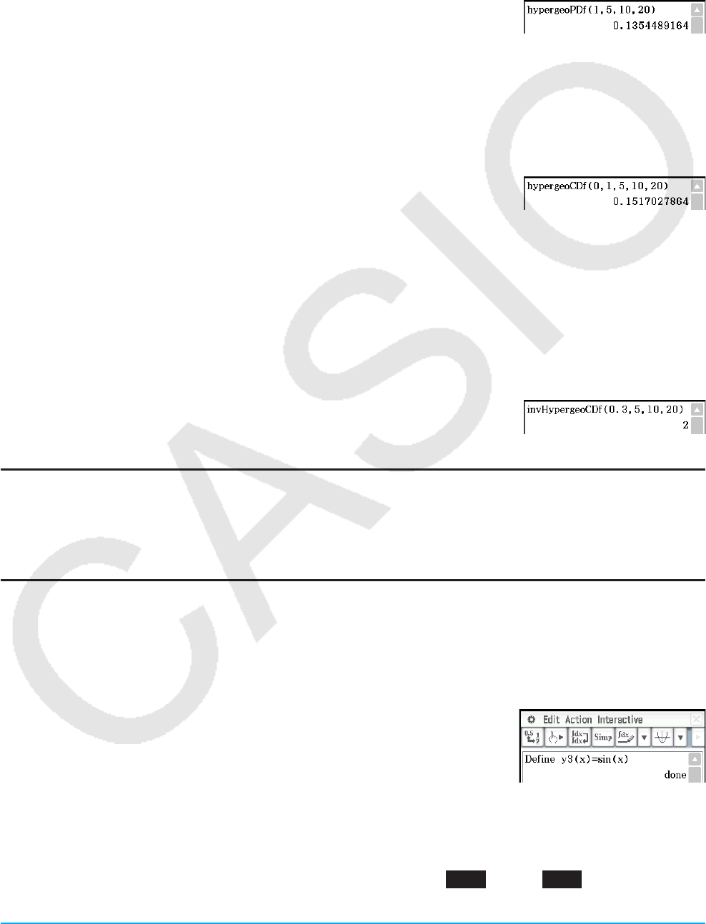
Chapter 2: Main Application 90
uhypergeoPDf [Action][Distribution/Inv.Dist][Discrete][hypergeoPDf]
Function: Returns the probability in a hypergeometric distribution that the success will occur on a specified
trial.
Syntax: hypergeoPDf(
x , n , M , N [ ) ]
Calculation Result Output:
prob
Example: Determine the hypergeometric probability when x = 1, n = 5,
M = 10, N = 20.
uhypergeoCDf [Action][Distribution/Inv.Dist][Discrete][hypergeoCDf]
Function: Returns the cumulative probability in a hypergeometric distribution that the success will occur
between specified lower value and upper value.
Syntax: hypergeoCDf(lower value, upper value,
n , M , N [ ) ]
Calculation Result Output:
prob
Example: Determine the hypergeometric cumulative distribution when lower
value = 0, upper value = 1, n = 5, M = 10, N = 20.
uinvHypergeoCDf [Action][Distribution/Inv.Dist][Inverse][invHypergeoCDf]
Function: Returns the minimum number of trials of a hypergeometric cumulative distribution for specified
values.
Syntax: invHypergeoCDf(
prob , n , M , N [ ) ]
Calculation Result Output:
x Inv, ½ x Inv
Important!
See “Important!” under “invBinomialCDf” on page 88.
Example: To determine the minimum number of trials when prob = 0.3, n = 5,
M = 10, N = 20
Using the Financial Submenu
The [Financial] submenu contains commands that are related to financial calculations.
For information about the functions included in this submenu, see “11-4 Financial Calculation Functions”.
Using the Command Submenu
u Define
Function 1: Defines function and registers it with Graph Editor.
Syntax 1: Define{
y1(x) − y100(x) ; x1(y) − x100(y) ; yt1(t) − yt100(t) ; xt1(t) − xt100(t) ;
r1() − r100()} = <expression>
Example: To define the function y = sin(x) and assign it to line “y3” of the
Graph Editor
Function 2: Creates a user-defined function.
For more information, see “12-3 User-defined Functions”.
uDispStat
Function: Displays previous statistical calculation results.
For more information, see “DispStat” on page 209 and the examples 1208 through 1210 under “Including
Statistical Graphing and Calculation Functions in a Program” on page 225.

Chapter 2: Main Application 91
u Clear_a_z
Function: Clears all single-character variables.
For more information, see “Clear_a_z” on page 84.
uDelVar
Function: Deletes a specified variable.
For more information, see “DelVar” on page 208.
uClear All Variables
Function: Clear variables that contain numbers, list and matrices.
2-8 Using the Interactive Menu
The [Interactive] menu includes most of the commands that are on the [Action] menu. Selecting a command on
the [Action] menu will simply input the command.
With the [Interactive] menu, you drag the stylus across existing input in the work area and then select a
command. This encloses the highlighted expression with the command and opens a dialog box if more
arguments are needed. When you select an [Interactive] menu item without highlighting an expression first, a
dialog box will open prompting you for the necessary arguments.
Tip
• Operation of the following [Interactive] menu commands is identical to the same commands on the [Action] menu. For
information about using these commands, see “2-7 Using the Action Menu”.
[Transformation], [Advanced], [Calculation], [Complex], [List]-[Create], [List]-[Statistics], [List]-[Calculation], [Matrix]-
[Create], [Matrix]-[Calculation], [Matrix]-[Row&Column], [Vector], [Equation/Inequality], [Assistant], [Distribution/Inv.Dist],
[Financial], Define
• The “DispStat”, “Clear_a_z,” and “DelVar” commands of the [Action] menu’s [Command] submenu are not included on the
[Interactive] menu.
Interactive Menu Example
[Interactive] menu operations come in handy in the following cases.
• When you want to use a command on an expression you are calculating
• When you want to use a command that requires multiple arguments
0235 To factorize the expression
x
3 – 3 x
2 + 3 x – 1
0236 To obtain the definite integral of
x
2 + 2 x , 1 s x s 2
Using the “apply” Command
The “apply” command is included on the [Interactive] menu only. You can use this command to execute only a
specific part of an expression and display its result.
0237 To calculate the result of diff(sin(
x ), x ) × cos( x ) + sin( x ) × diff(cos( x ), x ), and then calculate only part of
the expression
Note: This example assumes that your ClassPad is configured with the following mode settings:
Algebra, Complex, Radian, Descending Order.
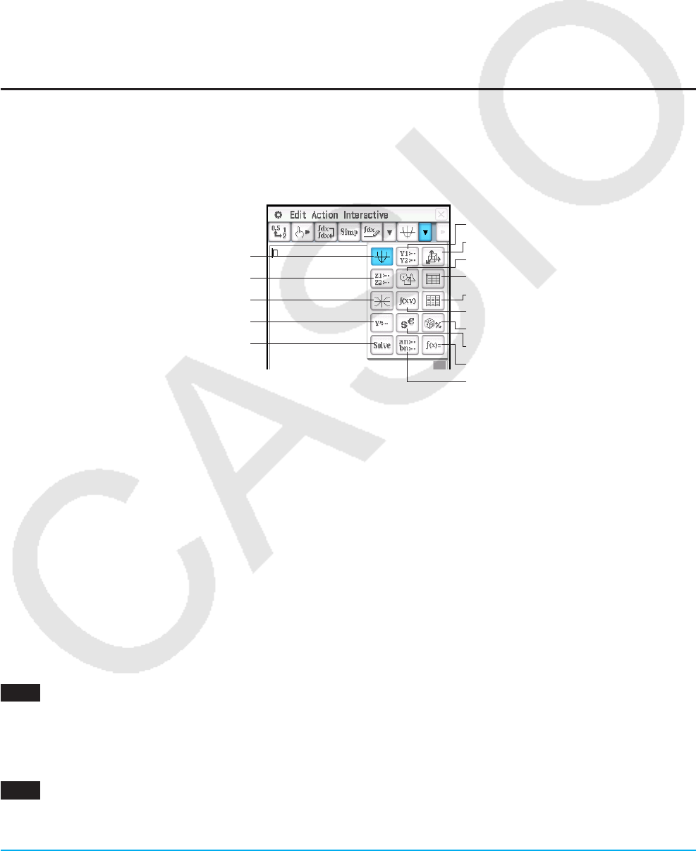
Chapter 2: Main Application 92
2-9 Using the Main Application in Combination with
Other Applications
You can access the windows of other ClassPad applications from the Main application and perform copy,
paste, drag and drop, and other operations between them.
Tip
• Copying data that includes color information from another application and pasting it into the Main application will cause
the color information to be disregarded, and the pasted data will become black. This is also true when dragging data from
another application to the Main application.
• Copying data in the Main application and pasting it into another application will cause the pasted data to be displayed in
accordance with the other application’s color settings. This is also true when dragging data from the Main application to
another application.
Using Another Application’s Window
uTo open another application’s window
1. Tap the right most toolbar down arrow button.
• This displays a palette of application icons.
Graph
3D Graph Editor
Conics Graph
Differential Equation Editor
Numeric Solver
Graph Editor
3D Graph
Geometry
Spreadsheet
Stat Editor
Conics Editor
Probability
Financial
Verify
Sequence Editor
2. Tap the button that corresponds to the window you want to display.
• This causes the window that corresponds to the button you tap to appear in the lower window.
uTo close another application’s window
1. Tap anywhere inside of the window you would like to close.
2. Tap the C button in the upper right corner, or tap O and then [Close].
• The Main application work area expands to fill the entire display.
Tip
• Even if you used the icon panel r icon to expand the lower window to fill the entire display, tapping O and then [Close]
closes it and returns to the work area window.
• Nothing happens if you tap O and then [Close] while the work area window is active.
uTo copy an expression in the work area and paste it into the Graph Editor window
0238 To copy “ x
2 – 1” in the work area and paste it into the Graph Editor window
• For more information about the Graph Editor window, see Chapter 3.
u To graph a function by dragging it from the work area to the Graph window
0239 To graph the expression “ x
2 – 1”, which has already been input into the work area

Chapter 2: Main Application 93
• As can be seen in this example, a graph can be drawn by dropping an expression in the form of f ( x ) into the
Graph window.
• When dropping a formula into the 3D Graph window instead of the Graph window, the formula must be in
form f ( x, y) (such as x^2+y^2).
Using the Stat Editor Window
You can use the Stat Editor window to create new LIST variables and edit existing LIST variables. You can also
use the Stat Editor window to specify a LIST variable’s name and display its contents.
uTo use a LIST variable with data input using Stat Editor to perform a calculation in the work
area
0240 To input data into “list1” and “list2” using Stat Editor, and then perform the calculation list1+list2 in the
work area
• list1 through list6 are LIST type system variables. For more information, see “Main Memory Data Types”
(page 28).
• For information about inputting and editing list data using the Stat Editor, see Chapter 7.
uTo use Stat Editor to recall a LIST variable created in the work area
0241 Continuing from example 0240 , to use Stat Editor to recall list variable “test”, which was created in the
work area
Using the Geometry Window
When there is a Geometry window on the display, you can drag values and expressions to the Geometry
window to draw the graph or figure of the value or expression. You can also drag a figure from the Geometry
window to the work area, which displays the corresponding expression or value.
uTo drag an expression from the work area to the Geometry window
0242 To input the expression x2/52 + y2/22 = 1 in the work area, and then drag it to the Geometry window
Tip: The following table shows the types of expressions you can drop into the Geometry window. When the expression is
not recognized, Geometry displays it as text.
Dropping this into the Geometry window: Displays this:
Linear equation in x and yAn infinite line
Equation of circle in x and yA circle
Equation of ellipse in x and yAn ellipse
Equation of hyperbola in x and yA hyperbola
2-dimensional vector (2 rows × 1 column format) A point
Equation y = f ( x)A curve
2 × n matrix, n t 3 A polygon (each column represents a vertex of the
polygon)
n × 2 matrix, n t 3 An open polygon
uTo drag a figure from the Geometry window to the work area
0243 To drag a point, circle, point and its image from the Geometry window to the work area
• For details about Geometry window operations, see Chapter 8.
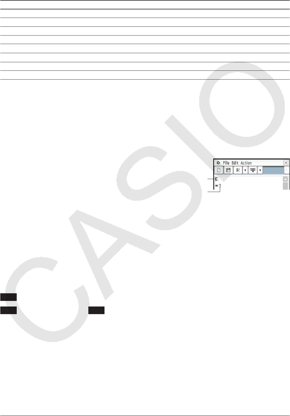
Chapter 2: Main Application 94
Tip: The following shows what happens when you drag a figure from the Geometry window to the work area.
Dropping this into the work area: Displays this:
Point Coordinates as a vector (2 × 1 matrix)
Line Equation of the line
Vector An ordered pair (head of vector assuming the tail is at the origin)
Circle, Arc, Ellipse, Function, or Curve Corresponding equation
Polygon 2 × n matrix
Open Polygon (Created by Animation) n × 2 matrix
Line Pair Simultaneous equations for the pair
A point and its image under a transformation Matrix expression for the transformation
2-10 Using Verify
Verify provides you with a powerful tool to check whether your numeric or algebraic manipulations are correct.
Verify will assist you in simplifying an expression by verifying whether or not the expression you entered is
equivalent to your original expression. If it is, you will get a pleasant response; if not, you will need to correct
your mistake before continuing.
uTo start up Verify
1. On the work area window, tap the right most
toolbar down arrow button.
2. On the icon palette that appears, tap W.Left-side expression
Right-side expression
uVerify window menus and buttons
• Clear the Verify window ............................................................................... File - New, Edit - Clear All or O
• Open or save a file ............................................................................................File - Open, File - Save or {
• Specify the complex number calculation range for Verify ...........................................................................T
• Specify the real number calculation range for Verify ..................................................................................Y
• Specify the positive real number calculation range for Verify .....................................................................U
• Verify the equation starting from the first line ..............................................................................................!
• Verify the equation starting from the current line ........................................................................................"
0244 To factor 50 completely
0245 Continuing from example 0244 , to rewrite
x
2 + 1 in factored form
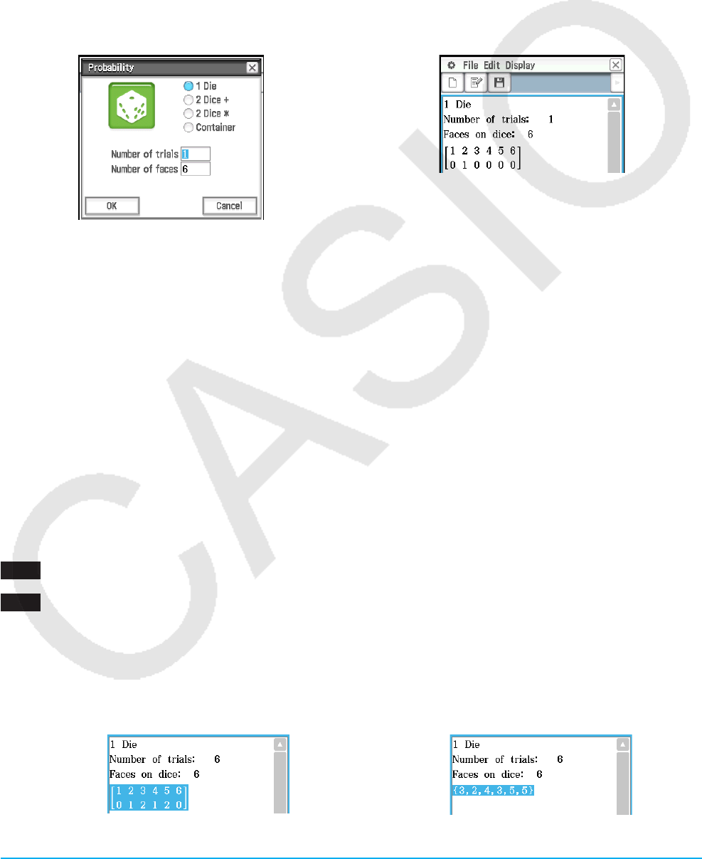
Chapter 2: Main Application 95
2-11 Using Probability
You can use Probability to simulate the following.
• The die faces that will appear when a single die is thrown a specified number of times (1 Die)
• The sum of the data of dice faces that will appear when a pair of dice is thrown a specified number of times (2
Dice +)
• The product of the data of dice faces that will appear when a pair of dice is thrown a specified number of
times (2 Dice ½)
• When any number of balls labeled A, B, C, D, E, and F are placed into a box, data about how many times
each ball will be drawn within a specified number of draws (Container)
You can specify any integer from 1 to 20 as the number of die faces.
Probability dialog box
Probability window
(Trial information and result)
uTo start up Probability
1. On the work area window, tap the right most toolbar down arrow button.
2. On the icon palette that appears, tap P. This will display an initial Probability dialog box.
uProbability window menus and buttons
• Clear the Probability window (and display the Probability dialog box) ......... File - New, Edit - Clear All or O
• Display the Probability dialog box and try the probability emulation
(the trial result will be added to the end of the current file) ...............................................Edit - Add or P
• Open or save a file ............................................................................................File - Open, File - Save or {
• Delete the currently selected trial data ......................................................................................... Edit - Delete
• Show the selected result as a frequency distribution table (in matrix form) ....................Display - Distribution
• Show the selected result as sample data (in list form) ................................................. Display - Sample Data
0246 To obtain the sum data when a two six-sided die are thrown 50 times
0247 After putting 10 A-balls, 20 B-balls, and 30 C-balls into a box, determine how many times each type of
ball will be drawn when there is a total of 50 draws. Each time a ball is drawn, it should be replaced into
the box before the next draw.
Tip: Under initial default settings, trial results are shown as a frequency distribution table in matrix form. Selecting
distribution table results and selecting [Sample Data] on the [Display] menu will change them to sample data in list
form. Conversely, selecting sample data results and selecting [Distribution] on the [Display] menu will change them to
distribution table results.
Distribution table (matrix form) Sample data (list form)
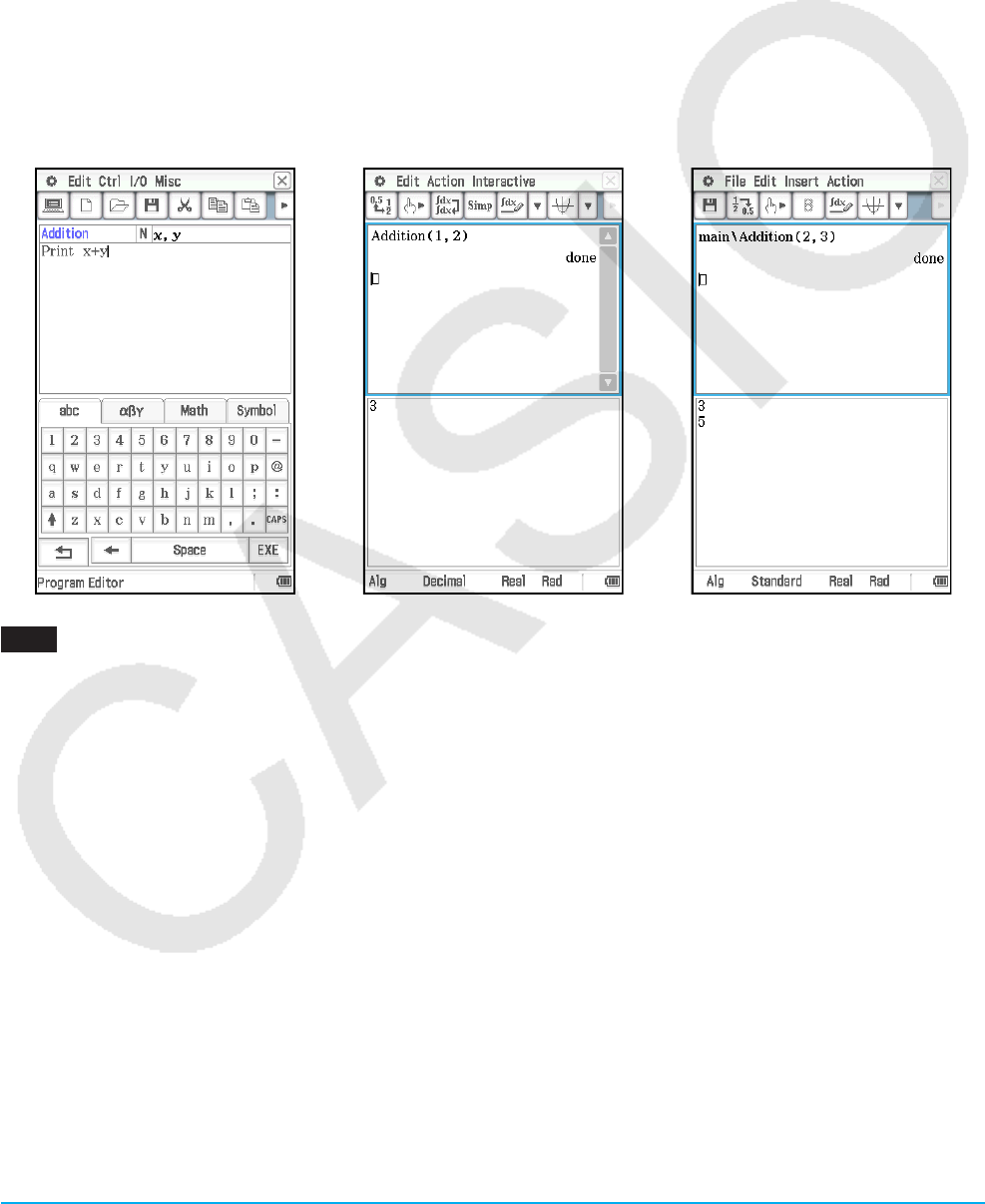
Chapter 2: Main Application 96
2-12 Running a Program in the Main Application
You can run a program in the Main application or the eActivity application.
Syntax: Folder name\Program name(parameter)
• You do not need to specify the folder name if the program you want to run is in the current folder. If you leave
ClassPad configured with its initial default settings, the current folder for both the Program application and the
Main application is the “main” folder, so you normally do not need to specify a folder name.
• Unless you change it, the current folder of the eActivity application is the “eAct” folder, so you always need
to specify the folder name. If you want to run a program that is in the “main” folder, input “main\Program
name(parameter)”.
Important!
If the program command “Pause” is used in a program, it is ignored when the program is called from Main or
eActivity.
Program Main application eActivity application
0248 To run the program named OCTA that we created and stored under “Creating a Program” (page 197) from
the Main application, and determine the surface area and volume of a regular octahedron with a side
length of 20 cm
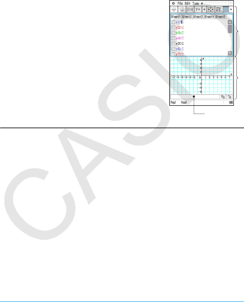
Chapter 3: Graph & Table Application 97
Chapter 3:
Graph & Table Application
The Graph & Table application allows you to input and graph rectangular coordinate equations (or inequalities),
polar coordinate equations, and parametric expressions. After you graph an expression, you can perform
various graph-based analytical operations, such as determining the points of intersection of two graphs, point of
inflection, and definite integral for a particular range of a parabola or other figure.
When you start up the Graph & Table application, two windows appear
on the display: 1 the Graph Editor window and 2 the Graph window.
• A Graph Editor sheet can contain up to 20 functions. You can have up
to 100 functions stored in the Graph Editor at one time. Functions stored
in the Graph Editor can be graphed on the Graph window.
• You can also use a function on the Graph Editor window to generate a
number table or a summary table. Number tables and summary tables
are displayed in a Table window.
• The Graph window and Table window have a message box along the
bottom that can display expressions and values, or they can be used for
input and editing.
Graph & Table Application-Specific Menus and Buttons
Graph Editor window
• Open batch saved data in the Graph Editor window ............................................. File - Open Graph Memory
• Save all of the expressions on the Graph Editor window .......................................File - Save Graph Memory
• Select the entire expression you are editing ........................................................................... Edit - Select All
• Clear all of the expressions from the Graph Editor window ......................................................Edit - Clear All
• Input a rectangular coordinate type function ...................................................................Type - y=Type or d
• Input a polar coordinate type function .............................................................................Type - r=Type or f
• Input a parametric function ......................................................................................Type - ParamType or g
• Input an x equality ...........................................................................................................Type - x=Type or h
• Input a rectangular coordinate type inequality
............................................... Type - Inequality - y>Type, y<Type, ytType, ysType or j, l, ', X
• Input an x inequality ...................... Type - Inequality - x>Type, x<Type, xtType, xsType or k, ;, Z, C
• Input two functions in a list and shade between them ............................................. Type - ShadeType or y
• Start modifying multiple graphs (Dynamic Modify, page 115) ............................... a - Dynamic Graph or 4
• Display the Draw Shade dialog box (page 101) ....................................................................a - Draw Shade
• Use a built-in function template for graphing ................................................................................ a - Built-In
• Delete all of the expressions on the active sheet ......................................................a - Sheet - Clear Sheet
• Return the active sheet name to its initial default ..................................................a - Sheet - Default Name
1
2
Message box

Chapter 3: Graph & Table Application 98
• Graph the selected function(s) ....................................................................................................................$
• Generate a summary table for the selected function ..................................................................................4
• Display the View Window dialog box to configure Graph window settings .................................................6
• Display the Table Input dialog box for configuring settings .........................................................................8
• Generate a table for the selected function ..................................................................................................#
Graph window
• Clear all of the Graph window contents ....................................................................................Edit - Clear All
• Perform a zoom operation (page 105) ....................................................................................................Zoom
• Display the coordinates at a particular point on a graph ..............................................Analysis - Trace or =
• Insert a point, a graphic, or text into an existing graph (page 112) ...................................... Analysis - Sketch
• Perform a G-Solve operation (page 114) ........................................................................... Analysis - G-Solve
• Modify a graph by changing the value of a parameter ..........................................................Analysis - Modify
• Open the image of a graph ................................................................................................. a - Open Picture
• Save a graph as image data ................................................................................................ a - Save Picture
• Clear the image of a graph ..................................................................................................a - Clear Picture
• Adjust the lightness of the graph screen background image placed
by the “Open Picture” command ........................................................................................... a - Fade I/O
• Start modifying multiple graphs (Dynamic Modify, page 115) ............................... a - Dynamic Graph or 4
• Display the Draw Shade dialog box ......................................................................................a - Draw Shade
• Re-draw a graph ......................................................................................................................... a - ReDraw
• Make the Graph Editor window active ........................................................................................................!
• Generate a number table for an existing graph ..........................................................................................#
• Display the Table Input dialog box for configuring settings .........................................................................8
• Generate a summary table for an existing graph ........................................................................................4
Table window
• Clear all of the Table window contents .....................................................................................Edit - Clear All
• Delete a row from a table .........................................................................................................T-Fact - Delete
• Insert a row into a table ............................................................................................................. T-Fact - Insert
• Add a row after the currently selected row ..................................................................................T-Fact - Add
• Draw a connect type graph using a generated table .............................................. Graph - G-Connect or $
• Draw a plot type graph using a generated table ............................................................ Graph - G-Plot or !
• Save the contents of a table to a list .....................................................................................a - Table to List
• Re-generate a table based on current table settings ..................................................................a - ReTable
• Delete the displayed table .................................................................................................... a - Delete Table
• Move the pointer to the location on a graph that corresponds
to the value selected in a table .....................................................................................................a - Link
• Make the Graph Editor window active ........................................................................................................!
• Display the Table Input dialog box for configuring settings .........................................................................8
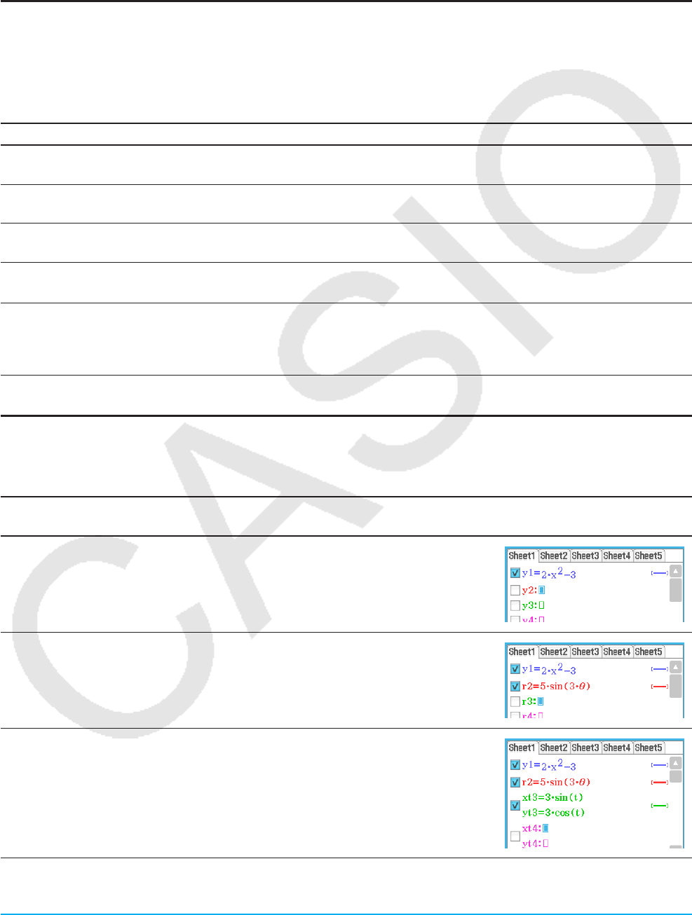
Chapter 3: Graph & Table Application 99
3-1 Storing Functions
Use the Graph Editor window to store a Graph & Table application function. This section covers Graph Editor
operations, and explains how to store functions.
Using Graph Editor Sheets
The Graph Editor window has five tabbed sheets named Sheet 1 through Sheet 5, each of which can contain
up to 20 functions. You can graph up to 20 functions simultaneously, as long as all of the functions are on the
same sheet.
The table below explains Graph Editor sheet operations.
To do this: Do this:
Select a sheet Tap the tab of the sheet you want to select. The currently selected sheet is the
“active” sheet.
Rename a sheet Tap the tab of the active sheet. On the dialog box that appears, enter up to 8
bytes for the sheet name, and then tap [OK].
Return the active sheet
name to its initial default
Tap a, [Sheet], and then [Default Name].
Initialize a Sheet Tap a, [Sheet], and then [Clear Sheet]. This clears all of the active sheet
functions and renames the sheet to its default name.
Initialize all the Sheets Tap [Edit], and then [Clear All]. In response to the confirmation dialog box that
appears, tap [OK]. This clears all of the expressions from the Graph Editor
window and returns the sheet names to their initial default names (Sheet 1
through Sheet 5).
Storing a Function
To input an expression, tap a blank line on the Graph Editor window and then perform the operations described
below.
To input this type of
expression:
Do this:
Rectangular coordinate
expression (y = f(x))
1. Tap [Type] - [y=Type].
2. Input an expression (such as: 2x2 – 3) that
contains variable x and then press E.
Polar coordinate
expression
1. Tap [Type] - [r=Type].
2. Input an expression (such as: 5sin(3)) that
contains variable and then press E.
Parametric expressions 1. Tap [Type] - [ParamType].
2. In the xt =, yt = lines, input expressions that
each contain t (such as: 3sin(t), 3cos(t)), and
then press E.
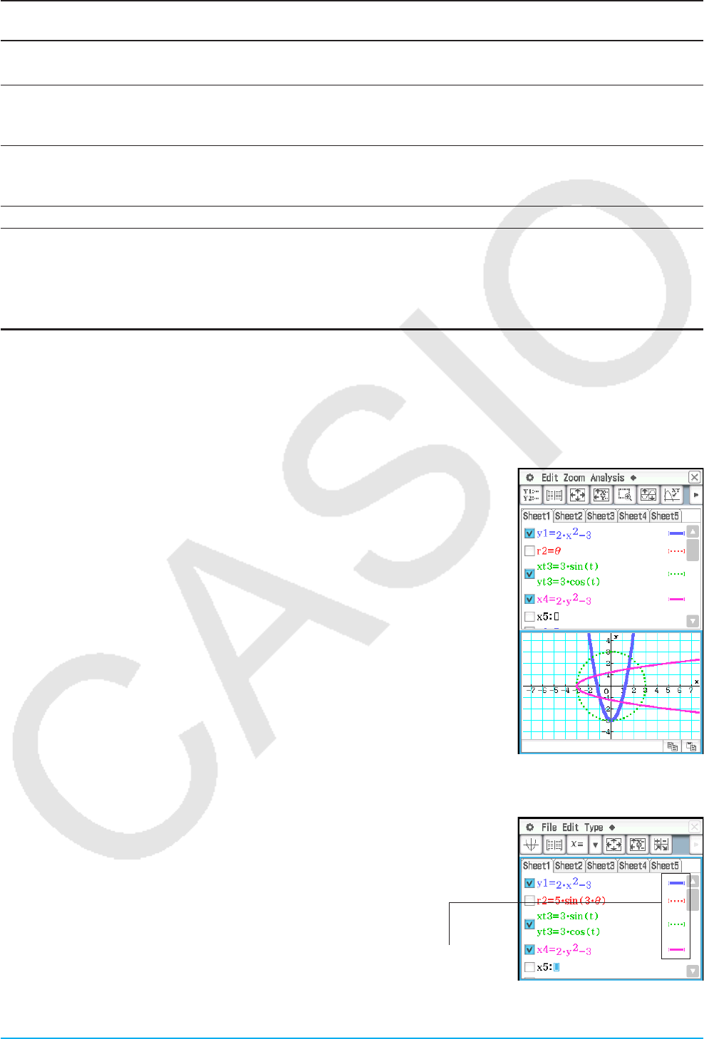
Chapter 3: Graph & Table Application 100
To input this type of
expression:
Do this:
x equality 1. Tap [Type] - [x=Type].
2. Input an expression that includes variable y and then press E.
y inequality
(left side y type)
1. Tap [Type], [Inequality], and then tap one of the following:
[y>Type], [y<Type], [ytType], [ysType].
2. Input an expression that includes variable x and then press E.
x inequality
(left side x type)
1. Tap [Type], [Inequality], and then tap one of the following:
[x>Type], [x<Type], [xtType], [xsType].
2. Input an expression that includes variable y and then press E.
Shade Type See “Shading the Region Bounded by Two Expressions” (page 101).
Tip: You can change the equality/inequality sign of an x-type (x=, x>, x<, xt, xs) or y-type (y=, y>, y<, yt, ys, Shade
Type) expression after you input it. Simply tap the current equality/inequality sign. On the Type dialog box that
appears, select the sign you want and then tap [OK].
Graphing a Stored Function
You can select multiple functions and graph them simultaneously, as long as all of the functions are on the
same sheet. You can turn graphing of each function on or off, and even specify the line style and color to be
used for each function.
uTo graph a specified function
1. Tap the tab of the sheet that contains the functions you want to graph to
make it active.
2. Select the check boxes of all the functions you want to graph, and clear the
check boxes of all the functions you do not want to graph.
3. You can tap the current line style and color to specify another style, if you
want.
• See “To specify the graph line style and color” below.
4. Tap $ to graph.
uTo specify the graph line style and color
1. Tap the style area next to the function whose line style and
color you want to specify. This displays the Style Settings
dialog box.
Style area
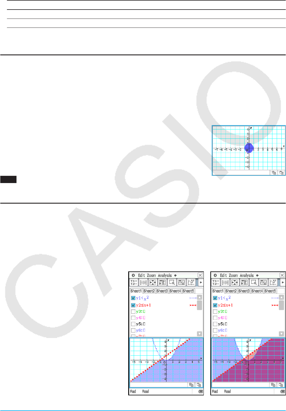
Chapter 3: Graph & Table Application 101
2. Configure the dialog box with the following settings.
To specify this: Perform this operation:
Line type Tap “Graph Plot” and then tap the desired line type.
Line color Tap “Line Color” and then tap the desired color.
3. To apply the settings, return to the dialog box in step 2 of this procedure and then tap [OK].
Shading the Region Bounded by Two Expressions
You can shade the region bounded by two expressions by specifying [ShadeType] as the function type and
then inputting the expressions in the syntax shown below.
{lower function f(x), upper function g(x)} | A < x < B
Note: A < x < B can be omitted. A < x < B can be replaced with x > A or x < B.
uTo shade the region bounded by two expressions
1. Tap [Type] - [ShadeType].
2. Use the above syntax to input two x-variable expressions, specify the
x-value range, and then press E.
Example: {x2 – 1, –x2 + 1} | –1 < x < 1
3. Tap $ to graph.
0301 To use the draw shade dialog box to shade the region bounded by
x2 – 1 and –x2 + 1
Overlaying Two Inequalities in an Intersection Plot / Union Plot
Use the following procedure to overlay two inequalities in an Intersection Plot or Union Plot, which are
described below.
Intersection Plot: Only the parts of the inequalities that overlap are shaded.
Union Plot: The inequalities are overlaid as they are.
uTo overlay two inequalities
y < x2, y s x + 1
1. Store y < x2 in line y1 and y s x + 1 in line
y2.
2. On the O menu, tap [Graph Format].
3. On the Graph Format dialog box that
appears, tap the [Inequality Plot] down
arrow and then select [Intersection] or
[Union].
4. Tap $ to graph.
Intersection Plot Union Plot

Chapter 3: Graph & Table Application 102
Saving Graph Editor Data to Graph Memory
Graph memory lets you store all of the expressions and their related information to a file for later recall. Each
graph memory file contains the following data:
• Functions on all five Graph Editor sheets (up to 100 functions)
• Whether the check box next to each function is selected (checked) or cleared (unchecked)
• The line style and color of each function
• The graph type of each function • Which sheet is currently active
• The View Window settings • Sheet names
uTo open a graph memory file
1. Tap [File] and then [Open Graph Memory]. This displays a list of names of graph memory files you have
stored in memory.
2. Select the name of the graph memory file you want, and then tap [OK].
uTo save Graph Editor data to graph memory
1. On the Graph Editor window, tap [File] and then [Save Graph Memory]. This displays a dialog box for
inputting a name for the graph memory file.
2. Enter the name and then tap [OK].
3-2 Using the Graph Window
This section explains Graph window operations, including configuring display settings, scrolling, zooming the
image, and more.
Configuring View Window Parameters for the Graph Window
The View Window dialog box lets you specify the maximum and minimum values for each axis, the space
between the marks on each axis (the scale), and other graph display parameters. Before drawing a graph, be
sure to first configure View Window parameters to ensure proper display of the graph.
u To configure View Window parameters
Note: Steps 2 and 3 of the procedure below can be performed in reverse, if
you want, as long as step 4 is performed next.
1. Tap 6, or tap O and then [View Window] to display the View Window
dialog box.

Chapter 3: Graph & Table Application 103
2. If you want to configure settings using preset ClassPad View Window parameters, perform the operations
described below.
To configure this setting: Do this:
ClassPad initial defaults On the [Memory] menu select [Initial], or tap the
[Default] button.
Configure settings optimized for trigonometric
function graphing
On the [Memory] menu, select [Trigonometric].
Display both the x-axis and y-axis in a range of
–10 to 10
On the [Memory] menu, select [Standard].
Configure View Window settings that maintain the
current background image
On the [Memory] menu, select [Picture].
Configure parameters automatically optimized for
a graph
On the [Memory] menu, select [Auto].
• For details about each preset parameter, see “View Window Preset Parameters” (page 103).
3. Configure View Window parameters required for the type of graph you want to draw.
Rectangular Coordinates
Use this item: To configure this View Window parameter:
xmin/ymin x-axis/y-axis minimum value
xmax/ymax x-axis/y-axis maximum value (Specify a value greater than xmin/ymin.)
xscale/yscale x-axis/y-axis marker spacing
xdot/ydot Value of each dot on the x-axis/y-axis
• Selecting the x-log and/or y-log check box at the top of the display will switch the applicable axis to
logarithmic scale. Selecting one of the check boxes results in a semi-log graph, while selecting both check
boxes results in a log-log graph.
Polar Coordinates and Parametric Coordinates
Use this item: To configure this View Window parameter:
t min/t max Minimum/maximum value of t
t step Step size of t (Specify a non-zero value.)
4. After all the parameters are the way you want, tap [OK].
• When you tap [OK] after changing View Window dialog box settings, the graph is redrawn automatically
using the new View Window settings.
View Window Preset Parameters
Selecting preset View Window parameters configures the settings shown in the table below.
Note
• The values in the explanations below apply during the vertical half-size view of the Graph window (which is
the initial default setting of the Graph & Table application). Tapping r on the icon panel will switch to the
full-screen view and change the View Window settings.
• The View Window settings will different from those shown below when the Graph window is displayed using
the horizontal view.
Parameter Name Description
Initial (Default) • Both xscale and yscale are set to 1. The x-axis direction is displayed from –7.7
(xmin) to 7.7 (xmax), while the y-axis direction is from –4.6 (ymin) to 4.6 (ymax).
• The following settings are configured: tmin = 0, tmax = 2π* radian = 360
degree = 400 grad, tstep = (tmax – tmin)/120*. The values depend on the
Basic Format Angle setting.

Chapter 3: Graph & Table Application 104
Parameter Name Description
Trigonometric • xscale is set to π/2* radian = 90 degree = 100 grad. The values depend on the
Basic Format Angle setting. This xscale is used as the basis to display an x-axis
direction in the range of xscale × –7.7 (xmin) to xscale × 7.7 (xmax). For example,
when the Angle setting is Degree, xmin = –693, xmax = 693.
• y-axis settings are fixed as follows, regardless of the Angle setting:
yscale = 1, ymin = –2.1, ymax = 2.1.
• tmin, tmax, tstep settings are the same as Initial Default.
Standard Both xscale and yscale are set to 1. Both the x-axis and y-axis directions are
displayed in the range of –10 (xmin, ymin) to 10 (xmax, ymax).
Picture View Window settings that maintain the current background image are applied.
Auto View Window settings are automatically optimized for the expression (the last
expression selected in the case of multiple expressions) selected for graphing on
the Graph Editor window.
* These values are displayed as decimal format values.
View Window parameter precautions
• When the View Window setting produces an axis that does not fit on the display, the scale of the axis is
indicated on the edge of the display closest to the origin.
• Changing the xmin (ymin) or xmax (ymax) value automatically changes the xdot (ydot) value, while changing
the xdot (ydot) value automatically changes the xmax (ymax) value.
Using View Window Memory
You can save your View Window setup for later use.
uTo save the current View Window setup
1. Tap 6, or tap O and then [View Window] to display the View Window dialog box.
2. Change parameters as required (see “To configure View Window parameters” on page 102).
3. Tap [File] and then [Save File]. This displays a dialog box for inputting a name for the View Window setup.
4. Enter the name and then tap [OK].
uTo recall a setup from View Window memory
1. Tap 6, or tap O and then [View Window] to display the View Window dialog box.
2. Tap [File] and then [Open File]. This displays a list of names of View Window setups stored in ClassPad
memory.
3. Select the name of the setup you want, and then tap [OK].
• This causes the current View Window parameters to be replaced by the parameters of the recalled setup.
Panning the Graph Window
You can drag the Graph window screen to scroll (pan) its contents.
uClassPad Operation
1. Holding the stylus anywhere against the Graph window, drag it in the direction you want.
• This causes the Graph window to scroll automatically in accordance with the dragging.
2. When the Graph window shows the area you want, remove the stylus from the display.
• This causes the graph to be redrawn on the Graph window.

Chapter 3: Graph & Table Application 105
Tip
• Graph window panning cannot be performed while any one of the following functions is being used: Modify, Trace, Sketch,
G-Solve, box zoom.
• While a panning operation is in progress on the Graph window, the coordinates of the point where the stylus is held
against the display is displayed in the status bar.
Scrolling the Graph Window
You can use either of the two operations to scroll the Graph window up,
down, left, or right.
• Tapping the graph controller arrows at the edges of the Graph window.
• Using the cursor key.
Display of the graph controller arrows is turned off under initial default settings.
Use the Graph Format dialog box to turn them on, if you want. For more
information, see “Graph Format Dialog Box” on page 38. Graph controller arrows
Zooming the Graph Window
You can zoom in on the Graph window image by holding two fingers against the screen while moving them
apart from each other. Moving two fingers closer to each other in a pinching action will zoom out.
Your ClassPad also provides you with a wide selection of zoom commands that you can use to enlarge or
reduce an entire graph or a specific area of a graph.
To perform this type
of zoom:
Do this:
To enlarge the
area enclosed in a
boundary
1. Tap [Zoom] and then [Box], or tap Q.
2. On the Graph window, drag the stylus to draw a selection boundary around the
area you want to enlarge.
3. Remove the stylus from the display.
• The area within the selection boundary will expand to fill the entire Graph window.
To enlarge or reduce
to a specified numeric
factor
1. Tap [Zoom] and then [Factor].
2. On the dialog box that appears, input the x- and y-axis zoom factor, and then tap
[OK].
3. Tap [Zoom] - [Zoom In] to enlarge to the specified factor, or [Zoom] - [Zoom Out]
to reduce.
To do this on the Graph window: Do this:
Automatically configure settings so the Graph screen fills the entire
screen in accordance with the graph being drawn
Tap [Zoom] and then [Auto], or
tap R.
Return a graph to its original View Window settings Tap [Zoom] and then [Original].
Adjust View Window x-axis values so that they are identical to the y-axis
values
Tap [Zoom] and then [Square].
Round View Window settings (xmin, xmax, xdot) to an appropriate
number of decimal places and redraw the graph
Tap [Zoom] and then [Round].
Make the value of each dot equal 1, which makes all coordinate values
integers
Tap [Zoom] and then [Integer].
Return View Window parameters to their settings prior to the last zoom
operation
Tap [Zoom] and then [Previous].
Return View Window parameters to their initial default (see “Initial
(Default)” under “View Window Preset Parameters” on page 103)
Tap [Zoom] and then [Initialize].
Redraw graphs using preset View Window parameter values See “Using Quick Zoom” below.

Chapter 3: Graph & Table Application 106
Using Quick Zoom
The quick zoom commands on the [Zoom] menu draw a graph using preset built-in View Window parameter
values.
Note
• The values in the explanations below apply during the vertical half-size view of the Graph window (which is
the initial default setting of the Graph & Table application). Tapping r on the icon panel will switch to the
full-screen view and change the View Window settings.
• The View Window settings will different from those shown below when the Graph window is displayed using
the horizontal view.
Command View Window Parameter Values*1
xmin xmax xscale ymin ymax yscale
Quick Trig *2*2*2–2.1 2.1 1
Quick log (x)–2 13.4 2 –4.6 4.6 1
Quick e^x–2.2 2.2 1 –1.4 9 1
Quick x^2 –7.7 7.7 2 –12 80 5
Quick –x^2 –7.7 7.7 2 –80 12 5
Quick Standard –10 10 1 –10 10 1
*1 Any View Window parameter that is not shown in the above table is unchanged when you execute a quick
zoom command.
*2 Depending on the Basic Format Angle setting, executing Quick Trig changes the xscale setting to π/2 (for
Radian), 90 (for Degree), or 100 (for Grad). The following settings are applied based on the xscale value:
xmin = –7.7 × xscale, xmax = 7.7 × xscale.
Using Built-in Functions for Graphing
Your ClassPad is pre-programmed with the commonly used functions listed below.
y = aⴢx + by = aⴢcos (bⴢx + c) + dy = aⴢe^(bⴢx + c) + d
y = aⴢx^2 + bⴢx + cy = aⴢtan (bⴢx + c) + dy = a^(bⴢx + c) + d
y = aⴢx^3 + bⴢx^2 + cⴢx + dy = aⴢlog (bⴢx + c) + dy = a /(bⴢx + c) + d
y = aⴢsin (bⴢx + c) + dy = aⴢln (bⴢx + c) + d
You can recall a built-in function and register it as-is into the Graph Editor window. You can then replace the
parameters in the function with values and graph the results, or you can leave the literal parameter names
unchanged and use Dynamic Modify (page 115) to modify the form of the graph.
uClassPad Operation
1. Tap [Type] - [ y =Type].
2. On the Graph Editor window, tap a and then [Built-In].
3. On the menu that appears, tap the built-in function you want to select.
• The selected built-in function is input as-is on the Graph Editor window. Input values for each parameter as
required.
• You can leave some or all of the literal parameter names unchanged and use Dynamic Modify (page 115) to
modify the form of the graph.
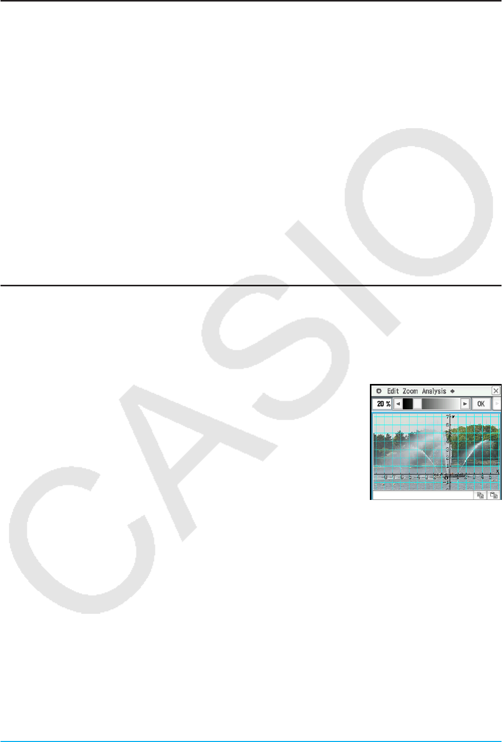
Chapter 3: Graph & Table Application 107
Saving a Screenshot of a Graph
Use the following procedures to save a screenshot of a graph as image data for later recall.
uTo open a screenshot of a graph
1. On the Graph window, tap a and then [Open Picture]. This displays a list of names of graph images you
have stored in memory.
2. Select the name of the image you want, and then tap [OK].
• The image you select is displayed as the Graph window background.
uTo save a screenshot of a graph
1. Draw the graph you want to save.
2. Tap a and then [Save Picture]. This displays a dialog box for inputting a name for the screenshot.
3. Enter the name and then tap [OK].
uTo clear the current screenshot of a graph
On the Graph window, tap a and then [Clear Picture].
Adjusting the Lightness (Fade I/O) of the Graph Window Background Image
You can adjust the lightness of the graph window background image within a range of 0% (as-is) to 100% (all
white). A higher setting value makes the image lighter, and a setting of 100% displays an all white background.
You can use this setting to adjust the background image to a level that makes the graph easier to see.
uTo adjust the lightness (Fade I/O) of the graph window background image
1. On the Graph window, tap a and then [Fade I/O].
• This causes a slider for adjusting image lightness to appear on the toolbar.
2. Use d and e to adjust the lightness value.
• Each press of d and e changes the setting value in steps of 5%.
3. After the setting is the way you want, tap [OK].
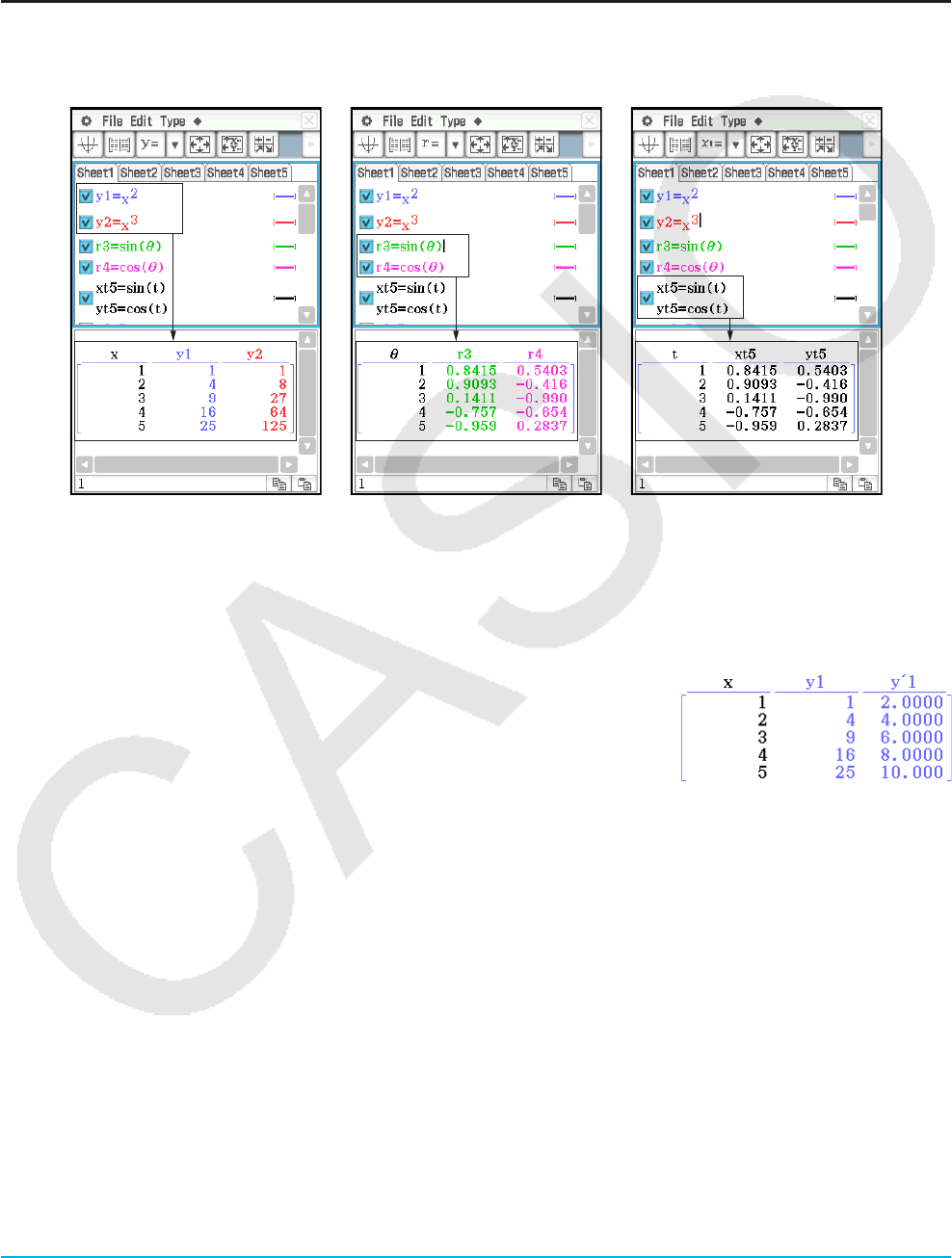
Chapter 3: Graph & Table Application 108
3-3 Using Table & Graph
The Graph & Table application includes a “Table window” for displaying number tables and summary tables
generated with the functions you input on the Graph Editor window.
Generating a Number Table
A number table can be created for one or more y=Type, r=Type, or ParamType (Parametric Type) functions
registered on the Graph Editor window.
y=Type: (x, y) number table r=Type: (, r) number table
ParamType: (t, xt, yt) number table
The following are the two methods that can be used to create a number table using the Graph & Table
application.
• Specifying the value range of x, , or t using the Table Input dialog box
• Specifying the value range of x, , or t using a list stored in ClassPad memory
Tip
• The derivative is also included in the number table when the Graph Format
“Derivative/Slope” check box is selected.
• You can specify the width of table cells using the [Cell Width Pattern] on the Graph
Format dialog box (page 38).
uTo generate a number table by specifying a range of values for x, , or t using the Table Input
dialog box
1. On the Graph Editor window, input the function(s) you want to use for number table creation, and select the
check box(es) to the left of the function(s) you want to use.
2. Tap the [Type] menu, and then select the type ([y=Type], [r=Type], or [ParamType]) of the function(s) you
want to use for number table creation.
3. Tap 8 to display the Table Input dialog box.
4. Input the values for the x-, -, or t -values of your table, and then tap [OK].
5. Tap # to generate the number table and display it on the Table window.
Tip: The above operation is possible only when “Table Input” (which is the initial default) is selected for the Graph Format
dialog box [Table Variable] item.
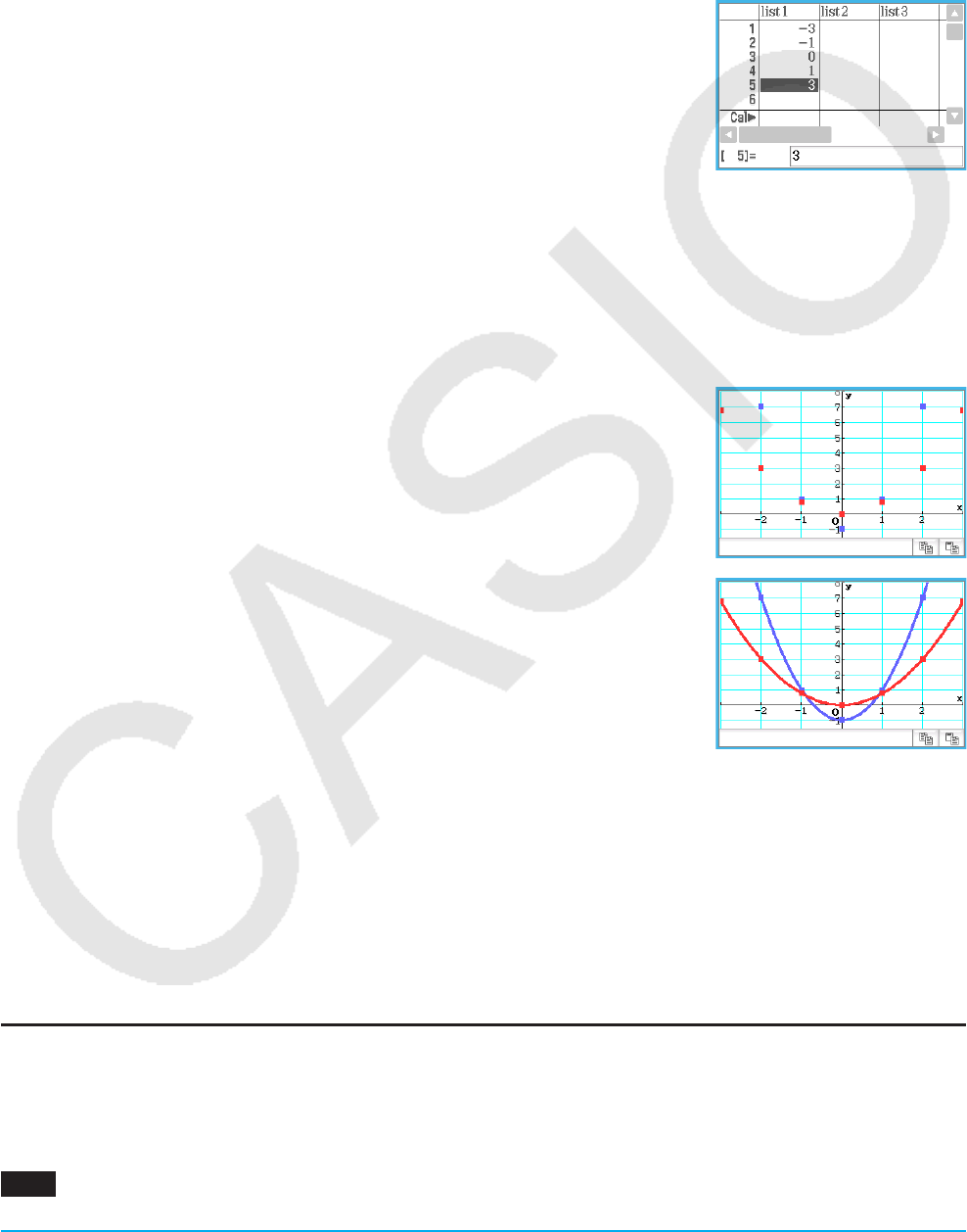
Chapter 3: Graph & Table Application 109
uTo generate a number table by assigning list values to x, , or t
1. Tap O and then [Graph Format] to display the Graph Format dialog box.
2. Tap [Special] tab, and then select a list option (list1 through list6 or a list variable created by you) for the
[Table Variable] item.
• By way of example, here we will select “list1”.
3. Tap [Set] to apply the settings and close the dialog box.
4. Tap O, [Window] and then [Stat Editor] to display the Stat Editor window.
5. In the list you selected in step 2 (list1 in this example), input the values you
want to assign to x, , or t.
• For information about Stat Editor window operations, see Chapter 7.
6. On the Graph Editor window, input the function(s) you want to use for
number table creation, and select the check box(es) to the left of the
function(s) you want to use.
7. Tap the [Type] menu, and then select the type ([y=Type], [r=Type], or [ParamType]) of the function(s) you
want to use for number table creation.
8. Tap # to generate the number table and display it on the Table window.
uTo draw a graph using a number table
Perform either of the operations below.
Tap [Graph] - [G-Plot] or tap !.
• This will draw a graph that plots the coordinates in the number table.
Tap [Graph] - [G-Connect] or $.
• This graphs the expression used to create the number table and plots the
coordinates in the table.
uTo save a number table to a list
1. On the Table window, select any cell in the column you want to save to a LIST variable.
• To save column y1, for example, select any cell in column y1.
2. Tap a and then [Table to List].
• This displays a dialog box for specifying a variable name.
3. Enter the name you want to give to the variable, and then tap [OK].
• This assigns the list of data you selected to a variable with the name you specified.
Showing Linked Displays of Number Table Coordinates and Graph Coordinates
(Link Trace)
With Link Trace, selecting a value in a number table created using a function causes a crosshair pointer (trace
pointer) to appear at the corresponding coordinates on the graph.
0302 To create a number table of y = 3log(x+5), graph the values, and perform link trace
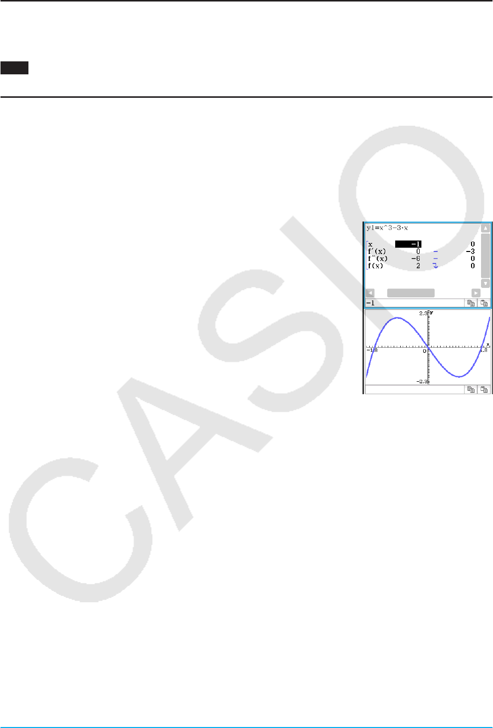
Chapter 3: Graph & Table Application 110
Generating Number Table Values from a Graph
You can input the coordinate values where the pointer is currently located on a graph into a table by simply
pressing E.
0303 To generate number table values from the y = x3 – 3x graph
Generating a Summary Table
A summary table can be created from a y=Type function registered on the Graph Editor window. The figure
below shows an example of the summary graph and table of y = x3 – 3x.
The following are the two methods that can be used to create a summary table using the Graph & Table
application.
• Creating a summary table with the View Window settings xmin as the lower limit value and xmax as
upper limit value
With this method, the x within the range of xmin and xmax where f (x) = 0 is
automatically calculated and added to the table. You can specify xmin and
xmax values, or you can use auto settings ([Memory] - [Auto] View Window
settings).
• Specifying the range of x-values for creating a summary table using a list stored in ClassPad memory
This method generates a summary table by looking up data stored in a list. A LIST variable is used to specify
the x-values. When using this method, it is up to you specify all of the correct x-values required to generate
the summary table. The summary table will not be generated correctly if you provide incorrect x-values.
Tip
• You can control whether or not the summary table should include an f (x) line (second derivative component) using the
[Summary Table f (x)] setting on the [Special] tab of the Graph Format dialog box (page 38). Turning on the [Summary
Table f (x)] option causes both first derivative components and second derivative components to be displayed in the
summary table. Turning it off shows first derivative components only.
• Some functions may not be solvable by the ClassPad’s internal summary table calculation. When this happens, the “Can’t
Solve!” error message appears on the display.
uTo generate a summary table using View Window
1. On the Graph Editor window, register the function you want to use to create the summary table.
• Make sure that only the check box of the function to be used for summary table creation is selected. Clear
the check boxes of all other functions on the Graph Editor window.
2. Tap 6 to display the View Window dialog box.
3. Perform any one of the operations below.
• Tap [Memory] and then [Auto]. This causes all settings on the View Window dialog box to change to “Auto”.
• Specify the x-values for the summary table by specifying values for the [xmin] and [xmax] settings.
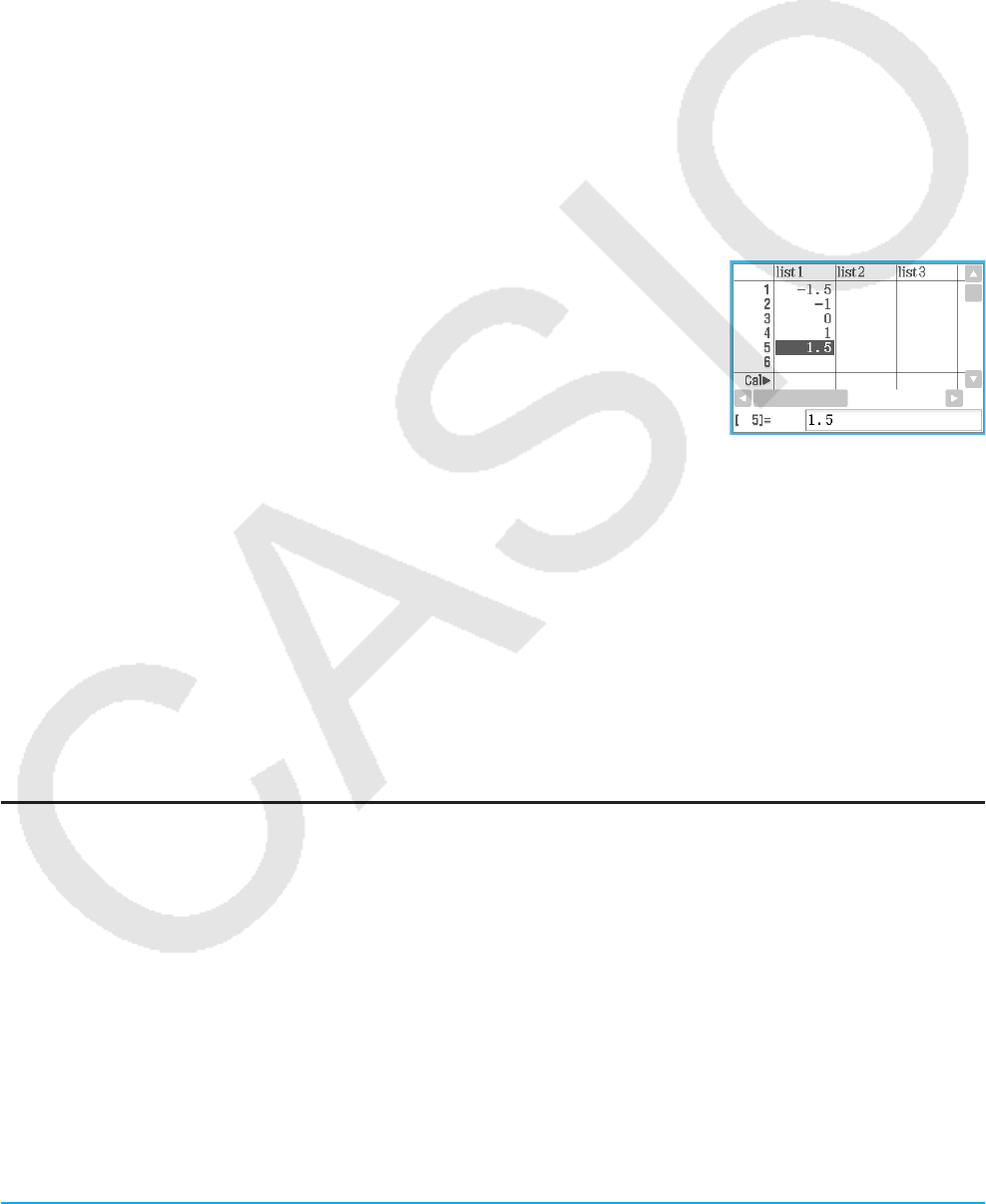
Chapter 3: Graph & Table Application 111
4. Tap [OK] to close the View Window dialog box.
• Tapping $ here graphs the function using the View Window settings.
5. Tap 4.
• This starts summary table generation, and displays the result on the Table window. Note that generation of
a summary table can take a bit of time.
Tip
• The above operation is possible only when “View Window” (which is the initial default) is selected for the Graph Format
dialog box [Summary Table] item.
• A monotone increasing function or other special function may not be solvable by the ClassPad’s internal summary table
calculation. If this happens, use the procedure below.
uTo generate a summary table by specifying all of the values for x
1. Tap O and then [Graph Format] to display the Graph Format dialog box.
2. Tap the [Special] tab, and then select a list option (list1 through list6 or a list variable created by you) for the
[Summary Table] item.
• By way of example, here we will select “list1”.
3. Tap [Set] to apply the settings and close the dialog box.
4. Tap O, [Window] and then [Stat Editor] to display the Stat Editor window.
5. In the list you selected in step 2 (list1 in this example), input the values you
want to assign to x.
6. Tap the Graph Editor window to make it active.
7. On the Graph Editor window, register the function you want to use to create
the summary table.
• Make sure that only the check box of the function to be used for summary table creation is selected. Clear
the check boxes of all other functions on the Graph Editor window.
8. Tap 4.
• This starts summary table generation using the x-values you input in step 5, and displays the result on the
Table window.
3-4 Using Trace
Trace lets you move a point along a graph and displays the coordinates for the current pointer location.
You can also link the trace operation to the number table used to draw a graph, so the pointer jumps to the
coordinates that are currently selected in the table.
Using Trace to Read Graph Coordinates
Starting the trace operation causes a crosshair pointer to appear on the graph. You can then press the cursor
key or tap the graph controller arrows to move the pointer. The coordinates are displayed as you move the
pointer.
u To perform a trace operation
1. On the Graph Editor window, input and store a function, and then tap $ to graph it.
• Here, input y = x2 – 3 into line y1.

Chapter 3: Graph & Table Application 112
2. Tap [Analysis], [Trace], or tap =.
• This will display the pointer at the coordinates where x = 0. The pointer will not be visible when it is located
at a point outside the graph display area.
• If “Undefined” appears in place of the xc or yc coordinate, it means that the current point is undefined.
Press the left or right cursor key to move to a point that is defined.
3. Press the left or right cursor key, or tap the left or right graph controller arrow.
• This moves the pointer along the graph, and displays the coordinates of
the current pointer location.
• You can also move the pointer to a particular point by inputting
coordinates. Pressing a number key displays a dialog box for inputting
coordinates. Input the values you want and then tap [OK].
• When there are multiple graphs on the Graph window, you can use the up
and down cursor keys or the up and down graph controller arrows to move the pointer between graphs.
4. To quit the trace operation, tap l on the icon panel.
Tip
• While the trace pointer is on the window, tapping the displayed coordinate values causes the coordinate values to appear
in the message box. You can then copy the coordinates to the clipboard.
• Selecting the [Derivative/Slope] check box on the Graph Format Dialog Box will show the derivative along with
coordinates while the trace pointer is on the display. Clearing the [Coordinates] check box will hide the coordinate display
while the trace pointer is on the display. For more information, see “Graph Format Dialog Box” on page 38.
3-5 Using the Sketch Menu
The [Sketch] menu lets you add points, lines, figures, and text after you draw a graph. You can also add
tangent and normal lines to your graph.
Using Sketch Menu Commands
This section describes how to use each of the commands on the [Sketch] menu.
u To clear figures inserted using the Sketch menu
To clear plots, lines, text, or other figures inserted using the [Sketch] menu, tap [Analysis], [Sketch], and then
[Cls]. This redraws the graph to what is stored on the Graph Editor window.
uTo plot a point on the Graph window
1. While the Graph window is active, tap [Analysis], [Sketch], and then [Plot].
2. Tap the location on the Graph window where you want to plot a point.
• Instead of tapping the Graph window, you could also use the keypad to specify the coordinates of the point.
Press a number key on the keypad. On the dialog box that appears, input x- and y-coordinate values, and
then tap [OK].
uTo draw a line on the Graph window
1. While the Graph window is active, tap [Analysis], [Sketch], and then [Line].
2. Tap the start point of the line and then tap the end point. This causes a straight line to be drawn between the
two points. The message box shows the equation of the line.
• Instead of tapping the Graph window, you can use the keypad to specify the coordinates of the start point
and end point. Press a number key on the keypad. On the dialog box that appears, input the coordinates
for the start point (x1, y1) and the end point (x2, y2), and then tap [OK].
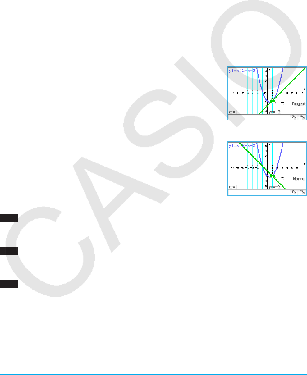
Chapter 3: Graph & Table Application 113
u To write text on the Graph window
1. While the Graph window is active, tap [Analysis], [Sketch], and then [Text].
2. On the dialog box that appears, enter the text you want and then tap [OK].
• This displays the word “Text” in the lower right corner of the Graph window.
3. Place the stylus on the screen and hold it there.
• This causes the text you input in step 2 to appear at the location where you are pointing with the stylus.
4. Drag the text to the location you want, and then lift the stylus from the screen.
Tip: You cannot edit text after inputting it into the Graph window.
uTo draw a line tangent to a graph
1. On the Graph Editor window, register the function you want to graph.
• By way of example, here we will register the following function: y = x2 – x – 2.
2. Tap $ to draw the graph. Next, tap [Analysis], [Sketch], and then [Tangent].
• This displays the crosshair pointer along with its corresponding coordinate values.
3. Press 1.
4. The x-value specification dialog box will have x = 1 input, so tap [OK].
• This draws the tangent to y = x2 – x – 2 at x = 1.
Tip: Instead of inputting coordinate values in steps 3 and 4, you can use the cursor
key or the graph controller arrows to move the pointer to the point of tangency on
the Graph window.
uTo draw a line that is normal to a graph
The procedure for drawing a line that is normal to a graph is virtually identical
to the procedure “To draw a line tangent to a graph”, above. The only
difference is in step 2, where you need to tap [Analysis], [Sketch], and then
[Normal] instead of [Tangent].
uTo graph the inverse of a function
0304 To graph y = x2 – x – 2 and then overlay it with x = y2 – y – 2
uTo draw a circle
0305 To draw a circle
uTo draw a vertical or horizontal line
0306 To draw a vertical line at x = 2

Chapter 3: Graph & Table Application 114
3-6 Analyzing a Function Used to Draw a Graph
Your ClassPad includes a G-Solve feature that lets you perform a variety of different analytical processes on an
existing graph.
What You Can Do Using the G-Solve Menu Commands
While there is a graph on the Graph window, you can use a [G-Solve] menu command to obtain the following
information.
• x-coordinate for a given y-coordinate .................................................Analysis - G-Solve - x-Cal/y-Cal - x-Cal
• y-coordinate for a given x-coordinate .................................................Analysis - G-Solve - x-Cal/y-Cal - y-Cal
• Root (the x-intercept) .................................................................................... Analysis - G-Solve - Root or Y
• Minimum value ................................................................................................ Analysis - G-Solve - Min or I
• Maximum value .............................................................................................. Analysis - G-Solve - Max or U
• Minimum value in the range displayed on the Graph window ................................. Analysis - G-Solve - f Min
• Maximum value in the range displayed on the Graph window ............................... Analysis - G-Solve - f Max
• y-intercept ...................................................................................................... Analysis - G-Solve - y-Intercept
• Point of intersection for two graphs .............................................................. Analysis - G-Solve - Intersection
• Integration value for a specified range ........................................................ Analysis - G-Solve - Integral - ∫dx
• Integration value between the two or more of the graph’s roots .............. Analysis - G-Solve - Integral - Root
• Integration value between the two or
more intersections of two graphs ............................................. Analysis - G-Solve - Integral - Intersection
• Point of inflection ...............................................................................................Analysis - G-Solve - Inflection
• Distance between two points ............................................................................ Analysis - G-Solve - Distance
• Volume of a solid of revolution ......................................................................... Analysis - G-Solve - π ∫ f(x)2dx
Tip: See “Graph Types and Executable Functions” (page 302) for information about graph types and executable G-Solve
functions.
Using G-Solve Menu Commands
When multiple solutions are obtained by a G-Solve command, only one solution is displayed at a time. For
example, executing [Analysis] - [G-Solve] - [Root] for a cubic function that has two roots will display only one
root at a time. In a case such as this, use the left and right cursor keys (or tap the left and right graph controller
arrows) to cycle between the available solutions.
uTo obtain the root of a function
1. On the Graph Editor window, input and store a function, and then tap $ to graph it.
• Here, input y = x(x + 2)(x – 2) into line y1.
2. Tap [Analysis], [G-Solve], and then [Root], or tap Y.
• This displays “Root” on the Graph window, and locates a pointer at the first
solution of the root (root for smallest value of x). The x- and y-coordinates
at the current pointer location are also shown on the Graph window.
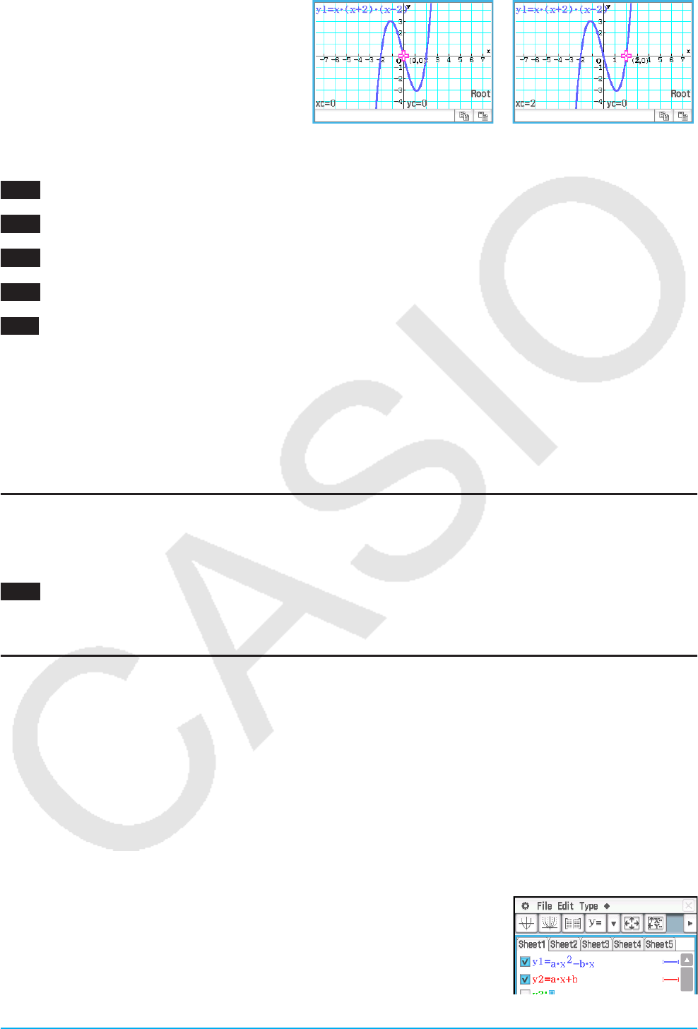
Chapter 3: Graph & Table Application 115
3. To obtain other roots, press the left or
right cursor key, or tap the left or right
graph controller arrows.
• If there is only one solution, the pointer
does not move when you press the
cursor key or tap the graph controller
arrow.
The following are examples for other G-Solve commands.
0307 To obtain the point of intersection for two graphs y = x + 1 and y = x2
0308 To determine coordinates at a particular point on a graph
0309 To graph the function y = x(x + 2)(x – 2) and obtain its definite integral in the domain of 1 s x s 2
0310 To graph the function y = x3 – 1 and determine its inflection point
0311 To graph the function y = x2 – x – 2 and obtain the volume of a solid of revolution as the line segment
from x = 1 to x = 2 is rotated on the x-axis
3-7 Modifying a Graph
A graph can be modified in real time as you change its parameters and/or variable values. The Graph & Table
application provides you with two methods for modifying a graph - “Direct Modify” and “Dynamic Modify”.
Modifying a Single Graph (Direct Modify)
“Direct Modify” changes the parameter in the equation of the original graph. This method can be used when
you are modifying a single graph.
0312 To graph the functions y = 2x2 + 3x – 1 and y = 2x + 1, and then find out how a change in the
parameters of each function affects the shape and position of the graphs
Modifying Multiple Graphs Simultaneously (Dynamic Modify)
“Dynamic Modify” changes the values assigned to common parameters of multiple functions. Use Dynamic
Modify when you want to modify multiple graphs at the same time.
uInputting a Graph Formula for Use with Dynamic Modify
Example: To input the following formula with two common parameters (a, b):
y = ax2 – bx and y = ax + b
1. On the Graph Editor window, tap [Type] - [y=Type].
2. Perform any one of the operations below.
- Input using built-in functions
(1) Tap a - [Built-In] - [y=a
·
x^2+b
·
x+c] to input y = ax2 + bx + c.
(2) Edit the function you input (y = ax2 + bx + c) to it becomes y = ax2 – bx,
and then press E.
(3) Tap the line below the function.
(4) Tap a - [Built-In] - [y=a
·
x+b] to input y = ax + b and then press E.
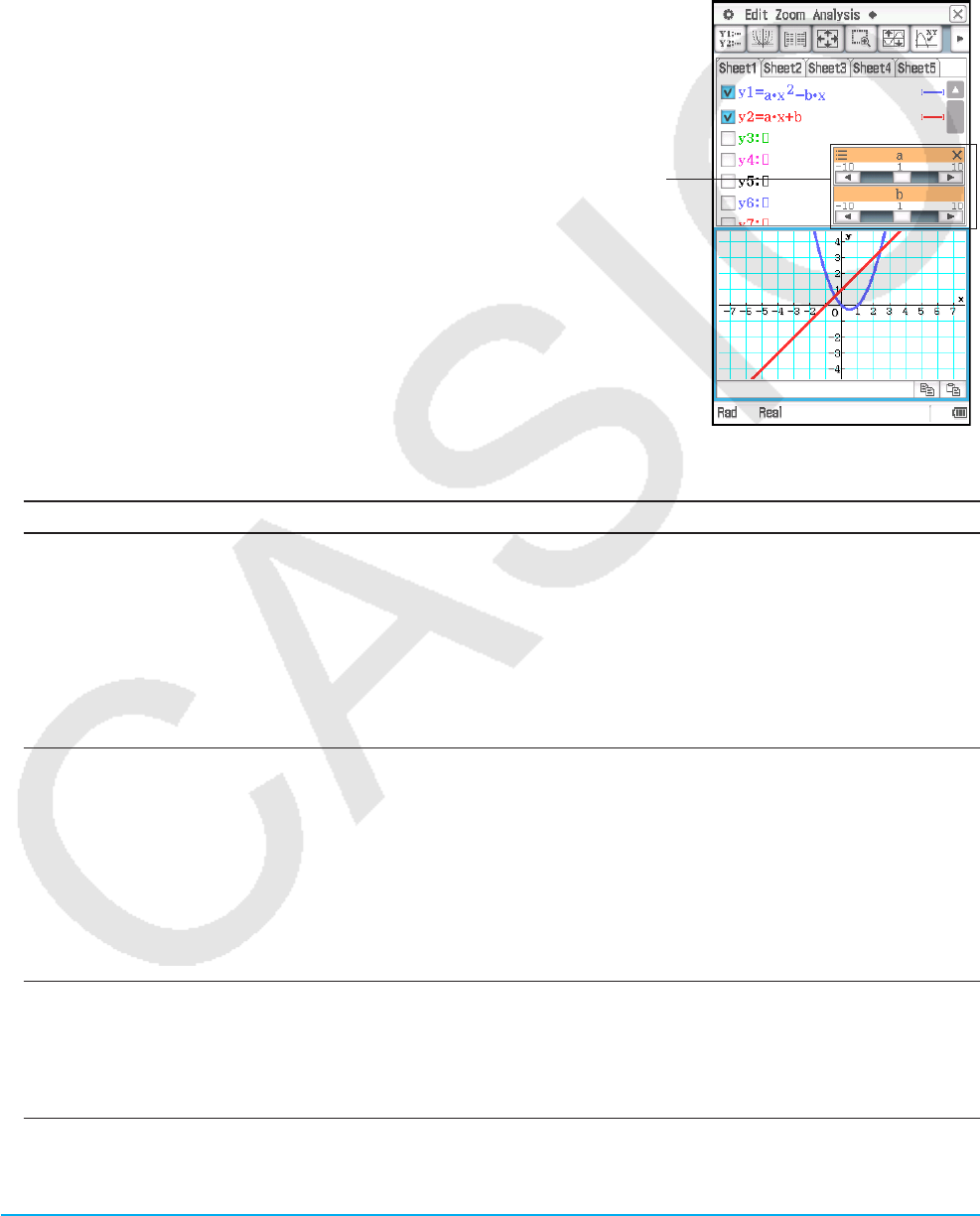
Chapter 3: Graph & Table Application 116
- Input using the soft keyboard and keyboard
(1) Display the soft keyboard and use it to perform the key operation below.
a*x{c-b*xw
(2) Tap the line below the formula you input and then perform the key operation below.
a*x+bw
u To run Dynamic Modify
1. On the Graph Editor window, input at least one formula that
contains a parameter.
2. Select the check box next to the graph formula(s) you want to
use with Dynamic Modify and clear the check boxes of all of the
other graphs.
• In the explanation below, there are two formulas registered
on the Graph Editor window: y = ax2 – bx and y = ax + b. The
check boxes of both of these formulas are selected for use with
Dynamic Modify.
3. To run Dynamic Modify, tap a and then [Dynamic Graph] or tap
4.
• This will display sliders for changing values assigned to
parameters a and b.
4. Tap the arrow buttons at either end of the a and b sliders.
• Each tap will change the values assigned to the applicable
parameter (a or b) and redraw the graph accordingly.
• The operations described below are supported while Dynamic
Modify is running.
Sliders
To do this: Do this:
Change the current
value, minimum value,
maximum value and step
value.
(1) Tap the upper left corner of the slider display box. On the menu that
appears, tap [Settings].
• This displays the Slider Settings dialog box. The number of tabs on
the dialog box will match the number of parameters in your graph
formula(s).
(2) Use the tabs to specify the current value, minimum value, maximum
value, and step value for each of the parameters.
(3) To close the dialog box and save your changes, tap [OK].
Automatically modify
the form of a graph (by
changing the value of
a specific parameter
between specified
minimum and maximum
values)
(1) Tap the upper left corner of the slider display box.
(2) On the menu that appears, tap [Auto Play].
• This starts an operation that automatically changes the value of the
applicable parameter between the minimum value and maximum value,
and then from the maximum value back to the minimum value. This
cycle will stop automatically after a few cycles from the minimum value
to the maximum value are complete. To stop a cycle part way through,
tap l on the icon panel or press c. (Simultaneous Auto Play
execution for multiple parameters is not supported.)
Temporarily hide sliders (1) Tap the upper left corner of the slider display box. On the menu that
appears, tap [Minimize].
• This hides all currently displayed sliders and causes the slider icon (a)
to appear in the status bar.
(2) To unhide the sliders, tap the slider icon (a) in the status bar.

Chapter 3: Graph & Table Application 117
uTo exit Dynamic Modify
Tap the close button (C) in the upper right corner of the slider display box.
Note
• While Dynamic Modify is running, up to three sliders can be displayed for the parameters included in the
graph formulas whose check boxes are selected. If there are more than three parameters in the selected
graph formulas, the three parameters are automatically assigned to sliders in accordance with the rules
below.
In the case of one graph formula, parameters are assigned to sliders from left to right until three are
assigned.
In the case of multiple graph formulas, parameters are assigned to sliders in the chronological order that the
graph formulas were registered (from left to right in each formula) until three are assigned.
• To change slider allocations from those applied automatically, perform the steps below.
1. Tap the upper left corner of the slider display box.
2. On the menu that appears, tap [Settings].
3. On the Slider Settings dialog box that appears, tap the “Parameter” line button.
4. On the parameter list that appears, tap the parameter you want to assign to the slider.
• If you use the above procedure to assign a different parameter to a slider, the parameter that was previously
assigned to the slider will retain the value it was set at when you changed the slider assignment. Also, the
minimum value, maximum value and step value will automatically change in accordance with the parameter
value. The automatically generated values will be applied if you later assign the parameter to a slider.
0313 To graph the functions y = ax2 – bx and y = ax + b, and then find out how a change in parameter a from
1 to 4 and a change in parameter b from –2 to 2 affect the shape and position of each graph
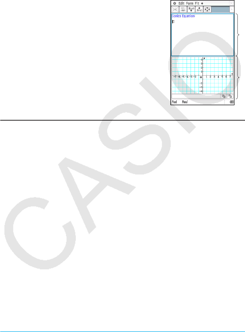
Chapter 4: Conics Application 118
Chapter 4:
Conics Application
The Conics application provides you with the capability to graph circular,
parabolic, elliptic, and hyperbolic functions. You can also use the Conics
application to quickly and easily determine the proper focal point, vertex,
directrix, and other information about each type of conics.
Starting up the Conics application displays two windows: 1 the Conics
Editor window and 2 the Conics Graph window.
A function input on the Conics Editor window is graphed on the Conics
Graph window.
1
2
Conics Application-Specific Menus and Buttons
Conics Editor window
• Draw a graph ..............................................................................................................................................^
• Start modifying a graph (Dynamic Modify, page 121) .................................................................................4
• Insert a Conics Form ....................................................................................Form - Insert Conics Form or q
• Adjust the equation so it fits a Conics Form ................................................... Fit - Fit into Conics Form or w
Conics Graph window
• Make the Conics Editor window active .......................................................................................................*
• Perform a G-Solve operation (page 120) ........................................................................... Analysis - G-Solve
Tip: The Conics application uses many of the same commands (Zoom, Trace, Sketch, etc.) as the Graph & Table
application.
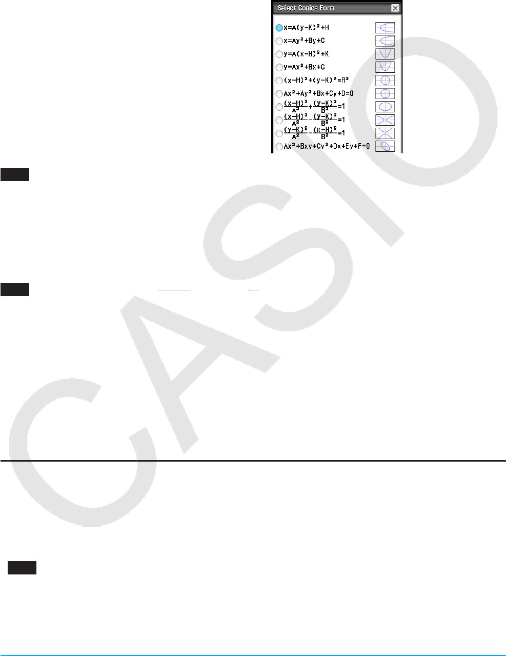
Chapter 4: Conics Application 119
4-1 Inputting an Equation
You can select one of the preset Conics Forms or input a conics equation manually. You can also transform a
manually input equation to a Conics Form.
uTo input an equation using a Conics Form
1. On the Conics Editor window, tap q to displays the
Select Conics Form dialog box.
2. Select the Conics Form of the type of equation you
want to graph, and then tap [OK].
• This displays the Conics Editor window, which will
contain the selected Conics Form.
3. Change the parameters of the equation as required.
Horizontal Parabola 1
Horizontal Parabola 2
Vertical Parabola 1
Vertical Parabola 2
Circle 1
Circle 2
Ellipse
Horizontal Hyperbola
Vertical Hyperbola
General Form
0401 To use a Conics Form to input the equation for a parabola with a horizontal axis (principal axis parallel
with x-axis)
uTo input an equation manually
Make the Conics Editor window active, and then use the soft keyboard for input.
uTo transform a manually input equation to a Conics Form
0402 To transform the equation ( − 1)2
22
2
4
+ ( − 2)2 = to the standard Conics Form x = Ay2 + By + C
Tip
• If the equation you input cannot be transformed into the standard Conics Form you selected, the message “Can’t
Transform into This Type” appears.
• An input equation may not transform correctly if it includes a square root calculation or some other function.
4-2 Drawing a Conics Graph
Tip: You can drag the Conics Graph window screen to scroll (pan) its contents (except for Trace, Sketch, G-Solve, box
zoom, and certain other functions).
Drawing a Parabola
A parabola can be drawn with either a horizontal or vertical orientation. The parabola type is determined by the
direction of its principal axis.
• A parabola with a horizontal axis is one whose principal axis is parallel to the x-axis. There are two possible
equations for a parabola with a horizontal axis:
x = A(y – K)2 + H and x = Ay2 + By + C.
0401 To draw the parabola x = 2(y – 1)2 – 2
• A parabola with a vertical axis is one whose principal axis is parallel to the y-axis. There are two possible
equations for a parabola with a vertical axis:
y = A(x – H)2 + K and y = Ax2 + Bx + C.

Chapter 4: Conics Application 120
Drawing a Circle
There are two forms that you can use to draw a circle.
• One form is the standard form, which allows you to specify the center point and radius:
(x – H)2 + (y – K)2 = R2
• The other form is the general form, which allows you to specify the parameters of each term:
Ax2 + Ay2 + Bx + Cy + D = 0
Drawing an Ellipse
You can use the standard equation ( − H)2
A2 + = 1
( − K)2
B2 to draw an ellipse.
Drawing a Hyperbola
A hyperbola can be drawn with either a horizontal or vertical orientation. The hyperbola type is determined by
the direction of its principal axis.
• The standard form of a hyperbola with a horizontal axis is: ( − H)2
A2 – = 1
( − K)2
B2
• The standard form of a hyperbola with a vertical axis is: ( − K)2
A2 – = 1
( − H)2
B2
Drawing a General Conics
Using the conics general equation Ax2 + Bxy + Cy2 + Dx + Ey + F = 0, you can draw a parabola or hyperbola
whose principal axis is not parallel either to the x-axis or the y-axis, a slanted ellipse, etc.
4-3 Using G-Solve to Analyze a Conics Graph
What You Can Do Using the G-Solve Menu Commands
While there is a graph on the Conics Graph window, you can use a command on the [Analysis] - [G-Solve]
menu to obtain the following information.
• x-coordinate for a given y-coordinate ................................................................. G-Solve - x-Cal/y-Cal - x-Cal
• y-coordinate for a given x-coordinate ................................................................. G-Solve - x-Cal/y-Cal - y-Cal
• Focus of a parabola, ellipse, or hyperbola .............................................................................G-Solve - Focus
• Vertex of a parabola, ellipse, or hyperbola ........................................................................... G-Solve - Vertex
• Directrix of a parabola ........................................................................................................ G-Solve - Directrix
• Axis of symmetry of a parabola ....................................................................................... G-Solve - Symmetry
• Length of the latus rectum of a parabola ...................................................... G-Solve - Latus Rectum Length
• Center point of a circle, ellipse, or hyperbola ........................................................................G-Solve - Center
• Radius of a circle ................................................................................................................. G-Solve - Radius
• Asymptotes of a hyperbola ...........................................................................................G-Solve - Asymptotes
• Eccentricity of a parabola, ellipse, or hyperbola ........................................................... G-Solve - Eccentricity
• x-intercept / y-intercept ...............................................................G-Solve - x-Intercept / G-Solve - y-Intercept
Tip: The color of Directrix, Symmetry, Asymptotes lines drawn using G-Solve is the color specified by the Graph Format
Sketch Color. For more information about Graph Format, see “Graph Format Dialog Box” (page 38).

Chapter 4: Conics Application 121
Using G-Solve Menu Commands
When multiple solutions are obtained by a G-Solve command, only one solution is displayed at a time. For
example, executing [Analysis] - [G-Solve] - [Focus] for an ellipse that has two foci will display only one focus
at a time. In a case such as this, use the left and right cursor keys (or tap the left and right graph controller
arrows) to cycle between the available solutions.
uTo determine the focus of the parabola x = 2(y – 1)2 – 2
1. On the Conics Editor window, input the conics equation and then tap ^ to graph it.
• Here, input the parabolic equation x = 2(y – 1)2 – 2.
2. Tap [Analysis] and then [G-Solve]. Next, on the submenu that appears,
select the command you want. To determine the focus for this example,
select [Focus].
• Press the left and right cursor keys to toggle the display between the two
foci.
The following are examples for other G-Solve commands.
0403 To determine the axis of symmetry of the parabola x = 2(y – 1)2 – 2
0404 To determine the center point of the circle x2 + y2 + 4x – 6y + 9 = 0
0405 To determine the radius of the circle x2 + y2 + 4x – 6y + 9 = 0
0406 To determine the asymptotes of the hyperbola − = 1
( − 1)2
22
( − 2)2
32
0407 To determine the eccentricity of the ellipse + = 1
( − 1)2
22
( − 2)2
32
0408 To determine the x-intercept of the parabola x = 2(y – 1)2 – 2
4-4 Modifying a Graph (Dynamic Modify)
A graph can be modified in real time as you change its parameter values.
uTo modify a graph
0409 To observe the form and position of the graph of the parabola x = ay2 + by + c as parameters a, b, and
c are each changed within a range of –2 to 2
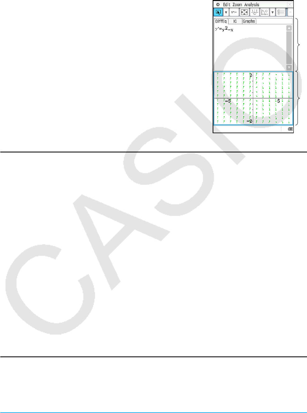
Chapter 5: Differential Equation Graph Application 122
Chapter 5:
Differential Equation Graph Application
This chapter explains how to use the Differential Equation Graph
application, which you can use to investigate families of solutions to
ordinary differential equations.
The Differential Equation Graph application has the following two types of
windows.
1 Differential Equation Editor window
Use this window to input expressions ([DiffEq] tab) and initial conditions
([IC] tab) for graphing. You also can input f ( x) type functions ([Graphs]
tab).
2 Differential Equation Graph window
This window shows the graph of the expression that you input into the
Editor window.
1
2
Differential Equation Editor Window-Specific Menus and Buttons
[DiffEq] tab, [IC] tab, [Graphs] tab
• Graph the selected function(s) ....................................................................................................................O
• Display the View Window dialog box to configure Differential Equation Graph window settings ................6
• Display the Main application window ..........................................................................................................~
• Delete the line of data at the current cursor location ..................................................................................q
[DiffEq] tab only
• Input a single first order differential equation ................................................... Type - 1st (Slope Field) or A
• Input a single second order differential equation or a set of
two first order differential equations ........................................................ Type - 2nd (Phase Plane) or B
• Input a higher order differential equation or a set of multiple
differential equations ..................................................................................... Type - Nth (No Field) or 9
[Graphs] tab only
• Input f(x) type functions .........................................................................................................Type - f (x) or d
• Input parametric functions ......................................................................................... Type - Parametric or g
[IC] tab and [Graphs] tab only
• Change graph line thickness to normal (1-dot line) or thick (2-dot line) ..............................................F, G
Differential Equation Graph Window-Specific Menus and Buttons
• Toggle arrows on or off to indicate the direction of slope field or
phase plane vectors ............................................................................................................... Edit - Arrows

Chapter 5: Differential Equation Graph Application 123
• Toggle the use of unit vectors on or off for slope field or phase
plane graphing ...............................................................................................................Edit - Unit Vectors
• Display the Differential Equation Editor window [DiffEq] tab ........................Edit - Editor - DiffEqGraph Editor
• Display the Differential Equation Editor window [IC] tab ..............................................Edit - Editor - IC Editor
• Display the Differential Equation Editor window [Graphs] tab ............................... Edit - Editor - Graph Editor
• Clear all currently registered initial conditions
(and, as a result, all solution curves) ...................................................................................Edit - Clear All
• Pan the graph window ....................................................................................................Analysis - Pan or T
• Select and move the initial condition point .................................................................. Analysis - Select or G
• Register the coordinates at the location you tap on the Differential
Equation Graph window as the initial condition, and graph the
solution curve based on that initial condition ........................................................ Analysis - Modify or J
• Make the Differential Equation Editor window active ..................................................................................A
• Display the View Window dialog box to configure Differential Equation
Graph window settings...........................................................................................................................6
• Display a trace cursor that can be positioned on any x, y coordinate .........................................................K
• Display a trace cursor that can be positioned on any grid point that has a field line ..................................L
• Display a trace cursor that can be positioned on any solution curve or
general graph ..........................................................................................................Analysis - Trace or =
• Turn display of axes and coordinate values on or off .................................................................................q
5-1 Graphing a Differential Equation
You can use the Differential Equation Graph application to graph a first order, a second order, or an nth-order
differential equation.
Graphing a First Order Differential Equation
This section explains how to input a first order differential equation, draw a slope field, and graph the solution
curve(s).
• A slope field is the family of solutions of a single, first order differential equation of the form y’= f (x, y). It is a
grid of solution lines where each line has the slope y’ for a given grid value of x and y. It is often referred to
as a “slope field” or “direction field” because only the direction of the field at any given point in known, not the
magnitude.
• You can overlay, onto the slope field, solution curves of the first order differential equation input for given
initial conditions on the [DiffEq] tab.
u To input a first order differential equation and draw a slope field
0501 To input y’ = y2 − x and draw its slope field
uTo input initial conditions and graph the solution curves
0502 After performing the operation under example 0501 , to graph three solution curves for the initial
conditions (xi, yi) = (0, 0), (0, 0.5), (0, 1)
Tip: You can specify whether or not a solution curve should be drawn for each initial condition input on the initial
condition editor. Use the initial condition editor to select the check box to the left of each initial condition input box
(Initial Condition 1, Initial Condition 2, etc.) whose solution curve you want to graph. The solution curve of any initial
condition whose check box is not selected will not be graphed.
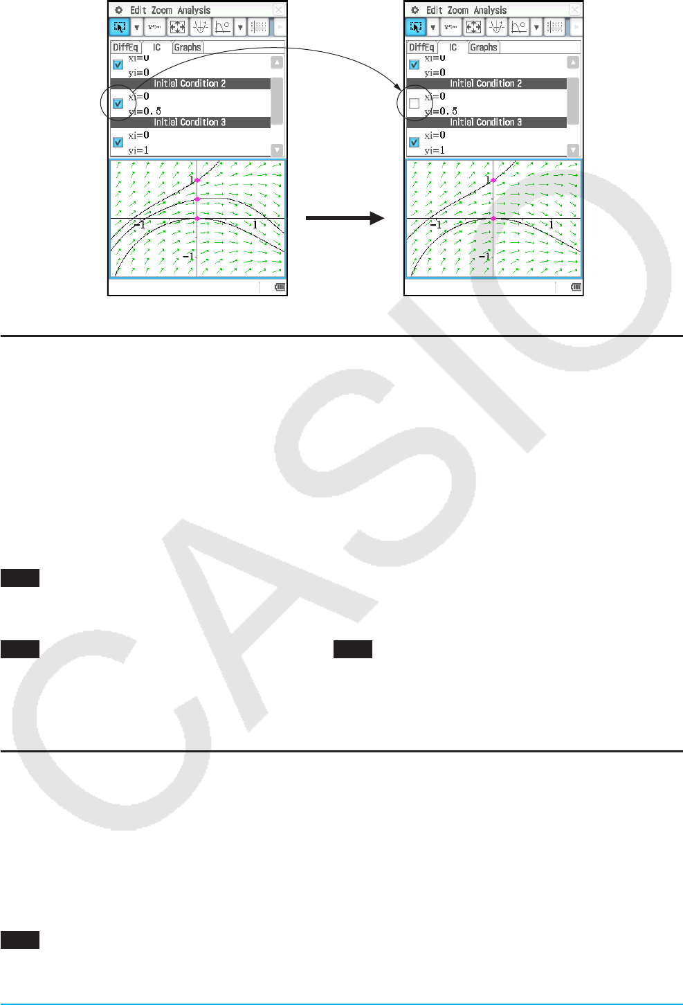
Chapter 5: Differential Equation Graph Application 124
Graphing a Second Order Differential Equation
This section explains how to input a second order differential equation, draw a phase plane, and graph the
solution curve(s). With this application, a second order differential equation is input in the form of a set of two
first order differential equations.
• A phase plane is the family of solutions of either a second order differential equation or two first order
differential equations of the form x’ = dx/dt = f (x, y) and y’ = dy/dt = g(x, y). A single second order differential
equation can also be graphed, but it must be written as two first order differential equations.
• You can overlay, onto the phase plane, solution curves of the second order differential equation input on the
[DiffEq] tab for given initial conditions.
u To input a second order differential equation and draw a phase plane
0503 To input {x’ = x, y’ = −y} and draw its phase plane
u To input initial conditions and graph the solution curves
0504 After performing the operation under example 0503 , to graph the solution curve of the initial condition
(xi, yi) = (1, 1)
Independent variable minimum value (tmin) = −7.7, maximum value (tmax) = 7.7, and initial value
(t0) = 0
Graphing an Nth-order Differential Equation
This section explains how to graph the solution curve(s) for an nth-order (higher order) differential equation
based on specified initial conditions. With this application, an nth-order differential equation is input in the form
of a set of multiple first order differential equations.
Note: For nth-order differential equations, only solution curves are drawn.
uTo input an nth-order differential equation and initial conditions, and then graph the solution
curves
0505 To specify the three initial conditions (xi, y1i, y2i) = (0, −1, 0), (0, 0, 0), (0, 1, 0) for the differential
equation y” = x − y, and graph its solution curves
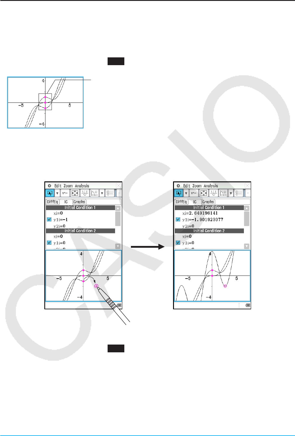
Chapter 5: Differential Equation Graph Application 125
Configuring and Modifying Initial Conditions
You can modify an existing initial condition on the Differential Equation Graph window by dragging it. You can
also configure a new initial condition on the Differential Equation Graph window by tapping the coordinates you
want to specify as the new initial condition.
uTo modify an initial condition on the Differential Equation Graph window
1. Perform the operation under example 0505 , which will produce a graph like the one shown below to appear
on the Differential Equation Graph window.
These dots are the currently configured initial conditions.
2. Tap [Analysis] - [Select] or G.
3. Tap one of the initial condition dots to select it, and then use the stylus to drag the dot to another location.
• Here we will drag the bottom dot, which is the Initial Condition 1 setting (xi, y1i, y2i) = (0, −1, 0). The
applicable initial condition will change to the coordinates of the location where you release the stylus after
dragging the dot, and the solution curve will be redrawn accordingly.
uTo configure new initial conditions on the Differential Equation Graph window
1. Perform the operation under example 0501 to produce a slope field on the Differential Equation Graph
window.
2. Tap [Analysis] - [Modify] or J.
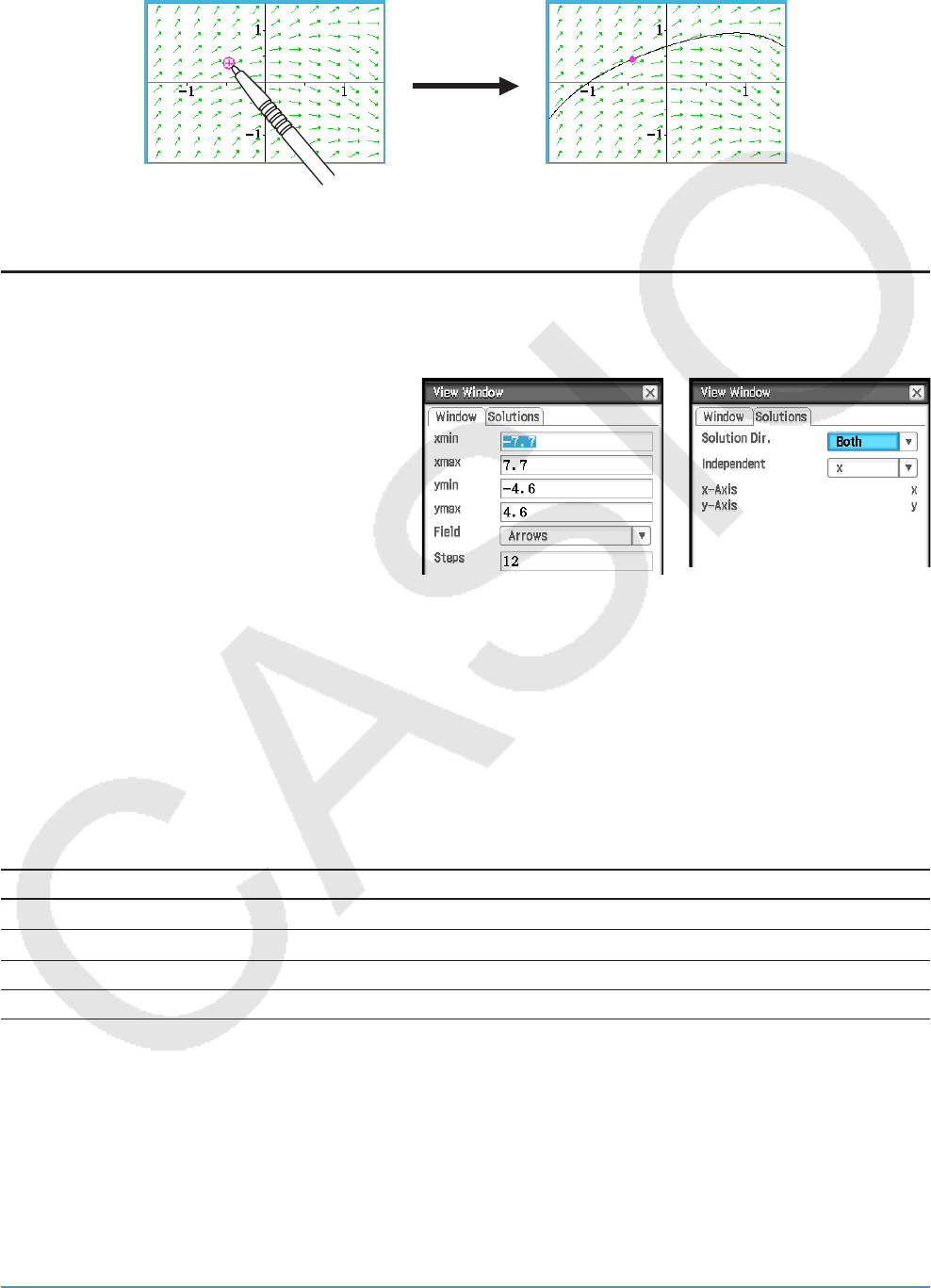
Chapter 5: Differential Equation Graph Application 126
3. On the Differential Equation Graph window, tap the coordinates that you want to specify as the new initial
condition.
• This will set the coordinates as the new initial condition and draw a solution curve.
• The newly configured initial condition is added to the initial condition editor. To view it, tap the [IC] tab.
Configuring Differential Equation Graph View Window Parameters
You can set a number of graphing parameters on the View Window dialog box. This dialog box contains two
tabs.
The [Window] tab lets you set the window
values and steps used for graphing a field. The
[Solutions] tab contains parameters used for
graphing solution curves.
uTo configure differential equation graph View Window settings
1. Tap 6 to display the View Window dialog box.
2. Input the required parameters on the [Window] and [Solutions] tabs.
• See “Differential equation graph View Window parameters” below.
3. After the settings are the way you want, tap [OK].
Differential equation graph View Window parameters
[Window] tab
Setting Description
xmin, xmax Minimum/maximum value along the (horizontal) x-axis
ymin, ymax Minimum/maximum value along the (vertical) y-axis
Field Specifies display of arrow, line or nothing.
Steps Number of steps or field lines used for graphing a field
[Solutions] tab
The variable assignments available on the [Solutions] tab vary depending on the graph type selected with the
Graph Editor. Some graph types have preset assignments for the independent, x-axis, and y-axis variables. If a
value is preset for the current graph type the value will still be displayed on the Solutions tab, but you will not be
able to change it.

Chapter 5: Differential Equation Graph Application 127
Setting Description
Solution Dir. A solution curve is graphed starting at the initial condition value t0 and continues until
it reaches a target value, which can be either tmin or tmax. The solution direction
determines the target values. Forward will graph the solution curve from t0 to tmax.
Backward will graph the solution curve from t0 to tmin. Both will graph the solution curve
from t0 to tmin, and then t0 to tmax.
Independent Assignment of the independent variable for differential equations
1st-order, Nth-order: x or t
2nd-order: t (fixed)
t0 (or x0) If the independent variable is different from the x-axis variable, you can enter the initial
value for the independent variable (2nd-order and Nth-order only).
tmin (or xmin),
tmax (or xmax)
If the independent variable is different from the x-axis variable, you can enter the
minimum/maximum value for the independent variable (2nd-order and Nth-order only).
x-Axis Variable assignment for the (horizontal) x-axis
1st-order: same as independent variable
2nd-order: x (fixed)
Nth-order: independent variable or y1 through y10
y-Axis Variable assignment for the (vertical) y-axis
1st-order, 2nd-order: y (fixed)
Nth-order: independent variable or y1 through y10
5-2 Drawing f ( x) Type Function Graphs and Parametric
Function Graphs
f ( x) type function graphs and parametric function graphs can be overlaid on differential equation graphs.
uTo draw an f ( x) type function graph
0506 To overlay a differential equation graph with the graphs of y = x2 and y = −x2
uTo draw a parametric function graph
0507 To graph {xt = 3sin(t) + 1, yt = 3cos(t) + 1}
(Angle unit setting: radian, 0 s t s 2π)
5-3 Using Trace to Read Graph Coordinates
The trace function let you read the coordinates on graphs drawn with the Differential Equation Graph
application. There are three types of trace: “point trace” (shows the coordinates of any point), “field trace”
(shows the coordinates of center of each field line), and “graph/curve trace” (shows the coordinates of points on
a graph or solution curve).
uTo start a point trace
On the Differential Equation Graph window, tap K.
u To start a field trace
Draw a slope field (page 123) or a phase plane (page 124), and then tap L.

Chapter 5: Differential Equation Graph Application 128
uTo start a graph/curve trace
1. Draw a solution curve (pages 123 through 124) or function graph (page 127).
2. Tap = or [Analysis] - [Trace].
5-4 Graphing an Expression or Value by Dropping It into
the Differential Equation Graph Window
You can use the procedures in this section to graph an expression or value by dragging it from the eActivity
application window or the Main application window, and dropping it into the Differential Equation Graph window.
To draw this type of graph: Drop this type of expression or value into the Differential Equation
Graph window:
Slope field 1st-order differential equation in the form of y’ = f (x, y)
Solution curve(s) of a 1st-
order differential equation
Matrix of initial conditions in the following form:
[[x1, y(x1)][x2, y(x2)] .... [xn, y(xn)]]
• Note that the Slope field should already be graphed on the Differential
Equation Graph window before the matrix is dropped in. If it isn’t, dropping
in the matrix will simply plot points at the coordinates indicated by each (x,
y) pair.
• Regardless of whether or not the Slope field is already graphed, values
in the dropped in matrix will be registered to the [IC] tab of the Differential
Equation Editor.
Solution curve(s) of an nth-
order differential equation
1) nth-order differential equation such as y” + y’ + y = sin(x), followed by
2) Matrix of initial conditions in the following form:
[[x1, y1(x1)][x2, y1(x2)] .... [xn, y1(xn)]] or
[[x1, y1(x1), y2(x1)][x2, y1(x2), y2(x2)] .... [xn, y1(xn), y2(xn)]]
f ( x) type function graph Function in the form y = f ( x)
0508 To drag the 1st-order differential equation y’ = exp(x) + x2 and then the initial condition matrix [0, 1] from
the eActivity application window to the Differential Equation Graph window, and graph the applicable
slope field and solution curve
0509 To drag the nth-order differential equation y” + y’ = exp(x) and then the initial condition matrix [[0, 1, 0]
[0, 2, 0]] from the eActivity application window to the Differential Equation Graph window, and graph the
applicable solution curves
Tip: An nth-order differential equation of the form f (y’, y”…, x) dropped into the Differential Equation Graph window will
be treated as f (y’, y”…, x) = 0.
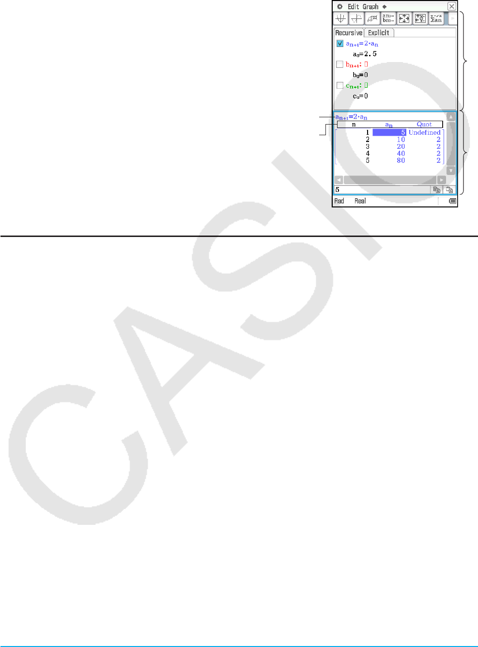
Chapter 6: Sequence Application 129
Chapter 6:
Sequence Application
The Sequence application provides you with the tools you need to
work with explicit sequences and recursive type sequences. Starting
up the Sequence application displays two windows.
1 Sequence Editor window
Use this window to input expressions for creating a sequence table.
2 Table window
Use this window to create and display table.
(a) Title: Shows the equation used in the calculations. The title is not
displayed when an item in column n is selected.
(b) Column names
1
2
(a)
(b)
Sequence Application-Specific Menus and Buttons
Sequence Editor window
• Specify the recursion type ([Recursive] tab only) ................................................. Type menu or ^&*(
• Turn display of sequence table subtotals on or off ....................................................... a - Σdisplay - On/Off
• Show (On) in the message box or hide (Off) the expression used to
draw a figure with Sketch, or show the expression only when E
is pressed (StepDisp)...................................................................... a - Set Sequence - On/Off/StepDisp
• Clear the contents of the currently active tab sheet .............................................................. a - Clear Sheet
• Delete the recursion expression in the current active line ..........................................................................w
Sequence Table window
• Draw a connect type graph ......................................................................................... Graph - Connect or $
• Draw a plot type graph ................................................................................................... Graph - G-Plot or !
• Save the contents of a table to a list .....................................................................................a - Table to List
• Regenerate the currently displayed table ...................................................................................a - ReTable
• Delete the currently displayed table .....................................................................................a - Delete Table
• Execute a table and graph link trace ..................................................................................................a - Link
• To input a recursion term, tap the [n, an] menu and then tap the term you want. If the [Explicit] tab is displayed,
you can also use the toolbar’s B to input a term-n.
Sequence RUN window
• Input the “rSolve” function ........................................................................................................... Calc - rSolve
• Input the “Σ” function ........................................................................................................................... Calc - Σ
• Use the [n, an] menu to input recursion expression terms. You can also use the [a0, a1] menu to input system
variables ranging from a0 to c2.
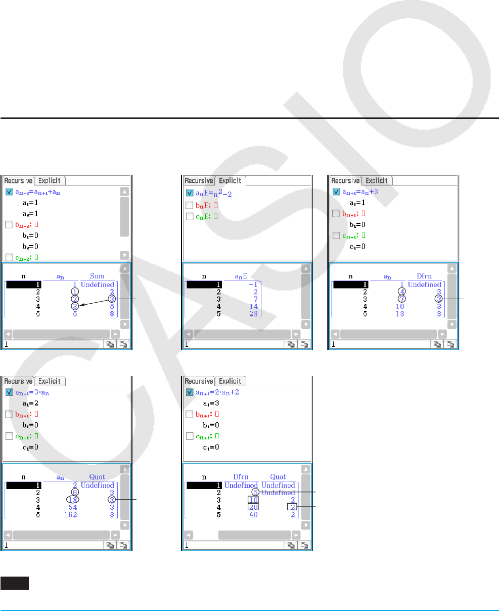
Chapter 6: Sequence Application 130
Buttons common to multiple windows
• Create an ordered pair table (Editor/Graph/RUN) ......................................................................................#
• Create a sequence table with column(s) that determine if a sequence
is an arithmetic sequence, geometric sequence, progression of
difference, or Fibonacci sequence (Editor/Graph/RUN) ..........................) (arithmetic), _ (geometric),
+ (progression of difference), ` (Fibonacci)
• Display the Sequence Table Input dialog box (Editor/Table/Graph/RUN) ..................................................8
• Draw a cobweb diagram on a graph (Editor/Table) ....................................................................................w
• Display the Sequence RUN window (Editor/Table/Graph) .........................................................................`
• Display the Sequence Editor window (Table/Graph/RUN) .........................................................................&
6-1 Recursive and Explicit Form of a Sequence
ClassPad supports use of three types of sequence expressions: an+1=, an+2= and anE.
Generating a Number Table
In addition to an ordered pair table, you can create a sequence table with column(s). This helps you determine if
the sequence is an arithmetic sequence, geometric sequence, progression of difference, or Fibonacci sequence.
3 = 2 + 1 3 = 7 − 4
Fibonacci Sequence Table Ordered Pair Table Arithmetic Sequence Table
3 = 18 ÷ 6 5 = 8 − 3
2 = 20 ÷ 10
Geometric Sequence Table Progression of Difference Table
0601 To create a number table (Fibonacci sequence table) to check the Fibonacci sequence expressed by
the recursion formula an+2 = an+1 + an, a1 = 1, a2 = 1
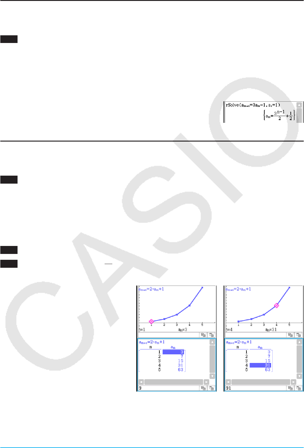
Chapter 6: Sequence Application 131
Determining the General Term of a Recursion Expression
You can use the rSolve function to convert the sequence expressed by a recursion expression to the general
term format an = f ( n).
0602 To determine the general term of the recursion expression an+1 = an + 2, a1 = 1
About rSolve
The rSolve function returns the explicit formula of a sequence that is defined in relation to one or two previous
terms, or a system of recursive formulas.
Syntax: rSolve (Eq, initial condition-1[, initial condition-2] [ ) ]
rSolve ({Eq-1, Eq-2}, {initial condition-1, initial condition-2} [ ) ] (Eq: Equation)
Example: To obtain the n-th term of a recursion formula an+1 = 3an – 1 with the
initial conditions a1 = 1
Calculating the Sum of a Sequence
Perform the following steps when you want to determine the sum of a specific range of the sequence of a
recursion expression or a general term expression.
0603 To calculate the sum of the general term expression anE = n2 + 2n – 1 in the range of
2 s n s 10
6-2 Graphing a Recursion
ClassPad lets you graph the values in a number table you create, and draw a cobweb diagram from the
recursion expression.
0604 To input the expression an+1 = 2an + 1, a1 = 1, create a number table, and graph the values in the table
0605 To input the expression an+1 =
− 1, a1 = 0.5 and draw a cobweb diagram
About LinkTrace
While the Table and Graph windows are on the
display, you can activate LinkTrace. To do this,
tap in the Table window to make it active. Next,
tap a and then [Link]. While LinkTrace is
active, the pointer on the Graph window jumps
automatically to the point indicated by the
coordinates in the currently selected table cell.
Note that LinkTrace does not work when the
selected cell is in the first column (column n).
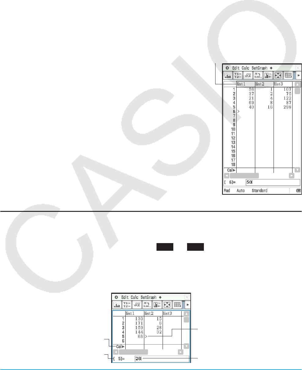
Chapter 7: Statistics Application 132
Chapter 7:
Statistics Application
The Statistics application provides you with the tools you need to perform the operations below.
Statistical data input (as list variables)
Statistical graph drawing:
Single-variable statistical graphs and paired-variable
statistical graphs
Statistical calculations:
Single-variable, paired-variable, regression, test,
confidence interval, and distribution calculations
Tip: Performing a statistical calculation, graphing operation or other operation causes calculation results to be assigned to
pre-determined system variables. For more information, see the “System Variable Table” on page 299.
7-1 Using Stat Editor
When you start up the Statistics application, the Stat Editor window shown
to the right appears on the display.
Stat Editor is a tool for creating and maintaining lists (list variables), and it
plays a very important role in ClassPad statistical calculations. ClassPad
uses lists as data sources for statistical calculations and for statistical
graphing. You can specify data by its list name.
The list name is located in the cell at the top of each list. The initial default
Stat Editor window shows six lists (columns), named list1 through list6.
List name
Basic List Operations
You can use the Stat Editor window to input and edit the data in the initially displayed list1 through list6. You
can also recall list variables you created with the Main application* and create new list variables.
* See
0240 and 0241 in the separate “Examples” booklet.
uTo input data into a list
1. On the Stat Editor window, select the cell where you want to input the data item.
• Use the cursor key to move the highlighting, or tap the cell with the stylus.
“Cal'” line
(see Tip on the
next page)
Number of line where
data is being input
Cell where data is being input
Input data

Chapter 7: Statistics Application 133
2. Input the data you want.
• You can input values, formulas, or variable names. If you input a formula, the value of the calculation result
will be input into the list. If you input a variable name, the value currently assigned to the variable (or the
variable name itself in the case of an undefined variable) will be input into the list.
• After you input a formula into a cell, the calculation result will be displayed as a decimal value or a fraction
in accordance with the “Decimal Calculation” setting of the Basic Format dialog box (page 36).
3. Press E to store the data in the cell.
Tip
• Inputting a formula that includes a list (page 57) into a “Cal'” line and then pressing E will cause the calculation result
list data to replace the contents currently in the list being input. For example, inputting {1,2,3}^2 into the “Cal'” line of list1
and then pressing E will cause list1 to be overwritten with {1,4,9}. Any data previously in list1 is lost.
• A list can contain up to 9,999 rows.
• A locked variable (page 30) causes the b icon to be displayed in the “Cal'” line, which cannot be edited.
uTo create a list
1. On the Stat Editor window, tap a list name cell to select it.
2. Enter up to eight bytes for the list name you want, and then press E.
• This creates a list variable with the name you specified. After that, you can input data using the procedure
under “To input data into a list”.
• If you enter a list name that is already used for another list, pressing E displays the contents of that list.
u To open an existing list
1. On the Stat Editor window, select the list name cell of the column where you want the list you will open to
appear.
• Instead of the above operation, you could also select any cell in the column where you want the list you will
open to appear and then tap [Edit] - [Open List].
2. Enter the variable name of the list you want to open, and then press E.
• If you enter a variable name that does not match the names of any of the existing lists in step 1, a new list
will be created using the name you entered.
uTo close a list
Select the list name cell of the column of the list you want to close, and then press KE.
Or, select any cell of the list you want to close, and then tap [Edit] - [Close List].
• This operation clears the list from the display only. The list is still stored as a list variable in memory, and can
be opened when you need it again.
Menus and Buttons Used for List Editing
• Jump to line 1 of the current list ........................................................................................... Edit - Jump - Top
• Jump to the line after the last line of the current list ........................................................ Edit - Jump - Bottom
• Sort list data ascending ......................................................................................Edit - Sort - Ascending or L
• Sort list data descending ................................................................................. Edit - Sort - Descending or :
• Delete a cell ............................................................................................................. Edit - Delete - Cell or H
• Delete all of the data in a list .............................................................................. Edit - Delete - Column or J
• Delete a list from memory ..................................................................................... Edit - Delete - List Variable
• Insert a cell into a list ................................................................................................... Edit - Insert Cell or K
• Select all the text in the currently selected cell ....................................................................... Edit - Select All

Chapter 7: Statistics Application 134
• Clear list variable data from list1 through list6 and initialize Stat Editor
window contents ..................................................................................................................Edit - Clear All
• Convert a mathematical expression in the currently selected cell to a decimal value ................................9
• Display two, three, or four columns in the Stat Editor window* ...................................................S / D / F
* You can also specify the number of display columns using the [Cell Width Pattern] setting on the [Special] tab
of the Graph Format dialog box (page 38).
Using CSV Files
You can import the contents of a CSV file stored with the ClassPad or transferred from a computer into the Stat
Editor. You also can save the contents of all the list data in the Stat Editor as a CSV file.
Import CSV File Requirements
A CSV file that has been output from the Stat Editor or Spreadsheet (Chapter 13), or a CSV file transferred from
a computer to storage memory can be used for import. The following types of CSV files are supported for import.
• A CSV file that uses the comma (,) or semi-colon (;) as its separator, and the period (.) or comma (,) as its
decimal symbol. A CSV file that uses the tab as its separator is not supported.
• CR, LF and CRLF are supported for the line break code.
For information about transferring files from a computer to the calculator, see “19-2 Performing Data
Communication between the ClassPad and a Personal Computer”.
Stat Editor Display and List Data Overwriting Following CSV File Import
When you import a CSV file into Stat Editor, everything displayed on the Stat Editor screen is cleared and
replaced with the imported CSV file data.
The first column of the CSV file data is imported into the Stat Editor column 1 list (list 1), the second column of
file data is imported into Stat Editor column 2 list (list 2), and so on. List data is created for each of the CSV file
columns. Any data previously stored in a list is overwritten by the imported data.
Except for data that is overwritten by the CSV file import, current list data cleared from the Stat Editor screen by
the import operation is retained in ClassPad memory.
uTo import the contents of a CSV file to the Stat Editor
1. Prepare the CSV file you want to import.
• See “Import CSV File Requirements” described above.
2. While the Stat Editor is on the display, tap [Edit] - [CSV] - [Open CSV].
3. On the dialog box that appears, select the CSV file you want to import and then tap [Open].
Important!
• Importing a CSV file that has a large number of rows and/or columns may cause an insufficient memory error.
If this happens, reduce the number of rows and/or columns in the CSV file.
• Following import, the contents of all cells that contain character strings are automatically replaced with 0.
uTo save the contents of all the list data in the Stat Editor as a single CSV file
1. While the Stat Editor is on the display, tap [Edit] - [CSV] - [Save CSV].
2. On the dialog box that appears, specify the export destination folder and then input a name for the export file.
3. Tap [Save].
Important!
The list name line and Cal' line are not output to the CSV file.

Chapter 7: Statistics Application 135
u To specify the CSV file separator and decimal symbol
1. While the Stat Editor is on the display, tap [Edit] - [CSV] - [CSV Format].
2. On the dialog box that appears, specify the desired settings for “CSV Separator” and “CSV Decimal Symbol”.
3. To save the settings, tap [OK].
7-2 Drawing a Statistical Graph
Up to nine graphs, including single-variable data and paired-variable data statistical graphs can be drawn
simultaneously ([SetGraph] - [StatGraph1] to [StatGraph9]).
In addition to graphs that can be drawn using [Set Graph], the graphs below can also be drawn at the same
time.
• Regression graphs (using [Linear Reg] and other regression commands on the [Calc] - [Regression] menu)
• Function graphs (using the Graph & Table application’s Graph Editor window)
Operation Flow Up to Statistical Graphing
Drawing a statistical graph requires the following basic steps: (1) preparation of the list data to be used; (2)
selection of the graph type and other graph settings; (3) drawing of the graph.
uTo prepare list data for statistical graphing
Prepare the list data using one of the patterns shown below.
Single Variable Paired Variable
Without frequency With frequency Without frequency With frequency
Single list Two lists Two lists Three lists
Data Data Frequency Paired data Paired data Frequency
Tip
• Single-variable data is data that consists of a single value. If you are trying to obtain the average height of the members
of a single class, for example, the single-variable would be height. With paired-variable statistical data there are two
values for each data item. An example of paired-variable statistical data would be the change in size of an iron bar as its
temperature changes. One variable would be temperature, and the other variable is the corresponding bar size.
• If you created user list data with another application, open it in the Stat Editor window. For more information, see “To
open an existing list” (page 133). You can specify a list displayed in the Stat Editor window as data to be used for statistical
graphing.
• You can display up to 99 lists on the Stat Editor window.
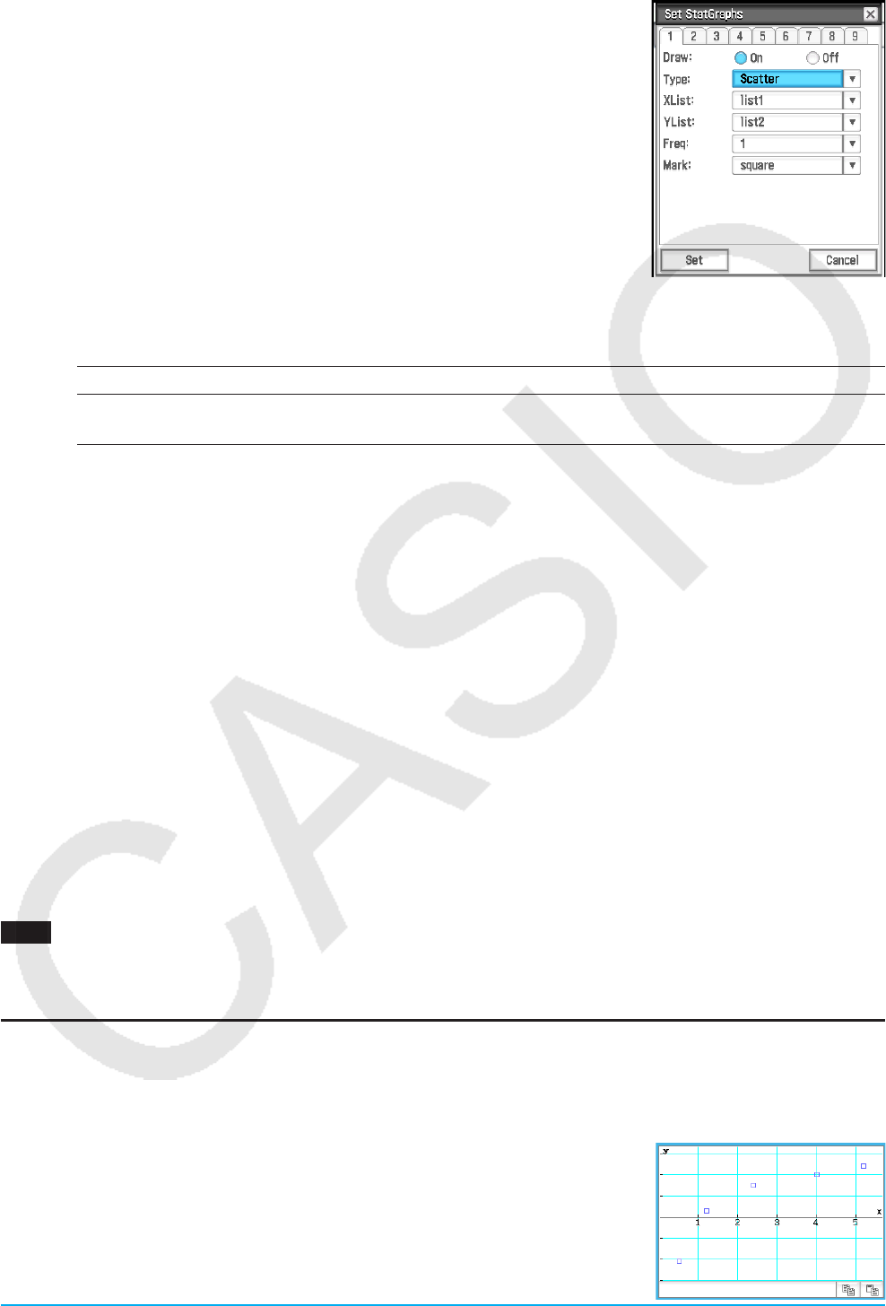
Chapter 7: Statistics Application 136
u To configure statistical graph settings
1. On the Stat Editor window, tap [SetGraph] - [Setting…] or tap G.
• This displays the Set StatGraphs dialog box. There are tabs named 1
through 9 that correspond to StatGraph1 through StatGraph9.
• Each tab is assigned a color. Tabs [1] and [6]: Blue; Tabs [2] and [7]: Red;
Tabs [3] and [8]: Green; Tabs [4] and [9]: Magenta; Tab [5]: Black
2. Tap the tab for the StatGraph setup whose configuration you want to
change.
3. Configure the StatGraph setup settings you want as described below.
Draw: Select the On setting if you want to draw the tab’s graph, or Off if you
do not want to draw it. After closing the dialog box, tap y on the
toolbar to execute the graph draw operation.
Type: Selects the type of graph to be drawn. The types of graphs available for selection depend on whether
the graph data is single-variable or paired-variable.
Single-variable NPPlot, Histogram, MedBox, NDist, Broken
Paired-variable Scatter, xyLine, LinearR, MedMed, QuadR, CubicR, QuartR, LogR,
ExpR, abExpR, PowerR, SinR, LogisticR
For details about each graph type, see “Graphing Single-Variable Statistical Data” (page 136) and
“Graphing Paired-Variable Statistical Data” (page 137).
XList, YList, Freq: Specifies the list data to be used for graphing. If you prepared frequency list data, use
Freq to specify the frequency list.
Mark: This setting is supported only when Scatter, xyLine, or NPPlot is specified for “Type”. Select square
(q), cross (w), large dot (;) or dot (') as the shape for graph lot points.
4. Tap [Set] to apply the settings for the tab you selected in step 2.
uTo draw a statistical graph
1. On the Stat Editor window, tap [SetGraph], and then confirm that there is at least one item from [StatGraph1]
to [StatGraph9] whose check box is selected.
• If no check box is selected, select at least one check box. Selecting multiple check boxes will cause the
corresponding graphs to be drawn simultaneously.
2. Configure the a - [Stat Window Auto] - [On] / [Off] setting as required.
• Selecting [On] for this setting configures View Window settings for drawing statistical graphs automatically.
See “Graph Format Dialog Box” (page 38) for details.
3. Tap y to display the Stat Graph window and draw the statistical graphs.
0701 To input the paired-variable data shown below and then plot the data on a scatter plot
list1 = 0.5, 1.2, 2.4, 4.0, 5.2 list2 = −2.1, 0.3, 1.5, 2.0, 2.4
Graphing Single-Variable Statistical Data
You can produce any of the graphs described below using single-variable data. The text in the parentheses of
the graph names below shows text that appears on the Type menu of the Set StatGraphs dialog box.
Normal Probability Plot (NPPlot)
The normal probability plot plots data against a theoretical normal distribution
using a scatter plot. If the scatter plot is close to a straight line, then the data is
approximately normal. A departure from the straight line indicates a departure
from normality.
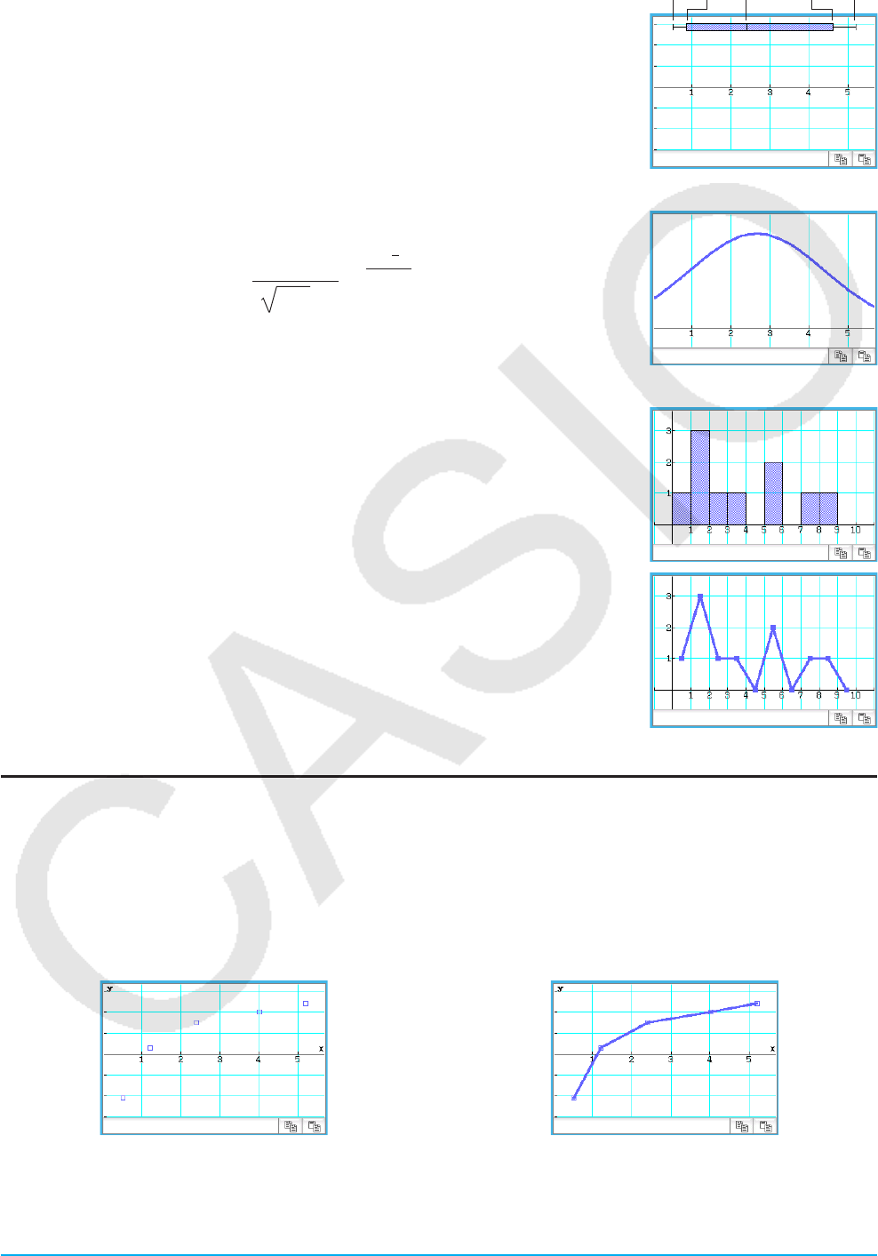
Chapter 7: Statistics Application 137
Med-Box Plot (MedBox)
This type of graph is often called a “Box and Whisker” graph. It lets you see
how a large number of data items are grouped within specific ranges. The lines
from minX to Q1, and from Q3 to maxX are called “whiskers”. If [Show Outliers]
box is checked on the Set StatGraphs dialog box (page 136), “outlier” square
symbols are shown instead of “whisker” lines where a data value is relatively
large or small compared to the other data values.
minX Q1 Med Q3 maxX
Normal Distribution Curve (NDist)
The normal distribution curve is graphed using the following normal distribution
function.
y = 1
2πσ e
–2σ
2
(x–x)
2
Histogram Bar Graph (Histogram), Broken Line Graph (Broken)
A histogram shows the frequency (frequency distribution) of each data class as
a rectangular bar. Classes are on the horizontal axis, while frequency is on the
vertical axis.
In the broken line graph, lines connect the pointers that fall at the center of
each histogram bar.
The Set Interval dialog box appears before the graph is drawn. You can use
this dialog box to change the start value (HStart) and step value (HStep) of the
histogram, if you want.
Graphing Paired-Variable Statistical Data
You can produce any of the graphs described below using paired-variable data. The text in the parentheses of
the graph names below shows text that appears in the Type menu of the Set StatGraphs dialog box (page 136).
kPlot graphs
Draws graphs by plotting paired-variable points with x data on the horizontal axis and y data on the vertical
axis.
Scatter plot (Scatter) xy line graph (xyLine)

Chapter 7: Statistics Application 138
k Regression graphs
Regression graphs of each of the paired-variable data can be drawn according to the model formulas under
“Regression types” below.
Linear regression graph Quadratic regression graph Logistic regression graph
Regression types:
Linear regression (LinearR) [Linear Reg] .............................................................. y = aⴢx + b, y = a + bⴢx
Linear regression uses the method of least squares to determine the equation that best fits your data
points, and returns values for the slope and y-intercept. The graphic representation of this relationship is a
linear regression graph.
Med-Med line (MedMed) [MedMed Line] ...................................................................................y = aⴢx + b
When you suspect that the data contains extreme values, you should use the Med-Med graph (which
is based on medians) in place of the linear regression graph. Med-Med graph is similar to the linear
regression graph, but it also minimizes the effects of extreme values.
Quadratic regression (QuadR) [Quadratic Reg] ............................................................. y = aⴢx2 + bⴢx + c
Cubic regression (CubicR) [Cubic Reg] ................................................................y = aⴢx3 + bⴢx2 + cⴢx + d
Quartic regression (QuartR) [Quartic Reg] .................................................y = aⴢx4 + bⴢx3 + cⴢx2 + dⴢx + e
Quadratic, cubic, and quartic regression graphs use the method of least squares to draw a curve that
passes the vicinity of as many data points as possible. These graphs can be expressed as quadratic, cubic,
and quartic regression expressions.
Logarithmic regression (LogR) [Logarithmic Reg] ....................................................................a + bⴢln(x)
Logarithmic regression expresses y as a logarithmic function of x. The normal logarithmic regression
formula is y = a + bⴢln(x). If we say that X = ln(x), then this formula corresponds to the linear regression
formula y = a + bⴢX.
aⴢebx Exponential regression (ExpR) [Exponential Reg].............................................................y = aⴢebⴢx
Exponential regression can be used when y is proportional to the exponential function of x. The normal
exponential regression formula is y = aⴢebⴢx. If we obtain the logarithms of both sides, we get ln(y) = ln(a) +
bⴢx. Next, if we say that Y = ln(y) and A = In(a), the formula corresponds to the linear regression formula Y
= A + bⴢx.
aⴢb
x Exponential regression (abExpR) [abExponential Reg] ........................................................y = aⴢbx
Exponential regression can be used when y is proportional to the exponential function of x. The normal
exponential regression formula in this case is y = aⴢbx. If we take the natural logarithms of both sides, we
get ln(y) = ln(a) + (ln(b))ⴢx. Next, if we say that Y = ln(y), A = ln(a) and B = ln(b), the formula corresponds to
the linear regression formula Y = A + Bⴢx.
Power regression (PowerR) [Power Reg] ......................................................................................y = aⴢxb
Power regression can be used when y is proportional to the power of x. The normal power regression
formula is y = aⴢxb. If we obtain the logarithms of both sides, we get ln(y) = ln(a) + bⴢln(x). Next, if we say
that X = ln(x), Y = ln(y), and A = ln(a), the formula corresponds to the linear regression formula Y = A + bⴢX.
Sinusoidal regression (SinR) [Sinusoidal Reg] ........................................................y = aⴢsin(bⴢx + c) + d
Sinusoidal regression is best for data that repeats at a regular fixed interval over time.
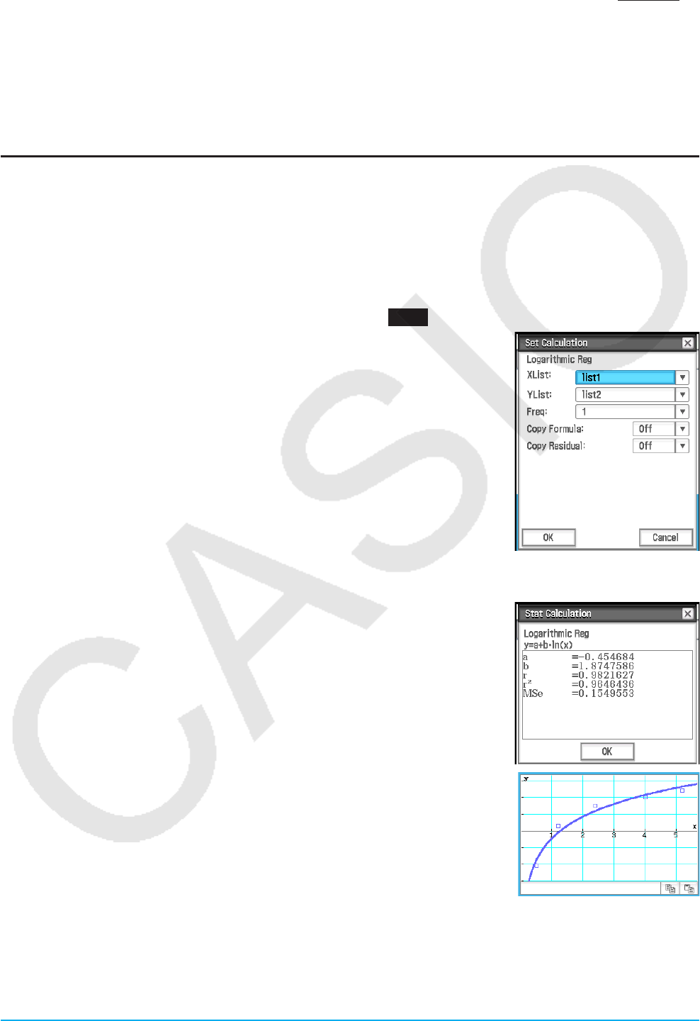
Chapter 7: Statistics Application 139
Logistic regression (LogisticR) [Logistic Reg] .................................................................... y = c
1 + aⴢe–bⴢx
Logistic regression is best for data whose values continually increase over time, until a saturation point is
reached.
Tip: Though ClassPad internally performs regression calculations after drawing a regression graph using the settings
of the Set StatGraphs dialog box (page 136), the calculation results (regression formula coefficients and other values)
cannot be displayed. To display regression calculation results, use the commands on the [Calc] - [Regression] menu,
which are shown in square brackets ([ ]) above.
Overlaying a Regression Graph on a Scatter Plot
You can use the Set StatGraphs dialog box (page 136) to plot a scatter plot* from paired-variable data and then
overlay a regression graph on it. This means you can visually determine which regression formula is closest to
the scatter plot.
* You can also overlay on other graph types as well.
uClassPad Operation
1. Draw the scatter plot. Here we will use the operation under 0701 in the separate “Examples” booklet.
2. On the [Calc] - [Regression] menu, select one of the regression calculation
commands (from [Linear Reg] to [Logistic Reg]).
• Here we will select [Logarithmic Reg]. This displays the Set Calculation
dialog box.
3. Here, we want to overlay on a scatter plot, so we specify XList, YList, and Freq the same as in step 1 of the
procedure for drawing a scatter plot.
4. Tap [OK].
• This displays the Stat Calculation dialog box. For information about this
dialog box’s contents, see “Performing Regression Calculations” (page 143).
5. Tap [OK].
• This draws the regression calculation graph over the scatter plot. This
regression graph is always drawn in blue.
• You can perform trace (page 111) on a regression graph. Trace scroll,
however, is not supported when a scatter plot is displayed.
Tip
• When performing Sinusoidal regression, make sure that “Radian” is selected for the [Angle] setting on the Basic Format
dialog box (page 36). The graph cannot be drawn correctly when the [Angle] setting is anything other than “Radian”.
• When performing Sinusoidal regression or Logistic regression, certain types of data may cause calculation to take a long
time. This is normal and does not indicate malfunction.

Chapter 7: Statistics Application 140
• Whenever you perform a regression calculation from the [Calc] - [Regression] menu, the [Previous Reg] check box on the
[SetGraph] menu is selected automatically. This tells ClassPad to remember the calculation results produced by the last
executed regression calculation command (the menu command selected in step 2 of the above procedure). As long as the
[Previous Reg] check box is selected, any time you draw a new graph, it is drawn based on the last regression calculation
results. To cancel drawing of this regression graph, clear the check box next to [Previous Reg] before re-drawing the
graph.
Overlaying a Function Graph on a Statistical Graph
You can overlay an existing statistical graph with any type of function graph.
Function graphs that can be overlaid are graphs of functions registered on the Graph Editor window of the
Graph & Table application (Chapter 3). The Graph Editor window can also be accessed from the Statistics
application.
uClassPad Operation
1. Draw a statistical graph as described under “Operation Flow Up to Statistical Graphing” (page 135).
2. Tap ! to display the Graph Editor window.
3. Input the function.
4. Select the check boxes of all the functions you want to graph, and clear the check boxes of all the functions
you do not want to graph.
5. Tap y on the Graph Editor window.
• This draws the function graph on the statistical graph.
• To close the Graph Editor window, Tap ! to make it active, and then tap C.
Tip: While the Stat Editor window [SetGraph] - [Graph Function] check box (or the Stat Graph window a - [Graph
Function] check box) is selected, each tap of y on the Stat Editor window will draw the statistical graph along with a
graph of the function registered by the Graph Editor window of the Graph & Table application.
Stat Graph Window Menus and Buttons
• Display the Stat Editor window ...................................................................................................................(
• Display the Graph Editor window ................................................................................................................!
• Redraw the displayed graph ............................................................................................. a - ReDraw or "
• Display the View Window dialog box ........................................................................O - View Window or 6
• Start a trace operation .................................................................................................Analysis - Trace or =
• Display the Set StatGraphs dialog box .......................................................................................................G
• Display the Main application work area window .........................................................................................~
• Pan the window ...........................................................................................................................................T
• Toggle the [Stat Window Auto] setting between auto and manual .............................................................s
Note
• For details about the commands included on the Calc menu, see sections 7-3 and 7-4 of this manual.
• For information about Zoom, Analysis - Trace, Analysis - Sketch, and the commands included in the a menu,
see “Chapter 3: Graph & Table Application”.

Chapter 7: Statistics Application 141
7-3 Performing Basic Statistical Calculations
Mean, standard deviation, and other statistical values can be obtained from single-variable data and paired-
variable data. Regression calculation can also be performed on paired-variable data. All of these calculations
are performed using [Calc] menu commands.
Calculating Statistical Values
You can use the procedure below to display a lists of various single-variable and paired-variable statistical values.
uTo display single-variable calculation results
1. On the Stat Editor window or Stat Graph window, tap [Calc] - [One-Variable].
2. On the dialog box that appears, specify the [XList] name, select the [Freq] setting, and then tap [OK].
• This displays the dialog box with the single-variable statistical calculation results described below.
o: sample mean
Σx: sum of data
Σx2: sum of squares
σx: population standard deviation
sx: sample standard deviation
n: sample size
minX: minimum
Q1: first quartile
Med: median
Q3: third quartile
maxX: maximum
Mode: mode*
ModeN: number of data mode
items
ModeF: data mode frequency
* If “Mode = 'ModeStat” is displayed, it means that solutions are stored in the “ModeStat” system variable.
To view the “ModeStat” contents, tap any list name cell on the Stat Editor window, input “ModeStat”, and
then press E.
Calculation Methods for Q1, Q3 and Median
Q1 and Q3 can be calculated in accordance with the [Q1, Q3 on Data] setting on the Basic Format dialog box
(page 36) as described below.
[Q1, Q3 on Data] unchecked (default):
(a) When all Frequency values are integers
With this calculation method, processing depends on whether the number of elements n in the population is
an even number or odd number.
Example: n = 8 Example: n = 9
Lower half group Upper half group Lower half group Upper half group
2
4 + 5
Median
Q1Q3
2
2 + 3
2
6 + 7
1 2 3 4 5 6 7 8
Median
12 3 4 5 6 7 8 9
Q3
2
7 + 8
Q1
2
2 + 3
When n is an even number, using the center point of the total population as the reference, the population
elements are divided into two groups: a lower half group and an upper half group. Q1 and Q3 then become
the values described below.
Q1 = {median of the group of n/2 items from the bottom of the population}
Q3 = {median of the group of n/2 items from the top of the population}
Median = {center point of the total population}

Chapter 7: Statistics Application 142
When n is an odd number, using the median of the total population as the reference, the population
elements are divided into two groups: values less than the median and values greater than the median.
The median value is excluded. Q1 and Q3 then become the values described below.
Q1 = {median of the group of (n − 1)/2 items from the bottom of the population}
Q3 = {median of the group of (n − 1)/2 items from the top of the population}
Median = {center point of the total population}
When n = 1, Q1 = Q3 = Median = population center point.
(b) When Frequency includes decimal fraction values
The Q1, Q3 and Median values for this calculation method are described below.
Q1 = {value of element whose cumulative frequency ratio is greater than 1/4 and nearest to 1/4}
When the cumulative frequency ratio for some data value is exactly 0.25, Q1 is the average of that data
value and the next data value.
Q3 = {value of element whose cumulative frequency ratio is greater than 3/4 and nearest to 3/4}
When the cumulative frequency ratio for some data value is exactly 0.75, Q3 is the average of that data
value and the next data value.
Median = {value of element whose cumulative frequency ratio is greater than 1/2 and nearest to 1/2}
When the cumulative frequency ratio for some data value is exactly 0.5, Median is the average of that data
value and the next data value.
The following shows an actual example of the above.
Data Value Frequency Cumulative Frequency Cumulative Frequency Ratio
1 0.1 0.1 0.1/1.0 = 0.1
2 0.1 0.2 0.2/1.0 = 0.2
3 0.2 0.4 0.4/1.0 = 0.4
4 0.3 0.7 0.7/1.0 = 0.7
5 0.1 0.8 0.8/1.0 = 0.8
6 0.1 0.9 0.9/1.0 = 0.9
7 0.1 1.0 1.0/1.0 = 1.0
• 3 is the value whose cumulative frequency ratio is greater than 1/4 and nearest to 1/4, so Q1 = 3.
• 5 is the value whose cumulative frequency ratio is greater than 3/4 and nearest to 3/4, so Q3 = 5.
• 4 is the value whose cumulative frequency ratio is greater than 1/2 and nearest to 1/2, so Median = 4.
[Q1, Q3 on Data] checked:
The Q1, Q3 and Median values for this calculation method are described below.
Q1 = {value of element whose cumulative frequency ratio is greater than or equal to 1/4 and nearest to 1/4}
Q3 = {value of element whose cumulative frequency ratio is greater than or equal to 3/4 and nearest to 3/4}
The following shows an actual example of the above. (Number of Elements: 10)
Data Value Frequency Cumulative Frequency Cumulative Frequency Ratio
1 1 1 1/10 = 0.1
2 1 2 2/10 = 0.2
3 2 4 4/10 = 0.4
4 3 7 7/10 = 0.7
5 1 8 8/10 = 0.8
6 1 9 9/10 = 0.9
7 1 10 10/10 = 1.0
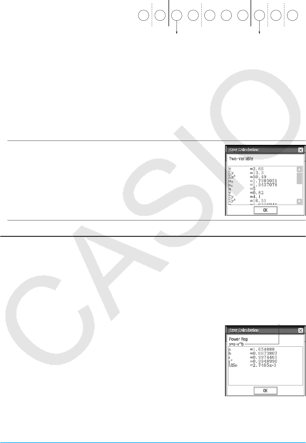
Chapter 7: Statistics Application 143
3 is the value whose cumulative frequency
ratio is greater than or equal to 1/4 and
nearest to 1/4, so Q1 = 3.
5 is the value whose cumulative frequency
ratio is greater than or equal to 3/4 and
nearest to 3/4, so Q3 = 5.
Reference Point (0.25) Reference Point (0.75)
Q1
0.1 0.2 0.4 0.7 0.8 0.9 1.0
Q3
1 2 63 3 4 4 4 75
• Median is calculated using the same method as that used when the [Q1, Q3 on Data] check box is
unchecked.
• It makes no different whether frequency values are all integers or include decimal fraction values when the
[Q1, Q3 on Data] check box is selected.
uTo display paired-variable calculation results
1. On the Stat Editor window or Stat Graph window, tap [Calc] - [Two-Variable].
2. On the dialog box that appears, specify the [XList] and [YList] names, select the [Freq] setting, and then tap
[OK].
• This displays the dialog box with the paired-variable statistical calculation results described below.
o, p : sample mean
Σx, Σy : sum of data
Σx2, Σy2 : sum of squares
σx, σy : population standard
deviation
sx, sy : sample standard deviation
n : sample size
Σxy : sum of products of
XList and YList data
minX, minY : minimum
maxX, maxY : maximum
Performing Regression Calculations
You can use the procedures under “Overlaying a Regression Graph on a Scatter Plot” (page 139) to specify a
model formula, and determine and graph the regression formula for paired-variable data. The dialog box that
appears when performing these operations provides the coefficients, constant term, and other values for the
regression formula. You can also copy the regression formula to the Graph Editor window and perform residual
calculation (which calculates the distance between the regression model and an actual plotted point during
regression calculations).
u To view regression calculation results
1. On the [Calc] - [Regression] menu, select one of the regression calculation
commands (from [Linear Reg] to [Logistic Reg]).
• For information about regression calculation characteristics, see
“Regression graphs” (page 138).
2. On the dialog box that appears, specify the [XList] and [YList] names, and
select the [Freq] setting.
Model formula

Chapter 7: Statistics Application 144
3. Tap [OK].
• This displays the dialog box with the regression calculation results described below.
a, b, c, d, e : coefficients of the model formula (shown at the top of the dialog box) corresponding to the
regression calculation
r : correlation coefficient (linear regression, logarithmic regression, exponential regression, and
power regression only)
r2 : coefficient of determination (except for Med-Med, sinusoidal regression, and logistic regression)
MSe : mean square error (except for Med-Med)
MSe Formulas
Depending on the regression calculation type, mean square error (MSe) is obtained using the following
formulas.
Linear: y = aⴢx+b: ;
Quadratic:
Quartic:
Exponential: aⴢebⴢx: ;
Power:
Sinusoidal:
y = a + bⴢx:
Cubic:
Logarithmic:
aⴢbx:
Logistic:
uTo copy a regression formula to the Graph & Table application
1. Perform steps 1 and 2 under “To view regression calculation results” (page 143).
2. On the dialog box that appears, tap the [Copy Formula] down arrow button, and then select the Graph &
Table line number (y1 through y20) to which you want to copy the formula.
3. Tap [OK].
• This copies the calculated regression expression to the line (y1 through y20) you selected.
uTo perform residual calculation
1. Perform steps 1 and 2 under “To view regression calculation results” (page 143).
2. On the dialog box that appears, tap the [Copy Residual] down arrow button, and then select [On] or the list
into which you want to copy the residual values.
3. Tap [OK].
• This assigns residual data to a system variable named “residual” (and also to the list if you specify a list in
step 2).
• Values assigned to the “residual” system variable shows the vertical distances between actually plotted
points and the regression model. A positive value indicates a plot that is higher than the regression model,
while a negative value indicates a plot that is lower.
You can use the following procedure to view the current “residual” system variable values.
1. On the Stat Editor window, select any cell in the column where you want the list you will open to appear and
then tap [Edit] - [Open List].
2. Enter “residual”, and then press E.
Σ
1
n – 2 i=1
n
(yi – (axi + b))2
Σ
1
n – 3 i=1
n
(yi – (axi2 + bxi + c))2
Σ
1
n – 5 i=1
n
(yi – (axi4 + bxi3 + cxi2 + dxi + e))2
Σ
1
n – 2 i=1
n
(ln yi – (ln a + bxi ))2
Σ
1
n – 2 i=1
n
(ln yi – (ln a + b ln xi))2
Σ
1
n – 2 i=1
n
(yi – (a·sin (bxi + c) + d ))2
Σ
1
n – 2 i=1
n
(yi – (a + bxi))2
Σ
1
n – 4 i=1
n
(yi – (axi3 + bxi2 + cxi + d ))2
Σ
1
n – 2 i=1
n
(yi – (a + b ln xi))2
Σ
1
n – 2 i=1
n
(ln yi – (ln a + (ln b)ⴢxi))2
Σ
1
n – 2 1 + ae–bxi
C
i=1
n
yi –
2
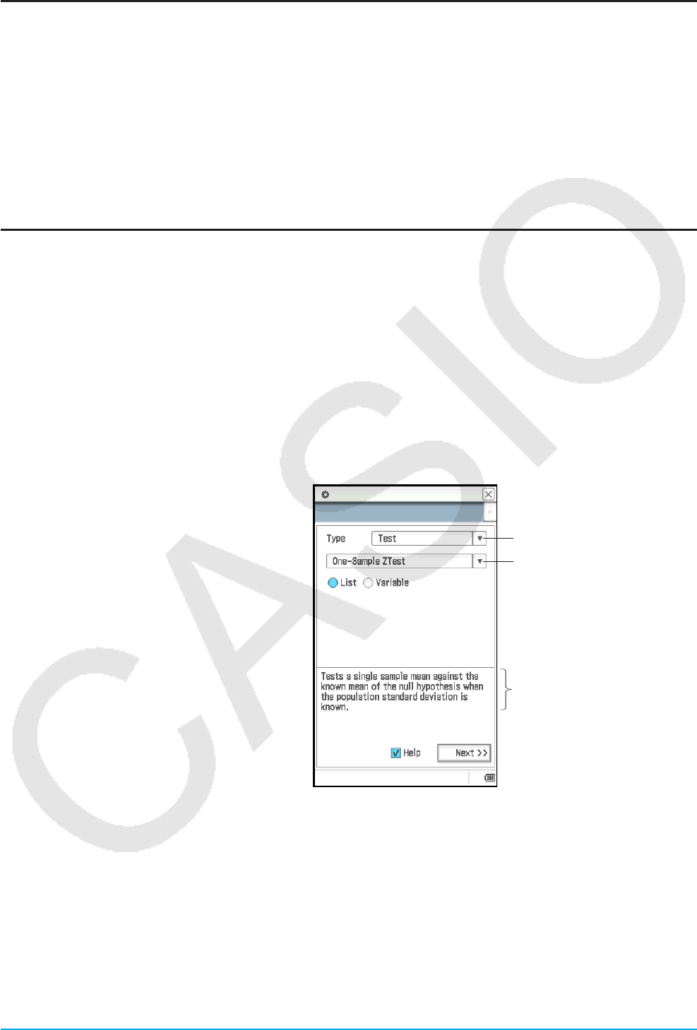
Chapter 7: Statistics Application 145
Viewing the Results of the Last Statistical Calculation Performed (DispStat)
To view the results of the last statistical calculation performed using a [Calc] menu command*, tap [Calc] -
[DispStat].
* Including test, confidence interval and distribution calculations.
7-4 Performing Advanced Statistical Calculations
You can perform test, confidence interval and distribution calculations using the wizard that you launch by
tapping [Calc] on the menu bar.
Performing Test, Confidence Interval and Distribution Calculations Using the Wizard
ClassPad includes built-in commands* for performing test, confidence interval, and distribution calculations.
The Statistics application lets you perform these types of calculations by simply inputting values and specifying
required information in accordance with instructions displayed by a wizard. This eliminates the need to input
commands and their arguments directly.
* For information about command syntax, see “12-4 Program Command Reference”.
uClassPad Operation
1. On the Stat Editor window, tap [Calc] and then tap [Test], [Interval], [Distribution] or [Inv. Distribution].
• This displays the Wizard window in the lower half of the screen.
• Selecting the [Help] check box causes the Wizard window to fill the display, and displays the description of
the command.
2. On the Command menu, select the
command you want to execute.
• For information about what is calculated
by each command, see “Tests” (page
146), “Confidence Intervals” (page 149), and
“Distributions” (page 151).
3. Select “List” to use list data for calculation,
or “Variable” to directly input values using a
wizard.
• Certain commands require data of a
specific type (list, variable, or matrix) for
calculation. For such commands, you will
not be provided with a choice of data type
options.
Type menu
Command menu
Help text
Displayed when the [Help]
check box is selected.
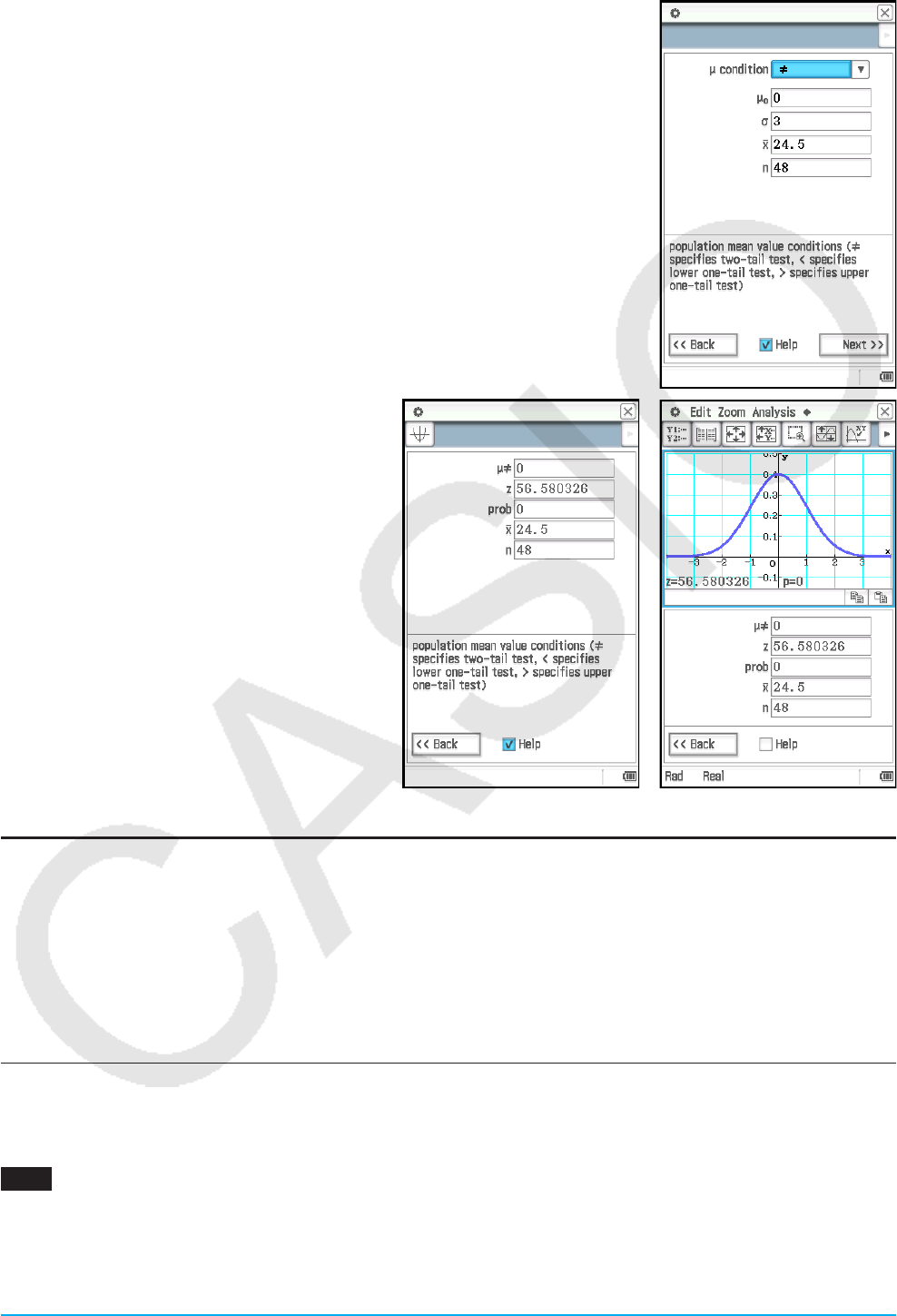
Chapter 7: Statistics Application 146
4. Tap [Next >>].
• This displays a screen for specifying conditions and inputting values.
• Initially, the top item on the screen will be selected, with help text about
the top item shown at the bottom of the screen. Tapping another item will
select it and display help text about it.
5. Input values and configure settings for each of the items on the screen.
6. Tap [Next >>].
• This displays the calculation results.
7. Tap $ to graph the results.
• You cannot graph interval calculations
and inverse distribution calculations.
Tip: You can back-step through the wizard
by tapping [<< Back]. After returning to a
previous screen you can change settings
and values and recalculate results. Closing
the wizard screen clears all settings and
values.
Tests
The Z Test provides a variety of different tests based on standard deviation based tests. They make it possible
to test whether or not a sample accurately represents the population when the standard deviation of a
population (such as the entire population of a country) is known from previous tests. The t Test is used instead
of the Z Test when the population standard deviation is unknown. You can also perform χ2 Test, ANOVA
(analysis of variance), and other test calculations.
The following describes the ClassPad commands for executing each type of statistical test calculation. It
includes the calculation formula used and a general overview of each command.
1-Sample Z Test .... [Test] - [One-Sample Z-Test] .....
z
= (o – μ0)/(σ/'n )
Tests a single sample mean against the known mean of the null hypothesis when the population standard
deviation is known. The normal distribution is used for the 1-Sample Z test.
0702 To specify
≠ 0, σ = 3 for n (sample size) = 48, o (sample mean) = 24.5 data and perform a 1-Sample
Z Test

Chapter 7: Statistics Application 147
0703 To specify > 120, σ = 19 for the data in lists to the right (list1 = data, list2 =
frequency) and perform a 1-Sample Z Test
2-Sample Z Test .... [Test] - [Two-Sample Z-Test] .....
Tests the difference between two means when the standard deviations of the two populations are known. The
normal distribution is used for the 2-Sample Z test.
1-Proportion Z Test .... [Test] - [One-Prop Z-Test] .....
z
= (x/n – p0)/ p0(1 – p0)/n
Tests a single sample proportion against the known proportion of the null hypothesis. The normal distribution is
used for the 1-Proportion Z test.
2-Proportion Z Test .... [Test] - [Two-Prop Z-Test] .....
z
= (x1/n1 – x2/n2)/ pˆ (1 – pˆ )(1/n1 + 1/n2)
Tests the difference between two sample proportions. The normal distribution is used for the 2-Proportion Z
test.
1-Sample t Test .... [Test] - [One-Sample t-Test] ..... t = (o – μ0)/(sx/'n )
Tests a single sample mean against the known mean of the null hypothesis when the population standard
deviation is unknown. The t distribution is used for the 1-Sample t test.
2-Sample t Test .... [Test] - [Two-Sample t-Test]
Tests the difference between two means when the standard deviations of the two populations are unknown.
The t distribution is used for the 2-Sample t test.
When the two population standard deviations are
equal (pooled) = (o1 − o2)/ s2(1/1 + 1/2)
= 1 + 2 − 2
s = ((1 − 1)s12 + (2 − 1)s22)/(1 + 2 − 2)
When the two population standard deviations are not
equal (not pooled)
= (o1 − o2)/ s12/1 + s22/2
= 1/(2/(1 − 1) + (1 − )2/(2 − 1))
= (s12/1)/(s12/1 + s22/2)
Linear Regression t Test .... [Test] - [Linear Reg t-Test] ..... = ( − 2)/(1 − 2)
= ( − o)( − p)/ ( − o)2 = p −
o
Y
Y
n: sample size (nt3)
Tests the linear relationship between the paired variables (x, y). The method of least squares is used to
determine a and b, which are the coefficients of the regression formula y = a + bx. The p-value is the probability
of the sample regression slope (b) provided that the null hypothesis is true, = 0. The t distribution is used for
the linear regression t test.

Chapter 7: Statistics Application 148
χ
2 Test (Chi-square Test) .... [Test] - [χ2 Test] ....
Tests the independence of two categorical variables arranged in matrix form. The χ2 test for independence
compares the observed matrix to the expected theoretical matrix. The χ2 distribution is used for the χ2 test.
• The minimum size of the matrix is 1 × 2. An error occurs if the matrix has only one column.
• The result of the expected frequency calculation is stored in the system variable named “Expected”.
0704 To specify observed matrix: a = 11 68 3
9 23 5 and perform a χ2 test
χ
2 GOF Test (Chi-square Goodness-of-Fit Test) .... [Test] - [χ2 GOF Test]
χ2 = ( − )2
= ( − )2
( − )2
( − )2
Y
Oi: The i-th element of the observed list, Ei: The i-th element of the expected list
Tests whether the observed count of sample data fits a certain distribution. For example, it can be used to
determine conformance with normal distribution or binomial distribution.
Tip: The calculation results χ2, p, df, and Contrib are stored in the system variables named “χ2value”, “prob”, “df”, and
“Contrib” respectively.
0705 To specify observed list: list1 = {1,2,3}, expected list: list2 = {4,5,6}, and df = 1, and then perform a χ2
test
2-Sample F Test .... [Test] - [Two-Sample F-Test] ..... = s12/s22
Tests the ratio between sample variances of two independent random samples. The F distribution is used for
the 2-Sample F test.
One-Way ANOVA (analysis of variance) .... [Test] - [One-Way ANOVA]
Tests the hypothesis that the population means of multiple populations are equal. It compares the mean of one
or more groups based on one independent variable or factor.
0706 To use Factor A data of list1 = {7,4,6,6,5}, list2 = {6,5,5,8,7}, and list3 = {4,7,6,7,6}, and perform One-
Way ANOVA
Tip
• To perform One-Way ANOVA using the wizard, you need to create up to six sets of list data (Factor A level 1 data, level 2
data, etc.). Specify the list data on the wizard screen and perform the calculation.
• One-Way ANOVA can also be performed using a program command (see the example 1209 under “Including Statistical
Graphing and Calculation Functions in a Program” on page 225). To perform One-Way ANOVA using a program command,
you need to create a “DependentList” that includes all Factor A level data (level1, level2, etc.) and a “FactorList(A)” that
specifies the levels for each of the blocks of data in the DependentList. If you use the program command to perform the
same test as shown in the example above, the two lists would be as shown below.
DependentList: {7,4,6,6,5,6,5,5,8,7,4,7,6,7,6} ... (All level 1, level 2, and level 3 data)
FactorList(A): {1,1,1,1,1,2,2,2,2,2,3,3,3,3,3} ... (Levels of each block of data)
χ2 =
R( − )2
R
R
= × /
,
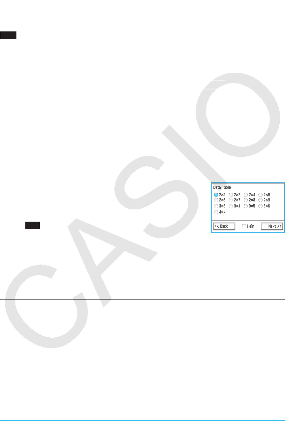
Chapter 7: Statistics Application 149
Two-Way ANOVA .... [Test] - [Two-Way ANOVA]
Tests the hypothesis that the population means of multiple populations are equal. It examines the effect of each
variable independently as well as their interaction with each other based on a dependent variable.
0707 The values in the table below are measurement results that show how the durability of a metal product
is affected by changes in heat treatment time (A) and temperature (B). Experiments were conducted
twice under each condition.
Temperature B1 Temperature B2
Time A1 113, 116 139, 132
Time A2 133, 131 126, 122
Perform analysis of variance on the null hypotheses listed below, using a 5% level of significance.
H0: Change in time does not affect durability.
H0: Change in treatment temperature does not affect durability.
H0: Changes in time and treatment temperature do not affect durability.
Use the Two-Way ANOVA test to test the above hypotheses. Input the following measurement data
into the indicated lists. This data is from the table above.
list1 = {113, 116} … (Factor A1 × B1), list2 = {139, 132} … (Factor A1 × B2)
list3 = {133, 131} … (Factor A2 × B1), list4 = {126, 122} … (Factor A2 × B2)
Tip
• To perform Two-Way ANOVA using the wizard, you need to create list data in the
quantity of data table vertical (number of Factor A levels) × horizontal (number of
Factor B levels). Specify the list data on the wizard screen and perform the
calculation. The dimensions that can be specified for Factor A × Factor B are shown in
the screen to the right.
• Two-Way ANOVA can also be performed using a program command (see the
example 1210 under “Including Statistical Graphing and Calculation Functions in a
Program” on page 225). To perform Two-Way ANOVA using a program command, create
a “DependentList” that includes all Factor A × Factor B level data, and “FactorList(A)” and “FactorList(B)” lists that specify
the levels for each of the blocks of data in the DependentList. If you use the program command to perform the same test
as shown in the example above, the three lists would be as shown below.
DependentList =
{113,116,139,132,133,131,126,122}
FactorList(A) = { 1, 1, 1, 1, 2, 2, 2, 2 }
FactorList(B) = { 1, 1, 2, 2, 1, 1, 2, 2 }
Confidence Intervals
A confidence interval is a range of values that has a specified probability of containing the parameter being
estimated. A confidence interval that is too broad makes it difficult to get an idea of where the parameter (actual
value) is located. A narrow confidence interval, on the other hand, limits the parameter range and makes it
possible to obtain highly accurate results.
The commonly used confidence levels are 68%, 95% and 99%. With a confidence interval of 95%, for example,
there is a 5% probability that a parameter will not be within the interval.
The following describes the ClassPad commands for executing each type of confidence interval calculation. It
includes an overview of each command and the formulas to obtain the confidence interval lower limit (Lower)
and upper limit (Upper).
Chapter 7: Statistics Application 150
1-Sample Z Interval .... [Interval] - [One-Sample Z Int] Lower, Upper = o Z α
2
σ
n
Calculates the confidence interval for the population mean based on a sample mean and known population
standard deviation.
0708 To specify the data below and perform a 1-Sample Z Interval calculation
list1: {299.4, 297.7, 301, 298.9, 300.2, 297}
Population standard deviation: 3
Significance level: 5% ( = confidence level: 95%)
2-Sample Z Interval .... [Interval] - [Two-Sample Z Int] Lower, Upper = (o1 – o2) Zα
2n1
1
2
σ
+n2
2
2
σ
Calculates the confidence interval for the difference between population means based on the difference
between sample means when the population standard deviations are known.
1-Proportion Z Interval .... [Interval] - [One-Prop Z Int] Lower, Upper = α
2
Z
x
nn
1n
xn
x
1–
Calculates the confidence interval for the population proportion based on a single sample proportion.
2-Proportion Z Interval .... [Interval] - [Two-Prop Z Int] Lower, Upper =
Calculates the confidence interval for the difference between population
proportions based on the difference between two sample proportions.
1-Sample t Interval .... [Interval] - [One-Sample t Int] Lower, Upper = o tn –1 α
2n
sx
Calculates the confidence interval for the population mean based on a sample mean and a sample standard
deviation when the population standard deviation is not known.
2-Sample t Interval .... [Interval] - [Two-Sample t Int]
Calculates the confidence interval for the difference between population means based on the difference
between sample means and sample standard deviations when the population standard deviations are not
known.
When the two population standard deviations
are equal (pooled) Lower, Upper = oo
s
s= ((1 – 1)s1
2 + (2 – 1)s2
2)/(1 + 2 – 2)
When the two population standard deviations
are not equal (not pooled) Lower, Upper = (o1 – o2) tdf
α
2+
n1
sx12
n2
sx22
df = 1/(C2/(n1 – 1) + (1 – C)2/(n2 – 1)) C = (sx1
2/n1)/(sx1
2/n1 + sx2
2/n2)
General Confidence Interval Precautions
If you input a C-Level (confidence level) value in the range of 0 s C-Level < 1, the value you input is used. To
specify a C-Level of 95%, for example, input “0.95”.
– Zα
2
x1
n1
x2
n2n1
n1
x11– n1
x1
+n2
n2
x21– n2
x2
Chapter 7: Statistics Application 151
Distributions
There is a variety of different types of distribution, but the most well-known is “normal distribution”, which is
essential for performing statistical calculations. Normal distribution is a symmetrical distribution centered on the
greatest occurrences of mean data (highest frequency), with the frequency decreasing as you move away from
the center. Poisson distribution, geometric distribution, and various other distribution shapes are also used,
depending on the data type.
Tip: Though list data can be used within the argument of a Distribution function (page 85), list data cannot be used in the
argument of the Statistics Wizard operations described here.
The following describes the ClassPad commands for executing each type of distribution calculation. It includes
the calculation formula used and a general overview of each command.
Normal Probability Density .... [Distribution] - [Normal PD]
Calculates the normal probability density for a specified value.
Specifying σ = 1 and = 0 produces standard normal distribution.
0709 To calculate normal probability density for the data below and graph the result
Data: 37.5 Population standard deviation: 2 Population mean: 35
Normal Cumulative Distribution .... [Distribution] - [Normal CD]
Calculates the cumulative probability of a normal distribution between a
lower bound (a) and an upper bound (b).
0710 To calculate normal cumulative distribution for the data below and graph the result
Lower bound: −∞ Upper bound: 36
Population standard deviation: 2 Population mean: 35
Inverse Normal Cumulative Distribution .... [Inv. Distribution] - [Inverse Normal CD]
Calculates the boundary value(s) of a normal cumulative probability distribution for specified values.
Tail: Left Tail: Right Tail: Center
2
+
=
Upper bound is returned. Lower bound is returned. Lower bound and upper bound
are returned.
0711 To calculate inverse normal cumulative distribution for the data below and graph the result
Tail: Left Probability: 0.7
Population mean: 35 Population standard deviation: 2
Student’s t Probability Density .... [Distribution] - [Student’s t PD]
Calculates the Student’s t probability density for a specified value.
Student’s t Cumulative Distribution …. [Distribution] - [Student’s t CD]
Calculates the cumulative probability of a Student’s t distribution
between a lower bound (a) and an upper bound (b).
πσ
2
f
(x) = (
σ
> 0)
1e–2 2
σ
(x – μ)2
μ
dx
f
(x) = ×
Γ
Γ
2
df
2
df + 1
.df
π
–df+1
2
df
x2
1+
p =
Γ
Γ
.df
π
2
df
2
df + 1 –df+1
2
df
x2
1+ dx
a
b
Chapter 7: Statistics Application 152
Inverse Student’s t Cumulative Distribution .... [Inv. Distribution] - [Inverse t CD]
Calculates the lower bound value of a Student’s t cumulative probability distribution for specified
values.
χ
χ
2 Probability Density .... [Distribution] - [χ2 PD]
Calculates the χ2 probability density for a specified value.
χ
2 Cumulative Distribution .... [Distribution] - [χ2 CD]
Calculates the cumulative probability of a χ2 distribution between a lower
bound and an upper bound.
Inverse
χ
2 Cumulative Distribution .... [Inv. Distribution] - [Inverse χ2 CD]
Calculates the lower bound value of a χ2 cumulative probability distribution for specified values.
F Probability Density .... [Distribution] - [F PD]
Calculates the F probability density for a specified value.
F Cumulative Distribution .... [Distribution] - [F CD]
Calculates the cumulative probability of an F distribution
between a lower bound and an upper bound.
Inverse F Cumulative Distribution .... [Inv. Distribution] - [Inverse F CD]
Calculates the lower bound value of an F cumulative probability distribution for specified values.
Binomial Distribution Probability .... [Distribution] - [Binomial PD]
Calculates the probability in a binomial distribution that success will
occur on a specified trial.
p: probability of success (0 s p s 1)
n: number of trials
Binomial Cumulative Distribution .... [Distribution] - [Binomial CD]
Calculates the cumulative probability in a binomial distribution that success will occur on or before a specified
trial.
Inverse Binomial Cumulative Distribution .... [Inv. Distribution] - [Inverse Binomial CD]
Calculates the minimum number of trials of a binomial cumulative probability distribution for
specified values.
Poisson Distribution Probability .... [Distribution] - [Poisson PD]
Calculates the probability in a Poisson distribution that success will occur on a specified trial.
0712 To calculate Poisson probability for the data below and graph the result
Specified trial: 10 Mean: 6
(x = 0, 1, 2, ...)
: mean (0 < )
∞
f (x) =
Γ
1
2
df
df
2x e
2
1df
2–1 x
2
–
p =
Γ
1
2
df
df
2
x e d
x
2
1df
2–1 x
2
–
a
b
∞
Γ2
n
Γ2
n + d
Γ2
d
f (x) =
n
2x
d
nn
2–1
d
n.x
1 +
n + d
2
–
××
∞
t

Chapter 7: Statistics Application 153
Poisson Cumulative Distribution .... [Distribution] - [Poisson CD]
Calculates the cumulative probability in a Poisson distribution that success will occur on or before a specified
trial.
0713 To calculate Poisson cumulative probability for the data below and graph the result
Lower bound: 2 Upper bound: 3 Mean: 2.26
Inverse Poisson Cumulative Distribution .... [Inv. Distribution] - [Inverse Poisson CD]
Calculates the minimum number of trials of a Poisson cumulative probability distribution for
specified values.
0714 To calculate inverse Poisson cumulative distribution for the data below and graph the result
Poisson cumulative probability: 0.8074 Mean: 2.26
Geometric Distribution Probability .... [Distribution] - [Geometric PD]
Calculates the probability in a geometric distribution that the success will
occur on a specified trial.
(x = 1, 2, 3, ...)
p: probability of success (0 s p s 1)
Geometric Cumulative Distribution .... [Distribution] - [Geometric CD]
Calculates the cumulative probability in a geometric distribution that the success will occur on or before a
specified trial.
Inverse Geometric Cumulative Distribution .... [Inv. Distribution] - [Inverse Geo CD]
Calculates the minimum number of trials of a geometric cumulative probability distribution for
specified values.
Hypergeometric Distribution Probability .... [Distribution] - [Hypergeometric PD]
Calculates the probability in a hypergeometric distribution that the success will occur on a
specified trial.
Hypergeometric Cumulative Distribution .... [Distribution] - [Hypergeometric CD]
Calculates the cumulative probability in a hypergeometric distribution that the
success will occur on or before a specified trial.
Inverse Hypergeometric Cumulative Distribution .... [Inv. Distribution] - [Inverse Hypergeometric]
Calculates the minimum number of trials of a hypergeometric cumulative probability
distribution for specified values.
t
Σ
= 1
x
m
t
=
×
=
×
∑
s
×
∑

Chapter 7: Statistics Application 154
Input and Output Terms
kInput Terms
C-Level: confidence level (0 s C-Level < 1)
Contrib: name of list specifying the contribution of
each observed count
df : degrees of freedom
Expected: name of list that is for saving expected
frequency
Freq, Freq(1), Freq(2): frequency (1 or list name)
List, List(1), List(2): list where sample data is located
Lower (Distribution): lower bound
M: number of success in population*1
Matrix (χ2 Test): name of matrix containing observed
values*2
n (Hypergeometric Distribution): number of trials from
population*1
n: sample size*1
n1 / n2: size of {sample 1 / sample 2}*1
N: population size (integer, n s N, M s N)
Numtrial: number of trials n*1
Observed (χ2 GOF Test): name of list containing
observed counts (all cells positive integers)
Observed (χ2 Test): name of matrix containing
observed values*2
p0: expected sample proportion (0 < p0 < 1)
p1 condition (2-Proportion Z Test): sample proportion
test conditions*3
Pooled: pooling On or Off
pos: probability of success p (0 s p s 1)
prob (Inv. Distribution): cumulative probability value
(0 s prob s 1)
Prop condition (1-Proportion Z Test): sample
proportion test conditions*4
sx: sample standard deviation (0 < sx)
sx1 / sx2: sample standard deviation of {sample 1 /
sample 2} (0 < sx1, 0 < sx2)
Upper (Distribution): upper bound
x (1-Proportion Z Test): sample value*1
x (1-Proportion Z Interval): data value*1
x (Binomial PD): specified trial (integer, 0 s x s n)
x (Poisson PD, Geometric PD, Hypergeometric PD):
specified trial*1
x (Other than the above): data value
x
_: sample mean
x
_
1 / x
_
2: sample mean of {sample 1 data / sample 2
data}
x1 / x2 (1-Proportion Z Interval): data value of {sample
1 / sample 2} (integer, 0 s x1, 0 s x2)
XList / YList: x-data list / y-data list
&
ρ
ρ
condition (LinearReg t Test): and
ρ
-value
test conditions*4
λ
: mean (0 < )
(Distribution): population mean
condition (1-Sample Z Test, 1-Sample t Test):
population mean value test conditions*4
0: assumed population mean
1 (2-Sample Z Test): population mean value test
conditions*3
1 (2-Sample t Test): sample mean value test
conditions*3
σ
: population standard deviation (0 < σ)
σ
1 condition (2-Sample F Test): population standard
deviation test conditions*3
σ
1 /
σ
2: population standard deviation of {sample 1 /
sample 2} (0 < σ1 / 0 < σ2)
*1 positive integer
*2 positive integers in all cells for 2 × 2 and larger matrices; positive real numbers for one row matrices
*3 “” specifies two-tail test, “<” specifies one-tail test where sample 1 is smaller than sample 2, “>” specifies
one-tail test where sample 1 is greater than sample 2.
*4 “” specifies two-tail test, “<” specifies lower one-tail test, “>” specifies upper one-tail test.

Chapter 7: Statistics Application 155
kOutput Terms
a: regression constant term (y-intercept)
A df : df * 5 of Factor A
A F: F value of Factor A
A MS: MS*6 of Factor A
A p: p-value of Factor A
A SS: SS*7 of Factor A
AB df * 8: df * 5 of Factor A × Factor B
AB F*8: F value of Factor A × Factor B
AB MS*8: MS*6 of Factor A × Factor B
AB p*8: p-value of Factor A × Factor B
AB SS*8: SS*7 of Factor A × Factor B
b: regression coefficient (slope)
B df : df * 5 of Factor B
B F: F value of Factor B
B MS: MS*6 of Factor B
B p: p-value of Factor B
B SS: SS*7 of Factor B
d:df : degrees of freedom of denominator (positive
integer)
df : degrees of freedom
Errdf : df * 5 of error
ErrMS: MS*6 of error
ErrSS: SS*7 of error
F: F value
Lower: confidence interval lower limit
n:df : degrees of freedom of numerator (positive
integer)
p: estimated sample proportion
p1 /
p2: estimated proportion of {sample 1 / sample 2}
prob (Binomial PD, Poisson PD, Geometric PD,
Hypergeometric PD): probability
prob (Binomial CD, Poisson CD, Geometric CD,
Hypergeometric CD): cumulative probability
prob (Normal PD, Student’s t PD, χ2 PD, F PD):
probability density
prob (Normal CD, Student’s t CD, χ2 CD, F CD):
distribution probability
prob (Test): p value
r: correlation coefficient
r
2: coefficient of determination
sx: sample standard deviation
sx1 / sx2: sample standard deviation of {sample 1 /
sample 2} (Displayed only for list format.)
sp: pooled sample standard deviation
se: standard error of estimation
SEb: standard error of the least squares slope
t: t value
t Low: lower bound value you input
t Up: upper bound value you input
Upper: confidence interval upper limit
x1InvN: Upper bound when Tail:Left, Lower bound
when Tail:Right or Tail:Center
x2InvN: Upper bound when Tail:Center
xInv: inverse cumulative distribution
½xInv: recalculation value of inverse cumulative
distribution*9
z: z value
z Low: standardized lower limit z value
z Up: standardized upper limit z value
χ
χ
2: χ2 value
*5 degrees of freedom
*6 mean square
*7 sum of squares
*8 Note that “AB df ”, “AB MS ”, “AB SS ”, “AB F ”, and “AB p” are not displayed in the calculation result window
if there are no repeated data pairs.
*9 In the calculation result window for certain distributions, “½xInv” is displayed only when there may be a
possibility of rounding error. To account for possible rounding error, ClassPad additionally obtains the
result using the probability that is next lowest for the least significant digit. For example, if the probability is
0.61, ClassPad would recalculate using 0.60. The recalculation result is only shown if it is different from the
original one.

Chapter 8: Geometry Application 156
Chapter 8:
Geometry Application
The Geometry application allows you to draw and analyze geometric figures.
For example, you can draw a circle and then draw a line that is tangent to
a particular point on the circle. The Geometry application also includes an
animation feature that lets you watch how a figure changes in accordance with
conditions you define.
Starting up the Geometry application displays a large white Geometry window.
Use this window to draw the figures you want. If you left figures on the
Geometry window the last time you exited the Geometry application, those
figures will appear the next time you start it up.
Geometry Application-Specific Menus and Buttons
• Clear all settings fixed with the measurement box ......................................................Edit - Clear Constraints
• Show hidden objects ................................................................................................................ Edit - Show All
• Specify the color of the currently selected object ........................................................................... Edit - Style
• Hide the currently selected object ............................................................................... Edit - Properties - Hide
• Show hidden names ....................................................................................... Edit - Properties - Show Name
• Hide the selected name ....................................................................................Edit - Properties - Hide Name
• Move the selected object to the front or to the back ...................Edit - Properties - To the front / To the back
• Move all text to the front ..........................................................................................Edit - Properties - All Text
• Pin an annotation position on the Geometry window .....................................................Edit - Properties - Pin
• Unpin an annotation on the Geometry window ......................................................... Edit - Properties - Unpin
• Specify the number format for each measurement used in
the Geometry window ...........................................................................Edit - Properties - Number Format
• Display the Animate submenu (page 174) ................................................................................ Edit - Animate
• Select a segment, line, or part of a figure (page 167) .......................................................View - Select or G
• Activate the pan function for dragging the Geometry window with the stylus ...................... View - Pan or T
• Adjust the size of the display image so it fills the display ......................................... View - Zoom to Fit or R
• Turn display of axes, coordinate values and grid on or off .....................................View - Toggle Axes or q
• Show grid points (On) or hide the grid (Off) ................................................................... View - Grid - On / Off
• Show grid lines ..................................................................................................................... View - Grid - Line
• Turn the Animation toolbar on or off ................................................................................ View - Animation UI
• Display a submenu for plotting points, and drawing lines and
other basic figures (pages 157 through 159) .............................................................. Draw - Basic Object
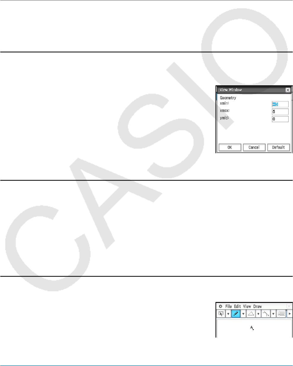
Chapter 8: Geometry Application 157
• Display a submenu for drawing a figure of specially shaped
figures such as triangles and rectangles (page 162) ............................................ Draw - Special Polygon
• Display a submenu for drawing functions (page 160) ............................................................ Draw - Function
• Insert a value or text connected with a displayed figure into
the display (pages 161 through 162) .............. Draw - Text / Attached Angle / Measurement / Expression
• Display a slider (page 172) for the currently selected object. ..................................................... Draw - Slider
• Display a submenu for geometric constructions (page 163) .................................................Draw - Construct
• Activate Toggle Select (page 167) .....................................................................Tap i and then tap a figure
Tip: The View menu Zoom Box (Q), Zoom In (W), and Zoom Out (E) commands are the same as the Graph &
Table application Box, Zoom In, and Zoom Out commands on the Zoom menu. For more information about these
commands, see “Chapter 3: Graph & Table Application”.
Configuring Geometry View Window Settings
You can use the following procedures to configure settings that control the appearance of the Geometry
application window.
Tap O, and then [View Window] to display the View Window dialog box. The
View Window dialog box allows you to configure the x-axis range of values.
The ymid value is used to center the Geometry window vertically. For example,
if we set ymid = 2, the y-axis will appear 2 units below the center of the
Geometry window.
The following are the allowable ranges for the indicated View Window
parameters.
−1 × 10⁶ s xmin s 1 × 10⁶
−1 × 10⁶ s ymid s 1 × 10⁶
−1 × 10⁶ s xmax s 1 × 10⁶
xmax − xmin t 1 × 10⁻⁴
About the Geometry Format Dialog Box
Settings for the Geometry application can be configured on the Geometry Format dialog box which appears
when you tap O and then [Geometry Format]. See “1-7 Configuring Application Format Settings” for more
information.
8-1 Drawing Figures
This section explains how to use the Geometry application to draw various types of figures. It also explains how
to use the geometric construction tools to investigate theorems and properties in Geometry.
Drawing a Figure
u To plot a point
1. Tap [Draw] - [Basic Object] - [Point], or tap [.
2. Tap the location on the screen where you want to plot a point.
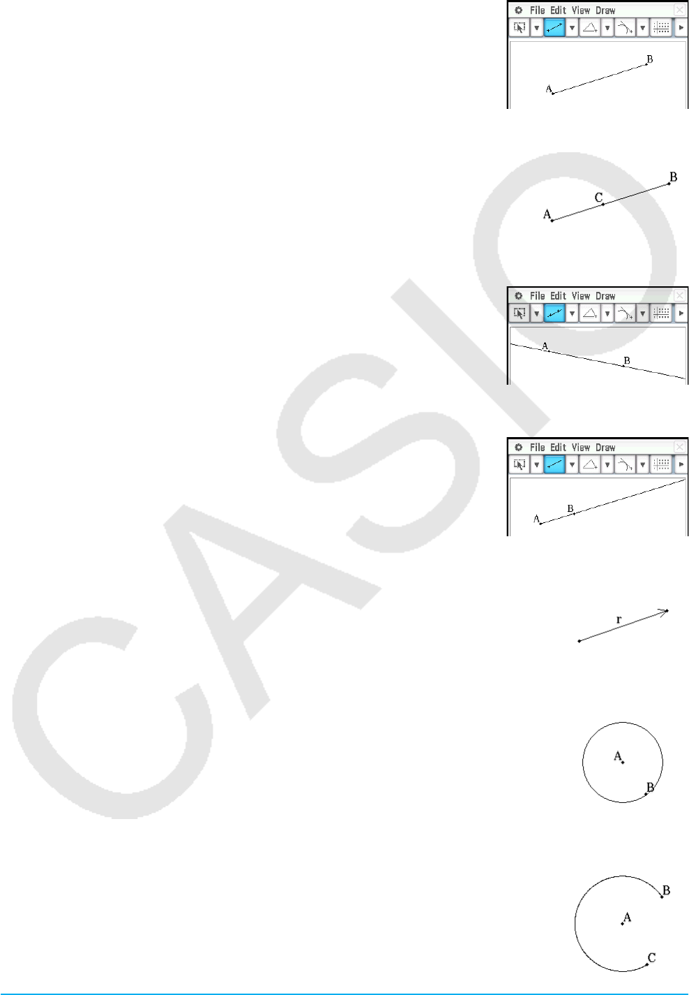
Chapter 8: Geometry Application 158
uTo draw a line segment
1. Tap [Draw] - [Basic Object] - [Line Segment], or tap y.
2. Tap the screen where you want the line segment to begin, and a point will be
drawn, and then tap the point where you want it to end.
uTo add a labeled point to an existing line
1. Tap [Draw] - [Basic Object] - [Point], or tap [.
2. Drag the stylus to the location on the line where you want to add a labeled point,
and then lift the stylus from the screen.
uTo draw an infinite line
1. Tap [Draw] - [Basic Object] - [Infinite Line], or tap w.
2. Tap two points on the screen through which you want the infinite line to
pass.
uTo draw a ray
1. Tap [Draw] - [Basic Object] - [Ray], or tap b.
2. Tap two points on the screen, or tap one point and then drag to the second
point.
uTo draw a vector
1. Tap [Draw] - [Basic Object] - [Vector], or tap H.
2. Tap the point where you want the vector to start, and then its end point.
uTo draw a circle
1. Tap [Draw] - [Basic Object] - [Circle], or tap U.
2. Tap the point where you want the center of the circle to be, and then tap a second
point anywhere on the circle’s circumference.
uTo draw an arc
1. Tap [Draw] - [Basic Object] - [Arc], or tap P.
2. Tap the point where you want the center of the arc to be, and then tap a second point
to designate where you want the arc to start.
3. Tap a third point, which is where you want the arc to end.
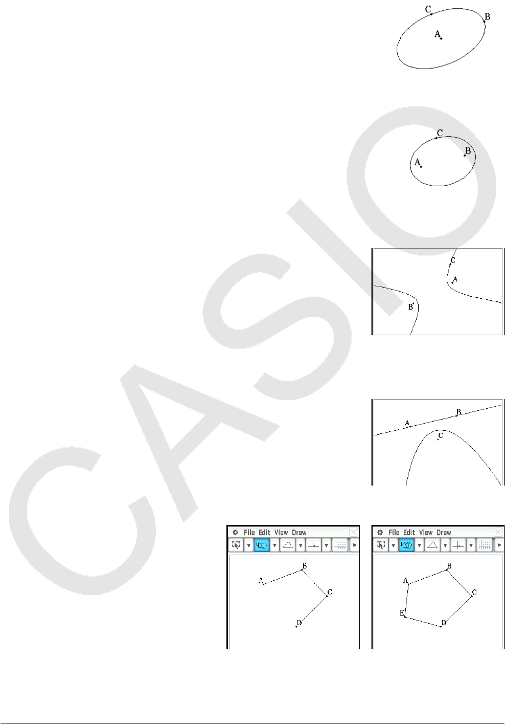
Chapter 8: Geometry Application 159
uTo draw an ellipse
1. Tap [Draw] - [Basic Object] - [Ellipse] - [Axes], or tap I.
2. Tap the point you want to specify as the center point.
3. Tap or drag to the point you want to specify as minor axis (nearest point on the
edge from the center point).
4. Tap or drag to the point you want to specify as major axis (farthest point on the
edge from the center point).
(Or)
1. Tap [Draw] - [Basic Object] - [Ellipse] - [Foci], or tap z.
2. Tap the two points that you want to specify as the foci of the ellipse (point 1 and
point 2).
• This causes a line to appear between point 1 and point 2.
3. Tap the point you want to specify as a point anywhere on the ellipse (point 3).
• This draws an ellipse whose line passes through point 3, using point 1 and
point 2 as foci.
uTo draw a hyperbola
1. Tap [Draw] - [Basic Object] - [Hyperbola], or tap x.
2. Tap the two points that you want to specify as the foci of the hyperbola (point
1 and point 2).
• This causes a line to appear between point 1 and point 2.
3. Tap the point you want to specify as a point anywhere on the hyperbola
(point 3).
• This draws a hyperbola whose line passes through point 3, using point 1
and point 2 as foci.
uTo draw a parabola
1. Tap [Draw] - [Basic Object] - [Parabola], or tap c.
2. Tap the two points that you want to specify the directrix (point 1 and point 2).
• This causes a line to appear between point 1 and point 2.
3. Tap the point you want to specify as the focus (point 3).
• This draws a parabola using the straight line that passes through point 1
and point 2 as the directrix, and point 3 as the focus.
u To draw a polygon
1. Tap [Draw] - [Basic Object] - [Polygon], or
tap 0.
2. Tap the point from which you want the
polygon to start.
3. Sequentially tap each of the vertices of the
polygon.
4. Finally, tap the start point again to complete
the polygon.
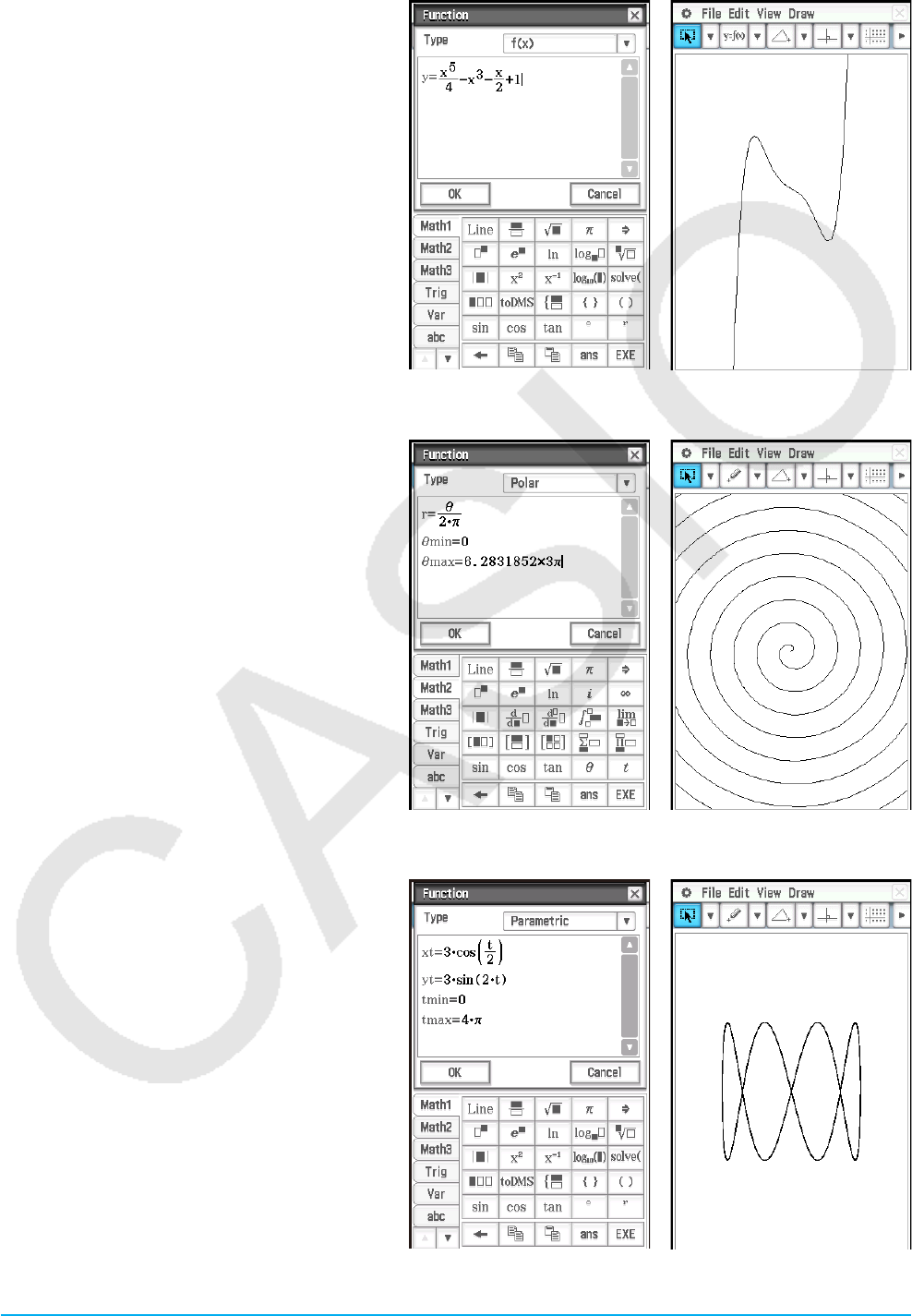
Chapter 8: Geometry Application 160
u To draw a function
1. Tap [Draw] - [Function] - [ f ( x)].
• Or you could tap { on the tool bar. Next on
the Function dialog box that appears, use
the Type box to select “f ( x)”.
2. On the Function dialog box, input the
function and then tap [OK] to draw it.
uTo draw a polar equation graph*
1. Tap [Draw] - [Function] - [Polar].
• Or you could tap { on the tool bar. Next on
the Function dialog box that appears, use
the Type box to select “Polar”.
2. On the Function dialog box, input an
expression in the syntax of r = f (), the
lower limit of (min) and its upper limit
(max).
3. Tap [OK] to draw the polar equation graph.
* In this example, the [Function Angle] setting
of the Geometry Format dialog box (page 40) is
set to “Radian”.
uTo draw a parametric equation graph*
1. Tap [Draw] - [Function] - [Parametric].
• Or you could tap { on the tool bar. Next on
the Function dialog box that appears, use
the Type box to select “Parametric”.
2. On the Function dialog box, input
expressions and values.
3. Tap [OK] to draw the parametric equation
graph.
* In this example, the [Function Angle] setting
of the Geometry Format dialog box (page 40) is
set to “Radian”.

Chapter 8: Geometry Application 161
Inserting Text Strings into the Screen
You can insert text strings into the screen while working on the Geometry application window. To do so, tap
[Text] on the [Draw] menu. On the dialog box that appears, input the text you want, and then tap [OK].
Attaching an Angle Measurement to a Figure
The measurement of an angle formed by two sides of a figure can be attached to the figure as shown here. To
do so, tap [Attached Angle] on the [Draw] menu.
uTo attach an angle measurement to a figure
Example: To attach the measurement of angle A in triangle
ABC
1. Draw the triangle.
2. Tap G. Next, tap side AB and then side AC to select them.
3. Tap [Draw] and then [Attached Angle].
• This attaches the angle measurement to the figure.
Tip: The two sides of the figure actually form four angles in the illustration shown here.
After attaching an angle measurement using the [Attached Angle] command, you
can drag it to the position of any one of the other three angles as shown in the
example below.
Example: To drag the angle measurement attached to interior angle A of
triangle ABC to its exterior supplementary angle
Displaying the Measurements of a Figure
You can display measurements on the Geometry application window. The measurements change dynamically
as you manipulate the figure.
uTo display a measurement of a figure
1. What you should select (point, line, figure, etc.) depends on the type of measurement you want to display.
To display this type of measurement: Select this:
Angle between two lines Two lines (Any two of the following: line segment,
infinite line, ray, or vector, one side of a polygon)
Supplementary angle of extended lines
Area of selected figure • All the sides or all the apexes of a polygon
• The circumference of a circle, ellipse, or arc
• Three points
Circumference or perimeter of selected figure

Chapter 8: Geometry Application 162
To display this type of measurement: Select this:
Coordinates of selected point Any single point (including the apex of a polygon)
Direction of line or vector A single line (line segment, infinite line, ray, vector,
or any side of a polygon)
Equation of selected curve Any line or curve
Distance between two points, or length of line Any two points, a line segment, or any side of a
polygon
Radius of circle or arc The radius of the circle or arc
Slope of line or vector A single line (line segment, infinite line, ray, vector,
or any side of a polygon)
2. Perform any one of the following operations.
- Tap [Draw] - [Measurement]. On the submenu that appears, select the measurement type you want to
display on the screen.
- Select the value in the measurement box and drop it directly into the Geometry application window.
- Tap the measurement icon button to the left of the measurement box.
Tip: For information about the measurement box, see “8-3 Using the Measurement Box”.
0801 To display the interior angle formed by two sides of a triangle
Displaying the Result of a Calculation that Uses On-screen Measurement Values
You can use the [Expression] command and the commands on the [Measurement] submenu to perform
calculations using the angle value, line length, surface area, and other measurement values attached to a
figure, and display the result on the Geometry window.
uTo display the result of a calculation that uses on-screen measurement values
0802 To display the sum of the interior angles of triangle ABC (⬔A+⬔B+⬔C)
Using the Special Polygon Submenu
The [Special Polygon] submenu allows you to draw specially shaped figures automatically. Simply select the
type of figure you want from the menu, and then touch the screen with the stylus to draw it. Or, touch the
screen with your stylus and drag to create a box indicating the size of the figure you would like to draw.
Each of the [Special Polygon] submenu figures is also available on the toolbar.
[Special Polygon] submenu
Triangle
Equilateral Triangle
Kite
Rectangle
Square
Isosceles Triangle
Trapezoid
Parallelogram
Rhombus
Regular n-gon
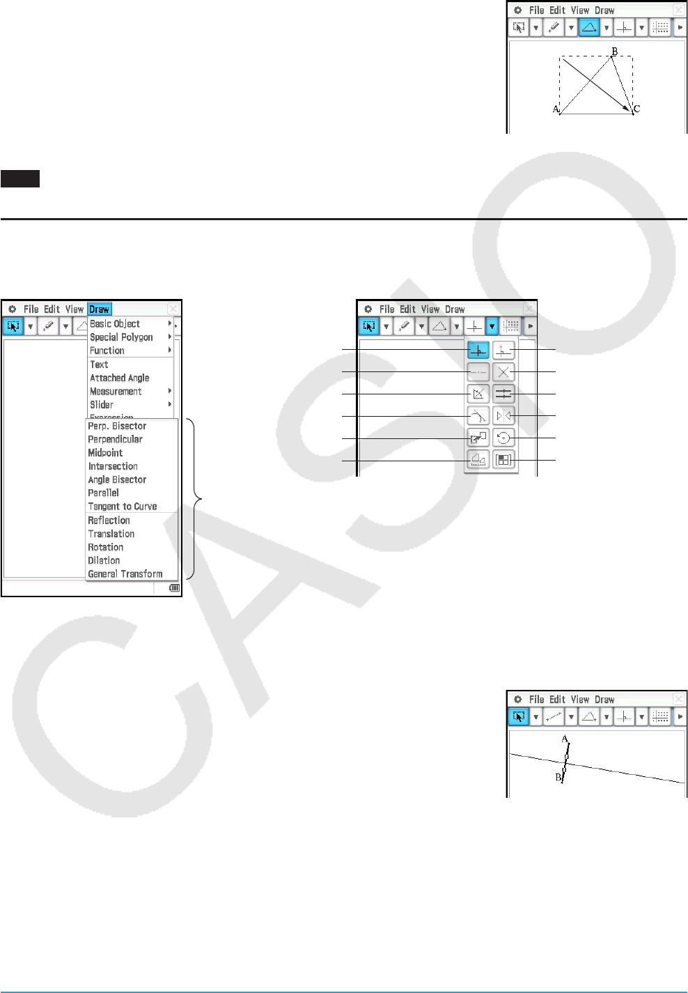
Chapter 8: Geometry Application 163
uTo draw a triangle
1. Tap [Draw], [Special Polygon], and then [Triangle].
2. Place the stylus on the screen and drag diagonally in any direction.
• This causes a selection boundary to appear, indicating the size of the
triangle that will be drawn. The triangle is drawn when you release the
stylus.
• In place of the above step 2, you can achieve the same result by simply
tapping the screen. This automatically draws the acute triangle you
selected.
0803 To draw a regular polygon
Using the Construct Submenu
The [Construct] submenu provides you with the means to study various geometric theorems. Each of the
[Construct] submenu figures is also available on the toolbar.
Perpendicular Bisector
Midpoint
Angle Bisector
Tangent to Curve
Translation
Dilation
Perpendicular
Intersection
Parallel
Reflection
Rotation
General Transform
[Construct] submenu
The following procedures include steps that require selection of a line segment or other figures. For details
about selecting figures, see “8-2 Editing Figures”.
uTo construct a perpendicular bisector
1. Draw a line segment.
2. Tap G, and then select the line segment.
3. Tap [Draw], [Construct], and then [Perp. Bisector]. This draws a
perpendicular bisector through your line segment.

Chapter 8: Geometry Application 164
uTo construct a perpendicular line that passes through a specified point on a line
1. Draw an infinite line, and then draw a point on the line through which you
want the perpendicular line to pass.
2. Select the line and the point.
3. Tap [Draw], [Construct], and then [Perpendicular]. This draws a line through
the point you selected, which is perpendicular to the line where the point is
located.
u To construct a midpoint
1. Draw a line segment and then select it.
2. Tap [Draw], [Construct], and then [Midpoint]. This adds a midpoint to the
segment.
uTo construct the point of intersection of two lines
1. Draw two lines that intersect, and then select both lines.
2. Tap [Draw], [Construct], and then [Intersection].
• This adds the point of intersection. The point(s) of intersection of two
circles or of a line and a circle can be constructed in the same manner.
uTo construct an angle bisector
1. Draw two line segments so they form an angle, and then select both line
segments.
2. Tap [Draw], [Construct], and then [Angle Bisector]. This bisects the angle.
uTo construct a line parallel to another line through a specified point
1. Draw a line and a point that is not on the line.
2. Select the line and the point.
3. Tap [Draw], [Construct], and then [Parallel]. This draws an infinite line that
passes through the selected point and is parallel to the selected line.
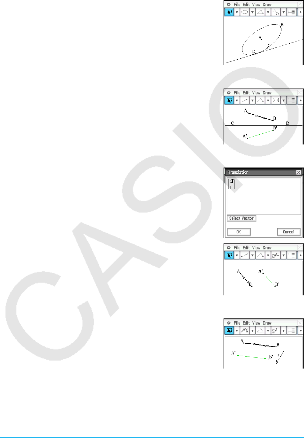
Chapter 8: Geometry Application 165
uTo construct a tangent to a curve through a specified point
1. Draw a curve, such as an ellipse.
2. Tap [Draw], [Construct], and then [Tangent to Curve].
• This highlights K on the toolbar.
3. Tap the point of tangency on the curve. This draws the tangent.
uTo reflect a line segment with respect to a specified line of symmetry
1. Draw a line segment and a line to use as the line of symmetry, and then
select the line segment.
2. Tap [Draw], [Construct], and then [Reflection].
• This highlights S on the toolbar.
3. Tap the line of symmetry. This reflects the line segment you drew in step 1
about the line of symmetry.
uTo translate a line segment by inputting a vector
1. Draw a line segment (AB), and then select it.
2. Tap [Draw], [Construct], and then [Translation] to display the Translation
dialog box.
3. Enter the vector for the translation.
• Vector values indicate the amount of movement in the x-axis direction
and in the y-axis direction. In the nearby screen, for example, the figure
selected in step 1 moves parallel to the x-axis by three.
4. Tap [OK]. This translates line segment AB in accordance with the vector
value you input, and draws line segment A’B’.
uTo translate a line segment by selecting a vector
1. Draw a line segment (AB), and a vector to use in the translation. Next, select
the line segment.
2. Tap [Draw], [Construct], and then [Translation] to display the Translation
dialog box.
3. Tap [Select Vector].
4. Tap the vector on the screen. This translates line segment AB in accordance
with the vector you selected, and draws line segment A’B’.

Chapter 8: Geometry Application 166
uTo rotate a line segment
1. Draw a line segment, and then select it.
2. Tap [Draw], [Construct], and then [Rotation].
• This highlights F on the toolbar.
3. Tap the screen once to select the center of rotation.
• This displays the Rotation dialog box.
4. Specify the angle of rotation in degrees, and then tap [OK].
uTo dilate a line segment toward a specified center point
1. Draw a line segment, and then select it.
2. Tap [Draw], [Construct], and then [Dilation].
• This highlights 2 on the toolbar.
3. Tap the center of dilation.
• This displays the Dilation dialog box.
4. Specify the dilation scale factor, and then tap [OK].
uTo transform a triangle using a matrix or vector (general transform)
1. Tap q to turn on coordinate display in the Geometry window.
2. Draw triangle ABC, and then select its three sides.
3. Tap [Draw], [Construct], and then [General Transform]. This displays the
Transform dialog box.
4. Enter the matrix for the transform.
• In this example, let’s input [[1, 0], [0, −1]].
5. Tap [OK]. This draws triangle A’B’C’, which is symmetrical to triangle ABC
about the x-axis.
6. Tap anywhere outside of the triangles to deselect the currently selected
triangle. Next, select triangle A’B’C’.
7. Tap [Draw], [Construct], and then [General Transform].
8. Enter the vector to perform parallel displacement.
• In this example, let’s input [1, 1].
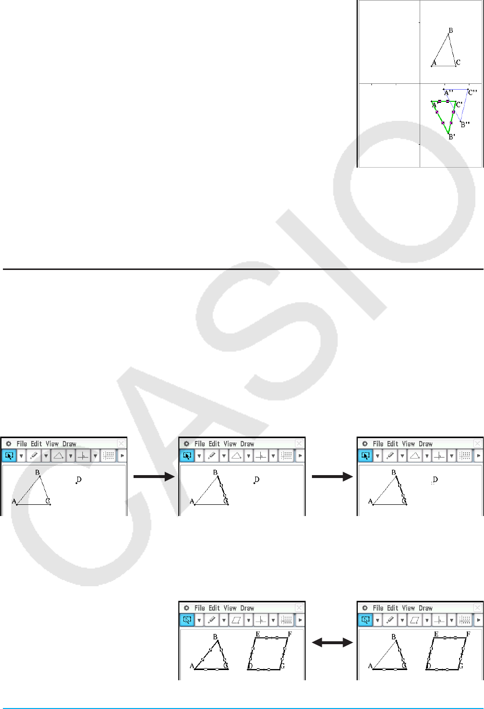
Chapter 8: Geometry Application 167
9. Tap [OK]. This performs the parallel displacement and draws triangle
A’’B’’C’’.
Tip: In the above example, we performed the transformation and the parallel
displacement operations separately. You could also perform both operations at
the same time, if you want. To do so, input both the matrix [[1, 0], [0, −1]] and the
vector [1, 1] in step 4, and then tap [OK]. This will produce the result shown in
step 9.
8-2 Editing Figures
This section explains how to move, copy, change the color of, and perform other editing operations on
Geometry application figures.
Selecting and Deselecting Figures
Before you can execute certain editing commands, you must first select the figure you want to edit. There are
two figure selection modes: Select and Toggle Select, each of which is described below.
u Using Select
Tap G on the toolbar. This causes the button to become highlighted, indicating that Select is enabled.
Select allows you to select as many figures as you would like, and then move, copy, paste, or perform other
operations on the selection as a single entity.
• Tap G on the toolbar. • To select side BC of the
triangle, tap it.
• Tapping point D selects
it, leaving side BC of the
triangle selected, too.
• To deselect all of the figures, tap anywhere on the screen where there are no figures.
u Using Toggle Select
Tap i on the toolbar. This causes the button to become highlighted, indicating that Toggle Select is enabled.
Toggle Select allows you to select and deselect figures.
For example, if you have multiple
figures selected, Toggle Select will
allow you to deselect a single part of
the selection. Tapping the part again
will turn the selection back on.

Chapter 8: Geometry Application 168
Moving and Copying Figures
uTo move a figure
1. Draw a figure, and then select it.
2. Drag the figure to move it to the location you want.
• A selection boundary appears around the figure when you drag it.
3. Remove the stylus from the screen.
uTo copy a figure
1. Draw a figure, and then select it.
2. Tap [Edit] - [Copy], and then [Edit] - [Paste].
3. Drag the pasted figure to the location you want.
Pinning an Annotation on the Geometry Window
You can pin an annotation on the Geometry window using the Pin function. By default, annotations are
‘Unpinned’, so they pan or zoom along with the Geometry window. Pinning an annotation fixes its position on
the screen so it is always displayed in the same location on the Geometry window.
uTo pin or unpin an annotation on the Geometry window
1. Select (highlight) the text on the Geometry window.
2. Tap [Edit], [Properties], and then [Pin] or [Unpin].
• When text is pinned, it maintains its position as shown here even when the window is panned.
Specifying the Number Format of a Measurement
You can specify the number format for each measurement value or all the measurement values on the
Geometry window. The initial default number format setting for measurement values is “Fix 2”.
uTo specify the number format for selected measurement value(s)
1. Select (highlight) the measurement(s) you want to specify the number format.
2. Tap the [Edit], [Properties], and then [Number Format].
3. On the dialog box that appears, select the number format you want by tapping it.
• For the meaning of each number format name, see “To specify the numeric value display format” on page 36.
4. Tap [OK].
• This will display the measurement value(s) you selected in the step 1 using the specified number format.
uTo specify the number format for all the measurement values on the Geometry window
1. Tap anywhere on the screen where there are no figures to deselect all of the figures.
2. Perform the procedure from step 2 under “To specify the number format for selected measurement value(s)”.
• This will display all the measurement values on the Geometry window using the specified number format.

Chapter 8: Geometry Application 169
Specifying the Color and Line Type of a Displayed Object
You can use the procedure below to specify the color and line type for the outline of a figure, the fill color inside
a figure, or the color of text, labels, and other non-figure objects.
uTo specify the color and line type of a particular object
1. Use the procedure under “Selecting and Deselecting Figures” (page 167) to
select the object whose color and/or line type you want to specify.
2. Tap [Edit] and then [Style] to display the dialog box shown to the right.
• The dialog box will show only supported settings, which depend on the
composition of the selected object.
3. Configure the dialog box with the following settings.
To specify this: Perform this operation:
Specify the text color Tap “Character Color” and then tap the desired color.
Specify the line type Tap “Graph Plot” and then tap the desired line type.
Specify the line color Tap “Line Color” and then tap the desired color.
Specify the figure fill color Tap “Area Color” and then tap the desired color. To specify no fill color,
tap “Clear”.
4. To apply the settings you configure, return to the dialog box in step 2 of this procedure and then tap [OK].
uTo specify the color and line type of all the objects on the Geometry window
1. Tap anywhere on the screen where there are no figures to deselect all of the figures.
2. Perform the procedure from step 2 under “To specify the color and line type of a particular object”.
Changing the Display Priority of Objects
Basically, objects you draw on the Geometry window are stacked in the order they are drawn (newest drawing
on top). You can use the operations in this section to move a drawn object to the top or the bottom of the stack.
You also can move all text to the front, if you want.
• To move a particular object to the front, select it and then tap [Edit] - [Properties] - [To the front].
• To move a particular object to the back, select it and then tap [Edit] - [Properties] - [To the back].
• To move all text to the front, tap [Edit], [Properties] and then [All Text].
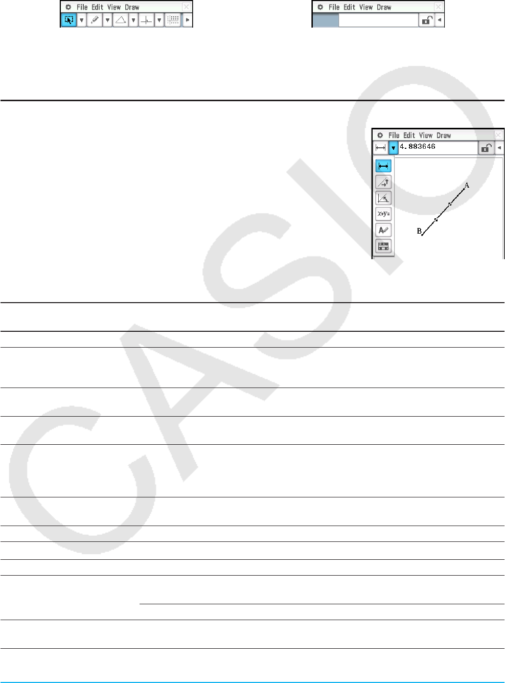
Chapter 8: Geometry Application 170
8-3 Using the Measurement Box
Tapping the u button to the right of the toolbar displays the measurement box. Tap t to return to the normal
toolbar.
Normal toolbar Measurement box
You can use the measurement box to view the measurements of a figure, to specify a measurement of a figure,
to fix a measurement of a figure, or to name a figure.
Viewing the Measurements of a Figure
The type of information that can be displayed in the measurement box depends
on the figure currently selected on the screen. The nearby screen shows
an example when a line segment is selected. You can change the display
information type by tapping one of the icons.
The following table describes the information that appears when you tap each icon, and explains when each
icon is available for selection.
Icon Icon Name This icon appears when this
is selected: Tapping this icon displays: Lockable
TCoordinates A single point Coordinates of the point Yes
tDistance/length
Two points on one figure or
two different figures, or a single
line segment or a vector
Distance between two points,
length of a line segment or
vector
Yes
QSlope Single line, line segment, or
vector
Slope of the line, line segment
or vector Yes
YDirection Single line, line segment, or
vector
Direction angle of the line
(angle of inclination) Yes
OEquation
Any single line or line segment,
vector, circle, arc, ellipse or
any other figure (parabola,
etc.) drawn by a function
Function of the figure (using
rectangular coordinates) Yes
5Equation edit Single parabola or any other
figure drawn by a function
Equation of the figure in the
function editing dialog box. No
]Radius Single circle or arc Radius of circle or arc Yes
3Circumference Single circle Length of the circumference Yes
vPerimeter Single polygon Sum of the lengths of the sides No
EArea
Any three points, an arc,
ellipse, or polygon Area No
Single circle Area Yes
Q
tAngle Two line segments Angle and its supplement
formed by the line segments Yes
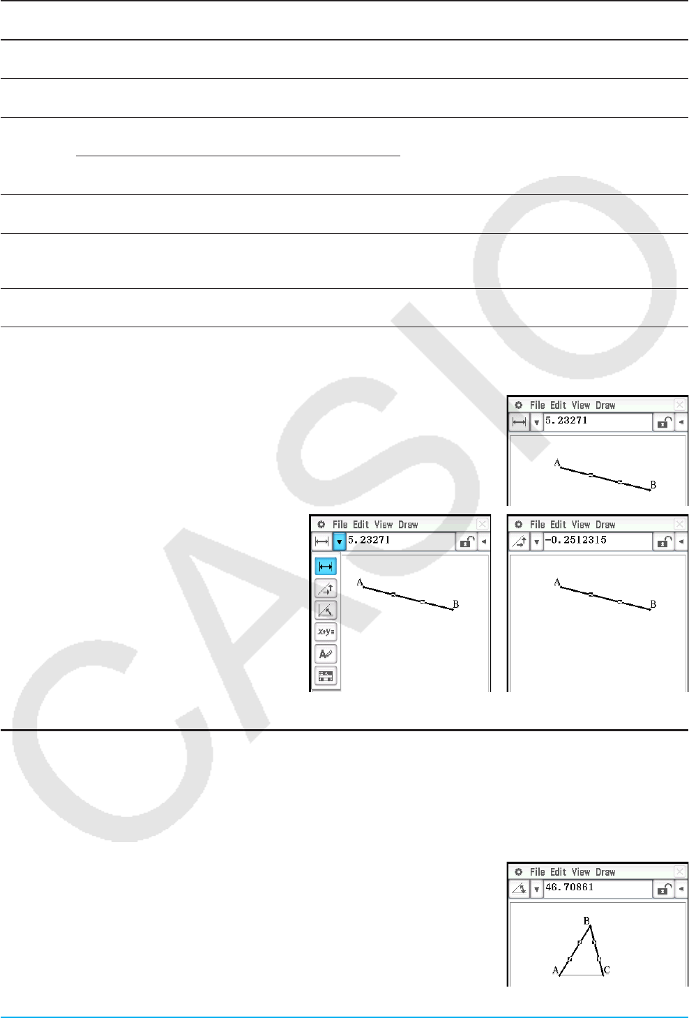
Chapter 8: Geometry Application 171
Icon Icon Name This icon appears when this
is selected: Tapping this icon displays: Lockable
KTangency Two circles or arcs, or a line
and circle Whether two items are tangent Yes
eCongruence Two line segments Whether line segments are the
same length Yes
6
Incidence Point and a line, arc, circle or
vector Whether a point is on the line/
curve Yes
Point on curve Point and a function, curve, or
ellipse
FRotation angle Two points created by
[Rotation] Angle of rotation *1
2Scale of dilation
Two points (like point A and
point A’) on a figure created by
[Dilation]
Scale of dilation *1
uText icon An object that includes text or
an object that can be named
Editable text used to name the
selected image No
*1 The value in the measurement box is always locked while this tool is selected.
uTo view the measurements of a line segment
1. Draw a line segment.
2. Tap u on the toolbar to display the measurement box.
3. Select the line segment.
• This displays the length of the line segment.
4. Tap the down arrow next to the
measurement box to cycle through other
measurements.
• In the case of the line segment, for
example, you can view its length, slope,
direction, and equation.
Specifying and Constraining a Measurement of a Figure
The following example shows how to specify and constrain (fix) an angle of a triangle. By “constraining a
measurement” we mean that it becomes fixed. For example, constraining (fixing) angle B of triangle ABC at 90
degrees will cause angle B to remain at 90 degrees regardless of where the apex is moved.
uTo specify and constrain the measure of an angle of a triangle*
1. Draw the triangle, and then select its side AB and side BC.
2. Tap u on the toolbar to display the measurement box.
• This displays the measure of angle B in the measurement box.
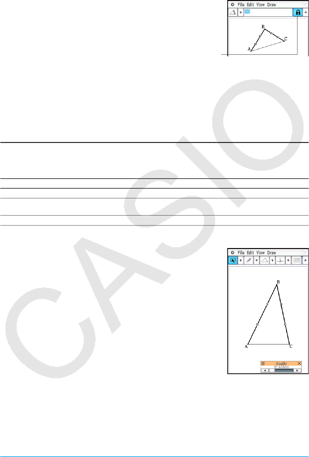
Chapter 8: Geometry Application 172
3. Input 90 into the measurement box and press E.
• This specifies and constrains the measure of angle B at 90 degrees.
A highlighted check box indicates the measurement is constrained (fixed).
* In this example, the [Measure Angle] setting of the Geometry Format dialog box (page 40) is set to “Degree”.
Tip: To cancel the constraint of a measurement value fixed using the above operation, tap the check box to the right of
the measurement box to unhighlight it. Each tap of the check box toggles the measurement value between fixed and
unfixed.
uTo clear all settings constrained with the measurement box
Tap [Edit] and then [Clear Constraints].
Using Sliders
Sliders can be displayed and used to change the settings of the objects in the table below. Select the desired
object and then display its slider using the procedure following the table.
For this type of selected object(s): This type of slider can be displayed:
Any two sides of a polygon or two line segments Angle, supplementary angle
Two points on one figure or two different figures, or a single
line segment or a vector
Length
Single circle or arc Radius
u To display a slider
1. Select the required object(s), as described in the table above.
2. Tap [Draw] - [Slider]. On the sub-menu that appears, select the type of
measurement ([Angle], [Supplementary Angle], [Length], [Radius]) you want
to perform with the slider.
• The items that appear on the sub-menu depend on the object you select in
step 1 of this procedure.
Note: Instead of step 2 in the above procedure, you could also perform the
steps below to display a slider.
(1) Tap u on the toolbar to display the measurement box.
(2) Tap the down arrow to the right of icon palette on measurement box
and then a.
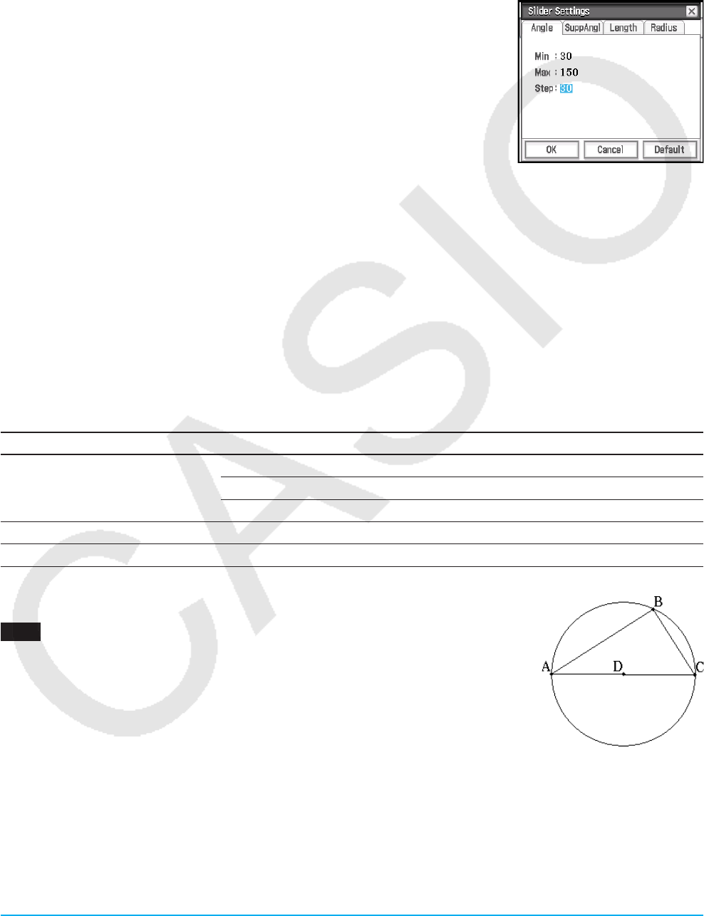
Chapter 8: Geometry Application 173
uTo specify the measurement minimum value, maximum value, and step value for a slider
1. Perform the operation under “To display a slider” to display a slider.
2. Tap the upper left corner of the slider display box.
3. On the menu that appears, tap [Settings].
4. On the Slider Settings dialog box that appears, display the tab for the measurement you want to change.
• The dialog box has four tabs: [Angle], [SuppAngl] (supplementary angle),
[Length], and [Radius]. You can select any of the tabs and change its
settings, regardless of the measurement controlled by the slider you
selected in step 1 of this procedure.
5. Input values for Min (minimum value), Max (maximum value), and Step (step value).
• For the Angle and SuppAngl tabs, you should input a value in the angle unit (degrees, radians, or grads)
currently specified by the “Measure Angle” setting on the Geometry Format dialog box. The input range
depends on the current angle unit setting: 0 to 180 for degrees, 0 to
π
for radians, and 0 to 200 for grads.
Attempting to input a value that is outside the current allowable range will automatically change the input
value so it is within range.
• On the Length and Radius tab, input a value that is greater than zero.
• To return the setting values on the currently displayed tab to their initial values, tap the [Default] button.
Refer to the “Initial Defaults” table for information about default settings.
6. After configuring the settings you want, tap [OK] to save them.
• This closes the Slider Settings dialog box.
Initial Defaults
Measurement Min Max Step
Angle, Supplementary Angle
Degree 30 150 30
Radian
π
/6 5
π
/6
π
/6
Grad 100/3 500/3 100/3
Length 1 10 1
Radius 1 5 1
uTo use a slider to seamlessly change an angle and/or length
0804 Angle B of triangle ABC is fixed at 90°, and the length of side AC is also
fixed. Confirm the movement of vertex B along the circumference of a
circle that has side AC as its diameter as angle A changes. Here, angle A
changes at 10° increments within a range of 10° to 80°.
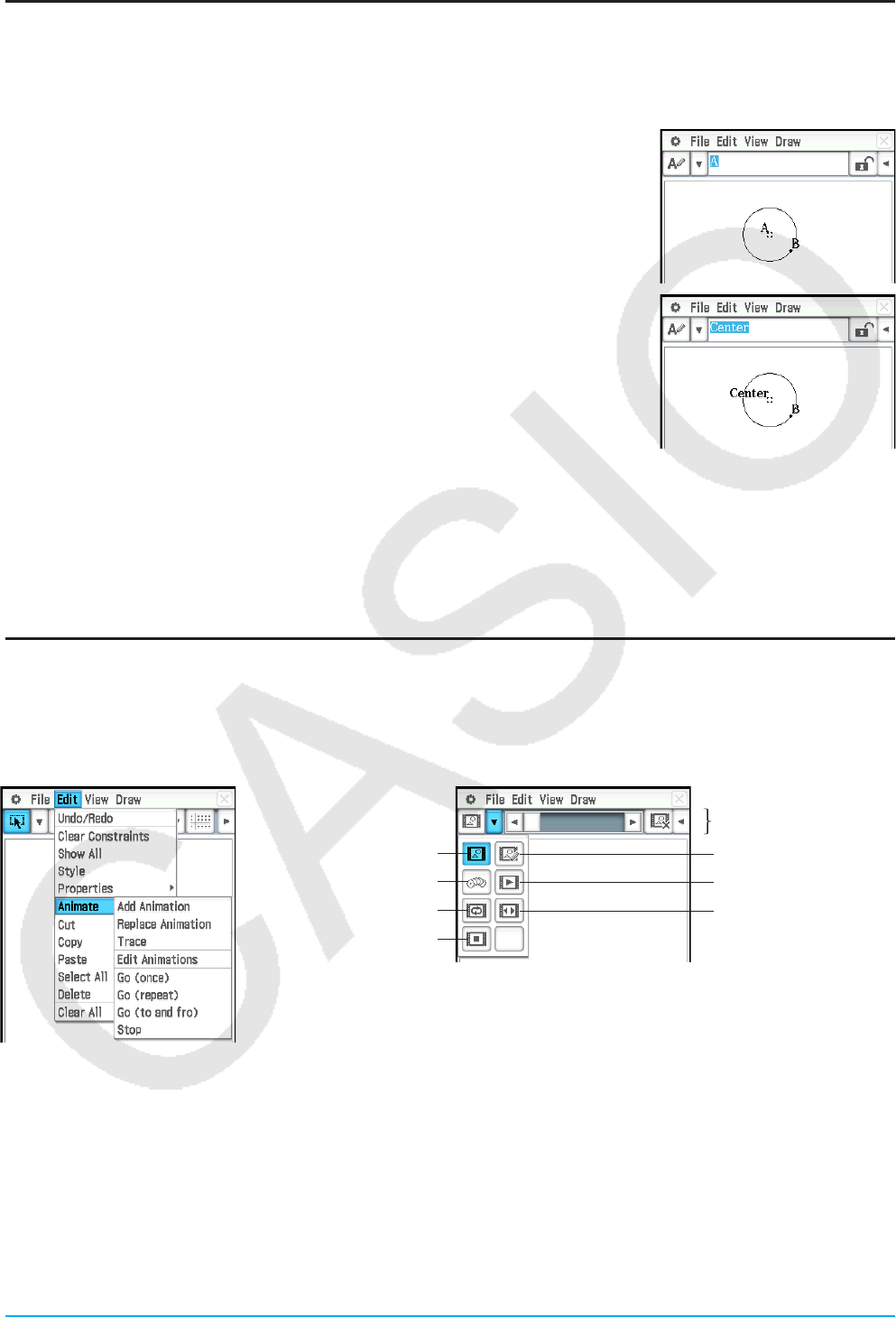
Chapter 8: Geometry Application 174
Changing a Label or Adding a Name to an Element
You can change the name of a point, or add a name to each element as explained in the following example.
uTo change the label name of the center of a circle from “B” to “Center”
1. Draw the circle, and then select its center point.
2. Tap the down arrow to the right of icon palette on measurement box and
then u.
• This displays the current name of the point in the measurement box. The
displayed name is highlighted so it can be edited.
3. Input a new name (“Center”) in the measurement box.
4. Press E or the check box to the right side of measurement box.
• This displays the changed name on the screen as shown here.
8-4 Working with Animations
An animation consists of one or more point/curve pairs, in which the curve can be a line segment, circle, ellipse,
or function. You build an animation by selecting a point/curve pair, and then adding it to an animation.
Using Animation Commands
You can build and run an animation either by executing menu commands or by using the animation toolbar that
appears when you tap [View] and then [Animation UI].
[Edit] – [Animate] [View] – [Animation UI]
Add Animation
Trace
Go (repeat)
Stop
Animation toolbar
Replace Animation
Go (once)
Go (to and fro)
• Most of the procedures in this section are performed using the [Animate] submenu.
• All of the [Animate] menu commands can be accessed from the animation toolbar, except for [Edit] - [Animate]
- [Edit Animations].
• To close the animation toolbar and return to the normal toolbar, tap the = button on the right side of the
animation toolbar, or tap [View] and then [Animation UI].
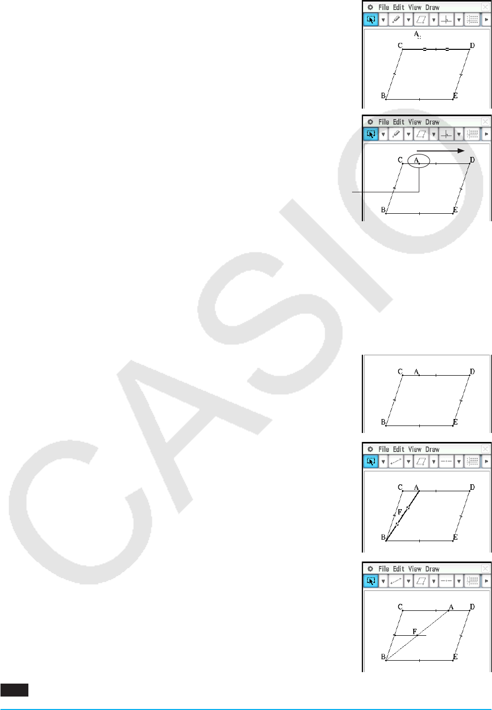
Chapter 8: Geometry Application 175
uTo add an animation and run it
1. Plot a point and draw a figure (here we draw a parallelogram). Or, you could
draw a circle, arc, ellipse, line segment, or function instead of a figure.
2. Select the point and a side of the parallelogram.
3. Tap [Edit], [Animate], and then [Add Animation].
• The point selected in step 2 moves along the side of the parallelogram.
4. Tap [Edit], [Animate], and then [Go (once)], [Go (repeat)], or [Go (to and fro)].
Point A moves along side CD.
5. Tap [Edit], [Animate], and then [Stop] to stop the animation.
• You can also stop the animation by tapping l on the icon panel.
uTo replace the current animation with a new one
1. Select the point and curve for the new animation.
2. Tap [Edit], [Animate], and then [Replace Animation].
• This discards the currently set animation and sets up an animation for a new point and curve set. Tap
[Edit], [Animate], and then [Go (once)] to see your new animation.
uTo trace a locus of points
Note: Using trace leaves a trail of points when the animation is run. The
procedure below is a continuation of the procedure under “To add an
animation and run it”.
1. Draw a line segment that connects point A with apex B.
2. Draw the center point of line segment AB.
• Select line segment and then tap [Draw] - [Construct] - [Midpoint].
3. Select the center point of line segment AB (point F) and then tap [Edit] -
[Animate] - [Trace].
4. Tap [Edit], [Animate], and then [Go (once)].
• This draws a line using point F as the locus, that is parallel to and whose
length is half that of side CD of the parallelogram.
0805 To create an animation that traces the locus of specific points

Chapter 8: Geometry Application 176
uTo edit an animation
Note: The steps below continue from the procedure under “To trace a locus of
points”.
1. While the animation you want to edit is on the display, tap [Edit], [Animate],
and then [Edit Animations].
• This displays the animation editing window in the lower window. The upper
window contains the animation that we just completed in “To trace a locus
of points”.
2. Edit the animation following the procedure below.
Steps:
This setting specifies how many steps point A takes to move along side CD.
The initial default value is 20, which can be changed to value from 2 to 100.
Animations:
The “A” under “Animations” indicates that point A is the point moved by the
animation. When you are building multiple animations, a list of all applicable points appears here.
Tapping [Remove] deletes the applicable animation.
“t0” and “t1” specify the range of movement of point A on side CD. The initial default values are t0 = 0 and
t1 = 1. During animation, the length of CD is considered to be one unit. The default values specify that
movement of point A is from start point C (point where length equals 0) up to end point D (point where length
equals 1).
Changing the value of t0 to 0.5, for example, causes point A to move from the middle of side CD to point D.
Changing the value of t0 to −1, causes point A to begin at a point outside side CD (in this case, at a point a
distance equivalent to the length of side CD) and ending with point D.
Traces:
This item shows the specified trace point. Tapping [Remove] cancels the trace point setting.
3. While the lower window is active, tap C to close the animation editing window.
uTo view an animation table
Note: The steps below continue from the procedure under “To trace a locus of
points”.
1. Tap line segment AB, which connects point A with apex B, to select it.
2. Tap u on the toolbar to display the measurement box.
• This displays the measurement of line segment AB in the measurement
box.
3. Tap # next to the measurement box.
• This displays a table showing the length of line segment AB for each
animation step in the bottom half of the screen.
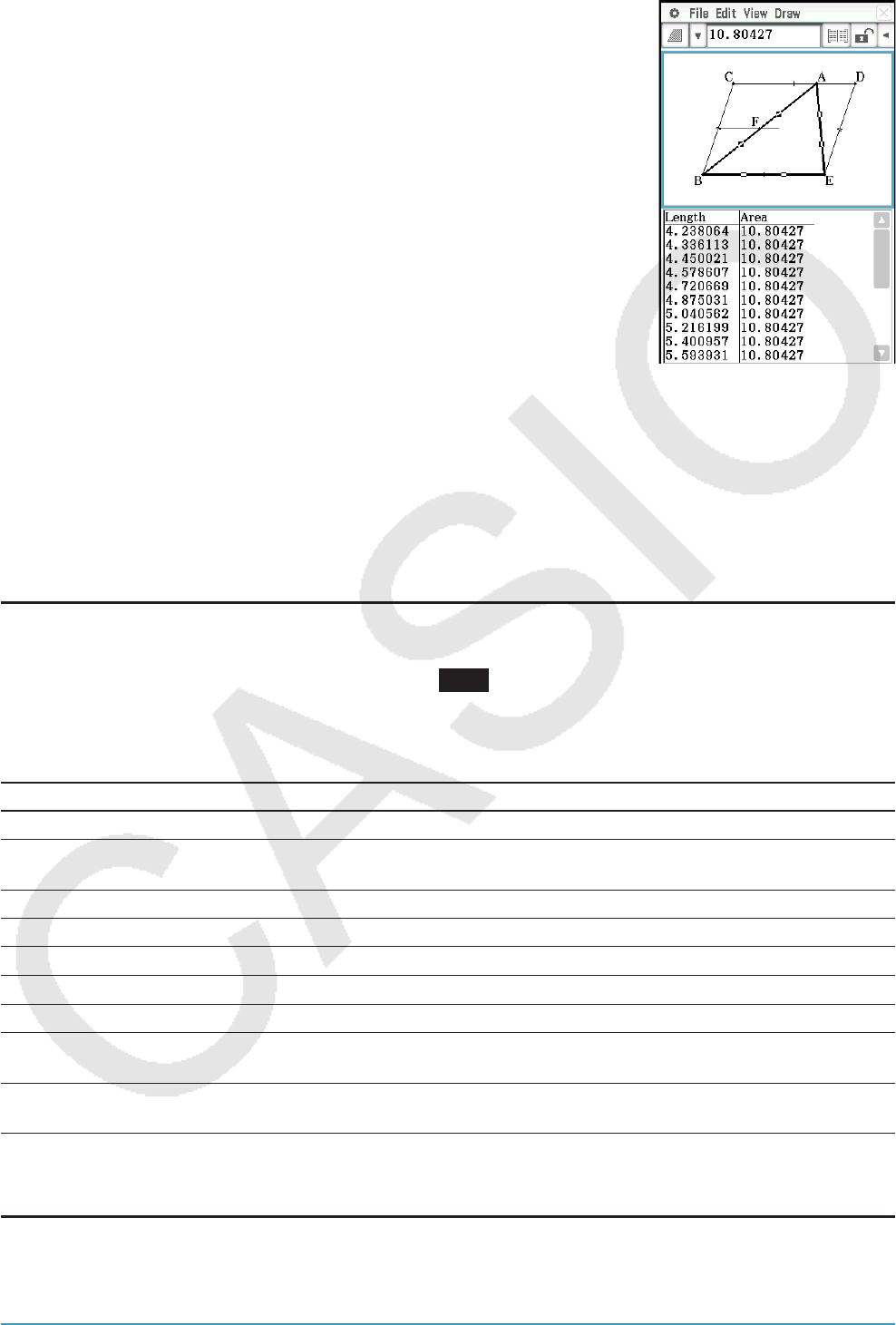
Chapter 8: Geometry Application 177
4. Next, let’s add a column to the table that shows the area of triangle ABE at
each step. Perform the steps below.
(1) Draw a line segment that connects point A with apex E.
(2) Select line segment AB, line segment AE, and side BE.
(3) Tap # next to the measurement box.
This adds a column that shows the area of triangle ABE at each step.
(As can be seen, the area of triangle ABE does not change even when
point A moves.)
8-5 Using the Geometry Application with Other
Applications
You can display the Geometry application from within the eActivity or Main application. This feature allows
you to visualize the relationship between Algebra and Geometry. You can, for example, drag a figure from the
Geometry window to the eActivity window to see its corresponding mathematical expression.
Drag and Drop
When you open Geometry within another application, you can drag and drop information between the two
application windows. You can see an actual example ( 0243 ) of how this is done using the Main application in
Chapter 2 of this manual.
The information that appears when you drop a figure into another application depends on the figure you are
dragging. Many of the possible outcomes are listed in the table below.
Geometric Figure Drag and drop into another application transforms to: *1
Point Ordered pair Yes
Line Segment, Infinite Line,
Ray
Linear equation Yes
Vector Ordered pair (head of vector, assuming the tail is at the origin) No
Circle, Arc Equation of a circle Yes
Ellipse Equation of an ellipse Yes
Function (
y = f (x)) Equation of the function Yes
Two Lines System of equations No
Polygon, or open polygon
created by animation
Matrix containing each vertex point No
Pairs of points related by a
transformation
Expression showing point relationship No
*1 Support for drag and drop into a Geometry Link row in an eActivity. For details about a Geometry Link row,
see “Inserting a Geometry Link Row” on page 184.
Copy and Paste
In addition to drag and drop, you can also copy figures or columns from an animation table and paste them into
another application.
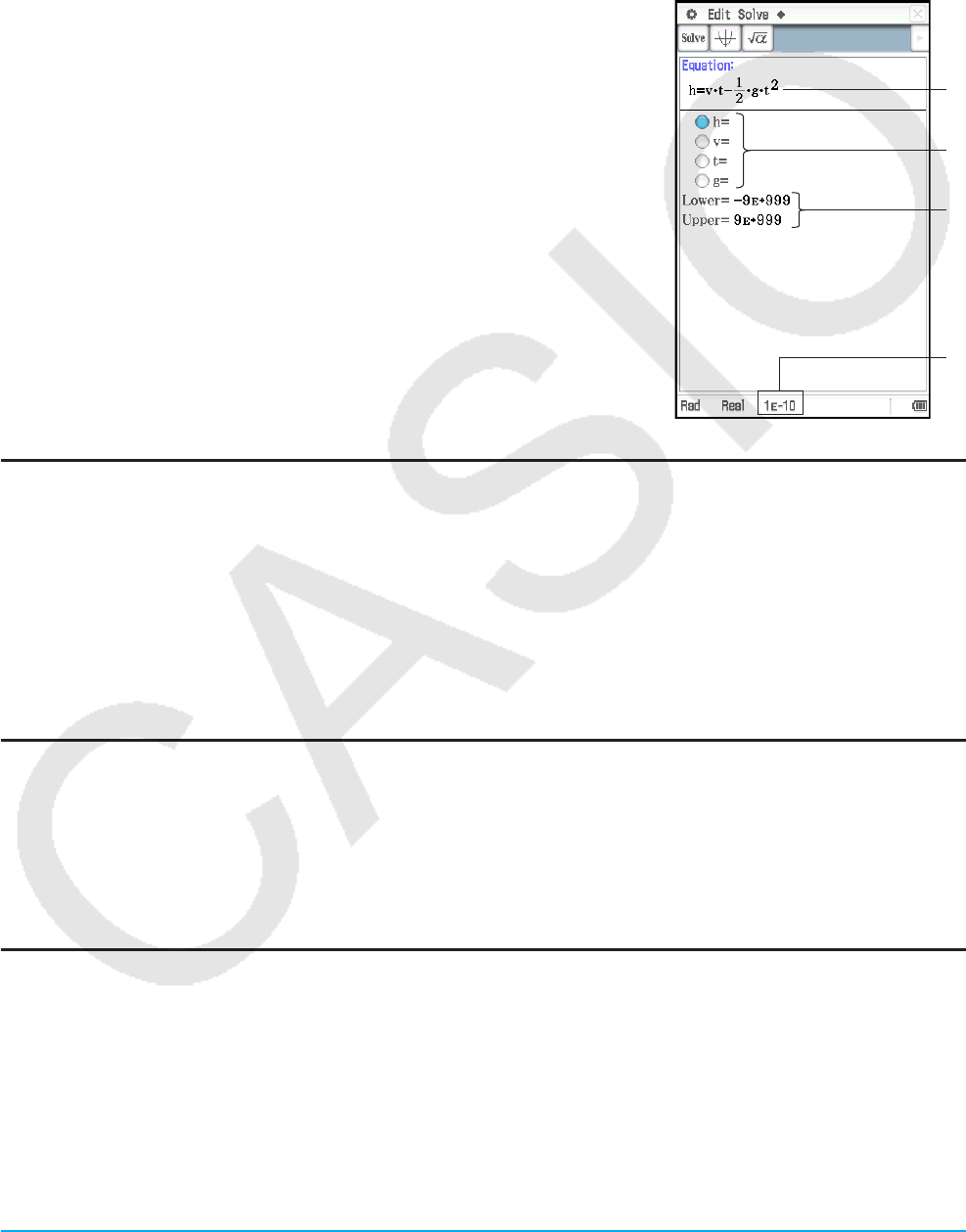
Chapter 9: Numeric Solver Application 178
Chapter 9:
Numeric Solver Application
Numeric Solver application lets you obtain the value of any variable in an equation without transforming or
simplifying the equation.
Starting up the Numeric Solver displays the Numeric Solver window. The
screen to the right shows an example of the window with a sample
equation input.
1 Equation input area. Inputting an equation that includes variables and
then pressing E will cause 2 and 3 to appear.
2 Equation variables. Input the initial value of each variable to the right
of the equals sign (=). Specify the variable you want to solve for by
selecting the option button to the left of it.
3 Solution lower limit and upper limit input area*
4 Current convergence range setting*
* Values shown in the sample screen are initial defaults.
Numeric Solver Application-Specific Menus and Buttons
• Solve the input equation for the specified variable ...................................................... Solve - Execute or 1
• Clear all single-character variables (a through z)* .................................................................... a - Clear a–z
• Initialize the upper boundary and lower boundary ...........................................................a - Initialize Bound
• Change the convergence range .......................................................................................... a - Convergence
* Performing the “Clear a–z” operation clears all single-character variables, regardless of variable data type.
Programs and functions with file names from “a” through “z” are also cleared.
Inputting an Equation
On the Numeric Solver window, input a single equation into the area under “Equation”.
• Use the soft keyboard to input an equation that contains at least one variable.
• If you do not input an equals sign, the ClassPad assumes that the expression is to the left of the equals sign,
and there is a zero to the right.
Solving an Equation
Numeric Solver solves equations by calculating approximations based on Newton’s method. Because of this,
you should keep the following points in mind about its solutions.
• Even if an equation has multiple solutions, only one solution is obtained for a particular Numeric Solver
operation. For example, x2−1 = 0 has the two solutions 1 and −1. Numeric Solver will display either of the
solutions first, depending on the value specified by “Lower” and “Upper”.
• Solutions may include errors that are not actual solutions. The accuracy of solutions can be determined by
viewing the [Left–Right] value in the Result dialog box. The closer the [Left–Right] value is to zero, the more
accurate the results.
1
3
4
2
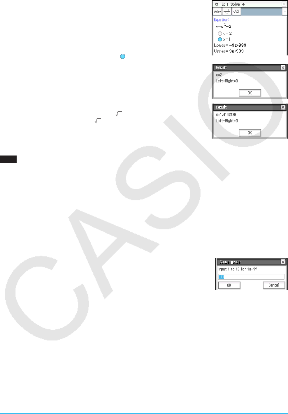
Chapter 9: Numeric Solver Application 179
uTo solve an equation
1. On the Numeric Solver window, input an equation.
• Here, we will input the equation y = x2 − 2, and solve for x when y = 0 and
y = 2.
2. Press E.
3. Input 2 as the values for variable y (to the right of y=).
4. Since we want to solve for x, select the option button to the left of variable x
(so the button next to the variable becomes ).
5. Tap 1.
• This displays the Result dialog box with the calculation result. Tap [OK] to
close the dialog box.
6. Input 0 as the values for variable y (to the right of y=).
7. Tap 1.
• Though the solution of x2 − 2 = 0 is x = ± 2, here the value that is
displayed is the decimal form of 2, which is near the last solution
obtained (x = 2).
To obtain the other solution, change the Upper value (to 0, for example) and
then tap 1.
0901 t is the time it would take for an object thrown straight up with initial velocity v to reach height h. Use the
formula h = vt − 1/2 gt2 to calculate the initial velocity v for a height of h = 14 meters and a time of t = 2
seconds. Gravitational acceleration is g = 9.8 m/s2.
Tip
• If ClassPad judges that the displayed results are not converging sufficiently, it displays the message “Did not converge.
Do you wish to continue the calculation?” Tap [Yes] to continue, or [No] to cancel the calculation.
• If the message “Can’t solve!” appears on the display, perform either (or both) of the operations below and then tap 1
again.
- Tap a - [Initialize Bound], or manually change the “Lower” and “Upper” values.
- Change the convergence range. See “To change the convergence range” below.
uTo change the convergence range
1. Tap a - [Convergence] to display the Convergence dialog box.
2. Enter an integer in the range of 1 to 13.
• A smaller value increases the allowable error range, and lessens the
chance of a “Can’t solve!” error. If a calculation causes a “Can’t solve!”
error, try changing this setting to a smaller value.
3. Tap [OK] to apply the setting and close the dialog box.
• The new setting value will be shown in the status bar (page 178).
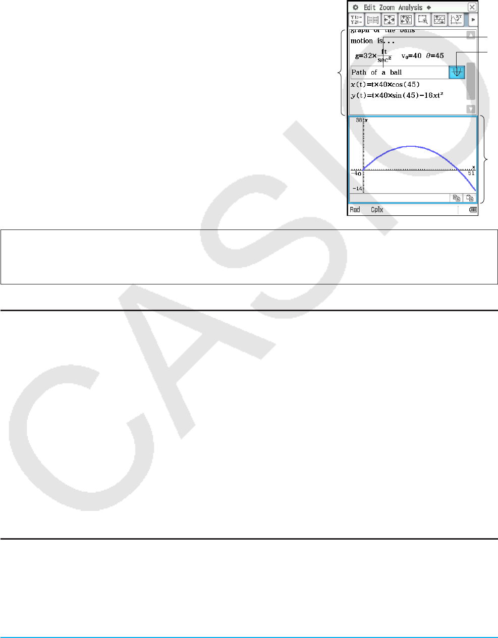
Chapter 10: eActivity Application 180
Chapter 10:
eActivity Application
The eActivity application lets you input and edit text, mathematical expressions, and ClassPad application data,
and save your input in a file called an “eActivity”.
A basic eActivity can contain text along with application data,
which is embedded as a row or a strip. A row can be a “Text
Row”, a “Calculation Row”, or a “Geometry Link”. A strip can be an
“application data strip” (Main, Graph & Table, Geometry, and so on).
Example eActivity windows
1 eActivity window
2 Graph strip
3 Expand button
4 Expanded graph window
1
3
4
2
Tip: A variety of eActivity files are available for download at the CASIO Website.
http://edu.casio.com/products/classpad/
After you download an eActivity file, you will need to transfer it from your computer to your ClassPad. See the
instructions provided at the CASIO Website for more information.
eActivity Application-Specific Menus and Buttons
• Clear variables that contain numbers, list and matrices ...........................................Edit - Clear All Variables
• Insert a row or strip .............................................Insert - Calculation Row (page 182); Text Row (page 181);
Geometry Link (page 184); Strip(1) or Strip(2) (page 182)
• Add help text to the currently selected strip ................................................................. Insert - Add Strip Help
• Insert a command ................................................................................................................. Action (page 61)
• Open or save a file ......................................................................................................................................{
• Bold the text that is currently selected (Text Input mode only) ...................................................................B
• Convert a text row to a calculation row or a calculation row to a text row ..........................................u / <
10-1 Creating an eActivity
Basic Steps for Creating an eActivity
1. Start the eActivity application.
• This displays the eActivity window as it appeared the last time it was used.
• If you are already in the eActivity application and there is data on the display, tap [File] and then [New].
Note that [New] clears data from the display without saving it.
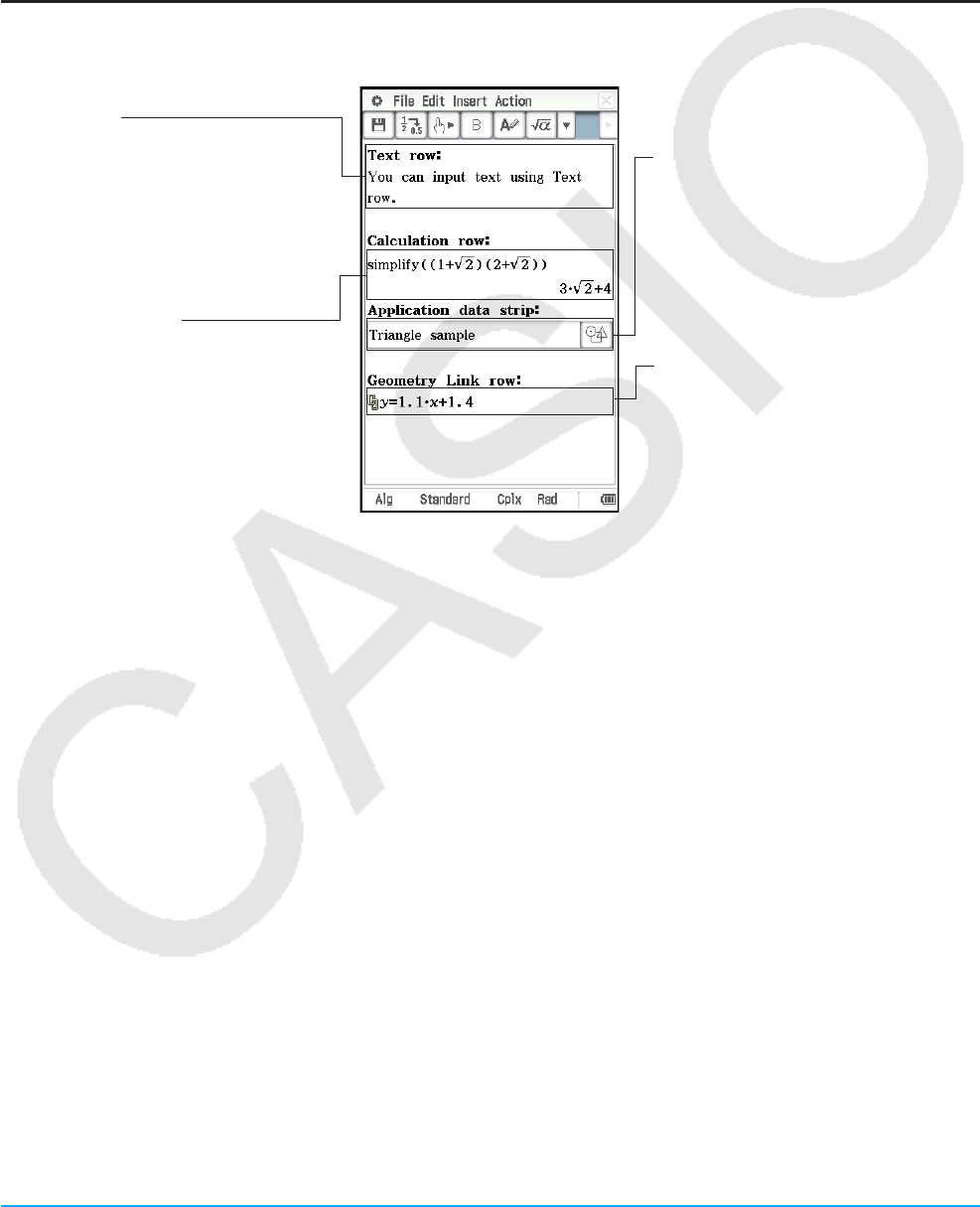
Chapter 10: eActivity Application 181
2. On the eActivity window, insert the text, expressions, application data, and other data you want to include in
the eActivity. For details, see “Inserting Data into an eActivity” below.
3. After the eActivity is the way you want, tap [File] and then [Save].
4. On the dialog box that appears, enter a file name and then tap [Save] to save the eActivity.
Tip: eActivity files are stored in a memory area that is separate from that used for storing other types of data (variable
data, Geometry data, Spreadsheet data, etc.). Because of this, you cannot access eActivity files data using the
Variable Manager. You have to use the eActivity application to perform eActivity file operations.
Inserting Data into an eActivity
The following describes the four types of data you can insert into an eActivity.
Text row
A text row can be
used to insert text data and
mathematical expression text in
natural format. You can also bold
the text in a text row.
Calculation row
Use the calculation row to insert
any of the calculation operations
that are available in the Main
application.
Application data strip
The application data strip lets you
display a window from a ClassPad
application (Main, Graph & Table,
Geometry, etc.) and use the
window to create data, which is
inserted into the eActivity.
Geometry Link row
Use this row to insert data
that is linked with a Geometry
window figure.
u To insert a text row
1. On the eActivity window toolbar, check to make sure that u is displayed. If it isn’t, tap < to toggle it to u.
• u indicates the Text Input mode is selected.
• If the cursor is located in a line that already contains input data, place the cursor at the end of the line, tap
[Insert] and then [Text Row]. This inserts a text row on the next line.
2. Use the soft keyboard or keypad keys to input the text you want.
• Pressing E will advance you to the next line without displaying results.
• Standard text (words separated by spaces) is automatically wrapped to the next line as required. A
continuous text or number string (one that does not include any spaces) will not be wrapped to the next line
if it does not fit within the width of the window.
• Note that any mathematical expressions or commands you input into a text row are treated as text. They
are not executed.
Tip
• Text can be changed to bold by dragging to select it and then tapping B. However, note that you cannot bold numeric
expressions of a natural display expression that you input with the template input mode (page 24).
• You can select a range of characters with the left and right cursor keys. Simply press the ClassPad f key and then
press e or d. Each press of the cursor key will select (highlight) the next character in the applicable direction.
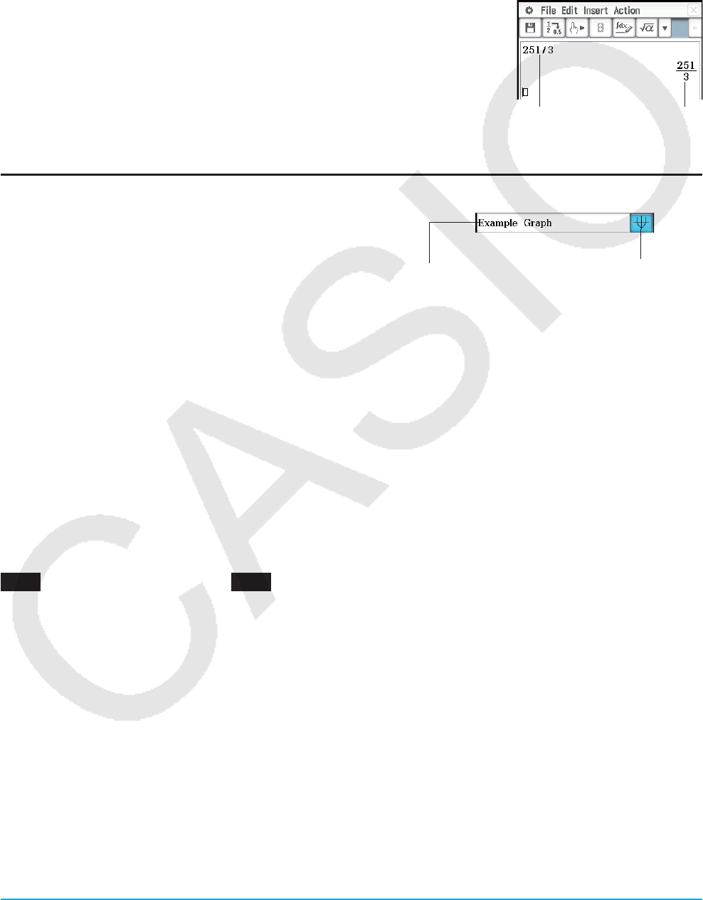
Chapter 10: eActivity Application 182
u To insert a calculation row
1. On the eActivity window toolbar, check to make sure that < is displayed. If it isn’t, tap u to toggle it to <.
• < indicates the Calculation Input mode is selected.
• If the cursor is located in a line that already contains input data, place the cursor at the end of the line, tap
[Insert] and then [Calculation Row]. This inserts a calculation row on the next line.
2. Use the soft keyboard or keypad keys to input the mathematical expression you want.
3. Press E after inputting an expression to display its result.
Tip
• If the input expression of a calculation row is not a valid expression, the row will
contain only the input expression, without an output expression.
• If you edit the expression in an existing calculation row and then press E, all of
the expressions following the line you edited are re-calculated and their results are
refreshed.
Inserting an Application Data Strip
An application data strip can be used to embed data from
other ClassPad applications into an eActivity. An application
data strip contains the elements shown to the right.
u To insert an application data strip
1. On the eActivity window, tap [Insert] and then [Strip(1)] or [Strip(2)]. Next, tap a menu item based on the type
of application data you want to insert. See “Application data strip list” below for details about application data
types.
• This inserts the data strip into the eActivity window, opens a data strip window in the lower half of the
display, and makes the data strip window active.
2. Perform the required input procedure in accordance with the type of window that is opened. For details, see
the examples, below.
3. After completing all the data strip window operations, tap C to close the window.
• This makes the eActivity window active, with the cursor in the strip you inserted in step 1.
4. Enter the title you want.
1001 To insert a Graph strip 1002 To insert a Notes strip
Expression
you input
Result
Title
You can enter a title,
if you want.
Expand button
Tap here to display
the application data in
the lower window.

Chapter 10: eActivity Application 183
Application data strip list
To insert this type of application data: Select this [Insert] menu item: Or tap this
button:
Graph window data (Graph & Table) Strip(1) - Graph $
Graph Editor window data (Graph & Table) Strip(1) - Graph Editor !
3D Graph window data Strip(1) - 3D Graph 7
3D Graph Editor window data Strip(1) - 3D Graph Editor Z
Geometry window data Strip(1) - Geometry 3
Spreadsheet window data Strip(1) - Spreadsheet Q
Stat Graph window data Strip(1) - Stat Graph y
Stat Editor window data Strip(1) - Stat Editor (
Notes window*1Strip(1) - Notes _
Main work area window data Strip(1) - Main ~
Conics Graph window data Strip(2) - Conics Graph ^
Conics Editor window data Strip(2) - Conics Editor *
Differential Equation Graph window data Strip(2) - DiffEqGraph O
Differential Equation Graph Editor window data Strip(2) - DiffEqGraph Editor A
Financial window data Strip(2) - Financial I
Probability window*2 data Strip(2) - Probability P
Numeric Solver window data Strip(2) - NumSolve 1
Sequence Editor window data Strip(2) - Sequence Editor &
Verify window*2 data Strip(2) - Verify W
Picture Plot window data Strip(2) - Picture Plot 5
*1 The Notes window can be used with the eActivity application only.
*2 The Probability window and Verify window can be used with the eActivity application and Main application.
For more information see “2-10 Using Verify” and “2-11 Using Probability”.
uTo add help text to a strip
1. Tap the title box of the strip to which you want to add help text.
2. Tap [Insert] - [Add Strip Help].
• A help window appears in the upper half of the display, while the window that was called from the strip
appears in the lower half of the display.
3. Input the help text into the help window.
4. After inputting all the text you want, tap C to close the help window.
• The strip will now have a ? button. Tapping ? will display the help window along with the application
window.
Tip: To delete help text from a strip, tap the title box of the strip whose help text you want to delete, and then tap [Insert] -
[Remove Strip Help].
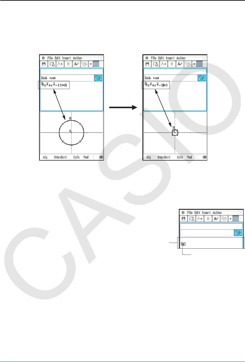
Chapter 10: eActivity Application 184
Inserting a Geometry Link Row
A mathematical expression in a Geometry Link row in an eActivity dynamically links to figure(s) in the Geometry
window.
Dragging a line or figure from the Geometry window to a Geometry Link row in an eActivity converts the line
or figure to its mathematical expression. Conversely, dragging an expression from a Geometry Link row to the
Geometry window converts the expression to its graphical form (line, curve, circle, etc.). This expression is
interlinked with its Geometry window figure, so modifying one causes a corresponding change in the other.
uTo use a Geometry Link row
Example: To drag one side of a triangle drawn on the Geometry window and link it to an eActivity
1. From the eActivity menu, tap [Insert], [Strip(1)], and then [Geometry] to insert a Geometry strip.
2. On the Geometry window that appears in the lower half of the screen, draw a triangle.
3. Tap the eActivity window to make it active.
4. Tap [Insert] and then [Geometry Link].
• This inserts a Geometry Link row in the next line.
5. Tap the Geometry window to make it active.
6. Tap one side of the triangle to select it, and then drag it to the right of the link symbol in the eActivity window.
• This inputs the equation of the line that represents the side of the triangle into the link.
• Modifying the equation in the Geometry Link row and pressing E causes a corresponding change in the
Geometry window.
Geometry Link row
Link symbol
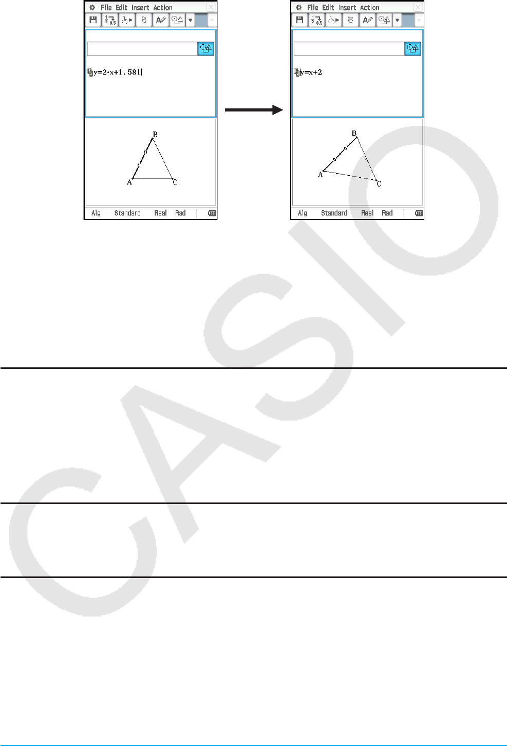
Chapter 10: eActivity Application 185
• The example above shows how the isosceles triangle ABC (CA = BC) changes when the equation in the
Geometry Link row is changed from y = 2x + 1.581 to y = x + 2.
Tip
• Pressing E after changing data in a Geometry Link updates the corresponding figure in the Geometry window.
• Changing the figure in the Geometry window will cause the linked data in an eActivity to update accordingly.
10-2 Transferring eActivity Files
File Compatibility
Note the following precautions when using the ClassPad’s data communication function to transfer eActivity
files with another ClassPad unit or a computer.
• The ClassPad II supports only eActivity files created with a ClassPad II unit or with ClassPad Manager.
eActivity files created with another ClassPad model cannot be opened by the ClassPad II.
• You may not be able to open an eActivity file created using a newer version ClassPad II using an older
version ClassPad II.
Transferring eActivity Files between a ClassPad Unit and a Computer
You can transfer eActivity files between ClassPad and a computer. For details, see “19-2 Performing Data
Communication between the ClassPad and a Personal Computer”.
Transferring eActivity Files between Two ClassPad Units
You can connect two ClassPad II units to each other and transfer eActivity files between them. For details
about how to do this, see “19-3 Performing Data Communication between Two ClassPads”.
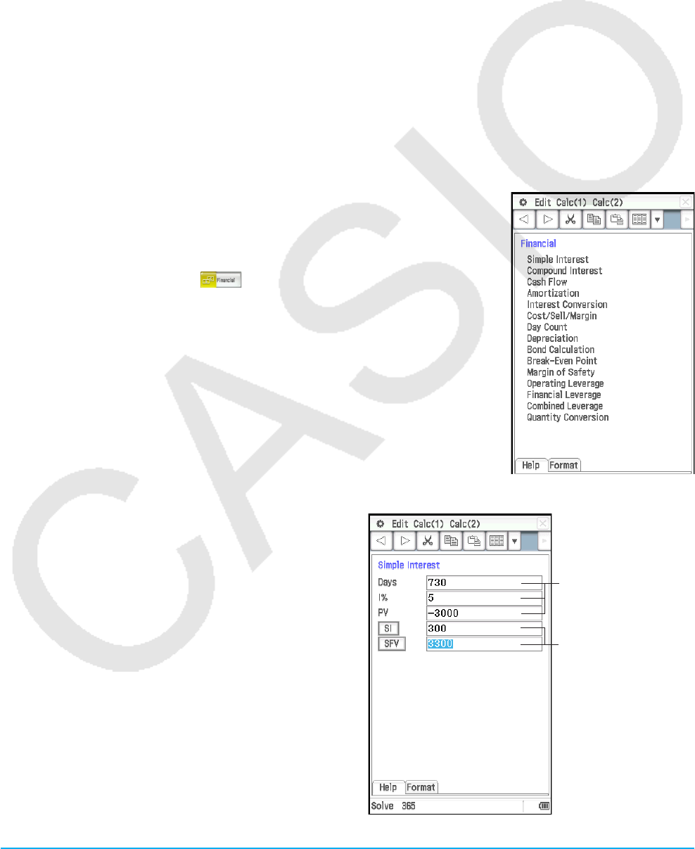
Chapter 11: Financial Application 186
Chapter 11:
Financial Application
You can use the Financial application to perform a variety of financial calculations.
Important!
Financial calculation rules and practices can differ according to country, geographic area, or financial institution.
It is up to you to determine whether the calculation results produced by this calculator are compatible with the
financial calculation rules that apply to you.
11-1 Financial Application Basic Operations
• Each time you select a calculation from the Financial application menu, a new page is added for that
calculation.
• Each page has input boxes for inputting values and input/calculation boxes that can be used both to input
values and display calculation results.
The examples below explain basic operations using the Financial application page.
Example: What is the final value after two years (730 days) of a $3,000
investment earning 5.0% simple interest? Also calculate the final
value during the same period for the same investment when the
simple interest rate is 3%.
1. On the application menu, tap to start the Financial application.
• If this is the first time the application is being started up, the Financial menu
window will appear.
2. Tap [Calc(1)] and then [Simple Interest] (or, on the Financial menu window,
tap “Simple Interest”).
• This will add a new page for performing the calculation (page 1) and
display the “Simple Interest” page.
Financial menu window
3. Input the following information: Days = 730; I%
(annual interest rate) = 5; PV (present value) =
−3000.
4. Tap [SI] and then [SFV].
• This will display the calculation results for simple
interest (SI) and simple future value (SFV =
principal + interest).
Input box
Input values in the box.
Input/calculation box
Input values when
required. For
calculation, tap the
button to the left of the
box.
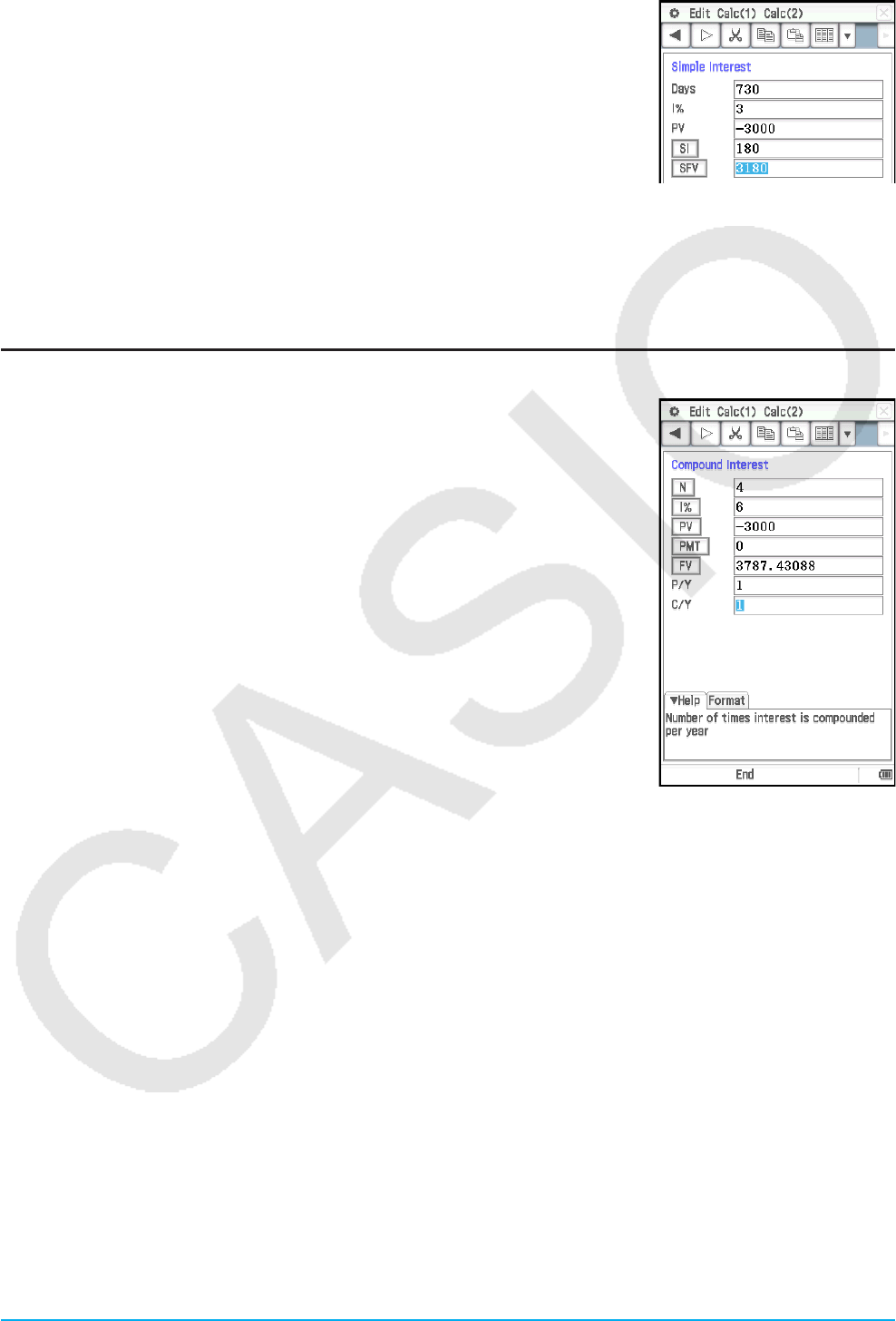
Chapter 11: Financial Application 187
5. Tap [Calc(1)] and then [Simple Interest] again.
• This adds a new page (page 2). The new page will inherit value input on
the previous page (under initial settings).
6. Change the I% value to 3, tap [SI], and then [SFV].
• The SI and SFV values are updated in accordance with the new I% value.
Tip
• If the cursor is in an input/calculation box, “Solve” will appear on the left side of the status bar. You can tap this to
complete the calculation instead of tapping the box to the left of the input/calculation box.
• Financial application pages remain in memory even if you exit the Financial application. The next time you start up the
Financial application, the page that was displayed the last time you exited the application will appear first.
Page Operations
As shown in the sample operation above, each time you select a calculation
from the Financial application menu, a new page is added for that calculation.
The following types of operations can be performed on a page.
• Display the previous page or following page*1 ..............................Tap , / .
• Display help about the currently selected field on the page ....... Tap [Help] tab
• Change the settings of the displayed page’s calculation ....... Tap [Format] tab
• Delete the currently displayed Financial application page*2
........................................................................................Edit - Delete Page
• Clear all the values from the displayed Financial application page
..........................................................................................Edit - Clear Page
• Delete all the Financial application pages and display the Financial
application initial screen*3 ..................................................... Edit - Clear All
*1 , and/or . on the toolbar indicates that there is a page before and/or
after the current page. < and/or > indicates there is no page before and/
or after the current page. In this case, tapping < or > will not change to
another page.
*2 Executing this operation when there is only one page will display the Financial menu window.
*3 Executing this operation will display the Financial menu window.
Note: If the currently displayed page is part way through a series of pages that are in memory, selecting
a calculation from the [Calc(1)] or [Calc(2)] menu will create a new page in the series and delete
everything after it. If you select a new calculation while page 3 of 5 is displayed, for example, the newly
created page will become 4 of 4.

Chapter 11: Financial Application 188
Configuring Financial Application Settings
Most financial calculations require that you define certain general parameters that affect the results they
produce. For example, you need to specify whether you use a 360-day or 365-day year, whether payments are
made at the beginning of a period or end of a period, etc.
The following are settings required by the Financial application.
Default settings
Configure default settings using the Financial
Format dialog box. These settings are applied
whenever you add a new page with the
Financial application.
Local settings
Configure local settings on the Format tab of
each page, or by tapping the status bar. Local
settings are applied to the currently displayed
page only.
Local settings are generally applied to the
currently displayed page only.
Note, however, that if you have one page
displayed (Page A) and then add a new page
(Page B), the initial settings of any Page B
local setting items that are also on Page A
will be those inherited from Page A. Default
settings will be applied as the initial settings of items on Page B that are not also included on Page A.
The table below shows setting items for each type of Financial calculation.
Setting Items
Financial Calculation
Simple
Interest
Compound
Interest
Amortization
Day Count Bond
Calculation
Break-even
Point
Days in Year Yes Yes Yes
Payment Date Yes Yes
Date Format Yes Yes
Automatically copy
common fields to
new calculation
Yes Yes Yes Yes Yes Yes
Odd Period Yes
Compounding
Frequency Yes
Bond Interval Yes
Profit Amount/Ratio Yes
Break-Even Value Yes
• The “Date Format” and “Automatically copy common fields to new calculation” setting items in the above table
can be configured on the Financial Format dialog box only.
• The “Automatically copy common fields to new calculation” option is automatically applied (and is the only
option available) for any setting item that is not included in the above table.
• For details about each of the setting items, see “Financial Format Dialog Box” (page 41).

Chapter 11: Financial Application 189
11-2 Performing Financial Calculations
The calculations in the table below can be performed with the Financial application. For actual calculation
examples, refer to the sections of this manual or the separate “Examples” booklet shown in the “Example”
column.
To perform this type of calculation: Select this menu item: Example
Interest without compounding based on the number of days money is
invested
Calc(1) - Simple
Interest Page 186
Interest based on compounding parameters specified by you Calc(1) - Compound
Interest 1101
Value of money paid out or received in varying amounts over time Calc(1) - Cash Flow 1102
Interest and principal portions of a payment or payments Calc(1) - Amortization 1103
Effective or nominal interest rate for interest compounded multiple
times during a year
Calc(1) - Interest
Conversion 1104
Cost, selling price, or margin of profit on an item given the other two
values
Calc(1) - Cost/Sell/
Margin 1105
Number of days between two dates, or the date that is a specified
number of days from another date Calc(1) - Day Count 1106
Amount that a business expense can be offset by income
(depreciated) over a given year Calc(1) - Depreciation 1107
Purchase price or annual yield of a bond Calc(1) - Bond
Calculation 1108
Amount you must sell to break even or to obtain a specified profit, as
well as amount of profit or loss on particular sales
Calc(2) - Break-Even
Point 1109
How much sales can be reduced before incurring losses Calc(2) - Margin of
Safety 1110
Degree of change in net earnings arising from a change in sales
amount
Calc(2) - Operating
Leverage 1111
Degree of change in net earning arising from a change in interest paid Calc(2) - Financial
Leverage 1112
Combined effects of operating and financial leverages Calc(2) - Combined
Leverage 1113
Number of items sold, selling price, or sales amount given other two
values; number of items manufactured, unit variable cost, or total
variable cost given other two values
Calc(2) - Quantity
Conversion 1114
11-3 Calculation Formulas
For information about terms used in formulas that are not explained in detail below, refer to “11-5 Input and
Output Field Names”.
Simple Interest
365-day Mode:
360-day Mode:
i
= I%
100
SI' = Days
365 × PV × i
SI' = Days
360 × PV × i
SI = –SI'
SFV = –(PV + SI')
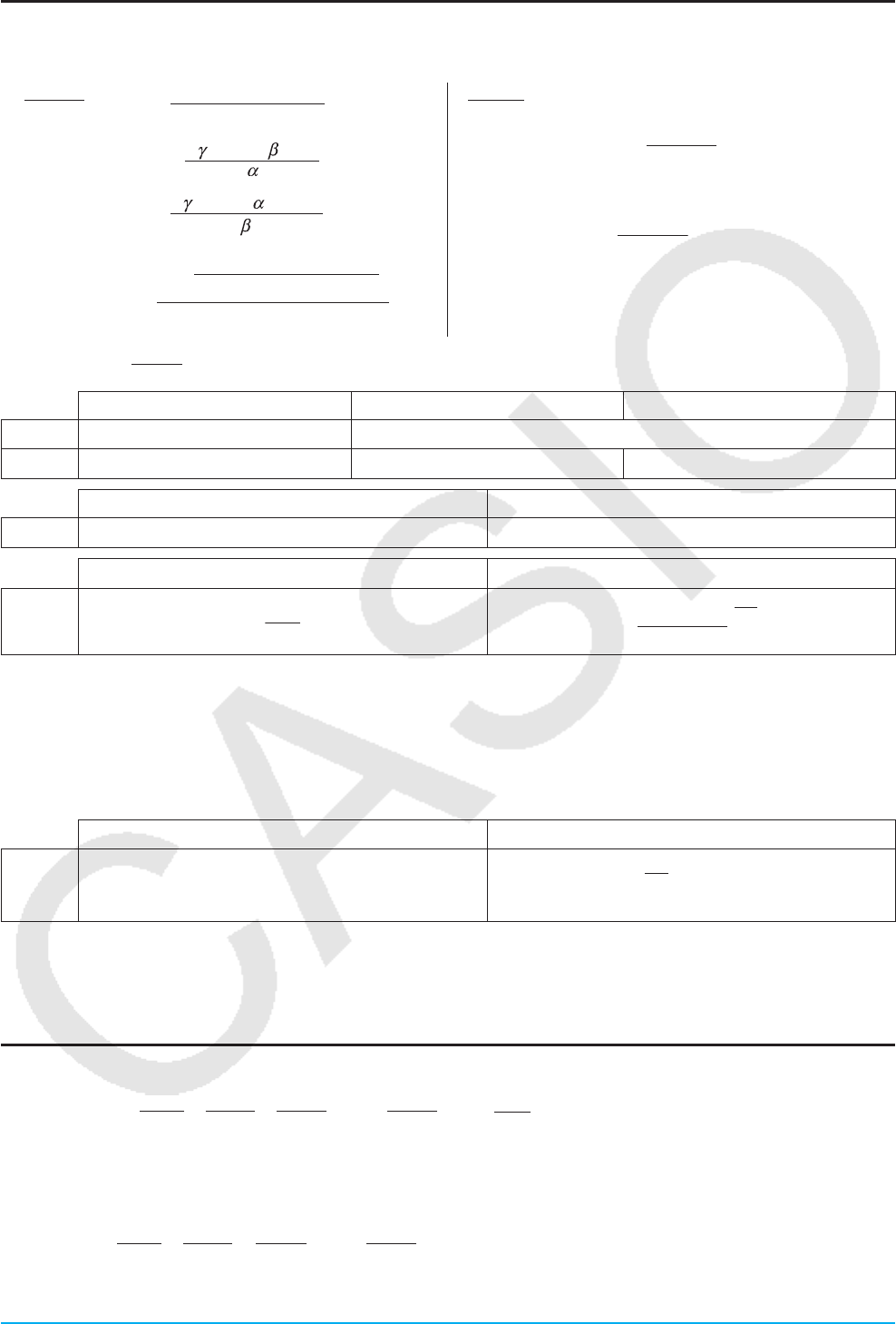
Chapter 11: Financial Application 190
Compound Interest
uWhen calculating PV, PMT, FV, n
I
% 0 PV = –
× PMT – × FV
β
γ
α
PMT = – PV – F
V
FV = – PV – PMT
n =
log (1 + iS ) × PMT – FV × i
(1 + iS ) × PMT + PV × i
{}
log (1 + i)
I
% = 0 PV = – (PMT × n + FV )
PMT = – n
PV + FV
FV = – (PMT × n + PV )
n = PMT
PV + FV
–
= (1 + i × S) × i
1 –
β
α
When “Odd Period” is “Off” When “Odd Period” is “CI” When “Odd Period” is “SI”
= (1 + i) –n (1 + i) –Intg (n)
= 1(1 + i) Frac (n) 1 + i × Frac (n)
When “Payment Date” is “End” When “Payment Date” is “Begin”
S = 01
When P/Y = C/Y = 1 When P/Y 1 and/or C/Y 1
i =
uWhen calculating I%
i (effective interest rate) is calculated using Newton’s Method.
× PV + × PMT + × FV = 0
I% is calculated from i using the formulas below:
When P/Y = C/Y = 1 When P/Y 1 and/or C/Y 1
I% =
Interest (I%) calculations are performed using Newton’s Method, which produces approximate values whose
precision can be affected by various calculation conditions. Interest calculation results produced by this
application should be used keeping the above in mind, or results should be confirmed separately.
Cash Flow
NPV = CF0 + + + + … +
(1+ i)
CF1
(1+ i)2
CF2
(1+ i)3
CF3
(1+ i)n
CFn (
=100
% , n: natural number up to 80)
NFV = NPV × (1 + i )n
IRR is calculated using Newton’s Method.
0 = CF0 + + + + … +
(1+ i)
CF1
(1+ i)2
CF2
(1+ i)3
CF3
(1+ i)n
CFn
100
I%I%
(1 + ) – 1
C/Y
P/Y
100 × [C/Y ]
i × 100
( )
× C/Y × 100
(1 + i )–1
P/Y
C/Y
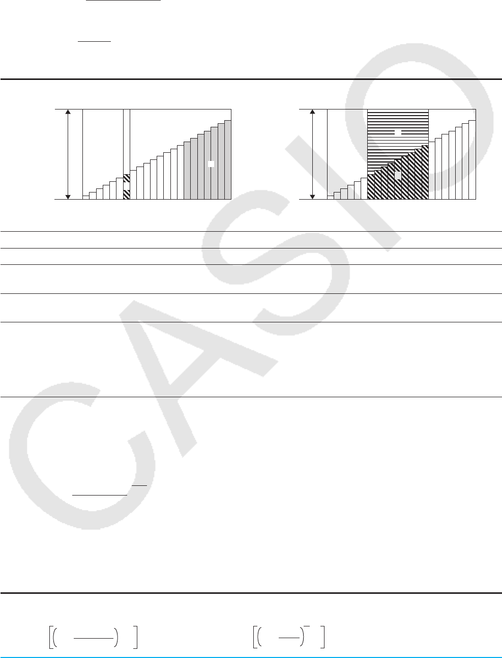
Chapter 11: Financial Application 191
In this formula, NPV = 0, and the value of IRR is equivalent to i × 100. It should be noted, however, that
minute fractional values tend to accumulate during the subsequent calculations performed automatically by
the ClassPad, so NPV never actually reaches exactly zero. IRR becomes more accurate the closer that NPV
approaches to zero.
PBP =
{
0 .................................. (CF0 t 0)
n – NPVn
NPVn+1 – NPVn
(Other than those above)
...
NPVn = Σ
n
k = 0
CFk
(1 + i)
k
n: smallest positive integer that satisfies the conditions
NPVn s 0, 0 s NPVn+1, or 0
Amortization
c
a
1 payment
Number of payments
1 PM1 PM2 Last............ ................... ..........
b
1 payment
Number of payments
1 PM1 PM2 Last............. ................ .............
e
d
a: interest portion of payment PM1 (INT)
b: principal portion of payment PM1 (PRN)
c: principal balance upon completion of
payment PM2 (BAL)
d: total principal paid from payment PM1 to
payment PM2 (ΣPRN)
e: total interest paid from payment PM1 to
payment PM2 (ΣINT) a + b = one repayment (PMT)
BAL0 = PV
(when “Payment Date” is “End”)
INT1 = 0, PRN1 = PMT
(when “Payment Date” is “Begin”)
Converting between the Nominal Interest Rate and Effective Interest Rate
The nominal interest rate (I % value input by user) is converted to an effective interest rate (I % ' ) for installment
loans where the number of annual payments is different from the number of annual compound calculation
periods.
I%' = I%
(1 + )– 1
[C/Y ]
[P/Y ]
{ }
×
100
100 × [C/Y ]
The following calculation is performed after conversion from the nominal interest rate to the effective interest
rate, and the result is used for all subsequent calculations.
i = I%' ÷ 100
Interest Conversion
EFF = n
APR/100
1 + – 1 × 100
n
APR = 100
EFF
1 + – 1 × n × 100
1
n
PM1=I PM1–1 ×I × ()
PM1=+PM1–1 ×
PM2=PM2–1 +PM2
Σ =PM1 +PM1+1 + … + PM2
PM2
PM1
Σ =PM1 +PM1+1 + … + PM2
PM2
PM1

Chapter 11: Financial Application 192
Cost/Sell/Margin
CST = SEL 100
MRG
1 – SEL =
100
MRG
1 –
CST MRG(%) = SEL
CST
1 – × 100
Depreciation
uStraight-Line Method
YR1(PV – FV )
SL1 = n12
×(PV – FV )
SLj = n
12 – YR1(YR112)
(PV – FV )
n12
×
SLn+1 =
uFixed-Percentage Method
100
YR1
I%
FP1 = PV × 12
× 100
I%
FPj = (RDVj–1 + FV ) × FPn+1 = RDVn (YR112)
RDV1 = PV – FV – FP1 RDVj = RDVj–1 – FPj RDVn+1 = 0 (YR112)
uSum-of-the-Years’-Digits Method
n (n + 1)
Z = 22
(Intg(n' ) + 1)(Intg(n' ) + 2 × Frac(n' ) )
Z' =
SYD1 = YR1
12
n
Z×(PV – FV )n' – j + 2
Z' )(PV – FV – SYD1)( j1)SYDj = (
RDV1 = PV – FV – SYD1RDVj = RDVj –1 – SYDj
n' – (n + 1) + 2
Z' )(PV – FV – SYD1)(YR112)
12 – YR1
12
×SYDn+1 = (
12
YR1
n' = n –
uDeclining-Balance Method
100n
YR1I%
D
B1 = PV × 12
× RDV1 = PV – FV – DB1 100n
I%
×
DBj = (RDVj–1 + FV )
RDVj = RDVj–1 – DB
j
(YR112)
DBn +1 = RDVn (YR112)
RDVn+1 = 0
Bond Calculation
uTerms in the formulas
PRC: price per $100 of face value
RDV: redemption price per $100 of face value
CPN: coupon rate (%)
YLD: annual yield (%)
M: number of coupon payments per year
(1 = Annual, 2 = Semi-annual)
N: number of coupon payments until maturity (n is
used when “Term” is specified for “Bond Interval”.)
INT: accrued interest
CST: price including interest
A: accrued days
D: number of days in coupon period where settlement occurs
B: number of days from purchase date until next coupon payment date = D – A
D
Issue date
Redemption date (d2)
Purchase date (d1) Coupon payment dates
AB

Chapter 11: Financial Application 193
uPRC when “Date” is specified for “Bond Interval”
For one or fewer coupon period to redemption:
PRC = − +
RDV + CPN/M
1+(B/D × (YLD/100)/M)A/D × CPN/
M
For more than one coupon period to redemption:
INT = −A/D × CPN/M CST = PRC × INT
PRC = − –
RDV Σ
N
k=1
(1 + (YLD/100)/M)
(N–1+B/D )(1 + (YLD/100)/M)
(k–1+B/D )+
CPN/M
()
A/D × CPN/
M
uPRC when “Term” is specified for “Bond Interval”
PRC = − INT
= 0 CST
= PRC
–
RDV Σ
n
k=1
n k
CPN/M
(1 + (YLD/100)/M) (1 + (YLD/100)/M)
()
uYLD
The Financial application performs annual yield (YLD) calculations using Newton’s Method, which produces
approximate values whose precision can be affected by various calculation conditions. Because of this, annual
yield calculation results produced by this application should be used keeping the above in mind, or results
should be confirmed separately.
Break-Even Point
uProfit (Profit Amount/Ratio Setting: Amount (PRF))
PRC – VCU
FC + PRF
QBE = PRC – VCU
FC + PRF
SBE =× PRC
uProfit Ratio (Profit Amount/Ratio Setting: Ratio (r%))
PRC × – VCU
QBE = FC
100
r%
1–
× PRC
PRC × – VCU
SBE =FC
100
r%
1–
Margin of Safety
SAL
M
OS = SAL – SBE
Financial Leverage
EBIT – ITR
DFL = EBIT
Operating Leverage
SAL – VC – FC
D
OL = SAL – VC
Combined Leverage
SAL – VC – FC – ITR
DCL = SAL – VC
Quantity Conversion
SAL = PRC × QTY VC = VCU × QTY

Chapter 11: Financial Application 194
11-4 Financial Calculation Functions
ClassPad mathematical functions can be used to perform some Financial application calculations. ClassPad
mathematical functions can be selected on the [Financial] submenu of the [Action] menu of the Main application
or eActivity application.
The table below shows a list of mathematical functions that perform financial calculations. For descriptions of
the arguments shown in each syntax and the values returned by each function, refer to “11-5 Input and Output
Field Names”.
Financial
Calculation Function Syntax This function
returns:
Simple
Interest
simpInt simpInt(Days,I%,PV) SI
simpFV simpFV(Days,I%,PV) SFV
Compound
Interest
cmpdFV*1cmpdFV(N,I%,PV,PMT,P/Y,C/Y) FV
cmpdIR*1cmpdIR(N,PV,PMT,FV,P/Y,C/Y) I%
cmpdN*1cmpdN(I%,PV,PMT,FV,P/Y,C/Y) N
cmpdPmt*1cmpdPmt(N,I%,PV,FV,P/Y,C/Y) PMT
cmpdPV*1cmpdPV(N,I%,PMT,FV,P/Y,C/Y) PV
Cash Flow
cashIRR cashIRR(Cash) IRR
cashNFV cashNFV(I%,Cash) NFV
cashNPV cashNPV(I%,Cash) NPV
cashPBP cashPBP(I%,Cash) PBP
Amortization
amortBal amortBal(PM1,PM2,I%,PV,PMT,P/Y,C/Y) BAL
amortInt amortInt(PM1,PM2,I%,PV,PMT,P/Y,C/Y) INT
amortPrn amortPrn(PM1,PM2,I%,PV,PMT,P/Y,C/Y) PRN
amortSumInt amortSumInt(PM1,PM2,I%,PV,PMT,P/Y,C/Y) ΣINT
amortSumPrn amortSumPrn(PM1,PM2,I%,PV,PMT,P/Y,C/Y) ΣPRN
Interest
Conversion
convEff convEff(N,I%) EFF
convNom convNom(N,I%) APR
Cost/Sell/
Margin
priceCost priceCost(Sell,Margin) Cost
priceSell priceSell(Cost,Margin) Sell
priceMargin priceMargin(Cost,Sell) Margin
Day Count dayCount dayCount(MM1,DD1,YYYY1,MM2,DD2,YYYY2) Days
Bond
Calculation
bondPriceDate*2bondPriceDate(MM1,DD1,YYYY1,MM2,DD2,
YYYY2,RDV,CPN,YLD) {PRC,INT,CST}
bondPriceTerm*3bondPriceTerm(N,RDV,CPN,YLD) {PRC,INT,CST}
bondYieldDate*2bondYieldDate(MM1,DD1,YYYY1,MM2,DD2,
YYYY2,RDV,CPN,PRC) YLD
bondYieldTerm*3bondYieldTerm(N,RDV,CPN,PRC) YLD
*1 P/Y and C/Y can be omitted. When they are omitted, calculations are performed using P/Y=1 and C/Y=1.
*2 “Date” must be specified for the Financial Format “Bond Interval”.
*3 “Term” must be specified for the Financial Format “Bond Interval”.

Chapter 11: Financial Application 195
11-5 Input and Output Field Names
The list below shows the names of the input and output fields displayed on the various Financial application
pages. When performing a calculation on your ClassPad, you can also get information using the [Help] tab.
APR: Nominal interest rate (as a percent)
BAL: Balance of principal after PM2
C/Y: Number of times interest is compounded per
year
Cash: List of income or expenses (up to 80 entries)
Cost (Cost/Sell/Margin): Production cost
Cost (Bond Calculation): Cost of bond (price plus
partial year interest)
CPN: Annual coupon rate
d1: Month (1-12); Day (1-31); Year (1902-2097)
d2: Month (1-12); Day (1-31); Year (1902-2097)
Days (Day Count): Number of days from d1 to d2
Days (Simple Interest): Number of days in investment
period
DB: Depreciation for year j calculated using the
declining-balance method
DCL: Degree of combined leverage
DFL: Degree of financial leverage
DOL: Degree of operating leverage
EBIT: Earnings before interest and taxes
EFF: Effective interest rate (as a percent)
FC: Fixed costs
FP: Depreciation for year j using the fixed-percentage
method
FV: Future value
NFV: Net future value
NPV: Net present value
P/Y: Number of installment periods per year
PBP: Payback period
PM1: Number of first installment period in interval
under consideration
PM2: Number of last installment period in interval
under consideration
PMT: Amount paid each period
PRC (Bond Calculation): Price of bond
PRC (Break-Even Point, Quantity Conversion):
Selling price per unit
PRF: Profit
PRN: Principal portion of PM1
PV: Present value (initial investment)
QBE: Number of units to be sold
QTY (Manufacturing): Number of units manufactured
QTY (Sales): Number of units sold
r%: Proportion of sales amount retained as a profit
(as a percent)
RDV (Bond Calculation): Redemption value
RDV (Depreciation): Residual value after depreciation
for year j
SAL: Amount obtained from sales
SAL (Operating Leverage): Amount currently
obtained from sales
SBE (Break-Even Point): Amount that must be
obtained from sales to break even
SBE (Margin of Safety): Break-even sales (amount
that must be obtained from sales to break even)
Sell: Selling price
SFV: Simple future value (principal + interest)
SI: Simple interest
SL: Depreciation for year j using the straight-line
method
sumINT: Total interest paid from PM1 to PM2
(inclusive)
sumPRN: Total principal paid from PM1 to PM2
(inclusive)
SYD: Depreciation for year j using the sum-of-the-
years’-digits method
VC: Variable cost for a certain level of production
VCU: Variable cost per unit
YLD: Yield to maturity (as a percent)
YR1: Number of depreciable months in first year
I%: Annual interest rate (as a percent)
INT (Amortization): Interest portion of PM1
INT (Bond Calculation): Interest accumulated during
partial year portion of investment period
INT (Financial Leverage, Combined Leverage):
Interest to be paid to bondholders
IRR: Interest rate of return
j: Year for which depreciation is being calculated
Margin: Margin of profit (portion of selling price not
absorbed by cost of production)
MOS: Margin of safety (portion of sales amount above
break-even point)
N (Bond Calculation): Number of periods
N (Compound Interest): Number of installment
periods
N (Depreciation): Number of years over which
depreciation occurs
N (Interest Conversion): Number of times interest is
compounded per year
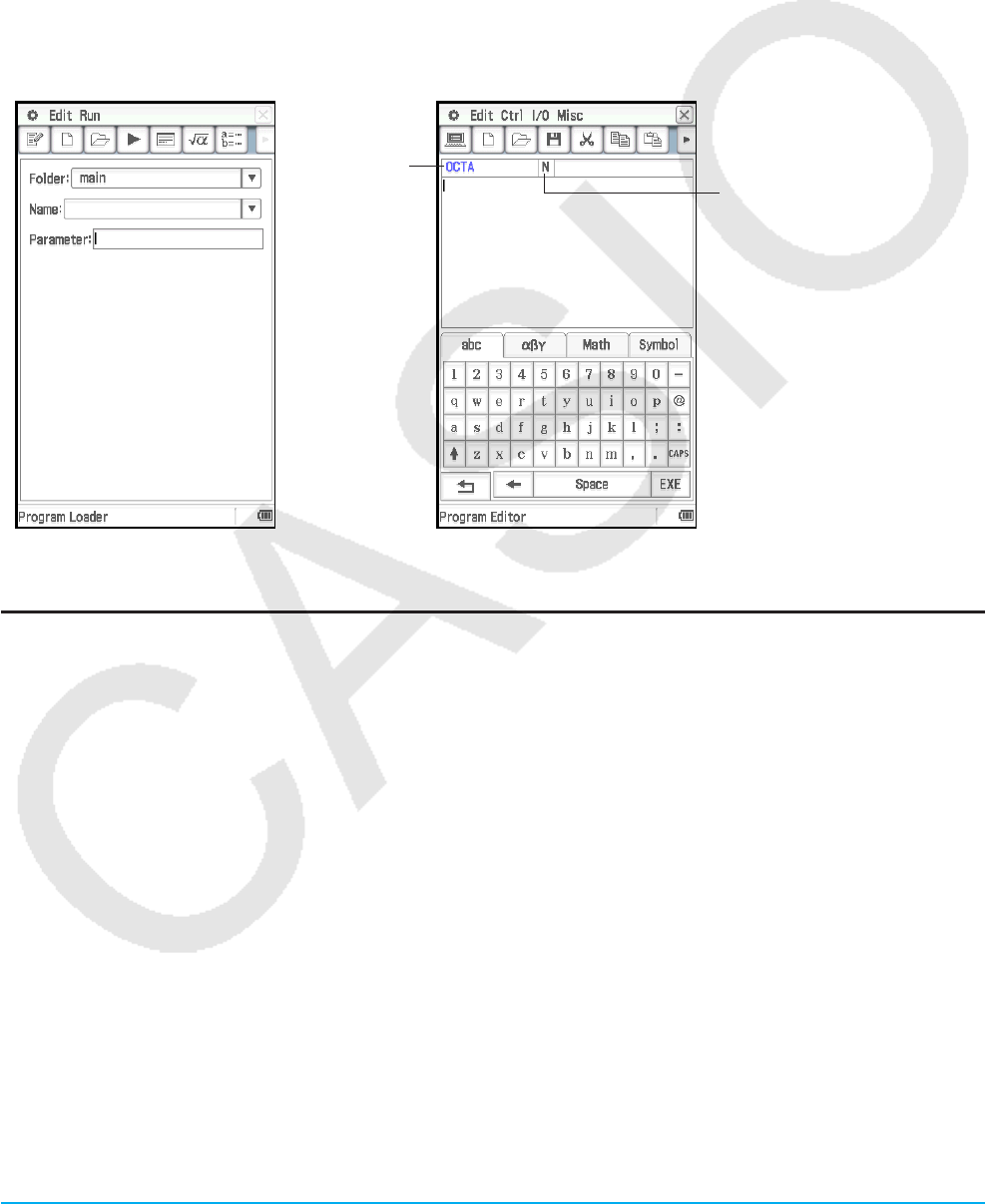
Chapter 12: Program Application 196
Chapter 12:
Program Application
The Program application comes in handy when you need to perform the same calculation a number of times.
You can create programs that automate graphing and other operations.
The Program application consists of a Program Editor for inputting and editing programs, and a Program
Loader for loading and executing existing programs.
• The Program Loader window appears when you start up the Program application.
• To display the Program Editor window, tap P on the Program Loader window, or tap O, [Window] and then
[Program Editor].
Program Loader window Program Editor window
File name
File type
N: Program file
T: Text file
F: User-defined
function file
Program Application-Specific Menus and Buttons
Program Loader window
• Display the Program Editor window .........................O - Window - Program Editor, Edit - Open Editor or P
• Run a program ....................................................................................................... Run - Run Program or .
Program Editor window
• Display the Program Loader window ................................................... O - Window - Program Loader or )
• Save a file ..........................................................................................................Edit - Save File - Save or {
• Save a file under a new name ................................................................................Edit - Save File - Save As
• Close a file ............................................................................................................................. Edit - Close File
• Convert a file to a program file .......................................................................Edit - Mode Change - 'Normal
• Convert a file to a text file .................................................................................. Edit - Mode Change - 'Text
• Convert a file to an edit prohibited program file ..................................................................... Edit - Compress
• Search for a newly specified text string ..................................................... Edit - Search - New Search or e
• Search again for a previously specified text string .....................................Edit - Search - Search Next or r
• Jump to the beginning/end of a program .................................Edit - Search - Jump to Top / Jump to Bottom
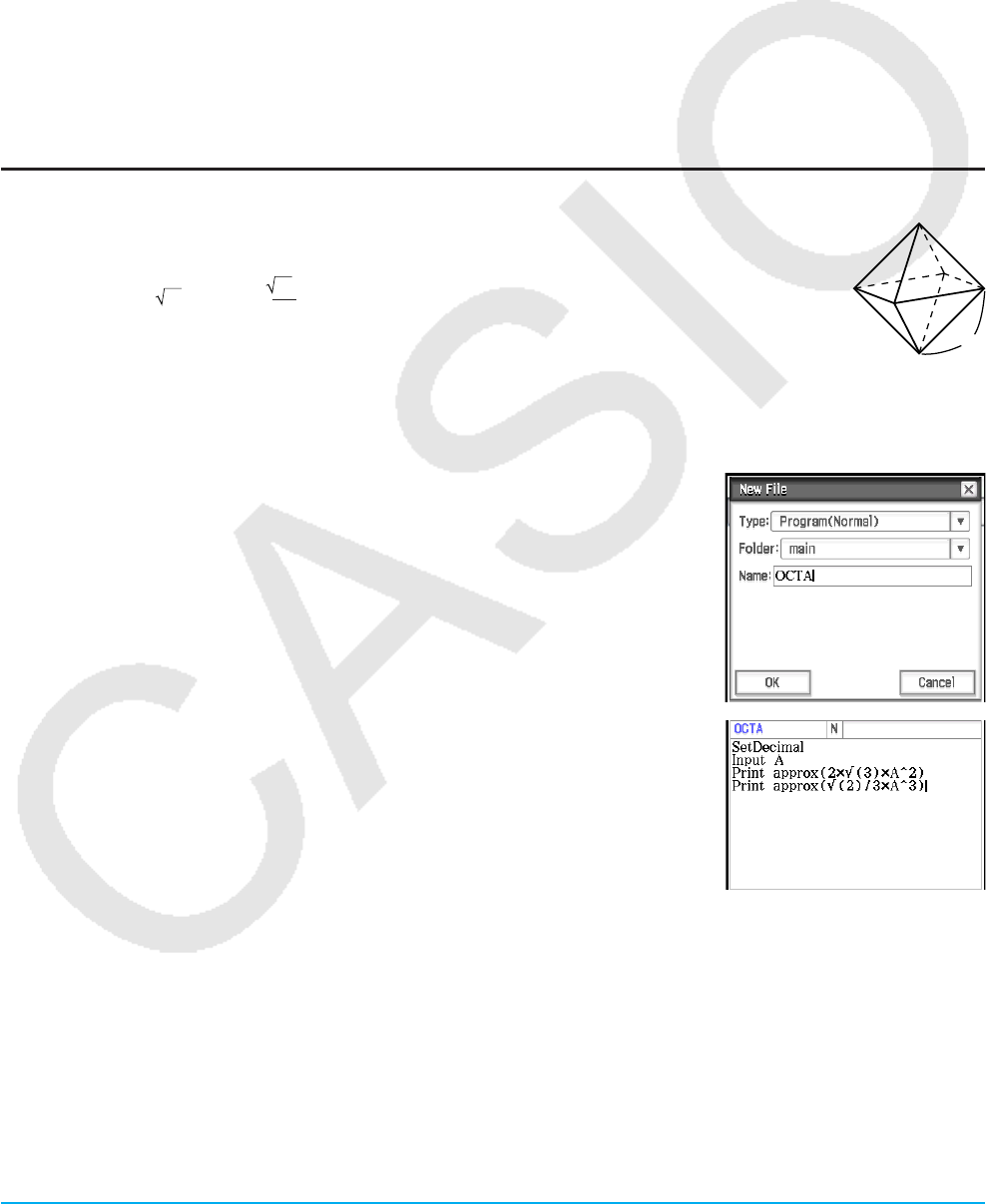
Chapter 12: Program Application 197
• Input a command (see “12-4 Program Command Reference”) ................................................. Ctrl, I/O, Misc
Program Loader window and Program Editor window common commands
• Display the Program Output window .....................................................O - Window - Program Output or _
• Display the Text File Contents window ....................................................... O - Window - Text File Contents
• Display the Main application work area window .................................................... O - Window - Main or ~
• Create a new file ............................................................................................................ Edit - New File or O
• Open an existing file .....................................................................................................Edit - Open File or ~
12-1 Creating and Running Program
This section explains the steps you need to perform in order to create and run a program.
Creating a Program
Example: To create a program named “OCTA” that uses the formulas below determines the
surface area (S) and volume (V) of a regular octahedron
S = 2 3 A2, V = 2
3 A3
uTo create and save a new program
1. On the Program Loader or Program Editor window, tap O.
2. On the dialog box that appears, configure the settings for the new file as described below.
• Leave the [Type] setting as “Program(Normal)”.
• Tap the [Folder] down arrow button and then select the folder where you
want to save the program file.
• In the [Name] box, input up to eight bytes for the program file name. Here,
we will input “OCTA”.
3. Tap [OK]. This displays a blank Program Editor window.
4. Input the necessary expressions and commands. Here, we will input the
program shown in the nearby screenshot.
• Each mathematical expression and command must be followed either by a
carriage return or colon (:).
• Use the menus shown below to input the “SetDecimal”, “Input”, and “Print”
commands.
[Misc] - [Setup(1)] - [SetDecimal]
[I/O] - [Input] - [Input]
[I/O] - [Output] - [Print]
For information about the menus, syntax, operation, and other details about commands, see “12-4 Program
Command Reference”.
• Calculation results of arguments that are input using the “approx(” function are displayed using rounded
decimal parts. Use the soft keyboard for input.
A
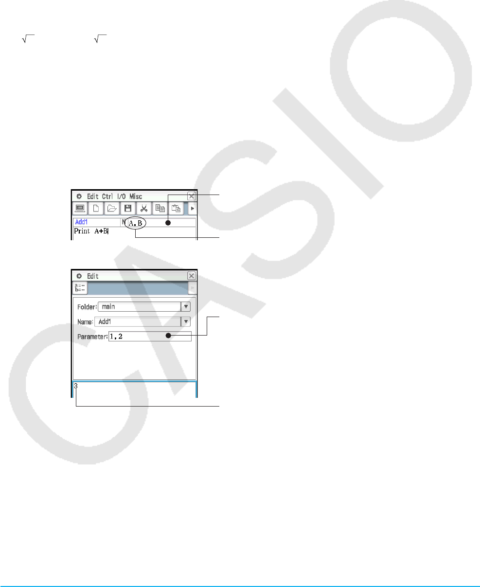
Chapter 12: Program Application 198
5. After the program is the way you want, tap {, or tap [Edit], [Save File] and then [Save] to save it.
• To run this program see “Running a Program” on page 199.
• If a message appears when you try to save the program, make the necessary corrections and try again.
For details about making corrections to a program, see “12-2 Debugging a Program”.
Tip
• The file name you input in step 2 of the above procedure is subject to the same rules as folder and variable names. For
more information, see “Folder and Variable Name Rules” on page 31.
• To input a program and save it without running it, perform the above procedure up to step 5, and then tap [Edit] and then
[Close File].
• If you want to use the calculation results produced by program execution in another calculation, include a line in the
program that uses the “⇒” command to assign the calculation result to a variable. For example, you could add the line
below to the above example program to assign the calculated surface area to variable S and the volume to variable V.
2 × (3) × A^2 ⇒ S: (2)/3 × A^3 ⇒ V
Note that calculation results produced within programs are not stored in Ans memory.
Pausing Program Execution
You can specify where execution of a program should pause by including either a Pause command or a Wait
command inside the program. For details about each command, see “12-4 Program Command Reference”.
Configuring Parameter Variables and Inputting Their Values When Creating a Program
If you input the names of variables used in a program into the parameter variable box when creating a program
on the Program Editor window, you will be able to input values for the variables on the Program Loader window
when you run the program.
Example: Parameter variable box
Indicates variables named “A” and “B” are used
within the program.
Parameter value input box
Inputting 1, 2 before running the program
assigns A = 1 and B = 2.
Executing the program produces the result
A + B = 1 + 2 = 3.
Tip: Variables that are specified as parameter variables within a program are automatically treated as local variables. For
information about local variables, see “Local” in the “Command List” (page 214).
Using a Subroutine to Call another Program
Including the name of another program file inside of a program causes execution to jump to the specified
program file.
Syntax: <program name>({<parameter variable name 1>,<parameter variable name 2>, ... })
The program that execution jumps from is called the “main program”, while the program to which execution
jumps is called a “subroutine”.
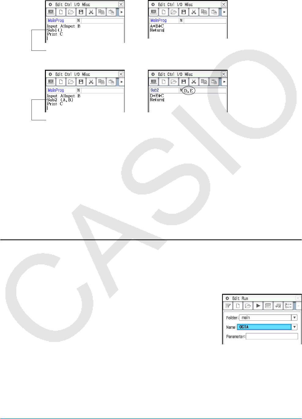
Chapter 12: Program Application 199
When program execution returns to the main program, it resumes from the point immediately after the
command that jumped to the subroutine.
Example 1: Main Program: Subroutine: “Sub1”
Example 2: Main Program: Subroutine: “Sub2”
Using Strings in a Program
A string is a series of characters inside of quotation marks. In a program, strings are used to specify display
text. A string made up of numbers (like “123”) or an expression (like “x–1”) cannot be processed as a
calculation.
Tip: To include quotation marks (") or a backslash (\) in a string, put a backslash (\) in front of the quotation marks (") or
backslash (\).
Examples:
To include Japan: “Tokyo” in a string To include main\abc in a string
Print "Japan:\"Tokyo\"" Print "main\\abc"
Running a Program
Example: To run the “OCTA” program created under “Creating a Program” (page 197) to calculate the surface
areas and volumes of three regular octahedrons, the lengths of whose sides are 7, 10, and 15
uTo run a program
1. On the Program Loader window, specify the program you want to run.
(1) Tap the [Folder] down arrow button, and then select the folder you want.
(2) Tap the [Name] down arrow button, and then tap the name of the file.
Here, we will tap “OCTA”.
• In this example, the “Parameter” input box is left blank. For information
about using the “Parameter” input box, see “Configuring Parameter
Variables and Inputting Their Values When Creating a Program” (page 198).
2. Tap ., or tap [Run] and then [Run Program] to run the program.
• This runs the program and displays a dialog box prompting for input of a value for variable A (length of one
side).
Jumps to subroutine program “Sub1”
Assigns the values of main program variables “A” and “B” to the parameter
variables (D and E) in subroutine “Sub2”, and then jumps to subroutine “Sub2”.
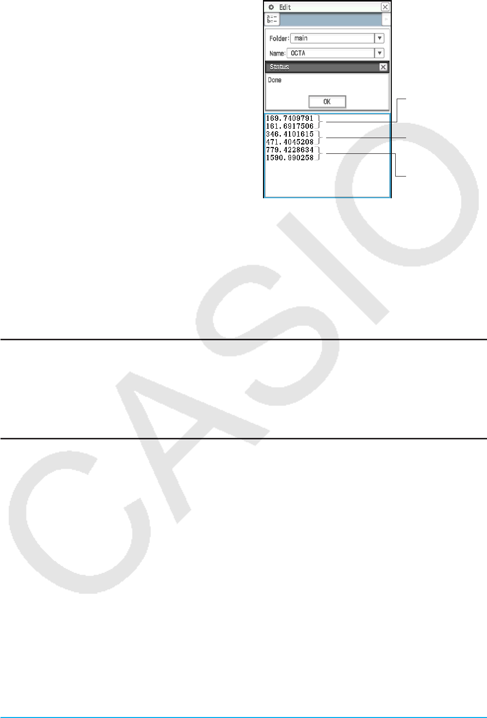
Chapter 12: Program Application 200
3. Input a side length of 7 and tap [OK].
• A Program Output window, showing the execution
results of the program, will appear in the lower half
of the screen.
• On the “Done” dialog box that appears after program
execution is complete, tap [OK].
4. Tap the Program Loader window and repeat steps 2
and 3 for sides of length 10 and 15.
Tip
• The Program Output window can be displayed by tapping O, [Window] and then [Program Output], or by tapping _ on
the Program Loader window. The Program Output window also appears whenever the DispText command is executed in
a program.
• Program Output window contents will remain displayed even if you run a different program. To clear the current contents,
tap [Edit] - [Clear All] while the Program Output window is displayed. Executing the ClrText command also clears the
currently stored Program Output window.
• You can run a program from the Main application or the eActivity application. For more information, see “2-12 Running a
Program in the Main Application”.
Terminating Program Execution
Pressing c while a program is running terminates the program.
Tip: Pressing c does not terminate the program if program execution is already paused by the Pause command
(see “12-4 Program Command Reference”). In this case, tap X on the status bar to resume program execution, and
then press c.
Creating a Text File
Use the procedure below to create a text file using the Program Editor window. You can also convert a
previously saved program file to a text file.
uTo create and save a new text file
1. On the Program Loader or Program Editor window, tap O.
2. On the dialog box that appears, configure the settings for the new file as described below.
• Tap the [Type] down arrow button and then select “Program(Text)”.
• Tap the [Folder] down arrow button and then select the folder where you want to save the text file.
• In the [Name] box, input up to eight bytes for the text file name.
3. Tap [OK]. This displays a blank Program Editor window.
4. Input the text you want.
5. After input is complete, tap {, or tap [Edit], [Save File] and then [Save] to save it.
uTo change a program file to a text file
While a program file is open, tap [Edit], [Mode Change], and then ['Text].
Calculation results
when A = 7
Calculation results
when A = 10
Calculation results
when A = 15
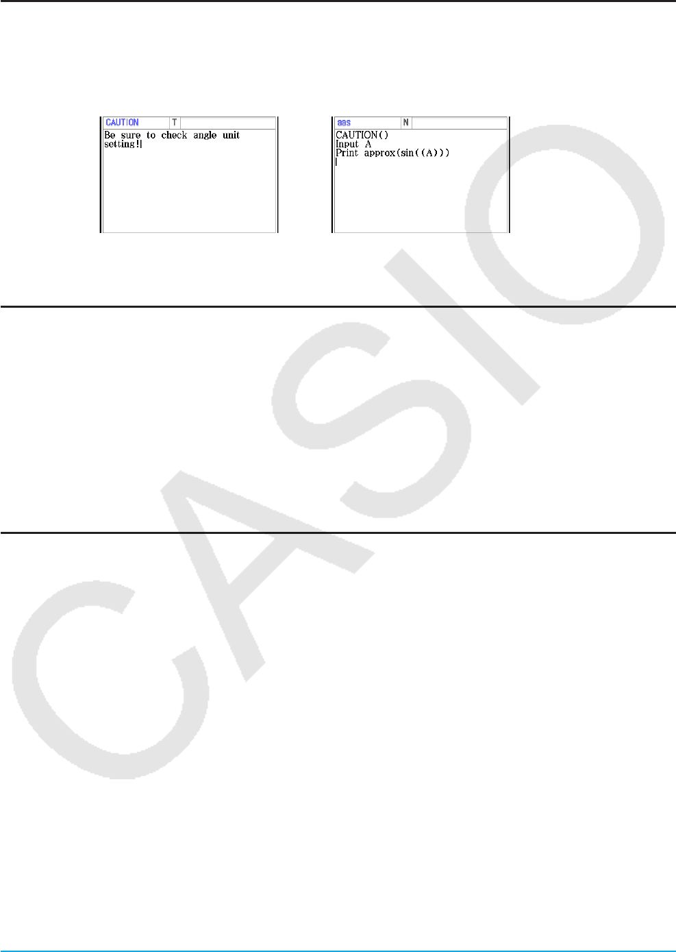
Chapter 12: Program Application 201
Tip: Note that the above operation is not possible while a user-defined function (page 203) is open.
Using Text Files
• Running a text file from the Program Loader window displays the contents of the file in the Text File Contents
window.
• Inserting a text file name followed by “()” inside a program causes the contents of the text file to be displayed
in the Text File Contents window when execution reaches the name.
Example:
File Name: “CAUTION” Program that displays contents of
“CAUTION” file
Converting a Text File to a Program File
You can convert a text file created on the ClassPad to a program file. You also can transfer a text file created
on your computer to a ClassPad unit, and then convert it to a program file.
uTo change a text file to a program file
While a text file is open, tap [Edit], [Mode Change], and then ['Normal].
Tip
• Note that the above operation is not possible while a user-defined function (page 203) is open.
• For information about transferring data between a computer and a ClassPad unit, see Chapter 19 of this manual.
Converting a Program File to an Executable File
You can use the procedure below to change a program file (PRGM file type) to an executable file (EXE file
type).
• An EXE file is about half the size as its corresponding PRGM file.
• An EXE file can only be executed. It cannot be edited. Because of this, converting a PRGM file to an EXE file
also generates an editable PRGM file as a backup.
u To convert a program file (PRGM) to an executable file (EXE)
1. Open the PRGM file that you want to convert and display it in the Program Editor window.
2. Tap [Edit] and then [Compress].
• This displays a dialog box for inputting the backup file name.
3. Enter the backup file name and then tap [OK].
• This saves two copies of the file. One is an EXE file under the name of the original PRGM file. The other is
a backup file, which is created under the name you specify here.
Original File: OCTA (type: PRGM)
Specified File Name: OCTA2
Resulting Files: OCTA (type: EXE), OCTA2 (type: PRGM)

Chapter 12: Program Application 202
12-2 Debugging a Program
A programming error that causes a program to behave in a manner not intended by the writer of the program
is called a “bug”. Finding and eliminating such errors is called “debugging the program”. Any of the following
conditions can indicate that your program has a bug and requires debugging.
• If an error message appears when you try to save the program
• If an error message appears when you try to run the program
• If a program produces some abnormal or unexpected result
Debugging After an Error Message Appears
When an error occurs, a dialog box appears to explain the cause of the error. Carefully read the text of the
error message and then tap its [OK] button. This closes the dialog box, opens the Program Editor window, and
positions the cursor at the location where the error occurred. Make the necessary corrections in accordance
with the explanation provided by the error message.
Tip: EXE type files (page 201) cannot be edited. Tapping the [OK] button on the error dialog box will simply close the dialog
box without displaying the Program Editor window. Open the backup PRGM file that was generated when you
created the EXE file by converting it from a PRGM file, and use it for debugging.
Debugging a Program Following Unexpected Results
If execution of a program produces unexpected or abnormal results, carefully read through the program and
correct errors as required.
Editing a Program
uTo edit a program
1. On the Program Loader window, tap ~, or tap [Edit] and then [Open File].
2. On the dialog box that appears, select the program you want to edit, as described below.
• Tap the [Type] down arrow button and then select “Program(Normal)”.
• Tap the [Folder] down arrow button and then select the folder that contains the program you want to edit.
• Tap the [Name] down arrow button, and then select the name of the program you want to edit.
3. Tap [OK].
4. Edit expressions and commands as required.
5. To overwrite the currently saved program with the edited version tap {, or tap [Edit], [Save File] and then
[Save].
• To save the edited version of the program as a different program, use [Edit] - [Save File] - [Save As].
uTo rename or delete a program
Programs are saved as variables, so you can rename and delete them using Variable Manager. For details,
see “Using Variable Manager” (page 29).

Chapter 12: Program Application 203
12-3 User-defined Functions
ClassPad lets you configure calculation operations as user-defined functions, which can then be used inside
of numeric expressions just like its built-in functions. User-defined functions can also be called up in other
applications.
Note
• User-defined functions are stored in ClassPad memory as “FUNC” (Function) type variables. Naming,
storage, and folder rules are identical to those for user variables.
• A user-defined function can contain only a single mathematical expression.
• A user-defined function cannot contain any command.
Creating a New User-defined Function
You can use either of the methods below to create user-defined functions.
• Using the Program application’s Program Editor window.
• Using the Main application’s Define command.
uTo create and save a new user-defined function using the Program Editor window
Example: To create a user-defined function named “f4” that calculates the following:
x × (x + 1) × (x – 2)
1. On the Program Loader or Program Editor window, tap O.
2. On the dialog box that appears, configure the settings for the new file as described below.
• Tap the [Type] down arrow button and then select “Function”.
• Tap the [Folder] down arrow button and then select the folder where you want to save the user-defined
function.
• In the [Name] box, input up to eight bytes for the user-defined function name. Here, we will input “f4”.
3. Tap [OK]. This displays a blank Program Editor window.
4. Input user-defined function arguments into the parameter variable box. Here,
we will input “x”.
5. Input the expression you want. Here, we will input “x × (x + 1) × (x – 2)”.
6. After the function is the way you want, tap {, or tap [Edit], [Save File] and
then [Save] to save it.
u To create a user-defined function using the Define command
Example: To create a user-defined function named “f2” that calculates the following:
2x + 3y + 1
1. On the Program Loader window, tap ~, or tap O, [Window] and then [Main] to display the Main application
window.
• You could also tap M on the icon panel to start up the Main application.
2. Tap [Interactive] and then [Define].
3. On the dialog box that appears, input the following.
• [Func name]: “f2”
• [Variable/s]: “x, y”
• [Expression]: 2x + 3y + 1
Parameter variable box

Chapter 12: Program Application 204
4. Tap [OK].
• This will cause the Define command to be executed in accordance with
your specifications, which will save user-defined function “f2”.
Tip: For information about the syntax of the Define command, see “Define” in the “Command List” (page 208).
Executing a User-defined Function
Example: To use the Main application to execute user-defined functions “f4”
and “f2” that were created under “Creating a New User-defined
Function”
As shown in the nearby screenshot, input the required arguments for each
variable name and then press E to execute.
Tip: User-defined functions are displayed on the catalog keyboard. You can change the keyboard view to show only user-
defined functions by tapping the catalog keyboard [Form] down arrow button and then selecting [User].
Editing a User-defined Function
uTo edit a user-defined function
1. On the Program Loader window, tap ~, or tap [Edit] and then [Open File].
2. On the dialog box that appears, select the function you want to edit, as described below.
• Tap the [Type] down arrow button and then select “Function”.
• Tap the [Folder] down arrow button and then select the folder that contains the function you want to edit.
• Tap the [Name] down arrow button, and then select the name of the function you want to edit.
3. Tap [OK].
4. Edit the expression and/or parameter variables as required.
5. To overwrite the currently saved function with the edited version tap {, or tap [Edit], [Save File] and then
[Save].
• To save the edited version of the function as a different program, use [Edit] - [Save File] - [Save As].
uTo rename or delete a user-defined function
User-defined functions are saved as variables, so you can rename and delete them using Variable Manager.
For details, see “Using Variable Manager” (page 29).

Chapter 12: Program Application 205
12-4 Program Command Reference
Using This Reference
• This reference lists ClassPad commands in alphabetical order. Commands that do not use alphabetic
characters (such as ⇒ and #) are at the top of the list.
• To the right of each command name is shown the Program Editor window menu sequence that you need to
use to input the command. For example, to input the “Break” command you would tap [Ctrl], then [Control],
then [Break].
Break Ctrl - Control
Syntax: Break
Function: This command terminates a loop and
Command name Menu
If a command has k to the right, it means that the command can be input from the soft keyboard only.
• Command names inside of explanation text are shown in bold.
Syntax Conventions
The table below explains each of the symbols that are used inside of command syntax.
Symbol Meaning
This indicates a space. Always make sure you input one space between a command and its
parameters.
Example: GetKey<variable name>
{ } You need to select one of the multiple options enclosed inside the braces ({ }).
Example: {On ; Off ; Number}
When inputting the command, do not include the braces or semicolons.
[ ] Anything inside brackets ([ ]) is optional. You can input the item inside the brackets or omit it.
When inputting the command, do not include the brackets.
… The term to the left of ellipsis (…) can be input more than once or repeated.
" " Characters inside of parentheses (" ") are a character string.
< > You should input what is described inside the angle brackets (< >). When inputting the
command, do not include the angle brackets.
Example: <variable>, <variable name>, <expression>, <integer from 0 to 9>

Chapter 12: Program Application 206Chapter 12: Program Application 206
Symbols
(Carriage Return) k
Function: Performs a carriage return operation.
Description: In Program Editor, press the E key to
input a carriage return.
• The carriage return can be used in a user program.
It cannot, however, be used in a manual calculation
performed in the Main application.
: (Multi-statement Command) Ctrl
Function: Use this command to link a series of
statements into a multi-statement (on a single line).
Description: The multi-statement command can
be used in a user program. It cannot, however, be
used in a manual calculation performed in the Main
application.
⇒
Ctrl
Syntax 1: {<expression> ; "<string>"} ⇒ <variable
name>
Syntax 2: {<expression> ; "<string>"} ⇒ <list
element>
Syntax 3: <expression> ⇒ <matrix element>
Function: The content of the expression on the left is
evaluated, and the result is assigned to the item on
the right.
’ (Comment) Ctrl - Misc
Function: Any text following this symbol is not
executed. You can use this command to include
comment text in your program.
Description: Any line that starts with the comment
symbol (’) is treated as comment text, which is
skipped during program execution.
" (quotation mark) Ctrl - Misc
Function: Any text inside of quotation marks is treated
as a string.
= Ctrl - Logic
Syntax: <expression 1> = <expression 2>
Function: Returns true when <expression 1> and
<expression 2> are equal, and returns false when
they are not.
≠
Ctrl - Logic
Syntax: <expression 1> ≠ <expression 2>
Function: Returns true when <expression 1> and
<expression 2> are not equal, and returns false when
they are.
< Ctrl - Logic
Syntax: <expression 1> < <expression 2>
Function: Returns true when <expression 1>
is less than <expression 2>, and returns false
when <expression 1> is equal to or greater than
<expression 2>.
> Ctrl - Logic
Syntax: <expression 1> > <expression 2>
Function: Returns true when <expression 1> is
greater than <expression 2>, and returns false when
<expression 1> is equal to or less than <expression
2>.
s
Ctrl - Logic
Syntax: <expression 1> s <expression 2>
Function: Returns true when <expression 1> is less
than or equal to <expression 2>, and returns false
when <expression 1> is greater than <expression 2>.
t
Ctrl - Logic
Syntax: <expression 1> t <expression 2>
Function: Returns true when <expression 1> is
greater than or equal to <expression 2>, and returns
false when <expression 1> is less than <expression
2>.
# Misc - String(2)
Syntax: # <string variable name>
Function: This command specifies a string variable
whose string is a variable name.
Example 1: When the content of variable exp1 is π
and the content of variable str1 is “exp1”, sin(#str1)
calculates sin(π).
Example 2: To cause a folder to be created during
program execution:
InputStrname, "Foldername" : NewFolder#name
A
abExpReg (abExpR)
Misc - Statistics(1) - Regression
Syntax: abExpReg xList, yList[,[FreqList (or 1)]
[, [<yn>] [,{On ; Off}]]]
Function: Performs y = a·bx regression.
Description: See SinReg.
and Ctrl - Logic
See “Bitwise Operations” (page 60).
B
BinomialPD k
Syntax: BinomialPD x value, Numtrial value, pos
value
Function: See “Binomial Distribution Probability”
(page 152).
Command List

Chapter 12: Program Application 207Chapter 12: Program Application 207
BinomialCD k
Syntax: BinomialCDLower value, Upper value,
Numtrial value, pos value
Function: See “Binomial Cumulative Distribution”
(page 152).
Break Ctrl - Control
Syntax: Break
Function: This command terminates a loop and
causes execution to advance to the next command
following the loop process.
Description:
• Break terminates a loop and causes execution to
advance to the next command following the loop
process.
• Break can be used inside of a For, Do, While, or
Switch process.
Broken Misc - Statistics(1) - Graph
Function: Used as a StatGraph command argument
to specify an option. See StatGraph.
C
CallUndef Misc - Graph&Table(1)
Function: Used as a ViewWindow command
argument to specify an option. See ViewWindow.
Case Ctrl - Switch
See Switch~Case~Default~SwitchEnd.
ChiCD k
Syntax: ChiCDLower value, Upper value, df value
Function: See “χ2 Cumulative Distribution” (page 152).
ChiPD k
Syntax: ChiPD x value, df value
Function: See “χ2 Probability Density” (page 152).
ChiGOFTest k
Syntax: ChiGOFTest<Observed list name>,
<Expected list name>, df value
Function: See “χ2 GOF Test” (page 148).
ChiTest k
Syntax: ChiTest<Observed matrix name>
Function: See “χ2 Test” (page 148).
ChrToNum Misc - String(1)
Syntax: ChrToNum"<string>", <storage variable
name>[,n]
Function: Converts the characters up to the nth
character of a string to their character code values
and assigns the string to the specified variable.
Description: Omitting “n” starts conversion from the
first character of the string. For information about
character codes, see “Character Code Table” on page
295.
Circle I/O - Sketch
Syntax: Circle<center x-coordinate>, <center
y-coordinate>, radius[,<color command>]
Function: Draws a circle.
Clear_a_z Misc - Variable
Syntax: Clear_a_z[<folder name>]
Function: Deletes all single letter lower-case named
variables from a through z from the specified folder.
Description:
• If you don’t specify a folder name, the variables of
the current folder are cleared.
• Deletes all variables from a through z, regardless of
type (program, etc.). See GetType for information
about variable types.
• Keep in mind that this command clears all data
types, including programs, functions, etc.
ClearSheet Misc - Graph&Table(1) - Sheet
Syntax: ClearSheet [{<sheet number> ; "<sheet
name>"}]
Function: Deletes the sheet name and expressions
on the sheet, and returns its settings to their default
values. Omitting the argument causes all sheets to be
cleared.
CloseComPort38k I/O - Communication
Syntax: CloseComPort38k
Function: Closes the 3-pin COM port.
ClrGraph I/O - Clear
Syntax: ClrGraph
Function: Clears the Graph window and returns View
Window parameters to their initial default settings.
ClrPict Misc - Graph&Table(2)
Syntax: ClrPict
Function: Clears an image recalled by the RclPict
command.
ClrText I/O - Clear
Syntax: ClrText
Function: Clears text from the Program Output
window.
Cls I/O - Clear
Syntax: Cls
Function: Clears sketch elements (lines and other
figures sketched on the Graph window), and graphs
drawn using drag and drop.

Chapter 12: Program Application 208Chapter 12: Program Application 208
ColorBlack, ColorBlue, ColorRed, ColorMagenta,
ColorGreen, ColorCyan, ColorYellow
I/O - Color
Function: Used as arguments of certain commands to
specify colors.
Description: The following commands use these
arguments: DrawShade, DrawGraph, TangentLine,
NormalLine, Inverse, Plot, PlotOn, PlotChg, Line,
Circle, Vertical, Horizontal, Text, PxlOn, PxlChg,
Print, Locate, SetGraphColor, SetSketchColor
Example: Text 10, 10, "CASIO", ColorBlue
CopyVar Misc - Variable
Syntax: CopyVar<source variable name>, <copy
destination variable name>
Function:
• Copies the contents of a variable to another
variable.
• If the copy destination variable has the same
name as the source variable name, the destination
variable is replaced with the source variable.
Cross Misc - Statistics(2)
Function: Used as a StatGraph command argument
to specify an option. See StatGraph.
CubicReg (CubicR)
Misc - Statistics(1) - Regression
Syntax: CubicReg xList, yList[,[FreqList (or 1)]
[, [<yn>][,{On ; Off}]]]
Function: Performs y = a·x3 + b·x2 + c·x + d
regression.
Description: See SinReg.
D
DateMode360 k
Syntax: DateMode360
Function: Specifies a 360-day year for financial
calculations.
DateMode365 k
Syntax: DateMode365
Function: Specifies a 365-day year for financial
calculations.
Default Ctrl - Switch
See Switch~Case~Default~SwitchEnd.
DefaultListEditor Misc - Statistics(2)
Syntax: DefaultListEditor
Function: Initializes the sort sequence and display
contents of the list on the Stat Editor window (list1 to
list6).
DefaultSetup Misc - Setup(1)
Syntax: DefaultSetup
Function: Initializes all setup data settings.
Define Ctrl - Misc
Syntax: Define[<folder name>\ ]<function
name> ([<variable name>[,<variable name>...]])
=<expression>
• If you do not specify a folder name, the function is
stored in the current folder.
Function: Creates a user-defined function.
Description: See “To create a user-defined function
using the Define command” on page 203.
DelFolder Misc - Variable - Folder
Syntax: DelFolder<folder name>
Function: Deletes a folder.
DelVar Misc - Variable
Syntax: DelVar<variable name>,
<variable name> ...
Function: Deletes a variable.
Description: Deletes all variables, regardless of type
(program, etc.), that have the specified variable name.
See GetType for information about variable types.
DispDfrTbl I/O - Display
Syntax: DispDfrTbl
Function: Creates and displays an arithmetic
sequence table.
DispDQTbl I/O - Display
Syntax: DispDQTbl
Function: Creates and displays a progression of
difference table.
DispFibTbl I/O - Display
Syntax: DispFibTbl
Function: Creates and displays a Fibonacci sequence
table.
DispFTable I/O - Display
Syntax: DispFTable
Function: Creates and displays a function table.
DispListEditor I/O - Display
Syntax: DispListEditor
Function: Displays the Stat Editor window.
DispQutTbl I/O - Display
Syntax: DispQutTbl
Function: Creates and displays a geometric sequence
table.
DispSeqTbl I/O - Display
Syntax: DispSeqTbl
Function: Creates and displays a recursion table.
DispSmryTbl I/O - Display
Syntax: DispSmryTbl
Function: Creates and displays a summary table.

Chapter 12: Program Application 209Chapter 12: Program Application 209
DispStat I/O - Display
Syntax: DispStat
Function: Displays previous statistical calculation
results.
DispText I/O - Display
Syntax: DispText
Function: This command displays the Program Output
window.
Description: You can use this command to re-display
the Program Output window following display of the
Graph window, Table window, or other window.
Example: To re-display the Program Output window
after it has been cleared by a graphing operation or
some other operation
GraphType "y=": Define y1(x) = (x): GTSelOn 1
ViewWindow : 0⇒FStart : 10⇒FEnd : 1⇒FStep
ClrText ← Initializes the Program Output window.
Print "y1(x) = (x)" ← Displays the graph expression on
the Program Output window.
Print "Tap Continue button." ← Tells user what to do
to continue program execution after reading the
message.
Pause ← Pauses program execution to allow user to read
Program Output window message.
DrawGraph ← Draws the graph.
DispFTable ← Displays the table.
Pause ← Pauses program execution to allow for graph
and table editing. Program Output window is not
displayed at this time.
DispText ← Re-displays the Program Output window.
Pause ← Pauses program execution to allow user to read
Program Output window message.
Distance I/O - Sketch
Syntax: Distance<x-coordinate 1>, <y-coordinate
1>, <x-coordinate 2>, <y-coordinate 2>
Function: Determines the distance between two
points.
Description: Executing this command makes the
Graph window active, displays pointers at the
locations of coordinates 1 and 2, and displays the
distance between the pointers.
Tip: An error occurs if <x-coordinate> or <y-coordinate> is
outside of the current Graph window.
Do~LpWhile Ctrl - Do
Syntax: Do : [<statement>] … : LpWhile<expression>
• <expression> is a condition that evaluates to true or
false.
Function: The specified statements are repeated as
long as the condition is true.
Description:
• The statements between Do~LpWhile are repeated
as long as the condition is true. When the condition
becomes false, execution jumps to the next
command after the LpWhile command.
• Since the condition comes after LpWhile, the
condition is not evaluated until the end of the loop is
reached.
• You can use a multi-statement command (:) in place
of the carriage return to separate statements.
• Do not use the Goto command to exit a
Do~LpWhile loop.
Dot Misc - Statistics(2)
Function: Used as a StatGraph command argument
to specify an option. See StatGraph.
DrawConics I/O - Draw
Syntax: DrawConics
Function: Draws a conics graph based on the data
registered on the Conics Editor window.
DrawFTGCon, DrawFTGPlot I/O - Draw
Syntax: DrawFTGCon
DrawFTGPlot
Function: Graphs a function using a generated
number table, in accordance with the conditions of
each command.
Description: FTG stands for “Function Table Graph”.
DrawFTGCon draws a connect type graph, while
DrawFTGPlot draws a plot type graph.
DrawGraph I/O - Draw
Syntax: DrawGraph[<expression>][,<color
command>]
Function: Graphs the selected expression or an
expression specified as a parameter.
Description: <expression> has a y= type expression
on the right side. Graphing of any other type of
expression is not supported by this command.
DrawSeqCon, DrawSeqPlt I/O - Draw
Syntax: DrawSeqCon
DrawSeqPlt
Function: Graphs a recursion expression whose
vertical axis is an (bn or cn) and whose horizontal axis
is n using a generated number table, in accordance
with the conditions of each command.
Description: DrawSeqCon draws a connect type
graph, while DrawSeqPlt draws a plot type graph.

Chapter 12: Program Application 210Chapter 12: Program Application 210
DrawSeqEtrCon, DrawSeqEtrPlt I/O - Draw
Syntax: DrawSeqEtrCon
DrawSeqEtrPlt
Function: Graphs a recursion expression whose
vertical axis is Σan (Σbn or Σcn) and whose horizontal
axis is n using a generated number table, in
accordance with the conditions of each command.
Description: DrawSeqEtrCon draws a connect type
graph, while DrawSeqEtrPlt draws a plot type graph.
DrawShade I/O - Draw
Syntax: DrawShade<expression 1>, <expression
2>[, <number 1>, <number 2>][,<color command>]
Function: Shades the area between expression 1
(lower curve) and expression 2 (upper curve) from
x-values of number 1 to number 2.
Description: Expression 1 and expression 2 have
a y= type expression on the right side. Graphing of
any other type of expression is not supported by this
command.
DrawStat I/O - Draw
Syntax: DrawStat
Function: Draws a statistical graph.
E
Else Ctrl - If
See If~Then~ElseIf~Else~IfEnd.
ElseIf Ctrl - If
See If~Then~ElseIf~Else~IfEnd.
ExpReg (ExpR)
Misc - Statistics(1) - Regression
Syntax: ExpReg xList, yList[,[FreqList (or 1)][, [<yn>]
[,{On ; Off}]]]
Function: Performs y = a·eb·x regression.
Description: See SinReg.
ExpToStr Misc - String(1)
Syntax: ExpToStr<expression>,<storage variable
name>
Function: Converts the result of an input expression
to a string and assigns the string to the specified
variable.
F
FCD k
Syntax: FCDLower value, Upper value, n:df value,
d:df value
Function: See “F Cumulative Distribution” (page 152).
FPD k
Syntax: FPD x value, n:df value, d:df value
Function: See “F Probability Density” (page 152).
For~To~(Step~)Next Ctrl - For
Syntax:
For<expression 1>⇒<control variable name>
To<expression 2> [Step<expression 3>]
[<statement>] … : Next
• <expression 1> is the initial value, <expression 2> is
the end value, and <expression 3> is the step.
Function: Anything between the For command and
the Next command is repeated for a count starting
with the initial value of the control variable and ending
when the control variable reaches the end value.
Each pass causes the value of the control variable to
be changed by the value specified by the step value.
The loop is terminated whenever the control variable
value exceeds the end value.
Description:
• 1 is used for the step if a step value is not specified.
• The initial value can be less than the end value, as
long as a positive value is specified for the step. In
this case, the value of the control value is increased
by the step with each pass.
• The initial value can be greater than the end value,
as long as a negative value is specified for the
step. In this case, the value of the control value is
decreased by the step with each pass.
• You can use a multi-statement command (:) in place
of the carriage return to separate statements.
• Do not use the Goto command to exit a For~Next
loop.
G
GeoCD k
Syntax: GeoCDLower value, Upper value, pos value
Function: See “Geometric Cumulative Distribution”
(page 153).
GeoPD k
Syntax: GeoPD x value, pos value
Function: See “Geometric Distribution Probability”
(page 153).
GetFolder Misc - Variable - Folder
Syntax: GetFolder<storage variable name>
Function: Gets the current folder name and assigns it
to a variable as a text string.

Chapter 12: Program Application 211Chapter 12: Program Application 211
GetKey I/O - Input
Syntax: GetKey<variable name>
Function: This command assigns the code number of
the last key pressed to the specified variable.
Description:
• This command assigns the code number of the last
key pressed to the specified variable. The following
shows a list of available code numbers.
Key Code Key Code Key Code
048 +43 {94
149 -45 E13
250 *60944 f28
351 /47 c29
452 =61 d30
553 (40 e31
654 )41 k144
755 ,44 K145
856 z45 f8
957 x60856 c12
.46 y60857
e147 Z60858
• 0 is assigned to the variable if no key was pressed.
GetPen I/O - Input
Syntax: GetPen<variable name 1>, <variable name
2>
Function: This command assigns the coordinates of
the point tapped on the screen to a specified variable.
Description: This command assigns the x-coordinate
(horizontal axis) to <variable 1> and the y-coordinate
(vertical axis) to <variable 2>. The coordinates at the
point in the upper left corner of the screen are (1, 1),
and coordinate values are specified in the range of
1 to 320 for the x-coordinate and 1 to 528 for the
y-coordinate.
GetType Misc - Variable
Syntax: GetType<variable name>, <storage
variable name>
Function: Gets the type of the specified variable and
assigns it to a storage variable as a text string.
Description: The following is a list of variable types.
• NUM*1• MAT • FUNC • MEM
• EXPR*2• PRGM • PICT • OTHR
• STR • EXE • GMEM • NONE*3
• LIST • TEXT • GEO
*1 Real number *2 Expression
*3 No applicable variable
For details about each type, see “Main Memory Data
Types” (page 28).
GetVar38k I/O - Communication
Syntax: GetVar38k<variable name>
Function: Receives variable names and variable
contents.
Description:
• The OpenComPort38k command must be executed
before this command is executed.
• The CloseComPort38k command must be
executed after this command is executed.
Goto~Lbl Ctrl - Jump
Syntax: Goto<label name> : Lbl<label name>
Function: This command causes program execution
to jump to a specific location.
Description:
• <label name> is a text string that is subject to the
same rules as variable names.
• Goto and Lbl are used in pairs. Program execution
jumps from Goto to the Lbl with the same label
name. A single Lbl can be used as the jump
destination of multiple Goto commands.
• This command can be used to loop back to the
beginning of a program or to jump to any location
within the program.
• An error occurs if ClassPad is unable to find a Lbl
with the same label as Goto.
• Note that the # command cannot be used in a label
name.
GraphType Misc - Graph&Table(1)
Syntax: GraphType"y=" ; "r=" ; "xt=" ; "x=" ; "y>" ;
"y<" ; "y t" ; "y s" ; "x>" ; "x<" ; "x t" ; "x s"
Function: Specifies the graph expression input type.
GTSelOff Misc - Graph&Table(1)
Syntax: GTSelOff<graph number>
Function: Deselects a graph expression.
Description: Graph number range: 1 to 100
GTSelOn Misc - Graph&Table(1)
Syntax: GTSelOn<graph number>
Function: Selects a graph expression.
Description: Graph number range: 1 to 100
H
Histogram Misc - Statistics(1) - Graph
Function: Used as a StatGraph command argument
to specify an option. See StatGraph.
Horizontal I/O - Sketch
Syntax: Horizontal<y-coordinate>[,<color
command>]
Function: Draws a horizontal line.

Chapter 12: Program Application 212Chapter 12: Program Application 212
HypergeoCD k
Syntax: HypergeoCDLower value, Upper value, n
value, M value, N value
Function: See “Hypergeometric Cumulative
Distribution” (page 153).
HypergeoPD k
Syntax: HypergeoPD x value, n value, M value, N
value
Function: See “Hypergeometric Distribution
Probability” (page 153).
I
If~Then~ElseIf~Else~IfEnd Ctrl - If
Syntax 1: If<expression> : Then : [<statement>] ...
: IfEnd
Function 1:
• If the expression is true, the statement in the Then
block is executed. After that, execution advances to
the next statement after IfEnd.
• If the expression is false, execution advances to the
next statement after IfEnd, without executing the
statement in the Then block.
Syntax 2: If<expression> : Then : [<statement>] ... :
Else : [<statement>] ... : IfEnd
Function 2:
• If the expression is true, the statement in the Then
block is executed. After that, execution advances to
the next statement after IfEnd.
• If the expression is false, the statement in the Else
block is executed instead of the Then block. After
that, execution advances to the next statement after
IfEnd.
Syntax 3: If<expression> : Then : [<statement>] ... :
ElseIf<expression> : Then : [<statement>] ... : IfEnd
Function 3:
• If the expression is true, the statement in the If Then
block is executed. After that, execution advances to
the next statement after IfEnd.
• If the If command expression is false, the ElseIf
command expression is tested. If it is true, the
statement in the ElseIf Then block is executed.
After that, execution advances to the next statement
after IfEnd. If it is false, execution advances to the
next statement after IfEnd.
Syntax 4: If<expression> : Then : [<statement>] ... :
ElseIf<expression> : Then : [<statement>] ... : Else :
[<statement>] ... : IfEnd
Function 4:
• If the expression is true, the statement in the If Then
block is executed. After that, execution advances to
the next statement after IfEnd.
• If the If command expression is false, the ElseIf
command expression is tested. If it is true, the
statement in the ElseIf Then block is executed.
After that, execution advances to the next statement
after IfEnd. If it is false, the Else block statement is
executed. After that, execution advances to the next
statement after IfEnd.
Description:
• With all four of the syntaxes described above, you
can use a multi-statement command (:) in place
of the carriage return to separate Then block
statements.
• The If~IfEnd command can be nested.
• The If~IfEnd loop can be exited using the Break
command or Return command.
• Do not use the Goto command to exit an If~IfEnd
loop.
IfEnd Ctrl - If
See If~Then~ElseIf~Else~IfEnd.
Input I/O - Input
Syntax: Input<variable name>[,"<string 1>"[,"<string
2>"]]
Function: When program execution reaches the Input
command, the user is prompted for input of a value,
which is assigned to the specified variable.
Description:
• If you do not specify anything for "<string 1>", the
prompt “<variable name>?” appears by default.
• The text specified for "<string 2>" is used as the
input dialog box title.
• This command pauses program execution and
displays a dialog box that contains the text string
indicated by "<string 1>" and an input box. A text
string enclosed within quotation marks (" ") or a
variable name can be specified for "<string 1>".
• Specifying a long text string can cause part of it to
be cut off when it is displayed in the dialog box.
• When the dialog box appears, input a value into
the input box and then tap [OK]. This closes the
dialog box, assigns the input value to the applicable
variable and resumes program execution.
• Tapping [Cancel] on the dialog box terminates
program execution.
Note:
• During execution of the Input command, program
execution is paused for input of data. While a
program is paused, you can input individual
mathematical expressions only. You cannot input
commands or a series of statements joined by
colons (:).

Chapter 12: Program Application 213Chapter 12: Program Application 213
InputFunc I/O - Input
Syntax: InputFunc<user-defined function name>
(<argument >[,<argument >…]) [,"<string 1>"[,"<string
2>"]]
Function: When program execution reaches the
InputFunc command, the user is prompted to input
the contents of the user-defined function.
Example: InputFunc v(v0, t), "To define function
v0(m/s), t(sec)", "define function"
Description: See Input.
InputStr I/O - Input
Syntax: InputStr<variable name>[,"<string 1>"[,"
<string 2>"]]
Function: When program execution reaches the
InputStr command, the user is prompted for input of
a string, which is assigned to a variable.
Description: See Input.
Intersection Misc - Graph&Table(1)
Function: Used as a SetInequalityPlot command
argument to specify an option. See SetInequalityPlot.
InvBinomialCD k
Syntax: InvBinomialCD prob value, Numtrial value,
pos value
Function: See “Inverse Binomial Cumulative
Distribution” (page 152).
InvChiCD k
Syntax: InvChiCD prob value, df value
Function: See “Inverse χ2 Cumulative Distribution”
(page 152).
Inverse I/O - Sketch
Syntax: Inverse<y or x graph number>[,<color
command>]
Function: Graphs the inverse of a function.
Description: Graph number range: 1 to 100
InvFCD k
Syntax: InvFCD prob value, n:df value, d:df value
Function: See “Inverse F Cumulative Distribution”
(page 152).
InvGeoCD k
Syntax: InvGeoCD prob value, pos value
Function: See “Inverse Geometric Cumulative
Distribution” (page 153).
InvHypergeoCD k
Syntax: InvHypergeoCD prob value, n value, M
value, N value
Function: See “Inverse Hypergeometric Cumulative
Distribution” (page 153).
InvNormCD k
Syntax: {InvNormCD ; InvNorm}"Tail setting",
Area value, value, value
Function: See “Inverse Normal Cumulative
Distribution” (page 151).
InvPoissonCD k
Syntax: InvPoissonCD prob value, value
Function: See “Inverse Poisson Cumulative
Distribution” (page 153).
InvTCD k
Syntax: InvTCD prob value, df value
Function: See “Inverse Student’s t Cumulative
Distribution” (page 152).
L
Lbl Ctrl - Jump
See Goto~Lbl.
Ldot Misc - Statistics(2)
Function: Used as a StatGraph command argument
to specify an option. See StatGraph.
Line I/O - Sketch
Syntax: Line<start point x-coordinate>, <start point
y-coordinate>, <end point x-coordinate>, <end point
y-coordinate>[,<color command>]
Function: Draws a line between two specified
coordinates.
Tip: The line is not drawn if a start point coordinate or
end point coordinate is outside of the current Graph
window.
LinearReg (LinearR)
Misc - Statistics(1) - Regression
Syntax: LinearReg xList, yList[,[FreqList (or 1)]
[, [<yn>][,{On ; Off}]]]
Function: Performs y = a·x + b regression.
Description: See SinReg.
LineType Misc - Setup(2)
Function: Used as a SetGrid command argument to
specify an option. See SetGrid.
LinRegTTest k
Syntax: LinRegTTest" &
ρ
condition", XList, YList[,
{Freq ; 1}]
Function: See “Linear Regression t Test” (page 147).
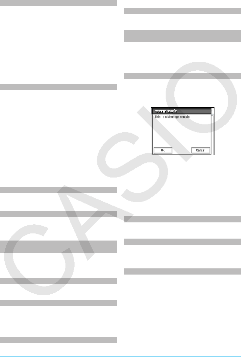
Chapter 12: Program Application 214Chapter 12: Program Application 214
Local Misc - Variable
Syntax: Local<variable name>, <variable name> ...
[,<color command>]
Function: Defines a local variable.
Description: The following are the merits of local
variables.
• Since local variables are deleted automatically,
use of local variables for temporary storage avoids
unnecessary use of available memory.
• Since local variables do not affect general (user)
variables, you can name local variables without
worrying about whether the name you are using is
already used by another variable.
Locate I/O - Output
Syntax 1: Locate<x-coordinate>, <y-coordinate>,
<expression>
Syntax 2: Locate<x-coordinate>, <y-coordinate>,
"<string>"
Function: This command displays the result of the
specified expression or the specified text string at the
specified coordinates on the display screen.
Description:
• The coordinates of the point at the upper left corner
of the effective area of the Locate command are (1,
1), and coordinate values can be specified in the
range of 1 to 580 for the x-coordinate and 1 to 580
for the y-coordinate. Note, however, that the actual
dot count of the ClassPad screen is 320 × 528.
• An expression result is displayed as a single line.
Lock Misc - Variable
Syntax: Lock<variable name>, <variable name> ...
Function: Locks variables.
LockFolder Misc - Variable - Folder
Syntax: LockFolder<folder name>
Function: Locks the specified folder and all the files
currently inside of it.
LogisticReg (LogisticR)
Misc - Statistics(1) - Regression
Syntax: LogisticReg xList, yList[,[<yn>][,{On ; Off}]]
Function: Performs y = c/(1 + a·e(−b·x)) regression.
Description: See SinReg.
LogP Misc - Graph&Table(1)
Function: Used as a ViewWindow command
argument to specify an option. See ViewWindow.
LogReg (LogR) Misc - Statistics(1) - Regression
Syntax: LogReg xList, yList[,[FreqList (or 1)][,[<yn>]
[,{On ; Off}]]]
Function: Performs y = a + b·ln(x) regression.
Description: See SinReg.
LpWhile Ctrl - Do
See Do~LpWhile.
M
MedBox Misc - Statistics(1) - Graph
Function: Used as a StatGraph command argument
to specify an option. See StatGraph.
MedMedLine (MedMed)
Misc - Statistics(1) - Regression
Syntax: MedMedLine xList, yList[,[FreqList (or 1)]
[,[<yn>] [,{On ; Off}]]]
Function: Performs y = a·x + b Med-Med calculation.
Description: See SinReg.
Message I/O - Output
Syntax: Message"<string 1>" [,"<string 2>"]
Function: This command pauses program execution
and displays a dialog box containing the text specified
by "<string 1>".
The text is positioned flush top left. The text specified
for "<string 2>" is used as the dialog box title.
Description:
• Text strings enclosed within quotation marks (" ") or
variable names can be specified for "<string 1>" and
"<string 2>".
• Tapping [OK] closes the dialog box and resumes
program execution.
• Tapping [Cancel] terminates program execution.
ModBox Misc - Statistics(1) - Graph
Function: Used as a StatGraph command argument
to specify an option. See StatGraph.
MoveVar Misc - Variable
Syntax: MoveVar<variable name>, <current folder
name>, <destination folder name>
Function: Moves a variable to the specified folder.
MultiSortA k
Syntax 1: MultiSortA<list name>
Syntax 2: MultiSortA<base list name>, <subordinate
list name>, <subordinate list name>, ...
Function: Sorts a statistical list in ascending order.
Description:
• Syntax 1 performs a simple list sort.
• Syntax 2 sorts multiple lists on the base list. Up to
five subordinate lists can be specified.

Chapter 12: Program Application 215Chapter 12: Program Application 215
MultiSortD k
Syntax 1: MultiSortD<list name>
Syntax 2: MultiSortD<base list name>, <subordinate
list name>, <subordinate list name>, ...
Function: Sorts a statistical list in descending order.
Description: See MultiSortA.
N
NDist Misc - Statistics(1) - Graph
Function: Used as a StatGraph command argument
to specify an option. See StatGraph.
NewFolder Misc - Variable - Folder
Syntax: NewFolder<folder name>
Function: Creates a new folder.
Next Ctrl - For
See For~To~(Step~)Next.
NormCD k
Syntax: NormCDLower value, Upper value, value,
value
Function: See “Normal Cumulative Distribution” (page
151).
NormPD k
Syntax: NormPD x value, value, value
Function: See “Normal Probability Density” (page 151).
NormalLine I/O - Sketch
Syntax: NormalLine<graph number>,
<x-coordinate>[,<color command>]
Function: Draws a normal line.
Description: Draws a line normal to the graph at the
specified x-value.
not Ctrl - Logic
See “Bitwise Operations” (page 60).
NPPlot Misc - Statistics(1) - Graph
Function: Used as a StatGraph command argument
to specify an option. See StatGraph.
NumToChr Misc - String(1)
Syntax: NumToChrn,<storage variable name>
Function: Converts numeric value n to the
corresponding text character(s) in accordance with
the character code table, and assigns the character(s)
as a string to the specified variable. For information
about character codes, see “Character Code Table”
on page 295.
NumToStr Misc - String(1)
Syntax: NumToStr<value>, {"Fix <integer from 0 to
9>" ; "Sci <integer from 0 to 9>"}, <storage variable
name>
Function: Converts a numeric value to a string of the
specified format, and assigns the resulting string to
the specified variable.
O
Off Misc - Setup(1)
Function: Used as the argument of Setup type
commands to turn off the setting.
On Misc - Setup(1)
Function: Used as the argument of Setup type
commands to turn on the setting.
OnePropZTest k
Syntax: OnePropZTest"Prop condition", p0 value, x
value, n value
Function: See “1-Proportion Z Test” (page 147).
OnePropZInt k
Syntax: OnePropZIntC-Level value, x value, n value
Function: See “1-Proportion Z Interval” (page 150).
OneSampleTInt k
Syntax 1: OneSampleTIntC-Level value, List
[, {Freq ; 1}]
Syntax 2: OneSampleTIntC-Level value, o value, sx
value, n value
Function: See “1-Sample t Interval” (page 150).
OneSampleTTest k
Syntax 1: OneSampleTTest" condition", 0 value,
List[, {Freq ; 1}]
Syntax 2: OneSampleTTest" condition", 0 value,
o value, sx value, n value
Function: See “1-Sample t Test” (page 147).
OneSampleZInt k
Syntax 1: OneSampleZIntC-Level value, value,
List[, {Freq ; 1}]
Syntax 2: OneSampleZIntC-Level value, value, o
value, n value
Function: See “1-Sample Z Interval ” (page 150).
OneSampleZTest k
Syntax 1: OneSampleZTest" condition", 0 value,
value, List[, {Freq ; 1}]
Syntax 2: OneSampleZTest" condition", 0 value,
value, o value, n value
Function: See “1-Sample Z Test” (page 146).

Chapter 12: Program Application 216Chapter 12: Program Application 216
OneVariable k
Syntax: OneVariable xList [,FreqList (or 1)]
Function: Single variable statistics calculation
Description:
xList: Name of list for storing x-axis data
FreqList: Name of list for storing frequency of “xList”
data
• “FreqList” can be omitted. Doing so sets “1” for
“FreqList”.
OneWayANOVA k
Syntax: OneWayANOVAFactorList(A),
DependentList
Function: See “One-Way ANOVA” (page 148).
OpenComPort38k I/O - Communication
Syntax: OpenComPort38k
Function: Opens the 3-pin COM port.
or Ctrl - Logic
See “Bitwise Operations” (page 60).
P
Pause Ctrl - Control
Syntax: Pause
Function: Pauses program execution and displays a
pause indicator on the right side of the status bar.
Description:
• You can perform manual operations on the
ClassPad display screen while program execution is
paused by the Pause command.
• Program execution remains paused until you tap
the X button on the status bar, or until six minutes
pass (after which program execution resumes
automatically).
PeriodsAnnual k
Syntax: PeriodsAnnual
Function: Specifies annual for the bond calculation
payment periods
PeriodsSemi k
Syntax: PeriodsSemi
Function: Specifies semiannual for the bond
calculation payment periods
Plot I/O - Sketch - Plot
Syntax: Plot<x-coordinate>, <y-coordinate>[,<color
command>]
Function: Displays a pointer at the location specified
by the coordinates and plots a point there.
PlotChg I/O - Sketch - Plot
Syntax: PlotChg<x-coordinate>, <y-coordinate>
[,<color command>]
Function: If there is a plot at the specified coordinates,
the plot within a 3×3-dot area centered on those
coordinates are deleted. If there is no plot at the
specified coordinates, a point is plotted within a 3×3-
dot area centered on those coordinates.
PlotOff I/O - Sketch - Plot
Syntax: PlotOff<x-coordinate>, <y-coordinate>
Function: Deletes the plot within a 3×3-dot area
centered on the specified coordinates.
PlotOn I/O - Sketch - Plot
Syntax: PlotOn<x-coordinate>, <y-coordinate>
[,<color command>]
Function: Plots a point within a 3×3-dot area centered
on the specified coordinates.
plotTest( I/O - Sketch - Plot
Syntax: plotTest(<x-coordinate>, <y-coordinate>)
Function: If a dot is present at the specified pixel,
returns a value that corresponds to the color of the
dot (Black: 1, Blue: 2, Red: 3, Magenta: 4, Green: 5,
Cyan: 6, Yellow: 7). Returns 0 if no dot is present at
the specified pixel.
Description: Only dots within the screen are valid.
PmtBgn k
Syntax: PmtBgn
Function: Specifies beginning of period for the
financial calculation payment date.
PmtEnd k
Syntax: PmtEnd
Function: Specifies end of period for the financial
calculation payment date.
PoissonCD k
Syntax: PoissonCDLower value, Upper value,
value
Function: See “Poisson Cumulative Distribution”
(page 153).
PoissonPD k
Syntax: PoissonPD x value, value
Function: See “Poisson Distribution Probability” (page
152).

Chapter 12: Program Application 217Chapter 12: Program Application 217
PowerReg (PowerR)
Misc - Statistics(1) - Regression
Syntax: PowerReg xList, yList[,[FreqList (or 1)]
[,[<yn>] [,{On ; Off}]]]
Function: Performs y = a·xb regression.
Description: See SinReg.
Print I/O - Output
Syntax 1: Print<expression>[,<color command>]
Syntax 2: Print"<string>"
Function: Displays the result of the specified
expression or the specified text string.
Description: An expression result is displayed as
a single line. When the result is a long expression,
fraction, or string, it may not fit on the display. In such
a case, use the PrintNatural command instead.
PrintNatural I/O - Output
Syntax: PrintNatural<expression>[,"<string>"]
Function: Pauses program execution and displays the
result of the specified expression in natural format.
Description:
• A text string enclosed within quotation marks (" ") or
a variable name can be specified for "<string>".
• Tapping [OK] closes the dialog box and resumes
program execution. Tapping [Cancel] terminates
program execution.
PTBrokenThck Misc - Graph&Table(1) - Plot Type
Syntax: PTBrokenThck<graph number>
Function: Specifies “Broken Thick” as the graph line
type.
Description: Graph number range: 1 to 100
PTDot Misc - Graph&Table(1) - Plot Type
Syntax: PTDot<graph number>
Function: Specifies “Dot Plot” as the graph line type.
Description: Graph number range: 1 to 100
PTNormal Misc - Graph&Table(1) - Plot Type
Syntax: PTNormal<graph number>
Function: Specifies “Normal” as the graph line type.
Description: Graph number range: 1 to 100
PTThick Misc - Graph&Table(1) - Plot Type
Syntax: PTThick<graph number>
Function: Specifies “Thick” as the graph line type.
Description: Graph number range: 1 to 100
PTThin Misc - Graph&Table(1) - Plot Type
Syntax: PTThin<graph number>
Function: Specifies “Thin” as the graph line type.
Description: Graph number range: 1 to 100
PxlChg I/O - Sketch - Pixel
Syntax: PxlChg<x-dot>, <y-dot>[,<color command>]
Function: Toggles display of the specified pixel on or
off.
PxlOff I/O - Sketch - Pixel
Syntax: PxlOff<x-dot>, <y-dot>
Function: Turns off display of the specified pixel.
PxlOn I/O - Sketch - Pixel
Syntax: PxlOn<x-dot>, <y-dot>[,<color command>]
Function: Turns on display of the specified pixel.
pxlTest( I/O - Sketch - Pixel
Syntax: pxlTest (<x-dot>, <y-dot>)
Function: If a dot is present at the specified pixel,
returns a value that corresponds to the color of the
dot (Black: 1, Blue: 2, Red: 3, Magenta: 4, Green: 5,
Cyan: 6, Yellow: 7). Returns 0 if no dot is present at
the specified pixel.
Q
QuadReg (QuadR)
Misc - Statistics(1) - Regression
Syntax: QuadReg xList, yList[,[FreqList (or 1)]
[,[<yn>] [,{On ; Off}]]]
Function: Performs y = a·x2 + b·x + c regression.
Description: See SinReg.
QuartReg (QuartR)
Misc - Statistics(1) - Regression
Syntax: QuartReg xList, yList[,[FreqList (or 1)]
[,[<yn>] [,{On ; Off}]]]
Function: Performs y = a·x4 + b·x3 + c·x2 + d·x + e
regression.
Description: See SinReg.
R
RclGMem Misc - Graph&Table(2)
Syntax: RclGMem{<variable name> ; <folder name\
file name>}
Function: Recalls GMem data (graph expression and
related information), which was previously saved
under the specified name.
Description: A folder path can be specified only up to
one level.
RclPict Misc - Graph&Table(2)
Syntax: RclPict<picture name>
Function: Recalls a Pict image, which was previously
saved under the specified name.

Chapter 12: Program Application 218Chapter 12: Program Application 218
RclVWin Misc - Graph&Table(2)
Syntax: RclVWin䡺{<variable name> ; <folder name\
file name>}
Function: Recalls View Window values, which were
previously saved under the specified name.
Description: A folder path can be specified only up to
one level.
Receive38k I/O - Communication
Syntax: Receive38k䡺<variable name>
Function: Receives Data Logger data.
Description:
• The OpenComPort38k command must be executed
before this command is executed.
• The CloseComPort38k command must be
executed after this command is executed.
• For details about using this command, see the user
documentation that comes with the EA-200.
• Note that you need to replace all instances of the
Receive command in the examples provided in
the EA-200 user documentation with the command
Receive38k. You should also adjust the other
commands in the EA-200 examples so they conform
to the ClassPad command syntax and usage as
described in this manual.
Rename Misc - Variable
Syntax: Rename䡺<current variable name>, <new
variable name>
Function: Renames a variable.
Return Ctrl - Control
Syntax: Return䡺{<variable>}
Function 1 (Main Program): Terminates program
execution.
Function 2 (Subroutine Program): Returns from a
subroutine.
Tip
• The Return command can be executed during an If, For,
Do, While, or Switch process.
• Appending a <variable> to the Return command in
the Main application and executing the command will
cause the variable to be displayed when the program is
complete.
S
Scatter Misc - Statistics(1) - Graph
Function: Used as a StatGraph command argument
to specify an option. See StatGraph.
Send38k I/O - Communication
Syntax: Send38k䡺<variable name>
Function: Sends Data Logger data.
Description:
• The OpenComPort38k command must be executed
before this command is executed.
• The CloseComPort38k command must be
executed after this command is executed.
• For details about using this command, see the user
documentation that comes with the EA-200.
• Note that you need to replace all instances of the
Send command in the examples provided in the
EA-200 user documentation with the command
Send38k. You should also adjust the other
commands in the EA-200 examples so they conform
to the ClassPad command syntax and usage as
described in this manual.
• <variable name> must be a variable that contains
a real number or a list. Anything else results in an
error.
SendVar38k I/O - Communication
Syntax: SendVar38k䡺<variable name>
Function: Sends variable names and variable
contents.
Description:
• The OpenComPort38k command must be executed
before this command is executed.
• The CloseComPort38k command must be
executed after this command is executed.
SeqSelOff Misc - Sequence
Syntax: SeqSelOff䡺{an+1 ; an+2 ; bn+1 ; bn+2 ; cn+1 ; cn+2 ;
anE ; bnE ; cnE}
Function: Deselects the specified sequence
expression. Specifying “anE”, “bnE”, or “cnE” as the
argument activates [Explicit]. Specifying any other
argument activates [Recursive].
SeqSelOn Misc - Sequence
Syntax: SeqSelOn䡺{an+1 ; an+2 ; bn+1 ; bn+2 ; cn+1 ; cn+2 ;
anE ; bnE ; cnE}
Function: Selects the specified sequence expression.
Specifying “anE”, “bnE”, or “cnE” as the argument
activates [Explicit]. Specifying any other argument
activates [Recursive].
SeqType Misc - Sequence
Syntax: SeqType䡺{"n" ; "an+1a0" ; "an+1a1" ; "an+2a0" ;
"an+2a1"}
Function: Specifies the recursion type.
Description: Specifying “n” as the argument activates
[Explicit]. Specifying any other argument activates
[Recursive].

Chapter 12: Program Application 219Chapter 12: Program Application 219
SetAxes Misc - Setup(2)
Syntax: SetAxes{On ; Off ; Number}
Function: Specifies the axis display mode as show
Graph window axes only (On), hide axes and scale
(Off), or show axes and scale (Number).
SetCellWidth Misc - Setup(4)
Syntax: SetCellWidth{2 ; 3 ; 4}
Function: Specifies the number of rows displayed on
the Stat Editor and data table windows.
SetComplex Misc - Setup(1)
Syntax: SetComplex
Function: Specifies the Complex mode (to perform
complex number calculations).
SetCoord Misc - Setup(2)
Syntax: SetCoord{On ; Off}
Function: Turns display of Graph window pointer
coordinates on or off.
SetDecimal Misc - Setup(1)
Syntax: SetDecimal
Function: Specifies the Decimal mode (displays
results in decimal format).
SetDegree Misc - Setup(1)
Syntax: SetDegree
Function: Specifies “Degree” for the angle unit.
SetDeriv Misc - Setup(3)
Syntax: SetDeriv{On ; Off}
Function: Turns display of Graph window pointer
coordinates and ordered pair table derivative on or
off.
SetDispGCon Misc - Setup(2)
Syntax: SetDispGCon{On ; Off}
Function: Turns display of graph controller arrows
during graphing on or off.
SetDrawCon Misc - Setup(2)
Syntax: SetDrawCon
Function: Specifies graphing by connecting plotting
points with lines.
SetDrawPlt Misc - Setup(2)
Syntax: SetDrawPlt
Function: Specifies graphing by plotting points only.
SetFix Misc - Setup(2)
Syntax: SetFix<integer from 0 to 9>
Function: Specifies the fixed number of decimal
places.
SetFolder Misc - Variable - Folder
Syntax: SetFolder<folder name> [,<storage variable
name>]
Function:
• Makes the specified folder the current folder.
Including a variable name at the end of this
command assigns the name of the previous current
folder to the variable as a text string.
• If the specified folder does not exist, this command
creates a new folder with the specified name, and
makes it the current folder.
SetFunc Misc - Setup(3)
Syntax: SetFunc{On ; Off}
Function: Turns display of graph function name and
function on or off.
SetGraphColor Misc - Setup(4)
Syntax: SetGraphColor<graph number>, <color
command>
Function: Specifies the graph color.
Description: The graph number range is 1 to 100.
SetGrad Misc - Setup(1)
Syntax: SetGrad
Function: Specifies “Grad” for the angle unit.
SetGrid Misc - Setup(2)
Syntax: SetGrid{On ; Off ; LineType}
Function: Specifies the Graph window grid type
display mode as show as dots (On), hide grid (Off),
and show as grid lines (LineType).
SetInequalityPlot Misc - Setup(4)
Syntax: SetInequalityPlot{Intersection ; Union}
Function: When graphing multiple inequalities, fills
areas where all inequality conditions are satisfied
(Intersection) or fills areas where each inequality
condition is satisfied (Union).
SetLabel Misc - Setup(2)
Syntax: SetLabel{On ; Off}
Function: Turns display of Graph window axis labels
on or off.
SetLeadCursor Misc - Setup(3)
Syntax: SetLeadCursor{On ; Off}
Function: Turns display of the leading cursor during
graphing on or off.
SetNormal Misc - Setup(2)
Syntax: SetNormal{1 ; 2}
Function: Specifies Normal 1 or Normal 2 as the auto
exponential display setting for values.
SetRadian Misc - Setup(1)
Syntax: SetRadian
Function: Specifies “Radian” for the angle unit.

Chapter 12: Program Application 220Chapter 12: Program Application 220
SetReal Misc - Setup(1)
Syntax: SetReal
Function: Specifies the Real mode (to perform real
number calculations).
SetSci Misc - Setup(2)
Syntax: SetSci<integer from 0 to 9>
Function: Specifies the fixed number of significant
digits.
SetSequence Misc - Setup(4)
Syntax: SetSequence{On ; Off ; StepDisp}
Function: Turns display of expressions created
after graphing on or off or specifies “step display”
(StepDisp).
Description: When StepDisp is selected, the
expression does not appear until you press E.
SetSimulGraph Misc - Setup(2)
Syntax: SetSimulGraph{On ; Off}
Function: Turns simultaneous drawing of multiple
graphs on or off.
SetSketchColor Misc - Setup(4)
Syntax: SetSketchColor [,<color command>]
Function: Specifies the color of an object drawn with
the Sketch function.
SetSmryTable Misc - Setup(3)
Syntax: SetSmryTable{<list name> ; VWin}
Function: Specifies whether summary table
generation is View Window dependent or List
dependent. Using VWin specifies View Window
dependent.
SetSmryTableQD Misc - Setup(3)
Syntax: SetSmryTableQD{On ; Off}
Function: Specifies whether the second derivative will
appear in summary tables.
SetStandard Misc - Setup(1)
Syntax: SetStandard
Function: Specifies the Standard mode (to leave
calculation results as expressions).
SetStatWinAuto Misc - Setup(4)
Syntax: SetStatWinAuto{On ; Off}
Function: Turns automatic setup of Statistics
application View Window on or off.
SetTVariable Misc - Setup(3)
Syntax: SetTVariable{<list name> ; TableInput}
Function: Specifies the variable reference location for
table generation.
Description: Use TableInput to specify a range and
generate a table.
SetΣdisp Misc - Setup(4)
Syntax: SetΣdisp{On ; Off}
Function: Turns display of subtotals for tables on or
off.
SheetActive Misc - Graph&Table(1) - Sheet
Syntax: SheetActive{<sheet number> ; "<sheet
name>"}
Function: Selects the sheet that contains the
expression to be graphed.
Description: Even after a sheet is renamed, it can still
be specified using its previous sheet number.
SheetName Misc - Graph&Table(1) - Sheet
Syntax: SheetName"<sheet name string>", <sheet
number>
Function: Assigns a name to a sheet
Description:
• A sheet name can be up to eight characters long.
• Sheet number range: 1 to 5
SinReg (SinR) Misc - Statistics(1) - Regression
Syntax: SinReg xList, yList[,[<yn>][,{On ; Off}]]
Function: Performs y = a·sin(b·x + c) + d regression.
Description:
xList: Name of list for storing x-axis data
yList: Name of list for storing y-axis data
• “yn” is the Graph Editor name (y1, y2, ...) that is the
copy destination of the regression expression. Copy
is not performed when “yn” is skipped.
• “On/Off” turns residual calculation on or off.
Residual calculation is turned off when this setting is
skipped.
Skip Ctrl - Control
Syntax: Skip
Function: Causes execution to jump to the statement
at the beginning of a loop.
Description:
• Skip causes execution to jump to the statement at
the beginning of a loop.
• Skip can be used inside of a For, Do, or While
process.
SmryTSelOn Misc - Graph&Table(1)
Syntax: SmryTSelOn<expression number>
Function: Deselects all currently selected expressions
and then selects only the specified summary table
expression.
Square Misc - Statistics(2)
Function: Used as a StatGraph command argument
to specify an option. See StatGraph.

Chapter 12: Program Application 221Chapter 12: Program Application 221
StatGraph Misc - Statistics(1)
Syntax 1: StatGraph<StatGraph number 1 to 9>,
{On ; Off}, Graph Type 1, xList, yList, FreqList (or 1),
Plot Type
Syntax 2: StatGraph<StatGraph number 1 to 9>,
{On ; Off}, Graph Type 2, xList, yList, FreqList (or 1)
Syntax 3: StatGraph<StatGraph number 1 to 9>,
{On ; Off}, Graph Type 3, xList, yList
Syntax 4: StatGraph<StatGraph number 1 to 9>,
{On ; Off}, Graph Type 4, xList, FreqList (or 1)
Syntax 5: StatGraph<StatGraph number 1 to 9>,
{On ; Off}, Graph Type 5, xList, Plot Type
Function: Configures statistical graph settings.
Description:
xList: Name of list for storing x-axis data
yList: Name of list for storing y-axis data
FreqList: Name of list for storing frequency of “xList”
and “yList” data
Graph Type 1: Scatter, xyLine
Graph Type 2: LinearR, MedMed, QuadR, CubicR,
QuartR, LogR, ExpR, abExpR, PowerR
Graph Type 3: SinR, LogisticR
Graph Type 4: Histogram, MedBox, ModBox,
NDist, Broken
Graph Type 5: NPPlot
Plot Type: Square, Cross, Dot, Ldot
StatGraphSel Misc - Statistics(1)
Syntax: StatGraphSel{On ; Off} {,"Reg," ; ,"Graph"}
Function: Turns statistical graphing on or off.
Description:
• “Reg” selects Previous Reg.
• “Graph” selects Graph Function.
• Skipping “Reg” and “Graph” turns StatGraph,
Previous Reg, and Graph Function on or off.
Step Ctrl - For
See For~To~(Step~)Next.
StepDisp Misc - Setup(4)
Function: Used as a SetSequence command
argument to specify an option. See SetSequence.
StoGMem Misc - Graph&Table(2)
Syntax: StoGMem{<variable name> ; <folder name\
file name>}
Function: Assigns a name to GMem data (graph
expression and related information) and stores it.
Description: A folder path can be specified only up to
one level.
Stop Ctrl - Control
Syntax: Stop
Function: Terminates program execution.
Description: This command terminates all program
execution, including that of the main program when a
subroutine program is running.
StoPict Misc - Graph&Table(2)
Syntax: StoPict<picture name>
Function: Assigns a name to a Pict image and stores
it.
StoVWin Misc - Graph&Table(2)
Syntax: StoVWin{<variable name> ; <folder name\
file name>}
Function: Assigns a name to View Window values
and stores them.
Description: A folder path can be specified only up to
one level.
StrCmp Misc - String(1)
Syntax: StrCmp"<string 1>", "<string 2>", <storage
variable name>
Function: Compares "<string 1>" and "<string
2>" (character code comparison) and assigns the
resulting value to the specified variable.
Description:
• Returns 0 when "<string 1>" = "<string 2>".
• Returns 1 when "<string 1>" > "<string 2>".
• Returns –1 when "<string 1>" < "<string 2>".
StrInv Misc - String(1)
Syntax: StrInv"<string>", <storage variable name>
Function: Inverts the sequence of a string and assigns
the resulting string to a variable.
StrJoin Misc - String(1)
Syntax: StrJoin"<string 1>", "<string 2>", <storage
variable name>
Function: Joins "<string 1>" and "<string 2>" and then
assigns the resulting string to the specified variable.
StrLeft Misc - String(1)
Syntax: StrLeft"<string>", n, <storage variable
name>
Function: Copies a string up to the nth character
from the left, and assigns the resulting string to the
specified variable.
StrLen Misc - String(1)
Syntax: StrLen"<string>", <storage variable name>
Function: Determines the length of a string (the
number of its characters) and assigns the resulting
value to the specified variable.

Chapter 12: Program Application 222Chapter 12: Program Application 222
StrLwr Misc - String(2)
Syntax: StrLwr"<string>", <storage variable name>
Function: Converts all the characters of a string to
lower case and assigns the resulting string to the
specified variable.
StrMid Misc - String(2)
Syntax: StrMid"<string>", n, <storage variable
name> [,<number of characters>]
Function: Copies a specific number of characters of a
string, starting from the nth character, and assigns the
resulting string to the specified variable.
Description: Omitting the number of characters
causes the string to be copied up to the end.
StrRight Misc - String(2)
Syntax: StrRight"<string>", n, <storage variable
name>
Function: Copies a string up to the nth character
from the right, and assigns the resulting string to the
specified variable.
StrRotate Misc - String(2)
Syntax: StrRotate"<string>", <storage variable
name> [,n]
Function: Rotates the left side part and right side
part of a string at the nth character, and assigns the
resulting string to the specified variable.
Description: Rotation is to the left when “n” is positive,
and to the right when “n” is negative. Omitting “n”
uses a default value of +1.
StrShift Misc - String(2)
Syntax: StrShift"<string>", <storage variable name>
[,n]
Function: Shifts a string left or right n characters, and
assigns the resulting string to the specified variable.
Description: Shift is to the left when “n” is positive,
and to the right when “n” is negative. Omitting “n”
uses a default value of +1.
StrSrc Misc - String(2)
Syntax: StrSrc"<string 1>", "<string 2>", <storage
variable name> [,<search start location>]
Function: Searches "<string 1>" starting from the
specified point (nth character from beginning of
string) to determine if it contains the data specified
by "<string 2>". If the data is found, this command
returns the location of the first character of "<string
2>", starting from the beginning of "<string 1>".
Description: Omitting the start point causes the
search to start from the beginning of "<string 1>".
strToExp( Misc - String(2)
Syntax: strToExp("<string>")
Function: Converts a string to an expression, and
executes the expression.
StrUpr Misc - String(2)
Syntax: StrUpr"<string>", <storage variable name>
Function: Converts all the characters of a string to
upper case and assigns the resulting string to the
specified variable.
Switch~Case~Default~SwitchEnd Ctrl - Switch
Syntax:
Switch<expression 1> : Case<expression 2> :
[<statement>] … : Break : Case<expression 3> … :
[<statement>] … : Break : … : Case<expression n> :
[<statement>] … : Break : Default : [<statement>] … :
SwitchEnd
• <expression 1> through <expression n> should be
expressions that produce real numbers.
Function: Executes one of a series of processes
based on the value of <expression>.
Description:
• This command executes the statement following
the Case expression that matches the Switch
expression.
• If there is no matching Case expression, the
statement following Default is executed. If there
is no Default specified, a non-match jumps to the
statement following SwitchEnd.
• You can use a multi-statement command (:) in place
of the carriage return to separate statements.
• Switch~SwitchEnd can be exited using the Break
command, Return command, or Goto command.
SwitchEnd Ctrl - Switch
See Switch~Case~Default~SwitchEnd.
T
TableInput Misc - Setup(3)
Function: Used as a SetTVariable command
argument to specify an option. See SetTVariable.
TangentLine I/O - Sketch
Syntax: TangentLine<graph number>,
<x-coordinate> [,<color command>]
Function: Draws a line tangent to the graph at the
specified x-value.
TCD k
Syntax: TCDLower value, Upper value, df value
Function: See “Student’s t Cumulative Distribution”
(page 151).
Text I/O - Sketch
Syntax: Text<horizontal pixel value>, <vertical pixel
value>, {<numeric value> ; "<string>" ; <variable>}
[,<color command>]
Function: Displays the specified text on the Graph
window.
Then Ctrl - If
See If~Then~ElseIf~Else~IfEnd.

Chapter 12: Program Application 223Chapter 12: Program Application 223
To Ctrl - For
See For~To~(Step~)Next.
TPD k
Syntax: TPD x value, df value
Function: See “Student’s t Probability Density” (page
151).
TwoPropZInt k
Syntax: TwoPropZIntC-Level value, x1 value, n1
value, x2 value, n2 value
Function: See “2-Proportion Z Interval” (page 150).
TwoPropZTest k
Syntax: TwoPropZTest"p1 condition", x1 value, n1
value, x2 value, n2 value
Function: See “2-Proportion Z Test” (page 147).
TwoSampleFTest k
Syntax 1: TwoSampleFTest"1 condition", List(1),
List(2)[, {Freq(1) ; 1}, {Freq(2) ; 1}]
Syntax 2: TwoSampleFTest"1 condition", sx1 value,
n1 value, sx2 value, n2 value
Function: See “2-Sample F Test” (page 148).
TwoSampleTInt k
Syntax 1: TwoSampleTIntC-Level value, List(1),
List(2)[, {Freq(1) ; 1}, {Freq(2) ; 1}, {On ; Off}]
Syntax 2: TwoSampleTIntC-Level value, o1 value, sx1
value, n1 value, o2 value, sx2 value, n2 value[, {On ; Off}]
• “On ; Off” turns Pooled condition on or off (turned off
when this setting is skipped).
Function: See “2-Sample t Interval” (page 150).
TwoSampleTTest k
Syntax 1: TwoSampleTTest"1 condition", List(1),
List(2)[, {Freq(1) ; 1}, {Freq(2) ; 1}, {On ; Off}]
Syntax 2: TwoSampleTTest"1 condition", o1 value,
sx1 value, n1 value, o2 value, sx2 value, n2 value[, {On ;
Off}]
• “On ; Off” turns Pooled condition on or off (turned off
when this setting is skipped).
Function: See “2-Sample t Test” (page 147).
TwoSampleZInt k
Syntax 1: TwoSampleZIntC-Level value, 1 value,
2 value, List(1), List(2)[, {Freq(1) ; 1}, {Freq(2) ; 1}]
Syntax 2: TwoSampleZIntC-Level value, 1 value,
2 value, o1 value, n1 value, o2 value, n2 value
Function: See “2-Sample Z Interval” (page 150).
TwoSampleZTest k
Syntax 1: TwoSampleZTest"1 condition", 1 value,
2 value, List(1), List(2)[, {Freq(1) ; 1}, {Freq(2) ; 1}]
Syntax 2: TwoSampleZTest"1 condition", 1 value,
2 value, o1 value, n1 value, o2 value, n2 value
Function: See “2-Sample Z Test” (page 147).
TwoVariable k
Syntax: TwoVariable xList, yList[, FreqList (or 1)]
Function: Performs paired-variable statistical
calculation.
Description:
xList: Name of list for storing x-axis data
yList: Name of list for storing y-axis data
FreqList: Name of list for storing frequency of “xList”
and “yList” data
• “FreqList” can be omitted. Doing so sets “1” for
“FreqList”.
TwoWayANOVA k
Syntax: TwoWayANOVAFactorList(A),
FactorList(B), DependentList
Function: See “Two-Way ANOVA” (page 149).
U
Union Misc - Graph&Table(1)
Function: Used as a SetInequalityPlot command
argument to specify an option. See SetInequalityPlot.
Unlock Misc - Variable
Syntax: Unlock<variable name>, <variable
name> ...
Function: Unlocks variables.
UnlockFolder Misc - Variable - Folder
Syntax: UnlockFolder<folder name>
Function: Unlocks the specified folder and all the files
currently inside of it.
V
Vertical I/O - Sketch
Syntax: Vertical<x-coordinate>[,<color command>]
Function: Draws a vertical line passing through the
x-coordinate value.
ViewWindow Misc - Graph&Table(1)
Syntax 1: ViewWindow[LogP{x ; y ; xy,}[xmin
value], [xmax value], [xscale value], [ymin value],
[ymax value], [yscale value], [tmin value], [tmax
value], [tstep value]
Syntax 2: ViewWindow CallUndef
Syntax 3: ViewWindow
Function:
Syntax 1: Specifies View Window values.
Syntax 2: Makes all View Window values “Undefined”.
Syntax 3: Initializes View Window settings.
Description:
• LogP specifies logarithmic settings for the
x-coordinate and y-coordinate.
• LogP and CallUndef are reserved words.
• Skipping values after xmin causes values previously
set for each item to be used.

Chapter 12: Program Application 224Chapter 12: Program Application 224
VWin Misc - Setup(3)
Function: Used as a SetSmryTable command
argument to specify an option. See SetSmryTable.
W
Wait Ctrl - Control
Syntax: Wait[<expression>]
Function: Pauses program execution, and then
restarts it after the number of seconds specified by
the expression passes.
Description:
• If you do not specify any expression, program
execution is paused until you tap the screen, or
press a key.
• The maximum valid specification for <expression>
is 360 seconds (six minutes). Specifying a value
greater than 360 causes program execution to
resume after 360 seconds, regardless of the
specified value.
• The ClassPad’s Auto Power Off function is disabled
during a pause caused by the Wait command.
• If the Auto Power Off trigger time is reached during
the pause, program execution resumes.
While~WhileEnd Ctrl - While
Syntax:
While<expression> : [<statement>] … : WhileEnd
• <expression> is a condition that evaluates to true or
false.
Function: Repeats the specified statements as long
as the condition is true.
Description:
• The statements between While~WhileEnd are
repeated as long as the condition is true. When the
condition becomes false, execution jumps to the
next command after the WhileEnd command.
• Since the condition comes after While, the condition
is evaluated before the loop is started.
• You can use a multi-statement command (:) in place
of the carriage return to separate statements.
• Do not use the Goto command to exit a
While~WhileEnd loop.
WhileEnd Ctrl - While
See While~WhileEnd.
X
xor Ctrl - Logic
See “Bitwise Operations” (page 60).
xyLine Misc - Statistics(1) - Graph
Function: Used as a StatGraph command argument
to specify an option. See StatGraph.
Z
ZAuto Misc - Graph&Table(1) - Zoom
Syntax: ZAuto
Function: Performs Auto Zoom.
ZFactor Misc - Graph&Table(1) - Zoom
Syntax: ZFactor<xfactor value>, <yfactor value>
Function: Specifies the Factor Zoom Factor value.

Chapter 12: Program Application 225
12-5 Including ClassPad Functions in Programs
This section provides actual examples that use graph drawing, statistical calculations and other ClassPad
functions.
Including Graphing Functions in a Program
1201 To register y > sin(x) as Graph Editor y1, and y < –x/12 as Graph Editor y2 and then draw the inequality
graph for the two expressions. On the resulting graph, only areas where the conditions of all of the
graphed inequalities are satisfied will be filled in.
1202 To graph (x – A)2/32 + (y – B)2/42. Make A and B the parameter variables and specify A=1 and B=2
when the program is run.
Including Table & Graph Functions in a Program
1203 To register y = 3x2 – 2 as Graph Editor y1 and then generate a number table based on the following: x
start value: 0, end value: 6, step value: 1. Next, use the number table to display a connect type graph.
Including Recursion Table and Recursion Graph Functions in a Program
1204 To register the recursion formula an+1 = –3 × an2 + 2 × an, a0 = 0.01 on the Sequence Editor window
and then generate a number table based on the following: n start value: 1, end value: 6. Next, use the
number table to display a connect type graph.
Including Statistical Graphing and Calculation Functions in a Program
1205 To input {0.5,1.2,2.4,4,5.2} for list1 and {–2.1,0.3,1.5,2,2.4} for list2, and then plot a scatter plot
1206 To graph the logarithmic regression of the list1 and list2 data in Example 1205
1207 To graph the sinusoidal regression of the list1 and list2 data in Example 1205
1208 To plot the scatter plot of the list1 and list2 data in Example 1205 . Next, use the list1 and list2 data to
calculate logarithmic regression and then display the calculation results and regression graph on the
same screen.
1209 To execute the One-Way ANOVA test program in Example 0706 (page 148)
1210 To execute the Two-Way ANOVA test program in Example 0707 (page 149)
1211 To specify
≠ 0, = 3 for n (sample size) = 48, o (sample mean) = 24.5 data and perform a 1-Sample
Z Test
Including Financial Calculation Functions in a Program
1212 To calculate the number of days from July 4, 1976 to another specified date. Calculate based on a 365-
day year.
1213 To execute the bond calculation program in Example 1108 (page 189)
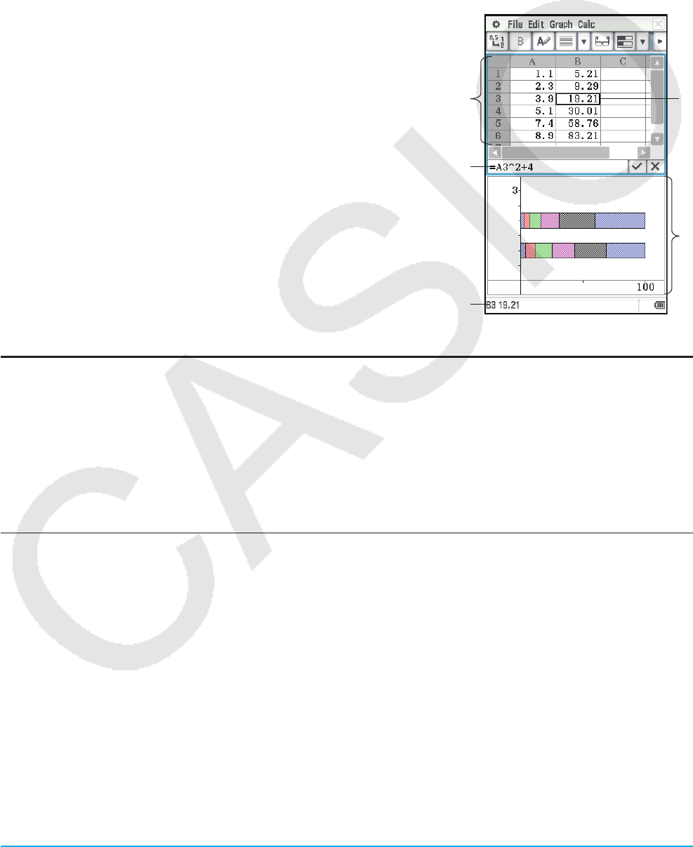
Chapter 13: Spreadsheet Application 226
Chapter 13:
Spreadsheet Application
The Spreadsheet application provides you with powerful, take-along-anywhere spreadsheet capabilities
including graphing and statistical calculations on your ClassPad. A spreadsheet has 999 rows and 64 columns
(A1 to BL999).
The Spreadsheet window shows a screen of cells and their contents. Each cell can contain a value, expression,
text, or a formula. Formulas can contain a reference to a specific cell or a range of cells.
Example Spreadsheet application windows
1 Spreadsheet window
2 Edit box … Shows the contents of the current cell as they were
input. You can tap the edit box and edit its contents.
3 Status bar … Shows the location (or range) of the current cell.
When a single cell is selected, the value of the cell is also shown.
4 Cell cursor … Indicates the currently selected cell(s).
5 Spreadsheet Graph window
1
2
5
3
4
Spreadsheet Window-Specific Menus and Buttons
The menus and buttons of the Spreadsheet window are described below. For information about the menus and
buttons of the Spreadsheet Graph window, see “13-2 Graphing”.
• Transfer data between a spreadsheet and CSV files ..................................................................... File - CSV
• Import variable data to spreadsheet .............................................................................................File - Import
• Export spreadsheet data to a variable ......................................................................................... File - Export
• Recalculate the contents of the cell(s) on the spreadsheet ................................................. File - Recalculate
• Display a dialog box for specifying the color of the text in the cell and the cell fill color ................ Edit - Style
• Toggle linking between text color and graph color on or off ....................................Edit - Format - Color Link
• Display the Options dialog box (see “Option Settings” on page 228) ......................... Edit - Format - Options
• Automatically resize columns to fit the data into the selected cells ..............Edit - Format - AutoFit Selection
• Display a dialog box for specifying column width .............................................. Edit - Format - Column Width
• Display a dialog box for specifying the number format (page 36)
of the selected cell(s) .................................................................................Edit - Format - Number Format
• Display or hide the Cell Viewer window ...................................................... Edit - Format - Cell Viewer or A
• Display a dialog box for specifying a cell to jump to .................................................. Edit - Select - Goto Cell
• Display a dialog box for specifying a range of cells to select ...............................Edit - Select - Select Range
• Insert row(s)/column(s) .......................................... Edit - Insert - Rows or K / Edit - Insert - Columns or a
• Delete the currently selected row(s)/column(s) .. Edit - Delete - Rows or H / Edit - Delete - Columns or J

Chapter 13: Spreadsheet Application 227
• Delete the contents of the currently selected cells ............................................................Edit - Delete - Cells
• Display a dialog box for specifying cell contents and a range of cells to fill ................... Edit - Fill - Fill Range
• Display a dialog box for specifying a sequence to fill a range of cells ......................Edit - Fill - Fill Sequence
• Sort the range of selected cells on the spreadsheet ................................ Edit - Sort/Search - Sort, L or :
• Search for strings in the cell(s) on the spreadsheet ....................................Edit - Sort/Search - Search or e
• Search for strings in the cell(s) on the spreadsheet again ............... Edit - Sort/Search - Search Again or r
• Graph the data in the selected range of cells (pages 239 through 241)
............................................................................. From Graph - Line (D) to Graph - Box Whisker ( 1)
• When graphing, treat each row/each column of the
selected range of cells as a data pair (page 237) ............... Graph - Row Series / Graph - Column Series
• Perform statistical calculations using the data
in the selected range of cells (page 244) ...................From Calc - One-Variable to Calc - Inv. Distribution
• Display the results of the last statistical calculation performed (page 248) .............................Calc - DispStat
• Input a mathematical function into the currently
selected cell (page 249) .........................................From Calc - Cell-Calculation to Calc - List-Calculation
• Toggle the selected cell(s) between decimal (floating point) and exact display* ................................u / ,
• Toggle the selected cell(s) between bold and normal .........................................................................M / B
• Toggle the data type of the selected cell(s) between text and calculation ..........................................u / <
• Specify left-justified text and right-justified values for selected cell(s) (default) ..........................................[
• Specify left-justified, centered, or right-justified for selected cell(s) ..............................................p, x, ]
* When cell(s) are calculation data types.
Changing the Width of a Column
You can use any one of the following methods to adjust the column width.
uUsing the stylus
Use the stylus to drag the edge of a column header left or right until the column is the desired width.
uUsing the Column Width command
1. Tap any cell in the column whose width you want to change.
• You could also drag the stylus to select multiple columns, if you want.
2. On the [Edit] menu, tap [Format] and then [Column Width].
3. On the dialog box that appears, enter a value in the [Width] box to specify the desired width of the column in
pixels.
4. Tap [OK] to change the column width.
uUsing the AutoFit Selection command
1. Select the cell you want to auto fit.
• You can also select any range of cells. In this case, the column width is adjusted to fit the largest data
value in each of the columns within the selected range of cells.
2. On the [Edit] menu, tap [Format] and then [AutoFit Selection].
• This causes the column width to be adjusted automatically so the entire value can be displayed.
• Note that [AutoFit Selection] also will reduce the width of a column, if applicable.

Chapter 13: Spreadsheet Application 228
Option Settings
You can use the Options dialog box to show or hide scrollbars, and specify
what the cell cursor does when you register input data.
uTo change option settings
1. Tap [Edit] - [Format] - [Options] and then use the Options dialog box that appears to perform the operation
described below.
To do this: Select this:
Show the scrollbars Scrollbars - On
Hide the scrollbars Scrollbars - Off
Have the cell cursor remain at the current cell when you register input Cursor Movement - Off
Have the cell cursor move to the next row below the current cell when
you register input
Cursor Movement - Down
Have the cell cursor move to the next column to the right of the current
cell when you register input
Cursor Movement - Right
2. After the setting is the way you want, tap [OK].
13-1 Inputting and Editing Cell Contents
Selecting Cells
Before performing any operation on a cell, you must first select it. You can select a single cell, a range of cells,
all the cells in a row or column, or all of the cells in the spreadsheet.
To select this: Do this:
A single cell Simply tap it with the stylus. When a single cell is selected, you can use the cursor
key to move the cell cursor up, down, left, or right.
A range of cells Drag the stylus across them. If you drag to the edge of the screen, it will scroll
automatically, until you remove the stylus from the screen.
Two non-contiguous
columns*1
Tap the header of one of the columns and then tap the header of the other column.
For example, to select columns A and C, tap the header of column A and then the
header of column C.
Two non-contiguous
rows*1
Tap the header of one of the rows and then tap the header of the other row. For
example, to select rows 3 and 6, tap the header of row 3 and then the header of row
6.
All the cells in a row
or column
Tap a column heading to select the column, or tap a row heading to select the row.
All of the cells in the
spreadsheet
Tap the box above row heading 1 (to the left of column heading A).
*1 This selection method can be used only to specify a range of data for graphing. For details about graphing,
see “13-2 Graphing”.

Chapter 13: Spreadsheet Application 229
Note
• Selection of non-contiguous rows and columns can be used for selection of up to two rows or two columns
only. You cannot select more than two non-contiguous rows or columns.
• These operations are not supported when selecting rows or columns for non-graphing operations, such as
statistical calculations, etc. Attempting these operations for a non-graphing operation will cause an error.
Inputting Data into a Cell
The following are the basic steps you need to perform whenever inputting or editing cell data.
uClassPad Operation
1. Tap a cell and then tap the edit box.
• This will change the toolbar to a data input toolbar like the one shown in
the nearby screenshot.
2. Input the data you want.
• You can input data using the keypad, the soft keyboard, the [Calc]
menu, and the data input toolbar. See the following sections for more
information.
3. After you are finished, tap the s button next to the edit box or press the
E key.
Data input toolbar
• This causes the entire spreadsheet to be re-calculated.
• If you want to cancel data input without saving your changes, tap the S button next to the edit box or tap
l on the icon panel.
Inputting a Formula
A formula is an expression that the Spreadsheet application calculates and evaluates when you input it, when
data related to the formula is changed, etc. A formula always starts with an equals sign (=), and can contain
values, mathematical expressions, cell references, and functions.
The screenshot to the right shows a simple example where a formula in cell B5
calculates the mean of the values in cells B1 through B3. Formulas are
calculated dynamically whenever related values are changed, and the latest
result is always displayed in the spreadsheet.
uTo input formula “=mean(B1:B3)” in cell B5
1. Tap cell B5 to select it.
2. On the [Calc] menu, tap [List-Statistics] and
then [mean].
• This will cause “=mean(” to be input into
the edit box.
3. Drag from cell B1 to cell B3.
• This will input “B1:B3”.
4. Tap the s button next to the edit box or
press the E key. This will finalize input
of “=mean(B1:B3)”.
• If you do not input the closing parenthesis ( ) ) it will be input automatically.

Chapter 13: Spreadsheet Application 230
Tip: As in the example shown above, tapping another cell while the first character in the edit box is an equals sign (=)
inserts a reference to the tapped cell into the edit box. Dragging across a range of cells will input a reference to the
selected range.
Inputting a Cell Reference
A cell reference is a symbol that references the value of one cell for use by another cell. If you input “=A1 + B1”
into cell C2, for example, Spreadsheet will add the current value of cell A1 to the current value of cell B1, and
display the result in cell C2.
There are two types of cell references: relative and absolute.
Relative Cell Reference
A relative cell reference is one that changes according to its location on the spreadsheet. The cell reference
“=A1” in cell C2, for example, is a reference to the cell located “two columns to the left and one cell up” from the
current cell (C2, in this case). Because of this, if we copy or cut the contents of cell C2 and paste them into cell
D12, for example, the cell reference will change automatically to “=B11”, because B11 is two columns to the left
and one cell up from cell D12.
Be sure to remember that relative cell references always change dynamically in this way whenever you move
them using cut and paste, or drag and drop.
However, when you cut or copy a relative cell reference from the edit box, it is copied to the clipboard as text
and pasted “as-is” without changing it. If “=A1” is in cell C2 and you copy “=A1” from the edit box and paste it
into cell D12, for example, D12 will also be “=A1”.
Absolute Cell References
An absolute cell reference is one that does not change, regardless of where it is located or where it is copied
to or moved to. You can make both the row and column of a cell reference absolute, or you can make only the
row or only the column of a cell reference absolute, as described below.
This cell reference: Does this:
$A$1 Always refers to column A, row 1.
$A1 Always refers to column A, but the row changes dynamically when moved, as
with a relative cell reference.
A$1 Always refers to row 1, but the column changes dynamically when moved, as
with a relative cell reference.
Let’s say, for example, that a reference to cell A1 is in cell C1. The following shows what each of the above cell
references would become if the contents of cell C1 were copied to cell D12.
$A$1 → $A$1 $A1 → $A12 A$1 → B$1
uTo input a cell reference “=A1” in cell B1
1. Tap cell B1 to select it, and then input “=”.
2. Tap cell A1 or use the data input toolbar and keypad to input [A] [1].
3. Tap the s button next to the edit box or press the E key.
Tip: If you want to input an absolute cell reference, use the stylus or cursor keys to move the editing cursor to the
appropriate location, and then use the editing toolbar to input a dollar ($) symbol.

Chapter 13: Spreadsheet Application 231
Cell Data Types (Text Data and Calculation Data)
When a single cell is selected, the toolbar will show u when it is a text data type cell, or < if it is a calculation
data type cell. When you create a new spreadsheet, all of the cells are initially text data type.
• With a text data type cell, any text or variable that does not have an equals sign (=) at the beginning is treated
as text. A single value is treated as a constant value.
• With a calculation data type cell, a formula or variable that does not have an equals sign (=) at the beginning
is treated as a constant value. Inputting 2{3w in a calculation data type cell, for example, will cause
the value 8 (the calculation result) to appear in the cell.
When this data type is
specified:
Inputting this into
the cell:
Causes this to be displayed:
Text u2 (treated as a constant value)
π (treated as text)
2^3 (treated as text)
Calculation <2 (treated as a constant value)
π (treated as a constant value)
2^3 (treated as a constant value)
uTo specify text or calculation as the data type for a particular cell
Select the cell(s) whose data type you want to specify, and then tap the third button from the left (u / <) to
toggle the data type between text and calculation.
Inputting a Constant into a Calculation Data Type Cell
You can use any one of the procedures below to input constants into calculation data type cells.
• Direct input of a value or expression
• Input of the same value into all of the cells in a specific range (Fill Range)
• Input of a numeric sequence generated by a single-variable formula into a column of cells
uTo input a value or expression into a calculation data type cell
1. Tap the cell where you want to input data.
2. If u is displayed on the toolbar, tap to toggle it to <.
3. Input the value or expression without inputting an equals sign (=) at the beginning.
• You can input an expression that returns a value as a calculation result.
4. Tap the s button next to the edit box or press the E key.
• The value you input or the calculation result of the expression you input appears in the cell.
• “#ERR” will appear in the cell if the expression cannot be executed or if there is a syntax error.
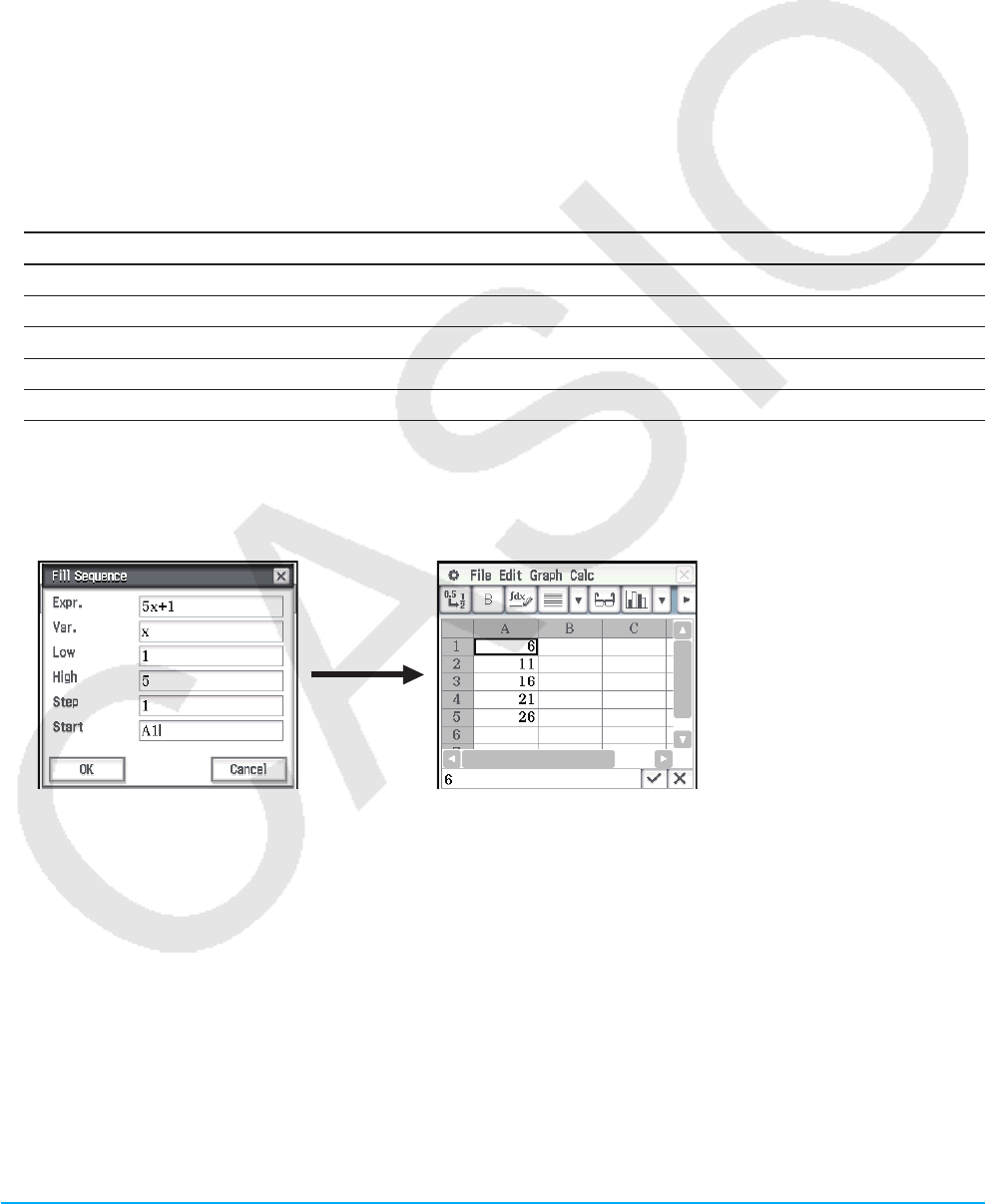
Chapter 13: Spreadsheet Application 232
uTo fill a range of cells with the same value (Fill Range)
1. Select the range of cells where you want to input the same value.
• Actually, you could skip this step and start with step 2, below.
2. On the [Edit] menu, tap [Fill] and then [Fill Range].
3. On the dialog box that appears, input the value or expression into the “Formula” box. You can also use the
dialog box’s “Range” box to specify the range of cells.
4. Tap [OK].
• The specified range of cells will automatically change to calculation data type cells, containing the value
you input in step 3.
uTo fill a column of cells with a numeric sequence (Fill Sequence)
1. Tap the cell from which you want input of the numeric sequence to start.
• Actually, you could skip this step and start with step 2, below.
2. On the [Edit] menu, tap [Fill] and then [Fill Sequence].
3. Use the dialog box that appears to configure the Fill Sequence operation as described below.
Parameter Description
Expr. Input the expression whose results you want to input.
Var. Specify the name of the variable whose value will change with each step.
Low/High Specify the smallest/greatest value to be assigned to the variable.
Step Specify the value that should be added to the variable value with each step.
Start Specify the starting cell from which the results of the expression should be inserted.
4. After everything is the way you want, tap [OK].
• This performs all the required calculations according to your settings, and inserts the results into the
spreadsheet.
Example:
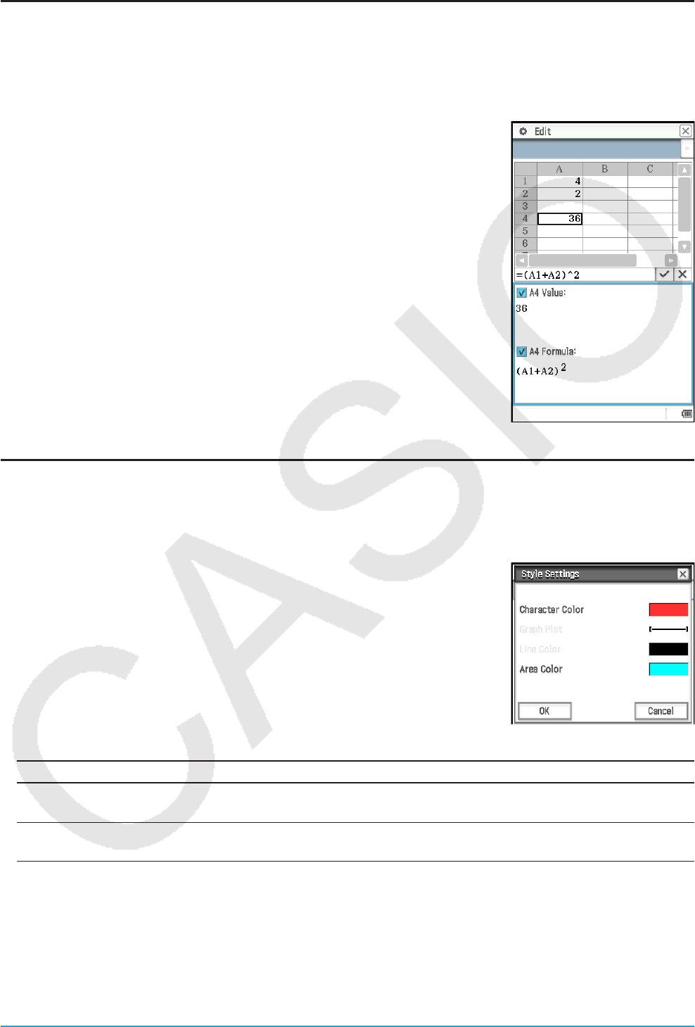
Chapter 13: Spreadsheet Application 233
Using the Cell Viewer Window
The Cell Viewer window lets you view both the formula contained in a cell, as well as the current value
produced by the formula.
uTo view or hide the Cell Viewer window
On the Spreadsheet toolbar, tap A. Or, on the Spreadsheet [Edit] menu,
select [Format] - [Cell Viewer].
• The above operation toggles display of the Cell Viewer window on or off.
• On the Cell Viewer window, you can select or clear its check boxes to toggle
display of the value and/or formula on or off.
• You can select a value or formula on the Cell Viewer window and then drag it
to another cell, or tap [Edit] - [Copy] to place it onto the clipboard.
Changing the Text Color and Fill Color of Specific Cells
For each cell, you can specify the text color and cell color.
uClassPad Operation
1. Select the range of cells whose text color and fill color settings you want to
change.
2. On the [Edit] menu, tap [Style].
• This displays the Style Settings dialog box.
3. Configure the above dialog box with the following settings.
To specify this: Perform this operation:
Text color Tap “Character Color” to display the Color Settings dialog box. Next, select the
text color you want and then tap [OK].
Cell color Tap “Area Color” to display the Color Settings dialog box. Next, select the fill
color you want and then tap [OK].
4. To apply the settings you configure, return to the Style Settings dialog box and then tap [OK].

Chapter 13: Spreadsheet Application 234
Copying or Cutting Cells and Pasting Them to Another Location
Use the procedures below to copy or cut one cell or multiple cells, and then paste them to another cell or cells.
For information about what happens when you copy or cut cells that include cell references and paste them to
another location, see “Relative Cell Reference” (page 230).
uTo copy or cut a single cell and paste it to another cell or cells
1. Tap the cell that you want to copy or cut.
2. Tap [Edit] - [Copy] (or [Cut]).
3. Tap the cell (or drag across the range of cells) to which you want to paste the cell you copied or cut.
4. Tap [Edit] - [Paste].
• This will paste content of the cell your copied or cut, including formatting (bold, calculation/text data type,
text color, fill color).
• If you selected a range of cells in step 3, the same content will be pasted to all of the selected cells. Note,
however that if the cell you copied or cut included a relative cell reference (such as “A1”, “B2”), the content
of the pasted cells will change in accordance with their relative positions.
Tip: You can also copy to a single cell by selecting a cell (with the cell cursor), and then dragging it to the copy
destination. If the destination cell already contains data, it is replaced with the newly dropped data.
uTo copy or cut a range of cells and paste them to another location in the spreadsheet
1. Tap the range of cells that you want to copy or cut.
2. Tap [Edit] - [Copy] (or [Cut]).
3. Tap the cell that is the upper left corner of the range of paste destination cells.
4. Tap [Edit] - [Paste].
• This will paste the contents, including formatting, of the range of cells you copied.
Tip: In place of the steps from step 2 of the above procedure, you could also copy the selected cells by dragging them to
the copy destination. If the destination cells already contain data, it is replaced with the newly dropped data.
Recalculating Spreadsheet Expressions
Recalculate is executed automatically whenever you switch to the Spreadsheet application from another
application, and whenever you open a spreadsheet file.
However, you need to recalculate manually in cases like that shown in the example below.
Example: To plot a scatter graph using random numbers
1. Input “=rand()” into cell A1, and then copy the contents of A1 to cells A2
through A5.
2. Select cells A1:A5 and then tap [Graph] - [Scatter] to plot the scatter graph.
3. Tap the Spreadsheet window to make it active, and then tap [File] -
[Recalculate].
• Each time you tap [File] - [Recalculate], random numbers are regenerated
and the graph is updated accordingly.

Chapter 13: Spreadsheet Application 235
Transferring Data between a Spreadsheet and CSV Files
You can import the contents of a CSV file stored with the ClassPad or transferred from a computer into a
spreadsheet. You also can save the contents of a spreadsheet as a CSV file.
uTo import the contents of a CSV file to a spreadsheet
1. Prepare the CSV file you want to import.
• See “Import CSV File Requirements” on page 134.
2. Tap [File] - [CSV] - [Open CSV].
• Tapping [Open] in the next step will overwrite all of the data on the spreadsheet with the CSV file data.
3. On the dialog box that appears, select the CSV file you want to import and then tap [Open].
Important!
Attempting to import a CSV file that has more than 64 columns or 999 rows will cause an “Invalid Data Size”
error.
uTo save spreadsheet contents as a CSV file
1. If required, tap [File] - [Recalculate] to recalculate the spreadsheet contents.
• Note that recalculation is not performed automatically when you save spreadsheet contents to a CSV file.
Be sure to perform recalculation if the spreadsheet contains a formula, which starts with an equals symbol
(=).
• Formulas are not saved to the CSV file. Only calculation results are saved.
• All ERROR cell data on the spreadsheet is saved as blank data.
2. Tap [File] - [CSV] - [Save CSV].
3. On the dialog box that appears, specify the export destination folder and then input a name for the export file.
4. Tap [Save].
uTo specify the CSV file separator and decimal symbol
Tap [File] - [CSV] - [CSV Format] to display the CSV format setting screen. Next, perform the procedure from
step 2 under “To specify the CSV file separator and decimal symbol” (page 135).
Importing and Exporting Variable Values
You can import LIST (list), MAT (matrix), EXPR (expression), and STR (string) variables* into a spreadsheet.
LIST, MAT, and EXPR type variable in spreadsheet data also can be exported.
* For information about variable types, see “Main Memory Data Types” (page 28).
uTo import the data assigned to a variable
1. In a spreadsheet, tap a single cell to specify it as the import destination of the variable data.
• If the variable you are importing is an EXPR or STR type, tapping the cell will input the variable data. For a
LIST or MAT type variable, data is input as shown in examples below when cell A1 is tapped.
LIST variable “{1,2,3}” MAT variable “[[1,2][3,4]]” *
* Same as 1 2
3 4
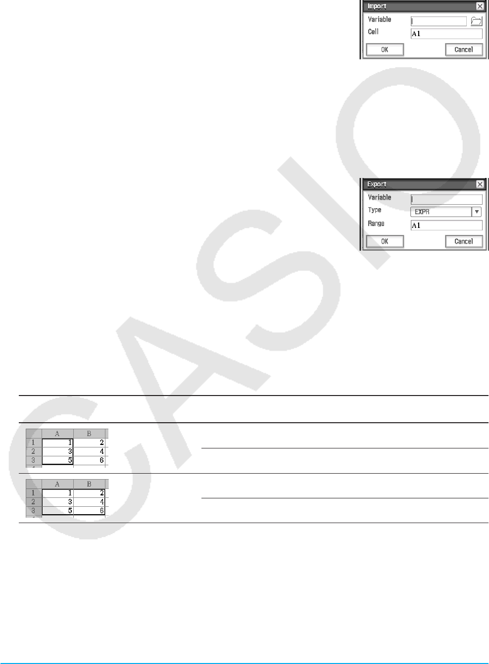
Chapter 13: Spreadsheet Application 236
• If any of the cells within the range where variable data is being input already contain data, the existing data
will be overwritten with the imported data.
• The data type of the cells to which data is imported will automatically change to calculation data type (LIST,
MAT, EXPR) or text data type (STR) in accordance with the type of variable imported into each cell.
2. On the [File] menu, tap [Import].
• This displays the Import dialog box along with a soft keyboard.
3. Type the variable name into the [Variable] box.
• Tapping the 2 icon on the Import dialog box will display the Variable
Manager, which you can use to select the variable you want. See “Using
Variable Manager” (page 29) for more information.
4. To import the specified variable data into the spreadsheet, tap [OK].
uTo export spreadsheet data to an EXPR variable
1. Select a single cell that contains the data you want to export to an EXPR variable.
• It makes no difference whether the cell you select contains a value, expression, or string. Note that string
data exported from a cell is exported as EXPR type data, not STR type data.
2. On the [File] menu, tap [Export].
• This displays the Export dialog box along with a soft keyboard. In this
case, “EXPR” will be automatically selected in the [Type] box.
3. Type the variable name into the [Variable] box.
4. After confirming that everything is the way you want, tap [OK].
uTo export spreadsheet data to a LIST or MAT (matrix) variable
1. Select the range of cells that contains the data you want to export to a LIST or MAT variable.
2. On the [File] menu, tap [Export].
3. On the dialog box that appears, tap the [Type] box down arrow button, and then select “LIST” or “MATRIX”
from the list of variable types that appears.
4. Type the variable name into the [Variable] box, and then tap [OK].
• The data in the range of cells you select in step 1 is exported as shown below, in accordance with the
variable type (“LIST” or “MATRIX”) you select in step 3.
When these cells are selected in
step 1:
When this is selected in step 3: Data is exported as:
Type: LIST {1,3,5}
Type: MATRIX [[1][3][5]]
Type: LIST {1,3,5,2,4,6}
Type: MATRIX [[1,2][3,4][5,6]]
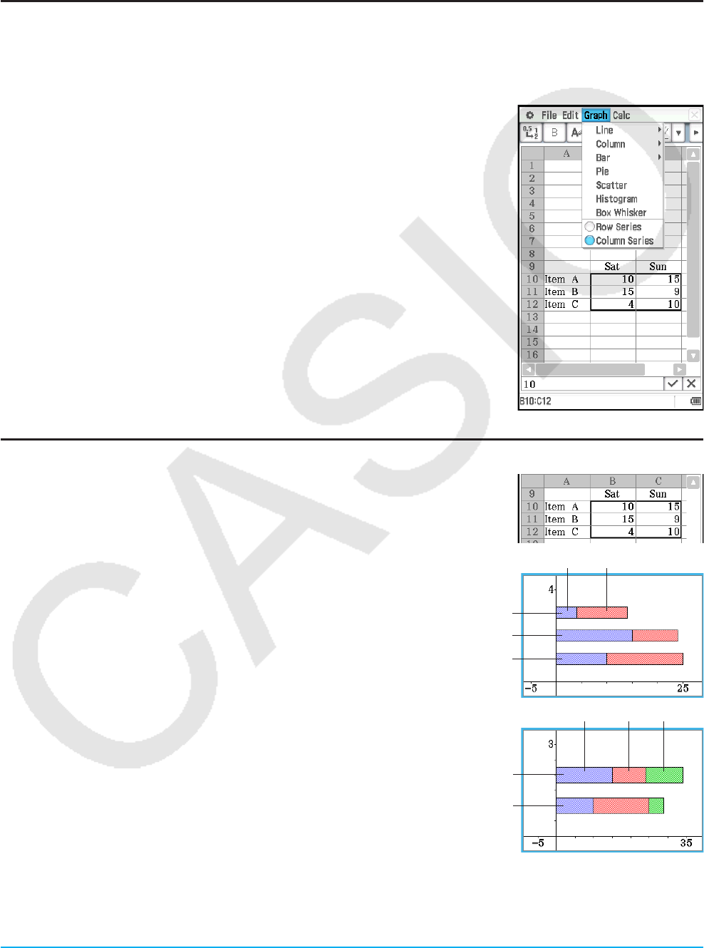
Chapter 13: Spreadsheet Application 237
13-2 Graphing
The Spreadsheet application lets you draw a variety of different graphs for analyzing data.
Basic Graphing Steps
The following are the basic steps for graphing spreadsheet data.
uClassPad Operation
1. Input the data you want to graph into the spreadsheet.
2. Select the cells that contain the data you want to graph.
3. On the [Graph] menu, tap [Column Series] to graph the data by column, or
tap [Row Series] to graph the data by row.
• For more information, see “Column Series and Row Series” below.
4. On the [Graph] menu, select the type of graph you want to draw. Or you can
tap the applicable icon on the toolbar.
• This will open the Spreadsheet Graph window in the lower half of the
display and draw the selected type of graph. See “Graph Menu and Graph
Examples” (page 239) for examples of the different types of graphs that are
available.
Tip: After the graph is drawn on the Spreadsheet Graph window, you can change to
another type of graph at any time by selecting the graph type you want on the
[Type] menu. Or you can tap the applicable icon on the toolbar.
Column Series and Row Series
For example, the nearby screenshot shows sales results for items A, B, and C
during Saturday and Sunday. Let’s say we select the column series and row
series and draw a stacked bar graph ([Graph] - [Bar] - [Stacked]).
• When [Graph] - [Column Series] is selected, each column is treated
as one set of data. Since this is a stacked graph, the first set of Sat
data (blue) and the second set of Sun data (red) are cumulative, and
there are three bars, one for each of the three items. This lets you
see the cumulative sales for each item.
Item C
Item B
Item A
Sat Sun
• When [Graph] - [Row Series] is selected, each row is treated as one
set of data. Item A data (blue), Item B data (red), and Item C data
(green) are cumulative, and there are two bars, one for each of the two
days of the week. This lets you see the cumulative sales for each day. Sun
Sat
ACB
Tip: You can switch an existing graph between column series and row series by tapping [Type] - [Column Series] or
[Type] - [Row Series].
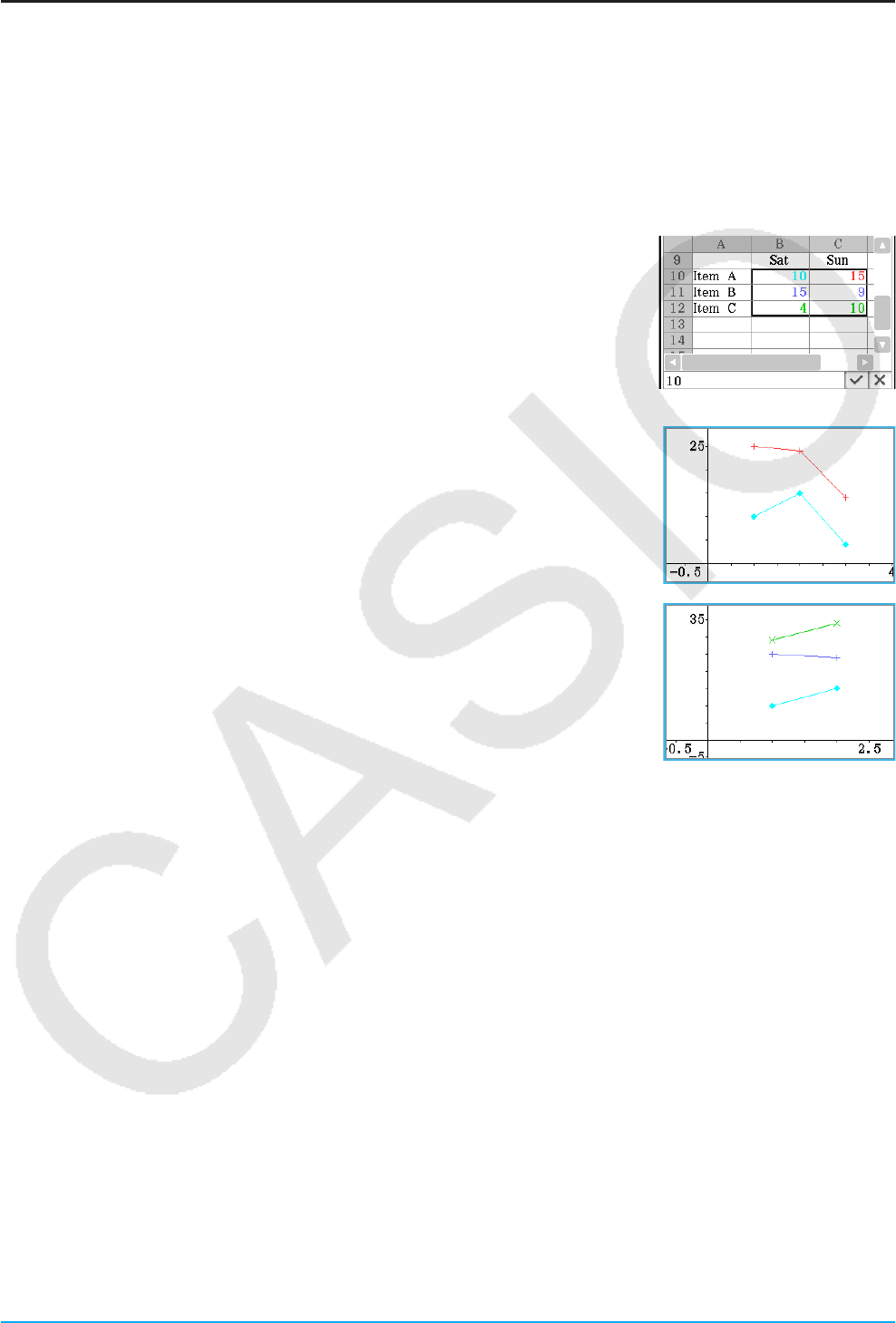
Chapter 13: Spreadsheet Application 238
Graph Colors and Color Link
Enabling Color Link (so there is a check mark next to it) on the Edit menu will cause the text color of the data
being graphed to be used when the data is graphed. Conversely, a color specified on the Graph window will be
applied as the text color of the corresponding data.
When Color Link is disabled (so there is no check mark next to it on the [Edit] - [Format] menu), graphing is
performed using default colors.
uTo use text colors as graph colors
Example: To draw a stacked line graph using the data in the nearby
screenshot, which is the same we graphed under “Column Series
and Row Series” (page 237)
1. Configure text color settings for each cell as shown in the nearby
screenshot.
• For information about color settings, see “Changing the Text Color and Fill
Color of Specific Cells” (page 233).
2. Tap [Graph] - [Column Series].
3. Tap [Edit] - [Format] - [Color Link] so there is a check mark next to [Color
Link].
4. Tap [Graph] - [Line] - [Stacked].
• This will draw a stacked line graph using the data colors.
5. Tap [Type] - [Row Series].
• This switches to a row series graph. For a line graph, the color of each
data’s first character (first row character in the case of Column Series, first
column character in the case of Row Series) is applied as the line color.
u To specify the graph drawing color on the Graph window
Example: To continue with the operation in the previous example and change the drawing color on the Graph
window
1. On the Graph window, select the point whose color you want to change by tapping it.
• Note that you cannot select a line. Line colors are always the same as the rightmost end point.
2. On the [Edit] menu, tap [Style].
• This displays the Style Settings dialog box.
3. Select the color you want and then tap [OK].
• This will change the point to the color you selected.
• Since there is a check mark next to [Color Link] on the [Edit] - [Format] menu, the corresponding data on
the Spreadsheet window will also change to the selected color.
Tip
• Changing the [Color Link] setting to either enabled (check mark next to it on the [Edit] - [Format] menu) or disabled (no
check mark) while a graph is displayed will cause the graph to be redrawn in accordance with the newly selected enabled/
disabled setting.
• When Color Link is enabled, the relationship between data text color and the graph color is as described below for each
type of graph.

Chapter 13: Spreadsheet Application 239
Line Graph, Column graph, Bar graph: The color of each data’s first character (first row character in the case of Column
Series, first column character in the case of Row Series) is applied as the color of the applicable portion (line, column,
bar) of graph.
Scatter graph: When plotting a scatter graph of multiple different data series, the text color of the y-value of each data
pair is used as the color of points plotted for the y-value. The text colors of x-values are ignored. When plotting a
scatter graph of a single data series (selecting [Graph] - [Column Series] to graph a single column of data or [Graph] -
[Row Series] to graph a single row of data) a point plotted on the graph will be the same color as the character color of
the corresponding data item. When the [Lines] item of the [View] menu is enabled (indicated by a check mark next to
it) on the Graph window, the color of a line is the same as the final rightmost point.
Histogram, Box Whisker: Histograms and box whiskers are always drawn using colors selected by ClassPad, regardless
of the current Color Link enabled/disabled setting.
Pie graph: The text color of each data item is used as the color of the pie piece that represents the data on the graph.
Spreadsheet Graph Window-Specific Menus and Buttons
• Change the color of a graph part selected on the Graph window .................................................. Edit - Style
• Deleted the regression graph selected on the Graph window ..................................................... Edit - Delete
• Clear all regression graphs on the Graph window
(except for graphs drawn using the [Graph] menu) .............................................................Edit - Clear All
• Change the function of the stylus so it can be used to select
and move points on the displayed graph .....................................................................View - Select or G
• Pan the graph window ......................................................................................................... View - Pan or T
• Adjust the size of the display image so it fills the display ........................................ View - Zoom to Fit or R
• Toggle display of axes and coordinate values on or off ..........................................View - Toggle Axes or q
• Toggle line graph and scatter graph plot markers on or off .....................................................View - Markers
• Toggle line graph and scatter graph connecting lines on or off ................................................... View - Lines
• Change the graph type (pages 239 through 241) ........... From Type - Line (D) to Type - Box Whisker ( 1)
• Switch between row and column for handling one group of graphed data (page 237)
.............................................................................................. Type - Row Series / Type - Column Series
• Draw a regression graph and display regression calculation results (page 242)
..............................From Calc - Regression - Linear Reg (d) to Calc - Regression - Logistic Reg (6)
• Show or hide (check box) of calculation results
when the regression graph draw command is selected ......................................................Calc - DispStat
• Convert the data of the selected column to a line graph ...................................................... Calc - Line or z
• Convert the data of the selected line to a column graph .................................................Calc - Column or '
• Set bin width for a histogram ................................................................................................. Calc - Bin Width
• Show outlying data for box whisker graph ...................................................................... Calc - Show Outliers
Tip: The View menu Zoom Box (Q), Zoom In (W), and Zoom Out (E) commands are the same as the Graph &
Table application Box, Zoom In, and Zoom Out commands on the Zoom menu. For more information about these
commands, see “Chapter 3: Graph & Table Application”.
Graph Menu and Graph Examples
The following explains each of the [Graph] menu commands, and shows examples of what happens to the
Graph window when you execute a command. Each command is followed by a button to show the graph
toolbar button that performs the same action as the command.
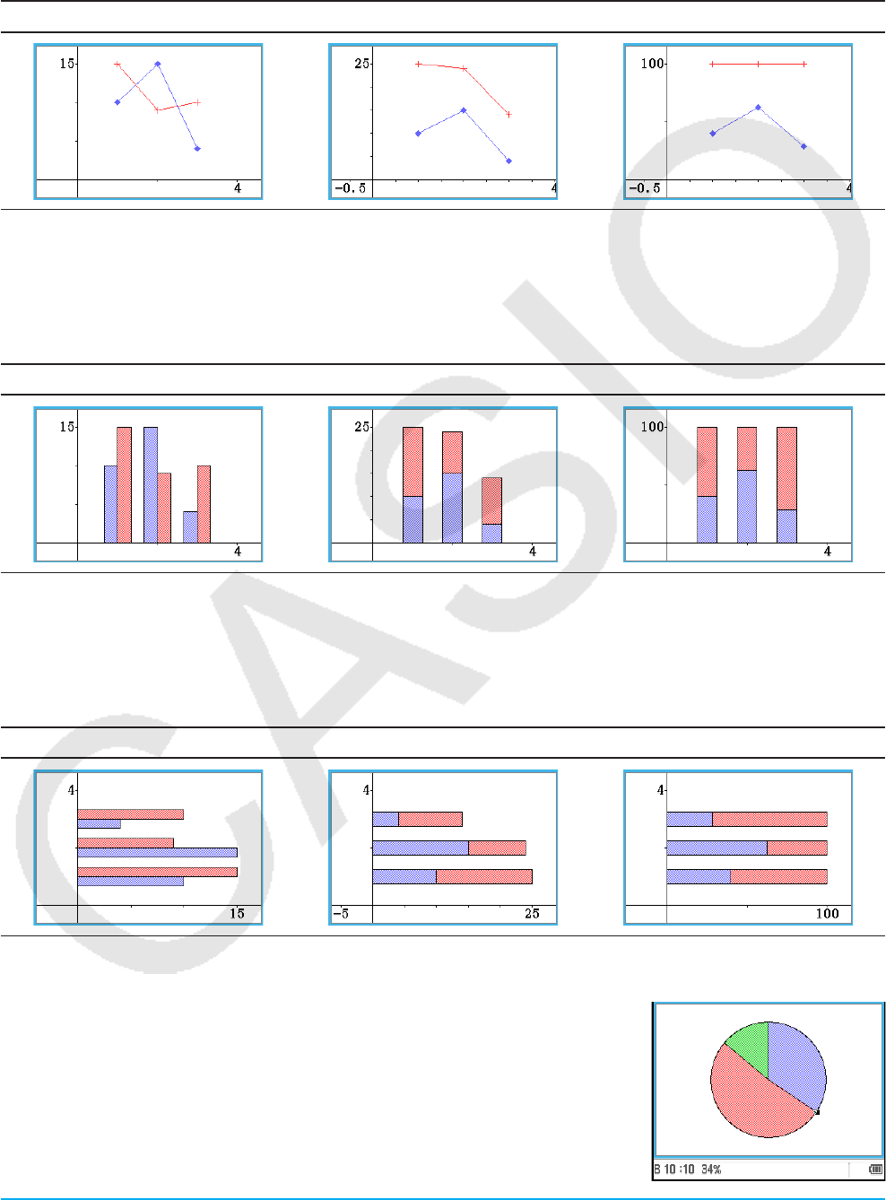
Chapter 13: Spreadsheet Application 240
Tip: The contents of the Spreadsheet window [Graph] menu and the Graph window [Type] menu are identical. On the
Graph window, you can uses the [Type] menu or the applicable icon on the toolbar to change the graph type after a
graph is drawn.
[Graph] - [Line] -
[Clustered] D[Stacked] F[100% Stacked] G
• After drawing a clustered line graph, you can change a line in the graph to a column graph. To do this, tap
any data point on the line you wish to change to a column graph, and then tap [Column] on the [Calc] menu or
tap '. You can change a column graph back to a line graph by selecting one of its columns and tapping z
or [Line] on the [Calc] menu.
[Graph] - [Column] -
[Clustered] D[Stacked] F[100% Stacked] G
• After drawing a clustered Column graph, you can change a column in the graph to a line graph. To do this,
tap any one of the columns you wish to change to a line graph, and then tap [Column] on the [Calc] menu or
tap z. You can change a line graph back to a column graph by selecting one of its data points and tapping
' or [Column] on the [Calc] menu.
[Graph] - [Bar] -
[Clustered] D[Stacked] F[100% Stacked] G
[Graph] - [Pie] Z
• When you select a pie chart, only the first series (column or row) of the
selected data is used.
• Tapping any of the sections of a pie graph causes three values to appear at
the bottom of the screen: the cell location, a data value for the section, and
a percent value that indicates the portion of the total data that the data value
represents.
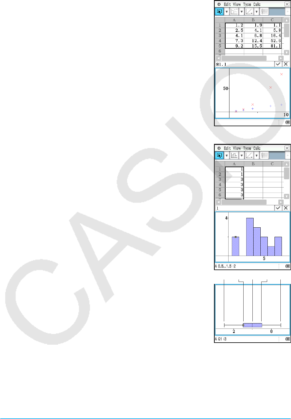
Chapter 13: Spreadsheet Application 241
[Graph] - [Scatter] X
• When plotting a scatter graph of multiple different data series, the first series
(column or row) of selected values is used as the x-values for all plots. The
other selected values are used as the y-value for each of the plots. This
means if you select three columns of data (like Columns A, B, and C), for
example, there will be two different plot point types: (A, B) and (A, C).
• When plotting a scatter graph of a single data series (selecting [Graph] -
[Column Series] to graph a single column of data or [Graph] - [Row Series]
to graph a single row of data), x-axis data numbers (1, 2, 3...) are fixed and
each data item is plotted on the y-axis.
• Scatter graphs initially have plotted points only. You can add lines by
selecting [Lines] on the [View] menu.
[Graph] - [Histogram] 3
• When you select a histogram graph, only the first series (column or row) of
the selected data is used.
• Tapping any of the bins of a histogram graph causes three values to appear
at the bottom of the screen. The first two values (from the left) indicate the
range of the selected bin, while the third value indicates the quantity of the
selected bin.
• You can specify the bin width after drawing a histogram graph. On the
Spreadsheet Graph window that shows the histogram, tap [Bin Width] on the
[Calc] menu.
[Graph] - [Box Whisker] 1
This type of graph lets you see how a large number of data items are grouped
within specific ranges. The lines from Min to Q1, and from Q3 to Max are called
“whiskers”. If [Calc] - [Show Outliers] box is checked on the Spreadsheet Graph
window, “outlier” circular symbols are shown instead of “whisker” lines where a
data value is relatively large or small compared to the other data values.
• When you select a box whisker graph, each column will be displayed as a
separate box whisker.
• Tapping the Q1, Q3, Med, Min, or Max location of a box whisker graph will
cause the applicable value to appear at the bottom of the screen.
Q3
MedMin MaxQ1

Chapter 13: Spreadsheet Application 242
Regression Graph Operations (Curve Fitting)
After plotting a scatter graph using paired-variable (x, y) data on the spreadsheet, you can draw a regression
graph that approximates the scatter graph and determine the regression formula.
uTo plot a scatter graph and then draw its regression graph
1. Enter the paired-variable data into the spreadsheet, and then select the range of cells where it is located.
• For information about how data is treated based on the range of cells that are selected, see “[Graph] -
[Scatter]” (page 241) under “Graph Menu and Graph Examples”.
2. Tap [Graph] and then [Scatter].
• This will open the Graph window in the lower half of the display and plot the scatter graph.
3. When plotting a scatter graph with multiple y-values, select one of the y-value plots that you want to use for
drawing the regression graph by tapping it.
4. On the Graph window, perform the following steps.
To draw this: Select this [Calc] menu item: Or tap this:
Linear regression curve Linear Reg d
Med-Med graph MedMed Line 2
Quadratic regression curve Quadratic Reg f
Cubic regression curve Cubic Reg g
Quartic regression curve Quartic Reg h
Quintic regression curve Quintic Reg j
Logarithmic regression curve Logarithmic Reg l
Exponential aⴢebx regression curve Exponential Reg k
Exponential aⴢbx regression curve abExponential Reg 4
Power regression curve Power Reg ;
Sinusoidal regression curve Sinusoidal Reg 5
Logistic regression curve Logistic Reg 6
• This superimposes the regression graph on the scatter graph. Also, the
regression calculation result window will appear in the upper half of the
display (except for Quintic Reg).
• Here, you can add a another regression graph by selecting a different
[Calc] menu item. Also, you can repeat step 3 to overlay a regression
graph for a different y-value.
5. To clear all regression graphs, tap [Edit] - [Clear All].
• You can also delete a particular regression graph by tapping to select it,
and then tapping [Edit] - [Delete].
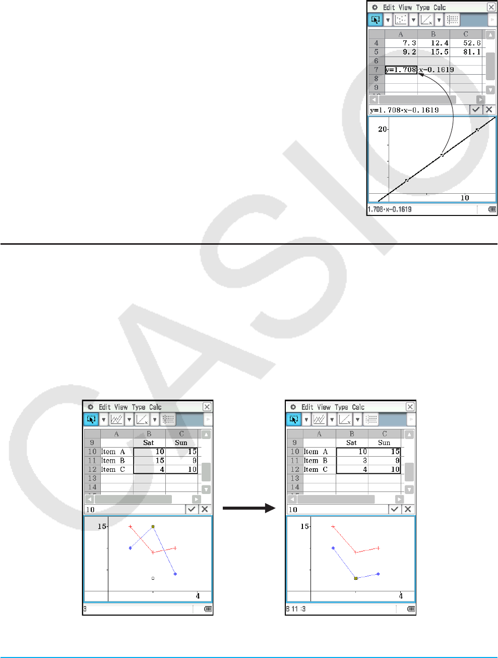
Chapter 13: Spreadsheet Application 243
Tip
• Regression graphs are normally drawn in blue, but you can change the color after drawing is complete. To change the
color after drawing is complete, tap the graph and then tap [Edit] - [Style] to display the Style Settings dialog box. Perform
the procedure under “To specify the graph drawing color on the Graph window” (page 238) to change the color.
• Exponential and abExponential regression curves ignore negative values when calculating the curve. A message appears
in the status bar to let you know when negative values are ignored.
• On the Graph window, after tapping a regression graph to select it you can drag it to
the Spreadsheet window and drop it into a cell to paste the function of the regression
graph into the cell. You can also achieve the same result by tapping the regression
graph, tapping [Edit] - [Copy] (or [Edit] - [Cut]), tapping a cell in the Spreadsheet
window, and then tapping [Edit] - [Paste]. Note that if you perform an [Edit] - [Cut]
operation, the regression graph will be deleted from the Graph window.
• For details about how to use the Link check box and [Output>>] button on the
regression calculation result window, see “To execute a regression calculation and
paste the results into the spreadsheet” (page 245).
Other Graph Window Operations
This section provides more details about the types of operations you can perform while the Graph window is on
the display.
uTo change the appearance of a graph by dragging a point
While a graph is on the Graph window, use the stylus to drag any one of its data points to change the
configuration of the graph.
• You can change curves, make bars or columns longer or shorter, or change the size of pie graph sections.
• Changing a graph automatically changes the graph’s data on the Spreadsheet window.
Drag Changes

Chapter 13: Spreadsheet Application 244
• If a regression curve is displayed for the data whose graph is being changed by dragging, the regression
curve also changes automatically in accordance with the drag changes.
• When you edit data in the spreadsheet and press E, your graph will update automatically.
Important!
• You can drag a point only if it corresponds to a fixed value on the spreadsheet. You cannot drag a point if it
corresponds to a formula.
• You may encounter the message “Insufficient System Memory to Run...” if you are using a large amount of
data and formulas.
uTo use drag and drop to obtain the data of a graph
While a graph is on the Graph window, you can select a part of the graph (point, bar, etc.) and drop it into
a Spreadsheet window cell. This will import the graph data into the spreadsheet. The data that is imported
depends on the graph type.
Dragging this to a cell in the
spreadsheet window:
Creates a table containing these values starting from the
cell where you dropped the data:
A point of a line graph, a column of a
column graph, or a bar of a bar graph
All of the values in the series associated with the point, column,
or bar
A point of a scatter graph All (x, y) values of the series associated with the point
A pieces of a pie graph A percentage value relative to the entire pie graph
Any of the bins of a histogram graph The values of the histogram graph
Any of the Q1, Q3, Med, Min, or Max
location of a box whisker graph
The graph’s values (Min, Q1, Median, Q3, Max)
uTo show or hide lines and markers for a line graph or a scatter graph
1. While a line graph or a scatter graph is on the Graph window, tap the [View] menu.
2. Tap the [Markers] or [Lines] item to toggle it between show (check box selected) and hide (check box
cleared).
• Line and scatter graphs can have markers only, lines only, or both markers and lines. You cannot turn off
both markers and lines at the same time.
13-3 Statistical Calculations
The upper part of the [Calc] menu includes the same menu items as the Statistics Application [Calc] menu.
Spreadsheet Application Statistics Application
Menu items with the same name perform the same functions, but there are some differences between the
Statistics Application and Spreadsheet Application in terms of operation procedures, calculation result display,
etc. This section explains statistical operations and functions that are peculiar to the Spreadsheet Application.
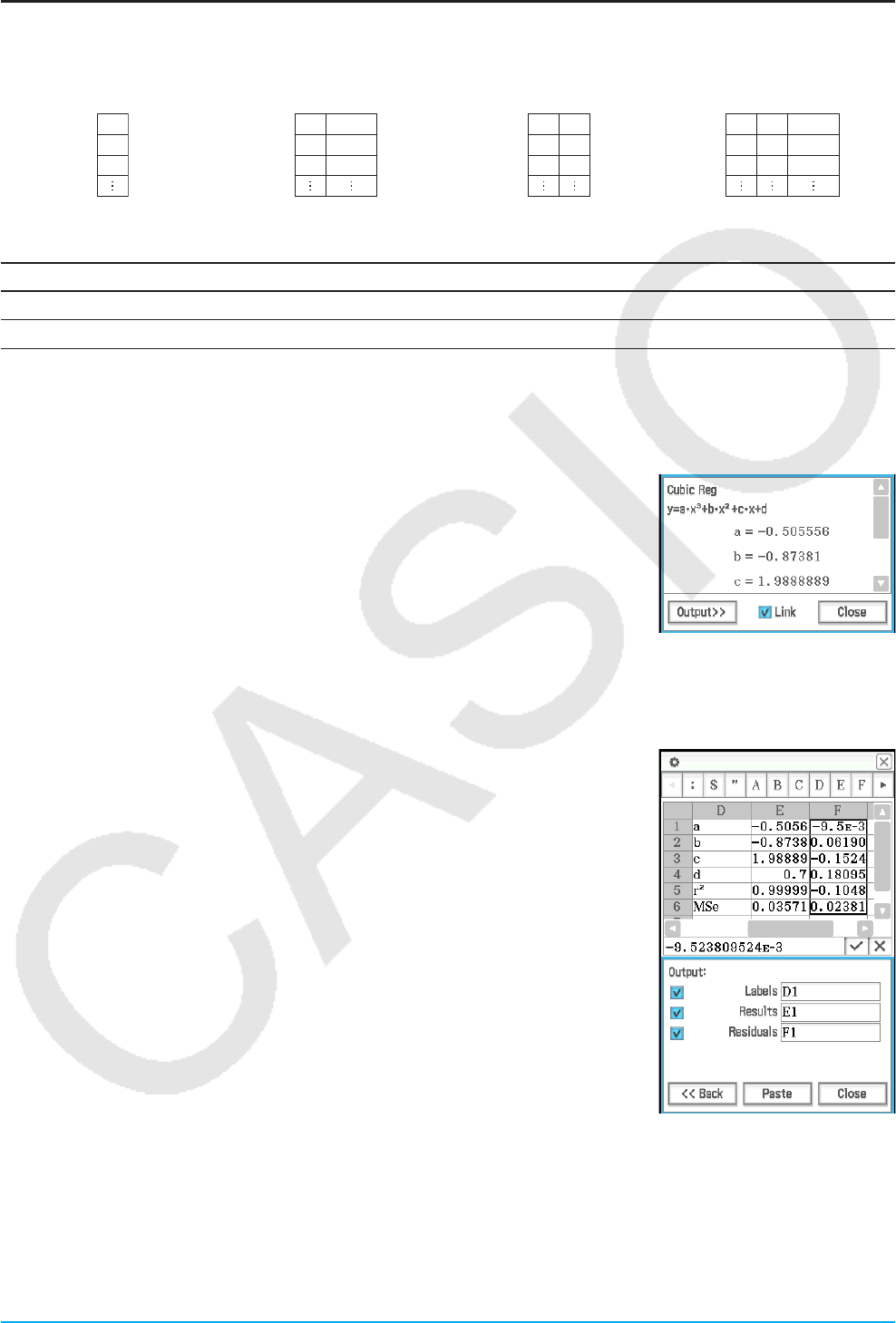
Chapter 13: Spreadsheet Application 245
Single-variable, Paired-variable and Regression Calculations
When performing these calculations, you need to prepare data of one of the formats shown below.
(a) (b) (c) (d)
X1
X2
X3
X1
X2
X3
Freq 1
Freq 2
Freq 3
X1
X2
X3
Y1
Y2
Y3
X1
X2
X3
Y1
Y2
Y3
Freq 1
Freq 2
Freq 3
Single-variable Data Single-variable Data
with Frequencies
Paired-variable Data Paired-variable Data
with Frequencies
To perform this type of calculation: Prepare this type of data:
Single-variable calculations (a) or (b)
Paired-variable and regression calculations (c) or (d)
For any of the above calculations, selecting a command displays a wizard screen. The example below shows
how to perform a regression calculation.
u To execute a regression calculation and paste the results into the spreadsheet
1. Enter the paired-variable data into the spreadsheet, and then select the
range of cells where it is located.
2. On the menu bar, tap [Calc] and then [Regression]. Next, on the submenu
that appears, tap the desired regression type.
• This displays a window which shows calculation results along with the
model formula for the selected regression type in the lower half of the
display.
• For details about each regression type, see “Regression types” (page
138). For information about calculation results other than model formula
coefficients, (r, MSe, etc.), see “To view regression calculation results”
(page 143).
3. On the calculation result window, tap the [Output>>] button.
• You can use this screen to specify the data to be output to the
spreadsheet. Under initial default settings, the Labels and Results check
boxes are selected. Select the check boxes of the items you want to
output.
4. On the output window, tap [Paste].
• This pastes a table of system variable labels to which regression
calculation results are assigned, the regression calculation results, and
residual values (items whose check boxes are selected).
Link check box
Changing the range of data you selected on the Spreadsheet window in step 1 above
will cause the regression calculation results displayed on the calculation result window
to be updated automatically. You can disable automatic updating (if you feel that
updating is taking too long or for any other reason) by clearing the Link check box on
the calculation result window.
Tip: For information about regression graphing, see “Regression Graph Operations (Curve Fitting)” (page 242).
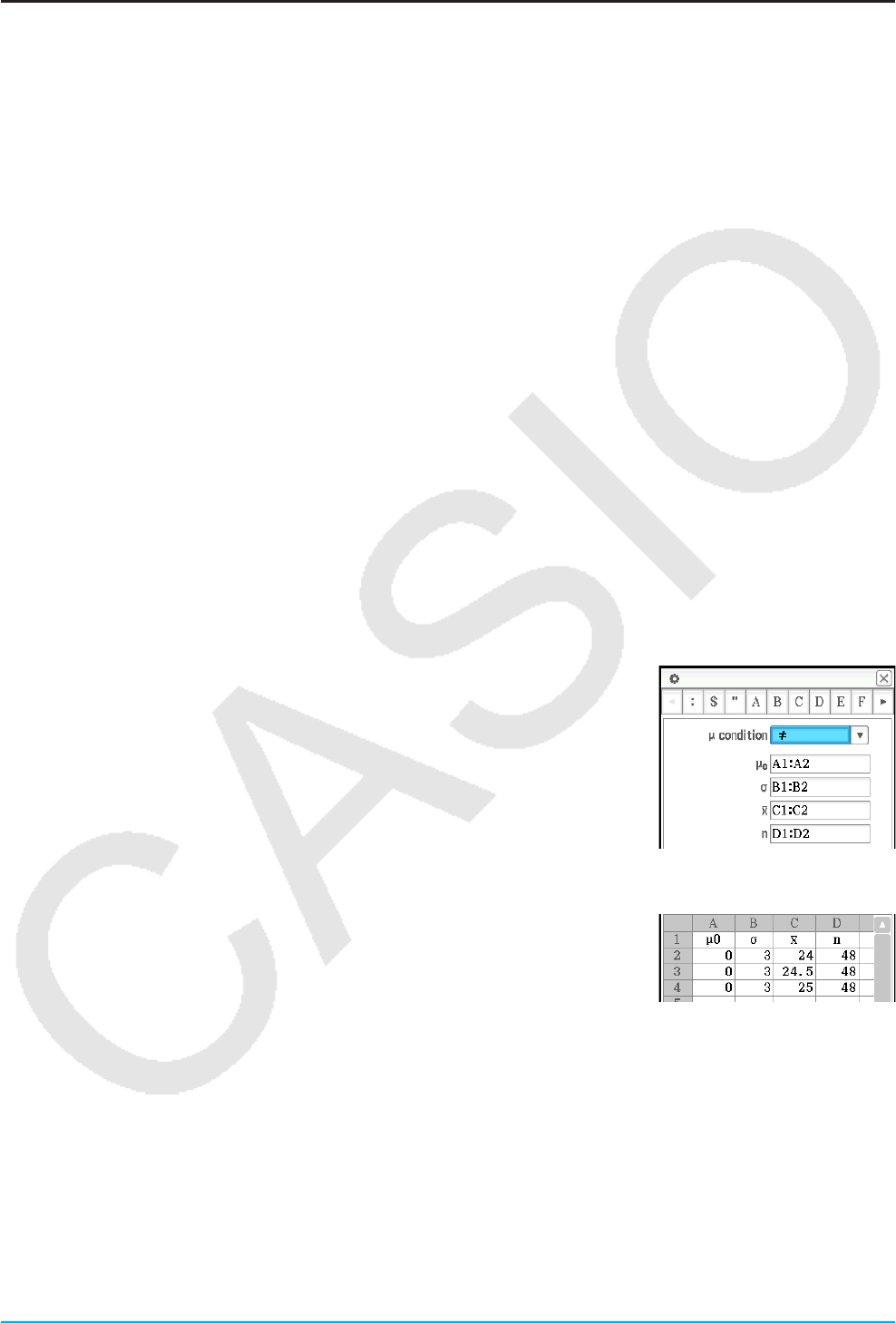
Chapter 13: Spreadsheet Application 246
Test and Interval Calculations
These calculations use the exact same wizard as the Statistics application.
For details about each calculation, see “Tests” (page 146) and “Confidence Intervals” (page 149) in “7-4 Performing
Advanced Statistical Calculations”. For information about command syntax, see “12-4 Program Command
Reference”.
The following are the differences between these calculations and the Statistics application.
• For the Linear Regression t Test, χ2 Test, χ2 GOF Test, One-Way ANOVA, and Two-Way ANOVA commands,
you need to input data to be used in the calculation into the spreadsheet beforehand.
• The other commands are always executed using a variable type syntax. Values can be input directly on the
wizard screen, or they can be input into a spreadsheets and referenced from there. One line of spreadsheet
data is used for one calculation execution, so calculations can be batch executed by providing the required
number of data lines. For an actual execution example, see “Z Tests, t Tests, Two-Sample F Test, and
Interval Calculations” below.
• After the calculation result window is displayed, an output window can be displayed for outputting calculation
result data to the spreadsheet.
Formats of Data Used for Calculation and Example Calculation
This section specifies the data formats for the data input in the spreadsheet for each type of calculation, and
shows an example of an actual calculation. m and n used in the explanation text below represent any two
natural numbers.
Z Tests, t Tests, Two-Sample F Test, and Interval Calculations
• Operation when inputting values directly on the wizard screen and performing the calculation is identical to
that when “Variable” is elected on the Statistics operation wizard screen.
• When the number of numeric input fields on the wizard screen is m, prepare n rows and m columns of data.
For example, in the case of the 1-Sample Z Test, there are four numeric
input fields as shown in the nearby screenshot. In this case, selecting 2 rows
× 4 columns of data (A1:D2) on the spreadsheet and running the wizard will
automatically input cell references into each field as shown in the nearby
screenshot. Increasing the number of rows causes batch calculation of each
line to be performed.
Important!
When you want to batch execute multiple calculations, be sure to input a set of
data for each calculation in each line. Calculation cannot be performed on the
wizard screen when data is grouped by columns.
Example: To prepare the data shown in the nearby screenshot, select the
range A2:D4, and execute the 1-Sample Z Test. In this case, the
condition is ≠ ( ≠ 0).
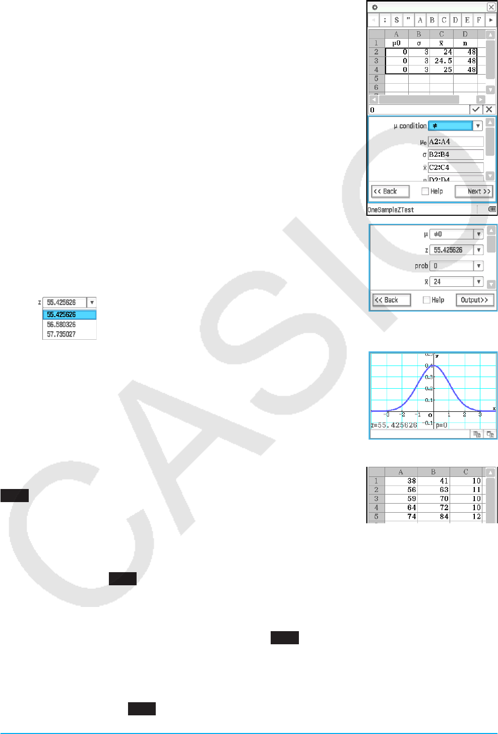
Chapter 13: Spreadsheet Application 247
1. On the Spreadsheet window, input the data and then select input range cells
A2:D4.
2. Tap [Calc] - [Test] - [One-Sample Z-Test], and then tap [Next>>].
3. This will automatically insert the cell references into the fields as shown in
the nearby screenshot (lower half).
• You can also directly input reference cell ranges for each field. If you
do, however, you can specify in the column direction (such as A1:A3).
Specifying in the row direction (such as A1:C1) will cause an error.
4. Tap [Next>>].
• A calculation is executed for each line of input data, which obtains three
results for z value. The calculation results for each line can be displayed by
tapping the down arrow button (v) of each field on the calculation result
window.
5. To graph the calculation results as a normal distribution graph, tap $.
Linear Regression t Test
In a spreadsheet, input paired-variable data (page 245 (c) or (d)) as test data.
1301 To perform a Linear Regression t Test on the paired-variable data
shown in the nearby screenshot
χ2 Test
For test data, input data of at least one row and two columns (observed matrix) into the spreadsheet. You can
see an actual example ( 0704 ) of how this is done using the Statistics application in Chapter 7 of this manual.
χ2 GOF Test
For test data, input two lists (observed list and expected list) into the spreadsheet. This is equivalent to inputting
two rows of data of n lines. You can see an actual example ( 0705 ) of how this is done using the Statistics
application in Chapter 7 of this manual.
One-Way ANOVA
For test data, input data (Factor A) into the spreadsheet that is n rows × 2 columns up to n × 6 columns. You
can see an actual example ( 0706 ) of how this is done using the Statistics application in Chapter 7 of this
manual.

Chapter 13: Spreadsheet Application 248
Two-Way ANOVA
When (Factor A count) × (Factor B count) = m, prepare test data that is n rows ×
m columns. For example, when there are Factor A items and one Factor B
items, input six columns of data into the spreadsheet. For example, select
A1:F3 on the spreadsheet and run the wizard. This will automatically assign
the cell references shown below to each factor.
Factor B1 Factor B2 Factor B3
Factor A1 A1:A3 B1:B3 C1:C3
Factor A2 D1:D3 E1:E3 F1:F3
1302 To perform the same calculation as Statistics application example 0707 using the Spreadsheet
application
Distribution Calculations
For details about the different types of distribution calculations, see “Distributions” (page 151).
uTo perform a distribution calculation and paste the results into the spreadsheet
1. Enter the single-variable or paired-variable data into the spreadsheet, and then select the range of cells
where it is located.
• The following shows the types of data that correspond to each type of distribution calculation, and the
variables that will be assigned the range of selected data.
Distribution Type Data Variable Assignment
Probability Density Single-variable x
Cumulative Distribution Paired-variable Lower, Upper
Inverse Cumulative Distribution Single-variable prob
2. On the menu bar, tap [Calc] and then [Distribution].
• The Distribution Calculation Wizard will appear in the lower half of the display.
3. Tap the v button to the right of the second item from the top and then select the desired distribution
calculation from the menu that appears.
4. Tap [Next >>].
• This will display a screen with the variable assignments for the range you selected in step 1 of this
procedure entered automatically in the input fields as the initial defaults.
5. Enter values for the other variables and then tap [Next >>].
• This displays the calculation results. If there are multiple calculation results, tap V to view them.
• You can tap $ here to display the distribution graph.
6. On the calculation result window, tap the [Output>>] button.
7. On the output window, tap [Paste].
• This pastes the calculation results in formula format.
About DispStat Command
Tapping [Calc] - [DispStat] displays a DispStat window that displays statistical calculation (one-variable, two-
variable, regression, test, interval, distribution, or inverse distribution calculations) results after a calculation is
performed.

Chapter 13: Spreadsheet Application 249
Tip: The DispStat window shows statistical calculation results of the last statistical calculation that was executed using
any ClassPad application (except for eActivity). For example, immediately after a calculation is executed using
“NormPD” command in the Main application, that calculation result is displayed on the DispStat window, even with
the Spreadsheet application. However, note that calculation results produced using a mathematical function, such as
“normPDf(”, are not displayed on the DispStat window.
13-4 Cell and List Calculations
Using the Cell Calculation Functions
Spreadsheet application special functions are included on the [Cell-Calculation] submenu of the [Calc] menu.
Selecting a menu item on the [Cell-Calculation] submenu will input the corresponding function into the currently
selected cell. This section provides explanations of the functions and input syntax of the cell calculation
functions.
Function Description
row Function: Returns the row number of a specified cell.
Syntax: row(cell)
col Function: Returns the column number of a specified cell.
Syntax: col(cell)
count Function: Returns a count of the number of cells in the specified range.
Syntax: count(start cell[:end cell])
cellif Function: Evaluates an equality or inequality, and returns one of three different expressions
based on whether the equality/inequality is true (expression 1), false (expression 2),
or inconclusive (expression 3).
With this function, the equality/inequality can include a string as in the following example:
cellif(A1="Red", 0,1,2).
Syntax: cellif(equation, expression 1, expression 2, expression 3)
cellif(inequality, expression 1, expression 2, expression 3)
1303 For each value in cells A1 through A5, to display “Big” in the neighboring B-column cell for values of 5
and greater, and “Small” for values less than 5
Using the List Calculation Functions
The [Calc] menu functions shown in the table below are also included (with the same name) on the Main
application [Action] - [List] - [Statistics] and [Action] - [List] - [Calculation] submenus.
[Calc] - [List-Statistics] submenu min, max, mean, median, mode, Q1, Q3, percentile, stdDev, variance
[Calc] - [List-Calculation] submenu sum, prod, cuml, Alist, percent, polyEval, sequence, sumSeq
Selecting a menu item on the [Calc] - [List-Statistics] submenu or [Calc] - [List-Calculation] submenu will input
the corresponding function into the currently selected cell. For information about the syntax and other details
about each function, see “Using the List-Statistics and List-Calculation Submenus” (page 72).
Tip: When a range of cells on a spreadsheet is specified as the arguments of these functions,
the cells are regarded of a single list of data even if the range extends over multiple
columns. For example, in the case of the nearby screenshot (where the range A1:B3 is
selected), the data is treated as the following list data: {1,3,5,2,4,6}.
1304 To determine the mean of the values in the block whose upper left corner is located at A1 and whose
lower right corner is located at C3, and input the result in cell C5
1305 When Column A is data and Column B is frequency, to totalize the data input
in A1 through B3 in the nearby screenshot and input the total into cell B5
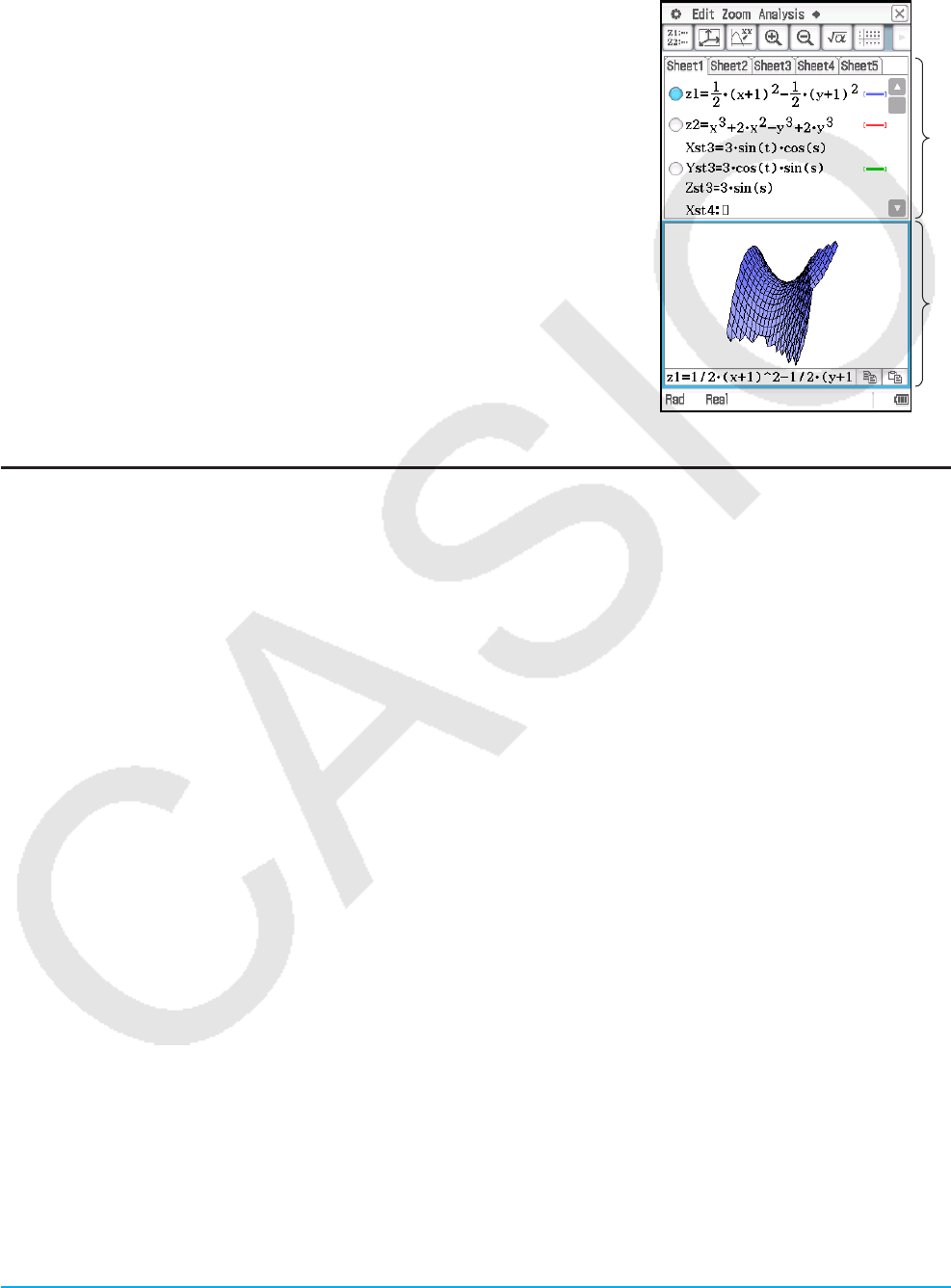
Chapter 14: 3D Graph Application 250
Chapter 14:
3D Graph Application
The 3D Graph application lets you draw a 3-dimensional graph of an
equation in the form z = f (x, y) or of a parametric equation.
The 3D Graph application has a 3D Graph Editor window (1) and a 3D
Graph window (2). Functions you input on the 3D Graph Editor window
are graphed on the 3D Graph window. You can select any one of the
expressions on the 3D Graph Editor window and graph it on the 3D Graph
window. 1
2
3D Graph Application-Specific Menus and Buttons
3D Graph Editor window
• Delete text in a selected area. When nothing is selected, deleted the entire line where the cursor is
located. .........................................................................................................................Edit - Delete or q
• Return the current sheet to its initial default name (Sheet 1 through Sheet 5) ............. Sheet - Default Name
• Return the contents and name of the currently active sheet to their initial defaults ......... Sheet - Clear Sheet
• Draw a graph ............................................................................................................................................. 7
• Toggle the equation type between z = f (x, y) and a parametric equation ..........................................x / z
• Insert variable s or t into a parametric equation .................................................................................s / [
3D Graph window
• View the displayed graph from the x-axis, y-axis, or z-axis ............................. Zoom - View-x, View-y, View-z
• Return View Window settings and zoom settings to their initial defaults ...............................Zoom - View-Init
• Make the 3D Graph Editor window active ...................................................................................................Z
• Display the coordinates at a particular point on a 3D graph ........................................Analysis - Trace or =
• Write text on the Graph window ................................................................................. Analysis - Sketch - Text
• Clear text on the Graph window ...................................................................................Analysis - Sketch - Cls
• Calculate a z-value for given x- and y-values, or s- and t-values, on the displayed graph ...... Analysis - z-Cal
• Automatically rotate a graph in the specified direction (Left → Right, Right → Left, Top → Bottom,
Bottom → Top) for about 30 seconds ....................................................................................a - Rotating
• Re-draw a graph ......................................................................................................................... a - ReDraw
• Show/hide axes and labels .........................................................................................................................q
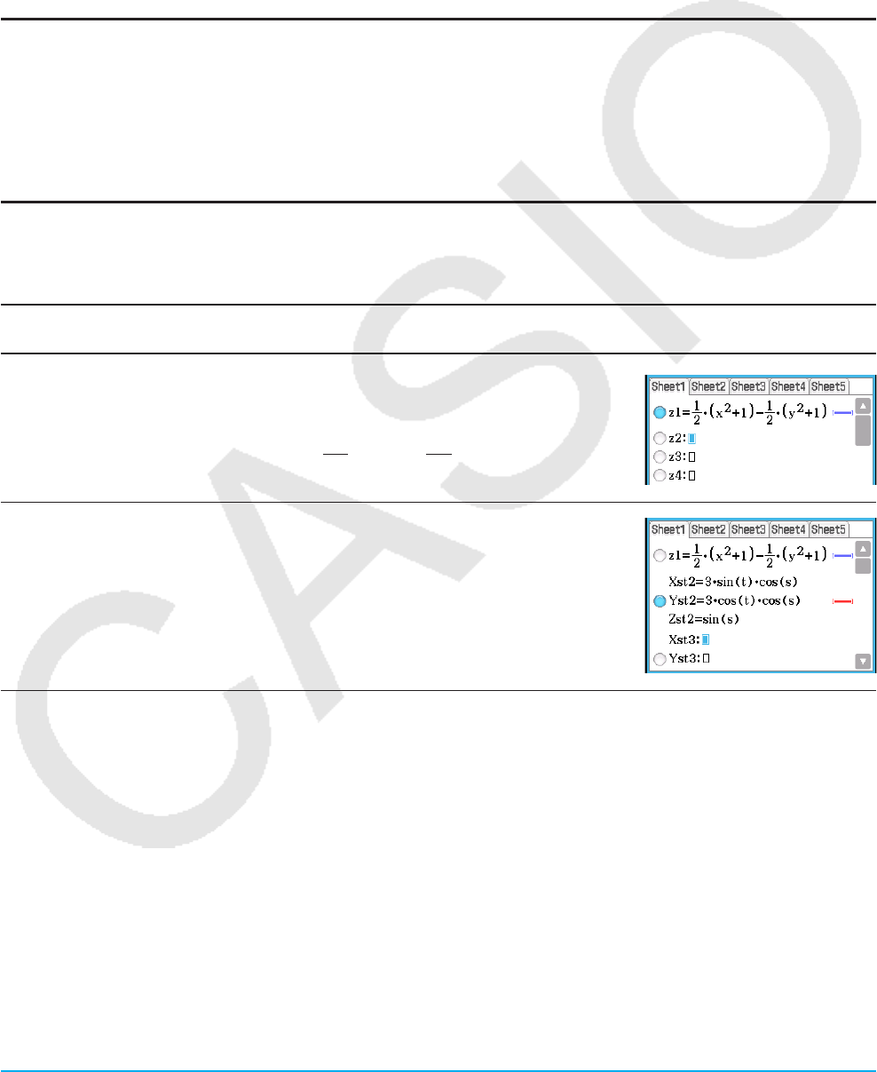
Chapter 14: 3D Graph Application 251
3D Graph Editor window and 3D Graph window
• Display the View Window dialog box to configure 3D Graph window settings ...........................................6
• Display the Main application work area window .........................................................................................~
14-1 Inputting an Expression
Use the 3D Graph Editor window to input 3D Graph application expressions.
Using 3D Graph Editor Sheets
3D Graph Editor sheet operations are similar to the sheet operations of the Graph & Table application. For
more information, see “Using Graph Editor Sheets” on page 99.
Note: The Graph & Table application allows simultaneous graphing of multiple functions, as long as they are
on the same sheet. With the 3D Graph application, however, you can graph only one function at a time.
Storing a Function
To input an expression, tap a blank line on the 3D Graph Editor window and then perform the operations
described below.
To input this type of
expression: Do this:
z = f (x, y) expression 1. If x is displayed on the toolbar, tap to toggle it
to z.
2. Input a formula that includes the variables x and
y (such as 1
2 ( x2 + 1) – 1
2 ( y2 + 1)) and then
press E.
Parametric expressions 1. If z is displayed on the toolbar, tap to toggle it
to x.
2. In the Xst =, Yst =, and Zst = lines, input
expressions that each contain s and/or t (such
as: 3sin(t)*cos(s)), and then press E.
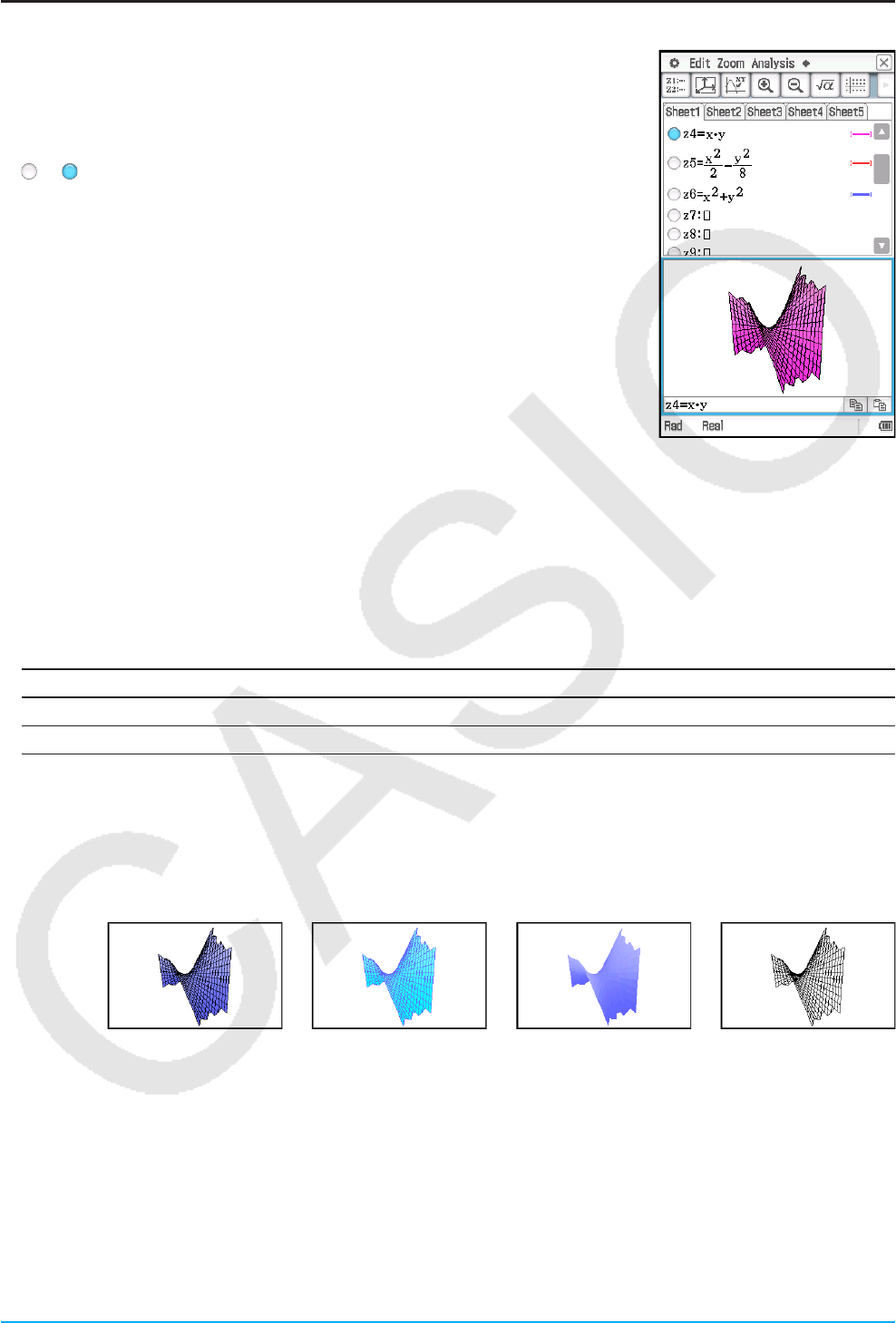
Chapter 14: 3D Graph Application 252
Graphing a Stored Function
uTo graph a specified function
1. Tap the tab of the sheet that contains the function you want to graph to make
it active.
2. Tap the button to the left of the formula you want to graph so it changes from
to .
3. Change the graph line color and area color as desired.
• See “To specify the graph line color and area color” below.
4. Tap 7 to graph.
Tip: You can also use drag and drop to input an expression displayed on the Main application work area into the 3D
Graph Editor window. To do this, perform the same steps as those for the Graph & Table application. For more
information, see “To graph a function by dragging it from the work area to the Graph window” on page 92.
uTo specify the graph line color and area color
1. Tap the style area next to the function whose line style and color you want to specify. This displays the Style
Settings dialog box.
2. Configure the dialog box with the following settings.
To specify this: Perform this operation:
Line color Tap “Line Color” and then tap the desired color.
Area color Tap “Area Color” and then tap the desired area color.
• “Clear” cannot be specified for both the “Line color” and “Area color” at the same time.
3. To apply the settings, return to the dialog box in step 2 of this procedure and then tap [OK].
4. To redraw the graph with the new settings, tap 7.
Graph examples using different settings
Line Color: Black Blue Clear Black
Area Color: Blue Cyan Blue Clear
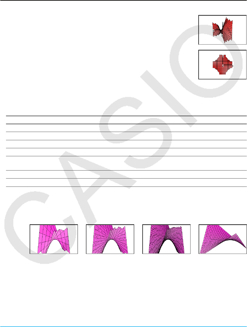
Chapter 14: 3D Graph Application 253
14-2 Using the 3D Graph Window
This section explains 3D Graph window operations, including configuring display settings, changing the angle
of a graph, rotating a graph, and more.
Configuring 3D Graph View Window Parameters
Use the 3D Graph View Window to specify maximum and minimum values for the
x-axis, y-axis, z-axis, s-variable, and t-variable.
You can also specify the number of lines you would like for drawing the grid. For the
xgrid enter the number of lines you would like drawn within the interval from xmin to
xmax. For example, if xmin = −3, xmax = 3 and xgrid = 15, 15 almost vertical lines will
be used to display your graph. The ygrid lines will be almost horizontal.
uTo configure View Window parameters
1. Tap 6, or tap O and then [View Window] to display the View Window dialog box.
2. Configure View Window parameters required for the type of graph you want to draw.
Use this item: To configure this View Window parameter: Initial default
xmin/ymin/zmin Minimum x-axis/y-axis/z-axis value –3
xmax/ymax/zmax Maximum x-axis/y-axis/z-axis value 3
xgrid/ygrid Number of grid lines used for x-axis/y-axis direction 25
angle Clockwise angle of x-axis 20
angle Eye position relative to the plane created by the x-axis and
y-axis, and the angle of the z-axis 70
smin/tmin Minimum s-variable/t-variable value –3.14159265358979
smax/tmax Maximum s-variable/t-variable value 3.14159265358979
3. After all the parameters are the way you want, tap [OK].
• When you tap [OK] after changing View Window dialog box settings, the graph is redrawn automatically
using the new View Window settings.
The following are examples of the 3D graph z = xy using a number of different 3D View Window setups.
xgrid, ygrid 10 25 50 25
xmin, ymin −3 −3 −3 −1.5
xmax, ymax 3 3 3 1.5
Important!
• As is evident from the above sample screenshots, the greater the xgrid and ygrid values, the more detailed
the graph. Also note, however, that larger values require more calculation, which means that the graphing
operation takes more time.
• Graphing may be impossible if the xgrid and ygrid values are too small.
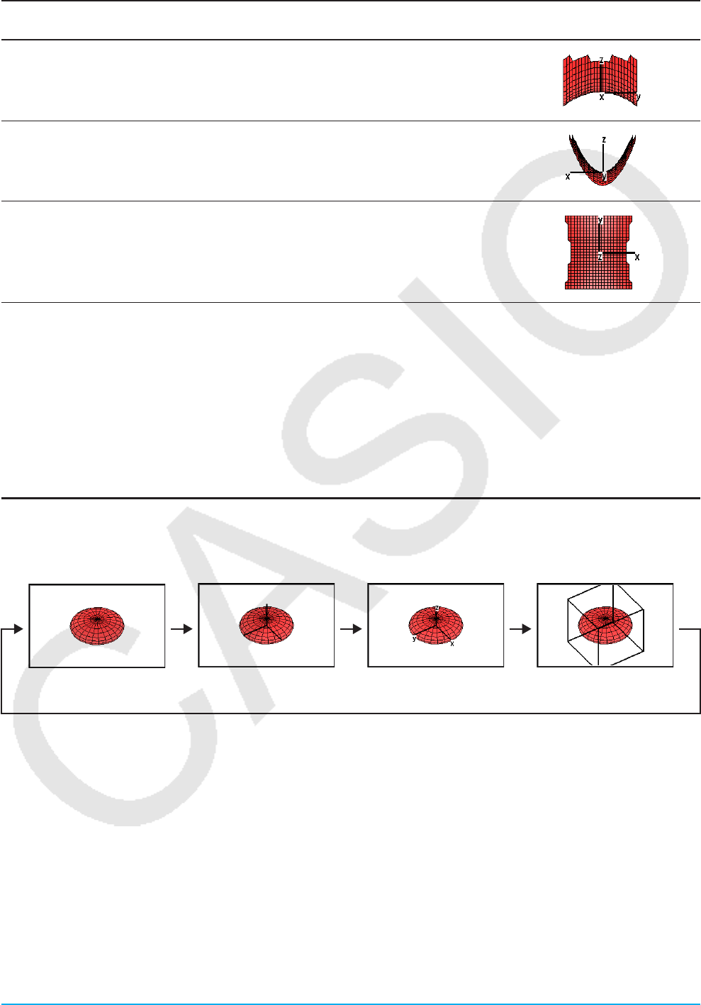
Chapter 14: 3D Graph Application 254
uTo switch the eye position
To view the graph: Do this: Display example
(z = x2/2 – y2/8)
Facing the x-axis Tap [Zoom] and then [View-x], or press the x key.
Facing the y-axis Tap [Zoom] and then [View-y], or press the y key.
Facing the z-axis Tap [Zoom] and then [View-z], or press the Z key.
uTo initialize the View Window settings
1. Tap 6, or tap O and then [View Window] to display the View Window dialog box.
2. On the [Memory] menu select [Initial], or tap the [Default] button.
3. Tap [OK].
Tip: You can also initialize the View Window settings by tapping [Zoom] and then [View-Init]. Note, however, that doing so
also initializes the zoom setting.
Showing and Hiding Axes and Labels
On the 3D Graph window, each tap of q or each press of the = key cycles the display settings of axes and
labels in the sequence shown below.
Axes: Off
Labels: Off
Axes: On
Labels: Off
Axes: On
Labels: On
Axes: Box
Labels: Off
You can configure the initial startup axes and labels display setting (the setting applied each time 3D Graph
Application is started up) using the [3D Format] tab of the Graph Format dialog box. For more information, see
“Graph Format Dialog Box” on page 38.

Chapter 14: 3D Graph Application 255
Rotating the Graph
A graph can be rotated manually using the touch panel or calculator keys, or it can be rotated automatically.
uTo rotate a graph manually using the stylus
Drag the stylus on the 3D Graph window in the direction you want to rotate the graph.
uTo rotate a graph manually using the cursor keys and graph controller arrows
Press the cursor key that indicates the direction you want to rotate the graph. Or you can tap the graph
controller arrow that indicates the direction you want to rotate.
Note
• Holding down a cursor key will rotate the graph continuously.
• Display of the graph controller arrows is turned off under initial default settings. Use the “G-Controller” check
box on the Graph Format dialog box to turn it on, if you want. For more information, see “Graph Format Dialog
Box” on page 38.
uTo rotate a graph automatically
1. To start automatic graph rotation, tap a and then [Rotating].
2. On the submenu that appears, select the rotation direction you want:
[Left → Right], [Right → Left], [Top → Bottom], or [Bottom → Top].
• Rotation continues for about 30 seconds and then stops automatically. You can also stop automatic
rotation by pressing the c key or tapping l on the icon panel.
3D Graph Example
1401 To graph the hyperbolic paraboloid z = x2
2 – y2
8
1402 To graph a parametric equation x = 3 · sin(t) · cos(s), y = 3 · cos(t) · cos(s), z = sin(s)
Using Trace to Read Graph Coordinates
Starting the trace operation causes a crosshair pointer to appear on the graph.
You can then press a cursor key or tap the graph controller arrows to move the
pointer to the location you want, and read the coordinates that appear on the
display. To start the trace operation and display the pointer, make the 3D
Graph window active, and then tap =, or tap [Analysis] and then [Trace].
• Each time you press the cursor key or tap a graph controller arrow, the
pointer moves the distance specified by the [grid] value on the 3D View
Window dialog box.
• Inputting a value while a trace operation is being performed displays a dialog box for inputting an x- and
y-value, or an s- and t-value. Inputting values for each of the variables on this dialog box causes the pointer to
jump to the corresponding location when you tap [OK].
To cancel the trace operation, tap l on the icon panel.
Tip: The initial default setting for the coordinate display is rectangular coordinates. With the [3D Format] tab of the Graph
Format dialog box, you can specify display of polar coordinates or you can hide coordinates, if you want. For more
information, see “Graph Format Dialog Box” on page 38.
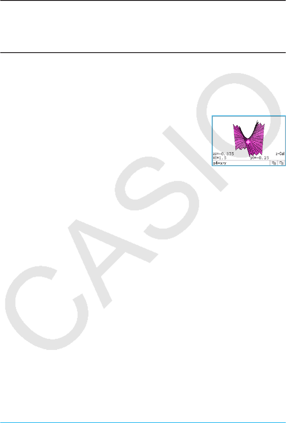
Chapter 14: 3D Graph Application 256
Inserting Text into a 3D Graph Window
You can insert text into a 3D Graph window and delete it as required.
For more information, see “To write text on the Graph window” on page 113, and “To clear figures inserted using
the Sketch menu” on page 112.
Calculating a z-value for Particular x- and y-values, or s- and t-values
Use the following procedure to calculate a z-value for given x- and y-values on the displayed graph.
uClassPad Operation
1. Draw the graph and make the 3D Graph window active.
2. Tap [Analysis], and then [z-Cal].
3. On the dialog box that appears, enter values for x and y, and then tap [OK].
• The 3D graph window shows x, y, and z coordinate values, which indicate
the current location of the crosshair pointer. The crosshair pointer will not
be visible on the graph if it is located outside of the current display area.
• Inputting a graph value while “z-Cal” is on the display cause a dialog box to
appear for specifying an x- and y-value, or an s- and t-value. You can use
this dialog box to specify other x- and y-values, or s- and t-values.
4. To cancel the z-Cal operation, tap l on the icon panel.
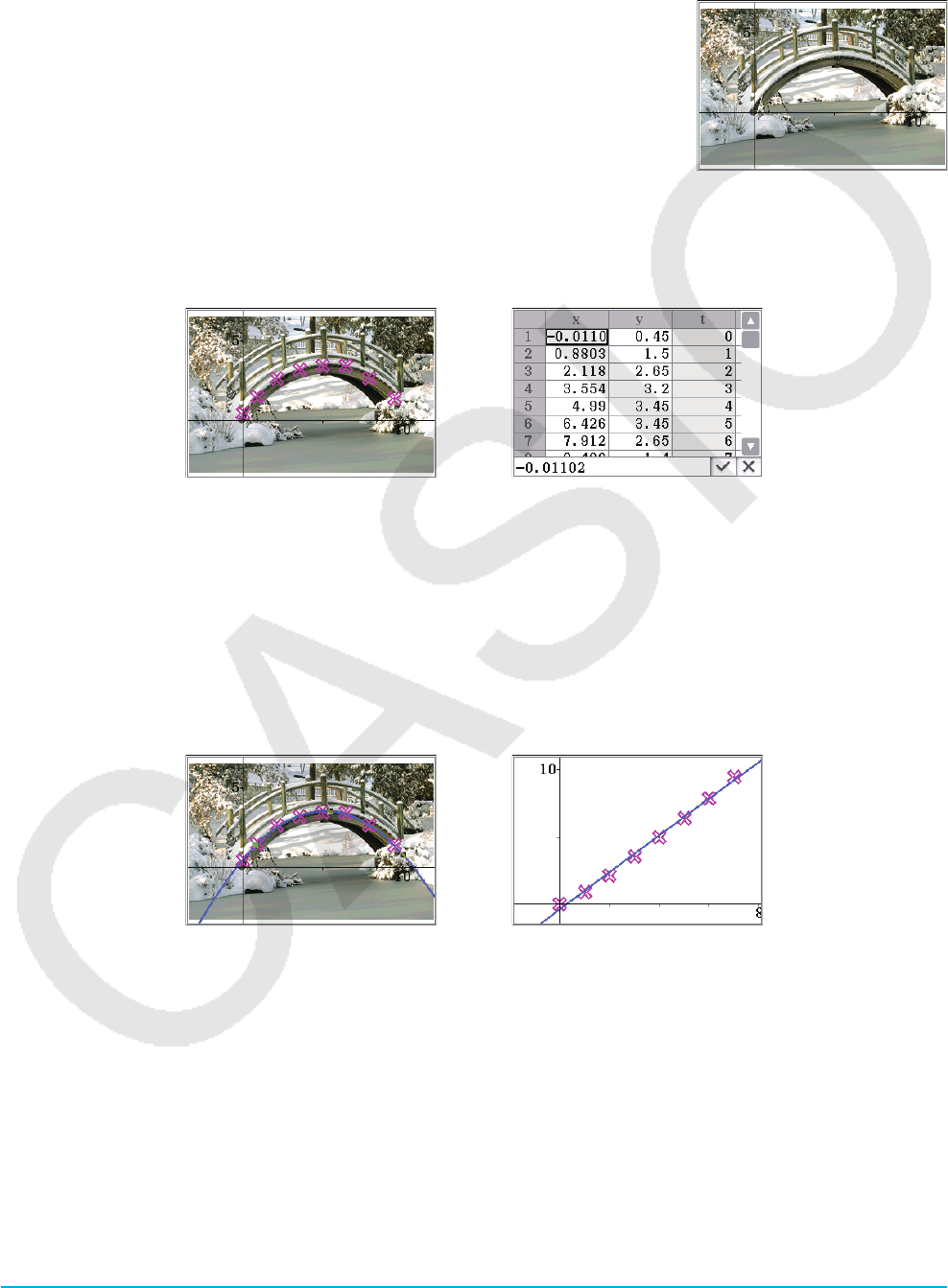
Chapter 15: Picture Plot Application 257
Chapter 15:
Picture Plot Application
Picture Plot is an application that lets you plot points (that represent
coordinates) on a photograph, illustration, or other graphic and perform various
types of analysis based on the plotted data (coordinate values).
The photograph to the right, for example, shows a uniquely curved bridge.
The plane of the frontmost edge of the bridge is treaded as the xy coordinate
plane, and the left side base of the bridge is treated as the origin (0, 0). This
makes it possible to express any point on along the edge of the bridge floor as
a coordinate (x, y).
The Picture Plot plot function makes it easy to plot points on a photograph such as this or some other image,
and extract the coordinate values of the plots.
Plotting points Coordinates (Plot List window)
You can use the plots to perform the following types of operations.
• Register and graph a y = f (x) form equation and overlay it on a photograph and plot.
• Perform regression calculation based on the plotted coordinate values and draw a regression graph that
overlays the plots. This makes it possible to produce the mathematical expression and graph of a path of
movement.
• Add time values (t) to the coordinate values (x, y) and plot points on the t-x plane or t-y plane. This makes it
possible to produce the mathematical expressions and graphs of the correlation between horizontal direction
movement and time, and the correlation between vertical direction movement and time.
x-y coordinate plot
regression graph example
t-x coordinate plot
regression graph example

Chapter 15: Picture Plot Application 258
Picture Plot Application-Specific Menus and Buttons
Picture Plot window
• Open the c2p or c2b file ................................................................................................................. File - Open
• Save the c2p or c2b file being edited ..............................................................................................File - Save
• Adjust the lightness of an image (page 259) .............................................................................File - Fade I/O
• When the currently open image is a c2b file, sequentially display the image in the file ...................File - Play
• Display a color setting dialog box for the currently selected plot ................................................... Edit - Style
• Start editing of plots in the c2b file ........................................................................Edit - Edit Plot (Animation)
• Activate the select function for selecting a plot .................................................................View - Select or G
• Activate the pan function for dragging the Picture Plot window with the stylus ................... View - Pan or T
• Show/hide axes and scale ......................................................................................View - Toggle Axes or q
• Display the Graph Editor dialog box .................................................................... Graph - Graph Editor or !
• Display a trace cursor that can be positioned on any x, y coordinate ............................. Graph - Trace or K
• Calculate the root, minimum value, maximum value or y-axis intercept of the currently
selected graph ..................................................................................................................Graph - G-Solve
• Display the t-y Plot window ......................................................................Graph - Transform Axes - t-y or v
• Display the t-x Plot window ......................................................................Graph - Transform Axes - t-x or c
• Display/activate the Plot List window ..........................................................................................................Q
• Enter the plot mode (for plotting points on the screen) ...............................................................................[
t-x Plot window, t-y Plot window
• Close the t-x or t-y Plot window and display the Picture Plot window .........................................................5
Plot List window
• Clear all current plot data and background images (return all Picture Plot window and
Plot List window content to its initial default state) ......................................................................File - New
• Open a Spreadsheet file as Plot List data .................................................................File - Open Spreadsheet
• Save Plot List data as a spreadsheet ....................................................................... File - Save Spreadsheet
• Import variable data to Plot List window .......................................................................................File - Import
• Export Plot List window data to a variable ................................................................................... File - Export
• Specify the number format of values on the Plot List window ....................................... Edit - Number Format
Items common to the Picture Plot window, t-x/t-y Plot window, and Plot List window
• Display the Time Setting dialog box ............................................................................... Graph - Time Setting
• Display a submenu (same as the one on page 242) for executing regression calculation
based on plots. ........................................................................................................... Graph - Regression
• Show/hide the regression calculation result dialog box ....................................................... Graph - Disp Stat

Chapter 15: Picture Plot Application 259
15-1 Using the Plot Function
You can plot points on the screen, overlay them with a graph of an expression in the form y = f (x), and draw a
regression graph that approximates the plots.
Starting a Picture Plot Operation
The Picture Plot application lets you use a still image (c2p file) or animation (c2b file) that contains a
mathematical meaningful object or scene as a background, and plot points on the background image. Because
of this, a Picture Plot operation always starts with opening of a background file.
Tip: c2p and c2b are special ClassPad file formats. You can use files that come preloaded on your ClassPad, or you can
obtain files from the CASIO support site (edu.casio.com).
uTo open a c2p or c2b file for use as the Picture Plot window background
1. On the application menu, tap to start the Picture Plot application.
• This will display a full-screen view of the Picture Plot window.
2. Tap [File] - [Open].
• This displays the file list screen.
3. Select the c2p or c2b file you want to open and then tap [Open].
• The file will open and its content will appear as the Picture Plot window background image.
What you should do next depends on the file type.
- c2p file: “Plotting Points on a c2p File Image” (page 259)
- c2b file: “Plotting Points on a c2b File Image” (page 260)
u To adjust the lightness (Fade I/O) of an image
1. While the Picture Plot screen is displayed, tap [File] and then [Fade I/O].
• This causes a slider for adjusting image lightness to appear on the toolbar.
2. Tap t or u on the toolbar to adjust the lightness value.
3. After the setting is the way you want, tap the [OK] button on the toolbar.
Plotting Points on a c2p File Image
This section explains how to plot points on a c2p file (still image) background.
uTo plot points on a c2p file image
1. Open the c2p file whose image you want to use as the Picture Plot window background.
2. Tap [ to enter the Plot mode.
3. Use the stylus to tap the points you want to plot.
• A plot point appears at each location you tap.
• To undo the last point you plotted, tap [Edit] - [Undo/Redo].
4. Repeat step 3 as many times as required to plot all of the points you want.
• You can plot up to 50 points per background image.
5. To exit the Plot mode, tap G.
6. To save the plot data to the c2p file, tap [File] - [Save].
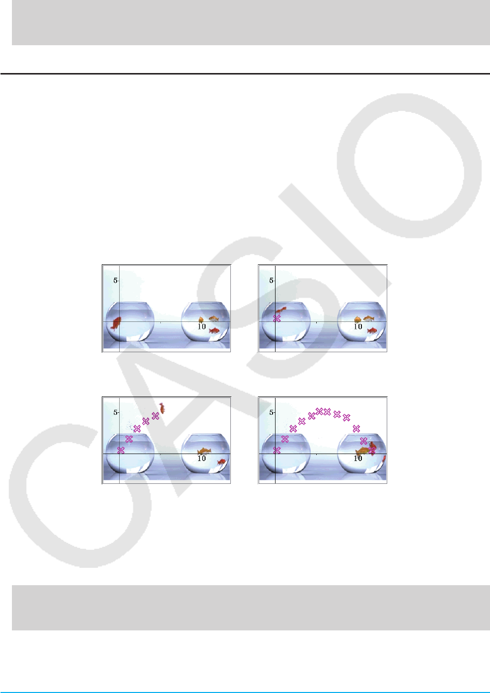
Chapter 15: Picture Plot Application 260
7. On the dialog box that appears, perform the required operation to save the file.
• For details about the information saved to a file, see “15-4 Picture Plot Application Files”.
Next, perform the operations below.
“Editing Plots on a Background Image” (page 261), “Overlaying a Graph on Background Image Plots”
(page 261).
Plotting Points on a c2b File Image
This section explains how to plot points on a c2b file (animation image) background. The maximum number of
plots allowed in a background animation (c2b) image is the same as the number of still images that make up
the animation file.
uTo plot points on a c2b file image
1. Open the c2b file whose image you want to use as the Picture Plot window background.
• This displays the first of the still images that make up the c2b file.
2. Tap [ to enter the Plot mode.
3. Use the stylus to tap the point you want to plot.
• This will display a plot point at the location you tap and advance to the next of the still images that make up
the c2b file.
• To undo the last point you plotted, tap [Edit] - [Undo/Redo].
4. Repeat step 3 as many times as required to plot all of the points you want.
• Plotting a point on the last still image of the c2b file will cause the “Plotting is finished.” dialog box to
appear. On the dialog box, tap [OK] to exit the Plot mode.
• To exit the Plot mode before displaying the final image of a c2b file, tap l.
5. To save the plot data to a c2b file, tap [File] - [Save].
6. On the dialog box that appears, perform the required operation to save the file.
• For details about the information saved to a file, see “15-4 Picture Plot Application Files” (page 266).
Next, perform the operations below.
“Editing Plots on a Background Image” (page 261), “Overlaying a Graph on Background Image Plots”
(page 261).

Chapter 15: Picture Plot Application 261
uTo view the images that make up a c2b file
1. With the c2b file whose images you want to view displayed as the background image of the Picture Plot
window, tap [File] - [Play] - [Auto] or [File] - [Play] - [Manual].
2. To exit this operation, tap m on the toolbar.
Editing Plots on a Background Image
You can use the procedures in this section to reposition individual plot points. You can also change the color of
all the plots or delete all the plots from an image.
uTo reposition a point plotted on a c2p background image
1. On the Picture Plot window, tap G or [View] - [Select].
2. Use the stylus to tap the plot point you want to reposition and then drag it to the location you want.
uTo reposition a point plotted on a c2b background image
1. On the Picture Plot window, tap [Edit] - [Edit Plot (Animation)].
• This enters the Edit plot mode and displays a full-screen view of the Picture Plot window.
2. On the toolbar, tap < or > to display the c2b image whose plot point you want to reposition.
3. Use the stylus to tap the plot point and then drag it to the location you want.
4. Repeat steps 2 and 3 for other plot points, if you want.
5. To exit the Edit plot mode, tap l.
uTo change the color of all points plotted on a c2p or c2b background image
1. c2p file image: On the Picture Plot window, tap G or [View] - [Select].
c2b file image: On the Picture Plot window, tap [Edit] - [Edit Plot (Animation)].
2. Tap any one of the plot points so it is selected, and then tap [Edit] - [Style].
3. On the dialog box that appears, select the color you want and then tap [OK].
uTo delete all plots and graphs from a background image
1. On the Picture Plot window, tap [Edit] - [Clear All].
2. On the confirmation dialog box that appears, tap [OK].
Overlaying a Graph on Background Image Plots
You can use the procedures in this section to overlay a graph on points you plotted on the Picture Plot window
background image.
uTo input an expression of the form y = f (x) and graph it
1. On the Picture Plot window, tap [Graph] - [Graph Editor].
• This displays the Graph Editor dialog box.
2. Input a function of x (such as: −x2 + 2) and then press E.
• This will register the function and move the cursor to the next line. You can
repeat step 2 above to register another function, if you want.
• You can register up to five functions.
3. Select the check boxes of the registered expressions you want to graph, and clear the check boxes of
expressions you do not want to graph.
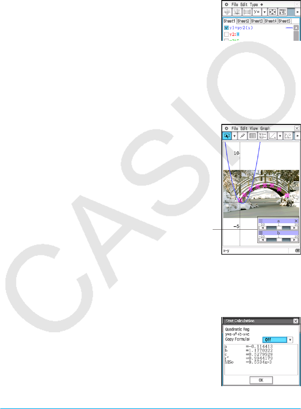
Chapter 15: Picture Plot Application 262
4. To graph, tap [Draw].
• This closes the dialog box and draws the graph(s) on the Picture Plot window.
Tip: Expressions registered on the Graph Editor dialog box above can be recalled from and graphed with the Graph &
Table application, by performing the steps below.
(1) On the Graph & Table Graph Editor window, input the line name (py1 through
py5) of the expression you want to recall and then input “(x)” to the right of the
name.
(2) Press E.
(3) To draw the graph, tap $.
uTo use Dynamic Graph to change the parameter values of a Picture Plot window graph
1. On the Picture Plot window, tap [Graph] - [Graph Editor].
• This displays the Graph Editor dialog box.
2. Use the soft keyboard to input a function of x (such as: y = a·x2 − b·x) that includes at least one parameter,
and then press E.
3. Select the check boxes of the functions you want to graph, and clear the check boxes of the functions you do
not want to graph.
4. To graph, tap [Dynamic].
• This will display sliders for changing values assigned to parameters a and
b, and will also draw a graph based on an initial value of 1 assigned to a
and b.
• Use the sliders to change the values of the graph expression parameters
and dynamically modify the form of the graph accordingly. For details
about this operation, see step 4 under “To run Dynamic Modify” (page 116).
5. To exit the Dynamic Modify operation, tap the close button (C) in the
upper right corner of the slider display box.
Sliders
Tip: In place of the soft keyboard in step 2 of the above procedure, you can also tap [Edit] - [Built-In(1)] or [Built-In(2)], and
then use the sub-menu of built-in functions that appears to input a function.
uTo overlay a regression graph on plotted points
1. On the Picture Plot window, tap [Graph] - [Regression].
• This displays the regression calculation type sub menu.
2. Tap the menu item that corresponds to the type of regression calculation*1
you want to perform.
• To perform quadratic regression, for example, tap [Quadratic Reg]. This
will perform regression calculations and display a Stat Calculation dialog
box*2 of calculation results like the one shown nearby.
3. If you want to register the calculation result regression formula to the Picture
Plot application’s Graph Editor, perform the steps below.
(1) Tap the down arrow button (v) on the right side of the “Copy Formula”
box.
(2) On the list that appears, select regression formula registration destination ( py1 through py5).
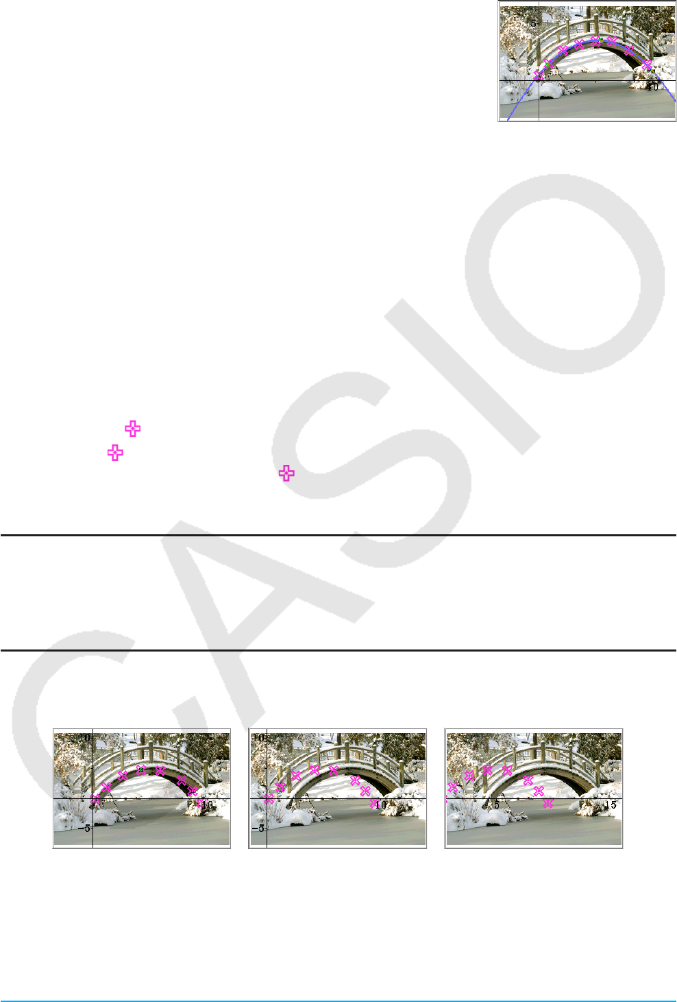
Chapter 15: Picture Plot Application 263
4. Tap [OK].
• This will graph the regression formula of the calculation results.
*1 For information about regression calculation types, see “Regression types” (page 138).
*2 This dialog box will appear when there is a check mark next to [DispStat] on the [Graph] menu. This menu
item has a check mark next to it under initial default settings.
For information about the meanings of the values that appear on this dialog box, see “To view regression
calculation results” (page 143).
uTo delete one of the graphs draw on the Picture Plot window
1. On the Picture Plot window, tap G or View - Select.
2. Tap the graph you want to delete.
• This will cause handles (;) to appear on the graph you tap to indicate that it is selected.
3. Tap [Edit] - [Delete].
uTo view the coordinates of a specific location on a graph (Trace)
1. Tap [Graph] - [Trace] or K.
• This will display in the center of the Picture Plot window.
2. You can move by tapping the location to which you want to move it.
• The coordinates at the current position of will be shown in the status bar.
• To exit the Trace operation, press c.
G-Solve
You can use the G-Solve function to calculate the root, min, max, and y-intercept of the graph that is currently
selected on the Picture Plot window. Picture Plot window G-Solve operations are the same as those with the
Graph & Table application. For more information, see “3-6 Analyzing a Function Used to Draw a Graph”.
Scrolling the Picture Plot Window
On the Picture Plot window, you can use the cursor keys to scroll the XY-coordinate axes up, down, left, and
right. Note that the background image is fixed and does not scroll.
You also can tap View - Pan or T and pan (grab-and-drag) the XY-coordinate axes.
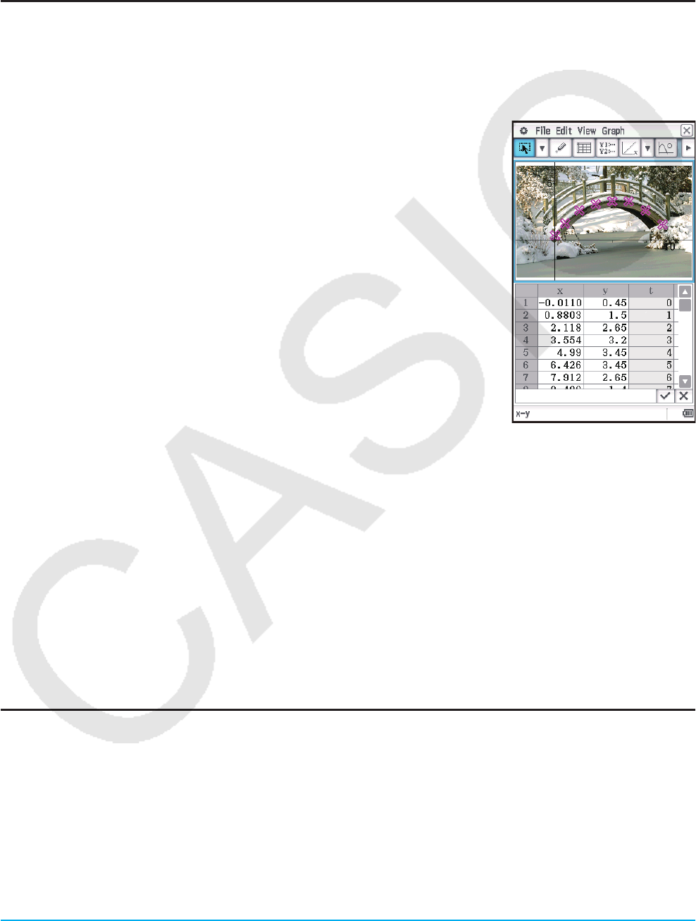
Chapter 15: Picture Plot Application 264
15-2 Using the Plot List
Each plot on the Picture Plot window has coordinate value data. You can use the Plot List window to display
and edit these coordinates.
Using the Plot List Window to Edit Plots
You can use the Plot List window to edit the coordinate values of previously plotted points and plot new points
by inputting coordinate values. You can also delete all of the plot data from an image.
uTo edit plot coordinate values
1. While the Picture Plot window is displayed, tap Q.
• This will display the Plot List window in the lower half of the screen.
• The x and y values of the Plot List window show plot coordinates. The
t value indicates time. (For more information about t values, see “15-3
Displaying Plots on t-y or t-x Coordinates”.) On this window you can edit
the x and y values only.
2. Tap a cell and then edit its contents.
• To edit cell contents, use the same operations as those for the
Spreadsheet application. See “13-1 Inputting and Editing Cell Contents”
for more information.
• The maximum allowable number of editing/input rows is 50 when the
background image is a c2p file. For a c2b file background image, the
maximum number of rows is the same as the number of still images that
make up the animation file.
• Any change you make to a value will be reflected by the corresponding
plot on the Picture Plot window. Inputting an x-value and y-value in a row
that is blank will plot a new point at the applicable coordinates.
3. To save edited plot data to the c2p or c2b file, tap [File] - [Save].
• This displays a dialog box. The current name of the file you are editing will appear by default in the file
name input box.
4. To overwrite the current file with the edited version, tap [Save]. On the “Overwrite?” dialog box that appears,
tap [OK] to save the file. To assign a different name to the edited version of the file, change the name in input
box and then tap [Save].
• You can also save the file after returning to the Picture Plot window, if you want.
• For details about the information saved to a file, see “15-4 Picture Plot Application Files”.
5. To exit editing and return to the Picture Plot window, tap 5 or the Picture Plot window.
• Note that the Plot List window cannot be closed while the Picture Plot application is running. To hide the
Plot List window and display a full-screen view of the Picture Plot window, make the Picture Plot window
active and then tap r.
Saving Data to and Importing Data from a Spreadsheet
You can save coordinate data (x-column and y-column data), including the cell format information (number
format, text color, fill color), that is plotted on the Plot List window as a spreadsheet.
You can also import A-column and B-column data from a spreadsheet created with the Spreadsheet application
to the x-column and y-column of the Plot List window. Cell format information that is supported by the Plot List
window is also imported.
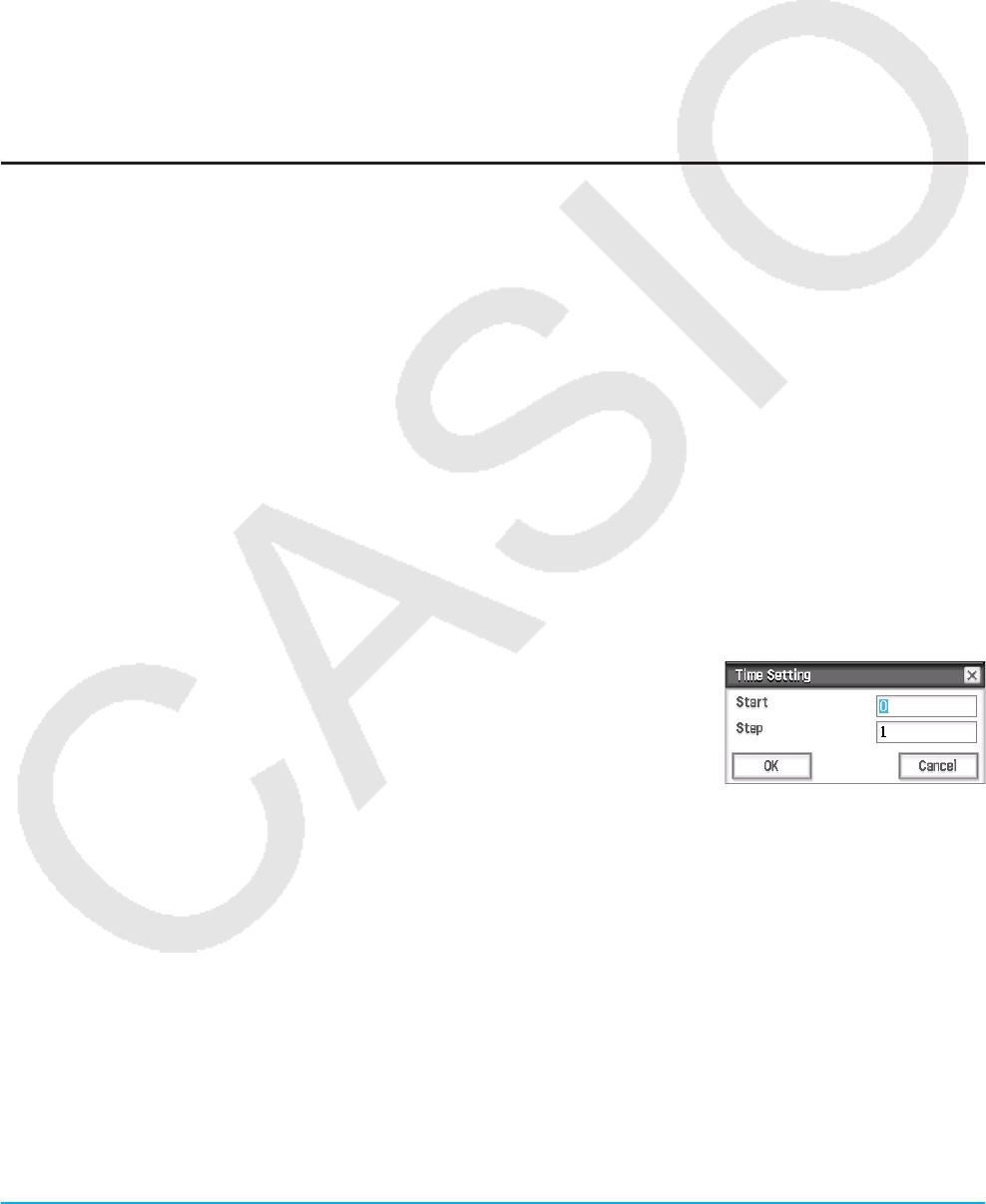
Chapter 15: Picture Plot Application 265
uTo save plot coordinate data as a spreadsheet
1. On the Plot List window, tap [File] - [Save Spreadsheet].
2. On the dialog box that appears, specify the file save destination folder and input a file name.
3. Tap [Save].
uTo import a spreadsheet as plot coordinate data
1. On the Plot List window, tap [File] - [Open Spreadsheet].
2. On the dialog box that appears, select the spreadsheet you want to import and then tap [Open].
Note: If the number of rows of spreadsheet you selected in step 2 of the above procedure exceeds the
allowable maximum (50 for a c2p file, equal to the number of still images for a c2b file), rows are
imported only up to the allowable maximum. Any spreadsheet data from Column C onwards and format
information that is not supported by the Plot List window is ignored.
Exporting Plot Data to and Importing Plot Data from a Variable
You can import LIST (list), MAT (matrix), and EXPR (expression) variables into the Plot List window. Data
inside of cells selected on the Plot List window can be exported as at LIST, MAT, or EXPR variable. The
steps of these operations are the same as those for the Spreadsheet application. For more information, see
“Importing and Exporting Variable Values” (page 235).
15-3 Displaying Plots on t-y or t-x Coordinates
As can be seen on the Plot List window, the data for each plot includes x- and y-coordinates, as well as a time
value t. On the Picture Plot screen each plot is normally displayed as coordinates (x, y) on an x-y plane, but
time value t can be used to display plots as coordinates (t, y) on a t-y plane or as coordinates (t, x) on a t-x
plane.
Under initial default settings, time values are 0, 1, 2, and so on (arithmetic progression with a start value of 0
and a step value of 1), in accordance with the sequence that the points are plotted. You can change the t value
assigned to each plot by changing the start value and step value.
uTo configure the time (t) value
1. On any Picture Plot application window, tap [Graph] - [Time Setting].
2. On the dialog box that appears, specify the start value and step value.
3. After the settings are the way you want, tap [OK].
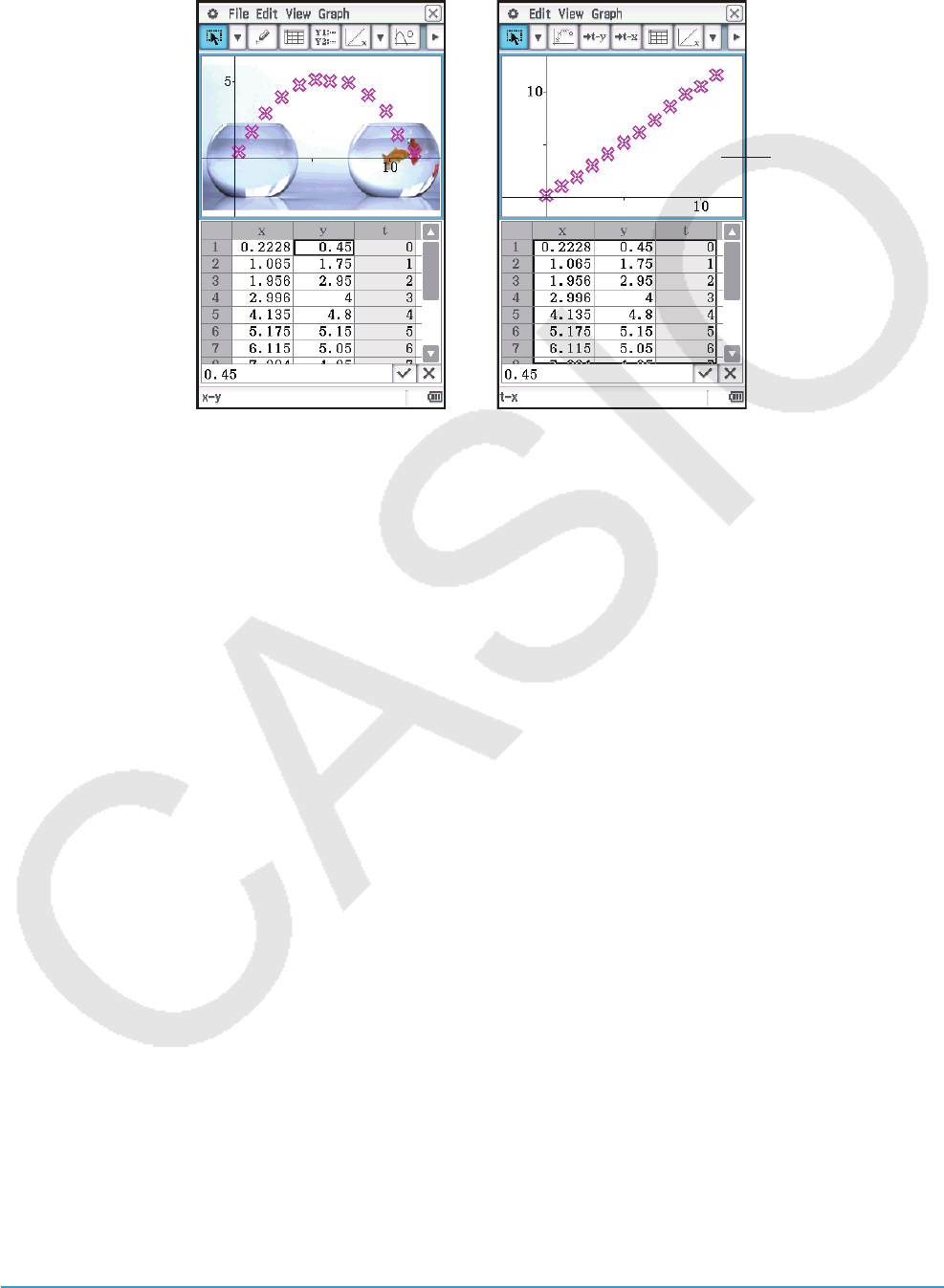
Chapter 15: Picture Plot Application 266
uTo display plots on t-y coordinates or t-x coordinates
To display plots on t-y coordinates, tap [Graph] - [Transform Axes] - [t-y] or tap v.
To display plots on t-x coordinates, tap [Graph] - [Transform Axes] - [t-x] or tap c.
The background
image is not displayed
on the t-x Plot window
and t-y Plot window.
Picture Plot window
(x-y coordinates)
t-x Plot window
(t-x coordinates)
Tip: You can tell which window (Picture Plot, t-y Plot, or t-x Plot) is displayed by checking the status bar.
15-4 Picture Plot Application Files
The Picture Plot application can be used to write plot data and/or various types of setting data directly into a
c2p or c2b file that is opened as a background image. The data and setting information that can be written to a
c2p or c2b file by the Picture Plot application is shown below.
• Plot data • Fade I/O setting
• Color setting of each plot • View Window settings
• Number format, text color, and fill color of each cell on the Plot List window
• Time setting (start value and step value)
• Axes/Grid settings
• Graph expressions (py1 through py5) that are registered on the Graph Editor dialog box
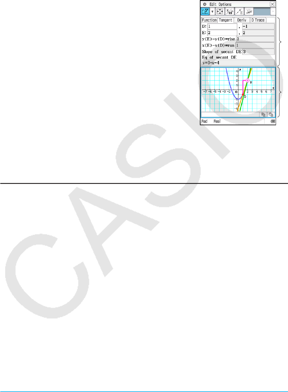
Chapter 16: Interactive Differential Calculus Application 267
Chapter 16:
Interactive Differential Calculus Application
The Interactive Differential Calculus Application helps you learn about
differential coefficients and/or derivative formulas that are the foundation
of differentiation.
It has a DiffCalc Table window (1) and a DiffCalc Graph window (2), and
the DiffCalc Table window has four tabs, described below.
[Function] tab: For input of y = f (x) functions used for differentiation. The
purpose of this tab is function input only, so the DiffCalc Graph window is
not displayed while this tab is displayed.
[Tangent] tab: This tab makes it possible to observe the slope of a straight
line passing through two points (D and E) on the function y = f (x) getting
closer to the slope of a tangent to point E as point D approaches point E.
This helps to demonstrate the fundamentals of differentiation.
[Deriv] tab: When the points (x1, y1), (x2, y2), … (xn, yn) on the function y
= f (x) have tangents with the slopes slope1, slope2, … slopen, the [Deriv]
tab can be used to plot the coordinates (x1, slope1), (x2, slope2), … (xn,
slopen) on the graph screen. After plotting a number of points, use the
function indicated by their loci to study the function indicated by them, and
consider what is the derivative (what expression is indicate by the function) of y = f (x).
[D Trace] tab: Displaying this tab causes x, f (x), f (x) number tables to be generated automatically based on the
f (x) function input on the [Function] tab. Selecting a different x-value provides a visual understanding of how the
f (x) value, tangent, f (x) value, and f (x) value change accordingly. At the same time, y = f (x) and y = f (x) are
graphed, and a tangent to the y = f (x) x-value are also drawn automatically.
DiffCalc Table Window-Specific Menus and Buttons
[Tangent] tab only
• Enable point E movement .................................................................................Options - Move Point E or q
• Lock point E ..........................................................................................................Options - Fix Point E or w
• Switch between the point (D or E) that moves when you press the left or right cursor key ................8 / 9
• Show the line tangent to point E .................................................................... Options - Show Tangent or 1
• Hide the line tangent to point E ....................................................................... Options - Hide Tangent or 2
[Deriv] tab only
• Delete the currently selected line in a number table .................................................................... Edit - Delete
• Manually input a derivative predicted function and draw a graph .....Calc - Predicted Function - Editor or D
• Clear the predicted function .........................................................................Calc - Predicted Function - Clear
• Determine regression from plots obtained from a number table and draw a graph
.....................................................Calc - Regression Function - Linear Reg (d) / Quadratic Reg (f) /
Cubic Reg (g) / Sinusoidal Reg (5)
• Clear the regression function ....................................................................Calc - Regression Function - Clear
[D Trace] tab only
• Display the Table Input dialog box for configuring x-value step setting ......................................................8
• Switch a number table between three value type combinations
(x, y1, y2; x, y2, y3; x, y1, y2, y3) ...........................................................................................................;
1
2

Chapter 16: Interactive Differential Calculus Application 268
16-1 Learning about Tangents Using the [Tangent] Tab
Consider the slope (differential coefficient) of a tangent to a point on a curve represented by y = f (x).
Two points (D and E) are placed on the graph of y = f (x), and a straight line (DE) through the two points and the
tangent of point E are drawn. As point D moves infinitely closer to point E, line DE moves infinitely closer to the
tangent of point E. This derives the slope of the line tangent to point E.
uTo use the [Tangent] tab
Example: On the graph of y = x2 − 2, derive the slope of the line tangent to a point (2, 2) on the graph of y =
x2 − 2.
1. On the application menu, tap to start the Interactive Differential Calculus application.
2. On the [Function] tab that appears, input x2 − 2 into the “y:” line under
“Function”.
3. Tap the [Tangent] tab.
• This will cause the display to appear as shown below.
Point D coordinates (1, −1)
Point E coordinates (2, 2)
y = x2 − 2 graph (blue)
shows the point that can be moved
using the right and left cursor keys.
Straight line linking point D and point E
(orange)
{Point E y-coordinate} −
{Point D
y-coordinate} (= rise)
{Point E x-coordinate} −
{Point D
x-coordinate} (= run)
Slope of secant DE (= rise/run)
Expression of secant DE
y = x2 − 2 tangent to point E (green)
4. Tap w (or Point - Fix Point E).
• This locks point E and allows relocation of point D only.
5. Use the left and right cursor keys to move point D on the y = x2 − 2 graph closer and closer to point E.
6. Move point D to the same location as point E.
• This will cause the rise and run values on the [Tangent] tab to become 0, and only the y = x2 − 2 (green)
tangent of point E (which is the same as point D) will remain displayed.
• Use the cursor keys to move point D and observe the Slope of secant DE and Eq (equation) of secant DE
immediately before and after the location where point D and point E are identical. This way you can study
the slope and expression of tangent y = x2 − 2.
Note
• To switch between the point (D or E) that moves when you press the left or right cursor key, press the up or
down cursor key, or tap 9 or 8. The point that will be moved when you press the left or right cursor key is
indicated by .
• You can also move the point E or point D using the stylus. Tap and hold one of the points with the stylus, and
then drag to the location to which you want to move it.
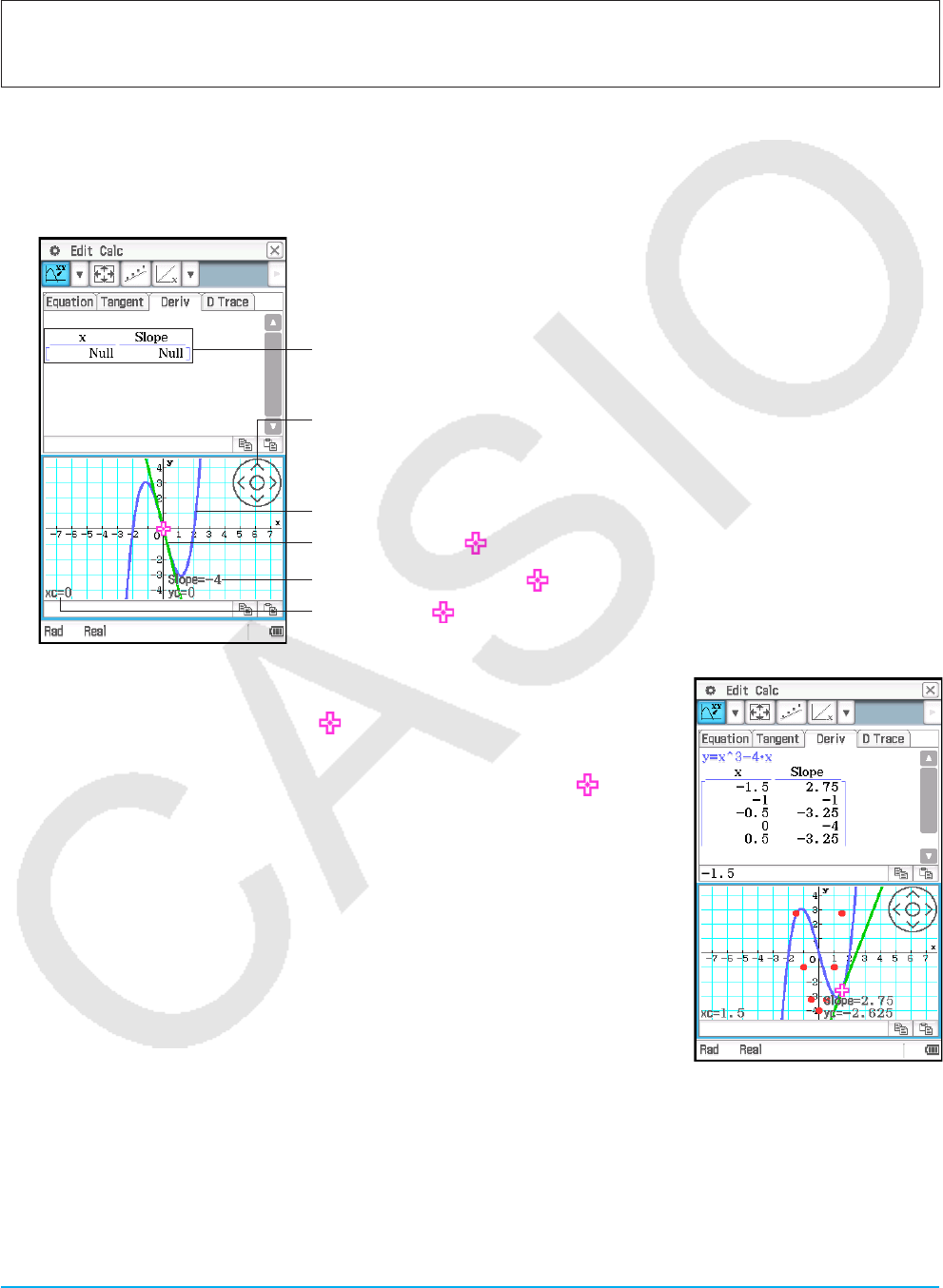
Chapter 16: Interactive Differential Calculus Application 269
16-2 Deriving the Derivative Using the [Deriv] Tab
uTo use the [Deriv] tab
Example: The slope of a tangent at a point (x, y) on the graph of y = x3 − 4x, is slope. Plot coordinates (x1,
slope1), (x2, slope2), (x3, slope3), …. (xn, slopen) on the DiffCalc Graph window, and predict the function that
passes through all of the plots. Also, use regression to confirm the function.
1. On the DiffCalc Table window, display the [Function] tab.
2. In the “y:” line under “Function”, input x3 − 4x.
3. Tap the [Deriv] tab.
• This will cause the display to appear as shown below.
(x, slope) number table
There are no table contents under initial default conditions.
[EXE] button and cursor buttons
y = x3 − 4x graph (blue)
Tangent at position of graph y = x3 − 4x graph (green)
Slope of tangent at position of graph y = x3 − 4x graph
x-coordinate of location
4. On the DiffCalc Graph window, plot a point at coordinates (x, slope).
(1) Use the cursor buttons to move around the graph.
(2) Tap the [EXE] button.
• This will add the x and slope values at the current location of to the
number table on the [Deriv] tab. At the same time, the (x, slope) will be
plotted on the DiffCalc Graph window.
(3) Repeat steps (1) and (2) above to plot at least four points.
• At this point, try to predict the expression (y = f (x) function) that will
produce a curve that passes through all of the plots.
5. Input the expression and graph it.
• In this example, we can predict a quadratic function curve, so we will try inputting y = 2x2 − 4.
(1) Tap Calc - Predicted Function - Editor or D.
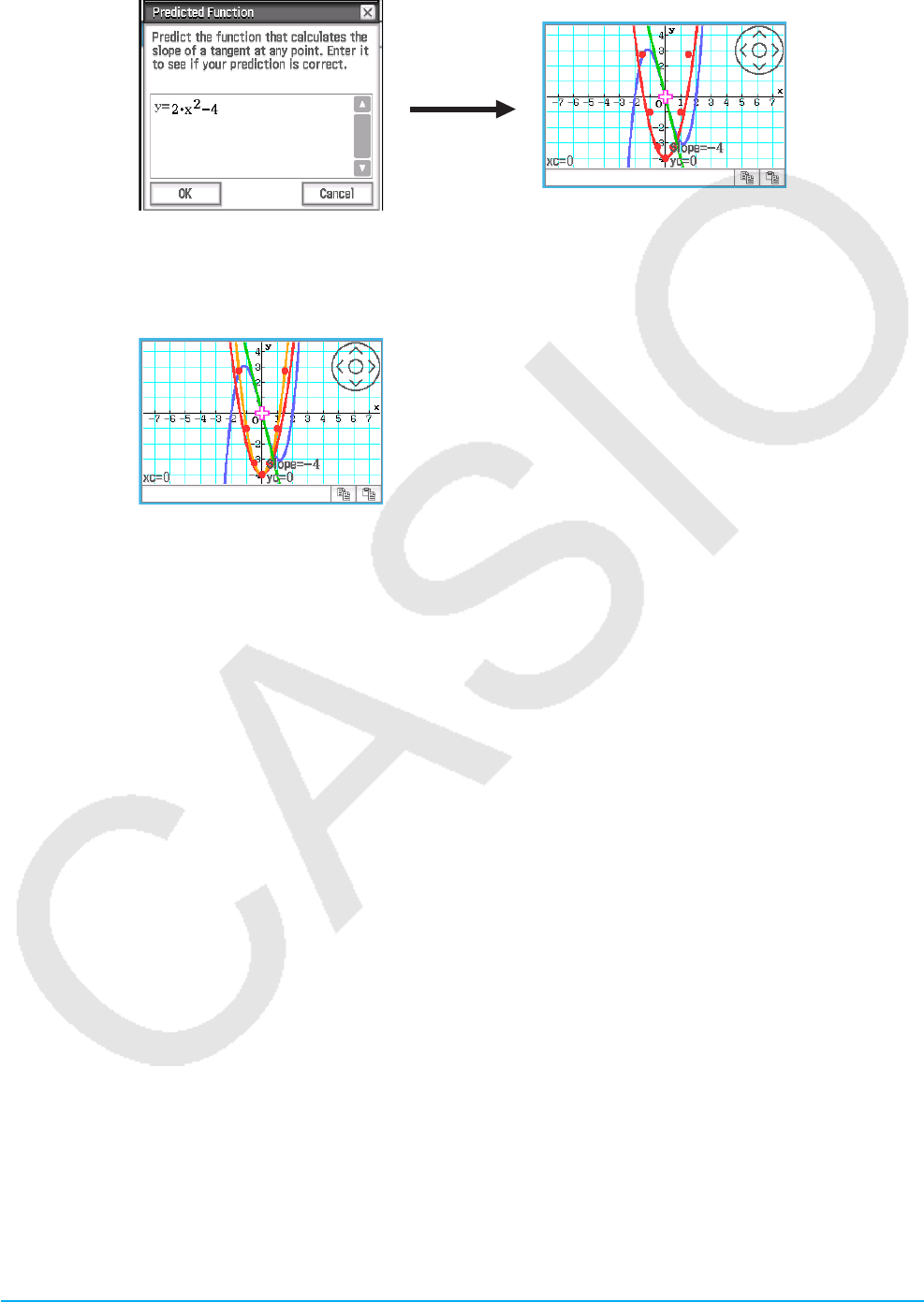
Chapter 16: Interactive Differential Calculus Application 270
(2) On the dialog box that appears, input 2x2 − 4 and then tap [OK].
• This will graph the expression you input.
6. Perform regression to check if the function you predicted is correct.
Since we predicted a quadratic function curve here, we will perform quadratic regression.
Tap Calc - Regression - Quadratic Reg or f.
• This draws the graph based on the calculation results.
Tip: There are four types of regression available on the Calc - Regression menu. Decide on the type of regression
calculation you want to perform based on the straight lines and curves expected from the shape of the plots.
Note
• In step 4 of the above procedure, be sure to plot at least four points for the (x, slope) coordinates. When there
are fewer than four plots, attempting to perform the steps from step 5 onward will cause the message “Plot at
least 4 points.” to appear to let you know you cannot go any further until you plot more points.
• The predicted expression you input in step 5 and the regression expression obtained in step 6 automatically
overwrite the applicable fields on the [Function] tab.
• For details about the regression calculation result dialog box that appears in step 6-(2) above, see the table in
step 3 of the procedure under “To view regression calculation results” (page 143).
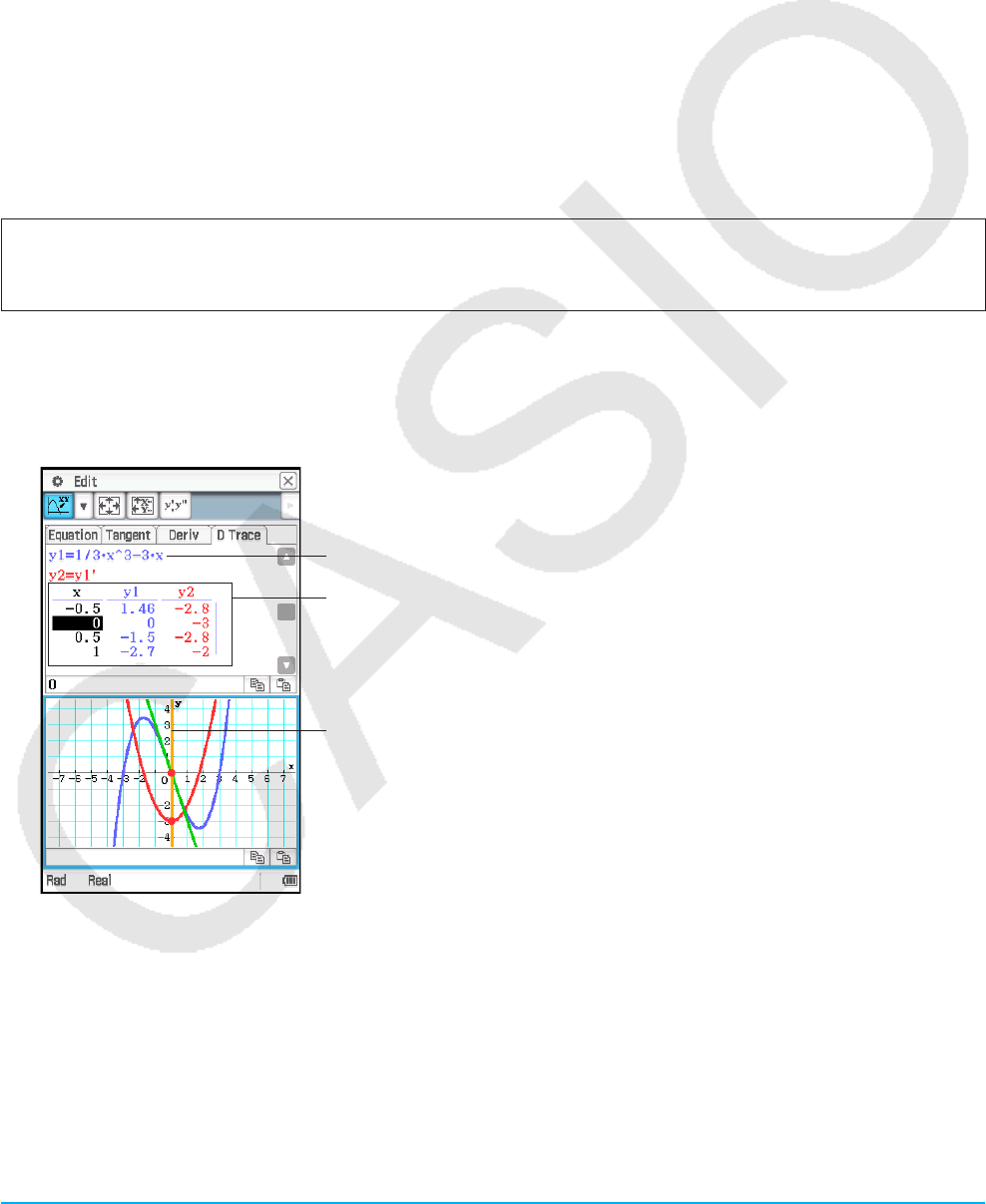
Chapter 16: Interactive Differential Calculus Application 271
16-3 Generating a Number Table and Graphing the
First Derivative and Second Derivative Using the
[D Trace] Tab
The [D Trace] tab can simultaneously handle the three types of functions below, which are based on the
functions input for “Function” on the [Function] tab.
x function y1 (= f (x))
y1 first derivative y2 = y1 (= f (x))
y1 second derivative y3 = y1 (= f (x))
You can use this tab to view the number table of y1, y2, and y3 values for each x value, and to check the graph
associated with the number table.*
* Defaults: x, y1, y2
uTo use the [D Trace] tab
Example: Simultaneously graph the function y1 = 1/3·x3 − 3x and its first derivative y2 = y1, and compare the
graphs. Also, use the graph and number table to observe changes in each of the graph’s y-values (y1, y2),
and study the relationship between the functions.
1. On the DiffCalc Table window, display the [Function] tab.
2. In the “y:” line under “Function”, input 1/3·x3 − 3x.
3. Tap the [D Trace] tab.
• This will cause the display to appear as shown below.
The function you input in step 2 above.
(x, y1, y2) number table
y1 is the value of y1 for each x (value of f (x)), and y2 is the value of y1 for each x
(value of f (x)). The colors of the y1, y2 text correspond to the colors of the graph
lines.
Use the left and right cursor keys to move the vertical line left and right. This will
also cause the following items to move accordingly: the point where the vertical
line intersects with y1 and y2 (both indicated by red dots), and the tangent (green)
of the y1 graph where the vertical line intersects with y1.
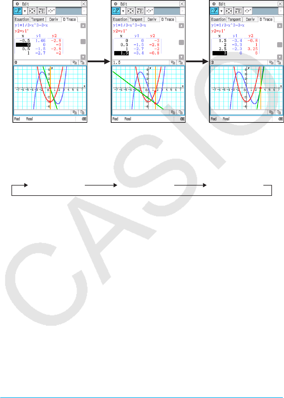
Chapter 16: Interactive Differential Calculus Application 272
4. Use the cursor keys to move the vertical line, and observe how the y1 and y2 values change.
• Compare y1 and y2. You should also observe the green tangent (y1 tangent) at this time.
• The current location of the vertical line (x value) corresponds to the highlighted cell in the x-column of the
number table.
• You can also move the vertical line by dragging it with the stylus.
uTo change the group of items displayed in the number table
Tap ; to cycle through the settings shown below.
x, y1, y2 display x, y2, y3 display x, y1, y2, y3 display
Changing the items of the number table will also change the graph drawn on the DiffCalc Graph window.
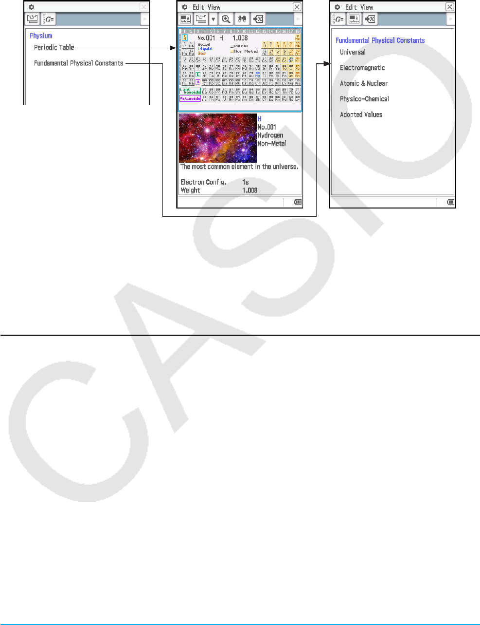
Chapter 17: Physium Application 273
Chapter 17:
Physium Application
The Physium application includes a built-in periodic table and fundamental physical constants. You can access
these from the Physium menu that appears when you start up the application.
Physium menu
• After displaying the periodic table from the Physium menu, you can look up the following information: atomic
number of elements, chemical symbols of elements, atomic weights, and electron configurations.
• When you select “Fundamental Physical Constants” on the Physium menu, a list of categories will appear.
Select the category whose constants you want to view.
• The periodic table and fundamental physical constants displayed by Physium can be assigned to variables for
use in calculations in the Main application, eActivity application, and other applications.
Physium Application Menus and Buttons
Physium window (Physium menu)
• Display the Periodic Table window ............................................................................................................ h
• Display the Physical Constants window ..................................................................................................... k
Periodic Table window
• Assign the atomic weight currently selected on the periodic table to a variable ..................Edit - Store or l
• Zoom the periodic table display ........................................................................................ View - Large or W
• Return a zoomed view of the periodic table to its normal size ........................................ View - Normal or E
• Enclose a particular element group in the periodic table with a blue boundary ...............View - Select Series
• Delete a blue boundary you displayed on the periodic table ............................ View - Deselect Series or h
• Display a list view of elements ........................................................................................ View - Search or e
• Make the Periodic Table Detail window active ............................................................................................p
Periodic Table Detail window
• Make the Periodic Table window active ......................................................................................................h
• Scroll back or forward through atomic numbers .................................................................................. ,/.
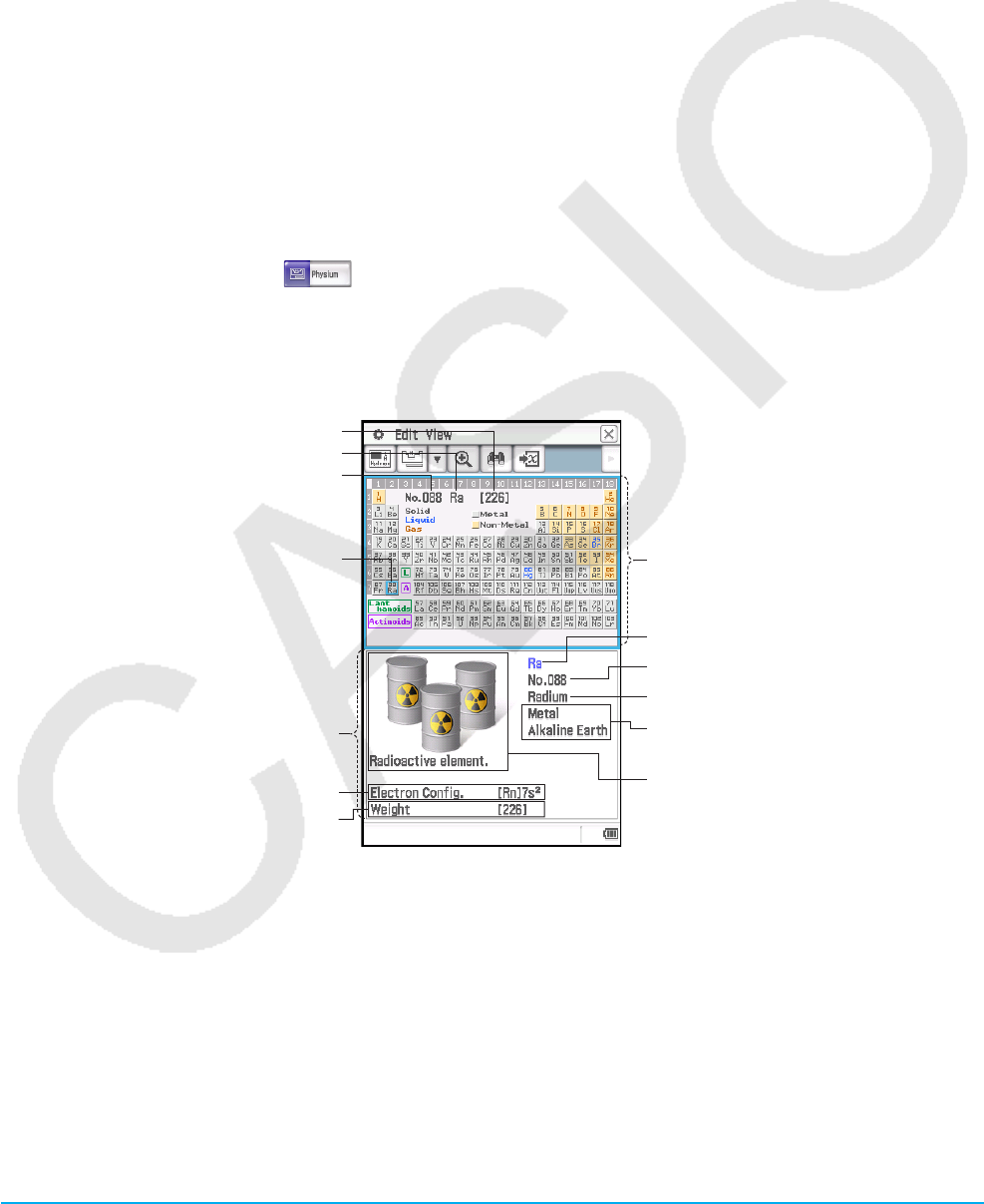
Chapter 17: Physium Application 274
• Assign the atomic weight of the displayed atom to a variable .............................................Edit - Store or l
Physical Constants window
• Return to the Fundamental Physical Constants category menu .......................................... View - Top or k
• Display details of the currently highlighted physical constant .....................................................................F
• Assign the current physical constant to a variable ...............................................................Edit - Store or l
• Display a list of universal physical constants. ........................................................................View - Universal
• Display a list of electromagnetic constants ................................................................. View - Electromagnetic
• Display a list of atomic and nuclear constants .......................................................... View - Atomic & Nuclear
• Display a list of physico-chemical constants ............................................................ View - Physico-Chemical
• Display a list of adopted values .................................................................................. View - Adopted Values
17-1 Periodic Table
uTo display the periodic table
1. On the application menu, tap to start the Physium application.
• This will display the Physium menu.
2. Tap “Periodic Table” or h.
• The upper half of the display shows the Periodic Table window, while the lower half shows the Period
Table Detail window. Details about the content of each of the windows are shown below.
Atomic weight
Chemical symbol
Atomic number
Cursor (light blue boundary)
Periodic Table Detail window
Electron configuration
Atomic weight*
Periodic Table window
Chemical symbol
Atomic number
Element name
Metal/non-metal classification and
element group name
Illustrative image and explanation
* An atomic weight value in square brackets ([ ]) indicates the atomic weight of the most well-known element
among isotopes.
uTo enclose a particular element group in the periodic table with the blue boundary
Tap View - Select Series. On the sub-menu that appears select the name of an element group (such as Rare
Earth), or tap the down arrow (v) on the toolbar and then select an element group button (such as i).
To clear a blue boundary displayed with this operation, tap View - Deselect Series or h.
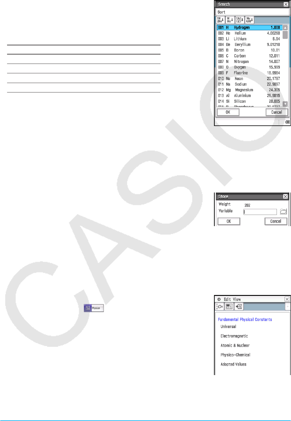
Chapter 17: Physium Application 275
uTo use the element list to search for an element
1. On the Periodic Table window, tap e.
• This displays a search dialog box that lists elements, like the one shown in
the screenshot nearby.
2. You can use the toolbar buttons shown in the table below to change the sort
sequence of the list, if you want.
To sort in this sequence: Tap this toolbar button:
Atomic number ascending d
Chemical symbol alphabetic f
Element name alphabetic L
Atomic weight ascending g
3. On the element list, tap the element you want to select so it is highlighted.
4. Tap [OK].
• This closes the Search dialog box and displays the periodic table with the
cursor (blue boundary) located at the element you tapped in step 3.
uTo assign an atomic weight to a variable
1. On the periodic table tap the element whose atomic weight you want to assign to the variable so the blue
boundary (cursor) is located there.
• You can also select an element using the element list as described under “To use the element list to
search for an element”.
2. Tap Edit - Store or l
3. On the dialog box that appears, enter the name of the variable you want to
use and then tap [OK].
• This assigns the atomic weight of the element you selected in step 1 of
this procedure to the variable whose name you input above.
uTo return to the Physium menu
On the menu bar, tap S.
17-2 Fundamental Physical Constants
uTo display the Fundamental Physical Constants category menu
1. On the application menu, tap to start the Physium application.
• This will display the Physium menu.
2. Tap “Fundamental Physical Constants” or k.
• This displays the Fundamental Physical Constants category menu.
uTo display a physical constant
On the Fundamental Physical Constants category menu, tap the name of the
category that contains the constant you want to display. You can also select
the physical constant category name you want (such as Electromagnetic) on
the View menu.
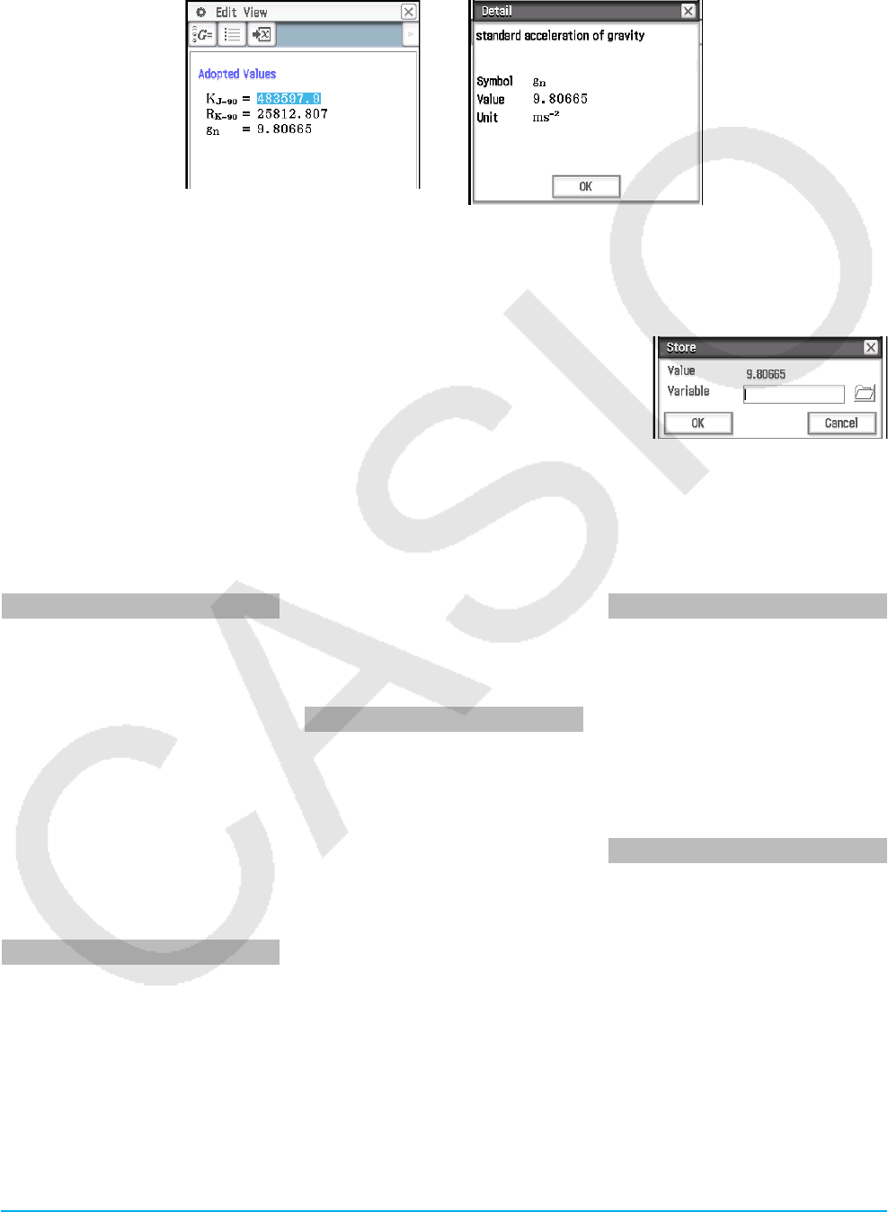
Chapter 17: Physium Application 276
uTo display detailed information about a physical constant
1. Tap the physical constant value whose information you want to view so it is highlighted.
2. Tap F.
uTo assign a physical constant to a variable
1. Tap the physical constant value you want to assign to the variable so it is highlighted.
2. Tap Edit - Store or l.
3. On the dialog box that appears, enter a variable name and then tap [OK].
• This assigns the physical constant you selected in step 1 of this procedure
to the variable whose name you input above.
uTo return to the Physium menu
On the menu bar, tap S.
List of Built-in Constants
Universal
c: speed of light in vacuum
0: magnetic constant
0: electric constant
Z0: characteristic impedance of
vacuum
G: Newtonian constant of
gravitation
h: Planck constant
H: Planck constant over 2π
mp: Planck mass
lp: Planck length
tp: Planck time
Electromagnetic
e: elementary charge
0: magnetic flux quantum
G0: conductance quantum
KJ: Josephson constant
RK: von Klitzing constant
B: Bohr magneton
N: nuclear magneton
Atomic & Nuclear
: fine-structure constant
R∞: Rydberg constant
a0: Bohr radius
me: electron mass
e: electron magnetic moment
m: muon mass
: muon magnetic moment
m: tau mass
mp: proton mass
p: proton magnetic moment
mn: neutron mass
n: neutron magnetic moment
Physico-Chemical
NA: Avogadro constant
mu: atomic mass constant
F: Faraday constant
R: molar gas constant
k: Boltzmann constant
Vm: molar volume of ideal gas
(273.15 K, 100 kPa)
: Stefan-Boltzmann constant
Adopted Values
KJ–90: conventional value of
Josephson constant
RK–90: conventional value of von
Klitzing constant
gn: standard acceleration of
gravity

Chapter 17: Physium Application 277
17-3 Precautions
• The atomic weights in this application are based on those recommended by 2013 IUPAC (International Union
of Pure and Applied Chemistry).
• Electron configurations are based on information in the “CRC Handbook of Chemistry and Physics 91st
Edition”.
• The physical constants in this application are based on those recommended by the 2014 CODATA.
• A scientific constant in this application may be slightly different depending on the year it is presented or books
it is presented. Refer to appropriate information that fits your purpose before use.
• The classification of rare earth elements may be slightly different from those in typical textbooks or magazines
in the USA.
• The classification of transition elements may be slightly different from those in typical textbooks or magazines
in the USA.
• Copyrights of the element graphic images revert to the individuals shown in the table below.
Element Name Copyright Holder
Hydrogen © ordus - Fotolia.com
Helium © Elenathewise - Fotolia.com
Lithium © Coprid - Fotolia.com
Beryllium © travis manley - Fotolia.com
Carbon © Paylessimages - Fotolia.com
Nitrogen © Stefan Korber - Fotolia.com
Oxygen © Kor_Alex - Fotolia.com
Fluorine © philippe Devanne -
Fotolia.com
Neon © Akasha+ - Fotolia.com
Sodium © davide tesoriero - Fotolia.com
Magnesium © Aviator70 - Fotolia.com
Aluminium © StudioAraminta - Fotolia.com
Silicon © wolandmaster - Fotolia.com
Phosphorus © Swettlana Gordacheva
-Fotolia.com
Sulfur © Alexander Mandl - Fotolia.com
Chlorine © L. Shat - Fotolia.com
Argon © uhotti - Fotolia.com
Potassium © Stefan Korber - Fotolia.com
Calcium © Birute Vijeikiene - Fotolia.com
Scandium © Melinda Nagy - Fotolia.com
Titanium © christian42 - Fotolia.com
Vanadium © Thomas Reimer - Fotolia.com
Chromium © sav_a - Fotolia.com
Manganese © cardiae - Fotolia.com
Iron © Novydel - Fotolia.com
Cobalt © SpbPhoto - Fotolia.com
Nickel © John Sfondilias - Fotolia.com
Copper © effe45 - Fotolia.com
Zinc © ibphoto - Fotolia.com
Element Name Copyright Holder
Gallium © Ron-Heidelberg - Fotolia.com
Germanium © Dario Sabljak - Fotolia.com
Selenium © Konstantin Shevtsov -
Fotolia.com
Bromine © Rade Cojbasic - Fotolia.com
Krypton © Morad HEGUI - Fotolia.com
Strontium © jonnysek - Fotolia.com
Yttrium © Jean-Philippe Capart -
Fotolia.com
Zirconium © Hiro - Fotolia.com
Niobium © Alexandr Blinov - Fotolia.com
Molybdenum © vnlit - Fotolia.com
Ruthenium © DeVIce - Fotolia.com
Rhodium © Pix by Marti - Fotolia.com
Palladium © Pix by Marti - Fotolia.com
Silver © Zee - Fotolia.com
Cadmium © Florian Ertl - Fotolia.com
Indium © 263 - Fotolia.com
Tin © dvs71 - Fotolia.com
Antimony © Andrew Barker - Fotolia.com
Tellurium © fotografiche.eu - Fotolia.com
Iodine © Aleksandr Bedrin -
Fotolia.com
Xenon © Eimantas Buzas - Fotolia.com
Caesium © John Tomaselli - Fotolia.com
Barium © Jim Parkin - Fotolia.com
Lanthanum © Tyler Olson - Fotolia.com
Cerium © photoiron - Fotolia.com
Praseodymium © Dario Bajurin - Fotolia.com
Neodymium © Igor Tarasov - Fotolia.com
Samarium © ケンジ - Fotolia.com

Chapter 17: Physium Application 278
Element Name Copyright Holder
Europium © wrangler - Fotolia.com
Gadolinium © khz - Fotolia.com
Terbium © Dragan Radojkovic -
Fotolia.com
Dysprosium © jonnysek - Fotolia.com
Holmium © beerkoff - Fotolia.com
Erbium © Kitch Bain - Fotolia.com
Thulium © Nomad_Soul - Fotolia.com
Ytterbium © Dmitrijs Gerciks - Fotolia.com
Lutetium © Viktor - Fotolia.com
Tantalum © Elridge - Fotolia.com
Tungsten © Sylvie Thenard - Fotolia.com
Rhenium © zmkstudio - Fotolia.com
Osmium © llandrea - Fotolia.com
Iridium © MACLEG - Fotolia.com
Platinum © Soul Concept - Fotolia.com
Gold © Paylessimages - Fotolia.com
Mercury © marcel - Fotolia.com
Lead © dabjola - Fotolia.com
Bismuth © Tommy - Fotolia.com
Radon © TOMO - Fotolia.com
Uranium © philipus - Fotolia.com
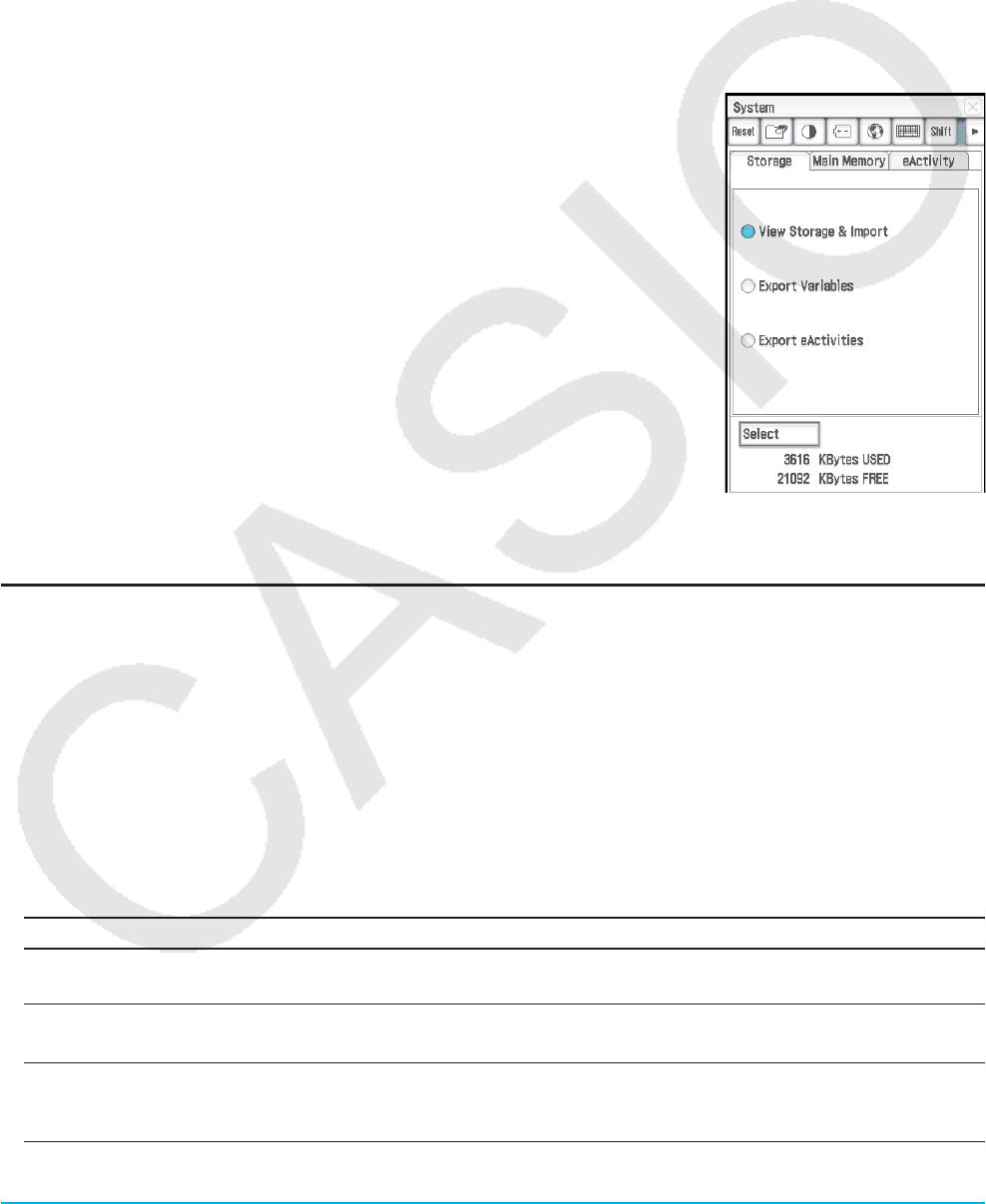
Chapter 18: System Application 279
Chapter 18:
System Application
You can use the System application to manage ClassPad memory (main memory, the eActivity area, and the
storage area), and to configure various system settings.
18-1 Managing Memory Usage
ClassPad has the following three independent memory areas for storing data: main memory area, eActivity
area, and storage area.
Main memory: This area is for storage of application data and variables,
except for eActivity.
eActivity area: This area is for storage of eActivity data.
Storage area: All ClassPad data can be exported as a single VCP file, and
individual main memory and/or eActivity area data items can be exported as
individual XCP files and stored in this area. When the ClassPad is connected
to a computer via a USB connection, this area can be used to transfer data
between the ClassPad and computer (page 288).
Starting up the System application displays a screen with three tabs, one
for each of the memory areas described above. Tapping a tab will display a
sheet for performing the operations below for the applicable memory area.
• Delete main memory and eActivity area data
• Search for and delete files and folders in the storage area, and create and
rename folders
• Import and export data (variable and eActivity) between main memory and
the eActivity area, and the storage area
Using the Storage Sheet
The [Storage] sheet appears first whenever the System application is started up. You can use this sheet to
import and export files. For details, see “VCP and XCP File Operations” (page 289). Here, we will display the
contents of the storage area, and show how to rename a file and delete a file.
uTo view storage area contents
1. On the System application window, tap the [Storage] tab.
2. Select “View Storage & Import” and then tap [Select].
• This displays the Storage dialog box. It shows the folders and files in the storage area.
3. On the Storage dialog box, perform the folder and file operations described below.
To do this: Do this:
Delete a folder or file Select the check box of the folder or file you want to delete and then tap [File]
- [Delete].
Create a folder Tap [File] - [Create Folder] or {. On the dialog box that appears, enter the
name you want to assign to the folder and then tap [OK].
Rename a folder Highlight the folder you want to rename and then tap [File] - [Rename]. On the
dialog box that appears, enter the name you want to assign to the folder and
then tap [OK].

Chapter 18: System Application 280
To do this: Do this:
Search for a file or folder Tap [Search] or e. On the dialog box that appears, enter the character string
you want to search for and then tap [Search]. To search again using the same
character string, tap r.
Change the file list view To display both the file name and file size, tap [View] - [Detail View] (long file
names may be cut off). To display the file name only, tap [View] - [List View].
4. Tap [Cancel] to close the Storage dialog box.
Using the Main Memory Sheet and eActivity Sheet
Main Memory Sheet
Tapping the [Main Memory] tab displays the Main Memory sheet.
This item: Shows how much memory is used by this type of data:
Setup Setup data
Graph Sheet Graph & Table application function data (including sheet name data and function
selection data)
3D Graph Sheet 3D Graph application function data (including sheet name data and function selection
data)
Graph Summary Summary table data
View Window View Window parameter values
3D View Window 3D View Window parameter values
Factor Zoom factor values
Table Range values and table result values
Conics Eqn Conics expressions
Sequence Sequence application data
DiffEqGraph Differential Equation Graph application function data
Stat List list1 through list6
Stat Result Statistical calculation results
Numeric Solve Solve expression and solve range
Ans Memory Main application Ans data
Random Value Random command setting data
Main History Main application history data
User Defined User-defined variables and user-created folders
Library “library” folder data
eActivity eActivity application temporary data*
Geometry Geometry application temporary data*
Spreadsheet Spreadsheet application temporary data*
Financial Financial application data
Picture Plot Picture Plot application temporary data*
DiffCalc Interactive Differential Calculus application data
System Other system data
Clipboard Clipboard data
* “temporary data” is data that is created by an application but not saved as a file.

Chapter 18: System Application 281
eActivity Sheet
Tapping the [eActivity] tab displays the eActivity sheet. This sheet lists the names of all the files that have been
created with the eActivity application, and shows the size of each file.
uTo delete Main Memory data or eActivity files
1. Tap the tab (Main Memory or eActivity) that contains the data you want to delete.
2. Select the check box next to the item whose data you want to delete.
3. Tap the [Delete] button.
4. On the confirmation dialog box that appears, tap [OK] to delete the selected data.
• Tapping [OK] displays the message “Now deleting...” while the data is being deleted.
Tip
• You cannot delete any data that has a dimmed check box.
• For information about deleting all variable data and program data, and deleting all eActivity data, see “To batch delete
specific data (Reset)”.
18-2 Configuring System Settings
Use the System application menu or toolbar buttons to configure system settings.
System Application Menus and Buttons
• Batch delete specific memory area data ....................................................................... System - Reset or ;
• Initialize the ClassPad ............................................................................................... System - Initialize or n
• Adjust display brightness ..............................................................................System - Display Settings or Z
• Configure power properties ........................................................... System - Power Properties - Power or X
• Specify the battery type being used ............................................. System - Power Properties - Battery or m
• Change the display text language .......................................................................... System - Language or ,
• Specify the complex number imaginary unit ............................................................. System - Imaginary Unit
• Change the arrangement of the alphabet soft keyboard ......................................... System - Keyboard or V
• Assign shift mode key operations to hard keys ...................................................... System - Shift Keys or .
• Optimize eActivity area and storage area ........................................... System - Memory Management or /
• Select the image data for the ending screen that appears
when the ClassPad is turned off ................................................................System - Ending Screen or N
• Adjust the alignment of the touch panel ............................................ System - Touch Panel Alignment or M
• Display software version information .............................................................System - About - Version or >
• Register a user name on a ClassPad ................................................................System - About - User Name
Configuring System Settings
u To batch delete specific data (Reset)
1. On the System application window, tap [System] - [Reset], or tap ;.
• This displays the Reset dialog box.

Chapter 18: System Application 282
2. On the Reset dialog box, select the type of reset operation you want to perform.
To delete this type of data: Select this option:
All variable and program data in main memory Variable/Program
All eActivity data in eActivity area eActivity Data
Data in storage area Storage Memory
All of the above three types All of the above
3. After selecting the type of reset operation you want to perform, tap [Reset].
4. In response to the confirmation message that appears, tap [OK] to perform the reset operation and return to
the application menu.
u To initialize your ClassPad
Warning!
Initializing the ClassPad deletes anything you have input and stored in memory (including eActivity data) since
you purchased the ClassPad or last initialized it. Before initializing the ClassPad, double-check to make sure
you do not need any of the data that will be deleted.
1. On the System application window, tap [System] - [Initialize], or n.
• This displays a confirmation asking if you really want to initialize your ClassPad.
2. Tap [OK] to perform the initialize operation.
• The initialize operation may take several minutes to complete (depending on the amount of data stored in
memory).
• After the initialize operation is complete, the touch panel alignment screen will appear. Follow the
instructions on the screen to configure initial settings. For more information about the setup operation, see
“Loading Batteries and Setting Up the ClassPad” in the separate Quick Start Guide.
uTo adjust display brightness
1. On the System application window, tap [System] - [Display Settings], or Z.
2. Tap t or u to change display brightness, and then tap [Set].
• Tapping [Initial] returns display brightness to its initial default.
u To configure power properties
1. On the System application window, tap [System] - [Power Properties] - [Power], or X.
2. On the dialog box that appears, perform the operations described below.
To do this: Do this:
Specify the Auto Power Off trigger time Tap the “Auto Power Off” down arrow button and then select
10 min or 60 min.
Specify the backlight duration Tap the “Backlight Duration” down arrow button and then
select 30 sec, 1 min, 3 min, or 10 min.
3. After all the settings are the way you want, tap [Set].
uTo specify the battery type
1. On the System application window, tap [System] - [Power Properties] - [Battery], or m.
2. Tap the type of battery you loaded and then tap [Set].
3. On the confirmation dialog box that appears, tap [OK].
• This registers the selected battery type and closes the confirmation dialog box.

Chapter 18: System Application 283
• If you tap [Cancel] instead of [OK], the confirmation dialog box will close without registering the selected
battery type.
uTo specify the display language
1. On the System application window, tap [System] - [Language], or ,.
2. On the dialog box that appears, select the language you want to use, and then tap [Set].
• This returns to the application menu.
u To specify the complex number imaginary unit (i or j )
1. On the System application window, tap [System] - [Imaginary Unit].
2. On the dialog box that appears, select the type of imaginary unit you want to use, and then tap [Set].
uTo specify the alphabetic keyboard arrangement
1. On the System application window, tap [System] - [Keyboard], or V.
2. On the dialog box that appears, select the keyboard arrangement you want to use, and then tap [Set].
• This returns to the application menu.
uTo assign shift mode key operations to hard keys
1. On the System application window, tap [System] - [Shift Keys], or ..
• This displays the Shift Key Assign dialog box.
2. Tap the down arrow button then select the hard key to which you want to assign a shift mode operation.
3. Specify the operation you want to assign to the hard key.
To do this: Do this:
Assign an auto text (string, function name, etc.) input
operation to the hard key
Enter the text you want to auto input to the right
of the [Set] button and then tap [Set].
Assign the Cut, Copy, Paste, or Undo/Redo operation
to the hard key
Tap the applicable button on the dialog box.
Clear the current assignment from the hard key Tap [Clear].
Return all key assignments to their initial defaults Tap [Default].
• The operation assigned to the hard key is displayed in the status bar.
4. After all the settings are the way you want, tap [OK] to apply them and close the Shift Key Assign dialog box.
Tip
• Performing any one of the following operations will cause all key assignments to be returned to their initial default settings:
“To batch delete specific data (Reset)” (page 281), “To initialize your ClassPad” (page 282), or “To perform the RAM reset
operation” (page 308).
• The initial default key assignments are shown below.
= : Copy x : Cut y : Paste Z : Undo
( : t) : , : | z : ⇒
1 : sin( 2 : cos( 3: tan( 5 : ln(
0 : π. : ie : ∞E : Ans
{ : (Template Input Mode) or '( (Line Input Mode)*1
/ : (Template Input Mode) or / (Line Input Mode)*1
4 : (Template Input Mode) or e^( (Line Input Mode)*1
6 : (Template Input Mode) or log( (Line Input Mode)*1
7, 8, 9, *, -, + : Undefined
*1 See “Template Input and Line Input” (page 24).
e

Chapter 18: System Application 284
u To optimize Flash ROM (eActivity area and storage area)
Tip: Optimizing Flash ROM increases the amount of memory available for storage.
1. On the System application window, tap [System] - [Memory Management], or /.
2. On the confirmation dialog box that appears, tap [Yes].
• After you tap [Yes], the message “Now Optimizing...” remains displayed while optimization is in progress.
The message “Complete!” appears when optimization is complete.
Important!
Never press the RESTART button on the back of the ClassPad while a Flash ROM optimization operation is
in progress. Doing so can damage memory, resulting in loss of all memory contents and malfunction of your
ClassPad. If this happens, you will need to request repair from your CASIO Maintenance Service Provider.
Note that repair of your ClassPad will not recover any lost memory contents.
3. Tap [OK] to close the “Complete!” message dialog box.
uTo select the image data for the ending screen that appears when the ClassPad is turned off
1. On the System application window, tap [System] - [Ending Screen], or N.
2. On the dialog box that appears, tap the down arrow button. On the list that appears, tap [Select Picture File]
and then tap the ending screen image you want to use.
• Tapping the [View] button displays a preview of the currently selected screen image. Tap [OK] to close the
preview image.
3. After the image you want is selected, tap [Set].
u To adjust touch panel alignment
1. On the System application window, tap [System] - [Touch Panel Alignment], or M.
2. Use the stylus to tap the center of each of the four crosses as they appear on the screen.
• When aligning your ClassPad try to tap the exact center of each cross.
u To view version information
On the System application window, tap [System] - [About] - [Version], or >.
Tap [OK] to close the Version dialog box.
uTo register a user name on a ClassPad
1. On the System application window, tap [System] - [About] - [User Name].
2. On the dialog box that appears, enter your name, and then tap [Set].
• The user name you registered appears at the bottom of the ending screen that appears when the ClassPad
is turned off.

Chapter 19: Performing Data Communication 285
Chapter 19:
Performing Data Communication
You can connect your ClassPad to a computer or to another ClassPad and exchange data with the connected
device. You can also connect to a Data Logger or a CASIO projector. This chapter explains how to connect a
ClassPad to an external device and how to transfer data between them.
Important!
Do not press the RESTART button on the back of the ClassPad while a data communication operation is in
progress. Doing so can damage memory, resulting in loss of all memory contents and malfunction of your
ClassPad. If this happens, you will need to request repair from your CASIO Maintenance Service Provider.
Note that repair of your ClassPad will not recover any lost memory contents.
19-1 Data Communication Overview
This section explains how to configure communication parameters using the Communication application,
and how to use the Select Connection Mode dialog box that appears when you establish a USB connection
between your ClassPad and an external device.
Using the ClassPad Communication Application
Before trying to transfer data with the ClassPad, you should perform the procedures described in this section to
configure its data communication parameters.
u To configure communication parameters
1. On the application menu, tap .
• This starts the Communication application and displays a window that
shows its current communication parameter settings.
2. Tap [Setup] and then [Open Setup Menu].
• This displays a dialog box for changing communication parameters, like
the one shown nearby.
3. Configure the communication parameter settings as described below.
• Items marked with an asterisk (*) are initial defaults.
Cable Type: To connect to another ClassPad unit or a Data Logger, select
“3pin cable”. To connect to a computer or a projector, select “USB cable*”.
Speed(3Pin): Select “9600 bps”, “38400 bps” or “115200 bps*” to specify
data rate for 3-pin communication. This setting specifies the data rate when
connected to another ClassPad, or a Data Logger. If the speed settings of
the ClassPad and the connected device are different from each other, the
slower setting is used.
Wakeup Enable: To turn on the wakeup function (see below), select “On*”. To turn off the wakeup function,
select “Off”. This setting is valid only the “3pin cable” is selected as the cable type.
4. When all the settings are the way you want, tap [Set] to save them.
• The Communication application window appears at this time, with the new parameters you just configured.
Check to make sure the settings are the way you want.
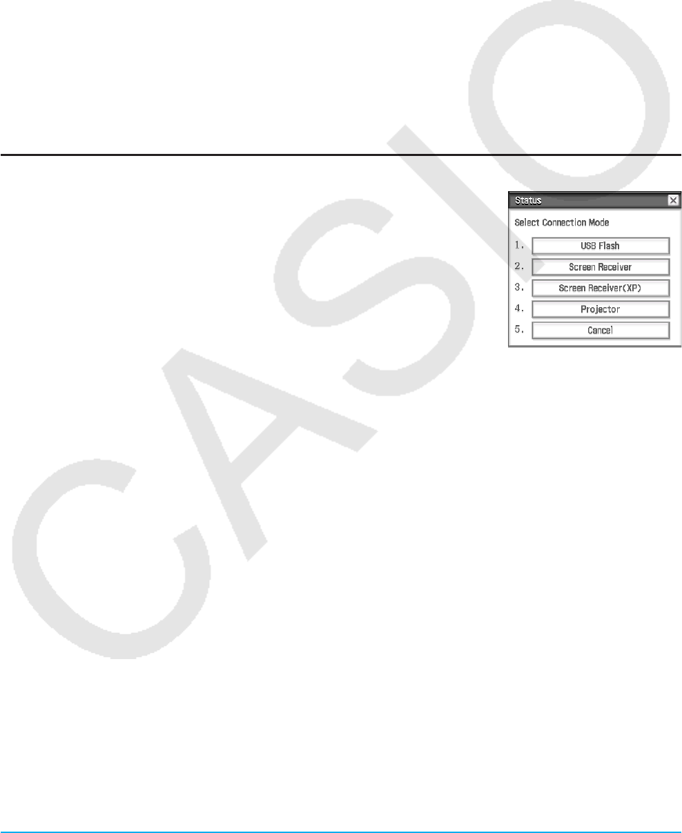
Chapter 19: Performing Data Communication 286
Wakeup
Wakeup is a function that automatically puts the ClassPad into data communication standby whenever the
ClassPad detects data coming in from an external device connected to the 3-pin port of the ClassPad. When
the sending device performs a data send operation, the receiver device’s wakeup function activates and data
receive is performed automatically. The receiver device operates normally as long as no data is being received.
Note that wakeup does not operate on the receiver device when any ongoing calculation or graphing operation
is being performed. Wakeup activates when the ongoing operation is complete.
Communication Application Menus and Buttons
• Select data to send ........................................................................................................Link - Transmit or E
• Enter receive standby .....................................................................................................Link - Receive or R
• Enter standby for operating system upgrading .................................................................... Link - OS Update
• Configure communication parameters ................................................................... Setup - Open Setup Menu
• Display the Exam Mode menu (page 311) ..............................................................................................Exam
• Start up Variable Manager ..........................................................................................................................5
Select Connection Mode Dialog Box
Connecting ClassPad to a computer or projector with the USB cable will cause
the Select Connection Mode dialog box shown nearby to appear. Tap the
button that corresponds to device that ClassPad is connected to.
USB Flash: Mode for connecting ClassPad to a computer for data transfer. See
“Connecting and Disconnecting with a Computer in the USB Flash Mode” (page
287) for details.
Screen Receiver: Mode for using the Screen Receiver software*1 on a
computer running Windows 7, Windows 8.1, Windows 10 or Mac OS, which
displays ClassPad screen contents on the computer screen.
Screen Receiver(XP): Mode for using the Screen Receiver software*1 on a computer running WindowsXP,
which displays ClassPad screen contents on the computer screen.
Projector: Mode for connecting ClassPad to a projector and projecting ClassPad screen contents. See
“Projecting ClassPad Screen Contents from a Projector” (page 294) for details.
Cancel: Closes the Select Connection Mode dialog box without changing the setting.
*1 See the Screen Receiver User’s Guide for details. Do not perform any operation on ClassPad until the
ClassPad screen contents are displayed by Screen Receiver.
Tip
• Instead of tapping on-screen buttons, you can also use the keypad keys 1 through 5 to select a connection mode.
• The Select Connection Mode dialog box will not appear right away if you connect the USB cable while a progress bar is
displayed or while a calculation is in progress. Disconnect the USB cable and wait until the progress bar disappears or the
calculation is complete, and then reconnect.
19-2 Performing Data Communication between the
ClassPad and a Personal Computer
You can perform the following operations when connected to a computer.
Transfer data between the ClassPad and a computer
Variable data and eActivity data, as well as VCP and XCP files (page 289) can be transferred between the
ClassPad and a computer.
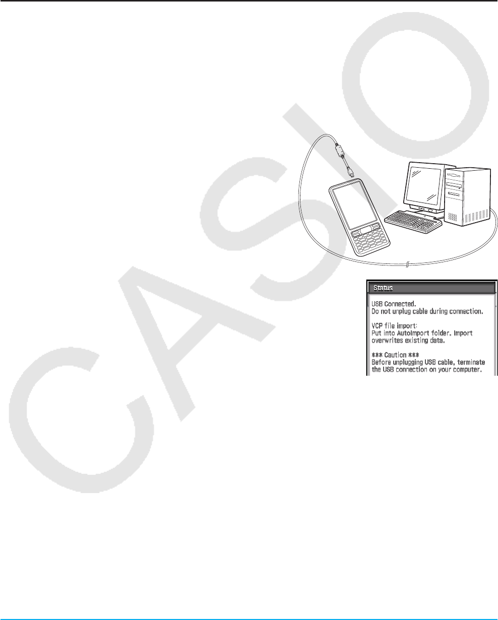
Chapter 19: Performing Data Communication 287
Transfer ClassPad display image data to the computer
For information about connecting ClassPad and Screen Receiver, see the Screen Receiver User’s Guide.
Computer System Requirements
• Windows 7 (32-bit, 64-bit) • Windows 8.1 (32-bit, 64-bit)
• Windows 10 (32-bit, 64-bit)
• Mac OS X 10.7, OS X 10.8, OS X 10.9, OS X 10.10, OS X 10.11, macOS 10.12
Connecting and Disconnecting with a Computer in the USB Flash Mode
Establishing a USB connection between ClassPad and a computer will cause the computer to recognize the
ClassPad’s storage area as a USB Flash Drive.
Important!
Do not touch the USB cable plugs and screen while a data communication operation is in progress. Static
electricity from your fingers can cause data communication to be terminated.
u To establish a connection between ClassPad and a computer
1. Connect one end of the USB cable that comes with the
ClassPad to the USB port of your computer.
2. Connect the other end of the USB cable to the
ClassPad as shown nearby.
• The ClassPad will turn on automatically and the
“Select Connection Mode” screen will appear.
3. Tap [USB Flash].
• Establishing a connection between the ClassPad and a computer will
cause the screen shown nearby to appear.
4. On your computer, open the ClassPad drive.
• The ClassPad drive represents the ClassPad’s storage area.
5. Perform the required operation on your computer to transfer the data.
u To terminate the connection between the ClassPad and a computer
1. Depending on the type of operating system your computer is running, perform one of the following
operations.
Windows: First, check the drive letter (E, F, G, etc.) assigned to the ClassPad drive. Click the “Safely
Remove Hardware” icon in the toolbar in the lower right corner of the display. On the menu that appears,
select the “USB mass storage device” whose letter matches the ClassPad drive letter. Check to make sure
the “Safe To Remove Hardware” message is displayed.
Mac OS: Drag the ClassPad drive icon to the Eject icon (Trash icon). Check to make sure that the ClassPad
drive icon is no longer on your desktop.
2. The message “Complete!” will appear on the ClassPad screen.* To close the message dialog box, tap [OK].
3. Disconnect the USB cable from the ClassPad.
* With some computer operating systems, the “Complete!” message will not appear on the ClassPad screen.
If this happens, disconnect the USB cable from the ClassPad. When a confirmation message appears on the
ClassPad screen, tap [OK].
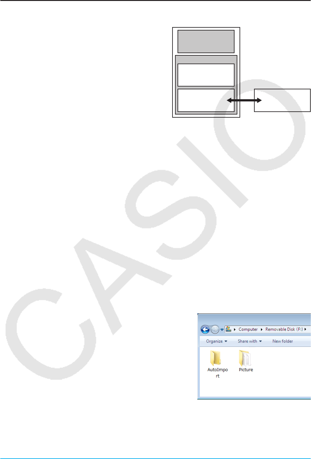
Chapter 19: Performing Data Communication 288
Transferring Data between the ClassPad and a Personal Computer
Establishing a connection between ClassPad and a
computer in USB Flash mode displays folder and files
stored in the ClassPad storage area as folders and files in
the computer’s ClassPad drive.
ClassPad has the following three independent memory
areas for storing data: main memory area, eActivity area,
and storage area. For details about these areas, see
Chapter 18.
ClassPad
Computer
Flash ROM
eActivity Area
Storage Area
(USB Flash Drive)
ClassPad Drive
Main Memory
Important!
Do not use a computer operation to format the ClassPad drive. Doing so will cause a “File System ERROR”
message to appear on the ClassPad screen after you terminate the USB connection between the ClassPad
and computer. When this happens, you will not be able to start up the ClassPad unless you perform an initialize
operation, which deletes all data currently in ClassPad memory.
Note
• When copying files to the ClassPad drive, it may take several minutes before copying starts. This is because
copying automatically performs optimization of the ClassPad’s Flash ROM. It does not indicate malfunction.
• Copying files to the ClassPad drive can cause the connection between the ClassPad and computer to be
dropped. If this happens, enter the System application and execute a Flash ROM optimize operation (page 284),
and then re-establish a connection between the ClassPad and computer.
• A USB connection between the ClassPad and a computer may be terminated automatically if the computer
enters a power save mode, sleep mode, or any other standby state.
uTo transfer data between ClassPad and a computer
1. When transferring data from your ClassPad to a computer, first perform the operations below.
• Export the data from the main memory or eActivity area to the storage area. Exported data is stored as an
XCP file, which is a ClassPad proprietary file format. See “To export variable data to XCP files” (page 290)
and “To export eActivity data to XCP files” (page 291).
• If you want to copy all ClassPad data to a computer, save all of the file data as a VCP file, which is also a
ClassPad Proprietary file format. See “To save a VCP file” (page 290).
2. Establish a connection between the ClassPad and computer,
and then open the ClassPad drive on the computer.
• See “To establish a connection between ClassPad and a
computer” (page 287).
3. Perform copy, delete, and other file operations as required.
• If you have a VCP file or XCP file you want to transfer to
ClassPad, copy it to the ClassPad drive.
4. After you finish all the operations you want to perform, terminate
the USB connection between ClassPad and the computer.
• When you terminate a USB connection, ClassPad
automatically imports a VCP file currently in the AutoImport
folder. For details, see “Auto Import of VCP Files” below.
• For information about how to import a VCP file manually, see “To open a VCP file” (page 290).
• For information about how to import an XCP file manually, see “To import an XCP file” (page 291).

Chapter 19: Performing Data Communication 289
Installing an Add-in Application
Use the procedure below to install an add-in application (c2a file).
1. Perform steps 1 through 4 under “To establish a connection between ClassPad and a computer” (page 287).
2. Copy the add-in application’s dc2a file to the ClassPad root directory.
3. Terminate the USB connection between ClassPad and the computer.
See “To terminate the connection between the ClassPad and a computer” (page 287).
• The icon of the application you just installed should now be visible on the application menu.
Auto Import of VCP Files
When you terminate a USB connection, ClassPad automatically imports a VCP file currently in the AutoImport
folder on the storage area.
• Only one VCP file inside the top level of the AutoImport folder is imported to main memory and the eActivity
area. Existing data is overwritten and new data is added. If there are multiple VCP files in the AutoImport
folder, you need to select the one to be imported manually.
• After auto import is complete, all folders and files in the AutoImport folder are moved to the SAVE-F folder.
Tip: The error message “Insufficient Memory” will appear if main memory or eActivity area memory runs low during the
import operation. If this happens, delete data you no longer need from the main memory or eActivity area and try
importing again.
Rules for ClassPad Files and Folders
• Up to 200 files per folder can be displayed on the storage memory information screen. If a folder has more
than 200 files and you need to display them all, divide them among multiple folders so the total number of files
in a single folder is not greater than 200.
• Though you can create folders on your computer nested to more than three levels in storage memory, the
ClassPad will display only up to the third level.
• The following are characters that can be used in file names and folder names.
A–Z, a–z, 0–9, !, #, $, %, ’, ,(comma), (, ), +, –, ., ;, =, @, [, ], ^, _, `, ~, space
VCP and XCP File Operations
When saving ClassPad eActivity data or variable data for storage on a computer or in the ClassPad storage
area, you need to convert it to a VCP file or XCP file. VCP files and XCP files can be imported later to ClassPad
from a computer or the ClassPad storage area when required.
A save operation saves the following variables and eActivity files.
(1) System variables: Ans, a0, list1, xmin, and other data
(2) User variables: Files saved with Geometry, Spreadsheet, Program, etc.
List files, Mat files, etc.
Image files saved as hard copies
(3) eActivity files
• Saving to a VCP file (***.vcp) saves all of the above files and data currently in ClassPad main memory and
eActivity area.
• Saving (exporting) to an XCP file (***.xcp) saves only the variables or eActivity files for a specific data type
(eActivity, Geometry, Spreadsheet, etc.).
VCP and XCP files can be transferred between ClassPad and a computer when there is a USB Flash
mode connection between them. For details, see “Transferring Data between the ClassPad and a Personal
Computer” (page 288).
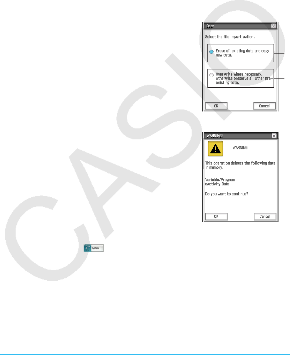
Chapter 19: Performing Data Communication 290
u To save a VCP file
1. On the icon panel, tap m to display the application menu.
2. Tap [MENU] at the top left of the application menu, and then tap [Save As].
3. On the file specification dialog box that appears, enter the file name and then tap [Save].
• On the “Complete!” dialog box that appears, tap [OK].
u To open a VCP file
1. On the icon panel, tap m to display the application menu.
2. Tap [MENU] at the top left of the application menu, and then tap [Open].
• This causes a file specification dialog box to appear. It shows the VCP files in the storage area.
3. Select the VCP file you want to open and then tap [Open].
• This displays the dialog box shown nearby.
4. Select the file import option you want and then tap [OK].
1 Deletes all data in the main memory and eActivity area and import
the file.
2 Overwrites existing data as necessary and imports non-existent data
as new data.
5. Tap [OK].
1
2
uTo create a new VCP file
1. On the icon panel, tap m to display the application menu.
2. Tap [MENU] at the top left of the application menu, and then tap [New].
• This displays the dialog box shown nearby.
3. To reset the ClassPad main memory and eActivity area, tap [OK].
u To export variable data to XCP files
1. On the application menu, tap to start up the System application.
2. On the [Storage] sheet that appears, select “Export Variables” and then tap [Select].
• This displays a dialog box for selecting a folder.
3. Select the folder or variables you want to export.
• The selection operation is the same as that for Variable Manager. For details, see “Using Variable
Manager” (page 29).
• When multiple variables are selected, each variable is exported to a different XCP file.
4. Tap [Export].
• This displays a dialog box for selecting the export destination folder.
5. Select the export destination folder you want and then tap [OK].

Chapter 19: Performing Data Communication 291
u To export eActivity data to XCP files
1. On the application menu, tap to start up the System application.
2. On the [Storage] sheet that appears, select “Export eActivities” and then tap [Select].
• This displays the eActivity data selection dialog box.
3. Select the eActivity you want to export.
4. Tap [Export].
• This displays a dialog box for selecting the export destination folder.
5. Select the export destination folder you want and then tap [OK].
u To import an XCP file
1. On the application menu, tap to start up the System application.
2. On the [Storage] sheet that appears, select “View Storage & Import” and then tap [Select].
• This displays the Storage dialog box. It shows the folders and files in the storage area.
3. Select the XCP files you want to import and then tap [Import].
4. On the dialog box that appears, select the import destination folder you want, and then tap [OK].
19-3 Performing Data Communication between Two
ClassPads
This section explains the operations required for transferring data from one ClassPad to another.
Connecting to Another ClassPad Unit
1. Turn both units off.
2. Connect the data communication cable as shown in the nearby
illustration. Insert both of the plugs securely, as far as they will go.
Transferring Data between Two ClassPads
You can transfer variable data and eActivity data between two ClassPad units. You can use either of the two
following methods to transfer data between two ClassPad units.
• Use the Communication application. The procedure below shows how to use this method.
• Use the “SendVar38k” and “GetVar38k” program commands. See “12-4 Program Command Reference”.

Chapter 19: Performing Data Communication 292
uClassPad Operation
1. Use the procedure under “Connecting to Another ClassPad Unit” above to connect the two units.
2. Use the procedure under “To configure communication parameters” (page 285) to configure the parameters of
the two units as shown below.
• Cable Type: 3pin cable • Speed (3Pin): 115200 bps • Wakeup Enable: On
On the sending ClassPad:
3. On the Communication application window, tap [Link] - [Transmit], or tap E.
• This displays the Select Data dialog box. A list that shows user folders and
the “main” folder appears first.
4. Select the data you want to send.
(1) Tap the [View] menu and then select the data type from the list that
appears.
To list this on the Select Data dialog box: Select this [View] menu command:
User folders and the “main” folder Data Folder List
Library variables Library
System variable groups Application Status
eActivity folders eActivity Folder List
(2) Select the data you want to send.
• On the Select Data dialog box, select the check box next to the data you want to send. You can also tap
the [All] menu and select one of the following commands to select or deselect data.
To do this: Select this [All] menu command:
Select all currently displayed items Select List
Deselect all currently displayed items Deselect List
Select all items in all lists Select All Lists
Deselect all items in all lists Deselect All Lists
• Opening a folder in [Data Folder List] or [eActivity Folder List] displays the variables and data contained
inside it, which can be individually selected for transfer. To select a variable or data contained in a
particular folder, tap its folder name to open it. To return to the folder list from a list of folder contents,
tap I in the lower left corner of the window.
• You can transfer all of the variables or data in a folder by selecting the check box next to the folder
name on the data folder list or eActivity folder list.
5. Tap [OK].
6. In response to the confirmation message that appears, tap [OK] to send the data.
• This sends the data you selected in step 4, and the receiving ClassPad automatically starts receiving the
data.
• The message “Complete!” appears to let you know when the send operation is finished.
7. Tap [OK] to return to the Select Data dialog box.
8. On the Select Data dialog box, tap [Cancel].
• This returns to the Communication application window.
On the receiving ClassPad:
9. The message “Complete!” appears to let you know when the receive operation is finished. Tap [OK].

Chapter 19: Performing Data Communication 293
Tip
• When wakeup is turned off on the receiving device, you need to perform the following operation on the receiving device
before performing step 3:
Start up the Communication application, tap [Link] and then [Receive], or tap R.
This puts the receiving unit into receive standby, which is indicated by the Standby dialog box on the display.
• When you send a variable or data item, it is normally stored in the current folder of the receiving device. A variable or data
item sent from the “library” folder of the sending device, however, is stored in the “library” folder of the receiving device.
Communication Standby
The ClassPad enters “communication standby” when you perform a send or receive operation. While in
communication standby, the ClassPad waits for the other unit to send data, or for it to get ready to receive data.
The following describes how communication standby affects certain ClassPad operations.
• Auto Power Off (page 282) becomes disabled.
• ClassPad power cannot be turned off.
• If data communication does not start within three minutes after the ClassPad enters data communication
standby, the message “Timeout” appears. When this happens, tap [Retry] to try again or [Cancel] to cancel
the data communication operation.
Interrupting an Ongoing Data Communication Operation
Pressing the c key on either the sending device or receiving device during a data communication
operation terminates it.
19-4 Connecting the ClassPad to a Data Logger
You can connect the Data Logger to your ClassPad and control Data Logger operation from your ClassPad.
Connecting a ClassPad to a Data Logger
1. Turn off the ClassPad and Data Logger.
2. Connect one end of the data communication cable (supplied SB-
62 cable) to the port of the Data Logger.
3. Connect the other end of the data communication cable to the
3-pin communication port of the ClassPad.
Ready
Sampling
Error Batt Power
SET UP START/STOP
CASIO EA-200
Tip
• For information about what you should do to transfer data, see the user documentation that comes with the EA-200.
• You can transfer setup information from the ClassPad to the Data Logger, trigger sampling from the ClassPad, and graph
sample results on your ClassPad. You can perform this procedure using the E-CON3 application, which is built into the
ClassPad. For details about the E-CON3 function and its operation, see the E-CON3 Application User’s Guide.

Chapter 19: Performing Data Communication 294
19-5 Connecting the ClassPad to a Projector
You can connect the ClassPad to a CASIO projector and project ClassPad screen contents onto a screen.
For information about connectable projectors, visit the site below.
http://edu.casio.com/support/projector/
Important!
Some projector models may require a firmware update in order to project ClassPad screen contents. Before
doing anything, go to the website above and check if your projector model requires updating.
Projecting ClassPad Screen Contents from a Projector
1. Turn off the ClassPad.
2. Connect one end of the special cable that comes with
the ClassPad to the USB port of your projector.
3. Connect the other end of the special cable as shown
nearby.
• ClassPad will turn on automatically and the Select
Connection Mode screen will appear.
4. Tap [Projector].
5. On the dialog box that appears, tap [OK].
Precautions when Connecting
• An hourglass figure may remain projected on the screen after you connect the ClassPad to a projector. Also,
changing to another screen while a graph is being drawn or while a program is running could possibly result in
the projected screen being different from the ClassPad screen. If this happens, performing some operation on
the ClassPad will restore normal display.
• If the ClassPad stops operating normally, disconnect the USB cable and then reconnect it. If this does not
correct the problem, disconnect the USB cable, turn the projector off and then back on, and then reconnect
the USB cable.
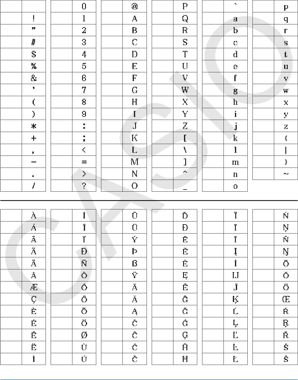
Appendix 295
Appendix
Character Code Table
Characters from character code 257 onwards are 2-byte characters.
32 48 64 80 96 112
33 49 65 81 97 113
34 50 66 82 98 114
35 51 67 83 99 115
36 52 68 84 100 116
37 53 69 85 101 117
38 54 70 86 102 118
39 55 71 87 103 119
40 56 72 88 104 120
41 57 73 89 105 121
42 58 74 90 106 122
43 59 75 91 107 123
44 60 76 92 108 124
45 61 77 93 109 125
46 62 78 94 110 126
47 63 79 95 111
257 270 283 296 309 322
258 271 284 297 310 323
259 272 285 298 311 324
260 273 286 299 312 325
261 274 287 300 313 326
262 275 288 301 314 327
263 276 289 302 315 328
264 277 290 303 316 329
265 278 291 304 317 330
266 279 292 305 318 331
267 280 293 306 319 332
268 281 294 307 320 333
269 282 295 308 321 334
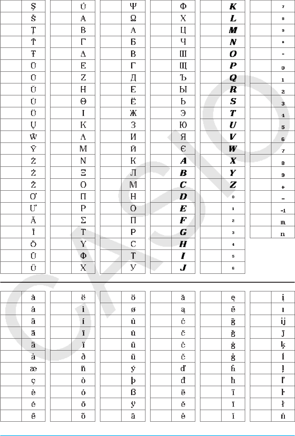
Appendix 296
335 358 381 404 427 487
336 359 382 405 428 488
337 360 383 406 429 489
338 361 384 407 430 490
339 362 385 408 431 491
340 363 386 409 432 496
341 364 387 410 433 497
342 365 388 411 434 498
343 366 389 412 435 499
344 367 390 413 436 500
345 368 391 414 437 501
346 369 392 415 438 502
347 370 393 416 439 503
348 371 394 417 440 504
349 372 395 418 441 505
350 373 396 419 442 506
351 374 397 420 480 507
352 375 398 421 481 508
353 376 399 422 482 509
354 377 400 423 483 510
355 378 401 424 484
356 379 402 425 485
357 380 403 426 486
513 524 535 546 557 568
514 525 536 547 558 569
515 526 537 548 559 570
516 527 538 549 560 571
517 528 539 550 561 572
518 529 540 551 562 573
519 530 541 552 563 574
520 531 542 553 564 575
521 532 543 554 565 576
522 533 544 555 566 577
523 534 545 556 567 578
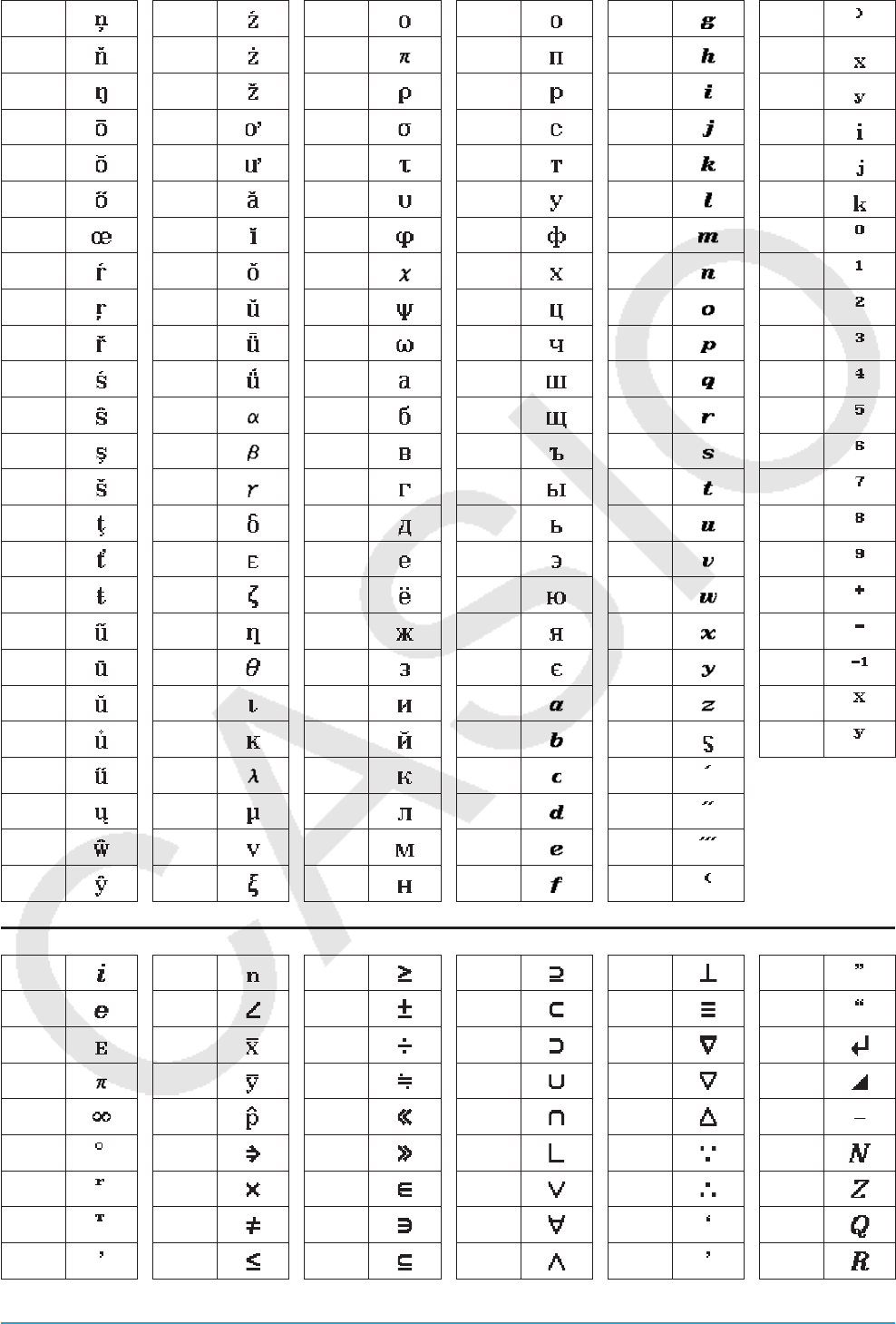
Appendix 297
579 604 629 654 679 741
580 605 630 655 680 742
581 606 631 656 681 743
582 607 632 657 682 744
583 608 633 658 683 745
584 609 634 659 684 746
585 610 635 660 685 752
586 611 636 661 686 753
587 612 637 662 687 754
588 613 638 663 688 755
589 614 639 664 689 756
590 615 640 665 690 757
591 616 641 666 691 758
592 617 642 667 692 759
593 618 643 668 693 760
594 619 644 669 694 761
595 620 645 670 695 762
596 621 646 671 696 763
597 622 647 672 697 764
598 623 648 673 698 765
599 624 649 674 736 766
600 625 650 675 737
601 626 651 676 738
602 627 652 677 739
603 628 653 678 740
769 778 787 796 805 814
770 779 788 797 806 815
771 780 789 798 807 816
772 781 790 799 808 817
773 782 791 800 809 818
774 783 792 801 810 819
775 784 793 802 811 820
776 785 794 803 812 821
777 786 795 804 813 822

Appendix 298
823 844 864 884 904 925
824 845 865 885 905 926
825 846 866 886 906 927
826 847 867 887 907 928
827 848 868 888 908 929
828 849 869 889 909 930
829 850 870 890 910 931
830 851 871 891 911 932
831 852 872 892 912 933
832 853 873 893 913 934
833 854 874 894 914 935
834 855 875 895 915 936
835 856 876 896 916 937
836 857 877 897 917 938
837 858 878 898 918 939
838 859 879 899 919 940
839 860 880 900 920 941
840 861 881 901 921 942
841 862 882 902 923 943
843 863 883 903 924

Appendix 299
System Variable Table
The table below shows an alphabetic listing of system variables.
• If a variable has an initial value, the value is shown inside of braces ({ }) in the “Name” column.
• The letter to the left of the slash in the “Op” column indicates whether or not input for the variable is supported,
while the letter to the right of the slash indicates whether or not the variable can be deleted (Y: Yes, N: No).
Note: Use the Define command to input a value for a Type “F” (FUNC) variable. For an example about how to
do this, see “Define” on page 90.
• The “Type” column indicates the data type of the variable.
Ex: EXPR, St: STR, L: LIST, M: MAT, F: FUNC, _r: Real Number
Name Description Op Type
a0 {0} Sequence variable Y/N Ex_r
a1 {0} Sequence variable Y/N Ex_r
a2 {0} Sequence variable Y/N Ex_r
aCoef Regression coefficient aN/N Ex_r
acSeq Sequence graph trace variable N/N Ex_r
anRecursion expression variable N/N St
an+1 Recursion expression variable Y/Y St
an+2 Recursion expression variable Y/Y St
an0Recursion internal variable N/N Ex_r
an1Recursion internal variable N/N Ex_r
an2Recursion internal variable N/N Ex_r
anESequence expression Y/Y St
anE0Recursion internal variable N/N Ex_r
angleAngle between line of vision and
x-axis of 3D Graph View Window
value
Y/N Ex_r
angleAngle between line of vision and
z-axis of 3D Graph View Window
value
Y/N Ex_r
ans Latest result output by Main or
eActivity application
N/N Ex/L/M/
St
anStart {0} Sequence variable Y/N Ex_r
b0 {0} Sequence variable Y/N Ex_r
b1 {0} Sequence variable Y/N Ex_r
b2 {0} Sequence variable Y/N Ex_r
bCoef Regression coefficient bN/N Ex_r
bcSeq Sequence graph trace variable N/N Ex_r
bnRecursion expression variable N/N St
bn+1 Recursion expression variable Y/Y St
bn+2 Recursion expression variable Y/Y St
bn0Recursion internal variable N/N Ex_r
bn1Recursion internal variable N/N Ex_r
bn2Recursion internal variable N/N Ex_r
bnESequence expression Y/Y St
bnE0Recursion internal variable N/N Ex_r
bnStart {0} Sequence variable Y/N Ex_r
Name Description Op Type
c0 {0} Sequence variable Y/N Ex_r
c1 {0} Sequence variable Y/N Ex_r
c2 {0} Sequence variable Y/N Ex_r
cCoef Regression coefficient cN/N Ex_r
ccSeq Sequence graph trace variable N/N Ex_r
cnRecursion expression variable N/N St
cn+1 Recursion expression variable Y/Y St
cn+2 Recursion expression variable Y/Y St
cn0Recursion internal variable N/N Ex_r
cn1Recursion internal variable N/N Ex_r
cn2Recursion internal variable N/N Ex_r
cnESequence expression Y/Y St
cnE0Recursion internal variable N/N Ex_r
cnStart {0} Sequence variable Y/N Ex_r
ConicsEq Conics expression Y/Y St
dCoef Regression coefficient dN/N Ex_r
df Degrees of freedom N/N Ex_r
dfADegrees of freedom for factor A N/N Ex_r
dfAB Degrees of freedom for factor A
× Factor B
N/N Ex_r
dfBDegrees of freedom for factor B N/N Ex_r
dfErr Degrees of freedom for error N/N Ex_r
eCoef Regression coefficient eN/N Ex_r
Expected Expected matrix for χ2 test N/N M_r
FEnd {5} Table creation variable Y/N Ex_r
FResult Table result variable N/N M
FStart {1} Table creation variable Y/N Ex_r
FStep {1} Table creation variable Y/N Ex_r
Fvalue F value N/N Ex_r
FvalueA F value for factor A N/N Ex_r
FvalueAB F value for factor A × factor B N/N Ex_r
FvalueB F value for factor B N/N Ex_r
GconHEnd
{5}
Graph transformation vertical
end point
N/N Ex_r
GconHStart
{1}
Graph transformation vertical
start point
N/N Ex_r

Appendix 300
Name Description Op Type
GconHStep
{1}
Graph transformation vertical
step value
N/N Ex_r
GconWEnd
{5}
Graph transformation horizontal
end point
N/N Ex_r
GconWStart
{1}
Graph transformation horizontal
start point
N/N Ex_r
GconWStep
{1}
Graph transformation horizontal
step value
N/N Ex_r
HStart {0} Start value for histogram Y/N Ex_r
HStep {1} Step value for histogram Y/N Ex_r
LInterval Lower limit of confidence interval N/N Ex_r
list1 Default list Y/Y L
list2 Default list Y/Y L
list3 Default list Y/Y L
list4 Default list Y/Y L
list5 Default list Y/Y L
list6 Default list Y/Y L
maxX Maximum value of xN/N Ex_r
maxY Maximum value of yN/N Ex_r
MeanSA Mean square for factor A N/N Ex_r
MeanSAB Mean square for factor A × factor
B
N/N Ex_r
MeanSB Mean square for factor B N/N Ex_r
MeanSErr Mean square for error N/N Ex_r
MedStat Median value N/N Ex_r
medx1Medmed graph summary point N/N Ex_r
medx2Medmed graph summary point N/N Ex_r
medx3Medmed graph summary point N/N Ex_r
medy1Medmed graph summary point N/N Ex_r
medy2Medmed graph summary point N/N Ex_r
medy3Medmed graph summary point N/N Ex_r
minX Minimum value of xN/N Ex_r
minY Minimum value of yN/N Ex_r
ModeFStat Frequency of mode values N/N Ex_r
ModeNStat Number of mode values N/N Ex_r
ModeStat Mode value N/N L_r
MSe Mean square error for regression N/N Ex_r
n1Stat Size of sample 1 N/N Ex_r
n2Stat Size of sample 2 N/N Ex_r
ncSeq Sequence graph trace variable N/N Ex_r
nSeq Sequence variable N/N Ex_r
nStat Sample size N/N Ex_r
Observed Observed matrix for χ2 test N/N M _r
ˆp Estimated proportion N/N Ex_r
ˆp1Estimated proportion of sample 1 N/N Ex_r
ˆp2Estimated proportion of sample 2 N/N Ex_r
prob p-value N/N Ex_r
Name Description Op Type
probAp-value of factor A N/N Ex_r
probAB p-value of factor A × factor B N/N Ex_r
probBp-value of factor B N/N Ex_r
py1(x) -
py5(x)
Picture Plot function expression Y/Y F
Q1Stat First quartile point N/N Ex_r
Q3Stat Third quartile point N/N Ex_r
r1() -
r100()
Graph expression input variable,
r= type
Y/Y F
r2Corr Coefficient of determination N/N Ex_r
randResult
{−1}
Internal variable used for next
random-number calculation
N/N Ex_r
rc {0} Graph coordinate value storage
variable
N/N Ex_r
rCorr Correlation coefficient N/N Ex_r
residual Residual data storage list N/N L_r
Seed {0} Random seed value N/N Ex_r
smax3D 3D Graph View Window display
s maximum value
Y/N Ex_r
smin3D 3D Graph View Window display
s minimum value
Y/N Ex_r
spPooled sample standard
deviation
N/N Ex_r
SqEnd {5} Sequence creation variable Y/N Ex_r
SqResult Sequence result variable N/N M
SqStart {1} Sequence creation variable Y/N Ex_r
Sres11 Statgraph1 calculation result N/N L_r
Sres12 Statgraph1 calculation result N/N L_r
Sres21 Statgraph2 calculation result N/N L_r
Sres22 Statgraph2 calculation result N/N L_r
Sres31 Statgraph3 calculation result N/N L_r
Sres32 Statgraph3 calculation result N/N L_r
Sres41 Statgraph4 calculation result N/N L_r
Sres42 Statgraph4 calculation result N/N L_r
Sres51 Statgraph5 calculation result N/N L_r
Sres52 Statgraph5 calculation result N/N L_r
Sres61 Statgraph6 calculation result N/N L_r
Sres62 Statgraph6 calculation result N/N L_r
Sres71 Statgraph7 calculation result N/N L_r
Sres72 Statgraph7 calculation result N/N L_r
Sres81 Statgraph8 calculation result N/N L_r
Sres82 Statgraph8 calculation result N/N L_r
Sres91 Statgraph9 calculation result N/N L_r
Sres92 Statgraph9 calculation result N/N L_r
sStat Standard error value for Linear
Reg t-Test calculation
N/N Ex_r
SumSA Sum of squares for factor A N/N Ex_r

Appendix 301
Name Description Op Type
SumSAB Sum of squares for factor A ×
factor B
N/N Ex_r
SumSB Sum of squares for factor B N/N Ex_r
SumSErr Sum of squares for error N/N Ex_r
sxSample standard deviation of x N/N Ex_r
sx1Sample standard deviation of
data 1
N/N Ex_r
sx2Sample standard deviation of
data 2
N/N Ex_r
sySample standard deviation of y N/N Ex_r
tc {0} Graph coordinate value storage
variable
N/N Ex_r
tLower Result of TCD calculation N/N Ex_r
tmax3D 3D Graph View Window display t
maximum value
Y/N Ex_r
tmin3D 3D Graph View Window display t
minimum value
Y/N Ex_r
tUpper Result of TCD calculation N/N Ex_r
Tvalue t value N/N Ex_r
tmax {2π} View Window t Max value Y/N Ex_r
tmin {0} View Window t Min value Y/N Ex_r
tStep
{π / 60}
View Window t Step value
Variable
Y/N Ex_r
UInterval Upper limit of confidence interval N/N Ex_r
oMean of xN/N Ex_r
o1Mean of data 1 N/N Ex_r
x1(y) -
x100(y)
Graph expression input variable,
x= type
Y/Y F
x1InvN Result of InvNorm calculation N/N Ex_r
o2Mean of data 2 N/N Ex_r
x2InvN Result of InvNorm calculation N/N Ex_r
xc {0} Graph coordinate value storage
variable
N/N Ex_r
xdot {0.1} View Window 1-dot x-axis value Y/N Ex_r
xfact {2} Factor zoom x-factor value Y/N Ex_r
xgrid3D 3D Graph View Window value Y/N Ex_r
xInv Result of inverse cumulative
distribution calculations
N/N Ex_r
xmax {7.7} View Window display range
x-axis maximum value
Y/N Ex_r
xmax3D 3D Graph View Window display
range x-axis maximum value
Y/N Ex_r
xmin {−7.7} View Window display range
x-axis minimum value
Y/N Ex_r
xmin3D 3D Graph View Window display
range x-axis minimum value
Y/N Ex_r
xscl {1} View Window display range
xscale
Y/N Ex_r
Name Description Op Type
xt1(t) -
xt100(t)
Graph expression input variable,
parametric type
Y/Y F
pMean of yN/N Ex_r
y1(x) -
y100(x)
Graph expression input variable,
y= type
Y/Y F
yc {0} Graph coordinate value storage
variable
N/N Ex_r
ydot {0.1} View Window 1-dot y-axis value Y/N Ex_r
yfact {2} Factor zoom y-factor value Y/N Ex_r
ygrid3D 3D Graph View Window value Y/N Ex_r
ymax {3.8} View Window display range
y-axis maximum value
Y/N Ex_r
ymax3D 3D Graph View Window display
range y-axis maximum value
Y/N Ex_r
ymin {−3.8} View Window display range
y-axis minimum value
Y/N Ex_r
ymin3D 3D Graph View Window display
range y-axis minimum value
Y/N Ex_r
yscl {1} View Window display range
yscale
Y/N Ex_r
yt1(t) -
yt100(t)
Graph expression input variable,
parametric type
Y/Y F
z1(x,y) -
z100(x,y)
3D Graph function expression Y/Y F
zc {0} Graph coordinate value storage
variable
N/N Ex_r
zLower Result of NormCD calculation N/N Ex_r
zmax3D 3D Graph View Window display
range z-axis maximum value
Y/N Ex_r
zmin3D 3D Graph View Window display
range z-axis minimum value
Y/N Ex_r
zUpper Result of NormCD calculation N/N Ex_r
Zvalue z value N/N Ex_r
c {0} Graph coordinate value storage
variable
N/N Ex_r
ΣxSum of xN/N Ex_r
σxPopulation standard deviation
of x
N/N Ex_r
Σx2Sum of x2N/N Ex_r
Σxy Sum of xy data N/N Ex_r
ΣySum of yN/N Ex_r
σyPopulation standard deviation
of y
N/N Ex_r
Σy2Sum of y2N/N Ex_r
χ2value χ2 value N/N Ex_r

Appendix 302
Graph Types and Executable Functions
䊊: Executable −: Not executable
Graph Type
Function
y=r=xt=x=y Inequality x Inequality y䉬Conics*1Stat -
Plot*2
Stat -
Reg*3
Stat -
Box*4
Zoom - Box 䊊䊊䊊䊊 䊊 䊊 䊊 䊊 䊊 䊊 䊊
Zoom - In 䊊䊊䊊䊊 䊊 䊊 䊊 䊊 䊊 䊊 䊊
Zoom - Out 䊊䊊䊊䊊 䊊 䊊 䊊 䊊 䊊 䊊 䊊
Zoom - Auto 䊊䊊䊊䊊 䊊 䊊 䊊 䊊 −−−
Zoom - Original 䊊䊊䊊䊊 䊊 䊊 䊊 䊊 䊊 䊊 䊊
Zoom - Square 䊊*5䊊*5䊊*5䊊*5䊊*5䊊*5䊊*5䊊*5䊊*5䊊*5䊊*5
Zoom - Round 䊊*6䊊*6䊊*6䊊*6䊊*6䊊*6䊊*6䊊*6䊊*6䊊*6䊊*6
Zoom - Integer 䊊*6䊊*6䊊*6䊊*6䊊*6䊊*6䊊*6䊊*6䊊*6䊊*6䊊*6
Zoom - Previous 䊊䊊䊊䊊 䊊 䊊 䊊 䊊 䊊 䊊 䊊
Zoom - Initialize / Quick types 䊊*6䊊*6䊊*6䊊*6䊊*6䊊*6䊊*6䊊*6䊊*6䊊*6䊊*6
Analysis - Trace 䊊䊊䊊䊊 䊊 䊊 䊊 䊊 䊊 䊊 䊊
Analysis - Sketch - Cls 䊊䊊䊊䊊 䊊 䊊 䊊 䊊 䊊 䊊 䊊
Analysis - Sketch - Plot 䊊䊊䊊䊊 䊊 䊊 䊊 䊊 䊊 䊊 䊊
Analysis - Sketch - Line 䊊*6䊊*6䊊*6䊊*6䊊*6䊊*6䊊*6䊊*6䊊*6䊊*6䊊*6
Analysis - Sketch - Text 䊊䊊䊊䊊 䊊 䊊 䊊 䊊 䊊 䊊 䊊
Analysis - Sketch - Tangent 䊊䊊䊊䊊 䊊 䊊 䊊 −−
䊊−
Analysis - Sketch - Normal 䊊䊊䊊䊊 䊊 䊊 䊊 −−
䊊−
Analysis - Sketch - Inverse 䊊−−
䊊−−−−−
䊊−
Analysis - Sketch - Circle 䊊*6䊊*6䊊*6䊊*6䊊*6䊊*6䊊*6䊊*6䊊*6䊊*6䊊*6
Analysis - Sketch - Vertical 䊊䊊䊊䊊 䊊 䊊 䊊 䊊 䊊 䊊 䊊
Analysis - Sketch - Horizontal 䊊䊊䊊䊊 䊊 䊊 䊊 䊊 䊊 䊊 䊊
Analysis - G-Solve -
x-Cal/y-Cal - x-Cal 䊊䊊 −− 䊊−−
䊊−−−
Analysis - G-Solve -
x-Cal/y-Cal - y-Cal 䊊䊊䊊 −䊊−−
䊊−−−
Analysis - G-Solve - Root 䊊−−− 䊊− −−−−−
Analysis - G-Solve - Min / Max 䊊−−− 䊊− −−−−−
Analysis - G-Solve - f Min / f Max 䊊−−− 䊊− −−−−−
Analysis - G-Solve - y-Intercept 䊊−−− 䊊−−
䊊−−−
Analysis - G-Solve - Intersection 䊊−−− 䊊− −−−−−
Analysis - G-Solve - Integral - ∫dx
䊊*6−−− − − − − − − −
Analysis - G-Solve - Integral - Root
䊊*6−−− − − − − − − −
Analysis - G-Solve - Integral -
Intersection 䊊*6−−− − − − − − − −
Analysis - G-Solve - Inflection 䊊−−− 䊊− −−−−−
Analysis - G-Solve - Distance 䊊䊊䊊䊊 䊊 䊊 䊊 −−−−
Analysis - G-Solve - π ∫
f (x)2dx 䊊*6−−− − − − − − − −
Analysis - Modify 䊊−−− − − − − − 䊊−
䉬 - Dynamic Graph (Dynamic
Modify) 䊊䊊䊊䊊 䊊 䊊 䊊 −−−−
*1 The special conics graph G-Solve commands below can be used when drawing a conics graph.
Focus, Vertex, Directrix, Symmetry, Latus Rectum Length, Center, Radius, Asymptotes, Eccentricity, x-Intercept
*2 The following statistical graphs: Scatter, Histogram, xyLine, Broken, NPPlot
*3 The following statistical graphs: NDist, LinearR, MedMed, QuadR, CubicR, QuartR, LogR, ExpR, abExpR, PowerR, SinR, LogisticR
*4 The following statistical graphs: MedBox, ModBox
*5 Cannot be executed during semi-log graph drawing (when a graph is drawn while either the x-log or y-log check box only is selected
on the View Window dialog box).
*6 Cannot be executed during semi-log graph or log-log grapy drawing (when a graph is drawn while either the x-log or y-log check box
is selected or when both check boxes are selected on the View Window dialog box).

Appendix 303
Error and Warning Message Tables
Error Message Table
Error Message Description
Access to Flash ROM –
Argument must be a variable name Variable argument specification is wrong. Use a
variable as the argument of the variable.
Main Memory is low on free space. Please delete
unwanted data in Main Memory to ensure saving
new data is possible.
There is not enough memory available to edit a file
you are attempting to open from with the calculator
application you are currently using.
Though file editing is still possible, you may not be
able to save your file edits.
It is recommended that you use Variable Manager to
delete unneeded data before editing a file.
Cannot save changes. Tap MEM to view memory
usage or OK to exit without saving.
There is not enough memory to save an edited file.
Tapping [MEM] on this dialog box will display Variable
Manager, which you can use to delete unneeded
data. Closing Variable Manager after deleting data will
return to the file you are editing so you can save it.
To return to the application menu without saving the
file, tap [OK] on the error message dialog box.
Circular Reference Circular reference exists for a variable.
Compressed programs cannot be edited. The file is compressed. Use the uncompressed
version of the file for editing.
Current Folder You attempted to perform an operation that is
prohibited for the current folder.
Delete or store operation is invalid for program/
function type –
Division by 0 –
Domain An argument value is outside of the specified
Domain range.
Exceeds Maximum Length of Line A line in your program exceeds the allowable length.
Exceeds Maximum Number of Folders Number of user folders exceeded the allowable
maximum during the Open process. User folders are
any folders used for main memory Variables.
Exceeds Maximum Number of Variables The operation you are attempting creates variables
that cause the maximum number of allowable
variables to be exceeded.
Exception Error Occurred –
Export failed. Error generated during export causing abnormal
export end.
File System ERROR A file system error occurred.
Flash ROM!
Initialize Flash ROM immediately at System
application!
–
Folder The folder name you specified for a command
argument does not exist. Or you have input the
name of a folder that cannot be specified (“library”
folder, etc.)
Function has invalid variable name –

Appendix 304
Error Message Description
Function Type The expression type that is selected cannot execute
a function.
History Full The operation you are performing creates a history
entry that causes history contents to exceed the
allowable limit.
Import failed. Error generated during import causing abnormal
import end.
Incorrect Argument –
Incorrect Jump A “Goto” command is used without a corresponding
“Lbl” command.
Incorrect Number of Arguments –
Incorrect Number of Parenthesis –
Incorrect Program Call –
Insufficient Elements –
Insufficient Memory There is not enough memory to complete the
operation you are trying to perform.
Note: Also refer “The calculation result cannot be
displayed….” (page 306).
Insufficient Storage Memory Insufficient available capacity in the storage area.
Invalid Boundary The specified boundary conditions are not
appropriate for the operation being performed.
Invalid Code –
Invalid Data Size You attempted to import a CSV file whose number
of rows and/or columns caused the application’s
allowable memory capacity to be exceeded.
Invalid Data Type • The calculation you are trying to perform has an
invalid data type as an argument.
• You are attempting to import or open an invalid file
type.
Invalid Dimension The two lists or matrices you are trying to perform a
calculation between have different dimensions.
Invalid file or folder name. Folder, file, or path name is too long, so the folder or
file cannot be created in the mass storage area.
Invalid for Local Variable You attempted to perform an operation that is
prohibited for a local variable.
Invalid in a Function or Current Expression You are trying to perform a calculation using an
expression that contains an illegal command (or
function).
Invalid Name You are trying to use an improper folder name,
variable name (including functions and programs), or
label name.
Invalid Outside Function or Program You are trying to execute a command that must
be used inside of a program as a local command,
outside of a program.
Invalid Path You are trying to specify an invalid path. This
error occurs when you include a system folder in
a path, when you include a system variable in a
path, or when you try to specify a path where path
specification is not allowed.

Appendix 305
Error Message Description
Invalid String The command you are trying to execute has an
invalid string specified as an argument.
Invalid Syntax The syntax you are trying to use is not correct.
Invalid Table Input Value You attempted to create a number table with more
than 9999 rows with the Graph & Table application
or Interactive Differential Calculus application.
Invalid Variable Reference The variable you are trying to access does not exist.
This error occurs when you try to read the contents
of a system variable that does not contain any data,
etc.
Invalid View Window Value –
Locked or Protected –
Maximum value needs to be larger than minimum –
Memory is full Memory has become full during a data
communication operation.
Nesting of subroutines exceeds 40 levels –
No file is specified –
No Sequences Selected –
No Sheet Name –
No Solution –
No Stat Graphs Selected –
No Variable –
No word is specified –
Non-Algebraic Variable in Expression You are attempting to use a variable that cannot be
used in a calculation.
Non-Real in Calc The ClassPad is in the Real mode but the value you
are inputting or the result produced by a calculation
is a complex number.
Not a Local Variable The variable you are trying to assign data to is not a
local variable.
Not a Numerical Value Result –
Not an Empty Folder You are trying to delete or perform some other
operation on a folder that is not empty.
Not Appropriate Numerical Value Input –
Not Found –
Not Function Name or Program Name –
Over 30 factors have occurred The number of factors in a summary table has
exceeded 30.
Overflow –
Page Size –
Receiving Failure –
Reserved Name or System Variable –
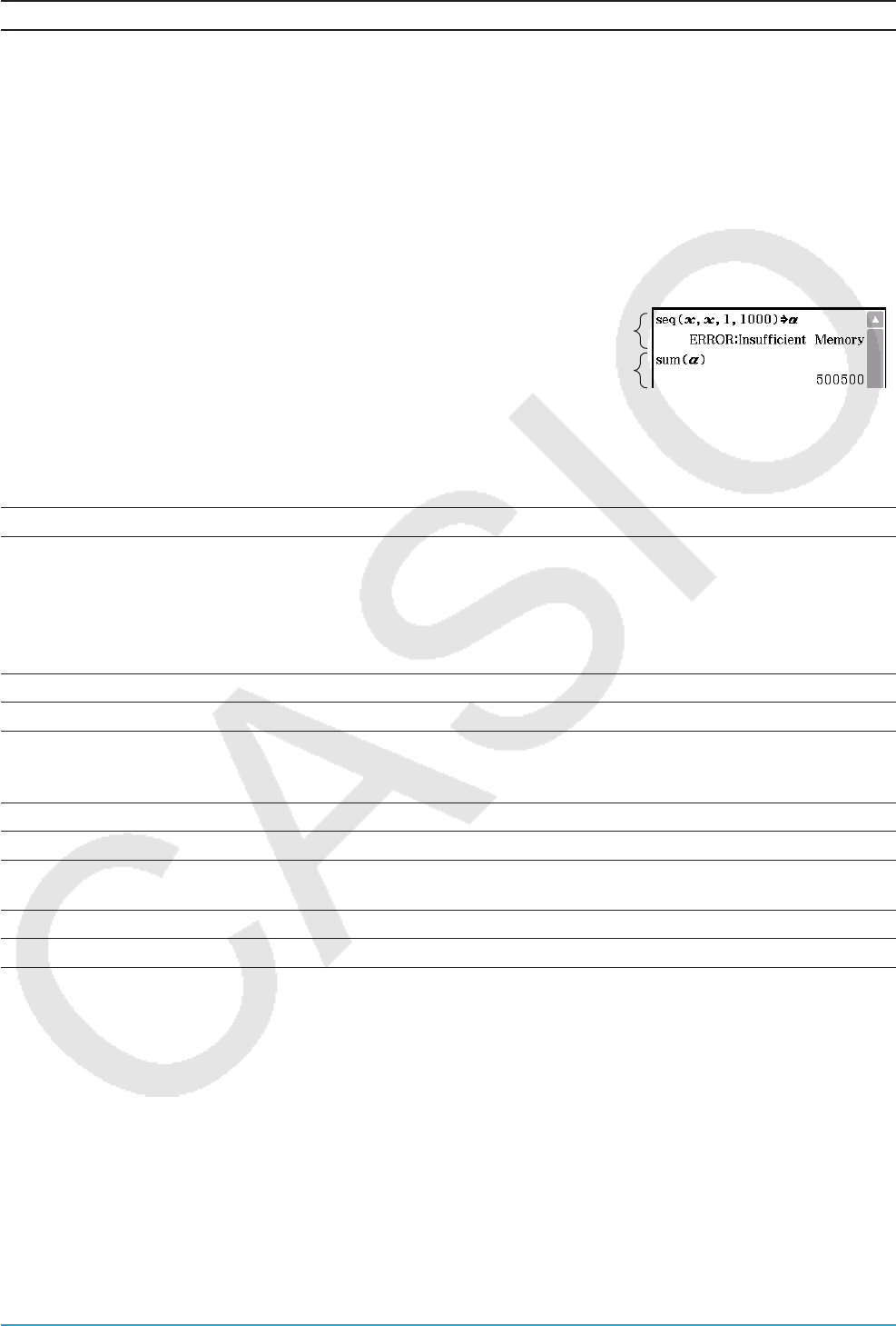
Appendix 306
Error Message Description
The calculation result cannot be displayed.
The result can be assigned to a variable using
Calculation S Variable. For example Seq (x, x, 1,
999)Slist1
The number of horizontal dots for the result of a
calculation that uses the Main or eActivity application
exceeds 32,787 (approximately 2,500 single-byte
characters).
Example: Executing the calculation seq(x, x, 1,
1000), whose calculation result produces a list of
1,000 elements {1, 2, 3 ... 1000}.
Though the calculation result cannot be displayed
when this error occurs, you may be able to use the
S command to assign the result to a variable and
use that variable in a calculation.
Example:
1
2
1 Assigns the calculation result of seq(x, x, 1, 1000)
to variable a (even though the result cannot be
displayed).
2 sum(a) can be used to obtain the total of the list
generated by seq(x, x, 1, 1000).
This function is disabled in Exam Mode. –
Though you can continue this operation, you will not
be able to save data because of insufficient memory.
Delete unnecessary data from memory.
There is not enough memory available to edit a file
you are attempting to open from with the calculator
application you are currently using, or you cannot
save the file after editing it.
Use Variable Manager to delete unneeded data
before editing a file.
Too Long String –
Transmission Failure –
Undefined Result in Condition Judgment A condition judgment program control command has
performed comparison with an undefined variable,
which returns a condition judgment of “Undefined”.
Undefined Variable –
Variable in Use –
View Window settings for log contain a 0 or negative
value. –
View Window value is out of range –
Wrong Argument Type –
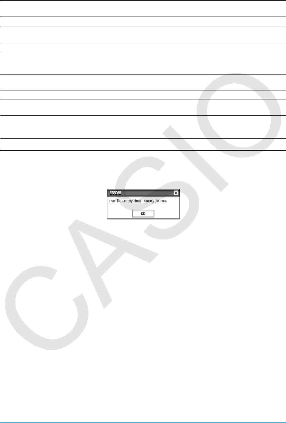
Appendix 307
Warning Message Table
Warning Message Description
Batteries are extremely low!
Replace batteries immediately! –
Can’t Solve! –
Can’t solve!
Adjust initial value or bounds.
Then try again.
NumSolve cannot solve an expression.
Insufficient memory for unit-to-unit communication.
Delete unnecessary eActivity contents. –
Only the first selected function will be done. –
Time out.
The end of condition was not satisfied. –
Too Many eActivity Files The data communication operation you are trying to
perform is not possible because there are too many
eActivity files.
Low Memory Error Processing
An error occurs on the ClassPad if it is unable to reserve enough work area memory to perform a particular
operation. When a low memory error occurs, any application in use at that point is shut down and an error
message like the one shown below appears.
Tapping the [OK] button clears the error.
Important!
• To avoid loss of data, you should make it a regular habit to periodically perform the save operation.
You may lose some of the data you are inputting with an application that shuts down due to a low memory
error. When the low memory error occurs while you are using the eActivity application to create data, for
example, any unsaved data you have input is lost.
Resetting and Initializing the ClassPad
The memory of your ClassPad is divided into four parts: main memory, a storage area for storing data, an
eActivity area, and a RAM area for executing various calculations and operations. Reset and initialize restore
normal ClassPad operation after some problem occurs.
RAM Reset: Perform RAM reset when the ClassPad freezes up or otherwise fails to perform as expected
for some reason. A RAM reset does not affect data stored in main memory, the storage area, or the eActivity
area, but it clears any data stored in the RAM area.
Memory Reset: There are four different types of memory reset operations. Deleting all variable and program
data in main memory, deleting all eActivity data, deleting all data in the storage area, deleting all three of the
above.
Memory Initialize: Memory Initialize deletes all data in ClassPad memory and returns all settings to their
initial factory defaults.
This section explains how to perform the RAM reset operations only. The memory reset and memory initialize
operations are performed using the System application. For details, see “18-2 Configuring System Settings”.

Appendix 308
u To perform the RAM reset operation
Important!
• The RAM reset operation deletes all data that is temporarily stored in ClassPad RAM. Performing the RAM
reset operation while a calculation is in progress will cause any data stored in RAM by the calculation to be
lost.
• Perform the RAM reset operation only when your ClassPad freezes up or when it begins to operate
abnormally for some reason.
1. Use the stylus to press the RESTART button on the back of the ClassPad.
• Following the RAM reset operation, the ClassPad restarts
automatically.
2. After the ClassPad restarts, perform the ClassPad setup operation. For
more information about the setup operation, see “Loading Batteries and
Setting Up the ClassPad” in the separate Quick Start Guide.
• The application menu appears after you finish the setup operation.
Number of Digits and Precision
Number of Digits
Standard Mode
The following applies when the check box next to the
“Decimal Calculation” item on the Basic Format dialog
box is not selected.
• Up to 611 digits are stored in memory for integer
values.
• Decimal values up to 15 digits are converted to
fraction format and saved in memory. When a
mathematical expression cannot be converted to
fraction format, the result is displayed in decimal
format.
• Values stored in memory are displayed as-is,
regardless of how [Number Format] settings
(Normal 1, Normal 2, Fix 0 to Fix 9, Sci 0 to Sci 9)
are configured (except when a decimal value is
displayed).
Decimal Mode
The following applies when the check box next to the
“Decimal Calculation” item on the Basic Format dialog
box is selected.
• Values stored in Ans memory and values assigned
to variables have the same number of digits as
defined for Standard mode values.
• Values are displayed in accordance with how
[Number Format] settings (Normal 1, Normal 2, Fix
0 to Fix 9, Sci 0 to Sci 9) are configured.
• Displayed values are rounded to the appropriate
number of decimal places.
• Some applications store values using a mantissa up
to 15 digits long and a 3-digit exponent.
Precision
• Internal calculations are performed using 15 digits.
• The error for a single mathematical expression (Decimal mode calculation error) is ±1 at the 10th digit. In
the case of exponential display, calculation error is ±1 at the least significant digit. Note that performing
consecutive calculations causes error to be cumulative. Error is also cumulative for internal consecutive
calculations performed for: ^(x
y), x
', x!, nPr, nCr, etc.
• Error is cumulative and tends to be larger in the vicinity of a function’s singular point(s) and inflection point(s),
and the vicinity of zero. With sinh(x) and tanh(x), for example, the inflection point occurs when x = 0. In this
vicinity, error is cumulative and precision is poor.
RESTART
Button

Appendix 309
Display Brightness and Battery Life
Display Brightness
The display brightness of your ClassPad is adjustable. The initial default brightness setting after purchase is
“Medium”. Display brightness will dim automatically if you do not perform any operation for about 30 seconds.
Performing an operation will cause display brightness to return to normal.
For details about how to configure the display brightness setting, see “Chapter 18: System Application”.
Battery Life
Battery life is affected by the display brightness and backlight duration settings. Battery life is also affected by
how the ClassPad is used. Using a program to execute a long series of calculations, for example, will shorten
battery life.
ClassPad Operation Display Brightness Batteries Approximate
Battery Life*1
Repeat of following three-step cycle
each hour.
(1) Application Menu display for 5
minutes
(2) Program application calculation
for 5 minutes
(3) Program application display for
50 minutes
Display brightness settings during
each of the three steps described
to the left.
(1) Initially “Medium”, dimmed after
30 seconds
(2) “Medium”
(3) Same as (1), above.
Alkaline 100 hours
Nickel-metal
hydride
(recommended
type only)
60 hours
*1 New alkaline batteries or fully-charged new nickel-metal hydride batteries, in an ambient temperature of
25°C. Battery life values are approximate and are intended for reference only.
Specifications
Calculation range: ±1 × 10−999 to ±9.999999999 × 10999 and 0.
Internal operations use 15-digit mantissa in the case of calculations that do not use algebraic methods
(calculations with Newton’s Method, for example)
Maximum allowable range for rounding of calculation results: −9.5999 < x < −9.5−308, 1.0−308 < x < 9.5999
Exponential display range: Normal 1: 10−2 > |x|, |x| t 1010, Normal 2: 10−9 > |x|, |x| t 1010
Program capacity: 500 KB (max.)
Storage memory capacity: 5.5 MB (max.) for the eActivity area
24 MB (max.) for the storage area
Power supply: Four AAA-size batteries LR03 (AM4), or four nickel-metal hydride batteries
Power consumption: 1.0 W
Approximate battery life:
Battery life values shown below are based on use of new alkaline batteries or fully-charged new nickel-
metal hydride batteries, in an ambient temperature of 25°C, and depend on the operating conditions ((a),
(b), or (c)).
(a) Continuous display in the Program application, each hour starting with “Medium” display brightness,
dimmed automatically after 30 seconds

Appendix 310
(b) Repeat of 1, 2, 3 sequence below each hour:
1 Application Menu display for 5 minutes
Start of display at “Medium” display brightness, dimmed automatically after 30 seconds
2 Program application calculation for 5 minutes
“Medium” display brightness
3 Program application display for 50 minutes
Display brightness same as 1, above.
(c) Power off
Batteries Condition
(a)
Condition
(b)
Condition
(c)
Four AAA-size alkaline batteries LR03 (AM4) 170 hours 100 hours 1 year
Four nickel-metal hydride batteries
(recommended type only)
100 hours
(Reference)
60 hours
(Reference) –
• The conditions below can greatly reduce battery life.
- Continuous program calculation execution
- Battery manufacturer and type, differences between individual batteries
- Operating conditions (applications used)
- ClassPad settings (display brightness setting, backlight duration setting, etc.)
Auto power off: Power is automatically turned off if no operation is performed for a specified period
(user-settable as approximately 10 minutes or approximately 60 minutes). The initial default setting is
approximately 10 minutes.
Ambient temperature range: 0°C to 40°C (32°F to 104°F)
Dimensions: 21.1 mm (H) × 89 mm (W) × 206 mm (D), 7/8ⴖ (H) × 3 1/2ⴖ (W) × 7 1/2ⴖ (D)
Weight: Approx. 315 g (11.1 oz) (including batteries)
Data communication:
Port: 3-pin data communication port, 4-pin mini USB port
Method: Start-stop (asynchronous), full-duplex
Transmission speed (BPS): 115200, 38400, 9600 bits/second (normal)
38400 bits/second (Send38k/Receive38k)
Parity: None
Bit length: 8 bits
Stop bit: Send38k: 2 bits, Receive38k: 1 bit
Flow control: X ON
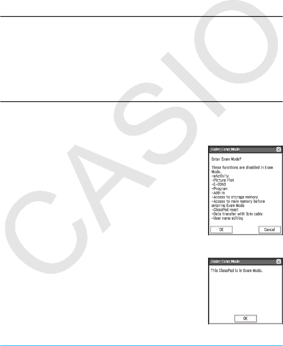
Exam Mode 311
Exam Mode
The Exam Mode puts some limits on ClassPad functions, which allows it to be used when taking an exam or
test. Use the Exam Mode only when actually taking an exam or test.
Entering the Exam Mode affects ClassPad operation as described below.
• The following applications and functions are disabled: eActivity, Picture Plot, E-CON3, Program, data transfer,
add-in applications, storage memory access, user name editing, resetting, OS Update.
• User data (main memory) is backed up. The backed up data will be restored when you exit the Exam Mode.
Any data created during an Exam Mode session will be deleted when the Exam Mode is exited.
Communication Application - Exam Mode Menu
The Communication application displays the Exam Mode menus shown below in the menu bar.
• Enter the Exam Mode .............................................................................................Exam - Enter Exam Mode
• Unlock the Exam Mode ........................................................................................ Exam - Unlock Exam Mode
• Display elapsed time in Exam Mode ............................................................................ Exam - Elapsed Time*
• Display Exam Mode Help ............................................................................................................. Exam - Help
* Entering the Exam Mode displays this menu.
Entering the Exam Mode
There are two ways to enter the Exam Mode.
(1) Using the keypad
1. Press fc to turn off the ClassPad.
2. While holding down the y and Z keys, also hold down the c
key until the dialog box shown nearby appears.
Note
The dialog box may not appear if you release the three keys too soon.
If this happens, perform the above procedure from step 1 again.
3. Tap [OK].
• Read the message on the dialog box that appears.
4. Tap [OK].
• This displays the dialog box shown nearby, indicating that the ClassPad
entered the Exam Mode.
5. Tap [OK].
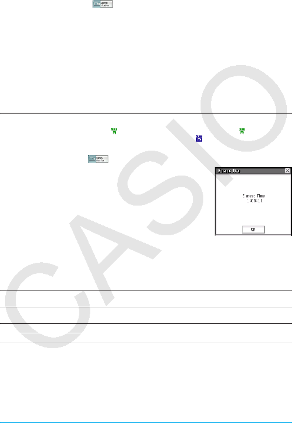
Exam Mode 312
(2) Using the Communication application
1. On the application menu, tap .
2. Tap [Exam] and then [Enter Exam Mode].
3. Perform steps 3 through 5 under “(1) Using the keypad”.
• Only the settings below are saved before entering the Exam Mode.
Basic Format: Number Format, Angle, Complex Format, Decimal Calculation, Assistant, Descending Order,
Variable is Real, Q1, Q3 on Data
Geometry Format: Number Format, Length Unit, Measure Angle, Function Angle
Advanced Format: Transform Definition, FFT Scaling Constant, Assume positive real
System setting: Battery Settings, Language, Imaginary Unit, Keyboard, Touch Panel Alignment
• Entering the Exam Mode causes the [Cable Type] setting of the Communication application to be fixed as
“3pin cable”.
ClassPad Operation in the Exam Mode
• The battery level indicator will change to . The battery level indicator will remain green ( ) for about 15
minutes after you enter the Exam Mode. After that, it will change to blue ( ).
• Use the procedure below to display the elapsed time in the Exam Mode.
1. On the application menu, tap .
2. Tap [Exam] and then [Elapsed Time].
You can restart the elapsed time count by performing one of the operations below.
- Press the RESTART button.
- Remove the calculator’s batteries.
- Re-enter the Exam Mode while already in the Exam Mode.
• The table below shows how certain operations affect the Exam Mode.
If you do this: The ClassPad stays in Exam
Mode.
Data input in Exam Mode is
retained.
Turn power off and then back on
again
Yes Yes
Press the RESTART button Yes No
Remove the ClassPad’s batteries Yes No

Exam Mode 313
Exiting the Exam Mode
There are three ways to exit the Exam Mode.
(1) Exiting the Exam Mode by Connecting to a Computer
1. Use the USB cable to connect the ClassPad that is in the Exam Mode to a computer.
• The ClassPad will turn on automatically and the Select Connection Mode dialog box will appear.
2. Tap [USB Flash].
3. On the computer, open the ClassPad drive.
• The ClassPad drive represents the ClassPad’s storage area.
4. On the computer, copy or delete any file that is on the ClassPad drive.
5. Terminate the connection between the ClassPad and computer.
• The dialog box shown nearby will appear when you exit the Exam
Mode.
(2) Exiting the Exam Mode by Allowing 12 Hours to Elapse
Approximately 12 hours after entering the Exam Mode, turning on the calculator will cause it to exit the
Exam Mode automatically.
Important!
If you press the RESTART button or if you replace batteries before turning on the calculator, it will re-enter
the Exam Mode when turned on, even if 12 hours have elapsed.
(3) Exiting the Exam Mode by Connecting to another ClassPad
1. On the ClassPad that is in the Exam Mode (ClassPad A), enter the Communication application and then
tap [Link] - [Receive].
2. Use the SB-62 cable to connect ClassPad A to another ClassPad that is not in the Exam Mode (ClassPad
B).
SB-62 cable
3. On ClassPad B*, enter the Communication application and then tap [Exam] - [Unlock Exam Mode] - [OK].
• You could also transfer any data from ClassPad B to ClassPad A.
Example: To transfer setup data to ClassPad A
1. On ClassPad B, enter the Communication application.
2. Tap [Setup] - [Open Setup Menu].

Exam Mode 314
3. Tap the [Cable Type] down arrow button, and then select [3pin cable].
4. Tap [Set].
5. Tap [Link] - [Transmit].
6. Tap [View] - [Application Status].
7. Select the check box next to the “Setup”.
8. Tap [OK].
9. In response to the confirmation message that appears, tap [OK].
* ClassPad with Exam Mode function
• Exiting the Exam Mode will cause the battery level indicator to change back to .
Displaying Exam Mode Help
You can display Exam Mode help in the Communication application.
1. On the application menu, tap .
2. Tap [Exam] and then [Help].

Manufacturer:
CASIO COMPUTER CO., LTD.
6-2, Hon-machi 1-chome, Shibuya-ku, Tokyo 151-8543, Japan
Responsible within the European Union:
Casio Europe GmbH
Casio-Platz 1, 22848 Norderstedt, Germany
www.casio-europe.com

CASIO COMPUTER CO., LTD.
6-2, Hon-machi 1-chome
Shibuya-ku, Tokyo 151-8543, Japan
One or more of the following patents may be used in the product.
U.S.Pats. 8,576,230 8,817,027
SA1701-E
© 2013 CASIO COMPUTER CO., LTD.
