Casio Fx 9860GII SD_9860GII_9860G AU PLUS_9750GII_7400GII 9860GII_Soft Soft CN
User Manual: Casio fx-9860GII_Soft fx-7400GII | 计算器 | 说明书 | CASIO
Open the PDF directly: View PDF ![]() .
.
Page Count: 467 [warning: Documents this large are best viewed by clicking the View PDF Link!]
- 目录
- 介绍 — 请首先阅读这一部分!
- 第1章 基本操作
- 第2章 手动计算
- 第3章 列表功能
- 第4章 方程计算
- 第5章 绘图
- 第6章 统计图形与计算
- 第7章 财务计算(TVM)
- 第8章 编程
- 第9章 电子表格
- 第10章 eActivity
- 第11章 存储器管理器
- 第12章 系统管理器
- 第13章 数据通信
- 第14章 使用SD卡和SDHC卡(仅限fx-9860G II SD)
- 附录
- E-CON2 Application (English) (fx-9750GII)
- 1 E-CON2 Overview
- 2 Using the Setup Wizard
- 3 Using Advanced Setup
- 4 Using a Custom Probe
- 5 Using the MULTIMETER Mode
- 6 Using Setup Memory
- 7 Using Program Converter
- 8 Starting a Sampling Operation
- 9 Using Sample Data Memory
- 10 Using the Graph Analysis Tools to Graph Data
- 11 Graph Analysis Tool Graph Screen Operations
- 12 Calling E-CON2 Functions from an eActivity
- E-CON3 Application (English) (fx-9860GII SD, fx-9860GII, fx-9860G AU PLUS)
- 1 E-CON3 Overview
- 2 Using the Setup Wizard
- 3 Using Advanced Setup
- 4 Using a Custom Probe
- 5 Using the MULTIMETER Mode
- 6 Using Setup Memory
- 7 Using Program Converter
- 8 Starting a Sampling Operation
- 9 Using Sample Data Memory
- 10 Using the Graph Analysis Tools to Graph Data
- 11 Graph Analysis Tool Graph Screen Operations
- 12 Calling E-CON3 Functions from an eActivity


i
• 本用户说明书的内容如有更改,恕不另行通知。
• 未经制造商明确的书面许可,不得以任何形式复制本用户说明书的任何内容。
• 请务必将所有用户文件妥善保管以便日后需要时查阅。

ii
目录
介绍 — 请首先阅读这一部分!
第1章 基本操作
1. 键 ..............................................................................................................................................................................................................1-1
2. 显示 ........................................................................................................................................................................................................ 1-2
3. 输入和编辑计算式 ......................................................................................................................................................................1-5
4. 使用数学输入/输出模式 .....................................................................................................................................................1-10
5. 选项(OPTN)菜单 ..............................................................................................................................................................1-22
6. 变量数据(VARS)菜单 ...................................................................................................................................................1-23
7. 程序(PRGM)菜单 .............................................................................................................................................................1-25
8. 使用设置屏幕 ..............................................................................................................................................................................1-26
9. 使用屏幕捕捉 ..............................................................................................................................................................................1-29
10. 如果问题仍然存在 ...... .............................................................................................................................................................1-30
第2章 手动计算
1. 基本计算 ............................................................................................................................................................................................ 2-1
2. 特殊功能 ............................................................................................................................................................................................ 2-6
3. 指定角度单位和显示格式 .................................................................................................................................................2-10
4. 函数计算 .........................................................................................................................................................................................2-12
5. 数值计算 .........................................................................................................................................................................................2-21
6. 复数计算 .........................................................................................................................................................................................2-30
7. 二进制、八进制、十进制和十六进制整数计算 ..............................................................................................2-33
8. 矩阵计算 .........................................................................................................................................................................................2-36
9. 向量计算 .........................................................................................................................................................................................2-49
10. 度量转换计算 ..............................................................................................................................................................................2-54
第3章 列表功能
1. 输入和编辑列表 ........................................................................................................................................................................... 3-1
2. 操控列表数据 .................................................................................................................................................................................3-5
3. 使用列表进行算术计算 .......................................................................................................................................................3-10
4. 在列表文件之间切换 .............................................................................................................................................................3-13
第4章 方程计算
1. 线性方程组 ....................................................................................................................................................................................... 4-1
2. 2至6次的高阶方程 ..................................................................................................................................................................... 4-2
3. 求解计算 ............................................................................................................................................................................................ 4-4
第5章 绘图
1. 图形样例 ............................................................................................................................................................................................ 5-1
2. 控制图形屏幕上的显示内容 ............................................................................................................................................... 5-3
3. 绘制图形 ............................................................................................................................................................................................ 5-6
4. 在图片存储区中存储图形 .................................................................................................................................................5-10
5. 在同一个屏幕上绘制两个图形 ......................................................................................................................................5-11
6. 手动绘图 .........................................................................................................................................................................................5-12
7. 使用表格 .........................................................................................................................................................................................5-15
8. 动态绘图 .........................................................................................................................................................................................5-20
9. 绘制递推公式图形 ...................................................................................................................................................................5-22
10. 绘制二次曲线图形 ...................................................................................................................................................................5-27
11. 更改图形的外观 ........................................................................................................................................................................5-27
12. 函数分析 .........................................................................................................................................................................................5-29

iii
第6章 统计图形与计算
1. 在进行统计计算之前 ................................................................................................................................................................ 6-1
2. 计算与绘制单变量统计数据 ............................................................................................................................................... 6-4
3. 计算与绘制双变量统计数据 ............................................................................................................................................6-10
4. 执行统计计算 ..............................................................................................................................................................................6-16
5. 测试 .....................................................................................................................................................................................................6-23
6. 置信区间 .........................................................................................................................................................................................6-37
7. 分布 .....................................................................................................................................................................................................6-40
8. 测试、置信区间和分布的输入和输出项 ...............................................................................................................6-52
9. 统计公式 .........................................................................................................................................................................................6-55
第7章 财务计算(TVM)
1. 在进行财务计算之前 ................................................................................................................................................................ 7-1
2. 单利 ........................................................................................................................................................................................................ 7-2
3. 复利 ........................................................................................................................................................................................................ 7-3
4. 现金流(投资评估) .................................................................................................................................................................. 7-5
5. 分期偿还 ............................................................................................................................................................................................ 7-7
6. 利率换算 ............................................................................................................................................................................................ 7-9
7. 成本、售价、毛利率 .............................................................................................................................................................7-10
8. 日/日期计算 .................................................................................................................................................................................7-11
9. 折旧 .....................................................................................................................................................................................................7-12
10. 债券计算 .........................................................................................................................................................................................7-14
11. 使用函数进行财务计算 .......................................................................................................................................................7-16
第8章 编程
1. 基本编程步骤 .................................................................................................................................................................................8-1
2. PRGM 模式功能键 ....................................................................................................................................................................... 8-2
3. 编辑程序内容 .................................................................................................................................................................................8-3
4. 文件管理 ............................................................................................................................................................................................ 8-5
5. 命令参考 ............................................................................................................................................................................................ 8-7
6. 在程序中使用计算器功能 .................................................................................................................................................8-21
7. PRGM 模式命令列表 ..............................................................................................................................................................8-37
8. 程序库 ...............................................................................................................................................................................................8-42
第9章 电子表格
1. 电子表格基础知识和功能菜单 .........................................................................................................................................9-1
2. 基本电子表格操作 ......................................................................................................................................................................9-2
3. 使用特殊S • SHT模式命令 ..................................................................................................................................................9-13
4. 绘制统计图形以及执行统计和回归计算 ...............................................................................................................9-15
5. S • SHT模式存储器 ...................................................................................................................................................................9-19
第10章 eActivity
1. eActivity概述 ..............................................................................................................................................................................10-1
2. eActivity功能菜单 ..................................................................................................................................................................10-2
3. eActivity文件操作 ..................................................................................................................................................................10-3
4. 输入和编辑数据 ........................................................................................................................................................................10-4
第11章 存储器管理器
1. 使用存储器管理器 ...................................................................................................................................................................11-1

iv
第12章 系统管理器
1. 使用系统管理器 ........................................................................................................................................................................12-1
2. 系统设置 .........................................................................................................................................................................................12-1
第13章 数据通信
1. 连接两台计算器 ........................................................................................................................................................................13-1
2. 将计算器连接到个人计算机 ............................................................................................................................................13-1
3. 执行数据通信操作 ...................................................................................................................................................................13-2
4. 数据通信注意事项 ...................................................................................................................................................................13-5
5. 屏幕图像发送 ...........................................................................................................................................................................13-11
第14章 使用SD卡和SDHC卡 (仅限fx-9860GII SD)
1. 使用SD卡 ........................................................................................................................................................................................14-1
2. 格式化SD卡 ..................................................................................................................................................................................14-3
3. SD卡使用注意事项 .................................................................................................................................................................14-3
附录
1. 错误消息表 .......................................................................................................................................................................................α-1
2. 输入范围 ............................................................................................................................................................................................α-4
E-CON2 Application (English)
(fx-9750GII)
1 E-CON2 Overview
2 Using the Setup Wizard
3 Using Advanced Setup
4 Using a Custom Probe
5 Using the MULTIMETER Mode
6 Using Setup Memory
7 Using Program Converter
8 Starting a Sampling Operation
9 Using Sample Data Memory
10 Using the Graph Analysis Tools to Graph Data
11 Graph Analysis Tool Graph Screen Operations
12 Calling E-CON2 Functions from an eActivity
E-CON3 Application (English)
(fx-9860GII SD, fx-9860GII, fx-9860G AU PLUS)
1 E-CON3 Overview
2 Using the Setup Wizard
3 Using Advanced Setup
4 Using a Custom Probe
5 Using the MULTIMETER Mode
6 Using Setup Memory
7 Using Program Converter
8 Starting a Sampling Operation
9 Using Sample Data Memory
10 Using the Graph Analysis Tools to Graph Data
11 Graph Analysis Tool Graph Screen Operations
12 Calling E-CON3 Functions from an eActivity

v
介绍 — 请首先阅读这一部分!
k 关于本用户说明书
u 各型号的特定功能和屏幕差异
本用户说明书包含多个不同型号的计算器。请注意,本用户说明书所述各型号不一定提供本文
所述的某些功能。本用户说明书中的所有截屏图像均来自fx-9860G II SD屏幕,其它型号的屏
幕外观可能稍有不同。
u 数学自然输入和显示
如果采用初始默认设置,fx-9860G II SD、fx-9860G II 或fx-9860G AU PLUS设置采用“数学
输入/输出模式”,该模式启用数学表达式的自然输入和显示方式。这意味着您可以按对应的书
写方式输入分数、平方根、微分和其他表达式。在“数学输入/输出模式”中,大多数计算结果
也使用自然显示方式显示。
您也可按照自己的意愿选择“线性输入/输出模式”,在一行中输入和显示计算表达式。fx-
9860G II SD、fx-9860G II 和fx-9860G AU PLUS输入/输出模式的初始默认设置为数学输入/
输出模式。
本用户说明书提供的示例主要使用线性输入/输出模式。如果您正在使用fx-9860G II SD、
fx-9860G II 或者fx-9860G AU PLUS,请注意以下几点。
• 关于在数学输入/输出模式与线性输入/输出模式之间的切换说明,请参见“使用设置屏幕”
(第1-26页)中的“Input/Output”模式设置。
• 关于使用数学输入/输出模式输入和显示的说明,请参见“使用数学输入/输出模式”(第
1-10页)。
u 如果您的计算器型号没有数学输入/输出模式(fx-7400G II 、fx-9750G II )
fx-7400G II 和fx-9750G II 没有数学输入/输出模式。在这些型号上执行本手册所述计算时,使
用线性输入模式。fx-7400G
II和fx-9750G II用户应忽略本手册关于数学输入/输出模式的所有
说明。
u !x( ')
上述字符串表示您应依次按下 !和 x,操作将输入一个 '符号。所有多键输入操作都采用
这种表达方式。首先显示的是键帽标记,然后是在圆括号中的输入字符或者命令。
u m EQUA
这表示您应首先按下 m,使用光标键( f、 c、 d、 e)选择 EQUA 模式,然后按
下 w。本文采用这种方式表达从主菜单进入某个模式时需要执行的操作。
u 功能键与菜单
• 按下功能键 1至 6,即可执行此计算器执行的许多操作。为每一个功能键指定的操作因计
算器所处模式而异,显示屏底部显示的功能菜单指示当前操作指定情况。
• 本用户说明书在功能键键帽标记之后的圆括号中显示对该功能键的指定的当前操
作。 1(Comp)示例表示按下 1即选择{Comp},功能菜单中也显示该项目。
• 如果功能菜单中显示的( g)对应于键 6,表示按下 6可显示菜单选项的下一页或者上一
页。
0
vi
u 菜单标题
• 本用户说明书中的菜单标题包括用于显示说明菜单所需的键操作。依次按下 K和{LIST}后,
菜单的键操作会显示为: [OPTN] - [LIST] 。
• 在菜单标题键操作中,不会显示换至另一个菜单页面的 6( g)键操作。
u 命令列表
PRGM 模式命令列表(第8-37页)提供各种功能键菜单的图形流程表,解释如何转换至您需要
的命令菜单。
示例:下述操作显示Xfct: [VARS] - [FACT] - [Xfct]
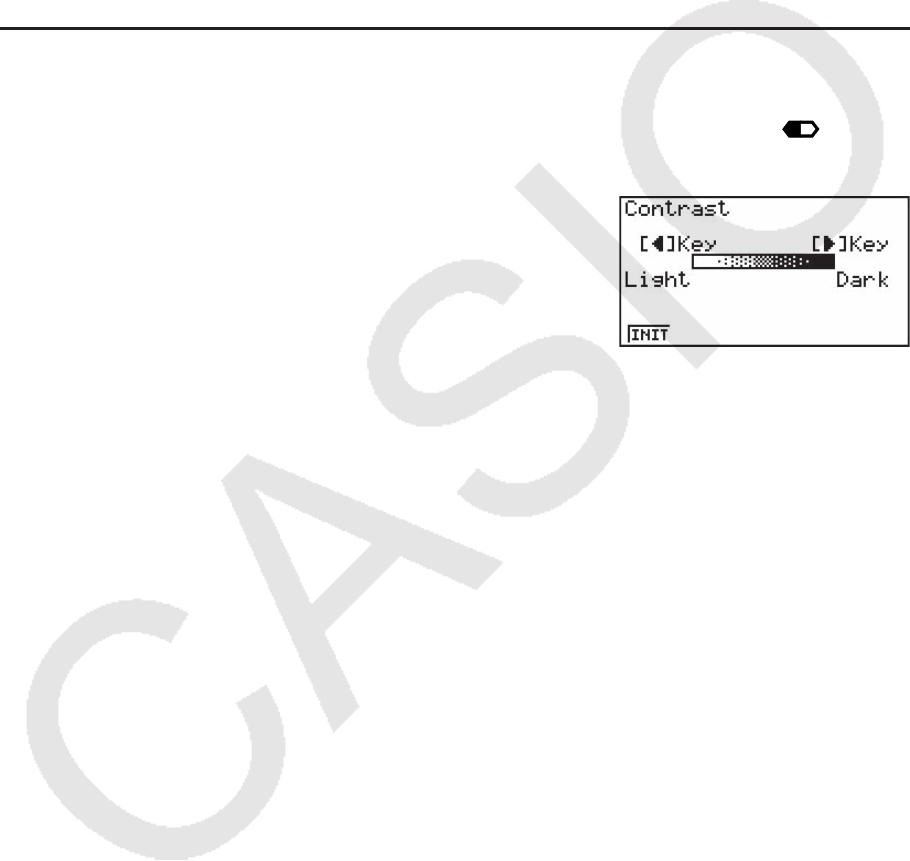
k 对比度调节
一旦显示屏上的目标变暗或难以看清,即可调节对比度。
1. 使用光标键( f、 c、 d、 e)选择 SYSTEM 图标然后依次按下 w和 1( )以显示
对比度调节屏幕。
2. 调节对比度。
• e光标键可使显示对比度变暗。
• d光标键可使显示对比度变亮。
• 1(INIT) 将显示对比度恢复到初始默认设置。
3. 如需退出显示对比度调节,按下 m。
vii
k 考试模式(仅限fx-9860GII SD/fx-9860GII/fx-9860G AU PLUS)
考试模式限制计算器的某些功能,使得能够用于考试或测验。仅在实际参加考试或测验时才使
用考试模式。
进入考试模式将影响计算器的下述操作。
• 以下模式和功能被禁用:e • ACT 模式、MEMORY 模式、E-CON3 模式、PRGM 模式、向量
命令、程序命令 (^ (输出命令)、: (多语句命令)、 _ (回车))、数据传输、插件应用程序、插
件语言、用户名编辑。
• 将用户数据(主存储器)备份。当您退出考试模式时,将恢复备份的数据。当退出考试模式
时,将删除考试模式会话期间所创建的所有数据。
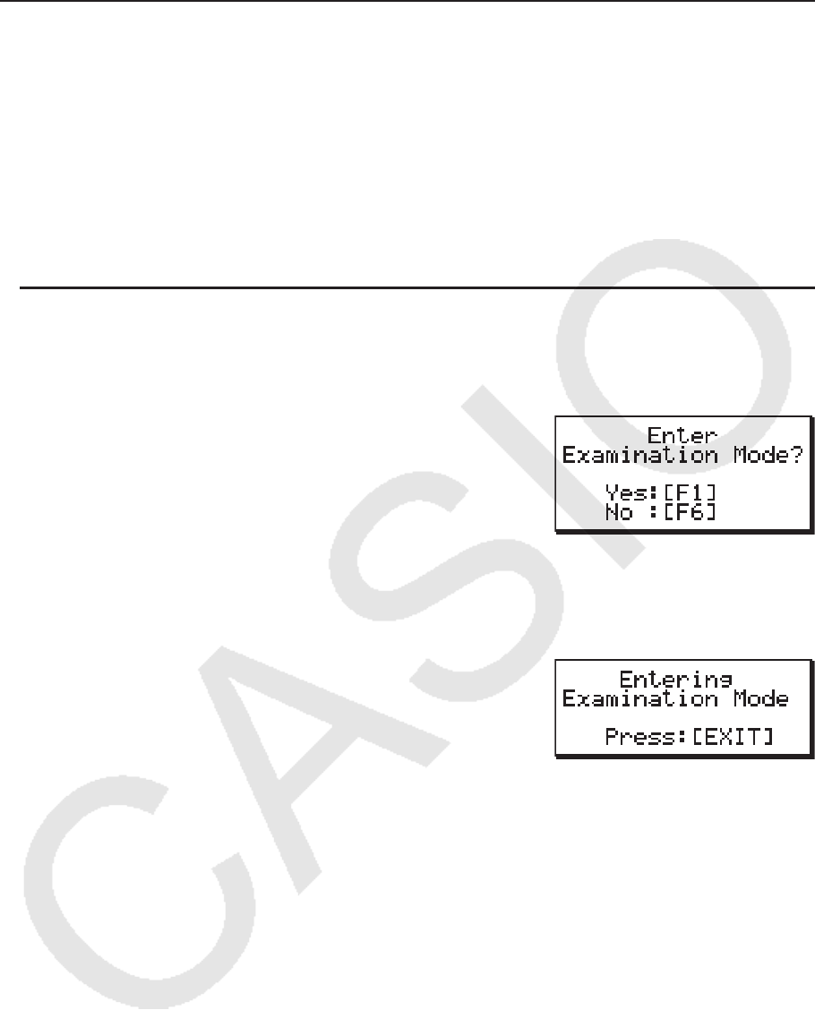
u 进入考试模式
1. 按下 !o(OFF) 关闭计算器。
2. 按住 c 和 h 键的同时,按下 o 键。
• 将显示如下对话框。
3. 按下 1(Yes)。
• 阅读对话框中出现的消息。
4. 按下 2。
• 将显示如下对话框。
5. 按下 J。
• 进入考试模式之前,仅保存下述设置。
Input/Output、Frac Result、Angle、Complex Mode、Display、Q1Q3 Type、Language
viii
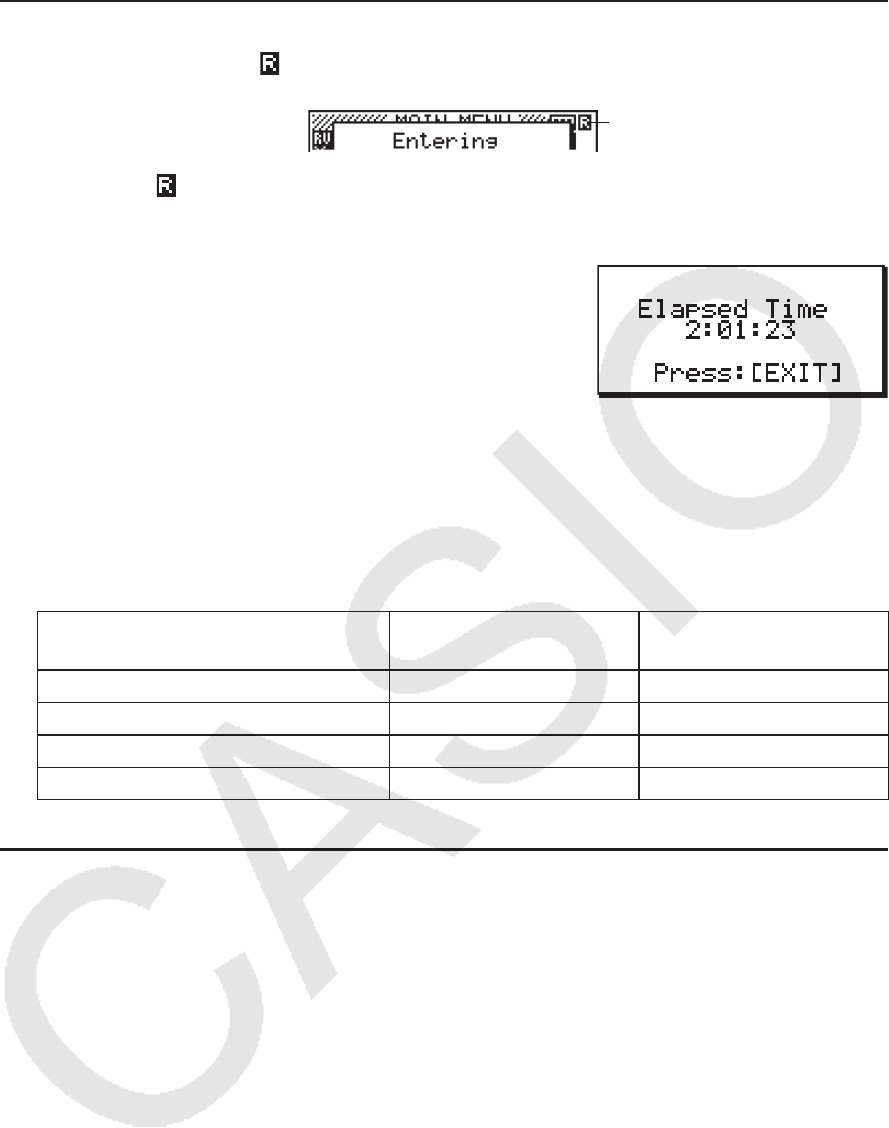
u 考试模式下计算器的操作
• 进入考试模式后,图标 ( ) 将在显示屏上闪烁。进入考试模式后约15分钟,图标的闪烁速度
会减慢。
图标
• 反显的图标 ( ) 表示正在进行计算操作。
• 在考试模式下,自动关机触发设置固定在约60分钟。
• 按下 a- 出现如下显示的对话框。对话框显示处于考试模式的经过时间。
您可以执行以下一种操作重新启动持续时间计数。
- 按下RESTART按钮。
- 取出计算器的电池。
- 删除主存储器数据。
- 已经处于考试模式时,再次进入考试模式。
• 下表显示了某些操作如何影响考试模式。
如果这样操作: 计算器保持在考试模式。 保留考试模式下所输入的
数据。
关闭电源,然后再次打开 是 是
按下RESTART按钮 是 否
取出计算器的电池 是 否
删除主存储器数据 是 否
u 退出考试模式
可以采取三种方式退出考试模式。
(1) 通过连接到计算机退出考试模式
1. 使用USB电缆将处于考试模式的计算器连接到计算机。
2. 当计算器上出现“Select Connection Mode”对话框时,按下计算器的 1 键。
3. 在计算机上启动FA-124软件。

ix
4. 在计算机上点击工具栏 按钮。
• 退出考试模式时,将出现如下显示的对话框。
• 此时,FA-124软件将显示错误消息,但将其忽略。
(2) 通过经过12小时后,退出考试模式
进入考试模式后大约12小时,打开计算器将使其自动退出考试模式。
重要!
即使已经经过了12个小时,在打开计算器之前,如果您按下RESTART按钮或如果您更换了
电池,当打开计算器时,计算器将重新进入考试模式。
(3) 通过连接到另一个计算器退出考试模式
1.
将处于考试模式的计算器(计算器A) 进入 LINK 模式, 然后按下 4(CABL)2(3PIN)。
2. 使用SB-62电缆将计算器A连接到未处于考试模式的另一个计算器(计算器B)上。
3. 在计算器A上, 按下 2(RECV)。
4. 将计算器B*进入 LINK 模式,然后按下 3(EXAM)1(UNLK)1(Yes)。
• 您也可以将任何数据从计算器B传输到计算器A。
示例: 将设置数据传输到计算器A
1. 将计算器B进入 LINK 模式,然后按下 1(TRAN)1(MAIN)1(SEL)。
2. 使用 c 和 f 选择“SETUP”。
3. 按下 1(SEL)6(TRAN)1(Yes)。
* 带有考试模式功能的计算器
• 计算器退出考试模式时, 图标将从显示屏上消失。
u 显示考试模式帮助信息
在 LINK 模式下,可显示考试模式帮助信息。
3(EXAM)2(ENTR) ... 显示有关进入考试模式的帮助信息。
3(EXAM)3(APP) ... 显示有关考试模式所禁用的模式和功能的帮助信息。
3(EXAM)4(EXIT) ... 显示有关退出考试模式的帮助信息。
1-1
第1章 基本操作
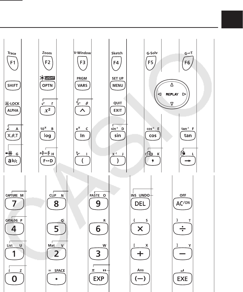
1. 键
k 键表格
本手册所述各型号不一定提供上述所有功能。您的计算器可能没有上述某些键。
页页 页页页页
页页页页页
2-1
5-29 5-5 5-3
2-15 1-18,
2-14
1-2
2-7
2-15 2-14
5-28 5-30 5-1
5-24
1-25 1-26
1-2 1-22 1-23 1-2
2-14
2-14
2-14 2-14
2-1
1-12
1-18
2-19 2-1 2-6
2-30
1-11
1-18
2-19
2-19
1-16
1-6
2-1
2-1
2-9
2-1
1-6,1-14
2-1
1-9
2-14
2-7
1-8
2-41
1-29
1-9
3-2
2-30
10-10 10-9
1
1-2
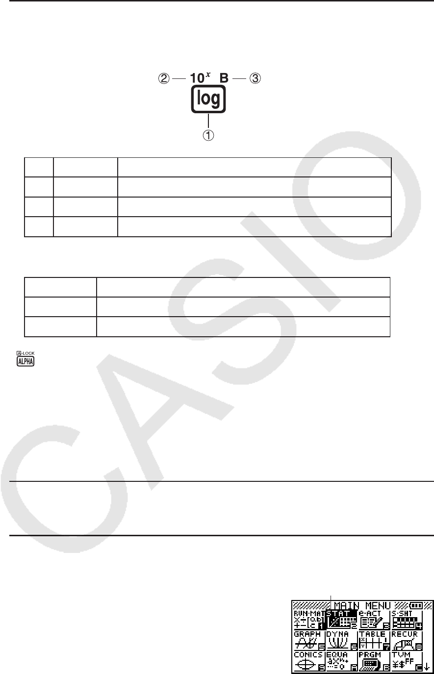
k 键标记
计算器的许多键用于执行多种功能。键盘上标记的功能采用彩色编码,帮助您便捷地找到您需
要的功能。
功能 键操作
1 log l
2 10
x !l
3 B al
键标记所使用的颜色代码如下所述。
颜色 键操作
黄色 按下 !,然后按下此键,可执行标记功能。
红色 按下 a,然后按下此键,可执行标记功能。
• 字母锁定
通常,一旦您按下 a,然后再按下一个键,即可输入字母字符,键盘会立即恢复至基本功
能。
如果您按下 !,然后再按下 a,则键盘会锁定于字母输入,直至您再次按下 a。
2. 显示
k 选择图标
本节说明如何选择“主菜单”内的图标,进入您想要的模式。
u 选择图标
1. 按下 m,显示“主菜单”。
2. 使用光标键( d、 e、 f、 c),
突出显示您想要的图标。
当前选定图标
1-3
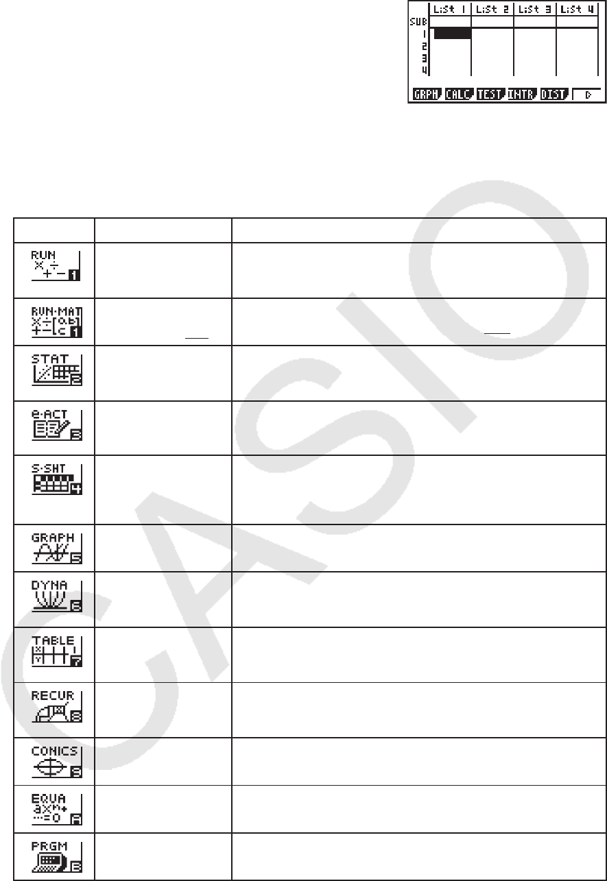
3. 按下 w,显示您所选取的图标模式的初始化屏幕。
在本例中,我们将进入 STAT 模式。
• 输入图标右下角标记的数字或者字母,无需突出显示“主菜单”内的图标,您也可进入模式。
• 仅限于使用上述程序进入某一模式。如果您使用其他任何程序,您最后进入的模式可能与您预
期选取模式不同。
每一个图标的含义解释如下。
图标 模式名称 描述
RUN
(仅限fx-7400G II )
使用此模式进行算术运算与函数运算,以及进行有关二进
制、八进制、十进制与十六进制数值的计算。
RUN • MAT*
1
(运行 • 矩阵 • 向量*
2
)
使用此模式进行算术运算、函数运算、以及二进制、八进
制、十进制与十六进制计算,矩阵计算和向量*
2
计算。
STAT
(统计)
使用此模式进行单变量(标准差)与双变量(回归)统计计
算、测试、分析数据并绘制统计图形。
e • ACT*
2
(eActivity)
eActivity可帮助您在类似于笔记本的界面中输入文本、数学
表达式和其他数据。当您需要将文本、公式、内置应用数据
存入文件时可使用此模式。
S • SHT*
2
(电子表格)
使用此模式进行电子表格计算。每个文件都包含一个26列
999行的电子表格。除了计算器的内置命令和 S • SHT 模式命
令之外,您还可使用与 STAT 模式中相同的程序进行统计计算
和绘制统计数据图形。
GRAPH 使用此模式存储图形函数并利用这些函数绘制图形。
DYNA*
1
(动态图形)
使用此模式存储图形函数并通过改变代入函数中变量的数值
绘制一个图形的多种形式。
TABLE 使用此模式存储函数,生成具有不同解(随着代入函数变量
的值改变而改变)的数值表格,并绘制图形。
RECUR*
1
(递归)
使用此模式存储递推公式,生成具有不同解(随着代入函数
变量的值改变而改变)的数值表格,并绘制图形。
CONICS*
1 使用此模式,可绘制圆锥曲线图形。
EQUA
(方程)
使用此模式,可求解带有2至6个未知数的线性方程以及2至
6次的高阶方程。
PRGM
(程序)
使用此模式,可将程序存储在程序区并运行程序。
1-4
图标 模式名称 描述
TVM*
1
(财务)
使用此模式,可进行财务计算并绘制现金流量与其它类型的
图形。
E-CON2*
3 使用此模式,可控制选配的EA-200数据分析仪。
E-CON3*2使用此模式,可控制选配的数据记录器。
LINK 使用此模式,可将存储内容或者备份数据传输至另一台设备
或PC机。
MEMORY 使用此模式,可管理存储在存储器中的数据。
SYSTEM 使用此模式可初始化存储器、调节对比度和进行其他系统设
置。
*
1
fx-7400G II 中不包括。
*
2
fx-7400G II /fx-9750G II 中不包括。
*3 仅限fx-9750G II
k 关于“功能菜单”
使用功能键( 1至 6)即可访问显示屏底部菜单栏中的菜单和命令。您可以通过菜单栏项目
的外观判断它是菜单还是命令。
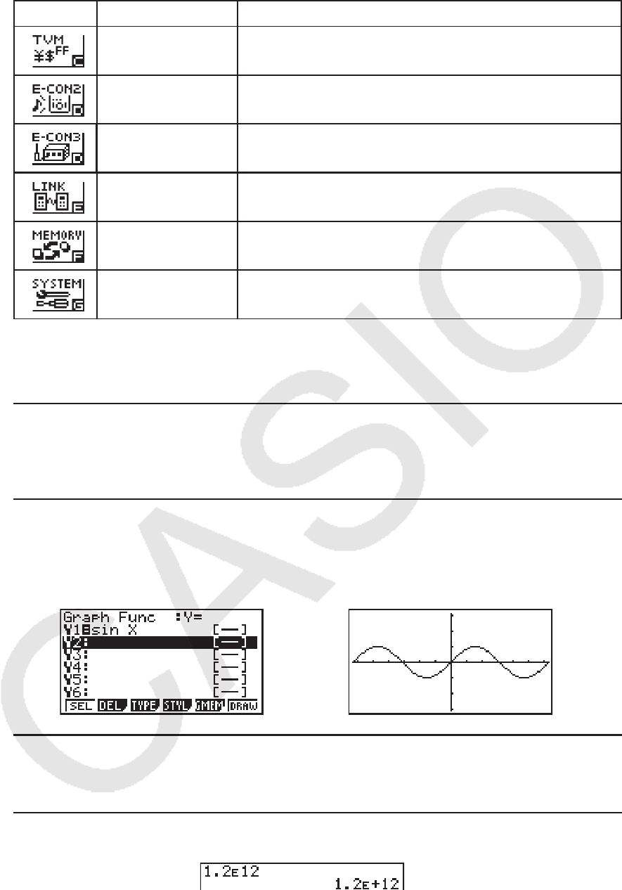
k 关于显示屏
此计算器使用两种类型的显示屏:文本屏幕和图形屏幕。文本屏幕可显示21列和8行字符,末行
(底部)用于功能键菜单。图形屏幕区域大小为127(宽)× 63 (高)点。
文本屏幕 图形屏幕
k 正常显示
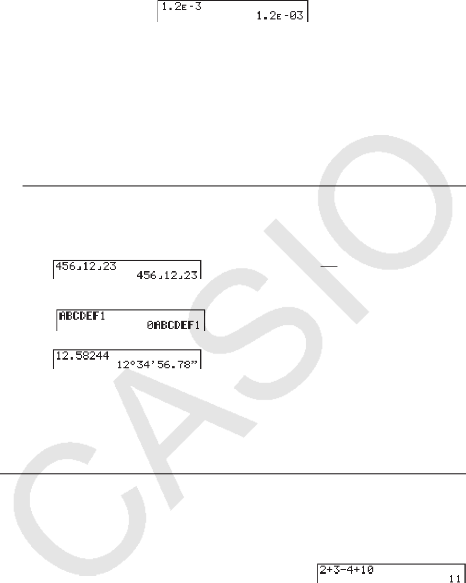
计算器通常可显示长达10位的数值。超过此限制的数值会自动转换并且显示为指数格式。
u 如何理解指数格式
1.2
E
+12表示结果等于1.2 × 10
12
。这意味着您应该将1.2中的小数点右移十二位,因为指数为
正。数值结果为1200000000000。
1-5
1.2
E
-03 表示结果等于1.2 × 10
-3
。这意味着您应该将1.2中的小数点左移三位,因为指数为负。
数值结果为0.0012。
您可以指定两种不同范围中的一种,自动转换为指数显示。
Norm 1 .............................. 10
-2
(0.01) > | x|, | x| > 10
10
Norm 2 .............................. 10
-9
(0.000000001) > | x|, | x| > 10
10
本手册中的所有例子均显示使用Norm 1得到的计算结果。
关于在Norm 1与Norm 2之间的切换详情,请参见第2-11页。
k 特殊显示格式
此计算器使用特殊显示格式显示分数、十六进制数值与度/分/秒数值。
u 分数
................................ 显示:456
12
23
u 十六进制数值
.............................. 显示:0ABCDEF1
(16)
,等于180150001
(10)
u 度/分/秒数值
................................ 显示:12°34’56.78”
•除了上述格式,此计算器也使用其他指示符或符号;本手册将在相应章节对其逐一说明。
3. 输入和编辑计算式
k 输入计算式
在准备输入计算式时,首先按下 A,清除显示屏。接着,依照其书写形式,从左到右精确地输
入计算式,然后按下 w,得到计算结果。
示例 2 + 3 - 4 + 10 =
Ac+d-e+baw
1-6
k 编辑计算式
使用 d和 e键,将光标移至您想要变更的位置处,然后进行下述某一操作。在您编辑计算式
之后,您可以按下 w执行计算。或者使用 e移至计算式末尾处并输入更多内容。
•
您可在输入时选择插入或者覆盖*
1
。如果采用覆盖方式,您输入的文本替代当前光标所在位置的
文本。您可通过执行以下操作在插入和覆盖方式之间切换: !D(INS)。光标显示为“ I ”时
表示插入,显示为“ ”时表示覆盖。
*
1
对于除fx-7400G II/fx-9750G II之外的所有型号,只有在选择线性输入/输出模式(第1-29
页)时才可执行插入和覆盖切换。
u 变更步骤
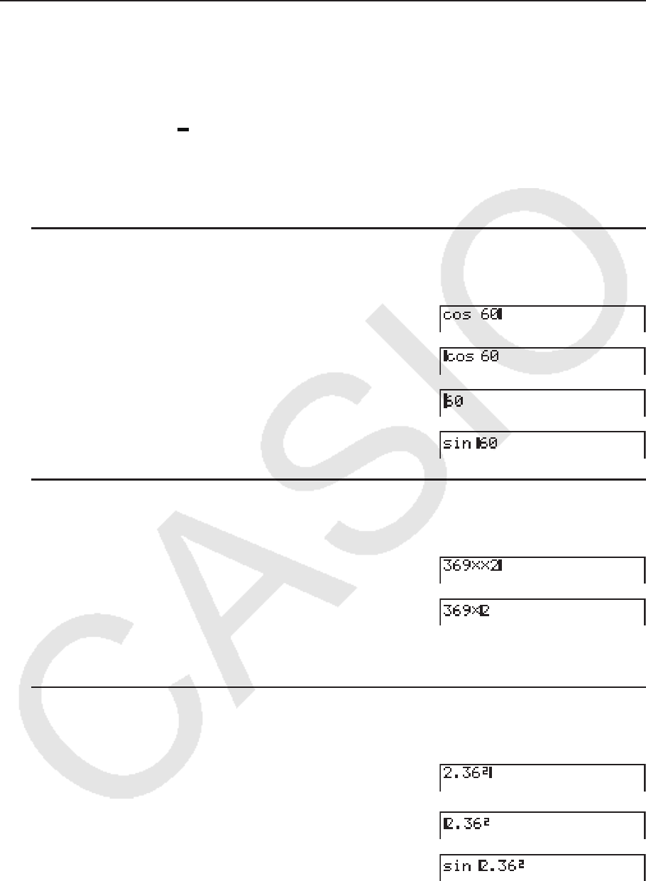
示例 将cos60改为sin60
Acga
ddd
D
s
u 删除步骤
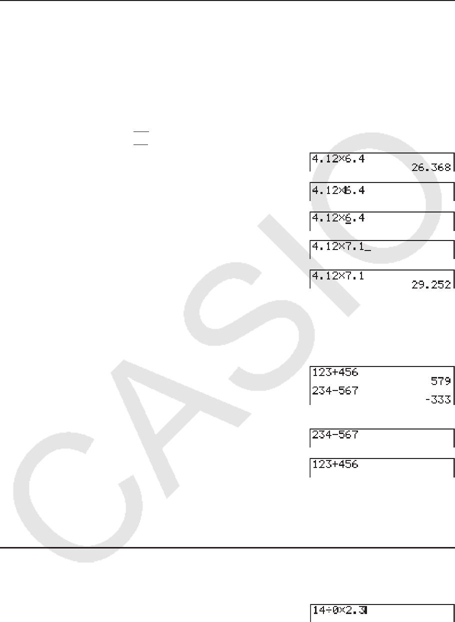
示例 将369 × × 2改为369 × 2
Adgj**c
dD
在插入模式中, D键是一个退格键。
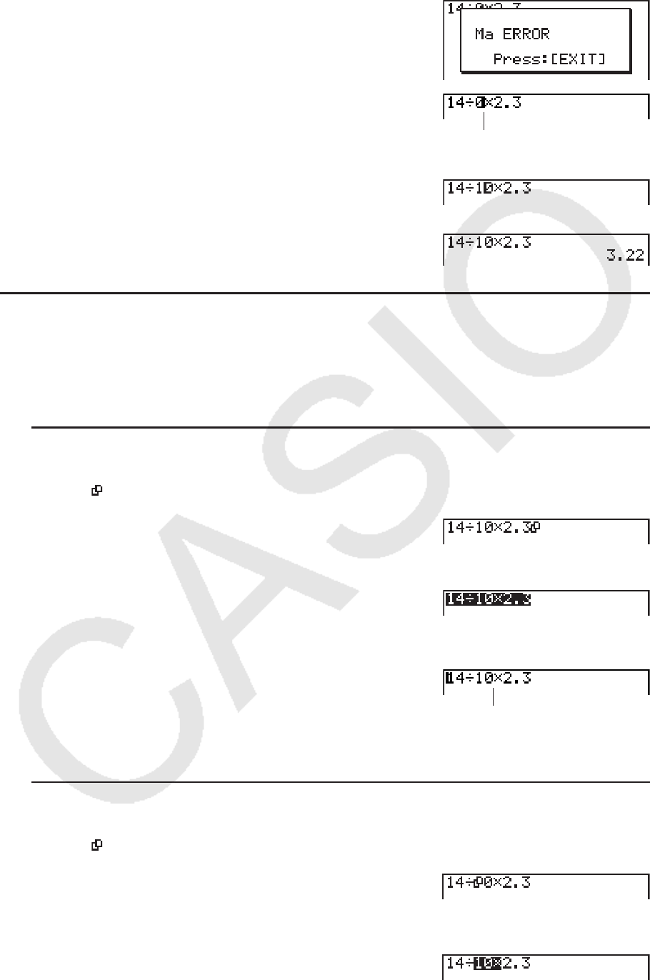
u 插入步骤
示例 将2.36
2
改为sin2.36
2
Ac.dgx
ddddd
s
1-7
k 使用重放存储器
最后一次执行的计算总是存储在重放存储器中。您可通过按下 d或 e调用重放存储器内容。
如果您按下 e,则在出现计算式时,光标在起始处。按下 d,则在计算式出现时,光标位于
末尾处。您可按照您的意愿修改计算式,然后再次执行。
• 只有在线性输入/输出模式中才可启用重放存储器。在数学输入/输出模式中,使用历史功能替
代重放存储器。详情请参见“历史功能”(第1-17页)。
例1 执行下述两个计算式
4.12 × 6.4 = 26.368
4.12 × 7.1 = 29.252
Ae.bc*g.ew
dddd
!D(INS)
h.b
w
在您按下 A之后,您可按下 f或 c以按照从最近到最早(多项重放功能)的顺序调用以前的
计算。一旦您调用计算,您就可以使用 e和 d,围绕计算式移动光标并进行修改,创建新的
计算式。
例2
Abcd+efgw
cde-fghw
A
f (返回一项计算)
f (返回两项计算)
• 计算式会始终保留在重放存储器中,直至您进行另一次计算。
• 当您按下 A键时,不会清除重放存储器的内容,因此即使在按下 A键之后,您也可以调用并
执行计算。
k 更正原计算式
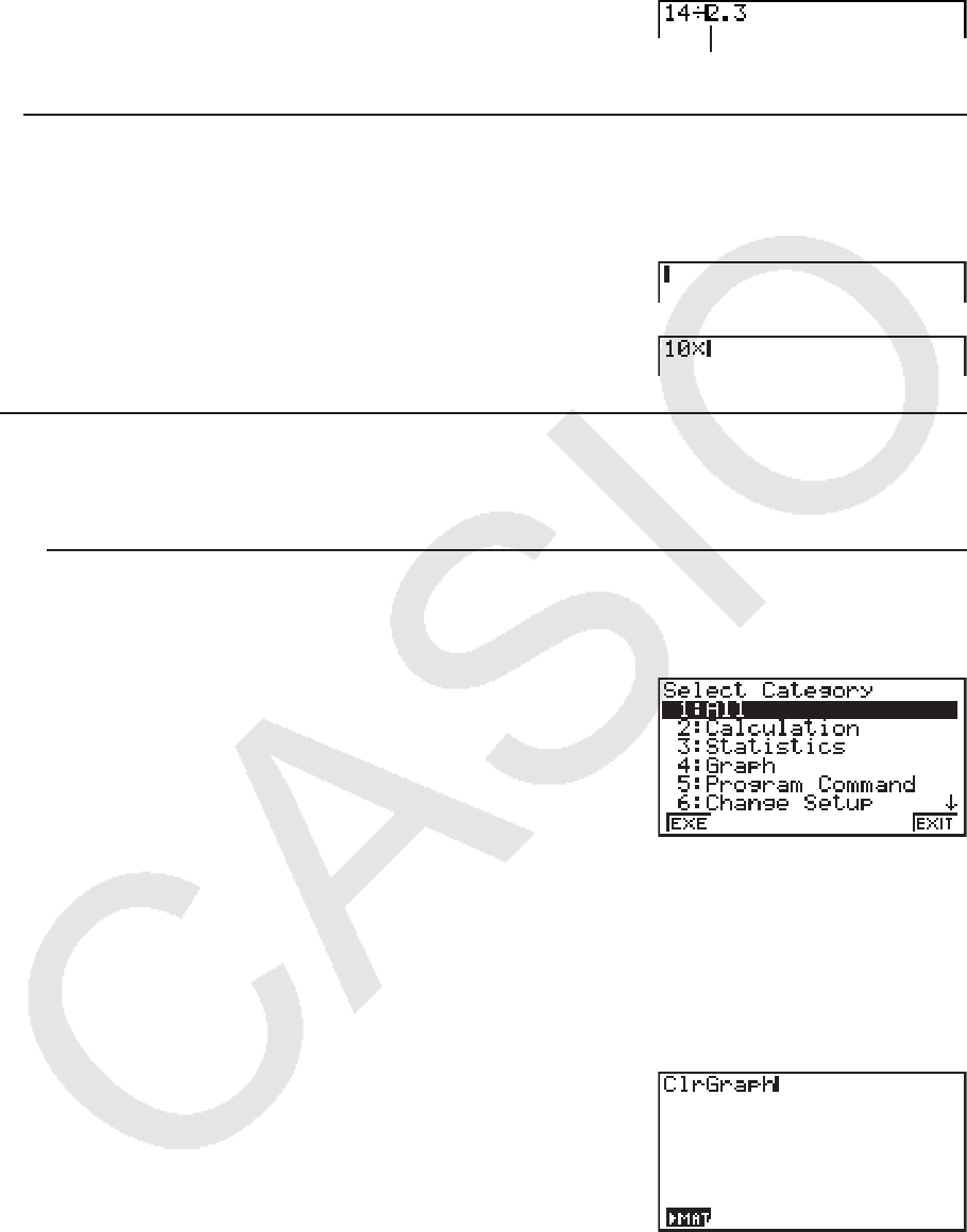
示例 14 ÷ 0 × 2.3被错误地输入为14 ÷ 10 × 2.3
Abe/a*c.d
1-8
w
按下 J。
光标自动定位于错误原因位置处。
进行必要的修改。
db
再次执行。
w
k 使用剪贴板复制和粘贴
您可将函数、命令或者其他输入内容复制(或者剪切)到剪贴板,然后在其它位置粘贴剪贴板
内容。
• 此处所述程序均使用线性输入/输出模式。关于在选定数学输入/输出模式期间的复制与粘贴操
作详情,请参见“在数学输入/输出模式中使用剪贴板复制和粘贴”(第1-18页)。
u 指定复制范围
1. 将光标(
I
)移至想要复制的文本起始或末尾处,然后按下 !i(CLIP)。该操作将使光标
变为“ ”。
2. 使用光标键移动光标并突出显示需要复制的文本范围。
3. 按下 1(COPY)将突出显示的文本复制到剪贴板,然后退出复制范围指定模式。
选定字符在复制时不会改变。
如需取消文本突出显示状态且不执行复制操作,按下 J。
u 剪切文本
1. 将光标(
I
)移至想要剪切的文本起始或末尾处,然后按下 !i(CLIP)。该操作将使光标
变为“ ”。
2. 使用光标键移动光标并突出显示需要剪切的文本范围。
1-9
3. 按下 2(CUT)将突出显示的文本剪切到剪贴板。
剪切操作将删除原始字符。
u 粘贴文本
将光标移至需要粘贴文本的位置,然后按下 !j(PASTE)。剪贴板的内容被粘贴到光标位
置。
A
!j(PASTE)
k 目录功能
目录是一个按照字母表顺序排列的列表,其中列出了此计算器上的所有命令。您可通过调
用“目录”,然后选择需要的命令以输入该命令。
u 使用“目录”输入命令
1. 按下 !e(CATALOG)显示命令的字母表顺序目录。
• 首先显示的屏幕是上一次用于命令输入的屏幕。
2. 按下 6(CTGY)以显示目录列表。
• 如果您愿意,也可跳过这一步,直接转到步骤5。
3. 使用光标键( f、 c)突出显示需要的命令目录,然后按下 1(EXE)或者 w。
• 由此可显示在目录中选定的命令列表。
4. 输入需要输入的命令的首字母。由此可显示以该字母开头的第一个命令。
5. 使用光标键( f, c)突出显示需要输入的命令,然后按下 1(INPUT)或 w。
示例 使用“目录”输入ClrGraph命令
A!e(CATALOG) I(C) c~ cw
按下 J或 !J(QUIT)以关闭“目录”。

1-10
4. 使用数学输入/输出模式
重要!
• fx-7400G
II和fx-9750G II未配置数学输入/输出模式。
在设置屏幕上,在“Input/Output”模式中选择“Math”(第1-29页),可启用数学输入/输
出模式,该模式允许自然输入和显示特定功能,与课本中显示方式一致。
• 本节操作均在数学输入/输出模式中执行。
- 初始默认设置为数学输入/输出模式。如果您已经改为线性输入/输出模式,在执行本节所述
操作之前请恢复数学输入/输出模式。关于如何切换模式的说明,请参见“使用设置屏幕”
(第1-26页)。
- 在执行本节操作之前切换到数学输入/输出模式。关于如何切换模式的说明,请参见“使用
设置屏幕”(第1-26页)。
• 在数学输入/输出模式中,所有输入均采用插入模式(非覆盖模式)输入。请注意,您在线性
输入/输出模式中用于切换到插入模式输入的 !D(INS)操作(第1-6页),与在数学输入/输
出模式中的功能完全不同。详情请参见“使用作为自变量的数值和表达式”(第1-14页)。
• 除非另有明确规定,本节中的所有操作均在 RUN • MAT 模式中执行。

1-11
k 数学输入/输出模式中的输入操作
u 数学输入/输出模式函数和符号
下列函数和符号可在数学输入/输出模式中用于自然输入。“字节”列显示了在数学输入/输出
模式中输入占用的存储器字节数。
函数/符号 键操作 字节
分数(假分数) v 9
带分数*
1 !v( &) 14
幂 M 4
平方 x 4
负幂(倒数) !)(
x -1
) 5
' !x( ') 6
立方根 !((
3
') 9
方根 !M(
x') 9
ex !I( ex) 6
10
x !l(10
x) 6
log(a,b) (从MATH菜单输入*
2
) 7
Abs (绝对值) (从MATH菜单输入*
2
) 6
线性微分*
3 (从MATH菜单输入*
2
) 7
二次微分*
3 (从MATH菜单输入*
2
) 7
积分*
3 (从MATH菜单输入*
2
) 8
∑ 计算*
4 (从MATH菜单输入*
2
) 11
矩阵、向量 (从MATH菜单输入*
2
) 14*
5
圆括号 (和 ) 1
大括号 (用于列表输入。) !*( { )和 !/( } ) 1
方括号 (用于矩阵/向量输入。) !+( [ )和 !-( ] ) 1
*
1
只有数学输入/输出模式支持带分数。
*
2
关于从MATH函数菜单输入函数的详情,请参见下述“使用MATH菜单”。
*
3
在数学输入/输出模式中无法指定公差。如果您希望指定公差,请使用线性输入/输出模式。
*
4
对于数学输入/输出模式中的 ∑ 计算,间距始终为1。如果您想指定不同的间距,使用线性输
入/输出模式。
*
5
这是对应于一个2 × 2矩阵的字节数。
u 使用MATH菜单
在 RUN • MAT 模式中,按下 4(MATH)可显示MATH菜单。
您可使用该菜单以自然方式输入矩阵、微分、积分等等。
1-12
• { MAT } ... {显示MAT子菜单,用于矩阵/向量的自然输入}
• { 2 × 2 } ... {输入一个2 × 2矩阵}
• { 3 × 3 } ... {输入一个3 × 3矩阵}
• {
m× n} ... {输入一个 m行和 n列矩阵/向量(最多6 × 6)}
• {2×1} ... {输入一个2 × 1向量}
• {3×1} ... {输入一个3 × 1向量}
• {1×2} ... {输入一个1 × 2向量}
• {1×3} ... {输入一个1 × 3向量}
• { log
a
b } ... {开始自然输入对数log
a
b}
• { Abs } ... {开始自然输入绝对值|X|}
• { d/ dx} ... {开始自然输入线性微分
dx
df(x)
x = a
}
• { d2
/ dx2
} ... {开始自然输入二次微分
dx2
d2
f
(
x
)
x
=
a
}
• { ∫ dx} ... {开始自然输入积分
f
(
x
)
dx
a
b
}
• { ∑ ( } ... {开始自然输入 ∑ 计算
f(x)
x=α
β
α
Σ
}
u 数学输入/输出模式输入示例
本节提供了大量不同示例,说明在数学输入/输出模式自然输入期间如何使用MATH函数菜单和
其他键。在输入数值和数据时,务请注意输入光标位置。
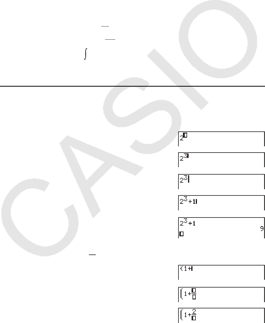
例1 如需输入2
3
+ 1
AcM
d
e
+b
w
例2 如需输入
()
1+ 2
5
2
A(b+
v
cc
1-13
f
e
)x
w
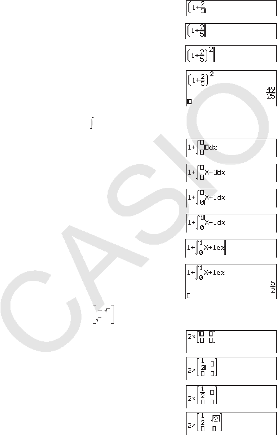
例3 如需输入
1+ x+ 1dx
0
1
Ab+4(MATH) 6( g) 1(
∫ dx)
v+b
ea
fb
e
w
例4 如需输入
2×
1
2
21
2
2
Ac*4(MATH) 1(MAT) 1(2x2)
vbcc
ee
!x( ') ce
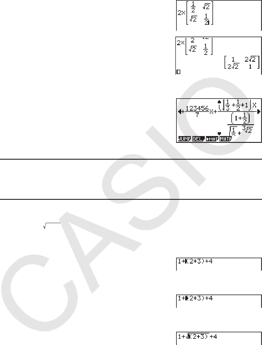
1-14
e!x( ') ceevbcc
w
u 如果显示窗口不能容纳整个计算式
显示屏的上、下、左或右边缘显示箭头,让您知道对应
方向上的屏幕之外还有计算式。
当您看见箭头时,您可使用光标键滚动屏幕内容,查看
相应部分。
u 数学输入/输出模式输入限制
某些类型的表达式可能导致计算式的垂直宽度超过一个显示行。计算式的最大允许垂直宽度大
约为两个显示屏(120点)。不可输入超过该限制的任何表达式。
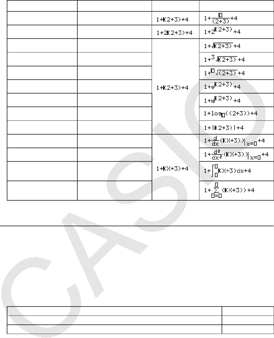
u 使用作为自变量的数值和表达式
输入的数值或者表达式可作为函数的自变量。例如,输入“(2+3)”之后,您可使其成为 '的自
变量,结果为 (2+3)。
示例
1. 移动光标,使其直接位于希望作为插入函数自变量的表达式的左侧。
2. 按下 !D(INS)。
• 该操作将使光标变为插入光标( ')。
3. 按下 !x( ')以插入 ' 函数。
• 该操作将插入 '函数并使圆括号表达式成为其自变量。
如上所示,在按下 !D(INS)之后,光标右侧的数值或者表达式成为下一步指定函数的自变
量。自变量范围包括到右侧第一个左括号或第一个函数之间的所有内容(sin(30), log2(4)等
等)。
1-15
该功能可用于以下函数。
函数 键操作 原始表达式 插入之后的表达式
假分数 v
幂 M
' !x( ')
立方根 !((
3
')
方根 !M(
x')
ex !I( ex)
10
x !l(10
x)
log(a,b) 4(MATH) 2(log
a
b)
绝对值 4(MATH) 3(Abs)
线性微分 4(MATH) 4(
d/ dx)
二次微分 4(MATH) 5(
d2
/ dx2
)
积分 4(MATH) 6( g)
1( ∫ dx)
∑ 计算 4(MATH) 6( g)
2( Σ ( )
• 在线性输入/输出模式中,按下 !D(INS)将变为插入模式。参见第1-6页详情。
u 在数学输入/输出模式中编辑计算式
在数学输入/输出模式中编辑计算式的程序基本上与在线性输入/输出模式中相同。详情请参
见“编辑计算式”(第1-6页)。
但请注意,数学输入/输出模式与线性输入/输出模式之间存在以下差别。
• 数学输入/输出模式不支持线性输入/输出模式中的覆盖模式输入。在数学输入/输出模式中,
总是在当前光标位置插入输入内容。
• 在数学输入/输出模式,按下 D键总是执行退格操作。
• 请注意在数学输入/输出模式中输入计算式时可使用的以下光标操作。
操作: 按下该键:
将光标从计算式末尾移至起始处 e
将光标从计算式起始处移至末尾 d
1-16
k 使用撤消和恢复操作
在数学输入/输出模式中,您可在输入计算表达式时使用以下程序(直至您按下 w键)以取消
上一次键操作和恢复刚撤消的键操作。
- 如需撤消上一次键操作,按下: aD(UNDO)。
- 如需恢复刚撤消的键操作,再次按下: aD(UNDO)。
•
您还可使用UNDO取消 A键操作。按下 A以清除刚输入的表达式之后,按下 aD(UNDO)将
恢复按下 A之前屏幕上的显示内容。
• 您还可使用UNDO取消光标键操作。如果您在输入期间按下 e,然后按下 aD(UNDO),
光标将返回按下 e之前的位置。
• 在键盘锁定字母时,禁用UNDO操作。键盘锁定字母期间按下 aD(UNDO)将执行删除操
作,功能与单独按下 D键相同。
示例
b+vbe
D
aD(UNDO)
c
A
aD(UNDO)
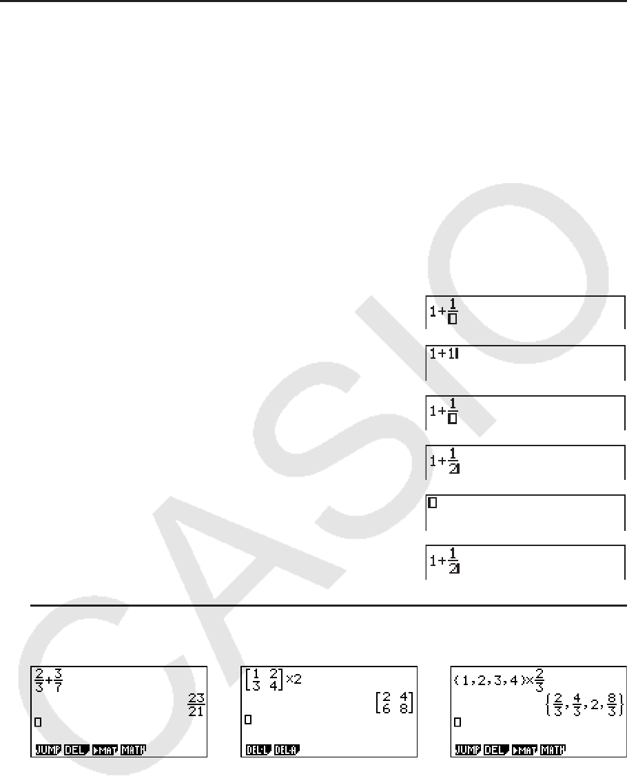
k 数学输入/输出模式计算结果显示
数学输入/输出模式计算产生的分数、矩阵、向量和列表以自然格式显示,与在课本中一样。
计算结果显示示例
• 根据设置屏幕中“Frac Result”的设置,分数可采用假分数或者带分数形式显示。详情请参
见“使用设置屏幕”(第1-26页)。
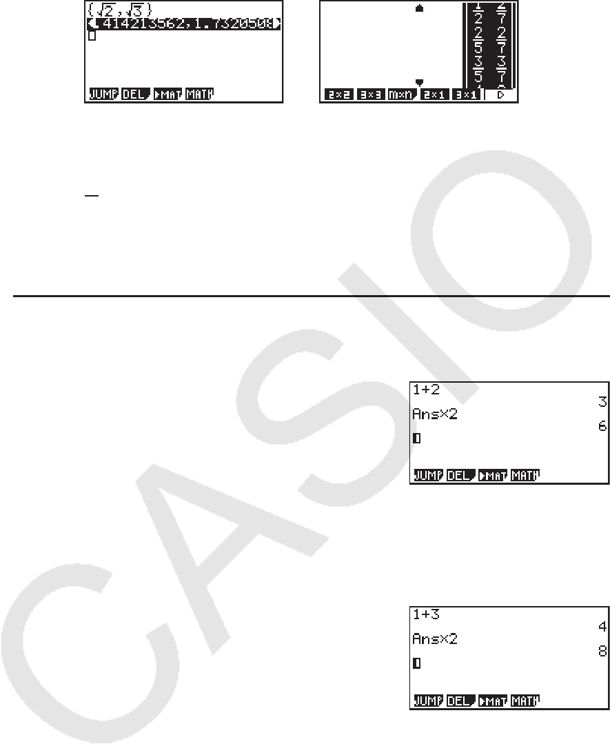
• 矩阵以自然格式显示,最多为6 × 6矩阵。超过六行或列的矩阵将在MatAns屏幕上显示,该
屏幕与线性输入/输出模式中使用的屏幕相同。
• 向量以自然格式显示,最多为1 × 6或6 × 1向量。超过六行或列的向量将在VctAns屏幕上显
示,该屏幕与线性输入/输出模式中使用的屏幕相同。
• 列表以自然格式显示,最多包含20个元素。超过20个元素的列表将在ListAns屏幕上显示,该
屏幕与线性输入/输出模式中使用的屏幕相同。
1-17
• 显示屏的上、下、左或右边缘显示箭头,让您知道对应方向的屏幕之外还有数据。
您可使用光标键滚动屏幕,查看需要的数据。
• 选定计算结果时按下 2(DEL) 1(DEL
•
L)将删除结果和对应的计算式。
• 假分数或者带分数之前的相邻乘号不可忽略。在此情况下必须输入乘号。
示例:
2× 2
5 c*cvf
• M、 x或 !)( x-1
)键操作后不可直接执行另一个 M、 x或 !)( x-1
)键操作。在此情
况下,使用圆括号分隔键操作。
示例: (3
2
)
-1
(dx)!)( x-1
)
k 历史功能
历史功能可在数学输入/输出模式中保留计算表达式和结果历史。最多可保存30组计算表达式和
结果。
b+cw
*cw
您还可编辑历史功能中保存的计算表达式并重新计算。由此可从编辑的表达式开始重新计算所
有表达式。
示例 如需将“1+2”改为“1+3”并重新计算
在上例之后执行以下操作。
ffffdDdw
• 保存在答案存储器中的数值总是取决于上次计算的结果。如果历史内容包括使用答案存储器的
操作,编辑计算式可能影响后续计算中使用的答案存储器数值。
- 如果有一系列计算式使用答案存储器(在下一次计算中包括前一次计算的结果),编辑计算
式将影响此后的其他所有计算结果。
- 如果历史记录中的第一次计算包括答案存储器内容,则由于历史记录中第一次计算之前没有
其他计算,所以答案存储器数值为“0”。

1-18
k 在数学输入/输出模式中使用剪贴板复制和粘贴
您可将函数、命令或者其他输入内容复制到剪贴板,然后在其它位置粘贴剪贴板内容。
• 在数学输入/输出模式中,您可只指定一行作为复制范围。
• 只有线性输入/输出模式支持CUT操作。在数学输入/输出模式中不支持该操作。
u 复制文本
1. 使用光标键将光标移至需要复制的行。
2. 按下 !i(CLIP)。光标将变为“ ”。
3. 按下 1(CPY
• L)将突出显示的文本复制到剪贴板。
u 粘贴文本
将光标移至需要粘贴文本的位置,然后按下 !j(PASTE)。剪贴板的内容被粘贴到光标位
置。
k 数学输入/输出模式中的计算操作
本节介绍数学输入/输出模式计算。
• 关于计算操作的详情,请参见“第2章 手动计算”。
u 使用数学输入/输出模式执行函数计算
示例 操作
=
4×5
6
10
3
=
3
π2
1
( )
cos (Angle: Rad)
A6 v4 *5 w
Ac(!E( π ) v3 e)w
log28= 3
123 = 1.988647795
7
2 + 3 × 364 − 4 = 10
A4(MATH) 2(log
a
b) 2 e8 w
A!M(
x') 7 e123 w
A2 +3 *!M(
x') 3 e64 e-4 w
4
3= 0.1249387366log
A4(MATH) 3(Abs) l3 v4 w
20
73
5
2+ 3 =
4
1
10
23
+
2
3
1.5 + 2.3i = i
A2 v5 e+3 !v( () 1 e4 w
A1.5 +2.3 !a( i) wM
dx
d
( )
x3+ 4x2+x − 6 x = 3 = 52 A4(MATH) 4( d/ dx) vM3 e+4
vx+v-6 e3 w
2x2 + 3x + 4dx =3
404
∫5
1
A4(MATH) 6( g) 1( ∫ dx) 2 vx+3 v+4
e1 e5 w
(
k2 − 3k + 5
)
= 55
∑
k=2
6 A4(MATH) 6( g) 2( ∑ ) a,(K) x-3 a,(K)
+5 ea,(K) e2 e6 w
1-19
k 使用数学输入/输出模式执行矩阵/向量计算
u 指定矩阵/向量尺寸(大小)
1. 在 RUN • MAT 模式中,按下 !m(SET UP) 1(Math) J。
2. 按下 4(MATH)以显示MATH菜单。
3. 按下 1(MAT)以显示以下菜单。
• { 2 ×2 } ... {输入一个2 × 2矩阵}
• { 3 ×3 } ... {输入一个3 × 3矩阵}
• {
m×n} ... {输入一个 m行× n列矩阵或向量(最大6 × 6)}
• {2×1} ... {输入一个2 × 1向量}
• {3×1} ... {输入一个3 × 1向量}
• {1×2} ... {输入一个1 × 2向量}
• {1×3} ... {输入一个1 × 3向量}
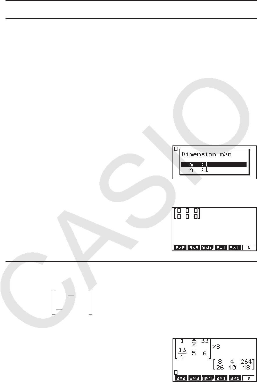
示例 创建一个2行 ×3列矩阵
3( m×n)
指定行数。
cw
指定列数。
dw
w
u 输入单元值
示例 执行下述计算
以下操作为前页计算示例的后续操作。
bebvceedde
bdveeefege
*iw
×8
33
65
1
13
4
1
2
1-20
u 为一个MAT模式矩阵分配使用数学输入/输出模式创建的矩阵
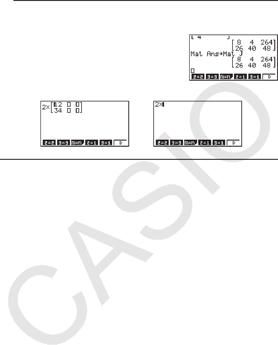
示例 将计算结果分配给Mat J
!c(Mat) !-(Ans) a
!c(Mat) a)(J) w
• 在光标位于矩阵顶部(左上方)按下 D键将删除整个矩阵。
D
⇒
k 在数学输入/输出模式中使用图形模式和EQUA模式
将数学输入/输出模式与以下任意模式结合使用,可帮助您输入数字表达式(与在课本中的书写
方式一样)并在自然显示格式下查看计算结果。
支持课本书写方式的表达式输入的模式:
RUN • MAT、e • ACT、GRAPH、DYNA、TABLE、RECUR、EQUA (SOLV)
支持自然显示格式的模式:
RUN • MAT、e • ACT、EQUA
以下说明了在 GRAPH 、 DYNA 、 TABLE 、 RECUR 和 EQUA 模式中的数学输入/输出模式操作,以
及 EQUA 模式中的自然计算结果显示。
• 关于每一种计算操作的详情,请参见相应章节。
• 关于数学输入/输出模式操作和 RUN • MAT 模式中的计算结果显示的详情,请参见“数学输入/
输出模式中的输入操作”(第1-11页)和“数学输入/输出模式中的计算操作”(第1-18页)。
• e • ACT 模式输入操作和结果显示与在 RUN • MAT 模式中一样。关于 e • ACT 模式操作的详情,请
参见“第10章 eActivity”。
1-21
u GRAPH模式中的数学输入/输出模式输入
您可使用数学输入/输出模式在 GRAPH 、 DYNA 、 TABLE 和 RECUR 模式中输入图形表达式。
例1 在 GRAPH 模式中,输入函数
y
=−−1
2
x2
'
2
x
'
然后绘制图形。确保在视图窗口中配置初
始默认设置。
mGRAPH vxv!x( ') c
ee-vv!x( ') cee
-bw
6(DRAW)
例2 在GRAPH模式中,输入函数
y
=x2−x−1d
x
∫x
4
1
2
1
0 然后绘制图形。
确保在视图窗口中配置初始默认设置。
mGRAPH K2(CALC) 3( ∫ dx)
bveevx-bvce
v-beaevw
6(DRAW)
• EQUA模式中的数学输入/输出模式输入和结果显示
您可在 EQUA 模式中使用数学输入/输出模式进行如下输入和显示。
• 对于方程组( 1(SIML))和高阶方程( 2(POLY)),尽可能以自然显示格式输出解(分
数、 '、 π 以自然格式显示)。
• 对于解算器( 3(SOLV)),您可使用数学输入/输出模式自然输入。
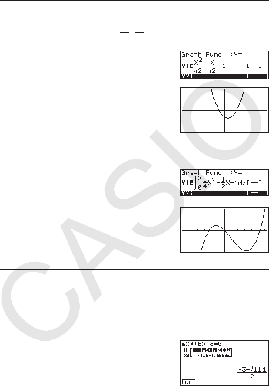
示例 在EQUA模式中求解二次方程
x2
+ 3 x + 5 = 0
mEQUA !m(SET UP)
cccc(Complex Mode)
2(a+b
i) J
2(POLY) 1(2) bwdwfww

1-22
5. 选项(OPTN)菜单
利用选项菜单,您可以使用计算器键盘上未标记的科学函数和功能。当您按下 K键时,选项
菜单内容因所处模式而异。
• 如果您按下 K在将二进制、八进制、十进制或十六进制设置为默认记数系统时,不会显示选
项菜单。
• 有关选项(OPTN)菜单命令的详情,请参见“ K键”项目“ PRGM 模式命令列表”中(第
8-37页)。
• 选项菜单项目的含义请参见每一种模式对应的章节。
下表显示了在选择 RUN • MAT (或者 RUN )或者 PRGM 模式时的选项菜单。
fx-7400G
II不包括下面标记星号(*)的项目。
• { LIST } ... {列表功能菜单}
• { MAT }* ... {矩阵/向量*
1
运算菜单}(*
1
fx-9750GII中不包括。)
• { CPLX } ... {复数计算菜单}
• { CALC } ... {泛函分析菜单}
• { STAT } ... {双变量统计估计值菜单} (fx-7400G
II)
{双变量统计估计值、分布、标准差、方差、测试功能菜单} (除fx-7400G
II之外的
所有型号)
• { CONV } ... {度量转换菜单}
• { HYP } ... {双曲线计算菜单}
• { PROB } ... {概率/分布计算菜单}
• { NUM } ... {数值计算菜单}
• { ANGL } ... {角度/坐标变换、六十进制输入/变换菜单}
• { ESYM } ... {工程符号菜单}
• { PICT } ... {图形保存/调用菜单}
• { FMEM } ... {函数存储器菜单}
• { LOGIC } ... {逻辑算子菜单}
• { CAPT } ... {屏幕捕捉菜单}
• { TVM }* ... {财务计算菜单}
• 在设置屏幕中为“Input/Output”模式设置选择“Math”时,不显示PICT、FMEM和CAPT
项目。

1-23
6. 变量数据(VARS)菜单
如需调用变量数据,按下 J,显示变量数据菜单。
{ V-WIN } / { FACT } / { STAT } / { GRPH } / { DYNA } / { TABL } / { RECR } / { EQUA } / { TVM } / { Str }
• 请注意,功能键( 3和 4)的EQUA和TVM项目只有在通过 RUN • MAT (或者 RUN )或
者 PRGM 模式访问变量数据菜单时才显示。
• 在将二进制、八进制、十进制与十六进制设置为初始默认记数系统时,如果您按下 J,不会
显示变量数据菜单。
• 某些型号的计算器可能不包括某些菜单项目。
• 关于变量数据(VARS)菜单的详情,请参见“ J键”项目在“ PRGM 模式命令列表”中
(第8-37页)。
• fx-7400G
II不包括下面标记星号(*)的项目。
u V-WIN — 调用视窗数值
• { X } / { Y } / { T, Ƨ} ... { x轴菜单}/{ y轴菜单}/{T, Ƨ菜单}
•
{ R-X } / { R-Y } / { R-T, Ƨ} ... { x轴菜单}/{ y轴菜单}/{T, Ƨ菜单} - 在对偶图右侧
• { min } / { max } / { scal } / { dot } / { ptch } ... {最小值}/{最大值}/{比例}/{点值*
1
}/{间距}
*
1
点值表示显示范围(Xmax值 - Xmin值)除以屏幕点距(126)。点值通常根据最小值和
最大值自动计算。更改点值会自动计算最大值。
u FACT — 调用缩放系数
• { Xfct }/{ Yfct } ... { x轴系数}/{ y轴系数}
u STAT — 调用统计数据
• { X } ... {单变量,双变量 x数据}
• {
n} / { ¯ x } / { ∑ x} / { ∑ x2
} / { Ʊx} / { s
x} / { minX } / { maxX } ... {数据个数}/{平均值}/{和}/{平方和}/{总体
标准差}/{样本标准差}/{最小值}/{最大值}
•
{ Y } ... {双变量 y数据}
• {
Κ} / { ∑ y} / { ∑ y2
} / { ∑ xy} / { Ʊy} / { s
y} / { minY } / { maxY } ... {平均值}/{和}/{平方和}/{ x数据与 y数据
的乘积之和}/{总体标准差}/{样本标准差}/{最小值}/{最大值}
•
{ GRPH } ... {图形数据菜单}
• { a} / { b} / { c} / { d} / { e} ... {回归系数与多项式系数}
• { r} / { r2
} ... {相关系数}/{可决系数}
• { MSe } ... {均方差}
• { Q
1
} / { Q
3
} ... {第一四分位数}/{第三四分位数}
• { Med } / { Mod } ... 输入数据的{中位数}/{众数}
• { Strt } / { Pitch } ... 直方图{起始分割}/{间距}
•
{ PTS } ... {汇总点数据菜单}
• {
x1
} / { y1
} / { x2
} / { y2
} / { x3
} / { y3
} ... {汇总点的坐标}
•
{ INPT } * ... {统计计算输入值}
• {
n} / { ¯ x } / {s
x} / { n1
} / { n2
} / { ¯ x 1
} / { ¯ x 2
} / { s
x1} / { s
x2} / { s
p} ...{样本大小}/{样本平均值}/{样本标准差}/
{样本1大小}/{样本2大小}/{样本1平均值}/{样本2平均值}/{样本1标准差}/{样本2标准差}/
{样本
p标准差}

1-24
•
{ RESLT } * ... {统计计算输出值}
• { TEST } ... {测试计算结果}
• {
p} / { z} / { t} / { Chi } / { F} / { ˆ p } / { ˆ p 1
} / { ˆ p 2
} / { df} / { s
e} / { r} / { r
2
} / { pa } / { Fa } / { Adf } / { SSa } / { MSa } / { pb } /
{ Fb } / { Bdf } / { SSb } / { MSb } / { pab } / { Fab } / { ABdf } / { SSab } / { MSab } / { Edf } / { SSe } / { MSe }
... {
p值}/{ z分数}/{ t分数}/{ χ 2
值}/{ F值}/{样本估计比例}/{样本1估计比例}/{样本2估计比例}/
{自由度}/{标准误差}/{相关系数}/{可决系数}/{系数A
p值}/{系数A F值}/{系数A自由度}/
{系数A平方和}/{系数A均方}/{系数B
p值}/{系数B F值}/{系数B自由度}/{系数B平方和}/
{系数B均方}/{系数AB
p值}/{系数AB F值}/{系数AB自由度}/{系数AB平方和}/{系数AB均
方}/{误差自由度}/{误差平方和}/{误差均方}
• { INTR } ... {置信区间计算结果}
•
{ Left } / { Right } / { ˆ p } / { ˆ p
1
} / { ˆ p
2
} / { df} ... {置信区间下限(左边缘)}/{置信区间上限(右边缘)}/
{样本估计比例}/{样本1估计比例}/{样本2估计比例}/{自由度}
• { DIST } ... {分布计算结果}
• {
p} / { xInv } / { x1Inv } / { x2Inv } / { zLow } / { zUp } / { tLow } / { tUp } ... {概率分布或累积分布计算结
果(
p值)}/{逆学生- t、 χ 2
、 F、二项、泊松、几何或超几何累积分布计算结果}/{逆累积
正态分布上限(右边缘)或下限(左边缘)}/{逆累积正态分布上限(右边缘)}/{累积正
态分布下限(左边缘)}/{累积正态分布上限(右边缘)}/{学生- t 累积分布下限(左边
缘)}/{学生-
t 累积分布上限(右边缘)}
u GRPH — 调用图形函数
• { Y } / {
r} ... {直角坐标或不等式函数}/{极坐标函数}
• { Xt } / { Yt } ... 参数图形函数{Xt}/{Yt}
• { X } ... {X=常量图形函数}
• 在输入数值之前按下这些键,指定存储区。
u DYNA* — 调用动态图形设置数据
• { Strt } / { End } / { Pitch } ... {系数范围初值}/{系数范围终值}/{系数值增量}
u TABL — 调用表格设置与内容数据
• { Strt } / { End } / { Pitch } ... {表格范围初值}/{表格范围终值}/{表格值增量}
• { Reslt *
1
} ... {表格内容矩阵}
*
1
只有在 RUN • MAT (或者 RUN )和 PRGM 模式中显示TABL菜单时,才会显示Reslt项目。
u RECR* — 调用递推公式* 1
、表格范围和表格内容数据
• { FORM } ... {递推公式数据菜单}
• {
an} / { an+1
} / { an+2
} / { bn} / { bn+1
} / { bn+2
} / { cn} / { cn+1
} / { cn+2
} ... { an}/{ an+1
}/{ an+2
}/{ bn}/{ bn+1
}/{ bn+2
}/{ cn}/
{
cn+1
}/{ cn+2
} 表达式
• { RANG } ... {表格范围数据菜单}
• { Strt } / { End } ... 表格范围{初值}/{终值}
• {
a0
} / { a1
} / { a2
} / { b0
} / { b1
} / { b2
} / { c0
} / { c1
} / { c2
} ... { a0
}/{ a1
}/{ a2
}/{ b0
}/{ b1
}/{ b2
}/{ c0
}/{ c1
}/{ c2
}值
• {
anSt } / { bnSt } / { cnSt } ... { an}/{ bn}/{ cn} 递推收敛/发散图形(WEB图形)的原点
• { Reslt *
2
}* ... {表格内容矩阵*
3
}
*
1
存储器中没有函数或递推公式数值表时产生一个错误。
*
2
只有在 RUN • MAT 和 PRGM 模式中才可使用“Reslt”。
*
3
表格内容自动存储在矩阵答案存储器中(MatAns)。

1-25
u EQUA* — 调用方程系数与解* 1 * 2
• { S-Rlt } / { S-Cof } ... 具有2至6个未知数的一次方程的{解}/{系数}的矩阵*
3
• { P-Rlt } / { P-Cof } ... 二次或者三次方程的{解}/{系数}的矩阵
*
1
系数和解自动存储在矩阵答案存储器中(MatAns)。
*
2
以下条件会产生错误。
- 当方程未输入任何系数时
- 当未获取任何方程的解时
*
3
不可同时调用一次方程的系数和解存储器数据。
u TVM* — 调用财务计算数据
• {
n} / { I%} / { PV} / { PMT} / { FV} ... {付款期限(分期)}/{年利率}/{当前值}/{付款金额}/{未来值}
• {
P/Y} / { C/Y} ... {每年分期付款期数}/{每年复利计算期数}
u Str — Str命令
• { Str } ... {字符串存储器}
7. 程序(PRGM)菜单
如需显示程序(PRGM)菜单,首先通过主菜单进入 RUN • MAT (或者 RUN )或者 PRGM 模式,
然后按下 !J(PRGM)。下面是程序(PRGM)菜单中可提供的选项。
• 在设置屏幕中为“Input/Output”模式设置选择“Math”时,不显示程序菜单。
• { COM } .......... {程序命令菜单}
• { CTL } ............ {程序控制命令菜单}
• { JUMP } ........ {转移命令菜单}
• { ? } .................... {输入命令}
• { ^} ................. {输出命令}
• { CLR } ............ {清除命令菜单}
• { DISP } ........... {显示命令菜单}
• { REL } ............ {条件转移关系算子菜单}
• { I/O } .............. {输入/输出控制/传输命令菜单}
• { : } ..................... {多语句命令}
• { STR } ............ {字符串命令}
当二进制、八进制、十进制或者十六进制被设置为默认记数系统时,如果您按下 !J(PRGM)
(在 RUN • MAT (或者 RUN )模式或者 PRGM 模式中),将显示以下功能键菜单。
• { Prog } ........... {程序调用}
• { JUMP } / { ? } / { ^} / { REL } / {:}
指定给功能键的功能与Comp模式下的功能相同。
如需详细了解从程序菜单访问的各种菜单的命令,请参见“第8章 编程”。
1-26
8. 使用设置屏幕
模式的设置屏幕显示模式设置的当前状态,以便您进行任何修改。下述程序显示如何改变设
置。
u 改变模式设置
1. 选择你需要的图标并按下 w,进入某一模式并显示其初始屏幕。在本例中,我们将进
入 RUN • MAT (或者 RUN )模式。
2. 按下 !m(SET UP)显示模式的设置屏幕。
• 此设置屏幕只是一个可能情况的示例。实际设置屏幕
内容将因您所处的模式以及该模式的当前设置而异。
3. 使用 f和 c光标键,突出显示您想要修改设置的项目。
4. 按下标记目标设置的功能键( 1至 6)。
5. 在完成修改之后,按下 J,退出设置屏幕。
k 设置屏幕功能键菜单
本节详细说明了可在设置屏幕中使用功能键进行的设置。 表示默认设置。
fx-7400G
II不包括下面标记星号(*)的项目。
u Mode(计算/二进制、八进制、十进制,十六进制模式)
• { Comp } ... {算术计算模式}
• { Dec } / { Hex } / { Bin } / { Oct } ... {十进制}/{十六进制}/{二进制}/{八进制}
u Frac Result(分数结果显示格式)
• { d/c } / { ab/c } ... {假}/{带}分数
u Func Type(图形函数类型)
按下以下某一功能键也可切换 v 键的功能。
• { Y
= } / { r= } / { Parm } / { X= } ... {直角坐标(Y=
f( x)类型)}/{极坐标}/ {参数}/{直角坐标(X= f( y)类
型)}图形
• { Y> } / { Y< } / { Y t} / { Y s} ... {
y> f( x)}/{ y< f( x)}/{ y f( x)}/{ y f( x)}不等式图形
• { X> } / { X< } / { X t} / { X s} ... {
x> f( y)}/{ x< f( y)}/{ x f( y)}/{ x f( y)}不等式图形
u Draw Type(图形绘制方法)
• { Con } / { Plot } ... {连接点}/{未连接点}

1-27
u Derivative(导数值显示)
• { On } / { Off } ... 在使用图形至表格、表格与图形以及跟踪时,{显示屏打开}/{显示屏关闭}
u Angle(默认角度单位)
• { Deg } / { Rad } / { Gra } ... {度}/{弧度}/{百分度}
u Complex Mode
• { Real } ... {仅在实数范围内计算}
• {
a+ bi} / { r∠ Ƨ} ... 复数计算的{直角坐标格式}/{极坐标格式}显示
u Coord(图形指针坐标显示)
• { On } / { Off } ... {显示屏打开}/{显示屏关闭}
u Grid(图形网格线显示)
• { On } / { Off } ... {显示屏打开}/{显示屏关闭}
u Axes(图形轴显示)
• { On } / { Off } ... {显示屏打开}/{显示屏关闭}
u Label(图形轴标签显示)
• { On } / { Off } ... {显示屏打开}/{显示屏关闭}
u Display(显示格式)
• { Fix } / { Sci } / { Norm } / { Eng } ... {固定小数位数规定}/{有效位数规定}/{正常显示设置}/{工程模式}
u Stat Wind(统计图形视窗设置方法)
• { Auto } / { Man } ... {自动}/{手动}
u Resid List(残值计算)
• { None } / { LIST } ... {无计算}/{计算残值数据列表规定}
u List File(列表文件显示设置)
• { FILE } ... {显示的列表文件设置}
u Sub Name(列表命名)
• { On } / { Off } ... {显示屏打开}/{显示屏关闭}
u Graph Func(在视图和跟踪期间显示函数)
• { On } / { Off } ... {显示屏打开}/{显示屏关闭}
u Dual Screen(双屏幕模式状态)
• { G +G } / { GtoT } / { Off } ... {在双屏幕的两侧绘图}/{在双屏幕的一侧的图形与在另一侧的数值表
格}/{双屏幕关闭}
u Simul Graph(同步制图模式)
• { O n } / { Off } ... {同步制图开启(所有图形同步绘制)}/{同步制图关闭(按照区域数字顺序绘
制图形)}
u Background(图形显示背景)
• { None } / { PICT } ... {无背景}/{图形背景图片规定}

1-28
u Sketch Line(覆盖线类型)
• { } / { } / { } / { } ... {标准线}/{粗线}/{虚线}/{点线}
u Dynamic Type*(动态图形类型)
• { Cnt } / { Stop } ... {不停止(连续)}/{10次制图后自动停止}
u Locus*(动态图形轨迹模式)
• { On } / { Off } ... {绘制轨迹}/{不绘制轨迹}
u Y =Draw Speed*(动态图形绘制速度)
• { Norm } / { High } ... {标准}/{高速}
u Variable(表格生成与图形绘制设置)
• { RANG } / { LIST } ... {使用表格范围}/{使用列表数据}
u ∑ Display*(递归表格中 ∑ 值的显示)
• { On } / { Off } ... {显示屏打开}/{显示屏关闭}
u Slope*(在当前圆锥截面图形指针位置处的导数显示)
• { On } / { Off } ... {显示屏打开}/{显示屏关闭}
u Payment*(付款期限设置)
• { BGN } / { END } ... 付款期限的{开始}/{结束}设置
u Date Mode*(每年天数设置)
• { 365 } / { 360 } ... 按照每年{365}*
1
/{360}天进行的利息计算
*
1
在 TVM 模式下,必须按照每年365天进行日期计算。否则会出现错误。
u Periods/YR. *(付款间隔时间规定)
• { Annu } / { Semi } ... {一年}/{半年}
u Ineq Type(不等式填充规定)
• { A ND } / { OR } ... 在绘制多个不等式图形时,{填充满足所有不等式条件的区域}/{填充满足每一
个不等式条件的区域}
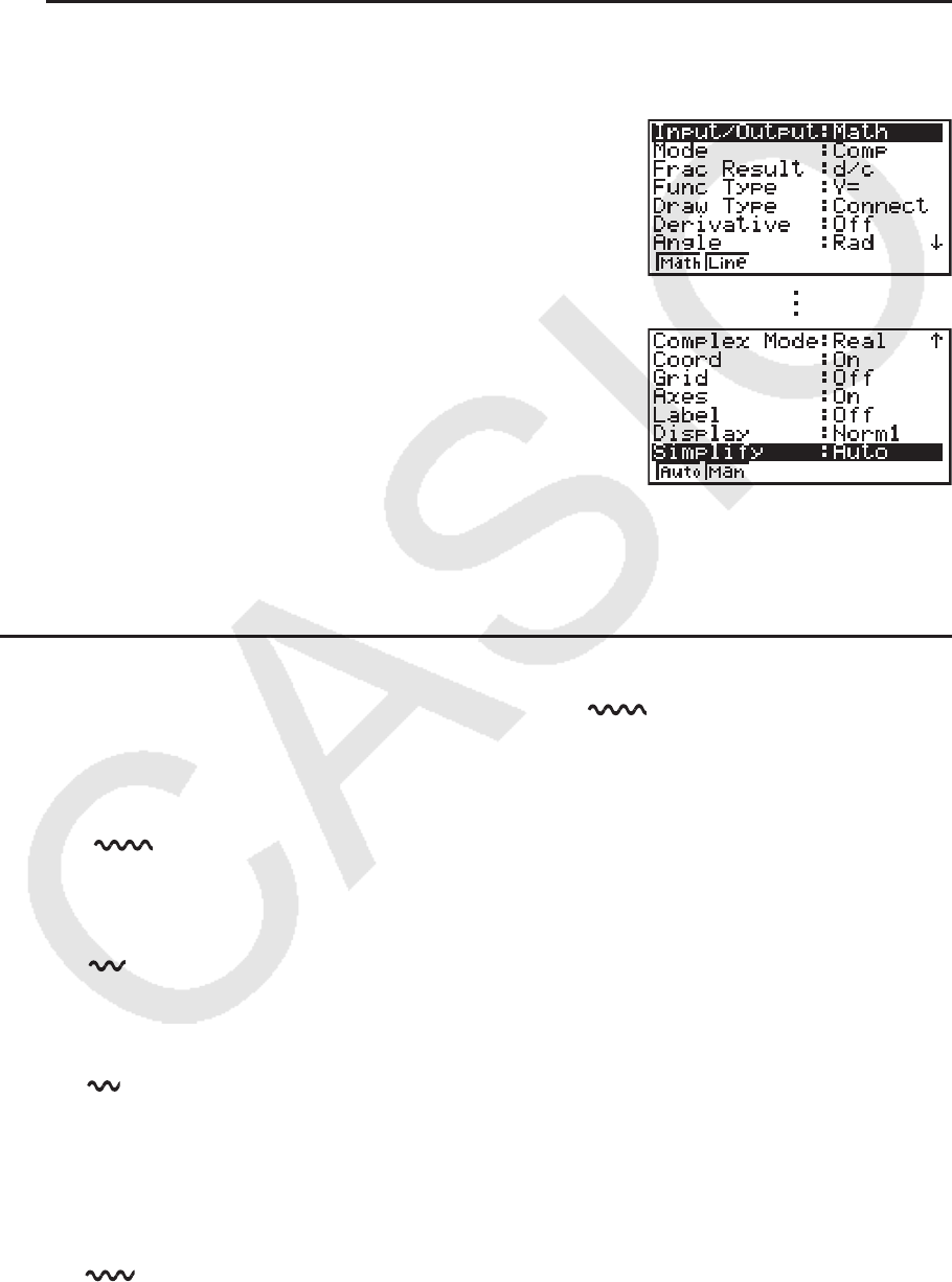
u Simplify(计算结果自动/手动减少规定)
• { Auto } / { Man } ... {自动减少并显示}/{显示但不减少}
u Q1Q3 Type(Q
1
/Q
3
计算公式)
• { Std } / { OnData } ... {使用低分组Q1的中位数和高分组Q3的中位数,在中点处在低分组与高分
组之间划分总体}/{生成累积频率比大于且最接近1/4 Q1的元素的值,以及累积频率比大
于且最接近3/4 Q3的元素的值}

1-29
fx-7400G II/fx-9750G II上不包括以下项目。
u Input/Output(输入/输出模式)
• { Math } / { Line } ... {数学}/{线性}输入/输出模式
u Auto Calc(电子表格自动计算)
• { On } / { Off } ... 自动{执行}/{不执行}公式
u Show Cell(电子表格单元格显示模式)
• { Form } / { Val } ... {公式}*
1
/{数值}
u Move(电子表格单元格光标方向) *
2
• { Low } / { Right } ... {向下移动}/{向右移动}
*
1
选择“Form”(公式)将使公式在单元格中的显示为公式。“Form”不会影响单元格中
的任何非公式数据。
*
2
指定在按下 w键以记录单元格输入、顺序命令生成数字表格以及从列表存储器中调用数据
时单元格光标的移动方向。
9. 使用屏幕捕捉
在操作计算器的任何时刻都可捕捉当前屏幕图像并将其保存到捕捉存储器中。
u 捕捉屏幕图像
1. 操作计算器并显示需要捕捉的屏幕。
2. 按下 !h(CAPTURE)。
• 由此可显示存储区选择对话框。
3. 输入1至20之间的一个值,然后按下 w。
• 由此可捕捉屏幕图像并将其保存到名为“Capt
n”( n = 输入值)的捕捉存储区域。
• 您不可捕捉显示正在进行操作或者数据图形的消息屏幕图像。
• 如果用于存储屏幕捕捉图像的主存储器空间不足,会产生一个存储器错误。

1-30
u 从捕捉存储器中调用屏幕图像
只有在选择线性输入/输出模式时才可执行该操作。
1. 在 RUN • MAT (或者 RUN )模式中,按下 K6( g)
6( g) 5(CAPT)( 4(CAPT)为fx-7400G
II上的对
应键) 1(RCL)。
2. 输入一个介于1至20的捕捉存储器编号,然后按下 w。
• 由此可显示在指定捕捉存储器中存储的图像。
3. 如需退出图像显示屏返回第1步的初始屏幕,按下 J。
• 您还可在程序中使用RclCapt命令从捕捉存储器中调用屏幕图像。
10. 如果问题仍然存在
如果您在尝试进行操作时发现问题未得以解决,请在确定计算器出现故障之前尝试以下操作。
k 使计算器恢复至原始模式设置
1. 在主菜单中,进入 SYSTEM 模式。
2. 按下 5(RSET)。
3. 按下 1(STUP),然后按下 1(Yes)。
4. 按下 Jm,返回主菜单。
现在进入正确模式并再次执行计算,监控显示屏上的结果。
k 重启和复位
u 重 启
如果计算器开始出现异常,您可通过按下RESTART按钮重新启动。但请注意,只有在不得已的
情况下才应使用RESTART按钮。通常,按下RESTART按钮会重新引导计算器的操作系统,因
此在计算器存储器中可保留程序、图形函数和其他数据。
fx-9860GⅡ SD
fx-9860GⅡ
fx-9860G AU PLUS
fx-9750GⅡ
fx-7400GⅡ
RESTART
按钮

1-31
重要!
关机时计算器备份用户数据(主存储器),开机时加载备份数据。
按下RESTART按钮时,计算器重新启动并加载备份数据。这表示,如果您在编辑程序、图形函
数或者其他数据之后按下RESTART按钮,任何尚未备份的数据都将丢失。
u 复 位
在您希望删除计算器存储器中的所有当前数据并将所有模式返回初始默认设置时,可使用复位
功能。
在执行复位操作之前,首先抄写所有重要数据。
有关详情,请参见“复位”(第12-3页)。
k 电池电量不足消息
如果显示屏上显示以下消息,请立即关闭计算器并按照说明更换电池。
如果您在未更换电池的情况下继续使用计算器,电源将自动关闭以保护存储器内容。一旦发生
这种情况,您将无法重新打开电源,而且存在存储器内容受到破坏或者完全丢失的危险。
• 一旦出现电池电量不足的消息,您将不能进行数据通信操作。

2-1
第2章 手动计算
1. 基本计算
k 算术计算
• 按照书写方式从左到右输入算术计算式。
• 使用 -键输入负值前的负号。
• 以15位尾数进行内部计算。结果在显示之前四舍五入至10位尾数。
• 对于混合算术运算,乘除优先于加减。
示例 操作
56 × (-12) ÷ (-2.5) = 268.8 56 *-12 /-2.5 w
(2 + 3) × 10
2= 500 (2 +3 )*1 E2 w
2 + 3 × (4 + 5) = 29 2 +3 *(4 +5 w*
1
4×5
6
= 0.3 6 /(4 *5 )w
*
1
最后的右括号(在操作 w键之前)可省略,无论需要多少。
k 小数位数、有效位数、正常显示范围
[SET UP]
-
[Display]
-
[Fix]
/
[Sci]
/
[Norm]
• 即使在您指定小数位数或者有效位数之后,仍然利用15位尾数进行内部计算,并存储显示数
值,尾数为10位。使用数值计算菜单栏(NUM)(第2-12页)的Rnd,可按照小数位数与有
效位数设置四舍五入显示数值。
• 通常,小数位数(Fix)和有效位数(Sci)设置保持有效,直至您改变它们或者改变正常显示
范围(Norm)设置。
例1 100 ÷ 6 = 16.66666666...
条件 操作 显示
100 /6 w 16.66666667
4位小数 !m(SET UP) ff
1(Fix) ewJw
16.6667
5个有效位 !m(SET UP) ff
2(Sci) fwJw
1.6667
E
+01
取消指定 !m(SET UP) ff
3(Norm) Jw
16.66666667
*
1
显示数值四舍五入至您指定的数位。
*1
*1
2

2-2
例2 200 ÷ 7 × 14 = 400
条件 操作 显示
200 /7 *14 w 400
3位小数 !m(SET UP) ff
1(Fix) dwJw
400.000
使用10位显示范围,
继续进行计算
200 /7 w
*
14 w
28.571
Ans ×
I
400.000
• 如果使用指定位数进行相同计算:
200 /7 w 28.571
内部存储的数值四舍五入至
在设置屏幕上指定的小数位
数。
K6( g) 4(NUM) * 4(Rnd) w
*
14 w
28.571
Ans ×
I
399.994
200 /7 w 28.571
您还可为特定计算指定内部
数值四舍五入的小数位数。
(示例:指定四舍五入至两位
小数)
6( g) 1(RndFi) !-(Ans) ,2 )
w
*
14 w
RndFix(Ans,2)
28.570
Ans ×
I
399.980
* fx-7400G
II: 3(NUM)
k 计算优先顺序
此计算器采用代数逻辑按照下述顺序计算公式中的各个部分:
1 A类函数
• 坐标转换Pol (
x, y), Rec ( r, Ƨ)
• 包括圆括号的函数(例如导数、积分、 ∑ 等等)
d/ dx、 d2
/ dx2
、 ∫ dx、 ∑ 、Solve、FMin、FMax、List → Mat、Fill、Seq、SortA、SortD、
Min、Max、Median、Mean、Augment、Mat → List、DotP、CrossP、Angle、UnitV、
Norm、P(、Q(、R(、t(、RndFix、log
a
b
• 复合函数*
1
、List、Mat、Vct、fn、 Y n、 r n、 X tn、 Y tn、 X n
2 B类函数
在使用这些函数时,先输入数值,然后按下功能键。
x2
、 x-1
、 x ! 、°’”、ENG符号,角度单位°、
r
、
g
3 幂/根 ^( xy),
x'
4 分数
a
b/
c
5 在 π 、存储器名称或者变量名称之前的缩写乘积形式。
2 π 、5A、Xmin、F Start等等。
6 C类函数
在使用这些函数时,先按下功能键,然后输入数值。
'、
3
'、log、ln、 ex、10
x、sin、cos、tan、sin
-1
、cos
-1
、tan
-
1
、sinh、cosh、tanh、sinh
-1
、cosh
-1
、tanh
-1
、(-)、 d、h、b、o、Neg、Not、Det、Trn、
Dim、Identity、Ref、Rref、Sum、Prod、Cuml、Percent、 AList、Abs、Int、Frac、Intg
、Arg、Conjg、ReP、ImP
2-3
7 A类函数、C类函数和圆括号之前的缩写乘积形式。
2 '3、A log2等等。
8 排列、组合
nP r、 nC r
9 度量转换命令
0 × 、÷、Int÷、Rnd
! +、-
@ 关系算子 =、 、>、<、 、
# And(逻辑算子)、and(位运算符)
$ Or、Xor(逻辑算子)、or、xor、xnor(位运算符)
*
1
您可将多个函数存储器(fn)位置或者图形存储器( Y n, r n, X tn, Y tn, X n)位置的内容组合
到复合函数中。例如,指定fn1(fn2)可产生复合函数fn1
°
fn2(参见第5-7页)。复合函数最
多可包含5个函数。
示例 2 + 3 × (log sin2 π 2
+ 6.8) = 22.07101691(角度单位 = Rad)
• 在RndFix计算式中,不能使用微分、二次微分、积分、 Σ 、最大/最小值、Solve、RndFix或
log
a
b计算表达式。
• 在使用一系列优先级别相同的函数时,从右向左执行计算。
exln 120 → ex{ln( 120 )}
否则,从左向右进行计算。
• 复合函数从右向左进行计算。
• 最先计算圆括号内的部分。
k 无理数计算结果显示 (仅限fx-9860G II SD/fx-9860G II /fx-9860G AU PLUS)
您可在设置屏幕中为“Input/Output”模式设置选择“Math”,配置计算器采用无理数格式显
示计算结果(包括 '或 π )。
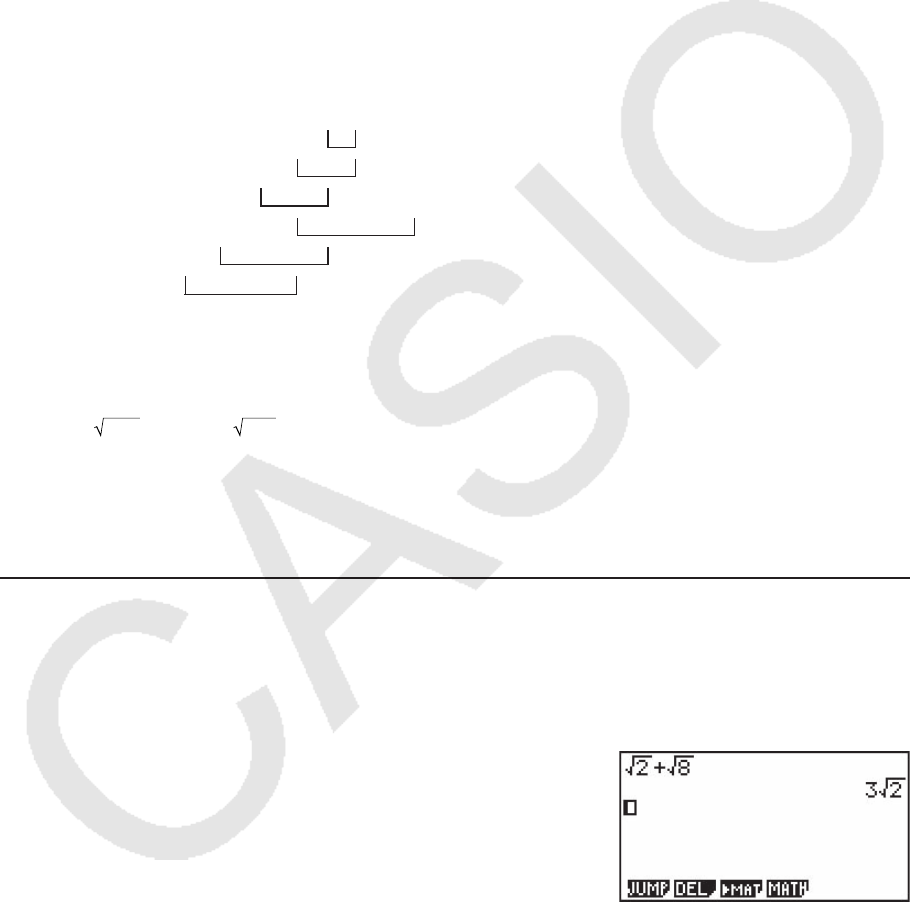
示例 '2 + '8 = 3 '2 (Input/Output: Math)
!x( ') ce+!x( ') iw
1
2
3
4
5
6

2-4
u 含有
'
的计算结果显示范围
使用 '格式的计算结果显示功能可用于最多两项包含 '的结果。 '格式的计算结果具有以下
某一形式。
± a'b、 ± d ± a'b、 ± a'
b
c ± d'
e
f
• 下面是每一个系数( a, b, c, d, e, f)可采用 ' 计算结果格式显示的范围。
1 <
a < 100, 1 < b < 1000, 1 < c < 100
0 <
d < 100, 0 < e < 1000, 1 < f < 100
• 在下例中,计算结果可采用 '格式,即使它们的系数(
a、 c、 d)已经超出上述范围。
'格式的计算结果使用公分母。
a'
b
c + d'
e
f → a
´
'
b
+
d
´
'
e
c
´
* c´是 c与 f的最小公倍数。
由于计算结果使用了一个公分母,计算结果仍可使用 '格式,即使系数( a´、 c´、 d´)超出对
应系数的范围(
a、 c、 d)。
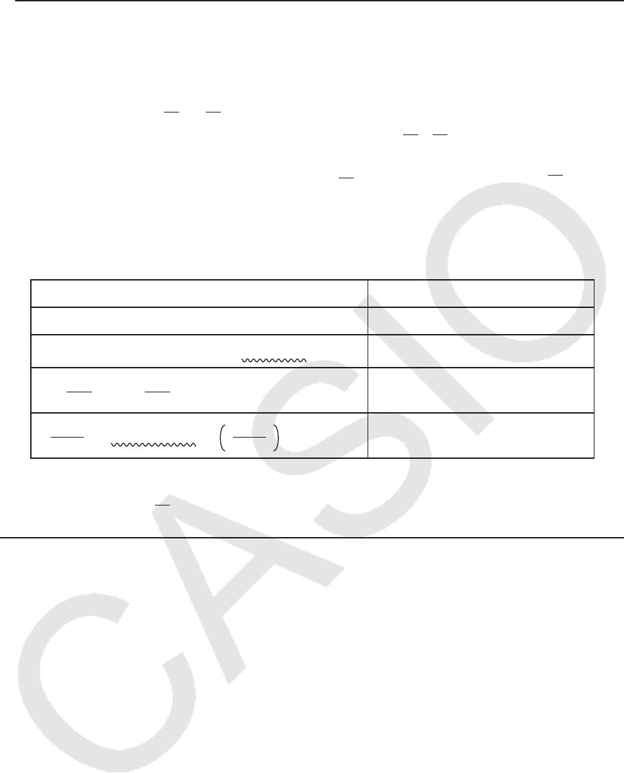
示例:
'
3
11
+
'
2
10
=
10'
3 + 11'
2
110
计算示例:
该计算: 产生此类显示:
2 × (3 - 2 '5) = 6 - 4 '5 '格式
35 '2 × 3 = 148.492424 (= 105 '2)*
1 小数格式
150
'
2
25 = 8.485281374*
1
23 × (5 - 2 '3) = 35.32566285 (= 115 - 46 '3)*
1 小数格式
'2 + '3 + '8= '3 + 3 '2 '格式
'
2 + '
3 + '
6 = 5.595754113*
2 小数格式
*
1
小数格式 - 因为数值超出了范围。
*
2
小数格式 - 因为计算结果有三项。
• 即使中间结果超过两项,也使用小数格式显示计算结果。
示例: (1 + '2 + '3) (1 - '2 - '3) (= - 4 - 2 '6)
= -8.898979486
• 如果计算公式有一个 '项和一个不能显示为分数的项,计算结果将采用小数格式显示。
示例:log3 + '2 = 1.891334817
2-5
u 使用
π
π 的计算结果显示范围
在以下情况下,使用 π 格式显示计算结果。
• 当计算结果可使用
nπ
n是一个最大为|10
6
|的整数。
• 当计算结果可使用ab
c π 或b
c π 格式显示时
但是,{
a位数+ b位数 + c位数}不得超过9(在减少上面的
ab
c 或 b
c 时)。*
1
*
2
同样, c的最大允
许位数为三。*
2
*
1
当 c < b时, a、 b和 c的位数在分数从假分数( b
c )转换为带分数时进行统计(
ab
c )。
*
2
在设置屏幕“Simplify”设置中指定“Manual”时,即使满足这些条件,也可使用小数格
式显示计算结果。
计算示例:
该计算: 产生此类显示:
78 π × 2 = 156 π π 格式
123456 π × 9 = 3490636.164 (= 11111104 π )*
3 小数格式
105
568
824 π = 105 71
103 π π 格式
2 258
3238 π = 6.533503684 129
1619 π2 *
4 小数格式
*
3
小数格式 - 因为计算结果整数部分不低于|10
6
|。
*
4
小数格式 - 因为ab
c π 形式的分母位数不小于四。
k 无乘号的乘法运算
在下述运算中,您可以省略乘号( × )。
• 在A类函数(第2-2页上的 1)和C类函数(第2-2页上的 6)之前,不包括负号
例1 2sin30、10log1.2、2'
3、2Pol(5, 12)等等
• 在常数、变量名称、存储器名称之前
例2 2 π 、2AB、3Ans、3Y
1 等等
• 在左圆括号之前
例3 3(5 + 6)、(A + 1)(B – 1)等等

2-6
如果您在执行一个包括除法和乘法运算的计算(其中乘号被略去),将自动插入括号,如下例
所示。
• 当乘号在左括号前或右括号后被略去。
例1 6 ÷ 2(1 + 2) → 6 ÷ (2(1 + 2))
6 ÷ A(1 + 2) → 6 ÷ (A(1 + 2))
1 ÷ (2 + 3)sin30 → 1 ÷ ((2 + 3)sin30)
• 当乘号在变量、常量等前被略去。
例2 6 ÷ 2π → 6 ÷ (2π)
2 ÷ 2'2 → 2 ÷ (2'2)
4π ÷ 2π → 4π ÷ (2π)
如果您在执行一个分数(包括带分数)前乘号被略去的计算,将自动插入括号,如下例所示。
示例 3
1
3
1
3
1
( )
(2 × ):2 → 2
示例
( )
5
4
5
4
5
4
(sin 2 × ):sin 2 → sin 2
k 溢出与错误
如果超出指定的输入或者计算范围,或者尝试进行非法输入,会导致显示屏出现错误消息。在
显示错误消息时,无法继续操作计算器。详情请参见第 α -1页上的“错误消息表”。
• 在显示错误消息时,大多数计算器键将失效。按下 J可清除错误并返回正常操作。
k 存储器容量
每次按下某个键时,使用一个或者两个字节。需要一个字节的函数包括: b、 c、 d、
sin、cos、tan、log、ln、 '和 π 。
需要两个字节的函数包括 d/ dx(、Mat、Vct、Xmin、If、For、Return、DrawGraph、
SortA(、PxlOn、Sum和
an+1
。
• 在线性输入/输出模式与数学输入/输出模式中输入函数与命令时所需的字节数不同。如需详细
了解在数学输入/输出模式中每一个函数所需的字节数,请参见第1-11页。
2. 特殊功能
k 使用变量计算
示例 操作 显示
193.2 aav(A) w 193.2
193.2 ÷ 23 = 8.4 av(A) /23 w 8.4
193.2 ÷ 28 = 6.9 av(A) /28 w 6.9
2-7
k 存储器
u 变量(字母存储器)
此计算器附带28个标准变量。您可使用变量存储计算式中需要使用的数值。变量以单字母名称
加以识别,包括字母表中的26个字母以及
r和 Ƨ。变量的最大赋值为尾数15位,指数2位。
• 即使在关闭电源时,也会保留变量内容。
u 为变量赋值
[数值] a [变量名称] w
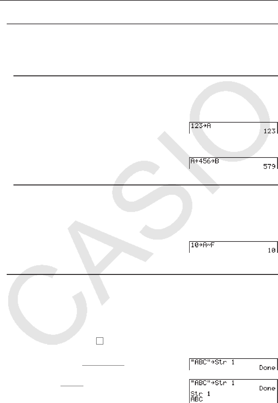
例1 指定变量A为123
Abcdaav(A) w
例2 变量A加456,将结果保存到变量B中
Aav(A) +efga
al(B) w
u 为多个变量指定相同数值
[数值] a [第一个变量名称] a3(~) [最后一个变量名称] w
•您不能使用“
r”或“ Ƨ”作为变量名称。
示例 为变量A至F指定数值10
Abaaav(A)
a3(~) at(F) w
u 字符串存储器
在字符串存储器中最多可存储20个字符串(名称为Str 1至Str 20)。存储的字符串可输出至显
示屏或者在其他支持字符串自变量的函数和命令中使用。
关于字符串操作的详情,请参见“字符串”(第8-18页)。
示例 为Str 1指定“ABC”,然后将Str 1输出至显示屏
A!a(A-LOCK) E(”) v(A)
l(B) I(C) E(”) a(释放字母锁定。)
aJ6( g) 5(Str) * bw
5(Str) * bw
* fx-7400G
II: 6(Str)
显示的字符串向左对齐。
2-8
• 在线性输入/输出模式中执行上述操作。该操作在数学输入/输出模式中不可执行。
u 函数存储器 [OPTN] - [FMEM]
函数存储器便于临时存储常用表达式。如需延长存储时间,我们建议您使用 GRAPH 模式存储表
达式,使用 PRGM 模式存储程序。
• { STO } / { RCL } / { fn } / { SEE } ... {函数存储}/{函数调用}/{函数区指定为表达式内的变量名称}/{函数
列表}
u 存储函数
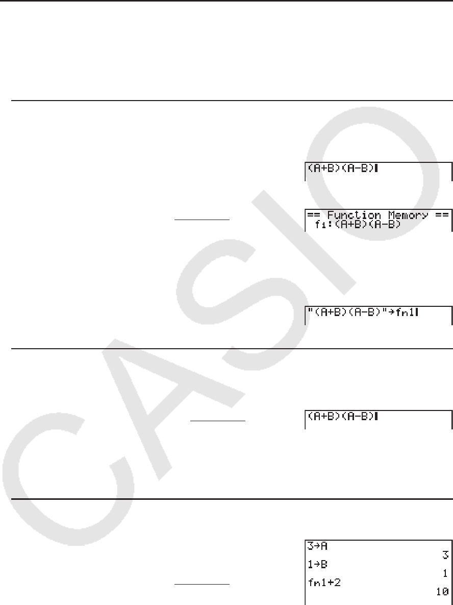
示例 将函数(A+B) (A–B)存储为1号函数存储器
(av(A) +al(B) )
(av(A) -al(B) )
K6( g) 6( g) 3(FMEM) *
1(STO) bw
* fx-7400G
II: 2(FMEM)
JJJ
• 如果您存储函数的函数存储器已经包含一个函数,则新函数替换前一个函数。
• 您可以使用 a在程序中将函数保存到函数存储器中。在这种
情况下,您必须使用双引号包括函数。
u 调用函数
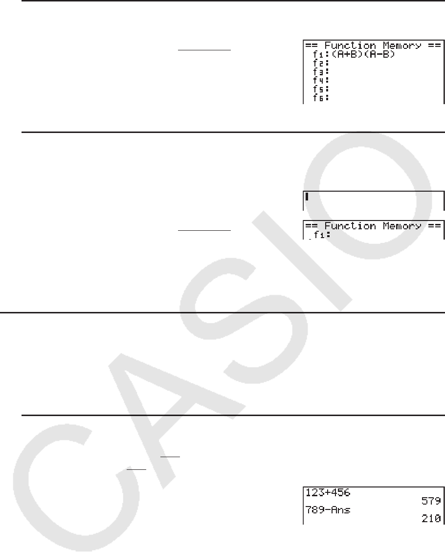
示例 调用1号函数存储器中的内容
AK6( g) 6( g) 3(FMEM) *
2(RCL) bw
* fx-7400G
II: 2(FMEM)
• 在显示屏上光标的当前位置处显示调用的函数。
u 调用作为变量的函数
Adaav(A) w
baal(B) w
K6( g) 6( g) 3(FMEM) * 3(fn)
b+cw
* fx-7400G
II: 2(FMEM)
2-9
u 显示可用函数列表
K6( g) 6( g) 3(FMEM) *
4(SEE)
* fx-7400G
II: 2(FMEM)
u 删除函数
示例 删除1号函数存储器中的内容
A
K6( g) 6( g) 3(FMEM) *
1(STO) bw
* fx-7400G
II: 2(FMEM)
• 在显示屏为空白时执行存储操作,将删除指定函数存储器中的函数。
k 答案功能
通过按下 w,答案功能可自动存储您计算所得的最新结果(除非 w键操作产生错误)。结果
存储在答案存储器中。
• 答案存储器中的最大值可保留15位尾数和2位指数。
• 按下 A键或关闭电源时,不会清除答案存储器中的内容。
u 在计算中使用答案存储器的内容
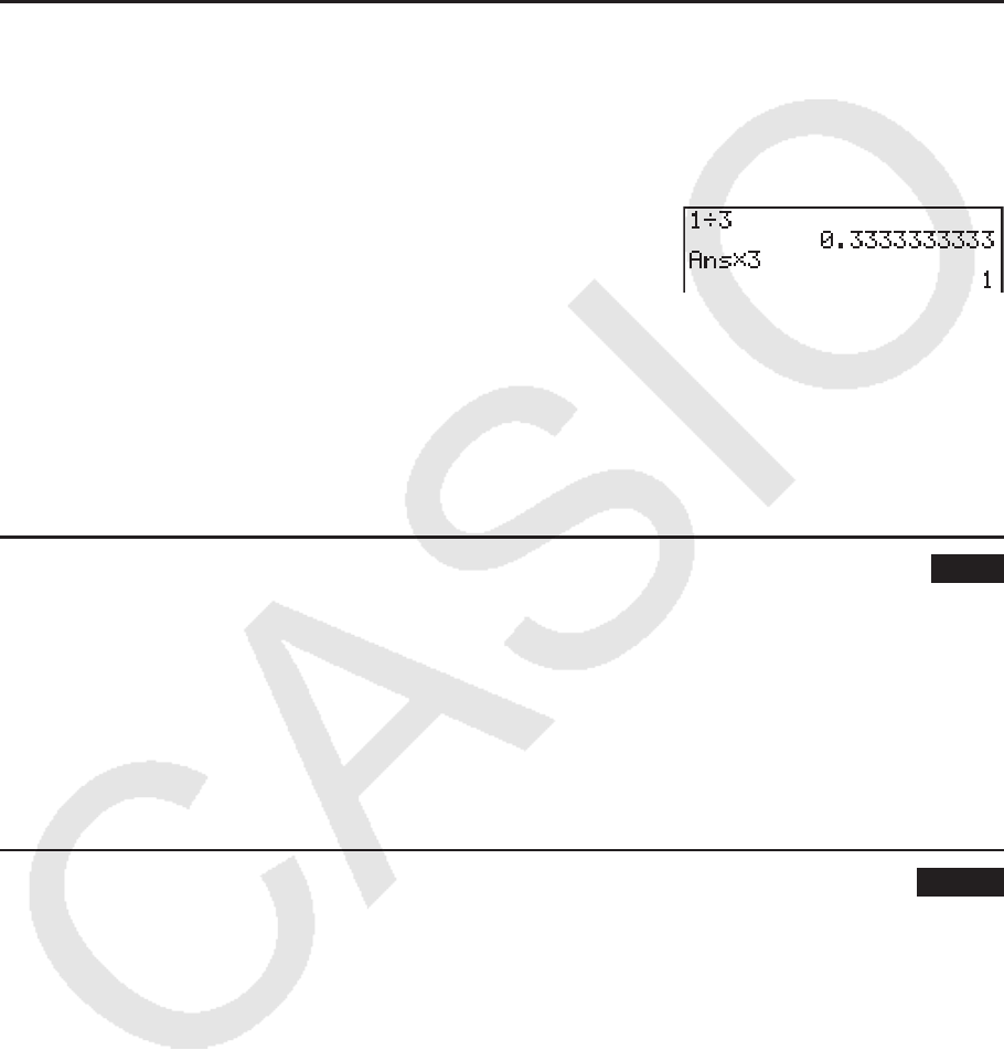
示例 123 + 456 = 579
789 - 579 = 210
Abcd+efgw
hij-!-(Ans) w
fx-7400G
II、fx-9750G II 用户
• 答案存储器内容不会因为字母存储器赋值操作而改变(例如: faal(B) w)。
2-10
fx-9860G II SD、fx-9860G II、fx-9860G AU PLUS 用户
• 在数学输入/输出模式中,调用答案存储器内容的操作与线性输入/输出模式中的操作不同。详
情请参见“历史功能”(第1-17页)。
• 执行为字母存储器(如 faal(B) w)赋值操作时,在数学输入/输出模式中将更新答
案存储器的内容,但在线性输入/输出模式中不会更新。
k 执行连续计算
答案存储器还可帮助您将某次计算的结果作为下一次计算的一个自变量。
示例 1 ÷ 3 =
1 ÷ 3 × 3 =
Ab/dw
(继续) *dw
连续计算也可与B类函数(
x2
、 x-1
、 x!,第2-2页)、+、-、^( xy)、
x'、° ' ”等等一起使用。
3. 指定角度单位和显示格式
在首次进行计算之前,您应该使用设置屏幕指定角度单位和显示格式。
k 设置角度单位 [SET UP] - [Angle]
1. 在设置屏幕上突出显示“Angle”。
2. 按下需要指定的角度单位对应的功能键,然后按下 J。
• { Deg } / { Rad } / { Gra } ... {度}/{弧度}/{百分度}
• 度、百分度与弧度之间的关系如下所示。
360°= 2 π 弧度 = 400 百分度
90°= π /2弧度 = 100 百分度
k 设置显示格式 [SET UP] - [Display]
1. 在设置屏幕上突出显示“Display”。
2. 按下需要设置的项目对应的功能键,然后按下 J。
• { Fix } / { Sci } / { Norm } / { Eng } ... {固定小数位数规定}/{有效位数规定}/{正常显示}/{工程模式}
2-11
u 指定小数位数(Fix)
示例 指定两位小数
1(Fix) cw
按下需要指定的小数位数( n = 0至9)对应的数字键。
• 显示数值四舍五入至您指定的小数位数。
u 指定有效位数(Sci)
示例 指定三个有效位
2(Sci) dw
按下需要指定的有效位数( n = 0至9)对应的数字键。如果指定0,则有效位数为10。
• 显示数值四舍五入至您指定的有效位数。
u 指定正常显示(Norm 1/Norm 2)
按下 3(Norm)在Norm 1与Norm 2之间转换。
Norm 1: 10
-2
(0.01) > | x|, | x| >10
10
Norm 2: 10
-9
(0.000000001) > | x|, | x| >10
10
u 指定工程记数法显示(Eng模式)
按下 4(Eng),在工程记数法与标准记数法之间切换。工程记数法生效时,显示屏上显示指示
符“/E”。
您可使用以下符号将数值转换为工程记数法,例如2000(= 2 × 10
3
) → 2k。
E(千兆兆) × 10
18 m(毫) × 10
-3
P(千万亿) × 10
15 μ (微) × 10
-6
T(万亿) × 10
12 n(毫微) × 10
-9
G(千兆) × 10
9 p(微微) × 10
-12
M(兆) × 10
6 f(毫微微) × 10
-15
k(千) × 10
3
• 工程记数法生效时,计算器自动选择一个工程符号以使尾数介于1至1000之间。

2-12
4. 函数计算
k 函数菜单
此计算器包括五个函数菜单,使您能够使用键面板上未印刷的科学函数。
• 在您按下 K键之前,函数菜单的内容因您通过主菜单进入的模式而异。下述例子显示了
在 RUN • MAT (或者 RUN )或者 PRGM 模式中显示的函数菜单。
u 双曲线计算(HYP) [OPTN] - [HYP]
• { sinh } / { cosh } / { tanh } ... 双曲线{正弦}/{余弦}/{正切}
• { sinh
-1
} / { cosh
-1
} / { tanh
-1
} ... 反双曲线{正弦}/{余弦}/{正切}
u 概率/分布计算(PROB) [OPTN] - [PROB]
• {
x!} ... {在输入一个数值之后按下,得到该数值的阶乘}
• {
nP r} / { nC r} ... {排列}/{组合}
• { RAND } ... {生成随机整数}
• { Ran# } / { Int } / { Norm } / { Bin } / { List } ... {生成随机数(0至1)}/{生成随机数}/{按照基于平均
值
ƫ和标准差 Ʊ的正态分布生成随机数}/{按照基于试验次数 n和概率 p的二项分布生成随机
数}/{生成随机数(0至1)和在ListAns中存储结果}
• { P (} / { Q (} / { R (} ... 正态概率{P(
t)}/{Q( t)}/{R( t)}
• {
t(} ... {正规化变量 t( x)的值}
u 数值计算(NUM) [OPTN] - [NUM]
• { Abs } ... {选择该项并输入数值,可得到该数值的绝对值}
• { Int } / { Frac } ... 选择该项并输入数值,可提取{整数}/{分数}部分。
• { Rnd } ... {将用于内部计算的数值四舍五入至10个有效位(与答案存储器中的数值相符),或者
四舍五入至您指定的小数位数(Fix)和有效位数(Sci)}
• { Intg } ... {选择该项并输入数值,可得到不大于此数值的最大整数。}
• { RndFi } ... {将用于内部计算的数值四舍五入至指定数位(0至9)(参见第2-2页)。}
• { GCD } ... {两个数值的最大公因子}
• { LCM } ... {两个数值的最小公倍数}
• { MOD } ... {除法余数(
n除以 m时的余数输出)}
• { MOD •
E } ... {幂值的除法余数( n的 p次方除以 m时的余数输出)}

2-13
u 角度单位、坐标变换、六十进制运算(ANGL) [OPTN] - [ANGL]
• { ° } / { r } / { g } ... 某个特定输入数值的{度}/{弧度}/{百分度}
• { ° ’ ” } ... {当输入一个度/分/秒数值时指定度(小时)、分钟、秒}
• {
° ’ ”
} ... {将十进制数值转换为度/分/秒数值}
• {
° ’ ”
} 菜单操作只有在显示屏显示计算结果时可用。
• { Pol( } / { Rec( } ... {直角坐标至极坐标}/{极坐标至直角坐标}的坐标转换
• { 'DMS } ... {将十进制数值转换为六十进制数值}
u 工程符号(ESYM) [OPTN] - [ESYM]
• { m } / {
} / { n } / { p } / { f } ...{毫(10
-3
)}/{微(10
-6
)}/{毫微(10
-9
)}/{微微(10
-12
)}/{毫微微
(10
-15
)}
• { k } / { M } / { G } / { T } / { P } / { E } ...{千(10
3
)}/{兆(10
6
)}/{千兆(10
9
)}/{万亿(10
12
)}/{千万亿
(10
15
)}/{千兆兆(10
18
)}
• { ENG } / { ENG } ... 将显示数值的小数位数向{左}/{右} 移动三位并将指数{减少}/{增大}三。
当您使用工程记数法时,工程符号也会相应地发生改变。
• {ENG}和{ENG}菜单操作只有在显示屏显示计算结果时可用。
k 角度单位
• 务必在设置屏幕将模式设置为Comp。
示例 操作
将4.25弧度转换为度:
243.5070629
!m(SET UP) cccccc* 1(Deg) J
4.25 K6( g) 5(ANGL) ** 2(r) w
47.3° + 82.5rad = 4774.20181° 47.3 +82.5 K6( g) 5(ANGL) ** 2(r) w
2°20´30˝ + 39´30˝ = 3°00´00˝ 2 K6( g) 5(ANGL) ** 4(° ’ ”) 20 4(° ’ ”) 30
4(° ’ ”) +0 4(° ’ ”) 39 4(° ’ ”) 30 4(° ’ ”)
w 5(
° ’ ”
)
2.255° = 2°15´18˝ 2.255 K6( g) 5(ANGL) ** 6( g) 3( 'DMS) w
* fx-7400G
II, fx-9750G II: ccccc ** fx-7400G II: 4(ANGL)
k 三角函数与反三角函数
• 在进行三角函数与反三角函数计算之前,必须设置角度单位。
(90°
= 弧度 = 100 百分度)
π
2

2-14
• 务必在设置屏幕将模式设置为Comp。
示例 操作
cos (
π
3
rad) = 0.5 !m(SET UP) cccccc* 2(Rad) J
c(!E( π ) /3 )w
2 •
sin 45° × cos 65° = 0.5976724775 !m(SET UP) cccccc* 1(Deg) J
2 *s45 *c65 w*
1
sin
-1
0.5 = 30°
(
当sin x = 0.5时的x)
!s(sin
-1
) 0.5 *
2
w
*
1
*可省略。 * fx-7400G II,fx-9750G II: ccccc
*
2
不必输入前导零。
k 对数函数与指数函数
• 务必在设置屏幕将模式设置为Comp。
示例 操作
log 1.23 (log
10
1.23) = 0.08990511144 l1.23 w
log
2
8 = 3 K4(CALC) * 6( g) 4(log
a
b) 2 ,8 )w
(-3)
4
= (-3) × (-3) × (-3) × (-3) = 81 (-3 )M4 w
7
123 (= 123
1
7
) = 1.988647795 7 !M(
x') 123 w
* fx-7400G
II: 3(CALC)
• 在连续输入两个或者多个幂时,线性输入/输出模式与数学输入/输出模式会产生不同的结果,
例如:2 M3 M2。
线性输入/输出模式: 2^3^2 = 64 数学输入/输出模式:
232 = 512
这是因为数学输入/输出模式在内部将上述输入处理为:2^(3^(2))。
k 双曲线函数与反双曲线函数
• 务必在设置屏幕将模式设置为Comp。
示例 操作
sinh 3.6 = 18.28545536 K6( g) 2(HYP) * 1(sinh) 3.6 w
cosh
-1
20
15 = 0.7953654612 K6( g) 2(HYP) * 5(cosh
-1
) (20 /15 )w
* fx-7400G
II: 1(HYP)

2-15
k 其它函数
• 务必在设置屏幕将模式设置为Comp。
示例 操作
'2 + '5 = 3.65028154 !x( ') 2 +!x( ') 5 w
(-3)
2
= (-3) × (-3) = 9 (-3 )xw
8! (= 1 × 2 × 3 × .... × 8) = 40320 8 K6( g) 3(PROB) *
1
1( x!) w
-3.5的整数部分是什么?
-3
K6( g) 4(NUM) *
2
2(Int) -3.5 w
*
1
fx-7400G II: 2(PROB) *
2
fx-7400G II: 3(NUM)
k 生成随机数(RAND)
u 生成随机数(0至1)(Ran#,RanList#)
Ran#和RanList#可随机或从0到1生成10位随机数。Ran#返回单个随机数,而RanList#以列表
形式返回多个随机数。下面显示了Ran#和RanList#的语法。
Ran# [a] 1 <
a < 9
RanList# (n [,a]) 1 <
n < 999
•
n 是尝试次数。RanList# 生成的随机数个数对应于 n,同时在ListAns屏幕上显示这些随机
数。必须输入
n数值。
• “
a”是随机序列。如果不输入“ a”,则返回随机数。如果将 a设置为1至9之间的某个整数,
返回对应个数的顺序随机数。
• 执行函数Ran#0可初始化Ran#和RanList#序列。在使用与前一次执行Ran#或RanList#不同
的序列生成顺序随机数时,或在生成某个随机数时也可初始化序列。
Ran#示例
示例 操作
Ran#
(生成一个随机数。)
K6( g) 3(PROB) * 4(RAND)
1(Ran#) w
(每次按下 w都会生成一个新的随机数。) w
w
Ran# 1
(生成序列1中的第一个随机数。)
(生成序列1中的第二个随机数。)
K6( g) 3(PROB) * 4(RAND)
1(Ran#) 1 w
w
Ran# 0
(初始化序列。)
Ran# 1
(生成序列1中的第一个随机数。)
1(Ran#) 0 w
1(Ran#) 1 w
* fx-7400G
II: 2(PROB)
2-16
RanList#示例
示例 操作
RanList# (4)
(生成四个随机数并在ListAns屏幕中显示结
果。)
K6( g) 3(PROB) * 4(RAND) 5(List)
4 )w
RanList# (3, 1)
(生成序列1的第一个到第三个随机数并在
ListAns屏幕中显示结果。)
JK6( g) 3(PROB) * 4(RAND)
5(List) 3 ,1 )w
(然后生成序列1的第四个到第六个随机数并
在ListAns屏幕中显示结果。)
Jw
Ran# 0
(初始化序列。)
J1(Ran#) 0 w
RanList# (3, 1)
(重新生成序列1的第一个到第三个随机数并
在ListAns屏幕中显示结果。)
5(List) 3 ,1 )w
* fx-7400G
II: 2(PROB)
u 生成随机整数(RanInt#)
RanInt#生成两个指定整数之间的随机整数。
RanInt# (A, B [,n]) A < B |A|,|B| < 1
E 10 B ï A < 1 E 10 1 < n < 999
• A为初值,B为终值。不输入
n值则原样返回生成的随机数。指定 n值,则以列表形式返回指定
个数的随机值。
示例 操作
RanInt# (1, 5)
(生成1至5之间的一个随机整数。)
K6( g) 3(PROB) * 4(RAND) 2(Int)
1 ,5 )w
RanInt# (1, 10, 5)
(生成1至10之间的五个随机整数并在ListAns
屏幕中显示结果。)
K6( g) 3(PROB) * 4(RAND) 2(Int)
1 ,10 ,5 )w
* fx-7400G
II: 2(PROB)
u 按照正态分布生成随机数(RanNorm#)
该函数按照基于指定平均值 ƫ和标准差 Ʊ值的正态分布生成一个10位随机数。
RanNorm# (
Ʊ, ƫ [,n]) Ʊ > 0 1 < n < 999
• 不输入
n 值则原样返回生成的随机数。指定 n值,则以列表形式返回指定个数的随机值。
2-17
示例 操作
RanNorm# (8, 68)
(按照平均身长为68cm和标准差为8的一组
一周岁以下婴儿的正态分布,随机生成一个
身长值。)
K6( g) 3(PROB) * 4(RAND) 3(Norm)
8 ,68 )w
RanNorm# (8, 68, 5)
(随机生成上例中的五个婴儿身长值并在列表
中显示。)
K6( g) 3(PROB) * 4(RAND) 3(Norm)
8 ,68 ,5 )w
* fx-7400G
II: 2(PROB)
u 按照二项分布生成随机数(RanBin#)
该函数按照基于试验次数 n和概率 p的二项分布生成随机整数。
RanBin# (n, p [,m]) 1 <
n < 100000 1 < m < 999 0 < p < 1
• 不输入
m值则原样返回生成的随机数。指定 m值,则以列表形式返回指定个数的随机值。
示例 操作
RanBin# (5, 0.5)
(按照正面概率为0.5的五次掷硬币的二项分
布,随机生成出现正面的次数。)
K6( g) 3(PROB) * 4(RAND) 4(Bin)
5 ,0.5 )w
RanBin# (5, 0.5, 3)
(执行三次上述掷硬币程序,在列表中显示
结果。)
K6( g) 3(PROB) * 4(RAND) 4(Bin)
5 ,0.5 ,3 )w
* fx-7400G
II: 2(PROB)
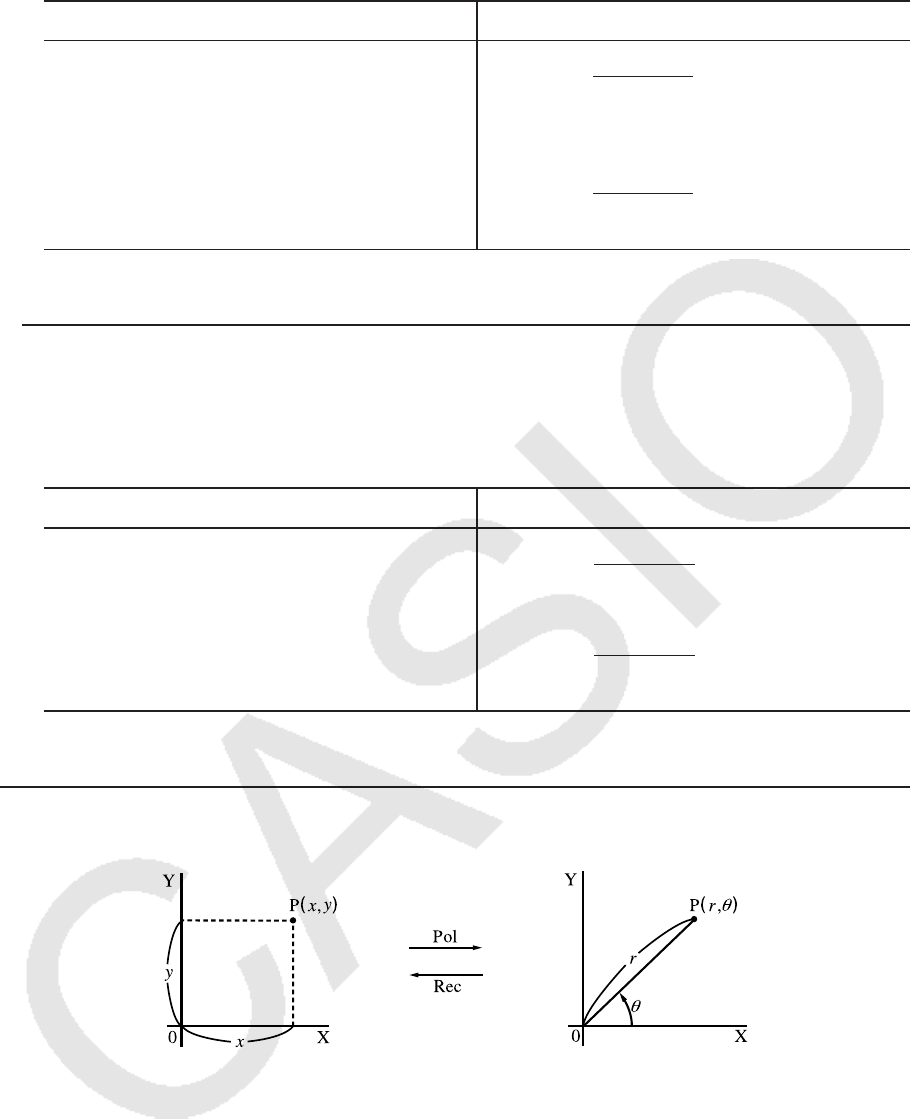
k 坐标转换
u 直角坐标 u 极坐标
• 使用极坐标, Ƨ的计算和显示范围为-180°< Ƨ < 180°(弧度与百分度的范围相同)。
• 务必在设置屏幕将模式设置为Comp。

2-18
示例 操作
计算
r和 Ƨ°(当 x = 14且 y = 20.7时)
!m(SET UP) cccccc*
1(Deg) J
K6( g) 5(ANGL) ** 6( g) 1(Pol()
14 ,20.7 )wJ
计算
x和 y(当 r = 25且 Ƨ = 56°时)
2(Rec() 25 ,56 )w
* fx-7400G
II, fx-9750G II: ccccc ** fx-7400G II: 4(ANGL)
k 排列与组合
u 排列 u 组合
• 务必在设置屏幕将模式设置为Comp。
例1 从10项中选择4项,计算可能的不同排列数
公式 操作
10 P 4 = 5040 10 K6( g) 3(PROB) * 2(n P r ) 4 w
* fx-7400G
II: 2(PROB)
例2 从10项中选择4项,计算可能的不同组合数
公式 操作
10 C 4 = 210 10 K6( g) 3(PROB) * 3( n C r ) 4 w
* fx-7400G
II: 2(PROB)
k 最大公因子(GCD),最小公倍数(LCM)
示例 操作
确定28和35的最大公因子
(GCD (28, 35) = 7)
K6( g) 4(NUM) * 6( g) 2(GCD) 28 ,
35 )w
确定9与15的最小公倍数
(LCM (9, 15) = 45)
K6( g) 4(NUM) * 6( g) 3(LCM) 9 ,15
)w
* fx-7400G
II: 3(NUM)
1 24.989 → 24.98979792 (r)
2 55.928 → 55.92839019 ( )
θ
1 13.979 → 13.97982259 (x)
2 20.725 → 20.72593931 (y)
n!n!
nPr=nCr=
(
n–r)! r!(
n–r
)!

2-19
k 除法余数(MOD),指数除法余数(MOD Exp)
示例 操作
确定137除以7的余数
(MOD (137, 7) = 4)
K6( g) 4(NUM) * 6( g) 4(MOD) 137 ,7
)w
确定5
3
除以3的余数
(MOD
•
E (5, 3, 3) = 2)
K6( g) 4(NUM) * 6( g) 5(MOD
•
E)
5 ,3 ,3 )w
* fx-7400G
II: 3(NUM)
k 分 数
• 在数学输入/输出模式中,分数输入方法与下述方法不同。关于在数学输入/输出模式中的分数
输入操作,参见第1-11页。
• 务必在设置屏幕将模式设置为Comp。
示例 操作
2 1 73
+3 =
5 4 20
= 3.65(转换为小数)*
1
2 $5 +3 $1 $4 w
M
1 1
+
2578 4572 = 6.066202547 × 10
-4
*
2 1 $2578 +1 $4572 w
1
2
× 0.5 = 0.25*
3 1 $2 *.5 w
*
1
分数和小数可相互转换。
*
2
当总字符数(包括整数,分子、分母与分隔符)超过10时,输入的分数自动转换为小数格
式。
*
3
包含分数与小数的计算以小数格式计算。
• 按下 !M(
<)键可在带分数与假分数格式之间切换分数显示。
k 工程记数法计算
使用工程记数法菜单输入工程符号。
• 务必在设置屏幕将模式设置为Comp。
示例 操作
999k(千)+ 25k (千)
= 1.024M(兆)
!m(SET UP) ff4(Eng) J999 K6( g) 6( g)
1(ESYM) * 6( g) 1(k) +25 1(k) w
9 ÷ 10 = 0.9 = 900m(毫)
= 0.9
9 /10 w
K6( g) 6( g) 1(ESYM) * 6( g) 6( g) 3(ENG)*1
2-20
= 0.0009k(千)
= 0.9
= 900m
3(ENG)*
1
2(ENG)*
2
2(ENG)*
2
* fx-7400G II: 5(ESYM)
*
1
将小数点向右移动三位,将显示的数值转换为较高一级工程单位。
*
2
将小数点向左移动三位,将显示的数值转换为较低一级工程单位。
k 逻辑算子(AND、OR、NOT、XOR) [OPTN] - [LOGIC]
逻辑算子菜单提供逻辑算子选项。
• { And } / { Or } / { Not } / { Xor } ... {逻辑AND}/{逻辑OR}/{逻辑NOT}/{逻辑XOR}
• 务必在设置屏幕将模式设置为Comp。
示例 当A = 3 且 B = 2时,A和B的逻辑AND是什么?A AND B = 1
操作 显示
3 aav(A) w
2 aal(B) w
av(A) K6( g) 6( g)
4(LOGIC) * 1(And) al(B) w
1
* fx-7400G
II: 3(LOGIC)
u 关于逻辑运算
• 逻辑运算的结果总是为0或者1。
• 下表显示了AND、OR和XOR运算可能产生的所有结果。
数值或者表达式A 数值或者表达式B A AND B A OR B A XOR B
A 0 B 0 1 1 0
A 0 B = 0 0 1 1
A = 0 B 0 0 1 1
A = 0 B = 0 0 0 0
• 下表显示了NOT运算产生的结果。
数值或者表达式A NOT A
A 0 0
A = 0 1
2-21
5. 数值计算
下面说明在按下 K4(CALC)( 3(CALC)为fx-7400G II上的对应键)时,显示的函数菜单
中包括的数值计算功能。可执行以下计算。
• { Int÷ } / { Rmdr } / { Simp } ... {商}/{余数}/{简化}
• { Solve } / {
d/ dx} / { d2
/ dx2
} / { ∫ dx} / { SolvN } ... {等式解}/{微分}/{二次微分}/{积分}/{ f( x) 函数解}
• { FMin } / { FMax } / { Σ ( } / { log
a
b } ... {最小值}/{极大值}/{求和}/{对数log
a
b}
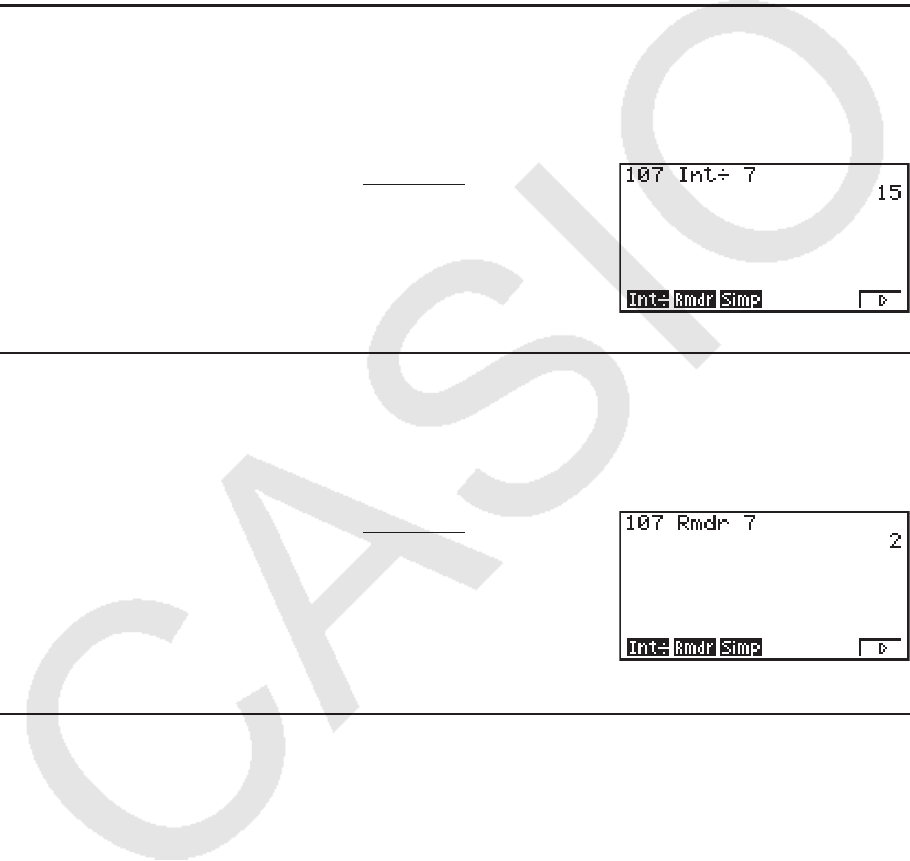
k 整数除以整数的商 [OPTN] - [CALC] - [Int÷]
“Int÷”函数可用于确定一个整数除以另一个整数得到的商。
示例 计算107 ÷ 7的商
AbahK4(CALC) * 6( g)
6( g) 1(Int÷) h
w
* fx-7400G
II: 3(CALC)
k 整数除以整数的余数 [OPTN] - [CALC] - [Rmdr]
“Rmdr”函数可用于确定一个整数除以另一个整数得到的余数。
示例 计算107 ÷ 7的余数
AbahK4(CALC) * 6( g)
6( g) 2(Rmdr) h
w
* fx-7400G
II: 3(CALC)
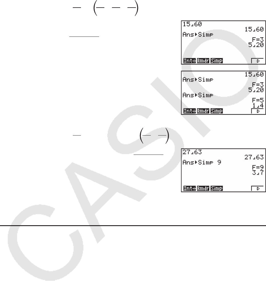
k 简化 [OPTN] - [CALC] - [Simp]
“ 'Simp”函数可用于手动简化分数。以下运算可用于在屏幕上显示未简化计算结果时执行简
化。
• { Simp } w ... 该函数可使用最小素数自动简化显示的计算结果。使用素数并在显示屏上显示简
化结果。
• { Simp }
n w ... 该函数按照指定的因子 n执行简化。
2-22
在初始默认设置下,此计算器在显示分数计算结果之前自动简化。在执行下面的计算示例之
前,使用设置屏幕将“Simplify”设置从“Auto”改为“Manual”(第1-28页)。
• 在设置屏幕中将“Complex Mode”设置为“a+b
i”或者“ r∠
θ
”时,即使“Simplify”设置
为“Manual”,分数计算结果在显示之前都会简化。
• 如果您希望手动简化分数(Simplify: Manual),确保“Complex Mode”设置为“Real”。
例1 简化 15
60 ==
15
60
5
20
1
4
Abf$gaw
K4(CALC) * 6( g) 6( g) 3(Simp) w
* fx-7400G II: 3(CALC)
3(Simp) w
“F=”值为因子。
例2 简化 27
63 并指定9作为因子 =
27
63
3
7
Ach$gdwK4(CALC) *
6( g) 6( g) 3(Simp) jw
* fx-7400G II: 3(CALC)
• 如果使用指定的因子不能执行简化,则产生一个错误。
• 在显示无法简化的值时执行 'Simp将返回初始值,而不显示“F=”。
k 求解计算 [OPTN] - [CALC] - [Solve]
下面是在程序中使用Solve函数的语法。
Solve( f( x), n, a, b) ( a:下限, b:上限, n:初始估计值)
在求解计算中有两种不同的输入方法:直接分配法和变量表输入法。
直接分配法(在此说明的方法)就是将数值之间赋给变量。这种输入方法与 PRGM 模式中Solve
命令使用的方法完全相同。

2-23
变量表输入法用于 EQUA 模式中的Solve函数。对于大多数Solve函数输入,推荐使用这种输入方
法。
在解不收敛时,会产生一个错误(Time Out)。
关于求解计算的说明,请参见第4-4页。
• 在上述任何一种函数中都不可使用二次微分、 ∑ 、最大/最小值或求解计算表达式。
• 在求解计算期间按下 A(显示屏上没有显示光标)会中断计算。
k 求解 f( x)函数 [OPTN] - [CALC] - [SolvN]
您可使用SolvN通过数值分析求解
f( x)函数。下面是输入语法。
SolvN (左侧[=右侧] [,变量] [, 下限, 上限])
• 右侧、变量、下限和上限都可省略。
• “左侧[=右侧]”是需要求解的表达式。支持的变量包括A至Z、
r和
θ
。在省略右侧时,按照右
侧 = 0求解。
• 变量指定需要求解的表达式中的变量(A至Z、
r、
θ
)。省略变量规定将采用X作为变量。
• 下限和上限规定了解的范围。您可输入数值或者表达式以规定范围。
• 以下函数不得在任何自变量中使用。
Solv(、
d2
/ dx2
、FMin(、FMax(、 ∑ (
在ListAns格式中,最多可同时显示10个计算结果。
• 如果没有解,显示消息“No Solution”。
• 如果可能存在与SolvN显示结果不同的解,显示“More solutions may exist.”。
示例 求解
x2
- 5 x- 6 = 0
K4(CALC) * 5(SolvN)
vx-fv-g)w
* fx-7400G II: 3(CALC)
J

2-24
k 微分计算 [OPTN] - [CALC] - [ d/ dx]
在进行微分计算时,首先显示函数分析菜单,然后按照下述语法输入数值。
K4(CALC) * 2( d/ dx) f( x) ,a,tol) * fx-7400G II: 3(CALC)
(
a:需要确定导数的点, tol:公差)
此类计算的微分定义为:
在该定义中, 无穷小 由 足够小的 Ax替代,f
'
( a)的邻近值计算如下:
为了尽可能提高精度,计算器使用中心差分法进行微分计算。
示例 确定在点
x = 3处,函数 y = x3
+ 4 x2
+ x - 6的导数,公差为
“
tol”= 1 E - 5
输入函数 f( x)。
AK4(CALC) * 2(
d/ dx) vMd+evx+v-g,
* fx-7400G
II: 3(CALC)
输入需要确定导数的点
x = a。
d,
输入公差值。
bE-f)w
在图形函数中使用微分计算
• 在图形函数中使用微分命令时省略公差( tol)值可简化图形绘制的计算。在这种情况下,为
加快绘制速度,精度会有所降低。如果指定公差值,在绘制图形时可达到正常执行微分计算时
的同等精度。
• 您还可在微分图形中使用以下格式,省略导数点的输入:Y2=
d/ dx(Y1)。在这种情况下,X值作
为导数点。
微分计算注意事项
• 在函数 f( x)中,只有X可作为表达式中的变量。其它变量(A至Z、不包括X、 r、 Ƨ)作为常
量,计算期间使用变量的当前指定值。
• 可不输入公差(
tol)值和右圆括号。如果省略公差( tol)值,计算器自动将 tol设置为1 E -10。
• 指定公差(
tol)值不小于1 E -14。如果解不能达到公差要求,就产生一个错误(Time Out)。
• 在微分计算期间按下 A(显示屏上没有显示光标)会中断计算。
d/dx (
f (x), a) ⇒f (a)
dx
d
f(a+Ax)–f(a)
f (a) = lim –––––––––––––
Ax
Ax→0
'
f(a+Ax)–f(a)
f (a) –––––––––––––
Ax
'
ⱌ

2-25
• 导致结果不准确和错误的可能原因包括:
-
x值中包含不连续点
-
x值剧烈波动
-
x值中包含局部极大值点和局部极小值点
-
x值中包含拐点
-
x值中包含不可微分点
- 微分计算结果趋近于零
• 在执行三角微分时,必须使用弧度(Rad模式)作为角度单位。
• 在微分计算式中,不能使用微分、二次微分、积分、 ∑ 、最大/最小值、求解、RndFix或log
a
b
计算表达式。
• 在数学输入/输出模式中,公差值固定为1
E -10,不可更改。
k 二次微分计算 [OPTN] - [CALC] - [ d2
/ dx2
]
在显示函数分析菜单之后,您可使用以下语法输入二次微分。
K4(CALC) * 3( d2
/ dx2
) f( x) ,a,tol) * fx-7400G II: 3(CALC)
(
a:微分系数点, tol:公差)
利用下述二阶微分公式,二次微分计算可以得出近似微分值,该公式的基础是牛顿的多项式内
插法。
在该表达式中,“
h的足够小增量”用于获取近似值 f
"
( a)。
示例 确定在
x = 3处,函数 y = x3
+ 4 x2
+ x - 6 的二次微分系数。
在此,我们使用的公差值
tol = 1 E - 5
输入函数 f( x)。
AK4(CALC) * 3(
d2
/ dx2
) vMd+evx+v-g,
* fx-7400G
II: 3(CALC)
输入3作为点 a,即微分系数点。
d,
输入公差值。
bE-f)
w
二次微分计算注意事项
• 在函数 f( x)中,只有X可作为表达式中的变量。其它变量(A至Z、不包括X、 r、 Ƨ)作为常
量,计算期间使用变量的当前指定值。
d
2
d
2
––– ( f(x), a)⇒––– f(a)
dx
2
dx
2
f
''(a)
=
180h
2
2 f(a + 3h) – 27 f(a + 2h) + 270 f(a + h) – 490 f(a) + 270 f(a – h) – 27 f(a –2h) + 2 f(a – 3h)
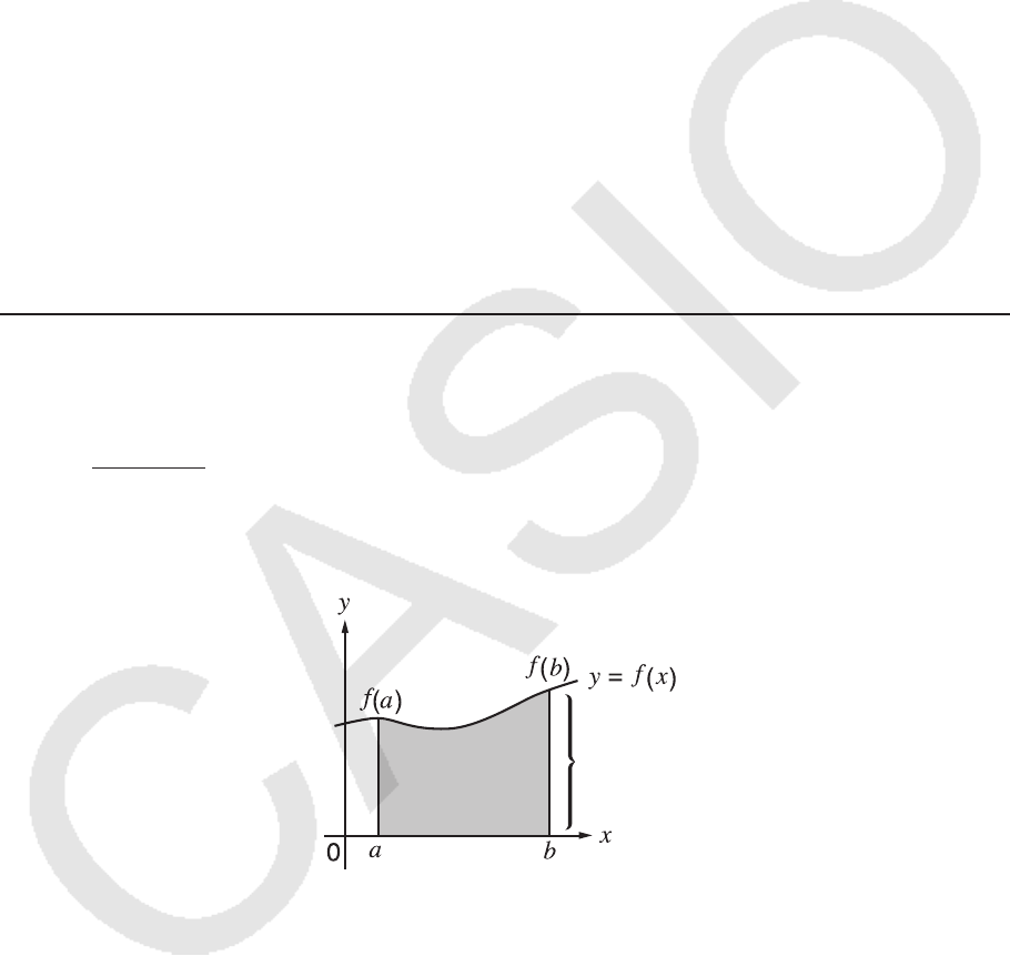
2-26
• 可不输入公差( tol)值和右圆括号。
• 指定公差(
tol)值不小于1 E -14。只要解不能达到公差要求,就产生一个错误(Time Out)。
• 在使用二次微分计算图形公式时,线性微分规则同样适用(第2-24页)。
• 导致结果不准确和错误的可能原因包括:
-
x值中包含不连续点
-
x值剧烈波动
-
x值中包含局部极大值点和局部极小值点
-
x值中包含拐点
-
x值中包含不可微分点
- 微分计算结果趋近于零
• 您可通过按下 A键中断正在执行的二次微分计算。
• 在执行三角二次微分时,必须使用弧度(Rad模式)作为角度单位。
• 在二次微分计算式中,不能使用微分、二次微分、积分、 ∑ 、最大/最小值、求解、RndFix或
log
a
b计算表达式。
• 在二次微分计算中,计算精度最高可达五位尾数。
• 在数学输入/输出模式中,公差值固定为1
E -10,不可更改。
k 积分计算 [OPTN] - [CALC] - [ ∫ dx]
在进行积分计算时,首先显示函数分析菜单,然后按照下述语法输入数值。
K4(CALC) * 4( ∫ dx) f( x) , a , b , tol ) * fx-7400G II: 3(CALC)
(
a: 起点,
b: 终点,
tol: 公差)
计算
∫
a
b
f(x)dx
的面积
如上图所示,通过计算从
a到 b的函数 y = f ( x)的积分值(其中 a < x < b且 f ( x) > 0)完成积分计
算。实际上是计算图中阴影部分的面积。
∫
(f(x), a,
b
,
tol)⇒
∫
a
b f(x)d
x
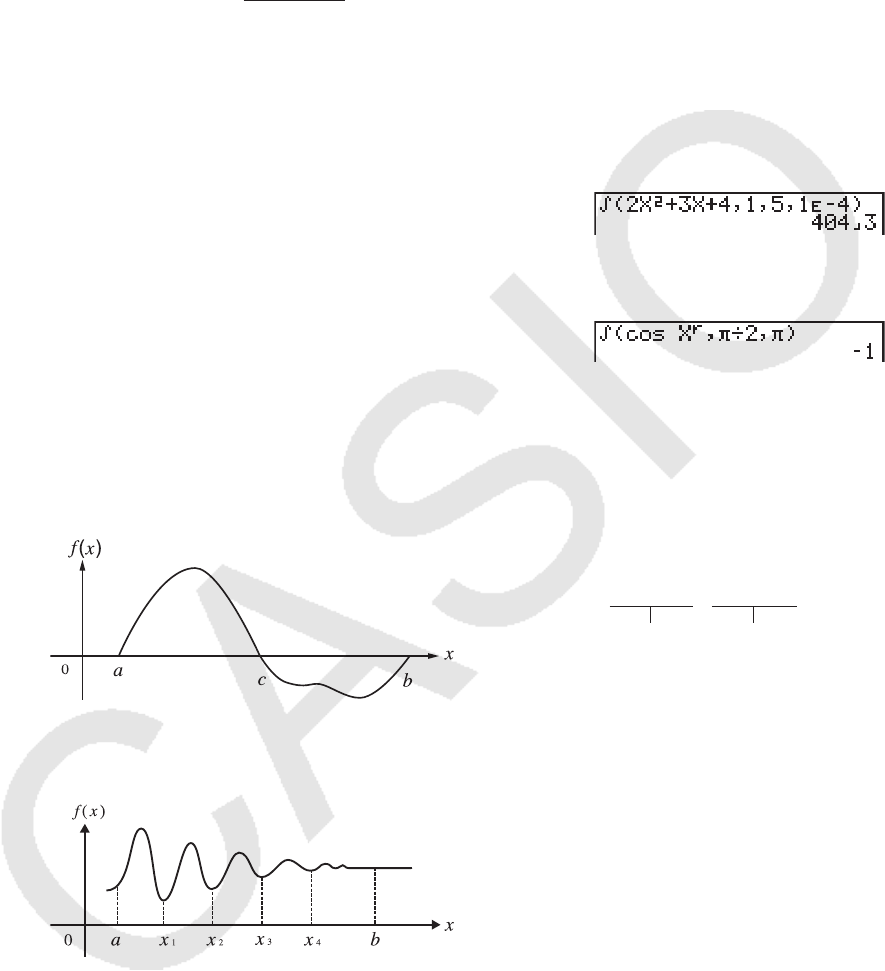
2-27
例1 执行下述函数的积分计算,公差“ tol” = 1 E - 4
输入函数 f
( x)。
AK4(CALC) * 4( ∫ dx) cvx+dv+e,
* fx-7400G
II: 3(CALC)
输入起点和终点。
b,f,
输入公差值。
bE-e)w
例2 当角度单位设置为“度”时,使用弧度进行三角函数积分计算(角度单位=
Deg)
计算结果显示示例
为确保得到正确的积分值,请注意以下几点。
(1) 进行积分计算的循环函数因不同区域而存在正负值时,可进行单循环计算,或将正负值区域
分开计算,然后加和结果。
正值
部分(
S)
负值部分(
S)
(2) 当积分分区的微小波动将引起积分值的剧烈波动时,则分别计算积分分区(将大波动区域分
割为较小的分区),然后将结果相加。
• 在积分计算期间按下 A(显示屏上没有显示光标)会中断计算。
• 在执行三角积分时,必须使用弧度(Rad模式)作为角度单位。
• 如果解不能达到公差要求,就产生一个错误(Time Out)。
∫
1
5
(2x
2
+ 3x + 4) dx
正值部分( S) 负值部分( S)
∫
a
b
f(x)dx =
∫
a
c
f(x)dx +
∫
c
b
f(x)dx
∫
a
b
f(x)dx =
∫
a
x
1
f(x)dx +
∫
x
1
x
2
f(x)dx +.....
+
∫
x
4
b
f(x)dx
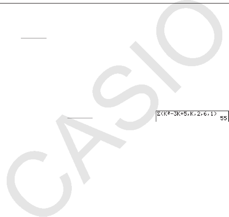
2-28
积分计算注意事项
• 在函数 f( x)中,只有X可作为表达式中的变量。其它变量(A至Z、不包括X、 r、 Ƨ)作为常
量,计算期间使用变量的当前指定值。
• 可不输入“
tol”和右圆括号。如果省略“ tol”,计算器自动使用默认值1 E -5。
• 积分计算可能需要较长时间才可完成。
• 在积分计算式中,不能使用微分、二次微分、积分、 ∑ 、最大/最小值、求解、RndFix或log
a
b
计算表达式。
• 在数学输入/输出模式中,公差值固定为1
E -5,不可更改。
k ∑ (求和)计算 [OPTN] - [CALC] - [ ∑ (]
在进行 ∑ 计算时,首先显示函数分析菜单,然后按照下述语法输入数值。
K4(CALC) * 6( g) 3( ∑ ( ) ak , k ,
α
,
β
, n ) * fx-7400G II: 3(CALC)
( n:分隔间距)
示例 进行下述计算:
使用 n = 1作为分隔间距。
AK4(CALC) * 6( g) 3( ∑ ( ) a,(K)
x-da,(K) +f,
a,(K) ,c,g,b)w
* fx-7400G
II: 3(CALC)
∑
∑ 计算注意事项
• 在 ∑ 计算期间,指定变量的值会发生变化。在执行计算之前,务必单独抄写以后可能需要使用
的指定变量值。
• 在输入数列
ak 的函数中,您只能使用一个变量。
•数列
ak 的初始项(α)和数列(β)的最终项 k 只能是整数。
• 可不输入
n和右圆括号。如果省略 n,计算器自动使用 n = 1。
• 确保最终项
β
的值大于初始项
α
的值。否则会出现错误。
• 如需中断正在执行的 ∑ 计算(显示屏上没有显示光标),按下 A键。
• 在 Σ 计算式中,不能使用微分、二次微分、积分、 Σ 、最大/最小值、求解、RndFix或logab计算
表达式。
• 在数学输入/输出模式中,分隔间距(
n)固定为1,不可更改。
β
Σ
(a
k
,k,
α
,
β
,n)=
Σa
k
=a
α
+a
α
+1
+........+ a
β
k =
α
6
Σ(k
2
–3
k+5)
k = 2

2-29
k 最大值/最小值计算 [OPTN] - [CALC] - [FMin]/[FMax]
在显示函数分析菜单之后,您可使用下述公式输入最大值/最小值计算式,求出函数在区间
a < x < b的最大值和最小值。
u 最小值
K4(CALC) * 6( g) 1(FMin) f
( x) , a , b , n ) * fx-7400G II: 3(CALC)
(
a:区间起点, b:区间终点, n:精度( n = 1至9))
u 最大值
K4(CALC) * 6( g) 2(FMax) f
( x) , a , b , n ) * fx-7400G II: 3(CALC)
(
a:区间起点, b:区间终点, n:精度( n = 1至9))
示例 求出在由起点 a = 0和终点 b = 3确定的区间上,精度为 n = 6时的函数
y = x2
- 4 x + 9的最小值
输入
f
( x)。
AK4(CALC) * 6( g) 1(FMin) vx-ev+j,
* fx-7400G
II: 3(CALC)
输入区间 a = 0, b = 3。
a,d,
输入精度 n = 6。
g)w
• 在函数 f
( x)中,只有X可作为表达式中的变量。其它变量(A至Z、不包括X、 r、 Ƨ)作为常
量,计算期间使用变量的当前指定值。
• 可不输入
n和右圆括号。
• 不连续点或者剧烈波动的部分会对精度产生不利影响,甚至引起错误。
• 输入较大的
n值,可提高计算的精度,但也会增加计算的所需时间。
• 输入的区间终点(
b)的值必须大于区间起点( a)的值。否则会出现错误。
• 您可通过按下 A键中断正在执行的最大值/最小值计算。
•
n值必须是1至9之间的整数。超出此区间的值会产生错误。
• 在最大值/最小值计算式中,不能使用微分、二次微分、积分、 ∑ 、最大/最小值、求
解、RndFix或log
a
b计算表达式。

2-30
6. 复数计算
与第2-1至2-15页所述的手动计算一样,您也可对复数进行加、减、乘、除、圆括号计算、函数
计算和存储器计算。
您可通过在设置屏幕上将Complex Mode项目改为以下某一设置,选择复数计算模式。
• { Real } ... 仅在实数范围内计算*
1
• { a+ bi} ... 执行复数计算并以直角坐标形式显示结果
• {
r∠ Ƨ} ... 执行复数计算并以极坐标形式显示结果*
2
*
1
但如果自变量中存在虚数,执行复数计算后以直角坐标形式显示结果。
示例:
ln 2
i = 0.6931471806 + 1.570796327 i
ln 2 i + ln (-2) = (Non-Real ERROR)
*
2
Ƨ的显示范围取决于设置屏幕上的Angle项目。
• Deg ... -180 <
Ƨ < 180
• Rad ... - π <
Ƨ < π
• Gra ... -200 <
Ƨ < 200
按下 K3(CPLX)( K2(CPLX)为fx-7400G II上的对应键)以显示复数计算编号菜单,包
含以下项目。
• { i} ... {虚数单位 i 输入}
• { Abs } / { Arg } ... 获取{绝对值}/{辐角}
• { Conj } ... {获取共轭数}
• { ReP } / { ImP } ... 提取{实部}/{虚部}
• { 'r∠ Ƨ} / { 'a+ bi} ... 将结果转换至{极坐标}/{直角坐标}形式
• 您还可使用 !a( i)替代 K3(CPLX)( K2(CPLX)为fx-7400G II上的对应键) 1( i)。
• Real、
a+ bi和 r∠ Ƨ模式得到的解在进行方根(
x')计算时有所不同(当 x < 0 , y = m/ n,
且
n为奇数时)。
示例:3
x' (-8) = - 2 (Real)
= 1 + 1.732050808
i ( a+ bi)
= 2 ∠ 60 (
r∠ Ƨ)
• 如需将“ ∠ ”算子输入极坐标表达式(
r∠ Ƨ),按下 !v( ∠ )。
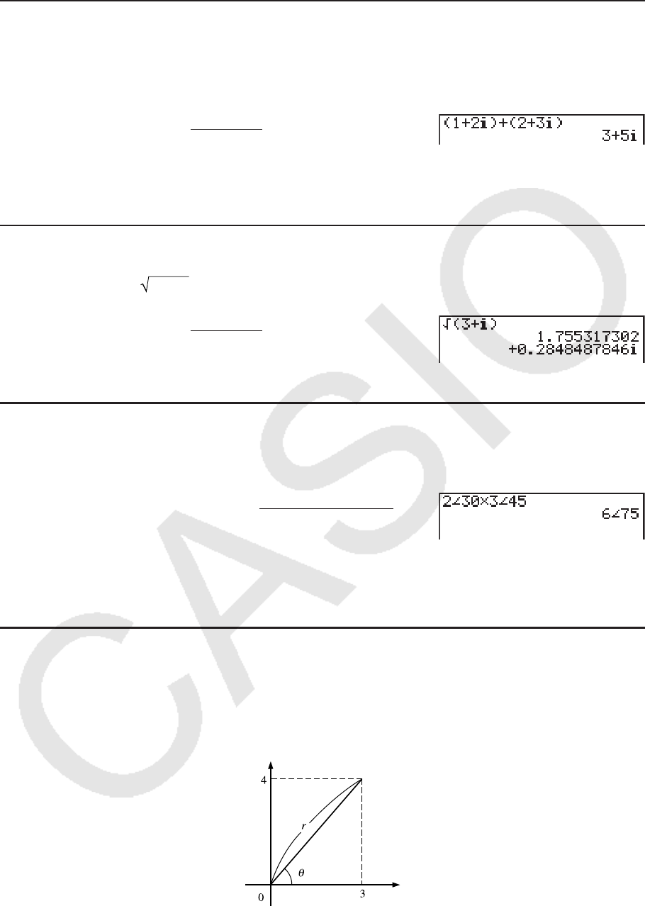
2-31
k 算术运算 [OPTN] - [CPLX] - [ i]
算术运算与手动计算中的操作相同。您甚至可使用圆括号和存储器。
示例 (1 + 2
i) + (2 + 3 i)
AK3(CPLX) *
(b+c1(
i) )
+(c+d1(
i) )w
* fx-7400G
II: 2(CPLX)
k 倒数、平方根和平方
示例 (3 + i)
AK3(CPLX) *
!x( ') (d+1(
i) )w
* fx-7400G
II: 2(CPLX)
k 使用极坐标形式的复数格式
示例 2 ∠ 30 × 3 ∠ 45 = 6 ∠ 75
!m(SET UP) cccccc*
1(Deg) c3(
r∠ Ƨ) J
Ac!v( ∠ ) da*d
!v( ∠ ) efw
* fx-7400G
II, fx-9750G II: ccccc
k 绝对值和辐角 [OPTN] - [CPLX] - [Abs]/[Arg]
此计算器将
a + bi形式的复数视为复数平面的坐标,计算绝对值 ⎮ Z ⎮ 和辐角(arg)。
示例 计算复数3 + 4
i的绝对值( r)和辐角( Ƨ),角度单位设定为度
虚轴
实轴
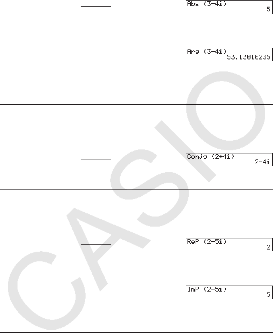
2-32
AK3(CPLX) * 2(Abs)
(d+e1(
i) )w
(绝对值计算)
* fx-7400G
II: 2(CPLX)
AK3(CPLX) * 3(Arg)
(d+e1(
i) )w
(辐角计算)
* fx-7400G
II: 2(CPLX)
• 当前角度单位(度、弧度、百分度)的设置不同,辐角计算结果也不同。
k 共轭复数 [OPTN] - [CPLX] - [Conj]
采用
a + bi形式的复数是 a - bi的共轭复数。
示例 计算复数2 + 4
i的共轭复数
AK3(CPLX) * 4(Conj)
(c+e1(
i) )w
* fx-7400G
II: 2(CPLX)
k 提取实部和虚部 [OPTN] - [CPLX] - [ReP]/[lmP]
使用下述程序,提取复数
a+ bi的实部 a和虚部 b 。
示例 提取复数2 + 5
i的实部和虚部
AK3(CPLX) * 6( g) 1(ReP)
(c+f6( g) 1(
i) )w
(实部提取)
* fx-7400G
II: 2(CPLX)
AK3(CPLX) * 6( g) 2(ImP)
(c+f6( g) 1(
i) )w
(虚部提取)
* fx-7400G
II: 2(CPLX)
k 极坐标与直角坐标形式转换 [OPTN] - [CPLX] - [ 'r∠ Ƨ]/[ 'a+ bi]
使用下述程序在直角坐标与极坐标之间转换复数显示形式。

2-33
示例 将直角坐标形式的复数1 + '3 i转换为极坐标形式
!m(SET UP) cccccc*
1(Deg) c2(
a+ bi) J
Ab+(!x( ') d)
K3(CPLX) ** 1(
i) 6( g) 3( 'r∠
θ
) w
* fx-7400G
II, fx-9750G II: ccccc
** fx-7400G
II: 2(CPLX)
Ac!v( ∠ ) ga
K3(CPLX) * 6( g) 4(
'a+ bi) w
* fx-7400G
II: 2(CPLX)
•复数的输入/输出范围通常为10位尾数和二位指数。
• 当复数超过21位时,实部和虚部分行显示。
• 下述函数可与复数一起使用。
'、
x2
、 x-1
、^( xy)、
3
'、
x'、ln、log、log
a
b、10
x、 ex、Int、Frac、Rnd、Intg、
RndFix(、 Fix、Sci、ENG、 ENG、° ’ ”、
° ’ ”
、
ab/ c、 d/ c
7. 二进制、八进制、十进制和十六进制整数计算
您可使用 RUN • MAT (或者 RUN )模式与二进制、八进制、十进制和十六进制设置进行包含二
进制、八进制、十进制、十六进制数值的计算。您也可在记数系统之间转换并进行位运算。
• 在二进制、八进制、十进制或者十六进制计算中,您不能使用科学函数。
• 在二进制、八进制、十进制或者十六进制计算中,您只能使用整数,即不允许使用小数值。如
果您输入一个包括小数部分的数值,则计算器会自动去除小数部分。
• 如果您尝试输入对于当前记数系统(二进制、八进制、十进制或者十六进制)无效的数值,计
算器会显示错误消息。下面显示可以用于每一个记数系统的数字。
二进制: 0、1
八进制: 0、1、2、3、4、5、6、7
十进制: 0、1、2、3、4、5、6、7、8、9
十六进制:0、1、2、3、4、5、6、7、8、9、A、B、C、D、E、F
• 使用原值的2的补数,可得到二进制、八进制、十进制或者十六进制值的负值。
• 下面是每一种记数系统的显示容量。
记数系统 二进制 八进制 十进制 十六进制
显示容量 16位 11位 10位 8位

2-34
• 用于十六进制数字的字母字符在显示屏上采用不同显示,以区别于文本字符。
正常文本 A B C D E F
十六进制数值 u v w x y z
键 v l I s c t
• 下面是每一种记数系统的计算范围。
二进制值
正值:0 <
x < 111111111111111
负值:1000000000000000 <
x < 1111111111111111
八进制值
正值:0 <
x < 17777777777
负值:20000000000 <
x < 37777777777
十进制值
正值:0 <
x < 2147483647
负值:-2147483648 <
x < -1
十六进制数值
正值:0 <
x < 7FFFFFFF
负值:80000000 <
x < FFFFFFFF
u 执行二进制、八进制、十进制或者十六进制计算
[SET UP] - [Mode] - [Dec]/[Hex]/[Bin]/[Oct]
1. 在主菜单中,选择 RUN • MAT (或者 RUN )。
2. 按下 !m(SET UP)。突出显示“Mode”,然后按下 2(Dec)、 3(Hex)、 4(Bin)或者
5(Oct)设置模式,指定默认的记数系统。
3. 按下 J切换到计算输入屏幕。这会出现带有下述项目的函数菜单。
• { d~o } / { LOG } / { DISP } ... {记数系统规定}/{位运算}/
{十进制/十六进制/二进制/八进制转换}菜单
k 选择记数系统
您可使用设置屏幕指定十进制、十六进制、二进制或者八进制作为默认的记数系统。
u 指定输入值的记数系统
您可指定输入的每一个数值的记数系统。按下 1(d~o)即可显示记数系统符号菜单。按下与目标
符号对应的功能键,然后输入数值。
• { d } / { h } / { b } / { o } ... {十进制}/{十六进制}/{二进制}/{八进制}
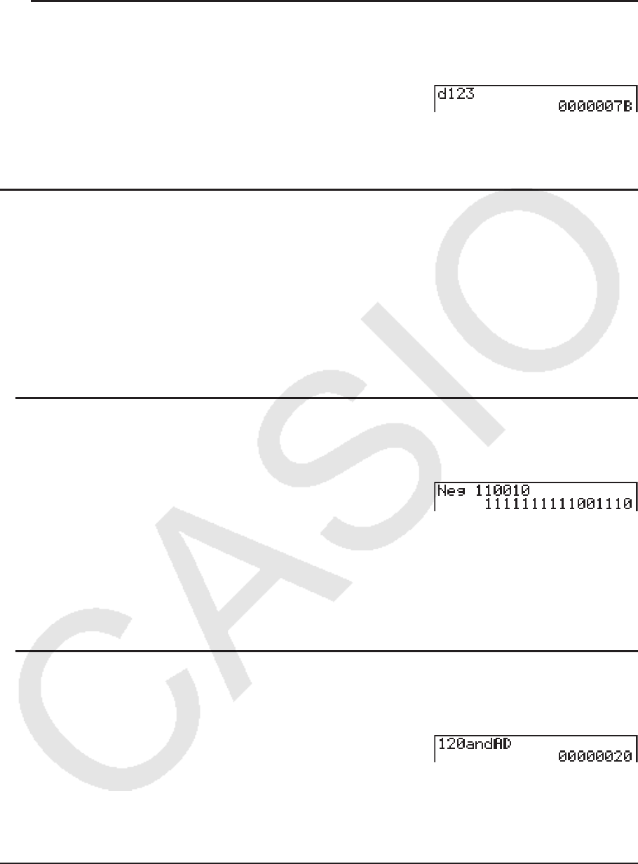
2-35
u 输入混合记数系统的数值
示例 当默认记数系统为十六进制时,输入123 10
!m(SET UP)
突出显示“Mode”,然后按下
3(Hex) J。
A1(d~o) 1(d) bcdw
k 负值与位运算
按下 2(LOG),显示非运算符和位运算符菜单。
• { Neg } ... {非}*
1
• { Not } / { and } / { or } / { xor } / { xnor } ... {NOT}*
2
/{AND}/{OR}/{XOR}/{XNOR}*
3
*
1
2的补数
*
2
1的补数(位补数)
*
3
逐位AND、逐位OR、逐位XOR、逐位XNOR
u 负 值
示例 求110010 2 的负值
!m(SET UP)
突出显示“Mode”,然后按下
4(Bin) J。
A2(LOG) 1(Neg)
bbaabaw
• 使用原值的二进制2的补数,可得到二进制、八进制和十六进制值的负值,然后返回原记数系
统的结果。使用十进制记数系统时,负值前带有一个负号。
u 位运算
示例 输入并执行“120 16 and AD 16 ”
!m(SET UP)
突出显示“Mode”,然后按下
3(Hex) J。
Abca2(LOG)
3(and) ADw
k 记数系统转换
按下 3(DISP)显示记数系统转换功能菜单。
• {
'Dec } / { 'Hex } / { 'Bin } / { 'Oct } ... 将显示值转换为对应的{十进制}/{十六进制}/{二进制}/
{八进制} 数值

2-36
u 将显示数值从一种记数系统转换为另一种记数系统
示例 将22 10 (默认记数系统)转换为相应的二进制或者八进制数值
A!m(SET UP)
突出显示“Mode”,然后按下
2(Dec) J。
1(d~o) 1(d) ccw
J3(DISP) 3( 'Bin) w
4( 'Oct) w
8. 矩阵计算
重要!
• fx-7400G II上不可执行矩阵计算。
在主菜单中,进入 RUN
•
MAT 模式,然后按下 1( 'MAT)即可执行矩阵计算。
利用26矩阵存储器(Mat A至Mat Z)加上一个矩阵答案存储器(MatAns),可进行以下矩阵
运算。
• 加、减、乘
• 标量乘法计算
• 行列式计算
• 矩阵转置
• 矩阵求逆
• 矩阵自乘
• 求矩阵的特定次幂
• 绝对值、整数部分提取、小数部分提取和最大整数计算
• 在矩阵单元中输入复数和使用复数相关的函数
• 使用矩阵命令进行矩阵修改
可为矩阵指定的最大行数为999,最大列数为999。
关于矩阵答案存储器(MatAns)
•计算器会将矩阵计算结果自动存储在矩阵答案存储器中。请注意以下关于矩阵答案存储器的要
点。
• 一旦进行矩阵计算,新的结果就会替代当前矩阵答案存储器的内容。以前的内容会被删除且不
可恢复。
• 将数值输入到矩阵中,不会影响矩阵答案存储器的内容。
• 当矩阵计算结果为m(行)× 1(列)或1(行)×
n(列)时,计算结果也存储在向量答案
存储器(VctAns)中。
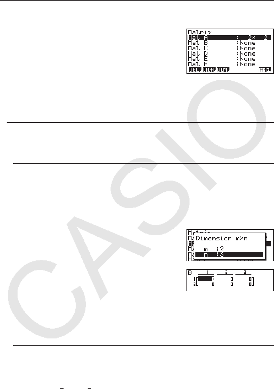
2-37
k 输入和编辑矩阵
按下 1( 'MAT),显示矩阵编辑器屏幕。使用矩阵编辑器输入和编辑矩阵。
m × n ... m(行) × n(列)矩阵
None ... 无预设矩阵
• { DEL } / { DEL
•
A } ... 删除{特定矩阵}/{所有矩阵}
• { DIM } ... {指定矩阵尺寸(单元数)}
• { M⇔V } ... 显示向量编辑器屏幕(第2-50页)
u 创建矩阵
创建矩阵时,您必须首先在矩阵编辑器中定义其尺寸(大小)。然后,您可以将数值输入矩
阵。
u 指定矩阵尺寸(大小)
示例 在Mat B区域中创建一个2行 × 3列矩阵
突出显示Mat B。
c
3(DIM) (可省略该步骤。)
指定行数。
cw
指定列数。
dw
w
• 新矩阵的所有单元均包含数值0。
• 更改矩阵的尺寸将删除其当前内容。
• 如果在您输入尺寸之后,矩阵区域名称旁仍然显示“Memory ERROR”,表示没有足够的存
储空间,无法创建您需要的矩阵。
u 输入单元值
示例 将下述数据输入矩阵B:
1 2 3
4 5 6

2-38
以下操作为前页计算示例的后续操作。
bwcwdw
ewfwgw
(将数据输入突出显示的单元。每次按下
w时,突出显示右侧的下一个单元。)
• 所显示的单元数值最多可显示六位正整数和五位负整数(负号占一位)。在显示指数值时,最
大指数为二位数。不显示小数值。
u 删除矩阵
您可以删除存储器中的一个特定矩阵或者所有矩阵。
u 删除特定矩阵
1. 在显示屏上显示矩阵编辑器时,使用 f和 c突出显示您想要删除的矩阵。
2. 按下 1(DEL)。
3. 按下 1(Yes)删除矩阵或者按下 6(No)中止运算,但不删除任何内容。
u 删除所有矩阵
1. 在显示屏上显示矩阵编辑器时,按下 2(DEL • A)。
2. 按下 1(Yes)删除矩阵或者按下 6(No)中止运算,但不删除任何内容。
k 矩阵单元运算
使用下述程序,为单元运算准备矩阵。
1. 在显示屏上显示矩阵编辑器时,使用 f和 c突出显示您想要使用的矩阵。
您可通过输入对应矩阵名称的字母跳转至特定矩阵。例如,输入 ai(N)可跳转至Mat N。
按下 !-(Ans)可跳转至矩阵当前存储器。
2. 按下 w,出现带有下述项目的功能菜单。
• { R•OP } ... {行运算菜单}
• { ROW }
• { DEL } / { INS } / { ADD } ... {删除}/{插入}/{添加}行
• { COL }
• { DEL } / { INS } / { ADD } ... {删除}/{插入}/{添加}列
• { EDIT } ... {单元编辑屏幕}
下述所有例子均使用矩阵A。
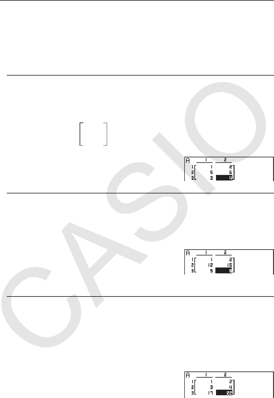
2-39
u 行计算
在显示屏上显示调用矩阵时,一旦按下 1(R•OP),就会显示以下菜单。
• { Swap } ... {行交换}
• { × Rw } ... {指定行与标量之积}
• { × Rw+ } ... {一行加上指定行与标量之积}
• { Rw+ } ... {将指定行加到另一行上}
u 交换两行
示例 交换下述矩阵的行2与行3:
所有运算示例均使用以下矩阵。
矩阵A =
1 2
3 4
5 6
1(R•OP) 1(Swap)
输入需要交换的行数。
cwdww
u 计算某一行的标量积
示例 计算行2与标量4的积
1(R•OP) 2( × Rw)
输入乘数。*
ew
指定行数。
cww
* 也可输入复数作为乘数(k)。
u 计算某一行之积并将结果加到另一行上
示例 计算行2与标量4的积,并将结果加到行3上
1(R•OP) 3( × Rw+)
输入乘数。*
ew
指定应该计算积的行数。
cw
指定应该加上结果的行数。
dww
* 也可输入复数作为乘数(k)。
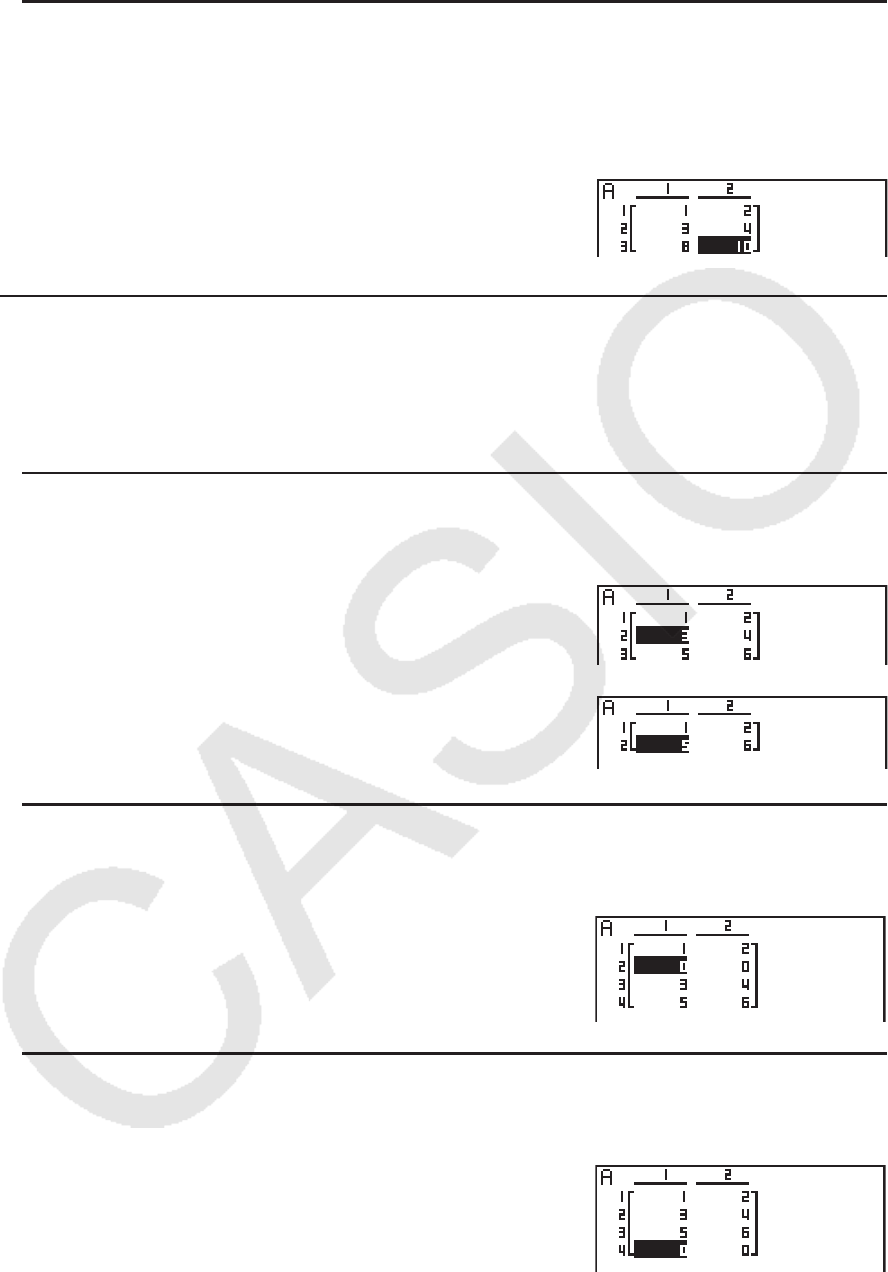
2-40
u 将两行相加
示例 将行2与行3相加
1(R•OP) 4(Rw+)
指定需要相加的行数。
cw
指定被加的行数。
dww
u 行运算
• { DEL } ... {删除行}
• { INS } ... {插入行}
• { ADD } ... {增加行}
u 删除行
示例 删除行2
2(ROW) c
1(DEL)
u 插入行
示例 在行1与行2之间插入一个新行
2(ROW) c
2(INS)
u 增加行
示例 在行3下新增一行
2(ROW) cc
3(ADD)
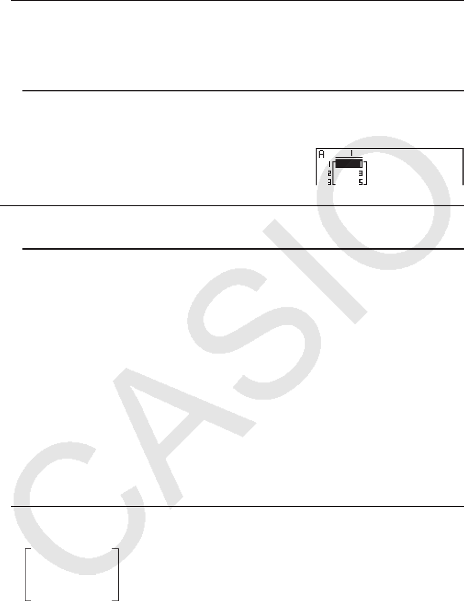
2-41
u 列运算
• { DEL } ... {删除列}
• { INS } ... {插入列}
• { ADD } ... {增加列}
u 删除列
示例 删除列2
3(COL) e
1(DEL)
k 使用矩阵命令修改矩阵 [OPTN] - [MAT]
u 显示矩阵命令
1. 在主菜单中,进入 RUN • MAT 模式。
2. 按下 K,显示选项菜单。
3. 按下 2(MAT)显示矩阵命令菜单。
下面仅说明用于创建矩阵和输入矩阵数据的矩阵命令菜单项目。
• { Mat } ... {Mat命令(矩阵规定)}
• { M → L } ... {Mat → List命令(将选定列的内容指定给列表文件)}
• { Aug } ... {Augment 命令(连接两个矩阵)}
• { Iden } ... {Identity命令(单位矩阵输入)}
• { Dim } ... {Dim命令(尺寸检查)}
• { Fill } ... {Fill命令(恒定单元值)}
• 您还可使用 !c(Mat)替代 K2(MAT) 1(Mat)。
u 矩阵数据输入格式 [OPTN] - [MAT] - [Mat]
下面显示当使用Mat命令输入数据以创建矩阵时,您应该使用的格式。
= [ [a
11
, a
12
, ..., a
1
n] [a
21
, a
22
, ..., a
2
n] .... [a
m1
, a
m2
, ..., a
mn] ]
→ Mat [字母A至Z]
a
11
a
12
... a
1n
a
21
a
22
... a
2n
a
m1
a
m2
... a
mn
...
...
...
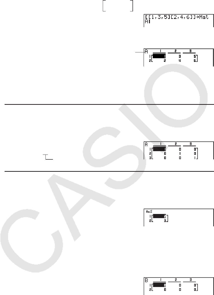
2-42
示例 输入下列数据作为矩阵A:
!+( [ ) !+( [ ) b,d,f
!-( ] ) !+( [ ) c,e,g
!-( ] ) !-( ] ) aK2(MAT)
1(Mat) av(A)
w 矩阵名称
• m和 n的最大值均为999。
• 如果在输入数据时存储器已满,会产生错误。
• 您也可在程序中使用上述格式输入矩阵数据。
u 输入单位矩阵 [OPTN] - [MAT] - [Iden]
使用Identity命令创建单位矩阵。
示例 创建3 × 3单位矩阵作为矩阵A
K2(MAT) 6( g) 1(Iden)
da6( g) 1(Mat) av(A) w
行/列数
u 检查矩阵尺寸 [OPTN] - [MAT] - [Dim]
使用Dim命令检查现有矩阵的尺寸。
例1 检查矩阵A的尺寸
K2(MAT) 6( g) 2(Dim)
6( g) 1(Mat) av(A) w
显示屏显示矩阵A由两行与三列组成。
由于Dim命令的结果为列表类型数据,因此保存在ListAns存储器中。
您还可使用{Dim}指定矩阵的尺寸。
例2 指定矩阵B中2行与3列的尺寸
!*( ) c,d!/( ) a
K2(MAT) 6( g) 2(Dim)
6( g) 1(Mat) al(B) w
• 可以使用“Dim”命令查看和配置向量尺寸设置。
1 3 5
2 4 6
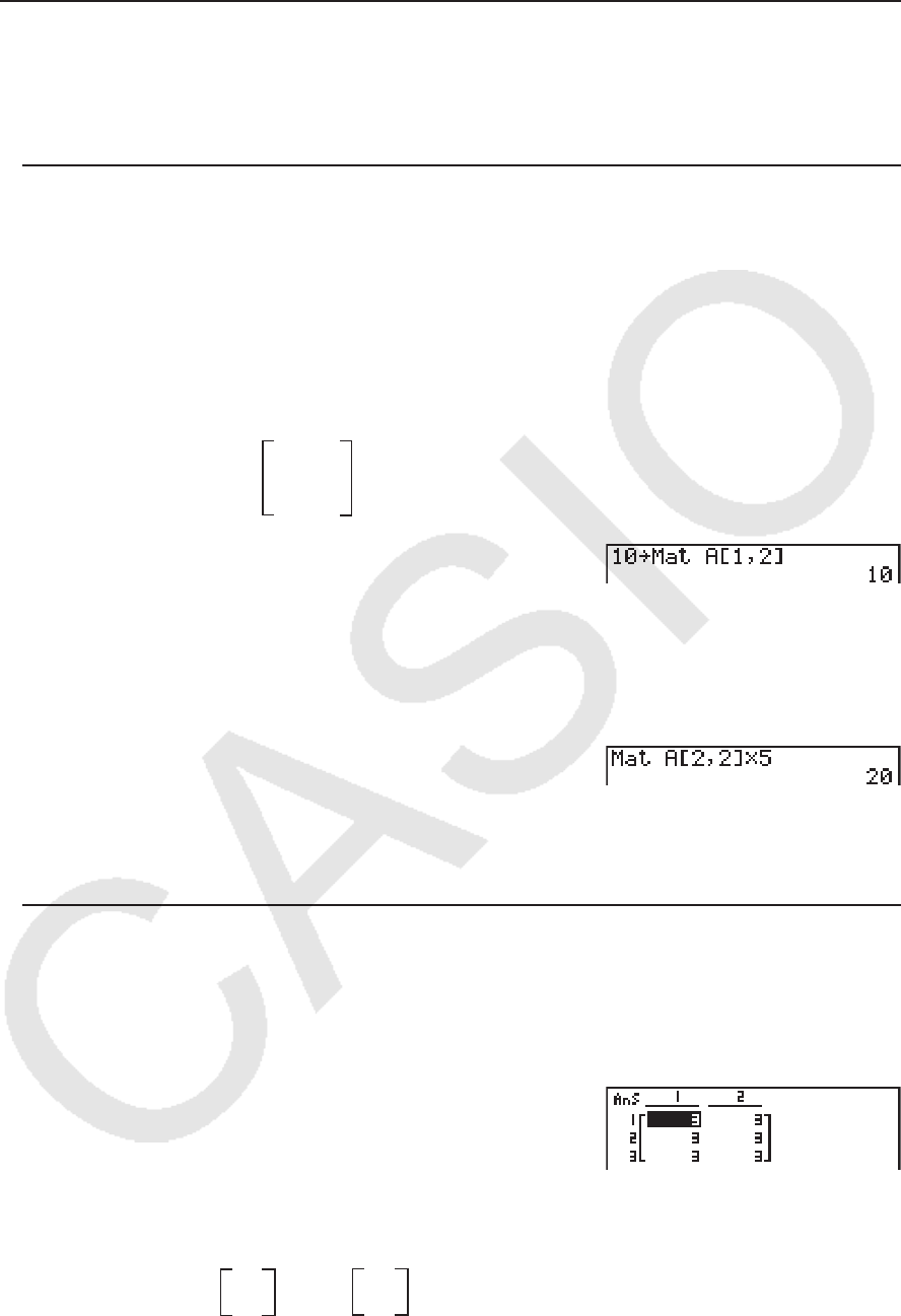
2-43
u 使用矩阵命令修改矩阵
您也可使用矩阵命令将数值指定到一个现有的矩阵并从一个现有的矩阵调用数值、用相同的数
值填充现有矩阵的所有单元、将两个矩阵合并为一个矩阵,以及将矩阵列的内容指定到列表文
件。
u 将数值指定给现有矩阵和从现有矩阵调用数值 [OPTN] - [MAT] - [Mat]
使用下述格式和Mat命令指定一个单元进行赋值和调用。
Mat X [
m, n]
X
= 矩阵名称(A至Z、或者Ans)
m = 行数
n = 列数
例1 将10指定给下述矩阵第1行第2列单元:
矩阵A =
1 2
3 4
5 6
baaK2(MAT) 1(Mat)
av(A) !+( ) b,c
!-( ) w
• 可以使用“Vct”命令对现有向量进行赋值。
例2 将上述矩阵第2行第2列单元的值乘以5
K2(MAT) 1(Mat)
av(A) !+( ) c,c
!-( ) *fw
• 可以使用“Vct”命令调用现有向量的值。
u 以相同数值填入矩阵,并且将两个矩阵合并为一个矩阵 [OPTN] - [MAT] - [Fill]/[Aug]
使用Fill命令以同一个数值填入一个现有矩阵的所有单元,或者使用Augment命令将两个现有矩
阵合并为一个矩阵。
例1 以数值3填入矩阵A的所有单元
K2(MAT) 6( g) 3(Fill)
d,6( g) 1(Mat) av(A) w
1(Mat) av(A) w
• 可以使用“Fill”命令以同一个数值填入所有向量元素。
例2 合并下述两个矩阵:
A = 1
2
B = 3
4
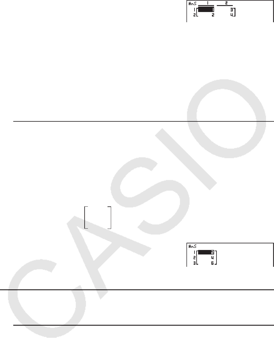
2-44
K2(MAT) 5(Aug)
1(Mat) av(A) ,
1(Mat) al(B) w
• 您合并的两个矩阵必须具有相同的行数。如果您尝试合并两个具有不同行数的矩阵,会产生错
误。
•您可使用矩阵答案存储器将上述矩阵输入和编辑操作的结果指定给矩阵变量。该操作采用以下
语法。
Fill (
n, Mat
α
)
Augment (Mat
α
、Mat
β
) → Mat
γ
上面的
α
、
β
和
γ
可以是A至Z的任何变量名称, n为任意值。
以上操作不会影响矩阵答案存储器的内容。
• 可以使用“Augment”命令将两个向量合并为一个矩阵。
u 将一个矩阵列的内容指定给一个列表 [OPTN] - [MAT] - [M → L]
使用以下格式和Mat → List命令指定一个列和一个列表。
Mat → List (Mat X,
m) → List n
X
= 矩阵名称(A至Z)
m = 列数
n = 列表号
示例 将下述第2列的内容指定到列表1:
矩阵A =
1 2
3 4
5 6
K2(MAT) 2(M → L)
1(Mat) av(A) ,c)
aK1(LIST) 1(List) bw
1(List) bw
k 矩阵计算 [OPTN] - [MAT]
使用矩阵命令菜单进行矩阵计算操作。
u 显示矩阵命令
1. 在主菜单中,进入 RUN • MAT 模式。
2. 按下 K,显示选项菜单。
3. 按下 2(MAT)显示矩阵命令菜单。
下面仅说明用于矩阵算术运算的矩阵命令。
• { Mat } ... {Mat命令(矩阵规定)}
• { Det } ... {Det命令(行列式命令)}
• { Trn } ... {Trn命令(矩阵转置命令)}
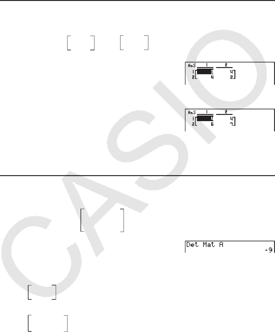
2-45
• { Iden } ... {Identity命令(单位矩阵输入)}
• { Ref } ... {Ref命令(列梯形形式命令)}
• { Rref } ... {Rref命令(简化列梯形形式命令)}
下述所有示例均假设矩阵数据已经存储在存储器中。
u 矩阵算术运算 [OPTN] - [MAT] - [Mat]/[Iden]
例1 下述两个矩阵相加(矩阵A + 矩阵B):
AK2(MAT) 1(Mat) av(A) +
1(Mat) al(B) w
例2 将例1中的两个矩阵(矩阵A × 矩阵B)相乘
AK2(MAT) 1(Mat) av(A) *
1(Mat) al(B) w
• 在进行加减计算时,两个矩阵必须具有相同的尺寸。如果您尝试加减不同尺寸的矩阵,会产生
错误。
• 相乘时(矩阵1 × 矩阵2),矩阵1的列数必须与矩阵2的行数相同。否则会产生错误。
u 行列式 [OPTN] - [MAT] - [Det]
示例 求下述矩阵的行列式:
矩阵A =
1 2 3
4 5 6
−1 −2 0
K2(MAT) 3(Det) 1(Mat)
av(A) w
• 只有方阵(行数与列数相同)才可求行列式。如果尝试求非方阵的行列式,会产生错误。
• 2 × 2矩阵的行列式计算如下。
| A | = a11 a12 =a
11a22 –a
12a21
a21 a22
• 3 × 3矩阵的行列式计算如下。
= a11a22a33 + a12a23a31 + a13a21a32 – a11a23a32 – a12a21a33 – a13a22a31
a11 a12 a13
a21 a22 a23
a31 a32 a33
|A| =
A = 1 1
2 1
2 3
2 1
B =
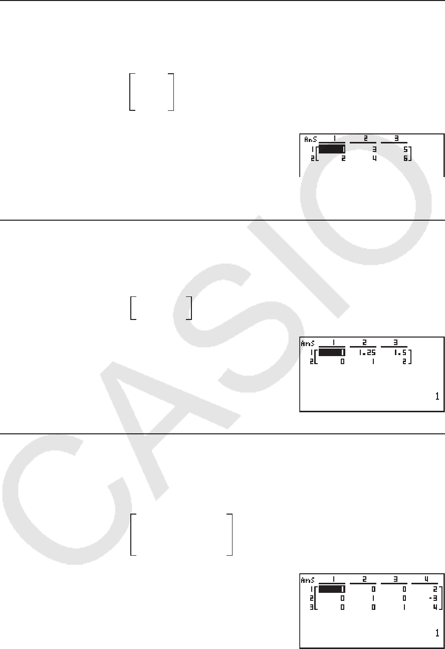
2-46
u 矩阵转置 [OPTN] - [MAT] - [Trn]
矩阵转置是指矩阵的行变为列,列变为行。
示例 转置下述矩阵:
矩阵A =
1 2
3 4
5 6
K2(MAT) 4(Trn) 1(Mat)
av(A) w
• “Trn”命令也可用于向量。它可将一个1行× n列向量转换为一个 n行× 1列向量,或将一
个 m行× 1列向量转换为一个1行× m列向量。
u 列梯形形式 [OPTN] - [MAT] - [Ref]
该命令使用高斯消去法确定矩阵的列梯形形式。
示例 求下述矩阵的列梯形形式:
矩阵A =
K2(MAT) 6( g) 4(Ref)
6( g) 1(Mat) av(A) w
u 简化列梯形形式 [OPTN] - [MAT] - [Rref]
该命令确定矩阵的简化列梯形形式。
示例 求下述矩阵的简化列梯形形式:
矩阵A =
K2(MAT) 6( g) 5(Rref)
6( g) 1(Mat) av(A) w
• 由于舍去了一些数位,所以列梯形形式和简化列梯形形式运算可能不能产生精确结果。
1 2 3
4 5 6
2 −1 3 19
1 1 −5 −21
0 4 3 0
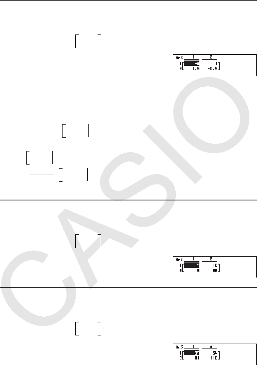
2-47
u 矩阵倒置 [ x-1
]
示例 倒置下述矩阵:
矩阵A =
K2(MAT) 1(Mat)
av(A) !)(
x-1
) w
• 只有方阵(行数与列数相同)才可倒置。如果尝试倒置非方阵,会产生错误。
• 行列式为零的矩阵不可倒置。如果尝试倒置行列式为零的矩阵,会产生错误。
• 对于行列式接近零的矩阵,计算精度会受到影响。
• 被倒置的矩阵必须满足以下条件。
A A–1 = A–1 A = E = 1 0
0 1
用于将矩阵A转变为倒置矩阵A
-1
的公式如下所示。
A = a b
c d
A–1=1
ad – bc
d–b
–c a
请注意ad - bc 0。
u 矩阵平方 [ x2
]
示例 计算下述矩阵的平方:
矩阵A =
K2(MAT) 1(Mat) av(A) xw
u 求矩阵的特定次幂 [^]
示例 求下述矩阵的三次方:
矩阵A =
K2(MAT) 1(Mat) av(A)
Mdw
• 对于矩阵幂计算,最大幂为32766。
1 2
3 4
1 2
3 4
1 2
3 4
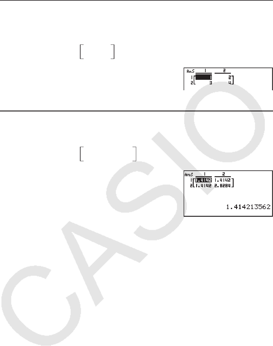
2-48
u 求一个矩阵的绝对值、整数部分、小数部分与最大整数
[OPTN] - [NUM] - [Abs]/[Frac]/[Int]/[Intg]
示例 求下述矩阵的绝对值:
矩阵A =
K6( g) 4(NUM) 1(Abs)
K2(MAT) 1(Mat) av(A) w
• 可以使用“Abs”命令求出一个向量元素的绝对值。
u 矩阵的复数计算
示例 求带有下述复数元素的矩阵的绝对值:
矩阵D =
AK6( g) 4(NUM) 1(Abs)
K2(MAT) 1(Mat) as(D) w
• 在矩阵和向量中支持下述复数函数。
i、Abs、Arg、Conjg、ReP、ImP
矩阵计算注意事项
• 舍去的数位会使行列式和倒置矩阵产生误差。
• 对每一个单元单独进行矩阵运算,因此计算可能需要较长时间才能完成。
• 矩阵计算显示结果的计算精度在最小有效位为 ± 1。
• 如果矩阵计算结果太大,不能装入矩阵答案存储器,则会产生错误。
• 您可使用下述操作,将矩阵答案存储器内容传输至另一个矩阵(或当矩阵答案存储器包含行列
式时,传输至变量)。
MatAns → Mat
α
上面的
α
是A至Z的任意变量名称。以上操作不会影响矩阵答案存储器的内容。
1 –2
–3 4
–1 + i 1 + i
1 + i –2 + 2i

2-49
9. 向量计算
重要!
• fx-7400G II/fx-9750G II上不可执行向量计算。
要进行向量计算,请使用主菜单进入RUN • MAT模式,然后按下 1( 'MAT)6(M⇔V)。
一个向量定义为以下两种形式中任一形式的一个矩阵:m(行)× 1(列)或1(行)
× n(列)。
可为m和n指定的最大允许值均为999。
您可使用26个向量存储器(Vct A至Vct Z)加上一个向量答案存储器(VctAns)进行下列向量
计算。
• 加、减、乘
• 标量乘法计算
• 内积计算
• 叉积计算
• 求向量的模(大小)
• 求两个向量形成的夹角
• 求单位向量
关于向量答案存储器(VctAns)
计算器会将向量计算结果自动存储在向量答案存储器中。请注意以下关于向量答案存储器的要
点。
• 一旦进行向量计算,新的结果就会替代当前向量答案存储器的内容。以前的内容会被删除且不
可恢复。
• 将数值输入到向量不会影响向量答案存储器的内容。
• 向量计算结果也将被存储在矩阵答案存储器(MatAns)中。

2-50
k 输入和编辑向量
按下 1( 'MAT)6(M⇔V),显示向量编辑器屏幕。使用向量编辑器输入和编辑向量。
m× n ... m(行)× n(列)向量
None ... 无预设向量
• {DEL}/{DEL•A} ... 删除{特定向量}/{所有向量}
• {DIM} ... 指定向量尺寸(m行× 1列或1行× n列)
• {M⇔V} ... 显示矩阵编辑器屏幕(第2-37页)
向量输入和编辑以及向量单元(元素)运算与矩阵计算操作相同。有关更多信息,请参见“输
入和编辑矩阵”(第2-37页)和“矩阵单元运算”(第2-38页)。但请注意,向量计算与矩阵
计算在以下方面是不同的。
• 在向量存储器元素输入屏幕上,功能菜单中没有1(R•OP)。
• 对于向量编辑,尺寸始终限制为m行× 1列或1行× n列。
k 向量计算 [OPTN]-[MAT]
使用向量命令菜单进行向量计算。
u 若要显示向量命令
1. 从主菜单中,进入RUN • MAT模式。
2. 按下K,显示选项菜单。
3. 按下2(MAT)6(g)6(g)显示向量命令菜单。
• {Vct} ... {Vct命令(向量规定)}
• {DotP} ... {DotP命令(内积命令)}
• {CrsP} ... {CrossP命令(叉积命令)}
• {Angle} ... {Angle命令(计算两个向量形成的夹角)}
• {UntV} ... {UnitV命令(计算单位向量)}
• {Norm} ... {Norm命令(计算向量的模(大小))}
向量计算注意事项
• 计算内积、叉积和两个向量形成的夹角时,这两个向量的尺寸必须相同。此外,叉积尺寸必须
为1 × 2、1 × 3、2 × 1或3 × 1。
• 对每一个元素独立进行向量计算,因此可能需要一段时间才能显示出计算结果。
• 向量计算显示结果的计算精度在最小有效位为±1。
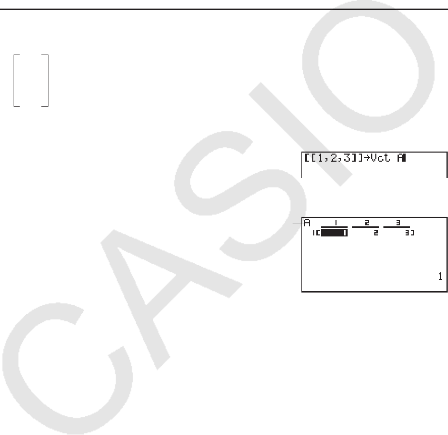
2-51
• 如果向量计算结果太大,不能装入向量答案存储器,则会产生错误。
• 您可以使用下述操作将向量答案存储器内容传输到另一向量。
VctAns → Vct Ơ
上面的α是A至Z的任意变量名称。以上操作不会影响向量答案存储器的内容。
• 向量存储器与矩阵存储器是相互兼容的,因此向量存储器内容可以根据需要指定到矩阵存储
器。
Vct Ơ → Mat ơ
上面的α和β是A至Z的任意变量名称。
u 向量数据输入格式 [OPTN]-[MAT]-[Vct]
下面显示当使用Vct命令输入数据以创建向量时,您应该使用的格式。
→ Vct [A至Z] [a11 a12 ... a1n] → Vct [A至Z]
示例 将下列数据输入Vct A: [ 1 2 3 ]
!+([)!+([)b,c,d
!-(])!-(])a
K2(MAT)6(g)6(g)1(Vct)
av(A)w
向量名称
• m和n的最大值均为999。
• 如果在输入数据时存储器已满,会产生错误。
• 您也可在程序中使用上述格式输入向量数据。
下述所有示例均假设向量数据已经存储在存储器中。
a11
a21
am1
...
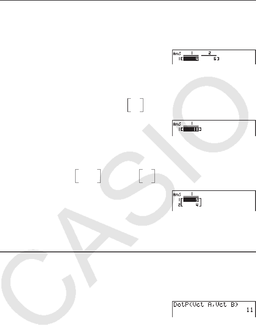
2-52
u 向量的加、减和乘 [OPTN]-[MAT]-[Vct]
例1 求下述两个向量之和(Vct A+Vct B):
Vct A = [ 1 2 ] Vct B = [ 3 4 ]
K2(MAT)6(g)6(g)
1(Vct)av(A)+
1(Vct)al(B)w
例2 求下述两个向量的乘积(Vct A × Vct B):
Vct A = [ 1 2 ] Vct B =
K2(MAT)6(g)6(g)
1(Vct)av(A)*
1(Vct)al(B)w
例3 求下述矩阵和向量的乘积(Mat A × Vct B):
Mat A = Vct B =
K2(MAT)1(Mat)
av(A)*6(g)6(g)
1(Vct)al(B)w
• 在进行加减计算时,两个向量必须具有相同的尺寸。
• 将Vct A(1×n)和Vct B(m×1)进行相乘时,n和m必须相同。
u 内积 [OPTN]-[MAT]-[DotP]
示例 求以下两个向量的内积
Vct A = [ 1 2 ] Vct B = [ 3 4 ]
K2(MAT)6(g)6(g)
2(DotP)1(Vct)av(A),
1(Vct)al(B))w
3
4
1 2
2 1
1
2
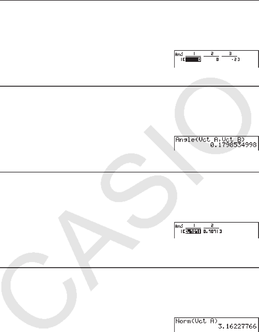
2-53
u 叉积 [OPTN]-[MAT]-[CrsP]
示例 求以下两个向量的叉积
Vct A = [ 1 2 ] Vct B = [ 3 4 ]
K2(MAT)6(g)6(g)
3(CrsP)1(Vct)av(A),
1(Vct)al(B))w
u 两个向量形成的夹角 [OPTN]-[MAT]-[Angle]
示例 求两个向量形成的夹角
Vct A = [ 1 2 ] Vct B = [ 3 4 ]
K2(MAT)6(g)6(g)
4(Angle)1(Vct)av(A),
1(Vct)al(B))w
u 单位向量 [OPTN]-[MAT]-[UntV]
示例 求以下向量的单位向量
Vct A = [ 5 5 ]
K2(MAT)6(g)6(g)
5(UntV)1(Vct)av(A)
)w
u 向量的模(大小) [OPTN]-[MAT]-[Norm]
示例 求向量的模(大小)
Vct A = [ 1 3 ]
K2(MAT)6(g)6(g)6(g)
1(Norm)6(g)6(g)6(g)
1(Vct)av(A))w
• 可以使用“Norm”命令计算一个矩阵的的模。

2-54
10. 度量转换计算
您可将某一测量单位的值转换为另一种单位的值。测量单位分为以下11个类别。“显示名
称”列中的指示符显示了在计算器功能菜单中显示的文本。
显示名称 类别 显示名称 类别 显示名称 类别
LENG 长度 TMPR 温度 PRES 压力
AREA 面积 VELO 速度 ENGY 能量/功
VLUM 体积 MASS 质量 PWR 功率
TIME 时间 FORC 力/重量
您可将某个类别中的任何单位转换为同一类别中的其他任何单位。
• 如果尝试将某一类别中的某个单位(例如“AREA”)转换为另一个类别中的某个单位(例
如“TIME”),会产生Conversion ERROR。
• 关于每个类别所包含单位的说明,请参见“单位转换命令列表”(第2-55页)。
k 执行单位转换计算 [OPTN] - [CONV]
使用下述语法输入需要转换的数值和转换命令,执行单位转换计算。
{需要转换的数值}{转换命令1} ' {转换命令2}
• 使用{转换命令1}指定需要转换的单位,使用{转换命令2}指定转换目标单位。
• ' 命令用于连接两个转换命令。该命令总是在转换菜单的 1( ')。
• 实数或包含实数元素的列表只能作为被转换的数值。在被转换的数值为列表输入时(或在指定
列表存储器时),对列表中的每个元素执行转换计算并以列表格式返回计算结果(ListAns屏
幕)。
•复数不可作为被转换的数值。只要作为被转换数值的列表中有一个元素包含复数,就会产生错
误。
例1 将50cm转换为英寸单位
AfaK6( g) 1(CONV) * 2(LENG)
f(cm) 1( ') 2(LENG) ec(in) w
* fx-7400G
II: 5(CONV)
例2 将{175, 162, 180}平方米转换为公顷
A!*({) bhf,bgc,
bia!/(})
K6( g) 1(CONV) * 3(AREA) c(m
2
)
1( ') 3(AREA) d(ha) w
* fx-7400G
II: 5(CONV)

2-55
k 单位转换命令列表
类别 显示名称 单位 类别 显示名称 单位
长
度
fm 费米
体
积
cm
3 立方厘米
Å 埃 mL 毫升
μ
m 微米 L 升
mm 毫米 m
3 立方米
cm 厘米 in
3 立方英寸
m 米 ft
3 立方英尺
km 千米 fl_oz(UK) 盎司
AU 天文单位 fl_oz(US) 液盎司(美)
l.y. 光年 gal(US) 加仑
pc 秒差距 gal(UK) 英制加仑
Mil 1/1000英寸 pt 品脱
in 英寸 qt 夸脱
ft 英尺 tsp 小匙
yd 码 tbsp 大匙
fath 英寻 cup 杯
rd 杆
时
间
ns 纳秒
mile 英里
μ
s 微秒
n mile 海里 ms 毫秒
面
积
cm
2 平方厘米 s 秒
m
2 平方米 min 分
ha 公顷 h 小时
km
2 平方千米 day 日
in
2 平方英寸 week 周
ft
2 平方英尺 yr 年
yd
2 平方码 s-yr 恒星年
acre 英亩 t-yr 回归年
mile
2 平方英里

2-56
类别 显示名称 单位 类别 显示名称 单位
温
度
℃ 摄氏度
压
力
Pa 帕
K 开尔文 kPa 千帕
°F 华氏度 mmH
2
O 毫米水柱
°R 兰氏度 mmHg 毫米汞柱
速
度
m/s 米每秒 atm 大气压
km/h 千米每小时 inH
2
O 英寸水柱
knot 海里每小时 inHg 英寸汞柱
ft/s 英尺每秒 lbf/in
2 磅每平方英寸
mile/h 英里每小时 bar 巴
质
量
u 原子质量单位 kgf/cm
2 千克力每平方厘米
mg 毫克
能
量
/
功
eV 电子伏特
g 克 J 焦耳
kg 千克 cal
th 热化学卡
mton 公吨 cal
15 卡 (15℃)
oz 常衡盎司 cal
IT 国际蒸汽表卡
lb 磅(质量) kcal
th 热化学千卡
slug 斯勒格 kcal
15 千卡 (15℃)
ton(short) 短吨(2000磅) kcal
IT 国际蒸汽表千卡
ton(long) 长吨(2240磅) l-atm 公升大气压
力
/
重
量
N 牛 kW
•
h 千瓦时
lbf 磅力 ft
•
lbf 英尺-磅
tonf 吨力 Btu 英热单位
dyne 达因 erg 尔格
kgf 千克力 kgf
•
m 千克力米
功
率
W 瓦
cal
th
/s 卡每秒
hp 马力
ft
•
lbf/s 英尺-磅每秒
Btu/min 英热单位每分
摘自:美国国家标准及技术研究所特种文献811(2008)
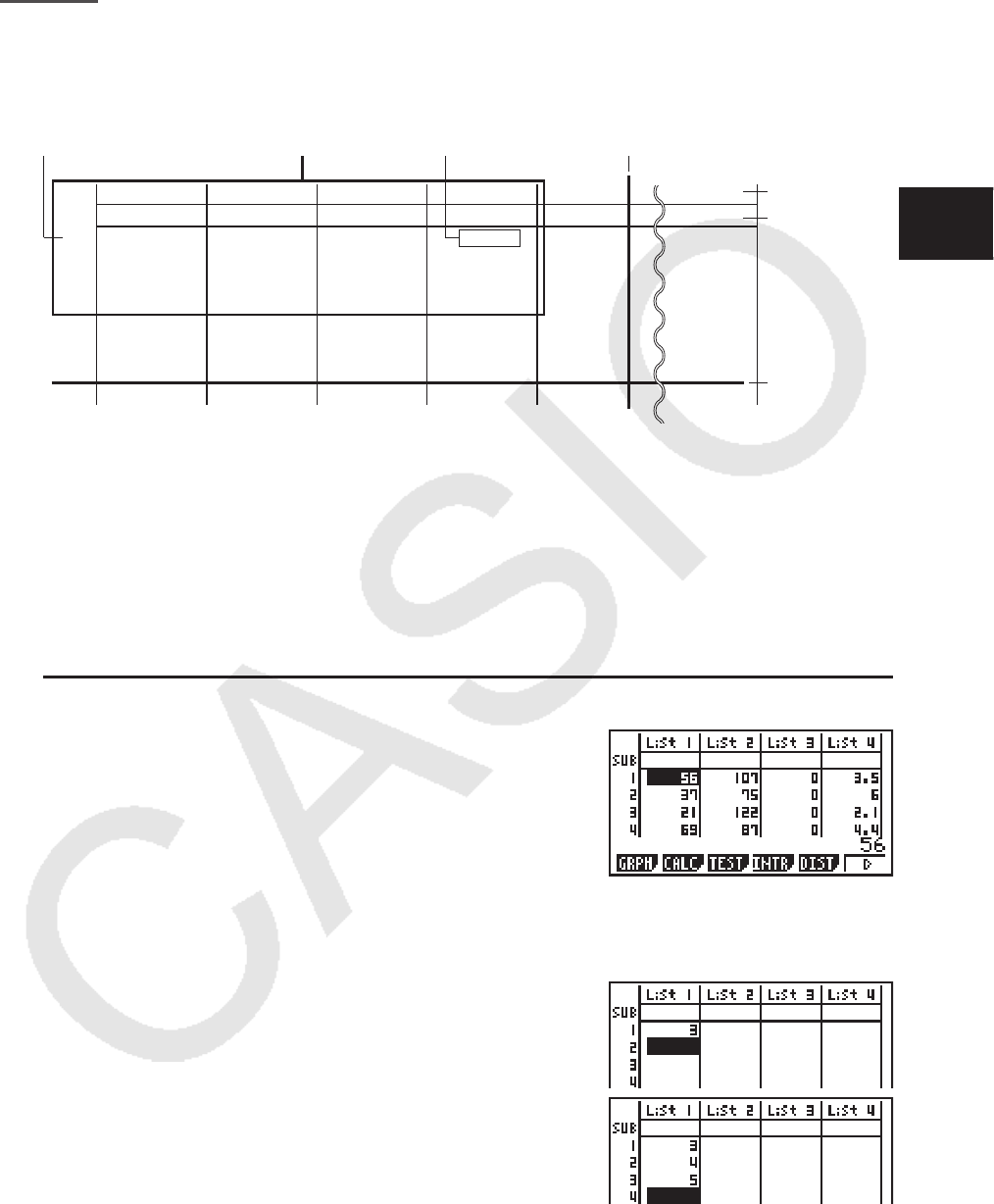
3-1
第3章 列表功能
列表是用于存储多个数据项的存储区。
利用本计算器,您可以在单个文件中存储多达26个列表,在存储器内存储多达六个文件。存储的列
表可用于算术、统计计算和制图。
单元号 显示范围 单元 列
列表名称
子名称
行
1. 输入和编辑列表
在进入 STAT 模式时,将首先显示“列表编辑器”。您可使用列表编辑器将数据输入列表并执行
其他各列表数据操作。
u 逐个输入数值
使用光标键,将突出显示部分移至需要选择的列表名称、子
名称或者单元。请注意, c不会突出显示不包含数值的单
元。
当突出显示部分位于屏幕上任何一个边缘时,屏幕会自动滚动。
以下示例从List 1单元1处的突出显示部分开始执行。
1. 输入一个数值并按下 w,将其存储到列表中。
dw
• 突出显示部分自动向下移至下一个单元以进行输入。
2. 在第二个单元中输入数值4,然后在下一个单元中输入
2 + 3的结果。
ewc+dw
• 您还可将某个表达式的结果或者复数输入单元。
• 在单个列表中,最多可在999个单元中输入数值。
List 1 List 2 List 3 List 4 List 5 List 26
1
SUB
56 1 107 3.5 4 0
2 37 2 75 6 0 0
3 21 4 122 2.1 0 0
4 69 8 87 4.4 2 0
5 40 16 298 3 0 0
64832486.8 3 0
7 93 64 338 2 9 0
8 30 128 49 8.7 0 0
••••••
••••••
••••••
•
•
•
•
• •••••
3
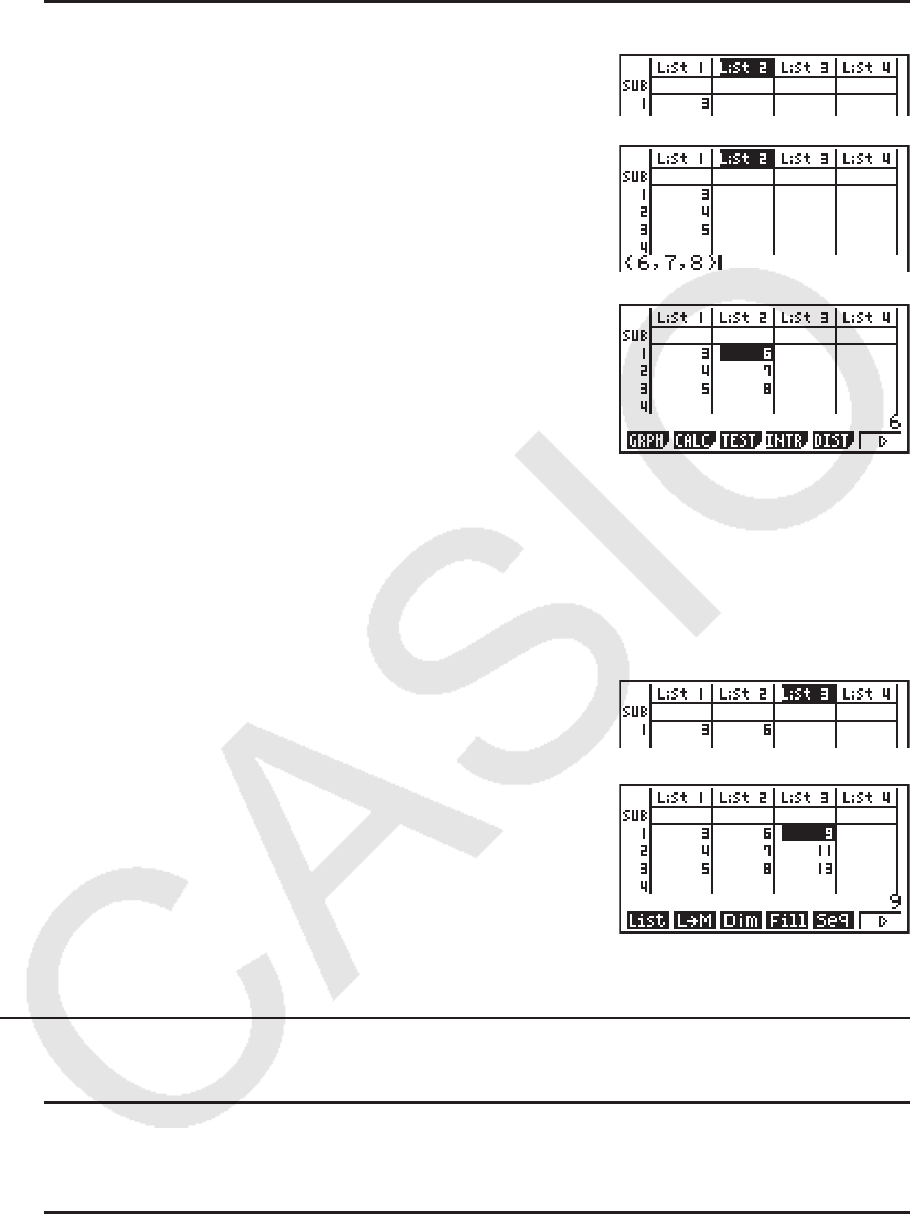
3-2
u 批量输入一系列数值
1. 使用光标键突出显示另一个列表。
2. 按下 !*( { ),然后输入您想要的数值,在每个数值之
间按下 ,。在输入最后一个数值之后按下 !/( } )。
!*( { ) g,h,i!/( } )
3. 按下 w,将所有数值存储到列表中。
w
• 请记住逗号可分隔数值,因此您不应在输入集合中最后一个数值之后输入逗号。
正确: {34, 53, 78}
错误: {34, 53, 78,}
您也可使用数学表达式内的列表名称,将数值输入到另一个单元中。下例显示如何将每一行的
数值添加到List 1与List 2中,以及将结果输入List 3。
1. 使用光标键突出显示想要输入计算结果的列表名称。
2. 按下 K并输入表达式。
K1(LIST) 1(List) b+
K1(LIST) 1(List) cw
• 您还可使用 !b(List)替代 K1(LIST) 1(List)。
k 编辑列表数值
u 更改单元数值
使用光标键突出显示想要更改数值的单元。输入新的数值并按下 w,以新数值替代旧数值。
u 编辑单元的内容
1. 使用光标键突出显示想要编辑内容的单元。
2. 按下 6( g) 2(EDIT)。
3. 可对数据进行任何修改。

3-3
u 删除单元
1. 使用光标键突出显示想要删除的单元。
2. 按下 6( g) 3(DEL),删除选定的单元,使其下方所有内容上移。
• 单元删除操作不会影响其他列表中的单元。如果在被删除单元所在的列表中,数据以某种方式
与邻近单元中的数据相关联,则删除单元可能造成相关数值不符。
u 删除列表中的所有单元
使用下述程序,删除列表中的所有数据。
1. 使用光标键突出显示想要删除数据的任何列表单元。
2. 按下 6( g) 4(DEL •
A) 后将显示一条确认消息。
3. 按下 1(Yes),删除选定列表中的所有单元;或者按下 6(No),取消删除操作,不删除任何
内容。
u 插入新单元
1. 使用光标键突出显示想要插入新单元的位置。
2. 按下 6( g) 5(INS),插入包含数值0的新单元,使其下方的每一项内容下移。
• 单元插入操作不会影响其他列表中的单元。如果在插入单元的列表中,数据以某种方式与邻近
单元中的数据相关联,则插入单元可能造成相关数值不符。
k 命名列表
您可为List 1至List 26指定“子名称”,每个名称最多8个字节。
u 命名列表
1. 在设置屏幕上,突出显示“Sub Name”,然后按下 1(On) J。
2. 使用光标键突出显示想要命名的列表的SUB单元。
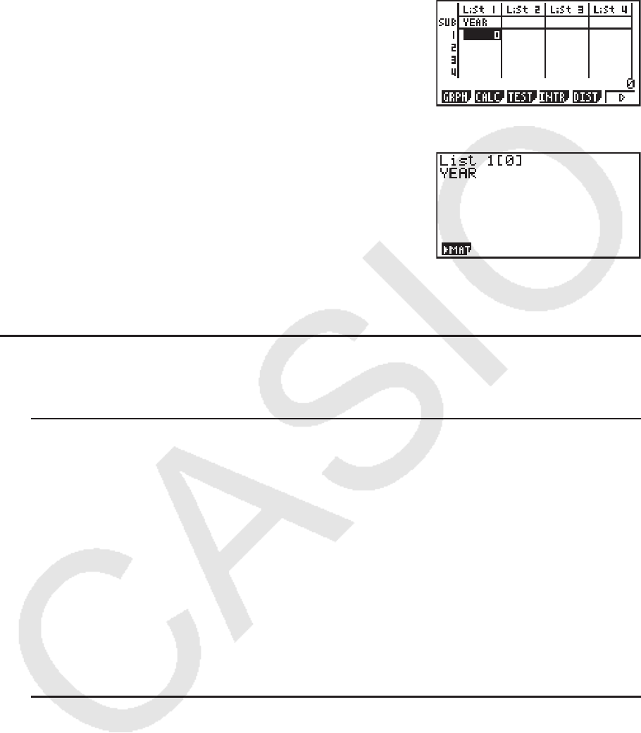
3-4
3. 输入名称,然后按下 w。
• 如需使用字母字符输入名称,按下 !a以进入ALPHA-LOCK模式。
示例:YEAR
-(Y) c(E) v(A) g(R) w
• 下述操作显示了在 RUN • MAT (或者 RUN )模式中的一个子名称。
!b(List)
n!+( [ ) a!-( ] ) w
(
n = 列表号1至26)
• 虽然每个子名称最多可输入8个字节,但列表编辑器中只显示其可容纳的字符。
• 如果在设置屏幕上“Sub Name”设定为“Off”,则不显示列表编辑器SUB单元。
k 列表数值排序
您可以升序或降序排列列表。突出显示部分可以位于列表的任何单元中。
u 单个列表的排序
升序
1. 当屏幕上显示列表时,按下 6( g) 1(TOOL) 1(SRT
•
A)。
2. 显示提示“How Many Lists?:”,询问您想要排列的列表数量。在此,我们将输入1,表示我
们只想排列一个列表。
bw
3. 针对“Select List List No:”提示,输入想要排列的列表编号。
bw
降序
使用与升序排序相同的程序。唯一的差别在于您应该按下 2(SRT
•
D),而不是 1(SRT
•
A)。
u 多个列表的排序
您可以将多个列表连接在一起进行排序,使其所有单元根据基本列表的顺序重新排列。按照升
序或者降序排列基本列表,同时连接列表的单元在排列时保持所有行的相对关系。

3-5
升序
1. 当屏幕上显示列表时,按下 6( g) 1(TOOL) 1(SRT
•
A)。
2. 显示提示“How Many Lists?:”,询问您想要排列的列表数量。在此,我们将对连接另一个
列表的基本列表进行排序,因此我们应该输入2。
cw
3. 针对“Select Base List List No:”提示,输入想要按照升序排列的列表编号。在此,我们将
指定List 1。
bw
4. 针对“Select Second List List No:”提示,输入想要连接到基本列表的列表编号。在此,我
们将指定List 2。
cw
降序
使用与升序排序相同的程序。唯一的差别在于您应该按下 2(SRT
•
D),而不是 1(SRT
•
A)。
• 可指定的排序列表数量介于1至6之间。
• 如果在单次排序操作中某个列表被指定多次,会产生错误。
如果被指定进行排序的列表数值数量(行)不同,也会产生错误。
2. 操控列表数据
列表数据可用于算术和函数计算。此外,各种列表数据的操控功能,也可使列表数据的操作变
得快捷、简便。
您可在 RUN •
MAT (或者 RUN )、 STAT 、 TABLE 、 EQUA 和 PRGM 模式中使用列表数据操控功
能。
k 访问列表数据操控功能菜单
下述所有例子均在进入 RUN •
MAT (或者 RUN )模式后执行。
按下 K后再按下 1(LIST)显示列表数据操控菜单,其中包含以下项目。
• { List } / { L → M } / { Dim } / { Fill } / { Seq } / { Min } / { Max } / { Mean } / { Med } / { Aug } / { Sum } / { Prod } / { Cum
l } / { % } / { A}
请注意,下述操作结尾处的所有右圆括号都可省略。
u 将列表内容传送到矩阵答案存储器 [OPTN] - [LIST] - [L → M]
(fx-7400G
II中不包括)
K1(LIST) 2(L → M) 1(List) <列表号1-26> ,1(List) <列表号1-26> ...
,1(List) <列表号1-26> )w
• 您可在上述操作部分跳过输入 1(List)。
• 所有列表都必须包含同样数量的数据项目。否则会出现错误。
示例:List → Mat (1, 2) w
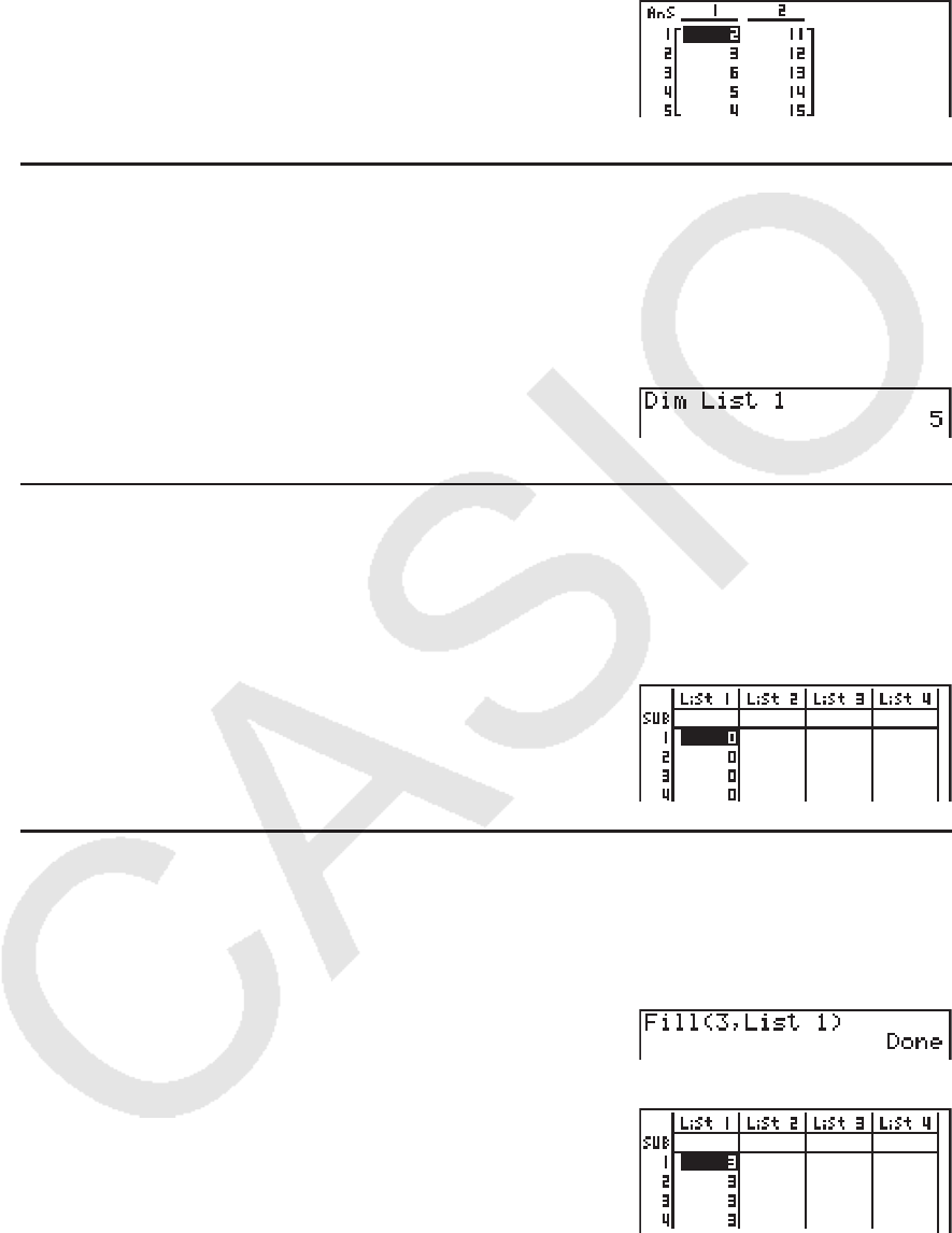
3-6
示例 将List 1(2, 3, 6, 5, 4)的内容传送到矩阵答案存储器的列1,将List 2(11,
12, 13, 14, 15)的内容传送到列2
AK1(LIST) 2(L → M)
1(List) b,1(List) c)w
u 统计列表中的数据项目数量 [OPTN] - [LIST] - [Dim]
K1(LIST) 3(Dim) 1(List) <列表号1 - 26> w
• 列表中包含的单元数称为其“尺寸”。
示例 统计List 1(36, 16, 58, 46, 56)中数值的数量
AK1(LIST) 3(Dim)
1(List) bw
u 通过指定数据项目数量,创建列表 [OPTN] - [LIST] - [Dim]
使用下述程序,在赋值语句中指定数据项目数并创建列表。
<数据数量
n> aK1(LIST) 3(Dim) 1(List) <列表号1 - 26> w ( n = 1 - 999)
示例 在List 1中创建五个数据项目(每个项目包含0值)
AfaK1(LIST) 3(Dim)
1(List) bw
您可通过进入 STAT 模式,查看新创建的列表。
u 使用相同值替代所有数据项目 [OPTN] - [LIST] - [Fill]
K1(LIST) 4(Fill) <数值> ,1(List) <列表号1 - 26> )w
示例 使用数字3替代List 1中的所有数据项目
AK1(LIST) 4(Fill)
d,1(List) b)w
下面显示了List 1的新内容。
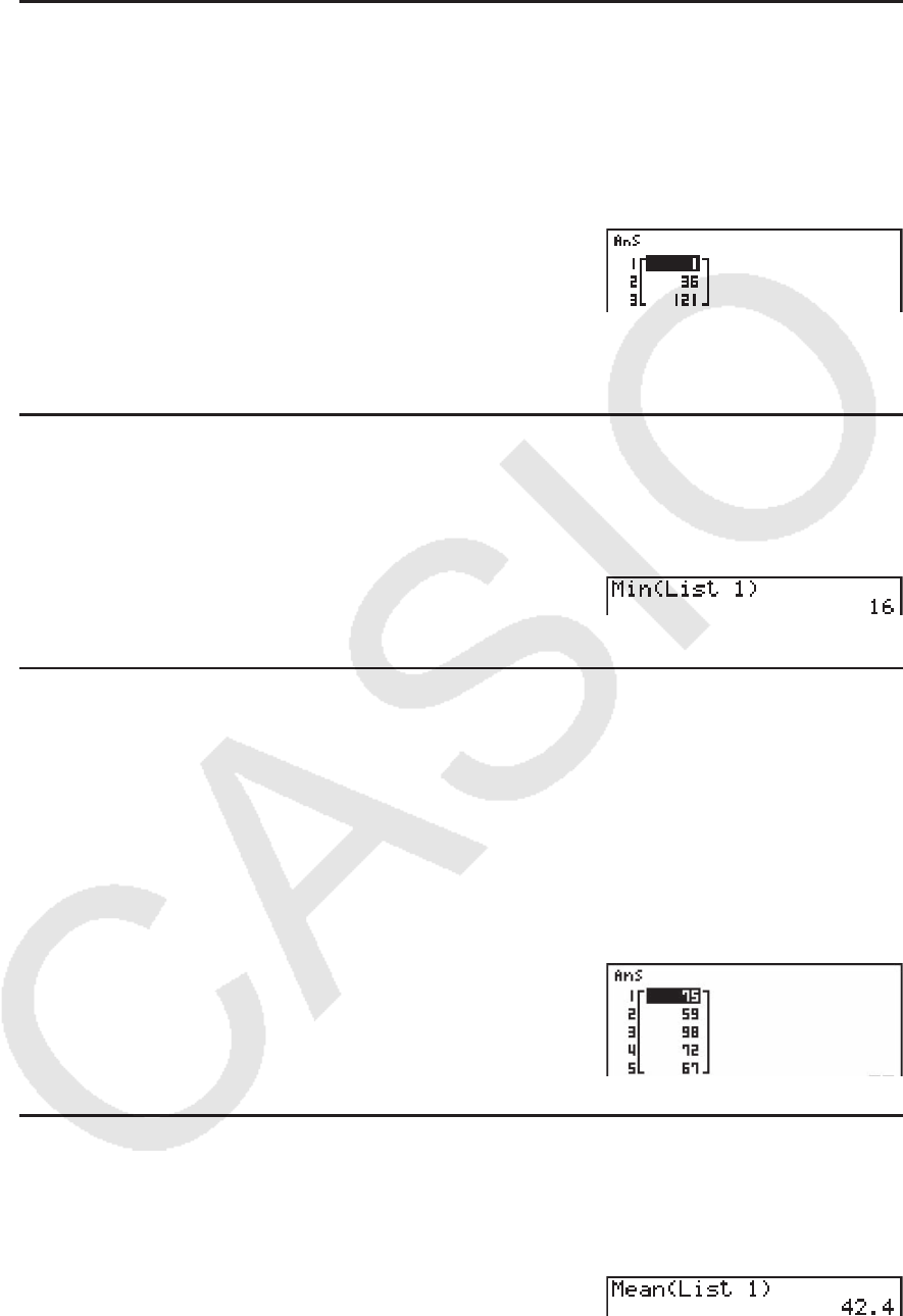
3-7
u 生成数列 [OPTN] - [LIST] - [Seq]
K1(LIST) 5(Seq) <表达式> , <变量名称> , <初值> , <终值> , <增量> )w
• 此运算结果存储在ListAns存储器中。
示例 将数列1
2
、6
2
、11
2
输入列表中 - 使用函数 f( x) = X
2
。使用的初值为1,终值为
11,增量为5。
AK1(LIST) 5(Seq) vx,
v,b,bb,f)w
指定终值12、13、14或者15,可得出与上述相同的结果,因为它们小于下一个增量(16)对应
的函数值。
u 找出列表中的 最小值 [OPTN] - [LIST] - [Min]
K1(LIST) 6( g) 1(Min) 6( g) 6( g) 1(List) <列表号1 - 26> )w
示例 找出List 1(36, 16, 58, 46, 56)中的最小值
AK1(LIST) 6( g) 1(Min)
6( g) 6( g) 1(List) b)w
u 找出两个列表中哪一个列表包含最大值 [OPTN] - [LIST] - [Max]
K1(LIST) 6( g) 2(Max) 6( g) 6( g) 1(List) <列表号1 - 26> ,1(List)
<列表号1 - 26> )w
• 两个列表都必须包含同样数量的数据项目。否则会出现错误。
• 此运算结果存储在ListAns存储器中。
示例 找出List 1(75, 16, 98, 46, 56)或者List 2(35, 59, 58, 72, 67)中哪个
列表包含最大值
K1(LIST) 6( g) 2(Max)
6( g) 6( g) 1(List) b,
1(List) c)w
u 计算数据项目的平均值 [OPTN] - [LIST] - [Mean]
K1(LIST) 6( g) 3(Mean) 6( g) 6( g) 1(List) <列表号1 - 26> )w
示例 计算List 1(36, 16, 58, 46, 56)中数据项目的平均值
AK1(LIST) 6( g) 3(Mean)
6( g) 6( g) 1(List) b)w
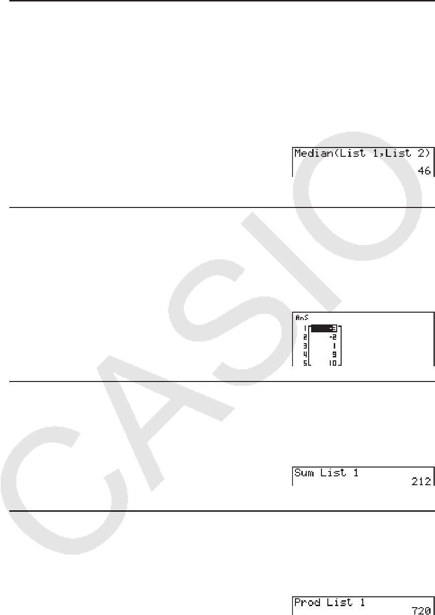
3-8
u 计算指定频率数据项目的中位数 [OPTN] - [LIST] - [Med]
该程序使用两个列表:一个包含数值的列表和一个包含每个数值出现频率的列表。第一个列表
中单元1的数据频率由第二个列表单元1中的数值表示,依此类推。
• 两个列表都必须包含同样数量的数据项目。否则会出现错误。
K1(LIST) 6( g) 4(Med) 6( g) 6( g) 1(List) <列表号1 - 26 (数据)> ,1(List)
<列表号1 - 26 (频率)> )w
示例 计算List 1(36, 16, 58, 46, 56)中数值的中位数,其频率由List 2(75, 89,
98, 72, 67)指示
AK1(LIST) 6( g) 4(Med)
6( g) 6( g) 1(List) b,
1(List) c)w
u 组合列表 [OPTN] - [LIST] - [Aug]
• 您可将两个不同的列表组合成一个列表。列表组合操作的结果存储在ListAns存储器中。
K1(LIST) 6( g) 5(Aug) 6( g) 6( g) 1(List) <列表号1 - 26> ,1(List)
<列表号1 - 26> )w
示例 组合List 1(-3, -2)和List 2(1, 9, 10)
AK1(LIST) 6( g) 5(Aug)
6( g) 6( g) 1(List) b,
1(List) c)w
u 计算列表中数据项目的和 [OPTN] - [LIST] - [Sum]
K1(LIST) 6( g) 6( g) 1(Sum) 6( g) 1(List) <列表号1 - 26> w
示例 计算List 1(36, 16, 58, 46, 56)中数据项目的和
AK1(LIST) 6( g) 6( g) 1(Sum)
6( g) 1(List) bw
u 计算列表中数值的积 [OPTN] - [LIST] - [Prod]
K1(LIST) 6( g) 6( g) 2(Prod) 6( g) 1(List) <列表号1 - 26> w
示例 计算List 1(2, 3, 6, 5, 4)中数值的积
AK1(LIST) 6( g) 6( g) 2(Prod)
6( g) 1(List) bw
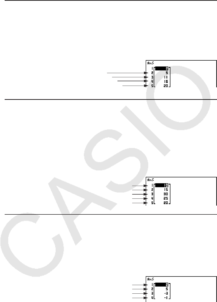
3-9
u 计算每个数据项目的累积频率 [OPTN] - [LIST] - [Cuml]
K1(LIST) 6( g) 6( g) 3(Cuml) 6( g) 1(List) <列表号1 - 26> w
• 此运算结果存储在ListAns存储器中。
示例 计算List 1(2, 3, 6, 5, 4)中每个数据项目的累积频率
AK1(LIST) 6( g) 6( g) 3(Cuml)
6( g) 1(List) bw
u 计算每个数据项目占据的百分比 [OPTN] - [LIST] - [%]
K1(LIST) 6( g) 6( g) 4(%) 6( g) 1(List) <列表号1 - 26> w
• 上述运算计算每个数据项目在列表总和中的百分比。
• 此运算结果存储在ListAns存储器中。
示例 计算List 1(2, 3, 6, 5, 4)中每个数据项目占据的百分比
AK1(LIST) 6( g) 6( g) 4(%)
6( g) 1(List) bw
u 计算列表中相邻数据之差 [OPTN] - [LIST] - [ A]
K1(LIST) 6( g) 6( g) 5( A) <列表号1 - 26> w
• 此运算结果存储在ListAns存储器中。
示例 计算List 1(1, 3, 8, 5, 4)数据项目之差
AK1(LIST) 6( g) 6( g) 5( A)
bw
2+3=
2+3+6=
2+3+6+5=
2+3+6+5+4=
× 100 =2/(2+3+6+5+4)
3/(2+3+6+5+4) × 100 =
6/(2+3+6+5+4) × 100 =
5/(2+3+6+5+4) × 100 =
4/(2+3+6+5+4) × 100 =
3 – 1 =
8 – 3 =
5 – 8 =
4 – 5 =
3-10
• 您可对列表计算结果(保存在ListAns存储器中)指定在列表存储器中的存储位置。例如,指
定“ AList 1 → List 2”将把 AList 1的结果保存到List 2中。
• 新 AList中的单元数比原始列表的单元数小1。
• 如果您对没有数据或只有一个数据项目的列表执行 AList,会产生错误。
3. 使用列表进行算术计算
您可使用两个列表或一个列表与一个数值执行算术计算。
计算结果存储在ListAns存储器中。
k 错误消息
• 涉及两个列表的计算在两个对应的单元之间进行。因此,如果两个列表没有相同数目的数值
(即它们有不同的“尺寸”),会产生错误。
• 一旦涉及任何两个单元的运算产生数学错误,会产生错误。
k 将列表输入计算式
您可使用三种方法将列表输入计算式。
• 指定使用列表编辑器创建的列表的列表号。
• 指定使用列表编辑器创建的列表的子名称。
• 直接输入数值列表。
u 指定使用列表编辑器创建的列表的列表号
1. 在 RUN • MAT (或者 RUN )模式中,执行以下键操作。
AK1(LIST) 1(List)
• 输入“List”命令。
2. 输入想要指定的列表号(1至26的整数)。
u 指定使用列表编辑器创建的列表的子名称
1. 在 RUN • MAT (或者 RUN )模式中,执行以下键操作。
AK1(LIST) 1(List)
• 输入“List”命令。
2. 输入想要指定的列表的子名称并使用双引号(" ")包围。
示例:"QTY"
列表
数值
列表
数值
+
−
×
÷
=列表
ListAns存储器

3-11
u 直接输入数值列表
您还可使用{,}和 ,直接输入数值列表。
示例 输入列表: 56, 82, 64
!*( { ) fg,ic,
ge!/( } )
u 将一个列表的内容指定给另一个列表
使用 a将一个列表的内容指定给另一个列表。
示例 将List 3(41, 65, 22)的内容指定给List 1
K1(LIST) 1(List) da1(List) bw
除了上述程序中的 1(LIST) 1(List) d操作之外,您可输入 !*( { ) eb,gf,
cc!/( } )。
u 调用特定列表单元中的数值
您可调用特定列表单元中的数值并将其用于计算式。指定单元编号并用方括号括住。
示例 计算保存在List 2的单元3中的数值的正弦值
sK1(LIST) 1(List) c!+( [ ) d!-( ] ) w
u 将数值输入特定单元
您可将数值输入列表中的特定单元。在您操作时,以前存储在单元中的数值被新输入的数值替
代。
示例 将数值25输入List 3的单元2
cfaK1(LIST) 1(List) d!+( [ ) c!-( ] ) w
k 调用列表内容
示例 调用List 1的内容
K1(LIST) 1(List) bw
• 上述操作显示您指定的列表内容并保存在ListAns存储器中。 此后您可在计算式中使用
ListAns存储器内容。
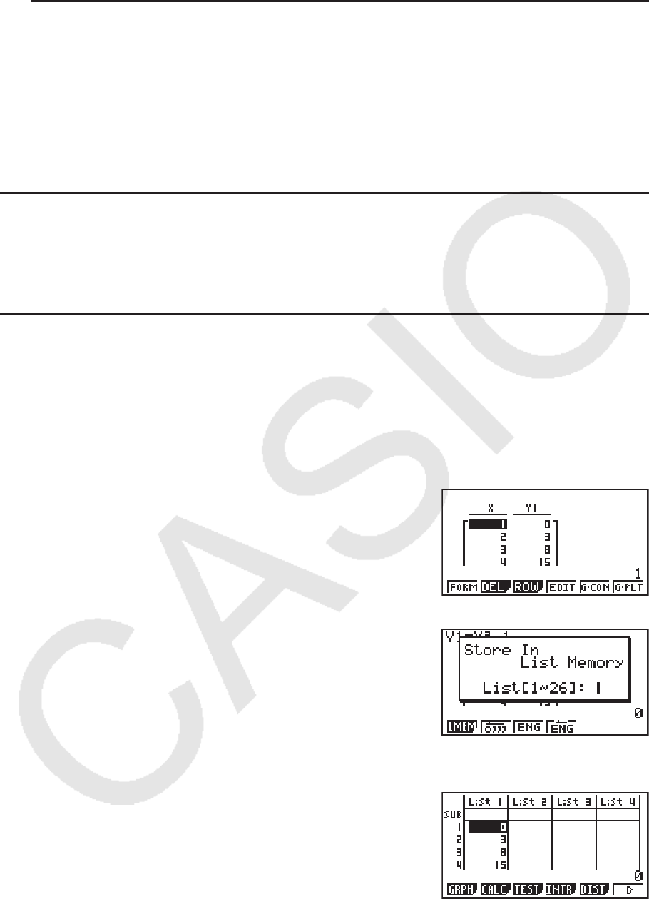
3-12
u 在计算式中使用ListAns存储器中的列表内容
示例 将ListAns存储器中的列表内容乘以36
K1(LIST) 1(List) !-(Ans) *dgw
• K1(LIST) 1(List) !-(Ans)操作调用ListAns存储器内容。
• 该操作以上述计算结果替代当前ListAns存储器内容。
k 使用列表绘制函数图形
在使用此计算器的制图函数时,您可输入诸如Y1 = List 1X的函数。如果List 1 包含数值1、2、
3,该函数将产生三个图形:Y = X、Y = 2X、Y = 3X。
对列表制图函数的使用存在某些限制。
k 将科学计算式输入列表
您可使用 TABLE 模式中的数值表格生成功能,将某些科学函数计算的结果输入列表。为此,首
先生成一个表格,然后使用列表复制功能将数值从表格复制到列表。
示例 使用TABLE模式为公式(Y1 =
x2
-1)创建一个数值表格,然后在STAT模式中
将表格复制到List 1
1. 在 TABLE 模式中,输入公式Y1 =
x2
-1。
2. 创建数值表格。
3. 使用 e移动突出部分到Y1列。
4. 按下 K1(LMEM)。
5. 按下 bw。
6. 进入 STAT 模式并确认 TABLE 模式列Y1已经复制到List 1。
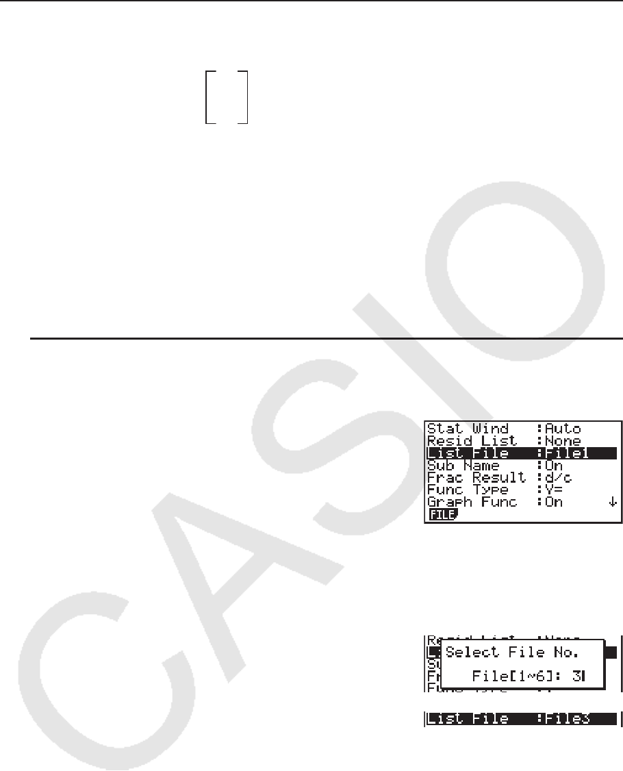
3-13
k 使用列表进行科学函数计算
列表可用作科学函数计算中的数值。当计算结果为列表时,该列表保存到ListAns存储器。
示例 使用List 3
41
65
22
执行sin (List 3)计算
使用弧度作为角度单位。
sK1(LIST) 1(List) dw
4. 在列表文件之间切换
您最多可在每个文件(File 1至File 6)中存储26个列表(List 1至List 26)。只需简单操作即
可在列表文件之间进行切换。
u 在列表文件之间切换
1. 在主菜单中,进入 STAT 模式。
按下 !m(SET UP),显示 STAT 模式设置屏幕。
2. 使用 c突出显示“List File”。
3. 按下 1(FILE),然后输入想要使用的列表文件的编号。
示例 选择文件3
1(FILE) d
w
所有后续列表操作皆应用于选定文件内包含的列表(上例中为List File 3)。

4-1
第4章 方程计算
在主菜单中,进入 EQUA 模式。
• { SIML } ... {带有2至6个未知数的线性方程}
• { POLY } ... {2至6阶方程}
• { SOLV } ... {求解计算}
1. 线性方程组
您可求解带有2至6个未知数的线性方程组。
• 带有2个未知数的线性方程组:
a1
x + b1
y = c1
a2
x + b2
y = c2
• 带有3个未知数的线性方程组:
a1
x + b1
y + c1
z = d1
a2
x + b2
y + c2
z = d2
a3
x + b3
y + c3
z = d3
…
1. 在主菜单中,进入 EQUA 模式。
2. 选择SIML(方程组)模式,指定未知数(变量)的个数。您可指定2至6个未知数。
3. 顺序输入系数。
• 突出显示当前选定输入的单元。每次输入一个系数后,突出显示部位按照以下顺序向后移
动:
a1
→ b1
→ c1
→ ... an → bn → cn → ( n = 2至6)
• 您也可输入分数和数值作为变量的指定系数。
• 在任何时候,您都可通过按下 J(在按下 w以保存系数值之前),取消正在输入的当前
系数值。由此可使系数返回输入之前的值。此后您可根据需要输入其他任何值。
• 如需更改已经通过按下 w保存的系数值,将光标移至需要编辑的系数。然后输入想要更改
的值。
• 按下 3(CLR),将所有系数设置为0。
4. 求解方程。
示例 求解下述线性方程组中的
x, y和 z
4 x + y
- 2 z = -1
x + 6 y + 3 z = 1
-5
x + 4 y + z = -7
4

4-2
1 m EQUA
2 1(SIML)
2(3)
3 ewbw-cw-bw
bwgwdwbw
-fwewbw-hw
4 1(SOLV)
• 内部计算使用15位尾数执行,但显示结果时使用10位尾数和2位指数。
• 线性方程组在求解时倒置由方程系数构成的矩阵。例如,带有3个未知数的线性方程组的求解
如下( x , y , z )。
因此,如果行列式的值接近零,解的精度也会降低。此外,带有3个或更多未知数的方程组可
能需要非常长的时间才可完成求解。
• 如果计算器无法求解,会产生错误。
•计算完成后,您可按下 1(REPT),更改系数值然后重新计算。
2. 2至6次的高阶方程
您的计算器可求解2至6次的高阶方程。
• 二次方程:
ax2
+ bx + c = 0 ( a 0)
• 三次方程:
ax3
+ bx2
+ cx + d = 0 ( a 0)
• 四次方程:
ax4
+ bx3
+ cx2
+ dx + e = 0 ( a 0)
…
1. 在主菜单中,进入 EQUA 模式。
2. 选择POLY(多项式)模式,然后指定方程的阶次。
您可指定的阶次为2至6。
3. 顺序输入系数。
• 突出显示当前选定输入的单元。每次输入一个系数后,突出显示部位按照以下顺序向后移
动:
a → b → c → ...
• 您也可输入分数和数值作为变量的指定系数。
• 在任何时候,您都可通过按下 J(在按下 w以保存系数值之前),取消正在输入的当前
系数值。由此可使系数返回输入之前的值。此后您可根据需要输入其他任何值。
–1
=
x
y
z
a1b1c1
a2b2c2
a3b3c3
d1
d2
d3
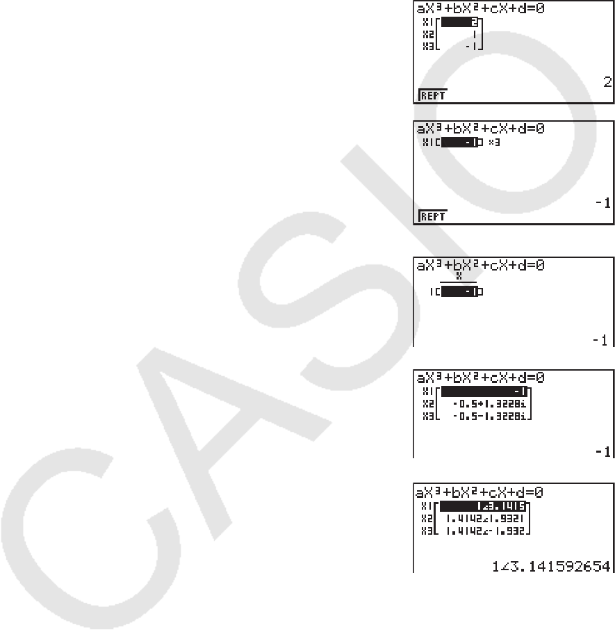
4-3
• 如需更改已经通过按下 w保存的系数值,将光标移至需要编辑的系数。然后输入想要更改
的值。
• 按下 3(CLR),将所有系数设置为0。
4. 求解方程。
示例 求解三次方程(角度单位= Rad)
x3
- 2 x2
- x + 2 = 0
1 m EQUA
2 2(POLY)
2(3)
3 bw-cw-bwcw
4 1(SOLV)
多重解(示例:
x3
+ 3 x2
+ 3 x + 1 = 0)
复数解(示例:
x3
+ 2 x2
+ 3 x + 2 = 0)
Complex Mode:Real(第1-27页)
Complex Mode:
a + bi
Complex Mode:
r∠
θ
• 内部计算使用15位尾数执行,但显示结果时使用10位尾数和2位指数。
• 显示屏可能需要较长时间才可显示三次或更高阶方程的计算结果。
• 如果计算器无法求解,会产生错误。
• 如果高阶方程存在多重解,可能无法得到精确结果。
• 计算完成后,您可按下 1(REPT),更改系数值然后重新计算。
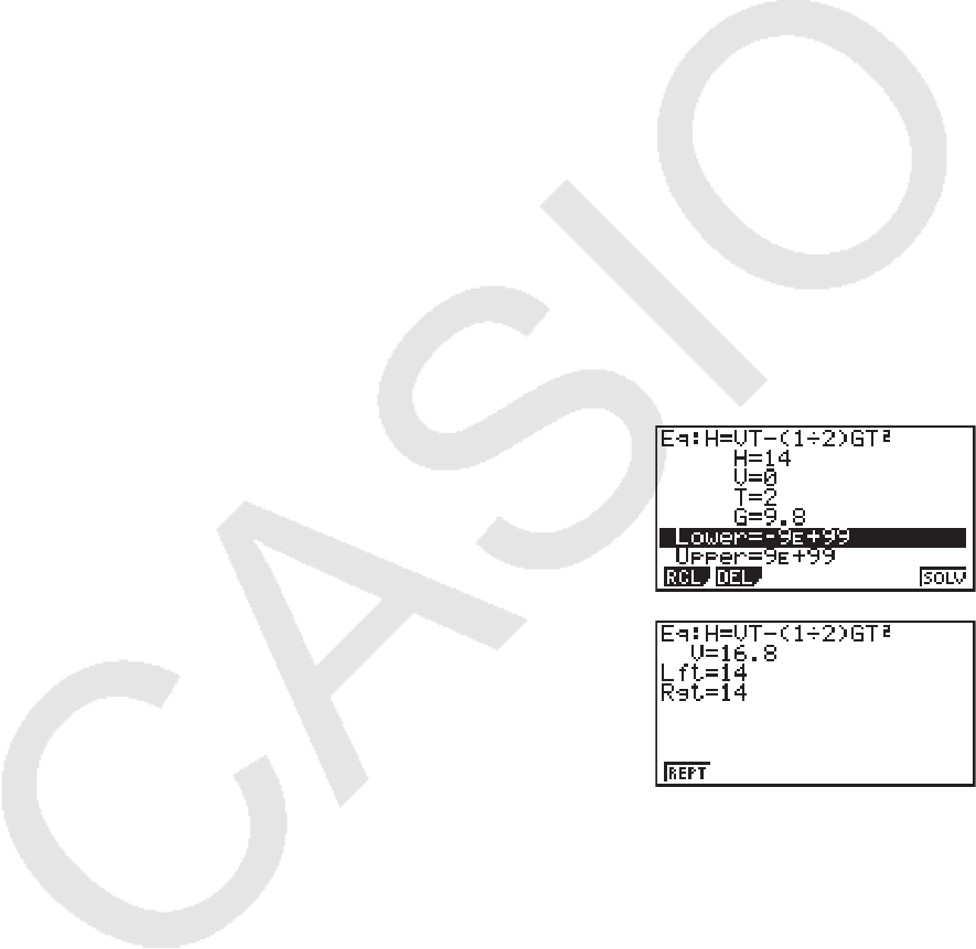
4-4
3. 求解计算
求解计算模式无需求解方程即可确定公式中任何变量的值。
1. 在主菜单中,进入 EQUA 模式。
2. 选择SOLV(求解)模式,然后按照书写方式输入方程。
• 如果您不输入等号,计算器假设表达式为等号左侧部分,等号右侧部分为0。
• 如果输入多个等号,会产生错误。
3. 在显示屏上显示的变量表中,输入每个变量的值。
• 您还可指定Upper和Lower值,定义方程解的上限和下限。
• 如果解超出指定范围,会产生错误。
4. 选择需要求解的变量以获取解。
“Lft”和“Rgt”表示使用解计算的左侧和右侧。*
1
*
1
使用牛顿法求得近似解。由于牛顿法可能得到真实解结果,因此计算器显示Lft和Rgt值供您
确认。Lft与Rgt值的差值越接近零,结果误差越小。
示例 一个物体以初始速度V抛向空中,在T 时间内达到高度H。使用以下公式求解在
H = 14(米)、T = 2(秒)且重力加速度为G = 9.8 (m/s
2
)条件下的初始速度
V。
H = VT - 1/2 GT
2
1 m EQUA
2 3(SOLV)
aM(H) !.(=) ac(V) a/(T) -
(b/c)a$(G) a/(T) xw
3 bew(H = 14)
aw(V = 0)
cw(T = 2)
j.iw(G = 9.8)
4 按下 fff突出显示V = 0,然后按下 6(SOLV)。
• 当计算器判断收敛性不足而无法显示结果时,显示屏上显示“Retry”消息。
• 求解计算产生单一解。如果你想获得高阶方程的多个解,(例如 ax2
+ bx + c = 0)请使用
POLY。
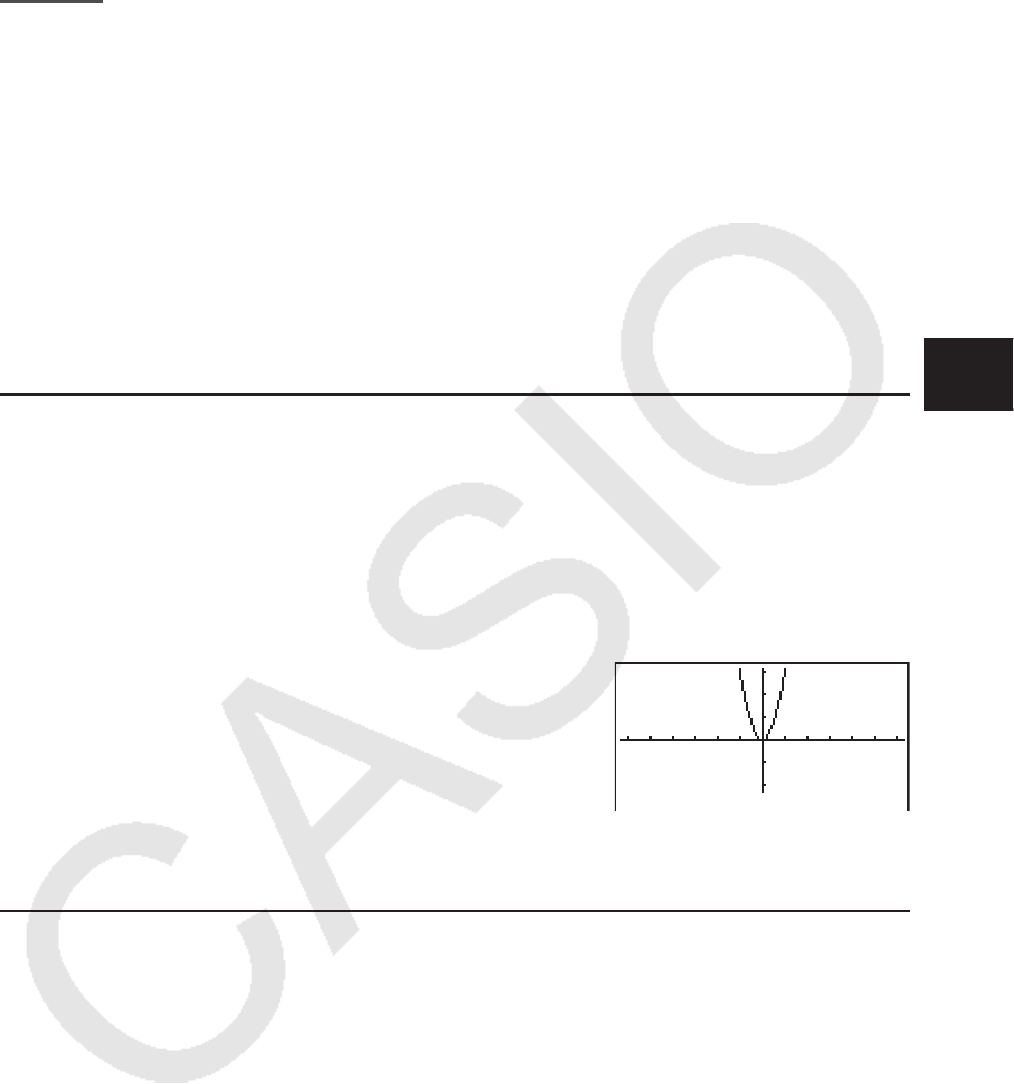
5-1
第5章 绘图
在主菜单中选择适合所需绘制图形类型或所需生成表格类型的图标。
• GRAPH ... 一般函数绘图
• RUN • MAT (或者 RUN )... 手动绘图(第5-12页至第5-15页)
• TABLE ... 生成数值表格(第5-15页至第5-19页)
• DYNA* ... 动态绘图(第5-20页至第5-22页)
• RECUR* ... 生成递归图形或数值表格(第5-22页至第5-26页)
• CONICS* ... 二次曲线绘图(第5-27页)
* fx-7400G II 中不包括。
1. 图形样例
k 如何绘制简单图形(1)
只需输入相关函数即可绘制图形。
1. 在主菜单中,进入 GRAPH 模式。
2. 输入需要绘制图形的函数。
在此,您需要使用视窗指定范围和图形的其他参数。参见第5-3页。
3. 绘制图形。
示例 绘制图形
y = 3 x2
1 m GRAPH
2 dvxw
3 6(DRAW) (或者 w)
• 按下 A,返回第2步中的屏幕(图形关系列表)。绘制图形之后,您可能通过按
下 !6(G ↔ T)在图形关系列表与图形屏幕之间切换。
k 如何绘制简单图形(2)
您最多可在存储器中存储20个函数,此后您可从其中选择需要绘制图形的某个函数。
1. 在主菜单中,进入 GRAPH 模式。
2. 指定函数类型并输入需要绘制图形的函数。您可使用 GRAPH 模式绘制以下类型表达式的图
形:直角坐标表达式(Y=
f( x))、极坐标表达式、参数化函数、直角坐标表达式(X= f( y))、
不等式。
3(TYPE) 1(Y=) ... 直角坐标(Y=
f( x)类型)
2(
r=) ... 极坐标
3(Parm) ... 参数化函数
4(X=) ... 直角坐标(X=
f( y)类型)
5(CONV) 1(
'Y=) 至 5( 'Y )
6( g) 1(
'X=) 至 5( 'X ) ... 更改函数类型
6( g) 1(Y>) 至 4(Y ) .... 左侧Y不等式
6( g) 6( g) 1(X>) 至 4(X ) .... 左侧X不等式
5
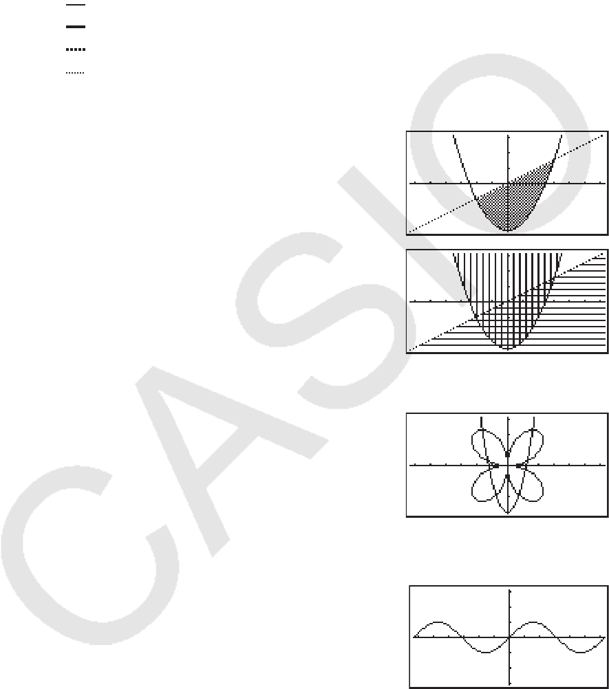
5-2
根据需要重复执行该步骤,输入所有需要的函数。
下一步应指定需要绘制存储器中保存的哪些函数图形(参见第5-6页)。如果您不在此选择具
体函数,图形操作将绘制当前保存在存储器中的所有函数的图形。
3. 绘制图形。
• 在上述步骤第2步中按下 4(STYL) 可显示功能菜单,您可使用该菜单为每一个图形选择以
下线型。
1() ... 标准线(初始默认设置)
2() ... 粗线(线宽为标准线型的两倍)
3() ... 虚线(粗虚线)
4() ... 点线(点状线)
• 在同时绘制多个不等式时,您可使用设置屏幕上的“Ineq Type”设置( !m(SET UP))
指定两种填充范围中的任何一种。
1(AND) ... 只填充满足所有绘制不等式条件的区域。
这是初始默认设置。
2(OR) ........ 填充所有满足绘制不等式条件的区域。
例1 输入下述函数并绘制其图形。
Y1 = 2
x2
- 3, r2 = 3sin2
θ
1 m GRAPH
2 3(TYPE) 1(Y=) cvx-dw
3(TYPE) 2(
r=) dscvw
3 6(DRAW)
例2 角度单位设置为“度”时使用弧度绘制三角函数图形。(角度单位=Deg)
Y1 = sin
x
r
1 m GRAPH
2 svK 6( g) 5(ANGL) 2(
r)w
3 6(DRAW)
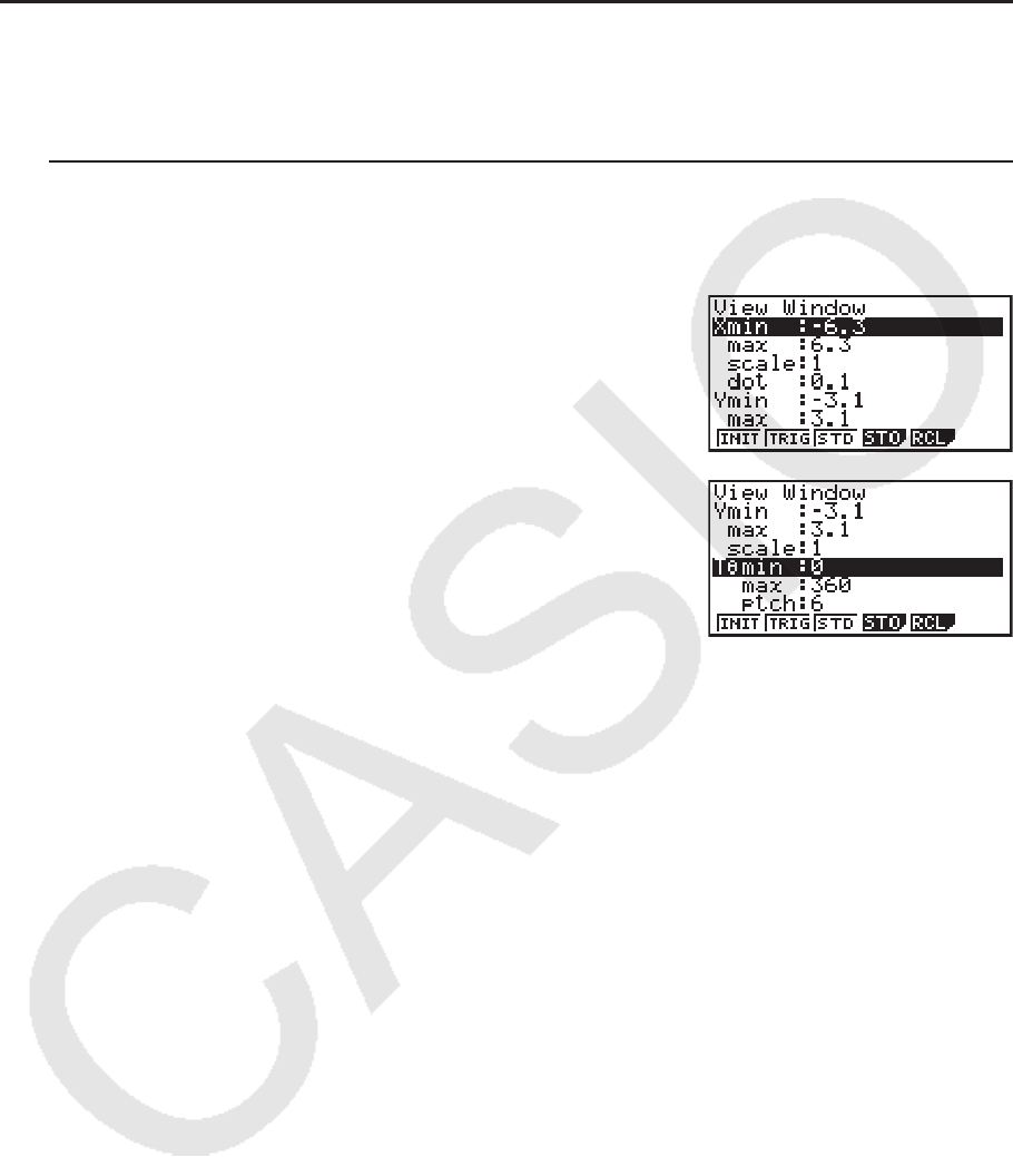
5-3
2. 控制图形屏幕上的显示内容
k 视窗(View Window)设置
使用View Window指定 x和 y轴的范围,并设定每一根轴上增量的间距。您应确保在绘制图形之
前设置视窗参数。
u 设置视窗
1. 在主菜单中,进入 GRAPH 模式。
2. 按下 !3(V-WIN),显示视窗设置屏幕。
直角坐标参数
Xmin/Xmax ... x轴最小值/最大值
Xscale ... x轴增量间距
Xdot ... 对应某个x轴点的值
Ymin/Ymax ... y轴最小值/最大值
Yscale ... y轴增量间距
极坐标参数
T
θ
min/T
θ
max ... 最小/最大T,
θ
值
T
θ
ptch ...T,
θ
间距
3. 按下 c可移动突出显示区域,为每个参数输入适当的值,然后分别按下 w。
• { INIT } / { TRIG } / { STD } ... 视窗{初始设置}/{使用指定角度单位的初始设置}/{标准化设置}
• { STO } / { RCL } ... 视窗设置{存储}/{调用}
完成所需设置后,按下 J或 !J(QUIT),退出视窗设置屏幕。
u 视窗设置注意事项
• 如果T
θ
ptch的输入值是零,会产生错误。
•任何非法输入(超出范围限值、只有负号却没有数值等等)都会产生错误。
•在T
θ
max小于T
θ
min时,T
θ
ptch变为负值。
• 您可输入表达式(例如2 π )作为视窗参数。
• 当视窗设置产生的轴无法在显示屏中完整显示时,显示屏上最靠近原点的边缘将显示轴的比
例。
• 更改视窗设置将清除显示屏上当前显示的图形,并只显示新设置的轴。
•更改Xmin或Xmax值会导致自动调整Xdot值。更改Xdot值会导致自动调整Xmax值。
• 如果视窗中的设置导致T
Ƨ ptch值相对于T
θ
min和T
θ
max设置差值而言过大,极坐标 ( r
=)或
者参数图形的显示会较为粗糙。另一方面,如果设置导致T
θ
ptch值相对于T
θ
min和T
θ
max
设置过小,图形绘制时间会非常长。
• 下面是视窗参数的输入范围。
-9.999999999
E
97至9.999999999
E
97

5-4
k 视窗存储器
您最多可在视窗存储器中保存六组视窗设置,以便在需要时调用。
u 保存视窗设置
1. 在主菜单中,进入 GRAPH 模式。
2. 按下 !3(V-WIN),显示视窗设置屏幕,然后输入所需数值。
3. 按下 4(STO),显示弹出窗口。
4. 按下某个数字键以指定需要保存设置的视窗存储器,然后按下 w。按下 bw,将设置保存
在视窗存储器1(V-Win1)中。
u 调用视窗存储器设置
1. 在主菜单中,进入 GRAPH 模式。
2. 按下 !3(V-WIN),显示视窗设置屏幕。
3. 按下 5(RCL),显示弹出窗口。
4. 按下某个数字键以指定需调用的设置所在的视窗存储器编号,然后按下 w。按下 bw,调
用视窗存储器1 (V-Win1)中的设置。
k 指定图形范围
您可在绘制函数图形之前定义范围(起点、终点)。
1. 在主菜单中,进入 GRAPH 模式。
2. 进行视窗设置。
3. 指定函数类型并输入函数。下面是函数输入的语法。
函数 ,!+( [ )起点 ,终点 !-( ] )
4. 绘制图形。
示例 图形
y = x2
+ 3 x - 2,范围:-2 < x < 4。
使用以下视窗设置。
Xmin = -3, Xmax = 5, Xscale = 1
Ymin = -10, Ymax = 30, Yscale = 5
1 m GRAPH
2 !3(V-WIN) -dwfwbwc
-bawdawfwJ
3 3(TYPE) 1(Y=) vx+dv-c,
!+( [ ) -c,e!-( ] ) w
4 6(DRAW)
• 您可在绘制直角坐标表达式、极坐标表达式、参数函数和不等式图形时定义范围。

5-5
k 缩 放
该功能可放大或者缩小显示屏上的图形。
1. 绘制图形。
2. 指定缩放类型。
!2(ZOOM) 1(BOX) ... 矩形框缩放
在显示区周围绘制一个矩形框,该区域放大至全屏。
2(FACT)
指定系数缩放的
x轴和 y轴缩放系数。
3(IN)/ 4(OUT) ... 系数缩放
计算器按照您指定的系数,以当前指针位置为中心缩放图形。
5(AUTO) ... 自动缩放
视窗
y轴设置自动调整,使图形沿着 y轴填充屏幕。
6( g) 1(ORIG) ... 原始尺寸
执行缩放操作之后,使图形返回原始尺寸。
6( g) 2(SQR) ... 图形修正
修正视窗
x轴值,使其等于 y轴值。
6( g) 3(RND) ... 坐标舍入
在当前指针位置舍入坐标值。
6( g) 4(INTG) ... 整数
每个点的宽度为1,因此坐标值为整数。
6( g) 5(PRE) ... 先前设置
视窗参数恢复到上次缩放操作之前的设置。
使用矩形框规定缩放范围
3. 使用光标键将屏幕中心的指针( )移至矩形框的某一角,然后按下 w。
4. 使用光标键移动指针。由此可在屏幕上显示一个矩形框。移动光标,直至需要放大的区域已
被矩形框包围,然后按下 w执行放大操作。
示例 绘制
y = ( x + 5)( x + 4)( x + 3)图形,然后执行矩形框缩放操作。
使用以下视窗设置。
Xmin = -8, Xmax = 8, Xscale = 2
Ymin = -4, Ymax = 2, Yscale = 1
1 m GRAPH
!3(V-WIN) -iwiwcwc
-ewcwbwJ
3(TYPE) 1(Y=) (v+f)(v+e)
(v+d)w
6(DRAW)
2 !2(ZOOM) 1(BOX)
3 d~ dw
4 d~ d, f~ fw
• 在执行矩形框缩放操作时,您必须指定两个不同的点,而且这两个点不能在同一条垂直线或者
水平线上。
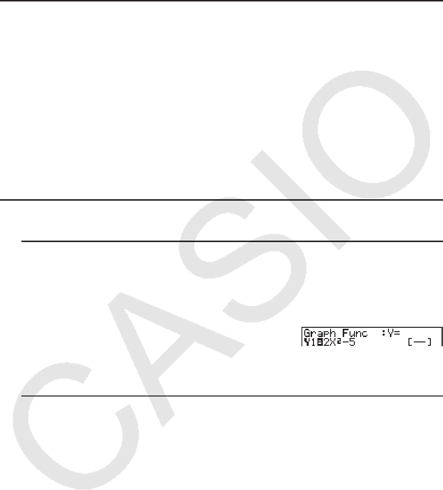
5-6
3. 绘制图形
您最多可在存储器中保存20个函数。可对存储器中的函数进行编辑、调用和绘制图形操作。
k 指定图形类型
在存储器中保存图形函数之前,必须指定其图形类型。
1. 显示屏上显示图形关系列表时,按下 3(TYPE)可显示图形类型菜单,包含以下项目。
• { Y= } / { r= } / { Parm } / { X= } ... {直角坐标(Y=
f( x)类型)}/{极坐标}/{参数}/{直角坐标(X= f( y)类
型)}图形
• {Y>}/{Y<}/{Y}/{Y} ... {Y>f (x)}/{Y<f (x)}/{Yf (x)}/{Yf (x)} 不等式图形
• {X>}/{X<}/{X}/{X} ... {X>f(y)}/{X<f(y)}/{Xf(y)}/{Xf(y)} 不等式图形
• {CONV}
• {
'Y=}/{'Y>}/{'Y<}/{'Y}/{'Y}/{'X=}/{'X>}/{'X<}/{'X}/{'X}
... {更改选定表达式的函数类型}
2. 按下与目标图形类型对应的功能键。
k 保存图形函数
u 保存直角坐标函数(Y=)
示例 在存储区Y1中保存以下表达式: y = 2 x2
- 5
3(TYPE) 1(Y=)(指定直角坐标表达式。)
cvx-f(输入表达式。)
w(保存表达式。)
• 同一个存储区中不可保存不同类型的函数。选择函数类型与需要保存的函数类型相同的存储
区,或者删除目标存储区中的函数。
u 存储参数化函数
示例 在存储区Xt3和Yt3中保存以下表达式:
x = 3 sinT
y = 3 cosT
3(TYPE) 3(Parm)(指定参数化表达式。)
dsvw(输入和保存
x表达式。)
dcvw(输入和保存
y表达式。)
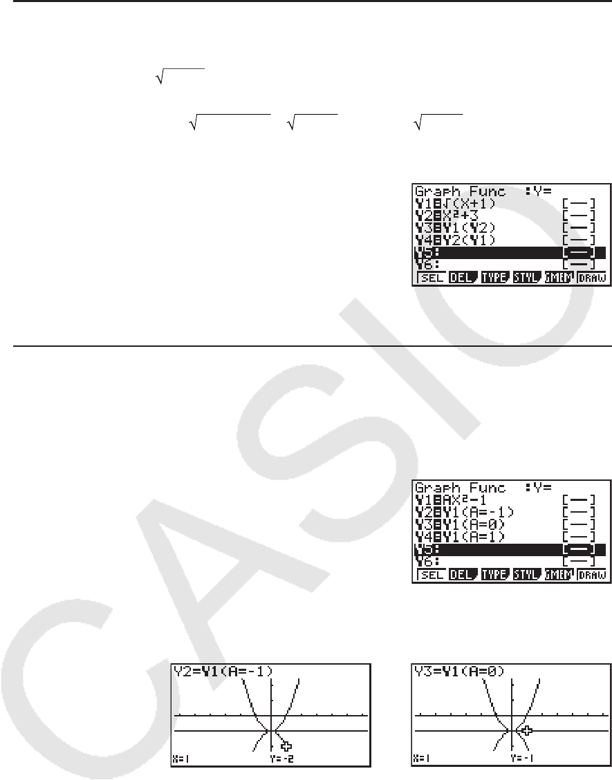
5-7
u 创建复合函数
示例 使用Y1和Y2中的关系创建Y3和Y4的复合函数
Y1 = (X + 1),Y2 = X
2
+ 3
将Y1
°
Y2指定给Y3,将Y2
°
Y1指定给Y4。
(Y1
°
Y2 = ((x
2
+ 3) +1) = (x
2
+ 4) Y2
°
Y1 = ( (X + 1))
2
+ 3 = X + 4 (X > -1))
将关系输入Y3和Y4。
3(TYPE) 1(Y=) J4(GRPH)
1(Y) b(1(Y) c)w
J4(GRPH) 1(Y) c
(1(Y) b)w
• 复合函数最多可包含五个函数。
u 将数值指定给图形函数的系数和变量
示例 将数值-1、0和1指定给Y = AX
2
-1中的变量A,然后为每个值绘制图形
3(TYPE) 1(Y=)
av(A) vx-bw
J4(GRPH) 1(Y) b(av(A)
!.(=) -b)w
J4(GRPH) 1(Y) b(av(A)
!.(=) a)w
J4(GRPH) 1(Y) b(av(A)
!.(=) b)w
ffff1(SEL)
6(DRAW)
上述三个画面由跟踪功能生成。
详情请参见“函数分析”(第5-29页)。

5-8
k 编辑和删除函数
u 编辑存储器中的函数
示例 将存储区Y1中的表达式从 y = 2 x2
- 5改为
y = 2 x2
- 3
e (显示光标。)
eeeeeDd(更改内容。)
w(保存新的图形函数。)
u 更改图形函数的线型
1. 在图形关系列表屏幕上,使用 f和 c突出显示想要更改线型的关系式。
2. 按下 4(STYL)。
3. 选择线型。
示例 将保存在存储区Y1中的
y = 2 x2
- 3的线型改为“Broken”
4 (STYL) 3 ( ) (选择“Broken”。)
u 更改函数的类型 *
1
1. 在显示屏上显示图形关系列表时,按下 f或者 c,突出显示包含需要更改类型的函数的区
域。
2. 按下 3(TYPE) 5(CONV)。
3. 选择想要更改的目标函数类型。
示例 将存储区Y1中的函数从
y = 2 x2
- 3改为 y < 2 x2
- 3
3(T YPE) 5(CONV) 3(
'Y<) (将函数类型改为“Y<”。)
*
1
只有直角坐标函数和不等式才可更改参数类型。
u 删除函数
1. 在显示屏上显示图形关系列表时,按下 f或者 c,突出显示包含您想要删除的函数的区
域。
2. 按下 2(DEL)或者 D。
3. 按下 1(Yes)删除函数或者 6(No)中止该步骤且不删除任何内容。
• 使用上述步骤删除参数化函数中的某一行(例如Xt2)也将删除配对行(Yt2对应Xt2)。
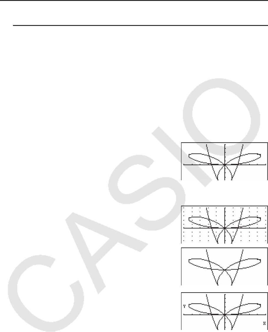
5-9
k 选择需要绘制图形的函数
u 指定图形的绘制/非绘制状态
1. 在图形关系列表上,使用 f和 c突出显示想要绘制的关系式。
2. 按下 1(SEL)。
• 每次按下 1(SEL)都可开启或者关闭绘图功能。
3. 按下 6(DRAW)。
示例 选择绘制以下函数图形:
Y1 = 2
x2
- 5, r2 = 5 sin3
θ
使用以下视窗设置。
Xmin = -5, Xmax = 5, Xscale = 1
Ymin = -5, Ymax = 5, Yscale = 1
T
θ
min = 0, T
θ
max =
π
, T
θ
ptch = 2
π
/ 60
cf(选择一个包含想指定非绘制特性函数的存储区。)
1(SEL) (指定非绘制特性。)
6(DRAW) 或者 w(绘制图形。)
• 您可使用设置屏幕的设置更改图形屏幕的外观,如下所示。
• Grid: On (Axes: On Label: Off)
该设置在屏幕上显示网格交点。
• Axes: Off (Label: Off Grid: Off)
该设置清除显示屏上的轴线。
• Label: On (Axes: On Grid: Off)
该设置显示
x和 y轴标签。

5-10
k 图形存储器
图形存储器最多可存储20组图形函数数据,以便您在以后需要时调用。
只需执行一次保存操作即可将以下数据保存在图形存储器中。
• 在当前显示的图形关系列表中的所有图形函数(最多20个)
• 图形类型
• 函数图形线型信息
• 绘制/非绘制状态
• 视窗设置(1组)
u 将图形函数保存在图形存储器中
1. 按下 5(GMEM) 1(STO) ,显示弹出窗口。
2. 按下某个数字键以指定需要保存图形函数的图形存储器,然后按下 w。按下 bw,将图形
函数保存在图形存储器1(G-Mem1)中。
• 图形存储器共有20个,编号为:G-Mem1至G-Mem20。
• 如果将函数保存在已经包含一个函数的存储区中,新函数将替代现有函数。
•如果数据超过可用存储空间,产生一个错误。
u 调用图形函数
1. 按下 5(GMEM) 2(RCL) ,显示弹出窗口。
2. 按下某个数字键以指定需要调用函数的图形存储器,然后按下 w。按下 bw,调用图形存
储器1(G-Mem1)中的图形函数。
• 如果调用图形存储区中的数据,将删除图形关系列表中的任何数据。
4. 在图片存储区中存储图形
图片存储器最多可存储20个图像,以便以后调用。您可在屏幕上与图片存储器中保存的另一个
图形一起重绘某个图形。
u 将图形保存在图片存储器中
1. 在 GRAPH 模式中绘制图形之后,按下 K1(PICT) 1(STO) ,显示弹出窗口。
2. 按下某个数字键以指定需要保存图片的图片存储器,然后按下 w。按下 bw,将图片函数
保存在图片存储器1(Pict 1)中。
• 图片存储器共有20个,编号为:Pict 1至Pict 20。
• 如果将图片保存在已经包含一个图片的存储区中,新图片将替代现有图片。
• 双图形屏幕或者使用分屏的其它任何类型的图形不可保存在图片存储器中。

5-11
u 调用存储的图形
1. 在 GRAPH 模式中绘制图形之后,按下 K1(PICT) 2(RCL) ,显示弹出窗口。
2. 按下某个数字键以指定需要调用函数的图形存储器,然后按下 w。按下 bw,调用图片存
储器1 (Pict 1)中的图片函数。
• 调用图片存储器内容将导致当前显示的图形被覆盖。
• 使用草图Cls功能(第5-28页)清除从图片存储器调用的图形。
5. 在同一个屏幕上绘制两个图形
k 将图形复制到副屏幕
双图形功能可将屏幕分为两部分。然后您可在每个屏幕中绘制两个不同的函数图形以进行比
较,或者在一侧绘制正常尺寸的图形,在另一侧显示放大视图。因此双图形是一种强大的图形
分析工具。
在双图形功能中,屏幕左侧为“主屏幕”,右侧为“副屏幕”。
u 主屏幕
主屏幕中的图形为根据函数实际绘制的图形。
u 副屏幕
副屏幕中的图形为通过复制或者缩放主屏幕图形产生的图形。您甚至可为副屏幕和主屏幕采用
不同的视窗设置。
u 将图形复制到副屏幕
1. 在主菜单中,进入 GRAPH 模式。
2. 在设置屏幕上,在Dual Screen中选择“G + G”。
3. 进行主屏幕视窗设置。
按下 6(RIGHT)以显示副图形设置屏幕。按下 6(LEFT),返回主屏幕设置屏幕。
4. 保存函数,在主屏幕中绘制图形。
5. 执行所需的双图形操作。
K1(COPY) ... 在副屏幕中复制主屏幕图形
K2(SWAP) ... 交换主屏幕内容和副屏幕内容
• 图形关系列表中公式的右侧显示指示符,提示使用双图形功能绘制的图形。
表示副屏幕图形(显示屏右侧)
表示在显示屏两侧绘制的图形
在上例所示屏幕中对标记“R”的函数执行绘图操作,将在显示屏的右侧绘制图形。标记“ B”
的函数则在图形的两侧绘制。
在突出显示某一函数时按下 1(SEL),将清除其“R”或者“ B”指示符。没有指示符的函数
在主屏幕中绘制(显示屏的左侧)。
5-12
示例 在主屏幕和副屏幕中绘制y = x(x + 1)(x - 1)图形。
使用以下视窗设置。
(主屏幕) Xmin = -2, Xmax = 2, Xscale = 0.5
Ymin = -2, Ymax = 2, Yscale = 1
(副屏幕) Xmin = -4, Xmax = 4, Xscale = 1
Ymin = -3, Ymax = 3, Yscale = 1
1 m GRAPH
2 !m(SET UP) cccc* 1(G + G) J
*fx-7400G
II, fx-9750G II: ccc
3 !3(V-WIN) -cwcwa.fwc
-cwcwbw
6(RIGHT) -ewewbwc
-dwdwbwJ
4 3(TYPE) 1(Y=) v(v+b)(
v-b)w
6(DRAW)
5 K1(COPY)
• 屏幕上显示图形时按下 A将返回第4步中的屏幕。
6. 手动绘图
k 直角坐标图形
在 RUN • MAT (或者 RUN ) 模式中输入图形命令,可绘制直角坐标图形。
1. 在主菜单中,进入 RUN • MAT (或者 RUN ) 模式。
2. 在设置屏幕上,将“Input/Output”设置改为“Linear”。
3. 进行视窗设置。
4. 输入用于绘制直角坐标图形的命令。
5. 输入函数。
示例 绘制 y = 2x2 + 3x - 4的图形。
使用以下视窗设置。
Xmin = -5, Xmax = 5, Xscale = 2
Ymin = -10, Ymax = 10, Yscale = 5
1 mRUN • MAT (或者RUN)
2 !m (SET UP)2(Line) J

5-13
3 !3(V-WIN) -fwfwcwc
-bawbawfwJ
4 !4(SKTCH) 1(Cls) w
5(GRPH) 1(Y=)
5 cvx+dv-ew
• 某些函数可使用内置函数图形轻松绘制。
• 您可绘制以下内置科学函数的图形。
直角坐标图形 极坐标图形
• sin x • cos x • tan x • sin
-1
x
• cos
-1
x • tan
-1
x • sinh x • cosh x
• tanh x • sinh
-1
x • cosh
-
1
x • tanh
-
1
x
• 'x • x2
• log x • ln x
• 10
x • ex • x-1
•
3
'x
• • •
• sin
θ
• cos
θ
• tan
θ
• sin
-1
θ
• cos
-1
θ
• tan-
1
θ
• sinh
θ
• cosh
θ
• tanh
θ
• sinh
-
1
θ
• cosh
-
1
θ
• tanh
-
1
θ
• '
θ
•
θ
2
• log
θ
• ln
θ
• 10
θ
• e
θ
•
θ
-1
•
3
'
θ
- 内置函数不要求提供 x和
θ
变量的输入值。
- 在输入内置函数时,不可输入其他算子或数值。
k 在同一个屏幕上绘制多个图形
使用下述程序将不同的值指定给表达式中的某个变量并覆盖屏幕上产生的图形。
1. 在主菜单中,进入 GRAPH 模式。
2. 在设置屏幕上,将“Dual Screen”设置改为“Off”。
3. 进行视窗设置。
4. 指定函数类型并输入函数。下面是函数输入的语法。
包含一个变量的表达式 ,!+( [ )变量 !.(=)
值 , 值 , ... , 值 !-( ] )
5. 绘制图形。
示例 当A依次变为3、1、-1时,绘制 y = A
x2
- 3的图形
使用以下视窗设置。
Xmin = -5, Xmax = 5, Xscale = 1
Ymin = -10, Ymax = 10, Yscale = 2
1 m GRAPH
2 !m(SET UP) cccc* 3(Off) J
*fx-7400G
II, fx-9750G II: ccc
3 !3(V-WIN) -fwfwbwc
-bawbawcwJ
dx (x)
d
dx2(x)
d2∫(x)dx

5-14
4 3(TYPE) 1(Y=) av(A) vx-d,
!+( [ ) av(A) !.(=) d,b,-b
!-( ] ) w
5 6(DRAW)
• 只可更改表达式中一个变量的值。
• 以下几个字符都不可作为变量名:X、Y、 r、
θ
、T。
• 不可将变量指定给函数内部的变量。
• 在开启Simul Graph功能时,指定变量值的所有图形同时绘制。
• 在绘制直角坐标表达式、极坐标表达式、参数函数和不等式图形时可使用覆盖功能。
k 使用复制和粘贴功能绘制函数图形
您可通过将函数复制到剪贴板,然后粘贴到图形屏幕上的方式绘制函数图形。
在图形屏幕中可粘贴两种类型的函数。
Type 1 (Y=表达式)
Y变量在等号左侧的函数以Y=表达式形式绘图。
示例:粘贴Y=X则绘制其图形
• Y左侧的任何空格都被忽略。
Type 2 (表达式)
粘贴此类表达式将绘制Y=表达式图形。
示例:粘贴X,则绘制Y=X图形
• 表达式左侧的任何空格都被忽略。
u 使用复制和粘贴功能绘制函数图形
1. 将需要绘制图形的函数复制到剪贴板。
2. 在主菜单中,进入 GRAPH 模式。
3. 在设置屏幕上,将“Dual Screen”设置改为“Off”。
4. 进行视窗设置。
5. 绘制图形。
6. 粘贴表达式。
示例 在当前显示
y = 2 x2
+ 3 x - 4的图形时,从剪贴板粘贴以前复制的函数Y=X
使用以下视窗设置。
Xmin = -5, Xmax = 5, Xscale = 2
Ymin = -10, Ymax = 10, Yscale = 5
1 m RUN • MAT (或者RUN)
a-(Y)!.(=)v
!i(CLIP)ddd1(COPY)
2 m GRAPH
3 !m(SET UP) cccc* 3(Off) J
*fx-7400G
II, fx-9750G II: ccc

5-15
4 !3(V-WIN) -fwfwcwc
-bawbawfwJ
5 3(TYPE) 1(Y=) cvx+dv-ew
6(DRAW)
6 !j(PASTE)
• 只有在设置屏幕上将“Dual Screen”设置选择为“Off”时才支持粘贴功能。
• 虽然对于通过粘贴函数方式绘制的图形数量没有限制,但跟踪和其他功能支持的图形总数为
30(使用1至20号表达式绘制的图形数量,加上使用粘贴功能绘制的图形)。
• 对于使用粘贴功能绘制的图形,在使用跟踪或者其他功能时显示的图形表达式采用以下显示格
式:Y=表达式。
• 在不清除图形屏幕存储器的条件下重新执行绘制功能将重新绘制所有图形,包括使用粘贴功能
产生的图形。
7. 使用表格
如需进入 TABLE 模式,在主菜单中选择 TABLE 图标。
k 存储函数和生成数值表格
u 存储函数
示例 将函数 y = 3 x2
- 2保存到存储区Y1
使用 f和 c将突出显示区域从表格关系列表移至想要保存函数的存储区。然后,输入函数并
按下 w以进行保存。
u 变量规定
您可在生成数值表格时使用两种方法为变量 x指定值。
• 表格范围方法
使用这种方法可指定变量值的更改条件。
• 列表
使用这种方法,将在列表中指定的数据替代
x变量以生成数值表格。
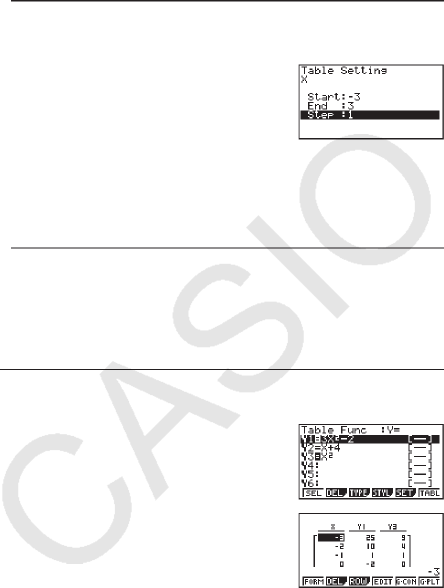
5-16
u 使用表格范围生成表格
示例 在变量 x从-3到3,以1为单位递增时生成一个表格
m TABLE
5(SET)
-dwdwbw
数值表格范围定义了函数计算期间变量
x值改变的条件。
Start ................. 变量
x初值
End .................... 变量
x终值
Step ................... 变量
x值变化量(间距)
指定表格范围之后,按下 J可返回表格关系列表。
u 使用列表生成表格
1. 屏幕上显示表格关系列表时,显示设置屏幕。
2. 突出显示Variable,然后按下 2(LIST),显示弹出窗口。
3. 选择想要指定给
x变量的值所在的列表。
• 例如,如需选择List 6,按下 gw。由此可将设置屏幕的Variable项目改为List 6。
4. 指定想要使用的列表之后,按下 J可返回前一个屏幕。
u 生成表格
示例 为保存在表格关系列表存储区Y1和Y3中的函数生成一个数值表格
使用 f和 c突出显示想要选择生成表格的函数,然后
按下 1(SEL)选择该函数。
屏幕上突出显示选定函数的“=”符号。如需取消选择
某个函数,将光标移至该函数,然后再次按 1(SEL)。
按下 6(TABL),使用选定的函数生成一个数值表格。变
量值
x根据指令列表的范围或者内容改变。
此处所示示例屏幕显示了根据List 6 (-3,-2,-1,0,1,2,3)的内容
产生的结果。
每个单元最多包含六位数,包括负号。

5-17
u 生成微分数值表格
如果将设置屏幕的Derivative项目设置改为On,只要生成一个数值表格,就会显示一个包括显
示导数的数值表格。
将光标置于某个微分系数位置会在第一行
显示“
dy/ dx”,这表示微分。
• 如果指定范围的图形或者覆盖图形包括在图形表达式
中,会产生一个错误。
u 指定函数类型
您可在三种类型中为某个函数指定某一类型。
• 直角坐标(Y=)
• 极坐标 (
r=)
• 参数函数(Parm)
1. 在屏幕上显示关系列表时按下 3(TYPE)。
2. 按下与您想要指定的函数类型对应的数字键。
• 仅为在关系列表上指定的函数类型生成数值表格(Table Func)。您不可为不同类型的函数生
成一个数值表格。
k 编辑表格
生成表格之后,您可使用表格菜单执行任何以下操作。
• 更改变量
x
• 编辑(删除、插入和附加)行
• 删除表格
• 绘制连接类型图形
• 绘制描点类型图形
• { FORM } ... {返回表格关系列表}
• { DEL } ... {删除表格}
• { ROW }
• { DEL } / { INS } / { ADD } ... {删除}/{插入}/{添加}行
• { G
• CON } / { G • PLT } ... {连接类型}/{描点类型}图形绘制
• 如果试图使用非法操作替代某个值(例如除以0),会产生错误且原始值保持不变。
• 您不能直接更改表格中其他(非
x)列中的值。
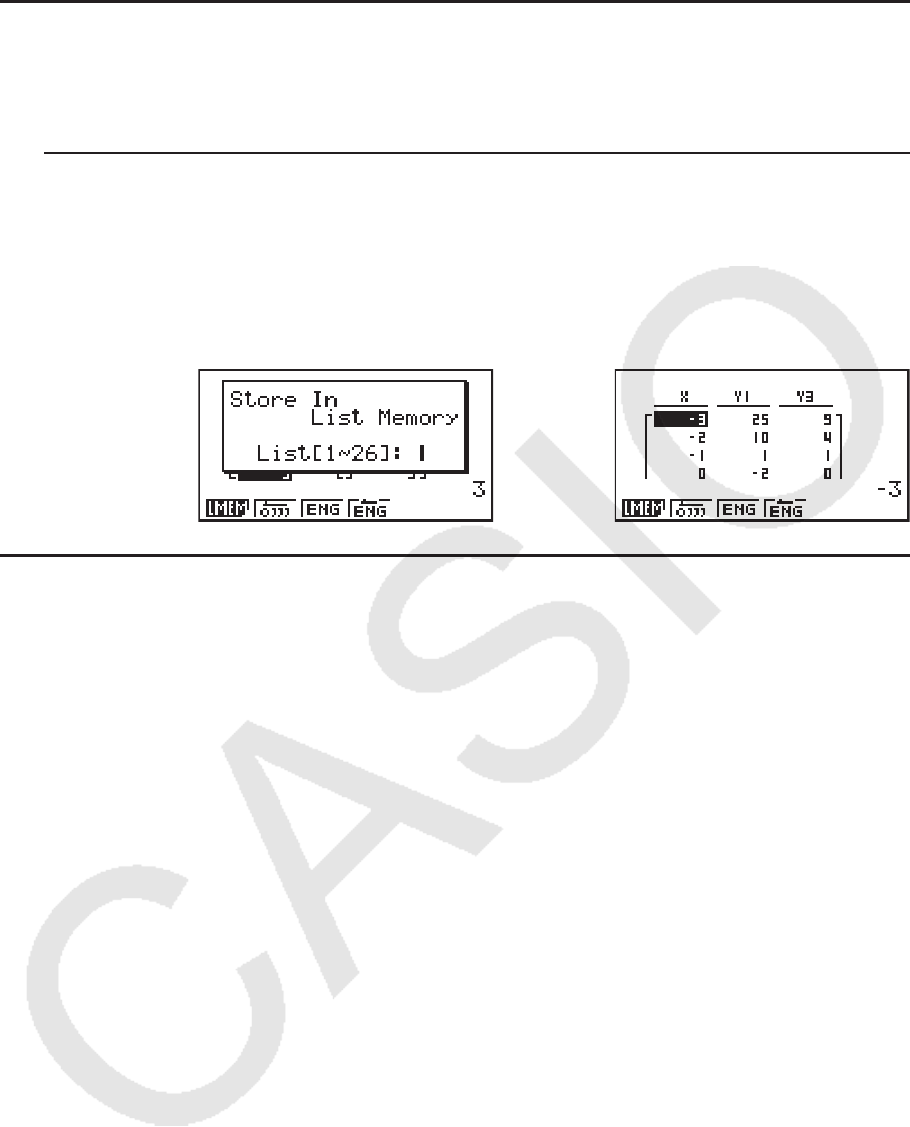
5-18
k 将表格列复制到列表
只需一个简单操作即可将数值表格列中的内容复制到列表中。
使用 d和 e将光标移至需要复制的列。光标可在任何行中。
u 将表格复制到列表
示例 将列 x的内容复制到List 1
K1(LMEM)
输入想要复制的列表编号,然后按下 w。
bw
k 使用数值表格绘制图形
使用下述程序生成一个数值表格,然后根据表格中的值绘制图形。
1. 在主菜单中,进入 TABLE 模式。
2. 进行视窗设置。
3. 保存函数。
4. 指定表格范围。
5. 生成表格。
6. 选择图形类型并绘制图形。
5(G
• CON) ... 线图
6(G
• PLT) ... 描点类型图形
• 绘制图形之后,按下 !6(G ↔ T)或者 A,返回数值表格屏幕。
示例 保存下面的函数,生成一个数值表格,然后绘制一张线图。指定范围:-3至
3,增量为1。
Y1 = 3
x2
- 2, Y2 = x2
使用以下视窗设置。
Xmin = 0, Xmax = 6, Xscale = 1
Ymin = -2, Ymax = 10, Yscale = 2
1 m TABLE
2 !3(V-WIN) awgwbwc
-cwbawcwJ

5-19
3 3(TYPE) 1(Y=) dvx-cw
vxw
4 5(SET) -dwdwbwJ
5 6(TABL)
6 5(G
• CON)
• 您可在绘制图形之后使用跟踪、缩放或草图功能。
k 同时显示数值表格和图形
将设置屏幕的Dual Screen设置为T+G,可同时显示数值表格和图形。
1. 在主菜单中,进入 TABLE 模式。
2. 进行视窗设置。
3. 将设置屏幕的Dual Screen设置为T+G。
4. 输入函数。
5. 指定表格范围。
6. 右侧副屏幕中显示数值表格。
7. 指定图形类型并绘制图形。
5(G
• CON) ... 线图
6(G
• PLT) ... 描点类型图形
示例 保存函数Y1 = 3
x2
- 2并同时显示其数值表格和线图。指定表格范围:-3至3,
增量为1。
使用以下视窗设置。
Xmin = 0, Xmax = 6, Xscale = 1
Ymin = -2, Ymax = 10, Yscale = 2
1 m TABLE
2 !3(V-WIN) awgwbwc
-cwbawcwJ
3 !m(SET UP) ccc* 1(T+G) J
*fx-7400G
II, fx-9750G II: cc
4 3(TYPE) 1(Y=) dvx-cw
5 5(SET)
-dwdwbwJ
6 6(TABL)
7 5(G
• CON)
• 在 TABLE 模式和 RECUR 模式中应用设置屏幕的“Dual Screen”设置。
• 通过按下 K1(CHNG) 或者 A,可激活数值表格。

5-20
8. 动态绘图
重要!
• fx-7400G II未配置 DYNA 模式。
k 使用动态图形
动态图形功能可帮助您定义函数系数的值域,然后观察系数值变化对图形产生的影响。它有助
于显示构成函数的系数和项如何影响图形的形状与位置。
1. 在主菜单中,进入 DYNA 模式。
2. 进行视窗设置。
3. 在设置屏幕上指定Dynamic Type。
1(Cnt) ... 连续
2(Stop) ... 10次绘图后自动停止
4. 使用光标键在内置函数类型列表中选择函数类型。*
1
5. 输入系数值,指定作为动态变量的系数。*
2
6. 指定初值、终值和增量。
7. 指定绘图速度。
3(SPEED) 1() ...... 每次绘图之后暂停(Stop&Go)
2() ......... 半正常速度(Slow)
3() ......... 正常速度 (Normal)
4() ....... 两倍正常速度(Fast)
8. 绘制动态图形。
*
1
下面是七个内置函数类型。
• Y=AX+B • Y=A(X+B)
2
+C • Y=AX
2
+BX+C • Y=AX^3+BX
2
+CX+D
• Y=Asin(BX+C) • Y=Acos(BX+C) • Y=Atan(BX+C)
按下 3(TYPE)并选择所需函数类型之后,您可输入实际函数。
*
2
您还可在此按下 w并显示参数设置菜单。
• 如果在动态绘图功能中选择多个函数,显示消息“Too Many Functions”。
示例 使用动态图形功能绘制
y = A ( x - 1)
2
- 1的图形,其中系数A的值域为2至5,
增量为1。图形绘制10次。
1 m DYNA
2 !3(V-WIN) 1(INIT) J
3 !m(SET UP) c* 2(Stop) J
*fx-9750G
II: !m(SET UP)
4 5(B-IN) c1(SEL)
5 4(VAR) cw-bw-bw
6 2(SET) cwfwbwJ
7 3(SPEED) 3() J
8 6(DYNA)
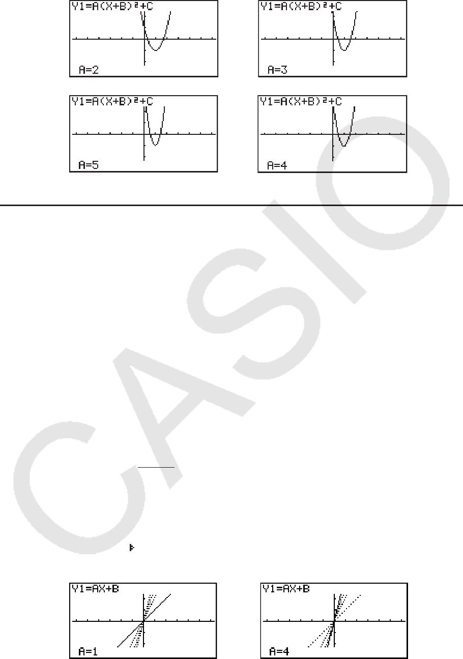
5-21
从 1重复执行至 4。
k 绘制动态图形轨迹
在设置屏幕上开启动态图形轨迹设置,可通过更改系数值叠加绘制的图形。
1. 在主菜单中,进入 DYNA 模式。
2. 进行视窗设置。
3. 将设置屏幕的“Locus”设置为“On”。
4. 使用光标键在内置函数类型列表中选择函数类型。
5. 输入系数值,指定作为动态变量的系数。
6. 指定初值、终值和增量。
7. 指定绘图速度为Normal。
8. 绘制动态图形。
示例 使用动态图形功能绘制
y = A x的图形,其中系数A的值域为1至4,增量为1。
图形绘制10次。
1 m DYNA
2 !3(V-WIN) 1(INIT) J
3 !m(SET UP) cc* 1(On) J
*fx-9750G
II: c
4 5(B-IN)1(SEL)
5 4(VAR)bwaw
6 2(SET)bwewbwJ
7 3(SPEED)3( )J
8 6(DYNA)
1
4
2
3
→
←
→
←
↓ ↑
····→
←····

5-22
k 图形计算点切换功能
使用该功能指定绘制动态图形X轴上的所有点,或间隔点。该设置仅用于动态函数Y=图形。
1. 按下 !m(SET UP),显示设置屏幕。
2. 按下 ccc* ,选择Y=Draw Speed。
*fx-9750G
II: cc
3. 选择绘图方法。
1(Norm) ... 绘制所有X轴点。(初始默认设置)
2(High) ... 绘制其它X轴间隔点。(绘制速度高于Normal)
4. 按下 J.
k 使用动态图形存储器
您可将动态图形条件和筛选数据保存在动态图形存储器中,以便以后需要时调用。由此可帮助
您节省时间,因为您可调用数据并立即开始执行动态图形绘制操作。请注意,您可在任何时候
将一组数据保存到存储器中。
u 将数据保存到动态图形存储器中
1. 在执行动态图形绘制操作时,按下 A ,切换至速度调节菜单。
2. 按下 5(STO)。在显示配置对话框时,按下 1(Yes),保存数据。
u 调用动态图形存储器中的数据
1. 显示动态图形关系列表。
2. 按下 6(RCL),调用动态图形存储器内容并绘制图形。
9. 绘制递推公式图形
重要!
• fx-7400G II未配置 RECUR 模式。
k 使用递推公式生成数值表格
您最多可输入三种以下递推公式类型并生成数值表格。
• 数列的通项 {
an},包括 an, n
• 线性两项递推公式,包括 an+1
, an, n
• 线性三项递推公式,包括 an+2
, an+1
, an, n
1. 在主菜单中,进入 RECUR 模式。
2. 指定递推类型。
3(TYPE) 1(
an) ... {数列的通项 an}
2(
an+1
) ... {线性两项递推公式}
3(
an+2
) ... {线性三项递推公式}

5-23
3. 输入递推公式。
4. 指定表格范围。指定
n的起点和终点。如有必要,指定初项值;如果您计划绘制公式图形,指
定指针起点值。
5. 显示递推公式数值表格。
示例 使用三项递推公式
an+2
= an+1
+ an生成一个数值表,其中初项 a1
= 1, a2
= 1
(斐波纳契数列),
n从1变为6。
1 m RECUR
2 3(TYPE) 3(
an+2
)
3 4(
n. an ··) 3( an+1
) +2( an) w
4 5(SET) 2(
a1
) bwgwbwbwJ
5 6(TABL)
* 前两个值对应于 a1
= 1和
a2
= 1。
• 按下 1(FORM),将返回保存递推公式的屏幕。
• 将设置屏幕的“ Σ Display”设置为“On”,表格中将包括每一项的和。
k 绘制递推公式图形
使用递推公式生成数值表格之后,您可在线图或描点类图形中绘制这些数值的图形。
1. 在主菜单中,进入 RECUR 模式。
2. 进行视窗设置。
3. 指定递推公式类型并输入公式。
4. 指定表格范围以及
n的初值和终值。如有必要,指定初项值和指针起点。
5. 选择图形的线型。
6. 显示递推公式数值表格。
7. 指定图形类型并绘制图形。
5(G
• CON) ... 线图
6(G
• PLT) ... 描点类型图形
示例 使用两项递推公式
an+1
= 2 an+ 1生成一个数值表格,其中初项 a1
= 1, n从1变
为6。使用表格数值绘制线图。
使用以下视窗设置。
Xmin = 0, Xmax = 6, Xscale = 1
Ymin = -15, Ymax = 65, Yscale = 5
1 m RECUR
2 !3(V-WIN) awgwbwc
-bfwgfwfwJ

5-24
3 3(TYPE) 2( an+1
) c2( an) +bw
4 5(SET) 2(
a1
) bwgwbwJ
5 1(SEL+S) f2() J
6 6(TABL)
7 5(G
• CON)
• 您可在绘制图形之后使用跟踪、缩放或草图功能。
• 按下 A,返回数值表格屏幕。绘制图形之后,您可能通过按下 !6(G ↔ T)在数值表格屏幕
与图形屏幕之间切换。
k 使用两个数列绘制相图
您可在 RECUR 模式中绘制通过输入两个表达式生成的数列的相图,其中一个值在水平轴上,另
一个值在垂直轴上。对于
an ( an+1
, an+2
), bn ( bn+1
, bn+2
), cn ( cn+1
, cn+2
),按照字母表排列的第一个
表达式的数列在水平轴上,后面的数列在垂直轴上。
1. 在主菜单中,进入 RECUR 模式。
2. 进行视窗设置。
3. 输入两个递推公式并选择这两个公式以生成表格。
4. 配置表格生成设置。
指定变量
n初值与终值,以及每一个递推公式的初项。
5. 显示递推公式数值表格。
6. 绘制相图。
示例 输入两个数列的两项递推公式
an+1
= 0.9 an和 bn+1
= bn + 0.1
n - 0.2,指定每一
个公式的初项
a1
= 1和 b1
= 1。生成一个当 n变量从1变为10的数值表格,并用
该表格绘制相图。
使用以下视窗设置。
Xmin = 0, Xmax = 2, Xscale = 1
Ymin = 0, Ymax = 4, Yscale = 1
1 m RECUR
2 !3(V-WIN) awcwbwc
awewbwJ
3 3(TYPE) 2(
an+1
) a.j2( an) w
4(
n. an ··) 3( bn) +a.b1( n) -a.cw
4 5(SET) 2(
a1
) bwbawbwbwJ
5 6(TABL)
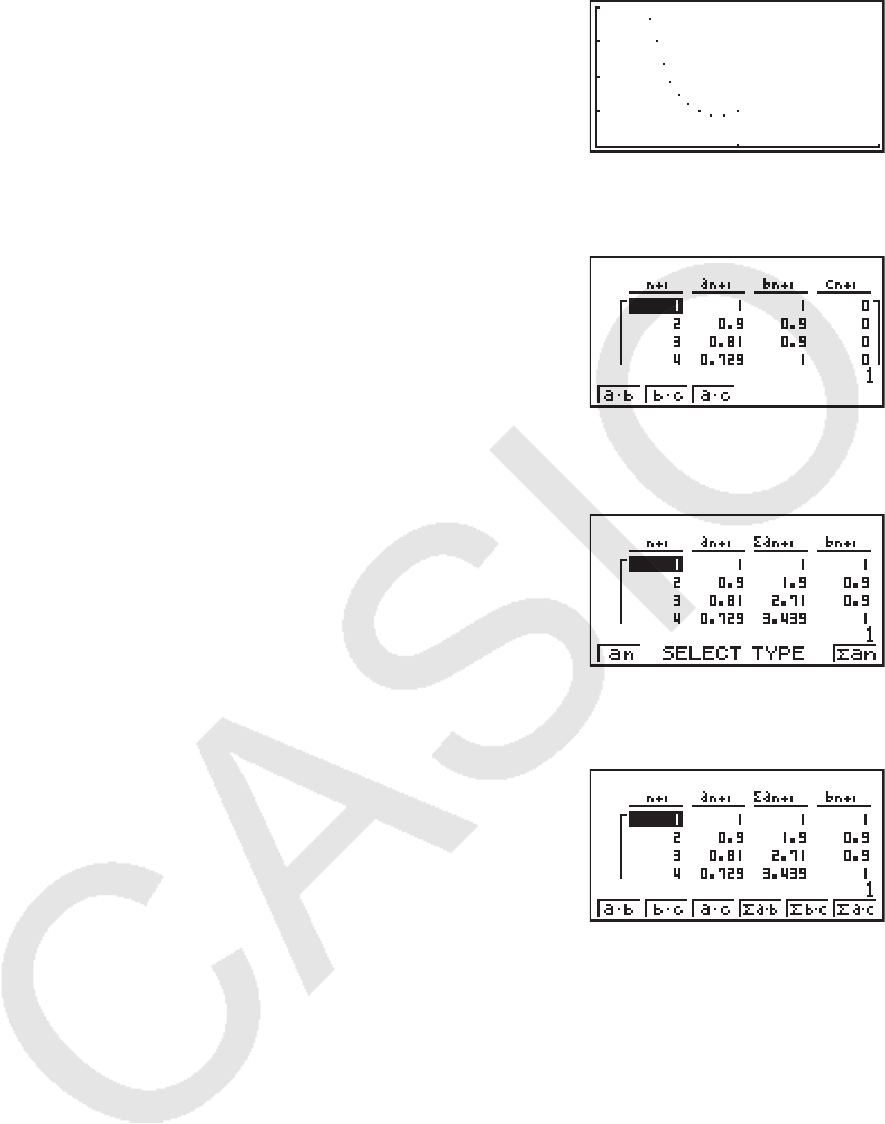
5-25
6 3(PHAS)
• 如果您在 RECUR 模式屏幕上输入三个表达式,然后选择这三个表达式创建表格,您需要指定
其中哪两个表达式用于绘制相图。为此,使用在表格屏幕上按下 3(PHAS)时显示的功能菜
单。
1(
a • b) ............. 使用 an ( an+1
, an+2
)和 bn ( bn+1
, bn+2
)绘制的图
形。
2(
b • c) .............. 使用 bn ( bn+1
, bn+2
)和 cn ( cn+1
, cn+2
)绘制的图
形。
3(
a • c) .............. 使用 an ( an+1
, an+2
)和 cn ( cn+1
, cn+2
)绘制的图
形。
• 将设置屏幕的“ Σ Display”设置为“On”,表格中将包括每一项的和。此时您可选择使用两
个原始数列,或使用两个数列之和绘制图形。为此,使用在表格屏幕上按下 3(PHAS)时显示
的功能菜单。
1(
an) .................. 使用数列绘图。
6( Σ an) .............. 使用数列之和绘图。
• 在设置屏幕的“ Σ Display”设置为“On”且选择使用在 RECUR 模式中输入的所有三个表达式
生成表格,使用在按下 3(PHAS)时表格屏幕上显示的功能菜单,指定想要使用的两个表达
式,以及使用数列数据还是数列之和数据。
1(
a • b) ............. 使用数列 an ( an+1
, an+2
)和 bn ( bn+1
, bn+2
)绘制的
图形
2(
b • c) .............. 使用数列 bn ( bn+1
, bn+2
)和 cn ( cn+1
, cn+2
)绘制的
图形
3(
a • c) .............. 使用数列 an ( an+1
, an+2
)和 cn ( cn+1
, cn+2
)绘制的
图形
4( Σ a • b) ......... 使用数列 an ( an+1
, an+2
)与 bn ( bn+1
, bn+2
)之和绘
制的图形
5( Σ b • c) ......... 使用数列 bn ( bn+1
, bn+2
)与 cn ( cn+1
, cn+2
)之和绘
制的图形
6( Σ a • c) ......... 使用数列 an ( an+1
, an+2
)与 cn ( cn+1
, cn+2
)之和绘
制的图形

5-26
k WEB图形(收敛,发散)
y = f( x)图形时,假设 an+1
= y, an = x,两项递推公式为 an+1
= f( an),其中包括 an+1
, an。此后,可
确定该函数为收敛函数或发散函数。
1. 在主菜单中,进入 RECUR 模式。
2. 进行视窗设置。
3. 选择两项递推公式类型,然后输入公式。
4. 指定表格范围、
n初值和终值点、初项值和指针起点。
5. 显示递推公式数值表格。
6. 绘制图形。
7. 按下 w,指定起点处显示一个指针。
按下 w多次。
如果收敛,屏幕上显示类似于蛛网的线条。如果不显示蛛网线条,表示发散或图形超出了显
示屏边界。出现这种情况时,增大视窗值并再试一次。
您可使用 fc选择图形。
示例 绘制递推公式
an+1
= -3( an)
2
+ 3 an, bn+1
= 3 bn + 0.2的WEB图形,检查发散
性或收敛性。使用下述表格范围:Start = 0,End = 6,
a0
= 0.01, anStr =
0.01,
b0
= 0.11, bnStr = 0.11
1 m RECUR
2 !3(V-WIN) awbwbwc
awbwbwJ
3 3(TYPE) 2(
an+1
) -d2( an) x+d2( an) w
d3(
bn) +a.cw
4 5(SET) 1(
a0
)
awgwa.abwa.bbwc
a.abwa.bbwJ
5 6(TABL)
6 4(WEB)
7 w~ w(
an收敛)
cw~ w(
bn发散)
• 如需更改线型,第4步后按下 1(SEL+S)。
• 在使用WEB图形功能时,您可指定 y = f( x)图形的线型。只有在设置屏幕上将“Draw Type”
设置选择为“Connect”时才可使用线型设置。
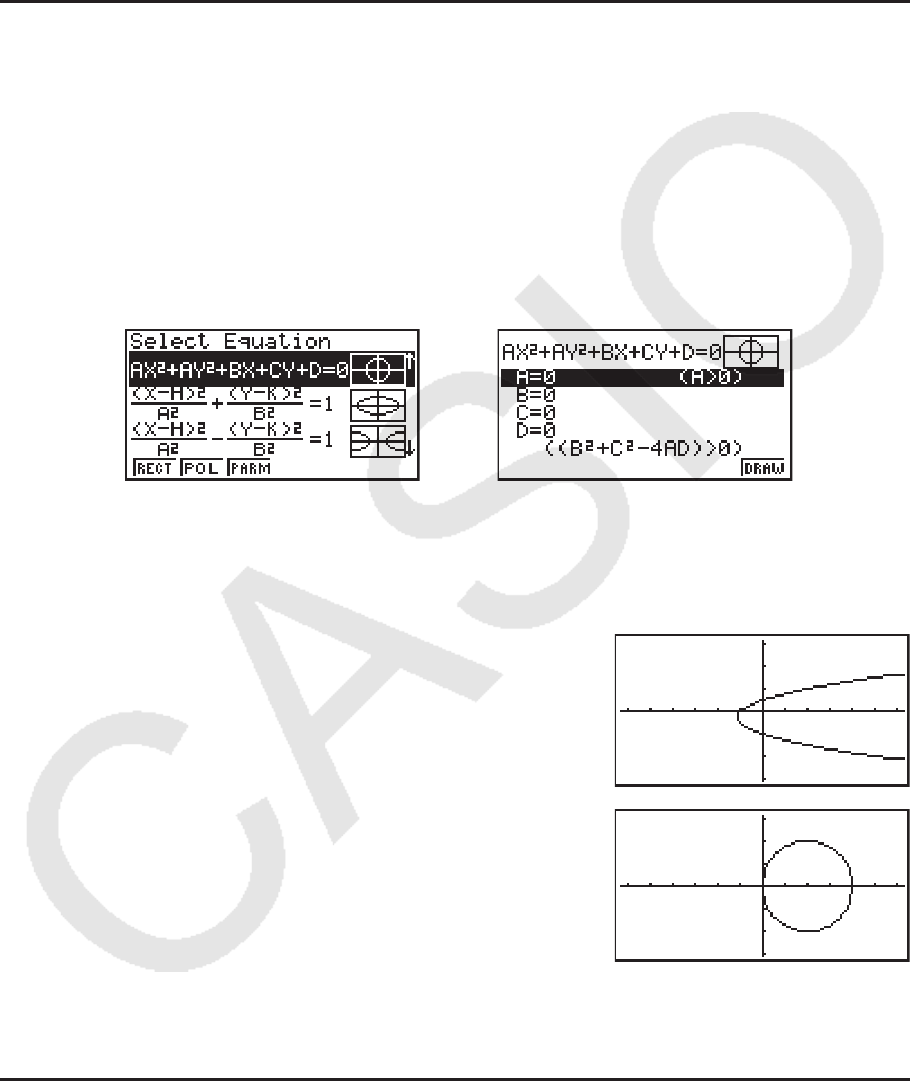
5-27
10. 绘制二次曲线图形
重要!
• fx-7400G II未配置 CONICS 模式。
k 绘制二次曲线图形
您可使用 CONICS 模式绘制抛物线、圆、椭圆和双曲线。您可输入需要绘制图形的直角坐标函
数、极坐标函数或者参数函数。
1. 在主菜单中,进入 CONICS 模式。
2. 选择函数类型。
1(RECT) .... {直角坐标}
2(POL) .... {极坐标}
3(PARM) .... {参数函数}
3. 选择对应于需要绘制的图形类型的函数模式。
R
w
4. 输入函数的系数并绘制图形。
示例 输入直角坐标函数
x= 2
y2 + y - 1并绘制一个开口向右的抛物线,然后输入极
坐标函数
r = 4cos
θ
并绘制一个圆。
1 mCONICS
2 1(RECT) c(X=AY
2
+BY+C) w
3 cwbw-bw6(DRAW)
4 JJ
5 2(POL) cccc(R=2Acos
θ
) w
6 cw6(DRAW)
11. 更改图形的外观
k 绘制一条线
草图功能可用于在图形内部绘制点和线。
您可使用草图功能在四种不同的线型中选择某一种线型。

5-28
1. 在主菜单中,进入 GRAPH 模式。
2. 进行视窗设置。
3. 在设置屏幕上,使用“Sketch Line”设置指定需要的线型。
1() ... 标准线(初始默认设置)
2() ... 粗线(线宽为标准线型的两倍)
3() ... 虚线(粗虚线)
4() ... 点线(点状线)
4. 输入图形的函数。
5. 绘制图形。
6. 选择想要使用的草图功能。*
1
!4
(SKTCH)
1(Cls) ... 清除屏幕
2(Tang) ... 切线
3(Norm) ... 曲线的法线
4(Inv) ... 反函数*
2
6( g) 1(PLOT)
{Plot}/{Pl
• On}/{Pl • Off}/{Pl • Chg} ... 点{绘图}/{开}/{关}/{更改}
6( g) 2(LINE)
{Line}/{F
• Line} ... {使用线连接2个由 6( g) 1(PLOT)绘制的点}/{在任
意2点之间绘制一条线}
6( g) 3(Crcl) ... 圆
6( g) 4(Vert) ... 垂直线
6( g) 5(Hztl) ... 水平线
6( g) 6( g) 1(PEN) ... 手绘
6( g) 6( g) 2(Text) ... 文本输入
7. 使用光标键将指针( )移至想要绘制的位置,然后按下 w。*
3
*
1
上述操作显示 GRAPH 模式中的功能菜单。在其它模式中,菜单项目可能有所不同。
*
2
对于反函数图形,在选择该选项之后立即开始绘制图形。
*
3
某些草图功能要求指定两个点。在按下 w指定第一个点之后,使用光标键将指针移至第二个
点所在位置,然后按下 w。
• 您可为以下草图功能指定线型型:Tangent、Normal、Inverse、Line、F • Line、Circle、
Vertical、Horizontal、Pen
示例 绘制一条与图形
y = x ( x + 2)( x - 2)的(2, 0)点相切的线。
1 m GRAPH
2 !3(V-WIN) 1(INIT) J
3 !m(SET UP) cccccccc* 1() J
*fx-7400G
II, fx-9750G II: ccccccc
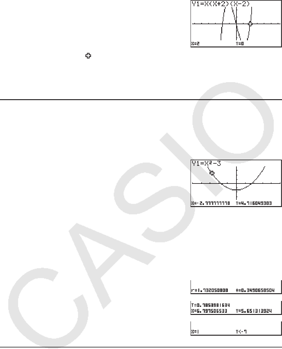
5-29
4 3(TYPE) 1(Y=) v(v+c)(v
-c)w
5 6(DRAW)
6 !4(SKTCH) 2(Tang)
7 e~ ew*
1
*
1
您可在此后通过移动“ ”指针并按下 w,绘制一条切线。
12. 函数分析
k 读取图形线条上的坐标
跟踪功能可使指针沿着某个图形移动,并在显示屏上读出坐标。
1. 在主菜单中,进入 GRAPH 模式。
2. 绘制图形。
3. 按下 !1(TRCE),图形中间显示一个指针。*
1
4. 使用 d和 e沿着图形将指针移至想要显示导数的点。
如果显示屏上有多个图形,按下 f和 c,沿着当前
指针位置的
x轴在它们之间移动。
5. 您还可通过按下 v,显示弹出窗口,然后输入坐标以移动指针。
即使您直接输入坐标也会显示弹出窗口。
如需退出跟踪操作,按下 !1(TRCE)。
*
1
如果指针位于图形显示区域之外的某一点,或出现无数值错误时,图形上不显示指针。
• 您可通过将设置屏幕的“Coord”项目设置为“Off”,关闭指针位置处的坐标显示。
• 下面显示了每一种函数类型显示的坐标形式。
极坐标图形
参数函数图形
不等式图形
k 显示导数
除了使用跟踪功能显示坐标之外,您还可显示当前指针位置的导数。
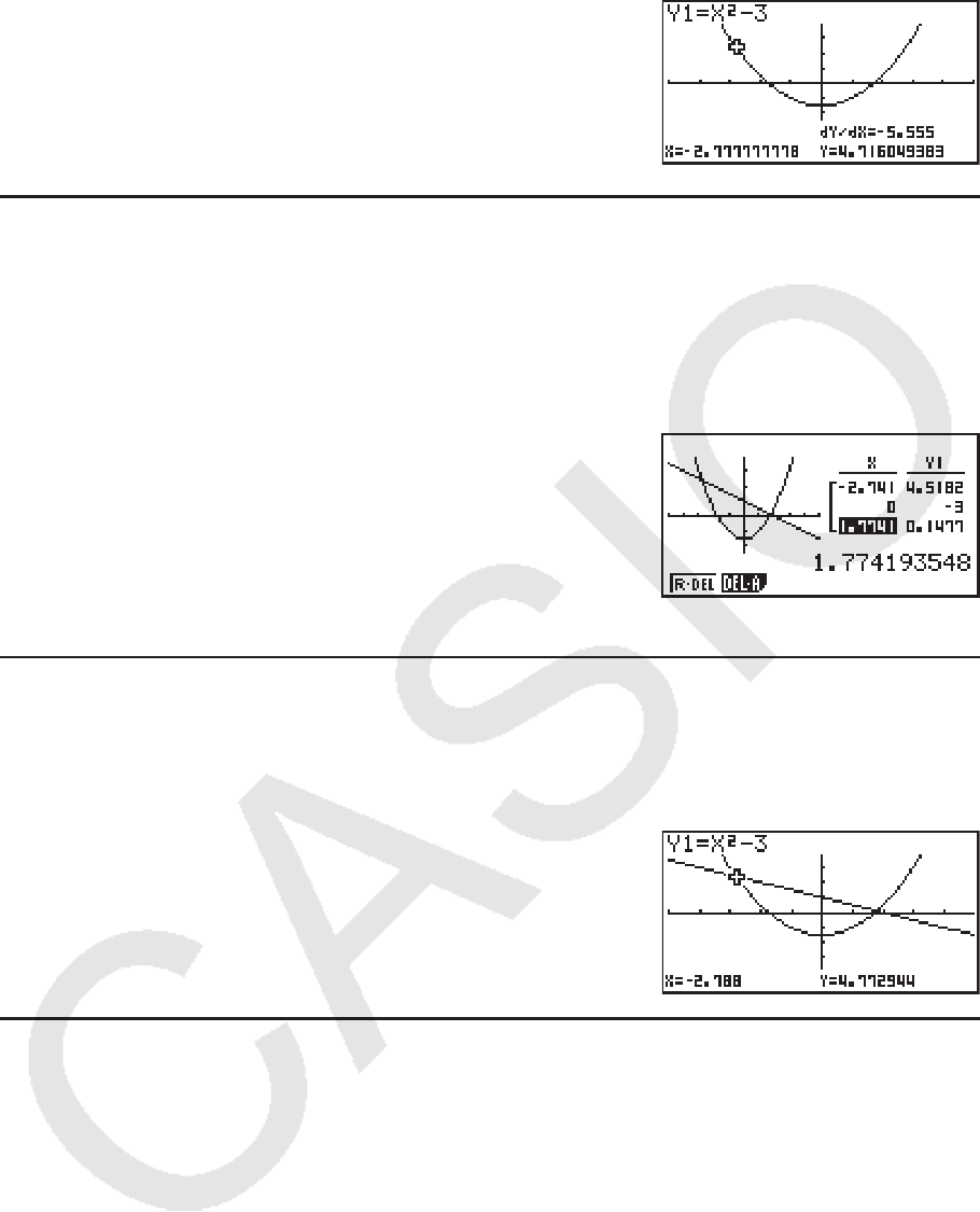
5-30
1. 在主菜单中,进入 GRAPH 模式。
2. 在设置屏幕中,将Derivative设置为On。
3. 绘制图形。
4. 按下 !1(TRCE),图形中间显示指针。此时
显示屏中还显示当前坐标和导数。
k 图形至表格
您可使用跟踪功能读取图形的坐标并将其保存在数值表格中。您还可使用双图形功能同时保存
图形和数值表格,因此这是一种重要的图形分析工具。
1. 在主菜单中,进入 GRAPH 模式。
2. 将设置屏幕的Dual Screen设置为GtoT。
3. 进行视窗设置。
4. 保存函数并在主屏幕(左侧)上绘制图形。
5. 启动跟踪功能。如果显示屏上有多个图形,按下 f和 c,
选择需要的图形。
6. 使用 d和 e,移动指针并按下 w,将坐标保存到数值
表格。根据所需保存数值的数量,重复执行该步骤。
7. 按下 K1(CHNG),激活数值表格。
k 坐标舍入
该功能舍入跟踪功能显示的坐标值。
1. 在主菜单中,进入 GRAPH 模式。
2. 绘制图形。
3. 按下 !2(ZOOM) 6( g) 3(RND)。由此可使视窗设置
根据Rnd值自动更改。
4. 按下 !1(TRCE),然后使用光标键沿着图形移动指针。
对当前显示的坐标进行舍入。
k 计算根
该功能提供用于分析图形的多种不同方法。
1. 在主菜单中,进入 GRAPH 模式。
2. 绘制图形。
3. 选择分析功能。
!5(G-SLV) 1(ROOT) ... 计算根
2(MAX) ... 局部最大值
3(MIN) ... 局部最小值
4(Y-ICPT) ...
y截距
5(ISCT) ... 两个图形的交点
6( g) 1(Y-CAL) ...
y坐标,对应于给定的 x坐标
6( g) 2(X-CAL) ...
x坐标,对应于给定的 y坐标
6( g) 3( ∫ dx) ... 给定范围的积分值
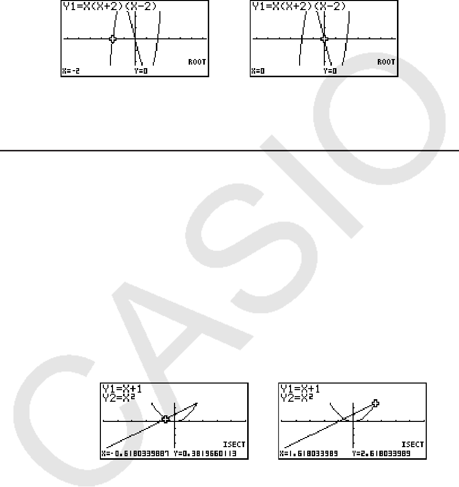
5-31
4. 如果屏幕上有多个图形,选择光标 ( k)位于编号最小的图形上。按下 f和 c,将光标移至
想要选择的图形。
5. 按下 w,选择光标所在处的图形并显示分析结果值。
如果分析结果包括多个值,按下 e,计算下一个值。
按下 d返回前一个值。
• 以下任一情况都会导致精度降低甚至无法求解。
- 解对应的图形是与
x轴的切点时
- 解是一个拐点时
k 计算两个图形的交点
使用下述程序计算两个图形的交点。
1. 绘制图形。
2. 按下 !5(G-SLV) 5(ISCT)。如果有三个或者更多图形,选择光标( k)位于编号最小的
图形上。
3. 按下 f和 c,将光标移至第二个图形。
4. 按下 w,选择第一个图形,由此可将光标的形状从 k变为
。
5. 按下 f和 c,将光标移至想要选择的图形。
6. 按下 w,计算两个图形的交点。
如果分析结果包括多个值,按下 e,计算下一个值。
按下 d返回前一个值。
示例 绘制下述两个函数图形,确定Y1和Y2的交点。
Y1 =
x + 1, Y2 = x2
• 您只能计算直角坐标图形(Y=
f( x)类型)与不等式图形(Y > f( x), Y < f( x), Y t f( x)或者Y s f( x))的交
点。
• 以下任一情况都会导致精度降低甚至无法求解。
- 当解是两个图形之间的切点时
- 解是一个拐点时
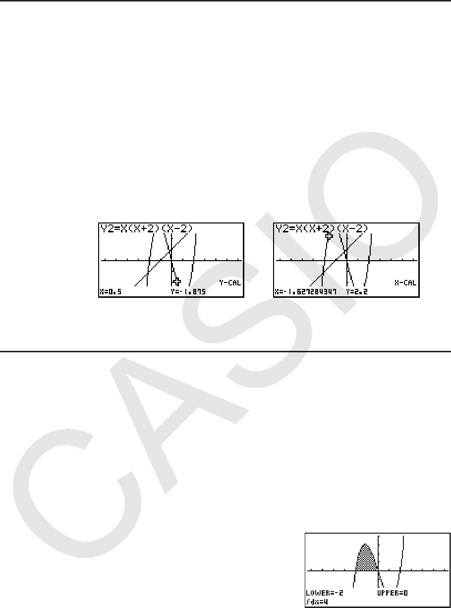
5-32
k 确定给定点的坐标
下述程序说明了如何确定给定 x的 y坐标,以及给定 y的 x坐标。
1. 绘制图形。
2. 选择想要执行的功能。如果有多个图形,选择光标( k)位于编号最小的图形上。
!5(G-SLV) 6( g) 1(Y-CAL) ...
y坐标,对应于给定的 x
6( g) 2(X-CAL) ... x坐标,对应于给定的 y
3. 使用 fc,将光标 ( k) 移至想要选择的图形,然后按下 w选择该图形。
4. 输入给定的
x坐标值或者 y坐标值。
按下 w,计算对应的
y坐标值或者 x坐标值。
示例 绘制以下两个函数图形,然后在图形Y2上确定
y坐标(当 x = 0.5时)和 x坐标
(当
y = 2.2时)。
Y1 =
x + 1, Y2 = x( x + 2)( x - 2)
• 如果上述程序产生多个结果,按下 e计算下一个值。按下 d ,返回前一个值。
• 参数函数图形不可计算X-CAL值。
k 计算给定范围的积分值
使用下述程序,计算给定范围的积分值。
1. 绘制图形。
2. 按下 !5(G-SLV) 6( g) 3( ∫ dx)。如果有多个图形,该操作将使选择光标( k)位于编号
最小的图形上。
3. 使用 fc,将光标 ( k) 移至想要选择的图形,然后按下 w选择该图形。
4. 使用 de,将下限指针移至所需位置,然后按下 w。
5. 使用 e将上限指针移至所需位置。
6. 按下 w,计算积分值。
示例 绘制下述函数图形,然后确定(-2, 0)处的积分值。
Y1 =
x( x + 2)( x - 2)
• 您还可在10键键盘上输入下限和上限值。
• 在设置范围时,确保下限小于上限。
• 只能计算直角坐标图形的积分值。

5-33
k 二次曲线图形分析
重要!
• fx-7400G II未配置 CONICS 模式。
您可使用二次曲线图形确定以下分析结果的近似值。
1. 在主菜单中,进入 CONICS 模式。
2. 选择函数类型。
1(RECT) .... {直角坐标}
2(POL) .... {极坐标}
3(PARM) .... {参数函数}
3. 使用 f和 c,选择想要分析的二次曲线。
4. 输入二次曲线常量。
5. 绘制图形。
绘制二次曲线图形之后,按下 !5(G-SLV),显示以下图形分析菜单。
u 抛物线图形分析
• { FOCS } / { VTX } / { LEN } / { e } ... {焦点}/{顶点}/{正焦弦长度}/{离心率}
• { DIR } / { SYM } ... {准线}/{对称轴}
• { X-IN } / { Y-IN } ... {
x截距}/{ y截距}
u 圆形图形分析
• { CNTR } / { RADS } ... {圆心}/{半径}
• { X-IN } / { Y-IN } ... {
x截距}/{ y截距}
u 椭圆图形分析
• { FOCS } / { VTX } / { CNTR } / { e } ... {焦点}/{顶点}/{中心}/{离心率}
• { X-IN } / { Y-IN } ... {
x截距}/{ y截距}
u 双曲线图形分析
• { FOCS } / { VTX } / { CNTR } / { e } ... {焦点}/{顶点}/{中心}/{离心率}
• { ASYM } ... {渐近线}
• { X-IN } / { Y-IN } ... {
x截距}/{ y截距}
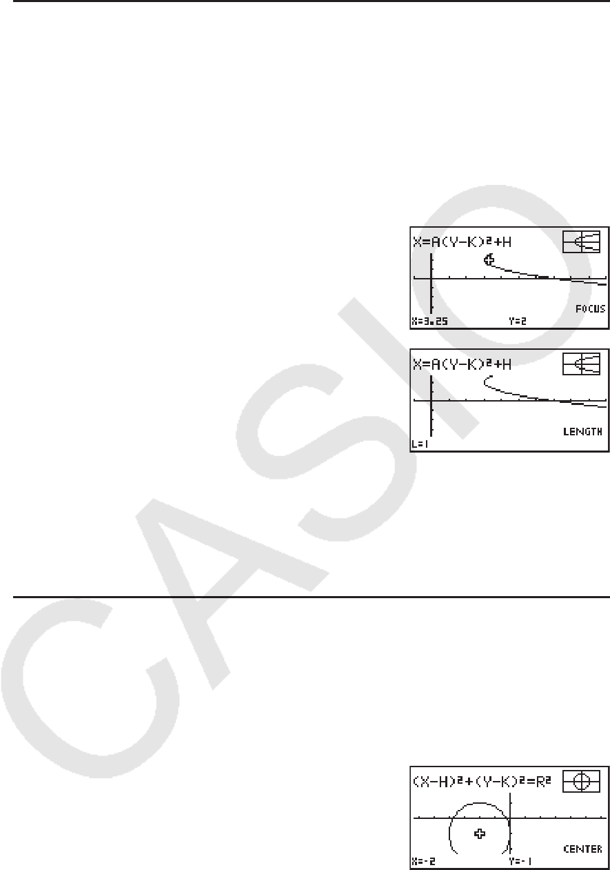
5-34
u 计算焦点和正焦弦的长度 [G-SLV]-[FOCS]/[LEN]
示例 确定抛物线X = (Y - 2)
2
+ 3的焦点和正焦弦的长度
使用以下视窗设置。
Xmin = -1, Xmax = 10, Xscale = 1
Ymin = -5, Ymax = 5, Yscale = 1
m CONICS
w
bwcwdw6(DRAW)
!5(G-SLV)
1(FOCS)
(计算焦点。)
!5(G-SLV)
5(LEN)
(计算正焦弦长度。)
• 在计算椭圆或者双曲线图形的两个焦点时,按下 e,计算第二个焦点。按下 d,返回第一个
焦点。
• 在计算双曲线图形的两个顶点时,按下 e,计算第二个顶点。按下 d,返回第一个顶点。
• 在计算椭圆的顶点时,按下 e将计算下一个值。
按下 d将滚动返回以前的数值。一个椭圆有四个顶点。
u 计算圆心 [G-SLV]-[CNTR]
示例 确定圆心
(X + 2)
2
+ (Y + 1)
2
= 2
2
m CONICS
ccccw
-cw-bwcw6(DRAW)
!5(G-SLV)
1(CNTR)
(计算圆心。)
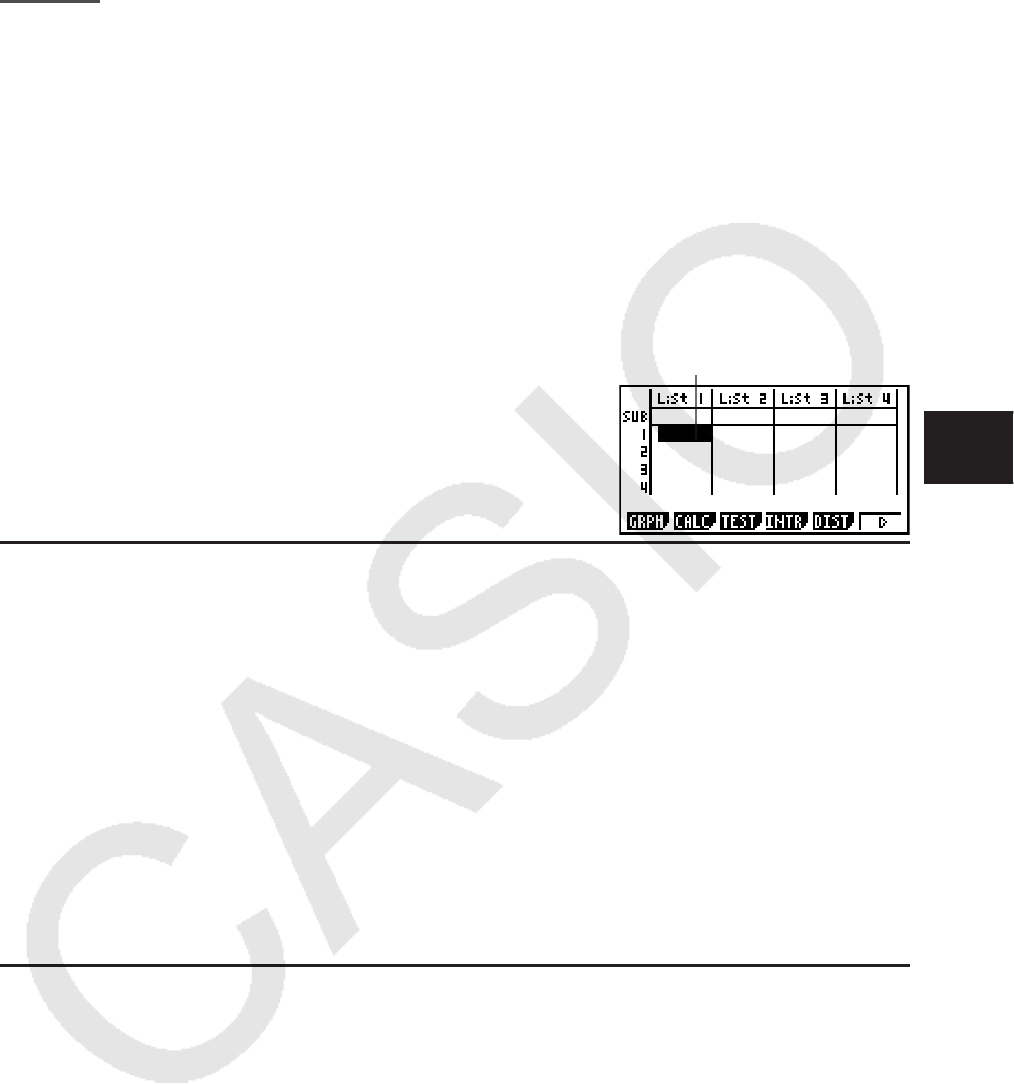
6-1
第6章 统计图形与计算
重要!
本章包含大量屏幕截图。在每一种情况下,输入新数据值是为了突出显示绘制图形的特性。请注
意,在您尝试绘制类似图形时,该计算器使用您通过列表功能输入的数据值。因此,当您进行制图
操作时,屏幕上出现的图形可能与本手册中显示的图形略有不同。
1. 在进行统计计算之前
在主菜单中,进入 STAT 模式即显示列表编辑器屏幕。
您可使用列表编辑器屏幕输入统计数据并执行统计计算。
使用 f、 c、 d和 e,围绕列表移
动突出显示区域。
输入数据之后,可使用它绘制图形并检查趋势。您还可使用
各种不同的回归计算分析数据。
• 关于使用统计数据列表的信息,请参见“第3章 列表功
能”。
k 更改图形参数
使用下述程序,可以在图形菜单(GPH1、GPH2、GPH3)中为每一个图形指定图形绘制/非绘
制状态、图形类型以及其他一般性设置。
显示屏上显示统计数据列表时,按下 1(GRPH),显示包含下述各项的图形菜单。
• { GPH1 } / { GPH2 } / { GPH3 } ... 绘制{1}/{2}/{3}图形*
1
• { SEL } ... {同时选择图形(GPH1、GPH2、GPH3)}
您可指定多个图形。
• { SET } ... {图形设置(图形类型、列表指定)}
*
1
所有图形的初始默认图形类型设置(图形1至图形3)都是散布图,但您可改为其他图形类
型。
1. 一般图形设置 [GRPH]-[SET]
本节说明如何使用一般图形设置屏幕对每一个图形(GPH1、GPH2、GPH3)进行以下设置。
• 图形类型(Graph Type)
所有图形的初始默认图形类型设置都是散布图。您可为每一个图形选择其他各种统计图形类
型。
• 列表(List)
对于单变量数据,初始默认统计数据为List 1;对于双变量数据,初始默认统计数据为List 1和
List 2。您可指定想要用于
x数据和 y数据的统计数据列表。
6
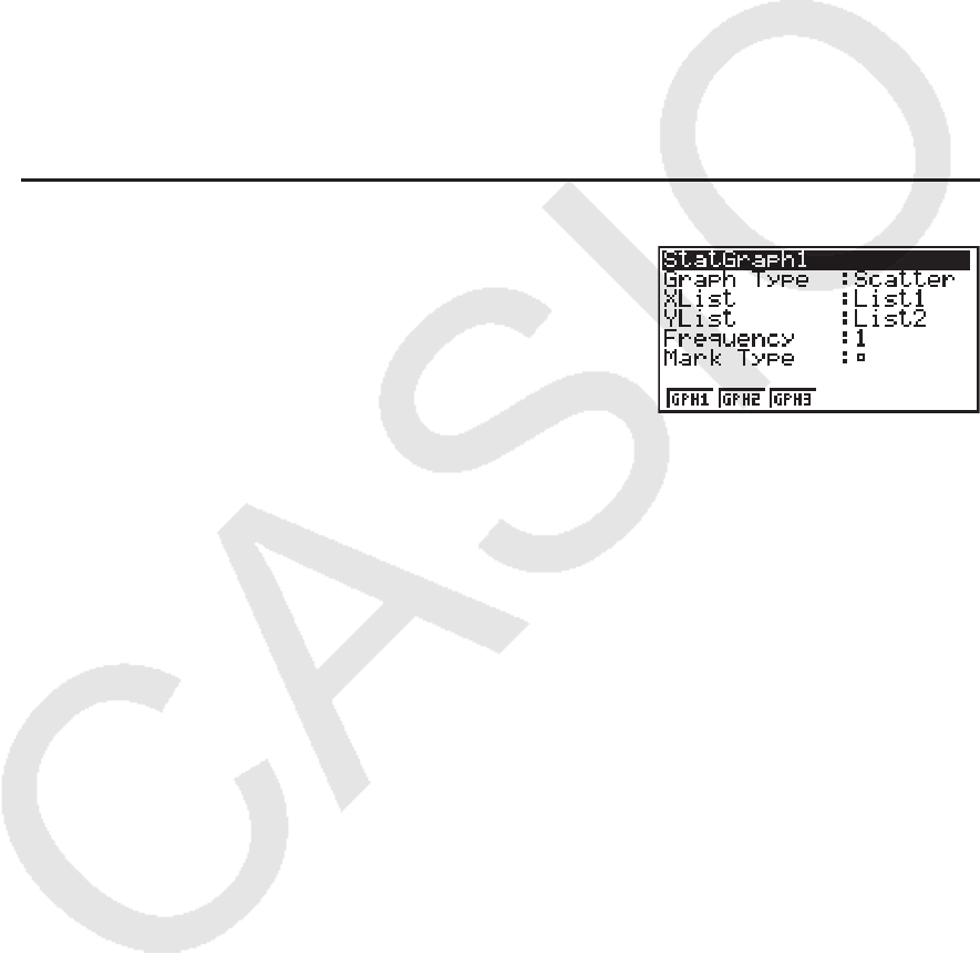
6-2
• 频率(Frequency)
此设置将指定一个包含频率数据的列表。
在统计上,“频率”是指数据项(或数据项集)发生的次数。频率在“频率分布表”中使用,
该表在一列中列出各个唯一的数据项,并在右侧列中显示频率(发生次数)。在此计算器中,
数据列和频率列是单独的列表。此设置将指定绘制统计图形时为频率列所使用的列表(List 1、
List 2等)。
•对于Med-Med图形(第6-12页),仅针对频率数据输入正整数。输入任何其它数值类型(比
如,小数值等)均会导致错误。
重要! (仅限fx-9860GII SD/fx-9860GII/fx-9860G AU PLUS)
•包含在频率列表中的值应该仅为0或正值。即使一个负值也会导致错误。
•频数为0的统计数据不用于最小和最大值的计算。
• 标记类型(Mark Type)
该设置可帮助您指定图形上描点的形状。
u 显示一般图形设置屏幕 [GRPH]-[SET]
按下 1(GRPH) 6(SET),显示一般图形设置屏幕。
• StatGraph(统计图形规定)
• { GPH1 } / { GPH2 } / { GPH3 } ... 图形{1}/{2}/{3}
• Graph Type(图形类型规定)
• { Scat } / {
xy} / { NPP } / { Pie } ... {散布图}/{ xy线图}/{正态概率图}/{饼图}
• { Hist } / { Box } / { Bar } / { N·Dis } / { Brkn } ... {直方图}/{Med-矩形框图}/{条线图}/{正态分布曲线}/{虚
线图}
• { X } / { Med } / { X^2 } / { X^3 } / { X^4 } ... {线性回归图}/{Med-Med图}/{二次回归图}/{三次回归图}/{四
次回归图}
• { Log } / { Exp } / { Pwr } / { Sin } / { Lgst } ... {对数回归图}/{指数回归图}/{幂回归图}/{正弦回归图}/{逻
辑回归图}
• XList( x轴数据列表)/YList ( y轴数据列表)
• { List } ... {List 1至26}
• Frequency(某个数值出现的次数)
• { 1 } ... {1对1描点}
• { List } ... {List 1至26}
• Mark Type(描点标记类型)
• { } / { × } / { • } ... 散布图描点

6-3
Graph Type选择“Pie”(饼图)时:
• Data(指定作为图形数据的列表。)
• { LIST } ... {List 1至List 26}
• Display(饼图值显示设置)
• { % } / { Data } ... 对于每一个数据元素{显示为百分比}/{显示为数值}
• % Sto Mem(将百分比值保存到指定列表。)
• { None } / { List } ... 对于百分比值:{不保存到列表}/{指定List 1至26并保存}
Graph Type选择“Box”(中位值-矩形框图)时:
•Outliers(异常值规定)
• { On } / { Off } ... {显示}/{不显示}Med-矩形框异常值
Graph Type选择“Bar”(条线图)时:
• Data1(第一个条状数据列表)
• { LIST } ... {List 1至26}
• Data2(第二个条状数据列表)/Data3(第三个条状数据列表)
• { None } / { LIST } ... {无}/{List 1至26}
• Stick Style(条型规定)
• { Leng } / { HZtl } ... {长度}/{水平}
2. 图形绘制/非绘制状态 [GRPH]-[SEL]
下述程序可用于在图形菜单中为每一个图形指定图形绘制(On)/非绘制(Off)状态。
u 指定图形的绘制/非绘制状态
1. 按下 1(GRPH) 4(SEL),显示图形On/Off屏幕。
• 请注意,StatGraph1设置用于图形1(图形菜单的GPH1),StatGraph2用于图形2,
StatGraph3用于图形Graph 3。
2. 使用光标键突出显示想要更改状态的图形,然后按下相关键以更改状态。
• { On } / { Off } ... {开(绘制)}/{关(非绘制)}
• { DRAW } ... {绘制所有设置为“开”的图形}
3. 如需返回图形菜单,按下 J。
• 在统计数据绘图功能中,视窗参数通常自动设置。如果您想手动设置视窗参数,您必须将Stat
Wind项目改为“Manual”。
当显示屏上显示统计数据列表时,执行下述程序。
!m(SET UP) 2(Man)
J(返回前一个菜单。)
请注意,无论Stat Wind项目是否设置为“Manual”,以下类型的图形都自动设置视窗参数。
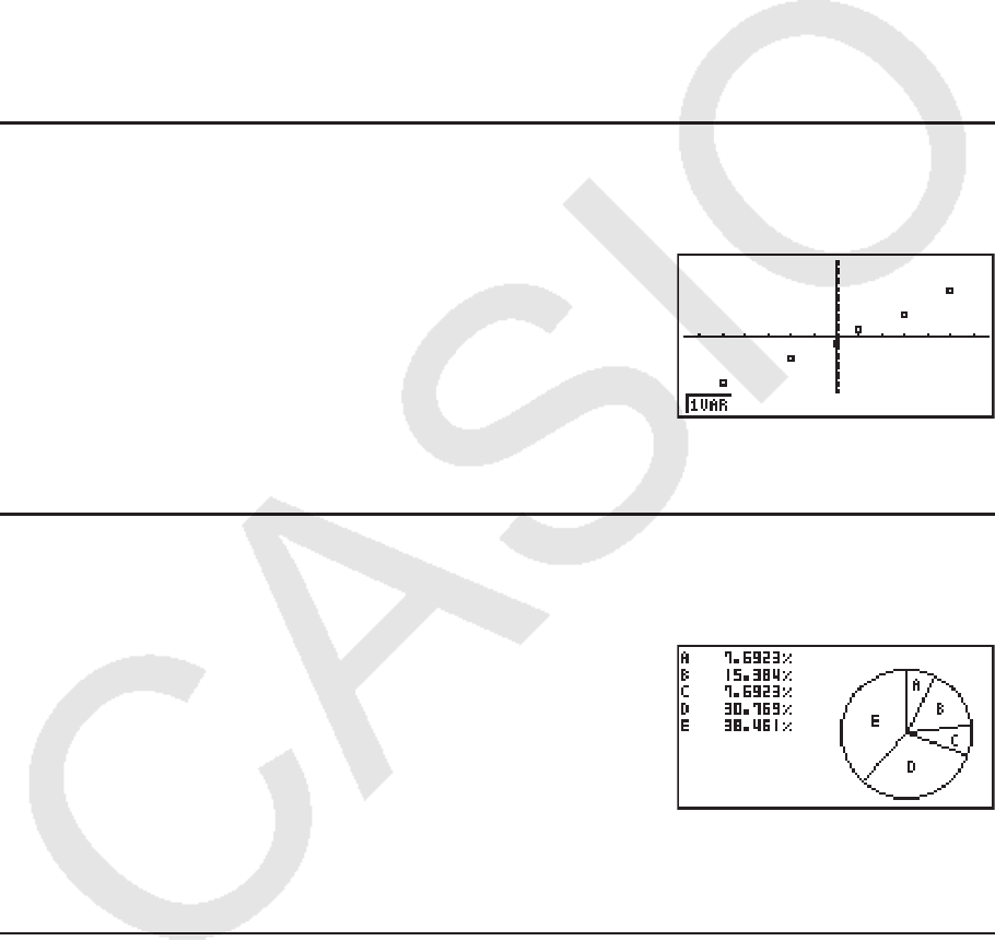
6-4
饼图、1-样本 Z测试、2-样本 Z测试、1-比例 Z测试、2-比例 Z测试、1-样本 t测试、2-样本 t测
试、 χ 2
GOF测试、 χ 2
双向测试、2-样本 F测试(仅限于忽略 x轴)。
• 默认设置自动采用List 1数据作为
x轴(水平)值,List 2数据作为 y轴(垂直)值。每一
组
x/ y数据都是散布图上的一个点。
2. 计算与绘制单变量统计数据
单变量数据是只带有单个变量的数据。如果您正在计算班级学生的平均身高,则只有一个变量
(身高)。
单变量统计包括分布计算与求和计算。下述图形类型可用于单变量统计。
在绘制每一个图形之前,您还可使用第6-1页“更改图形参数”中的程序进行所需设置。
k 正态概率图
该图将数据累积比与正态分布累积比进行对比。XList指定输入数据的列表,Mark Type用于从
标记{ / × / • }中选想要绘制的标记。
按下 A, J或 !J(QUIT),返回统计数据列表。
k 饼 图
您可根据特定列表中的数据绘制饼图。图形数据项目(列表行)的最大数量为20。图形标记为
A、B、C等等,分别对应于用于图形数据的列表的行1、2、3等等。
在一般图形设置屏幕上,将“Display”选择为“%”时(第6-3页),每个字母表标签字母都对
应显示一个百分比值。
k 直方图
XList指定输入数据的列表框,Freq指定输入数据频率的列表。在不指定频率时,Freq指定为1。
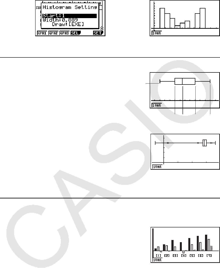
6-5
w(DRAW)
在绘制图形之前,显示以上屏幕。此时,您可改变Start和Width值。
k Med-矩形框图形
通过此类图形,您可以了解大量数据项如何在特定范
围内分组。一个矩形框包含了从第一四分位数(Q1)
到第三四分位数(Q3)区域中的所有数据,在中位值
(Med)处绘制了一条直线。直线(称为“须线”)从
矩形框的一端延长至数据的最小值(minX)和最大值
(maxX)。
在统计数据列表中,按下 1(GRPH),显示图形菜单,按
下 6(SET),然后将想要使用的图形(GPH1、GPH2、
GPH3)的类型改为Med-矩形框图形。
如需绘制矩形框之外的数据,可首先指定“MedBox”作
为图形类型。然后,在您指定图形类型的同一屏幕上,将
Outliers项目设置为“On”并绘制图形。
• 即使Med-矩形框图形根据单个列表绘制,在设置屏幕上更改“Q1Q3 Type”设置也可能导致
Q1和Q3位置改变。
k 条线图
您最多可指定三个列表用于绘制条线图。图形标记为[1]、[2]、[3]等等,分别对应于用于图形数
据的列表的行1、2、3等等。
• 以下任一情况都会产生错误并取消绘制条线图。
- 在使用图形On/Off屏幕(第6-3页)指定绘制多个图形(某一图形被指定为条线图,另一个
图形被指定为不同的图形类型)时出现Condition ERROR。
-
在使用两或三个指定列表绘制图形且指定列表的列表元素数量不同时出现Dimension ERROR。
- 在Data1和Data3指定列表,而Data2指定为“None”时出现Condition ERROR。
⇒
minX
MedQ1 Q3 maxX
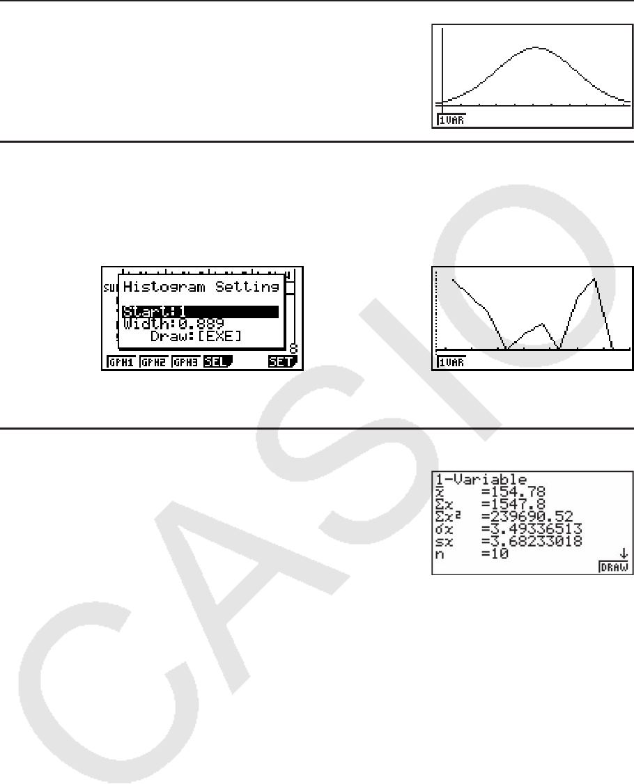
6-6
k 正态分布曲线
使用正态分布函数绘制正态分布曲线。
XList指定输入数据的列表框,Freq指定输入数据频率的列
表。在不指定频率时,Freq指定为1。
k 虚线图形
使用直线连接直方图中点。
XList指定输入数据的列表框,Freq指定输入数据频率的列表。在不指定频率时,Freq指定为
1。
w(DRAW)
在绘制图形之前,显示以上屏幕。此时,您可改变Start和Width值。
k 显示单变量图形的计算结果
单变量统计可表示为图形与参数值。在显示这些图形时,如
果按下 1(1VAR),显示单变量计算结果,如右图所示。
• 使用 c滚动列表,以便查看超出屏幕底部的项目。
下面说明了每一个参数的含义。
⇒
Q1 ........................ 第一四分位数
Med .................... 中位值
Q3 ........................ 第三四分位数
maxX ................ 最大值
Mod .................... 众数
Mod:
n ................ 众数项数
Mod:F ................ 众数频率
¯ x ............................ 平均值
∑ x ........................ 和
∑ x2
...................... 平方和
σ x .......................... 总体标准差
s
x ........................... 样本标准差
n ............................ 数据项数
minX ................. 最小值
6-7
• 按下 6(DRAW),返回原单变量统计图形。
• 如果Mod有多个解,则全部显示。
• 您可使用设置屏幕的“Q1Q3 Type”设置,将Q1和Q3计算模式选择为“Std”(标准计算)
或者“OnData”(法式计算)。
如需详细了解选择“Std”或“OnData”时的计算方法,参见下面的“Std与OnData设置的计
算方法”。
k Std与OnData设置的计算方法
Q1和Q3以及Med可根据设置屏幕的“Q1Q3 Type”设置进行计算,如下所述。
u Std
在使用这种计算方法时,处理方式取决于总体中的元素个数 n是偶数还是奇数。
当元素个数
n是偶数时:
以总体的中心点为参照,总体元素分为两组:下半组与上半组。因此Q1和Q3以及Med的值变为
如下所述。
Q1 = {从总体底部开始, 2
n 个项目组的中位值}
Q3 = {从总体顶部开始, 2
n 个项目组的中位值}
Med = {第 2
n 个和第 2
n +1个元素平均值}
中心点 中心点 中心点
当元素个数
n是奇数时:
以总体的中位值为参照,总体元素分为两组:下半组(值低于中位值)与上半组(值高于中位
值)。不包括中位值。因此Q1和Q3以及Med的值变为如下所述。
Q1 = {从总体底部开始, 2
n- 1 个项目组的中位值}
Q3 = {从总体顶部开始, 2
n- 1 个项目组的中位值}
Med = {第 2
n + 1 个元素}
• 当 n = 1时,Q1 = Q3 = Med = 总体中心点。
2
4 + 5=中位值
= Q1
2
2 + 3= Q3
2
6 + 7
12345678
6-8
中心点 中心点
• 当频数包含小数值时 (仅限fx-9860GII SD/fx-9860GII/fx-9860G AU PLUS)
对于这种计算方法,Q1和Q3以及Med值如下所述。
Q1 = {累积频率比大于0.25且最接近0.25的元素的值}
当一些数据值的累计频率比恰好为0.25时,Q1是该数据值和下一个数据值的平均值。
Q3 = {累积频率比大于0.75 且最接近0.75的元素的值}
当一些数据值的累计频率比恰好为0.75时,Q3是该数据值和下一个数据值的平均值。
Med = {累积频率比大于0.5且最接近0.5的元素的值}
当一些数据值的累计频率比恰好为0.5时,Med是该数据值和下一个数据值的平均值。
下面是一个上述方法的实例。
数据值 频率 累积频率 累积频率比
1 0.1 0.1 0.1/1.0 = 0.1
2 0.1 0.2 0.2/1.0 = 0.2
3 0.2 0.4 0.4/1.0 = 0.4
4 0.3 0.7 0.7/1.0 = 0.7
5 0.1 0.8 0.8/1.0 = 0.8
6 0.1 0.9 0.9/1.0 = 0.9
7 0.1 1.0 1.0/1.0 = 1.0
• 累积频率比大于0.25且最接近0.25的值为3,因此Q1 = 3。
• 累积频率比大于0.75且最接近0.75的值为5,因此Q3 = 5。
• 累积频率比大于0.5且最接近0.5的值为4,因此Med = 4。
中位值
1234567 98
= Q1
2
2 + 3= Q3
2
7 + 8
6-9
u OnData
对于这种计算方法,Q1和Q3以及Med值如下所述。
Q1 = {累积频率比大于0.25且最接近0.25的元素的值}
Q3 = {累积频率比大于0.75且最接近0.75的元素的值}
下面是一个上述方法的实例。
(元素个数: 10)
数据值 频率 累积频率 累积频率比
1 1 1 1/10 = 0.1
2 1 2 2/10 = 0.2
3 2 4 4/10 = 0.4
4 3 7 7/10 = 0.7
5 1 8 8/10 = 0.8
6 1 9 9/10 = 0.9
7 1 10 10/10 = 1.0
• 累积频率比大于或等于0.25且最接近0.25的值为3,因此Q1 = 3。
• 累积频率比大于或等于0.75且最接近0.75的值为5,因此Q3 = 5。
参照点(0.25) 参照点(0.75)
• 使用与将“Q1Q3 Type”设置选择为“Std ”时所使用的方法相同的方法计算Med。
• 当将“Q1Q3 Type”设置选择为“OnData”时,频率值是所有整数还是包含小数值没有不
同。
• 仅fx-9860GII SD/fx-9860GII/fx-9861G AU PLUS支持使用小数的频率值。
Q1
0.1 0.2 0.4 0.7 0.8 0.9 1.0
Q3
12633444 75
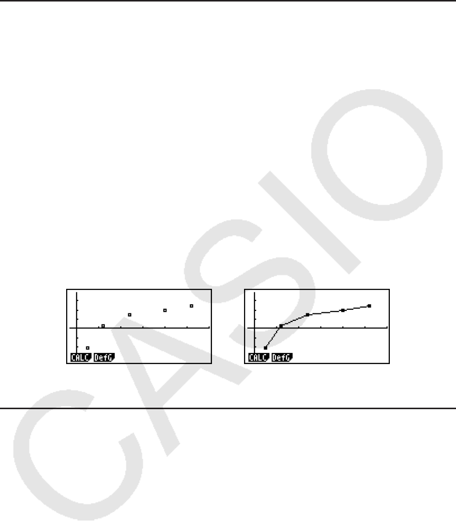
6-10
3. 计算与绘制双变量统计数据
k 绘制散布图和 xy线图
下述程序绘制一个散布图并连接各点,产生一个 xy线图。
1. 在主菜单中,进入 STAT 模式。
2. 将数据输入列表。
3. 将图形类型指定为Scat(散布图)或
xy( xy线图),然后执行图形操作。
按下 A, J或 !J(QUIT),返回统计数据列表。
示例 输入下述两组数据。然后在散布图绘制数据点并连接各点,产生
xy线图。
0.5, 1.2, 2.4, 4.0, 5.2 ( xList)
-2.1, 0.3, 1.5, 2.0, 2.4 (
yList)
1 m STAT
2 a.fwb.cwc.ewewf.cwe
-c.bwa.dwb.fwcwc.ew
3 (散布图) 1(GRPH) 6(SET) c1(Scat) J1(GPH1)
3 (
xy线图) 1(GRPH) 6(SET) c2( xy) J1(GPH1)
(散布图) (
xy 线图)
k 绘制回归图形
使用下述程序输入双变量统计数据,使用这些数据执行回归计算,然后绘制计算结果图形。
1. 在主菜单中,进入 STAT 模式。
2. 将数据输入列表,然后绘制散布图。
3. 选择回归类型,执行计算并显示回归参数。
4. 绘制回归图形。
示例 输入下述两组数据并在散布图上绘制数据点。接下来对数据执行对数回归计
算,显示回归参数,然后绘制对应的回归图形。
0.5, 1.2, 2.4, 4.0, 5.2 ( xList)
-2.1, 0.3, 1.5, 2.0, 2.4 (
yList)
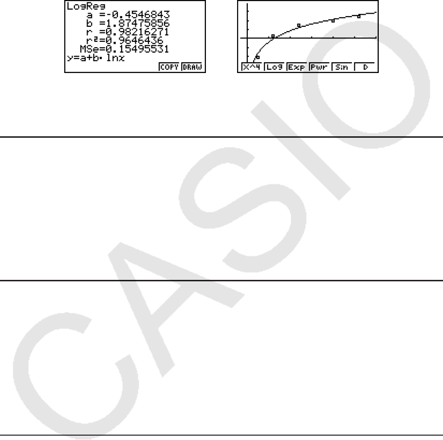
6-11
1 m STAT
2 a.fwb.cwc.ewewf.cwe
-c.bwa.dwb.fwcwc.ew
1(GRPH) 6(SET) c1(Scat) J1(GPH1)
3 1(CALC) 6( g) 2(Log)
4 6(DRAW)
• 您可在回归图形上执行跟踪功能。您不可执行跟踪滚动功能。
• 输入一个正整数频率数据。其他类型的值(小数等等)会产生错误。
k 选择回归类型
在绘制双变量统计数据的图形之后,您可使用显示屏底部的功能菜单选择各种不同的回归类
型。
• { ax+ b} / { a+ bx} / { Med } / { X^2 } / { X^3 } / { X^4 } / { Log } / { ae^ bx} / { ab^ x} / { Pwr } / { Sin } / { Lgst } ...
{线性回归(
ax+ b形式)}/{线性回归( a+ bx形式)}/{Med-Med}/{二次回归}/{三次回
归}/{四次回归}/{对数回归}/{指数回归(
aebx形式)}/{指数回归( abx形式)}/{幂回归}/{正弦
回归}/{逻辑回归}计算与绘图
• { 2VAR } ... {双变量统计结果}
k 显示回归计算结果
一旦执行回归计算,显示屏上即显示回归公式参数计算结果(例如下列线性回归中的 a和 b:
y = ax + b)。您可使用这些参数获取统计计算结果。
在显示屏上显示图形时,按下功能键选择某个回归类型之后,立即计算回归参数。
以下参数用于线性回归、对数回归、指数回归和幂回归。
r ..................... 相关系数
r
2 .................... 可决系数
MSe ............ 均方差
k 绘制统计计算结果图形
显示屏上显示参数计算结果时,您可通过按下 6(DRAW),绘制显示的回归公式图形。
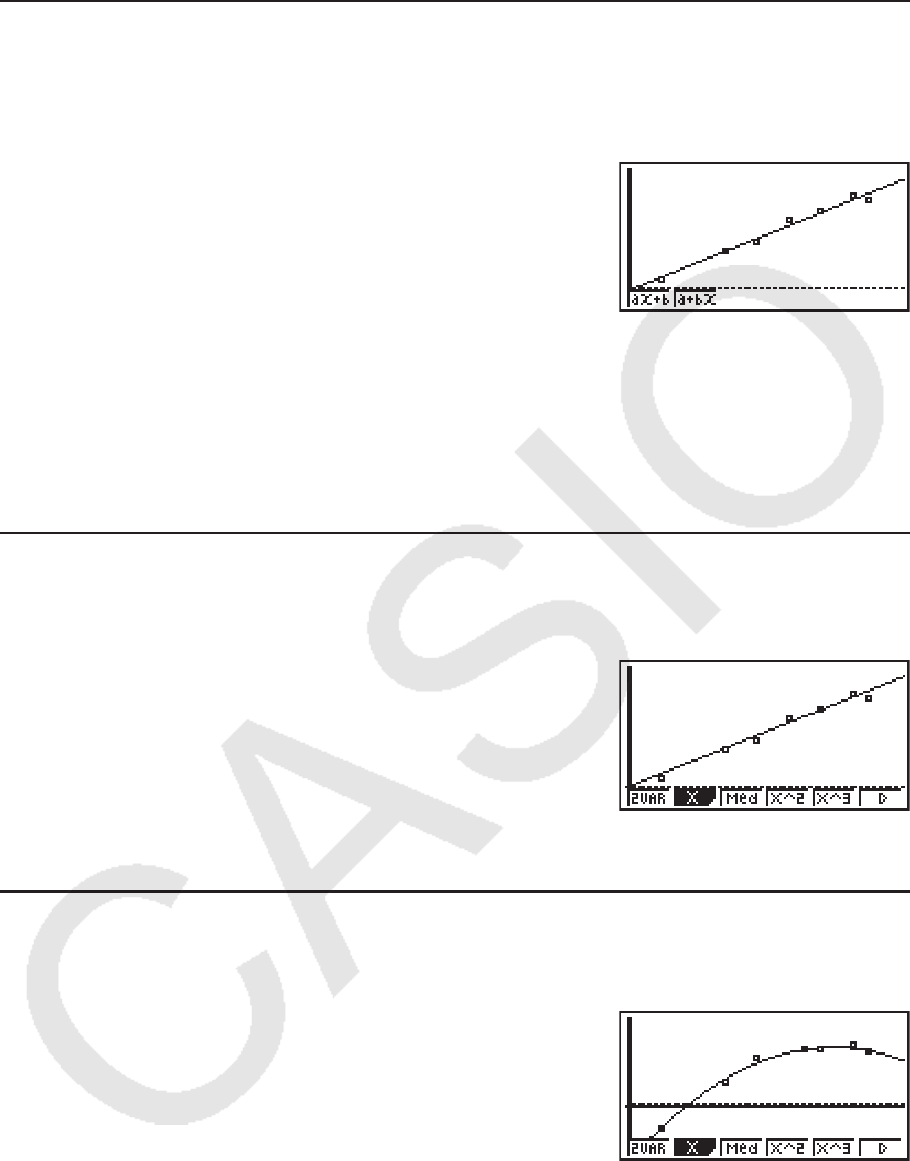
6-12
k 线性回归图形
线性回归使用最小二乘法绘制一条与尽可能多的数据点接近的直线,并返回直线斜率与 y截距
(当
x = 0时的 y坐标)。
表述这种关系的图形即线性回归图形。
1(CALC) 2(X)
1(
ax+ b) 或者 2( a+ bx)
6(DRAW)
下面是线性回归模型公式。
y = ax + b
a .................... 回归系数(斜率)
b .................... 回归常数项( y截距)
y = a + bx
a .................... 回归常数项( y截距)
b .................... 回归系数(斜率)
k Med-Med图形
在估计有大量极值时, 可使用Med-Med图形替代最小二乘法。这类似于线性回归,但可将极值
产生的影响降低到最低限度。
1(CALC) 3(Med)
6(DRAW)
下面是Med-Med图形模型公式。
y = ax + b
a .................... Med-Med图形斜率
b .................... Med-Med图形 y截距
k 二次/三次/四次回归图形
二次/三次/四次回归图形即将散布图的数据点连接在一起。它使用最小二乘法绘制尽可能接近
最多数据点的曲线。表述这种关系的图形即二次/三次/四次回归图形。
示例二次回归
1(CALC) 4(X^2)
6(DRAW)
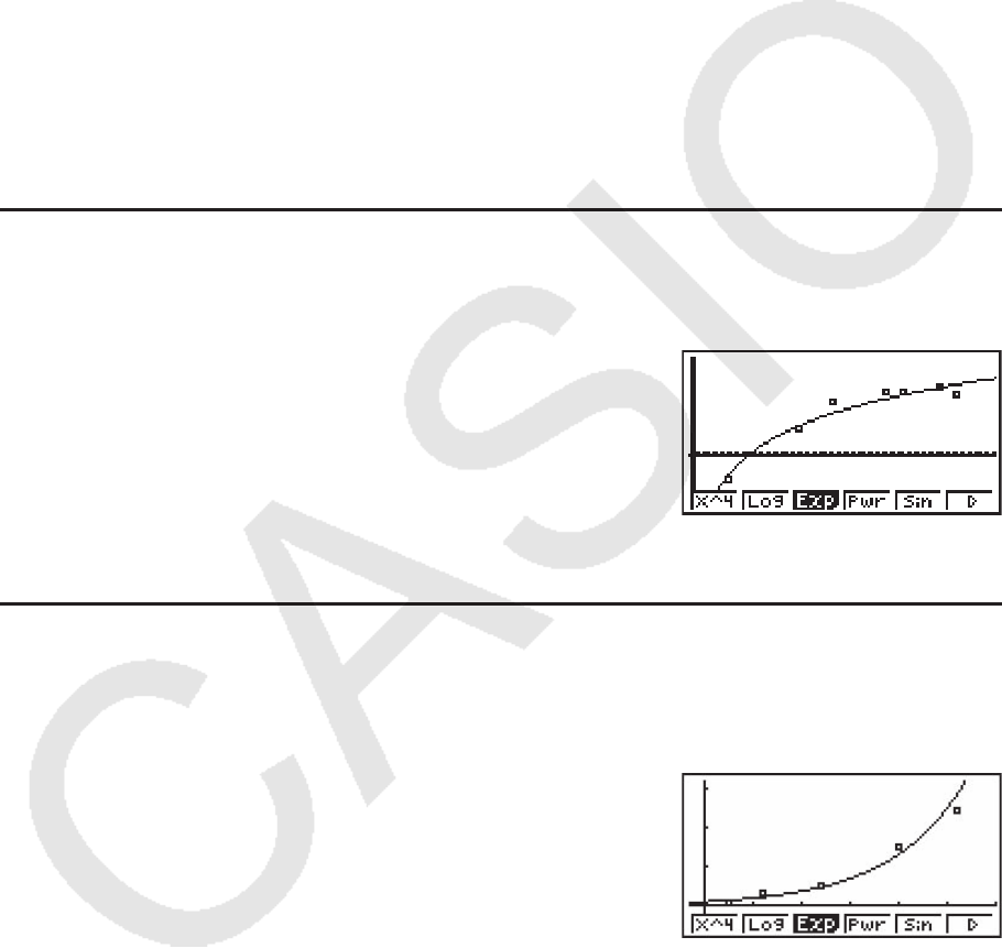
6-13
三次回归
模型公式 .....................
y = ax3
+ bx2
+ cx + d
a ........... 回归第三系数
b ........... 回归第二系数
c ............ 回归第一系数
d ........... 回归常数项( y截距)
四次回归
模型公式 .....................
y = ax4
+ bx3
+ cx2
+ dx + e
a ........... 回归第四系数
b ........... 回归第三系数
c ............ 回归第二系数
d ........... 回归第一系数
e ............ 回归常数项( y截距)
k 对数回归图形
对数回归表达式 y为 x的对数函数。标准对数回归公式为 y = a + b × ln x,所以如果X = ln x,
该公式对应于线性回归公式
y = a + bX。
1(CALC) 6( g) 2(Log)
6(DRAW)
下面是对数回归模型公式。
y = a + b・ln x
a .................... 回归常数项
b .................... 回归系数
k 指数回归图形
指数回归表达式 y为 x指数函数的乘积形式。标准指数回归公式为 y = a × ebx,因此如果两边取
对数,则得到ln
y = ln a + bx。接下来,如果Y = ln y且A = ln a,该公式对应于线性回归公式
Y = A +
bx。
1(CALC) 6( g) 3(Exp)
1(
aeˆbx)或 2( abˆx)
6(DRAW)
下面是指数回归模型公式。
y = a・ ebx
a .................... 回归系数
b .................... 回归常数项
y = a・ bx
a .................... 回归常数项
b .................... 回归系数
二次回归
模型公式 .....................
y = ax2
+ bx + c
a .......... 回归第二系数
b .......... 回归第一系数
c ........... 回归常数项 ( y截距)
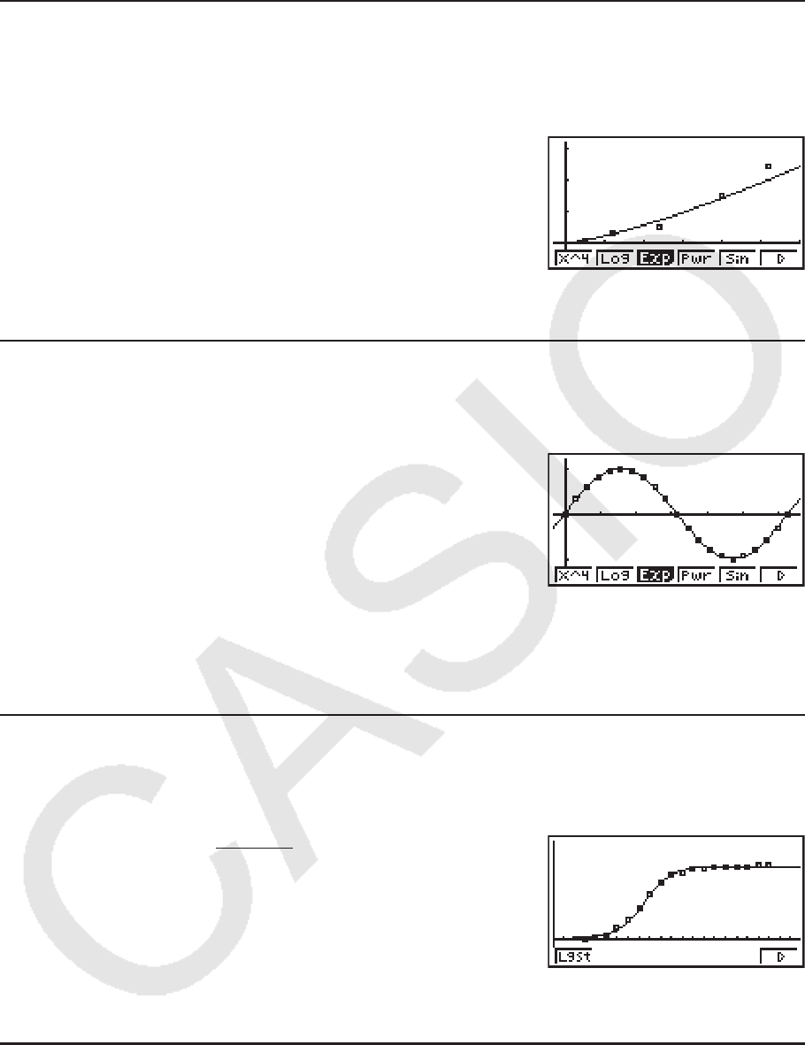
6-14
k 幂回归图形
幂回归表达式 y为 x的幂函数的乘积形式。标准幂回归公式为 y = a × xb,因此如果两边取对数,
则得到In
y = ln a + b × ln x。接下来,如果X = ln x,Y = ln y且A = ln a,该公式对应于线
性回归公式Y = A +
bX。
1(CALC) 6( g) 4(Pwr)
6(DRAW)
下面是幂回归模型公式。
y = a・ xb
a .................... 回归系数
b .................... 回归幂
k 正弦回归图形
正弦回归最适合用于循环数据。
下面是正弦回归模型公式。
y = a・sin( bx + c) + d
1(CALC) 6( g) 5(Sin)
6(DRAW)
绘制正弦回归图形会使角度单位自动改为Rad(弧度)。在执行正弦回归计算但不绘制图形时,
角度单位不会改变。
• 某些类型的数据可能需要较长计算时间。这属于正常现象。
k 逻辑回归图形
逻辑回归最适合用于以时间为基准的现象,其中某个量持续增长,直至达到饱和点。
下面是逻辑回归模型公式。
1(CALC) 6( g) 6( g) 1(Lgst)
6(DRAW)
• 某些类型的数据可能需要较长计算时间。这属于正常现象。
k 残值计算
在回归计算期间,可计算实际绘图点( y坐标)与回归模型距离。
在显示屏上显示统计数据列表时,调用设置屏幕,为“Resid List”指定一个LIST(“List
1”至“List 26”)。计算所得残值数据保存在指定的列表中。
从绘图点到回归模型的垂直距离将保存在列表中。
高于回归模型的图形部分为正,低于回归模型的图形部分为负。
y=c
1 + ae–bx
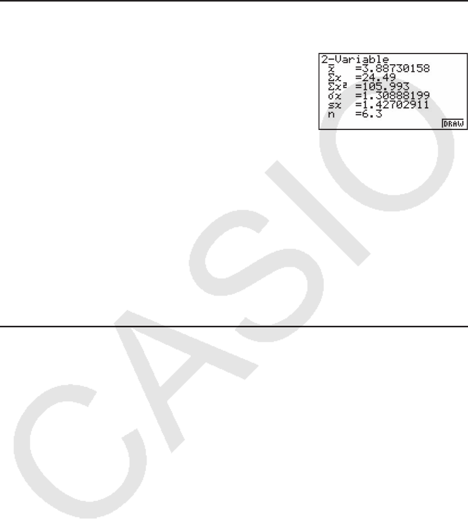
6-15
所有回归模型都可执行残值计算并保存结果。
选定列表中已经存在的任何数据都被清除。每一个图形的残值在保存时采用的优先顺序都与模
型中所用的数据相同。
k 显示双变量图形的计算结果
双变量统计可表示为图形与参数值。在显示这些图形时,如果按下 1(CALC) 1(2VAR),显
示双变量计算结果,如下图所示。
• 使用 c滚动列表,以便查看超出屏幕底部的项目。
o ................. xList中保存数据的平均值
∑ x ............... xList中保存数据的和
∑ x2
............. xList中保存数据的平方和
σ
x ................ xList中保存数据的总体标准差
s
x ................. xList中保存数据的样本标准差
n .................. 数据项数
p ...................
yList中保存数据的平均值
∑ y ............... yList中保存数据的和
∑ y2
............ yList中保存数据的平方和
σ
y ................ yList中保存数据的总体标准差
s
y ................. yList中保存数据的样本标准差
∑ xy ........... xList和 yList中保存数据之积的和
minX .......
xList中保存数据的最小值
maxX ......
xList中保存数据的最大值
minY .......
yList中保存数据的最小值
maxY ......
yList中保存数据的最大值
k 将回归图形公式复制到GRAPH模式
您可将回归公式计算结果复制到 GRAPH 模式图形关系列表,然后进行保存和对比。
1. 显示屏上显示回归计算结果(参见第6-11页的“显示回归计算结果”)时,按下 5(COPY)
。
• 由此可显示 GRAPH 模式图形关系列表。*
1
2. 使用 f和 c,在显示的结果中突出显示想要复制回归公式的区域。
3. 按下 w,保存复制的图形公式并返回前一个回归计算结果显示屏幕。
*
1
在 GRAPH 模式中不可编辑图形公式的回归公式。
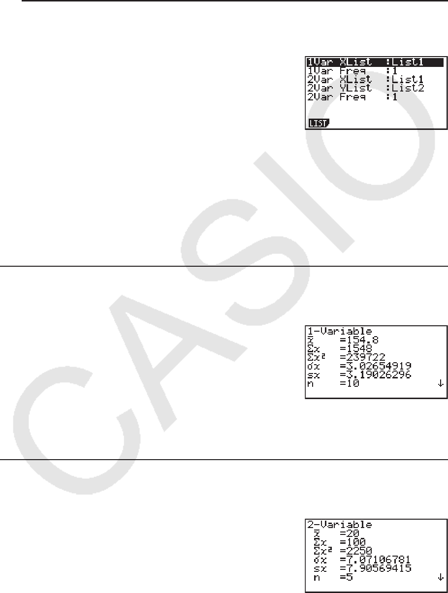
6-16
4. 执行统计计算
至此,所有统计计算都已在显示图形之后进行。下述程序可用于单独进行统计计算。
u 指定统计计算数据列表
您必须输入想要进行计算的统计数据并在开始计算之前指定其位置。显示统计数据,然后按下
2(CALC) 6(SET)。
下面是每一个项目的含义。
1Var XList ...... 单变量统计
x值的位置(XList)
1Var Freq ........ 单变量频率值的位置(Frequency)
2Var XList ...... 双变量统计
x值的位置(XList)
2Var YList ...... 双变量统计
y值的位置(YList)
2Var Freq ........ 双变量频率值的位置(Frequency)
• 本节计算均依据上述规定。
k 单变量统计计算
在前面“显示单变量图形的计算结果”的示例中,绘制图形之后显示统计计算结果。它们是图
形显示中所用变量特性的数值表达。
也可通过显示统计数据列表并按下 2(CALC) 1(1VAR),
直接获得这些数值。
此后,按下 f或 c滚动统计计算结果显示内容,以便查看变量特性。
关于这些统计值的含义,请参见“显示单变量图形的计算结果”(第6-6页)。
k 双变量统计计算
在前面“显示双变量图形的计算结果”的示例中,绘制图形之后显示统计计算结果。它们是图
形显示中所用变量特性的数值表达。
也可通过显示统计数据列表并按下 2(CALC) 2(2VAR),
直接获得这些数值。
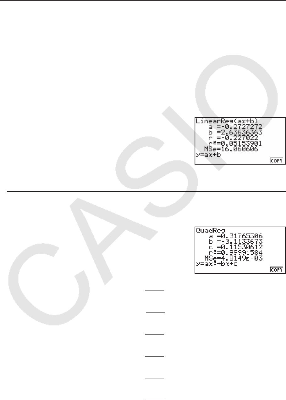
6-17
此后,按下 f或 c滚动统计计算结果显示内容,以便查看变量特性。
关于这些统计值的含义,请参见“显示双变量图形的计算结果”(第6-15页)。
k 回归计算
在从“线性回归图形”到“逻辑回归图形”的说明中,绘制图形之后显示回归计算结果。在
此,回归直线或回归曲线的每一个系数值都表示为一个数字。
您可从数据输入屏幕直接确定相同的表达式。
按下 2(CALC) 3(REG),显示包含下述各项的功能菜单。
• { ax+ b} / { a+ bx} / { Med } / { X^2 } / { X^3 } / { X^4 } / { Log } / { ae^ bx} / { ab^ x} / { Pwr } / { Sin } / { Lgst } ...
{线性回归(
ax+ b形式)}/{线性回归( a+ bx形式)}/{Med-Med}/{二次回归}/{三次回归}/
{四次回归}/{对数回归}/{指数回归(
aebx形式)}/{指数回归( abx形式)}/{幂回归}/{正弦回
归}/{逻辑回归}参数
示例 显示单变量回归参数
2(CALC) 3(REG) 1(X) 1(
ax+ b)
该屏幕上显示的参数的含义与“线性回归图形”至“逻辑回归图形”中的参数含义相同。
u 计算可决系数(r
2
)和MSe
您可使用 STAT 模式计算二次回归、三次回归和四次回归的可决系数(r
2
)。以下类型的MSe计
算可用于每一种回归类型。
• 线性回归 (
ax + b) ..........................................
(
a + bx) ........................................
• 二次回归 ................................................................
• 三次回归 ................................................................
• 四次回归 ................................................................
• 对数回归 ................................................................
M
Se = Σ
1
n – 2
i=1
n
(y
i
– (ax
i
+ b))
2
M
Se = Σ
1
n – 2 i=1
n
(yi– (a+bxi))2
M
Se =
Σ
1
n – 3
i=1
n
(y
i
– (ax
i
+ bx
i
+ c))
2
2
M
Se =
Σ
1
n – 4
i=1
n
(y
i
– (ax
i3
+ bx
i
+ cx
i
+ d ))
2
2
M
Se = Σ
1
n – 5
i=1
n
(y
i
– (ax
i4
+ bx
i3
+ cx
i
+ dx
i
+ e))
2
2
M
Se =
Σ
1
n – 2
i=1
n
(y
i
– (a + b ln x
i
))
2
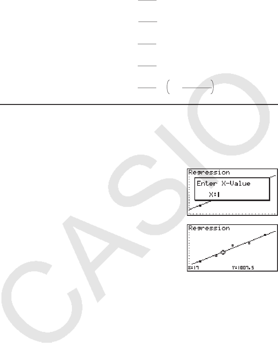
6-18
• 指数回归 (
a・ ebx) ...........................................
(
a・ bx) ............................................
• 幂回归 .....................................................................
• 正弦回归 ................................................................
• 逻辑回归 ................................................................
u 回归图形的估计值计算
STAT 模式还包括一个Y-CAL函数,该函数在绘制双变量统计回归之后,使用回归计算特定 x值
对应的估计
y值。
下面是使用Y-CAL函数的一般程序。
1. 绘制回归图形之后,按下 !5(G-SLV) 1(Y-CAL),进入图形选择模式,然后按下 w。
如果显示屏上有多个图形,使用 f和 c选择想要的图形,然后按下 w。
• 由此可显示一个
x值输入对话框。
2. 输入 x值然后按下 w。
• 由此可在显示屏的底部显示
x和 y的坐标,然后将指针移
至图形上的对应点。
3. 此时按下 v或者数字键将显示
x值输入对话框,如果需要,您可执行下一次估计值计算。
• 如果计算坐标不在显示范围内,不会显示指针。
• 如果设置屏幕的“Coord”设置为“Off”,则不显示指针。
• Y-CAL函数也可用于由DefG功能绘制的图形。
M
Se = Σ
1
n – 2 i=1
n
(ln yi – (ln a + bxi ))2
M
Se = Σ
1
n – 2 i=1
n
(ln yi– (ln a + (ln b) · xi ))2
M
Se =
Σ
1
n – 2
i=1
n
(ln y
i
– (ln a + b ln x
i
))
2
M
Se =
Σ
1
n – 2
i=1
n
(y
i
– (a sin (bx
i
+ c) + d ))
2
M
Se = Σ
1
n – 2 1 + ae–bxi
C
i=1
n
yi–
2
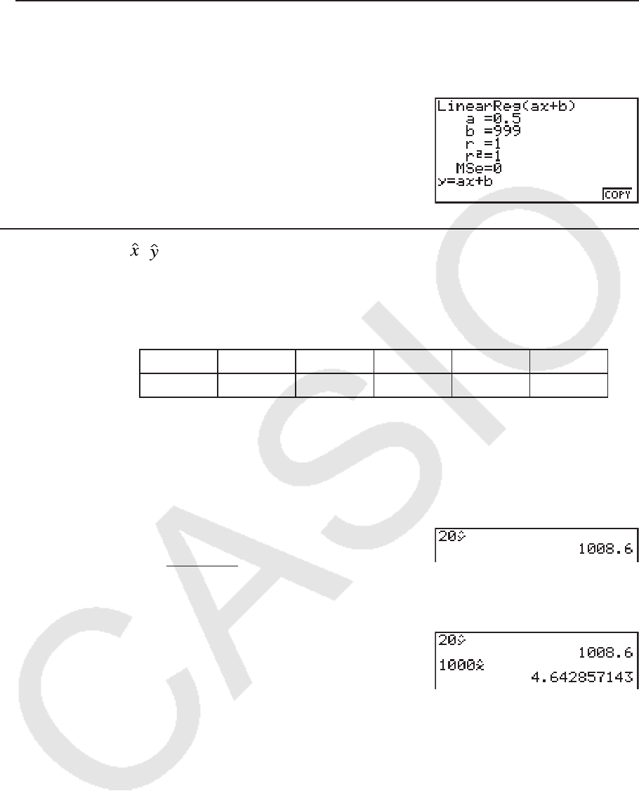
6-19
u 从回归计算结果屏幕复制回归公式的功能
除了可在绘制统计图形(例如散布图)之后复制回归计算结果屏幕的正常回归公式复制功能之
外, STAT 模式还可提供一个功能,帮助您复制回归计算产生的回归公式。如需复制产生的回归
公式,按下 6(COPY)。
k 估计值计算( , )
使用 STAT 模式绘制回归图形之后,您可使用 RUN • MAT (或者 RUN )模式计算回归图形 x和 y
参数的估计值。
示例 使用邻近数据执行线性回归并在
xi = 20且 yi = 1000时估算 ţ与 ů x 的值
xi 10 15 20 25 30
yi 1003 1005 1010 1011 1014
1. 在主菜单中,进入 STAT 模式。
2. 将数据输入列表并绘制线性回归图形。
3. 在主菜单中,进入 RUN • MAT (或者 RUN )模式。
4. 按下以下按键。
ca( xi的值)
K5(STAT) * 2(
ţ) w
* fx-7400G
II: 4(STAT)
显示 xi = 20对应的估计值 ţ。
baaa( yi的值)
1(
ˆ x ) w
显示 yi = 1000对应的估计值 ˆ x 。
• 您无法获取Med-Med、二次回归、三次回归、四次回归、正弦回归或者逻辑回归图形的估计
值。
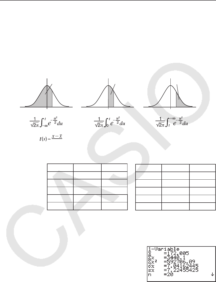
6-20
k 正态概率分布计算
您可使用 RUN • MAT (或者 RUN )模式计算单变量统计的正态概率分布。
按下 K6( g) 3(PROB)( 2(PROB)为 fx-7400G
II上的对应键) 6( g)以显示功能菜单,
包含以下项目。
• { P( } / { Q( } / { R( } ... 获取正态概率{P(
t)}/{Q( t)}/{R( t)} 数值
• {
t( } ... {获取正规化变量 t( x)的值}
• 使用下述公式计算正态概率P(
t)、Q( t)、和R( t)以及正规化变量 t( x)。
标准正态分布
示例 下列表格显示了20名大学生身高的测量结果。确定身高在160.5 cm到175.5
cm范围内的学生的百分比。身高为175.5 cm的学生的百分比。
班级编号 身高(cm) 频率
1 158.5 1
2 160.5 1
3 163.3 2
4 167.5 2
5 170.2 3
P(
t
)Q(
t
)R(
t
)
tt t
00 0
σ
x
班级编号 身高(cm) 频率
6 173.3 4
7 175.5 2
8 178.6 2
9 180.4 2
10 186.7 1
1. 在主菜单中,进入 STAT 模式。
2. 在List 1输入身高数据,在List 2中输入频率数据。
3. 执行单变量统计计算。
只需执行单变量统计计算即可立即获取正规化变量。
2(CALC) 6(SET)
1(LIST) bw
c2(LIST) cw!J(QUIT)
2(CALC) 1(1VAR)
4. 按下 m,选择 RUN • MAT (或者 RUN )模式,按下 K6( g) 3(PROB)( 2(PROB)为
fx-7400G
II上的对应键),调用概率计算(PROB)菜单。
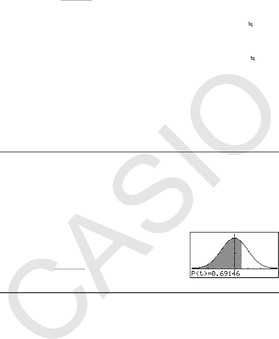
6-21
3(PROB) * 6( g) 4( t() bga.f)w
* fx-7400G
II: 2(PROB)
(160.5 cm的正规化变量
t ) 结果: -1.633855948
( -1.634)
4( t() bhf.f)w
(175.5 cm的正规化变量
t ) 结果: 0.4963343361
( 0.496)
1(P() a.ejg)-
1(P() -b.gde)w
(总和百分比) 结果: 0.638921
(总和的63.9%)
3(R() a.ejg)w
(百分比) 结果: 0.30995
(31.0百分比)
k 绘制正态概率分布图形
您可在 RUN • MAT (或者 RUN )模式中使用手动制图功能绘制正态概率分布图形。
1. 在主菜单中,进入 RUN • MAT (或者 RUN )模式。
2. 输入用于绘制直角坐标图形的命令。
3. 输入概率值。
示例 绘制正态概率P (0.5)图形。
1 m RUN • MAT (或者RUN)
2 !4(SKTCH) 1(Cls) w
5(GRPH) 1(Y=)
3 K6( g) 3(PROB) * 6( g) 1(P() a.f)w
* fx-7400G
II: 2(PROB)
k 使用分布函数计算
重要!
• fx-7400G II上不可执行以下操作。
您可在 RUN • MAT 模式或者 PRGM 模式中使用特殊函数,执行与 STAT 模式分布函数计算相同的
计算(第6-40页)。
示例 当总体标准差为
σ
= 1.5且总体平均值为 ƫ = 2时,在RUN • MAT模式中计算数
据{1, 2, 3}的正态概率分布。
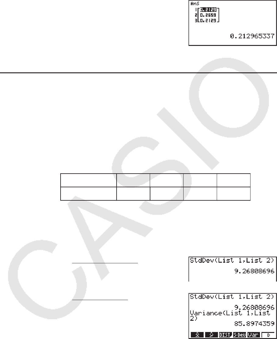
6-22
1. 在主菜单中,进入 RUN • MAT 模式。
2. 按下以下按键。
K5(STAT) 3(DIST) 1(NORM)
1(NPd) !*( { ) b,c,d
!/( } ) ,b.f,c)w
• 如需详细了解分布函数的功能及其语法,请参见“在程序中执行分布计算”(第8-29页)。
k 使用列表数据确定标准差和方差
您可使用函数确定指定列表数据的标准差和方差。在 RUN • MAT (或者RUN)模式中执行该计
算。您可使用通过 STAT 模式列表编辑器保存到列表(List 1至List 26)的数据或者在 RUN •
MAT(或者RUN) 模式屏幕上直接输入的数据进行计算。
语法 StdDev(List
n [,List m])
Variance(List
n [,List m])
List
n ......... 样本数据
List
m ........ Frequency数据
示例 保存下面List 1中的
x数据和List 2中的频率值,确定标准差和方差
x 60 70 80 90
频率 3 5 4 1
1. 在主菜单中,进入 STAT 模式。
2. 使用列表编辑器保存上述数据。
3. 在主菜单中,进入 RUN • MAT(或者RUN) 模式。
4. 按下以下按键。
K5(STAT) 4(S • Dev) *J
1(LIST) 1(List) b,1(List) c)w
* fx-7400GII: 4(STAT) 3(S • Dev)
J5(STAT) 5(Var)* J
1(LIST) 1(List) b,1(List) c)w
* fx-7400GII: 4(STAT) 4(Var)
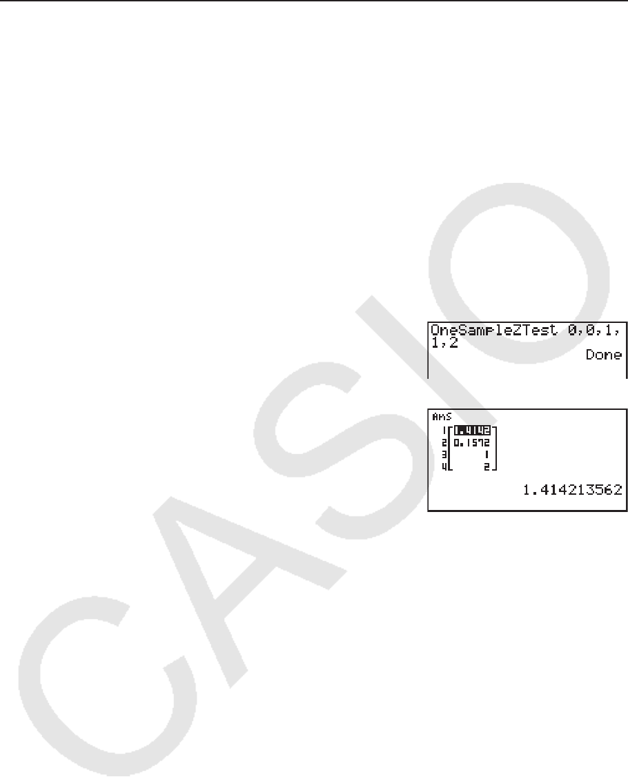
6-23
k 使用TEST命令计算
重要!
• fx-7400G II上不可执行以下操作。
您可在 RUN • MAT 模式或者 PRGM 模式中使用特殊函数,执行与 STAT 模式 Z测试、 t测试和其它
测试计算相同的计算(第6-23页)。
示例 在下述条件下执行1-样品
Z测试时,确定 z分数和 p值:
测试条件(
ƫ条件)
ƫ0
*,假设总体平均值 ƫ0
= 0,总体标准差 Ʊ = 1,样本
平均值
o
= 1,样本数 n = 2
* “
ƫ条件 ƫ0
”可通过在1-样本 Z测试命令“OneSampleZTest”中将初始自
变量设置为0进行指定。
1. 在主菜单中,进入 RUN • MAT 模式。
2. 执行以下按键操作。
K5(STAT) 6( g) 1(TEST) 1(Z)
1(1-S) a,a,b,b,c
w
JJJ
1(LIST) 1(List) !-(Ans) w
以下计算结果显示为ListAns元素1至4。
1:
z分数
2:
p值
3: o
4:
n
• 如需详细了解支持的TEST命令功能及其语法,请参见“在程序中使用TEST命令执行某个命
令”(第8-32页)。
5. 测试
重要!
• fx-7400G II上不可执行测试计算。
Z 测试 提供各种不同的基于标准化的测试。当通过以前的测试确定某个总体(例如一个国家的全
部人口)的标准差时,它们能够测试样本是否精确地反映总体。
Z测试用于需要重复进行的市场
调查以及民意调查。

6-24
1-样本
Z 测试 在总体标准差已知时,对未知总体平均值进行测试。
2-样本
Z 测试 在两个总体标准差已知时,依据独立样本测试两个总体平均值是否相等。
1-比例
Z 测试 测试成功的未知比例。
2-比例
Z 测试 测试并比较两个总体的成功比例。
t 测试 在总体标准差未知时测试假设。与经证实的假设相反的假设称为 虚假设 ,而已经证实的假
设称为 备择假设 。
t测试通常用于测试虚假设。然后确定采用虚假设或者备择假设。
1-样本
t 测试 在总体标准差未知时,测试单个未知总体平均值的假设。
2-样本
t 测试 在总体标准差未知时,比较总体平均值。
线性回归
t 测试 计算配对数据线性关联的强度。
借助
χ
χ 2
测试 ,提供许多独立群组并针对每个群组包含样本的概率测试假设。
χ
χ 2
GOF测试 ( χ 2
单向测试)测试观察的样本数据计数是否符合某个特定分布。例如,可用于确定
是否符合正态分布或者二项分布。
χ
χ 2
双向测试 生成主要由两个定性变量(例如“是”和“否”)构成的列联表并评估这些变量的独
立性。
2-样本 F 测试 测试样本方差比值的假设。例如,它可用于测试多个可疑因素(例如吸烟、饮酒、
缺乏维生素、大量饮用咖啡、缺少活动、不良生活习惯等)的致癌作用。
ANOVA 测试在有多个样本时各样本的总体平均值相等的假设。例如,它可用于测试材料不同组
合对最终产品的质量与寿命是否有影响。
单向ANOVA 用于存在一个独立变量和一个因变量的情况。
双向ANOVA 用于存在两个独立变量和一个因变量的情况。
以下几页说明了在上述原则基础上的各种统计计算方法。有关统计原则与术语的详细说明,请
参阅标准统计教材。
在初始 STAT 模式屏幕中,按下 3(TEST),显示包含以下项目的测试菜单。
• 3(TEST) 1(Z) ...
Z测试(第6-25页)
2(t) ...
t测试(第6-27页)
3(CHI) ... χ 2
测试(第6-30页)
4(F) ... 2-样本
F测试(第6-31页)
5(ANOV) ... ANOVA(第6-32页)
完成所有参数的设置之后,使用 c突出显示“Execute”,然后按下面的某个功能键执行计算
或者绘制图形。
• 1(CALC) ... 执行计算。
• 6(DRAW) ... 绘制图形。
• 视窗设置针对图形绘制功能自动优化。
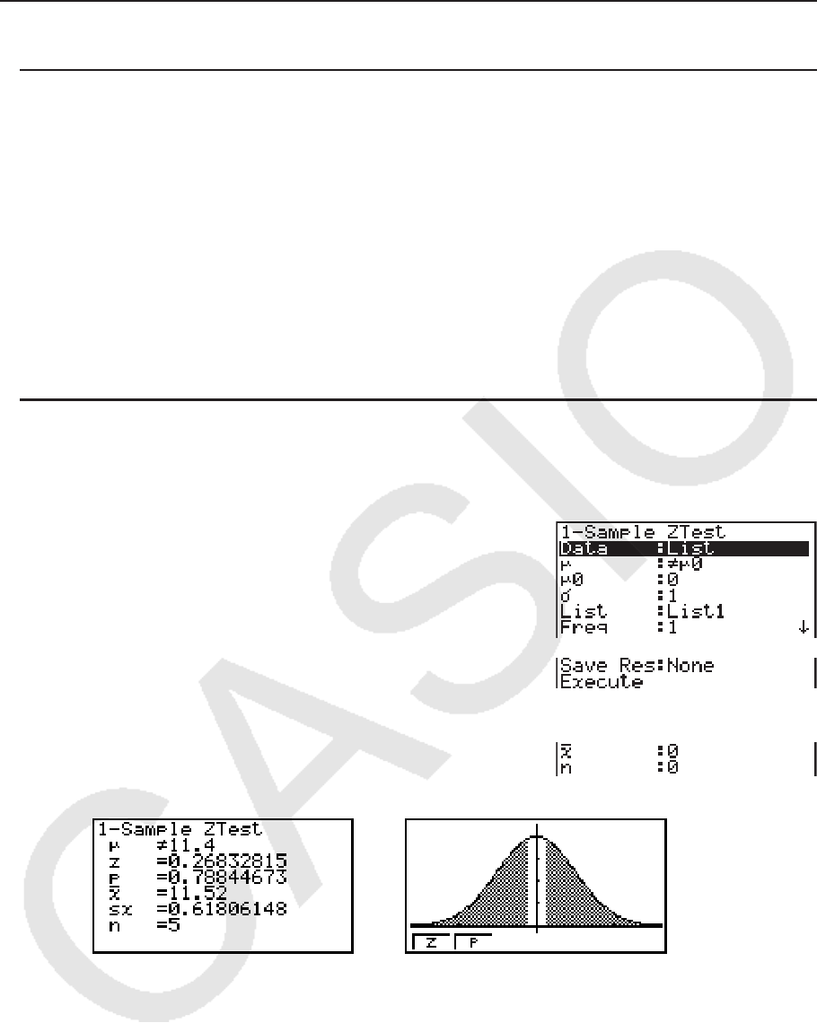
6-25
k Z测试
u Z测试常用功能
您可在绘制 Z测试结果输出图形之后使用以下图形分析功能。
• 1(Z) ... 显示 z分数。
按下 1(Z),在显示屏底部显示 z分数,并在图形中的对应位置显示指针(除非该位置在图形屏
幕范围之外)。
如果是双尾测试,则显示两点。使用 d和 e移动指针。
• 2(P) ... 显示 p值。
按下 2(P),在屏幕底部显示 p值,但不显示指针。
• 自动执行分析功能可将 z和 p值分别保存在字母变量Z和P中。
u 1-样本 Z 测试
该测试用于在已知总体标准差时测试假设。 1-样本 Z 测试 应用于正态分布。
在统计数据列表中执行以下键操作。
3(TEST)
1(Z)
1(1-S)
下面显示了与列表数据规定不同的参数数据规定项目。
计算结果输出示例
μ
11.4 ................ 测试方向
s
x ............................. 仅在Data: List设置情况下显示。
• [Save Res]不保存第2行的
μ
条件。
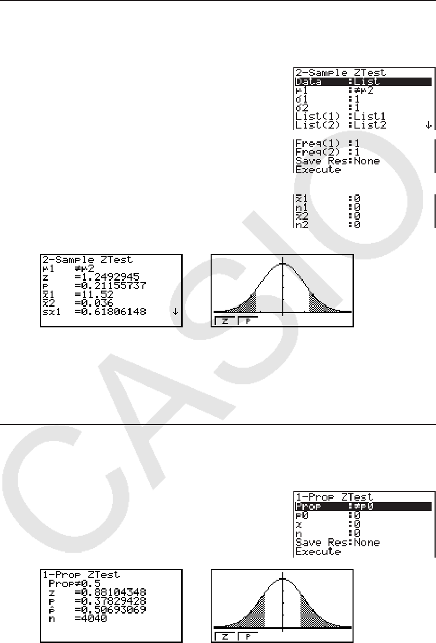
6-26
u 2-样本 Z 测试
该测试用于在已知两个总体标准差时测试假设。 2-样本 Z 测试 应用于正态分布。
在统计数据列表中执行以下键操作。
3(TEST)
1(Z)
2(2-S)
下面显示了与列表数据规定不同的参数数据规定项目。
计算结果输出示例
μ
1
μ
2
.................... 测试方向
s
x1
........................... 仅在Data: List设置情况下显示。
s
x2
........................... 仅在Data: List设置情况下显示。
• [Save Res]不保存第2行的
μ
1
条件。
u 1-比例 Z 测试
该测试用于测试成功的未知比例。 1-比例 Z 测试 应用于正态分布。
在统计数据列表中执行以下键操作。
3(TEST)
1(Z)
3(1-P)
计算结果输出示例
Prop 0.5 ............ 测试方向
• [Save Res]不保存第2行的比例条件。
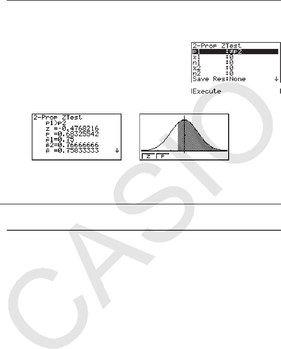
6-27
u 2-比例 Z测试
该测试用于比较成功的比例。 2-比例 Z 测试 应用于正态分布。
在统计数据列表中执行以下键操作。
3(TEST)
1(Z)
4(2-P)
计算结果输出示例
p
1
>
p2
.................... 测试方向
• [Save Res]不保存第2行的
p1
条件。
k t测试
u t测试常用功能
您可在绘制 t测试结果输出图形之后使用以下图形分析功能。
• 1(T) ... 显示 t分数。
按下 1(T),在显示屏底部显示 z分数,并在图形中的对应位置显示指针(除非该位置在图形屏
幕范围之外)。
如果是双尾测试,则显示两点。使用 d和 e移动指针。
• 2(P) ... 显示 p值。
按下 2(P),在屏幕底部显示 p值,但不显示指针。
• 自动执行分析功能可将
t和 p值分别保存在字母变量T和P中。
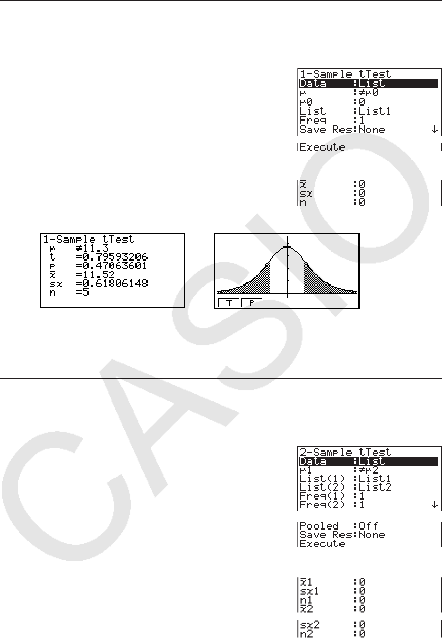
6-28
u 1-样本 t 测试
该测试在总体标准差未知时使用单个未知总体平均值的假设测试。 1-样本 t 测试 应用于 t分布。
在统计数据列表中执行以下键操作。
3(TEST)
2(t)
1(1-S)
下面显示了与列表数据规定不同的参数数据规定项目。
计算结果输出示例
μ
11.3 ................ 测试方向
• [Save Res]不保存第2行的
μ
条件。
u 2-样本 t 测试
2-样本 t 测试 在总体标准差未知时,比较总体平均值。 2-样本 t 测试 应用于 t分布。
在统计数据列表中执行以下键操作。
3(TEST)
2(t)
2(2-S)
下面显示了与列表数据规定不同的参数数据规定项目。
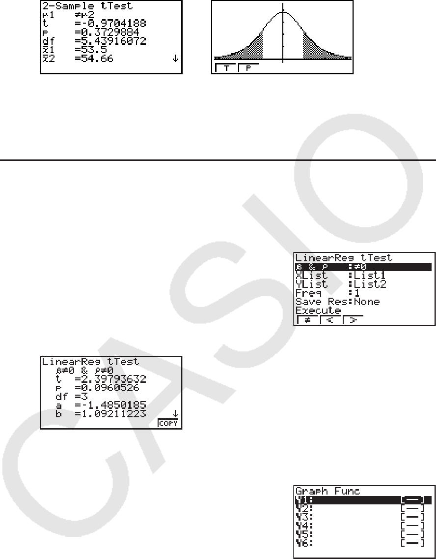
6-29
计算结果输出示例
μ
1
μ
2
.................... 测试方向
s
p ............................. 仅在Pooled: On 设置情况下显示。
• [Save Res]不保存第2行的
μ
1
条件。
u 线性回归 t测试
线性回归 t 测试 将配对变量数据集作为( x, y)对进行处理,使用最小二乘法确定回归公式
y = a + bx数据最精确的 a, b系数。此外,它还确定相关系数和 t分数,并计算 x与 y之间的关联程
度。
在统计数据列表中执行以下键操作。
3(TEST)
2(t)
3(REG)
计算结果输出示例
β
0 &
ρ
0 .............. 测试方向
显示屏上显示计算结果时按下 6(COPY),将回归公式复制到图形关系列表。
在设置屏幕上为[Resid List]项目指定一个列表时,回归公式残值数据在完成计算之后自动保存
到指定的列表。
• 您不可为线性回归
t测试绘制图形。
• [Save Res]不保存第2行
β
&
ρ
条件。
• 当[Save Res]指定的列表与设置屏幕上[Resid List]项目指定的列表相同时,只将[Resid List]
数据保存到列表中。
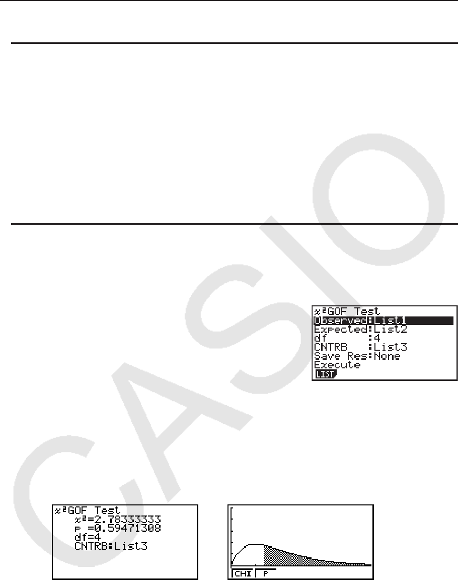
6-30
k Ƶ2
测试
• Ƶ2
测试常用功能
您可在绘制图形之后使用以下图形分析功能。
• 1(CHI) ... 显示 χ 2
值。
按下 1(CHI),在显示屏底部显示 χ 2
值,并在图形中的对应位置显示指针(除非该位置在图形屏
幕范围之外)。
• 2(P) ... 显示 p值。
按下 2(P),在屏幕底部显示 p值,但不显示指针。
• 自动执行分析功能可将 χ 2
和 p值分别保存在字母变量C和P中。
• Ƶ2
GOF测试( Ƶ2
单向测试)
χ
χ 2
GOF测试 ( Ƶ2
单向测试)测试样本数据的频率是否符合某个特定分布。例如,可用于确定是
否符合正态分布或者二项分布。
在统计数据列表中执行以下键操作。
3(TEST)
3(CHI)
1(GOF)
然后,指定包含数据的列表。下面显示了上述项目的含义。
Observed ......... 包含已观测计数(所有单元为正整数)的List(1至26)名称
Expected .......... 用于保存期望频率的List(1至26)名称
CNTRB .............. 指定一个列表(List 1至List 26),用于保存计算结果所得的每个观测计
数的贡献。
计算结果输出示例
CNTRB ............... 用于输出贡献值的列表
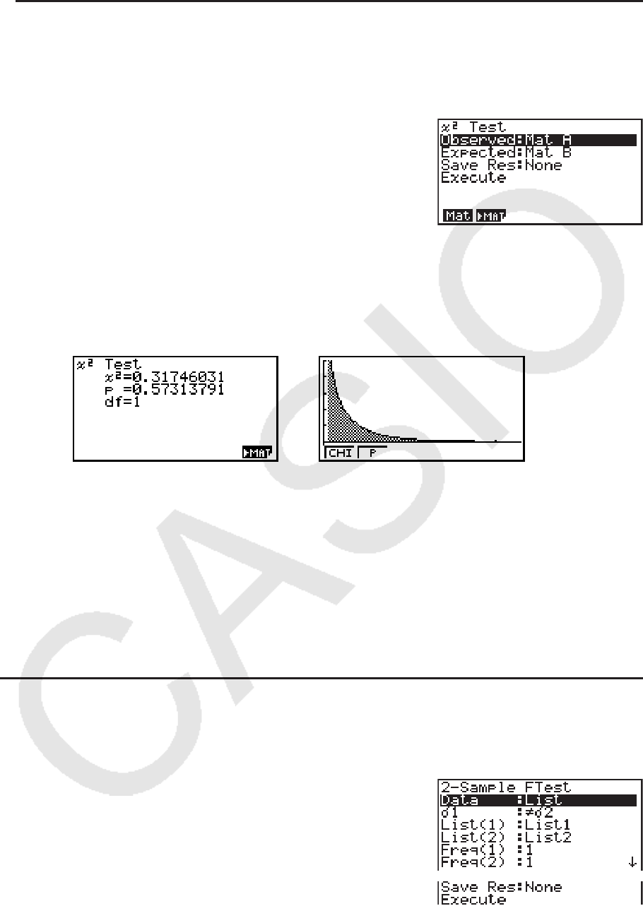
6-31
• Ƶ2
双向测试
χ
χ 2
双向测试 设置大量独立群组并针对每个群组包含样本的比例测试假设。 χ 2
测试应用于二分变量
(包括两种可能值的变量,例如是/否)。
在统计数据列表中执行以下键操作。
3(TEST)
3(CHI)
2(2WAY)
然后,指定包含数据的矩阵。下面显示了上述项目的含义。
Observed ......... 包含已观测计数(所有单元为正整数)的矩阵(A至Z)名称
Expected .......... 用于保存期望频率的矩阵(A至Z)名称
计算结果输出示例
• 矩阵至少包括两行和两列。如果矩阵只有一行或者一列,会产生错误。
• 在突出显示“Observed”和“Expected”时,按下 1(Mat),将显示矩阵(A至Z)设置屏
幕。
•在设置参数时按下 2( 'MAT) 可进入矩阵编辑器,您可使用该编辑器编辑和查看矩阵的内
容。
•在显示计算结果时按下 6( 'MAT) 可进入矩阵编辑器,您可使用该编辑器编辑和查看矩阵的
内容。
•不支持从矩阵编辑器切换到向量编辑器。
k 2-样本 F 测试
2-样本 F 测试 测试样本方差比值的假设。 F测试应用于 F分布。
在统计数据列表中执行以下键操作。
3(TEST)
4(F)
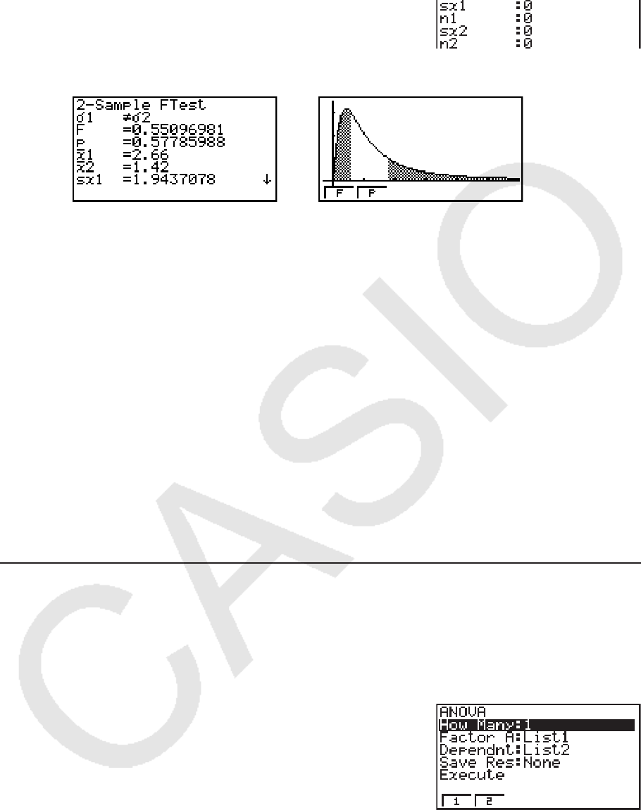
6-32
下面显示了与列表数据规定不同的参数数据规定项目。
计算结果输出示例
σ
1
σ
2
................... 测试方向
¯x1
............................. 仅在Data: List设置情况下显示。
¯x2
............................. 仅在Data: List设置情况下显示。
您可在绘制图形之后使用以下图形分析功能。
• 1(F) ... 显示 F值。
按下 1(F),在显示屏底部显示 F值,并在图形中的对应位置显示指针(除非该位置在图形屏幕
范围之外)。
如果是双尾测试,则显示两点。使用 d和 e移动指针。
• 2(P) ... 显示 p值。
按下 2(P),在屏幕底部显示 p值,但不显示指针。
• 自动执行分析功能可将 F和 p值分别保存在字母变量 F和P中。
• [Save Res]不保存第2行的 σ 1
条件。
k ANOVA
ANOVA 测试在有多个样本时各样本的总体平均值相等的假设。
单向ANOVA 用于存在一个独立变量和一个因变量的情况。
双向ANOVA 用于存在两个独立变量和一个因变量的情况。
在统计数据列表中执行以下键操作。
3(TEST)
5(ANOV)
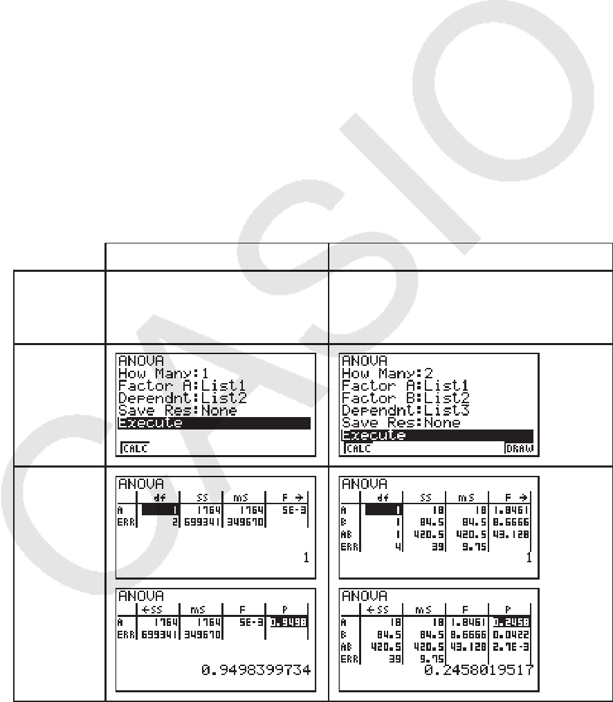
6-33
下面说明了列表数据规定中每一个项目的含义。
How Many ...... 选择单向ANOVA或双向ANOVA(等级数)
Factor A ........... 类别列表(List 1至26)
Dependnt ........ 用作样本数据的列表(List 1至26)
Save Res .......... 用于存储计算结果的第一个列表(None或List 1至22)*
1
Execute ............. 执行计算或者绘制图形(仅限双向ANOVA)
*
1
[Save Res]将表格的每个垂直列保存到其自身列表中。最左侧的列保存到指定列表中,右侧
每个后续列保存到下一个顺序编号的列表。最多可使用五个列表保存列。您可在1至22范围内
指定第一个列表编号。
只有双向ANOVA才会显示以下项目。
Factor B ........... 类别列表(List 1至26)
完成所有参数的设置之后,使用 c突出显示“Execute”,然后按下面的某个功能键执行计算
或者绘制图形。
• 1(CALC) ... 执行计算。
• 6(DRAW) ... 绘制图形(仅限双向ANOVA)。
计算结果以表格形式显示,与教科书中一样。
数据和计算结果示例
单向ANOVA 双向ANOVA
数据 List1={1,1,2,2}
List2={124,913,120,1001}
List1={1,1,1,1,2,2,2,2}
List2={1,1,2,2,1,1,2,2}
List3={113,116,139,132,133,131,126,122}
设置屏幕
计算结果

6-34
单向ANOVA
第1行(A) .................. Factor A
df值、 SS值、 MS值、 F值、 p值
第2行(ERR) ........... 错误
df值、 SS值、 MS值
双向ANOVA
第1行(A) .................. Factor A
df值、 SS值、 MS值、 F值、 p值
第2行(B) ................... Factor B
df值、 SS值、 MS值、 F值、 p值
第3行(AB) ............... Factor A × Factor B
df值、 SS值、 MS值、 F值、 p值
* 如果每个单元中都只有一个观察值,则不显示第3行。
第4行(ERR) ........... 错误
df值、 SS值、 MS值
F ................................... F值
p .................................... p值
df ................................ 自由度
SS ................................. 平方和
MS ............................... 均方
在双向ANOVA中,您可绘制交互描点图。图形的数量取决于Factor B,X轴数据的数量取决于
Factor A。Y轴为每个类别的平均值。
您可在绘制图形之后使用以下图形分析功能。
• 1(Trace) 或者 !1(TRCE) ... 跟踪功能
按下 d或 e,沿着对应方向在图形上移动指针。如果有多个图形,您可通过按下 f和 c在
图形之间移动。
• 制图功能只能用于双向ANOVA。无论设置屏幕的设置如何,视窗设置都自动执行。
• 使用跟踪功能分别将条件数自动保存到字母变量A,将平均值保存到变量M。
6-35
k ANOVA(双向)
u 说 明
下表显示某一种金属产品的测量结果,该产品采用以下两个处理等级的热处理工艺:时间(A)
和温度(B)。该实验在同等条件下各重复两次。
采用5%的显著性水平,对以下虚假设进行方差分析。
H
o
:强度不随时间而改变
H
o
:强度不随热处理温度而改变
H
o
:强度不随时间与热处理温度的相互作用而改变
u 解
使用双向ANOVA测试上述假设。
输入上述数据,如下所示。
List1={1,1,1,1,2,2,2,2}
List2={1,1,2,2,1,1,2,2}
List3={113,116,139,132,133,131,126,122}
将 List 3(每个群组的数据)定义为Dependent。将List 1和List 2(List 3中每个数据项目的因
子数)分别定义为Factor A和Factor B。
执行测试后产生以下结果。
• 时间差(A)显著性水平P = 0.2458019517
显著性水平(
p = 0.2458019517)大于显著性水平值(0.05),因此不舍弃假设。
• 温度差(B)显著性水平P = 0.04222398836
显著性水平(
p = 0.04222398836)小于显著性水平值(0.05),因此舍弃假设。
• 相互影响(A × B)显著性水平P = 2.78169946e-3
显著性水平(
p = 2.78169946e-3)小于显著性水平值(0.05),因此舍弃假设。
上述测试表示时间差不显著,温度差显著,相互影响非常显著。
B(热处理温度) B1 B2
A1 113 , 116
133 , 131
139 , 132
126 , 122
A2
A(时间)
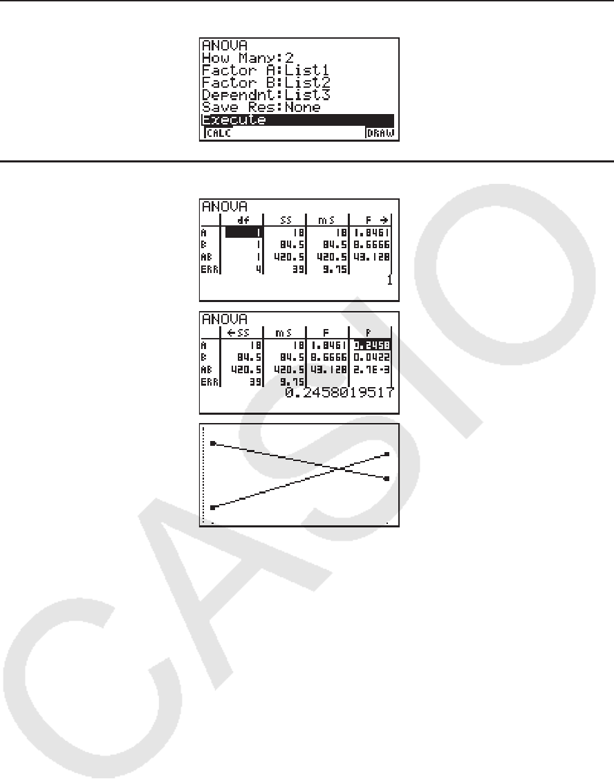
6-36
u 输入示例
u 结 果

6-37
6. 置信区间
重要!
•fx-7400G II上不可执行置信区间计算。
置信区间是一个范围(区间),包括统计值(通常为总体平均值)。
如果置信区间太宽,会导致难以了解总体值(真值)的位置。而另一方面,较窄的置信区间会
限制总体值,导致难以得到可靠的结果。最常用的置信区间为95%和99%。提高置信水平可加
宽置信区间,而降低置信水平则会使置信区间变窄,但它也会增加意外忽略总体值的概率。例
如,如果置信区间为95%,则总体值不在所得5%区间内。
在计划进行调查,然后对数据进行
t测试和 Z测试时,您还必须考虑样本数量、样本的大小、置
信区间宽度和置信水平。置信水平因应用而异。
1-样本 Z 区间 在总体标准差已知时,计算未知总体平均值的置信区间。
2-样本
Z 区间 在两个样本的总体标准差已知时,计算两个总体平均值之差的置信区间。
1-比例
Z 区间 计算未知成功比例的置信区间。
2-比例
Z 区间 计算两个总体中成功比例之差的置信区间。
1-样本
t 区间 在总体标准差未知时,计算未知总体平均值的置信区间。
2-样本
t 区间 在两个总体标准差均未知时,计算两个总体平均值之差的置信区间。
在初始 STAT 模式屏幕中,按下 4(INTR),显示包含以下项目的置信区间菜单。
• 4(INTR) 1(Z) ... Z区间(第6-38页)
2(t) ...
t区间(第6-39页)
完成所有参数的设置之后,使用 c突出显示“Execute”,然后按下面的功能键执行计算。
• 1(CALC) ... 执行计算。
• 置信区间功能没有任何绘图函数。
u 关于置信区间的一般注意事项
如果为C-Level设置输入的值在0 < C-Level < 1范围内,则设定值为输入值。如果输入值在
1 < C-Level < 100范围内,设定值为输入值的1/100。
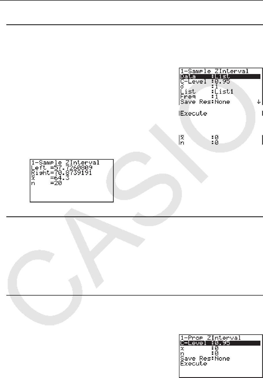
6-38
k Z区间
u 1-样本 Z区间
1-样本 Z 区间 在总体标准差已知时,计算未知总体平均值的置信区间。
在统计数据列表中执行以下键操作。
4(INTR)
1(Z)
1(1-S)
下面显示了与列表数据规定不同的参数数据规定项目。
计算结果输出示例
u 2-样本 Z区间
2-样本 Z 区间 在两个样本的总体标准差已知时,计算两个总体平均值之差的置信区间。
在统计数据列表中执行以下键操作。
4(INTR)
1(Z)
2(2-S)
u 1-比例 Z区间
1-比例 Z 区间 使用数据数量计算未知成功比例的置信区间。
在统计数据列表中执行以下键操作。
4(INTR)
1(Z)
3(1-P)
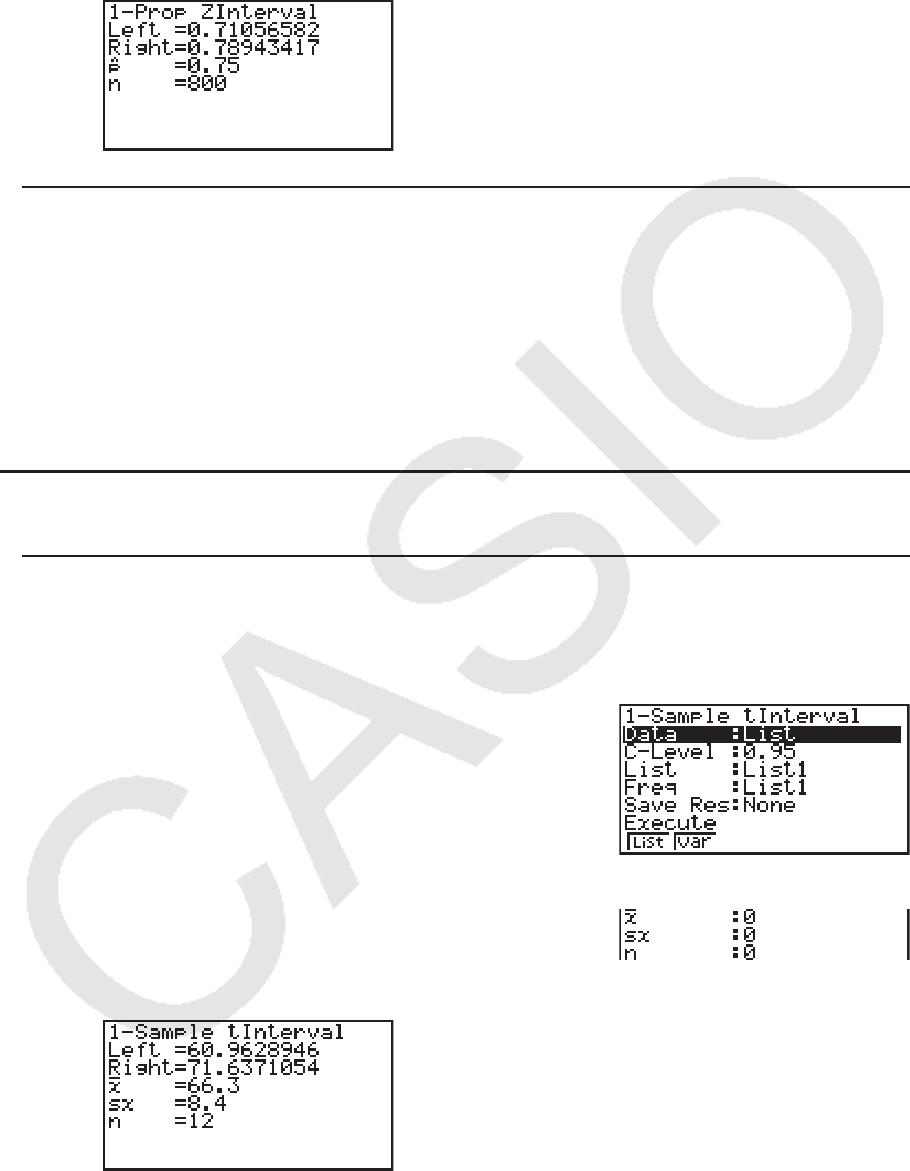
6-39
利用参数规定指定数据。
计算结果输出示例
u 2-比例 Z区间
2-比例 Z 区间 使用数据数量计算两个总体中成功比例之差的置信区间。
在统计数据列表中执行以下键操作。
4(INTR)
1(Z)
4(2-P)
k t区间
u 1-样本 t区间
1-样本 t 区间 在总体标准差未知时,计算未知总体平均值的置信区间。
在统计数据列表中执行以下键操作。
4(INTR)
2(t)
1(1-S)
下面显示了与列表数据规定不同的参数数据规定项目。
计算结果输出示例

6-40
u 2-样本 t区间
2-样本 t 区间 在两个总体标准差均未知时,计算两个总体平均值之差的置信区间。 t区间应用于
t分布。
在统计数据列表中执行以下键操作。
4(INTR)
2(t)
2(2-S)
7. 分布
重要!
• fx-7400G II上不可执行分布计算。
分布类型多种多样,其中最常见的是“正态分布”,它是进行统计计算的基本方法。正态分布
是以平均值数据的最大发生次数(最高频率)为中心的对称分布,距离中心越远,频率越低。
根据数据类型,还可使用泊松分布、几何分布和其他各种分布形状。
一旦确定分布形状,即可确定特定的趋势。您可计算在小于特定值的分布中的数据概率。
例如,在制造某种产品时,分布可用于计算收益率。一旦设定某个数值标准,即可在估算达标
产品的百分比时计算正态概率。相反,将成功率表(例如80%)设置为假设条件,使用正态分
布估算有多大比例的产品可达到该值。
正态概率密度 通过一个指定的 x值,计算正态分布的概率密度。
累积正态分布 计算两个指定值之间的正态分布数据的概率。
反向累积正态分布 计算可代表某个特定累积概率的正态分布范围内位置的数值。
学生- t 概率密度 通过一个指定的 x值,计算 t概率密度。
学生- t 累积分布 计算在两个指定值之间的 t分布数据的概率。
反向学生- t累积分布 计算指定百分比对应的学生- t累积概率密度的下限值。
类似于 t分布,也可计算
χ
χ 2
、 F、 二项 、 泊松 、 几何 和 超几何 分布的概率密度(或者概率)、累
积分布和反向累积分布。
在初始 STAT 模式屏幕中,按下 5(DIST),显示包含以下项目的分布菜单。
• 5(DIST) 1(NORM) ... 正态分布(第6-41页)
2(t) ... 学生-
t分布(第6-43页)
3(CHI) ... χ 2
分布(第6-44页)
4(F) ...
F分布(第6-45页)
5(BINM) ... 二项分布(第6-46页)
6( g) 1(POISN) ... 泊松分布(第6-48页)
6( g) 2(GEO) ... 几何分布(第6-49页)
6( g) 3(H.GEO) ... 超几何分布(第6-51页)
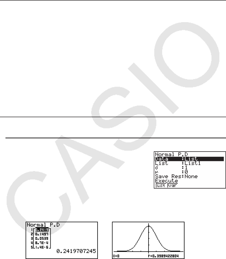
6-41
完成所有参数的设置之后,使用 c突出显示“Execute”,然后按下面的某个功能键执行计算
或者绘制图形。
• 1(CALC) ... 执行计算。
• 6(DRAW) ... 绘制图形。
k 常见分布函数
• 当设置屏幕的“Stat Wind”设置为“Auto”时,自动设置视窗设置以绘制图形。当“Stat
Wind”设置为“Manual”时,使用当前视窗设置绘制图形。
• 绘制图形之后,您可使用P-CAL函数计算特定
x值的估计 p值。P-CAL函数只能在绘制正态概率
密度、学生-
t概率密度、 Ƶ2
概率密度或者 F概率密度图形之后才可使用。
下面是使用P-CAL函数的一般程序。
1. 在绘制分布图形之后,按下 !5(G-SLV) 1(P-CAL),显示 x值输入值对话框。
2. 输入
x值然后按下 w。
• 由此可在显示屏的底部显示
x和 p值,然后将指针移至图形上的对应点。
3. 此时按下 v或者数字键将显示
x值输入对话框,如果需要,您可执行下一次估计值计算。
4. 完成之后,按下 J,清除显示屏中的坐标值和指针。
• 自动执行分析功能可将
x和 p值分别保存在字母变量X和P中。
k 正态分布
• 正态概率密度 5(DIST) 1(NORM) 1(NPd)
正态概率密度计算一个指定的
x值或列表的概率密度( p)。
在指定一个列表时,每个列表元素的计算结果都以列表形式
显示。
• 正态概率密度应用于标准正态分布。
• 指定
Ʊ = 1和 ƫ = 0即指定标准正态分布。
计算结果输出示例
在指定一个列表时 指定一个 x值时的图形
• 只有在指定一个变量并输入一个 x值数据时才支持绘图功能。
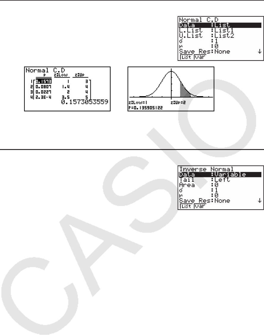
6-42
• 累积正态分布 5(DIST) 1(NORM) 2(NCd)
累积正态分布计算下限与上限之间正态分布的正态累积概
率。
计算结果输出示例
在指定一个列表时 指定一个 x值时的图形
• 只有在指定一个变量并输入一个
x值数据时才支持绘图功能。
• 反向累积正态分布 5(DIST) 1(NORM) 3(InvN)
反向累积正态分布计算指定值的累积正态分布概率的边界
值。
Area:概率值
(0 < Area < 1)
反向累积正态分布计算可代表某个特定累积概率的正态分布范围内位置的数值。
尾部:左侧
积分区间的上边界
f(x)dx =p
−∞
∫
Upper
f(x)dx =p
+∞
∫
Lower
f(x)dx =p
∫
Upper
Lower
尾部:右侧
积分区间的下
边界
尾部:中间
积分区间的上和
下边界
指定概率并使用该公式计算积分区间。
• 本计算器采用以下规定执行上述计算: ∞ = 1E99,- ∞ = -1E99
• 反向累积正态分布没有任何绘图功能。
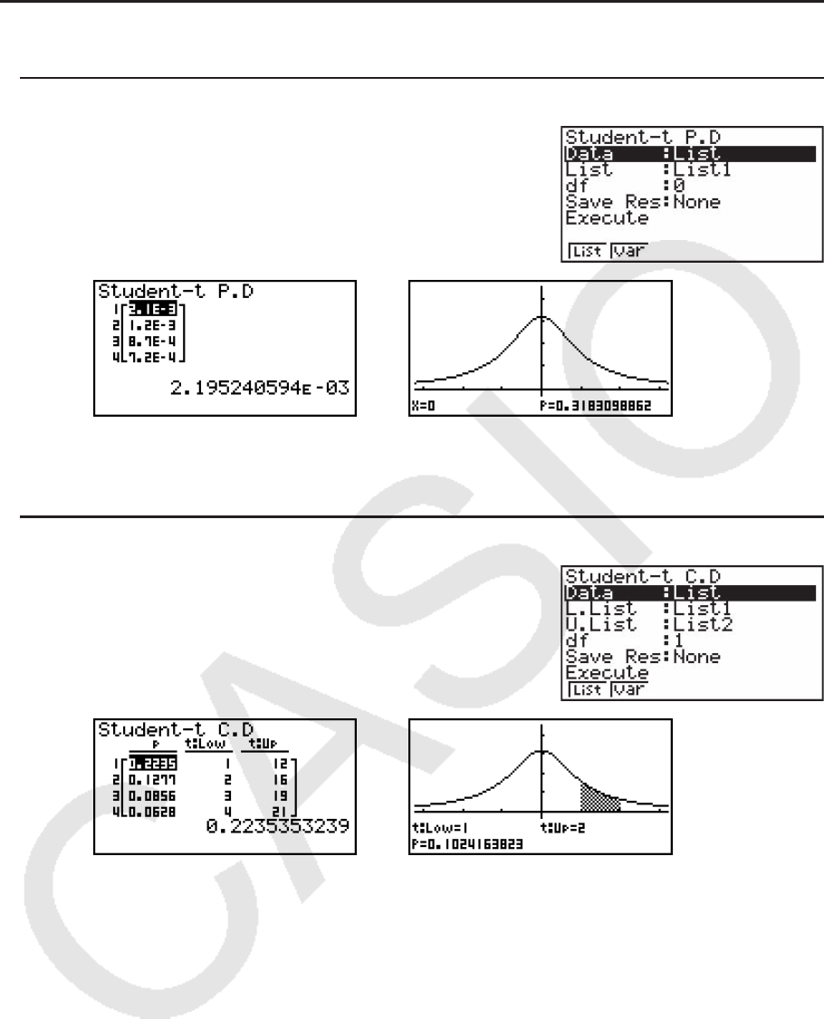
6-43
k 学生- t分布
• 学生- t概率密度 5(DIST) 2(t) 1(tPd)
学生-
t概率密度计算一个指定的 x值或列表的概率密度
(
p)。在指定一个列表时,每个列表元素的计算结果
都以列表形式显示。
计算结果输出示例
在指定一个列表时 指定变量( x)时的图形
• 只有在指定一个变量并输入一个 x值数据时才支持绘图功能。
• 学生- t累积分布 5(DIST) 2(t) 2(tCd)
学生-
t累积分布计算下限与上限之间学生- t分布的学生- t累积
概率。
计算结果输出示例
在指定一个列表时 指定变量( x)时的图形
• 只有在指定一个变量并输入一个 x值数据时才支持绘图功能。
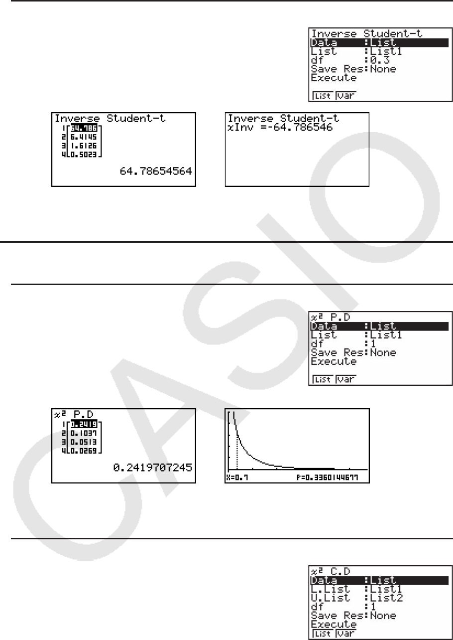
6-44
• 反向学生- t累积分布 5(DIST) 2(t) 3(InvN)
反向学生-
t累积分布计算指定 df(自由度)值的学生- t累积分
布的下限值。
计算结果输出示例
在指定一个列表时 在指定变量( x)时
• 反向学生- t累积分布没有任何绘图功能。
k Ƶ2
分布
• Ƶ2
概率密度 5(DIST) 3(CHI) 1(CPd)
Ƶ2
概率密度计算一个指定的 x值或列表的 Ƶ2
概率密度( p)。
在指定一个列表时,每个列表元素的计算结果都以列表形式
显示。
计算结果输出示例
在指定一个列表时 指定变量( x)时的图形
• 只有在指定一个变量并输入一个 x值数据时才支持绘图功能。
• Ƶ2
累积分布 5(DIST) 3(CHI) 2(CCd)
Ƶ2
累积分布计算下限与上限之间 Ƶ2
分布的累积概率。
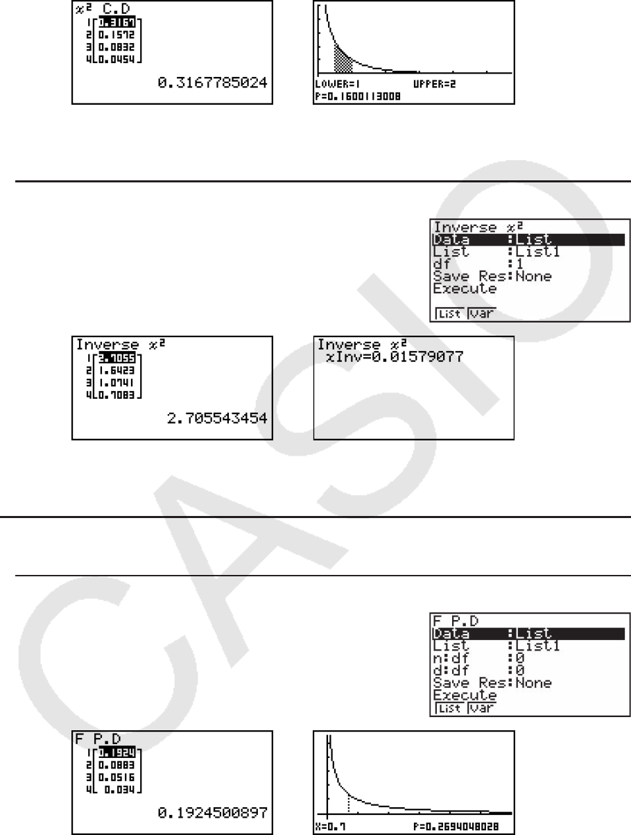
6-45
计算结果输出示例
在指定一个列表时 指定变量( x)时的图形
• 只有在指定一个变量并输入一个 x值数据时才支持绘图功能。
• 反向 Ƶ2
累积分布 5(DIST) 3(CHI) 3(InvC)
反向
Ƶ2
累积分布计算指定 df (自由度)值的 Ƶ2
累积分布概率
的下限值。
计算结果输出示例
在指定一个列表时 在指定变量( x)时
• 反向 Ƶ2
累积分布没有任何绘图功能。
k F分布
• F概率密度 5(DIST) 4(F) 1(FPd)
F概率密度计算一个指定的 x值或列表的 F概率密度( p)。
在指定一个列表时,每个列表元素的计算结果都以列表形式
显示。
计算结果输出示例
在指定一个列表时 指定变量( x)时的图形
• 只有在指定一个变量并输入一个 x值数据时才支持绘图功能。
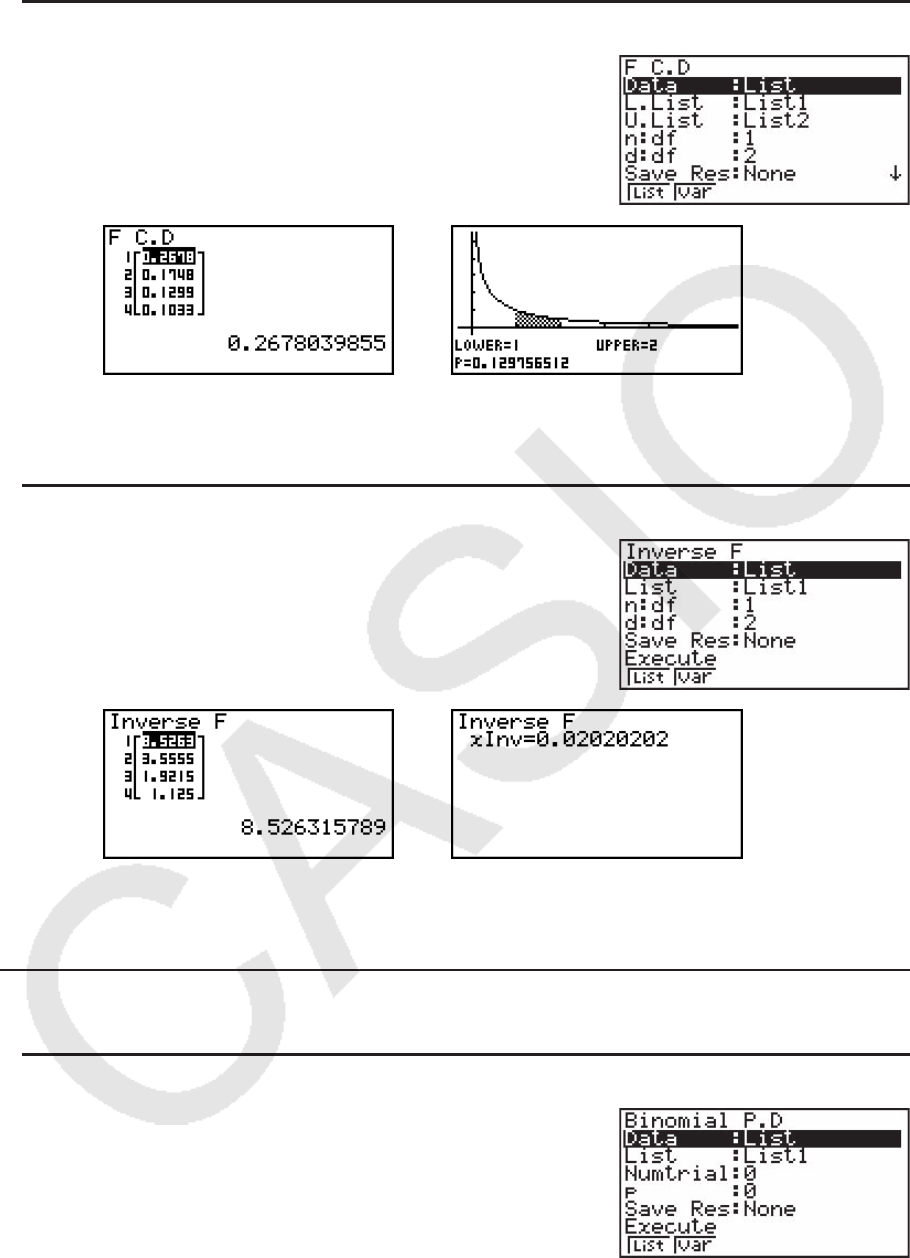
6-46
• F累积分布 5(DIST) 4(F) 2(FCd)
F累积分布计算下限与上限之间 F分布的累积概率。
计算结果输出示例
在指定一个列表时 指定变量( x)时的图形
• 只有在指定一个变量并输入一个 x值数据时才支持绘图功能。
• 反向 F累积分布 5(DIST) 4(F) 3(InvF)
反向
F累积分布计算指定 n: df和 d: df(分子和分母的自由度)
值的
F累积分布概率的下限值。
计算结果输出示例
在指定一个列表时 在指定变量( x)时
• 反向 F累积分布没有任何绘图功能。
k 二项分布
• 二项概率 5(DIST) 5(BINM) 1(BPd)
二项概率以指定的试验次数与每次试验的成功概率计算离散
二项分布在特定
x值或每个列表元素处的概率。在指定一个列
表时,每个列表元素的计算结果都以列表形式显示。
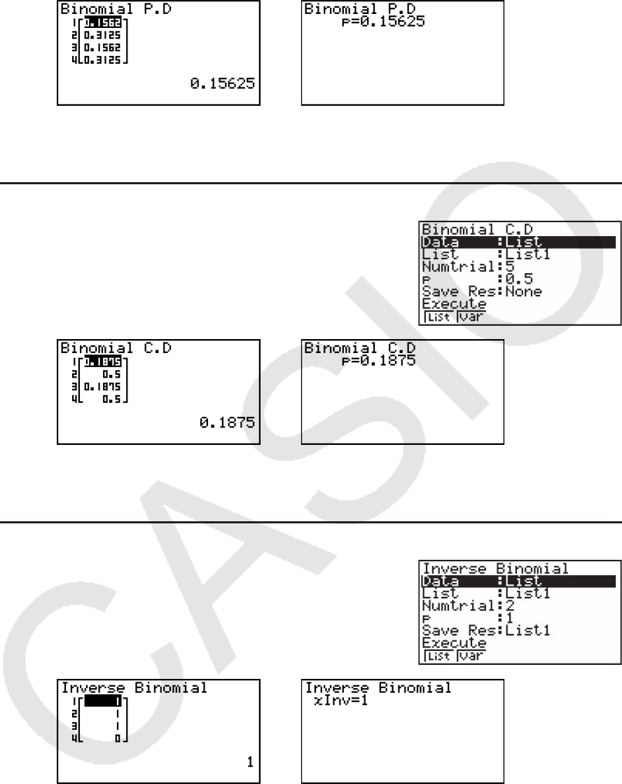
6-47
计算结果输出示例
在指定一个列表时 在指定变量( x)时
• 二项概率没有任何绘图功能。
• 二项累积分布 5(DIST) 5(BINM) 2(BCd)
二项累积分布计算二项分布(在规定试验次数或该次数之前
成功)中的累积概率。
计算结果输出示例
在指定一个列表时 在指定变量( x)时
• 二项累积分布没有任何绘图功能。
• 反向二项累积分布 5(DIST) 5(BINM) 3(InvB)
反向二项累积分布计算指定值的二项累积分布的最小试验次
数。
计算结果输出示例
在指定一个列表时 在指定变量( x)时
• 反向二项累积分布没有任何绘图功能。
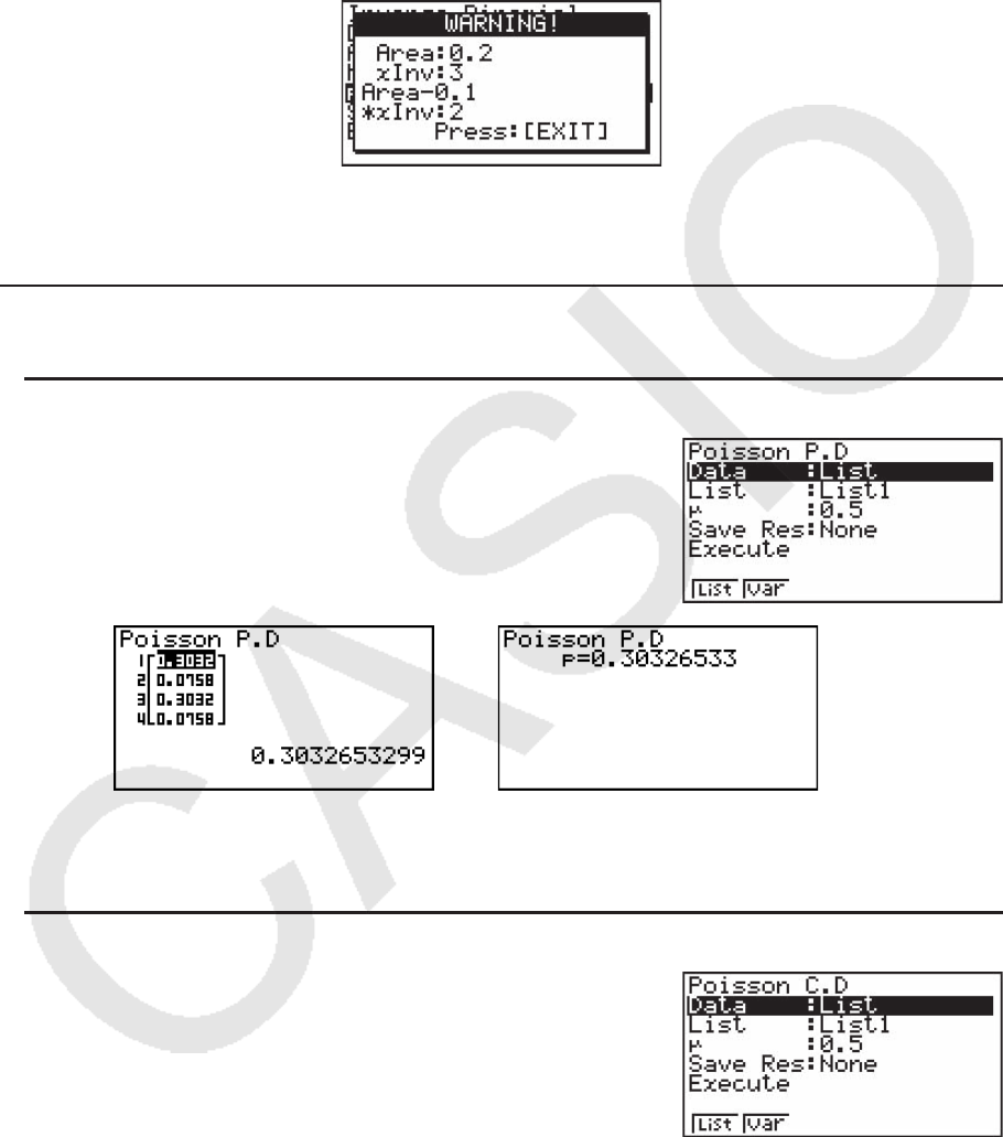
6-48
重要!
在执行反向二项累积分布计算时,计算器使用指定的Area值和另一个值(Area值最小有效位数
减1)( `Area值),计算最小试验次数值。
结果指定给系统变量
xInv(计算结果使用Area)和 `xInv(计算结果使用 `Area)。计算器总
是只显示
xInv值。但在 xInv与 `xInv值不同时,以下消息与这两个值同时显示。
反向二项累积分布的计算结果为整数。在第一个自变量的位数不低于10时,精度可能降低。请
注意,即使计算精度稍有变化,也会影响计算结果。如果出现警告消息,请检查显示的值。
k 泊松分布
•泊松概率 5(DIST) 6( g) 1(POISN) 1(PPd)
泊松概率以指定的平均值计算离散泊松分布在特定
x值或每个
列表元素处的概率。
计算结果输出示例
在指定一个列表时 在指定变量( x)时
• 泊松概率没有任何绘图功能。
• 泊松累积分布 5(DIST) 6( g) 1(POISN) 2(PCd)
泊松累积分布计算泊松分布(在规定试验次数或该次数之前
成功)中的累积概率。
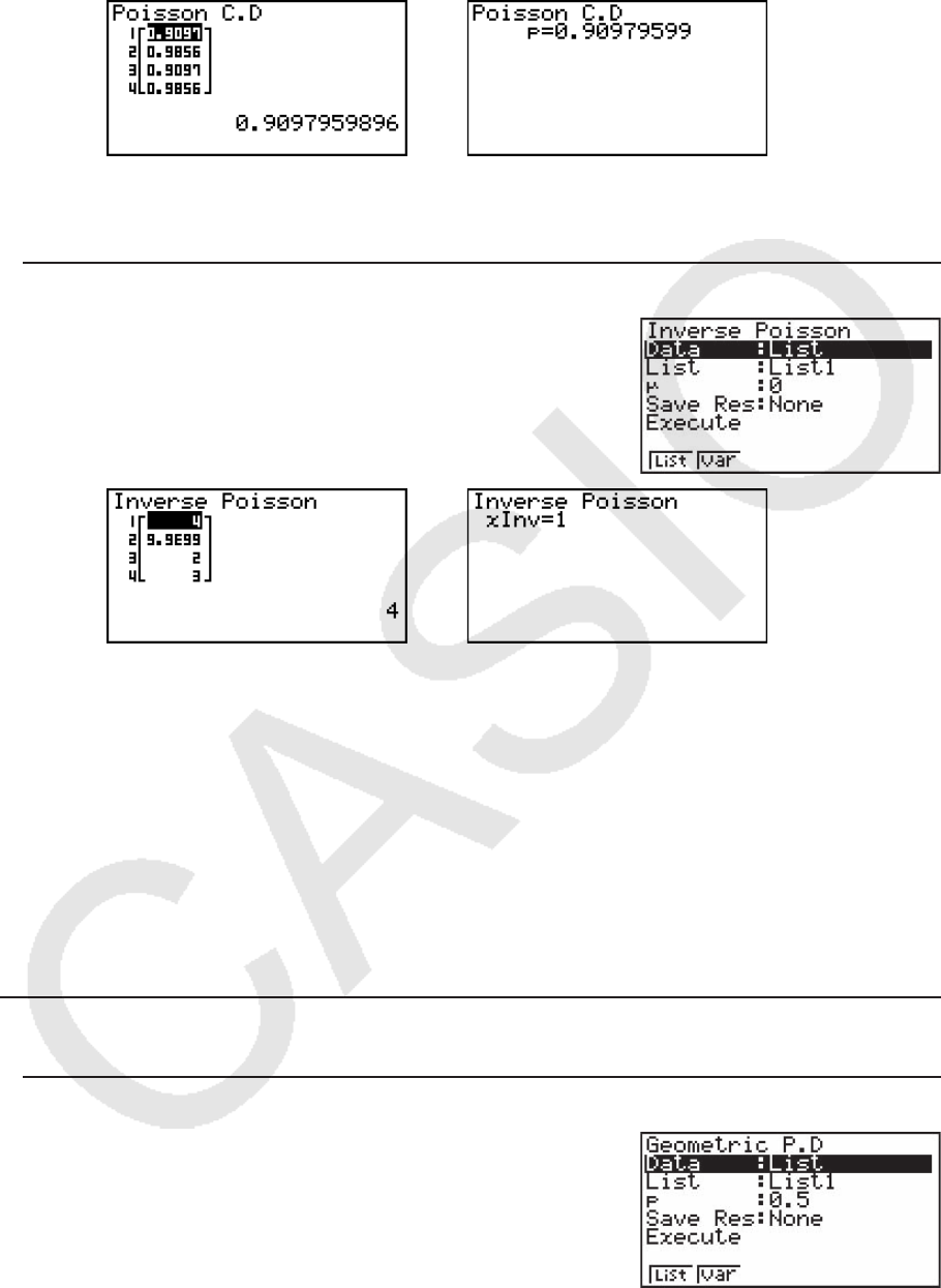
6-49
计算结果输出示例
在指定一个列表时 在指定变量( x)时
• 泊松累积分布没有任何绘图功能。
• 反向泊松累积分布 5(DIST) 6( g) 1(POISN) 3(InvP)
反向泊松累积分布计算指定值的泊松累积概率分布的最小试
验次数。
计算结果输出示例
在指定一个列表时 在指定变量( x)时
• 反向泊松累积分布没有任何绘图功能。
重要!
在执行反向泊松累积分布计算时,计算器使用指定的Area值和另一个值(Area值最小有效位数
减1)( `Area值),计算最小试验次数值。
结果指定给系统变量
xInv(计算结果使用Area)和 `xInv(计算结果使用 `Area)。计算器总
是只显示
xInv值。但在 xInv与 `xInv值不同时,消息与这两个值同时显示。
反向泊松累积分布的计算结果为整数。在第一个自变量的位数不低于10时,精度可能降低。请
注意,即使计算精度稍有变化,也会影响计算结果。如果出现警告消息,请检查显示的值。
k 几何分布
• 几何概率 5(DIST) 6( g) 2(GEO) 1(GPd)
几何概率以指定的成功概率计算几何分布在特定
x值或每个列
表元素处的概率,以及首次成功时的试验次数。
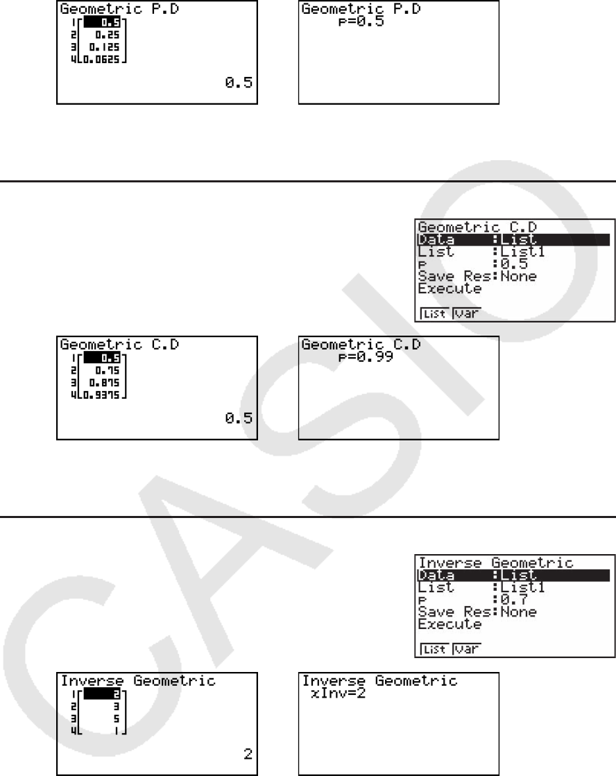
6-50
计算结果输出示例
在指定一个列表时 在指定变量( x)时
• 几何概率没有任何绘图功能。
• 几何累积分布 5(DIST) 6( g) 2(GEO) 2(GCd)
几何累积分布计算几何分布(在规定试验次数或该次数之前
成功)中的累积概率。
计算结果输出示例
在指定一个列表时 在指定变量( x)时
• 几何累积分布没有任何绘图功能。
•反向几何累积分布 5(DIST) 6( g) 2(GEO) 3(InvG)
反向几何累积分布计算指定值的几何累积概率分布的最小试
验次数。
计算结果输出示例
在指定一个列表时 在指定变量( x)时
• 反向几何累积分布没有任何绘图功能。
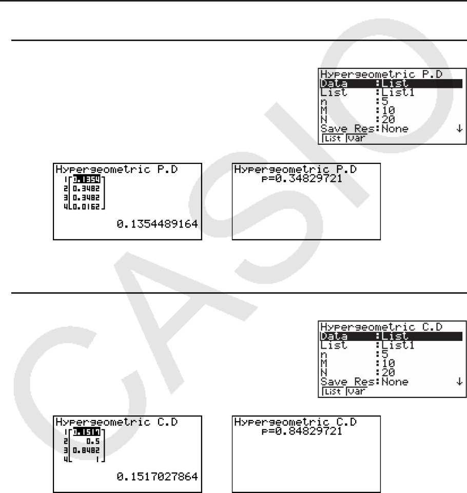
6-51
重要!
在执行反向几何累积分布计算时,计算器使用指定的Area值和另一个值(Area值最小有效位数
减1)( `Area值),计算最小试验次数值。
结果指定给系统变量
xInv(计算结果使用Area)和 `xInv(计算结果使用 `Area)。计算器总
是只显示
xInv值。但在 xInv与 `xInv值不同时,消息与这两个值同时显示。
反向几何累积分布的计算结果为整数。在第一个自变量的位数不低于10时,精度可能降低。请
注意,即使计算精度稍有变化,也会影响计算结果。如果出现警告消息,请检查显示的值。
k 超几何分布
• 超几何概率 5(DIST) 6( g) 3(H.GEO) 1(HPd)
超几何概率以指定的成功概率计算超几何分布在特定
x值或每
个列表元素处的概率,以及首次成功时的试验次数。
计算结果输出示例
在指定一个列表时 在指定变量( x)时
• 超几何概率没有任何绘图功能。
• 超几何累积分布 5(DIST) 6( g) 3(H.GEO) 2(HCd)
超几何累积分布计算超几何分布(在规定试验次数或该次数
之前成功)中的累积概率。
计算结果输出示例
在指定一个列表时 在指定变量( x)时
• 超几何累积分布没有任何绘图功能。
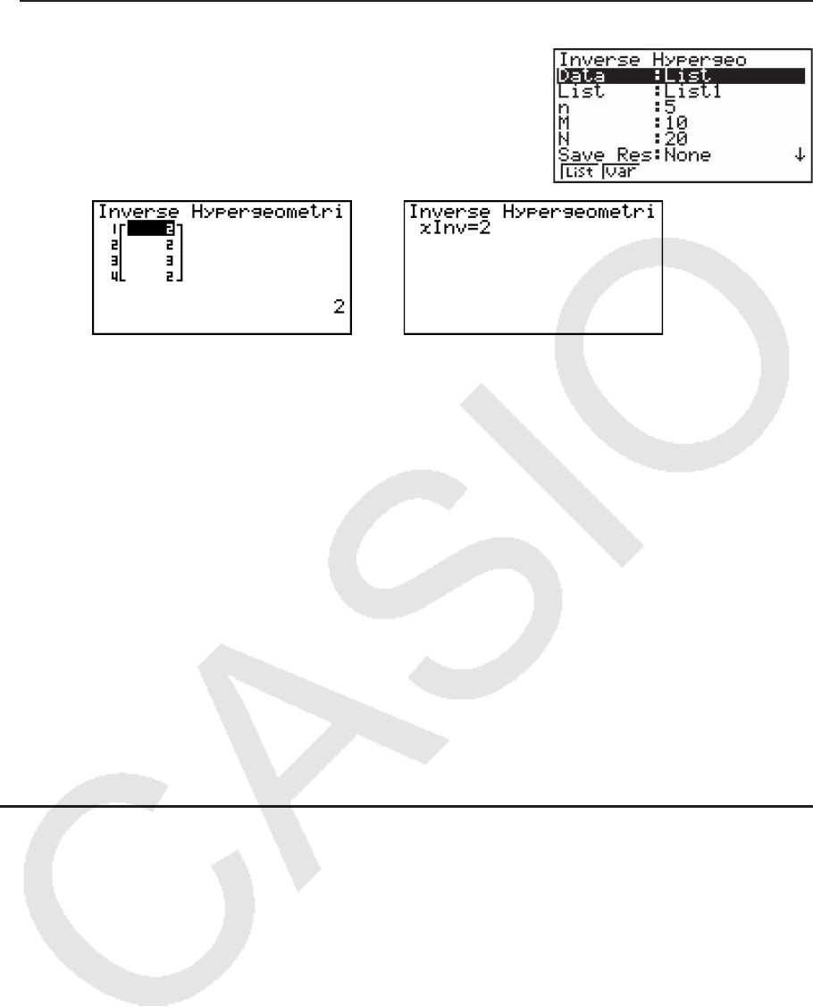
6-52
• 反向超几何累积分布 5(DIST) 6( g) 3(H.GEO) 3(InvH)
反向超几何累积分布计算指定值的超几何累积概率分布的最
小试验次数。
计算结果输出示例
在指定一个列表时 在指定变量( x)时
• 反向超几何累积分布没有任何绘图功能。
重要!
在执行反向超几何累积分布计算时,计算器使用指定的Area值和另一个值(Area值最小有效位
数减1)( `Area值),计算最小试验次数值。
结果指定给系统变量
xInv(计算结果使用Area)和 `xInv(计算结果使用 `Area)。计算器总
是只显示
xInv值。但在 xInv与 `xInv值不同时,消息与这两个值同时显示。
反向超几何累积分布的计算结果为整数。在第一个自变量的位数不低于10时,精度可能降低。
请注意,即使计算精度稍有变化,也会影响计算结果。如果出现警告消息,请检查显示的值。
8. 测试、置信区间和分布的输入和输出项
(除fx-7400G II之外的所有型号)
下面说明了测试、置信区间和分布使用的输入和输出项。
k 输入项
Data ...................................................... 数据类型
ƫ(1-样本 Z测试) ...................... 总体平均值测试条件(“ ƫ0
”指定双尾测试、“< ƫ0
”指定下单
尾测试、“>
ƫ0
”指定上单尾测试。)
ƫ1
(2-样本 Z测试) .................... 总体平均值测试条件(“ ƫ2
”指定双尾测试、“< ƫ2
”指定样本
1小于样本2的单尾测试、“>
ƫ2
”指定样本1大于样本2的单尾测
试。)
Prop(1-比例
Z测试) ............. 样本比例测试条件(“ p0
”指定双尾测试、“< p0
” 指定下单尾
测试、“>
p0
”指定上单尾测试。)
p1
(2-比例 Z测试) .................. 样本比例测试条件(“ p2
”指定双尾测试、“< p2
”指定样本1小
于样本2的单尾测试、“>
p2
”指定样本1大于样本2的单尾测试。
)
ƫ(1-样本 t测试) ....................... 总体平均值测试条件(“ ƫ0
”指定双尾测试、“< ƫ0
”指定下单
尾测试、“>
ƫ0
”指定上单尾测试。)

6-53
ƫ1
(2-样本 t测试) ................... 样本平均值测试条件(“ ƫ2
”指定双尾测试、“< ƫ2
”指定样本
1小于样本2的单尾测试、“>
ƫ2
” 指定样本1大于样本2的单尾测
试。)
β
&
ρ
(线性回归 t测试) .....
ρ
值测试条件(“ 0”指定双尾测试、“< 0”指定下单尾测
试、“> 0”指定上单尾测试。)
Ʊ1
(2-样本 F测试) ................. 总体标准差测试条件(“ Ʊ2
”指定双尾测试、“< Ʊ2
”指定样本
1小于样本2的单尾测试、“>
Ʊ2
” 指定样本1大于样本2的单尾测
试。)
ƫ0 .............................................................. 假设的总体平均值
Ʊ ............................................................... 总体标准差( Ʊ > 0)
Ʊ1
.............................................................. 样本1的总体标准差( Ʊ1
> 0)
Ʊ2 .............................................................. 样本2的总体标准差( Ʊ2
> 0)
Lis t ....................................................... 内容用作数据的列表(List 1至26)
List1 ..................................................... 内容用作样本1数据的列表(List 1至26)
List 2 ..................................................... 内容用作样本2数据的列表(List 1至26)
Freq ....................................................... 频率(1或List 1至26)
Freq1 ................................................... 样本1的频率(1或List 1至26)
Freq2 ................................................... 样本2的频率(1或List 1至26)
Execute .............................................. 执行计算或者绘制图形
o ................................................................ 样本平均值
o1
............................................................. 样本1平均值
o2
............................................................. 样本2平均值
n ................................................................ 样本大小(正整数)
n1
.............................................................. 样本1的大小(正整数)
n2 .............................................................. 样本2的大小(正整数)
p0 .............................................................. 期望样本比例(0 < p0
< 1)
p1 .............................................................. 样本比例测试条件
x(1-比例 Z测试) ...................... 样本值( x > 0 整数)
x(1-比例 Z区间) ...................... 数据(0或者正整数)
x1 .............................................................. 样本1的数据值( x1
> 0整数)
x2 .............................................................. 样本2的数据值( x2
> 0整数)
s
x ............................................................... 样本标准差(s
x > 0)
s
x1 ............................................................. 样本1 的标准差(s
x1
> 0)
s
x2 ............................................................. 样本2 的标准差(s
x2
> 0)
XList ....................................................
x轴数据列表(List 1至6)
YList ....................................................
y轴数据列表(List 1至6)
C-Level ............................................... 置信水平(0 < C-Level < 1)
Pooled .................................................. 合并On(生效)或Off(未生效)
x(分布) ........................................... 数据
Ʊ(分布) .......................................... 标准差( Ʊ > 0)
ƫ(分布) .......................................... 平均值
Lower(分布) .............................. 下边界
Upper(分布) .............................. 上边界
df(分布)......................................... 自由度( df > 0)

6-54
n: df(分布) .................................... 分子自由度(正整数)
d: df(分布) .................................... 分母自由度(正整数)
Numtrial(分布) ...................... 试验次数
p(分布) .......................................... 成功概率(0 < p < 1)
k 输出项
z ................................................................ z分数
p ............................................................... p值
t ................................................................. t分数
Ƶ2 .............................................................. Ƶ2
值
F ............................................................... F值
pˆ ................................................................. 估计样本比例
pˆ
1 .............................................................. 样本1估计比例
pˆ 2 .............................................................. 样本2估计比例
o ................................................................ 样本平均值
o1
............................................................. 样本1平均值
o2
............................................................. 样本2平均值
s
x .............................................................. 样本标准差
s
x1 ............................................................. 样本1标准差
s
x2 ............................................................. 样本2标准差
s
p .............................................................. 合并样本标准差
n ............................................................... 样本大小
n1 .............................................................. 样本1大小
n2 .............................................................. 样本2大小
df .............................................................. 自由度
a ................................................................ 常数项
b ................................................................ 系数
s
e ............................................................... 标准误差
r ................................................................ 相关系数
r2 .............................................................. 可决系数
Left ........................................................ 置信区间下限(左边缘)
Right ..................................................... 置信区间上限(右边缘)
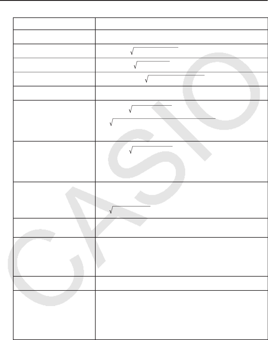
6-55
9. 统计公式
k 测 试
测试
1-样本
Z测试
z
= (o – μ0)/(σ/'n )
2-样本
Z测试
z
= (o1 – o2)/ (σ /n1) + (σ /n2)
2
1
2
2
1-比例
Z测试
z
= (x/n – p0)/ p0(1 – p0)/n
2-比例
Z测试
z
= (x1/n1 – x2/n2)/ pˆ (1 – pˆ )(1/n1 + 1/n2)
1-样本
t测试
t = (o – μ0)/(sx/'n )
2-样本
t测试(合并)
t = (o1 – o2)/ sp2(1/n1 + 1/n2)
df = n1 + n2 − 2
sp = ((n1 – 1)sx1
2 + (n2 – 1)sx2
2)/(n1 + n2 – 2)
2-样本
t测试(未合并)
t = (o1 – o2)/ sx1
2/n1 + sx2
2/n2
C = (sx1
2/n1)/(sx1
2/n1 + sx2
2/n2)
df = 1/(C2/(n1 – 1) + (1 – C)2/(n2 – 1))
线性回归
t测试
t = r (n – 2)/(1 – r2)
b = Σ(xi – o)(yi – p)/Σ(xi – o)2a = p – bo
i=1
n
i=1
n
χ 2
GOF测试
Oi: 观察列表的第 i个元素
Ei: 期望列表的第 i个元素
χ 2
双向测试
Oij: 观察矩阵的第 i行,第 j列
Eij: 期望矩阵的第 i行,第 j列
2-样本
F测试
F = sx1
2/sx2
2
ANOVA测试
F = MS/MSe
SS = Σni (oi − o)2
MS = SS/Fdf MSe = SSe/Ed
f
i=1
k
Fdf = k − 1 Edf = Σ(ni – 1)
SSe = Σ(ni – 1)sxi2
i=1
k
i=1
k
χ2 = Σ(Oi − Ei)2/Ei
i
k
χ2 = ΣΣ(Oij − Eij)2/Eij
i
k
j
R
k
R
Eij = ΣOij •ΣOij / ΣΣOi
j
i=1
k
j=1i=1j=1
R
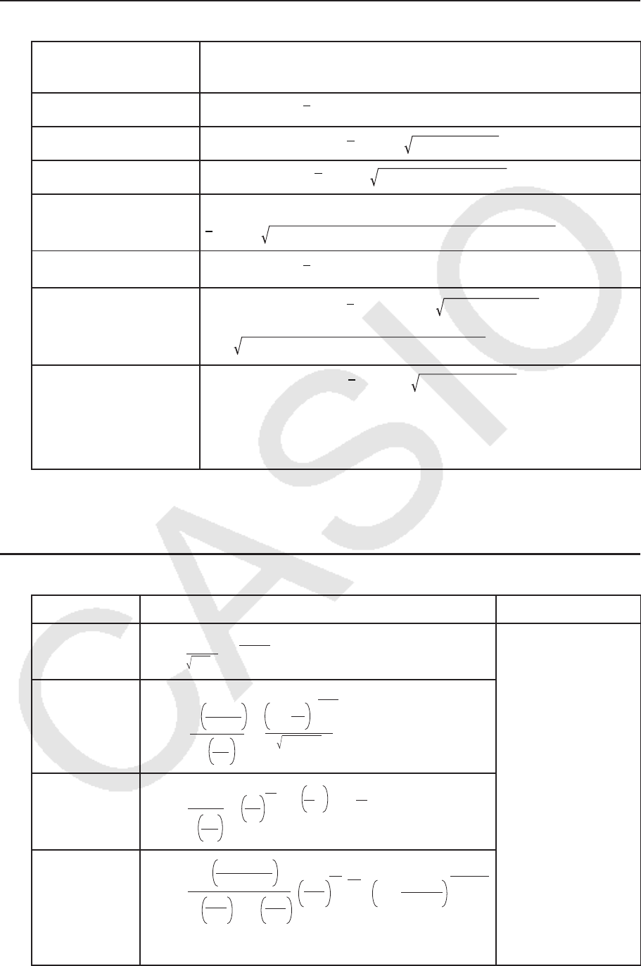
6-56
k 置信区间
置信区间 Left:置信区间下限(左边缘)
Right:置信区间上限(右边缘)
1-样本
Z区间
Left, Right = o + Z( /2) · σ/
'
n
α
2-样本
Z区间
Left, Right = (o1 – o2) + Z( /2) σ /n1 + σ /n2
2
1
2
2
α
1-比例
Z区间
Left, Right = x/n + Z( /2) 1/n · (x/n · (1 – x/n))
α
2-比例
Z区间
Left, Right = (x1/n1 – x2/n2)
+Z( /2) (x1/n1· (1 – x1/n1))/n1 + (x2/n2· (1 – x2/n2))/n2
α
1-样本
t区间
Left, Right = o + tn−1( /2) · sx/
'
n
α
2-样本
t区间(合并)
Left, Right = (o1 – o2) + tn1+n2−2 ( /2) sp2(1/n1 + 1/n2)
sp = ((n1 – 1)sx1
2 + (n2 – 1)sx2
2)/(n1 + n2 – 2)
α
2-样本
t区间(未合并)
Left, Right = (o1 – o2) + tdf ( /2) sx1
2/n1 + sx2
2/n2
df = 1/(C2/(n1 – 1) + (1 – C)2/(n2 – 1))
α
C = (sx1
2/n1)/(sx1
2/n1 + sx2
2/n2)
α
:显著性水平
α
= 1 - [C-Level ] C-Level :置信水平(0 < C-Level < 1)
Z(
α
/2):标准正态分布的上
α
/2点
tdf (
α
/2): t 分布的上
α
/2点,自由度为 df
k 分布(连续)
分布 概率密度 累积分布
正态分布
πσ
2
p(x) = 1e–
22
σ
(x – μ)2
μ
(
> 0)
σ
p = p(x)dx
Upper
Lower
∫
学生-
t分布
p(x) = ×
Γ
Γ
× df
π
– df+1
2
2
df
2
df + 1
df
x2
1 +
χ 2
分布
p(x) = ×
(x⭌ 0)
Γ
1
2
df
df
2
× x
2
1df
2–1x
2
–
× e
F分布
ndf
2x
ddf
ndf ndf
2–1
ddf
ndf × x
1 +
ndf + ddf
2
p(x) =
–
Γ2
ndf +ddf
Γ2
ndf × Γ 2
ddf
(x⭌ 0)

6-57
分布 反向累积分布
正态分布
p = p(x)dx
Upper
–∞
∫
p = p(x)dx
Lower
∞
∫
p = p(x)dx
Upper
Lower
∫
尾部
=左侧 尾部=右侧 尾部=中间
学生-
t分布
p = p(x)dx
Lower
∞
∫
χ 2
分布
F分布
k 分布(离散)
分布 概率
二项分布
p(x) = nCxpx(1–p)n –x(x = 0, 1, ·······, n)
n: 试验次数
泊松分布 (x = 0, 1, 2, ···)
p(x) =x!
e–
μ
μ
×x
μ
: 平均值(
μ
> 0)
几何分布
p(x) = p(1– p)x – 1 (x = 1, 2, 3, ···)
超几何分布
p(x) =MCx×N – MCn – x
NCn
n: 从总体提取的元素个数(0 < x整数)
M: 属性A中包含的元素个数(0 < M整数)
N: 总体元素的个数( n < N, M < N整数)
分布 累积分布 反向累积分布
二项分布
p = Σ p(x)
x=0
X
pHΣ p(x)
x=0
X
泊松分布
几何分布
p = Σ p(x)
x=1
X
pHΣ p(x)
x=1
X
超几何分布
p = Σ p(x)
x=0
X
pHΣ p(x)
x=0
X
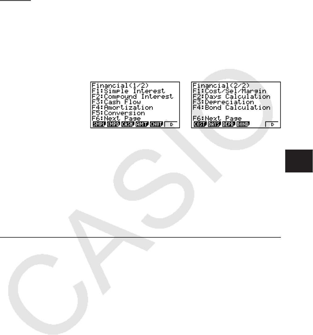
7-1
第7章 财务计算(TVM)
重要!
• fx-7400G II未配置 TVM 模式。
1. 在进行财务计算之前
在主菜单中,进入 TVM 模式并显示财务屏幕,如下所示。
财务1屏幕 财务2屏幕
• { SMPL } ... {单利}
• { CMPD } ... {复利}
• { CASH } ... {现金流(投资评估)}
• { AMT } ... {分期偿还}
• { CNVT } ... {利率换算}
• { COST } ... {成本、售价、毛利率}
• { DAYS } ... {日/日期计算}
• { DEPR } ... {折旧计算}
• { BOND } ... {债券计算}
k 设置项目
u Payment
• { BGN }/{ END } ... 指定付款{开始日期}/{结束日期}
u Date Mode
• { 365 }/{ 360 } ... 指定按照每年{365天}/{360天}进行计算
u Periods/YR.(付款间隔时间规定)
• { Annu }/{ Semi } ... {一年}/{半年}
在使用 TVM 模式时,请注意以下关于设置屏幕设置的注意事项。
• 在 TVM 模式中绘制图形时,以下图形设置屏幕设置全部关闭:Axes、Grid、Dual Screen。
• 在标签项目开启期间绘制财务图形时,垂直轴显示标签CASH(存款、取款),水平轴显示标
签TIME(频率)。
7
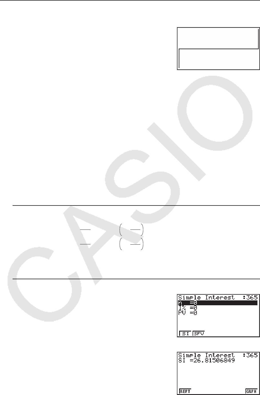
7-2
k 在TVM模式中绘图
在执行财务计算之后,您可使用 6(GRPH)绘制结果,如下图所示。
• 显示屏上显示图形时按下 !1(TRCE)将激活跟踪功能,该功能可用于查找其他财务数值。
例如,对于单利计算,按下 e可显示
PV、 SI和 SFV。按下 d,以相反顺序显示相同的值。
• 缩放、滚动和草图功能不可用于 TVM 模式。
• 选择使用正值或负值的现值(PV)或者购买价格(PRC),取决于您正准备执行的计算类
型。
• 请注意在查看 TVM 模式计算结果时,图形仅供参考。
• 请注意在这个模式下得到的计算结果仅供参考。
• 在进行实际财务交易时,必须将通过该计算器获得的计算结果与您的财务机构提供的计算结果
进行核对。
2. 单利
该计算器使用下述公式计算单利。
u 公 式
365日模式 SI : 利息
n : 利息期数
360日模式
PV : 本金
I% : 年利
SFV : 本金加利息
在财务1屏幕中按下 1(SMPL),显示下述单利计算的输入屏幕。
1(SMPL)
n .................. 利息期数(日)
I% .............. 年利率
PV .............. 本金
完成参数配置之后,使用下述某个功能菜单执行对应的计算。
• { SI } ... {单利}
• { SFV } ... {单利终值}
SI' = n
365 × PV × i
SI' = n
360 × PV × i
I%
100
i=
I%
100
i=
SI = –SI'
SFV = –(PV + SI')

7-3
• 如果参数配置不正确,会产生一个错误(Ma ERROR)。
使用下述功能菜单在计算结果屏幕之间导航。
• { REPT } ... {参数输入屏幕}
• { GRPH } ... {绘制图形}
绘制图形之后,您可按下 !1(TRCE),开启跟踪功能并沿着图形读取计算结果。
在开启跟踪功能时,每次按下 e将按照以下顺序循环显示数值:现值(
PV) → 单利( SI) →
单利终值(
SFV)。按下 d,按照相反顺序循环显示。
按下 J,返回参数输入屏幕。
3. 复利
该计算器使用下述标准公式计算复利。
u PV、PMT、FV、 n
I % 0
PMT = PV + × FV
β
α
–
FV =
β
α
PV + × PMT
–
n =
log (1+ iS)× PMT – FV × i
(1+ iS)× PMT + PV × i
{}
log (1+ i)
I %
= 0
PV =ï (PMT × n + FV) PMT = – n
PV + FV
FV =ï (PMT × n + PV) n = PMT
PV + FV
–
= (1+ i× S)× , = (1 + i)
i
1 ––n
ββ
α
0 .........Payment : End
(设置屏幕)
1 .........Payment : Begin
(设置屏幕)
i =
100
I%
I%
(1+ ) –1
C/Y
P/Y
100 × [C/Y]
............................... (P/Y = C/Y = 1)
(上述以外的
其他)
{
S =
.....
{
PV = – (α× PMT + × FV)
β
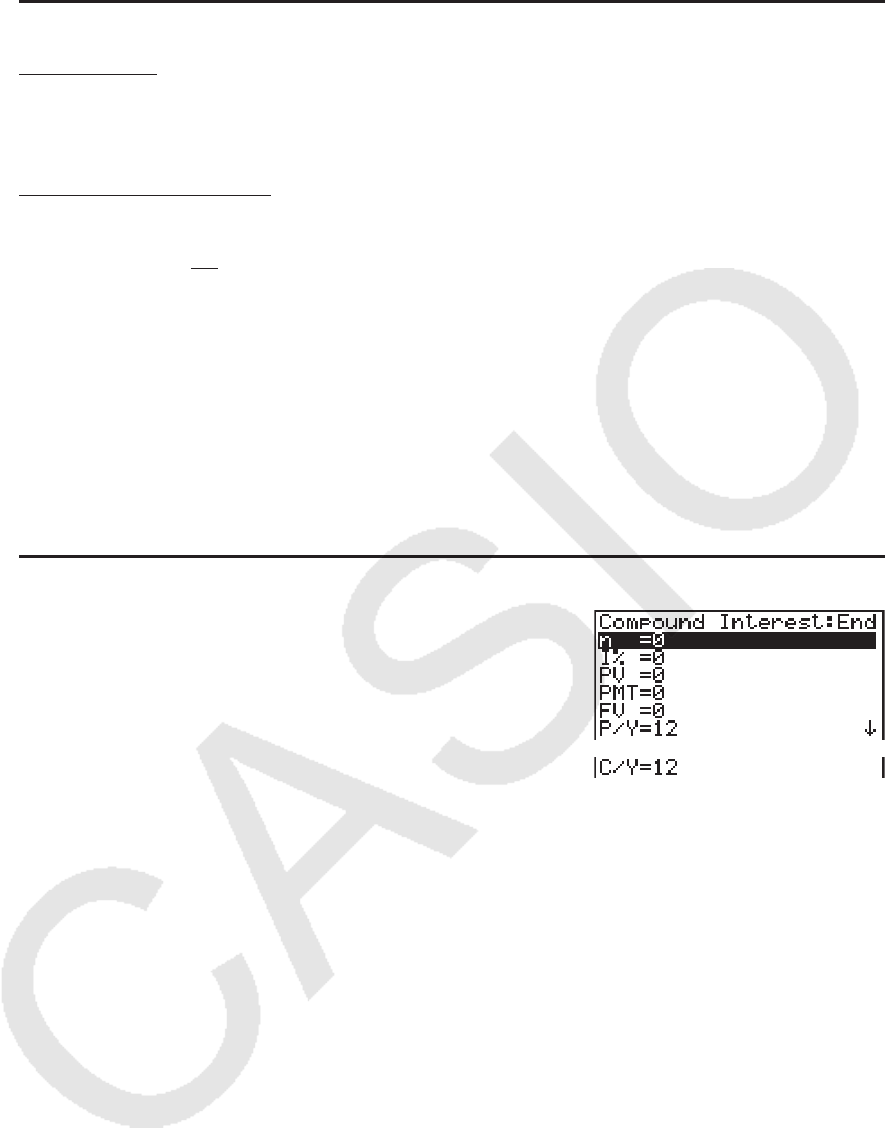
7-4
u I %
i (实际利率)
i (实际利率)使用牛顿法计算。
PV + α × PMT +
β
× FV = 0
将
i(实际利率)换算为 I %
n ................... 复利期数 FV .............. 终值
I% ............... 年利率 P/Y ............. 每年分期付款次数
PV .............. 现值 C/Y ............. 每年复利计算期数
PMT ......... 付款金额
• 存款用加号(+)表示,取款用减号(-)表示。
在财务1屏幕中按下 2(CMPD),显示下述复利计算的输入屏幕。
2(CMPD)
n ................... 复利期数
I% ............... 年利率
PV .............. 现值(贷款时为贷款金额;储蓄时为本金)
PMT ......... 每次付款金额(贷款时为还款金额;储蓄时为存款金额)
FV .............. 终值(贷款时为未付余额;储蓄时为本金加利息)
P/ Y ............ 每年分期付款期数
C/ Y ........... 每年复利计算期数
重要!
输入数值
期数(
n)以正值表示。现值( PV)或者终值( FV)之一为正时,则另一个( PV或者 FV)为
负。
精度
该计算器使用牛顿法计算利息,结果为近似值,其精度受到各种计算条件的影响。因此,在利
用该计算器得出利息计算结果时,应牢记上述局限性或核对结果。
{ }
×C/Y×100...
I%=(1+ i )–1
P/Y
C/Y(上述以外的其他)
i×100 ................................. (P/Y = C/Y = 1)
{
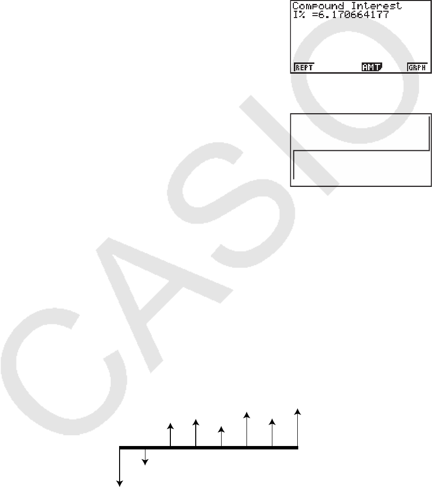
7-5
完成参数配置之后,使用下述某个功能菜单执行对应的计算。
• { n } ... {复利期数}
• { I% } ... {年利率}
• { PV } ... {现值}(贷款:贷款金额;储蓄:余额)
• { PMT } ... {支付金额}(贷款:分期还款金额;储蓄:存款)
• { FV } ... {终值}(贷款:未付余额;储蓄:本金加利息)
• { AMT } ... {分期偿还}
• 如果参数配置不正确,会产生一个错误(Ma ERROR)。
使用下述功能菜单在计算结果屏幕之间导航。
• { REPT } ... {参数输入屏幕}
• { AMT } ... {分期偿还}
• { GRPH } ... {绘制图形}
绘制图形之后,您可按下 !1(TRCE),开启跟踪功能并沿着图形读取计算结果。
按下 J,返回参数输入屏幕。
4. 现金流(投资评估)
该计算器使用折现现金流量(DCF)方法进行投资评估:一个固定时期内,将现金流相加。该
计算器可执行下述四种类型的投资评估。
• 净现值 (
NPV)
• 净终值 (
NFV)
• 内部收益率 (
IRR)
• 投资回收期 (
PBP)
如下所示的现金流量图有助于观察资金流动。
在这个图形中,初始投资用 CF0 表示。随后第一年的现金流用 CF1 表示,第二年用 CF2 表示,依
此类推。
投资评估可用于清楚确定一个投资项目是否实现了预期的目标利润。
CF0
CF1
CF2CF3CF4
CF5CF6
CF7

7-6
uNPV
n: 自然数,最大为254
uNFV
uIRR
在该公式中, NPV = 0, IRR等于 i × 100。但请注意,在计算器自动进行的后续计算中,会累
计微小的小数值,所以
NPV实际上从不会正好为零。 NPV越接近于零, IRR越准确。
u PBP
n: 满足 NPVn < 0、 NPVn+1 > 0或者0条件的最小正整数
在财务1屏幕中按下 3(CASH),显示下述现金流的输入屏幕。
3(CASH)
I% .................利率
Csh ............现金流列表
如果您尚未将数据输入列表,按下 5( 'LIST)并将数据输入列表。
完成参数配置之后,使用下述某个功能菜单执行对应的计算。
• { NPV } ... {净现值}
• { IRR } ... {内部收益率}
• { PBP } ... {投资回收期}
• { NFV } ... {净终值}
• { 'LIST } ... {将数据输入列表}
• { LIST } ... {指定用于输入数据的列表}
NPV = CF0+ + + + … +
(1+ i)
CF1
(1+ i)2
CF2
(1+ i)3
CF3
(1+ i)n
CFni=100
I%
NFV = NPV × (1 + i)
n
0 = CF
0
+ + + + … +
(1+ i)
CF
1
(1+ i)
2
CF
2
(1+ i)
3
CF
3
(1+ i)
n
CF
n
NPVn = Σ
n
k = 0
CFk
(1 + i)k
PBP =
{
0 .................................. (CF0> 0)
n – NPVn
NPVn+1 – NPVn
(上述以外的其他)
...
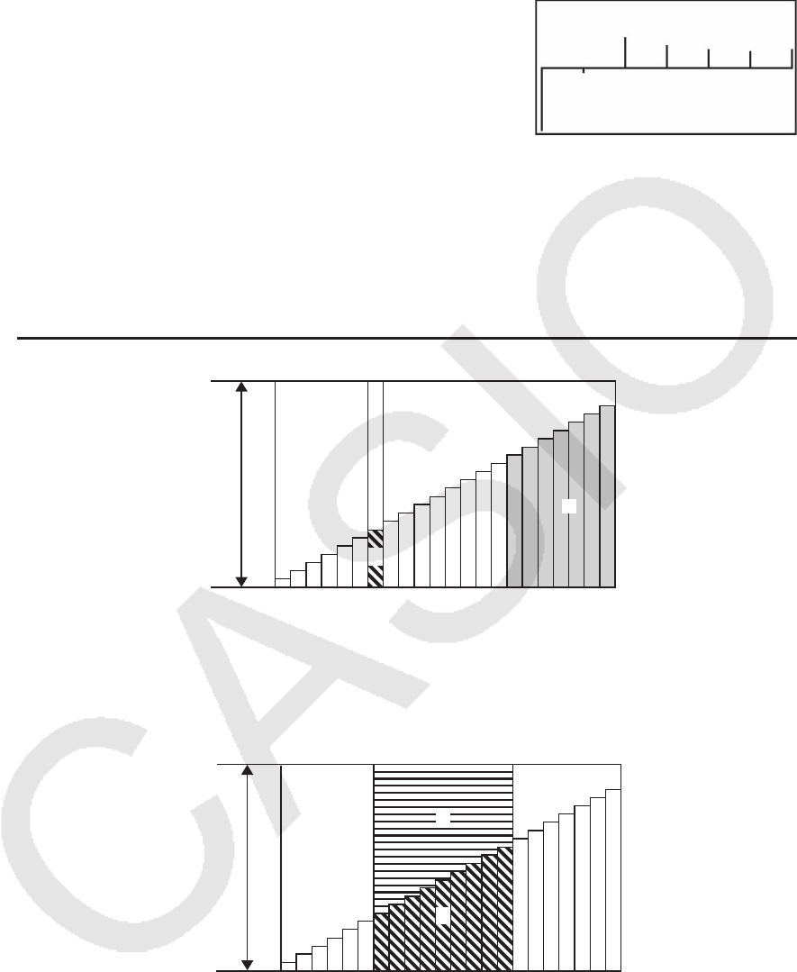
7-7
• 如果参数配置不正确,会产生一个错误(Ma ERROR)。
使用下述功能菜单在计算结果屏幕之间导航。
• { REPT } ... {参数输入屏幕}
• { GRPH } ... {绘制图形}
绘制图形之后,您可按下 !1(TRCE),开启跟踪功能并沿着图形读取计算结果。
按下 J,返回参数输入屏幕。
5. 分期偿还
该计算器可用于计算每月还款中的本金和利息部分、剩余本金以及已还的本金和利息金额。
u 公 式
a:PM1每月还款中的利息部分( INT)
b:PM1每月还款中的本金部分( PRN)
c:PM2每月还款之后的本金余额( BAL)
d: 从PM1每月还款到PM2每月还款的本金总额(
∑ PRN)
e: 从PM1每月还款到PM2每月还款的利息总额(
∑ INT)
*
a + b = 一次放款金额 ( PMT)
c
a
1付款
付款次数
1 PM1 PM2 最后................... .............................. ................
b
1付款
付款次数
1 PM1 PM2 最后.................... ......................... ....................
e
d
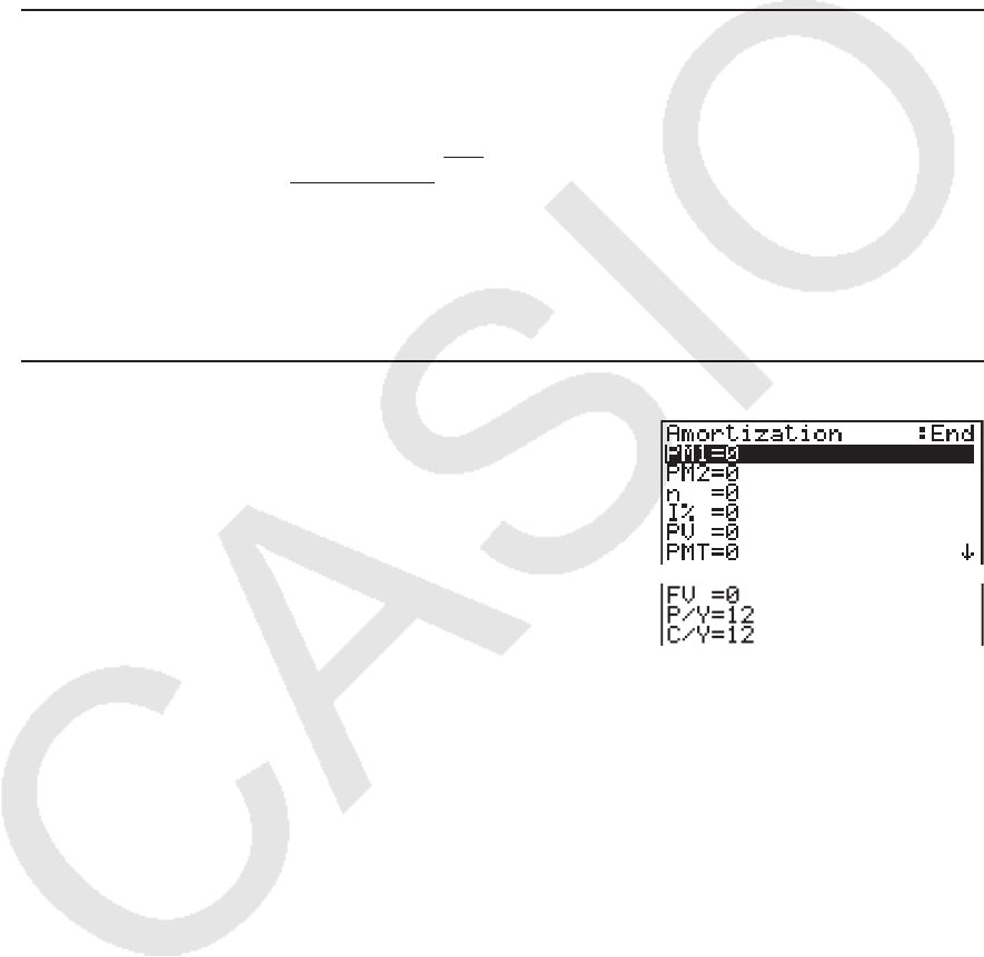
7-8
BAL0 = PV (在分期付款期间开始时, INT1 = 0且 PRN1 = PMT)
u 名义利率与实际利率之间的换算
当每年分期还款次数与复利计算期数不同时,名义利率(用户输入的 I%值)换算为实际利率
(
I% ')。
在将名义利率换算为实际利率之后,进行下述计算,计算结果用于所有后续计算。
在财务1屏幕中按下 4(AMT),显示下述分期还款的输入屏幕。
4(AMT)
PM1 ..........每月还款1至
n次中的第一次还款
PM2 ..........每月还款1至
n次中的第二次还款
n ..................分期还款次数
I% ...............利率
PV ..............本金
PMT .........每次还款金额
FV ..............最后一次还款后的余额
P/ Y ............每年还款次数
C/ Y ...........每年复利计算次数
完成参数配置之后,使用下述某个功能菜单执行对应的计算。
• { BAL } ... {PM2每月还款之后的本金余额}
• { INT } ... {PM1每月还款中的利息部分}
• { PRN } ... {PM1每月还款中的本金部分}
• { Σ INT } ... {从PM1每月还款至PM2每月还款中的总利息}
• { Σ PRN } ... {从PM1每月还款至PM2每月还款中的总本金}
a : INT
PM1
=IBAL
PM1–1
× i I× (PMT ig )
b : PRN
PM1
= PMT + BAL
PM1–1
×i
c : BAL
PM2
= BAL
PM2–1
+ PRN
PM2
d : Σ PRN = PRN
PM1
+ PRN
PM1+1
+ … + PRN
PM2
e : Σ INT = INT
PM1
+ INT
PM1+1
+ … + INT
PM2
PM2
PM1
PM2
PM1
I
%'=I%
(1+ ) –1
[C/Y]
[P/Y]
{ }
×100
100 × [C/Y]
i= I%'÷100
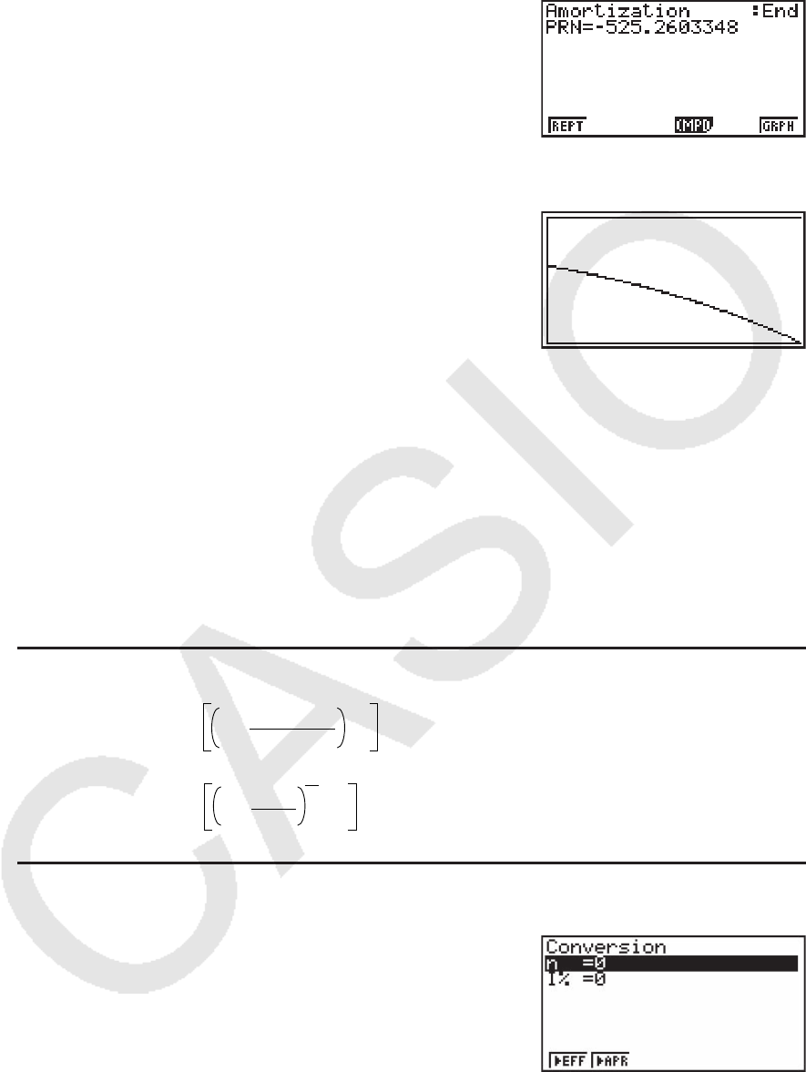
7-9
• { CMPD } ... {复利}
• 如果参数配置不正确,会产生一个错误(Ma ERROR)。
使用下述功能菜单在计算结果屏幕之间导航。
• { REPT } ... {参数输入屏幕}
• { CMPD } ... {复利}
• { GRPH } ... {绘制图形}
绘制图形之后,您可按下 !1(TRCE),开启跟踪功能并沿着图形读取计算结果。
首次按下 !1(TRCE),显示当
n = 1时的 INT和 PRN。随后每次按下 e可显示当 n = 2, n = 3
等时的
INT和PRN。
按下 J,返回参数输入屏幕。
6. 利率换算
本节所述程序说明如何在年百分利率与实际利率之间换算。
u 公 式
APR : 年百分利率(%)
EFF : 实际利率(%)
n : 复利期数
在财务1屏幕中按下 5(CNVT),显示下述利率换算的输入屏幕。
5(CNVT)
n ..................复利期数
I% ...............利率
E
FF = n
APR/100
1+ –1 × 100
n
A
PR = 100
EFF
1+ –1 × n×100
1
n
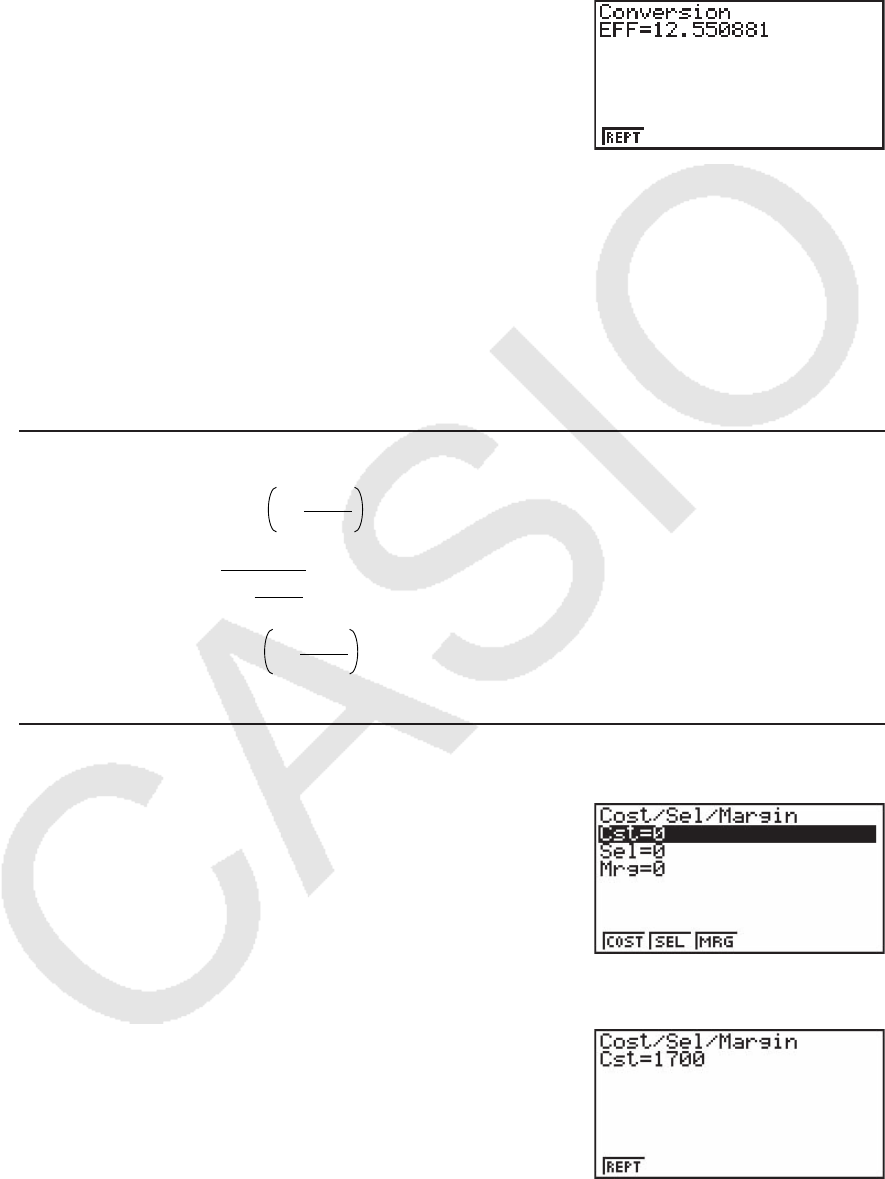
7-10
完成参数配置之后,使用下述某个功能菜单执行对应的计算。
• { 'EFF } ... {年百分利率换算为实际利率}
• { 'APR } ... {实际利率换算为年百分利率}
• 如果参数配置不正确,会产生一个错误(Ma ERROR)。
使用下述功能菜单在计算结果屏幕之间导航。
• { REPT } ... {参数输入屏幕}
7. 成本、售价、毛利率
只需输入成本、售价或者毛利率中任何两个值即可计算另一个值。
u 公 式
CST : 成本
SEL : 售价
MRG : 毛利率
在财务2屏幕中按下 1(COST),显示下述输入屏幕。
6( g) 1(COST)
Cst .............成本
Sel ..............售价
Mrg ...........毛利率
完成参数配置之后,使用下述某个功能菜单执行对应的计算。
• { COST } ... {成本}
• { SEL } ... {售价}
• { MRG } ... {毛利率}
• 如果参数配置不正确,会产生一个错误(Ma ERROR)。
使用下述功能菜单在计算结果屏幕之间导航。
• { REPT } ... {参数输入屏幕}
CST = SEL 100
MRG
1–
SEL =
100
MRG
1–
CST
M
RG(%) = SEL
CST
1– × 100
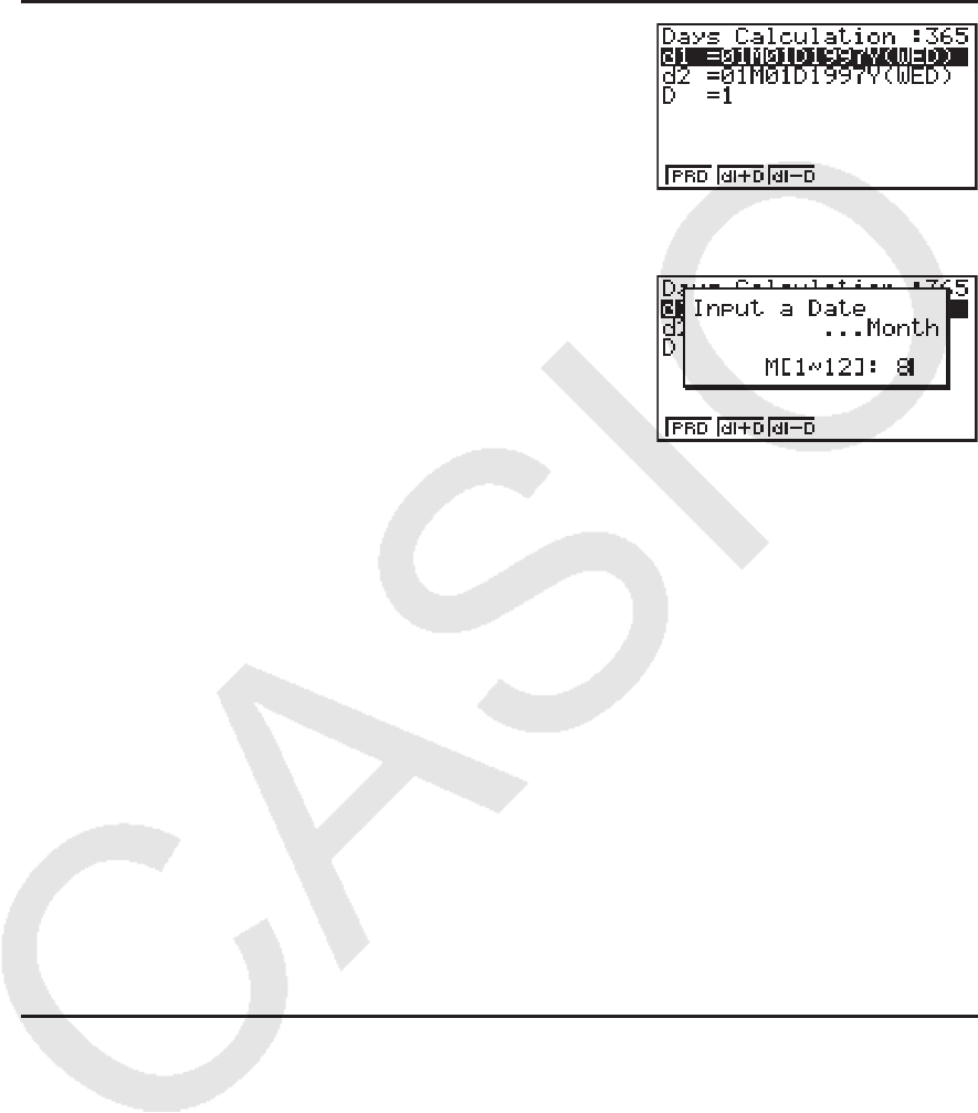
7-11
8. 日/日期计算
您可以计算两个日期之间的天数,或者确定在某个日期之前或者之后一定天数的日期。
在财务2屏幕中按下 2(DAYS),显示下述日/日期计算的
输入屏幕。
6( g) 2(DAYS)
d1 .................日期1
d2 ...............日期2
D ...................天数
如需输入某个日期,首先突出显示d1或者d2。按下一个
数字键,输入月份,显示屏上将显示类似于下图的输入屏幕。
输入月、日、年,每次输入后按下 w。
完成参数配置之后,使用下述某个功能菜单执行对应的计算。
• { PRD } ... {从d1到d2的天数(d2 - d1)}
• { d1+D } ... {d1+天数(d1 + D)}
• { d1-D } ... {d1-天数(d1 - D)}
• 如果参数配置不正确,会产生一个错误(Ma ERROR)。
使用下述功能菜单在计算结果屏幕之间导航。
• { REPT } ... {参数输入屏幕}
• 在财务计算中,设置屏幕可用于指定一年365天或者360天。日/日期计算还可按照当前的每年
天数设置执行,但当设定一年360天时,不能进行下述计算。否则会产生错误。
(日期)+(天数)
(日期)-(天数)
• 允许计算范围为1901年1月1日至2099年12月31日。
• 360日日期模式计算
下面说明在设置屏幕的Date Mode项目设置为360时,如何进行计算。
• 如果d1是某个月的第31天,d1作为所用月份的第30天。
• 如果d2是某个月的第31天,d2作为下个月的第1天,除非d1是第30天。

7-12
9. 折旧
折旧功能可用于计算指定年度由收入抵消的业务支出费用(折旧)。
•该计算器支持以下四类折旧计算。
直线法(
SL)、固定百分比法( FP)、年数总和法( SYD)、余额递减法( DB)。
• 以上任何一种方法都可用于计算指定时期的折旧。第
j年的折旧量与未折旧量的表格和图形。
u 直线法(SL)
SLj : 第 j年的折旧费
n : 使用寿命
PV : 原始成本(基础)
FV : 残值帐面价值
j : 折旧费计算年份
Y−1 : 折旧第一年中的月数
u 固定百分比法(FP)
FPj : 第 j年的折旧费
RDVj: 第 j年年底的剩余应折旧价值
I% : 折旧率
u 年数总和法(SYD)
SYDj : 第 j年的折旧费
RDVj : 第 j年年底的剩余应折旧价值
{Y–1}(PV–FV )
SL1 = n12
u
(PV–FV )
SLj = n12–{Y–1}
({Y–1}≠12)
(PV–FV )
n12
u
SLn+1 =
100
I%
FPj = (RDVj–1 + FV )×
100 {Y–1}
I%
FP1 = PV ×12
×
FPn+1 = RDVn ({Y–1}≠12)
RDV1 = PV –FV –FP1
RDVj = RDVj–1 –FPj
RDVn+1 = 0 ({Y–1}≠12)
n(n+1)
Z = 2
2
(n' 整数部分 +1)(n' 整数部分 + 2*n' 小数部分 )
Z' =
SYD1 = {Y–1}
12
n
Z×(PV –FV )
n'–j+2
Z' )(PV –FV –SYD1)( j≠1)SYDj = (
RDV1 = PV –FV –SYD1
RDVj = RDVj–1 –SYDj
n'–(n+1)+2
Z' )(PV –FV –SYD1)({Y–1}≠12)
12–{Y–1}
12
×SYDn+1 = (
12
{Y–1}
n' = n–
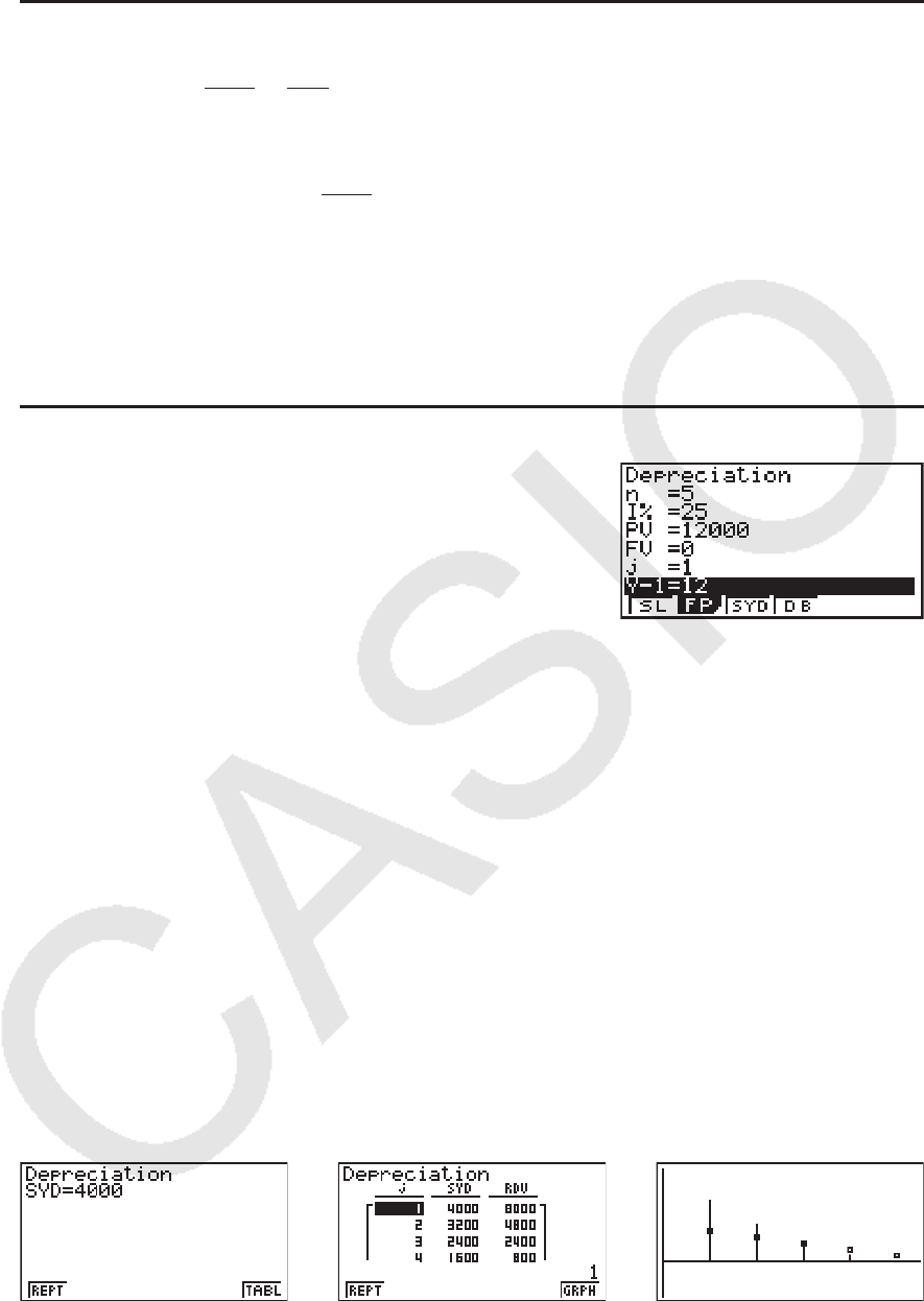
7-13
u 余额递减法(DB)
DBj : 第 j年的折旧费
RDVj : 第 j年年底的剩余应折旧价值
I% : 折旧系数
在财务2屏幕中按下 3(DEPR),显示下述折旧计算的输入屏幕。
6( g) 3(DEPR)
n ...................使用寿命
I% ...............固定百分比(FP)法中的折旧率,余额递减(DB)法中的折旧系数
PV ..............原始成本(基础)
FV ..............残值帐面价值
j ....................折旧费计算年份
Y-1 ...............折旧第一年中的月数
完成参数配置之后,使用下述某个功能菜单执行对应的计算。
• { SL } ... {使用直线法计算第
j年的折旧}
• { FP } ... { FP } ........... {使用固定百分比法计算第
j年的折旧}
{ I% } ........... {计算折旧率}
• { SYD } ... {使用年数总和法计算第
j年的折旧}
• { DB } ... {使用余额递减法计算第
j年的折旧}
计算结果输出示例
{SYD} {SYD} - {TABL} {SYD} - {GRPH}
RDV1 = PV –FV –DB1
({Y–1}≠12)
({Y–1}≠12)
100n
Y–1I%
DB1 = PV ×
100n
I%
12
×
×
DBj = (RDVj–1 +FV )
RDVj = RDVj–1 –DBj
DBn+1 = RDVn
RDVn+1 = 0
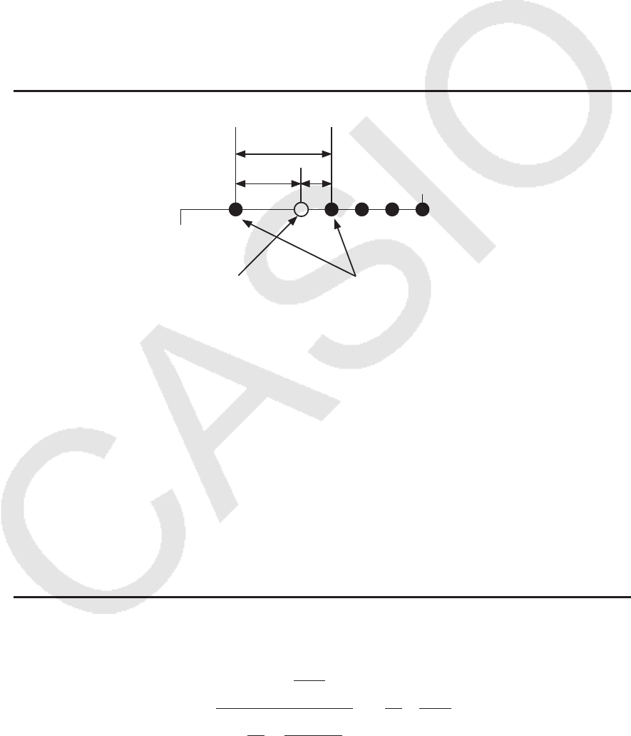
7-14
如果参数配置不正确,会产生一个错误(Ma ERROR)。
使用下述功能菜单在计算结果屏幕之间导航。
• { REPT } ... {参数输入屏幕}
• { TABL } ... {显示表格}
• { GRPH } ... {绘制图形}
10. 债券计算
债券计算功能用于计算债券的购买价格或者年收益率。
在开始进行债券计算之前,使用设置屏幕配置“Date Mode”和“Periods/YR.”设置项目(第
7-1页)。
u 公 式
D
发行日期
偿还日期 (d2)
购买日期 (d1) 息付款日
A B
PRC : 每100美元面值的价格
CPN : 年息票利率(%)
YLD : 到期收益率(%)
A : 应计天数
M : 每年配息次数(1=每年,2=每半年)
N : 结算日与到期日之间的配息次数
RDB : 每100美元面值的赎回价格
D: 结算时计息期内的天数
B: 从结算日到下一个配息日的天数= D - A
INT : 应计利息
CST : 包括利息的价格
u 每100美元面值的价格(PRC)
• 不超过一个偿还计息期
PRC = + (– )
RDV +M
CPN
1+ ( ×)
D
B
M
YLD/100 ×
D
A
M
CPN
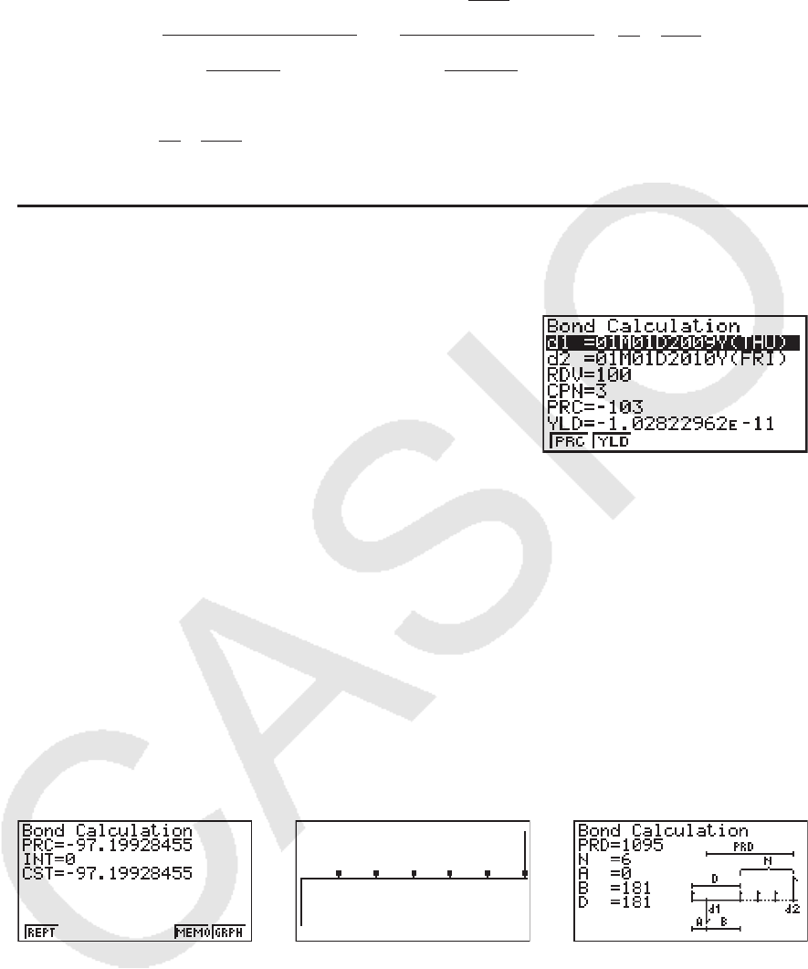
7-15
• 多个偿还计息期
u 年收益率(YLD)
使用牛顿法计算YLD。
在财务2屏幕中按下 4(BOND),显示下述债券计算的输入屏幕。
6( g) 4(BOND)
d1 ............... 购买日期(月、日、年)
d2 ............... 偿还日期(月、日、年)
RDV ........... 每100美元的赎回价格
CPN ........... 息票利率
PRC ........... 每100美元面值的价格
YLD .......... 年收益率
完成参数配置之后,使用下述某个功能菜单执行对应的计算。
• {PRC} ... {计算债券的价格(PRC)、应计利息(INT)、和债券成本(CST)}
• {YLD} ... {计算到期收益率}
计算结果输出示例
{PRC} {PRC} - {GRPH} {PRC} - {MEMO}
如果参数配置不正确,会产生一个错误(Ma ERROR)。
使用下述功能菜单在计算结果屏幕之间导航。
• { REPT } ... {参数输入屏幕}
• { GRPH } ... {绘制图形}
• { MEMO } ... {显示用于计算的天数}
×
D
A
M
CPN
INT = – CST = PRC +INT
+×
D
A
M
CP
N
PRC = ––
RDV
(1+ )
M
YLD/100 (1+ )
M
YLD/100
M
CPN
Σ
N
k=1
(N–1+B/D )(k–1+B/D )
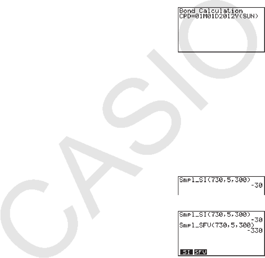
7-16
MEMO屏幕
• 下例说明了MEMO屏幕显示项目的含义。
PRD ....... 从d1到d2的天数
N ............... 结算日与到期日之间的配息次数
A ............... 应计天数
B ............... 从结算日到下一个配息日的天数(D - A)
D ............... 结算时计息期内的天数
• 在显示MEMO屏幕时,每次按下 w,可顺序显示从偿还年份到购买年份的配息日(CPD)。
该功能只有在设置屏幕的“Date Mode”设置为“365”时才有效。
11. 使用函数进行财务计算
重要!
• 在fx-7400G II上不可执行以下操作。
您可在 RUN • MAT 模式或者 PRGM 模式中使用特殊函数,执行与 TVM 模式财务计算相同的计算。
示例 计算年单利为5%时,2年期(730天)300美元贷款中支付的总利息加本金。
使用的Date Mode设置为365。
1. 在主菜单中,进入 RUN • MAT 模式。
2. 按下以下按键。
K6( g) 6( g) 6( g) 1(TVM)
1(SMPL) 1(SI) hda,f,
daa)w
2(SFV) hda,f,daa)
w
• 使用 TVM 模式设置屏幕( !m(SET UP))更改Date Mode设置。
您还可在 PRGM 模式中使用特殊命令(DateMode365, DateMode360)更改设置。
• 如需详细了解财务计算函数的功能及其语法,请参见“在程序中执行财务计算”(第8-34页)。
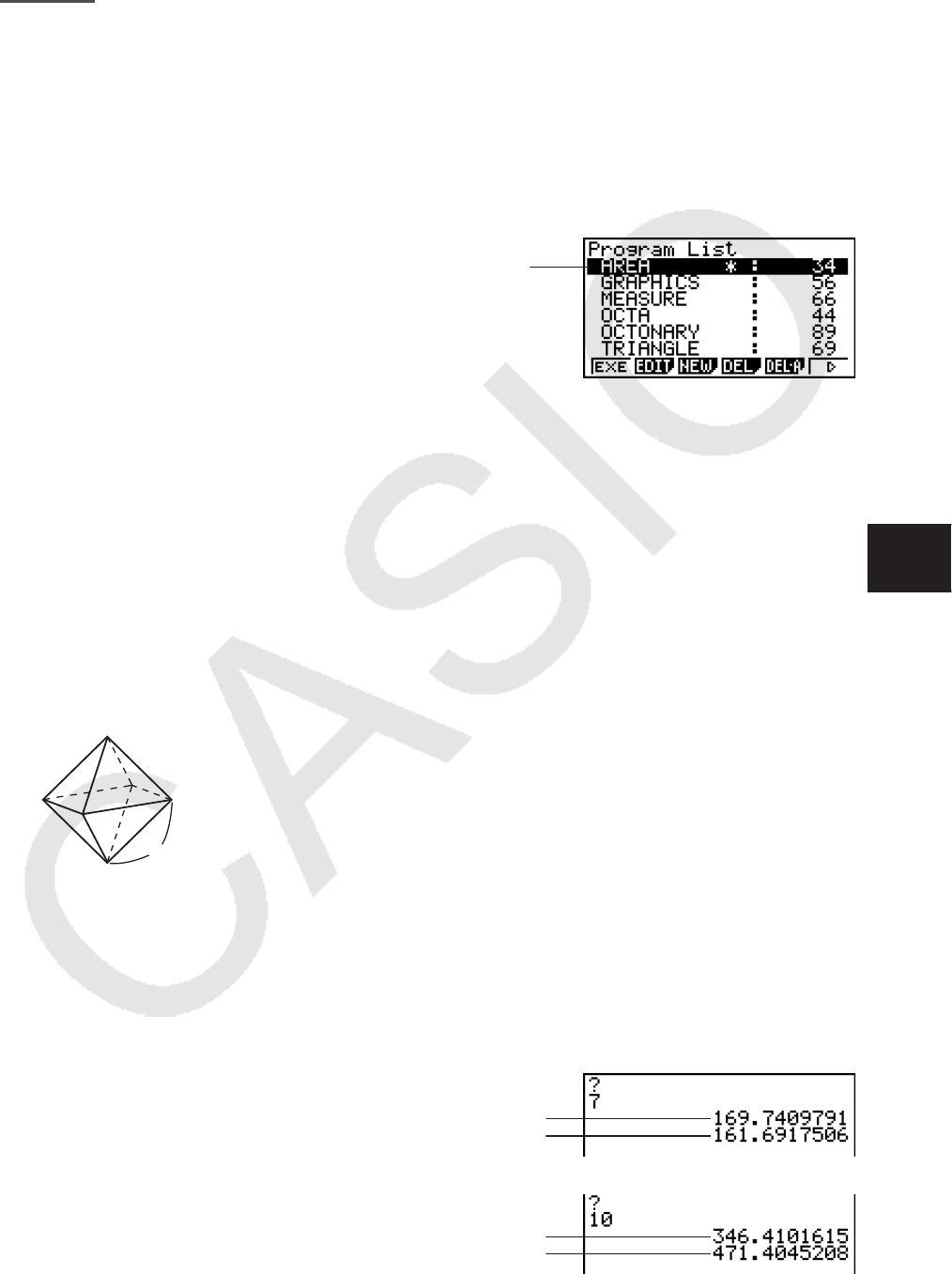
8-1
第8章 编程
重要!
在PRGM模式下输入都需要用到线性输入/输出模式。
1. 基本编程步骤
正如手动计算多语句一样,命令与计算也顺序进行。
1. 在主菜单中,进入 PRGM 模式。在您操作时,显示屏上显示程序列表。
选定的程序区
(使用 f和 c移动)
文件按照名称的字母表顺序排列。
2. 登记文件名。
3. 输入程序。
4. 运行程序。
• 程序列表右侧的数值表示每一个程序使用的字节数。
• 文件名最多可使用八个字符。
• 下面是文件名中可使用的字符:A至Z、
r、
θ
、空格、[、]、 {、}、'、”、~、0 至 9、.、+、-
、×、÷
• 登记文件名需要使用32个字节的存储区。
示例 计算三个正八面体的表面积(cm
2
)和体积(cm
3
),其边长分别为7、10和
15cm
将计算公式存储在文件名OCTA下。
下述是用于计算已知边长A的正八面体表面积S与体积V的公式。
1 m PRGM
2 3(NEW) j(O) I(C) /(T) v(A) w
3 !J(PRGM) 4(?) aav(A) 6( g) 5(:)
c*!x( ') d*av(A) x6( g) 6( g) 5( ^)
!x( ') c/d*av(A) Md
JJ
4 1(EXE) 或 w
hw(A的值)
A = 7时的S
w
A = 7时的V
ww
baw
A = 10时的S
w
A = 10时的V
A
S = 2'3 A
2
, V = A
3
––––
'2
3
8

8-2
ww
bfw
A = 15时的S
w*
1
A = 15时的V
*
1
显示屏上显示程序的最终结果时按下 w,退出程序。
• 您还可通过输入以下命令在 RUN • MAT (或者 RUN )模式中运行某个程序:Prog "<文件名>"
w。
• 在显示屏显示使用该方法执行程序后的最终结果时,按下 w, 重新执行程序。
• 如果无法找到Prog "<文件名>" 指定的程序,会产生一个错误。
2. PRGM模式功能键
• { NEW } ... {新程序}
u 在登记文件名时
• { RUN } / { BASE } ... {一般计算}/{数位} 程序输入
• { Q} ... {密码登记}
• { SYBL } ... {符号菜单}
u 在输入程序时 —— 1(RUN) ... 默认设置
• { TOP } / { BTM } ... 程序的{顶部}/{底部}
• { SRC } ... {搜索}
• { MENU } ... {模式菜单}
• { STAT } / { MAT }* / { LIST } / { GRPH } / { DYNA }* / { TABL } / { RECR }*
... {统计}/{矩阵}/{列表}/{图形}/{动态图形}/{表格}/{递归}菜单
• { A ↔ a } ... {在大写和小写输入模式之间切换}
• { CHAR } ... {显示一个用于选择各种数学符号、特殊符号和重音字符的屏幕}
*fx-7400G
II中不包括。
• 按下 !J(PRGM),显示以下程序(PRGM)菜单。
• { COM } ... {程序命令菜单}
• { CTL } ... {程序控制命令菜单}
• { JUMP } ... {转移命令菜单}
• { ? } / { ^} ... {输入}/{输出} 命令
• { CLR } / { DISP } ... {清除}/{显示} 命令菜单
• { REL } ... {条件转移关系算子菜单}
• { I/O } ... {输入/输出控制/传输命令菜单}
• { : } ... {多语句命令}
• { STR } ... {字符串命令}
关于这些命令的详细说明,请参见第8-7页的“命令参考”。

8-3
• 按下 !m(SET UP),显示下图所示的模式命令菜单。
• { ANGL } / { COOR } / { GRID } / { AXES } / { LABL } / { DISP } / { S/L } / { DRAW } / { DERV } / { BACK } / { FUNC } /
{ SIML } / { S-WIN } / { LIST } / { LOCS }* / { T-VAR } / { Σ DSP }* / { RESID } / { CPLX } / { FRAC } / { Y
• SPD }* / { D
ATE }* / { PMT }* / { PRD }* / { INEQ } / { SIMP } / { Q1Q3 } *fx-7400G
II中不包括。
关于这些命令的详细说明,请参见第1-26页的“设置屏幕功能键菜单”。
u 在输入程序时 —— 2(BASE)
*
1
• { TOP } / { BTM } / { SRC }
• { MENU }
• { d~o } ... {十进制}/{十六进制}/{二进制}/{八进制}值输入
• { LOG } ... {位运算符}
• { DISP } ... 将显示值换算为{十进制}/{十六进制}/{二进制}/{八进制}
• { A ↔ a } / { SYBL }
• 按下 !J(PRGM),显示以下PRGM (PROGRAM)菜单。
• { Prog } ... {程序调用}
• { JUMP } / { ? } / { ^}
• { REL } ... {条件转移关系算子菜单}
• { : } ... {多语句命令}
• 按下 !m(SET UP),显示下图所示的模式命令菜单。
• { Dec
} / { Hex } / { Bin } / { Oct }
*
1
按下 2(BASE)之后的程序输入状态由文件名右侧的
B
表示。
• { EXE } / { EDIT } ... 程序{执行}/{编辑}
• { NEW } ... {新程序}
• { DEL } / { DEL
•
A } ... 删除{特定程序}/{所有程序}
• { SRC } / { REN } ... 文件名{搜索}/{更改}
3. 编辑程序内容
k 调试程序
程序中阻碍程序正确运行的问题称为“程序错误”,解决此类问题的过程称为“调试”。下述
症状中的任何一个都表明您的程序中包含程序错误,需要调试。
• 程序运行时出现错误消息
• 结果不在您的预期范围内
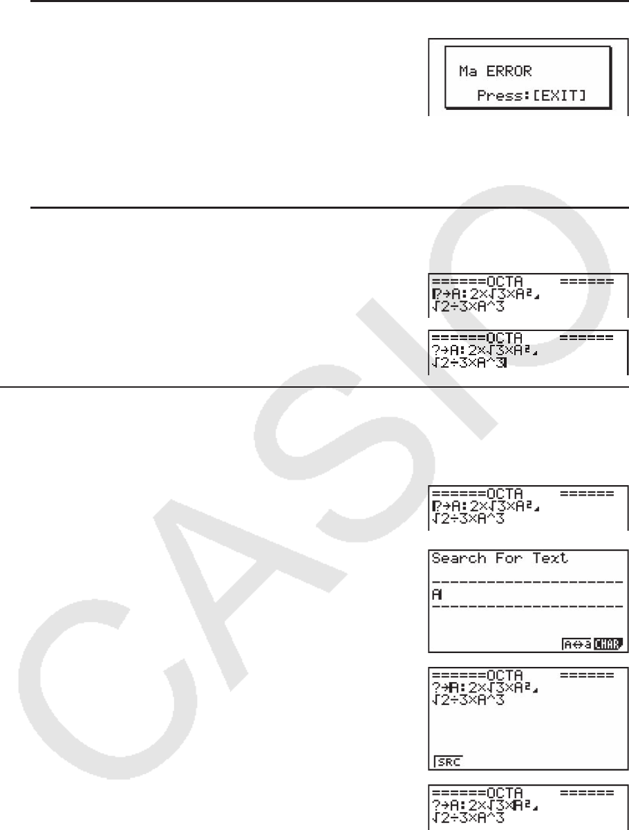
8-4
u 排除导致错误消息的程序错误
如右图所示,只要在程序执行期间出现任何非法事件,即显示
错误消息 。
在显示此类消息时,按下 J,显示程序中产生错误的位置。光标将在问题所在位置闪烁。查
看“错误消息表”(第
α
-1页),确定此类问题的解决步骤。
• 请注意,如果程序已使用密码保护,按下 J不会显示错误所在位置。
u 排除导致错误结果的程序错误
如果您的程序产生异常结果,检查程序内容并进行必要的修改。
1(TOP) ..... 将光标移至程序的顶部
2(BTM) .... 将光标移至程序的底部
k 搜索程序内部数据
示例 搜索程序OCTA中的字母“A”
1. 调用程序。
2. 按下 3(SRC)并输入想要查找的数据。
3(SRC)
av(A)
3. 按下 w,开始搜索。屏幕上显示程序的内容,光标位于指
定数据的第一个所在位置。*
1
4. 每次按下 w或 1(SRC)都会使光标跳至指定数据的下一个
所在位置。*
2
*
1
如果未在程序中找到您指定的搜索数据,显示消息“Not Found”。
*
2
如果程序中已没有其他出现指定数据的位置,搜索操作结束。
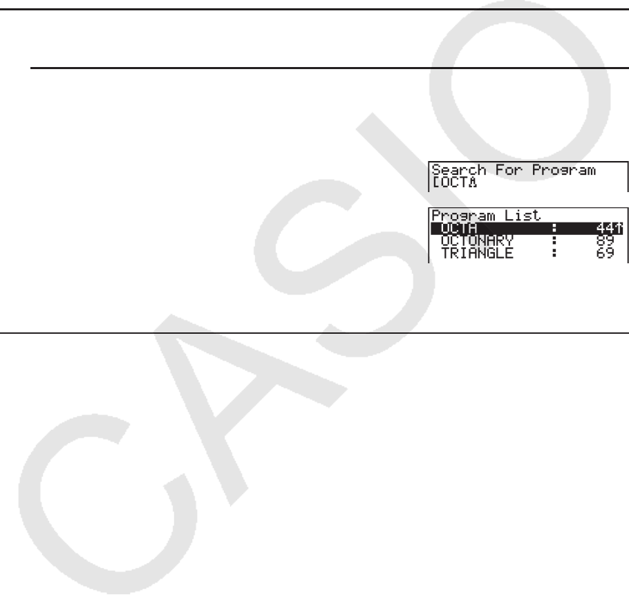
8-5
•您不能指定换行符号( _)或者显示搜索数据的命令( ^)。
• 屏幕上显示程序内容后,您即可使用光标键将光标移至另一个位置,然后搜索下一个数据所在
位置。按下 w时,只搜索从当前光标位置开始的程序部分。
• 一旦搜索到某个数据所在位置,如果输入字符或者移动光标,将取消搜索操作。
• 如果在输入字符进行搜索时出现错误,可按下 A,清除输入的内容并从开始处重新输入。
4. 文件管理
k 搜索文件
u 使用初始字符搜索方法查找文件
示例 使用初始字符搜索方法调用名为OCTA的程序
1. 显示屏上显示程序列表时,按下 6( g) 1(SRC),输入想要查找文件的初始字符。
6( g) 1(SRC)
j(O) I(C) /(T)
2. 按下 w,开始搜索。
• 突出显示以输入字符开头的名称。
• 如果没有以输入字符开头的文件名的程序,显示屏上显示消息“Not Found”。如果出现这种
情况,按下 J,清除错误消息。
k 编辑文件名
1. 显示屏上显示程序列表时,使用 f和 c突出显示想要编辑名称的文件,然后按下 6( g) 2
(REN)。
2. 进行任何所需修改。
3. 按下 w,登记新名称并返回程序列表。
根据您对文件名的修改,程序列表重新排序。
• 如果您进行的修改产生与存储器内已经存储的程序名相同的文件名,则会显示消息“Already
Exists”。出现这种情况时,您可以进行下述两种操作中的任何一种,解决这一问题。
- 按下 J,清除错误并返回文件名编辑屏幕。
- 按下 A,清除文件名并输入新的名称。

8-6
k 删除程序
u 删除特定程序
1. 显示屏上显示程序列表时,使用 f和 c,突出显示想要删除的程序的名称。
2. 按下 4(DEL)。
3. 按下 1(YES),删除选定程序;或者按下 6(NO),中止操作,但不删除任何内容。
u 删除所有程序
1. 显示屏上显示程序列表时,按下 5(DEL
•
A)。
2. 按下 1(YES),删除列表中的所有程序;或者按下 6(NO),中止操作,但不删除任何内
容。
• 您还可通过从主菜单进入 MEMORY 模式,删除所有程序。详情请参见“第11章 存储器管理
器”。
k 登记密码
在输入程序时,您可使用密码保护,只有拥有密码的用户才可查看程序内容。
• 您不需要输入密码即可运行程序。
• 密码输入程序与文件名输入程序完全相同。
1. 显示屏上显示程序列表时,按下 3(NEW),输入新程序文件的文件名。
2. 按下 5( Q),然后输入密码。
3. 按下 w,登记文件名和密码。现在您可输入程序文件的内容。
4. 输入程序之后,按下 !J(QUIT),退出程序文件并返
回程序列表。使用密码保护的文件在文件名右侧由一个 星
号标记。
k 调用密码保护的程序
1. 在程序列表中,使用 f和 c突出显示想要调用的程序的名称。
2. 按下 2(EDIT)。
3. 输入密码并按下 w,调用程序。
• 在调用密码保护的程序时,如果输入错误密码将显示“Mismatch”消息。

8-7
5. 命令参考
k 命令索引
Break ............................................................................. 8-10
CloseComport38k ............................................... 8-17
ClrGraph .................................................................... 8-13
ClrList ........................................................................... 8-13
ClrMat .......................................................................... 8-13
ClrText ......................................................................... 8-13
ClrVct ............................................................................ 8-14
DispF-Tbl、DispR-Tbl .................................... 8-14
Do~LpWhile ............................................................. 8-10
DrawDyna ................................................................. 8-14
DrawFTG-Con、DrawFTG-Plt .............. 8-14
DrawGraph .............................................................. 8-14
DrawR-Con、DrawR-Plt .............................. 8-14
DrawR Σ -Con、DrawR Σ -Plt ....................... 8-15
DrawStat .................................................................... 8-15
DrawWeb ................................................................... 8-15
Dsz .................................................................................... 8-11
Exp( ................................................................................. 8-18
Exp 'Str( ................................................................... 8-18
For~To~(Step~)Next ............................................ 8-9
Getkey .......................................................................... 8-16
Goto~Lbl ..................................................................... 8-12
If~Then~(Else~) IfEnd ........................................ 8-9
Isz ...................................................................................... 8-12
Locate ............................................................................ 8-16
Menu .............................................................................. 8-13
OpenComport38k ............................................... 8-17
Prog ................................................................................. 8-10
PlotPhase ................................................................... 8-15
RclCapt ........................................................................ 8-20
Receive( ....................................................................... 8-17
Receive38k ............................................................... 8-17
Return .......................................................................... 8-11
Send( .............................................................................. 8-17
Send38k ...................................................................... 8-17
Stop ................................................................................. 8-11
StrCmp( ....................................................................... 8-18
StrInv( .......................................................................... 8-19
StrJoin( ........................................................................ 8-19
StrLeft( ........................................................................ 8-19
StrLen( ......................................................................... 8-19
StrLwr( ........................................................................ 8-19
StrMid( ......................................................................... 8-19
StrRight( ..................................................................... 8-19
StrRotate( .................................................................. 8-19
StrShift( ..................................................................... 8-20
StrSrc( .......................................................................... 8-20
StrUpr( ......................................................................... 8-20
While~WhileEnd ................................................. 8-10
? (输入命令) ............................................................ 8-8
^(输出命令) .......................................................... 8-8
: (多语句命令) ....................................................... 8-8
_(回车) ..................................................................... 8-8
’ (注释文本分隔符) ..................................... 8-8
S (转移代码) ..................................................... 8-12
=、 、>、<、
、 (关系算子) ............ 8-18
+ .......................................................................................... 8-20
下面是本节在说明各种命令时遵循的规则。
粗体文本 ................................... 必须输入的实际命令和其他项目以粗体显示。
{波形括号} ............................... 波形括号用于包括大量项目,在使用命令时必须在这些项目中进行选
择。在输入命令时不得输入波形括号。
[方括号] ..................................... 方括号用于包括可选项目。在输入命令时不得输入方括号。
数值表达式 ............................. 数值表达式(例如10、10 + 20、A)表示常数、计算式、数值常数等
等。
字母字符 ................................... 字母字符表示文字串(例如AB)。

8-8
k 基 本操作命 令
? (输入命令)
功能: 在程序执行期间,提示输入数值以代入变量。
语法: ? → <变量名称>、"<提示>" ? → <变量名称>
示例: ? → A _
描述:
• 该命令可暂时中断程序执行并提示输入数值或者表达式以代入变量。如果不指定提示内容,执
行该命令将显示“?”,表示计算器正在等待输入。如果指定提示内容,显示“<提示>?”,提
示用户输入。提示内容最多可输入255个字节的文本。
• 与输入命令相对应的输入必须是数值或者表达式,表达式不能是多语句。
• 您可指定一个列表名称、矩阵名称、向量名称、字符串存储器、函数存储器(fn)、图形
(Yn)等等作为变量名称。
^ (输出命令)
功能: 在程序执行期间显示中间结果。
描述:
• 该命令可暂时中断程序执行并在命令之前显示字母字符文字或者计算结果。
• 在手动计算期间,输出命令应在通常按下 w键的位置使用。
: (多语句命令)
功能: 连接两个语句,以便不间断地顺序执行。
描述:
• 与输出命令( ^)不同,使用多语句命令连接的语句连续执行。
• 多语句命令可用于连接两个计算表达式或者两个命令。
• 您还可使用 _ 指示的回车,替代多语句命令。
_ ( 回车)
功能: 连接两个语句,以便不间断地顺序执行。
描述:
• 回车命令的操作与多语句命令相同。
• 您可在程序中只输入一个回车,产生一个空行。使用回车替代多语句命令,可使显示的程序更
易于阅读。
’(注释文本分隔符)
功能: 表示插入程序内部的注释文本。
描述: 在一行的开头输入一个撇号('),从该行的开头直至下一个多语句命令(:)、回车
( _)或输出命令( ^)之间的所有内容均视为不可执行的注释文本。
8-9
k 程 序命令(COM)
If~Then~(Else~)IfEnd
功能: 只有在If-条件为真(非0)时才执行Then-语句。在If-条件为假(0)时执行Else-语句。
Then-语句或者是Else-语句之后都执行IfEnd-语句。
语法:
If <条件>
_
:
^
Then <语句>
_
:
^
<语句>
数值表达式
_
:
^
Else <语句>
_
:
^
<语句>
_
:
^
IfEnd
参数: 条件,数值表达式
描述:
(1) If ~ Then ~ IfEnd
• 当条件为真时,执行Then-语句,然后跳转至IfEnd之后的语句。
• 当条件为假时,执行IfEnd之后的语句。
(2) If ~ Then ~ Else ~ IfEnd
• 当条件为真时,执行Then-语句,然后继续执行IfEnd之后的语句。
• 当条件为假时,跳转至Else-语句,然后继续执行IfEnd之后的语句。
For~To~(Step~)Next
功能: 该命令重复执行For-语句到Next-语句之间的所有语句。第一次执行时,将初值分配给控
制变量,以后每次执行时根据步长值更改控制变量的值。直至控制变量的值超过终值时,停止
执行。
语法:
For <初值> → <控制变量名称> To <终值> Step <步长值>
_
:
^
Next
参数:
• 控制变量名称:A至Z
• 初值:产生一个值的数值或者表达式(即sin
x、A等等)
• 终值:产生一个值的数值或者表达式(即sin
x、A等等)
• 步长值:数值(默认值:1)
描述:
• 默认步长值为1。
• 使初值小于终值并指定正步长值,可使控制变量在每次执行之后递增。使初值大于终值并指定
负步长值,可使控制变量在每次执行之后递减。
8-10
Do~LpWhile
功能: 只要条件为真(非0),该命令可重复执行特定命令。
语法:
Do
_
:
^
<语句>
_
:
^
LpWhile < 条件 >
数值表达式
参数: 表达式
描述:
• 只要条件为真(非0),该命令可重复执行循环中的命令。当条件为假(0)时,执行
LpWhile-语句之后的语句。
• 由于条件在LpWhile-语句之后,因此会在循环内所有命令都已执行之后,测试(检查)条件。
While~WhileEnd
功能: 只要条件为真(非0),该命令可重复执行特定命令。
语法:
While < 条件 >
_
:
^
<语句>
_
:
^
WhileEnd
数值表达式
参数: 表达式
描述:
• 只要条件为真(非0),该命令可重复执行循环中的命令。当条件为假(0)时,执行
WhileEnd-语句之后的语句。
• 由于条件在While-语句之后,因此会在执行循环内的命令之前,测试(检查)条件。
k 程 序 控 制命 令(CTL)
Break
功能: 该命令中断执行某个循环并从该循环之后的下一个命令继续执行。
语法: Break _
描述:
• 该命令中断执行某个循环并从该循环之后的下一个命令继续执行。
• 该命令可用于中断执行For-语句、Do-语句和While-语句。
Prog
功能: 该命令可指定另一个程序作为子程序执行。在 RUN • MAT (或者 RUN )模式中,该命令执
行新程序。
语法: Prog "文件名" _
示例: Prog "ABC" _
描述:
• 即使该命令在某个循环中,执行该命令也会立即中断循环并启动子程序。
• 您可根据需要在主程序内多次使用该命令,调用独立的子程序以执行特定任务。
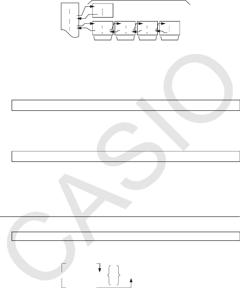
8-11
• 在同一个主程序中,子程序可在多处使用,也可由任意数量的主程序调用。
主程序 子程序
1级 2级 3级 4级
• 调用子程序时,将从头开始执行该子程序。子程序执行完成后,返回主程序,继续执行Prog命
令后面的语句。
• 子程序中的Goto~Lbl命令只在该子程序内有效。它不能用于跳转到该子程序外部的标签。
• 如果由Prog命令指定文件名的子程序不存在,会产生一个错误。
• 在 RUN • MAT (或者 RUN )模式中,输入Prog命令并按下 w,启动命令指定的程序。
Return
功能: 该命令从子程序中返回。
语法: Return _
描述: 在主程序内执行Return 命令将导致停止执行程序。在子程序内执行Return命令可终止子
程序并返回跳转到该子程序之前的程序位置。
Stop
功能: 该命令终止执行程序。
语法: Stop _
描述:
• 该命令可终止执行程序。
• 在一个循环内执行该命令,可终止执行程序而不会产生错误。
k 转 移命 令(JUMP)
Dsz
功能: 该命令为计数转移,每次使控制变量的值递减1,在变量的当前值变为零时执行转移。
语法:
变量值 0
Dsz <变量名称> : <语句>
_
:
^
<语句>
变量值 = 0
参数: 变量名称:A至Z、 r、
θ
[示例] Dsz B : 将指定给变量B的值递减1。
描述: 该命令每次将控制变量的值递减1,然后测试(检查)该值。如果当前值非0,继续执行
下一个语句。如果当前值为0,跳转至多语句命令(:)、显示命令( ^)或者回车( _)后面
的语句。
D
CEIJ
Prog "E" Prog "I" Prog "J"
A
Prog "D"
Prog "C"
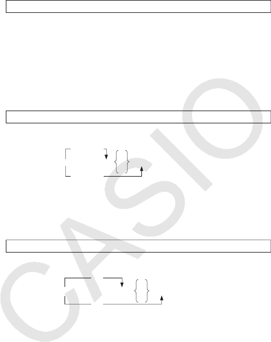
8-12
Goto~Lbl
功能: 该命令执行指向指定位置的无条件转移。
语法: Goto <标签名称> ~ Lbl <标签名称>
参数: 标签名称:数值(0至9)、变量(A至Z、
r、
θ
)
描述:
• 该命令包括两个部分:Goto
n(其中 n为上述参数)和Lbl n(其中 n是Goto n参考的参数)。
该命令可使程序跳转到
n参数与Goto-语句相符合的Lbl-语句。
• 该命令可用于返回一个程序的开始处或者跳转至程序内的任何位置。
• 该命令可与有条件转移和计数转移命令结合使用。
• 如果没有与Goto-语句指定值相符合的Lbl-语句,会产生一个错误。
Isz
功能: 该命令为计数转移,每次使控制变量的值递增1,在变量的当前值变为零时执行转移。
语法:
变量值 0
Isz <变量名称> : <语句>
_
:
^
<语句>
变量值 = 0
参数: 变量名称:A至Z、 r、
θ
[示例] Isz A : 将指定给变量A的值递增1。
描述: 该命令每次将控制变量的值递增1,然后测试(检查)该值。如果当前值非0,继续执行
下一个语句。如果当前值为0,跳转至多语句命令(:)、显示命令( ^)或者回车( _)后面
的语句。
⇒ (转移代码)
功能: 该代码用于设置有条件转移的条件。当条件为假时,执行转移。
语法:
真
<左侧> <关系算子> <右侧> ⇒ <语句>
_
:
^
<语句>
假
参数:
• 左侧/右侧:变量(A至Z、
r、
θ
)、数值常数、变量表达式(例如:A×2)
• 关系算子:=、 、>、<、 、 (第8-18页)
描述:
• 有条件转移可比较两个变量的内容或者两个表达式的结果,并决定是否根据比较结果执行转
移。
• 如果比较返回结果为真,则继续执行 ⇒ 命令后的语句。如果比较返回结果为假,跳转至多语
句命令(:)、显示命令( ^)或者回车( _)后面的语句。

8-13
Menu
功能: 在程序中创建一个分支菜单。
语法: Menu "<字符串(菜单名称)>", "<字符串(分支名称)1>", <数值或变量1>,
"<字符串(分支名称)2>", <数值或变量2>, ... , "<字符串(分支名称)
n>", <数值或变量 n>
参数: 数值(0至9)、变量(A至Z、
r、
θ
)
描述:
• 每个"<字符串(分支名称)
n>", <数值或变量 n> 部分是一个分支集,必须包括整个分支集。
• 可包括2至9个分支集。如果只有1个或超过9个分支集,会产生错误。
• 在程序运行时选择菜单上的某个分支,将跳转到结合Goto命令时使用的同一类型标签(Lbl
n)。
将“"<字符串(分支名称)
n>", <数值或变量 n>”指定为“"OK", 3”,则指定跳转到Lbl 3。
示例: Lbl 2 _
Menu "IS IT DONE?", "OK", 1, "EXIT", 2 _
Lbl 1 _
"IT’S DONE !"
k 清除 命 令(CLR)
ClrGraph
功能: 该命令清除图形屏幕。
语法: ClrGraph _
描述: 该命令在程序执行期间清除图形屏幕。
ClrList
功能: 该命令删除列表数据。
语法: ClrList <列表名称>
ClrList
参数: 列表名称:1至26、Ans
描述: 该命令删除“列表名称”指定的列表中的数据。如果没有指定“列表名称”,删除所有
列表数据。
ClrMat ( fx-7400G II中不包括)
功能: 该命令删除矩阵数据。
语法: ClrMat <矩阵名称>
ClrMat
参数: 矩阵名称:A至Z、Ans
描述: 该命令删除“矩阵名称”指定的矩阵中的数据。如果没有指定“矩阵名称”,删除所有
矩阵数据。
ClrText
功能: 该命令清除文本屏幕。
语法: ClrText _
描述: 该命令在程序执行期间清除屏幕中的文本。

8-14
ClrVct (fx-7400G II/fx-9750GII中不包括)
功能: 该命令可删除向量数据。
语法: ClrVct <向量名称>
ClrVct
参数: 向量名称:A至Z,Ans
描述: 该命令可删除“向量名称”指定的向量中的数据。如果没有指定“向量名称”,删除所
有向量数据。
k 显示命 令(DISP)
DispF-Tbl、DispR-Tbl* *(fx-7400G II中不包括) 无参数
功能: 这些命令显示数值表格。
描述:
• 这些命令在程序执行期间可按照该程序定义的条件产生数值表格。
• DispF-Tbl产生函数表,而DispR-Tbl产生递归表。
DrawDyna (fx-7400G II中不包括) 无参数
功能: 该命令执行动态图形绘制操作。
描述: 该命令在程序执行期间按照该程序定义的绘图条件执行动态图形绘制操作。
DrawFTG-Con、DrawFTG-Plt 无参数
功能: 该命令使用生成表格中的数值绘制函数图形。
描述:
• 该命令按照该程序定义的条件绘制函数图形。
• DrawFTG-Con产生一个连接图形,而DrawFTG-Plt产生一个描点图形。
DrawGraph 无参数
功能: 该命令可绘制图形。
描述: 该命令按照该程序定义的绘图条件绘制图形。
DrawR-Con、DrawR-Plt (fx-7400G II中不包括) 无参数
功能: 这些命令可绘制递归表达式图形,其中 an( bn或者 cn)为垂直轴, n为水平轴。
描述:
• 这些命令按照该程序定义的条件绘制递归表达式图形,其中
an ( bn或者 cn)为垂直轴, n为水平
轴。
• DrawR-Con产生一个连接图形,而DrawR-Plt产生一个描点图形。

8-15
DrawR Σ -Con、DrawR Σ -Plt (fx-7400G II中不包括) 无参数
功能: 这些命令可绘制递归表达式,其中 Σ an ( Σ bn或者 Σ cn)为垂直轴, n为水平轴。
描述:
• 这些命令按照该程序定义的条件绘制递归表达式图形,其中 Σ an ( Σ bn或者 Σ cn)为垂直轴, n为
水平轴。
• DrawR Σ -Con产生一个连接图形,而DrawR Σ -Plt产生一个描点图形。
DrawStat
功能: 该命令可绘制统计图。
语法: 参见第8-25页的“在程序中使用统计计算和图形”。
描述: 该命令按照该程序定义的条件绘制统计图形。
DrawWeb (fx-7400G II中不包括)
功能: 该命令绘制递归表达式的收敛/发散图形(WEB图形)。
语法: DrawWeb <递归类型>[, <行数>] _
示例: DrawWeb
an+1
( bn+1
或者 cn+1
), 5 _
描述:
• 该命令绘制递归表达式的收敛/发散图形(WEB图形)。
• 省略行数规定,可自动设定为默认值30。
PlotPhase (fx-7400G II中不包括)
功能: 根据对应于
x轴和 y轴的数列绘制相图。
语法: PlotPhase <
x轴数列名称>, < y轴数列名称>
描述:
• 在指定递归表时,每个自变量只能采用以下命令。
an、 bn、 cn、 an+1
、 bn+1
、 cn+1
、 an+2
、 bn+2
、 cn+2
、 Σ an、 Σ bn、 Σ cn、 Σ an+1
、 Σ bn+1
、 Σ cn+1
、 Σ an+2
、
Σ bn+2
、 Σ cn+2
• 如果指定的数列名称对应的数列中没有保存在递归表中的数值,会产生一个存储器ERROR。
示例: PlotPhase Σ bn+1
, Σ an+1
将 Σ bn+1
用于 x轴, Σ an+1
用于 y轴,绘制一个相图。
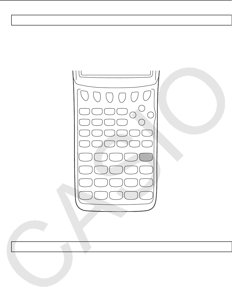
8-16
k 输入 /输出命 令(I/O)
Getkey
功能: 该命令返回与上次按键相对应的代码。
语法: Getkey _
描述:
• 该命令返回与上次按键相对应的代码。
• 如果再执行该命令之前没有按键,则返回数值0。
• 该命令可在一个循环内使用。
Locate
功能: 该命令在文本屏幕的特定位置上显示字母数字字符。
语法: Locate <列编号>, <行编号>, <数值>
Locate <列编号>, <行编号>, <数值表达式>
Locate <列编号>, <行编号>, "<字符串>"
[示例] Locate 1, 1, "AB" _
参数:
• 行编号:从1至7的数字
• 列编号:从1至21的数字
• 数值和数值表达式
• 字符串
71
72
73
74
75
76
61
62
63
64
65
66
51
52
53
54
55
56
41
42
43
44
45
46
31
32
33
35 25
36 26
77
78
79
67
68
69
57
58
59
47
27
48 28
49
37
38
39 29

8-17
描述:
• 该命令在文本屏幕的特定位置上显示数值(包括变量内容)或者文本。如果有计算输入,显示
该计算结果。
• 行数介于1至7之间,列数介于1至21之间。
示例: Cls _
Locate 7, 1, "CASIO FX"
该程序在屏幕中央显示“CASIO FX”。
• 在某些情况下,应该在运行上述程序之前执行ClrText命令。
Receive( / Send(
功能: 该命令接收连接设备的数据或向连接设备发送数据。
语法: Receive(<数据>) / Send(<数据>)
描述:
• 该命令接收连接设备的数据或向连接设备发送数据。
• 可通过该命令接收(发送)下述类型的数据。
• 代入变量的单个数值
• 矩阵数据(所有数值 - 不可指定单个数值)
• 列表数据(所有数值 - 不可指定单个数值)
OpenComport38k / CloseComport38k
功能: 打开和关闭三针COM端口(串行)。
描述: 参见下面的Receive38k/Send38k命令。
Receive38k / Send38k
功能: 以38 kbps的数据传输率执行数据发送和接收操作。
语法: Send38k <表达式>
<变量名称>
Receive38k
<列表名称>
描述:
• 在执行该命令之前必须执行OpenComport38k命令。
• 在执行该命令之后必须执行CloseComport38k命令。
• 如果在没有连接通信电缆时执行该命令,程序将继续执行且不产生错误。
← (21, 1)
← (21, 7)
(1, 1) →
(1, 7) →

8-18
k 有条 件 转 移关 系算子(REL)
= 、 、 > 、 < 、 、
功能: 这些关系算子可与有条件转移命令一起使用。
语法: <左侧> <关系算子> <右侧>
参数:
• 左侧/右侧:变量(A至Z、
r、
θ
)、数值常数、变量表达式(例如:A × 2)
• 关系算子: =、 、>、<、 、
k 字 符串
字符串是一系列由双引号包括的字符。在程序中,字符串用于指定显示文本。由数字(例如"123")
或者表达式(例如"
x
- 1")构成的字符串不可作为计算式处理。
如需在屏幕的特定位置上显示一个字符串,使用Locate命令(第8-16页)。
• 如需在字符串中包括双引号(")或者反斜线(\),在双引号(")或者反斜线(\)之前输入
一个反斜线(\)。
例1: 在字符串中包含Japan:“Tokyo”
"Japan:\"Tokyo\""
例2: 在字符串中包含main\abc
"main\\abc"
您可以在 PRGM 模式中按下 6(CHAR) 2(SYBL),从显示的菜单输入一个反斜线;也可在按下
!e(CATALOG)时,从显示的字符串类别中输入一个反斜线。
• 您可将字符串指定给字符串存储器(Str 1至Str 20)。关于字符串的详情,请参见“字符串
存储器”(第2-7页)。
• 您可使用“+”命令(第8-20页)在一个自变量内部连接字符串。
•
字符串函数(Exp(、StrCmp(等等)中的函数或者命令作为单独的字符进行处理。例如,“sin”
函数作为一个单独字符进行处理。
Exp(
功能: 将字符串转换为表达式并执行该表达式。
语法: Exp("<字符串>"[)]
Exp
'
Str(
功能: 将一个图形表达式转换为字符串,并将其代入指定的变量。
语法: Exp 'Str(<公式>, <字符串变量名称>[)]
描述: 图形表达式(Y
n
、r、X
t
、Y
t
、X)、递归公式( an、 an+1
、 an+2
、 bn、 bn+1
、 bn+2
、 cn、
cn+1
、 cn+2
)或者函数存储器(f
n
)可作为第一个自变量(<公式>)。
StrCmp(
功能: 比较“<字符串1>”和“<字符串2>”(字符代码比较)。
语法: StrCmp("<字符串1>", "<字符串2>"[)]
描述: 比较两个字符串并返回以下某一个值。

8-19
“<字符串1>” = “<字符串2>”时,返回0。
“<字符串1>” > “<字符串2>”时,返回1。
“<字符串1>” < “<字符串2>”时,返回-1。
Strlnv(
功能: 颠倒字符串的顺序。
语法: StrInv("<字符串>"[)]
StrJoin(
功能: 连接“<字符串1>”和“<字符串2>”。
语法: StrJoin("<字符串1>", "<字符串2>"[)]
注意: 使用“+”命令也可达到同样结果(第8-20页)。
StrLeft(
功能: 复制一个字符串中从左侧到第
n个字符的部分。
语法: StrLeft("<字符串>",
n[)] (0 < n < 9999, n是一个自然数)
StrLen(
功能: 返回字符串的长度(字符个数)。
语法: StrLen("<字符串>"[)]
StrLwr(
功能: 将字符串的所有字符转换为小写字符。
语法: StrLwr("<字符串>"[)]
StrMid(
功能: 提取一个字符串中从第
n到第 m个字符。
语法: StrMid("<字符串>",
n [, m)] (0 < n < 9999, n是一个自然数)
描述: 如果省略“
m”,将提取从第 n个字符到字符串末尾的部分。
StrRight(
功能: 复制一个字符串中从右侧到第
n个字符的部分。
语法: StrRight("<字符串>",
n[)] (0 < n < 9999, n是一个自然数)
StrRotate(
功能: 在字符串中第
n个字符处调换左侧与右侧部分。
语法: StrRotate("<字符串>", [,
n)] (-9999 < n < 9999, n是一个整数)
描述: 当“
n”为正值时,向左调换;当“ n”为负值时,向右调换。如果省略“ n”,默认值
为+1。
示例: StrRotate("abcde", 2) ........ 返回字符串“cdeab”。

8-20
StrShift(
功能: 将字符串向左或者向右平移
n个字符。
语法: StrShift("<字符串>", [,
n)] (-9999 < n < 9999, n是一个整数)
描述: 当“
n”为正值时,向左调换;当“ n”为负值时,向右调换。如果省略“ n”,默认值
为+1。
示例: StrShift("abcde", 2) ........ 返回字符串“cde”。
StrSrc(
功能: 从指定点(从字符串开始位置第
n个字符)搜索“<字符串1>”,确定该字符串是否包
含“<字符串2>”指定的数据。如果找到该数据,该命令返回“<字符串2>”第一个字符的位
置,并从“<字符串1>”的开始位置计数。
语法: StrSrc("<字符串1>", "<字符串2>"[,
n)] (0 < n < 9999, n是一个自然数)
描述: 如果省略起点,搜索从“<字符串1>”的起始位置开始。
StrUpr(
功能: 将字符串的所有字符转换为大写字符。
语法: StrUpr("<字符串>"[)]
+
功能: 连接“<字符串1>”和“<字符串2>”。
语法: "<字符串1>"+"<字符串2>"
示例: "abc"+"de" → Str 1 ............................ 将“abcde”代入Str 1。
k 其他
RclCapt
功能: 显示由捕捉存储器编号指定的内容。
语法: RclCapt <捕捉存储器编号> (捕捉存储器编号:1至20)

8-21
6. 在程序中使用计算器功能
k 文本显示
您只需在双引号之间加上程序,即可包括程序中的文本。
在程序执行期间,显示屏上会出现此类文本,表示您可以向输入提示与结果添加标签。
程序 显示
"CASIO" CASIO
? → X ?
"X =" ? → X X = ?
• 如果文本后面是计算公式,必须在文本与计算式之间插入显示命令( ^) 。
• 如果输入字符超过21个,文本移至下一行。如果文本超过21个字符,屏幕自动滚动。
• 注释文本最多可指定255个字节。
k 在程 序中使 用矩 阵行 运 算 (fx-7400G II 中不包括)
利用这些命令,您可操纵程序中的矩阵行。
• 对于该程序,进入 RUN • MAT 模式,然后使用矩阵编辑器输入矩阵,然后进入 PRGM 模式输入
程序。
u 交 换两 行 内容(Swap)
例1 交换下述矩阵的行2与行3的值:
矩阵A =
1 2
3 4
5 6
下面是用于该程序的语法。
Swap A , 2 , 3 _
需要交换的行
矩阵名称
Mat A
执行该程序后产生以下结果。

8-22
u 计 算 标 量 积( `Row)
例2 计算例1中的矩阵行2与标量4之积
下面是用于该程序的语法。
`Row 4 , A , 2 _
行
矩阵名称
乘数
Mat A
u 计算 标 量 积 并 将结 果 加 到另一行( `Row+)
例3 计算例1中矩阵行2与标量4的积,并将结果加到行3上
下面是用于该程序的语法。
`Row+ 4 , A , 2 , 3 _
需要相加的行
需要计算标量积的行
矩阵名称
乘数
Mat A
u 将两 行 相 加(Row+)
例4 将例1中的矩阵行2加到行3上
下面是用于该程序的语法。
Row+ A , 2 , 3 _
被加行的编号
相加行的编号
矩阵名称
Mat A
k 在程序中使用图形函数
您可将图形函数加入程序,绘制复杂图形并使图形相互叠加。下面显示了使用图形函数进行编
程时需要使用的各种类型的语法。
• 视窗 View Window -5, 5, 1, -5, 5, 1 _
• 图形函数输入 Y = Type _ .................... 指定图形类型。
"X
2
- 3" → Y1*
1
_
• 图形绘制操作 DrawGraph _
*
1
使用 J4(GRPH) 1(Y) b输入该Y1(显示为 )。如果使用计算器按键输入“Y”,
会产生一个错误(Syntax ERROR)。

8-23
u 其 它 绘 图 函 数 的 语 法
• V-Window View Window <Xmin>, <Xmax>, <Xscale>, <Ymin>, <Ymax>, <Yscale>,
<T
θ
min>, <T
θ
max>, <T
θ
pitch>
StoV-Win <视窗区域> ................................ 区域:1至6
RclV-Win <视窗区域> ................................. 区域:1至6
• Zoom Factor <X系数>, <Y系数>
ZoomAuto .............................................................. 无参数
• Pict StoPict < 图片区域 > ......................................... 区域:1至6
数值表达式
RclPict < 图片区域 > ......................................... 区域:1至6
数值表达式
• Sketch PlotOn <X坐标>, <Y坐标>
PlotOff <X坐标>, <Y坐标>
PlotChg <X坐标>, <Y坐标>
PxlOn <行编号>, <列编号>
PxlOff <行编号>, <列编号>
PxlChg <行编号>, <列编号>
PxlTest <行编号>, <列编号>
Text <行编号>, <列编号>, "<文本>"
Text <行编号>, <列编号>, <表达式>
SketchThick <Sketch或Graph语句>
SketchBroken <Sketch或Graph语句>
SketchDot <Sketch或Graph语句>
SketchNormal <Sketch或Graph语句>
Tangent <函数>, <X坐标>
Normal <函数>, <X坐标>
Inverse <函数>
Line
F-Line <X坐标1>, <Y坐标1>, <X坐标2>, <Y坐标2>
Circle <圆心X坐标>, <圆心Y坐标>, <半径R值>
Vertical <X坐标>
Horizontal <Y坐标>
k 在程序中使用动态图形函数
在程序中使用动态图形函数可执行重复的动态图形运算。下面说明如何在程序内指定动态图形
范围。
• 动态图形范围
1 → D Start _
5 → D End _
1 → D pitch _

8-24
k 在程 序中使 用表 格和 图 形 函 数
程序中的表格和图形函数可生成数值表格并执行绘图操作。下面显示了使用表格和图形函数进
行编程时需要使用的各种类型的语法。
• 表格范围设置 • 图形绘制操作
1 → F Start _ 连接类型:DrawFTG-Con _
5 → F End _ 描点类型:DrawFTG-Plt _
1 → F pitch _
• 数值表格生成
DispF-Tbl _
k 在程序中使用递归表格和图形函数
在程序中加入递归表格和图形函数可生成数值表格并执行绘图操作。下面显示了使用递归表格
和图形函数进行编程时需要使用的各种类型的语法。
• 递归公式输入
a
n+1
Type _ .... 指定递归类型。
"3
an + 2" → an+1
_
"4
bn + 6" → bn+1
_
• 表格范围设置 • 数值表格生成
1 → R Start _ DispR-Tbl _
5 → R End _ • 图形绘制操作
1 →
a0
_ 连接类型:DrawR-Con _, DrawR Σ -Con _
2 →
b0
_ 描点类型:DrawR-Plt _, DrawR Σ -Plt _
1 →
an Start _ • 统计收敛/发散图形(WEB图形)
3 →
bn Start _ DrawWeb an+1
, 10 _
k 在程 序中使 用列表 排序函 数
利用这些函数,您可以升序或降序排列列表中的数据。
• 升序
1 2
SortA ( List 1, List 2, List 3 )
被排序的列表(最多可指定六个列表)
1 431
2 K11
• 降序
3
SortD ( List 1, List 2, List 3 )
被排序的列表(最多可指定六个列表)
3 432

8-25
k 在程 序中使 用统计 计算 和图形
在程序中加入统计计算和绘图功能可计算统计数据并绘制图形。
u 设 置 条 件 和绘 制 统 计图 形
在StatGraph命令之后(“S-Gph1”、“S-Gph2”或“S-Gph3”),您必须指定以下图形条
件:
• 图形绘制/非绘制状态(DrawOn/DrawOff)
• 图形类型(Graph Type)
•
x轴数据位置(列表名称)
•
y轴数据位置(列表名称)
• 频率数据位置(列表名称)
• 标记类型(Mark Type)
• 饼图显示设置(%或者数据)
• 饼图百分比数据存储列表规定(无或列表名称)
• 第一个条线图数据(列表名称)
• 第二个和第三个条线图数据(列表名称)
• 条线图定向(长度(Length)或者水平(Horizontal))
规定的图形条件取决于图形类型。参见“更改图形参数”(第6-1页)。
• 下面是散布图或
xyLine图的典型图形条件规定。
S-Gph1 DrawOn, Scatter, List 1, List 2, 1, Square _
对于
xy直线图,将上述规定中的“Scatter”替换为“ xyLine”。
• 下面是正态概率图的典型图形条件规定。
S-Gph1 DrawOn, NPPlot, List 1, Square _
• 下面是单变量图形的典型图形条件规定。
S-Gph1 DrawOn, Hist, List 1, List 2 _
相同的格式可用于下述类型的图形,只要将上述规定中的“Hist”替换为适当的图形类型。
直方图 ............................................. Hist 正态分布 ............................................... N-Dist
中位值矩形框 ............................ MedBox*
1
虚线 ........................................................... Broken
*
1
Outliers:On Outliers:Off
S-Gph1 DrawOn, MedBox, List 1, 1, 1 S-Gph1 DrawOn, MedBox, List 1, 1, 0
• 下面是回归图形的典型图形条件规定。
S-Gph1 DrawOn, Linear, List 1, List 2, List 3 _
相同的格式可用于下述类型的图形,只要将上述规定中的“Linear”替换为适当的图形类型。
线性回归 ....................................... Linear 对数回归 ............................................... Log
Med-Med ....................................... Med-Med 指数回归 ............................................... ExpReg(a・eˆb
x)
二次回归 ....................................... Quad ExpReg(a・bˆ
x)
三次回归 ....................................... Cubic 幂回归 ..................................................... Power
四次回归 ....................................... Quart
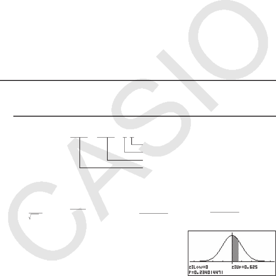
8-26
• 下面是正弦回归图形的典型图形条件规定。
S-Gph1 DrawOn, Sinusoidal, List 1, List 2 _
• 下面是逻辑回归图形的典型图形条件规定。
S-Gph1 DrawOn, Logistic, List 1, List 2 _
• 下面是饼图的典型图形条件规定。
S-Gph1 DrawOn, Pie, List 1, %, None _
• 下面是条线图的典型图形条件规定。
S-Gph1 DrawOn, Bar, List 1, None, None, StickLength _
• 如需绘制统计图形,在图形条件规定行后插入“DrawStat”命令。
ClrGraph
S-Wind Auto
{1, 2, 3} → List 1
{1, 2, 3} → List 2
S-Gph1 DrawOn, Scatter, List 1, List 2, 1, Square _
DrawStat
k 在程序中使用分布图形 (fx-7400G II 中不包括)
在程序中使用特殊命令绘制分布图形。
• 绘制累积正态分布图形
1 DrawDistNorm < Lower >, < Upper > [,
σ
, ƫ]
总体平均值 *
1
总体标准差 *
1
数据上限
数据下限
1 4151
*
1
该项可省略。如果省略这些项目,在执行计算时使用 Ʊ = 1且 ƫ = 0。
• 如果执行DrawDistNorm,将按照指定条件执行上述计算并
绘制图形。此时,填充图形上的ZLow <
x < ZUp区域 。
• 同时,
p、ZLow和ZUp计算结果值分别指定给变量 p、ZLow和ZUp,而 p指定给Ans。
πσ
2
p = dx
1e–
22
σ
(x–μ)2
μ
Upper
Lower
∫
ZUp =
σ
Upper –
μ
ZLow =
σ
Lower –
μ
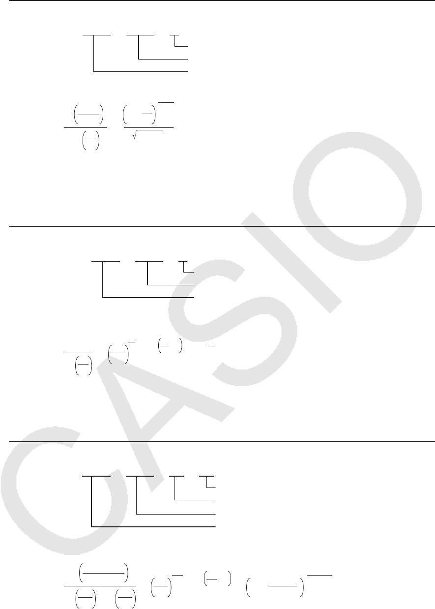
8-27
• 绘制学生- t累积分布图形
1 DrawDistT < Lower >, < Upper >, < df>
自由度
数据上限
数据下限
1 4152
• 如果执行DrawDistT,将按照指定条件执行上述计算并绘制图形。此时,填充图形上的
Lower <
x < Upper区域 。
• 同时,
p计算结果值、Lower和Upper输入值分别指定给变量 p、tLow和tUp,而 p指定给
Ans。
• 绘制 Ƶ2
累积分布图形
1 DrawDistChi < Lower >, < Upper >, < df>
自由度
数据上限
数据下限
1 4153
• 如果执行DrawDistChi,将按照指定条件执行上述计算并绘制图形。此时,填充图形上的
Lower <
x < Upper区域 。
• 同时,计算结果
p指定给变量 p和Ans。
• 绘制 F累积分布图形
1 DrawDistF < Lower >, < Upper >, < ndf>, < ddf>
分母自由度
分子自由度
数据上限
数据下限
1 4154
• 如果执行DrawDistF,将按照指定条件执行上述计算并绘制图形。此时,填充图形上Lower <
x < Upper区域。
• 同时,计算结果
p指定给变量 p和Ans。
tLow = Lower tUp = Uppe
r
Γ2
df + 1
df
x2
1 +
df + 1
2
p = ×
–
Γ2
df dx
df
×
π
Upper
Lower
∫
1
p = ×
Γ2
df
df
2df
2××
2
1dxx – 1 x
2
e–
Upper
Lower
∫
ndf
2ndf
2
p = ×××
–
Γ2
ndf +ddf
×
Γ2
ndf Γ2
ddf ddf
ndf
ndf + ddf
2
ddf
ndf × xdxx – 1 1 +
Upper
Lower
∫

8-28
k 在程 序中执行 统计 计算
• 单变量统计计算
1 1-Variable List1 , List 2
频率数据(Frequency)
x轴数据(XList)
1 4161
• 双变量统计计算
1 2-Variable List 1 , List 2 , List 3
频率数据(Frequency)
y 轴数据(YList)
x轴数据(XList)
1 4162
• 回归统计计算
1LinearReg(a x+b) List 1 , List 2 , List 3
频率数据(Frequency)
y 轴数据(YList)
x轴数据(XList)
1 416611
* 下述任何一种类型都可指定为计算类型。
LinearReg(a
x+b) ........ 线性回归( ax+ b类型)
LinearReg(a+b
x) ........ 线性回归( a+ bx类型)
Med-MedLine ............... Med-Med计算
QuadReg ........................... 二次回归
CubicReg ........................... 三次回归
QuartReg .......................... 四次回归
LogReg ................................ 对数回归
ExpReg(a・eˆb
x) ........ 指数回归( a・ ebx类型)
ExpReg(a・bˆ
x) ........... 指数回归( a・ bx类型)
PowerReg ......................... 幂回归
• 正弦回归统计计算
SinReg List 1 , List 2
y轴数据(YList)
x轴数据(XList)
• 逻辑回归统计计算
LogisticReg List 1 , List 2
y轴数据(YList)
x轴数据(XList)
计算类型*

8-29
k 在程序中执行分布计算 (fx-7400G II中不包括)
• 只要省略方括号([ ])中的任何值,则由以下值替代。
σ
=1,
ƫ=0,尾部=L(左侧)
• 关于每个概率密度函数的计算公式,请参见“统计公式”(第6-55页)。
• 正态分布
NormPD(: 返回指定数据的正态概率密度( p值)。
语法: NormPD(
x[,
σ
, ƫ)]
• 可为
x指定单个数值或者列表。计算结果 p指定给变量 p和Ans(当 x是列表时,为ListAns)。
NormCD(: 返回指定数据的累积正态分布(
p值)。
语法: NormCD(Lower, Upper[,
σ
, ƫ)]
• 可为Lower 和Upper指定单个数值或者列表。计算结果
p、ZLow和ZUp分别指定给变
量
p、ZLow和ZUp。计算结果 p也指定给Ans(当Lower和Upper是列表时,为ListAns)。
InvNormCD(: 返回指定
p值的反向累积正态分布(下限及/或上限值)。
语法: InvNormCD([ "L(或-1) 或R(或1) 或 C(或0)" , ]
p[,
σ
, ƫ])
尾部(左侧、右侧、中间)
• 可为 p指定单个数值或者列表。计算结果按照下述尾部设置输出。
尾部 = 左侧
Upper值指定给变量
x1InvN和Ans(当 p是列表时,为ListAns)。
尾部 = 右侧
Lower值指定给变量
x1InvN和Ans(当 p是列表时,为ListAns)。
尾部 = 中间
Lower和Upper值分别指定给变量
x1InvN和 x2InvN。
Lower仅指定给Ans(当
p是列表时,为ListAns)。
• 学生- t分布
tPD(: 返回指定数据的学生- t概率密度( p值)。
语法: tPD(
x, df [)]
• 可为
x指定单个数值或者列表。计算结果 p指定给变量 p和Ans(当 x是列表时,为ListAns)。
tCD(: 返回指定数据的学生-
t累积分布( p值)。
语法: tCD(Lower,Upper,
df [)]
• 可为Lower 和Upper指定单个数值或者列表。计算结果
p、tLow和tUp分别指定给变量 p, tLow
和tUp。计算结果
p也指定给Ans(当Lower和Upper是列表时,为ListAns)。
InvTCD(: 返回指定
p值的反向学生- t累积分布(Lower值)。
语法: InvTCD(
p, df [)]
• 可为
p指定单个数值或者列表。Lower值指定给 xInv和Ans变量(当 p是列表时,为ListAns)。

8-30
• Ƶ2
分布
ChiPD(: 返回指定数据的 Ƶ2
概率密度( p值)。
语法: ChiPD(
x, df [)]
• 可为
x指定单个数值或者列表。计算结果 p指定给变量 p和Ans(当 x是列表时,为ListAns)。
ChiCD(: 返回指定数据的
Ƶ2
累积分布( p值)。
语法: ChiCD(Lower,Upper,
df [)]
• 可为Lower和Upper指定单个数值或者列表。计算结果
p指定给变量 p和Ans(当Lower和Upper
是列表时,为ListAns)。
InvChiCD(: 返回指定
p值的反向 Ƶ2
累积分布(Lower值)。
语法: InvChiCD(
p, df [)]
• 可为
p指定单个数值或者列表。Lower值指定给 xInv和Ans变量(当 p是列表时,为ListAns)。
• F分布
FPD(: 返回指定数据的 F概率密度( p值)。
语法: FPD(
x, ndf, ddf [)]
• 可为
x指定单个数值或者列表。计算结果 p指定给变量 p和Ans(当 x是列表时,为ListAns)。
FCD(: 返回指定数据的
F累积分布( p值)。
语法: FCD(Lower,Upper,
ndf, ddf [)]
• 可为Lower和Upper指定单个数值或者列表。计算结果
p指定给变量 p和Ans(当Lower和Upper
是列表时,为ListAns)。
InvFCD(: 返回指定数据的反向
F累积分布(Lower值)。
语法: InvFCD(
p, ndf, ddf [)]
• 可为
p指定单个数值或者列表。Lower值指定给 xInv和Ans变量(当 p是列表时,为ListAns)。
• 二项分布
BinomialPD(: 返回指定数据的二项概率( p值)。
语法: BinomialPD([
x,] n,P[)]
• 可为
x指定单个数值或者列表。计算结果 p指定给变量 p和Ans(当 x是列表时,为ListAns)。
BinomialCD(: 返回指定数据的二项累积分布(
p值)。
语法: BinomialCD([X,]
n,P[)]
• 可为每个X指定单个数值或者列表。计算结果
p指定给变量 p和Ans(当省略X或X是列表时,
为ListAns)。
InvBinomialCD(: 返回指定数据的反向二项累积分布。
语法: InvBinomialCD(
p, n,P[)]
• 可为
p指定单个数值或者列表。计算结果X值指定给 xInv和Ans变量(当 p是列表时,为
ListAns)。

8-31
• 泊松分布
PoissonPD(: 返回指定数据的泊松概率( p值)。
语法: PoissonPD(
x, [)]
• 可为
x指定单个数值或者列表。计算结果 p指定给变量 p和Ans(当 x是列表时,为ListAns)。
PoissonCD(: 返回指定数据的泊松累积分布(
p值)。
语法: PoissonCD(X,
[)]
• 可为每个X指定单个数值或者列表。计算结果
p指定给变量 p和Ans(当X是列表时,为
ListAns)。
InvPoissonCD(: 返回指定数据的反向泊松累积分布。
语法: InvPoissonCD(
p, [)]
• 可为
p指定单个数值或者列表。计算结果X值指定给 xInv和Ans变量(当 p是列表时,为
ListAns)。
• 几何分布
GeoPD(: 返回指定数据的几何概率( p值)。
语法: GeoPD(
x, P[)]
• 可为
x指定单个数值或者列表。计算结果 p指定给变量 p和Ans(当 x是列表时,为ListAns)。
GeoCD(: 返回指定数据的几何累积分布(
p值)。
语法: GeoCD(X,P[)]
• 可为每个X指定单个数值或者列表。计算结果
p指定给变量 p和Ans(当X是列表时,为
ListAns)。
InvGeoCD(: 返回指定数据的反向几何累积分布。
语法: InvGeoCD(
p,P[)]
• 可为
p指定单个数值或者列表。计算结果X值指定给 xInv和Ans变量(当 p是列表时,为
ListAns)。
• 超几何分布
HypergeoPD(: 返回指定数据的超几何概率( p值)。
语法: HypergeoPD(
x, n, M, N[)]
• 可为
x指定单个数值或者列表。计算结果 p指定给变量 p和Ans(当 x是列表时,为ListAns)。
HypergeoCD(: 返回指定数据的超几何累积分布(
p值)。
语法: HypergeoCD(X,
n, M, N[)]
• 可为每个X指定单个数值或者列表。计算结果
p指定给变量 p和Ans(当X是列表时,为
ListAns)。

8-32
InvHypergeoCD(: 返回指定数据的反向超几何累积分布。
语法: InvHypergeoCD(
p, n, M, N[)]
• 可为
p指定单个数值或者列表。计算结果X值指定给 xInv和Ans变量(当 p是列表时,为
ListAns)。
k 在程序中使用TEST命令执行某个命令 (fx-7400G II 中不包括)
• 下面是该命令“
ƫ条件”自变量的规定范围。
“<”或-1,当
ƫ < ƫ0
“ ”或0,当 ƫ ƫ0
“>”或1,当 ƫ > ƫ0
上述规定也适用于“
ρ
条件”和“ ơ&
ρ
条件”规定方法。
• 如需了解此处未详述的自变量,请参见“测试”(第6-23页)和“测试、置信区间和分布的输
入和输出项”(第6-52页)。
• 关于每个命令的计算公式,请参见“统计公式”(第6-55页)。
• Z测试
OneSample ZTest: 执行1-样本 Z-测试计算。
语法: OneSample
ZTest " ƫ条件", ƫ0
,
σ
, o, n
输出值: Z、 p、 o、 n分别指定给变量 z、 p、 o、 n和ListAns元素1至4。
语法: OneSample
ZTest " ƫ条件", ƫ0
,
σ
, List[, Freq]
输出值:
Z、 p、 o、s
x、 n分别指定给变量 z、 p、 o、s
x、 n和ListAns元素1至5。
TwoSample ZTest: 执行2-样本 Z-测试计算。
语法: TwoSample
ZTest " ƫ1
条件",
σ
1
,
σ
2, o1
, n1
, o2
, n2
输出值: Z、 p、 o1
、 o2
、 n1
、 n
2
分别指定给变量 z、 p、 o1
、 o2
、 n1
、 n
2
和ListAns元
素1至6。
语法: TwoSample
ZTest " ƫ1
条件",
σ
1
,
σ
2, List1, List2[, Freq1 [, Freq2]]
输出值:
Z、 p、 o1
、 o2
、
s
x1
、s
x2
、 n1
、 n2
分别指定给变量 z、 p、 o1
、 o2
、
s
x1
、s
x2
、
n1
、 n2
和ListAns元素1至8。
OneProp ZTest: 执行1-比例 Z-测试计算。
语法: OneProp
ZTest " p条件", p0
, x, n
输出值: Z、 p、 pˆ、 n分别指定给变量 z、 p、 pˆ、 n 和ListAns元素1至4。
TwoProp ZTest: 执行2-比例 Z-测试计算。
语法: TwoProp
ZTest " p1
条件", x1
, n1
, x2
, n2
输出值: Z、 p、 pˆ
1
、 pˆ
2
、 pˆ、 n
1
、 n
2
分别指定给变量 z、 p、 pˆ
1
、 pˆ
2
、 pˆ、 n
1
、 n
2
和
ListAns元素1至7。

8-33
• t测试
OneSampleTTest: 执行1-样本 t-测试计算。
语法: OneSampleTTest "
ƫ
条件", ƫ0
, o, s
x, n
OneSampleTTest "
ƫ
条件", ƫ0
, List[, Freq]
输出值:
t、 p、 o、s
x、 n分别指定给相同名称的变量和ListAns元素1至5。
TwoSampleTTest: 执行2-样本 t-测试计算。
语法: TwoSampleTTest "
ƫ1
条件", o1
, s
x1
, n1
, o2
, s
x2
, n2
[,Pooled条件]
TwoSampleTTest "
ƫ1
条件", List1, List2, [, Freq1[, Freq2[, Pooled条件]]]
输出值: 当Pooled条件 = 0时,
t、 p、 df、 o1
、 o2
、s
x1
、s
x2
、 n1
、 n2
分别指定给相同
名称的变量和ListAns元素1至9。
当Pooled条件 = 1时, t、 p、 df、 o1
、 o2
、s
x1
、s
x2
、s
p、 n1
、 n2
分别指定给
相同名称的变量和ListAns元素1至10。
注意: 如果想要关闭Pooled条件,指定0;如果想要开启该条件,指定1。省略输
入则视为关闭Pooled条件。
LinRegTTest: 执行线性回归 t-测试计算。
语法: LinRegTTest "
ơ&
ρ
条件", XList, YList[, Freq]
输出值:
t、 p、 df、 a、b、s、r、r
2
分别指定给相同名称的变量和ListAns元素1至8。
• Ƶ2
测试
ChiGOFTest: 执行拟合优度卡方测试。
语法: ChiGOFTest List 1, List 2, df, List 3
(List 1是Observed列表,List 2是Expected列表,List 3是CNTRB列
表。)
输出值:
Ƶ2
、 p、 df分别指定给相同名称的变量和ListAns元素1至3。CNTRB列表保
存在List 3中。
ChiTest: 执行卡方测试。
语法: ChiTest MatA, MatB
(MatA是Observed矩阵,MatB是Expected矩阵。)
输出值:
Ƶ2
、 p、 df分别指定给相同名称的变量和ListAns元素1至3。Expected矩阵
指定给MatB。
• F测试
TwoSample FTest: 执行2-样本 F-测试计算。
语法: TwoSample
FTest "
σ
1
条件", s
x1
, n1
, s
x2
, n2
输出值: F、 p、s
x1
、s
x2
、 n1
、 n2
分别指定给相同名称的变量和ListAns元素1至6。
语法: TwoSample
FTest "
σ
1
条件", List1, List2, [, Freq1 [, Freq2]]
输出值:
F、 p、 o1
、 o2
、s
x1
、s
x2
、 n1
、 n2
分别指定给相同名称的变量和ListAns元素
1至8。

8-34
• ANOVA
OneWayANOVA: 执行单因素ANOVA方差分析。
语法: OneWayANOVA List1, List2 (List1 为Factor列表(A),List2为
Dependent列表。)
输出值: Adf, Ass, Ams, AF, Ap, ERRdf, ERRss, ERRms分别指定给变量Adf, SSa,
MSa, Fa, pa, Edf, SSe, MSe。
此外,输出值指定给MatAns,如下所示。
TwoWayANOVA: 执行二因素ANOVA方差分析。
语法: TwoWayANOVA List1, List2, List3(List1是Factor列表(A),List2是
Factor列表(B),List3是Dependent列表)
输出值: Adf、Ass、Ams、AF、Ap、Bdf、Bss、Bms、BF、Bp、ABdf、ABss、
ABms、ABF、ABp、ERRdf、ERRss、ERRms分别指定给变量Adf、
SSa、MSa、Fa、pa、Bdf、SSb、MSb、Fb、pb、ABdf、SSab、
MSab、Fab、pab、Edf、SSe、MSe。
此外,输出值指定给MatAns,如下所示。
k 在程序中执行财务计算 (fx-7400G II 中不包括)
• 设置命令
• 用于财务计算的日期模式设置
DateMode365 .......... 365天
DateMode360 .......... 360天
• 付款期限设置
PmtBgn ......................... 开始日期
PmtEnd ........................ 结束日期
• 债券计算付款周期
PeriodsAnnual ....... 一年
PeriodsSemi .............. 半年
MatAns = Adf
ERRdf
Ass
ERRss
Ams
ERRms
AF
0
Ap
0
MatAns =
Adf
Bdf
ABdf
ERRdf
Ass
Bss
ABss
ERRss
Ams
Bms
ABms
ERRms
AF
BF
ABF
0
Ap
Bp
ABp
0

8-35
• 财务计算命令
关于每个自变量的含义,请参见“第7章 财务计算(TVM)”。
• 单利
Smpl_SI: 根据单利计算返回利息。
语法: Smpl_SI(
n, I%, PV)
Smpl_SFV: 根据单利计算返回本金加利息总值。
语法: Smpl_SFV(
n, I%, PV)
• 复利
注意:
• 所有复利计算均可省略P/Y和C/Y。如果省略,计算时采用P/Y=12且C/Y=12。
• 如果您使用复利函数执行计算(Cmpd_n(、Cmpd_I%(、Cmpd_PV(、Cmpd_PMT(、Cmpd_
FV(),您输入的自变量和计算结果将保存到适当变量(
n, I%, PV等等)。如果您使用其他任
何类型的财务计算函数执行计算,自变量与计算结果不指定给变量。
Cmpd_n: 返回复利期数。
语法: Cmpd_
n( I%, PV, PMT, FV, P/Y, C/Y)
Cmpd_I%: 返回年利。
语法: Cmpd_
I%( n, PV, PMT, FV, P/Y, C/Y)
Cmpd_PV: 返回现值(分期付款时为贷款金额;储蓄时为本金)。
语法: Cmpd_PV(
n, I%, PMT, FV, P/Y, C/Y)
Cmpd_PMT: 返回固定时期相等的输入/输出值(分期付款时为付款金额;储蓄时为存款金
额)。
语法: Cmpd_PMT(
n, I%, PV, FV, P/Y, C/Y)
Cmpd_FV: 返回输入/输出终值或本金加利息总额。
语法: Cmpd_FV(
n, I%, PV, PMT, P/Y, C/Y)
• 现金流(投资评估)
Cash_NPV: 返回净现值。
语法: Cash_NPV(
I%, Csh)
Cash_IRR: 返回内部收益率。
语法: Cash_IRR(Csh)
Cash_PBP: 返回投资回收期。
语法: Cash_PBP(
I%, Csh)
Cash_NFV: 返回净终值。
语法: Cash_NFV(
I%, Csh)
• 分期偿还
Amt_BAL: 返回PM2每月还款之后的本金余额。
语法: Amt_BAL(PM1, PM2,
I%, PV, PMT, P/Y, C/Y)
Amt_INT: 返回PM1每月还款中支付的利息。

8-36
语法: Amt_INT(PM1, PM2,
I%, PV, PMT, P/Y, C/Y)
Amt_PRN: 返回 PM1每月还款中支付的本金加利息。
语法: Amt_PRN(PM1, PM2,
I%, PV, PMT, P/Y, C/Y)
Amt_ ∑ INT: 返回从PM1每月还款至PM2每月还款支付的本金加利息总额。
语法: Amt_ ∑ INT(PM1, PM2,
I%, PV, PMT, P/Y, C/Y)
Amt_ ∑ PRN: 返回从PM1每月还款至PM2每月还款支付的本金总额。
语法: Amt_ ∑ PRN(PM1, PM2,
I%, PV, PMT, P/Y, C/Y)
• 利率换算
Cnvt_EFF: 返回从名义利率到实际利率换算后的利率。
语法: Cnvt_EFF(
n, I%)
Cnvt_APR: 返回从实际利率到名义利率换算后的利率。
语法: Cnvt_APR(
n, I%)
• 成本、售价、毛利率计算
Cost: 返回根据指定售价和毛利率计算的成本。
语法: Cost(Sell, Margin)
Sell: 返回根据指定成本和毛利率计算的售价。
语法: Sell(Cost, Margin)
Margin: 返回根据指定成本和售价计算的毛利率。
语法: Margin(Cost, Sell)
• 日/日期计算
Days_Prd: 返回从指定d1到指定d2的天数。
语法: Days_Prd(MM1, DD1, YYYY1, MM2, DD2, YYYY2)
• 债券计算
Bond_PRC: 以列表形式返回根据指定条件计算的债券价格。
语法: Bond_PRC(MM1, DD1, YYYY1, MM2, DD2, YYYY2, RDV, CPN, YLD) = {PRC,
INT, CST}
Bond_YLD: 返回根据指定条件计算的收益率。
语法: Bond_YLD(MM1, DD1, YYYY1, MM2, DD2, YYYY2, RDV, CPN, PRC)
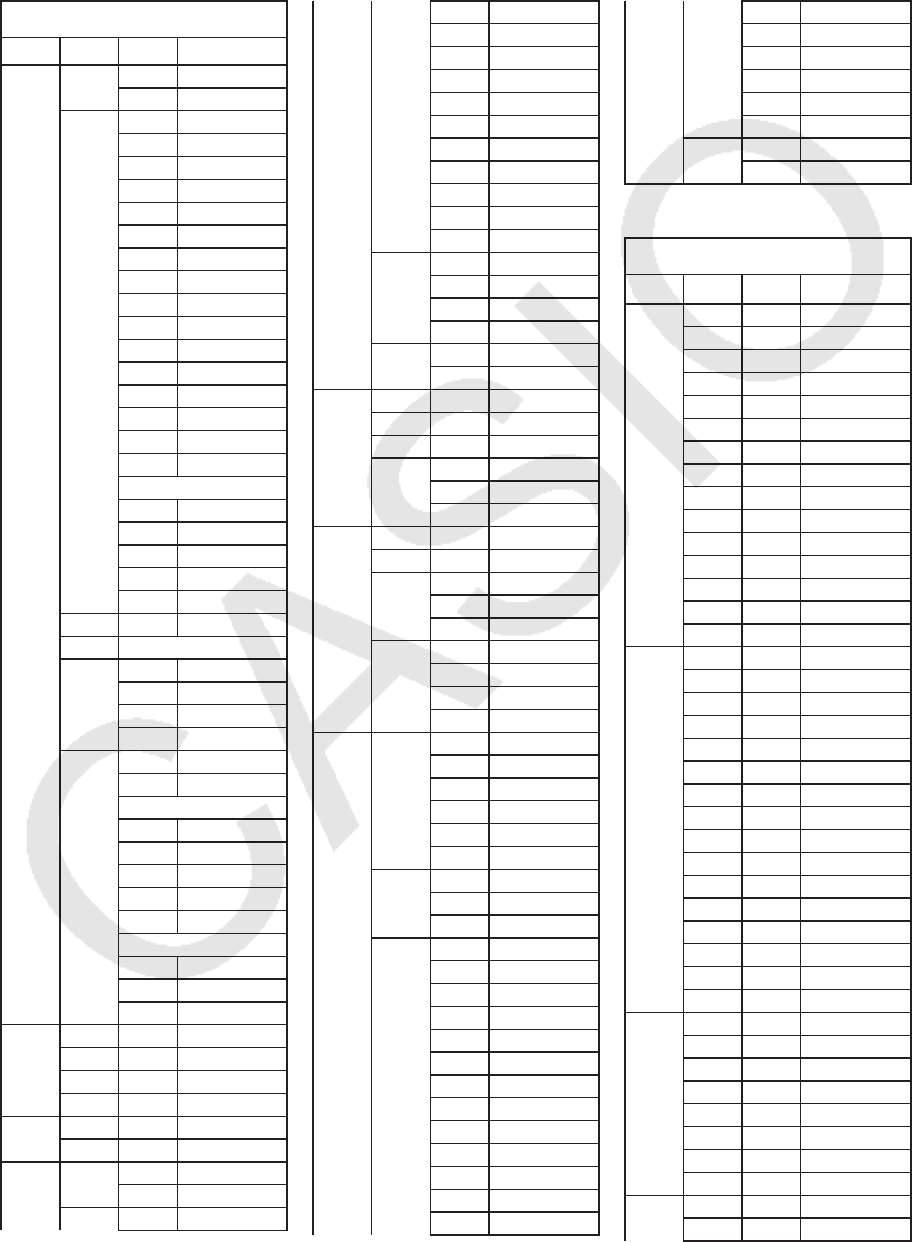
8-37
7. PRGM模式命令列表
本手册所述各型号不一定提供下列所有命令。
RUN程序
4(MENU) 键
1级 2级 3级 命令
STAT DRAW On DrawOn
Off DrawOff
GRPH GPH1 S-Gph1_
GPH2 S-Gph2_
GPH3 S-Gph3_
Scat Scatter
xy xyLine
Hist Hist
Box MedBox
Bar Bar
N-Dis N-Dist
Brkn Broken
XLinear
Med Med-Med
X^2 Quad
X^3 Cubic
X^4 Quart
Log Log
*1
Pwr Power
Sin Sinusoidal
NPP NPPlot
Lgst Logistic
Pie Pie
List List_
TYPE *2
DIST DrwN
DrawDistNorm_
Drwt DrawDistT_
DrwC DrawDistChi_
DrwF DrawDistF_
CALC 1VAR 1-Variable_
2VAR 2-Variable_
*3
Med Med-MedLine_
X^2 QuadReg_
X^3 CubicReg_
X^4 QuartReg_
Log LogReg_
*4
Pwr PowerReg_
Sin SinReg_
Lgst LogisticReg_
MAT Swap Swap_
×Rw `Row_
×Rw+ `Row+_
Rw+ Row+_
LIST Srt-A SortA(
Srt-D SortD(
GRPH SEL On G_SelOn_
Off G_SelOff_
TYPE Y=Y=Type
r=r=Type
Parm ParamType
X=X=Type
Y>Y>Type
Y<Y<Type
YtY
t
Type
YsY
s
Type
X>X>Type
X<X<Type
XtX
t
Type
XsX
s
Type
STYL
— NormalG_
— ThickG_
・・・・・
BrokenThickG_
······
DotG_
GMEM Sto StoGMEM_
Rcl RclGMEM_
DYNA On D_SelOn_
Off D_SelOff_
Var D_Var_
TYPE Y=Y=Type
r=r=Type
Parm ParamType
TABL On T_SelOn_
Off T_SelOff_
TYPE Y=Y=Type
r=r=Type
Parm ParamType
STYL
— NormalG_
— ThickG_
・・・・・
BrokenThickG_
······
DotG_
RECR SEL+S On R_SelOn_
Off R_SelOff_
— NormalG_
— ThickG_
・・・・・
BrokenThickG_
······
DotG_
TYPE a
n
a
n
Type
a
n+1
a
n+1
Type
a
n+2
a
n+2
Type
n.a
n..
nn
a
n
a
n
a
n+1
a
n+1
a
n+2
a
n+2
b
n
b
n
b
n+1
b
n+1
b
n+2
b
n+2
c
n
c
n
c
n+1
c
n+1
c
n+2
c
n+2
∑
a
n
∑
∑
a
n
∑
a
n+1
∑
∑
a
n+1
∑
a
n+2
∑
∑
a
n+2
∑
b
n
∑
∑
b
n
∑
b
n+1
∑
∑
b
n+1
∑
b
n+2
∑
∑
b
n+2
∑
c
n
∑
∑
c
n
∑
c
n+1
∑
∑
c
n+1
∑
c
n+2
∑
∑
c
n+2
RANG a
0
Sel_a
0
a
1
Sel_a
1
K键
1级 2级 3级 命令
LIST List List_
L→
MList
→
Mat(
Dim Dim_
Fill Fill(
Seq Seq(
Min Min(
Max Max(
Mean Mean(
Med Median(
Aug Augment(
Sum Sum_
Prod Prod_
Cuml Cuml_
%Percent_
A
A
List_
MAT Mat Mat_
M→
LMat
→
List(
Det Det_
Trn Trn_
Aug Augment(
Iden Identity_
Dim Dim_
Fill Fill(
Ref Ref_
Rref Rref_
Vct Vct_
DotP DotP(
CrsP CrossP(
Angle Angle(
UntV UnitV(
Norm Norm(
CPLX ii
Abs Abs_
Arg Arg_
Conj Conjg_
ReP ReP_
ImP ImP_
'r∠
θ
'r∠
θ
θ
'a+bi 'a+bi
CALC Solve Solve(
d/dx d/dx(
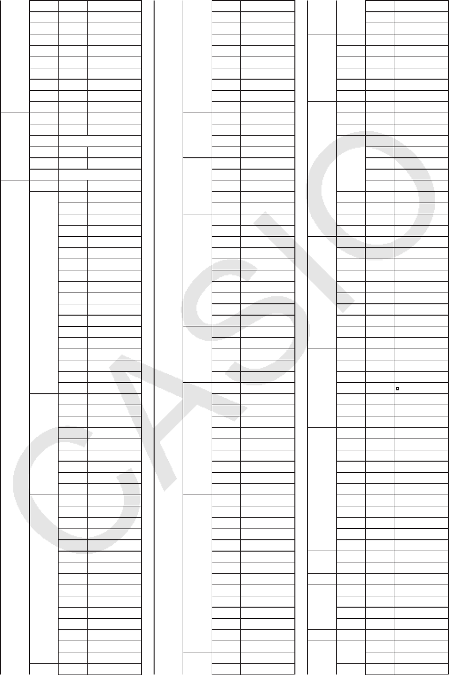
8-38
d
2
/dx
2
d
2
/dx
2
(
∫
dx
∫
∫
(
SolveN SolveN(
FMin FMin(
FMax FMax(
Σ
(
Σ
Σ
(
log
a
blog
a
b(
Int÷ Int÷
Rmdr Rmdr
Simp 'Simp
STAT xˆx
ˆ
yˆy
ˆ
DIST *5
S·Dev StdDev(
Var Variance(
TEST *6
CONV
''
LENG fm [fm]
Å[Å]
μm [μm]
mm [mm]
cm [cm]
m[m]
km [km]
AU [AU]
I.y. [I.y.]
pc [pc]
Mil [Mil]
in [in]
ft [ft]
yd [yd]
fath [fath]
rd [rd]
mile [mile]
n mile [n mile]
AREA cm² [cm²]
m² [m²]
ha [ha]
km² [km²]
in² [in²]
ft² [ft²]
yd² [yd²]
acre [acre]
mile² [mile²]
VLUM cm³ [cm³]
mL [mL]
L[L]
m³ [m³]
in³ [in³]
ft³ [ft³]
fl_oz(UK)
[fl_oz(UK)]
fl_oz(US)
[fl_oz(US)]
gal(US) [gal(US)]
gal(UK) [gal(UK)]
pt [pt]
qt [qt]
tsp [tsp]
tbsp [tbsp]
cup [cup]
TIME ns [ns]
μs [μs]
ms [ms]
s[s]
min [min]
h[h]
day [day]
week [week]
yr [yr]
s-yr [s-yr]
t-yr [t-yr]
TMPR
°
C[°
C]
K[K]
°
F[°
F]
°
R[°
R]
VELO m/s [m/s]
km/h [km/h]
knot [knot]
ft/s [ft/s]
mile/h [mile/h]
MASS u[u]
mg [mg]
g[g]
kg [kg]
mton [mton]
oz [oz]
lb [lb]
slug [slug]
ton(short)
[ton(short)]
ton(long)
[ton(long)]
RORC N[N]
lbf [lbf]
tonf [tonf]
dyne [dyne]
kgf [kgf]
PRES Pa [Pa]
kPa [kPa]
mmH
2
O[mmH
2
O]
mmHg [mmHg]
atm [atm]
inH
2
O[inH
2
O]
inHg [inHg]
lbf/in² [lbf/in²]
bar [bar]
kgf/cm² [kgf/cm²]
ENGY eV [eV]
J[J]
cal
th
[cal
th
]
cal
15
[cal
15
]
cal
IT
[cal
IT
]
kcal
th
[kcal
th
]
kcal
15
[kcal
15
]
kcal
IT
[kcal
IT
]
I-atm [I-atm]
kW
•
h[kW
•
h]
ft
•
lbf [ft
•
lbf]
Btu [Btu]
erg [erg]
kgf
•
m[kgf
•
m]
PWR W[W]
cal
th
/s [cal
th
/s]
hp [hp]
ft
•
lbf/s [ft
•
lbf/s]
Btu/min [Btu/min]
HYP sinh sinh_
cosh cosh_
tanh tanh_
sinh
–1
sinh
–1
_
cosh
–1
cosh
–1
_
tanh
–1
tanh
–1
_
PROB X! !
nPr P
nCr C
RAND Ran# Ran#_
Int RanInt#(
Norm RanNorm#(
Bin RanBin#(
List RanList#(
P( P(
Q( Q(
R( R(
t( t(
NUM Abs Abs_
Int Int_
Frac Frac_
Rnd Rnd
Intg Intg_
RndFi RndFix(
GCD GCD(
LCM LCM(
MOD MOD(
MOD
•
EMOD_Exp(
ANGL
°
°
°
rr
gg
°
’ ’’
Pol( Pol(
Rec( Rec(
'DMS 'DMS
ESYM mm
μμ
nn
pp
ff
kk
MM
GG
TT
PP
EE
PICT Sto StoPict_
Rcl RclPict_
FMEM fn fn
LOGIC And _And_
Or _Or_
Not Not_
Xor Xor_
CAPT Rcl RclCapt_
TVM SMPL SI Smpl_SI(
SFV Smpl_SFV(
CMPD nCmpd_n(

8-39
I% Cmpd_I%(
PV Cmpd_PV(
PMT Cmpd_PMT(
FV Cmpd_FV(
CASH NPV Cash_NPV(
IRR Cash_IRR(
PBP Cash_PBP(
NFV Cash_NFV(
AMT BAL Amt_BAL(
INT Amt_INT(
PRN Amt_PRN(
Σ
INT Amt_
Σ
INT(
Σ
PRN Amt_
Σ
PRN(
CNVT EFF Cnvt_EFF(
APR Cnvt_APR(
COST Cost Cost(
Sell Sell(
Mrg Margin(
DAYS PRD Days_Prd(
BOND PRC Bond_PRC(
YLD Bond_YLD(
J键
1级 2级 3级 命令
V-WIN X min Xmin
max Xmax
scal Xscl
dot Xdot
Y min Ymin
max Ymax
scal Yscl
T,
θ
min T
θ
θ
min
max T
θ
θ
max
ptch T
θ
θ
ptch
R-X min RightXmin
max RightXmax
scal RightXscl
dot RightXdot
R-Y min RightYmin
max RightYmax
scal RightYscl
R-T,
θ
min RightT
θ
θ
min
max RightT
θ
θ
max
ptch RightT
θ
θ
ptch
FACT Xfct Xfct
Yfct Yfct
STAT Xnn
xx
Σ
x
Σ
Σ
x
Σ
x
2
Σ
Σ
x
2
σ
x
σ
σ
x
s
x
s
x
minX minX
maxX maxX
Yyy
Σ
y
Σ
Σ
y
Σ
y
2
Σ
Σ
y
2
Σ
xy
Σ
Σ
xy
σ
y
σ
σ
y
s
y
s
y
minY minY
maxY maxY
GRPH aa
bb
cc
dd
ee
rr
r
2
r
2
MSe MSe
Q
1
Q
1
Med Med
Q
3
Q
3
Mod Mod
Strt H_Start
Pitch H_pitch
PTS x
1
x
1
y
1
y
1
x
2
x
2
y
2
y
2
x
3
x
3
y
3
y
3
INPT nn
xx
s
x
s
x
n1 n1
n2 n2
x
1
x
1
x
2
x
2
s
x1
s
x1
s
x2
s
x2
s
p
s
p
RESLT *7
GRPH YY
rr
Xt Xt
Yt Yt
XX
DYNA Strt D_Start
End D_End
Pitch D_pitch
TABL Strt F_Start
End F_End
Pitch F_pitch
Reslt F_Result
RECR FORM a
n
a
n
a
n+1
a
n+1
a
n+2
a
n+2
b
n
b
n
b
n+1
b
n+1
b
n+2
b
n+2
c
n
c
n
c
n+1
c
n+1
c
n+2
c
n+2
RANG Strt R_Start
End R_End
a
0
a
0
a
1
a
1
a
2
a
2
b
0
b
0
b
1
b
1
b
2
b
2
c
0
c
0
c
1
c
1
c
2
c
2
a
n
St a
n
Start
b
n
St b
n
Start
c
n
St c
n
Start
Reslt R_Result
EQUA S-Rlt Sim_Result
S-Cof Sim_Coef
P-Rlt Ply_Result
P-Cof Ply_Coef
TVM nn
I% I%
PV PV
PMT PMT
FV FV
P/Y P/Y
C/Y C/Y
Str Str_
!J(PRGM) 键
1级 2级 3级 命令
COM If If_
Then Then_
Else Else_
I-End IfEnd
For For_
To _To_
Step _Step_
Next Next
Whle While_
WEnd WhileEnd
Do Do
Lp-W LpWhile_
CTL Prog Prog_
Rtrn Return
Brk Break
Stop Stop
JUMP Lbl Lbl_
Goto Goto_
⇒
⇒
⇒
Isz Isz_
Dsz Dsz_
Menu Menu_
??
^^
CLR Text ClrText
Grph ClrGraph
List ClrList_
Mat ClrMat_
Vct ClrVct_
DISP Stat DrawStat
Grph DrawGraph
Dyna DrawDyna
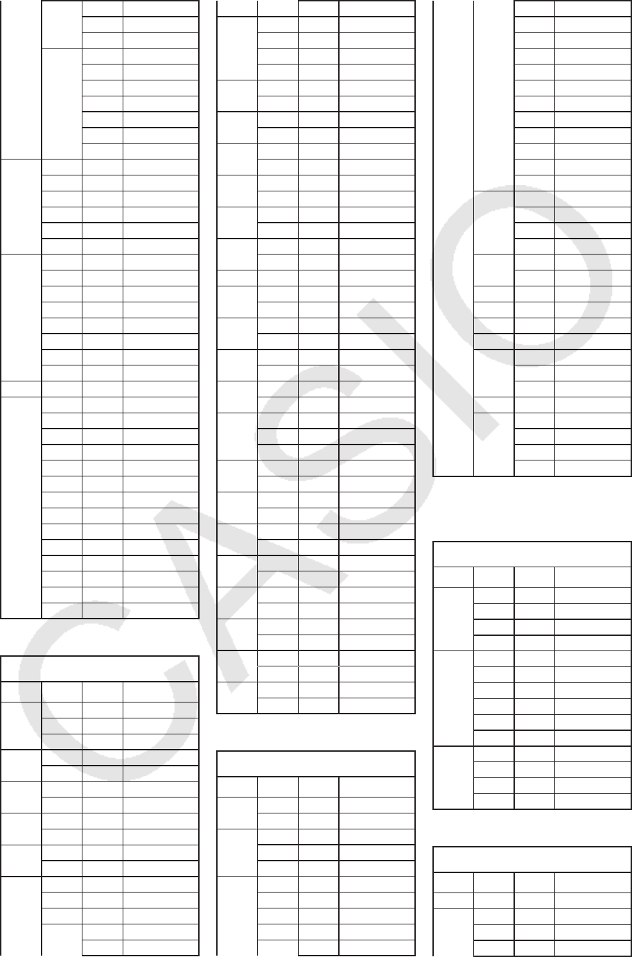
8-40
F-Tbl Tabl DispF-Tbl
G-Con DrawFTG-Con
G-Plt DrawFTG-Plt
R-Tbl Tabl DispR-Tbl
Phase PlotPhase
Web DrawWeb_
an-Cn DrawR-Con
Σ
a-Cn DrawR
Σ
Σ
-Con
an-Pl DrawR-Plt
Σ
a-Pl DrawR
Σ
Σ
-Plt
REL
==
>>
<<
tt
t
ss
s
I/O Lcte Locate_
Gtky Getkey
Send Send(
Recv Receive(
S38k Send38k_
R38k Receive38k_
Open
OpenComport38k
Close
CloseComport38k
:
:
STR Join StrJoin(
Len StrLen(
Cmp StrCmp(
Src StrSrc(
Left StrLeft(
Right StrRight(
Mid StrMid(
E'SExp
'Str(
Exp Exp(
Upr StrUpr(
Lwr StrLwr(
Inv StrInv(
Shift StrShift(
Rot StrRotate(
!m(SET UP) 键
1级 2级 3级 命令
ANGL Deg Deg
Rad Rad
Gra Gra
COOR On CoordOn
Off CoordOff
GRID On GridOn
Off GridOff
AXES On AxesOn
Off AxesOff
LABL On LabelOn
Off LabelOff
DISP Fix Fix_
Sci Sci_
Norm Norm_
Eng On EngOn
Off EngOff
Eng Eng
S/L
⎯ S-L-Normal
— S-L-Thick
·····
S-L-Broken
······
S-L-Dot
DRAW Con G-Connect
Plot G-Plot
DERV On DerivOn
Off DerivOff
BACK None BG-None
Pict BG-Pict_
FUNC On FuncOn
Off FuncOff
SIML On SimulOn
Off SimulOff
S-WIN Auto S-WindAuto
Man S-WindMan
LIST File File_
LOCS On LocusOn
Off LocusOff
T-VAR Rang VarRange
List VarList_
Σ
DSP On
∑
∑
dispOn
Off
∑
∑
dispOff
RESID None Resid-None
List Resid-List_
CPLX Real Real
a+bi a+bi
r∠
θ
r∠
θ
θ
FRAC d/c d/c
ab/c ab/c
Y
•
SPD Norm
Y=DrawSpeedNorm
High
Y=DrawSpeedHigh
DATE 365 DateMode365
360 DateMode360
PMT Bgn PmtBgn
End PmtEnd
PRD Annu PeriodsAnnual
Semi PeriodsSemi
INEQ And IneqTypeAnd
Or IneqTypeOr
SIMP Auto SimplfyAuto
Man SimplfyMan
Q1Q3 Std Q1Q3TypeStd
OnD
Q1Q3TypeOnData
!键
1级 2级 3级 命令
ZOOM Fact Factor_
Auto ZoomAuto
V-WIN V-Win ViewWindow_
Sto StoV-Win_
Rcl RclV-Win_
SKTCH Cls Cls
Tang Tangent_
Norm Normal_
Inv Inverse_
GRPH Y=Graph_Y=
r=Graph_r=
Parm Graph(X,Y)=(
X=cGraph_X=
G-
∫
dx Graph_
∫
∫
Y>Graph_Y>
Y<Graph_Y<
YtGraph_Y
t
YsGraph_Y
s
X>Graph_X>
X<Graph_X<
XtGraph_X
t
XsGraph_X
s
PLOT Plot Plot_
Pl-On PlotOn_
Pl-Off PlotOff_
Pl-Chg PlotChg_
LINE Line Line
F-Line F-Line_
Crcl Circle_
Vert Vertical_
Hztl Horizontal_
Text Text_
PIXL On PxlOn_
Off PxlOff_
Chg PxlChg_
Test PxlTest(
STYL
⎯ SketchNormal_
— SketchThick_
·····
SketchBroken_
······
SketchDot_
BASE程序
4(MENU) 键
1级 2级 3级 命令
d~o dd
hh
bb
oo
LOG Neg Neg_
Not Not_
and and
or or
xor xor
xnor xnor
DISP
'Dec 'Dec
'Hex 'Hex
'Bin 'Bin
'Oct 'Oct
!J(PRGM) 键
1级 2级 3级 命令
Prog Prog_
JUMP Lbl Lbl_
Goto Goto_
⇒
⇒
⇒
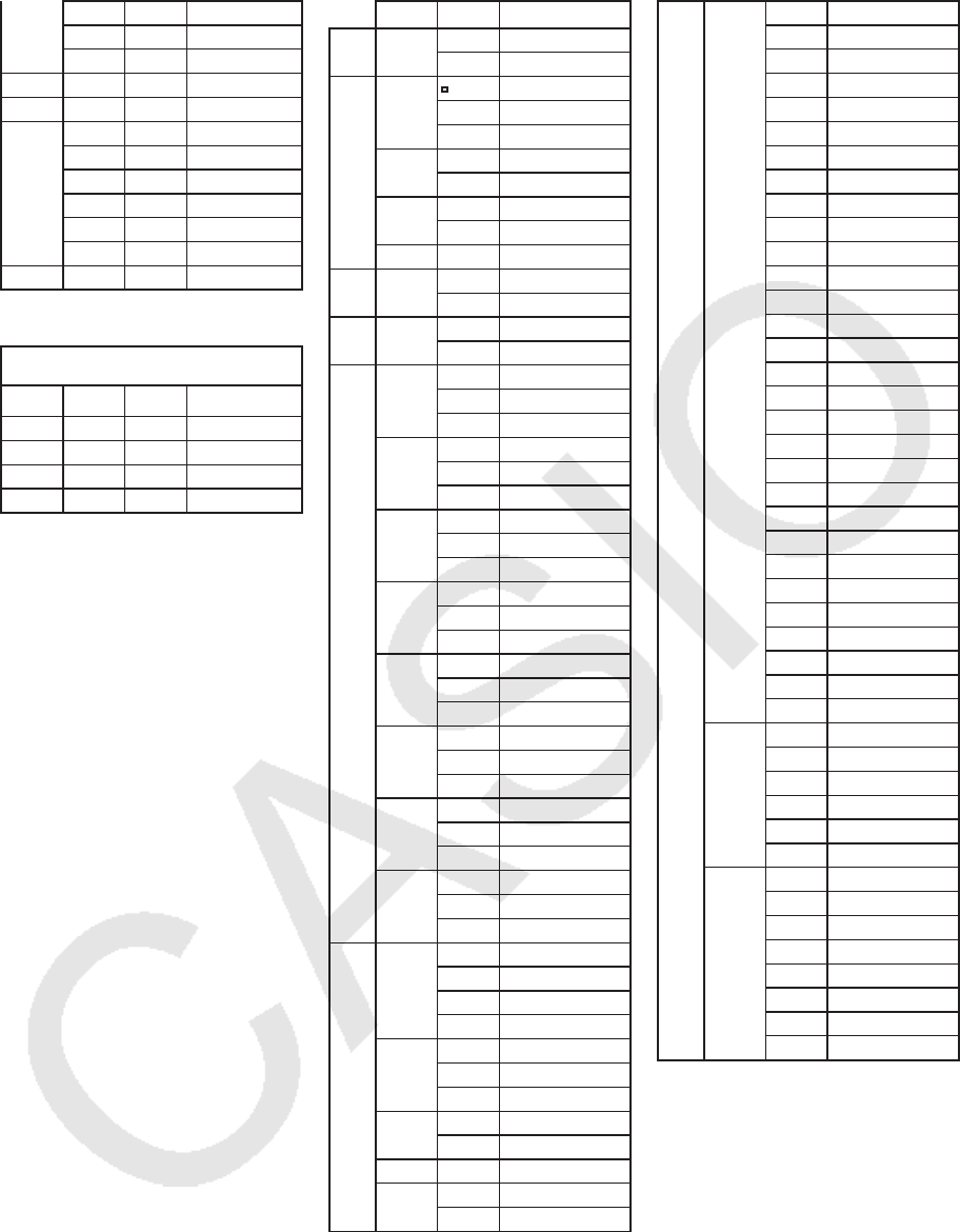
8-41
Isz Isz_
Dsz Dsz_
Menu Menu_
??
^^
REL
==
>>
<<
tt
t
ss
s
::
!m(SET UP) 键
1级 2级 3级 命令
Dec Dec
Hex Hex
Bin Bin
Oct Oct
3级 4级 命令
*1Exp ae^bx Exp(ae^bx)
ab^x Exp(ab^x)
*2 MARK Square
×Cross
k
Dot
STICK Leng StickLength
Hztl StickHoriz
%DATA %%
Data Data
None None
*3X ax+b LinearReg(ax+b)
a+bx LinearReg(a+bx)
*4EXP ae^bx ExpReg(a•e^bx)
ab^x ExpReg(a•b^x)
*5 NORM NPd NormPD(
NCd NormCD(
InvN InvNormCD(
tTPd tPD(
TCd tCD(
Invt InvTCD(
CHI CPd ChiPD(
CCd ChiCD(
InvC InvChiCD(
F FPd FPD(
FCd FCD(
InvF InvFCD(
BINM BPd BinomialPD(
BCd BinomialCD(
InvB InvBinomialCD(
POISN PPd PoissonPD(
PCd PoissonCD(
InvP InvPoissonCD(
GEO GPd GeoPD(
GCd GeoCD(
InvG InvGeoCD(
H
•
GEO HPd HypergeoPD(
HCd HypergeoCD(
InvH InvHyperGeoCD(
*6Z 1-S
OneSampleZTest_
2-S
TwoSampleZTest_
1-P OnePropZTest_
2-P TwoPropZTest_
t1-S
OneSampleTTest_
2-S
TwoSampleTTest_
REG LinRegTTest_
Chi GOF ChiGOFTest_
2-WAY ChiTest_
F
TwoSampleFTest_
ANOV 1-W OneWayANOVA_
2-W TwoWayANOVA_
*7 TEST pp
zz
tt
Chi Ƶ
2
FF
pˆ pˆ
pˆ
1
pˆ
1
pˆ
2
pˆ
2
df df
s
e
s
e
rr
r
2
r
2
pa pa
Fa Fa
Adf Adf
SSa SSa
MSa MSa
pb pb
Fb Fb
Bdf Bdf
SSb SSb
MSb MSb
pab pab
Fab Fab
ABdf ABdf
SSab SSab
MSab MSab
Edf Edf
SSe SSe
MSe MSe
INTR Left Left
Right Right
pˆ pˆ
pˆ
1
pˆ
1
pˆ
2
pˆ
2
df df
DIST pp
xInv xInv
x1Inv x1Inv
x2Inv x2Inv
zLow zLow
zUp zUp
tLow tLow
tUp tUp
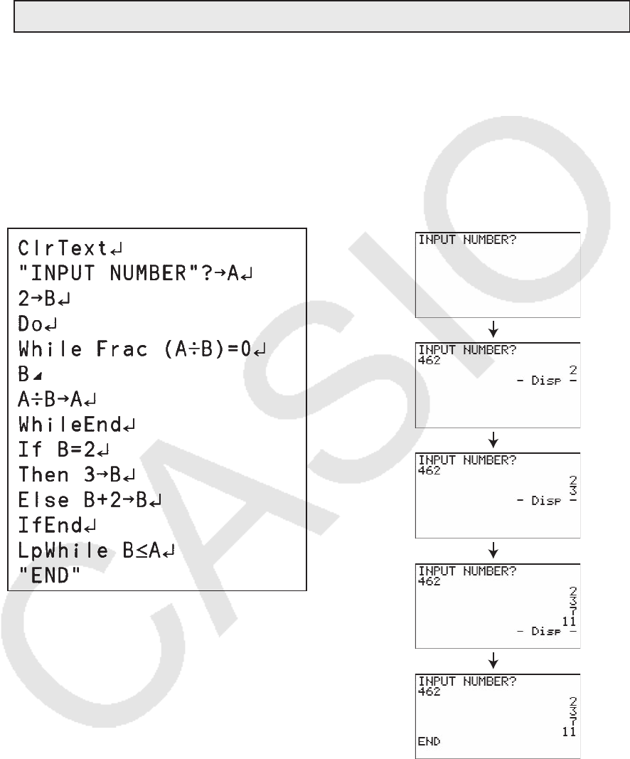
8-42
8. 程序库
• 在尝试进行任何编程之前,必须检查还有多少可用存储字节。
程序名称 素因子分解
描述
该程序持续使用因子分解自然数,直至得到所有素因子。
功能
该程序的输入为自然数A,使用B(2、3、5、7......)除该自然数,找出A的素因子。
• 如果某次除法运算未得到余数,运算结果指定给A。
• 上述程序反复执行,直至B > A。
示例 462 = 2 × 3 × 7 × 11
egcw
w
ww
w
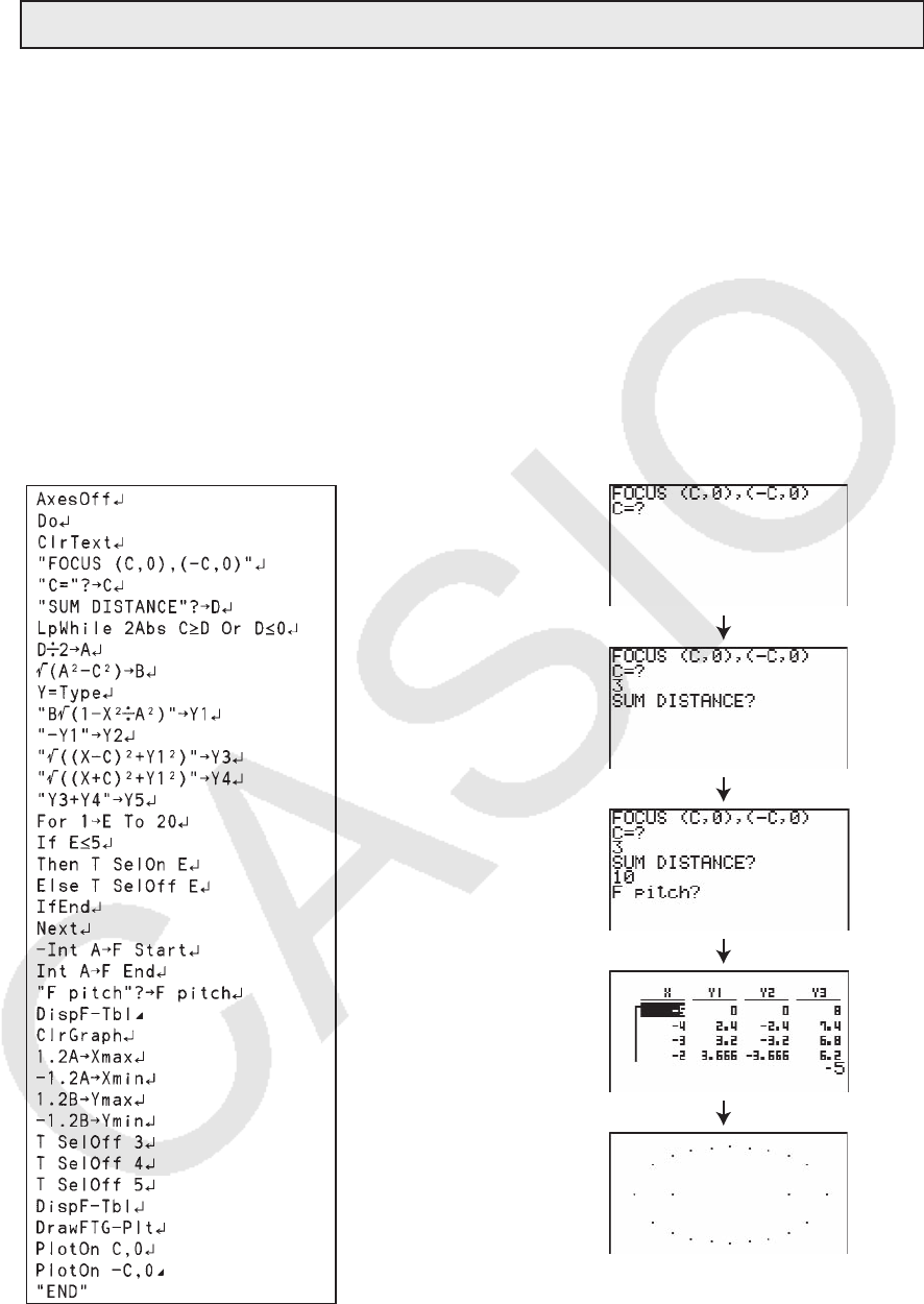
8-43
程序名称 椭圆
描述
该程序显示一个数值表,其中数值为根据输入的椭圆焦点、轨迹与焦点间距之和以及X间距(步
长)计算的结果。
Y1:上半部分椭圆的坐标值
Y2:下半部分椭圆的坐标值
Y3:右焦点与轨迹间距
Y4:左焦点与轨迹间距
Y5:Y3与Y4之和
此后,程序绘制焦点与以Y1和Y2为坐标的数值点。
功能
该程序显示椭圆轨迹与两个焦点的间距之和相等。
dw
baw
bw
w
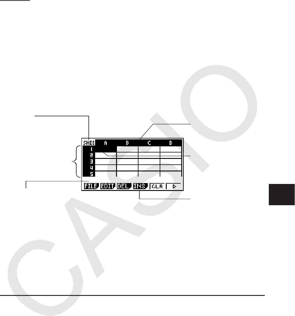
9-1
第9章 电子表格
电子表格应用程序可为您提供强大、便携的电子表格功能。
本节所有操作均在 S
•
SHT 模式中执行。
重要!
• fx-7400G II和fx-9750G II未配置 S •
SHT 模式。
1. 电子表格基础知识和功能菜单
在主菜单上选择 S
•
SHT ,显示电子表格屏幕。自动进入 S
•
SHT 模式可新建一个文件名
为“SHEET”的电子表格。
电子表格屏幕显示许多单元格(方块)及每个单元格中的数据。
文件名
尽可能显示完整的文件名。 列字幕(A至Z)
行号
(1至999)
单元格光标
编辑框
显示单元格光标当前所在单元格的内容。在
选择多个单元格时,编辑框显示选定单元格
范围。
功能菜单
您可将以下类型的数据输入单元格。
常量 常量是指您一旦完成输入即不会改变数值的量。常量可以是一个数值或之前没有等
号 (=) 计算公式(例如7+3、sin30、A1 × 2等等)。
文本 以引号(")开头的字符串作为文本进行处理。
公式 公式以等号 (=) 开头,例如=A1 × 2,完成输入后执行。
请注意, S
•
SHT 模式不支持复数。
k 电子表格屏幕功能菜单
• { FILE } ... 显示以下FILE子菜单。
• { NEW } / { OPEN } / { SV
•
AS } / { RECAL }
• { EDIT } ... 显示以下EDIT子菜单。
• { CUT } / { PASTE } / { COPY } / { CELL } / { JUMP } / { SEQ } / { FILL } / { SRT
•
A } / { SRT
•
D }
• 只有在执行CUT或COPY之后才会直接显示PASTE。
• { DEL } ... 显示以下DEL(删除)子菜单。
• { ROW } / { COL } / { ALL }
• { INS } ... 显示以下INS(插入)子菜单。
• { ROW } / { COL }
9

9-2
• { CLR } ... 清除选定单元格范围中的内容。
• { GRPH } ... 显示以下GRPH 菜单。(与 STAT 模式中一样。)
• { GPH1 } / { GPH2 } / { GPH3 } / { SEL } / { SET }
• { CALC } ... 显示以下CALC(统计计算)菜单。(与 STAT 模式中一样。)
• { 1VAR } / { 2VAR } / { REG } / { SET }
• { STO } ... 显示以下STO(存储)子菜单。
• { VAR } / { LIST } / { FILE } / { MAT } / { VCT }
• { RCL } ... 显示以下RCL(调用)子菜单。
• { LIST } / { FILE } / { MAT }
/ { VCT }
• 数据输入功能菜单
• { GRAB } ... 进入GRAB模式,输入一个单元格参考名称。
• { $ } ... 输入单元格绝对参考命令($)。
• { : } ... 输入单元格范围指定命令(:)。
• { If } ... 输入CellIf( 命令。
• { CEL } ... 显示用于输入以下指令的子菜单。
• CellMin(, CellMax(, CellMean(, CellMedian, CellSum, CellProd(
• { REL } ... 显示用于输入以下关系算子的子菜单。
• =, , >, <, ,
2. 基本电子表格操作
本节说明电子表格文件操作、如何移动光标、选择一个或者多个单元格,以及如何输入和编辑
数据。
k 电子表格文件操作
u 新建一个文件
1. 按下 1(FILE) 1(NEW).
2. 在显示的对话框上,输入文件名(最多八个字符),然后按下 w。
• 由此可新建一个文件并显示一个空白电子表格。
• 如果在第2步中输入的文件名已经存在,则不创建新文件,而是打开现有文件。
u 打开一个文件
1. 按下 1(FILE) 2(OPEN)。
2. 在显示的文件列表上,使用 f和 c,选择想要的文件,然后按下 w。

9-3
u Auto Save
在 S
•
SHT 模式中,只要您对当前打开的文件进行编辑,Auto Save可自动执行保存功能。这表
示您不需要执行任何手动保存操作。
u 使用新名称保存文件
1. 按下 1(FILE) 3(SV
•
AS)。
2. 在显示的对话框上,输入文件名(最多八个字符),然后按下 w。
• 如果您在第2步中输入的文件名已经存在,将显示一条消息,请您确认是否希望使用新文件
替代现有文件。按下 1(Yes)可替代现有文件,或者按下 6(No)可取消保存操作并返回第2
步的文件名输入对话框。
u 删除一个文件
1. 按下 1(FILE) 2(OPEN)。
2. 在显示的文件列表上,使用 f和 c,选择想要的文件,然后按下 1(DEL)。
3. 由此将显示一条确认消息。按下 1(Yes),删除文件;或者按下 6(No),取消操作且不删除
任何内容。
4. 如需从文件列表返回电子表格,按下 J。
• 删除当前打开的文件将自动新建一个名为“SHEET”的文件并显示其电子表格。
k 重新计算当前打开电子表格中的所有公式
S
•
SHT 模式中有一个Auto Calc功能,可在您打开某个电子表格或者执行任何编辑操作后自动重
新计算其中的所有公式。在初始出厂默认设置中已启用Auto Calc功能。您还可根据自己的意愿
手动执行重新计算。
u Auto Calc
Auto Calc是一个 S
•
SHT 模式设置项目(第1-29页)。
在启用Auto Calc(On)时,如果打开某个电子表格或者执行任何编辑操作,将重新计算该电子表
格中的所有公式。但应注意,重新计算操作会减慢整体处理速度。如果禁用Auto Calc(Off),您
需要手动执行重新计算操作。
u 手动执行电子表格重新计算
按下 1(FILE) 4(RECAL)。该操作重新计算当前打开文件中的所有公式并显示相关结果。
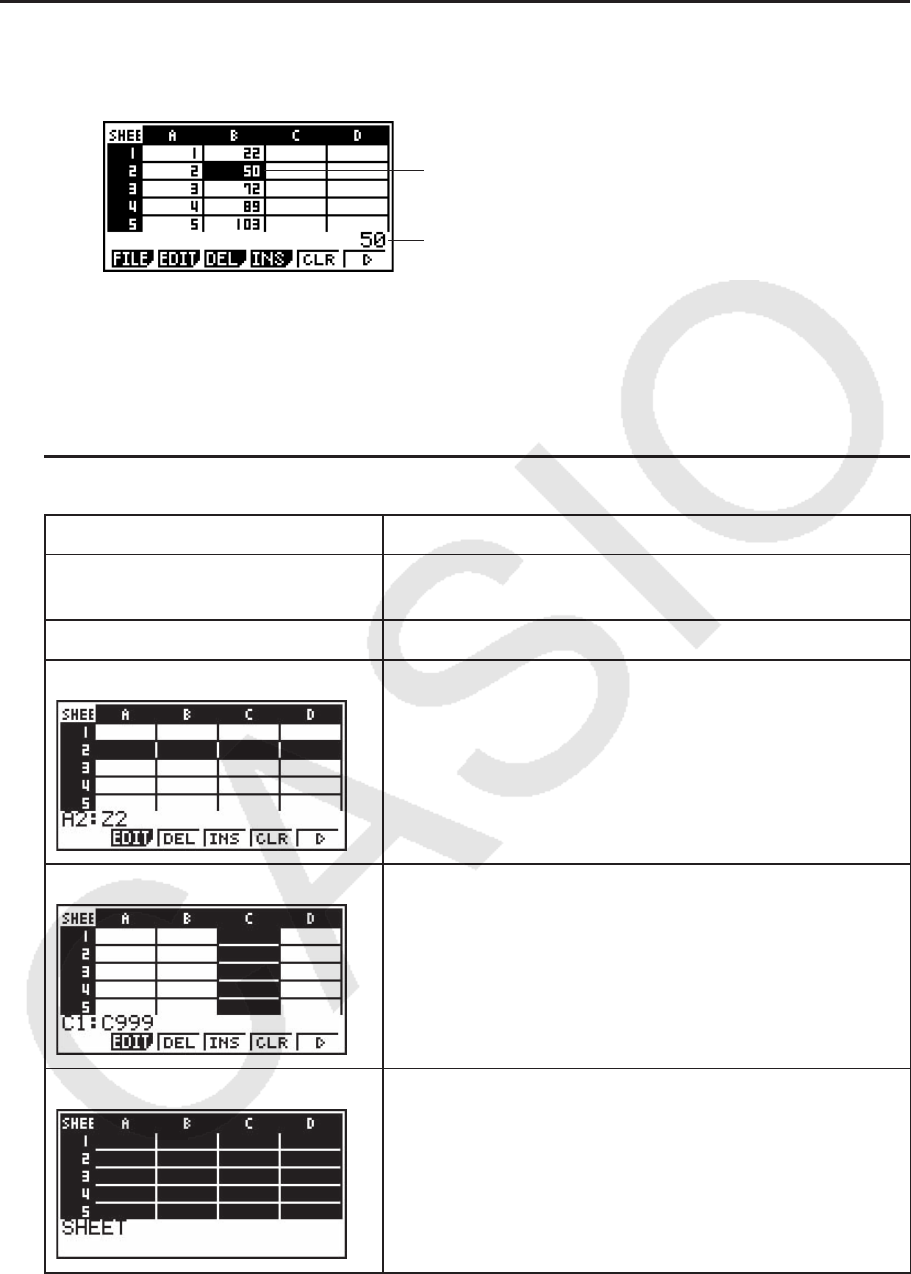
9-4
k 使用单元格光标
单元格光标显示在电子表格中选定的单元格。突出显示的单元格即由单元格光标当前选定的单
元格。
单元格光标
编辑框
在使用单元格光标选定一个单元格时,编辑框中显示该单元格的内容。可在编辑框中编辑单元
格内容。
在使用单元格光标选定多个单元格时,编辑框中显示选择范围。在此情况下,您可对选定的整
个单元格范围执行复制、删除或者其它单元格操作。
u 选择单元格
选择目标: 操作:
单个单元格 使用光标键将单元格光标移至目标单元格,或者使用
JUMP命令直接跳至该单元格。
一系列单元格 参见“选择一系列单元格”(第9-5页)。
一整行单元格
将单元格光标移至目标行所在的A列,然后按下 d。例
如当单元格光标位于单元格A2时,按下 d,由此可选
择整个第二行(从A2到Z2)。此后编辑框中将显示A2:
Z2(表示选定范围)。
一整列单元格
将单元格光标移至目标列所在的第1行,然后按下 f。
例如当单元格光标位于单元格C1时,按下 f,由此可
选择整个C列(从C1到C999)。此后编辑框中将显示
C1:C999(表示选定范围)。
电子表格中的所有单元格
在选定整个A列时按下 d,或者在选定整个第1行时按
下 f。由此可选择电子表格中的所有单元格并在编辑
框中显示电子表格文件名。
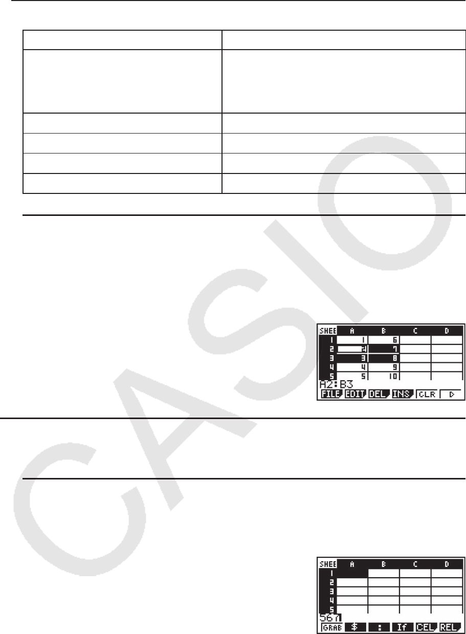
9-5
u 使用JUMP命令移动单元格光标
单元格光标的目标移动位置: 操作:
一个特定单元格 1. 按下 2(EDIT) 4(JUMP) 1(GO)。
2. 在显示的对话框上,输入跳转目标单元格的名
称(A1至Z999)。
3. 按下 w。
当前列的第1行 按下 2(EDIT) 4(JUMP) 2(TOP ↑ )。
当前行的A列 按下 2(EDIT) 4(JUMP) 3(TOP ← )。
当前列的最后一行 按下 2(EDIT) 4(JUMP) 4(BOT ↓ )。
当前行的Z列 按下 2(EDIT) 4(JUMP) 5(BOT → )。
u 选择一系列单元格
1. 将单元格光标移至目标单元格范围的起点。
• 您可根据需要选择整行或整列单元格作为起点。关于选择单元格的详情,请参见第9-4页
的“选择单元格”。
2. 按下 !i(CLIP)。
• 这会将单元格光标改为粗线边界,而不是通常的突出显示形式。
3. 使用光标键将单元格光标移至目标单元格范围的终点。
• 编辑框将显示选定单元格的范围。
• 如需取消单元格选择,按下 J。执行该操作后,单元
格光标将位于选定范围的终点。
k 数据(常量、文本、公式)输入基础知识
首先介绍一些适用于任何输入数据类型的基本步骤。
u 使用新数据覆盖单元格中的当前数据
1. 将单元格光标移至想要输入数据的单元格。
• 如果您选择的单元格已经包含数据,以下步骤将使用新的输入覆盖现有数据。
2. 使用计算器按键输入数据。
• 在执行按键操作输入数值或者文本(例如 b, al(B)
等等),编辑框中将显示向左对齐的相关数据。
• 在继续执行第3步之前,如需取消输入操作,按下 J。
该操作将使单元格内容恢复到第1步的状态。
3. 如需结束并应用输入,按下 w。
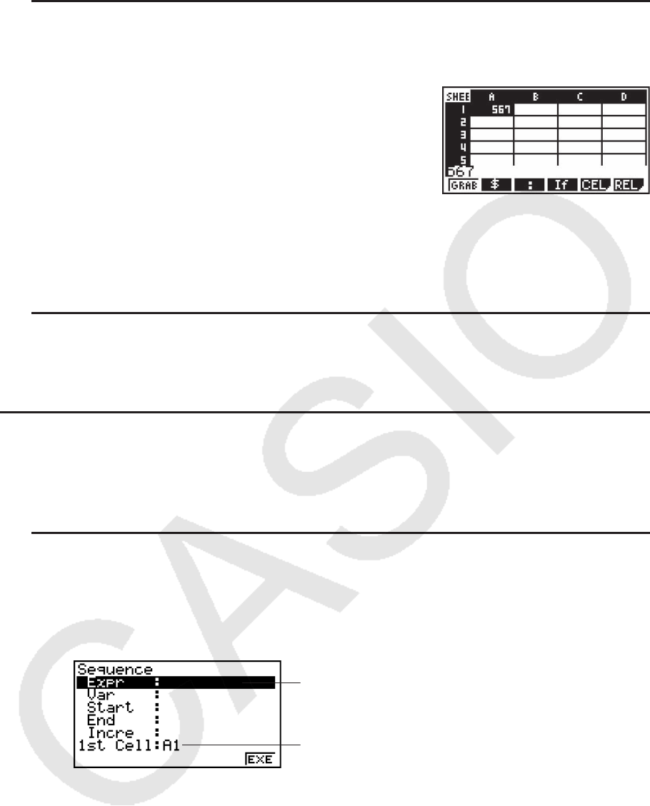
9-6
u 编辑单元格数据
1. 将单元格光标移至想要编辑内容的单元格。
2. 按下 2(EDIT) 3(CELL)。
• 编辑框中的单元格内容将从向左对齐改变为向右对齐。
编辑框中将显示一个文本光标,以便您编辑其内容。
3. 使用 e和 d在单元格的内容中移动光标,根据需要进行编辑。
• 在继续执行第4步之前,如需取消编辑操作,按下 J。该操作将使单元格内容恢复到第1步
的状态。
4. 如需结束并应用输入,按下 w。
u 在单元格中输入数据期间移动单元格光标
在出厂默认设置下,在单元格中输入数据期间按下 w,将使单元格光标移至下一行。您可使用
第1-29页所述的“Move”设置将该光标移动指定为移至下一列。
k 在单元格中输入常量(数值、计算结果、数列)
常量是指您一旦完成输入即不会改变数值的量。常量可以是一个数值或之前没有等号 (=) 计算公
式(例如7+3、sin30、A1 × 2等等)。 例如,输入 sdaw, 将使单元格显示数值0.5(计
算结果)(在Angle单位设置为Deg时)。
u 根据某个函数表达式自动输入数列
1. 将单元格光标移至想要开始输入数列的单元格。
• 在初始默认设置下,自动输入数列操作将从起始单元格向下执行。您可使用第1-29页所述
的“Move”设置指定不同的方向。
2. 按下 2(EDIT) 5(SEQ),显示数列屏幕,然后指定函数表达式和数值,生成所需数列。
您可为屏幕上突出显示的项目输入数据。
在第1步中选定单元格的参考名称
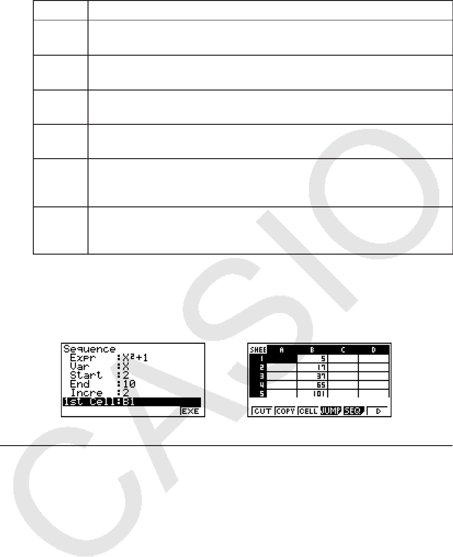
9-7
项目 描述
Expr 输入函数表达式
f( x) 以生成数列。
示例: a+(X) x+bw (X
2
+ 1)
Var 输入在Expr中输入函数表达式时使用的变量名。
示例: a+(X) w (X)
Start 输入用于替代Var指定变量的值的初值(X
1
)。
示例: cw
End 输入用于替代Var指定变量的值的终值(X
n
)。
示例: baw
Incre 输入 增量值(
m) (连续值X
1
)的数列为:(X
2
= X
1
+ m),(X
3
= X
2
+ m),依
此类推。生成的数列范围为X
1
+ ( n - 1) m < X
n
。
示例: cw
1st Cell 输入想要输入数列第一个值的单元格的参考名称(A1、B2等等)。只有在起
始单元格与第1步指定的单元格不同时才需要在此指定一个单元格。
示例: al(B) bw (B1)
• 每次您在输入用于设置项目的数据之后按下 w时,突出显示区域将转移到下一个设置项
目。您还可使用 f和 c将突出显示区域向上或者向下移动。
• 执行下一步将从指定指令单元格开始自动输入数字串。如果用于输入数列数值的一系列单元
格中有任何单元格包含数据,现有数据将由数列数值替代。
3. 为所有设置项目输入数据后按下 6 (EXE)或者 w 键,开始生成和输入数列。
k 在单元格中输入文本
如需输入文本,确保在单元格中首先输入 aE(”)。引号(")用于告知计算器后续内容为文
本,应原样显示,无需计算。显示文本时不包括引号(")。
⇒
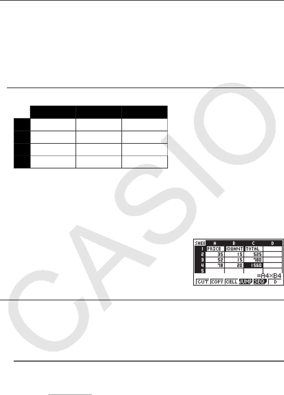
9-8
k 在单元格中输入公式
例如,我们准备生成一个表格,其中数据来自公式<PRICE> × <QUANTITY> = <TOTAL>。为
此,我们在A列输入<PRICE>值,在B列输入<QUANITY>值,在C列输入计算公式(例如= A1
× B1、= A2 × B2,依此类推)。如果启用(On)了Auto Calc功能,每次更改A或B列数值时
都会重新计算并更新C列的值。
在该例中,请注意我们必须在C列中首先输入 (=),表示它是一个公式。除了数值、算术算子和
单元格参考名称之外,公式还可包含内置函数命令(第2-12页)和特殊 S
•
SHT 模式命令(第
9-13页)。
u 公式输入示例
A B C
1 PRICE QUANTITY TOTAL
2 35 15 525
3 52 15 780
4 78 20 1560
步骤
1. 在单元格A2至B4中输入第1行的文本和相关数值。
2. 将光标移至单元格C2,然后输入A2 ×B2的公式。
!.(=)av(A) c*al(B) cw
3. 将单元格C2中的公式复制到单元格C3和C4。将单元格光标移至单元格C2,然后执行下述操
作。
2(EDIT) 2(COPY) c1(PASTE) c1(PASTE) J
• 关于复制和粘贴操作的详情,请参见“复制和粘贴单元
格内容”(第9-9页)。
k 输入单元格参考名称
电子表格上的每个单元格都有一个“参考名称”,该名称由其列名称(A至Z)与行名称(1至
999)组合而成。单元格参考名称可用于公式,由此可将调用单元格的数值代入公式。详情请参
见前文的“在单元格中输入公式”。在输入单元格参考名称时有两种方法:直接输入名称和使
用GRAB命令输入。下面说明如何使用这些方法在单元格B1中输入=A1+5。
u 使用直接输入方法输入单元格参考名称
将单元格光标移至单元格B1,然后执行下述操作。
!.(=)av(A) b+fw

9-9
u 使用GRAB命令方法输入单元格参考名称
将单元格光标移至单元格B1,然后执行下述操作。
!.(=)1(GRAB) d1(SET) +fw
• 在您按下 1(GRAB)时显示的子菜单上的 2(GO)至 6(BOT →) 命令与JUMP命令子菜单上
的 1(GO) 至 5(BOT →)命令完全相同。关于这些命令,请参见第9-5页“使用JUMP命令移
动单元格光标”。
k 相对和绝对单元格参考名称
单元格参考名称有两种类型:相对和绝对。正常情况下,单元格参考名称视为相对类型。
相对单元格参考名称
在公式=A1+5中,单元格参考名称A1表示一个相对单元格参考。称其为“相对”是因为复制公
式并粘贴在不同的单元格中会导致单元格参考名称随着粘贴目标单元格位置而改变。例如,如
果公式=A1+5最初位于单元格B1中,将其复制并粘贴到单元格C3中将在单元格C3中产生公式
=B3+5。从A列移至B列(一列)将使A变为B,而从第1行移至第3行(两行)将使1变为3。
重要!: 如果复制和粘贴操作的结果导致相对单元格参考名称超出电子表格单元格的范围,相
关列字母及/或行号将被替代为问号(?),单元格数据将显示“ERROR”。
绝对参考名称
如果您希望单元格参考名称的行或列,或者行与列部分在目标粘贴位置保持不变,您需要创建
一个绝对单元格参考名称。您可在希望保持不变的单元格参考名称前添加一个美元符号($)。
在使用美元符号($)创建绝对单元格参考名称时有三种选择:绝对列与相对行($A1)、相对
列与绝对行(A$1)以及绝对行与列($A$1)。
u 输入绝对单元格参考名称符号($)
在电子表格单元格中输入一个单元格参考时,按下 2($)。
例如,以下按键操作输入绝对单元格参考名称 = $B$1
!.(=)2($) al(B) 2($) b
k 复制和粘贴单元格内容
您可复制一个或者多个单元格的内容并将其粘接到另一个位置。一旦执行复制操作,即可将内
容复制到多个位置。
u 复制和粘贴电子表格数据
1. 选择想要复制的单元格。
• 详情请参见“选择单元格”(第9-4页)。
2 按下 2(EDIT) 2(COPY)。
• 由此将进入选定数据的粘贴等待状态,此时 1菜单项变为(PASTE)。
• 在执行下面的第4步之前,您可随时按下 J以退出粘贴等待状态。
3. 使用光标键将单元格光标移至数据粘贴目标位置。
• 如果您在第1步中选择一系列单元格,单元格光标选择的单元格将成为粘贴范围的左上角单
元格。
• 如果选择位置在复制范围内部,执行下述步骤将使现有数据被粘贴数据覆盖。
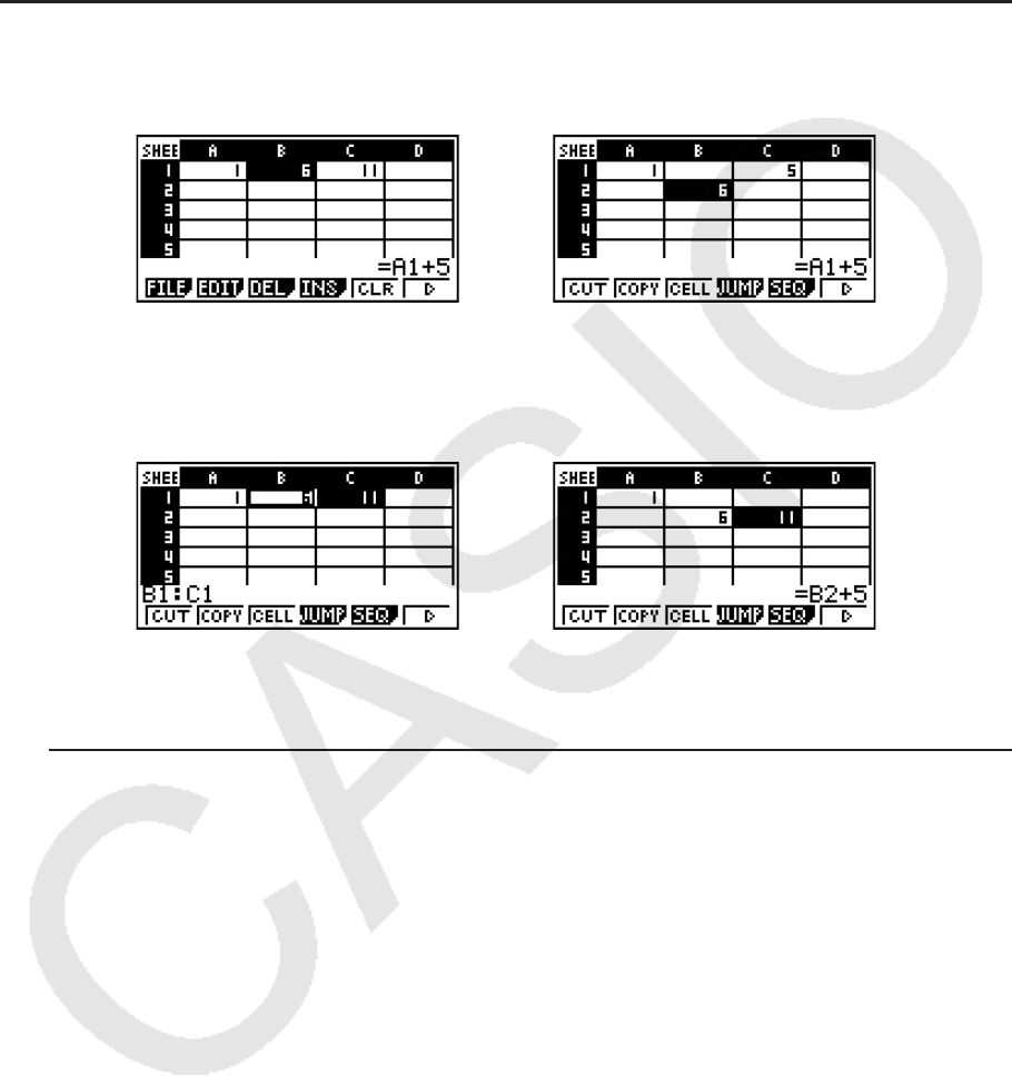
9-10
4. 按下 1(PASTE)。
• 由此将粘贴复制数据。
• 如需将相同数据粘贴到其他位置,重复第3步和第4步。
5. 完成数据粘贴之后,按下 J以退出粘贴等待状态。
k 剪切和粘贴单元格内容
您可使用剪切和粘贴功能将一个或者多个单元格的内容移至其他位置。单元格内容(无论是包
括相对还是绝对单元格名称参考)一般都不会因剪切和粘贴操作而改变。
剪切单元格中B1的公式=A1+5并将其粘贴到单元格B2中。A1参考名称保持不变。
在剪切和粘贴一系列单元格时,影响这些单元格内部关系的参考名称(无论是相对还是绝对参
考名称)会相应改变以保持正确关系。
剪切B1:C1部分单元格包括公式=B1+5并将其粘贴到B2:C2中。为保持与粘贴范围内左侧单元
格的关系,粘贴到C2的公式变为=B2+5。
u 剪切和粘贴电子表格数据
1. 选择想要剪切的单元格。
• 详情请参见“选择单元格”(第9-4页)。
2 按下 2(EDIT) 1(CUT)。
• 由此将进入选定数据的粘贴等待状态,此时 1菜单项变为(PASTE)。
• 在执行下面的第4步之前,您可随时按下 J以退出粘贴等待状态。
3. 使用光标键将单元格光标移至数据粘贴目标位置。
• 如果您在第1步中选择一系列单元格,单元格光标选择的单元格将成为粘贴范围的左上角单
元格。
• 如果选择位置在剪切范围内部,执行下述步骤将使现有数据被粘贴数据覆盖。
4. 按下 1(PASTE)。
•由此可将第1步中选定的单元格中的数据粘贴到在第3步选定的位置。
• 无论启用还是禁用Auto Calc功能(第9-3页),粘贴剪切数据将导致重新计算电子表格中的
所有公式。
⇒
⇒
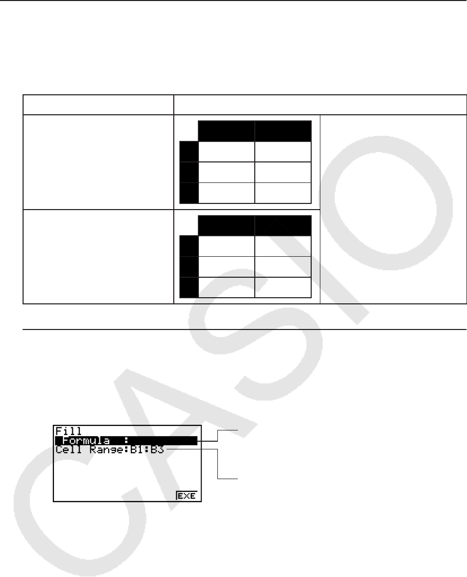
9-11
k 在一系列单元格中输入同一个公式
需要在指定范围的单元格中输入同一个公式时,使用Fill命令。关于相对和绝对单元格名称参考
的规则与复制和粘贴操作相同。
例如,如果需要在单元格B1、B2和B3中输入同一个公式,通过Fill命令只需在单元格B1中输入
一次公式即可。请注意下面关于Fill命令在此情况下处理单元格名称参考的方式。
单元格B1包含内容: Fill命令执行的操作:
=A1 × 2 A B
1
=A1 × 2
2
=A2 × 2
3
=A3 × 2 * 注意,在实际操作中单元格
B1、B2和B3将显示计算结
果,而非此处所示公式。
=$A$2 × 2 A B
1
=$A$2 × 2
2
=$A$2 × 2
3
=$A$2 × 2
u 在一系列单元格中输入同一个公式
1. 选择想要输入同一个公式的单元格范围。
• 在本例中,我们假设已经选定B1:B3。参见“选择一系列单元格”(第9-5页)。
2. 按下 2(EDIT) 6( g) 1(FILL)。
3. 在显示的Fill屏幕上,输入想要输入的公式。
您可为屏幕上突出显示的项目输入数据。
这是在第1步中选定单元格范围。
• 在“Formula”行中,输入=A1 × 2 ( !.(=) av(A) b*cw)。按下 w将导致
单元格光标移至“Cell Range”行。
• 如果单元格范围中的任何单元格已经包含数据,执行下一步将使用新的填充数据(公式)覆
盖现有数据。
4. 按下 6(EXE)或者 w键。
• 由此将在指定的单元格范围中输入公式。

9-12
k 常量数据排序
请注意只有常量数据才可排序。您可在一行中选择多个列或者在一列中选择多个行进行排序。
u 对常量数据排序
1. 在一行中选择一组列单元格,或者在一列中选择一组行单元格。
• 参见“选择一系列单元格”(第9-5页)。
• 如果选定范围中的任何单元格包含非常量数据,将显示一条Syntax ERROR消息。
2. 根据想要执行的排序类型,执行以下任何一种操作。
升序排序: 2(EDIT) 6( g) 2(SRT
•
A)
降序排序: 2(EDIT) 6( g) 3(SRT
•
D)
k 删除和插入单元格
u 删除整行或者整列单元格
选择想要删除的行或者列,然后按下 3(DEL)。由此将立即删除选定的行或列,且不显示确认
消息。
您还可执行以下步骤删除行或列。
1. 选择想要删除的行或列中的一个或者多个单元格。
• 如果想删除第2至第4行,您可选择A2:B4、C2:C4或者其它任何包括删除目标行的单元格范
围。
• 例如,如果想删除列A和B您可选择A1:B1、A2:B4等等。
2. 按下 3(DEL)。
• 由此将进入删除等待状态。如果你决定取消删除操作,按下 J。
3. 如需删除包含在第1步选定单元格的整行,按下 1(ROW)。如需删除整列,按下 2(COL)。
u 删除电子表格中所有单元格的内容
1. 按下 3(DEL) 3(ALL)。
2. 针对显示的确认消息,按下 1(Yes),删除数据;或者按下 6(No),取消操作且不删除任何
内容。
u 插入一行或一列空白单元格
1. 执行以下某一操作以指定插入位置和插入的行数或列数。
• 插入行
从插入目标行的下一行开始,选择想要插入的相同行数。
示例:如需插入第2行上的三行,您可选择A2:A4、B2:C4等等。
• 插入列
从插入目标列的右侧一列开始,选择想要插入的相同列数。
示例:如需插入B列左侧三列,您可选择B2:D4, B10:D20等等。

9-13
2. 按下 4(INS)。
• 由此将进入插入等待状态。如果你决定取消插入操作,按下 J。
3. 按下 1(ROW),插入适当数量的行;或按下 2(COL) 插入列。
• 如果插入操作导致包含数据的当前单元格超出A1:Z999范围,将出现一条Range ERROR消
息。
u 清除特定单元格的内容
选择想要清除的某个单元格或者一组单元格,然后按下 5(CLR)。
3. 使用特殊 S
•
SHT 模式命令
S
•
SHT 模式有许多特殊命令,例如可返回一组单元格之和的CellSum(,以及指定分支条件的
CellIf(。这些特殊命令可在公式内部使用。
k 特殊 S
•
SHT 模式命令列表
“输入键操作”只能在单元格输入期间执行。
您可省略每个命令语法中方括号([ ])中的内容。
命令 描述
CellIf(
(分支条件)
在作为分支条件的等式或者不等式为真时返回表达式1,为假时返回
表达式2。
输入键操作: 4(If)
语法: CellIf(等式,表达式1,表达式2[)] 或CellIf(不等式,表达式
1,表达式2[)]
示例:
=CellIf(A1>B1, A1, B1)
当 {单元格A1值} > {单元格B1值}时,返回A1的值。否则,返回B1
的值。
CellMin(
(单元格最小值)
返回指定范围单元格中的最小值。
输入键操作: 5(CEL) 1(Min)
语法: CellMin(起始单元格:结束单元格[)]
示例:
=CellMin(A3:C5)
返回单元格范围A3:C5中数据的最小值。
CellMax(
(单元格最大值)
返回指定范围单元格中的最大值。
输入键操作: 5(CEL) 2(Max)
语法: CellMax(起始单元格:结束单元格[)]
示例:
=CellMax(A3:C5)
返回单元格范围A3:C5中数据的最大值。
CellMean(
(单元格平均值)
返回指定范围单元格中的平均值。
输入键操作: 5(CEL) 3(Mean)
语法: CellMean(起始单元格:结束单元格[)]
示例:
=CellMean(A3:C5)
返回单元格范围A3:C5中数据的平均值。
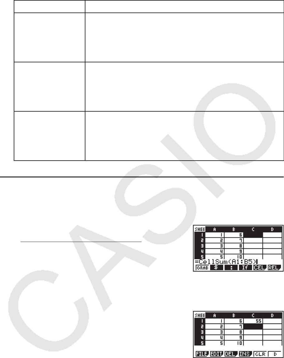
9-14
命令 描述
CellMedian(
(单元格中位值)
返回指定范围单元格中的中位值。
输入键操作: 5(CEL) 4(Med)
语法: CellMedian(起始单元格:结束单元格[)]
示例:
=CellMedian(A3:C5)
返回单元格范围A3:C5中数据的中位值。
CellSum(
(单元格之和)
返回指定范围单元格中的中位值。
输入键操作: 5(CEL) 5(Sum)
语法: CellSum(起始单元格:结束单元格[)]
示例:
=Cellsum(A3:C5)
返回单元格范围A3:C5中数据之和。
CellProd(
(单元格之积)
返回指定范围单元格数据之积。
输入键操作: 5(CEL) 6(Prod)
语法: CellProd(起始单元格:结束单元格[)]
示例:
=CellProd(B3:B5)
返回单元格范围B3:B5中数据之积。
k S
•
SHT 模式命令示例
本例在单元格C1中输入特殊 S
•
SHT 模式公式CellSum(,以计算单元格范围A1:B5中所有数据之
和。假设单元格范围A1:B5中已经存在数据。
1. 将单元格光标移至单元格C1,然后执行下述操作。
!.(=) 5(CEL) 5(Sum)
Jav(A) b3(:) al(B) f)
• 您可执行以下操作,使用GRAB功能(第9-9页)和CLIP
功能(第9-5页)替代上述操作的下划线部分。
J1(GRAB) 4(TOP ← ) (进入GRAB模式并将光标移至A1。)
!i(CLIP) ecccc (指定CLIP功能的选择范围。)
w)
2. 按下 w,结束公式输入。
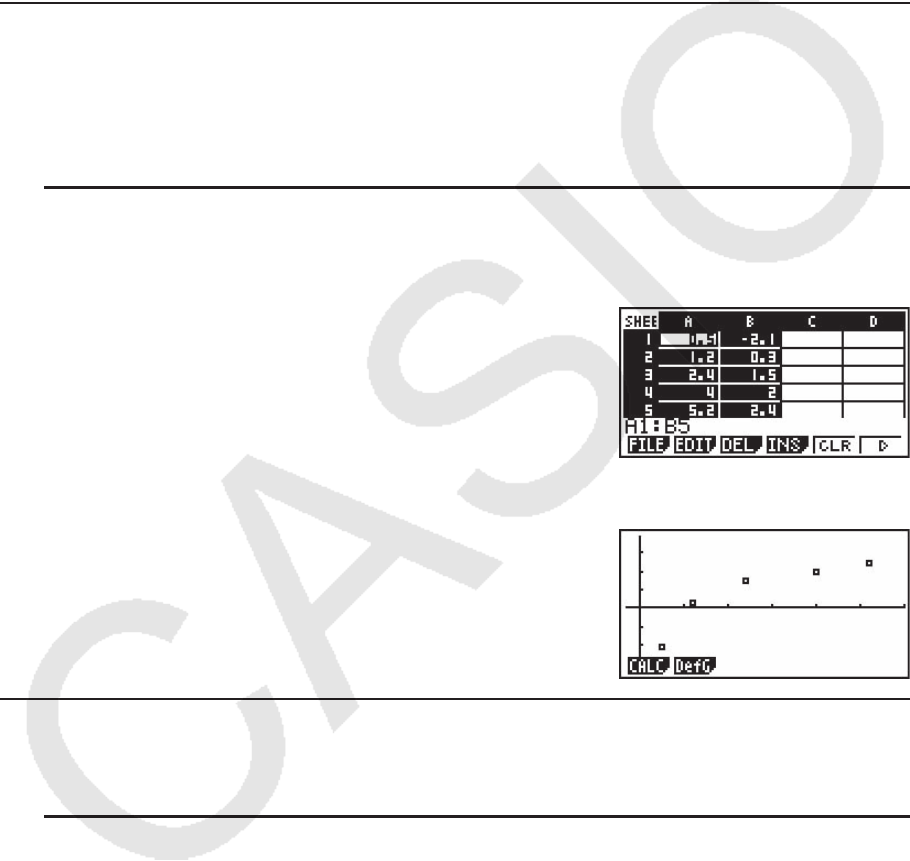
9-15
4. 绘制统计图形以及执行统计和回归计算
在希望检查两组数据之间的关联(例如温度与某种产品的价格)时,以其中一组数据作为 x轴,
另一组数据作为
y轴绘制图形,可方便绘制趋势图。
您可使用电子表格输入每一组数据的数值,然后绘制散布图或其他类型的图形。执行数据回归
计算可产生回归公式和关联系数,而且可在散布图上叠加回归图形。
S
•
SHT 模式绘图、统计计算和回归计算使用与 STAT 模式相同的功能。下面是一个 S
•
SHT 模式
独有的操作示例。
k 统计图形操作示例(GRPH菜单)
输入以下数据并绘制统计图形(本例为散布图)。
0.5, 1.2, 2.4, 4.0, 5.2 (
x轴数据)
-2.1, 0.3, 1.5, 2.0, 2.4 (
y轴数据)
u 输入数据并绘制统计图形(散布图)
1. 将统计计算数据输入电子表格。
• 在此,我们将
x轴数据输入A列,将 y轴数据输入B列。
2. 选择想要绘制图形的单元格范围(A1:B5)。
3. 按下 6( g) 1(GRPH),显示GRPH菜单,然后按下 1(GRPH1)。
• 由此将利用在第2步中选定单元格范围中的数据绘制一个
散布图。
• 此处所示图形采用 S
•
SHT 模式的初始默认设置。您可在
GRPH菜单上更改在按下 6(SET)时屏幕显示的图形设
置配置。详情请参见后文“一般图形设置屏幕操作”。
k 一般图形设置屏幕操作
您可使用一般图形设置屏幕指定用于绘制图形的数据范围以及选择需要绘制的图形。
u 配置统计图形设置
1. 将统计计算数据输入电子表格,然后选择想要绘制图形的单元格范围。
• 实际上,此时不需要执行上述步骤。您还可在输入数据和选择需要绘制图形的单元格范围之
前,首先配置设置。

9-16
2. 按下 6( g) 1(GRPH) 6(SET)。
• 由此将显示一般图形设置屏幕(本例为StatGraph1)。
您可设置屏幕上突出显示的项目。
在选择某些设施项目时会显示一个功能菜单。
• 您在第1步中选择的列数将决定在一般图形设置屏幕上自动输入的信息。
如果您选择以下列数: 将自动输入以下信息:
1 XCellRange
2 XCellRange,YCellRange
3 XCellRange,YCellRange,Frequency
• 下面说明该屏幕的每一个设置项目。
项目 描述
StatGraph1 选择目标设置名称。您最多可登记三种不同设置,名称分别为
StatGraph 1、2或3。
Graph Type 选择图形类型。初始默认设置为Scat(散布图)。
XCellRange 指定用于绘制
x轴(XCellRange)的单元格范围。某些图形类型只显示
XCellRange。
YCellRange 指定用于绘制
y轴(YCellRange)的单元格范围。某些图形类型不显示
YCellRange。
Frequency 指定包含每一个图形数据项目的频率值的单元格范围。如果您不想使用
频率值,选择 1(1)。
Mark Type 指定在散布图上使用的标记类型( 、× 或者 • )。
3. 使用 f和 c,突出显示想要更改的设置项目。在显示的功能菜单上,选择想要的设置。
• 关于StatGraph1、Graph Type和Mark Type设置的详情,请参见“显示一般图形设置屏
幕”(第6-2页)。
• 如果您想更改XCellRange、YCellRange或Frequency设置,突出显示想要更改的项目,然
后直接输入单元格范围或者选择 1(CELL) (对于Frequency,为 2(CELL) ),然后编辑
当前输入范围。在手动输入单元格范围时,使用 1(:),在两个定义范围的单元格之间输入
一个冒号(:)。
4. 在配置所需设置之后,按下 J或者 w。
k 统计计算操作示例(CALC菜单)
本例使用“绘制散布图和 xy线图”(第6-10页)的数据执行双变量统计计算。
0.5, 1.2, 2.4, 4.0, 5.2 (
x数据)
-2.1, 0.3, 1.5, 2.0, 2.4 (
y数据)
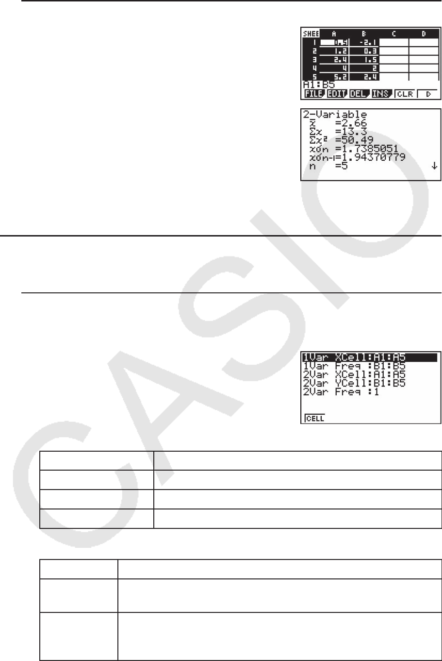
9-17
u 执行双变量统计计算和回归计算
1. 将上述 x数据输入电子表格的单元格A1:A5,将 y数据输
入单元格B1:B5,然后选择想要输入数据的单元格范围
(A1:B5)。
2. 按下 6( g) 2(CALC),显示CALC菜单,然后按
下 2(2VAR)。
• 由此将根据您在第1步中选择的数据显示一个双变量计算
结果屏幕。使用 e和 d,滚动结果屏幕。如需关闭屏
幕,按下 J。
• 关于结果屏幕上的一个数值的含义,请参见“显示双变
量图形的计算结果”(第6-15页)。
3. 如需返回文件列表,按下 J。
k 使用统计计算数据范围指定屏幕
您可使用特殊设置屏幕指定用于统计计算的数据范围。
u 指定用于统计计算的数据范围
1. 将统计计算数据输入电子表格,然后选择单元格范围。
2. 按下 6( g) 2(CALC) 6(SET)。
• 由此将显示类似于右图的设置屏幕。
• 您在第1步中选择的列数将决定在统计计算数据范围指定屏幕上自动输入的信息。
如果您选择以下列数: 将自动输入以下信息:
1 1Var XCell和2Var XCell
2 1Var Freq和2Var YCell
3 2Var Freq
• 下面说明该屏幕的每一个设置项目。
项目 描述
1Var XCell
1Var Freq
此处指定的单元格范围数据在执行单变量统计计算时用于变量
x和
Frequency数值。
2Var XCell
2Var YCell
2Var Freq
此处指定的单元格范围数据在执行双变量统计计算时用于变量
x、变量
y和Frequency数值。

9-18
3. 如果您希望更改单元格范围,使用 f和 c,突出显示想要更改的项目并输入新的单元格范
围。
• 如需输入冒号(:),按下 1(:)。
• 如需编辑当前输入单元格范围,按下 1(CELL)(对于1Var XCell、2Var XCell和2Var
YCell)或者 2(CELL)(对于1Var Freq和2Var Freq)。
4. 在配置所需设置之后,按下 J或者 w。
k STAT模式与 S
•
SHT 模式功能菜单对应表
在 STAT 模式和 S
•
SHT 模式中,统计图形函数在GRPH功能菜单上,统计/回归计算函数在
CALC功能菜单上。在 STAT 模式和 S
•
SHT 模式中,这些菜单及其子菜单的结构相同。关于每个
菜单项目的详情,请参考下表所指页面。
关于该菜单项目的信息: 参考:
{GRPH} - {GPH1} “更改图形参数”(第6-1页)
{GRPH} - {GPH2}
{GRPH} - {GPH3}
{GRPH} - {SEL} “图形绘制/非绘制状态”(第6-3页)
{GRPH} - {SET} “更改图形参数”(第6-1页)
“一般图形设置”(第6-1页)
“显示一般图形设置屏幕”(第6-2页)
“一般图形设置屏幕操作”(第9-15页)
{CALC} - {1VAR} “单变量统计计算”(第6-16页)
{CALC} - {2VAR} “双变量统计计算”(第6-16页)
{CALC} - {REG} “回归计算”(第6-17页)
{CALC} - {SET} “使用统计计算数据范围指定屏幕”(第9-17页)

9-19
5. S
•
SHT 模式存储器
您可使用计算器的不同类型存储器(变量、列表存储器、文件存储器、矩阵存储器、向量存储
器)存储数据,并在数据表格中调用存储器中的数据。
k 将电子表格数据保存到存储器
下表概述每一类存储器的存储操作。关于每一种操作的详情,参见表格后面的操作示例。
存储器类型 存储操作
变量
(A ~ Z、
r、
θ
)
您可将单个单元格的内容指定给变量。
在选定单个单元格时,按下 6( g) 3(STO) 1(VAR),然后在显示
的屏幕上指定变量名。
列表存储器
(List 1 ~ List 26)
您可将一系列单元格中的数据保存到列表存储器中的单行或单列。
在选择单行或单列中的一系列单元格时,按下 6( g) 3(STO)
2(LIST),然后在显示的屏幕上指定变量名。
文件存储器
(File 1至File 6)
您可将跨越多行与多列的一系列单元格中的数据保存到文件存储器
中。在选定一系列单元格时,按下 6( g) 3(STO) 3(FILE),然后
在显示的屏幕上指定文件编号。
选定范围的第一列保存为指定文件的List 1,第二列保存为List 2,
依此类推。
矩阵存储器
(Mat A ~ Mat Z)
您可将跨越多行与多列的一系列单元格中的数据保存到矩阵存储器
中。在选定一系列单元格时,按下 6( g) 3(STO) 4(MAT),然后
在显示的屏幕上指定矩阵名称。
选定范围的第一列保存为指定矩阵的List 1,第二列保存为List 2,
依此类推。
向量存储器
(Vct A ~ Vct Z)
您可将一系列单元格中的数据保存到向量存储器中的一行或一列。在
选择单行或单列中的一系列单元格时,按下 6( g) 3(STO)
5(VCT),然后在显示的屏幕上指定向量名。
重要!
下面说明在单元格不包含任何数据、单元格包含文本或者某个单元格出现ERROR消息时,如果
尝试将数据保存到存储器中会出现什么情况。
• 如果您正在将数据指定给某个变量,会出现一个错误。
• 如果您正在将数据保存到列表存储器、文件存储器、矩阵存储器或向量存储器,将0写入相关
单元格。
u 示例:在列表存储器中存储列数据
1. 在单个列中,选择想要存储在列表存储器中的单元格范围。
• 例如,您可选择A1:A10。
2. 按下 6( g) 3(STO) 2(LIST)。
• 由此将显示类似于右图的屏幕。“Cell Range”设置将
显示在第1步中选定单元格范围。
3. 按下 c,突出显示“List[1-26]”。

9-20
4. 输入想要存储数据的列表存储器中的列表号(1至26),然后按下 w。
• 执行下一步将使用由“Cell Range”指定的单元格范围中的数据覆盖此处指定列表存储器编
号下当前存储的任何数据。
5. 按下 6(EXE)或者 w键存储数据。
k 在电子表格中调用存储器中的数据
下表概述每一类存储器的调用操作。关于每一种操作的详情,参见表格后面的操作示例。
存储器类型 调用操作
列表存储器
(List 1 ~ List 26)
您可在单行或单列的一系列单元格中调用指定列表存储器中的数据。
在选择单行或者单列中的第一个单元格时,按下 6( g) 4(RCL)
1(LIST),然后在显示的屏幕上指定列表编号。
沿着列方向还是行方向调用数据取决于设置屏幕的“Move”设置
(第1-29页)。
文件存储器
(File 1 ~ File 6)
您可在电子表格中调用指定文件存储器中的数据。选择作为调用数据
左上角的单元格,然后按下 6( g) 4(RCL) 2(FILE)。接下来,在
显示屏幕上指定文件存储器编号。
矩阵存储器
(Mat A ~ Mat Z)
您可在电子表格中调用指定矩阵存储器中的数据。选择作为调用数据
左上角的单元格,然后按下 6( g) 4(RCL) 3(MAT)。接下来,在
显示屏幕上指定矩阵名称。
向量存储器
(Vct A ~ Vct Z)
您可在单行或单列的一系列单元格中调用指定向量存储器中的数据。
在选择单行或者单列中的第一个单元格时,按下 6( g) 4(RCL)
4(VCT),然后在显示的屏幕上指定向量名称。
u 示例:在电子表格中调用矩阵存储器中的数据
1. 在电子表格上,选择想要输入调用数据的左上角单元格。
2. 按下 6( g) 4(RCL) 3(MAT)。
• 由此将显示类似于右图的屏幕。“1st Cell”设置将显示
在第1步中选定单元格名称。
3. 选择想要调用数据的矩阵存储器的名称(A至Z),然后按下 w。
4. 按下 6(EXE)或者 w调用数据。
重要!
在调用列表存储器、文件存储器、矩阵存储器或向量存储器数据时,如果被调用的数据超出数
据表格的允许范围(A1:Z999),将出现一个错误。
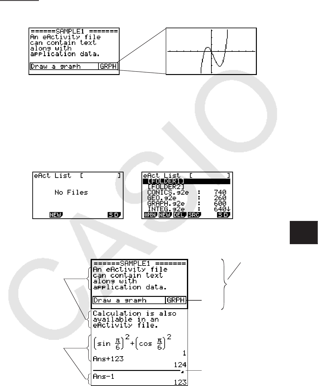
10-1
第10章 eActivity
您可使用e • ACT模式在eActivity文件中输入数据。您可输入文本和数值表达式,也可粘贴“数
据条”等计算器内置应用程序的数据(例如图形、表格等等)。
例如,老师可使用eActivity文件为学生布置数学习题并提供求解提示。学生可使用eActivity文
件记录课堂笔记、问题备忘录及其答案等等。
重要!
• fx-7400G II和fx-9750G II未配置 e • ACT 模式。
1. eActivity概述
在主菜单上选择 e • ACT 模式之后,首先显示文件菜单。
存储器中没有 e • ACT 模式文件 存储器中至少有一个 e • ACT 模式文件
在e • ACT模式中打开某个文件将显示一个工作区屏幕,您可使用该屏幕输入和编辑文本、计算
表达式和其他数据。
计算器的
显示区
文本行
数据条
数学计算行
停止行
10

10-2
下面说明您可在eActivity文件中输入和编辑的数据类型。
文本行 .............................. 文本行可用于输入作为文本的字符、数字和表达式。
计算行 .............................. 使用计算行输入可执行的计算公式。结果将在下一行显示。计算方式与
在 RUN • MAT 模式中一样,同时也启用了自然输入方式。
停止行 .............................. 停止行可用于在特定点停止计算。
数据条 .............................. 数据条可用于在eActivity中嵌入来自图形、Conics Graph、电子表格或者其
他内置应用程序的数据。
2. eActivity功能菜单
k 文件列表功能菜单
• { OPEN } ... 打开eActivity文件或者文件夹。
• { NEW } ... 创建eActivity文件。
• { DEL } ... 删除eActivity文件。
• { SRC } ... 搜索eActivity文件。
• { SD } / { SMEM } ... 在计算器主存储器文件与SD卡存储器文件之间切换文件菜单中显示的文件
(仅限支持SD卡的型号)。当文件菜单显示主存储器文件时,该菜单项目显示{SD};当
文件菜单显示SD卡文件时,该菜单项目显示{SMEM}。
• 只有在存储器中没有eActivity文件时,才显示 2(NEW)功能键。
• 在首次使用 e
•
ACT 模式时,至少需要128 kB存储器空间。如果存储空间不足,会显示一条
Memory Full错误消息。
k 工作区屏幕功能菜单
工作区功能菜单的部分内容取决于当前选定的行(数据条)。
• 工作区屏幕常用菜单项目
• { FILE } ... 显示以下文件操作子菜单。
• { SAVE } ... 保存当前编辑的文件。
• { SV
•
AS } ... 将当前编辑的文件保存为另一个名称。
• { OPT } ... 参见(第11-11页)“优化永久存储器或者SD卡存储器”。
• { CAPA } ... 显示器的屏幕,其中显示了被编辑文件的数据大小以及剩余存储器容量。
• { STRP } ... 插入数据条。
• { JUMP } ... 显示以下子菜单以控制光标移动。
• { TOP } / { BTM } / { PgUp } / { PgDn } ... 参见第10-4页。
• { DEL-L } ... 删除当前选定或者光标所在位置的行。
• { INS } ... 在当前选定行或光标所在行的上方插入新行时,显示以下插入子菜单。
• { TEXT } ... 插入一个文本行。
• { CALC } ... 插入一个计算行。
• { STOP } ... 插入一个计算停止行。
• { 'MAT } ... 显示矩阵编辑器(第10-6页)/向量编辑器(第10-7页)。
• { 'LIST } ... 显示列表编辑器(第10-7页)。

10-3
• 选择某个文本行时的菜单
• { TEXT } ... 将当前行从文本行改为计算行。
• { CHAR } ... 显示用于输入数学符号、特殊符号和各种语言字符的菜单。
• { A
⇔
⇔ a } ... 在启用字母字符输入期间在大写和小写输入之间切换(按下 a键)。
• { MATH } ... 显示MATH菜单(第1-11页)。
• 选择某个计算行或停止行时的菜单
• { CALC } ... 将当前行从计算行改为文本行。
• { MATH } ... 与“选择某个文本行时的菜单”下的{MATH}相同。
• 选择某个数据条时的菜单
• { FILE } ... 显示以下文件操作子菜单。
• { SAVE } / { SV
•
AS } / { OPT } / { CAPA } ... 与“工作区屏幕常用菜单项目”下的{FILE}子菜单相
同。
• { SIZE } ... 显示当前光标位置的数据条的大小。
• { CHAR } ... 与“选择某个文本行时的菜单”下的{CHAR}相同。
• { A
⇔
⇔ a } ... 与“选择某个文本行时的菜单”下的{A
⇔
⇔ a}相同。
3. eActivity文件操作
本节说明在eActivity文件菜单屏幕中可执行的各种不同文件操作。在显示文件菜单时,可执行
本节所有操作。
本节不包括文件夹操作。关于文件夹的详情,请参见“第11章 存储器管理器”。
u 新建一个文件
1. 显示文件菜单时,按下 2(NEW)。
• 由此将显示一个文件名输入屏幕。
2. 输入最长8个字符的文件名,然后按下 w。
• 由此可显示一个空白工作区屏幕。
光标
• 下面是文件名中可使用的字符。
A至Z、{、}、’、˜、0至9
u 打开一个文件
使用 f和 c,突出显示想要打开的文件,然后按下 1(OPEN) 或者 w*。
* 如果出现错误,删除捕捉存储器和剪贴板数据,或者将数据传输至您的电脑。
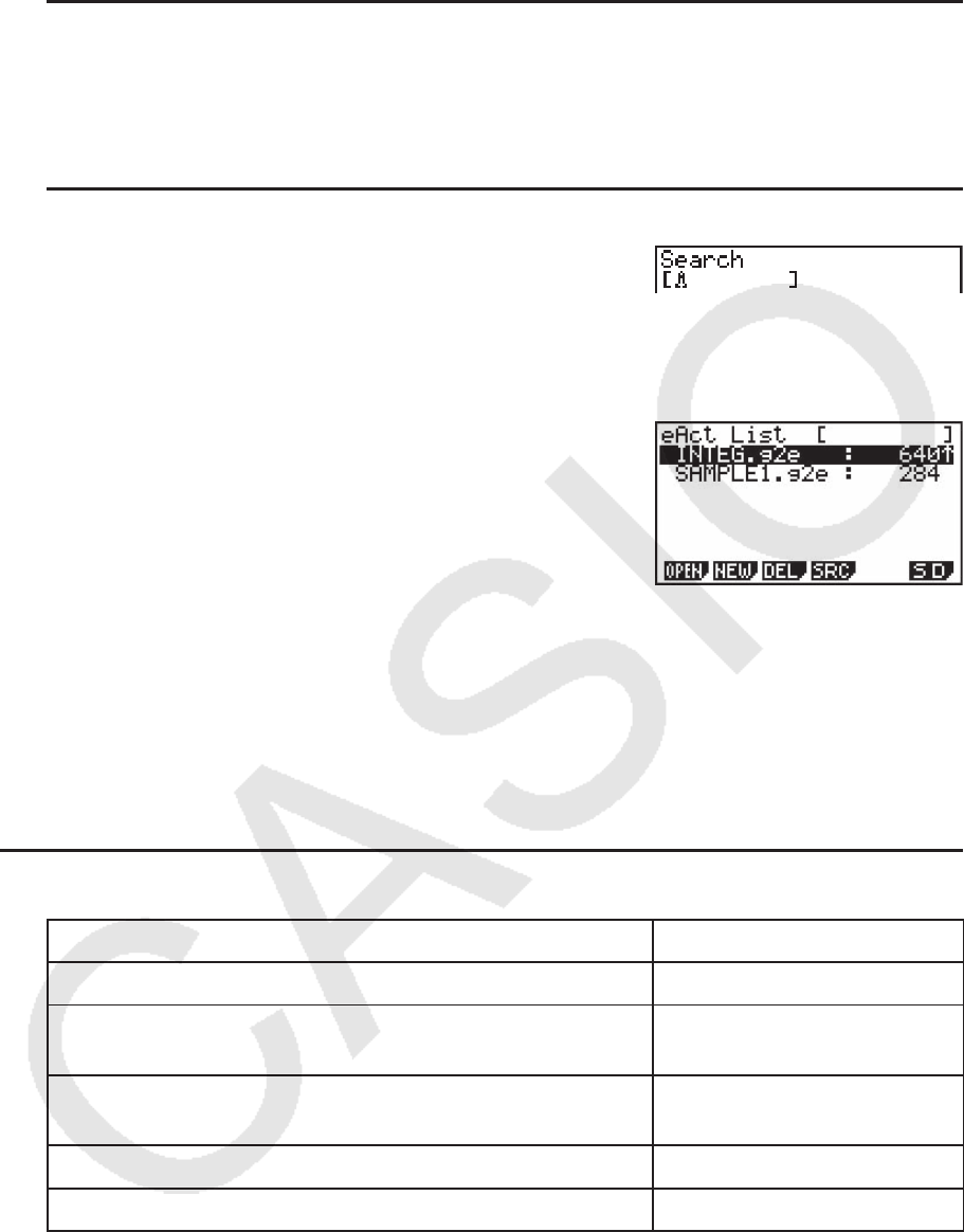
10-4
u 删除一个文件
1. 使用 f和 c,突出显示想要删除的文件,然后按下 3(DEL)。
• 由此将显示一条“Delete eActivity?”确认消息。
2. 按下 1(Yes),删除文件;或者按下 6(No),取消操作且不删除任何内容。
u 搜索一个文件
1. 显示文件菜单时,按下 4(SRC)。
• 由此将显示一个文件搜索屏幕。
2. 输入想要查找的部分或者完整文件名。
• 从左向右搜索文件名字符。输入“IT”返回ITXX、ITABC、IT123等名称,但不包括XXIT
或ABITC。
3. 按下 w。
• 如果某个名称与在第2步中输入的文本匹配,将在文件菜
单上选定该名称。
• 如果没有找到匹配项,将显示消息“Not Found”。按下 J键,关闭消息对话框。
4. 输入和编辑数据
本节所有操作均在eActivity工作区屏幕上执行。使用“eActivity文件操作”(第10-3页)中的
步骤新建文件或者打开现有文件。
k 光标移动和滚动操作
目标操作: 按键操作:
前后移动光标 f或者 c
向前滚动一屏 !f或者
6( g) 1(JUMP) 3(PgUp)
向后滚动一屏 !c或者
6( g) 1(JUMP) 4(PgDn)
将光标移至工作区屏幕的起始处 6( g) 1(JUMP) 1(TOP)
将光标移至工作区屏幕的结束处 6( g) 1(JUMP) 2(BTM)
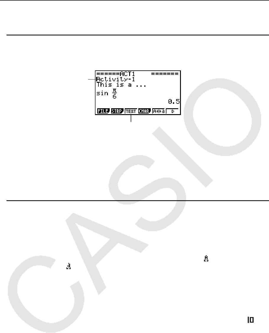
10-5
k 输入文本行
使用文本行输入字母数字字符、表达式等等。
u 输入作为文本的字符和表达式
1. 将光标移至文本行。
•光标位于文本行中时,F3功能菜单项目中将显示“TEXT”。这表示启用了文本输入。
文本行光标
3 键菜单变为“TEXT”。
• 如果光标在某个计算行中,F3功能菜单项目将显示“CALC”。按下 3(CALC),将计算行
改为文本行。
• 如果光标位于某个数据条内,使用 f和 c ,将光标移至文本行。
• 在功能菜单上,依次选择{INS}和{TEXT},将在光标当前所在行的上方插入新文本行。
2. 在文本数据条中插入所需文本或者表达式。
• 参见下述“文本行输入和编辑操作”。
u 文本行输入和编辑操作
• 一个文本行最多可输入255个文本字节。文本行中的文本自动换行以适应显示区(文字 换行功
能)。但请注意,数值表达式和命令不换行*
1
。
计算行的左侧和右侧将显示滚动箭头( ]'),
提醒您某些计算表达式已超出计算行显示区。在此情况下,您可使用向左和向右光标键滚动计算
式。
• 5(A ↔ a) 功能键可在大写和小写输入之间切换。该功能只有在启用字母文本输入的情况下才
可使用。详情请参见第2-7页。在选定大写输入模式时,文本行光标为 ;选定小写输入模式
时,文本行光标为 。
• 按下 w,在文本中输入回车符。回车符不显示任何符号。
• 如果某个文本分为多行,按下 A键将只删除光标当前所在的行。不会删除其他行的部分文
本。
• 在文本行中输入表达式时必须使用自然输入方式(第1-10页)。
*
1
此外,任何包括在使用按下 4(CHAR)时显示的菜单输入的符号“ ’ ”、“{”或“ ” 的
文字都不会换行。
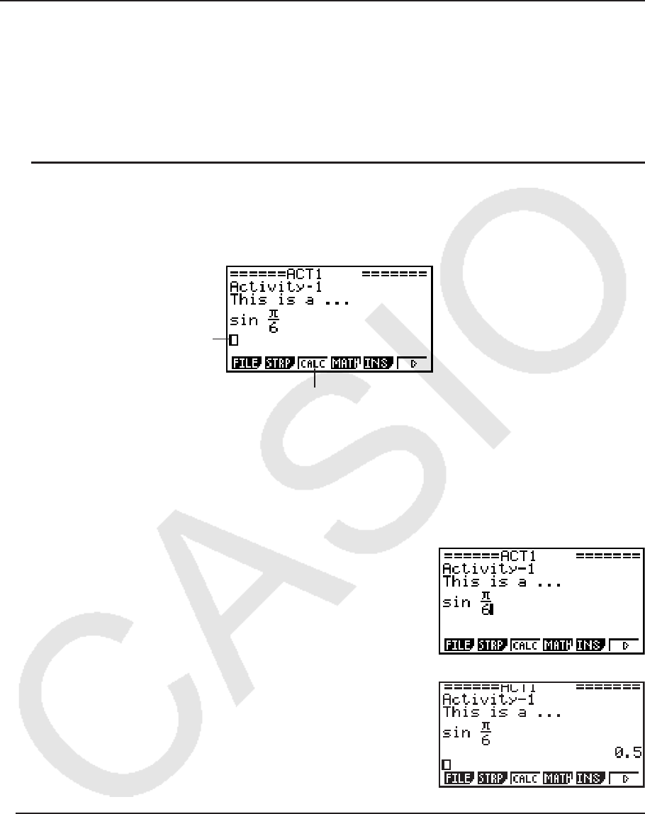
10-6
k 输入计算行
在eActivity计算行中输入一个计算表达式并按下 w,将在下一行显示计算结果。这种计算行的
使用方式可与在 RUN
•
MAT 模式中相同(第1-3页)。计算行及其结果构成一组。
• 请注意,文字换行功能不适合数学计算行。计算行的左侧和右侧将显示滚动箭头( ]'),提
醒您某些计算表达式已超出计算行显示区。在此情况下,您可使用向左和向右光标键滚动计算
式。
u 将计算公式输入eActivity
1. 将光标移至计算行。
•光标位于计算行中时,F3功能菜单项目中将显示“CALC”。这表示启用了计算表达式输
入。
数学计算行光标
这将使 3键菜单变为“CALC”。
• 如果光标在某个文本行中,F3功能菜单项目将显示“TEXT”。按下 3(CALC),将计算行
改为文本行。
• 如果光标位于某个数据条内,使用 f和 c,将光标移至计算行。
• 在功能菜单上,依次选择{INS}和{CALC},将在光标当前所在行的上方插入新计算行。
2. 输入一个计算表达式(示例: s$!E( π ) cg)。
• 计算行输入和编辑操作与在自然输入 RUN
•
MAT 模式中
相同。
3. 如需获取计算结果,按下 w。
u 使用矩阵编辑器进行矩阵计算
选择功能菜单上的{ 'MAT},显示矩阵编辑器。
e • ACT模式中的矩阵编辑器操作和矩阵计算基本上与在 RUN
•
MAT 模式中相同。关于矩阵编辑
器和矩阵计算操作的详情,请参见“矩阵计算”(第2-36页)。但请注意,e • ACT模式矩阵编
辑器操作和矩阵计算与下述 RUN
•
MAT 模式中的操作不同。
• 单独保存每个文件的e • ACT模式矩阵变量值。矩阵变量将与从非e • ACT模式调用时产生的变
量值不同。

10-7
u 使用向量编辑器进行向量计算
选择功能菜单上的{ 'MAT},显示向量编辑器。
e • ACT模式中的向量编辑器操作和向量计算基本上与在RUN • MAT模式中相同。关于向量编辑
器和向量计算操作的详情,请参见“向量计算”(第2-49页)。但请注意,e • ACT模式向量编
辑器操作和向量计算与下述RUN • MAT模式中的操作不同。
• 单独保存每个文件的e • ACT模式向量存储器。向量存储器将与从非e • ACT模式调用时产生的
存储器不同。
u 使用列表编辑器进行列表计算
选择功能菜单上的{ 'LIST},显示列表编辑器。
e • ACT模式中的列表编辑器操作与在 STAT 模式中相同(“输入和编辑列表”,第3-1页)。该
处理过程和计算基本上与在 RUN
•
MAT 模式中相同(第3-5页的“操控列表数据”和第3-10页
的“使用列表进行算术计算”)。但请注意,e • ACT模式列表编辑器操作和列表计算与下述其
它模式中的操作不同。
• e • ACT模式列表编辑器功能菜单只提供 STAT 模式列表编辑器功能菜单的第二个屏幕。
• 如需在e • ACT模式下从列表编辑器返回工作区屏幕,按下 J。
•在e • ACT模式中,单独保存每个文件的列表变量值。列表变量将与从非e • ACT模式调用时产
生的变量值不同。
k 输入计算停止行
在工作区屏幕上编辑包括多行的计算行之后,按下 w,将重新计算编辑行之后的所有计算式。
如果有大量计算行或如果某些计算较为复杂,重新计算过程可能需要相当长时间。插入计算停
止行将在该行所在位置停止重新计算过程。
u 插入停止行
在功能菜单上,依次选择{INS}和{STOP},将在当前选定行或数据条上插入一个停止行。
k 使用数据条
“数据条”是用于在eActivity文件中嵌入内置应用程序数据的工具。每个数据条只能关联一个
内置应用程序屏幕,数据条可存储屏幕产生的数据(图形等等)。
下表显示了可插入数据条的内置应用程序屏幕。“数据条名称”列显示在按下 2(STRP)时弹出
对话框中包括的名称。
数据条数据类型表
数据类型 数据条名称
RUN • MAT 模式计算数据(在从eActivity调用 RUN
•
MAT 模式时,以自
然输入模式启动。)
Run (Math)
GRAPH 模式图形屏幕数据 Graph
GRAPH 模式图形关系列表屏幕数据 Graph Editor
TABLE 模式表格关系列表屏幕数据 Table Editor
CONICS 模式图形屏幕数据 Conics Graph

10-8
数据类型 数据条名称
CONICS 模式函数列表屏幕数据 Conics Editor
STAT 模式统计图形屏幕数据 Stat Graph
STAT 模式列表编辑器数据 List Editor
EQUA 模式计算解屏幕数据 Solver
RECUR 模式递归类型选择屏幕 Recur Editor
Notes屏幕数据(Notes是一种特殊的eActivity应用程序。详情请参见第
10-9页的“Notes数据条”。)
Notes
RUN
•
MAT 模式矩阵编辑器数据 Matrix Editor
RUN
•
MAT 模式向量编辑器数据 Vector Editor
EQUA 模式方程组解屏幕数据 Simul Equation
EQUA 模式高阶方程解屏幕数据 Poly Equation
DYNA 模式图形屏幕数据 Dynamic Graph
TVM 模式计算解屏幕数据 Financial
S
•
SHT 模式电子表格屏幕数据 Spreadsheet
E-CON3 或 E-CON2 模式设置向导数据 Econ SetupWizard
E-CON3 或 E-CON2 模式高级设置数据 Econ AdvancSetup
E-CON3 或 E-CON2 模式高级设置数据
(执行该数据条将根据首次执行数据条时记录在数据条中的设置信息立
即开始取样。)
Econ Sampling
E-CON3 或 E-CON2 模式高级设置数据
(执行该数据条将根据首次执行数据条时记录在数据条中的取样数据绘
制图形。)
Econ Graph
u 插入数据条
1. 将光标移至想要插入数据条的位置。
2. 按下 2(STRP)。
• 由此将显示一个对话框和可插入数据条列表。关于该对
话框上的显示名称和数据类型的信息,请参见“数据条
数据类型表”(第10-7页)。
3. 使用 c和 f,选择对应于想要插入的数据类型的数据条。
• 在本例中,我们将选择“Graph”( GRAPH 模式图形屏幕数据)。
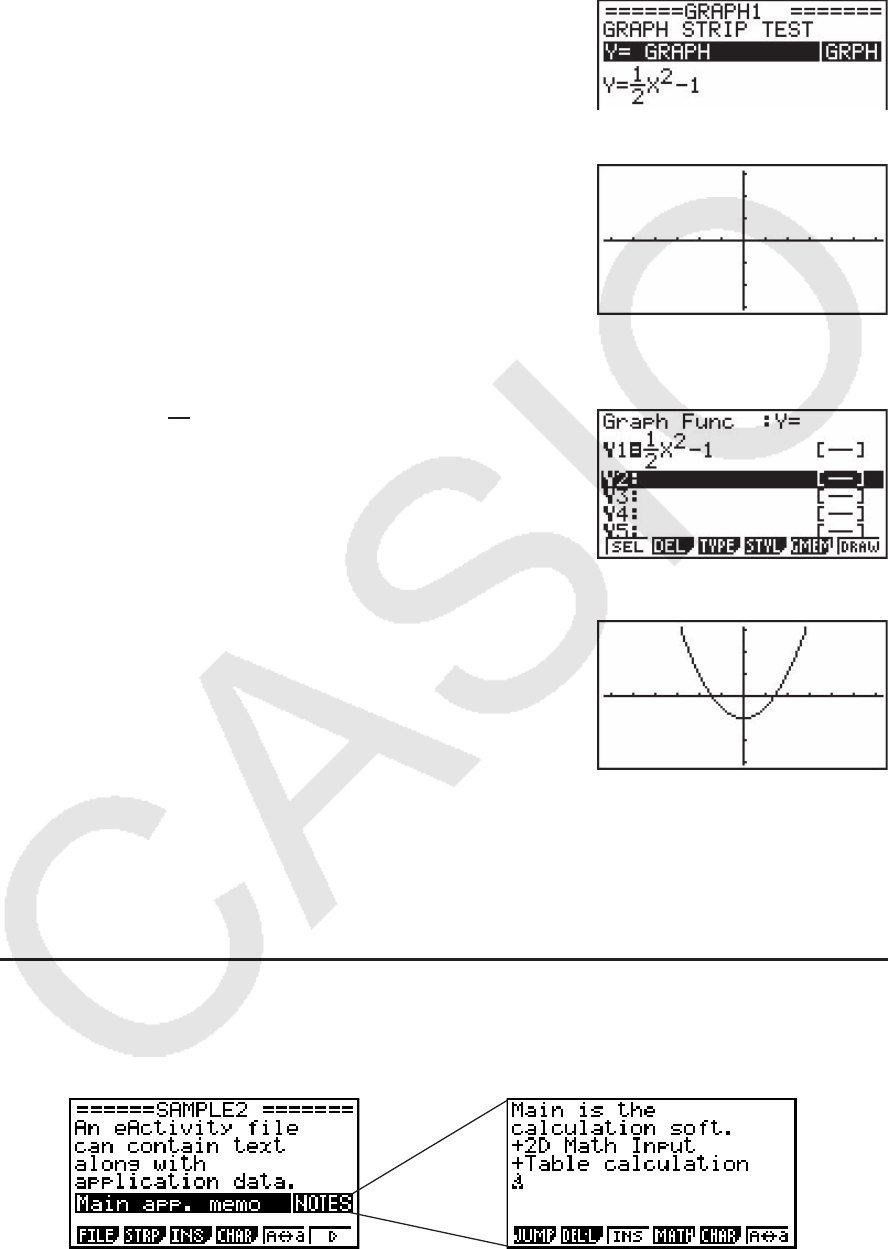
10-9
4. 按下 w。
• 由此可将选定类型的数据条(本例为Graph数据条)插入第1步光标所在行的上一行。
5. 输入最长16个字符的数据条标题,然后按下 w。
6. 再次按下 w,开始创建数据条数据。
• 由此将启动选定数据条类型的内置应用程序(本例
为 GRAPH 模式),然后显示图形屏幕。此时,由于没有
其他数据,显示一个空图形屏幕。
7. 按下 J,显示图形函数列表屏幕。
8. 输入想要绘制图形的函数。
(示例:Y = 2
1 X
2
-1)
9. 按下 6(DRAW)。
• 由此将绘制输入的函数图形。
10. 如需返回eActivity工作区屏幕,按下 !a( ')。
• 在第8步绘制图形的数据将保存在Graph数据条中。
•保存的图形数据只与该Graph数据条链接。它与从主菜单输入的模式数据无关。
11. 在此再次按下 w,显示图形屏幕并根据数据条保存的数据绘制图形。
u Notes数据条
“Notes”是一种特殊的eActivity文本编辑器,可方便您将较长的文本说明写入工作区屏幕。在
工作区屏幕上您可从Notes数据条调用Notes屏幕。Notes屏幕上的输入和编辑操作与eActivity文
本行操作完全相同。
下面说明了Notes屏幕功能菜单项目。

10-10
• { JUMP } ... 显示一个JUMP菜单,您可使用该菜单跳转至数据的顶部( 1(TOP))、底部
( 2(BTM))、前一页( 3(PgUp))或者下一页( 4(PgDn))。
• { DEL-L } ... 删除当前选定或者光标所在位置的行。
• { INS } ... 在光标当前所在行的上方插入新行。
• { MATH } ... 显示MATH菜单(第1-11页)。
• { CHAR } ... 显示用于输入数学符号、特殊符号和各种语言字符的菜单。
• { A
⇔
⇔ a } ... 在启用字母字符输入期间在大写和小写输入之间切换(按下 a键)。
u 更改数据条的标题
1. 使用 c和 f,选择想要更改标题的数据条。
2. 输入最长16个字符的数据条标题,然后按下 w。
• 一旦输入第一个字符,现有标题的其余部分都会消失。输入完整的新标题。如果您希望编辑
部分现有标题,首先按下 d或者 e以移动光标。
• 按下 J而不是 w,将退出标题编辑操作,且不更改任何内容。
u 从数据条调用应用程序
使用 c和 f,选择想要调用应用程序的数据条,然后按下 w。
• 由此将显示对应于选定数据条的应用程序屏幕。如果数据条已经包含数据,使用上次保存的数
据调用应用程序。
•如果选择Conics Graph数据条,而且在按下 w时没有输入任何图形数据,将显示Conics
Editor屏幕,而不是Conics Graph屏幕。
u 在eActivity工作区屏幕与从数据条调用的应用程序屏幕之间切换
按下 !a( ')。
每次按下 !a( '),都会在eActivity工作区屏幕与从数据条调用的应用程序屏幕之间切换。
u 从某个数据条调用的应用程序屏幕转换到另一个应用程序屏幕
按下 !,( ,)。在显示的对话框上,使用 c和 f选择应用程序的名称,然后按下 w。
u 显示数据条存储器使用情况屏幕
1. 使用 c和 f,选择想要查看数据条。
2. 按下 1(FILE) 5(SIZE)。
• 由此将显示当前选定数据条的存储器使用情况屏幕。
3. 如需退出存储器使用情况屏幕,按下 J。

10-11
u 删除行或者数据条
1. 将光标移至想要删除的行或者数据条。
• 如果您将光标移至计算行,请注意计算式和结果都会被删除。
2. 按下 6( g) 2(DEL-L)。
• 由此将显示一条确认消息。
3. 按下 1(Yes),删除文件;或者按下 6(No),取消操作且不删除任何内容。
k 保存文件
在工作区屏幕中输入或者编辑某个文件之后,使用本节步骤保存文件。
操作系统版本为2.0或者更高的eActivity文件扩展名可能为“g2e”。在本手册所述型号的计算
器上执行以下任一eActivity文件保存操作(操作系统版本为2.0或者更高),都将在文件名后添
加“g2e”扩展名。
• 保存新建文件
• 使用“另存为”操作保存现有文件( 1(FILE) 2(SV-AS))
如果您使用本手册所述型号的计算器将eActivity文件保存为扩展名为“g1e”的文件(从型号较
旧的计算器传输的文件),文件扩展名将根据以下规则确定。
• “g2e”扩展名用于eActivity文件,这些文件包括2.0或更高版本操作系统新增特性的数据
(不包括数学函数和命令)。
例如,此处“2.0或更高版本操作系统新增特性的数据”可表示以 '或 π 格式显示的计算结果
数据。
• “g1e”表达式用于上述范围之外的eActivity文件。
u 使用新版本替换现有文件
按下 1(FILE) 1(SAVE),保存当前打开的文件。
u 使用新名称保存文件
1. 在eActivity工作区屏幕上,按下 1(FILE) 2(SV-AS)。
• 由此将显示一个文件名输入屏幕。
2. 输入最长8个字符的文件名,然后按下 w。
• 如果您在第2步中输入的文件名已经存在,将显示一条消息,请您确认是否希望使用新文件
替代现有文件。按下 1(Yes)可替代现有文件,或者按下 6(No)可取消保存操作并返回第2
步的文件名输入对话框。
重要!
• 在操作系统版本低于2.0的计算器上,无法打开扩展名为“g2e”的eActivity文件。
•打开扩展名为“g1e”的eActivity文件,输入2.0或更高版本操作系统增加的函数,然后保存文
件,可能导致新保存的文件保留“g1e”扩展名。虽然您可以在操作系统版本低于2.0的计算器
上打开此类文件(因为扩展名为“g1e”),但您无法使用从2.0版操作系统开始增加的数学函
数和命令。
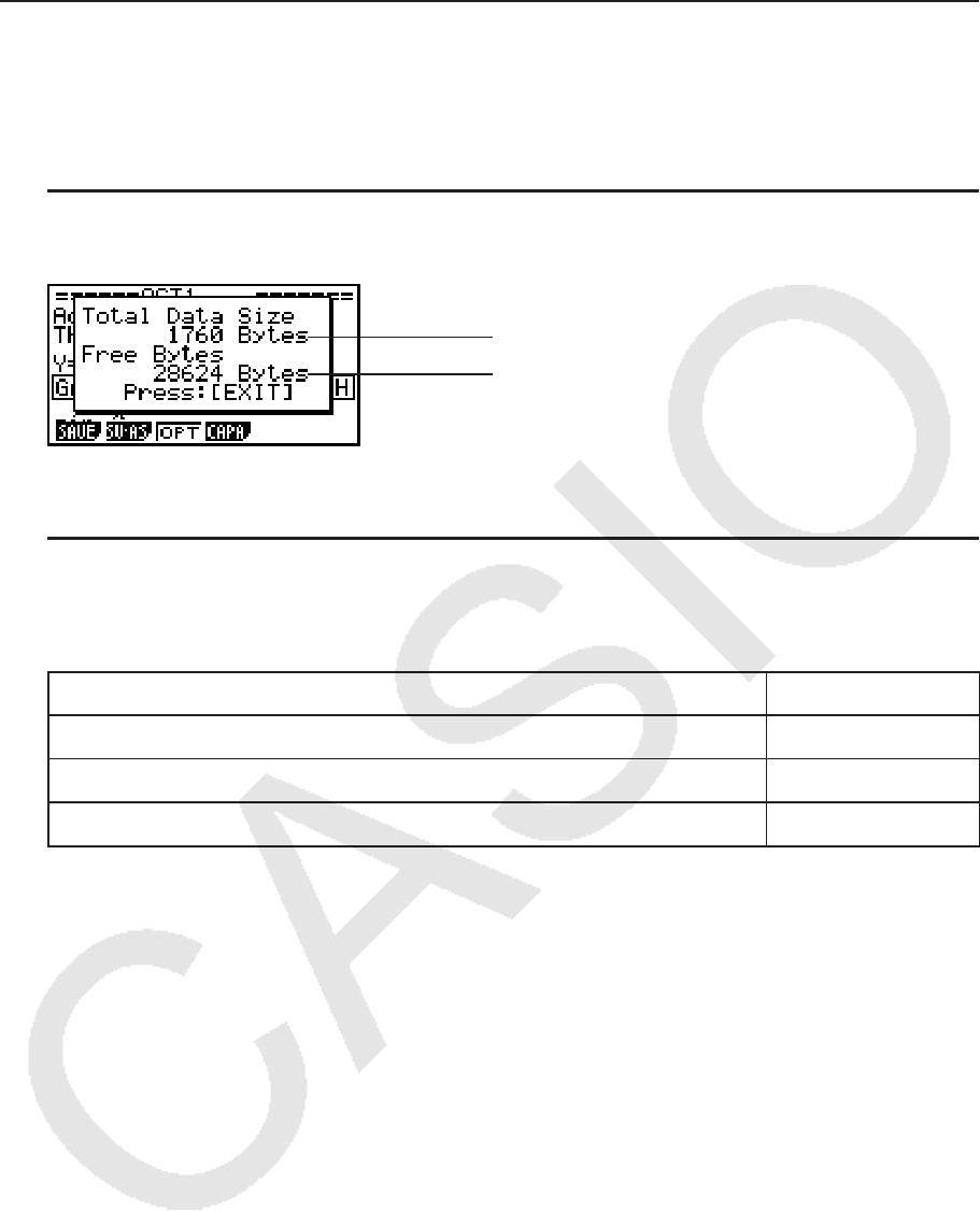
10-12
k 显示eActivity存储器使用情况屏幕
eActivity文件的最大容量大约为30000字节*。您可使用eActivity文件存储器使用情况屏幕查看
当前操作文件的剩余存储容量。
* 实际最大文件容量取决于捕捉存储器和剪贴板存储器的使用情况,可能小于30000字节。
u 显示eActivity存储器使用情况屏幕
在工作区屏幕上,按下 1(FILE) 4(CAPA)。
文件使用情况
剩余文件存储容量
如需退出存储器使用情况屏幕,按下 J。
u 从工作区屏幕返回文件列表
按下 J。
如果显示的确认消息要求您确认是否希望保存当前显示的文件,可执行以下某一操作。
操作: 按下该键:
使用编辑后的文件覆盖现有eActivity文件,然后返回文件列表 1(Yes)
返回文件列表但不保存当前编辑的文件 6(No)
返回eActivity工作区屏幕 A

11-1
第11章 存储器管理器
fx-7400G II/fx-9750G II
这些型号支持以下数据操作:数据显示、搜索和删除。
重要!
fx-7400G II/fx-9750G II计算器未配置永久存储器或卡插槽。因此,不支持下述永久存储器和
SD卡存储操作。
fx-9860G
II SD/fx-9860G II/ fx-9860G AU PLUS
这些型号配有主存储器和永久存储器,因此支持以下数据操作:数据显示、搜索和删除,以及
存储器之间的数据复制。
主存储器是可用于输入数据、执行计算和运行程序的工作区。主存储器中的数据相对安全,但
如果电池电量耗尽或者执行全面复位时,这些数据会被删除。
永久存储器使用“闪存”,因此即使切断电源也可保证数据安全。
正常情况下,您应使用永久存储器保存需要长期安全存储的数据,只有在需要时才将数据载入
主存储器。
• fx-9860G
II SD也支持使用SD卡存储器(在将SD卡插入卡插槽时)。
1. 使用存储器管理器
在主菜单中,选择 MEMORY 图标,进入 MEMORY 模式。
• 在fx-7400G
II/fx-9750G II上,将显示右图所示主存储器信
息屏幕。关于使用该屏幕的详情,请参见“存储器信息屏
幕”(第11-2页)。
• 在其它型号上,显示右图屏幕。
• { MAIN } ... {显示主存储器信息}
• { SMEM } ... {显示永久存储器信息}
• { SD } ... {显示SD卡存储器信息}(仅限fx-9860G
II SD)
• { BKUP } ... {主存储器备份}
•{ OPT } ... {永久存储器,SD卡优化}
11
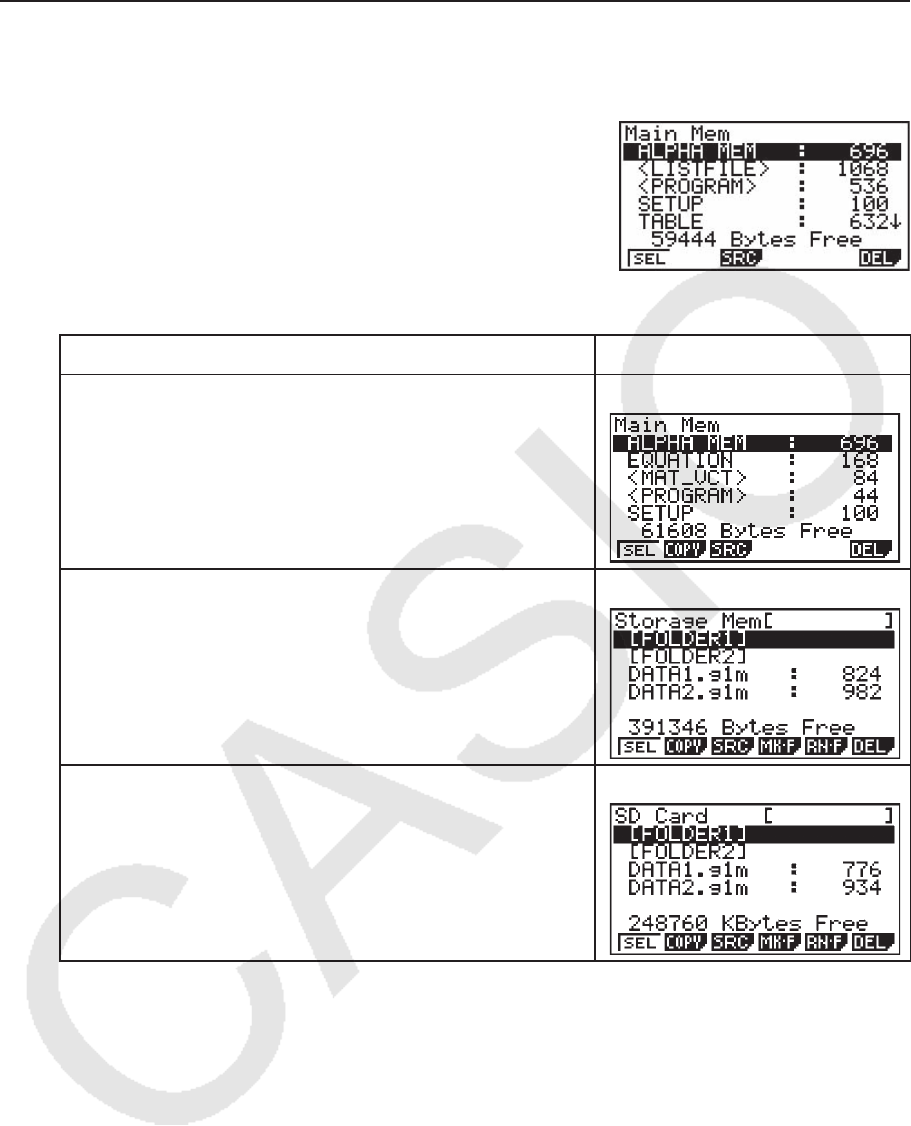
11-2
k 存储器信息屏幕
存储器信息屏幕每次显示某个存储器的信息:计算器的主存储器、永久存储器或者SD卡存储
器。
• 由于fx-7400G
II或者 fx-9750G II计算器只有主存储器,因
此只有主存储器信息屏幕显示主存储器内容。
• 对于其它型号的计算器,执行以下某一 MEMORY 模式菜单操作,显示所需存储器信息屏幕。
在显示该存储器信息屏幕时: 按下该键:
主存储器 1(MAIN)
永久存储器 2(SMEM)
SD卡存储器(仅限fx-9860G
II SD) 3(SD)
• 使用光标 f和 c键移动突出显示位置并检查每一类数据使用的字节数。
• 第7行显示在当前选定存储器(主存储器、永久存储器或者SD卡)中尚未使用的存储容量字节
数。
• 首次将数据保存到永久存储器中时,计算器将自动保留一个管理存储区域,因此“Free”值会
减少65536字节。
• 在主存储器屏幕上,< >表示数据组。在永久存储器和SD卡屏幕上,[ ]表示文件夹。
突出显示某个数据组或者文件夹,并按下 w,显示数据组或者文件夹内容。按下 J,返回前
一个屏幕。
在显示永久存储器或者SD卡文件夹的内容时,屏幕的第一行显示文件夹名称。

11-3
可检查以下数据。
主存储器
数据名称 内容
ALPHA MEM 字母变量
<CAPTURE> 捕捉存储器组
CAPT
n( n = 1至20) 捕捉存储器
CONICS*
1 圆锥曲线论设置数据
DYNA MEM*
1 动态图形存储器
EQUATION 方程数据
FINANCIAL*
1 财务数据
<F-MEM> 函数存储器组
F-MEM
n( n = 1至20) 函数存储器
<G-MEM> 图形存储器组
G-MEM
n( n = 1至20) 图形存储器
<LISTFILE> 列表文件组
LIST
n( n = 1至26和Ans) 列表存储器内容
LIST FILE
n( n = 1至6) 列表文件
<MAT_VCT>*
2 矩阵组/向量组
<MATRIX>*
3 矩阵组*
3
MAT
n ( n = A至Z和Ans)*
1 矩阵
VCT
n ( n = A至Z和Ans)*
2 向量
<PICTURE> 图片存储器组
PICT
n( n = 1至20) 图片存储器
<PROGRAM> 程序组
每个程序名称 程序
RECURSION*
1 递归数据
SETUP 设置数据
STAT 统计结果数据
<STRING> 字符串存储器组
STR
n ( n = 1至20) 字符串存储器
SYSTEM 操作系统和应用程序共享数据(剪贴板、重放、历史等等)
<S-SHEET>*
2 电子表格组
每个电子表格名称*
2
电子表格数据
每个附加应用程序名称*
2 应用程序特定数据
TABLE 表格数据
<V-WIN> 视窗存储器组
V-WIN
n( n = 1至6) 视窗存储器
Y=DATA 图形表达式
*
1
fx-7400G II中不包括。 *
2
fx-7400G II/fx-9750G II中不包括。 *3 仅限fx-9750GII
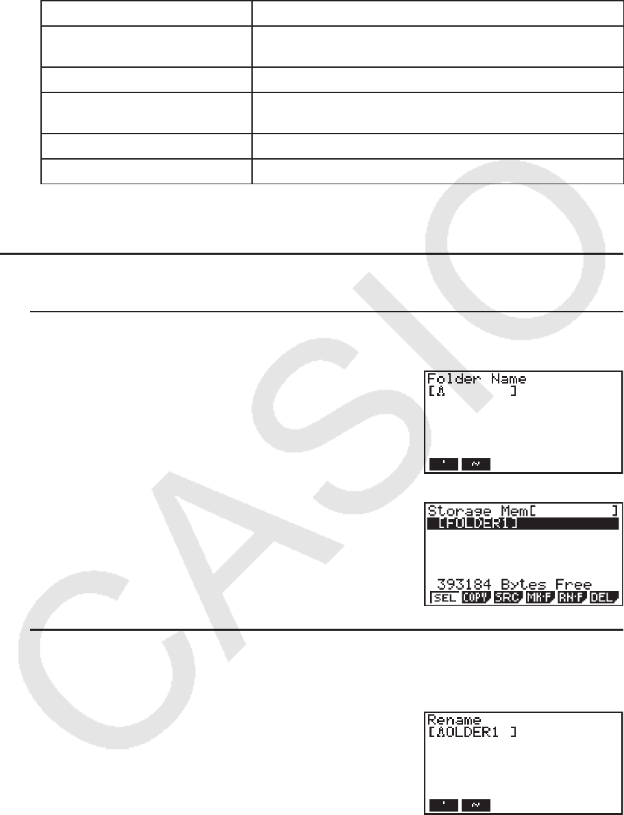
11-4
永久存储器,SD卡 *
1
数据名称 内容
*.g1m或者.g2m文件名 已经复制到永久存储器或者SD卡并列在主存储器表中的数
据项目。 这些文件的扩展名为“.g1m”或者“.g2m”。
eActivity数据名称 保存在永久存储器或者SD卡中的eActivity数据。
附加软件名称(应用程序、语
言、菜单)
保存在永久存储器或者SD卡中的附加应用程序、附加语言
和附加菜单。
文件夹名称 使用方括号([ ])括起。
末知 由于写入错误等原因导致不可用的区域。
*
1
当永久存储器或者SD卡上没有数据时,显示“No Data”。“No Card”消息表示计算器中
没有装入SD卡。
k 在永久存储器或者SD卡中创建一个文件夹
u 新建一个文件夹
1. 显示屏上显示永久存储器或者SD卡数据时,按下 4(MK • F),显示文件夹名称输入屏幕。
2. 输入最长八个字符的文件夹名称。
• 只支持以下字符:A至Z、{、}、’、~、0至9
输入任何无效字符都将产生“Invalid Name”错误。
• 如果您输入的名称与现有文件重复,也会产生
“Invalid Name”错误。
• 如需取消文件夹创建操作,按下 J。
3. 按下 w,创建文件夹并返回永久存储器或者SD卡存储器
信息屏幕。
u 重新命名文件夹
1. 在永久存储器或者SD卡存储器信息屏幕上,选择想要重新命名的文件夹。
2. 按下 5(RN
• F),显示重新命名文件夹屏幕。
3. 输入最长八个字符的文件夹名称。
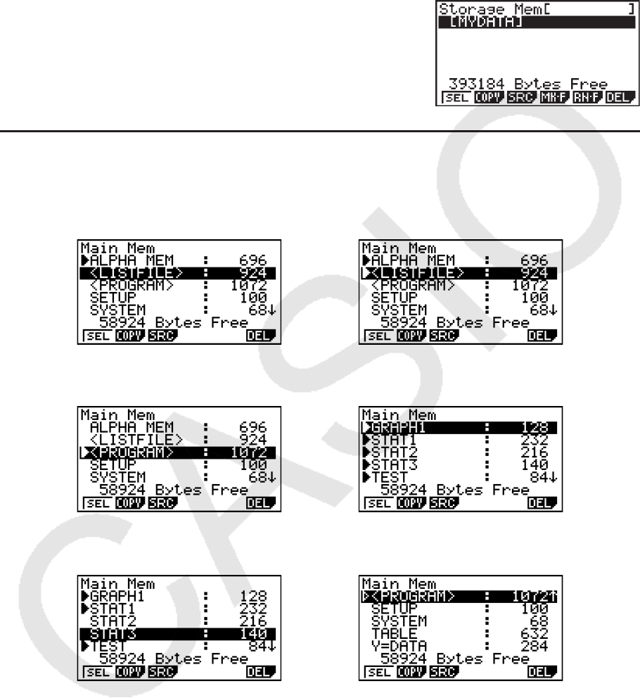
11-5
• 只支持以下字符:A至Z、{、}、’、~、0至9
输入任何无效字符都将产生“Invalid Name”错误。
• 如果您输入的名称与现有文件重复,也会产生“Invalid Name”错误。
• 如需取消文件夹创建操作,按下 J。
4. 按下 w,重命名文件夹并返回永久存储器或者SD卡存储
器信息屏幕。
k 选择数据
• 按下 1(SEL),选择当前突出显示的项目,该项目由旁边的黑色选择指针标识( )。再次按
下 1(SEL)将取消选择项目,使选择指针消失。
• 您可根据需要选择多个文件。
1(SEL)
• 选择某个组或文件夹也将选择其中的所有内容。取消选择某个组或文件夹将取消选择其中所有
内容。
• 如果选择数据组或文件夹中的一个或者多个单独项目,每个项目旁都会出现一个黑色选择指针
( ),组或文件夹名称旁出现一个白色选择指针( g)。
• 返回 MEMORY 模式初始化屏幕,取消选择所有当前选定的项目。
→
←
w
→
J
→
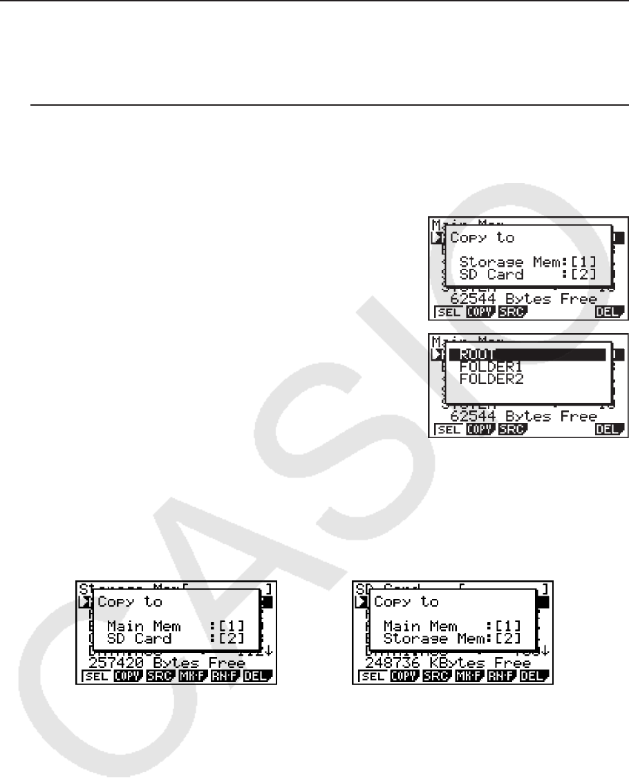
11-6
k 复制数据
重要!
• fx-7400G II或者fx-9750G II计算器上不支持数据复制操作。
u 从主存储器复制到永久存储器
注意
• 以下步骤将选定数据保存到单独文件。为保存到永久存储器中的文件指定一个名称。
1. 在主存储器数据信息屏幕上,选择想要复制的数据。
2. 按下 2(COPY)。
• 由此显示永久存储器/SD卡选择屏幕(仅限fx-9860G
II
SD)。*
1
3. 按下 b,选择永久存储器(仅限fx-9860G
II SD)。*
2
• 由此可显示文件夹选择屏幕。
4. 选择复制数据的目标文件夹。
• 由此将显示文件名输入屏幕。
5. 输入文件指定的名称。
• 如需取消复制操作,按下 J。
6. 按下 w。
• 该操作复制数据。
7. 复制操作完成时显示“Complete!”消息。按下 J将返回 MEMORY 模式初始屏幕。
*
1
从永久存储器或者SD卡复制数据后将显示以下某一个屏幕(仅限fx-9860G II SD)。
按下 b,选择主存储器并复制数据,但不显示文件夹选择屏幕。
在从永久存储器及/或SD卡向主存储器复制数据时,不显示文件名输入屏幕。
*
2
如需向SD卡复制,按下 c。如果计算器没有装入任何SD卡,将显示“No Card”错误消
息。
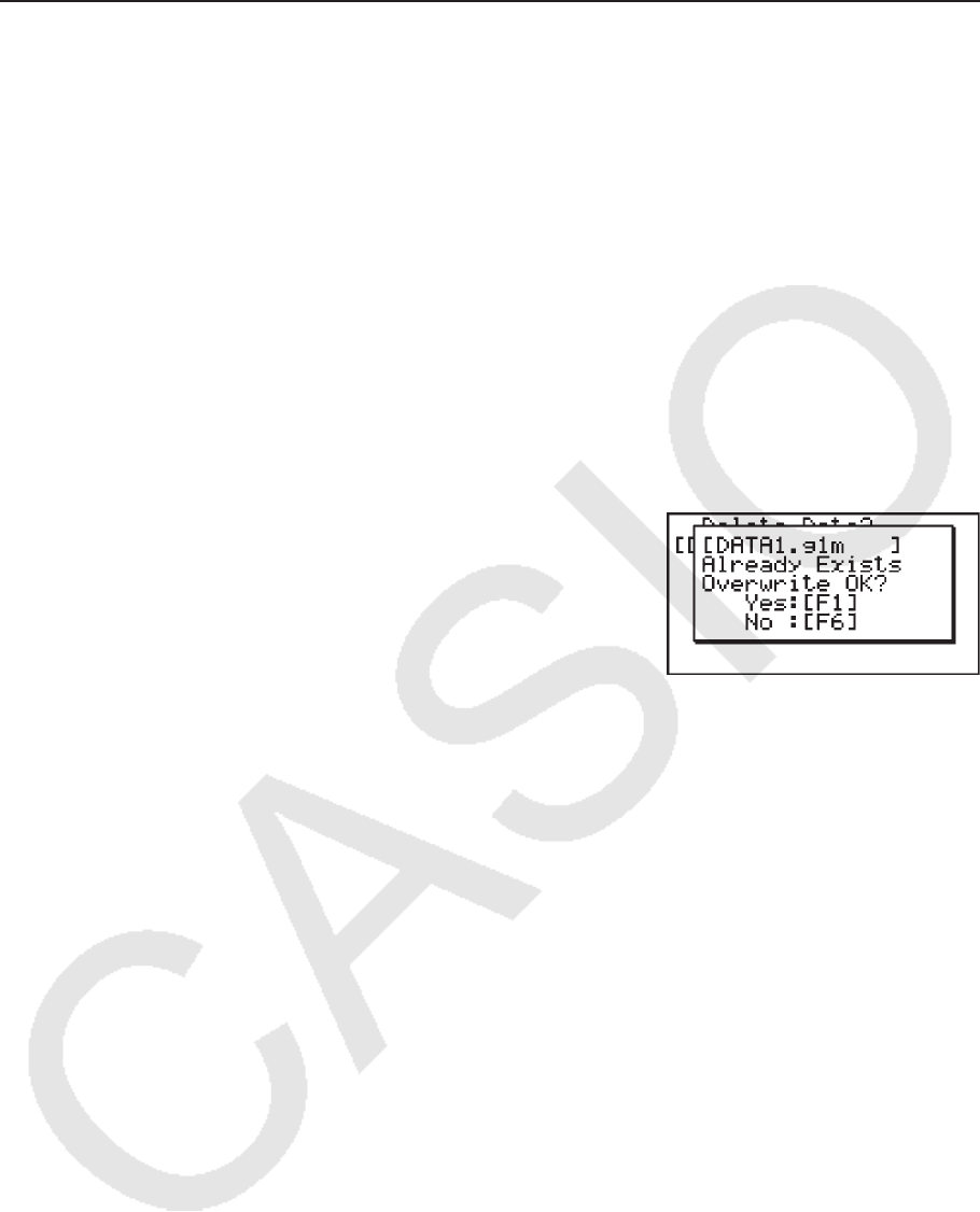
11-7
k 数据复制期间的错误检查
以下错误检查在执行数据复制操作期间执行。
低电池电量检查
计算器在开始数据复制操作之前执行低电池电量检查。如果电池电量降低到Level 1,出现低电
池电量错误且不执行复制操作。
可用存储容量检查
计算器检查可用存储容量是否足以存储复制数据。
如果存储空间不足,会出现“Memory Full”错误。
在数据项目数量过大时,会出现“Too Much Data”错误。
如果有足够的可用空间,但要求执行碎片整理操作,会出现“Fragmentation ERROR”。
如果出现“Fragmentation ERROR”,执行优化步骤(第11-11页)。
覆盖检查
计算器检查复制目标位置是否有任何现有数据与被复制的数据同名。
如果存在同名数据,显示一条覆盖确认消息。
• 1(Yes) ... 使用新数据覆盖现有数据
• 6(No) ... 继续处理下一个数据项目,但不复制同名数据
• 按下 A将取消复制操作并返回 MEMORY 模式初始屏幕。
覆盖检查仅用于以下类型的数据。其他所有类型的数据在复制时都不检查数据文件是否同名。
• 程序
• 矩阵/向量
• 列表文件
• 图形存储器
• 动态图形存储器
• 电子表格数据
覆盖检查仅用于相同类型的数据。如果不同类型的数据具有相同名称,在执行复制操作时不考
虑同名数据。
覆盖检查仅适用于复制操作的目标位置。
类型不匹配错误检查
eActivity数据、附加应用程序,附加语言、附加菜单和备份数据不可复制到主存储器。否则会
产生类型不匹配错误。
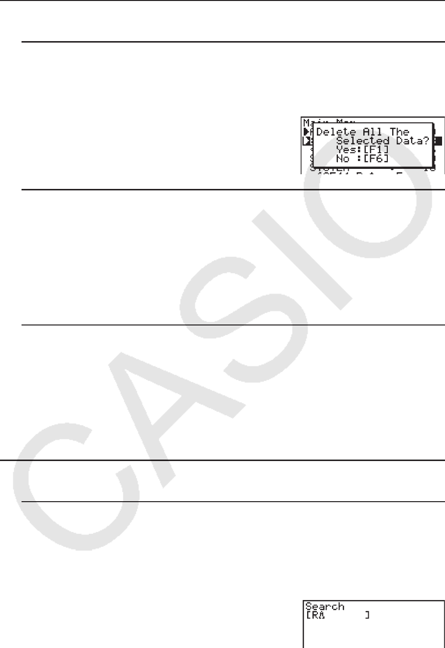
11-8
k 删除文件
u 删除主存储器文件
1. 显示主存储器信息屏幕。
• 参见第11-2页的“存储器信息屏幕”。
2. 选择想要删除的文件。您可根据需要选择多个文件。
3. 按下 6(DEL)。
• 按下 1(Yes),删除文件。
• 按下 6(No),取消删除操作。
u 删除永久存储器文件
1. 显示永久存储器信息屏幕。
• 参见第11-2页的“存储器信息屏幕”。
2. 选择想要删除的文件。您可根据需要选择多个文件。
3. 按下 6(DEL)。
• 按下 1(Yes),删除文件。
• 按下 6(No),取消删除操作。
u 删除SD卡文件(仅限fx-9860G II SD )
1. 显示SD卡存储器信息屏幕。
• 参见第11-2页的“存储器信息屏幕”。
2. 选择想要删除的文件。您可根据需要选择多个文件。
3. 按下 6(DEL)。
• 按下 1(Yes),删除文件。
• 按下 6(No),取消删除操作。
k 搜索文件
u 在主存储器中搜索一个文件
示例 在主存储器中搜索名称以字母“R”开头的所有文件
1. 显示主存储器信息屏幕。
• 参见第11-2页的“存储器信息屏幕”。
2. 按下 3(SRC)。
• 输入关键词字母“R”。
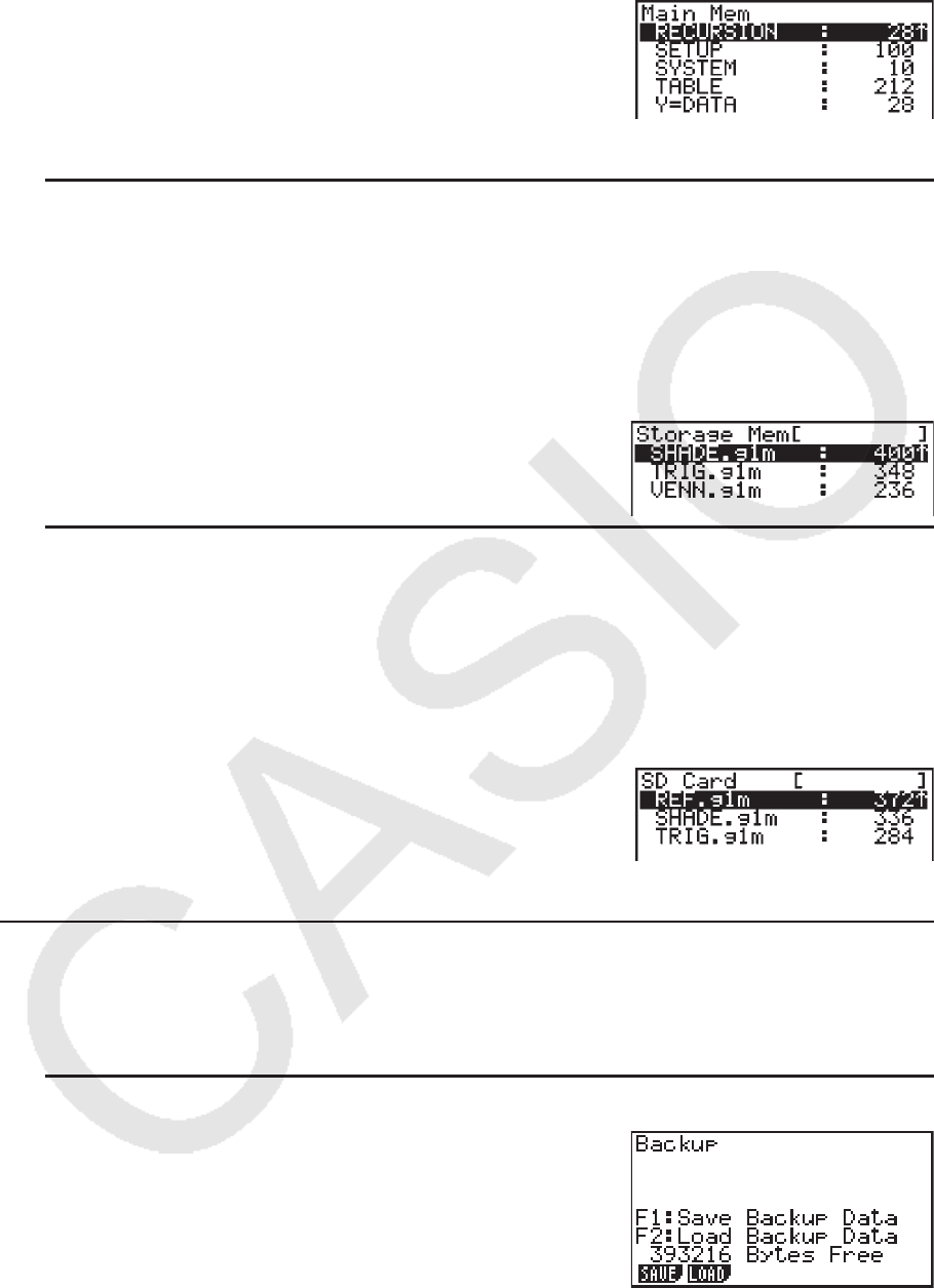
11-9
• 显示屏上突出显示以字母“R”开头的第一个文件名。
• 您可输入最长八个字符的关键词。
u 在永久存储器中搜索一个文件
示例 在永久存储器中搜索名称以字母“S”开头的所有文件
1. 显示永久存储器信息屏幕。
• 参见第11-2页的“存储器信息屏幕”。
2. 按下 3(SRC)。
• 输入关键词字母“S”。
• 显示屏上突出显示以字母“S”开头的第一个文件名。
u 在SD卡中搜索文件名(仅限fx-9860G II SD)
示例 在SD卡中搜索名称以字母“R”开头的所有文件
1. 显示SD卡存储器信息屏幕。
• 参见第11-2页的“存储器信息屏幕”。
2. 按下 3(SRC)。
• 输入关键词字母“R”。
• 显示屏上突出显示以字母“R”开头的第一个文件名。
• 如果没有与关键词匹配的文件名,显示消息“Not Found”。
k 备份主存储器数据
重要!
• fx-7400G II或者fx-9750G II计算器上不支持数据备份。
u 备份主存储器数据
1. 在初始 MEMORY 式屏幕上,按下 4(BKUP)。
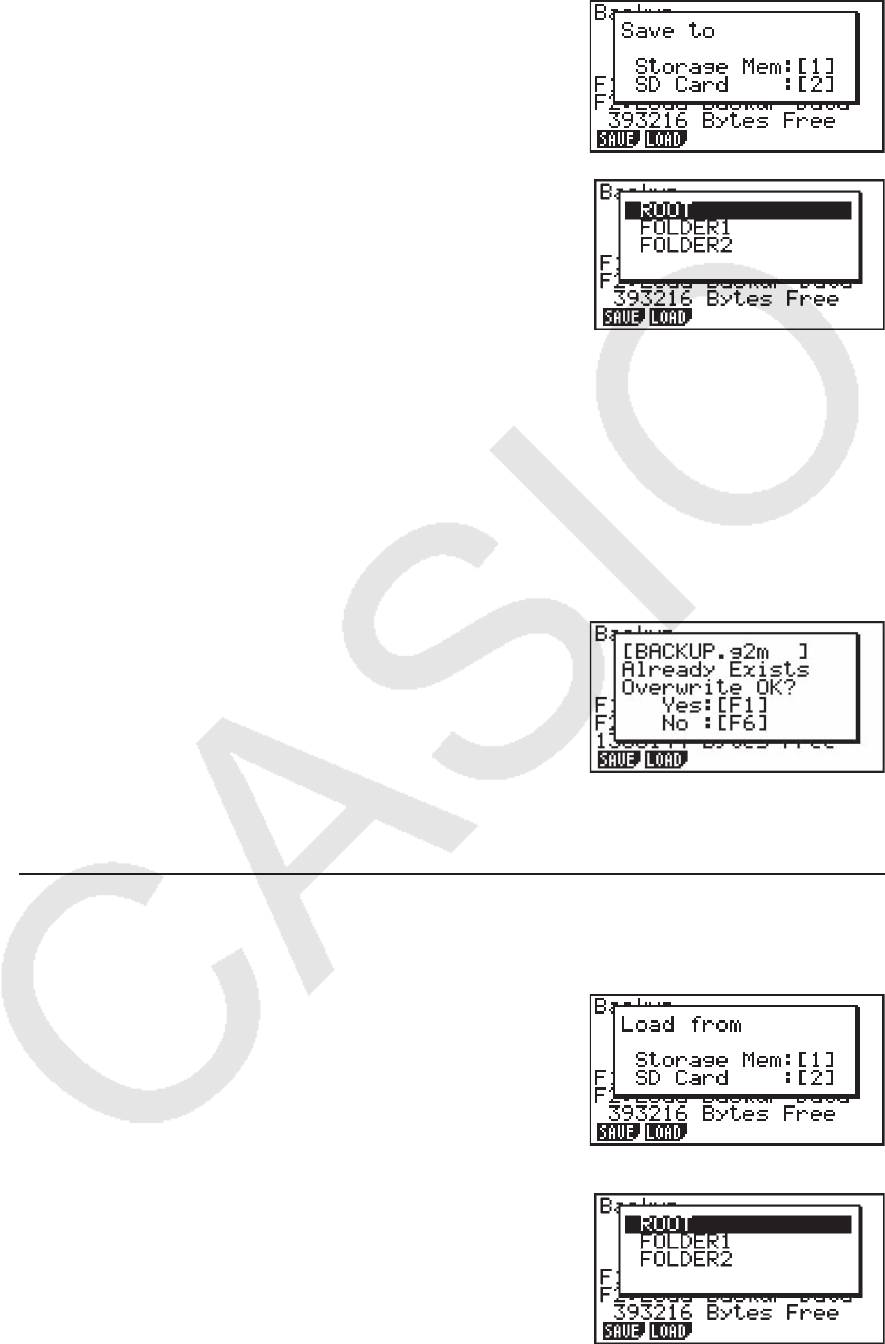
11-10
2. 按下 1(SAVE)。
由此显示保存位置选择屏幕(仅限fx-9860G
II SD)。
• b ... 永久存储器
• c ... SD卡
3. 按下 b或者 c(仅限fx-9860G
II SD)。
由此可显示文件夹选择屏幕。
4. 使用 f和 c,选择想要保存数据的文件夹。
5. 按下 w,开始备份。
• 备份数据保存在BACKUP.g2m文件中。
备份操作完成时显示“Complete!”消息。
按下 J,返回第1步显示的屏幕。
如果永久存储器中已经存在备份数据,显示以下消息。
按下 1(Yes),备份数据;或者按下 6(No),取消备份操作。
如果永久存储器中的可用空间不足以完成备份操作,显示“Memory Full”消息。
u 将备份数据恢复到主存储器
1. 在初始 MEMORY 模式屏幕上,按下 4(BKUP)。
• 在显示的屏幕上,您可确认永久存储器上是否存在备份数据。
2. 按下 2(LOAD)。
由此显示恢复源数据选择屏幕(仅限fx-9860G
II SD)。
• b ... 从永久存储器恢复
• c ... 从SD卡恢复
3. 按下 b或者 c(仅限fx-9860G
II SD)。
由此可显示文件夹选择屏幕。
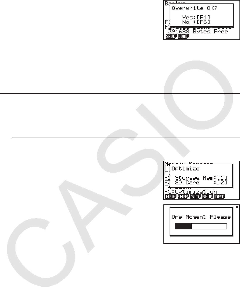
11-11
4. 使用 f和 c,选择文件夹。
5. 按下 w。*
1
• 显示一条确认消息,要求您确认是否希望恢复备份数
据。
*
1
如果存储器中没有保存备份数据,将显示消息“No
Data”。按下 J,返回第1步中的屏幕。
按下 1(Yes),恢复数据并删除该区域中的当前数据。
按下 6(No),取消数据的备份操作。
恢复操作完成时显示“Complete!”消息。
按下 J,返回第1步显示的屏幕。
k 优化永久存储器或者SD卡存储器
经过大量存储和载入操作之后,永久存储器或者SD卡存储器可能产生大量文件碎片。文件碎片
可能导致存储器中的存储区无法存储数据。因此,您应定期执行永久存储器或者SD卡优化操
作,该操作可重新安排永久存储器或者SD卡中的数据,提高存储器使用效率。
u 优化永久存储器
1. 在初始 MEMORY 模式屏幕上,按下 5(OPT),优化永久存储器。
2. 选择想要优化的存储器(仅限fx-9860G
II SD)。
• b ... 永久存储器
• c ... SD卡
3. 按下 b或者 c,开始优化。
优化操作完成时显示“Complete!”消息。
按下 J,返回初始 MEMORY 模式屏幕。
• 在某些情况下,在执行优化步骤之后,您可能发现可用存储容量保持不变。这是计算器的正常
现象。
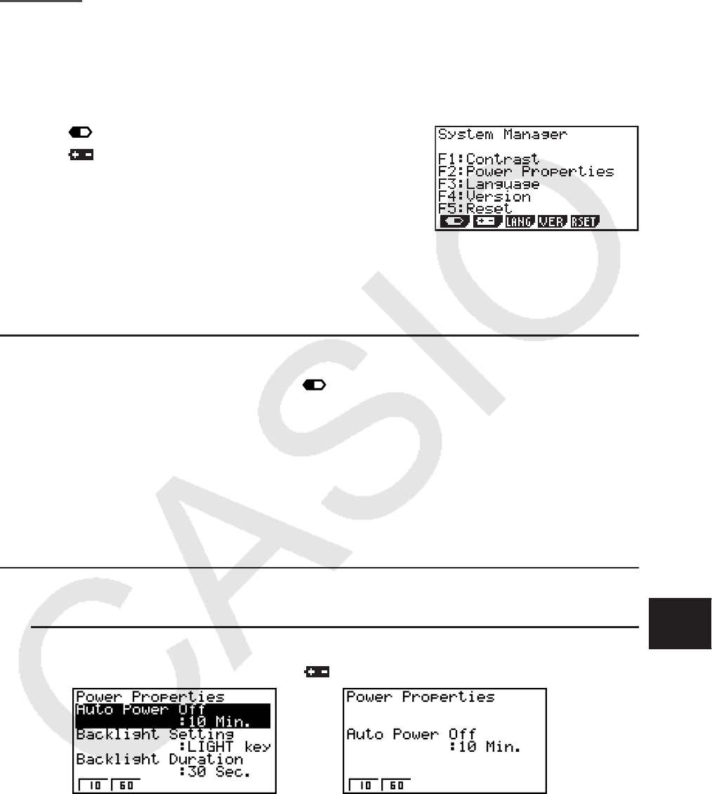
12-1
第12章 系统管理器
使用系统管理器查看系统信息和进行系统设置。
1. 使用系统管理器
在主菜单中,进入 SYSTEM 模式并显示以下菜单项目。
• 1() ... {显示对比度调节}
• 2() ... {自动断电时间设置}
• 3(LANG) ... {系统语言}
• 4(VER) ... {版本}
• 5(RSET) ... {系统复位操作}
2. 系统设置
k 对比度调节
在显示初始 SYSTEM 模式屏幕时,按下 1( ),显示对比度调节屏幕。
• e光标键可使显示对比度变暗。
• d光标键可使显示对比度变亮。
• 1(INIT) 将显示对比度恢复到初始默认设置。
按下 J或者 !J(QUIT),返回初始 SYSTEM 模式屏幕。
显示屏上显示任何画面时,都可通过依次按下 !和 e或者 d调节对比度。如需退出对比度
调节,再次按下 !。
k 电源属性设置
u 指定自动断电触发时间
在显示初始 SYSTEM 模式屏幕时,按下 2( ),显示电源属性设置屏幕。
带有背光照明功能的型号 没有背光照明功能的型号
• 1(10) ... {10分钟}(初始默认设置)
• 2(60) ... {60分钟}
按下 J或者 !J(QUIT),返回初始 SYSTEM 模式屏幕。
12
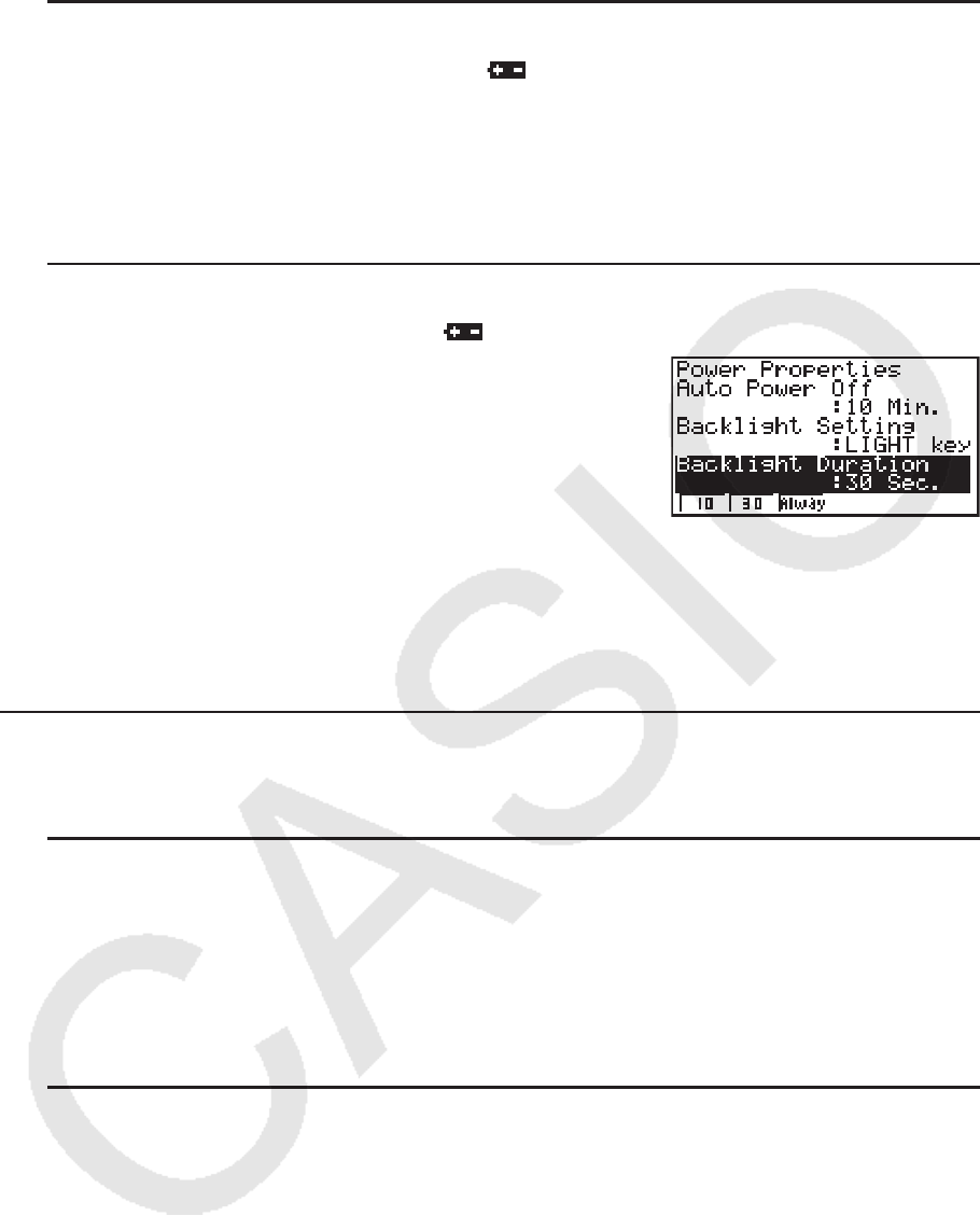
12-2
u 指定背光照明键(仅限带有背光照明功能的型号)
1. 在显示初始 SYSTEM 模式屏幕时,按下 2( ),显示电源属性设置屏幕。
2. 使用 f和 c,选择“Backlight Setting”。
• 1(LIGHT) ... {背光照明开启/关闭: !K(LIGHT)}
• 2(ANY) ... {背光照明开启:任意键}
3. 按下 J或 !J(QUIT),返回初始 SYSTEM 模式屏幕。
u 指定背光照明持续时间(仅限带有背光照明功能的型号)
1. 在初始 SYSTEM 模式屏幕上,按下 2( ),显示电源属性设置屏幕。
2. 使用 f和 c,选择“Backlight Duration”。
• 1(10) ... {在执行最后一次按键操作10秒之后关闭背光照明}
• 2(30) ... {在执行最后一次按键操作30秒之后关闭背光照明}(初始默认设置)
• 3(Always) ... {保持背光照明开启,直至按下背光照明键或关闭计算器}
3. 按下 J或 !J(QUIT),返回初始 SYSTEM 模式屏幕。
k 系统语言设置
使用LANG指定内置应用程序的显示语言。
u 选择消息语言
1. 在初始 SYSTEM 模式屏幕上,按下 3(LANG),显示消息语言选择屏幕。
2. 使用 f和 c光标键选择目标语言,然后按下 1(SEL)。
3. 弹出窗口使用您选择的语言。检查内容,然后按下 J。
4. 按下 J或 !J(QUIT),返回初始 SYSTEM 模式屏幕。
u 选择菜单语言(fx-9860G II SD/fx-9860G II/fx-9860G AU PLUS)
1. 在初始 SYSTEM 模式屏幕上,按下 3(LANG),显示消息语言选择屏幕。
2. 按下 6(MENU)。
3. 使用 f和 c光标键选择目标语言,然后按下 1(SEL)。
4. 弹出窗口使用您选择的语言。检查内容,然后按下 J。
• 按下 6(MSG),返回消息语言选择屏幕。
5. 按下 J或 !J(QUIT),返回初始 SYSTEM 模式屏幕。
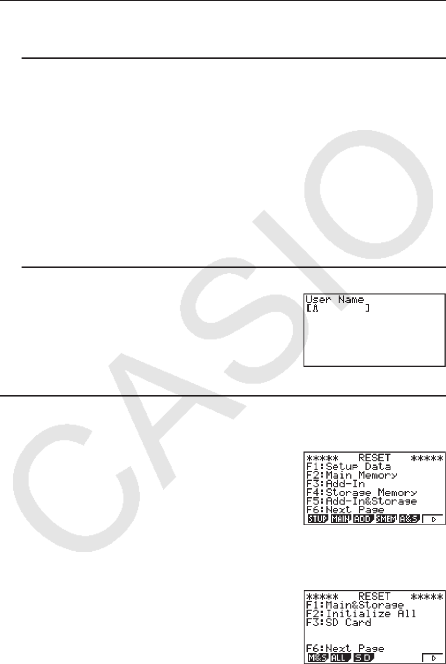
12-3
k 版本列表
使用VER(版本)显示操作系统版本。您还可登记所需用户名。
u 显示版本信息
1. 在初始 SYSTEM 模式屏幕上,按下 4(VER),显示版本列表。
2. 使用 f和 c,滚动屏幕。列表内容如下所述。
• 所有型号都显示标记星号(*)的项目。其他项目只在支持相关功能的型号上显示。
- 操作系统版本*
- 附加应用程序名称和版本(只显示安装的附件)
- 消息语言和版本*
- 菜单语言和版本
- 用户名*
3. 按下 J或 !J(QUIT),返回初始 SYSTEM 模式屏幕。
• 实际显示的操作系统版本取决于计算器型号。
u 登记用户名
1. 在显示版本列表时,按下 1(NAME),显示用户名输入屏
幕。
2. 输入最长8个字符的用户名。
3. 输入名称之后,按下 w即可登记,然后返回版本列表。
• 如果想取消用户名输入并返回版本列表(不登记名称),
按下 J。
k 复 位
1. 在显示初始 SYSTEM 模式屏幕时,按下 5(RSET),显示复位屏幕1。
重要!
复位屏幕上显示的项目取决于计算器型号。
• 1(STUP) ... {设置初始化}
• 2(MAIN) ... {主存储器数据清空}
• 3(ADD) ... {附加应用程序清空}*
• 4(SMEM) ... {永久存储器数据清空}*
• 5(A&S) ... {附加应用程序和永久存储器数据清空}*
在上述屏幕中按下 6( g),显示下图所示复位屏幕2。
• 1(M&S) ... {主存储器数据和永久存储器数据清空}*
• 2(ALL) ... {所有存储器清空}*
• 3(SD) ... {SD卡格式化}(仅限fx-9860G
II SD)
* fx-7400G
II/fx-9750G II中不包括。
下表显示功能键的功能。您可使用功能键删除特定数据。
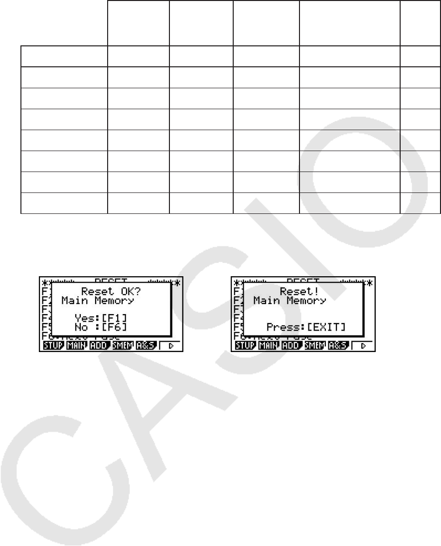
12-4
功能键功能
初始化
设置信息
删除主存
储器数据
删除附加
应用程序
删除永久存储器数据
(不包括附加应用
程序)
格式化
SD卡
1(STUP) ○
2(MAIN) ○ ○
3(ADD) ○
4(SMEM) ○
5(A&S) ○ ○
6( g) 1(M&S) ○ ○ ○
6( g) 2(ALL) ○ ○ ○ ○
6( g) 3(SD) ○
2. 按下与想要执行的复位操作对应的功能键。
3. 针对显示的确认消息,按下 1(Yes),执行指定的复位操作;或者按下 6(No)取消操作。
4. 完成复位操作时显示一条提醒消息。
在第2步按下 2(MAIN)时
显示的屏幕。
在第2步按下 2(MAIN)时
显示的屏幕。
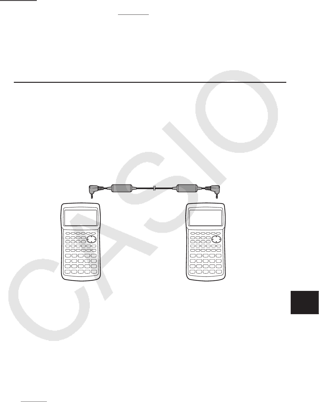
13-1
第13章 数据通信
本章全面介绍如何在两台通过选配的SB-62电缆*相连的CASIO Power Graphic计算器之间传输
程序。
* 某些地区计算器随附。
1. 连接两台计算器
下述步骤说明如何使用SB-62电缆连接两台计算器。
u 连接两台计算器
1. 检查并确保两台计算器的电源都已关闭。
2. 使用SB-62电缆连接两台计算器。
• 在fx-7400G II上不要求执行第3步。
3. 在两台计算器上上执行以下步骤,指定3PIN电缆类型。
(1)在主菜单中,进入 LINK 模式。
(2) 按下 4(CABL)。由此可显示电缆类型选择屏幕。
(3) 按下 2(3PIN)。
SB-62电缆
•下面显示了支持该配置的型号。
fx-9860G
II SD、fx-9860G II、fx-9860G AU PLUS、fx-9750G II、fx-7400G II、
fx-9860G Slim(OS 1.11)、fx-9860G SD(OS 2.0/1.05)、fx-9860G(OS 2.0/1.05)、
fx-9860G AU(OS 2.0/1.05)、fx-7400G系列、CFX-9850G系列
2. 将计算器连接到个人计算机
您可使用Program-Link软件(FA-124)和一条特殊电缆*
1
在计算器和计算机之间建立连接。
关于建立连接和数据传输步骤的详情,请参见FA-124用户说明书。
*
1
对于fx-9860G II SD、fx-9860G II和fx-9860G AU PLUS,使用Program-Link软件和选配的
USB电缆*。
对于fx-9750G
II和fx-7400G II,您需要购买FA-124。
* 某些地区计算器随附。
13
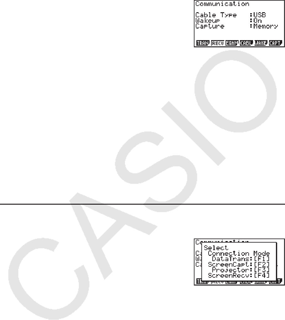
13-2
3. 执行数据通信操作
在主菜单中,进入 LINK 模式。显示屏上显示以下数据通信主菜单。
• { TRAN } ... {显示数据发送屏幕}
• { RECV } ... {显示数据接收屏幕}
• {EXAM} ... {显示考试模式菜单}
• { CABL } ... {显示电缆类型选择屏幕}
(fx-7400G
II中不包括)
• { WAKE } ... {显示唤醒设置屏幕}
• { CAPT } ... {显示屏幕图像发送设置屏幕}
通信参数采用以下固定设置。
• 3针串行端口
• 速度(BPS): 最高9600 bps(连接CFX-9850G系列或者fx-7400G系列计算器)
最高115200 bps(连接其它fx-9860G
II SD、fx-9860G II、fx-9860G AU
PLUS、fx-9750G
II、fx-7400G II、fx-9860G Slim(OS 1.11)、
fx-9860G SD(OS 2.0/1.05)、fx-9860G(OS 2.0/1.05)或者
fx-9860G AU(OS 2.0/1.05)计算器)
• 奇偶校验(PARITY):NONE
• USB端口*
• 通信速度符合USB标准。
* fx-7400G
II未配置USB端口。
k 选择连接模式屏幕 (除fx-7400G II之外的所有型号)
将USB电缆连接到计算器后,将显示旁边的对话框。您可使用该对话框选择USB电缆连接模式
(屏幕图像发送模式)。
• 1(DataTrans) ... {用于与PC机传输数据的模式选择}
• 2(ScreenCapt) ... {用于使用FA-124屏幕捕捉功能将计算器截屏图像发送至PC机的模式选择}
• 3(Projector) ... {用于将计算器屏幕输出至CASIO OHP设备或者CASIO投影仪的模式选择}
• 4(ScreenRecv) ... {用于使用 fx-9860GII Manager PLUS屏幕接收器功能将计算器屏幕图像
发送至PC机的模式选择}
如需在PC机与计算器存储器之间传输数据,按下 1。
使用键 2至 4选择适当的模式,将计算器屏幕图像发送到外部设备。关于按下 2至 4键的
计算器操作详情,请参见“屏幕图像发送”(第13-11页)。
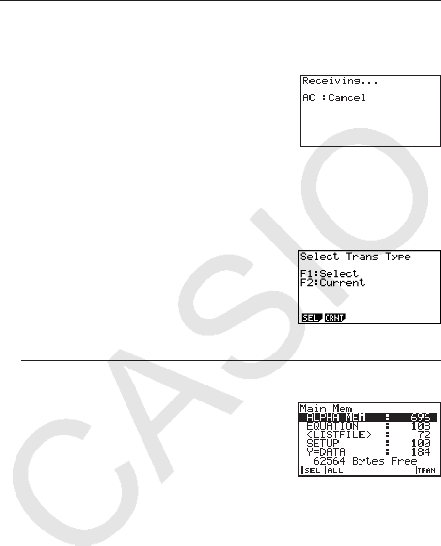
13-3
k 执行数据传输操作
连接两台计算器然后执行以下步骤。
接收计算器
如需设置计算器接收数据,在显示数据通信主菜单时按下
2(RECV) 。
计算器进入数据接收等待状态并等待数据送达。在实际操作中,一旦发送计算器发出数据,即
开始数据接收。
发送计算器
如需设置计算器发送数据,在显示数据通信主菜单时按下 1(TRAN) 。
由此可显示用于指定数据选择方法的屏幕。
• { SEL } ... {选择新数据}
• { CRNT } ... {自动选择以前选定的数据*
1
}
*
1
一旦切换到另一个模式,以前选定的数据存储器即被清空。
u 发送选定的数据项目 (示例:发送用户数据)
按下 1(SEL)或者 2(CRNT),显示数据项目选择屏幕。
• { SEL } ... {选择光标所在位置的数据项目}
• { ALL } ... {选择所有数据}
• { TRAN } ... {发送选定的数据项目}
使用 f和 c光标键将光标移至想要选择的数据项目,然后按下 1(SEL)进行选择。当前选定
的数据项目标有“
”。按下 6(TRAN),发送所有选定的数据项目。
• 如需取消选择某个数据项目,将光标移至该项目,然后再次按 1(SEL)。
数据项目选择屏幕上只显示包含数据的项目。如果数据项目过多,单个屏幕无法完全显示,将
光标移至屏幕最后一行项目可使列表滚动。
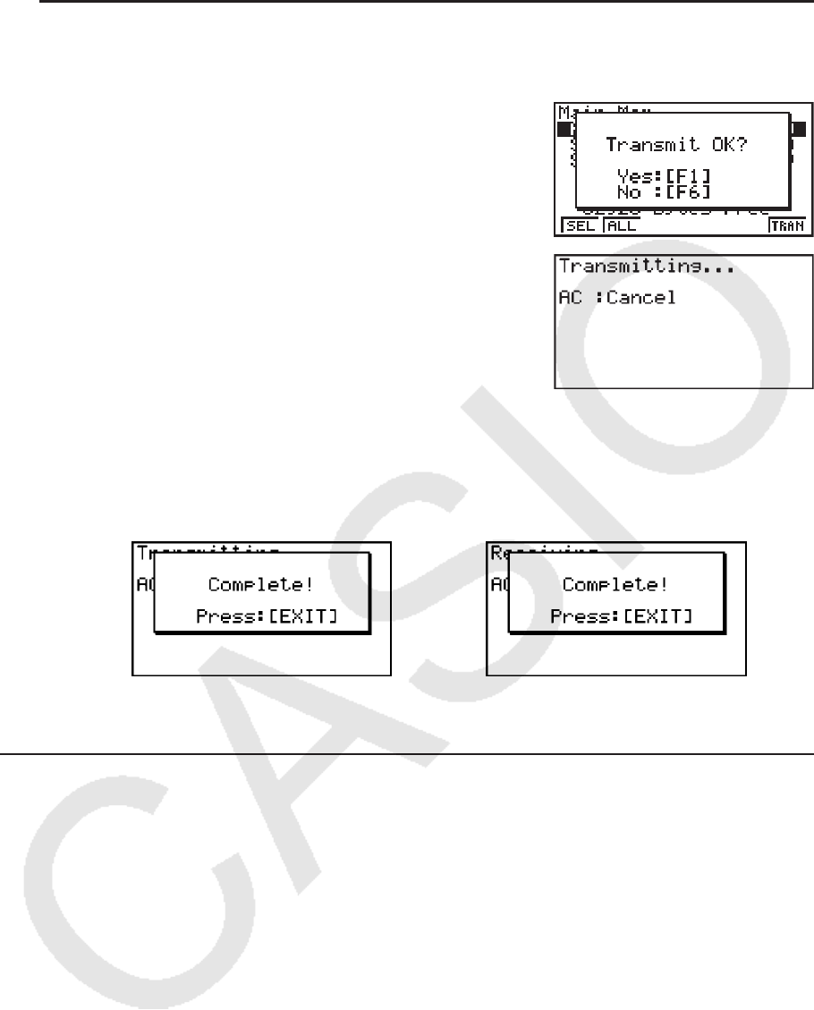
13-4
u 执行发送操作
在选择需要发送的数据项目之后,按下 6(TRAN)。显示一条消息,确认您希望执行发送操
作。
• 1(Yes) ... 发送数据
• 6(No) ... 返回数据选择屏幕
按下 1(Yes),发送数据。
• 您可在任何时候通过按下 A中断数据操作。
下面显示了在完成数据通信操作之后发送与接收计算器的显示画面。
发送计算器 接收计算器
按下 J,返回数据通信主菜单。
k 配置接收设备的唤醒功能
在接收设备上开启唤醒功能时,接收设备在数据传输开始时自动开启。
fx-7400G
II
• 接收设备在唤醒之后自动进入接收模式。
除fx-7400G II 之外的所有型号
• 在两台计算器之间通信时(将电缆类型设置为3PIN),接收设备在唤醒之后自动进入接收模
式。
• 在与计算机通信时(将电缆类型设置为USB),将USB电缆连接到计算机和计算器(计算器关
闭时)将使计算器开启并显示“Select Connection Mode”对话框。

13-5
1. 在接收设备的数据通信主菜单上,按下 5(WAKE)。
由此可显示唤醒设置屏幕。
• { On } ... {开启唤醒功能}
• { Off } ... {关闭唤醒功能}
2. 按下 1(On)。
由此将开启唤醒功能并返回数据通信主菜单。
3. 关闭接收设备。
4. 连接接收设备与发送设备。
5. 在发送设备上启动发送操作将使接收设备自动开启并执行数据传输操作。
4. 数据通信注意事项
下面是可发送的数据项目类型。
数据项目 内容 覆盖检查 *
6
ALPHA MEM 字母存储器内容 无
<CAPTURE> 捕捉存储器组
CAPT
n 捕捉存储器(1至20)数据 无
CONICS*1 圆锥曲线论设置数据 无
DYNA MEM*1 动态图形函数 是
EQUATION 方程计算系数值 无
<E-CON2>*1 E-CON2或E-CON3存储器组
CPn*1自定义调查存储器(1至99)内容 是
SUn*1E-CON设置存储器(1至99)内容 是
SDn*1E-CON测量存储器(CH1、CH2、CH3、
CHSNC、CHMIC、CHFFT)内容 是
Econ2Now*2E-CON2当前设置存储器内容 是
Econ3Now*3E-CON3当前设置存储器内容 是
FINANCIAL*1 财务数据 无
<F-MEM> 函数存储器组
F-MEM
n 函数存储器(1至20)内容 无
<G-MEM> 图形存储器组
G-MEM
n 图形存储器(1至20)内容 是
<LISTFILE> 列表文件组
LIST
n 列表存储器(1至26和Ans)内容 是
LIST FILE
n 列表文件存储器(1至6)内容 是
<MAT_VCT>*5 矩阵组/向量组
<MATRIX>*4 矩阵组*4
MAT
n*1 矩阵存储器(A至Z和Ans)内容 是
VCT
n*5 向量存储器(A至Z和Ans)内容 是
<PICTURE> 图片存储器组

13-6
数据项目 内容 覆盖检查 *
6
PICT n 图片(图形)存储器(1至20)数据 无
<PROGRAM> 程序组
程序名称 程序内容(列出所有程序。) 是
RECURSION*1 递归数据 无
SETUP 设置数据 无
STAT 统计结果数据 无
<STRING> 字符串存储器组
STR
n 字符串存储器(1至20)数据 无
SYSTEM 操作系统和应用程序共享数据(剪贴板、重放、
历史等等) 无
<S-SHEET>*5 电子表格组
电子表格数据
名称*5
电子表格数据
(列出所有电子表格数据。) 是
TABLE 表格数据 无
<V-WIN> 视窗存储器组
V-WIN
n 视窗存储器(1至6)内容 无
Y=DATA 图形表达式、图形绘制/非绘制状态、视窗内容、
缩放系数 无
*
1
fx-7400G II中不包括。 *2 fx-9750GII
*3 fx-9860GII SD/fx-9860GII/fx-9860G AU PLUS *
4
仅限fx-9750GII
*5 fx-7400G II/fx-9750G II中不包括。
*
6
无覆盖检查:如果接收设备已经包含相同类型的数据,新数据覆盖现有数据。
有覆盖检查:如果接收设备已经包含相同类型的数据,显示一条消息,要求确认是否使用新
数据覆盖现有数据。
数据项目名称
• 1(YES) ... {使用新数据覆盖接收设备的现有数据}
• 6(NO) ... {跳至下一个数据项目}
在执行数据通信时注意以下注意事项。
• 在尝试向尚未准备好接收数据的接收设备发送数据时,会产生错误。出现这种情况时,按
下 J,清除错误,在设置接收设备接收数据之后再试一次。
• 在设置接收数据之后大约6分钟内,如果接收设备没有接收任何数据,会产生错误。出现这种
情况时,按下 J,清除错误。
• 如果电缆断开连接、两台设备的参数不匹配或者出现其他任何通信问题,在数据通信期间会产
生错误。出现这种情况时,按下 J,清除错误,在再次尝试数据通信之前排除故障。如果数
据通信由于 J键操作或者错误而中断,此前已经成功接收的数据将保存在接收设备的存储器
中。
• 如果接收设备存储器在数据通信期间已满,会产生错误。出现这种情况时,按下 J,清除错
误,删除接收设备上的多余数据,为新数据提供空间,然后再试一次。

13-7
k 与其它型号的计算器交换数据
在本节中,“OS 2.0计算器”指以下型号。
• fx-9860G
II SD、fx-9860G II、fx-9860G AU PLUS、fx-9750G II、fx-7400G II
• 操作系统已经升级到2.0版本的fx-9860G SD、fx-9860G和fx-9860G AU
OS 2.0计算器支持与以下型号的计算器交换数据。
OS 2.0计算器、fx-9860G系列、fx-7400G系列、CFX-9850G系列
在与以上型号的计算器执行交换数据操作时,OS 2.0计算器将决定是否发送或者接收特定数
据,并根据要求转换数据。下面说明在OS 2.0计算器与其它型号计算器之间交换数据时执行的
基本操作。
• 从OS 2.0计算器向其它型号的计算器发送数据
OS 2.0计算器支持但接收型号不支持的数据有两种选择:不发送或者在发送之前转换到接收型
号支持的格式。
• 从其它型号的计算器向OS 2.0计算器发送数据
基本上,从其它型号的计算器发送的数据都原样接收。但是,如果OS 2.0计算器的功能与发送
型号的功能存在差异,OS 2.0计算器将根据需要转换数据。
下面详细说明OS 2.0计算器与其它计算器型号之间的数据兼容性。
u fx-9860GII SD、fx-9860G II、fx-9860G AU PLUS、fx-9750G II、
fx-9860G SD(OS 2.0)、fx-9860G(OS 2.0)、fx-9860G AU(OS 2.0)
和fx-7400G
II 之间的数据传输
发送设备: fx-7400G II
接收设备: fx-9860G II SD、fx-9860G II、fx-9860G AU PLUS、fx-9750G II、fx-9860G
SD(OS 2.0)、fx-9860G(OS 2.0)、fx-9860G AU(OS 2.0)
传输所有数据。
发送设备: fx-9860G
II SD、fx-9860G II、fx-9860G AU PLUS、fx-9750G II、fx-9860G
SD(OS 2.0)、fx-9860G(OS 2.0)、fx-9860G AU(OS 2.0)
接收设备: fx-7400G
II
• 以下数据不从fx-9860G II SD、fx-9860G II、fx-9860G AU PLUS、fx-9860G SD(OS 2.0)、
fx-9860G(OS 2.0)、fx-9860G AU(OS 2.0)发送,或者在由fx-7400G
II接收时被忽略。
- CONICS 模式数据
- DYNA 模式数据
- E-CON2或E-CON3 模式数据
- 矩阵/向量数据
- RECUR 模式数据
- TVM 模式数据
- STAT 模式函数和变量数据,在fx-7400G
II中没有变量的对应函数(示例: Ƶ2
GOF测试计算
结果数据等等)
- 剪贴板和历史数据(包括“SYSTEM”数据项目。)
- e • ACT 模式数据*
1
- S • SHT 模式数据*
1

13-8
*
1
可从fx-9860G II SD、fx-9860G II、fx-9860G AU PLUS、fx-9860G SD(OS 2.0)、
fx-9860G(OS 2.0)或者fx-9860G AU(OS 2.0)计算器传输。
• 程序数据原样传输。
但被传输程序中任何fx-7400G
II不支持的命令都将替代为符号(@)。在fx-7400G II上运行
此类程序会产生错误。
u 从OS 2.0计算器向任何旧型号计算器发送数据
下面是在从OS 2.0计算器向fx-9860G系列或者CFX-9850G系列计算器传输数据时的一般规
则。
• 不传输以下数据。
- 字符串存储器数据
- TVM 模式债券计算和折旧计算数据
- STAT 模式函数和变量数据,在接收计算器型号上没有变量的对应函数(示例:
Ƶ2
GOF测试
计算结果数据等等)
• 以下数据在发送之前由OS 2.0计算器转换到接收计算器型号支持的格式。
- GRAPH 模式、 DYNA 模式图形类型设置数据
在传输到fx-9860G系列或者CFX-9850G系列计算器时,X=、X>、X<、X 和X 类型的表
达式转换为X=c类型的表达式
- 图形线型设置数据
在向CFX-9850G 系列计算器发送数据时,线型在发送之前转换如下:标准:蓝色;粗线:
橙色;虚线、点线:绿色。
- STAT 模式Graph1、Graph2和Graph3设置数据
在向fx-9860G系列计算器发送数据时,饼图和条线图在发送之前转换为ScatterPlot。其他
设置不发送。
• 程序数据原样传输。
但被传输程序中任何其它型号计算器不支持的命令都将替代为(@)。在其它型号计算器上运
行此类程序会产生错误。
• 如果在向其它型号的计算器发送数据时,OS 2.0计算器上出现错误消息,请参考以下说明。
Invalid Data Size
- 矩阵/向量数据超过256行或256列*
1
- 列表数据超过256行
- 表格数据超过256行
- 递归表格数据超过256行*
1
*
3
- EQUA 模式输入数据包括4至6阶方程
Complex Number in data
- 矩阵/向量数据包括一个内含复数的元素*
1
- 列表数据包括一个内含复数的元素
- EQUA 模式方程组输入数据有一个复数系数
- EQUA 模式方程组计算结果包括一个复数解

13-9
Invalid Data Number
- 列表数据的编号大于List 6
- 图片数据的编号大于Pict 6*
2
- 函数存储器数据的编号大于F-Mem 6*
2
- 图形存储器数据的编号大于G-Mem 6*
2
*
1
可从fx-7400G II之外的其他OS 2.0计算器发送。
*
2
只能传输到fx-9750G系列或者CFX-9850G 系列计算器。
*
3
只能传输到fx-9860G系列计算器。
u 从OS 2.0计算器向CFX-9850G系列计算器发送数据
发送设备: OS 2.0计算器
接收设备: CFX-9850G系列
以下数据不从OS 2.0计算器发送,或者由CFX-9850G系列计算器接收时被忽略。
• 捕捉存储器数据
• 剪贴板、重放和历史数据(包括“SYSTEM”数据项目。)
• CONICS 模式数据*
1
• E-CON2或E-CON3 模式数据*
1
• RECUR 模式 cn ( cn+1
, cn+2
)表达式*
1
• RECUR 模式表格数据*
1
• 设置数据
• STAT 模式数据
• TABLE 模式表格数据
• TVM 模式数据*
1
• 视窗 x点数据
• 方程组和高阶方程的计算结果
*
1
可从fx-7400G II之外的其他OS 2.0计算器发送。
u 从OS 2.0计算器向fx-7400G系列计算器发送数据
发送设备: OS 2.0计算器
接收设备: fx-7400G系列
以下数据不从OS 2.0计算器发送,或者由fx-7400G系列计算器接收时被忽略
• 任何被指定复数的字母变量(A至Z、
r、 Ƨ)
• 答案存储器
• 捕捉存储器数据
• 剪贴板、重放和历史数据(包括“SYSTEM”数据项目。)
• CONICS 模式数据*
1
• DYNA 模式数据*
1
• E-CON2或E-CON3 模式数据*
1
• EQUA 模式数据

13-10
• 函数存储器数据
• 图形存储器数据
• 矩阵/向量数据*
1
• 图片存储器数据
• RECUR 模式数据*
1
• 设置数据
• STAT 模式数据
• TABLE 模式表格数据
• TVM 模式数据*
1
• 编号为V-Win 2或者更大的视窗存储器
• 视窗
x点数据
• 不包括Y=
f( x)类型表达式的图形表达式、Y不等式和参数表达式
*
1
可从fx-7400G II之外的其他OS 2.0计算器发送。
u 从OS 2.0计算器(不包括fx-9750G II/fx-7400G II)向fx-9750G II 、
fx-7400G
II 、fx-9860G系列、CFX-9850G系列或者fx-7400G系列计算器发送
数据
发送设备: fx-9860G II SD、fx-9860G II、fx-9860G AU PLUS
接收设备: fx-9750G
II、fx-7400G II、fx-9860G系列、CFX-9850G系列、fx-7400G系
列
• 当一项数据包括一个平方根( ')或者圆周率( π )表达式时,作为小数值发送。
- 字母存储器数据(A至Z、
r、
θ
)
- Ans存储器数据*
1
- EQUA 模式线性方程组和高阶方程的系数与计算结果*
1
- 历史数据(包括“SYSTEM”数据项目。)*
1
- 列表数据
- 矩阵/向量数据*
1
• 以下数学输入/输出模式中的数值表达式输入在发送之前转换为线性输入/输出模式。
- 在 DYNA 模式和 RECUR 模式中登记的图形表达式*
1
- 在 EQUA 模式中登记的求解表达式
- 在 GRAPH 模式和 TABLE 模式中登记的图形表达式*
1
*
1
fx-7400G系列计算器无法接收。
u 从fx-9860G系列计算器向OS 2.0计算器发送数据
发送设备: fx-9860G系列
接收设备: OS 2.0计算器
• X=c类型表达式转换为X=类型表达式。
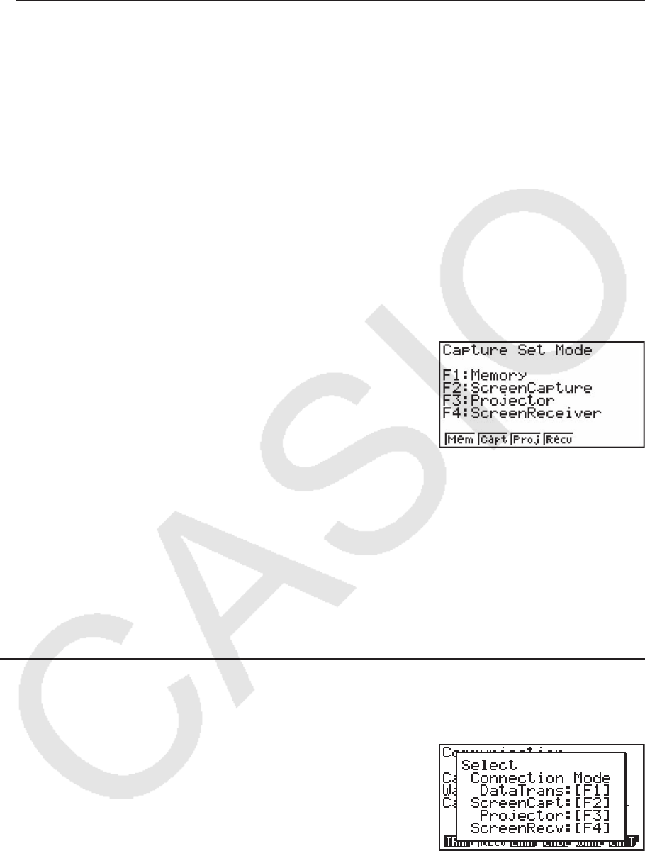
13-11
u 从CFX-9850G系列计算器向OS 2.0计算器发送数据
发送设备: CFX-9850G系列
接收设备: OS 2.0计算器
• X=c类型表达式转换为X=类型表达式。
• 视窗Xmin和Xmax值按原样发送。由于CFX-9850G系列计算器上没有Xdot值,OS 2.0计算器
使用发送的Xmin和Xmax值自动计算该值。
• 执行数据传输操作可将图形存储器与动态图形存储器设置值改为初始默认设置。
• 在从CFX-9850系列计算器接收图形表达式数据时,线型设置转换如下:蓝色:标准;橙色:
粗线;绿色:点线。
5. 屏幕图像发送
在显示数据通信主菜单时按下 6(CAPT),将显示“Capture Set Mode”屏幕。您可使用该屏
幕选择屏幕图像发送模式。
• 1(Mem) ... {用于与PC机传输数据的模式选择(屏幕图像发送关闭)}
• 2(Capt) ... {用于使用FA-124屏幕捕捉功能将计算器截屏图像发送至PC机的模式选择(手动
屏幕图像发送开启)}
• 3(Proj)* ... {用于将计算器屏幕输出至CASIO OHP设备或者CASIO投影仪的模式选择(自动
屏幕图像发送开启)}
• 4(Recv)* ... {用于使用 fx-9860GII Manager PLUS屏幕接收器功能将计算器屏幕图像发送至
PC机的模式选择(自动屏幕图像发送开启)}
*fx-7400G
II中不包括。
k 选择连接模式屏幕 (除fx-7400G II之外的所有型号)
在连接USB电缆与计算器时显示的“Select Connection Mode”对话框上,您可执行与在
Capture Set Mode屏幕上相同的模式选择操作。
Select Connection Mode屏幕上的选项与Capture Set Mode屏幕上的选项对应关系如下:
1(DataTrans) = 1(Mem), 2(ScreenCapt) = 2(Capt), 3(Projector) = 3(Proj),
4(ScreenRecv) = 4(Recv)。

13-12
• 以下类型的屏幕图像无法使用自动屏幕图像发送功能传输到另一台计算器或者计算机。
- 数据传输期间显示的屏幕
- 计算期间显示的屏幕
- 执行复位之后显示的屏幕
- 低电池电量屏幕
k 向计算机传输屏幕图像
使用以下步骤向计算机传输计算器屏幕图像。使用计算机上的FA-124软件执行该步骤。
1. 使用USB电缆连接计算器与计算机。
在fx-7400G
II上
2. 在计算器上,按下 6(CAPT) 2(Capt)。
在其它型号上
2. 在计算器上,在连接USB电缆与计算器时显示“Select Connection Mode”对话框,此时按
下 2(ScreenCapt)。
3. 在计算器上,显示想要传输的屏幕。
4. 使用FA-124执行传输操作。
5. 在计算器上,按下 !h(CAPTURE)。
6. 将屏幕数据发送到计算机。
k 向OHP设备自动发送屏幕图像 (fx-7400G II中不包括)
以下步骤以固定间隔时间将该计算器的屏幕发送到OHP设备。
1. 使用USB电缆连接计算器与OHP设备。
• 将USB电缆连接到计算器后,将显示“Select Connection Mode”对话框。
2. 按下 3(Projector)。
3. 显示想要发送的图像。
4. 显示的图像自动发送给OHP设备。
5. 如需继续执行自动屏幕图像发送,返回第3步。
6. 如需停止自动屏幕图像发送,按下数据通信主菜单上的 6(CAPT) 1(Mem)。
关于连接OHP设备以及如何在连接OHP设备的状态下使用计算器的说明,请参见OHP设备的随
附用户说明书。

13-13
k 使用fx-9860GII Manager PLUS向计算机自动发送屏幕图像 (fx-7400G II中不包括)
使用以下步骤向计算机传输计算器屏幕图像。使用计算机上的fx-9860GII Manager PLUS软件
执行该步骤。
1. 在 fx-9860GII Manager PLUS软件上启动Screen Receiver之后,使用USB电缆将计算器连
接到计算机。
• 将USB电缆连接到计算器后,将显示“Select Connection Mode”对话框。
2. 按下 4(ScreenRecv)。
3. 在计算器上,显示想要传输的屏幕。
4. 显示的图像自动发送给计算机。
5. 如需继续执行自动屏幕图像发送,返回第3步。
6. 如需停止自动屏幕图像发送,按下数据通信主菜单上的 6(CAPT) 1(Mem)。
k 连接投影仪 (fx-7400G II中不包括)
您可将计算器连接到CASIO投影仪,并将计算器屏幕内容投影到屏幕上。
u 可连接的投影仪
有关可连接的投影仪的信息,请访问以下网站。
http://edu.casio.com/support/projector/
• 您还可将计算器连接到YP-100多功能演示套件,使用上述型号之外的投影仪投影。
u 使用投影仪投影计算器屏幕内容
1. 使用计算器随附USB电缆连接到投影仪(或者YP-100设备)。
• 将USB电缆连接到计算器后,将显示“Select Connection Mode”对话框。
2. 按下 3(Projector)。
u 连接注意事项
• 在将计算器连接到投影仪(或者YP-100)之后,屏幕上可能留下一个沙漏图形。此外,如果
正在绘制图形时或PRGM模式程序正在运行时切换到另一个画面,可能会导致投影画面与计算
器画面不同。如果出现这种情况,在计算器上执行某些操作即可恢复正常显示。
• 如果计算器正常停止工作,拔下USB电缆,然后重新连接。如果这种方法不能解决问题,拔下
USB电缆,重新启动投影仪(或者YP-100),然后重新连接USB电缆。

14-1
第14章 使用SD卡和SDHC卡 (仅限fx-9860G II
SD)
此计算器支持使用SD存储卡和SDHC存储卡*。在本手册中,所提到的“SD卡”均
指SD存储卡和SDHC存储卡。
* 仅限USB POWER GRAPHIC 2
您可使用SD卡存储计算器数据。您可在主存储器、永久存储器与SD卡之间复制数
据。
重要!
• 只能使用SD存储卡或SDHC存储卡。在使用其他类型的存储卡时不能保证正常工作。
• 在使用之前必须阅读SD卡随附用户文档。
• 某些类型的SD卡可能降低处理速度。
• 某些类型的SD卡和工作条件可能缩短电池使用寿命。
• SD卡带有一个写保护开关,可避免意外删除数据。但请注意,在采用写保护的磁盘上复制、删
除数据或者执行格式化之前,您需要取消写保护。
• 静电、电气噪音和其他现象可能意外删除或者破坏存储卡数据。因此,您应随时将重要数据备
份到其它介质(CD-R、CD-RW、硬盘等等)
• SDHC徽标是SD-3C,LLC的商标。
1. 使用SD卡
重要!
• 在插拔SD卡时必须关闭计算器。
• 请注意,在将存储卡插入计算器时,应确保方向正确(某一面必须向上,某一端必须插入)。
强行按照错误方向将存储卡插入插槽可能损坏存储卡和插槽。
u 拔出防尘卡
• 您的计算器在出厂时,卡插槽已插入一张防尘卡。在使用SD卡之前,首先执行第14-2页的
“拔出SD卡”步骤,拔出防尘卡。
14
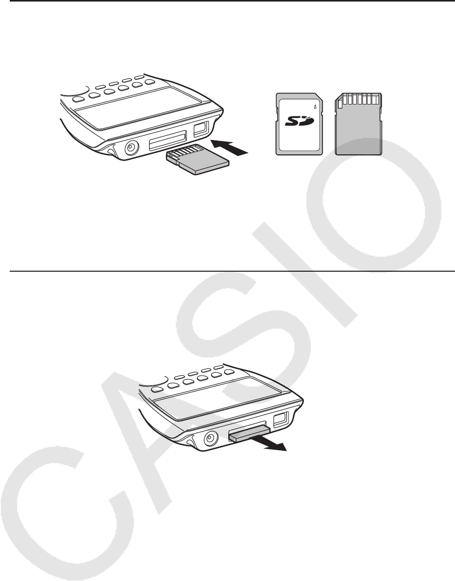
14-2
u 插入SD卡
1. 使SD卡背面朝上(与计算器键盘方向相同)。
2. 将SD卡小心地插入计算器的卡插槽。
重要!
• 切勿将SD卡之外的其他任何物品插入卡插槽。否则可能损坏计算器。
• 一旦水或者任何异物进入卡插槽,立即关闭计算器,取出电池并联系您的零售商或者最近的
CASIO授权维修中心。
u 拔出SD卡
1. 推入SD卡即可松开。
• 此时SD卡将弹出插槽。
2. 用手指捏住SD卡并将其抽出插槽。
重要!
• 切勿在传输数据期间拔出SD卡。否则不仅无法保存向SD卡传输的数据,而且会破坏SD卡内
容。
• 在拔出SD卡时用力过大可能损坏插槽或存储卡。
前面 背面

14-3
2. 格式化SD卡
• 使用“复位”(第12-3页)中的步骤格式化SD卡。
3. SD卡使用注意事项
• 通常可通过重新格式化存储卡排除SD卡问题。但是,最好使用多张SD卡以免出现数据存储问
题。
• 建议在首次使用新SD卡之前执行存储卡格式化(初始化)。
• 如果已经在计算机或者其他设备上格式化SD卡,您无需重新格式化即可直接使用。计算机或
者其他设备也能够使用由计算器格式化的SD卡。
• 在访问SD卡时切勿执行以下任何操作。
- 拔出SD卡
- 连接或者断开USB线
- 关闭计算器
- 在连接到计算机时,退出FA-124软件或者关闭计算机
• 请注意,在将SD卡插入计算器时,应确保方向正确(某一面必须向上,某一端必须插入)。
强行按照错误方向将SD卡插入插槽可能损坏存储卡和插槽。
• 在电池电量较低时使用某些SD卡可能导致显示屏变为空白,且不显示电池电量不足警告消
息。如果出现这种情况,更换电池。
k 支持的SD卡
SD存储卡 最大容量:2 GB
SDHC存储卡 最大容量:32 GB
重要!
数据写入和读取所需的时间取决于所用SD卡的类型。
关于SD卡的详情(规格、功能等等),请联系SD卡制造商。

α-1
附录
1. 错误消息表
消息 含义 解决措施
Syntax
ERROR
• 语法错误
• 尝试输入非法命令
• 按下 J,显示错误并进行必要的
修正。
Ma ERROR • 计算结果超出显示范围。
• 计算超出函数的输入范围。
• 数学错误(被零除等等)
• 无法达到 Σ 计算、微分计算等的规定
精度。
• 无法获取方程计算等的解。
• 检查输入值并修正,确保数值在允
许极限值范围内。
Go ERROR 1 没有对应于Goto
n的Lbl n。
2 程序区Prog "文件名"中没有保存程
序。
1 正确输入对应于Goto n的Lbl n,
或者在不需要时删除Goto
n。
2 将程序保存在程序区Prog "文件
名"中,或者在不需要时删除Prog
"文件名"。
Nesting
ERROR
• Prog "文件名"的子程序嵌套超过10
层。
• 确保Prog "文件名"未用于从子程序
返回主程序。如果使用,删除所有
不必要的Prog "文件名"。
• 跟踪子程序跳转目标位置,确保没
有跳转至初始程序区。确保正确返
回。
Stack ERROR • 执行超出数值堆栈或者命令堆栈容量
的计算。
• 简化公式,将数值堆栈的层数控制
在10层以内,将命令堆栈的层数控
制在26层以内。
• 将公式分为两个或者多个部分。
Memory
ERROR
• 运算或者存储器存储操作超过可用存
储器容量。
• 将使用的存储器数量保持在当前指
定的存储器数量范围之内。
• 简化试图存储的数据,使其不超过
可用存储容量。
• 删除不再需要的数据,为新数据提
供空间。
Argument
ERROR
• 命令的自变量定义不正确。 • 纠正自变量。
Dimension
ERROR
• 矩阵、向量或者列表计算期间使用错
误的维数。
• 检查矩阵、向量或列表维数。
Range ERROR 1 输入了不正确的视窗值。
2 在重新绘制图形时超出视窗范围设
置。
3 在范围屏幕上输入不正确的值并使用
该值执行操作。
4 粘贴、调用或其他操作超出电子表格
单元格范围。
1 更改视窗值,使其不超出范围。
2 使用正确设置重新绘制。
3 输入正确的范围值。
4 重复执行该步骤,注意不要超过单
元格范围。
α

α-2
消息 含义 解决措施
Condition
ERROR
• 在尚未达到计算或者功能的所有规定
条件时执行计算或者功能。
• 检查条件并进行必要的修正。
Non-Real
ERROR
• 在设置屏幕上将Complex Mode设置
为Real时,即使自变量为实数,计算
结果仍然包含复数。
• 将Complex Mode 设置改为Real之
外的其他设置。
Complex
Number In
List
• 在不允许使用复数数据的计算或者操
作时,使用了包含复数的列表。
• 将列表中的所有数据改为实数。
Complex
Number In
Matrix
• 在不允许使用复数数据的计算或者操
作时,使用了包含复数的矩阵。
• 将矩阵中的所有数据改为实数。
Complex
Number In
Matrix or
Vector
• 在不允许使用复数数据的计算或者操
作时,使用了包含复数的矩阵。
• 将矩阵或向量中的所有数据改为实
数。
Complex
Number In
Data
• 使用该计算器的某个功能发送的数据
(矩阵等等)包括复数数据,但接收
计算器的对应功能不支持包括复数的
数据。
示例:试图向CFX-9850G发送包含
复数元素的矩阵。
• 发送不包括复数的数据。
Can't Simplify • 尝试使用 'Simp函数(第2-21页)
简化分式,但是无法使用指定的因子
简化。
示例:使用因子3简化分式4/8。
• 指定不同的因子或者执行 'Simp
时不指定任何因子。
Can't Solve!
Adjust initial
value or
bounds. Then
try again.
• 求解计算无法在指定范围内求解。 • 更改指定范围。
• 修正输入表达式。
No Variable 1 动态图形使用的图形函数中没有指定
变量。
2 求解方程中没有变量。
1 为图形函数指定变量。
2 输入一个包括变量的求解方程。
Conversion
ERROR
• 试图使用单位转换命令在两种不同类
别的单位之间进行转换。
• 在转换表达式中两次使用同一命令执
行转换计算。
• 在转换表达式中,指定同一类别中
的两个不同命令。
Com ERROR • 程序数据通信期间电缆连接或者参数
设置出现问题。
• 检查并确保电缆连接和参数设置正
常。
Transmit
ERROR
• 数据通信期间电缆连接或者参数设置
出现问题。
• 检查并确保电缆连接和参数设置正
常。
Receive
ERROR
• 数据通信期间电缆连接或者参数设置
出现问题。
• 检查并确保电缆连接和参数设置正
常。
Memory Full • 接收设备的存储器在程序数据通信期
间装满。
• 删除接收设备中保存的某些数据并
重试。

α-3
消息 含义 解决措施
Invalid Data
Size
• 接收设备不支持试图发送的数据大
小。
示例:试图将一个超过256行的矩
阵从fx-9750G
II发送到旧型号计算
器。
• 确保接收设备支持发送的数据大
小。
Invalid Data
Number
• 接收设备不支持试图发送的数据的数
据编号。
示例:试图将List 7从fx-9750G
II发
送到最多支持List 6的旧型号计算
器。
• 在发送数据时指定接收设备支持的
数据编号。
Time Out • 求解计算或者积分计算无法满足收敛
条件。
• 如果您正在执行求解计算,尝试更
改初始默认估计值。
• 如果您正在执行积分计算,尝试增
大
tol值。
Circular
ERROR
• 电子表格中存在循环参考(例如单元
格A1中使用“=A1”)。
• 更改单元格内容,删除循环参考。
Please
Reconnect
• 在更新操作系统时由于某种原因连接
中断。
• 重新连接并重试。
Too Much
Data
• 数据项数过大。 • 删除多余数据。
Fragmentation
ERROR
• 必须优化存储器才可继续保存数据。 • 优化存储器。
Invalid Name • 输入的文件名包括无效字符。 • 使用正确的字符输入有效文件名。
Invalid Type • 指定了非法数据类型。 • 指定有效数据。
Storage
Memory Full
• 永久存储器已满。 • 删除多余数据。
No Card* • 计算器中没有装入SD卡。 • 装入SD卡。
SD Card Full* • SD卡已满。 • 删除多余数据。
Invalid file
name or folder
name.*
• 未在SD卡上找到该计算器支持的数
据或者文件夹。
• 使用包含该计算器支持的数据/文
件夹的存储卡替换该卡。
Invalid Card* • 装入与计算器不兼容的SD卡。 • 更换为兼容的存储卡。
Card is
protected*
• SD卡使用了写保护。 • 取消写保护。
Data ERROR • 出现数据错误。 • 检查并确保写入正确类型的数据并
重试。
Card ERROR* • 出现SD卡错误。 • 拔出并正确插入SD卡,然后重
试。如果再次出现该错误,重新格
式化SD卡。
Data is
protected*
• 已经使用计算机等设备开启了装入计
算器的SD卡的只读属性。
• 关闭SD卡的只读属性。
* 仅限fx-9860G
II SD

α-4
2. 输入范围
函数 实数解的输入范围 内部
数位 精度 注意
sin
x
cos x
tan x
(DEG) | x| < 9 × (10
9
)°
(RAD) |
x| < 5 × 10
7
π rad
(GRA) |
x| < 1 × 10
10
grad
15位
一般而言,精
度为第10位
± 1。*
但对于tan
x:
|
x| 90(2 n+1): DEG
|
x| π /2(2 n+1): RAD
|
x| 100(2 n+1): GRA
sin
-1
x
cos
-1
x
tan
-1
x
| x| < 1
同上 同上
|
x| < 1 × 10
100
sinh x
cosh x
tanh x
| x| < 230.9516564 同上 同上
|
x| < 1 × 10
100
sinh
-1
x
cosh
-1
x
tanh
-1
x
| x| < 1 × 10
100
同上 同上
1 <
x < 1 × 10
100
| x| < 1
log
x
In x 1 × 10
-99
< x < 1 × 10
100 同上 同上 • 复数可作为自变量。
10
x
ex
-1 × 10
100
< x < 100
同上 同上
• 复数可作为自变量。
-1 × 10
100
< x < 230.2585092
'
x
x2
0 < x < 1 × 10
100
同上 同上
• 复数可作为自变量。 | x| < 1 × 10
50
1/ x
3
'
x
| x| < 1 × 10
100
, x 0 同上 同上
• 复数可作为自变量。 | x| < 1 × 10
100
x! 0 <
x < 69
(
x是一个整数) 同上 同上
nP r
nC r
结果 < 1 × 10
100
n, r( n和 r是整数)
0 <
r < n, n < 1 × 10
10
同上 同上
Pol (
x, y) x2
+ y2
< 1 × 10
100 同上 同上
Rec
(
r ,
θ
)
|
r| < 1 × 10
100
(DEG) |
θ
| < 9 × (10
9
)°
(RAD) |
θ
| < 5 × 10
7
π rad
(GRA) |
θ
| < 1 × 10
10
grad
同上 同上
但对于tan
θ
:
|
θ
| 90(2 n+1): DEG
|
θ
| π /2(2 n+1): RAD
|
θ
| 100(2 n+1): GRA
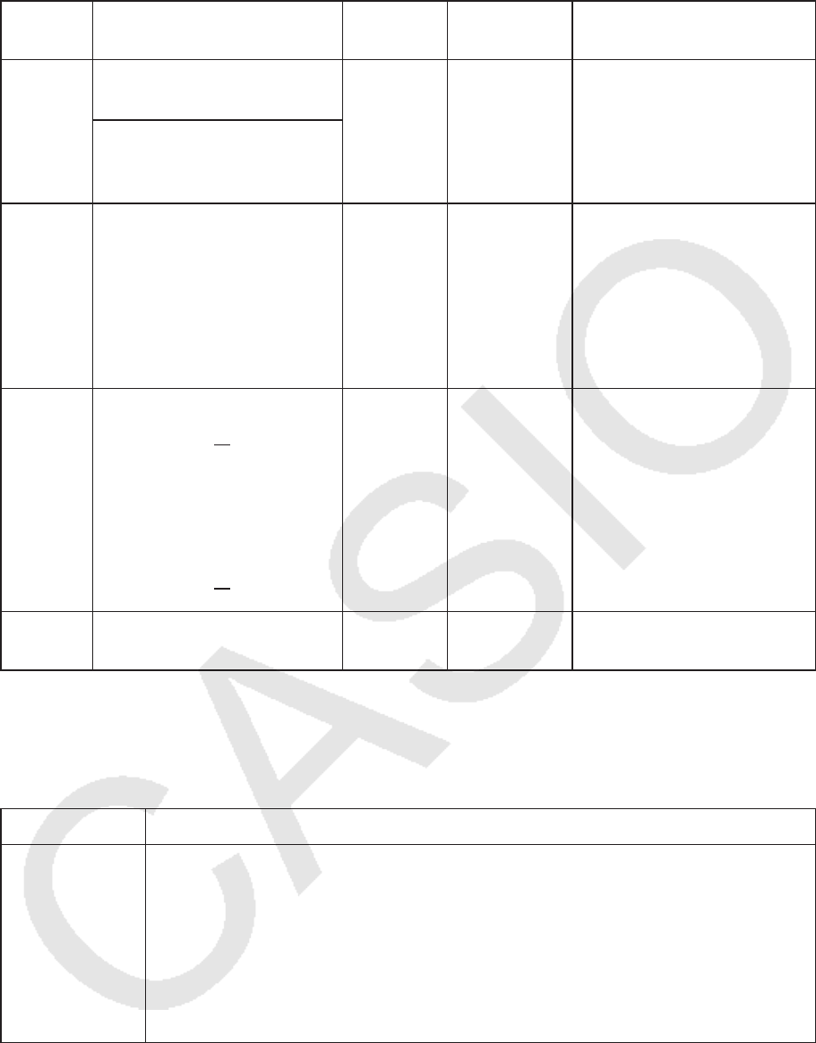
α-5
函数 实数解的输入范围 内部
数位 精度 注意
° ’ ”
←⎯
° ’ ”
| a|, b, c < 1 × 10
100
0 < b, c
15位
一般而言,精
度为第10位
± 1。*
|
x| < 1 × 10
100
六十进制显示:
|
x| < 1 × 10
7
^( xy)
x > 0:
-1 × 10
100
< ylog x < 100
x = 0 : y > 0
x < 0 : y = n, m
––––
2n+1
( m, n是整数)
但是:
-1 × 10
100
< ylog | x| < 100
同上 同上
• 复数可作为自变量。
x'
y
y > 0 : x 0
-1 × 10
100
< 1
x log y < 100
y = 0 : x > 0
y < 0 : x = 2 n+1, 2n+1
––––
m
( m 0; m, n是整数)
但是:
-1 × 10
100
< 1
x log | y| < 100
同上 同上
• 复数可作为自变量。
ab/ c 整数、分子与分母的总数不
得超过10位(包括除号)。 同上 同上
* 对于单独计算,计算误差为第10位 ± 1。(对于指数显示,计算误差为最后一个有效位 ± 1。)在连
续计算中,误差会累积,因而可能产生较大误差。(这一点同样适用于内部连续计算,例如^(
xy)、
x'
y、 x ! 、
3
'
x、 nP r、 nC r等等。)
在函数的奇点和拐点附近,误差可能累积并放大。
函数 输入范围
二进制、八进
制、十进制、十
六进制计算
转换后数值在以下范围内:
DEC: -2147483648 <
x < 2147483647
BIN: 1000000000000000 <
x < 1111111111111111(负)
0 <
x < 111111111111111(0, 正)
OCT: 20000000000 <
x < 37777777777(负)
0 <
x < 17777777777(0, 正)
HEX: 80000000 <
x < FFFFFFFF(负)
0 <
x < 7FFFFFFF(0, 正)

E-CON2
Application
(fx-9750GII)
(English)

• All of the explanations provided here assume that you are already familiar
with the operating precautions, terminology, and operational procedures of
the calculator and the EA-200.
• Unless specifically indicated otherwise, all page references in this
“E-CON2 Application” chapter are to pages in this chapter.
Contents

1-1
E-CON2 Overview
1 E-CON2 Overview
• From the Main Menu, select E-CON2 to enter the E-CON2 Mode.
• The “E-CON2 Mode” provides the functions listed below for simple and more efficient data
sampling using the CASIO EA-200.
•1(SET) ........ Displays a screen for setting up the EA-200.
•2(MEM) ....... Displays a screen for saving EA-200 setup data under a file name.
•3(PROG) ..... Performs program conversion.
• This function can be used to convert EA-200 setup data configured
using E-CON2 to an EA-200 control program (or EA-100 control
program) that can run on the fx-9860G SD/fx-9860G.
• It also can be used to convert data to a program that can be run on
a CFX-9850 Series/fx-7400 Series calculator.
•4(STRT) ...... Starts data collection.
•5(GRPH) ..... Graphs data sampled by the EA-200, and provides tools for analyzing
graphs. Graph Analysis tools include calculation of periodic frequency,
various types of regression, Fourier series calculation, and more.
•6(HELP) ...... Displays E-CON2 help.
• Pressing the K key (Setup Preview) or a cursor key while the E-CON2 main menu is on
the screen displays a preview dialog box that shows the contents of the setup in the
current setup memory area.
To close the preview dialog box, press J.
Note
For details about setup data and the current setup memory area, see “6 Using Setup
Memory” (page 6-1).
About online help
Pressing the 6(HELP) key displays online help about the E-CON2 Mode.
E-CON2 Main Menu

2 Using the Setup Wizard
This section explains how to use the Setup Wizard to configure the EA-200 setup quickly
and easily simply by replying to questions as they appear.
If you need more control over specific sampling parameters, you should consider using the
Advanced Setup procedure on page 3-1.
kSetup Wizard Parameters
Setup Wizard lets you make changes to the following three EA-200 basic sampling
parameters using an interactive wizard format.
• Sensor (Select Sensor):
Specify a CASIO or VERNIER* sensor from a menu of choices.
*Vernier Software & Technology
• Total Sampling Time:
Specify a value within the range of 0.01 second to 30 days.
• Sampling Time Unit (Select Unit):
Specify seconds (sec), minutes (min), hours (hour), or days (day) as the time unit of the
value you input for the total sampling time (Total Sampling Time).
Note
For some sensors (EA-200 built-in microphone, Vernier Photogate, etc.), sampling
parameters are different from those shown above. The differences between sampling
parameters and setup procedures for each sensor are described in this section.
Setup Wizard Rules
Note the following rules whenever you use the Setup Wizard.
• The EA-200 sampling channel is CH1 or SONIC.
• The trigger for a Setup Wizard setup is always the w key.
2-1
Using the Setup Wizard
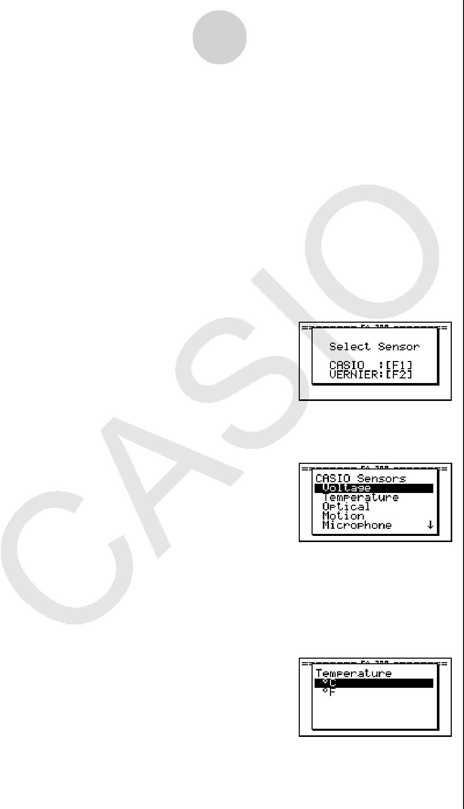
uTo configure an EA-200 setup using Setup Wizard
Before getting started...
• Before starting the procedure below, make sure you first decide if you want to start
sampling immediately using the setup you configure with Setup Wizard, or if you want to
store the setup for later sampling.
• See sections 6-1, 7-1, and 8-1 of this chapter (E-CON2 Application) for information about
procedures required to start sampling and to store a setup. We recommend that you read
through the entire procedure first, referencing the other sections and pages as noted,
before actually trying to perform it.
• To terminate Setup Wizard part way through and cancel the setup, press !J(QUIT).
1. Display the E-CON2 main menu (page 1-1).
2. Press 1(SET) and then 1(WIZ).
• This launches the Setup Wizard and displays the “Select Sensor” screen.
2-2
Using the Setup Wizard
3. Press 1 to specify a CASIO sensor or 2 to specify a Vernier sensor.
• Pressing either key will display the corresponding sensor list. The following shows the
sensor list that appears when you press 1.
4. Specify the sensor you want to use.
Use the f and c cursor keys to move the highlighting to the sensor you want to use,
and then press w.
• If the sensor you specified has more than one option (more detailed specifications, such
as sampling unit, mode, etc.), an option list will appear on the display at this time. If this
happens, advance to step 5 (where you will see an example of the screen that appears
when you select 1 - [Temperature] in step 4).
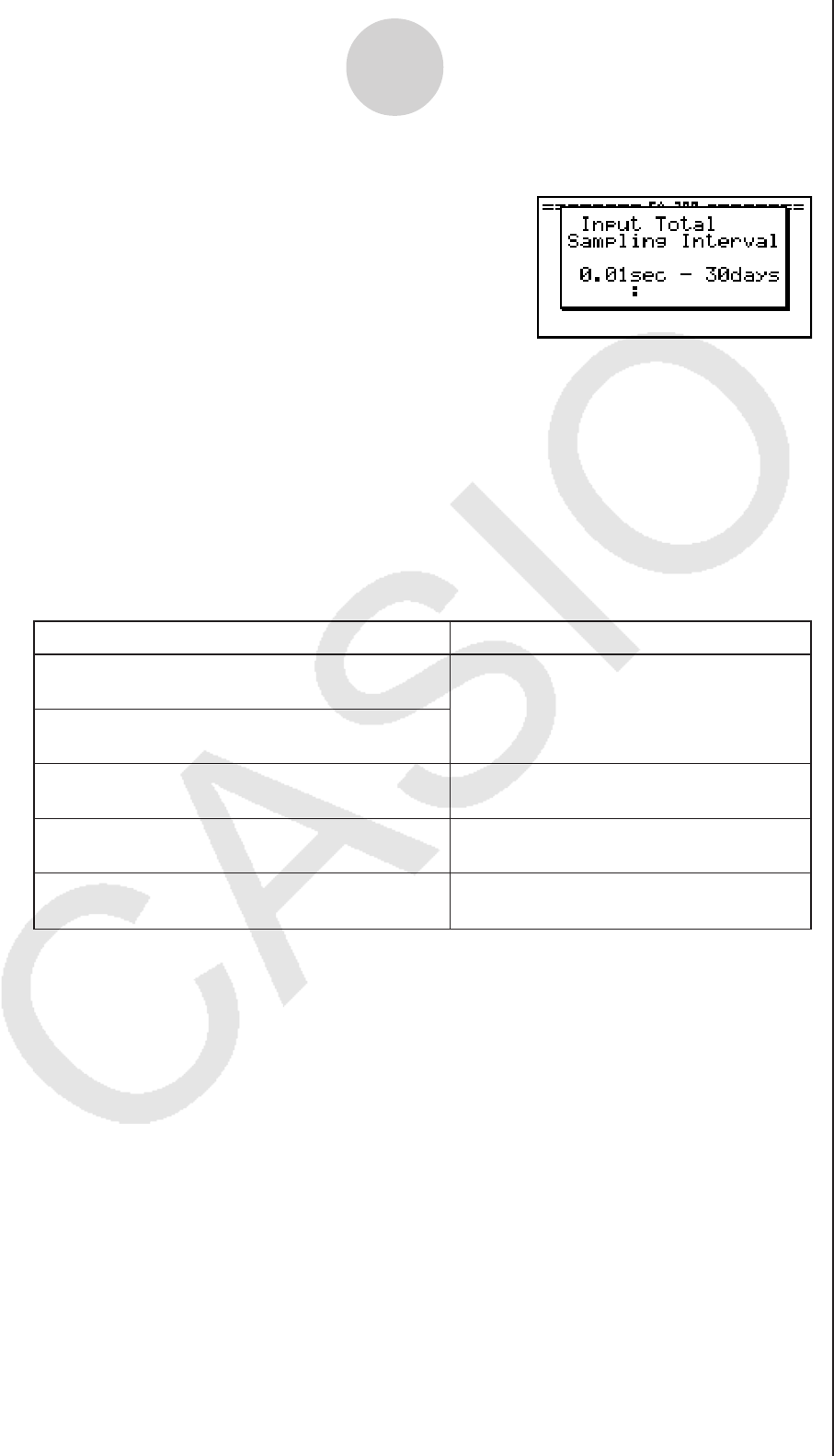
2-3
Using the Setup Wizard
• If the “Input Total Sampling Interval” screen appears, skip to step 6.
5. Select the options for the sensor you specified in step 4.
Use the f and c cursor keys to move the highlighting to the option you want to select,
and then press w.
• If the “Input Total Sampling Interval” screen appears, advance to step 6.
Important!
When special settings are required by the sensor and/or option you select, other screens
other than the “Input Total Sampling Interval” screen will appear on the display. The
following shows where you should go to find information about the operations you need to
perform for each sensor/option selection.
6. Use the number input keys to input the total sampling time. Just input a value.
In step 8 of this procedure, you will be able to specify the unit (seconds, minutes, hours,
days) of the value you input here.
Note
• With some sensors ([CASIO] - [Microphone] - [Sound wave], etc.) sampling time is
limited to a few seconds. The unit for such a sensor is always seconds, and so the
“Select Unit” screen does not appear.
• If you specify a total sampling time value in the range of 10 seconds to 23 hours, 59
minutes, 59 seconds, real-time graphing will be performed during sampling. This is the
same as selecting the Realtime Mode on the “Advanced Setup” screen.
If you select this sensor/option: Go here for more information:
[CASIO] - [Microphone] - [Sound wave & FFT]
[CASIO] - [Microphone] - [FFT only]
[VERNIER] - [Photogate] - [Gate] “To configure a setup for Photogate
alone” on page 2-6
[VERNIER] - [Photogate] - [Pulley] “To configure a setup for Photogate and
Smart Pulley” on page 2-7
[CASIO] - [Speaker] - [y=f(x)] “Outputting the Waveform of a Function
through the Speaker” on page 2-8
“Using Setup Wizard to Configure
Settings for FFT (Frequency
Characteristics) Data Sampling” on
page 2-5
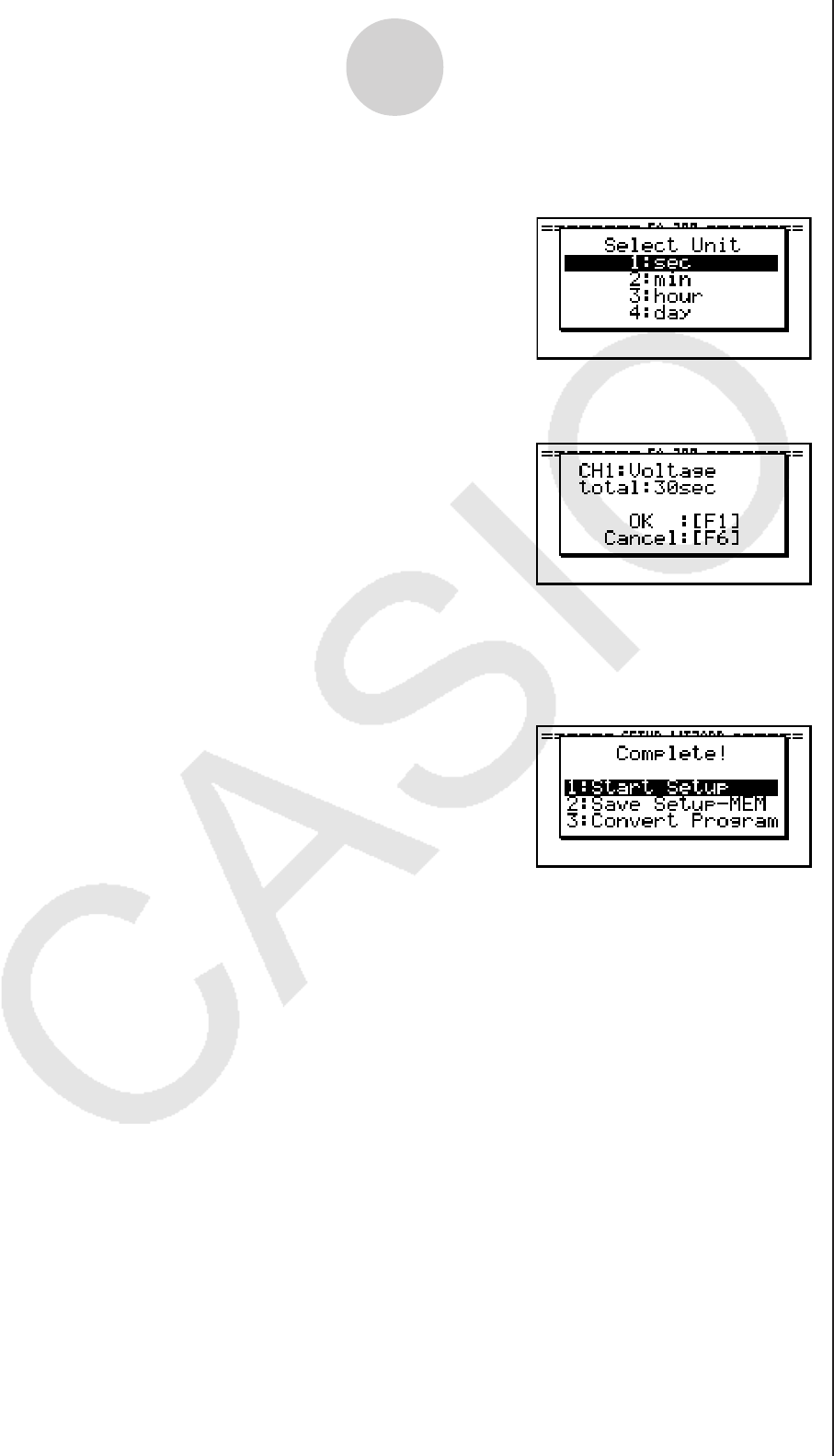
8. Use number keys b through e to specify the unit for the value you specified in step 6.
• This displays a confirmation screen like the one shown below.
2-4
Using the Setup Wizard
7. After inputting total sampling time value you want, press w. This displays the “Select
Unit” screen.
10. Press number keys described below to specify what you want to do with the setup you
have configured.
b(Start Setup) ............... Starts sampling using the setup (page 8-1)
c(Save Setup-MEM) ..... Saves the setup (page 6-1)
d(Convert Program) ...... Converts the setup to a program (page 7-1)
9. If there is not problem with the contents of the confirmation screen, press 1.
If you need to change the setup, press 6 or J. This will return to step 6 (for setting
the total sampling interval), where you can change the setting.
• Pressing 1 will take you to the final Setup Wizard screen.
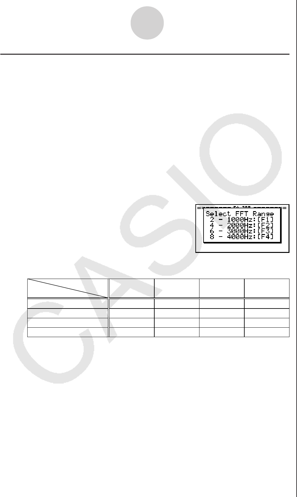
2-5
Using the Setup Wizard
kUsing Setup Wizard to Configure Settings for FFT (Frequency
Characteristics) Data Sampling
When you perform sound sampling executed the EA-200’s built-in microphone (by specifying
[CASIO] - [Microphone] as the sensor), Setup Wizard will provide you with three options:
[Sound wave], [Sound wave & FFT], and [FFT only]. “Sound wave” records the following two
dimensions for the sampled sound data: elapsed time (horizontal axis) and volume (vertical
axis). “FFT” records the following two dimensions: frequency (horizontal axis) and volume
(vertical axis).
The following shows the settings for recording FFT data.
1. Perform the first two steps of the procedure under “To configure an EA-200 setup using
Setup Wizard” on page 2-2.
2. On the “Select Sensor” screen, select [CASIO] - [Microphone] - [Sound wave & FFT] or
[CASIO] - [Microphone] - [FFT only].
• This causes a “Select FFT Range” screen to appear.
• You can select one of four settings for FFT Range. The setting you select will
automatically apply the applicable fixed parameters shown below.
Setting
Parameter
Frequency pitch
Frequency max
Sampling interval
Number of samples
2 Hz
1000 Hz
8192
2 - 1000 Hz:
1
61 sec
μ
4 Hz
2000 Hz
8192
4 - 2000 Hz:
2
31 sec
μ
6 Hz
3000 Hz
8192
6 - 3000 Hz:
3
20 sec
μ
8 Hz
4000 Hz
4096
8 - 4000 Hz:
4
31 sec
μ
The following explains the meaning of each parameter.
Frequency pitch: Pitch in Hz at which sampling is performed
Frequency max: Upper limit of sampling frequency (lower limit is fixed at 0 Hz)
Sampling interval: Interval in
μ
seconds at which sampling is performed
Number of samples: Number of times sampling is performed
3. Use function keys 1 through 4 to select an FFT Range setting.
• Selecting an FFT Range causes the final Setup Wizard screen to appear.
4. Perform step 10 under “To configure an EA-200 setup using Setup Wizard” on page 2-2
to finalize the procedure.
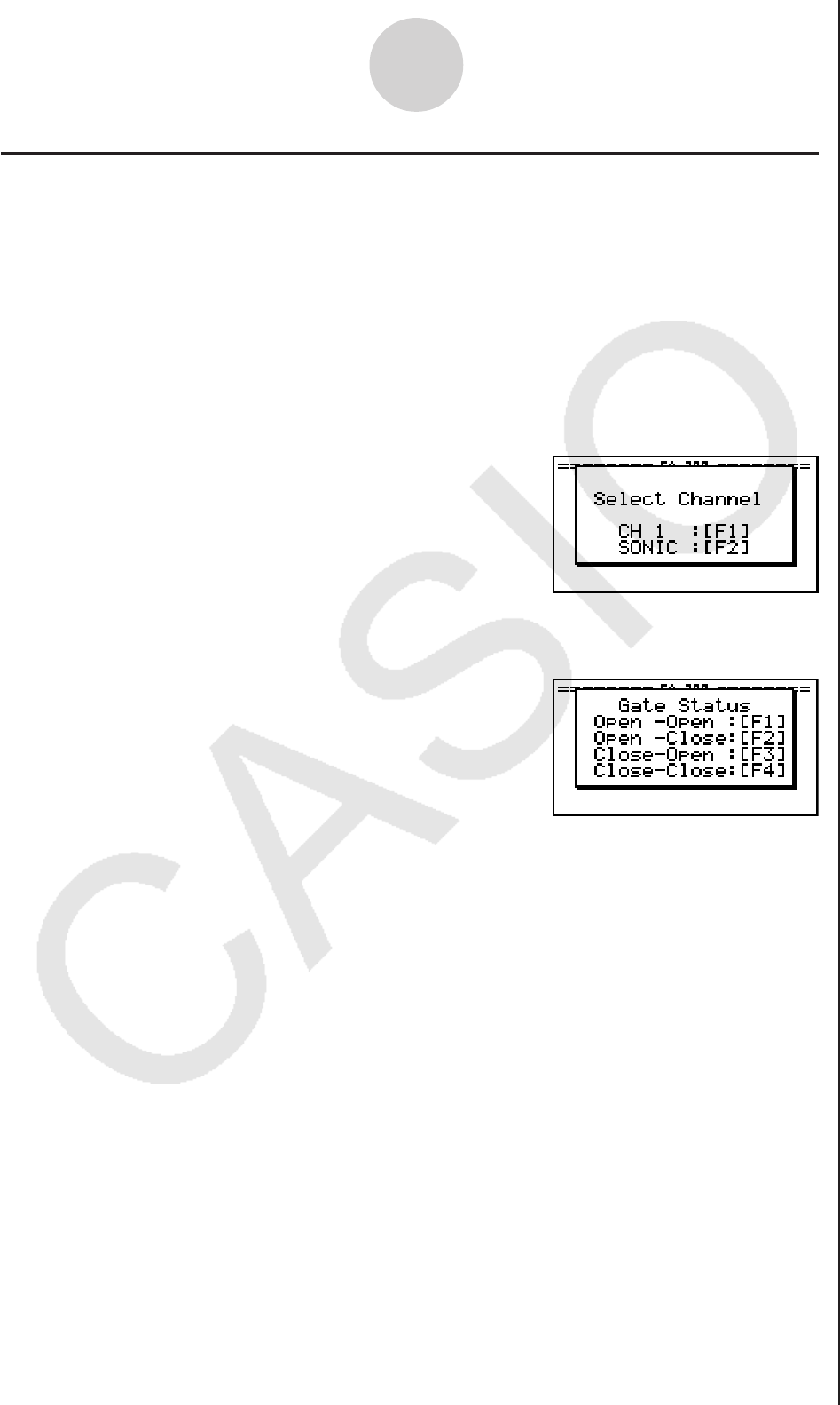
2-6
Using the Setup Wizard
kUsing Setup Wizard to Configure a Photogate Setup
Connection of a Vernier Photogate requires configuration of setup parameters that are
slightly different from parameters for other types of sensors.
uu
uu
uTo configure a setup for Photogate alone
1. Perform the first two steps of the procedure under “To configure an EA-200 setup using
Setup Wizard” on page 2-2.
2. On the “Select Sensor” screen, select [VERNIER] - [Photogate] - [Gate].
• This displays a screen where you specify whether Photogate is connected to the CH1 or
SONIC channel.
3. Press 1 to specify CH1 or 2 to specify SONIC.
• This causes a “Gate Status” screen to appear.
• “Open” means the photo path is not blocked, while “Close” means the photo path is
blocked.
• The gate status defines what Photogate status should cause timing to start, and what
status should cause timing to stop.
Open-Open ...... Timing starts when the gate opens, and continues until it closes and
then opens again.
Open-Close ...... Timing starts when the gate opens, and continues until it closes.
Close-Open ...... Timing starts when the gate closes, and continues until it opens.
Close-Close ...... Timing starts when the gate closes, and continues until it opens and
then closes again.
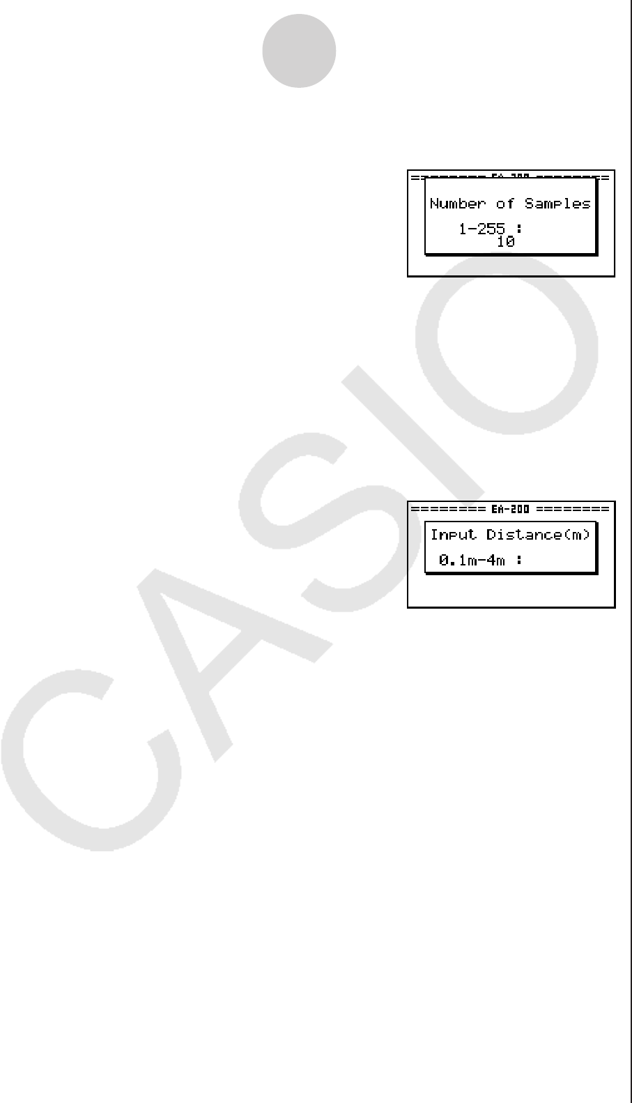
2-7
Using the Setup Wizard
5. Input an integer in the range of 1 to 255 to specify the number of samples.
6. Perform step 10 under “To configure an EA-200 setup using Setup Wizard” on page 2-2
to finalize the procedure.
uu
uu
uTo configure a setup for Photogate and Smart Pulley
1. Perform the first two steps of the procedure under “To configure an EA-200 setup using
Setup Wizard” on page 2-2.
2. On the “Select Sensor” screen, select [VERNIER] - [Photogate] - [Pulley].
• This causes an “Input Distance(m)” screen to appear.
• The distance you specify here is the distance the weight travels after it is released.
• Input a value in the range of 0.1 to 4 to specify the distance in meters.
3. Perform step 10 under “To configure an EA-200 setup using Setup Wizard” on page 2-2
to finalize the procedure.
4. Use function keys 1 through 4 to select a Gate Status setting.
• Selecting a gate status causes a screen for specifying the number of samples to appear.

2-8
Using the Setup Wizard
kOutputting the Waveform of a Function through the Speaker
Normally, the Setup Wizard helps you configure setups for sensors connected to the EA-200.
If you select [CASIO] - [Speaker] - [y=f(x)] on the “Select Sensor” screen, however, it
configures the EA-200 to output the sound that corresponds to a function that you input and
graph on the calculator.
uu
uu
uTo configure a setup for speaker output
1. Connect the data communication cable (SB-62) to the communication port of the
calculator and the MASTER port of the EA-200.
2. Perform the first two steps of the procedure under “To configure an EA-200 setup using
Setup Wizard” on page 2-2.
3. On the “Select Sensor” screen, select [CASIO] - [Speaker] - [y=f(x)].
This displays a screen like the one shown below.
4. Press w to advance to the View Window setting screen.
• The following settings are configured automatically: Ymin = –1.5 and Ymax = 1.5. Do not
change these settings.
5. Press w or J to advance to the graph function list.
6. In line “Y1”, input the function of the waveform for the sound you want to input.
• Note that the angle unit is always radians.
• Input a function where the value of “Y” is within the range of –1.5 to +1.5.
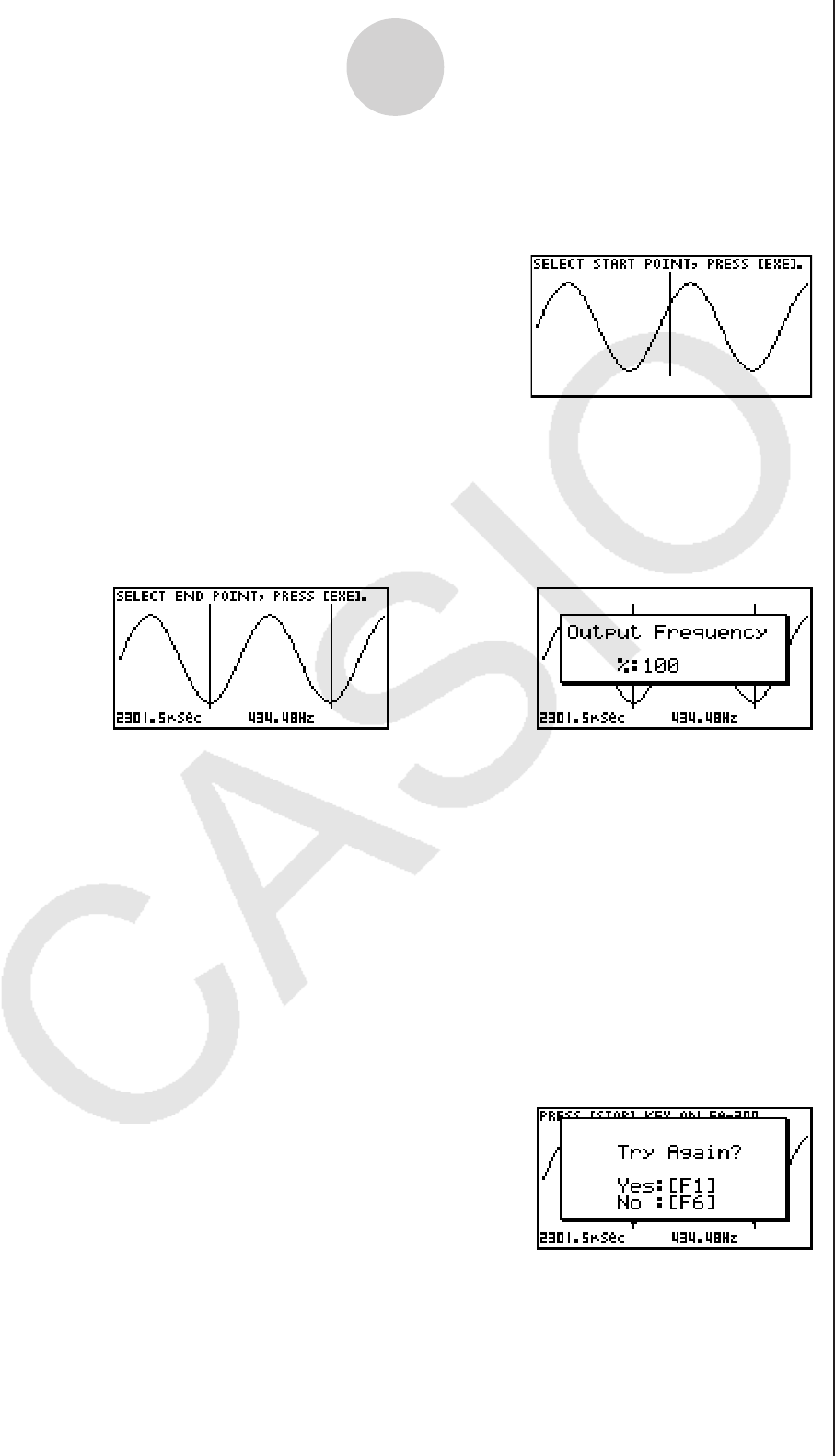
2-9
Using the Setup Wizard
7. Press 6(DRAW) to graph the function.
• This graphs the function and displays a vertical cursor line as shown below. Use the
graph to specify the range that you want to output to the speaker.
8. Use the d and e cursor keys to move the cursor to the start point of the output, and
then press w to register it.
9. Use the d and e cursor keys to move the cursor to the end point of the output, and
then press w to register it.
• After you specify the start point and end point, an output frequency dialog box shown
below appears on the display.
10. Input a percent value for the output frequency value you want.
• To output the original sound as-is, specify 100%. To raise the original sound by one octave,
input a value of 200%. To lower the original sound by one octave, input a value of 50%.
11. After inputting an output frequency value, press w.
• This outputs the waveform between the start point and end point from the EA-200 speaker.
• If the sound you configured cannot be output for some reason, the message “Range
Error” will appear. If this happens, press J to scroll back through the previous setting
screens and change the setup as required.
12. To terminate sound output, press the EA-200 [START/STOP] key.
13. Press w.
• This displays a screen like the one shown below.
/

2-10
Using the Setup Wizard
14. Perform one of the following operations, depending on what you want to do.
To change the output frequency and try again:
Press 1(Yes) to return to the “Output Frequency” dialog box. Next, repeat the above
steps from step 10.
To change the output range of the waveform graph and try again:
Press 6(No) to return to the graph screen in step 7. Next, repeat the above steps from
step 8.
To change the function:
Press 6(No) and then J to return to the graph function list in step 6. Next, repeat the
above steps from step 6.
To exit the procedure and return to the E-CON2 main menu:
Press 6(No) and then press J twice.

3 Using Advanced Setup
Advanced Setup provides you with total control over a number of parameters that you can
adjust to configure the EA-200 setup that suits your particular needs.
The procedures in this section provide the general steps you should perform when using
Advanced Setup to configure an EA-200 setup, and to returns setup settings to their initial
default values. You can find details about individual settings and the options that are
available with each setting are provided by the explanations that start on page 3-3.
kAdvanced Setup Operations
uTo configure an EA-200 setup using Advanced Setup
The following procedure describes the general steps for using Advanced Setup. Refer to the
pages as noted for more information.
1. Display the E-CON2 main menu (page 1-1).
2. Press 1(SET). This displays the “Setup EA-200” submenu.
3. Press 2(ADV). This displays the Advanced Setup menu.
4. If you want to configure a custom probe at this point, press f(Custom Probe). Next,
follow the steps under “To configure a custom probe setup” on page 4-1.
• You can also configure a custom probe during the procedure under “To configure Channel
Setup settings” on page 3-3.
• Custom probe configurations you have stored in memory can be selected using Channel
in step 5, below.
5. Use the Advanced Setup function keys described below to set other parameters.
•b(Channel) .... Displays a screen that shows the sensors that are currently
assigned to each channel (CH1, CH2, CH3, SONIC, Mic). You can
also use this dialog to change sensor assignments. See “Channel
Setup” on page 3-3 for more information.
•c(Sample) ..... Displays a screen for selecting the sampling mode, and for
specifying the sampling interval, the number of samples, and the
warm-up mode. When “Fast” is selected for “Mode”, this dialog box
also displays a setting for turning FFT (frequency characteristics)
graphing on and off. See “Sample Setup” on page 3-5 for more
information.
3-1
Using Advanced Setup
Advanced Setup Menu

3-2
Using Advanced Setup
•d(Trigger) ...... Displays a screen for configuring sampling start (trigger) conditions.
See “Trigger Setup” on page 3-8 for more information.
•e(Graph) ....... Displays a screen for configuring graph settings. See “Graph Setup”
on page 3-13 for more information.
• You can return the settings on the above setup screens (b through e) using the
procedure described under “To return setup parameters to their initial defaults”.
6. After you configure a setup, you can use the function key operations described below to
start sampling or perform other operations.
•1(STRT) ...... Starts sampling using the setup (page 8-1).
•2(MLTI) ....... Starts MULTIMETER Mode sampling using the setup (page 5-1).
•3(MEM) ....... Saves the setup (page 6-1).
•4(PROG) ..... Converts the setup to a program (page 7-1).
•5(GRPH) ..... Graphs data sampled by the EA-200, and provides tools for analyzing
graphs (page 10-1).
•6(ABT) ........ Displays version information about the EA-200 unit that is currently
connected to the calculator.
uTo return setup parameters to their initial defaults
Perform the following procedure when you want to return the parameters of the setup in the
current setup memory area to their initial defaults.
1. While the Advanced Setup menu (page 3-1) is on the display, press g(Initialize).
2. In response to the confirmation message that appears, press 1(Yes) to initialize the
setup.
• To clear the confirmation message without initializing the setup, press 6(No).

3-3
Using Advanced Setup
kChannel Setup
The Channel Setup screen shows the sensors that are currently assigned to each channel
(CH1, CH2, CH3, SONIC, Mic).
uu
uu
uTo configure Channel Setup settings
1. While the Advanced Setup menu (page 3-1) is on the display, press b(Channel).
• This displays the Channel Setup screen.
Currently selected channel
Channel Setup Screen
2. Use the f and c cursor keys to move the highlighting to the channel whose setting
you want to change.
3. What you need to do next depends on the currently selected channel.
• CH1, CH2, or CH3
Press a function key to display a menu of sensors that can be assigned to the selected
channel.
1(CASIO) ...... Displays a menu of CASIO sensors.
2(VRNR) ....... Displays a menu of Vernier sensors.
3(CSTM) ....... Displays a menu of custom probes.
4(None) ......... Press this key when you want leave the channel without any sensor
assigned to it.
• SONIC Channel
Press a function key to display a menu of sensors that can be assigned to this channel.
1(CASIO) ...... Displays a menu of CASIO sensors, but only “Motion” can be
selected.
2(VRNR) ....... Displays a menu of Vernier sensors. You can select “Motion” or
“Photogate”.
Note
• On the menu that appears after you select “Motion” from either the CASIO or
Vernier sensor menu, select either “meters” or “feet” as the sampling unit.
• After selecting “Motion” from either the CASIO or Vernier sensor menu, you can
press the K key to toggle “smoothing (correction of measurement error)” on
(“-Smooth” displayed) and off (“-Smooth” not displayed).

3-4
Using Advanced Setup
• From the menu that appears after you select “Photogate” as the sensor, select
[Gate] or [Pulley].
[Gate] ............... Select this option when using the Photogate sensor alone.
[Pulley] ............. Select this option when using the Photogate sensor along with a
smart pulley.
4(None) ......... Select this option to disable the SONIC channel.
• Mic Channel
For this channel, the sensor is automatically set to Built-in (External) Microphone.
However, you need to configure the settings described below.
1(Snd) ........... Select this option to record elapsed time and volume 2-dimensional
sampled sound data (elapsed time on the horizontal axis, volume on
the vertical axis).
2(FFT) ........... Select this option to record frequency and volume 2-dimensional
sampled sound data (frequency on the horizontal axis, volume on the
vertical axis).
4(None) ......... Select this option to disable the Mic channel.
4. Repeat steps 2 and 3 as many times as necessary to configure all the channels you want.
5. After all the settings are the way you want, press w.
• This returns to the Advanced Setup menu.
Note
• When you select a channel on the Channel Setup screen, the sampling range of the
selected channel appears in the bottom line of the screen.
In the above example, the range of the temperature sensor assigned to CH2 appears on the
display.
If the sampling range value is too long to fit on the display, only the part of the value that fits
on the display will be shown.
• Whenever the current Sample Setup (page 3-5) and Trigger Setup (page 3-8) settings
become incompatible due to a change in Channel Setup settings, these settings revert
automatically to their initial defaults. Selecting the Mic channel with Channel Setup while
the Sample Setup has “Extended” selected for the sampling mode, for example, will cause
the sampling mode to change automatically to “Fast” (which is the initial default setting
when the Mic channel is selected). For information about the channels that can be selected
for each sampling mode, see “Sample Setup” (page 3-5).
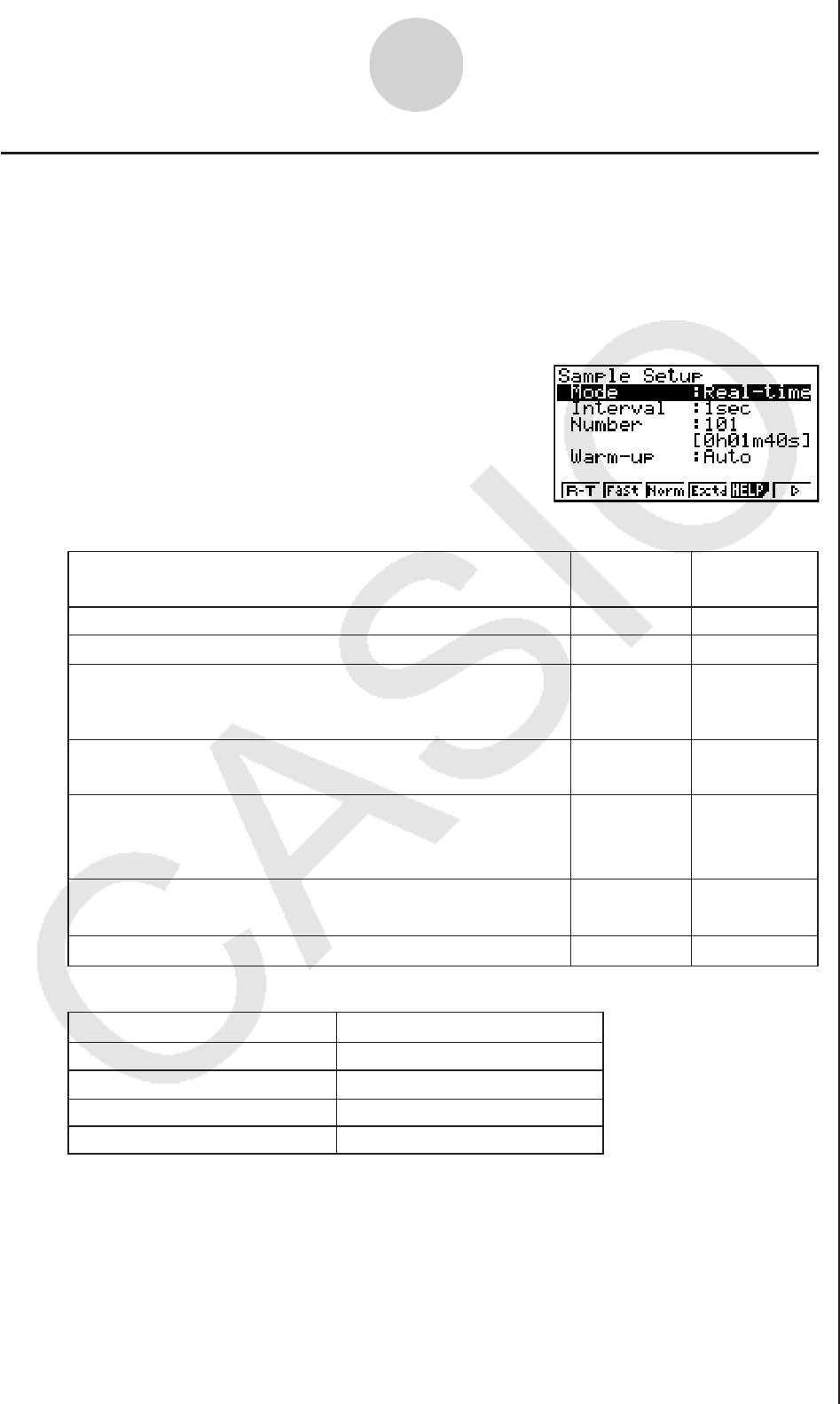
3-5
Using Advanced Setup
kSample Setup
The Sample Setup screen lets you configure a number of settings that control sampling.
uu
uu
uTo configure Sample Setup settings
1. While the Advanced Setup menu (page 3-1) is on the display, press c(Sample).
• This displays the Sample Setup screen, with the “Mode” line highlighted, which indicates
that you can select the sampling mode.
• Note that the mode you select also determines the channel(s) you can use.
Sampling mode: Selectable Channel(s)
Realtime, Extended, Normal CH1, CH2, CH3, SONIC
Fast CH1, Mic
Sound Mic
Clock, Period CH1
Perform sampling over a long time (weather, etc.)
• The EA-200 enters a power off sleep state while standing
by.
Press this
key:
To do this: To select
this mode:
1(R-T)
Normal
Graph data in real-time as it is sampled
4(Extd)
Period
2(Fast)
Clock
Perform sampling of high-speed phenomena (sound, etc.)
6(g)
1(Snd) SoundSample sound using the EA-200’s built-in microphone
6(g)
2(Clck)
Extended
Record the time of the occurrence of a particular trigger
event as an absolute value starting from 0, which is the
sampling start time
6(g)
3(Priod)
Fast
Perform periodic sampling, from a start trigger event to an
end trigger event
3(Norm)
Realtime
Perform sampling other than that described above
2. Select the sampling mode that suits the type of sampling you want to perform.

3-6
Using Advanced Setup
4. To change the number of samples setting, move the highlighting to “Number”. Next, press
1 to display a dialog box for specifying the number of samples.
• The total sampling time shown at the bottom of the dialog box is calculated by multiply-
ing the “Sampling Interval” value you specified in step 3 by the number of samples you
specify here.
Important!
• When all of the following conditions exist, a “Distance” setting appears in place of the
“Number” setting. See “To configure the Distance setting” (page 3-7) for information
about configuring the “Distance” setting.
• Channel Setup (page 3-3): 2(VRNR) - [Photogate] - [Pulley]
• Sampling Mode (page 3-5): Clock
5. To change the warm-up time setting, move the highlighting to “Warm-up”. Next, perform
one of the function key operations described below.
Note
• The “Warm-up” setting will not be displayed on the Sample Setup screen if “Fast”,
“Sound” or “Extended” is currently selected as the sampling mode.
Important!
• When the following condition exists, an “FFT Graph” setting appears in place of the
“Warm-up” setting. See “To configure the FFT Graph setting” (page 3-7) for information
about configuring the “FFT Graph” setting.
• Sampling Mode (page 3-5): Fast
To do this: Press this key:
Have the warm-up time for each sensor set automatically 1 (Auto)
Input a warm-up time, in seconds, manually 2 (Man)
Disable the warm-up time 3 (None)
3. To change the sampling interval setting, move the highlighting to “Interval”. Next, press
1 to display a dialog box for specifying the sampling interval.
• The range of values you can select depends on the current sampling mode setting.
If this sampling mode is selected: This is the allowable setting range:
Realtime 0.2 to 299 sec
Fast 20 to 500
μ
sec
Extended 5 to 240 min
Period “=Trigger” only (no value input required)
Sound 20 to 27
μ
sec
Clock “=Trigger” only (no value input required)
Normal 0.0005 to 299 sec

3-7
Using Advanced Setup
6. After all the settings are the way you want, press w.
• This returns to the Advanced Setup menu.
Note
• Whenever the current Channel Setup (page 3-3) and Trigger Setup (page 3-8) settings
become incompatible due to a change in Sample Setup settings, these settings revert
automatically to their initial defaults. Selecting “Realtime” as the sampling mode with
Sample Setup while the Mic channel is selected with Channel Setup and the Trigger
Setup has “Mic” selected for “Source”, for example, will cancel the Channel Setup Mic
channel selection and change the Trigger Setup “Source” setting to “[EXE] key”.
For information about the channels that can be selected for each sampling mode, see
step 2 of “To configure Sample Setup settings”. For information about the trigger sources
that can be selected for each sampling mode, see “Trigger Setup” (page 3-8).
uu
uu
uTo configure the Distance setting
In place of step 3 of the procedure under “To configure Sample Setup settings”, press 1 to
display a dialog box for specifying the distance the weight travels in meters.
• Specify a value in the range of 0.1 to 4 meters.
uu
uu
uTo configure the FFT Graph setting
In place of step 5 of the procedure under “To configure Sample Setup settings”, press 1 to
display a dialog box for turning frequency characteristic graphing (FFT Graph) on and off.
To do this: Press this key:
Turn on graphing of frequency characteristics after sampling 1(On)
Turn off graphing of frequency characteristics after sampling 2(Off)
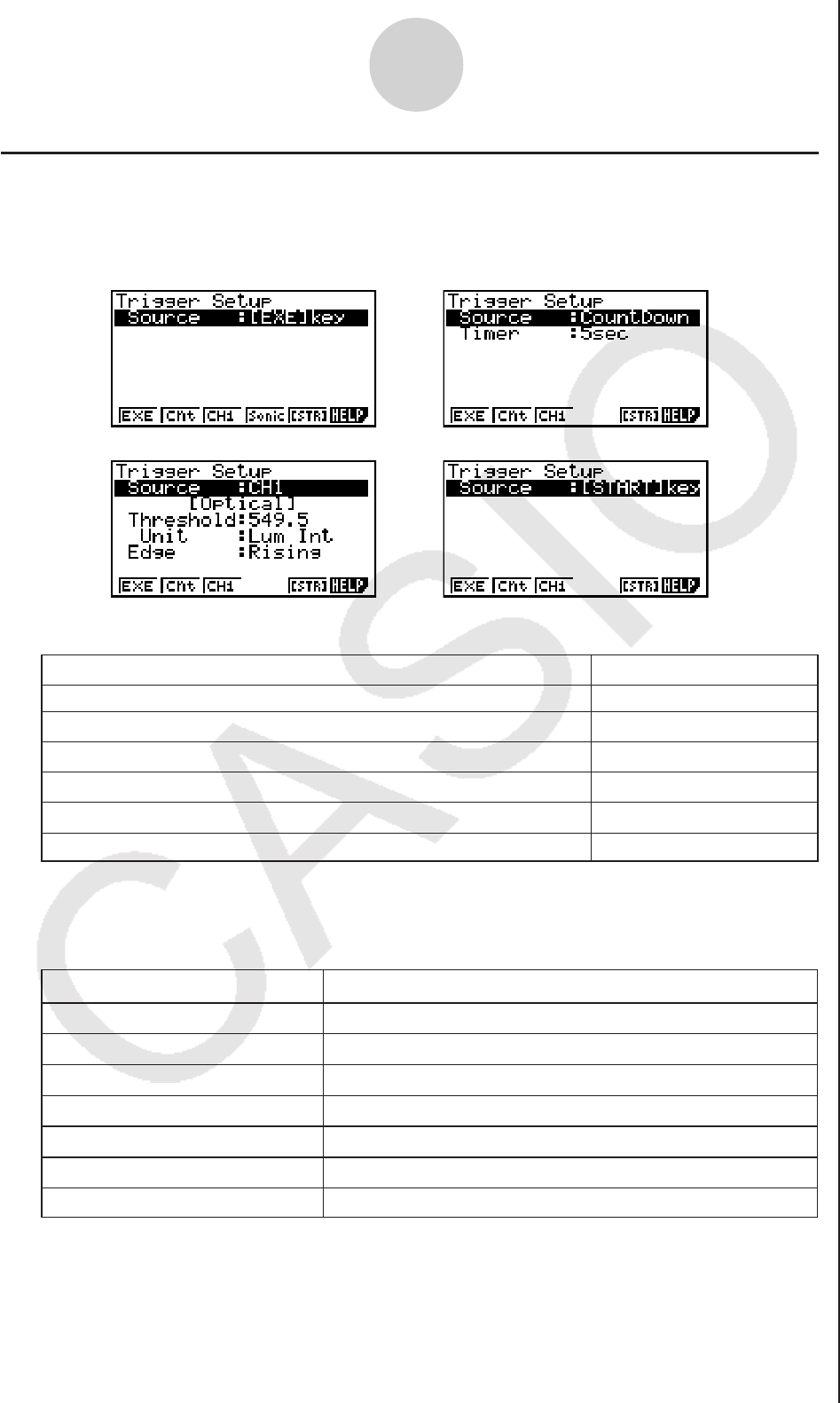
3-8
Using Advanced Setup
The following table describes each of the six available trigger sources.
Note
The trigger sources you can select depends on the sampling mode selected with the Sample
Setup (page 3-5).
For this sampling mode: The following trigger source(s) can be selected:
Realtime [EXE]
key, Count Down
Fast [EXE]
k
ey, Count Down, CH1, Mic
Normal [EXE]
k
ey, Count Down, CH1, SONIC,
[START]
k
ey
Extended [EXE]
k
ey
Sound [EXE]
k
ey, Count Down, Mic
Clock CH1
Period CH1
kTrigger Setup
You can use the Trigger Setup screen to specify the event that causes sampling to start (w
key operation, etc.) The event that causes sampling to start is called the “trigger source”,
which is indicated as “Source” on the Trigger Setup screen.
To start sampling when this happens: Select this trigger source:
After the specified number of seconds are counted down Count Down
When the EA-200’s built-in microphone detects sound Mic
When the w key is pressed [EXE] key
When input at the SONIC channel reaches a specified value SONIC
When input at CH1 reaches a specified value CH1
When the EA-200’s [START/STOP] key is pressed [START] key

3-9
Using Advanced Setup
• The trigger source is always “[EXE] key” when the sampling mode is “Extended”, and
“CH1” when the sampling mode is “Clock” or “Period”.
uu
uu
uTo configure Trigger Setup settings
1. While the Advanced Setup menu (page 3-1) is on the display, press d(Trigger).
• This displays the Trigger Setup screen with the “Source” line highlighted.
• The function menu items that appears in the menu bar depend on the sampling mode
selected with Sample Setup (page 3-5). The above screen shows the function menu
when “Normal” is selected as the sample sampling mode.
2. Use the function keys to select the trigger source you want.
• The following shows the trigger sources that can be selected for each sampling mode.
Sampling Mode Trigger Source
Realtime 1(EXE) : [EXE] key, 2(Cnt) : Count Down
Fast 1(EXE) : [EXE] key, 2(Cnt) : Count Down, 3(CH1),
5(Mic)
Normal 1(EXE) : [EXE] key, 2(Cnt) : Count Down, 3(CH1),
4(Sonic), 5(STR) : [START] key
Sound 1(EXE) : [EXE] key, 2(Cnt) : Count Down, 5(Mic)

If this is the trigger
source: Do this next:
[EXE] key Press w to finalize Trigger Setup and return to the Advanced
Setup menu.
Count Down Specify the countdown start time. See “To specify the
countdown start time” below.
CH1 Specify the trigger threshold value and trigger edge direction.
See “To specify the trigger threshold value and trigger edge
type”, “To configure trigger threshold, trigger start edge, and
trigger end edge settings” on page 3-11 or “To configure
Photogate trigger start and end settings” on page 3-12.
SONIC Specify the trigger threshold value and motion sensor level.
See “To specify the trigger threshold value and motion sensor
level” on page 3-12.
Mic Specify microphone sensitivity. See “To specify microphone
sensitivity” below.
[START] key Press w to finalize Trigger Setup and return to the Advanced
Setup menu.
uu
uu
uTo specify the countdown start time
1. Move the highlighting to “Timer”.
2. Press 1(Time) to display a dialog box for specifying the countdown start time.
3. Input a value in seconds from 1 to 10.
4. Press w to finalize Trigger Setup and return to the Advanced Setup menu.
uu
uu
uTo specify microphone sensitivity
1. Move the highlighting to “Sense” and then press one of the function keys describe below.
3. Perform one of the following operations, in accordance with the trigger source that was
selected in step 2.
To select this level of microphone sensitivity: Press this key:
Low 1(Low)
High 3(High)
Medium 2(Mid)
3-10
Using Advanced Setup
2. Press w to finalize Trigger Setup and return to the Advanced Setup menu (page 3-1).
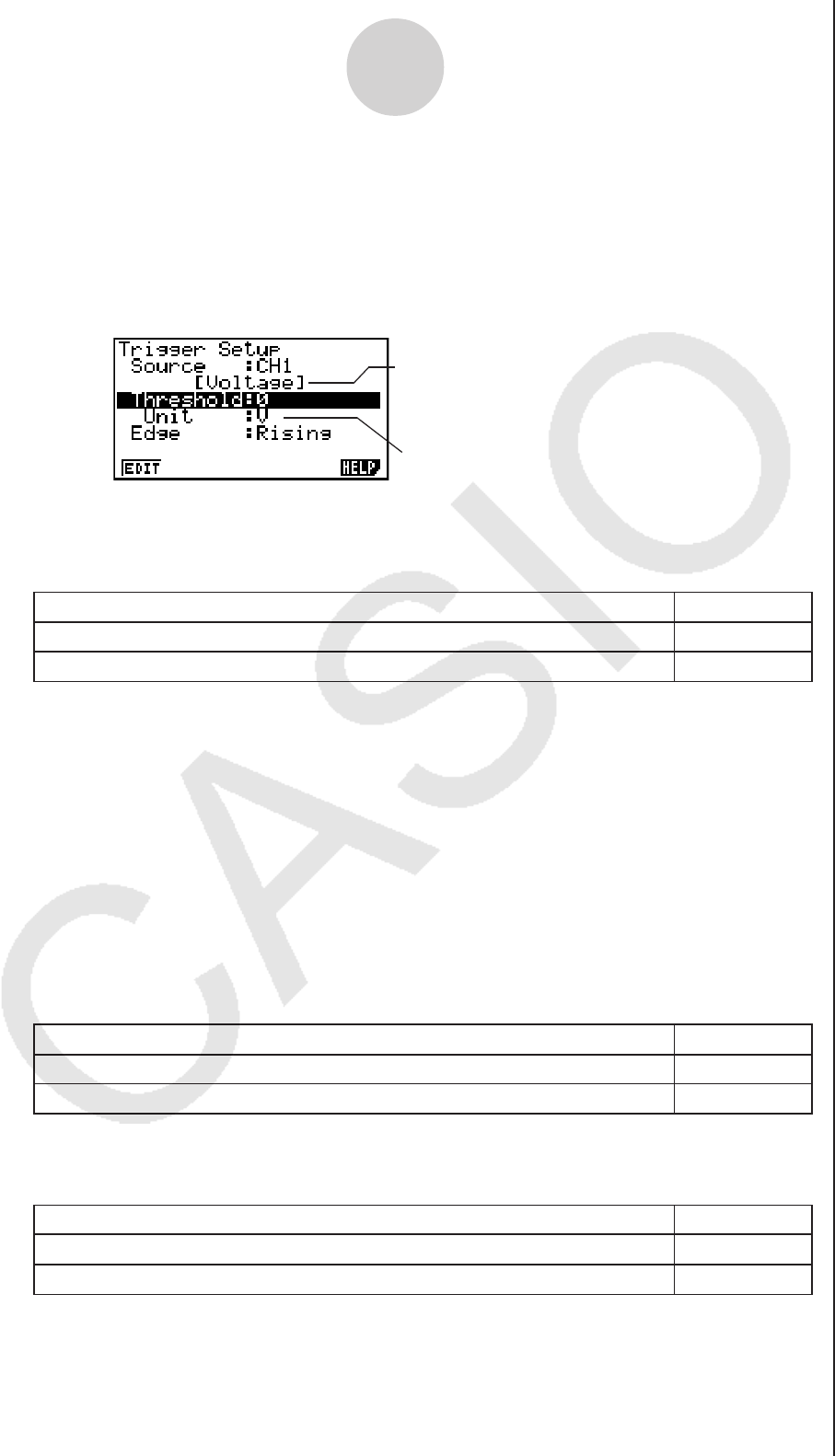
3-11
Using Advanced Setup
uu
uu
uTo specify the trigger threshold value and trigger edge type
Perform the following steps when “Fast”, “Normal”, or “Clock” is specified as the sampling
mode (page 3-5).
1. Move the highlighting to “Threshold”.
2. Press 1(EDIT) to display a dialog box for specifying the trigger threshold value, which is
value that data needs to attain before sampling starts.
3. Input the value you want, and then press w.
4. Move the highlighting to “Edge”.
5. Press one of the function keys described below.
6. Press w to finalize Trigger Setup and return to the Advanced Setup menu (page 3-1).
uu
uu
uTo configure trigger threshold, trigger start edge, and trigger end edge settings
Perform the following steps when “Period” is specified as the sampling mode (page 3-5).
1. Move the highlighting to “Threshold”.
2. Press 1(EDIT) to display a dialog box for specifying the trigger threshold value, which is
value that data needs to attain before sampling starts.
3. Input the value you want.
4. Move the highlighting to “Start to”.
5. Press one of the function keys described below.
To select this type of edge: Press this key:
Falling 1(Fall)
Rising 2(Rise)
6. Move the highlighting to “End Edge”.
7. Press one of the function keys described below.
To select this type of edge: Press this key:
Falling 1(Fall)
Rising 2(Rise)
8. Press w to finalize Trigger Setup and return to the Advanced Setup menu (page 3-1).
Measurement unit supported by assigned sensor
Sensor assigned to CH1 or SONIC by Channel Setup
(page 3-3)
To select this type of edge: Press this key:
Falling 1(Fall)
Rising 2(Rise)

3-12
Using Advanced Setup
uu
uu
uTo configure Photogate trigger start and end settings
Perform the following steps when CH1 is selected as a Photogate trigger source.
1. Move the highlighting to “Start to”.
2. Press one of the function keys described below.
3. Move the highlighting to “End Gate”.
4. Press one of the function keys described below.
5. Press w to finalize Trigger Setup and return to the Advanced Setup menu (page 3-1).
uu
uu
uTo specify the trigger threshold value and motion sensor level
1. Move the highlighting to “Threshold”.
2. Press 1(EDIT) to display a dialog box for specifying the trigger threshold value, which is
value that data needs to attain before sampling starts.
3. Input the value you want, and then press w.
4. Move the highlighting to “Level”.
5. Press one of the function keys described below.
To specify this Photogate status: Press this key:
Photogate closed 1(Close)
Photogate open 2(Open)
To specify this Photogate status: Press this key:
Photogate closed 1(Close)
Photogate open 2(Open)
6. Press w to finalize Trigger Setup and return to the Advanced Setup menu (page 3-1).
To select this type of level:
Press this key:
Below 1(Blw)
Above 2(Abv)
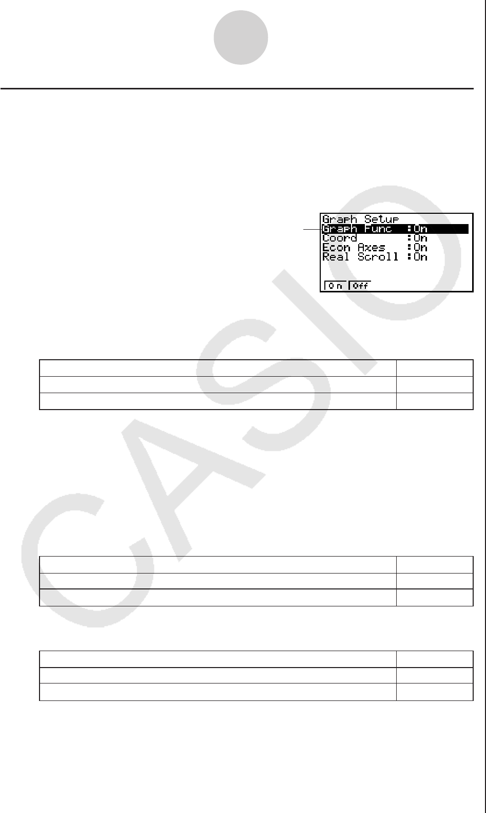
3-13
Using Advanced Setup
To specify this graph source data name display setting: Press this key:
Display source data name 1(On)
Hide source data name 2(Off)
kGraph Setup
Use the Graph Setup screen to configure settings for the graph produced after sampling is
complete. You use the Sample Setup settings (page 3-5) to turn graphing on or off.
uu
uu
uTo configure Graph Setup settings
1. While the Advanced Setup menu (page 3-1) is on the display, press e(Graph).
• This displays the Graph Setup screen.
Currently selected item
Graph Setup Screen
• When the graph data is stored in a sample data memory file, the file name appears as
the source data name. When the graph data is stored in current data area, the channel
name appears.
Note
• For details about sample data memory and current data area, see “9 Using Sample Data
Memory”.
2. To change the graph source data name display setting, use the f and c cursor keys
to move the highlighting to “Graph Func”. Next, press one of the function keys described
below.
3. To change the trace operation coordinate display setting, use the f and c cursor keys
to move the highlighting to “Coord”. Next, press one of the function keys described below.
4. To change the numeric axes display setting, use the f and c cursor keys to move the
highlighting to “Econ Axes”. Next, press one of the function keys described below.
To specify this coordinate display setting for the trace operation: Press this key:
Display trace coordinates 1(On)
Hide trace coordinates 2(Off)
To specify this axes display setting: Press this key:
Display axes 1(On)
Hide axes 2(Off)

3-14
Using Advanced Setup
To specify this real-time scrolling setting: Press this key:
Real-time scrolling on 1(On)
Real-time scrolling off 2(Off)
5. To change the real-time scroll setting, use the f and c cursor keys to move the
highlighting to “RealScroll”. Next, press one of the function keys described below.
6. Press w to finalize Graph Setup and return to the Advanced Setup menu.
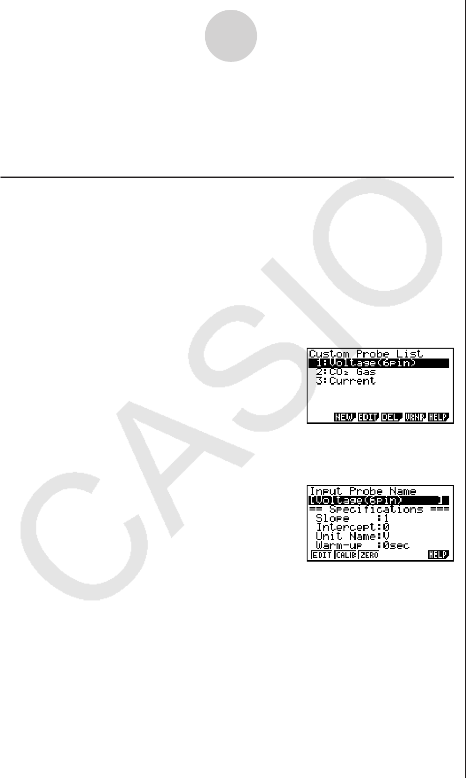
4 Using a Custom Probe
You can use the procedures in this section to configure a custom probe for use with the EA-
200. The term “custom probe” means any sensor other than the CASIO or Vernier sensors
specified as standard for the E-CON2 Mode.
kConfiguring a Custom Probe Setup
To configure a custom probe setup, you must input values for the constants of the fixed
linear interpolation formula (ax + b). The required constants are slope (a) and intercept (b). x
in the above expression (ax + b) is the sampled voltage value (sampling range: 0 to 5 volts).
uu
uu
uTo configure a custom probe setup
1. From the E-CON2 main menu (page 1-1), press 1(SET) and then c(ADV) to display
the Advanced Setup menu.
• See “3 Using Advanced Setup” for more information.
2. On the Advanced Setup menu (page 3-1), press f(Custom Probe) to display the Custom
Probe List.
• The message “No Custom Probe” appears if the Custom Probe List is empty.
3. Press 2(NEW).
• This displays a custom probe setup screen like the one shown below.
4-1
Using a Custom Probe
• The initial default setting for the probe name is “Voltage(6pin)”. The first step for
configuring custom probe settings is to change this name to another one. If you want to
leave the default name the way it is, skip steps 4 and 5.
4. Press 1(EDIT).
• This enters the probe name editing mode.
5. Input up to 18 characters for the custom probe name, and then press E.
• This will cause the highlighting to move to “Slope”.
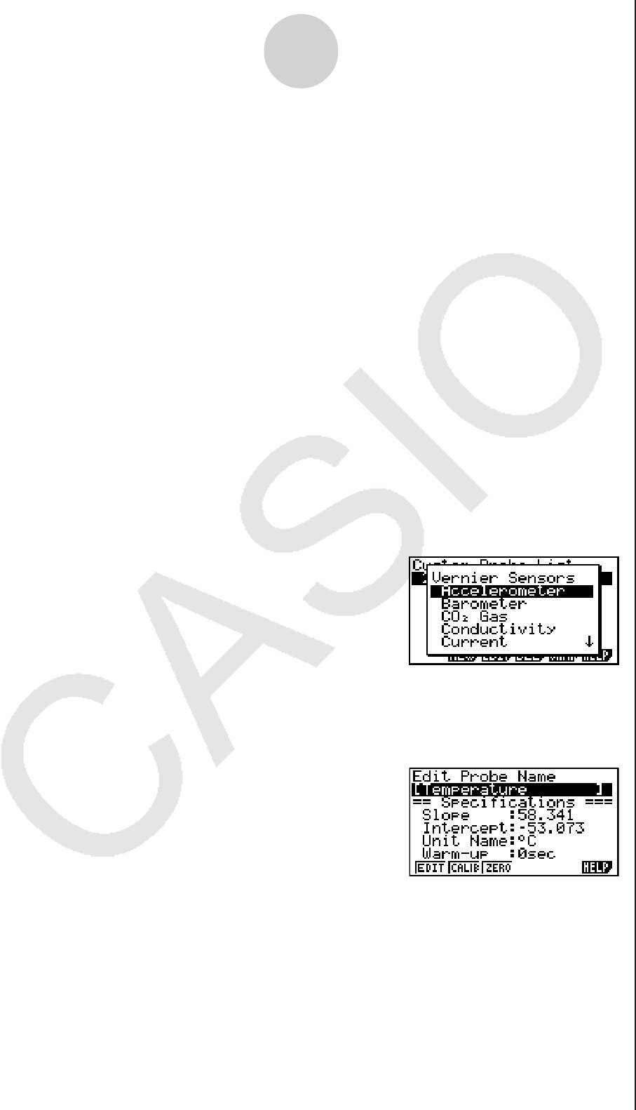
4-2
Using a Custom Probe
6. Use the function keys described below to configure the custom probe setup.
• To change the setting of an item, first use the f and c cursor keys to move the
highlighting to the item. Next, use the function keys to select the setting you want.
(1) Slope
Press 1(EDIT) to input the slope for the linear interpolation formula.
(2) Intercept
Press 1(EDIT) to input the intercept for the linear interpolation formula.
(3) Unit Name
Press 1(EDIT) to input up to eight characters for the unit name.
(4) Warm-up
Press 1(EDIT) to input the warm-up time.
7. Press wand then input a memory number (1 to 99).
• This saves the custom probe setup and returns to the Custom Probe List, which should
now contain the new custom probe setup you configured.
uu
uu
uTo recall the specifications of a Vernier sensor and configure custom
probe settings
1. Perform the first two steps of the procedure under “To configure a custom probe setup” on
page 4-1.
2. Press 5(VRNR).
• This displays a Vernier sensor list.
3. Use the f and c keys to move the highlighting to the Vernier sensor whose setting
you want to use as the basis of the custom probe settings, and then press w.
• The name and specifications of the Vernier sensor you select will appear on the custom
probe setup screen.
• To complete this procedure, perform steps 4 through 7 under “To configure a custom
probe setup” (page 4-1).

kAuto Calibrating a Custom Probe
Auto calibration automatically corrects the slope and intercept values of a custom probe
setup based on two actual samples.
Important!
• Before performing the procedure below, you should prepare two conditions whose
measurement values are known.
• When inputting reference value in step 5 of the procedure below, input the exact known
measurement value of the condition you will sample in step 4. When inputting reference
value in step 7 of the procedure below, input the exact known measurement value of the
condition you will sample in step 6.
uu
uu
u To auto calibrate a custom probe
1. Connect the calculator and EA-200, and connect the custom probe you want to auto
calibrate to CH1 of the EA-200.
2. What you should do first depends on whether you are configuring a new custom probe for
calibration, or editing the configuration of an existing custom probe.
If you are configuring a new custom probe:
• Perform steps 1 through 6 of the procedure under “To configure a custom probe setup”
on page 4-1.
• Auto calibrate will automatically set the slope and intercept, so you do not need to
specify them in step 6 of the above procedure.
If you are editing the configuration of an existing custom probe:
• Perform steps 1 through 3 of the procedure under “To edit a custom probe setup” on
page 4-6.
3. Press 2(CALIB).
• This will start the first sampling operation with the sensor connected to EA-200’s CH1,
and then display a screen like the one shown below.
4-3
Using a Custom Probe
First sampling operation
Real-time display of sampled values

4-4
Using a Custom Probe
4. After the sampled value stabilizes, hold down w for a few seconds.
• This will register the first sampled value and display it on the screen. At this time the
cursor will appear at the bottom of the display, ready for input of a reference value.
5. Use the key pad to input the reference value for the first sampled value, and then press
w.
• This cause sampling of the second value to be performed automatically, and display the
same type of screen that appeared in step 3.
6. After the sampled value stabilizes, hold down w for a few seconds.
• This will register the second sampled value and display it on the screen. The cursor will
appear at the bottom of the display, ready for input of a reference value.
Second sampling operation
7. Use the key pad to input the reference value for the second sampled value, and then
press w.
• This will return to the custom probe setup screen.
• The E-CON2 will calculate the slope and intercept value based on the two reference
values that you input, and configure the settings automatically. The automatically
configured values will appear on the custom probe setup screen, where you can view
them.

8. Press w, and then input a memory number from 1 to 99.
• This saves the custom probe setup and returns to the custom probe list.
kZero Adjusting a Custom Probe
This procedure zero adjusts a custom probe and sets its intercept value based on an actual
sample using the applicable custom probe.
u To zero adjust a custom probe
1. Connect the calculator and EA-200, and connect the custom probe you want to zero
adjust to CH1 of the EA-200.
2. What you should do first depends on whether you are configuring a new custom probe for
zero adjusting, or editing the configuration of an existing custom probe.
If you are configuring a new custom probe:
• Perform steps 1 through 6 of the procedure under “To configure a custom probe setup”
on page 4-1.
• Auto calibrate will automatically set the intercept, so you do not need to specify it in step
6 of the above procedure.
If you are editing the configuration of an existing custom probe:
• Perform steps 1 through 3 of the procedure under “To edit a custom probe setup” on
page 4-6.
3. Press 3(ZERO).
• This will start the sampling operation with the sensor connected to EA-200’s CH1, and
then display a screen like the one shown below.
4-5
Using a Custom Probe

4. At the point your want to perform zero adjustment (the point that the displayed value is
the appropriate zero adjust value), press w.
• This will return to the custom probe setup screen.
• The E-CON2 will set the intercept value automatically based on the sampled value. The
automatically configured value will appear on the custom probe setup screen, where you
can view it.
5. Press w, and then input a memory number from 1 to 99.
• This saves the custom probe setup and returns to the custom probe list.
kManaging Custom Probe Setups
Use the procedures in this section to edit and delete existing custom probe setups.
u To edit a custom probe setup
1. Display the Custom Probe List.
2. Select the custom probe setup whose configuration you want to edit.
• Use the f and c cursor keys to highlight the name of the custom probe you want.
3. Press 3(EDIT).
• This displays the screen for configuring a custom probe setup.
• To edit the custom probe setup, perform the procedure starting from step 6 under “To
configure a custom probe setup” on page 4-1.
u To delete a custom probe setup
1. Display the Custom Probe List.
2. Select the custom probe setup you want to delete.
• Use the f and c cursor keys to highlight the name of the custom probe setup you
want.
3. Press 4(DEL).
4. In response to the confirmation message that appears, press 1(Yes) to delete the
custom probe setup.
• To clear the confirmation message without deleting anything, press 6(No).
4-6
Using a Custom Probe

5-1
Using the MULTIMETER Mode
5 Using the MULTIMETER Mode
You can use the Channel Setup screen (page 3-3) to configure a channel so that EA-200
MULTIMETER Mode sampling is triggered by a calculator operation.
uu
uu
u To use the MULTIMETER Mode
1. Connect the calculator and EA-200, and connect the sensors you want to the applicable
EA-200 channels.
2. From the Advanced Setup menu (page 3-1), use the Channel Setup screen (page 3-3) to
configure sensor setups for each channel you will be using.
3. After configuring the sensor setups, press w to return to the Advanced Setup menu
(page 3-1), and then press 2(MLTI).
• This starts sampling in the EA-200 MULTIMETER mode and displays a list of sample
values for each channel.
• Displayed sample data is refreshed at 0.5-second intervals.
• Do not connect sensors to any other channels except for those you specified in step 2.
• Data sampled in the MULTIMETER mode is not saved in memory.
4. To end MULTIMETER mode sampling, press the w key.

6-1
Using Setup Memory
6 Using Setup Memory
Creating EA-200 setup data using the Setup Wizard or Advanced Setup causes the data to
be stored in the “current setup memory area”. The current contents of the current setup
memory area are overwritten whenever you create other setup data.
You can use setup memory to save the current setup memory area contents to calculator
memory to keep it from being overwritten, if you want.
kSaving a Setup
A setup can be saved when any one of the following conditions exist.
• After configuring a new setup with Setup Wizard
See step 8 under “To configure an EA-200 setup using Setup Wizard” on page 2-2.
• After configuring a new setup with Advanced Setup
See step 6 under “To configure an EA-200 setup using Advanced Setup” on page 3-1 for
more information.
• While the E-CON2 main menu (page 1-1) is on the display
Performing the setup save operation while the E-CON2 main menu is on the display saves
the contents of the current setup memory area (which were configured using Setup Wizard
or Advanced Setup).
Details on saving a setup are listed below.
uTo save a setup
1. If the final Setup Wizard screen (page 2-4) is on the display, advance to step 2. If it isn’t,
start the save operation by performing one of the function key operations described
below.
✔If the Advanced Setup menu (page 3-1) is on the display, press 3(MEM).
✔If the E-CON2 main menu (page 1-1) is on the display, press 2(MEM).
• Performing any one of the above operations causes the setup memory list to appear.
• The message “No Setup-MEM” appears if setup memory is empty.

2. If you are starting from the final Setup Wizard screen, press c(Save Setup-MEM).
If you are starting from another screen, press 2(SAVE).
• This displays the screen for inputting the setup name.
6-2
Using Setup Memory
3. Input up to 18 characters for the setup name.
4. Press w and then input a memory number (1 to 99).
• If you start from the final Setup Wizard screen (page 2-4), this saves the setup and the
message “Complete!” appears. Press w to return to the final Setup Wizard screen
(page 2-4).
• If you start from the Advanced Setup menu (page 3-1) or the E-CON2 main menu (page
1-1), this saves the setup and returns to the setup memory list which includes the name
you assigned it.
Important!
• Since you assign both a setup name and a file number to each setup, you can assign
the same name to multiple setups, if you want.
kUsing and Managing Setups in Setup Memory
All of the setups you save are shown in the setup memory list. After selecting a setup in the
list, you can use it to sample data or you can edit it.
uTo preview saved setup data
You can use the following procedure to check the contents of a setup before you use it for
sampling.
1. On the E-CON2 main menu (page 1-1), press 2(MEM) to display the setup memory list.
2. Use the f and c cursor keys to highlight the name of the setup you want.
3. Press K(Setup Preview).
• This displays the preview dialog box.
4. To close the preview dialog box, press J.

uTo recall a setup and use it for sampling
Be sure to perform the following steps before starting sampling with the EA-200.
1. Connect the calculator to the EA-200.
2. Turn on EA-200 power.
3. In accordance with the setup you plan to use, connect the proper sensor to the
appropriate EA-200 channel.
4. Prepare the item whose data is to be sampled.
5. On the E-CON2 main menu (page 1-1), press 2(MEM) to display the setup memory list.
6. Use the f and c cursor keys to highlight the name of the setup you want.
7. Press 1(STRT).
8. In response to the confirmation message that appears, press 1.
• Pressing w sets up the EA-200 and then starts sampling.
• To clear the confirmation message without sampling, press 6.
Note
• See “Operations during a sampling operation” on page 8-2 for information about
operations you can perform while a sampling operation is in progress.
uTo change the name of setup data
1. On the E-CON2 main menu (page 1-1), press 2(MEM) to display the setup memory list.
2. Use the f and c cursor keys to highlight the name of the setup you want.
3. Press 3(REN).
• This displays the screen for inputting the setup name.
6-3
Using Setup Memory
4. Input up to 18 characters for the setup name, and then press w.
• This changes the setup name and returns to the setup memory list.

uTo delete setup data
1. On the E-CON2 main menu (page 1-1), press 2(MEM) to display the setup memory list.
2. Use the f and c cursor keys to highlight the name of the setup you want.
3. Press 4(DEL).
4. In response to the confirmation message that appears, press 1(Yes) to delete the
setup.
• To clear the confirmation message without deleting anything, press 6(No).
uTo recall setup data
Recalling setup data stores it in the current setup memory area. You can then use Advanced
Setup to edit the setup. This capability comes in handy when you need to perform a setup
that is slightly different from one you have stored in memory.
1. On the E-CON2 main menu (page 1-1), press 2(MEM) to display the setup memory list.
2. Use the f and c cursor keys to highlight the name of the setup you want.
3. Press 5(LOAD).
4. In response to the confirmation message that appears, press 1(Yes) to recall the setup.
• To clear the confirmation message without recalling the setup, press 6(No).
Note
• Recalling setup data replaces any other data currently in the current setup memory area.
6-4
Using Setup Memory

7 Using Program Converter
Program Converter converts an EA-200 setup you configured using Setup Wizard or
Advanced Setup to a program that can run on the calculator. You can also use Program
Converter to convert a setup to a CFX-9850 Series/fx-7400 Series-compatible program.*1 *2
*1See the documentation that came with your scientific calculator or EA-200 for information
about how to use a converted program.
*2See online help (PROGRAM CONVERTER HELP) for information about supported CFX-
9850 Series and fx-7400 Series models.
kConverting a Setup to a Program
A setup can be converted to a program when any one of the following conditions exists.
• After configuring a new setup with Setup Wizard
See step 8 under “To configure an EA-200 setup using Setup Wizard” on page 2-2.
• After configuring a new setup with Advanced Setup
See step 6 under “To configure an EA-200 setup using Advanced Setup” on page 3-1 for
more information.
• While the E-CON2 main menu (page 1-1) is on the display
Performing the program converter operation while the E-CON2 main menu is on the
display converts the contents of the current setup memory area (which were configured
using Setup Wizard or Advanced Setup).
The program converter procedure is identical in all of the above cases.
uTo convert a setup to a program
1. Start the converter operation by performing one of the key operations described below.
✔If the final Setup Wizard screen (page 2-4) is on the display, press d(Convert Program).
✔If the Advanced Setup menu (page 3-1) is on the display, press 4(PROG).
✔If the E-CON2 main menu (page 1-1) is on the display, press 3(PROG).
• After you perform any one of the above operations, the program converter screen will
appear on the display.
7-1
Using Program Converter

2. Enter up to eight characters for the program name.
Note
Using the program converter initial default settings will create a program like the one
below.
• Associated Scientific Calculator: fx-9860 Series
• Associated Data Logger: EA-200
• Calibration: None
• Password: None
If you want to use these settings the way they are without changing them, skip steps 3
through 7 and go directly to step 8. If you want to change any of the settings, perform the
applicable operations in steps 3 through 7.
3. Specify the scientific calculator model to be associated with the program. Perform one of
the following key operations to associate the program with a scientific calculator.
7-2
Using Program Converter
• The number part of the scientific calculator model number you specify will appear in line
“F1:” of the program converter screen.
Note
For information about 1(CALC)4(→38K), see “Converting a CFX-9850 Series
Program to a fx-9860 Series Compatible Program” (page 7-4).
4. Specify the Data Logger model (EA-100 or EA-200) to be associated with the program.
Perform one of the following key operations to associate the program with a Data Logger.
To associate the program with this Data Logger: Perform this key operation:
EA-200 2(TYPE) 1(200)
EA-100 2(TYPE) 2(100)
CFX-9850 Series
To associate the program with this calculator: Perform this key operation:
fx-9860 Series 1(CALC) 1(9860)
fx-7400 Series 1(CALC) 3(7400)
1(CALC) 2(9850)
• The number part of the Data Logger model number you specify will appear in line “F2:”
of the program converter screen.
Important!
• Note that the capabilities of the EA-100 and EA-200 are different. Because of this, you
should keep in mind that an EA-200 program converted to an EA-100 program and used
to perform sampling with an EA-100 setup may not produce the desired results.

5. If you plan to use a custom probe connected to CH1 of the Data Logger, specify whether
calibration or zero adjust should be performed. Perform one of the following key
operations to configure the desired setting.
• The operation you specify will appear in line “F3:” of the program converter screen.
6. To password protect the program, press 4().
• This will cause the “Password?” prompt and password input field to appear under the
program name input field.
Zero adjust of the CH1 custom probe
To perform this operation: Perform this key operation:
Calibration of the CH1 custom probe 3(CALB) 1(CALIB)
No calibration 3(CALB) 3(None)
3(CALB) 2(ZERO)
7. Enter up to eight characters for the password.
• If you change your mind about assigning a password, press J here. This will cause
the password input field to disappear and cancel password input.
8. After everything is the way you want, press w to convert the program in accordance
with the setup.
• The message “Complete!” appears when conversion is complete. To clear the message
and return to the screen that was on the display in step 1, press w or J.
7-3
Using Program Converter
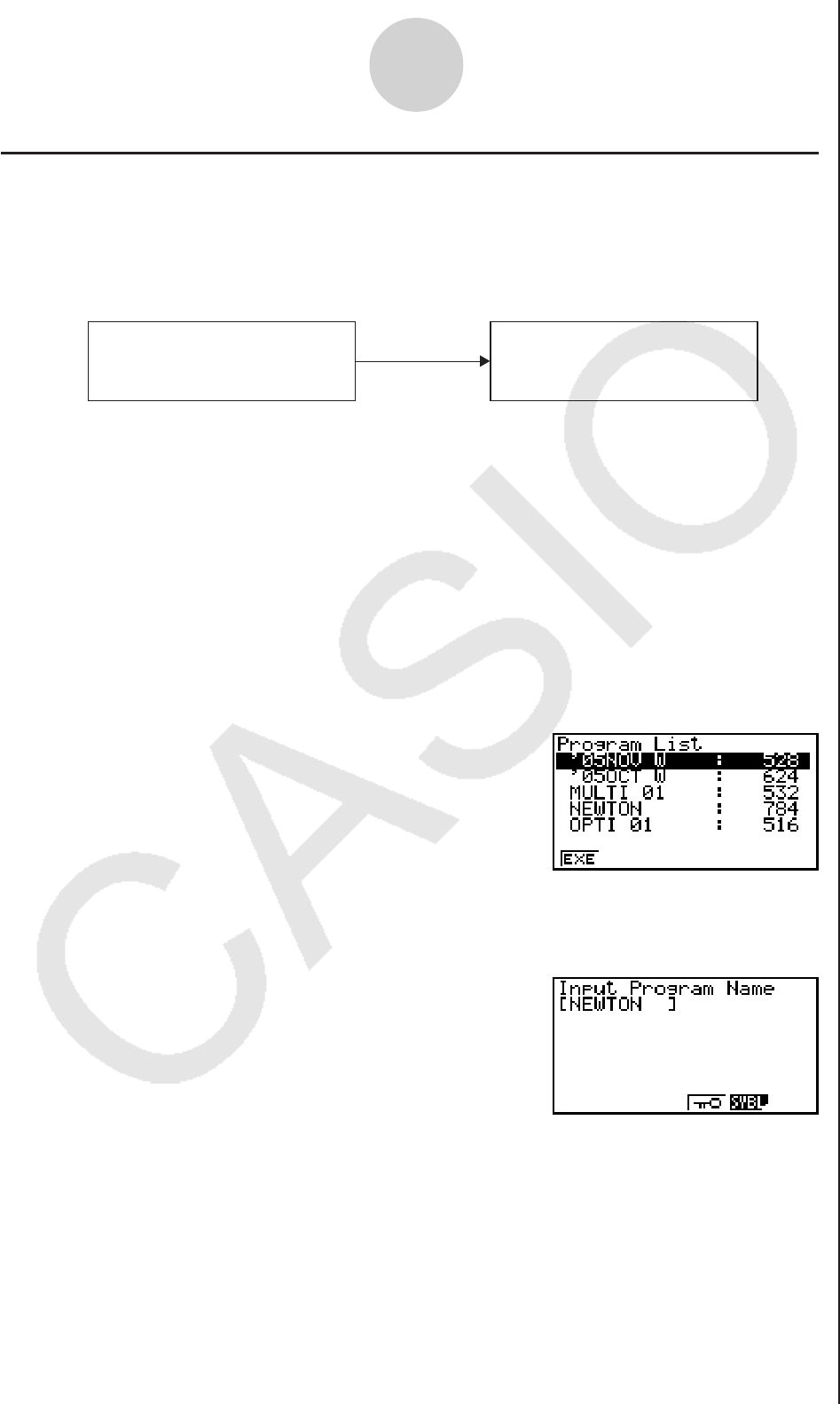
kConverting a CFX-9850 Series Program to a fx-9860 Series Compatible
Program
To use an EA-200 control program created on the CFX-9850 Series calculator (for use on
the CFX-9850) on the E-CON2, you need to convert the program to an fx-9860 program.
Conversion can be performed using the program converter.
press 1(EXE) or w.
• A program name input screen will appear after conversion is complete.
7-4
Using Program Converter
EA-200 Control Program for
CFX-9850 Series
EA-200 Control Program for
fx-9860 Series
Convert
uTo convert a program
1. Transfer the EA-200 control program created for the CFX-9850 Series to the fx-9860
main memory.
• Use the cable that comes bundled with the fx-9860 to connect its 3-pin serial port to the
3-pin serial port of the CFX-9850. For details, see “Chapter 13 Data Communications”.
2. Perform step 1 under “To convert a setup to a program” on page 7-1, which displays the
program converter screen.
3. Press 1(CALC) and then press 4(→38K).
• This displays a list of programs currently in main memory.
4. Use f and c to move the highlighting of the program you want to convert, and then

5. Enter up to eight characters for the program name.
• If you want to password protect the program, perform steps 6 and 7 under “To convert a
setup to a program” after inputting the program name.
6. Press w to start conversion of the program.
• The message “Complete!” appears when conversion is complete. To clear the message,
press w or J.
7-5
Using Program Converter

8 Starting a Sampling Operation
The section describes how to use a setup configured using the E-CON2 Mode to start an
EA-200 sampling operation.
kBefore getting started...
Be sure to perform the following steps before starting sampling with the EA-200.
1. Connect the calculator to the EA-200.
2. Turn on EA-200 power.
3. In accordance with the setup you plan to use, connect the proper sensor to the
appropriate EA-200 channel.
4. Prepare the item whose data is to be sampled.
kStarting a Sampling Operation
A sampling operation can be started when any one of the following conditions exist.
• After configuring a new setup with Setup Wizard
See step 8 under “To configure an EA-200 setup using Setup Wizard” on page 2-2.
• After configuring a new setup with Advanced Setup
See step 6 under “To configure an EA-200 setup using Advanced Setup” on page 3-1.
• While the E-CON2 main menu (page 1-1) is on the display
Starting a sampling operation while the E-CON2 main menu is on the display performs
sampling using the contents of the current setup memory area (which were configured
using Setup Wizard or Advanced Setup).
• While the setup memory list is on the display
You can select the setup you want on the setup memory list and then start sampling.
The following procedures explain the first three conditions described above. See “To recall a
setup and use it for sampling” on page 6-3 for information about starting sampling from the
setup memory list.
8-1
Starting a Sampling Operation

uTo start sampling
1. Start the sampling operation by performing one of the function key operations described
below.
✔If the final Setup Wizard screen (page 2-4) is on the display, press b(Start Setup).
✔If the Advanced Setup menu (page 3-1) is on the display, press 1(STRT).
✔If the E-CON2 main menu (page 1-1) is on the display, press 4(STRT).
• After you perform any one of the above operations, a sampling start confirmation screen
like the one shown below will appear on the display.
2. Press w.
• This sets up the EA-200 using the setup data in the current setup memory area.
• The message “Setting EA-200...” remains on the display while EA-200 setup is in
progress. You can cancel the setup operation any time this message is displayed by
pressing A.
• The screen shown below appears after EA-200 setup is complete.
8-2
Starting a Sampling Operation
3. Press w to start sampling.
• The screens that appear while sampling is in progress and after sampling is complete
depend on setup details (sampling mode, trigger setup, etc.). For details, see
“Operations during a sampling operation” below.
uOperations during a sampling operation
Sending a sample start command from the calculator to the EA-200 causes the following
sequence to be performed.
Setup Data Transfer → Sampling Start → Sampling End →
Transfer of Sample Data from the EA-200 to the Calculator
The table on the next page shows how the trigger conditions and sensor type specified in the
setup data affects the above sequence.
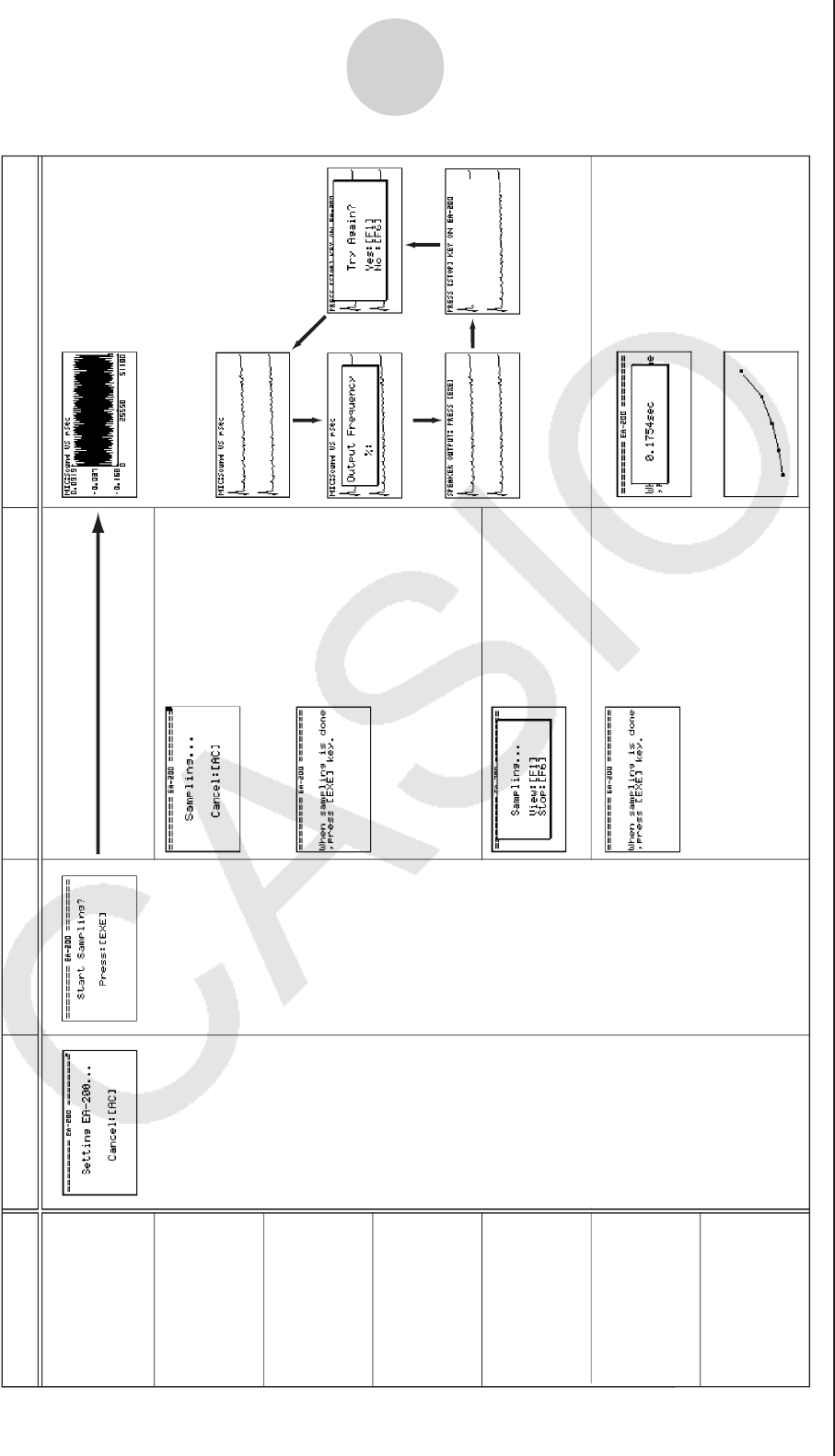
8-3
Starting a Sampling Operation
Mode
Real-time
Fast
Normal
Sound
Extended
Period
Clock
1. EA-200 Setup 2. Start Standby 3. Sampling 4. Graphing
Starts Sampling
• The screen shown below appears when CH1,
SONIC, or Mic is used as the trigger.
Graph screen does not show all sampled values,
but only a partial preview.
Pressing 1 advances to
“4. Graphing”.
Pressing w there returns to
“3. Sampling”.
w
w1
w
The following three graph types
can be produced when Photo-
gate-Pulley is being used.
1.
Time and distance graph
2.
Time and velocity graph
3.
Time and acceleration graph
Sample values is stored as List
data only.
• When Number of Samples = 1
•
When Number of Samples > 1
Input values.
w
Sampled values are saved as
Current Sample Data.
•
When Mode = Sound
Outputting through
speaker
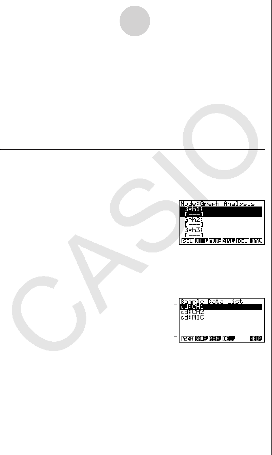
9-1
Using Sample Data Memory
9 Using Sample Data Memory
Performing an EA-200 sampling operation from the E-CON2 Mode causes sampled results
to be stored in the “current data area” of E-CON2 memory. Separate data is saved for each
channel, and the data for a particular channel in the current data area is called that channel’s
“current data”.
Any time you perform a sampling operation, the current data of the channel(s) you use is
replaced by the newly sampled data. If you want to save a set of current data and keep it
from being replaced by a new sampling operation, save the data in sample data memory
under a different file name.
kManaging Sample Data Files
uu
uu
uTo save current sample data to a file
1. On the E-CON2 main menu (page 1-1), press 5(GRPH).
• This displays the Graph Mode screen.
• For details about the Graph Mode screen, see “10 Using the Graph Analysis Tools to
Graph Data”.
2. Press 2(DATA).
• This displays the Sampling Data List screen.
List of current data files
“cd” stands for “current data”. The
text on the right side of the colon
indicates the channel name. Sampling Data List Screen
Graph Mode Screen
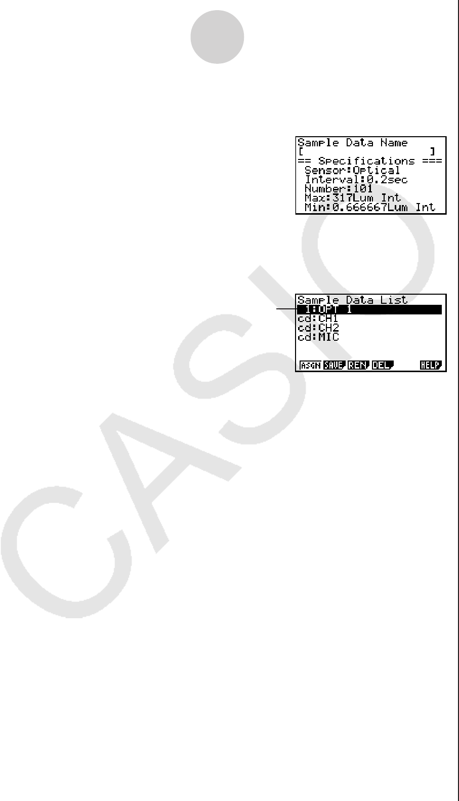
4. Enter up to 18 characters for the data file name, and then press w.
• This displays a dialog box for inputting a memory number.
5. Enter a memory number in the range of 1 to 99, and then press w.
• This saves the sample data at the location specified by the memory number you input.
• If you specify a memory number that is already being used to store a data file, a
confirmation message appears asking if you want to replace the existing file with the
new data file. Press 1 to replace the existing data file, or 6 to return to the memory
number input dialog box in Step 4.
6. To return to the E-CON2 main menu (page 1-1), press J twice.
Note
• You could select another data file besides a current data file in step 3 of the above
procedure and save it under a different memory number. You do not need to change the
file’s name as long as you use a different file number.
9-2
Using Sample Data Memory
The sample data file you save is indicated
on the display using the format:
<memory number>:<file name>.
3. Use the f and c cursor keys to move the highlighting to the current data file you want
to save, and then press 2(SAVE).
• This displays the screen for inputting a data name.

uu
uu
uTo rename an existing sample data file
Note
• You cannot use this procedure to rename a current data file name.
1. On the E-CON2 main menu (page 1-1), press 5(GRPH).
• This displays the Graph Mode screen.
2. Press 2(DATA).
• This displays the Sampling Data List screen.
3. Use the f and c cursor keys to move the highlighting to the data file you want to
rename, and then press 3(REN).
• This displays the screen for inputting a file name.
4. Enter up to 18 characters for the new data file name, and then tap w.
• This returns to the Sampling Data List screen.
5. To return to the E-CON2 main menu (page 1-1), press J twice.
uu
uu
uTo delete a sample data file
1. On the E-CON2 main menu (page 1-1), press 5(GRPH).
• This displays the Graph Mode screen.
2. Press 2(DATA).
• This displays the Sampling Data List screen.
3. Use the f and c cursor keys to move the highlighting to the data file you want to
delete, and then press 4(DEL).
4. In response to the confirmation message that appears, press 1(Yes) to delete the data
file.
• To clear the confirmation message without deleting the data file, press 6(No).
• This returns to the Sampling Data List screen.
5. To return to the E-CON2 main menu (page 1-1), press J twice.
9-3
Using Sample Data Memory

10-1
Using the Graph Analysis Tools to Graph Data
10 Using the Graph Analysis Tools to Graph Data
Graph Analysis tools make it possible to analyze graphs drawn from sampled data.
kAccessing Graph Analysis Tools
You can access Graph Analysis tools using either of the two methods described below.
uu
uu
uAccessing Graph Analysis tools from the Graph Mode screen, which is
displayed by pressing 5(GRPH) on the E-CON2 main menu (page 1-1)
• The main menu appears after you perform a sampling operation. Press 5(GRPH) at
that time.
• When you access Graph Analysis tools using this method, you can select from among a
variety of other Analysis modes. See “Selecting an Analysis Mode and Drawing a Graph”
(page 10-2) for more information about the other Analysis modes.
uu
uu
uAccessing Graph Analysis tools from the screen of a graph drawn after a
sampling operation is executed from the Setup Wizard or from Advanced
Setup (Realtime Mode)
Graph Mode Screen
• In this case, data is graphed after the sampling operation is complete, and the calculator
accesses Graph Analysis tools automatically. See “Graph Screen Key Operations” on
page 11-1.
Graph Screen

kSelecting an Analysis Mode and Drawing a Graph
This section contains a detailed procedure that covers all steps from selecting an analysis
mode to drawing a graph.
Note
• Step 4 through step 6 are not essential and may be skipped, if you want. Skipping any
step automatically applies the initial default values for its settings.
• If you skip step 2, the default analysis mode is the one whose name is displayed in the
top line of the Graph Mode screen.
uu
uu
uTo select an analysis mode and draw a graph
1. On the E-CON2 main menu (page 1-1), press 5(GRPH).
• This displays the Graph Mode screen.
2. Press 3(MODE), and then select the analysis mode you want from the menu that
appears.
• The name of the currently selected mode appears in the top line of the Graph Mode
screen.
10-2
Using the Graph Analysis Tools to Graph Data
Analysis mode name
3. Press 2(DATA).
• This displays the Sampling Data List screen.
Graph three sets of sampled data
simultaneously [Norm]
Perform this menu
operation:
To do this: To select this
mode:
Graph Analysis
Graph sampled data along with its first and
second derivative graph [diff] d/dt & d2/dt2
Display the graphs of different sampled data in
upper and lower windows for comparison [CMPR]/[GRPH] Compare Graph
Output sampled data from the speaker,
displaying graph of the raw data in the upper
window and the output waveform in the lower
window
[CMPR]/[Snd] Compare Sound
Display the graph of sampled data in the upper
window and its first derivative graph in the
lower window
[CMPR]/[d/dt] Compare d/dt
Display the graph of sampled data in the upper
window and its second derivative graph in the
lower window
[CMPR]/[d2/dt2] Compare d2/dt2
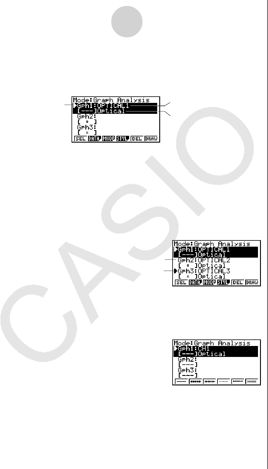
b. Repeat step a to turn each of the graphs listed on the Graph Mode screen on or off.
6. Select the graph style you want to use.
a. On the Graph Mode screen, use the f and c cursor keys to move the highlighting to
the graph (Gph1, Gph2, etc.) whose style you want to specify, and then press 4(STYL).
This will cause the function menu to change as shown below.
10-3
Using the Graph Analysis Tools to Graph Data
4. Specify the sampled data for graphing.
a. Use the f and c cursor keys to move the highlighting to the name of the sampled
data file you want to select, and then press 1(ASGN) or w.
• This returns to the Graph Mode screen, which shows the name of the sample data file
you selected.
b. Repeat step a above to specify sample data files for other graphs, if there are any.
• If you select “Graph Analysis” as the analysis mode in step 2, you must specify sample
data files for three graphs. If you select “Compare Graph” as the analysis mode in step
2, you must specify sample data files for two graphs. With other modes, you need to
specify only one sample data file.
• For details about Sampling Data List screen operations, see “9 Using Sample Data Memory”.
5. Turn on graphing for each of the graphs listed on the Graph Mode screen.
a. On the Graph Mode screen, use the f and c cursor keys to select a graph, and then
press 1(SEL) to toggle graphing on or off.
Graphing turned off.
Graphing turned on.
Graph Mode Screen
Graph on/off indicator Sample data file name
Name of sensor used for sampling
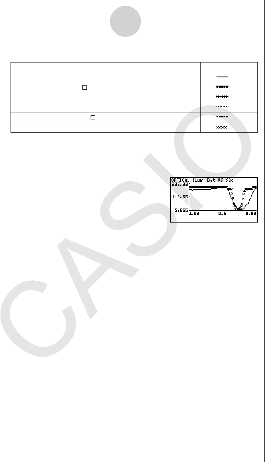
10-4
Using the Graph Analysis Tools to Graph Data
Graph Screen
b. Use the function keys to specify the graph style you want.
c. Repeat a and b to specify the style for each of the graphs on the Graph Mode screen.
7. On the Graph Mode screen, press 6(DRAW) or w.
• This draws the graph(s) in accordance with the settings you configured in step 2 through
step 6.
Line graph with square ( ) data markers
To specify this graph style: Press this key:
Line graph with dot ( • ) data markers 1()
Line graph with X (×) data markers 3()
2( )
Scatter graph with dot ( • ) data markers 4()
Scatter graph with square ( ) data markers 5()
Scatter graph with X (×) data markers 6()
• When a Graph screen is on the display, the function keys provide you with zooming and
other capabilities to aid in graph analysis.
For details about Graph screen function key operations, see the following section.
uu
uu
uTo deselect sampled data assigned for graphing on the Graph Mode
screen
1. On the Graph Mode screen, use the f and c cursor keys to move the highlighting to
the graph (Gph1, Gph2, etc.) whose sampled data you want to deselect.
2. Press 5(DEL).
• This will deselect sample data assigned to the highlighted graph.

11-1
Graph Analysis Tool Graph Screen Operations
11
Graph Analysis Tool Graph Screen Operations
This section explains the various operations you can perform on the graph screen after
drawing a graph.
You can perform these operations on a graph screen produced by a sampling operation, or by the
operation described under “Selecting an Analysis Mode and Drawing a Graph” on page 10-2.
kGraph Screen Key Operations
On the graph screen, you can use the keys described in the table below to analyze (CALC)
graphs by reading data points along the graph (Trace) and enlarging specific parts of the
graph (Zoom).
!1
(TRCE)
Description
Key Operation
Displays a trace pointer on the graph along with the coordinates of the
current cursor location. Trace can also be used to obtain the periodic
frequency of a specific range on the graph and assign it to a variable.
See “Using Trace” on page 11-3.
Displays a function menu of special View Window commands for the
E-CON2 Mode graph screen.
For details about each command, see “Configuring View Window
Parameters” on page 11-14.
!2
(ZOOM)
!3(V-WIN)
Starts a zoom operation, which you can use to enlarge or reduce the
size of the graph along the x-axis or the y-axis. See “Using Zoom” on
page 11-4.
K1
(
PICT
)
Saves the currently displayed graph as a graphic image. You can recall a
saved graph image and overlay it on another graph to compare them.
For details about these procedures, see “5-4 Storing a Graph in Picture
Memory” under Chapter 5 of this manual.
K2
(
LMEM
)
Displays a menu of functions for saving the sample values in a specific
range of a graph to a list. See “Transforming Sampled Data to List Data”
on page 11-5.
Displays a menu that contains the following commands: Cls, Plot,
F-Line, Text, PEN, Vert, and Hztl. For details about each command, see
“5-10 Changing the Appearance of a Graph” under Chapter 5 of this
manual.
!4(SKTCH)

kScrolling the Graph Screen
Press the cursor keys while the graph screen is on the display scrolls the graph left, right, up,
or down.
Note
• The cursor keys perform different operations besides scrolling while a trace or graph
operation is in progress. To perform a graph screen scroll operation in this case, press
J to cancel the trace or graph operation, and then press the cursor keys.
11-2
Graph Analysis Tool Graph Screen Operations
DescriptionKey Operation
Displays a menu of functions for zooming and editing a particular graph
when the graph screen contains multiple graphs. See “Working with
Multiple Graphs” on page 11-10.
Starts an operation for outputting a specific range of a sound data
waveform graph from the speaker. See “Outputting a Specific Range of a
Graph from the Speaker” on page 11-12.
K3(EDIT)
K6(SPKR)
Displays a menu that lets you transform a sample result graph to a
function using Fourier series expansion, and to perform regression to
determine the tendency of a graph. See “Using Fourier Series Expansion
to Transform a Waveform to a Function” on page 11-6, and “Performing
Regression” on page 11-8.
Displays the graph function list, which lets you select a Y=f(x) graph to
overlay on the sampled result graph. See “Overlaying a Y=f(x) Graph on
a Sampled Result Graph” on page 11-9.
K4(CALC)
K5(Y=fx)

11-3
Graph Analysis Tool Graph Screen Operations
kUsing Trace
Trace displays a crosshair pointer on the displayed graph along with the coordinates of the
current cursor position. You can use the cursor keys to move the pointer along the graph.
You can also use trace to obtain the periodic frequency value for a particular range, and
assign the range (time) and periodic frequency values in separate Alpha-Memory values.
uu
uu
uTo use trace
1. On the graph screen, press !1(TRCE).
• This causes a trace pointer to appear on the graph. The coordinates of the current trace
pointer location are also shown on the display.
2. Use the d and e cursor keys to move the trace pointer along the graph to the location
you want.
• The coordinate values change in accordance with the trace pointer movement.
• You can exit the trace pointer at any time by pressing J.
uu
uu
uTo obtain the periodic frequency value
1. Use the procedure under “To use trace” above to start a trace operation.
2. Move the trace pointer to the start point of the range whose periodic frequency you want
to obtain, and then press w.
3. Move the trace pointer to the end point of the range whose periodic frequency you want
to obtain.
• This causes the period and periodic frequency value at the start point you selected in
step 2 to appear along the bottom of the screen.

4. Press w to assign the period and periodic frequency values to Alpha-Memory variables.
• This displays a dialog box for specifying variable names for [Period] and [Frequency]
values.
• The initial default variable name settings are “S” for the period and “H” for the periodic
frequency. To change to another variable name, use the up and down cursor keys to
move the highlighting to the item you want to change, and then press the applicable
letter key.
5. After everything is the way you want, press w.
• This stores the values and exits the trace operation.
• For details about using Alpha-Memory, see “Variables (Alpha Memory)” on page 2-7
under Chapter 2 of this manual.
kUsing Zoom
Zoom lets you enlarge or reduce the size of the graph along the x-axis or the y-axis.
Note
• When there are multiple graphs on the screen, the procedure below zooms all of them.
For information about zooming a particular graph when there are multiple graphs on the
screen, see “Working with Multiple Graphs” on page 11-10.
uu
uu
uTo zoom the graph screen
1. On the graph screen, press !2(ZOOM).
• This causes a magnifying glass cursor ( ) to appear in the center of the screen.
11-4
Graph Analysis Tool Graph Screen Operations
2. Use the cursor keys to move the magnifying glass cursor to the location on the screen
that you want at the center of the enlarged or reduced screen.

3. Press w.
• This causes the magnifying glass to disappear and enters the zoom mode.
• The cursor keys perform the following operations in the zoom mode.
4. To exit the zoom mode, press J.
kTransforming Sampled Data to List Data
Use the following procedure to transform the sampled data in a specific range of a graph into
list data.
uu
uu
uTo transform sampled data to list data
1. On the graph screen, press K, and then 2(LMEM).
• This displays the [LMEM] menu.
2. Press 2(SEL).
• This displays the trace pointer for selecting the range on the graph.
3. Move the trace pointer to the start point of the range you want to convert to list data, and
then press w.
11-5
Graph Analysis Tool Graph Screen Operations
To do this: Press this cursor key:
Reduce the size of the graph image horizontally d
Enlarge the graph image horizontally e
Reduce the size of the graph image vertically c
Enlarge the graph image vertically f
4. Move the trace pointer to the end point of the range you want to convert to list data, and
then press w.
• This displays a dialog box for specifying the lists where you want to store the time data
and the sampled data.
/
• The initial default lists are List 1 for the time and List 2 for sample data. To change to
another list (List 1 to List 26), use the up and down cursor keys to move the highlighting
to the list you want to change, and then input the applicable list number.
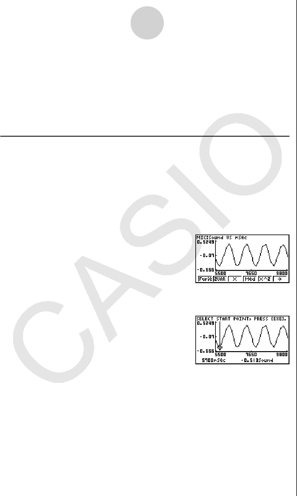
5. After everything is the way you want, press w.
• This saves the lists and the message “Complete!” appears. Press w to return to the
graph screen.
• For details about using list data, see “Chapter 3 List Function”.
Note
• Pressing 1(All) in place of 2(SEL) in step 2 converts the entire graph to list data. In this
case, the “Store Sample Data” dialog box appears as soon as you press 1(All).
kUsing Fourier Series Expansion to Transform a Waveform to a Function
Fourier series expansion is effective for studying sounds by expressing them as functions.
The procedure below assumes that there is a graph of sampled sound data already on the
graph screen.
uu
uu
uTo perform Fourier series expansion
1. On the graph screen , press K, and then 4(CALC).
• The [CALC] menu appears at the bottom of the display.
2. Press 1(Furie).
11-6
Graph Analysis Tool Graph Screen Operations
• This displays the trace pointer for selecting the graph range.
3. Move the trace pointer to the start point of the range for which you want to perform
Fourier series expansion, and then press w.
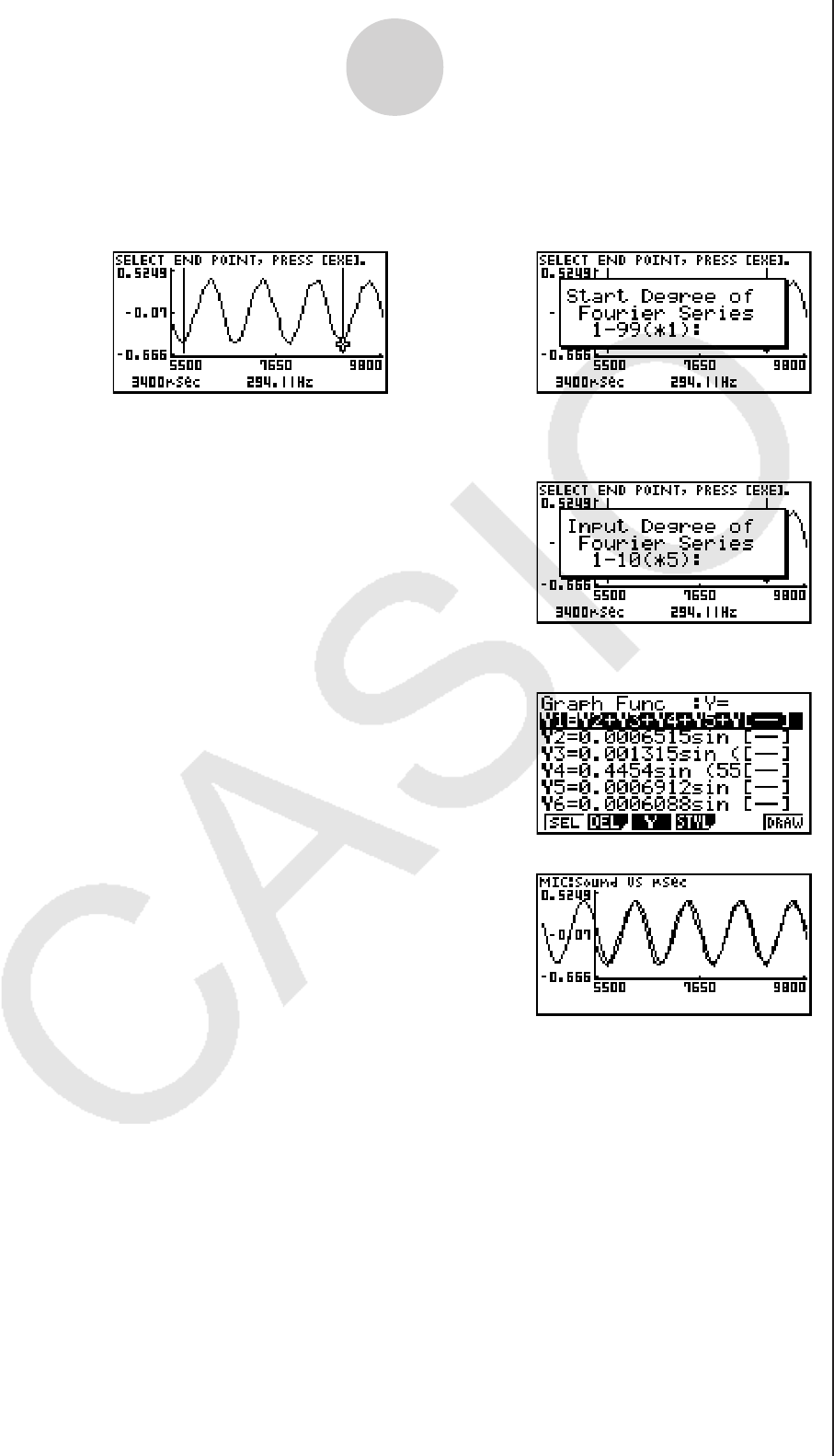
4. Move the trace pointer to the end point of the range for which you want to perform Fourier
series expansion, and then press w.
• This displays a dialog box for specifying the start degree of the Fourier series.
5. Input a value in the range of 1 to 99, and then press w.
• This displays a dialog box for inputting the degree of the Fourier series.
/
6. Input a value in the range of 1 to 10, and then press w.
• The graph function list appears with the calculation result.
11-7
Graph Analysis Tool Graph Screen Operations
7. Pressing 6(DRAW) here graphs the function.
• This lets you compare the expanded function graph and the original graph to see if they
are the same.
Note
When you press 6(DRAW) in step 7, the graph of the result of the Fourier series
expansion may not align correctly with the original graph on which it is overlaid. If this
happens, shift the position the original graph to align it with the overlaid graph.
For information about how to move the original graph, see “To move a particular graph on
a multi-graph display” (page 11-12).
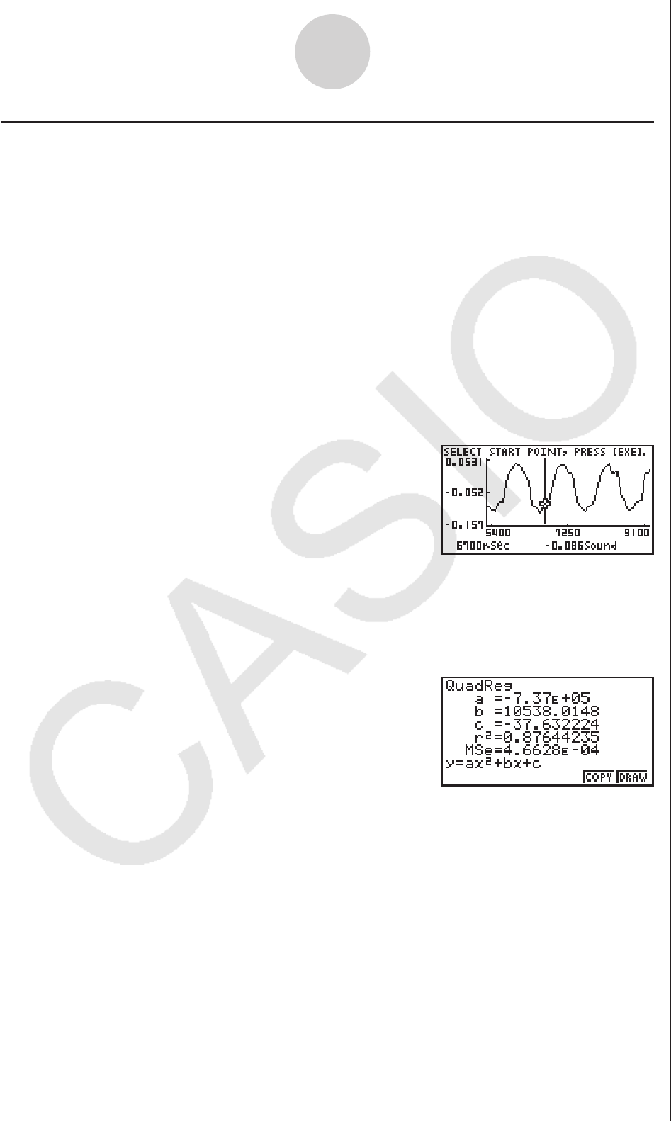
kPerforming Regression
You can use the procedure below to perform regression for a range specified using the trace
pointer. All of the following regression types are supported: Linear, Med-Med, Quadratic,
Cubic, Quartic, Logarithmic, Exponential, Power, Sine, and Logistic.
For details about these regression types, see page 6-11 through 6-14 under Chapter 6 of this
manual.
The following procedure shows how to perform quadratic regression. The same general
steps can also be used to perform the other types of regression.
uu
uu
uTo perform quadratic regression
1. On the graph screen, press K, and then 4(CALC).
• The [CALC] menu appears at the bottom of the display.
2. Press 5(X^2).
• This displays the trace pointer for selecting the range on the graph.
3. Move the trace pointer to the start point of the range for which you want to perform
quadratic regression, and then press w.
4. Move the trace pointer to the end point of the range for which you want to perform
quadratic regression, and then press w.
• This displays the quadratic regression calculation result screen.
11-8
Graph Analysis Tool Graph Screen Operations
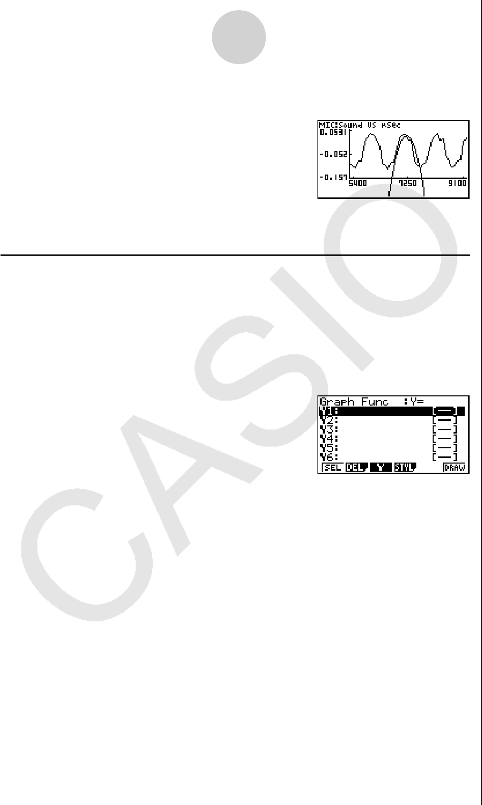
5. Press 6(DRAW).
• This draws a quadratic regression graph and overlays it over the original graph.
• To delete the overlaid quadratic regression graph, press !4(SKTCH) and then
1(Cls).
kOverlaying a Y=f(x) Graph on a Sampled Result Graph
Use the following procedure when you want to overlay a Y=f(x) graph on the sampled result
graph.
uu
uu
uTo overlay a Y=f(x) graph on an existing graph
1. On the graph screen, press K, and then 5(Y=fx).
• This displays the graph function list. Any functions you have previously input on the
graph function list appear at this time.
11-9
Graph Analysis Tool Graph Screen Operations
2. Input the function you want to graph.
• To input a function, use the f and c cursor keys to move the highlighting to the line
where you want to input it, and then use the calculator keys for input. Press w to store
the function.
3. On the graph function list, specify which functions you want to graph.
• Graphing is turned on for any function whose “=” symbol is highlighted. To toggle
graphing of a function on or off, use the f and c cursor keys to move the highlighting
to the function, and then press 1(SEL).
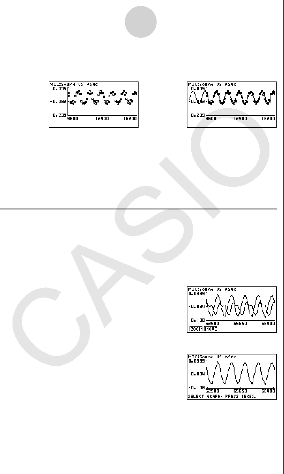
4. After the graph function list settings are configured the way you want, press 6(DRAW).
• This overlays graphs of all the functions for which graphing is turned on, over the graph
that was originally on the graph screen.
11-10
Graph Analysis Tool Graph Screen Operations
2. Press 1(ZOOM).
• This displays only one of the graphs that were originally on the graph screen.
/
Original Graph Overlaid with Y=f(x) Graph
• To delete the overlaid graph, press !4(SKTCH) and then 1(Cls).
Important!
• The screenshot shown in step 4 above is of a function that was calculated and stored by
performing regression on a graph that was drawn using sampled data. Note that
overlaying a Y=f(x) graph on a sampled data graph does not automatically draw a
regression graph based on sampled data.
kWorking with Multiple Graphs
The procedures in this section explain how you can zoom or move a particular graph when
there are multiple graphs on the display.
uu
uu
uTo zoom a particular graph on a multi-graph display
1. When the graph screen contains multiple graphs, press K, and then 3(EDIT).
• The [EDIT] menu appears at the bottom of the display.
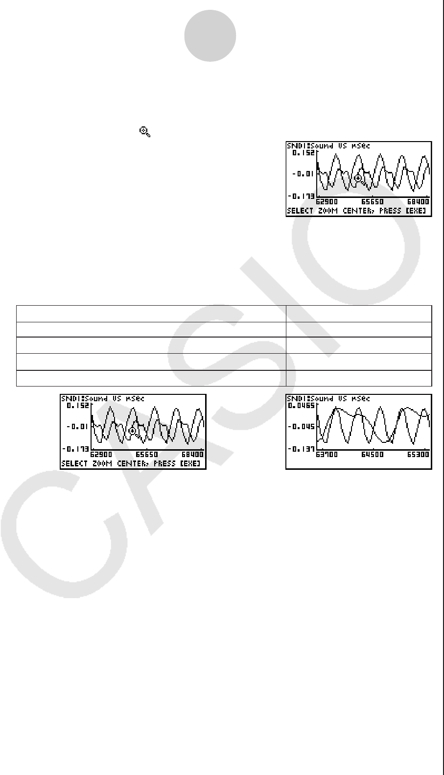
11-11
Graph Analysis Tool Graph Screen Operations
3. Use the f and c cursor keys to cycle through the graphs until the one you want is
displayed, and then press w.
• This enters the zoom mode and causes all of the graphs to reappear, along with a
magnifying glass cursor ( ) in the center of the screen.
4. Use the cursor keys to move the magnifying glass cursor to the location on the screen
that you want at the center of the enlarged or reduced screen.
5. Press w.
• This causes the magnifying glass to disappear and enters the zoom mode.
• The cursor keys perform the following operations in the zoom mode.
6. To exit the zoom mode, press J.
To do this: Press this cursor key:
Reduce the size of the graph image horizontally d
Enlarge the graph image horizontally e
Reduce the size of the graph image vertically c
Enlarge the graph image vertically f
/
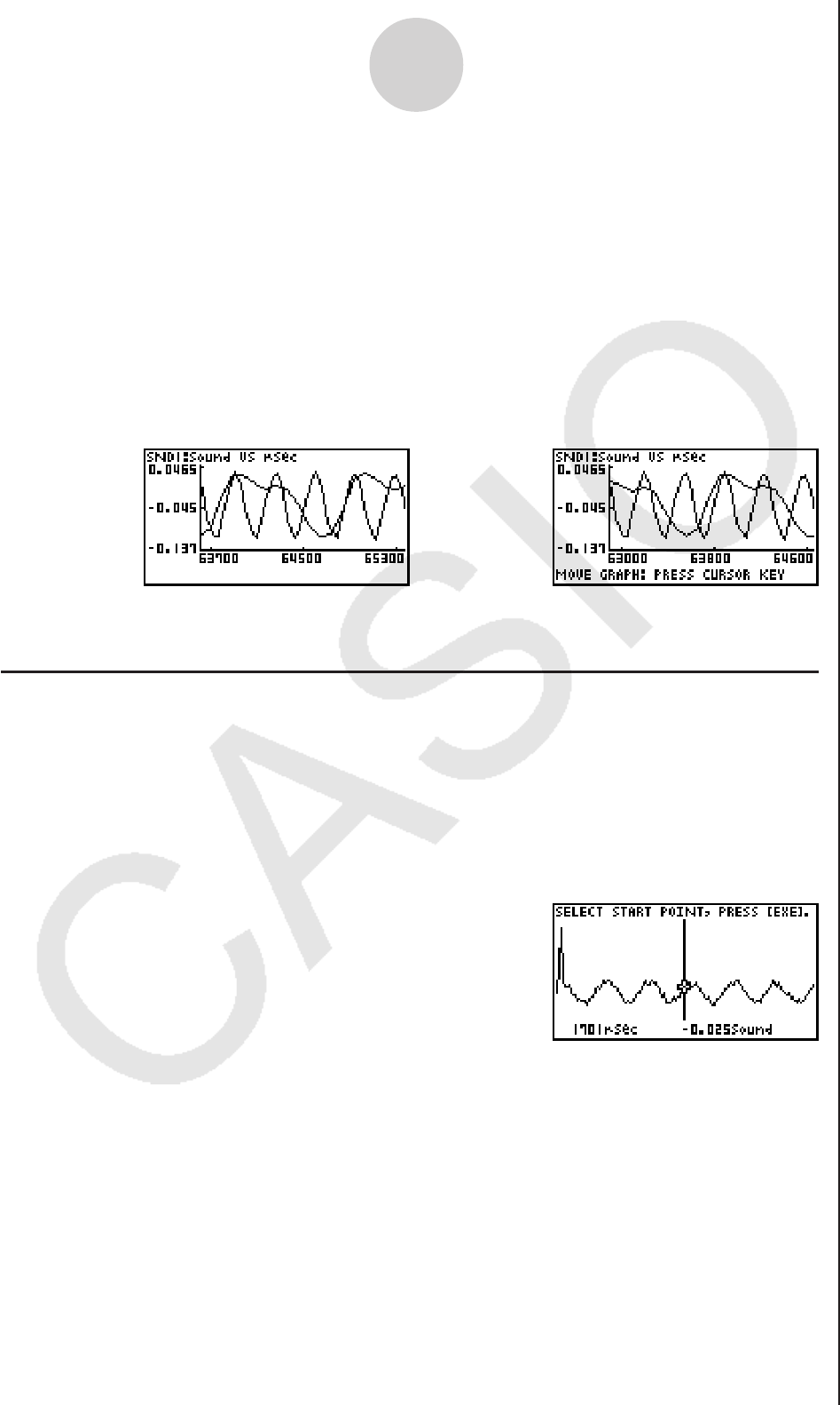
2. Move the trace pointer to the start point of the range you want to output from the speaker,
and then press w.
11-12
Graph Analysis Tool Graph Screen Operations
/
5. To exit the move mode, press J.
kOutputting a Specific Range of a Graph from the Speaker
Use the following procedure to output a specific range of a sound data waveform graph from
the speaker.
uu
uu
uTo output a graph from the speaker
1. On the graph screen, press K, and then 6(SPKR).
• This displays the trace pointer for selecting the range on the graph.
uu
uu
uTo move a particular graph on a multi-graph display
1. When the graph screen contains multiple graphs, press K, and then 3(EDIT).
• This displays the [EDIT] menu.
2. Press 2(MOVE).
• This displays only one of the graphs that were originally on the graph screen.
3. Use the f and c cursor keys to cycle through the graphs until the one you want is
displayed, and then press w.
• This enters the move mode and causes all of the graphs to reappear.
4. Use the d and e cursor keys to move the graph left and right, or the f and c
cursor keys to move the graph up and down.

4. Input a percent value for the output frequency value you want.
• The output frequency specification is a percent value. To output the original sound as-is,
specify 100%. To raise the original sound by one octave, input a value of 200%. To lower
the original sound by one octave, input a value of 50%.
5. After inputting an output frequency value, press w.
• This outputs the waveform between the start point and end point from the EA-200
speaker.
• If the sound you configured cannot be output for some reason, the message “Range
Error” will appear. If this happens, press J to scroll back through the previous setting
screens and change the setup as required.
6. To terminate sound output, press the EA-200 [START/STOP] key.
7. Press w.
• This displays a screen like the one shown below.
/
3. Move the trace pointer to the end point of the range you want to output from the speaker,
and then press w.
• After you specify the start point and end point, an output frequency dialog box shown
below appears on the display.
11-13
Graph Analysis Tool Graph Screen Operations
8. If you want to retry output from the speaker, press 1(Yes). To exit the procedure and
return to the graph screen, press 6(No).
• Pressing 1(Yes) returns to the “Output Frequency” dialog box. From there, repeat the
above steps from step 4.
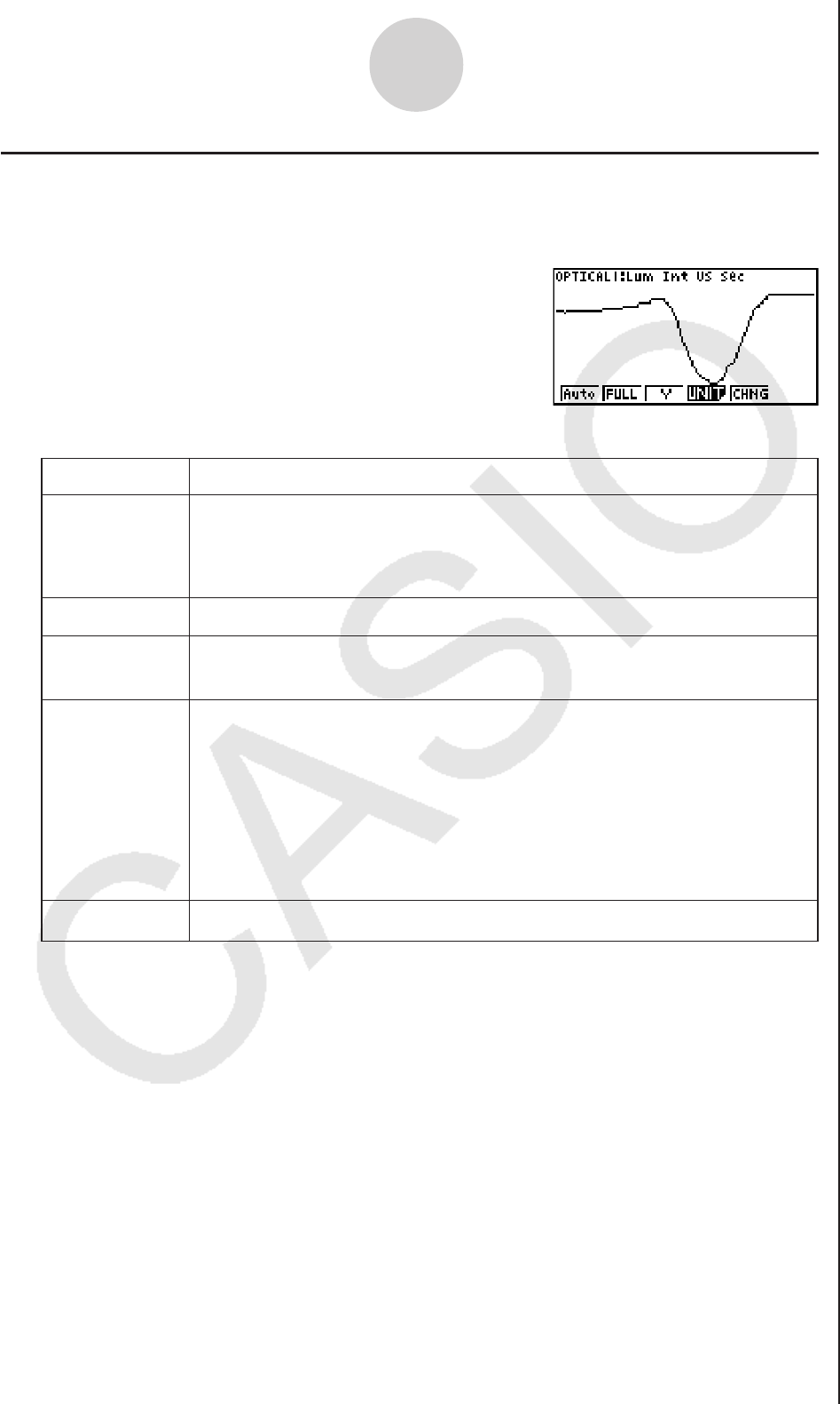
11-14
Graph Analysis Tool Graph Screen Operations
kConfiguring View Window Parameters
Pressing !3(V-Window) while the graph screen is on the display displays a View
Window function key menu along the bottom of the display.
Press the function key that corresponds to the View Window parameter you want to configure.
To exit the View Window function key menu and return to the standard function key menu,
press J.
1
(
Auto
)
Description
Function Key
Automatically applies the following View Window parameters.
Y-axis Elements: In accordance with screen size
X-axis Elements: In accordance with screen size when 1 data item
equals 1 dot; 1 data equals 1 dot in other cases
Resizes the graph so all of it fits in the screen along the Y-axis, without
changing the X-axis dimensions.
Specifies the unit of the numeric axis grid displayed by the Econ Axes
setting of the graph setup screen (page 3-13).
1(μ sec): microseconds
2(msec): milliseconds
3(sec): seconds
4(DHMS):days, hours, minutes, seconds (1 day, 2 hours, 30 minutes,
5 seconds = 1d2h30m5s)
5(Auto):Auto selection
Toggles display of the source data on the graph screen on and off.
2
(
FULL
)
3(Y)
4(UNIT)
5(CHNG)
Resizes the graph so all of it fits in the screen.

12-1
Calling E-CON2 Functions from an eActivity
12
Calling E-CON2 Functions from an eActivity
You can call E-CON2 functions from an eActivity by including an “Econ strip” in the eActivity
file. The following describes each of the four available Econ strips.
uEcon SetupWizard strip
This strip calls the E-CON2 Setup Wizard. The Econ Setup Wizard strip makes it
possible to perform the following series of operations from the eActivity: EA-200
setup using the Setup Wizard R Sampling R Graphing.
Note
• In the case of the Econ SetupWizard strip, the “3: Convert Program” is not available
on the “Complete!” dialog box.
uEcon AdvancedSetup strip
This strip calls the E-CON2 Advanced Setup screen. The Advanced Setup provides
access to almost all executable functions (except for the program converter),
including detailed EA-200 setup and sampling execution; graphing and Graph
Analysis Tools; simultaneous sampling with multiple sensors using the
MULTIMETER Mode, etc.
Note
• Using an Econ Advanced Setup strip to configure a setup causes the setup
information to be registered in the applicable strip. This means that the next time you
open the strip, sampling can be performed in accordance with the previously
configured setup information.
uEcon Sampling strip
This strip executes EA-200 measurement. To store EA-200 setup information for this
strip, perform the Econ Advance Setup operation the first time the strip is executed.
uEcon Graph strip
This strip graphs sampled data that is recorded in the strip. The sampled data is
recorded to the strip the first time the strip is executed.
uu
uu
uEcon Strip Memory Capacity Precautions
• The memory capacity of each Econ strip is 25 KB. An error will occur if you
perform an operation that causes this capacity to be exceeded. Particular care is
required when handling a large number of samples, which can cause memory
capacity to be exceeded.
• Always make sure that FFT Graph is turned off whenever performing sampling
with the microphone. Leaving FFT Graph turned on cause memory capacity to be
exceeded.
• If an error occurs, press !a(') to return to the eActivity workspace screen
and perform the procedure again.
• For information about checking the memory usage of each strip, see “10-5
eActivity File Memory Usage Screen” iunder Chapter 10 of this manual.
For details about eActivity operations, see “Chapter 10 eActivity” under Chapter 10 of this
manual.

E-CON3
Application
(fx-9860GII SD, fx-9860GII,
fx-9860G AU PLUS)
(English)

Important!
• Do not install Add-in E-CON2 on a calculator that has E-CON3 installed.
Doing so may cause operational problems.
• All explanations in this section assume that you are fully familiar with all
calculator and Data Logger (CMA CLAB* or CASIO EA-200) precautions,
terminology, and operational procedures.
• The E-CON3 application is designed to get the most out of the
measurement functions of the CASIO EA-200 Data Logger. Though
it can run on a CMA CLAB Data Logger, CLAB does not have a
SONIC port, microphone, or speaker as is equipped on the EA-200.
While a calculator is connected to a CLAB Data Logger, attempting to
configure E-CON3 application settings and perform measurement using
parameters that are not supported by CLAB will cause an error.
• Unless specifically indicated otherwise, all page references in this
“E-CON3 Application” chapter are to pages in this chapter.
* For information about CMA and the CLAB Data Logger, visit
http://cma-science.nl/.

1-1
E-CON3 Overview
1 E-CON3 Overview
• From the Main Menu, select E-CON3 to enter the E-CON3 Mode.
E-CON3 Main Menu
• The “E-CON3 Mode” provides the functions listed below for simple and more efficient data
sampling using a Data Logger.
•1(SET) ......... Displays a screen for setting up a Data Logger.
•2(MEM)........ Displays a screen for saving Data Logger setup data under a file
name.
•3(PROG) ..... Performs program conversion.
• This function can be used to convert Data Logger setup data
configured using E-CON3 to a Data Logger control program that can
run on the fx-9860G SD/fx-9860G.
• It also can be used to convert data to a program that can be run on
a CFX-9850 Series/fx-7400 Series calculator.
•4(STRT)....... Starts data collection.
•5(GRPH)...... Graphs data sampled by a Data Logger, and provides tools for analyzing
graphs. Graph Analysis tools include calculation of periodic frequency,
various types of regression, Fourier series calculation, and more.
•6(HELP)....... Displays E-CON3 help.
• Pressing the K key (Setup Preview) or a cursor key while the E-CON3 main menu is
on the screen displays a preview dialog box that shows the contents of the setup in the
current setup memory area.
To close the preview dialog box, press J.
Note
For details about setup data and the current setup memory area, see “6 Using Setup
Memory” (page 6-1).
About online help
Pressing the 6(HELP) key displays online help about the E-CON3 Mode.

2 Using the Setup Wizard
This section explains how to use the Setup Wizard to configure the Data Logger setup
quickly and easily simply by replying to questions as they appear.
If you need more control over specific sampling parameters, you should consider using the
Advanced Setup procedure on page 3-1.
k Setup Wizard Parameters
Setup Wizard lets you make changes to the following three Data Logger basic sampling
parameters using an interactive wizard format.
• Sensor (Select Sensor):
Specify a CASIO, VERNIER* or CMA sensor from a menu of choices.
*Vernier Software & Technology
• Total Sampling Time:
Specify a value within the range of 0.01 second to 30 days.
• Sampling Time Unit (Select Unit):
Specify seconds (sec), minutes (min), hours (hour), or days (day) as the time unit of the
value you input for the total sampling time (Total Sampling Time).
Note
For some sensors (EA-200 built-in microphone, Vernier Photogate, etc.), sampling
parameters are different from those shown above. The differences between sampling
parameters and setup procedures for each sensor are described in this section.
Setup Wizard Rules
Note the following rules whenever you use the Setup Wizard.
• The EA-200 sampling channel is CH1 or SONIC.
• The CLAB sampling channel is CH1 only.
• The trigger for a Setup Wizard setup is always the w key.
2-1
Using the Setup Wizard

u To configure a Data Logger setup using Setup Wizard
Before getting started...
• Before starting the procedure below, make sure you first decide if you want to start
sampling immediately using the setup you configure with Setup Wizard, or if you want to
store the setup for later sampling.
• See sections 6-1, 7-1, and 8-1 of this chapter (E-CON3 Application) for information about
procedures required to start sampling and to store a setup. We recommend that you read
through the entire procedure first, referencing the other sections and pages as noted,
before actually trying to perform it.
• To terminate Setup Wizard part way through and cancel the setup, press !J(QUIT).
1. Display the E-CON3 main menu (page 1-1).
2. Press 1(SET) and then 1(WIZ).
• This launches the Setup Wizard and displays the “Select Sensor” screen.
3. Press one of the following function keys to specify the manufacturer of the sensor you are
using for measurement: 1(CASIO), 2(VERNIER), 3(CMA).
• Pressing either key will display the corresponding sensor list.
4. Specify the sensor you want to use.
Use the f and c cursor keys to move the highlighting to the sensor you want to use,
and then press w.
• If the sensor you specified has more than one option (more detailed specifications, such
as sampling unit, mode, etc.), an option list will appear on the display at this time. If this
happens, advance to step 5.
• If the “Input Total Sampling Interval” screen appears, skip to step 6.
5. Select the options for the sensor you specified in step 4.
Use the f and c cursor keys to move the highlighting to the option you want to select,
and then press w.
• If the “Input Total Sampling Interval” screen appears, advance to step 6.
Important!
When special settings are required by the sensor and/or option you select, other screens
other than the “Input Total Sampling Interval” screen will appear on the display. The
following shows where you should go to find information about the operations you need to
perform for each sensor/option selection.
2-2
Using the Setup Wizard

2-3
Using the Setup Wizard
If you select this sensor/option: Go here for more information:
[CASIO] - [Microphone] - [Sound wave & FFT] “Using Setup Wizard to Configure
Settings for FFT (Frequency
Characteristics) Data Sampling” on
page 2-4
[CASIO] - [Microphone] - [FFT only]
[VERNIER] - [Photogate] - [Gate] or
[CMA] - [Photogate] - [Gate]
“To configure a setup for Photogate
alone” on page 2-5
[VERNIER] - [Photogate] - [Pulley] or
[CMA] - [Photogate] - [Pulley]
“To configure a setup for Photogate
and Smart Pulley” on page 2-6
[CASIO] - [Speaker] - [y=f(x)]
“Outputting the Waveform of a
Function through the Speaker” on
page 2-6
6. Use the number input keys to input the total sampling time. Just input a value.
In step 8 of this procedure, you will be able to specify the unit (seconds, minutes, hours,
days) of the value you input here.
Note
• With some sensors ([CASIO] - [Microphone] - [Sound wave], etc.) sampling time is
limited to a few seconds. The unit for such a sensor is always seconds, and so the
“Select Unit” screen does not appear.
• If you specify a total sampling time value in the range of 10 seconds to 23 hours, 59
minutes, 59 seconds, real-time graphing will be performed during sampling. This is the
same as selecting the Realtime Mode on the “Advanced Setup” screen.
7. After inputting total sampling time value you want, press w. This displays the “Select
Unit” screen.
8. Use number keys b through e to specify the unit for the value you specified in step 6.
• This displays a confirmation screen.
9. If there is not problem with the contents of the confirmation screen, press 1.
If you need to change the setup, press 6 or J. This will return to step 6 (for setting
the total sampling interval), where you can change the setting.
• Pressing 1 will take you to the final Setup Wizard screen.
10. Press number keys described below to specify what you want to do with the setup you
have configured.
b(Start Setup) .................Starts sampling using the setup (page 8-1)
c(Save Setup-MEM) .......Saves the setup (page 6-1)
d(Convert Program) ........Converts the setup to a program (page 7-1)

k Using Setup Wizard to Configure Settings for FFT (Frequency
Characteristics) Data Sampling (EA-200 only)
When you perform sound sampling executed the EA-200’s built-in microphone (by specifying
[CASIO] - [Microphone] as the sensor), Setup Wizard will provide you with three options:
[Sound wave], [Sound wave & FFT], and [FFT only]. “Sound wave” records the following two
dimensions for the sampled sound data: elapsed time (horizontal axis) and volume (vertical
axis). “FFT” records the following two dimensions: frequency (horizontal axis) and volume
(vertical axis).
The following shows the settings for recording FFT data.
1. Perform the first two steps of the procedure under “To configure a Data Logger setup
using Setup Wizard” on page 2-2.
2. On the “Select Sensor” screen, select [CASIO] - [Microphone] - [Sound wave & FFT] or
[CASIO] - [Microphone] - [FFT only].
• This causes a “Select FFT Range” screen to appear.
• You can select one of four settings for FFT Range. The setting you select will
automatically apply the applicable fixed parameters shown below.
Setting
Parameter
Frequency pitch
Frequency max
Sampling interval
Number of samples
2 Hz
1000 Hz
8192
2 - 1000 Hz:
1
61 sec
μ
4 Hz
2000 Hz
8192
4 - 2000 Hz:
2
31 sec
μ
6 Hz
3000 Hz
8192
6 - 3000 Hz:
3
20 sec
μ
8 Hz
4000 Hz
4096
8 - 4000 Hz:
4
31 sec
μ
The following explains the meaning of each parameter.
Frequency pitch: Pitch in Hz at which sampling is performed
Frequency max: Upper limit of sampling frequency (lower limit is fixed at 0 Hz)
Sampling interval: Interval in
μ
seconds at which sampling is performed
Number of samples: Number of times sampling is performed
3. Use function keys 1 through 4 to select an FFT Range setting.
• Selecting an FFT Range causes the final Setup Wizard screen to appear.
4. Perform step 10 under “To configure a Data Logger setup using Setup Wizard” on page
2-2 to finalize the procedure.
2-4
Using the Setup Wizard

2-5
Using the Setup Wizard
k Using Setup Wizard to Configure a Photogate Setup
Connection of a Vernier or CMA Photogate requires configuration of setup parameters that
are slightly different from parameters for other types of sensors.
u To configure a setup for Photogate alone
1. On the E-CON3 main menu, press 1(SET)1(WIZ) to start the setup wizard.
• This displays the “Select Sensor” dialog box.
2. If you are using a Vernier Photogate alone, select [VERNIER] - [Photogate] - [Gate].
When the “Select Channel” dialog box appears, advance to step 3 of this procedure.
If you are using a CMA Photogate alone, select [CMA] - [Photogate] - [Gate]. When the
“Gate Status” dialog box appears, advance to step 4 of this procedure.
3. Press 1(CH1) or 2(SONIC) to specify the channel where the Photogate is connected.
• This displays the “Gate Status” dialog box.
4. On the “Gate Status” dialog box, select a gate status for measurement by pressing a
function key ( 1 through 4).
• The gate status defines what Photogate status should cause timing to start, and what
status should cause timing to stop.
1(Open-Open) ........ Timing starts when the gate opens, and continues until it closes
and then opens again.
2(Open-Close) ........ Timing starts when the gate opens, and continues until it closes.
3(Close-Open) ........ Timing starts when the gate closes, and continues until it opens.
4(Close-Close) ....... Timing starts when the gate closes, and continues until it opens
and then closes again.
• Selecting a gate status causes a screen for specifying the number of samples to appear.
5. Input an integer in the range of 1 to 255 to specify the number of samples.
6. Perform step 10 (in the case of a Vernier Photogate) or steps 9 and 10 (in the case of a
CMA Photogate) under “To configure a Data Logger setup using Setup Wizard” (page
2-2).

2-6
Using the Setup Wizard
u To configure a setup for Photogate and Smart Pulley
1. On the E-CON3 main menu, press 1(SET)1(WIZ) to start the setup wizard.
2. This displays the “Select Sensor” dialog box.
3. If you are using a Vernier Photogate with Pulley, select [VERNIER] - [Photogate] -
[Pulley]. When the “Select Channel” dialog box appears, advance to step 4 of this
procedure.
If you are using a CMA Photogate with Pulley, select [CMA] - [Photogate] - [Pulley]. When
the “Input Distance(m)” dialog box appears, advance to step 5 of this procedure.
4. Press 1(CH1) or 2(SONIC) to specify the channel where the Photogate is connected.
• This displays the “Input Distance(m)” dialog box.
5. On the “Input Distance(m)” dialog box, input a value in the range of 0.1 to 4.0 and then
press w.
6. Perform step 10 (in the case of a Vernier Photogate) or steps 9 and 10 (in the case of a
CMA Photogate) under “To configure a Data Logger setup using Setup Wizard” (page
2-2).
k Outputting the Waveform of a Function through the Speaker
(EA-200 only)
Normally, the Setup Wizard helps you configure setups for sensors connected to a Data
Logger. If you select [CASIO] - [Speaker] - [y=f(x)] on the “Select Sensor” screen, however, it
configures the EA-200 to output the sound that corresponds to a function that you input and
graph on the calculator.
u To configure a setup for speaker output
1. Connect the data communication cable (SB-62) to the communication port of the
calculator and the MASTER port of the EA-200.
2. Perform the first two steps of the procedure under “To configure a Data Logger setup
using Setup Wizard” on page 2-2.
3. On the “Select Sensor” screen, select [CASIO] - [Speaker] - [y=f(x)].
This displays a screen like the one shown below.
4. Press w to advance to the View Window setting screen.
• The following settings are configured automatically: Ymin = –1.5 and Ymax = 1.5. Do not
change these settings.
5. Press w or J to advance to the graph function list.
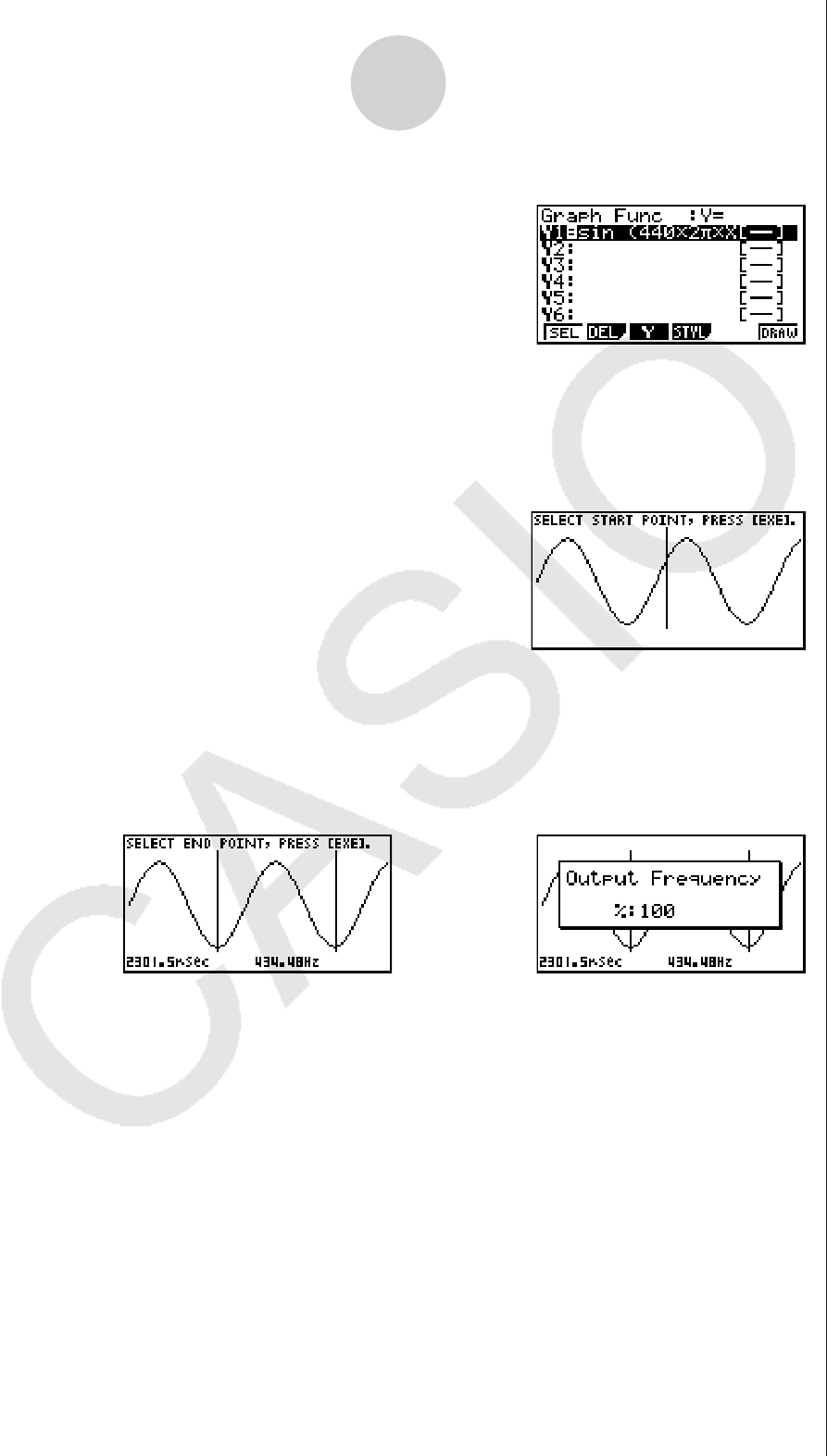
2-7
Using the Setup Wizard
6. In line “Y1”, input the function of the waveform for the sound you want to input.
• Note that the angle unit is always radians.
• Input a function where the value of “Y” is within the range of –1.5 to +1.5.
7. Press 6(DRAW) to graph the function.
• This graphs the function and displays a vertical cursor line as shown below. Use the
graph to specify the range that you want to output to the speaker.
8. Use the d and e cursor keys to move the cursor to the start point of the output, and
then press w to register it.
9. Use the d and e cursor keys to move the cursor to the end point of the output, and
then press w to register it.
• After you specify the start point and end point, an output frequency dialog box shown
below appears on the display.
/
10. Input a percent value for the output frequency value you want.
• To output the original sound as-is, specify 100%. To raise the original sound by one
octave, input a value of 200%. To lower the original sound by one octave, input a value
of 50%.
11. After inputting an output frequency value, press w.
• This outputs the waveform between the start point and end point from the EA-200
speaker.
• If the sound you configured cannot be output for some reason, the message “Range
Error” will appear. If this happens, press J to scroll back through the previous setting
screens and change the setup as required.
12. To terminate sound output, press the EA-200 [START/STOP] key.

2-8
Using the Setup Wizard
13. Press w.
• This displays a screen like the one shown below.
14. Perform one of the following operations, depending on what you want to do.
To change the output frequency and try again:
Press 1(Yes) to return to the “Output Frequency” dialog box. Next, repeat the above
steps from step 10.
To change the output range of the waveform graph and try again:
Press 6(No) to return to the graph screen in step 7. Next, repeat the above steps from
step 8.
To change the function:
Press 6(No) and then J to return to the graph function list in step 6. Next, repeat the
above steps from step 6.
To exit the procedure and return to the E-CON3 main menu:
Press 6(No) and then press J twice.
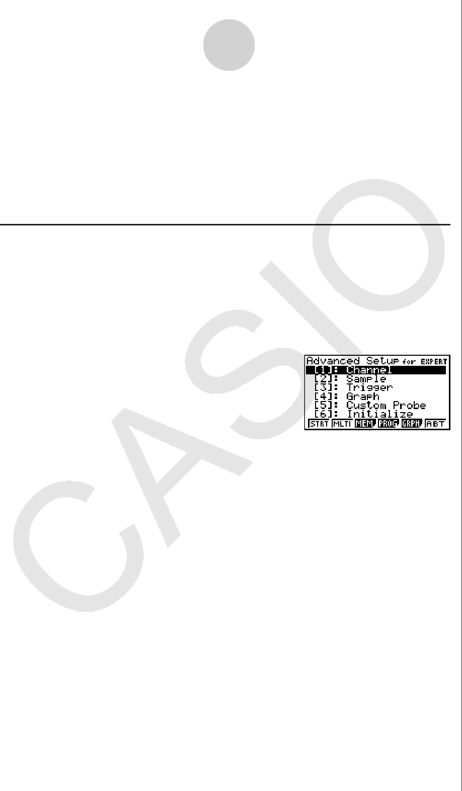
3-1
Using Advanced Setup
3 Using Advanced Setup
Advanced Setup provides you with total control over a number of parameters that you can
adjust to configure the Data Logger setup that suits your particular needs.
The procedures in this section provide the general steps you should perform when using
Advanced Setup to configure a Data Logger setup, and to returns setup settings to their
initial default values. You can find details about individual settings and the options that are
available with each setting are provided by the explanations that start on page 3-3.
k Advanced Setup Operations
u To configure a Data Logger setup using Advanced Setup
The following procedure describes the general steps for using Advanced Setup. Refer to the
pages as noted for more information.
1. Display the E-CON3 main menu (page 1-1).
2. Press 1(SET). This displays the “Setup Data Logger” submenu.
3. Press 2(ADV). This displays the Advanced Setup menu.
Advanced Setup Menu
4. If you want to configure a custom probe at this point, press f(Custom Probe). Next,
follow the steps under “To configure a custom probe setup” on page 4-1.
• You can also configure a custom probe during the procedure under “To configure
Channel Setup settings” on page 3-3.
• Custom probe configurations you have stored in memory can be selected using Channel
in step 5, below.
5. Use the Advanced Setup function keys described below to set other parameters.
•b(Channel)......Displays a screen that shows the sensors that are currently
assigned to each channel (CH1, CH2, CH3, SONIC, Mic). You can
also use this dialog to change sensor assignments. See “Channel
Setup” on page 3-3 for more information.
•c(Sample) .......Displays a screen for selecting the sampling mode, and for
specifying the sampling interval, the number of samples, and the
warm-up mode. When “Fast” is selected for “Mode”, this dialog box
also displays a setting for turning FFT (frequency characteristics)
graphing on and off. See “Sample Setup” on page 3-5 for more
information.

3-2
Using Advanced Setup
•d(Trigger)........Displays a screen for configuring sampling start (trigger) conditions.
See “Trigger Setup” on page 3-8 for more information.
•e(Graph) .........Displays a screen for configuring graph settings. See “Graph Setup”
on page 3-13 for more information.
• You can return the settings on the above setup screens ( b through e) using the
procedure described under “To return setup parameters to their initial defaults”.
6. After you configure a setup, you can use the function key operations described below to
start sampling or perform other operations.
•1(STRT)....... Starts sampling using the setup (page 8-1).
•2(MLTI) ........ Starts MULTIMETER Mode sampling using the setup (page 5-1).
•3(MEM)........ Saves the setup (page 6-1).
•4(PROG) ..... Converts the setup to a program (page 7-1).
•5(GRPH)...... Graphs data sampled by the Data Logger, and provides tools for
analyzing graphs (page 10-1).
•6(ABT) ......... Displays version information about the Data Logger unit that is
currently connected to the calculator.
u To return setup parameters to their initial defaults
Perform the following procedure when you want to return the parameters of the setup in the
current setup memory area to their initial defaults.
1. While the Advanced Setup menu (page 3-1) is on the display, press g(Initialize).
2. In response to the confirmation message that appears, press 1(Yes) to initialize the
setup.
• To clear the confirmation message without initializing the setup, press 6(No).

k Channel Setup
The Channel Setup screen shows the sensors that are currently assigned to each channel
(CH1, CH2, CH3, SONIC, Mic).
u To configure Channel Setup settings
1. While the Advanced Setup menu (page 3-1) is on the display, press b(Channel).
• This displays the Channel Setup screen.
Currently selected channel
Channel Setup Screen
2. Use the f and c cursor keys to move the highlighting to the channel whose setting
you want to change.
3. What you need to do next depends on the currently selected channel.
• CH1, CH2, or CH3
Press a function key to display a menu of sensors that can be assigned to the selected
channel.
1(CASIO) ....... Displays a menu of CASIO sensors.
2(VRNR) ........ Displays a menu of Vernier sensors.
3(CMA) .......... Displays a menu of CMA sensors.
4(CSTM) ........ Displays a menu of custom probes.
5(None) ......... Press this key when you want leave the channel without any sensor
assigned to it.
• SONIC Channel (EA-200 only)
Press a function key to display a menu of sensors that can be assigned to this channel.
1(CASIO) ....... Displays a menu of CASIO sensors, but only “Motion” can be
selected.
2(VRNR) ........ Displays a menu of Vernier sensors. You can select “Motion” or
“Photogate”.
Note
• On the menu that appears after you select “Motion” from either the CASIO or
Vernier sensor menu, select either “meters” or “feet” as the sampling unit.
• After selecting “Motion” from either the CASIO or Vernier sensor menu, you can
press the K key to toggle “smoothing (correction of measurement error)” on
(“-Smooth” displayed) and off (“-Smooth” not displayed).
3-3
Using Advanced Setup

• From the menu that appears after you select “Photogate” as the sensor, select
[Gate] or [Pulley].
[Gate] ................Select this option when using the Photogate sensor alone.
[Pulley] ..............Select this option when using the Photogate sensor along with a
smart pulley.
5(None) ......... Select this option to disable the SONIC channel.
• Mic Channel (EA-200 only)
For this channel, the sensor is automatically set to Built-in (External) Microphone.
However, you need to configure the settings described below.
1(Snd) ........... Select this option to record elapsed time and volume 2-dimensional
sampled sound data (elapsed time on the horizontal axis, volume on
the vertical axis).
2(FFT) ........... Select this option to record frequency and volume 2-dimensional
sampled sound data (frequency on the horizontal axis, volume on the
vertical axis).
5(None) ......... Select this option to disable the Mic channel.
4. Repeat steps 2 and 3 as many times as necessary to configure all the channels you want.
5. After all the settings are the way you want, press w.
• This returns to the Advanced Setup menu.
Note
• When you select a channel on the Channel Setup screen, the sampling range of the
selected channel appears in the bottom line of the screen.
In the above example, the range of the temperature sensor assigned to CH2 appears on the
display.
If the sampling range value is too long to fit on the display, only the part of the value that fits
on the display will be shown.
• Whenever the current Sample Setup (page 3-5) and Trigger Setup (page 3-8) settings
become incompatible due to a change in Channel Setup settings, these settings revert
automatically to their initial defaults. Selecting the Mic channel with Channel Setup while
the Sample Setup has “Extended” selected for the sampling mode, for example, will cause
the sampling mode to change automatically to “Fast” (which is the initial default setting
when the Mic channel is selected). For information about the channels that can be selected
for each sampling mode, see “Sample Setup” (page 3-5).
3-4
Using Advanced Setup
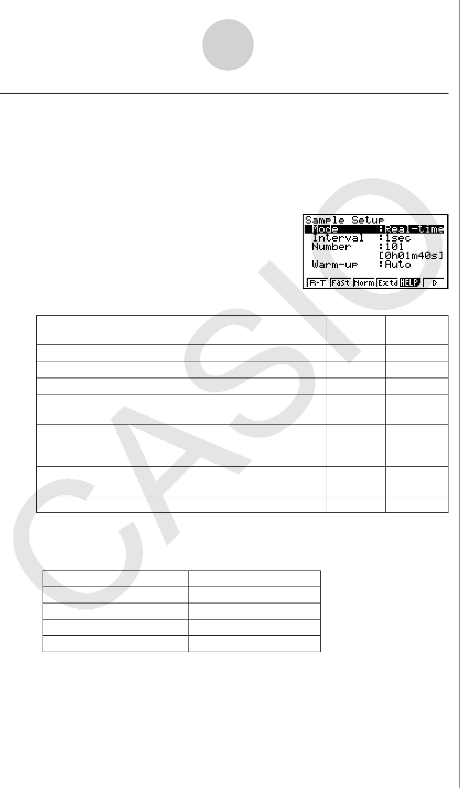
k Sample Setup
The Sample Setup screen lets you configure a number of settings that control sampling.
u To configure Sample Setup settings
1. While the Advanced Setup menu (page 3-1) is on the display, press c(Sample).
• This displays the Sample Setup screen, with the “Mode” line highlighted, which indicates
that you can select the sampling mode.
2. Select the sampling mode that suits the type of sampling you want to perform.
To do this: Press this
key:
To select
this mode:
Graph data in real-time as it is sampled 1(R-T) Realtime
Perform sampling of high-speed phenomena (sound, etc.) 2(Fast) Fast
Perform sampling over a long time (weather, etc.) 4(Extd) Extended*
Sample sound using the built-in microphone (EA-200 only) 6(g)
1(Snd) Sound
Record the time of the occurrence of a particular trigger
event as an absolute value starting from 0, which is the
sampling start time
6(g)
2(Clck) Clock
Perform periodic sampling, from a start trigger event to an
end trigger event
6(g)
3(Priod) Period
Perform sampling other than that described above 3(Norm) Normal
* While performing measurements with the Extended mode, the EA-200 will enter a
power off sleep state while standing by.
• Note that the mode you select also determines the channel(s) you can use.
Sampling mode: Selectable Channel(s)
Realtime, Extended, Normal CH1, CH2, CH3, SONIC
Fast CH1, Mic
Sound Mic
Clock, Period CH1
3-5
Using Advanced Setup

3. To change the sampling interval setting, move the highlighting to “Interval”. Next, press
1 to display a dialog box for specifying the sampling interval.
• The range of values you can select depends on the current sampling mode setting.
If this sampling mode is selected: This is the allowable setting range:
Realtime 0.2 to 299 sec
Fast 20 to 500
μ
sec
Extended 5 to 240 min
Period “=Trigger” only (no value input required)
Sound 20 to 27
μ
sec
Clock “=Trigger” only (no value input required)
Normal 0.0005 to 299 sec
4. To change the number of samples setting, move the highlighting to “Number”. Next, press
1 to display a dialog box for specifying the number of samples.
• The total sampling time shown at the bottom of the dialog box is calculated by
multiplying the “Sampling Interval” value you specified in step 3 by the number of
samples you specify here.
Important!
• When all of the following conditions exist, a “Distance” setting appears in place of the
“Number” setting. See “To configure the Distance setting” (page 3-7) for information
about configuring the “Distance” setting.
• Channel Setup (page 3-3): 2(VRNR) - [Photogate] - [Pulley],
3(CMA) - [Photogate] - [Pulley]
• Sampling Mode (page 3-5): Clock
5. To change the warm-up time setting, move the highlighting to “Warm-up”. Next, perform
one of the function key operations described below.
Note
• The “Warm-up” setting will not be displayed on the Sample Setup screen if “Fast”,
“Sound” or “Extended” is currently selected as the sampling mode.
To do this: Press this key:
Have the warm-up time for each sensor set automatically 1(Auto)
Input a warm-up time, in seconds, manually 2(Man)
Disable the warm-up time 3(None)
Important!
• When the following condition exists, an “FFT Graph” setting appears in place of the
“Warm-up” setting. See “To configure the FFT Graph setting” (page 3-7) for information
about configuring the “FFT Graph” setting.
• Sampling Mode (page 3-5): Fast
3-6
Using Advanced Setup

6. After all the settings are the way you want, press w.
• This returns to the Advanced Setup menu.
Note
• Whenever the current Channel Setup (page 3-3) and Trigger Setup (page 3-8) settings
become incompatible due to a change in Sample Setup settings, these settings revert
automatically to their initial defaults. Selecting “Realtime” as the sampling mode with
Sample Setup while the Mic channel is selected with Channel Setup and the Trigger
Setup has “Mic” selected for “Source”, for example, will cancel the Channel Setup Mic
channel selection and change the Trigger Setup “Source” setting to “[EXE] key”.
For information about the channels that can be selected for each sampling mode,
see step 2 of “To configure Sample Setup settings”. For information about the trigger
sources that can be selected for each sampling mode, see “Trigger Setup” (page 3-8).
u To configure the Distance setting
In place of step 3 of the procedure under “To configure Sample Setup settings”, press 1 to
display a dialog box for specifying the distance the weight travels in meters.
• Specify a value in the range of 0.1 to 4 meters.
u To configure the FFT Graph setting
In place of step 5 of the procedure under “To configure Sample Setup settings”, press 1 to
display a dialog box for turning frequency characteristic graphing (FFT Graph) on and off.
To do this: Press this key:
Turn on graphing of frequency characteristics after sampling 1(On)
Turn off graphing of frequency characteristics after sampling 2(Off)
3-7
Using Advanced Setup
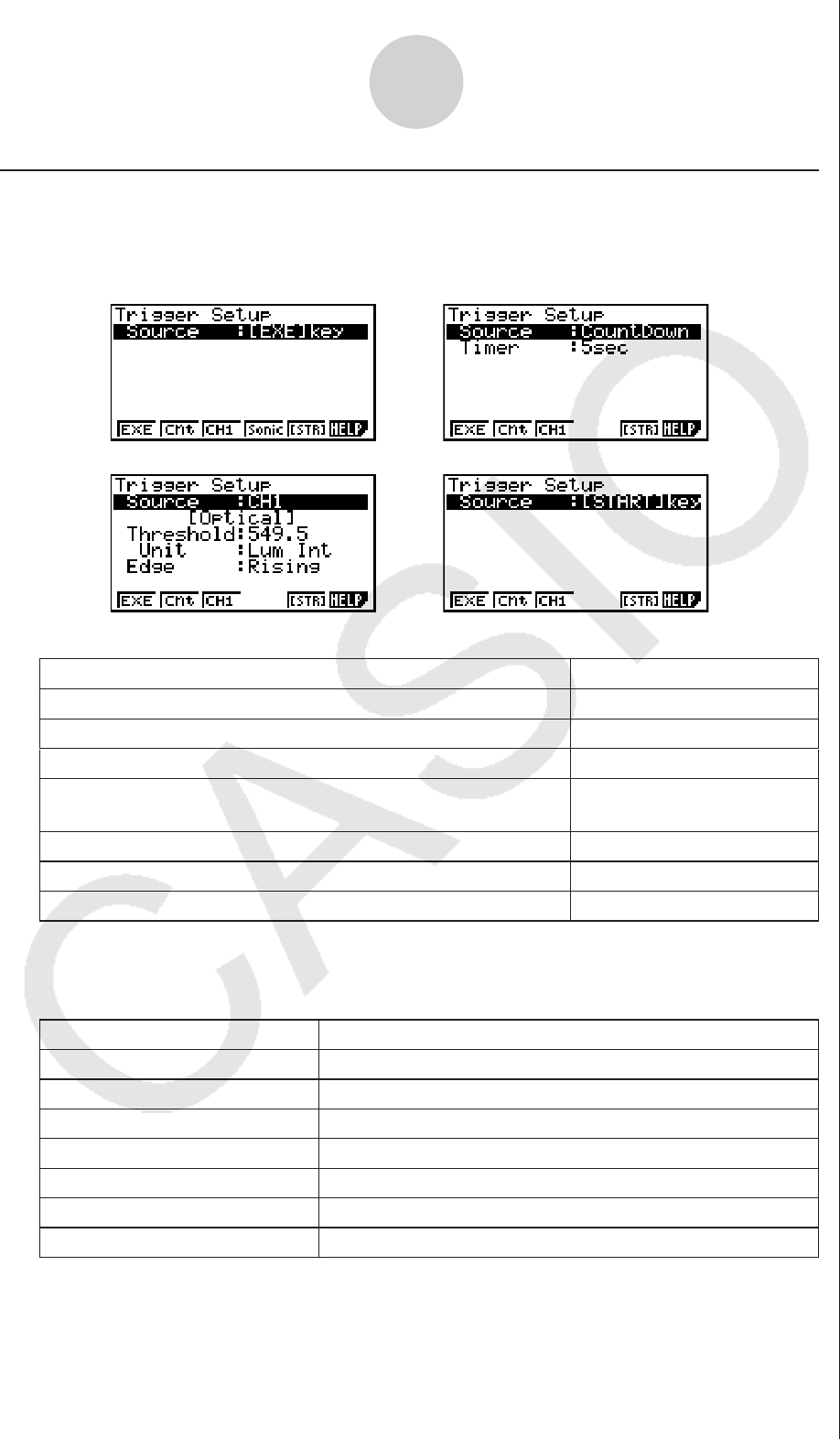
k Trigger Setup
You can use the Trigger Setup screen to specify the event that causes sampling to start ( w
key operation, etc.) The event that causes sampling to start is called the “trigger source”,
which is indicated as “Source” on the Trigger Setup screen.
The following table describes each of the six available trigger sources.
To start sampling when this happens: Select this trigger source:
When the w key is pressed [EXE] key
After the specified number of seconds are counted down Count Down
When input at CH1 reaches a specified value CH1
When input at the SONIC channel reaches a specified value
(EA-200 only) SONIC
When the built-in microphone detects sound (EA-200 only) Mic
When the [START/STOP] key is pressed (EA-200 only) [START] key
When [Button] is pressed (CLAB only) [START] key
Note
The trigger sources you can select depends on the sampling mode selected with the Sample
Setup (page 3-5).
For this sampling mode: The following trigger source(s) can be selected:
Realtime [EXE]
key, Count Down
Fast [EXE]
k
ey, Count Down, CH1, Mic
Normal [EXE]
k
ey, Count Down, CH1, SONIC,
[START]
k
ey
Extended [EXE]
k
ey
Sound [EXE]
k
ey, Count Down, Mic
Clock CH1
Period CH1
3-8
Using Advanced Setup

u To configure Trigger Setup settings
1. While the Advanced Setup menu (page 3-1) is on the display, press d(Trigger).
• This displays the Trigger Setup screen with the “Source” line highlighted.
• The function menu items that appears in the menu bar depend on the sampling mode
selected with Sample Setup (page 3-5). The above screen shows the function menu
when “Normal” is selected as the sample sampling mode.
2. Use the function keys to select the trigger source you want.
• The following shows the trigger sources that can be selected for each sampling mode.
Sampling Mode Trigger Source
Realtime 1(EXE) : [EXE] key, 2(Cnt) : Count Down
Fast 1(EXE) : [EXE] key, 2(Cnt) : Count Down, 3(CH1),
5(Mic)
Normal 1(EXE) : [EXE] key, 2(Cnt) : Count Down, 3(CH1),
4(Sonic), 5(STR) : [START] key
Sound 1(EXE) : [EXE] key, 2(Cnt) : Count Down, 5(Mic)
• The trigger source is always “[EXE] key” when the sampling mode is “Extended”, and
“CH1” when the sampling mode is “Clock” or “Period”.
3-9
Using Advanced Setup

3. Perform one of the following operations, in accordance with the trigger source that was
selected in step 2.
If this is the trigger
source: Do this next:
[EXE] key Press w to finalize Trigger Setup and return to the Advanced
Setup menu.
Count Down Specify the countdown start time. See “To specify the
countdown start time” below.
CH1 Specify the trigger threshold value and trigger edge direction.
See “To specify the trigger threshold value and trigger edge
type”, “To configure trigger threshold, trigger start edge, and
trigger end edge settings” on page 3-11 or “To configure
Photogate trigger start and end settings” on page 3-12.
SONIC Specify the trigger threshold value and motion sensor level.
See “To specify the trigger threshold value and motion sensor
level” on page 3-12.
Mic Specify microphone sensitivity. See “To specify microphone
sensitivity” below.
[START] key Press w to finalize Trigger Setup and return to the Advanced
Setup menu.
u To specify the countdown start time
1. Move the highlighting to “Timer”.
2. Press 1(Time) to display a dialog box for specifying the countdown start time.
3. Input a value in seconds from 1 to 10.
4. Press w to finalize Trigger Setup and return to the Advanced Setup menu.
u To specify microphone sensitivity
1. Move the highlighting to “Sense” and then press one of the function keys describe below.
To select this level of microphone sensitivity: Press this key:
Low 1(Low)
Medium 2(Mid)
High 3(High)
2. Press w to finalize Trigger Setup and return to the Advanced Setup menu (page 3-1).
3-10
Using Advanced Setup
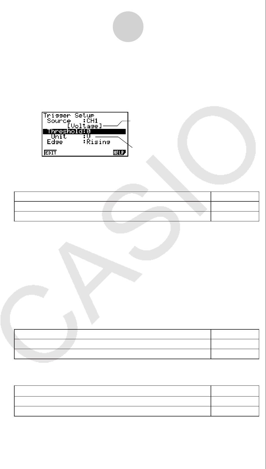
u To specify the trigger threshold value and trigger edge type
Perform the following steps when “Fast”, “Normal”, or “Clock” is specified as the sampling
mode (page 3-5).
1. Move the highlighting to “Threshold”.
2. Press 1(EDIT) to display a dialog box for specifying the trigger threshold value, which is
value that data needs to attain before sampling starts.
Measurement unit supported by assigned sensor
Sensor assigned to CH1 or SONIC by Channel Setup
(page 3-3)
3. Input the value you want, and then press w.
4. Move the highlighting to “Edge”.
5. Press one of the function keys described below.
To select this type of edge: Press this key:
Falling 1(Fall)
Rising 2(Rise)
6. Press w to finalize Trigger Setup and return to the Advanced Setup menu (page 3-1).
u To configure trigger threshold, trigger start edge, and trigger end edge
settings
Perform the following steps when “Period” is specified as the sampling mode (page 3-5).
1. Move the highlighting to “Threshold”.
2. Press 1(EDIT) to display a dialog box for specifying the trigger threshold value, which is
value that data needs to attain before sampling starts.
3. Input the value you want.
4. Move the highlighting to “Start to”.
5. Press one of the function keys described below.
To select this type of edge: Press this key:
Falling 1(Fall)
Rising 2(Rise)
6. Move the highlighting to “End Edge”.
7. Press one of the function keys described below.
To select this type of edge: Press this key:
Falling 1(Fall)
Rising 2(Rise)
8. Press w to finalize Trigger Setup and return to the Advanced Setup menu (page 3-1).
3-11
Using Advanced Setup

u To configure Photogate trigger start and end settings
Perform the following steps when CH1 is selected as a Photogate trigger source.
1. Move the highlighting to “Start to”.
2. Press one of the function keys described below.
To specify this Photogate status: Press this key:
Photogate closed 1(Close)
Photogate open 2(Open)
3. Move the highlighting to “End Gate”.
4. Press one of the function keys described below.
To specify this Photogate status: Press this key:
Photogate closed 1(Close)
Photogate open 2(Open)
5. Press w to finalize Trigger Setup and return to the Advanced Setup menu (page 3-1).
u To specify the trigger threshold value and motion sensor level
1. Move the highlighting to “Threshold”.
2. Press 1(EDIT) to display a dialog box for specifying the trigger threshold value, which is
value that data needs to attain before sampling starts.
3. Input the value you want, and then press w.
4. Move the highlighting to “Level”.
5. Press one of the function keys described below.
To select this type of level: Press this key:
Below 1(Blw)
Above 2(Abv)
6. Press w to finalize Trigger Setup and return to the Advanced Setup menu (page 3-1).
3-12
Using Advanced Setup
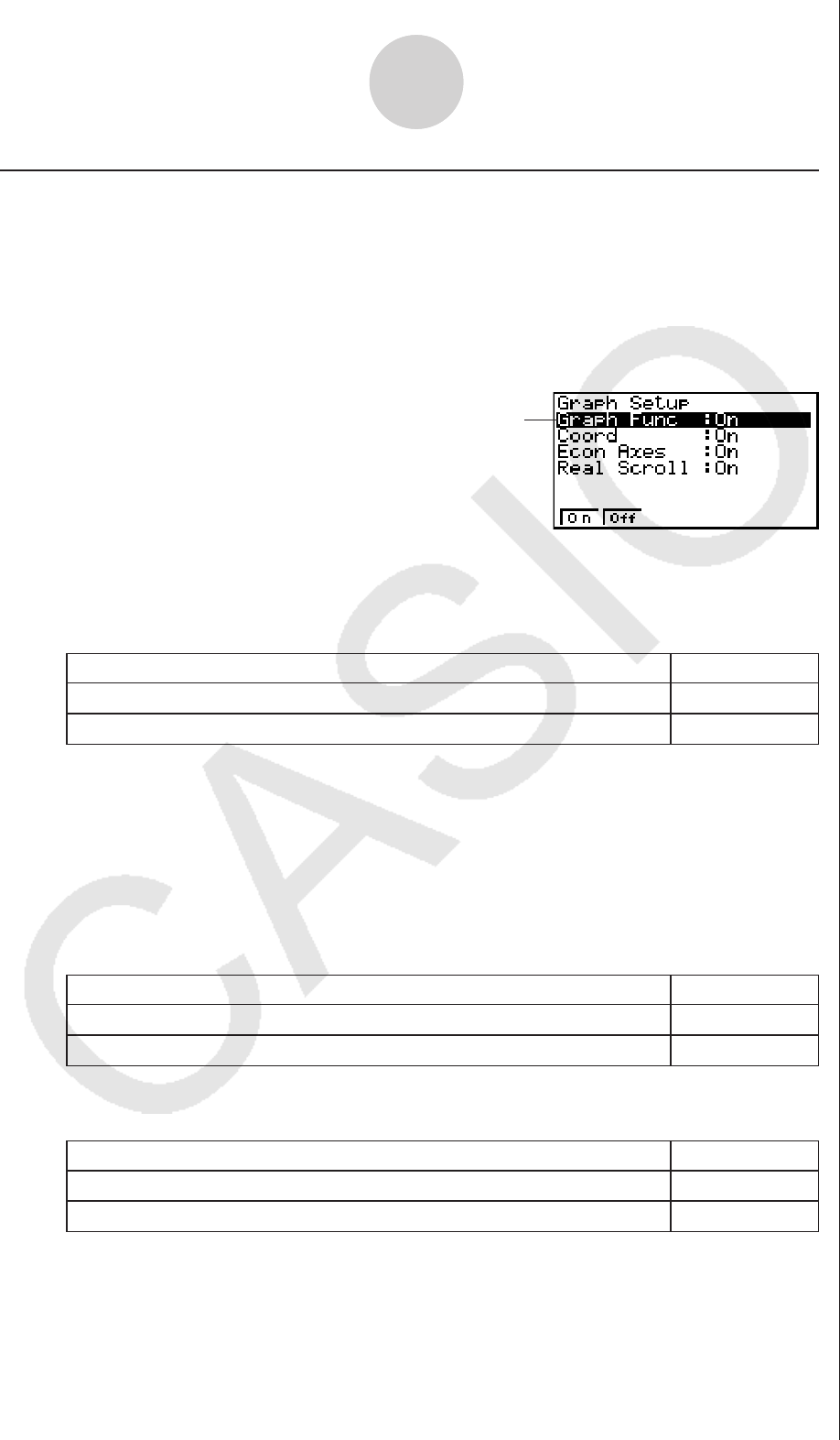
k Graph Setup
Use the Graph Setup screen to configure settings for the graph produced after sampling is
complete. You use the Sample Setup settings (page 3-5) to turn graphing on or off.
u To configure Graph Setup settings
1. While the Advanced Setup menu (page 3-1) is on the display, press e(Graph).
• This displays the Graph Setup screen.
Currently selected item
Graph Setup Screen
2. To change the graph source data name display setting, use the f and c cursor keys
to move the highlighting to “Graph Func”. Next, press one of the function keys described
below.
To specify this graph source data name display setting: Press this key:
Display source data name 1(On)
Hide source data name 2(Off)
• When the graph data is stored in a sample data memory file, the file name appears as
the source data name. When the graph data is stored in current data area, the channel
name appears.
Note
• For details about sample data memory and current data area, see “9 Using Sample Data
Memory”.
3. To change the trace operation coordinate display setting, use the f and c cursor keys
to move the highlighting to “Coord”. Next, press one of the function keys described below.
To specify this coordinate display setting for the trace operation: Press this key:
Display trace coordinates 1(On)
Hide trace coordinates 2(Off)
4. To change the numeric axes display setting, use the f and c cursor keys to move the
highlighting to “Econ Axes”. Next, press one of the function keys described below.
To specify this axes display setting: Press this key:
Display axes 1(On)
Hide axes 2(Off)
3-13
Using Advanced Setup

5. To change the real-time scroll setting, use the f and c cursor keys to move the
highlighting to “RealScroll”. Next, press one of the function keys described below.
To specify this real-time scrolling setting: Press this key:
Real-time scrolling on 1(On)
Real-time scrolling off 2(Off)
6. Press w to finalize Graph Setup and return to the Advanced Setup menu.
3-14
Using Advanced Setup

4 Using a Custom Probe
You can use the procedures in this section to configure a custom probe for use with a Data
Logger.
Important!
• The sensors (CASIO, Vernier, CMA) that appear on the list during Channel Setup (page
3-3) are E-CON3 mode standard sensors. If you want to use a sensor that is not included in
the list, configure custom probe settings.
• A sensor with an output voltage in the range of 0 to 5 volts can be configured with E-CON3
as a custom probe. Use of sensors with an output voltage outside of this range is not
supported.
k Configuring a Custom Probe Setup
To configure a custom probe setup, you must input values for the constants of the fixed
linear interpolation formula (
ax + b). The required constants are slope ( a) and intercept ( b). x
in the above expression ( ax + b) is the sampled voltage value (sampling range: 0 to 5 volts).
u To configure a custom probe setup
1. From the E-CON3 main menu (page 1-1), press 1(SET) and then c(ADV) to display
the Advanced Setup menu.
• See “3 Using Advanced Setup” for more information.
2. On the Advanced Setup menu (page 3-1), press f(Custom Probe) to display the
Custom Probe List.
• The message “No Custom Probe” appears if the Custom Probe List is empty.
3. Press 1(NEW).
• This displays a custom probe setup screen like the one shown below.
• The initial default setting for the probe name is “Voltage(6pin)”. The first step for
configuring custom probe settings is to change this name to another one. If you want to
leave the default name the way it is, skip steps 4 and 5.
4. Press 1(EDIT).
• This enters the probe name editing mode.
4-1
Using a Custom Probe

5. Input up to 18 characters for the custom probe name, and then press E.
• This will cause the highlighting to move to “Slope”.
6. Use the function keys described below to configure the custom probe setup.
• To change the setting of an item, first use the f and c cursor keys to move the
highlighting to the item. Next, use the function keys to select the setting you want.
(1) Slope
Press 1(EDIT) to input the slope for the linear interpolation formula.
(2) Intercept
Press 1(EDIT) to input the intercept for the linear interpolation formula.
(3) Unit Name
Press 1(EDIT) to input up to eight characters for the unit name.
(4) Warm-up
Press 1(EDIT) to input the warm-up time.
7. Press w and then input a memory number (1 to 99).
• This saves the custom probe setup and returns to the Custom Probe List, which should
now contain the new custom probe setup you configured.
u To recall the specifications of a Vernier or CMA sensor and configure
custom probe settings
1. Perform the first two steps of the procedure under “To configure a custom probe setup”
on page 4-1.
2. Press 4(VRNR) or 5(CMA).
• This displays a sensor list.
3. Use the f and c keys to move the highlighting to the sensor whose setting you want
to use as the basis of the custom probe settings, and then press w.
• The name and specifications of the sensor you select will appear on the custom probe
setup screen.
• To complete this procedure, perform steps 4 through 7 under “To configure a custom
probe setup” (page 4-1).
4-2
Using a Custom Probe

k Auto Calibrating a Custom Probe
Auto calibration automatically corrects the slope and intercept values of a custom probe
setup based on two actual samples.
Important!
• Before performing the procedure below, you should prepare two conditions whose
measurement values are known.
• When inputting reference value in step 5 of the procedure below, input the exact known
measurement value of the condition you will sample in step 4. When inputting reference
value in step 7 of the procedure below, input the exact known measurement value of the
condition you will sample in step 6.
u To auto calibrate a custom probe
1. Connect the calculator and Data Logger, and connect the custom probe you want to auto
calibrate to CH1 of the Data Logger.
2. What you should do first depends on whether you are configuring a new custom probe for
calibration, or editing the configuration of an existing custom probe.
If you are configuring a new custom probe:
• Perform steps 1 through 6 of the procedure under “To configure a custom probe setup”
on page 4-1.
• Auto calibrate will automatically set the slope and intercept, so you do not need to
specify them in step 6 of the above procedure.
If you are editing the configuration of an existing custom probe:
• Perform steps 1 through 3 of the procedure under “To edit a custom probe setup” on
page 4-6.
3. Press 2(CALIB).
• This will start the first sampling operation with the sensor connected to Data Logger’s
CH1, and then display a screen like the one shown below.
Real-time display of sampled values
4-3
Using a Custom Probe
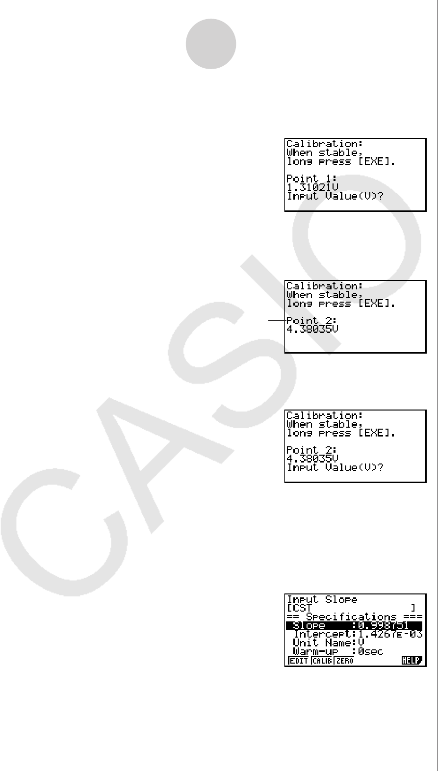
4. After the sampled value stabilizes, hold down w for a few seconds.
• This will register the first sampled value and display it on the screen. At this time the
cursor will appear at the bottom of the display, ready for input of a reference value.
5. Use the key pad to input the reference value for the first sampled value, and then press
w.
• This cause sampling of the second value to be performed automatically, and display the
same type of screen that appeared in step 3.
Second sampling operation
6. After the sampled value stabilizes, hold down w for a few seconds.
• This will register the second sampled value and display it on the screen. The cursor will
appear at the bottom of the display, ready for input of a reference value.
7. Use the key pad to input the reference value for the second sampled value, and then
press w.
• This will return to the custom probe setup screen.
• The E-CON3 will calculate the slope and intercept value based on the two reference
values that you input, and configure the settings automatically. The automatically
configured values will appear on the custom probe setup screen, where you can view
them.
8. Press w, and then input a memory number from 1 to 99.
• This saves the custom probe setup and returns to the custom probe list.
4-4
Using a Custom Probe

k Zero Adjusting a Custom Probe
This procedure zero adjusts a custom probe and sets its intercept value based on an actual
sample using the applicable custom probe.
u To zero adjust a custom probe
1. Connect the calculator and Data Logger, and connect the custom probe you want to zero
adjust to CH1 of the Data Logger.
2. What you should do first depends on whether you are configuring a new custom probe for
zero adjusting, or editing the configuration of an existing custom probe.
If you are configuring a new custom probe:
• Perform steps 1 through 6 of the procedure under “To configure a custom probe setup”
on page 4-1.
• Auto calibrate will automatically set the intercept, so you do not need to specify it in step
6 of the above procedure.
If you are editing the configuration of an existing custom probe:
• Perform steps 1 through 3 of the procedure under “To edit a custom probe setup” on
page 4-6.
3. Press 3(ZERO).
• This will start the sampling operation with the sensor connected to Data Logger’s CH1,
and then display a screen like the one shown below.
4. At the point your want to perform zero adjustment (the point that the displayed value is
the appropriate zero adjust value), press w.
• This will return to the custom probe setup screen.
• The E-CON3 will set the intercept value automatically based on the sampled value. The
automatically configured value will appear on the custom probe setup screen, where you
can view it.
5. Press w, and then input a memory number from 1 to 99.
• This saves the custom probe setup and returns to the custom probe list.
4-5
Using a Custom Probe

k Managing Custom Probe Setups
Use the procedures in this section to edit and delete existing custom probe setups.
u To edit a custom probe setup
1. Display the Custom Probe List.
2. Select the custom probe setup whose configuration you want to edit.
• Use the f and c cursor keys to highlight the name of the custom probe you want.
3. Press 2(EDIT).
• This displays the screen for configuring a custom probe setup.
• To edit the custom probe setup, perform the procedure starting from step 6 under “To
configure a custom probe setup” on page 4-1.
u To delete a custom probe setup
1. Display the Custom Probe List.
2. Select the custom probe setup you want to delete.
• Use the f and c cursor keys to highlight the name of the custom probe setup you
want.
3. Press 3(DEL).
4. In response to the confirmation message that appears, press 1(Yes) to delete the
custom probe setup.
• To clear the confirmation message without deleting anything, press 6(No).
4-6
Using a Custom Probe

5 Using the MULTIMETER Mode
You can use the Channel Setup screen (page 3-3) to configure a channel so that Data
Logger MULTIMETER Mode sampling is triggered by a calculator operation.
u To use the MULTIMETER Mode
1. Connect the calculator and Data Logger, and connect the sensors you want to the
applicable Data Logger channels.
2. From the Advanced Setup menu (page 3-1), use the Channel Setup screen (page 3-3) to
configure sensor setups for each channel you will be using.
3. After configuring the sensor setups, press w to return to the Advanced Setup menu
(page 3-1), and then press 2(MLTI).
• This starts sampling in the Data Logger MULTIMETER mode and displays a list of
sample values for each channel.
• Displayed sample data is refreshed at 0.5-second intervals.
• Do not connect sensors to any other channels except for those you specified in step 2.
• Data sampled in the MULTIMETER mode is not saved in memory.
4. To end MULTIMETER mode sampling, press the w key.
5-1
Using the MULTIMETER Mode

6 Using Setup Memory
Creating Data Logger setup data using the Setup Wizard or Advanced Setup causes the
data to be stored in the “current setup memory area”. The current contents of the current
setup memory area are overwritten whenever you create other setup data.
You can use setup memory to save the current setup memory area contents to calculator
memory to keep it from being overwritten, if you want.
k Saving a Setup
A setup can be saved when any one of the following conditions exist.
• After configuring a new setup with Setup Wizard
See step 8 under “To configure a Data Logger setup using Setup Wizard” on page 2-2.
• After configuring a new setup with Advanced Setup
See step 6 under “To configure a Data Logger setup using Advanced Setup” on page 3-1
for more information.
• While the E-CON3 main menu (page 1-1) is on the display
Performing the setup save operation while the E-CON3 main menu is on the display saves
the contents of the current setup memory area (which were configured using Setup Wizard
or Advanced Setup).
Details on saving a setup are listed below.
u To save a setup
1. If the final Setup Wizard screen is on the display, advance to step 2. If it isn’t, start the
save operation by performing one of the function key operations described below.
If the Advanced Setup menu (page 3-1) is on the display, press 3(MEM).
If the E-CON3 main menu (page 1-1) is on the display, press 2(MEM).
• Performing any one of the above operations causes the setup memory list to appear.
• The message “No Setup-MEM” appears if setup memory is empty.
6-1
Using Setup Memory

2. If you are starting from the final Setup Wizard screen, press c(Save Setup-MEM).
If you are starting from another screen, press 2(SAVE).
• This displays the screen for inputting the setup name.
3. Input up to 18 characters for the setup name.
4. Press w and then input a memory number (1 to 99).
• If you start from the final Setup Wizard screen, this saves the setup and the message
“Complete!” appears. Press w to return to the final Setup Wizard screen.
• If you start from the Advanced Setup menu (page 3-1) or the E-CON3 main menu (page
1-1), this saves the setup and returns to the setup memory list which includes the name
you assigned it.
Important!
• Since you assign both a setup name and a file number to each setup, you can assign
the same name to multiple setups, if you want.
k Using and Managing Setups in Setup Memory
All of the setups you save are shown in the setup memory list. After selecting a setup in the
list, you can use it to sample data or you can edit it.
u To preview saved setup data
You can use the following procedure to check the contents of a setup before you use it for
sampling.
1. On the E-CON3 main menu (page 1-1), press 2(MEM) to display the setup memory list.
2. Use the f and c cursor keys to highlight the name of the setup you want.
3. Press K(Setup Preview).
• This displays the preview dialog box.
4. To close the preview dialog box, press J.
6-2
Using Setup Memory

u To recall a setup and use it for sampling
Be sure to perform the following steps before starting sampling with a Data Logger.
1. Connect the calculator to a Data Logger.
2. Turn on Data Logger power.
3. In accordance with the setup you plan to use, connect the proper sensor to the
appropriate Data Logger channel.
4. Prepare the item whose data is to be sampled.
5. On the E-CON3 main menu (page 1-1), press 2(MEM) to display the setup memory list.
6. Use the f and c cursor keys to highlight the name of the setup you want.
7. Press 1(STRT).
8. In response to the confirmation message that appears, press 1.
• Pressing w sets up the Data Logger and then starts sampling.
• To clear the confirmation message without sampling, press 6.
Note
• See “Operations during a sampling operation” on page 8-2 for information about
operations you can perform while a sampling operation is in progress.
u To change the name of setup data
1. On the E-CON3 main menu (page 1-1), press 2(MEM) to display the setup memory list.
2. Use the f and c cursor keys to highlight the name of the setup you want.
3. Press 3(REN).
• This displays the screen for inputting the setup name.
4. Input up to 18 characters for the setup name, and then press w.
• This changes the setup name and returns to the setup memory list.
6-3
Using Setup Memory

u To delete setup data
1. On the E-CON3 main menu (page 1-1), press 2(MEM) to display the setup memory list.
2. Use the f and c cursor keys to highlight the name of the setup you want.
3. Press 4(DEL).
4. In response to the confirmation message that appears, press 1(Yes) to delete the
setup.
• To clear the confirmation message without deleting anything, press 6(No).
u To recall setup data
Recalling setup data stores it in the current setup memory area. You can then use Advanced
Setup to edit the setup. This capability comes in handy when you need to perform a setup
that is slightly different from one you have stored in memory.
1. On the E-CON3 main menu (page 1-1), press 2(MEM) to display the setup memory list.
2. Use the f and c cursor keys to highlight the name of the setup you want.
3. Press 5(LOAD).
4. In response to the confirmation message that appears, press 1(Yes) to recall the setup.
• To clear the confirmation message without recalling the setup, press 6(No).
Note
• Recalling setup data replaces any other data currently in the current setup memory
area.
6-4
Using Setup Memory

7 Using Program Converter
Program Converter converts a Data Logger setup you configured using Setup Wizard or
Advanced Setup to a program that can run on the calculator. You can also use Program
Converter to convert a setup to a CFX-9850 Series/fx-7400 Series-compatible program.*
1*2
*1 See the documentation that came with your scientific calculator or EA-200 for information
about how to use a converted program.
*2 See online help (PROGRAM CONVERTER HELP) for information about supported CFX-
9850 Series and fx-7400 Series models.
k Converting a Setup to a Program
A setup can be converted to a program when any one of the following conditions exists.
• After configuring a new setup with Setup Wizard
See step 8 under “To configure a Data Logger setup using Setup Wizard” on page 2-2.
• After configuring a new setup with Advanced Setup
See step 6 under “To configure a Data Logger setup using Advanced Setup” on page 3-1
for more information.
• While the E-CON3 main menu (page 1-1) is on the display
Performing the program converter operation while the E-CON3 main menu is on the
display converts the contents of the current setup memory area (which were configured
using Setup Wizard or Advanced Setup).
The program converter procedure is identical in all of the above cases.
u To convert a setup to a program
1. Start the converter operation by performing one of the key operations described below.
If the final Setup Wizard screen is on the display, press d(Convert Program).
If the Advanced Setup menu (page 3-1) is on the display, press 4(PROG).
If the E-CON3 main menu (page 1-1) is on the display, press 3(PROG).
• After you perform any one of the above operations, the program converter screen will
appear on the display.
7-1
Using Program Converter

2. Enter up to eight characters for the program name.
Note
Using the program converter initial default settings will create a program like the one
below.
• Associated Scientific Calculator: fx-9860 Series
• Associated Data Logger: EA-200
• Calibration: None
• Password: None
If you want to use these settings the way they are without changing them, skip steps 3
through 7 and go directly to step 8. If you want to change any of the settings, perform the
applicable operations in steps 3 through 7.
3. Specify the scientific calculator model to be associated with the program. Perform one of
the following key operations to associate the program with a scientific calculator.
To associate the program with this calculator: Perform this key operation:
fx-9860 Series 1(CALC) 1(9860)
CFX-9850 Series 1(CALC) 2(9850)
fx-7400 Series 1(CALC) 3(7400)
• The number part of the scientific calculator model number you specify will appear in line
“F1:” of the program converter screen.
Note
For information about 1(CALC)4(→ 38K), see “Converting a CFX-9850 Series
Program to a fx-9860 Series Compatible Program” (page 7-4).
4. Specify the Data Logger model (EA-100 or EA-200) to be associated with the program.
Perform one of the following key operations to associate the program with a Data Logger.
To associate the program with this Data Logger: Perform this key operation:
EA-200 2(TYPE) 1(200)
EA-100 2(TYPE) 2(100)
• The number part of the Data Logger model number you specify will appear in line “F2:”
of the program converter screen.
Important!
• Note that the capabilities of the EA-100 and EA-200 are different. Because of this, you
should keep in mind that an EA-200 program converted to an EA-100 program and used
to perform sampling with an EA-100 setup may not produce the desired results.
7-2
Using Program Converter

5. If you plan to use a custom probe connected to CH1 of the Data Logger, specify
whether calibration or zero adjust should be performed. Perform one of the following key
operations to configure the desired setting.
To perform this operation: Perform this key operation:
Calibration of the CH1 custom probe 3(CALB) 1(CALIB)
Zero adjust of the CH1 custom probe 3(CALB) 2(ZERO)
No calibration 3(CALB) 3(None)
• The operation you specify will appear in line “F3:” of the program converter screen.
6. To password protect the program, press 4().
• This will cause the “Password?” prompt and password input field to appear under the
program name input field.
7. Enter up to eight characters for the password.
• If you change your mind about assigning a password, press J here. This will cause
the password input field to disappear and cancel password input.
8. After everything is the way you want, press w to convert the program in accordance with
the setup.
• The message “Complete!” appears when conversion is complete. To clear the message
and return to the screen that was on the display in step 1, press w or J.
7-3
Using Program Converter
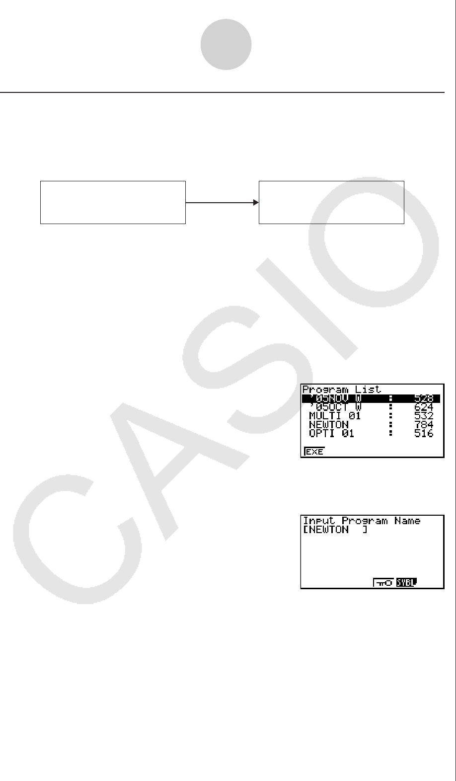
k Converting a CFX-9850 Series Program to a fx-9860 Series Compatible
Program
To use an EA-200 control program created on the CFX-9850 Series calculator (for use on
the CFX-9850) on the E-CON3, you need to convert the program to an fx-9860 program.
Conversion can be performed using the program converter.
EA-200 Control Program for
CFX-9850 Series
EA-200 Control Program for
fx-9860 Series
Convert
u To convert a program
1. Transfer the EA-200 control program created for the CFX-9850 Series to the fx-9860
main memory.
• Use the cable that comes bundled with the fx-9860 to connect its 3-pin serial port to the
3-pin serial port of the CFX-9850. For details, see “Chapter 13 Data Communications”.
2. Perform step 1 under “To convert a setup to a program” on page 7-1, which displays the
program converter screen.
3. Press 1(CALC) and then press 4(→ 38K).
• This displays a list of programs currently in main memory.
4. Use f and c to move the highlighting of the program you want to convert, and then
press 1(EXE) or w.
• A program name input screen will appear after conversion is complete.
5. Enter up to eight characters for the program name.
• If you want to password protect the program, perform steps 6 and 7 under “To convert a
setup to a program” after inputting the program name.
6. Press w to start conversion of the program.
• The message “Complete!” appears when conversion is complete. To clear the message,
press w or J.
7-4
Using Program Converter

8 Starting a Sampling Operation
The section describes how to use a setup configured using the E-CON3 Mode to start a Data
Logger sampling operation.
k Before getting started...
Be sure to perform the following steps before starting sampling with a Data Logger.
1. Connect the calculator to a Data Logger.
2. Turn on Data Logger power.
3. In accordance with the setup you plan to use, connect the proper sensor to the
appropriate Data Logger channel.
4. Prepare the item whose data is to be sampled.
k Starting a Sampling Operation
A sampling operation can be started when any one of the following conditions exist.
• After configuring a new setup with Setup Wizard
See step 8 under “To configure a Data Logger setup using Setup Wizard” on page 2-2.
• After configuring a new setup with Advanced Setup
See step 6 under “To configure a Data Logger setup using Advanced Setup” on page 3-1.
• While the E-CON3 main menu (page 1-1) is on the display
Starting a sampling operation while the E-CON3 main menu is on the display performs
sampling using the contents of the current setup memory area (which were configured
using Setup Wizard or Advanced Setup).
• While the setup memory list is on the display
You can select the setup you want on the setup memory list and then start sampling.
The following procedures explain the first three conditions described above. See “To recall a
setup and use it for sampling” on page 6-3 for information about starting sampling from the
setup memory list.
8-1
Starting a Sampling Operation

u To start sampling
1. Start the sampling operation by performing one of the function key operations described
below.
If the final Setup Wizard screen is on the display, press b(Start Setup).
If the Advanced Setup menu (page 3-1) is on the display, press 1(STRT).
If the E-CON3 main menu (page 1-1) is on the display, press 4(STRT).
• After you perform any one of the above operations, a sampling start confirmation screen
like the one shown below will appear on the display.
2. Press w.
• This sets up the Data Logger using the setup data in the current setup memory area.
• The message “Setting Data Logger...” remains on the display while Data Logger setup is
in progress. You can cancel the setup operation any time this message is displayed by
pressing A.
• The screen shown below appears after Data Logger setup is complete.
3. Press w to start sampling.
• The screens that appear while sampling is in progress and after sampling is complete
depend on setup details (sampling mode, trigger setup, etc.). For details, see
“Operations during a sampling operation” below.
u Operations during a sampling operation
Sending a sample start command from the calculator to a Data Logger causes the following
sequence to be performed.
Setup Data Transfer → Sampling Start → Sampling End →
Transfer of Sample Data from the Data Logger to the Calculator
The table on the next page shows how the trigger conditions and sensor type specified in the
setup data affects the above sequence.
8-2
Starting a Sampling Operation
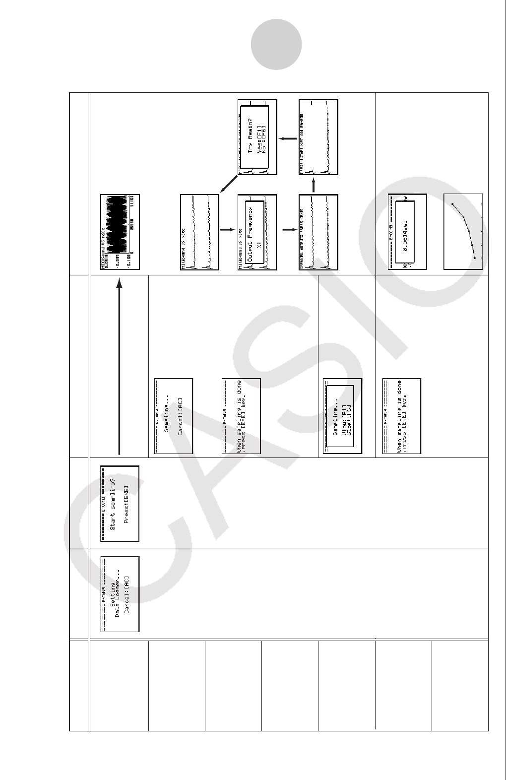
Mode
Real-time
Fast
Normal
Sound
Extended
Period
Clock
1.
Data Logger Setup
2. Start Standby 3. Sampling 4. Graphing
Starts Sampling
• The screen shown below appears when CH1,
SONIC, or Mic is used as the trigger.
Graph screen does not show all sampled values,
but only a partial preview.
Pressing 1 advances to
“4. Graphing”.
Pressing w there returns to
“3. Sampling”.
w
w1
w
The following three graph types
can be produced when Photo-
gate-Pulley is being used.
1. Time and distance graph
2. Time and velocity graph
3.
Time and acceleration graph
Sample values is stored as List
data only.
•When Number of Samples = 1
•
When Number of Samples > 1
Input values.
w
Sampled values are saved as
Current Sample Data.
•
When Mode = Sound
Outputting through
speaker
8-3
Starting a Sampling Operation
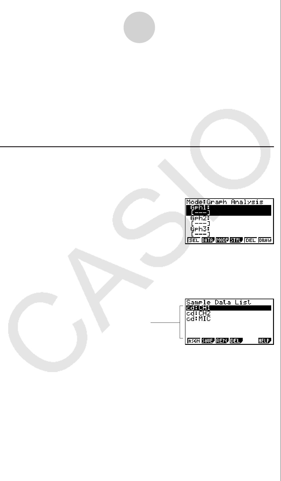
9 Using Sample Data Memory
Performing a Data Logger sampling operation from the E-CON3 Mode causes sampled
results to be stored in the “current data area” of E-CON3 memory. Separate data is saved
for each channel, and the data for a particular channel in the current data area is called that
channel’s “current data”.
Any time you perform a sampling operation, the current data of the channel(s) you use is
replaced by the newly sampled data. If you want to save a set of current data and keep it
from being replaced by a new sampling operation, save the data in sample data memory
under a different file name.
k Managing Sample Data Files
u To save current sample data to a file
1. On the E-CON3 main menu (page 1-1), press 5(GRPH).
• This displays the Graph Mode screen.
Graph Mode Screen
• For details about the Graph Mode screen, see “10 Using the Graph Analysis Tools to
Graph Data”.
2. Press 2(DATA).
• This displays the Sampling Data List screen.
List of current data files
Sampling Data List Screen
9-1
Using Sample Data Memory
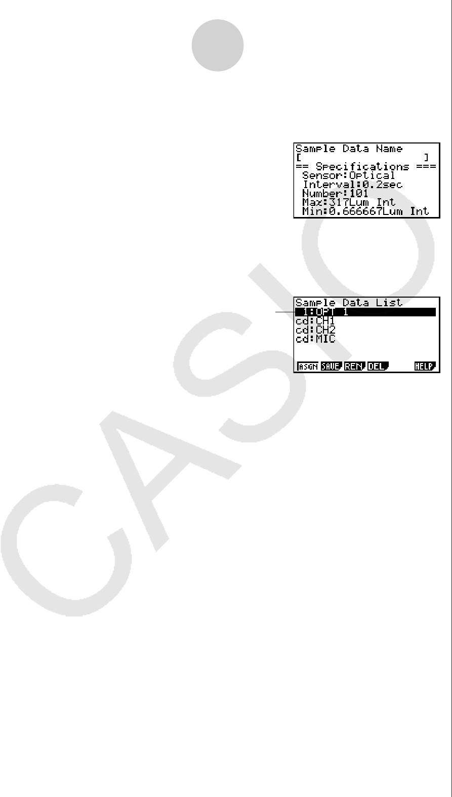
3. Use the f and c cursor keys to move the highlighting to the current data file you want
to save, and then press 2(SAVE).
• This displays the screen for inputting a data name.
4. Enter up to 18 characters for the data file name, and then press w.
• This displays a dialog box for inputting a memory number.
5. Enter a memory number in the range of 1 to 99, and then press w.
• This saves the sample data at the location specified by the memory number you input.
The sample data file you save is indicated
on the display using the format:
<memory number>:<file name>.
• If you specify a memory number that is already being used to store a data file, a
confirmation message appears asking if you want to replace the existing file with the
new data file. Press 1 to replace the existing data file, or 6 to return to the memory
number input dialog box in Step 4.
6. To return to the E-CON3 main menu (page 1-1), press J twice.
Note
• You could select another data file besides a current data file in step 3 of the above
procedure and save it under a different memory number. You do not need to change the
file’s name as long as you use a different file number.
9-2
Using Sample Data Memory

u To rename an existing sample data file
Note
• You cannot use this procedure to rename a current data file name.
1. On the E-CON3 main menu (page 1-1), press 5(GRPH).
• This displays the Graph Mode screen.
2. Press 2(DATA).
• This displays the Sampling Data List screen.
3. Use the f and c cursor keys to move the highlighting to the data file you want to
rename, and then press 3(REN).
• This displays the screen for inputting a file name.
4. Enter up to 18 characters for the new data file name, and then tap w.
• This returns to the Sampling Data List screen.
5. To return to the E-CON3 main menu (page 1-1), press J twice.
u To delete a sample data file
1. On the E-CON3 main menu (page 1-1), press 5(GRPH).
• This displays the Graph Mode screen.
2. Press 2(DATA).
• This displays the Sampling Data List screen.
3. Use the f and c cursor keys to move the highlighting to the data file you want to
delete, and then press 4(DEL).
4. In response to the confirmation message that appears, press 1(Yes) to delete the data
file.
• To clear the confirmation message without deleting the data file, press 6(No).
• This returns to the Sampling Data List screen.
5. To return to the E-CON3 main menu (page 1-1), press J twice.
9-3
Using Sample Data Memory
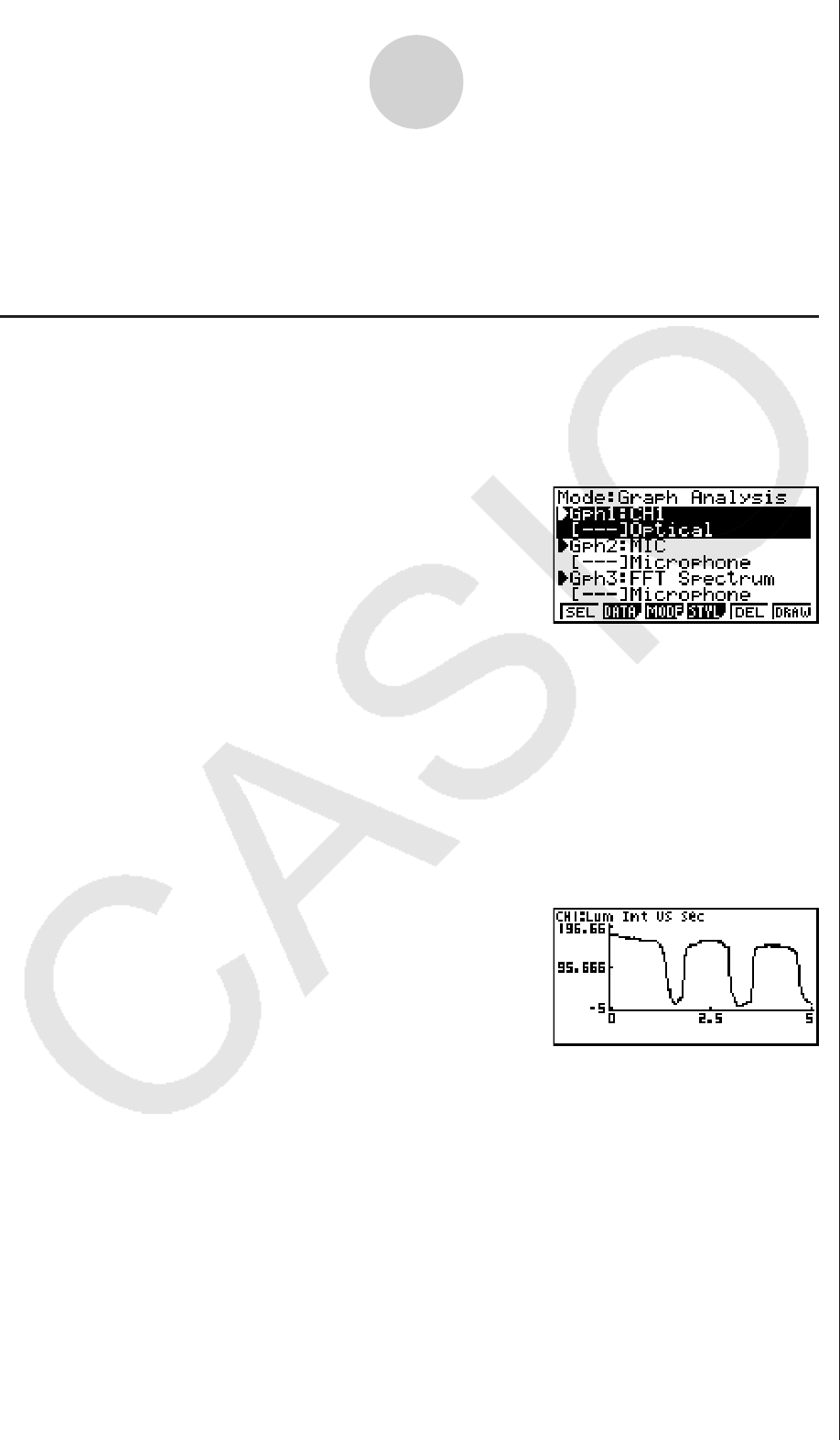
10 Using the Graph Analysis Tools to Graph
Data
Graph Analysis tools make it possible to analyze graphs drawn from sampled data.
k Accessing Graph Analysis Tools
You can access Graph Analysis tools using either of the two methods described below.
u Accessing Graph Analysis tools from the Graph Mode screen, which is
displayed by pressing 5(GRPH) on the E-CON3 main menu (page 1-1)
Graph Mode Screen
• The main menu appears after you perform a sampling operation. Press 5(GRPH) at
that time.
• When you access Graph Analysis tools using this method, you can select from among
a variety of other Analysis modes. See “Selecting an Analysis Mode and Drawing a
Graph” (page 10-2) for more information about the other Analysis modes.
u Accessing Graph Analysis tools from the screen of a graph drawn after a
sampling operation is executed from the Setup Wizard or from Advanced
Setup (Realtime Mode)
Graph Screen
• In this case, data is graphed after the sampling operation is complete, and the calculator
accesses Graph Analysis tools automatically. See “Graph Screen Key Operations” on
page 11-1.
10-1
Using the Graph Analysis Tools to Graph Data
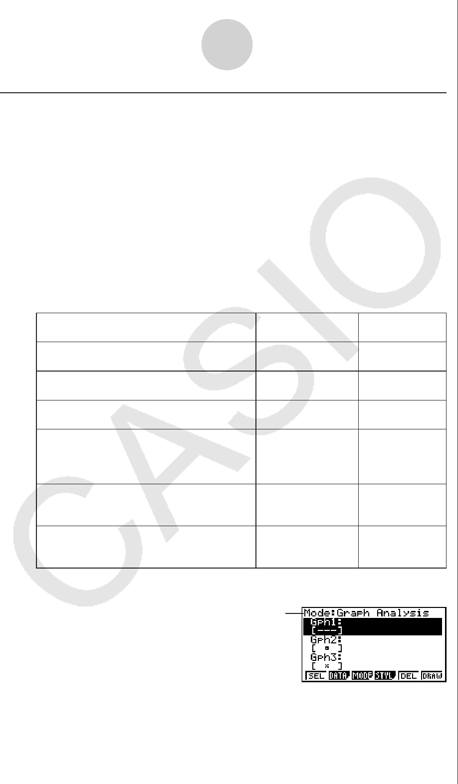
k Selecting an Analysis Mode and Drawing a Graph
This section contains a detailed procedure that covers all steps from selecting an analysis
mode to drawing a graph.
Note
• Step 4 through step 6 are not essential and may be skipped, if you want. Skipping any
step automatically applies the initial default values for its settings.
• If you skip step 2, the default analysis mode is the one whose name is displayed in the
top line of the Graph Mode screen.
u To select an analysis mode and draw a graph
1. On the E-CON3 main menu (page 1-1), press 5(GRPH).
• This displays the Graph Mode screen.
2. Press 3(MODE), and then select the analysis mode you want from the menu that
appears.
To do this: Perform this menu
operation:
To select this
mode:
Graph three sets of sampled data
simultaneously [Norm] Graph Analysis
Graph sampled data along with its first and
second derivative graph [diff] d/dt & d
2/dt2
Display the graphs of different sampled data
in upper and lower windows for comparison [CMPR]/[GRPH] Compare Graph
Output sampled data from the speaker,
displaying graph of the raw data in the upper
window and the output waveform in the lower
window (EA-200 only)
[CMPR]/[Snd] Compare Sound
Display the graph of sampled data in the
upper window and its first derivative graph in
the lower window
[CMPR]/[d/dt] Compare d/dt
Display the graph of sampled data in the
upper window and its second derivative
graph in the lower window
[CMPR]/[d2/dt2]Compare d
2/dt2
• The name of the currently selected mode appears in the top line of the Graph Mode
screen.
Analysis mode name
3. Press 2(DATA).
• This displays the Sampling Data List screen.
10-2
Using the Graph Analysis Tools to Graph Data
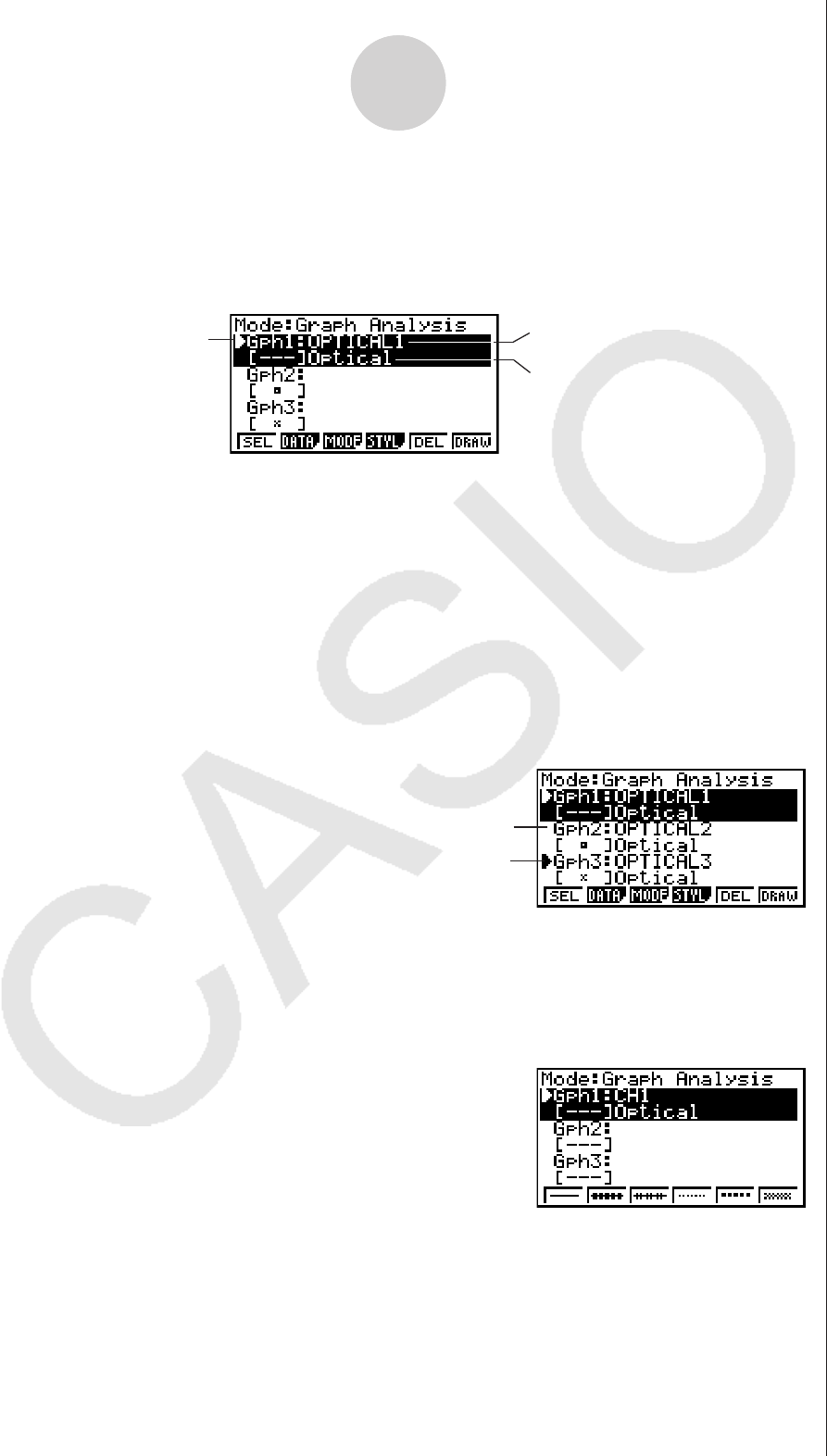
4. Specify the sampled data for graphing.
a. Use the f and c cursor keys to move the highlighting to the name of the sampled
data file you want to select, and then press 1(ASGN) or w.
• This returns to the Graph Mode screen, which shows the name of the sample data file
you selected.
Graph Mode Screen
Graph on/off indicator Sample data file name
Name of sensor used for sampling
b. Repeat step a above to specify sample data files for other graphs, if there are any.
• If you select “Graph Analysis” as the analysis mode in step 2, you must specify sample
data files for three graphs. If you select “Compare Graph” as the analysis mode in step
2, you must specify sample data files for two graphs. With other modes, you need to
specify only one sample data file.
• For details about Sampling Data List screen operations, see “9 Using Sample Data
Memory”.
5. Turn on graphing for each of the graphs listed on the Graph Mode screen.
a. On the Graph Mode screen, use the f and c cursor keys to select a graph, and then
press 1(SEL) to toggle graphing on or off.
Graphing turned off.
Graphing turned on.
b. Repeat step a to turn each of the graphs listed on the Graph Mode screen on or off.
6. Select the graph style you want to use.
a. On the Graph Mode screen, use the f and c cursor keys to move the highlighting to
the graph (Gph1, Gph2, etc.) whose style you want to specify, and then press 4(STYL).
This will cause the function menu to change as shown below.
10-3
Using the Graph Analysis Tools to Graph Data
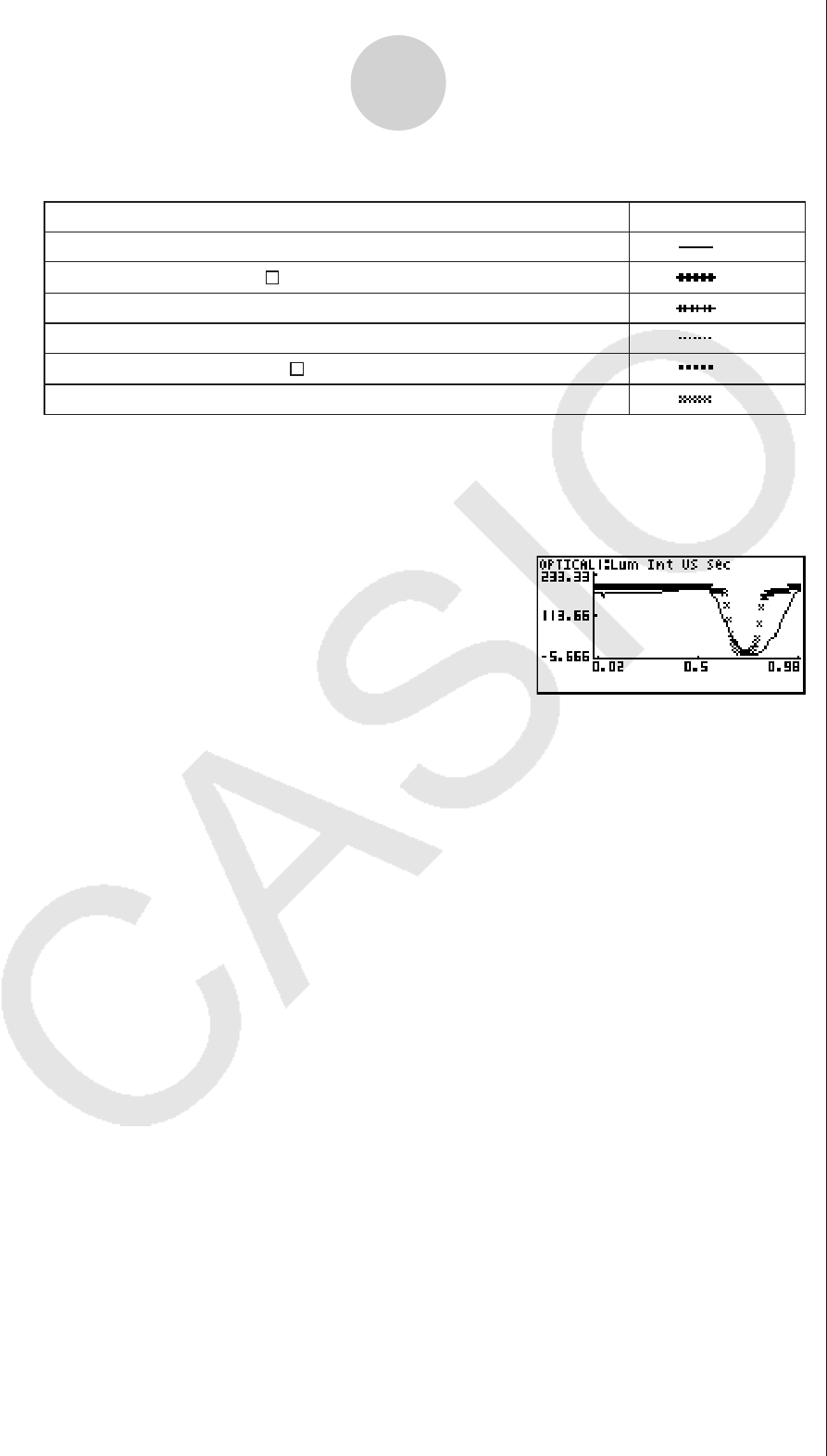
b. Use the function keys to specify the graph style you want.
To specify this graph style: Press this key:
Line graph with dot ( • ) data markers 1()
Line graph with square ( ) data markers 2()
Line graph with X ( × ) data markers 3()
Scatter graph with dot ( • ) data markers 4()
Scatter graph with square ( ) data markers 5()
Scatter graph with X ( × ) data markers 6()
c. Repeat a and b to specify the style for each of the graphs on the Graph Mode screen.
7. On the Graph Mode screen, press 6(DRAW) or w.
• This draws the graph(s) in accordance with the settings you configured in step 2 through
step 6.
Graph Screen
• When a Graph screen is on the display, the function keys provide you with zooming and
other capabilities to aid in graph analysis.
For details about Graph screen function key operations, see the following section.
u To deselect sampled data assigned for graphing on the Graph Mode
screen
1. On the Graph Mode screen, use the f and c cursor keys to move the highlighting to
the graph (Gph1, Gph2, etc.) whose sampled data you want to deselect.
2. Press 5(DEL).
• This will deselect sample data assigned to the highlighted graph.
10-4
Using the Graph Analysis Tools to Graph Data

11 Graph Analysis Tool Graph Screen
Operations
This section explains the various operations you can perform on the graph screen after
drawing a graph.
You can perform these operations on a graph screen produced by a sampling operation, or by
the operation described under “Selecting an Analysis Mode and Drawing a Graph” on page
10-2.
k Graph Screen Key Operations
On the graph screen, you can use the keys described in the table below to analyze (CALC)
graphs by reading data points along the graph (Trace) and enlarging specific parts of the
graph (Zoom).
Key Operation Description
!1
(TRCE)
Displays a trace pointer on the graph along with the coordinates of the
current cursor location. Trace can also be used to obtain the periodic
frequency of a specific range on the graph and assign it to a variable.
See “Using Trace” on page 11-3.
!2
(ZOOM)
Starts a zoom operation, which you can use to enlarge or reduce the
size of the graph along the x-axis or the y-axis. See “Using Zoom” on
page 11-4.
!3(V-WIN)
Displays a function menu of special View Window commands for the
E-CON3 Mode graph screen.
For details about each command, see “Configuring View Window
Parameters” on page 11-14.
!4(SKTCH)
Displays a menu that contains the following commands: Cls, Plot,
F-Line, Text, PEN, Vert, and Hztl. For details about each command,
see “5-10 Changing the Appearance of a Graph” under Chapter 5 of
this manual.
K1
(
PICT
)
Saves the currently displayed graph as a graphic image. You can recall
a saved graph image and overlay it on another graph to compare them.
For details about these procedures, see “5-4 Storing a Graph in Picture
Memory” under Chapter 5 of this manual.
K2
(
LMEM
)
Displays a menu of functions for saving the sample values in a specific
range of a graph to a list. See “Transforming Sampled Data to List
Data” on page 11-5.
K3(EDIT)
Displays a menu of functions for zooming and editing a particular graph
when the graph screen contains multiple graphs. See “Working with
Multiple Graphs” on page 11-10.
11-1
Graph Analysis Tool Graph Screen Operations

Key Operation Description
K4(CALC)
Displays a menu that lets you transform a sample result graph to a
function using Fourier series expansion, and to perform regression
to determine the tendency of a graph. See “Using Fourier Series
Expansion to Transform a Waveform to a Function” on page 11-6, and
“Performing Regression” on page 11-8.
K5(Y=fx)
Displays the graph function list, which lets you select a Y=f(x) graph to
overlay on the sampled result graph. See “Overlaying a Y=f(x) Graph
on a Sampled Result Graph” on page 11-9.
K6(SPKR)
Starts an operation for outputting a specific range of a sound data
waveform graph from the speaker (EA-200 only). See “Outputting a
Specific Range of a Graph from the Speaker” on page 11-12.
k Scrolling the Graph Screen
Press the cursor keys while the graph screen is on the display scrolls the graph left, right, up,
or down.
Note
• The cursor keys perform different operations besides scrolling while a trace or graph
operation is in progress. To perform a graph screen scroll operation in this case, press
J to cancel the trace or graph operation, and then press the cursor keys.
11-2
Graph Analysis Tool Graph Screen Operations
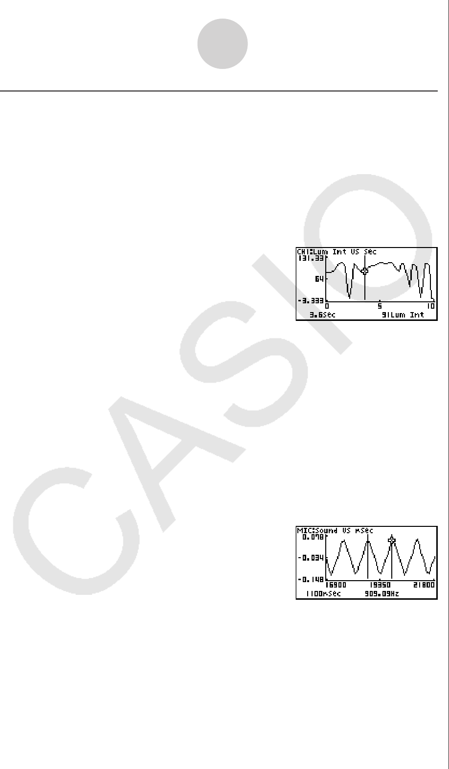
k Using Trace
Trace displays a crosshair pointer on the displayed graph along with the coordinates of the
current cursor position. You can use the cursor keys to move the pointer along the graph.
You can also use trace to obtain the periodic frequency value for a particular range, and
assign the range (time) and periodic frequency values in separate Alpha-Memory values.
u To use trace
1. On the graph screen, press !1(TRCE).
• This causes a trace pointer to appear on the graph. The coordinates of the current trace
pointer location are also shown on the display.
2. Use the d and e cursor keys to move the trace pointer along the graph to the location
you want.
• The coordinate values change in accordance with the trace pointer movement.
• You can exit the trace pointer at any time by pressing J.
u To obtain the periodic frequency value
1. Use the procedure under “To use trace” above to start a trace operation.
2. Move the trace pointer to the start point of the range whose periodic frequency you want
to obtain, and then press w.
3. Move the trace pointer to the end point of the range whose periodic frequency you want
to obtain.
• This causes the period and periodic frequency value at the start point you selected in
step 2 to appear along the bottom of the screen.
11-3
Graph Analysis Tool Graph Screen Operations

4. Press w to assign the period and periodic frequency values to Alpha-Memory variables.
• This displays a dialog box for specifying variable names for [Period] and [Frequency]
values.
• The initial default variable name settings are “S” for the period and “H” for the periodic
frequency. To change to another variable name, use the up and down cursor keys to
move the highlighting to the item you want to change, and then press the applicable
letter key.
5. After everything is the way you want, press w.
• This stores the values and exits the trace operation.
• For details about using Alpha-Memory, see “Variables (Alpha Memory)” on page 2-7
under Chapter 2 of this manual.
k Using Zoom
Zoom lets you enlarge or reduce the size of the graph along the x-axis or the y-axis.
Note
• When there are multiple graphs on the screen, the procedure below zooms all of them.
For information about zooming a particular graph when there are multiple graphs on the
screen, see “Working with Multiple Graphs” on page 11-10.
u To zoom the graph screen
1. On the graph screen, press !2(ZOOM).
• This causes a magnifying glass cursor ( ) to appear in the center of the screen.
2. Use the cursor keys to move the magnifying glass cursor to the location on the screen
that you want at the center of the enlarged or reduced screen.
11-4
Graph Analysis Tool Graph Screen Operations

3. Press w.
• This causes the magnifying glass to disappear and enters the zoom mode.
• The cursor keys perform the following operations in the zoom mode.
To do this: Press this cursor key:
Enlarge the graph image horizontally e
Reduce the size of the graph image horizontally d
Enlarge the graph image vertically f
Reduce the size of the graph image vertically c
4. To exit the zoom mode, press J.
k Transforming Sampled Data to List Data
Use the following procedure to transform the sampled data in a specific range of a graph into
list data.
u To transform sampled data to list data
1. On the graph screen, press K, and then 2(LMEM).
• This displays the [LMEM] menu.
2. Press 2(SEL).
• This displays the trace pointer for selecting the range on the graph.
3. Move the trace pointer to the start point of the range you want to convert to list data, and
then press w.
4. Move the trace pointer to the end point of the range you want to convert to list data, and
then press w.
• This displays a dialog box for specifying the lists where you want to store the time data
and the sampled data.
/
• The initial default lists are List 1 for the time and List 2 for sample data. To change to
another list (List 1 to List 26), use the up and down cursor keys to move the highlighting
to the list you want to change, and then input the applicable list number.
11-5
Graph Analysis Tool Graph Screen Operations
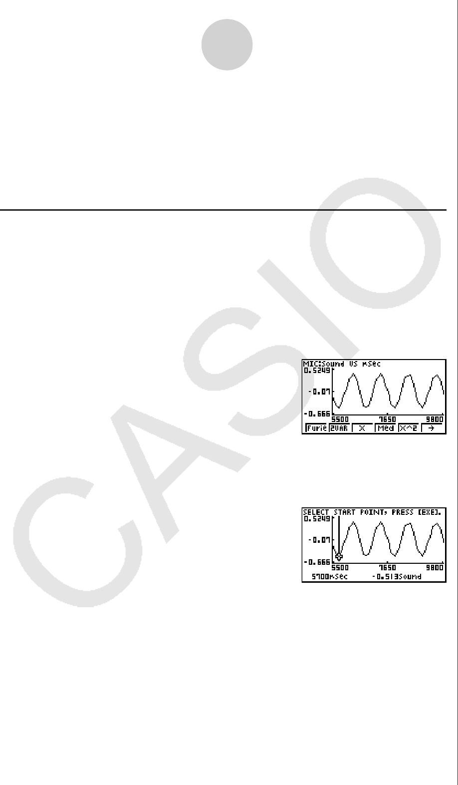
5. After everything is the way you want, press w.
• This saves the lists and the message “Complete!” appears. Press w to return to the
graph screen.
• For details about using list data, see “Chapter 3 List Function”.
Note
• Pressing 1(All) in place of 2(SEL) in step 2 converts the entire graph to list data. In
this case, the “Store Sample Data” dialog box appears as soon as you press 1(All).
k Using Fourier Series Expansion to Transform a Waveform to a
Function
Fourier series expansion is effective for studying sounds by expressing them as functions.
The procedure below assumes that there is a graph of sampled sound data already on the
graph screen.
u To perform Fourier series expansion
1. On the graph screen , press K, and then 4(CALC).
• The [CALC] menu appears at the bottom of the display.
2. Press 1(Furie).
• This displays the trace pointer for selecting the graph range.
3. Move the trace pointer to the start point of the range for which you want to perform
Fourier series expansion, and then press w.
11-6
Graph Analysis Tool Graph Screen Operations

4. Move the trace pointer to the end point of the range for which you want to perform Fourier
series expansion, and then press w.
• This displays a dialog box for specifying the start degree of the Fourier series.
/
5. Input a value in the range of 1 to 99, and then press w.
• This displays a dialog box for inputting the degree of the Fourier series.
6. Input a value in the range of 1 to 10, and then press w.
• The graph function list appears with the calculation result.
7. Pressing 6(DRAW) here graphs the function.
• This lets you compare the expanded function graph and the original graph to see if they
are the same.
Note
When you press 6(DRAW) in step 7, the graph of the result of the Fourier series
expansion may not align correctly with the original graph on which it is overlaid. If this
happens, shift the position the original graph to align it with the overlaid graph.
For information about how to move the original graph, see “To move a particular graph on
a multi-graph display” (page 11-12).
11-7
Graph Analysis Tool Graph Screen Operations
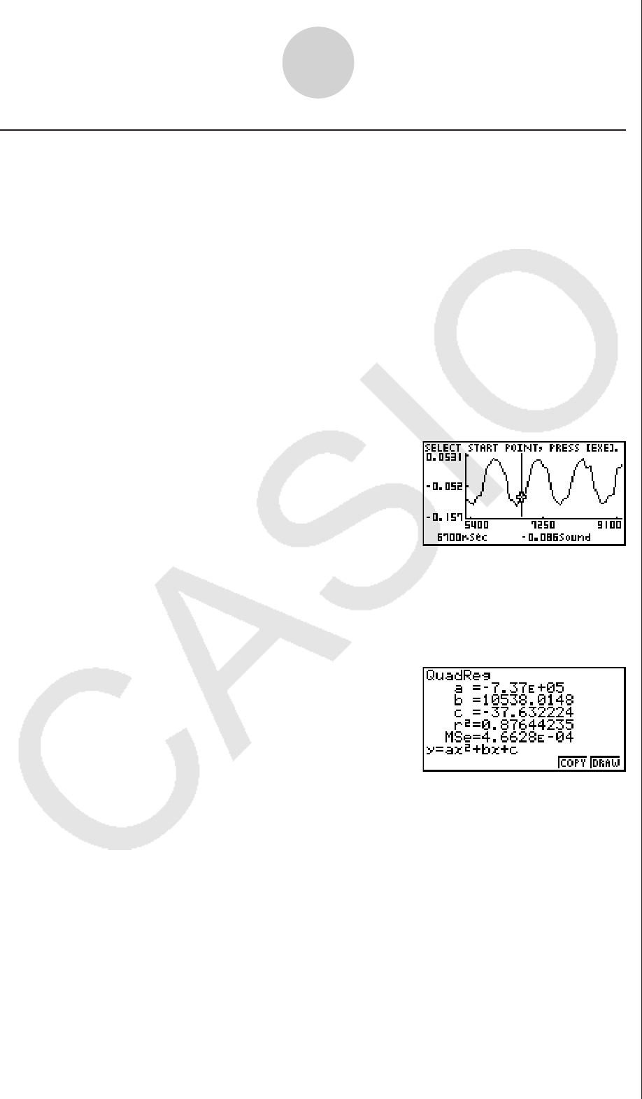
k Performing Regression
You can use the procedure below to perform regression for a range specified using the trace
pointer. All of the following regression types are supported: Linear, Med-Med, Quadratic,
Cubic, Quartic, Logarithmic, Exponential, Power, Sine, and Logistic.
For details about these regression types, see page 6-11 through 6-14 under Chapter 6 of
this manual.
The following procedure shows how to perform quadratic regression. The same general
steps can also be used to perform the other types of regression.
u To perform quadratic regression
1. On the graph screen, press K, and then 4(CALC).
• The [CALC] menu appears at the bottom of the display.
2. Press 5(X^2).
• This displays the trace pointer for selecting the range on the graph.
3. Move the trace pointer to the start point of the range for which you want to perform
quadratic regression, and then press w.
4. Move the trace pointer to the end point of the range for which you want to perform
quadratic regression, and then press w.
• This displays the quadratic regression calculation result screen.
11-8
Graph Analysis Tool Graph Screen Operations
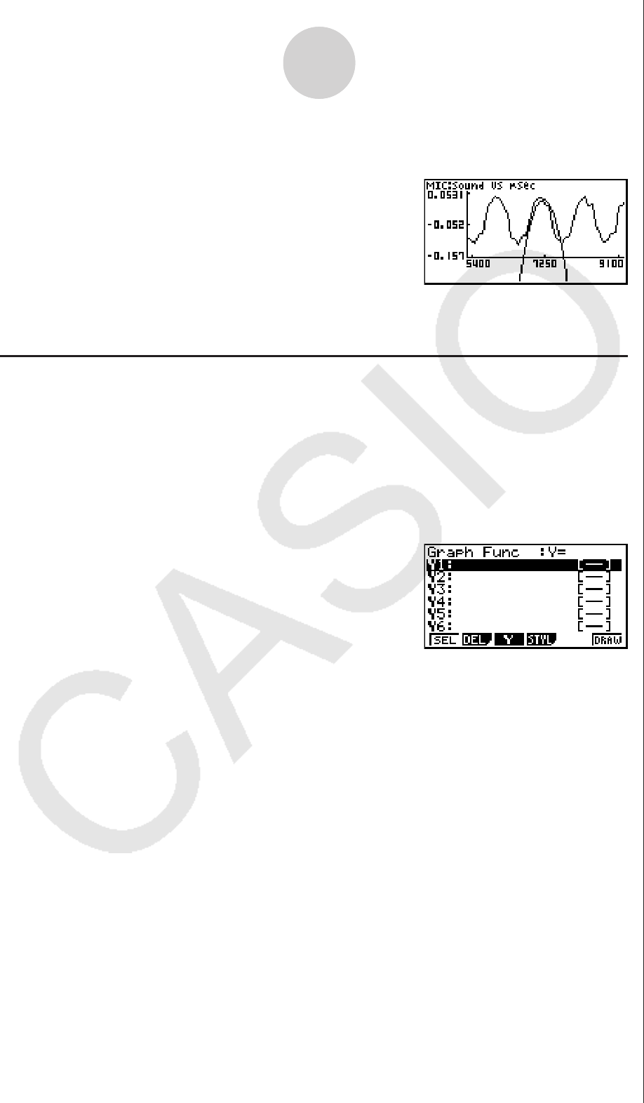
5. Press 6(DRAW).
• This draws a quadratic regression graph and overlays it over the original graph.
• To delete the overlaid quadratic regression graph, press !4(SKTCH) and then
1(Cls).
k Overlaying a Y=f(x) Graph on a Sampled Result Graph
Use the following procedure when you want to overlay a Y=f(x) graph on the sampled result
graph.
u To overlay a Y=f(x) graph on an existing graph
1. On the graph screen, press K, and then 5(Y=fx).
• This displays the graph function list. Any functions you have previously input on the
graph function list appear at this time.
2. Input the function you want to graph.
• To input a function, use the f and c cursor keys to move the highlighting to the line
where you want to input it, and then use the calculator keys for input. Press w to store
the function.
3. On the graph function list, specify which functions you want to graph.
• Graphing is turned on for any function whose “=” symbol is highlighted. To toggle
graphing of a function on or off, use the f and c cursor keys to move the highlighting
to the function, and then press 1(SEL).
11-9
Graph Analysis Tool Graph Screen Operations
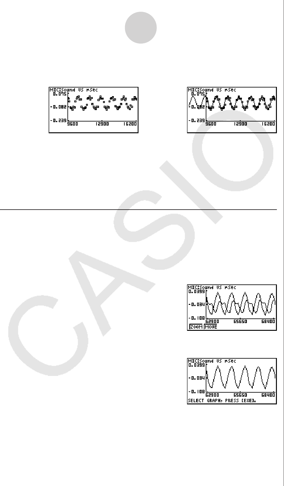
4. After the graph function list settings are configured the way you want, press 6(DRAW).
• This overlays graphs of all the functions for which graphing is turned on, over the graph
that was originally on the graph screen.
/
Original Graph Overlaid with Y=f(x) Graph
• To delete the overlaid graph, press !4(SKTCH) and then 1(Cls).
Important!
• The screenshot shown in step 4 above is of a function that was calculated and stored
by performing regression on a graph that was drawn using sampled data. Note that
overlaying a Y=f(x) graph on a sampled data graph does not automatically draw a
regression graph based on sampled data.
k Working with Multiple Graphs
The procedures in this section explain how you can zoom or move a particular graph when
there are multiple graphs on the display.
u To zoom a particular graph on a multi-graph display
1. When the graph screen contains multiple graphs, press K, and then 3(EDIT).
• The [EDIT] menu appears at the bottom of the display.
2. Press 1(ZOOM).
• This displays only one of the graphs that were originally on the graph screen.
11-10
Graph Analysis Tool Graph Screen Operations
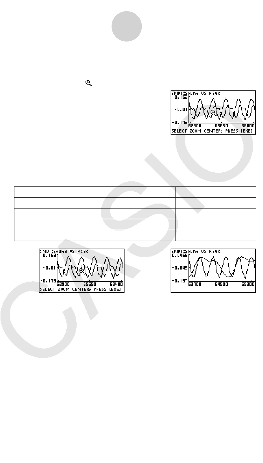
3. Use the f and c cursor keys to cycle through the graphs until the one you want is
displayed, and then press w.
• This enters the zoom mode and causes all of the graphs to reappear, along with a
magnifying glass cursor ( ) in the center of the screen.
4. Use the cursor keys to move the magnifying glass cursor to the location on the screen
that you want at the center of the enlarged or reduced screen.
5. Press w.
• This causes the magnifying glass to disappear and enters the zoom mode.
• The cursor keys perform the following operations in the zoom mode.
To do this: Press this cursor key:
Enlarge the graph image horizontally e
Reduce the size of the graph image horizontally d
Enlarge the graph image vertically f
Reduce the size of the graph image vertically c
/
6. To exit the zoom mode, press J.
11-11
Graph Analysis Tool Graph Screen Operations
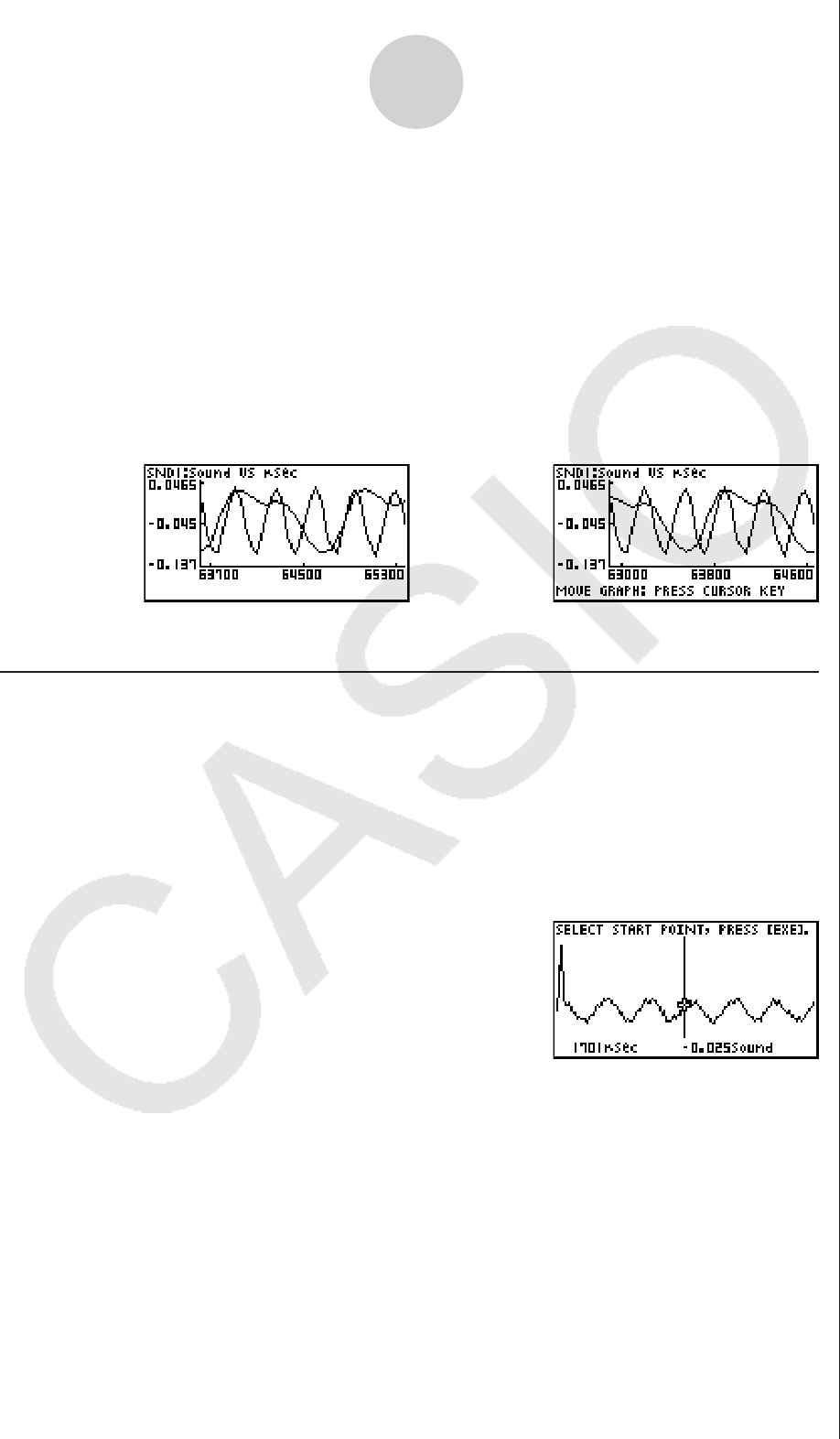
u To move a particular graph on a multi-graph display
1. When the graph screen contains multiple graphs, press K, and then 3(EDIT).
• This displays the [EDIT] menu.
2. Press 2(MOVE).
• This displays only one of the graphs that were originally on the graph screen.
3. Use the f and c cursor keys to cycle through the graphs until the one you want is
displayed, and then press w.
• This enters the move mode and causes all of the graphs to reappear.
4. Use the d and e cursor keys to move the graph left and right, or the f and c
cursor keys to move the graph up and down.
/
5. To exit the move mode, press J.
k Outputting a Specific Range of a Graph from the Speaker
(EA-200 only)
Use the following procedure to output a specific range of a sound data waveform graph from
the speaker.
u To output a graph from the speaker
1. On the graph screen, press K, and then 6(SPKR).
• This displays the trace pointer for selecting the range on the graph.
2. Move the trace pointer to the start point of the range you want to output from the speaker,
and then press w.
11-12
Graph Analysis Tool Graph Screen Operations
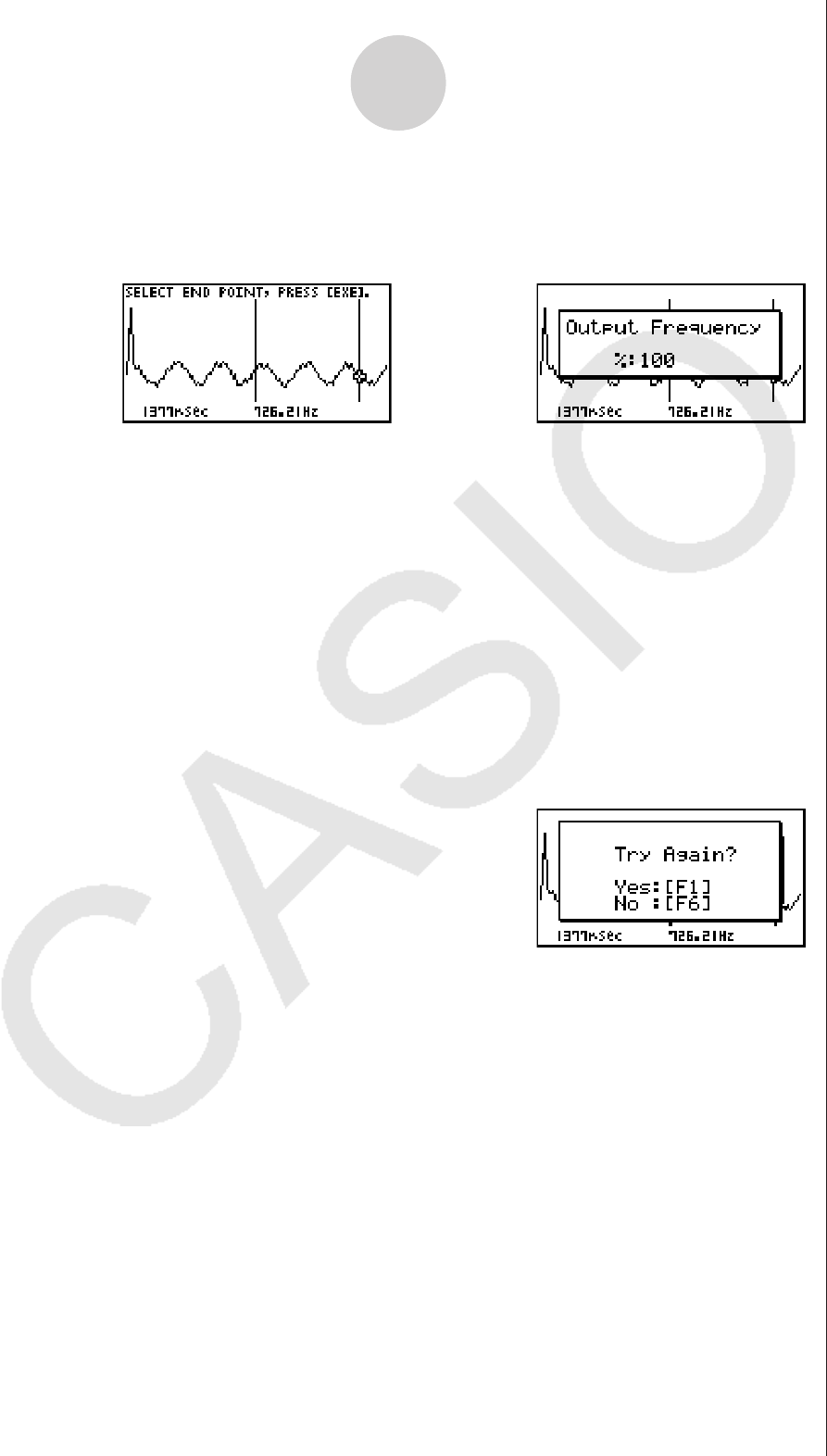
3. Move the trace pointer to the end point of the range you want to output from the speaker,
and then press w.
• After you specify the start point and end point, an output frequency dialog box shown
below appears on the display.
/
4. Input a percent value for the output frequency value you want.
• The output frequency specification is a percent value. To output the original sound as-is,
specify 100%. To raise the original sound by one octave, input a value of 200%. To
lower the original sound by one octave, input a value of 50%.
5. After inputting an output frequency value, press w.
• This outputs the waveform between the start point and end point from the EA-200
speaker.
• If the sound you configured cannot be output for some reason, the message “Range
Error” will appear. If this happens, press J to scroll back through the previous setting
screens and change the setup as required.
6. To terminate sound output, press the EA-200 [START/STOP] key.
7. Press w.
• This displays a screen like the one shown below.
8. If you want to retry output from the speaker, press 1(Yes). To exit the procedure and
return to the graph screen, press 6(No).
• Pressing 1(Yes) returns to the “Output Frequency” dialog box. From there, repeat the
above steps from step 4.
11-13
Graph Analysis Tool Graph Screen Operations
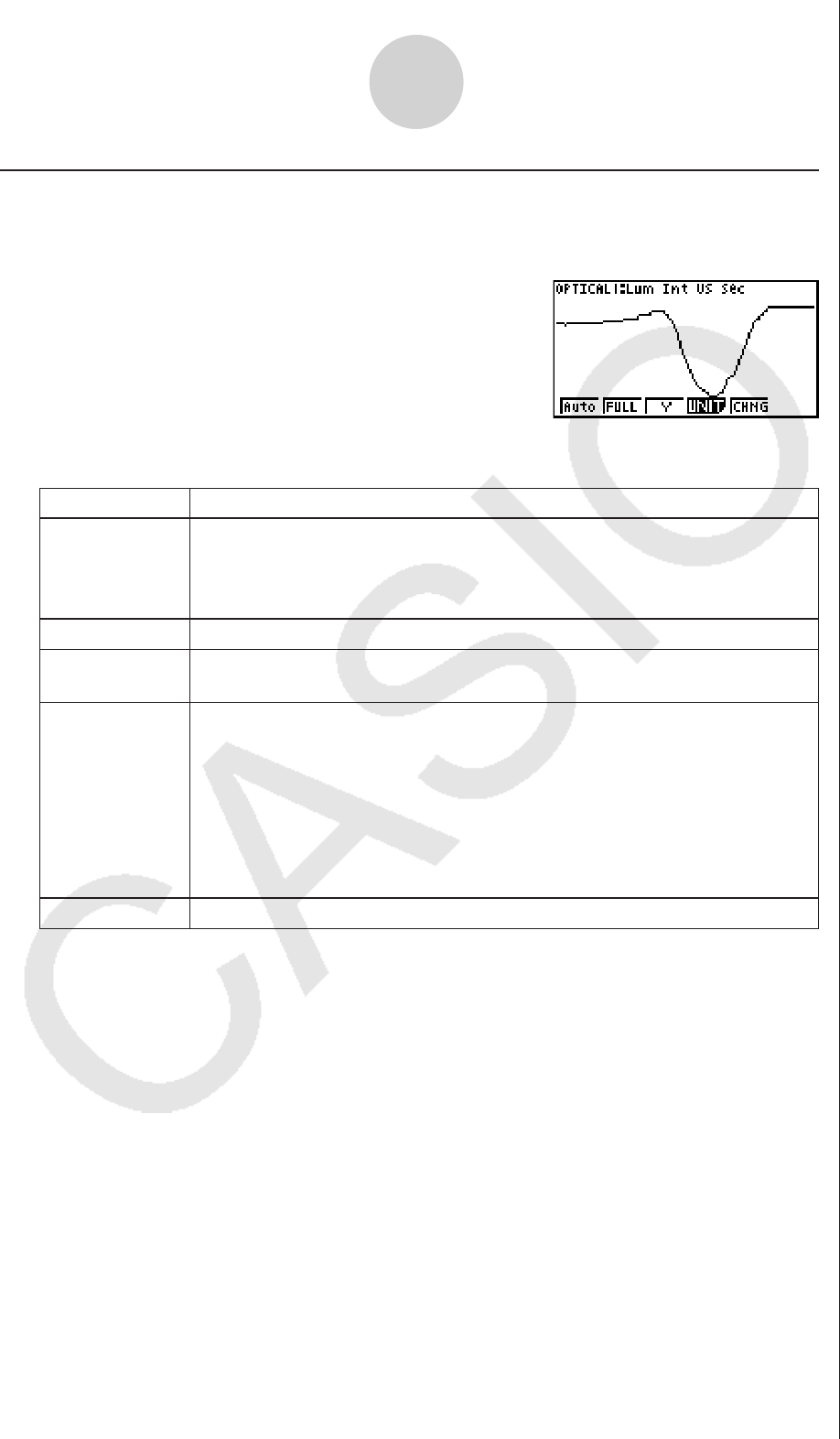
11-14
Graph Analysis Tool Graph Screen Operations
k Configuring View Window Parameters
Pressing !3(V-Window) while the graph screen is on the display displays a View
Window function key menu along the bottom of the display.
Press the function key that corresponds to the View Window parameter you want to
configure.
Function Key Description
1
(
Auto
)
Automatically applies the following View Window parameters.
Y-axis Elements: In accordance with screen size
X-axis Elements: In accordance with screen size when 1 data item
equals 1 dot; 1 data equals 1 dot in other cases
2
(
FULL
)
Resizes the graph so all of it fits in the screen.
3(Y) Resizes the graph so all of it fits in the screen along the Y-axis, without
changing the X-axis dimensions.
4(UNIT)
Specifies the unit of the numeric axis grid displayed by the Econ Axes
setting of the graph setup screen (page 3-13).
1(
μ
sec): microseconds
2(msec): milliseconds
3(sec): seconds
4(DHMS) : days, hours, minutes, seconds (1 day, 2 hours, 30 minutes,
5 seconds = 1d2h30m5s)
5(Auto): Auto selection
5(CHNG) Toggles display of the source data on the graph screen on and off.
To exit the View Window function key menu and return to the standard function key menu,
press J.

12 Calling E-CON3 Functions from an eActivity
You can call E-CON3 functions from an eActivity by including an “Econ strip” in the eActivity
file. The following describes each of the four available Econ strips.
uEcon SetupWizard strip
This strip calls the E-CON3 Setup Wizard. The Econ Setup Wizard strip makes it
possible to perform the following series of operations from the eActivity: Data Logger
setup using the Setup Wizard R Sampling R Graphing.
Note
• In the case of the Econ SetupWizard strip, the “3: Convert Program” is not available
on the “Complete!” dialog box.
uEcon AdvancedSetup strip
This strip calls the E-CON3 Advanced Setup screen. The Advanced Setup provides
access to almost all executable functions (except for the program converter),
including detailed Data Logger setup and sampling execution; graphing and
Graph Analysis Tools; simultaneous sampling with multiple sensors using the
MULTIMETER Mode, etc.
Note
• Using an Econ Advanced Setup strip to configure a setup causes the setup
information to be registered in the applicable strip. This means that the next time
you open the strip, sampling can be performed in accordance with the previously
configured setup information.
uEcon Sampling strip
This strip executes Data Logger measurement. To store Data Logger setup
information for this strip, perform the Econ Advance Setup operation the first time the
strip is executed.
uEcon Graph strip
This strip graphs sampled data that is recorded in the strip. The sampled data is
recorded to the strip the first time the strip is executed.
uEcon Strip Memory Capacity Precautions
• The memory capacity of each Econ strip is 25 KB. An error will occur if you perform
an operation that causes this capacity to be exceeded. Particular care is required
when handling a large number of samples, which can cause memory capacity to be
exceeded.
• Always make sure that FFT Graph is turned off whenever performing sampling
with the microphone. Leaving FFT Graph turned on cause memory capacity to be
exceeded.
• If an error occurs, press !a(' ) to return to the eActivity workspace screen
and perform the procedure again.
• For information about checking the memory usage of each strip, see “10-5 eActivity
File Memory Usage Screen” under Chapter 10 of this manual.
For details about eActivity operations, see “Chapter 10 eActivity” under Chapter 10 of this
manual.
12-1
Calling E-CON3 Functions from an eActivity

Manufacturer:
CASIO COMPUTER CO., LTD.
6-2, Hon-machi 1-chome, Shibuya-ku, Tokyo 151-8543, Japan
Responsible within the European Union:
Casio Europe GmbH
Casio-Platz 1, 22848 Norderstedt, Germany
www.casio-europe.com

CASIO COMPUTER CO., LTD.
6-2, Hon-machi 1-chome
Shibuya-ku, Tokyo 151-8543, Japan
SA1512-D
© 2014 CASIO COMPUTER CO., LTD.
