Casio Fx CG500 CG500_Ex Ex EN
User Manual: Casio fx-CG500_Ex fx-CG500 | Calculators | Manuals | CASIO
Open the PDF directly: View PDF ![]() .
.
Page Count: 47
- Contents
- Chapter 2: Main Application
- Chapter 3: Graph & Table Application
- Chapter 4: Conics Application
- Chapter 5: Differential Equation Graph Application
- Chapter 6: Sequence Application
- Chapter 7: Statistics Application
- Chapter 8: Geometry Application
- Chapter 9: Numeric Solver Application
- Chapter 10: eActivity Application
- Chapter 11: Financial Application
- Chapter 12: Program Application
- Chapter 13: Spreadsheet Application
- Chapter 14: 3D Graph Application


2
Contents
Chapter 2: Main Application ................................................................................................. 3
Chapter 3: Graph & Table Application ............................................................................... 13
Chapter 4: Conics Application ........................................................................................... 19
Chapter 5: Differential Equation Graph Application......................................................... 21
Chapter 6: Sequence Application ...................................................................................... 26
Chapter 7: Statistics Application ....................................................................................... 28
Chapter 8: Geometry Application ...................................................................................... 32
Chapter 9: Numeric Solver Application ............................................................................. 35
Chapter 10: eActivity Application ...................................................................................... 36
Chapter 11: Financial Application ...................................................................................... 37
Chapter 12: Program Application ...................................................................................... 42
Chapter 13: Spreadsheet Application ................................................................................ 44
Chapter 14: 3D Graph Application ..................................................................................... 46
About this booklet...
This booklet contains a collection of examples of operations explained in the fx-CG500 User’s Guide.
Use this booklet in combination with the User’s Guide.
Chapter 2: Main Application 3
Chapter 2:
Main Application
0201
Calculation Key Operation
56 × (–12) ÷ (–2.5) = 268.8 56*(z12)/(z2.5)E
2 + 3 × (4 + 5) = 29 2+3*(4+5)E
=
6/(4*5)E or N*6c4*5E
* The soft keyboard [Math1] key set
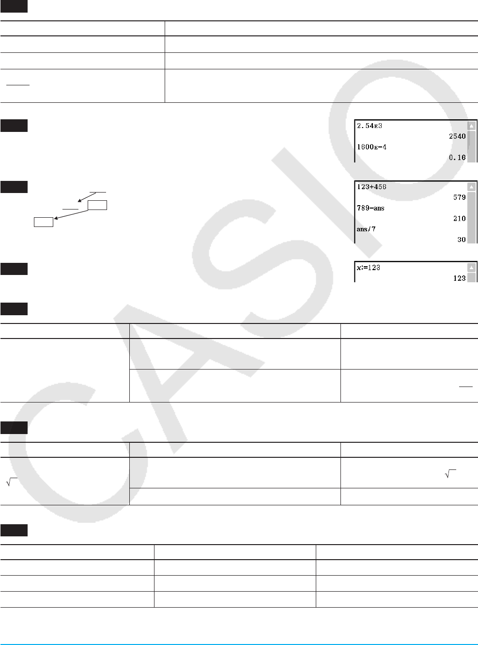
0202 2.54 × 103 = 2540 2.54e3E
1600 × 10–4 = 0.16 bgaaE-ew
0203 123 + 456 = 579 123+456E
789 – 579 = 210 789-DE
210 ÷ 7 = 30 /7E
0204 x:=123E
0205 Tapping u while the calculator is configured for Standard mode (Normal 1) display
Expression Calculator Operation Displayed Result
100 ÷ 6 = 16.6666666...
100/6u
(Switches to Decimal mode format.) 16.66666667
u (Switches back to Standard mode format.) 50
3
0206 Tapping u while the calculator is configured for Decimal mode (Normal 1) display
Expression Calculator Operation Displayed Result
2 + 2 = 3.414213562...
!2e+2u
(Switches to Standard mode format.) 2 + 2
u (Switches back to Decimal mode format.) 3.414213562
0207 (Complex mode and Real mode calculation results)
Expression Complex Mode Real Mode
solve (x3 – x2 + x – 1 = 0, x){x = –i, x = i, x = 1} {x = 1}
i + 2 i 3·iERROR: Non-Real in Calc
(1 + '3 i)(⬔(2,45°)) ⬔(4,105) ERROR: Non-Real in Calc
Chapter 2: Main Application 4
0208 (Assistant mode and Algebra mode calculation results)
Expression Assistant Mode Algebra Mode
x2 + 2x + 3x + 6 x2 + 2
·
x + 3
·
x + 6 x2 + 5
·
x + 6
expand ((x+1)2)x2 + 2
·
x
·
1 + 12x2 + 2
·
x + 1
x + 1 (When 1 is assigned to x)x + 1 2
0209 1. Tap location 1. 2. K3E
Re-calculated
1
0210 0211
0212
0213
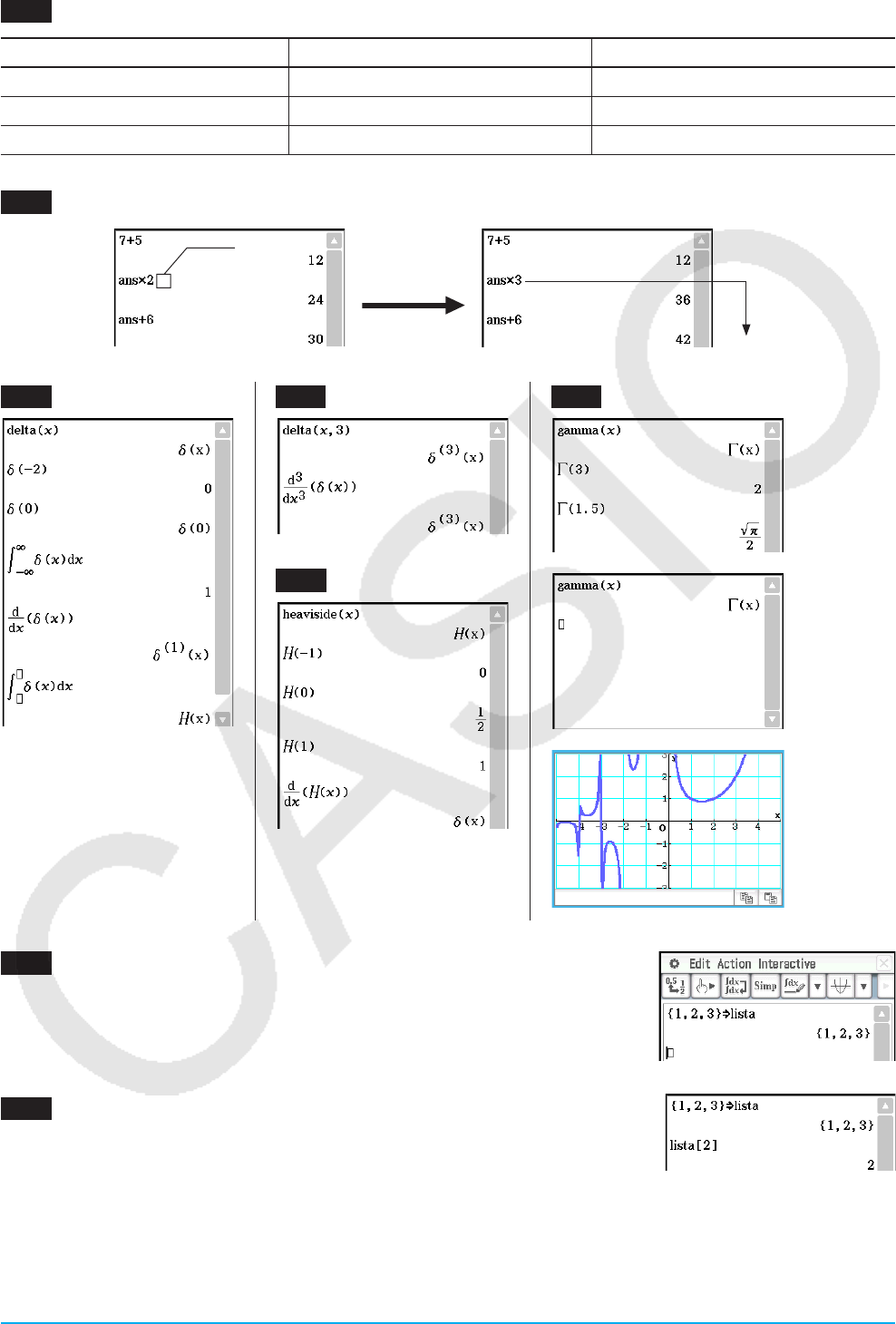
0214 {1,2,3}WlistaE
or
)1,2,3eWlistaE
0215 lista[2]E
or
lista[d2E
Chapter 2: Main Application 5
0216 5Wlista[2]E
Tip: You can also perform the above operations on the “ans” variable when it contains LIST data.
Example: {1, 2, 3} E {1, 2, 3}
D[2]E 2
0217 list3*{6,0,4}E
0218 {10,20,30}W{x,y,Z}
E
0219 [[1,2][3,4]]Wmat1E
or
[d[d1,2e[d3,4eeW
mat1E
0220 mat1[2,1]E
↑
↑
Row Column
0221 5Wmat1[1,2]E
Tip: You can also perform the above operations on the “ans” variable when it contains MATRIX data.
0222
1. 6 (Creates a 1-row × 2-column matrix.)
1e2
2. 6 (Adds one column to the matrix.)
3
3. 7 (Adds one row to the matrix.)
4e5e6
4. Assign the matrix to the variable named “mat2”.
eWmat2E
Chapter 2: Main Application 6
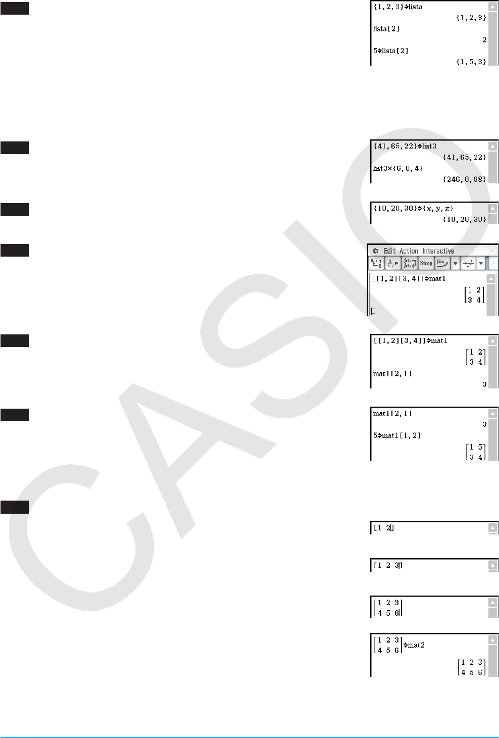
0223 [[1,1][2,1]]+
[[2,3][2,1]]E
0224 81e1cd2e1
e*
82e3cd2e1E
0225 [[1,2][3,4]]*5E
0226 [[1,2][3,4]]{3E
0227 81e2cd3e4em3E
0228 710c20730eW7xcy7ZE
0229
1. Tap the down arrow button next to the < button, and then tap 1.
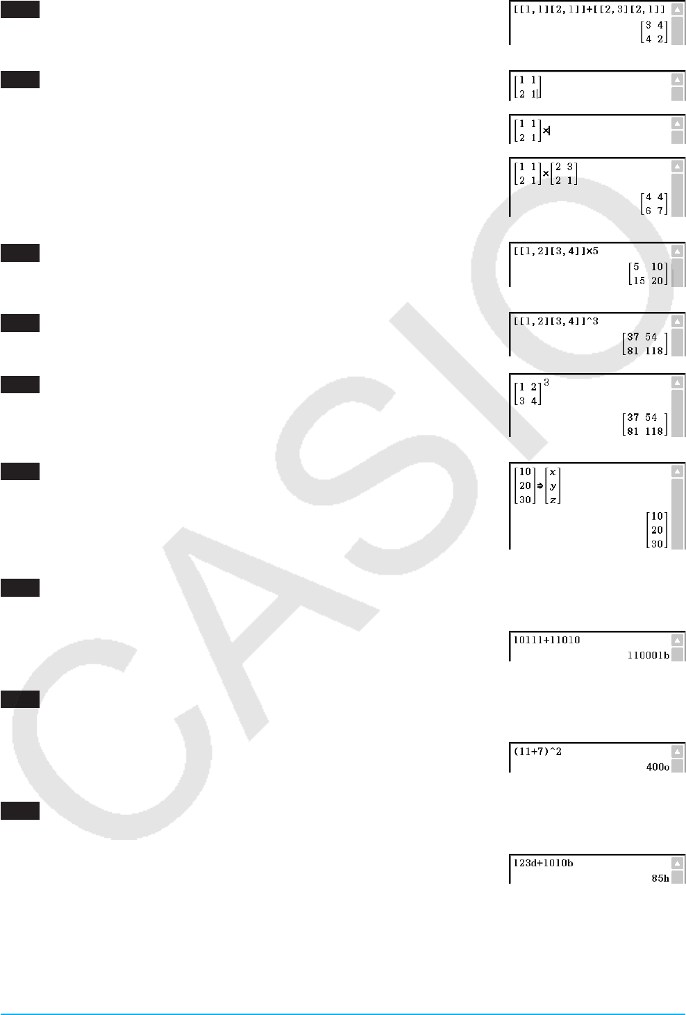
2. 10111+11010E
0230
1. Tap the down arrow button next to the < button, and then tap 2.
2. (11+7){2E
0231
1. Tap the down arrow button next to the < button, and then tap 4.
2. 123d+1010bE
Chapter 2: Main Application 7
0232
10102 and 11002 = 10002 (Number base: Binary)
1010pandp1100E
10112 or 110102 = 110112 (Number base: Binary)
1011porp11010E
10102 xor 11002 = 1102 (Number base: Binary)
1010pxorp1100E
not (FFFF16) = FFFF000016 (Number base: Hexadecimal)
not(ffff)E
0233
baseConvert( 579,15,12)E
baseConvert( 100,13,10)E
baseConvert( 123,16,3)E
0234
Since a solution of s = 1 is obtained for point P, it means it exists on straight
line l.
A solution cannot be obtained (No Solution) for s in the case of point Q, so it
means that the point does not exist on straight line l.
0235
1. x{3-3x{2+3x-1
2. Drag the stylus across the expression to select it.
3. Tap [Interactive], [Transformation], [factor], and then [factor].
Chapter 2: Main Application 8
0236
1. x{2+2x
2. Drag the stylus across the expression to select it.
3. Tap [Interactive], [Calculation], and then [
∫
]. This displays the
∫
dialog box.
4. Tap “Definite” to select it.
5. Input the required data for each of the following three arguments.
Variable: x, Lower: 1, Upper: 2
6. Tap [OK].
0237
1. Input the calculation below and execute it.
diff(sin(x),x) × cos(x) + sin(x) × diff(cos(x),x)
2. Drag the stylus across “diff(sin(x),x)” to select it.
3. Tap [Interactive], [Assistant] and then [apply].
• This executes the part of the calculation you selected in step 2. The part of the calculation that is not
selected (× cos(x) + sin(x) × diff(cos(x),x)) is output to the display as-is.
0238
1. Tap ! to display the Graph Editor window in the lower window.
2. Drag the stylus across “x^2 – 1” in the work area to select it.
3. Drag the selected expression to the Graph Editor window.
• This copies the expression to the location where you dropped it.
Chapter 2: Main Application 9
0239
1. Tap $ to display the Graph window in the lower window.
2. Drag the stylus across “x^2 – 1” in the work area to select it.
3. Drag the selected expression to the Graph window.
0240
1. On the work area window, tap ( to display the Stat Editor window in the lower window.
2. In the Stat Editor window, input {1, 2, 3} into “list1” and {4, 5, 6} into “list2”.
3. Make the work area window active, press k, and then perform the following calculation: list1 + list2 ⇒
list3.
4. Press k to hide the keyboard.
• Here you can see that list3 contains the result of list1 + list2.
Chapter 2: Main Application 10
0241
1. Tap the Main application work area window to make it active.
2. Perform the operation {12, 24, 36} ⇒ test, which assigns the list data {12, 24, 36} to the LIST variable named
“test”.
3. Tap the Stat Editor window to make it active, and then use e key to scroll the screen to the right until the
blank list to the right of “list6” is visible.
4. Tap the blank cell next to “list6”, input “test”, and then tap w.
• This displays the list data {12, 24, 36}, which is assigned to the variable
named “test”.
0242
1. Input the expression x^2/5^2 + y^2/2^2 = 1 in the work area.
2. Tap 3 to display the Geometry window in the lower window.
3. Drag the stylus across the expression in the work area to select it, and then
drag the selected expression to the Geometry window.
• An ellipse appears in the Geometry window.
0243
Point Circle A point and its image
Chapter 2: Main Application 11
0244
1. Start up Verify.
2. Input 50 and press E.
3. Following the equal sign (=), input 25 × 3 and press E.
4. Tap [OK] to close the error dialog that appears.
5. Change 25 × 3 to 25 × 2 and press E.
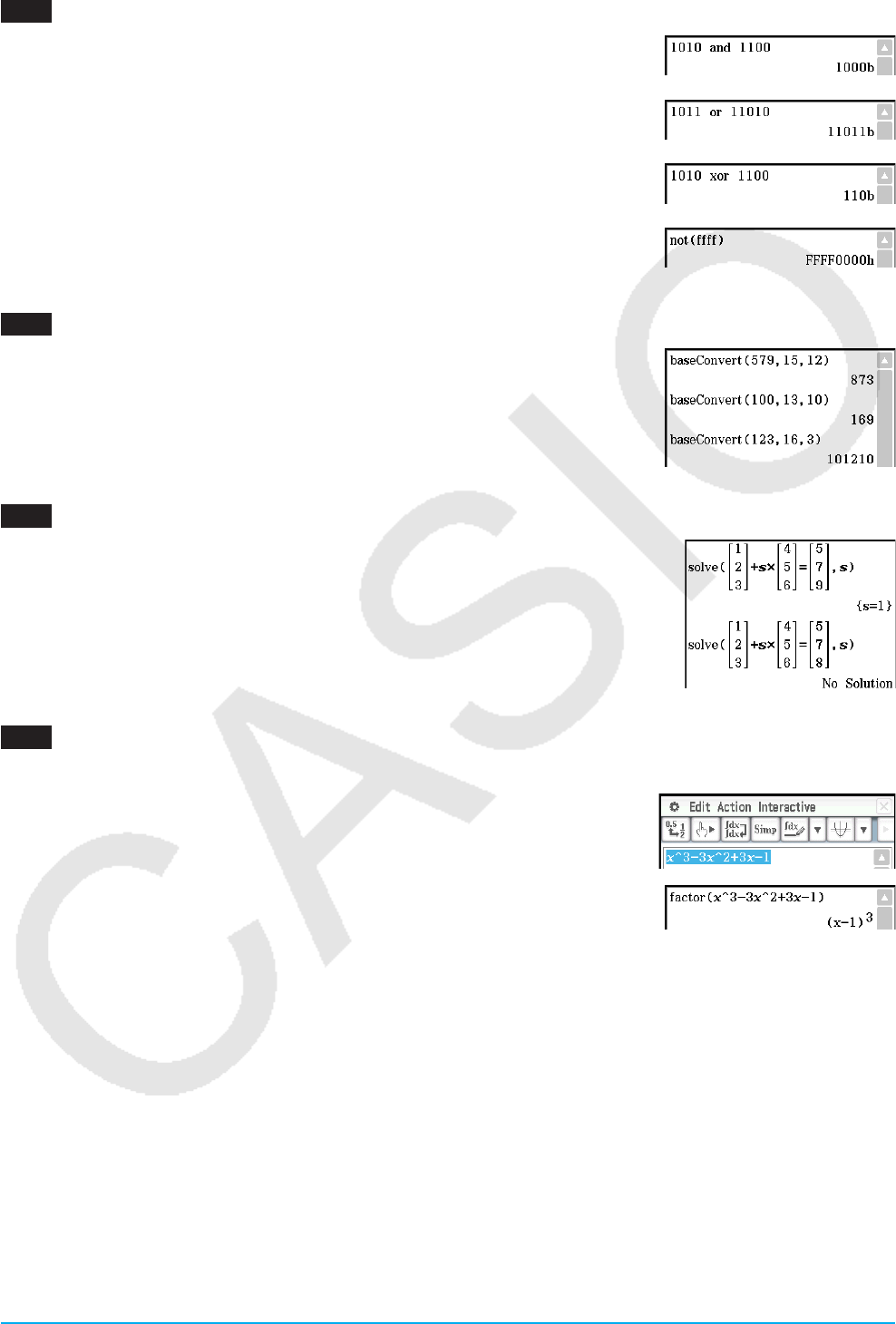
6. Following the next equal sign (=), input 5 × 5
× 2 and press E.
0245
1. Tap O and then tap [OK] to clear the window.
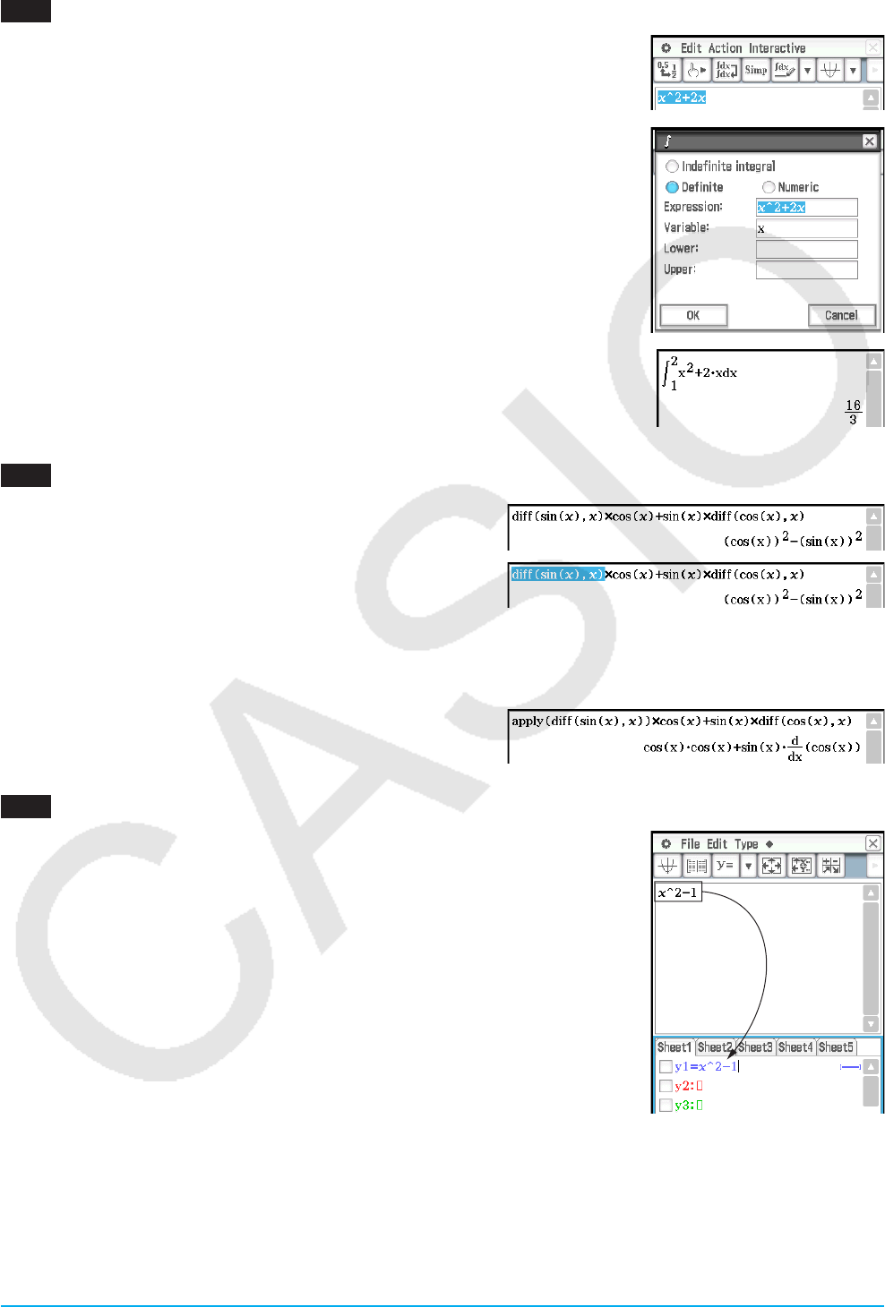
2. Tap the down arrow on the toolbar and select T.
3. Input x^2 + 1 and press E.
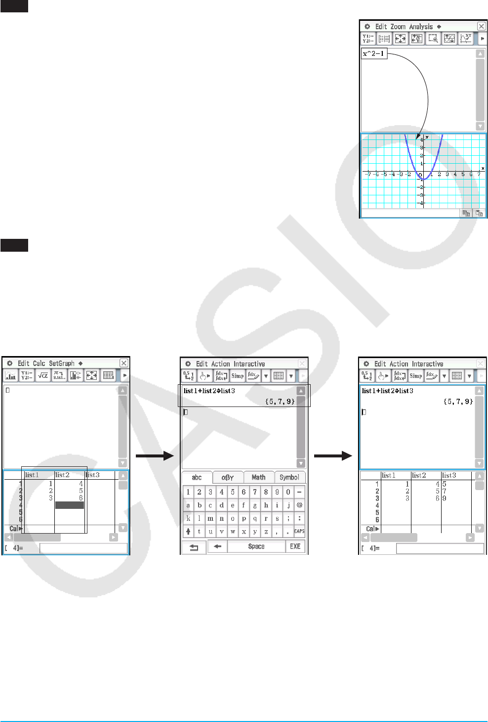
4. Input (x + i)(x – i) and press E.
0246
1. Start up Probability, and then select “2 Dice +”.
2. Enter 50 into the “Number of trials” box.
3. Tap [OK] to display the result in the
Probability window.
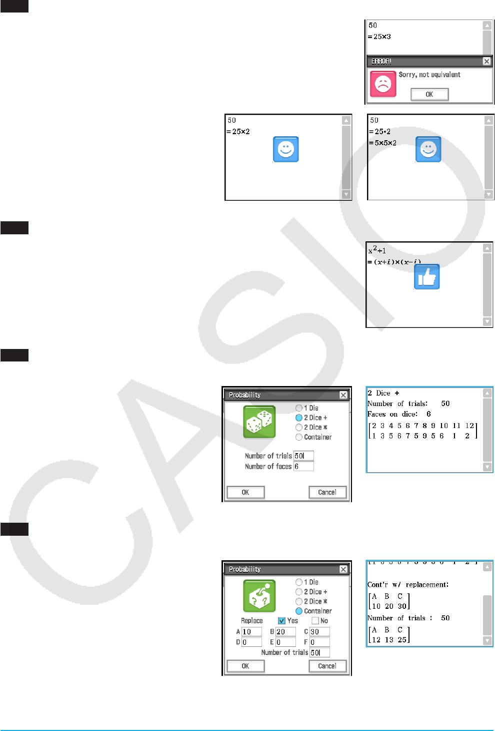
0247
1. Tap P to display the Probability dialog box, and then select “Container”.
2. Configure the following settings on the
dialog box.
Replace: Yes*, A: 10, B: 20, C: 30
(Leave other letters set to zero.),
Number of trials: 50
3. Tap [OK].
* Indicates the ball is replaced before the next draw. If the ball is not replaced, select “No”.

Chapter 2: Main Application 12
0248
1. OCTA()E
2. Enter 20 and then tap [OK].
• This will run OCTA and display the results in the
program output window.
Program output
window
Chapter 3: Graph & Table Application 13
Chapter 3:
Graph & Table Application
0301
1. On the a menu, tap [Draw Shade].
2. On the dialog box that appears, input the
following: Lower Func: x2 – 1, Upper Func:
–x2 + 1.
Leave x min and x max blank.
3. Tap [OK].
0302
1. Tap 8 to display the Table Input dialog box, and then configure it with the settings below.
Start: –4.9, End: 7.1, Step: 2
2. On the Graph Editor window, input and store y = 3log(x + 5) into line y1, and then tap #.
• This generates a number table and displays it.
3. Tap a and then [Link].
• This displays the Graph window and draws the graph, with the trace
pointer located on the graph line. The coordinates of the trace pointer
location will also be shown.
• Tapping a cell in the y1 column causes the trace pointer to move the
location of the cell’s value.
• You can move the highlighting in the number table by pressing the up
and down cursor keys, or by tapping the cell you want to select. Doing
so causes the trace pointer to jump to the corresponding location on the
graph.
4. To quit the linked trace operation, tap l on the icon panel.
0303
1. Tap 8 to display the Table Input dialog box, and then configure it with the following settings.
Start: 0, End: 1, Step: 0.2
2. Input the function y = x3 – 3x on the Graph Editor window, and then tap $ to graph it.
3. Tap # to generate the number table.
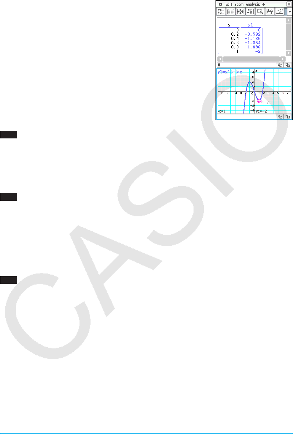
Chapter 3: Graph & Table Application 14
4. Tap the Graph window to make it active. Next, tap [Analysis] and then
[Trace].
• This causes a pointer to appear on the graph.
5. Use the cursor key to move the pointer along the graph until it reaches a
point whose coordinates you want to input into the table.
6. Press E to input the coordinates at the current cursor position at the end
of the table.
7. Repeat steps 5 and 6 to input the rest of the coordinates you want.
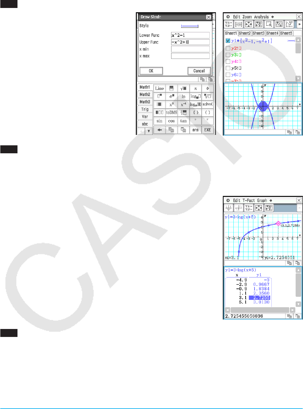
0304
1. In line y1 of the Graph Editor window, input and save x2 – x – 2, and then tap $.
2. Tap [Analysis], [Sketch], and then [Inverse].
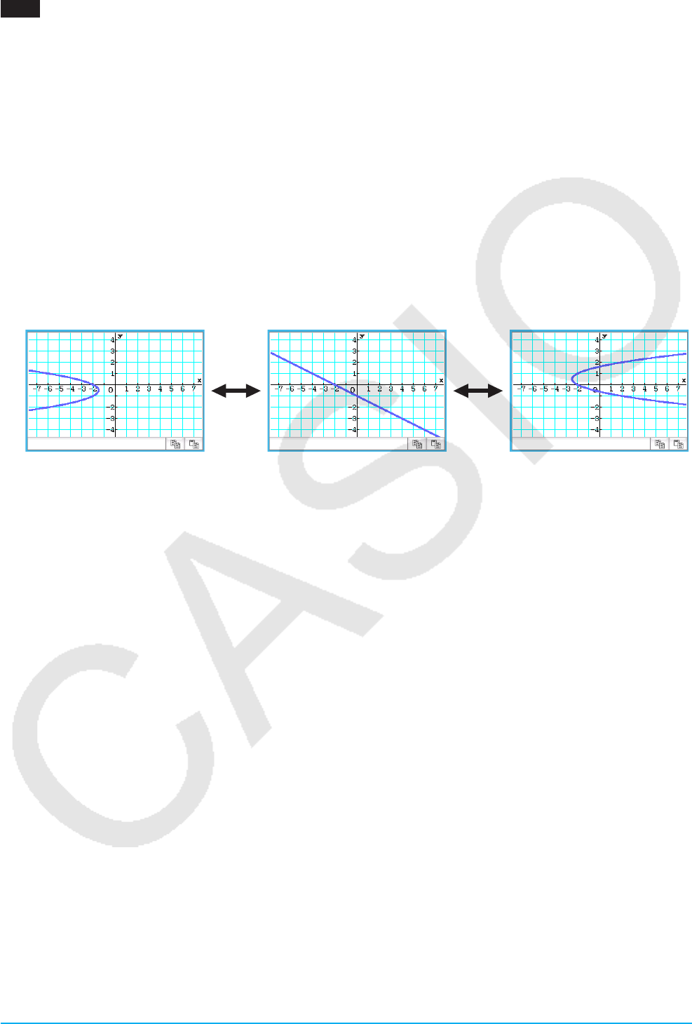
• This graphs the inverse function. The message box briefly shows the inverse function.
Tip: If a function does not have an inverse, the graph produced by the [Inverse] command will be the result of
interchanging the x and y variables of the original function.
0305
1. While the Graph window is active, tap [Analysis], [Sketch], and then [Circle].
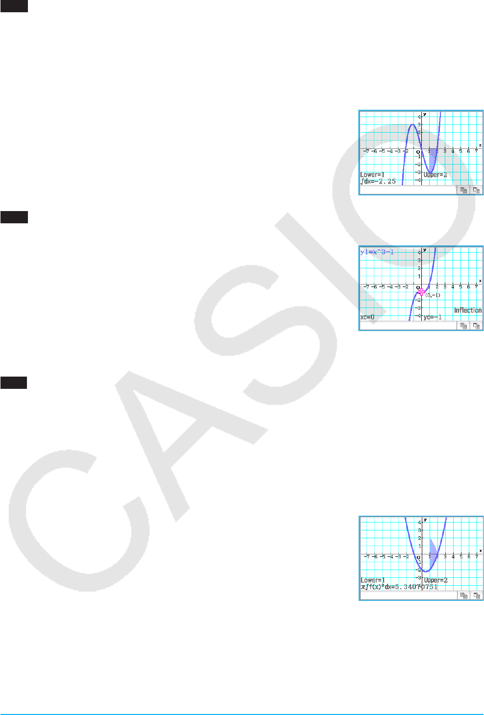
• This display “Circle” on the Graph window.
2. Tap the point where you want the center of the circle to be, and then tap a second point anywhere on the
circle’s circumference.
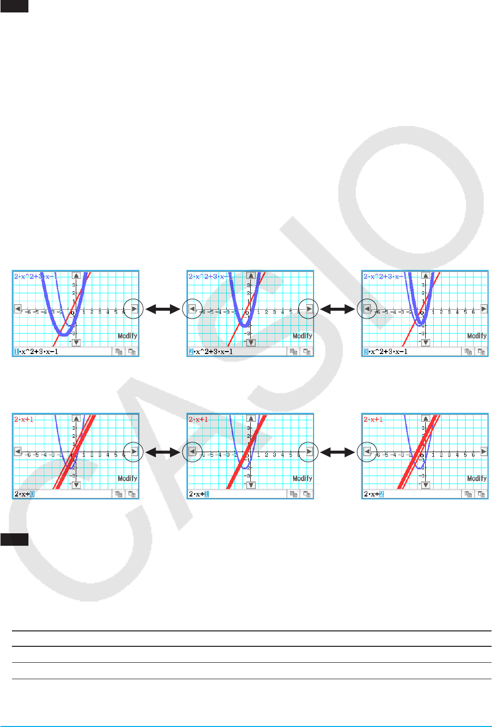
• This draws the circle, and the message box shows the function for the circle.
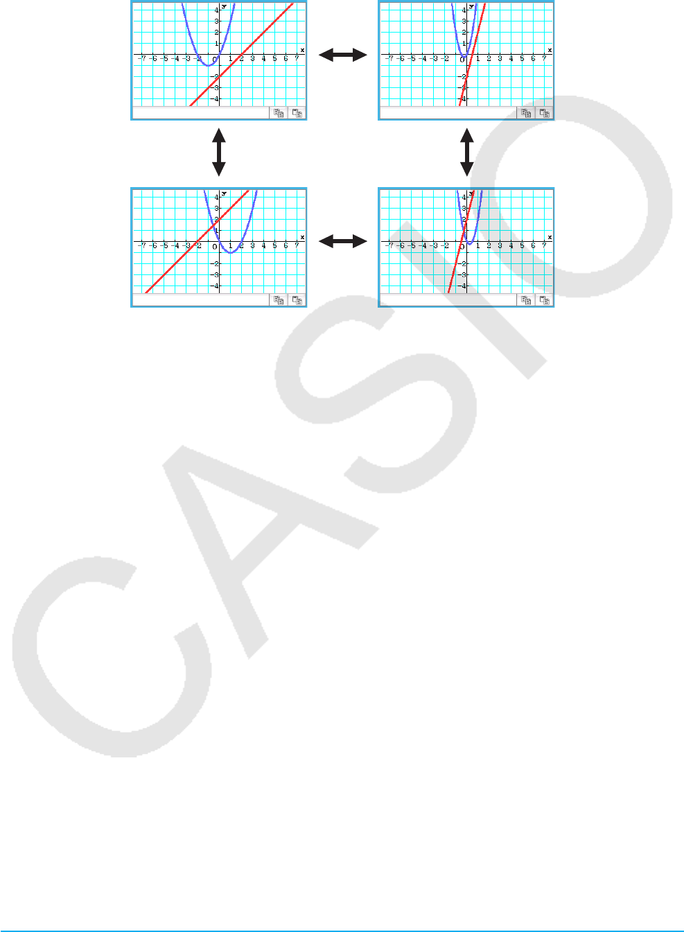
• You can also draw a circle by specifying the coordinates of its center point and specifying its radius value.
In place of the operation in step 2 of the above procedure, press a number key on the keypad. On the
dialog box that appears, enter the required values and then tap [OK].
0306
1. While the Graph window is active, tap [Analysis], [Sketch], and then [Vertical].
• This display “Vertical” on the Graph window.
2. Press 2.
• This displays a dialog box for specifying the x-coordinate of the vertical line, with 2 specified as the
x-coordinate.
• Instead of inputting a value here, you can use the stylus to tap the point through which the vertical line
should pass.
3. Tap [OK].
To draw a horizontal line, tap [Analysis], [Sketch], and then [Horizontal] in place of [Vertical] in step 1 of the
above procedure. In the case of a horizontal line, you need to specify the y-coordinate in step 2.
Chapter 3: Graph & Table Application 15
0307
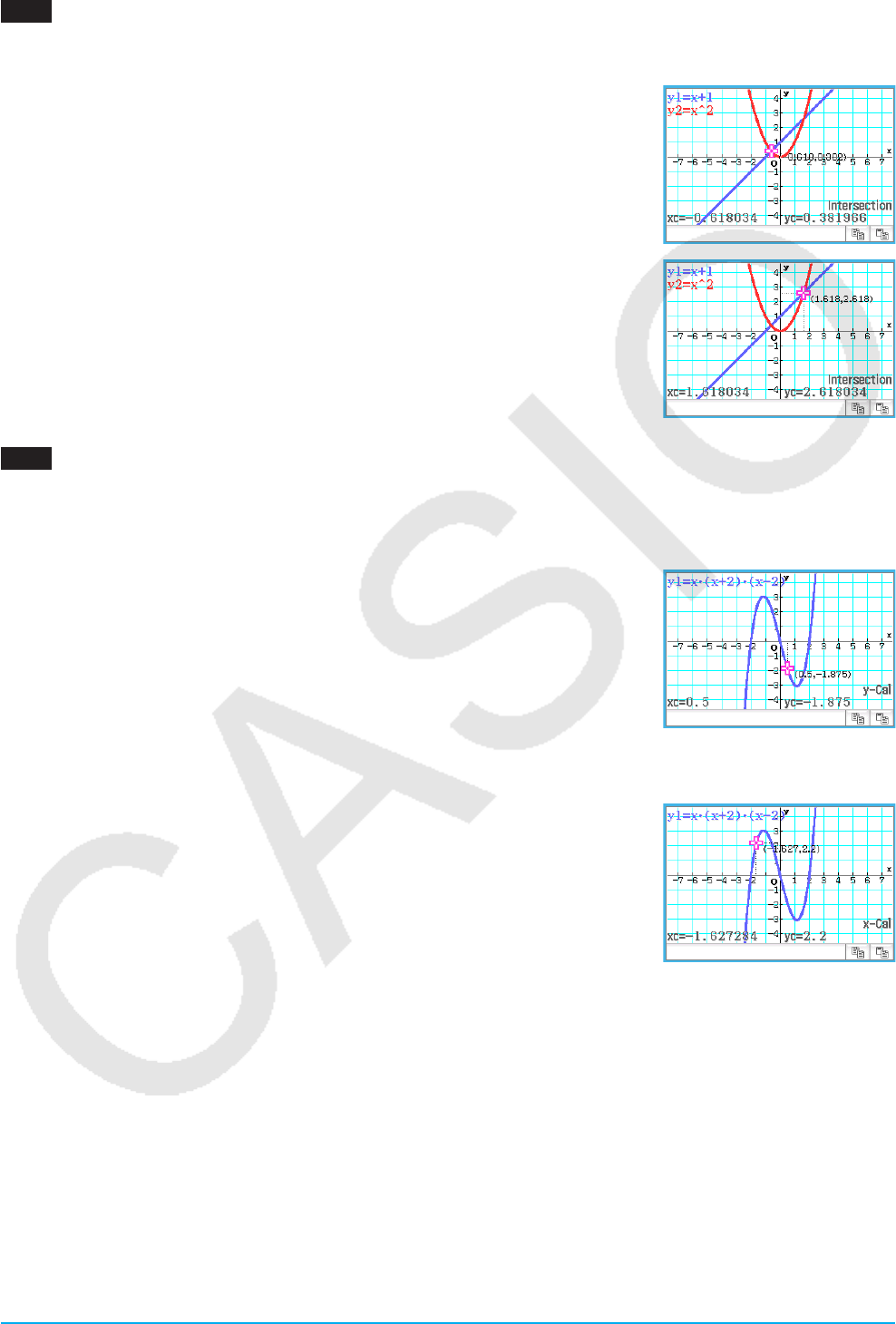
1. On the Graph Editor window, input and store y = x + 1 into line y1 and y = x2 into y2, and then tap $ to
graph them.
2. Tap [Analysis], [G-Solve], and then [Intersection].
• This causes “Intersection” to appear on the Graph window, with a pointer
located at the point of intersection. The x- and y-coordinates at the current
pointer location are also shown on the Graph window.
3. To obtain other points of intersection, press the left or right cursor key, or tap
the left or right graph controller arrows.
0308
1. On the Graph Editor window, input and store y = x (x + 2)(x – 2) into line y1, and then tap $ to graph it.
2. To obtain the value of y for a particular x-value, tap [Analysis], [G-Solve], [x-Cal/y-Cal], and then [y-Cal].
• This displays a dialog box for specifying the x-value.
3. For this example, input 0.5 and then tap [OK].
• This moves the pointer to the location on the graph where x = 0.5, and
displays the x-coordinate and y-coordinate at that location.
4. To obtain the value of x for a particular y-value, tap [Analysis], [G-Solve], [x-Cal/y-Cal], and then [x-Cal].
• This displays a dialog box for specifying the y-value.
5. For this example, input 2.2 and then tap [OK].
• This moves the pointer to the location on the graph where y = 2.2, and
displays the x-coordinate and y-coordinate at that location.
Tip: When there are multiple results for the above procedure, press e to calculate the next value. Pressing d returns
to the previous value.
Chapter 3: Graph & Table Application 16
0309
1. On the Graph Editor window, input and store y = x (x + 2)(x – 2) into line y1, and then tap $ to graph it.
2. Tap [Analysis], [G-Solve], [Integral], and then [∫
dx].
• This displays “Lower” on the Graph window.
3. Press 1.
• This displays a dialog box for inputting an interval for the x-values, with 1 specified for the lower limit of the
x-axis (Lower).
4. Tap the [Upper] input box and then input 2 for the upper limit of the x-axis.
5. Tap [OK].
0310
1. On the Graph Editor window, input and store y = x3 – 1 into line y1, and then tap $ to graph it.
2. Tap [Analysis], [G-Solve], and then [Inflection].
• This causes “Inflection” to appear on the Graph window, with a pointer
located at the point of inflection.
Tip: If your function has multiple inflection points, use the cursor keys or graph controller arrows to move the pointer
between them and display their coordinates.
0311
1. On the Graph Editor window, input and store y = x2 – x – 2 into line y1, and then tap $ to graph it.
2. Tap [Analysis], [G-Solve], and then [π ∫ f(x)2dx].
• This displays a crosshair pointer on the graph, and the word “Lower” in the lower right corner of the Graph
window.
3. Press 1.
• This displays a dialog box for inputting an interval of values for x, with 1 specified for the lower limit of the
x-axis (Lower).
4. Tap the [Upper] input box and then input 2 for the upper limit of the x-axis.
5. Tap [OK].
• This causes a silhouette of the solid of revolution to appear on the Graph
window, and its volume to appear in the message box.
Chapter 3: Graph & Table Application 17
0312
1. If the graph controller is not displayed on the Graph window, perform the operation below.
(1) Tap O and then [Graph Format] to display the Graph Format dialog box.
(2) Select the “G-Controller” check box.
(3) Tap [Set].
2. On the Graph Editor window, input 2x2 + 3x – 1 in line y1, and 2x + 1 in line y2.
3. Tap $ to graph the function.
4. Tap [Analysis] and then [Modify].
• This displays a dialog box for inputting the step.
5. Input the amount of change (step) in the parameter value, and then tap [OK].
• This causes “Modify” to appear on the Graph window and the y1 graph (2x2 + 3x – 1) to become active,
which is indicated by a thick graph line.
• The function of the currently active graph is displayed in the Graph window message box.
6. In the function displayed in the message box, select the parameter you want to change.
7. Tap the left or right graph controller button to change the value of the parameter you selected in step 5.
• To increase the value of the parameter, tap the right graph controller arrow.
• To decrease the value of the parameter, tap the left graph controller arrow.
• At this point, you could select other parameters and change their values as well, if you want.
8. To modify the y2 graph (2x + 1), tap the down graph controller arrow to make it the graph active.
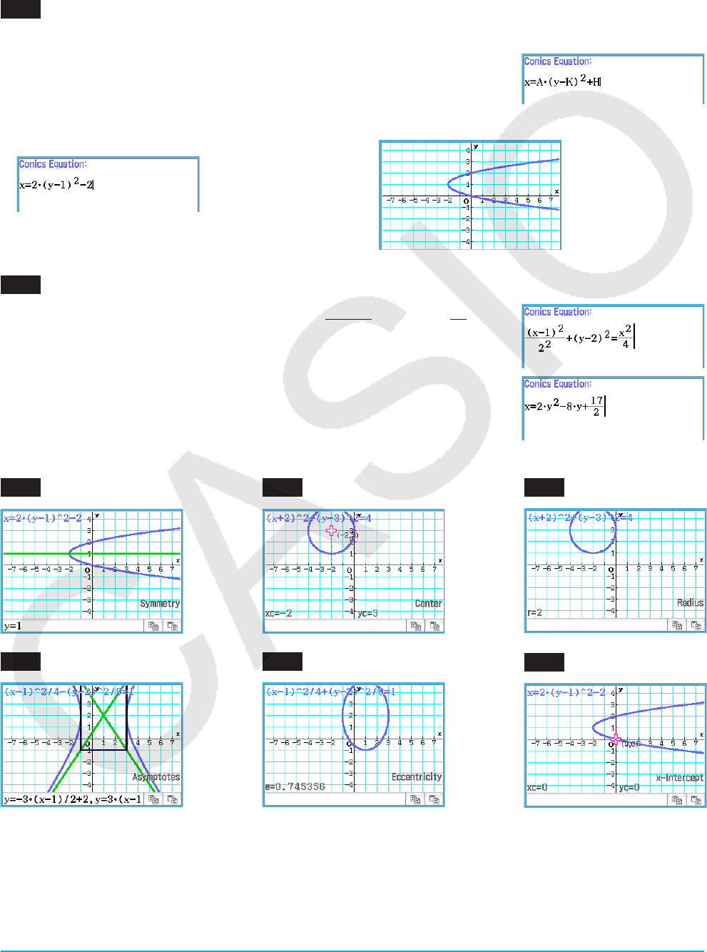
• Repeat steps 6 and 7 to modify the currently selected graph.
9. To quit graph modification, tap l on the icon panel.
0313
1. On the Graph Editor window, input ax2 – bx in line y1, and ax + b in line y2.
2. Tap a and then [Dynamic Graph] or tap 4.
3. On the menu that appears when you tap the upper left corner of the slider display box, tap [Settings].
4. On the Slider Settings dialog box that appears, use the [Slider 1] and [Slider 2] tabs to input the values
shown in the table below for the minimum values, maximum values, and step values of parameters a and b.
Tab Parameter Min Max Step
[Slider 1] a141
[Slider 2] b–2 2 1
5. Tap [OK] to close the dialog box.
Chapter 3: Graph & Table Application 18
6. Modify the graphs by changing the value of parameter a or b.
• To change parameter a and b values, tap the L or R buttons to increase or decrease the value by the
Step value, or tap the upper left corner of the slider display box and then tap [Auto Play] on the menu that
appears.
• If you tapped [Auto Play], tap l or press c to stop graph form modification.
Chapter 4: Conics Application 19
Chapter 4:
Conics Application
0401
1. On the Conics Editor window, tap q to display the Select Conics Form dialog box.
2. Select “x = A(y – K)2 + H” and then tap [OK].
• This inputs “x = A(y – K)2 + H” in the Conics Editor window.
3. Change the parameters of the equation as follows:
A = 2, K = 1, H = –2.
4. Tap ^ to graph the equation.
0402
1. On the Conics Editor window, input the equation (x − 1)2
22
x2
4
+ (y − 2)2 = .
2. Tap w to display the Select Conics Form dialog box, select “x = Ay2 + By +
C”, and then tap [OK].
• This transforms the equation to the form you selected.
0403 Symmetry 0404 Center 0405 Radius
0406 Asymptotes 0407 Eccentricity 0408 x-Intercept
Chapter 4: Conics Application 20
0409
1. On the Conics Editor window, tap q to display the Select Conics Form dialog box.
2. Select “x = Ay2 + By + C” and then tap [OK].
• This inputs “x = A
·
y2 + B
·
y + C” in the Conics Editor window.
3. Tap 4.
• This will display sliders for changing values assigned to parameters A, B, and C.
4. On the menu that appears when you tap the upper left corner of the slider display box, tap [Settings].
5. On the Slider Settings dialog box that appears, use the [Slider 1], [Slider 2], and [Slider 3] tabs to input the
values shown below for the settings of parameters A, B, and C.
Value: –2, Min: –2, Max: 2, Step: 1
6. Tap [OK] to close the dialog box.
7. Modify the graphs by changing the value of parameter A, B, or C.
• Use the L and R buttons of the A, B, and C sliders to change the value assigned to increase or
decrease the value assigned to each parameter by the Step value.
• Tapping the upper left corner of the slider display box and then tapping [Auto Play] on the menu that
appears will automatically cycle the value assigned to the applicable parameter between its minimum and
maximum values.
(Simultaneous execution of multiple parameters with Auto Play is not supported.)
8. To quit graph modification, tap the close button (C) in the upper right corner of the slider display box.
Chapter 5: Differential Equation Graph Application 21
Chapter 5:
Differential Equation Graph Application
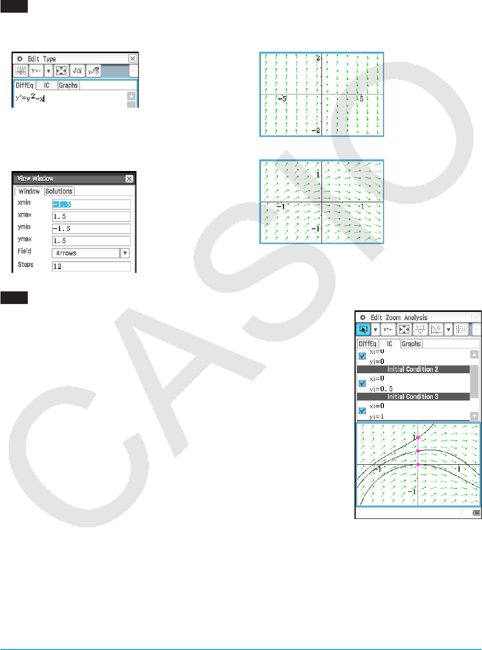
0501
1. On the Differential Equation Editor window, tap [Type] - [1st (Slope Field)] or A.
2. Y{c-Xw3. Tap O to draw the slope field.
4. Tap 6, and configure the View Window settings
as shown below.
5. Tap [OK].
This updates the slope field in accordance with the
new View Window settings.
0502
1. Activate the Differential Equation Editor window and then tap the [IC] tab.
• This displays the initial condition editor.
2. On the initial condition editor, input the following initial conditions:
(xi, yi) = (0, 0), (0, 0.5), (0, 1).
3. Tap O.
• This graphs the three solution curves over the slope field of y’ = y2 – x.
Chapter 5: Differential Equation Graph Application 22
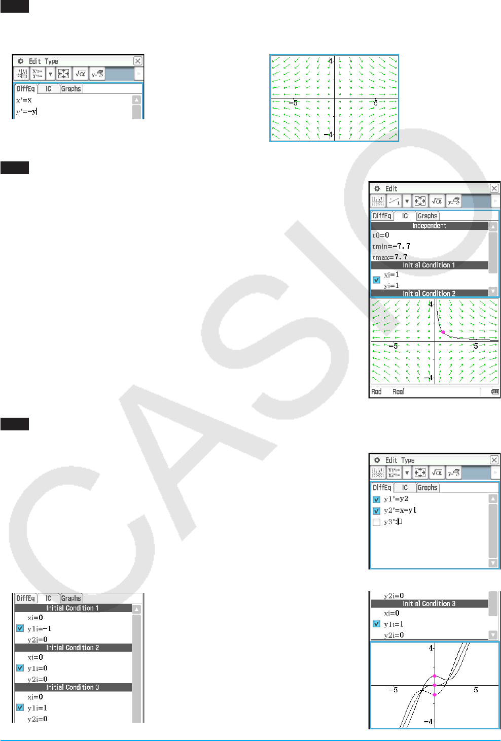
0503
1. On the Differential Equation Editor window, tap [Type] - [2nd (Phase Plane)] or B.
2. Xw-Yw3. Tap O to draw the phase plane.
0504
1. Activate the Differential Equation Editor window and then tap the [IC] tab.
• This displays the initial condition editor.
2. Input (xi, yi) = (1, 1) on the initial condition editor.
3. Tap O.
• This graphs the solution curve and overlays it on the phase plane of x’ = x,
y’ = −y.
0505
1. On the Differential Equation Editor window, tap [Type] - [Nth (No Field)] or 9.
2. Input y’’ = x − y by dividing it into two first order differential equations. If
we let y1 = y and y2 = y’, we see that y1’ = y’ = y2 and y2’ = y’’ = x − y1.
Ycw
X-Ybw
3. Tap the [IC] tab to display the initial condition editor.
4. Input (xi, y1i, y2i) = (0, −1, 0), (0, 0, 0), (0, 1, 0). 5. Tap O.
Chapter 5: Differential Equation Graph Application 23
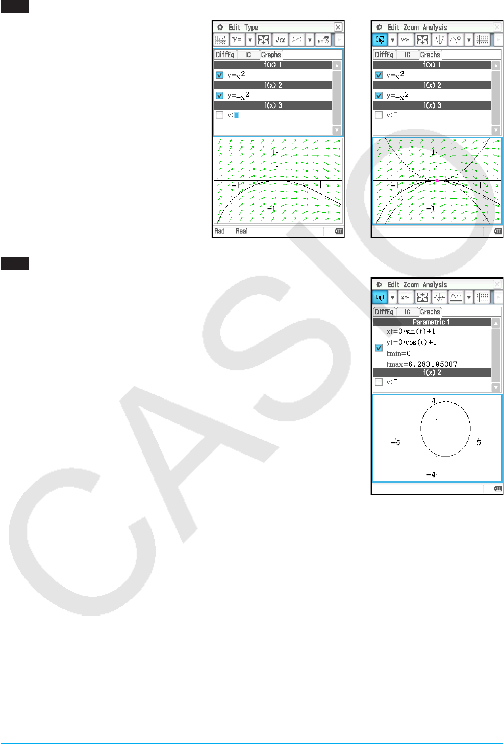
0506
1. On the Differential Equation Editor
window, tap the [Graphs] tab.
2. Tap [Type] - [ f ( x)] or d, and then input
y = x2 and y = −x2.
3. Tap O.
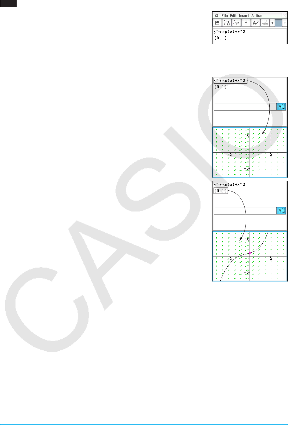
• This will overlay the graphs of y = x2
and y = −x2 on the differential equation
graph.
0507
1. On the Differential Equation Editor window, tap the [Graphs] tab.
2. Confirm that “Rad” is displayed as the angle unit setting on the left side of
the status bar. If it isn’t, tap the angle setting until “Rad” is displayed.
3. Tap [Type] - [Parametric] or g, and then input the expression for the graph
xt = 3sin(t) + 1 and yt = 3cos(t) + 1, and 0 s t s 2π for the range of t.
4. Tap O to draw the graph.
• To adjust the graph window, tap [Zoom] and then [Quick Initialize].
Chapter 5: Differential Equation Graph Application 24
0508
1. Start up the eActivity application and input the following expression and
matrix.
y’ = exp(x) + x2
[0,1]
2. From the eActivity application menu, tap [Insert], [Strip(2)], and then
[DiffEqGraph].
• This inserts a Differential Equation Graph data strip, and displays the Differential Equation Graph window in
the lower half of the screen.
3. Drag the stylus across “y’ = exp(x) + x2” on the eActivity application window
to select it.
4. Drag the selected expression to the Differential Equation Graph window.
• This draws the slope field of y’ = exp(x) + x2 and registers the equation in
the differential equation editor ([DiffEq] tab).
5. Drag the stylus across “[0,1]” on the eActivity application window to select it.
6. Drag the selected matrix to the Differential Equation Graph window.
• This graphs the solution curve of y’ = exp(x) + x2 in accordance with the
initial condition defined by the matrix and registers the initial condition in
the initial condition editor ([IC] tab).
Chapter 5: Differential Equation Graph Application 25
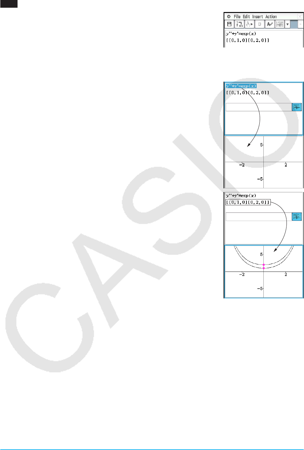
0509
1. Start up the eActivity application and input the following expression and
matrix.
y” + y’ = exp(x)
[[0,1,0][0,2,0]]
2. From the eActivity application menu, tap [Insert], [Strip(2)], and then
[DiffEqGraph].
• This inserts a Differential Equation Graph data strip, and displays the Differential Equation Graph window in
the lower half of the screen.
3. Drag the stylus across “y” + y’ = exp(x)” on the eActivity application window
to select it.
4. Drag the selected expression to the Differential Equation Graph window.
• This registers y” + y’ = exp(x) on the differential equation editor ([DiffEq]
tab). The Differential Equation Graph window contents do not change at
this time.
5. Drag the stylus across “[[0,1,0][0,2,0]]” on the eActivity application window to
select it.
6. Drag the selected matrix to the Differential Equation Graph window.
• This graphs the solution curves of y” + y’ = exp(x) in accordance with the
initial condition defined by the matrix, and registers the initial condition in
the initial condition editor ([IC] tab).
Chapter 6: Sequence Application 26
Chapter 6:
Sequence Application
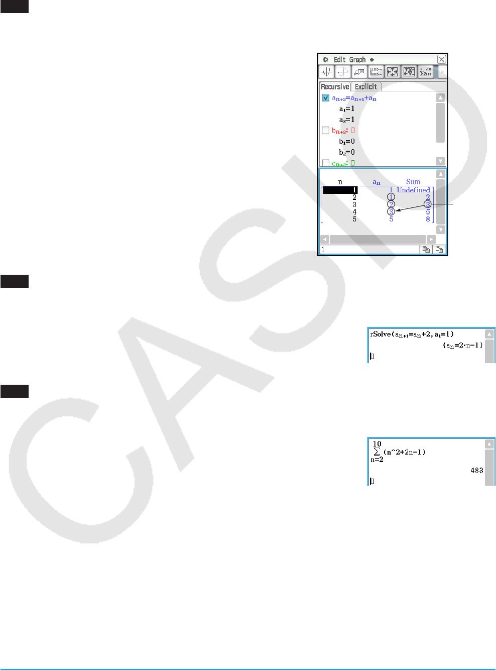
0601
1. On the Sequence Editor window, tap the [Recursive] tab.
2. Tap [Type] - [an+2Type a1,a2].
3. Input the recursion expression an+2 = an+1 + an and the initial
values a1 = 1, a2 = 1.
4. Tap 8 to display the Sequence Table Input dialog box.
5. Input the n-value range as shown below, and then tap [OK].
Start: 1 End: 5
6. Tap the down arrow button next to #, and then select ` to
create the table.
−3 = 2 + 1
0602
1. On the Sequence Editor window, tap ` to display the Sequence RUN window.
2. Tap [Calc] - [rSolve] to input the rSolve function.
3. As the argument of the rSolve function, input the expression “an+1 = an + 2,
a1 = 1”.
4. Press E.
0603
1. On the Sequence Editor window, tap ` to display the Sequence RUN window.
2. Tap [Calc] - [Σ] to input the Σ function.
3. As the arguments of the Σ function, specify the range of n = 2 to 10 and input
the expression “anE = n2 + 2n − 1”.
4. Press E.
Chapter 6: Sequence Application 27
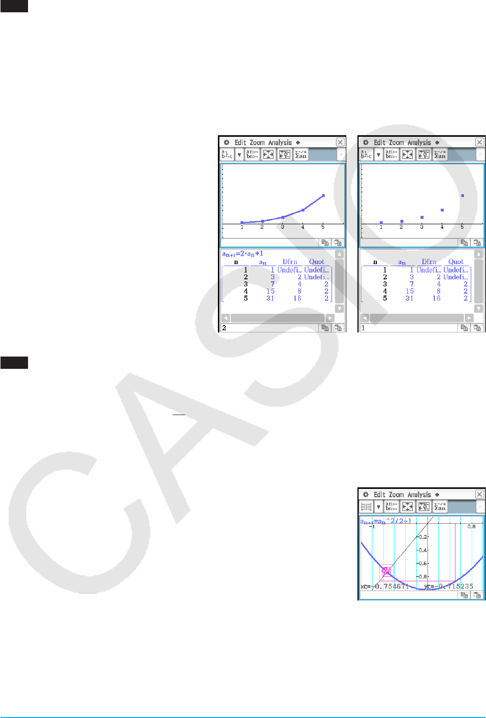
0604
1. On the Sequence Editor window, tap the [Recursive] tab.
2. Tap [Type] - [an+1Type a1].
3. Input the recursion expression an+1 = 2an + 1 and the initial values a1 = 1.
4. Tap the down arrow button next to #, and then select + to create the table.
5. Tap 6, configure View Window settings as shown below, and then tap [OK].
xmin = 0 xmax = 6 xscale = 1 xdot: (Specify auto setting.)
ymin = –15 ymax = 65 yscale = 5 ydot: (Specify auto setting.)
6. Tap $ to draw a connect type graph, or tap
! to draw a plot type graph.
In this example, “4 Cells” is selected for the
[Cell Width Pattern] setting of the Graph
Format dialog box (see “1-7 Configuring
Application Format Settings” in the User’s
Guide).
Connect type graph Plot type graph
0605
1. On the Sequence Editor window, tap the [Recursive] tab.
2. Tap [Type] - [an+1Type a1].
3. Input the recursion expression an+1 =
− 1 and the initial values a1 = 0.5.
4. Tap the Table window to make it active.
5. Tap 6, configure View Window settings as shown below, and then tap [OK].
xmin = −1.2 xmax = 1 xscale = 0.2
ymin = −1 ymax = 0.1 yscale = 0.2
6. Tap w to start drawing a cobweb diagram.
7. Press E for each step of the web.
On the cobweb graph window, you can restart drawing of the cobweb diagram by selecting [Trace] on the
[Analysis] menu.
Chapter 7: Statistics Application 28
Chapter 7:
Statistics Application
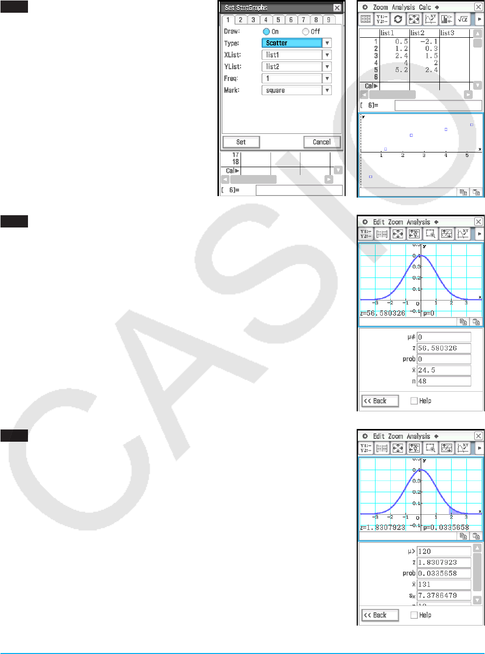
0701
1. On the Stat Editor window, input the two lists
(list1 = 0.5, 1.2, 2.4, 4.0, 5.2, list2 = −2.1,
0.3, 1.5, 2.0, 2.4).
2. Tap G to display the Set StatGraphs dialog
box.
3. Configure the settings shown in the screen
to the right and then tap [Set].
4. Tap y to draw the scatter plot.
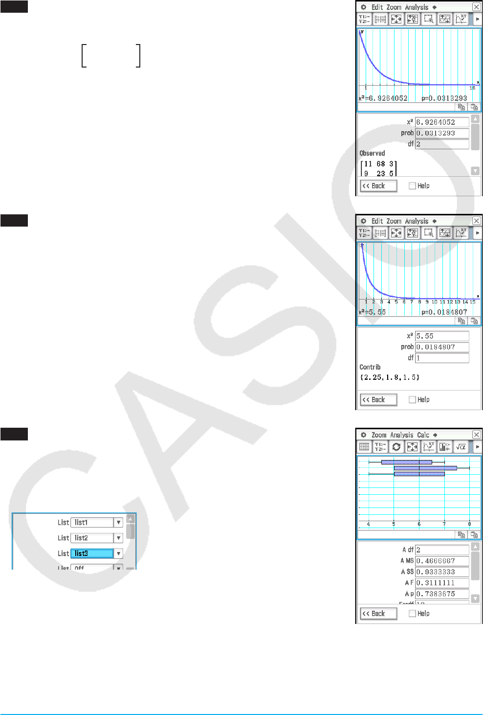
0702
1. On the Stat Editor window, tap [Calc] - [Test] .
2. Select [One-Sample Z-Test] and [Variable], and then tap [Next>>].
3. Select the μ condition [⫽] and input values.
μ0 = 0, σ = 3, o = 24.5, n = 48
4. Tap [Next>>] to display the calculation results.
5. Tap $ to graph the results.
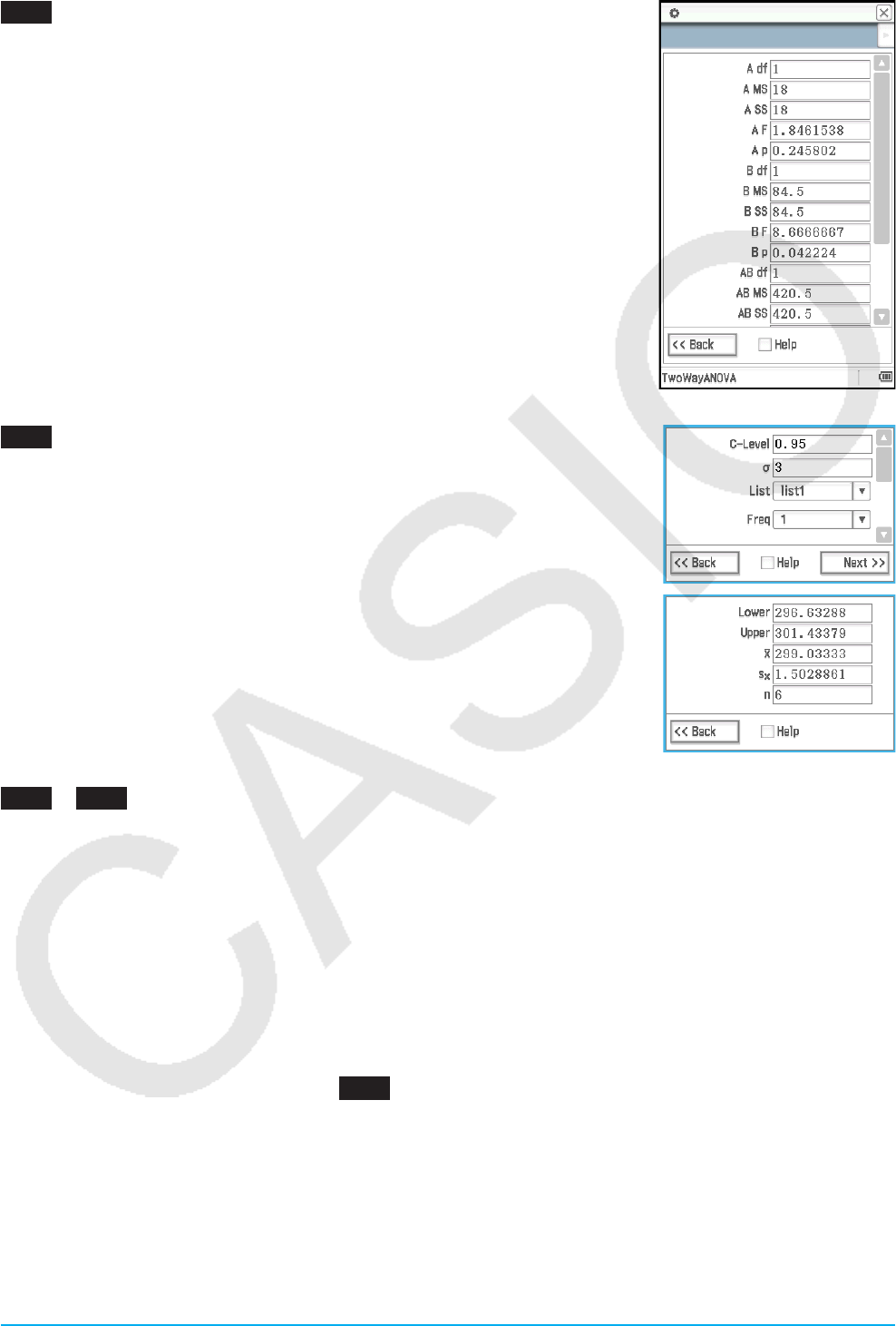
0703
1. Input the list data into [list1] and [list2] in the Stat Editor.
list1 = {120,125,130,135,140,145}, list2 = {1,2,4,1,1,1}
2. Tap [Calc] - [Test].
3. Select [One-Sample Z-Test] and [List], and then tap [Next>>].
4. Select the μ condition [>] and input values.
μ0 = 120, σ = 19
5. Select List [list1] and Freq [list2].
6. Tap [Next>>] to display the calculation results.
7. Tap $ to graph the results.
Chapter 7: Statistics Application 29
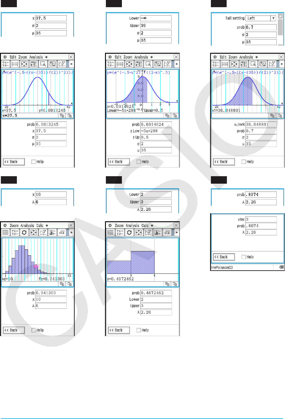
0704
1. On the Stat Editor window, tap ~ to display the Main application work area
window.
2. Input the matrix 11 68 3
9 23 5 and assign it to variable a (see “2-5 Matrix and
Vector Calculations” in the User’s Guide).
3. Tap the Stat Editor window to make it active.
4. Tap [Calc] - [Test] - [χ2 Test] and then tap [Next>>].
5. Input “a” in the Matrix dialog box, and then tap [Next>>].
• This displays the calculation results.
6. Tap $ to graph the results.
0705
1. On the Stat Editor window, tap ~ to display the Main application work area
window.
2. Assign {1,2,3} to list1 and {4,5,6} to list2 (see “2-4 List Calculations” in the
User’s Guide).
3. Tap the Stat Editor window to make it active.
4. Tap [Calc] - [Test] - [χ2 GOF Test] and then tap [Next>>].
5. Leaving “Observed” (list1) and “Expected” (list2) at their initial default
settings, input 1 for “df”.
6. Tap [Next>>] to display the calculation results.
7. Tap $ to graph the results.
0706
1. Input the list data into [list1], [list2] and [list3] in the Stat Editor.
list1 = {7,4,6,6,5}, list2 = {6,5,5,8,7}, list3 = {4,7,6,7,6}
2. Tap [Calc] - [Test] - [One-Way ANOVA] and then tap [Next>>].
3. Select Lists [list1], [list2], and [list3].
4. Tap [Next>>] to display the calculation results.
5. Tap $ to graph the results.
Note: The screen shown nearby is displayed when the [Q1, Q3 on Data]
check box on the Basic Format dialog box is cleared (unchecked).
Chapter 7: Statistics Application 30
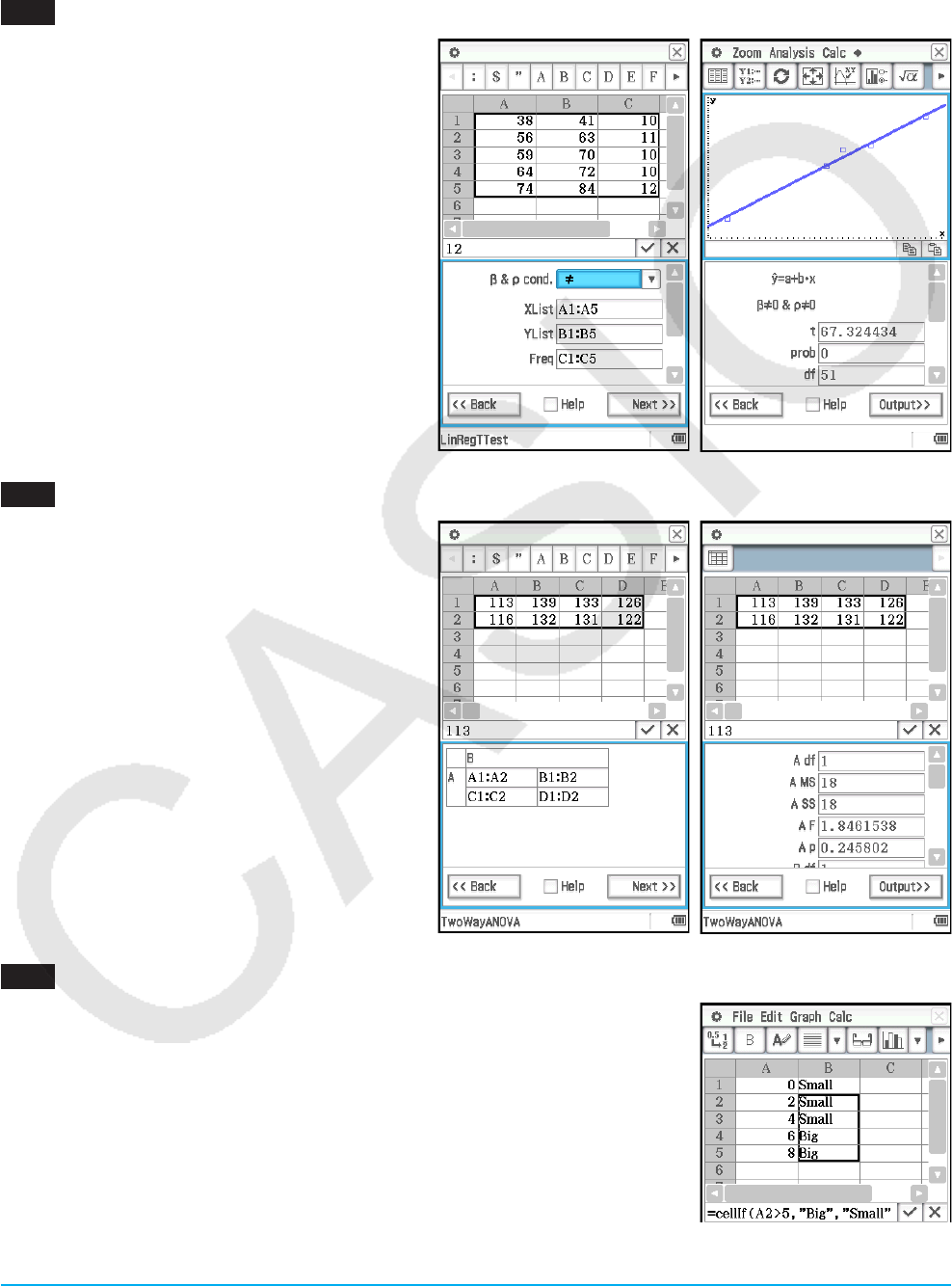
0707
1. On the Stat Editor window, tap ~ to display the Main application work area
window.
2. Assign {113,116} to list1, {139,132} to list2, {133,131} to list3, and {126,122}
to list4 (see “2-4 List Calculations” in the User’s Guide).
3. Tap the Stat Editor window to make it active.
4. Tap [Calc] - [Test] - [Two-Way ANOVA] and then tap [Next>>].
5. Select “2 × 2” as the dimensions of the ANOVA data table, and then tap
[Next>>].
6. Assign list1 for (1,1), list2 for (1,2), list3 for (2,1), and list4 for (2,2), and then
tap [Next>>].
• This displays the calculation results.
• The results indicate that altering the time is not significant, altering the
temperature is significant, and interaction between time and temperature is
highly significant.
0708
1. Input the data {299.4, 297.7, 301, 298.9, 300.2, 297} into [list1] in the Stat
Editor.
2. Tap [Calc] and then [Interval].
3. Select [One-Sample Z Int] and [List], and then tap [Next>>].
4. Input the values (C-Level = 0.95, σ = 3).
5. Select List [list1] and Freq [1].
6. Tap [Next >>] to display the calculation results.
0709 to 0714
1. On the Stat Editor window, perform the following operation:
0709: Tap [Calc] - [Distribution] - [Normal PD]
0710: Tap [Calc] - [Distribution] - [Normal CD]
0711: Tap [Calc] - [Inv. Distribution] - [Inverse Normal CD]
0712: Tap [Calc] - [Distribution] - [Poisson PD]
0713: Tap [Calc] - [Distribution] - [Poisson CD]
0714: Tap [Calc] - [Inv. Distribution] - [Inverse Poisson CD]
2. Tap [Next >>], and then input values.
3. Tap [Next >>] to display the calculation results.
4. Tap $ to graph the results (except for 0714 ).
• See the next page of this manual for the calculation result and graph screen.
Chapter 7: Statistics Application 31
0709 [Normal PD] 0710 [Normal CD] 0711 [Inverse Normal CD]
0712 [Poisson PD] 0713 [Poisson CD] 0714 [Inverse Poisson CD]
Tip: Graphing the results of one of the following calculations may take a long time when the absolute value of
the argument is large: Binomial PD, Binomial CD, Poisson PD, Poisson CD, Geometric PD, Geometric CD,
Hypergeometric PD, or Hypergeometric CD calculations.
Chapter 8: Geometry Application 32
Chapter 8:
Geometry Application
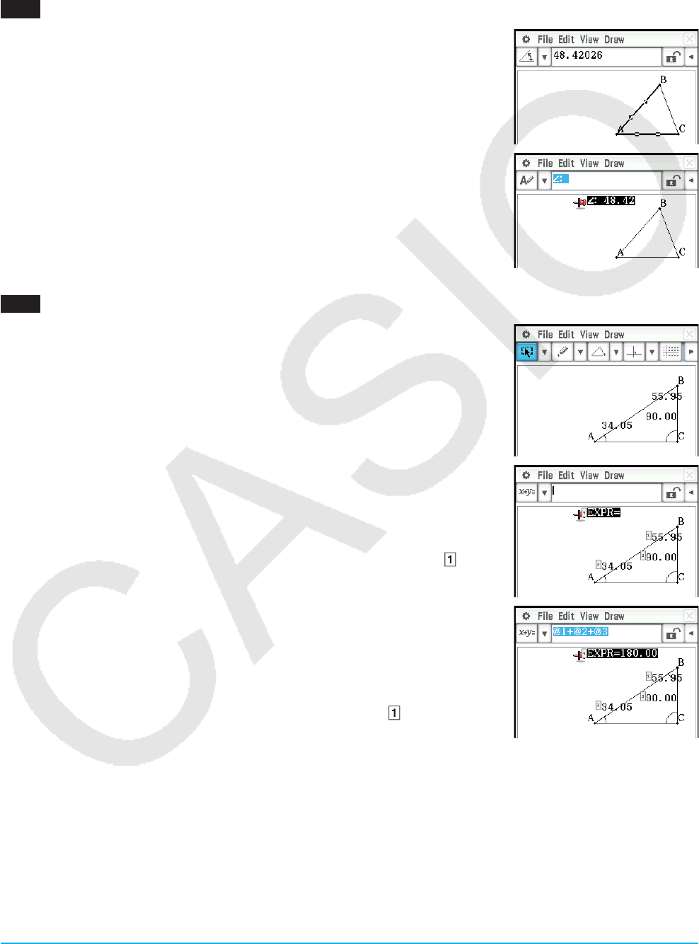
0801
1. Draw the triangle.
2. Tap G. Next, tap side AB and then side AC to select them.
3. Tap the u button to the right of the toolbar.
• This displays the measurement box, which indicates the specified angle.
4. Tap [Draw], [Measurement], and then [Angle].
• This shows the angle measurement on the screen.
• You can also perform the operation below in place of step 4.
- Select (highlight) value in the measurement box and drop it into the
Geometry window.
- Tap the Q button on the far left of the measurement box.
0802
1. Draw a triangle and then display the inside angle value of each angle.
• For information about displaying angle values, see “To attach an angle
measurement to a figure” in the User’s Guide.
2. Tap [Draw] - [Expression].
• This displays an “EXPR=” object.
3. Tap the u button to the right of the toolbar.
• This will display the measurement box and also display numeric labels for
each measurement currently on the screen.
4. Now you can use the numeric labels to specify measurement values in the
calculation you input in the measurement box.
• To input a measurement value in the measurement box, input the at
sign (@) followed by the numeric label of the value. To input value , for
example, you would input “@1”.
• Since we want to calculate the sum of the interior angles of the triangle
here, you would input the following: @1+@2+@3.
5. After inputting the calculation expression, press E.
• The calculation result is displayed to the right of “EXPR=”.
Tip: In step 4 above, you also can input the numeric label of a displayed measurement
value into the measurement box by tapping the label. Tapping , for example,
will input “@1” into the measurement box.
Chapter 8: Geometry Application 33
0803
1. Tap [Draw], [Special Polygon], and then [Regular n-gon].
• This displays the n-gon dialog box.
2.
Enter a value indicating the number of sides of the polygon, and then tap [OK].
3. Place the stylus on the screen and drag diagonally in any direction.
• This causes a selection boundary to appear, indicating the size of the
polygon that will be drawn. The polygon is drawn when you release the
stylus.
0804
1. Specify “Degree” for the Geometry Format “Measure Angle” (see “1-7 Configuring Application Format
Settings” in the User’s Guide).
2. Draw triangle ABC and select sides AB and BC.
3. Tap the u button to the right of the toolbar.
• This will display the measurement box, which shows the current value of angle B.
4. Input 90 into the measurement box
and then press E.
• This locks the angle B at 90°.
5. Tap in a blank area on the screen to deselect everything and then select the AC side.
• This displays the measurement box, which shows the length of side AC.
6. Tap .
• This causes the icon to change to , indicating that the length of AC is locked.
7. Tap the following: [Draw] - [Construct] - [Midpoint].
• This creates midpoint D on side AC.
8. Tap the following: [Draw] - [Basic Object] - [Circle].
• This deselects side AC and enters the circle drawing mode.
9. Tap point D and then point B.
• With point D as the center point, draw a circle that circumscribes triangle
ABC.
10. Tap [View] and then [Select].
• This exits the circle drawing mode and enables selection.
11. Select side AB and side AC, and then tap the following: [Draw] - [Slider] -
[Angle].
• This displays a slider.
12. On the menu that appears when you tap the upper left corner of the slider
display box, tap [Settings].
Chapter 8: Geometry Application 34
13. On the Slider Setting dialog box that appears, input 10 for Min, 80 for Max, and 10 for Step, and then tap
[OK].
14. On the menu that appears when you tap the upper left corner of the slider display box, tap [Auto Play].
• This causes angle A to change at 10° increments within the range of 10° to 80°. At this time, vertex B
moves along the circumference of the circle.
• Instead of tapping [Auto Play], you could also tap the slider L and R buttons to change angle A
manually.
15. After you are finished using the slider, tap the close button (C) in the upper right corner of the slider display
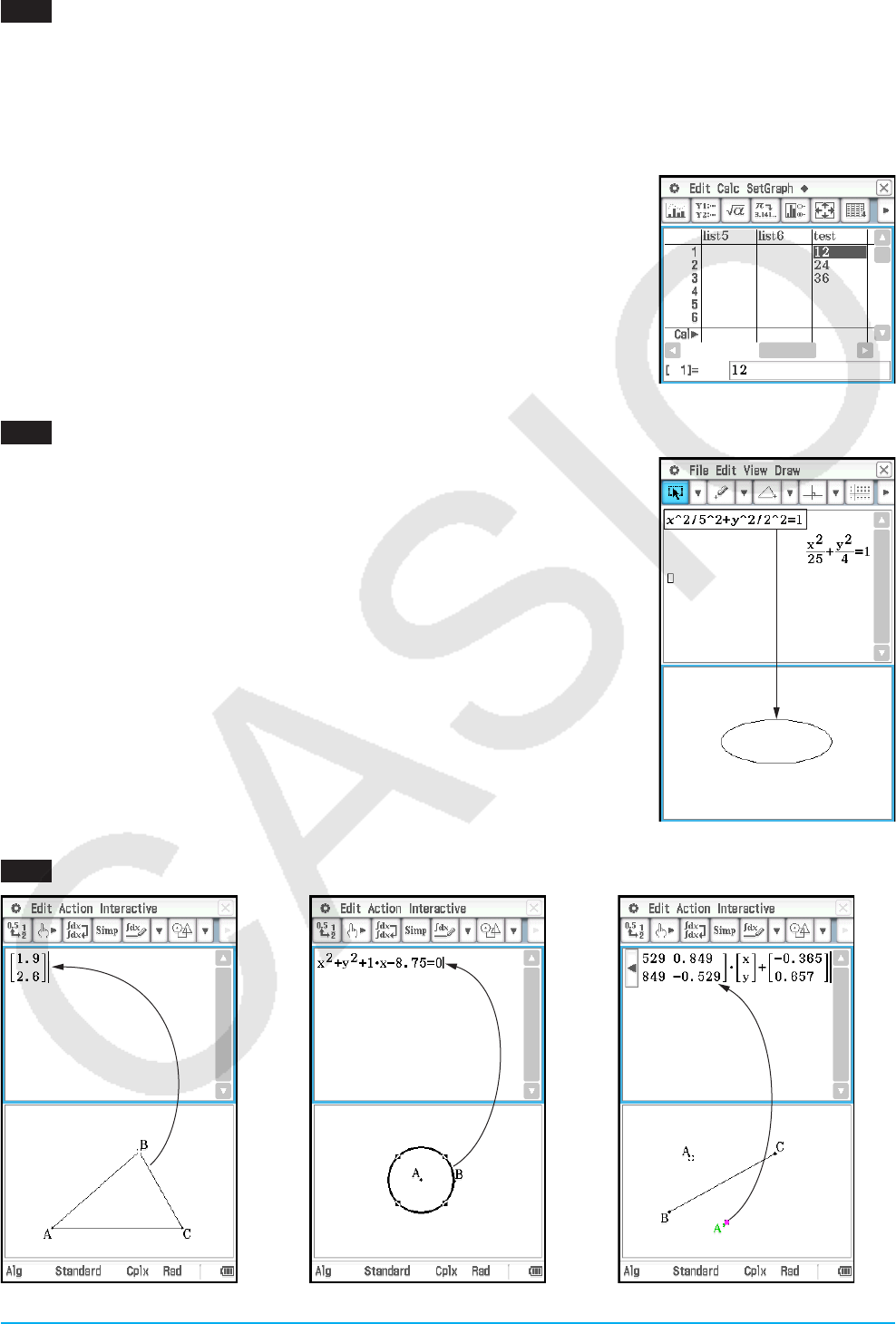
box.
0805
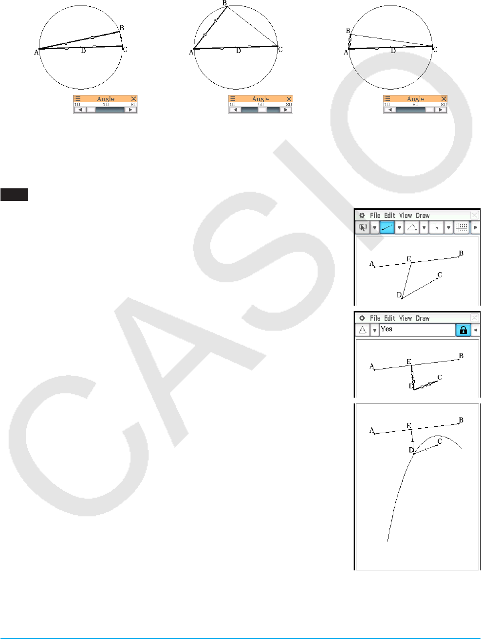
1. Draw a line segment AB and plot point C, which is not on line segment AB.
2. As shown in the nearby screen, draw line segments DE and DC.
3. Select only line segments AB and DE, and then tap u on the toolbar to
display the measurement box.
4. Input 90 into the measurement box and press E.
• This fixes the angle between AB and DE at 90 degrees.
5. Select only line segments DE and DC, and then tap the down arrow next to
the measurement box.
6. Tap the e icon, and then select the check box to the right of the
measurement box.
• This makes line segments DE and DC congruent in length.
7. Select only point E and line segment AB, and then tap [Edit] - [Animate] -
[Add Animation].
8. Select only point D, and then tap [Edit] - [Animate] - [Trace].
• This should cause a parabola to be traced on the display. Note that line
segment AB is the directrix and point C is the focus of the parabola.
9. Tap [Edit], [Animate], and then [Go (once)].
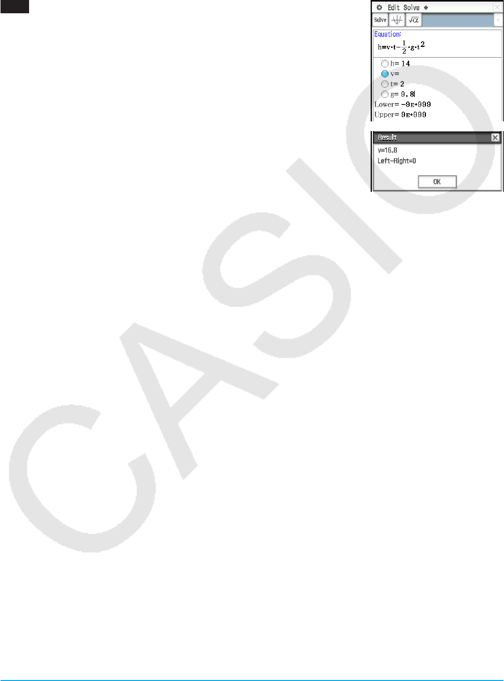
Chapter 9: Numeric Solver Application 35
Chapter 9:
Numeric Solver Application
0901
1. On the Numeric Solver window, input the equation:
h = vt – 1/2 gt2
2. On the list of expression variables that appears, enter values for the
variables:
h = 14, t = 2, and g = 9.8.
3. Here, we will solve for v, so tap the option button to the left of variable v.
4. Tap 1.
• The [Left–Right] value shows the difference between the left side and right
side results.
Chapter 10: eActivity Application 36
Chapter 10:
eActivity Application
1001
1. On the eActivity window, tap [Insert], [Strip(1)], and then [Graph].
• This inserts a Graph strip, and displays the Graph window in the lower half of the screen.
2. On the Graph window, tap ! to display the Graph Editor window.
3. Enter functions to graph, and then tap $ to graph the functions.
Graph window
eActivity window Graph Editor window
4. After you finish performing the operation you want, tap C to close the Graph window.
5. Tap the Graph Editor window, and then tap C to return to the eActivity
window.
6. Enter the title you want in the Graph strip title box.
1002
1. On the eActivity window, tap [Insert], [Strip(1)], and then [Notes].
• This inserts a Notes strip and displays the Notes window in the lower half
of the screen.
2. Enter text you want in the Notes window.
3. After you finish entering text, you can close the Notes window by tapping
C.
Tip: The expand button of a data strip is highlighted to indicate that it is expanded in
the lower window.
Chapter 11: Financial Application 37
Chapter 11:
Financial Application
The operations in the examples below can be started from any Financial application window.
1101 Compound Interest
What will be the value of an ordinary annuity at the end of 10 years if $100 is
deposited each month into an account that earns 7% compounded monthly?
Before performing the calculation, change the “Odd Period” setting to
“Compound (CI)” and the “Payment Date” to “End of period”.
1. Tap [Calc(1)] - [Compound Interest].
2. Input the values below into the applicable fields
N = 120 (12 months × 10 years), I% = 7, PV = 0,
PMT = –100, P/Y = 12 (month), C/Y = 12 (month)
3. Tap [FV] to obtain the future value.
1102 Cash Flow
How much should you be willing to pay (NPV) for an investment with the cash
flow values shown in the nearby table, if your required rate of return (I%) is
10% per year?
Period Cash Flow
00
1 100
2 200
3 300
4 400
5 500
1. Tap ( to open the Stat Editor window in the lower half of the display.
2. Input the cash flow values in cells 1 through 6 under “list1”.
3. Tap the Cash field (which currently shows “<empty>”).
4. On the dialog box that appears, select “list1” for “List variables”, and then tap
[OK].
5. Input 10 into the I% field.
6. Tap [NPV] to obtain the net present value.
1103 Amortization
In this example, first use a Compound Interest page to calculate the monthly
payment of a loan, and then use the result to perform Amortization page
calculations. Specify “Compound (CI)” for “Odd Period”, and “End of period” for
“Payment Date”.
Page 1 (Compound Interest): Use a Compound Interest page to determine
the monthly payment ([PMT]) on a 20-year (N = 20 × 12 = 240) mortgage
with a loan amount (PV) of $100,000 at an annual rate (I%) of 8.025%,
compounded monthly (C/Y = 12). There are 12 payment periods per year
(P/Y). Be sure to input zero for the future value (FV), which indicates that
the loan will be completely paid off at the end of 20 years (240 months). Page 1 calculation results
Chapter 11: Financial Application 38
Page 2 (Amortization): Use the monthly payment value you obtained on
Page 1 (PMT = –837.9966279) to determine the following information for
payment 10 (PM1) through 15 (PM2).
• The balance (BAL) of the principal remaining after payment 15
• The interest amount (INT) included in payment 10
• The principal amount (PRN) included in payment 10
• Total interest to be paid (ΣINT) from payment 10 to payment 15
• Total principal to be paid (ΣPRN) from payment 10 to payment 15
As on Page 1, the mortgage has a loan amount (PV) of $100,000 at an
annual rate (I%) of 8.025%, compounded monthly (C/Y = 12) for 20 years.
Page 2 calculation results
Page 1 (Compound Interest) operations:
1. Tap [Calc(1)] - [Compound Interest].
2. Input the values below into the applicable fields.
N = 240, I% = 8.025, PV = 100000, FV = 0, P/Y = 12, C/Y = 12
3. Tap [PMT] to obtain the payment value.
Page 2 (Amortization) operations:
4. Tap [Calc(1)] - [Amortization].
• PV, I%, and PMT values will automatically be copied from Page 1 to
Page 2.
5. Input 10 for PM1 and 15 for PM2.
6. Tap [BAL], [INT], [PRN], [ΣINT], and then [ΣPRN].
1104 Interest Conversion
What is the nominal interest rate ([APR]) on a certificate that offers an annual
effective interest rate ([EFF]) of 5%, compounded bi-monthly (N = 6)?
1. Tap [Calc(1)] - [Interest Conversion].
2. Input 6 for N and 5 for EFF.
3. Tap [APR] to obtain the nominal interest rate.
1105 Cost/Sell/Margin
What is the selling price ([Sell]) required to obtain a margin of profit ([Margin])
of 60% on an item that cost $40 ([Cost])?
1. Tap [Calc(1)] - [Cost/Sell/Margin].
2. Input 60 for Margin and 40 for Cost.
3. Tap [Sell] to obtain the selling price.
1106 Day Count
How many days ([Days]) are there from March 3, 2005 (d1) to June 11, 2005
(d2)? Be sure to change the “Days in Year” setting to “365 days” before
performing a Day Count calculation.
1. Tap [Calc(1)] - [Day Count].
2. Input dates for d1 and d2.
3. Tap [Days] to obtain the number of days.
Chapter 11: Financial Application 39
1107 Depreciation
Use the sum-of-the-years’-digits method ([SYD]) to calculate the first year
( j = 1) of depreciation on an $12,000 (PV) computer, with a useful life (N) of
five years.
Use a depreciation ratio (I%) of 25%, and assume that the computer can be
depreciated for a full 12 months in the first year (YR1). Next, calculate the
depreciation amount ([SYD]) for the second year ( j = 2).
First year
Second year
Calculate the depreciation amount for the first year:
1. Tap [Calc(1)] - [Depreciation].
2. Input the values below into the applicable fields.
N = 5 (years), I% = 25, PV = 12000, FV = 0*, j = 1, YR1 = 12
3. Tap [SYD].
• This displays the depreciation amount for the first year in the [SYD] field,
and the residual value after depreciation for the first year in the RDV field.
Calculate the depreciation amount for the second year:
4. Change the j value to 2, and then tap [SYD].
* At the end of the useful life the value of the computer will be 0, so we enter 0
in the FV field.
Note: You can also tap [SL] to calculate depreciation using straight-line method, [FP] using fixed-percentage
method, or [DB] using declining-balance method. Each depreciation method will produce a different
residual value after depreciation (RDV) for the applicable year ( j ).
1108 Bond Calculation
You want to purchase a semiannual corporate bond that matures on
12/15/2006 (d2) to settle on 6/1/2004 (d1). The bond is based on the 30/360
day-count method with a coupon rate (CPN) of 3%. The bond will be redeemed
at 100% of its par value (RDV). For 4% yield to maturity (YLD), calculate the
bond’s price ([PRC]) and accrued interest (INT).
Before performing the calculation, change the “Days in Year” setting to
“360 days”, “Bond Interval” to “Date”, and the “Compounding Frequency” to
“Semiannual”.
1. Tap [Calc(1)] - [Bond Calculation].
2. Input the values below into the applicable fields.
d1 = 6/1/2004, d2 = 12/15/2006, RDV = 100, CPN = 3, YLD = 4
3. Tap [PRC].
• This displays the bond’s price in the [PRC] field, accrued interest in the INT
field, and cost of bond in the Cost field.
Chapter 11: Financial Application 40
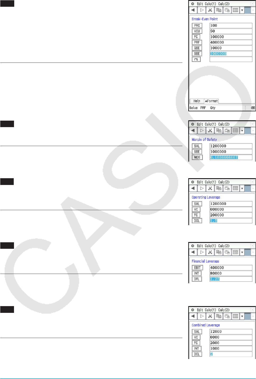
1109 Break-Even Point
Your company is producing items with a unit variable cost ([VCU]) of $50/
unit and fixed costs ([FC]) of $100,000. The items will be sold for a sales price
([PRC]) of $100/unit.
What is the break-even point sales amount ([SBE]) and sales quantity ([QBE])
required for a profit ([PRF]) of $400,000?
Before performing the calculation, change the “Profit Amount/Ratio” setting to
“Amount (PRF)” and the “Break-Even Value” to “Quantity”.
1. Tap [Calc(2)] - [Break-Even Point].
2. Input the values below into the applicable fields.
PRC = 100, VCU = 50, FC = 100000, PRF = 400000
3. Tap [QBE] to obtain the sales quantity.
4. Tap [SBE] to obtain the break-even point sales amount.
1110 Margin of Safety
What is the margin of safety ([MOS]) when the sales amount ([SAL]) is
$1,200,000 and the break-even sales amount ([SBE]) is $1,000,000?
1. Tap [Calc(2)] - [Margin of Safety].
2. Input 1200000 into the [SAL] field and 1000000 into the [SBE] field, and then
tap [MOS].
1111 Operating Leverage
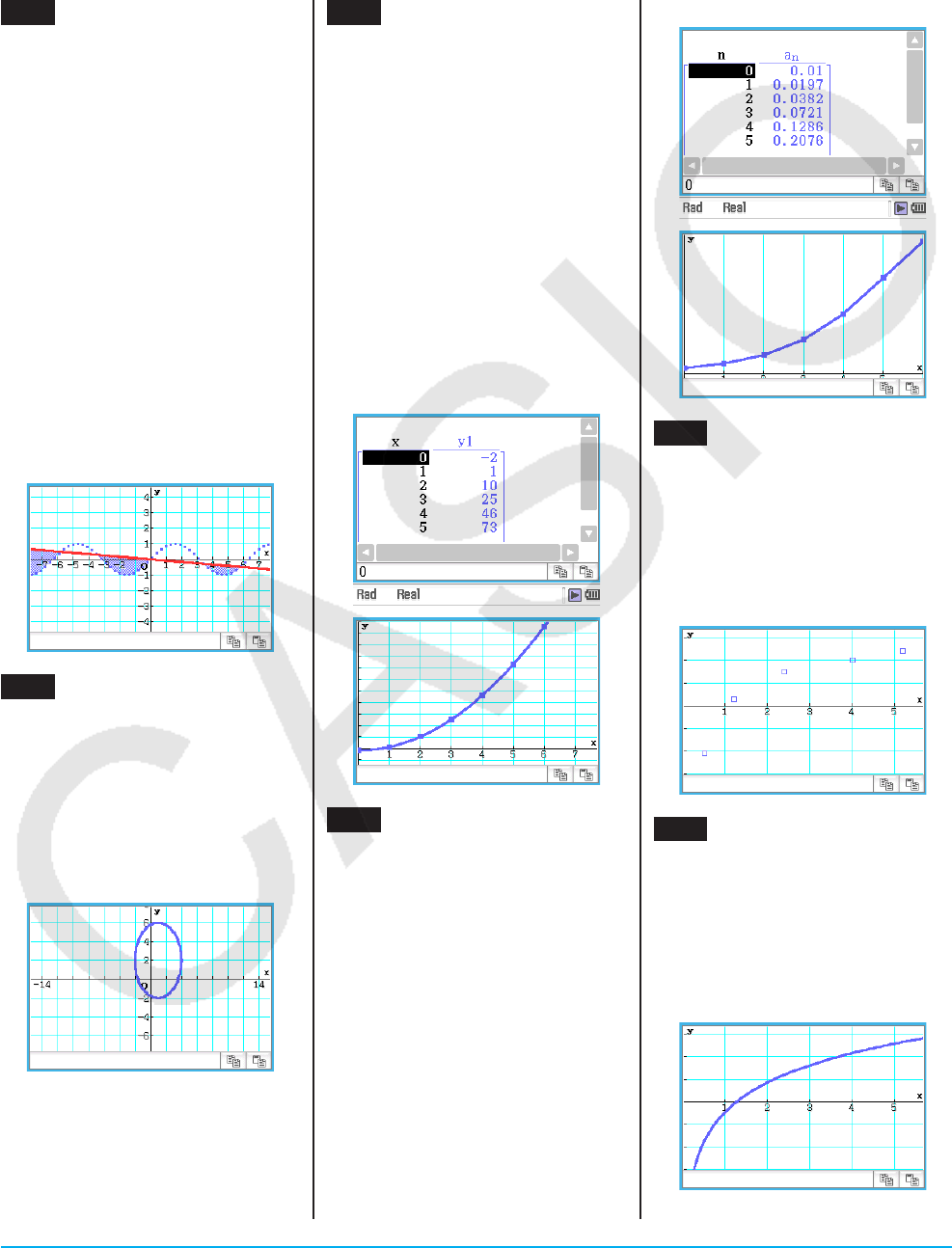
What is the degree of operating leverage for a company with sales ([SAL])
of $1,200,000, variable costs ([VC]) of $600,000, and fixed costs ([FC]) of
$200,000?
1. Tap [Calc(2)] - [Operating Leverage].
2. Input 1200000 into the [SAL] field, 600000 into the [VC] field, and 200000
into the [FC] field, and then tap [DOL].
1112 Financial Leverage
Calculate the financial leverage ([DFL]) for a company that earns $400,000
before interest and taxes ([EBIT]), $80,000 of which is paid to bondholders
([INT]).
1. Tap [Calc(2)] - [Financial Leverage].
2. Input 400000 into the [EBIT] field and 80000 into the [INT] field, and then tap
[DFL].
1113 Combined Leverage
Calculate the Combined Leverage ([DCL]) for a company with variable costs
([VC]) of $6,000, fixed costs ([FC]) of $2,000, and sales ([SAL]) of $12,000, of
which $1,000 is paid to bondholders ([INT]).
1. Tap [Calc(2)] - [Combined Leverage].
2. Input 12000 into the [SAL] field, 6000 into the [VC] field, 2000 into the [FC]
field, and 1000 into the [INT] field, and then tap [DCL].

Chapter 11: Financial Application 41
1114 Quantity Conversion
Calculate the sales quantity (Sales: [QTY]) when the sales amount ([SAL]) is
$100,000 and the sales price ([PRC]) is $200 per unit. Next, calculate the total
variable costs of production (Manufacturing: [VC]) when the variable cost per
unit ([VCU]) is $30 and the number of units manufactured ([QTY]) is 500.
1. Tap [Calc(2)] - [Quantity Conversion].
2. Input 100000 into the [SAL] field and 200 into the [PRC] field, and then tap
[QTY].
3. Input 30 into the [VCU] field and 500 into the [QTY] field, and then tap [VC].
Chapter 12: Program Application 42
Chapter 12:
Program Application
Note: The notation in the “Program” uses 䡺 to represent a space and _ for a carriage return.
1201
Program:
DefaultSetup_
ClrGraph_
ViewWindow_
SetInequalityPlot䡺
Intersection_
GraphType䡺"y>"_
Define䡺y1(x)=sin(x)_
GTSelOn䡺1_
PTDot䡺1_
SheetActive䡺1_
DrawGraph_
GraphType䡺"y<"_
Define䡺y2(x)=−x/12_
GTSelOn䡺2_
PTNormal䡺2_
SheetActive䡺1_
DrawGraph
Result screen:
1202
Program:
ClrGraph_
ViewWindow䡺–15.4,15.4,2,–7.6,
7.6,2_
"(x–1)^2/3^2+(y–2)^2/4^2= 1"
SConicsEq_
DrawConics
Result screen:
1203
Program:
DefaultSetup_
ClrGraph_
ViewWindow䡺0,7.7,1,–14,110,
10_
GraphType䡺"y="_
Define䡺y1(x)=3×x^2–2_
GTSelOn䡺1_
0SFStart_
6SFEnd_
1SFStep_
SheetActive䡺1_
DispFTable_
Pause_
DrawFTGCon
Result screen:
1204
Program:
DefaultSetup_
ViewWindow䡺0,6,1,−0.01,0.3,1_
SeqType "an+1a0"_
"−3an^2+2an"San+1_
0SSqStart_
6SSqEnd_
0.01Sa0_
DispSeqTbl_
Pause_
DrawSeqCon
Result screen:
1205
Program:
{0.5,1.2,2.4,4,5.2}Slist1_
{–2.1,0.3,1.5,2,2.4}Slist2_
StatGraph䡺1, On, Scatter, list1,
list2, 1, Square_
DrawStat
Result screen:
1206
Program:
{0.5,1.2,2.4,4,5.2}Slist1_
{–2.1,0.3,1.5,2,2.4}Slist2_
StatGraph䡺1, On, LogR, list1,
list2, 1_
DrawStat
Result screen:
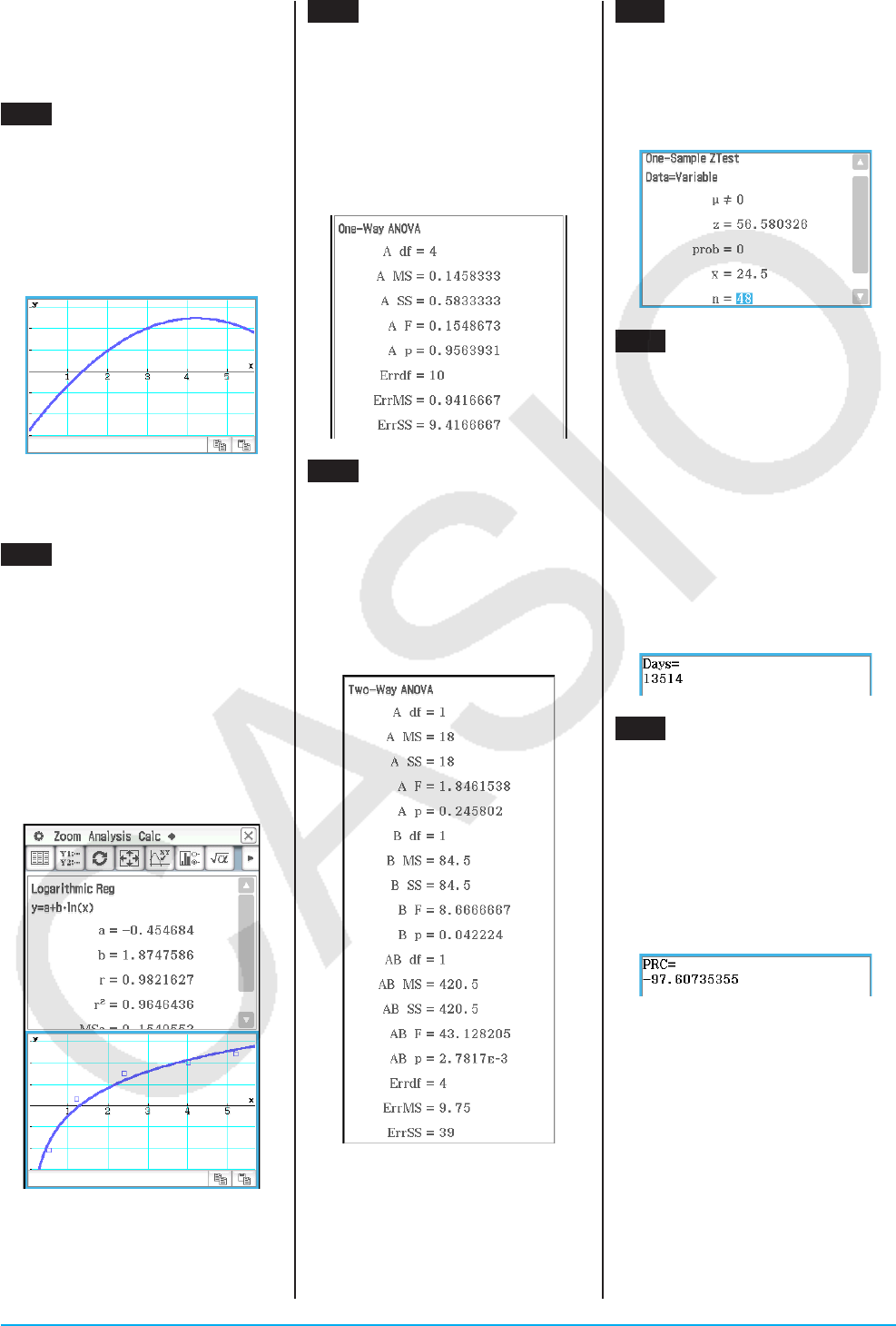
Chapter 12: Program Application 43
Note: MedMed, QuadR, CubicR,
QuartR, LinearR, ExpR, abExpR,
or PowerR can also be specified in
instead of LogR for the graph type.
1207
Program:
{0.5,1.2,2.4,4,5.2}Slist1_
{–2.1,0.3,1.5,2,2.4}Slist2_
StatGraph䡺1, On, SinR, list1,
list2_
DrawStat
Result screen:
Note: LogisticR can also be
specified in instead of SinR for the
graph type.
1208
Program:
StatGraphSel䡺Off
{0.5,1.2,2.4,4,5.2}Slist1_
{–2.1,0.3,1.5,2,2.4}Slist2_
StatGraph䡺1, On, Scatter, list1,
list2, 1, Square_
DrawStat_
LogReg䡺list1, list2, 1_
DispStat_
DrawStat
Result screen:
1209
Program:
{7,4,6,6,5,6,5,5,8,7,4,7,6,7,6}
Slist1_
{1,1,1,1,1,2,2,2,2,2,3,3,3,3,3}
Slist2_
OneWayANOVA䡺list1, list2_
DispStat
Result screen:
1210
Program:
{1,1,1,1,2,2,2,2}Slist1_
{1,1,2,2,1,1,2,2}Slist2_
{113,116,139,132,133,131,126,
122}Slist3_
TwoWayANOVA list1, list2, list3_
DispStat
Result screen:
1211
Program:
OneSampleZTest䡺"≠",0,3,24.5,
48_
DispStat
Result screen:
1212
Program:
Input Month_
Input Date_
Input Year_
DateMode365_
dayCount(07,04,1976,Month,
Date,Year)Sdays_
Print "Days="_
Print days
Result screen:
Shows the result for the following
input: Month: 7, Date: 4, Year:
2013.
1213
Program:
DateMode360_
PeriodsSemi_
bondPriceDate(6,1,2004,12,15,
2006,100,3,4)Slist1_
list1[1]Sprice_
Print "PRC="_
Print approx(price)
Result screen:
Chapter 13: Spreadsheet Application 44
Chapter 13:
Spreadsheet Application
1301
1. On the Spreadsheet window, input the data
and then select input range cells A1:C5.
2. Tap [Calc] - [Test] - [Linear Reg t-Test], and
then tap [Next>>].
• This will automatically insert the cell
references into the fields as shown in the
nearby screen shot.
3. Tap [Next>>].
4. Tap $ to draw the linear regression graph.
1302
1. On the Spreadsheet window, input the data
and then select input range cells A1:D2.
2. Tap [Calc] - [Test] - [Two-Way ANOVA], and
then tap [Next>>].
3. Select “2 × 2” as the dimensions of the
ANOVA data table, and then tap [Next>>].
4. After confirming that cell references have
been automatically inserted into the fields
as shown in the nearby screen shot, tap
[Next>>].
1303
1. Input values into cells A1 through A5.
2. Tap cell B1. Next, on the [Calc] menu, tap [Cell-Calculation] and then [cellIf].
• This will input “=cellif(” into the cell.
3. Tap A1 to input the cell reference “A1”.
4. Tap the edit box and then use the soft keyboard to input the rest of the
expression.
5. Tap the s button next to the edit box or press the E key.
6. Copy the contents of cell B1 to cells B2 through B5. =cellif(A1>5,"Big","Small")
Chapter 13: Spreadsheet Application 45
1304
1. Input values into cells A1 through C3.
2. Tap cell C5. Next, on the [Calc] menu, tap [List-Statistics] and then [mean].
• This will input “=mean(” into the cell.
3. Drag from cell A1 to cell C3 to input the cell reference “A1:C3”.
4. Tap the s button next to the edit box or press the E key.
1305
1. Input values into cells A1 through B3.
2. Tap cell B5. Next, on the [Calc] menu, tap [List-Calculation] and then [sum].
3. Drag from cell A1 to cell A3 to input the cell reference “A1:A3”.
4. Press , and then drag from B1 to B3 to input the cell reference “B1:B3”.
5. Tap the s button next to the edit box or press the E key.
Chapter 14: 3D Graph Application 46
Chapter 14:
3D Graph Application
Note: The example below uses initial default View Window settings.
1401
1. In the 3D Graph application, make the 3D Graph Editor window active.
2. If x is displayed on the toolbar, tap to toggle it to z.
3. In a blank line (z5 in this example), input x2
2 – y2
8.
4. Press E.
• This stores the expression you input and selects it, which is indicated by
the button changing to “ ”.
5. Tap 7 to graph the expression.
1402
1. In the 3D Graph application, make the 3D Graph Editor window active.
2. If z is displayed on the toolbar, tap to toggle it to x.
3. In a blank Xst line (Xst6 in this example), input 3sin(t) × cos(s).
4. In the Yst line immediately under the Xst line, input 3cos(t) × cos(s).
5. In the Zst line immediately under the Yst line, input sin(s).
6. Press E.
7. Tap 7 to graph the expression.

CASIO COMPUTER CO., LTD.
6-2, Hon-machi 1-chome
Shibuya-ku, Tokyo 151-8543, Japan
SA1702-A
© 2017 CASIO COMPUTER CO., LTD.
