Crystal Instruments SPIDER20 MINI-DYNAMIC SIGNAL ANALYZER AND DATA RECORDER User Manual Spider 20 20E Manual
Crystal Instruments Corp. MINI-DYNAMIC SIGNAL ANALYZER AND DATA RECORDER Spider 20 20E Manual
Contents
- 1. User Manual 1
- 2. User Manual 2
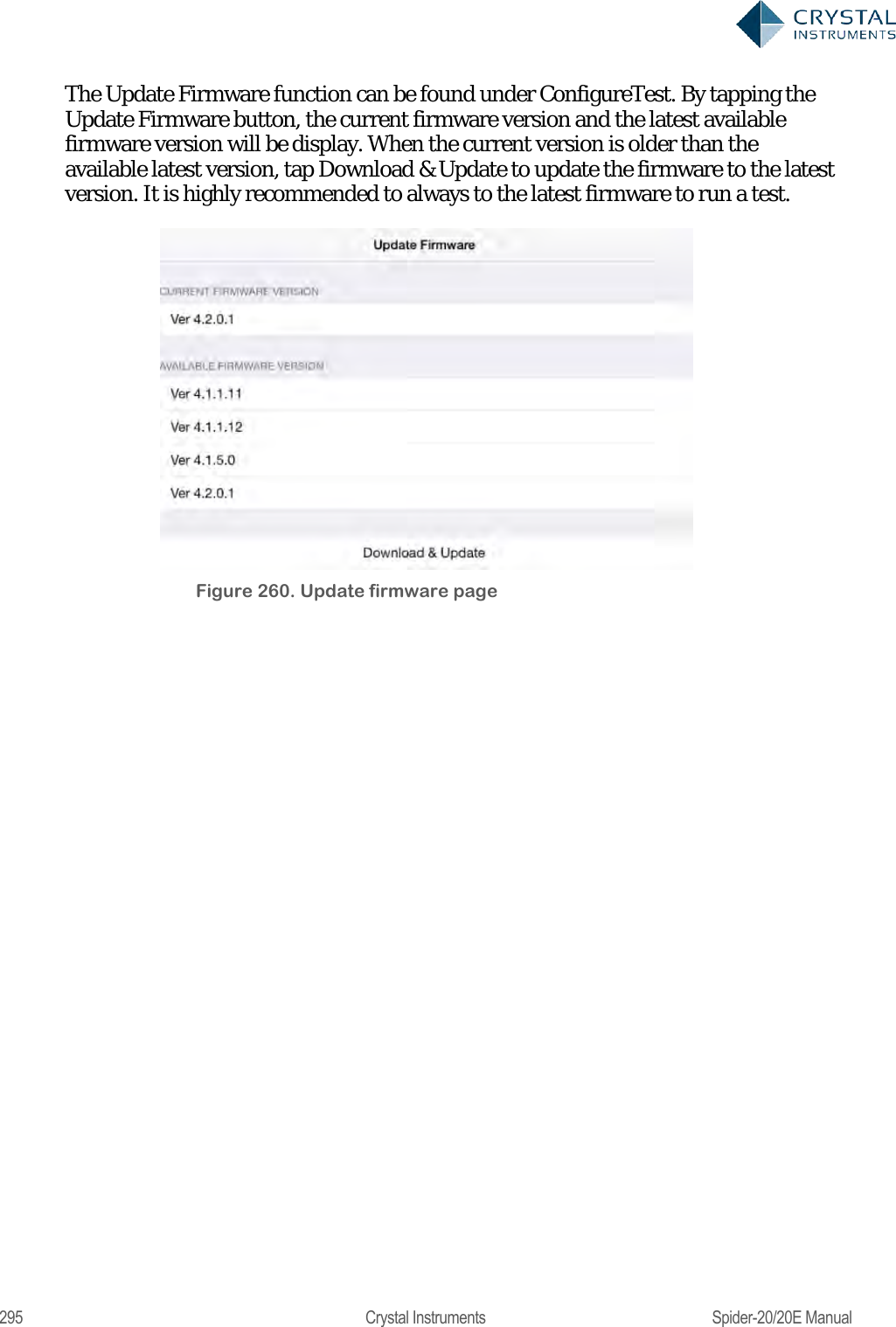
User Manual 2
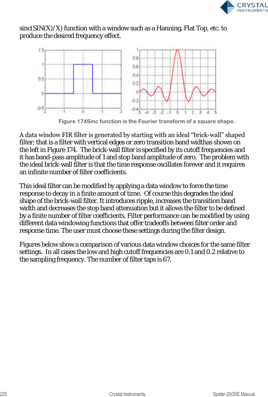
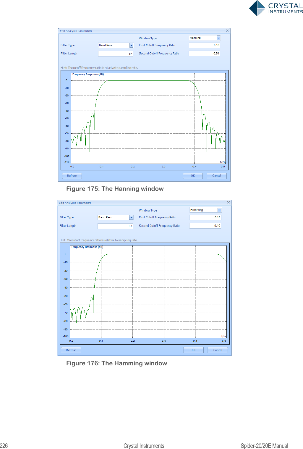
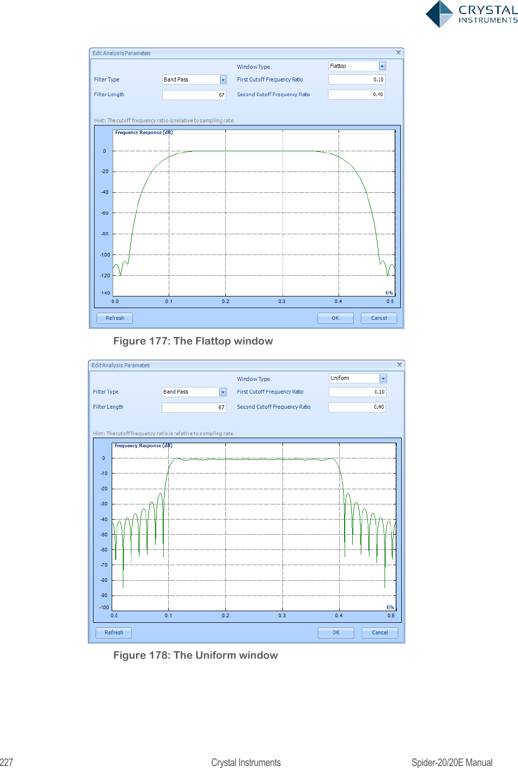
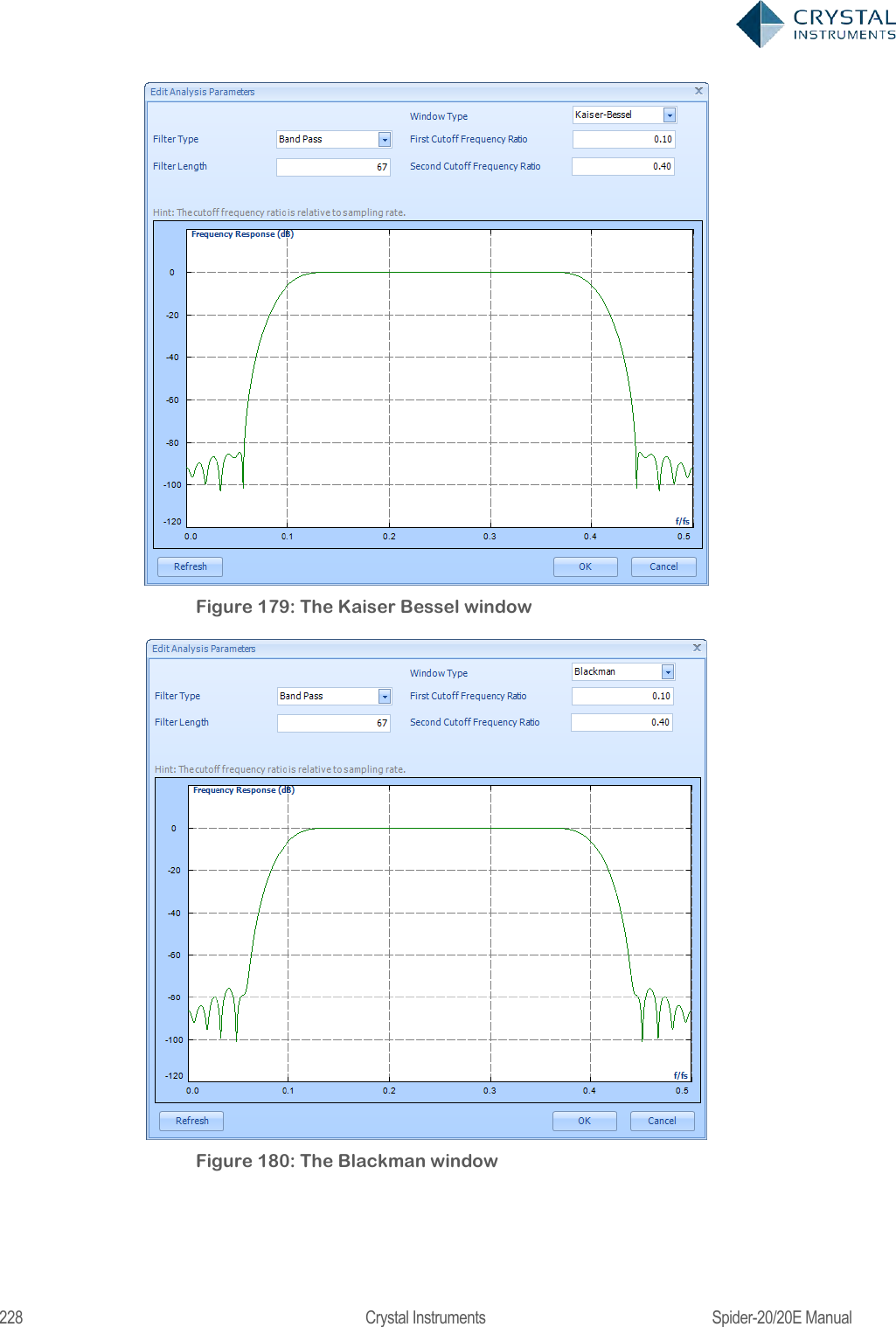
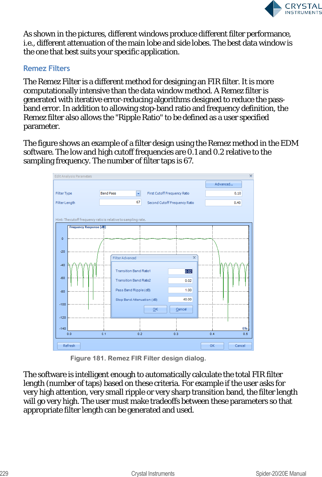
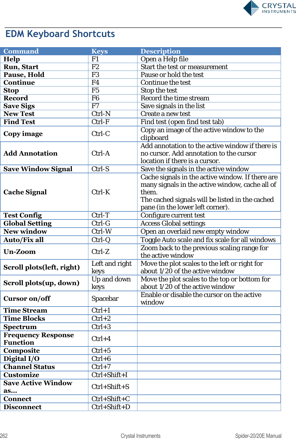
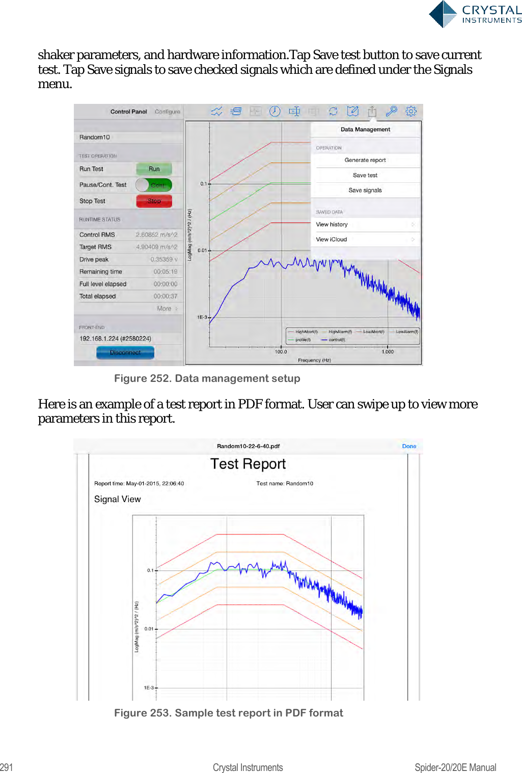
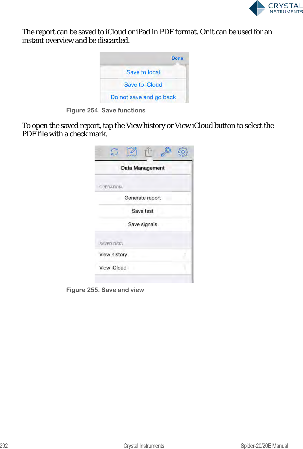
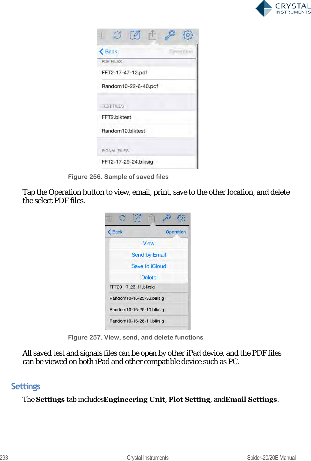
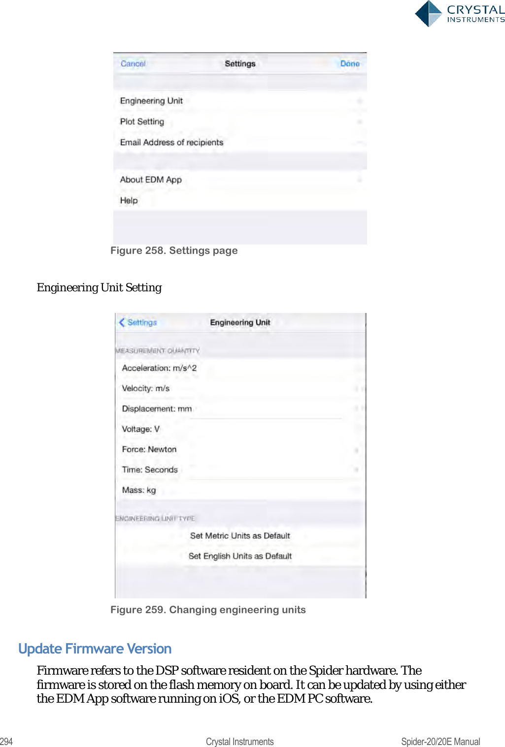
![224 Crystal Instruments Spider-20/20E Manual A digital filter can be understood by considering the equation which defines how the input signal is related to the output signal: = 0+ 11++ Where x[n] is the current input signal sample, x[n-1] is the previous signal sample and x[n-N] is the last sample in the series. The series multiplies the most recent N+1 samples with the associated N+1 filter coefficients. y[n] is the current output signal and bi are the filter coefficients. The number N is known as the filter order; an Nth-order filter has (N + 1) terms on the right-hand side. N+1 filter coefficients are also referred to as ―taps‖. This equation illustrates why a higher order filter has a slower response time. It takes more samples and therefore more time for an event to work its way through the series until the output is no longer affected by the event. A lower order filter has fewer coefficients and therefore a faster response time. The previous equation can also be expressed as a convolution of the filter coefficients and the input signal, specifically: ==0 The Impulse Response of the filter shows how historical data affects the current filtered value. The longer the impulse response, the more the older data will affect the current filtered value. To find the impulse response we set =[] Where δ[n] is the Kronecker delta impulse. The equation below shows that the impulse response for an FIR filter is simply the set of coefficients bn, as follows ==0== 0 FIR filters are stablebecause the output is a sum of a finite number of finite multiples of the input values that can be no greater than =0 times the largest value appearing in the input. Data Windows FIR Filters In the academic world, hundreds of methods are available to design FIR filters to meet various criteria. EDM includes the most popular filter design methods: Data Window and Remez. Both methods are discussed below. The Data Window FIR Filter Design method is the easiest to understand. The name "Window" comes from the fact that these filters are created by scaling a](https://usermanual.wiki/Crystal-Instruments/SPIDER20.User-Manual-2/User-Guide-3054612-Page-44.png)
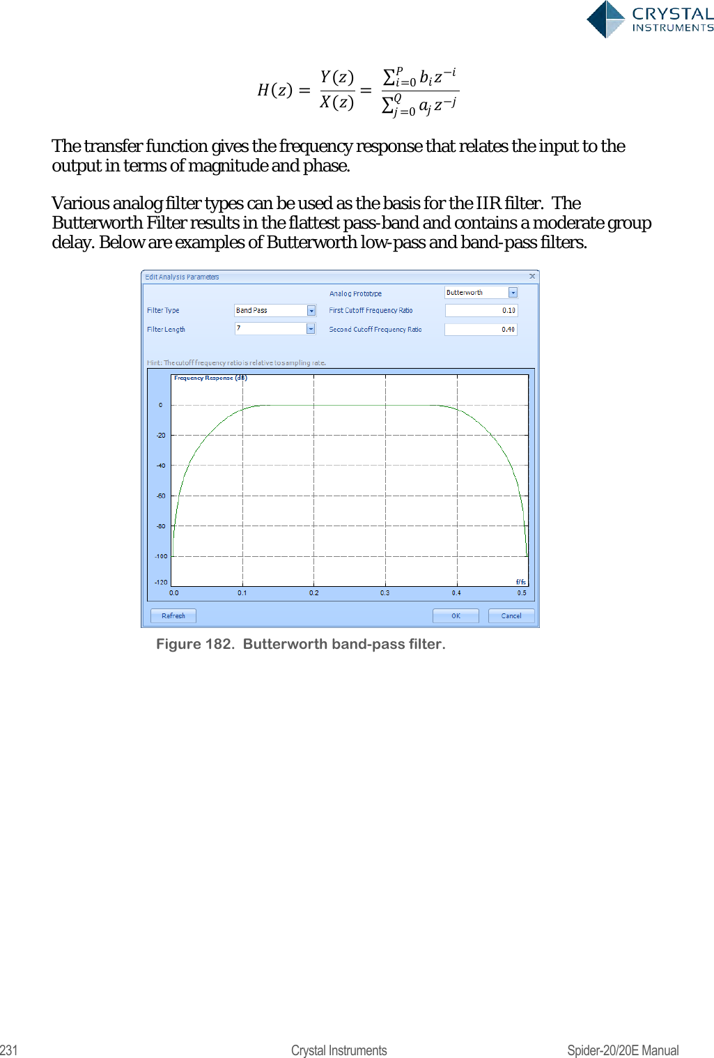
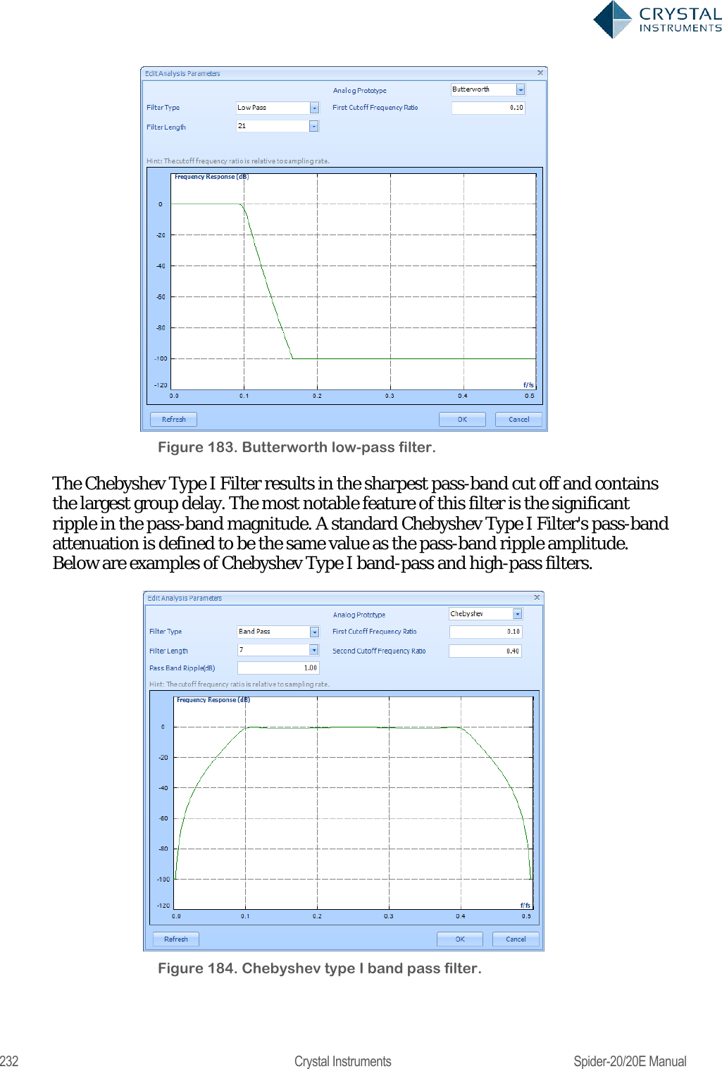
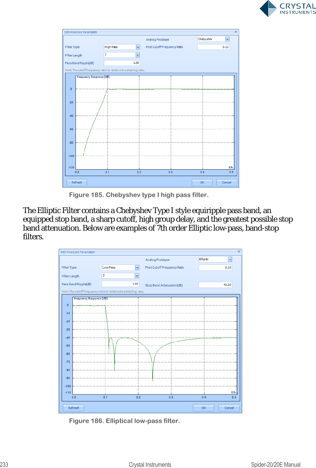
![230 Crystal Instruments Spider-20/20E Manual IIR Real Time Digital Filters Infinite impulse response (IIR)filters have an impulse response that decays very slowly and theoretically lasts forever. This is due to the fact that the filter input includes the measured signal and also the filter output creating a feedback path which results in the infinite impulse duration. This is in contrast to finite impulse response filters (FIR) which have fixed-duration impulse responses. The design procedure for IIR filters is somewhat more complicated than FIR filter design because there is no direct design method like the data window method for FIR filters. IIR filters are typically designed by starting with an ideal analog filter in terms of the frequency response characteristics such as the Chebyshev, Butterworth, or Bessel filter. Then the analog filter is converted into a digital filter using a method known as the Bilinear transformation or the impulse invariance method. An IIR digital filter can be understood by considering the equation that defines how the input signal is related to the output signal: = 0+ 11++11 Where P is the feed-forward filter order, are the feed-forward filter coefficients, Q is the feedback filter order,are the feedback filter coefficients,x[n] is the input signal and y[n] is the output signal. The previous equation can also be expressed as a convolution of the filter coefficients and the input signal. ==0 =0 Which, when rearranged, becomes: =0= =0 0= 1 To find the transfer function of the filter, we first take the Z-transform of each side of the above equation, where we use the time-shift property to obtain: ()=0= ()=0 We define the transfer function to be:](https://usermanual.wiki/Crystal-Instruments/SPIDER20.User-Manual-2/User-Guide-3054612-Page-50.png)
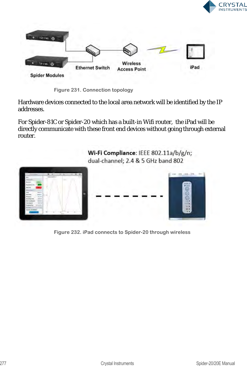
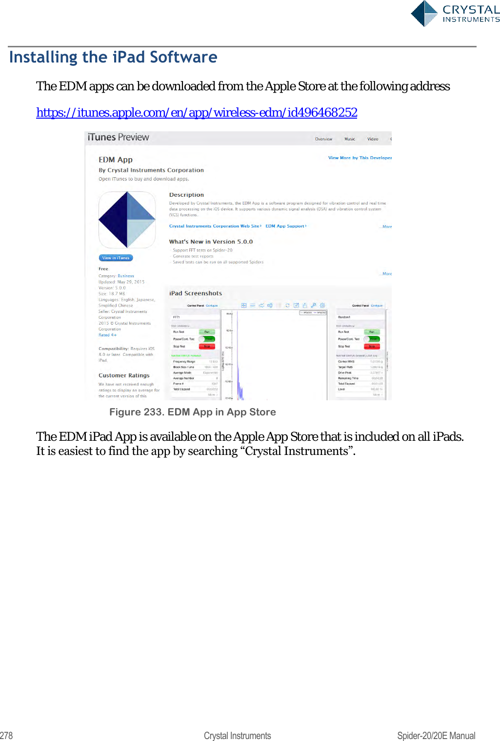
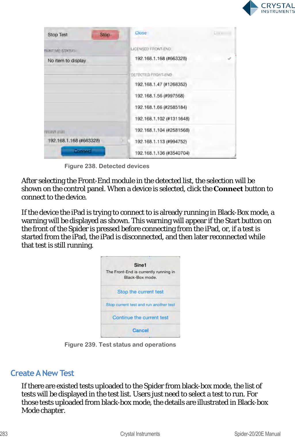
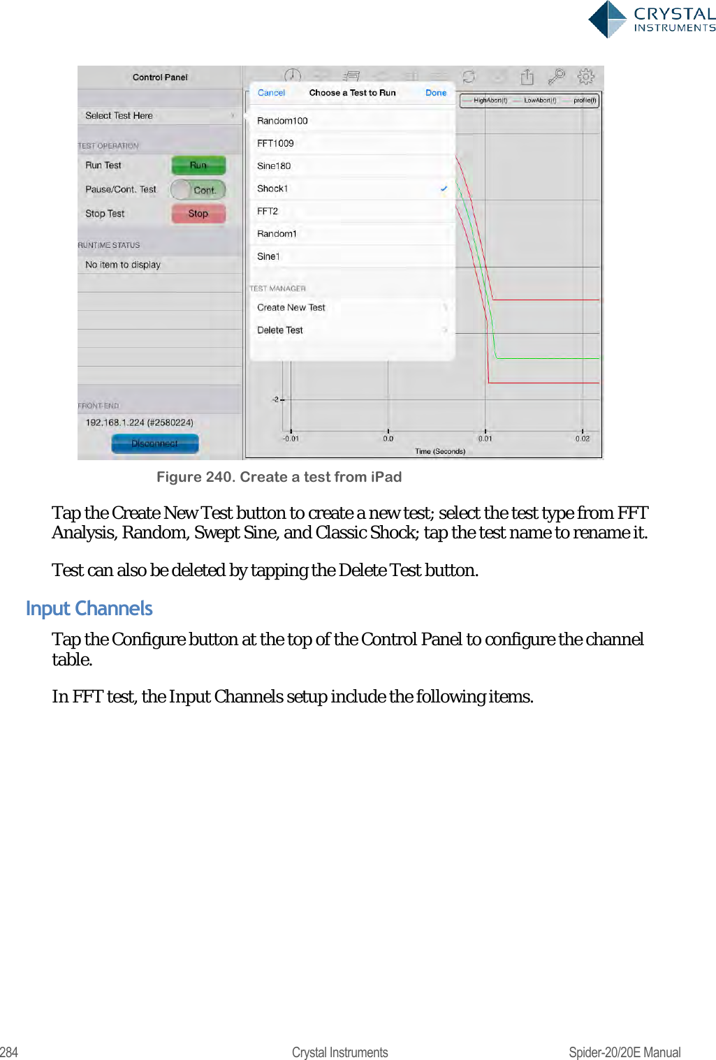
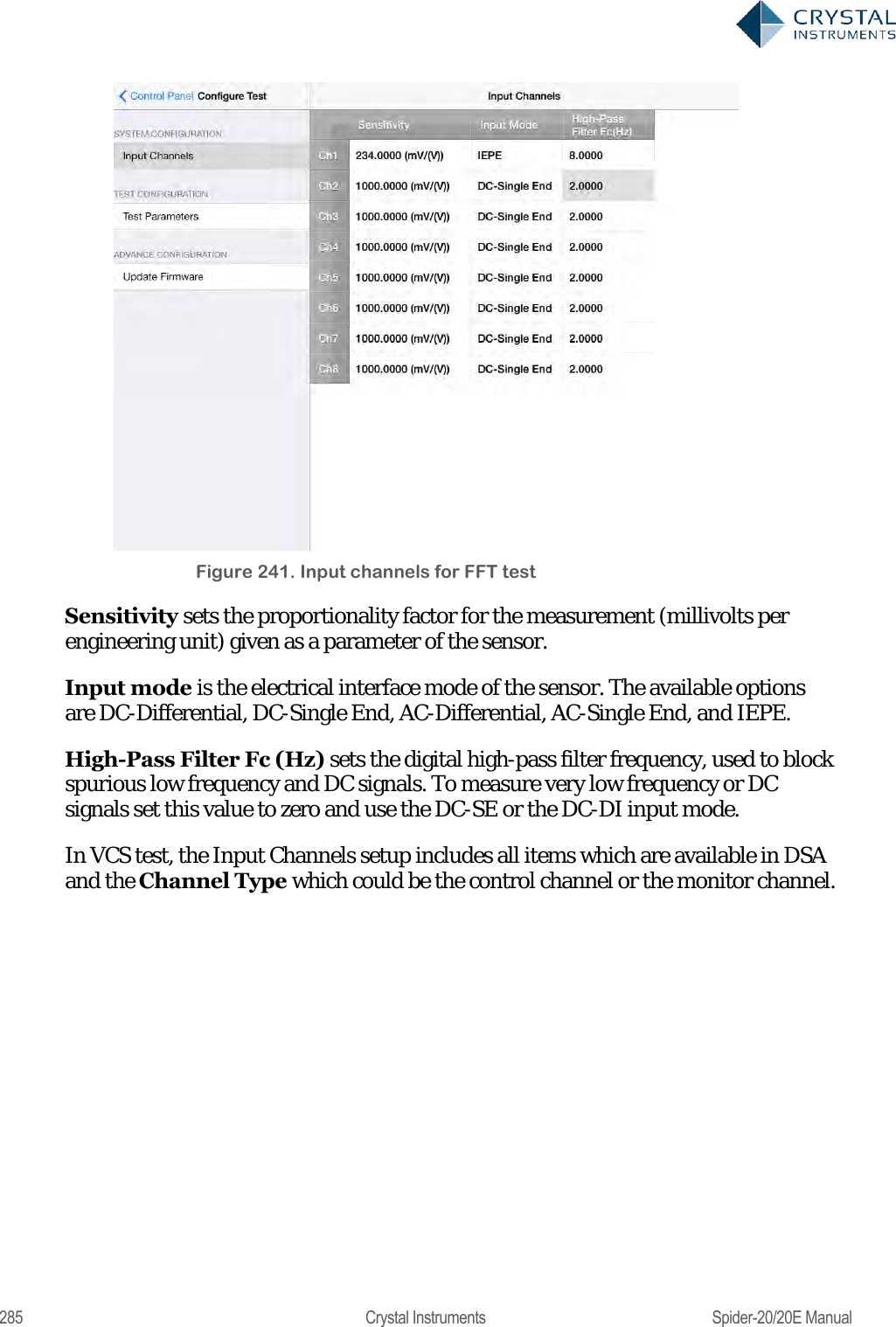
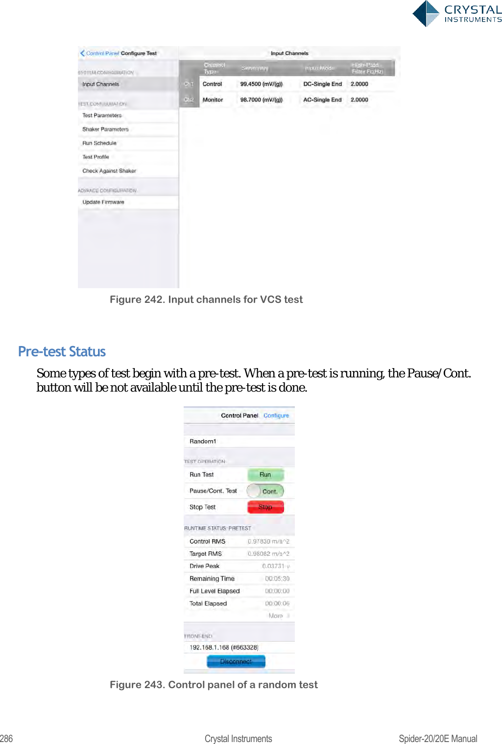
![280 Crystal Instruments Spider-20/20E Manual Control the Spider from the iPad Network Connection In order to connect, the iPad on its wireless connection must be on the same network as the Spider on its wireless/wired connection. Spider-20 and Spider-81C are equipped with built-in wireless connection. Because they are wireless device themselves, the App on the iPad can establish a point-to-point wireless connection with Spider-20 and Spider-81C. No external routers are required in this connection. Following are the factory settings of Spider-20 and Spider-81C. WI-FI ID: Spider_SERIAL_No WI-FI Password: [BLANK] DHCP Gateway: 192.168.1.10 Subnet Mask: 255.255.255.0 DHCP Server: Enabled For the wired Spider device such as Spider-80X, Spider-81, and Spider-81B, the best way to do this is to use a wireless access point connected directly to the Spider. The iPad then connects to it through Wi-Fi. If the access point has a DHCP server, it should be enabled so that all devices automatically get a configured IP address. On the iPad, the wireless setting is configured under Settings->Wi-Fi. If the Spider or the wireless router has DHCP server enabled, user should use DHCP IP address on the iPad. If the Spider or the wireless router doesn‘t have DHCP server enabled, use can either enable it or use static IP address on the iPad. When iPad has the Wi-Fi enabled, the list of available network will be shown with SSID. Tap the wireless Spider‘s SSID or the wireless router with wired Spider connected, the connection between the iPad and the Spider will be automatically established. Unless very necessary, DHCP address is highly recommended to avoid encountering network issue. License Key The iPad must load a license key corresponding to the serial number of the Spider in order to connect to it. License Keys are loaded either directly from the Crystal Instruments servers or from local disks. While loading license keys, the iPad must have internet access and the user must have the account password associated with the Spider‘s serial number.](https://usermanual.wiki/Crystal-Instruments/SPIDER20.User-Manual-2/User-Guide-3054612-Page-100.png)
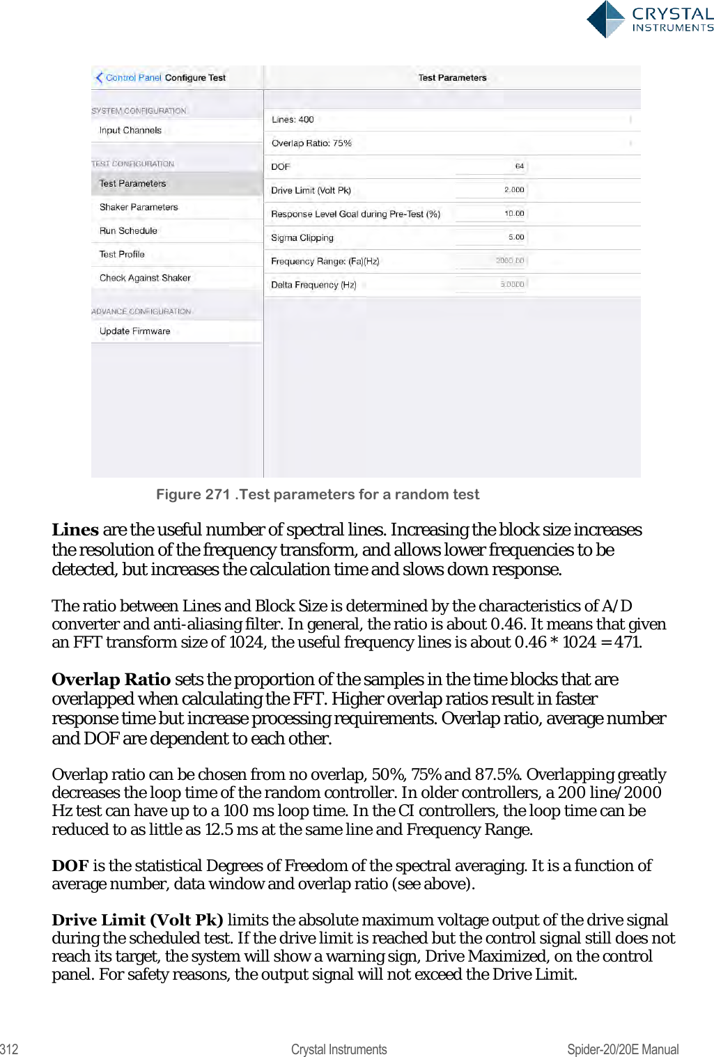
![311 Crystal Instruments Spider-20/20E Manual type. As the DOF increases, the variance of this distribution decreases. The relationship is: = 2 2[][] where is the spectral estimate, E[] is the expected value, and Var[] is the variance. On the basis of control accuracy, it is therefore desirable to increase the DOF as much as possible (by using a large average number). On the basis of response time, however, a large average number is undesirable. There is a tradeoff between accuracy and responsiveness. Block overlapping can help decrease response time while maintaining a large DOF. Overlapping involves reusing a specified number of samples in subsequent blocks. With no overlapping, DOF is approximately twice the average number. With a non-rectangular window, the DOF will be about 1.3 times the average number with 50% overlap, which will allow a higher DOF value for the same total number of samples. Increasing overlap beyond 50%, however, will not yield any more advantage in reducing the variance. However a higher overlap ratio will still be beneficial to reduce the loop-time of control. Random Test Parameters In the Test Configuration window, the Test Parameters section has settings for the main analysis parameters of the random test.](https://usermanual.wiki/Crystal-Instruments/SPIDER20.User-Manual-2/User-Guide-3054612-Page-131.png)