007 1680 040
User Manual: 007-1680-040
Open the PDF directly: View PDF ![]() .
.
Page Count: 742 [warning: Documents this large are best viewed by clicking the View PDF Link!]

IRIS Performer™
Programmer’s Guide
Document Number 007-1680-040

IRIS Performer™ Programmer’s Guide
Document Number 007-1680-040
CONTRIBUTORS
Written by George Eckel
Edited by Steven Hiatt
Illustrated by Dany Galgani
Production by Derrald Vogt and Linda Rae Sande
Engineering contributions by Sharon Clay, Brad Grantham, Don Hatch, Jim Helman, Michael
Jones, Martin McDonald, John Rohlf, Allan Schaffer, Chris Tanner, Jenny Zhao, Yair Kurzion,
and Tom McReynolds
© Copyright 1995 -1997 Silicon Graphics, Inc.— All Rights Reserved
This document contains proprietary and confidential information of Silicon Graphics, Inc. The
contents of this document may not be disclosed to third parties, copied, or duplicated in any
form, in whole or in part, without the prior written permission of Silicon Graphics, Inc.
RESTRICTED RIGHTS LEGEND
Use, duplication, or disclosure of the technical data contained in this document by the
Government is subject to restrictions as set forth in subdivision (c) (1) (ii) of the Rights in
Technical Data and Computer Software clause at DFARS 52.227-7013 and/or in similar or
successor clauses in the FAR, or in the DOD or NASA FAR Supplement. Unpublished rights
reserved under the Copyright Laws of the United States. Contractor/manufacturer is Silicon
Graphics, Inc., 2011 N. Shoreline Blvd., Mountain View, CA 94039-7311.
Indigo, Indy, IRIS, IRIS Indigo, ImageVision Library, Onyx, OpenGL, Silicon Graphics, and the
Silicon Graphics logo are registered trademarks and Crimson, Elan Graphics,
Geometry Pipeline, Indigo Elan, Indigo2, IRIS GL, IRIS Graphics Library, IRIS InSight,
IRIS Inventor, IRIS Performer, IRIX, Personal IRIS, POWER Series, Performance Co-Pilot,
RealityEngine, RealityEngine2, and Showcase are trademarks of Silicon Graphics, Inc.
AutoCAD is a registered trademark of Autodesk, Inc. DrAW Computing Associates is a
trademark of DrAW Computing Associates. Netscape is a trademark of Netscape
Communications Corp. Motif is a registered trademark of Open Software Foundation.
WindView is a trademark of Wind River Systems. X Window System is a trademark of
Massachusetts Institute of Technology.
Many of the techniques and methods disclosed in this Programmer’s Guide are covered by
patents held by Silicon Graphics including U.S. Patent Nos. 5,051,737; 5,369,739; 5,438,654;
5,394,170; 5,528,737; 5,528,738; 5,581,680; 5,471,572 and patent applications pending.
We encourage you to use these features in your IRIS Performer application on Silicon Graphics
systems.
This functionality and IRIS Performer are not available for re-implementation and distribution
on other platforms without the explicit permission of Silicon Graphics.

iii
Contents
List of Examples xix
Figures xxiii
List of Tables xxvii
About This Guide xxxi
Why Use IRIS Performer? xxxi
What You Should Know Before Reading This Guide xxxii
Internet and Hard Copy Reading for the Performer Series xxxii
How to Use This Guide xxxiv
What This Guide Contains xxxiv
Sample Applications xxxv
Conventions xxxvi
Bibliography xxxvi
X, Xt, IRIS IM, and Window Systems xxxviii
Visual Simulation xxxix
Mathematics of Flight Simulation xxxix
Virtual Reality xxxix
Geometric Reasoning xl
Conference Proceedings xl
Survey Articles in Magazines xli
1. IRIS Performer Programming Interface 3
General Naming Conventions 3
Prefixes 3
Header Files 4
Naming in C and C++ 4
Abbreviations 4
Macros, Tokens, and Enums 5

iv
Contents
Class API 5
Object Creation 5
Set Routines 6
Get Routines 6
Action Routines 7
Enable and Disable of Modes 7
Mode, Attribute, or Value 7
Base Classes 8
Inheritance Graph 9
Libpr and Libpf Objects 11
User Data 11
pfDelete() and Reference Counting 12
Copying Objects with pfCopy() 16
Printing Objects with pfPrint() 17
Determining Object Type 18
2. Setting Up the Display Environment 23
Using Pipes 25
The Functional Stages of a Pipeline 25
Creating and Configuring a pfPipe 27
Example of pfPipe Use 29
Using Channels 30
Creating and Configuring a pfChannel 31
Setting Up a Scene 31
Setting Up a Viewport 32
Setting Up a Viewing Frustum 32
Setting Up a Viewpoint 34
Example of Channel Use 36
Controlling the Video Output 39
Using Multiple Channels 40
One Window per Pipe, Multiple Channels per Window 40
Using Channel Groups 44
Multiple Channels and Multiple Windows 48

Contents
v
3. Nodes and Node Types 51
Nodes 51
Attribute Inheritance 51
pfNode 53
pfGroup 55
Working With Nodes 58
Instancing 58
Bounding Volumes 61
Node Types 63
pfScene Nodes 63
pfSCS Nodes 64
pfDCS Nodes 64
pfFCS Nodes 65
pfSwitch Nodes 66
pfSequence Nodes 66
pfLOD Nodes 69
pfASD Nodes 69
pfLayer Nodes 69
pfGeode Nodes 71
pfText Nodes 72
pfBillboard Nodes 74
pfPartition Nodes 77
Sample Program 79
4. Database Traversal 85
Scene Graph Hierarchy 87
Database Traversals 87
State Inheritance 88
Database Organization 88
Application Traversal 89

vi
Contents
Cull Traversal 90
Traversal Order 90
Visibility Culling 91
Organizing a Database for Efficient Culling 94
Sorting the Scene 97
Paths Through the Scene Graph 99
Draw Traversal 100
Controlling and Customizing Traversals 100
pfChannel Traversal Modes 100
pfNode Draw Mask 101
pfNode Cull and Draw Callbacks 102
Process Callbacks 105
Process Callbacks and Passthrough Data 107
Intersection Traversal 109
Testing Line Segment Intersections 110
Intersection Requests: pfSegSets 110
Intersection Return Data: pfHit Objects 111
Intersection Masks 112
Discriminator Callbacks 114
Line Segment Clipping 114
Traversing Special Nodes 115
Picking 115
Performance 115
Intersection Methods for Segments 116
5. Frame and Load Control 121
Frame-Rate Management 121
Selecting the Frame Rate 122
Achieving the Frame Rate 122
Fixing the Frame Rate 123

Contents
vii
Maintaining Frame Rate Using Dynamic Video Resolution 128
The Channel in DVR 129
DVR Scaling 129
Customizing DVR 130
Understanding the Stress Filter 131
Level-of-Detail Management 132
Level-of-Detail Models 133
Level of Detail States 136
Level-of-Detail Range Processing 138
Level-of-Detail Transition Blending 141
Terrain Level of Detail 143
Dynamic Load Management 144
Successful Multiprocessing With IRIS Performer 147
Review of Rendering Stages 147
Choosing a Multiprocessing Model 148
Asynchronous Database Processing 153
Rules for Invoking Functions While Multiprocessing 155
Multiprocessing and Memory 158
Shared Memory and pfInit() 159
pfDataPools 160
Passthrough Data 160
6. Creating Visual Effects 165
Using pfEarthSky 165
Atmospheric Effects 166
7. Importing Databases 173
Overview of IRIS Performer Database Creation and Conversion 173
libpfdu - Utilities for Creation of Efficient IRIS Performer Run-Time Structures 174
pfdLoadFile - Loading Arbitrary Databases into IRIS Performer 175
Database Loading Details 177

viii
Contents
Developing Custom Importers 180
Structure and Interpretation of the Database File Format 180
Scene Graph Creation using Nodes as defined in libpf 181
Defining Geometry and Graphics State for libpr 181
Creation of a IRIS Performer Database Converter using libpfdu 182
Maximizing Database Loading and Paging Performance with PFB and PFI Formats 192
pfconv 192
pficonv 193
Supported Database Formats 193
Description of Supported Formats 195
AutoDesk 3DS Format 195
Silicon Graphics BIN Format 196
Side Effects POLY Format 197
Brigham Young University BYU Format 199
Optimizer CSB Format 200
Virtual Cliptexture CT Loader 200
Designer’s Workbench DWB Format 200
AutoCAD DXF Format 201
MultiGen OpenFlight Format 203
McDonnell-Douglas GDS Format 205
Silicon Graphics GFO Format 205
Silicon Graphics IM Format 207
AAI/Graphicon IRTP Format 208
Silicon Graphics Open Inventor Format 208
Lightscape Technologies LSA and LSB Formats 210
Medit Productions MEDIT Format 213
NFF Neutral File Format 214
Wavefront Technology OBJ Format 216
Silicon Graphics PFB Format 217
Silicon Graphics PFI Format 218
Silicon Graphics PHD Format 219
Silicon Graphics PTU Format 221
USNA Standard Graphics Format 223

Contents
ix
Silicon Graphics SGO Format 224
USNA Simple Polygon File Format 227
Sierpinski Sponge Loader 228
Star Chart Format 228
3D Lithography STL Format 229
SuperViewer SV Format 230
Geometry Center Triangle Format 234
UNC Walkthrough Format 234
WRL Format 235
Database Operators with Pseudo Loaders 235
8. Geometry 239
Geometry Sets 239
Primitive Types 241
pfGeoSet Draw Mode 242
Primitive Connectivity 244
Attributes 246
Attribute Bindings 248
Indexed Arrays 249
pfGeoSet Operations 251
3D Text 251
pfFont 251
pfString 253

x
Contents
9. Graphics State 259
Immediate Mode 259
Rendering Modes 261
Rendering Values 266
Enable / Disable 266
Rendering Attributes 267
Graphics Library Matrix Routines 283
Sprite Transformations 283
Display Lists 285
State Management 286
State Override 287
pfGeoState 288
10. ClipTextures 297
Overview 298
Cliptexture Levels 299
Cliptexture Assumptions 300
Image Cache 301
Toroidal Loading 304
Updating the Clipcenter 306
Virtual Cliptextures 307
Cliptexture Support Requirements 308
Special Features 308
How Cliptextures Interact with the Rest of the System 309
Cliptexture Support in IRIS Performer 310
Cliptexture Manipulation 311
Cliptexture API 313
Preprocessing ClipTextures 313
Building a MIPmap 314
Formatting Image Data 315
Tiling an Image 315
Cliptexture Configuration 316

Contents
xi
Configuration API 317
libpr Functionality 317
Configuration Utilities 321
Configuration Files 323
Post-Scene Graph Load Configuration 339
MPClipTextures 339
pfMPClipTexture Utilities 341
Using Cliptextures with Multiple Pipes 344
Texture Memory and Hardware Support Checking 347
Manipulating Cliptextures 347
Cliptexture Load Control 348
Invalidating Cliptextures 353
Virtual ClipTextures 353
Custom Read Functions 360
Using Cliptextures 361
Cliptexture Insets 361
Estimating Cliptexture Memory Usage 365
Using Cliptextures in Multipipe Applications 369
Virtualizing Cliptextures 371
Customizing Load Control 371
Custom Read Functions 372
Cliptexture Sample Code 373
11. Windows 377
pfWindows for both OpenGL and IRIS GL 377
Creating a pfWindow 378
Configuring the Framebuffer of a pfWindow 381
pfWindows and GL Windows 384
Manipulating a pfWindow 385
Alternate Framebuffer Configuration Windows 387
Window Share Groups 388
Synchronization of Swapbuffers for Multiple Windows 388
Communicating with the Window System 389
More pfWindow Examples 389

xii
Contents
12. pfPipeWindows and pfPipeVideoChannels 395
Using pfPipeWindows 395
Creating, Configuring and Opening pfPipeWindow 395
pfPipeWindows in Action 406
Controlling Video Displays 408
Creating a pfPipeVideoChannel 409
Multiple pfPipeVideoChannels in a pfPipeWindow 410
Configuring a pfPipeVideoChannel 411
Use pfPipeVideoChannels to Control Frame Rate 411
13. Managing Nongraphic System Tasks 415
Handling Queues 415
Multiprocessing 416
Queue Contents 416
Adding or Retrieving Elements 416
pfQueue Modes 418
Running the Sort Process on a Different CPU 422
High-Resolution Clocks 422
Video Refresh Counter (VClock) 423
Memory Allocation 423
Allocating Memory With pfMalloc() 424
Shared Arenas 425
Allocating Locks and Semaphores 426
Datapools 426
CycleBuffers 427
Asynchronous I/O 429
Error-Handling and Notification 430
File Search Paths 431

Contents
xiii
14. Dynamic Data 435
pfFlux 435
Creating and Deleting a pfFlux 435
Initializing the Buffers 436
pfFlux Buffers 437
Coordinating pfFlux and Connected pfEngines 439
Synchronized Flux Evaluation 441
Fluxed Geosets 442
Fluxed Coordinate Systems 444
Replacing pfCycleBuffer With pfFlux 445
pfEngine 446
Creating and Deleting Engines 447
Setting Engine Types and Modes 448
For an example of animation using a user-defined engine, see user_engine.C in
sample/pguide/libpf/C++. 454
Setting Engine Sources and Destinations 454
Setting Engine Masks 455
Setting Engine Iterations 455
Setting Engine Ranges 455
Evaluating pfEngines 455
Animating a Geometry 456
15. Active Surface Definition 461
Overview 461
Using ASD 463
LOD Reduction 463
Hierarchical Structure 464
ASD Solution Flow Chart 466
A Very Simple ASD 467
Morphing Vector 468
A Very Complex ASD 469
ASD Elements 469
Vertices 470
Evaluation Function 472

xiv
Contents
Data Structures 473
Triangle Data Structure 475
Attribute Data Array 480
Vertex Data Structure 482
Default Evaluation Function 483
pfASD Queries 484
Aligning an Object to the Surface 485
Adding a Query Array 485
Using ASD for Multiple Channels 486
Connecting Channels 487
Combining pfClipTexture and pfASD 487
ASD Evaluation Function Timing 488
Query Results 488
Aligning a Geometry With a pfASD Surface Example 489
Aligning Light Points Above a pfASD Surface Example 490
Paging 492
Interest Area 493
Preprocessing for Paging 494
Multi-resolution Paging 494
16. Light Points 499
Uses of Light Points 499
Creating a Light Point 500
Setting the Behavior of Light Points 501
Intensity 501
Directionality 501
Emanation Shape 502
Distance 505
Attenuation through Fog 505
Size 506
Fading 507
Callbacks 508
Multisample, Size, and Alpha 510
Reducing CPU Processing Using Textures 512

Contents
xv
Preprocessing Light Points 513
Stage Configuration Callbacks 513
How the Light Point Process Works 514
Calligraphic Light Points 515
Calligraphic Versus Raster Displays 516
LPB Hardware Configuration 519
Visibility Information 521
Required Steps For Using Calligraphic Lights 521
Accounting for Projector Differences 524
Callbacks 526
Frame to Frame Control 527
Significance 528
Debunching 529
Defocussing Calligraphic Objects 529
Using pfCalligraphic Without pfChannel 529
Timing Issues 530
Light Point Process and Calligraphic 530
Debugging Calligraphic Lights on Non-Calligraphic Systems 531
Calligraphic Light Example 531
17. Math Routines 541
Vector Operations 541
Matrix Operations 543
Quaternion Operations 547
Matrix Stack Operations 549
Creating and Transforming Volumes 550
Defining a Volume 550
Creating Bounding Volumes 552
Transforming Bounding Volumes 553
Intersecting Volumes 554
Point-Volume Intersection Tests 554
Volume-Volume Intersection Tests 554

xvi
Contents
Creating and Working With Line Segments 556
Intersecting With Volumes 557
Intersecting With Planes and Triangles 558
Intersecting With pfGeoSets 558
General Math Routine Example Program 561
18. Statistics 567
Interpreting Statistics Displays 567
Status Line 568
Stage Timing Graph 569
Load and Stress 572
CPU Statistics 573
Rendering Statistics 575
Fill Statistics 576
Collecting and Accessing Statistics in Your Application 576
Displaying Statistics Simply 577
Enabling and Disabling Statistics for a Channel 578
Statistics in libpr and libpf—pfStats Versus pfFrameStats 578
Statistics Rules of Use 579
Reducing the Cost of Statistics 582
Statistics Output 583
Customizing Displays 585
Setting Update Rate 585
The pfStats Data Structure 585
Statistics Examples 586
19. Performance Tuning and Debugging 589
Performance-Tuning Overview 589
How IRIS Performer Helps Performance 590
Draw Stage and Graphics Pipeline Optimizations 591
Cull and Intersection Optimizations 593
Application Optimizations 594

Contents
xvii
Specific Guidelines for Optimizing Performance 594
Graphics Pipeline Tuning Tips 595
Process Pipeline Tuning Tips 598
Database Concerns 602
Special Coding Tips 607
Performance Measurement Tools 608
Using pixie and prof to Measure Performance 609
Using gldebug and ogldebug to Observe Graphics Calls 609
Using glprof to Find Performance Bottlenecks 610
Guidelines for Debugging 615
Shared Memory 615
Use the Simplest Process Model 616
Avoid Floating-Point Exceptions 616
When the Debugger Won’t Give You a Stack Trace 617
Tracing Members of IRIS Performer Objects 617
Memory Corruption and Leaks 618
Purify 618
Libdmalloc 619
Notes on Tuning for RealityEngine Graphics 620
Multisampling 620
Transparency 620
Texturing 621
Other Tips 622
20. Programming with C++ 625
Overview 625
Class Taxonomy 626
Programming Basics 627
Header Files 627
Creating and Deleting IRIS Performer Objects 630
Invoking Methods on IRIS Performer Objects 632
Passing Vectors and Matrices to Other Libraries 632

xviii
Contents
Porting from C API to C++ API 632
Typedefed Arrays vs. Structs 633
Interface Between C and C++ API Code 633
Subclassing pfObjects 634
Initialization and Type Definition 635
Defining Virtual Functions 636
Accessing Parent Class Data Members 637
Multiprocessing and Shared Memory 637
Initializing Shared Memory 637
Data Members and Shared Memory 638
libpf Objects and Multiprocessing 639
Performance Hints 640
Glossary 641
Index 663

xix
List of Examples
Example 1-1 How to Use User Data 12
Example 1-2 Objects and Reference Counts 13
Example 1-3 Using pfDelete() with libpr Objects 14
Example 1-4 Using pfDelete() with libpf Objects 15
Example 1-5 Using pfCopy() 16
Example 1-6 General-Purpose Scene Graph Traverser 18
Example 2-1 pfPipes in Action 29
Example 2-2 Using pfChannels 37
Example 2-3 Multiple Channels, One Channel per Pipe 43
Example 2-4 Channel-Sharing 46
Example 3-1 Making a Scene 55
Example 3-2 Hierarchy Construction Using Group Nodes 57
Example 3-3 Creating Cloned Instances 61
Example 3-4 Automatically Updating a Bounding Volume 62
Example 3-5 Using pfSwitch and pfSequence Nodes 67
Example 3-6 Marking a Runway With a pfLayer Node 70
Example 3-7 Adding pfGeoSets to a pfGeode 71
Example 3-8 Adding pfStrings to a pfText 72
Example 3-9 Setting Up a pfBillboard 75
Example 3-10 Setting Up a Partition 78
Example 3-11 Inheritance Demonstration Program 79
Example 4-1 Application Callback to Make a Pendulum 89
Example 4-2 pfNode Draw Callbacks 103
Example 4-3 Cull-Process Callbacks 105
Example 4-4 Using Passthrough Data to Communicate With Callback Routines 108
Example 5-1 Frame Control Excerpt 127
Example 5-2 Setting LOD Ranges 139

xx
List of Examples
Example 5-3 Default Stress Function 146
Example 6-1 How to Configure a pfEarthSky 166
Example 8-1 Loading Characters into a pfFont 253
Example 8-2 Setting Up and Drawing a pfString 253
Example 9-1 Using pfDecal() to Draw Road With Stripes 265
Example 9-2 Pushing and Popping Graphics State 287
Example 9-3 Using pfOverride() 288
Example 9-4 Inheriting State 290
Example 10-1 Estimating System Memory Requirements 367
Example 11-1 Opening a pfWindow 378
Example 11-2 Using the Default Overlay Window 389
Example 11-3 Creating a Custom Overlay Window 390
Example 11-4 pfWindows and X Input 391
Example 12-1 Creating a pfPipeWindow 396
Example 12-2 pfPipeWindow With Alternate Configuration Windows
for Statistics 400
Example 12-3 Custom Initialization of pfPipeWindow State 402
Example 12-4 Configuration of a pfPipeWindow Framebuffer 405
Example 12-5 Opening and Closing a pfPipeWindow 406
Example 14-1 Fluxed pfGeoSet 443
Example 14-2 Connecting Engines and Fluxs 457
Example 15-1 Aligning Light Points Above a pfASD Surface 491
Example 16-1 Raster Callback Skeleton 509
Example 16-2 Preprocessing a Display List - Light Point Process code 514
Example 16-3 Setting pfCalligraphic Parameters 527
Example 16-4 Calligraphic Lights 531
Example 17-1 Matrix and Vector Math Examples 546
Example 17-2 Quaternion Example 548
Example 17-3 Quick Sphere Culling Against a Set of Half-Spaces 556
Example 17-4 Intersecting a Segment With a Convex Polyhedron 558
Example 17-5 Intersection Routines in Action 561
Example 19-1 Drawing an Object Without Calling pfDraw() 606
Example 19-2 General Traversal 611

List of Examples
xxi
Example 19-3 Using the Traverser 615
Example 20-1 Legal Creation of Objects in C++ 631
Example 20-2 Illegal Creation of Objects in C++ 631
Example 20-3 Class Definition for a Subclass of pfDCS 635
Example 20-4 Overloading the libpf Application Traversal 636
Example 20-5 Changeable Static Data Member 639


xxiii
Figures
Figure 1-1 Partial Inheritance Graph of IRIS Performer Data Types 10
Figure 2-1 From Scene Graph to Visual Display 24
Figure 2-2 Single Graphics Pipeline 26
Figure 2-3 Dual Graphics Pipeline 27
Figure 2-4 Symmetric Viewing Frustum 33
Figure 2-5 Heading, Pitch, and Roll Angles 35
Figure 2-6 Single-Channel and Multiple-Channel Display 41
Figure 3-1 Nodes in the IRIS Performer Hierarchy 52
Figure 3-2 Shared Instances 59
Figure 3-3 Cloned Instancing 60
Figure 4-1 Culling to the Frustum 92
Figure 4-2 Sample Database Objects and Bounding Volumes 94
Figure 4-3 How to Partition a Database for Maximum Efficiency 96
Figure 4-4 Intersection Methods 117
Figure 5-1 Frame Rate and Phase Control 124
Figure 5-2 Real Size of Viewport Rendered Under Increasing Stress 128
Figure 5-3 Level-of-Detail Node Structure 133
Figure 5-4 Level-of-Detail Processing 135
Figure 5-5 Stress Processing 145
Figure 5-6 Multiprocessing Models 152
Figure 6-1 Layered Atmosphere Model 167
Figure 7-1 BIN-Format Data Objects 196
Figure 7-2 Soma Cube Puzzle in DWB Form 201
Figure 7-3 The Famous Teapot in DXF Form 202
Figure 7-4 Spacecraft Model in FLIGHT Format 204
Figure 7-5 GFO Database of Mies van der Rohe’s German Pavilion 206
Figure 7-6 Aircar Database in IRIS Inventor Format 209

xxiv
Figures
Figure 7-7 LSA-Format City Hall Database 211
Figure 7-8 LSB-Format Operating Room Database 213
Figure 7-9 Silicon Graphics Office Building as OBJ Database 216
Figure 7-10 Plethora of Polyhedra in PHD Format 219
Figure 7-11 Terrain Database Generated by PTU Tools 221
Figure 7-12 Model in SGO Format 224
Figure 7-13 Sample STLA Database 229
Figure 7-14 Early Automobile in SuperViewer SV Format 231
Figure 8-1 Primitives and Connectivity 245
Figure 8-2 pfGeoSet Structure 247
Figure 8-3 Indexing Arrays 249
Figure 8-4 Deciding Whether to Index Attributes 250
Figure 9-1 pfGeoState Structure 293
Figure 10-1 Cliptexture Components 298
Figure 10-2 Image Cache Components 299
Figure 10-3 Mem Region Update 302
Figure 10-4 Tex Region Update 303
Figure 10-5 Cliptexture Cache Hierarchy 304
Figure 10-6 Invalid Border 305
Figure 10-7 Clipcenter Moving 306
Figure 10-8 Virtual Cliptexture Concepts 307
Figure 10-9 pfMPClipTexture Connections 340
Figure 10-10 pfuClipCenterNode Connections 343
Figure 10-11 Master and Slave Cliptexture Resource Sharing 344
Figure 10-12 Cliptexture Insets 362
Figure 10-13 Supersampled Inset Boundary 364
Figure 10-14 Offset Slave Tex Regions 370
Figure 12-1 Directing Video Output 408
Figure 13-1 pfQueue Object 415
Figure 13-2 pfCycleBuffer and pfCycleMemory Overview 428
Figure 14-1 pfEngine Drives a pfFlux Node Animated a pfFCS Node 444
Figure 15-1 Morphing Range Between LODs 465
Figure 15-2 Large Geometry 466

Figures
xxv
Figure 15-3 ASD Information Flow 467
Figure 15-4 A Very Simple pfASD 468
Figure 15-5 Reference Positions 471
Figure 15-6 Triangulated Image 471
Figure 15-7 LOD1 Replaced by LOD2 472
Figure 15-8 Data Structures 473
Figure 15-9 ASD Data Structures 474
Figure 15-10 Discontinuous, Neighboring LODs 477
Figure 15-11 Triangle Mesh 477
Figure 15-12 Using the tsid Field 478
Figure 15-13 Counter Clockwise Ordering of Vertices and Reference
Points in Arrays 479
Figure 15-14 Vertex Neighborhoods 482
Figure 15-15 pfASD Evaluation Process 488
Figure 15-16 Example Setup for Geometry Alignment 489
Figure 15-17 Aligning Light Points Above a pfASD Surface 490
Figure 15-18 Tiles at Different LODs 493
Figure 16-1 VASI Landing Light 500
Figure 16-2 Attenuation Shape 503
Figure 16-3 Attenuation of Light 504
Figure 16-4 Lit Multisamples 511
Figure 16-5 Calligraphic Hardware Configuration 519
Figure 18-1 Stage Timing Statistics Display 568
Figure 18-2 Conceptual Diagram of a Draw-Stage Timing Line 570
Figure 18-3 Other Statistics Classes 574


xxvii
List of Tables
Table 1-1 Routines that Modify libpr Object Reference Counts 13
Table 2-1 Attributes in the Share Mask of a Channel Group 45
Table 3-1 IRIS Performer Node Types 53
Table 3-2 pfGroup Functions 56
Table 3-3 DCS Transformations 65
Table 3-4 FCS Functions 65
Table 3-5 pfSequence Functions 66
Table 3-6 pfLOD Functions 69
Table 3-7 pfLayer Functions 70
Table 3-8 pfGeode Functions 71
Table 3-9 pfText Functions 72
Table 3-10 pfBillboard Functions 74
Table 3-11 pfPartition Functions 78
Table 4-1 Traversal Attributes for the Major Traversals 86
Table 4-2 Cull Callback Return Values 102
Table 4-3 Intersection-Query Token Names 111
Table 4-4 Database Classes and Corresponding Node Masks 113
Table 4-5 Representing Traversal Mask Values 113
Table 4-6 Possible Traversal Results 114
Table 5-1 Frame Control Functions 123
Table 5-2 LOD Transition Zones 141
Table 5-3 Multiprocessing Models 148
Table 5-4 Trigger Routines and Associated Processes 157
Table 6-1 pfEarthSky Routines 168
Table 6-2 pfEarthSky Attributes 168
Table 7-1 Database-Importer Source Directories 173
Table 7-2 libpfdu Database Converter Functions 175

xxviii
List of Tables
Table 7-3 Loader Name Composition 176
Table 7-4 libpfdu Database Converter Management Functions 178
Table 7-5 pfdBuilder Modes and Attributes 191
Table 7-6 Supported Database Formats 194
Table 7-7 Geometric Definitions in LSA Files 210
Table 7-8 Object Tokens in the SGO Format 225
Table 7-9 Mesh Control Tokens in the SGO Format 226
Table 7-10 IRIS Performer Pseudo Loaders 236
Table 8-1 pfGeoSet Routines 240
Table 8-2 Geometry Primitives 241
Table 8-3 pfGeoSet PACKED_ATTR Formats 244
Table 8-4 Attribute Bindings 248
Table 8-5 pfFont Routines 252
Table 8-6 pfString Routines 255
Table 9-1 pfGeoState Mode Tokens 262
Table 9-2 pfTransparency Tokens 263
Table 9-3 pfGeoState Value Tokens 266
Table 9-4 Enable and Disable Tokens 266
Table 9-5 Rendering Attribute Tokens 267
Table 9-6 Texture Image Sources 270
Table 9-7 Texture Load Modes 273
Table 9-8 Texture Generation Modes 277
Table 9-9 pfFog Tokens 281
Table 9-10 pfHlightMode() Tokens 282
Table 9-11 Matrix Manipulation Routines 283
Table 9-12 pfSprite Rotation Modes 284
Table 9-13 pfGeoState Routines 291
Table 10-1 Tiling Algorithms 314
Table 10-2 Image Cache Configuration File Fields 326
Table 10-3 Image Tile Filename Tokens 330
Table 10-4 Cliptexture Configuration File Fields 333
Table 10-5 Parameter Tokens 336

List of Tables
xxix
Table 10-6 Image Tile Filename Tokens 338
Table 11-1 pfWinType() Tokens 380
Table 11-2 pfWinFBConfigAttrs() Tokens 382
Table 11-3 Window System Types 385
Table 11-4 pfWinMode() Tokens 386
Table 12-1 pfPWinType Tokens 398
Table 12-2 Processes From Which to Call Main pfPipeWindow Functions 404
Table 13-1 Thread Information 418
Table 13-2 Default Input and Output Ranges 421
Table 13-3 pfVClock Routines 423
Table 13-4 Memory Allocation Routines 424
Table 13-5 pfNotify Functions 430
Table 13-6 Error Notification Levels 430
Table 13-7 pfFilePath Routines 431
Table 14-1 pfEngine Types 447
Table 15-1 Fields in the Triangle Data Structure 475
Table 16-1 Raster Versus Calligraphic Displays 516
Table 17-1 Routines for 3-Vectors 542
Table 17-2 Routines for 4x4 Matrices 543
Table 17-3 Routines for Quaternions 547
Table 17-4 Matrix Stack Routines 549
Table 17-5 Routines to Create Bounding Volumes 552
Table 17-6 Routines to Extend Bounding Volumes 553
Table 17-7 Routines to Transform Bounding Volumes 553
Table 17-8 Testing Points for Inclusion in a Bounding Volume 554
Table 17-9 Testing Volume Intersections 555
Table 17-10 Intersection Results 555
Table 17-11 Available Intersection Tests 559
Table 17-12 Discriminator Return Values 560
Table 20-1 Corresponding Routines in the C and C++ API 626
Table 20-2 Header Files for libpf Scene Graph Node Classes 627
Table 20-3 Header Files for Other libpf Classes 628

xxx
List of Tables
Table 20-4 Header Files for libpr Graphics Classes 628
Table 20-5 Header Files for Other libpr Classes 629
Table 20-6 Data and Functions Provided by User Subclasses 635

xxxi
About This Guide
Welcome to the IRIS Performer™ application development environment. IRIS Performer
provides a programming interface (with ANSI C and C++ bindings) for creating
real-time graphics applications and offers high-performance rendering in an easy-to-use
3D graphics toolkit. IRIS Performer interfaces to both the OpenGL® graphics library and
the IRIS Graphics Library™ (also known as IRIS GL™); these libraries combined with the
IRIX™ operating system form the foundation of a powerful suite of tools and features for
creating real-time 3D graphics applications on Silicon Graphics® systems.
Why Use IRIS Performer?
Use IRIS Performer for building visual simulation applications and virtual reality
environments, for rapid rendering in on-air broadcast and virtual set applications, for
assembly viewing in large simulation-based design tasks, or to maximize the graphics
performance of any application. Applications that require real-time visuals, free-running
or fixed-frame-rate display, or high-performance rendering will benefit from using IRIS
Performer.
IRIS Performer drastically reduces the work required to tune your application’s
performance. General optimizations include the use of highly-tuned routines for all
performance critical operations and the reorganization of graphics data and operations
for faster rendering. IRIS Performer also handles Silicon Graphics architecture-specific
tuning issues for you by selecting the best rendering and multiprocessing modes at run
time, based on the system configuration.
IRIS Performer is an integral part of the Silicon Graphics visual simulation systems, such
as the and provides the interface to advanced features available exclusively with the
Silicon Graphics product line, such as the InfiniteReality™, OCTANE™, and O2™ graphics
subsystems . IRIS Performer teamed with InfiniteReality or OCTANE provide a
sophisticated image generation system in a powerful, flexible, and extensible software
environment. IRIS Performer is also tuned to operate at peak efficiency on each graphics
platform produced by Silicon Graphics; you don’t need the hardware sophistication of
InfiniteReality graphics to benefit from IRIS Performer.

xxxii
About This Guide
What You Should Know Before Reading This Guide
To use IRIS Performer, you should be comfortable programming in ANSI C or C++. You
should also have a fairly good grasp of graphics programming concepts (terms such as
“texture map” and “homogeneous coordinate” aren’t explained in this guide). It will
help if you’re at least familiar with the OpenGL library. If you’re a newcomer to these
topics, see the references listed under “Bibliography” at the end of this introduction and
examine the glossary for definitions of terms or usage unique to IRIS Performer.
On the other hand, though you need to know a little about graphics, you don’t have to
be a seasoned C (or C++) programmer, a graphics hardware guru, or a graphics-library
virtuoso to use IRIS Performer. IRIS Performer puts the engineering expertise behind
Silicon Graphics hardware and software at your fingertips, so you can minimize your
application development time while maximizing the application’s performance and
visual impact.
For a consise description of IRIS Performer basics, see the “Getting Started with
Performer” guide.
Internet and Hard Copy Reading for the Performer Series
You can use a web browser to search through the Performer libraries. For the very latest
version of Performer class names and definitions, method names and declarations,
tokens, man pages, and sample code, use the API Search Tool. To do so, point your
browser at:
•http://<LOCALHOST>/performer
•http://techpubs.sgi.com/library/manuals/3000/007-3632-001/html
Printed books in the IRIS Performer series include:
•IRIS Performer Programmer’s Guide (007-1680-nnn)
•IRIS Performer Getting Started Guide (007-3560-nnn)

About This Guide
xxxiii
You can read online versions of the following books:
•IRIS Performer Programmer’s Guide
•IRIS Performer Getting Started Guide
•IRIS Performer Class Reference Guide for C Programmers
•IRIS Performer Class Reference Guide for C++ Programmers
To read these online books, point your browser at:
•http://techpubs.sgi.com/library/dynaweb_bin/0620/bin/nph-dynaweb.cgi/dynaweb/SGI_De
veloper/Perf_PG/@Generic__BookView
For general information about Performer, point your browser at:
• http://www.sgi.com/Technology/Performer
Answers to common questions
• Silicon Graphics maintains a publicly accessible directory of questions that
developers often ask about IRIS Performer, along with answers to those questions.
Each question-and-answer pair is provided in a file of its own, named by topic. To
obtain any of these files, use anonymous ftp to connect to sgigate.sgi.com; then cd to
the directory /pub/Performer/selected-topics and use ls to see a list of available topics.
Alternatively, use a World Wide Web browser to look at
ftp://sgigate.sgi.com/pub/Performer/selected-topics.
Electronic forum for discussions about IRIS Performer:
• The info-performer mailing list provides a forum for discussion of IRIS Performer
including technical and non-technical issues. Subscription requests should be sent
to info-performer-request@sgi.com. Much like the comp.sys.sgi.* newsgroups on the
Internet, it isn’t an official support channel but is monitored by several interested
Silicon Graphics employees familiar with the toolkit.
For other related reading, see “Bibliography” on page xxxvi.

xxxiv
About This Guide
How to Use This Guide
The best way to get started is to read the “IRIS Performer Getting Started” manual. If you
like learning from sample code, turn to Chapter 1, “Getting Acquainted With IRIS
Performer,” which takes you on a tour of some demo programs. These programs let you
see for yourself what IRIS Performer does. Even if you aren’t developing a visual
simulation application, you might want to look at the demos to see high-performance
rendering in action. At the end of Chapter 2 you’ll find suggestions pointing to possible
next steps; alternatively, you can browse through the summary below to find a topic of
interest.
What This Guide Contains
This guide is divided into the following chapters and appendices:
• Chapter 1, “IRIS Performer Programming Interface,” describes the fundamental
ideas behind the Performer programming interface.
• Chapter 2, “Setting Up the Display Environment,” describes how to set up
rendering pipelines, windows, and channels (cameras).
• Chapter 3, “Nodes and Node Types,” describes the data structures used in IRIS
Performer’s memory-based scene-definition databases.
• Chapter 4, “Database Traversal,” explains how to manipulate and examine a scene
graph.
• Chapter 5, “Frame and Load Control,” explains how to control frame rate,
synchronization, and dynamic load management. This chapter also discusses the
load management techniques of multiprocessing and level-of-detail.
• Chapter 6, “Creating Visual Effects,” describes how to use environmental,
atmospheric, lighting, and other visual effects to enhance the realism of your
application.
• Chapter 7, “Importing Databases,” describes database formats and sample
conversion utilities.
• Chapter 8, “Geometry,” discusses the classes used to create geometry in Performer
scenes.
• Chapter 9, “Graphics State,” describes the graphics state, which contains all of the
fields that together define the appearance of geometry.

About This Guide
xxxv
• Chapter 10, “ClipTextures,” describes how to work with large, high-resolution
textures.
• Chapter 11, “Windows,” describes how to create, configure, manipulate, and
communicate with a window in Performer.
• Chapter 12, “pfPipeWindows and pfPipeVideoChannels,” describes the unified
window and video channel control and management provided by pfPipeWindows
and pfPipeVideoChannels.
• Chapter 13, “Managing Nongraphic System Tasks,” describes clocks, memory
allocation, synchronous I/O, error handling and notification, and search paths.
• Chapter 14, “Dynamic Data,” describes how to connect pfFlux, pfFCS, and
pfEngine nodes, which together can be used for animating geometries.
• Chapter 15, “Active Surface Definition,” describes the Active Surface Definition
(ASD): a library that handles real-time surface meshing and morphing.
• Chapter 16, “Light Points,” describes the calligraphic lights, which are intensely
bright lights.
• Chapter 17, “Math Routines,” details the comprehensive math support provided as
part of IRIS Performer.
• Chapter 18, “Statistics,” discusses the various kinds of statistics you can collect and
display about the performance of your application.
• Chapter 19, “Performance Tuning and Debugging,” explains how to use
performance measurement and debugging tools and provides hints for getting
maximum performance.
• Chapter 20, “Programming with C++,” discusses the differences between using the
C and C++ programming interfaces.
Sample Applications
You can find the sample code for all of the sample IRIS Performer applications installed
under /usr/share/Performer/src/pguide.

xxxvi
About This Guide
Conventions
This guide uses the following typographical conventions:
Bold is used for function names, with parentheses appended to the name.
Also, bold lowercase letters represent vectors, and bold uppercase
letters denote matrices.
Italics indicates filenames, IRIX command names, command-line option flags,
variables, and book titles.
Fixed-width is used for code examples and system output.
Bold Fixed-width
indicates user input, items that you should type in from the keyboard.
Note that in some cases it’s convenient to refer to a group of similarly named IRIS
Performer functions by a single name; in such cases an asterisk is used to indicate all the
functions whose names start the same way. For instance, pfNew*() refers to all functions
whose names begin with “pfNew”: pfNewChan(),pfNewDCS(),pfNewESky(),
pfNewGeode(), and so on.
Most code examples in this guide are written in C; some are in C++. All code examples
are available in both C and C++ forms in the source directory
/usr/share/Performer/src/pguide.
Bibliography
You should be familiar with most of the concepts presented in the first few books listed
here—notably Computer Graphics: Principles and Practice and the OpenGL or IRIS GL™
books—to make the best use of IRIS Performer and this programming guide. Most of the
other books listed here, however, delve into more advanced topics and are listed as
further reading for those interested. Information is also provided on electronic access to
Silicon Graphics’ files containing answers to frequently asked IRIS Performer questions.

About This Guide
xxxvii
Computer Graphics
For a general treatment of a wide variety of graphics-related topics, see:
• Foley, J.D., A. van Dam, S.K. Feiner, and J.F. Hughes. Computer Graphics: Principles
and Practice, 2nd Ed. Reading, Mass.: Addison-Wesley Publishing Company, Inc.,
1990.
• Newman, W.M., and R.F. Sproull, Principles of Interactive Computer Graphics, 2nd Ed.
New York: McGraw-Hill, Inc., 1979.
For specific topics of interest to developers using IRIS Performer, also see:
• Akeley, Kurt, “RealityEngine Graphics,” Computer Graphics Annual Conference Series
(SIGGRAPH), 1993. pp. 309-318.
• Michael Jones, Sharon Clay,James Helman, John Rohlf, Andy Bigos, Philippe
Tarbouriech, Wes Hoffman, Eric Johnston, Michael Limber, and Scott
Watson,”Designing Real-Time 3D Graphics for Entertainment,” Course Notes of 1997
SIGGRAPH Course #6.
• Willis, L. R., Jones, M. T., and Zhao, J. ``A Method for Continuous Adaptive
Terrain’’, Proceedings of the 1996 Image Conference. June 23-28, 1996, Scottsdale
Arizona.
• John S. Montrym, Daniel R. Baum, David L. Dignam, Christopher J. Migdal,
“InfiniteReality: A Real-Time Graphics System,” Computer Graphics Annual
Conference Series (SIGGRAPH), 1997. pp. 293-302.
• Rohlf, John and James Helman, “IRIS Performer: A High Performance
Multiprocessing Toolkit for Real-Time 3D Graphics,” Computer Graphics Proceedings,
Annual Conference Series (SIGGRAPH), 1994, pp. 381-394.
• Shoemake, Ken. “Animating Rotation with Quaternion Curves,” SIGGRAPH ‘85
Conference Proceedings Vol 19, Number 3, 1985.The IRIS GL and OpenGL Graphics
Libraries
For information about IRIS GL, see these Silicon Graphics publications:
•Graphics Library Programming Guide, Volumes I and II
•Graphics Library Programming Tools and Techniques
To order all three of the above manuals, call 1-800-800-SGI1 (in the U.S. and Canada) and
specify part number M4-GLGT-5.2. Outside the U.S. and Canada, please contact your
local sales office or distributor.

xxxviii
About This Guide
For information about OpenGL, see:
• Neider, Jackie, Tom Davis, and Mason Woo, OpenGL Programming Guide. Reading,
Mass.: Addison-Wesley Publishing Company, Inc., 1993. A comprehensive guide to
learning OpenGL.
• OpenGL Architecture Review Board, OpenGL Reference Manual. Reading, Mass.:
Addison-Wesley Publishing Company, Inc., 1993. A compilation of OpenGL
reference pages.
•The OpenGL Porting Guide, a Silicon Graphics publication shipped in IRIS
InSight-viewable on-line format. Provides information on updating IRIS GL-based
software to use OpenGL.
X, Xt, IRIS IM, and Window Systems
In conjunction with OpenGL, you may wish to learn about the X window system, the Xt
Toolkit Intrinsics library, and IRIS IM (though note that if you use IRIS Performer’s
pfWindow routines, windows are handled for you; in that case you don’t need to know
about any of these topics). For information on X, Xt, and Motif, see the O’Reilly X
Window System Series, Volumes 1,2, 4, and 5 (usually referred to simply as “O’Reilly”
with a volume number):
• Nye, Adrian, Volume One: Xlib Programming Manual. Sebastopol, California:
O’Reilly & Associates, Inc., 1991.
• Volume Two: Xlib Reference Manual, published by O’Reilly & Associates, Inc.,
Sebastopol, California.
• Volume Four: X Toolkit Intrinsics Programming Manual, by Adrian Nye and Tim
O’Reilly, published by O’Reilly & Associates, Inc., Sebastopol, California.
• Volume Five: X Toolkit Intrinsics Reference Manual, published by O’Reilly &
Associates, Inc., Sebastopol, California.
For information on IRIS IM, Silicon Graphics’ port of OSF/Motif™, and on making your
application interact well with the Silicon Graphics desktop, see these Silicon Graphics
publications:
•IRIS IM Programming Guide (007-1472-nnn)
•Indigo Magic User Interface Guidelines (007-2167-nnn)
•Indigo Magic Desktop Integration Guide (007-2006-nnn)
All three of these books are shipped in IRIS InSight™-viewable on-line format.

About This Guide
xxxix
Visual Simulation
For information about visual simulation and the use of simulation systems in training
and research, see:
• Rolfe, J.M., and K.J. Staples, eds. Flight Simulation. Cambridge: Cambridge
University Press, 1986. Provides a comprehensive overview of visual simulation
from the basic equations of motion to the design of simulator cabs, optical and
display systems, motion bases, and instructor/operator stations. Also includes a
historical overview and an extensive bibliography of visual simulation and
aerodynamic simulation references.
• Rougelot, Rodney S. “The General Electric Computer Color TV Display,” in Faiman,
M., and J. Nievergelt, eds. Pertinent Concepts in Computer Graphics. Urbana,
Ill.:University of Illinois Press, 1969, pp. 261-281. This extensive report gives an
excellent overview of the origins of visual simulation. It shows many screen images
of the original systems developed for various NASA programs and includes the
first real-time textured image. This article provides the basis for understanding the
historical development of computer image generation and real-time graphics.
• Schacter, Bruce J., ed. Computer Image Generation. New York: John Wiley & Sons, Inc.,
1983. Reviews the computer image generation process and provides a detailed
analysis of early approaches to system design and implementation. The
bibliography refers to early papers by the designers of the first image-generation
systems.
Mathematics of Flight Simulation
Stevens, Brian L., and Frank L. Lewis. Aircraft Control and Simulation. New York: John
Wiley & Sons, Inc., 1992. This book describes the complete implementation of a
flight-dynamics model for the F-16 fighter aircraft. It provides the basic equations of
motion and explains how the more complex issues are handled in practice. Some source
code, in FORTRAN, is included.
Virtual Reality
Kalawsky, Roy S. Science of Virtual Reality and Virtual Environments. Reading, Mass.:
Addison-Wesley Publishing Company, Inc., 1993.

xl
About This Guide
Geometric Reasoning
These two books address geometric reasoning in general, rather than any specifically
computer-related or Performer-specific topics:
• Abbott, Edwin A. Flatland: A Romance of Many Dimensions, 6th Ed. New York: Dover
Publications, Inc., 1952. The story of A. Square and his journeys among the
dimensions.
• Polya, George. How to Solve It: A New Aspect of Mathematical Method, 2nd Ed.
Princeton, NJ: Princeton University Press, 1973.
Conference Proceedings
The proceedings of the I/ITSEC (Interservice/Industry Training, Simulation, and
Education Conference) are a primary source of published visual simulation experience.
In the past this conference has been known as the National Training Equipment
Center/Industry Conference (NTEC/IC) and the Interservice/Industry Training
Equipment Conference (I/ITEC). Proceedings are available from the National Technical
Information Service (NTIS). Here are NTIS order numbers for several of the older
proceedings:
• Seventh N/IC, November 1974: AD-A000-970 NTEC
• Eighth N/IC, November 1975: AD-A028-885 NTEC
• Ninth N/IC, November 1976: AD-A031-447 NTEC
• Tenth N/IC, November 1977: AD-A047-905 NTEC
• Eleventh N/IC, November 1978: AD-A061-381 NTEC
• First I/ITEC, November 1979: AD-A077-656 NTEC
• Third I/ITEC, November 1981: AD-A109-443 NTEC

About This Guide
xli
The IMAGE Society is dedicated solely to the advancement of visual simulation
technology and its applications. It holds conferences and workshops, the proceedings of
which are an excellent source of advice and guidance for visual simulation developers.
The society can be reached through electronic mail at image@acvax.inre.asu.edu. Some
of the IMAGE proceedings published by the Air Force Human Resources Lab AFHRL at
Williams AFB prior to the formation of the IMAGE Society are also available from the
NTIS. Order numbers are:
• IMAGE, May, 1977: AD-A044-582 AFHRL
• IMAGE II (closing), July, 1981: AD-A104-676 AFHRL
• IMAGE II (proceedings), November, 1981: AD-A110-226 AFHRL
The Society of Photo-Optical Instrumentation Engineers (SPIE) also has articles of
interest to visual simulation developers in their conference proceedings. Some of the
interesting publications are:
• Vol. 17, Photo-Optical Techniques in Simulators, April, 1969
• Vol. 59, Simulators & Simulation, March, 1975
• Vol. 162, Visual Simulation & Image Realism, August, 1978
Survey Articles in Magazines
•Aviation Week & Space Technology, January 17, 1983. Special issue on visual
simulation.
• Fischetti, Mark A., and Carol Truxal. “Simulating the Right Stuff.” IEEE Spectrum,
March, 1985, pp. 38-47.
• Schacter, Bruce. “Computer Image Generation for Flight Simulation.” IEEE
Computer Graphics & Applications, October, 1981, pp. 29-68.
• Schacter, Bruce, and Narendra Ahuja. “A History of Visual Flight Simulation.”
Computer Graphics World, May, 1980, pp. 16-31.
• Tucker, Jonathan B., “Visual Simulation Takes Flight.” High Technology Magazine,
December, 1984, pp. 34-47.


This chapter describes the fundamental ideas behind the IRIS Performer
programming interface.
“IRIS Performer Programming Interface”
Chapter 1


3
Chapter 1
1. IRIS Performer Programming Interface
This chapter describes the fundamental ideas behind the IRIS Performer programming
interface in the following sections:
• “General Naming Conventions” on page 3
• “Class API” on page 5
• “Base Classes” on page 8.
General Naming Conventions
The IRIS Performer API uses naming conventions to help you understand what a given
command will do and even predict the appropriate names of routines for desired
functionality. Following similar naming practices in the software that you develop will
make it easier for you and others on your team to understand and debug your code.
The API is largely object-oriented; it contains classes of objects comprised of methods
that:
• Configure their parent objects.
• Apply associated operations, based on the current configuration of the object.
Both C and C++ bindings are provided for IRIS Performer. In addition, naming
conventions provide a consistent and predictable API and indicate the kind of operations
performed by a given command.
Prefixes
The prefix of the command tells you in which library a C command or C++ class is found.
All exposed IRIS Performer C commands and C++ classes begin with `pf’. The utility
libraries use an additional prefix letter, such as `pfu’ for the libpfutil general utility
library, `pfi’ for the libpfui input handling library, and `pfd’ for the libpfdu database
utility library. Libpr level commands still have the `pf’ prefix as they are still in the main
libpf library.

4
Chapter 1: IRIS Performer Programming Interface
Header Files
Each IRIS Performer library contains a main header file in /usr/include/Performer that
contains type and class definitions, the C API for that library, and global routines that are
part of the C and C++ API. Libpf is broken into two distinct pieces: the low-level
rendering layer, libpr, and the application layer, libpf, and each has their own main header
file: pr.h and pf.h. Since libpf is considered to include libpr,pf.h includes pr.h. C++ class
header files are found under /usr/include/Performer/{pf, pr, ...}. Each class has its own C++
header file and that header must be included to use that class.
#include <Performer/pf.h>
#include <Performer/pf/pfGroup.h>
.....
pfGroup *group;
Naming in C and C++
All C++ class method names have an expanded C counterpart. Typically, the C routine
will include the class name in the routine, whereas the C++ method will not.
C: pfGetPipeScreen();
C++: pipe->getScreen();
For some very general routines on the most abstract classes, the class name is omitted.
This is the case with the child API on pfNodes:
C: pfAddChild(node,child);
C++: node->addChild(child);
Command and type names are mixed case where the first letter of a new word in a name
is capitalized. C++ method names always start with a lower case letter.
pfTexture *texture;
texture->loadFile();
Abbreviations
Type names do not use abbreviations. The C API acting on that type will often use
abbreviations for the type names, as will the associated tokens and enums.

Class API
5
In procedure names, a name will always be abbreviated or never, and the same
abbreviation will always be used and will be in the pfNew* C command. For example:
the pfTexture object uses ‘Tex’ in its API, such as pfNewTex(). If a type name has multiple
words, the abbreviation will use the first letter of the first words and then the first syllable
of the last word.
pfPipeWindow *pwin = pfNewPWin();
pfPipeVideoChannel *pvchan = pfNewPVChan();
pfTexLOD *tlod = pfNewTLOD();
Macros, Tokens, and Enums
Macros, tokens, and enums all use full upper-case. Token names associated with a class
and methods of a class start with the abbreviated name for that class, such as texture to
“tex” in PFTEX_SHARPEN.
Class API
The API of a given class, such as pfTexture, is comprised of:
• API to create an instance of the object
• API to set parameters on the object
• API to get those parameter settings
• API to perform actions on the configured object
Object Creation
Objects are always created with
C: pfThing *thing = pfNewThing();
C++: pfThing *thing = new pfThing;
Libpf objects are automatically created out of the shared memory arena. Libpr objects
take as an argument an arena pointer which, if NULL, will cause allocation off the heap.

6
Chapter 1: IRIS Performer Programming Interface
Set Routines
A set routine has the form:
C: pfThingParam(thing, ... ) (note no ‘Set’ in the name)
C++: thing->setParam()
Set routines are usually very fast and are not order dependent. Work required to process
the settings happens once when the object is first used after settings have changed. If
particularly expensive options must be done, there will be a pfConfigThing routine or
method to explicitly force this work that must be called before the object is to be used.
Get Routines
For every ‘set’ there is a matching ‘get’ routine to get back the value that was set.
C: pfGetThingParam(thing, ... )
C++: thing->getParam()
If the set/get is for a single value, that value is usually the return value of the routine. If
there are multiple values together, the ‘get’ routine will then take as arguments pointers
to result variables.
Getting Current In-Use Values
Get routine return values that have been previously set by the user, or default values if
no settings have been made. Sometimes a value other than the user-specified value is
currently in use and that is the value that you would like to get. For these cases, there is
a separate ‘getCur’ routine to get the current in-use value.
C: pfGetCurThingParam()
C++: thing->getcurParam()
These ‘cur’ routines may only be able to give reasonable values in the process which
associated operations are happening. Example: to get the current texture
(pfGetCurTex()), you need to be in the draw process since that is the only process that
has a current texture.

Class API
7
Action Routines
An action routine has the form:
C: pfVerbThing(), such as pfApplyTex()
C++: thing->verb(), such as tex->apply()
Action routines can have parameter scope and apply only to that parameter. These
routines have the form
C: pfVerbThingParam(), such as pfApplyTexMinLOD()
C++: thing->verbParam(), such as tex->applyMinLOD()
Apply and Draw Routines
The Apply and Draw action routines do graphics operations and so must happen either
in the draw process or in display list mode.
C: pfApplypfGeoState()
pfDrawGSet()
C++: gstate->apply()
gset->draw()
Enable and Disable of Modes
Features that can be enabled and disabled are done so with pfEnable() and pfDisable(),
respectively.
pfGetEnable() takes PFEN_* tokens naming the graphics state operation to enable or
disable. A GetEnable() is used to query enable status and will return 1 or 0 if the given
mode is enabled or disabled, respectively.
ex: pfEnable(PFEN_TEXTURE), pfDisable(PFEN_TEXTURE),
pfGetEnable(PFEN_TEXTURE);
Mode, Attribute, or Value
Classes instances are configured by having their internal fields set. These fields may be
simple modes or complex attribute structures. Mode values are ints or tokens, attributes
are typically pointers to objects, and values are floats.
pfGStateMode(gstate, PFSTATE_DECAL, PFDECAL_LAYER)
pfGStateAttr(gstate, PFSTATE_TEXTURE, texPtr)
pfGStateVal(gstate, PFSTATE_ALPHAREF, 0.5)

8
Chapter 1: IRIS Performer Programming Interface
Base Classes
IRIS Performer provides an object-oriented programming interface to most of its data
structures. Only IRIS Performer functions can change the values of elements of these data
structures; for instance, you must call pfMtlColor() to set the color of a pfMaterial
structure rather than modifying the structure directly.
For a more transparent type of memory, IRIS Performer provides pfMemory. All object
classes are derived from pfMemory. pfMemory instances must be explicitly allocated
with the new operator and cannot be allocated statically, on the stack, or included
directly in other object definitions. pfMemory is managed memory; it includes special
fields, such as size, arena, and ref count, that are initialized by the pfMemory new()
function.
Some very simple and unmanaged data types are not encapsulated for speed and easy
access. Examples include pfMatrix, pfSphere and pfVec3. These data types are referred
to as public structures and are inherited from pfStruct.
Unlike pfMemory, pfStructs can be:
• Allocated statically.
• Allocated on the stack.
• Included directly in other structure and object definitions.
pfStructs allocated off the stack or allocated statically are not in the shared memory arena
and thus are not safe for multiprocessed use. Also, pfStructs allocated off the stack in a
procedure do not exist after the procedure exits so they should not be given to persistent
objects, such as a pfVec3 array of vertices for a pfGeoSet.
In order to allow some functions to apply to multiple data types, IRIS Performer uses the
concept of class inheritance. Class inheritance takes advantage of the fact that different
data types (classes) often share attributes. For example, a pfGroup is a node which can
have children. A pfDCS (Dynamic Coordinate System) has the same basic structure as a
pfGroup, but also defines a transformation to apply to its children—in other words, the
pfDCS data type inherits the attributes of the pfGroup and adds new attributes of its
own. This means that all functions that accept a pfGroup* argument will alternatively
accept a pfDCS* argument.

Base Classes
9
For example, pfAddChild() takes a pfGroup* argument, but
pfDCS *dcs = pfNewDCS();
pfAddChild(dcs, child);
appends child to the list of children belonging to dcs.
Because the C language does not directly express the notion of classes and inheritance,
arguments to functions must be cast before being passed, for example,
pfAddChild((pfGroup*)dcs, (pfNode*)child);
In the example above, no such casting is required because IRIS Performer provides
macros that perform the casting when compiling with ANSI C, for example:
#define pfAddChild(g, c) pfAddchild((pfGroup*)g, (pfNode*)c)
Note: Using automatic casting eliminates type checking—the macros will cast anything
to the desired type. If you make a mistake and pass an unintended data type to a casting
macro, the results may be unexpected.
No such trickery is required when using the C++ API. Full type checking is always
available at compile time.
Inheritance Graph
The relations between classes can be arranged in a directed acyclic inheritance graph in
which each child inherits all of its parent’s attributes, as illustrated in Figure 1-1. IRIS
Performer does not use multiple inheritance, so each class has only one parent in the
graph.
Note: It’s important to remember that an inheritance graph is different from a scene
graph. The inheritance graph shows the inheritance of data elements and member
functions among user-defined data types; the scene graph shows the relationship among
instances of nodes in a hierarchical scene definition.
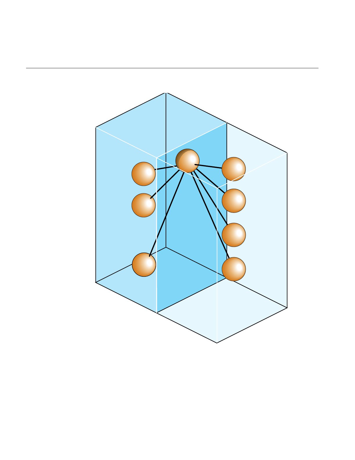
10
Chapter 1: IRIS Performer Programming Interface
Figure 1-1 Partial Inheritance Graph of IRIS Performer Data Types
Some classes
found in
libpf
Some classes
found in
libpr
pfNode
pfChannel
pfMaterial
pfGeoSet
pfFrustum
pfObject
pfLight
pfPipe

Base Classes
11
IRIS Performer objects are divided into two groups: those found in the libpf library and
those found in the libpr library. These two groups of objects have some common
attributes, but also differ in some respects.
While IRIS Performer only uses single inheritance, some objects encapsulate others,
hiding the encapsulated object but also providing a functional interface that mimics its
original one. For example a pfChannel has a pfFrustum, a pfFrameStats has a pfStats, a
pfPipeWindow has a pfWindow, and a pfPipeVideoChannel has a pfVideoChannel. In
these cases, the first object in each pair provides functions corresponding to those of the
second. For example, pfFrustum has a routine,
pfMakeSimpleFrust(frust, 45.0f);
and pfChannel has a corresponding routine,
pfMakeSimpleChan(channel, 45.0f);
Libpr
and
Libpf
Objects
All of the major classes in IRIS Performer are derived from the pfObject class. This
common, base class unifies the data types by providing common attributes and
functions. Libpf objects are further derived from pfUpdatable. The pfUpdatable abstract
class provides support for automatic multi-buffering for multiprocessing. pfObjects have
no special support for multiprocessing and so all processes share the same copy of the
pfObject in the shared arena. libpr objects allocated from the heap are only visible in the
process in which they are created or in child processes created after the object. Changes
made to such an object in one process are not visible in any other process.
Explicit multi-buffering of pfObjects is available through the pfFlux class. In general,
libpr provides lightweight and low-level modular pieces of functionality that are then
enhanced by more powerful libpf objects.
User Data
The primary attribute defined by the pfObject is class is the custom data a user gets to
define on any pfObject called “user data.” pfUserDataSlot attaches the user-supplied
data pointer to user data. pfUserData attaches the user-supplied data pointer to user data
slot. Example 1-1 shows how to use user data.

12
Chapter 1: IRIS Performer Programming Interface
Example 1-1 How to Use User Data
typedef struct
{
float coeffFriction;
float density;
float *dataPoints;
}
myMaterial;
myMaterial *granite;
granite = (myMaterial *)pfMalloc(sizeof(myMaterial), NULL);
granite->coeffFriction = 0.5f;
granite->density = 3.0f;
granite->dataPoints = (float *)pfMalloc(sizeof(float)*8, NULL);
graniteMtl = pfNewMtl(NULL);
pfUserData(graniteMtl, granite);
pfDelete() and Reference Counting
Most kinds of data objects in IRIS Performer can be placed in a hierarchical scene graph,
using instancing when an object is referenced multiple times. Scene graphs can become
quite complex, which can cause problems if you’re not careful. Deleting objects can be a
particularly dangerous operation, for example, if you delete an object that another object
still references.
Reference counting provides a bookkeeping mechanism that makes object deletion safe:
an object is never deleted if its reference count is greater than zero.
Alllibpr objects (such as pfGeoState and pfMaterial) have a reference count that specifies
how many other objects refer to it. A reference is made whenever an object is attached to
another using the IRIS Performer routines shown in Table 1-1.

Base Classes
13
When object A is attached to object B, the reference count of A is incremented.
Additionally, if A replaces a previously referenced object C, then the reference count of
C is decremented. Example 1-2 demonstrates how reference counts are incremented and
decremented.
Example 1-2 Objects and Reference Counts
pfGeoState *gstateA, *gstateC;
pfGeoSet *gsetB;
/* Attach gstateC to gsetB. Reference count of gstateC
* is incremented. */
pfGSetGState(gsetB, gstateC);
/* Attach gstateA to gsetB, replacing gstateC. Reference
* count of gstateC is decremented and that of gstateA
* is incremented. */
pfGSetGState(gsetB, gstateA);
Table 1-1 Routines that Modify libpr Object Reference Counts
Routine Action
pfGSetGState Attaches a pfGeoState to a pfGeoSet
pfGStateAttr Attaches a state structure (such as a pfMaterial) to
a pfGeoState
pfGSetHlight Attaches a pfHighlight to a pfGeoSet
pfTexDetail Attaches a detail pfTexture to a base pfTexture
pfGSetAttr Attaches attribute and index arrays to a pfGeoSet
pfTexImage Attaches an image array to a pfTexture
pfAddGSet, pfReplaceGSet,
pfInsertGSet Modify pfGeoSet/pfGeode association

14
Chapter 1: IRIS Performer Programming Interface
This automatic reference counting done by IRIS Performer routines is usually all you’ll
ever need. However, the routines pfRef(),pfUnref(), and pfGetRef() allow you to
increment, decrement, and retrieve the reference count of a libpr object should you wish
to do so. (These routines also work with objects allocated by pfMalloc(); see the IRIS
Performer Programmer’s Guide for more information).
An object whose reference count is equal to 0 can be deleted with pfDelete().pfDelete()
works for all libpr objects and all pfNodes but not for other libpf objects like pfPipe and
pfChannel. pfDelete() first checks the reference count of an object. If the reference count
is non-positive, pfDelete() decrements the reference count of all objects that the current
object references, then it deletes the current object. pfDelete() doesn’t stop here but
continues down all reference chains, deleting objects until it finds one whose count is
greater than zero. Once all reference chains have been explored, pfDelete returns a
boolean indicating whether it successfully deleted the first object or not. Example 1-3
illustrates the use of pfDelete() with libpr.
Example 1-3 Using pfDelete() with libpr Objects
pfGeoState *gstate0, *gstate1;
pfMaterial *mtl;
pfGeoSet *gset;
gstate0 = pfNewGState(arena); /* initial ref count is 0 */
gset = pfNewGSet(arena); /* initial ref count is 0 */
mtl = pfNewMtl(arena); /* initial ref count is 0 */
/* Attach mtl to gstate0. Reference count of mtl is
* incremented. */
pfGStateAttr(gstate0, PFSTATE_FRONTMTL, mtl);
/* Attach mtl to gstate1. Reference count of mtl is
* incremented. */
pfGStateAttr(gstate1, PFSTATE_FRONTMTL, mtl);
/* Attach gstate0 to gset. Reference count of gstate0 is
* incremented. */
pfGSetGState(gset, gstate0);
/* This deletes gset, gstate0, but not mtl since gstate1 is
* still referencing it. */
pfDelete(gset);

Base Classes
15
Example 1-4 illustrates the use of pfDelete() with libpf.
Example 1-4 Using pfDelete() with libpf Objects
pfGroup *group;
pfGeode *geode;
pfGeoSet *gset;
group = pfNewGroup(); /* initial parent count is 0 */
geode = pfNewGeode(); /* initial parent count is 0 */
gset = pfNewGSet(arena); /* initial ref count is 0 */
/* Attach geode to group. Parent count of geode is
* incremented. */
pfAddChild(group, geode);
/* Attach gset to geode. Reference count of gset is
* incremented. */
pfAddGSet(geode, gset);
/* This has no effect since the parent count of geode is 1.*/
pfDelete(geode);
/* This deletes group, geode, and gset */
pfDelete(group);
Some notes about reference counting and pfDelete():
• All reference count modifications are locked so that they guarantee mutual
exclusion when multiprocessing.
• Objects added to a pfDispList don’t have their counts incremented due to
performance considerations.
• In the multiprocessing environment of libpf, the successful deletion of a pfNode
doesn’t have immediate effect but is delayed one or more frames until all processes
in all processing pipelines are through with the node. This accounts for the fact that
pfDispLists don’t reference-count their objects.

16
Chapter 1: IRIS Performer Programming Interface
•pfUnrefDelete(obj) is shorthand for
if(pfUnref(obj) ==0)
pfDelete(obj);
This is true when pfUnrefGetRef is atomic.
• Objects whose count reaches zero are not automatically deleted by IRIS Performer.
You must specifically request that an object be deleted with pfDelete() or
pfUnrefDelete().
Copying Objects with pfCopy()
pfCopy() is currently implemented for libpr (and pfMalloc()) objects only. Object
references are copied and reference counts are modified appropriately, as illustrated in
Example 1-5.
Example 1-5 Using pfCopy()
pfGeoState *gstate0, *gstate1;
pfMaterial *mtlA, *mtlB;
gstate0 = pfNewGState(arena);
gstate1 = pfNewGState(arena);
mtlA = pfNewMtl(arena); /* initial ref count is 0 */
mtlB = pfNewMtl(arena); /* initial ref count is 0 */
/* Attach mtlA to gstate0. Reference count of mtlA is
* incremented. */
pfGStateAttr(gstate0, PFSTATE_FRONTMTL, mtlA);
/* Attach mtlB to gstate1. Reference count of mtlB is
* incremented. */
pfGStateAttr(gstate1, PFSTATE_FRONTMTL, mtlB);
/* gstate1 = gstate0. The reference counts of mtlA and mtlB
* are 2 and 0 respectively. Note that mtlB is NOT deleted
* even though its reference count is 0. */
pfCopy(gstate1, gstate0);
pfMalloc and the related routines provide a consistent method to allocate memory, either
from the user’s heap (using the C-library malloc function) or from a shared memory
arena (using the IRIX malloc function).

Base Classes
17
Printing Objects with pfPrint()
pfPrint() can print many different kinds of objects to a file, for example, you can print
nodes and geosets. To do so, you specify in the argument of the function the object to
print, the level of verbosity, and the destination file. An additional argument, which,
specifies different data according to the type of object being printed.
The different levels of verbosity include:
• PFPRINT_VB_OFF—no printing.
• PFPRINT_VB_ON—minimal printing (default).
• PFPRINT_VB_NOTICE—minimal printing (default).
• PFPRINT_VB_INFO—considerable printing.
• PFPRINT_VB_DEBUG—exhaustive printing.
If the object to print is a type of pfNode, which specifies whether the print traversal
should only traverse the current node (PFTRAV_SELF) or the entire scene graph where
the node specified in the argument is the root node (PFTRAV_SELF |
PFTRAV_DESCEND). For example, to print an entire scene graph, in which scene is the
root node, to the file, fp, with default verbosity, use the following line of code.
file = fopen (“scene.out”,”w”);
pfPrint(scene, PFTRAV_SELF | PFTRAV_DESCEND, PFPRINT_VB_ON, fp);
fclose(file);
If the object to print is a pfFrameStats, which should specify a bitmask of the frame
statistics classes that you want printed. The values for the bitmask include:
• PFSTATS_ON Enables the specified classes.
• PFSTATS_OFF Disables the specified classes.
• PFSTATS_DEFAULT Sets the specified classes to their default values.
• PFSTATS_SET Sets the class enable mask to enmask.
For example, to print select classes of a pfFrameStats structure, stats, to stderr, use the
following line of code.
pfPrint(stats, PFSTATS_ENGFX | PFFSTATS_ENDB | PFFSTATS_ENCULL,
PFSTATS_ON, NULL);

18
Chapter 1: IRIS Performer Programming Interface
If the object to print is a pfGeoSet, which is ignored and information about that pfGeoSet
is printed according to the verbosity indicator. The output contains the types, names, and
bounding volumes of the nodes and pfGeoSets in the hierarchy. For example, to print the
contents of a pfGeoSet, gset, to stderr, use the following line of code.
pfPrint(gset, NULL, PFPRINT_VB_DEBUG, NULL);
Note: When the last argument, file, is set to NULL, the object is printed to stderr.
Determining Object Type
Sometimes you have a pointer to a pfObject but you don’t know what it really is—is it a
pfGeoSet, a pfChannel, or something else? pfGetType() returns a pfType which specifies
the type of a pfObject. This pfType can be used to determine the class ancestry of the
object. Another set of routines, one for each class, returns the pfType corresponding to
that class, e.g. pfGetGroupClassType() returns the pfType corresponding to pfGroup.
pfIsOfType() tells whether an object is derived from a specified type, as opposed to
being the exact type.
With these functions you can test for class type as shown in Example 1-6.
Example 1-6 General-Purpose Scene Graph Traverser
void
travGraph(pfNode *node)
{
if (pfIsOfType(node, pfGetDCSClassType()))
doSomethingTransforming(node);
/* If ’node’ is derived from pfGroup then recursively
* traverse its children */
if (pfIsOfType(node, pfGetGroupClassType()))
for (i = 0; i < pfGetNumChildren(node); i++)
travGraph(pfGetChild(node, i));
}
Because IRIS Performer allows subclassing of built-in types, when decisions are made
based on the type of an object, it is usually better to use pfIsOfType() to test the type of
an object rather than to test for the strict equality of the pfTypes. Otherwise the code will
not have reasonable default behavior with file loaders or applications which use
subclassing.

Base Classes
19
The pfType returned from pfGetType() is useful for programs but it is not in a readable
form for you. Calling pfGetTypeName() on a pfType returns a null-terminated ASCII
string that identifies an object’s type. For a pfDCS, for example, pfGetTypeName()
returns the string, “pfDCS.” The type returned by pfGetType() can then be compared to
a class type using pfIsOfType(). Class types can be returned by methods such as
pfGetGroupClassType().


This chapter describes how to create a display environment by configuring
rendering pipelines, channels, and viewpoints.
“Setting Up the Display Environment”
Chapter 2


23
Chapter 2
2. Setting Up the Display Environment
libpf is a visual-database processing and rendering system. The visual database has at its
root a pfScene (as described in Chapter 3 and Chapter 4). The chain of events in leading
from the scene graph to the display includes:
1. A pfScene is viewed by a pfChannel.
2. The pfChannel view of the pfScene is rendered by a pfPipe into a frame buffer.
3. A pfPipeWindow manages the frame buffer.
4. The images in the frame buffer are transmitted to a display system which is
managed by a pfPipeVideoChannel.
Figure 2-1 shows this chain of events.
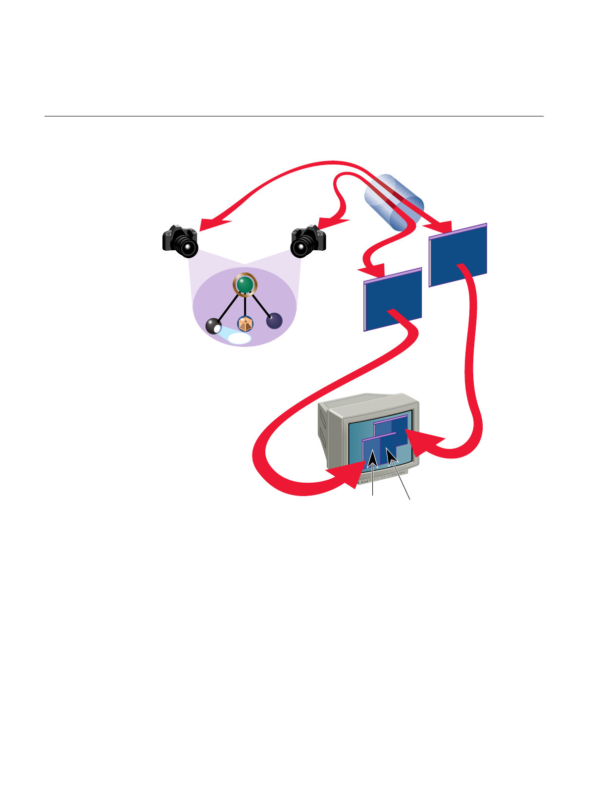
24
Chapter 2: Setting Up the Display Environment
Figure 2-1 From Scene Graph to Visual Display
This chapter describes how to implement this chain of events using pfPipes,
pfPipeWindows, and pfChannels.
Scene graph
pfChannel 1
pfChannel 0
pfPipe
pfPipeWindow 0
pfPipeWindow 1
Display system
pfChannel 0 pfChannel 1
pfScene

Using Pipes
25
Using Pipes
This section describes rendering pipelines (pfPipes) and their implementation in IRIS
Performer. Each rendering pipeline draws into one or more windows (pfPipeWindows)
associated with a single Geometry Pipeline. A minimum of one rendering pipeline is
required, although it is possible to have more than one.
The Functional Stages of a Pipeline
This rendering pipeline comprises three primary functional stages:
APP Simulation processing, which includes reading input from control
devices, simulating the vehicle dynamics of moving models, updating
the visual database, and interacting with other networked simulation
stations.
CULL Traverses the visual database and determines which portions of it are
potentially visible (a procedure known as culling), selects a level of detail
for each model, sorts objects and optimizes state management, and
generates a display list for the draw function.
DRAW Traverses the display list and issues graphics library commands to a
Geometry Pipeline in order to create an image for subsequent display.
Figure 2-2 shows the process flow for a single-pipe system. The application constructs
and modifies the scene definition (a pfScene) associated with a channel. The traversal
process associated with that channel’s pfPipe then traverses the scene graph, building an
IRIS Performer libpr display list. As shown in the figure, this display list is used as input
to the draw process that performs the actual graphics library actions required to draw the
image.
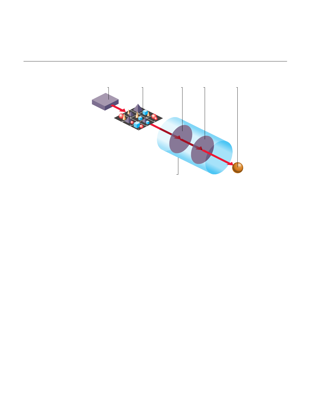
26
Chapter 2: Setting Up the Display Environment
Figure 2-2 Single Graphics Pipeline
IRIS Performer also provides additional processes for application processing tasks, such
as database loading and intersection traversals, but these processes are per-application
and are asynchronous to the software rendering pipeline(s).
An IRIS Performer application renders images using one or more pfPipes. Each pfPipe
represents an independent software-rendering pipeline. Most IRIS systems contain only
one Geometry Pipeline™, so a single pfPipe is usually appropriate. This single pipeline is
often associated with a window that occupies the entire display surface.
Alternative configurations include Onyx2™ systems with InfiniteReality graphics
(allowing up to eight Geometry Pipelines). Applications can render into multiple
windows, each of which is connected to a single Geometry Pipeline through a pfPipe
rendering pipeline.
Figure 2-3 shows the process flow for a dual-pipe system. Notice both the differences and
similarities between these two figures. Each pipeline (pfPipe) is independent in
multiple-pipe configurations; the traversal and draw tasks are separate, as are the libpr
display lists that link them. In contrast, these pfPipes are controlled by the same
application process, and in many situations access the same shared scene definition.
Scene Frame BufferTraversal/CullApplication Draw
Pipeline 0
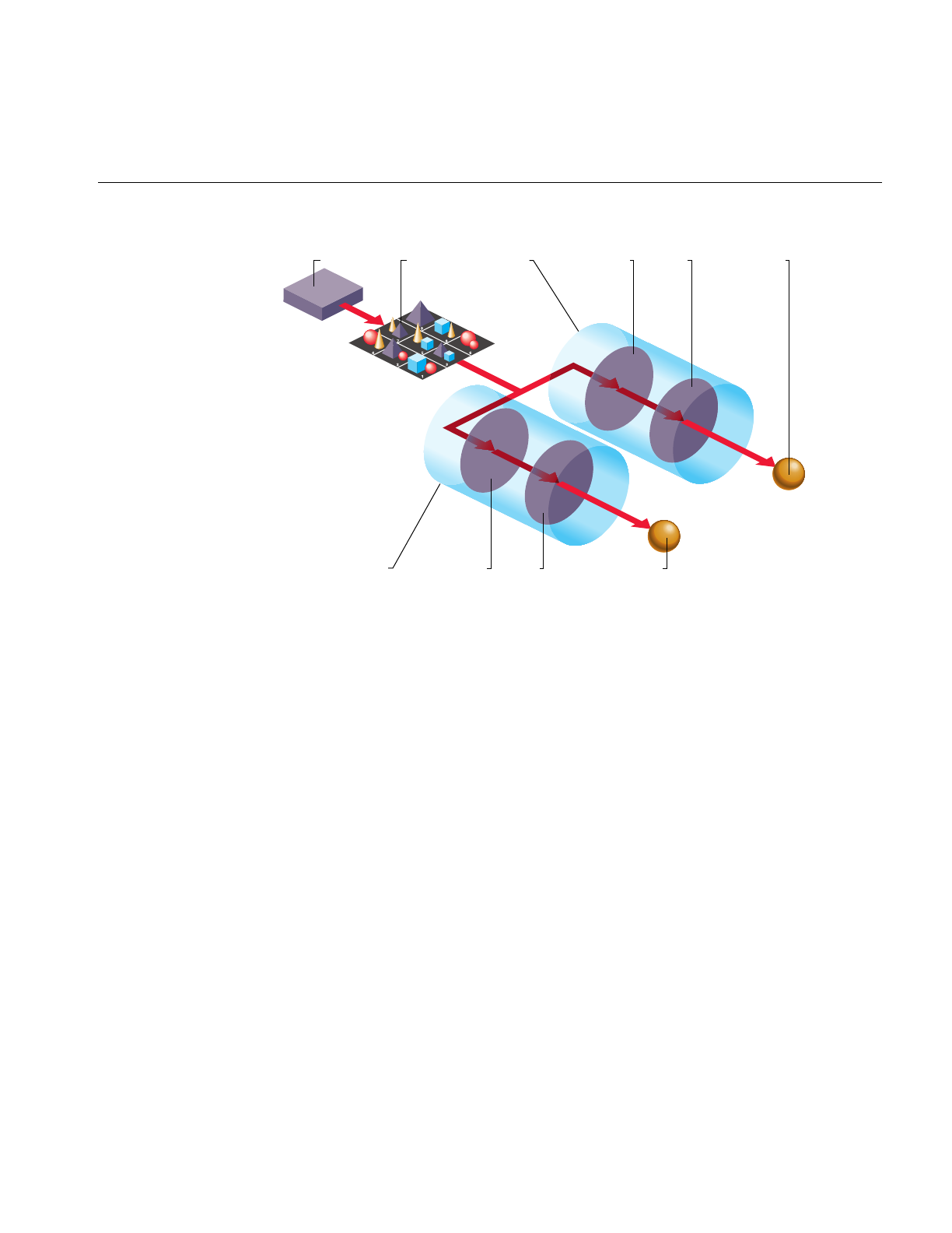
Using Pipes
27
Figure 2-3 Dual Graphics Pipeline
Each of these stages can be combined into a single IRIX process or split into multiple
processes (pfMultiprocess) for enhanced performance on multiple CPU systems.
Multiprocessing and multiple pipes are advanced topics that are discussed in
“Successful Multiprocessing With IRIS Performer” in Chapter 5.
Creating and Configuring a pfPipe
pfPipes and their associated processes are created when pfConfig() is called. They exist
for the duration of the application. After pfConfig(), the application can get handles to
the created pfPipes using pfGetPipe(). The argument to pfGetPipe() indicates which
pfPipe to return and is an integer between 0 and numPipes-1, inclusive. The pfPipe handle
is then used for further configuration of the pfPipe.
pfMultipipe() specifies the number of pfPipes desired. pfMultiprocess() specifies the
multiprocessing mode used by all pfPipes; the default is one. These two routines are
discussed further in“Successful Multiprocessing With IRIS Performer” in Chapter 5.
Scene Frame BufferTraversal/CullApplication DrawPipeline 1
Pipeline 0 Frame BufferTraversal/Cull Draw

28
Chapter 2: Setting Up the Display Environment
A key part of pfPipe initialization is the determination of the graphics hardware pipeline
(or screen) and the creation of a window on that screen. The screen of a pfPipe can be set
explicitly using pfPipeScreen(). Under single pipe operation, pfPipes can also inherit the
screen of their first opened window. Under multipipe operation, the screen of all pfPipes
must be determined before the pipes are configured by pfConfigStage() or the first call
topfFrame(). There may be other operations that require pre-set knowledge of the screen
even under single pipes, such as custom configuration of video channels, discussed in
“Creating and Configuring a pfChannel” on page 31.
Once the screen of a pfPipe has been set, it cannot be changed. All windows of a pfPipe
must be opened on the same screen. A graphics window is associated with a pfPipe
through the pfPipeWindow mechanism. If you do not create a pfPipeWindow, IRIS
Performer will automatically create and open a full screen window with a default
configuration for your pfPipe.
Once you create and initialize a pfPipe, you can query information about its
configuration parameters. pfGetPipeScreen() returns the index number of the hardware
pipeline for the pfPipe, starting from zero. On single-pipe systems the return value will
be zero. If no screen has been set, the return value will be (-1). pfGetPipeSize() returns
the full screen size, in pixels, of the rendering area associated with a pfPipe.
You may have application states associated with pfPipe stages and processes that need
special initialization. For this purpose, you may provide a stage configuration callback
for each pfPipe stage using pfStageConfigFunc(pipe, stageMask, configFunc) and
specify the pfPipe, the stage bitmask (including one or more of PFPROC_APP,
PFPROC_CULL, and PFPROC_DRAW), and your stage configuration callback routine.
At any time, you may call the function pfConfigStage() from the application process to
trigger the execution of your stage configuration callback in the process associated with
that pfPipe’s stage. The stage configuration callback will be invoked at the start of that
stage within the current frame (the current frame in the application process, and
subsequent frames through the cull and draw phases of the software rendering pipeline).
Use a pfStageConfigFunc() callback function to configure performer processes not
associated with pfPipes, such as the database process, PFPROC_DBASE, and the
intersection process, PFPROC_ISECT. A common process initialization task for real-time
applications is the selection and/or specification of a CPU on which to run.

Using Pipes
29
Example of pfPipe Use
The sample source code shipped with IRIS Performer includes several simple examples
of pfPipe use in both C and C++. Specifically, look at the following examples under the
C and C++ directories in /usr/share/Performer/src/pguide/libpf/, such as hello.c,simple.c, and
multipipe.c.
Example 2-1 illustrates the basics of using pipes. The code in this example is adapted
from IRIS Performer sample programs.
Example 2-1 pfPipes in Action
main()
{
int i;
/* Initialize IRIS Performer */
pfInit();
/* Set number of pfPipes desired -- THIS MUST BE DONE
* BEFORE CALLING pfConfig().
*/
pfMultipipe(NumPipes);
/* set multiprocessing mode */
pfMultiprocess(ProcSplit);
...
/* Configure IRIS Performer and fork extra processes if
* configured for multiprocessing.
*/
pfConfig();
...
/* Optional custom mapping of pipes to screens.
* This is actually the reverse as the default.
*//
for (i=0; i < NumPipes; i++)
pfPipeScreen(pfGetPipe(i), NumPipes-(i+1));
{
/* set up optional DRAW pipe stage config callback */
pfStageConfigFunc(-1 /* selects all pipes */,
PFPROC_DRAW /* stage bitmask */,
ConfigPipeDraw /* config callback */);
/* Config func should be done next pfFrame */
pfConfigStage(i, PFPROC_DRAW);
}

30
Chapter 2: Setting Up the Display Environment
InitChannels();
...
/* trigger the configuration and opening of pfPipes
* and pfWindows
*/
pfFrame();
/* Application’s simulation loop */
while(!SimDone())
{
...
}
}
/* CALLBACK FUNCTIONS FOR PIPE STAGE INITIALIZATION */
void
ConfigPipeDraw(int pipe, uint stage)
{
/* Application state for the draw process can be initialized
* here. This is also a good place to do real-time
* configuration for the drawing process, if there is one.
* There is no graphics state or pfState at this point so no
* rendering calls or pfApply*() calls can be made.
*/
pfPipe *p = pfGetPipe(pipe);
pfNotify(PFNFY_INFO, PFNFY_PRINT,
“Initializing stage 0x%x of pipe %d”, stage, pipe);
}
Using Channels
This section describes how to use pfChannels. A pfChannel is a view of a scene. A
pfChannel is a required element for an IRIS Performer application because it establishes
the visual frame of reference for what is rendered in the drawing process.

Using Channels
31
Creating and Configuring a pfChannel
When you create a new pfChannel, it is attached to a pfPipe for the duration of the
application. The pfPipe renders the pfScene viewed by the pfChannel into a
pfPipeWindow that is managed by that pipe. Use pfNewChan() to create a new
pfChannel and assign it to a pfPipe. pfChannels are automatically assigned to the first
pfPipeWindow of the pfPipe. In the sample program, the following statement creates a
new channel and assigns it to pipe p.
chan = pfNewChan(p);
The pfChannel is automatically placed in the first pfPipeWindow of the pfPipe. A
pfPipeWindow is created automatically if one is not explicitly created with
pfNewPWin().
The simplest configuration uses one pipe, one channel, and one window. You can use
multiple channels in a single pfPipeWindow on a pfPipe, thereby allowing channels to
share hardware resources. Using multiple channels is an advanced topic that is discussed
in the section of this chapter on “Using Multiple Channels.” For now, focus your
attention on understanding the concepts of setting up and using a single channel.
The primary function of a pfChannel is to define the view of a scene. A view is fully
characterized by a viewport, a viewing frustum, and a viewpoint. The following sections
describe how to set up the scene and view for a pfChannel.
Setting Up a Scene
A pfChannel draws the pfScene set by pfChanScene(). A channel can draw only one
scene per frame but can change scenes from frame to frame. Other pfChannel attributes
such as LOD modifications, described in “pfLOD Nodes” in Chapter 3, affect the scene.
A pfChannel also renders an environmental model known as pfEarthSky. A pfEarthSky
defines the method for clearing the channel viewport before rendering the pfScene and
also provides environmental effects, including ground and sky geometry and fog and
haze. A pfEarthSky is attached to a pfChannel by pfChanESky().

32
Chapter 2: Setting Up the Display Environment
Setting Up a Viewport
A pfChannel is rendered by a pfPipe into its pfPipeWindow. The screen area that displays
a pfChannel’s view is determined by the origin and size of the window and the channel
viewport specified by pfChanViewport. The channel viewport is relative to the lower left
corner of the window and ranges from 0 to 1. By default, a pfChannel viewport covers
the entire window.
Suppose that you want to establish a viewport that is one-quarter of the size of the
window, located in the lower left corner of the window. Use pfChanViewport(chan, 0.0,
0.25, 0.0, 0.25) to set up the one-quarter window viewport for the channel chan.
You can then set up other channels to render to the other three-quarters of the window.
For example, you can use four channels to create a four-way view for an architectural or
CAD application. See “Using Multiple Channels” on page 40 to learn more about
multiple channels.
Setting Up a Viewing Frustum
A viewing frustum is a truncated pyramid that defines a viewing volume. Everything
outside this volume is clipped, while everything inside is projected onto the viewing
plane for display. A frustum is defined by
• field-of-view (FOV) in the horizontal and vertical dimensions
• near and far clipping planes
A viewing frustum is created by the intersections of the near and far clipping planes with
the top, bottom, left, and right sides of the infinite viewing volume formed by the FOV
and aspect ratio settings. The aspect ratio is the ratio of the vertical and horizontal
dimensions of the FOV.
Figure 2-4 shows the parameters that define a symmetric viewing frustum. To establish
asymmetric frusta refer to the pfChannel(3pf) or pfFrustum(3pf) reference pages for
further details.
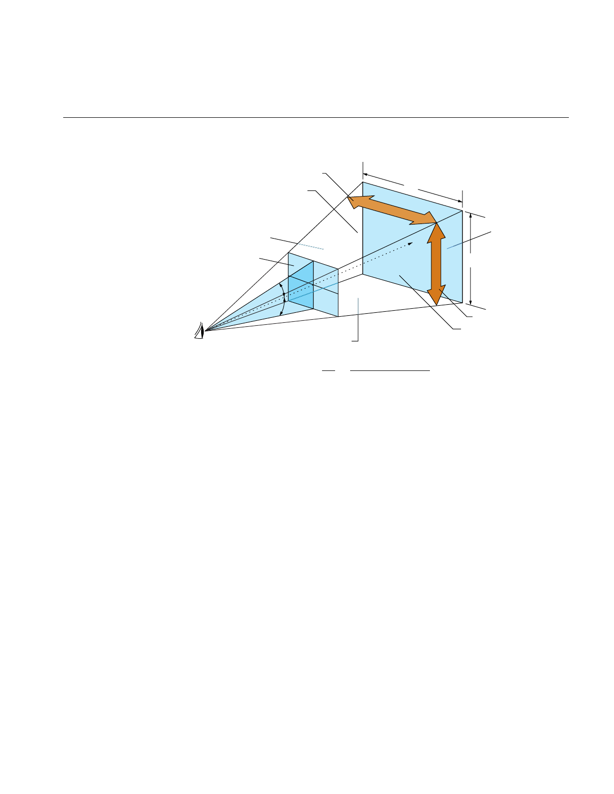
Using Channels
33
Figure 2-4 Symmetric Viewing Frustum
The viewing frustum is called symmetric when the vertical half-angles are equal and the
horizontal half-angles are equal.
Field-of-View
The FOV is the angular width of view. Use pfChanFOV(chan, horiz, vert) to set up
viewing angles in IRIS Performer. The quantities horiz and vert are the total horizontal
and vertical fields of view in degrees; usually you specify one and let IRIS Performer
compute the other. If you’re specifying one angle, pass any amount less than or equal to
zero, or greater than or equal to 180, as the other angle. IRIS Performer automatically
computes the unspecified FOV angle to fit the pfChannel viewport using the aspect-ratio
preserving relationship
tan(vert/2) / tan(horiz/2) = aspect ratio
Vertical FOV
Horizontal FOV
y
x
Top
Left
Right
Bottom
Line of sight
Aspect Ratio = =
x
y
tan(vertical FOV/2)
tan(horizontal FOV/2)
Eyepoint
Near
Far

34
Chapter 2: Setting Up the Display Environment
That is, the ratio of the tangents of the vertical and horizontal half-angles is equal to the
aspect ratio. For example, if horiz is 45 degrees and the channel viewport is twice as wide
as it is high (so the aspect ratio is 0.5), then the vertical field-of-view angle, vert, is
computed to be 23.4018 degrees. If both angles are unspecified, pfChanFOV() assumes a
default value of 45 degrees for horiz and computes the value of vert as described.
Clipping Planes
Clipping planes define the near and far boundaries of the viewing volume. These
distances describe the extent of the visual range in the view, because geometry outside
these boundaries is clipped, meaning that it isn’t drawn.
Use pfChanNearFar(chan, near, far) to specify the distance along the line of sight from
the viewpoint to the near and far planes that bound the viewing volume. These clipping
planes are perpendicular to the line of sight. For the best visual acuity, choose these
distances so that near is as far away as possible from the viewpoint and far is as close as
possible to the viewpoint. Minimizing the range between near and far provides more
resolution for distance comparisons and fog computations.
Setting Up a Viewpoint
A viewpoint describes the position and orientation of the viewer. It is the origin of the
viewing location, the direction of the line of sight from the viewer to the scene being
viewed, and an up direction. The default viewpoint is at the origin (0, 0, 0) looking along
the +Y axis, with +Z up and +X to the right.
Use pfChanView(chan, point, dir) to define the viewpoint for the pfChannel identified
by chan. Specify the view origin for point in x,y,z world coordinates. Specify the view
direction for dir in degrees by giving the degree measures of the three Euler angles:
heading,pitch, and roll.
Heading is a rotation about the z axis, pitch is a rotation about the x axis, and roll is a
rotation about the y axis. The value of dir is the product of the rotations ROTy(roll)∗
ROTx(pitch)∗ ROTz(heading), where ROTa(angle) is a rotation matrix about axis a of angle
degrees.

Using Channels
35
Angles have not only a degree value, but also a sense, + or –, indicating whether the
direction of rotation is clockwise or counterclockwise. Because different systems follow
different conventions, it is very important to understand the sense of the Euler angles as
they are defined by IRIS Performer. IRIS Performer follows the right-hand rule. According
to the right-hand rule, counterclockwise rotations are positive. This means that a rotation
about the x axis by +90 degrees shifts the +Y axis to the +Z axis, a rotation about the y
axis by +90 degrees shifts the +Z axis to the +X axis, and a rotation about the z axis by
+90 degrees shifts the +X axis to the +Y axis.
Figure 2-5 shows a toy plane (somewhat reminiscent of the Ryan S-T) at the origin of a
coordinate system with the angles of rotation labeled for heading, pitch, and roll. The
arrows show the direction of positive rotation for each angle.
Figure 2-5 Heading, Pitch, and Roll Angles
A roll motion tips the wings from side to side. A pitch motion tips the nose up or down.
A yaw motion steers the plane, changing its heading. Accurate readings of these angles
are critical information for a pilot during a flight, and a thorough understanding of how
the angles function together is required for creation of an accurate flight simulation
visual with IRIS Performer. The same is also true of marine and other vehicle
simulations.
X+ Pitch
Y
Z
+ Heading
+ Roll

36
Chapter 2: Setting Up the Display Environment
Alternatively, you can use pfChanViewMat(chan, mat) to create a 4x4 homogeneous
matrix mat that defines the view coordinate system for channel chan. The upper left 3x3
submatrix defines the coordinate system axes, and the bottom row vector defines the
origin of the coordinate system. The matrix must be orthonormal, or the results will be
undefined. You can construct matrices using tools in the libpr library.
The origin and heading, pitch, and roll angles, or the view matrix, create a complete view
specification. The view specification can locate the eyepoint frame-of-reference origin at
any point in world coordinates. The gaze vector, the eye’s +Y axis, can point in any
direction. The up vector, the eye’s +Z axis, can point in any direction perpendicular to the
gaze vector.
You can query the system for the view and eyepoint-direction values with
pfGetChanView(), or obtain the view matrix directly with pfGetChanViewMat().
The view direction can be modified by one or more offsets, relative to the eyepoint
frame-of-reference. View offsets are useful in situations where several channels render
the same scene into adjacent displays for a wider field-of-view or higher resolution.
Offsets are also used for multiple viewer perspectives, such as pilot and copilot views.
Use pfChanViewOffsets(chan, xyz, hpr) to specify additional translation and rotation
offsets for the viewpoint and direction; xyz specifies a translation vector and hpr specifies
a heading/pitch/roll rotation vector. Viewing offsets are automatically added each
frame to the view direction specified by pfChanView() or pfChanViewMat().
For example, to create three different perspectives of the same scene as displayed by
three windows in an airplane cockpit, use azimuth offsets of 45, 0, and -45 for left,
middle, and right views. To create vertical view groups such as might be seen through
the windscreen of a helicopter, use both azimuth and elevation offsets. Once the view
offsets have been set up, you need only set the view once per frame. View offsets are
applied after the eyepoint position and gaze direction have been established. As with the
other angles, be aware that the conventions for measuring azimuth and elevation angles
vary between graphics systems, so you should verify that the sense of the angles is
correct.
Example of Channel Use
Example 2-2 shows how to use various pfChannel-related functions. The code is derived
from IRIS Performer sample programs.

Using Channels
37
Example 2-2 Using pfChannels
main()
{
pfInit();
...
pfConfig();
...
InitScene();
InitPipe();
InitChannel();
/* Application main loop */
while(!SimDone())
{
...
}
}
void InitChannel(void)
{
pfChannel *chan;
chan = pfNewChan(pfGetPipe(0));
/* Set the callback routines for the pfChannel */
pfChanTravFunc(chan, PFTRAV_CULL, CullFunc);
pfChanTravFunc(chan, PFTRAV_DRAW, DrawFunc);
/* Attach the visual database to the channel */
pfChanScene(chan, ViewState->scene);
/* Attach the EarthSky model to the channel */
pfChanESky(chan, ViewState->eSky);
/* Initialize the near and far clipping planes */
pfChanNearFar(chan, ViewState->near, ViewState->far);
/* Vertical FOV is matched to window aspect ratio. */
pfChanFOV(chan, 45.0f/NumChans, -1.0f);
/* Initialize the viewing position and direction */
pfChanView(chan, ViewState->initView.xyz,
ViewState->initView.hpr);
}

38
Chapter 2: Setting Up the Display Environment
/* CULL PROCESS CALLBACK FOR CHANNEL*/
/* The cull function callback. Any work that needs to be
* done in the cull process should happen in this function.
*/
void
CullFunc(pfChannel * chan, void *data)
{
static long first = 1;
if (first)
{
if ((pfGetMultiprocess() & PFMP_FORK_CULL) &&
(ViewState->procLock & PFMP_FORK_CULL))
pfuLockDownCull(pfGetChanPipe(chan));
first = 0;
}
PreCull(chan, data);
pfCull(); /* Cull to the viewing frustum */
PostCull(chan, data);
}
/* DRAW PROCESS CALLBACK FOR CHANNEL*/
/* The draw function callback. Any graphics functionality
* outside IRIS Performer must be done here. I/O with pure * IRIS GL
devices must happen here.
*/
void
DrawFunc(pfChannel *chan, void *data)
{
PreDraw(chan, data); /* Clear the viewport, etc. */
pfDraw(); /* Render the frame */
/* draw HUD, read IRIS GL devices, or whatever else needs
* to be done post-draw.
*/
PostDraw(chan, data);
}

Controlling the Video Output
39
Controlling the Video Output
You use pfPipeVideoChannel to query and control the configuration of a hardware video
channel. The methods allow you to, for example, query or specify the origin and size of
the video output and scale the display.
By default, all pfVideoChannels on a pfPipe use the first entire video channel on the
screen selected by the pfPipe. Each pfPipeWindow initially has a default
pfPipeVideoChannel already assigned to it. When pfChannels are added to
pfPipeWindows, they will be using, by default, this first pfPipeVideoChannel. You can
get a pfPipeVideoChannel of a pfPipeWindow with pfGetPWinPVChan() and
specifying the index of the pfPipeVideoChannel on the pfPipeWinow; the initial default
one will be at index 0. You can then reconfigure this pPipeVideoChannel to select a
different video channel or change the attributes of the selected video channel. You can
create a pfPipeVideoChannel with pfNewPVChan(). To use this for a given pfChannel,
you must add it to a pfPipeWindow that will cover the screen area of the desired video
channel. When a pfPipeVideoChannel is added to a pfPipeWindow with
pfAddPWinPVChan(), the index into the pfPipeWindow list of video channels is
returned and by default the pfPipeVideoChannel will get the next active hardware video
channel after the previous pfPipeVideoChannel on that pfPipeWindow. You can
explicitly select the hardware video channel with pfPVChanId(). The pfChannel will
then reference this pfPipeVideoChannel through the index that you got back from
pfAddPWinPVChan() and assign to the pfChannel with pfChanPWinPVChanIndex().
pvc = pfNewPVChan(p);
pvcIndex = pfPWinAddPVChan(pw, pvc);
pfChanPWinPVChanIndex(chan, pvcIndex);
Note that the screen of the pfPipe must be known to fully specify the desired video
channel. Queries on the pfPipeVideoChannel will return values indicating unknown
configuration until the screen is known. The screen can be determined by IRIS Performer
when the window is opened in the DRAW process but you can also explicitly set the
screen of the pfPipe with pfPipeScreen().
You can also get to the hardware video channel structure, pfVideoChannelInfo(), for
more configuration options, such as reading gamma data or even a specific video format.
For more information on pfPipeWindows and pfPipeVideoChannels, see Chapter 12,
“pfPipeWindows and pfPipeVideoChannels.”

40
Chapter 2: Setting Up the Display Environment
Using Multiple Channels
Each rendering pipeline can render multiple channels with multiple
pfPipeVideoChannels to a single pfPipeWindows. Multiple pfPipeWindows can also be
used but at the cost of some additional processing overhead. The pfChannel is assigned
to the proper pfPipeWindow and selects its pfPipeVideoChannel from that
pfPipeWindow. The pfChannel must also have a viewport, set with pfChanViewport(),
that covers the proper window area to match that of the desired pfPipeVideoChannel.
Each channel represents an independent viewpoint into either a shared or an
independent visual database. Different types of application can have vastly different
pipeline-window-channel configurations. This section describes two extremes: visual
simulation applications where there is typically one window per pipeline, and highly
interactive uses that require dynamic window and channel configuration.
One Window per Pipe, Multiple Channels per Window
Often there will is a single channel associated with each pipeline, as shown in the top half
of Figure 2-6. This section describes two important uses for multiple-channel support—
multiple pipelines per system and multiple windows per pipeline—the second of which
is illustrated in the bottom half of Figure 2-6.
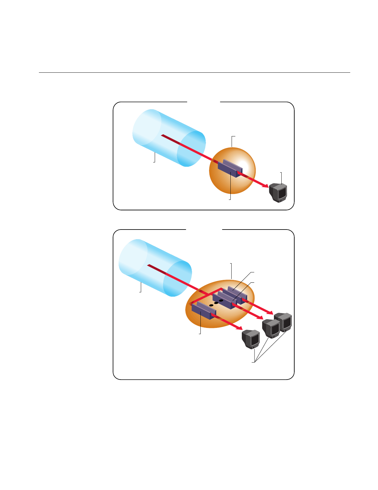
Using Multiple Channels
41
Figure 2-6 Single-Channel and Multiple-Channel Display
Frame Buffer
Pipeline
Channel 0
Pipeline
Channel
n
−1
Frame Buffer
Channel 0
Channel 1
Display
Device
Display
Device
Single Channel
Multiple Channel

42
Chapter 2: Setting Up the Display Environment
One situation that requires multiple channels occurs when inset views must appear
within an image. A simple example of this application is a driving simulator in which the
screen image represents the view out the windshield. If a rear-view mirror is to be drawn,
it must overlay the main forward view to provide a separate view of the same database
within the borders of the simulated mirror’s frame.
Channels are physically rendered in the order that they are assigned to a pfPipeWindow
on their parent pfPipe. Channels, upon creation, are assigned to the end of the channel
list of the first window of their pfPipe. In the driving simulator example, creating pipes
and channels with the following structure creates two channels on a single shared
pipeline:
pipeline = pfGetPipe(0);
frontView = pfNewChan(pipeline);
rearView = pfNewChan(pipeline);
In this case, IRIS Performer’s actual drawing order becomes:
1. Clear frontView.
2. Draw frontView.
3. Clear rearView.
4. Draw rearView.
This default ordering results in the rear-view mirror image always overlaying the
front-view image, as desired. You can control and re-order the drawing of channels
within a pfPipeWindow with the pfInsertChan(pwin, where, chan) and
pfMoveChan(pwin, where, chan) routines. More details about multiple channels and
multiple window are discussed in the next section.
When the host has multiple Geometry Pipelines, as supported on Onyx RealityEngine2
systems, you can create a pfPipe and pfChannel pair for each hardware pipeline. The
following code fragment illustrates a two-channel, two-pipeline configuration:
leftPipe = pfGetPipe(0);
leftView = pfNewChan(leftPipe);
rightPipe = pfGetPipe(1);
rightView = pfNewChan(rightPipe);
This configuration forms the basis for a high-performance stereo display system, since
there is a hardware pipeline dedicated to each eye and rendering occurs in parallel.

Using Multiple Channels
43
The two-channel stereo-view application described in this example and the inset-view
application described in the previous example can be combined to provide stereo views
for a driving simulator with an inset rear-view mirror. The correct management of each
eye’s viewpoint and the mirror reflection helps provide a convincing sense of physical
presence within the vehicle.
The third common multiple-channel situation involves support for multiple video
outputs per pipeline. To do this, first associate each pipeline with a set of nonoverlapping
channels, one for each desired view. Next, use one of the following video-splitting
methods:
• Use the multi-channel hardware options, available from Silicon Graphics, for
systems such as the 8 channel Display Generator(DG) for Onyx2 InfiniteReality,
where you can create up to eight independent video outputs from a single Graphics
Pipeline, with each video output corresponding to one of the tiled channels. The
OCTANE video option supports four video outputs and the RealityEngine2
Multi-Channel Option supports six video channels per Graphics Pipeline.
• Connect multiple video monitors in series to a single pipeline’s video output.
Because each monitor receives the same display image, a masking bezel is used to
obscure all but the relevant portion of each display surface.
The three multiple-channel concepts described here can be used in combination. For
example, use of three InfiniteReality pipelines, each equipped with the 8 channel DG ,
allows creation of up to 24 independent video displays. The channel-tiling method can
also be used for some or all of these displays.
Example 2-3 shows how to use multiple channels on separate pipes.
Example 2-3 Multiple Channels, One Channel per Pipe
pfChannel *Chan[MAX_CHANS];
void InitChannel(int NumChans)
{
/* Initialize each channel on a separate pipe */
for (i=0; i< NumChans; i++)
Chan[i] = pfNewChan(pfGetPipe(i));
...
/* Make channel n/2 the master channel (can be any
* channel).
*/

44
Chapter 2: Setting Up the Display Environment
ViewState->masterChan = Chan[NumChans/2];
{
long share;
/* Get the default channel-sharing mask */
share = pfGetChanShare(ViewState->masterChan);
/* Add in the viewport share bit */
share |= PFCHAN_VIEWPORT;
if (GangDraw)
{
/* add GangDraw to channel share mask */
share |= PFCHAN_SWAPBUFFERS_HW;
}
pfChanShare(ViewState->masterChan, share);
}
/* Attach channels */
for (i=0; i< NumChans; i++)
if (Chan[i] != ViewState->masterChan)
pfAttachChan(ViewState->masterChan, Chan[i]);
...
/* Continue with channel initialization */
}
Using Channel Groups
In many multiple-channel situations, including the examples described in the previous
section, it is useful for channels to share certain attributes. For the three-channel cockpit
scenario, each pfChannel shares the same eyepoint while the left and right views are
offset using pfChanViewOffsets(). IRIS Performer supports the notion of channel groups,
which facilitate attribute sharing between channels.
pfChannels can be gathered into channel groups that share like attributes. A channel
group is created by attaching one pfChannel to another, or to an existing channel group.
Use pfAttachChan() to create a channel group from two channels or to add a channel to
an existing channel group. Use pfDetachChan() to remove a pfChannel from a channel
group.

Using Channel Groups
45
Achannel share mask defines shared attributes for a channel group. The attribute tokens
listed in Table 2-1 are bitwise OR-ed to create the share mask.
UsepfChanShare() to set the share mask for a channel group. By default, channels share
all attributes except PFCHAN_VIEW_OFFSETS. When you add a pfChannel to a channel
group, it inherits the share mask of that group.
A change to any shared attribute is applied to all channels in a group. For example, if you
change the viewpoint of a pfChannel that shares PFCHAN_VIEW with its group, all
other pfChannels in the group will acquire the same viewpoint.
Two attributes are particularly important to share in adjacent-display multiple-channel
simulations: PFCHAN_SWAPBUFFERS and PFCHAN_LOD. PFCHAN_LOD ensures
that geometry that straddles displays is drawn the same way in each channel. In this case,
all channels will use the same LOD modifier when rendering their scenes so that LOD
behavior is consistent across channels. PFCHAN_SWAPBUFFERS ensures that channels
refresh the display with a new frame at the same time. pfChannels in different pfPipes
that share PFCHAN_SWAPBUFFERS_HW will frame-lock the graphics pipelines
together.
Table 2-1 Attributes in the Share Mask of a Channel Group
Token Shared Attributes
PFCHAN_FOV Horizontal and vertical fields of view
PFCHAN_VIEW View position and orientation
PFCHAN_VIEW_OFFSETS (x,y,z) and (heading,pitch,roll) offsets of the view direction
PFCHAN_NEARFAR Near and far clipping planes
PFCHAN_SCENE All channels display the same scene
PFCHAN_EARTHSKY All channels display the same earth/sky model
PFCHAN_STRESS All channels use the same stress filter
PFCHAN_LOD All channels use the same LOD modifiers
PFCHAN_SWAPBUFFERS All channels swap buffers at the same time
PFCHAN_SWAPBUFFERS_HW Synchronize swap buffers for channels on different graphics
pipelines

46
Chapter 2: Setting Up the Display Environment
Example 2-4 illustrates the use of multiple channels and channel-sharing.
Example 2-4 Channel-Sharing
pfChannel *Chan[MAX_CHANS];
main()
{
pfInit();
...
/* Set number of pfPipes desired. THIS MUST BE DONE
* BEFORE CALLING pfConfig().
*/
pfMultipipe(NumPipes);
...
pfConfig();
...
InitScene();
InitChannels();
pfFrame();
/* Application main loop */
while(!SimDone())
{
...
}
}
void InitChannel(int NumChans)
{
/* Initialize all channels on pipe 0 */
for (i=0; i< NumChans; i++)
Chan[i] = pfNewChan(pfGetPipe(0));
...
/* Make channel n/2 the master channel (can be any
* channel).
*/
ViewState->masterChan = Chan[NumChans/2];
...

Using Channel Groups
47
/* Attach all Channels as slaves to the master channel */
for (i=0; i< NumChans; i++)
if (Chan[i] != ViewState->masterChan)
pfAttachChan(ViewState->masterChan, Chan[i]);
pfSetVec3(xyz, 0.0f, 0.0f, 0.0f);
/* Set each channel’s viewing offset. In this case use
* many channels to create one multichannel contiguous
* frustum with a 45˚ field of fiew.
*/
for (i=0; i < NumChans; i++)
{
float fov = 45.0f/NumChans;
pfSetVec3(hpr, (((NumChans - 1) * 0.5f) - i) * fov,
0.0f, 0.0f);
pfChanViewOffsets(Chan[i], xyz, hpr);
}
...
/* Now, just configure the master channel and all of the
* other channels will share those attributes.
*/
chan = ViewState->masterChan;
pfChanTravFunc(chan, PFTRAV_CULL, CullFunc);
pfChanTravFunc(chan, PFTRAV_DRAW, DrawFunc);
pfChanScene(chan, ViewState->scene);
pfChanESky(chan, ViewState->eSky);
pfChanNearFar(chan, ViewState->near, ViewState->far);
pfChanFOV(chan, 45.0f/NumChans, -1.0f);
pfChanView(chan, ViewState->initView.xyz,
ViewState->initView.hpr);
...
}

48
Chapter 2: Setting Up the Display Environment
Multiple Channels and Multiple Windows
For some interactive applications, you may want to be able to dynamically control the
configuration of Channels and Windows. IRIS Performer allows you to dynamically
create, open, and close windows. You can also move channels amongst the windows of
the shared parent pfPipe, and re-order channels within a pfPipeWindow. Channels can
be appended to the end of a pfPipeWindow channel list with pfAddChan() and removed
with pfRemoveChan(). A channel can only be attached to one pfPipeWindow — no
instancing of pfChannels is allowed. When a pfChannel is put on a pfPipeWindow, it is
automatically deleted from its previous pfPipeWindow. A channel that is not assigned to
a pfPipeWindow is not drawn (though it may still be culled).
You can control and re-order the drawing of channels within a pfPipeWindow with the
pfInsertChan(pwin, where, chan) and pfMoveChan(pwin, where, chan) routines. Both
of these routines do a type of insertion: pfInsertChan() will add chan to pwin’s channel
list in front of the channel in the list at location where.pfMoveChan() will delete chan
from it’s old location and move it to where in pwin’s channel list.
If you have pfChannels in different pfPipeWindows or pfPipes that are supposed to
combine to form a continuous scene, you will want to ensure that both the vertical retrace
and doublebuffering of these windows is synchronized. This is required for both
reasonable performance and visual quality. Use the genlock(7) system video feature to
ensure that the verticial retraces of different graphics pipelines are synchronized. To
synchronize double buffering, you want to either specify
PFCHAN_SWAPBUFFERS_HW in the share mask of the pfChannels and put the
pfChannels in a share group, or else create a pfPipeWindow swap group, discussed in
Chapter 12, “pfPipeWindows and pfPipeVideoChannels.”

This chapter describes the structure of IRIS Performer’s scene-definition
databases and component data types.
“Nodes and Node Types”
Chapter 3


51
Chapter 3
3. Nodes and Node Types
A scene graph holds the data that defines a virtual world. The scene graph includes
low-level descriptions of object geometry and their appearance, as well as higher-level,
spatial information, such as specifying the positions, animations, and transformations of
objects, as well as additional application-specific data.
Scene graph data is encapsulated in many different types of nodes. One node might
contain the geometric data of an object; another node might contain the transformation
for that object to orient and position it in the virtual world. The nodes are associated in a
hierarchy that is an adirected, acyclic graph. IRIS Performer and your application can act
on the scene graph to perform various complex operations efficiently, such as database
intersection and rendering scenes.
This chapter focuses on the data types themselves rather than instances of those types.
Chapter 4, “Database Traversal,” discusses traversing sample scene graphs in terms of
actual objects rather than abstract data types.
Nodes
A scene is represented by a graph of nodes. A node is a subclass of pfNode. Only nodes
can be in scene graphs and have child nodes. In general, nodes either contain descriptive
information about scene graph geometry, or they create groups and hierarchies of nodes.
Many classes, such as pfEngine and pfFlux, that are not nodes can interact with nodes.
Attribute Inheritance
The basic element of a scene hierarchy is the node. While IRIS Performer supplies many
specific types of nodes, it also uses a concept called class inheritance, which allows
different node types to share attributes. An attribute is a descriptive element of geometry
or its appearance.
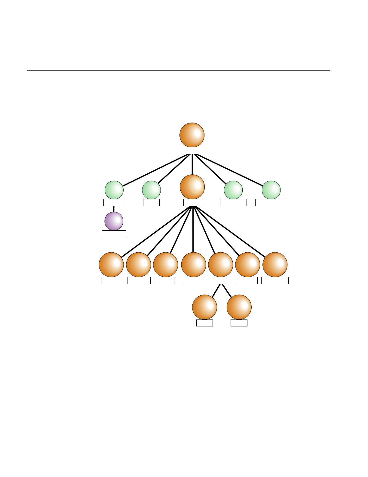
52
Chapter 3: Nodes and Node Types
pfNode
IRIS Performer’s node hierarchy begins with the pfNode class, as shown in Figure 3-1.
Figure 3-1 Nodes in the IRIS Performer Hierarchy
All node types are derived from pfNode; they inherit pfNode’s attributes and the libpf
routines for setting and getting attributes. In general, a node type inherits the attributes
and routines of all its parent nodes in the type hierarchy.
pfGeode pfText
pfBillboard
pfGroup pfASD pfLightSource
pfNode
pfDCSpfFCS
pfLOD pfSCS pfSwitch pfSequencepfPartition pfLayerpfScene

Nodes
53
Table 3-1 lists the basic node class and gives a simple description for each node type.
pfNode
As shown in Figure 3-1, all libpf nodes are arranged in a type hierarchy, which defines the
inheritance of functionality. A pfNode is an abstract class, meaning that a pfNode can
never be explicitly created by an application, and all other nodes inherit the functionality
of pfNode.. Its purpose is to provide a root to the type hierarchy and to define the
attributes that are common to all node types.
Table 3-1 IRIS Performer Node Types
Node Type Node Class Description
pfNode Abstract Basic node type
pfGroup Branch Groups zero or more children
pfScene Root Parent of the visual database
pfSCS Branch Static Coordinate System
pfDCS Branch Dynamic Coordinate System
pfFCS Branch Flux Coordinate System
pfSwitch Branch Selects among multiple children
pfSequence Branch Sequences through its children
pfLOD Branch Level-of-detail node
pfLayer Branch Renders coplanar geometry
pfLightSource Leaf Contains specifications for a light source
pfGeode Leaf Contains geometric specifications
pfBillboard Leaf Rotates geometry to face the eyepoint
pfPartition Branch Partitions geometry for efficient intersections
pfText Leaf Renders 2D and 3D text
pfASD Leaf Controls transition between LOD levels.

54
Chapter 3: Nodes and Node Types
pfNode Attributes
The following pfNode attributes are inherited by all other libpf node types:
• Node name
• Parent list
• Bounding geometry
• Intersection and traversal masks
• Callback functions and data
• User data
Bounding geometry, intersection masks, user data, and callbacks are advanced topics
that are discussed in Chapter 4, “Database Traversal.”
The routines that set, get, and otherwise manipulate these attributes can be used by all
libpf node types, as indicated by the keyword ‘Node’ in the routine names. Nodes used
as arguments to pfNode routines must be cast to pfNode* to match parameter
prototypes, as shown in this example:
pfNodeName((pfNode*) dcs, "rotor_rotation");
However, you usually don’t need to do this casting explicitly. When you use the C API
and compile with the –ansi flag (which is the usual way to compile IRIS Performer
applications),libpf provides macro wrappers around pfNode routines that automatically
perform argument casting for you. When you use the C++ API, such type casting is not
necessary.
pfNode Operations
In addition to sharing attributes, certain basic operations are provided for all node types.
They include:
New Create and return a handle to a new node.
Get Get node attributes.
Set Set node attributes.
Find Find a node based on its name.
Print Print node data.

Nodes
55
Copy Copy node data.
Delete Delete a node.
The Set operation is implied in the node attribute name. The names of the
attribute-getting functions contain the string “Get”.
An Example of Scene Creation
Example 3-1 illustrates the creation of a scene that includes two different kinds of
pfNodes. (For information about pfScene nodes, see “pfScene Nodes” on page 63; for
information about pfDCS nodes, see “pfDCS Nodes” on page 64.)
Example 3-1 Making a Scene
pfScene *scene;
pfDCS *dcs1, *dcs2;
scene = pfNewScene(); /* Create a new scene node */
dcs1 = pfNewDCS(); /* Create a new DCS node */
dcs2 = pfNewDCS(); /* Create a new DCS node */
pfCopy(dcs2, dcs1); /* Copy all node attributes */
/* from dcs1 to dcs2 */
pfNodeName(scene, "Scene_Graph_Root"); /* Name scene node */
pfNodeName(dcs1,"DCS_1"); /* Name dcs1 */
pfNodeName(dcs2,"DCS_2"); /* Name dcs2 */
...
/* Use a pfGet*() routine to determine node name */
printf("Name of first DCS node is %s.", pfGetNodeName(dcs1));
...
/* Recursively free this node if it’s no longer referenced */
pfDelete(scene);
...
pfGroup
In addition to inheriting the pfNode attributes described in the “pfNode” section of this
chapter, a pfGroup also maintains a list of zero or more child nodes that are accessed and
manipulated using group operators. Children of a pfGroup can be either branch or leaf
nodes. Traversals process the children of a pfGroup in left-to-right order.
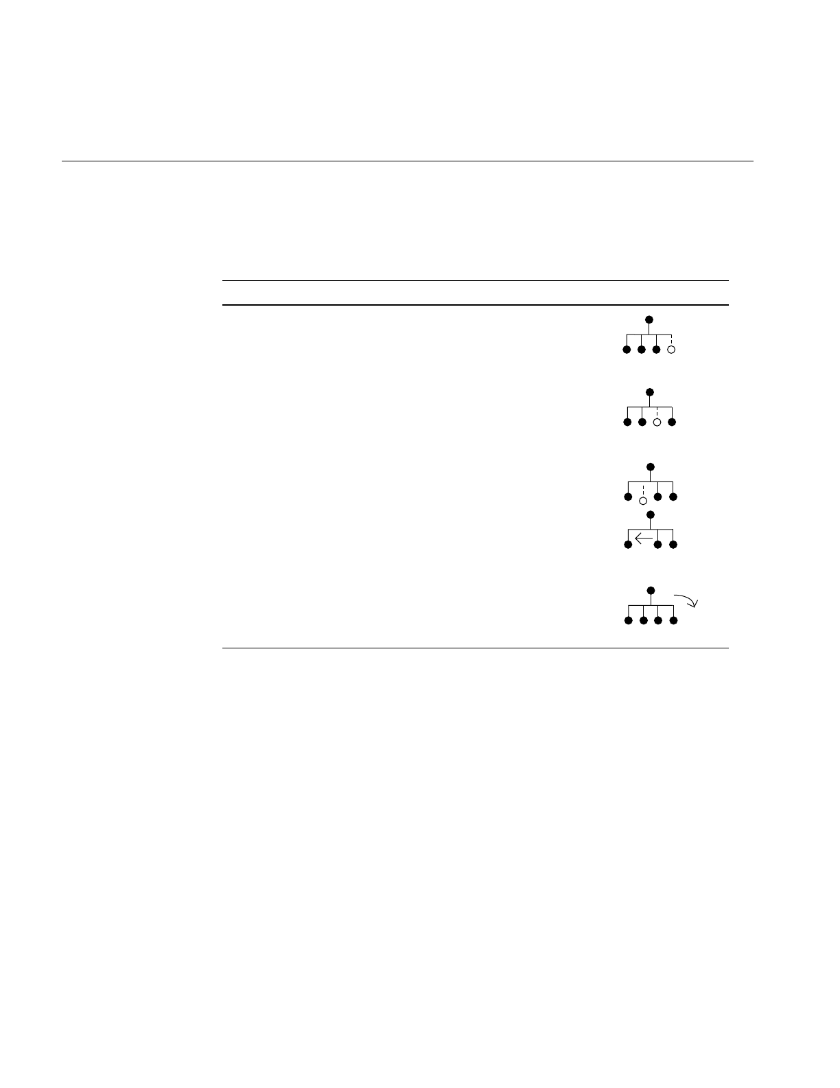
56
Chapter 3: Nodes and Node Types
Table 3-2 lists the pfGroup functions, with a description and a visual interpretation of
each.
pfGroup nodes can organize a database hierarchy either logically or spatially. For
example, if your database contains a model of a town, a logical organization might be to
group all house models under a single pfGroup. However, this kind of organization is
less efficient than a spatial organization, which arranges geometry by location. A spatial
organization improves culling and intersection performance; in the example of the town,
spatial organization would consist of grouping houses with their local terrain geometry
instead of with each other. Chapter 4 describes how to spatially organize your database
for best performance.
Table 3-2 pfGroup Functions
Function Name Description Diagram
pfAddChild(group, child) Appends child to the list for group.
pfInsertChild(group, index, child) Insertschild before the child whose
place in the list is index.
pfRemoveChild(group, child) Detaches child from the list and
shifts the list to fill the vacant spot.
Returns 1 if child was removed.
Returns 0 if child was not found in
the list. Note that the “removed”
node is only detached, not deleted. .
pfGetNumChildren(group) Returns the number of children in
group.
index = 2
4

Nodes
57
The code fragment in Example 3-2 illustrates building a hierarchy using pfGroup nodes.
Example 3-2 Hierarchy Construction Using Group Nodes
scene = pfNewScene();
/* The following loop constructs a sample hierarchy by
* adding children to several different types of group
* nodes. Notice that in this case the terrain was broken
* up spatially into a 4x4 grid, and a switch node is used
* to cause only one vehicle per terrain node to be
* traversed.
*/
for(j = 0; j < 4; j++)
for(i = 0; i < 4; i++)
{
pfGroup *spatial_terrain_block = pfNewGroup();
pfSCS *house_offset = pfNewSCS();
pfSCS *terrain_block_offset = pfNewSCS();
pfDCS *car_position = pfNewDCS();
pfDCS *tank_position = pfNewDCS();
pfDCS *heli_position = pfNewDCS();
pfSwitch *current_vehicle_type;
pfGeode *heli, *car, *tank;
pfAddChild(scene, spatial_terrain_block);
pfAddChild(spatial_terrain_block,
terrain_block_offset);
pfAddChild(spatial_terrain_block, house_offset);
pfAddChild(spatial_terrain_block,
current_vehicle_type);
pfAddChild(current_vehicle_type, car_position);
pfAddChild(current_vehicle_type, tank_position);
pfAddChild(current_vehicle_type, heli_position);
pfAddChild(car_position, car);
pfAddChild(tank_position, tank);
pfAddChild(heli_position, heli);
}
...
/* The following shows how one might use IRIS Performer to
* manipulate the scene graph at run time by adding and
* removing children from branch nodes in the scene graph.

58
Chapter 3: Nodes and Node Types
*/
for(j = 0; j < 4; j++)
for(i = 0; i < 4; i++)
{
pfGroup *this_terrain;
this_terrain = pfGetChild(scene, j*4 + i);
if (pfGetNumChildren(this_terrain) > 2)
this_tank = pfGetChild(this_terrain, 2);
if (is_tank_disable(this_tank))
{
pfRemoveChild(this_terrain, this_tank);
pfAddChild(disabled_tanks, this_tank);
}
}
...
Working With Nodes
This section describes the basic concepts involved in working with nodes. It explains
howshared instancing can be used to create multiple copies of an object, and how changes
made to a parent node propagate down to its children. A sample program that illustrates
these concepts is presented at the end of the chapter.
Instancing
A scene graph is typically constructed at application initialization time by creating and
adding new nodes to the graph. If a node is added to two or more parents it is termed
instanced and is shared by all its parents. Instancing is a powerful mechanism that saves
memory and makes modeling easier. libpf supports two kinds of instancing, which are
described in the following sections.
Shared Instancing
Shared instancing is the result of simply adding a node to multiple parents. If an
instanced node has children, then the entire subgraph rooted by the node is considered
to be instanced. Each parent shares the node; thus, modifications to the instanced node
or its subgraph are experienced by all parents. Shared instances can be nested—that is,
an instance can itself instance other nodes.
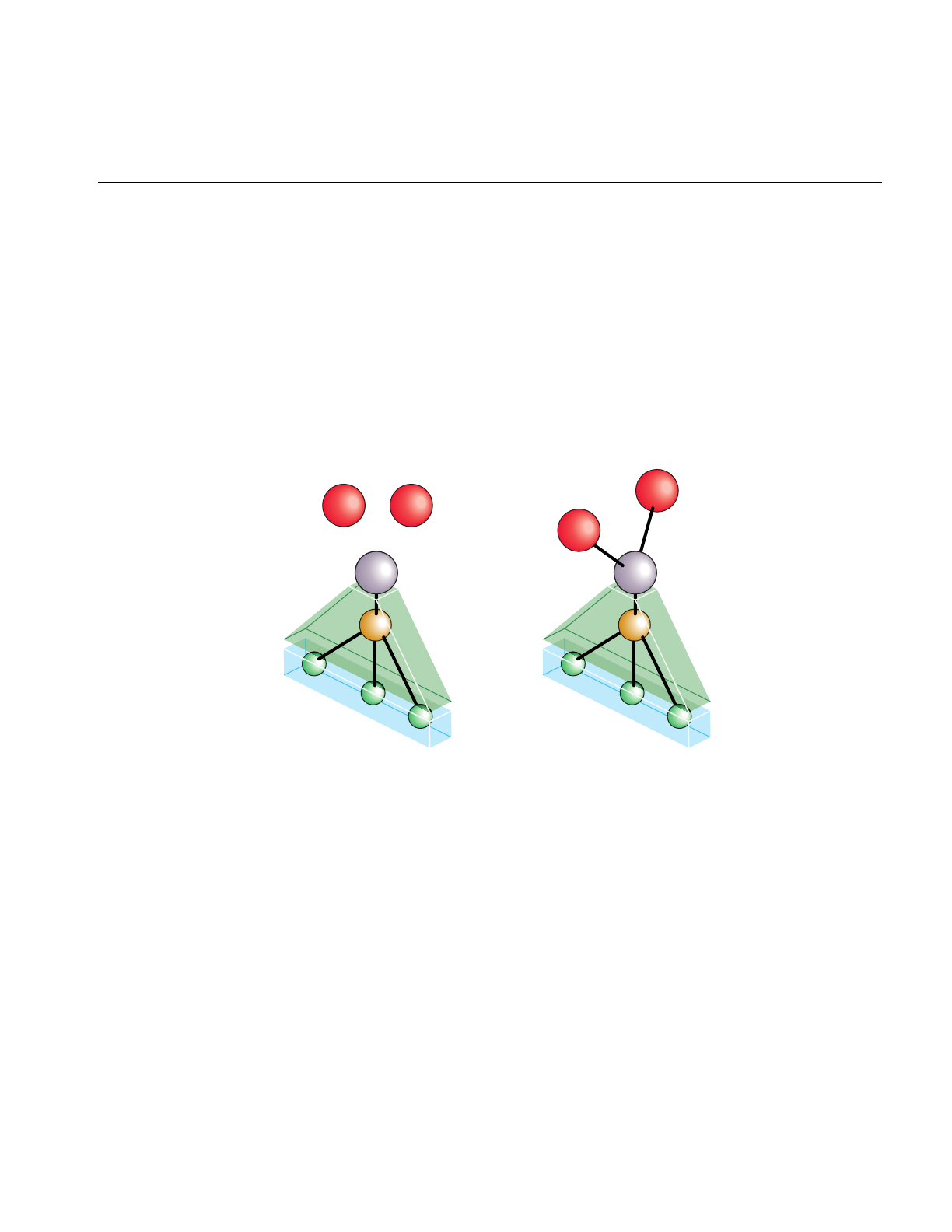
Working With Nodes
59
In the following sample code, group0 and group1 share a node:
pfAddChild(group0, node);
pfAddChild(group1, node);
Figure 3-2 shows the structure created by this code. Before the instancing operation, the
two groups and the node to be shared all exist independently, as shown in the left portion
of the figure. After the two function calls shown above, the two groups both reference the
same shared hierarchy. (If the original groups referenced other nodes, those nodes would
remain unchanged.) Note that each of the group nodes considers the shared hierarchy to
be its own child.
Figure 3-2 Shared Instances
Cloned Instancing
In many situations shared instancing isn’t desirable. Consider a subgraph that represents
a model of an airplane with articulations for ailerons, elevator, rudder, and landing gear.
Shared instances of the model result in multiple planes that share the same articulations.
Consequently, it’s impossible for one plane to be flying with its landing gear retracted
while another is on a runway with its landing gear down.
Group 0 Group 1
n
Group 0
Group 1
n
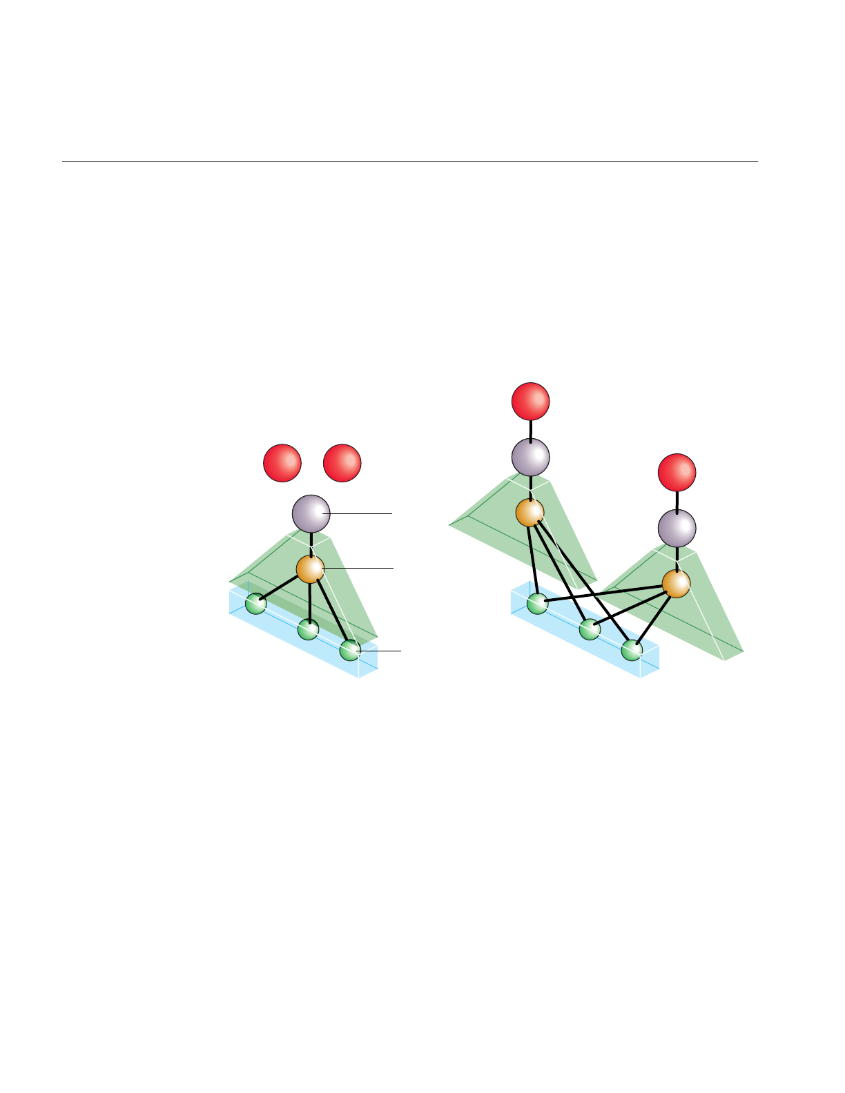
60
Chapter 3: Nodes and Node Types
Cloned instancing provides the solution to this problem by cloning—creating new copies
of variable nodes in the subgraph. Leaf nodes containing geometry are not cloned and
are shared to save memory. Cloning the airplane model generates new articulation
nodes, which can be modified independently of any other cloned instance. The cloning
operation, pfClone(), is actually a traversal and is described in detail in Chapter 4.
Figure 3-3 shows the result of cloned instancing. As in the previous figure, the left half of
the drawing represents the situation before the operation, and the right half shows the
result of the operation.
Figure 3-3 Cloned Instancing
The cloned instancing operation constructs new copies of each internal node of the
shared hierarchy, but uses the same shared instance of all the leaf nodes. In use, this is an
important distinction, because the number of internal nodes may be relatively few, while
the number and content of geometry-containing leaf nodes is often quite extensive.
Nodes G1 and G2 in Figure 3-3 are the groups that form the root nodes after the cloned
instancing operation is complete. Node P is the parent or root node of the instanced
object, and D is a dynamic coordinate system contained within it. Nodes A, B, and C are
the leaf geometry nodes; they are shared rather than copied.
Dynamic
coordinate
system
Leaf
G1 G2
PRoot
D
A
B
C
P1
D1
A
B
C
P2
D2
G1
G2

Working With Nodes
61
The code in Example 3-3 shows how to create cloned instances.
Example 3-3 Creating Cloned Instances
pfGroup *g1, *g2, *p;
pfDCS *d;
pfGeode *a, *b, *c;
...
/* Create initial instance of scene hierarchy of p under
* group g1: add a DCS to p, then add three pfGeode nodes
* under the DCS.
*/
pfAddChild(g1,p);
pfAddChild(p,d);
pfAddChild(d,a);
pfAddChild(d,b);
pfAddChild(d,c);
...
/* Create cloned instance version of p under g2 */
pfAddChild(g2, pfClone(p,0));
/* Notice that pfGeodes are cloned by instancing rather than
* copying. Also notice that the second argument to
* pfClone() is 0; that argument is currently required by
* IRIS Performer to be zero.
*/
...
Bounding Volumes
libpf uses bounding volumes for culling and to improve intersection performance. libpf
computes bounding volumes for all nodes in a database hierarchy unless the bound is
explicitly set by the application. The bounding volume of a branch node encompasses the
spatial extent of all its children. libpf automatically recomputes bounds when children are
modified.
By default, bounding volumes are dynamic; that is, libpf automatically recomputes them
when children are modified. For instance, in Example 3-4 when the DCS is rotated
nothing more needs to be done to update the bounding volume for g1.

62
Chapter 3: Nodes and Node Types
Example 3-4 Automatically Updating a Bounding Volume
pfAddChild(g1,dcs);
pfAddChild(dcs, helicopter);
...
pfDCSRot(dcs, heading+10.0f, pitch,roll);
...
pfDCSRot(dcs, heading, pitch - 5.0f, roll + 2.0f);
In some cases, you may not want bounding volumes to be recomputed automatically. For
example, in a merry-go-round with horses moving up and down, you know that the
horses stay within a certain volume. Using pfNodeBSphere(), you can specify a
bounding sphere within which the horse always remains and tell IRIS Performer that the
bounding volume is “static”—not to be updated no matter what happens to the node’s
children. You can always force an update by setting the bounding volume to NULL with
pfNodeBSphere(), as follows:
pfNodeBSphere(node, NULL, NULL, PFBOUND_STATIC);
At the lowest level, within pfGeoSets, bounding volumes are maintained as
axially-aligned boxes. When you add a pfGeoSet to a pfGeode or directly invoke
pfGetGSetBBox() on the pfGeoSet, a bounding box is created for the pfGeoSet. Neither
the bounding box of the pfGeoSet nor the bounding volume of the pfGeode is updated
if the geometry changes inside the pfGeoSet. You can force an update by setting the
pfGeoSet bounding box and then the pfGeode bounding volume to a NULL bounding
box, as follows:
• Recompute the pfGeoSet bounding box from the internal geometry:
pfGSetBBox(gset, NULL);
• Recompute the pfGeode bounding volume from the bounding boxes of its
pfGeoSets:
pfNodeBSphere(geode, NULL, PFBOUND_DYNAMIC);

Node Types
63
Node Types
This section describes the node types and the functions for working with each node type.
For more information about pfLPointState and pfLightSource, see Chapter 6, “Creating
Visual Effects.”
pfScene Nodes
A pfScene is a root node that is the parent of a visual database. Use pfNewScene() to
create a new scene node. Before the scene can be drawn, you must call
pfChanScene(channel, scene) to attach it to a pfChannel.
Any nodes that are within the graph that is parented by a pfScene are culled and drawn
once the pfScene is attached to a pfChannel. Because pfScene is a group, it uses pfGroup
routines; however, a pfScene cannot be the child of any other node. The following
statement adds a pfGroup to a scene:
pfAddChild(scene, root);
In the simplest case, the pfScene is the only node you need to add. Once you have a
pfPipe, pfChannel, and pfScene, you have all the necessary elements for generating
graphics using IRIS Performer.
pfScene Default Rendering State
pfScene nodes may specify a global pfGeoState that all other pfGeoStates in nodes below
the pfScene will inherit from. Specification of this scene pfGeoState is done via the
function pfSceneGState(). This functionality allows for the subtle optimization of
pushing the most frequently used pfGeoState attributes for a particular scene graph into
a global state and having the individual states inherit these attributes rather than specify
them. This can save IRIS Performer work during culling (by having to ‘unwrap’ fewer
pfGeoStates) and thus possibly increase frame rate.
There are several database utility functions in libpfdu designed to help with this
optimization. pfdMakeSceneGState() returns an ‘optimal’ pfGeoState based on a list of
pfGeoStates.pfdOptimizeGStateList() takes an existing global pfGeoState, a new global
pfGeoState, and a list of pfGeoState’s that should be optimized and cause all attributes
of pfGeoStates in the list of pfGeoStates to be inherited if they are the same as the
attribute in the new global pfGeoState. Lastly pfdMakeSharedScene() will cause this

64
Chapter 3: Nodes and Node Types
optimization to happen for all of the pfGeoStates under the pfScene that was passed into
the function. For more information on pfGeoStates see Chapter 8, “Geometry,” which
discusses libpr in more detail. For more information of the creation and optimization of
databases see Chapter 7, “Importing Databases,” which discusses building database
converters and libpfdu.
pfSCS Nodes
A pfSCS is a branch node that represents a static coordinate system. A pfSCS node
contains a fixed modeling transformation matrix that cannot be changed once it is
created. pfSCS nodes are useful for positioning models within a database. For example,
a house that is modeled at the origin should be placed in the world with a pfSCS because
houses rarely move during program execution.
Use pfNewSCS(matrix) to create a new pfSCS using the transformation defined by
matrix. To find out what matrix was used to create a given pfSCS, call pfGetSCSMat().
For best graphics performance, matrices passed to pfSCS nodes (and the pfDCS node
type described in the next section) should be orthonormal (translations, rotations, and
uniform scales). Nonuniform scaling requires renormalization of normals in the graphics
pipe. Projections and other non-affine transformations are not supported.
While pfSCS nodes are useful in modeling, using too many of them can reduce culling,
rendering, and intersection performance. For this reason, libpf provides the pfFlatten()
traversal. pfFlatten() will traverse a scene graph and apply static transformations
directly to geometry to eliminate the overhead associated with managing the
transformations. pfFlatten() is described in detail in Chapter 4, “Database Traversal.”
pfDCS Nodes
A pfDCS is a branch node that represents a dynamic coordinate system. Use a pfDCS
when you want to apply an initial transformation to a node and also change the
transformation during the application. Use a pfDCS to articulate moving parts and to
show object motion.
Use pfNewDCS() to create a new pfDCS. The initial transformation of a pfDCS is the
identity matrix. Subsequent transformations are set by specifying a new transformation
matrix, or by replacing the rotation, scale, or translation in the current transformation
matrix. The pfDCS transforms each child C(i) to C(i)∗Scale∗Rotation∗Translation.

Node Types
65
Table 3-3 lists functions for manipulating a pfDCS, including rotating, scaling, and
translating the children of the pfDCS.
pfFCS Nodes
A pfFCS is a branch node that represents a flux coordinate system. The transformation
matrix of a pfFCS is contained in the pfFlux which is linked to it. This linkage allows a
pfEngine to animate the matrix of a pfFCS. The linkage also allows multiple pfFCSs to
share the same transform.
Use pfNewFCS(flux) to create a new pfFCS linked to flux.
Table 3-4 lists functions for manipulating a pfFCS. pfFCS, pfFlux, and pfEngine are fully
described in Chapter 14, “Dynamic Data.”
Table 3-3 DCS Transformations
Function Name Description
pfNewDCS Create a new pfDCS node.
pfDCSTrans Set the translation coordinates to x, y, z.
pfDCSRot Set the rotation transformation to h, p, r.
pfDCSCoord Rotate and translate by coord.
pfDCSScale Scale by a uniform scale factor.
pfDCSMat Use a matrix for transformations.
pfGetDCSMat Retrieve the current matrix for a given pfDCS.
Table 3-4 FCS Functions
Function Description
pfNewFCS Create a new pfFCS node.
pfFCSFlux Link a flux to a given pfFCS.
pfGetFCSFlux Get a pointer to the flux linked to a given pfFCS.

66
Chapter 3: Nodes and Node Types
pfSwitch Nodes
A pfSwitch is a branch node that selects one, all, or none of its children. Use
pfNewSwitch() to return a handle to a new pfSwitch. To select all the children, use the
PFSWITCH_ON argument to pfSwitchVal(). Deselect all the children (turning the
switch off) using PFSWITCH_OFF. To select a single child, give the index of the child
from the child list. To find out the current value of a given switch, call pfGetSwitchVal().
Example 3-5 (in the “pfSequence Nodes” section) illustrates a use of pfSwitch nodes to
control pfSequence nodes.
pfSequence Nodes
A pfSequence is a pfGroup that sequences through a range of its children, drawing each
child for a specified duration. Each child in a sequence can be thought of as a frame in an
animation. A sequence can consist of any number of children, and each child has its own
duration. You can control whether an entire sequence repeats from start to end, repeats
from end to start, or terminates.
Use pfNewSeq() to create and return a handle to a new pfSequence. Once the
pfSequence has been created, use the group function pfAddChild() to add the children
that you want to animate.
Table 3-5 describes the functions for working with pfSequences.
pfGetFCSMat Retrieve the current matrix for a given pfFCS.
pfGetFCSMatPtr Get a pointer to the current matrix for a given pfFCS.
Table 3-5 pfSequence Functions
Function Description
pfNewSeq Create a new pfSequence node.
pfSeqTime Set the length of time to display a frame.
pfGetSeqTime Find out the time allotted for a given frame.
Table 3-4 (continued) FCS Functions
Function Description

Node Types
67
Example 3-5 demonstrates a possible use of both switches and sequences. First,
sequences are set up to contain animation sequences for explosions, fire, and smoke; then
a switch is used to control which sequences are currently active.
Example 3-5 Using pfSwitch and pfSequence Nodes
pfSwitch *s;
pfSequence *explosion1_seq, *explosion2_seq, *fire_seq,
*smoke_seq;
...
s = pfNewSwitch();
explosion1_seq = pfNewSeq();
explosion2_seq = pfNewSeq();
fire_seq = pfNewSeq();
smoke_seq = pfNewSeq();
pfAddChild(s, explosion1_seq);
pfAddChild(s, explosion2_seq);
pfAddChild(s, fire_seq);
pfAddChild(s, smoke_seq);
pfSwitchVal(s, PFSWITCH_OFF);
...
if (direct_hit)
{
pfSwitchVal(s, PFSWITCH_ON); /* Select all sequences */
/* Set first explosion sequence to go double normal
* speed and repeat 3 times. */
pfSeqInterval Set the range of frames and sequence type.
pfGetSeqInterval Find out interval parameters.
pfSeqDuration Control the speed and number of repetitions of the entire sequence.
pfGetSeqDuration Retrieve speed and repetition information for the sequence.
pfSeqMode Start, stop, pause, and resume the sequence.
pfGetSeqMode Find out the sequence’s current mode.
pfGetSeqFrame Get the current frame.
Table 3-5 (continued) pfSequence Functions
Function Description

68
Chapter 3: Nodes and Node Types
pfSeqMode(explosion1_seq, PFSEQ_START);
pfSeqDuration(explosion1_seq, 2.0f, 3);
/* Set second explosion sequence to display first child
* of sequence for 2 seconds before continuing. */
pfSeqMode(explosion2_seq, PFSEQ_START);
pfSeqTime(explosion2, 0.0f, 2.0f);
/* Set fire to wait on first frame of sequence until .3
* seconds after second explosion. */
pfSeqMode(fire_seq, PFSEQ_START);
pfSeqTime(fire_seq, 0.0f, 2.3f);
/* Set smoke to wait until .1 seconds after fire. */
pfSeqMode(smoke_seq, PFSEQ_START);
pfSeqTime(smoke_seq, 0.0f, 2.4f);
}
else if (explosion && (expl_type == 0))
{
pfSeqMode(explosion1_seq, PFSEQ_START);
pfSwitchVal(s, 0);
}
else if (explosion && (expl_type == 1))
{
pfSeqMode(explosion2_seq, PFSEQ_START);
pfSwitchVal(s, 1);
}
else if (fire_is_burning)
{
pfSeqMode(fire_seq, PFSEQ_START);
pfSwitchVal(s, 2);
}
else if (smoking)
{
pfSeqMode(smoke_seq, PFSEQ_START);
pfSwitchVal(s, 3);
}
else
pfSwitchVal(s, PFSWITCH_OFF);
...

Node Types
69
pfLOD Nodes
A pfLOD is a level-of-detail node. Level-of-detail switching is an advanced concept that
is discussed in Chapter 5, “Frame and Load Control.” A level-of-detail node specifies
how its children are to be displayed, based on the visual range from the channel’s
viewpoint. Each child has a defined range, and the entire pfLOD has a defined center.
Table 3-6 describes the functions for working with pfLODs.
pfASD Nodes
pfASD nodes handle dynamic generation and morphing of the visible part of a surface
based on multiple LODs. pfASD nodes allow for the smooth LOD transition of large and
complex surfaces, such as large area terrain. For informaton on pfASD nodes, see
Chapter 15, “Active Surface Definition.”
pfLayer Nodes
A pfLayer is a leaf node that resolves the visual priority of coplanar geometry. A pfLayer
allows the application to define a set of base geometry and a set of layer geometry
(sometimes called decal geometry). The base geometry and the decal geometry should be
coplanar, and the decal geometry must lie within the extent of the base polygons.
Table 3-6 pfLOD Functions
Function Description
pfNewLOD Create a level of detail node.
pfLODRange Set a range at which to use a specified child node.
pfGetLODRange Find out the range for a given node.
pfLODCenter Set the pfLOD center.
pfGetLODCenter Retrieve the pfLOD center.
pfLODTransition Set the width of a specified transition.
pfGetLODTransition Get the width of a specified transition.

70
Chapter 3: Nodes and Node Types
Table 3-7 describes the functions for working with pfLayers.
pfLayer nodes can be used to overlay any sort of markings on a given polygon and are
important to avoid flimmering. Example 3-6 demonstrates how to display runway
markings as a decal above a coplanar runway. This example uses the performance mode
PFDECAL_BASE_FAST for layering; as described in the pfLayer and pfDecal reference
pages, other available modes are PFDECAL_BASE_HIGH_QUALITY,
PFDECAL_BASE_DISPLACE, and PFDECAL_BASE_STENCIL.
Example 3-6 Marking a Runway With a pfLayer Node
pfLayer *layer;
pfGeode *runway, *runway_markings;
...
/* avoid flimmering of runway and runway_markings */
layer = pfNewLayer();
pfLayerBase(layer, runway);
pfLayerDecal(layer, runway_markings);
pfLayerMode(layer, PFDECAL_BASE_FAST);
Table 3-7 pfLayer Functions
Function Description
pfNewLayer Create a pfLayer node.
pfLayerMode Specify a hardware mode to use in drawing decals.
pfGetLayerMode Get current mode.
pfLayerBase Specify the child containing base geometry.
pfGetLayerBase Find out which child contains base geometry.
pfLayerDecal Specify the child containing decal geometry.
pfGetLayerDecal Find out which child contains decal geometry.

Node Types
71
pfGeode Nodes
pfGeode is short for geometry node and is the primary node for defining geometry in libpf.
A pfGeode contains a list of geometry structures called pfGeoSets, which are part of the
IRIS Performer libpr library. pfGeoSets encapsulate graphics state and geometry and are
described in the “Geometry Sets” section of Chapter 8, “Geometry.” It is important to
understand that pfGeoSets are not nodes but are simply elements of a pfGeode.
Table 3-8 describes the functions for working with pfGeodes.
Example 3-7 shows how to attach several pfGeoSets to a pfGeode.
Example 3-7 Adding pfGeoSets to a pfGeode
pfGeode *car1;
pfGeoSet *muffler, *frame, *windows, *seats, *tires;
muffler = read_in_muffler_geometry();
frame = read_in_frame_geometry();
seats = read_in_seat_geometry();
tires = read_in_tire_geometry();
pfAddGSet(car1, muffler);
pfAddGSet(car1, frame);
pfAddGSet(car1, seats);
pfAddGSet(car1, tires);
...
Table 3-8 pfGeode Functions
Function Description
pfNewGeode Create a pfGeode.
pfAddGSet Add a pfGeoSet.
pfRemoveGSet Remove a pfGeoSet.
pfInsertGSet Insert a pfGeoSet.
pfReplaceGSet Replace a pfGeoSet.
pfGetGSet Supply a pointer to the specified pfGeoSet.
pfGetNumGSets Determine how many pfGeoSets are in the given pfGeode.

72
Chapter 3: Nodes and Node Types
pfText Nodes
A pfText node is libpf leaf node that contains a set of libpr pfStrings that should be
rendered based on the libpf cull and draw traversals. In this sense a pfText is similar to a
pfGeode except that it renders 3-dimensional text through the libpr pfString and pfFont
mechanisms rather than rendering standard 3-dimensional geometry via libpr pfGeoSet
and pfGeoState functionality. pfText nodes are useful for displaying 3-dimensional text
and other collections of geometry from a fixed index list. Table 3-9 lists the major pfText
functions.
Using the pfText facility is easy. Example 3-8 shows how a pfFont is defined, how
pfStrings are created that reference that font, and then how those pfStrings are added to
a pfText node for display. See the description of pfStrings and pfFonts in Chapter 8,
“Geometry,” for information on setting up individual strings to input into a pfText node
Example 3-8 Adding pfStrings to a pfText
int nStrings,i;
char tmpBuf[8192];
char fontName[128];
pfFont *fnt = NULL;
/* Create a new text node
pfText *txt = pfNewText();
/* Read in font using libpfdu utility function */
scanf(“%s”,fontName);
fnt = pfdLoadFont(“type1”,fontName,PFDFONT_EXTRUDED);
Table 3-9 pfText Functions
Function Description
pfNewText Create a pfText.
pfAddString Add a pfString.
pfRemoveString Remove a pfString.
pfInsertString Insert a pfString.
pfReplaceString Replace a pfString.
pfGetString Supply a pointer to the specified pfString.
pfGetNumStrings Determine how many pfStrings are in the given pfText.

Node Types
73
/* Cant render pfText or libpr pfString without a pfFont */
if (fnt == NULL)
pfNotify(PFNFY_WARN,PFNFY_PRINT,
”No Such Font - %s\n”,fontName);
/* Read nStrings text strings from standard input and */
/* Attach them to a pfText */
scanf(“%d”,&nStrings);
for(i=0;i<nStrings;i++)
{
char c;
int j=0;
int done = 0;
pfString *curStr = NULL;
while(done < 2) /* READ STRING - END on ‘||’ */
{
c = getchar();
if (c == ‘|’)
done++;
else
done = 0;
tmpBuf[j++] = c;
}
tmpBuf[PF_MAX2(j-2,0)] = ‘\0’;
/* Create new libpr pfString structure to attach to pfText */
curStr = pfNewString(pfGetSharedArena());
/* Set the font for the libpr pfString */
pfStringFont(curStr, fnt);
/* Assign the char string to the pfString */
pfStringString(curStr, tmpBuf);
/* Add this libpr pfString to the pfText node */
/* Like adding a libpr pfGeoSet to a pfGeode */
pfAddString(txt, curStr);
}
pfAddChild(SceneGroup, txt);

74
Chapter 3: Nodes and Node Types
pfBillboard Nodes
A pfBillboard is a pfGeode that rotates its children’s geometry to follow the view
direction or the eyepoint. Billboards are useful for portraying complex objects that are
roughly symmetrical in one or more axes. The billboard rotates to always present the
same image to the viewer using far fewer polygons than a solid model uses. In this way,
billboards reduce both transformation and pixel fill demands on the graphics subsystem
at the expense of some additional host processing. A classic example is a textured
billboard of a single quadrilateral representing a tree.
Because a pfBillboard is also a pfGeode, you can pass a pfBillboard argument to any
pfGeode routine. To add geometry, call pfAddGSet() (see “pfGeode Nodes” on page 71).
Each pfGeoSet in the pfBillboard is treated as a separate piece of billboard geometry; each
one turns so that it always faces the eye point.
pfBillboards can be either constrained to rotate about an axis, as is done for a tree or a
lamp post, or constrained only by a point, as when simulating a cloud or a puff of smoke.
Specify the rotation mode by calling pfBboardMode(); specify the rotational axis by
calling pfBboardAxis(). Since rotating the geometry to the eyepoint doesn’t fully
constrain the orientation of a point-rotating billboard, modes are available to use the
additional degree of freedom to align the billboard in eye space or world space. Usually
the normals of billboards are specified to be parallel to the rotational axis to avoid
lighting anomalies.
pfFlatten() is highly recommended for billboards. If a billboard lies beneath a pfSCS or
pfDCS, an additional transformation is done for each billboard. This can have a
substantial performance impact on the cull process, where billboards are transformed.
Table 3-10 describes the functions for working with pfBillboards.
Table 3-10 pfBillboard Functions
Function Description
pfNewBboard Create a pfBillboard node.
pfBboardPos Set a billboard’s position.
pfGetBboardPos Find out a billboard’s position.
pfBboardAxis Specify the rotation or alignment axis.
pfGetBboardAxis Find out the rotation or alignment axis.

Node Types
75
Example 3-9 demonstrates the construction of a pfBillboard node. The code can be found
in /usr/share/Performer/src/pguide/libpf/C/billboard.c.
Example 3-9 Setting Up a pfBillboard
static pfVec2 BBTexCoords[] ={{0.0f, 0.0f},
{1.0f, 0.0f},
{1.0f, 1.0f},
{0.0f, 1.0f}};
static pfVec3 BBVertCoords[4] = /* XZ plane for pt bboards */
{{-0.5f, 0.0f, 0.0f},
{ 0.5f, 0.0f, 0.0f},
{ 0.5f, 0.0f, 1.0f},
{-0.5f, 0.0f, 1.0f}};
static pfVec3 BBAxes[4] = {{1.0f, 0.0f, 0.0f}, /* X */
{0.0f, 1.0f, 0.0f}, /* Y */
{0.0f, 0.0f, 1.0f}, /* Z */
{0.0f, 0.0f, 1.0f}}; /*world Zup*/
static int BBPrimLens[] = { 4 };
static pfVec4 BBColors[] = {{1.0, 1.0, 1.0, 1.0}};
/* Convert static data to pfMalloc’ed data */
static void*
memdup(void *mem, size_t bytes, void *arena)
{
void *data = pfMalloc(bytes, arena);
memcpy(data, mem, bytes);
return data;
}
/* For pedagogical use only. Reasonable performance
* requires more then one pfGeoSet per pfBillboard.
pfBboardMode Specify a billboard’s rotation type.
pfGetBboardMode Find out a billboard’s rotation type.
Table 3-10 (continued) pfBillboard Functions
Function Description

76
Chapter 3: Nodes and Node Types
*/
pfBillboard*
MakeABill(pfVec3 pos, pfGeoState *gst, long bbType)
{
pfGeoSet *gset;
pfGeoState *gstate;
pfBillboard *bill;
void *arena = pfGetSharedArena();
gset = pfNewGSet(arena);
gstate = pfNewGState(arena);
pfGStateMode(gstate, PFSTATE_ENLIGHTING, PF_OFF);
pfGStateMode(gstate, PFSTATE_ENTEXTURE, PF_ON);
/*.... Create/load texture map for billboard... */
pfGStateAttr(gstate, PFSTATE_TEXTURE, texture);
pfGSetGState(gset, gstate);
pfGSetAttr(gset, PFGS_COORD3, PFGS_PER_VERTEX,
memdup(BBVertCoords, sizeof(BBVertCoords), arena),
NULL);
pfGSetAttr(gset, PFGS_TEXCOORD2, PFGS_PER_VERTEX,
memdup(BBTexCoords, sizeof(BBTexCoords), arena),
NULL);
pfGSetAttr(gset, PFGS_COLOR4, PFGS_OVERALL,
memdup(BBColors, sizeof(BBColors), arena),
NULL);
pfGSetPrimLengths(gset,
(int*)memdup(BBPrimLens, sizeof(BBPrimLens), arena));
pfGSetPrimType(gset, PFGS_QUADS);
pfGSetNumPrims(gset, 1);
pfGSetGState(gset, gst);
bill = pfNewBboard();
switch (bbType)
{
case PF_X: /* axial rotate */
case PF_Y:
case PF_Z:
pfBboardAxis(bill, BBAxes[bbType]);
pfBboardMode(bill, PFBB_ROT, PFBB_AXIAL_ROT);
break;

Node Types
77
case 3: /* point rotate */
pfBboardAxis(bill, BBAxes[bbType]);
pfBboardMode(bill, PFBB_ROT, PFBB_POINT_ROT_WORLD);
break;
}
pfAddGSet(bill, gset);
pfBboardPos(bill, 0, pos);
return bill;
}
pfPartition Nodes
A pfPartition is a pfGroup that organizes the scene graphs of its children into a static data
structure that can be more efficient for intersections. Currently, partitions are only useful
for data that lies more or less on an XY plane, such as terrain. A pfPartition would
therefore be inappropriate for a skyscraper model.
Partition construction comes in two phases. After a piece of the scene graph has been
placed under the pfPartition, pfBuildPart() examines the spatial arrangement of
geometry beneath the pfPartition and determines an appropriate origin and spacing for
the grid. Because the search is exhaustive, this examination can be time-consuming the
first time through. Once a good partitioning is determined, the search space can be
restricted for future database loads using the partition attributes.
The second phase is invoked by pfUpdatePart(), which distributes the pfGeoSets under
the pfPartition into cells in the spatial partition created by pfBuildPart().pfUpdatePart()
needs to be called if any geometry under the pfPartition node changes.
During intersection traversal, the segments in a pfSegSet (see “Intersection Requests:
pfSegSets” in Chapter 4) are scan-converted onto the grid, yielding faster access to those
pfGeoSets that potentially intersect the segment. A pfPartition can be made to function
as a normal pfGroup during intersection traversal by OR-ing PFTRAV_IS_NO_PART
into the intersection traversal mode in the pfSegSet.

78
Chapter 3: Nodes and Node Types
Table 3-11 describes the functions for working with pfPartitions.
Example 3-10 demonstrates setting up and using a pfPartition node.
Example 3-10 Setting Up a Partition
pfGroup *terrain;
pfPartition *partition;
pfScene *scene;
...
terrain = read_in_grid_aligned_terrain();
...
/* create a default partitioning of a terrain grid */
partition = pfNewPart();
pfAddChild(scene, partition);
pfAddChild(partition, terrain);
pfBuildPart(partition);
...
Table 3-11 pfPartition Functions
Function Description
pfNewPart Create a pfPartition.
pfPartVal Set the desired pfPartition value.
pfGetPartVal Find out the attributes of specified value.
pfPartAttr Set the desired pfPartition attribute.
pfGetPartAttr Find out the attributes of specified attribute.
pfBuildPart Construct a spatial partitioning based on the attributes.
pfUpdatePart Traverse the partition’s children and incorporate changes.
pfGetPartType Determine what kind of partition is being used.

Sample Program
79
/* use the partitions to perform efficient intersections
* of sets of segments with the terrain */
for(i = 0; i < numVehicles; i++)
pfNodeIsectSegs(partition, vehicle_segment_set[i],
hit_struct);
...
Sample Program
The sample program shown in Example 3-11 demonstrates scene graph construction,
shared instancing, and transformation inheritance. The program uses IRIS Performer
objects and functions that are described fully in later chapters.
This program reads the names of two objects from the command line, although defaults
are supplied if file names are not given. These files are loaded and a second instance of
each object is created. In each case, this instance is made to orbit the original object, and
the second pair are also placed in orbit around the first. This program is “inherit.c” and is
part of the suite of IRIS Performer Programmer’s Guide example programs.
Example 3-11 Inheritance Demonstration Program
/*
* inherit.c - transform inheritance example
*/
#include <math.h>
#include <Performer/pf.h>
#include <Performer/pfdu.h>
int
main(int argc, char *argv[])
{
pfPipe *pipe;
pfPipeWindow *pw;
pfScene *scene;
pfChannel *chan;
pfCoord view;
float z, s, c;
pfNode *model1, *model2;
pfDCS *node1, *node2;
pfDCS *dcs1, *dcs2, *dcs3, *dcs4;
pfSphere sphere;

80
Chapter 3: Nodes and Node Types
char *file1, *file2;
/* choose default objects of none specified */
file1 = (argc > 1) ? argv[1] : “blob.nff”;
file2 = (argc > 1) ? argv[1] : “torus.nff”;
/* Initialize Performer */
pfInit();
pfFilePath(
“.”
“:./data”
“:../data”
“:../../data”
“:../../../data”
“:../../../../data”
“:/usr/share/Performer/data”);
/* Single thread for simplicity */
pfMultiprocess(PFMP_DEFAULT);
/* Load all loader DSO’s before pfConfig() forks */
pfdInitConverter(file1);
pfdInitConverter(file2);
/* Configure */
pfConfig();
/* Load the files */
if ((model1 = pfdLoadFile(file1)) == NULL)
{
pfExit();
exit(-1);
}
if ((model2 = pfdLoadFile(file2)) == NULL)
{
pfExit();
exit(-1);
}
/* scale models to unit size */
node1 = pfNewDCS();
pfAddChild(node1, model1);
pfGetNodeBSphere(model1, &sphere);
if (sphere.radius > 0.0f)

Sample Program
81
pfDCSScale(node1, 1.0f/sphere.radius);
node2 = pfNewDCS();
pfAddChild(node2, model2);
pfGetNodeBSphere(model2, &sphere);
if (sphere.radius > 0.0f)
pfDCSScale(node2, 1.0f/sphere.radius);
/* Create the hierarchy */
dcs4 = pfNewDCS();
pfAddChild(dcs4, node1);
pfDCSScale(dcs4, 0.5f);
dcs3 = pfNewDCS();
pfAddChild(dcs3, node1);
pfAddChild(dcs3, dcs4);
dcs1 = pfNewDCS();
pfAddChild(dcs1, node2);
dcs2 = pfNewDCS();
pfAddChild(dcs2, node2);
pfDCSScale(dcs2, 0.5f);
pfAddChild(dcs1, dcs2);
scene = pfNewScene();
pfAddChild(scene, dcs1);
pfAddChild(scene, dcs3);
pfAddChild(scene, pfNewLSource());
/* Configure and open GL window */
pipe = pfGetPipe(0);
pw = pfNewPWin(pipe);
pfPWinType(pw, PFPWIN_TYPE_X);
pfPWinName(pw, “IRIS Performer”);
pfPWinOriginSize(pw, 0, 0, 500, 500);
pfOpenPWin(pw);
chan = pfNewChan(pipe);
pfChanScene(chan, scene);
pfSetVec3(view.xyz, 0.0f, 0.0f, 15.0f);
pfSetVec3(view.hpr, 0.0f, -90.0f, 0.0f);
pfChanView(chan, view.xyz, view.hpr);

82
Chapter 3: Nodes and Node Types
/* Loop through various transformations of the DCS’s */
for (z = 0.0f; z < 1084; z += 4.0f)
{
pfDCSRot(dcs1,
(z < 360) ? (int) z % 360 : 0.0f,
(z > 360 && z < 720) ? (int) z % 360 : 0.0f,
(z > 720) ? (int) z % 360 : 0.0f);
pfSinCos(z, &s, &c);
pfDCSTrans(dcs2, 1.0f * c, 1.0f * s, 0.0f);
pfDCSRot(dcs3, z, 0, 0);
pfDCSTrans(dcs3, 4.0f * c, 4.0f * s, 4.0f * s);
pfDCSRot(dcs4, 0, 0, z);
pfDCSTrans(dcs4, 1.0f * c, 1.0f * s, 0.0f);
pfFrame();
}
/* show objects static for three seconds */
sleep(3);
pfExit();
exit(0);
}

This chapter explains how to manipulate, traverse, and examine a scene graph.
“Database Traversal”
Chapter 4


85
Chapter 4
4. Database Traversal
Chapter 3, “Nodes and Node Types,” described the node types used by libpf. This
chapter describes the operations that can be performed on the run-time database defined
by a scene graph. These operations typically work with part or all of a scene graph and
are known as traversals because they traverse the database hierarchy. IRIS Performer
supports four major kinds of database traversals:
• Application
• Cull
• Draw
• Intersection
The application traversal updates the active elements in the scene graph for the next
frame. This includes processing active nodes and invoking user supplied callbacks for
animations or other embedded behaviors.
Visual processing consists of two basic traversals: culling and drawing. The cull traversal
selects the visible portions of the database and puts them into a display list. The draw
traversal then runs through that display list and sends rendering commands to the
Geometry Pipeline. Once you have set up all the necessary elements, culling and
drawing are automatic, although you can customize each traversal for special purposes.
The intersection traversal computes the intersection of one or more line segments with
the database. The intersection traversal is user-directed. Intersections are used to
determine
• height above terrain
• line-of-sight visibility
• collisions with database objects

86
Chapter 4: Database Traversal
Like other traversals, intersection traversals can be directed by the application through
identification masks and function callbacks. Table 4-1 lists the routines and data types
relevant to each of the major traversals; more information about the listed traversal
attributes can be found later in this chapter and in the appropriate reference pages.
Table 4-1 Traversal Attributes for the Major Traversals
Traversal
Attribute Application
PFTRAV_APP Cull
PFTRAV_CULL Draw
PFTRAV_DRAW Intersection
PFTRAV_ISECT
Controllers pfChannel pfChannel pfChannel pfSegSet
Global
Activation pfFrame()
pfSync()
pfAppFrame()
pfFrame() pfFrame() pfFrame()
pfNodeIsect-
Segs(), pfChan-
NodeIsectSegs()
Global
Callbacks pfChanTrav-
Func() pfChanTrav-
Func() pfChanTrav-
Func() pfIsectFunc()
Activation
within
Callback
pfApp() pfCull() pfDraw() pfFrame()
pfNodeIsect-
Segs(), pfChan-
NodeIsectSegs()
Path
Activation NA pfCullPath() NA NA
Modes pfChanTrav-
Mode() pfChanTrav-
Mode() pfChanTrav-
Mode() pfSegSet (also
discriminator
callback)
Node
Callbacks pfNodeTrav-
Funcs() pfNodeTrav-
Funcs() pfNodeTrav-
Funcs() pfNodeTrav-
Funcs()
Traverser
Masks pfChanTrav-
Mask() pfChanTrav-
Mask() pfChanTrav-
Mask() pfSegSet mask
Traversee
Masks pfNodeTrav-
Mask() pfNodeTrav-
Mask() pfNodeTrav-
Mask() pfNodeTrav-
Mask()
pfGSetIsect-
Mask()

Scene Graph Hierarchy
87
Scene Graph Hierarchy
A visual database, also known as a scene, contains state information and geometry. A
scene is organized into a hierarchical structure known as a graph. The graph is composed
of connected database units called nodes. Nodes that are attached below other nodes in
the tree are called children. Children belong to their parent node. Nodes with the same
parent are called siblings.
Database Traversals
The scene hierarchy supplies definitions of how items in the database relate to one
another. It contains information about the logical and spatial organization of the
database. The scene hierarchy is processed by visiting the nodes in depth-first order and
operating on them. The process of visiting, or touching, the nodes is called traversing the
hierarchy. The tree is traversed from top to bottom and from left to right. IRIS Performer
implements several types of database traversals, including application, clone, cull,
delete, draw, flatten, and intersect. These traversals are described in more detail later in
this chapter.
The principal traversals (application, cull, draw and intersect) all use a similar traversal
mechanism that employs traversal masks and callbacks to control the traversal. When a
node is visited during the traversal, processing is performed in the following order:
1. Prune the node based on the bitwise AND of the traversal masks of the node and
the pfChannel (or pfSegSet). If pruned, traversal continues with the nodes siblings.
2. Invoke the node’s pre-traversal callback, if any, and either prune, continue, or
terminate the traversal, depending on callback’s return value.
3. Traverse, beginning again at step 1, the node’s children or geometry (pfGeoSets). If
the node is a pfSwitch, a pfSequence, or a pfLOD, the state of the node affects which
children are traversed.
4. Invoke the node’s post-traversal callback, if any.

88
Chapter 4: Database Traversal
State Inheritance
In addition to imposing a logical and spatial ordering of the database, the hierarchy also
defines how state is inherited between parent and child nodes during scene graph
traversals. For example, a parent node that represents a transformation causes the
subsequent transformation of each of its children when it and they are traversed. In other
words, the children inherit state, which includes the current coordinate transformation,
from their parent node during database traversal.
Atransformation is a 4x4 homogeneous matrix that defines a 3D transformation of
geometry, which typically consist of scaling, rotation, and translation. The node types
pfSCS and pfDCS both represent transformations. Transformations are inherited through
the scene graph with each new transformation being concatenated onto the ones above
it in the scene graph This allows chained articulations and complex modeling
hierarchies.
The effects of state are propagated downward only, not from left to right nor upward.
This means that only parents can affect their children—siblings have no effect on each
other nor on their parents. This behavior results in an easy-to-understand hierarchy that
is well suited for high-performance traversals.
Graphics state such as textures and materials are not inherited by way of the scene graph,
but are encapsulated in leaf geometry nodes called pfGeode nodes, which are described
in the section “Node Types” in Chapter 3.
Database Organization
IRIS Performer uses the spatial organization of the database to increase the performance
of certain operations such as drawing and intersections. It is therefore recommended that
you consider the spatial arrangement of your database. What you might think of as a
logical arrangement of items in the database may not match the spatial arrangement of
those items in the visual environment, which can reduce IRIS Performer’s ability to
optimize operations on the database. See “Organizing a Database for Efficient Culling”
on page 94 for more information about spatial organization in a visual database and the
efficiency of database operations.

Application Traversal
89
Application Traversal
The application traversal is the first traversal that occurs during the processing of the
scene graph in preparation for rendering a frame. It is initiated by calling pfAppFrame().
If pfAppFrame() is not explicitly called, the traversal is automatically invoked by
pfSync() or pfFrame(). An application traversal can be invoked for each channel, but
usually channels share the same application traversal (see pfChanShare()).
The application traversal updates dynamic elements in the scene graph, such as
geometric morphing. The application traversal is also often used for implementing
animations or other custom processing when it is desirable to have those behaviors
embedded in the scene graph and invoked by IRIS Performer rather than requiring
application code to invoke them every frame.
The traversal proceeds as described in “Database Traversals”. The selection of which
children to traverse is also affected by the application traversal mode of the channel, in
particular the choice of all, none or one of the children of pfLOD, pfSequence and
pfSwitch nodes is possible. By default, the traversal obeys the current selection dictated
by these nodes.
The following example (this loader reads both Open Inventor and VRML files) shows a
simple callback changing the transformation on a pfDCS every frame.
Example 4-1 Application Callback to Make a Pendulum
int
AttachPendulum(pfDCS *dcs, PendulumData *pd)
{
pfNodeTravFuncs(dcs, PFTRAV_APP, PendulumFunc, NULL);
pfNodeTravData(dcs, PFTRAV_APP, pd);
}
int
PendulumFunc(pfTraverser *trav, void *userData)
{
PendulumData *pd = (PendulumData*)userData;
pfDCS *dcs = (pfDCS*)pfGetTravNode(trav);
if (pd->on)
{
pfMatrix mat;
double now = pfGetFrameTimeStamp();
float frac, dummy;

90
Chapter 4: Database Traversal
pd->lastAngle += (now - pd->lastTime)*360.0f*pd->frequency;
if (pd->lastAngle > 360.0f)
pd->lastAngle -= 360.0f;
// using sinusoidally generated angle
pfSinCos(pd->lastAngle, &frac, &dummy);
frac = 0.5f + 0.5f * frac;
frac = (1.0f - frac)*pd->angle0 + frac*pd->angle1;
pfMakeRotMat(mat,
frac, pd->axis[0], pd->axis[1], pd->axis[2]);
pfDCSMat(dcs, mat);
pd->lastTime = now;
}
return PFTRAV_CONT;
}
Cull Traversal
The cull traversal occurs in the cull phase of the libpf rendering pipeline and is initiated
by calling pfFrame(). A cull traversal is performed for each pfChannel and determines
the portion of the scene to be rendered. The traversal processes the subgraphs of the
scene that are both visible and selected by nodes in the scene graph that control traversal
(e.g. pfLOD, pfSequence, pfSwitch). The visibility culling itself is performed by testing
bounding volumes in the scene graph against the channel’s viewing frustum.
For customizing the cull traversal, libpf provides traversal masks and function callbacks
for each node in the database, as well as a function callback in which the application can
do its own culling of custom data structures.
Traversal Order
The cull is a depth-first, left-to-right traversal of the database hierarchy beginning at a
pfScene, which is the hierarchy’s root node. For each node, a series of tests is made to
determine whether the traversal should prune the node—that is, eliminate it from further
consideration—or continue on to that node’s children. The cull traversal processing is
much as described earlier, in particular the draw traversal masks are compared and the
node is checked for visibility before the traversal continues on to the nodes children:

Cull Traversal
91
1. Prune the node, based on the channel’s draw traversal mask and the node’s draw
mask.
2. Invoke the node’s pre-cull callback and either prune, continue, or terminate the
traversal, depending on callback’s return value.
3. Prune the node if its bounding volume is completely outside the viewing frustum.
4. Traverse, beginning again at step 1, the node’s children or geometry (pfGeoSets) if
the node is completely or partially in the viewing frustum. If the node is a pfSwitch,
a pfSequence, or a pfLOD, the state of the node affects which children are traversed.
5. Invoke the node’s post-cull callback.
The following sections discuss these steps in more detail.
Visibility Culling
Culling determines whether a node is within a pfChannel’s viewing frustum for the
current frame. Nodes that are not visible are pruned—omitted from the list of objects to
be drawn—so that the Geometry Pipeline doesn’t waste time processing primitives that
couldn’t possibly appear in the final image.
Hierarchical Bounding Volumes
Testing a node for visibility compares the bounding volume of each object in the scene
against a viewing frustum that is bounded by the near and far clip planes and the four
sides of the viewing pyramid. Both nodes (see Chapter 3, “Nodes and Node Types”), and
pfGeoSets (see Chapter 8, “Geometry”), have bounding volumes that surround the
geometry that they contain. Bounding volumes are simple geometric shapes whose
centers and edges are easy to locate. Bounding volumes are organized hierarchically so
that the bounding volume of a parent encloses the bounding volumes of all its children.
You can specify bounding volumes or let IRIS Performer generate them for you (see
“Bounding Volumes” in Chapter 3).
Figure 4-1 shows a frustum and three objects surrounded by bounding boxes. Two of the
objects are outside the frustum; one is within it. One of the objects outside the frustum
has a bounding box whose edges intersect the frustum, as shown by the shaded area. The
visibility test for this object returns TRUE, because its bounding box does intersect the
view frustum even though the object itself doesn’t.
92
Chapter 4: Database Traversal
Figure 4-1 Culling to the Frustum
PFIS_FALSE
PFIS_ALL_IN
PFIS_TRUE

Cull Traversal
93
Visibility Testing
The cull traversal begins at the root node of a channel’s scene graph (the pfScene node)
and continues downward, directed by the results of the cull test at each node. At each
node the cull test determines the relationship of the node’s bounding volume to the
viewing frustum. Possible results are that the bounding volume is entirely outside, is
entirely within, is partially within, or completely contains the viewing frustum.
If the intersection test indicates that the bounding volume is entirely outside the frustum,
the traversal prunes that node—that is, it doesn’t consider the children of that node and
continues with the node’s next sibling.
If the intersection test indicates that the bounding volume is entirely inside the frustum,
the node’s children are not cull tested because the hierarchical nature of bounding
volumes implies that the children must also be entirely within the frustum.
If the intersection test indicates that the bounding volume is partially within the frustum,
or that the bounding volume completely contains the frustum, the testing process
continues with the children of that node. Because a bounding volume is larger than the
object it surrounds, it is possible for a bounding volume to be partially within a frustum
even when none of its enclosed geometry is visible.
By default, IRIS Performer tests bounding volumes all the way down to the pfGeoSet
level (see Chapter 8, “Geometry”) to provide fine-grained culling. However, if your
application is spending too much time culling, you can stop culling at the pfGeode level
by calling pfChanTravMode(). Then if part of a pfGeode is potentially visible, all
geometry in that pfGeode is drawn without cull-testing it first.
Visibility Culling Example
Figure 4-2 portrays a simple database that contains a toy block, train, and car. The block
is outside the frustum, the bounding volume of the car is partially inside the frustum,
and the train is completely inside the frustum.

94
Chapter 4: Database Traversal
Figure 4-2 Sample Database Objects and Bounding Volumes
Organizing a Database for Efficient Culling
Efficient culling depends on having a database whose hierarchy is organized spatially. A
good technique is to partition the database into regions, called tiles. Tiling is also required
fordatabase paging. Instead of culling the entire database, only the tiles that are within the
view frustum need to be traversed.

Cull Traversal
95
The worst case for the cull traversal performance is to have a very flat hierarchy—that is,
a pfScene with all the pfGeodes directly under it and many pfGeoSets in each pfGeode—
or a hierarchy that is organized by object type (for example, having all trees in the
database grouped under one pine tree node, rather than arranged spatially).
Figure 4-3 shows a sample database represented by cubes, cones, pyramids, and spheres.
Organizing this database spatially, rather than by object type, promotes efficient culling.
This type of spatial organization is the most effective control you have over efficient
traversal.
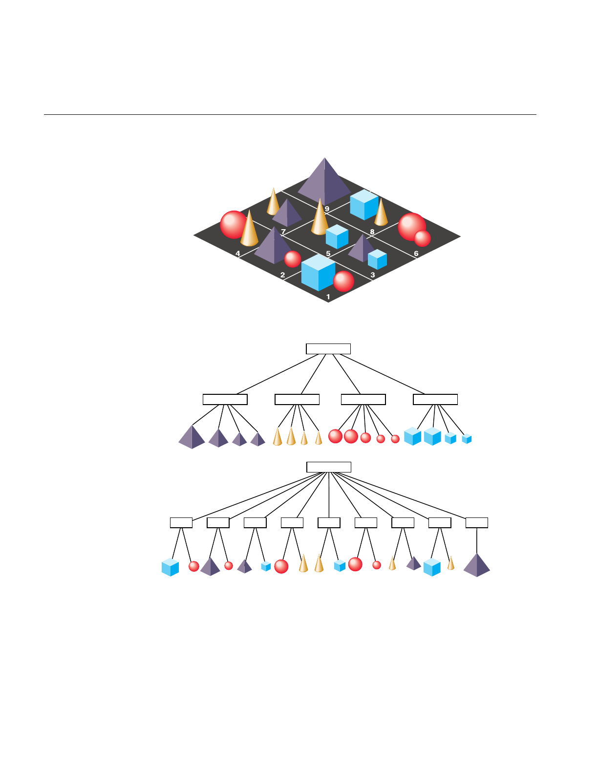
96
Chapter 4: Database Traversal
Figure 4-3 How to Partition a Database for Maximum Efficiency
Board
Pyramids Cones Spheres Cubes
Board
Tile 1 Tile 9Tile 2 Tile 3 Tile 4 Tile 5 Tile 6 Tile 7 Tile 8

Cull Traversal
97
When modeling a database, you should consider other trade-offs as well. Small amounts
of geometry in each culling unit, whether pfGeode or pfGeoSet, provide better culling
resolution and result in sending less non-visible geometry to the pipeline. Small pieces
also improve the performance of line-segment intersection inquiries (see“Database
Concerns” in Chapter 19). However, using many small pieces of geometry can increase
the traversal time and can also reduce drawing performance. The optimal amount of
geometry to place in each pfGeoSet depends on the application, database, system CPU,
and graphics hardware.
Custom Visibility Culling
Existence within the frustum isn’t the only criterion that determines an object’s visibility.
The item may be too distant to be seen from the viewpoint, or it may be obscured by other
objects between it and the viewer, such as a wall or a hill. Atmospheric conditions can
also affect object visibility. An object that is normally visible at a certain distance may not
be visible at that same distance in dense fog.
Implementing more sophisticated culling requires knowledge of visibility conditions
and control over the cull traversal. The cull traversal can be controlled through traversal
masks, which are described in the section titled “Controlling and Customizing
Traversals.”
Knowing whether an object is visible requires either prior information about the spatial
organization of a database, such as cell-to-cell visibilities, or run-time testing such as
computing line-of-sight visibility (LOS). You can compute simple LOS visibility by
intersecting line segments that start at the eyepoint with the database. See the
“Intersection Traversal” section of this chapter.
Sorting the Scene
During the cull traversal, a pfChannel can rearrange the order in which pfGeoSets are
rendered for improved performance and image quality. It does this by binning and
sorting. Binning is the act of placing pfGeoSets into specific bins which are rendered in a
specific order. IRIS Performer provides two default bins: one for opaque geometry and
one for blended, transparent geometry. The opaque bin is drawn before the transparent
bin so transparent surfaces are properly blended with the background scene.
Applications are free to add new bins and specify arbitrary bin orderings.

98
Chapter 4: Database Traversal
Sorting is done on a per-bin basis. pfGeoSets within a given bin are sorted by a specific
criterion. Two useful criteria provided by IRIS Performer are sorting by graphics state
and sorting by range. When sorting by state, pfGeoSets are sorted first by their
pfGeoState, then by an application-specified hierarchy of state modes, values, and
attributes which are identified by PFSTATE_* tokens and are described in the libpr
chapter. State sorting can offer a huge performance advantage since it greatly reduces the
number of mode changes carried out by the Geometry Pipeline. State sorting is the
default sorting configuration for the opaque bin.
Range sorting is required for proper rendering of blended, transparent surfaces which
must be rendered in back-to-front order so that each surface is properly blended with the
current background color. Front-to-back sorting is also supported. The default sorting for
the transparent bin is back-to-front sorting (Note that the sorting granularity is
per-pfGeoSet, not per-triangle so transparency sorting is not perfect).
pfChannel bins are given rendering order and sorting configuration with
pfChanBinOrder() and pfChanBinSort() respectively. A bin’s order is simply an integer
identifying its place in the list of bins. An order less than 0 or PFSORT_NO_ORDER
means that pfGeoSets which fall into the bin are drawn immediately without any
ordering or sorting. Multiple bins may have the same order but the rendering precedence
among these bins is undefined.
A bin’s sorting configuration is given as a token identifying the major sorting criterion
and then an optional list of tokens, terminated with the PFSORT_END token, that defines
a state sorting hierarchy.
PFSORT_BY_STATE
pfGeoSets are sorted first by pfGeoState then by the state elements
found between the PFSORT_STATE_BGN and PFSORT_STATE_END
tokens, for example.
PFSORT_FRONT_TO_BACK
pfGeoSets are sorted by nearest to farthest range from the eyepoint.
Range is computed from eyepoint to the center of the pfGeoSet’s
bounding volume.

Cull Traversal
99
PFSORT_BACK_TO_FRONT
pfGeoSets are sorted by farthest to nearest range from the eyepoint.
Range is computed from eyepoint to the center of the pfGeoSet’s
bounding volume.
PFSORT_QUICK
A special, low-cost sorting technique. pfGeoSets must fall into a bin
whose order is 0 in which case they will be sorted by pfGeoState and
drawn immediately. This is the default sorting mode for the
PFSORT_OPAQUE_BIN bin.
For example, the specification:
static int sort[] = {PFSORT_STATE_BGN,
PFSTATE_TEXTURE, PFSTATE_FRONTMTL,
PFSORT_STATE_END, PFSORT_END};
pfChanBinSort(chan, PFSORT_OPAQUE_BIN, PFSORT_BY_STATE,
sort);
will sort the opaque bin by pfGeoState, then by pfTexture, then by pfMaterial.
A pfGeoSet’s draw bin may be set directly by the application with pfGSetDrawBin().
Otherwise IRIS Performer automatically determines if the pfGeoSet belongs in the
default opaque or transparent bins.
Paths Through the Scene Graph
You can define a chain, or path, of nodes in a scene graph using the pfPath data structure.
(Note that a pfPath has nothing to do with filesystem paths as specified with the PFPATH
environment variable or with specifying a path for a user to travel through a scene.) Once
you’ve specified a pfPath with a call to pfNewPath(), you can traverse and cull that path
as a subset of the entire scene graph using pfCullPath(). The function pfCullPath() must
only be called from the cull callback function set by pfChanTravFunc()—see “Process
Callbacks” on page 105 for details. For more information about the pfPath structure, see
the pfPath(3pf) and pfList(3pf) reference pages.
When IRIS Performer looks for intersections, it can return a pfPath to the node containing
the intersection. This feature is particularly useful when you’re using instancing, in
which case you can’t use pfGetParent() to find out where in the scene graph the given
node is. Finding out the pfPath to a given node is also useful in implementing picking.

100
Chapter 4: Database Traversal
Draw Traversal
The cull traversal generates a libpr display list of geometry and state commands (see
“Display Lists” in Chapter 9), which describes the scene that is visible from a pfChannel.
The draw traversal simply traverses the display list and sends commands to the
Geometry Pipeline to generate the image.
Traversing a pfDispList is much faster than traversing the database hierarchy because the
pfDispList flattens the hierarchy into a simple, efficient structure. In this way, the cull
traversal removes much of the processing burden from the draw traversal; throughput
greatly increases when both traversals are running in parallel.
Controlling and Customizing Traversals
The result of the cull traversal is a display list of geometry to be rendered by the draw
traversal. What gets placed in the display list is determined by both visibility and by
other user-specified modes and tests.
pfChannel Traversal Modes
The PFTRAV_CULL argument to pfChanTravMode() modifies the culling traversal. The
cull mode is a bitmask that specifies the modes to enable, it is formed by the logical OR
of one or more of these tokens:
• PFCULL_VIEW
• PFCULL_GSET
• PFCULL_SORT
• PFCULL_IGNORE_LSOURCES
Culling to the view frustum is enabled by PFCULL_VIEW. Culling to the pfGeoSet-level
is enabled by PFCULL_GSET and can produce a tighter cull that improves rendering
performance at the expense of culling time.
PFCULL_SORT causes the cull to sort geometry by state—for example, by texture or by
material, in order to optimize rendering performance. It also causes transparent
geometry to be drawn after opaque geometry for proper transparency effects.

Controlling and Customizing Traversals
101
By default, the enabled culling modes are PFCULL_VIEW | PFCULL_GSET |
PFCULL_SORT. It is recommended that these modes be enabled unless the cull traversal
becomes a significant bottleneck in the processing pipeline. In this case, try disabling
PFCULL_GSET first, then PFCULL_SORT.
Normally, a pfChannel’s cull traversal pre-traverses the scene, following all paths from
the scene to all pfLightSources in the scene so that light sources can be set up before the
normal scene traversal. If you with to disable this pre-traversal, set the
PFCULL_IGNORE_LSOURCES cull enable bit but your pfLightSources will not
illuminate the scene.
The PFTRAV_DRAW argument to pfChanTravMode() modifies the draw traversal. A
mode of PFDRAW_ON is the default and will cause the pfChannel to be rendered. A
mode of PFDRAW_OFF indicates that the pfChannel should not be drawn and
essentially turns off the pfChannel.
pfNode Draw Mask
Each node in the database hierarchy can be assigned a mask that dictates whether the
node is added to the display list and thereby whether it is drawn. This mask is called the
draw mask (even though it is evaluated in the cull traversal) because it tells the cull
process whether the node is drawable or not.
The draw mask of a node is set with pfNodeTravMask(). The channel also has a draw
mask, which you set with pfChanTravMask(). By default, the masks are all 1s, or
0xffffffff.
Before testing a node for visibility, the cull traversal ANDs the two masks together. If the
result is zero, the cull prunes the node. If the result is nonzero, the cull proceeds normally.
Mask testing occurs before all visibility testing and function callbacks.
Masks allow you to draw different subgraphs of the scene on different channels, to turn
portions of the scene graph on and off, or to ignore hidden portions of the scene graph
while drawing but make them active during intersection testing.

102
Chapter 4: Database Traversal
pfNode Cull and Draw Callbacks
One of the primary mechanisms for extending IRIS Performer is through the use of
function callbacks, which can be specified on a per-node basis. IRIS Performer allows
separate cull and draw callbacks, which are invoked both before and after node
processing. Node callbacks are set with pfNodeTravFuncs().
Cull callbacks can direct the cull traversal, while draw callbacks are added to the display
list and later executed in the draw traversal for custom rendering. There are pre-cull and
pre-draw callbacks, invoked before a node is processed, and post-cull and post-draw
callbacks, invoked after the node is processed.
The cull callbacks return a value indicating how the cull traversal should proceed, as
shown in Table 4-2.
Callbacks are processed by the cull traversal in the following order:
1. If a pre-cull callback is defined, then call the pre-cull callback to get a cull result and
find out whether traversal should continue. Possible return values are listed in
Table 4-2.
2. If the pre-cull callback returns PFTRAV_PRUNE, the traversal returns to the parent
and continues with the node’s siblings, if any. If the callback returns
PFTRAV_TERM, the traversal terminates immediately. Otherwise, cull processing
continues.
3. If the pre-cull callback doesn’t set the cull result using pfCullResult(), and
view-frustum culling is enabled, then perform the standard node-within-frustum
test and set the cull result accordingly.
4. If the cull result is PFIS_FALSE, skip the traversal of children. The post-cull callback
is invoked and traversal returns so that the parent node can traverse any siblings.
Table 4-2 Cull Callback Return Values
Value Action
PFTRAV_CONT Continue and traverse the children of this node.
PFTRAV_PRUNE Skip the subgraph rooted at this node and continue.
PFTRAV_TERM Terminate the entire traversal.

Controlling and Customizing Traversals
103
5. If a pre-draw callback is defined, then place a libpr display-list packet in the display
list so that the node’s pre-draw callback will be called by the draw process. If
running a combined CULLDRAW traversal, invoke the pre-draw callback directly
instead.
6. Process the node, continuing the cull traversal with each of the node’s children or
adding the node’s geometry to a display list (for pfGeodes). If the cull result was
PFIS_ALL_IN, view-frustum culling is disabled during the traversal of the children.
7. If a post-draw callback is defined, then place a libpr display-list packet in the display
list so that the node’s post-draw callback will be called by the draw process. If
running a combined CULLDRAW traversal, invoke the post-draw callback directly
instead.
8. If a post-cull callback is defined, then call the post-cull callback.
Draw callbacks are commonly used to place tags or change state while a subgraph is
rendered. Note that if the pre-draw callback is called, the post-draw callback is
guaranteed to be invoked. This way the callback can restore any state modified by the
pre-draw callback. This is useful for state changes such as pfPushMatrix() and
pfPopMatrix(), as shown in the environment-mapping code that’s part of Example 4-2.
For doing customized culling, the pre-cull callback can determine whether a
PFIS_ALL_IN has already turned off view-frustum culling using
pfGetParentCullResult(), in which case it may not wish to do its own cull testing. It can
also find out the result of the standard cull test by calling pfGetCullResult().
Cull callbacks can also be used to render geometry (pfGeoSets) or change graphics state.
Anylibpr drawing commands are captured in a display list and are later executed during
the draw traversal (see “Display Lists” in Chapter 9). However, direct graphics library
calls can be made safely only in draw function callbacks, because only the draw process
of multiprocess IRIS Performer configurations is known to be associated with a window.
Example 4-2 shows some sample node callbacks.
Example 4-2 pfNode Draw Callbacks
void
LoadScene(char *filename)
{
pfScene *scene = pfNewScene();
pfGroup *root = pfNewGroup();
pfGroup *reflectiveGeodes = NULL;

104
Chapter 4: Database Traversal
root = pfdLoadFile(filename);
...
reflectiveGeodes =
ReturnListofGeodesWithReflectiveMaterials(root);
/* Use a node callback in the Draw process to turn on
* and off graphics library environment mapping before
* and after drawing all of the pfGeodes that have
* pfGeoStates with reflective materials.
*/
pfNodeTravFuncs(reflectiveGeodes, PFTRAV_DRAW,
pfdPreDrawReflMap, pfdPostDrawReflMap);
}
/* This callback turns on graphics library environment
* mapping. Because it changes graphics state it must be a
* Draw process node callback. */
long
pfdPreDrawReflMap(pfTraverser *trav, void *data)
{
texgen(TX_S, TG_SPHEREMAP, 0);
texgen(TX_T, TG_SPHEREMAP, 0);
texgen(TX_S, TG_ON, NULL);
texgen(TX_T, TG_ON, NULL);
return NULL;
}
/* This callback turns off graphics library environment
* mapping. Because it also changes graphics state it also
* must be a Draw process node callback. Also notice that
* it is important to return the graphics library’s state to
* the state at which it was in before the preNode callback
* was even made.
*/
long
pfdPostDrawReflMap(pfTraverser *trav, void *data)
{
texgen(TX_S, TG_OFF, NULL);
texgen(TX_T, TG_OFF, NULL);
return NULL;
}

Process Callbacks
105
Process Callbacks
libpf processes a visual database with a software-rendering pipeline composed of
application, cull, and draw stages. The system of process callbacks allows you to insert
your own custom culling and drawing functions into the rendering pipeline.
Furthermore, these callbacks are invoked by the proper process when your IRIS
Performer application is configured for multiprocessing.
By default, IRIS Performer culls and draws all active pfChannels when pfFrame() is
called. However, you can specify cull and draw function callbacks so that pfFrame() will
cause IRIS Performer to call your custom functions instead. These functions have the
option of using the default IRIS Performer processing in addition to their own custom
processing.
When multiprocessing is used, the rendering pipeline works on multiple frames at once.
For example, when the draw process is rendering frame n, the cull process is working on
frame n+1, and the application process is working on frame n+2. This situation requires
careful management of data so that data generated by the application is propagated to
the cull process and then to the draw process at the right time. IRIS Performer manages
data that is passed to the process callbacks to ensure that the data is frame-coherent and
isn’t corrupted.
Example 4-3 illustrates the use of a cull-process callback.
Example 4-3 Cull-Process Callbacks
InitChannels()
{
...
/* create and configure all channels*/
...
/* define callbacks for cull and draw processes */
pfChanTravFunc(chan, PFTRAV_CULL, CullFunc);
pfChanTravFunc(chan, PFTRAV_DRAW, DrawFunc);
...
}
/* The Cull callback. Any work that needs to be done in the
* Cull process should happen in this function.
*/
void
CullFunc(pfChannel * chan, void *data)
{

106
Chapter 4: Database Traversal
static long first = 1;
/* Lock down whatever processor the cull is using when
* the cull callback is first called.
*/
if (first)
{
if ((pfGetMultiprocess() & PFMP_FORK_CULL) &&
(ViewState->procLock & PFMP_FORK_CULL))
pfuLockDownCull(pfGetChanPipe(chan));
first = 0;
}
/* User-defined pre-cull processing. Application-
* specific cull knowledge might be used to provide
* things like line-of-sight culling.
*/
PreCull(chan, data);
/* standard Performer culling to the viewing frustum */
pfCull();
/* User-defined post-cull processing; this routine might
* be used to do things like record cull state from this
* cull to be used in future culls.
*/
PostCull(chan, data);
}
/* The draw function callback. I/O with IRIS GL devices must
* happen here. Any graphics library functionality outside
* IRIS Performer must be done here.
*/
void
DrawFunc(pfChannel *chan, void *data)
{
/* pre-Draw tasks like clearing the viewport */
PreDraw(chan, data);
pfDraw(); /* render the frame */
/* draw HUD, read IRIS GL devices, and so on */
PostDraw(chan, data);
}

Process Callbacks
107
Process Callbacks and Passthrough Data
Cull and draw callbacks are specified on a per-pfChannel basis using the functions
pfChanTravFunc() with PFTRAV_CULL and PFTRAV_DRAW, respectively.
pfAllocChanData() allocates passthrough data, data which is passed down the rendering
pipeline to the callbacks.
In the cull phase of the rendering pipeline, IRIS Performer invokes the cull callback with
a pointer to the pfChannel that is being culled and a pointer to the pfChannel’s
passthrough data buffer. The cull callback may modify data in the buffer. The potentially
modified buffer is then copied and passed to the user’s draw callback.
Default IRIS Performer processing is triggered by pfCull() and pfDraw(). By default,
pfFrame() calls pfCull() first, then calls pfDraw(). If process callbacks are defined,
however,pfCull() and pfDraw() are not invoked automatically and must be called by the
callbacks to use IRIS Performer’s default processing. pfCull() should be called only in the
cull callback; it causes IRIS Performer to cull the current channel and to generate a
display list suitable for rendering.
Channels culled by pfCull() may be drawn in the draw callback by pfDraw(). It is legal
for the draw callback to call pfDraw() more than once. Multi-pass renderings performed
with multiple calls to pfDraw() are typical when you use accumulation buffer
techniques.
When the draw callback is invoked, the window will have already been properly
configured for drawing the pfChannel. Specifically, the viewport, perspective, and
viewing matrices are set to their correct values. User modifications of these values are not
reset by pfDraw(). If a draw callback is specified, IRIS Performer doesn’t automatically
clear the viewport; it leaves that responsibility to the application. pfClearChan() can be
called from the draw callback to clear the channel viewport. If chan has a pfEarthSky(),
then the pfEarthSky() is drawn. Otherwise, the viewport is cleared to black and the
z-buffer is cleared to its maximum value.
You should call pfPassChanData() to indicate that user data should be passed through
the rendering pipeline, which propagate the data downstream to cull and draw
callbacks. The next call to pfFrame() copies the channel buffer into internal buffers, so
that the application is then free to modify data in the buffer without fear of corruption.
The pfPassChanData() function should be called only when necessary, since calling it
imposes some buffer-copying overhead. In addition, passthrough data should be as
small as possible to reduce the time spent copying data.

108
Chapter 4: Database Traversal
The code fragment in Example 4-4 is an example of cull and draw callbacks and the
passthrough data that is used to communicate with them.
Example 4-4 Using Passthrough Data to Communicate With Callback Routines
typedef struct
{
long val;
} PassData;
void cullFunc(pfChannel *chan, void *data);
void drawFunc(pfChannel *chan, void *data);
int main()
{
PassData *pd;
/* allocate passthrough data */
pd = (PassData*)pfAllocChanData(chan,sizeof(PassData));
/* initialize channel callbacks */
pfChanTravFunc(chan, PFTRAV_CULL, cullFunc);
pfChanTravFunc(chan, PFTRAV_DRAW, drawFunc);
/* main simulation loop */
while (1)
{
pfSync();
pd->val = 0;
pfPassChanData(chan);
pfFrame();
}
}
void
cullFunc(pfChannel *chan, void *data)
{
PassData *pd = (PassData*)data;
pd->val++;
pfCull();
}
void
drawFunc(pfChannel *chan, void *data)

Intersection Traversal
109
{
PassData *pd = (PassData*)data;
fprintf(stderr, "%ld\n", pd->val);
pfClearChan(chan);
pfDraw();
}
This example would, regardless of the multiprocessing mode, have the values 0, 1, and 1
forpd->val at the points where pfFrame(),pfCull(), and pfDraw() are called. In this way,
control data can be sent down the pipeline from the application, through the cull, and on
to the draw process with frame synchronization without regard to the active
multiprocessing mode.
When configured as a process separate from the draw, the cull callback should not
attempt to send graphics commands to an IRIS Performer window because only the
draw process is attached to the window. Callbacks should not modify the IRIS Performer
database, but they can use pfGet() routines to inquire about database information. The
draw callback should not call swapbuffers() (or an equivalent function when using
OpenGL) because IRIS Performer must control buffer swapping in order to manage the
necessary frame and channel synchronization. However, if you need special control over
buffer swapping, use pfPipeSwapFunc() to register a function as the given pipe’s
buffer-swapping function. Once your function is registered, it will be called instead of
swapbuffers() and may then invoke either of these functions.
Intersection Traversal
You can make spatial inquiries in IRIS Performer by testing the intersection of line
segments with geometry in the database. For example, a single line segment pointing
straight down from the eyepoint can determine your height above terrain, four such
segments can simulate the four tires of a car, and segments swept out by points on a
moving object can determine collisions with other objects.

110
Chapter 4: Database Traversal
Testing Line Segment Intersections
The testing of each line segment or group of spatially grouped segments requires a
traversal of part or all of a scene graph. You make these inquiries using
pfNodeIsectSegs(), which intersects the specified group of segments with the subgraph
rooted at the specified node. pfChanNodeIsectSegs() functions similarly, but includes a
channel so that the traversal can make decisions based on the level-of-detail specified by
pfLOD nodes.
Intersection Requests: pfSegSets
A pfSegSet is a structure that embodies an intersection request.
typedef struct _pfSegSet
{
long mode;
void* userData;
pfSeg segs[PFIS_MAX_SEGS];
ulong activeMask;
ulong isectMask;
void* bound;
long (*discFunc)(pfHit*);
} pfSegSet;
The segs field is an array of line segments making up the query. You tell
pfNodeIsectSegs() which segments to test with by setting the corresponding bit in the
activeMask field. If your pfSegSet contains many closely-grouped line segments, you can
specify a bounding volume using the data structure’s bound field. pfNodeIsectSegs()can
use that bounding volume to more quickly test the request against bounding volumes in
the scene graph. The userData field is a pointer with which you can point to other
information about the request that you might want access to in a callback. The other
fields are described below. The pfSegSet isn’t modified during the traversal.

Intersection Traversal
111
Intersection Return Data: pfHit Objects
Intersection information is returned in pfHit objects. These can be queried using
pfQueryHit() and pfMQueryHit(). Table 4-3 lists the items that can be queried from a
pfHit object.
The PFQHIT_FLAGS field is bit vector with bits that indicate whether an intersection
occurred and whether the point, normal, primitive and transformation information is
valid. For some types of intersections only some of the information has meaning; for
instance, for a pfSegSet bounding volume intersecting a pfNode bounding sphere, the
point information may not be valid.
Queries can be performed singly by calling pfQueryHit() with a single query token, or
several at a time by using pfMQueryHit() with an array of tokens. In the latter case, the
return information is placed in the specified order into a return array.
Table 4-3 Intersection-Query Token Names
Query Token Description
PFQHIT_FLAGS Status and validity information
PFQHIT_SEGNUM Index of the segment in pfSegSet request
PFQHIT_SEG Line segment as currently clipped
PFQHIT_POINT Intersection point in object coordinates
PFQHIT_NORM Geometric normal of an intersected triangle
PFQHIT_VERTS Vertices of an intersected triangle
PFQHIT_TRI Index of an intersected triangle
PFQHIT_PRIM Index of an intersected primitive in pfGeoSet
PFQHIT_GSET pfGeoSet of an intersection
PFQHIT_NODE pfGeode of an intersection
PFQHIT_NAME Name of pfGeode
PFQHIT_XFORM Current transformation matrix
PFQHIT_PATH Path in scene graph of intersection

112
Chapter 4: Database Traversal
Intersection Masks
Before using pfNodeIsectSegs() to intersect the geometry in the scene graph, you must
set intersection masks for the nodes in the scene graph and correspondingly in your
search request.
Setting the Intersection Mask
pfNodeTravMask() sets the intersection masks in a subgraph of the scene down through
GeoSets. For example:
pfNodeTravMask(root, PFTRAV_ISECT, 0x01,
PFTRAV_SELF | PFTRAV_DESCEND, PF_SET)
sets the intersection mask of all nodes and GeoSets in the scene graph to 0x01. A
subsequent intersection request would then use 0x01 as the mask in pfNodeIsectSegs().
A description of how to use this mask follows.
Specifying Different Classes of Geometry
Databases can contain different classes of objects, and only some of those may be relevant
for a particular intersection request. For example, the wheels on a truck follow the
ground, even through a small pond; therefore, you only want to test for intersection with
the ground and not with the water. For a boat, on the other hand, intersections with both
water and the lake bottom have significance.
To accommodate distinctions between classes of objects, each node and GeoSet in a scene
graph has an intersection mask. This mask allows traversals, such as intersections, to
either consider or ignore geometry by class.
For example, you could use four classes of geometry to control tests for collision
detection of a moving ship, collision detection for a falling bowling ball, and line-of-sight
visibility. Table 4-4 matches database classes with the pfNodeTravMask and
pfGSetIsectMask values used to support the traversal tests listed above.

Intersection Traversal
113
Once the mask values at nodes in the database have been set, intersection traversals can
be directed by them. For example, the line segments for ship collision detection should
be sensitive to the water, ground, and pier, while a those for a bowling ball would ignore
intersections with water and the clouds, testing only against the ground and pier.
Line-of-sight ranging should be sensitive to all the geometry in the scene. Table 4-5 lists
the traversal mask values and mask representations that would achieve the proper
intersection tests.
The intersection traversal prunes a node as soon as it gets a zero result from doing a
bitwise AND of the node intersection mask and the traversal mask specified by the
pfSegSet’sisectMask field. Thus, all nodes in the scene graph should normally be set to be
the bitwise OR of the masks of their children. After setting the class-specific masks for
different subgraphs of the scene, this can be accomplished by calling
pfNodeTravMask(root, PFSET_OR, PFTRAV_SET_FROM_CHILD, 0x0);
which sets each node’s mask by OR-ing 0x0 with the current mask and the masks of the
node’s children.
Table 4-4 Database Classes and Corresponding Node Masks
Database Class Node Mask
Water 0x01
Ground 0x02
Pier 0x04
Clouds 0x08
Table 4-5 Representing Traversal Mask Values
Intersection Class Mask Value Mask Representation
Ship 0x07 (Water | Ground | Pier)
Bowling ball 0x06 (Ground | Pier)
Line-of-sight ranging 0x0f (Water | Ground | Pier | Clouds)

114
Chapter 4: Database Traversal
Note that this traversal, like that used to update node bounding volumes, is unusual in
that it propagates information up the graph from leaf nodes to root.
Discriminator Callbacks
If you need to make a more sophisticated discrimination than node masks allow about
when an intersection is valid, IRIS Performer can issue a callback on each successful
intersection and let you decide whether the intersection is valid in the current context.
If a callback is specified in pfNodeIsectSegs(), then at each level where an intersection
occurs—for example, with bounding volumes of libpf pfGeodes (mode
PFTRAV_IS_GEODE), libpr GeoSets (mode PFTRAV_IS_GSET), or individual geometric
primitives (mode PFTRAV_IS_PRIM)—IRIS Performer invokes the callback, giving it
information about the candidate intersection. The value you return from the callback
determines whether the intersection should be ignored and how the intersection
traversal should proceed.
If the return value includes the bit PFTRAV_IS_IGNORE, the intersection is ignored. The
intersection traversal itself can also be influenced by the callback. The traversal is subject
to three possible fates, as detailed in Table 4-6.
Line Segment Clipping
Usually, the intersection point of most interest is the one that is nearest to the beginning
of the segment. By default, after each successful intersection, the end of the segment is
clipped so that the segment now ends at the intersection point. Upon the final return
from the traversal, it contains the closest intersection point.
Table 4-6 Possible Traversal Results
Set Bits Meaning
PFTRAV_CONTContinue the traversal inside this subgraph or GeoSet.
PFTRAV_PRUNEContinue the traversal but skip the rest of this subgraph or GeoSet.
PFTRAV_TERMTerminate the traversal here.

Intersection Traversal
115
However, if you want to examine all intersections along a segment you can use a
discriminator callback to tell IRIS Performer not to clip segments—simply leave out the
PFTRAV_IS_CLIP_END bit in the return value. If you want the farthest intersection
point, you can use PFTRAV_IS_CLIP_START so that after each intersection the new
segment starts at the intersection point and extends outward.
Traversing Special Nodes
Level-of-detail nodes are intersected against the model for range zero, which is typically
the highest level-of-detail. If you want to select a different model, you can turn off the
intersection mask for the LOD node and place a switch node in parallel (having the same
parent and children as the LOD) and set it to the desired model.
Sequences and switches intersect using the currently active child or children. Billboards
are not intersected, since no eyepoint is defined for intersection traversals.
Picking
pfChanPick() provides a simple interface for intersection testing by enabling the user to
move a mouse to select one or more geometries. The method uses pfNodeIsectSegs()
and uses the high bit, PFIS_PICK_MASK, of the intersection mask in the scene graph.
Setting up picking with pfNodePickSetup() sets this bit in the intersection mask
throughout the specified subgraph, but does not enable caching inside pfGeoSets. See
“Performance” on page 115.
pfChanPick() has an extra feature: it can either return the closest intersection
(PFPK_M_NEAREST) or return all pfHits along the picking ray (PFPK_M_ALL).
Performance
The intersection traversal uses the hierarchical bounding volumes in the scene graph to
allow culling of the database and then processes candidate GeoSets by testing against
their internal geometry. For this reason, the hierarchy should reflect the spatial
organization of the database. High-performance culling has similar requirements (see
Chapter 19, “Performance Tuning and Debugging”).

116
Chapter 4: Database Traversal
Performance Trade-offs
IRIS Performer currently retains no information about spatial organization of data within
GeoSets, so each triangle in the GeoSet must be tested. Although large GeoSets are good
for rendering performance in the absence of culling, spatially localized GeoSets are best
for culling (since a GeoSet is the smallest culling unit), and spatially localized GeoSets
with few primitives are best for intersections.
Front Face/Back Face
One way to speed up intersection testing is to turn on PFTRAV_IS_CULL_BACK. When
this flag is enabled, only front-facing geometry is tested.
Enabling Caching
Precomputing information about normals and projections speeds up intersections inside
GeoSets. For the best performance, you should enable caching in GeoSets when you set
the intersection masks with pfNodeTravMask().
If the geometry within a GeoSet is dynamic, such as waves on a lake, caching can cause
incorrect results. However, for geometry that changes only rarely, you can use
pfGSetIsectMask() to recompute the cache as needed.
Intersection Methods for Segments
Normally, when intersecting down to the primitive level each line segment is separately
tested against each bounding volume in the scene graph, and after passing those tests is
intersected against the pfGeoSet bounding box. Segments that intersect the bounding
box are eventually tested against actual geometry.
When a pfSegSet has a spatially localized group of at least several line segments, you can
speed up the traversal by providing a bounding volume. You can use
pfCylAroundSegs() to create a bounding cylinder for the segments, and place a pointer
to the resulting cylinder in the pfSegSet’s bound field; then OR the PFTRAV_IS_BCYL bit
into the pfSegSet’s mode field.
If only a rough volume-volume intersection is required, you can specify a bounding
cylinder in the pfSegSet without any line segments at all and request discriminator
callbacks at the PFTRAV_IS_NODE or PFTRAV_IS_GSET level.

Intersection Traversal
117
Figure 4-4 illustrates some aspects of this process. The portion of the figure labeled A
represents a single segment; B is a collection of nonparallel segments, not suitable for
tightly bounding with a cylinder; and C shows parallel segments surrounded by a
bounding cylinder. In the bottom portion of the figure, the bounding cylinder around the
segments intersects the bounding box around the object; each segment in the cylinder
thus must be tested individually to see if any of them intersect.
Figure 4-4 Intersection Methods


This chapter explains how to control frame rate, synchronization, and
dynamic load management.
“Frame and Load Control”
Chapter 5


121
Chapter 5
5. Frame and Load Control
This chapter describes how to manage the display operations of a visual simulation
application to maintain the desired frame rate and visual performance level.In addition
this chapter covers advanced topics including multiprocessing and shared memory
management.
Frame-Rate Management
Aframe is the period of time in which all processing must be completed before updating
the display with a new image, for example, a frame rate of 60Hz means the display is
updated 60 times per second and the time extent of a frame is 16.7ms. The ability to fit all
processing within a frame depends on several variables, some of which are:
• the number of pixels being filled
• the number of transformations and modal changes being made
• the amount of processing required to create a display list for a single frame
• the quantity of information being sent to the graphics subsystem
Through intelligent management of Silicon Graphics CPU and graphics hardware, IRIS
Performer minimizes the above variables in order to achieve the desired frame rate.
However, in some cases, peak frame rate is less important than a fixed frame rate. Fixed
frame rate means that the display is updated at a consistent, unvarying rate. While a
simple step towards achieving a fixed frame rate is to reduce the maximum frame rate to
an easily achievable level, we shall explore other (less Draconian) mechanisms in this
chapter that do not adversely impact frame rates.
As discussed in the following sections, IRIS Performer lets you select the frame rate and
has built-in functionality to maintain that frame rate and control overload situations
when the draw time exceeds or grows uncomfortably close to a frame time. While these
methods can be effective, they do require some cooperation from the run-time database.
In particular, databases should be modeled with levels-of-detail and be spatially
arranged.

122
Chapter 5: Frame and Load Control
Selecting the Frame Rate
IRIS Performer is designed to run at the fixed frame rate as specified by pfFrameRate().
Selecting a fixed frame rate does not in itself guarantee that each frame can be completed
within the desired time. It is possible that some frames might require more computation
time than is allotted by the frame rate. By taking too long, these frames cause dropped or
skipped frames. A situation in which frames are dropped is called an overload or overrun
situation. A system that is close to dropping frames is said to be in stress.
Achieving the Frame Rate
The first step towards achieving a frame rate is to make sure that the scene can be
processed in less than a frame’s time—hopefully much less than a frame’s time.
Although minimizing the processing time of a frame is a huge effort, rife with tricks and
black magic, certain techniques stand out as IRIS Performer’s main weapons against
slothful performance:
• Multiprocessing. The use of multiple processes on multi-CPU systems can
drastically increase throughput.
• View culling. By trivially rejecting portions of the database outside the viewing
volume, performance can be increased by orders of magnitude.
• State sorting. Many graphics pipelines are sensitive to graphics mode changes.
Sorting a scene by graphics state greatly reduces mode changes, increasing the
efficiency of the hardware.
• Level-of-detail. Objects that are far away project to a relatively small area of the
display so fewer polygons can be used to render the object without substantial loss
of image quality. The overall result is fewer polygons to draw and improved
performance.
Multiprocessing and level-of-detail is discussed in this chapter while view culling and
state sorting are discussed in Chapter 4, “Database Traversal.” More information on
sorting in the context of performance tuning can be found in Chapter 19, “Performance
Tuning and Debugging.”

Frame-Rate Management
123
Fixing the Frame Rate
Frame intervals are fixed periods of time but frame processing is variable in nature.
Because things change in a scene, such as when objects come into the field of view, frame
processing cannot be fixed. In order to maintain a fixed frame rate, the average frame
processing time must be less than the frame time so that fluctuations don’t exceed the
selected frame time. Alternately, the scene complexity can be automatically reduced or
increased so that the frame rate stays within a user-defined “sweet spot”. This
mechanism requires that the scene be modeled with levels-of-detail (pfLOD nodes).
Each frame, IRIS Performer calculates the system load for each frame. Load is calculated
as the percentage of the frame period it took to process the frame. Then if the default IRIS
Performer fixed frame rate mechanisms are enabled, load is used to calculate system
stress, which is in turn used to adjust the level of detail (LOD) of visible models. LOD
management is IRIS Performer’s primary method of managing system load.
Table 5-1 shows the IRIS Performer functions for controlling frame processing.
Figure 5-1 shows a frame-timing diagram that illustrates what occurs when frame
computations are not completed within the required interval. The solid vertical lines in
Figure 5-1 represent frame-display intervals. The dashed vertical lines represent video
refresh intervals.
Table 5-1 Frame Control Functions
Function Description
pfFrameRate Set the desired frame rate.
pfSync Synchronize processing to frame boundaries.
pfFrame Initiate frame processing.
pfPhase Control frame boundaries.
pfChanStressFilter Control how stress is applied to LOD ranges.
pfChanStress Manually control the stress value.
pfGetChanLoad Determine the current system load.
pfChanLODAttr Control how LOD is performed, including global LOD
adjustment and blending (fade).
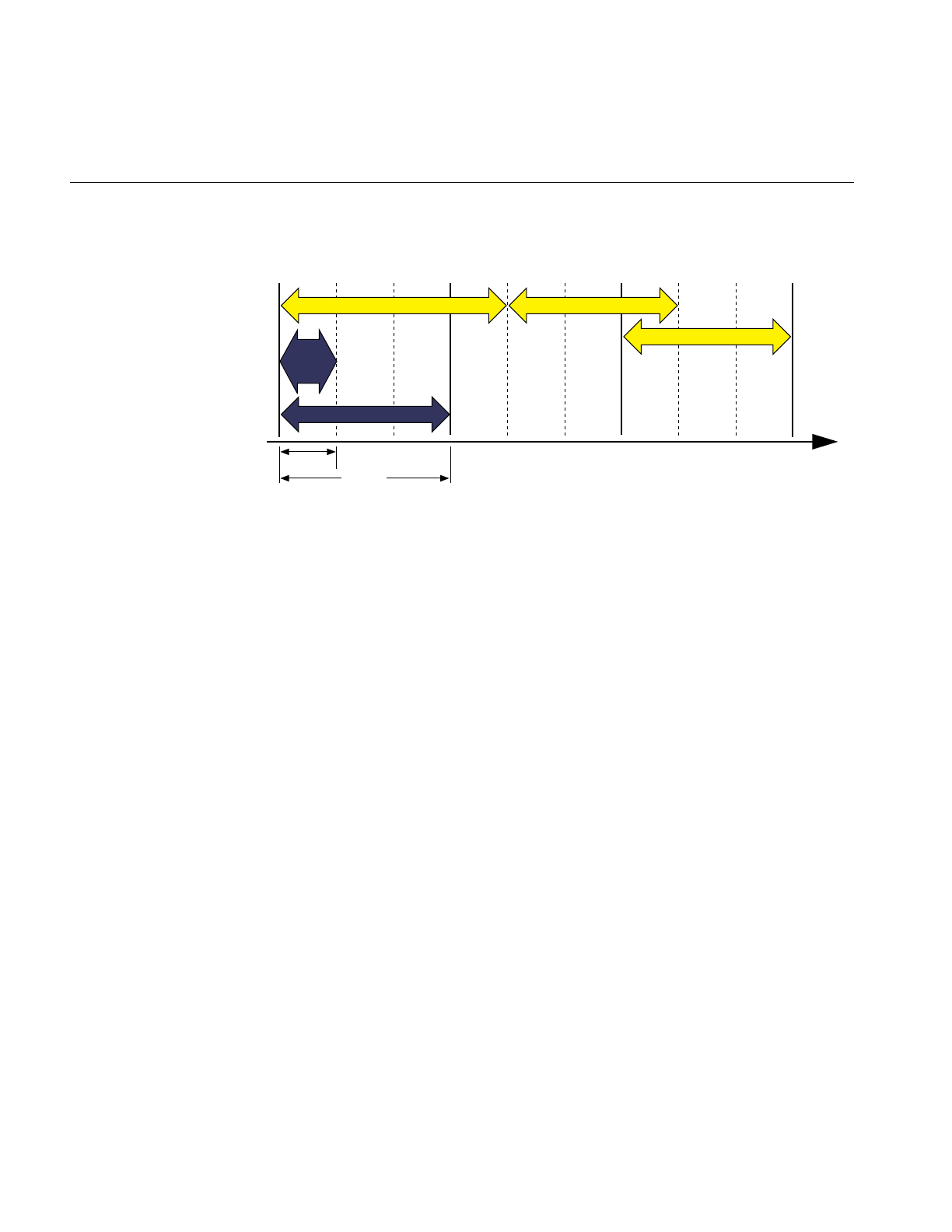
124
Chapter 5: Frame and Load Control
Figure 5-1 Frame Rate and Phase Control
In this example, the video scan rate is 60 Hz and the frame rate is 20 Hz. With the video
hardware running at 60 Hz, each of the 20 Hz frames should be scanned to the video
display three times, and the system should wait for every third vertical retrace signal
before displaying the next image. The numbers across the top of the figure represent the
refresh count modulo three. New images are displayed on refreshes whose count modulo
three is zero, as shown by the solid lines.
In the first frame of this example, the new image isn’t yet completed when the third
vertical retrace signal occurs; the same image must therefore be displayed again during
the next interval. This situation is known as frame overrun, because the frame
computation time extends past a refresh boundary.
Frame Synchronization
Because of the overrun, the frame and refresh interval timing is no longer synchronized;
it’s out of phase. A decision must be made either to display the same image for the
remaining two intervals, or to switch to the next image even though the refresh isn’t
aligned on a frame boundary. The frame-rate control mode, discussed in the next section,
determines which choice is selected.
Knowing that the situation illustrated in Figure 5-1 is a possibility, you can specify a
frame control mode to indicate what you would like the system to do when a frame
overrun occurs.
1/60TH
1/20TH
Overrun Floating
Locked
Time in seconds
0120120120
Refresh count
modulo three
Frame display interval
Video
refresh
interval

Frame-Rate Management
125
To specify a method of frame-rate control, call pfPhase(). There are the following choices:
• Free run without phase control (PFPHASE_FREE_RUN) tells the application to run
as fast as possible—to display each new frame as soon as it’s ready, without
attempting to maintain a constant frame rate.
• Free run without phase control but with a limit on the maximum frame rate
(PFPHASE_LIMIT) tells the application to run no faster the rate specified by
pfFrameRate.
• Fixed frame rate with floating phase (PFPHASE_FLOAT) allows the drawing
process to display a new frame (using swapbuffers(3G)) at any time, regardless of
frame boundaries.
• Fixed frame rate with locked phase (PFPHASE_LOCK) requires the draw process to
wait for a frame boundary before displaying a new frame.
• The draw by default will wait for a new cull result to execute its stage functions.
This behavior can be changed by including the token PFPHASE_SPIN_DRAW with
the desired mode token from the above choices. This will allow the draw to run
every frame, redrawing the previous cull result. This can allow you to make
changes of your own in draw callback functions. Objects such as viewing frustum,
pfLODs, pfDCSs, and anything else normally processed by the CULL or application
processes will not be updated until the next full cull result is available.
Free-Running Frame-Rate Control
The simplest form of frame-rate control, called free-running, is to have no control at all.
This uncontrolled mode draws frames as quickly as the hardware is able to process them.
In free-running mode, the frame rate may be 60 Hz in the areas of low database
complexity, but could drop to a slower rate in views that place greater demand on the
system. Use pfPhase(PFPHASE_FREE_RUN) to specify a free-running frame rate.
In applications in which real-time graphics provide the majority of visual cues to an
observer, the variable frame rates produced by the free-running mode may be
undesirable. The variable lag in image update associated with variable frame rate can
lead to motion sickness for the simulation participants, especially in motion
platform-based trainers or ingressive head-mounted displays. For these and other
reasons it is usually preferable to maintain a steady, consistent frame-update rate.

126
Chapter 5: Frame and Load Control
Fixed Frame-Rate Control
Assume that the overrun frame in Figure 5-1 completes processing during the next
refresh period, as shown. After the overrun frame, the simulation is still running at the
chosen 20-Hz rate and is updating at every third vertical retrace. If a new image is
displayed at the next refresh, its start time lags by 1/60th of a second, and therefore it is
out of phase by that much.
Subsequent images are displayed when the refresh count modulo three is one. As the
simulation continues and additional extended frames occur, the phase continues to drift.
This mode of operation is called floating phase, as shown by the frame in Figure 5-1
labeled Floating. Use pfPhase(PFPHASE_FLOAT) to select floating-phase frame control.
The alternative to displaying a new image out of phase is to display the old image for the
remainder of the current update period, then change to the new image at the normal
time. This locked phase extends each frame overrun to an integral multiple of the selected
frame time, making the overrun more evident but also maintaining phase throughout the
simulation. This timing is shown by the frame in Figure 5-1 labeled Locked. Although this
mode is the most restrictive, it is also the most desirable in many cases. Use
pfPhase(PFPHASE_LOCK) to select phase-locked frame control.
For example, a 20-Hz phase-locked frame rate is selected by specifying:
pfPhase(PFPHASE_LOCK);
pfFrameRate(20.0f);
These specifications prevent the system from switching to a newly computed image until
a display period of 1/20th second has passed from the time the previous image was
displayed. The frame rate remains fixed even when the Geometry Pipeline finishes its
work in less time. Fixed frame-rate display therefore involves setting the desired frame
rate and selecting one of the two fixed-frame-rate control modes.
Frame Skipping
When multiple frame times elapse during the rendering of a single frame, the system
must choose which frame to draw next. If the per-frame display lists are processed in
strict succession even after a frame overrun, the visual image slowly recedes in time and
the positional correlation between display and simulation is lost. To avoid this problem,
only the most recent frame definition received by the draw process is sent to the
Geometry Pipeline, and all intervening frame definitions are abandoned. This is known
as dropping or skipping frames and is performed in both of the fixed frame-rate modes.

Frame-Rate Management
127
Because the effects of variable frame rates, phase variance, and frame dropping are
distracting, you should choose a frame rate with care. Steady frame rates are achieved
when the frame time allows the worst-case view to be computed without overload. The
structure of the visual database, particularly in terms of uniform “complexity density,”
can be important in maximizing the system frame rate. See “Organizing a Database for
Efficient Culling” in Chapter 4 and Figure 4-3 for examples of the importance of database
structure.
Maintaining a fixed frame rate involves managing future system load by adjusting
graphics display actions to compensate for varying past and present loads. The theory
behind load management and suggested methods for dealing with variable load
situations are discussed in the “Level-of-Detail Management” section of this chapter.
Sample Code
Example 5-1 demonstrates a common approach to frame control. The code is based on
part of the main.c source file used in the perfly sample application.
Example 5-1 Frame Control Excerpt
/* Set the desired frame rate. */
pfFrameRate(ViewState->frameRate);
/* Set the MP synchronization phase. */
pfPhase(ViewState->phase);
/* Application main loop */
while (!SimDone())
{
/* Sleep until next frame */
pfSync();
/* Should do all latency-critical processing between
* pfSync() and pfFrame(). Such processing usually
* involves changing the viewing position.
*/
PreFrame();
/* Trigger cull and draw processing for this frame. */
pfFrame();
/* Perform non-latency-critical simulation updates. */
PostFrame();
}
128
Chapter 5: Frame and Load Control
Maintaining Frame Rate Using Dynamic Video Resolution
When frame rate is not maintained, some frames display longer than others. If, for
example, when the frame rate is 30 frames per second, a frame takes longer than 1/30th
of a second to fill the frame buffer, the frame is not displayed. Consequently, the current
frame is displayed for two instead of one 1/30ths of a second. The result of inconsistent
frame rates is jerky motion within the scene.
Note: You have some control over what happens when a frame rate is missed. You can
choose, for example, to begin the next frame in the next 1/60th of a second, or wait for
the start of the next 1/30th second. For more information about handling frame drawing
overruns, see pfPhase in “Free-Running Frame-Rate Control” on page 125.
The key to maintaining frame rate is limiting the amount of information to be rendered.
IRIS Performer can take care of this problem automatically for you when you use the
PFPVC_DVR_AUTO token with pfPVChanDVRMode().
In PFPVC_DVR_AUTO mode, IRIS Performer checks every rendered frame to see if it
took too long to render. If it did, IRIS Performer reduces the size of the image, and
correspondingly, the number of pixels in it. Afterwards, the video hardware enlarges the
images to the same size as the pfChannel; in this way, the image is the correct size, but it
contains a reduced number of pixels, as suggested in Figure 5-2.
Figure 5-2 Real Size of Viewport Rendered Under Increasing Stress
Although the viewport is reduced as stress increases, the viewer never sees the image
grow smaller because bipolar filtering is used to enlarge the image to the size of the
channel.

Maintaining Frame Rate Using Dynamic Video Resolution
129
The Channel in DVR
When using Dynamic Video Resolution (DVR), the origin and size of a channel are
dynamic. For example, a viewport whose lower-left corner is at the center of a pfPipe
(with coordinates 0.5, 0.5) would be changed to an origin of (0.25, 0.25) with respect to
the full pfPipe window if the DVR settings were scaled by a factors of 0.5 in both X and
Y dimensions.
If you are doing additional rendering into a pfChannel, you may need to know the size
and the actual rendered area of the pfChannel. Use pfGetChanOutputOrigin() and
pfGetChanOutputSize() to get the actual rendered origin and size, respectively, of a
pfChannel. pfGetChanOrigin() and pfGetChanSize() gives the displayed origin and
size of the pfChannel and these functions should be used for mapping mouse positions
or other window-relative non-rendering positions to the pfChannel area.
Additionally, if DVR alters the rendered size of a pfChannel, a corresponding change
should be made to the width of points and lines. For example, when a channel is scaled
in size by one half, lines and points must be drawn half as wide as well so that when the
final image is enlarged, in this case by a factor of two, the lines and points scale correctly.
pfChanPixScale() sets the pixel scale factor. pfGetChanPixScale() returns this value for
a channel. pfChannels set this pixel scale automatically.
DVR Scaling
DVR scales linearly in response to the most common cause of draw overload: filling the
polygons. For example, if the DRAW stage process overran by 50%, to get back in under
the frame time, the new scene must draw 30% fewer pixels. We can do this with DVR by
rendering to a smaller viewport and letting the video hardware rescale the image to the
correct display size.
If pfPVChanMode() is set to PFPVC_DVR_AUTO, IRIS Performer automatically scales
each of the pfChannels. pfChannels automatically scale themselves according to the scale
set on the pfPipeVideoChannel they are using.
If the pfPVChanMode() is PFPVC_DVR_MANUAL, you control scaling according to
your own policy by setting the scale and size of the pfPipeVideoChannel in the
application process between pfSync() and pfFrame(). For example:
Total pixels drawn last frame = ChanOutX * ChanOutY * Depth Complexity

130
Chapter 5: Frame and Load Control
To make the total pixels drawn 30% less, do the following:
NewChanOutX = NewChanOutY = .7 * (Chan OutX * ChanOut.)
New ChanOut X = sqrt (.7) * ChanOutX
New ChanOut X = sqrt (.7) * ChanOut X
NewChanOut = sqrt (.7) * ChanOut
Customizing DVR
Your application has full control over DVR behavior. You can either configure the
automatic mode or implement your own response control.
Automatic resizing can cause problems when an image has so much information in it the
viewport is reduced too drastically, perhaps to only a few hundred pixels, so that when
the image is enlarged, the image resolution is unacceptably blurry. To remedy this
problem, pfPipeVideoChannel includes the following methods to limit the reduction of
a video channel:
pfPVChanMaxDecScale()
sets the maximum X and Y decrement scaling that can happen in a single
step of automatic dynamic video resizing. A scale value of (-1), the
default, removes the upper bound on decremental scales.
pfPVChanMaxIncScale()
sets the maximum X and Y increment scaling that can happen in a single
step of automatic dynamic video resizing. A scale value of (-1), the
default, removes the upper bound on incremental scales.
pfPVChanMinDecScale()
sets the minimum X and Y decrement scaling that can happen in a single
step of automatic dynamic video resizing. The default value is 0.0.
pfPVChanMinIncScale()
sets the minimum X and Y increment scaling that can happen in a single
step of automatic dynamic video resizing. The default value is 0.0.
pfPVChanStress()
sets the stress of the pfPipeVideoChannel for the current frame. This call
should be made in the application process after pfSync and before
pfFrame to affect the next immediate draw process frame.
pfPVChanStressFilter()
sets the parameters for computing stress if it is not explicitly set for the
current frame by pfPVChanStress.

Maintaining Frame Rate Using Dynamic Video Resolution
131
Each of these methods have corresponding Get methods that return the values set by
these methods.
To resize the video channel manually, use pfPipeVideoChannel sizing methods, such as
pfPVChanOutputSize(),pfPVChanAreaScale(), and pfPVChanScale().
The pfPipeVideoChannel associated with a channel is returned by pfGetChanPVChan().
If there is more than one pfPipeVideoChannel associated with a pfPipeWindow, each one
is identified by an index number. In the case of multiple pfPipeVideoChannels, the
pfPipeVideoChannel index is set using pfChanPWinPVChanIndex() and returned by
pfGetChanPWinPVChanIndex().
Understanding the Stress Filter
pfPVChanStressFilter() sets the parameters for computing stress for a
pfPipeVideoChannel when the stress is not explicitly set for the current frame by
pfPVChanStress().
void pfPipeVideoChannel::setStressFilter(float *frameFrac,
float *lowLoad, float *highLoad, float *pipeLoadScale,
float *stressScale, float *maxStress);
frameFrac is the fraction of a frame that pfPipeVideoChannel is expected to take to render
the frame, for example, if the rendering time is equal to the period of the frame rate,
frameFrac is 1.
If there is only one pfPipeVideoChannel, it is best if frameFrac is 1. If there are more than
one pfPipeVideoChannels on the pfPipe, by default frameFrac is divided among the
pfPipeVideoChannels. You can set frameFrac explicitly for each pfPipeVideoChannel
such that a channel rendering visually-complex scenes is allocated more time than a
channel rendering simple scenes.
pfGetPFChanStressFilter() returns the stress filter parameters for pfPipeVideoChannel.
IfstressScale is non-zero, stress is computed for the pfPipeVideoChannel every frame. low
and high define a hysteresis band for system load. When the load is above lowLoad and
below highLoad, stress is held constant. When the load falls outside of the lowLoad and
highLoad parameters, IRIS Performer reduces or increases stress respectively by
dynamically resizing the output area of the pfPipeVideoChannel until the load stabilizes
between lowLoad and highLoad.

132
Chapter 5: Frame and Load Control
If pipeStressScale is non-zero, the load of the pfPipe of the pfPipeVideoChannel are
considered in computing the stress. maxStress is the clamping value above which the
stress value cannot go. For more information about the stress filter, see the reference page
for pfPipeVideoChannel.
Level-of-Detail Management
All graphics systems have finite capabilities that affect the number of geometric
primitives that can be displayed per frame at a specified frame rate. Because of these
limitations, maximizing visual cues while minimizing the polygon count in a database is
often an important aspect of database development. Level-of-detail processing is one of
the most beneficial tools available for managing database complexity for the purpose of
improving display performance.
The basic premise of LOD processing is that objects that are barely visible, either because
they are located a great distance from the eyepoint or because atmospheric conditions
reduce visibility, don’t need to be rendered in great detail in order to be recognizable.
This is in stark contrast to brutishly mandating that all polygons be rendered regardless
of their contribution to the visual scene. Both atmospheric effects and the visual effect of
perspective decrease the importance of details as range from the eyepoint increases. The
predominant visual effect of distance is the perspective foreshortening of objects, which
makes them appear to shrink in size as they recede into the distance.
To save rendering time, objects that are visually less important in a frame can be rendered
with less detail. The LOD approach to optimizing the display of complex objects is to
construct a number of progressively simpler versions of an object and to select one of
them for display as a function of range.
This requires you to create multiple models of an object with varying levels of detail. You
also must supply a rule to determine how much detail is appropriate for a given distance
to the eyepoint. The sections that follow describe how to create multiple LOD models
and how to control when the changeover to a different LOD occurs.
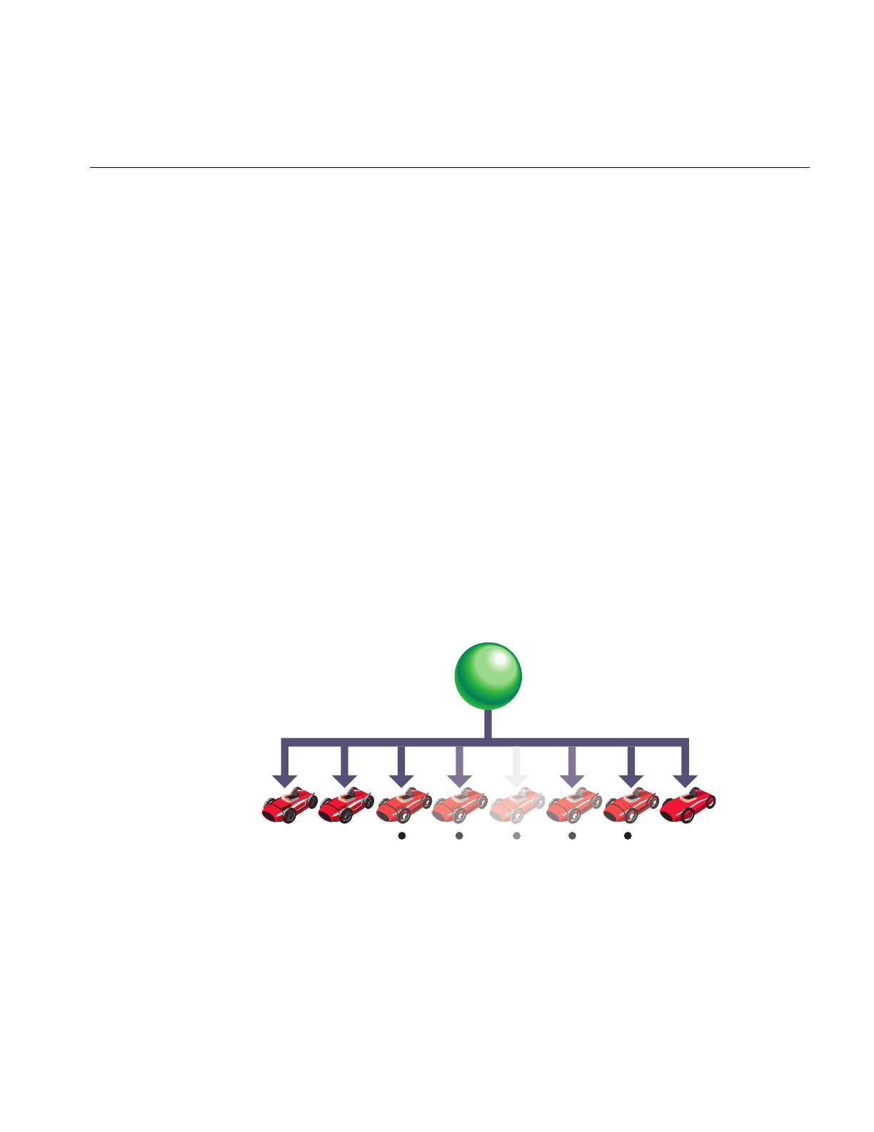
Level-of-Detail Management
133
Level-of-Detail Models
Most objects comprise smaller objects that become visually insignificant at ranges where
the conglomerate object itself is still quite prominent. For example, a complex model of
an automobile might have door handles, side- and rear-view mirrors, license plates, and
other small details.
A short distance away, these features may no longer be visible, even though the car itself
is still a visually significant element of the scene. It is important to realize that as a group,
these small features may contain as many polygons as the larger car itself, and thus have
a detrimental effect on rendering speed.
You can construct two LOD models simply by providing one model that contains all of
the detailed features and another model that contains only the car body itself and none
of the detailed features. A more sophisticated scheme uses multiple LOD models that are
grouped under an LOD node.
Figure 5-3 shows an LOD node with multiple children numbered 1 through n. In this
case, the model named LOD 1 is the most detailed model and models LOD 2 through
LODn represent progressively coarser models. Each of these LOD models might contain
children that also have LOD components. Associated with the LOD node is a list of
ranges that define the distance at which each model is appropriate to display. There is no
limit to the number of levels of detail that can be used.
Figure 5-3 Level-of-Detail Node Structure
Level
of Detail
Node
LOD 1 LOD 2 LOD
n

134
Chapter 5: Frame and Load Control
The object can be transformed as needed. During the culling phase of frame processing,
the distance from the eyepoint to the object is computed and used (with other factors) to
select which LOD model to display.
The IRIS Performer pfLOD node contains a value known as the center of LOD
processing. The LOD center point is an x, y,z location that defines the point used in
conjunction with the eyepoint for LOD range-switching calculations, as described in the
“Level-of-Detail Range Processing” section of this chapter.
Figure 5-4 shows an example in which multiple LOD models grouped under a parent
LOD node are used to represent a toy race car.
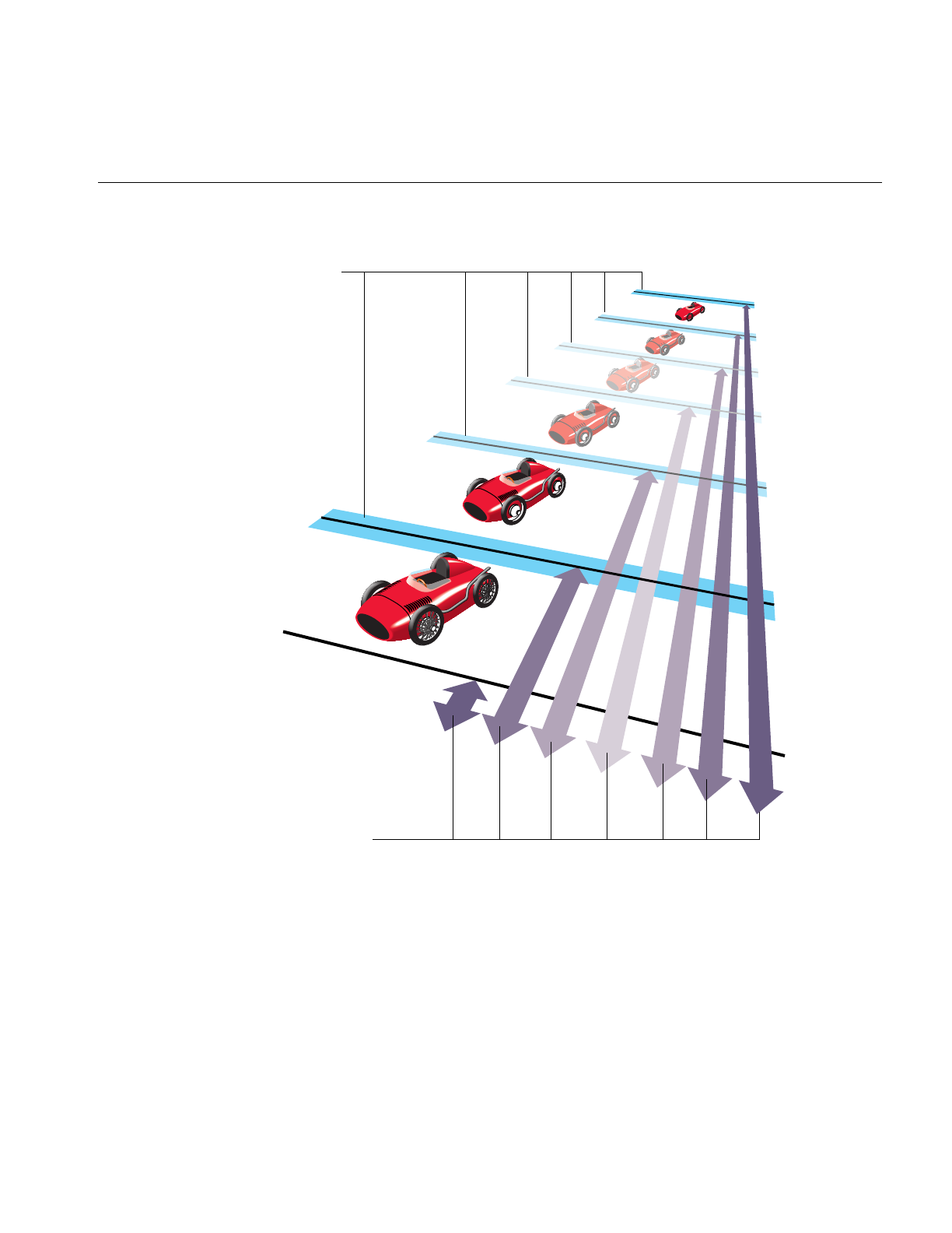
Level-of-Detail Management
135
Figure 5-4 Level-of-Detail Processing
Figure 5-4 demonstrates that each car in a row of identical cars placed at increasing range
from the eyepoint is drawn using a different child of the tree’s LOD node.
LOD 1
LOD 2
LOD
n
Switch
ranges
Blend
zones

136
Chapter 5: Frame and Load Control
The double-ended arrows indicate a switch range for each level of detail. When the car
is closer to the eyepoint than the first range, nothing is drawn. When the car is between
the first and second ranges, LOD 1 is drawn. When the car is between the second and
third ranges, LOD 2 is drawn.
This range bracketing continues until the final range is passed, at which point nothing is
drawn. The pfLOD node’s switch range list contains one more entry than the number of
child nodes to allow for this range bracketing.
IRIS Performer provides the ability to specify a blend zone for each switch between LOD
models. Such that pfLOD nodes now also hold a list of these transition distances over
which IRIS Performer should ‘blend’ between neighboring LODs. These blend zones will
be discussed in more detail in “Level-of-Detail Transition Blending” on page 141.
Level of Detail States
In addition to standard LOD nodes, IRIS Performer also supports LOD state—the
pfLODState. A pfLODState is an essence a way of creating classes or priorities among
LODs. A pfLODstate contains eight parameters used to modify four different ways in
which IRIS Performer calculates LOD switch ranges and LOD transition distances. LOD
states contain the following parameters:
• Scale for LODs switch Ranges.
• Offset for LODs switch Ranges.
• Scale for the effect of Stress of switch Ranges.
• Offset for the effect of Stress on switch Ranges.
• Scale for the transition distances per LOD switch
• Offset for the transition distances per LOD switch
• Scale for the effect of Stress on transition distances
• Offset for the effect of Stress on transition distances

Level-of-Detail Management
137
These LOD states can then be attached to either single or multiple LOD nodes such that
the LOD behavior of groups or classes of objects can be different and be easily modified.
The reference pages for pfLODLODState() and pfLODLODStateIndex() contain
detailed information on how to attach pfLODStates.
LOD states are useful because in a particular scene there often exists an object of focus
such as a sign, a target, or some other object of particular visual significance that needs
to be treated specially with regard to visual importance and thus LOD behavior. It stands
to reason, that this particular object (or small group of objects) should be at the highest
detail possible despite being farther away than other elements in the scene which might
not be as visually significant. In fact, it might be feasible to diminish the detail of these
less important objects (like rocks and trees) in favor of the other more important objects
(despite these objects being further relatively in range). In this case one would just create
two LOD states. The first would be for the important objects and would effectively
disable the effect of stress on these nodes as well as scale the switch ranges such that the
object(s) would maintain more detail for further ranges. The second LOD state would be
used to make the objects of less importance be more responsive to system stress and
possibly scale their switch ranges such that they would show even less detail than
normal. In this way, LOD states allow biasing among different LODs to maintain
desirable rendering speeds while maintaining the visual integrity of various objects
depending on their subjective importance (rather than solely on their current visual
significance).
In some multichannel applications, LOD states are used to control the action of LODs in
different viewing channels that have different visual significance criteria—for instance
one channel might be a normal channel while a second might represent an infra-red
display. Rather than simple use of LOD states, it is also possible to specify a list of LOD
states to a channel and use indexes from this list for particular LODs (via
pfChanLODStateList() and pfLODLODStateIndex()). In this way, in the normal
channel a car’s geometry might be particularly important while in the infra-red channel,
the hot exhaust of the same car might be much more important to observe. This type of
channel dependent LOD can be set up by using two distinct and different LOD states for
the same index in the lists of LOD states specified for unique channels.
Note that because IRIS Performer performs LOD calculations in a range squared space
as much as possible for efficiency reasons, LOD computation becomes more costly when
LOD states contain scales that are not equal to 1.0 or offsets not equal to 0.0 for transitions
or switch ranges—these offsets force IRIS Performer to perform otherwise avoidable
square roots calculations in order to correctly calculate the effects of scale and offset on
the LOD.

138
Chapter 5: Frame and Load Control
Level-of-Detail Range Processing
The LOD switch ranges present in LOD nodes are processed before being used to make
the level of detail selection. The goal of range setting is to switch LODs as objects reach
certain levels of perceptibility. The size of a channel in pixels, the field of view used in
viewing, and the distance from the observer to the display surface all affect object
perceptibility.
IRIS Performer uses a channel size of 1024x1024 pixels and a 45-degree field of view as
the basis for calculating LOD switching ranges. The screen space size of a channel and
the current field of view are used to compute an LOD scale factor that is updated
whenever the channel size or the field of view changes.
There is an additional global LOD scale factor that can be used to adjust switch ranges
based on the relationship between the observer and the display surface. The default
global scale factor is 1.
Note that LOD switch ranges are also effected by LOD states that have been attached to
either a particular LOD or to a channel that contains the LOD. These LOD states provide
the mechanism to apply both a scale and an offset for an LODs switch ranges and to the
effect of system stress on those switch ranges. See “Level of Detail States” on page 136 for
more information of pfLODStates.
Ultimately a LODs switch range without regard to system stress can be computed as
follows:
switch_range[i] =
(range[i] *
LODStateRangeScale *
ChannelLODStateRangeScale +
LODStateRangeOffset +
ChannelLODStateRangeOffset) *
ChannelLODScale *
ChannelSizeAndFOVFactor;

Level-of-Detail Management
139
If IRIS Performer channel stress processing is active, the computed range is modified as
follows:
switch_range[i] *=
(ChannelLODStress *
LODStateRangeStressScale *
ChannelLODStateRangeStressScale +
LODStateRangeStressOffset +
ChannelLODStateRangeStressOffset);
Example 5-2 illustrates how to set LOD ranges.
Example 5-2 Setting LOD Ranges
/* setLODRanges() -- sets the ranges for the LOD node. The
* ranges from 0 to NumLODs are equally spaced between min
* and max. The last range, which determines how far you
* can get from the object and still see it, is set to
* visMax.
*/
void
setLODRanges(pfLOD *lod,float min, float max, float visMax)
{
int i;
float range, rangeInc;
rangeInc = (max - min)/(ViewState->shellLOD + 1);
for (range = min, i = 0; i < ViewState->shellLOD; i++)
{
ViewState->range[i] = range;
pfLODRange(lod, i, range);
range += rangeInc;
}
ViewState->range[i] = visMax;
pfLODRange(lod, i, visMax);
}
/* generateShellLODs() -- creates shell LOD nodes according
* to the parameters specified in the shared data structure.
*/
void
generateShellLODs(void)
{
int i;
pfGroup *grp;

140
Chapter 5: Frame and Load Control
pfVec4 clr;
long numLOD = ViewState->shellLOD;
long numPnts = ViewState->shellPnts;
long numPcs = ViewState->shellPcs;
for (i = 1; i <= numLOD; i++)
{
if (ViewState->shellColor == SHELL_COLOR_SING)
pfSetVec4(clr, 0.9f, 0.1f, 0.1f, 1.0f);
else
/* set the color. highest level = RED;
* middle LOD = GREEN; lowest LOD = BLUE
*/
pfSetVec4(clr,
(i <= (long)floor((double)(numLOD/2.0f)))?
(-2.0f/numLOD) * i + 1.0f + 2.0f/numLOD:
0.0f,
(i <= (long)floor((double)(numLOD/2)))?
(2.0f/numLOD) * (i - 1):
(-2.0f/numLOD) * i + 2.0f,
(i <= (long)floor((double)(numLOD/2)))?
0.0f:
(2.0f/numLOD) * i - 1.0f,
1.0f);
/* build a shell GeoSet */
grp = createShell(numPcs, numPnts,
ViewState->shellSweep, &clr,
ViewState->shellDraw);
normalizeNode((pfNode *)grp);
/* add geode as another level of detail node */
pfAddChild(ViewState->LOD, grp);
/* simplify the geometry, but don’t have less than
* 4 points per circle or less than 3 pieces */
numPnts = (numPnts > 7) ? numPnts-4 : 4;
numPcs = (numPcs > 6) ? numPcs-4 : 3;
}
}
...
ViewState->LOD = pfNewLOD();
generateShellLODs();

Level-of-Detail Management
141
/* get the LOD’s extents */
pfGetNodeBSphere(ViewState->LOD, &(ViewState->bSphere));
pfLODCenter(ViewState->LOD, ViewState->bSphere.center);
/* set ranges for LODs; there should be (num LODs + 1)
* range entries */
setLODRanges(ViewState->LOD, ViewState->minRange,
ViewState->maxRange, ViewState->max);
Level-of-Detail Transition Blending
An undesirable effect called popping occurs when the sudden transition from one LOD to
the next LOD is visually noticeable. This distracting image artifact can be ameliorated
with a slight modification to the normal LOD-switching process.
In this modified method a transition per LOD switch is established rather than making a
sudden substitution of models at the indicated switch range. These transitions specify
distances over which to blend between the previous and next LOD. These zones are
considered to be centered at the specified LOD switch distance, as shown by the
horizontal shaded bars of Figure 7-3. Note that IRIS Performer limits the transition
distances to be equal to the shortest distance between the switch range and the two
neighboring switch ranges. For more information, see the pfLODTransition() reference
page.
As the range from eyepoint to LOD center-point transitions the blend zone, each of the
neighboring LOD levels is drawn by using transparency to composite samples taken
from the present LOD model with samples taken from the next LOD model. For example,
at the near, center, and far points of the transition blend zone between LOD 1 and LOD
2, samples from both LOD 1 and LOD 2 are composited until the end of the transition
zone is reached, where all the samples are obtained from LOD 2.
Table 5-2 lists the transparency factors used for transitioning from one LOD range to
another LOD range.
Table 5-2 LOD Transition Zones
Distance LOD 1 LOD 2
Near edge of blend zone 100% opaque 0% opaque
Center of blend zone 50% opaque 50% opaque
Far edge of blend zone 0% opaque 100% opaque

142
Chapter 5: Frame and Load Control
LOD transitions are made smoother and much less noticeable by applying a blending
technique rather than making a sudden transition. Blending allows LOD transitions to
look good at ranges closer to the eye than LOD popping allows. Decreasing switch
ranges in this way improves the ability of LOD processing to maximize the visual impact
of each polygon in the scene without creating distracting visual artifacts.
The benefits of smooth LOD transition have an associated cost. The expense lies in the
fact that when an object is within a blend zone, two versions of that object are drawn.
This causes blended LOD transitions to increase the scene polygon complexity during
the time of transition. For this reason, the blend zone is best kept to the shortest distance
that avoids distracting LOD-popping artifacts. Currently, fade level of detail is
supported only on RealityEngine graphics systems.
Note that the actual ‘blend’ or ‘fade’ distance used by IRIS Performer can also be adjusted
by the LOD priority structures called pfLODStates. pfLODStates hold an offset and scale
for the size of transition zones as well as an offset and scale for how system stress can
affect the size of the transition zones. See “Level of Detail States” on page 136 for more
information on pfLODStates.
Note also, that there exists a global LOD transition scale on a per channel basis that can
affect all transition distances uniformly.
Thus for an LOD with 5 switch ranges R0, R1, R2, R3, R4 to switch between four models
(M0, M1, M2, M3), there are 5 transition zones T0 (fade in M0), T1 (blend between M0
and M1), T2 (blend between M1 and M2), T3 (blend between M2 and M3), T4 (fade out
M3). The actual fade distances (without regard to channel stress) are as follows.
fadeDistance[i] =
(transition[i] *
LODStateTransitionScale *
ChannelLODStateTransitionScale +
LODStateTransitionOffset +
ChannelLODStateTransitionOffset) *
ChannelLODFadeScale;

Level-of-Detail Management
143
If IRIS Performer management of channel stress is turned on then the above fade distance
is modified as follows:
fadeDistance[i] /=
(ChannelStress *
LODStateTransitionStressScale *
ChannelLODStateTransitionStressScale +
LODStateTransitionStressOffset +
ChannelLODStateTransitionStressOffset);
Terrain Level of Detail
In creating LOD models and transitions for objects, it’s often safe to assume that theentire
model should transition at the same time. It’s quite reasonable to make features of an
automobile such as door handles disappear from the scene at the same time even when
the passenger door is slightly closer than the driver’s door. It is much less clear that this
approach would work for very large objects such as an aircraft carrier or a space station,
and it’s clearly not acceptable for objects that span a large extent, such as a terrain surface.
Attempts to handle large-extent objects with discrete LOD tools focus on breaking the big
object into myriad small objects and treating each small object independently. This works
in some cases but often fails at the junction between two or more independent objects
where cracks or seams exist when different detail levels apply to the objects. Some terrain
processing systems have attempted to provide a hierarchy of crack filling geometry that
is enabled based on the LOD selections of two neighboring terrain patches. This “digital
grout” becomes untenable when more than a few patches share a common vertex.
You can always make the transitions between LODs smooth by using active surface
definition (ASD). ASD treats the entire terrain as a single connected surface rather than
multiple patches that are loaded into memory as necessary. The surface is modeled with
several hierarchical level-of-detail (LOD) meshes in data structures that allow for the
rapid evaluation of smooth LOD transitions, load management on the evaluation itself,
and efficient generation of a meshed terrain surface of the visible triangles for the current
frame. For more information, refer to the Chapter 15, “Active Surface Definition.”

144
Chapter 5: Frame and Load Control
Arbitrary Morphing
Terrain level of detail using an interpolative active surface definition is a restricted form
of the more general notion of object morphing. Morphing of models such as the car in a
previous example can simply involve scaling a small detail to a single point and then
removing it from the scene. Morphing is possible even when the topologies of
neighboring pairs do not match. Both models and terrain can have vertex, normal, color,
and appearance information interpolated between two or more representations. The
advantages of this approach include: reduced graphics complexity since blending is not
used, constant intersection truth for collision and similar tasks, and monotonic database
complexity that makes system load management much simpler. Such evaluation might
make use of the compute process and pfFlux objects to hold the vertex data and to
modify the scene graph control to chose the proper form of the object. pfSwitch nodes
can take a pfFlux for holding its value; see the pfSwitchValFlux() reference page. pfLOD
nodes can take a flux for controlling range with pfLODRangeFlux(). See the pfLOD and
pfEngine reference pages for more information on morphing.
Dynamic Load Management
Because the effects of variable image update rates can be objectionable, many simulation
applications are designed to operate at a fixed frame rate. One approach to selecting this
fixed frame rate is to select an update rate constrained by the most complex portion of
the visual database. Although this conservative approach may be acceptable in some
cases, IRIS Performer supports a more sophisticated approach using dynamic LOD
scaling.
Using multiple LOD models throughout a database provides the traversal system with a
parameter that can be used to control the polygonal complexity of models in the scene.
The complexity of database objects can be reduced or increased by adjusting a global
LOD range multiplier that determines which LOD level is drawn.
Using this facility, a closed-loop control system can be constructed that adjusts the
LOD-switching criteria based on the system load, also called stress, in order to maintain
a selected frame rate.
Figure 5-5 illustrates a stress-processing control system.
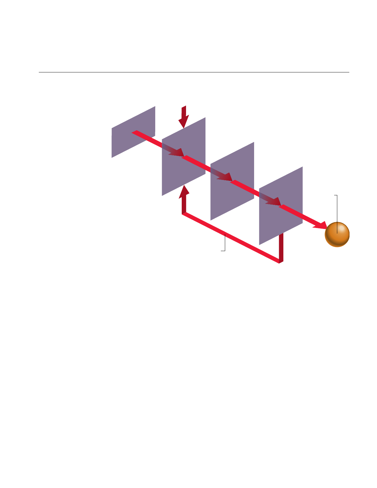
Dynamic Load Management
145
Figure 5-5 Stress Processing
In Figure 5-5, the desired and actual frame times are compared by the stress filter. Based
on the user-supplied stress parameters, the stress filter adjusts the global LOD scale
factor by increasing it when the system is overloaded and decreasing it when the system
is underloaded. In this way, the system load is monitored and adjusted before each frame
is generated.
The degree of stability for the closed-loop control system is an important issue. The ideal
situation is to have a critically damped control system—that is, one in which just the right
amount of control is supplied to maintain the frame rate without introducing
undesirable effects. The effects of overdamped and underdamped systems are visually
distracting. An underdamped system oscillates, causing the system to continuously
alternate between two different LOD models without reaching equilibrium.
Overdamped systems may fail to react within the time required to maintain the desired
frame rate. In practice, though, dynamic load management works well, and simple stress
functions can handle the slowly changing loads presented by many databases.
Stress
Parameters
Desired Frame Time
Stress Filter
(Set LOD)
Traversal
(Use LOD)
Rendering
Frame
Buffer
Actual Frame Time

146
Chapter 5: Frame and Load Control
The default stress function is controlled with user-selectable parameters. These
parameters are set using the function pfChanStressFilter().
The default stress function is implemented by the code fragment in Example 5-3.
Example 5-3 Default Stress Function
/* current load */
curLoad = drawTime * frameRate * frameFrac;
/* integrated over time */
if (curLoad < lowLoad)
stressLevel -= stressParam * stressLevel;
else
if (curLoad > highLoad)
stressLevel += stressParam * stressLevel;
/* limited to desired range */
if (stressLevel < 1.0)
stressLevel = 1.0;
else
if (stressLevel > maxStress)
stressLevel = maxStress;
The parameters lowLoad and highLoad define a “comfort zone” for the control system. The
first if-test in the code fragment demonstrates that this comfort zone acts as a dead band.
Instantaneous system load within the bounds of the dead band doesn’t result in a change
in the system stress level. If the size of the comfort zone is too small, oscillatory distress
is the probable result. It is often necessary to keep the highLoad level below the 100% point
so that blended LOD transitions don’t drive the system into overload situations.
For those applications in which the default stress function is either inappropriate or
insufficient, you can compute the system stress yourself and then set the stress load
factor. Your filter function can access the same system measures that the default stress
function uses, but it’s also free to keep historical data and perform any feedback-transfer
processing that application-specific dynamic load management may require.

Successful Multiprocessing With IRIS Performer
147
The primary limitation of the default stress function is that it has a reactive rather than
predictive nature. One of the major advantages of user-written stress filters is their ability
to predict future stress levels before increased or decreased load situations reach the
pipeline. Often the simulation application knows, for example, when a large number of
moving models will soon enter the viewing frustum. If their presence is anticipated, then
stress can be artificially increased so that no sudden LOD changes are required as they
actually enter the field of view.
Successful Multiprocessing With IRIS Performer
This section describes an advanced topic that applies only to systems with more than one
CPU. If you don’t have a multiple-CPU system, you may want to skip this
section.
IRIS Performer uses multiprocessing to increase throughput for both rendering and
intersection detection. Multiprocessing can also be used for tasks that run
asynchronously from the main application like database management. Although IRIS
Performer hides much of the complexity involved, you need to know something about
how multiprocessing works in order to use multiple processors well.
Review of Rendering Stages
IRIS Performer application renders images using one or more pfPipes as independent
software-rendering pipelines. The flow through the rendering pipeline can be modeled
using these functional stages:
Intersection Test for intersections between segments and geometry to simulate
collision detection or line-of-sight for example.
Application Do requisite processing for the visual simulation application, including
reading input from control devices, simulating the vehicle dynamics of
moving models, updating the visual database, and interacting with
other networked simulation stations.
Cull Traverse the visual database and determine which portions of it are
potentially visible, perform level-of-detail selection for models with
multiple representations, and build sorted, optimized display list for the
draw stage.
Draw Issue graphics library commands to a Geometry Pipeline in order to
create an image for subsequent display.
Advanced

148
Chapter 5: Frame and Load Control
You can partition these stages into separate parallel processes in order to distribute the
work among multiple CPUs. Depending on your system type and configuration, you can
use any of several available multiprocessing models.
Choosing a Multiprocessing Model
Use pfMultiprocess() to specify which functional stages, if any, should be forked into
separate processes. The multiprocessing mode is actually a bitmask where each bit
indicates that a particular stage should be configured as a separate process. For example,
the bit PFMP_FORK_DRAW means the draw stage should be split into its own process.
Table 5-3 lists some convenience tokens that represent common multiprocessing modes:
Table 5-3 Multiprocessing Models
Model Name Description
PFMP_APPCULLDRAW Combine the application, cull, and draw stages into a single
process. In this model, all of the stages execute within a single frame
period. This is the minimum-latency mode of operation.
PFMP_APP_CULLDRAW
or
PFMP_FORK_CULL
Combine the cull and draw stages in a process that is separate from
the application process. This model provides a full frame period for
the application process, while culling and drawing share this same
interval. This mode is appropriate when the host’s simulation tasks
are extensive but graphic demands are light, as might be the case
when complex vehicle dynamics are performed but only a simple
dashboard gauge is drawn to indicate the results.
PFMP_APPCULL_DRAW
or
PFMP_FORK_DRAW
Combine the application and cull stages in a process that is separate
from the draw process. This mode is appropriate for many
simulation applications when application and culling demands are
light. It allocates a full CPU for drawing and has the APP and CULL
stages share a frame period. Like the PFMP_APP_CULLDRAW
mode, this mode has a single frame period of pre-draw latency.
PFMP_APP_CULL_DRAW
or
PFMP_FORK_CULL |
PFMP_FORK_DRAW
Perform the application, cull, and draw stages as separate
processes. This is the full maximum-throughput multiprocessing
mode of IRIS Performer operation. In this mode, each pipeline stage
is allotted a full frame period for its processing. Two frame periods
of latency exist when using this high degree of parallelism.

Successful Multiprocessing With IRIS Performer
149
You can also use pfMultiprocess() to specify the method of communication between the
cull and draw stages, using the bitmasks PFMP_CULLoDRAW and
PFMP_CULL_DL_DRAW.
Cull-Overlap-Draw Mode
Setting PFMP_CULLoDRAW specifies that the cull and draw processes for a given frame
should overlap—that is, that they should run concurrently. For this to work, the cull and
draw stages must be separate processes (PFMP_FORK_DRAW must be true). In this
mode the two stages communicate in the classic producer-consumer model, by way of a
pfDispList that is configured as a ring (FIFO) buffer; the cull process puts commands on
the ring while the draw process simultaneously consumes these commands.
The main benefit of using PFMP_CULLoDRAW is reduced latency, since the number of
pipeline stages is reduced by one and the resulting latency is reduced by an entire frame
time. The main drawback is that the draw process must wait for the cull process to begin
filling the ring buffer.
Forcing pfDisplayList Generation
When the cull and draw stages are in separate processes, they communicate through a
pfDispList; the cull process generates the display list, and the draw process traverses and
renders it. (The display list is configured as a ring buffer when using
PFMP_CULLoDRAW mode, as described in the “Cull-Overlap-Draw Mode” section).
However, when the cull and draw stages are in the same process (as occurs with the
PFMP_APPCULLDRAW or PFMP_APP_CULLDRAW multiprocessing models) a
display list isn’t required and by default one will not be used. Leaving out the pfDispList
eliminates overhead. When no display list is used, the cull trigger function pfCull() has
no effect; the cull traversal takes place when the draw trigger function pfDraw() is
invoked.
In some cases you may want an intermediate pfDispList between the cull and draw
stages even though those stages are in the same process. The most common situation that
calls for such a setup is multipass rendering, when you want to cull only once but render
multiple times. With PFMP_CULL_DL_DRAW enabled, pfCull() generates a pfDispList
that can be rendered multiple times by multiple calls to pfDraw().

150
Chapter 5: Frame and Load Control
Intersection Pipeline
The intersection pipeline is a two-stage pipeline consisting of the application and the
intersection stages. The intersection stage may be configured as a separate process by
setting the PFMP_FORK_ISECT bit in the bitmask given to pfMultiprocess(). When
configured as such, the intersection process is triggered for the current frame when the
application process calls pfFrame(). Then in the special intersection callback set with
pfIsectFunc(), you can invoke any number of intersection requests with
pfNodeIsectSegs(). To support this operation, the intersection process keeps a copy of
the scene graph pfNodes.
The intersection process is asynchronous so that if it does not finish within a frame time
it does not slow down the rendering pipeline(s).
The Compute Process
The compute process is an asynchronous process provided for doing extensive
asynchronous computation. The compute stage is done as part of pfFrame() in the
application process unless it is configured to run as separate process by setting the
PFMP_FORK_COMPUTE bit in the pfMultiprocess() bitmask. The compute process is
asynchronous so that if it does not finish within a frame time, it will not slow down the
rendering pipeline. The compute process is intended to work with pfFlux objects, placing
the results of asynchronous computation in pfFluxes. pfFlux will automatically manage
the needed multibuffering and frame consistency requirements for the data.See
Chapter 14, “Dynamic Data,” for more information on pfFlux. Some IRIS Performer
objects, such as pfASD, do their computation in the compute stage so pfCompute() must
be called from any compute user callback if one has been specified with
pfComputeFunc().
Multiple Rendering Pipelines
By default, IRIS Performer uses a single pfPipe, which in turn draws one or more
pfChannels into one or more pfPipeWindows. If you want to use multiple rendering
pipelines, as on two- or three-Geometry Pipeline Onyx RealityEngine2 systems, use
pfMultipipe()to specify the number of pfPipes required. When using multiple pipelines,
the PFMP_APPCULLDRAW and PFMP_APPCULL_DRAW modes are not supported
and IRIS Performer defaults to the PFMP_APP_CULL_DRAW multiprocessing
configuration. Regardless of the number of pfPipes, there is always a single application
process which triggers the rendering of all pipes with pfFrame().

Successful Multiprocessing With IRIS Performer
151
Multithreading
For additional multiprocessing and attendant increased throughput, the CULL stage of
the rendering pipeline may be multithreaded. Multithreading means that a single pipeline
stage is split into multiple processes, or threads which concurrently work on the same
frame. Use pfMultithread() to allocate a number of threads for the cull stage of a
particular rendering pipeline.
Cull multithreading takes place on a per-pfChannel basis, that is, each thread does all
the culling work for a given pfChannel. Thus, an application with only a single channel
will not benefit from multithreading the cull and an application with multiple, equally
complex channels will benefit most by allocating a number of cull threads equal to the
number of channels. However, it is legal to allocate fewer cull threads if you do not have
enough CPUs—in this case the threads are assigned to channels on a need basis.
Order of Calls
The multiprocessing model set by pfMultiprocess() is used for each of the rendering
pipelines. In programs that configures the application stage as a separate process, all IRIS
Performer calls must be made from the process that calls pfConfig() or the results are
undefined. Both pfMultiprocess(),pfMultithread(), and pfMultipipe() must be called
after pfInit() but before pfConfig().pfConfig() configures IRIS Performer according to
the required number of pipelines and the desired multiprocessing and multithreading
modes, forks the appropriate number of processes, and then returns control to the
application. pfConfig() should be called only once during each IRIS Performer
application.
Comparative Structure of Models
Figure 5-6 shows timing diagrams for each of the process models. The vertical lines are
frame boundaries. Five frames of the simulation are shown to allow the system to reach
steady-state operation. Only one of these models can be selected at a time, but they are
shown together so that you can compare their structures.
Boxes represent the functional stages and are labeled as follows:
Anapplication process for the nth frame
Cncull process for the nth frame
Dndraw process for the nth frame
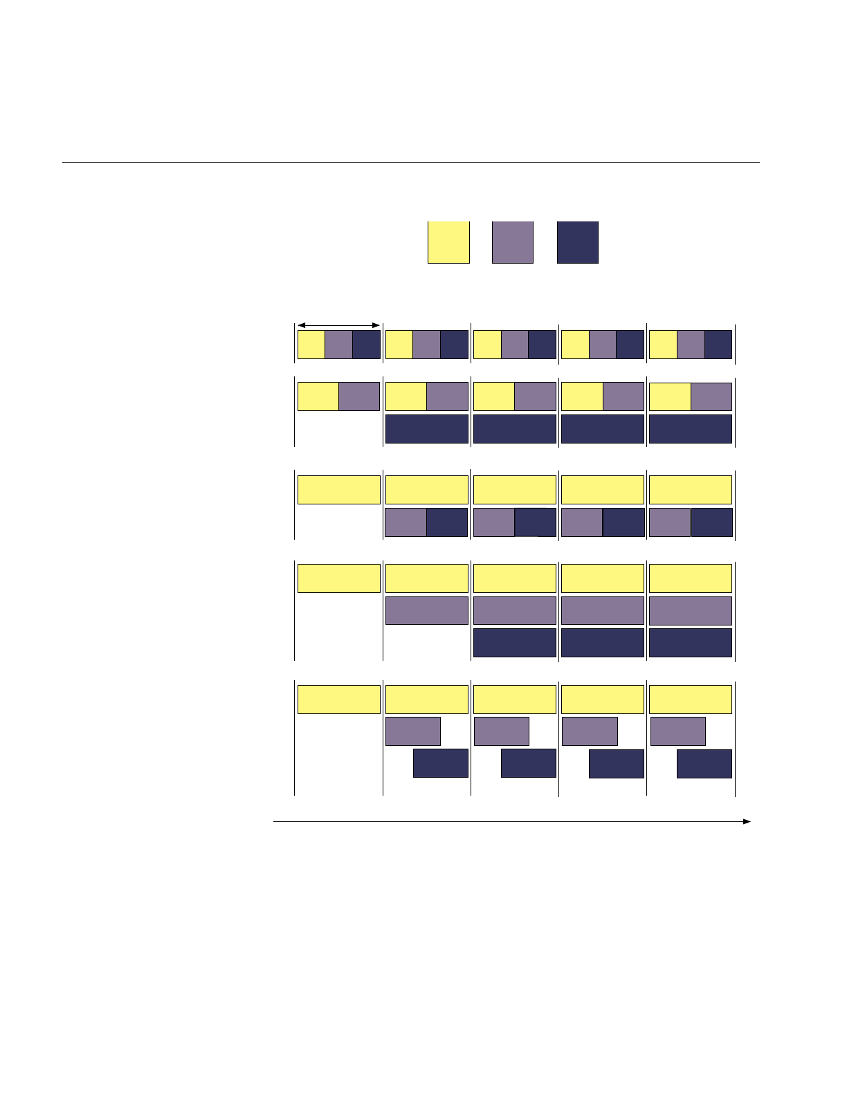
152
Chapter 5: Frame and Load Control
Figure 5-6 Multiprocessing Models
A0 C0 D0 A1 C1 D1 A2 C2 D2 A3 C3 D3 A4 C4 D4
A0 A1
C0
A2
C1
A3
C2
A4
C3
D0
A0
C0
D0
A1
C1
D1
A2
C2
D2
A3
C3
A4
A0
C0
D0
A1
C1
D1
A2
C2
D2
A3
C3
A4
D3
C1 C2 C3
Start Frame 0 Frame 1 Frame 2 Frame 3 Frame 4
APP
ACULL
CDRAW
D
Host
Simulation
Process
Cull
Process
(traversal)
Draw
Process
Period=1/Frame Rate
PFMPAPPCULLDRAW
PFMP_APP_CULLDRAW
P0
P1
PFMP_APP_CULL_DRAW
P0
P1
P2
P0
P1
P2
PFMP_APP_CULL0DRAW
A0 C0 A1 C1 A2 C2 A3 C3 A4 C4
D0 D1 D2 D3
PFMPAPPCULL_DRAW
P0
P1
D1 D2 D3
Time

Successful Multiprocessing With IRIS Performer
153
Notice that when a stage is split into its own process, the amount of time available for all
stages increases. For example, in the case where the application, cull, and draw stages are
3 separate processes, it is possible for total system performance to be tripled over the
single process configuration.
Asynchronous Database Processing
Many databases are too large to fit into main memory. A common solution to this
problem is called database paging where the database is divided into manageable chunks
on disk and loaded into main memory when needed. Usually chunks are paged in just
before they come into view and are deleted from the scene when they are comfortably
out of viewing range.
All this paging from disk and deleting from main memory takes a lot of time and is
certainly not amenable to maintaining a fixed frame rate. The solution supported by IRIS
Performer is asynchronous database paging in which a process, completely separate from
the main processing pipeline(s), handles all disk I/O and memory allocations and
deletions. To facilitate asynchronous database paging, IRIS Performer provides the
pfBuffer structure and the DBASE process.
DBASE Process
The database (or DBASE) process is forked by pfConfig()if the PFMP_FORK_DBASE bit
was set in the mode given to pfMultiprocess(). The database process is triggered when
the application process calls pfFrame() and invokes the user-defined callback set with
pfDBaseFunc(). The database process is totally asynchronous. If it exceeds a frame time
it does not slow down any rendering or intersection pipelines.
The DBASE process is intended for asynchronous database management when used
with pfBuffer.
pfBuffer
A pfBuffer is a logical buffer which isolates database changes to a single process,
avoiding disastrous collisions on data from multiple processes. In typical use, a pfBuffer
is created with pfNewBuffer(), made current with pfSelectBuffer() and merged with the
main IRIS Performer buffer with pfMergeBuffer(). While the DBASE process is intended
for pfBuffer use, other processes forked by the application may also use different
pfBuffers in parallel for multithreaded database management. By ensuring that only a

154
Chapter 5: Frame and Load Control
single process uses a given pfBuffer at a given time and following a few scoping rules
discussed below, the application can safely and efficiently implement asynchronous
database paging
A pfNode is said to have buffer scope or be “in” a particular pfBuffer. This is an important
concept because it affects what you can do with a given node. A newly-created node is
automatically “in” the currently active pfBuffer until that pfBuffer is merged using
pfMergeBuffer(). At that instant, the pfNode is moved into the main IRIS Performer
buffer, otherwise known as the application buffer.
A rule in pfBuffer management is that a process may only access nodes that are in its
current pfBuffer. As a result, a database process may not directly add a newly created
subgraph of nodes to the main scene graph because all nodes in the main scene graph
have application buffer scope only—they are isolated from the database pfBuffer. This
may seem inconvenient at first but it eliminates catastrophic errors like, for example, the
application process traverses a group at the same time you add a child, changing its child
list and causing the traversal to chase a bad pointer.
Remedies to the inconveniences stated above are the pfBufferAddChild(),
pfBufferRemoveChild() and pfBufferClone() routines. The first two routines are
identical to their non-buffer counterparts pfAddChild() and pfRemoveChild() except
the buffer versions do not happen immediately. Other functions, pfBufferAdd(),
pfBufferInsert(),pfBufferReplace(), and pfBufferRemove(), perform the
buffer-oriented delayed-action versions of the corresponding non-buffer pfList
functions. In all cases the add, insert, replace, or removal request is placed on a list in the
current pfBuffer and is processed later at pfMergeBuffer() time.
pfBufferClone() supports the notion of maintaining a “library” of common objects like
trees or houses in a special library pfBuffer. The main database process then clones
objects from the library pfBuffer into the database pfBuffer, possibly pfFlatten()ing them
for improved rendering performance. pfBufferClone() is identical to pfClone() except
the buffer version requires that the source pfBuffer be specified and that all cloned nodes
have scope in the source pfBuffer.
pfAsyncDelete
We’ve discussed how to create subgraphs for database paging: create and select a current
pfBuffer, create nodes and build the subgraph, call pfBufferAddChild() and finally
pfMergeBuffer() to incorporate the subgraph into the application’s scene. But what about
freeing the memory of old, unwanted subgraphs? For this we turn to pfAsyncDelete().

Successful Multiprocessing With IRIS Performer
155
pfDelete() is the normal mechanism for deleting objects and freeing their associated
memory. However, pfDelete() can be a very costly routine since it must traverse,
unreference, and register a deletion request for every IRIS Performer object it encounters
which has a 0 reference count. pfAsyncDelete(), in conjunction with a forked DBASE
process, moves the burden of deletion to the asynchronous database process so that all
rendering and intersection pipelines are not adversely affected.
pfAsyncDelete() may be called from any process and places an asynchronous deletion
request on a global list that is processed later by the DBASE stage when its trigger
routine, pfDBase() is called. A major difference from pfDelete() is that pfAsyncDelete()
does not immediately check the reference count of the object to be deleted and so does
not return a value indicating whether the deletion was successful or not. At this time
there is no way of querying the result of a pfAsyncDelete() request so care should be
taken that the object to be deleted has no reference counts or memory leaks will result.
Rules for Invoking Functions While Multiprocessing
There are some restrictions on which functions can be called from an IRIS Performer
process while multiple processes are running. Some specialized processes (such as the
process handling the draw stage) can call only a few specific IRIS Performer functions,
and can’t call any other kinds of functions. This section lists general and specific rules
concerning function invocation in the various IRIS Performer and user processes.
In this section, the term “the draw process” refers to whichever process is handling the
draw stage, regardless of whether that process is also handling other stages. Similarly,
“the cull process” and “the application process” refer to the processes handling the cull
and application stages, respectively.
This is a general list of the kinds of routines you can call from each process:
application configuration routines, creation and deletion routines, set and get
routines, and trigger routines such as pfAppFrame(), pfSync(),
pfFrame()
database creation and deletion routines, set and get routines, pfDBase(),
pfMergeBuffer()
cull pfCull(),pfCullPath(), IRIS Performer graphics routines
draw pfClearChan(),pfDraw(),pfDrawChanStats(), IRIS Performer
graphics routines, graphics library routines

156
Chapter 5: Frame and Load Control
More specific elaborations:
• You should call configuration routines only from the application process, and only
after pfInit() and before pfConfig().pfInit() must be the first IRIS Performer call
except for those routines that configure shared memory (see “Memory Allocation”
in Chapter 13). Configuration routines don’t take effect until pfConfig() is called.
These are the configuration routines:
–pfMultipipe()
–pfMultiprocess()
–pfMultithread()
–pfHyperpipe()
• You should call creation routines, such as pfNewChan(),pfNewScene(), and
pfAllocIsectData(), only in the application process after calling pfConfig() or in a
process which has an active pfBuffer. There is no restriction on creating libpr objects
like pfGeoSets and pfTextures.
•pfDelete() should only be called from the application or database processes.
pfAsyncDelete() may be called from any process.
• Read-only routines—that is, the pfGet*() functions—can be called from any IRIS
Performer process. However, if a forked draw process queries a pfNode, the data
returned will not be frame-accurate. (See “Multiprocessing and Memory” on
page 158.)
• Write routines—functions that set parameters—should be called only from the
application process or a process with an active pfBuffer. It is possible to call a write
routine from the cull process, but it isn’t recommended since any modifications to
the database will not be visible to the application process if it is separate from the
cull (as when using PFMP_APP_CULLDRAW or PFMP_APP_CULL_DRAW).
However, for transient modifications like custom level-of-detail switching, it is
reasonable for the cull process to modify the database. The draw process should
never modify any pfNode.

Successful Multiprocessing With IRIS Performer
157
• IRIS Performer graphics routines should be called only from the cull or draw
processes. These routines may modify hardware graphics state. They are the
routines which can be captured by an open pfDispList. (See “Display Lists” in
Chapter 9.) If invoked in the cull process, these routines are captured by an internal
pfDispList and later invoked in the draw process; but if they are invoked in the
draw process they immediately affect the current window. These graphics routines
can be roughly partitioned into those that
– apply a graphics entity: pfApplyMtl(),pfApplyTex(), and pfLightOn()
– enable or disable a graphics mode: pfEnable(),pfDisable()
– set or modify graphics state: pfTransparency(),pfPushState(),pfMultMatrix()
– draw geometry or modify the screen: pfDrawGSet(),pfDrawString(),
pfClear()
• Graphics library routines should be called only from the draw process. Since there
is no open display list to capture these commands, an open window is required to
accept them.
• “Trigger” routines should be called only from the appropriate processes (see
Table 5-4).
Table 5-4 Trigger Routines and Associated Processes
Trigger Routine Process/Context
pfAppFrame
pfSync
pfFrame
APP/main loop
pfPassChanData
pfPassIsectData APP/main loop
pfApp APP/channel APP callback
pfCull
pfCullPath CULL/channel CULL callback
pfDraw
pfDrawBin DRAW/channel DRAW callback
pfNodeIsectSegs
pfChanNodeIsectSegs ISECT/callback or APP/main loop
pfDBase DBASE/callback

158
Chapter 5: Frame and Load Control
• User-spawned processes created with sproc() can trigger parallel intersection
traversals through multiple calls to pfNodeIsectSegs() and
pfChanNodeIsectSegs().
• Functions pfApp(),pfCull(),pfDraw(), and pfDBase() are only called from within
the corresponding callback specified by pfChanTravFunc() or pfDBaseFunc().
Multiprocessing and Memory
In IRIS Performer, as is often true of multiprocessing systems, memory management is
the most difficult aspect of multiprocessing. Most data management problems in an IRIS
Performer application can be partitioned into three categories:
• Memory visibility. IRIS Performer uses fork(), which—unlike sproc()— generates
processes that don’t share the same address space. The processes also cannot share
global variables that are modified after the fork() call. After calling fork(), processes
must communicate through explicit shared memory.
• Memory exclusion. If multiple processes read or write the same chunk of data at the
same time, consequences can be dire. For example, one process might read the data
while in an inconsistent state and end up dumping core while dereferencing a
NULL pointer.
• Memory synchronization. IRIS Performer is configured as a pipeline where
different processes are working on different frames at the same time. This pipelined
nature is illustrated in Figure 5-6, which shows that, for instance, in the
PFMP_APP_CULL_DRAW configuration the application process is working on
frame n while the draw process is working on frame n-2. If, in this case, if we have
only a single memory location representing the viewpoint, then it is possible for the
application to set the viewpoint to that of frame n and the draw process to
incorrectly use that same viewpoint for frame n-2. Properly synchronized data is
called frame accurate.
Fortunately, IRIS Performer transparently solves all of the above problems for most IRIS
Performer data structures and also provides powerful tools and mechanisms that the
application can use to manage its own memory.

Successful Multiprocessing With IRIS Performer
159
Shared Memory and pfInit()
pfInit() creates a shared memory arena that is shared by all processes spawned by IRIS
Performer and all user processes that are spawned from any IRIS Performer process. A
handle to this arena is returned by pfGetSharedArena() and should be used as the arena
argument to routines that create data that must be visible to all processes. Routines that
accept an arena argument are the pfNew*() routines found in the libpr library and the
IRIS Performer memory allocator, pfMalloc(). In practice, it is usually safest to create
libpr objects like pfGeoSets and pfMaterials in shared memory. libpf objects like pfNodes
are always created in shared memory.
Allocating shared memory does not by itself solve the memory visibility problem
discussed above. You must also make sure that the pointer that references the memory is
visible to all processes. IRIS Performer objects, once incorporated into the database via
routines like pfAddGSet(),pfAddChild(), and pfChanScene(), automatically ensure
that the object pointers are visible to all IRIS Performer processes.
However, pointers to application data must be explicitly shared. A common way of
doing this is to allocate the shared memory after pfInit() but before pfConfig() and to
reference the memory with a global pointer. Since the pointer is set before pfConfig()
forks any processes, these processes will all share the pointer’s value and can thereby
access the same shared memory region. However, if this pointer value changes in a
process, its value will not change in any other process, since forked processes don’t share
the same address space.
Even with data visible to all processes, data exclusion is still a problem. The usual
solution is to use hardware spin locks so that a process can lock the data segment while
reading or writing data. If all processes must acquire the lock before accessing the data,
then a process is guaranteed that no other processes will be accessing the data at the same
time. All processes must adhere to this locking protocol, however, or exclusion isn’t
guaranteed.
In addition to a shared memory arena, pfInit() creates a semaphore arena whose handle
is returned by pfGetSemaArena(). Locks can be allocated from this semaphore arena by
usnewlock() and can be set and unset by ussetlock() and usunsetlock(), respectively.

160
Chapter 5: Frame and Load Control
pfDataPools
pfDataPools—named shared memory arenas with named allocation blocks—provide a
complete solution to the memory visibility and memory exclusion problems, thereby
obviating the need to set global pointers between pfInit() and pfConfig(). For more
information about pfDataPools, see the pfDataPools reference page.
Passthrough Data
The techniques discussed thus far don’t solve the memory synchronization problem.
IRIS Performer’s libpf library provides a solution in the form of passthrough data. When
using pipelined multiprocessing, data must be passed through the processing pipeline
so that data modifications reach the appropriate pipeline stage at the appropriate time.
Passthrough data is implemented by allocating a data buffer for each stage in the
processing pipeline. Then, at well-defined points in time, the passthrough data is copied
from its buffer into the next buffer along the pipeline. This copying guarantees memory
exclusion, but you should minimize the amount of passthrough data to reduce the time
spent copying.
Allocate a passthrough data buffer for the rendering pipeline using pfAllocChanData();
for data to be passed down the intersection pipeline, call pfAllocIsectData(). Data
returned from pfAllocChanData() is passed to the channel cull and draw callbacks that
are set by pfChanTravFunc(). Data returned from pfAllocIsectData() is passed to the
intersection callback specified by pfIsectFunc().
Passthrough data isn’t automatically passed through the processing pipeline. You must
first call pfPassChanData() or pfPassIsectData() to indicate that the data should be
copied downstream. This requirement allows you to copy only when necessary—if your
data hasn’t changed in a given frame, simply don’t call a pfPass*() routine, and you’ll
avoid the copy overhead. When you do call a pfPass*() routine, the data isn’t
immediately copied but is delayed until the next call to pfFrame(). The data is then
copied into internal IRIS Performer memory and you’re free to modify your passthrough
data segment for the next frame.

Successful Multiprocessing With IRIS Performer
161
Modifications to all libpf objects—such as pfNodes and pfChannels—are automatically
passed through the processing pipeline, so frame-accurate behavior is guaranteed for
these objects. However, in order to save substantial amounts of memory, libpr objects
such as pfGeoSets and pfGeoStates don’t have frame-accurate behavior; modifications to
such objects are immediately visible to all processes. If you want frame-accurate
modifications to libpr objects you must use the passthrough data mechanism, use a
frame-accurate pfSwitch to select among multiple copies of the objects you want to
change or use the pfCycleBuffer memory type.


This chapter describes how to use environmental, atmospheric, lighting, and
other visual effects to enhance the realism of your application.
“Creating Visual Effects”
Chapter 6


165
Chapter 6
6. Creating Visual Effects
This chapter describes how to use environmental, atmospheric, lighting, and other visual
effects to enhance the realism of your application.
Using pfEarthSky
A pfEarthSky is a special set of functions that clears a pfChannel’s viewport efficiently
and implements various atmospheric effects. A pfEarthSky is attached to a pfChannel
with pfChanESky(). Several pfEarthSky definitions can be created, but only one can be
in effect for any given channel at a time.
A pfEarthSky can be used to draw a sky and horizon, to draw sky, horizon, and ground,
or just to clear the entire screen to a specific color and depth. The colors of the sky,
horizon, and ground can be changed in real time to simulate a specific time of day. At the
horizon boundary, the ground and sky share a common color, so that there is a smooth
transition from sky to horizon color. The width of the horizon band can be defined in
degrees.
A pfChannel’s earth-sky model is automatically drawn by IRIS Performer before the
scene is drawn unless the pfChannel has a draw callback set with pfChanTravFunc(). In
this case it is the application’s responsibility to clear the viewport. Within the callback
pfClearChan() draws the channel’s pfEarthSky.

166
Chapter 6: Creating Visual Effects
Example 6-1 shows how to set up an pfEarthSky().
Example 6-1 How to Configure a pfEarthSky
pfEarthSky *esky;
pfChannel *chan;
sky = pfNewESky();
pfESkyMode(esky, PFES_BUFFER_CLEAR, PFES_SKY_GRND);
pfESkyAttr(esky, PFES_GRND_HT, -1.0f);
pfESkyColor(esky, PFES_GRND_FAR, 0.3f, 0.1f, 0.0f, 1.0f);
pfESkyColor(esky, PFES_GRND_NEAR, 0.5f, 0.3f, 0.1f,1.0f);
pfChanESky(chan, esky);
Atmospheric Effects
The complexities of atmospheric effects on visibility are approximated within IRIS
Performer using a multiple-layer sky model, set up as part of the pfEarthSky function. In
this design, individual layers are used to represent the effects of ground fog, clear sky,
and clouds. Figure 6-1 shows the identity and arrangement of these layers.
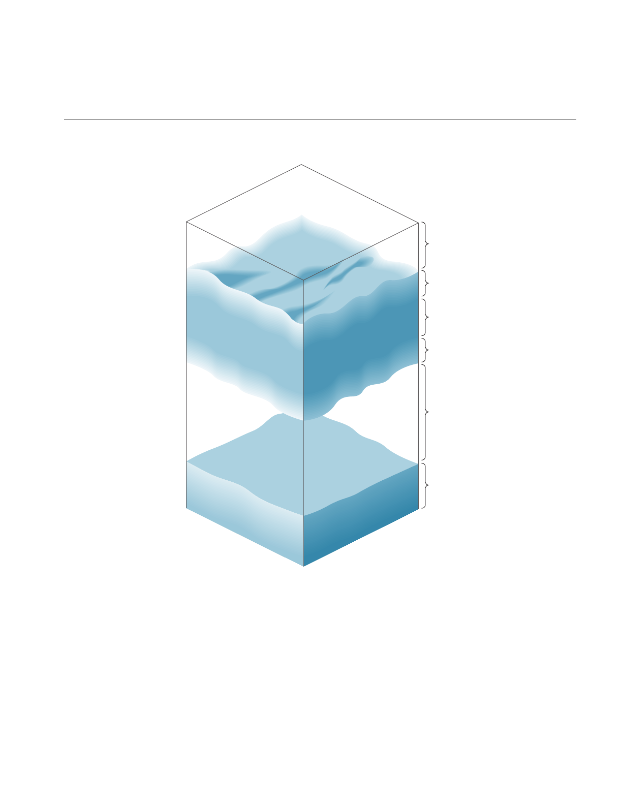
Atmospheric Effects
167
Figure 6-1 Layered Atmosphere Model
General
visibility
Upper
transition
zone
Clouds
Lower
transition
zone
General
visibility
Groung fog

168
Chapter 6: Creating Visual Effects
The lowest layer consists of ground fog, extending from the ground up to a user-selected
altitude. The fog thins out with increasing altitude, disappearing entirely at the bottom
of the general visibility layer. This layer extends from the top of the ground fog layer to
the bottom of the cloud layer’s lower transition zone, if such a zone exists. The transition
zone provides a smooth transition between general visibility and the cloud layer. (If there
is no cloud layer, then general visibility extends upward forever.) The cloud layer is
defined as an opaque region of near-zero visibility; you can set its upper and lower
boundaries. You can also place another transition zone above the cloud layer to make the
clouds gradually thin out into clear air.
Set up the atmospheric simulation with the commands listed in Table 6-1
You can set any pfEarthSky attribute, mode, or color in real time. Selecting the active
pfFog definition can also be done in real time. However, changing the parameters of a
pfFog once they are set isn’t advised when in multiprocessing mode.
The default characteristics of a pfEarthSky are listed in Table 6-2.
Table 6-1 pfEarthSky Routines
Function Action
pfNewESky Create a pfEarthSky
pfESkyMode Set the render mode
pfESkyAttr Set the attributes of the earth and sky models
pfESkyColor Set the colors for earth and sky and clear
pfESkyFog Set the fog functions
Table 6-2 pfEarthSky Attributes
Attribute Default
Clear method PFES_FAST (full screen clear)
Clear color 0.0 0.0 0.0
Sky top color 0.0 0.0 0.44
Sky bottom color 0.0 0.4 0.7
Ground near color 0.5 0.3 0.0

Atmospheric Effects
169
By default, an earth-sky model isn’t drawn. Instead, the channel is simply cleared to
black and the Z-buffer is set to its maximum value. This default action also disables all
other atmospheric attributes. To enable atmospheric effects, select PFES_SKY,
PFES_SKY_GRND, or PFES_SKY_CLEAR when turning on the earth-sky model.
Clouds are disabled when the cloud top is less than or equal to the cloud bottom. Cloud
transition zones are disabled when clouds are disabled.
Fog is enabled when either the general or ground fog is set to a valid pfFog. If ground fog
isn’t enabled, no ground fog layer will be present and fog will be used to support general
visibility. Setting a fog attribute to NULL disables it. See “Atmospheric Effects” on
page 166 for further information on fog parameters and operation.
The earth-sky model is an attribute of the channel and thus accesses information about
the viewer’s position, current field of view, and other pertinent information directly from
pfChannel. To set the pfEarthSky in a channel, use pfChanESky().
Ground far color 0.4 0.2 0.0
Horizon color 0.8 0.8 1.0
Ground fog NULL (no fog)
General visibility NULL (no fog)
Cloud top 20000.0
Cloud bottom 20000.0
Cloud bottom color 0.8 0.8 0.8
Cloud top color 0.8 0.8 0.8
Transition zone bottom 15000.0
Transition zone top 25000.0
Ground height 0
Horizon angle 10 degrees
Table 6-2 (continued) pfEarthSky Attributes
Attribute Default


This chapter describes a variety of database formats and their corresponding
conversion utilities.
“Importing Databases”
Chapter 7


173
Chapter 7
7. Importing Databases
Once you’ve learned how to create visual simulation applications with IRIS Performer
your next task is to import visual databases into those applications. IRIS Performer
provides import and export functions for more than 30 popular database formats to ease
this effort.
This chapter describes:
• The steps involved in creating custom loaders for other data formats.
• Each pre-existing file-loading utilities.
• Several utility functions in the IRIS Performer database utility library that can make
the process of database conversion easier for you.
Overview of IRIS Performer Database Creation and Conversion
Source code is provided for most of the tools discussed in this chapter. In most cases the
loaders are short, easy to understand, and easy to modify.
Table 7-1 lists the subdirectories of /usr/share/Performer/src/lib where you can find the
source code for the database processing tools.
Table 7-1 Database-Importer Source Directories
Directory Name Directory Contents
libpfdu General database processing tools and utilities
libpfdb Load, convert, and store specific database formats
libpfutil Additional utility functions

174
Chapter 7: Importing Databases
Before you can import a database, you must create it. Some simulation applications
create data procedurally; for examples of this approach, see the “Silicon Graphics PHD
Format” on page 219 or the “Sierpinski Sponge Format” sections of this chapter.
In most cases, however, you must create visual databases manually. Several software
packages are available to help with this task, and most such systems facilitate geometric
modeling, texture creation, and interactive specification of colors and material
properties. Some advanced systems support level-of-detail specification, animation
sequences, motion planning for jointed objects, automated roadway and terrain
generation, and other specialized functions.
libpfdu
- Utilities for Creation of Efficient IRIS Performer Run-Time Structures
There are several layers of support in IRIS Performer for loading 3-D models and 3-D
environments into IRIS Performer run-time scene graphs. IRIS Performer contains the
libpfdu library devoted to the import of data into (and export of data from) IRIS Performer
run-time structures. Note that two database exporters have already been written for the
Medit and DWB database formats.
At the top level of the API, IRIS Performer provides a standard set of functions to read in
files and convert databases of unknown type. This functionality is centered around the
notion of a database converter. A database converter is an abstract entity that knows how
to perform some or all of a set of database format conversion functions with a particular
database format. Moreover, converters must follow certain API guidelines for standard
functionality such that they can be easily integrated into IRIS Performer in a run-time
environment without IRIS Performer needing any prior knowledge of a particular
converter’s existence. This run-time integration is done through the use of dynamic
shared object (DSO) libraries.

libpfdu - Utilities for Creation of Efficient IRIS Performer Run-Time Structures
175
pfdLoadFile - Loading Arbitrary Databases into IRIS Performer
Table 7-2 describes the general routines for 3-D databases provided by libpfdu.
The database loader utility library, libpfdu, provides a convenient function, named
pfdLoadFile(), that imports database files stored in any of the supported format listed in
Table 7-6.
Loading database files with pfdLoadFile() is easy. The function prototype is
pfNode *pfdLoadFile(char *fileName);
pfdLoadFile() tests the filename-extension portion of fileName (the substring starting at
the last period in fileName, if any) for one of the format-name codes listed in Table 7-6,
then calls the appropriate importer.
The file-format selection process is implemented using dynamic loading of DSOs, which
are IRIX Dynamic Shared Objects. This process allows new loaders that are developed as
database formats change to be used with IRIS Performer-based applications without
requiring recompilation of the IRIS Performer application. If at all possible,
pfdInitConverter() should be called before pfConfig() for the potential formats that may
be loaded. This will pre-load the DSO and allow it to initialize any of its own data
structures and classes. This is required if the loader DSO extends IRIS Performer classes
or uses any node traversal callbacks so that if multiprocessing these data elements will
all have been pre-created and be valid in all potential processes. pfdInitConverter()
automatically calls pfdLoadNeededDSOs_EXT() to pre-load additional DSOs needed
by the loader if the given loader has defined that routine. These routines take a file name
so that the loader has the option to search through the file for possible DSO references in
the file.
Table 7-2 libpfdu Database Converter Functions
Function Name Description
pfdInitConverter Initialize the library and its classes for the desired format
pfdLoadFile Load a database file into an IRIS Performer scene graph
pfdStoreFile Store a run-time scene graph into a database file
pfdConvertFrom Convert an external run-time format into an IRIS Performer scene graph
pfdConvertTo Convert an IRIS Performer scene graph into an external run-time format

176
Chapter 7: Importing Databases
Loading Process Internals
The details of the loading process internal to pfdLoadFile() include:
1. Searching for the named file using the current IRIS Performer file path.
2. Extraction of the file-type extension.
3. Translation of the extension using a registered alias facility, formation of the DSO
name.
4. Formation of a loader function name.
5. Finding that function within the DSO using dlsym().
6. Searching first the current executable and loaded DSOs for the proper load function
and then searching through a list of user-defined and standard directories for that
DSO. Dynamic loading of the indicated DSO using dlopen().
7. Invocation of the loader function.
Loader Name
The loader function name is constructed from two components:
• A prefix always consisting of “pfdLoadFile_”.
• Loader suffix, which is the file extension string.
Examples of several complete loader function names are shown in Table 7-3.
Table 7-3 Loader Name Composition
File Extension Loader Function Name
dwb pfdLoadFile_dwb
flt pfdLoadFile_flt
medit pfdLoadFile_medit
obj pfdLoadFile_obj
pfb pfdLoadFile_pfb

libpfdu - Utilities for Creation of Efficient IRIS Performer Run-Time Structures
177
Shell Environment Variables
Several shell environment variables are used in the loader location process. These are
PFLD_LIBRARY{N32,64}_PATH, LD_LIBRARY{N32,64}_PATH, and PFHOME.
Confusion about loader locations can be resolved by consulting the sources mentioned
above to understand the use of these directory lists and reading the following section,
“Database Loading Details” on page 177. When the pfNotifyLevel is set to the value for
PFNFY_DEBUG (5)or greater, the DSO and loader function names are printed as
database are loaded, as is the name of each directory that is searched for the DSO.
The IRIS Performer sample programs, including perfly, use pfdLoadFile() for database
importing. This allows them to simultaneously load and display databases in many
disparate formats. As you develop your own database loaders, follow the source code
examples in any of the libpfdb loaders. Then you will be able to load your data into any
IRIS Performer application. You will not need to rebuild perfly or other applications to
view your databases.
Database Loading Details
Details about the database loading process are described further in this section, the
pfdLoadFile reference page, and the source code which is in
/usr/share/Performer/src/lib/libpfdu/pfdLoadFile.c.
The routines pfdInitConverter(), pfdLoadFile(),pfdStoreFile(),pfdConvertFrom(), and
pfdConvertTo() exist only as a level of indirection to allow a user to manipulate all
databases regardless of format through a central API. They are in fact merely a
mechanism for creating an open environment for data sharing among the multitudes of
three-dimensional database formats. Each of these routines determines, using file-type
extensions, which database converter to load as a run-time DSO. The routine then calls
the appropriate functionality from that converter’s DSO. All converters must provide
API that is exactly the same as the corresponding libpfdu API with _EXT added to the
routine names (for example, for “.medit” files, the suffix is “_medit”). Note that multiple
physical extensions can be mapped to one converter extension via calls to
pfdAddExtAlias(). Several aliases are pre-defined upon initialization of libpfdu.

178
Chapter 7: Importing Databases
It is also important to note that because each of these converters are unique entities that
they each may have state that is important to their proper function. Moreover, their
database format may allow for multiple IRIS Performer interpretations and so there
exists API, shown in Table 7-4, not only to initialize and exit database converters, but also
to set and get modes, attributes, and values that might affect the converter’s
methodology.
Once again each converter provides the equivalent routines with _EXT added to the
function name.
For example, the converter for the Open Inventor format would define the function
pfdInitConverter_iv() if it needed to be initialized before it was used. Likewise, it would
define the function pfdLoadFile_iv() to read an Open Inventor “.iv” file into an IRIS
Performer scene graph.
Note: Because each converter is an individual entity (DSO) and deals with a particular
type of database, it may be the case that a converter will not provide all of the
functionality listed above, but rather only a subset. For instance, most converters that
come with IRIS Performer only implement their version of pfdLoadFile but not
pfdStoreFile,pfdConvertFrom, or pfdConvertTo. However, users are free to add this
functionality to the converters via compliant API and IRIS Performer’s libpfdu will
immediately recognize this functionality. Also, libpfdu traps access to non-existent
converter functionality and returns gracefully to the calling code while notifying the user
that the functionality could not be found.
Table 7-4 libpfdu Database Converter Management Functions
Function Name Description
pfdInitConverter Initialize a database conversion DSO
pfdExitConverter Exit a database conversion DSO
pfdConverterMode Specify a mode for a specific conversion DSO
pfdGetConverterMode Get a mode setting from a specific conversion DSO
pfdConverterAttr Specify an attribute for a conversion DSO
pfdGetConverterAttr Get an attribute setting from a conversion DSO
pfdConverterVal Specify a value for a conversion DSO
pfdGetConverterVal Get a value setting from a conversion DSO

libpfdu - Utilities for Creation of Efficient IRIS Performer Run-Time Structures
179
Finding and initializing a Converter
When one of the general database converter functions is called, it in turn calls the
corresponding routine provided by the converter, passing on the arguments it was given.
But the first time a converter is called, a search occurs to identify the converter and the
functions it provides. This is accomplished as follows.
• Parse the extension - what appears after the final “.” in the filename. This is referred
to as EXT in the following bulleted items.
• Check to see if any alias was created for the EXT extension with pfdAddExtAlias().
If a translation is defined, EXT is replaced with that extension.
• Check the current executable to see if the symbol pfdLoadFile_EXT is already
defined, i.e. if the loader was statically linked into the executable or a DSO was
previously loaded by some other mechanism. If not, the search continues.
– Generate a DSO library name to search for using on the extension prototype
“libpfEXT_{igl,ogl}{-g,}.so”. This means the following strings will be
constructed based upon whether OpenGL or IRIS GL is being used with IRIS
Performer:
libpfEXT_igl.so for the optimized IRIS GL loader
libpfEXT_igl-g.so for the debug IRIS GL loader
libpfEXT_ogl.so for the optimized OpenGL loader
libpfEXT_ogl-g.so for the debug OpenGL loader
– Look for the DSO in several places including:
.
$PFLD_LIBRARY_PATH
$LD_LIBRARY_PATH
$PFHOME/usr/lib{,32,64}/libpfdb
$PFHOME/usr/share/Performer/lib/libpfdb
– Open the DSO via dlopen().

180
Chapter 7: Importing Databases
• Once the object has been found, processing continues.
– Query all libpfdu converter functionality from the symbol table of the DSO
using dlsym() with function names generated by appending _EXT to the name
of the corresponding pfd routine name. This symbol dictionary is retained for
future use.
– Invoke the converter’s initialization function, pfdInitConverter_EXT(), if it
exists.
– Invoke pfdLoadNeededDSOs_EXT() if it exists. This routine can then
recursively call pfdInitConverter_EXT(), as needed.
Developing Custom Importers
Having fully described how database converters can be integrated into IRIS Performer
and the types of functionality they provide, the next undertaking is actually
implementing a converter from scratch. IRIS Performer makes a great effort at allowing
the quick and easy development of effective and efficient database converters.
While creating a new file loader for IRIS Performer isn’t inherently difficult, it does
require a solid understanding of the following issues:
• The structure and interpretation of the data file to be read
• The scene graph concepts and nodes of libpf
• The geometry and attribute definition objects of libpr
Structure and Interpretation of the Database File Format
In order to effectively convert a database into an IRIS Performer scene graph it is
important to have a substantial understanding of several concepts related to the original
database format:
• the parsing of the file based on the database format
• the data types represented in the format and their IRIS Performer correspondence
• the scene graph structure of the file (if any)
• the method of graphics state definition and inheritance defined in the format.

Developing Custom Importers
181
Before trying to convert sophisticated 3-D database formats into IRIS Performer it is
important to have a thorough grasp of how every structure in the format needs to affect
how IRIS Performer performs its run-time management of a scene graph. However,
although it requires a great deal of understanding to convert complex behaviors of
external formats into IRIS Performer, it is still very straight forward to migrate basic
structure, geometry, and graphics state into efficient IRIS Performer run-time structures
via the functionality provided in the IRIS Performer database builder - pfdBuilder.
Scene Graph Creation using Nodes as defined in
libpf
Creating an IRIS Performer scene graph requires a definite knowledge of the following
IRIS Performer libpf node types - pfScene, pfGroup, and pfGeode.
These nodes can be used to define a minimally functional IRIS Performer scene graph.
See Chapter 5 for more details on libpf and IRIS Performer scene graphs and node types.
Defining Geometry and Graphics State for
libpr
In order to input geometry and graphics into IRIS Performer, it is important to have an
understanding of how IRIS Performer’s low level rendering objects work in libpr, IRIS
Performer’s performance rendering library. The main libpr rendering primitives are a
pfGeoSet and a pfGeoState. A pfGeoSet is a collection of like geometric primitives that
can all be rendered in exactly the same way in one large continuous chunk. A pfGeoState
is a complete definition of graphics mode settings for the rendering hardware and
software. It contains many attributes such as texture and material. Given a pfGeoSet and
a corresponding pfGeoState, libpr can completely and efficiently render all of the
geometry in the pfGeoSet. For a more detailed description of pfGeoSets and pfGeoStates
see Chapter 10 which goes into detail on all libpr primitives and how IRIS Performer will
use them.
However, realizing that IRIS Performer’s structuring of geometry and graphics state is
optimized for rendering speed and not for modelling ease or general conceptual
partitioning, IRIS Performer now contains a new mechanism for translating external
graphics state and geometry into efficient libpr structures. This new mechanism is the
pfdBuilder that exists in libpfdu.

182
Chapter 7: Importing Databases
The pfdBuilder allows the immediate mode input of graphics state and primitives
through very simple and exposed data structures. After having received all of the
relevant information, the pfdBuilder builds efficient and somewhat optimized libpr data
structures and returns a low-level libpf node that can be attached to an IRIS Performer
scene graph. The pfdBuilder is the recommended method of importing data from non
IRIS Performer-based formats into IRIS Performer.
Creation of a IRIS Performer Database Converter using
libpfdu
Creating a new format converter is very simple process. More than thirty database
loaders are shipped with IRIS Performer in source code form to serve as practical
examples of this process. The loaders read formats that range from trivial to complex,
and should serve as an instructive starting point for those developing loaders for other
formats. These loaders can be found in the directory
/usr/share/Performer/src/lib/libpfdb/libpf*.
This section describes the libpfdu framework for creating a 3-D database format
converter. Let’s consider writing a converter for a simple ASCII format that is called the
Imaginary Immediate Mode format with the file type extension “.iim”. This format is
much like the more elaborate “.im” format loader used at SGI for the purposes of testing
basic IRIS Performer functionality.
The first thing to do is set up the routine that pfdLoadFile() will call when it attempts to
load a file with the extension “.iim”.
extern pfNode *pfdLoadFile_iim(char *fileName)
{
}
This function needs to perform several basic actions:
1. Find and open the given file.
2. Reset the libpfdu pfdBuilder for input of new geometry and state.
3. Setup any pfdBuilder modes that the converter needs enabled.
4. Setup local data structures that can be used to communicate geometry and graphics
state with the pfdBuilder.
5. Setup a libpf pfGroup which can hold all of the logical partitions of geometry in the
file (or hold a subordinate collection of nodes as a general scene graph if the format
supports it).

Developing Custom Importers
183
6. Optionally set up a default state to use for geometry with unspecified graphics state.
7. Parse the file which entails:
• Filling in the local geometry and graphics state data structures.
• Passing them to the pfdBuilder as inputted from the file
• Ask the pfdBuilder to build the data structures into IRIS Performer data
structures when a logical partition of the file has ended.
• Attach the IRIS Performer node returned by the build to the higher level group
which will hold the entire IRIS Performer representation of this file. Note that
this step becomes more complex if the format supports the notion of hierarchy
only in that the appropriate libpf nodes must be created and attached to each
other via pfAddChild() to build the hierarchy. In this case requests are made for
the builder to build after inputting all of the geometry and state found in a
particular leaf node in the database.
8. Delete local data structures used to input geometry and graphics state.
9. Close the file.
10. Perform any optional optimization of the IRIS Performer scene graph.
Optimizations might include calls to pfdFreezeTransforms(),pfFlatten() or
pfdCleanTree().
11. Return the pfGroup containing the entire IRIS Performer representation of the
database file.
Steps 1-8 expand the function outline to the following:
extern pfNode *pfdLoadFile_iim(char *fileName)
{
FILE* iimFile;
pfdGeom* polygon;
pfGroup* root;
/* Performer has utility for finding and opening file */
if ((iimFile = pfdOpenFile(fileName)) == NULL)
return NULL;
/* Clear builder from previous converter invocations */
pfdResetBldrGeometry();
pfdResetBldrState();
/* Call pfdBldrMode for any needed modes here */

184
Chapter 7: Importing Databases
/* Create polygon structure */
/* holds one N-sided polygon where N is < 300 */
polygon = pfdNewGeom(300);
/* Create pfGroup to hold entire database */
/* loaded from this file */
root = pfNewGroup();
/* Specify state for geometry with no graphics state */
/* As well as default enables, etc. This routine */
/* should invoke pfdCaptureDefaultBldrState()*/
SetupDefaultGraphicsStateIfThereIsOne();
/* Do all the real work in parsing the file and */
/* converting into Performer */
ParseIIMFile(iimFile, root, polygon);
/* Delete local polygon struct */
pfdDelGeom(polygon);
/* Close File */
fclose(iimFile);
/* Optimize IRIS Performer scene graph */
/* via use of pfFlatten, pfdCleanTree, etc. */
OptimizeGraph(root);
return (pfNode*)root;
}

Developing Custom Importers
185
Now, for at the heart of the file loader lies the ParseIIMFile() function. The specifics of
parsing a file are completely dependent on the format so the parsing will be left as an
exercise to the reader. However, the following code fragments should show a framework
for what goes into integrating the parser with the pfdBuilder framework for geometry
and graphics state data conversion. Note that several possible graphics state inheritance
models might be used in external formats and that the pfdBuilder is designed to support
all of them:
• The default pfdBuilder state inheritance is that of immediate mode graphics state.
Immediate mode state is specified through calls to pfdBldrStateMode(),
pfdBldrStateAttr(), and pfdBldrStateVal().
• There also exists a pfdBuilder state stack for hierarchical state application to
geometry. This is accomplished through the use of pfdPushBldrState() and
pfdPopBldrState() in conjuncture with the normal use of the immediate mode
pfdBuilder state API.
• Lastly, there is a pfdBuilder named state list that can be used to define a number of
‘named materials’ or ‘named state definitions’ that can then be recalled in one API
called (for instance a user might define a ‘brick’ state with a red material and a brick
texture. Later he might just want to say ‘brick’ is the current state and then input the
walls of several buildings). This type of state naming is accomplished by fully
specifying the state to be named via the immediate mode API, and then calling
pfdSaveBldrState(). This state can then be recalled via pfdLoadBldrState().
ParseIIMFile(FILE *iimFile, pfGroup *root, pfdGeom *poly)
{
while((op = GetNextOp(iimFile)) != NULL)
{
switch(op)
{
case GEOMETRY_POLYGON:
polygon->numVerts = GetNumVerts(iimFile);
/* Determine if polygon has Texture Coords */
if (pfdGetBldrStateMode(PFSTATE_ENTEXTURE)==PF_ON)
polygon->tbind = PFGS_PER_VERTEX;
else
polygon->tbind = PFGS_OFF;
/* Determine if Polygon has normals */
if (AreThereNormalsPerVertex() == TRUE)
polygon->nbind = PFGS_PER_VERTEX;
else if
(pfdGetBldrStateMode(PFSTATE_ENLIGHTING)==PF_ON)

186
Chapter 7: Importing Databases
polygon->nbind = PFGS_PER_PRIM;
else
polygon->nbind = PFGS_OFF;
/* Determine if Polygon has colors */
if (AreThereColorsPerVertex() == TRUE)
polygon->cbind = PFGS_PER_VERTEX;
else if (AreThereColorsPerPrim() == TRUE)
polygon->cbind = PFGS_PER_PRIM;
else
polygon->cbind = PFGS_OFF;
for(i=0;i<polygon->numVerts;i++)
{
/* Read ith Vertex into local data structure */
polygon->coords[i][0] = GetNextVertexFloat();
polygon->coords[i][1] = GetNextVertexFloat();
polygon->coords[i][2] = GetNextVertexFloat();
/* Read texture coord for ith vertex if any */
if (polygon->tbind == PFGS_PER_VERTEX)
{
polygon->texCoords[i][0] = GetNextTexFloat();
polygon->texCoords[i][1] = GetNextTexFloat();
}
/* Read normal for ith Vertex if normals bound*/
if (polygon->nbind == PFGS_PER_VERTEX)
{
polygon->norms[i][0] = GetNextNormFloat();
polygon->norms[i][1] = GetNextNormFloat();
polygon->norms[i][2] = GetNextNormFloat();
}
/* Read only one normal per prim if necessary */
else if ((polygon->nbind == PFGS_PER_PRIM) &&
(i == 0))
{
polygon->norms[0][0] = GetNextNormFloat();
polygon->norms[0][1] = GetNextNormFloat();
polygon->norms[0][2] = GetNextNormFloat();
}
/* Get Color for the ith Vertex if color bound*/
if (polygon->cbind == PFGS_PER_VERTEX)
{
polygon->colors[i][0] =

Developing Custom Importers
187
GetNextColorFloat();
polygon->colors[i][1] =
GetNextColorFloat();
polygon->colors[i][2] =
GetNextColorFloat();
}
/* Get one color per prim if necessary */
else if ((polygon->cbind == PFGS_PER_PRIM) &&
(i == 0))
{
polygon->colors[0][0] =
GetNextColorFloat();
polygon->colors[0][1] =
GetNextColorFloat();
polygon->colors[0][2] =
GetNextColorFloat();
}
}
/* Add this polygon to pfdBuilder */
/* Because it is a single poly, 1 */
/* is specified here */
pfdAddBldrGeom(1);
break;
case GRAPHICS_STATE_TEXTURE:
{
char *texName;
pfTexture *tex;
texName = ReadTextureName(iimFile);
if (texName != NULL)
{
/* Get prototype tex from pfdBuilder*/
tex =
pfdGetTemplateObject(pfGetTexClassType());
/* This clears that object to default */
pfdResetObject(tex);
/* If just the name of a pfTexture is */
/* set, pfdBuilder will auto find & Load */
/* the texture*/
pfTexName(tex,texName);
/* This is the current pfdBuilder */
/* texture and texturing is on */
pfdBldrStateAttr(PFSTATE_TEXTURE,tex);

188
Chapter 7: Importing Databases
pfdBldrStateMode(PFSTATE_ENTEXTURE, PF_ON);
}
else
{
/* No texture means disable texturing */
/* And set current texture to NULL */
pfdBldrStateMode(PFSTATE_ENTEXTURE,PF_OFF);
pfdBldrStateAttr(PFSTATE_TEXTURE, NULL);
}
}
break;
case GRAPHICS_STATE_MATERIAL:
{
pfMaterial *mtl;
mtl = pfdGetTemplateObject(pfGetMtlClassType());
pfdResetObject(mtl);
pfMtlColor(mtl, PFMTL_AMBIENT,
GetAmRed(), GetAmGreen(), GetAmBlue());
pfMtlColor(mtl, PFMTL_DIFFUSE,
GetDfRed(), GetDfGreen(), GetDfBlue());
pfMtlColor(mtl, PFMTL_SPECULAR,
GetSpRed(), GetSpGreen(), GetSpBlue());
pfMtlShininess(mtl, GetMtlShininess());
pfMtlAlpha(mtl, GetMtlAlpha());
pfdBldrStateAttr(PFSTATE_FRONTMTL, mtl);
pfdBldrStateAttr(PFSTATE_BACKMTL, mtl);
}
break;
case GRAPHICS_STATE_STORE:
pfdSaveBldrState(GetStateName());
break;
case GRAPHICS_STATE_LOAD:
pfdLoadBldrState(GetStateName());
break;
case GRAPHICS_STATE_PUSH:
pfdPushBldrState();
break;
case GRAPHICS_STATE_POP:
pfdPopBldrState();
break;
case GRAPHICS_STATE_RESET:
pfdResetBldrState();
break;
case GRAPHICS_STATE_CAPTURE_DEFAULT:
pfdCaptureDefaultBldrState();

Developing Custom Importers
189
break;
case BEGIN_LEAF_NODE:
/* Not really necessary because it is */
/* destroyed on build*/
pfdResetBldrGeometry();
break;
case END_LEAF_NODE:
{
pfNode *nd = pfdBuild();
if (nd != NULL)
pfAddChild(root,nd);
}
break;
}
}
}
One of the fundamental structures involved in the above routine outline is the pfdGeom
structure which users fill in with information about a single primitive, or a single strip of
primitives. The pfdGeom structure is essential in communicating with the pfdBuilder
and is defined as follows:
typedef struct _pfdGeom
{
int flags;
int nbind, cbind, tbind;
int numVerts;
short primtype;
float pixelsize;
/* Non-indexed attributes */
/* ..do not set if poly is indexed */
pfVec3 *coords;
pfVec3 *norms;
pfVec4 *colors;
pfVec2 *texCoords;
/* Indexed attributes */
/* ..do not set if poly is non-indexed */
pfVec3 *coordList;
pfVec3 *normList;
pfVec4 *colorList;
pfVec2 *texCoordList;
/* Index lists*/

190
Chapter 7: Importing Databases
/* ..do not set if poly is non-indexed */
ushort *icoords;
ushort *inorms;
ushort *icolors;
ushort *itexCoords;
struct _pfdGeom *next;
} pfdGeom;
See the pfdGeoBuilder(3pf) reference pages for more information on using this structure
along with its sister structure, the pfdPrim.
The above should provide a well-defined framework for creating a database converter
that can be used with any IRIS Performer applications via the pfdLoadFile()
functionality.
However, it is also important to note that there are a multitude of pfdBuilder modes and
attributes that can be used to affect some of the basic methods that the builder actually
uses:

Developing Custom Importers
191
Table 7-5 pfdBuilder Modes and Attributes
Function Name Token Description
pfd{Get}BldrMode PFDBLDR_MESH_ENABLE
PFDBLDR_MESH_SHOW_TSTRIPS
PFDBLDR_MESH_INDEXED
PFDBLDR_MESH_MAX_TRIS
PFDBLDR_MESH_RETESSELLATE
PFDBLDR_MESH_LOCAL_LIGHTING
PFDBLDR_AUTO_COLORS
PFDBLDR_AUTO_NORMALS
PFDBLDR_AUTO_ORIENT
PFDBLDR_AUTO_ENABLES
PFDBLDR_AUTO_CMODE
PFDBLDR_AUTO_DISABLE_TCOORDS_BY_STATE
PFDBLDR_AUTO_DISABLE_NCOORDS_BY_STATE
PFDBLDR_AUTO_LIGHTING_STATE_BY_NCOORDS
PFDBLDR_AUTO_LIGHTING_STATE_BY_MATERIALS
PFDBLDR_AUTO_TEXTURE_STATE_BY_TEXTURES
PFDBLDR_AUTO_TEXTURE_STATE_BY_TCOORDS
PFDBLDR_BREAKUP
PFDBLDR_BREAKUP_SIZE
PFDBLDR_BREAKUP_BRANCH
PFDBLDR_BREAKUP_STRIP_LENGTH
PFDBLDR_SHARE_MASK
PFDBLDR_ATTACH_NODE_NAMES
PFDBLDR_DESTROY_DATA_UPON_BUILD
PFDBLDR_PF12_STATE_COMPATIBLE
PFDBLDR_BUILD_LIMIT
PFDBLDR_GEN_OPENGL_CLAMPED_TEXTURE_COORDS
PFDBLDR_OPTIMIZE_COUNTS_NULL_ATTRS
pfd{Get}BldrAttr PFDBLDR_NODE_NAME_COMPARE
PFDBLDR_STATE_NAME_COMPARE

192
Chapter 7: Importing Databases
Because the pfdBuilder is released as source code, it is easy to add further functionality
and more modes and attributes to even further customize this central functionality.
In fact, because the pfdBuilder acts as a “data funnel” in converting data into IRIS
Performer run-time structures, it is easy to control the behavior of many standard
conversion tasks through merely globally setting builder modes which will subsequently
affect all converters that use the pfdBuilder to process their data.
Maximizing Database Loading and Paging Performance with PFB and PFI Formats
“Description of Supported Formats” on page 195 describes all of the file formats
supported by IRIS Performer. Although you can use files in these formats directly, you
can dramatically reduce database loading time by pre-converting databases into the PFB
format and images into the PFI format.
To convert to the PFB file format or the PFI image format, use the pfconv and pficonv
utilities.
pfconv
The pfconv utility converts from any format for which a pfdLoadFile...() function exists
into any format for which a pfdStoreFile...() exists. The most common format to convert
to is the PFB format. For example, to convert cow.obj into the PFB format, use the
following command:
% pfconv cow.obj cow.pfb
By default, pfconv optimizes the scene graph when doing the conversion. The
optimizations are controlled with the -o and -O command line options. Builder options
are controlled with the -b and -B command line options. Converter modes are controlled
with the -m and -M command line options. Refer to the help page for more specific
information about the command line options by entering:
% pfconv -h

Supported Database Formats
193
Example Conversion
When converting to the PFB format, texture files can be converted to the PFI format using
the following command line options:
% pfconv -M pfb, 5, 1
5 means PFPFB_SAVE_TEXTURE_PFI.
1 means convert .rgb texture images to .pfi.
pficonv
The pficonv utility converts from IRIS libimage format to PFI format image files. For
example, to convert cafe.rgb into the PFI format, use the following command:
% pficonv cafe.rgb cafe.pfi
Mipmaps can be automatically generated and stored in the resulting PFI files by adding
-m to the command line.
Supported Database Formats
Vendors of several leading database construction and processing tools have provided
database-loading software for you to use with IRIS Performer. This section describes
these loaders, the loaders developed by the IRIS Performer engineering team, and
several loaders developed in the IRIS Performer user community for other database
formats.
Importing your databases is simple if they’re in formats for which IRIS Performer
database loaders have already been written. Each of the loaders listed in Table 7-6 is
included with IRIS Performer. If you want to import or export databases in any of these
formats, refer to the appropriate section of this chapter for specific details about the
individual loaders.

194
Chapter 7: Importing Databases
Table 7-6 Supported Database Formats
Name Description
3ds AutoDesk 3DStudio binary data
bin SGI format used by powerflip
bpoly Side Effects Software PRISMS binary data
byu Brigham Young University CAD/FEA data
csb OpenGL Optimizer Format
ct Cliptexture config file loader - auto-generates viewing geometry
dwb Coryphaeus Software Designer’s Workbench data
dxf AutoDesk AutoCAD ASCII format
flt11 MultiGen public domain Flight v11 format
flt MultiGen OpenFlight format provided by MultiGen
gds McDonnell-Douglas GDS things data
gfo Old SGI radiosity data format
im Simple IRIS Performer data format
irtp AAI/Graphicon Interactive Real-Time PHIGS
iv SGI Open Inventor format (VRML 1.0 superset)
lsa Lightscape Technologies ASCII radiosity data
lsb Lightscape Technologies binary radiosity data
medit Medit Productions medit modeling data
nff Eric Haines’ ray tracing test data
pfb IRIS Performer fast binary format
obj Wavefront Technologies data format
pegg Radiosity research data format
phd SGI polyhedron data format

Description of Supported Formats
195
Description of Supported Formats
This section describes the different database file for mats that IRIS Performer supports.
AutoDesk 3DS Format
The AutoDesk 3DS format is used by the 3DStudio program and by a number of 3D
file-interchange tools. The IRIS Performer loader for 3DS files is located in the
/usr/share/Performer/src/lib/libpfdb/libpf3ds directory. This loader uses an auxiliary library,
3dsftk.a, to parse and interpret the 3ds file.
poly Side Effects Software PRISMS ASCII data
ptu Simple IRIS Performer terrain data format
sgf US Naval Academy standard graphics format
sgo Paul Haeberli’s graphics data format
spf US Naval Academy simple polygon format
sponge Sierpinski sponge 3D fractal generator
star Astronomical data from Yale University star chart
stla 3D Structures ASCII stereolithography data
stlb 3D Structures binary stereolithography data
stm Michael Garland’s terrain data format
sv John Kichury’s i3dm modeler format
tri University of Minnesota Geometry Center data
unc University of North Carolina walkthrough data
wrl OpenWorlds VMRL 2.0 provided by DRaW Computing
Table 7-6 (continued) Supported Database Formats
Name Description
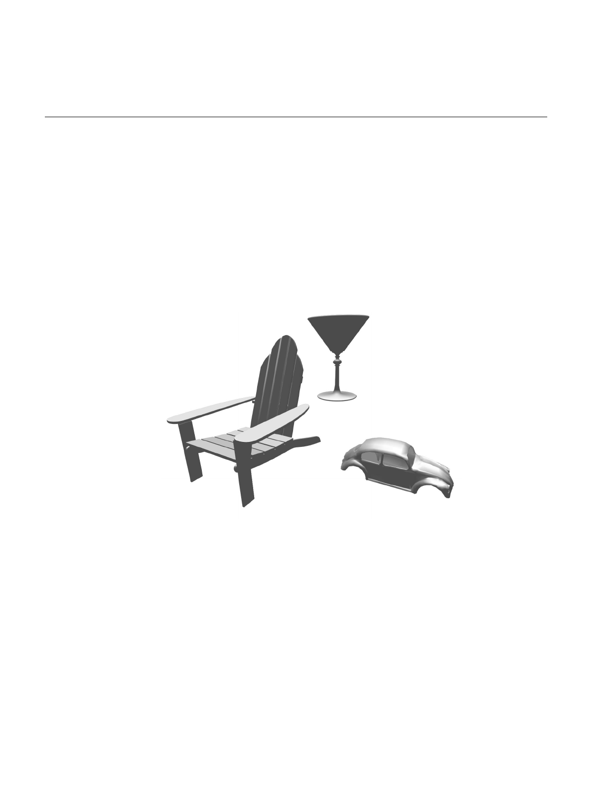
196
Chapter 7: Importing Databases
pfdLoadFile() uses the function pfdLoadFile_3ds() to import data from 3DStudio files
into IRIS Performer run-time data structures.
Silicon Graphics BIN Format
The Silicon Graphics BIN format is supported by both Showcase™ and the powerflip
demonstration program. BIN files are in a simple format that specifies only independent
quadrilaterals.
The image in Figure 7-1 shows several of the BIN-format objects provided in the IRIS
Performer sample data directory.
Figure 7-1 BIN-Format Data Objects
The source code for the BIN-format importer pfdLoadFile_bin() is provided in the file
pfbin.c. This code shows how easy it can be to implement an importer. Since
pfdLoadFile_bin() is based on the pfdBuilder() utility function, it will build efficient
triangle-strip pfGeoSets from the quadrilaterals of a given BIN file. The BIN format has
the following structure:

Description of Supported Formats
197
1. A 4-byte magic number, 0x5432, which identifies the file as a BIN file.
2. A 4-byte number that contains the number of vertices, which is four times the
number of quadrilaterals.
3. Four bytes of zero.
4. A list of polygon data for each vertex in the object. The data consists of three
floating-point words of information about normals, followed by three floating-point
words of vertex information.
The BIN format uses these data structures:
typedef struct
{
float normal[3];
float coordinate[3];
} Vertex;
typedef struct
{
long magic;
long vertices;
long zero;
Vertex vertex[1];
} BinFile;
pfdLoadFile() uses the function pfdLoadFile_bin() to import data from BIN format files
into IRIS Performer run-time data structures:
The pfdLoadFile_bin() function composes a random color for each file it reads. The
chosen color has red, green, and blue components uniformly distributed within the
range 0.2 to 0.7 and is fully opaque.
Side Effects POLY Format
The Side Effects software PRISMS database modeler format supports both ASCII and
binary forms of the POLY format. The IRIS Performer loader for ASCII “.poly” files is
located in the /usr/share/Performer/src/lib/libpfdb/libpfpoly directory. The binary format
“.bpoly” loader is located in the directory /usr/share/Performer/src/lib/libpfdb/libpfbpoly.
These formats are equivalent in content and differ only in representation.

198
Chapter 7: Importing Databases
The POLY format is an easy to understand ASCII data representation with the following
structure:
1. A text line containing the keyword “POINTS”
2. One text line for each vertex in the file. Each line begins with a vertex number,
followed by a colon, followed by the X, Y, and Z axis coordinates of the vertex,
optional additional information, and a new-line character. The optional information
includes color specification in the form “c(R,G,B,A)”, a normal vector of the form
“n(NX,NY,NZ)”, or a texture coordinate in the form “uv(S,T)” where each of the
values shown are floating point numbers.
3. A text line containing the keyword “POLYS”
4. One text line for each polygon in the file. Each line begins with a polygon number,
followed by a colon, followed by a series of vertex indices, optional additional
information, an optional “<“character, and a new-line. The optional information
includes color specification in the form “c(R,G,B,A)”, a normal vector of the form
“n(NX,NY,NZ)”, or a texture coordinate in the form “uv(S,T)” where the values in
parentheses are floating point numbers.
Here is a sample POLY format file for a cube with colors, texture coordinates, and
normals specified at each vertex:
POINTS
1: -0.5 -0.5 -0.5 c(0, 0, 0, 1) uv(0, 0) n(0, -1, 0)
2: -0.5 -0.5 0.5 c(0, 0, 1, 1) uv(0, 0) n(0, -1, 0)
3: 0.5 -0.5 0.5 c(1, 0, 1, 1) uv(1, 0) n(0, -1, 0)
4: 0.5 -0.5 -0.5 c(1, 0, 0, 1) uv(1, 0) n(0, -1, 0)
5: -0.5 -0.5 0.5 c(0, 0, 1, 1) uv(0, 0) n(0, 0, 1)
6: -0.5 0.5 0.5 c(0, 1, 1, 1) uv(0, 1) n(0, 0, 1)
7: 0.5 0.5 0.5 c(1, 1, 1, 1) uv(1, 1) n(0, 0, 1)
8: 0.5 -0.5 0.5 c(1, 0, 1, 1) uv(1, 0) n(0, 0, 1)
9: -0.5 0.5 0.5 c(0, 1, 1, 1) uv(0, 1) n(0, 1, 0)
10: -0.5 0.5 -0.5 c(0, 1, 0, 1) uv(0, 1) n(0, 1, 0)
11: 0.5 0.5 -0.5 c(1, 1, 0, 1) uv(1, 1) n(0, 1, 0)
12: 0.5 0.5 0.5 c(1, 1, 1, 1) uv(1, 1) n(0, 1, 0)
13: -0.5 -0.5 -0.5 c(0, 0, 0, 1) uv(0, 0) n(0, 0, -1)
14: 0.5 -0.5 -0.5 c(1, 0, 0, 1) uv(1, 0) n(0, 0, -1)
15: 0.5 0.5 -0.5 c(1, 1, 0, 1) uv(1, 1) n(0, 0, -1)
16: -0.5 0.5 -0.5 c(0, 1, 0, 1) uv(0, 1) n(0, 0, -1)
17: -0.5 -0.5 -0.5 c(0, 0, 0, 1) uv(0, 0) n(-1, 0, 0)
18: -0.5 0.5 -0.5 c(0, 1, 0, 1) uv(0, 1) n(-1, 0, 0)
19: -0.5 0.5 0.5 c(0, 1, 1, 1) uv(0, 1) n(-1, 0, 0)
20: -0.5 -0.5 0.5 c(0, 0, 1, 1) uv(0, 0) n(-1, 0, 0)

Description of Supported Formats
199
21: 0.5 0.5 0.5 c(1, 1, 1, 1) uv(1, 1) n(1, 0, 0)
22: 0.5 0.5 -0.5 c(1, 1, 0, 1) uv(1, 1) n(1, 0, 0)
23: 0.5 -0.5 -0.5 c(1, 0, 0, 1) uv(1, 0) n(1, 0, 0)
24: 0.5 -0.5 0.5 c(1, 0, 1, 1) uv(1, 0) n(1, 0, 0)
POLYS
1: 1 2 3 4 <
2: 5 6 7 8 <
3: 9 10 11 12 <
4: 13 14 15 16 <
5: 17 18 19 20 <
6: 21 22 23 24 <
pfdLoadFile() uses the functions pfdLoadFile_poly() and pfdLoadFile_bpoly() to
import data from “.poly” and “.bpoly” format files into IRIS Performer run-time data
structures:
Brigham Young University BYU Format
The Brigham Young University “.byu” format is used as an interchange format by some
finite element analysis packages. The IRIS Performer loader for “.byu” files is located in
the /usr/share/Performer/src/lib/libpfdb/libpfbyu directory.
The format of a BYU file consists of four parts as defined below:
1. A text line containing four counts: the number of parts, the number of vertices, the
number of polygons, and the number of elements in the connectivity array.
2. The part definition list, containing the starting polygon number and ending
polygon number (one pair per line) for parts lines.
3. The vertex list, which has the X, Y, Z coordinates of each vertex in the database
packed two per line. This means that vertices 1 and 2 are on the first line, 3 and 4 are
on the second, and so on for (vertices + 1)/2 lines of text in the file.
4. The connectivity array, with an entry for each polygon. These entries may span
multiple lines in the input file and each consists of three or more vertex indices with
the last negated as an end of list flag. For example, if the first polygon were a quad,
the connectivity array might start with “1 2 3 -4” to define a polygon that connects
the first four vertices in order.

200
Chapter 7: Importing Databases
The following BYU format file defines two adjoining quads:
2 6 2 0
1 1
2 2
0 0 0 10 0 0
10 10 0 0 10 0
10 10 10 0 10 10
1 2 3 -4
4 3 5 -6
pfdLoadFile() uses the function pfdLoadFile_byu() to import data from “.byu” format
files into IRIS Performer run-time data structures.
Optimizer CSB Format
IRIS Performer can load native OpenGL Optimizer format files using this loader.
OpenGL Optimizer can also load IRIS Performer’s PFB native format files, providing full
database interoperability. This allows you to use OpenGL Optimizer database
simplification and optimization tools on IRIS Performer databases.
Virtual Cliptexture CT Loader
The IRIS Performer CT loader allows you to create and configure cliptextures and virtual
cliptextures, complete with a scenegraph containing simple geometry and callbacks. See
the Cliptexture chapter for more details.
Designer’s Workbench DWB Format
The binary DWB format is used for input and output by the Designer’s Workbench,
EasyT, and EasyScene database modeling tools produced by Coryphaeus Software. DWB
is an advanced database format that directly represents many of IRIS Performer’s
attribute and hierarchical scene graph concepts.
An importer for this format, named pfdLoadFile_dwb(), has been provided by
Coryphaeus Software for your use. The loader code and its associated documentation are
in the /usr/share/Performer/src/lib/libpfdb/libpfdwb directory.The image in Figure 7-2 shows
a model of the Soma Cube puzzle invented by Piet Hein. The model was created using
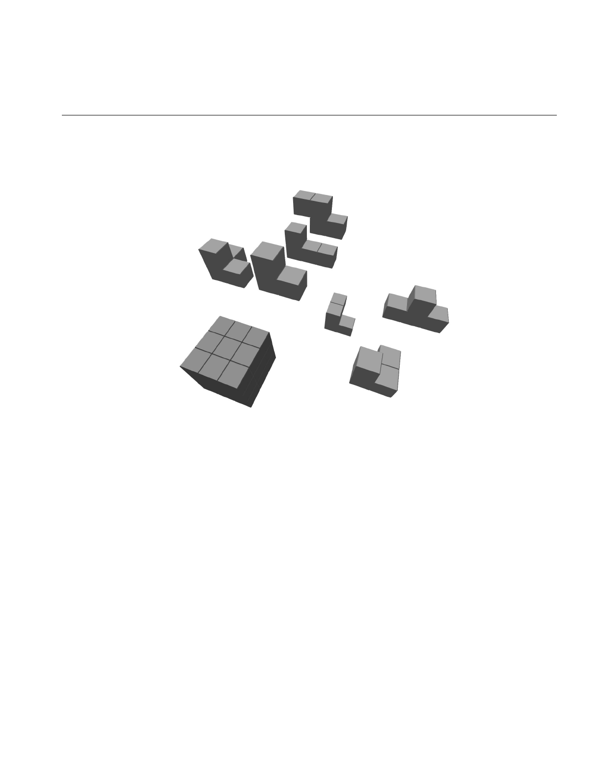
Description of Supported Formats
201
Designer’s Workbench. Each of the pieces is stored as an individual DWB-format file. Do
you see how to form the 3 x 3 cube at the lower left from the seven individual pieces?
Figure 7-2 Soma Cube Puzzle in DWB Form
pfdLoadFile() uses the function pfdLoadFile_dwb() to load Designer’s Workbench files
into IRIS Performer run-time data structures.
AutoCAD DXF Format
The DXF format originated with Autodesk’s AutoCAD database modeling system. The
version recognized by the pfdLoadFile_dxf() database importer is a subset of ASCII
Drawing Interchange Format (DXF) Release 12. The binary version of the DXF format,
also known as DXF, isn’t supported. Source code for the importer is in the file
/usr/share/Performer/src/lib/libpfdb/libpfdxf/pfdxf.c.pfdLoadFile_dxf() was derived from
the DXF-to-DKB data file converter developed and placed in the public domain by
Aaron A. Collins.
The image in Figure 7-3 shows a DXF model of the famous Utah teapot. This model was
loaded from DXF format using the pfdLoadFile_dxf() database importer.

202
Chapter 7: Importing Databases
Figure 7-3 The Famous Teapot in DXF Form
The DXF format has an unusual though well-documented structure. The general
organization of a DXF file is
1. HEADER section with general information about the file
2. TABLES section to provide definitions for named items, including:
■LTYPE, the line-type table
■LAYER, the layer table
■STYLE, the text-style table
■VIEW, the view table
■UCS, the user coordinate-system table
■VPORT, the viewport configuration table
■DIMSTYLE, the dimension style table
■APPID, the application identification table

Description of Supported Formats
203
3. BLOCKS section containing block definition entities
4. ENTITIES section containing entities and block references
5. END-OF-FILE
Within each section are groups of values, where each value is defined by a two-line pair
of tokens. The first token is a numeric code indicating how to interpret the information
on the next line. For example, the sequence
10
1.000
20
5.000
30
3.000
defines a “start point” at the XYZ location (1, 5, 3). The codes 10, 20, and 30 indicate,
respectively, that the primary X, Y, and Z values follow. All data values are retained in a
set of numbered registers (10, 20, and 30 in this example), which allows values to be
reused. This simple state-machine type of run-length coding makes DXF files
space-efficient at the cost of making them harder to interpret.
pfdLoadFile() uses the function pfdLoadFile_dxf() to load DXF format files into IRIS
Performer run-time data structures.
Several widely available technical books provide full details of this format if you need
more information. Chief among these are AutoCAD Programming, 2nd Edition, by Dennis
N. Jump, Windcrest Books, 1991, and AutoCAD: The Complete Reference, Second Edition, by
Nelson Johnson, Osborne McGraw-Hill, 1991.
MultiGen OpenFlight Format
The OpenFlight format is a binary format used for input and output by the MultiGen and
ModelGen database modeling tools produced by MultiGen. It is a comprehensive format
that can represent nearly all of IRIS Performer’s advanced concepts, including object
hierarchy, instancing, level-of-detail selection, light-point specification, texture mapping,
and material property specification.
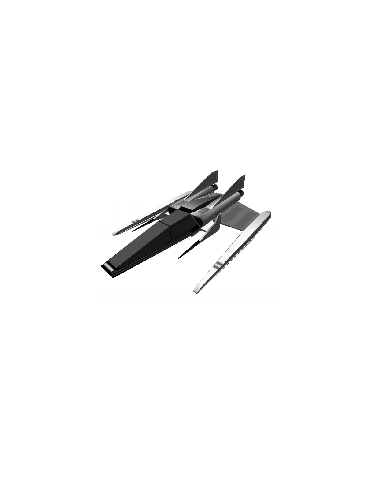
204
Chapter 7: Importing Databases
MultiGen has provided an OpenFlight-format importer, pfdLoadFile_flt(), for your use.
The loaders and associated documentation are in the directories
/usr/share/Performer/src/lib/libpfdb/libpfflt11 and libpfflt14. Refer to the Readme files in these
directories for important information about the loaders and for help in contacting
MultiGen for information about pfdLoadFile_flt() or the OpenFlight format.
The image in Figure 7-4 shows a model of a spacecraft created by Viewpoint Animation
Engineering using MultiGen. This OpenFlight format model was loaded into IRIS
Performer using pfdLoadFile_flt().
Figure 7-4 Spacecraft Model in FLIGHT Format
pfdLoadFile() uses the function pfdLoadFile_flt() to load OpenFlight format files into
IRIS Performer run-time data structures.
Files in the OpenFlight format are structured as a linear sequence of records. The first few
bytes of each record are a header containing an op-code, the length of the record, and
possibly an ASCII name for the record. The first record in the file is a special “database
header” record whose op-code, stored as a 2-byte short integer, has the value 1. This
opcode header can be used to identify OpenFlight-format files. By convention, these files
have a “.flt” filename extension.

Description of Supported Formats
205
pfdLoadFile_flt() makes use of several environment variables when locating data and
texture files. These variables and several additional functions, including
pfdConverterMode_flt(),pfdGetConverterMode_flt(), and pfdConverterAttr_flt()
assist in OpenFlight file processing.
McDonnell-Douglas GDS Format
The “.gds” format (also known as the “Things” format) is used in at least one CAD
system, and a minimal loader for this format has been developed for IRIS Performer
users. The IRIS Performer loader for “.gds” files is located in the
/usr/share/Performer/src/lib/libpfdb/libpfgds directory.
The GDS format subset accepted by the pfdLoadFile_gds() function is easy to describe.
It consists of the following five sequential sections in an ASCII file.
1. The number of vertices, which is given following a “YIN” tag.
2. The vertices, with one X, Y, Z triple per line for vertices lines.
3. The number zero on a line by itself.
4. The number of polygons on a line by itself.
5. A series of polygon definitions, each of which is represented on two or more lines.
The first line contains the number one and the name of a material to use for the
polygon. The next line or lines contain the indices for the polygons vertices. The
first number on the first line is the number of vertices. This is followed by that
number of vertex indices on that, and possibly subsequent, lines.
pfdLoadFile() uses the function pfdLoadFile_gds() to load “.gds” format files into
IRIS Performer.
Silicon Graphics GFO Format
The GFO format is the simple ASCII format of the barcelona database that is provided in
the IRIS Performer sample database directory. This database represents the famous
German Pavilion at the Barcelona Exhibition of 1929, which was designed by Ludwig
Mies van der Rohe and is shown in Figure 7-5.
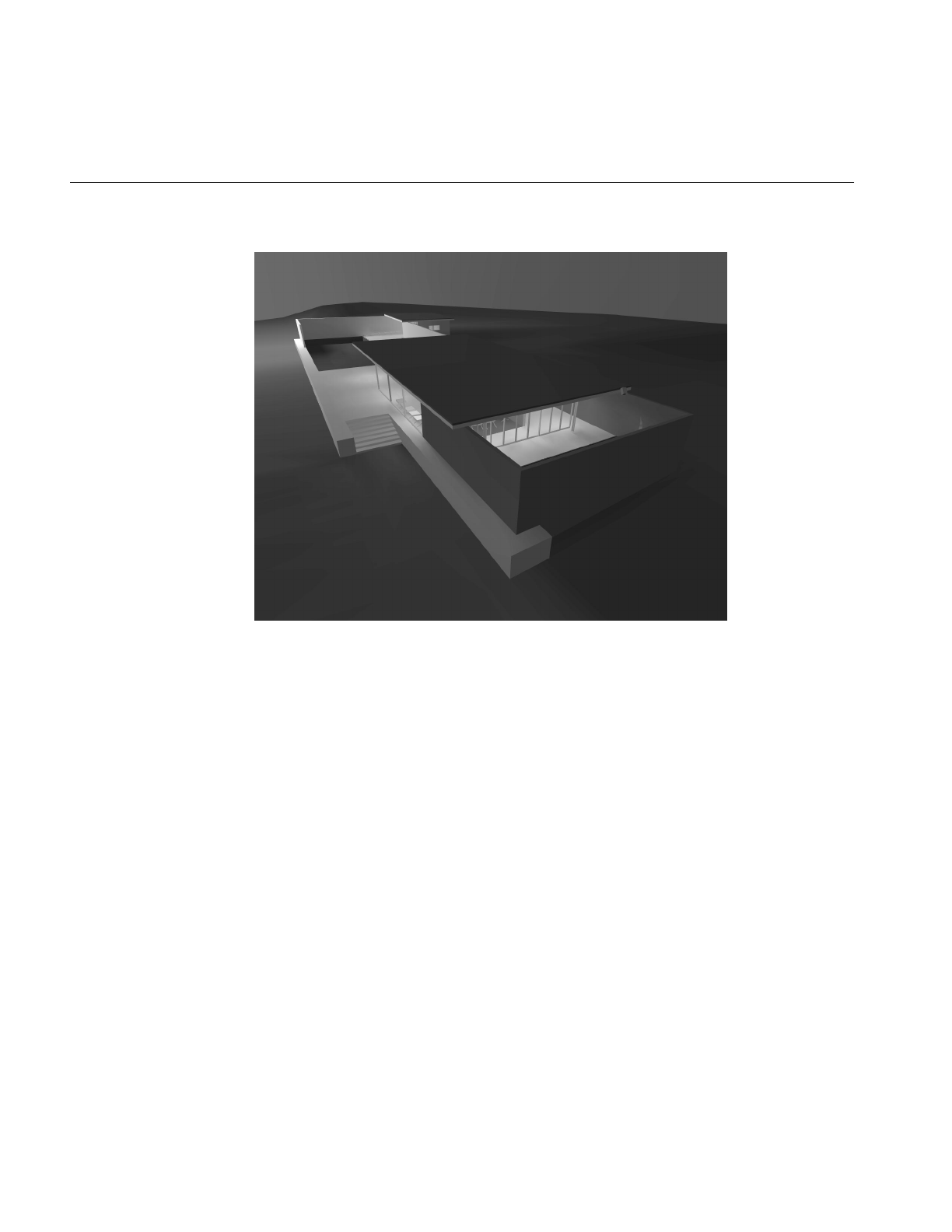
206
Chapter 7: Importing Databases
Figure 7-5 GFO Database of Mies van der Rohe’s German Pavilion
The source code for the GFO-format loader is provided in the file
/usr/share/Performer/src/lib/libpfdb/libpfgfo/pfbin.c.
pfdLoadFile() uses the function pfdLoadFile_gfo() to load GFO format files into IRIS
Performer run-time data-structures.
When working with GFO files, remember that hardware lighting isn’t used since all
illumination effects have already been accounted for with the ambient color at each
vertex.
The GFO format defines polygons with a color at every vertex. It is the output format of
an early radiosity system. Files in this format have a simple ASCII structure, as indicated
by the following abbreviated GFO file:

Description of Supported Formats
207
scope {
v3f {42.9632 8.7500 0.9374}
cpack {0x8785a9}
v3f {42.9632 8.0000 0.9374}
cpack {0x8785a9}
...
v3f {-1.0000 -6.5858 10.0000}
cpack {0xffffff}
polygon {cpack[0] v3f[0] cpack[1] v3f[1] cpack[2] v3f[2] cpack[3] v3f[3] }
polygon {cpack[4] v3f[4] cpack[5] v3f[5] cpack[6] v3f[6] cpack[7] v3f[7] }
...
polygon {cpack[7330] v3f[7330] cpack[7331] v3f[7331] cpack[7332] v3f[7332]
cpack[7333] v3f[7333] }
instance {
polygon[0]
polygon[1]
...
polygon[2675]
}
}
This example is taken from the file barcelona-l.gfo, one of only two known databases in the
GFO format. The importer uses functions from the libpfdu library (such as those from the
pfdBuilder) to generate efficient shared triangle strips. This increases the speed with
which GFO databases can be drawn and reduces the size and complexity of the loader,
since the builder’s functions hide the details of the pfGeoSet construction process.
Silicon Graphics IM Format
The “.im” format is a simple format developed for test purposes by the IRIS Performer
engineering team. As new features are added to IRIS Performer, the “.im” loader is
extended to allow experimentation and testing. A recent example of this is support for
pfText, pfString, and pfFont objects which can be seen by running perfly on the sample
data file fontsample.im. The IRIS Performer “.im” loader is in the
/usr/share/Performer/src/lib/libpfdb/libpfim directory.
Here is an example IM format file that creates an extruded 3D text string. Copy this to a
file ending in the extension “.im” and load it into Perfly. For a complete example of how
text is handled in IRIS Performer, use Perfly to examine the file
/usr/share/Performer/data/fontsample2.im.

208
Chapter 7: Importing Databases
breakup 0 0.0 0 0
new root top
end_root
new font mistr-extruded Mistr 3
end_font
new str_text textnode mistr-extruded 1
Hello World||
end_text
attach top textnode
pfdLoadFile() uses the function pfdLoadFile_im() to load “.im” format files into IRIS
Performer run-time data structures:
pfdLoadFile_im() searches the current IRIS Performer file path for the named file and
returns a pointer to the pfNode parenting the imported scene graph, or NULL if the file
isn’t readable or doesn’t contain a valid database.
AAI/Graphicon IRTP Format
The AAI/Graphicon “.irtp” format is used by the TopGen database modeling system
and by the Graphicon-2000 image generator. The name IRTP is an acronym for
Interactive Real-Time PHIGS. The IRIS Performer “.irtp” loader is in the
/usr/share/Performer/src/lib/libpfdb/libpfirtp directory. Though loader does not support the
more arcane IRTP features, such as binary separating planes or a global matrix table, it
has served as a basis for porting applications to IRIS Performer and the RealityEngine.
pfdLoadFile() uses the function pfdLoadFile_irtp() to load IRTP format files into IRIS
Performer run-time data-structures.
Silicon Graphics Open Inventor Format
The Open Inventor object-oriented 3D-graphics toolkit defines a persistent data format
that is also a superset of the VRML networked graphics data format. The image in
Figure 7-6 shows a sample Open Inventor data file.
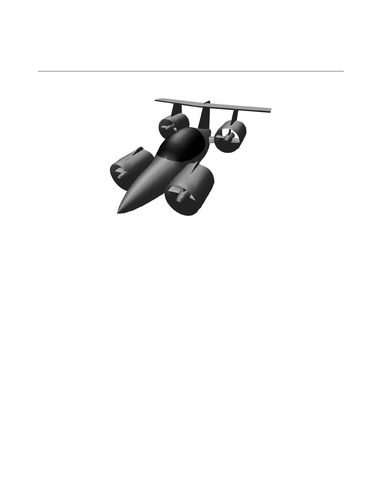
Description of Supported Formats
209
Figure 7-6 Aircar Database in IRIS Inventor Format
The model in Figure 7-6 represents one design for the perennial “personal aircar of the
future” concept. It was created, using Imagine, by Mike Halvorson of Impulse, and was
modeled after the Moller 400 as described in Popular Mechanics.
The Open Inventor data-file loader provided with IRIS Performer reads both binary and
ASCII format Open Inventor data files. Open Inventor scene graph description files in
both formats have the suffix “.iv” appended to their file names.
Here is a simple Open Inventor file that defines a cone:
#Inventor V2.1 ascii
Separator {
Cone {
}
}
The source code for the Open Inventor format importer is provided in the libpfdb/libpfiv
source directory.
pfdLoadFile() uses the function pfdLoadFile_iv() to load Open Inventor format files into
IRIS Performer run-time data-structures. IRIS Performer also comes with an Inventor
loader that works with Open Inventor 2.0, if Open Inventor 2.1 is not installed.

210
Chapter 7: Importing Databases
Lightscape Technologies LSA and LSB Formats
The Lightscape Visualization system is a product of Lightscape Technologies, Inc., and is
designed to compute accurate simulations of global illumination within complex 3D
environments. The output files created with Lightscape Visualization can be read into
IRIS Performer for real-time visual exploration.
Lightscape Technologies provides importers for two of their database formats, the simple
ASCII LSA format and the comprehensive binary LSB format. These loaders are in the
/usr/share/Performer/src/lib/libpfdb/libpflsa and libpflsb directories, in the files pflsa.c and
pflsb.c.Files in the LSA format are in ASCII and have the following components:
1. a 4x4 view matrix representing a default transformation
2. counts of the number of independent triangles, independent quadrilaterals, triangle
meshes, and quadrilateral meshes in the file
3. geometric data definitions
There are four types of geometric definitions in LSA files. The formats of these definitions
are as shown in Table 7-7.
Table 7-7 Geometric Definitions in LSA Files
Geometric Type Format
Triangle t X1 Y1 Z1 C1 X2 Y2 Z2 C2 X3 Y3 Z3 C3
Triangle meshtm n
X1 Y1 Z1 C1
X2 Y2 Z2 C2
...
Quadrilateralq X1 Y1 Z1 C1 X2 Y2 Z2 C2 X3 Y3 Z3 C3 X4 Y4 Z4 C4
Quadrilateral meshqm n
X1 Y1 Z1 C1
X2 Y2 Z2 C2
...
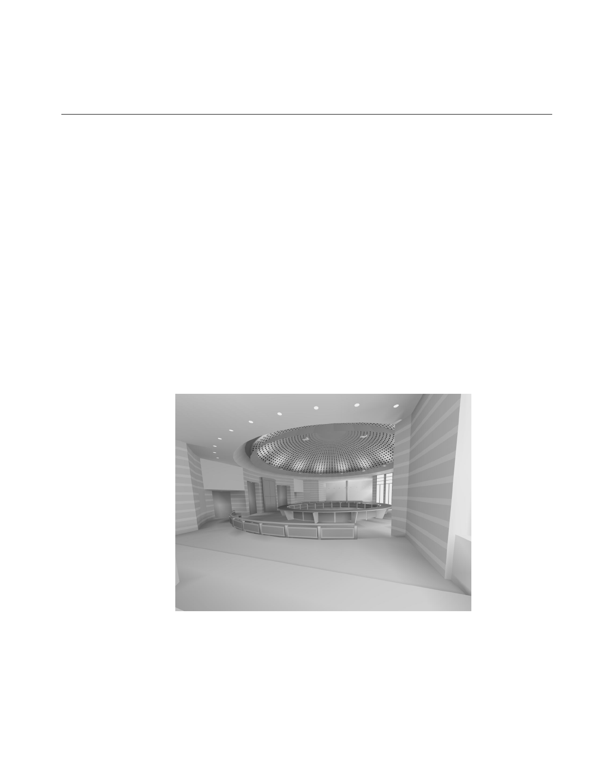
Description of Supported Formats
211
The Cn values in Table 7-7 refer to colors in the format accepted by the IRIS GL function
cpack(); these colors should be provided in decimal form. The X, Y, and Z values are
vertex coordinates. Polygon vertex ordering in LSA files is consistently
counter-clockwise, and polygon normals are not specified. The first few lines of the LSA
sample file chamber.0.lsa provide an example of the format:
0.486911 0.03228900 0.979046 0.9596590
-1.665110 0.00944197 0.286293 0.2806240
0.000000 1.92730000 -0.017805 -0.0174524
0.240398 -5.54670000 13.021200 13.4945000
1782 4751 0 0
t 4.35 -7.3677 2.57 6188666 6.5 -9.3 2.57 5663353 4.35 -9.3 2.57 5728890
t 6.5 -9.3 2.57 5663353 4.35 -7.3677 2.57 6188666 6.5 -8.2463 2.57 6057596
The count line indicates that the file contains 1782 independent triangles and 4751
independent quadrilaterals, which together represent 11,284 triangles. The image in
Figure 7-7 shows this database, the New Jerusalem City Hall. This was produced by
A.J. Diamond of Donald Schmitt and Company, Toronto, Canada, using the Lightscape
Visualization system.
Figure 7-7 LSA-Format City Hall Database

212
Chapter 7: Importing Databases
pfdLoadFile() uses the function pfdLoadFile_lsa() to load LSA format files into IRIS
Performer run-time data-structures.
Files in the LSB binary format have a very different structure from LSA files.
Representing not just polygon data, they contain much of the structural information
present in the “.ls” files used by the Lightscape Visualization system, including material,
layer, and texture definitions as well as a hierarchical mesh definition for geometry. This
information is structured as a series of data sections, which include:
• the signature, a text string that identifies the file
• the header, which contains global file information
• the material table, defining material properties
• the layer table, defining grouping and association
• the texture table, referencing texture images
• geometry in the form of clusters
The format of the geometric clusters is somewhat complicated. A cluster is a group of
coplanar surfaces called patches that share a common material, layer, and normal. Each
patch shares at least one edge with another patch in the cluster. Each patch defines either
a convex quadrilateral or a triangle, and patches represent quad-trees called nodes. Each
node points to its corner vertices and its children. The leaf nodes point to their corner
vertices and the child pointers can optionally point to the vertices that split an edge of
the node. Only the locations of vertices that are corners of the patches are stored in the
file; other vertices are created by subdividing nodes of the quad-tree as the LSB file is
loaded. The color information for each vertex is unique and is specified in the file.
The image in Figure 7-8 shows an LSB-format database developed during the design of
a hospital operating room. This database was produced by the DeWolff Partnership of
Rochester, New York, using the Lightscape Visualization system.
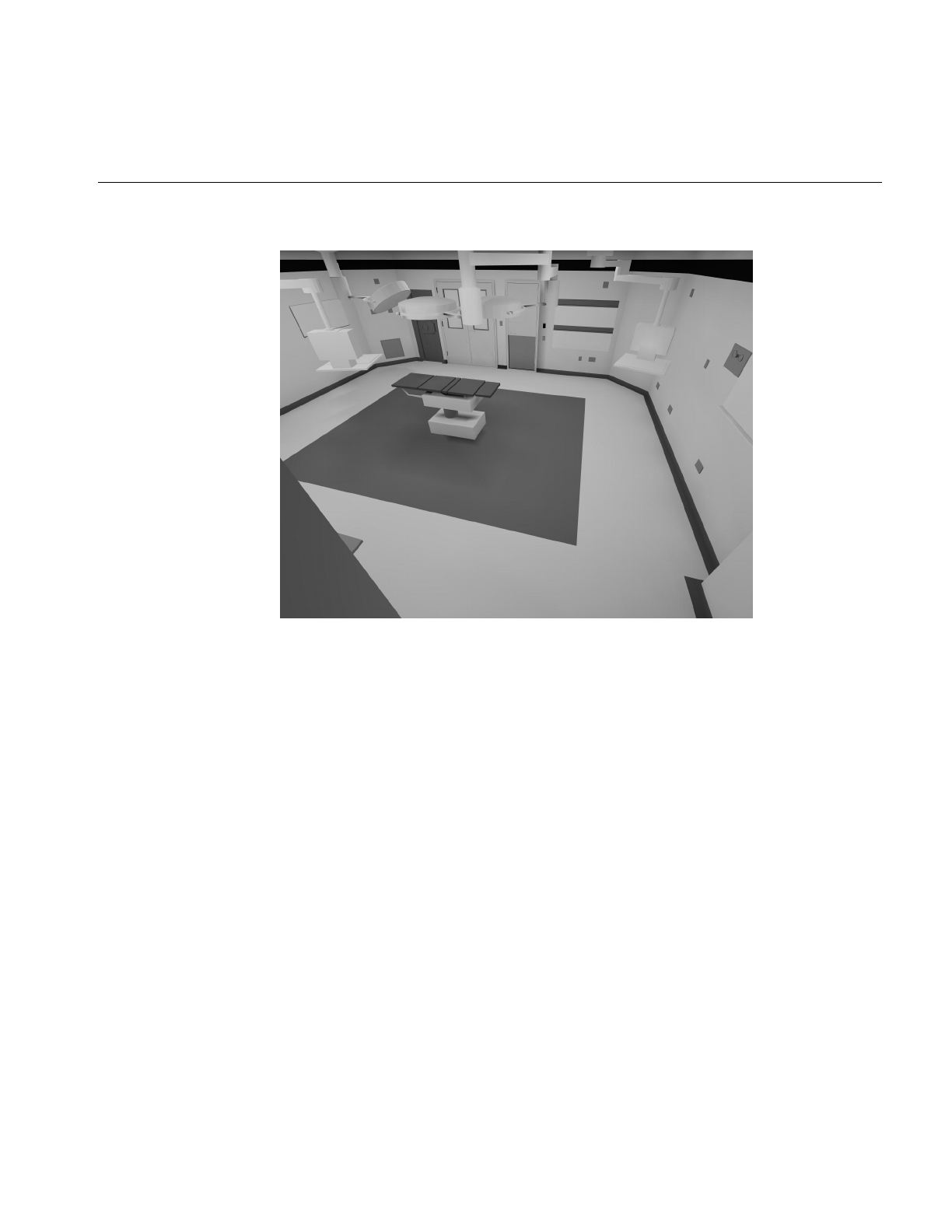
Description of Supported Formats
213
Figure 7-8 LSB-Format Operating Room Database
pfdLoadFile() uses the function pfdLoadFile_lsb() to load LSB format files into IRIS
Performer run-time data-structures.
When working with Lightscape Technologies files, remember that hardware lighting
isn’t needed because all illumination effects have already been accounted for with the
ambient color at each vertex.
Medit Productions MEDIT Format
The “.medit” format is used by the Medit database modeling system produced by Medit
Productions. The IRIS Performer “.medit” loader is in the
/usr/share/Performer/src/lib/libpfdb/libpfmedit directory.
pfdLoadFile() uses the function pfdLoadFile_medit() to load MEDIT format files into
IRIS Performer run-time data-structures.

214
Chapter 7: Importing Databases
NFF Neutral File Format
The “.nff” format was developed by Eric Haines as a way to provide standard procedural
databases for evaluating ray tracing software. IRIS Performer includes an extended NFF
loader with superquadric torus support, a named build keyword, and numerous small
bug fixes. The “.nff” loader is located in the /usr/share/Performer/src/lib/libpfdb/libpfnff
directory.
The file /usr/share/Performer/data/sampler.nff uses each of the NFF data types. It is an
excellent way to explore the “Show Tree”, “Draw Style”, and “Highlight Mode” features
of Perfly. It is included here:
#-- torus
f .75 .00 .25 .6 .8 20 0
t 5 5 0 0 0 1 2 1
build torus
#-- cylinder
f .00 .75 .25 .6 .8 20 0
c
15 5 -3 2
15 5 3 2
#-- put a disc on the top and bottom of the cylinder
d 15 5 -3 0 0 -1 0 2
d 15 5 3 0 0 1 0 2
build cylinder
#-- cone
f .00 .25 .75 .6 .8 20 0
c
25 5 -3 3
25 5 3 0
#-- put a disc on the bottom of the cone
d 25 5 -3 0 0 -1 0 3
build cone
#-- sphere
f .75 .00 .75 .6 .8 20 0
s 5 15 0 3
build sphere
#-- hexahedron
f .25 .25 .50 .6 .8 20 0
h 13 13 -2 17 17 2

Description of Supported Formats
215
build hexahedron
#-- superquadric sphere
f .80 .10 .30 .6 .8 20 0
ss 25 15 0 2 2 2 .1 .4
build superquadric_sphere
#-- disc (washer shape)
f .20 .20 .90 .6 .8 20 0
d 5 25 0 0 0 1 1 2.5
build disc
#-- grid (height field)
f .80 .80 .10 .6 .8 20 0
g 4 4 12 18 22 28 0 4
0 0 0 0
0 1 0 0
0 0 -1 0
0 0 0 0
build grid
#-- superquadric torid
f .40 .20 .60 .6 .8 20 0
st 25 25 0 0.5 0.5 0.5 .33 .33 3
build superquadric_torid
#-- polygon with no normals
f .20 .20 .20 .6 .8 20 0
p 4
-5 -5 -10
35 -5 -10
35 35 -10
-5 35 -10
build polygon
pfdLoadFile() uses the function pfdLoadFile_nff() to load NFF format files into IRIS
Performer run-time data-structures.

216
Chapter 7: Importing Databases
Wavefront Technology OBJ Format
The OBJ format is an ASCII data representation read and written by the Wavefront
Technology Model program. A number of database models in this format have been
placed in the public domain, making this a useful format to have available. IRIS
Performer provides the function pfdLoadFile_obj() to import OBJ files. The source code
for pfdLoadFile_obj() is in the file pfobj.c in the /usr/share/Performer/src/lib/libpfdb/libpfobj
loader source directory.
The OBJ-format database shown in Figure 7-9 models an office building that’s part of the
Silicon Graphics corporate campus in Mountain View, California.
Figure 7-9 Silicon Graphics Office Building as OBJ Database

Description of Supported Formats
217
Files in the OBJ format have a flexible all-ASCII structure, with simple keywords to direct
the parsing of the data. This format is best illustrated with a short example that defines
a texture-mapped square:
#-- ‘v’ defines a vertex; here are four vertices
v -5.000000 5.000000 0.000000
v -5.000000 -5.000000 0.000000
v 5.000000 -5.000000 0.000000
v 5.000000 5.000000 0.000000
#-- ‘vt’ defines a vertex texture coordinate; four are given
vt 0.000000 1.000000 0.000000
vt 0.000000 0.000000 0.000000
vt 1.000000 0.000000 0.000000
vt 1.000000 1.000000 0.000000
#-- ‘usemtl’ means select the material definition defined
#-- by the name MaterialName
usemtl MaterialName
#-- ‘usemap’ means select the texturing definition defined
#-- by the name TextureName
usemap TextureName
#-- ‘f’ defines a face. This face has four vertices ordered
#-- counter-clockwise from the upper left in both geometric
#-- and texture coordinates. Each pair of numbers separated
#-- by a slash indicates vertex and texture indices,
#-- respectively, for a polygon vertex.
f 1/1 2/2 3/3 4/4
pfdLoadFile() uses the function pfdLoadFile_obj() to load Wavefront OBJ files into IRIS
Performer run-time data-structures.
Silicon Graphics PFB Format
Although IRIS Performer has no true, native database format, the PFB format is designed
to exactly replicate the IRIS Performer scene graph, which increases loading speed. A file
in the PFB format has the following advantages:
• PFB files often load in one tenth (or less) of the time it takes an equivalent file in
another format to load.
• PFB files are often half the size of equivalent files in another format.

218
Chapter 7: Importing Databases
You can think of the PFB format as being a cache. You can convert your files into PFB for
fast and efficient loading or paging, but you should always keep your original files in
case you wish to modify them.
Converting to the PFB Format
You can convert files into the PFB format in one of the following ways:
• Use the function, pfdStoreFile_pfb() in libpfpfb.
• Use pfconv.
Silicon Graphics PFI Format
The PFI image file format is designed for fast loading of images into pfTextures.
pfLoadTexFile() can load PFI files as the image of a pfTexture. Since the format of the
image in a PFI file matches that of a pfTexture, data is not reformatted at load time.
Eliminating the reformatting often cuts the load time of textures to half of the load time
of the same image in the IRIS libimage format.
PFI files can contain the mipmaps of the image. This feature saves significant time in the
IRIS Performer DRAW process since it does not have to generate the mipmaps.
Creating PFI Files
PFI files are created in the following ways:
•pfSaveTexFile() creates a PFI file from a pfTexture.
• The pfdImage methods in libpfdu create PFI files.
• pficonv converts IRIS libimage files into PFI files.
• pfconv converts all referenced image files into PFI files when the setting
PFPFB_SAVE_TEXTURE_PFI mode is PF_ON. The command line options to do this
with pfconv is -Mpfb,5.

Description of Supported Formats
219
Silicon Graphics PHD Format
The PHD format was created to describe the geometric polyhedron definitions derived
mathematically by Andrew Hume and by the Kaleido program of Zvi Har’El. This format
describes only the geometric shape of polyhedra; it provides no specification for color,
texture, or appearance attributes such as specularity.
The IRIS Performer sample data directories contain numerous polyhedra in the PHD
format. The image in Figure 7-10 shows many of the polyhedron definitions laboriously
computed by Andrew Hume.
Figure 7-10 Plethora of Polyhedra in PHD Format
The source code for the PHD-format importer is in the file
/usr/share/Performer/src/lib/libpfdb/libpfpoly/pfphd.c.
PHD format files have a line-structured ASCII form; an initial keyword defines the
contents of each line of data. The file format consists of a filename definition (introduced
by the keyword file) followed by one or more object definitions.

220
Chapter 7: Importing Databases
Object definitions are bracketed by the keywords object.begin and object.end and contain
one or more polygon definitions. Objects can have a name in quotes following the
object.begin keyword; such a name is used by the loader for the name of the
corresponding IRIS Performer node.
Polygon definitions are bracketed by the keywords polygon.begin and polygon.end and
contain three or more vertex definitions.
Vertex definitions are introduced by the vertex keyword and define the X, Y, and Z
coordinates of a single vertex.
The following is a PHD-format definition of a unit-radius tetrahedron centered at the
origin of the coordinate axes. It is derived from the database developed by Andrew
Hume but has since been translated, scaled, and reformatted.
file 000.phd
object.begin "tetrahedron"
polygon.begin
vertex -0.090722 -0.366647 0.925925
vertex 0.544331 -0.628540 -0.555555
vertex 0.453608 0.890430 0.037037
polygon.end
polygon.begin
vertex -0.907218 0.104757 -0.407407
vertex -0.090722 -0.366647 0.925925
vertex 0.453608 0.890430 0.037037
polygon.end
polygon.begin
vertex -0.090722 -0.366647 0.925925
vertex -0.907218 0.104757 -0.407407
vertex 0.544331 -0.628540 -0.555555
polygon.end
polygon.begin
vertex 0.453608 0.890430 0.037037
vertex 0.544331 -0.628540 -0.555555
vertex -0.907218 0.104757 -0.407407
polygon.end
object.end
pfdLoadFile() uses the function pfdLoadFile_phd() to load PHD format files into IRIS
Performer run-time data-structures.
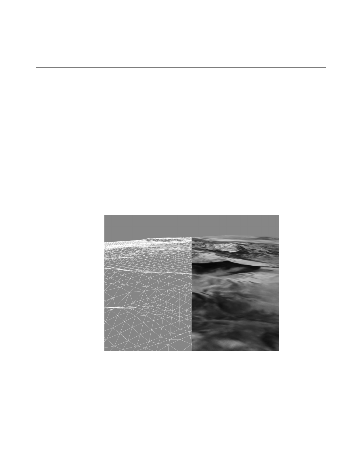
Description of Supported Formats
221
ThepfdLoadFile_phd() function composes a color with red, green, and blue components
uniformly distributed within the range 0.2 to 0.7 that is consistent for each polygon with
the same number of vertices within a single polyhedron.
Silicon Graphics PTU Format
The PTU format is named for the IRIS Performer Terrain Utilities, of which the
pfdLoadFile_ptu() function is the sole example at the present time. This function accepts
as input the name of a control file (the file with the “.ptu” filename extension) that defines
the desired terrain parameters and references additional data files.
The database shown in Figure 7-11 represents a portion of the Yellowstone National Park.
This terrain database was generated completely by the IRIS Performer Terrain Utility
data generator from digital terrain elevation data and satellite photographic images.
Image manipulation is performed using the Silicon Graphics ImageVision Library™
functions.
Figure 7-11 Terrain Database Generated by PTU Tools

222
Chapter 7: Importing Databases
The PTU control file has a fixed format that doesn’t use keywords. The contents of this
file are simply ASCII values representing the following data items:
1. The name to be assigned to the top-level pfNode built by pfdLoadFile_ptu().
2. The number of desired levels-of-detail (LOD) for the resulting terrain surface. The
pfdLoadFile_ptu() function will construct this many versions of the terrain, each
representing the whole surface but with exponentially fewer numbers of polygons
in each version.
3. The numbers of highest-LOD tiles that will tessellate the entire terrain surface in the
X and Y axis directions.
4. Two numeric values that define the mapping of texture image pixels to
world-coordinate terrain geometry. These values are the number of meters per texel
(texture pixel) of filtered grid post data in the X and Y axis dimensions.
5. The name of an image file that represents terrain height at regularly spaced sample
points in the form of a monochrome image whose brightness at each pixel indicates
the height at that sample point. Additional arguments are the number of samples in
the input image in the X and Y directions, as well as the desired number of samples
in these directions. The pfdLoadFile_ptu() function resamples the grid posts from
the original to the desired resolution by filtering the height image using SGI
ImageVision Library functions.
6. The name of an image file that represents the terrain texture image at regularly
spaced sample points. Subsequent arguments are the number of samples in the
image in the X and Y directions as well as the desired number of samples in these
directions. This image will be applied to the terrain geometry. The scale values
provided in the PTU file allow the terrain grid and texture image to be adjusted to
create an orthographic alignment.
7. An optional second texture-image filename that serves as a detail texture when the
terrain is viewed on RealityEngine systems. This texture is used in addition to the
base texture image.
8. An optional detail-texture spline-table definition. The blending of the primary
texture image and the secondary detail texture is controlled by a blend table defined
by this spline function. The spline table is optional even when a detail texture is
specified. Detail texture and its associated blend functions are applicable only on
RealityEngine systems.
The source code for the PTU-format importer is provided in the file
/usr/share/Performer/src/lib/libpfdb/libpfptu/pfptu.c.

Description of Supported Formats
223
pfdLoadFile() uses the function pfdLoadFile_ptu() to load PTU format files into IRIS
Performer run-time data-structures.
USNA Standard Graphics Format
The “.sgf” format is used at the United States Naval Academy as a standard graphics
format for geometric data. The loader was developed based on the description of the
standard graphics format as described by David F. Rogers and J. Alan Adams in the book
Mathematical Elements for Computer Graphics. The IRIS Performer “.sgf” format loader is
located in the directory /usr/share/Performer/src/lib/libpfdb/libpfsgf.
Here is the vector definition for four stacked squares in SGF form:
0, 0, 0
1, 0, 0
1, 1, 0
0, 1, 0
0, 0, 0
1.0e37, 1.0e37, 1.0e37
0, 0, 1
1, 0, 1
1, 1, 1
0, 1, 1
0, 0, 1
1.0e37, 1.0e37, 1.0e37
0, 0, 2
1, 0, 2
1, 1, 2
0, 1, 2
0, 0, 2
1.0e37, 1.0e37, 1.0e37
0, 0, 3
1, 0, 3
1, 1, 3
0, 1, 3
0, 0, 3
1.0e37, 1.0e37, 1.0e37
pfdLoadFile() uses the function pfdLoadFile_sgf() to load SGF format files into IRIS
Performer run-time data-structures.

224
Chapter 7: Importing Databases
Silicon Graphics SGO Format
The Silicon Graphics Object format is used by several cool utility programs and was one
of the first database formats supported by IRIS Performer. The image in Figure 7-12
shows a model generated by Paul Haeberli and loaded into perfly by the
pfdLoadFile_sgo() database importer.
Figure 7-12 Model in SGO Format
Objects in the SGO format have per-vertex color specification and multiple data formats.
Objects contained in SGO files are constructed from three data types:
• lists of quadrilaterals
• lists of triangles
• triangle meshes
Objects of different types can be included as data within one SGO file.

Description of Supported Formats
225
The SGO format has the following structure:
1. A magic number, 0x5424, which identifies the file as an SGO file.
2. A set of data for each object. Each object definition begins with an identifying token,
followed by geometric data. There can be multiple object definitions in a single file.
An end-of-data token terminates the file.
The layout of an SGO file is
<SGO-file magic number>
<data-type token for object #1>
<data for object #1>
<data-type token for object #2>
<data for object #2>
...
<data-type token for object #n>
<data for object #n>
<end-of-data token>
Each of the identifying tokens is 4 bytes long. Table 7-8 lists the symbol, value, and
meaning for each token.
The next word following any of the three object types is the number of 4-byte words of
data for that object. The format of this data varies depending on the object type.
Table 7-8 Object Tokens in the SGO Format
Symbol Value Meaning
OBJ_QUADLIST 1 Independent quadrilaterals
OBJ_TRILIST 2 Independent triangles
OBJ_TRIMESH 3 Triangle mesh
OBJ_END 4 End-of-data token

226
Chapter 7: Importing Databases
For quadrilateral list (OBJ_QUADLIST) and triangle list (OBJ_TRILIST) objects, there are
nine words of floating-point data for each vertex, as follows:
1. Three words that specify the components of the normal vector at the vertex.
2. Three words that specify the red, green, and blue color components, scaled to the
range 0.0 to 1.0.
3. Three words that specify the X, Y, and Z coordinates of the vertex itself.
In quadrilateral lists, vertices are in groups of four, so there are 4 × 9 = 36 words of data
for each quadrilateral. In triangle lists, vertices are in groups of three, for 3 × 9 = 27 words
per triangle.]
The triangle mesh, OBJ_TRIMESH, is the most complicated of the three object data types.
Triangle mesh data consists of a set of vertices followed by a set of mesh-control
commands. Triangle mesh data has the following format:
1. A long word that contains the number of words in the complete triangle mesh data
packet.
2. A long word that contains the number of floating-point words required by the
vertex data, at nine words per vertex.
3. The data for each vertex, consisting of nine floating-point words representing
normal, color, and coordinate data.
4. A list of triangle mesh controls.
The triangle mesh controls, each of which is one word in length, are listed in Table 7-9.
The triangle-mesh controls are interpreted sequentially. The first control must always be
OP_BGNTMESH, which initiates the mesh-decoding logic. After each mesh control is a
word (of type long integer) that indicates how many vertex indices follow. The vertex
Table 7-9 Mesh Control Tokens in the SGO Format
Symbol Value Meaning
OP_BGNTMESH 1 Begin a triangle strip.
OP_SWAPTMESH 2 Exchange old vertices.
OP_ENDBGNTMESH 3 End, then begin a strip.
OP_ENDTMESH 4 Terminate triangle mesh.

Description of Supported Formats
227
indices are in byte offsets, so to access vertex n, you must use the byte offset n × 9 × 4. See
the graphics library reference books listed under “Bibliography” on page xxxvi for more
information on triangle meshes (particularly see the IRIS GL books, if you’re using IRIS
GL, for information on the swap-triangle-mesh concept).
pfdLoadFile() uses the function pfdLoadFile_sgo() to load SGO format files into IRIS
Performer run-time data-structures.
You can find the source code for the SGO-format importer in the file pfsgo.c. This importer
doesn’t attempt to decode any triangle meshes present in input files; instead, it
terminates the file conversion process as soon as an OBJ_TRIMESH data-type token is
encountered. If you use SGO-format files containing triangle meshes you’ll need to
extend the conversion support to include the triangle mesh data type.
USNA Simple Polygon File Format
The “.spf” format is used at the United States Naval Academy as a simple polygon file
format for geometric data. The loader was developed based on the description in the
book Mathematical Elements for Computer Graphics. The IRIS Performer “.spf” loader is in
the /usr/share/Performer/src/lib/libpfdb/libpfspf directory.
The following “.spf” format file is defined in that book.
polygon with a hole
14,2
4,4
4,26
20,26
28,18
28,4
21,4
21,8
10,8
10,4
10,12
10,20
17,20
21,16
21,12
9,1,2,3,4,5,6,7,8,9
5,10,11,12,13,14

228
Chapter 7: Importing Databases
If you look at this file in Perfly you will see that the hole is not cut out of the letter “A” as
might be desired. Such computational geometry computations are not considered the
province of simple database loaders.
pfdLoadFile() uses the function pfdLoadFile_spf() to load SPF format files into IRIS
Performer run-time data-structures.
Sierpinski Sponge Loader
The Sierpinski Sponge (a.k.a. Menger Sponge) loader is not based on a data format but
rather is a procedural data generator. The loader interprets the portion of the user
provided “file name” before the period and extension as an integer which specifies the
number of recursive subdivisions desired in data generation. For example, providing the
pseudo filename “3.sponge” to perfly will result in the Sponge loader being invoked and
generating a sponge object using three levels of recursion, resulting in a 35712 polygon
database object. The IRIS Performer “.sponge” loader can be found in the
/usr/share/Performer/src/lib/libpfdb/libpfsponge directory.
pfdLoadFile() uses the function pfdLoadFile_sponge() to load Sponge format files into
IRIS Performer run-time data-structures.
Star Chart Format
The “.star” format is a distillation of astronomical data from the Yale Compact Star Chart.
The sample data file /usr/share/Performer/data/3010.star contains data from the YCSC that
has been reduced to a list of the 3010 brightest stars as seen from Earth and positioned as
3010 points of light on a unit-radius sphere. The IRIS Performer “.star” loader can read
this data and is provided as a convenience for making dusk, dawn, and night-time
scenes. The loader is in the /usr/share/Performer/src/lib/libpfdb/libpfstar directory.
Data in a “.star” file is simply a series of ASCII lines with the “s” (for star) keyword
followed by X, Y, and Z coordinates, brightness, and an optional name. Here are the 10
brightest stars (excluding Sol) in the “.star” format:
s -0.18746032 0.93921369 -0.28763914 1.00 Sirius
s -0.06323564 0.60291260 -0.79529721 1.00 Canopus
s -0.78377002 -0.52700269 0.32859191 1.00 Arcturus
s 0.18718566 0.73014212 0.65715599 1.00 Capella
s 0.12507832 -0.76942003 0.62637711 0.99 Vega
s 0.13051330 0.68228769 0.71933979 0.99 Capella
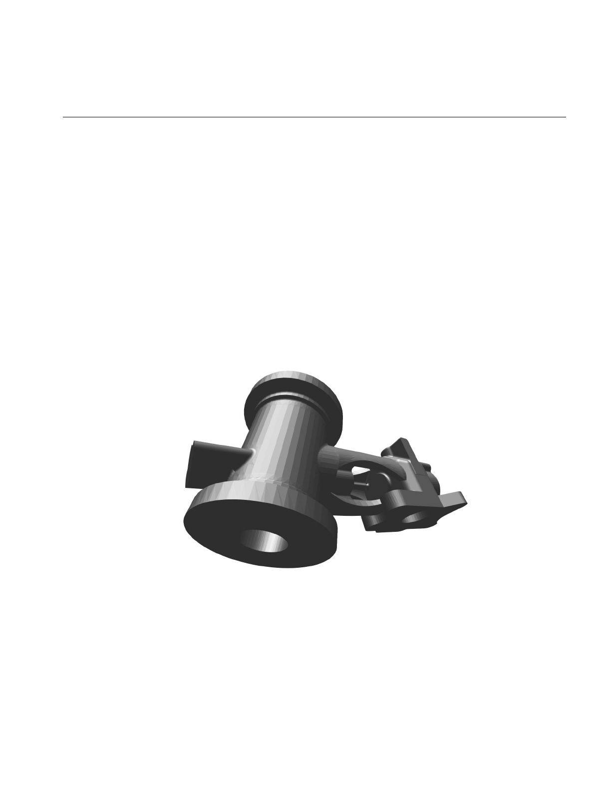
Description of Supported Formats
229
s 0.19507207 0.97036278 -0.14262892 0.98 Rigel
s -0.37387931 -0.31261155 -0.87320572 0.94 Rigil Kentaurus
s -0.41809806 0.90381104 0.09121194 0.94 Procyon
s 0.49255905 0.22369388 -0.84103900 0.92 Achernar
pfdLoadFile() uses the function pfdLoadFile_star() to load Star format files into IRIS
Performer run-time data-structures.
3D Lithography STL Format
The STL format is used to define 3D solids to be imaged by 3D lithography systems. STL
defines objects as collections of triangular facets, each with an associated face normal.
The ASCII version of this format is known as STLA and has a very simple structure.
The image in Figure 7-13 shows a typical STLA mechanical CAD database. This model is
defined in the bendix.stla sample data file.
Figure 7-13 Sample STLA Database
The source code for the STLA-format loader is in the files
/usr/share/Performer/src/lib/libpfdb/libpfstla/pfstla.c.

230
Chapter 7: Importing Databases
STLA-format files have a line-structured ASCII form; an initial keyword defines the
contents of each line of data. An STLA file consists of one or more facet definitions, each
of which contains
1. the facet normal, indicated with the facet normal keyword
2. the facet vertices, bracketed by outer loop and endloop keywords
3. the endloop keyword
Here is an excerpt from nut.stla, one of the STLA files provided in the IRIS Performer
sample data directories. These are the first two polygons of a 524-triangle hex-nut object:
facet normal 0 -1 0
outer loop
vertex 0.180666 -7.62 2.70757
vertex -4.78652 -7.62 1.76185
vertex -4.436 -7.62 0
endloop
endfacet
facet normal -0.381579 -0.921214 -0.075915
outer loop
vertex -4.48833 -7.59833 0
vertex -4.436 -7.62 0
vertex -4.78652 -7.62 1.76185
endloop
endfacet
Use this function to import data from STLA-format files into IRIS Performer run-time
data structures:
pfNode *pfdLoadFile_stla(char *fileName);
pfdLoadFile_stla() searches the current IRIS Performer file path for the file named by the
fileName argument and returns a pointer to the pfNode that parents the imported scene
graph, or NULL if the file isn’t readable or doesn’t contain recognizable STLA format
data.
SuperViewer SV Format
The SuperViewer (SV) format is one of the several database formats that the I3DM
database modeling tool can read and write. The I3DM modeler was developed by John
Kichury of Silicon Graphics and is provided with IRIS Performer. The source code for the
SV format importer is in the file pfsv.c.
Description of Supported Formats
231
The passenger vehicle database shown in Figure 7-14 was modeled using I3DM and is
stored in the SV database format.
Figure 7-14 Early Automobile in SuperViewer SV Format
Within SV files, object geometry and attributes are described between text lines that
contain the keywords model and endmodel. For example:
model wing
geometry and attributes
endmodel

232
Chapter 7: Importing Databases
Any number of models can appear within a SuperViewer file. The geometry and
attribute data mentioned above each consist of one of the following types:
• 3D Polygon with vertex normals and optional texture coordinates
poly3dn <num_vertices> [textured]
x1 y1 z1 nx1 ny1 nz1 [s1 t1]
x2 y2 z2 nx2 ny2 nz2 [s2 t2]
...
Where
–Xn Yn Zn are the nth vertex coordinates
–Nxn Nyn Nzn are the nth vertex normals
–Sn Tn are the nth texture coordinates
• 3D Triangle mesh with vertex normals and optional texture coordinates
tmeshn <num_vertices> [textured]
x1 y1 z1 nx1 ny1 nz1 [s1 t1]
x2 y2 z2 nx2 ny2 nz2 [s2 t2]
...
Where
–Xn Yn Zn are the nth vertex coordinates
–Nxn Nyn Nzn are the nth vertex normals
–Sn Tn are the nth texture coordinates
• Material definition. If the material directive exists before a model definition, it is
taken as a new material specification. Its format is:
material n Ar Ag Ab Dr Dg Db Sr Sg Sb Shine Er Eg Eb
Where
–n is an integer specifying a material number
–Ar Ag Ab is the ambient color
–Dr Dg Db is the diffuse color
–Sr Sg Sb is the specular color
–Shine is the material shininess
–Er Eg Eb is the emissive color

Description of Supported Formats
233
If the material directive exists within a model description, the format is:
material n
Where n is an integer specifying which material (as defined by the material
description above) is to be assigned to subsequent data.
• Texture definition. If the texture directive exists before a model definition it is taken
as a new texture specification. Its format is:
texture n TextureFileName
If the texture directive exists within a model description, the format is:
texture n
Where n is an integer specifying which texture (as defined by the texture
description above) is to be assigned to subsequent data.
• Backface polygon display mode. The backface directive is specified within model
definitions to control backface polygon culling:
backface mode
Where a mode of “on” allows the display of backfacing polygons and a mode of “off”
suppresses their display.
In actual use the SV format is somewhat self-documenting. Here is part of the SV file
apple.sv from the /usr/share/Performer/data directory:
material 20 0.0 0.0 0 0.400000 0.000000 0 0.333333 0.000000 0.0 10.0000 0 0 0
material 42 0.2 0.2 0 0.666667 0.666667 0 0.800000 0.800000 0.8 94.1606 0 0 0
material 44 0.0 0.2 0 0.000000 0.200000 0 0.000000 0.266667 0.0 5.0000 0 0 0
texture 4 prchmnt.rgb
texture 6 wood.rgb
model LEAF
material 44
texture 4
backface on
poly3dn 4 textured
1.35265 1.35761 13.8338 0.0686595 -0.234553 -0.969676 0 1
0.88243 0.96366 14.0329 0.0502096 -0.376701 -0.924973 0 0.75
-4.44467 1.24026 13.5669 0.0363863 -0.337291 -0.940697 0.0909091 0.75
-2.37938 2.17479 13.3626 0.0363863 -0.337291 -0.940697 0.0909091 1

234
Chapter 7: Importing Databases
poly3dn 4 textured
-2.37938 2.17479 13.3626 0.0363863 -0.337291 -0.940697 0.0909091 1
-4.44467 1.24026 13.5669 0.0363863 -0.337291 -0.940697 0.0909091 0.75
-9.23775 2.34664 13.1475 0.0344832 -0.284369 -0.958095 0.181818 0.75
-6.69592 3.94535 12.6716 0.0344832 -0.284369 -0.958095 0.181818 1
This excerpt specifies material properties and references texture images stored in the files
prchmnt.rgb and wood.rgb, and then defines two polygons.
pfdLoadFile() uses the function pfdLoadFile_sv() to load SuperViewer files into IRIS
Performer run-time data-structures.
Geometry Center Triangle Format
The “.tri” format is used at the University of Minnesota’s Geometry Center as a simple
geometric data representation. The loader was developed by inspection of a few sample
files. The IRIS Performer “.tri” loader is in the /usr/share/Performer/src/lib/libpfdb/libpftri
directory.
These files have a very simple format: a line per vertex with position and normal given
on each line as 6 ASCII numeric values. The file is simply a series of these triangle
definitions. Here are the first two triangles from the data file
/usr/share/Performer/data/mobrect.tri:
1.788180 1.000870 0.135214 0.076169 -0.085488 0.993423
1.574000 0.925908 0.146652 0.089015 -0.086072 0.992304
1.793360 0.634711 0.099409 0.076402 -0.111845 0.990784
0.836848 -0.595230 0.197960 0.156677 0.044503 0.986647
0.709638 -0.345676 0.210010 0.157642 0.021968 0.987252
0.581200 -0.535321 0.234807 0.145068 0.030985 0.988936
pfdLoadFile() uses the function pfdLoadFile_tri() to load “.tri” format files into IRIS
Performer run-time data-structures.
UNC Walkthrough Format
The “.unc” format was once used at the University of North Carolina as a format for
geometric data in an architectural walkthrough application. The loader was developed
based on inspection of a few sample files. The IRIS Performer “.unc” loader is in the
/usr/share/Performer/src/lib/libpfdb/libpfunc directory.

Database Operators with Pseudo Loaders
235
pfdLoadFile() uses the function pfdLoadFile_unc() to load UNC format files into IRIS
Performer run-time data-structures.
WRL Format
The VRML 2.0 format for IRIS Performer, wrl, is made by DRaW Computing AssociatesR.
It accepts geometry and texture only. Basic geometry nodes like Sphere, Cone, Cylinder,
Box and related nodes like Shape, Material, Appearance, TextureTransform,
ImageTexture, and ElevationGrid are supported. Also, complex geometries can be
obtained using the IndexedFaceSet node. You can do geometric manipulations to nodes
using Group nodes and Transform nodes. You can also make very complex structures
using PROTOs, where you group many geometry nodes.
Database Operators with Pseudo Loaders
The IRIS Performer dynamic database loading mechanism provides additional DSOs
that operate on the resulting scene graph from a file or set of files after the file(s) are
loaded. This mechanism, called “pseudo loaders,” enables the desired-operator DSO to
be specified as additional suffixes to the file name. The DSO matching the last suffix is
loaded first and provided the entire filename. That pseudo loader then can parse the
arbitrary filename and invoke the next operator or loader and then operate on the results.
This process allows additional arguments to be buried in the specified filename for the
pseudo loader to detect and parse.
One set of pseudo loaders included with IRIS Performer are the rot, trans, and scale
loaders. These loaders take hpr and xyz arguments in addition to their Filename and can
be invoked from any program using pfdLoadFile(), for example:
% perfly cow.obj.-90,90,0.rot
-90, 90, and 0 are the h,p, and r values, respectively.
If you are using a shell with argument expansion, such as csh, you can create interesting
cow art. Try out the following example:
% perfly cow.obj.{0,1},0,0.trans cow.obj.{0,1,2,3,4},0,-5.trans
Specifying a base filename is only needed if the specified pseudo loader expects a file to
operate on. Loaders can generate their scene graphics procedurally based on simple
parameters specified in the command string.

236
Chapter 7: Importing Databases
The pseudo loaders in the IRIS Performer distribution are described in Table 7-10.
Pseudo loaders should define pfdLoadNeededDSOs_EXT() for:
• Pre-initializing DSOs.
• Loading other, special files.
• Performing additional initialization, such as class initialization, that should happen
before pfConfig().
Table 7-10 IRIS Performer Pseudo Loaders
Pseudo Loaders Description
libpfrot Add pfSCS at root to rotate scene graph by specified <h>,<p>,<r>
libpftrans Add pfSCS at root to translate scene graph by specified <x>,<y>,<z>
libpfscale Add pfSCS at root to sale scene graph by specified <x>,<y>,<z>
libpfclosest Adds run-time app callback to highlight closest point each frame
libpfcliptile Adds callback to compute for the specified
<tilename>,<minS>,<minT>,<maxS>,<maxT> the proper virtual cliptexture
viewing parameters.
libpfsphere Generates a sphere database with morphing LOD starting from an n-gon for
specified <n>, power of 2.
libpfvct Convert normal cliptexture .ct file to virtual cliptexture

This chapter discusses the classes used to create the shapes in Performer
scenes.
“Geometry”
Chapter 8


239
Chapter 8
8. Geometry
All libpr geometry is defined by modular units that employ a flexible specification
method. These basic groups of geometric primitives are termed pfGeoSets.
Geometry Sets
A pfGeoSet is a collection of geometry that shares certain characteristics. All items in a
pfGeoSet must be of the same primitive type (whether they’re points, lines, or triangles)
and share the same set of attribute bindings (you can’t specify colors-per-vertex for some
items and colors-per-primitive for others in the same pfGeoSet). A pfGeoSet forms
primitives out of lists of attributes that may be either indexed or nonindexed. An indexed
pfGeoSet uses a list of unsigned short integers to index an attribute list. (See “Attributes”
on page 246 for information about attributes and bindings.)
Indexing provides a more general mechanism for specifying geometry than hard-wired
attribute lists and also has the potential for substantial memory savings as a result of
shared attributes. Nonindexed pfGeoSets are sometimes easier to construct, usually a bit
faster to render, and may save memory (since no extra space is needed for index lists) in
situations where vertex sharing isn’t possible. A pfGeoSet must be either completely
indexed or completely nonindexed; it’s not legal to have some attributes indexed and
others nonindexed.
Note: libpf applications can include pfGeoSets in the scene graph with the pfGeode
(Geometry Node).

240
Chapter 8: Geometry
Table 8-1 lists a subset of the routines that manipulate pfGeoSets.
Table 8-1 pfGeoSet Routines
Function Description
pfNewGSet Create a new pfGeoSet.
pfDelete Delete a pfGeoSet.
pfCopy Copy a pfGeoSet.
pfGSetGState Specify the pfGeoState to be used.
pfGSetGStateIndex Specify the pfGeoState index to be used.
pfGSetNumPrims Specify the number of primitive items.
pfGSetPrimType Specify the type of primitive.
pfGSetPrimLengths Set the lengths array for strip primitives.
pfGetGSetPrimLength Get the length for the specified strip primitive.
pfGSetAttr Set the attribute bindings.
pfGSetDrawMode Specify draw mode, e.g., flat shading or wireframe.
pfGSetLineWidth Set the line width for line primitives.
pfGSetPntSize Set the point size for point primitives.
pfGSetHlight Specify highlighting type for drawing.
pfDrawGSet Draw a pfGeoSet.
pfGSetBBox Specify a bounding box for the geometry.
pfGSetIsectMask Specify an intersection mask for pfGSetIsectSegs.
pfGSetIsectSegs Intersect line segments with pfGeoSet geometry.
pfQueryGSet Determine the number of triangles or vertices.
pfPrint Print the pfGeoSet contents.

Geometry Sets
241
Primitive Types
All primitives within a given pfGeoSet must be of the same type. To set the type of all
primitives in a pfGeoSet named gset, call pfGSetPrimType(gset,type). Table 8-2 lists the
primitive type tokens, the primitive types that they represent, and the number of vertices
in a coordinate list for that type of primitive.
where the parameters in the last column represent:
numPrims is the number of primitive items in the pfGeoSet, as set by
pfGSetNumPrims().
lengths is the array of strip lengths in the pfGeoSet, as set by
pfGSetPrimLengths() (note that length is measured here in terms of
number of vertices).
Table 8-2 Geometry Primitives
Token Primitive Type Number of Vertices
PFGS_POINTS Points numPrims
PFGS_LINES Independent line segments 2 * numPrims
PFGS_LINESTRIPS Strips of connected lines Sum of lengths array
PFGS_FLAT_LINESTRIPS Strips of flat-shaded lines Sum of lengths array
PFGS_TRIS Independent triangles 3 * numPrims
PFGS_TRISTRIPS Strips of connected triangles Sum of lengths array
PFGS_FLAT_TRISTRIPS Strips of flat-shaded triangles Sum of lengths array
PFGS_TRIFANS Fan of conected triangles Sum of lengths array
PFGS_FLAT_TRIFANS Fan of flat-shaded triangles Sum of lengths array
PFGS_QUADS Independent quadrilaterals 4 * numPrims
PFGS_POLYS Independent polygons Sum of lengths array

242
Chapter 8: Geometry
Connected primitive types (line strips, triangle strips, and polygons) require a separate
array that specifies the number of vertices in each primitive. Length is defined as the
number of vertices in a strip for STRIP primitives and is the number of vertices in a
polygon for the POLYS primitive type. The number of line segments in a line strip is
numVerts - 1, while the number of triangles in a triangle strip and polygon is numVerts -
2. Use pfGSetPrimLengths() to set the length array for strip primitives.
The number of primitives in a pfGeoSet is specified by pfGSetNumPrims(gset,num). For
strip and polygon primitives, num is the number of strips or polygons in gset.
pfGeoSet Draw Mode
In addition to the primitive type, pfGSetDrawMode() further defines how a primitive is
drawn. Triangles, triangle strips, quadrilaterals and polygons can be specified as either
filled or as wireframe, where only the outline of the primitive is drawn. Use the
PFGS_WIREFRAME argument to enable/disable wireframe mode. Another argument,
PFGS_FLATSHADE, specifies that primitives should be shaded. If flat shading is
enabled, each primitive or element in a strip is shaded with a single color.
PFGS_COMPILE_GL
At the next draw for each pfState, compile gset’s geometry into a GL
display list and subsequently render the display list.
PFGS_DRAW_GLOBJ
Select the rendering of an already created display list but do not force a
re-compile.
PFGS_PACKED_ATTRS
Use the gset’s packed attribute arrays, set with the
PFGS_PACKED_ATTRS to pfGSetAttr, to render geometry with GL
vertex arrays. This mode is only available under OpenGL operation.
pfGeoSets are normally processed in immediate mode which means that pfDrawGSet()
sends attributes from the user-supplied attribute arrays to the Graphics Pipeline for
rendering. However, this kind of processing is subject to some overhead, particularly if
the pfGeoSet contains few primitives. In some cases it may help to use GL display lists
(this is different from the libpr display list type pfDispList) or compiled mode. In compiled
mode, pfGeoSet attributes are copied from the attribute lists into a special data structure
called a display list during a compilation stage. This data structure is highly optimized
for efficient transfer to the graphics hardware. However, compiled mode has some major
disadvantages:

Geometry Sets
243
• compilation is usually costly
• a GL display list must be recompiled whenever its pfGeoSet’s attributes change
• the GL display list uses a significant amount extra host memory
In general, immediate-mode will offer excellent performance with minimal memory
usage and no restrictions on attribute volatility which is a key aspect in may advanced
applications. Despite this, experimentation may show databases or machines where
compiled mode offers a performance benefit.
To enable or disable compiled mode, call pfGSetDrawMode() with the
PFGS_COMPILE_GL token. When enabled, compilation is delayed until the next time
the pfGeoSet is drawn with pfDrawGSet(). Subsequent calls to pfDrawGSet() will then
send the compiled pfGeoSet to the graphics hardware.
To select a display list to render, without recompiling it, use
pfGSetDrawMode(PFGS_DRAW_GLOBJ}.
Packed Attributes
Packed attributes is an optimized way of sending formatted data to the graphics pipeline
under OpenGL that does not incur the same memory overead or re-compilation burden
as GL display lists. To render geometry with packed attributes, use the
pfGSetDrawMode(PFGS_PACKED_ATTRS) method when using OpenGL. This
pfGSetAttr list includes the currently bound PER_VERTEX vertex attribute data packed
into a single non-indexed array. When specifying a packed attribute array, the optional
vertex attributes, colors, normals, and texture coordinates, can be NULL. This array, like
the other attribute arrays, is then shared between Perfomrer, the GL, and accessible by
the user. Optionally, you can put your vertex coordinates in this packed array but in this
case the vertices must be duplicated in the normal coordinate array becuase vertex
coordinate data is used internally for other non-drawing operations such as intersections
and computation of bounding geometry. Packed attribute arrays also allow IRIS
Performer to extend the vertex attribute types accepted by pfGeoSets. There are several
base formats that expect all currently bound attributes of specified data type (unsigned
byte, short, or float) to be in the attribute array. Attributes specieid by the format but not
bound to vertices are assumed to not be present and the present data packed with the
data for each vertex starting on a 32bit word-aligned boundary. Then, there are several
derived formats that let you put some attribute data in the packed array while leaving
the rest in the normal individual coordinate attribute arrays. Table 8-3 shows the
different base formats supported.

244
Chapter 8: Geometry
To create packed attributes, you can use the utility pfuTravCreatePackedAttrs(), which
traverses a scene graph to create packed attributes for pfGeoSets and, optionally,
pfDelete redundant attribute arrays. This utility packs the pfGeoSet attributes using
pfuFillGSetPackedAttrs(). Examples of packed attribute usage can be seen in
/usr/share/Performer/src/pguide/libpr/C/packedattrs.c and in
/usr/share/Performer/src/sample/C/perfly.c and /usr/share/Performer/src/sample/C++/perfly.C.
Primitive Connectivity
A pfGeoSet requires a coordinate array that specifies the world coordinate positions of
primitive vertices. This array is either indexed or not, depending on whether a
coordinate index list is supplied. If the index list is supplied, it’s used to index the
coordinate array; if not, the coordinate array is interpreted in a sequential order.
A pfGeoSet’s primitive type dictates the connectivity from vertex to vertex to define
geometry. Figure 8-1 shows a coordinate array consisting of four coordinates, A, B, C,
and D, and the geometry resulting from different primitive types. This example uses
index lists that index the coordinate array.
Table 8-3 pfGeoSet PACKED_ATTR Formats
Format Description
PFGS_PA_C4UBN3ST2FV3F Accepts all currently bound coordinate attributes, colors are
unsigned bytes normals are shorts. Vertices are duplicated in
the packed attribute array.
PFGS_PA_C4UBN3ST2F Vertices are in the normal coordinate array.
PFGS_PA_C4UBT2F Normals and vertices are in the normal coordinate array.
PFGS_PA_C4UBN3ST2SV3F All bound coordinate attributes are in the packed attribute
array. Colors are unsigned bytes, normals are shorts, and
texture coordinates are unsigned shorts.
PFGS_PA_C4UBN3ST3FV3F Texture coordinates are 3D floats.
PFGS_PA_C4UBN3ST3SV3F Texture coordinates are 2D shorts.
Geometry Sets
245
Note: Flat-shaded line strip and flat-shaded triangle strip primitives have the vertices
listed in the same order as for the smooth-shaded varieties.
Figure 8-1 Primitives and Connectivity
A
B
C
D
XA, YA, ZA
XB, YB, ZB
XC, YC, ZC
XD, YD, ZD
XN, YN, ZN
O
1
2
3
...
n
Vertex list
Points
Primitive
type
Geometry
Index list
Line segments Line strips
0
1
2
3
0
3
1
2
0
1
3
2
2
3
0
1
3
2
1
0
Independent
triangles
Primitive
type
Geometry
Index list
Quadrilaterals Triangle strips Polygons
0
1
3
3
1
2
0
1
2
3
0
1
3
2
...
n
0
1
2
3
...
n

246
Chapter 8: Geometry
Attributes
The definition of a primitive isn’t complete without attributes. In addition to a primitive
type and count, a pfGeoSet references four attribute arrays (see Figure 8-2):
• colors (red, green, blue, alpha)
• normals (Nx, Ny, Nz)
• texture coordinates (S, T)
• vertex coordinates (X, Y, Z)
(A pfGeoState is also associated with each pfGeoSet; see Chapter 9, “Graphics State” for
details.) The four components listed above can be specified with pfGSetAttr() and in two
ways: by indexed specification—using a pointer to an array of components and a pointer
to an array of indices; or by direct specification—providing a NULL pointer for the
indices, which indicates that the indices are sequential from the initial value of zero. The
choice of indexed or direct components applies to an entire pfGeoSet; that is, all of the
supplied components within one pfGeoSet must use the same method. However, you
can emulate partially indexed pfGeoSets by using indexed specification and making each
nonindexed attribute’s index list be a single shared “identity mapping” index array
whose elements are 0, 1, 2, 3,…, N-1 where N is the largest number of attributes in any
referencing pfGeoSet. (You can share the same array for all such emulated pfGeoSets.).
The direct method avoids one level of indirection and may have a performance
advantage compared with indexed specification for some combinations of CPU and
graphics subsystem.
Note: it is highly recommended that pfMalloc() be used to allocate your arrays of
attribute data. This will allow IRIS Performer to reference-count the arrays and delete
them when appropriate. It will also allow you to easily put your attribute data into
shared memory for multiprocessing by specifying an arena such as pfGetSharedArena()
topfMalloc(). While perhaps convenient, it is very dangerous to specify pointers to static
data for pfGeoSet attributes. Early versions of IRIS Performer permitted this but it is
strongly discouraged and may have undefined and unfortunate consequences.
Attribute arrays can be created through pfFlux to support the multiprocessed generation
of the vertex data for a dynamic object, such as ocean waves, or morphing geometry.
pfFlux will automatically keep separate copies of data for separate proceses so that one
process can generate data while another draws it. The pfFluxed buffer can be handed
directly to pfGSetAttr(). In fact, the entire pfGeoSet can be contained in a pfFlux. Index
lists cannot be pfFluxed. See Chapter 14, “Dynamic Data,” for more information on
pfFlux.
Geometry Sets
247
Figure 8-2 pfGeoSet Structure
3,1,8,3,2...
Normal
index
GeoState
primitive type
primitive count
color array
color index
normal array
normal index
texture coord array
texture coord index
vertex coord array
vertex coord index
pfGeoSet
Normal
array
0:nx ny nz
1:nx ny nz
2:nx ny nz
o,1,3,2,8,2...
Color
index
Color
array
0: R G B A
1: R G B A
2: R G B A
0,1,2,3,4,5...
Tex coord
index
Tex coord
array
0: S T
1: S T
2: S T
11,4,8,2,6...
Vertex
index
Vertex
array
0: X Y Z
1: X Y Z
2: X Y Z

248
Chapter 8: Geometry
Attribute Bindings
Attribute bindings specify where in the definition of a primitive an attribute has effect.
You can leave a given attribute unspecified; otherwise, its binding location is one of the
following:
• overall (one value for the entire pfGeoSet)
• per primitive
• per vertex
Only certain binding types are supported for some attribute types.
Table 8-4 shows the attribute bindings that are legal for each type of attribute.
Attribute lists, index lists, and binding types are all set by pfGSetAttr().
For FLAT primitives (PFGS_FLAT_TRISTRIPS,PFGS_FLAT_TRIFANS,
PFGS_FLAT_LINESTRIPS), the PFGS_PER_VERTEX binding for normals and colors has
slightly different meaning. In these cases, per-vertex colors and normals should not be
specified for the first vertex in each line strip or for the first two vertices in each triangle
strip since FLAT primitives use the last vertex of each line segment or triangle to compute
shading.
Table 8-4 Attribute Bindings
Binding Token Color Normal Texture
Coordinate Coordinate
PFGS_OVERALL Yes Yes No No
PFGS_PER_PRIM Yes Yes No No
PFGS_PER_VERTEX Yes Yes Yes Yes
PFGS_OFF Yes Yes Yes No
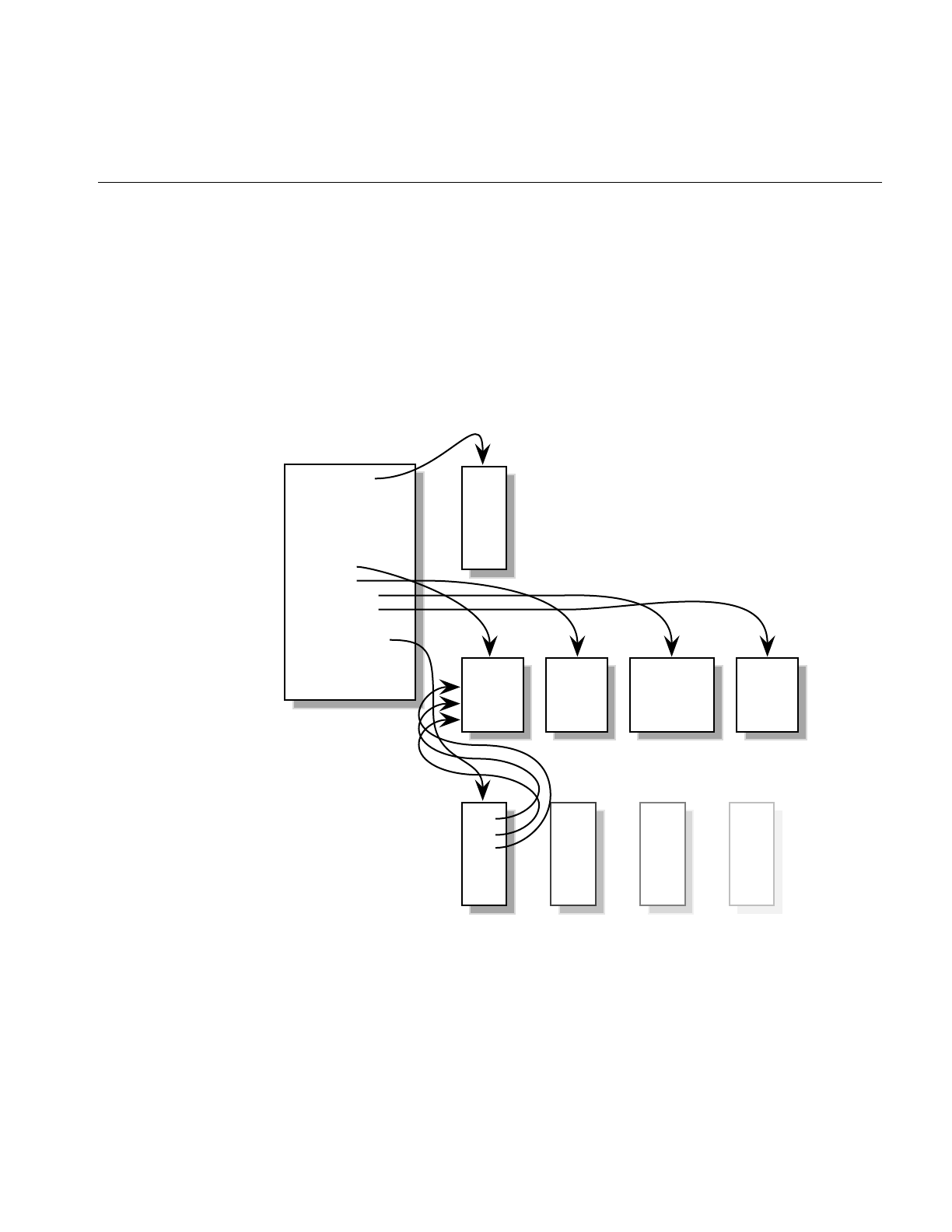
Geometry Sets
249
Indexed Arrays
A cube has six sides; together those sides have 24 vertices. In a vertex array, you could
specify the primitives in the cube using 24 vertices. However, most of those vertices
overlap. If more than one primitive can refer to the same vertex, the number of vertices
can be streamlined to 8. The way to get more than one primitive to refer to the same
vertex is to use an index; three vertices of three primitives use the same index which
points to the same vertex information. Adding the index array adds an extra step in the
determination of the attribute, as shown in Figure 8-3.
Figure 8-3 Indexing Arrays
Indexing can save system memory, but rendering performance is often lost.
StripLengths
PrimCoords
ColorBind
MormalBind
TexCoordBind
CoordSet
ColorSet
NormalSet
TexCoordSet
CoordIndexSet
ColorIndexSet
NormalIndexSet
TextCoordIndexSet < x, y, z >
.
.
.
< r, g, b >
.
.
.
< nx, ny, nz >
.
.
.
< x, y, z >
.
.
.
n1
n2
n3
.
.
.
n1
n2
n3
.
.
.
n1
n2
n3
.
.
.
n1
n2
n3
.
.
.
n1
n2
n3
.
.
.
pfGeoSet
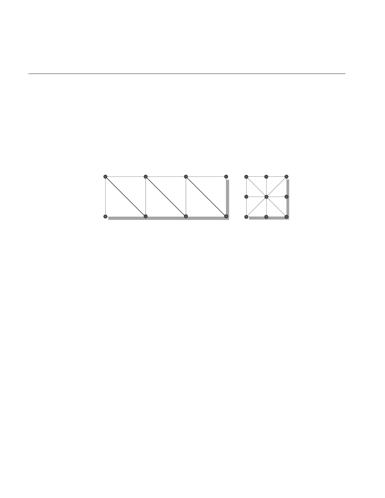
250
Chapter 8: Geometry
When to Index Attributes
The choice of using indexed or sequential attributes applies to all of the primitives in a
pfGeoSet; that is, all of the primitives within one pfGeoSet must be referenced
sequentially or by index; you cannot mix the two.
The governing principle for indexing attributes or not is how many vertexes in a
geometry are shared. Consider the following two examples in Figure 8-4 where each dot
marks a vertex.
Figure 8-4 Deciding Whether to Index Attributes
In the triangle strip, each vertex is shared by two adjoining triangles. In the square, the
same vertex is shared by eight triangles. Consider the task that is required to move these
vertices when, for example, morphing the object. If the vertices were not indexed, in the
square, the application would have to look up and alter eight triangles to change one
vertex.
In the case of the square, it is much more efficient to index the attributes. On the other
hand, if the attributes in the triangle strip were indexed, since each vertex is shared by
only two triangles, the index look-up time would exceed the time it would take to simply
update the vertices sequentially. In the case of the triangle strip, rendering is improved
by handling the attributes sequentially.
The deciding factor governing whether or not to index attributes relates to the number
of primitives that share the same attribute: if attributes are shared by many primitives,
the attributes should be indexed; if attributes are not shared by many primitives, the
attributes should be handled sequentially.

3D Text
251
pfGeoSet Operations
There are many operations you can perform on pfGeoSets. pfDrawGSet() “draws “the
indicated pfGeoSet by sending commands and data to the Geometry Pipeline, unless
IRIS Performer’s display-list mode is in effect. In display-list mode, rather than sending
the data to the pipeline, the current pfDispList “captures” the pfDrawGSet() command.
The given pfGeoSet is then drawn along with the rest of the pfDispList with the
pfDrawDList() command.
When the PFGS_COMPILE_GL mode of a pfGeoSet is not active (pfGSetDrawMode()),
pfDrawGSet() uses rendering loops tuned for each primitive type and attribute binding
combination to reduce CPU overhead in transferring the geometry data to the hardware
pipeline. Otherwise, pfDrawGSet() sends a special, compiled data structure.
Table 8-1 lists other operations that you can perform on pfGeoSets. pfCopy() does a
shallow copy, copying the source pfGeoSet’s attribute arrays by reference and
incrementing their reference counts. pfDelete() frees the memory of a pfGeoSet and its
attribute arrays (if those arrays were allocated with pfMalloc() and provided their
reference counts reach zero). pfPrint() is strictly a debugging utility and will print a
pfGeoSet’s contents to a specified destination. pfGSetIsectSegs() allows intersection
testing of line segments against the geometry in a pfGeoSet; see “Intersecting With
pfGeoSets” in Chapter 17 for more information on that function.
3D Text
In addition to the pfGeoSet, libpr offers two other primitives which together are useful
for rendering a specific type of geometry—three-dimensional characters. See Chapter 3,
“Nodes and Node Types” and the description for pfText nodes for an example of how to
set up three-dimension text within the context of libpf.
pfFont
The basic primitive supporting text rendering is the libpr pfFont primitive. A pfFont is
essentially a collection of pfGeoSets in which each pfGeoSet represents one character of
a particular font. pfFont also contain metric data, such as a per-character spacing, the
three-dimensional escapement offset used to increment a text ‘cursor’ after the character
has been drawn. Thus, pfFont maintain all of the information that is necessary to draw
any and all valid characters of a font. However, note that pfFont are passive and have

252
Chapter 8: Geometry
little functionality on their own, for example you cannot draw a pfFont—it simply
provides the character set for the next higher-level text data object, the pfString.
Table 8-5 lists some routines that are used with a pfFont.
Table 8-5 pfFont Routines
Function Description
pfNewFont Create a new pfFont.
pfDelete Delete a pfFont.
pfFontCharGSet Set the pfGeoSet to be used for a specific character of this pfFont.
pfFontCharSpacing Set the 3D spacing to be used to update a text cursor after this character has
been rendered.
pfFontMode Specify a particular mode for this pfFont.
Valid Modes to set:
PFFONT_CHAR_SPACING — specify whether to use fixed or variable
spacings for all characters of a pfFont. Possible values are
PFFONT_CHAR_SPACING_FIXED and
PFFONT_CHAR_SPACING_VARIABLE, the latter being the default.
PFFONT_NUM_CHARS — specify how many characters are in this font.
PFFONT_RETURN_CHAR — specify the index of the character that is
considered a ‘return’ character and thus relevant to line justification.
pfFontAttr Specify a particular attribute of this pfFont.
Valid Attributes to set:
PFFONT_NAME - name of this font.
PFFONT_GSTATE - pfGeoState to be used when rendering this font.
PFFONT_BBOX - bounding box that bounds each individual character.
PFFONT_SPACING - Set the overall character spacing if this is a fixed
width font (also the spacing used if one hasn’t been set for a particular
character).

3D Text
253
Example 8-1 Loading Characters into a pfFont
/* Setting up a pfFont */
pfFont *ReadFont(void)
{
pfFont *fnt = pfNewFont(pfGetSharedArena());
for(i=0;i<numCharacters;i++)
{
pfGeoSet* gset = getCharGSet(i);
pfVec3* spacing = getCharSpacing(i);
pfFontCharGSet(fnt, i, gset);
pfFontCharSpacing(fnt, i, spacing);
}
}
pfString
Simple rendering of three-dimensional text can be done using a pfString. A pfString is an
array of font indices stored as 8-bit bytes, 16-bit shorts, or 32-bit integers. Each element
of the array contains an index to a particular character of a pfFont structure. A pfString
can not be drawn until it has been associated with a pfFont object via a call to
pfStringFont(). To render a pfString once it references a pfFont, call the function
pfDrawString().
pfStrings support the notion of ‘flattening’ to trade off memory for faster processing
time. This will cause individual, non-instanced geometry to be used for each character,
eliminating the cost of translating the text cursor between each character when drawing
the pfString.
Example 8-2 Setting Up and Drawing a pfString
/* Create a string a rotate it for 2.5 seconds */
void
LoadAndDrawString(const char *text)
{
pfFont *myfont = ReadMyFont();
pfString *str = pfNewString(NULL);
pfMatrix mat;
float start,t;
/* Use myfont as the 3-d font for this string */
pfStringFont(str, fnt);

254
Chapter 8: Geometry
/* Center String */
pfStringMode(str, PFSTR_JUSTIFY, PFSTR_MIDDLE);
/* Color String is Red */
pfStringColor(str, 1.0f, 0.0f, 0.0f, 1.0f);
/* Set the text of the string */
pfStringString(str, text);
/* Obtain a transform matrix to place this string */
GetTheMatrixToPlaceTheString(mat);
pfStringMat(str, &mat);
/* optimize for draw time by flattening the transforms */
pfFlattenString(str);
/* Twirl text for 2.5 seconds */
start = pfGetTime();
do
{
pfVec4 clr;
pfSetVec4(clr, 0.0f, 0.0f, 0.0f, 1.0f);
/* Clear the screen to black */
pfClear(PFCL_COLOR|PFCL_DEPTH, clr);
t = (pfGetTime() - start)/2.5f;
t = PF_MIN2(t, 1.0f);
pfMakeRotMat(mat, t * 315.0f, 1.0f, 0.0f, 0.0f);
pfPostRotMat(mat, mat, t * 720.0f, 0.0f, 1.0f, 0.0f);
t *= t;
pfPostTransMat(mat, mat, 0.0f,
150.0f * t + (1.0f - t) * 800.0f, 0.0f);
pfPushMatrix();
pfMultMatrix(mat);
/* DRAW THE INPUT STRING */
pfDrawString(str);
pfPopMatrix();

3D Text
255
pfSwapWinBuffers(pfGetCurWin());
} while(t < 2.5f);
}
Table 8-6 lists the key routines used to manage pfStrings.
Table 8-6 pfString Routines
Function Description
pfNewString Create a new pfString
pfDelete Delete a pfString.
pfStringFont Set the pfFont to use when drawing this pfString.
pfStringString Set the character array that this pfString will represent/render.
pfDrawString Draw this pfString
pfFlattenString Flatten all positional translations and the current specification matrix into
individual pfGeoSets so that more memory is used, but no matrix transforms
or translates have to be done between each character of the pfString.
pfStringColor Set the color of the pfString.
pfStringMode Specify a particular mode for this pfString.
Valid Modes to set:
PFSTR_JUSTIFY — set the line justification and has the following possible
values: PFSTR_FIRST or PFSTR_LEFT,PFSTR_MIDDLE or
PFSTR_CENTER, and PFSTR_LAST or PFSTR_RIGHT.
PFSTR_CHAR_SIZE — set the number of bytes per character in the input
string and has the following possible values: PFSTR_CHAR,
PFSTR_SHORT,PFSTR_INT.
pfStringMat Specify a transform matrix that will affect the entire character string when the
pfString is drawn
pfStringSpacing
Scale Specify a scale factor for the escapement translations that happen after each
character is drawn. This routine is useful for changing the spacing between
characters and even between lines.


The chapter describes the graphics state, which contains all of the fields that
together define the shape and appearance of a geometry.
“Graphics State”
Chapter 9


259
Chapter 9
9. Graphics State
The graphics state is a class of fields that define everything about the shape and texture
of an object in a IRIS Performer scene. Fields include such things as transparency,
shading, reflectance, and texture. The graphics state is set globally for all objects in the
scene graph. Individual objects, however, can override graphics state settings. The cost,
however, is efficiency. For performance reasons, therefore, it is important to set the fields
in the graphics state to satisfy the greatest number of objects in the scene.
This chapter describes in detail all of the fields in the graphics state.
Immediate Mode
The graphics libraries are immediate-mode state machines; if you set a mode, all
subsequent geometry is drawn in that mode. For the best performance, mode changes
need to be minimized and managed carefully. libpr manages a subset of graphics library
state and identifies bits of state as graphics state elements. Each state element is identified
with a PFSTATE token, e.g., PFSTATE_TRANSPARENCY corresponds to the
transparency state element. State elements are loosely partitioned into three categories:
modes, values and attributes.
Modes are the graphics state variables, such as transparency and texture enable, that
have simple values like ON and OFF. An example of a mode command is
pfTransparency(mode).
Values are not modal, rather they are real numbers which signify a threshold or quantity.
An example of a value is the reference alpha value specified with the pfAlphaFunc()
command.
Attributes are references to encapsulations (structures) of graphics state. They logically
group the more complicated elements of state, such as textures and lighting models.
Attributes are structures that are modified through a procedural interface and must be
applied to have an effect. For example, pfApplyTex(tex) applies the texture map, tex, to
subsequently drawn geometry.

260
Chapter 9: Graphics State
In libpr, there are three methods of setting state:
• immediate mode
• display list mode
• pfGeoState mode
Like the graphics libraries, libpr supports the notion of both immediate and display-list
modes. In immediate mode, graphics mode changes are sent directly to the Geometry
Pipeline, i.e., they have immediate effect. In display-list mode, graphics mode changes
are captured by the currently active pfDispList, which can be drawn later. libpr display
lists differ from graphics library objects because they capture only libpr commands and
are reusable. libpr display lists are useful for multiprocessing applications in which one
process builds up the list of visible geometry and another process draws it. “Display
Lists” on page 285 describes libpr display lists.
A pfGeoState is a structure that encapsulates all the graphics modes and attributes that
libpr manages. You can individually set the state elements of a pfGeoState to define a
graphics context. The act of applying a pfGeoState with pfApplyGState() configures the
state of the Geometry Pipeline according to the modes, values, and attributes set in the
pfGeoState. For example, the following code fragment shows equivalent ways (except
for some inheritance properties of pfGeoStates described later) of setting up some
lighting parameters suitable for a glass surface:
/* Immediate mode state specification */
pfMaterial *shinyMtl;
pfTransparency(PFTR_ON);
pfApplyMtl(shinyMtl);
pfEnable(PFEN_LIGHTING);
/* is equivalent to: */
/* GeoState state specification */
pfGeoState *gstate;
pfGStateMode(gstate, PFSTATE_TRANSPARENCY, PFTR_ON);
pfGStateAttr(gstate, PFSTATE_FRONTMTL, shinyMtl);
pfGStateMode(gstate, PFSTATE_ENLIGHTING, PF_ON);
pfApplyGState(gstate);
In addition, pfGeoStates have unique state inheritance capabilities that make them very
convenient and efficient; they provide independence from ordered drawing. pfGeoStates
are described in the “pfGeoState” section of this chapter.

Immediate Mode
261
Libpr routines have been designed to produce an efficient structure for managing
graphics state. You can also set graphics state directly through the GL. However, libpr will
have no record of these settings and will not be able to optimize them and may make
incorrect assumptions about current graphics state if the resulting state does not match
thelibpr record when libpr routines are called. Therefore, it is best to use the libpr routines
whenever possible to change graphics state and to restore libpr state if you go directly
through the GL.
The following sections will describe the rendering geometry and state elements in detail.
There are three types of state elements: modes, values and attributes. Modes are simple
settings that take a set of integer values that include values for enabling and disabling the
mode. Modes may also have associated values that allow a setting from a defined range.
Attributes are complex state structures that encapsulate a related collection of modes and
values. Attribute structures will not include in their definition an enable or disable as the
enabling or disabling of a mode is orthogonal to the particular related attribute in use.
Rendering Modes
libpr manages a subset of the rendering modes found in the graphics libraries. In
addition, libpr abstracts certain concepts like transparency, providing a higher-level
interface that hides the underlying implementation mechanism.
libpr provides tokens that identify the modes that it manages. These tokens are used by
pfGeoStates and other state-related functions like pfOverride(). The following table
enumerates the PFSTATE_ tokens of supported modes, each with a brief description and
default value.

262
Chapter 9: Graphics State
Table 9-1 lists and describes the mode tokens.
The mode control functions described in the following sections should be used in place
of their graphics library counterparts so that IRIS Performer can correctly track the
graphics state. Use pfGStateMode() with the appropriate PFSTATE token to set the
mode of a pfGeoState.
Table 9-1 pfGeoState Mode Tokens
Token Name Description Default Value
PFSTATE_TRANSPARENCY Transparency modes PFTR_OFF
PFSTATE_ALPHAFUNC Alpha function PFAF_ALWAYS
PFSTATE_ANTIALIAS Antialiasing mode PFAA_OFF
PFSTATE_CULLFACE Face culling mode PFCF_OFF
PFSTATE_DECAL Decaling mode for coplanar
geometry PFDECAL_OFF
PFSTATE_SHADEMODEL Shading model PFSM_GOURAUD
PFSTATE_ENLIGHTING Lighting enable flag PF_OFF
PFSTATE_ENTEXTURE Texturing enable flag PF_OFF
PFSTATE_ENFOG Fogging enable flag PF_OFF
PFSTATE_ENWIREFRAME pfGeoSet wireframe mode enable
flag PF_OFF
PFSTATE_ENCOLORTABLE pfGeoSet colortable enable flag PF_OFF
PFSTATE_ENHIGHLIGHTING pfGeoSet highlighting enable flag PF_OFF
PFSTATE_ENLPOINTSTATE pfGeoSet light point state enable flag PF_OFF
PFSTATE_ENTEXGEN Texture coordinate generation
enable flag PF_OFF

Immediate Mode
263
Transparency
You can control transparency using pfTransparency(). Possible transparency modes are:
In addition, the flag PFTR_NO_OCCLUDE may be logically OR-ed into the transparency
mode in which case geometry will not write depth values into the frame buffer. This will
prevent it from occluding subsequently rendered geometry. Enabling this flag improves
the appearance of unordered, blended transparent surfaces.
There are two basic transparency mechanisms: screen-door transparency which requires
hardware multisampling and blending. Blending offers very high quality transparency
but for proper results requires that transparent surfaces be rendered in back-to-front
order after all opaque geometry has been drawn. When using transparent texture maps
to “etch” geometry or if the surface has constant transparency, screen-door transparency
is usually good enough. Blended transparency is usually required to avoid “banding” on
surfaces with low transparency gradients like clouds and smoke.
Shading Model
Selects flat shading or Gouraud (smooth) shading. pfShadeModel() takes one of two
tokens: PFSM_FLAT or PFSM_GOURAUD. One some graphics hardware flat shading
can offer a significant performance advantage.
Table 9-2 pfTransparency Tokens
Transparency mode Description
PFTR_OFF Transparency disabled.
PFTR_ON
PFTR_FAST Use the fastest, but not necessarily the best, transparency provided
by the hardware.
PFTR_HIGH_QUALITY Use the best, but not necessarily the fastest, transparency provided
by the hardware.
PFTR_MS_ALPHA Use screen-door transparency when multisampling. Fast but limited
number of transparency levels.
PFTR_BLEND_ALPHA Use alpha-based blend with background color. Slower but high
number of transparency levels.

264
Chapter 9: Graphics State
Alpha Function
pfAlphaFunc() is an extension of the IRIS GL function afunction(3g) and the OpenGL
function glAlphaFunc(); it allows IRIS Performer to keep track of the hardware mode.
The alpha function is a pixel test that compares the incoming alpha to a reference value
and uses the result to determine whether or not the pixel is rendered. The reference value
must be specified in the range [0, 1]. For example, a pixel whose alpha value is 0 is not
rendered if the alpha function is PFAF_GREATER and the alpha reference value is also
0. Note that rejecting pixels based alpha can be faster than using transparency alone. A
common technique for improving the performance of filling polygons is to set an alpha
function that will reject pixels of low (possibly non-zero) contribution. Alpha function is
typically used for see-through textures like trees.
Decals
On Z-buffer based graphics hardware, coplanar geometry can cause unwanted artifacts
due to the finite numerical precision of the hardware which cannot accurately resolve
which surface has visual priority. This can result in flimmering, a visual “tearing” or
“twinkling” of the surfaces. pfDecal() is used to accurately draw coplanar geometry on
IRIS platforms and it supports two basic implementation methods, each with its
advantages:
The stencil decaling method uses a hardware resource known as a stencil buffer and
requires that a single stencil plane (see IRIS GL stencil() and OpenGL glStencilOp() man
pages) be available for IRIS Performer. This method offers the highest image quality but
requires that geometry be coplanar and rendered in a specific order which reduces
opportunities for the performance advantage of sorting by graphics mode.
A potentially faster method is the displace decaling method. In this case, each layer is
displaced towards the eye so it “hovers” slightly above the preceding layer. Displaced
decals need not be coplanar, can be drawn in any order but the displacement may cause
geometry to incorrectly “poke through” other geometry.
The specificaton of a decal plane can improve the dispace decaling method. The object
geometry will be projected onto the specified plane and if the same plane is specified for
base and layer geometry, the base and layer polygons will be generated with identical
depth values. If the objects are drawn in priority order, no further operation is necessary.
Otherwise, displace can be applied to the planed geometry for a supior result. Decal
planes can be specified on pfGeoSets with pfGSetDecalPlane(), on a pfGeoState with the
PFSTATE_DECALPLANE attribute to pfGStateAttr(), or globally with
pfApplyDecalPlane().

Immediate Mode
265
Decals consist of base geometry and layer geometry. The base defines the depth values of the
decal while layer geometry is simply “inlaid” on top of the base. Multiple layers are
supported but limited to 8 when using displaced decals. Realize that these layers imply
superposition; there is no limit to the number of polygons in a layer, only to the number
of distinct layers.
The decal mode indicates whether the subsequent geometry is base or layer and the decal
method to use. For example, a mode of PFDECAL_BASE_STENCIL means that
subsequent geometry is to be considered as base geometry and drawn using the stencil
method. All combinations of base/layer and displace/stencil modes are supported but
you should make sure to use the same method for a given base-layer pair.
Example 9-1 illustrates the use of pfDecal().
Example 9-1 Using pfDecal() to Draw Road With Stripes
pfDecal(PFDECAL_BASE_STENCIL);
/* ... draw underlying geometry (roadway) here ...*/
pfDecal(PFDECAL_LAYER_STENCIL);
/* ... draw coplanar layer geometry (stripes) here ... */
pfDecal(PFDECAL_OFF);
Note: libpf applications can use the pfLayer node to include decals within a scene graph.
Frontface / Backface
pfCullFace() controls which side of a polygon (if any) is discarded in the Geometry
Pipeline. Polygons are either front-facing or back-facing. A front-facing polygon is
described by a counterclockwise order of vertices in screen coordinates, and a
back-facing one has a clockwise order. pfCullFace() has four possible arguments:
PFCF_OFF Disable face-orientation culling
PFCF_BACK Cull back-facing polygons
PFCF_FRONT Cull front-facing polygons
PFCF_BOTH Cull both front- and back-facing polygons

266
Chapter 9: Graphics State
In particular, backface culling is highly recommended since it offers a significant
performance advantage for databases where polygons are never be seen from both sides
(databases of “solid” objects or with constrained eyepoints).
Antialiasing
pfAntialias() is used to turn the antialiasing mode of the hardware on or off. Currently,
antialiasing is implemented differently by each different graphics system. Antialiasing
can produce artifacts as a result of the way IRIS Performer and the active hardware
platform implement the feature. See the reference page pfAntialias() for implementation
details.
Rendering Values
Some modes may also have associated values. These values are set through
pfGStateVal(). Table 9-3 lists and describes the value tokens.
Enable / Disable
pfEnable() and pfDisable() control certain rendering modes. Certain modes do not have
effect when enabled but require that other attribute(s) be applied. Table 9-4 lists and
describes the tokens and also lists the attributes required for the mode to become truly
active.
Table 9-3 pfGeoState Value Tokens
Token Name Description Range Default Value
PFSTATE_ALPHAREF Set the alpha function reference value. 0.0 - 1.0 0.0
Table 9-4 Enable and Disable Tokens
Token Action Attribute(s) Required
PFEN_LIGHTING Enable or disable lighting. pfMaterial
pfLight
pfLightModel
PFEN_TEXTURE Enable or disable texture. pfTexEnv
pfTexture

Immediate Mode
267
By default all modes are disabled.
Rendering Attributes
Rendering attributes are state structures that are manipulated through a procedural
interface. Examples include pfTexture, pfMaterial, and pfFog. libpr provides tokens that
enumerate the graphics attributes it manages. These tokens are used by pfGeoStates and
other state-related functions like pfOverride(). Table 9-5 lists and describes the tokens.
PFEN_FOG Enable or disable fog. pfFog
PFEN_WIREFRAME Enable or disable pfGeoSet wireframe
rendering. none
PFEN_COLORTABLE Enable or disable pfGeoSet colortable
mode. pfColortable
PFEN_HIGHLIGHTING Enable or disable pfGeoSet highlighting. pfHighlight
PFEN_TEXGEN Enable or disable automatic texture
coordinate generation. pfTexGen
PFEN_LPOINTSTATE Enable or disable pfGeoSet light points pfLPointState
Table 9-5 Rendering Attribute Tokens
Attribute Token Description Apply Routine
PFSTATE_LIGHTMODEL Lighting model pfApplyLModel
PFSTATE_LIGHTS Light source definitions pfLightOn
PFSTATE_FRONTMTL Front-face material pfApplyMtl
PFSTATE_BACKMTL Back-face material pfApplyMtl
PFSTATE_TEXTURE Texture pfApplyTex
PFSTATE_TEXENV Texture environment pfApplyTEnv
PFSTATE_FOG Fog model pfApplyFog
PFSTATE_COLORTABLE Color table for pfGeoSets pfApplyCtab
Table 9-4 (continued) Enable and Disable Tokens
Token Action Attribute(s) Required

268
Chapter 9: Graphics State
Rendering attributes control which attributes are applied to geometric primitives when
they’re processed by the hardware. All IRIS Performer attributes consist of a control
structure, definition routines, and an apply function, pfApply* (except for lights which
are “turned on”).
Each attribute has an associated pfNew*() routine that allocates storage for the control
structure. When sharing attributes across processors in a multiprocessor application, you
should pass the pfNew*() routine a shared memory arena from which to allocate the
structure. If you pass NULL as the arena, the attribute is allocated from the heap and isn’t
sharable in a non-shared address space (fork()) multiprocessing application.
All attributes can be applied directly, referenced by a pfGeoState or captured by a display
list. When changing an attribute, that change isn’t visible until the attribute is reapplied.
Detailed coverage of attribute implementation is available in the reference pages.
Texture
IRIS Performer supports texturing through pfTextures and pfTexEnvs, which provide
encapsulated suppport for graphics library textures (see texdef2d() for IRIS GL, or
glTexImage2D() for OpenGL) and texture environments (see IRIS GL’s tevdef(3g) or
OpenGL’s glTexEnv()). A pfTexture defines a texture image, format, and filtering. A
pfTexEnv specifies how the texture should interact with the colors of the geometry it’s
applied to. You need both to display textured data, but you don’t need to specify them
both at the same time. For example, you could have pfGeoStates each of which had a
different texture specified as an attribute and still use an overall texture environment
specified with pfApplyTEnv().
A pfTexture is created by calling pfNewTex(). If the desired texture image exists as a disk
file in IRIS libimage format (the file often has a “.rgb” suffix ) or in the IRIS Performer fast
loading image format (a “.pfi” suffix), you can call pfLoadTexFile() to load the image into
CPU memory and completely configure the pfTexture
pfTexture *tex = pfLoadTexFile(“brick.rgba”);
PFSTATE_HIGHLIGHT Definition of pfGeoSet highlighting style pfApplyHlight
PFSTATE_LPOINTSTATE pfGeoSet light point definition pfApplyLPState
PFSTATE_TEXGEN Texture coordinate generation definition pfApplyTGen
Table 9-5 (continued) Rendering Attribute Tokens
Attribute Token Description Apply Routine

Immediate Mode
269
Otherwise, pfTexImage() lets you directly provide a GL-ready image array in the same
external format as specified on the pfTexture and as expected by texdef2d() in IRIS GL
and glTexImage2D() in OpenGL.
void pfTexImage(pfTexture* tex, uint* image,
int comp, int sx, int sy, int sz);
IRIS GL and OpenGL both expect packed texture data with each row beginning on a long
word boundary. However, IRIS GL and OpenGL expect the individual components of a
texel to be packed in opposite order. For example, IRIS GL expects four component texels
to be packed as ABGR OpenGL expects the texels to be packed as RGBA. If you provide
your own image array in a multiprocessing environment, it should be allocated from
shared memory (along with your pfTexture) to allow different processes to access it. A
basic example demonstrating loading a image file and placing the resulting pfTexture on
scene graph geometry is at /usr/share/Performer/src/pguide/libpf/C/texture..c.
Note: The size of your texture must be an integral power of two on each side. IRIS GL
scales up your textures to the next power of two, making them take up to four times more
space in hardware texture memory! OpenGL simply refuses to accept badly sized
textures. You can rescale your texture images with the izoom or imgworks programs
(shipped with IRIX 5.3 in the eoe2.sw.imagetools and imgtools.sw.tools subsystems; and
with IRIX 6.2 in the eoe.sw.imagetools and imgworks.sw.tools subsystems).
Your texture source does not have to be a static image. pfTexLoadMode() can be used to
set one of the sources listed in Table 9-6 with PFTEX_LOAD_SOURCE. Note that sources
other than CPU memory may not be supported on all graphics platforms, or may have
some special restrictions. There are several sample programs that demonstrate paging
sequences of texture from different texture sources. For paging from host memory there
are:
•/usr/share/Performer/src/pguide/libpr/C/texlist.c
•/usr/share/Performer/src/pguide/libpr/C/mipmap.c
•/usr/share/Performer/src/pguide/libpfutil/movietex.c

270
Chapter 9: Graphics State
These examples demonstrates the use of different texture sources for paging textures,
and libpufitl utilties for managing texture resources. One thing these examples do is use
pfTexLoadImage() to update the pointer to the image data to avoid the expensive
reformating the texture. This requires that the provided image data be the same size as
the original image data, as well as same number of components and same formats.
Video Texturing
The source of texture image data can be live video input. IRIS Performer supports the
video input mechanisms of Sirius Video on RealityEngine and InfiniteReality, DIVO on
Onyx2/InfiniteReality, and O2 and OCTANE video input. IRIS Performer includes a
sample program that features video texturing:
/usr/share/Performer/src/pguide/libpf/movietex.c. This example demonstrates all video
initialization, including the creation of video library resources, is done in the draw
process, as required by the video library. Part of that initialization includes setting the
proper number of components on the pfTexture and choosing a texture filter and
potentially internal format. Those basic operations are discussed further in this section.
IRIS Performer will automatically download the frame of video when the texture object
is applied through the referencing pfGeoState. Alternatively, you may want to schedule
this download to happen at the beginning or end of the rendering frame and can force it
with token with pfLoadTex().
Textures must be created with sizes that are powers of two the input video frame is
usually not in powers of two. The [0,1] texture coordinate range can be scaled into the
valid part of the pfTexture with a texture matrix. This matrix can be applied directly to
the global state with pfApplyTMat() to affect all pfGeoSets, or can be set on a pfGeoState
with the PFSTATE_TEXMAT attribute to pfGStateAttr().
Table 9-6 Texture Image Sources
PFTEX_SOURCE_ Token Texture image is take from:
IMAGE CPU memory location specified by pfTexLoadImage() or
pfTexImage().
FRAMEBUFFER framebuffer location offset from window origin as specified by
pfTexLoadOrigin().
VIDEO Default video source on the system.

Immediate Mode
271
Texture Management
Texture storage is limited only by virtual memory, but for real-time applications you
must consider the amount of texture storage the graphics hardware supports. Textures
that don’t fit in the graphics subsystem will be paged as needed when pfApplyTex() is
called. Libpr provides routines for managing hardware texture memory so that a
real-time application does not have to get a surprise texture load. pfIsTexLoaded(),
called from the drawing process, will tell you if the pfTexture is currently properly
loaded in texture memory. The initially required textures of an application, or all of the
textures if they will fit, can be pre-loaded into texture memory as part of application
initialization. pfuMakeSceneTexList() will make a list of all textures referenced by a
scene graph and pfuDownloadTexList() will load a list of textures into hardware texture
memory (and must be called in the draw process). The perfly sample program does this
as part of its initialization and displays the textures as it pre-loads them.
There are additional routines to asist with the progressive loading and unloading of
pfTextures.pfIdleTex() can be used to free up the hardware texture memory owned by a
pfTexture.f texture paging, GL host and hardware texture memory resources can be freed
with pfDeleteGLHandle() from the drawing process.IRIS Performer will automatically
re-allocate those resources if the pfTexture is used again. For an example of management
of texture resources, see the example program
/usr/share/Performer/src/pguide/libpfutil/texmem.c that uses the pfuTextureManager from
libpfutil for basic texture paging support.
pfLoadTex(), called from the drawing process, can be used to explicitly load a texture
into graphics hardware texture memory (which will include doing any necessary
formatting of the texture image). By default, pfLoadTex() will load the entire texture
image, including any required minification or magnification levels, into texture memory.
pfSubloadTex() and pfSubloadTexLevel() can also be used in the drawing process to do
an immediate load of texture memory managed by the given pfTexture and these
routines allow you to specify all loading parameters (source, origin, size, etc.). This is
useful for loading different images for the same pfTexture in different graphics pipelines.
pfSubloadTex() allows you to load a subsection of the texture tile by tile.
A special pfTexFormat() formatting mode, PFTEX_SUBLOAD_FORMAT, allows part or
all of the image in texture memory owned by the pfTexture to be replaced via
pfApplyTex(),pfLoadTex(), or pfSubloadTex(), without having to go through the
expensive reformatting phase. This allows you to quickly update the image of a
pfTexture in texture memory. The PFTEX_SUBLOAD_FORMAT used with an
appropriatepfTexLoadSize() and pfTexLoadOrigin() allows you to control what part of
the texture will be loaded by subsequent calls to pfLoadTex() orpfApplyTex(). There are

272
Chapter 9: Graphics State
also different loading modes that cause pfApplyTex() to automatically reload or subload
a texture from a specified source. If you want the image of a pfTexture to be updated
upon every call to pfApplyTex(), you can set the loading mode of the pfTexture with
pfTexLoadMode() to be PFTEX_BASE_AUTO_REPLACE. pfTexLoadImage() allows
you to continuously update the memory location of an IMAGE source texture without
triggering any reformatting of the texture.
Note: In IRIS GL, the SUBLOAD format (same as the FAST_DEFINE format on old
versions of IRIS Performer) can only be used on non-MIPmapped textures. The fast
texture loading uses the IRIS GL subtexload() and OpenGL glTexSubImage() calls. In
IRIS GL, subload sizes must be integral multiples of 32.
Hint: There are texture formatting modes that can improve texture performance and
these are the modes that are used by default by IRIS Performer. Of most importance is
the 16-bit texel internal formats. These formats cause the resulting texels to have 16 bits
of resolution instead of the standard 32. These formats can have dramatically faster
texture fill performance and cause the texture to take up half the hardware texture
memory. Therefore, they are strongly recommended and are used by default. There are
different formats for each possible number of components to give a choice of how the
compression is to be done. These formats are described in the pfTexFormat(3pf) reference
page.
There may also be formatting modes for internal or external image formats that IRIS
Performer does not have a token for. However, the GL value can be specified. Specifying
GL values will make your application GL specific and may also cause future porting
problems, so it should only be done if absolutely necessary.
pfTextures also allow you to define a set of textures that are mutually exclusive, should
always be applied to the same set of geometry, and thus that can share the same location
in hardware texture memory. With pfTexList(tex, list) you can specify a list of textures to
be in a texture set managed by the base texture, tex. The base texture is what gets applied
with pfApplyTex(), or assigned to geometry through pfGeoStates. With pfTexFrame(),
you can select a given texture from the list (-1 selects the base texture and is the default).
This allows you to define a texture movie where each image is the frame of the movie.
You can have an image on the base texture to display when the movie is not playing.

Immediate Mode
273
There are additional loading modes for pfTexLoadMode() described in Table 9-7 to
control how the textures in the texture list share memory with the base texture.
Texture list textures can share the exact graphics texture memory as the base texture but
this has the restriction that the textures must all be the exact same size and format as the
base texture. Texture list textures can also indicate that they are mutually exclusive which
will cause the texture memory of previous textures to be freed before applying the new
texture. This method has no restrictions on the texture list, but is less efficient than the
previous method. Finally, texture list textures can be treated as completely independent
textures that should all be kept resident in memory for rapid access upon their
application.
IpfTexFilter() sets a desired filter to a specified filtering method on a pfTexture. The
minification and magnification texture filters are described with bitmask tokens. If filters
are partially specified, IRIS Performer will fill in the rest with machine dependent fast
defaults. The PFTEX_FAST token can be included in the bitmask to allow IRIS Performer
to make machine dependent substitutions where there are large performance differences.
Table 9-7 Texture Load Modes
PFTEX_LOAD_
modeToken Load Mode Values Description
SOURCE SOURCE_IMAGE,
SOURCE_FRAMEBUFFER
PFTEX_SOURCE_VIDEO
PFTEX_SOURCE_DMBUF
PFTEX_SOURCE_DMVIDEO
Source of image data is host memory image,
framebuffer, default video source, digital
media buffer, or a video library digital
media buffer.
BASE BASE_APPLY
BASE_AUTO_SUBLOAD Loading of image for pfTexture is done as
required for pfApply, or automatically
subloaded upon every pfApply.
LIST LIST_APPLY
LIST_AUTO_IDLE
LIST_AUTO_SUBLOAD
Loading of list texture image is as separate
apply, causes freeing of previous list texture
in hardware texture memory, or is
subloaded into memory managed by the
base texture.
VIDEO_
INTERLACED OFF, INTERLACED_ODD,
INTERLACED_EVEN, video input is interlaced or not and if so,
which field (even or odd) is spatially higher.

274
Chapter 9: Graphics State
There are a variety of texture filter functions that can improve the look of textures when
they are minified and magnified. By default, textures use MIPmapping when minified
(though this costs an extra 1/3 in storage space to store the minification levels). Each level
of minification or magnification of a texture is twice the size of the previous level.
Minification levels are indicated with positive numbers and magnification levels are
indicated with non-positive numbers. The default magnification filter for textures is
bilinear interpolation. The use of detail textures and sharpening filters can improve the
look of magnified textures. Detailing actually uses an extra detail texture that you
provide that is based on a specified level of magnification from the corresponding base
texture. The detail texture can be specified with the pfTexDetail() command. By default,
MIPmap levels are generated for the texture automatically. OpenGL operation allows for
the specification of custom MIPmap levels. Both MIPmap levels and detail levels can be
specified with pfTexLevel(). The level number should be a positive number for a
minification level and a non-positive number for a magnification (detail) level. If you are
providing your own minification levels, you must provide all log2(MAX(texSizeX,
texSizeY)) minification levels. There is only one detail texture for a pfTexture.
The magnification filters use spline functions to control their rate of application as a
function of magnification, and specified level of magnification for detail textures. These
splines can be specified with pfTexSpline(). The specification of the spline is a set of
control points that are pairs of non-decreasing magnification levels (specified with
non-positive numbers) and corresponding scaling factors. Magnification filters can be
applied to all components of a texture, only the RGB components of a texture, or to just
the alpha components. OpenGL does not allow different magnification filters (between
detail and sharpen) for RGB and alpha channels.
Note: The specification of detail textures may have GL dependencies and magnifications
filters may not be available on all hardware configurations. The pfTexture reference page
describes these details.
Texture Formats
The format in which an image is stored in texture memory is defined with pfTexFormat():
void pfTexFormat(pfTexture *tex, int format, int type)

Immediate Mode
275
format specifies which format to set. Valid formats and their basic types include:
• PFTEX_INTERNAL_FORMAT— specifies how many bits per component are to be
used in internal hardware texture memory storage. The default is 16 bits per full
texel and is based on the number of components and external format.
• PFTEX_IMAGE_FORMAT—describes the type of image data and must mach the
number of components, such as PFTEX_LUMINANCE,
PFTEX_LUMINANCE_ALPHA, PFTEX_RGB, and PFTEX_RGBA. The default is
the token in this list that matches the number of components. Other OpenGL
selections can be specified with the GL token.
• PFTEX_EXTERNAL_FORMAT—specifies the format of the data in the pfTexImage
array. The default is packed 8 bits per component. There are special fast-loading
hardware ready formats, such as PFTEX_UNSIGNED_SHORT_5_5_5_1.
• PFTEX_SUBLOAD_FORMAT—a boolean to specify if the texture will be a
sub-loadable paging texture. Default is FALSE.
In general you will just need to specify the number of components inpfTexImage(). You
may want to specify a fast loading hardware-ready external format, such as
PFTEX_UNSIGNED_SHORT_5_5_5_1, in which case IRIS Performer will automatically
choose a matching internal format. as See the pfTexFormat(3pf) refrence page for more
informaton on texture configuration details.
Controlling Texture LOD with pfTexLOD
You can control the levels of detail (LODs) of a texture that are accessed and used with
pfTexLOD to force higher or lower MIPmap levels to be used when minifying. You
canuse this to give the graphics hardware a hint about what levels can be accessed
(IMPACT hardware takes great advantage of such a hint) and you can use this to have
multiple textures sharing a single MIPmap pyramid in texture memory. For example, a
distant object and an a close one may use different LODs of the same pfTexture texture.
The pfGeoStates of those pfGeoSets would have different pfTexLOD objects that
referenced the proper texture LODs. pfTexLevel() would be used to specify and update
the proper image for each LOD in the pfTexture. You can use LODs to specify to yourself
and the GL which LODs of texture should be loaded from disk into main memory. For
example, if the viewer is in one LOD, most of the texture in that LOD can often be viewed
and, consequently, should be paged into texture memory. You can set LOD parameters
on a pfTexture directly or use pfTexLOD.

276
Chapter 9: Graphics State
To use a pfTexLOD object, you
1. Set the ranges of the LOD, using pfTLODRange(), and their corresponding
minimum and maximum resolution MIPmap. Because the minimum and maximum
limits can be floating point values, new levels can be smoothly blended in when
they become available to avoid popping from one LOD to another.
2. Optionally, set the bias levels, using pfTLODBias(), to force blurring of a texture to
simulate motion blur and depth of field, or to force a texture to be sharper, or to
compensate for asymmetric minification of a MIPmapped texture.
Note: Any LOD settings on pfTexture take priority over current pfTexLOD settings.
3. Enable LOD control over texture by using the following methods:
pfEnable(PFEN_TEXLOD);
pfGeoState::pfGStateMode(myTxLOD, PFSTATE_ENTEXLOD, ON);
where myTxLOD is an instance of pfTexLOD, and ON is a non-zero integer.
4. Apply the LOD settings to the texture using pfApplyTLOD().
See the sample program /usr/share/Performer/src/pguide/libpr/C/texlod.c for an example of
using a pfTexLOD.
Note: You can only control the LOD of a texture when using OpenGL.
Setting the Texture Environment with pfTexEnv
The environment specifies how the colors of the geometry, potentially lit, and the texture
image interact. This is described with a pfTexEnv object. The mode of interaction is set
with pfTEnvMode() and valid modes include:
• PFTE_MODULATE—the gray scale of the geometry is mixed with the color of the
texture (the default).
This option multiplies the shaded color of the geometry by the texture color. If the
texture has an alpha component, the alpha value modulates the geometry’s
transparency, for example, if a black and white texture, such as text, is applied to a
green polygon, the polygon remains green and the writing appears as dark green
lettering.
• PFTE_DECAL—the texture alpha component acts as a selector between 1.0 for the
texture color and 0.0 for the base color to decal an image onto geometry.

Immediate Mode
277
• PFTE_BLEND—the alpha acts as a selector between 0.0 for the base color and 1.0 for
the texture color modulated by a constant texture blend color specified with
pfTEnvBlendColor(). The alpha/intensity components are multiplied.
• PFTE_ADD—the RGB components of the base color are added to the product of the
texture color modulated by the current texture environment blend color. The
alpha/intensity components are multiplied.
Automatic Texture Coordinate Generation
Automatic texture coordinate generation is provided with the pfTexGen state attribute.
pfTexGen closely corresponds to IRIS GL’s texgen() and OpenGL’s glTexGen() functions.
When texture coordinate generation is enabled, a pfTexGen applied with
pfApplyTGen() will automatically generate texture coordinates for all rendered
geometry. Texture coordinates are generated from geometry vertices according to the
texture generation mode set with pfTGenMode(). Available modes and their function
are listed in Table 9-8. Some modes refer to a plane which is set with pfTGenPlane() and
to a line that is specified as a point and direction with pfTGenPoint().
Table 9-8 Texture Generation Modes
PFTG_ Mode Token Texture coordinates are calculated as...
OBJECT_PLANE distance of vertex from plane in object coordinates
EYE_PLANE distance of vertex from plane in eye coordinates. The plane is transformed
by the inverse of the ModelView matrix when the pfTexGen is applied.
EYE_PLANE_IDENT distance of vertex from plane in eye coordinates. The plane is not
transformed by the inverse of the ModelView matrix when the pfTexGen
is applied
SPHERE_MAP an index into a 2D reflection map based on vertex position and normal.
Specifics of the calculation are found in the graphics libraries’ man pages.
OBJECT_DISTANCE
_TO_LINE distance in object space from vertex to specified line
EYE_DISTANCE_TO
_LINE distance in eye space from eye to a specified vector through the vertex

278
Chapter 9: Graphics State
Lighting
IRIS Performer lighting is an extension of graphics library lighting (see lmdef(3g) for
IRIS GL or glLight() and related functions in OpenGL), but IRIS Performer divides the
actions of lmdef() into lights and light models, just as OpenGL does. The light embodies
the color, position, and type (for example, infinite or spot) of the light. The light model
specifies the environment for infinite (the default) or local viewing, and two-sided
illumination..
The lighting model describes the type of lighting operations to be considered, including
local lighting, two-sided lighting, and light attenuation. The fastest light model is infinite
single-sided lighting. A pfLightModel state attribute object is created with
pfNewLModel(). A light model also allows you to specify ambient light for the scene,
such as might come from the Sun, with pfLModelAmbient().
pfLights and created by calling pfNewLight(). A light has color and position. The light
colors are specified with pfLightColor():
void pfLightColor(pfLightSource* lsource, int which, float r,
float g, float b);
which specifies one of three light colos:
• PFLT_AMBIENT
• PFLT_DIFFUSE
• PFLT_SPECULAR
You to position the light source using pfLightPos():
void pfLightPos(pfLight* light, float x, float y,
float z, float w);
w is the distance between the location in the scene defined by (x,y,z) and the light source,
lsource. If w equals zero, lsource is infinitely far away and (x,y,z) defines a vector pointing
from the origin in the direction of lsource; if w equals one, lsource is located at the position,
(x,y,z). The default position is (0, 0, 1, 0): directly overhead, infinitely far away.
pfLights are attached to a pfGeoState through the PFSTATE_LIGHTS attribute.

Immediate Mode
279
The transformation matrix that is on the matrix stack at the time the light is applied
controls the interpretation of the light source direction:
1. To attach a light to the viewer (like a miner’s head-mounted light), call pfLightOn()
only once with an identity matrix on the stack.
2. To attach a light to the world (like the sun or moon), call pfLightOn() every frame
with only the viewing transformation on the stack.
3. To attach a light to an object (like the headlights of a car), call pfLightOn() every
frame with the combined viewing and modeling transformation on the stack.
The number of lights you can have turned on at any one time is limited by
PF_MAX_LIGHTS, just as is true with the graphics libraries.
Note: In IRIS GL, attenuation is also part of the light model definition. In OpenGL,
attenuation is defined per-light. There is separate libpr API for setting each of these:
pfLModelAtten() for IRIS GL and pfLightAtten() for OpenGL. You can use
pfQueryFeature() with a feature specifier value of PFQFTR_LMODEL_ATTENUATION
or PFQFTR_LIGHT_ATTENUATION to find out which is supported in the current
run-time environment.
Note: libpf applications can include light sources in a scene graph with the pfLightSource
node.
Materials
IRIS Performer materials are an extension of graphics library materials (see lmdef(3g) for
IRIS GL or glMaterial() for OpenGL). pfMaterials encapsulate the ambient, diffuse,
specular, and emissive colors of an object as well as its shininess and transparency. A
pfMaterial is created by calling pfNewMtl(). As with any of the other attributes, a
pfMaterial can be referenced in a pfGeoState, captured by a display list, or invoked as an
immediate mode command.
pfMaterials, by default, allow object colors to set the ambient and diffuse colors. This
allows the same pfMaterial to be used for objects of different colors, removing the need
for material changes and thus improving performance. This mode can be changed with
pfMtlColorMode(mtl, side, PFMTL_CMODE_*). IRIS GL only supports the front
material tracking the current color while OpenGL allows front or back materials to track
the current color. If the same material is used for both front and back materials, there is
no difference in functionality.

280
Chapter 9: Graphics State
With the method, pfMtlSide(), you can specifiy whether to apply the the material on the
side facing the viwer (PFMTL_FRONT), the side not facing the viewer (PFMTL_BACK),
or both.(PFMTL_BOTH). Back-sided lighting will only take affect if there is a two-sided
lighting model active. Two sided lighting typically has some significant performance
cost.
Object materials only have effect when lighting is active.
Color Tables
A pfColortable substitutes its own color array for the normal color attribute array
(PFGS_COLOR4) of a pfGeoSet. This allows the same geometry to appear differently in
different views simply by applying a different pfColortable for each view. By leaving the
selection of color tables to the global state, you can use a single call to switch color tables
for an entire scene. In this way, color tables can simulate time-of-day changes, infrared
imaging, psychedelia, and other effects.
pfNewCtab() creates and returns a handle to a pfColortable. As with other attributes,
you can specify which color table to use in a pfGeoState or you can use pfApplyCtab()
to set the global color table, either in immediate mode or in a display list. For an applied
colortable to have effect, colortable mode must also be enabled.
Fog
A pfFog is created by calling pfNewFog(). As with any of the other attributes, a pfFog
can be referenced in a pfGeoState, captured by a display list, or invoked as an immediate
mode command. Fog is the atmospheric effect of aerosol water particles that occlude
vision over distance. The IRIS hardware can simulate this phenomenon in several
different fashions. A fog color is blended with the resultant pixel color based on the range
from the viewpoint and the fog function. pfFog supports several different fogging
methods. Table 9-9 lists the pfFog tokens and their corresponding actions.

Immediate Mode
281
pfFogType() uses these tokens to set the type of fog. A detailed explanation of fog types
is given in the reference page pfFog(3pf) and in the IRIS GL fogvertex(3g) and OpenGL
glFog(3g) reference pages.
You can set the near and far edges of the fog with pfFogRange(). For exponential fog
functions, the near edge of fog is always zero in eye coordinates. The near edge is where
the onset of fog blending occurs, and the far edge is where all pixels are 100% fog color.
The token PFFOG_PIX_SPLINE selects a spline function to be applied when generating
the hardware fog tables. This is further described in the pfFog(3pf) reference page. Spline
fog allows the user to define an arbitrary fog ramp that can more closely simulate
real-world phenomena like horizon haze.
For best fogging effects the ratio of the far to the near clipping planes should be
minimized. In general, it’s more effective to add a small amount to the near plane than
to reduce the far plane.
Table 9-9 pfFog Tokens
pfFog Token Action
PFFOG_VTX_LIN Compute fog linearly at vertices.
PFFOG_VTX_EXP Compute fog exponentially at vertices (ex).
PFFOG_VTX_EXP2 Compute fog exponentially at vertices (ex squared).
PFFOG_PIX_LIN Compute fog linearly at pixels.
PFFOG_PIX_EXP Compute fog exponentially at pixels (ex).
PFFOG_PIX_EXP2 Compute fog exponentially at pixels (ex squared).
PFFOG_PIX_SPLINE Compute fog using a spline function at pixels.

282
Chapter 9: Graphics State
Highlights
IRIS Performer provides a mechanism for highlighting geometry with alternative
rendering styles, useful for debugging and interactivity. A pfHighlight, created with
pfNewHlight(), encapsulates the state elements and modes for these rendering styles. A
pfHighlight can be applied to an individual pfGeoSet with pfGSetHlight(), or can be
applied to multiple pfGeoStates through a pfGeoState or pfApplyHlight(). The
highlighting effects are added to the normal rendering phase of the geometry.
pfHighlights make use of special outlining and fill modes and have a concept of a
foreground color and a background color that can both be set with pfHlightColor(). The
available rendering styles can be combined by OR-ing together tokens for
pfHlightMode() and are described in Table 9-10.
Table 9-10 pfHlightMode() Tokens
PFHL_ Mode
Bitmask Token Description
LINES Outlines the triangles in the highlight foreground color according to
pfHlightLineWidth().
LINESPAT
LINESPAT2 Outlines triangles with patterned lines in the highlight foreground color, or in
two colors using the background color.
FILL Draws geometry with the highlight foreground color. Combined with
SKIP_BASE, this is a fast highlighting mode.
FILLPAT
FILLPAT2 Draws the highlighted geometry as patterned with one or two colors.
FILLTEX Draw highlighting fill pass with a special highlight texture.
LINES_R
FILL_R Reverses the highlighting foreground and background colors for lines and fill,
respectively.
POINTS Renders the vertices of the geometry as points according to pfHlightPntSize().
NORMALS Displays the normals of the geometry with lines according to
pfHlightNormalLength().
BBOX_LINES
BBOX_FILL Displays the bounding box of the pfGeoSet as outlines and/or filled box.
Combined with PFHL_SKIP_BASE, this is a fast highlighting mode.
SKIP_BASE Causes the normal drawing phase of the pfGeoSet to be skipped. This is
recommended when using PFHL_FILL or PFHL_BBOX_FILL.

Immediate Mode
283
For a demonstration of the highlighting styles, see the sample program,
/usr/share/Performer/pguide/src/libpr/C/hlcube.c.
Graphics Library Matrix Routines
IRIS Performer provides extensions to the standard graphics library
matrix-manipulation functions. These functions are similar to their graphics library
counterparts, with the exception that they can be placed in IRIS Performer display lists.
Table 9-11 lists and describes the matrix manipulation routines.
Sprite Transformations
A sprite is a special transformation used to efficiently render complex geometry with
axial or point symmetry. A classic sprite example is a tree which is rendered as a single,
texture-mapped quadrilateral. The texture image is of a tree and has an alpha component
whose values which “etches” the tree shape into the quad. In this case, the sprite
transformation rotates the quad around the tree trunk axis so that it always faces the
viewer. Another example is a puff of smoke which again is a texture-mapped quad but
is rotated about a point to face the viewer so it appears the same from any viewing angle.
The pfSprite transformation mechanism supports both these simple examples as well as
more complicated ones involving arbitrary 3D geometry.
Table 9-11 Matrix Manipulation Routines
Routines Action
pfScale Concatenate a scaling matrix.
pfTranslate Concatenate a translation matrix.
pfRotate Concatenate a rotation matrix.
pfPushMatrix Push down the matrix stack.
pfPushIdentMatrix Push the matrix stack and load an identity matrix on top.
pfPopMatrix Pop the matrix stack.
pfLoadMatrix Add a matrix to the top of the stack.
pfMultMatrix Concatenate a matrix.

284
Chapter 9: Graphics State
A pfSprite is a structure which is manipulated through a procedural interface. It is
different from “attributes” like pfTexture and pfMaterial since it affects transformation,
rather than state related to appearance. A pfSprite is activated with pfBeginSprite(). This
enables “sprite mode” and any pfGeoSet that is drawn before sprite mode is ended with
pfEndSprite() will be transformed by the pfSprite. First, the pfGeoSet is translated to the
location specified with pfPositionSprite(). Then, it is rotated, either about the sprite
position or axis depending on the pfSprite’s configuration. Note that pfBeginSprite(),
pfPositionSprite() and pfEndSprite() are display listable and this will be captured by
any active pfDispList.
A pfSprite’s rotation mode is set by specifying the PFSPRITE_ROT token to
pfSpriteMode(). In all modes, the Y axis of the geometry is rotated to point to the eye
position. Rotation modes are listed below.
Table 9-12 pfSprite Rotation Modes
PFSPRITE_ Rotation Token Rotation Characteristics
AXIAL_ROT Geometry’s Z axis is rotated about the axis specified with
pfSpriteAxis().
POINT_ROT_EYE Geometry is rotated about the sprite position with the object
coordinate Z axis constrained to the window coordinate Y axis, i.e.,
geometry’s Z axis stays “upright”.
POINT_ROT_WORLD Geometry is rotated about the sprite position with the object
coordinate Z axis constrained to the sprite axis.

Immediate Mode
285
Rather than using the graphics hardware’s matrix stack, pfSprites transform small
pfGeoSets on the CPU for improved performance. However, when a pfGeoSet contains
a certain number of primitives it becomes more efficient to use the hardware matrix
stack. While this threshold is dependent on the CPU and graphics hardware used, you
may specify it with the PFSPRITE_MATRIX_THRESHOLD token to pfSpriteMode().
The corresponding value is the minimum vertex requirement for hardware matrix
transformation. Any pfGeoSet with fewer vertices will be transformed on the CPU. If you
want a pfSprite to affect non-pfGeoSet geometry you should set the matrix threshold to
zero so that the pfSprite will always use the matrix stack. When using the matrix stack,
pfBeginSprite() pushes the stack and pfEndSprite() pops the matrix stack so the sprite
transformation is limited in scope.
pfSprites are dependent on the viewing location and orientation and the current
modeling transformation. You can specify these with calls to pfViewMat() and
pfModelMat() respectively. Note that libpf-based applications need not call these
routines since libpf does it automatically.
Display Lists
libpr supports display lists, which can capture and later execute libpr graphics
commands. pfNewDList() creates and returns a handle to a new pfDispList. A
pfDispList can be selected as the current display list with pfOpenDList(), which puts the
system in display list mode. Any subsequent libpr graphics commands, such as
pfTransparency(),pfApplyTex(), or pfDrawGSet(), are added to the current display list.
Commands are added until pfCloseDList() returns the system to immediate mode. It is
not legal to have multiple pfDispLists open at a given time but a pfDispList may be
reopened in which case commands are appended to the end of the list.
Once a display list is constructed, it can be executed by calling pfDrawDList(), which
traverses the list and sends commands down the Geometry Pipeline.
pfDispLists are designed for multiprocessing, where one process builds a display list of
the visible scene and another process draws it. The function pfResetDList() facilitates
this by making pfDispLists reusable. Commands added to a reset display list overwrite
any previously entered commands. A display list is typically reset at the beginning of a
frame and then filled with the visible scene.

286
Chapter 9: Graphics State
pfDispLists support concurrent multiprocessing, where the producer and consumer
processes simultaneously write and read the display list. The PFDL_RING argument to
pfNewDList() creates a ring buffer or FIFO-type display list. pfDispLists automatically
ensure ring buffer consistency by providing synchronization and mutual exclusion to
processes on ring buffer full or empty conditions.
For more information and the application of display lists, see Chapter 10, “ClipTextures.”
Combining Display Lists
The contents of one pfDispList may be appended to a second pfDispList by using the
function, pfAppendDList(). All pfDispList elements in src are appended to the
pfDispList dlist.
Alternately, you can append the contents of one pfDispList to a second pfDispList by
using the function pfDispList::append(). All pfDispList elements in src are appended to
the pfDispList on which the append method is invoked.
State Management
pfState is a structure that represents the entire libpr graphics state. A pfState maintains a
stack of graphics states that can be pushed and popped to save and restore state. The top
of the stack describes the current graphics state of a window as it’s known to IRIS
Performer.
pfInitState() initializes internal libpr state structures and should be called at the
beginning of an application before any pfStates are created. Multiprocessing applications
should pass a usinit() semaphore arena pointer to pfInitState(), such as
pfGetSemaArena(), so IRIS Performer can safely manage state between processes.
pfNewState() creates and returns a handle to a new pfState, which is typically used to
define the state of a single window. If using pfWindows, discussed in Chapter 11,
“Windows,”, a pfState is automatically created for the pfWindow when the window is
opened and the current pfState is switched when the current pfWindow changes.
pfSelectState() can be used to efficiently switch a different complete pfState.
pfLoadState() will force the full application of a pfState.

Immediate Mode
287
Pushing and Popping State
pfPushState() pushes the state stack of the currently active pfState, duplicating the top
state. Subsequent modifications of the state through libpr routines are recorded in the top
of stack. Consequently, a call to pfPopState() restores the state elements that were
modified after pfPushState().
The code fragment in Example 9-2 illustrates how to push and pop state.
Example 9-2 Pushing and Popping Graphics State
/* set state to transparency=off and texture=brickTex */
pfTransparency(PFTR_OFF);
pfApplyTex(brickTex);
/* ... draw geometry here using original state ... */
/* save old state. establish new state */
pfPushState();
pfTransparency(PFTR_ON);
pfApplyTex(woodTex);
/* ... draw geometry here using new state ...*/
/* restore state to transparency=off and texture=brickTex */
pfPopState();
State Override
pfOverride() implements a global override feature for libpr graphics state and attributes.
pfOverride() takes a mask that indicates which state elements to affect and a value
specifying whether the elements should be overridden. The mask is a bitwise OR of the
state tokens listed previously.
The values of the state elements at the time of overriding become fixed and cannot be
changed until pfOverride() is called again with a value of zero to release the state
elements.

288
Chapter 9: Graphics State
The code fragment in Example 9-3 illustrates the use of pfOverride().
Example 9-3 Using pfOverride()
pfTransparency(PFTR_OFF);
pfApplyTex(brickTex);
/*
* Transparency will be disabled and only the brick texture
* will be applied to subsequent geometry.
*/
pfOverride(PFSTATE_TRANSPARENCY | PFSTATE_TEXTURE, 1);
/* Draw geometry */
/* Transparency and texture can now be changed */
pfOverride(PFSTATE_TRANSPARENCY | PFSTATE_TEXTURE, 0);
pfGeoState
A pfGeoState encapsulates all the rendering modes, values, and attributes managed by
libpr. See “Rendering Modes” on page 261, “Rendering Values” on page 266, and
“Rendering Attributes” on page 267 for more information. pfGeoStates provide a
mechanism for combining state into logical units and define the appearance of geometry.
For example, you can set a brick-like texture and a reddish-orange material on a pfGeoSet
and use it when drawing brick buildings.
You can specify texture matricies on pfGeoSets.
Local and Global State
There are two levels of rendering state: local and global. A record of both is kept in the
current pfState. The local state is that defined by the settings of the current pfGeoState.
The rendering state and attributes of a pfGeoState can be either locally set or globally
inherited. If all state elements are set locally, a pfGeoState becomes a full graphics
context—that is, all state is then defined at the pfGeoState level. Global state elements are
set with libpr immediate mode routines like pfEnable(), pfApplyTex(),pfDecal(),
pfTransparency() or by drawing a pfDispList containing these commands with
pfDrawDList(). Local state elements for subsequent pfGeoSets are set by applying a
pfGeoState with pfApplyGState() (note that pfDrawGSet() automatically calls
pfApplyGState() if the pfGeoSet has an attached pfGeoState). The state elements applied
by a pfGeoState are those modes, enables, and attributes that are explicitly set on the

Immediate Mode
289
pfGeoState. Those settings revert back to the pfState settings for the next call to
pfApplyGState(). A pfGeoState can be explicitly loaded into a pfState to affect future
pfGeoStates with pfLoadGState().
Note: By default, all state elements are inherited from the global state. Inherited state
elements are evaluated faster than values that have been explicitly set.
While it can be useful to have all state defined at the pfGeoState level, it usually makes
sense to inherit most state from global default values and then explicitly set only those
state elements that are expected to change often.
Examples of useful global defaults are lighting model, lights, texture environment, and
fog. Highly variable state is likely to be limited to a small set such as textures, materials,
and transparency. For example, if the majority of your database is lighted, simply
configure and enable lighting at the beginning of your application. All pfGeoStates will
be lighted except the ones for which you explicitly disable lighting. Then attach different
pfMaterials and pfTextures to pfGeoStates to define specific state combinations.
Note: Caution should be used when enabling modes in the global state. These modes
may have cost even when they have no visible effect. Therefore, geometry that cannot use
these modes should have a pfGeoState that explicitly disables the mode. Modes to be
especially careful of include the texturing enable and transparency.
You specify that a pfGeoState should inherit state elements from the global default with
pfGStateInherit(gstate, mask).mask is a bitmask of tokens that indicates which state
elements to inherit. These tokens are listed in the “Rendering Modes”, “Rendering
Values”, and “Rendering Attributes” sections of this chapter. For example,
PFSTATE_ENLIGHTING | PFSTATE_ENTEXTURE makes gstate inherit the enable
modes for lighting and texturing.
A state element ceases to be inherited when it is set in a pfGeoState. Rendering modes,
values, and attributes are set with pfGStateMode(),pfGStateVal(), and pfGStateAttr(),
respectively. For example, to specify that gstate is transparent and textured with treeTex,
use
pfGStateMode(gstate, PFSTATE_TRANSPARENCY, PFTR_ON);
pfGStateAttr(gstate, PFSTATE_TEXTURE, treeTex);

290
Chapter 9: Graphics State
Applying pfGeoStates
Use pfApplyGState() to apply the state encapsulated by a pfGeoState to the Geometry
Pipeline. The effect of applying a pfGeoState is similar to applying each state element
individually. For example, if you set a pfTexture and enable a decal mode on a
pfGeoState, applying it essentially calls pfApplyTex() and pfDecal(). If in display-list
mode, pfApplyGState() is captured by the current display list.
State is (logically) pushed before, and popped after, pfGeoStates are applied, so that
pfGeoStates don’t inherit state from each other. This is a very powerful and convenient
characteristic since as a result, pfGeoStates are order-independent, and you don’t have to
worry about one pfGeoState corrupting another. The code fragment in Example 9-4
illustrates how pfGeoStates inherit state.
Example 9-4 Inheriting State
/* gstateA should be textured */
pfGStateMode(gstateA, PFSTATE_ENTEXTURE, PF_ON);
/* gstateB inherits the global texture enable mode */
pfGStateInherit(gstateB, PFSTATE_ENTEXTURE);
/* Texturing is disabled as the global default */
pfDisable(PFEN_TEXTURE);
/* Texturing is enabled when gstateA is applied */
pfApplyGState(gstateA);
/* Draw geometry that will be textured */
/* The global texture enable mode of OFF is restored
so that gstateB is NOT textured. */
pfApplyGState(gstateB);
/* Draw geometry that will not be textured */
The actual pfGeoState pop is a lazy pop that doesn’t happen unless a subsequent
pfGeoState requires the global state to be restored. This means that the actual state
between pfGeoStates isn’t necessarily the global state. If a return to global state is
required, call pfFlushState() to restore the global state. Any modification to the global
state made using libpr functions—pfTransparency(),pfDecal(), and so on—becomes the
default global state.

Immediate Mode
291
For best performance, set as little local pfGeoState state as possible. You can accomplish
this by setting global defaults that satisfy the majority of the requirements of the
pfGeoStates being drawn. By default, all pfGeoState state is inherited from the global
default.
pfGeoSets and pfGeoStates
There is a special relationship between pfGeoSets and pfGeoStates. Together they
completely define both geometry and graphics state. You can attach a pfGeoState to a
pfGeoSet with pfGSetGState() to specify the appearance of geometry. Whenever the
pfGeoSet is drawn with pfDrawGSet(), the attached pfGeoState is first applied using
pfApplyGState(). If a pfGeoSet does not have a pfGeoState, its state description is
considered undefined. To inherit all values from the global pfState, a pfGeoSet should
have a pfGeoState with all values set to inherit, the default.
This combination of routines allows the application to combine geometry and state in
high-performance units which are unaffected by rendering order. To further increase
performance, sharing pfGeoStates among pfGeoSets is encouraged.
pfGeoState Routines
Table 9-13 lists and describes the pfGeoState routines.
Table 9-13 pfGeoState Routines
Function Description
pfNewGState Create a new pfGeoState.
pfCopy Make a copy of the pfGeoState.
pfDelete Delete the pfGeoState.
pfGStateMode Set a specific state mode.
pfGStateVal Set a specific state value.
pfGStateAttr Set a specific state attribute.
pfGStateInherit Specify which state elements are inherited from the global state.
pfApplyGState Apply pfGeoState’s non-inherited state elements to graphics.

292
Chapter 9: Graphics State
pfGeoState Structure
Figure 9-1 diagrams the conceptual structure of a pfGeoState.
pfLoadGState Load pfGeoState’s settings into the pfState, inherited by future
pfGeoStates.
pfGetCurGState Return the current pfGeoState in effect.
pfGStateFuncs Assign pre/post callbacks to pfGeoState
pfApplyGStateTable Specify table of pfGeoStates used for indexing.
Table 9-13 (continued) pfGeoState Routines
Function Description
Immediate Mode
293
Figure 9-1 pfGeoState Structure
pfFog
pfTexGen
color
start
end
pfTexture
size
component
count
image
modes
detail texture
pfTexture
size
component
count
image
modes
detail texture
light model
lights [8]
front material
back material
texture
texture enviroment
color table
fog model
modes
values
texture generation
pfLPointState
pfGeoState
on/off tag
ambient
color
position
direction
spread
exponent
pfLight
pfLight
Model
pfColortable
table address
table size
pfTexEnv
texture index
blend
modes
attenuation
ambient
local/infinite flag
two-side flag
alpha
ambient
diffuse
emission
shininess
specular
pfMaterial
alpha
ambient
diffuse
emission
shininess
specular
pfMaterial


This chapter describes how to work with large, high-resolution textures.
“ClipTextures”
Chapter 10


297
Chapter 10
10. ClipTextures
As CPUs get faster and storage gets cheaper, applications are moving away from scenes
with small, synthetic textures to large textures, taken from real environments, giving the
viewer realistic renderings of actual locations.
There has customarily been a trade-off between the complexity of a texture and the area
it covers: if a texture covers a large area, its resolution must be limited so that it can fit
into texture memory; high-resolution textures are limited to small regions for the same
reason.
A cliptexture allows you to circumvent many of these system resource restrictions by
virtualizing MIPmapped textures. Only those parts of the texture needed to display the
textured geometry from a given location are stored in system and texture memory. IRIS
Performer provides support for this technique, called cliptexturing, though a subclass of
a pfTexture called a pfClipTexture. This functionality allows you to display textures too
large to fit in texture memory, or even in system memory; you can put the entire world
into a single texture.
IRIS Performer supports texture load management from disk to system memory and
from system to texture memory, synchronizing clipped regions with the viewpoint, and
many the other tasks needed to virtuaize a texture relative to the viewer location.
This chapter describes cliptextures in the following parts:
• “Overview” on page 298
• “Cliptexture API” on page 313
• “Preprocessing ClipTextures” on page 313
• “Cliptexture Configuration” on page 316
• “Configuration API” on page 317
• “Post-Scene Graph Load Configuration” on page 339
• “Manipulating Cliptextures” on page 347
• “Using Cliptextures” on page 361
298
Chapter 10: ClipTextures
Overview
Cliptexturing avoids the size limitations of normal MIPmaps by clipping the size of each
level of a mipmap texture to a fixed area, called the clip region. A MIPmap contains a
range of levels, each four times the size of the previous one. If the clip region is larger
than a particular level, the entire level is kept in texture memory. Levels larger than the
clip region are clipped to the clip region’s size. The clip region is set by the application,
trading off texture memory consumption against image quality. The clip region size is set
through the clip size, which is the length of the sides (in texels) of the clip region’s sides.
Figure 10-1 Cliptexture Components
The clip region positioned so as to be centered about the clip center, or as close as possible
to the clipcenter while remaining entirely within the cliptexture. The clipcenter is set by
the application, usually to the location on the texture corresponding to the location
closest to the viewer on the cliptextured geometry. The clipcenter is specified in texel
coordinates, which is the texture coordinates (s and t values, ranging from 0.0 to 1.0,
scaled by the dimensions of the finest level of the cliptexture, level 0).
Clip size
Clip region
Entire level in
texture memory
Overview
299
Cliptexture Levels
Texture memory contains the MIPmap levels, the larger ones clipped to the clip region
size; the rectangle of texture memory corresponding to each clipped level is called a tex
region. As the viewer moves relative to the cliptextured geometry, the clipcenter must be
updated. When this happens, the clipped mipmap levels must have their texture data
updated, in order to represent the area closest to the center. This updating usually must
happen every frame, and is done by IRIS Performer image caches.
To facilitate loading only portions of the texture at a time, the texture data must first be
subdivided into a contiguous set of rectangular areas, called tiles. These tiles can then
loaded individually from disk into texture memory.
Texture memory must be loaded from system memory; it can’t be loaded directly from
disk. In order to improve the performance of texel downloading, the region in system
memory is made larger than the destination texture memory and organized into a
lookahead cache, called the mem region.
Figure 10-2 Image Cache Components
Clip region
Entire level in
texture memory
Mem region
Tex region

300
Chapter 10: ClipTextures
Image caches must know three things in order to update clipped texture levels:
• Where and how the data is stored on disk, so they can retrieve it,
• Location and size of system memory cache, called the mem region,
• The texture memory they are responsible to update when the cilpcenter moves (the
tex region).
Cliptexture Assumptions
For the cliptexture algorithm to work seamlessly, applications must abide by the
following assumptions:
• An application can only view a clip region’s worth of high resolution texel data on
its textured geometry from any viewpoint.
• The application views the texture from one location at a time. Multiple views
require multiple cliptextures.
• The viewer must move smoothly relative to the cliptextured geometry; no
“teleporting” (abrupt changes in position).
Given these assumptions, your application can maintain a high-resolution texture by
keeping only those parts of the texture closest to the viewer in texture memory; the
remainder of the texture is on disk and cached in system memory.
Why Do These Assumptions Work?
Only the textured geometry closest to the viewer needs a high-resolution texture. Far
away objects are smaller on the screen, so the texels used on that object also appear
smaller (cover a smaller screen area). In normal MIPmapping, coarser MIPmap levels are
chosen as the texel size gets smaller relative to the pixel size. These coarser levels contain
less texels, since each texel covers a larger area on the textured geometry.
Cliptextures take advantage of this facts by storing only part of each large MIPMap level
in texture memory, just enough so that when you look over the geometry, the MIPmap
algorithm starts choosing texels from a lower level (because the texels are getting small
on the screen) before you run out of texels on the clipped level. Because coarser levels
have texels that cover a larger area, at a great enough distance, MIPmapping is choosing
texels from the unclipped, smaller levels.

Overview
301
When a clip size is chosen, cliptexture levels can be thought of as belonging to one of two
categories:
• Clipped levels, which are texture levels that are larger than the clip size.
• Non-clipped levels, which are small enough to fit entirely within the clip region.
The non-clipped levels are viewpoint independent; each non-clipped texture level is
complete. Clipped levels, however, must be updated as the viewer moves relative to the
textured geometry.
Image Cache
The image cache organizes its system memory as a grid of fixed size texture tiles. This
grid of texture data forms a lookahead cache, called the mem region. The cache
automatically anticipates texture download requirements, updating itself with texture
tiles it expects to use soon.
Image caches update texture memory by transferring image data from disk files. The
data is transferred in two steps. Data is moved from disk files a tile at a time into the mem
region in system memory. The mem region is updated so that it always contains the
image data corresponding to the tex region and its immediate surroundings. The border
of extra surrounding data allows the image cache to update the tex region as necessary
without having to wait for tiles to be loaded into the mem region from disk.
The image cache also contains a tex region, the rectangle of texel data in a given level’s
texture memory. This rectangle of data is in texture memory, and is being updated from
a corresponding rectangle of data in the memregion. As the center moves, the tex region
being loaded into texture memory can get close to the edge of the mem region. When this
happens, tiles in the mem region are updated with new data from disk so that the tex
region is moved closer to the center of the image data.
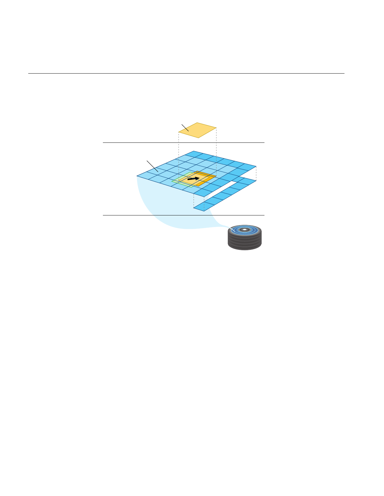
302
Chapter 10: ClipTextures
Figure 10-3 Mem Region Update
As the center moves, the clipped region on each clipped level of the image cache shifts
position. The clipped regions on each level move at different rates; each coarser level
only moves at one half the speed of the level above it. The image cache reflects the change
on its level by tracking the position of the clipped region with its tex region. Data in
texture memory must be updated to match the texel data in the translated tex region.
This updating is done by copying rectangles of texel data from the shifted tex region area
in the mem region to the appropriate locations in texture memory. The amount of
updating is minimized by only updating the portions of the texture memory that actually
need new data. The majority of the tex region data only has to shift position in texture
memory; this is done by translating texture coordinates, and taking advantage of the
wrap mode when accessing texels from texture memory.
Mem region
Tex region
Disk files
Texture memorySystem memoryDisk
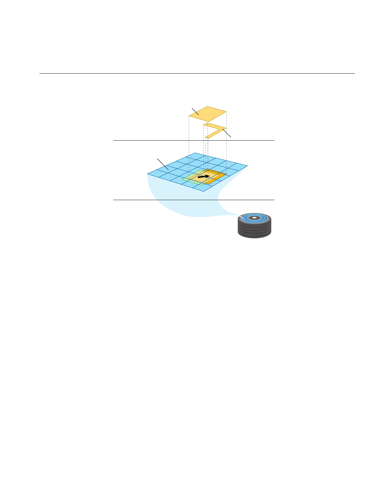
Overview
303
Figure 10-4 Tex Region Update
By loading textures to system memory before they’re needed in texture memory, the
latency caused by waiting for tiles downloading from a disk is reduced.
1. Texture data on disk is cached into system memory in an image cache’s mem region.
2. Texture data in the tex region part of the mem region is used to update texture
memory.
Mem region
Tex region update
Tex region
Disk files
Texture memorySystem memoryDisk
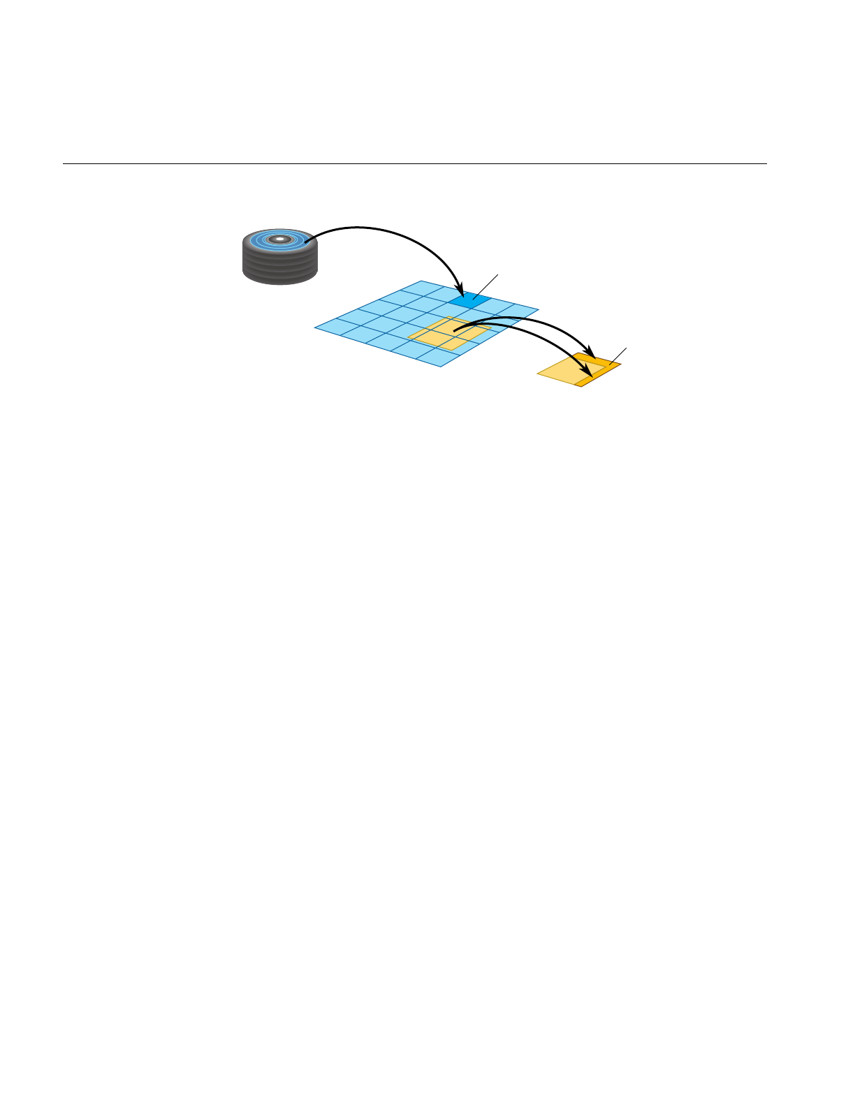
304
Chapter 10: ClipTextures
Figure 10-5 Cliptexture Cache Hierarchy
Toroidal Loading
In order to minimize the bandwidth required to download texels from system to texture
memory, the image cache’s tex regions are updated using toroidal loading. A toroidal load
assumes that changes in the contents of the clip region are incremental, such that the
update consists of:
• New texels that need to be loaded.
• Texels that are no longer valid.
• Texels that are still in the clip region, but have shifted position.
Toroidal loading minimizes texture downloading by only updating the part of the
texture region that needs new texels. Shifting texels that remain visible isn’t necessary,
since the coordinates of the clip region wrap around to the opposite side.
Invalid Borders
Being able to impose alignment requirements to the regions being downloaded to texture
memory improves performance. Cliptextures support the concept of an invalid border to
provide this feature. It is the area around the perimeter of a clip region that can’t be used.
The invalid border shrinks the usable area of the clip region, and can be used to
dynamically change the effective size of the clip region. Shrinking the effective clipsize
can be a useful load control technique.
Image cache
Image cache grid
Texture data on disk
Texture memory
Tex region
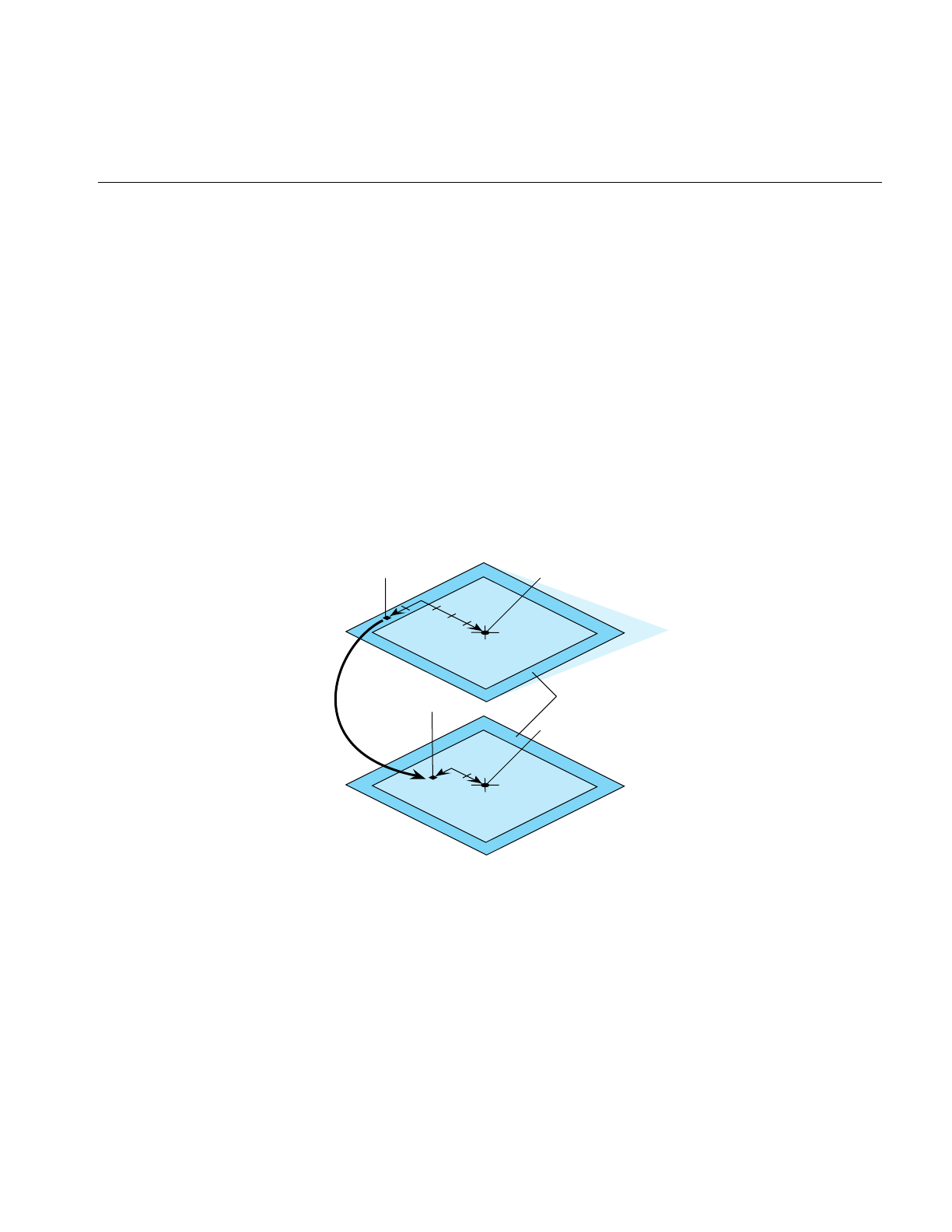
Overview
305
When texturing requires texels from a portion of an invalid border at a given MIPmap
level, the texturing system moves down a level, and tries again. It keeps going down to
coarser levels until it finds texels at the proper coordinates that are not in the invalid
region. This is always guaranteed to happen, since each level covers the same area with
less texels (coarser level texels cover more area on textured geometry). Even if the
required texel is clipped out of every clipped level, the unclipped pyramid levels will
contain it.
You can use an invalid border to force the use of lower levels of the MIPmap to:
• Reduce the abrupt discontinuity between MIPmap levels if the clip region is small:
using coarser LODs blends MIPmap levels over a larger textured region.
• Improve performance when a texture must be roamed very quickly.
Since the invalid border can be adjusted dynamically, it can reduce the texture and
system memory loading requirements at the expense of a blurrier image.
Figure 10-6 Invalid Border
Required texel
Invalid border
Clip region
Clip center
Clip center
Required texel
Fine
Coarser
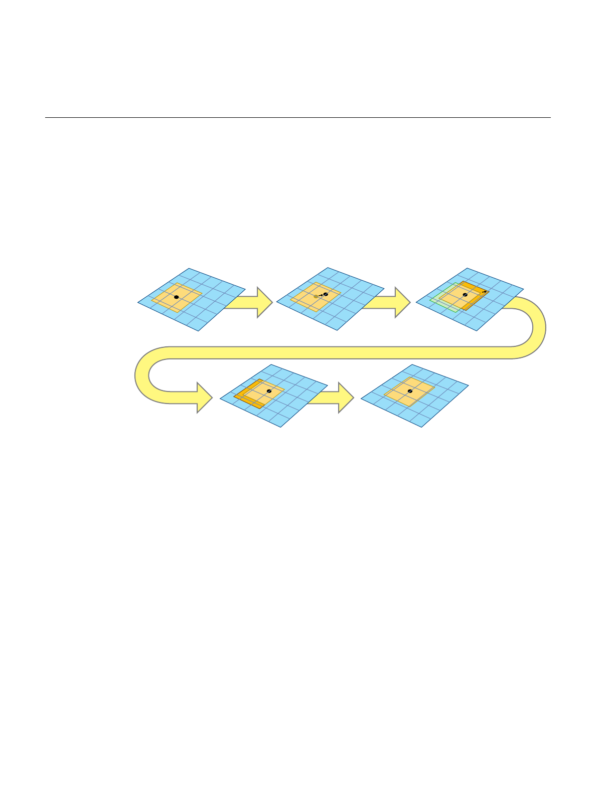
306
Chapter 10: ClipTextures
Updating the Clipcenter
To figure out what part of the texture must be loaded in each of the clipped levels, you
must know where the viewer is relative to the geometry being textured. Often this
position is computed by finding the location of the cliptextured geometry that is closest
to the viewer, and converting that to a location on the texture. This position is called the
cliptexture center and it must be updated every frame as the viewer moves relative to the
cliptextured geometry.
Figure 10-7 Clipcenter Moving
The clipcenter is set by the application for level 0, The cliptexture code then derives the
clipcenter location on all MIPmap levels. As the viewer roams over a cliptexture, the
centers of each MIPmap level move at a different rate. For example, moving the
clipcenter one unit corresponds to the center moving one half that distance in each
dimension in the next-coarser MIPmap level.
Most of the work of cliptexturing is updating the center properly and updating the
texture data in the clipped levels reliably and efficiently each frame.
Centered Center moves Texture coordinates wrap
Toroidal loads Same as centered
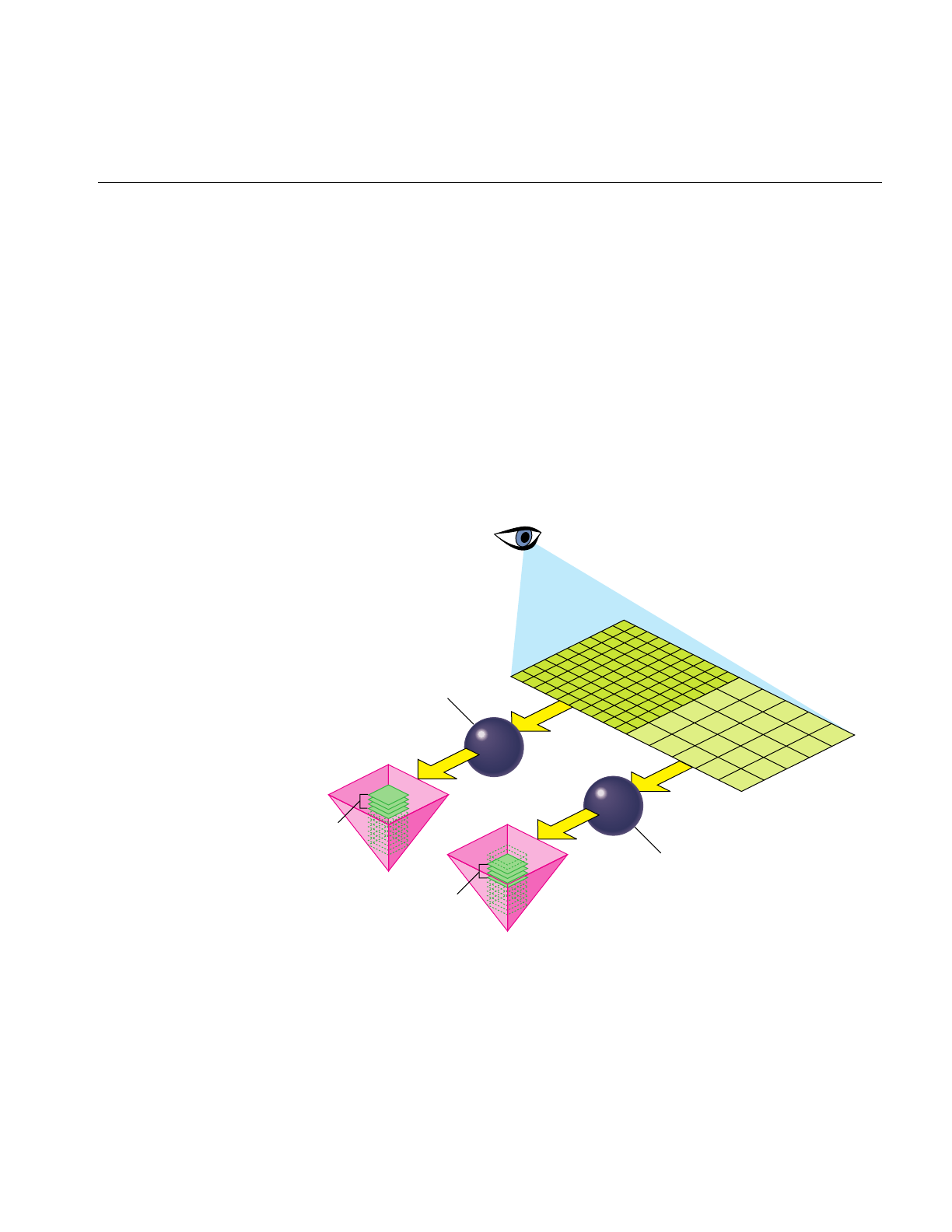
Overview
307
Virtual Cliptextures
Cliptextures save texture memory by limiting the extent of texture levels. Every level in
the mipmap is represented in texture memory, and can be accessed as the geometry is
textured. There are limits to the number of levels the cliptexturing hardware can access
while rendering, which restricts the cliptextures maximum size.
This limit can be exceeded by only accessing a subset of all the MIPmap’s levels in texture
memory on each piece of geometry, “virtualizing” the cliptexture. The virtual offset is
sets a virtual “level 0” in the MIPmap, while the number of effective levels indicates how
many levels starting from the new level 0 can be accessed. The minlod and maxlod
parameters are used to ensure that only valid levels are displayed. The application
typically divides the cliptextured terrain into pieces, using the relative position of the
viewer and the terrain to update the parameter values as each piece is traversed.
Figure 10-8 Virtual Cliptexture Concepts
For more information about virtual cliptextures, see “Virtual ClipTextures” on page 353.
Callback
Callback
Effective
levels
Effective
levels

308
Chapter 10: ClipTextures
Cliptexture Support Requirements
Ideally, pfClipTextures would be interchangeable with pfTextures in IRIS Performer.
Unfortunately, this is only partially true. The following sections describe some of the
differences between IRIS Performer textures and cliptextures.
Centering
Every level is complete in a regular texture. Cliptextures have clipped levels, where only
the portion of the level near the cliptexture center is complete. In order to look correct, a
cliptextures center must be updated as the channel’s viewport moves relative to the
cliptextured geometry.
Cliptextures require functionality that recalculates the center position whenever the
viewer moves (essentially each frame). This means that a relationship has to exist
between the cliptexture and a channel.
Applying
Textures only need to be applied once. Cliptextures must be applied every time the center
moves (essentially each frame). In order to apply at the right time, cliptextures need to
be connected to a pfPipe.
Texel Data
A texture does not know where its data comes from. The application just supplies it as a
pointer to region of system memory when the texture is applied.
Cliptextures need to update their contents as the center moves and they are reapplied
each frame. As a result, they need to know where their image data resides on the disk. In
order to maximize performance, cliptextures also cache their texel data in system
memory. As a result, cliptextures are a lot more work to configure, since you have to tell
them how to find their data on disk, and how you want the data cached in system
memory.
Special Features
Since cliptexture levels are so large, IRIS Performer offers additional features not
available to regular textures.

Overview
309
Insets
With certain restrictions, cliptexture levels can be partially populated, containing
“islands” of high resolution data. This can be useful if the application only needs
high-resolution texel data in relatively small, widely scattered areas of a large cliptexture.
A example of this might be an airline flight simulator, where high resolution data is only
needed in the vicinity of the airports used by the simulator.
For more information about insets, see “Cliptexture Insets” on page 361.
Virtualization
To further increase the size of cliptextures that IRIS Performer can use, the levels
themselves can be virtualized; It then selects a subset of all the available texture levels to
be loaded into memory. This requires additional support by the application. Virtual
cliptextures are described in detail in “Virtual ClipTextures” on page 353.
Multiple Pipe Support
Since cliptextures require both system and texture memory resources, IRIS Performer has
provided functionality to share the system memory resources when a cliptexture is used
in a multipipe application. “Slave” cliptextures and a “master” cliptexture share system
memory resources, but have their own classes and texture memory.
How Cliptextures Interact with the Rest of the System
As a result of their special requirements, cliptextures are used differently than pfTextures
with many different IRIS Performer classes. The following sections describe these
differences.
Geostates
When everything is configured properly, a pfClipTexture is interchangeable with a
pfTexture when used in a geostate.

310
Chapter 10: ClipTextures
Pipes
A pfClipTexture can be connected to a pfMPClipTexture, a multiprocessing component,
which is connected to a pfPipe. From the pipe’s point of view, a pfMPClipTexture is
something it can apply to.
Channels
Some functionality must be supplied to update a cliptexture’s center as the channel
moves with respect to the cliptextured geometry. This functionality can be supplied by
the application, or IRIS Performer can do it automatically if the application uses
clipcenter nodes.
A clipcenter node is added to the scenegraph and is traversed by the APP process just
like every other node in the scenegraph. pfMPClipTexture, which contains the
cliptextured geometry, should be a child node of the clipcenter node. When the clipcenter
node is traversed by a channel, the clipcenter node computes the relationship between
the cliptextured geometry and the channel’s eyepoint, and updates the cliptexture’s
center appropriately.
Cliptexture Support in IRIS Performer
Cliptexture is a large and diverse piece of functionality. As a result, cliptexture support
is found in nearly every major library in IRIS Performer.
libpr Support
The pfImageCache class defines image caches which manage the updating of clipped
levels, pfImageTile classes are used to define non-clipped cliptexture levels and define
pieces of clipped levels downloaded from disk to system memory. The pfQueue class
supports read queues, which manage the read requests from disk to system memory in
image caches, while the pfClipTexture class itself defines cliptextures themselves, virtual
mipmaps composed of image caches and image tile levels. The pfTexLoad class defines
download requests when image caches download texels from system to texture memory.
libpf Support
libpf adds multiprocessing support for using cliptextures in scene graphs. the
pfMPClipTexture class ties together pfClipTextures, pfPipes, cliptexture centering

Overview
311
functionality (often pfuClipCenterNode nodes) and the application itself in a
multiprocessing environment. additional functionality in the pfPipe class ensures that
cliptextures are applied properly.
libpfutil Support
libpfutil provides easy to use clipcentering functionality through the
pfuClipCenterNode class, a subclass of the pfGroup class. This library also provides
traversals to simply the work of finding cliptextures in a scene graph using
pfuFindClipTextures(), code for post loader configuration, where pfMPClipTextures are
created, and attached to pipes and clipcenter nodes using pfuProcessClipCenters() and
pfuProcessClipCentersWithChannel(). The pfuAddMPClipTextureToPipes() and
pfuAddMPClipTexturesToPipes() routines connect pfMPClipTextures to the proper
pipes, handling multipipe issues in a clean way. Load time configuration is simplified
using the pfuInitClipTexConfig(),pfuMakeClipTexture(), and pfuFreeClipTexConfig()
along with the appropriate callbacks for image caches and image tiles. Image cache
configuration is supported with pfuInitImgCacheConfig(),pfuMakeImageCache(),
and pfuFreeImgCacheConfig() routines.
libpfdu Support
The cliptexture configuration file parsers are supported here; pfdLoadClipTexture() and
pfdLoadClipTextureState() work with cliptexture configuration files to simplify the
creation and configuration of cliptextures. The companion programs that create and
configure pfdLoadImageCache() and pfdLoadImageCacheState(). All of these parsers
use the pfuMakeClipTexture() and pfuMakeImageCache() configuration routines.
libpfdb Support
Example cliptexture loaders, including the libpfim example cliptexture loader, the libpfct
demo loader and libpfvct virtual pseudo loader are all included here.
Cliptexture Manipulation
While the scene graph is being viewed, the application may want to dynamically alter
the appearance or performance characteristics of the cliptexture. The mpcliptexure
provides functionality to support parameter changes in the APP process, providing
frame-accurate updating. Here are some of the parameters that might be changed.

312
Chapter 10: ClipTextures
Load Control
The DTR functionality (described in detail elsewhere in this chapter) is largely automatic.
Some high performance applications may need to adjust DTR parameters to improve
appearance performance trade-offs.
Invalid Border
The invalid border can be adjusted at runtime to shrink the effective size of the clip
region.This might be done to provide additional load control beyond the per-level
control that DTR provides.
Share Masks
When operating master and slave cliptextures in a multipipe application, the application
may want to change the sharemask, which controls the synchronization of parameters
between master and slave cliptextures.
Read Function
The image cache creates requests to read image tiles from disk to the image cache’s
system memory cache. The read function processes these requests and actually does the
data transfer. IRIS Performer provides set of read functions that attempts to do direct-io
reads for speed, but falls back to normal reads if direct-IO is not possible.
The application can replace the IRIS Performer default function with its own custom read
function. This could be useful for implementing special functionality, such as dynamic
decompression pfcliptexture data.
Read Queue Sorting
The read queue provides dynamic sorting of the read requests to improve performance
and minimize latency. The application can provide custom sorting routines.

Cliptexture API
313
Cliptexture API
Cliptexturing has a large API. Not only is there are lot of cliptexture functionality
scattered throughout the library, but there is often more than one way to use a particular
piece of functionality. In order to make things clearer, and make it easier to use the API
described here, the cliptexture API is grouped and ordered in the same way an
application writer would use it.
The API is grouped into four sections:
• Preprocessing the cliptexture data.
• Configuring cliptextures and image caches.
• Post-load-time configuration.
• Run-time manipulation.
Preprocessing ClipTextures
Before using cliptextures, large textures must be preprocessed, as follows:
1. Start with the highest-resolution version of the image (texture) and build a MIPmap
of the image.
2. Choose a clip size.
3. Tile each MIPmap level.
Every image that is larger than the clip size must be cut into tiles. All of the tiles in
one MIPmap level must be equal in size. You generally choose a tile size that’s about
1/4 of the clip size or less.
4. Divide the levels into separate files to maximize download performance.
The files should be named properly so that the image caches can access them.
5. If the configuration parsers are used, cliptexture configuration files are also created
at this time.
The following sections describe the steps in this procedure in greater detail.

314
Chapter 10: ClipTextures
Building a MIPmap
Building a MIPmap of an image requires an algorithm that performs the following tasks:
1. Start with the highest-resolution version of the image (texture). The image
dimensions in pixels must be in powers of 2, for example, 8192 X 8192.
2. Average every four adjacent texels of a high resolution image into a single texture
(essentially blurring it and shrinking it by a factor of two in both dimensions).
3. Save the result as a new, blurrier, smaller image.
4. Convert the MIPmaps into a compatible format.
5. Repeat the first two steps with each blurrier image until you have a single texel
whose color is the average of all the texel colors in the original image.
Each successive reduction is called a level of detail (LOD). The more the reduction, the
higher the level of detail, the coarser the image.
There are a variety of tools that tile textures. IRIS Performer provides some simple ones
available in the /usr/share/Performer/src/tools directory. They are listed in Table 10-1.
For more information about MIPmaps, see the OpenGL Programming Guide.
Table 10-1 Tiling Algorithms
Program Description
rsets Shrinks and tiles one or more .rgb image files recursively. rsets stops tiling when it
reaches the clip size you give it. rsets assumes that the original image is square.
rgb2raw Converts .rgb images into a raw format that can be downloaded directly into texture
memory. Files should be in a raw format to avoid conversions at download time.
shrink Is a subset of rsets functionality; makes a tree-like structure of LOD images from an
.rgb image.
to5551 Converts from .rgb to the 5551 raw format.
to888 Converts from .rgb to the 888 raw format.
to8888 Converts from .rgb to the 8888 raw format.
viewtile Enables the user to view a raw format image tile.

Preprocessing ClipTextures
315
Formatting Image Data
The texel data must be in a format that can be used in IRIS Performer textures. This
means the texels must have contiguous color components, whose size and type match a
supported format. Keep in mind that these texels will be loaded dynamically, on an
as-needed basis, so the smaller the size of each texel, the better the performance of the
cliptexture. You should choose the smallest texel format that provides acceptable color
quality. A good choice might be RGBA 5551, which takes up 16 bits per texel. IRIS
Performer provides some tools for converting from rgb format to 5551 or 888 RGBA.
They are named to5551 and to888 and are found in /usr/share/Performer/src/tools.
For more information about file formats, see “Building a MIPmap” on page 314.
Tiling an Image
Dividing a texture into tiles allows you to look at a subset of all texels in the texture. In
this way, you can selectively download from disk into the texture memory only those
texels that the user is viewing and those they might soon look at. Since downloading
texture tile files from disk to texture memory takes a long time, the image cashes decide
which tiles a viewer might need next and download them in advance.
Note: In the highest resolution LOD, one texel corresponds to one pixel.
Texel tiles in each level are loaded into memory separately, from coarsest to finest. The
high-resolution tiles take longer to download than the coarser tiles. If a viewer advances
through a scene so quickly that the high-resolution tiles cannot download from disk into
texture memory in time, lower-resolution tiles are displayed instead. The effect is that if
the viewer goes too fast, the tiles become blurry. When the viewer slows down, the tiles
displayed are less coarse.
Using lower instead of higher-resolution levels is controlled by cliptexture’s load control
mechanism, DTR. Without DTR, IRIS Performer waits for all of the levels to download
before displaying any one of them. DTR removes this restriction, displaying the levels
that have been downloaded.
If you want to break up a rgb image into tiles, IRIS Performer provides the subimg
program in /usr/share/Performer/src/tools.

316
Chapter 10: ClipTextures
Tile Size
Small tiles, while less efficient, are better at load leveling, since the time it takes to load a
new tile into system memory is smaller. It also means that the total size of an image cache
in system memory can be smaller. We’ve found that tile sizes of 512 x 512 and 1024 x 1024
provide a good trade-off between download efficiency and low latency, but download
performance is very sensitive to system configuration. Experimenting is the best way to
find a good tile size.
Cliptexture Configuration
After preprocessing the texture data, you need to configure cliptextures. Configuration
is actually a two step process; the configuration that can be done by the scenegraph
loader, and the configuration that requires pfPipes and pfChannels to be present. We’ll
discuss the first stage of configuration here.
Configuration Considerations
An application must configure the cliptexture in two steps:
• Loader—when the scene graph is constructed.
• Post-loading—when the channel and pipes are known to the application.
This process is complex. IRIS Performer supplies a number of utilities to make the job
easier.
To manipulate cliptexture parameters, the application makes calls to the
pfMPClipTexture in the APP process. The pfMPClipTexture updates the cliptexture in a
frame-accurate manner.
Load-Time Configuration
This is the time the scene graph is being constructed. Geostates are pointed to
cliptextures; the cliptextures themselves are created and configured using the cliptexture
configuration files and the libpfdu parsers. If the application does its own configuration,
it should use the libpfutil routines to simplify the process and to ensure adequate error
checking. If the application opts to use IRIS Performer clipcentering support, clipcenter
nodes are inserted into the scenegraph at the root of the cliptextured geometry and
connected to the corresponding cliptexture.

Configuration API
317
Post-Load-Time Configuration
At this stage the scene graph has been created and the channels and pipes have been
defined. The libpfutil traversers (pfuProcessClipCenters() or
pfuProcessClipCentersWithChannel()) are used to create pfMPClipTextures,
connecting them with the appropriate cliptextures and clipcenter nodes. These routines
return a list of pfMPClipTextures, which can be used to with
pfuAddMPClipTextureToPipes() and pfuAddMPClipTexturesToPipes() to attach the
pfMPClipTextures to the appropriate pfPipes. These routines can be used for single pipe
and multipipe applications with little or no change to the calling sequence.
Configuration API
Since cliptexture configuration is complex, we provide three different cliptexture
configuration API layers, allowing different trade-offs between flexibility and simplicity.
libpr Functionality
The lowest layer, using the libpr calls, is the most complex and difficult. A cliptexture has
the same configuration requirements as a MIPmapped pfTexture, where texel format,
type and texture dimensions must be configured. In addition, cliptextures have to know
about system memory caching, the file configuration of the texture data, load control,
read queue, and other cliptexture specific configurations.
Using the libpr layer directly is not recommended, since it is error prone and does not
buy much flexibility compared to the libpfutil configuration routines. Here is a list of the
libpr calls you must consider when configuring a cliptexture directly:
These are the functions needed to configure the cliptexture itself. The cliptexture contains
two types of levels: image cache levels and image tile levels. Image caches support
clipped levels in a cliptexture. They know where their texture data resides on disk, they
understand clip regions, and setup system memory caching and updating. Every
properly-configured image cache points to an image tile, called a proto tile, which
contains global information about the texel format, size, and file information about the
image tiles the image cache uses to update clipped texture levels.

318
Chapter 10: ClipTextures
Configuring an Image Cache Level
Image tiles can be used by themselves to represent unclipped levels. Essentially the
unclipped level is represented by a single tile covering the entire level. Because image
tiles do not understand clip regions and can not do dynamic updating, image tiles cannot
be used to represent clipped levels.
To configure an image cache level, use the following calls:
• pfNewClipTexture
• pfTexName
• pfClipTextureVirtualSize
• pfClipTextureClipSize
• pfTexImage
• pfTexFormat
• pfClipTextureInvalidBorder
• pfClipTextureEffectiveLevels
• pfClipTextureAllocatedLevels
• pfClipTextureLevel
Configuring an Image Cache Proto Tile
There are also image tile calls in this sequence. They are used to configure the image
cache’s proto tile, which is used as a template for the tiles the image cache will use to load
texel data from disk to system memory cache.
To configure an image cache proto tile, use the following calls:
• pfNewImageTile
• pfImageTileReadFunc
• pfGetImageTileMemInfo (page size)
• pfImageTileMemInfo
• pfImageTileReadQueue
• pfImageTileHeaderOffset

Configuration API
319
• pfImageTileNumFileTiles
• pfImageTileSize
• pfImageTileFileName
• pfImageTileFileImageType
• pfImageTileMemImageType
Configuring an Image Cache
To configure an image cache, use the following calls:
• pfImageCacheName
• pfImageCacheTexRegionOrigin
• pfImageCacheMemRegionOrigin
• pfImageCacheImageSize
• pfImageCacheMemRegionSize
• pfImageCacheTileFileNameFormat
• pfImageCacheTexRegionSize
• pfImageCacheMemRegionSize
• pfImageCacheTex
• pfImageCacheTexSize
• pfImageCacheFileStreamServer
• pfImageCacheProtoTile—copies the information into the image cache’s proto tile.
• pfDelete (tmp proto tile)—now that it’s copied into the image cache, you can delete
it.
Configuring a pfTexture
Image caches can be used independently of cliptextures, if they are, they need to be
associated with a pfTexture, and that texture needed to be configured.

320
Chapter 10: ClipTextures
To configure a pfTexture, use the following calls:
• pfTexImage
• pfTexFormat
Configuring the Default Tile
Image caches can have a default tile defined, which is the tile to use if a tile on disk can’t
be found. Default tiles can be useful for “filling in” border regions of a cliptexture level.
Default tiles are covered in more detail in section “default_tile” on page 332.
To configure the default tile, use the following calls:
• pfNewImageTile
• pfCopy (proto to default)
• pfImageTileFileName
• pfImageTileReadQueue
• pfImageTileDefaultTile
Configuring Image Tiles
Image tiles need there own configuration, since they need to know about the file they
should load from, texel formats, etc.
To configure an image tile, use the following calls:
• pfNewImageTile
• pfImageTileMemImageFormat
• pfImageTileFileImageFormat
• pfImageTileMemImageType
• pfImageTileSize
• pfImageTileHeaderOffset
• pfClipTextureLevel
• pfLoadImageTile

Configuration API
321
Configuration Utilities
Using the libpr calls to configure a cliptexture is difficult and error prone. IRIS Performer
provides utilities to make cliptexture configuration easier and more robust. The
configuration utility API is broken into two groups. One group is used to configure
cliptextures, the other configures image caches. Each group contains three functions, an
init function, a config function, and a free function. These functions work with a structure
that the application fills in.
The init function initializes the optional fields in the structure with default values, and
the mandatory fields with illegal values. Configuring the structure allows the
configuration function to do more error checking, and to allow the application to avoid
the tedium of filling in optional field. The application then sets fields in the structure to
parameterize how the cliptexture or image cache should be configured. The application
then calls the configuration function on the filled in structure. The free function is then
called with the structure to ensure that all allocated values are freed.
Cliptexture Configuration
Methods to configure the cliptexture include:
pfuInitClipTexConfig(pfuClipTexConfig *config)
Initialize the values of the pfuClipTexConfig structure that has been
allocated by the application.
pfuMakeClipTexture(pfuClipTexConfig *config)
Return a cliptexture configured as directed by the values in the
pfuClipTexConfig structure.
pfuFreeClipTexConfig(pfuClipTexConfig *config)
Free any malloc’d structures that the application or the init function may
have created.

322
Chapter 10: ClipTextures
Image Cache Configuration
Methods to configure the image cache include:
pfuInitImgCacheConfig(pfuImgCacheConfig *config)
Initialize the values of the pfuClipTexConfig structure that has been
allocated by the application.
pfuMakeImageCache(pfuImgCacheConfig *config)
Return a cliptexture configured as directed by the values in the
pfuClipTexConfig structure.
pfuFreeImgCacheConfig(pfuImgCacheConfig *config)
Free any malloc’d structures that the application or the init function may
have created.
All of these functions are defined in libpfutil/cliptexture.c. The structures themselves are
defined in pfutil.h.
Filling in the Structures
Filling the pfuImgCacheConfig structure to create and configure the image cache is
considerably simpler than setting fields in the pfuClipTexConfig structure. This is
because the cliptexture configuration must also create and configure image cache and
image tiles to populate its levels. The configuration code does this supplying a function
pointer to configure the image cache levels and a function pointer for configuring image
tile levels. Each function pointer also has a void data pointer so you can pass data to the
functions. The function pointers expect functions with the following forms:
pfImageCache *exampleICacheConfigFunction(pfClipTexture *ct,
int level, struct _pfuCilpTexConfig *icInfo)
pfImageTile *exampleITileConfigFunction(pfClipTexture *ct,
int level, struct _pfuClipTexConfig *icInfo)
The cliptexture and image cache configuration parsers, described in the next section, use
the configuration utilities. You can look at the parsers as example code. For example, you
may want to look at pfdLoadImageTileFormat() and pfdLoadImageCache() formats for
example functions for the function pointers. The parsers are in the
/usr/share/Performer/src/lib/libpfdu/pfdLoadImage.c file.

Configuration API
323
Configuration Files
The easiest and most commonly used method to configure cliptextures is to create
cliptexture and image cache configuration files, then use the configuration parsers to
create and configure cliptextures. The configuration files can be created and stored along
with the texture data files. Configuration files allow an application or loader to simply
call a single function to create and configure cliptextures.
Configuration files are ascii text files containing a token parameter format. Values are
separated by white space and the token parameter sequences can be placed in the file in
arbitrary order. Comments can also added to the configuration files, making them
self-documenting.
Using Configuration Files
Four parser functions are available to create and configure cliptextures and image caches
using configuration files:
pfClipTexture *pfdLoadClipTexture(const char *fileName)
pfImageCache *pfdLoadImageCache(const char *fileName)
These parser functions take a configuration file name, and use it to configure and create
a cliptexture or an image cache respectively. The cliptexture configuration file may refer
to image cache configuration files, which will be searched for and used automatically.
Two other versions of these parsers also take a pointer to a configuration utility structure.
This allows the user to pre-configure using the configuration structure, then finish with
the parser and configuration files.
pfClipTexture *pfdLoadClipTextureState(const char *fileName,
pfuClipTexConfig *state)
pfImageCache *pfdLoadImageCacheState(const char *fileName,
pfuImgCacheConfig *state)
The parsers use IRIS Performer’s pfFindFile() functionality to search for the
configuration files. The parsers support environment variable expansion and relative
pathnames to make it simpler to create configuration files that refer to other
configuration or data files.

324
Chapter 10: ClipTextures
Creating Configuration Files
To successfully use cliptextures, you must first prepare the texture data and create the
configuration files:
1. Create an image cache configuration file for each level using an image cache in the
cliptexture.
The configuration file should describe the:
• Format and tiling of the texture data.
• Location and names of the files containing the texture data.
• Size of the tex region in texture memory.
• Size and layout of the mem region in system memory.
2. Create a cliptexture configuration file.
It contains the:
• Name and location of each image cache configuration file.
• Names and locations of the texture data for each image tile level in the
cliptexture. Remember, image tile levels can’t be clipped levels, so they can only
be used in the pyramid levels. Image cache levels can be used anywhere.
• General properties of the cliptexture.
• Look at the example cliptexture configuration files in the
/usr/share/Performer/data/clipdata directory. The cliptexture configuration files use
the .ct suffix. The image cache configuration files use .ic for their suffixes.
3. Test the image cache configuration files individually, using the pguide/libpr/C/icache
program.
4. Test the cliptexture configuration file using the /pguide/libpr/C/cliptex or the
/pguide/libpf/C/cliptex programs
5. When the configuration and data files are complete and tested, your application an
create and configure a cliptexture by calling pfdLoadClipTexture(fname) using the
name of the cliptexture configuration file. If more control is needed, you can use
pfdLoadClipTextureState(fname, state) initializing and configuring the
configuration utility cliptexture structure, pfuClipTexConfig.

Configuration API
325
Configuration File Tips
Unfortunately, cliptexture configuration is not trivial, even with documentation and
example programs. Success in creating working configuration files requires a two prong
approach:
• Keep them simple: set the minimum number of fields possible. Take advantage of
default value. Try to find a similar example configuration file to copy from.
• Work bottom-up: create and test image cache configuration files first, gradually
building up to the cliptexture configuration file.
We’ve found that parameterized naming of the image caches and tile files works the best.
If you’ve named your files consistently, this can be easy. If things don’t work, you can fall
back and name your file explicitly as a sanity check. Read the error messages carefully;
they try to point out where in the configuration file the parser found problems. If you
need more information, try re-running the program with PFNFYLEVEL set to 5 or 9.
A number of example configuration files and cliptextures are available on the IRIS
Performer release. Working from one of them can save a lot of time. Some places to look
are:
•data/clipdata/hunter
•data/clipdata/moffett
•data/asddata
Cliptexture Loaders
Finally, your application might be able to take advantage of some of the cliptexture
loaders. The libpfim loader supports loading a cliptexture, and updating its center as a
function of viewposition. The libpfct loader creates a cliptexture with simple terrain.
Virtual cliptextures, mentioned in “Virtual ClipTextures” on page 353, can also be created
using the libpfspherepatch or libpfvct loaders. These loaders can be used as examples if
you need to write your own loader that supports cliptextures.

326
Chapter 10: ClipTextures
Image Cache Configuration File Details
Image cache configuration files supply the following information to IRIS Performer:
• Format of the texel data.
• Size of the entire texture at a particular MIPmap level.
• How to find the files containing the texel data for this image cache.
• Size and layout of image cache tiles in memory.
• Size of the image cache that should be kept in texture memory.
• A default image tile to use if one is missing.
• The size each level should be clipped to
• The amount of border that should be invalidated at each level
• How to find the image cache configuration files
• How to find the tiles consisting the levels that aren’t image caches
Configuration Fields
Configuration fields are either tokens or parameter values, as listed in Table 10-2. All
fields are character strings and all parameters must be separated by white space. The
token names marked with an asterisk (*) are optional, and default to reasonable values.
Table 10-2 Image Cache Configuration File Fields
Token Name Parameters Description
ic_version2.0 no data field Starts image cache config files: type and version
*tex_size 3 integers area of tex memory for level if not tex_region_size
*header_offset integer beginning of file to skip over in bytes
*tiles_in_file 3 integers dimensions of grid of tiles stored in each file
*s_streams filepath list list of streams used to access files in S dimension
*t_streams filepath list list of streams used to access files in T dimension
*r_streams filepath list list of streams used to access files in R dimensions
*default_tile filepath string tile to use if expected tile isn’t available

Configuration API
327
Image Cache Configuration File Description
The ic_version2.0 token must be first in an image cache configuration file. This token
identifies the file as an image cache configuration file and what version the configuration
file is formatted in.
Next the parser looks for tokens and any associated data values. In general, the order of
the tokens in the file must follow the sequence specified in the table above. The tokens
marked with an asterisk are optional. Optional tokens have default values, which are
used if the token and value are omitted.Tokens can have:
• No arguments.
• A fixed number of arguments.
• A variable number of arguments.
*page_size integer system page size; memory allocation alignment
*read_func 1 or 2 strings custom read function; library, func or func in app
*lookahead integer extra tiles in mem region for lookahead caching
ext_format string External format of stored texels
int_format string Internal format used by graphics hw
img_format string Image format of stored texels
icache_size 3 integers size of complete image level in texels
tex_region_size 3 integers area to load in texture memory; matches clip size
mem_region_size 3 integers dimensions of system memory cache in tiles
tile_size 3 integers dimensions of each file in texels
tile_format scanf-style string parameterized path to tile files
tile_params list of symbols parameter types in order in tile_format string
Table 10-2 (continued) Image Cache Configuration File Fields
Token Name Parameters Description

328
Chapter 10: ClipTextures
If a token has a fixed number of arguments, the token must be followed by a white
space-separated list containing the specified number of arguments. If the token has a
variable number of arguments, one of its arguments specifies the number of arguments
used.
Any time a token is expected by the parser, a comment can be substituted. A comment
can’t be put anywhere in the file, however. For example, if a token expects arguments,
you can’t place a comment between any of them; you have to place it after all of the
previous tokens arguments. There are a variety of supported comment tokens; they are
interchangeable. The comment tokens are #,//,;,comment, or rem.
ext_format, int_format, and img_format
One of the first things that must be specified in an image cache is the format of the texel
data. This includes the external format (ext_format), internal format (int_format) and
image format (img_format). The arguments expected by these format parameters are the
ascii string names of the format’s enumerates. For example, a valid external format
would be ext_format PFTEX_FLOAT. Consult the pfTexture man pages for a list of the
valid formats of each type.
icache_size, mem_region_size, and tex_region_size
The next set of parameters that must be specified in the image cache configuration file is
its size on disk, in system memory, and in texture memory. The icache_size token
requires the size of the image cache. This means the dimensions, in texels, in the s,t, and
r dimensions of the complete texture at this level. Since three dimensional textures are
not currently supported, the r parameter will always be 1.
An image cache’s texels are organized into a set of fixed sized pieces, called tiles. Both in
system memory and on disk, the texels are broken up this way. At any given time, an
array of these texel tiles are cached in system memory. They are arranged as an array in
system memory. If the center of the image cache nears the edge of this array, the most
distant tiles are dropped out, and new tiles are read in from disk. The larger the array of
tiles in system memory, the more of the complete texture is cached there, and the less
likely new tiles may need to be swapped in. The benefit is offset by the cost of tying up
more system memory to hold the texel tiles.

Configuration API
329
The arrangement and dimensions of tiles in system is defined for each image cache, and
is set with the mem_region_size token. This token expects three arguments which
determine the number of tiles in the s, t, and r dimensions of the grid. Since three
dimensional textures aren’t currently supported, the r dimension is always 1.
A subset of the texels in system memory are cached in the texture memory itself. These
texels are arranged in a rectangular region. The dimensions of this region are defined by
the tex_region_size token. It expects three arguments, the number of texels in the s,t,
and r dimensions. Again, since three dimensional textures aren’t supported, the r value
is always 1.
The image cache configuration file allows some leeway in the arrangement of texel tiles
on disk. There can be one or more tiles on each disk file, and the file itself could contain
non-texel information at the beginning of the file. The tiles themselves can have
user-specified dimensions. While there is some flexibility in how tiles are stored in files
on disk, there are restrictions also. Any header must be the same size for every file in an
image cache. The same is true for the tile size, and the number and layout of tiles in each
file. If there is more than one tile in a file, the tiles must be arranged in row-major order.
In other words, as you pass from the first tile to the last, the s dimension must be
incrementing fastest.
tile_format and tile_params
The image cache texel data is stored in one or more files. The configuration file provides
a way for IRIS Performer to find these files. The files usually have similar names, varying
in a predictable way, such as by tile position in the image cache array and size of the
image cache. The files themselves are grouped in on or more directories. The file name
and file path information is divided into a number of groups within the configuration
file. There is a scanf-style string specifying the path to find image cache files. There are a
number of parameters in the string that vary as a function of the tile required, and
characteristics of the image cache.
The next group of tokens describes the location of the configuration files defining the
location of the texture data tiles for the image cache. You can define the texture tile
configuration filenames with a scanf-style string containing parameter values, as is done
with image caches. To create parameterized image cache names, you must define the
tile_format and tile_params tokens.

330
Chapter 10: ClipTextures
The tile_format token is followed by a scanf-style string describing the filepath and
filename of the image cache configuration files. The argument contains constant parts,
interspersed with %d or %s parameters. The number of parameters must match the
number of symbols supplied as parameters to the tile_params token. If the tile_format
string starts with the pattern $ENVNAME,${ENVNAME} or $(ENVNAME), then the value of
ENVNAME will be assumed to be an environment variable, and expanded into the
basename.
The possible values of the image tile file name parameters is given in the table below.
Table 10-3 Image Tile Filename Tokens
Image Tile Filename Tokens Description
PFIMAGECACHE_TILE_FILENAMEARG_VSIZE_S Virtual size S width
PFIMAGECACHE_TILE_FILENAMEARG_VSIZE_T Virtual size T width
PFIMAGECACHE_TILE_FILENAMEARG_VSIZE_R Virtual size R width
PFIMAGECACHE_TILE_FILENAMEARG_TILENUM_S Tiles from origin in S
PFIMAGECACHE_TILE_FILENAMEARG_TILENUM_T Tiles from origin in T
PFIMAGECACHE_TILE_FILENAMEARG_TILENUM_R Tiles from origin in R
PFIMAGECACHE_TILE_FILENAMEARG_TILEORG_S Texels from origin in S
PFIMAGECACHE_TILE_FILENAMEARG_TILEORG_T Texels from origin in T
PFIMAGECACHE_TILE_FILENAMEARG_TILEORG_R Texels from origin in R
PFIMAGECACHE_TILE_FILENAMEARG_STREAMSERVERNAME From streams
PFIMAGECACHE_TILE_FILENAMEARG_CACHENAME The tile_base value
PFIMAGECACHE_TILE_FILENAMEARG_FILENUM_S Files from origin in S
PFIMAGECACHE_TILE_FILENAMEARG_FILENUM_T Files from origin in T
PFIMAGECACHE_TILE_FILENAMEARG_FILENUM_R Files from origin in R

Configuration API
331
header_offset, tiles_in_file, and tile_size
The header_offset argument specifies the size of the file’s header in bytes. This many
bytes will be skipped over as a file is read. The tiles_in_file token requires three
arguments, specifying the number of tiles in the s, t, and r dimensions. The r dimension
must always be 1, since 3d textures aren’t supported. The tile_size parameter defines
the texel dimensions of each tile in s, t, and r. Again, r must be 1. Both the header_offset
and the tiles_in_file tokens are optional. They default to the values 0 and 1 1 1
respectively, specifying no header and a single tile in each file.
One of the major bottlenecks to sustained cliptexture performance is the speed of
copying texels from disk to system memory. Cliptextures can be configured to maximize
the bandwidth of this transfer, by distributing image tiles over multiple disks, and
downloading them in parallel. The streams section of the configuration file is used for
this purpose.
num_streams, s_streams, t_streams, and r_streams
A stream, short for stream device, can be thought of as a separate disk that can be
accessed in parallel with other disks. Each disk is mounted in a file system, and therefore
has a unique filepath segment. The streams tokens allow the user to identify these stream
filepath segments, and how the image tiles are distributed among them. The stream
devices are arranged in a three dimensional grid, with s, t, and r dimensions, just like the
image tiles are in memory. The stream device is accessed by taking the position of the tile,
counting tiles from the origin in the s, t, and r directions, and generating a coordinate,
modulo the number of stream devices in the corresponding s, t, and r directions. The s, t,
and r values generated are used to look up the appropriate stream device. If the stream
server name is part of the tile file name format string, it effects which disk is used to find
the tile.
Stream servers improve bandwidth at the expense of duplicating image tiles over
multiple disks. You must insure that the proper image tiles are available for any disk
which is addressed by the tile’s s, t, and r coordinates modulo the available number of
stream servers for each of those dimensions. The stream server tokens are optional. The
s_streams token is followed by a list of filepaths. These are the names that will be
indexed from the list by taking the s coordinate of the tile’s position in the image cache
grid, modulo the number of s stream devices. The names in the s_stream list do not have
to be unique.
The t_streams and r_streams tokens work in exactly the same way, in the t and r
directions, respectively.

332
Chapter 10: ClipTextures
Sometimes only a subregion of the entire cliptexture is of interest to the application. This
is especially true when you consider that the number of tiles in the s, t, and r directions
must all be a power of two. To save space, improve performance, and make creating
image caches more convenient, a default tile can be defined, and tiles of no interest can
simply be omitted. If a tile can’t be found, and a default tile is defined, then the default
one is used in place of the missing one.
default_tile
Unlike normal tiles, which are read from disk as they are needed, the default tile is loaded
as part of the configuration process. The tile is named in the configuration file as the
argument to the default_tile token. The argument is a filepath to the default tile. If the
tile_base token has been defined, it is pre-pended to the file path, otherwise it is used
as-is.
Cliptexture Configuration File Details
Image cache configuration files supply the following information to IRIS Performer:
• Format of the texel data.
• Size of the entire texture at a particular MIPmap level.
• How to find the files containing the texel data for this image cache.
• Size and layout of image cache tiles in memory.
• Size of the image cache that should be kept in texture memory.
• A default image tile to use if one is missing.
• The size each level should be clipped to
• The amount of border that should be invalidated at each level
• How to find the image cache configuration files
• How to find the tiles consisting the levels that aren’t image caches

Configuration API
333
Configuration Fields
Configuration fields are either tokens or parameter values, as listed in Table 10-4. All
fields are character strings and all parameters must be separated by white space.
Table 10-4 Cliptexture Configuration File Fields
Token Name Parameters Description
# or // or ; or comment comment comment symbols; comment to end of line
ct_version2.0 no data field Starts file: type and version
ext_format string External format of stored texels
int_format string Internal format used by graphics hw
img_format string Image format of stored texels
virt_size 3 integers size of complete texture at level 0 (finest level)
clip_size integer size of clip region square for clipped levels
*invalid_border integer width of clip region perimeter to not use
*tile_size 3 integers size of tiles (used when if no icache config files)
*smallest_icache 3 integers smallest icache level dimensions
*lookahead integer extra tiles in mem region
*icache_format scanf string icache fnames: no field? list files
*effective_levels integer levels used for texturing in virtual cliptexture
*icache_params string list format tokens in order
*icache_files list of filenames only if icache_format is default
*tile_files list of filenames pyramid; only if tile_format default
*effective_levels integer levels used for texturing in virtual cliptexture
*allocated_levels integer total virtual cliptexture levels in texture memory
*header_offset 1 integer Byte offset to skip user’s file header
*tiles_in_file 3 integers Image tile arrangement in each file
*read_func 1 or 2 strings custom read function; lib & func or func in app

334
Chapter 10: ClipTextures
Cliptexture Configuration File Description
The ct_version2.0 token must be first in an cliptexture configuration file. This token
identifies the file as an cliptexture configuration file and what version the configuration
file is formatted in.
Next the parser looks for tokens and any associated data values. In general, the order of
the tokens in the file must follow the sequence specified in the table above. The tokens
marked with an asterisk are optional. Optional tokens have default values, which are
used if the token and value are omitted.
Tokens can have:
• No arguments.
• A fixed number of arguments.
• A variable number of arguments.
If a token has a fixed number of arguments, the token must be followed by a white
space-separated list containing the specified number of arguments. If the token has a
variable number of arguments, one of its arguments specifies the number of arguments
used.
Any time a token is expected by the parser, a comment can be substituted. A comment
can’t be put anywhere in the file, however. For example, if a token expects arguments,
you can’t place a comment between any of them; you have to place it after all of the
previous tokens arguments. There are a variety of supported comment tokens; they are
interchangeable. The comment tokens are #,//,;,comment, or rem.
*tile_format scanf string Tile filename format
*tile_params string list Format parameter tokens in order
*page_size integer system page size; memory allocation alignment
Table 10-4 (continued) Cliptexture Configuration File Fields
Token Name Parameters Description

Configuration API
335
ext_format, int_format, and img_format
One of the first things that must be specified in a cliptexture is the format of the texel data.
This includes the external format (ext_format), internal format (int_format) and image
format (img_format). The arguments expected by these format parameters are the ascii
string names of the format’s enumerates. For example, a valid external format would be
ext_format PFTEX_FLOAT. Consult the pfTexture man pages for a list of the valid
formats of each type.
virt_size and clip_size
The next group of tokens characterizes the image cache itself. The virt_size token
expects three integer arguments. They define the s, t, and r dimensions of the level 0 layer
of the cliptexture in texels. The clip_size token describes the size of each layer that
exists in texture memory. It also takes three integers, describing the s, t, and r dimensions
of the clipped region. This value is the same for all levels of a cliptexture. If the image
cache configuration files’ clip_size differs from this value, the cliptexture overrides it.
invalid_border
The invalid_border defines the region of each clipped level that shouldn’t be used. If a
texel is needed in that region, the next level down is used instead. If the invalid border is
large, the system may have to go down multiple levels, or even down to the pyramidal,
unclipped part of the MIPmap. The invalid border argument is a single integer,
describing the width of the border in texels.
smallest_icache
The smallest_icache token describes the s, t, and r dimensions of the lowest level that
is described as an image cache. This parameter is needed because the unclipped,
pyramidal part of the MIPmap can also be configured as image caches. This is an optional
token. If it isn’t included in the file, the last clipped level is considered the smallest image
cache in the cliptexture.
icache_files, icache_format and icache_params
The next group of tokens describes the location of the configuration files defining the
image cache levels of the cliptexture. There are two methods of describing where the
image cache configuration files. You can explicitly list the filenames in order with
icache_files.

336
Chapter 10: ClipTextures
The other method is to define the image cache configuration filenames with a scanf-style
string containing parameter values, as is done with image caches. This is usually the
preferred method. To create parameterized image cache names, you must define the
icache_format and icache_params tokens. If the format string starts with the pattern
$ENVNAME,${ENVNAME} or $(ENVNAME), then the value of ENVNAME will be assumed to be
an environment variable, and expanded into the basename.
The icache_format token is followed by a scanf-style string describing the filepath and
filename of the image cache configuration files. The argument contains constant parts,
interspersed with %d or %s parameters. The number of parameters must match the
integer given with the num_icache_params token. The tile parameters themselves follow
the icache_params token.
icache_files
The number of parameters must match the number of parameters in icache_format. All
of these parameters are optional. The list of available parameter tokens is given in
Table 10-5.
The parameter values are used to construct the name of the image cache configuration
file; uniquely naming that file for each level of the cliptexture.
Near the bottom of the cliptexture, the size of lower levels are too small to warrant image
caches. These levels are specified directly, referring to a single filename containing a
single image tile for each level. The filenames for these tile files are specified in exactly
the same way as the image cache configuration files are. Instead of icache_base,
icache_format,num_icache_parameters, and icache_parameters,tile_base,
tile_format,num_tile_parameters, and tile_parameters are used. The parameters
available for use in the tile_format string are identical to the ones used for
icache_format.
Table 10-5 Parameter Tokens
Parameter Token Name Description
PFCLIPTEX_FNAMEARG_LEVEL Cliptexture level (top is 0)
PFCLIPTEX_FNAMEARG_LEVEL_SIZE Largest value of level’s virtual size
PFCLIPTEX_FNAMEARG_IMAGE_CACHE_BASE Value of icache_base
PFCLIPTEX_FNAMEARG_TILE_BASE Value of tile_base

Configuration API
337
tile_files
If image cache configuration files and/or image tiles are to be explicitly named, they are
listed in order, from the top (largest) level to the bottom, using the icache_files and
tile_files tokens. These tokens can only be used if the corresponding format,
num_parameters, and parameter tokens aren’t. The number of filenames listed after
icache_files and tile_files must exactly match the number of cached and uncached
levels, respectively, in the cliptexture.
header_offset, tiles_in_file, and tile_size
The header_offset argument specifies the size of the file’s header in bytes. This many
bytes will be skipped over as a file is read. The tiles_in_file token requires three
arguments, specifying the number of tiles in the s, t, and r dimensions. The r dimension
must always be 1, since 3d textures aren’t supported. The tile_size parameter defines
the texel dimensions of each tile in s, t, and r. Again, r must be 1. Both the header_offset
and the tiles_in_file tokens are optional. They default to the values 0 and 1 1 1
respectively, specifying no header and a single tile in each file.
The image cache texel data is stored in one or more files. The configuration file provides
a way for IRIS Performer to find these files. The files usually have similar names, varying
in a predictable way, such as by tile position in the image cache array and size of the
image cache. The files themselves are grouped in on or more directories. The file name
and file path information is divided into a number of groups within the configuration
file. There is a scanf-style string specifying the path to find image cache files. There are a
number of parameters in the string that vary as a function of the tile required, and
characteristics of the image cache.
tile_base, tile_format and tile_params
The tile_format token expects a scanf-style argument. If the string starts with the
pattern $ENVNAME,${ENVNAME} or $(ENVNAME), then the value of ENVNAME will be
assumed to be an environment variable, and expanded into the basename.
The argument contains constant parts, interpersed with %d or %s parameters.The tile
parameters themselves follow the tile_params token. The number of parameters must
match the number of parameters in tile_format.

338
Chapter 10: ClipTextures
The possible values of the image tile file name parameters is given in the table below.
Optional Image Cache Configuration Files
If the cliptexture has a very regular structure from level to level, the cliptexture
configuration file can be augmented with some extra fields, and the image cache
configuration files dispensed with. We recommend you start with the image cache
configuration files, however, because it makes it easier to gradually create and test your
configuration files using the icache and cliptex utilities in the
/usr/share/Performer/src/pguide/libpr/C directory.
Table 10-6 Image Tile Filename Tokens
Image Tile Filename Tokens Description
PFIMAGECACHE_TILE_FILENAMEARG_VSIZE_S Virtual size S width
PFIMAGECACHE_TILE_FILENAMEARG_VSIZE_T Virtual size T width
PFIMAGECACHE_TILE_FILENAMEARG_VSIZE_R Virtual size R width
PFIMAGECACHE_TILE_FILENAMEARG_TILENUM_S Tiles from origin in S
PFIMAGECACHE_TILE_FILENAMEARG_TILENUM_T Tiles from origin in T
PFIMAGECACHE_TILE_FILENAMEARG_TILENUM_R Tiles from origin in R
PFIMAGECACHE_TILE_FILENAMEARG_TILEORG_S Texels from origin in S
PFIMAGECACHE_TILE_FILENAMEARG_TILEORG_T Texels from origin in T
PFIMAGECACHE_TILE_FILENAMEARG_TILEORG_R Texels from origin in R
PFIMAGECACHE_TILE_FILENAMEARG_STREAMSERVERNAME From streams
PFIMAGECACHE_TILE_FILENAMEARG_CACHENAME The tile_base value
PFIMAGECACHE_TILE_FILENAMEARG_FILENUM_S Files from origin in S
PFIMAGECACHE_TILE_FILENAMEARG_FILENUM_T Files from origin in T
PFIMAGECACHE_TILE_FILENAMEARG_FILENUM_R Files from origin in R

Post-Scene Graph Load Configuration
339
Image cache configuration files can be removed if the image caches of the cliptexture are
essentially the same, and configuration of each image cache is simple. The image caches
should only different in size between levels; the tile size, formats, tile filename format,
etc. should be the same. Also image cache configuration files aren’t optional when
features like streams are configured.
To stop using image cache configuration files, you should add a TILE_SIZE token to the
cliptexture configuration file, and be sure to have TILE_FORMAT and TILE_PARAMS
specified.The tile specification in the cliptexture configuration file will be used for all tile
files the ones used by the image caches and the ones in representing pyramid levels.
In order to make the parser stop using the image cache configuration files, remove the
entries referring to them such as icache_format, icache_params, or icache_tiles.
An example of a cliptexture configuration file that doesn’t use image cache configuration
files is /usr/share/Performer/data/clipdata/hunter/hl.noic.ct.
Post-Scene Graph Load Configuration
There are a number of cliptexture configuration steps that can’t be completed until the
IRIS Performer application’s pipes and channels have been created. This configuration
stage centers around configuring cliptextures to be properly applied and centered each
frame.
Two jobs must be accomplished. Each cliptexture must be attached to a pipe through its
own pfMPClipTexture so it can be applied each frame, and a centering callback must be
established to update the cliptexture as the channel’s viewpoint moves with respect to
the cliptextured geometry.
MPClipTextures
pfMPClipTexture is a multiprocess wrapper for a pfClipTexture. A pfMPClipTexture
allows you to:
• Change the center of the pfClipTexture in the APP process.
• Automatically perform the necessary texture downloading (applying) in the CULL
process.
• Control the cliptexture parameters in the APP process.
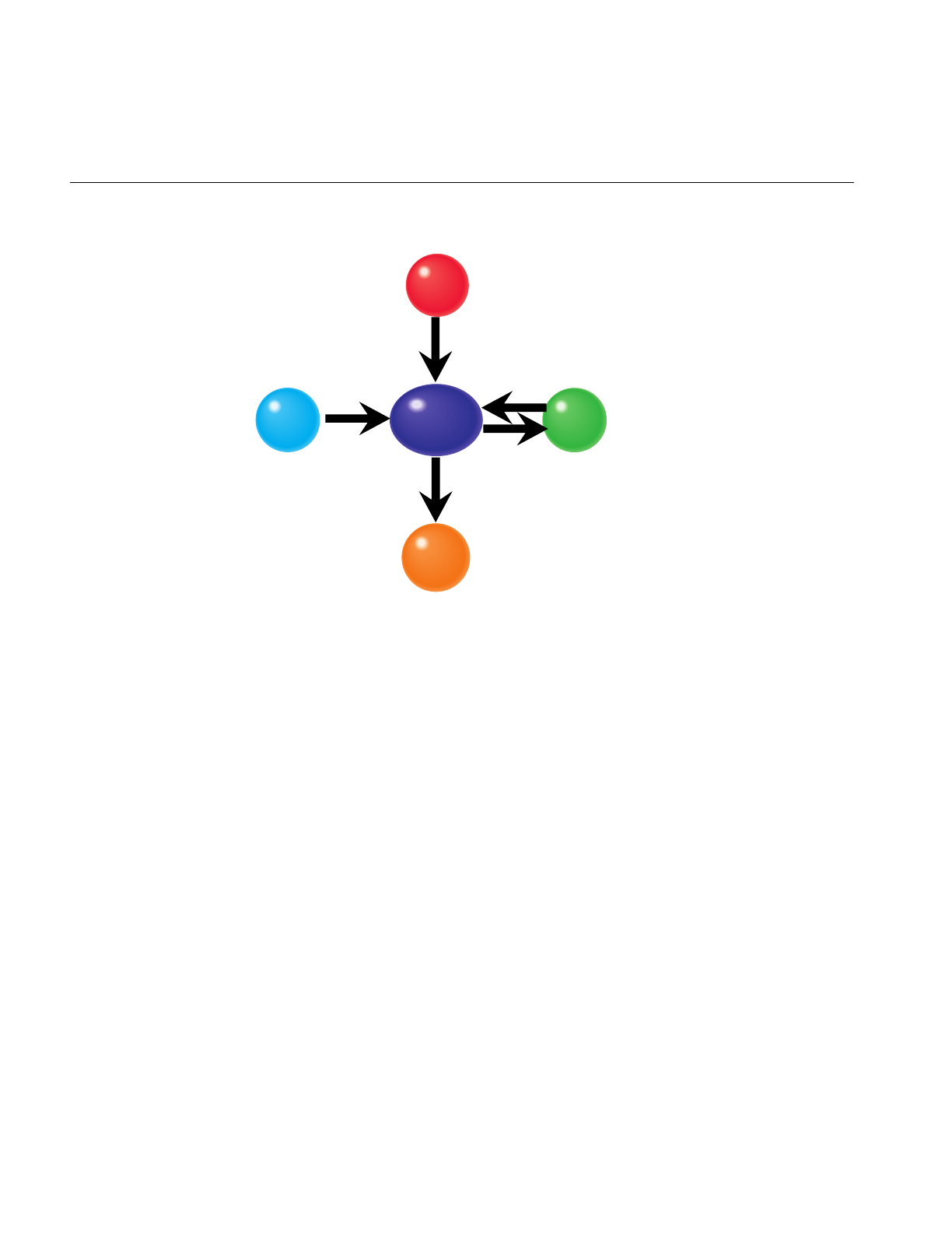
340
Chapter 10: ClipTextures
Figure 10-9 pfMPClipTexture Connections
Connecting MPcliptextures to pfPipes
To automatically apply of the pfClipTexture at the correct times and in the correct
processes, you must:
1. Create a pfMPClipTexture object.
2. Attach the pfMPClipTexture to the cliptexture you want to control.
3. Attach the pfMPClipTexture object to a pfPipe using the pfPipe.
Note: If you use pfMPClipTexture, you should never call either pfUpdateMPClipTexture
or pfApplyMPClipTexture the pfPipe should do the applying.
When you attach a pfMPClipTexture to a pfPipe using pfAddMPClipTextureToPipes(),
or pfAddMPClipTexturesToPipes() pfPipe automatically updates and applies
pfClipTexture at the correct time. The functions take three arguments, an
pfMPClipTexture or list of pfMPClipTextures, a pipe to attach to, called the master pipe,
and a list of other pipes the application wants to use with the pfMPClipTextures.
APP
process
MPClipTexture
Clip Center
node Pipe
Clip Texture

Post-Scene Graph Load Configuration
341
• pfAddMPClipTextureToPipes(pfMPClipTexture, masterpipe, pipe_list)
• pfAddMPClipTexturesToPipes(pfMPClipTexture_list, masterpipe, pipe_list)
The pipe_list is used for multipipe applications. It is the list of pipes that slave
pfMPClipTextures should attached to. Setting pipe_list is NULL is equivalent to adding
slave pfMPClipTextures to every other pipe in the application.
There are additional libpf routines that can be useful:
•pfRemoveMPClipTexture() detaches a pfMPClipTexture from a pfPipe. f a
pfMPClipTexture is removed that is the master of other pfMPClipTextures, the
slaves will be removed from their pipes as well.
•pfGetNumMPClipTextures() returns the number of pfMPClipTextures attached to
a pfPipe.
•pfGetMPClipTexture() returns a pointer to the pfMPClipTexture that is attached to
a pfPipe.
libpf Functionality
You can do this directly with the libpf API using the following calls:
• pfNewMPClipTexture—create a new pfMPClipTexture.
• pfMPClipTextureClipTexture—attach the pfMPClipTexture to the cliptexture.
• pfAddMPClipTexture - (a pfPipeCall)—attach the pfMPClipTexture to a pipe.
• pfMPClipTexturePipe—tell the pfMPClipTexture what pipe it’s attached to.
pfMPClipTexture Utilities
IRIS Performer provides utilities to make it easy to attach pfMPClipTextures to pipes,
and to automatically do pfMPClipTexture centering as well. As a bonus, the utility code
requires little or no changes to convert a single pipe application to a multipipe one.
To use the pfMPClipTexture utilities, you need to use IRIS Performer’s clipcenter nodes
to center the pfMPClipTexture. clipcenter nodes are a subclass of pfGroup nodes. They
have additional functionality that allows them to connect to a pfMPClipTexture, the
cliptextured geometry (through their child nodes), and properly update the
pfMPClipTexture’s center each frame. At load time, clipcenter nodes are placed at the

342
Chapter 10: ClipTextures
root of the subtree containing the cliptextured geometry. All the cliptextures in the scene
are created configured and attached to the clipcenter node at this time as well.
Once you have a scenegraph with geometry, cliptextures, and clipcenter nodes, it’s easy
to make pfMPClipTextures, attach them to pipes and to centering callbacks. The function
pfuProcessClipCenters() traverses the scene graph, looking for clipcenter nodes. As
each node is encountered, the function creates an MP cliptexture, attaches it to the
associated cliptexture and the clipcenter node, and saves a pointer to the MP cliptexture
in a pfList. When the function returns, it provides the list of MP cliptextures that were
created. The pfuProcessClipCentersWithChannel() routine performs the same
operations, but also sets a channel pointer in the clipcenter node. When the channel
pointer is set, the clipcenter node only will update a pfMPClipTexture center when that
channel traverses it. This is useful for multichannel applications.
Clipcenter Node
In order for cliptextures to be rendered correctly, the clipcenter must move along with the
viewer. IRIS Performer has made this task simpler by providing a special node for the
scene graph that does this calculation and applies it to the cliptexture each frame. This
node, called the clipcenter node, is a subclass of a pfGroup node. In addition to pfGroup
functionality, pfuClipCenterNode’s can do the following:
• Points to the cliptexture. This allows cliptextures to be attached to clipcenter nodes
at load time.
• Points to the geometry textured by the clipcenter node’s cliptexture. The clipcenter
node is assumed rooted in the subtree containing the cliptextured geometry.
• Points to an optional simplified version of the cliptextured geometry to make
centering calculations go faster.
• Points to the pfMPClipTexture attached to the cliptexture. The node also has API to
automatically create an pfMPClipTexture and attach it to the cliptexture.
• Contains a replaceable post-APP callback function for updating a
pfMPClipTexture’s center.
• Can point to a pfChannel, and only update the pfMPClipTexture center only when
that pfChannel traverses the clipcenternode.
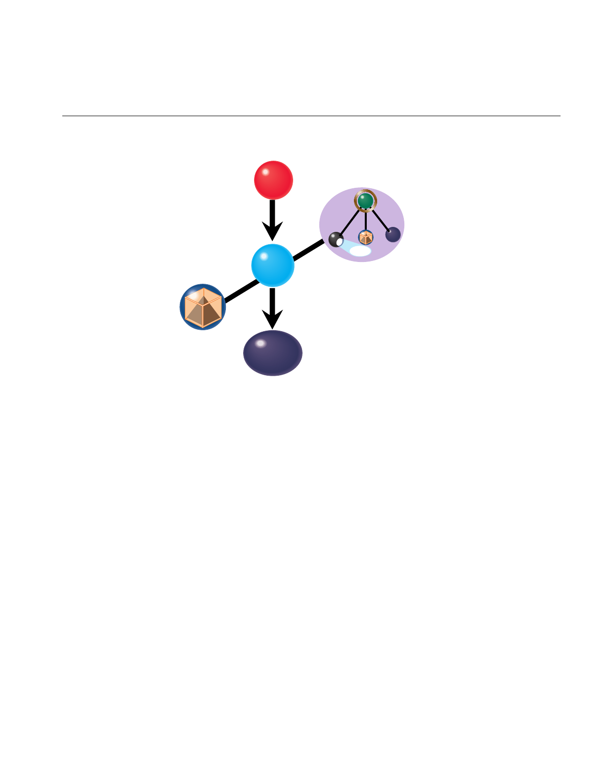
Post-Scene Graph Load Configuration
343
Figure 10-10 pfuClipCenterNode Connections
The clipcenter node uses a simple algorithm, setting the cliptexture center to be the point
on the textured geometry closest to the viewer. Other algorithms can be substituted by
replacing the callback function.
Clipcenter nodes can be created by calling the utility routine pfuNewClipCenterNode().
There are set and get functions to attach cliptextures, channels, custom centering
callbacks, simplified cliptextured geometry, as well as a get to return the
pfMPClipTexture. See the pfuClipCenterNode man page for details on the API.
The clipcenter node source code is available in pfuClipCenterNode.C and
pfuClipCenterNode.h, in the /usr/share/Performer/src/lib/libputil directory. It is
implemented as a C++ class with C++ and C API. It also has example code illustrating to
subclass the clipcenternode further to customize it.
If the configuration has been done properly, and if pfuClipCenterNodes have been used
for centering, most of the per-frame operations for cliptextures is automatic. Centering is
computed and applied by the clipcenter nodes during the APP traversal, and cliptexture
application is automatically handled by the pfPipes attached to the pfMPClipTextures.
Channel
MPClipTexture
Clip Center
node
Geometry
Scene graph
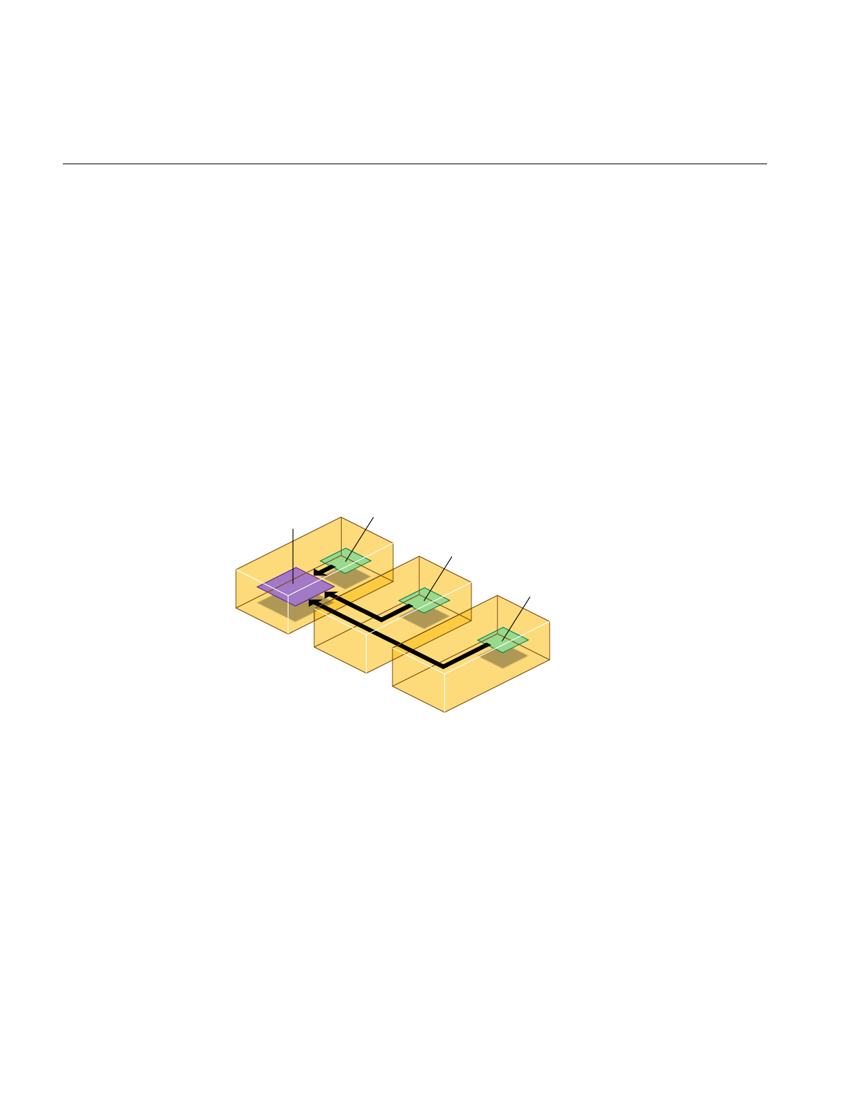
344
Chapter 10: ClipTextures
Using Cliptextures with Multiple Pipes
Cliptextures use a lot of texture memory, system memory (for their caches) and disk i/o
bandwidth. Many multipipe applications produce multiple views from the same
location, looking in different directions. It would be very inefficient to create a
completely separate cliptexture for each pipe: although there is separate texture memory
and graphics hardware from each pipe, the system memory and disk resources are
shared by the entire system.
Cliptextures have been designed to support multipipe rendering without excessive drain
on system memory and disk i/o bandwidth. Cliptextures that are to be used in multiple
pipes can be split into master and slave cliptextures. The master cliptexture is complete; it
contains an image cache and a region of texture memory to control. A slave cliptexture
points to its master, and shares its image cache, using it to download into its own texture
memory. All the slave cliptextures share their master’s system memory cache and disk
i/o resources, reducing the load on the system.
Figure 10-11 Master and Slave Cliptexture Resource Sharing
Making Masters and Slaves
Master and slave relationships can be established between image caches, cliptextures,
and pfMPClipTextures. The process starts with an object already configured you way
you want it. Then another object of the same type is created, and is set to be a slave of the
configured object. This is done with the setMaster() function. When an object is made the
slave of another object, it automatically configures itself to match it’s master. It also
makes all the connections necessary to share its master’s resources.
Master Slave Slave
Mem region Tex region
Tex region
Tex region

Post-Scene Graph Load Configuration
345
If two cliptextures are made into a master and slave, all of their image caches must have
the same master/slave relationship. This is done automatically. This is also true for
pfMPClipTextures. The pfMPClipTextures that will be the master and slave must be
connected to cliptextures. Only the masters have to be configured, however. When the
other pfMPClipTexture becomes a slave, it configures its cliptexture, and makes it and its
image caches slaves as well.
Multipipe Cliptexture API
IRIS Performer tries to make multipipe cliptexturing as transparent as possible. Simply
call setmaster on a cliptexture, passing it a pointer to the cliptexture that should be its
master.
(master_mct is a pfMPClipTexture that’s already configured)
•pfMPClipTexture *slave_mct = pfNewMPClipTexture()
•pfClipTexture *slave_ct = pfNewClipTexture()
•pfMPClipTextureClipTexture(slave_mct, slave_ct)
•pfMPClipTextureMaster(slave_mct, master_mct)
At this point, slave_mct and master_mct are connected; slave_mct is configured to match
master_mct and shares it’s image cache resources. The cliptextures and image caches are
also configured and linked. To make pfClipTextures or pfImageCaches masters and
slaves, use the same procedure.
When you attach a pfMPClipTexture to a pfPipe with pfAddMPClipTexture() provides
automatic multipipe support. If a pfMPClipTexture is added to a pipe that is already
connected to another pipe, the function silently creates a new pfMPClipTexture, makes
it a slave of the pfMPClipTexture that is already connected to another pipe, and adds the
slave to the pipe in place of the one passed as an argument to the function.
Multipipe Utilities
Although it isn’t difficult to set up master and slave cliptextures directly, it’s usually not
necessary.The previously described utility routines, pfuAddMPClipTextureToPipes()
and pfuAddMPClipTexturesToPipes() can take multiple pipe arguments. A master
pipe and a list of slave pipes is specified. The routine makes the pfMPClipTexture a
master and attaches it to the master pipe. It then creates slave pfMPClipTextures, attaches
them to the master cliptexture, and attaches a slave cliptexture to each pipe in the

346
Chapter 10: ClipTextures
slave_pipes list. This routine does extra checking of pipe and cliptexture state, and is
guaranteed not to generate errors, even if the function is applied more than once.
Master/Slave Share Masks
A group of cliptextures grouped by master/slave relationships can do more than share
mem region resources. By default, slave cliptextures also track a number of their master’s
attribute values. This means changing a master’s center, for example, automatically
causes the slaves to change their center locations to match their master’s. The attributes
that a slave can track are divided into groups called share groups. The application can
control which groups are shared by setting a slave’s share mask. Changing the sharing of
a slave only affects that slave’s sharing with its master. Changing the master share mask
has no effect. The share mask is set with the following call:
pfMPClipTextureShareMask(uint mask)
The mask can be set using one or more of the following values:
• PFMPCLIPTEXTURE_SHARE_CENTER—slave track the master’s center.
• PFMPCLIPTEXTURE_SHARE_DTR—slave tracks DTR; DTR mode, tex load time
(actual or calculated), fade count, and blur margin.
• PFMPCLIPTEXTURE_SHARE_EDGE—slaves track texture level parameters;
LODbias invalid border.
• PFMPCLIPTEXTURE_SHARE_LOD—slaves track minLOD and maxLOD.
• PFMPCLIPTEXTURE_SHARE_VIRTUAL—slaves track lodOffset and num
effective levels.
• PFMPCLIPTEXTURE_SHARE_DEFAULT—a bitwise ‘or’ of all the masks listed
above.
PFMPCLIPTEXTURE_SHARE_DEFAULT is the default sharemask value, which
provides maximum sharing between master and slave cliptextures. If an application
would like to control one or more slaves independently, it needs to change the slave’s
sharemask, then start setting the slaves parameters directly as needed.

Manipulating Cliptextures
347
Texture Memory and Hardware Support Checking
At the first application or formatting of a cliptexture, IRIS Performer compares the
expected size of the cliptexture texel data in texture memory against the systems texture
memory size. If it looks like the cliptexture won’t fit into texture memory, it shrinks the
clip size by two and tries again. It will keep shrinking the clip size until either the
cliptexture will fit or the clip size is zero. The system taking into account texture memory
banking and paging, to come up with a more accurate estimate.
Note that the resizing mechanism doesn’t take into account other textures or cliptextures
in use by the application. You should adjust your application so that IRIS Performer
doesn’t have to auto-shrink the cliptexture. See “Estimating Cliptexture Memory Usage”
on page 365 for calculating cliptexture system memory and texture memory usage.
During the checking phase, IRIS Performer also checks to see if cliptextures are
supported in hardware on the system. To cliptexture properly, the clipped levels need
hardware support. If cliptexturing isn’t supported, then the cliptexture is reconfigured so
only the unclipped, pyramid levels are loaded, and indicates to the system that the
texture is a normal MIPmap. The rest of the cliptexture support is unchanged. This
means that image caches in the pyramid levels will still work. This feature allows the
application writer to run and do some testing of cliptexturing applications even if the
system it’s run on doesn’t support cliptexturing.
Manipulating Cliptextures
Once cliptextures have been configured and connected into the application, they can be
manipulated by the application in the APP process. Applying and centering cliptextures
happens each frame, and is usually an automatic process, set up during post-load
configuration. Other parameters that can be adjusted include load control parameters,
min and max LOD levels, and virtual cliptexture control. Some of these parameters may
only need to be set once in the application, others, like the parameter setting for virtual
cliptextures, need to happen multiple times per frame.

348
Chapter 10: ClipTextures
Cliptexture Load Control
The virtualization of pfTextures into pfClipTextures, allowing very large texture maps,
comes at a price. As the clipcenter moves, cliptextures have to download data from disk
to system memory, and from system memory to texture memory. Because of these
download requirements, cliptextures are sensitive to available system bandwidth.
Without some sort of download load control, a fast moving center would cause a
cliptextures to “freeze”, waiting for the system to catch up with its updates.
While mem region updates happen asynchronously, tex region updates must happen in
the DRAW process, competing with geometry rendering and individual texture loading.
Real time applications require that cliptextures, like other IRIS Performer features, must
be controlled in a way such that an upper bound can be set on their use of resources. IRIS
Performer’s cliptexture load control, called Dynamic Texture Resolution (DTR), provides
this functionality.
Dynamic Texture Resolution
Dynamic Texture Resolution (DTR) is similar to Dynamic Visual Resolution (DVR): the
bandwidth requirements are adjusted to meet system limitations by lowering the
resolution of the texture data displayed by the cliptexture.
DTR controls bandwidth by analyzing the cliptexture in the CULL process. It checks each
cliptexture level, ensuring that the mem region contains updated tiles corresponding to
the tex region, and that there is enough time to update the tex region within the
download time limit.
This checking goes from level to level, from coarser levels to finer ones. When a level is
found that can’t be displayed, DTR adjusts the cliptexture parameters so that no levels
above the finest complete level are displayed. At that point, DTR stops checking levels
until the next frame. In order not to waste CULL processing time on levels that aren’t
visible, DTR will not try to sharpen more than one level beyond the current minLOD and
virtualLODoffset values. It will go one level beyond these values so that it can react
quickly if the values change.
This way the cliptexture updating will always keep up with the movement of the
clipcenter, and will never display invalid data. When the center moves too quickly, DTR
will “blur down” to coarser complete levels, then “sharpen up” to finer levels when the
center slows down and the system can catchup. In this way DTR can trade visual quality
against updating bandwidth. The visual result: the faster a viewer goes, the less time
there is to download texture, the blurrier the texture data gets.

Manipulating Cliptextures
349
The nature of cliptexturing makes load control work. When the clipcenter moves, this
change is reflected at every clipped level of the cliptexture. But because each texel in a
level covers four times the geometry of the texel in the next finer level, the clipcenter only
moves half the distance each time you go down a level. This translates into less
demanding texture download requirement.
DTR has other features, such as read queue sorting, which prioritize the order in which
read requests are done to improve mem region update performance. The rate at which
levels are blurred and sharpened can also be controlled to minimize visual artifacts.
Load Control API
DTR controls three aspects of load control, which can be turned on and off
independently: tex region updating (from the mem region in system memory), mem
region updating (loading from disks), and read queue sorting (reducing the latency of
read requests for downloads from disk to the mem region).
pfMPClipTextureDTRMode(DTRMode)
DTRMode is a bitmask; if a bit is set, that DTR feature is enabled. It has the following bits
defined:
•PF_DTR_MEMLOAD - enable mem region load control from disk
•PF_DTR_TEXLOAD - enable tex region load control; DRAW download time
•PF_DTR_READSORT - enable priority sorting of the read queue
All three bits are enabled by default, which means that DTR has all modes enabled.
Besides the bitmask to control what parts of DTR are enabled, there are parameters to
available to adjust load control performance. The DTR parameters, and how they affect
DTR functionality are discussed below:
Download Time
The memload component of DTR is relatively simple; it computes whether all the tiles in
a level’s mem region that cover the tex region are valid. If any are not, the tex region can’t
be updated and DTR invalidates that level. If the texload component of DTR is enabled,
DTR must also compute the time it takes to download from the mem region to the tex
region. The application provides the load control with a total download time in
milliseconds:
pfMPClipTextureTexLoadTime(float _msec)

350
Chapter 10: ClipTextures
This is the total time DTR has available to update the cliptexture’s texture memory each
frame. As DTR analyzes each cliptexture level that needs updating, it computes all the
regions in the level’s texture memory that need updating.If a level can be updated, DTR
determines whether there is enough download time left to update the level. If there is,
DTR marks that level valid, subtracts the time needed to download that level from the
total, and starts analyzing the next finest level in the cliptexture.
Cost Tables
IRIS Performer contains texture download cost tables, which DTR uses to estimate the
time it will take to carry out those texture subloads. These tables are a 2D array of floating
point values, indexed by width and height of the texture rectangle being subloaded. The
cost tables themselves are indexed by machine type, and can be read by the application.
The application can also define its own cost tables and configure the system to use it. The
cost table API is shown below:
pfPerf(int type, void *table)
pfQueryPerf(int type, void **table)
The text field indicates whether the cost table should be the one chosen by the system:
•PFQPERF_DEFAULT_TEXLOAD_TABLE - the one supplied by the application
•PFQPERF_USER_TEXLOAD_TABLE - or the one currently in use
•PFQPERF_CUR_TEXLOAD_TABLE - The default table is the current one unless a
application supplies a cost table, then the application’s cost table takes precedence.
For more details on cost tables, see the man pages for pfPerf() and pfQueryPerf(). The
cost table structure is named pfTexSubloadCostTable, defined in
/usr/include/Performer/pr.h.

Manipulating Cliptextures
351
Changing Levels
The DTR load control system is designed to minimize visual artifacts as it adjusts for
different download demands. Instead of abruptly sharpening the texture as new levels
with valid texture data become available, DTR blurs in new levels over a number of
frames, making the process of load control less noticeable. The application can control
the rate at which newly valid levels are displayed. The application sets a fade count, which
controls the number of frames it takes to fade in a new level . Each frame, the cliptexture
will sharpen 1/fadecount of the way from its current (possible fractional) level to the
next level. This process is repeated each frame, resulting in an exponential fade-in
function. If the fade count is 0, then fading is disabled, and DTR will show new levels
immediately.
pfMPClipTextureFadeCount(int _frames)
If the clipcenter roaming speed leaves barely enough bandwidth to bring in a new
cliptexture level, a distracting “LOD flicker” between to cliptexture LOD levels can
result. Since DTR must blur immediately if a level becomes invalid, the only way to
prevent flicker is to be conservative when sharpening, building in a hysteresis factor.
There is a parameter, called blur margin which helps determine when DTR should
sharpen.
Theblurmargin parameter also helps cliptextures blur smoothly when DTR can’t keep up.
It is a floating point value, which can be interpreted as a fraction of the cliptexture’s tex
load time. When blurmargin isn’t zero, DTR will load all the levels it can within the
texload time, but not display all of them. Instead it will only sharpen to the level that
would have been reached if the texload time was scaled by the blurmargin. This leaves a
cushion of extra time that can be used up before DTR will be forced to blur to a coarser
level. The default blurmargin value of .5 usually causes the finest level displayed to be
one level coarser then the finest level loaded.The application can adjust the blurmargin
by calling:
pfMPClipTextureBlurMargin(float margin)
DTR needs this cushion in order to fade smoothly. A cliptexture can only fade between
two valid levels; if it waits until its current level is invalid, the cliptexture must
immediately jump to the next coarser level or it will show invalid data. This abrupt
blurring is very noticeable. The blur margin allows the DTR system to anticipate when it
will lose a level, and smoothly fade to the next coarser level over a number of frames.

352
Chapter 10: ClipTextures
Total Texload Time and Texload Time Fraction
Using the texload time, blur margin, and fade count parameters is sufficient to control a
single cliptexture from a pipe, but the interface is awkward if multiple cliptextures are
applying from the same pipe. Since each pipe has the same amount of DRAW process
time available per frame, no matter how many cliptextures are applied from it, it would
be more convenient to provide a total amount of download time, then divide it among
the cliptextures using the pipe.
IRIS Performer provides this interface using the total texload time and texload time
fraction parameters. The application can set the total texture download time available on
a pipe, then assign fractional values for each cliptexture, indicating how the download
time should be divided. The total texload time is a pfPipe call, while the fractional values
are set on pfMPClipTextures:
pfPipeTotalTexLoadTime(float msecs)
pfMPClipTextureTexLoadTimeFrac(float frac)
The fractional values should indicate the relative priority of each pfMPClipTexture on
the pipe. The fractional values don’t have to add up to 1; the DTR code will normalize
them against the sum of all the fractional values set on the pipe’s pfMPClipTextures.
The total tex load time on the pipe is scaled by the normalized fractional value on each
cliptexture. The scaled tex load time is then used as the cliptexture’s texture download
time. Explicitly setting the tex load time on a pfMPClipTexture will override the
computed fractional time.
Read Queue Sorting
When the clipcenter moves quickly, the number of read requests for texture data tiles that
move into the clipped levels mem regions can grow much faster than the read function
can service them. If there isn’t enough bandwidth to display a particular level, itsread
requests may become “stale”, becoming obsolete as the location of the requested tile
moves into, then passes out of a level’s mem region.For DTR to be robust, the read queue
must be culled and sorted to remove stale read requests, and move the requests for tiles
closest to the clipcenter to the front of the queue. The cliptexture’s read queue is a sorting
queue, which means that a function can process the elements of the queue
asynchronously. DTR uses the read queue to cull read requests for tiles that are no longer
in their mem region, and to prioritize the other requested tiles as a function of level and
distance from the clipcenter. Sophisticated applications can provide their own sorting
function.

Manipulating Cliptextures
353
Invalidating Cliptextures
Sometimes an application may want to force a cliptexture to completely reload itself. For
example, The pfuGridifyClipTexture() function modifies the cliptexture’s texel data in
system memory with a system of grid marks to make debugging and analysis easier. It
modifies the read function to add a grid to every tile as it’s loaded into system memory,
then invalidates the cliptexture. For more information on gridify, look at the source code
in the /usr/share/Performer/src/lib/libpfutil/gridify.C file.
Invalidating a cliptexture forces it to completely reload its texture memory. Invalidating
is only supported for cliptextures, not MPcliptextures. This means that an application
cannot call invalidate from the APP process. Instead, it must call invalidate from the
CULL process, usually in a pre-cull callback. The invalidate call itself is simple:
pfInvalidateClipTexture(pfClipTexture *cliptex)
Invalidation is not needed for normal operation, but it is useful as a way to immediately
update a cliptexture’s texture memory.
Virtual ClipTextures
Regular cliptextures limit the size of each level but do not restrict the number of levels
you can access. Virtual cliptextures take the virtualization a step further by allowing you
to use only a subset of all the levels you have data for.
Although InfiniteReality supports cliptextures of virtual size up to 8Mx8M = 2^23x2^23
texels (i.e. 24 levels), the hardware is only capable of addressing a region of at most
32Kx32K = 2^15x2^15 texels (i.e. 16 levels). By limiting the set of texture MIPMap levels,
the cliptextures can be enlarged. A larger, virtual, cliptexture is defined just like a normal
cliptexture, except that the size of the cliptexture can exceed the 32K X 32K maximum
level size dictated by the hardware.
Virtual cliptextures do use more texture memory and require more callbacks in the CULL
process, but they allow enormous cliptextures that are limited only by the precision of
the texture coordinates. Cliptextures over one million texels on a side have been
demonstrated.

354
Chapter 10: ClipTextures
Although virtual cliptextures require dividing the cliptextured geometry into sections
for a given MIPmap levelrange, the division is much coarser and less restrictive than
texture tiling. Cliptextured geometry usually doesn’t need to be clipped to sectional
boundaries, for example, since there is a lot of leeway when there are more MIPmap
levels available than are needed for a given section of geometry.
For a sample application implementing virtual cliptextures, see
/usr/share/Performer/src/pguide/libpf/C/virtcliptex.c.
Selecting the Levels
The application is responsible for choosing which 16 (or less) levels can be accessed at
any given time by setting two parameters: virtualLODOffset and numEffectiveLevels. Most
applications make numEffectiveLevels the maximum number allowed by the hardware, 16
on InfiniteReality. Smaller values may be chosen in some cases to improve stability.
VirtualLODOffset sets the initial level in the cliptexture where 0 is the finest level.
For example, if numEffectiveLevels = 16 and virtualLODOffset = 0 then the texels the
hardware can access are limited to the 32Kx32K region surrounding the current
clipcenter, measured in finest-level texels (actually somewhat less than this; see the file
/usr/share/Performer/doc/clipmap/IRClipmapBugs.html or
/usr/share/Performer/doc/clipmap/IRClipmapBugs.txt for details on cliptexture limitations
on InfiniteReality graphics); attempting to access outside this range results in the value
of the nearest texel in the good region; i.e. the texels forming the border of the 32Kx32K
area will appear to be “smeared” out to fill the virtual cliptexture.
IncreasingvirtualLODOffset from 0 to 1 doubles the size of the accessible region in both S
and T (so that it’s 32Kx32K level 1 texels, which are twice as big as level 0 texels), but
makes the finest level inaccessible.
The maximum virtualLODOffset allowable is numVirtualLevels-numEffectiveLevels; when
set to that value, the entire S,T range of the virtual cliptexture is accessible, and the finest
level from which texels are available is the 32Kx32K level.
In general, it is appropriate to choose a large value of virtualLODOffset when the
viewpoint is far away from the scene and more S,T area is visible; smaller values of
virtualLODOffset are appropriate as the eye moves closer to the scene, gaining needed
higher resolution at the expense of range in S,T.

Manipulating Cliptextures
355
ChangingvirtualLODOffset and numEffectiveLevels has no effect on the contents of texture
memory nor any effect on the texture coordinates stored in the geosets and passed to the
graphics: the texture coordinates, as well as the clipcenter, are always expressed in the
space of the entire virtual cliptexture rather than the smaller “effective” cliptexture of up
to 16 levels within it. (In contrast, changing the clipcenter requires texture downloading;
thus it is a much more expensive operation and therefore it is not practical to change the
clipcenter more than once per frame, whereas virtualLODOffset and numEffectiveLevels
can be changed multiple times per frame, as we will see below.)
How to Set Virtual Cliptexture Parameters
IRIS Performer supports two different methods for managing virtualLODOffset and
numEffectiveLevels of a cliptexture. The simpler of the two methods allows the parameters
to be set and changed at most once per frame; the more sophisticated method allows
them to be changed multiple times per frame (different values for different parts of the
scene). In addition to virtualLODOffset and numEffectiveLevels described above, the
parameters minLOD, maxLOD, LODBiasS and LODBiasT often need to be set in the
same way, so we will show how to set those as well.
Per-Frame Setting of Virtual Cliptexture Parameters
The easy way to manage the virtual cliptexture parameters is to set the values of the
parameters on the pfMPClipTexture controlling the pfClipTexture:
int LODOffset, numEffectiveLevels;
float minLOD, maxLOD;
float LODBiasS, LODBiasT, LODBiasR;
...
mpcliptex->setVirtualLODOffset(LODOffset);
mpcliptex->setNumEffectiveLevels(numEffectiveLevels);
mpcliptex->setLODRange(minLOD, maxLOD);
mpcliptex->setLODBias(LODBiasS, LODBiasT, LODBiasR);
You make these calls in the APP process, either in the main program loop, a channel APP
func, or a pre- or post-node APP func. The last value you give during the APP in a
particular frame will be used for rendering that frame and all subsequent frames, until
you change the value again.
This simple technique is the one that is used by the clipfly program when you manipulate
the LODOffset and EffectiveLevels sliders (when using a naive scene loader such as the
.im loader that doesn’t do its own management of virtualLODOffset and
numEffectiveLevels): clipfly makes these calls in its channel pre-APP function.

356
Chapter 10: ClipTextures
This technique is also used by the .spherepatch loader; in this case the calls are made in
a post-APP function of a node in the scene graph, using parameters that are intelligently
chosen based on the current distance from the eye to the closest point on the textured
geometry, and are updated every frame.
Notice that even though the .spherepatch loader manages the virtualLODOffset and
numEffectiveLevels, you can still modify or override its behavior with the clipfly GUI
controls. This is accomplished using a special set of “limit” parameters that are provided
as a convenience and stored on the pfMPClipTexture. The intended use is for
applications such as clipfly to set the limits based on GUI input or other criteria:
mpcliptex->setLODOffsetLimit(lo, hi);
mpcliptex->setEffectiveLevelsLimit(lo, hi);
mpcliptex->setMinLODLimit(lo, hi);
mpcliptex->setMinLODLimit(lo, hi);
mpcliptex->setLODBiasLimit(Slo, Shi, Tlo, Thi, Rlo, Rhi);
Then the callback functions of intelligent loaders such as .spherepatch query the limits:
mpcliptex->getLODOffsetLimit(&lo, &hi);
mpcliptex->getEffectiveLevelsLimit(&lo, &hi);
mpcliptex->getMinLODLimit(&lo, &hi);
mpcliptex->getMinLODLimit(&lo, &hi);
mpcliptex->setLODBiasLimit(&Slo, &Shi, &Tlo, &Thi, &Rlo, &Rhi);
The loaders use the limits to modify the selection of the final parameters sent to
pfMPClipTexture.
The limits are not enforced by pfMPClipTexture; they are provided merely to facilitate
communication from the application to the function controlling the parameters. That
function is free to ignore or only partially honor the limits if it wishes.
The limits may also be queried frame-accurately from the pfMPClipTexture in the CULL
process, so they can also be used by scene loaders such as the .ct loader that use the
per-tile method described in the next section.

Manipulating Cliptextures
357
Per-Tile Setting of Virtual Cliptexture Parameters
Many applications require accessing a wider range of the cliptexture’s data than can be
obtained by a single setting of virtualLODOffset and numEffectiveLevels. This can be
accomplished by partitioning the database into “tiles” roughly according to distance
from the eye or from the texture’s clipcenter, and setting the parameters for each tile
every frame in the pre-CULL func of the pfGroup or pfGeode representing that tile, by
calling pfClipTexture::applyVirtual(),pfTexture::applyMinLOD(),
pfTexture::applyMaxLOD(), and pfTexture::applyLODBias().
Tiling Strategies
Choosing a database tiling strategy requires careful thought and tuning. The most
conceptually straightforward method is to use a static 2d grid-like spatial partitioning.
This method requires tuning the granularity of the partitioning for the particular
database and capabilities of the machine: if a tile is too big and sufficiently close to the
eye, there may be no possible combination of virtualLODOffset and numEffectiveLevels
that allows access to both the necessary spatial range and texture LOD range without
garbage in the distance or excess bluriness in the foreground; but if there are too many
tiles, the overhead of changing the parameters for each tile can become excessive.
In general, assuming the maximum active area is 32Kx32K (as it is on InfiniteReality),
each tile should be small enough so that it covers at most approximately 16K texels at the
finest texture LOD that will be used when rendering it; this is so that when the clipcenter
is close enough to the tile to require accessing that finest texture LOD, the 32Kx32K good
area centered at approximately the clipcenter will be able to cover it with some slop left
over to account for the inexact placement of the good area (see the IR cliptexture bugs
doc). (Finer tiles such as 8Kx8K or even 4Kx4K can be used for improved stability under
extreme magnification; see the IR cliptexture bugs doc).
This rule has two important consequences:
• If your cliptexture has insets (i.e. localized regions in which higher-res data is
available) you can make the tiling coarser in the regions where only low-res data is
available, and finer at the insets.
• If you use pfLODs to optimize your database, the coarse LODs of the pfLOD can
(and should) be tiled more coarsely than the fine ones.
This is because the coarser LODs are used at far distances, and at those far distances
the mipmapping hardware will only want to access correspondingly coarse texture
levels anyway, so the 16Kx16K can be measured in terms of the texels of those
coarse texture levels.

358
Chapter 10: ClipTextures
A more general tiling strategy that requires less empirical database tuning than the static
tiling method is to make the tiles be concentric rings around the texture’s clipcenter (in
2d) or around the eye point (in 3d), with sizes increasing in approximately powers of 2.
However, since the clipcenter and view position changes, this means the tiles must move
as well, which requires dynamically changing the topology of the scene graph and/or
morphing the geometry so that the tiles always form those concentric rings around the
current focus.
The .ct loader and pfASD’s ClipRings both use this dynamic strategy. The .ct loader is
interesting in that the morphing is done for the sole purpose of forming these concentric
tiles for virtual-cliptexturing an otherwise trivial scene. It looks like simply a square
textured by the cliptexture, but if you turn on scribed mode in perfly or clipfly, you can see
the morphing rings that make up the square.
Doing Per-tile Updates
To do per-tile updates, use the following procedure:
1. On each tile (typically a pfGroup or pfGeode) put a pre-node CULL func:
tile->setTravFuncs(PFTRAV_CULL, tilePreCull, NULL);
2. Make sure the effect of the tile’s pre-CULL func happens in the DRAW before the
contents of the tile are rendered, and that the tile’s contents do not co-mingle with
other tiles (this is not guaranteed by default, for the benefit of CULL whose sole
purpose is to return a CULL result without losing the advantages of uncontained
CULL sorting):
tile->setTravMode(PFTRAV_CULL, PFTRAV_CULL_SORT,
PFN_CULL_SORT_CONTAINED);
3. In the pre-node CULL func for the tile, set the parameters:
static int tilePreCull(pfTraverser *trav, void *)
{
int virtualLODOffset, numEffectiveLevels;
float minLOD, maxLOD;
float biasS, biasT, biasR;
//Choose intelligent values for parameters.
cliptex->applyVirtualParams(virtualLODOffset,
numEffectiveLevels);
cliptex->applyMinLOD(minLOD);
cliptex->applyMaxLOD(maxLOD);
cliptex->applyLODBias(biasS,biasT,biasR);
}

Manipulating Cliptextures
359
The values given to the apply functions are not stored in the pfClipTexture or retained
from frame to frame; when you call these functions, they override the corresponding
values stored in the cliptexture.
It is not necessary to call all four of the apply...() functions; only use the ones you care
about (e.g. most applications would not care about LODBias). However, if you ever call
a given one of these functions, say applyMinLOD(), on a particular cliptexture for any
tile, then you must call applyMinLOD() for every tile on that cliptexture during that
frame and forever after; if you omit it the tile will not necessarily get the value stored on
the pfMPClipTexture or pfClipTexture; rather, it will get whatever value happened to be
most recently set when rendering that tile in the DRAW (which may be nondeterministic
due to CULL sorting of the scene graph).
How to Choose Virtual Cliptexture Parameters
The libpfutil library provides a function called pfuCalcVirtualClipTexParams, which can be
very useful in selecting the virtual cliptexture parameters, no matter whether you are
updating per-frame or per-tile.
Essentially, you give to pfuCalcVirtualClipTexParams every piece of information you know
about the cliptexture:
• The tile in question.
• The limits specified elsewhere, for example, by the clipfly GUI.
pfuCalcSizeFinestMipLOD() returns the lower bounds on minLODPixTex, which is one
of the input parameters to pfuCalcVirtualClipTexParams.
The function returns optimal values for virtualLODOffset,numEffectiveLevels,minLOD,
maxLOD that you can:
• Set on the pfMPClipTexture in the APP process if your application is using the
per-frame method.
• Apply to the pfClipTexture per-tile in the CULL process if using the per-tile method.
For more details; you may also want to read the commented source code to understand
its constraints and heuristics, and how to modify pfuCalcVirtualClipTexParams to
implement your own algorithm if it does not exactly suit your needs.

360
Chapter 10: ClipTextures
Custom Read Functions
Sometimes the read function supplied by IRIS Performer to download texture data from
disk to mem region isn’t good enough. The application may need to do additional
operations at read time, such as uncompression, or may need a more sophisticated read
function, such as an interruptible one for reading large tiles from slow storage devices. A
read function may need to signal an applications secondary caching system; for example,
reading from tape storage to disk.
IRIS Performer provides support for application supplied custom read functions. The
read function is supplied at configuration time, and there is API in both the configuration
utilities and the cliptexture and image cache configuration files for supplying a read
function.
A read function is called by the image caches read queue. The read queue expects a read
function with the following function signature:
int ExampleReadFunction(pfImageTile *it, int ntexels)
The image tile pointer provides information about the read request, such as the disk to
read from, the dimensions and format of the texel data, and the destination tile in system
memory to write to. The ntexels argument is an integer indicating the number of texels to
read from disk. The read function returns another integer indicating the number of texels
actually read. Two example read functions are supplied in
/usr/share/Performer/src/lib/libpfdu/pfdLoadImage.c,ReadNormal() and ReadDirect().
These functions are C versions of the C++ functions that IRIS Performer uses to read
texture data. In IRIS Performer, the ReadDirect() function is called by the read queue; it
tries to use direct i/o to get the highest possible disk read performance. If the read direct
call fails, it calls ReadNormal(), which uses normal fopen()-style read.
When providing a read function at configuration time, You supply the function name,
and optionally the name of a DSO library containing the function. If no dynamic shared
library is supplied, The read function is searched for in the application’s executable.
To set read custom read functions using the configuration utilities, simply fill in the
readFunc field in the pfuImgCacheConfig or pfuClipTexConfig structure (the first
structure has priority over the second if both are set). The field should contain a pointer
to the customer read function. Be sure the function has the proper signature.

Using Cliptextures
361
When supplying custom read functions in the configuration files, you simply provide an
entry in one of two formats:
read_func
ReadFunctionName
read_func
DSOlibraryName ReadFunctionName
For hints on when and how to use custom read functions, see the customizing read
functions in “Custom Read Functions” on page 372.
Using Cliptextures
This section provides guidelines for using cliptextures, describing common cliptexture
application techniques, ways to solve problems, and some hints and tips to make using
cliptextures easier.
Cliptexture Insets
Cliptexture load control makes it possible to create cliptextures with incompletely filled
levels. A cliptexture, being much larger than an ordinary texture, may not be used in a
homogeneous way. Some areas of the cliptexture may be viewed in detail, others only at
a distance. A good example of this usage pattern is flight simulation. The terrain around
an airport will be seen from low altitude, terrain far from population centers may never
be seen below 40,000 feet. It is also possible that high resolution data is simply not
available for the entire cliptexture. Both of these cases make it valuable to create
cliptextures with incompletely populated values.
Regions of filled in data are called insets. Insets can be any shape, and do not need to
match tile boundaries (although this requires filling the rest of the tile with super
sampled data). For an inset to work properly, all of the levels from the pyramid up to the
finest level desired, must be available within the inset boundaries.
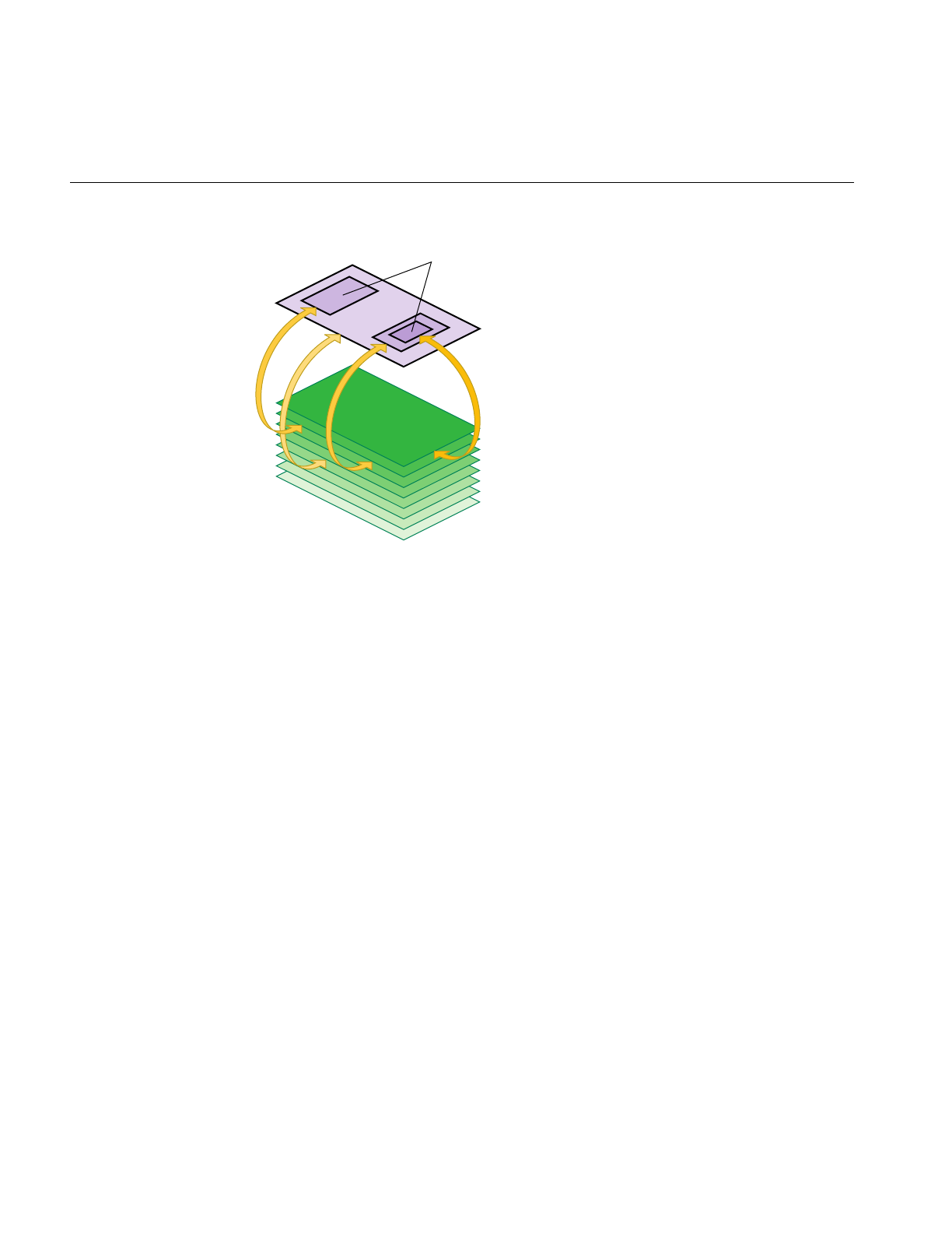
362
Chapter 10: ClipTextures
Figure 10-12 Cliptexture Insets
Insets are supported in cliptextures as a natural consequence of load control. As the
clipped region moves from a region that has texel data to one that doesn’t, DTR will blur
the texture down to the highest level that can completely fill the clipped region.
Adding Insets to Cliptextured Data
In large cliptextures, it may not be practical or even desirable to completely fill each level
with texel data. Cliptexture’s load control, DTR, automatically adjusts the finest visible
level based on what texels are available. If finer levels are not available, DTR
automatically “blurs down” to the highest complete level in the clip region.
Applications may use insets if there are only limited areas where the viewer is close to
the terrain. An example application would be a commercial flight simulator, where the
inset high-resolution data would be around the airports where the aircraft takes-off and
lands. The terrain over which the aircraft cruises can be lower resolution.
Insets and DTR
To create insets properly, you have to understand how DTR load control works. At the
beginning of each frame, DTR examines a level’s mem region to see if the tiles covering
the tex region are all loaded. If the tiles are all available, DTR will make that level visible.
Insets

Using Cliptextures
363
DTR does this examination starting with the coarsest clipped level. If the current level is
complete, it marks that level as visible and repeats the process for the next finest level,
until it gets to the top level or finds an incomplete level.
Building Insets
To create an inset, assume you have a cliptexture that is complete at a coarse level. You
choose an area of the clipmap that you would like to have visible at some finer level. In
order to make that area available, you have to provide texel data in that area for each
level from the coarse complete level to the finer level you want to show.
When the clip region is completely enclosed by the finer level data, DTR checks all the
levels from the pyramid level on up, and allows the finer level to be shown in that area.
(The pyramid levels are always complete; see Figure 10-1.)
Because DTR works from the bottom up (coarser to finer levels), an inset area must have
texel data available from the finest level all the way down to the pyramid level. If a level’s
clip region is missing or incomplete, DTR does not allow the image to sharpen up to that
level; the inset gets blurry.
Inset Boundaries
When the clipcenter is set such that the clip region is completely enclosed by the insetted
area, a properly constructed inset is sharp, using the finer resolution texel data. But what
happens when the clip region only partially covers an inset? In that case, DTR does not
sharpen up beyond the finest complete level, and the clip region gets blurry, including the
part of the clip region covered by the inset. Remember, the clip region only sharpens to the
finest level that is complete within the clip region.
This bluriness may not be a problem. If you know that the application moves far enough
away from the terrain before the clip region crosses an inset border, MIPmapping uses
the coarser texture levels before DTR forces the texture to use them. Sometimes, the
application would like a static boundary between the inset and the surrounding coarser
data, even when crossing an inset boundary close to the textured geometry.
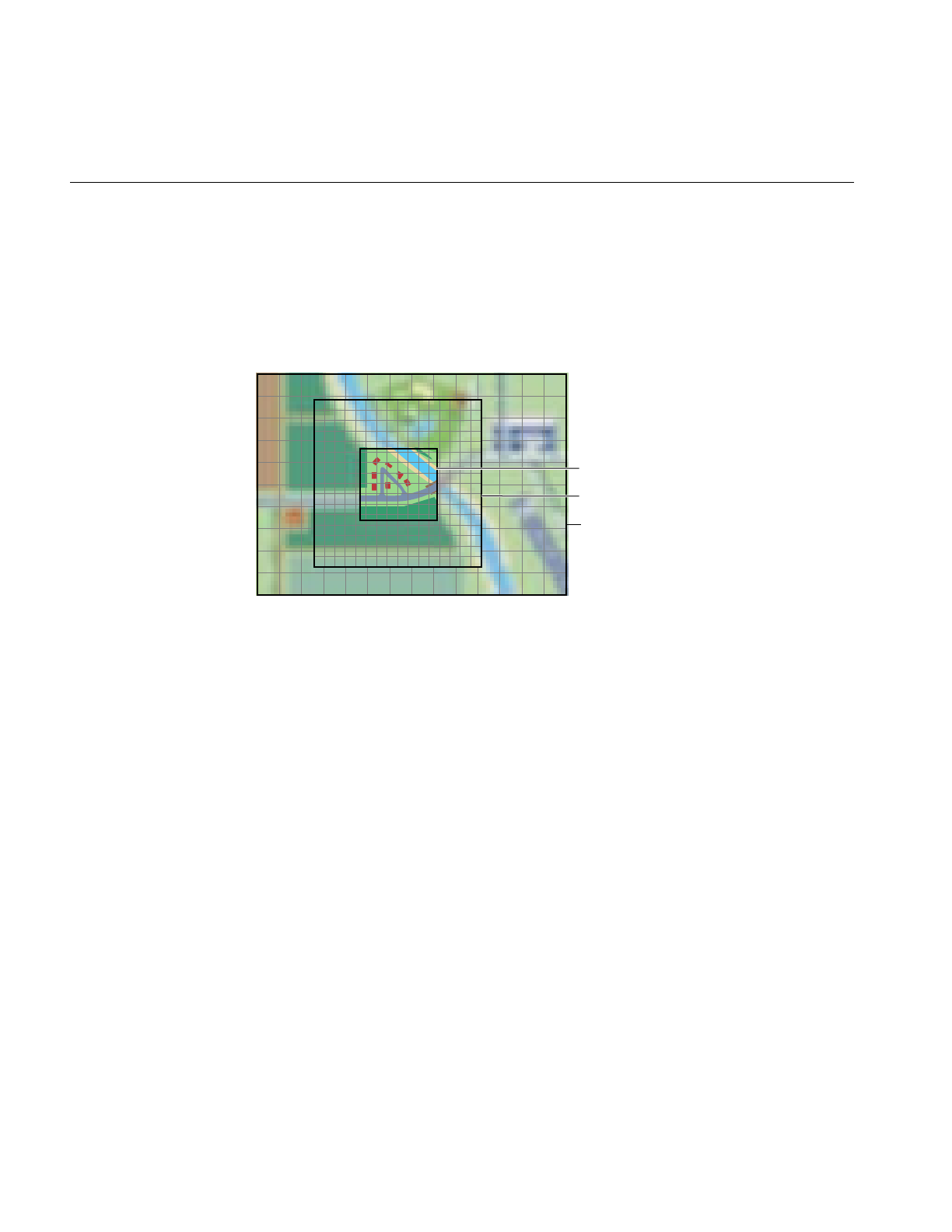
364
Chapter 10: ClipTextures
Supersampled Data
Getting a static inset border requires creating a boundary of supersampled data around
the inset. This means creating texel data for the insetted levels that is deliberately made
as blurry as the surrounding base level. This border of blurry data must be at least as
wide as the clip region to ensure a smooth transition.
Figure 10-13 Supersampled Inset Boundary
How does this work? When the clip region crosses an inset border, it starts to cover the
boundary region. Since the boundary region has the same levels filled in as the inset
region, DTR still sees complete data up to the same finer level. The texel data of the
border has been blurred, however, so it looks like the coarser base level. This allows a hard
transition between the finer inset data and the surrounding coarse data. Since DTR still
sees complete levels, as you move away from the inset, it doesn’t suddenly blur.
Since the boundary data is at least as wide as the clip region, the inset boundary has
moved out of the clip region before the clip region hits the far edge of the boundary
region. At this point, DTR blurs down to the coarser base level, since the finer data is no
longer incomplete, but there is no visual change, since the boundary texels were blurry
already.
Note: Supersampled borders do not guarantee a seamless transition between insets and
their surroundings, only that the inset region does not suddenly blur or sharpen as the
clip region crosses the inset border. Seamless transitions only happen if the application is
careful to get far enough from the clipmapped terrain to already be using the coarse
levels before crossing the inset border.
Inset
Coarse level
Supersampled boundary

Using Cliptextures
365
Multiple Insets
Insets do not have to be any particular size or shape, although they are usually multiples
of the tile size, and at least as big as the clip region so they can be viewed without a seam
of bluriness. Typically, insets are designed so when the application is close enough to
view the finer inset levels, the clip region is already completely enclosed by the inset
region.
Keep in mind that insets are not the same size on each level, since texels from coarser
levels cover more geometry. If an inset isn’t a multiple of the tile size at a given level, the
tile has to be partially inset data, and partially supersampled data, or all fine data, since
DTR does not work with partial tiles.
Estimating Cliptexture Memory Usage
Because cliptextures are a voracious consumer of system and texture memory, it is
important to accurately predict the system resources required to run a cliptexture
application. It is better to customize your application than to rely on the cliptexture auto
resizing feature, since auto-resizing doesn’t take into account multiple cliptextures or
pfTextures in your application.
Cliptextures use both system memory (texel caching, read queue elements as well object
overhead) and texture memory. The following estimation ignores the smaller
contributors to system memory overhead and concentrates on image cache consumption
of system memory for mem regions and tex regions in texture memory.
System Memory Estimation
The following values are required to estimate system memory requirements:
• Size of clipmap level 0
• Clip size (in texels)
• Tile size (in texels; assuming tile size is the same for all levels)
• Texel size in bytes
• Whether the tiles have high disk latency

366
Chapter 10: ClipTextures
Given these values, compute the estimate for system memory requirements using the
following procedure:
1. Round up clip size to even multiple of tile size in each dimension.
2. Divide each dimension by tile size in that dimension.
3. Add 2 tiles to each dimension for a tile boundary of 1.
If there is high latency downloading, such as reading tiles Over the network, or
decompressing tiles, add 4 tiles per dimension, giving a tile boundary of 2.
You now have the number of tiles in each dimension per clipped level.
4. Multiply each tile number in each dimension by the corresponding tile size in that
dimension.
You now have the number of texels in each dimension.
5. Multiply the texel dimensions together.
6. Scale by the size of each texel.
7. Add in the fixed cost of image cache structs.
You now have the system memory cost in bytes for each clipped level.
8. Treat each level bigger than clip size as clipped. Add 4/3rds of the clip size scaled
by the texel size for the pyramid levels.
This estimate is a bit too conservative, since the lowest clipped levels may exceed
the entire level size with a border of 2 tiles. It is a function of tile size and clip size.
9. Scale the clipped level size by the number of clipped levels.
Example Estimating System Memory Requirements
The example uses the following values in its estimation:
• 2M top level
• 1K clip size
• 512 Tile Size (everything square)
• 1 byte texel size (LMV example)
Example 10-1 estimates system memory requirements using the preceding procedure.

Using Cliptextures
367
Example 10-1 Estimating System Memory Requirements
1. No-op: 1K, 1K (for both s and t).
2. 1K/512 = 2, 2 (for both s and t).
3. 2+4 = 6, 6 (for both s and t; high latency on tile download)
4. 6 * 512 = 3K, 3K (for both s and t)
5. 3K * 3K = 9M
6. 9M * 1 = 9M
7. 9M * 10 = 90M (for 2M -> 4K levels) + 2M (for 2K level) = 92M
8. 4/3 * 1K * 1K= 1.3M
9. Total Size 92M + 1.3M = 93.3M
Texture Memory Estimation
The following values are required to estimate texture memory requirements:
• Clip size (in texels).
• Whether the clipmap is virtual or non-virtual.
• Number of levels in use (if less than 16).
Given these values, you can compute the estimate for texture memory requirements
using one of the following guidelines:
• If the clipmap is virtual, multiply the number of levels by the square of the clip size.
• If the clipmap is non-virtual:
1. Multiply the number of levels bigger than the clip size by the square of the clip
size.
2. Add 4/3 times the clip size squared.
There is, however, a further complication involved in accurately estimating texture
memory requirements.

368
Chapter 10: ClipTextures
Texture Memory Usage: A Further Complication
InfiniteReality rendering boards come with either 16 or 64 megabytes of texture memory.
Unfortunately, you ca not just use the texture memory any way you want. The texture
memory is divided into two equal banks. Each adjacent mipmap level clipmapped or
not, must be placed in opposite banks. This ends up restricting the amount of texture
memory available for clipmapping.
A further restriction is that texture formats can take up 16 bits or 32 bits of data per texel,
but nothing in-between. This means an 888 RGB format takes up 32 bits per texel, just like
an 8888 RGBA format.
To give you an example of this restriction, consider an example using RGB texel data, 8
bits per component, and a clip size of 2048 by 2048. The largest level is 8K by 8K. The
system has an RM board with 64M of texture memory, so it would seem that there is
plenty room, but the following calculation shows otherwise:
1. The cliptexture’s non-virtual, so the total texture memory requirement is the clip
size times the number of clipped levels plus 4/3 of the pyramid:
2. 4K, 4K levels are clipped to 2K X 2K: RGB, 8 bits per channel 4 bytes (not 3!) per
texel times 2K X 2K = 4M of texels per level;
3. 6M of texture memory per clipped level
4. So that’s 32M of texture memory
5. 2K and below is the pyramid, so 4/3 of 16M = 21-1/3M
6. Total is 53-1/3M of texture memory.
Unfortunately, the texture does not fit into texture memory because:
1. 64M of texture memory means two 32M banks.
2. Each level must be in the opposite 32M bank.
3. Consequently, 8K level becomes 16M in bank 0 (16M left).
4. At the 4K level, 16M goes into bank 1 (16M left).
5. At the 2K level, 16M goes into bank 0 (0M left).
6. At the 1K level, 8M goes into bank 1 (8M left).
7. At the 512 level, there is no room in bank 0!!

Using Cliptextures
369
The best you could do is to have only 1 clipped level, as follows:
1. At the 4K level,16M goes into bank 0 (16M left).
2. At the 2K level, 16M goes into bank 1 (16M left).
3. At the 1K level, 8M goes into bank 0 (8M left).
4. At the 512 level, 4M goes into bank 1 (12M left).
5. At the 256 level, 2M goes into bank 0 (6M left); and so on.
Probably a better solution would be to use the 5551 format RGBA texels, which only use
16 bits per texel, allowing more levels, as follows:
1. At the 32K level, 8M goes into bank 0 (24M left).
2. At the 16K level, 8M goes into bank 1 (24M left).
3. At the 8K level, 8M goes into bank 0 (16M left).
4. At the 4K level, 8M goes into bank 1 (16M left).
5. At the 2K level, 8M goes into bank 0 (8M left).
6. At the 1K level, 4M goes into bank 1 (12M left).
7. At the 512 level, 2M goes into bank 0 (6M left).
8. At the 256 level, 1M goes into bank 1 (11M left); and so on.
You can get a lot more mileage out of smaller texel formats than less levels. This becomes
even more true for RMs with only 16M of texture memory.
Using Cliptextures in Multipipe Applications
IRIS Performer provides good support for multipipe cliptextures, allowing applications
to ignore many of the differences between single pipe and multi-pipe operations. The
primary issue in multi-pipe applications is knowing when to make master/slave
cliptextures, what parameters should be shared, and when and how to create separate
centers in different master and slave cliptextures.
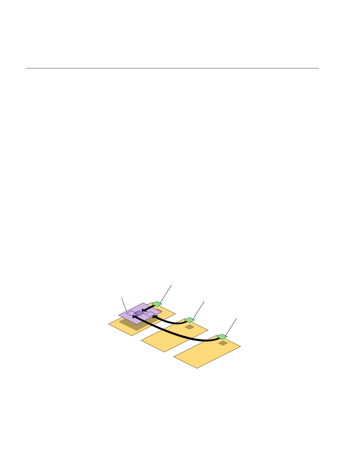
370
Chapter 10: ClipTextures
When to Make Master/Slave Cliptexture Groups
When it’s possible, it is desirable to make master/slave cliptexture groups in multipipe
applications. Master/slave groups share the same mem regions and disk access
bandwidth, reducing the load on the system. Masters and slave can also take advantage
of sharegroups, automating some of the work of synchronizing slave cliptextures with
their masters.
Master and slave cliptextures don’t work when the different cliptextures represent
different textures. Separate cliptextures must be created for each texture that has to be
displayed. Another condition that prevents using master/slave cliptexture groups is
when the center for the cliptexture in each pipe is completely independent. Master and
slave cliptextures assume that the tex region for each cliptexture is always completely
enclosed by the shared mem region. If that assumption is violated, the cliptexture data
will be invalid for the parts of the tex region outside of the shared mem region, and the
cilptextures will print error messages.
Slave Cliptextures with Offset Centers
There is no reason for the slave cliptextures to have the same centers as the master, as
long as the tex regions always stay within the mem region. Sometimes it is desirable for
an application to have views with slightly different viewpoints for each pipe. This can be
done by turning of clipcenter sharing, and having the application set a slave’s center
directly. The application is responsible for keeping the tex region inside the master’s
mem region at all times. The position of the master’s center determines the groups mem
region, so the master’s center can not be offset from the center of the mem region.
Figure 10-14 Offset Slave Tex Regions
Master Slave Slave
Mem region
Tex region
Offset tex region
Offset tex region

Using Cliptextures
371
Virtualizing Cliptextures
Virtual cliptextures are one of the most challenging features to use in an IRIS Performer
application. Cliptextures themselves are challenging enough, since they tie together
functionality in the scene graph, pfPipes and pfChannels. Virtual cliptextures add an
additional level of complication, since they require that the application segment the
terrain, estimate the texture LOD levels needed for each terrain segment based on the
current eyepoint, and update the virtual cliptexture parameters appropriately.
Some tips to consider when working with virtual cliptextures:
• Get your application working with a non-virtual cliptexture first. It’s hard to
separate virtual cliptexture problems form basic cliptexture configuration problems
(which are usually easier to fix).
• Start off with a single segment and as little complexity in the application as possible,
then get that working. It makes debugging much simpler.
• When in doubt, print it out. For debugging purposes, a well placed set of pfNotify()
statements can be really helpful. It’s also useful to set up a canonical scene, where
you know what parameters should be generated, then compare them against what
the program does.
• Take maximum advantage of sample code and utilities. Try to re-use some of the
example code provided by IRIS Performer. Using (or just reading) through the
loaders, example programs, and utilities listed in this section “Cliptexture Sample
Code” on page 373 can save you hours of work.
Customizing Load Control
Setting texload time, multiple cliptexture load control, normally, bandwidth from disk to
system memory is optimized by image cache configuration. You can use the streams
feature in image cache configuration files to maximize bandwidth by configuring the
system with as more disks and disk controllers, and copying the texture data files over
multiple disks. By using the streams feature in image cache configuration files, you can
then parallelize the disk downloads over separate disks and disk controllers. You can
also stripe disks to increase disk download bandwidth.

372
Chapter 10: ClipTextures
Texture memory bandwidth is more a matter of careful rationing of DRAW process time
each frame. You will have to ration between sending geometry and texture data to the
graphics pipeline. You can adjust the cliptexture’s texload time to minimize idle time in
the draw process. DTR computes texture download time using a cost table to estimate
what the download updates will cost each frame. It’s a good estimate, but not a perfect
one. You may have to build in some time margin in the DRAW process to avoid dropping
frames.
Download time setting can be as simple as finding the minimum time that still allows the
cliptexture to completely sharpened when the clipcenter is stationary. If the texload time
is too small, a cliptexture can get “stuck” and never sharpen beyond a given level.
Sophisticated users might consider adjusting the invalid border as well, which will
change the effective clip size of the cliptexture. This could be used to allow a new level
to be gradually loaded over a number of frames; trading off a finer visible level against a
smaller effective clip region.
Custom Read Functions
Custom read functions allow the application to control what happens when texture data
is downloaded from disk. Operations include: texture data decompression, texture data
image processing, signaling an update of a disk cache from tape, etc. As described in the
API section, replacing the read function is fairly easy to do in IRIS Performer.
One caveat: increasing the overhead of read functions can have undesirable
consequences. The latency of read operations determines the minimum size of the image
cache mem regions, since they need to lookahead to compensate for high latency reads.
Low bandwidth read operations effect how fast the center can move before DTR must
blur down to coarser levels.
One way around these problems is to implement a lookahead disk cache. Rather than
have the read function decompress files, have it read files from a cache of files that have
already been decompressed by an asynchronous process. The read function can signal
the other process to decompress more files as it gets close to the edge of the cache.
Texture data image processing, since it is relatively fast compared to disk reads, usually
doesn’t require such elaborate measures. Changing the read function can be done in
conjunction with modifying the image cache mem region data to ensure that all data read
from disk is processed. A good example of this technique is the gridify feature, described
in “Invalidating Cliptextures” on page 353.

Using Cliptextures
373
Cliptexture Sample Code
The best way to learn to use cliptextures is to work from existing code. IRIS Performer
has a number of demo programs, test programs, loader code, and utilities, with different
levels of sophistication:
Test and Demo Programs
•/usr/share/Performer/src/pguide/libpr/C/icache.c - a simple libpr-style program that uses
an image cache and the texture transform matrix to scroll texture across a polygon.
•/usr/share/Performer/src/pguide/libpr/C/icache_mwin.c - This program is a
multiwindow version of icache; it uses master and slave image caches. Note that
the tex regions of the slaves image caches are offset from the master.
•/usr/share/Performer/src/pguide/libpr/C/cliptex.c - a simple libpr-style program that
uses a cliptexture to display a bird’s eye view of data. On a system that supports
cliptexturing, it moves the clipcenter, allowing the user to see the rectangle of
texture resolution move as the center translates between opposite diagonals.
•/usr/share/Performer/src/pguide/libpr/C/cliptex_mwin.c - This is a multiwindow version
of cliptex. It uses master and slave cliptextures.
•/usr/share/Performer/src/pguide/libpf/C/cliptex.c - This is a libpf implementation using
cliptextures. Rather than use clipcenter nodes, it uses a simple centering mechanism
based on the x and y coordinates of the channel’s viewpoint.
•/usr/share/Performer/src/pguide/libpf/C/virtcliptex.c - This is the virtual cliptexture
version of the cliptex program. It will take any size cliptexture and virtualize it. It
divides a flat terrain in the x,y plane into a rectangular grid, attaching geodes with
callbacks to each grid square. The callback calculates the virtual cliptexture
parameters and applies them.
IRIS Performer Cliptexture Applications
•/usr/share/Performer/src/app/sample/C/perfly.c - This sample application supports
cliptextured scene graphs. It assumes that the loaders will do the basic
configuration, but it does the post loading cliptexture configuration, creating
pfMPClipTextures and attaching them to pipes. It assumes that clipcenter nodes are
in the scenegraph, and that they will do the centering work. Pressing g will toggle
the gridify feature.
•/usr/share/Performer/src/app/sample/C/clipfly.c - This is the cliptexture version of the
perfly sample application. It contains extra interface sliders and buttons that allow
you to control many more cliptexture parameters.

374
Chapter 10: ClipTextures
Loaders that Support Cliptextures
•/usr/share/Performer/src/lib/libpfdb/libpfim/pfim.c - This is the IRIS Performer example
loader. It contains simple tokens to create clipcenter nodes and cliptextures. It is a
good starting point for cliptexture configuration in the loader.
•/usr/share/Performer/src/lib/libpfdb/libpfct/pfct.C - This is a more sophisticated
cliptexture sample loader. It automatically creates some simple cliptextured
geometry, and supports virtual cliptextures, providing the geometry segmentation
and scene graph callbacks.
•/usr/share/Performer/src/lib/libpfdb/libpfvct/pfvct.C - This is a very simple
pseudo-loader that will adjust a cliptextures parameters so it can be used as a
virtual cliptexture, even if its dimensions are smaller than 32K by 32K.
•/usr/share/Performer/src/lib/libpfspherepatch/pfspherepatch.C - this is a cliptexture loader
designed to apply a cliptexture to a sphere. It is a good example of a specific
cliptexture application.
Cliptexture Utility Code
•/usr/share/Performer/src/lib/libpfutil/gridify.C - the gridify functionality illustrates
techniques for dynamically modifying cliptexture data, and illustrates how to
replace the cliptexture’s read function.
•/usr/share/Performer/src/lib/libpfutil/trav.c - the function pfuFindClipTextures
illustrates how to traverse the scenegraph to find cliptextures.
•/usr/share/Performer/src/lib/libpfutil/pfuClipCenterNode.C - this code defines the
clipcenter node, and contains example code for creating customized clipcenters by
subclassing.
•/usr/share/Performer/src/lib/libpfutil/clipcenter.c - the pfuProcessClipCenters() and
pfuProcessClipCentersWithChannel() functions illustrate how to use clipcenters in
an application.
•/usr/share/Performer/src/lib/libpfutil/cliptexture.c - the
pfuAddMPClipTextureToPipes() and pfuAddMPClipTexturesToPipes()
functions illustrate how to work with cliptextures and pipes.

This chapter describes how to create, configure, manipulate, and communicate
with a window in Performer.
“Windows”
Chapter 11


377
Chapter 11
11. Windows
Rendering to the graphics hardware requires a window. A window is an allocated area
of the screen with associated framebuffer resources. The X window system manages the
use of shared resources amongst the different windows. Windows can be requested
directly from an X window server. With a bit of interfacing, both IRIS GL and OpenGL
graphics contexts can render into X windows.
This chapter describes how to create, configure, manipulate, and communicate with a
window using pfWindow in IRIS Performer. The extended libpf object pfPipeWindow,
based on pfWindow, is also mentioned in this chapter as the two objects share much
functionality. Likewise, for good understanding of windowing issues, the next chapter,
Chapter 12, “pfPipeWindows and pfPipeVideoChannels,” should also be read.
pfWindows for both OpenGL and IRIS GL
An X window with an OpenGL graphics context is called an OpenGL/X window. An
X window with an IRIS GL graphics context is called a mixed model IRIS GL (GLX)
window. IRIS GL supports a third option: pure IRIS GL windows. Pure IRIS GL windows
are convenient and flexible for rendering purposes but can not be used as X windows in
X applications. If, for example, you want to put your rendering window inside a larger
Motif® window, you will need an X window. Libpr provides utilities to shield you from
the differences between the different types of windows and guide you in your dealings
with the window system. Applications that use the IRIS Performer window utilities can
be completely portable between IRIS GL and OpenGL and sill have the option of using
pure IRIS GL windows if desired when running in IRIS GL. You’ll be able to use your
windows in X applications, or direct your rendering to a pre-created window. The libpr
windowing support centers around the pfWindow. The libpf windowing support is based
on pfWindow and uses a pfPipeWindow.

378
Chapter 11: Windows
pfWindows are structures for managing any of the different kinds of windows and
associated pfState. pfWindows provide an efficient windowing interface between your
application and the window system. pfWindows shield you from the functional and
performance differences between the different graphics libraries and the different
window system interfaces and allow you to configure, manipulate, and query IRIS GL,
IRIS GL mixed model (GLX), and OpenGL/X windows through a GL and window
system independent interface. pfWindows also keep track of your graphics state: they
include a pfState which is automatically initialized when you open a window, and
switched for you when you change windows.
IRIS Performer automatically configures and initializes your window so that it will be
ready to start rendering efficiently. In the simplest case, pfWindows make creating a
graphics application that can run on any Silicon Graphics machine with IRIS GL or
OpenGL a snap. pfWindows do not limit your ability to configure any part or all of your
windowing environment yourself; you can use the libpr pfWindows to manage your GL
windows even if you create and configure the actual windows yourself.
Creating a pfWindow
A pfWindow structure is created with pfNewWin(). It can then be immediately opened
with pfOpenWin(). Example 11-1 shows the most basic pfWindow operations in libpr
program: to open and clear a pfWindow and swap front and back color buffers.
Example 11-1 Opening a pfWindow
int main (void)
{
pfWindow *win;
/* Initialize Performer */
pfInit();
pfInitState(NULL);
/* Create and open a Window */
win = pfNewWin(NULL);
pfWinName(win, “Hello from IRIS Performer”);
pfOpenWin();
/* Rendering loop */
while (1)
{
/* Clear to black and max depth */

Creating a pfWindow
379
pfClear(PFCL_COLOR | PFCL_DEPTH, NULL);
...
pfSwapWinBuffers(win);
}
}
The pfWindow in Example 11-1 will have the following configuration:
Window system interface
OpenGL windows will be an X window using the OpenGL/X interface.
IRIS GL windows will be pure IRIS GL.
Screen: The pfWindow will open a window on the screen specified by the
DISPLAY environment variable, or else on screen 0.
Position and size:
The position and size will be undefined and the window will come up
as a rubber-bend for the user to place and stretch.
Framebuffer configuration:
The window will be doublebuffered RGBA with depth and stencil
buffers allocated. The size of these buffers will depend on the available
resources of the current graphics hardware platform. GLX and
OpenGL/X windows will also have multisample buffers allocated if
they are available on current hardware platform.
Libpr state: A pfState will be created and initialized with all modes disabled and no
attributes set.
Graphics state: The pfWindow will be in RGBA color mode with subpixel vertex
positioning, depth testing and viewport clipping enabled. The Viewing
projection will be a two-dimensional one-one orthographic mapping
from eye coordinates to window coordinates with distances to near and
far clipping planes -1 and 1, respectively. The model matrix will be the
current matrix and will be initialized to the identity matrix.
Typically, pfWindows go through a bit more initialization than that of Example 11-1. The
type of pfWindow type, set with pfWinType() is a bitmask that selects the window
system interface and the type of rendering window. The default window type is a normal
graphics rendering window and is pure IRIS GL under IRIS GL operation and X under
OpenGL. operation. Table 11-1 lists the possible selectors that can be OR-ed together for
specification of the window type.

380
Chapter 11: Windows
The selection of screen can be done explicitly with pfWinScreen(), or implicitly by
opening a connection to the window system using pfOpenScreen() with the desired
screen as the default screen. A window system connection can communicate with any
screen on the system; the default screen only determines the screen for windows that do
not have a screen explicitly set for them. Only one window system connection should be
opened for a process. See “Communicating with the Window System” later in this
section for details on efficient interaction with the window system.
The position and/or size, is set with pfWinOriginSize(). If the x and y components of the
origin are (-1), the window will open with position undefined for the user to place. If the
x or y components of the size are (-1), the window will open with both position and size
undefined (the default) for the user to place and stretch. The X window manager may
override negative origins and place the window at (0,0). If the window is already opened
when pfWinOriginSize() is called, the window will be reconfigured to the specified
origin and size upon the next pfSelectWin(). Similarly, pfWinFullScreen() will cause a
window to open as full screen or to become full screen upon the next call to
pfSelectWin(). A full screen window will have its border automatically removed so that
the drawing area truly gets the full rendering surface. The routines for querying the
Table 11-1 pfWinType() Tokens
PFWIN_TYPE_
Bitmask Token Description
X Window will be an X window, as opposed to a pure IRIS GL window. This only
has effect under IRIS GL operation.
STATS Window will have framebuffer resources to accommodate hardware statistics
modes. This type cannot be combined with PFWIN_TYPE_OVERLAY or
PFWIN_TYPE_NOPORT.
OVERLAY Window will have only overlay planes for rendering. This type cannot be
combined with PFWIN_TYPE_STATS or PFWIN_TYPE_NOPORT.
NOPORT Window will have a graphics context but no physical window or graphics or
framebuffer rendering resources and will not be placed on the screen. This
token can not be used in combination with any other type token.
PBUFFER The pfWindow drawable will be created as a pbuffer and will not be visible.
UNMANAGED Other than select upon open, no unrequested window management operations
are done on automatically on the pfWindow.

Configuring the Framebuffer of a pfWindow
381
position and size work a bit differently than the pattern established by the rest of libpr get
and set pairs of routines. This is because a user may change the origin or size
independently of the program and under certain conditions, querying the true current X
window size and origin can be expensive. pfGetWinOrigin() and pfGetWinSize() will
always be fast and will return the last explicitly set origin and size, such as by
pfOpenWin(),pfWinOriginSize(), or pfWinFullScreen(). If the window origin or size
has been changed, but not through a pfWindow routine, the values returned by
pfGetWinOrigin() and pfGetWinSize() may not be correct. pfGetWinCurOriginSize()
will return an accurate size and origin relative to the pfWindow parent. For pure IRIS GL
windows, this will also be reasonably fast; however, for X windows, it will be expensive
and should not be done in real-time situations. The parent of an IRIS GL window is
always the screen, but not so with X windows. pfGetWinCurScreenOriginSize() will
return the size and the screen-relative origin of the pfWindow. If the pfWindow is an X
window, this command will be quite expensive and is not recommended accept for rare
use or initialization purposes.
pfPipeWindows, discussed in Chapter 12, “pfPipeWindows and pfPipeVideoChannels,”
take advantage of the multiprocessed libpf environment to always be able to return an
accurate window size and origin relative to the window parent. However, even for
pfPipeWindows, getting a screen-relative origin can be an expensive operation.
Hint: Users are strongly encouraged to write programs that are window-relative and do
not depend on knowing the current exact location of a window relative to its parent or
screen.
Configuring the Framebuffer of a pfWindow
IRIS Performer provides a default framebuffer configurations for the current graphics
hardware platform for the standard window types: normal rendering, statistics (stats),
and overlay. You may want to define your own framebuffer configuration, such as
single-buffered, stereo, etc. You can use utilities in libpr to help you with this task, or
create your own framebuffer configuration structure with X utilities, or even create the
window yourself and apply it to the pfWindow. pfOpenWin() will respect any specified
framebuffer configuration. Additionally, pfOpenWin() uses any window or graphics
context that is assigned to it and only creates what is undefined.

382
Chapter 11: Windows
pfWinFBConfigAttrs() can be used to specify an array of framebuffer attribute tokens
listed in Table 11-2. The tokens are exactly like the OpenGL/X tokens and the same
attribute list can be used for all window types: pure IRIS GL, mixed model IRIS GL, and
OpenGL/X windows. Note that if an attribute array is specified, the tokens modify
configuration with no attributes set, not the default IRIS Performer framebuffer
configuration.
Table 11-2 pfWinFBConfigAttrs() Tokens
PFFB_ Token Value Description
BUFFER_SIZE integer > 0 The size of the color index buffer
LEVEL integer > 0 The color plane level:
normal color planes have level = 0
overlay color planes have level > 0
underlay color planes have level < 0
There may be only one or no levels for overlay and
underlay color planes on some graphics hardware
configurations.
RGBA Boolean:
true if
present
Use RGBA color planes (instead of color index)
DOUBLEBUFFER Boolean:
true if
present
Use double-buffered color buffers
STEREO Boolean:
true if
present
Allocate left and right stereo color buffers (allocates back
left and back right if DOUBLEBUFFER is specified.
AUX_BUFFER integer > 0 Number of additional color buffers to allocate
RED_SIZE
GREEN_SIZE
BLUE_SIZE
ALPHA_SIZE
integer > 0 Minimum number of bits color for components R, G, and
B will all be the same and be the maximum specified.
Alpha may be different.
DEPTH_SIZE integer > 0 Number of bits in the depth buffer
STENCIL integer > 0 Number of bits allocated for stencil. One is used by
pfDecal rendering and three or four are used by the
hardware fill statistics in pfStats.

Configuring the Framebuffer of a pfWindow
383
If you desire more control over the exact framebuffer configuration of your pfWindow,
you have several options. For pure IRIS GL windows you can make GL framebuffer
configuration calls, such as RGBsize(),zbsize(), and mssize(), directly. You can tell IRIS
Performer to not do any window configuration by setting an empty attribute array. For
X windows you can provide the appropriate framebuffer description for the current GL
operation to the pfWindow using pfWinFBConfig(). X uses visuals to describe available
framebuffer configurations. XVisualInfo pointer with XGetVisualInfo() will return a list
of all visuals on the system and you can search through them to find the appropriate
configuration. OpenGL/X also uses GLXFBConfigSGIX to describe framebuffer
configurations. You can select either the visual or the GLXFBConfigSGIX for your
window and set it on the pfWindow with pfWinFBConfig().pfGetWinFBConfig() will
always return the corresponding X visual.
libpr also offers utilities for creating framebuffer configurations (pfFBConfig)
independently of a pfWindow. pfChooseFBConfig() takes an attribute array of tokens
from Table 11-2 and will return a pfFBConfig structure that can be used with your
pfWindows, or with X Windows created outside of libpr, such as with Motif. You may get
back a framebuffer configuration that is better than the one you requested. IRIS
Performer will give you back the maximum framebuffer configuration that meets your
request that will not add any serious performance degradations. There are specific
machine dependent instances where when possible, for performance reasons, we do
limit the framebuffer configuration. See the pfChooseWinFBConfig() reference page for
the specific details. The libpfutil utility pfuChooseFBConfig() in
/usr/share/Performer/src/lib/libpfutil/xwin.c provides a limiting framebuffer configuration
chooser, complete with source code.
You can use pfQuerySys() to query particular framebuffer resources in the current
hardware configuration and then use pfQueryWin() to query your resulting framebuffer
configuration.
ACCUM_RED_SIZE
ACCUM_GREEN_SIZE
ACCUM_BLUE_SIZE
ACCUM_ALPHA_SIZE
integer > 0 Number of bits per RGBA component for the
accumulation color buffer.
USE_GL Boolean:
true if
present
Accepted for compatibility with X routines. Has no effect.
Table 11-2 (continued) pfWinFBConfigAttrs() Tokens
PFFB_ Token Value Description

384
Chapter 11: Windows
There is a special utility for supporting mixed model IRIS GL (GLX) windows. GLX
windows use a special attribute array returned by GLXgetconfig() and expected by
GLXlink() for creating a framebuffer configuration and graphics window. You can set
and get this special GL-dependent attribute array with pfWinFBConfigData() and
pfGetWinFBConfigData(), respectively. This configuration array is useful for hooking
up GLX windows with X windows from other toolkits or with Motif. Under OpenGL
operation, pfWinFBConfigData() just expects a configuration attribute array
appropriate for glXChooseVisual() or pfChooseWinFBConfig().
pfWindows and GL Windows
libpr allows you direct access to the GL and X window handles, or to create your own
windows and set them on the pfWindow.
You can create your own windows (and/or in the case of OpenGL/X, graphics contexts)
and set them on the pfWindow. You can then call pfOpenWin() to make sure everything
is hooked up correctly, apply any specified origin and size, and to initialize your IRIS
Performer state. Under pure IRIS GL operation, a window and a graphics context are the
same thing. A pure IRIS GL window is created with the winopen() command and can be
assigned to the pfWindow with pfWinWSDrawable(), or pfWinGLCxt().
pfOpenWin() will automatically call pfInitGfx() and will automatically create a new
pfState for your window. If you have your own window management and do not call
pfOpenWin() then you should definitely call pfInitGfx() to initialize the window’s
graphics state for IRIS Performer rendering and you will also need to call pfNewState()
to create a pfState for IRIS Performer’s state management.
For X windows, IRIS Performer maintains two windows and a graphics context. The top
level X window is the one that placed on the screen and is the one that you should use in
your application for selecting X events. This top level window is very lightweight and
has minimal resources allocated to it. IRIS Performer then maintains a separate X
window that is a child of the parent X window and is the one that is attached to the
graphics context. This allows you to select different framebuffer resources for the same
drawing area by just selecting a different graphics window and graphics context pair for
the parent X window. pfWindows directly support this functionality and this is discussed
in the next section, “Manipulating a pfWindow“. Finally, with OpenGL, you may choose
to draw to a different X Drawable than a window. X windows are created with the X
functionXCreateWindow(). Mixed model IRIS GL windows have an X window serve as
both the graphics drawable and the GL context. OpenGL graphics contexts are created
Advanced

Manipulating a pfWindow
385
withglXCreateContext(). The parent X Window can be set with pfWinWSWindow(), the
graphics window or X Drawable is set with pfWinWSDrawable(), and can be an X
window, pbuffer, or pixmap. The graphics context is set with pfWinGLCxt(). For
compatibility between GLs, IRIS Performer defines the following GL and Window
System independent types defined in Table 11-3 If you create your own window but
want to use pfQueryWin() you must also provide the framebuffer configuration
information with pfWinFBConfig() and pfWinFBConfigData() for OpenGL and GLX
respectively. pfQueryWin() uses the internally stored visual, and in the case of GLX, the
attribute array given to the GLX call GLXlink().
Manipulating a pfWindow
Windows are opened with pfOpenWin() and closed with pfCloseWin(). When a
window is closed, its graphics context is deleted. If you have multiple windows, you
select the window to draw to with pfSelectWin(). Multiple windows can be made more
efficient using share groups configured with pfWinShare() to share hardware resources.
Multiple windows can be made to have swapbuffers execute simultaneously through
window swap groups created with pfAttachWinSwapGroup(). There are also some
additional modes on pfWindows to control their behavior under various operations. This
section goes through the basics of these important features.
Table 11-3 Window System Types
pfWS Type X Type pfWindow Set/Get Routine
pfWSWindow X Window pfWinWSWindow()
pfGetWinWSWindow()
pfWSDrawable Drawable (window, pbuffer, pixmap) pfWinWSDrawable()
pfGetWinWSDrawable()
pfGLContext IRIS GL:
int
OpenGL: GLXContext
pfWinGLCxt()
pfGetWinGLCxt()
pfFBConfig XVisualInfo* or GLXFBConfigSGIX* pfWinFBConfig()
pfGetWinFBConfig()
pfWSConnection Display* pfGetCurWSConnection()

386
Chapter 11: Windows
There are some modes you can set that can effect the general look and behavior of your
window and alternate configuration windows. These boolean modes can be individually
set and changed at any time with pfWinMode() and the tokens in Table 11-4.
Table 11-4 pfWinMode() Tokens
PFWIN_ Token Description
NOBORDER Window will be without normal window system border
HAS_OVERLAY Overlay alternate configuration window will be managed by the pfWindow.
pfOpenWin() will automatically create an overlay window if one has not
already been set.
pfWinIndex(win, PFWIN_OVERLAY_WIN) will also automatically create
and open an overlay window if one has not already been set. This mode only
has effect for X windows.
HAS_STATS Statistics alternate configuration window will be managed by the
pfWindow.pfOpenWin() will automatically create a statistics window if one
has not already been set.
pfWinIndex(win, PFWIN_OVERLAY_WIN) will also automatically create
and open a statistics window if one has not already been set and if the
current window cannot support statistics.This mode only has effect for X
windows.
AUTO_RESIZE The graphics window and active alternate configuration windows are
automatically resized to match the parent pfWinWSWindow(). This mode is
enabled by default and only has effect for X windows.
ORIGIN_LL The origin of the pfWindow, for placement purposes, will be the lower-left
corner. X uses the upper left corner as the origin and pure IRIS GL uses the
lower-level. This mode is enabled by default.
EXIT The application will receive a DeleteWindow message upon selection of the
“Exit” from the window system menu on the window border. This mode
only has effect for X windows.

Manipulating a pfWindow
387
Alternate Framebuffer Configuration Windows
IRIS Performer supports multiple framebuffer configurations for the same drawing area
in a GL independent fashion with alternate configuration windows. An IRIS Performer
alternate configuration window has the same window parent (pfWinWSWindow()) but
may have a different drawable and graphics context. There are standard alternate
configuration windows for overlay and statistics windows that can be automatically
created upon demand. For pure IRIS GL, alternate configuration windows must have
their graphics context be the same as the base window. The rest of this section assumes
the use of X windows in either GLX or OpenGL/X.
An alternate configuration window is created as a full pfWindow and is an alternate
configuration window by virtue of being given to a base window in a pfList of alternate
configuration windows, or being directly assigned as one of the standard alternate
configuration windows with either of pfWinOverlayWin() or pfWinStatsWin(). A
pfWindow may be an alternate configuration window of only one base window at a time;
alternate configuration windows may not be instanced between base windows. The
sharing of window attributes between alternate configuration windows, such as the
parent X window and GL objects (for OpenGL windows), must be set with pfWinShare()
on the base window and applied to the alternate configuration windows with
pfAttachWin(). You select the desired alternate configuration window to draw into with
pfWinIndex() and provide an index into your alternate configuration window list or one
of the standard indices (PFWIN_GFX_WIN, PFWIN_OVERLAY_WIN, or
PFWIN_STATS_WIN). PFWIN_GFX_WIN is the default window index and selects the
base window. If the alternate configuration window has not been opened, it will be
opened automatically upon being selected for rendering. Example 11-2 demonstrates
creating a pfWindow using the default overlay window. The graphics drawable and
graphics context of an alternate configuration window of a pfWindow can be closed with
pfCloseWinGL(). This can be called on the base window, in which case the active
alternate configuration window’s GL window and context will be closed, or it can be
called on the alternate configuration window pfWindow directly. The main parent
window will remain on the screen and a new alternate configuration window can be
applied to it or pfOpenWin() can be called to create a new graphics window and context.

388
Chapter 11: Windows
Window Share Groups
Multiple windows on a screen will require duplicate processing and resources unless
they are set up as share groups. A pfWindow is attached to the group of another with
pfAttachWin(groupWin, attachee). The attributes to be shared are set with
pfWinShare() on any of the windows in the group. The full list of attributes are in the
reference page for pfWindow (and similarly for pfPipeWindow) but most notably are
PFWIN_SHARE_GL_CXT for using the same graphics context across multiple windows,
PFWIN_SHARE_STATE for sharing full state information, and
PFWIN_SHARE_GL_OBJS for sharing display lists and textures across windows. These
specific share parameters are only supported by OpenGL/X operation. In particular,
sharing GL objects is important if a display list (such as for fonts) are to be created for one
context and used in multiple contexts. When default alternate configuration windows
are automatically created (overlay and stats) they are configured to share GL objects with
the base window. A libpf pfPipeWindow example of window share groups is in
/usr/share/Performer/src/pguide/libpf/C/multiwin.c.
Synchronization of Swapbuffers for Multiple Windows
OpenGL pfWindows in window swap groups will have simultaneous hardware
execution of swapbuffers. There is a similar mechanism for pfPipeWindows activated
through pfChannel share groups sharing PFCHAN_SWAPBUFFERS_HW that supports
both OpenGL and IRIS GL and is discussed in Chapter 2, “Setting Up the Display
Environment.”
A window swap group is created by attaching windows with
pfAttachWinSwapGroup(groupWin, attachee). There is no global list maintained for
the swap group and their status so you cannot get back a list of windows in the group.
However, pfWinInSwapGroup() will return 1 if the specified window as been
synchornized to a swap group and 0 otherwise. This synchronization configuration will
actually take place upon a call to pfSelectWin() for the window. Windows of separate
screens can be attached but this also requires a BNC cable (of any Ohms) to be attached
to the swap ready connectors of the graphics pipelines. Detach from swap groups is not
supported. GLX barriers are used for multipipeline synchronization. If necessary, you
can have a pfWindow explicitly join a specific barrier group with pfWinSwapBarrier().
When windows of multiple screens are attached, the video vertical retrace of those
screens should also be syncrhonized with genlock(7).

Communicating with the Window System
389
Communicating with the Window System
You can communicate with a local or remote window server by means of a window
system connection, a pfWSConnection (in X, also known as a Display connection). You
can use your pfWSConnection for selecting X events for your window, as is
demonstrated in Example 11-4.
Libpr offers several utilities for creating a connection to a window server. A given
connection can communicate with any screen managed by that window server so usually
a process only needs one connection. A process should not share the connection of
another process, so you will need a connection per process. Typically, there is exactly one
window server on a machine but that is not required. Libpr maintains a pfWSConnection
for the current process. By default, this connection obeys the setting of the DISPLAY
environment variable which can point to a window server on a local or a remote
machine. The current connection can be requested with pfGetCurWSConnection(), and
can be set with pfSelectWSConnection(). It is recommended that whenever possible,
this connection be used to limit the total number of open connections. pfOpenScreen()
is a convenient mechanism for opening a connection with a specified default screen.
pfOpenWSConnection() allows you to specify the exact name specifying the desired
target for the connection. Both pfOpenScreen() and pfOpenWSConnection() allow you
to specify if you would like the new connection to automatically be made the current
libpr pfWSConnection; this is recommended.
More pfWindow Examples
Example 11-2 demonstrates the creation of a window with a default overlay window.
Example 11-2 Using the Default Overlay Window
int main (void)
{
pfWindow *win, *over;
/* Initialize Performer */
pfInit();
pfInitState(NULL);
/* Initialize the window. */
win = pfNewWin(NULL);
pfWinOriginSize(win, 100, 100, 500, 500);
pfWinName(win, “Iris Performer”);
pfWinType(win, PFWIN_TYPE_X);

390
Chapter 11: Windows
pfWinMode(win, PFWIN_HAS_OVERLAY, 1);
pfOpenWin(win);
/* First select and draw into the overlay window */
pfWinIndex(win, PFWIN_OVERLAY_WIN);
/* Select causes the index to be applied */
pfSelectWin(win);
...
/* Then select the main gfx window */
pfWinIndex(win, PFWIN_GFX_WIN);
pfSelectWin(win);
...
}
Example 11-3 demonstrates creating a custom overlay window and is taken from the
sample program /usr/share/Performer/src/pguide/libpr/C/winfbconfig.c.
Example 11-3 Creating a Custom Overlay Window
static int OverlayAttrs[] = {
PFFB_LEVEL, 1, /* Level 1 indicates overlay visual */
PFFB_BUFFER_SIZE, 8,
None,
};
int main (void)
{
pfWindow *win, *over;
/* Initialize Performer */
pfInit();
pfInitState(NULL);
/* Initialize the window. */
win = pfNewWin(NULL);
pfWinOriginSize(win, 100, 100, 500, 500);
pfWinName(win, “Iris Performer”);
pfWinType(win, PFWIN_TYPE_X);
pfWinMode(win, PFWIN_HAS_OVERLAY, 1);
over = pfNewWin(NULL);
pfWinName(over, “Iris Performer Overlay”);
pfWinType(over, PFWIN_TYPE_X | PFWIN_TYPE_OVERLAY);
/* See if we can get the desired overlay visual */
if (!(pfChooseWinFBConfig(over, OverlayAttrs)))
pfNotify(PFNFY_NOTICE, PFNFY_PRINT,
“pfChooseWinFBConfig failed for OVERLAY win”);

More pfWindow Examples
391
pfOpenWin(win);
/* First select and draw into the overlay window */
pfWinIndex(win, PFWIN_OVERLAY_WIN);
/* Select causes the index to be applied */
pfSelectWin(win);
...
/* Then select the main gfx window */
pfWinIndex(win, PFWIN_GFX_WIN);
pfSelectWin(win);
...
}
Example 11-4 demonstrates the selection of X input events on a pfWindow. This example
is taken from /usr/share/Performer/src/pguide/libpr/C/hlcube.c. See the
/usr/share/Performer/src/pguide/libpf/C/complex.c sample program for a detailed example of
using either GL or forked X input on pfWindows.
Example 11-4 pfWindows and X Input
pfWSConnection Dsp;
void main (void)
{
pfWindow *win;
pfWSWindow xwin;
/* Initialize Performer */
pfInit();
pfInitState(NULL);
/* Initialize the window. */
win = pfNewWin(NULL);
pfWinOriginSize(win, 100, 100, 500, 500);
pfWinName(win, “Iris Performer”);
pfWinType(win, PFWIN_TYPE_X);
pfOpenWin(win);
...
/* set up X input event handling on pfWindow */
Dsp = pfGetCurWSConnection();
xwin = pfGetWinWSWindow(win);
XSelectInput(Dsp, xwin, KeyPressMask );
XMapWindow(Dsp, xwin);
XSync(Dsp,FALSE);
...
do_events(win);

392
Chapter 11: Windows
}
static void
do_events(pfWindow *win)
{
while (1) {
while (XPending(dsp))
{
XEvent event;
XNextEvent(Dsp, &event);
switch (event.type)
{
case KeyPress:
....
}
}
}

This chapter describes advanced topics in setting the display.
“pfPipeWindows and pfPipeVideoChannels”
Chapter 12


395
Chapter 12
12. pfPipeWindows and pfPipeVideoChannels
This chapter describes the additional windowing and video-channel based functionality
provided by pfPipeWindows and pfPipeVideoChannels. These libpf objects, based on
their libpr counterparts, pfWindows and pfVideoChannels, provide automatic
configuration, multiprocessing, and extended functionality by being hooked together
with pfChannels.
Using pfPipeWindows
IRIS Performer can automatically create and open a full screen window with a default
configuration for your pfPipe. At the other extreme, you can create and configure your
own windows and set them on a pfPipe. Your window may be OpenGL/X, pure IRIS GL,
IRIS GLX (also known as mixed model). For all window types, there is a single interface
for creating, configuring, and managing the windows. In all cases, the pfPipeWindow is
the mechanism by which a pfPipe knows about and keeps track of the windows to which
it is to render, the size of the render area, and the framebuffer configuration. pfPipes and
pfChannels need this information for proper viewport and frustum management and for
using rendering features like antialiasing, transparency for fade LOD, and layers for
decal geometry that are all affected by framebuffer configuration.
In the simplest case, IRIS Performer automatically creates a pfPipeWindow for the
application and automatically open a full screen window upon the first call to pfFrame().
This trivial case is demonstrated in Example 12-1.
Creating, Configuring and Opening pfPipeWindow
In most cases, there are some window parameters, such as size and origin, that you will
want to set. You may also have custom graphics state that you need to set to fully
initialize your rendering window. This section describes the basics for setting up
windows through the pfPipeWindow mechanism.

396
Chapter 12: pfPipeWindows and pfPipeVideoChannels
A pfPipeWindow can be created for a pfPipe using pfNewPWin(pipe). If you create a
pfPipeWindow, then you are responsible for explicitly opening it. The call to
pfOpenPWin(pwin) from the application process will cause the next call to pfFrame() to
trigger the opening of the pfPipeWindow in the draw process. A pfPipeWindow created
in the application will be a rubber-band window of undefined size for the user to stretch
out. This is in contrast to the full screen window that IRIS Performer creates on your
behalf in the fully automatic case. To easily get a full screen window, you can use the
pfPWinFullScreen() function. pfPWinOriginSize() can be used to set a fixed position
and size for the window. The code in Example 12-1, placed in the application process,
will create and open a window in the lower-left corner of the screen of size 500 pixels on
each side.
Example 12-1 Creating a pfPipeWindow
main()
{
pfPipe *pipe;
pfPipeWindow *pwin;
pfInit();
....
pfConfig();
/* Create pfPipeWindow for pfPipe 0 */
pipe = pfGetPipe(0;
pwin = pfNewPWin(pipe);
/* Set the origin and size of the pfPipeWindow */
pfPWinOriginSize(pwin, 0, 0, 500, 500);
/* Tell IRIS Performer that the pfPipeWindow is ready to
* be opened
*/
pfOpenPWin(pwin);
/* trigger the opening of the pfPipeWindow
* in the draw process
*/
pfFrame();
...
while(!SimDone())
{ ... }
}

Using pfPipeWindows
397
The pfPipeWindow is always physically opened in the draw process when processing
the application frame that requested the window to be opened. When both the cull and
draw processes are running as separate processes, there might be a 2 frame delay
(2 additional calls to pfFrame()) for the window do actually be opened. Additionally, if
the draw is running as a separate process, the window won’t be opened right after
pfFrame but some time in that following frame. If the pfPhase is such that the application
process is allowed to spin ahead while the draw process does expensive initialization
(anything but PFPHASE_FREE_RUN), the application process may execute many
pfFrame() calls before the window is physically opened in the draw process. If in the
application process you need to check on a result from opening the window, such as
framebuffer configuration, you will want to do something that is in effect equivalent to
the following:
while (!pfIsPWinOpen(pwin)) pfFrame();
pfPipeWindows are actually built upon libpr pfWindows, but have added support for
handling the multiprocessed environment of libpf applications and fit into the libpf
display hierarchy of pfPipes, pfPipeWindows, and pfChannels. Additionally,
pfPipeWindows support the multiprocessing environment of libpf by having a separate
copy of each pfPipeWindow in each pipeline process. All of the “windowness” of
pfPipeWindows really comes from the fact that there is a pfWindow internal to the
pfPipeWindow. Many of the basic support routines, such pfPWinFullScreen() and
pfWinFullScreen(), have very similar functionality for pfWindows and pfPipeWindows.
However, there are situations where pfPipeWindows are able to provide the same
functionality in a much more efficient manner. Management of dynamic window origin
and size is one case where pfPipeWindows have a real advantage over pfWindows.
pfPipeWindows are able to take advantage of the multiprocessed libpf environment to
always be able to return an accurate window size and origin relative to the window
parent. A process separate from the rendering process is notified by the window system
of changes in the pfPipeWindow’s size in an efficient manner without impacting the
window system or the rendering process. This can be forced off for the real-time static
displays of a deployed visual simulation system by making the pfPipeWindow of type
PFPWIN_TYPE_NOXEVENTS which will prevent IRIS Performer from tracking the
window. Further details regarding basic window creation and configuration are
discussed with pfWindows in Chapter 11, “Windows.”
Note: pfPWin*() routines expect a pfPipeWindow and the pfWin*() routines a
pfWindow(). These routines are not interchangeable; pfWindow routines cannot accept
pfPipeWindows and visa versa. The PFWIN_* tokens can be used with the
pfPipeWindow routines.

398
Chapter 12: pfPipeWindows and pfPipeVideoChannels
Windows have some intrinsic type attributes that must be set before the window is
opened. The selection of the screen of a window is determined by the pfPipe that it is
opened on, or set for both the pfWindow and its pfPipe with the call pfPWinScreen(), or
else by the value of the DISPLAY variable when the window is finally opened. The
window system configuration of the window must also be set before the window is
opened. Windows under OpenGL operation will always be X windows. However, under
IRIS GL operation, a pfPipeWindow will by default be a pure IRIS GL window. To render
IRIS GL into an X window, the X window type must be specified with the command,
pfPWinType(pwin, PFPWIN_TYPE_X). An open window must be closed for its type to
be changed. The window type argument is actually a bitmask and the type of a
pfPipeWindow can include the attributes listed in Table 12-1.
pfPipeWindows have a target default framebuffer configuration. The ability to meet this
target will depend on the current graphics hardware configuration, as well as their type.
The following parameters are part of the target default configuration and are listed in
their order of priority. If the goal framebuffer configuration cannot be created on the
current graphics hardware configuration, lower priority parameters will be downgraded
as specified.
• double buffered,
• RGB mode with eight bits per color component (four if eight cannot be supported),
Table 12-1 pfPWinType Tokens
PFPWIN_TYPE_*
Bitmask Token Type Attributes
X Rendering will be done to an X window. Ignored by OpenGL as all OpenGL
rendering is done to X windows.
STATS The window’s normal drawing configuration will support graphics statistics.
This affects framebuffer configuration and fill statistics.
SHARE The pfPipeWindow will automatically be attached to the first pfPipeWindow of
the parent pipe with pfAttachPWin()
PBUFFER The window drawable is a pbuffer; not visible on the screen.
NOXEVENTS Window size and position tracking will not be done.
UNMANAGED No automatic window management operations other than select for rendering
will happen. Window will not be auto-sized, or tracked. Swapbuffers will not
automatically be done.

Using pfPipeWindows
399
• z-buffer with depth of 23 or 24 bits, as available
• one bit stencil buffer (windows type PFWIN_TYPE_STATS will still require 4 bits of
stencil),
• multisample buffer of eight, four, or zero samples as available.
• four bit stencil buffer if still available after the above is satisfied.
pfPipeWindows have IRIS Performer libpr rendering state automatically initialized when
they are opened. Additionally the following graphics state is automatically initialized
when a window is opened, or upon any call to pfInitGfx() for an open window:
• in pure IRIS GL windows, the framebuffer configuration is restored to default;
however, if multisample buffers already exist, the default multisampled
configuration is used,
• RGB mode is enabled,
• z-buffer is enabled and a z range is set,
• viewport clipping is enabled,
• subpixel vertex accuracy is enabled,
• the viewing matrix is initialized to a two-dimensional one-to--one mapping from
eye coordinates to window coordinates.,
• the model matrix is initialized to the identity matrix and made the current GL
matrix,
• backface removal is enabled,
• smooth shading is enabled,
• if the current graphics hardware platform supports multisampling, multisampled
antialiasing will be enabled with pfAntialias(PFAA_ON),
• a default modulating texture environment is created,
• a default lighting model is created.

400
Chapter 12: pfPipeWindows and pfPipeVideoChannels
Custom framebuffer configuration for a pfPipeWindow can be specified with
pfPWinFBConfigAttrs(),pfPWinFBConfig(), and pfChoosePWinFBConfig(). These
routines have identical functionality as each of the corresponding pfWindow routines.
However, the function pfChoosePWinFBConfig() has the constraint that it be called in
the draw process because it creates and stores internal data from the window server that
must be kept local to the process in which it is called. Table 12-2 lists the different
pfPipeWindow routines and describes multiprocessing constraints.
The flexibility in changing the framebuffer configuration of a pfPipeWindow is GL
dependent. IRIS GL supports reconfiguration of the framebuffer. However, in GLX or
OpenGL/X windows, it is considerably trickier. The main window can remain in place
but structures under it must be switched or replaced. If multiple framebuffer
configurations are likely to be desired, multiple graphics contexts can be created for the
window using pfWindows. pfPipeWindows and pfWindows both allow you to have a
list of alternate pfWindows that render to exactly the same screen area but may have
different framebuffer configuration. You then select the current configuration for a
pfPipeWindow with pfPWinIndex(). There are two kinds of common alternate
configuration windows that can be created automatically for you: overlay windows
created in the overlay planes and windows to support hardware fill statistics (discussed
in Chapter 18, “Statistics”). You can use pfPWinMode() to indicate that you would like
these windows created for you automatically. Special tokens to pfPWinIndex() are used
to select these common special alternate configuration windows—PFWIN_GFX_WIN,
PFWIN_OVERLAY_WIN and PFWIN_STATS_WIN—where PFWIN_GFX_WIN selects
the normal default drawing window. Note that only a pfWindow, never a
pfPipeWindow, can be an alternate configuration window. The source code in
Example 12-2 is taken from /usr/share/Performer/src/pguide/libpf/C/pipewin.c and
demonstrates the automatic creation and selection of overlay and statistics windows for
a pfPipeWindow. This also shows usage of pfChannels and interaction between
pfPipeWindows and pfChannels discussed in the section “Creating and Configuring a
pfChannel” in Chapter 2.
Example 12-2 pfPipeWindow With Alternate Configuration Windows for Statistics
main()
{
pfPipe *pipe;
pfPipeWindow *pwin;
pfInit();
....
pfConfig();
/* Create pfPipeWindow for pfPipe 0 */

Using pfPipeWindows
401
pipe = pfGetPipe(0);
pwin = pfNewPWin(pipe);
/* request automatic default overlay and stats windows */
pfPWinMode(pwin, PFWIN_HAS_OVERLAY, PF_ON);
pfPWinMode(pwin, PFWIN_HAS_STATS, PF_ON);
/* Open the main graphics window */
pfOpenPWin(pwin);
pfFrame();
while(!SimDone())
{
...
if (Shared->winSel == PFWIN_STATS_WIN))
{
/* select statistics window and enable fill stats */
pfPWinIndex(Shared->pw, PFWIN_STATS_WIN);
pfFStatsClass(fstats,
PFSTATSHW_ENGFXPIPE_FILL, PFSTATS_ON);
pfEnableStatsHw(PFSTATSHW_ENGFXPIPE_FILL);
}
else
{
/* we are not doing statistics so turn them off */
pfFStatsClass(fstats,
PFSTATSHW_ENGFXPIPE_FILL, PFSTATS_OFF);
pfDisableStatsHw(PFSTATSHW_ENGFXPIPE_FILL);
pfPWinIndex(Shared->pw, Shared->winSel);
...
}
}
/* Channel draw process drawing function */
void DrawFunc(void pfChannel *chan)
{
pfPipeWindow *pwin;
pwin = pfGetChanPWin(chan);
if (pfGetPWinIndex(pwin) == PFWIN_OVERLAY_WIN)
{
/* Draw overlay image */
DrawOverlay();
/* Put back the normal drawing window */
pfPWinIndex(pwin, PFWIN_GFX_WIN);
/* Indicate that we will now draw to the window */
pfSelectPWin(pwin);
}

402
Chapter 12: pfPipeWindows and pfPipeVideoChannels
/* call the main IRIS Performer drawing function */
pfDraw();
}
Notice that in Example 12-2, although the pfPipeWindow is doublebuffered, the front
and back color buffers are never explicitly swapped. For pfPipeWindows, this operation
is done automatically after all channels on the parent pfPipe have completed their
drawing for the given frame. The color buffers of a pfPipeWindow may be swapped
explicitly with pfSwapWinBuffers. This call may be placed in a user-swap function call
back placed on the pfPipe with pfPipeSwapFunc() to replace the pfPipe normal swap
behavior. The swap callback will be called in the draw process at the end of the frame
after all pfChannels in all pfWindows have been drawn for the pfPipe. The function is
called for all of the pfPipeWindows on the pfPipe. This is additionally useful for doing
end-of-frame rendering or readbacks from the framebuffer.
You may need to set additional window and graphics state to complete the initialization
of your pfPipeWindow. Calling pfOpenPWin() from the application process does not
give you the opportunity to do this. However, with pfPWinConfigFunc(), you can
supply a window configuration callback function that will enable you to open and
initialize your pfPipeWindow in the draw process. A call to pfConfigPWin() will trigger
one call of the window configuration callback in the draw process upon the next call to
pfFrame().pfConfigPWin() can be called at any time to trigger the calling of the current
window configuration function in the draw process. Example 12-3 demonstrates
initializing a pfPipeWindow from a draw process window configuration callback. It
creates a global light to serve as the Sun in the window configuration callback. (see the
/usr/share/Performer/src/pguide/libpf/C/complex.c example).
Example 12-3 Custom Initialization of pfPipeWindow State
main()
{
pfPipe *pipe;
pfPipeWindow *pwin;
pfInit();
....
pfConfig();
/* Create pfPipeWindow for pfPipe 0 */
pipe = pfGetPipe(0);
pwin = pfNewPWin(pipe);
/* Set the configuration function for the pfPipeWindow */
pfPWinConfigFunc(pwin, OpenPipeWindow);
/* Indicate that OpenPipeWindow should be called in the

Using pfPipeWindows
403
* draw process.
*/
pfConfigPWin(pwin);
/* trigger OpenPipeWindow to be called in the draw process */
pfFrame();
while(!SimDone())
{ ... }
}
/* Initialize graphics state in the draw process */
void
OpenPipeWindow(pfPipeWindow *pw)
{
/* Set some configuration stuff */
pfPWinOriginSize(pw, 0, 0, 500, 500);
/* Open the window - will give us initialized libpr and *
graphics state
*/
pfOpenPWin(pw);
/* create a global light in the “south-west” (QIII) */
Sun = pfNewLight(NULL);
pfLightPos(Sun, -0.3f, -0.3f, 1.0f, 0.0f);
}
In Example 12-3 the functions pfPWinOriginSize() and pfOpenPWin() are now called
in the draw process, as opposed to the application process as in Example 12-1. In general,
configuring or editing any libpf object must be done in the application process.
pfPipeWindows must be created in the application process. However, pfPipeWindows
may be configured, edited, opened and closed in the pfPWinConfigFunc() configuration
callback which will be called in the draw process. Window operations are best done in a
configuration callback, though they can also be done in the drawing callback for a
pfChannel on the window. Any function which aspires to directly affect the graphics
context must be called in the drawing process. Table 12-2 shows which processes
(application or draw via a configuration function) that pfPipeWindow calls can be made
from and further detail about these functions can be found in the discussion of
pfWindows in Chapter 11, “Windows.”

404
Chapter 12: pfPipeWindows and pfPipeVideoChannels
Table 12-2 Processes From Which to Call Main pfPipeWindow Functions
pfPipeWindow Function Application Process Draw process
pfNewPWin() Yes. No.
pfPWinMode() Yes, Yes.
pfPWinIndex() Yes, Yes.
pfPWinConfigFunc() Yes. No.
pfOpenPWin()
pfClosePWin()
pfClosePWinGL()
Yes. Yes.
pfPWinOriginSize()
pfPWinFullScreen() Yes. Yes.
pfGetPWinCurOriginSize()
pfGetPWinCurScreenOriginSize() X — Yes.
IRIS GL — No. Yes.
pfPWinFBConfigAttrs() Yes. Yes.
pfChoosePWinFBConfig() No. Yes.
pfPWinFBConfig() Yes, but the pfFBConfig* must be
valid for access in the draw process. Yes.
pfPWinType()
pfPWinScreen()
pfPWinShare(), pfAttachWin()
Yes (before opened). Yes (before opened).
pfPWinWSWindow()
pfPWinWSDrawable() X — Yes.
IRIS GL — ID must be valid in the
draw process.
Yes.
pfPWinGLCxt() Yes, but the context must be created
in the draw process. Yes.
pfQueryWin()
pfMQueryWin() No. Yes.
pfAddPWinPVChan() Yes. Yes.
pfAttachPWinSwapGroup Yes. Yes.

Using pfPipeWindows
405
IRIS Performer provides GL independent framebuffer configuration utilities. In most
cases, pfPWinFBConfigAttrs(pwin, attrs) can be used to select a framebuffer
configuration for your pfPipeWindow based on the array of attribute tokens, attrs. If attrs
is NULL, the default framebuffer configuration will be selected. If attrs is not NULL, the
rules for default values follow the rules for configuring windows in OpenGL and X
which are different from values in the IRIS Performer default window configuration.
Such window framebuffer configuration should be done in the draw process in a
window configuration callback function before the call to pfOpenPWin(). Window
framebuffer configuration for pfPipeWindows is identical to that of pfWindows and is
discussed in more detail in Chapter 11, “Windows,” but the following is a simple
example of the specification of framebuffer configuration taken from the sample source
code example program /usr/share/Performer/src/pguide/libpf/C/pipewin.c:
Example 12-4 Configuration of a pfPipeWindow Framebuffer
static int FBAttrs[] = {
PFFB_RGBA,
PFFB_DOUBLEBUFFER,
PFFB_DEPTH_SIZE, 24,
PFFB_RED_SIZE, 8,
PFFB_SAMPLES, 8,
PFFB_STENCIL_SIZE, 1,
NULL,
};
main()
{
pfPipe *pipe;
pfPipeWindow *pwin;
pfInit();
....
pfConfig();
/* Create pfPipeWindow for pfPipe 0 */
pipe = pfGetPipe(0);
pwin = pfNewPWin(pipe);
/* Set the framebuffer configuration */
pfPWinFBConfigAttrs(Shared->pw, FBAttrs);
/* Indicate that the window is ready to open */
pfOpenPWin(pwin);
/* trigger the opening of the window in the draw */
pfFrame();
...
}

406
Chapter 12: pfPipeWindows and pfPipeVideoChannels
If you want to do all of your own window creation and management you can do so and
just give IRIS Performer the handles to your windows with the pfPWinWSDrawable()
function; you may also provide a parent X window with the pfPWinWSWindow()
function. pfOpenPWin() will make use of any windows that have already been
provided. More details regarding the creation and configuration of pfPipeWindows and
pfWindows are discussed in Chapter 11, “Windows.”
pfPipeWindows in Action
pfPipeWindows allow for a reasonable amount of flexibility in the running application.
pfPipeWindows can be re-ordered on their parent pfPipe to control the order that they
are drawn in with the command pfMovePWin(pipe, index, pwin). pfPipeWindows can
be dynamically opened and closed in the application or draw processes with
pfOpenPWin() and pfClosePWin(). Additionally, pfConfigPWin() can be re-issued at
any time from the application process to call the current window configuration function
to dynamically open, close, and reconfigure pfPipeWindows.
The following example is taken from the distributed source code example file
/usr/share/Performer/src/pguide/libpf/C/pipewin.c and demonstrates the dynamic closing of
a window from the application process in the simulation loop and the reuse of
pfConfigPWin() to reopen the window.
Example 12-5 Opening and Closing a pfPipeWindow
main()
{
...
/* main simulation loop */
while (!Shared->exitFlag)
{
/* wait until next frame boundary */
pfSync();
pfFrame();
/* Set view parameters for next frame */
UpdateView();
pfChanView(chan, Shared->view.xyz, Shared->view.hpr);
/* Close pfPipeWindow */
if (Shared->closeWin == 1)
{
pfClosePWin(Shared->pw);
ct = pfGetTime();

Using pfPipeWindows
407
Shared->closeWin = 2;
}
/* then wait two seconds and reconfig window */
else if ((Shared->closeWin == 2) &&
(pfGetTime() - ct > 2.0f))
{
pfConfigPWin(Shared->pw);
Shared->closeWin = 3;
pfNotify(PFNFY_NOTICE, PFNFY_PRINT, “OPEN”);
}}
...
}
Motif
You may want your windows to reside within a larger Motif interface and window
hierarchy. IRIS Performer supports this and allows you to run the Motif main loop in a
separate process so that you can maintain control of your simulation loop. The Motif
interface is created in its own process and Motif event handlers and callbacks will be
executed in that process. The Motif callbacks set flags in shared memory to communicate
with the main application. Part of this communication is the sharing of X windows
between IRIS Performer and Motif. The example program
/usr/share/Performer/src/pguide/libpf/C/motif.c demonstrates the basic elements of this
integrated IRIS Performer-Motif hook-up.
Multiple pfPipeWindows and Multiple pfPipes
The use of multiple windows on a single graphics pipe can add overhead. The sharing of
the graphics context between windows consumes almost all of this overhead. To simply
share a single graphics context across windows of two pfPipe objects, include
PFPWIN_TYPE_SHARE in the pfPWinType() call. The sharing of pfPipeWindows and
attributes can be completely controlled by setting up the sharing manually to create
pfPipeWindow share groups with pfPWinAttach(groupPWin, attachee) and
pfPWinShare() as is done with pfWindows, discussed in Chapter 11, “Windows.”
pfPipeWindows can have pfWindows in their share group if a pfPipeWindow is the main
group window.
Multiple windows, particularly those on separate graphics pipelines, that are intended
to produce results that can be seen as a single image, such as projected side by side on a
large screen or to video outputs used for a stereo display, must have their video vertical
retraces synchronized with genlock(7) and their doublebuffering synchronized. This is
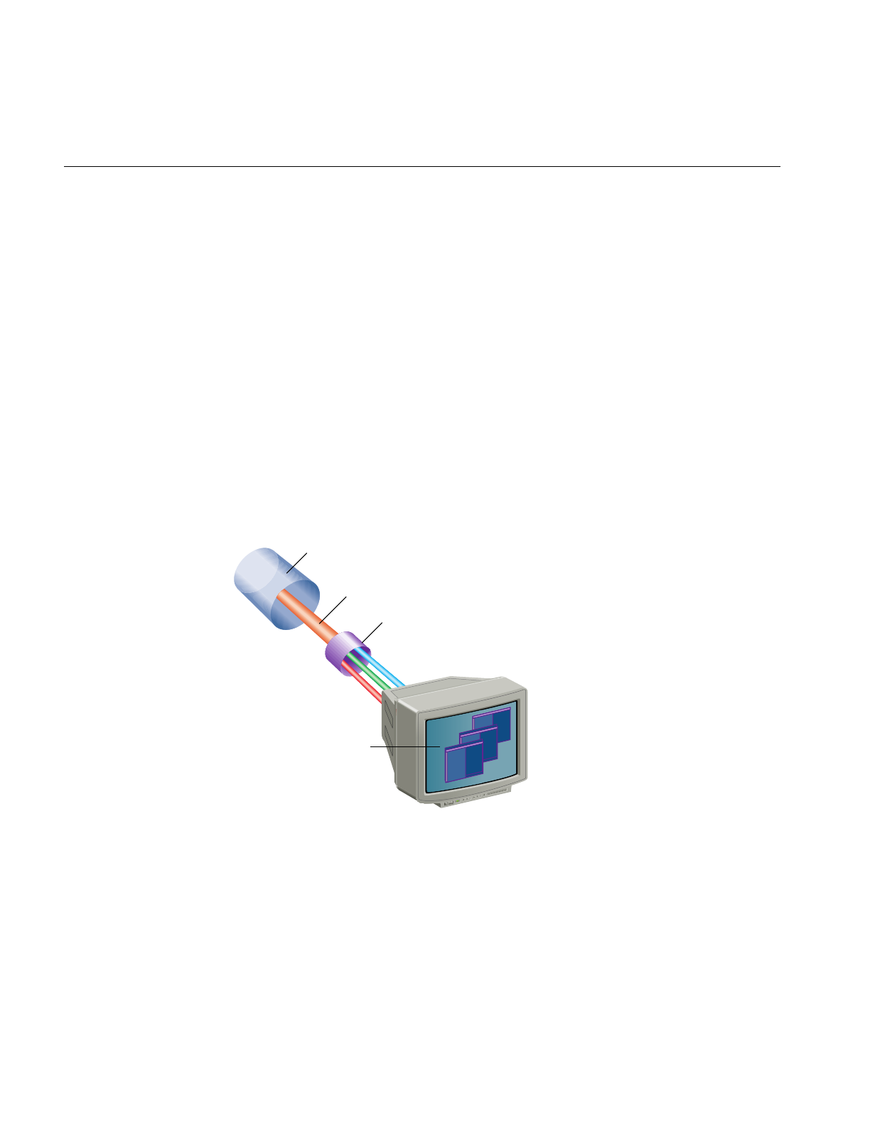
408
Chapter 12: pfPipeWindows and pfPipeVideoChannels
necessary for both image quality and performance reasons as the last window to finish
operation can hold up all of the rendering processes. Window double buffering
synchronization can be done through pfChannel share groups with the
PFCHAN_SWAPBUFFERS_HW token, as discussed in Chapter 2, “Setting Up the
Display Environment,” or explicitly by attaching the windows to form window swap
groups with pfAttachPWinSwapGroup(groupPWin, attachee) as discussed in
Chapter 11, “Windows.” pfPipeWindows can have pfWindows in their swap groups if a
pfPipeWindow is the main group window. The sample program
/usr/share/Performer/src/pguide/libpf/C/multipipe.c demonstrates multipipe
synchronization.
Controlling Video Displays
You use pfPipeVideoChannel to direct the output of pfChannels to specified video
displays, as shown in Figure 12-1. IRIS Performer uses the XSGIvc(3), which is a Silicon
Graphics extension of the X library, for video channel management.
Figure 12-1 Directing Video Output
pfPipe
pfChannel
pfPipeVideoChannel
(channels 0, 1, 2)
pfPipeWindow

Controlling Video Displays
409
pfPipeVideoChannels are based on pfVideoChannels; however, pfPipeVideoChannels
are maintained by libpf and are used by libpf to render the output of pfChannels within
a pfPipeWindow. The pfVideoChannel API is duplicated for pfPipeVideoChannels.
pfPVChan*() methods operate on a pfPipeVideoChannel and pfVChan*() methods
operate on a pfVideoChannel.
There are several sample programs to help understand the use of pfVideoChannels and
pfPipeVideoChannels. The libpr program
/usr/share/Performer/src/pguide/libpr/C/queryvchan.c shows how to query video channel
attributes through IRIS Performer and how to query additional attributes directly
through the XSGIvc interface. /usr/share/Performer/src/pguide/libpr/C/vchan.c shows basic
video channel creation. On an InfiniteReality, this example does resizing and translation
of the video channel output area. The libpf program
/usr/share/Performer/src/pguide/libpf/C/pvchan.c shows basic pfPipeVideoChannel creation
and hookup.
Creating a pfPipeVideoChannel
You create a pfPipeVideoChannel from a pfPipe using pfNewPVChan() and providing
the parent pfPipe. The pfPipeVideoChannel is then attached to a pfPipeWindow with
pfAddPWinPVChan() which will return an index into the pfPipeWindow’s video
channel list. Additionally, if the pfPipeVideoChannel has not already been assigned a
hardware video channel with pfPVChanId(), the next active video channel will be
assigned.
pfPipe *p = pfGetPipe(0);
pfPipeVideoChannel *pvc = pfNewPVChan(p);
pfPVChanId(pvc,0);
pvcIndex = pfPWinAddPVChan(pwin, pvc);
To find out if a pfPipeVideoChannel with its current video channel assignment is active
for displaying output, call pfIsPVChanActive(), which will return 0 if the video channel
assignment is not fully defined or if the channel is not active and will return 1 otherwise.
The assignment of a hardware video channel is not complete until the screen of the
pfPipe is known and so might not be done immediately if the pfPipe screen has not been
set with pfPipeScreen() or if the pfPipeWindow is not open. Even if you have explicitly
assigned a hardware video channel Id, it is only meaningful relative to a known screen.
The hardware video channel assignment can be changed at any time with
pfPVChanId(). It is an error to have multiple pfPipeWindows and pfPipeVideoChannels
attempt to manage the same hardware video channel. The index returned by
pfAddPWinPVChan() is then used for a pfChannel to reference this

410
Chapter 12: pfPipeWindows and pfPipeVideoChannels
pfPipeVideoChannel. pfPipeWindows always have an initial pfPipeVideoChannel
already attached whose default video channel will be the first active video channel on the
screen of the pfPipe. So, only add pfPipeVideoChannels if you actually need additional
video channels.
Multiple pfPipeVideoChannels in a pfPipeWindow
The only video channels a pfPipeVideoChannel can manage are those of the screen of the
pfPipe. Use pfGetNumScreenPVChans() to find out how many active video channels
are on a given screen.
To add additional pfPipeVideoChannels to a single pfPipeWindow, use
pfPWinAddPVChan(). The routine returns an index number associated with the
pfPipeWindow, or -1 if an error occurs. If the pfPipeVideoChannel does not already have
an assigned hardware video channel, the next active video channel relative to the video
channels already attached to the pfPipeWindow will be assigned.
There are list routines to manage the list of pfPipeVideoChannels on a pfPipeWindow.
Use pfGetPWinNumPVChans() to find out how many pfPipeVideoChannels are being
managed by the pfPipeWindow. pfPWinRemovePVChan() and
pfPWinRemovePVChanIndex() disassociate a pfPipeVideoChannel from a
pfPipeWindow, using either the pfPipeWindow object or an index number to specify the
pfPipeWindow.
There are additional utilities to find pfPipeVideoChannels on pfPipeWindows. You can
obtain the index value of a pfPipeVideoChannel for a pfPipeWindow using
pfGetPWinPVChanIndex(), which returns the index of a pfPipeVideoChannel, or -1 of
the pfPipeVideoChannel is not registered with the pfPipeWindow. Use
pfGetPWinPVChanId() to find a pfPipeVideoChannel on a pfPipeWindow with the
specified hardware Id. NULL will be returned if no such pfPipeVideoChannel exists on
the specified pfPipeWindow.

Controlling Video Displays
411
Configuring a pfPipeVideoChannel
pfPipeVideoChannels are bound to their hardware video channels in a lazy fashion as
needed by configuration requests. Basic queries of a video channel do not require any
explicit binding. Changing a video channel’s properties does require explicit binding.
pfPipeWindows manage this process. However, explicit binding and unbinding might
be necessary if changes are made to video channels directly through the XSGIvc API and
not through the pfPipeVideoChannel API. This is quite reasonable since
pfPipeVideoChannels do not duplicate all of XSGIvc. A pfPipeVideoChannel is bound to
its hardware video channel with pfBindPVChan(). All of the pfPipeVideoChannels
associated with a pfPipeWindow can be bound in one step with pfBindPWinPVChans()
and unbound with pfUnbindPWinPVChans(). You can get the XSGIvc handle from a
pfPipeVideoChannel to do your own configuration or extended queries with
pfGetPVChanInfo().
Use pfPipeVideoChannels to Control Frame Rate
There are two mechanisms by which pfPipeVideoChannels can help you maintain
constant frame rate in your application. Dynamic Video Resolution (DVR) addresses
reducing load caused by filling to many pixels. Pan/Zoom video scan-out to sample
different parts of the frame buffer, under resize, to be selected asynchronously to a draw
process. Both of these mechanisms make use of editing the size and or origin of the
output area of a pfPipeVideoChannel, supported by InfiniteReality graphics platforms.
Use pfPVChanOutputSize() and pfPVChanOutputAreaScale() will change the output
area size of the bound video channel. pfPVChanOutputOrigin() will change the origin
of the output area. The pfPipeVideoChannel(3) references more routines to manage
video channel origin and size.
On InfiniteReality graphics platforms, you can use pfPipeVideoChannels to dynamically
adjust the size of the output area of the video channel. The output area is then
automatically zoomed up to full video channel size by the InfiniteReality hardware using
bilinear filtering. This operation has no added performance cost or latency. This feature
can be used to allow pfChannels to reduce their viewport size to the reduced video
channel output area. Reducing the number of pixels drawn reduces the fill load for the
pfPipe and can be used as a load management technique for maintaining constant frame
rates. pfPipeVideoChannels support manual resizing, allowing you to implement your
own load management, or will automatically resize the output area and the pfChannel
viewports. You can enable and select a resizing mode with pfPVChanDVRMode() and
providing PFPVC_DVR_MANUAL or PFPVC_DVR_AUTO. The default value is
PFPVC_DVR_OFF. For more information, see “Maintaining Frame Rate Using Dynamic
Video Resolution” on page 128.

412
Chapter 12: pfPipeWindows and pfPipeVideoChannels
pfPipeVideoChannels also support asynchronous editing of their size and origin. This
can be used in an asynchronous process, or in an application process that is reliably
running at frame rate, to edit the origin and size of the video channel. These changes will
affect the following video field if the pfPVChanMode() for PFVCHAN_AUTO_APPLY
is set to 1 (default is 0) and the PFVCHAN_SYNC mode is set to
PFVCHAN_SYNC_FIELD (default is PFVCHAN_SYNC_FRAME which selects apply
upon swapbuffers).
Real-time changes to pfPipeVideoChannel origin or size should be done between
pfSync() and pfFrame() to affect the next draw frame or video field.

This chapter describes clocks, memory allocation, synchronous I/O, error
handling and notification, and search paths.
“Managing Nongraphic System Tasks”
Chapter 13

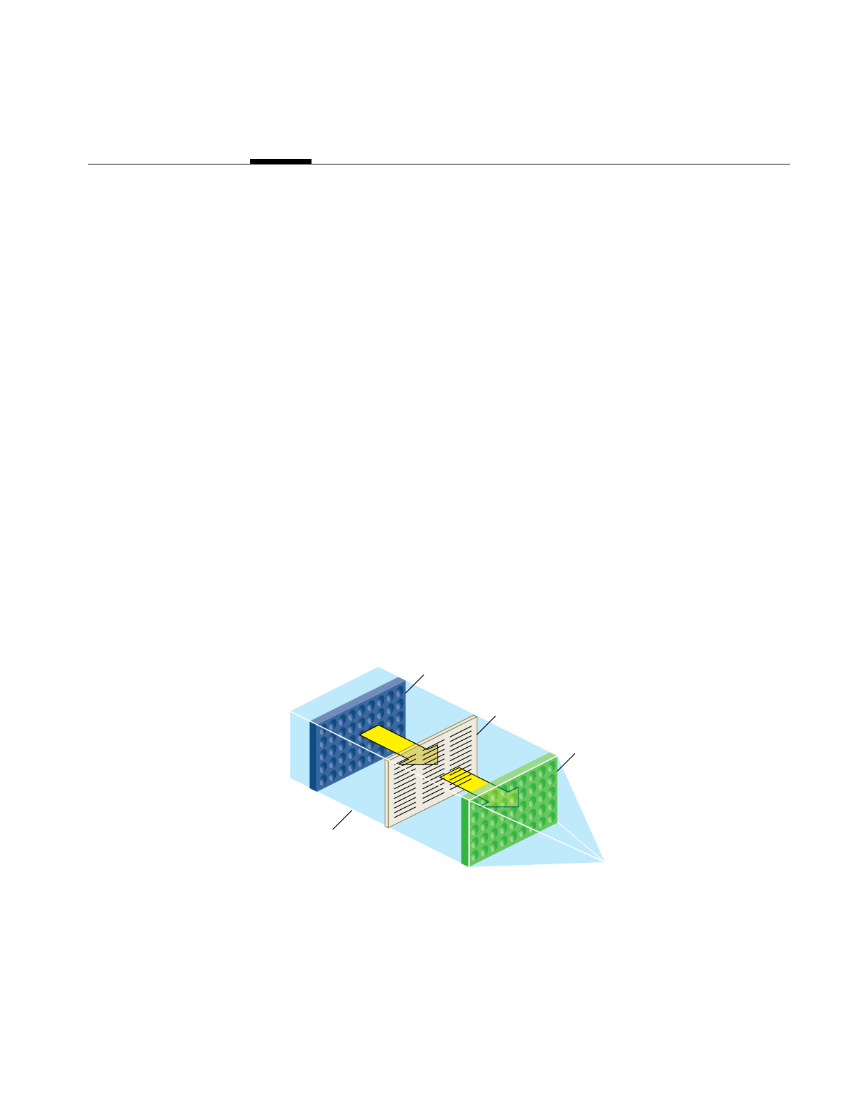
415
Chapter 13
13. Managing Nongraphic System Tasks
This chapter describes objects that manage nongraphic tasks, including
• Queues
• Clocks
• Memory allocation
• Synchronous I/O
• Error handling and notification
• Search paths
Handling Queues
A pfQueue object is a queue of elements, which are all the same type and size; the default
size is the size of a void pointer. A pfQueue object actually consists of three interrelated
queues, as shown in Figure 13-1.
Figure 13-1 pfQueue Object
Input
buffer
pfQueue object
Sorted
list
Output
buffer

416
Chapter 13: Managing Nongraphic System Tasks
• Input buffer—where processes dump values to be added to the pfQueue object.
• Output buffer—values at one end of the queue that processes may remove from the
pfQueue object.
• Sorted list—sorted values that processes may not remove from the pfQueue object.
Note: In non-sorting mode, there is only the Input buffer; values in the output buffer and
the Sorted list are transferred into the input buffer.
Values in the Input buffer are not sorted and are not part of the Sorted list. Values in the
Sorted list and the Output buffer are sorted (when the pfQueue object is in sort mode)
according to a user-defined sorting function. Sorted values of highest priority are
automatically moved from the Sorted list to the Output buffer whenever the pfQueue
object is sorted. Priority is defined by the sorting function, for example, if a pfQueue
object contains pointers to tiles of texture, the sorting function might sort according to the
proximity of the viewer and the tile: the closer the tile is to the viewer, the higher its
priority, the more likely the pointer to the tile will be in the Output buffer. Processes do
not have access to values in the Sorted list; only to those values in the Output buffer.
Multiprocessing
Because there are separate input and output buffers, multiple processes can add or
retrieve elements, but only one process can actually insert elements into the Input buffer
and one process retrieve elements from the Output buffer at one time. The process
adding elements to the Input buffer can be different from the process removing elements
from the Output buffer.
Queue Contents
The contents of the pfQueue object can be any fixed-size object, for example, pfQueues
often contain pointers to Performer objects. You might use a pfQueue object, for example,
to organize tiles of texture according to the direction the viewer is looking and the
proximity of the viewer to the tiles. Because you declare the size and type of objects in
the pfQueue in the constructor, you cannot change the type or size of its elements after
its creation.

Handling Queues
417
Adding or Retrieving Elements
You can insert elements into the Input buffer or remove them from the Output buffer
using the following methods, respectively:
• pfQueue::insert()
• pfQueue::remove()
These methods can be used by multiple processes asynchronously without collision.
Warning: Do not insert NULL elements into the queue.
The pfQueue object is resized dynamically when the number of elements inserted into
the queue exceeds its declared size; the size is doubled automatically. Doubling the size
prevents repeated, incremental, costly resizing of the queue.
Tip: Doubling the size of the queue can cause excessive memory allocation. It is
important therefore to accurately declare the size of the queue.
You can set the size of the queue in the constructor of the pfQueue object or afterwards
by using pfQueue::setArrayLen().pfQueue::getNum() returns the number of elements
in the queue.
Retrieving Elements From the Queue
It is possible for you to
1. Create a thread to retrieve elements from the Output buffer.
2. Use the pfQueue::remove() method to retrieve the element.
3. Delete the thread.
It is much easier, however, to use the pfQueue::addServiceProc() method to perform all
of those tasks. This method
• Creates a thread.
• Returns the thread ID.
• Invokes the developer-supplied function in the argument of the function.
• Deletes the thread.

418
Chapter 13: Managing Nongraphic System Tasks
The developer-supplied function must take, as it’s argument, an element from the
Output buffer and process it. For example, if the queue contains pointers to tiles of
texture, the function might download a tile from disk to the image cache.
Related Methods
pfQueue provides a variety of other methods, described in Table 13-1, that return
information about the threads created to process the elements in the Output buffer of the
pfQueue object.
pfQueue Modes
pfQueue objects can run in one of two modes:
• non-sorting
• sorting
Either the elements in the queue are sorted according to some criteria specified by a
developer-supplied sorting function, or not.
The sorting function is null and the sorting mode is non-sorting by default.
Table 13-1 Thread Information
Method1 Description
getServiceProcPID() Returns the ID of the created thread.
pfGetGlobalQueueServiceProcPID() Returns the ID of the nth thread.
getNumServiceProcs() Returns the number of currently active threads.
pfGetNumGlobalQueueServiceProcs() Returns the number of processes that have been
sproc’d by all pfQueue’s.
pfGetGlobalQueueServiceProcQueue() Returns the pfQueue associated with a particular
thread.
exitServiceProc() Terminates a specific thread.
exitAllServiceProcs() Terminates all pfQueue object threads.

Handling Queues
419
Non-Sorting Mode
In non-sorting mode, the Sorting list and the Output buffer are empty; all pfQueue
elements are in the Input buffer. Processes append new input objects to the front of the
queue while (potentially) other processes read and remove pfQueue objects from the
other end of the queue.
A process can potentially read and remove all of the elements in a non-sorted queue.
Access to the elements is not random, however; it is sequential and ordered according to
FIFO.
Sorting the pfQueue
Multiple processes can add to the Input buffer asynchronously. The objects remain
unsorted and separate from the Sorted list and Output buffer until the sorting function
is triggered. At that time,
1. The objects in the Input buffer are flushed into the Sorted list.
2. The objects in the Sorting list and the Output buffer are resorted together.
To sort the elements in a pfQueue, you:
1. Specify a developer-supplied sorting function using pfQueue::setSortFunc().
2. Enable sorting by passing a non-NULL argument to pfQueue::setSortMode().
3. Specify the maximum and minimum number of values for the input and output of
the sorting function using pfQueue::setInputRange() and
pfQueue::setOutputRange().
Tip: You must specify the sorting function before enabling sorting, otherwise sorting
remains disabled and pfQueue returns a warning.
The sorting function runs in a separate thread parallel to the function specified in the
argument of pfQueue. You can even specify that the sorting function run on a CPU
different from the one processing the pfQueue object, as described in “Running the Sort
Process on a Different CPU” on page 422.
In sorting mode, only those elements in the Output buffer are available to processes.
Access to the elements in the Output buffer is not random, but sequential and in a FIFO
order.

420
Chapter 13: Managing Nongraphic System Tasks
Sorting Function
The sorting function sorts, according to its own criteria, the elements in the Sorting list
and the Output buffer. To sort the queue, you must
• Implement your own function to sort the pfQueue object.
• Identify the function in your application using pfQueue::setSortFunc().
• Make the function return a value of type that matches that of
pfQueueSortFuncType.
• Make the function handle an input data structure of type pfQueueSortFuncData(),
defined as follows:
typedef struct {
pfList *sortList; //list of elements to sort
volatile int *inSize; //number of elements on input queue
volatile int *outSize; //number of elements on output queue
int inHi; // maximum number of elements at the input
int inLo; // minimum number of elements at the input
int outHi; // maximum number of elements at the output
int outLo; // minimum number of elements at the output
} pfQueueSortFuncData;
The actual data in the pfQueue object is maintained in a pfList, which the
pfQueueSortFuncData struct points to.
Input and Output Ranges
The range values work as triggers to start the sorting function, which sleeps otherwise.
For example, when the number of unprocessed inputs is greater than inHi, pfQueue calls
the sorting function to sort the pfQueue object.
You can set the minimum and maximum number of input and output elements entered
before the sort is triggered using the following methods:
• pfQueue::setInputRange()
• pfQueue::setOutputRange()

Handling Queues
421
Table 13-2 shows the default range values:
The range values have no effect in non-sorting mode.
Triggering the Sort
The sorting function sleeps until one of the following conditions occurs:
• The number of elements in the Input buffer exceeds the input maximum range
value.
• The number of elements in the Output buffer drops below the output minimum
range value.
•pfQueue::notifySortProc() is called.
By increasing the maximum number of values allowed in the Input buffer, or reducing
the minimum number of values allowed in the Output buffer, the sorting function is
potentially called fewer times.
Table 13-2 shows that, using default range values, the queue is sorted when three or more
elements are added to the Input buffer or when two or less values remain in the Output
buffer.
The pfQueue::notifySortProc() is provided for those times when the queue should be
sorted without regard to the number of elements in the Input or Output buffers. For
example, if an element in the queue changes, it might be necessary to resort the queue.
If, for example, the elements are sorted alphabetically, the sort function should be
explicitly called when one of the elements is renamed.
Table 13-2 Default Input and Output Ranges
Range Minimum Maximum
Input 0 3
Output 2 5

422
Chapter 13: Managing Nongraphic System Tasks
Running the Sort Process on a Different CPU
You can run the sorting process on a different CPU from the one processing the pfQueue
by:
• Using getSortProcPID() to get the process ID of the sorting function and assigning
the process to run on a specified CPU with IRIS Performer or IRIX utilities.
• Using the pfuProcessManager provided in libpfutil. See the
pfuInitDefaultProcessManager(3) reference page for more information.
High-Resolution Clocks
IRIS Performer provides access to a high-resolution clock that reports elapsed time in
seconds to support for timing operations. To start a clock, call pfInitClock() with the
initial time in seconds—usually 0.0—as the parameter. Subsequent calls to pfInitClock()
reset the time to whatever value you specify. To read the time, call pfGetTime(). This
function returns a double-precision floating point number representing the seconds
elapsed from initialization added to the latest reset value.
The resolution of the clock depends on your system type and configuration. In most
cases, the resolved time interval is under a microsecond, and so is much less than the
time required to process the pfGetTime() call itself. Onyx, Crimson™, Indigo2™, Indigo®,
and Indy™ systems all provide submicrosecond resolution. Newer systems, including
Onyx2, OCTANE, and O2 have even higher resolution clocks and use the
CYCLE_COUNTER functionality through syssgi(2). On a machine that uses a fast
hardware counter, the first invocation of pfInitClock() forks off a process that
periodically wakes up and checks the counter for wrapping. This additional process can
be suppressed using pfClockMode().
If IRIS Performer cannot find a fast hardware counter to use, it defaults to the time-of-day
clock, which typically has a resolution between one and ten milliseconds. This clock
resolution can be improved by using fast timers. See the ftimer(1) reference page for more
information on fast timers.
By default, processes forked after the first call to pfInitClock() share the same clock and
will all see the results of any subsequent pfInitClock(). All such processes receive the
same time.

Memory Allocation
423
Unrelated processes can share the same clock by calling pfClockName() with a clock
name before calling pfInitClock(). This provides a way to name and reference a clock. By
default, unrelated processes don’t share clocks.
Video Refresh Counter (VClock)
The video refresh counter (VClock) is a counter that increments once for every vertical
retrace interval. There is one VClock per system. In systems where multiple graphics
pipelines are present, but not genlocked (synchronized, see the setmon(3) reference
page), screen 0 is used as the source for the counter. A process can be blocked until a
certain count, or the count modulo some value (usually desired number of video fields
per frame) is reached.
Table 13-3 lists and describes the pfVClock routines.
When using pfVClockSync(), the calling routine is blocked until the current count
modulo rate is offset. The VClock functions can be used to synchronize several channels
or pipelines.
Memory Allocation
You can use IRIS Performer memory-allocation functions to allocate memory from the
heap, from shared memory, and from data pools.
Table 13-3 pfVClock Routines
Function Action
pfInitVClock Initialize the clock to a value.
pfGetVClock Get the current count.
pfVClockSync Block the calling process until a count is reached.

424
Chapter 13: Managing Nongraphic System Tasks
Table 13-4 lists and describes the IRIS Performer shared memory routines.
Allocating Memory With pfMalloc()
pfMalloc() can allocate memory either from the heap or from a shared memory arena.
Multiple processes can access memory allocated from a shared memory arena, whereas
memory allocated from the heap is visible only to the allocating process. Pass a
shared-memory arena pointer to pfMalloc() to allocate memory from the given arena.
pfGetSharedArena() returns the pointer for the arena allocated by pfInitArenas(), or
NULL if the given memory was allocated from the heap. Alternately, an application can
create its own shared memory arena; see the acreate(3P) reference page for information
on how to create an arena.
To allocate memory from the heap, pass NULL to pfMalloc() instead of an arena pointer.
Under normal conditions pfMalloc() never returns NULL. If the allocation fails,
pfMalloc() generates a pfNotify() of level PFNFY_FATAL, so unless the application has
set a pfNotifyHandler(), the application will exit.
Memory allocated with pfMalloc() must be freed with pfFree(), not with the standard C
library’s free() function. Using free() with data allocated by pfMalloc() will have
devastating results.
Table 13-4 Memory Allocation Routines
Function Action
pfInitArenas Create arenas for shared memory and semaphores.
pfSharedArenaSize Specify the size of a shared memory arena.
pfGetSharedArena Get the shared memory arena pointer.
pfGetSemaArena Get the shared semaphore/lock arena pointer.
pfMalloc Allocate from an arena or the heap.
pfFree Release memory allocated with pfMalloc().

Memory Allocation
425
Memory allocated with pfMalloc() has a reference count (see “pfDelete() and Reference
Counting” in Chapter 1 for information on reference counting). For example, if you use
pfMalloc() to create attribute and index arrays, which you then attach to pfGeoSets using
pfGSetAttr(), IRIS Performer automatically tracks the reference counts for the arrays,
letting you delete the arrays much more easily than if you create them without
pfMalloc(). All the reference-counting routines (including pfDelete()) work with data
allocated using pfMalloc(). Note, however, that pfFree() doesn’t check the reference
count before freeing memory; use pfFree() only when you’re sure the data you’re freeing
isn’t referenced.
pfGetSize() returns the size in bytes of any data allocated by pfMalloc(). Since the size
of such data is known, pfCopy() also works on allocated data.
Although pfMalloc()-allocated data behaves in many ways like a pfObject (see “Nodes”
in Chapter 3), such data doesn’t contain a user data pointer. This omission avoids
requiring an extra word to be allocated with every piece of pfMalloc() data.
Note: All libpr objects are allocated using pfMalloc(), so you can use pfGetArena(),
pfGetSize(), and pfFree() on all such objects. However, it’s recommended that you use
pfDelete() instead of pfFree() for libpr objects, in order to maintain reference-count
checking.
Shared Arenas
pfInitArenas() creates two arenas, one for the allocation of shared memory with
pfMalloc() and one for the allocation of semaphores and locks with usnewlock() and
usnewsema(). The arenas are visible to all processes forked after pfInitArenas() is called.
Applications using libpf don’t need to explicitly call pfInitArenas(), since it’s invoked by
pfInit().
The shared memory arena can be allocated by memory-mapping either swap space
(/dev/zero, the default) or an actual disk file (in the directory specified by the environment
variable PFTMPDIR). The latter requires sufficient disk space for as much of the shared
memory arena as will be used, and disk files are somewhat slower than swap space in
allocating memory.

426
Chapter 13: Managing Nongraphic System Tasks
By default, IRIS Performer creates a large shared memory arena of 256 MB. Though this
approach makes large numbers appear when you run ps(1), it doesn’t consume any
substantial resources, since swap or file system space isn’t actually allocated until
accessed (that is, until pfMalloc() is called).
Because IRIS Performer cannot increase the size of the arena after initialization, an
application requiring a larger shared memory arena should call pfSharedArenaSize() to
specify the maximum amount of memory to be used. Arena sizes as large as 1.7 GB are
usually acceptable; but you may need to set the virtual-memory-use and memory-use
limits, using the shell limit command or setrlimit(), to allow your application to use that
much memory. To use arenas larger than 4G, you must use 64-bit operation.
If you are having difficulties in creating a large arena, it could be due to fragmentation of
the address space from too many DSOs. You can reduce the number of DSOs you are
using by compiling some of them statically. You can also change the default address of
the DSOs by running rqs(1) with a custom so_locations file.
Allocating Locks and Semaphores
An application requiring lockable pieces of memory should consider using pfDataPools,
described below. Alternatively, when a lock or semaphore is required in an application
that has called pfInitArenas(), you can call pfGetSemaArena() to get an arena pointer,
and you can allocate locks or semaphores using usnewlock() and usnewsema().
Datapools
Datapools, or pfDataPools, are also a form of shared memory, but they work differently
from pfMalloc(). Datapools allow unrelated processes to share memory and lock out
access to eliminate data contention. They also provide a way for one process to access
memory allocated by another process.
Any process can create a datapool by calling pfCreateDPool() with a name and byte size
for the pool. If an unrelated process needs access to the datapool, it must first put the
datapool in its address space by calling pfAttachDPool() with the name of the datapool.
The datapool must reside at the same virtual address in all processes. If the default choice
of an address causes a conflict in an attaching process pfAttachDPool() will fail. To avoid
this pfDPoolAttachAddr() can be called before pfCreateDPool() to specify a different
address for the datapool.

Memory Allocation
427
Any attached process can allocate memory from the datapool by calling pfDPoolAlloc().
Each block of memory allocated from a datapool is assigned an ID so that other processes
can retrieve the address using pfDPoolFind().
Once you’ve allocated memory from a datapool, you can lock the memory chunk (not the
entire pfDataPool) by calling pfDPoolLock() before accessing the memory. This locking
mechanism works only if all processes wishing to access the datapool memory use
pfDPoolLock() and pfDPoolUnlock(). After a piece of memory has been locked using
pfDPoolLock(), any subsequent pfDPoolLock() call on the same piece of memory will
block until the next time a pfDPoolUnlock() is called for that memory.
pfDataPools are pfObjects, so call pfDelete() to delete them. Calling pfReleaseDPool()
unlinks the file used for the datapool—it doesn’t immediately free up the memory that
was used or prevent further allocations from the datapool; it just prevents processes from
attaching to it. The memory is freed when the last process referring to the datapool
pfDelete()s it.
CycleBuffers
A multiprocessed environment often requires that data be duplicated so that each
process can work on its own copy of the data without adversely colliding with other
processes. pfCycleBuffer is a memory structure which supports this programming
paradigm. A pfCycleBuffer consists of one or more pfCycleMemories which are
equally-sized memory blocks. The number of pfCycleMemories per pfCycleBuffer is
global and is set once with pfCBufferConfig(), and is typically equal to the number of
processes accessing the data.
Note: pfFlux replaces the functionality of pfCycleBuffer.
Each process has a global index, set with pfCurCBufferIndex(), which indexes a
pfCycleBuffer’s array of pfCycleMemories. When each process has a different index (and
its own address space), mutual exclusion is ensured if the process limits its
pfCycleMemory access to the currently indexed one.
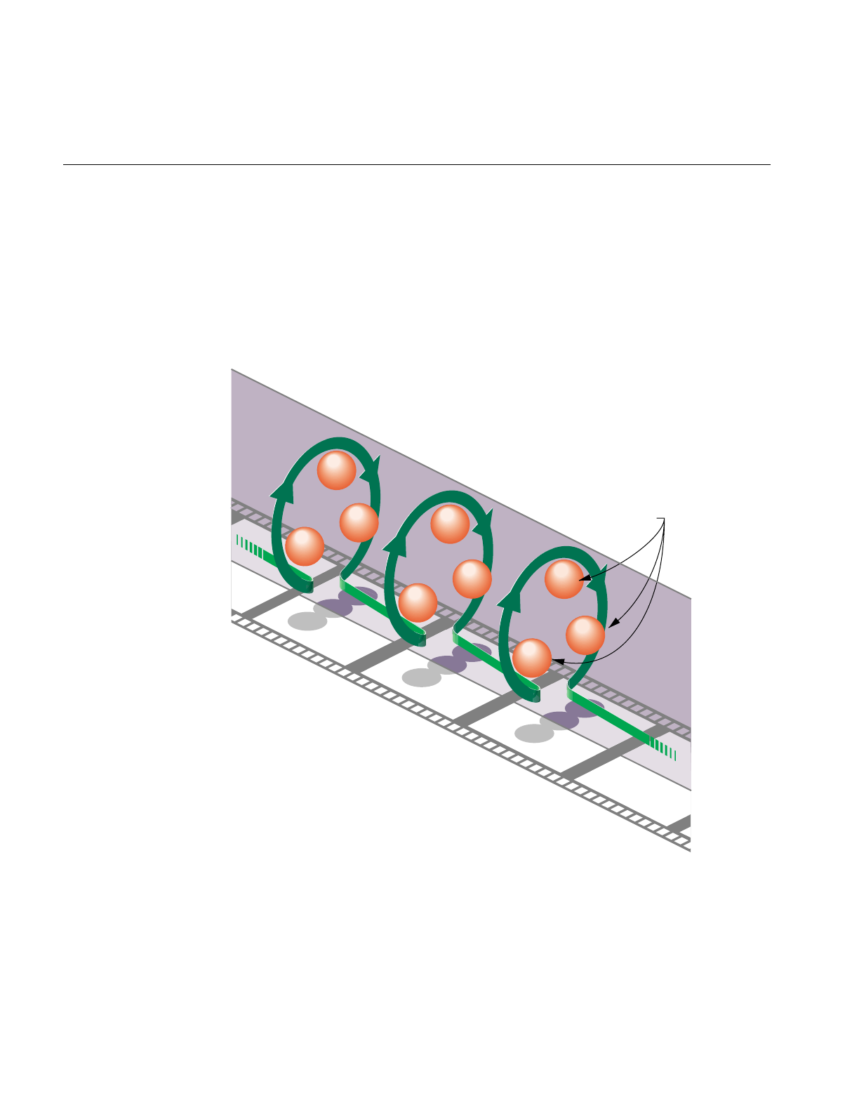
428
Chapter 13: Managing Nongraphic System Tasks
The “cycle” term of pfCycleBuffer refers to its suitability for pipelined multiprocessing
environments where processes are arranged in stages like an assembly line and data
propagates down one stage of the pipeline each frame. In this situation, the array of
pfCycleMemories can be visualized as a circular list. Each stage in the pipeline accesses
a different pfCycleMemory and at frame boundaries the global index in each process is
advanced to the next pfCycleMemory in the chain. In this way, data changes made in the
head of the pipeline are propagated through the pipeline stages by “cycling” the
pfCycleMemories.
Figure 13-2 pfCycleBuffer and pfCycleMemory Overview
0
2
1
pfCycleBuffer
pfCycleMemories
2
1
0
App
1
0
2
App
Cull
Draw
App
Cull
Draw Cull
Draw
Frame
n
Frame
n
+1 Frame
n
+2

Asynchronous I/O
429
Cycling the memory buffers works if each current pfCycleMemory is completely
updated each frame. If this is not the case, buffer cycling will eventually access a “stale”
pfCycleMemory whose contents were valid some number of frames ago but are invalid
now. pfCycleBuffers manage this by frame-stamping a pfCycleMemory whenever
pfCBufferChanged() is called. The global frame count is advanced with
pfCBufferFrame() which also copies most recent pfCycleMemories into “stale”
pfCycleMemories thereby automatically keeping all pfCycleBuffers current.
A pfCycleBuffer consisting of pfCycleMemories of nbytes size is allocated from memory
arena with pfNewCBuffer(nbytes, arena). To initialize all the pfCycleMemories of a
pfCycleBuffer to the same data call pfInitCBuffer(). pfCycleMemory is derived from
pfMemory so you can use inherited routines like pfCopy,pfGetSize, and pfGetArena()
on pfCycleMemories.
While pfCycleBuffers may be used for application data, their primary use is as pfGeoSet
attribute arrays, e.g., coordinates or colors. pfGeoSets accept pfCycleBuffers (or
pfCycleMemory) references as attribute references and automatically select the proper
pfCycleMemory when drawing or intersecting with the pfGeoSet.
Note: libpf applications need not call pfCBufferConfig() or pfCBufferFrame() since the
libpf routines pfConfig() and pfFrame() call these respectively.
Asynchronous I/O
A nonblocking file interface is provided to allow real-time programs access to disk files
without affecting program timing. The system calls pfOpenFile(),pfCloseFile(),
pfReadFile(), and pfWriteFile() work in an identical fashion to their IRIX counterparts
open(),close(),read(), and write().
When pfOpenFile() or pfCreateFile() is called, a new process is created using sproc(),
which manages access to the file. Subsequent calls to pfReadFile(),pfWriteFile(), and
pfSeekFile() place commands in a queue for the file manager to execute and return
immediately. To determine the status of a file operation, call pfGetFileStatus().

430
Chapter 13: Managing Nongraphic System Tasks
Error-Handling and Notification
IRIS Performer provides a general method for handling errors both within IRIS
Performer and in the application. Applications can control error-handling by installing
their own error-handling functions. You can also control the level of importance of an
error.
Table 13-5 lists and describes the functions for setting notification levels.
pfNotify() allows an application to signal an error or print a message that can be
selectively suppressed. pfNotifyLevel() sets the notification level to one of the values
listed in Table 13-6.
The environment variable PFNFYLEVEL can be set to override the value specified in
pfNotifyLevel(). Once the notification level is set via PFNFYLEVEL it can not be
changed by an application.
Table 13-5 pfNotify Functions
Function Action
pfNotifyHandler Install user error-handling function.
pfNotifyLevel Set the error-notification level.
pfNotify Generate a notification.
Table 13-6 Error Notification Levels
Token Meaning
PFNFY_ALWAYS Always print regardless of notify level
PFNFY_FATAL Fatal error
PFNFY_WARN Serious warning
PFNFY_NOTICE Warning
PFNFY_INFO Information and floating point exceptions
PFNFY_DEBUG Debug information
PFNFY_FP_DEBUG Floating point debug information

File Search Paths
431
Once the notify level is set, only those messages with a priority greater than or equal to
the current level are printed or handed off to the user function. Fatal errors cause the
program to exit unless the application has installed a handler with pfNotifyHandler().
Setting the notification level to PFNFY_FP_DEBUG has the additional effect of trapping
floating point exceptions such as overflows or operations on invalid floating point
numbers. It may be a good idea to use a notification level of PFNFY_FP_DEBUG while
testing your application, so that you will be informed of all floating-point exceptions that
occur.
File Search Paths
IRIS Performer provides a mechanism to allow referencing a file via a set of path names.
Applications can create a search list of path names in two ways: the PFPATH
environment variable and pfFilePath(). (Note that the PFPATH environment variable
controls file search paths and has nothing to do with the pfPath data structure.)
Table 13-7 describes the routines for working with pfFilePaths.
Pass a search path to pfFilePath() in the form of a colon-separated list of path names.
Calling pfFilePath() a second time replaces the current path list rather than appending
to it.
The environment variable PFPATH is also a colon-separated list of path names, similar
to the PATH variable. pfFindFile() searches the paths in PFPATH first, then those given
in the most recent pfFilePath() call; it returns the complete pathname for the file if the file
is found. IRIS Performer applications should use pfFindFile() (either directly or through
routines such as pfdLoadFile()) to look for input data files.
Table 13-7 pfFilePath Routines
Routine Action
pfFilePath Create a search path.
pfFindFile Search for the file using the search path.
pfGetFilePath Supply current search path.

432
Chapter 13: Managing Nongraphic System Tasks
pfGetFilePath() returns the last search path specified by a pfFilePath() call. It doesn’t
return the path specified by the PFPATH environment variable—if you want to find out
that value, call getenv(3c).

This chapter describes how to connect pfFlux, pfFCS, and pfEngine nodes,
which together can be used for animating geometries.
“Dynamic Data”
Chapter 14


435
Chapter 14
14. Dynamic Data
Making your data dynamic allows your scenes to change. Geometries can change
location, orientation, color, texture, or change into different things altogether.
pfEngines compute the changes. pfFluxs are the containers for the output of those
engines.
This chapter explains how to create dynamic structures that can generate and manipulate
their own dynamic data using pfFlux, pfEngine, and pfFCS.
pfFlux
pfFlux is a container for dynamic data that enables multiprocessed generation and use of
data in the scene graph. A pfFlux internally consists of multiple buffers of data, each of
which is associated with a frame number. The numbering allows multiple processes to
each have a copy of the data containing the frame they are working on. Multiple reader
processes can share a copy of the current results, or be using the frame of results that is
appropriate for that process.
Creating and Deleting a pfFlux
pfFlux::pfFlux() creates and returns a handle to a pfFlux. Each pfFlux buffer is a
pfFluxMemory. When you create a pfFlux, you specify the number of buffers it contains
as well as the size of each buffer. The pfFlux buffers will automatically be allocated from
the same arena as the parent pfFlux. If for the number of buffers you specify
PFFLUX_DEFAULT_NUM_BUFFERS, the flux will be created with a default number of
buffers automatically for the current multi-process configuration of your application, as
set by pfMultiprocess. You can globally redefine this default number of buffers for
successive creation of pfFluxes using pfFlux::setDefaultNumBuffers(). If you change
the default number of buffers, the effect takes place only for pfFluxs created after the
change.

436
Chapter 14: Dynamic Data
Note: IRIS Performer sets the default number of pfFlux buffers when pfConfig() is called
according to the number and type of processes requested with pfMultiprocess().
Generally, the number of buffers is equal to one more than the number of running
processes that typically might generate pfFlux data or use pfFluxed results. DBASE and
LPOINT processes are not included in the count but ISECT and COMPUTE processes
and additional graphic pipes creating additional DRAW and possibly CULL processes
do add to the default number of pfFlux buffers.
You can return the number of buffers in a pfFlux and the number of bytes in the buffers
using the getDefaultNumBuffers() and getDataSize() methods, respectively.
To delete a pfFlux, as with all pfObjects, use pfDelete().
Initializing the Buffers
Generally, pfFlux buffers do not require initialization because they are fully recomputed
for every frame. One case where you would want to initialize them is when the data in
the buffers is static. For example, if you have a pfFlux of coordinates where most do not
change, rather than continuously updating this static data, it is far more efficient to
initialize the buffers. You cannot depend on the order in which you get pfFlux buffers at
run-time and coordinates in the buffer can not assume results from the previous frame.
If an element in the buffer is ever to be dynamic, it should always be recomputed.
IRIS Performer provides two ways of initializing or setting the data held in the pfFlux
buffers:
•pfFlux::initData() to provide a template
•pfFlux::callDataFunc() to provide a callback function
You can immediately initialize all buffers pfFlux by calling the initData() method and
providing a template data buffer that will be directly copied into the pfFlux buffers.
In the argument of pfFlux::callDataFunc(), you pass a pointer to data, and a pointer to a
callback function that operates on the buffers in a pfFlux. This function will be
immediately called on each buffer of the pfFlux.
An initialization callback can also be provided when the pfFlux is created
pfFlux *flux = new pfFlux(initFunc, PFFLUX_DEFAULT_NUM_BUFFERS);

pfFlux
437
and the function will be called for each flux buffer. If the pfFlux is not created with
enough buffers and a new pfFluxMemory buffer must be created at runtime, the callback
function will be called. For better and reliable performance, you generally want to ensure
that you have given yourself enough buffers up front.
pfFlux Buffers
A pfFlux buffer is of type pfFluxMemory. Each buffer consists of a:
• Header
• Data portion
The header portion consists of:
• Pointer to the data portion of the pfFluxMemory.
• Frame number set automatically or explicitly by pfFlux::setFrame().
• Set of flags, including read and write.
The data portion of a pfFluxMemory contains one frame of information. The
getFluxMemory() method returns a pointer to the data portion of a pfFluxMemory
To return the parent pfFlux containing the buffer, use pfFlux::getFlux(), which returns
NULL if the specified data is not part of a pfFlux. This is useful to find out, for example,
if an attribute buffer of a pfGeoSet is a pfFlux.
At a given moment, a pfFlux buffer is either readable or writable, but never both. When
a buffer is writable, its data can be changed. When a buffer is readable, its data should
not be changed because there might be other processes reading that same buffer that
would then be immediately affected by any changes. For performance reasons, a buffer
marked readable is not locked.
Reading pfFlux Buffers
To get the current results for reading from a pfFlux, you can use the getCurData()
method with code similar to the following C example:
pfVec3 *cur_verts;
cur_verts = (pfVec3*)pfGetFluxCurData(flux);

438
Chapter 14: Dynamic Data
In this example, getCurData():
• Finds a readable buffer in the pfFlux, flux, whose frame number is the closest to the
current flux frame number, but not greater then the current flux frame number.
• Returns a pointer, cur_verts, to that buffer.
If you have an old copy of a data buffer from a previous call to getCurData() and now
just want do update to a new version and no longer have a pointer to the parent flux, you
can use pfFlux::getWritableData() and provide your data pointer. For performance
reasons, it is better to save your pfFlux pointer and not depend on this convenience.
WhengetCurData() is called, it is expected to hold previous results of computation. This
computation might be done explicitly by your code in another process, or might be done
automatically if the pfFlux is the destination of a pfEngine. Additionally, the pfEngine
computation might be triggered immediately if the pfFlux is a pfEngine destination and
if the pfFlux mode PFFLUX_ON_DEMAND mode is set by the setMode() method and if
the client pfEngine sources are dirty. pfEngine details are discussed more later in this
chapter.
Writing to pfFlux Buffers
When you want to write data to a pfFlux buffer, you use the getWritableData() method
with code similar to the following C++ example:
pfVec3 *verts;
int i, num_verts;
verts = (pfVec3*)flux->getWritableData();
/* Set all verts to 1.0, 2.0, 3.0 */
num_verts = flux->getDataSize() / sizeof(pfVec3);
for (i = 0; i < num_verts; i++)
verts[i].set(1.0f, 2.0f, 3.0f);
flux->writeComplete();

pfFlux
439
When pfGetFluxWritableData() is called, pfFlux searches for the buffer whose frame
number is equal to the pfFlux frame number. There are three possible results:
• If there is a match and the buffer is writable, getWritableData() returns a pointer to
that buffer.
• If there is a match but the buffer is readable, getWritableData() causes one of the
following actions to occur, according to whether the PFLUX_WRITE_ONCE mode
specified in pfFluxMode() is set to:
– PF_ON, pfGetFluxWritableData() returns NULL if there is already a readable
buffer with a frame number that matches the current flux frame number.
– PF_OFF, pfGetFluxWritableData() returns a pointer to the readable data buffer.
• If there is no match, an unused buffer is made writable and it’s frame buffer number
is set to that of the current pfFlux frame number.
If pfGetFluxWritableData() is called again for the same frame and the
PFFLUX_WRITE_ONCE mode is PF_ON (off by default), information is not copied
again into the same buffer; instead, NULL is returned. In this way, the mode can prevent
modified data from being clobbered by a second call to pfGetFluxWritableData() and
the NULL return value can be used to avoid needlessly recomputing unused data.
pfFluxWriteComplete() should be called when computation for a writable pfFlux buffer
is complete. This method changes the specified buffer from writable to readable.
Coordinating pfFlux and Connected pfEngines
pfFluxs maintain pointers to:
• pfEngines, called source engines, whose destinations are this pfFlux.
• A list of pfEngines, called client engines, that use this pfFlux as a source.
To return a handle to these engines, use pfGetFluxSrcEngine() and
pfGetFluxClientEngine(), respectively.
To return the number of connected source and client pfEngines, use
pfGetFluxNumSrcEngines() and pfGetFluxNumClientEngines(), respectively.

440
Chapter 14: Dynamic Data
pfFluxWriteComplete() method triggers client pfEngine evaluation according to
whether the PFFLUX_PUSH mode specified in pfFluxMode() is set to:
• PF_ON, pfEngineEvaluate() is performed on its client pfEngines to push the results
through a chain of computation.
• PF_OFF, pfEngineSrcChanged() is performed on its clients to tell those pfEngines
that they have dirty sources.
Triggering pfFlux Evaluation
pfFlux evaluation is really a convenient one-step combined evaluation of a source
pfEngine combined with getting and completing a writable buffer of data. Triggering the
evaluation of pfFlux may trigger the evaluation of the pfFlux’s source pfEngines,
particularly if the PFFLUX_ON_DEMAND mode is set to PF_ON.
To explicitly trigger a pfFlux, the evaluate method can be used with a mask that is
provided and passed through evaluation chains to potentially limit which pfFluxes in a
chain are evaluated. For a pfFlux to be evaluated, both of the following conditions must
be satisfied:
• The bits in the current mask must match any of the bits in the evaluation mask
associated with a pfFlux.
•pfFluxEvaluate() or pfFluxEvaluateEye() is called.
The mask is a bitmask that you use to trigger the evaluation of the source pfEngines of a
pfFlux. pfFluxMask() and pfGetFluxMask() set and get, respectively, the evaluation
mask of a pfFlux. The default mask is PFFLUX_BASIC_MASK. Masks enable selective
evaluation of pfFlux source pfEngines.
pfFluxEvaluate() triggers an evaluation of pfFlux source pfEngines if any of the bits in
the current mask match any of the bits in the evaluation mask of the pfFlux.
pfFluxEvaluateEye() is the same pfFluxEvaluate() but also makes it easy to pass the
current eye point through a chain of computation. This is a particularly common case in
scene graphs and one very common use is morphing level of detail based on distance
from the current eyepoint.
Calling pfFluxEvaluate() or pfFluxEvaluateEye() is the equivalent of calling
pfEngineEvaluate() on the source engines followed by calling pfFluxWriteComplete()
on the pfFlux.
For more information about pfEngine, see “pfEngine” on page 446.

pfFlux
441
Synchronized Flux Evaluation
There are times when you want to ensure that the dynamic data for a given frame in a
number of pfFluxes becomes readable at precisely the same time. Particularly when
computations are so complicated that they must be completed over multiple frames, you
might want the computations of vertices for the different pfGeoSets for a given frame to
be made usable at the same time. Consider the following example:
You are using pfASD and you need shapes comprised of multiple
pfGeoSets to move together in response to morphing terrain.
One pfGeoSet might encapsulate the texture of a roof, another a wall,
another a window, and another a door. Since a pfGeoSet can only
encompass one texture, each of these parts of a house must remain
separate pfGeoSets whose data must be encapsulated in separate
pfFluxes. If, for rendering, the roof of one frame was used with the
wall of another, it might appear that the house is breaking apart.
IRIS Performer uses sync flux groups to ensure that the same frame of data is being used
from all fluxes in a group.
Synchronizing pfFluxes with Flux Sync Groups
You can make one or more pfFluxes belong to a flux sync group using the pfFlux
setSyncGroup() method and providing the integer identifier of the desired group. To get
the flux sync group identifier of a pfFlux, use the getSyncGroup() method.
Note: IRIS Performer doesn’t maintain a list of pfFluxes in a flux group, instead an
internal field in pfFlux identifies the flux sync group it belongs to. For this reason, there
is now way to get a list from IRIS Performer of all of the fluxes in a sync group.
For convenience, a flux sync group can be identified by a string name, set with
pfFlux::getSyncGroupName(). The unsigned integer identifier can be gotten from the
string name using pfFlux::getNamedSyncGroup().pfFlux::getNamedSyncGroup will
also automatically generate a new sync group identifier for a new name. The identifier of
the first flux sync group you create is automatically one.
Note: Once you name a sync group, the name cannot be changed.
pfFlux::getNumNamedSyncGroups() returns the number of named sync groups.

442
Chapter 14: Dynamic Data
Enabling a Flux Sync Group
To enable group synchronization of the pfFluxs in the flux sync group, enable the sync
group using pfFlux::enableSyncGroup(). You can disable group synchronization using
pfFlux::disableSyncGroup().
pfFlux::getEnableSyncGroup() returns whether or not a sync group is enabled.
Initially, all pfFluxes are all part of flux sync group zero, which can never be enabled.
Evaluating a Synchronized Flux Group
After all of the pfFluxes in an enabled flux sync group are calculated, you must call
pfFlux::syncGroupReady() to specify that the fluxs are ready to be read.
When pfFrame is called, pfFlux::syncComplete() is called on flux sync groups, which
• Marks the writable buffers with the current flux frame number.
• Makes their writable buffers readable.
Fluxed Geosets
Most often you use dynamic data to change the attributes, location, or the orientation of
geometries. Morphing geometries, for example, is a matter of repositioning the vertices
of a geometry.
You can, however, use dynamic data to change the higher level description of geometries.
You might, for example, create a geometry editor that adds or subtracts triangles to and
from geometries.
Note: While IRIS Performer is set up to flux any object derived from pfMemory, only
pfGeode and pfGeoSet are currently modified to accept fluxed and unfluxed forms
without any special pfFlux method.
To dynamically change a pfGeoSet, you must operate on the data held in the pfFlux
buffers, usually when the buffers are initialized.

pfFlux
443
Example of a Fluxed pfGeoSet
Example 14-1 shows how to turn the data portion of a pfFluxMemory into a fluxed
pfGeoSet using pfFluxedGSetInit().
Example 14-1 Fluxed pfGeoSet
int make_fluxed_gset(pfFluxMemory *fmem)
{
pfGeoSet *gset;
pfVec3 *coords;
if (fmem == NULL)
return pfFluxedGSetInit(fmem);
pfFluxedGSetInit(fmem);
gset = (pfGeoSet*)fmem->getData();
gset->setPrimType(PFGS_TRIS);
... // finish initializing pfGeoSet
return 0;
}
main()
{
pfFlux *fluxed_gset;
pfGeoSet *gset;
pfInit();
pfMultiprocess(PFMP_DEFAULT);
pfConfig();
fluxed_gset = new pfFlux(make_fluxed_gset,
PFFLUX_DEFAULT_NUM_BUFFERS);
gset = (pfGeoSet*)fluxed_gset->getCurData();
...
}
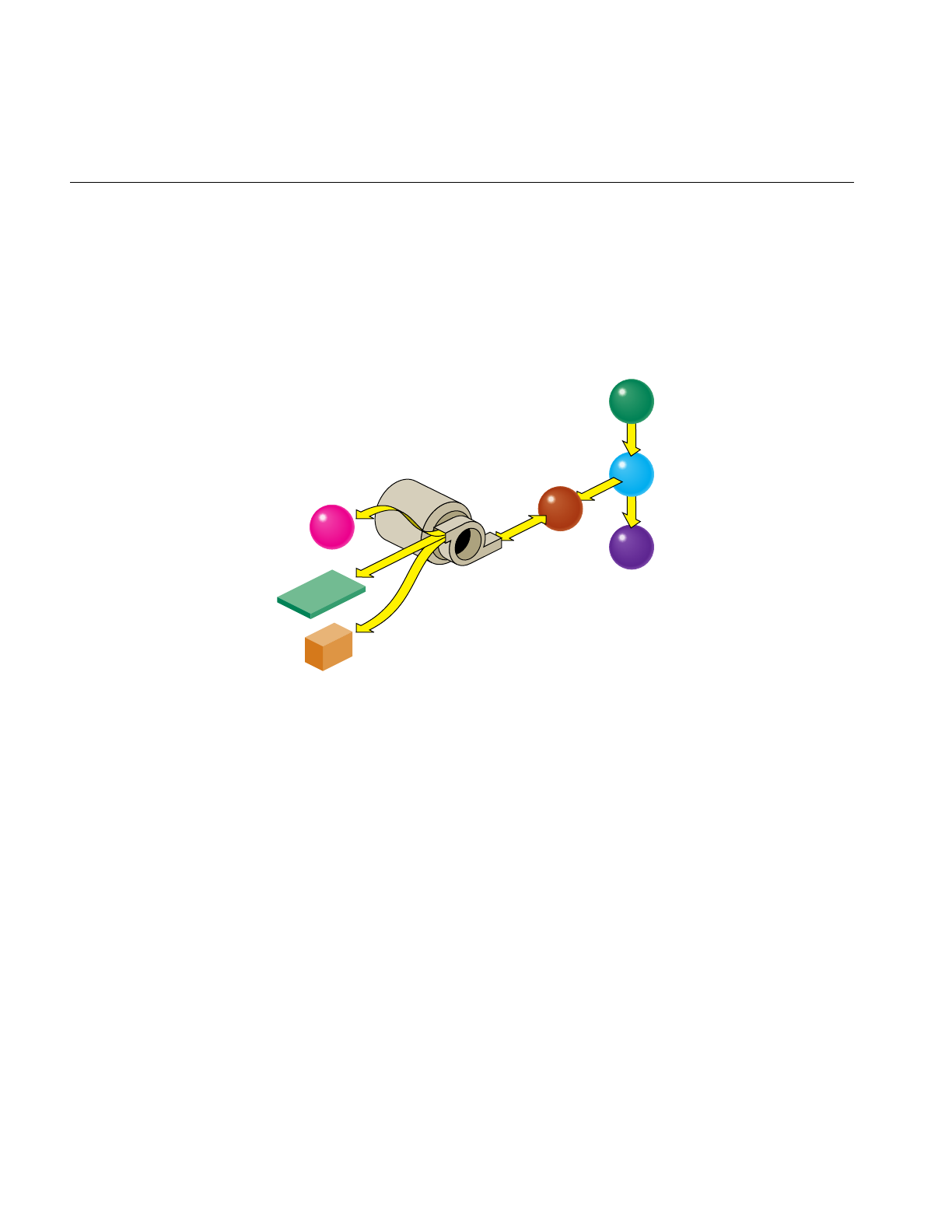
444
Chapter 14: Dynamic Data
Fluxed Coordinate Systems
A pfFCS is similar to a pfDCS node in that both nodes contain dynamic data. In addition
to pfDCS functionality, however, a pfFCS uses a pfFlux to hold its matrix. This fluxed
matrix can then be computed by a pfEngine and potentially asynchronously. This is the
structure shown in Figure 14-1.
Figure 14-1 pfEngine Drives a pfFlux Node Animated a pfFCS Node
In this figure, the pfEngine performs calculations on the data input from multiple
sources, including a pfMemory, a container for static data, a pfFlux, and an additional
source pfEngine. The main pfEngine sends its resulting matrix to a pfFlux. The pfFlux is
attached to the pfFCS with the pfFCS setFlux() method. This flux then:
• Can trigger the pfEngine to directly recompute its data if in
PFFLUX_ON_DEMAND mode when the pfFCS calls getCurData() on the flux
• Will use frame accurate results with other fluxes if a member of a flux sync group
• Contains the matrix for the pfFCS node to produce a transformed coordinate system
for the current frame for children of the node in the scene graph.
pfEngine
pfMemory
pfFlux
pfEngine pfFlux
pfGroup
pfFCS
pfGeoSet

pfFlux
445
Since a pfFCS node is of type pfGroup, you can connect many nodes to it. This
functionality is valuable if many geometries need to share the a transformation, such as
the moving limbs of a walking character whose overall location is changing every frame.
For an example of a pfEngine, pfFlux, pfFCS example, see fcs_engine.C in
sample/pguide/libpf/C++.
Replacing pfCycleBuffer With pfFlux
Prior to version 2.2 of IRIS Performer, the customary way of manipulating dynamic data
was to use a pfCycleBuffer. Morphing was accomplished using pfCycleBuffer and
pfMorph. While pfCycleBuffer and pfMorph are still supported for compatibility, they
are obsoleted by pfEngine and pfFlux.
Note: If your applications do not contain pfCycleBuffer or pfMorph, skip to the next
section. This section explains how to replace pfCycleBuffer and pfMorph with pfFlux
and pfEngine.
pfFlux Differences
pfFlux is similar to, but far more powerful than, pfCycleBuffer:
• Where pfCycleBuffer is unaware of the nodes driving it, pfFlux is aware of its
parent nodes. When attached to a pfEngine, for example, a pfFlux can trigger a
pfEngine to recompute it’s output.
• pfFlux provides a mechanism for updating data in processes that are completely
asynchronous to the main APP, CULL, DRAW pipeline stages.

446
Chapter 14: Dynamic Data
Converting to pfFlux
To convert from pfCycleBuffer to pfFlux, use code similar to the following:
/* Replace pfCyclebuffer creation with pfFlux: */
pfFlux *flux = pfFlux(size, PFFLUX_DEFAULT_NUM_BUFFERS);
/* replace getting of read-only data
* pfCBufGetCurData() for read becomes:
*/
curData = flux->getCurData();
/* replace getting of data to edit.*/
/* get writable buffer BEFORE editing data */
data = flux->getWritableData();
/* ... edit data */
/* declare data edited after editing for the frame is done.
* Replace pfCBufferChanged(pfCycleBuffer *cbuf) becomes:
*/
flux->WriteComplete();
pfEngine
A pfEngine performs calculations. The source can either be static data, such as a
pfMemory, or dynamic data, such as a pfFlux. The destination of a pfEngine is fed into a
pfFlux, as shown in Figure 14-1.

pfEngine
447
Creating and Deleting Engines
The constructor for pfEngine requires that you specify the computation type of pfEngine
you are creating. IRIS Performer provides many types of engines, each performing a
different calculation on the input data. Table 14-1 describes the engine types:
pfEngine::getFunction() returns the pfEngine type. These engine types are described in
further detail in “Setting Engine Types and Modes” on page 448.
To delete a pfEngine, as with all pfObjects, use pfDelete().
Table 14-1 pfEngine Types
Engine Description
PFENG_SUM Sums the input array of floats into a destination array of floats.
PFENG_MORPH Morphs between the input data
PFENG_BLEND Is a light-weight version of PFENG_MORPH.
PFENG_TRANSfORM Translates a set of data with a matrix operation.
PFENG_ALIGN Generates a translation matrix from the input data.
PFENG_MATRIX Generates a matrix of type rotation, translation, scale,
non-uniform scaling, or combine, using pre or post
multiplication.
PFENG_ANIMATE Same as PFENG_MATRIX except that the sources are arrays of
animation frames.
PFENG_BBOX Computes the bounding box of the input array of data.
PFENG_TIME Takes a time, in seconds, and makes it into a frame number that is
useful in driving the frame source of PFENG_MORPH,
PFENG_BLEND, and PFENG_ANIMATE.
PFENG_STROBE Switches iteration sets of floats, called items, between an on and
off based on time.
PFENG_USER_FUNCTION User-defined function.

448
Chapter 14: Dynamic Data
Setting Engine Types and Modes
Table 14-1 lists the different types of IRIS Performer-supplied pfEngines. Many of the
pfEngines have different modes of operation. For example, PFENG_ANIMATE offers the
following modes:
• PFENG_ANIMATE_ROT
• PFENG_ANIMATE_TRANS
• PFENG_ANIMATE_SCALE_UNIFORM
• PFENG_ANIMATE_SCALE_XYZ
• PFENG_ANIMATE_BASE_MATRIX
All of these modes specify what the engine changes. PFENG_ANIMATE_ROT, for
example, specifies that the engine rotates a geometry, PFENG_ANIMATE_TRANS
translates a geometry, and PFENG_ANIMATE_SCALE_UNIFORM scales a geometry.
pfEngine::setMode() sets the mode value; pfEngine::getMode() returns the mode value.
The following sections describe the engine types and their mode values, if any.
PFENG_SUM Engines
PFENG_SUM adds arrays of floats to form a destination array of floats. One use for
PFENG_SUM is aligning geometries to height, such as buildings, to a pfASD terrain.
Since PFENG_SUM can have as few as one source it can be used to simply copy data from
one location to another.
PFENG_MORPH Engines
Morphing is the smooth transition from one appearance to another. The effect is achieved
through the reorientation of the vertices in pfGeoSets. Morphing can refer to geometries
and their attributes. For example, you could “morph” the following:
• Color to simulate a flickering fire.
• Texture coordinates to simulate rippling ocean waves.
• Coordinates to make a 3D model of a face smile or frown.

pfEngine
449
PFENG_MORPH sets the destination of the pfEngine to a weighted sum of its sources.
To specify the weighting, you use either:
• PFENG_MORPH_WEIGHTS
• PFENG_MORPH_FRAME
PFENG_MORPH_WEIGHTS contains an array of floats, or weighting values.
PFENG_MORPH_SRC(n) is also an array; there is one element for each pfEngine source.
To create the morph weighting, element 0 of PFENG_MORPH_WEIGHTS is multiplied
by PFENG_MORPH_SRC(0); element 1 is multiplied by PFENG_MORPH_SRC(1), and
so on.
PFENG_MORPH_FRAME contains a single float. This float specifies the weighting
between two pfEngine sources, PFENG_MORPH_SRC(n). The integer portion of the
float specifies the first of the two consecutive sources, and the decimal portion of the float
specifies the weighting between those sources. For example, a
PFENG_MORPH_FRAME of 3.8 would mean PFENG_MORPH_SRC(3) * 0.2 +
PFENG_MORPH_SRC(4) * 0.8.
For an example of a morph engine, see morph_engine.C in sample/pguide/libpf/C++.
PFENG_BLEND Engines
PFENG_BLEND is a light-weight version of PFENG_MORPH. PFENG_BLEND sets the
pfEngine destination to a weighted sum of elements of the pfEngine sources.
To specify the weighting, you use either:
• PFENG_BLEND_WEIGHTS
• PFENG_BLEND_FRAME
These weighting mechanisms work identically to those in “PFENG_MORPH Engines,”
with the following exception: the source, PFENG_BLEND_SRC(n), should contain
iteration elements. Each element is a set of floats, called items. The number of elements in
each set is called a stride. So, the iteration items for pfEngine source 0 begin at items
number 0 * stride; for source 1, at items number 1 * stride, and so on.
PFENG_BLEND_WEIGHTS contains an array of floats, one for each of the pfEngine
sources, PFENG_BLEND_SRC(n).

450
Chapter 14: Dynamic Data
PFENG_BLEND_WEIGHTS(0) is multiplied by the items starting at
PFENG_BLEND_SRC(0*stride); PFENG_BLEND_WEIGHTS(1) is multiplied by the
items starting at PFENG_BLEND_SRC(1*stride) and so on.
PFENG_BLEND_FRAME contains a single float. This float specifies the weighting
between two consecutive PFENG_BLEND_SRC(n) sources. The integer portion of the
float specifies the first of the two consecutive sources, and the decimal portion of the float
specifies the weighting between those sources. For example, a PFENG_BLEND_FRAME
of 3.8 would mean PFENG_BLEND_SRC(3) * 0.2 + PFENG_BLEND_SRC(4) * 0.8.
For an example of a blend engine, see blend_engine.C in sample/pguide/libpf/C++.
PFENG_TRANSFORM Engines
PFENG_TRANSFORM transforms the PFENG_TRANSFORM_SRC(n) array of floats by
the matrix contained in PFENG_TRANSFORM_MATRIX.
PFENG_ALIGN Engines
PFENG_ALIGN generates an alignment matrix based on the sources. One use for
PFENG_ALIGN is to align moving objects, such as vehicles, to a pfASD.
PFENG_ALIGN_POSITION determines the translational portion of the matrix. If
PFENG_ALIGN_POSITION is NULL, the translational portion of the matrix is set to all
zeros.
PFENG_ALIGN_NORMAL and PFENG_ALIGN_AZIMUTH determine the rotation
portion of the matrix. If either are NULL, the rotation portion of the matrix is set to all
zeros.
PFENG_MATRIX Engines
PFENG_MATRIX generates a matrix based on its sources. Applied to vertex coordinates
of pfGeoSets, these routines provide the same mathematical effect as using pfDCSs in a
scene graph. However, these pfEngines will use the host to compute the vertices and thus
eliminate the need for matrices to be evaluated in the graphics pipeline. This trade-off
might produce a faster rendering frame rate if there are sufficient host CPU resources for
the computation involved.

pfEngine
451
The following tokens specify the kind of action performed by the PFENG_MATRIX
engine:
PFENG_MATRIX_ROT rotates a geometry according to heading, pitch, and roll values;
the equivalent is pfDCS::setRot().
PFENG_MATRIX_TRANS transforms a geometry; the equivalent is pfDCS::setTrans().
PFENG_MATRIX_SCALE_UNIFORM uniformly scales a geometry; the equivalent is
pfDCS::setScale().
PFENG_MATRIX_SCALE_XYZ non-uniformly scales a geometry; the equivalent is
pfDCS::setScale(x, y, z).
PFENG_MATRIX_BASE_MATRIX contains a pfMatrix that is either pre or post
multiplied against the matrix generated by the other sources, depending on the
PFENG_MATRIX_MODE mode set by the setMode() method; PF_OFF specifies
pre-multiplication, PF_ON specifies post-multiplication.
Any or all of the sources can be NULL, in which case they have no effect on the resulting
matrix.
PFENG_ANIMATE Engines
PFENG_ANIMATE animates a matrix based on its sources. This engine type is similar to
PFENG_MATRIX, but instead of using single values for rotation, translation, and scaling,
PFENG_ANIMATE uses arrays of values.
To specify the weighting, you use either:
• PFENG_ANIMATE_WEIGHTS
• PFENG_ANIMATE_FRAME
PFENG_ANIMATE_WEIGHTS contains a float for each of the values in the rotation,
translation, and scale sources. PFENG_ANIMATE_SRC(n) is also an array; there is one
element for each pfEngine source.
To create an animation, element zero of PFENG_ANIMATE_WEIGHTS is multiplied by
PFENG_ANIMATE_SRC(0); element one is multiplied by PFENG_ANIMATE_SRC(1),
and so on.

452
Chapter 14: Dynamic Data
PFENG_ANIMATE_FRAME contains a single float. This float specifies the weighting
between two of the values in the rotation, translation, and scale sources. The integer
portion of the float specifies the first of the two consecutive values, and the fractional
portion of the float specifies the weighting between those values. For example, a
PFENG_ANIMATE_FRAME of 3.8 would mean PFENG_ANIMATE_SRC(3) * 0.2 +
PFENG_ANIMATE_SRC(4) * 0.8.
The following tokens specify the kind of action performed by the PFENG_ANIMATE
engine.
PFENG_ANIMATE_ROT rotates a geometry according to heading, pitch, and roll
values; the equivalent is pfDCS::setRot().
PFENG_ANIMATE_TRANS transforms a geometry; the equivalent is
pfDCS::setTrans().
PFENG_ANIMATE_SCALE_UNIFORM uniformly scales a geometry; the equivalent is
pfDCS::setScale().
PFENG_ANIMATE_SCALE_XYZ non-uniformly scales a geometry; the equivalent is
pfDCS::setScale(x, y, z).
PFENG_ANIMATE_BASE_MATRIX contains a pfMatrix that is either pre- or
post-multiplied against the matrix generated by the other sources depending on the
PFENG_MATRIX_MODE mode set by the pfEngine method, setMode().
Any or all of the sources can be NULL, in which case they have no effect on the resulting
matrix.
For an example of an animate engine, see fcs_animate.C in sample/pguide/libpf/C++.
For more information about animation, see “Animating a Geometry” on page 456.
PFENG_BBOX Engines
PFENG_BBOX generates a bounding box that contains the coordinates of the pfEngine
source, PFENG_BBOX_SRC.

pfEngine
453
PFENG_TIME Engines
PFENG_TIME takes a time in seconds and converts it to a frame number, which can drive
the sources of the following engine types: PFENG_MORPH, PFENG_BLEND, and
PFENG_ANIMATE.
PFENG_TIME_TIME is the source time in seconds. This is usually connected to the
pfFlux returned from pfFlux::getFrame().
PFENG_TIME_SCALE contains four floats that are used to modify the incoming time:
• PFENG_TIME_SCALE[0] is an initial offset.
• PFENG_TIME_SCALE[1] is a scale factor.
• PFENG_TIME_SCALE[2] is a range.
• PFENG_TIME_SCALE[3] is a final offset.
The PFENG_TIME_MODE mode, set with pfEngineMode(), determines how the
destination number moves between its start and end point. The two mode values
include:
• PFENG_TIME_CYCLE makes the destination number go from start to end then
restarts again at the beginning.
• PFENG_TIME_SWING makes the destination number go back and forth between
the start and end.
Note: This mode is related to the interval mode of a pfSequence.
If the PFENG_TIME_TRUNC mode is set to PF_ON, the result is truncated.
PFENG_STROBE Engines
PFENG_STROBE switches iteration sets of floats, called items, between ON and OFF
based on time. One use of PFENG_STROBE is light point animations.
PFENG_STROBE_TIME is the source time in seconds. This data is usually connected to
the pfFlux returned from pfFlux::getFrame().

454
Chapter 14: Dynamic Data
PFENG_STROBE_TIMING contains iterations sets of three floats:
• PFENG_STROBE_TIMING[n*stride + 0] is the ON duration.
• PFENG_STROBE_TIMING[n*stride + 1] is the OFF duration.
• PFENG_STROBE_TIMING[n*stride + 2] is an offset.
PFENG_STROBE_ON contains iteration sets of floats, called items.
PFENG_STROBE_OFF contains iteration sets of floats, called items. If
PFENG_STROBE_OFF is NULL, all off states are 0.0.
For an example of animation using a strobe engine, see strobe_engine.C in
sample/pguide/libpf/C++.
PFENG_USER_FUNCTION Engines
When a pfEngine is of type PFENG_USER_FUNCTION, you specify the function of the
pfEngine using pfEngine::setUserFunction().pfEngine::getUserFunction() returns the
pfEngine type.
For an example of animation using a user-defined engine, see user_engine.C in
sample/pguide/libpf/C++.
Setting Engine Sources and Destinations
pfEngine sources can be any number of objects, including pfFluxs, pfMemory’s, and
pfEngines. The sources provide the input data for the pfEngine. pfEngine destinations
are pfFluxs, which contain the pfEngine output.
pfEngine::setSrc() and pfEngine::setDst() set the pfEngine sources and destination,
respectively.pfEngine::getSrc() and pfEngine::getDst() return the pfEngine sources and
destination, respectively. pfEngine::getNumSrcs() returns the number of sources. A
pfEngine can only have one destination.

pfEngine
455
Setting Engine Masks
pfEngine masks are bit masks that provide a means of selectively triggering pfEngines.
Only those pfEngines that have masks that match the evaluation mask can be triggered,
as shown in the evaluation method:
pfEngine::evaluate(int mask)
pfEngine::setMask() and pfEngine::getMask() set and return pfEngine masks,
respectively.
Setting Engine Iterations
You can make pfEngines repeat their calculations, called iterations, when operating on an
array of data instead of on a single piece of data. You also specify the unit of data, called
an item, for example, a vector would have three items per unit. For example, if you want
to add two arrays of 100 pfVec3s each, you set iteration to 100 and item to 3.
pfEngine::setIterations() and pfEngine::getIterations() set and get iterations,
respectively.
Setting Engine Ranges
There are times when you might like to reduce computation needs by not evaluating
engines, for example, when the eye point is far from the geometry being animated by a
pfEngine.
You establish the location of an animated geometry, and an area located around the
geometry using pfEngine::setEvaluationRange(). Only when the eye position is within
that area can the pfEngine be evaluated.
The range functionality is only enabled when the PFENG_RANGE mode, created by
pfEngine::setMode(), is set to PF_ON; the default is PF_OFF.
Evaluating pfEngines
To evaluate a pfEngine, you use one of the forms of pfEngine::evaluate() or
pfFlux::evaluate().

456
Chapter 14: Dynamic Data
For more information about pfFlux::evaluate(), see “Triggering pfFlux Evaluation” on
page 440.
The two forms of evaluate() are:
void pfEngine::evaluate(int mask);
void pfEngine::evaluate(int mask, pfVec3 eye_pos);
For more information about mask, see “Setting Engine Masks” on page 455.
The second form of the method specifies the location of the viewer. The engine is only
evaluated if the location of the viewer, eye_pos, is within the range of the pfEngine, set by
pfEngine::setEvaluationRange(). For more information about the range of a pfEngine,
see “Setting Engine Ranges” on page 455.
Note: The eye position has no effect on evaluation of the pfEngine if the
PFENG_RANGE_CHECK mode is PF_OFF, the default.
Animating a Geometry
To animate a geometry using a combination of pfFlux, pfFCS, and pfEngines nodes, use
the following guidelines:
1. Initialize and populate the pfFluxes.
2. Connect pfMemory or pfFluxes as the sources of a pfEngine.
3. Connect a pfFlux to the output destination of the pfEngine.
4. Connect the pfFlux containing the output of the pfEngine to the scene graph in one
of three ways:
• connect it as an attribute of a pfGeoSet using setAttr()
• connect it as the bounding box of a pfGeoSet using setBound() where the mode
argument is set to PFBOUND_FLUX
• connect it directly to a pfFCS using setFlux()
5. Set up any needed flux sync groups for synchronizing transformations.
This scenario is the simplest set up; it is represented graphically in Figure 14-1. More
complicated scenarios include chaining pfEngines together or running multiple
geometries off of one pfFCS node.

Animating a Geometry
457
The following code sample provides an implementation of the animation procedure:
Example 14-2 Connecting Engines and Fluxs
// create the nodes
pfFlux *myData1 = new pfFlux(100 * sizeof(pfVec3));
pfFlux *myData2 = new pfFlux(100 * sizeof(pfVec3));
pfEngine *myEngine = new pfEngine(PFENG_SUM);
pfFlux *engineOutput = new pfFlux(100 * sizeof(pfVec3));
pfFCS myFCS = new pfFCS();
pfGeode myGeode = new pfGeode();
// initialize and populate the flux nodes
myData1->init();
myData2->init();
// attach the pfFlux nodes as the source of the pfEngine
myEngine->setSrc(0, myData1, 0, 3);
myEngine->setSrc(0, myData12, 0, 3);
// attach a pfFlux to the output of the pfEngine
myEngine->setDst(engineOutput, 0, 3);
myEngine->iterations(100, 3);
// connect the pfFlux output node to the scenegraph
myFCS->setFlux(engineOutput);
// attach child geometry to be tranformed by the FCS
myFCS->addChild(myGeode);
...
// compute the data in the source pfFluxes to the engine
float *current = (float *)myData1->getWritableData();
... // compute data
myData1->writeComplete();


This chapter describes the Active Surface Definition (ASD): a library that
handles real-time surface meshing and morphing.
“Active Surface Definition”
Chapter 15


461
Chapter 15
15. Active Surface Definition
Active Surface Definition (ASD) is a powerful real-time surface meshing and morphing
library. It enables you to roam surfaces that are too large to hold in system memory very
quickly. The surfaces, called meshes, are represented by triangles from more than one
LODs.
ASD is a library that handles real-time surface meshing and morphing in a
multiprocessing and multichannel environment. pfASD is an IRIS Performer scene
graph node that allows you to place ASD information in a scene graph.
This chapter describes how to create and use ASD.
Overview
In the past, IRIS Performer applications have dealt with large surfaces in two ways:
• Level of detail (LOD), where the whole surface is one LOD.
• Patches, where the surface is broken into geometrical subunits, each of which can be
at a different LOD level.
Each of these approaches has its disadvantages:
• When the entire surface is one LOD, with large surfaces, memory limitations often
require such a high LOD that the resolution is poor.
• Patches can only morph between adjacent LODs, which is insufficient in large
surfaces. The result is visible borders between LODs.

462
Chapter 15: Active Surface Definition
Active Surface Definition (ASD) is designed to solve these problems. ASD is a powerful
real-time surface meshing and morphing library characterized by the following features:
1. Transitions between different levels of detail (LOD) appear smooth and void of
spatial or temporal artifacts. Vertex position, normal, color, and texture coordinates
can be morphed.
2. LODs can be generated using simple adaptations of well-known,
non-uniform-tessellation surface subdivision algorithms.
3. ASD is real-time; in multiprocessor mode, it can sustain 60HZ operation while
displaying complex surfaces.
4. Nearly-coplanar objects, such as road surfaces, are accurately represented in the
non-uniform tessellation of each LOD using local textures.
5. Objects, such as buildings, may be modeled and rendered using alternate
algorithms, yet remain attached to the surface.
6. Triangles substantially outside the viewing frustum are culled from rendering.
7. The evaluation function that specifies the morphing factor for each geometry is
specified at run-time, which allows traversal to be optimized for different
applications and data sets.
8. Huge surfaces, such as one-meter data of the entire United State, are supported
using run-time paging from disk memory.
The pfASD approach uses a modeling surface that is a single, connected surface rather
than a collection of patches.
An ASD surface contains several hierarchical level of detail (LOD) meshes where one
level encapsulates a coarser LOD than the next. When rendering an ASD surface, an
evaluation function selects polygons from the appropriate LODs and constructs a valid
meshing to best approximate the real surface on the screen.
Unlike existing LOD schemes, pfASD selects triangles from many different LODs and
combines them into a final surface. This feature lets a fly-through over a surface use
polygons from higher LODs for drawing nearby portions of the surface in combination
with polygons from low LODs that represent distant portions of the surface.
To review an ASD application, see perf/test/simpleASD/simpleASD.C.

Using ASD
463
Using ASD
Modern computer graphics systems render objects represented by faceted surfaces
comprised of triangles. While rendering performance is increasing steadily, it remains
necessary to limit the number of triangles that are rendered if a real-time rendering rate
of 60 frames per second or greater is to be maintained.
Triangles may be omitted with no loss of image quality if they represent objects that are
not in the field of view (view frustum culling) or if they represent objects whose visibility
is occluded by other, nearer objects.
The number of rendered triangles can also be dramatically reduced with little or no loss
of image quality if multiple representations of each object are maintained, and the
representation used has as little detail as is necessary for displaying a good-quality
image. This technique and a body of others related to it are collectively referred to as level
of detail (LOD) reduction, and the multiple object representations are known as LODs.
LOD Reduction
LOD reduction is not a new idea, having been practiced in the field of real-time image
generation for at least two decades. Early implementations eliminated the sudden,
visible transition from one level of detail to another by alpha blending two models over
a period of several frame times. More recently the fade transition has been replaced by a
geometric morph solution, which eliminates the need to temporarily render additional
triangles, and interacts more nicely with depth buffer hidden surface elimination.
When the object being rendered is very large, there is no single level of detail that is
optimal for the entire object. Instead, it is desirable to render the object with a smooth
variation of level of detail, allowing nearer portions to be represented accurately, and
farther portions to be represented efficiently.
The need for spatially varying level of detail is particularly acute when rendering terrain,
which may range from several feet to hundreds of miles from the viewpoint. Early
attempts to support multiple LOD terrain modeled the surface as separate tiles, each of
which was rendered at a single level of detail. This approach results in physical
discontinuities between neighboring tiles rendered with different levels of detail, which
are visible as obvious ``walls.’’

464
Chapter 15: Active Surface Definition
Triangulated Irregular Networks
Triangulated irregular networks (TINs) can approximate a surface with fewer polygons
than other uniformly-grided representations. However, TIN models are hard to create
dynamically at interactive rates. Regular data, on the other hand, allows easier
construction of LODs at interactive rates. We propose a new terrain framework, Active
Surface Definition (ASD), that combines the advantages of both regular and irregular
networks. The terrain database is pre-computed and stored in a hierarchical structure of
efficient, irregular triangulations. LOD reduction is performed on the data structure at
real-time frame rates, varying levels of detail both spatially and temporally.
Hierarchical Structure
Active Surface Definition defines a hierarchical structure that organizes all the LODs of
a terrain. At run-time ASD traverses the structure, selecting triangles from different
LODs to render the portion of the terrain that is within the culling frustum. Triangles are
rendered either at pre-stored locations, when they are in a particular fully-morphed
portion of a LOD range, or at computed morphed locations, when they are in the
morphing transition portions of the LOD range, as shown in Figure 15-1.
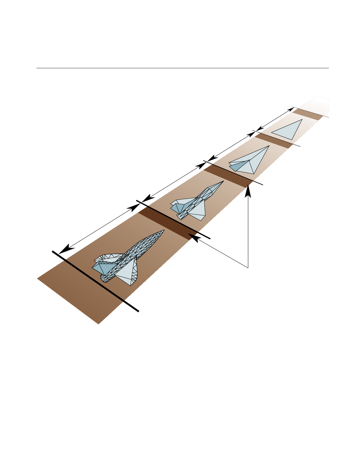
Using ASD
465
Figure 15-1 Morphing Range Between LODs
Figure 15-1 shows the complete object represented by an LOD. ASD is often used for very
large terrains, like a map of the United States, so the entire terrain cannot fit into a single
LOD range. In that case, parts of the large terrain would be represented by different
LODs, as shown in Figure 15-2.
LOD 1 LOD 2 LOD 3 LOD 4
Morphing zones
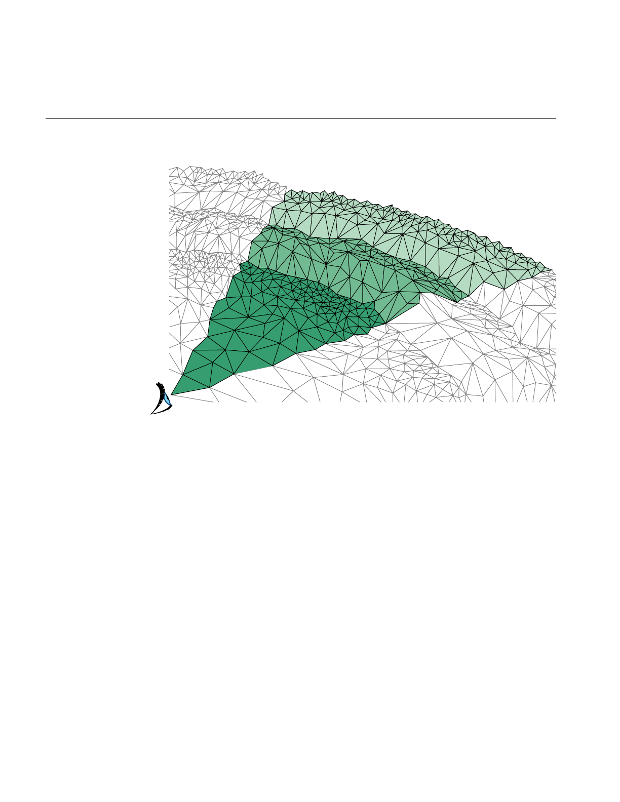
466
Chapter 15: Active Surface Definition
Figure 15-2 Large Geometry
In Figure 15-2, different parts of the terrain are displayed at different levels of resolution.
ASD Solution Flow Chart
To visualize large terrains using ASD, you use the following steps, which are portrayed
in Figure 15-3:
1. Collect raw, elevation data.
2. Use a modeler to create ASD structures from the raw elevation data. There are
various triangle tessellation algorithms that can be used to model the terrain into
TINs. Adaptive tessellation and accurate representation and minimum visual
distraction between LODs are potentially all supported by pfASD structures.
3. Place the ASD structures into a scene graph by attaching them to pfASD nodes.
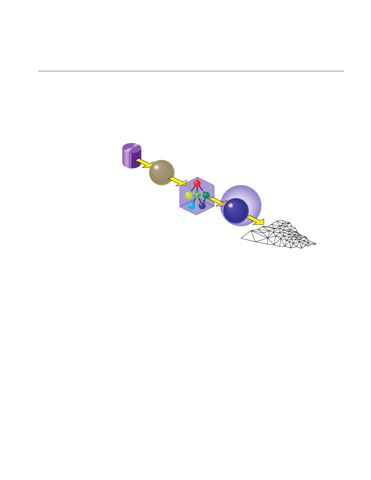
A Very Simple ASD
467
4. Design an evaluation function that shows when a particular triangle on a particular
LOD level in ASD structure should be selected.
5. IRIS Performer traverses and evaluates pfASD structures at run-time to create an
active mesh that is used for rendering.
Figure 15-3 ASD Information Flow
A Very Simple ASD
To demonstrate the ASD concept, we shall now build a very simple ASD surface. The
surface has two representations, which corresponds to two levels of detail (LOD). The
coarser level, LOD 0, has only a single triangle: T0. The finer level, LOD 1, has four
triangles: T1, T2, T3, T4, as shown in Figure 15-4.
Raw elevation data
Modeler
pfASD structures
Performer
Active mesh
Evaluation
function
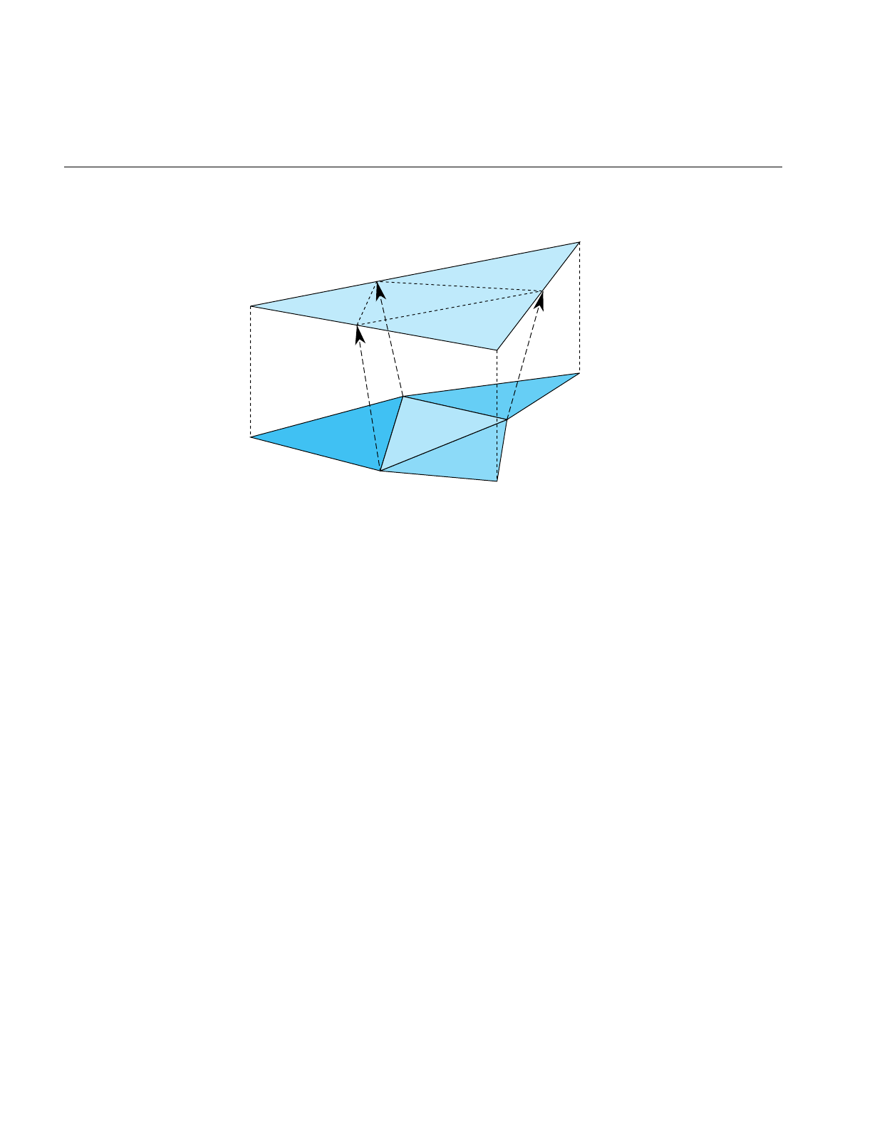
468
Chapter 15: Active Surface Definition
Figure 15-4 A Very Simple pfASD
pfASD requires that we specify a morphing relationship for the vertices in the two levels
of detail. This relationship guides ASD to choose triangles from the appropriate LODs
and place vertices in the correct positions.
Morphing Vector
Each triangle in LOD 0 can have up to four replacement triangles in a higher LOD. pfASD
imposes the limitation that the replacement of T0 must include the vertices V0, V1, V2,
and may include three more vertices. In our case, the replacement of T0 includes the
vertices V0, V1, V2, M0, M1, M2. We express the morph behavior between two levels by
describing the morph behavior of the triangle vertices.
Since V0, V1, and V2 remain unchanged, we need only specify the morphing behavior,
or the morphing vector, M0, M1, and M2. The morphing vector of a vertex is a vector
connecting the vertex to an edge of the lower resolution triangle. We specify morphing
vectors d0, d1, and d2 for the vertices M0, M1,and M2, respectively. The triangles in
LOD1 can now morph smoothly by morphing the vertex M0, M1, and M2 along their
morphing vectors d0, d1, and d2.
V0
V0
V1
V1
V2
V2
T0
T1 T2
T3
T4
M0
M2
M1
__
d0
__
d2
__
d1
LOD 0
LOD 1

ASD Elements
469
We call the edge position (M1+d1) unmorphed, and the M1 position fully morphed. The
unmorphed position is the reference position of a vertex because it is a reference to show
how a vertex should be coplanar with the triangle in the lower LOD when we replace the
lower LOD triangle with a higher LOD triangles, while providing the least amount of
visual distraction. The fully-morphed position is the final position of a vertex; that
position should be chosen from the original raw data by various triangulation
algorithms. It is recommended that the reference position be defined after the final
position is chosen to most accurately design the adaptive tessellation of a terrain. pfASD
handles the morphing of other attributes, such as normals, colors, and texture
coordinates as well.
This completes the construction of a very simple pfASD. When flying over this model—
say from V0 towards M1—pfASD shall morph M0 and M2 first, and continue to morph
M1 as we get closer to the edge [V1,V2]. In other words, pfASD will morph closer
triangles into their higher LOD first.
A Very Complex ASD
To view a complex ASD, run perfly with the yosemite data supplied in the images. Observe
that the entire, visible terrain is represented by more than one LOD.
ASD Elements
pfASDs create active meshes to accurately and efficiently render terrains. A mesh is a
surface tessellated into triangles, as shown in Figure 15-2. Each frame contains an active
mesh. ASD reduces visual discontinuities between meshes by morphing geometry.
pfASD is defined by the following elements:
• Vertices
• Triangles
• Evaluation function

470
Chapter 15: Active Surface Definition
Vertices
The triangles of all LODs share a single pool of vertices: those vertices that define the
triangles of the highest LOD. A few vertices exist in all the LODs. These vertices define
the triangles in LOD0, and are typically chosen as corners of the terrain or other
significant features. Each of the remaining vertices exists in a contiguous set of LODs,
including the highest LOD. In order to facilitate the gradual introduction of a vertex into
the terrain, the actual position of each vertex is supplemented by a reference position. If
i is the lowest LOD that includes a vertex, then that vertex is located at its actual position
in LODs i through (n-1), and is morphed between its reference position and its actual
position during the morphing zone of LODi that is adjacent to LOD(i-1) range.
Note: ASD could be extended to support multiple reference positions per vertex,
allowing vertices to morph between multiple LODs. This extension may be supplied in
the near future depending on demands.
A vertex is represented by its final position (pfVec3) and a morphing vector (pfVec3),
which represents the difference between the final position and the reference position. The
current position of a vertex is computed as:
Vvertex = V0 + mVd
V0 is the final position of a vertex, m is the current morphing weight, and Vd is the
morphing vector. Notice that the reference position of a vertex is always chosen to lie on
an edge of a triangle from the lower LOD, though not necessarily at the centers of these
edges. This is to ensure that the replacement of the lower LOD by the higher LOD
happens when they are at coplanar positions, which eliminates sudden popping
artifacts.
Attributes are represented by final position as well, as shown in Figure 15-5.
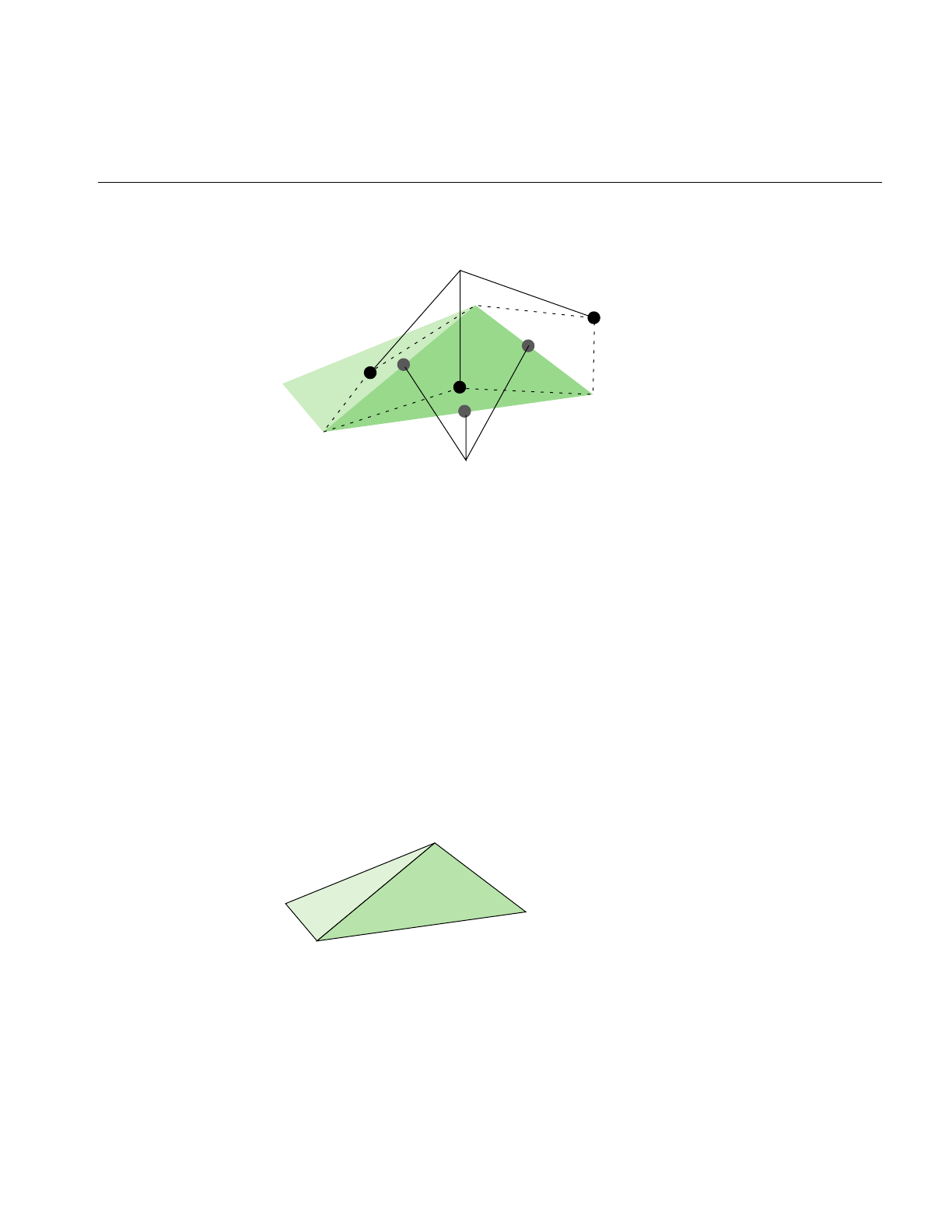
ASD Elements
471
Figure 15-5 Reference Positions
Normals, colors, and texture coordinates can all be linearly interpolated, as specified.
A vertex always morphs along the morphing vector, vd. When m = 1, the vertex is at a
no-morph position, which means it most likely is not part of the active mesh, because it
is on an edge of the parent triangle.
Triangles
A triangle exists in only one particular LOD. If the triangle is too coarse to accurately
represent the current terrain, the triangle is removed from the active mesh. The position
of a triangle is determined by the positions of its vertices, which may be morphed along
the morphing vector.
In the pfASD structure, each triangle node, called an pfASDFace, can have up to four
children. A sequence of frames may render the meshes shown in Figure 15-6.
Figure 15-6 Triangulated Image
Reference positions
Final positions
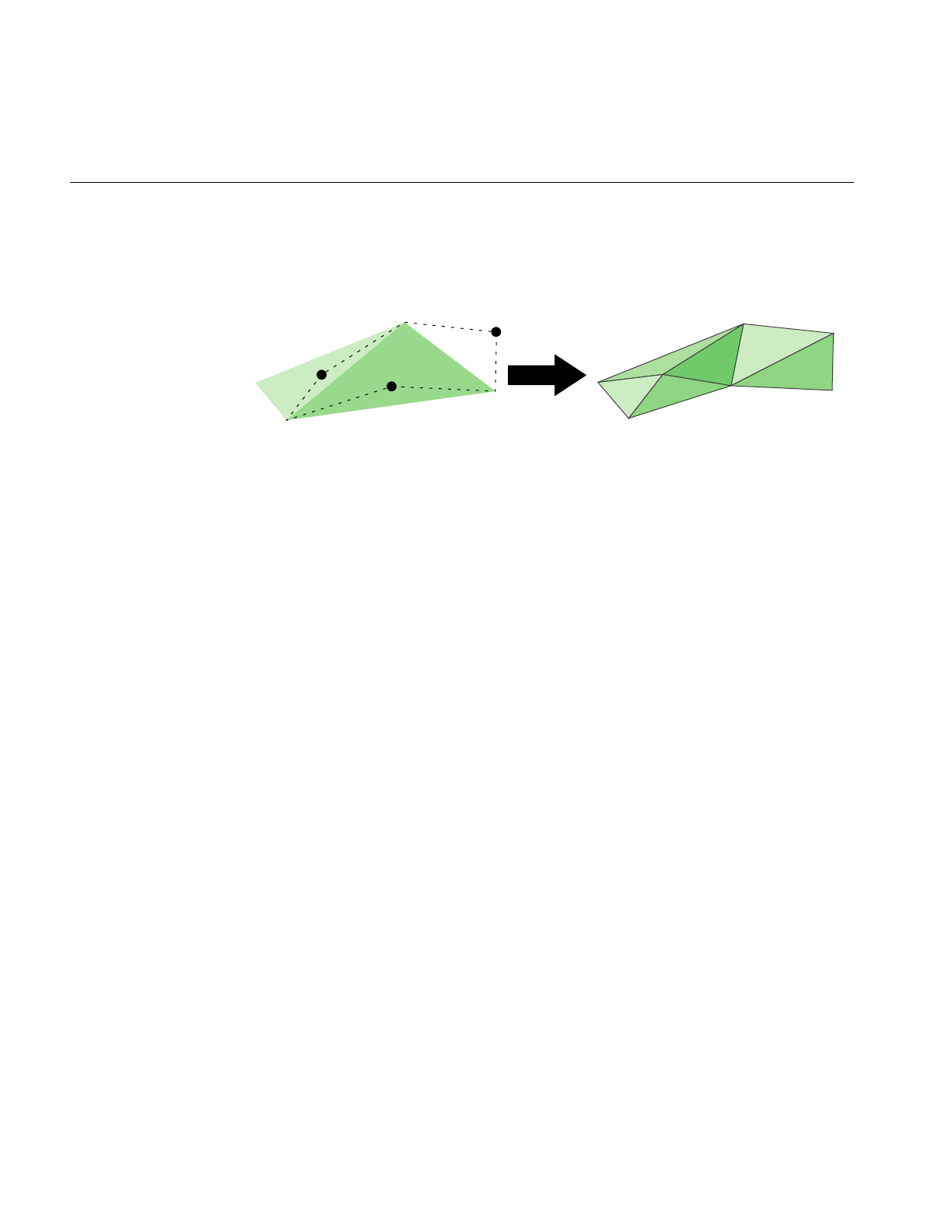
472
Chapter 15: Active Surface Definition
As the distance between a vertex, P, and a viewer changes through the morphing range,
the side of the triangle associated with P is replaced by two edges from the next LOD.
Figure 15-7 shows how the next LOD triangles replace the current LOD triangles.
Figure 15-7 LOD1 Replaced by LOD2
Figure 15-7 shows the shapes of the triangles in two adjacent LODs.
Notice that only one side of the triangle on the left is changed; in this case, the original
triangle is now replaced by two triangles. The triangle that was on the right is now
completely gone; in it’s place are four triangles, as labeled. One triangle can be replaced
by up to four child triangles, depending on whether one, two, or three sides of the
triangles are replaced by two lines.
Sides shared by two triangles are evaluated only once. Morphing the shared side of one
triangle necessarily morphs it to the same position in the neighboring triangle.
Evaluation Function
The evaluation function determines the morph weight of every vertex. This function
returns a floating point value between 0.0 and 1.0 where 1.0 means the vertex is not
morphed and therefore not active. Since it is not active, it is not in the current mesh; it’s
geometry is represented by coarser LOD triangles. 0.0 means that the triangle is
completely morphed. In this case, the vertices are in their final positions in the active
mesh. Any number between 0.0 and 1.0 signifies a morphed position. IRIS Performer
constructs a smooth mesh based on the results from the evaluation function.
You can customize an evaluation function so that it applies to your application. For
example, instead of distance, your evaluation function might be based on altitude.
For more information about the evaluation function, see “Default Evaluation Function”
on page 483.
1
2
3
4
LOD1 LOD2
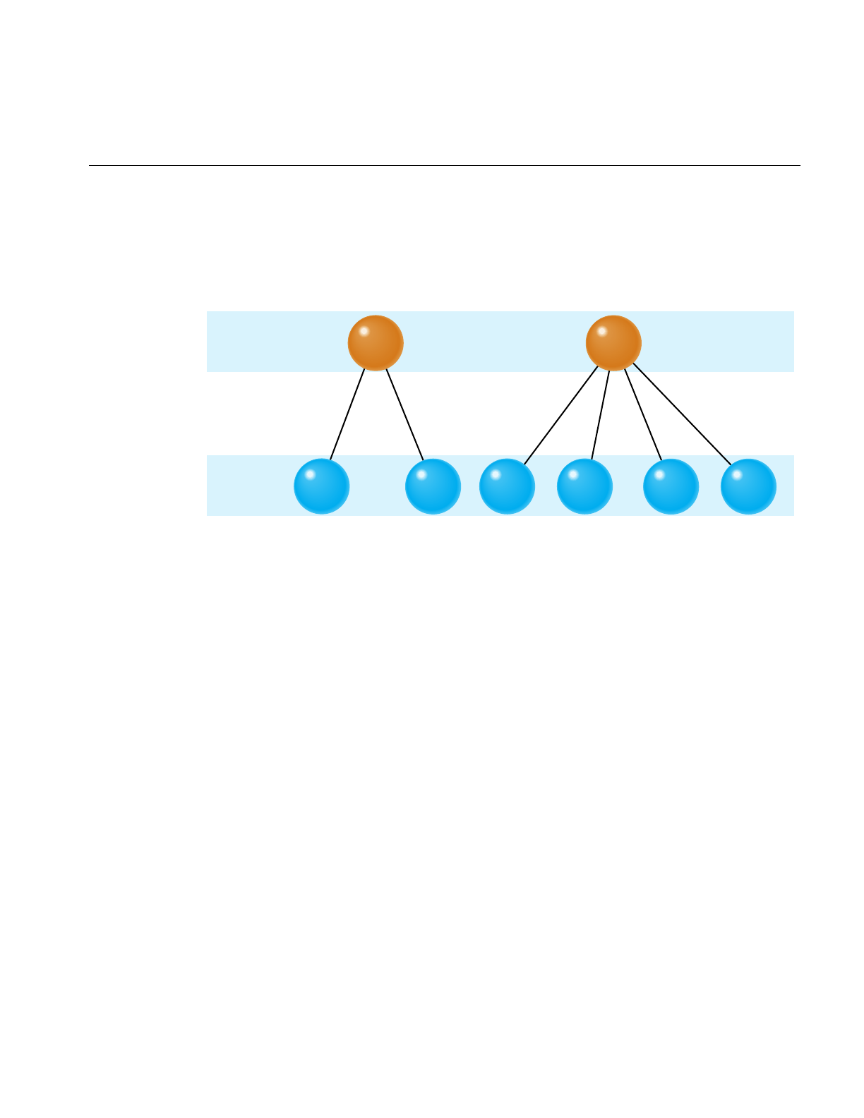
Data Structures
473
Data Structures
Raw geometry data is converted into a tree-like, hierarchical structure of data, as shown
in Figure 15-8.
Figure 15-8 Data Structures
In Figure 15-8. each horizontal layer of triangles is equivalent to a single LOD mesh. The
nodes in the tree structure represent triangles in LOD layers of the terrain. Each triangle
contains three end vertices and up to three reference vertices. These vertices are indices
into the vertex and attribute arrays.
A vertex may be shared by multiple triangles within a single LOD and by many more
triangles throughout the data structure. A single position pair suffices for all the triangles
that share a vertex, but each triangle may specify its own vertex attribute pairs. This is
the reason that the vertex and attribute arrays are represented separately.
In Figure 15-8, the nodes in the top, root level represent the two LOD0 triangles shown
in Figure 15-6. The six triangles from LOD1, labeled C1 through C6, correspond to nodes
from the second level in the tree.
P1 P2
C1 C2 C6
LOD0
LOD1 C3 C4 C5
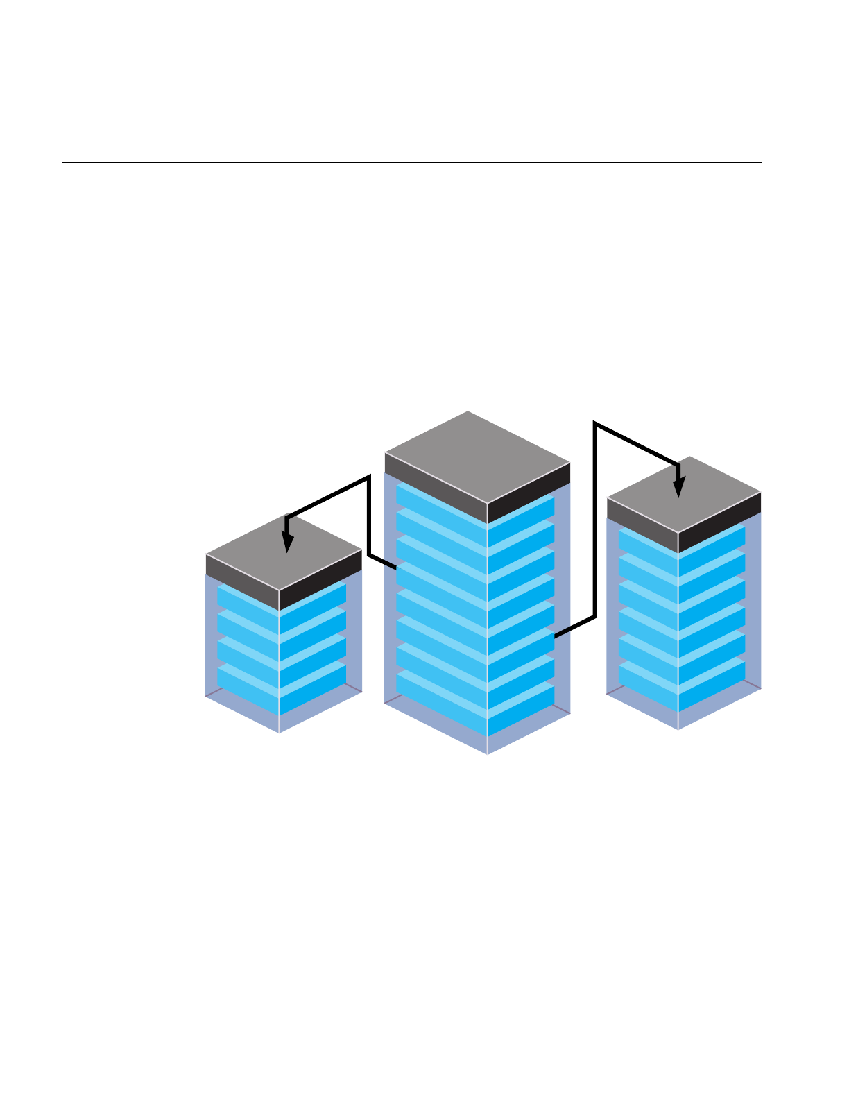
474
Chapter 15: Active Surface Definition
IRIS Performer uses three data structures to encapsulate the triangle mesh information:
• Triangle—encapsulates information about the sides, vertices, attributes, reference
points, parent, and children of a triangle.
• Attributes—encapsulates information about the attributes of each vertex, including
the normal, color, and texture coordinates.
• Vertex—encapsulates information about a morphing vector and the coordinates of
its final position.
Figure 15-9 shows the data structures, their fields, and their relationships.
Figure 15-9 ASD Data Structures
The following sections describe these data structures in detail.
vertID
vert
vertDif
neighborhood
pfTerrainVert
normal (3)
normalDif (3)
Color (4)
ColorDif (4)
Tcood (2)
TcoodDif (2)
pfTerrainAttr
faceID
level
tsid
vert (3)
split (3)
attr (3)
satt (3)
child (4)
pfsFace

Data Structures
475
Triangle Data Structure
The Triangle data structure in PFASD contains information about the triangles in the
triangle mesh.
typedef struct pfASDFace
{
int level;
int tsid;
int vert[3];
int attr[3]
int refvert[3];
int refattr[3];
int child[4];
int refvert[3];
ushort gstateid;
ushort mask;
} pfASDFace;
Table 15-1 describes the fields in the Triangle data structure.
Table 15-1 Fields in the Triangle Data Structure
Field Definition
level Triangle’s LOD level.
tsid Triangle strip ID.
vert[3] Coordinates of the triangle’s three vertices.
refvert[3] Coordinates of the triangle’s (up to) three reference points.
attr[3] Pointer to attribute values for each of the triangle’s three vertices.
refattr[3] Pointer to attribute values for each of the triangle’s (up to) three reference
points.
child[4] Triangle IDs of the triangle’s (up to) four child triangles.
gstateid GeoState ID.
mask Specifies whether or not to render the triangle.

476
Chapter 15: Active Surface Definition
Triangle IDs and LOD Levels
Each triangle in the database has an ID. Since one triangle can be replaced by as many as
four triangles, child[4] is an array of child triangle IDs. The child IDs may be listed in any
order in the array. Do not list the same child more than once in the child array.
If a triangle does not have four children, as is the case of the triangle on the left in
Figure 15-7, enter the token PFASD_NIL_ID in the child[4] array where normally you
would enter the IDs of the child triangles.
An ASD node may very likely have more than one texture in it, so it contains more than
onepfGeoState; one for each texture. gstateid specifies the pfGeoState object the triangle
face uses.
There are times when you might like to have a triangle face specified in the structure, but
not draw it. For example, you need the triangles of the ground under an airport so that
you can place the airport on it. However, since the triangles are covered by the airport,
you don’t want to render them. mask allows you to prevent the rendering of the triangle
face specified in the structure.
As shown in Figure 15-8, each triangle is resident in a particular LOD level. level defines
the LOD of the triangle. If the viewer is moving within one LOD, chances are they need
to see other triangles at the same LOD level.
Discontinuous, Neighboring LODs
There are many cases in which you can have neighboring triangles with discontinuous
LOD levels, for example, a high-resolution insert of a scene might be LOD level 5 and
surrounded by triangles of LOD 1.
When neighboring triangles have discontinuous LOD levels, the lower-resolution
triangles must have, as shown in Figure 15-10:
• Reference vertices on all triangle edges.
• PFASD_NIL_ID entered in the fields for all four of it’s children.
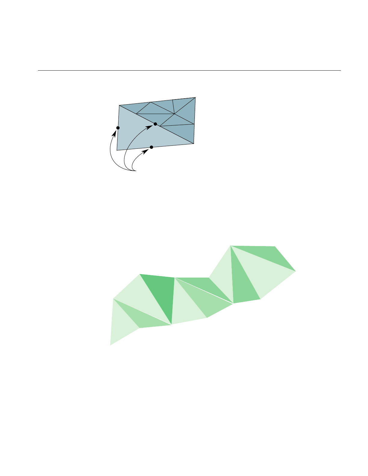
Data Structures
477
Figure 15-10 Discontinuous, Neighboring LODs
Triangle Strips
You can increase the rendering speed of your application by using triangle strips.
Triangle strips are groups of contiguous triangles that together form a strip, as shown in
Figure 15-11.
Figure 15-11 Triangle Mesh
Triangle strips improve rendering performance because, after the first triangle in the
strip, each additional triangle can be added by defining only one additional vertex.
Reference vertices defined
45
67
8
9
10
11
12
13
14

478
Chapter 15: Active Surface Definition
pfASD does not generate triangle strips dynamically. Triangle strips are pre-generated at
modeling time and represented using tsid in the pfASDFace structure. Only triangles
from the same ASD face tree level can be in the same triangle strip. The tsid numbers are
sorted at run-time to connect as many triangles from the same triangle strips together as
possible. Triangles with consecutive tsid values are placed in one triangle strip.
pfASD:
1. Evaluates the LOD structure.
2. Picks the triangles at the desired LODs.
3. Culls the triangles to the visible frustum.
4. Sorts the triangles by their tsid.
5. Generates triangle strips of triangles with consecutive tsid values.
Figure 15-12 shows an example of a set of triangles with consecutive tsid values.
Figure 15-12 Using the tsid Field
pfASD generates a triangle strip from the vertices marked 0, 1, and 2 in the triangle with
tsid=2, followed by the vertex marked 2 in the triangle with tsid=3. The triangle with
tsid=6 marks the beginning of the next triangle strip, vertices marked 0, 1, and 2 in
triangle with tsid=6, followed by vertices marked 2 from triangles with tsid 7, 8, 9, 10, and
11. It is very important to start a triangle strip on an even triangle strip ID. For example,
triangles in the first triangle strip can have IDs 0, 1, 2...; but they can’t have 1, 2, 3,...
Vertices should be listed in pfASDFace in counter clockwise order, with the last vertex to
be the vertex in the triangle strip.
tsid=3
tsid=2
tsid=6
tsid=7
tsid=8
tsid=9
tsid=10
tsid=11
0
0
00
000
0
1
1
111111
2
2
2
2
2
2
2
2
Data Structures
479
At the termination of a triangle strip, there must be a non-consecutive tsid in the next
triangle, as shown in Figure 15-12. Assigning the numbers 3 and 6 forces these triangles
into separate triangle strips. Assigning all triangles to the same tsid would separate all of
them into strips with only one triangle.
Note: pfASD sorts all the visible triangles by tsid.tsid values, therefore, must not overlap
in different areas of the surface. pfASD does not check that triangles with consecutive tsid
values are indeed neighboring.
Vertex and Reference Point Arrays
The vertex and reference point arrays, vert[3] and refvert[3], each contain three
pfASDVert, which are the coordinates of the vertices and reference points. For more
information on pfASDVert, see “Vertex Data Structure” on page 482.
The order of the vertices and the reference points in the arrays must be counter clockwise,
as shown in Figure 15-13.
Figure 15-13 Counter Clockwise Ordering of Vertices and Reference Points in Arrays
Any of the vertices can be the first in the array. The first reference point in the array,
however, must be the one on the side between the first and second vertex points, for
example, the reference point on the hypotenuse of the triangle in Figure 15-13 should not
be entered as the first reference point in the refvert{3] array because the bottom leg of the
triangle contains the first two vertex points entered into the vert[3] array.
If a triangle does not have three reference points, as is the case of the triangle on the left
in Figure 15-5 (where only the hypotenuse has a reference point), enter the token
PFASD_NIL_ID in the refvert{3] array where normally you would enter the indices of the
reference points.
A
0
C
1
B
2

480
Chapter 15: Active Surface Definition
Attributes
Each vertex can have it’s own set of attributes. The attribute format is described in
“Attribute Data Array” on page 480. The arrays, attr[3] and refattr[3], point to three
vertex attribute array entries and three reference point attribute array entries.
If a vertex or reference point is not assigned an attribute, enter the token PFASD_NIL_ID
in the attr[3] or refattr[3] arrays where normally you would enter the pointer to the
attribute array.
Attribute Data Array
Each vertex and reference point can be assigned an attribute. An attribute is an
interleaved list of floats that consists of normal, color, and texture definitions, as follows:
float normal[3];
float normalDif[3];
float Color[4];
float ColorDif[4];
float Tcood [2];
float TcoodDif [2]
If any attribute is not defined, it should not be represented in the array, in which case the
stride is shorter.
Each attribute has two listings: the values of the attributes at the final positions, and how
much they change during morphing. For example, the normal[3] array specifies the
vector that is normal to the vertex at the final position, while the normalDif[3] array
specifies the difference between the normal and its final position and the normal at its
reference point.
Color{4] and ColorDif[4] similarly specify the RGBA values at a vertex, and the color
morphing vector.
The texture coordinates, Tcood [2] and TcoodDif [2], specify the texture coordinates of
vertices at their final position and the texture coordinates of the morphing vector.

Data Structures
481
Setting the Attributes
The attribute array of floats can contain normal, color, and texture coordinate
information, or it can contain any combination of attributes. You specify which of the
attributes are in the attribute array of floats by setting the pfASDAttr() mask. To specify
that you are including some or all of the attribute values in the attribute array, you use
pfASDAttr() with one or more of the following tokens OR’d together:
• PFASD_NORMALS
• PFASD_COLORS
• PFASD_TCOORDS
For example, to specify normal and color attributes only, use the following statement:
pfASDAttr(PFASD_NORMAL | PFASD_COLOR);
If certain attributes are not specified in pfASDAttr, they should not be included in the
attribute array. pfASD only takes one set of per-vertex-per-face attributes and one set of
overall attributes.
Global Attributes
If you want to use the same attribute value for all normals, colors, or texture coordinates,
you can specify a global attribute value rather than making the same entry for each
normal, color, or texture coordinate attribute. To specify a global attribute, use the
following statement:
pfASDAttr(..., PFASD_OVERALL_ATTR, attr);
attr, an array of floats, holds a set of attributes and their morphing vectors. You can mix
a global attribute with a different attribute that is per vector.

482
Chapter 15: Active Surface Definition
Vertex Data Structure
The vertex data structure, defined as follows, holds the coordinate information of
vertices and their vertex vectors.
typedef struct pfASDVert
{
pfVec3 v0, vd;
int neighborid[2];
int vertid;
} pfASDVert;
Each vertex has an ID, vertid, a set of coordinates, vo, and a vertex vector, vd. The vertex
vector is the vector stretching from the final vertex toward the reference point.
In a triangle strip, a line segment is commonly shared by two adjoining triangles, as
shown in Figure 15-14.
Figure 15-14 Vertex Neighborhoods
The new vertex is shared by the adjoining triangles. Those triangles are referred to as the
neighborhoods of the vertex. The neighborhood array contains the triangle IDs of the
adjoining triangles in the previous LOD.
If a side is not shared by two triangles, then one of the neighborhood array values should
be PFASD_NIL_ID.
Neighborhood (0)
Neighborhood (1)

Data Structures
483
Default Evaluation Function
The default evaluation function, which returns a value between 0.0 and 1.0, is based on
the distance between the vertex and the eyepoint: the farther away a vertex is, the lower
its resolution.
To use the default evaluation function, you must fill in the pfASDLODRange structure
for each LOD.
typedef struct pfASDLODRange
{
float switchin;
float morph;
} pfASDLODRange;
LOD[i].switchin is the far edge of the LOD[i]. Take any vertex of a triangle in LOD[i] and
compute the distance between the vertex and eyepoint. If this distance is more than
LOD[i].switchin, the morphing weight of this vertex is 1.0 (NO_MORPH). If it is less, the
morphing weight is calculated against the morphing zone.
LOD[i].morph is the length of the morphing zone from the LOD[i].switchin far edge. The
morph weight is (1-(LOD[i].switchin-dist)/LOD[i].morph). If the distance is less than
LOD[i].switchin - LOD[i].morph, the morph weight is 0.0 (COMPLETE_MORPH).
Overriding the Default Evaluation Function
The evaluation function can be based on many things beside distance. For example, you
might implement the evaluation function based on:
• Line of sight—geometries directly in front of the camera have the highest resolution
while geometries more peripheral have a lower resolution.
• Direction—high resolution LODs appear only in one direction, for example, given
the fuzzy nature of clouds, when a pilot looks straight ahead the clouds do not need
to be rendered with great detail. When the pilot looks down, however, you might
like them to see the terrain in great detail.
• True size of projected triangle—triangles are replaced when they physically reach a
specified size on the projector screen.

484
Chapter 15: Active Surface Definition
• Event driven—an event triggers a change of LODs, for example, when a bomb
explodes.
• Shape—specific shapes in the scene, perhaps a tank, could be rendered in higher
resolution than the surrounding countryside.
None of these evaluation criteria can use the default evaluation function. Instead you
must write your own evaluation function and register it as a callback function with
pfASD using the following method:
extern void pfASDEvalFunc(pfASD* _asd, pfASDEvalFuncType _eval);
The evaluation function you provide, eval, must return a float between 0.0 and 1.0 and
conform to a fixed format. pfASDEvalFuncType takes the argument vertid, which is the
index of the vertex from the next LOD whose reference position is on this edge. Refer to
asdfly/pfuEvalFunc.c for examples.
pfASD Queries
pfASD supplies a query mechanism for two kinds of objects:
• Vertices with a down vector.
A vertex query answers the question: Where does the ray through the vertex in the
given down direction hit the surface?
• Triangles with a projection vector and a down vector.
A triangle query answers the question: Given a triangle, how does it project onto
the current morphing pfASD? Or, given a triangle, supply a list of triangles
describing the projection of this triangle on the surface.
pfASD has a mechanism for manipulating arrays of vertices and triangles, and for
reporting query results of surface geometries. Query results are kept in a pfFlux buffer.
The application may read this buffer directly or connect it to a pfEngine for processing.
These query mechanisms must run in sync with the evaluation function. The query
results must be used in the same frame that the morphing status of a pfASD becomes
active. To synchronize the behavior of pfASD geometry and query points, you need to
set the correct pfFlux flags, as described in “Aligning Light Points Above a pfASD
Surface Example” on page 490.

pfASD Queries
485
Before describing the technical details of setting up a query array, the following section
describes how to use these arrays.
Aligning an Object to the Surface
In the visual simulation arena, you often place objects on surfaces. Since the pfASD
surfaces morph, the objects on top must move to remain on the surface. Some objects
require only position changes. Others require angle changes as well. A building on top
of a mountain side, for example, requires only a position change to match the current
altitude of the surface under it. A car standing on the same mountain side, however,
requires changing both its position and its angle in order to remain aligned to the surface.
In the case of the building, it is enough to query the intersection between a query ray and
the surface. In the case of the car, however, you must also calculate the surface normal at
the intersection point.
Casting a Shadow
We often wish to cast the shadow of objects on the surface underneath them. Since the
pfASD surface is morphing, we must morph the shadows accordingly. Given a triangle
and a projection direction, we want to project the triangle on the surface and tessellate its
projection so that we get a 3D representation of the shadow. We can later use these
shadow triangles as decals to paint the shadow on the surface.
Generating Decals
Many times you wish to draw decals on a surface. In the context of surfaces, you may
wish to add a road as a decal on the morphing surface. To make the road touch the
surface, you must tessellate the polygons of the road so they conform to the shape of the
surface. To tessellate the road, you project a triangle downwards and then tessellate the
result.
Adding a Query Array
To add an array to the pool of queries, you use:
• pfASD::addQueryArray() to add an array of vertices.
• pfASD::addQueryGeoSets() to add an array of triangles.

486
Chapter 15: Active Surface Definition
Both methods require a pfFlux as input. After completing the evaluation of a pfASD
frame, pfASD fills the specified pfFlux objects with query results for all the visible query
arrays. The query results become relevant at the next pfFrame along with the
newly-evaluated pfASD geometry.
To make sure the query results are used only when their corresponding geometry is
active, add the corresponding pfFlux and the pfASD node to the same sync group using
pfASD::setSyncGroup() and pfFlux::setSyncGroup().
Using ASD for Multiple Channels
A channel is a view of a scene. There are three approaches to linking multiple channels:
• Each channel uses the same database, the same viewpoint, the same evaluation
function, and the same LODs, but the viewing angle is different for each channel.
The effect is multiple channels that together create a continuous view, like that of a
horizon. The views of the scenes in each channel move together. For more
information on this approach to multiple channels, see “Controlling Video
Displays” on page 408.
• Each channel uses the same database, a different viewpoint, the same evaluation
function, and potentially different LODs.
The effect is two or more views of the same scene, for example, one view might look
along the terrain, another view might look down at the same terrain from above.
This approach uses the pfASD API for creating multiple channels, as described in
“Connecting Channels” on page 487.
• Each channel uses the same database, a different viewpoint, different evaluation
functions, and potentially different LODs.
The effect is two or more views of potentially unrelated parts of a scene, for
example, if the database is the earth, one view might be of someone traveling
around the north pole, another view might be of someone traveling around the
south pole.
Because the only thing common to the two views is the database, you need to create
two pfASD objects; one to handle each view.
The following section explains how to do the second approach to connecting channels.

Combining pfClipTexture and pfASD
487
Connecting Channels
When you have two channels that share the same database and evaluation function and
differ only in that they have different viewing angles of the same part of a scene, you can
save processing time and save memory by attaching the two channels using
pfChanASDattach();pfChanASDdetach() detaches two channels.
Making the two channels part of the same pfASD, processing time is improved because
only one evaluation function is computed. Having one pfASD instead of two saves
memory because two pfASDs requires maintaining two sets of the same scene.
Combining pfClipTexture and pfASD
A pfClipTexture is able to manage very large bodies of data, presenting only the part that
is in view of the user. pfASD modifies the pfClipTexture such that the different parts of
the pfClipTexture are presented using the correct LOD level.
To use a pfClipTexture as part of a pfASD, use the following procedure:
1. Put the pfClipTexture into a pfGeoState.
2. Set the pfGeoState to a pfASD.
pfASD accepts a list of pfGeoStates.
3. Define the center of the pfClipTexture in one of two ways:
• Attach a pfuClipCenterNode to a pfASD, as shown in the .im loader
Use pfuTexGenClipCenterNode and convert the eyepoint through texgen into
texture space as the clipcenter. This technique should be used when cliptexture
is applied using texgen.
Set the proxy box equal to the rough boundary of the pfASD database. the
boundary of the pfASD can be queried by calling pfGetASDBBox(asd, box).
or
• Use a PRE callback function with pfASD to set the clip center yourself. To see an
example, refer to terrain.c.
4. If the clip texture is virtual, pfASD automatically sorts geometry into concentric
cliprings to support the appropriate cliptexture limit and offset. Set the
environment variable, PFASD_CLIPRINGS, to activate this feature. See libpfdem and
libpfevt for examples.
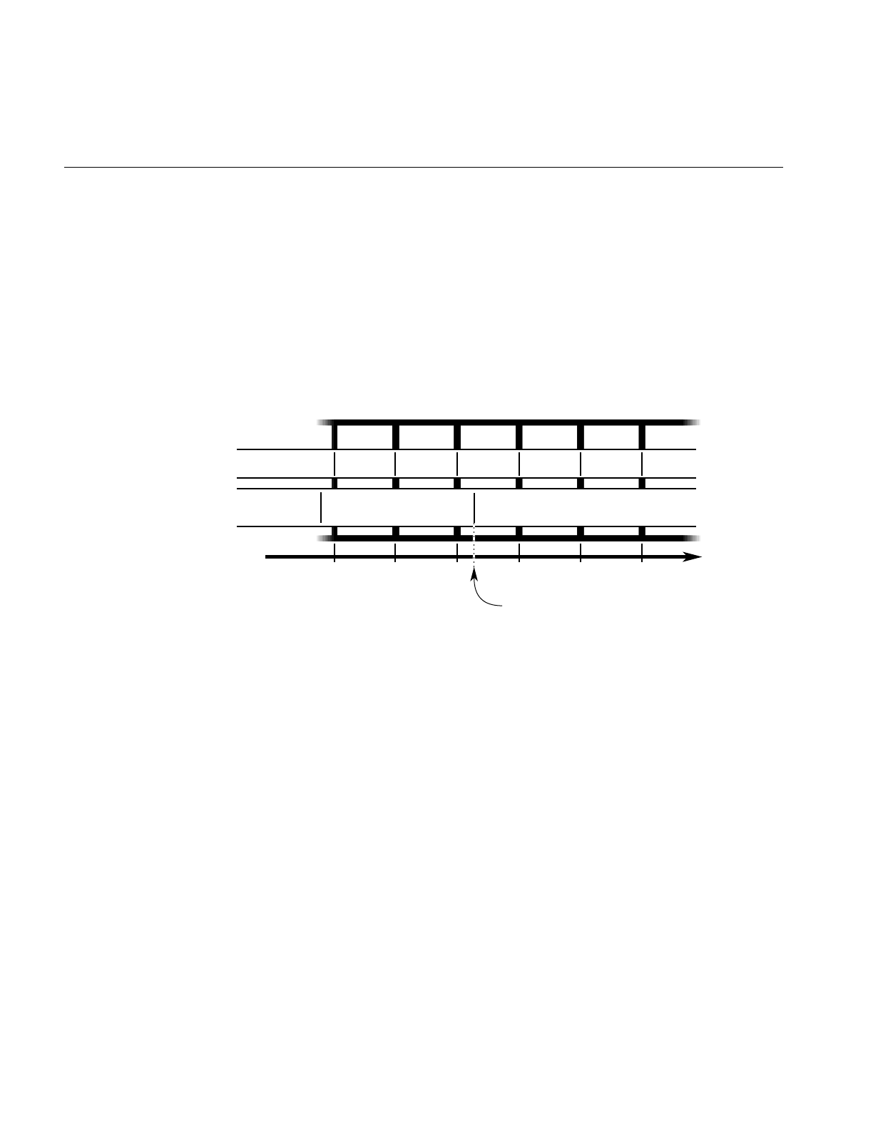
488
Chapter 15: Active Surface Definition
ASD Evaluation Function Timing
The pfASD evaluation function commonly runs as a separate, asynchronous process.
This process does not necessarily finish its evaluation when the App-Cull-Draw frame
finishes. The new pfASD geometry becomes active (visible) at the end of the pfFrame that
follows the completion of the pfASD evaluation.
For example, if Draw frames 0, 1, 2, 3, 4... end at times 100, 200, 300, 400, 500... and the
pfASD evaluation finishes at time 320, the new geometry is introduced into the scene
graph at time 400, as shown in Figure 15-15.
Figure 15-15 pfASD Evaluation Process
In Figure 15-15, it is important to align objects to the old geometry in Draw frame 2, and
align to the new geometry in Draw frame 3.
Query Results
The query results must affect the aligned geometry in the same frame that the pfASD
geometry becomes active. To achieve this, you must connect both the pfASD node and
Matrix-Flux to the same sync group. In this way, when pfASD changes the active surface
geometry, it also activates the newly calculated query results.
ASD
Geometry
ASD
Evaluation
Frame
Time
Draw frame: 0
100 200 300 400 500 600
12345
asd0 asd0 asd0 asd1 asd1
01 2
The pfASD evaluation process
completes at time 320 but the
new pfASD geometry enters
the scene graph at time 400
ASD Evaluation Function Timing
489
In general, you should move as much processing to the pfASD process as possible. In
Figure 15-15, all the query/alignment operations take place in the pfASD process. Since
the entire evaluation is triggered by the query array writing to Result-Flux, the
generation of the new pfFCS matrix in Matrix-Flux also takes place in the pfASD process.
The only change to the time critical APP-CULL-DRAW sequence is a single
pfFlux::getCurData() to get the updated pfFCS matrix.
Aligning a Geometry With a pfASD Surface Example
To align some geometry to a pfASD surface using query points, use the following
procedure:
1. Pick an anchor point where you want the target geometry to go.
2. Generate a query array containing the anchor point and add it to pfASD.
3. Request pfASD to store the query results in the pfFlux marked Result-Flux.
4. Generate an additional pfFlux and connect it to the pfFCS node matrix controlling
the target geometry.
Figure 15-16 diagrams this procedure.
Figure 15-16 Example Setup for Geometry Alignment
pfASD
SyncGroup=1
Query
arrays
Result Flux
(PUSH)
pfEngine
(ALIGN)
pfFCS
Matrix
Geode
Target
geometry
Matrix Flux
SyncGroup=1
getWritable
getCurData

490
Chapter 15: Active Surface Definition
At run-time:
1. pfASD starts its frame by evaluating the ASD surface and generating optimized
geometry for it.
2. pfASD calculates the query array values.
3. pfASD writes the results into the pfFlux marked Result Flux.
4. The write operation triggers a calculation of the pfEngine because the Result-Flux is
a PUSH flux.
5. The pfEngine generates a transformation matrix and stores it in the pfFlux marked
Matrix Flux.
6. The pfFCS node controlling the transformation of the target geometry has a fluxed
matrix.
7. When the pfFCS node is traversed, it retrieves the newly-generated matrix from
Matrix-flux and uses it to align its child geometry.
Note: If you run the pfASD evaluation function in a separate process, the evaluation of
the query arrays may happen asynchronously at some point during the IRIS Performer
frame.
Aligning Light Points Above a pfASD Surface Example
The following example, diagramed in demonstrate how to link pfASD queries to a
pfEngine. For a GeoSet containing light point primitives, this code places all the
primitives at some offset above the surface.
Figure 15-17 Aligning Light Points Above a pfASD Surface
get
attr_flux asd
offset_array
result_flux
pfEngine
(ALIGN)

ASD Evaluation Function Timing
491
Example 15-1 Aligning Light Points Above a pfASD Surface
// Generate a flux for pfASD to store the query results.
results_flux = pfNewFlux(nofLightPoints *
sizeof(pfVec3),PFFLUX_DEFAULT_NUM_BUFFERS, pfGetSharedArena());
// Make so that writing into this flux will trigger evaluation of
// connected engines.
pfFluxMode(results_flux, PFFLUX_PUSH, PF_ON);
// Generate final flux - this flux will contain the final aligned
// light points.
attr_flux = pfNewFlux(nofLightPoints * 3 * sizeof(float),
PFFLUX_DEFAULT_NUM_BUFFERS, pfGetSharedArena());
// Add flux to the same syncGroup as its aligning pfASD.
pfFluxSyncGroup(attr_flux, 1);
// Initalize the flux to the unaligned point positions.
// The engine will only modify a portion of the buffer (the Z
// values), so we must initialize the (X,Y) values now.
// Assume vertexList contains the original vertices.
FluxInitData(attr_flux, vertexList);
// Add the array of positions to pfASD. Request position-only
// queries.
query_id = pfASDAddQueryArray(asd_hook, vertexList, down,
nofLightPoints, PR_QUERY_POSITION, results_flux);
// Get maximum bounding box of the vertex array - this box
// contains all possible positions of the query array points.
pfASDGetQueryArrayPositionSpan(asd, query_id, &box);
// Generate a SUM engine to sum the query vertex results with a
// constant array.
sum_engine = pfNewEngine(PFENG_SUM, pfGetSharedArena());
pfEngineIterations(sum_engine, nofLightPoints, 1);
// Inform pfEngine of its two sources and one destination.
// offset_array should contain a constant offset for each light
// point. We request sum_engine to modify the Z coordinate of
// each light point vertex.
pfEngineSrc(sum_engine, PFENG_SUM_SRC(0), offset_array, NULL,
0, PF_Z, 3);
pfEngineSrc(sum_engine, PFENG_SUM_SRC(1), results, NULL,

492
Chapter 15: Active Surface Definition
0, PF_Z, 3);
pfEngineDst(sum_engine, attr_flux, NULL, PF_Z, 3);
// Generate GeoSet to hold the final aligned geometry.
gset = pfNewGSet(pfGetSharedArena());
// standard pfGeoSet initialization code
// (GeoState, color, NumPrims, etc) omitted.
pfGSetPrimType(gset, PFGS_POINTS);
// Add flux_attr as the COORD3 attribute of the geoset.
pfGSetAttr(gset, PFGS_COORD3, PFGS_PER_VERTEX,
(void *) attr_flux, NULL);
// Set the GeoSet bounding box staticly. This will help avoiding
// recalculation or mis-calculation of bounding boxes for culling.
pfGSetBBox(gset, &box, PFBOUND_STATIC);
// Setup range based evaluation. assume ‘center’ contains the
// center of box.
pfEngineEvaluationRange(sum_engine, center, 0.0, 40000.0);
pfEngineMode(sum_engine, PFENG_RANGE_CHECK, PF_ON);
Paging
Large scale surface simulations require large amounts memory to store high resolution
surfaces. For example, the earth sampled from a height of 100m requires tens of gigabytes
of disk space. Such large amounts of memory cannot reside entirely in system memory.
Consequently, efficient database paging is essential in supporting a 30 Hz frame rate.
A common paging method is to page in tiles. Each area block contains all the LOD
information describing an area. The problem with this method of paging is that in a
surface that extends far into the distance, the large number of tiles visible to the viewer
consumes more memory than is available on a system.
The hierarchical structure of ASD provides a different paging method: LOD paging. Each
LOD is divided into a set of blocks; each block representing an area of the scene at a
particular resolution. These tiles are paged in independently. All tiles for a single LOD
are the same size; tiles for different LODs, however, can be different sizes.
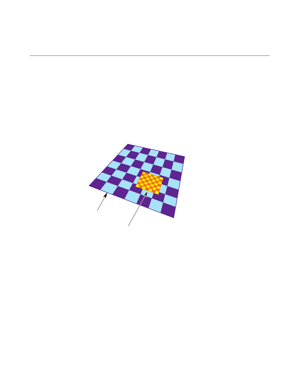
Paging
493
Interest Area
In one LOD, the blocks most likely accessed, according to the view and position of the
viewer, are called the interest area of the LOD. It is these blocks that get paged in.
The interest area for an LOD whose resolution is based on range is bounded by the
maximum range value for that LOD. The interest area is smaller for higher resolution
LODs, larger for lower resolutions LODs. As a result, the memory requirements of ASD
are reduced because not all LODs in an area are paged in: triangles closer to the viewer
are paged in at a higher resolution LOD that those triangles further from the viewer, as
shown in Figure 15-18.
Figure 15-18 Tiles at Different LODs
Each square in Figure 15-18 holds the same amount of information: the large pages hold
a large amount of low-resolution information while the small pages hold a small amount
of high-resolution information.
If the observer does not make discontinuous jumps in location between 2 frames, you use
an algorithm that anticipates what the viewer needs to see next based on the evaluation
function. For example, if the evaluation function is based on distance, you would page
blocks into memory in the direction you expect the viewer to go and release from
memory those pages the viewer is leaving.
Paging area
Interest area

494
Chapter 15: Active Surface Definition
Preprocessing for Paging
Preprocessing pages improves performance.
1. Determine the appropriate tiles size for each LOD based on the evaluation function.
2. Assign triangles in each LOD into tiles and store each tile in a paging unit, such as a
file.
Assign a triangle to one tile only. Triangles with the same parent node must be
assigned to the same tile.
3. Generate a set of fast-paging files for a specific set of paging areas.
When the application is run, it should anticipate the pages the viewer will need and then
page them into memory from disk and preprocess them.
Order of Paging
Paging in lower LOD pages before higher LOD pages ensures that a page at some level
of LOD is always ready for the viewer. When you travel so fast through a surface that the
higher resolution LODs do not have time to load, the surface has a lower resolution,
which is what you would expect to see when traveling fast.
Multi-resolution Paging
pfASD supports multi-resolution paging. The format of a paging file, where all of the
geometries are in one tile, is described by the following structure:
int numfaces
int numverts
/* numfaces of the following */
int faceid1
/* structure of the face faceid1 */
pfASDFace face
/* structure of the face faceid2 */
int faceid2
pfASDFace face
...
/* numfaces of the following */
/* face bounding box of faceid */
pfBox box1
/* face bounding box of faceid2 */

Paging
495
pfBox box2
...
/* numverts of the following */
int vertid1
/* structure of vertex vertid1 */
pfASDVert vert
int vertid2
/* structure of vertex vertid2 */
pfASDVert vert
...
To calculate the paging area, use the following code:
page[0] = (int)(lods[i].switchin/tilesize[0]) + lookahead[0];
page[1] = (int)(lods[i].switchin/tilesize[1]) + lookahead[1];
lods[i] is the pfASDLODRange of LOD[i].tilesize is the size of the tile in LOD[i].lookahead
is the number of extra tiles in one direction to page in to memory to overcome a paging
delay
To process the paging tiles into a fast paging format, use pfdProcessASDTiles() in
pfdProcASD.c.pfdProcessASDTiles() returns a new set of files as xxxx.asd. These files are
paged in real-time.
For an example of writing a file, see pfdWriteFile() in libpfdu/pfdBuildASD.c.


This chapter describes light points and calligraphic lights, which are intensely
bright light points.
“Light Points”
Chapter 16


499
Chapter 16
16. Light Points
IRIS Performer provides sophisticated light point objects:
• pfLPointState lights are emissive objects that do not illuminate their surroundings,
such as stars, beacons, strobes, runway edge, and taxiway lights.
• pfCalligraphic light points are pfLPointState light objects with calligraphic
extensions; they are intensely-bright light points that require special display
equipment.
Uses of Light Points
Light points are bright points of light that have the following characteristics:
• Intensity
• Directionality
• Attenuation Shape
• Distance computation
• Attenuation through fog
• Size and fading
These attributes make light points excellent for use as stars, beacons, strobes, runway
edge and end illumination, and taxiway lights.
For example, three light points with specific directionality may be used to create a VASI
light system at an airport that appears:
• Red when the pilot is above the landing glide path.
• Green when the pilot is below the landing glide path.
• White when the pilot is on the landing glide path, as shown in Figure 16-1.

500
Chapter 16: Light Points
Figure 16-1 VASI Landing Light
Creating a Light Point
To create a light point:
1. Create a pfGeoSet of points (PFGS_POINTS).
pfGeoSet *lpoint = pfNewGSet(arena);
pfGSetPrimType(lpoint, PFGS_POINTS);
2. Create a pfLPointState and define its mode and values.
pfLPState *lpstate = pfNewLPState(arena);
pfLPStateMode(lpstate, PFLPS_SIZE_MODE, PFLPS_SIZE_MODE_ON);
pfLPStateVal(lpstate, PFLPS_SIZE_MIN_PIXEL, 0.25f);
pfLPStateVal(lpstate, PFLPS_SIZE_ACTUAL, 0.07f);
pfLPStateVal(lpstate, PFLPS_SIZE_MAX_PIXEL, 4.0f);
3. Attach the pfLPointState to the pfGeoState associated with the pfGeoSet.
pfGStateMode( gstate, PFSTATE_ENLPOINTSTATE, PF_ON);
pfGStateAttr( gstate, PFSTATE_LPOINTSTATE, lpstate);
pfGSetGState( gset, gstate ) ;
This pfGeoSet must have a PFGS_COLOR4 attribute binding of
PFGS_PER_VERTEX.
VASI
Red
White
Green

Setting the Behavior of Light Points
501
Setting the Behavior of Light Points
The pfLPointState attached to a pfGeoSet controls the behavior of all light points in the
pfGeoSet. For example, the color, position, and direction vector of each light point is set
by the color, vertex, and normal stored in the pfGeoSet.
You use pfLPStateMode, to enable or disable the behaviour, and pfLPStateVal to set the
following pfLPointState values:
• Intensity—setting the intensity of light from no attenuation, 1, to fully attenuated, 0.
• Directionality—specifying the direction and the shape of the emanation of light.
The shapes are either a single or a pair of opposite-facing elliptical cones.
pfLPStateShape() specifies the shape of the emanation.
• Fading—specifying how the light point fades when receding into the distance.
Fading is often more realistic than simply shrinking the point size to 0.
• Fog punch-through—specifying how a light point is obscured by fog.
• Size—setting the maximum and minimum size of the light point based on
perspective.
The following sections describe how to set these values.
Intensity
The intensity of the light points in a pfLPointState can be attenuated using
pfLPStateVal(), as follows:
pfLPStateVal(lpstate, PFLPS_INTENSITY, intensity)
The intensity value, intensity, must range between zero and one; one, no attenuation, is
the default.
The intensity of each light point is defined by its four component colors.
Directionality
Each light point has a normal, which defines the direction of its emanation. By default,
all of the light points in a pfLPointState point in the same direction. That direction is
defined as the “front” of the light point.

502
Chapter 16: Light Points
If all light points in a pfGeoSet share the same normal, use the PFGS_OVERALL attribute
to optimize the light point computation.
If the light points are directional, the pfGeoSet attributes must specify normals.
Enabling Directionality
To enable or disable light point directionality, use the following method:
pfLPStateMode(lpstate, PFLPS_DIR_MODE, mode);
The mode value can be:
• PFLPS_DIR_MODE_ON, the default, turns on directionality computation.
• PFLPS_FOG_MODE_OFF, disables directionality computation.
To specify whether or not the light point emanates towards the front and back, use the
following method:
pfLPStateMode(PFLPS_SHAPE_MODE, mode);
The mode value can be:
• PFLPS_SHAPE_MODE_UNI, the default, makes the light point is not visible from
the back side.
• PFLPS_SHAPE_MODE_BI, makes the light point bidirectional, the behavior is the
same for both sides.
• PFLPS_SHAPE_MODE_BI_COLOR, makes the light point bidirectional, but if seen
from the back side, the light change its color. This color is set using
pfLPStateBackColor().
Emanation Shape
The emanation shape is an elliptical cone, as shown in Figure 16-2.
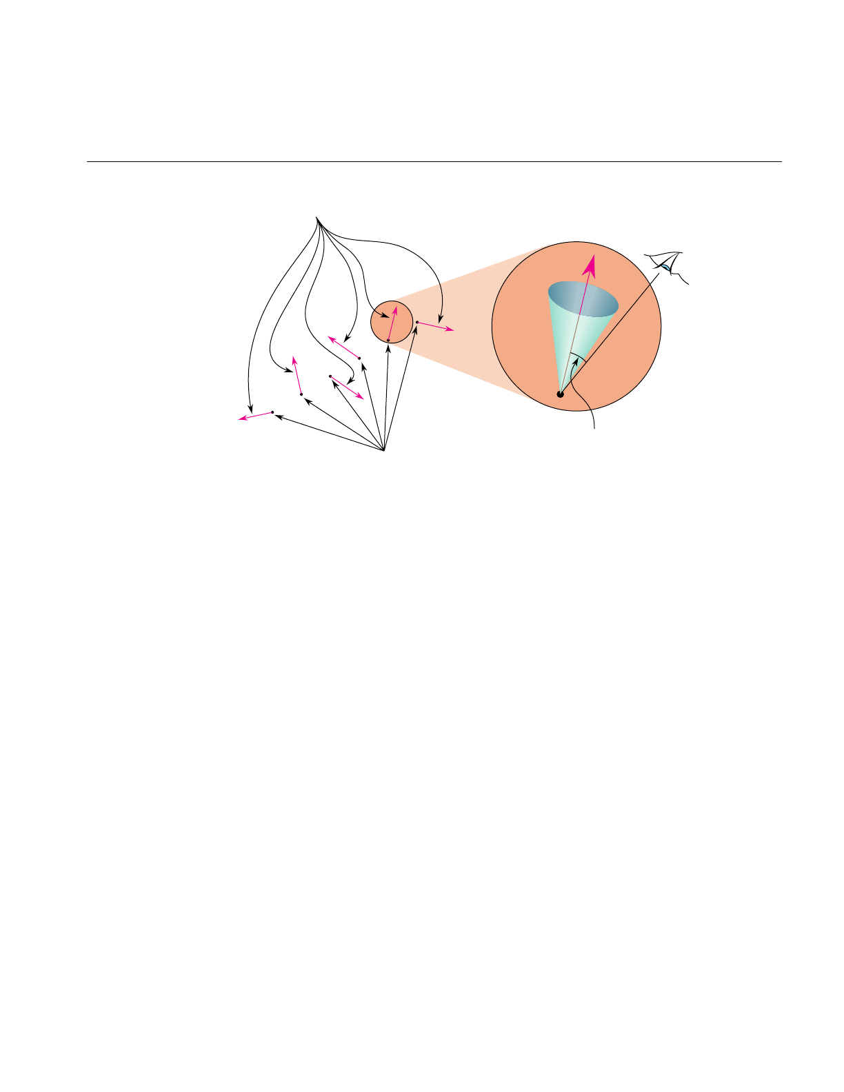
Setting the Behavior of Light Points
503
Figure 16-2 Attenuation Shape
Optionally, the intensity of light can fall off from the normal to the edge of the cone.
The direction of emanation is defined along the Y axis and the shape is defined in the
local coordinate system. The coordinate system is rotated so that the Y axis aligns with
the normal of each light point.
To specify the shape of emanation, use the following method:
pfLPStateShape(lpstate, horiz, vert, roll, falloff, ambient)
Shape
horiz and vert are total-angles (not angles to the normal) in degrees, which specify the
horizontal and vertical dimensions of the cone about the normal. The maximum value
for these angles is 180 degrees, which creates a non-directional light point. The default
values for horiz and vert is 90 degrees.
Tip: A symmetric cone (where horiz and vert are equal) is faster to compute than an
asymmetric cone.
Light points
Normals
Eye point angle
Eye point
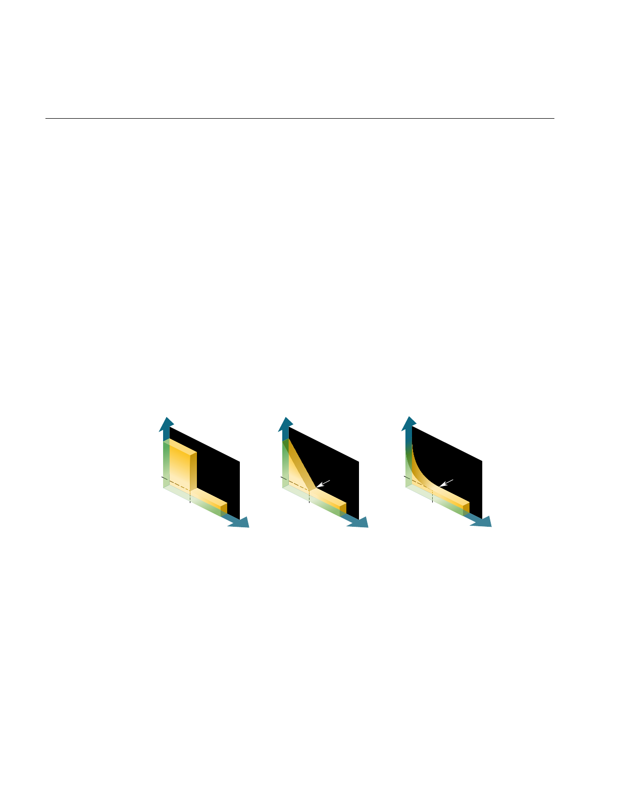
504
Chapter 16: Light Points
Rotation
The cone is rotated by roll degrees through +Y. The default roll value is 0.
Falloff
When the vector from the light’s position to the eye point is outside the cone, the light
point’s intensity is ambient. The default ambient value is 0.
If the vector from the light’s position to the eye point is within the cone, the intensity of
the light point is based on the angle between the normal and that vector. The intensity
values range from 1.0, when the eye point lies on the normal, to ambient, at the edge of
the cone. How the light attenuates between the normal and the edge of the cone is
specified by falloff.
falloff is an exponent that modifies the light point’s intensity. A value of 0 indicates that
there is no falloff; a value of 1, the default, indicates a linear falloff; values greater than 1
indicate a progressively greater geometric falloff, as shown in Figure 16-3.
Figure 16-3 Attenuation of Light
Ambient
Angle deviation
from normal
Light
intensity
falloff = 0
Ambient
Angle deviation
from normal
Light
intensity
falloff = 1
Edge of
cone
Ambient
Angle deviatio
n
from normal
Light
intensity
falloff > 1
Edge of
cone

Setting the Behavior of Light Points
505
Distance
The distance between the light point and the eye point is used when computing the light
point’s size and intensity through fog. Since these calculations are intensive, IRIS
Performer provides an approximation for the distance between the light point and the
eye point using the following method:
pfLPState(lpstate, PFLPS_RANGE_MODE, mode)
The mode value can be:
• PFLPS_RANGE_MODE_TRUE, approximates the distance using the depth (Z)
difference between the eye and the light point.
• PFLPS_RANGE_MODE_DEPTH, the default, uses the real distance between the
eye and the light point.
Tip: The wider the field of vision (FOV), the less accurate is the approximation.
Attenuation through Fog
Light points are visible at greater distance than non-emissive polygons. For that reason,
the light points appear to punch-through fog. To account for this higher visibility, you
can supply a punch-through value in the following method:
pfLPStateVal(PFLPS_FOG_SCALE, punch-through);
punch-through is a float that is multiplied times the distance. When punch-through is less
than 1.0, the product of the distance and the punch-through value is less than the distance.
The revised distance is used in calculating the apparent brightness of the light point;
when the punch-throughis less than 1.0, the light point appears brighter than it otherwise
would. The default punch-through value is 0.25.
Enabling Punch-Through
To use punch-through, you must first enable it using the following method:
pfLPStateMode(lpstate, PFLPS_FOG_MODE, mode);

506
Chapter 16: Light Points
The mode value can be:
• PFLPS_FOG_MODE_ON, the default, enables fog punch-through computation.
• PFLPS_FOG_MODE_OFF, does not modify the distance before fog is applied.
Size
Light points can exhibit perspective behavior. The following method sets the size of all
the light points in a pfGeoSet:
pfLPStateVal(lpstate,PFLPS_SIZE_ACTUAL, real-size);
real-size is a float that is multiplied times the distance. When real-size is less than 1.0, the
product of the distance and the real-size value is less than the distance. The revised
distance is used in calculating the apparent size of the light point; when the real-size is
less than 1.0, the light point appears larger than it otherwise would. The default real-size
value is 0.25.
Size Limitations
The apparent size of a light point can only range between the minimum and maximum
sizes specified by the following lines of code:
pfLPStateVal(lpstate,PFLPS_SIZE_MIN_PIXEL, min-size);
pfLPStateVal(lpstate,PFLPS_SIZE_MAX_PIXEL, max-size);
Limiting Size Calculations
To optimize rendering, you can avoid changing the size (glPointSize) of each light point
when the difference between the new and old sizes is less than a specified amount, called
the threshold. To set the threshold value, use the following method:
pfLPStateVal(lpstate, PFLPS_SIZE_DIFF_THRESH, threshold);
Enabling Perspective
To use real-size, you must first enable it using the following method:
pfLPStateMode(lpstate, PFLPS_SIZE_MODE, mode);

Setting the Behavior of Light Points
507
The mode value can be:
• PFLPS_SIZE_MODE_ON, makes real-size follow perspective, so that light points
closer to the eye are rendered larger than those points farther away.
• PFLPS_SIZE_MODE_OFF, the default value, disables perspective computations.
If perspective is not enabled, pfGeoSet (pfGSetPntSize) specifies the size of the
rendered light points.
Fading
You can enhance the illusion of perspective by making the light point become more and
more transparent as it receded from view using the following method:
pfLPStateVal(lpstate,PFLPS_TRANSP_PIXEL_SIZE, transp-size);
transp-size is a light point size. When the actual size is smaller than transp-size, the light
point becomes transparent.
Using fading to simulate perspective is often more realistic than shrinking the light point
size; fading avoids the aliasing problems that occur when light points become too small.
Fading Calculation
Fading is calculated as follows:
Max(
clamp
, 1-
scale
*(
transp-size
-
computed-size
)^
exp
)
You set the values in this argument in the following lines of code:
pfLPStateVal(lpstate, PFLPS_TRANSP_EXPONENT, exp);
pfLPStateVal(lpstate, PFLPS_TRANSP_SCALE, scale);
pfLPStateVal(lpstate, PFLPS_TRANSP_CLAMP, clamp)
;
Enabling Fading
To use fading, you must first enable it using the following method:
pfLPStateMode(lpstate, PFLPS_TRANSP_MODE, mode)

508
Chapter 16: Light Points
The mode value can be:
• PFLPS_TRANSP_MODE_ON, enables fading when the computed size is less than
transp-size
• PFLPS_TRANSP_MODE_OFF, the default, disables fading.
Callbacks
For each light point, two parameters are computed based on the location of the eye point,
the location of the light point, and the fog:
• Alpha—specifies the intensity and transparency of a light point. Non-transparent
light points have the maximum intensity given by their four color components.
• Size—specifies the diameter of each light point if the perspective mode,
PFLPS_SIZE_MODE, is enabled; otherwise, the size is constant for all of the light
points in a pfGeoSet.
Instead of accepting the calculations done by IRIS Performer, you can use callback
functions to supply your own calculations. Callback functions can be completed:
• Before IRIS Performer calculates the parameters, thus replacing the Performer
calculation completely.
• After IRIS Performer calculates the parameters, thus modifying Performer’s result.
You enable, disable, and specify the kind of callback used in the following method:
pfLPStateMode(lpstate, PFLPS_CALLBACK_MODE, mode)
The mode value can be:
• PFLPS_CALLBACK_MODE_OFF, the default, means that no callback is attached to
lpstate
• PFLPS_CALLBACK_MODE_PRE, means that the callback is executed before IRIS
Performer has calculated the parameters. Your callback function must compute the
size and alpha values for all the light points in the pfGeoSet.
• PFLPS_CALLBACK_MODE_POST, means that the callback is executed after IRIS
Performer’s computation.

Callbacks
509
To install a callback on a pfLPointState use the following method:
pfRasterFunc(lpstate, (void *) yourCallback(pfRasterData*),
void **userData);
userdata is a pointer to the following structure, which is given to your callback and the
function itself:
typedef struct {
pfLPointState *lpstate; /* Read Only LPState */
pfGeoSet *geoset; /* Read Only GeoSet */
void *userData; /* Provided when setting the callback */
float *sizes; /* Write Only - resulting sizes */
float *alphas; /* Write Only - resulting alphas */
} pfRasterData;
geoset is the currently-preprocessed pfGeoSet. lpstate is the pfLPointState applied to that
pfGeoSet. userData is the same data provided when declaring the callback.
sizes and alphas are pre-allocated arrays that contain the callback function results used by
the DRAW process. If you use a pre-callback, you must provide a size and an alpha value
for every light point in the pfGeoSet. A negative alpha value indicates that the backcolor
must be used in place of the light point color.
Example 16-1 provides the skeleton of a raster callback. A more detailed example is on
the pfLPointState man page.
Example 16-1 Raster Callback Skeleton
void myCallback(pfRasterData *rasterData)
{
pfVec3* vertices;
unsigned short *vindex;
pfVec3* norms;
unsigned short *nindex;
int nbind;
pfFog *fog;
int fogEnabled = 0;
int i,n;
int sizeMode;
pfMatrix ViewMat, InvModelView;
/* get pointers to the geoset */
pfGetGSetAttrLists(rasterData->gset,PFGS_COORD3, &vertices, &vindex);
pfGetGSetAttrLists(rasterData->gset,PFGS_NORMAL3, &norms, &nindex);

510
Chapter 16: Light Points
nbind = pfGetGSetAttrBind(rasterData->gset,PFGS_NORMAL3);
/* get matrices */
pfGetViewMat(ViewMat);
pfGetInvModelMat(InvModelMat);
/* get the number of lights */
n = pfGetGSetNumPrims(rasterData->gset);
/* see if there’s fog */
fog = pfGetCurFog();
if (pfGetEnable(PFEN_FOG) && fog)
fogEnabled = 1;
/* get information on the lpstate */
sizeMode = pfGetLPStateMode(rasterData->lpstate,PFLPS_SIZE_MODE);
........
........
/* do the computation */
for (i=0; i<n; i++)
{
/* get the normal */
if (vindex)
{
if (nbind & PFGS_OVERALL)
nj=nindex[0];
else if (nbind)
nj=nindex[i];
else
nj=-1; /* this geoset has no normals */
........
rasterData->alphas[i] = ....
rasterData->sizes[i] = ....
}
Multisample, Size, and Alpha
On Infinite Reality, light points of a given size, up to 100 multisamples, have the same
number of multisamples, even when the light points cross multiple pixels.
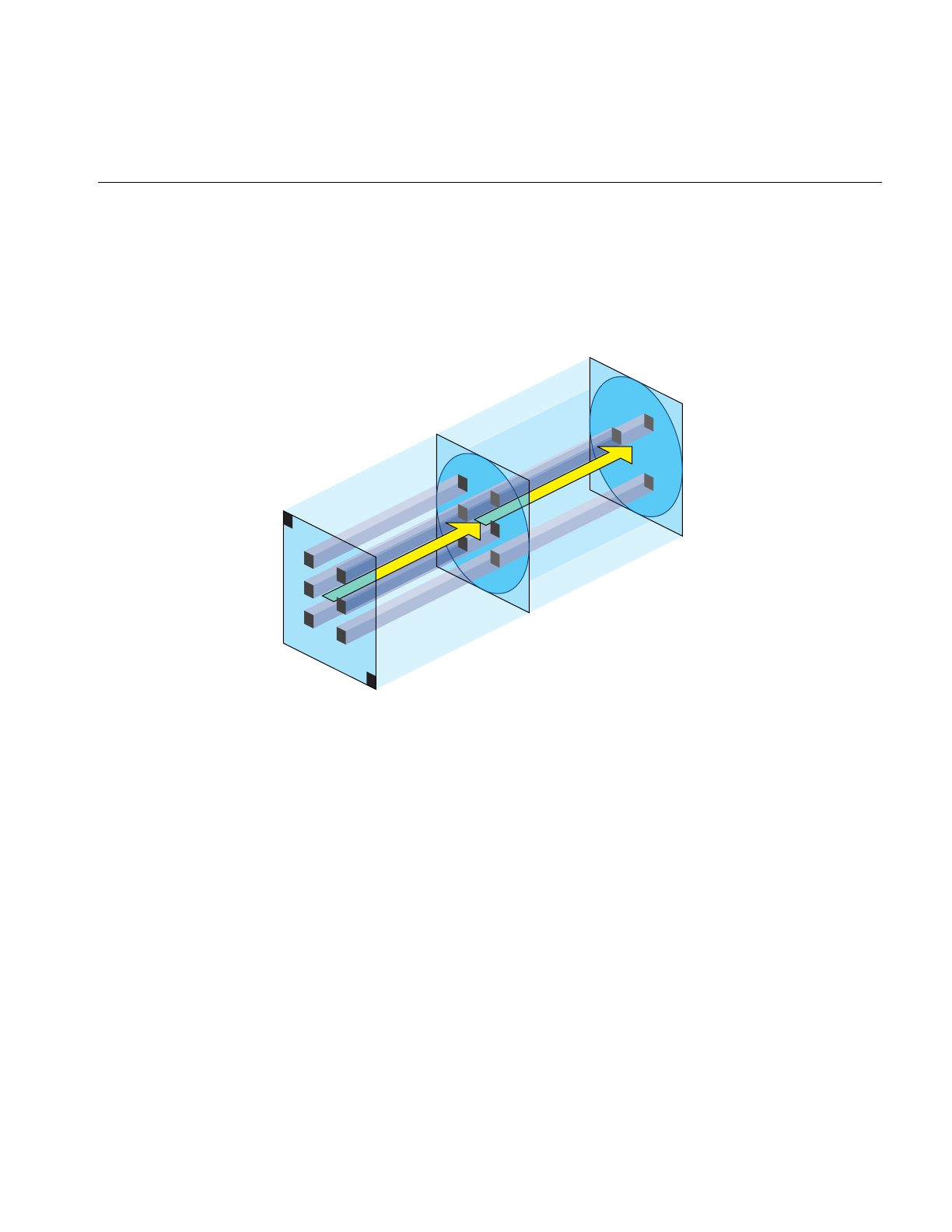
Callbacks
511
The intensity of a light point is defined by its alpha value. If pfTransparency is set to
PFTR_MS_ALPHA_MASK, the alpha value modifies the number of multisamples lit in
a light point. For example, if alpha= 0.5, size = 1.0, and the number of multisamples per
pixel is 8, the number of illuminated multisamples per the light point is 3.0, as shown in
Figure 16-4.
Figure 16-4 Lit Multisamples
The area of a circle with diameter 1.0 is 0.785. The number of multisamples per pixel is
given in the frame buffer configuration. If there are 8 multisamples, only 0.785 of them,
about 6, are in the light point. Since alpha = 0.5, only half of the 6 multisamples are
actually lit.
pfCalligMultisample() tells pfCalligraphic how many multisamples are used in the
specified video channel. pfGetCalligMultisample() returns the current setting. Make
this call as soon as the information is known or changed.
8 multisamples
per pixel
Light point with
diameter = 1.0
Alpha = 0.5

512
Chapter 16: Light Points
Minimum Number of Multisamples
If your light points move, you must have at least two multisamples lit per light point; if
you only have one, the light point is either on or off. This condition creates flicker. With
two multisamples, the light point can transition to a different location with one
multisample on and the other off.
Reducing CPU Processing Using Textures
Light point computations are expensive. You can replace some of the computation by
using a table lookup mechanism and the texture hardware to get an alpha value for each
light point. This mechanism uses a precomputed texture and glTexGen to approximate:
• Fog attenuation.
• Fading over distance.
• Falloff attenuation when the eye point is not on the normal.
Because only one texture per polygon is supported by the hardware, it is not possible to
approximate all three computations at once. The fading and the fog are combined in one
texture, however, so it is possible to select both at the same time.
The following methods specify the attenuations:
pfLPStateMode(lpstate, PFLPS_DIR_MODE, PFLPS_DIR_MODE_XXX)
pfLPStateMode(lpstate,PFLPS_TRANSP_MODE, PFLPS_TRANSP_MODE_XXX)
pfLPStateMode(lpstate, PFLPS_FOG_MODE, PFLPS_MODE_XXX)
XXX is either:
• TEX, for texture lookup.
• ALPHA, for CPU computation.
Default values are equivalent to APLHA computation.
Tip: Falloff is the most expensive effect to compute on the CPU. For that reason, it is
better to use PFLPS_DIR_MODE_TEX if the point is not omnidirectional.
Only use textures for low quality light points; textures are approximations with
numerous limitations, including incorrect falloff attenuation if the emanation is not
symmetric, and incompatibility with callbacks.

Preprocessing Light Points
513
Preprocessing Light Points
To optimize your application, you should fork off a light point process to preprocesses
your light point computations. The light point process runs in parallel with the DRAW
process but on a different CPU. Preprocessing the light points:
• Computes the size and alpha of each light point and passes the result directly to the
DRAW process.
• Executes callbacks attached to the pfLPointState.
To fork off a light point process, use the PFMP_FORK_LPOINT token in
pfMultiprocess() and call it before pfConfig().
Note: You can start a light point process in perfly using the -m option and adding 16 to
your preferred multiprocess model.
Stage Configuration Callbacks
As with any other IRIS Performer process, callback functions can configure the process
stages using:
pfStageConfigFunc(-1, PFPROC_LPOINT, ConfigLPoint);
pfConfigStage(-1, PFPROC_LPOINT | PFPROC_XXX ....);
pfChanTravFunc(chan, PFTRAV_LPOINT, LpointFunc);
pfStageConfigFunc() specifies a callback function, and pfConfigStage() triggers it at the
start of the current application frame; both are methods in pfConfig. Configuration
callbacks are typically used for process initialization, for example:
• Assigning non-degrading priorities and locking processes to CPUs.
• Downloading textures in the DRAW stage callback.
pfStageConfigFunc() identifies the IRIS Performer stages, such as PFPROC_ISECT,
PFPROC_APP, and PFPROC_DBASE, to configure.
pfChanTravFunc
The pfChannel method, pfChanTravFunc(), sets a callback function for either the APP,
CULL, DRAW, or Light Point process using one of the following tokens: PFTRAV_APP,
PFTRAV_CULL, PFTRAV_DRAW or PFTRAV_LPOINT, respectively.

514
Chapter 16: Light Points
User-data that is passed to these functions by pfChanData() is allocated on a per-channel
basis by pfAllocChanData().
How the Light Point Process Works
This section explains how the light point process works. All the functions exist in the API,
however, all of the processing is done automatically by IRIS Performer.
Note: Light point processing is not done automatically if your application is only using
the libpr process model.
If the light point process is enabled, a special bin, PFSORT_LPSTATE_BIN, is created to
sort all of the pfGeoSets that have a pfLPointState attached to their pfGeoState. This bin
is directly used as a display list, LPointBinDL, as shown in Example 16-2.
All bins, except PFSORT_LPSTATE_BIN, are handed to the DRAW process. The DRAW
process, after rendering everything in the other bins, renders a ring display list, called
DrawRingDL, as shown in Example 16-2. The ring display list contains a synchronization
mechanism: the DRAW process waits until it sees the PFDL_END_OF_FRAME token.
Example 16-2 Preprocessing a Display List - Light Point Process code
/* open the draw ring display list */
pfOpenDList(DrawRingDL);
/* preprocess the light points bin. */
/* so the results go in the DrawRingFL */
pfPreprocessDList(LPointBinDL,PFDL_PREPROCESS_LPSTATE);
/* Signal the end of the list to the Draw process */
pfAddDListCmd(PFDL_END_OF_FRAME);
/* close the draw display list */
pfCloseDList(DrawRingDL);

Calligraphic Light Points
515
Calligraphic Light Points
Calligraphic light points are very bright lights that can be displayed only on
specially-equipped display systems. Displaying calligraphic light points requires
• A calligraphic light point board (LPB) with a special device driver. The driver is not
part of the IRIS Performer distribution.
• A calligraphic display system.
• Special cables running between the graphics pipe video synchronization and the
raster manager (RM) boards on the LPB.
• A platform, such as an InifiniteReality, OnyxIR, or Onyx2, that has a visibility (VISI)
bus.
Note: If you are not running on a system that has a VISI bus, or you do not have this
optional hardware, you are limited to raster light points, as supported by pfLPointState.
The functionality described in the remainder of this chapter is not available on your
system. Nevertheless, a program and database designed for calligraphic light points can
be simulated on a non-calligraphic system.
Unlike raster displays, calligraphic displays direct the display system’s electron beam at
specified places on the screen. By directing the beam at specified places for specified
durations, it is possible to produce extremely bright light sources.
Warning: It is possible to destroy your display system by allowing the electron
beam to remain too long on the same screen location either by allotting too long a time
or by an application hanging. Extreme caution is required.

516
Chapter 16: Light Points
Calligraphic Versus Raster Displays
Table 16-1 summarizes the differences between raster and calligraphic displays.
Whenever the calligraphic mode renders a black pixel to the screen, it is completely
transparent and the raster image shows through.
Table 16-1 Raster Versus Calligraphic Displays
Raster Calligraphic
Requires no special hardware. Requires special hardware, including a Light Point Board
(LPB), cables, and a calligraphic-enabled display system.
Applications using calligraphic light points must run on a
machine that has a VISI board.
The electron beam sweeps across
and down the screen left-to-right
and top-to-bottom.
The beam lands only on those parts of the screen where
calligraphic lights are located.
The electron beam stays on each
pixel the same amount of time. The electron beams stays on pixels for a variable length of
time potentially producing exceedingly bright light sources.
A black dot produces a black pixel. A black dot produces nothing; it is invisible.
if more than one point is drawn at
the same location, only the last
point drawn is visible.
Light points are added to whatever light is already falling on
the pixel. A calligraphic light does not hide another
calligraphic light.
Raster images are displayed within
set time intervals, for example, 60
times a second.
When raster and calligraphic are displayed, the calligraphic
light points are displayed in whatever time is left after the
raster image is scanned. For more information, see “Display
Modes” on page 517.
No real dangers associated with
raster displays. A hanging application, for example, can leave the electron
beam aimed at a single point on the screen and quickly burn
it out. The same result is true if you programmatically light
up a pixel for too long.
If the entire image is not drawn to
the buffer, frames are dropped
until the entire image is ready for
display.
If all of the light points are not drawn, frames are not
dropped, some light points are just not drawn.
(If a raster image is repeated in successive frames, the light
points are also repeated.)

Calligraphic Light Points
517
When a pixel on the screen is targeted for raster and calligraphic light, both the raster and
calligraphic light points are displayed at the same pixel thus making it large (raster) and
bright (calligraphic).
Display Modes
A calligraphic display system can run in three modes:
• Calligraphic-only
• Mixed mode
• Raster only
In calligraphic-only mode, only calligraphic points can be rendered by the display
system.
In mixed mode, both raster and calligraphic images are rendered on the same display
system; the raster image is displayed first and the calligraphic image is displayed in
whatever time remains before the vertical sync. This mode requires a special video
format used by the Video Format Compiler available on the SGI web site at
http://www.sgi.com/Products/software/vfc/.
You can combine a calligraphic-only display with a raster-only display on the same video
channel; the effect is to give the full frame to the calligraphic display so that you can
render the maximum number of light points. It is also more expensive and sometimes not
convenient for mechanical reasons.
Light point modes are specified by pfLPStateMode() and one of the following tokens:
• PFLPS_DRAW_MODE_RASTER, the default mode, forces the light points to be
raster, even if the system has a calligraphic display.
• PFLPS_DRAW_MODE_CALLIGRAPHIC, enables the rendering of calligraphic
light points on calligraphic display systems.

518
Chapter 16: Light Points
Maximum Number of Calligraphic Lights
The maximum number of calligraphic lights that can be displayed is related to:
• Raster display time.
• Duration of the calligraphic display time.
• Time spent jumping from one calligraphic light point to another.
The maximum number of calligraphic lights that can be displayed is inversely
proportional to the raster display time. For example, in a mixed mode, if the screen
refreshes every 1/60th of a second, the calligraphic display time is 1/60th of a second
minus the time it takes for the raster mode to draw its image on the screen. The shorter
the raster display time, the more calligraphic lights that can be displayed.
At night, it is possible to reduce the time for the raster display, which has the effect of
reducing the global raster brightness. Reducing the raster display time increases the
maximum number of calligraphic light points that can be displayed. To reduce the raster
display time, you need:
• Two different video formats made using the Video Format Compiler.
• Preprogram the projector so it recognizes the format change when it happens on the
fly by the application.
Changing the video format is done using the XSGIvc extension.
The maximum number of calligraphic lights that can be displayed is inversely
proportional to the draw time of the calligraphic light points. Unlike raster lights, you
can control the length of time the electron beam hits a specified location on the display
system; the longer the duration, the brighter the light. Also, the longer the duration, the
less time is left for drawing other calligraphic light points.
Finally, the time it takes the electron beam to jump between calligraphic light points also
adversely affects the maximum number of light points that can be displayed; the more
time spent jumping between calligraphic light points, the fewer light points that can be
displayed.
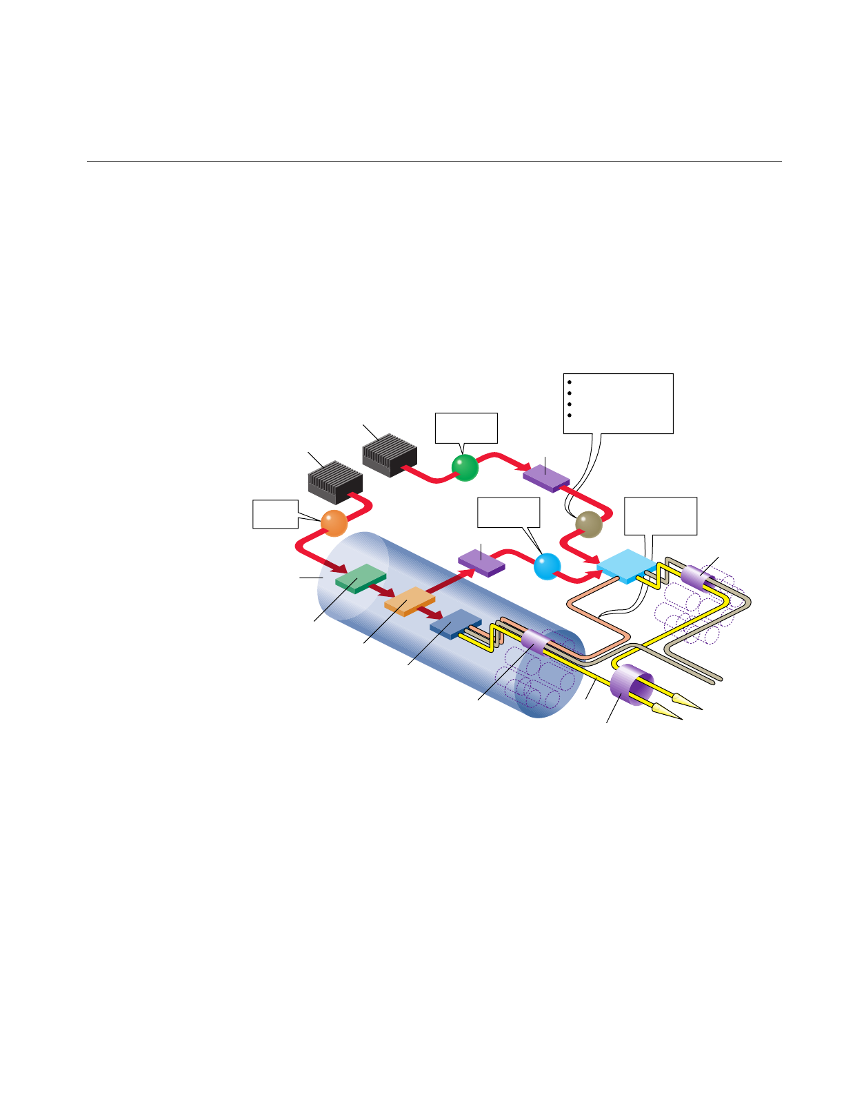
Calligraphic Light Points
519
LPB Hardware Configuration
A Light Point Board (LPB) is a circuitry card that enables the rendering of calligraphic
lights by providing the interface with a calligraphic display. The LPB is:
• Connected to one graphics pipeline only.
• Connected to all the video channels produced by a single pipe.
• Connected to all (1,2 or 4) raster manager (RM) boards of its pipe.
Figure 16-5 Calligraphic Hardware Configuration
Graphics
pipeline
CPU
CPU VME bus
LPB
VISI bus
Z-buffer
comparison
Light Point
process
Color
Focus
Exposure time
Quality and position
of light point
Draw
process
Geometry
Engine Raster
Manager Video
Channel 0...7
Channel 0...7
Channel 0
Sync signals,
including
Swap Ready
Video signal
Calligraphi
c
light points
RGB
Fiber
optic
cable

520
Chapter 16: Light Points
That configuration shows that:
• A CPU is used for the light point process so the computation and the
communication to the LPB through the VME bus are done in parallel to the DRAW
Process. It is mandatory to start a light point process for calligraphic, see
“Preprocessing Light Points” on page 513.
• The VME bus transfers to the LPB all of the calligraphic light point information,
including the color, focus, exposure time, quality, and position of each calligraphic
light point. The only information not transferred by the VME bus is occlusion
information, which is supplied by the VISI bus.
• The VISI (visibility) bus specifies whether all, part, or none of a calligraphic light
point is displayed. A calligraphic light might be partially displayed, or not at all, if a
geometry in the scene is between the light point and the viewer. Each light point has
a unique ID; this ID is used to match the information in the VISI bus with the correct
light point.
The VISI bus is a connector on each RM board. The Visibility information is
available only to the LPB.
Note: The LPB board may be used in a system without a VISI bus (systems prior to
InfiniteReality), in which case no Z-buffer information is given to the board, so all
light points are 100% visible.
• The LPB uses the vertical and horizontal (not the composite) synchronization
signals to trigger the calligraphics display. Use ircombine to set the Hsync in place of
the composite sync.
• The LPB receives the Swap Ready signal when the raster display has completed
drawing to the display buffer so it should also swap it’s internal buffers.
If the LPB does not get a Swap Ready signal, the LPB redisplays the same
calligraphic light points; since the raster frame is repeated, the calligraphic lights
must remain unchanged. Do not forget to connect the SwapReady signal to the light
point board, even if you are using a single pipe configuration.
• The LPB receives the VISI and VME bus light point information and combines it
and send the result to the calligraphic display.

Calligraphic Light Points
521
Visibility Information
All the calligraphic light point information is computed by the light point process and
goes directly to the LPB. The only missing information is knowing how much of each
light point can be seen. To compute that value:
1. A footprint of the calligraphic light point is sent to the graphic pipe.
2. The footprint is compared against the Z-buffer.
3. The result of the test is sent to the LPB using the VISI bus.
The graphic pipe takes great care that the number of multisamples covered is a constant
wherever the light point is. The number of multisamples is not constant after the
footprint covers more than 100 multisamples, however. A footprint can cover numerous
pixels, but is limited to 256 multisamples by the LPB.
pfCalligZFootPrintSize() sets the diameter of the footprint,
pfGetCalligZFootPrintSize() returns the diameter. The number of multisamples
covered by a footprint is equal to:
(n x size2)/(4 x ms)
ms is the number of multisamples per pixel.
Required Steps For Using Calligraphic Lights
To use calligraphic light points, you have to configure the channels on the LPB board and
the corresponding channels using ircombine. ircombine operates on:
• Video format combinations.
• Descriptions of raster sizes and timings used on video outputs.
• Configuration of the underlying frame buffer.
You must also enable the channels on the LPB board before starting the application.
IRIS Performer does not provide direct access to the LPB drivers. You can, however, write
a program that does.

522
Chapter 16: Light Points
Now, in IRIS Performer a few steps are still necessary.
1. Check and open the LPB on each pipe, as follows:
pfQueryFeature(PFQFTR_CALLIGRAPHIC, &q)
pfCalligInitBoard(pipe)
2. Start a light point process to process the light point calculations, as follows:
pfMultiprocess(PFMP_APP_CULL_DRAW | PFMP_FORK_LPOINT);
pfConfig();
3. Initialize the IRIS Performer stages, as follows:
pfStageConfigFunc(-1,PPROC_LPOINT,ConfigLPoint)
pfFrame();
4. Set the callback function in the light point process, as follows:
pfChanTravFunc(chan, PFTRAV_LPOINT, LpointFunc);
5. Enable the calligraphic display on all of the channels, as follows:
pfChanCalligEnable(chan[i], 1);
6. Synchronize the VME and VISI bus signals on the LPB, as follows:
pfCalligSwapVME(pipe);
pfCalligSwapVME(pipe);
You know have calligraphic light points in your application if you have calligraphic light
points in your database.
Customizing LPB Initialization
Instead of using the default initialization, IRIS Performer provides a set of functions that
allow your application to customize the initialization of the LPB.
pfInitBoard() opens the LPB device and retrieves the current configuration. This
function returns TRUE if successful, FALSE otherwise. You can also use pfIsBoardInit()
to determine if the board has been initialized. Each LPB must be initialized before calling
pfConfig().
pfCalligCloseBoard() closes the device.
Note: The board number and the pipe number are the same because there is only one
board per pipe.

Calligraphic Light Points
523
To access to the LPB directly, return its ID using pfGetCalligDeviceID(). The ID allows
you to make direct calls to the LPB driver.
pfGetCalligInfo() returns a pointer to the configuration information structure
maintained by the LPB driver. To use this structure, LPB_info, you must include the driver
lpb.h file before any IRIS Performer include files.
Note: lpb.his not distributed with IRIS Performer; it is part of the LPB driver distribution.
Once a board is initialized, you can find out how much memory is available and divide
it up between all of the enabled channels on the pipe. You can return the total amount of
LPB memory in bytes by calling pfGetCalligBoardMemSize().
By default, each channel receives the same amount of memory. To set up a different
partitioning of memory, use pfCalligPartition().
You can attach a pfCalligraphic to a specific pfChannel using the following code:
pfCalligraphic *callig = pfNewCallig(arena)
pfCalligChannel(callig, pipe, chan)
callig can then be attached to the pfPipeVideoChannel using pfPVChanCallig().
You can also set the pfCalligraphic on individual pfChannels using pfChanCallig(). You
must enable calligraphic light point processing on the specified channels so the
GangSwap mechanism is correctly handled by IRIS Performer, as follows:
pfChanCalligEnable(chan, 1);
Note: The video channel number does not have to be the same channel number as the
calligraphic board.
pfCalligWin() changes the resolution of the X and Y data accepted by the projector. The
default values are for an EIS projector (2^16). If you have a conversion interface between
the LPB and your projector, the scaling may already be done by the conversion interface.
You can use pfCalligWin() to display calligraphic points on only part of the screen, or to
make multiple viewports.
pfCalligXYSwap() switches the X and Y axes in the display. You can also reverse the X
or Y axes by giving negative width and height values in pfCalligWin().

524
Chapter 16: Light Points
Accounting for Projector Differences
Some display systems, such as the EIS projector, can calculate:
• Slew values, the time for the electron beam to go from one calligraphic point to
another.
• Gamma correction, which takes into account that projectors differ in the colors they
project.
If your system cannot perform those calculations, the light point board can calculate
those values for your application.
Slew Values
A slew table is two dimensional; it gives the time, in nanoseconds, it takes the electron
beam to go from one calligraphic point to another on one axis. A default, generic slew
table, which contains conservative values, is loaded in the LPB when it is initialized.
The longer the slew time, the longer the electron beam has to reach a calligraphic light
point on the display; any consequent wobble can dampen out in that time providing a
very stable light point. Conversely, longer slew times subtract from the total time in
which calligraphic light points can be drawn. Consequently, longer slew times could
mean that fewer calligraphic points are drawn per frame.
There are eight slew tables defined by the pfCalligSlewTableEnum. For each axis, there
are three slew tables: one table for high-quality (very stable) light points, one table for
medium-quality (slightly shorter slew times) light points, and another for low-quality
(very short slew times) light points.
You specify the drawing quality using pfLPStateVal() with one of the following mode
values:
• PFLPS_QUALITY_MODE_HIGH
• PFLPS_QUALITY_MODE_MEDIUM
• PFLPS_QUALITY_MODE_LOW

Calligraphic Light Points
525
Two other tables are used when the defocus value changes in between two points; one
table is used for high-quality light points, another table for medium- and low-quality
light points.
typedef enum {
pfXSlewQuality0 = 0, /* High quality on the X axis */
pfXSlewQuality1 = 1, /* Medium quality on the X axis */
pfXSlewQuality2 = 2, /* Low quality on the X axis */
pfYSlewQuality0 = 3, /* High quality on the Y axis */
pfYSlewQuality1 = 4, /* Medium quality on the Y axis */
pfYSlewQuality2 = 5, /* Low quality on the Y axis */
pfDefocusQuality0 = 6,/* High quality if focus change */
pfDefocusQuality1 = 7 /* Medium and Low quality if focus change */
} pfCalligSlewTableEnum;
To load or upload customized slew tables, use the following methods:
•pfCalligDownLoadSlewTable(); downloads a specified slew table into the LPB.
•pfCalligUpLoadSlewTable(); returns a slew table.
Color Correction
Each projector has its own color characteristics; a light point that appears blue on one
projector might appear aqua on another. To color correct the projected images, the light
point board maintains one gamma table per channel. Each gamma table consists of three
one-dimensional tables, one for each color component.
typedef enum {
pfRedGammaTable = 0,
pfGreenGammaTable = 1,
pfBlueGammaTable = 2
} pfCalligGammaTableEnum;
The default value provided by IRIS Performer is a linear ramp that can be modified with
the following methods:
•pfCalligDownLoadGammaTable() downloads a specified gamma table into the
LPB.
•pfCalligUpLoadGammaTable() returns a gamma table.

526
Chapter 16: Light Points
Callbacks
Like raster lights, calligraphic light points can have a callback function attached to the
pfLPointState that can occur before (PRE) or after (POST) the light point processing. The
calligraphic and raster callback functions compute different parameters.
If the stress test determines that a calligraphic light point is not going to be drawn as a
raster light point, the calligraphic callback is not be call; the raster callback is called
instead if set. For more information about the stress test, see “Significance” on page 528.
To install a Calligraphic callback on a pfLPointState you use a line of code similar to the
following:
pfCalligFunc(lpstate, (void *) yourCallback(pfCalligData*),
void **
userData
);
userData is a user pointer given to your callback identifying the callback function and the
following structure:
typedef struct {
pfLPointState *lpstate; /* Read Only LPState */
pfGeoSet *geoset; /* Read Only GeoSet */
void *userData; /* Provided when setting the callback */
unsigned short *index; /* Read Write - index visible lpoints */
int *n; /* Read Write - # of visible lpoints */
pfVec3 *coords2D; /* Read Write - screen space X,Y,Z */
float *intensity;/* Write Only - resulting intensity */
float **focus; /* Write Only - optional (de)focus */
float **drawTime;/* Write Only - optional drawTime */}
pfCalligData;
} pfRasterData;
geoset is the pfGeoSet that is currently preprocessed. lpstate is the pfLPointState applied
to that pfGeoSet. userData is the same as the data provided when declaring the callback.
index is a preallocated vector that points to light points that are visible. Even in a PRE
callback the light points are projected on the screen before the user callback is called; the
points outside of the screen are not in the index vector. See the man page on how to use
the index vector in a Callback.
n is a pointer to the number of elements in the index vector.
coords2D contains the coordinates of the light points on the screen, including the
Z coordinates in screen space. The original coordinates can be accessed through the

Calligraphic Light Points
527
pfGeoSet.It is legal to change the values in coord2D in the callback, for example, to align
the points on a grid.
intensity is a pre-allocated vector that contains the intensity of individual light points. A
PRE callback must compute intensity.
focus is a NULL pointer. It is possible to provide an individual focus value for each point
by:
1. Allocating from the arena an array of floats of size n.
2. Filling the array with the focus values.
3. Setting focus to point to that array.
You should not allocate an array in real-time; instead, allocate temporary memory
beforehand and use userData to pass the memory address to the callback.
drawTime is a NULL pointer. With it you can provide an array of floats that give a draw
time for each light point.
Frame to Frame Control
Before calling pfLPoint() in the light point process callback function, you can change the
parameters in a pfCalligraphic object on a frame by frame basis, as shown in
Example 16-3.
Example 16-3 Setting pfCalligraphic Parameters
myLPointFunc(pfChannel *chan, void *data)
{
pfCalligraphic *calligraphic = pfGetCurCallig();
if (calligraphic != NULL)
{
pfCalligFilterSize(calligraphic,FilterSizeX,FilterSizeY);
pfCalligDefocus(calligraphic,Defocus);
pfCalligRasterDefocus(calligraphic,rasterDefocus);
pfCalligDrawTime(calligraphic, DrawTime);
pfCalligStress(calligraphic, Stress)
}
pfLPoint();
}

528
Chapter 16: Light Points
FillterSizeX and FilterSizeY set the debunching distances along each axis. A filter size of 0
disables the debunching along that axis. Debunching can also be disabled on the
pfLPointState. For more information about debunching, see “Debunching” on page 529.
Defocus sets the defocus applied to all calligraphic light points, unless a callback function
returns a defocus array. In that case, each light point has a callback defocus value
regardless of the one set on the pfCalligraphic object.
In a raster plus calligraphic video mode, a calligraphic system usually has the capability
to apply a global defocus to the raster image, which is specified by the rasterDefocus
parameter passed to the projector. This parameter affects the entire image, not just the
raster light points.
For more information about defocus, see “Defocussing Calligraphic Objects” on
page 529.
DrawTime is the time, in nano seconds, in which all calligraphic light points must be
drawn, unless a callback returns a drawTime array, which controls individual draw
times. The overall effect of changing the draw time is to reduce or increase the intensity
of all calligraphic light points.
TheStress value is compared against the significance value of a pfLPointState to determine
whether the light points are displayed as calligraphic or raster. The Stress value should
be as stable as possible to avoid having points going from raster to calligraphic or from
calligraphic to raster each frame. For more information about stress, see “Significance”
on page 528.
Significance
If there is not enough time to draw all of the calligraphic light points, some calligraphic
light points can either not be drawn or, instead, drawn as raster light points, depending
on the stress value of the calligraphic light point, described in “Frame to Frame Control”
on page 527, and the significance value of the pfLPointState.
The stress value of a calligraphic light point is compared against the significance value of
the pfLPointState. If the significance is greater or equal than the stress, the light is
rendered as a calligraphic, otherwise the light is rendered as a raster light.
To set the significance, use pfLPStateVal(lpstate, PFLPS_SIGNIFICANCE,
significance).

Using pfCalligraphic Without pfChannel
529
Debunching
Debunching eliminates some calligraphic points when they occur close together on the
display system. Bunched calligraphic light points can create a heap effect, or worse, burn
the display system where there is a group of calligraphic light points.
The debunching distances are set in pfCalligraphic on the X and Y axis, as described in
“Frame to Frame Control” on page 527.
If two points in a pfGeoSet are within the debunching distance, the point with the lowest
intensity is not rendered.
If you do not want a pfLPointState to be affected by debunching, you can disable it using
pfLPStateMode() with the PFLPS_DEBUNCHING_MODE_OFF mode;
PFLPS_DEBUNCHING_MODE_ON, the default, enables debunching.
Defocussing Calligraphic Objects
Defocussing a calligraphic light point is often done to produce a specific lighting effect,
for example, to simulate rainy conditions, light points should appear defocussed. The
defocus is set within pfCalligraphic (see “Frame to Frame Control” on page 527) for all
light points for one Frame, but it is possible to clamp the defocussing values by setting a
min_defocus and a max_defocus value in the pfLPState using the following methods:
pfLPStateVal(lpstate,PFLPS_MIN_DEFOCUS,
min_defocus
);
pfLPStateVal(lpstate, PFLPS_MAX_DEFOCUS,
max_defocus
);
Using pfCalligraphic Without pfChannel
pfCalligraphic is a libpr object, so programs based only on libpr can have access to
pfCalligraphic without having access to a pfChannel, which is a libpf object. This section
describes what pfChannel does automatically with pfCalligraphic objects.
The LPB is connected to the VME bus and the VISI bus. Both buses contain information
for calligraphic light points buffered in the LPB. VISI and VME busses load their
information into the LPB buffer. The SwapReady connection to the graphic pipe
synchronizes the activity on the VISI bus; SwapReady tells the board when
glXSwapBuffers() is called, and that at the next VSync, the next frame should be
displayed.

530
Chapter 16: Light Points
pfCalligSwapVME() performs the same synchronization for the VME bus; whenever
you call pfSwapPWinBuffers() you must first call pfCalligraphicSwapVME(),
otherwise the light point board will not be synchronized with the rest of the system.
Tip: To resynchronize the LPB, make two consecutive calls to pfCalligSwapVME(), for
example, perfly makes these calls after the IRIS Performer logo has been displayed.
Note: These synchronization mechanisms are handled automatically in libpf, unless you
override the channel swap buffer and call pfSwapPWinBuffers().
Timing Issues
The SwapReady signal should always occur after a VME Swap signal. If this does not
happen, the light point board starts a TooLate timer and two things may happen:
• The LPB starts to draw the buffer assuming the VME Swap signal has been lost.
In this instance, not all of the calligraphic lights are rendered.t all of the calligraphic
lights are rendered. pfCalligraphic handles this exception by making sure the LPB
buffer always contains an end-of-buffer token at the end of the valid data.
• The VME Swap signal is received shortly after the Swap Ready, making the LPB
behave normally.
The LPB needs some time before it can accept new information from the VME, and the
VISI bus needs some time after it has received the corresponding swap command.
pfWaitForVmeBus() and pfWaitForVisiBus() allow the application to wait for the board
to get ready before sending it new information.
Light Point Process and Calligraphic
The light point process is the same whether the light points are raster or calligraphic. The
only difference is that, with calligraphic light points, pfCalligraphic has to be selected
before calling pfPreprocessDList, which is done automatically by pfChannel.
pfSelectCalligraphic() selects the channel and LPB board to which the calligraphic light
points are sent. pfGetCurCalligraphic() returns the current value set by
pfSelectCalligraphic().

Debugging Calligraphic Lights on Non-Calligraphic Systems
531
Debugging Calligraphic Lights on Non-Calligraphic Systems
If you are developing on a non-calligraphics-enabled system but would like to see the
effects of your pfCalligraphics programming, you can set the environment variable,
PF_LPOINT_BOARD. In this mode, the LPB is simulated, the calligraphic computations
are performed, and raster light points are displayed in place of the calligraphic lights
with the following limitations:
• Calligraphic defocus has no effect.
• A calligraphic light point size is defined with the Z-footprint.
Calligraphic Light Example
Example 16-4 shows a sample implementation of calligraphic lights. You can find the
source code in perf/sample/pguide/libpf/C/callig.c.
Example 16-4 Calligraphic Lights
#include <stdlib.h>
#include <Performer/pf.h>
#include <Performer/pfutil.h>
#include <Performer/pfdu.h>
static NumScreens=1;
static NumPipes=1;
static void ConfigPipeDraw(int pipe, uint stage);
static void OpenPipeWin(pfPipeWindow *pw);
static void OpenXWin(pfPipeWindow *pw);
static void DrawChannel(pfChannel *chan, void *data);
/*
* Usage() -- print usage advice and exit. This
* procedure is executed in the application process.
*/
static void
Usage (void)
{
pfNotify(PFNFY_FATAL, PFNFY_USAGE, “Usage: multipipe file.ext
...\n”);

532
Chapter 16: Light Points
exit(1);
}
int
main (int argc, char *argv[])
{
float t = 0.0f;
pfScene *scene;
pfPipe *pipe[4];
pfChannel *chan[4];
pfNode root;
pfSphere sphere;
int loop;
/* Initialize Performer */
pfInit();
pfuInitUtil();
/* specify the number of pfPipes */
/* Configure and open GL windows */
if ((NumScreens = ScreenCount(pfGetCurWSConnection())) > 1)
{
NumPipes = NumScreens;
}
pfMultipipe (NumPipes);
/* Initialize Calligraphic HW */
for (loop=0; loop < NumPipes; loop++)
{
int q;
pfQueryFeature(PFQFTR_CALLIGRAPHIC, &q);
if (!q)
{
pfNotify(PFNFY_NOTICE,PFNFY_RESOURCE, “Calligraphic points
are NOT supported on this platform”);
}
if (pfCalligInitBoard(loop) == TRUE)
{
/* get the memory size */
pfNotify(PFNFY_NOTICE, PFNFY_RESOURCE,“StartCalligraphic:
board(%d) has %d Bytes of memory”,0, pfGetCalligBoardMemSize(loop));
}
else
{

Calligraphic Light Example
533
pfNotify(PFNFY_NOTICE, PFNFY_RESOURCE, “Could not init
calligraphic board %d”, loop);
}
}
/* Force Multiprocessor mode to use the light point process */
pfMultiprocess(PFMP_APP_CULL_DRAW | PFMP_FORK_LPOINT);
/* Load all loader DSO’s before pfConfig() forks */
if (argc > 1)
pfdInitConverter(argv[1]);
/* Configure multiprocessing mode and start parallel processes.*/
pfConfig();
/* Append to PFPATH additional standard directories where geometry
and textures exist */
scene = pfNewScene();
if (argc > 1)
{
if (!(getenv(“PFPATH”)))
pfFilePath(“.:./data:../data:../../data:/usr/share/Performer/data”);
/* Read a single file, of any known type. */
if ((root = pfdLoadFile(argv[1])) == NULL)
{
pfExit();
exit(-1);
}
/* Attach loaded file to a pfScene. */
pfAddChild(scene, root);
/* determine extent of scene’s geometry */
pfGetNodeBSphere (scene, &bsphere);
/* Create a pfLightSource and attach it to scene. */
pfAddChild(scene, pfNewLSource());
}
for (loop=0; loop < NumPipes; loop++)
pfPipeWindow *pw;

534
Chapter 16: Light Points
char str[PF_MAXSTRING];
pipe[loop] = pfGetPipe(loop);
pfPipeScreen(pipe[loop], loop);
pw = pfNewPWin(pipe[loop]);
pfPWinType(pw, PFPWIN_TYPE_X);
sprintf(str, “IRIS Performer - Pipe %d”, loop);
pfPWinName(pw, str);
if (NumScreens > 1)
{
pfPWinOriginSize(pw, 0, 0, 300, 300);
} else
pfPWinOriginSize(pw, (loop&0x1)*315, ((loop&0x2)>>1)*340, 300,
300);
pfPWinConfigFunc(pw, OpenPipeWin);
pfConfigPWin(pw);
}
/* set up optional DRAW pipe stage config callback */
pfStageConfigFunc(-1 /* selects all pipes */, PFPROC_DRAW /* stage
bitmask */, ConfigPipeDraw);
pfConfigStage(-1, PFPROC_DRAW);
pfFrame();
/* Create and configure pfChannels - by default, channels are
placed in the first window on their pipe */
for (loop=0; loop < NumPipes; loop++)
{
chan[loop] = pfNewChan(pipe[loop]);
pfChanScene(chan[loop], scene);
pfChanFOV(chan[loop], 45.0f, 0.0f);
pfChanTravFunc(chan[loop], PFTRAV_DRAW, DrawChannel);
pfChanCalligEnable(chan[loop], 1);
/* synchronize the lpoint board with the swap ready signal */
pfCalligSwapVME(loop);
pfCalligSwapVME(loop);
}
/* Simulate for twenty seconds. */
while (t < 30.0f)

Calligraphic Light Example
535
{
pfCoord view;
float s, c;
/* Go to sleep until next frame time. */
pfSync();
/* Initiate cull/draw for this frame. */
pfFrame();
pfSinCos(45.0f*t, &s, &c);
pfSetVec3(view.hpr, 45.0f*t, -10.0f, 0);
pfSetVec3(view.xyz, 2.0f * bsphere.radius * s, -2.0f *
bsphere.radius *c, 0.5f * bsphere.radius);
for (loop=0; loop < NumPipes; loop++)
pfChanView(chan[loop], view.xyz, view.hpr);
}
/* Terminate parallel processes and exit. */
pfExit();
return 0;
}
/* ConfigPipeDraw() --
* Application state for the draw process can be initialized
* here. This is also a good place to do real-time
* configuration for the drawing process, if there is one.
* There is no graphics state or pfState at this point so no
* rendering calls or pfApply*() calls can be made.
*/
static void
ConfigPipeDraw(int pipe, uint stage)
{
pfPipe *p = pfGetPipe(pipe);
int x, y;
pfNotify(PFNFY_NOTICE, PFNFY_PRINT, “Initializing stage 0x%x of
pipe %d on screen %d, connection \”%s\””, stage,
pipe,pfGetPipeScreen(p),pfGetPipeWSConnectionName(p));
pfGetPipeSize(p, &x, &y);
pfNotify(PFNFY_NOTICE, PFNFY_PRINT, “Pipe %d size: %dx%d”, pipe,
x,y);
}

536
Chapter 16: Light Points
/*
* OpenPipeWin() -- create a GL window: set up the
* window system, IRIS GL, and IRIS Performer. This
* procedure is executed for each window in the draw process
* for that pfPipe.
*/
void
OpenXWin(pfPipeWindow *pw)
{
/* -1 -> use default screen or that specified by shell DISPLAY
variable */
pfuGLXWindow *win;
pfPipe *p;
p = pfGetPWinPipe(pw);
if (!(win = pfuGLXWinopen(p, pw, “TESTIN”)))
pfNotify(PFNFY_FATAL, PFNFY_RESOURCE,“OpenXPipeline: Could not
create GLX Window.”);
win = win; /* suppress compiler warn */
}
static void
OpenPipeWin(pfPipeWindow *pw)
{
pfPipe *p;
pfLight *Sun;
p = pfGetPWinPipe(pw);
/* open the window on the specified screen. By default,
* if a screen has not yet been set and we are in multipipe mode,
* a window of pfPipeID i will now open on screen i
*/
pfOpenPWin(pw);
pfNotify(PFNFY_NOTICE, PFNFY_PRINT,
PipeWin of Pipe %d opened on screen %d”,
pfGetId(p),pfGetPipeScreen(p));
/* create a light source in the “south-west” (QIII) */
Sun = pfNewLight(NULL);

Calligraphic Light Example
537
pfLightPos(Sun, -0.3f, -0.3f, 1.0f, 0.0f);
}
static void
DrawChannel (pfChannel *channel, void *data)
{
static int first = 1;
if (first)
{
first = 0;
pfNotify(PFNFY_NOTICE,PFNFY_PRINT,”Calligraphics: 0x%p”,
pfGetChanCurCallig(channel));
}
/* erase framebuffer and draw Earth-Sky model */
pfClearChan(channel);
/* invoke Performer draw-processing for this frame */
pfDraw();
}


This chapter details IRIS Performer’s comprehensive set of mathematical
functions.
“Math Routines”
Chapter 17


541
Chapter 17
17. Math Routines
This chapter describes the IRIS Performer math routines. Math routines let you create,
modify, and manipulate vectors, matrices, line segments, planes, and bounding volumes
such as spheres, boxes, and cylinders.
Vector Operations
A basic set of mathematical operations is provided for setting and manipulating floating
point vectors of length 2, 3, and 4. The types of these vectors are pfVec2, pfVec3 and
pfVec4, respectively. The components of a vector are denoted by PF_X, PF_Y, PF_Z, and
PF_W with indices of 0, 1, 2, and 3, respectively. In the case of 4-vectors, the PF_W
component acts as the homogeneous coordinate in transformations.
IRIS Performer supplies macro equivalents for many of the routines described in this
section. Inlining the macros instead of calling the routines can substantially improve
performance. The C++ interface provides the same, fast performance as the inlined
macros.
Table 17-1 lists the routines, what they do (in mathematical notation), and the macro
equivalents (where available) for working with 3-vectors. Most of the same operations
are also available for 2-vectors and 4-vectors, substituting “2” or “4” for “3” in the routine
names. The only operations not available for 2-vectors are vector cross-products, point
transforms, and vector transforms; the only operations unavailable for 4-vectors are
vector cross-products and point transforms, that is, there are no such routines as
pfCrossVec2(), pfCrossVec4(),pfXformPt2(),pfXformPt4(), or pfXformVec2().

542
Chapter 17: Math Routines
Note: For the duration of this chapter, bold lowercase letters represent vectors and bold
uppercase letters represent matrices. “×” indicates cross product, “.” denotes dot product,
and vertical bars indicate the magnitude of a vector.]
Table 17-1 Routines for 3-Vectors
Routine Effect Macro Equivalent
pfSetVec3(d, x, y, z) d = (x,y,z) PFSET_VEC3
pfCopyVec3(d, v) d = vPFCOPY_VEC3
pfNegateVec3(d,v) d = -vPFNEGATE_VEC3
pfAddVec3(d, v1, v2) d = v1 + v2PFADD_VEC3
pfSubVec3(d, v1, v2) d = v1 - v2PFSUB_VEC3
pfScaleVec3(d, s, v) d = svPFSCALE_VEC3
pfAddScaledVec3(d, v1, s, v2) d = v1 + sv2PFADD_SCALED_VEC3
pfCombineVec3(d,s1,v1,s2,v2) d = s1v1 + s2v2PFCOMBINE_VEC3
pfNormalizeVec3(d) d = d/|d| none
pfCrossVec3(d, v1, v2) d= v1×v2none
pfXformPt3(d, v, m) d = vM, where v=(vx,vy,vz,) and M
is the 4×3 submatrix. none
pfFullXformPt3(d, v, M) d = vM/dw, where v=(vx,vy,vz, 1) none
pfXformVec3(d, v, M) d = vM, where v=(vx,vy,vz, 0) none
pfDotVec3(v1, v2) v1.v2PFDOT_VEC3
pfLengthVec3(v) |v| PFLENGTH_VEC3
pfSqrDistancePt3(v1, v2) |v2 - v1|2PFSQR_DISTANCE_PT3
pfDistancePt3(v1, v2) |v2 - v1| PFDISTANCE_PT3
pfEqualVec3(v1, v2) returns TRUE if v1=v
2, FALSE
otherwise PFEQUAL_VEC3
pfAlmostEqualVec3(v1,v2,tol) returns TRUE if each element of v1 is
within tol of the corresponding
element of v2, FALSE otherwise
PFALMOST_EQUAL_
VEC3

Matrix Operations
543
Matrix Operations
A pfMatrix is a 4x4 array of floating-point numbers that is used primarily to specify a
transformation in homogeneous coordinates (x,y,z,w). Transforming a vector by a
matrix means multiplying the matrix on the right by the row vector on the left.
Table 17-2 describes the IRIS Performer mathematical operations that act on matrices.
Table 17-2 Routines for 4x4 Matrices
Routine Effect Macro Equivalent
pfMakeIdentMat(d) D = IPFMAKE_IDENT_MAT
pfMakeVecRotVecMat(d,v1,v2) D = M such that v2=v1M.
v1, v2normalized.none
pfMakeQuatMat(d, q)) D = M, where M is the rotation of
the quaternion q.none
pfMakeRotMat(d, deg, x, y, z) D = M, where M rotates by deg
around (x,y,z)none
pfMakeEulerMat(d, h, p, r) D = RPH, where R,P, and H are the
transforms for roll, pitch, and
heading.
none
pfMakeTransMat(d, x, y, z) D = M, where M translates by
(x,y,z)PFMAKE_TRANS_MAT
pfMakeScaleMat(d, x, y, z) D = M, where M scales by (x,y,z) PFMAKE_SCALE_MAT
pfMakeCoordMat(d, c) D = M, where M rotates by (h,p,r)
and translates by (x,y,z), with h,p,
r,x,y, and z all specified by c
none
pfGetOrthoMatQuat(s, q) returns, in q, a quaternion with the
rotation specified by s. none
pfGetOrthoMatCoord(s, d) returns, in d, the rotation and
translation specified by snone
pfSetMatRow(d, r, x, y, z, w) Set rth row of D equal to (x, y, z, w) PFSET_MAT_ROW
pfGetMatRow(m, r, x, y, z, w) (*x, *y, *z, *w) = rth row of MPFGET_MAT_ROW

544
Chapter 17: Math Routines
pfSetMatCol(d, c, x, y, z, w) Setcth column of D equal to (x, y, z,
w) PFSET_MAT_COL
pfGetMatCol(m, c, x, y, z, w) (*x, *y, *z, *w) = cth column of MPFGET_MAT_COL
pfSetMatRowVec3(d, r, v) Set rth row of D equal to vPFSET_MAT_ROWVEC3
pfGetMatRowVec3(m, r, d) d = rth row of MPFGET_MAT_ROWVEC3
pfSetMatColVec3(d, c, v) Set cth column of D equal to vPFSET_MAT_COLVEC3
pfGetMatColVec3(m, c, d) d = cth column of MPFGET_MAT_COLVEC3
pfCopyMat(d, m) D = MPFCOPY_MAT
pfAddMat(d, m1, m2) D = M1+M2none
pfSubMat(d, m1, m2) D = M1 - M2none
pfMultMat(d, m1, m2) D = M1M2none
pfPostMultMat(d, m) D = DM none
pfPreMultMat(d, m) D = MD none
pfTransposeMat(d, m) D = MT none
pfPreTransMat(d, m, x, y, z) D = TM, where T translates by
(x,y,z)none
pfPostTransMat(d, x, y, z, m) D = MT, where Ttranslates by
(x,y,z)none
pfPreRotMat(d, deg, x, y, z, m) D = RM, where R rotates by deg
around (x,y,z)none
pfPostRotMat(d, m, deg, x, y, z) D = MR, where R rotates by deg
around (x,y,z)none
pfPreScaleMat(d, x, y, z, m) D = SM, where S scales by (x,y,z) none
pfPostScaleMat(d, m, x, y, z) D = MS, where Sscales by (x,y,z) none
pfInvertFullMat(d, m)) D = M-1 for general matrices none
pfInvertAffMat(d, m) D = M-1, with M affine none
Table 17-2 (continued) Routines for 4x4 Matrices
Routine Effect Macro Equivalent

Matrix Operations
545
Some of the math routines that take a matrix as an argument are restricted to affine,
orthogonal, or orthonormal matrices, these restrictions being noted by Aff, Ortho and
OrthoN, respectively. (If such a restriction isn’t noted in a libpr routine name, the routine
can take a general matrix.)
An affine transformation is one that leaves the homogeneous coordinate unchanged—
that is, in which the last column is (0,0,0,1). An orthogonal transformation is one that
preserves angles. It can include translation, rotation, and uniform scaling, but no
shearing or nonuniform scaling. An orthonormal transformation is an orthogonal
transformation that preserves distances; that is, one that contains no scaling.
In the visual simulation library, libpf, most routines require the matrix to be orthogonal,
although this isn’t noted in the routine names.
The standard order of transformations for a hierarchical scene involves postmultiplying
the transformation matrix for a child by the matrix for the parent. For instance, assume
your scene involves a hand attached to an arm attached to a body. To get a transformation
matrix H for the hand, postmultiply the arm’s transformation matrix (A) by the body’s
(B): H = AB. To transform the hand object (at location h in hand coordinates) to body
coordinates, calculate h’ = hH.
pfInvertOrthoMat(d, m) D = M-1, with M orthogonal none
pfInvertOrthoNMat(d, m) D = M-1, with M orthonormal none
pfInvertIdentMat(d, m) D = M-1, with M equal to the
identity matrix none
pfEqualMat(d, m) returns TRUE if D=M, FALSE
otherwise PFEQUAL_MAT
pfAlmostEqualMat(d, m, tol) returns TRUE if each element of D
is within tol of the corresponding
element of M, FALSE otherwise
PFALMOST_EQUAL_MA
T
Table 17-2 (continued) Routines for 4x4 Matrices
Routine Effect Macro Equivalent

546
Chapter 17: Math Routines
Example 17-1 Matrix and Vector Math Examples
/*
* test Rot of v1 onto v2
*/
{
pfVec3 v1, v2, v3;
pfMatrix m1;
MakeRandomVec3(v1);
MakeRandomVec3(v2);
pfNormalizeVec3(v1);
pfNormalizeVec3(v2);
pfMakeVecRotVecMat(m1, v1, v2);
pfXformVec3(v3, v1, m1);
AssertEqVec3(v3, v2, “Arb Rot To”);
}
/*
* test inversion of Affine Matrix
*/
{
pfVec3 v1, v2, v3;
pfMatrix m1, m2, m3;
MakeRandomVec3(v3);
pfMakeScaleMat(m2, v3[0], v3[1], v3[2]);
pfPreMultMat(m1, m2);
MakeRandomVec3(v1);
pfNormalizeVec3(v1);
MakeRandomVec3(v2);
pfNormalizeVec3(v2);
pfMakeVecRotVecMat(m1, v1, v2);
s = pfLengthVec3(v2)/pfLengthVec3(v1);
pfPreScaleMat(m1, s, s, s, m1);
MakeRandomVec3(v1);
pfNormalizeVec3(v1);
MakeRandomVec3(v2);
pfNormalizeVec3(v2);
pfMakeVecRotVecMat(m2, v1, v2);
MakeRandomVec3(v3);
pfMakeTransMat(m2, v3[0], v3[1], v3[1]);

Quaternion Operations
547
pfPreMultMat(m1, m2);
pfInvertAffMat(m3, m1);
pfPostMultMat(m3, m1);
AssertEqMat(m3, ident, “affine inverse”);
Quaternion Operations
A pfQuat is the IRIS Performer data structure (a pfVec4) whose for floating point values
represent the components of a quaternion. Quaternions have many beneficial properties.
The most relevant of these is their ability to represent 3D rotations in a manner that
allows relatively simple yet meaningful interpolation between rotations. Much like
multiplying two matrices, multiplying two quaternions results in the concatenation of
the transformations. For more information on quaternions, see the article by Sir William
Rowan Hamilton “On quaternions; or on a new system of imaginaries in algebra,” in the
Philosophical Magazine, xxv, pp. 10-13 (July 1844), or refer to the sources noted in the
pfQuat(3pf) reference page.
The properties of spherical linear interpolation makes quaternions much better suited
than matrices for interpolating transformation values from keyframes in animations. The
most common usage then is to use pfSlerpQuat() to interpolate between two
quaternions representing two rotational transformations. The quaternion that results
from the interpolation can then be passed to pfMakeQuatMat() to generate a matrix for
use in a subsequent IRIS Performer call such as pfDCSMat(). While converting a
quaternion to a matrix is relatively efficient, converting a matrix to a quaternion with
pfGetOrthoMatQuat() is expensive and should be avoided when possible.
Because a pfQuat is also a pfVec4, all of the pfVec4 routines and macros may be used on
pfQuats as well.
Table 17-3 Routines for Quaternions
Routine Effect Macro Equivalent
pfMakeRotQuat(q, a, x, y, z) Sets q to rotation of a degrees about
(x, y, z) none
pfGetQuatRot(q, a, x, y, z) Sets *a to angle and (*x, *y, *z) to
axis of rotation represented by q none
pfConjQuat(d, q) d = conjugate of q PFCONJ_QUAT

548
Chapter 17: Math Routines
Example 17-2 Quaternion Example
/*
* test quaternion slerp
*/
pfQuat q1, q2, q3;
pfMatrix m1, m2, m3, m3q;
pfVec3 axis;
float angle1, angle2, angle, t;
MakeRandomVec3(axis);
pfNormalizeVec3(axis);
angle1 = -drand48()*90.0f;
angle2 = drand48()*90.0f;
t = drand48();
pfMakeRotMat(m1, angle1, axis[0], axis[1], axis[2]);
pfMakeRotQuat(q1, angle1, axis[0], axis[1], axis[2]);
pfMakeQuatMat(m3q, q1);
pfLengthQuat(q) returns length of q PFLENGTH_QUAT
pfMultQuat(d, q1, q2) d = q1 * q2 PFMULT_QUAT
pfDivQuat(d, q1, d2) d = q1 / q1 PFDIV_QUAT
pfInvertQuat(d, q1) d = 1 / q1
pfExpQuat(d, q) d = exp(q) none
pfLogQuat(d, q) d = ln(q) none
pfSlerpQuat(d, t, q1, q2) d = interpolation with weight t
between q1 (t=0.0) and q2 (t=1.0) none
pfSquadQuat(d, t, q1, q2, a, b) d = quadratic interpolation
between q1 and q2 none
pfQuatMeanTangent(d, q1,
q2, q3) d = mean tangent of q1, q2 and q3. none
Table 17-3 (continued) Routines for Quaternions
Routine Effect Macro Equivalent

Matrix Stack Operations
549
pfMakeRotMat(m2, angle2, axis[0], axis[1], axis[2]);
pfMakeRotQuat(q2, angle2, axis[0], axis[1], axis[2]);
pfMakeQuatMat(m3q, q2);
AssertEqMat(m2, m3q, “make rot quat q2”);
angle = (1.0f-t) * angle1 + t * angle2;
pfMakeRotMat(m3, angle, axis[0], axis[1], axis[2]);
pfMakeRotQuat(q1, angle1, axis[0], axis[1], axis[2]);
pfMakeRotQuat(q2, angle2, axis[0], axis[1], axis[2]);
pfSlerpQuat(q3, t, q1, q2);
pfMakeQuatMat(m3q, q3);
AssertEqMat(m3q, m3, “quaternion slerp”);
{
Matrix Stack Operations
IRIS Performer allows you to create a stack of transformation matrices, which is called a
pfMatStack.
Table 17-4 lists and describes the matrix stack routines. Note that none of these routines
has a macro equivalent. The matrix at the top of the matrix stack is denoted “TOS,” for
“Top of Stack.”
Table 17-4 Matrix Stack Routines
Routine Operation
pfNewMStack Allocate storage.
pfResetMStack Reset the stack.
pfPushMStack Duplicate the TOS and push it on the stack.
pfPopMStack Pop the stack.
pfPreMultMStack Premultiply the TOS by a matrix.
pfPostMultMStack Postmultiply the TOS by a matrix.
pfLoadMStack Set the TOS matrix.
pfGetMStack Get the TOS matrix.

550
Chapter 17: Math Routines
Creating and Transforming Volumes
libpr provides a number of volume primitives, including sphere, box, cylinder, half-space
(plane), and frustum. libpf uses the frustum primitive for a view frustum, and uses other
volume primitives for bounding volumes:
• pfNodes use bounding spheres.
• pfGeoSets use bounding boxes.
• Segments use bounding cylinders.
Defining a Volume
This section describes how to define geometric volumes.
pfGetMStackTop Get a pointer to the TOS matrix.
pfGetMStackDepth Return the current depth of the stack.
pfPreTransMStack Premultiply the TOS by a translation.
pfPostTransMStack Postmultiply the TOS by a translation.
pfPreRotMStack Premultiply thee TOS by a rotation.
pfPostRotMStack Postmultiply the TOS by a rotation.
pfPreScaleMStack Premultiply the TOS by a scale factor.
pfPostScaleMStack Postmultiply the TOS by a scale factor.
Table 17-4 (continued) Matrix Stack Routines
Routine Operation

Creating and Transforming Volumes
551
Spheres
Spheres are defined by a center and a radius, as shown by the pfSphere structure’s
definition:
typedef struct {
pfVec3 center;
float radius;
} pfSphere;
A point p is in the sphere with center c and radius r if |p - c|< r.
Axially Aligned Boxes
An axially aligned box is defined by its two corners with the smallest and largest values
for each coordinate. Its edges are parallel to the X, Y, and Z axes. It’s represented by the
pfBox data structure:
typedef struct {
pfVec3 min;
pfVec3 max;
} pfBox;
A point (x, y, z) is in the box if minx<x<maxx,miny<y<maxy, and minz<z<maxz,.
Cylinders
A cylinder is defined by its center, radius, axis, and half-length, as shown by the
definition of the pfCylinder data structure:
typedef struct {
pfVec3 center;
float radius;
pfVec3 axis;
float halfLength;
} pfCylinder;
A point p is in the cylinder with center c, radius r, axis a, and half-length h, if |(p-c).a|
< h and | (p-c) - ((p-c).a)a | <r.

552
Chapter 17: Math Routines
Half-spaces (Planes)
A half-space is defined by a plane with a normal pointing away from the interior. It’s
represented by the pfPlane data structure:
typedef struct {
pfVec3 normal;
float offset;
} pfPlane;
A point p is in the half-space with normal n and offset d if p.n<d.
Frusta
Unlike the other volumes, a pfFrustum isn’t an exposed structure. You can allocate
storage for a pfFrustum using pfNewFrust() and you can set the frustum using
pfMakePerspFrust() or pfMakeOrthoFrust().
Creating Bounding Volumes
The easiest and most efficient way to create a volume is to use one of the bounding
operations. The routines in Table 17-5 create a bounding volume that encloses other
geometric objects.
Table 17-5 Routines to Create Bounding Volumes
Routine Bounding Volume
pfBoxAroundPts Box enclosing a set of points
pfBoxAroundBoxes Box enclosing a set of boxes
pfBoxAroundSpheres Box enclosing a set of spheres
pfCylAroundSegs Cylinder around a set of segments
pfSphereAroundPts Sphere around a set of points
pfSphereAroundBoxes Sphere around a set of boxes
pfSphereAroundSpheres Sphere around a set of spheres

Creating and Transforming Volumes
553
Bounding volumes can also be defined by extending existing volumes, but in many cases
the tightness of the bounds created through a series of extend operations is substantially
inferior to that of the bounds created with a single pf*Around*() operation.
Table 17-6 lists and describes the routines for extending bounding volumes.
Transforming Bounding Volumes
Transforming the volumes with an orthonormal transformation—that is, with no skew
or nonuniform scaling, is straightforward for all of the volumes except for the axially
aligned box. A straight transformation of the vertices doesn’t suffice because the new box
would no longer be axially aligned, so an aligned box must be created that encloses the
transformed vertices. Hence a transformation of a box isn’t generally reversed by
applying the inverse transformation to the new box.
Table 17-7 lists and describes the routines that transform bounding volumes.
Table 17-6 Routines to Extend Bounding Volumes
Routine Operation
pfBoxExtendByPt Extend a box to enclose a point.
pfBoxExtendByBox Extend a box to enclose another box.
pfSphereExtendByPt Extend a sphere to enclose a point.
pfSphereExtendBySphere Extend a sphere to enclose a sphere.
Table 17-7 Routines to Transform Bounding Volumes
Routine Operation
pfOrthoXformPlane Transform a plane or half-space.
pfOrthoXformFrust Transform a frustum.
pfXformBox Transform and extend a bounding box.
pfOrthoXformCyl Transform a cylinder.
pfOrthoXformSphere r Transform a sphere.

554
Chapter 17: Math Routines
Intersecting Volumes
IRIS Performer provides a number of routines that test for intersection with volumes.
Point-Volume Intersection Tests
The point-volume intersection test returns PFIS_TRUE if the specified point is in the
volume and PFIS_FALSE otherwise. Table 17-8 lists and describes the routines that test a
point for inclusion within a bounding volume.
Volume-Volume Intersection Tests
IRIS Performer provides a number of volume-volume tests that are used internally for
bounding-volume tests when culling to a view frustum or when testing a group of line
segments against geometry in a scene (see “Intersecting With pfGeoSets” on page 558).
You can intersect spheres, boxes, and cylinders against half-spaces and against frustums
for culling. You can intersect cylinders against spheres for testing grouped segments
against bounding volumes in a scene.
Table 17-8 Testing Points for Inclusion in a Bounding Volume
Routine Test
pfBoxContainsPt Point inside a box
pfSphereContainsPt Point inside a sphere
pfCylContainsPt Point inside a cylinder
pfHalfSpaceContainsPt Point inside a half-space
pfFrustContainsPt Point inside a frustum

Intersecting Volumes
555
Table 17-9 lists and describes the routines that test for volume intersections.
The volume-volume intersection tests are designed to quickly locate empty intersections
for rejection during a cull. If the complete intersection test is too time-consuming, the
result PFIS_MAYBE is returned, to indicate that the two volumes might intersect.
The returned value is a bitwise OR of tokens, as shown in Table 17-10.
Table 17-9 Testing Volume Intersections
Routine Action: Test if A Inside B
pfHalfSpaceContainsSphere Sphere inside a half-space
pfFrustContainsSphere Sphere inside a frustum
pfSphereContainsSphere Sphere inside a sphere
pfSphereContainsCyl Cylinder inside a sphere
pfHalfSpaceContainsCyl Cylinder inside a half-space
pfFrustContainsCyl Cylinder inside a frustum
pfHalfSpaceContainsBox Box inside a half-space
pfFrustContainsBox Box inside a frustum
pfBoxContainsBox Box inside a box
Table 17-10 Intersection Results
Test Result Meaning
PFIS_FALSE No intersection
PFIS_MAYBE Possible intersection
PFIS_MAYBE | PFIS_TRUE A contains at least part of B
PFIS_MAYBE | PFIS_TRUE | PFIS_ALL_IN A contains all of B

556
Chapter 17: Math Routines
This arrangement allows simple code such as that shown in Example 17-3.
Example 17-3 Quick Sphere Culling Against a Set of Half-Spaces
long
HSSContainsSphere(pfPlane **hs, pfSphere *sph, long numHS)
{
long i, isect;
isect = ~0;
for (i = 0 ; i < numHS ; i++)
{
isect &= pfHalfSpaceContainsSphere(sph,hs[i]);
if (isect == PFIS_FALSE)
return isect;
}
/* if not ALL_IN all half spaces, don’t know for sure */
if (!(isect & PFIS_ALL_IN))
isect &= ~PFIS_TRUE;
return isect;
}
Creating and Working With Line Segments
A pfSeg represents a line segment starting at position pos, extending for a distance length
in the direction dir:
typedef struct {
pfVec3 pos;
pfVec3 dir;
float length;
} pfSeg;
The routines that operate on pfSegs assume that dir is of unit length and that length is
positive; otherwise, the results of operations are undefined.

Creating and Working With Line Segments
557
You can create line segments in three different ways:
• Specify a point and a direction directly in the structure—pfSeg().
• Specify two endpoints: pfMakePtsSeg().
• Specify one endpoint and an orientation in polar coordinates—pfMakePolarSeg().
• Specify starting and ending distances along an existing segment—pfClipSeg().
Intersection tests are the most important operations that use line segments. You can test
the intersection of segments with volumes (half-spaces, spheres, and boxes), with 2D
geometry (planes and triangles), and with geometry inside pfGeoSets.
Intersecting With Volumes
IRIS Performer supports intersections of segments with three types of convex volumes.
pfHalfSpaceIsectSeg() intersects a segment with the half-space defined by a plane with
an outward facing normal. pfSphereIsectSeg() intersects with a sphere and
pfBoxIsectSeg() intersects with an axially aligned box.
The intersection test of a segment and a convex volume can have one of five results:
• The segment lies entirely outside the volume.
• The segment lies entirely within the volume.
• The segment lies partially inside the volume with the starting point inside.
• The segment lies partially inside the volume with the ending point inside.
• The segment lies partially inside the volume with both endpoints outside.
As with the volume-volume tests, the segment-volume intersection routines return a
value that is the bitwise OR of some combination of the tokens PFIS_TRUE,
PFIS_ALL_IN, PFIS_START_IN, and PFIS_MAYBE. (When PFIS_TRUE is set
PFIS_MAYBE is also set for consistency with those routines that do quick intersection
tests for culling.)
The functions take two arguments that return the distances along the segment of the
starting and ending points. The return values are designed so that you can AND them
together for testing for the intersection of a segment against the intersection of a number
of volumes. For example, a convex polyhedron is defined as the intersection of a set of
half-spaces. Example 17-4 shows how to intersect a segment with a polyhedron.

558
Chapter 17: Math Routines
Example 17-4 Intersecting a Segment With a Convex Polyhedron
long
HSSIsectSeg(pfPlane **hs, pfSeg *seg, long nhs, float *d1,
float *d2)
{
long retval = 0xffff;
for (long i = 0 ; i < nhs ; i++)
{
retval &= pfHalfSpaceIsectSeg(hs[i], seg, d1, d2);
if (retval == 0)
return 0;
pfClipSeg(seg, *d1, *d2);
}
return retval;
}
Note that these routines do not actually clip the segment. If you want the segment to be
clipped to the interior of the volume, you must call pfClipSeg(), as in the example above.
Intersecting With Planes and Triangles
Intersections with planes and triangles are simpler than those with volumes.
pfPlaneIsectSeg() and pfTriIsectSeg() return either PFIS_TRUE or PFIS_FALSE,
depending on whether an intersection has occurred. The distance of the intersection
along the segment is returned in one of the arguments.
Intersecting With pfGeoSets
You can intersect line segments with the drawable geometry that’s within pfGeoSets by
calling pfGSetIsectSegs(). The operation is very similar to that of pfNodeIsectSegs(),
except that rather than operating on an entire scene graph, only the triangles within the
pfGeoSet are “traversed.”
pfGSetIsectSegs() takes a pfSegSet and tests to see whether any of the segments intersect
the polygons inside the specified pfGeoSet. By default, information about the closest
intersection along each segment is returned as a set of pfHit objects, one for each line
segment in the request. Each pfHit object indicates the location of the intersection, the
normal, and what element was hit. This element identification includes the index of the
primitive within the pfGeoSet and the triangle index within the primitive (for tristrips
and quads primitives), as well as the actual triangle vertices.

Creating and Working With Line Segments
559
You can also extract information from a pfHit object using pfQueryHit() and
pfMQueryHit(). (See “Intersection Requests: pfSegSets” and “Intersection Return Data:
pfHit Objects” in Chapter 4 for more information about pfSegSets and pfHit objects.) The
principal difference between those routines and pfGSetIsectSegs() is that with
pfGSetIsectSegs() information concerning the libpf scene graph (such as transformation,
geode, name, and path) is never used.
Two types of intersection testing are possible, as shown in Table 17-11.
You can use PFTRAV_IS_GSET for crude collision detection and PFTRAV_IS_PRIM for
fine-grained testing. You can enable both bits and dynamically choose whether to go
down to the primitive level by using a discriminator callback (see “Discriminator
Callbacks”). pfGSetIsectSegs() performs only primitive-level testing for pfGeoSets
consisting of triangles (PFGS_TRIS), quads (PFGS_QUADS), and tristrips
(PFGS_TRISTRIPS), and all are decomposed into triangles.
Intersection Masks
Each pfGeoSet has an intersection mask that you set using pfGSetIsectMask(). The mask
in the pfGeoSet is useful when pfGeoSets are embedded in a larger data structure; it
allows you to define pfGeoSets to belong to different classes of geometry for
intersection—for example, water, ground, foliage. pfGSetIsectSegs() also takes a mask,
and an intersection test is performed only if the bitwise AND of the two masks is
nonzero.
Table 17-11 Available Intersection Tests
Test Name Function
PFTRAV_IS_GSET Intersect the segment with the bounding box of the pfGeoSet.
PFTRAV_IS_PRIM Intersect the segment with the polygon-based primitives inside the
pfGeoSet.

560
Chapter 17: Math Routines
Discriminator Callbacks
If a callback is specified in pfGSetIsectSegs() function is invoked when a successful
intersection occurs, either with the bounding box of the pfGeoSet or with a primitive. The
discriminator can decide what action to take based on the information about the
intersection contained in a pfHit object. The return value from the discriminator
determines whether the current intersection is valid and should be copied into the return
structure, whether the rest of the geometry in the pfGeoSet is examined, and whether the
segment should be clipped before continuing.
Unless the return value includes the bit PFTRAV_IS_IGNORE, the intersection is
considered successful and is copied into the array of pfHit structures for return.
The bits of the PFTRAV_* tokens determine whether to continue, as shown in
Table 17-12.
The bits PFTRAV_IS_CLIP_END and PFTRAV_IS_CLIP_START cause the segment to be
clipped at the end or at the start using the intersection point. By default, in the absence
of a discriminator, segments are end-clipped at each successful intersection at the finest
level (bounding box or primitive level) requested. Hence, the closest intersection point is
always returned.
The discriminator is passed a pfHit. You can use pfQueryHit() to examine information
about the intersection, including which segment number within the pfSegSet the
intersection is for and the current segment as clipped by previous intersections.
Table 17-12 Discriminator Return Values
Result Meaning
PFTRAV_CONT Continue examining geometry inside the pfGeoSet.
PFTRAV_PRUNE Terminate the traversal now.
PFTRAV_TERM Terminate the traversal now.

General Math Routine Example Program
561
General Math Routine Example Program
Example 17-5 demonstrates the use of many of the available IRIS Performer math
routines.
Example 17-5 Intersection Routines in Action
/*
* simple test of pfCylIsectSeg
*/
{
pfVec3 tmpvec;
pfSetVec3(pt1, -2.0f, 0.0f, 0.0f);
pfSetVec3(pt2, 2.0f, 0.0f, 0.0f);
pfMakePtsSeg(&seg1, pt1, pt2);
pfSetVec3(cyl1.axis, 1.0f, 0.0f, 0.0f);
pfSetVec3(cyl1.center, 0.0f, 0.0f, 0.0f);
cyl1.radius = 0.5f;
cyl1.halfLength = 1.0f;
isect = pfCylIsectSeg(&cyl1, &seg1, &t1, &t2);
pfClipSeg(&clipSeg, &seg1, t1, t2);
AssertFloatEq(clipSeg.length, 2.0f, “clipSeg.length”);
pfSetVec3(tmpvec, 1.0f, 0.0f, 0.0f);
AssertVec3Eq(clipSeg.dir, tmpvec, “clipSeg.dir”);
pfSetVec3(tmpvec, -1.0f, 0.0f, 0.0f);
AssertVec3Eq(clipSeg.pos, tmpvec, “clipSeg.pos”);
}
/*
* simple test of pfTriIsectSeg
*/
{
pfVec3 tr1, tr2, tr3;
pfSeg seg;
float d = 0.0f;
long i;
for (i = 0 ; i < 30 ; i++)
{
float alpha = 2.0f * drand48() - 0.5f;
float beta = 2.0f * drand48() - 0.5f;
float lscale = 2.0f * drand48();

562
Chapter 17: Math Routines
float target;
long shouldisect;
MakeRandomVec3(tr1);
MakeRandomVec3(tr2);
MakeRandomVec3(tr3);
MakeRandomVec3(pt1);
pfCombineVec3(pt2, alpha, tr2, beta, tr3);
pfCombineVec3(pt2, 1.0f, pt2, 1.0f - alpha - beta, tr1);
pfMakePtsSeg(&seg, pt1, pt2);
target = seg.length;
seg.length = lscale * seg.length;
isect = pfTriIsectSeg(tr1, tr2, tr3, &seg, &d);
shouldisect = (alpha >= 0.0f &&
beta >= 0.0f &&
alpha + beta <= 1.0f &&
lscale >= 1.0f);
if (shouldisect)
if (!isect)
printf(“ERROR: missed\n”);
else
AssertFloatEq(d, target, “hit at wrong distance”);
else if (isect)
printf(“ERROR: hit\n”);
}
/*
* simple test of pfCylContainsPt
*/
{
pfCylinder cyl;
pfVec3 pt;
pfVec3 perp;
pfSetVec3(cyl.center, 1.0f, 10.0f, 5.0f);
pfSetVec3(cyl.axis, 0.0f, 0.0f, 1.0f);
pfSetVec3(perp, 1.0f, 0.0f, 0.0f);
cyl.halfLength = 2.0f;
cyl.radius = 0.5f;
pfCopyVec3(pt, cyl.center);
if (!pfCylContainsPt(&cyl, pt))
printf(“center of cylinder not in cylinder!!!!\n”);

General Math Routine Example Program
563
pfAddScaledVec3(pt, cyl.center, 0.9f*cyl.halfLength,
cyl.axis);
if (!pfCylContainsPt(&cyl, pt))
printf(“0.9*halfLength not in cylinder!!!!\n”);
pfAddScaledVec3(pt, cyl.center, -0.9f*cyl.halfLength,
cyl.axis);
if (!pfCylContainsPt(&cyl, pt))
printf(“-0.9*halfLength not in cylinder!!!!\n”);
pfAddScaledVec3(pt, cyl.center, -0.9f*cyl.halfLength,
cyl.axis);
pfAddScaledVec3(pt, pt, 0.9f*cyl.radius, perp);
if (!pfCylContainsPt(&cyl, pt))
printf(printf(“-0.9*halfLength not in cylinder!!\n”);
pfAddScaledVec3(pt, cyl.center, 0.9f*cyl.halfLength,
cyl.axis);
pfAddScaledVec3(pt, pt, -0.9f*cyl.radius, perp);
if (!pfCylContainsPt(&cyl, pt))
printf(“-0.9*halfLength not in cylinder!!!!\n”);
pfAddScaledVec3(pt, cyl.center, 1.1f*cyl.halfLength,
cyl.axis);
if (pfCylContainsPt(&cyl, pt))
printf(“1.1*halfLength in cylinder!!!!\n”);
pfAddScaledVec3(pt, cyl.center, -1.1f*cyl.halfLength,
cyl.axis);
if (pfCylContainsPt(&cyl, pt))
printf(“-1.1*halfLength in cylinder!!!!\n”);
pfAddScaledVec3(pt, cyl.center, -0.9f*cyl.halfLength,
cyl.axis);
pfAddScaledVec3(pt, pt, 1.1f*cyl.radius, perp);
if (pfCylContainsPt(&cyl, pt))
printf(“1.1*radius in cylinder!!!!\n”);
pfAddScaledVec3(pt, cyl.center, 0.9f*cyl.halfLength,
cyl.axis);
pfAddScaledVec3(pt, pt, -1.1f*cyl.radius, perp);
if (pfCylContainsPt(&cyl, pt))
printf(“1.1*radius in cylinder!!!!\n”);
}


This chapter discusses the various kinds of available statistics on the
performance of your application.
“Statistics”
Chapter 18


567
Chapter 18
18. Statistics
This chapter describes the IRIS Performer profiling utilities. Statistics are available on
nearly every aspect of IRIS Performer’s operation and can be used to diagnose both
functionality and performance problems, as well as for writing benchmarks and for load
management. For more detailed information on interpreting statistics to tune the
performance of your application, refer to Chapter 19, “Performance Tuning and
Debugging.”
To collect most IRIS Performer statistics, all you have to do is enable them; IRIS
Performer then collects them automatically for you in pfStats and pfFrameStats data
structures (for libpr and libpf, respectively). You can query the contents of these structures
from your program, or write the data to files. A libpf application can also display the
contents of a pfFrameStats structure in a channel by calling pfDrawChanStats() or
pfDrawFStats(). The statistics drawn for a channel are the statistics accumulated in the
channel’s own pfFrameStats. Such a display isn’t necessary for statistics collection. The
pointer to the pfFrameStats structure for a channel can be gotten with
pfGetChanFStats(). You can then control which statistics for the channel are being
accumulated.
Most of the IRIS Performer demo programs display some subset of these statistics. This
chapter first explains some of the complex graphical displays and then discusses how to
display statistics from a libpf-based application. Subsequent sections explain how to
access and manipulate statistics from within an application. Topics include enabling and
disabling statistics classes, printing, querying, and copying statistics data, as well as
some basic examples showing common uses of statistics. At the end of this chapter is a
discussion of the different statistics classes for libpr and libpf, along with details of their
use.
Interpreting Statistics Displays
Many types of statistics can be displayed in a channel. Most such displays consist simply
of labeled numbers and are fairly self-explanatory; however, some of the displays, such
as the stage timing graph, warrant further explanation.

568
Chapter 18: Statistics
IRIS Performer tracks the time spent in the application, cull, and draw stages of the
rendering pipeline. The basic statistics display shows a timing graph for each stage of the
past several frames, as well as showing the current frame rate and load information. This
profiling diagram is useful for optimizing both the database and application structure.
Figure 18-1 shows a sample stage timing graph from an IRIS Performer demo program.
It might be helpful to refer to a running example as well—by turning on a statistics
display in perfly, for instance—while reading this section.
Figure 18-1 Stage Timing Statistics Display
The statistics diagram in Figure 18-1 is the simplest of the standard statistics displays.
There are several other standard display formats, each emphasizing other classes of
statistics. Statistics collection, though highly optimized, can take extra time in IRIS
Performer operations. Because of this, you have a great deal of fine control over exactly
what statistics are currently being collected and what statistics are being displayed.
Statistics are divided into classes (separated into vertically stacked boxes in a display),
and into modes within each class. The next several sections describe the classes shown in
a typical statistics display.
Status Line
The top line of a standard statistics display, above the box that the rest of the statistics are
drawn in, shows the current average frame rate followed by a slash and the target frame
rate. (To set a target frame rate, call pfFrameRate().) The rest of that status line indicates
what frame-rate control method you’re using (FLOAT, FREE, LIMIT, or LOCK—for
details, see “Achieving the Frame Rate” in Chapter 5), your multiprocess model (set with
pfMultiprocess()), and the average time (in milliseconds) spent in the channel draw
callback. An optional part of the status line indicates the number of triangles in the scene.

Interpreting Statistics Displays
569
Stage Timing Graph
The main part of the timing display is the stage timing graph, occupying the top portion
of the statistics display. The red vertical lines (the darker ones in Figure 18-1) mark video
retrace intervals, which occur at the video refresh rate of the system (commonly 60 times
per second); a field is the period of time between two video retrace boundaries. The green
vertical lines (the lighter ones in the figure) indicate frame boundaries. Note that frame
boundaries are always on field boundaries and are an integral number of fields.
The segmented horizontal line segments in the top portion of the timing graph show the
time taken by each of the IRIS Performer pipeline stages and additional processes:
i (intersection), a (application), c (cull), d (draw), l(lpoint, db(dbase) and cx(compute) for
each of the four frames shown (0 through 3). On screen, all stages belonging to a given
frame are drawn in one color; different colors indicate different frames. You will notice
that the application lines show a change in color. This point is where pfFrame() returned
and is the start of the next application frame. At that point is a label for the stage name,
and the age of the frame being represented. The stages of the most recent frame, at the
right of the graph, are marked a0, c0, and d0; previous frames have higher numbers (so
“a-1” indicates the application stage of the immediately previous frame).
All stages performed by the same IRIX process are connected by vertical lines. If two
stages are performed by different processes, they are not connected by a vertical line. In
most multiprocessing modes, a stage of one frame occurs at the same time as another
stage for a different frame, so that (for instance) d0 is directly below c-1 in the graph. The
exception is the PFMP_CULLoDRAW model, in which the cull and draw stages for a
given frame are performed in tandem; in this mode d0 is directly below c0 in the graph.
(In Figure 18-1, the PFMP_APPCULLDRAW model was used and all stages are part of
separate processes.)
These stage timings are helpful when choosing a process model and balancing the cull
and draw tasks for a database. Furthermore, the timing graph can show you how close
you are to an improvement in frame rate as you view the database.
The timing lines for each stage are broken into pieces displayed at slightly different
heights and thicknesses to show the time taken by significant subtasks within each stage.
Raised segments reflect time spent in user code, intermediate lines reflect time spent in
IRIS Performer code, and lowered lines reflect time waiting on other operations.
Figure 18-2 illustrates the parts of a draw-stage timing line. Note that this figure isn’t
drawn to scale; sizes are exaggerated in order to discuss the individual parts more easily.
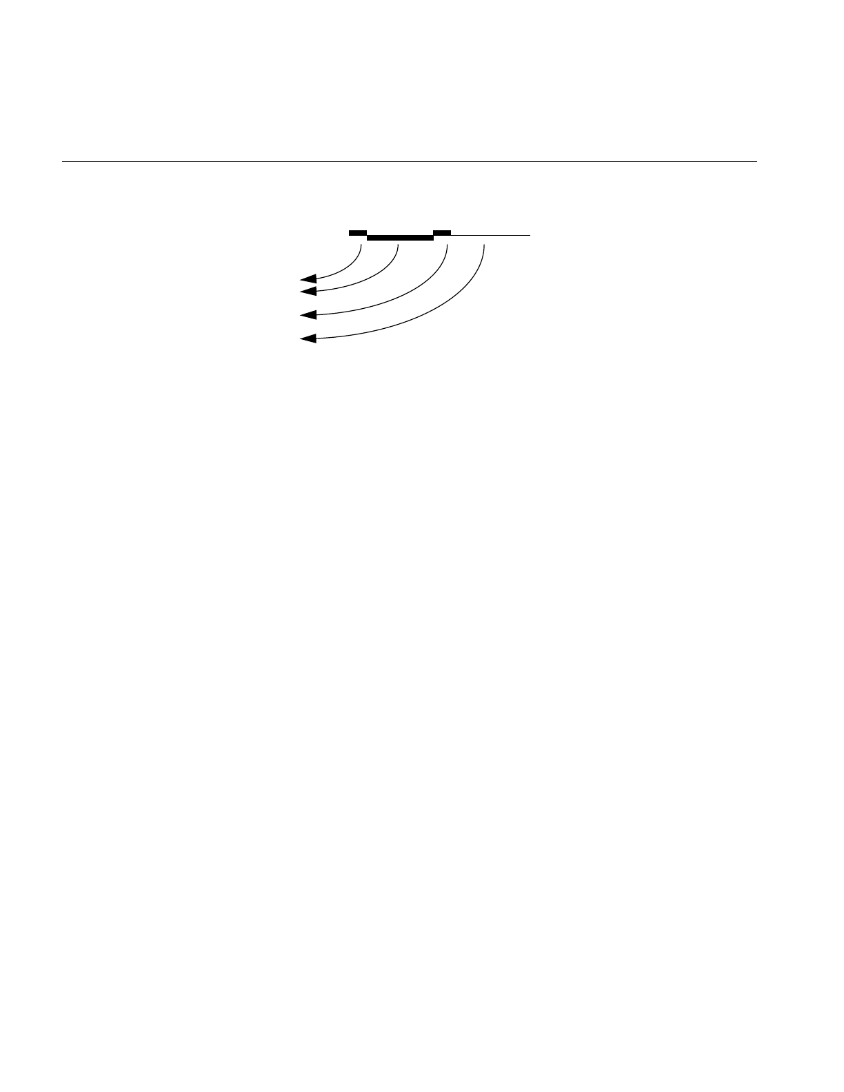
570
Chapter 18: Statistics
Figure 18-2 Conceptual Diagram of a Draw-Stage Timing Line
The following explains the potential displayed elements of each stage line in the timing
graph. Note that if you run your app or perfly you may not see some parts if the
corresponding operations are not needing to be done.
The application stage is divided into five subsegments, starting at the point where
pfFrame() returns and the new application frame is beginning:
• The time spent in the application’s main loop between the pfFrame() call and the
pfSync() call (highest segment in application line, drawn as a thick, bright line).
• The time spent cleaning the scene graph from application changes during pfSync();
drawn as mid-height thick, bright line. This will also include the time for
pfAppFrame() which is called from pfSync() if not already called for the current
frame by the user. pfSequences are also evaluated as part of pfAppFrame().
• The time spent sleeping in pfSync() while waiting for the next field or frame
boundary (depending on pfPhase and process model); the lowest point in the
application line, drawn as a thin pale dotted line. Note that in single process with
pfPhase of FREE_RUN, there will be a sleep period to wait for the swapbuffer of the
draw to complete before continuing with the application since any other graphics
call would effective force such a sleep anyway and in a place where its timing effect
could not be measured.
• The time spent in the application code between calling pfSync() and calling
pfFrame(); drawn as bright raised line. This is the critical path section and this line
should be as small as possible or non-existent.
• The time spent in pfFrame() cleaning the scene graph after any changes that might
have been made in the previous subsegment, and then checking intersections;
drawn as mid-height thick bright line. This line should typically be very small or
non-existent as it is part of the critical path and implies database changes between
pfSync() and pfFrame() which would be an expensive place to do such changes.
Before pfDraw
During pfDraw
After pfDraw
Drawing stats

Interpreting Statistics Displays
571
• The time spent waiting while the cull and other downstream process copy updated
information from the application and then starting the downstream stages on the
now-finished frame (drawn as a low thin line). The end of this line is where
pfFrame() returns and the user main application section (or post frame section)
starts again.
The cull stage is divided into only two subsegments:
• The time spent receiving updates from the application (in some multiprocessing
models, this overlaps with the last subsegment of the application stage). This time is
displayed for all channels even though it is only done one time. This is drawn as a
lowered thick line.
• The time spent in the channel cull callback for the given channel, including time
spent in pfCull() (drawn as raised line). Note that there may be a large space
between this and the update line if there are multiple channels on the same pfPipe
that are processed first.
The draw stage has potentially six subsegments:
• The time spent in the channel draw callback before the call to pfDraw() (a very
short thick dark raised segment. This will include the time for your call to
pfClearChan(). However, under normal circumstances, this segment should barely
be visible at all). Operations taking place during this time should only be
latency-critical since they are holding off the draw for the current frame.
• The time spent by IRIS Performer traversing the scene graph in pfDraw(); drawn as
lowered bright thick segment. This should typically be the largest segment of the
draw line.
• The time spent in the channel draw callback after pfDraw() (another short thick
dark raised segment;). On InfiniteReality, if graphics pipeline timing statistics have
been enabled (PFFSTATS_ENGFXPFTIMES), this line will include the time to finish
the fill for this channel. Otherwise, it only includes the time for the CPU to execute
and send graphics commands and graphics pipeline processing from this channel
could impact the timing of other channels.
• The time to rendering raster light points computed by a forked lpoint process. This
is drawn as a very raised bright line and if it exists will be the highest point in the
draw line.

572
Chapter 18: Statistics
• The last channel drawn on the pipe will include the time for the graphics pipeline to
finish its drawing. Even if you have no operations after pfDraw() in you draw
callback, this line for the last channel might look quite long, particularly if you are
very fill-limited and do not have InfiniteReality graphics pipeline statistics enabled.
It is possible for rendering calls issued in the previous section to fill up the graphics
FIFO and have calls issued on this section have to wait while the graphics pipeline
processes the commands and FIFO drains, making the time look longer than
expected. If there is no forked lpoint process, this line will be combined with the
post-draw line of the last pfChannel.
• The time spent waiting for the graphics pipeline to finish drawing the current
frame, draw the channel statistics (for all channels), and make the call to swap color
buffers. This is drawn as a pale dotted line. The hardware will complete the
swapbuffers upon the following vertical field or frame line.
Below the stage timing lines, the average time for each stage (in milliseconds) is shown.
Note that the time given for the draw stage is the same as the time shown for the draw
stage on the status line above the statistics box.
Load and Stress
The lower portion of the channel statistics diagram shows the recent history of graphics
load and stress management. The load measure is based on the amount of time taken to
draw previous frames in the channel relative to the specified goal frame time. A wavy
red horizontal line is drawn to show the last three seconds of graphics load. A pair of
white horizontal lines represent the upper and lower bounds of graphics load for
invoking stress management. Thus, when the red line wanders outside the boundaries
set by the white lines, stress management is invoked.
Stress management causes scaling of LODs in the database to meet the target frame rate
with maximum scene detail. The last three seconds of stress are shown in white while
stress management is running. Thus, the channel statistics graph can be used to tune the
upper and lower bounds of the hysteresis band for invoking stress management and for
tuning LODs of objects in the database.

Interpreting Statistics Displays
573
CPU Statistics
The CPU statistics keep track of system usage and requires that the corresponding
hardware statistics be enabled:
pfEnableStatsHw(PFSTATSHW_ENCPU);
The percentage of time CPUs spend idle, busy, in user code, and waiting on the Graphics
Pipeline, or on the swapping of memory is calculated. The statistics packages counts the
number of
• context switches (process and graphics)
• system calls
• times the graphics FIFO is found to be full
• times a CPU went to sleep waiting on a full graphics FIFO
• graphics pipeline IOCTLs issued (by the system)
• swapbuffers seen
All of these statistics are computed over an elapsed period of time.
Note: Use an interval of at least one second.
PFSTATSHW_CPU_SYS
This mode calculates the above CPU statistics for the entire system. This
mode is enabled by default.
PFSTATSHW_CPU_IND
This mode enables calculates the above CPU statistics for each
individual CPU; it is much more expensive than using just the summed
statistics.
CPU statistics, illustrated (with some other statistics) in Figure 18-3, give you
information on system usage and load. The numbers shown correspond exactly to
numbers given by osview; they’re updated every update period just like other statistics
(see “Setting Update Rate” on page 585 for information on how to change the update
rate). These numbers represent averages (per second) across all CPUs; thus, if one or
more CPUs is busy with some other task, the CPU statistics shown may not accurately
reflect IRIS Performer CPU use. Note that the top line of the CPU statistics panel shows
the total number of frames during the last update period, and the total time elapsed
during that period.
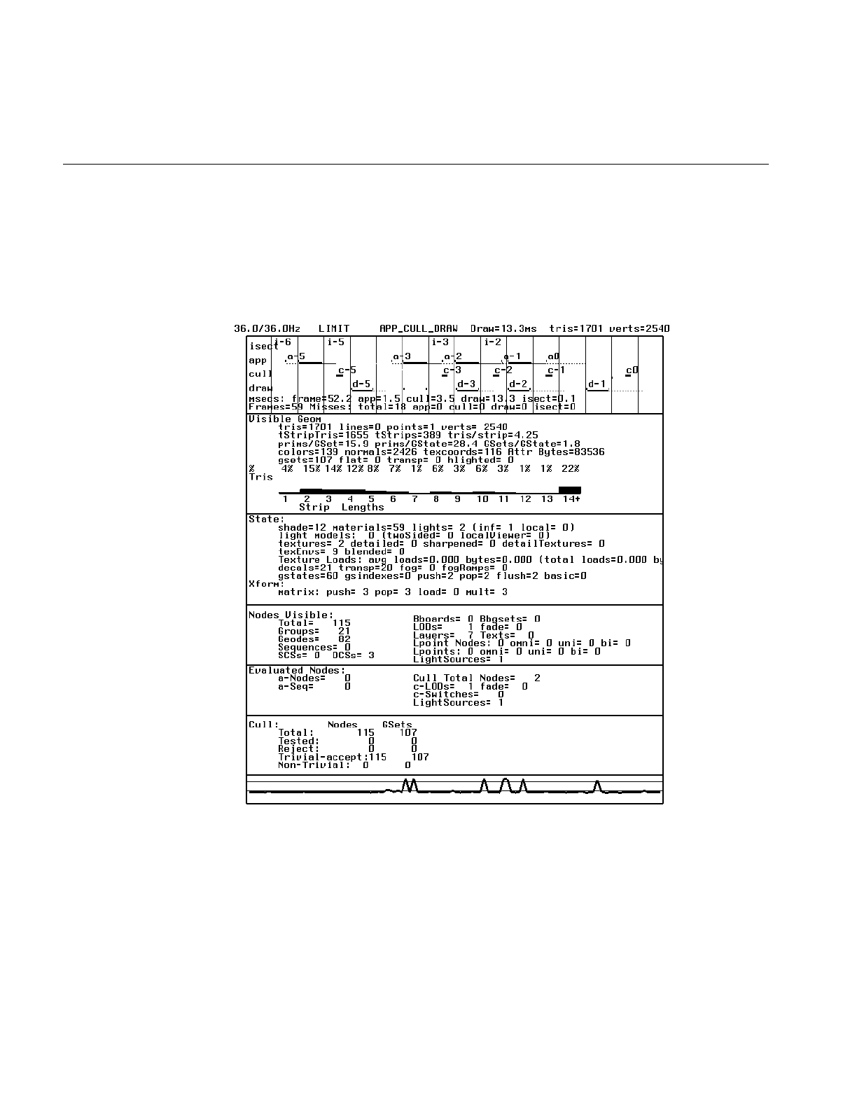
574
Chapter 18: Statistics
RTMon Statistics
The IRIX kernel collects timestamps via the rtmon daemon, rtmond(1). IRIS Performer
will issue rtmon timestamps for all operations in the timing graph if the rtmon statistics
are enabled via pfStatsClass(PFFSTATS_ENRTMON, PF_ON).
Figure 18-3 Other Statistics Classes

Interpreting Statistics Displays
575
Rendering Statistics
Several other classes of statistics can be shown, each representing a different aspect of
rendering performance. Some of these classes show:
• Data about visible geometry, including a histogram showing the percentage of
triangles in the scene that are part of strips of a given length (from 1 to 14). Quads
are counted as strips of length two; independent triangles count as strips of length
one. This histogram is mostly useful as a diagnostic to see how well your database
is structured for drawing efficiency; if it shows too many very short strips you may
want to go back and restructure your database. (As a general rule of thumb,
consider a “very short strip” to be one that’s less than 4 triangles long but that
number may vary depending on your database). To enable these statistics on a
channel do:
pfFStatsClass(pfGetChanFStats(chan),
PFSTATS_ENGFX, PFSTATS_ON);
• A summary of the graphics state operations (including loading of textures), and of
the number of operations that have recently been performed on the transformation
stack (also part of the GFX stats class), the number of libpf nodes being drawn, in
several categories (including billboards, light points, and geodes), plus the number
of nodes of each type evaluated in the application and cull stages which can be
enabled with
pfFStatsClass(pfGetChanFStats(chan),
PFSTATS_ENDB, PFSTATS_ON);
• Cull statistics, including how many nodes and pfGeoSets are being tested, how
many are accepted, and how many are rejected by the libpf culling task, enabled
with
pfFStatsClass(pfGetChanFStats(chan),
PFFSTATS_ENDB, PFSTATS_ON);
• Graphics pipeline timing statistics showing the time spent rendering as measured
by the graphics pipeline. This timing is then used internally for more accurate load
management. This is supported by InfiniteReality graphics platforms.
pfFStatsClass(pfGetChanFStats(chan),
PFSTATSHW_ENGFXPIPE_TIMES, PFSTATS_ON);

576
Chapter 18: Statistics
Fill Statistics
The fill statistics display indicates how many millions of pixels have been drawn since
the last statistics update. (For information on setting the length of time between statistics
updates, see “Setting Update Rate” on page 585). It also computes the average depth
complexity of the image, which is the average number of times each pixel was touched per
frame.
The depth complexity of a scene is also be displayed in the main channel. Each pixel will
be colored according to how many times that pixel was written to during display, rather
than according to the current rendering modes. The colors used range from dark blue
(not written to at all) to bright pink (written over many times). This color scheme is used
in calculating fill statistics; the coloring is done whenever you gather fill statistics, even
when you aren’t displaying the totals in your channel statistics display.
Stencil planes are used to store the number of times a pixel is written and thus to calculate
fill statistics. If n stencil planes are available, no more than 2n writes to any given pixel
will be counted. By default, the calculation of fill statistics uses three stencil planes; to
change that default, call pfStatsHwAttr().
Fill statistics are part of the libpr pfStats statistics but can be enabled on both pfStats and
pfFrameStats classes. To enable fill statistics you simply do:
pfStatsClass(statsptr,
PFSTATSHW_ENGFXPIPE_FILL, PFSTATS_ON);
To enable fill statistics for a channel’s pfFrameStats do:
pfFStatsClass(pfGetChanFStats(chan),
PFSTATSHW_ENGFXPIPE_FILL, PFSTATS_ON);
Examples of fill statistics can be found in perfly and in
/usr/share/Performer/src/pguide/libpr/C/fillstats.c.
Collecting and Accessing Statistics in Your Application
If you just want to bring up a statistics display in your application, you may not need to
know details about the data structures used for statistics. If, however, you want to do
more complicated statistics-handling (including collecting statistics without displaying
them), you need more advanced information. This section provides a general overview
of statistics manipulation, followed by subsections containing specific information.

Collecting and Accessing Statistics in Your Application
577
If you use libpf, a wide variety of statistics-manipulation functions is available. If you use
libpr, however, you must do some things on your own. For instance, you have to bind
your own pfStats structure in which to accumulate statistics.
Furthermore, you can’t access some kinds of statistics except through libpf calls—for
instance, you can’t get culling statistics using libpr calls. If you want full access to
statistics, you must use libpf. There are, however, libpr routines that allow you to do your
own cumulative totaling and averaging of collected statistics.
To create your own statistics display, enable the statistics classes you want to use and
disable any modes you don’t want to use. Then enable any relevant hardware, if
necessary, with pfEnableStatsHw().
To ensure the accuracy of timing with your rendering statistics, you want to flush the
graphics pipeline before calling pfGetTime(). You can do this in IRIS GL with finish()
and in OpenGL with glFinish(). These calls are expensive and shouldn’t be done more
than at the start and end of drawing in frame.
Displaying Statistics Simply
To put up a simple statistics display, all you have to do is call the function
pfDrawChanStats() and pass it a pointer to the pfChannel whose statistics you want to
display. The pfDrawChanStats() routine can be called from any process within the
application; the statistics will be displayed in the channel specified.
If you want to display one channel’s statistics in another channel, call pfDrawFStats();
for an example of this technique, as well as the enabling and disabling of every statistics
class, see the statistics programming example in the file
/usr/share/Performer/src/pguide/libpf/C/stats.c.
By default, a statistics display shows all enabled statistics. If you want to show only a
subset of the statistics you’re collecting, call pfChanStatsMode() with an enabling
bitmask indicating which classes are to be displayed.

578
Chapter 18: Statistics
Enabling and Disabling Statistics for a Channel
For efficiency, you may want to turn off statistics collection for a given channel when
you’re not displaying that channel’s statistics. In particular, the stage timing statistics are
enabled by default, so if you’re using a channel whose statistics you don’t care about, you
should disable statistics for that channel. To turn off statistics for a channel, call:
pfFStatsClass(pfGetChanFStats(chan),
PFSTATS_ALL, PFSTATS_OFF);
Use the same function with different parameters to enable all or specific classes of
statistics for a channel. You can specify which classes to enable in order to minimize
statistics collection overhead.
Statistics in
libpr
and
libpf
—pfStats Versus pfFrameStats
libpf statistics accumulate into a pfFrameStats structure to later be displayed, printed,
queried, or otherwise operated on. The pfFrameStats structure actually contains four
buffers of statistics: a buffer for the previous frame’s statistics, a buffer of averaged
statistics for the previous update period, a buffer of accumulated statistics for the current
update period, and a buffer of statistics being accumulated for the current frame.
The pfFrameStats structure is built upon the libpr pfStats structure, so the pfFrameStats
API includes routines to duplicate the functionality of pfStats. The duplicated API exists
because the routines cannot be intermixed. pfStats routines can only be used on pfStats
structures and pfFrameStats routines can only be called with pfFrameStats structures.
However, pfstats classes and class modes (designated with the PFSTATS_ prefix) can be
enabled on a pfFrameStats structure.
The pfStats statistics classes include the system and hardware statistics for the graphics
pipeline and the CPU, as well the pixel fill statistics and rendering statistics on geometry,
graphics state, and matrix transformations. Some of the libpr statistics commands, such
as pfEnableStatsHw(PFSTATSHW_ENGFXPIPE_FILL), require an active graphics
context and thus should only be called from the draw process. However, these
commands are usually never necessary in a libpf application because the pfFrameStats
operation will handle these commands automatically.

Collecting and Accessing Statistics in Your Application
579
Statistics Class Structures
The pfFrameStats structure and the pfStats structure are both inherited from the pfObject
structure. Thus, you can use the pfObject routines (pfCopy(),pfPrint(),pfDelete(),
pfUserData(),pfGetType(), and so on) with pfStats and pfFrameStats structures.
However, some pfObject routines will not support all of the semantics of a pfStats or
pfFrameStats structure, so some pfStats versions of a few of these routines take extra
arguments. These routines will have a pfFrameStats version as well. In particular,
pfCopyStats() and pfCopyFStats() should be used to copy pfStats and pfFrameStats
structures, respectively.
Routines that have “FStats” in their names (rather than just “Stats”) expect to be passed
a full pfFrameStats structure rather than a pfStats structure. The pfFrameStats API
includes additional routines beyond pfStats for supporting libpf statistics. For example,
pfDrawFStats() to display statistics in a channel and pfFStatsCountNode() to
accumulate the static database statistics for the scene graph rooted at the provided node.
Additionally, pfFrameStats has special support for the multiprocessed environment of
libpf and ensures that the statistics operations are all done in the correct process. All
modifying of a pfFrameStats structure, including enabling and disabling of classes,
printing, and copying, should all be done in the application process. pfDrawFStats() and
pfDrawChanStats() can be called in either the application process or the draw process.
Statistics Rules of Use
Enabling and disabling of statistics and setting of modes and attributes on a statistics
structure should always be done in the application process; the settings will
automatically be passed down the process pipeline. To enable classes of statistics on a
pfFrameStats, call pfFStatsClass() and provide a statistics structure, a bitmask of
statistics-enabling tokens (tokens with “STATS_EN” in their names) for the desired
classes, and the token PFSTATS_ON. Obtain the statistics structure from the desired
channel by calling pfGetChanFStats(). For example,
pfFStatsClass(pfGetChanFStats(chan), PFFSTATS_ENCULL |
PFFSTATS_ENDB, PFSTATS_ON);
enables the cull statistics and database statistics classes, leaving settings alone for any
other classes. Notice that the classes specific to pfFrameStats have a PFFSTATS_ prefix.
You can use PFSTATS_SET instead of PFSTATS_ON to enable only the specified classes
(disabling any others that might already be enabled).

580
Chapter 18: Statistics
Statistics Tokens
There are five main types of statistics tokens:
• Statistics class enable bitmasks, used for selecting a set of classes to enable with
pfStatsClass(). Class enables and disables are specified with bitmasks. Each
statistics class has an enable token: a PFSTATS_EN* token that can be OR-ed with
other statistics enable tokens and the result passed in to enable and disable statistics
operations. These bitmasks are also used when printing with pfPrint() or copying
with pfCopy() and pfCopyStats(), as well as with the pfResetStats(),
pfClearStats(),pfAverageStats(), and pfAccumulateStats() routines (and their
pfFrameStats counterparts). These tokens are of the form PFSTATS_EN* and
PFFSTATS_EN* for pfStats and pfFrameStats class respectively. The PFSTATS_ALL
token will select all statistics classes, and also all statistics buffers in the case of a
pfFrameStats structure. The token PFSTATS_EN_MASK selects all pfStats classes
and the token PFFSTATS_EN_MASK selects all pfFrameStats statistics classes,
which includes all pfStats classes.
• Value tokens, used to specify how to set a value for a specified pfStats or
pfFrameStats class enable or mode. Value tokens include PFSTATS_ON,
PFSTATS_OFF, and PFSTATS_DEFAULT. Another value token, PFSTATS_SET, is
used to specify that the entire class enable or mode bitmask should be set to the
specified mask. These tokens are used in conjunction with the class bitmasks and
the class name tokens for pfStatsClass() and pfStatsClassMode().
• Class name tokens, used to name a specific class. For instance, these tokens can be
passed to pfStatsClassMode() to set individual modes of a statistics class.
• Class mode tokens, of which each statistics class has its own, and which have the
form PFSTATS_class_mode and PFFSTATS_class_mode for pfStats and
pfFrameStats class modes, respectively.
• Statistics query tokens, used with pfQueryStats(), pfMQueryStats(),
pfQueryFStats(), and pfMQueryFStats(). These tokens are of the form
PFSTATSVAL_* and PFFSTATSVAL_* and have matching pfStatsVal* types for
holding the returned data. The token PFFSTATS_BUF_MASK selects the
pfFrameStats statistics buffers.

Collecting and Accessing Statistics in Your Application
581
Statistics Buffers
You can only access the PREV and CUM statistics buffers from the IRIS Performer
application process. Statistics from desired buffers in other processes should be queried
in the application process and then passed down the process pipeline, which you can do
using the channel data utility.
The AVG buffer is copied down the process pipeline at the end of each update period and
so is available to by queried by other processes. The CUR statistics buffer is the current
working area and contains the statistics accumulated so far from previous stages current
frame; the contents of the CUR buffer is very dependent on the multiprocess
configuration (but is almost always empty in the application process, so queries should
access the PREV buffer). Statistics that are added to the CUR buffer via copying,
accumulation, or immediate mode collection (such as with pfStatsCountGSet() and
pfFStatsCountNode()) will be propagated down the process pipeline and then back up
to the application process to be included in the PREV buffer.
In a libpf application, most statistics collection is completely automatic. The application
must simply enable the desired classes of statistics via pfStatsClass() and/or
pfStatsClassMode().
The IRIS Performer processes are responsible for actually opening the pfFrameStats
structure in which to accumulate the enabled statistics classes, as well as for managing
any statistics hardware resources. All types of libpf statistics can be accumulated without
ever making specific calls to open a structure for accumulation or enabling statistics
hardware.
When using only libpr statistics, however, one must explicitly open a pfStats structure for
statistics accumulation by calling pfOpenStats().
Hardware statistics resources must also be managed by an application using only libpr
statistics. Statistics function calls that have “HW” in their names, such as
pfEnableStatsHw() and pfStatsHwAttr(), directly access system hardware (such as
graphics hardware and CPU); be careful to make such calls only from the relevant
process.pfEnableStatsHw() expects PFSTATSHW_EN* bitmask tokens. Statistics classes
which have corresponding statistics hardware have a PFSTATSHW_ prefix in their token
names.
In a libpf application, IRIS Performer takes care of enabling the correct hardware modes
that correspond to enabled classes of statistics. For more information about specific
statistics classes, see the pfFrameStats(3pf) and pfStats(3pf) reference pages.

582
Chapter 18: Statistics
Reducing the Cost of Statistics
Collecting and displaying statistics can have a big impact on performance. This section
describes ways to reduce that impact.
Enabling Only Statistics of Interest
Each channel has its Process Frame Times (PFTIMES) statistics class enabled by default.
This class maintains a short history of process frames times, as well as averaging frame
times over the default update period of two seconds.
To minimize unnecessary overhead, turn off statistics on channels when you’re not using
them. To turn off all statistics for a channel, call pfFStatsClass() in the application process
with the statistics structure of the given channel:
pfFStatsClass(pfGetChanFStats(chan), PFSTATS_ALL,
PFSTATS_OFF);
Each statistics class has default mode settings. The short history of process frame time is
used to draw the timing graph. By default, this history consists of four frames of each
IRIS Performer process (app, cull, draw, intersections).
Maintaining this short history of statistics can be disabled by calling pfStatsClassMode()
with the token PFFSTATS_PFTIMES_HIST:
pfStatsClassMode(fstats, PFFSTATS_PFTIMES,
PFFSTATS_PFTIMES_HIST, PFSTATS_OFF);
This is useful if you’re only interested in the average frame times of each task with
minimal overhead and you don’t need to display the timing graph. However, for most
applications, the overhead incurred by keeping the timing history is not noticeable.
Controlling Update Rate
The update rate controls how often statistics are averaged and new results are made
available in the AVG buffer for display or query. Change the update rate by calling
pfFStatsAttr(fstats, {PFFSTATS_UPDATE_FRAMES,
PFFSTATS_UPDATE_SECS}, val);

Collecting and Accessing Statistics in Your Application
583
When the update rate is nonzero, statistics are accumulated every frame. When the
update period is set to zero, no statistics accumulation or averaging is done and only
statistics in the PREV and CUR buffers are maintained.
When statistics are accumulated and averaged, the averaging happens only in the
application process, but accumulation is done in each IRIS Performer process.
Statistics Output
Once you’ve collected some statistics, you need to be able to access and manipulate them.
Printing
To print the contents of pfStats and pfFrameStats structures, use the general pfPrint()
routine. The verbosity-level parameter to pfPrint() sets the level of detail to use in
printing statistics. Statistics class-enable bitmasks can be used to select a subset of
statistics to print. For instance, to print only the enabled statistics:
pfPrint(stats, pfGetStatsClass(stats, PFSTATS_ALL),
PFPRINT_VB_INFO, 0);
When printing the contents of pfFrameStats structures, you can select which buffers are
to be printed: PREV, CUR, AVG, or CUM. The selected statistics from all selected buffers
are printed. The following call prints the currently enabled statistics from the previous
frame and from the averaged statistics buffer:
pfPrint(stats, PFFSTATS_BUF_PREV | PFFSTATS_BUF_AVG |
pfGetStatsClass(stats, PFSTATS_ALL),
PFPRINT_VB_INFO, 0);
Copying
You can copy entire pfStats and pfFrameStats structures with the general pfCopy()
command. pfCopy() copies all of the statistics data, as well as information on mode
settings and which classes are enabled. The source and destination structures must be of
the same type. If both statistics structures are pfFrameStats structures, then all statistics
from all buffers are copied.

584
Chapter 18: Statistics
The pfCopyStats() and pfCopyFStats() routines copies only statistics data (not class
enables or mode settings) and accepts a class enable bitmask to select statistics classes for
the copy. For example:
pfCopyStats(statsA, statsB, pfGetStatsClass(statsB,
PFSTATS_ALL));
For a pfFrameStats structure, a PFFSTATS_BUF_* token can be included in the stats
enable bitmask to select the buffer to be accessed. If no buffer is specified, the CUR buffer
is used. For example,
pfCopyFStats(fstats, stats, PFFSTATS_BUF_PREV |
pfGetStatsClass(stats, PFSTATS_ALL));
copies the currently enabled classes of stats to the PREV pfStats in fstats.
In this case, it’s an error to select more than one statistics buffer, so PFSTATS_ALL cannot
be used as the select. If you specify two pfFrameStats structures, the buffer select is used
for both structures; if you select multiple buffers then each selected statistics class from
each selected buffer is copied. The pfCopyFStats() routine allows you to copy between
two different buffers of two pfFrameStats structures.
This routine takes explicit specification of PFFSTATS_BUF_* selects for source and
destination. Any PFFSTATS_BUF_* included with the class enable bitmask is simply
ignored, making it safe to specify PFSTATS_ALL. This routine will not accept a pfStats
structure.
Querying
pfQueryStats() and pfMQueryStats() (and corresponding pfFrameStats versions) can be
used to get values of out a pfStats or pfFrameStats structure and into an exposed
structure.
These routines are useful when you want to use specific statistics for your own custom
load management or for benchmarking, and you can use them to implement your own
custom statistics utility routines. pfQueryStats() and pfMQueryStats() both take a
pfStats (or pfFrameStats for pfQueryFStats() and pfMQueryFStats()) and return the
number of bytes written to the provided destination buffer. pfQueryStats() takes a token
that specifies a single query, while pfMQueryStats() expects a token buffer for multiple
queries. If an error is encountered, both query routines immediately halt and return with
the total number of bytes successfully written.

Collecting and Accessing Statistics in Your Application
585
There are specific tokens for querying individual values or entire classes of statistics. The
query tokens are of the form PFSTATSVAL_* and PFFSTATSVAL_*, and the
corresponding exposed structure names are of the form pfStatsVal* and pfFStatsVal*.
Queries on pfFrameStats structures with PFFSTATSVAL_* tokens expect a
PFFSTATS_BUF_* select token to be ORed with the query select. It’s an error to include
more than one pfFrameStats buffer select token. If no buffer select token is provided, the
CUR buffer will be queried. The statistics query tokens and structures are defined in
prstats.h and pfstats.h.
Customizing Displays
The standard statistics displays have several parameters hard-wired in. For instance, you
can’t change the colors used in such displays. If you want to use different colors, you’ll
have to use your own display routines.
Setting Update Rate
To set the frequency at which statistics are automatically collected, use pfFStatsAttr().
See the pfFrameStats(3pf) reference page for details. If you want to turn off cumulative
statistics collection (and thus running averages) entirely, set the update rate to zero.
(Note that doing this will change your statistics display; in particular, your actual frame
rate will be changed and other averages will not be displayed.)
The pfStats Data Structure
The pfStats data structure contains four statistics buffers: one for current statistics, one
for previous statistics, one for cumulative statistics, and one for averages.
If you’re using libpf calls to have IRIS Performer keep track of statistics for you, you
should always look at the previous-stats buffer; the current-stats buffer is kept in a state
of flux, and if you look at it you’re likely to find meaningless numbers there.
If, on the other hand, you’re using libpr and keeping track of your own statistics, the
current-stats buffer does contain accurate information.

Statistics Examples
This section contains some examples of statistics calls.
Setting statistics class enables and modes
Set all stats class enables on a pfStats to their default values:
pfStatsClass(stats, PFSTATS_ALL, PFSTATS_DEFAULT);
Set all modes for the PFSTATS_GFX class on a pfFrameStats to their default values:
pfFStatsClassMode(fstats, PFSTATS_GFX, PFSTATS_ALL,
PFSTATS_DEFAULT);
Note that pfStatsClassMode() takes a class name as its class specifier (second argument)
and not a bitmask. However, you can use PFSTATS_CLASS to refer to the modes of all
classes;
pfFStatsClassMode(fstats, PFSTATS_MODE, PFSTATS_ALL,
PFSTATS_DEFAULT);
sets all modes of all pfStats classes to their default values. For pfFrameStats classes, there
is PFFSTATS_CLASS:
Set the entire class enable mask to all PFSTATS_ALL, effectively enabling all statistics
classes:
pfFStatsClass(fstats, PFFSTATS_ALL, PFSTATS_SET);
Force off all modes of the PFSTATS_GFX class of a pfStats:
pfStatsClassMode(stats, PFSTATS_GFX, PFSTATS_OFF,
PFSTATS_SET);
To track triangle strip lengths on a pfFrameStats, enable the graphics statistics class
mode:
pfFStatsClassMode(fstats, PFSTATS_GFX,
PFSTATS_GFX_TSTRIP_LENGTHS, PFSTATS_ON);

This chapter explains how to use performance measurement and debugging
tools and provides hints for deriving maximum performance from your
applications.
“Performance Tuning and Debugging”
Chapter 19


589
Chapter 19
19. Performance Tuning and Debugging
This chapter provides some basic guidelines to follow when tuning your application for
optimal performance. It also describes how to use debugging tools like pixie,prof, gldebug,
and glprof to debug and tune your applications. It concludes with some specific notes on
tuning applications on systems with RealityEngine graphics.
Performance-Tuning Overview
This section contains some general performance-tuning principles. Some of these issues
are discussed in more detail later in this chapter.
• Remember that high performance doesn’t come by accident. You must design your
programs with speed in mind for optimal results.
• Tuning graphical applications, particularly IRIS Performer applications, requires a
pipeline-based approach. You can think of the graphics pipeline as comprising three
separate stages; the pipeline runs only as fast as the slowest stage, so improving the
performance of the pipeline requires improving the slowest stage’s performance.
The three stages are:
– The host (or CPU) stage, in which routines are called and general processing is
done by the application. This stage can be thought of as a software pipeline,
sometimes called the rendering pipeline, itself comprising up to three
sub-stages—the application, cull, and draw stages—as discussed at length
throughout this guide.
– The transformation stage, in which transformation matrices are applied to
objects to position them in space (this includes matrix operations, setting
graphics modes, transforming vertices, handling lighting, and clipping
polygons).
– The fill stage, which includes clearing the screen and then drawing and filling
polygons (with operations such as Gouraud shading, z-buffering, and texture
mapping).

590
Chapter 19: Performance Tuning and Debugging
• You can estimate your expected frame rate based on the makeup of the scene to be
drawn and graphics speeds for the hardware you’re using. Be sure to include fill
rates, polygon transform rates, and time for mode changes, matrix operations, and
screen clear in your calculations.
• Measure both the performance of complex scenes in your database and of
individual objects and drawing primitive to verify your understanding of the
performance requirements.
• Use the IRIS Performer diagnostic statistics to evaluate how long each stage takes
and how much it does. See Chapter 18, “Statistics,” for more information. These
statistics are referred to frequently in this chapter.
• Use system tools to help profile and analyze your application. The IRIS GL glprof
utility (described in “Using glprof to Find Performance Bottlenecks” on page 610)
will profile the rendering of an IRIS GL programs and show what was drawn and
help figure out what stage of the graphics hardware pipeline is the significant
bottleneck.
• Tuning an application is an incremental process. As you improve one stage’s
performance, bottlenecks in other stages may become more noticeable. Also, don’t
be discouraged if you apply tuning techniques and find that your frame rate doesn’t
change—frame rates only change by a field at a time (which is to say in increments
of 16.67 milliseconds for a 60 Hz display), while tuning may provide speed
increases of finer granularity than that. To see performance improvements that
don’t actually increase frame rate, look at the times reported by IRIS Performer
statistics on the cull and draw processes (see Chapter 18 for more information).
• See the graphics library books listed in the “Bibliography” on page xxxvi for
information about how to get peak performance from your graphics hardware,
beyond what IRIS Performer does for you.
How IRIS Performer Helps Performance
IRIS Performer uses many techniques to increase application performance. Knowing
about what IRIS Performer is doing and how it affects the various pipeline stages may
help you write more efficient code. This section lists some of the things IRIS Performer
can do for you.

How IRIS Performer Helps Performance
591
Draw Stage and Graphics Pipeline Optimizations
During drawing, IRIS Performer
• Sets up an internal record of what routines and rendering methods are fastest for
the current graphics platform. This information can be queried in any process with
pfQueryFeature(). You can use this information at run time when setting state
properties on your pfGeoStates.
• Has machine-dependent fast options for commands that are very performance
sensitive. Use the _ON and _FAST mode settings whenever possible to get
machine-dependent high-performance defaults. Some examples include:
•pfAntialias(PFAA_ON)
•pfTransparency(PFTR_ON)
•pfDecal(PFDECAL_BASE_FAST)
•pfTexFilter(tex, filt, PFTEX_FAST)
•pfTevMode(tev, PFTEV_FAST)
• Sets up default modes for drawing, multiprocessing, statistics, and other areas, that
are chosen to provide high scene quality and performance. Some rendering defaults
differ from GL defaults: backface elimination is enabled by default
(pfCullFace(PFCF_BACK)) and lighting materials use lmcolor() in IRIS GL and
glColorMaterial() in OpenGL to minimize the number of materials required in a
database (pfMtlColorMode(mtl, side, PFMTL_CMODE_AD)).
• Uses a large number of specialized routines for rendering different kinds of objects
extremely quickly. There’s a specialized drawing routine for each possible pfGeoSet
configuration (each choice of primitive type, attribute bindings, and index
selection). Each time you change from one pfGeoSet to another, one of these
specialized routines is called. However, this happens even if the new pfGeoSet has
the same configuration as the old one, so larger pfGeoSets are more efficient than
smaller ones—the function-call overhead for drawing many small pfGeoSets can
reduce performance. As a rule of thumb, a pfGeoSet should contain at least
4 triangles, and preferably between 8 and 64. If the pfGeoSet is too large, it can
reduce the efficiency of other parts of the process pipeline.

592
Chapter 19: Performance Tuning and Debugging
• Caches state changes, because applying state changes is costly in the draw stage.
IRIS Performer accumulates state changes until you call one of the pfApply*()
functions, at which point it applies all the changes at once. Note that this differs
from the graphics libraries, in which state changes are immediate. If you have
several state changes to make in IRIS Performer, set up all the changes before
applying them, rather than using the one-change-at-a-time approach (with each
change followed by an apply operation) that you might expect if you’re used to
graphics library programming.
• Evaluates state changes lazily—that is, it avoids making any redundant changes.
When you apply a state change, IRIS Performer compares the new graphics state to
the previous one to see if they’re different. If they are, it checks whether the new
state sets any modes. If it does, IRIS Performer checks each mode being set to see
whether it’s different from the previous setting. To take advantage of this feature,
share pfGeoStates and inherit states from the global state wherever possible. Set all
the settings you can at the global level and let other nodes inherit those settings,
rather than setting each node’s attributes redundantly. To do this within a database,
you can set up pfGeoStates with your desired global state and apply them to the
pfChannel or pfScene with pfChanGState() or pfSceneGState(). You can do this
through the database loader utilities in libpfdu trivially for a given scene with
pfdMakeSharedScene(), or have more control over the process with
pfdDefaultGState(),pfdMakeSceneGState(), and pfdOptimizeGStateList().
• Provides an optimized immediate mode rendering display list data type,
pfDispList, in libpr. The pfDispList type reduces host overhead in the drawing
process and requires much less memory than a graphics library display list. libpf
uses pfDispLists to pass results from the cull process to the draw process when the
PFMP_CULL_DL_DRAW mode is turned on as part of the multiprocessing model.
For more information about display lists, see “Display Lists” in Chapter 9; for more
information about multiprocessing, see “Successful Multiprocessing With IRIS
Performer” in Chapter 5.

How IRIS Performer Helps Performance
593
Cull and Intersection Optimizations
To help optimize culling and intersection, IRIS Performer
• Provides pfFlatten() to resolve instancing (via cloning) and static matrix
transformations (by pre-transforming the cloned geometry). It can be especially
important to flatten small pfGeoSets; otherwise matrix transformations must be
applied to each small pfGeoSet at significant computational expense. Note that
flattening resolves only static coordinate systems, not dynamic ones, but that where
desired, pfDCS nodes can be converted to pfSCS nodes automatically using the IRIS
Performer utility function pfdFreezeTransforms(), which allows for subsequent
flattening. Using pfFlatten(), of course, increases performance at the cost of greater
memory use. Further, the function pfdCleanTree() can be used to remove needless
nodes: identity matrix pfSCS nodes, single child pfGroup nodes, and the like.
• Uses bounding spheres around nodes for fast culling—the intersection test for
spheres is much faster than that for bounding boxes. If a node’s bounding sphere
doesn’t intersect the viewing frustum, there’s no need to descend further into that
node. There are bounding boxes around pfGeoSets; the intersection test is more
expensive but provides greater accuracy at that level.
• Provides the pfPartition node type to partition geometry for fast intersection
testing. Use a pfPartition node as the parent for anything that needs intersection
testing.
• Provides level-of-detail (LOD) capabilities in order to draw simpler (and thus
cheaper) versions of objects when they’re too far away for the user to discern small
details.
• Allows intersection performance enhancement via precomputation of polygon
plane equations within pfGeoSets. This pre-computation is in the form of a traversal
that is nearly always appropriate—only in cases of non-intersectable or dynamically
changing geometry might these cached plane equations be disadvantageous. This
optimization is performed by pfuCollideSetup() using the PFTRAV_IS_CACHE bit
mask value.
• Sorts pfGeoSets by graphics state in the cull process, in order to minimize state
changes and flatten matrix transformations, when libpf creates display lists to send
to the draw process (as occurs in the PFMP_CULL_DL_DRAW multiprocessing
mode). This procedure takes extra time in the cull stage, but can greatly improve
performance when rendering a complex scene that uses many pfGeoStates. The
sorting is enabled by default; it can be turned off and on by calling the function
pfChanTravMode(chan, PFTRAV_CULL, mode) and including or excluding the
PFCULL_SORT token. See “pfChannel Traversal Modes” in Chapter 4 and “Sorting
the Scene” in Chapter 4 for more information on sorting.

594
Chapter 19: Performance Tuning and Debugging
Application Optimizations
During the application stage, IRIS Performer
• Divides the application process into two parts: the latency-critical section (which
includes everything between pfSync() and pfFrame()), where last-minute
latency-critical operations are performed before the cull of the current frame can
start; and the noncritical portion, after pfFrame() and before pfSync(). The critical
section is displayed in the channel statistics graph drawn with pfDrawChanStats().
• Provides an efficient mechanism to automatically propagate database changes
down the process pipeline, and provides pfPassChanData() for passing custom
application data down the process pipeline.
• Minimizes overhead copying database changes to the cull process by accumulating
unique changes and updating the cull once inside pfFrame(). This updated period
is displayed in the MP statistics of the channel statistics graph drawn with
pfDrawChanStats().
• Provides a mechanism for performing database intersections in a forked process:
pass the PFMP_FORK_ISECT flag to pfMultiprocess() and declare an intersection
callback with pfIsectFunc().
• Provides a mechanism for performing database loading and editing operations in a
forked process, such as the DBASE process: pass the PFMP_FORK_DBASE flag to
pfMultiprocess() and declare an intersection callback with pfDBaseFunc().
Specific Guidelines for Optimizing Performance
While IRIS Performer provides inherent performance optimization, there are specific
techniques you can use to increase performance even more. This section contains some
guidelines and advice pertaining to database organization, code structure and style,
managing system resources, and rules for using IRIS Performer.

Specific Guidelines for Optimizing Performance
595
Graphics Pipeline Tuning Tips
Tuning the graphics pipeline requires identifying and removing bottlenecks in the
pipeline. You can remove a bottleneck either by minimizing the amount of work being
done in the stage that has the bottleneck or, in some cases, by reorganizing your
rendering to more effectively distribute the workload over the pipeline stages. This
section contains specific tips for finding and removing bottlenecks in each stage of the
graphics pipeline. For more information on this topic, refer to the graphics library
documentation (see “Bibliography” on page xxxvii for information on ordering these
books).
Host Bottlenecks
Here are some ways to minimize the time spent in the host stage of the graphics pipeline:
• Function calls, loops, and other programming constructs require a certain amount
of overhead. To make such constructs cost-effective, make sure they do as much
work as possible with each invocation. For instance, drawing a pfGeoSet of triangle
strips involves a nested loop, iterating on strips within the set and triangles within
each strip; it therefore makes sense to have several triangles in each strip and
several strips in each set. If you put only two triangles in a pfGeoSet, you’ll spend
all that loop overhead on drawing those two triangles, when you could be drawing
many more with little extra cost. The channel statistics can display (as part of the
graphics statistics) a histogram showing the percentage of your database that is
drawn in triangle strips of certain lengths.
• Only bind vertex attributes that are actually in use. For example, if you bind
per-vertex colors on a set of flat-shaded quads, the software will waste work by
sending those colors to the graphics pipeline, which will ignore them. Similarly, it’s
pointless to bind normals on an unlit pfGeoSet.
• Nonindexed drawing has less host overhead than indexed drawing because
indexed drawing requires an extra memory reference to get the vertex data to the
graphics pipeline. This is most significant for primitives that are easily host-limited,
such as independent polygons or very short triangle strips. However, indexed
drawing can be very helpful in reducing the memory requirements of a very large
database.
• Enable state sorting for pfChannels (this is the default). By sorting, the CPU does
not need to examine as many pfGeoStates. The graphics channel statistics can be
used to report the pfGeoSet-to-pfGeoState drawing ratio.

596
Chapter 19: Performance Tuning and Debugging
Transform Bottlenecks
A transform bottleneck can arise from expensive vertex operations, from a scene that’s
typically drawn with many very tiny polygons, from a scene modeled with inefficient
primitive types, or from excessive mode or transform operations. Here are some tips on
reducing such bottlenecks:
• Connected primitives will have better vertex rates than independent primitives,
and quadrilaterals are typically much more efficient in vertex operations than
independent triangles are.
• The expensive vertex operations are generally lighting calculations. The fastest
lighting configuration is always one infinite light. Multiple lights, local viewing
models, and local lights have (in that order) dramatically increasing cost. Two-sided
lighting also incurs some additional transform cost. On some graphics platforms,
texturing and fog can add further significant cost to per-vertex transformation. The
channel graphics statistics will tell you what kinds of lights and light models are
being used in the scene.
• Matrix transforms are also fairly expensive, and definitely more costly than one or
two explicit scale, translate, or rotate operations. When possible, flatten matrix
operations into the database with pfFlatten().
• The most frequent causes of mode changes are shademodel() (or glShadeModel()),
textures, and object materials. The speed of these changes depends on the graphics
hardware; however, material changes do tend to be expensive. Sharing materials
among different objects can be increased with the use of pfMtlColorMode() that is
PFMTL_CMODE_AD by default. However, on some older graphics platforms (such
as the Elan, Extreme, and VGX), the use of pfMtlColorMode() (which actually calls
the IRIS GL function lmcolor() or the OpenGL function glColorMaterial()) has
some associated per-vertex cost and should be used with some caution.
• If you cull stage is not a bottleneck, make sure your pfChannels sort the scene by
graphics state. Even if you are running in single process mode, the extra time taken
to sort the database is often more than offset by the savings in rendering time. See
“Sorting the Scene” in Chapter 4 for more details on how to configure sorting.

Specific Guidelines for Optimizing Performance
597
Fill Bottlenecks
Here are some methods of dealing with fill-stage bottlenecks:
• One technique to hide the cost of expensive fill operations is to fill the pipeline from
the back forward so that no part is sitting idle waiting for an upstream stage to
finish. The last stage of the pipeline is the fill stage, so by drawing backgrounds or
clearing the screen via pfClearChan() first, before pfDraw(), you can keep the fill
stage busy. In addition, if you have a couple of large objects that reliably occlude
much of the scene, drawing them very early on can both fill up the back-end stage
and also reduce future fill work, because the occluded parts of the scene will fail a
z-buffer test and will not have to write z values to the z-buffer or go on to more
complex fill operations.
• Use the pfStats fill statistics (available for display through the channel statistics) to
visualize your depth complexity and get a count of how many pixels are being
computed each frame.
• Be aware of the cost of any fill operations you use and their relative cost on the
relevant graphics hardware configuration. Quick experiments you can do to test for
a fill limitation include:
– Rendering the scene into a smaller window, assuming that doing so will not
otherwise affect the scene drawn (a non-zero pfChannel LOD scale will cause a
change in object LODs when you shrink the window).
– Using pfOverride() to force the disabling of an expensive fill mode.
If either of these tests causes a significant reduction in the time to draw the scene,
then a significant fill bottleneck probably exists.
Note: Some features may invoke expensive modes that need to be used with caution
on some hardware platforms. pfAntialias() and pfTransparency() enable blending if
multisampling isn’t available. Globally enabling these functions on machines
without multisampling can produce significant performance degradation due to the
use of blending for an entire scene. Blending of even opaque objects incurs its full
cost. pfDecal() may invoke stenciling (particularly if you have requested the decal
mode PFDECAL_BASE_HIGH_QUALITY or if there is no faster alternative on the
current hardware platform), which can cause performance degradations on some
system. pfFeature() can be used to verify the availability and speed of these features
on the current graphics platform.

598
Chapter 19: Performance Tuning and Debugging
• The cost of specific fill operations can vary greatly depending on the graphics
hardware configuration. As a rule of thumb, flat shading is much faster than
Gouraud shading because it reduces both fill work and the host overhead of
specifying per-vertex colors. Z-buffering is typically next in cost, and then stencil
and blending. On a RealityEngine, the use of multisampling can add to the cost of
some of these operations, specifically z-buffering and stenciling. See
“Multisampling” on page 620 for more information. Texturing is considered free on
RealityEngine and Impact systems but is relatively expensive on a VGX and is
actually done in the host stage on lower-end graphics platforms, such as Extreme
and XZ. Some of the low-end graphics platforms also implement z-buffering on the
host.
• You may not be able to achieve benchmark-level performance in all cases for all
features. For instance, if you frequently change modes and you use short triangle
strips, you get much less than the peak triangle mesh performance quoted for the
machine. Fill rates are sensitive to both modes, mode changes, and polygon sizes.
As a general rule of thumb, assume that fill rates average around 70% of peak on
general scenes to account for polygon size and position as well as for pipeline
efficiency.
Process Pipeline Tuning Tips
These simple tips will help you optimize your IRIS Performer process pipeline:
• Use pfMultiprocess() to set the appropriate process model for the current machine.
• You usually shouldn’t specify more processes with pfMultiprocess() than there are
CPUs on the system. The default multiprocess mode (PFMP_DEFAULT) attempts
an optimal configuration for the number of unrestricted CPUs. However, if there are
fewer processors than significant tasks (consider APP, CULL, DRAW, ISECT,
DBASE) you will want experiment with the different two-process models to find the
one that will yield the best overall frame rate. Use of pfDrawChanStats(), described
in Chapter 18, “Statistics,” will greatly help with this task.
• Put only latency-critical tasks between the pfSync() and pfFrame() calls. For
example, put latency-critical updates, like changes to the viewpoint, after pfSync()
but before pfFrame(). Put time-consuming tasks, such as intersection tests and
system dynamics, after pfFrame().
• You will also want to refer to the IRIX REACT™ documentation for setting up a
real-time system.

Specific Guidelines for Optimizing Performance
599
• For maximum performance, use the IRIS Performer utilities in libpfutil for setting
non-degrading priorities and isolating CPUs (pfuPrioritizeProcs(),
pfuLockDownProc(),pfuLockDownApp(),pfuLockDownCull(),
pfuLockDownDraw()). These facilities require that the application runs with root
permissions. The source code for these utilities is in
/usr/share/Performer/src/lib/libpfutil/lockcpu.c. For an example of there use, see the
sample source code in /usr/share/Performer/src/pguide/libpf/C/bench.c. For more
information about priority scheduling and real-time programming, see the chapter
of the IRIX System Programming Guide entitled “Using Real-Time Programming
Features.” and the IRX REACT technical report.
• Make sure you aren’t generating any floating-point exceptions. Floating-point
exceptions can cause an individual computation to incur tens of times its normal
cost. Furthermore, a single floating point exception can lead to many further
exceptions in computations that use the exceptional result and can even propagate
performance degradation down the process pipeline. IRIS Performer will detect and
tell you about the existence of floating point exceptions if your pfNotifyLevel() is
set to PFNFY_INFO or PFNFY_DEBUG. You can then run your application in dbx
and your application will stop when it encounters an exception, enabling you to
trace the cause.
• Make sure the main pipeline (APP, CULL, DRAW processes) do not make per-frame
memory allocations or deallocations (asynchronous processes like DBASE can do
per-frame allocations). You can use the libdmalloc runtime malloc debugging
library’s tracing feature to verify that no memory allocation routines are being
called. See the “Memory Corruption and Leaks” section later in this chapter for
more about libdmalloc.
• Minimize the amount of channel data allocated by pfAllocChanData() and call
pfPassChanData() only when necessary to reduce the overhead of copying the
data. Copying pointers instead of data is often sufficient.

600
Chapter 19: Performance Tuning and Debugging
Cull Process Tips
Here are a couple of suggestions for tuning the cull process:
• The default channel culling mode enables all types of culling. If your cull process is
your most expensive task, you may want to consider doing less culling operations.
When doing database culling, always use view-frustum culling (PFCULL_VIEW),
and usually use graphics library mode database sorting (PFCULL_SORT) and
pfGeoSet culling (PFCULL_GSET) as well:
pfChanTravMode(chan, root,
PFCULL_VIEW | PFCULL_GSET | PFCULL_SORT);
A cull-limited application might realize a quick gain from turning off pfGeoSet
culling. If you think your database has few textures and materials, you might turn
off sorting. However, if possible it would be better to try improving cull
performance by improving database construction. “Efficient Intersection and
Traversals” on page 602 discusses optimizing cull traversals in more detail.
• Look at the channel culling statistics for:
– A large amount of the database being traversed by the culling process and
being trivially rejected as not being in the viewing frustum. This can be
improved with better spatial organization of the database.
– A large number of database nodes being non-trivially culled. This can be
improved with better spatial organization and breakup of large pfGeodes and
pfGeoSets.
– A surprising number of LODs in their fade state (the fade computations can be
expensive, particularly if channel stress management has been enabled).
• Balance the database hierarchy with the scene complexity: the depth of the
hierarchy, the number of pfGeoStates, and the depth of culling. See “Balancing Cull
and Draw Processing with Database Hierarchy” on page 604 for details.
• pfNodes that have significant evaluation in the cull stage include pfBillboards,
pfLightPoints, pfLightSources, and pfLODs.

Specific Guidelines for Optimizing Performance
601
Draw Process Tips
Here are some suggestions specific to the draw process:
• Minimize host work done in the draw process before the call to pfDraw(). Time
spent before the call to pfDraw() is time that the graphics pipeline is idle. Any
graphics library (or X) input processing or mode changes should be done after
pfDraw() to take effect the following frame.
• Use only one pfPipe per hardware graphics pipeline and preferably one
pfPipeWindow per pfPipe. Use multiple channels within that pfPipeWindow to
manage multiple views or scenes. It’s fairly expensive to simultaneously render to
multiple graphics windows on a single hardware graphics pipeline and is not
advisable for a real-time application.
• Pre-define and pre-load all of the textures in the database into hardware texture
memory by using a pfApplyTex() function on each pfTexture. You can do this
texture-applying in the pfConfigStage() draw callback or (for multipipe
applications to allow parallelism) the pfConfigPWin() callback. This approach
avoids the huge performance impact that results when textures are encountered for
the first time while drawing the database and must then be downloaded to texture
memory. Utilities are provided in libpfutil to apply textures appropriately; see the
pfuDownloadTexList() routine in the distributed source code file
/usr/share/Performer/src/lib/libpfutil/tex.c. The perfly application demonstrates this; see
the perfly source file generic.c in either the C-language
(/usr/share/Performer/src/sample/C/common) or C++ language
(/usr/share/Performer/src/sample/C++/common) versions of perfly.
• Minimize the use of pfSCSs and pfDCSs and nodes with draw callbacks in the
database since aggressive state sorting is kept local to subtrees under these nodes.
• Don’t do any graphics library input handling in the draw process. Instead, use
X input handling in an asynchronous process. IRIS Performer provides utilities for
asynchronous input handling in libpfutil with source code provided in
/usr/share/Performer/src/lib/libpfutil/input.c. For a demonstration of asynchronous
X input handling, see provided sample applications, such as perfly, and also the
distributed sample programs /usr/share/Performer/src/pguide/libpf/C/motif.c and
/usr/share/Performer/src/pguide/libpfui/C/motifxformer.c.

602
Chapter 19: Performance Tuning and Debugging
Efficient Intersection and Traversals
Here are some tips on optimizing intersections and traversals:
• Use pfPartition nodes on pieces of the database that will be handed to intersection
traversal. These nodes impose spatial partitioning on the subgraph beneath them,
which can dramatically improve the performance of intersection traversals.
Note: Subgraphs under pfDCS, pfLOD, pfSwitch, and pfSequence nodes are not
partitioned so intersection traversals of these subgraphs will not be affected.
• Use intersection caching. For static objects, enable intersection caching at
initialization—first call pfNodeTravMask(), specifying intersection traversal
(PFTRAV_ISECT), and then include PFTRAV_IS_CACHE in the mode for
intersections. You can turn this mode on and off for dynamic objects as appropriate.
• Use intersection masks on nodes to eliminate large sections of the database when
doing intersection tests. Note that intersections are sproc()-safe in the current
version of IRIS Performer; you can check intersections in more than one process.
• Bundle segments for intersections with bounding cylinders. You can pass as many
as 32 segments to each intersection request. If the request contains more than a few
segments and if the segments are close together, the traversal will run faster if you
place a bounding cylinder around the segments using pfCylAroundSegs() and pass
that bounding cylinder to pfNodeIsectSegs(). The intersection traversal will use the
cylinder rather than each segment when testing the segments against the bounding
volumes of nodes and pfGeoSets.
Database Concerns
Optimizing your databases can provide large performance increases.
libpr
Databases
The following tips will help you achieve peak performance when using libpr:
• Minimize the number of pfGeoStates by sharing as much as possible.
• Initialize each mode in the global state to match the majority of the database, in
order to set as little local state for individual pfGeoStates as possible.
• Use triangle strips wherever possible; they produce the largest number of polygons
from a given number of vertices, so they use the least memory and are drawn the
fastest of the primitive types.

Specific Guidelines for Optimizing Performance
603
• Use the simplest possible attribute bindings and use flat-shaded primitives
wherever possible. If you’re not going to need an object’s attributes, don’t bind
them—anything you bind will have to be sent to the pipeline with the object.
• Flat-shaded primitives and simple attribute bindings reduce the transformation and
lighting requirements for the polygon. Note that the flat-shaded triangle-strip
primitive renders faster than a regular triangle strip, but you have to change the
index by two to get the colors right (that is, you need to ignore the first two vertices
when coloring). See “Attribute Bindings” in Chapter 8 for more information.
• Use nonindexed drawing wherever possible, especially for independent polygon
primitives and short triangle strips.
• When building the database, avoid fragmentation in memory of data to be
rendered. Minimize the number of separate data and index arrays. Keep the data
and index arrays for pfGeoSets contiguous and try to keep separate pfGeoSets
contiguous to avoid small, fragmented pfMalloc() memory allocations.
• The ideal size of a pfGeoSet (and of each triangle strip within the pfGeoSet)
depends a great deal on the specific CPU and system architecture involved; you
may have to do benchmarks to find out what’s best for your machine. For a general
rule of thumb, use at least 4 triangles per strip on any machine, and 8 on most. Use
5 to 10 strips in each pfGeoSet, or a total of 24 to 100 triangles per pfGeoSet.
libpf
Databases
When you’re using libpf, the following tips can improve the performance of database
tasks:
• Use pfFlatten(), especially when a pfScene contains many small instanced objects
and billboards. Use pfdCleanTree() and (if application considerations permit)
pfdFreezeTransforms() to minimize the cull traversal processing time and
maximize state sorting scope.
• Initialize each mode in the scene pfGeoState to match the majority of the database,
in order to set as little local state for individual pfGeoStates as possible. The utility
function pfdMakeSharedScene() provides an easy to use mechanism for this task.
• Minimize the number of very small pfGeoSets (that is, those containing four or
fewer total triangles). Each tiny pfGeoSet means another bounding box to test
against if you’re culling down to the pfGeoSet level (that is, when PFCULL_GSET is
set with pfChanTravMode()) as well as another item to sort during culling. (If your
pfGeoSets are large, on the other hand, you should definitely cull down to the
pfGeoSet level.)

604
Chapter 19: Performance Tuning and Debugging
• Be sparing in the use of pfLayers. Layers imply that pixels are being filled with
geometry that is not visible. If fill performance is a concern, this should be
minimized in the modeling process by cutting layers into their bases when possible.
However, this will produce more polygons which require more transform and host
processing so it should only be done if it will not greatly increase database size.
• Make the hierarchy of the database spatially coherent so that culling will be more
accurate and geometry that is outside the viewing frustum will not be drawn. (See
Figure 4-3 for an example of a spatially organized database.)
Balancing Cull and Draw Processing with Database Hierarchy
Construct your database to minimize the draw-process time spent traversing and
rendering the culled part of the database without the cull-process time becoming the
limiting performance factor. This process involves making tradeoffs as a simpler cull
means a less efficient draw stage. This section describes these tradeoffs and some good
rules to follow to give you a good start.
If the cull and draw processes are performed in parallel, the goal is to minimize the larger
of the culling and drawing times. In this case, an application can spend approximately
the same amount of time on each task. However, if both culling and drawing are
performed in the same process, the goal is to optimize the sum of these two times, and
both processes must be streamlined to minimize the total frame time. Important
parameters in this optimization include the number of pfGeoSets, the average branching
factor of the database hierarchy, and the enabled channel culling traversal modes. The
pfDrawChanStats() function (see Chapter 18, “Statistics”) can easily provide diagnostic
information to aid in this tuning.
The average number of immediate children per node can directly affect the culling
process. If most nodes have a high number of children, the bounding spheres are more
likely to intersect the viewing frustum and all those nodes will have to be tested for
visibility. At the other extreme, a very low number of children per node will mean that
each bounding sphere test can only eliminate a small part of the database and so many
nodes may still have to be traversed. A good place to start is with a quad-tree type
organization where each node has about four children and the bounding geometry of
sibling nodes are adjacent but have minimal intersection. In the ideal case, projected to a
two-dimensional plane on the ground, the spatial extent of each node and its parents
would form a hierarchy of boxes.

Specific Guidelines for Optimizing Performance
605
The transition from pfGeodes to pfGeoSets is an important point in the database
structure. If there are many very small pfGeoSets within a single pfGeode, not culling
down to pfGeoSets can actually improve overall frame time because the cost of drawing
the tiny pfGeoSets may be small relative to the time spent culling them. Adding more
pfGeodes to break up the pfGeoSets can help by providing a slightly more accurate cull
at less cost than considering each pfGeoSet individually. In addition, pfGeodes are culled
by their bounding spheres, which is faster than the culling of pfGeoSets which are culled
by their bounding boxes.
The size (both spatial extend and number of triangles) can also directly impact culling
and drawing performance. If pfGeoSets are relatively large, there will be fewer to cull so
pfGeoSet culling can probably be afforded. pfGeoSets with more triangles will draw
faster. However, pfGeoSets with larger spatial extent are more likely to have geometry
that is being drawn that is outside of the viewing frustum which wastes time in the
graphics stage. Breaking up some of the large pfGeoSets can improve graphics
performance by allowing a more accurate cull.
With some added cost to the culling task, the use of Level-of-Detail nodes (pfLODs) can
make a tremendous difference in graphics performance and image quality. LODs allow
objects to be automatically drawn with a simplified version when they are in a state that
yields little contribution to the scene (such as being far from the eyepoint). This allows
you to have many more objects in your scene than if you always were drawing all objects
at full complexity. However, you do not want the cull to be testing all LODs of an object
every frame when only one will be used. Again, proper use of hierarchy can help.
pfLODs (non-fading) can be inserted into the hierarchy with actual object pfLODs
grouped beneath them. If the parent LOD is out of range for the current viewpoint, the
child LODs will never be tested. The pfLODs of each object can be placed together under
a pfGroup so that no LOD tests for the object will be done if the object is outside of the
viewing frustum.
Calling pfFlatten(),pfdFreezeTransforms(), or pfdCleanTree() to remove extraneous
nodes can often help culling performance. Use pfFlatten() to de-instance and apply
pfSCS node transformations to leaf geometry—resulting in less work during the cull
traversal. This will allow both better database sorting for the draw, and also better
caching of matrix and bounding information which can speed up culling. When these
scene graph modifications are not acceptable, you may reduce cull time by turning off
culling of pfGeoSets but this will directly impact rendering performance by forcing the
rendering of geometry that is outside the viewing frustum.

606
Chapter 19: Performance Tuning and Debugging
Tip: Making the scene into a graphics library object in the draw callback can show the
result of the cull, which can give a visual check of what is actually being sent to the
graphics subsystem. Check for objects that are far from the viewing frustum, which can
indicate that the pfGeodes or pfGeoSets need to be broken up. Additionally, the
rendering time of the GL object should be compared to the pfDraw() rendering time to
see if the pfGeoSets have enough triangles in them to not incur host overhead.
Alternately, the view frustum can be made larger than that used in the cull to allow
simple cull volume visualization during real-time simulation. The IRIS Performer sample
program perfly supports this option. Press the z key while in perfly to enable cull volume
visualization and inspect the resulting images for excessive off-screen geometric content.
Such content is a clear sign that the database could profitably be further subdivided into
smaller components.
The code fragment in Example 19-1, taken from the sample program
/usr/share/Performer/src/pguide/libpf/C/bench.c, makes an IRIS GL object and then
temporarily draws that instead of calling pfDraw().
Example 19-1 Drawing an Object Without Calling pfDraw()
if (SharedFlags->glObject == MAKE_GL_OBJECT)
{
static have_obj = 0;
fprintf(stderr, "Making object\n");
if (have_obj)
delobj(1);
makeobj(1); /* OpenGL: glNewList() */
pfDraw();
closeobj(); /* OpenGL: glEndList() */
SharedFlags->glObject = DRAW_GL_OBJECT;
have_obj = 1;
}
else if (SharedFlags->glObject == DRAW_GL_OBJECT)
callobj(1); /* OpenGL: glCallList() */
else if (SharedFlags->glObject == PERF_DRAW)
pfDraw();
Graphics and Modeling Techniques to Improve Performances
On machines with fast texture mapping, texture should be used to replace complex
geometry. Complex objects, such as trees, signs, and building fronts, can be effectively
and efficiently represented by textured images on single polygons in combination with
applying pfAlphaFunc() to remove parts of the polygon that don’t appear in the image.

Specific Guidelines for Optimizing Performance
607
Using texture to reduce polygonal complexity can often give both an improved picture
and improved performance. This is because
• The image texture provides scene complexity, and the texture hardware handles
scaling of the image with MIP-map interpolation functions for minification (and, on
RealityEngine systems, Sharpen and DetailTexture functions for magnification).
• Using just a few textured polygons rather than a complex model containing many
individual polygons reduces system load.
In order to represent a tree or other 3D object as a single textured polygon, IRIS Performer
can rotate polygons to always face the eyepoint. An object of this type is known as a
billboard and is represented by a pfBillboard node. As the viewer moves around the
object, the textured polygon rotates so that the object appears three-dimensional. For
more information on billboards, see “pfBillboard Nodes” in Chapter 3.
To determine if the current graphics platform has fast texture mapping, look for a
PFQFTR_FAST return value from:
pfFeature(PFQFTR_TEXTURE, &ret);
pfAlphaFunc() with a function PFAF_GEQUAL and a reference value greater than zero
can be used whenever transparency is used to remove pixels of low contribution and
avoid their expensive processing phase.
Special Coding Tips
For maximum performance, routines that make extensive use of the IRIS Performer
linear algebra routines should use the macros defined in prmath.h to allow the compiler
to in-line these operations.
Use single- rather than double-precision arithmetic where possible and avoid the use of
short-integer data in arithmetic expressions. Append an ‘f’ to all floating point constants
used in arithmetic expressions.

608
Chapter 19: Performance Tuning and Debugging
BAD In this example, values in both of the expressions involving the floating
point variable x are promoted to double precision when evaluated:
float x;
if (x < 1.0)
x = x + 2.0;
GOOD In this example, both of the expressions involving the floating point
variable x remain in single-precision mode, because there is an ‘f’
appended to the floating point constants:
float x;
if (x < 1.0f)
x = x + 2.0f;
Performance Measurement Tools
Performance measurement tools can help you track the progress of your application by
gathering statistics on certain operations. IRIS Performer provides run-time profiling of
the time spent in parts of the graphics pipeline for a given frame. The
pfDrawChanStats() function displays application, cull, and draw time in the form of a
graph drawn in a channel; see Chapter 18, “Statistics,” for more information on that and
related functions. There are advanced debugging and tuning tools available from Silicon
Graphics that can be of great assistance. WorkShop product in the CASEVision™ tools
provides a complete development environment for debugging and tuning of host tasks.
The Performance Co-Pilot™ helps you to tune host code in a real-time environment. There
is also the WindView™ product from WindRiver that works with IRIX REACT to do full
system profiling in a real-time environment. However, progress can be made with the
basic tools that are in the IRIX development environment: prof,pixie, and glprof. The IRIS
GL debugging utility, gldebug, can also be used to aid in performance tuning, as can the
OpenGL equivalent, ogldebug. This section briefly discusses getting started with these
tools.
Note: See the graphics library manuals, available from Silicon Graphics, for complete
instructions on using these graphics tools. See the IRIX System Programming Guide to
learn more about pixie and prof.

Performance Measurement Tools
609
Using
pixie
and
prof
to Measure Performance
You can use the IRIX performance analysis utilities pixie and prof to tune the application
process. Use pixiefor basic-block counting and use profforprogram counter (PC) sampling.
PC sampling gives run-time estimation of where significant amounts of time are spent,
whereas basic-block counting will report the number of times a given instruction is
executed.
To isolate statistics for the application process, even in single-process models, run the
application through pixie or prof in APP_CULL_DRAW mode to separate out the process
of interest. Both pixie and prof can generate statistics for an individual process.
When using IRIS Performer DSO libraries with prof you may want to provide the -dso
option to prof with the full pathname of the library of interest to have IRIS Performer
routines included in the analysis. When using pixie you will need to have the.pixie
versions of the DSO libraries in your LD_LIBRARY_PATH. Additionally, you will need
a.pixie version of the loader DSO for your database in your LD_LIBRARY_PATH. You
may have to pixie the loader DSO separately since pixie will not find it automatically if
your executable was not linked with it. When using prof to do PC sampling, link with
unshared libraries exclusively and use the –p option to ld. Then set the environment
variable PROFDIR to indicate the directory in which to put profiling data files.
When profiling, run the program for a while so that the initialization will not be
significant in the profiling output. When running a program for profiling, run a set
number of frames and then use the automatic exit described below.
Using
gldebug
and
ogldebug
to Observe Graphics Calls
You can use the graphics utilities gldebug (IRIS GL) and ogldebug (OpenGL) to both debug
and tune IRIS Performer applications. The application must be run in single-process
mode in order to use gldebug but ogldebug can handling multiprocessed programs.
Use gldebug or ogldebug to:
• Show which graphics calls are being issued.
• Look for frequent mode changes, or unnecessary mode settings that can be caused if
your initialization of the global state doesn’t match the majority of the database.
• Look for unnecessary vertex bindings such as unneeded per-vertex colors, or
normals for a flat-shaded object.

610
Chapter 19: Performance Tuning and Debugging
Follow these steps to examine one frame of the application in a gldebug session:
1. Start up profiler of choice:
IRIS% gldebug -i ignore -s -F your_prog_name prog_options
OPEN% ogldebug your_prog_name prog_options
2. Turn off output and breakpoints from the control panel.
3. Set a breakpoint at swapbuffers() or glXSwapBuffers().
4. Click the “Continue” button and go to the frame of interest.
5. Turn on breakpoints.
Execution stops at swapbuffers() (or glXSwapBuffers()).
6. Turn on all trace output.
7. Click the “Continue” button.
Execution stops at the next swapbuffers(), outputting one full scene to
GLdebug.history (or progname.pid.trace for ogldebug).
8. Quit and examine the output.
Note: Since IRIS Performer avoids unnecessary mode settings, recording one frame
shows modes that are set during that frame, but it doesn’t reflect modes that were set
previously. It’s therefore best to have a program that can come up in the desired location
and with the desired modes, then grab the first two frames: one for initialization, and one
for continued drawing.
Using
glprof
to Find Performance Bottlenecks
You can use the IRIS GL graphics-profiling utility glprof to estimate where there are
graphics bottlenecks so that you can tune the database. You don’t have to relink the
program or run it in single-process mode to use glprof.
Use glprof to:
• See if certain views or individual objects are inherently fill- or transform-limited
– If a scene or object is fill-limited, there can be more complex geometry in the
LOD(s).
– If a scene or object is transform-limited, you need to simplify or add LOD(s),
especially for small objects.

Performance Measurement Tools
611
• See significant mode changes
• Get additional scene graphics state and fill statistics such as the number of pixels
fixed with polygons of different sizes and different modes
Note that since only glprof simulates the graphics pipeline, it may not always be entirely
accurate in predicting performance.
You can use predraw callbacks on nodes to output glprof_object tags that will appear in a
glprof trace. This method has the disadvantage of turning off sorting, which may increase
the number of mode changes and also the balance of bottlenecks in the scene because it
may change the drawing order. However, it has the advantage of giving per-object
drawing statistics, and it indicates whether a specific object is fill- or transform-limited.
Example 19-2 shows sample code for a traversal that installs and removes the glprof
object tags taken from trav.c. The example demonstrates general-user traversal code, then
uses this traversal to install and remove glprof callbacks. This code is simplified from that
found in /usr/src/Performer/src/lib/libpfutil/trav.c.
Example 19-2 General Traversal
void
InitMyTraverser(MyTraverser *trav)
{
trav->preFunc = NULL;
trav->postFunc = NULL;
trav->mstack = NULL;
trav->data = NULL;
trav->node = NULL;
trav->depth = 0;
}
/* handle return value for pruning or terminating */
#define PFU_DO_RET(_ret) \
switch (_ret) \
{ \
case PFTRAV_PRUNE: \
trav->node = prevNode; \
if (needPop) \
pfPopMStack(trav->mstack); \
return PFTRAV_CONT; \
case PFTRAV_TERM: \
trav->node = prevNode; \
if (needPop) \

612
Chapter 19: Performance Tuning and Debugging
pfPopMStack(trav->mstack); \
return PFTRAV_TERM; \
}
int
MyTraverse(pfNode *node, MyTraverser *trav)
{
int i;
int numChild = 1;
int ret = PFTRAV_CONT, needPop = 0;
pfNode *prevNode = trav->node;
if (node == NULL)
{
pfNotify(PFNFY_WARN, PFNFY_USAGE,
“MyTraverse() Null node”);
return PFTRAV_CONT;
}
/*
* for SCS and DCS push the transform on the stack
*/
if (pfIsOfType(node, pfGetSCSClassType()) &&
trav->mstack)
{
pfMatrix mat;
pfGetSCSMat((pfSCS *)trav->node, mat);
pfPushMStack(trav->mstack);
pfPreMultMStack(trav->mstack, mat);
needPop = 1;
}
/* call pre-traversal callback */
trav->node = (pfNode *)node;
if (trav->preFunc)
ret = (*trav->preFunc)(trav);
PFU_DO_RET(ret);
/* after preFunc, in case topology changed */
if (pfIsOfType(node, pfGetGroupClassType()))
{
numChild = pfGetNumChildren(node);
if (pfIsOfType(node, pfGetGroupClassType()))

Performance Measurement Tools
613
for (i = 0 ; i < numChild ; i++)
{
trav->depth++;
ret = MyTraverse((pfNode*)pfGetChild(group,
i), trav);
trav->depth--;
PFU_DO_RET(ret);
}
}
PFU_DO_RET(ret);
/* call post traversal callback */
trav->node = node;
if (trav->postFunc)
ret = (*trav->postFunc)(trav);
PFU_DO_RET(ret);
if (needPop)
pfPopMStack(trav->mstack);
return PFTRAV_CONT;
}
/***********************************************************
* Traversals and callbacks for installing and removing
* pre-draw callbacks (pfNodeTravFuncs) for generating GL * Prof tags
during drawing
* WARNING: removes any existing pre or post-draw callbacks
***********************************************************/
/*
* glprof pre-draw traversal callback
* issues glprof_object calls
*/
static int
cbGLProf(pfTraverser *trav, void *data)
{
const pfNode *node = pfGetTravNode(trav);
const char *nn;
static char name[80];
if (node != NULL &&
(nn = pfGetNodeName(node))

614
Chapter 19: Performance Tuning and Debugging
{
/* if it exists, use the node name for the tag */
strncpy(name, nn, 79);
}
else
{
/* otherwise, use the node type string for the tag */
strncpy(name, pfGetTypeName((pfObject *)node), 79);
}
glprof_object(name);
return 0;
}
/*
* callback for placing glprof callbacks as
* pre-draw callbacks on nodes
*/
static int
cbPutGLProfTag(MyTraverser *trav)
{
pfNode *node = trav->node;
if (node != NULL &&
((pfIsOfType(node, pfGetGeodeClassType()))
pfNodeTravFuncs(node, PFTRAV_DRAW, cbGLProf, NULL);
return PFTRAV_CONT;
}
/*
* callback to remove the pre-draw glprof tag callbacks
*/
static int
cbRmGLProfTag(MyTraverser *trav)
{
pfNode *node = trav->node;
if (node != NULL &&
(pfIsOfType(node, pfGetGeodeClassType()) ||
pfIsOfType(node, pfGetGroupClassType()))
pfNodeTravFuncs(node, PFTRAV_DRAW, NULL, NULL);
return PFTRAV_CONT;
}
/* glprof object tag traversal */
void
DoGLProfTraversal(pfNode *node, int mode)
{
MyTraverser trav;

Guidelines for Debugging
615
InitMyTraverser(&trav);
pfNotify(PFNFY_INFO, PFNFY_PRINT,
“doing travGLProf: mode = %d”, mode);
if (mode) /* place glprof tag callbacks */
trav.preFunc = cbPutGLProfTag;
else /* remove the callbacks */
trav.preFunc = cbRmGLProfTag;
MyTraverse(node, &trav);
}
Use this traverser in a program with a code fragment like that in Example 19-3.
Example 19-3 Using the Traverser
{
/* mode = 1 - install glprof tag node callbacks
* mode = 0 - remove glprof tag node callbacks
*/
DoGLProfTraversal((pfNode *)scene, DBGT_GLPROF, mode);
}
Guidelines for Debugging
This section lists some general guidelines to keep in mind when debugging IRIS
Performer applications.
Shared Memory
Because malloc() doesn’t allocate memory until that memory is used, core dumps may
occur when arenas don’t find enough disk space for paging. The IRIX kernel can be
configured to actually allocate space upon calling malloc(), but this change is pervasive
and has performance ramifications for fork() and exec(). Reconfiguring the kernel is not
recommended, so be aware that unexplained core dumps can result from inadequate
disk space.

616
Chapter 19: Performance Tuning and Debugging
Be sure to initialize pointers to shared memory and all other nonshared global values
before IRIS Performer creates the additional processes in the call to pfConfig(). Values
put in global variables initialized after pfConfig() will only be visible to the process that
set them.
For detailed information about other aspects of shared memory, see “Memory
Allocation” in Chapter 13.
Use the Simplest Process Model
When debugging an application that uses a multiprocess model, first use a single-process
model to verify the basic paths of execution in the program. You don’t have to restructure
your code; simply select single-process operation by calling
pfMultiprocess(PFMP_APPCULLDRAW) to force all tasks to initiate execution
sequentially on a frame-by-frame basis.
If an application fails to run in multiprocess mode but runs smoothly in single-process
mode, you may have a problem with the initialization and use of data that’s shared
among processes.
If you need to debug one of multiple processes, use
IRIS% dbx -p progname
while the process is running. This will show the related processes and allow you to
choose a process to trace. The application process will always be the process with the
lowest process id. In order after that will be the (default) clock process, then the cull
process, and then the draw.
Once the program works, experiment with the different multiprocess models to achieve
the best overall frame rate for a given machine. Don’t specify more processes than CPUs.
Use pfDrawChanStats() to compare the frame timings of the different stages and frame
times for the different process models.
Avoid Floating-Point Exceptions
Arrange error handling for floating-point operations. To see floating-point errors, turn
debug messages on and enable floating-point traps. Set
pfNotifyLevel(PFNFY_DEBUG).

Guidelines for Debugging
617
The goal is to have no NaN (Not a Number), INF (infinite value), or floating-point
exceptions resulting from numerical computations.
When the Debugger Won’t Give You a Stack Trace
If a NULL or invalid function pointer is called, the program will die with a segmentation
fault, bus error, or illegal instruction, and the debugger will often be unable to give a
stack trace.
(dbx) where
> 0 <Unknown>() [< unknown >, 0x0]
When this happens, you can usually still get a single level of trace by looking at the return
address register.
(dbx) $ra/i
[main:6, 0x400c18] lw ra,28(sp)
Once you know this information, you may be able to set a breakpoint to stop just before
the bad function pointer and then get a full stack trace from there.
Tracing Members of IRIS Performer Objects
Debuggers like dbx allow you to set a breakpoint or trace on a particular variable or
address in memory.
However, this feature does not work well on programs that use atomic shared memory
access functions like test_and_set() which are implemented using the MIPS instructions
ll and sc. Calling such a function on an address that is on the same memory page
(typically 4096 bytes) as the address where a breakpoint is set will result in the program
being killed with a SIGTRAP signal.
IRIS Performer uses test_then_add() to implement pfMemory::ref() and
pfMemory::unref(), so you will almost always run into this problem if you try to trace a
member of an IRIS Performer object (anything derived from pfMemory).
You can get around the problem by setting the following environment variable before
running the program:
%setenv _PF_OLD_REFCOUNTING

618
Chapter 19: Performance Tuning and Debugging
This tells IRIS Performer to use an alternate (slower) implementation of shared memory
reference counting that avoids the ll and sc operations so that breakpoints on variables
can be used.
Memory Corruption and Leaks
A number of tools are available for debugging memory corruption errors and memory
leaks; no single one is ideal for all purposes. We will briefly describe and compare two
useful tools: purify and libdmalloc.
Purify
Purify is a product of PureAtria; see their web site http://www.pureatria.com for
ordering information.
Purify works by rewriting your program (and all dynamic shared libraries it uses),
intercepting malloc and associated functions, and inserting instruction sequences before
each load and store instruction that immediately catch illegal memory accesses (e.g.
uninitialized memory reads, out-of-bounds memory reads or writes, freed memory
reads or writes, and multiple frees) and also keeps track of memory leaks. When an error
is encountered, a stack trace is given for the error, as well as a stack trace from when the
memory in question was originally allocated. When used in conjunction with a
debugger like dbx, you can set a breakpoint to stop when purify encounters an error so
that you can examine the program state.
Purify is immensely useful for tracking down memory problems. Its main drawbacks are
that it is very slow (to compile and run programs) and it currently doesn’t know about
the functions amalloc/afree/arealloc, which are very important in IRIS Performer
applications (pfMalloc and associated functions are implemented in terms of them).
You can trick purify into telling you about some shared arena memory access errors by
telling the run-time linker to use malloc in place of amalloc; however, this cannot work
if there are forked processes sharing the arena, so to use this trick you must run in
single-process (PFMP_APPCULLDRAW) mode. To do this, compile the following into a
DSO called pureamalloc.so:
malloc(int n) {return malloc(n);}
afree(void*p) {free(p);}
arealloc(void*p, int n) {return realloc(p, n);}

Memory Corruption and Leaks
619
and tell the runtime linker to point to it:
%setenv _RLDN32_LIST `pwd`/pureamalloc.so:DEFAULT
(this assumes you are using the N32 ABI; see the rld man page for the equivalents for the
O32 and 64 ABIs).Then run “perfly -m0” or any other program in
PFMP_APPCULLDRAW mode.
For more information on Purify, visit PureAtria’s web site: http://www.pureatria.com.
Libdmalloc
Libdmalloc is a library that was developed internally at Silicon Graphics. It is officially
unsupported but you can get it through IRIS Performer’s ftp site.
Libdmalloc is implemented as a dynamic shared object (DSO) that you can link in to your
program at runtime. It intercepts all calls to malloc, free, and associated functions, and
checks for memory corruption of the particular piece of memory being accessed. It also
attempts to purposely break programs that make bad assumptions: it initializes newly
malloced (or amalloced) memory with a fill pattern to break programs that depend on it
being 0’s, and similarly fills freed memory with a fill pattern to break programs that look
at freed memory. Finally, the entire malloc arena and any shared arenas are checked for
corruption during exit() and execve(). Error messages are printed to stderr whenever an
error is detected (which is typically later than the error actually occured, unlike purify’s
immediate detection). Libdmalloc doesn’t know about UMRs (uninitialized memory
reads) or stack variables, unlike purify.
Libdmalloc’s advantages are that it knows about amalloc/afree/arealloc, and it has
virtually no overhead, so you can leave it on all the time (it will check for errors in every
program you run). If it uncovers a reproducible bug in an area that purify knows about
too, then you can use purify to trace the exact location of the problem— purify is much
better at that than libdmalloc.
When using libdmalloc, you can easily toggle verbose tracing of all calls to
malloc/free/realloc and amalloc/afree/arealloc by sending the processes a signal at
runtime— there should be none of these calls per-frame in the main pipeline of a tuned
IRIS Performer application.

620
Chapter 19: Performance Tuning and Debugging
For more information, install libdmalloc from the IRIS Performer ftp site and read the file
/usr/share/src/dmalloc/README and, for IRIS Performer-specific suggestions,
/usr/share/src/dmalloc/SOURCEME.dmalloc.performer.
Notes on Tuning for RealityEngine Graphics
This section contains some specific notes on performance tuning with RealityEngine
graphics.
Multisampling
Multisampling provides full-scene antialiasing with performance sufficient for a
real-time visual simulation application. However, it isn’t free and it adds to the cost of
some other fill operations. With RealityEngine graphics, most other modes are free until
you add multisampling— multisampling requires some fill operations to be performed
on every subpixel. This is most noticeable with z-buffering and stenciling operations, but
also applies to blendfunction() and glBlendFunc(). Texturing is an example of a fill
operation that can be free on a RealityEngine and isn’t affected by the use of
multisampling.
The multisampling hardware reduces the cost of subpixel operations by optimizing for
pixels that are fully opaque. Pixels that have several primitives contributing to their
result are thus more expensive to evaluate and are called complex pixels. Scenes usually
end up having a very low ratio of complex pixels.
Multisampling offers an additional performance optimization that helps balance its cost:
a virtually free screen clear. Technically, it doesn’t really clear the screen but rather allow
you to set the z values in the framebuffer to be undefined. Therefore, use of this clear
requires that every pixel on the screen be rendered every frame. This clear is invoked
with a pfEarthSky using the PFES_TAG option to pfESkyMode(). Refer to the
pfEarthSky(3pf) reference page for more detailed information.
Transparency
There are two ways of achieving transparency on a RealityEngine: blending, and
screen-door transparency with multisampling.

Notes on Tuning for RealityEngine Graphics
621
Blended transparency, using the IRIS GL blendfunction() routine (or the OpenGL
glBlendFunc() equivalent), can be used with or without multisampling. Blending
doesn’t increase the number of complex pixels, but is expensive for complex pixels.
To reduce the number of pixels with very low alpha, one can use a pfAlphaFunc() that
ignores pixels of low alpha, such as alpha less than 3 or 4. This will slightly improve fill
performance and probably not have a noticeable effect on scene quality. Many scenes can
use values as high as 60 or 70 without suffering degradation in image quality. In fact, for
a scene with very little actual transparency, this can reduce the fuzzy edges on textures
that simulate geometry (such as trees and fences) that arise from MIP-mapping.
Screen-door transparency gives order-independent transparent effects and is used for
achieving the fade-LOD effect. It’s a common misperception that screen-door
transparency on RealityEngine gives you n levels of transparency for n multisamples. In
fact, n samples gives you 4n levels of transparency, because RealityEngine uses 2-pixel
by 2-pixel dithering. However, screen-door transparency causes a dramatic increase in
the number of complex pixels in a scene, which can affect fill performance.
Texturing
Texturing is free on a RealityEngine if you use a 16-bit texel internal texture format. There
are 16-bit texel formats for each number of components. These formats are used by
default by IRIS Performer but can be set on a pfTexture with pfTexFormat(). Using a
32-bit texel format will yield half the fill rate of the 16-bit texel formats.
Do not use huge ranges of texture coordinates on individual triangles. This can incur
both an image quality degradation and a severe performance degradation. Keep the
maximum texture coordinate range for a given component on a single triangle under
1 << (13-log2(
TexCSize
))
where TexCSize is the size in the dimension of that component.
The use of Detail Texture and Sharpen can greatly improve image quality. Minimize the
number of different detail and sharpen splines (or just use the internal default splines).
Applying the same detail texture to many base textures can incur a noticeable cost when
base textures are changed. Detail textures are intended to be derived from a
high-resolution image that corresponds to that of the base texture.

622
Chapter 19: Performance Tuning and Debugging
Other Tips
Two final notes on RealityEngine performance:
• Changing the width of antialiased lines and points is expensive.
•pfMtlColorMode() (which calls the IRIS GL function lmcolor() or the OpenGL
function glColorMaterial()) has a huge performance benefit.

This chapter discusses the differences in programming using the C and C++
programming interfaces.
“Programming with C++”
Chapter 20


625
Chapter 20
20. Programming with C++
This chapter provides an overview of some of the differences between programming IRIS
Performer using the C++ Application Programming Interface (C++ API) rather than the
C-language Application Programming Interface (C API) which is described in the earlier
chapters of this guide.
Overview
Although this guide uses the C API throughout, the C++ API is in every way equal and
in some cases superior in functionality and performance to the C API.
Every function available in the C API is available in the C++ API. All of the C API
routines tightly associated with a class have a corresponding member function in the
C++ API, for example, pfGetDCSMat() becomes pfDCS::getMat(). Routines not closely
associated with a class are the same in both APIs. Examples include high-level global
functions such as pfMultiprocess() and pfFrame() and low-level graphics functions such
as pfAntialias().
Most of the routines associated with a class can be divided into three categories: setting
an attribute, getting attribute and acting on the object. In the C API, sets were usually
expressed as pf<Class><Attribute>, gets as pfGet<Class><Attribute> and simple actions
as pf<Action><Class>, where <Class> is the abbreviation for the full name of the class.
In some cases where there was no room for confusion or this usage was awkward, the
routine names were shortened, for example, pfAddChild().
The principal difference in the naming of member functions in the C++ API and the
corresponding routine name in the C-language API is in the naming of member functions
where the “pf” prefix and the <Class> identifier are dropped. In addition, the word “set”
or “get” is prefixed when attribute values are being set or retrieved. Hence, value setting
functions are usually have names of the form pfClass::set<Attribute>, value getting
functions are named pfClass::get<Attribute>, and actions appear as pfClass::<Action>.

626
Chapter 20: Programming with C++
Note: Member function whose names begin with “pf_”, “pr_” or “nb_” are internal
functions and should not be used by applications. These functions may have
unpredictable side effects and also should not be overridden by application subclasses.
Class Taxonomy
There are three main types of C++ classes in IRIS Performer. The following description is
based on this categorization of the main types: public structs,libpr classes, and libpf classes.
A fourth distinct class is pfType, the class used to represent the type of libpr and libpf
classes.
Public Structs
These classes are public structs with exposed data members. They include pfVec2,
pfVec3, pfVec4, pfMatrix, pfQuat, pfSeg, pfSphere, pfBox, pfCylinder and pfSegSet.
libpr Classes
These classes derive from pfMemory. When multiprocessing, all processes share the
same copy of the object’s data members.
libpf Classes
These classes derive from pfUpdatable and when multiprocessing, each APP, CULL and
ISECT process has a unique copy of the object’s data members.
Table 20-1 Corresponding Routines in the C and C++ API
C Routine C++ Member Function Description
pfMtlColor() pfMaterial::setColor() Set material color
pfGetMtlColor() pfMaterial::getColor() Get material color
pfApplyMtl() pfMaterial::apply() Apply the material

Programming Basics
627
pfType Class
As with the C API, information about the class hierarchy is maintained with pfType
objects.
Programming Basics
Header Files
The C++ include files for libpf and libpr are in /usr/include/Performer/pf and
/usr/include/Performer/pr, respectively. An application using a class should include the
corresponding header file.
Table 20-2 Header Files for libpf Scene Graph Node Classes
libpf
Class Include File
pfASD <Performer/pf/pfASD.h>
pfBillboard <Performer/pf/pfBillboard.h>
pfDCS <Performer/pf/pfDCS.h>
pfFCS <Performer/pf/pfFCS.h>
pfGeode <Performer/pf/pfGeode.h>
pfGroup <Performer/pf/pfGroup.h>
pfLOD <Performer/pf/pfLOD.h>
pfLayer <Performer/pf/pfLayer.h>
pfLightPoint <Performer/pf/pfLightPoint.h>
pfLightSource <Performer/pf/pfLightSource.h>
pfNode <Performer/pf/pfNode.h>
pfPartition <Performer/pf/pfPartition.h>
pfSCS <Performer/pf/pfSCS.h>
pfScene <Performer/pf/pfScene.h>

628
Chapter 20: Programming with C++
pfSequence <Performer/pf/pfSequence.h>
pfSwitch <Performer/pf/pfSwitch.h>
pfText <Performer/pf/pfText.h>
Table 20-3 Header Files for Other libpf Classes
libpf
Class Include File
pfBuffer <Performer/pf/pfBuffer.h>
pfChannel <Performer/pf/pfChannel.h>
pfEarthSky <Performer/pf/pfEarthSky.h>
pfLODState <Performer/pf/pfLODState.h>
pfMPClipTexture <Performer/pf/pfMPClipTexture.h>
pfPipe <Performer/pf/pfPipe.h>
pfPipeWindow <Performer/pf/pfPipeWindow.h>
pfPipeVideoChannel <Performer/pf/pfPipeVideoChannel.h>
pfTraverser
pfPath <Performer/pf/pfTraverser.h>
Table 20-4 Header Files for libpr Graphics Classes
libpr
Class Include File
pfColortable <Performer/pr/pfColortable.h>
pfClipTexture <Performer/pr/pfClipTexture.h>
pfDispList <Performer/pr/pfDispList.h>
pfFog <Performer/pr/pfFog.h>
pfFont <Performer/pr/pfFont.h>
pfGeoSet
pfHit <Performer/pr/pfGeoSet.h>
Table 20-2 (continued) Header Files for libpf Scene Graph Node Classes
libpf
Class Include File

Programming Basics
629
pfGeoState <Performer/pr/pfGeoState.h>
pfHighlight <Performer/pr/pfHighlight.h>
pfLPointState <Performer/pr/pfLPointState.h>
pfLight
pfLightModel <Performer/pr/pfLight.h>
pfMaterial <Performer/pr/pfMaterial.h>
pfSprite <Performer/pr/pfSprite.h>
pfState <Performer/pr/pfState.h>
pfString <Performer/pr/pfString.h>
pfTexture
pfTexGen
pfTexEnv
<Performer/pr/pfTexture.h>
Table 20-5 Header Files for Other libpr Classes
libpr
Class Include File
pfCycleBuffer
pfCycleMemory <Performer/pr/pfCycleBuffer.h>
pfDataPool <Performer/pr/pfDataPool.h>
pfEngine <Performer/pr/pfEngine.h>
pfFile <Performer/pr/pfFile.h>
pfFlux <Performer/pr/pfFlux.h>
pfSphere
pfBox
pfCylinder
pfPolytope
pfFrustum
pfSeg
pfSegSet
<Performer/pr/pfGeoMath.h>
Table 20-4 (continued) Header Files for libpr Graphics Classes
libpr
Class Include File

630
Chapter 20: Programming with C++
There are additional C++ object classes in the utility libraries. Header files for those
classes are similarly named with their own library name for the directory and prefix for
the header file name. Libpui C++ has a fullC++ API and its header files are named like the
example, <Performer/pfui/pfiTrackball.h>. Libpfutil has some C++ classes and the
header files are named as <Performer/pfu/pfuProcessManager.h>.
Creating and Deleting IRIS Performer Objects
The IRIS Performer base classes all provide operator new and operator delete. All libpr
and libpf objects, except pfObject, pfMemory, and their derivatives, must be explicitly
created with operator new and deleted with operator delete. Objects of these classes
cannot be created statically, on the stack or in arrays.
All objects of classes derived from pfObject or pfMemory are reference counted and must
be deleted using pfDelete(), rather than the delete operator. pfDelete() checks the
reference count of the object and when multiprocessing, delays the actual deletion until
other processes are done with the object. To decrement the reference count and delete
with a single call use pfUnrefDelete().
pfVec2
pfVec3
pfVec4
pfMatrix
pfQuat
pfMatStack
<Performer/pr/pfLinMath.h>
pfList <Performer/pr/pfList.h>
pfMemory <Performer/pr/pfMemory.h>
pfObject <Performer/pr/pfObject.h>
pfQueue <Performer/pr/pfQueue.h>
pfStats <Performer/pr/pfStats.h
pfType <Performer/pr/pfType.h
pfWindow <Performer/pr/pfWindow.h
pfVideoChannel <Performer/pr/pfVideoChannel.h>
Table 20-5 (continued) Header Files for Other libpr Classes
libpr
Class Include File

Programming Basics
631
Note: Public structs such as pfVec3, pfSphere, etc. may be deleted either with pfDelete()
or the delete operator.
The default new operator creates objects in the current shared memory arena, if one
exists. libpr objects and public structures have an additional new operator that takes an
arena argument. This new operator allows allocation from the heap (indicated by an
arena of NULL) or from a shared memory arena created by the application with IRIX
acreate().
Example 20-1 Legal Creation of Objects in C++
// legal creation of libpf objects
pfDCS *dcs = new pfDCS; // only way
// legal creation of libpr objects
pfGeoSet *gs = new pfGeoSet; // from default arena
pfGeoSet *gs = new(NULL) pfGeoSet; // from heap
// legal creation of public structs
pfVec3 *vert = new pfVec3; // from default arena
pfVec3 *verts = new pfVec3[10]; // array from default
static pfVec3 vert(0.0f, 0.0f, 0.0f); // static
Example 20-2 Illegal Creation of Objects in C++
// illegal creation of libpf objects
pfDCS *dcs = new(NULL) pfDCS; // not in shared mem
pfDCS *dcs = new pfDCS[10]; // array
// illegal creation of libpr objects
pfGeoSet *gs = new pfGeoSet[10]; // array
// illegal creation of public structs
pfVec3 *vert = new(NULL) pfVec3[10];// array, non-default new
Caution: This last item in Example 20-2 is illegal because C++ does not provide a
mechanism to delete arrays of objects allocated with a new operator defined to take
additional arguments, for example, operator new(size_t s, void *arena). Attempting to
delete an array of objects allocated in this manner can cause unpredictable and fatal
results such as the invocation of the destructor a large number of times on pointers inside
and outside of the original allocation.

632
Chapter 20: Programming with C++
Invoking Methods on IRIS Performer Objects
Since libpr and libpf objects are allocated, they can only be maintained by reference.
Passing Vectors and Matrices to Other Libraries
Passing arrays of floats is very common in graphics programming. Calls to IRIS GL or
OpenGL often require an array of floats or a matrix. In the C API, the data types such as
pfMatrix are arrays and so can be passed straight through to OpenGL routines, for
example,
pfMatrix ident;
pfMakeIdentMat(ident);
glLoadMatrix(ident);
In the C++ API, the data field of the pfMatrix must be passed instead, for example,
pfMatrix ident;
ident.makeIdent();
glLoadMatrix(ident.mat);
Porting from C API to C++ API
When compiled with C++, IRIS Performer supports three usages of the API:
1. Pure C++ API. This is the default style of usage.
2. Pure C API. This can be achieved by defining the token PF_CPLUSPLUS_API to be
0, for example, by adding the line:
#define PF_CPLUSPLUS_API 0
in source files before they include any IRIS Performer header files. In this mode all
data types are the same as when compiling with C.
3. C++ API and C API. This mode can be enabled by defining the token PF_C_API to
be 1, for example, by adding the line
#define PF_C_API 1
in source files before they include any IRIS Performer header files. In this mode,
both C++ and C functions are available and data types are C++. See the section
below concerning passing certain data types.

Porting from C API to C++ API
633
Typedefed Arrays vs. Structs
In the C API, the pfVec2, pfVec3, pfVec4, pfMatrix and pfQuat data types are all
typedefed arrays. In the C++ API, they are all structs. When converting C code to use the
C++ API or when compiling CAPI code with both APIs enabled, be sure to change
routines in your code that pass objects of these types. In the C++ API, you almost always
want to pass arguments of these types by reference rather than by value.
For example, the C API routine
void MyVectorAdd(pfVec2 dst, pfVec2 v1, pfVec2 v2)
{
dst[0] = v1[0] + v2[0];
dst[1] = v1[1] + v2[1];
}
should be rewritten for the C++ API to pass by reference
void MyVectorAdd(pfVec2& dst, pfVec2& v1, pfVec2& v2)
{
dst[0] = v1[0] + v2[0];
dst[1] = v1[1] + v2[1];
}
or
void MyVectorAdd(pfVec2* dst, pfVec2* v1, pfVec2* v2)
{
dst->vec[0] = v1->vec[0] + v2->vec[0];
dst->vec[1] = v1->vec[1] + v2->vec[1];
}
Without this change, time will be wasted copying v1 and v2 by value and the result will
not be returned to the routine calling MyVectorAdd().
Interface Between C and C++ API Code
The same difference in passing conventions applies if you are calling a C function from
code that uses the C++ API. Functions passing typedefed arrays with the C API must
have a different prototype for use with the C++ API. Macros for use in C prototypes
bilingual can be found in /usr/include/Performer/prmath.h.

634
Chapter 20: Programming with C++
#if PF_CPLUSPLUS_API
#define PFVEC2 pfVec2&
#define PFVEC3 pfVec3&
#define PFVEC4 pfVec4&
#define PFQUAT pfQuat&
#define PFMATRIX pfMatrix&
#else
#define PFVEC2 pfVec2
#define PFVEC3 pfVec3
#define PFVEC4 pfVec4
#define PFQUAT pfQuat
#define PFMATRIX pfMatrix
#endif /* PF_CPLUSPLUS_API */
These macros are used in the C API prototypes for IRIS Performer that pass typedefed
arrays, for example,
extern float pfDotVec2(const PFVEC2 v1, const PFVEC2 v2);
But they are not necessary or appropriate for when passing pointers to typedefed arrays
in C, for example,
extern void pfFontCharSpacing(pfFont *font, int ascii,
pfVec3 *spacing);
because a pointer to a struct is passed in the same manner as a pointer to an array.
Subclassing pfObjects
With the C API, the main mechanism for extending the functionality of the classes
provided in IRIS Performer is the specification of the user data pointer on pfObjects with
pfUserData() and the specification of callbacks on pfNodes with pfNodeTravFuncs()
andpfNodeTravData(). The C++ API also supports these mechanisms, but also provides
the additional capacity to subclass new data types from the classes defined in IRIS
Performer. Subclassing allows additional member data fields and functions to be added
to IRIS Performer classes. At it’s simplest, subclassing merely provides a way of adding
additional data fields that is more elegant than hanging new data structures off of a
pfObject’s user data pointer. But in some uses, subclassing also allows significantly more
control over the functional behavior of the new object because virtual functions can be
overloaded to bypass, replace or augment the processing handled by the parent class
from IRIS Performer.

Subclassing pfObjects
635
Initialization and Type Definition
The new object should provide two static functions, a constructor that initializes the
instances pfType* and a static data member for the type system as shown in the following
table;
The init() member function should initialize any data structures that are related to the
class as a whole, as opposed to any particular instance. The most important of these is
the entry of the class into the type system. For example, the Rotor class defined in the
Open Inventor loader (see Rotor.h and Rotor.C in /usr/share/Performer/src/lib/libpfdb/libpfiv)
is a subclass of pfDCS. It’s initialization function merely enters the class into the type
system.
Example 20-3 Class Definition for a Subclass of pfDCS
public Rotor : public pfDCS
{
static void init();
static pfType* getClassType(){ return classType; };
static pfType* classType;
}
pfType *Rotor::classType = NULL;
Rotor::Rotor()
{
setType(classType); // set the type of this instance
...
}
void
Rotor::init()
Table 20-6 Data and Functions Provided by User Subclasses
Class Data or Function Function
static void init() Initialize the new class
static pfType* getClassType() Returns the pfType* of the new class
static pfType* classType Stores the pfType* of the new class
constructor Sets the pfType* for each instance

636
Chapter 20: Programming with C++
{
if (classType == NULL)
{
pfDCS::init();
classType =
new pfType(pfDCS::getClassType(), “Rotor”);
}
}
As described in the section below, the initialization function, Rotor::init() should be
called before pfConfig().
Defining Virtual Functions
Below is the example of the Rotor class which specifies the traversal function for the libpf
application traversal. When overloading a traversal function, it is usually desirable to
invoke the parent class function, in this case, pfDCS::app(). It is not currently possible to
overload libpf’s intersection or culling traversals. See “libpf Objects and
Multiprocessing” on page 639.
Example 20-4 Overloading the libpf Application Traversal
int
Rotor::app(pfTraverser *trav)
{
if (enable)
{
pfMatrix mat;
double now = pfGetFrameTimeStamp();
// use delta and renorm for large times
prevAngle += (now - prevTime)*360.0f*frequency;
if (prevAngle > 360.0f)
prevAngle -= 360.0f;
mat.makeRot(prevAngle, axis[0], axis[1], axis[2]);
setMat(mat);
prevTime = now;
}
return pfDCS::app(trav);
}
int

Multiprocessing and Shared Memory
637
Rotor::needsApp(void)
{
return TRUE;
}
The same behavior could also be implemented in either the C or C++ IRIS Performer API
using a callback function specified with pfNodeTravFuncs().
Note: Classes of pfNodes that need to be visited during the application traversal even in
the absence of any application callbacks should define the virtual function needsApp()
to return TRUE.
Accessing Parent Class Data Members
Accesses to parent class data is made through the functions on the parent class. Data
members on built-in classes should never be accessed directly.
Multiprocessing and Shared Memory
Initializing Shared Memory
In general to assure safe multiprocess operation with any DSOs providing C++ virtual
functions or defining new pfTypes. Initialization should be carried out in the following
sequence:
1. Call pfInit(). This initializes the type system and for libpf applications sets up
shared memory.
2. Call the init function for utility libraries that you are using if you use their C++ API.
This includes pfuInit() for libpfutil and pfiInit() for libpfui.
3. Initialize any application-supplied classes:
a) Load any application-specific C++ DSOs
b) Call pfdInitConverter() to initialize and load any converter DSOs and allow
those DSOs to initialize any potential C++ classes.
c) Enter any user-supplied pfTypes into the type system, for example, call
Rotor::init()

638
Chapter 20: Programming with C++
4. Call pfConfig(). This forks off other processes as specified by pfMultiprocess().
New pfTypes created after this point cannot be used in any forked processes.
5. Create libpf and libpr objects.
Note: Pure libpr applications that do their own multiprocessing outside of IRIS
Performer with fork() should explicitly create shared memory with pfInitArenas()
before calling pfInit(). Otherwise, the type system will not be visible in the address space
of other processes.
More on Shared Memory and the Type System
IRIS Performer objects or other objects that use pfTypes can only be shared between
related processes. Related processes are those created with fork() or sproc() from the main
process after pfInit() in a libpf application, for example, processes created by pfConfig().
New pfTypes should be added before pfConfig() forks off other processes so that the
static data member containing the class type is visible in all processes, otherwise
pf<Class>::getClassType() will return NULL in other processes. This effectively
precludes the creation of subclasses of IRIS Performer objects after pfConfig().
Virtual Address Spaces and Virtual Functions
When using virtual functions, it’s very important that the object code reside at the same
address in all processes. Normally, this is not an issue since the object code for all IRIS
Performer classes is loaded (whether statically linked or loaded as dynamic shared
objects, DSOs) before pfConfig() is called to fork off processes. For user-defined C++
classes with virtual functions, it’s important that the object code reside at the same virtual
address space in all processes that access them. For this reason, the DSOs for any
user-defined classes should be loaded before pfConfig() regardless of whether they use
the pfType system or not.
Data Members and Shared Memory
Non-static Member Data
The default operator new for objects derived from pfObject causes all instances to be
created in shared memory, so that objects will be visible to other related processes that
need to see them.
Advanced
Advanced

Multiprocessing and Shared Memory
639
Static Member Data
Classes having static data members that may change value and need to be visible from
all processes, should allocate shared memory for the data (for example, pfMalloc or new
pfMemory) and set the static data member to point to this memory before pfConfig() as
shown in the following example.
Example 20-5 Changeable Static Data Member
class Rotor : public pfDCS
{
static int* instanceCount;
}
Rotor::instanceCount = NULL;
void Rotor::init()
{
...
instanceCount = new(sizeof(int)) pfMemory;
*instanceCount = 0;
}
Rotor::Rotor()
{
...
(*instanceCount)++; // increment the creation counter
}
A static data member whose value is set before pfConfig() and never changes thereafter
does not need to be allocated from shared memory. The classType member of Rotor is an
example of this since the class should be initialized, i.e. Rotor::init() called, before
pfConfig().
libpf
Objects and Multiprocessing
The multiprocessing behavior of libpf objects (i.e. those deriving from pfNode or
pfUpdatable) differs from that of libpr objects. Both are typically created in shared
memory, but with a libpr object, all processes share the same data members, while libpf
objects have a built in multiprocessing data mechanism that provides different copies in
the APP, CULL and ISECT stages of the IRIS Performer pipeline. The term multibuffering
refers to the maintenance and frame-accurate updating of these data.
Advanced

640
Chapter 20: Programming with C++
With a user-defined subclass of a libpf class, the original data elements of the libpf parent
class are still multibuffered. However, the parallel multibuffer copies maintained in the
other processes are instances of the parent class rather than the subclass. This is not
normally visible to the application, since even for callbacks in the CULL and ISECT
processes, the application always works from the pointer to the copy used in the APP
process, in part so that objects can be identified by comparison of pointers. However, this
difference would be visible if the virtual traversal functions for culling or intersection
were overloaded. These virtual functions should not be overloaded by the subclass since
they will not have any effect when the CULL or ISECT stages are in separate processes.
Node callbacks specified with pfNodeTravFuncs() should be used instead.
If you require multibuffering of your subclassed data members, use a pfCycleBuffer or a
pfFlux to hold this data.
Subclassing will be vastly simplified and more flexible in a future release.
Performance Hints
Constructor Overhead
It’s quite natural to frequently construct and destroy arrays of public structs such as
pfVec3 on the stack. Beware, even though the constructors for these classes are empty, it
still requires a function call for each element of the array. The same applies to classes that
contain arrays of structs, for example, pfSegSet contains an array of pfSegs.
Math Operators
Assignment operators, for example, “+=”, are significantly faster than their
corresponding binary operators, for example, “+” because the latter involves
constructing a temporary object for the return value.
Advanced

641
Glossary
alias
An alternate extension for a file type as processed by the pfdLoadFile() utility. For
example, VRML “.wrl” files are in a sense an alias for Open Inventor “.iv” files since the
Open Inventor loader can read VRML files as well. Once the alias is established, files with
alternate extensions will be loaded by the designated loader.
application buffer
The main (and usually only) buffer of libpf data structures such as the nodes in the scene
graph. Alternate buffers may be created and data can be constructed in these new buffers
from parallel processes to support high- performance asynchronous database paging
during real-time simulation.
arena
An area (allocation area) from which shared memory is allocated. Usually the arena is the
default one created by pfInit() or pfInitArenas(), but some objects (e.g. those in libpr)
may be created in any arena returned by acreate(). IRIS Performer calls that accept an
arena pointer as an argument can also accept the NULL pointer, indicating that the
memory should be allocated from the heap. See also heap.
asynchronous database paging
An advanced method of scene-graph creation, asynchronous database paging allows
desired data to be read from a disk or network connection and IRIS Performer internal
data structures to be built for this data using one or more processes running on separate
CPUs rather than performing these tasks in the application process. Once the data
structures are created in these database processes, they must be explicitly merged into
the application buffer.
attribute binding
The binding of an attribute specifies how often an attribute is specified and the scope of
each specification. For example given a collection of triangles for rendering, a color can
be specified with each vertex of each triangle, with each triangle or once for the entire
collection of triangles.

642
Glossary
base geometry
The object with the lowest visual priority in a pfLayer node’s list of children. This would
be the runway, for example, in a runway and stripes airport database example. See also
layer geometry.
bezel
The beveled border region surrounding any item, but most notably, around the edge of
a CRT monitor.
billboard
Geometry that rotates to follow the eyepoint. This is often simply a single texture
mapped quadrilateral used to represent an object that has roughly cylindrical or
spherical symmetry, such as a tree or a puff of smoke, respectively. IRIS Performer
supports billboards that can rotate about an axis for cylindrical objects or a point for
spherical objects.
binning
The action of the sort phase of libpf’s cull traversal that segregates drawable geometry
into major sections (such as opaque and transparent) before the per-bin sorting based in
the contents of associated pfGeoStates, so that state changes can be reduced by drawing
groups of similar geometry sequentially while still drawing semitransparent objects in
the desired order within the frame.
bins
The unique collections into which the cull traversal segregates drawable geometry. The
number of bins is defined by calls to pfChanBinSort() and pfChanBinOrder(). Typical
bins are those for opaque and transparent geometry, where opaque objects are rendered
first for superior image quality when using blended transparency.
blur margin
There is a parameter, called blur margin which helps determine when DTR should
sharpen.
bounding volume
A convex region that encompasses a geometric object or a collection of such objects. IRIS
Performer pfGeoSets have axis-aligned bounding boxes which are rectangular boxes
whose faces are along the X, Y, or Z axes. Each IRIS Performer pfGeode has a bounding
sphere that contains the bounding box of each pfGeoSet in the pfGeode. Performer group
nodes have hierarchical bounding spheres that contain (bound) the geometry in their

Glossary
643
descendent nodes. The purpose of bounding volumes is to allow a quick test of a region
for being off-screen or out of range of intersection search vectors.
buffer scope
All IRIS Performer nodes are created in a pfBuffer, either the primary application buffer
or in an alternate returned by pfNewBuffer(). Only one pfBuffer is considered “current,”
and this buffer can be selected using pfSelectBuffer(). All new nodes are created in the
current pfBuffer and will be visible only in the current buffer until that pfBuffer is merged
into the application buffer using pfMergeBuffer(). A process cannot access nodes that do
not have scope in its current buffer except through the special “buffer” commands:
pfBufferAddChild(),pfBufferRemoveChild(), and pfBufferClone(). Thus they are said
to have buffer scope.
channel
A visual channel specifies how a geometric scene should be rendered to the display
device. This includes the viewport area on the screen as well as the location, orientation
and field of view associated with the viewer or camera.
channel group
A set of channels that share attributes such as the eyepoint or callbacks. When a shared
attribute is set on any member of the group, all members get the new value. Channel
groups are most commonly used for adjacent displays making up a panorama.
channel share mask
A bit mask indicating the attributes that are shared by all channels in a channel group.
Typical shared attributes are field of view, view specification, near and far clipping
distances, the scene to be drawn, stress parameters, level of detail parameters, the
earth/sky model, and swapbuffer timing.
children
IRIS Performer’s hierarchical scene graph of pfNodes has internal nodes derived from
the pfGroup class, and each node attached below a pfGroup type node is known as a
child of that node. The complete list of child nodes are collectively termed the children
of that node.
class hierarchy
The provenance through which IRIS Performer classes are defined. This class hierarchy
defines the data elements and member functions of these data types through the notion
of class inheritance as described below.

644
Glossary
class inheritance
Class inheritance describes the process of defining one object as a special version of
another. For example, a pfSwitch node is a special version of a pfGroup node in that it
has control information about which children are active for drawing or intersection. In
all other respects, a pfSwitch has the same capabilities as a pfGroup, and the Performer
API supports this notion directly in both the C and C++ API by allowing a pfSwitch node
to be used wherever a pfGroup is called for in a function argument. This same flexibility
is supported for all derived types.
clipped
Geometry is said to be clipped when some or all of its geometric extent crosses one or
more clipping planes and the portion of the geometry beyond the clipping plane is
mathematically trimmed and discarded.
clipping planes
The normal clipping planes are those that define the viewing frustum. These are the left,
right, top, bottom, near, and far clipping planes. All rendered geometry is clipped to the
intersection of the half-spaces defined by these planes and only the portion inside all six
is displayed by the graphics hardware.
clip texture
(aka ClipMap) virtualizes MIPmapped textures using hardware and software support so
that only the texels in the region close to the viewer (known as the clipped region) need
to be loaded in texture memory.
cloned instancing
The style of instancing that creates a (possibly partial) copy of a node hierarchy rather
than simply making a reference to the parent node. This allows pfDCS nodes and other
internal nodes to be changed in the copy without changing those in the original. Also see
shared instancing.
cloning
Making a copy of a data structure recursively copying down to some specified level. In
IRIS Performer pfCopy() creates a shallow copy. pfClone() creates a deeper copy that
creates new copies of internal nodes, but not of leaf nodes. This means that the pfDCS,
pfSwitch, and other internal nodes in the cloned hierarchy are separate from those in the
original.

Glossary
645
compiled mode
IRIS Performer pfGeoSets are designed for rapid immediate-mode rendering and in most
situations outperform IRIS GL and OpenGL display list usage. In those cases where GL
display lists are desired, pfGeoSets may be placed in compiled mode, whereby a GL
display list will be created the first time the pfGeoSet is rendered and this display list will
be used for subsequent renderings until the pfGeoSet compiled mode flag is explicitly
reset. Once a pfGeoSet is compiled, any changes to its data arrays by the pfMorph node
or other means will not be effective until the compiled-mode flag is cleared.
complex pixels
Pixels for which several different geometric primitives contribute to the pixel’s assigned
color value. Such pixels are rare in typical scenes, and only exist at edges of polygons
unless multisample blending is in use. When this blending mode is used, then all pixels
rendered as neither fully opaque nor fully transparent are complex pixels.
cost tables
Performer contains texture download cost tables, which DTR uses to estimate the time it
will take to carry out those texture subloads.
critically damped
A closed-loop control system notion where the feedback transfer function is just right:
not so slow that the system goes out of range before correction is applied and not so fast
that overcorrection causes rapid swings or variation. This should be the goal of any user
specified stress management function.
cull
See culling.
cull volume visualization
The visual display of the culling volume, usually the same as the viewing frustum, to
which the scene is culled before rendering. Normally the projected culling volume fills
the display area. By rendering with a larger field of view or from a eye point that differs
from the origin of the frustum, the tightness of culling can be determined for database
tuning. The culling volume itself is often drawn in wireframe.

646
Glossary
culling
Discarding database objects that are not visible. Usually this refers to discarding objects
located outside the current viewing frustum. This is done by comparing the bounding
volume of these database objects with the six planes that bound the frustum. Objects
completely outside may be safely discarded. See also occlusion culling.
data fusion
IRIS Performer’s ability to read data in a variety of different database formats and
convert it into the internal IRIS Performer scene database format. Further, the ability of
these different formats to provide special run-time behavior via callback functions or
node subclassing and to have these different data formats all active in their native modes
simultaneously
database paging
Loading databases from disk or network into memory for traversal during real-time
simulation. Database paging is implicit in large area simulations due to the huge
database sizes inherent in any high-resolution earth database. A frequent component of
database paging is texture paging, in which new textures are downloaded to the graphics
system at the same time new geometry is loaded from disk.
debug libraries
IRIS Performer libraries compiled with debugging symbols left in are known as debug
libraries. These libraries provide greater and more accurate stack trace information when
examining core dumps, such as during application development.
decal geometry
Objects that appear “above” other objects in pfLayer geometry. In a runways and stripes
example, the stripes would be the decal geometry. There can be multiple layers of decals
with successively higher visual priorities. See layer geometry.
depth complexity
The “pixel rendering load” of a frame which is defined as the total number of pixels
written divided by the number of pixels in the image. For example, an image of two
full-screen polygons would have a depth complexity of 2. It is often observed that
different types of simulation images have predictable depth complexities, with values
ranging from a low of 2.5 for high altitude flight simulation to 4 or more for
ground-based simulations. These figures can serve as a guide when configuring
hardware and estimating frame rates for visual simulation systems. IRIS Performer fill
statistics provide detailed accounting and real-time visualization of depth complexity, as
seen in perfly.

Glossary
647
displace decaling
An implementation method for decal geometry that uses a Z-displacement to render
coplanar geometry. The actual displacement used is a combination of a fixed offset and a
range-based scaled offset which are combined to produce the effective offset.
display list
A list into which graphics commands are placed for efficient traversal. Both IRIS
Performer and the underlying graphics libraries (OpenGL or IRIS GL) have their own
display list structures.
draw mask
A bit-mask specified for both pfNodes and pfChannels which together selects a subset of
the scene graph for rendering. The node and channel draw masks are logically AND-ed
together during the CULL traversal which prunes the node if the result is zero. Draw
masks may be used to “categorize” the scene graph where each bit represents a particular
characteristic. Each node contains these masks, binary values whose bits serve as flags to
indicate if the node and its children are considered drawable, intersectable, pickable, and
so on. Most of these bits are available for application use.
drop
Refers to frame processing. When in locked or fixed phase and a processing stage takes
too long, the frame is dropped and not rendered. Dropped frames are a sure sign of
system overload.
DSO
See dynamic shared object.
dynamic
Something that is updated automatically when one of its attributes or children in a scene
graph changes. Often refers to the update of hierarchical bounding volumes in the scene
graph.
dynamic shared object
A Library which is not copied into the final application executable file but is instead
loaded dynamically (that is, when the application is launched). Since DSOs are shared,
only one copy of a given DSO is loaded into memory at a time, no matter how many
applications are using it. DSOs also provide the dynamic binding mechanism used by the
IRIS Performer database loaders.

648
Glossary
Euler angles
A set of three angles used to represent a rotation.
See heading,pitch and roll.
fade count
The application sets a fade count, which controls the number of frames over which a new
DTR level is faded in.
fixed frame rate
Rendering images at a consistent chosen frame rate. Fixed frame rates are a central theme
of visual simulation and are supported in IRIS Performer via the PFPHASE_LOCK and
PFPHASE_FLOAT modes. Maintaining a fixed frame rate in databases of varying
complexity is difficult and is the task of IRIS Performer stress processing, which changes
LOD scales based in measured system load.
flatten
Flattening consists of taking multiple instances of a single object and converting them
into separate objects (deinstancing) and then applying any static transformations defined
by pfSCS nodes to the copied geometry; this action improves performance at a cost in
memory space.
flimmering
The visual artifact associated with improperly drawing coplanar Z-buffered geometry.
The term is derived from the German verb flimmern, which is has synonyms flitter, flicker,
sparkle, twinkle, and vibrate (as in, die Augen flimmern mir, my eyes are swimming.) One
way to understand flimmering is to consider the screen space interpolation of Z-depth
values, wherein a discrete difference of depth must be interpolated across a discrete
number of pixels (or sub-pixels). When two polygons that would be coplanar in an
infinite precision real-number context are considered in this discrete interpolation space,
it is clear that the interpolated depth values will differ when the delta-Z to delta-pixels
ratios are relatively prime. The image that results is essentially a Moirè pattern showing
the modular relationship of the differences in the least significant bits of interpolated
depth between the polygons. The libpr pfDecal() function and libpf pfLayer() node exist
to handle the drawing of coplanar geometry without flimmering.
floating phase
The style of frame overload management where the next frame after an overloaded
frame is allowed to start at any vertical retrace boundary rather than being forced to wait
for a specific boundary as in the LOCKED phase.

Glossary
649
frame
The term frame is used to mean “image” in most IRIS Performer contexts. The image
being rendered by the hardware is drawn into a “frame buffer” which is simply an image
memory. This image, when delivered via video signals to a monitor or projector, exists as
one or two video fields. In the one-field case, also known as non-interlaced, each row of
the image is read from the frame buffer and generated as video in sequential order. In the
interlaced method, the first field of display comprises alternate lines, one field for the odd
lines and one field for the even lines. In this mode a frame consists of two fields, as the
norm for NTSC broadcast video. Also, the frame is the unit of work in Performer; the
main loop in any Performer application consists of calls to pfFrame().
frame accurate
In a pipelined multiprocessing model, at any particular time the different stages of the
pipeline is working on different frames. Data in the pipeline is called frame accurate
when a change made to the data in a particular frame is not visible in downstream stages
of the pipeline until those stages begin processing that frame. Processing of libpf objects
are frame accurate because multiple copies of data are retained for the different pipeline
stages.
free-running
The unconstrained phase relationship of image generation where frame rendering is
initiated as soon as the previous frame is complete without consideration of a minimum
or maximum frame rate.
frustum
A truncated pyramid—two parallel rectangular faces, one smaller than the other, and
four trapezoidal faces that connect the edges of one rectangular face with the
corresponding edges of the other rectangular face. Note that it is pronounced as it is
spelled and contains only one “r” despite common misuse. Also, the plural of frustum is
frusta, which does not contain an “s”.
gaze vector
The +Y axis from the eyepoint—informally, the direction the eye is facing.
graph
A network of nodes connected by arcs. An IRIS Performer scene graph is so termed due
to its having this form. In particular, a Performer scene graph must be an acyclic graph.
See also scene graph.

650
Glossary
graphics context
The set of modes and other attributes maintained by IRIS GL or OpenGL in both system
software and the hardware graphics pipeline that defines how subsequent geometry is
to be rendered. It is this information which must be saved and restored when drawing
occurs in multiple windows on a single graphics pipeline.
graphics state elements
Individual libpr state components, such as material color, line stipple pattern, point size,
current texture definition, and the other elements that comprise the graphics context.
heading
In the context of X-axis to the right, Y-axis forward, and Z-axis up, then heading is
rotation about the Z-axis. This is the disturbing rotation that pivots your car clockwise or
counterclockwise during a skid. Heading is also known as yaw, but IRIS Performer uses
the term heading to keep the H, P, and R abbreviations distinct from X, Y, and Z. Also see
Euler angles.
heap
The process heap is the normal area from which memory is allocated by malloc() when
more memory is required, sbrk() is automatically called to increase the process virtual
memory. Also see arena.
identity matrix
A square matrix with ones down the main diagonal and zeroes everywhere else. This
matrix is the multiplicative identity in matrix multiplication.
immediate mode rendering
Immediate mode rendering operations are those which immediately issue rendering
commands and transfer data directly to the graphics hardware rather than compiling
commands and data into data structures such as display lists. See compiled mode.
instancing
An object in the scene is called instanced if there is more than one path through the scene
graph that reaches it. Instancing is most commonly used to place the same model in more
than one location by instancing it under more than one pfDCS transformation node.
intersection pipeline
Like the rendering pipeline, IRIS Performer supports a two-stage multiprocessing
pipeline between the APP and ISECT processes. See also rendering pipeline.

Glossary
651
latency
The amount of time between an input and the response to that input. For example
rendering latency is usually defined as the time from which the eyepoint is set until the
display devices scans out the last pixel of the first field corresponding to that eye point.
latency-critical
Operations which must be performed during the current frame and which will reliably
finish quickly. An example of this would be reading the current position of a
head-tracking device from shared memory.
layer geometry
Objects that appear “above” other objects in pfLayer geometry. In a runways and stripes
example, the stripes would be the decal geometry. There can be multiple layers of decals
with successively higher visual priorities. See also base geometry.
level of detail
The idea of representing a single object, such as a house, with several different geometric
models (a cube, a simple house, and a detailed house, for example) that are designed for
display at different distances. The models and ranges are designed such that the viewer
is unaware of the substitutions being made. This is possible because distant objects
appear smaller and thus can be rendered with less detail. The IRIS Performer pfLOD
node and the associated pfLODState implement this scheme.
libpf
One of IRIS Performer’s two core libraries. libpf manages multiprocessing and scene
graph traversals. Built on top of libpr. Multiple copies of libpf objects are automatically
maintained so that the APP, CULL and ISECT stages of the processing pipeline do not
collide
libpfdu
IRIS Performer’s database utilities library. Layered on top of libpf and libpr. Includes
functions for building and optimizing geometry before putting it into a scene graph.
libpfutil
IRIS Performer’s general utility library which is distributed in source form for both usage
and information.

652
Glossary
libpr
One of IRIS Performer’s two core libraries. libpr manages graphics state and rendering,
while also providing a number of math and shared memory utility functions. Provides
the foundation for libpf. All processes share the same copy of libpr objects.
libpr classes
The low-level structured data types of libpr. These objects—with the exception of
pfCycleBuffers—lack the special multibuffered multiprocess data exclusion support that
libpf objects provide.
light point
A point of light such as a star or a runway light. Accurate display of light points requires
that they attenuate and fog differently than other geometry (see punch through). In flight
simulation, light points often have additional parameters concerning angular
distributions of illumination.
load
The processing burden of rendering a frame. This includes both processing performed on
the host CPU and in the graphics subsystem. It is the maximum of these times (sum in
single process mode) that is used to compute the system stress level for adjusting
pfLODState values.
locked phase
A style of frame overload processing where drawing may only begin on specific vertical
retraces, namely those that are an integer multiple of the basic frame rate.
morph attribute
One of the collections of arrays of floating point data used in the pfMorph node’s linear
combination processing. This process multiplies each element of each source array by a
changeable weight value for that source array and sums the result of these products to
produce the destination array.
morphing
The mathematical manipulation of pfGeoSet data (positions, normals, colors, texture
coordinates) to cause a shape-shifting behavior. This is very useful for animated
characters, continuous terrain level of detail, for smooth object level of detail, and for a
number of advanced applications. In IRIS Performer, morphing is provided by the
pfMorph node.

Glossary
653
multiple inheritance
Deriving a class from more than one other class. This is in contrast to single inheritance
in which a type hierarchy is a tree. IRIS Performer does not use multiple inheritance.
multithreaded
In the context of IRIS Performer culling, multithreading is an option for increased
parallelism when multiple pfChannels exist in a single IRIS Performer rendering
pipeline. In this case, multiple cull processes are created to work on culling the channels
of a pfPipe in parallel. For example, a single IRIS Performer pipeline stage (such as the
CULL) is multithreaded when configured as multiple, concurrent processes. These
“threads” are not arranged in pipeline fashion but work in parallel on the same frame.
mutual exclusion
Controlling access to a data structure so that two or more threads in a multiprocessing
application cannot simultaneously access a data structure. Mutual exclusion i s often
required to prevent a partially updated data structure from being accessed while it is in
an invalid state.
node
An IRIS Performer libpf data object used to represent the structure of a visual scene.
Nodes are either leaf nodes that contain geometry via libpr, or are internal nodes derived
from pfGroup that control and define part of the scene hierarchy.
nonblocking file access
A method of obtaining data from a file without having to wait for any other processes to
finish using the file. Such accesses involve a two-step transaction in which the
application first indicates the task to be performed and is given a handle. This handle can
later be used to inquire about the status of the file action: is it in progress, has it
completed, or has there been an error.
non-degrading priorities
Process priorities are used by the operating system to decide when and for how long
processes should run. A non-degrading priority specifies that the process scheduling
should not take into account how long the process has been running when deciding
whether to let another process run. The use of non-degrading priorities is important for
real-time performance.

654
Glossary
occlusion culling
The discarding of objects which are not visible because they are occluded by other closer
objects in the scene, e.g. a city behind a mountain. See also culling.
opera lighting
The generic term for a powerful carbon-arc lamp producing an intense light such as that
invented by John H. Kliegl and Anton T. Kliegl for use in public staged events and
cinematographic undertakings that is often mounted within a dual-gimballed
exoskeletal framework to afford the lamp sufficient freedom of orientation that the
projected beam can be made to track and highlight performers as they move across a
stage. The temperature of the thermal plasma that develops between the carbon
electrodes of such arc lamps can be determined by spectroscopic investigation of its
dissociated condition, and has been found to be between 20,000˚C and 50,000˚C. The
term can also refer to a stage-lighting technique that projects an image of a background
scene onto the stage or screen. Accurate visual simulation of both of these light types (as
well as common vehicle headlights, airplane landing lights, and searchlights) is provided
by the projected texture capability of the pfLightSource node.
overload
A condition where the time taken to process a frame is longer than the desired frame rate
allows. This causes the goal of a fixed-frame rate to be unattainable, and thus is an
undesired situation.
overrun
A synonym for overload in the context of fixed frame rate rendering.
pair-wise morphing
The geometric blending of two topologically equivalent objects. Usually this is done by
specifying weights for each object, e.g. 90% of object A plus 10% of object B. Each vertex
in the resulting object is a linear interpolation between the vertices in the original object.
See morphing.
parent
The IRIS Performer node directly above a given node is known as the parent node.

Glossary
655
passthrough data
Data which is passed down the steps in the rendering pipeline until it reaches a callback.
Such data provides the mechanism whereby an application can communicate
information between the app, cull, and draw stages in a pipelined manner without code
changes in single-CPU and multiprocessing applications.
path
A series of nodes from a scene graph’s root down to a specific node defines a path to that
node. When there are multiple paths to a node (and thus the scene graph is really a graph
rather than a tree) this path can be important when interpreting an intersection or picking
request. For example, if a car model uses instancing for the tires, just knowing that a tire
is picked is not sufficient for further processing.
perfly
The application distributed with IRIS Performer that serves as a demonstration program
installed in /usr/sbin as well as a programming example found in
/usr/share/Performer/src/sample/apps/C and /usr/share/Performer/src/sample/apps/C++ for the
C and C++ versions, respectively.
phase
An application’s synchronization mode—defining how the system behaves if the
processing and drawing time for a given frame extends past the time allotted for a frame.
See also locked phase and floating phase.
pipe
Used to refer to both an IRIS Performer software rendering pipeline and to a graphics
hardware rendering pipeline, such as a RealityEngine. See rendering pipeline.
pitch
In the context of X-axis to the right, Y-axis forward, and Z-axis up, then pitch is rotation
about the X-axis. This is the rotation that would raise or lower the nose of an aircraft. Also
see Euler angles.
popping
The term for the highly noticeable instantaneous switch from one level of detail to the
next when morph or blend transitions are not used. This problem is distracting and
should be eliminated in high-quality simulation applications.

656
Glossary
process callbacks
The mechanism through which a developer takes control of processing activities in the
various IRIS Performer traversals and major processing stages: the application traversal,
the cull traversal, the draw traversal, and the intersection traversal all provide a
mechanism for registered process callbacks. These are user functions that are invoked at
the beginning of the indicated processing stage, and in the process handling the
traversal.
projective texturing
A texture technique that allows texture images to be projected onto polygons in the same
manner as a slide or movie projector would exhibit keystone distortion when images are
cast non-obliquely onto a wall or screen. This effect is perfect for projected headlights and
similar lighting effects.
prune
To eliminate a node from further consideration during culling.
punch through
Decreasing the rate at which intensely luminous objects such as light points are
attenuated as a function of distance. Normal fogging is inappropriate for such objects
because up close they are actually much brighter than can be rendered given the dynamic
range of the frame buffer and raster display devices.
reference counting
The counter within each pfObject and pfMemory object that keeps track of how many
other data structures are referencing the particular instance. The primary purpose is to
indicate when an object may be safely deleted because it is no longer referenced.
rendering pipeline
An IRIS Performer rendering pipeline, represented in an application by a pfPipe.
Typically a rendering pipeline has three stages APP, CULL and DRA.W. These stages
may be handled in separate processes or combined into one or two processes.

Glossary
657
right-hand rule
Derived from a simple visual example for the direction of positive rotation about an axis,
the right-hand rule states that the curled fingers of the right hand indicate the direction
of positive rotation when the right hand is placed about the desired axis with the thumb
pointing in the positive direction. The positive angle is the one that rotates the primary
axes toward each other. For example, a positive rotation (counter clockwise) about the
X-axis takes the positive Y-axis into the position previously occupied by the positive
Z-axis.
roll
In the context of X-axis to the right, Y-axis forward, and Z-axis up, then roll is rotation
about the Y-axis. This is the rotation that would raise and lower the wings of an aircraft,
leading to a turn. Also see Euler angles.
scene
A collection of geometry to be rendered into a pfChannel.
scene complexity
The complexity of the scene for rendering purposes, in particular the amount of
geometry, transformations, and graphics state changes in the scene.
scene graph
A hierarchical assembly of IRIS Performer nodes linked by explicit attachment arcs that
constitutes a virtual world definition for traversal and subsequent display.
search path
A list of directory names given to IRIS Performer to specify where to look for data files
which aren’t specified as full path names.
sense
An indication of whether a positive angle is interpreted as representing a clockwise or
counterclockwise rotation with respect to an axis. All CCW rotations in IRIS Performer
are specified by positive (+) angles and negative angles represent CW rotations.
shadow map
A special texture map created by rendering a scene from the view of a light source and
then recording the depth at each pixel. This Z-map is then used with projective texturing
in a second pass to implement cast shadows. The entire process is automated by the IRIS
Performer pfLightSource node.

658
Glossary
share groups
The attributes that a slave share mask can track are divided into groups called share
groups.
share mask
The share mask associates master and/or slave cliptextures.
shared instancing
The simplest form of instancing whereby two or more parent nodes share the same node
as a child. In this situation, any change made to the child will be seen in each instance of
that node. Also see cloned instancing.
shininess
The coefficient of specular reflectivity assigned to a pfMaterial that governs the
appearance of highlights on geometry to which it is bound.
siblings
The name given to nodes that have the same parent in a scene graph.
skip
Refers to frame processing. See drop.
sorting
The grouping together of geometry with similar graphics state for more efficient
rendering with fewer graphics state changes. IRIS Performer sorts during scene graph
traversal.
spacing
The relative motion required to move the starting point for subsequent pfFont rendering
after drawing a particular character pfGeoSet in a pfFont. This motion is a pfVec3 to
allow arbitrary escapement for character sets that use vertical rather than horizontal text
layouts. Note that for vertically oriented fonts, the origin should be such that motion by
the spacing value crosses the character: in other words, the origin should be on the left
for left-to-right fonts and at the top for top-to-bottom fonts, on the bottom for
bottom-to-top fonts, and on the right for right-to-left fonts.
spatial organization
The grouping together of geometric objects that are spatially close to each other in the
scene graph. For optimal culling performance, the scene should be organized spatially.

Glossary
659
sprite
A transformation that rotates a piece of geometry, usually textured, so that it always faces
the eye point.
stage
This is a section of the IRIS Performer software rendering pipeline and is one of
application, culling, or drawing. Sometimes used to refer to either of the two
non-pipeline tasks of intersection and asynchronous database processing.
state
State refers to attributes used to render an object that are managed during traversal. State
commonly falls into two areas, traversal state that affects which portions of the scene
graph are traversed and graphics state that affects how something is rendered. Graphics
state includes the current transformation, the graphics modes managed by pfGeoStates
and other state such as stenciling.
stencil decaling
An implementation method for pfLayer nodes that uses an extra bit per pixel in the frame
buffer to record the Z-buffer pass or fail status of the base geometry. This bit is then used
as a visibility determination (rather than the Z-buffer test) for each of the layers, which
are rendered in bottom (lowest visual priority) to top (highest visual priority) order.
Z-buffer updating is disabled during the stencil rendering operation, and is restored
when the pfLayer node has been completely rendered. Stencil-bit processing is the
highest quality mode of pfLayer operation.
stress
IRIS Performer stress processing is the closed-loop feedback mechanism that monitors
cull and draw times to determine how pfLODState range scale factors should be adjusted
to compensate for system load in order to maintain a chosen frame rate.
subgraph
A connected subset of a scene graph; usually, the set consisting of all descendents of a
particular node.
texel
Short for “texture element”—a pixel of a texture.
texture mapping
Displaying a texture as though it were the surface of a given polygon.

660
Glossary
tile
A section of a spatially subdivided database or a rectangular subregion of a larger texture
image.
transformation
Homogeneous 4x4 matrices that define 3D transformations—some combination of
scaling, rotation, and translation.
transition distance
The distance at which one level-of-detail model is switched for another. When fading or
morphing between levels-of-detail, the distance at which 50% of each model is rendered.
See level of detail.
traversals
One of IRIS Performer’s pre-order visitations of a hierarchical scene graph. Traversals for
application, culling, and intersection processing are internal to libpf and user-written
traversals are supported by the pfuTraverser tools.
traversing
See traversals.
trigger routine
A routine that initiates a traversal or the invocation of a callback in another process.
pfCull() triggers the cull traversal. pfFrame() triggers processing for the current frame.
up vector
The +Z axis of the eyepoint, defining the display’s “up” direction. Must be perpendicular
to the gaze vector.
view volume visualization
The display of the viewing frustum for a particular channel; usually done by rendering
a wireframe version of the frustum with a different eye point or field-of-view. See cull
volume visualization.
viewing frustum
The frustum containing the portion of the scene database visible from the current
eyepoint.

Glossary
661
viewpoint
The location of the camera or eye used to render the scene.
viewport
The portion of the framebuffer used for rendering. Each pfChannel has a viewport in the
framebuffer of its corresponding pfPipeWindow.
visual
An construct that the X Window System uses to identify framebuffer configurations.
widget
A manipulable or decorative element of a graphical user interface. Much of the
programming for GUI elements is associated with defining the reaction of widgets to
user mouse and keyboard events.
window manager
A special X window system client which handles icons, window placement, and window
borders and titles.


663
API Search Tool, xxxii
APP, 25
application areas
rapid rendering, xxxi
simulation based design, xxxi
virtual reality, xxxi
virtual sets, xxxi
visual simulation, xxxi
application buffer, 154
defined, 641
application traversal, 89
applying pfGeoStates, 290
arenas, 424
defined, 641
See also shared memory
arithmetic, precision of, 607
array allocation of pfObjects
guaranteed failure, 630
ASD, 143, 461, 469
and pfEngine, 490
flow chart, 466
paging, 492
simple example, 467
vertices, 470
ASD, and cliptexture, 487
aspect ratio matching, 32
assembly mock-up, xxxi
assignment operators, 640
asynchronous database paging, definition, 641
asynchronous database processing, 153
Numbers
3DS format. See formats
A
Abbot, Edwin A., xl
accessing GL, 261
acreate(), 424, 631, 641
activation of traversals, 86
active database
billboards, 74
active scene graph. See application traversal
Active Surface Definition, 461
active surface definition, 143
Adams, J. Alan, 223
addQueryArray, 485
addQueryGeoSets, 485
affine transformations, 545
Ahuja, Narendra, xli
airplane, 35
Akeley, Kurt, xxxvii
alias, definition, 641
align geometry, 489
allocating memory. See memory
alpha function, 264
animation, 66, 456
using quaternions for, 547
antialiasing, 266
Index

664
Index
asynchronous deletion, 154
asynchronous I/O, 429
atmospheric effects
enabling, 169
attribute
global, 481
attribute binding, definition, 641
attribute data structure, 480
Attributes, 474
attributes, 480
bindings, 248, 603
flat-shaded, 248
overview, 246
traversals, 86
AutoCAD, 201
automatic type casting, 8
average statistics, 585
See also statistics
axes, default, 34
axially aligned boxes, 551
B
base classes, 8
base geometry, 265
definition, 642
basic-block counting, 609
behaviors, 89
bezel, definition, 642
billboards, 74, 607
defined, 642
implementation using sprites, 283
binary operators, 640
BIN format. See formats
binning, definition, 642
bins, definition, 642
blended transparency, 263
blur, 348
blur margin, 351, 642
bottlenecks, 595
fill, 597
host, 595
transform, 596
bounding volumes
defined, 642
See also volumes
boxes, axially aligned, 551
buffer scope, 154
defined, 643
BYU format. See formats
C
C++, See IRIS Performer C++ API
C++ code examples, xxxvi
cache, 335
caching
intersections, 602
state changes, 592
callbacks
culling, 99, 102-104
customized culling, 90
discriminators for intersections, 560
draw, 102-104
function, 102
node, 102
post-cull, 103
post-draw, 103
pre-cull, 102
pre-draw, 103
process, 105
calligraphic, color correction, 525
calligraphic, simulating, 531
calligraphic light point, 515

665
Index
calligraphic lights, number of, 518
calligraphic vs. raster displays, 516
CASEVision, 608
C code examples, xxxvi
channel, 310
channels
channel share group
definition, 643
channel share groups, 44
configuring
creating, 31
definition, 643
multiple, rendering, 40
share mask, definition, 643
children, of a node, definition, 643
classes
libpf
pfBillboard, 53, 74, 627
pfBuffer, 153, 628
pfChannel, 24, 31, 628
pfDCS, 53, 64, 88, 627
pfEarthSky, 31, 165, 628
pfFrameStats, 567
pfGeode, 53, 71, 627
pfGroup, 53, 627
pfLayer, 53, 69, 627
pfLightPoint, 627
pfLightSource, 53, 627
pfLOD, 53, 69, 627
pfLODState, 628
pfNode, 51, 53, 54, 627
pfPartition, 53, 77, 627
pfPath, 628
pfPipe, 24, 27, 628
pfPipeWindow, 24, 395, 628
pfScene, 23, 53, 63, 627
pfSCS, 53, 64, 88, 627
pfSequence, 53, 66, 628
pfSwitch, 53, 66, 628
pfText, 53, 628
pfTraverser, 628
libpfdu
pfdBuilder, 185
pfdGeom, 189
pfdPrim, 190
libpr
pfBox, 551, 629
pfColortable, 628
pfCycleBuffer, 427, 629
pfCycleMemory, 427, 629
pfCylinder, 551, 629
pfDataPool, 426, 629
pfDispList, 592, 628
pfFile, 629
pfFog, 628
pfFont, 251, 628
pfFrustum, 629
pfGeoSet, 239, 591, 628
pfGeoState, 629
pfHighlight, 629
pfHit, 559, 628
pfLight, 629
pfLightModel, 629
pfList, 630
pfLPointState, 629
pfMaterial, 629
pfMatrix, 543, 630
pfMatStack, 549, 630
pfMemory, 630
pfObject, 630
pfPlane, 552
pfPolytope, 629
pfQuat, 547, 630
pfSeg, 556, 629
pfSegSet, 110, 629
pfSphere, 551, 629
pfSprite, 283, 629
pfState, 629
pfStats, 567, 585, 630
pfString, 253, 629
pfTexEnv, 629

666
Index
classes
libpr (continued)
pfTexGen, 629
pfTexture, 629
pfType, 630
pfVec2, 541, 630
pfVec3, 541, 630
pfVec4, 541, 630
pfWindow, 630
class hierarchy, definition, 643
class inheritance, 8
definition, 644
class names, xxxii
Clay, Sharon, xxxvii
clip_size, 335
clip center, 298, 306
clip center node, 342
clipped, definition, 644
clipped level, 301
clipping planes, definition, 644
clip region, 298
clip size, 298
cliptexture, 297-374, 644
center, 308
configuration, 316, 321
inset, 361
invalidating, 353
load control, 348
loaders, 374
manipulating, 347
multipipe applications, 369
multiprocessing, 339
preprocessing, 313
read queue, 352
sample code, 373
slave, 370
slave and master, 344, 370
test and demo programs, 373
utility code, 374
virtual, 307, 353, 371
with multiple pipes, 344
cliptexture, and ASD, 487
clocks
high-resolution, 422
cloned instancing, 59
definition, 644
cloning, definition, 644
close(), 429
closed loop control system, 144
color correction, 525
compiled mode, 242
definition, 645
complex pixels, definition, 645
computer aided design, xxxi
conferences
I/ITSEC, xl
IMAGE, xli
SIGGRAPH, xxxvii
SPIE, xli
configuration
cliptexture, 316, 321, 324
devault tile, 320
files, 323
image cache, 319, 322, 327
image cache proto tile, 318
image tile, 320
limage cache level, 318
load time, 316
optional image cache, 338
pfChannel, 31
pfFrustum, 32
pfPipe, 27
pfPipeWindow, 395
pfScene, 31
pfTexture, 319
tips, 325
utilities, 321
viewpoint, 34
viewport, 32

667
Index
configuration fields, 326
configuration file, 323
creating, 324
containment, frustum, 93
conventions
typographical, xxxvi
coordinate systems, 34
dynamic. See pfDCS nodes
static. See pfSCS nodes
coplanar geometry, 69, 264
copying pfObjects, 16
core dump
from aggregate pfObject allocation, 630
from mixing malloc() and pfFree(), 424
from mixing pfMalloc() and free(), 424
from static pfObject allocation, 630
from unshared pfObject allocation, 630
Coryphaeus
DWB format, 174
cost tables, 350, 645
counter, video, 423
counting, basic-block, 609
CPU statistics, 573
critically damped, definition, 645
CULL, 25
culling
callbacks, 90
definition, 646
efficient, 94
multithreading, 151
traversal, 90
traversals. See traversals
cull-overlap-draw multiprocessing model, 149
cull volume visualization, definition, 645
cumulative statistics, 585
See also statistics
current statistics, 585
See also statistics
cycle buffers, 161, 427
cylinders
as bounding volumes’, 551
bounding, 602
D
database loaders, 635
database paging, 94, 153
definition, 646
databases
formats. See formats
importing, 173
optimization, 604
organization, 88, 94
See also traversals
traversals, 85-117
data fusion
defined, 646
datapools. See pfDataPool data structures
data structures, 473
Davis, Tom, xxxviii
dbx,616
See also debugging
DCS. See pfDCS nodes
debugging
dbx,616
gldebug,609
guidelines, 615
ogldebug,609
shared memory and, 615
debug libraries, definition, 646
decal geometry, definition, 646
decals, 485
decals. See coplanar geometry
default tile, 320
configuration, 320

668
Index
deleting objects, 12
demonstration programs, xxxvi
depth complexity, definition, 646
detail texture, 607
device, streaming, 331
DeWolff Partnership, 212
Diamond, A. J., 211
disable
graphics modes, 266
discriminator callbacks
for intersections, 560
displace decaling, 264
defined, 647
display, raster vs. calligraphic, 516
display, stereo, 42
displaying statistics. See statistics
display list, 285, 592
display list mode, 242
display lists, definition, 647
dlopen(), 176, 179
dlsym(), 176, 180
documentation
IRIS GL references, xxxvii
OpenGL references, xxxviii
Donald Schmitt and Company, 211
double-precision arithmetic, 607
download time
cliptexture, 349
DRAW, 25
DrAW Computing Associates, 235
draw mask, 101
draw mask, definition, 647
draw traversals. See traversals
drop, definition, 647
DTR, 312, 348
DVR, 128
DWB format. See formats
DXF format. See formats
dynamic, definition, 647
dynamic coordinate systems. See pfDCS nodes
dynamics, simulation of, xxxix
dynamic shared objects
defined, 647
Dynamic Texture Resolution, 348
dynamic video resolution, 128
E
earth/sky model, 31
effective levels, 307
effects, atmospheric, enabling, 169
elastomeric propulsion system, 35
enabling
atmospheric effects, 169
fog, 169
graphics modes, 266
statistics classes, 579
engine, and ASD, 490
environmental model, 31
environment variables
DISPLAY, 389
LD_LIBRARY_PATH, 177, 609
PFHOME, 177
PFLD_LIBRARY_PATH, 177
PFNFYLEVEL, 430
PFPATH, 431, 432
PFTMPDIR, 425
PROFDIR, 609
error-handling
floating-point operations, 616
notification levels, 430
Euler angles, 34
defined, 648

669
Index
evaluation function, 472
default, 483
overriding, 483
timing, 488
example code, 75, 173, 177, 182, 269, 283, 390, 391,
576, 577, 586, 599, 601, 606, 611, 635, 655
examples, 29, 400
exceptions, floating-point, 616
exec(), 615
ext_format, 328, 335
extending bounding volumes, 553
extensibility
callback functions, 637
subclassing
help subclassing objects, 634
user data, 11
F
face culling, 265
fade count, 351, 648
Feiner, Steven K., xxxvii
field, video, 569
field of view, 32
files
formats. See formats
loading. See databases
fill statistics, 576
See also statistics
filter
stress filter, 130
Fischetti, Mark. A., xli
fixed frame rates, 121
defined, 648
flat-shaded line strip, 244
flat-shaded primitives, 242
flatten, definition, 648
FLIGHT format. See formats
flight simulation, xxxix
flimmering, 264, 648
floating phase, definition, 648
floating-point exceptions, 599, 616
fog
atmospheric effects, 168
configuring, 280
data structures, 168, 280
enabling, 169
performance cost, 596
Foley, James D., xxxvii
forbidden fruit
See reserved functions, 626
fork(), 158, 615, 638
formats
3DS, 195
BIN, 196
BYU, 199
DWB, 200
DXF, 201
FLIGHT, 203
GDS, 205
GFO, 205
IM, 207
IRTP, 208
LSA, 210
LSB, 210
MEDIT, 213
NFF, 214
OBJ, 216
Open Inventor, 208
PHD, 219
POLY, 197
PTU, 221
SGF, 223
SGO, 224
SPF, 227

670
Index
formats (continued)
SPONGE, 228
STAR, 228
STL, 229
SV, 230
TRI, 234
UNC, 234
VRML, 208
FOV. See field of view, 32
frame accurate, definition, 649
frame rate, 128
frames
definition, 649
management, 121
overrun, 124
synchronization, 124
free(), 424
free-store management, 12
frustum, 32
as camera. See channel
as culling volume, 552
definition of, 649
FTP, xxxiii
function callbacks, 102
G
gaze vector, definition, 649
GDS format. See formats
genlock, 423
geometry
coplanar. See coplanar geometry
nodes, 71
rotating, 74, 607
volumes. See volumes
getenv(), 432
getting started, xxxi
GFO format. See formats
gift software, xxxvi
gldebug, 608, 609, 610
GLdebug.history, 610
gldebug utility, 609
global attribute, 481
global state, 288
glprof, 608
glprof utility, 610
glXChooseVisual(), 384
GLXFBConfigSGIX, 383
GLXgetconfig(), 384
GLXlink(), 384, 385
graph
defined, 649
stage timing. See stage timing graph
graphics
attributes, 259
load. See load management
modes, 259, 261
pipelines. See pipelines
state, 259
state elements, definition, 650
statistics, 575
See also statistics
values, 259, 266
graphics context, definition, 650
graphics libraries
database sorting, 600
input handling, 601
IRIS GL, xxxi
objects, 606
OpenGL, xxxi
See also IRIS GL, OpenGL
grout, digital, 143

671
Index
H
Haeberli, Paul, 224
Haines, Eric, 214
half-spaces, 552
Halvorson, Mike, 209
Hamilton, Sir William Rowan, 547
handling flimmering, 69
Har’El, Zvi, 219
header_offset, 337
header file, 4
header files, 627
heading, 34
defined, 650
heap, 641
defined, 650
Hein, Piet, 200
Helman, James, xxxvii
help, 32, 69
accessing the FTP site, xxxiii
accessing the mailing list, xxxiii
C++ argument passing, 633
channel groups, 44
channels, 30
clearing a channel, 107
database formats, 193
database paging, 153
default shared arena size, 426
display lists, 242
drawing a background, xxxiv, 163, 165
drawing text, 72
flimmering, 648
frame rates, 121
geometry specification, 239
graphics attributes, 259
inheriting transformations, 79
instancing, 58
interfacing C and C++ code, 633
level of detail, 132
morphing, 448
multiple pipelines, 26
multiprocess configuration, 27
node callback functions, 102
overview of chapter contents, xxxiv
performance tuning, 589
pipes, 25
scene graphs, 87
scene graph structure, 94
shared memory, 423
traversals, 85
understanding process models, 151
understanding statistics, 568
viewports, 32
view specification, 36
where to start, xxxi
windows, 395
writing a loader, 182
help process callback functions, 105
high-resolution clocks, 422
Hughes, John F., xxxvii
Hume, Andrew, 219
I
I3DM modeler, 230
icache_files, 335, 336
icache_format, 335
icache_params, 335
icache_size, 328
identity matrix, definition, 650
I/ITSEC, xl
illegal C++ object creation examples, 631
image, tiling, 315
image cache, 299, 335
configuration, 319, 322, 324, 327
image cache configuration, details, 326

672
Index
image cache level, 317, 318
image cache level, configuration, 318
image cache proto tile, 318
image data, formatting, 315
IMAGE Society, xli
image tile, 320
image tile level, 317
IM format. See formats
img_format, 328, 335
immediate-mode, 242
immediate mode rendering, definition, 650
include files, 627
index attributes, 250
indexed pfGeoSets, 239
industrial simulation, xxxi
INF (infinite value) exception, 617
info-performer, xxxiii
inheriting
attributes, 51
classes, 8
state, 88
init function, 321
initializing
C++ virtual functions, 637
pfType system, 637
inline, 541
in-lining math functions, 607
input handling, 601
inset, 309
adding to cliptexture, 362
and DTR, 362
boundary, 363
building, 363
cliptexture, 361
multiple, 365
inset views, 42
instancing, 58
cloned, 59
definition, 650
shared, 58
int_format, 328, 335
Interest Area, 493
internal API, 626
interpolation, MIP-map, 607
intersections
caching, 602
masks, 112, 559
performance, 602
pipeline, definition, 650
See also discriminator callbacks
tests
geometry sets, 558
planes, 558
point-volume, 554
segments, 557
segment-volume, 557
triangles, 558
volume-volume, 554
traversals. See traversals
invalid_border, 335
invalid border, 304, 312
I/O
asynchronous, 429
handling, 601
IRIS GL, xxxi
documentation, xxxvii
functions
afunction(), 264
blendfunction(), 620, 621
finish(), 577
fogvertex(), 281
lmcolor(), 591, 596, 622
lmdef(), 278, 279
mssize(), 383
RGBsize(), 383

673
Index
IRIS GL
functions (continued)
shademodel(), 596
stencil(), 264
subtexload(), 272
swapbuffers(), 109
tevdef(), 268
texdef2d(), 268, 269
texgen(), 277
winopen(), 384
zbsize(), 383
IRIS IM, 407
IRIS Image Vision Library, 221
IRIS Inventor. See Open Inventor
IRIS Performer
bibliography, xxxvi-xli
C++ API, 625
accessor functions, 625
header files, 627
member functions, 625
new, 630
object creation, 630
object deletion, 630
public structs, 626
reserved functions, 626
static class data, 639
subclassing, 634
using both C and C++ API, 632
using the C API with C++, 632
C API, 625
differences between C and C++
error-handling, 430
FTP site, xxxiii
getting started, xxxiv
introduction, xxxi
mailing list, xxxiii
ordering documentation, xxxvii
type system, 18, 626, 627, 635
why use IRIS Performer, xxxi
IRIS Performer API, 3
IRIX kernel, 615
IRTP format. See formats
J
Johnson, Nelson, 203
Jones, Michael, xxxvii
Jones, M. T., xxxvii
Jump, Dennis N., 203
K
Kalawsky, Roy S., xxxix
Kaleido, polyhedron generator, 219
kernel, 615
keyframing
using quaternions for, 547
Kichury, John, 230
L
latency
controlling, 598
defined, 651
latency-critical
definition, 651
updates, 598
layer geometry, 264, 265
definition, 651
level of detail, 461
blended transitions, 142
cannonical channel resolution, 138
cannonical field of view, 138
defined, 651
stress management
switching, 69
use in optimization, 593

674
Index
Lewis, Frank L., xxxix
libpf, 341
and cliptextures, 310
defined, 651
libpfdb, 173
and cliptextures, 311
libpfdu, 173, 174
and cliptextures, 311
defined, 651
libpfim, 325
libpfutil, 173
and cliptextures, 311
defined, 651
libpr
and cliptextures, 310, 317
defined, 652
graphics state, 259
Libpr and Libpf objects, 11
libpr classes, 652
lighting
overview, 278
Light Point Board, 519
light points
definition, 652
lights, bright, 515
Lightscape Technologies, 210
line segments, 556
See also pfSegSet data structures
load, definition, 652
load control, cliptextures, 312
loaders, 182
loading files. See databases
load management
level-of-detail scaling, 144-147
statistics, 572
load-time configuration, cliptextures, 316
local state, 288
locked phase, definition, 652
locks, allocating, 426
LOD (level of detail), 462
managing, 132
neighboring, 476
See also level of detail
See also load management
LOD range, 465
LOD reduction, 463
lookahead cache, 299, 301
LPB, 515, 519
LSA. See formats
LSB. See formats
M
macros, 607
PFADD_SCALED_VEC3, 542
PFADD_VEC3, 542
PFALMOST_EQUAL_MAT, 545
PFALMOST_EQUAL_VEC3, 542
PFCOMBINE_VEC3, 542
PFCONJ_QUAT, 547
PFCOPY_MAT, 544
PFCOPY_VEC3, 542
PFDISTANCE_PT3, 542
PFDIV_QUAT, 548
PFDOT_VEC3, 542
PFEQUAL_MAT, 545
PFEQUAL_VEC3, 542
PFGET_MAT_COL, 544
PFGET_MAT_COLVEC3, 544
PFGET_MAT_ROW, 543
PFGET_MAT_ROWVEC3, 544
PFLENGTH_QUAT, 548
PFLENGTH_VEC3, 542
PFMAKE_IDENT_MAT, 543
PFMAKE_SCALE_MAT, 543
PFMAKE_TRANS_MAT, 543

675
Index
macros (continued)
PFMATRIX, 634
PFMULT_QUAT, 548
PFNEGATE_VEC3, 542
PFQUAT, 634
PFSCALE_VEC3, 542
PFSET_MAT_COL, 544
PFSET_MAT_COLVEC3, 544
PFSET_MAT_ROW, 543
PFSET_MAT_ROWVEC3, 544
PFSET_VEC3, 542
PFSQR_DISTANCE_PT3, 542
PFSUB_VEC3, 542
PFVEC2, 634
PFVEC3, 634
PFVEC4, 634
mailing list, xxxiii
malloc(), 615
See also memory, pfMalloc()
man pages, xxxii
Marker, L. R., xxxvii
masks, intersection, 112, 559
master cliptexture, 344
materials, 279
math routines, 541-563
in-lining, 607
matrices
4 by 4, 543
affine, 545
composition order, 545
manipulating, 283
stack functions, 549
matrix routines
transformations, 543
matrix. See transformation
matrix stack, 549
maxlod, 307
measuring performance, 608
MEDIT format. See formats
Medit Productions
Medit, 174
mem_region_size, 328
member functions, 625
overloaded, 634
memory
allocating, 424, 615
multiprocessing, 158
shared. See shared memory
memory mapping, for shared arena, 425
memory requirements, 365
mem region, 300
Menger sponge, 228
mesh, 461, 469
method names, xxxii
minification, 607
MIPmap, 298
MIPmap, building, 314
MIP-map interpolation functions, 607
MIPmap level, 299
mixed model programming, 395
mode changes, 596
modelers
AutoCAD, 201
Designer’s Workbench, 200
EasyScene, 200
EasyT, 200
I3DM, 230
Imagine, 209
Kaleido,219
Model,216
ModelGen, 203
MultiGen, 203
Moller 400 aircar, 209
morph attribute, definition, 652

676
Index
morphing, 448
defined, 652
morphing vector, 468, 470
Motif, 407
multibuffering, 639
Multi-Channel Option, 43
multiple channels, 36, 43, 44
rendering, 40
multiple channels, and ASD, 486
multiple hardware pipelines, 26
multiple inheritance
avoidance of, 11
definition, 653
multiple pipelines. See pipelines
multiprocess, cliptexture, 339
multiprocessing
display-list generation, forcing, 149
functions, invoking during, 155
memory management, 158
models of
cull-overlap-draw, 149
timing diagrams, 151
order of calls, 151
pipelines, 105
pipelines, multiple, 150
uses for, 147
multisampling, 620
multithreading, 151
defined, 653
mutual exclusion, definition, 653
N
NaN (Not a Number) exception, 617
Neider, Jackie, xxxviii
neighborhood array, 482
Newman, William M., xxxvii
NFF format. See formats
node draw mask, 101
nodes
callbacks, 102
defined, 653
pruning, 90
sequences, 66
nonblocking access, definition, 653
nonblocking file interface, 429
non-clipped level, 301
non-degrading priorities, definition, 653
notification levels for errors, 430
num_streams, 331
numEffectiveLevels, 356
Nye, Adrian, xxxviii
O
O’Reilly, Tim, xxxviii
object creation, 5
object derivation, 8
object type, 18
object type, determining, 18
OBJ format. See formats
occlusion culling, definition, 654
ogldebug, 608, 609, 610
ogldebug utility, 609
online books, xxxiii
Onyx RealityEngine. See RealityEngine graphics
open(), 429

677
Index
OpenGL, xxxi
documentation, xxxviii
functions
glAlphaFunc(), 264
glBlendFunc(), 620, 621
glColorMaterial(), 591, 596, 622
glFinish(), 577
glFog(), 281
glLight(), 278
glMaterial(), 279
glShadeModel(), 596
glStencilOp(), 264
glTexEnv(), 268
glTexGen(), 277
glTexImage2D(), 268, 269
glTexSubImage(), 272
glXCreateContext(), 385
Open Inventor, 89, 178, 208
loader, C++ implementation, 635
opera lighting
defined, 654
operator
delete, 630
new, 630
optimial pfGeoSet size, 591
optimization
database parameters, 604
organization of databases. See databases
orthogonal transformations, 545
orthonormal transformations, 545, 553
overload, definition, 654
overrun, definition, 654
overrun, frame, 124
P
paging
multi-resolution, 494
preprocessing, 494
paging, in ASD, 492
paging, order of in ASD, 494
parameters,virtual cliptexture, 355
parent, of a node, defined, 654
parser, 323
partitions, 77
pass-through data
defined, 655
passthrough data, 107, 160
paths
definition, 655
search paths, 431
through scene graph, 99
perfly, 127, 177, 568, 576
definition, 655
performance
costs
lighting, 596
multisampling, 620
intersection, 602
measurement, 608
tuning
database structure, 602
graphics pipeline, 595
guidelines, specific, 594
optimizations, built-m, 590
overview, 589
process pipeline, 598
RealityEngine graphics, 620
Performance Co-Pilot, 608
Performer Terrain Utilities, 221
PF_DTR_MEMLOAD, 349
PF_DTR_READSORT, 349
PF_DTR_TEXLOAD, 349
pfAddMPClipTexture(), 340, 345
pfAddPWinPVChan(), 39, 404, 409
pfAppFrame(), 570
pfApplyDecalPlane(), 264

678
Index
pfApplyTLOD(), 276
pfApplyTMat(), 270
pfASD, 478
and pfEngine, 490
queries, 484
PFASD_COLORS, 481
PFASD_NORMALS, 481
PFASD_TCOORDS, 481
pfASDFace, 471
pfASDLODRange, 483
pfASDVert, 479
pfAttachPWinSwapGroup(), 408
pfAttachWin(), 388
pfAttachWinSwapGroup(), 385, 388
PFB file format, 192
pfBillboard, 74
pfBillboard nodes, 607
pfBindPVChan(), 411
pfBindPWinPVChans, 411
pfBox, 551
pfChannel data structures. See channels
pfChanPixScale, 129
pfChanPWinPVChanIndex, 131
pfChanPWinPVChanIndex(), 39
pfChoosePWinFBConfig(), 400
pfClipTexture, 297, 310
and ASD, 487
pfCompute(), 150
pfComputeFunc(), 150
pfconv, 192
pfCylinder, 551
pfDataPool data structures, 426
multiprocessing with, 160
pfdBuilder, 207
pfDCS nodes, 593
pfDeleteGLHandle(), 271
pfdInitConverter(), 175
pfDispList, 285
pfDispList data structures, 285
pfdLoadClipTexture, 311
pfdLoadClipTextureState, 311
pfdLoadImageCache, 311
pfdLoadImageCacheState, 311
pfdLoadNeededDSOs(), 175
pfdLoadNeededDSOs_EXT(), 180
pfdProcessASDTiles, 495
pfdWriteFile, 495
pfEngine, 445
and ASD, 490
pfFlux, 435
pfFog data structures, 168, 280
See also fog
pfFont, 251
pfFrame(), 395
pfFrameStats data structures, 567
See also pfStats data structures
pfGeode, 71
pfGeoSet, 239
and bounding volumes, 550
compilation, 242
connectivity, 244
draw modes, 242
intersection mask, 559
intersections with segments, 558
primitive types, 241
pfGeoSet data structures
adding to pfGeode nodes, 13, 71
pfGeoState data structures
applying, 290
attaching to pfGeoSets, 291
overview, 288
pfGetChanOrigin(), 129
pfGetChanOutputOrigin(), 129

679
Index
pfGetChanOutputSize(), 129
pfGetChanPixScale, 129
pfGetChanPWinPVChanIndex, 131
pfGetChanSize(), 129
pfGetCurCalligraphic(), 530
pfGetMPClipTexture(), 341
pfGetNumMPClipTextures(), 341
pfGetNumScreenPVChans(), 410
pfGetPFChanStressFilter(), 131
pfGetPVChanId, 131
pfGetPVChanInfo(), 411
pfGetPWinNumPVChans(), 410
pfGetPWinPVChanId, 410
pfGetPWinPVChanIndex, 410
PFGS_FLAT_TRIFANS, 248
PFGS_PACKED_ATTRS, 243
pfGSetDecalPlane(), 264
pfHit, 559
pficonv, 193
PFI image format, 192
pfiInit(), 637
pfImageCache, 310
pfInitBoard(), 522
pfIsBoardInit(), 522
pfIsPVChanActive(), 409
pfLayer, 69
pfLoadGState(), 289
pfLOD nodes, 69
pfLODRangeFlux(), 144
pfMatrix, 543
pfMatStack, 549
pfMPClipTexture, 310, 339
connecting to pfPipes, 340
pfMQueryWin(), 404
pfNewLModel(), 278
pfNewPVChan(), 39, 409
PFNFYLEVEL environment variable, 430
pfNode, 54
and bounding volumes, 550
pfNode data structures, 51
attributes, 54
operations, 54
pfObject data structures, 8
actual type of, 18
pfOpenPWin(), 405
pfPartition, 77
pfPath data structures, 99
PFPATH environment variable, 431, 432
pfPipe
configuration, 27
data structures. See pipelines
pfPipeScreen(), 39, 409
pfPipeSwapFunc(), 402
pfPipeVideoChannel, 408
pfPlane, 552
pfPrint, 17
pfPVChanDVRMode(), 128
pfPVChanId(), 39, 409
pfPVChanMaxDecScale, 130
pfPVChanMaxIncScale, 130
pfPVChanMinDecScale, 130
pfPVChanMinIncScale, 130
pfPVChanMode(), 129
pfPVChanOutputAreaScale(), 411
pfPVChanOutputOrigin(), 411
pfPVChanOutputSize(), 411
pfPVChanStress, 130
pfPVChanStress(), 131
pfPVChanStressFilter, 130
pfPVChanStressFilter(), 131
pfPWinAddPVChan, 410

680
Index
pfPWinAttach(), 407
pfPWinRemovePVChan, 410
pfPWinRemovePVChanIndex(), 410
pfPWinShare(), 407
pfPWinType(), 407
pfQueryWin(), 404
pfQueue, 310, 415
pfRemoveMPClipTexture(), 341
pfScene nodes, 31
pfSCS, 64
pfSCS nodes, 593
pfSeg, 556
and bounding volumes, 550
pfSegSet
data structure, definition, 110
intersection with, 558
pfSelectWin(), 385, 388
pfSequence, 66
pfsFace, 475
pfSphere, 551
pfState data structures, 286
pfString, 253
pfSwitch, 66
pfSwitchValFlux(), 144
pfSync(), 570
pfTEnvMode(), 276
pfTerrainAttr(), 481
pfTexEnv data structures. See texturing
pfTexFormat(), 274
pfTexImage, 320
pfTexLOD, 276
pfTexture, 319
configuration, 319
pfTexture data structures. See texturing
pfTGenPoint(), 277
pfuAddMPClipTexturesToPipes, 311, 317
pfuAddMPClipTextureToPipes, 311, 317
pfuCalcSizeFinestMipLOD, 359
pfuCalcVirtualClipTexParams, 359
pfuChooseFBConfig(), 383
pfuClipCenterNode, 342
pfuClipTexConfig structure, 322
pfuDownloadTexList(), 271
pfuFindClipTextures, 311
pfuFreeClipTexConfig, 311
pfuFreeImgCacheConfig, 311
pfuImgCacheConfig, 322
pfuInit(), 637
pfuInitClipTexConfig, 311
pfuInitImgCacheConfig, 311
pfuMakeClipTexture, 311
pfuMakeImageCache, 311
pfuMakeSceneTexList(), 271
pfUnbindPWinPVChans, 411
pfuNewClipCenterNode, 343
pfuProcessClipCenters, 311, 317, 342
pfuProcessClipCentersWithChannel, 311, 317, 342
pfVec2, 541
pfVec3, 541
pfVec4, 541
pfVideoChannel, 39
pfVideoChannelInfo(), 39
pfWaitForVmeBus(), 530
pfWinShare(), 388
pfWinSwapBarrier(), 388
phase
defined, 655
PHD format. See formats
PHIGS, 208
physics of flight, xxxix
Picking, 115

681
Index
picking, 99
pipe, definition, 655
pipelines
functional stages, 25
multiple, 150, 423
multiprocessing, 105
overview, 25
pipe windows, 395
pitch, 34
defined, 655
pixie, 608, 609
pixie,609
plant walkthroughs, xxxi
point-volume intersection tests, 554
Polya, George, xl
POLY format. See formats
poor programming practices
array allocation of pfObjects, 630
popping
definition, 655
in LOD transitions, 141
positive rotation, 35
previous statistics, 585
See also statistics
primitives
attributes, 246
connectivity, 244
flat-shaded, 242
types, 241
printing objects, 17
process callbacks, 105
defined, 656
processor isolation, 599
process priority, 599
prof, 608, 609
profiling
glprof,610
prof,609
program counter sampling, 609
projective texture
defined, 656
proto tile, 317, 318
prune, definition, 656
pruning nodes, 90
PTU format. See formats
public structs, 626
punch through, definition, 656
Q
quaternion, 547
references, xxxvii
spherical linear interpolation, 547
use in C++ API, 626
query array, 485
queue, 415
queue, retrieving elements, 417
R
r_streams, 331
rapid rendering, for on-air broadcast, xxxi
raster displays, 516
REACT, 599, 608
read(), 429
ReadDirect, 360
read function, 312
custom, 360, 372
sorting, 352
ReadNormal, 360
read queue, 312, 352
RealityEngine graphics
pipelines, multiple, 150
tuning, 620

682
Index
real-time programming, 599
reference count, definition, 656
reference counting, 12
reference point array, 479
reference position, 471
reference vertices, 476
refresh rate, 124
rendering
modes, 261
multiple channels, 40
stages of, 147
rendering pipelines
definition, 656
See pipelines
rendering values, 266
reserved functions, 626
right hand rule, 35
right-hand rule, defined, 657
Rogers, David F., 223
Rohlf, John, xxxvii
Rolfe, J. M., xxxix
roll, 34
defined, 657
rotating geometry to track eyepoint, 74, 607
rotations
quaternion, 547
Rougelot, Rodney S., xxxix
routines, 541
for 3-Vectors, 542
for 4x4 Matrices, 543
for quatermions, 547
matrix stack, 549
pfAccumulateStats(), 580
pfAddChan(), 48
pfAddChild(), 56, 154, 183
pfAddGSet(), 13, 71, 72
pfAddMat(), 544
pfAddScaledVec3(), 542
pfAddVec3(), 542
pfAllocChanData(), 107, 160, 599
pfAllocIsectData(), 160
pfAlmostEqualMat(), 545
pfAlmostEqualVec3(), 542
pfAlphaFunc(), 259, 264, 606, 607
pfAlphaFunction(), 621
pfAntialias(), 266, 399, 591, 597, 625
pfApp(), 158
pfAppFrame(), 89
pfApplyCtab(), 267, 280
pfApplyFog(), 267
pfApplyGState(), 260, 288, 290, 291
pfApplyGStateTable(), 292
pfApplyHlight(), 268, 282
pfApplyLModel(), 267
pfApplyLPState(), 268
pfApplyMtl(), 157, 267
pfApplyTEnv(), 267, 268
pfApplyTex(), 157, 259, 267, 271, 272, 288, 601
pfApplyTGen(), 268, 277
pfAsynchDelete(), 154
pfAttachChan(), 44
pfAttachDPool(), 426
pfAttachPWin(), 398
pfAttachWin(), 387
pfAverageStats(), 580
pfBboardAxis(), 74
pfBboardMode(), 75
pfBboardPos(), 74
pfBeginSprite(), 284, 285
pfBoxAroundBoxes(), 552
pfBoxAroundPts(), 552
pfBoxAroundSpheres(), 552
pfBoxContainsBox(), 555
pfBoxContainsPt(), 554
pfBoxExtendByBox(), 553
pfBoxExtendByPt(), 553
pfBoxIsectSeg(), 557
pfBufferAddChild(), 154, 643
pfBufferClone(), 154, 643

683
Index
routines (continued)
pfBufferRemoveChild(), 154, 643
pfBuildPart(), 77, 78
pfCBufferChanged(), 429
pfCBufferConfig(), 427, 429
pfCBufferFrame(), 429
pfChanBinOrder(), 98, 642
pfChanBinSort(), 98, 642
pfChanESky(), 31, 165, 169
pfChanFOV(), 33
pfChanGState(), 592
pfChanLODAttr(), 123
pfChanLODLODStateIndex(), 137
pfChanLODStateList(), 137
pfChanNearFar(), 34
pfChanNodeIsectSegs(), 110
pfChanPick(), 115
pfChanScene(), 31, 63
pfChanShare(), 45, 89, 398
pfChanStatsMode(), 577
pfChanStress(), 123
pfChanStressFilter(), 123, 146
pfChanTravFunc(), 99, 107, 160
pfChanTravFuncs(), 165
pfChanTravMask(), 101
pfChanTravMode(), 93, 100, 101, 593, 603
pfChanView(), 34, 36
pfChanViewMat(), 36
pfChanViewOffsets(), 44
pfChooseFBConfig(), 383
pfChoosePWinFBConfig(), 400, 404
pfChooseWinFBConfig(), 383, 384
pfClear(), 157
pfClearChan(), 107, 165, 571, 597
pfClearStats(), 580
pfClipSeg(), 557, 558
pfClockMode(), 422
pfClockName(), 423
pfClone(), 154
pfCloseDList(), 285
pfCloseFile(), 429
pfClosePWin(), 404, 406
pfClosePWinGL(), 404
pfCloseWin(), 385
pfCloseWinGL(), 387
pfCombineVec3(), 542
pfConfig(), 27, 151, 153, 429, 616, 638, 639
pfConfigPWin(), 402, 406, 601
pfConfigStage(), 28, 601
pfConjQuat(), 547
pfCopy(), 16, 251, 425, 583
pfCopyFStats(), 579, 584
pfCopyGSet(), 240
pfCopyGState(), 291
pfCopyMat(), 544
pfCopyStats(), 579, 580, 584
pfCopyVec3(), 542
pfCreateDPool(), 426
pfCreateFile(), 429
pfCrossVec3(), 542
pfCull(), 107, 149, 158, 571
pfCullFace(), 265, 591
pfCullPath(), 99
pfCullResult(), 102
pfCurCBufferIndex(), 427
pfCylAroundSegs(), 552, 602
pfCylContainsPt(), 554
pfdAddExtAlias(), 177
pfDBase(), 155, 158
pfDBaseFunc(), 153, 594
pfdBldrStateAttr(), 185
pfdBldrStateMode(), 185
pfdBldrStateVal(), 185
pfdCleanTree(), 183, 593, 603, 605
pfdConverterAttr(), 178
pfdConverterMode(), 178
pfdConverterVal(), 178
pfdConvertFrom(), 175
pfdConvertTo(), 175
pfDCSCoord(), 65
pfDCSMat(), 65
pfDCSRot(), 65

684
Index
routines (continued)
pfDCSScale(), 65
pfDCSTrans(), 65
pfdDefaultGState(), 592
pfDecal(), 264, 288, 591, 597, 648
pfDelete(), 12, 14, 155, 240, 251, 252, 291, 425, 427
datapools, 427
pfDetachChan(), 44
pfdExitConverter(), 178
pfdFreezeTransforms(), 593, 603, 605
pfdGetConverterAttr(), 178
pfdGetConverterMode(), 178
pfdGetConverterVal(), 178
pfdInitConverter(), 178, 637
pfDisable(), 157, 266
pfDistancePt3(), 542
pfDivQuat(), 548
pfdLoadBldrState(), 185
pfdLoadFile(), 175, 177, 180, 190, 431
pfdMakeSceneGState(), 63, 592
pfdMakeSharedScene(), 63, 592, 603
pfdOptimizeGStateList(), 63, 592
pfDotVec3(), 542
pfDPoolAlloc(), 427
pfDPoolAttachAddr(), 426
pfDPoolFind(), 427
pfDPoolLock(), 427
pfDPoolUnlock(), 427
pfdPopBldrState(), 185
pfdPushBldrState(), 185
pfDraw(), 107, 149, 158, 571, 597, 601, 606
pfDrawChanStats(), 567, 577, 579, 594, 604,
608, 616
pfDrawDList(), 251, 285, 288
pfDrawFStats(), 567, 577, 579
pfDrawGSet(), 157, 240, 242, 243, 251, 288, 291
pfDrawString(), 157, 253, 255
pfdSaveBldrState(), 185
pfdStoreFIle(), 175
pfEarthSky(), 107
pfEnable(), 157, 266, 288
pfEnableStatsHw(), 577, 578, 581
pfEndSprite(), 284, 285
pfEqualMat(), 545
pfEqualVec3(), 542
pfESkyAttr(), 168
pfESkyColor(), 168
pfESkyFog(), 168
pfESkyMode(), 168, 620
pfExpQuat(), 548
pfFeature(), 597, 607
pfFilePath(), 431
pfFindFile(), 431
pfFlatten(), 64, 154, 183, 593, 596, 603, 605
pfFlattenString(), 255
pfFlushState(), 290
pfFogRange(), 281
pfFogType(), 281
pfFontAttr(), 252
pfFontCharGSet(), 252
pfFontCharSpacing(), 252
pfFontMode(), 252
pfFrame(), 89, 90, 105, 107, 123, 150, 153, 160, 396,
402, 429, 570, 594, 625
pfFrameRate(), 122, 123, 568
pfFree(), 424, 425
pfFrustContainsBox(), 555
pfFrustContainsCyl(), 555
pfFrustContainsPt(), 554
pfFrustContainsSphere(), 555
pfFSatsClass(), 579
pfFStatsAttr(), 585
pfFStatsClass(), 576, 582
pfFStatsCountNode(), 579, 581
pfFullXformPt3(), 542
pfGetArena(), 425
pfGetBboardAxis(), 74
pfGetBboardMode(), 75
pfGetBboardPos(), 74
pfGetChanFStats(), 567, 579
pfGetChanLoad(), 123
pfGetChanView(), 36

685
Index
routines (continued)
pfGetChanViewMat(), 36
pfGetChanViewOffsets, 36
pfGetCullResult(), 103
pfGetCurGState(), 292
pfGetCurWSConnection(), 385, 389
pfGetDCSMat(), 65
pfGetFilePath(), 431
pfGetFileStatus(), 429
pfGetGSet(), 71, 72
pfGetLayerBase(), 70
pfGetLayerDecal(), 70
pfGetLayerMode(), 70
pfGetLODCenter(), 69
pfGetLODRange(), 69
pfGetMatCol(), 544
pfGetMatColVec3(), 544
pfGetMatRow(), 543
pfGetMatRowVec3(), 544
pfGetMStack(), 549
pfGetMStackDepth(), 550
pfGetMStackTop(), 550
pfGetNumChildren(), 56
pfGetNumGSets(), 71, 72
pfGetOrthoMatCoord(), 543
pfGetOrthoMatQuat(), 543
pfGetParent(), 99
pfGetParentCullResult(), 103
pfGetPartAttr(), 78
pfGetPartType(), 78
pfGetPipe(), 27
pfGetPipeScreen(), 28
pfGetPipeSize(), 28
pfGetPWinCurOriginSize(), 404
pfGetPWinCurScreenOriginSize(), 404
pfGetQuatRot(), 547
pfGetRef(), 14
pfGetSCSMat(), 64
pfGetSemaArena(), 159, 424, 426
pfgetSemaArena(), 286
pfGetSeqDuration(), 67
pfGetSeqFrame(), 67
pfGetSeqInterval(), 67
pfGetSeqMode(), 67
pfGetSeqTime(), 66
pfGetSharedArena(), 159, 246, 424
pfGetSize(), 425
pfGetSwitchVal(), 66
pfGetTime(), 422
pfGetType(), 18
pfGetTypeName(), 19
pfGetVClock(), 423
pfGetWinCurOriginSize(), 381
pfGetWinCurScreenOriginSize(), 381
pfGetWinFBConfig(), 385
pfGetWinFBConfigData(), 384
pfGetWinGLCxt(), 385
pfGetWinOrigin(), 381
pfGetWinSize(), 381
pfGetWinWSDrawable(), 385
pfGetWinWSWindow(), 385
pfGSetAttr(), 13, 240, 246, 425
pfGSetBBox(), 240
pfGSetDrawMode(), 240, 242, 243, 251
pfGSetGState(), 13, 240, 291
pfGSetGStateIndex(), 240
pfGSetHlight(), 13, 240, 282
pfGSetIsectMask(), 116, 240, 559
pfGSetIsectSegs(), 240, 251, 558, 559
pfGSetLineWidth(), 240
pfGSetNumPrims(), 240, 241, 242
pfGSetPntSize(), 240
pfGSetPrimLengths(), 240, 241, 242
pfGSetPrimType(), 240
pfGStateAttr(), 13, 289, 291
pfGStateFuncs(), 292
pfGStateInherit(), 289, 291
pfGStateMode(), 262, 289, 291
pfGStateVal(), 266, 291
pfHalfSpaceContainsBox(), 555
pfHalfSpaceContainsCyl(), 555
pfHalfSpaceContainsPt(), 554

686
Index
routines (continued)
pfHalfSpaceContainsSphere(), 555
pfHalfSpaceIsectSeg(), 557
pfHlightColor(), 282
pfHlightLineWidth(), 282
pfHlightMode(), 282
pfHlightNormalLength(), 282
pfHlightPntSize(), 282
pfHyperpipe(), 156
pfIdleTex(), 271
pfIndex(), 570
pfInit(), 151, 159, 425, 637, 638, 641
pfInitArenas(), 424, 425, 426, 638, 641
pfInitCBuffer(), 429
pfInitClock(), 422
pfInitGfx(), 384, 399
pfInitState(), 286
pfInitVClock(), 423
pfInsertChan(), 42, 48
pfInsertChild(), 56
pfInsertGSet(), 13, 71, 72
pfInvertAffMat(), 544
pfInvertFullMat(), 544
pfInvertIdentMat(), 545
pfInvertOrthoMat(), 545
pfInvertOrthoNMat(), 545
pfInvertQuat(), 548
pfIsectFunc(), 150, 160, 594
pfIsOfType(), 18
pfIsTexLoaded(), 271
pfLayer(), 648
pfLayerBase(), 70
pfLayerDecal(), 70
pfLayerMode(), 70
pfLengthQuat(), 548
pfLengthVec3(), 542
pfLightAtten(), 279
pfLightOn(), 157, 267, 279
pfLModelAtten(), 279
pfLoadMatrix(), 283
pfLoadMStack(), 549
pfLoadState(), 286
pfLoadTex(), 271
pfLoadTexFile(), 268
pfLODCenter(), 69
pfLODLODState(), 137
pfLODLODStateIndex(), 137
pfLODRange(), 69
pfLODTransition(), 141
pfLogQuat(), 548
pfMakeCoordMat(), 543
pfMakeEulerMat(), 543
pfMakeOrthoFrust(), 552
pfMakePerspFrust(), 552
pfMakePolarSeg(), 557
pfMakePtsSeg(), 557
pfMakeQuatMat(), 543
pfMakeRotMat(), 543
pfMakeRotOntoMat(), 543
pfMakeRotQuat(), 547
pfMakeScaleMat(), 543
pfMakeTransMat(), 543
pfMalloc(), 14, 159, 246, 424, 425, 426, 603
pfMergeBuffer(), 153, 154, 643
pfModelMat(), 285
pfMoveChan(), 42, 48
pfMovePWin(), 406
pfMQueryFStats(), 580, 584
pfMQueryHit(), 111, 559
pfMQueryStats(), 580, 584
pfMtlColorMode(), 279, 591, 596, 622
pfMultipipe(), 150, 151
pfMultiprocess(), 27, 148, 149, 150, 151, 153, 568,
594, 616, 625, 638
pfMultithread(), 151
pfMultMat(), 544
pfMultMatrix(), 157, 283
pfMultQuat(), 548
pfNegateVec3(), 542
pfNewBboard(), 74
pfNewBuffer(), 153, 643
pfNewCBuffer(), 429

687
Index
routines (continued)
pfNewChan(), 31
pfNewCtab(), 280
pfNewDCS(), 65
pfNewDList(), 285
pfNewDPool(), 426
pfNewESky(), 168
pfNewFog(), 280
pfNewFont(), 252
pfNewFrust(), 552
pfNewGeode(), 71, 72
pfNewGSet(), 240
pfNewGState(), 291
pfNewHlight(), 282
pfNewLayer(), 70
pfNewLight(), 278
pfNewLModel(), 278
pfNewLOD(), 69
pfNewMaterial(), 279
pfNewMStack(), 549
pfNewMtl(), 279
pfNewPart(), 78
pfNewPath(), 99
pfNewPWin(), 396, 404
pfNewScene(), 63
pfNewSCS(), 64
pfNewSeq(), 66
pfNewState(), 286, 384
pfNewString(), 255
pfNewSwitch(), 66
pfNewTex(), 268
pfNewWin(), 378
pfNodeBSphere(), 62
pfNodeIsectSegs(), 110, 112, 115, 150, 558, 602
pfNodeTravData(), 634
pfNodeTravFuncs(), 102, 634, 637, 640
pfNodeTravMask(), 101, 112, 116, 602
pfNormalizeVec3(), 542
pfNotify(), 424, 430
pfNotifyHandler(), 424, 430, 431
pfNotifyLevel(), 430, 599, 616
pfOpenDList(), 285
pfOpenFile(), 429
pfOpenPWin(), 396, 402, 403, 404, 406
pfOpenScreen(), 380, 389
pfOpenStats(), 581
pfOpenWin(), 378, 381, 384, 385, 386, 387
pfOpenWSConnection(), 389
pfOrthoXformCyl(), 553
pfOrthoXformFrust(), 553
pfOrthoXformPlane(), 553
pfOrthoXformSphere(), 553
pfOverride(), 261, 267, 287, 597
pfPartAttr(), 78
pfPassChanData(), 107, 160, 594, 599
pfPassIsectData(), 160
pfPhase(), 123, 125
pfPipeScreen(), 28
pfPlaneIsectSeg(), 558
pfPopMatrix(), 103, 283
pfPopMStack(), 549
pfPopState(), 287
pfPositionSprite(), 284
pfPostMultMat(), 544
pfPostMultMStack(), 549
pfPostRotMat(), 544
pfPostRotMStack(), 550
pfPostScaleMat(), 544
pfPostScaleMStack(), 550
pfPostTransMat(), 544
pfPostTransMStack(), 550
pfPreMultMat(), 544
pfPreMultMStack(), 549
pfPreRotMat(), 544
pfPreRotMStack(), 550
pfPreScaleMat(), 544
pfPreTransMat(), 544
pfPrint(), 240, 251, 583
pfPushIdentMatrix(), 283
pfPushMatrix(), 103, 283
pfPushMStack(), 549
pfPushState(), 157, 287

688
Index
routines (continued)
pfPWinConfigFunc(), 402, 403, 404
pfPWinFBConfig(), 400, 404
pfPWinFBConfigAttrs(), 400, 404, 405
pfPWinFullScreen(), 396, 397, 404
pfPWinGLCxt(), 404
pfPWinIndex(), 400, 404
pfPWinMode(), 400, 404
pfPWinOriginSize(), 396, 403, 404
pfPWinScreen(), 398, 404
pfPWinShare(), 404
pfPWinType(), 398, 404
pfPWinWSDrawable(), 404, 406
pfPWinWSWindow(), 404, 406
pfQuatMeanTangent(), 548
pfQueryFeature(), 279, 591
pfQueryFStats(), 580, 584
pfQueryGSet(), 240
pfQueryHit(), 111, 559, 560
pfQueryStats(), 580, 584
pfQuerySys(), 383
pfQueryWin(), 383, 385
pfReadFile(), 429
pfRef(), 14
pfReleaseDPool(), 427
pfRemoveChan(), 48
pfRemoveChild(), 56, 154
pfRemoveGSet(), 71, 72
pfReplaceGSet(), 13, 71, 72
pfResetDList(), 285
pfResetMStack(), 549
pfResetStats(), 580
pfRotate(), 283
pfScale(), 283
pfScaleVec3(), 542
pfSceneGState(), 63, 592
pfSeekFile(), 429
pfSegIsectPlane(), 558
pfSegIsectTri(), 558
pfSelectBuffer(), 153, 643
pfSelectState(), 286
pfSelectWin(), 380
pfSelectWSConnection(), 389
pfSeqDuration(), 67
pfSeqInterval(), 67
pfSeqMode(), 67
pfSeqTime(), 66
pfSetMatCol(), 544
pfSetMatColVec3(), 544
pfSetMatRow(), 543
pfSetMatRowVec3(), 544
pfSetVec3(), 542
pfShadeModel(), 263
pfSharedArenaSize(), 424, 426
pfSlerpQuat(), 548
pfSphereAroundBoxes(), 552
pfSphereAroundPts(), 552
pfSphereAroundSpheres(), 552
pfSphereContainsCyl(), 555
pfSphereContainsPt(), 554
pfSphereContainsSphere(), 555
pfSphereExtendByPt(), 553
pfSphereExtendBySphere(), 553
pfSphereIsectSeg(), 557
pfSpriteAxis(), 284
pfSpriteMode(), 284, 285
pfSqrDistancePt3(), 542
pfSquadQuat(), 548
pfStageConfigFunc(), 28
pfStatsClass(), 576, 581
pfStatsClassMode(), 580, 581, 582
pfStatsCountGSet(), 581
pfStatsHwAttr(), 576, 581
pfStringColor(), 255
pfStringFont(), 253
pfStringMat(), 255
pfStringMode(), 255
pfSubloadTex(), 271
pfSubloadTexLevel(), 271
pfSubMat(), 544
pfSubVec3(), 542
pfSwitchVal(), 66

689
Index
routines (continued)
pfSync(), 89, 123, 570, 594
pfTevMode(), 591
pfTexDetail(), 13, 274
pfTexFilter(), 273, 591
pfTexFormat(), 271, 272, 621
pfTexFrame(), 272
pfTexImage(), 13, 269, 270
pfTexLevel(), 274
pfTexList(), 272
pfTexLoadImage(), 272
pfTexLoadMode(), 269, 272, 273
pfTexLoadOrigin(), 270
pfTexLoadSize(), 271
pfTexSpline(), 274
pfTGenMode(), 277
pfTGenPlane(), 277
pfTranslate(), 283
pfTransparency(), 157, 259, 263, 288, 591, 597
pfTransposeMat(), 544
pfTriIsectSeg(), 558
pfuCollideSetup(), 593
pfuDownloadTexList(), 601
pfuLockDownApp(), 599
pfuLockDownCull(), 599
pfuLockDownDraw(), 599
pfuLockDownProc(), 599
pfUnref(), 14
pfUnrefDelete(), 16
pfUpdatePart(), 77, 78
pfuPrioritizeProcs(), 599
pfUserData(), 634
pfVClockSync(), 423
pfViewMat(), 285
pfWinFBConfig(), 385
pfWinFBconfig(), 383
pfWinFBConfigAttrs(), 382
pfWinFBConfigData(), 384, 385
pfWinFullScreen(), 380, 397
pfWinGLCxt(), 384, 385
pfWinIndex(), 386, 387
pfWinMode(), 386
pfWinOriginSize(), 380
pfWinOverlayWin(), 387
pfWinScreen(), 380
pfWinShare(), 387
pfWinStatsWin(), 387
pfWinType(), 379
pfWinWSDrawable(), 384, 385
pfWinWSWindow(), 385, 386, 387
pfWriteFile(), 429
pfXformBox(), 553
pfXformPt3(), 542
pfXformVec3(), 542
Ryan S-T airplane, 35
S
s_streams, 331
sample code, xxxii, 29, 75, 173, 177, 182, 269, 283, 390,
391, 405, 406, 407, 576, 577, 586, 599, 601, 606, 611,
635, 655
sample programs, 177, 655
sample source directory, xxxvi
sampling, program counter, 609
scan rate, 124
scene, definition, 657
scene complexity, definition, 657
scene graph
defined, 657
state inheritance, 88
scene graphs, 87
Schacter, Bruce J., xxxix, xli
screen-door transparency, 263
SCS. See pfSCS nodes
search paths, 431
definition, 657

690
Index
segments, 556
See also pfSegSet
semaphores, allocating, 426
sense, definition of, 657
setmon(), 423
setrlimit(), 426
setSyncGroup, 486
SGF format. See formats
SGO format. See formats
shading
flat, 263
Gouraud, 263
shadow, 485
shadow map
defined, 657
shared arena, memory mapping, 425
shared instancing, 58
defined, 658
shared memory
allocation, 631
arenas, 424
datapools, 426
debugging and, 615
share groups, 346, 658
share mask, 312, 346, 658
sharing channel attributes, 44
sharpen texture, 607
shininess, definition, 658
Shoemake, Ken, xxxvii
siblings, of a node, defined, 658
Sierpinski sponge, 174, 228
SIGGRAPH, xxxvii
Silicon Graphics Object format. See formats
simulation based design, xxxi
single inheritance, 11
single-precision arithmetic, 607
slave cliptexture, 344
slew table, 525
smallest_icache, 335
Software Systems, 203
Soma cube puzzle, 200
sorting, 418
defined, 658
sorting for transparency, 263
source code, 29, 75, 173, 177, 182, 269, 283, 390, 391,
400, 405, 406, 407, 576, 577, 586, 599, 601, 606, 611,
635, 655
source code examples, xxxvi
spacing
character, 251
definition, 658
spatial organization, 94
definition, 658
SPF format. See formats
spheres
as bounding volumes, 551
SPIE, xli
SPONGE format. See formats
sprite, 283
defined, 659
sproc(), 158, 429, 602, 638
Sproull, Robert F., xxxvii
stack, 630
stage, definition, 659
stages of rendering, 147
stage timing graph, 568, 569
See also statistics
Staples, J. K., xxxix
STAR format. See formats

691
Index
state
changes, 592
defined, 659
inheritance, 88
local and global, 288
state elements, 259
state specification
global, 288
local, 288
static coordinate systems. See pfSCS nodes
static data in C++ classes, 639
statistics, 567
average, 585
CPU, 573
cumulative, 585
current, 585
data structures, 567, 585
displaying, 567, 568, 577
enabling, 579
fill, 576
graphics, 575
previous, 585
stage timing
defaults, 578
graph, 569
use in applications, 577
stencil decaling, 264
defined, 659
stereo display, 42
Stevens, Brian L., xxxix
STL format. See formats
stream, 331
stress, definition, 659
stress filter, 130
stress filter for DVR, 131
stress management, 144
stress management. See load management
structures
libpfdu
pfdBuilder, 207
subclassing, 634
subgraph, definition, 659
supersampled data, 364
SuperViewer, 230
SV format. See formats
switch nodes, 66
synchronization of frames, 124
T
t_streams, 331
tearing, 264
testing
intersections. See intersections
visibility, 93
tex_region_size, 328
texel, definition, 659
texel coordinates, 298
texel data, 308, 315
texel format, 317
texel tile, 315
texload time, 352
tex region, 300
text, 72
texture
detail, 607
magnification, 607
minification, 607
sharpen, 607
texture, coordinate generation, 277
texture, loading, 275
texture, tiling, 315

692
Index
texture coordinates, 480
texture mapping, defined, 659
texture memory, 303
texturing
overview, 268
performance cost, 596, 620
RealityEngine graphics, 621
representing complex objects, 606
tile, algorithm, 314
tile, defined, 660
tile, updates, 358
tile_base, 337
tile_files, 337
tile_format, 329, 337
tile_params, 329, 337
tile_size, 337
tiles, 299
tiles_in_file, 337
tile size, 316
tiling, strategy, 357
tiling an image, 315
TIN, 464
tokens, xxxii
APP_CULL_DRAW, 609
PF_MAX_LIGHTS, 279
PF_OFF, 262
PFAA_OFF, 262
PFAF_ALWAYS, 262
PFAF_GREATER, 264
PFBOUND_STATIC, 62
PFCF_BACK, 265
PFCF_BOTH, 265
PFCF_FRONT, 265
PFCF_OFF, 262, 265
PFCHAN_EARTHSKY, 45
PFCHAN_FOV, 45
PFCHAN_LOD, 45
PFCHAN_NEARFAR, 45
PFCHAN_SCENE, 45
PFCHAN_STRESS, 45
PFCHAN_SWAPBUFFERS, 45
PFCHAN_SWAPBUFFERS_HW, 388, 408
PFCHAN_VIEW, 45
PFCHAN_VIEW_OFFSETS, 45
PFCULL_GSET, 100, 101
PFCULL_IGNORE_LSOURCES, 100, 101
PFCULL_SORT, 100, 101, 593
PFCULL_VIEW, 100, 101
PFDECAL_BASE_STENCIL, 265
PFDECAL_LAYER_STENCIL, 265
PFDECAL_OFF, 262, 265
PFDL_RING, 286
PFDRAW_OFF, 101
PFDRAW_ON, 101
PFEN_COLORTABLE, 267
PFEN_FOG, 267
PFEN_HIGHLIGHTING, 267
PFEN_LIGHTING, 266
PFEN_LPOINTSTATE, 267
PFEN_TEXGEN, 267
PFEN_TEXTURE, 266
PFEN_WIREFRAME, 267
PFES_BUFFER_CLEAR, 166
PFES_FAST, 168
PFES_GRND_FAR, 166
PFES_GRND_HT, 166
PFES_GRND_NEAR, 166
PFES_SKY, 169
PFES_SKY_CLEAR, 169
PFES_SKY_GRND, 166, 169
PFFB_ACCUM_ALPHA_SIZE, 383
PFFB_ACCUM_BLUE_SIZE, 383
PFFB_ACCUM_GREEN_SIZE, 383
PFFB_ACCUM_RED_SIZE, 383
PFFB_ALPHA_SIZE, 382
PFFB_AUX_BUFFER, 382
PFFB_BLUE_SIZE, 382
PFFB_BUFFER_SIZE, 382
PFFB_DEPTH_SIZE, 382

693
Index
tokens (continued)
PFFB_DOUBLEBUFFER, 382
PFFB_GREEN_SIZE, 382
PFFB_RED_SIZE, 382
PFFB_RGBA, 382
PFFB_STENCIL, 382
PFFB_STEREO, 382
PFFB_USE_GL, 383
PFFOG_PIX_EXP, 281
PFFOG_PIX_EXP2, 281
PFFOG_PIX_LIN, 281
PFFOG_PIX_SPLINE, 281
PFFOG_VTX_EXP, 281
PFFOG_VTX_EXP2, 281
PFFOG_VTX_LIN, 281
PFFONT_BBOX, 252
PFFONT_CHAR_SPACING, 252
PFFONT_CHAR_SPACING_FIXED, 252
PFFONT_CHAR_SPACING_VARIABLE, 252
PFFONT_GSTATE, 252
PFFONT_NAME, 252
PFFONT_NUM_CHARS, 252
PFFONT_RETURN_CHAR, 252
PFFONT_SPACING, 252
PFGS_COLOR4, 280
PFGS_COMPILE_GL, 243, 251
PFGS_FLAT_LINESTRIPS, 241, 248
PFGS_FLAT_TRISTRIPS, 241, 248
PFGS_FLATSHADE, 242
PFGS_LINES, 241
PFGS_LINESTRIPS, 241
PFGS_OFF, 248
PFGS_OVERALL, 248
PFGS_PER_PRIM, 248
PFGS_PER_VERTEX, 248
PFGS_POINTS, 241
PFGS_POLYS, 241
PFGS_QUADS, 241, 559
PFGS_TRIS, 241, 559
PFGS_TRISTRIPS, 241, 559
PFGS_WIREFRAME, 242
PFHL_BBOX_FILL, 282
PFHL_BBOX_LINES, 282
PFHL_FILL, 282
PFHL_FILL_R, 282
PFHL_FILLPAT, 282
PFHL_FILLPAT2, 282
PFHL_FILLTEX, 282
PFHL_LINES, 282
PFHL_LINES_R, 282
PFHL_LINESPAT, 282
PFHL_LINESPAT2, 282
PFHL_NORMALS, 282
PFHL_POINTS, 282
PFHL_SKIP_BASE, 282
PFIS_ALL_IN, 103, 555, 557
PFIS_FALSE, 102, 554, 555, 558
PFIS_MAYBE, 555, 557
PFIS_PICK_MASK, 115
PFIS_START_IN, 557
PFIS_TRUE, 554, 555, 557, 558
PFMP_APP_CULL_DRAW, 148, 150, 156, 158, 569
PFMP_APP_CULLDRAW, 148, 149, 156
PFMP_APPCULL_DRAW, 148, 150
PFMP_APPCULLDRAW, 148, 149, 150, 616
PFMP_CULL_DL_DRAW, 149, 592, 593
PFMP_CULLoDRAW, 149, 569
PFMP_FORK_COMPUTE, 150
PFMP_FORK_CULL, 148
PFMP_FORK_DBASE, 153
PFMP_FORK_DRAW, 148, 149
PFMP_FORK_ISECT, 150
PFMTL_CMODE_AD, 596
PFNFY_ALWAYS, 430
PFNFY_DEBUG, 177, 430, 616
PFNFY_FATAL, 424, 430
PFNFY_FP_DEBUG, 430, 431
PFNFY_INFO, 430
PFNFY_NOTICE, 430
PFNFY_WARN, 430
PFPB_LEVEL, 382
PFPHASE_FLOAT, 125

694
Index
tokens (continued)
PFPHASE_FREE_RUN, 125, 397
PFPHASE_LIMIT, 125
PFPHASE_LOCK, 125
PFPK_M_ALL, 115
PFPK_M_NEAREST, 115
PFPROC_APP, 28
PFPROC_CULL, 28
PFPROC_DBASE, 28
PFPROC_DRAW, 28
PFPROC_ISECT, 28
PFPVC_DVR_AUTO, 128, 129, 411
PFPVC_DVR_MANUAL, 129, 411
PFPWIN_TYPE_NONEVENTS, 397
PFPWIN_TYPE_NOPORT, 380
PFPWIN_TYPE_OVERLAY, 380
PFPWIN_TYPE_SHARE, 398, 407
PFPWIN_TYPE_STATS, 380, 398
PFPWIN_TYPE_X, 380, 398
PFQFTR_LIGHT_ATTENUATION, 279
PFQFTR_LMODEL_ATTENUATION, 279
PFQHIT_FLAGS, 111
PFQHIT_GSET, 111
PFQHIT_NAME, 111
PFQHIT_NODE, 111
PFQHIT_NORM, 111
PFQHIT_PATH, 111
PFQHIT_POINT, 111
PFQHIT_PRIM, 111
PFQHIT_SEG, 111
PFQHIT_SEGNUM, 111
PFQHIT_TRI, 111
PFQHIT_VERTS, 111
PFQHIT_XFORM, 111
PFSM_FLAT, 263
PFSM_GOURAUD, 262, 263
PFSORT_BACK_TO_FRONT, 99
PFSORT_BY_STATE, 98
PFSORT_END, 98
PFSORT_FRONT_TO_BACK, 98
PFSORT_NO_ORDER, 98
PFSORT_QUICK, 99
PFSORT_STATE_BGN, 98
PFSORT_STATE_END, 98
PFSPRITE_AXIAL_ROT, 284
PFSPRITE_MATRIX_THRESHOLD, 285
PFSPRITE_POINT_ROT_EYE, 284
PFSPRITE_POINT_ROT_WORLD, 284
PFSPRITE_ROT, 284
PFSTATE_ALPHAFUNC, 262
PFSTATE_ALPHAREF, 266
PFSTATE_ANTIALIAS, 262
PFSTATE_BACKMTL, 267
PFSTATE_COLORTABLE, 267
PFSTATE_CULLFACE, 262
PFSTATE_DECAL, 262
PFSTATE_ENCOLORTABLE, 262
PFSTATE_ENFOG, 262
PFSTATE_ENHIGHLIGHTING, 262
PFSTATE_ENLIGHTING, 262, 289
PFSTATE_ENLPOINTSTATE, 262
PFSTATE_ENTEXGEN, 262
PFSTATE_ENTEXTURE, 262, 289
PFSTATE_ENWIREFRAME, 262
PFSTATE_FOG, 267
PFSTATE_FRONTMTL, 267
PFSTATE_HIGHLIGHT, 268
PFSTATE_LIGHTMODEL, 267
PFSTATE_LIGHTS, 267
PFSTATE_LPOINTSTATE, 268
PFSTATE_SHADEMODEL, 262
PFSTATE_TEXENV, 267
PFSTATE_TEXGEN, 268
PFSTATE_TEXTURE, 267
PFSTATE_TRANSPARENCY, 259, 262
PFSTATS_ENGFX, 575
PFSTATS_ON, 575
PFSTR_CENTER, 255
PFSTR_CHAR, 255
PFSTR_CHAR_SIZE, 255
PFSTR_FIRST, 255
PFSTR_INT, 255

695
Index
tokens (continued)
PFSTR_JUSTIFY, 255
PFSTR_LAST, 255
PFSTR_LEFT, 255
PFSTR_MIDDLE, 255
PFSTR_RIGHT, 255
PFSTR_SHORT, 255
PFSWITCH_OFF, 66
PFSWITCH_ON, 66
PFTEX_BASE_APPLY, 273
PFTEX_BASE_AUTO_REPLACE, 272
PFTEX_BASE_AUTO_SUBLOAD, 273
PFTEX_FAST, 273
PFTEX_FAST_DEFINE, superceeded, 272
PFTEX_LIST_APPLY, 273
PFTEX_LIST_AUTO_IDLE, 273
PFTEX_LIST_AUTO_SUBLOAD, 273
PFTEX_LOAD_BASE, 273
PFTEX_LOAD_LIST, 273
PFTEX_LOAD_SOURCE, 269
PFTEX_SOURCE_FRAMEBUFFER, 270
PFTEX_SOURCE_IMAGE, 270
PFTEX_SOURCE_VIDEO, 270
PFTEX_SUBLOAD_FORMAT, 271
PFTG_EYE_PLANE, 277
PFTG_EYE_PLANE_IDENT, 277
PFTG_OBJECT_PLANE, 277
PFTG_SPHERE_MAP, 277
PFTR_BLEND_ALPHA, 263
PFTR_FAST, 263
PFTR_HIGH_QUALITY, 263
PFTR_MS_ALPHA, 263
PFTR_NO_OCCLUDE, 263
PFTR_OFF, 262, 263
PFTR_ON, 263
PFTRAV_CONT, 102, 114, 560
PFTRAV_CULL, 100, 107
PFTRAV_DRAW, 107
PFTRAV_IS_BCYL, 116
PFTRAV_IS_CACHE, 593
PFTRAV_IS_CLIP_END, 115, 560
PFTRAV_IS_CLIP_START, 115, 560
PFTRAV_IS_CULL_BACK, 116
PFTRAV_IS_GEODE, 114
PFTRAV_IS_GSET, 114, 116, 559
PFTRAV_IS_IGNORE, 114, 560
PFTRAV_IS_NO_PART, 77
PFTRAV_IS_NODE, 116
PFTRAV_IS_PRIM, 114, 559
PFTRAV_PRUNE, 102, 114, 560
PFTRAV_TERM, 102, 114, 560
PFVCHAN_AUTO_APPLY, 412
PFVCHAN_SYNC, 412
PFVCHAN_SYNC_FIELD, 412
PFWIN_AUTO_RESIZE, 386
PFWIN_EXIT, 386
PFWIN_GFX_WIN, 387, 400
PFWIN_HAS_OVERLAY, 386
PFWIN_HAS_STATS, 386
PFWIN_NOBORDER, 386
PFWIN_ORIGIN_LL, 386
PFWIN_OVERLAY_WIN, 386, 387, 400
PFWIN_SHARE_GL_CXT, 388
PFWIN_SHARE_GL_OBJS, 388
PFWIN_SHARE_STATE, 388
PFWIN_STATS_WIN, 387, 400
PFWIN_TYPE_NOPORT, 380
PFWIN_TYPE_OVERLAY, 380
PFWIN_TYPE_STATS, 380
tokens, comment, 328
toroidal loading, 304
transformations
affine, 545
definied, 660
inheritance through scene graph, 88
order of composition, 545
orthogonal, 545
orthonormal, 545, 553
specified by matrices, 543
transition distance, definition, 660
transparency, 263, 620

696
Index
traversals
activation, 86
application, 89
attributes, 86
culling, 85, 90, 97
customizing, 90, 97
node pruning, 90
visibility testing, 91-94
database. See databases
definition, 660
draw, 85, 100
intersection, 85, 109-117
Triangle data structure, 475
triangle strip, 477
triangulated irregular networks, 464
TRI format. See formats
trigger routine, definition, 660
tristrip, 477
Truxal, Carol, xli
tsid, 479
tsid values, 478
Tucker, Johanathan B., xli
type, actual, of objects, 18
type system
multiprocessing implications, 638
typographical conventions, xxxvi
U
UNC format. See formats
University of Minnesota Geometry Center, 234
University of North Carolina, 234
updatable objects, 639
updates, latency-critical, 598
up vector, defined, 660
user data, 11
usinit(), 286
usnewlock(), 159, 425, 426
usnewsema(), 425, 426
ussetlock(), 159
usunsetlock(), 159
utilities
configuration, 321
V
van Dam, Andries, xxxvii
van der Rohe, Ludwig Mies, 206
VClock. See video counter
vector routines, 541
vectors
2-component, 541
3-component, 541
4-component, 541
vehicly simulation, xxxix
vertex data structure, 482
vertex neighborhoods, 482
video, dynamic video resolution, 128
video, multiple outputs, 409
video counter, 423
video field, 569
video output, 408
video scan rate, 124
video splitting, 43
view
matrix, 36
offset, 36
viewing angles, 34
viewing frustum
definition, 660
intersection with, 93
viewing offsets, 36
viewing parameters, 32, 34

697
Index
viewpoint, 34
definition, 661
viewports, 32
defined, 661
views, inset, 42
view volume visualization, definition, 660
virt_size, 335
virtual addresses and multiprocessing, 638
virtual cliptexture, 353, 371
parameters, 359
set parameters, 355
virtual clip textures, 307
virtual functions, address space issues, 638
virtualLODOffset, 357
virtual offset, 307
virtual reality, xxxi
virtual reality markup language, 89
See also VRML, 89
virtual set, xxxi
visibility culling, 91-94
VISI bus, 515
visual, defined, 661
visual priority. See coplanar geometry
visual simulation, xxxi
visual simulation, origins of, xxxix
VME bus, 520
volumes
bounding, 61
boxes, 550
creating, 552
cylinders, 550, 602
dynamic, 61
extending, 553
hierarchical, 91
intersection testing, 554
spheres, 550
visibility testing, 93
boxes, axially aligned, 551
cylinders, 551
geometric, 550
half-spaces, 552
intersections. See intersections
primitives, 550
spheres, 551
transforming, 553
VRML, 89, 208
VRML 2.0, 235
W
Wavefront, 216
widget, defined, 661
windows, 395
WindRiver, 608
WindView, 608
wireframe, 242
Woo, Mason, xxxviii
wood, balsa, 35
WorkShop, 608
world’s fair, 1929, Barcelona Spain, 205
write(), 429
wrl format, 235
X
XCreateWindow(), 384
XSGIvc library, 408
X windows, 407
X window system, xxxviii

698
Index
Y
Yale Compact Star Chart, 228
Yellowstone National Park, 221
Z
z-fighting, 264
Zhao, J., xxxvii


Tell Us About This Manual
As a user of Silicon Graphics products, you can help us to better understand your needs
and to improve the quality of our documentation.
Any information that you provide will be useful. Here is a list of suggested topics:
• General impression of the document
• Omission of material that you expected to find
• Technical errors
• Relevance of the material to the job you had to do
• Quality of the printing and binding
Please send the title and part number of the document with your comments. The part
number for this document is 007-1680-040.
Thank you!
Three Ways to Reach Us
• To send your comments by electronic mail, use either of these addresses:
– On the Internet: techpubs@sgi.com
– For UUCP mail (through any backbone site): [your_site]!sgi!techpubs
•Tofax your comments (or annotated copies of manual pages), use this
fax number: 650-932-0801
• To send your comments by traditional mail, use this address:
Technical Publications
Silicon Graphics, Inc.
2011 North Shoreline Boulevard, M/S 535
Mountain View, California 94043-1389
