007 2852 001
User Manual: 007-2852-001
Open the PDF directly: View PDF ![]() .
.
Page Count: 428 [warning: Documents this large are best viewed by clicking the View PDF Link!]

OpenGL Optimizer™
Programmer’s Guide:
An Open API for
Large-Model Visualization
Document Number 007-2852-001

OpenGL Optimizer™ Programmer’s Guide: An Open API for Large-Model
Visualization
Document Number 007-2852-001
CONTRIBUTORS
Written by Leif Wennerberg
Illustrated by Dany Galgani and Martha Levine
Edited by Christina Cary
Engineering contributions by Brian Cabral, Michael Hopcroft, Zi-Cheng Liu, Trina
Roy, Tonia Spyridi, and Julie Yen,
© 1997, Silicon Graphics, Inc.— All Rights Reserved
The contents of this document may not be copied or duplicated in any form, in whole
or in part, without the prior written permission of Silicon Graphics, Inc.
RESTRICTED RIGHTS LEGEND
Use, duplication, or disclosure of the technical data contained in this document by
the Government is subject to restrictions as set forth in subdivision (c) (1) (ii) of the
Rights in Technical Data and Computer Software clause at DFARS 52.227-7013
and/or in similar or successor clauses in the FAR, or in the DOD or NASA FAR
Supplement. Unpublished rights reserved under the Copyright Laws of the United
States. Contractor/manufacturer is Silicon Graphics, Inc., 2011 N. Shoreline Blvd.,
Mountain View, CA 94043-1389.
IRIS, OpenGL, Silicon Graphics, and the Silicon Graphics logo are registered
trademarks, ImageVision, Inventor, IRIS InSight, IRIS Performer, IRIX, Open
Inventor, OpenGL Optimizer, and Performer are trademarks, and Silicon Surf is a
service mark of Silicon Graphics, Inc. MIPSPro is a trademark of MIPS Technologies,
Inc. Alias is a registered trademark, and Alias|Wavefront is a trademark, of
Alias|Wavefront, a division of Silicon Graphics Limited. SDRC is a registered
trademark of Structural Dynamics Research Corporation. X Window System is a
trademark of Massachusetts Institute of Technology. Motif is a trademark of the
Open Software Foundation, Inc.

iii
List of Chapters
About This Guide xxvii
PART I Getting Started
1. Overview of OpenGL Optimizer 3
2. Installing, Compiling, and Running 17
3. Basic I/O Tools: The Application viewDemo 29
4. Scene Graph Tuning With the optimizeDemo Application 61
PART II High-Level Strategic Tools for Fast Rendering
5. Sending Efficient Graphics Data to the Hardware 93
6. Rendering Appropriate Levels of Detail 111
7. Culling Unneeded Objects From the Scene Graph 123
8. Organizing the Scene Graph Spatially 139
PART III Specific Tools for Fast Rendering
9. Interactive Highlighting and Manipulating 155
10. Efficient High-Quality Lighting Effects: Reflection Mapping 169
PART IV Managing and Rendering Higher-Order Geometric Primitives
11. Higher-Order Geometric Primitives and Discrete Meshes 183
12. Creating and Maintaining Surface Topology 269
13. Rendering Higher-Order Primitives: Tessellators 285

iv
List of Chapters
PART V Traversers, Low-Level Geometry Processing, and Multiprocessing
14. Traversing a Large Scene Graph 313
15. Manipulating Triangles and Rebuilding Renderable Objects 327
16. Managing Multiple Processors 339
PART VI Utilities and Troubleshooting
17. Utilities 365
18. Trouble Shooting 377
Glossary 383
Index 387

v
Table of Contents
List of Figures xxiii
List of Tables xxv
0. About This Guide xxvii
Audience for This Guide xxvii
How to Use This Guide xxviii
What This Guide Contains xxviii
Recommended Reference Materials xxxi
Silicon Graphics Publications xxxi
Third-Party Publications xxxi
Conventions Used in This Guide xxxii
PART I Getting Started
1. Overview of OpenGL Optimizer 3
Difficulties With Visualizing Large CAD Datasets 4
How OpenGL Optimizer Helps 5
Graphics Pipeline 6
Bottlenecks in the Pipeline 7
Tools to Optimize the Generate Stage 8
Tools to Optimize the Traversal Stage 11
Tools to Optimize the Transform Stage 12
Optimal Use of Rasterization Hardware 15
2. Installing, Compiling, and Running 17
Installing the Library and Supporting Software 17
Environment Variables to Set Before Compiling an Application 19

vi
Table of Contents
Sample Applications 20
Running a Sample Application 20
viewDemo Application 20
viewXmDemo Application 21
xdemo Application 21
optimizeDemo Application 22
mergeLODDemo 22
repTest Application 22
topoTest Application 22
opviz Application 23
zebraFly Application 23
Simple First Program 24
Simple Program Code 24
Compiling and Running the Simple Program 27
3. Basic I/O Tools: The Application viewDemo 29
Always First: Call opInit() 29
Reading and Writing Scene-Graph Files: The Extendable Loading Class opGenLoader
30 Saving a Scene Graph to a File 31
File Format Conversions 31
Class Declaration for opGenLoader 31
Main Features of the Methods in opGenLoader 32
Adding a Scene Graph Loader 32
Viewing Class: opViewer 33
Class Declaration for opViewer 35
Main Features of the Methods in opViewer 37
Basic Tools for Rendering Implementations: opKeyCallback and opDrawImpl 38
Class Declaration for opDrawImpl 38
Main Features of the Methods in opDrawImpl 39
Default opDrawImpl for opViewer: opDefDrawImpl 40
Class Declaration for opDefDrawImpl 40
Main Features of the Methods in opDefDrawImpl 40
opDefDrawImpl Keybindings 41

Table of Contents
vii
Application viewDemo: A First Look in the Toolkit 42
Analogous X Window and Motif Applications 43
Compiling and Running viewDemo 43
viewDemo Code 44
4. Scene Graph Tuning With the optimizeDemo Application 61
General Features of Values Returned by Scene Graph Tools 62
Compiling and Running optimizeDemo 62
optimizeDemo Code 64
PART II High-Level Strategic Tools for Fast RenderingChapter 8
5. Sending Efficient Graphics Data to the Hardware 93
Display Lists 94
Vertex Arrays 95
Shortening Representations of Surface Normal Data 96
Avoiding OpenGL Mode Switching 96
Removing Color Bindings 96
Removing csAppearance Effects 97
Class Declaration for opCollapseAppearances 97
Main Features of the Methods in opCollapseAppearance 97
Simplifying a Scene Graph: opFlattenScene() 98

viii
Table of Contents
Creating OpenGL Connected Primitives 100
Features of Trifans and Tristrips 100
How Trifans and Tristrips Are Constructed 101
How Attributes of Shared Vertices Are Managed 101
Strategies for Using Trifans, Tristips, or a Combination of Both 102
Count Vertices, Not Triangles, to Assess Graphic Pipeline Load 102
Merging Triangles Into Fans: opTriFanner 103
Class Declaration for opTriFanner 103
Main Features of the Methods in opTriFanner 104
Merging Triangles Into Strips: opTriStripper 105
Class Declaration for opTriStripper 105
Main Features of the Methods in opTriStripper 105
Tuning Triangle Strips: Fixing Tristrips That Are Too Short 106
Merging Triangles Into Both Strips and Fans: opTriFanAndStrip 107
Class Declaration for opTriFanAndStrip 107
Main Features of the Methods in opTriFanAndStrip 108
Merging Triangles Using Multiple Processors: opMPTriFanAndStrip 109
Class Declaration for opMPTriFanAndStrip 109
Main Features of the Methods in opMPTriFanAndStrip 110
Observing Trifans and Tristrips: opColorizeStrips() 110
6. Rendering Appropriate Levels of Detail 111
Overview of Simplification Tools 111
Simplifier Classes 112
Levels of Detail 112
LOD Insertion Tools 113
opSimplify: Base Class for Adding Level-of-Detail Nodes 113
Class Declaration for opSimplify 113
Main Features of the Methods in opSimplify: 114
Successive Relaxation Algorithm: opSRASimplify 115
Class Declaration for opSRASimplify 115
Main Features of the Methods in opSRASimplify 116

Table of Contents
ix
Rossignac Simplification Algorithm: opLatticeSimplify 118
Class Declaration for opLatticeSimplify 118
Main Features of the Methods in opLatticeSimplify 118
Merging Graphs With Differing Levels of Detail: opMergeScenes 119
Class Declaration for opMergeScenes 121
Main Features of the Methods in opMergeScenes 121
7. Culling Unneeded Objects From the Scene Graph 123
View-Frustum Culling 124
When to Use View-Frustum Culling 124
View-Frustum Culling and Pipeline Load Balancing 124
Spatialization to Balance Pipeline Load When View-Frustum Culling 125
Occlusion Culling 126
When to Use Occlusion Culling 126
Occlusion Culling and Pipeline Load Balancing 128
Changing the Fraction of the Bounding Box Required for Elimination 129
Rendering With View-Frustum and Occlusion Culling: opOccDrawImpl 129
Class Declaration for opOccDrawImpl 130
Main Features of the Methods in opOccDrawImpl 131
Key Bindings for opOccDrawImpl 132
View-Frustum and Occlusion Cull Draw Traversal: opDrawAction 133
Class Declaration for opDrawAction 133
Main Features of the Methods in opDrawAction 134
Tuning Tips for Occlusion Culling 134
Culling Takes Longer Than Rendering 134
Occluded Geometry Is Not Culled 135
Very Small Speedup and Fast Culling 135
Detail Culling 135
Class Declaration for opDetailSimplify 136
Main Features of the Methods in opDetailSimplify 136
Back-Face Culling 137
Two Lights Decreases Performance 138
Setting Backface Culling: opBackFaceCullScene() 138

x
Table of Contents
8. Organizing the Scene Graph Spatially 139
Effect of Spatialization on Cull Traversals 139
Granularity Tradeoffs 140
When to Spatialize 140
Spatialization Algorithm 140
Spatialization Control Parameters 141
Spatialization Classes 141
Spatialization Tool: opSpatialize 142
Class Declaration for opSpatialize 142
Main Features of the Methods in opSpatialize 143
Classes for Component Procedures of Spatialization 143
Spatializing a Scene Graph: opGeoSpatialize 144
Class Declaration for opGeoSpatialize 146
Main Features of the Methods in opGeoSpatialize 146
Merging csGeoSets in a Scene Graph: opCombineGeoSets 147
Class Declaration for opCombineGeoSets 149
Main Features of the Methods in opCombineGeoSets 149
Spatializing a Single csShape: opTriSpatialize 150
Class Declaration for opTriSpatialize 152
PART III Specific Tools for Fast Rendering
9. Interactive Highlighting and Manipulating 155
Overview of Highlighting and Picking 155
How Picking Can Accelerate Rendering Rates 156
Interaction With a Rendered Object: opPickDrawImpl 156
Class Declaration for opPickDrawImpl 157
Main Features of the Methods in opPickDrawImpl 158
Key Bindings for opPickDrawImpl 160
Scene Graph Modification: opPick 161
Class Declaration for opPick 162
Main Features of the Methods in opPick 163
Sample Use of opPick 165

Table of Contents
xi
Node to Override Appearances: opHighlight 167
Class Declaration for opHighlight 167
Sample Use of opHighlight for Picking and Highlighting 168
10. Efficient High-Quality Lighting Effects: Reflection Mapping 169
Simple Mapping: Remote View of a Remote Environment 170
Sphere Map 172
Gaussian Map 172
Accurate Mapping: Local View of a Local Environment 173
Cylinder Map 175
Reflection-Mapping Class: opReflMap 177
Class Declaration for opReflMap 177
Main Features of the Methods in opReflMap 179
PART IV Managing and Rendering Higher-Order Geometric Primitives
11. Higher-Order Geometric Primitives and Discrete Meshes 183
Features and Uses of Higher-Order Geometric Primitives 184
Reps Relationship to the Rendering Process 184
Trimmed NURBS 184
Necessary Objects Used by Reps 185
Pi 185
Classes for Points 185
Classes for Scalar Functions 186
Class Declaration for opScalar 186
Class Declaration for opCompositeScalar 186
Main Features of the Methods in opCompositeScalar 186
Trigonometric Functions 187
Polynomials 187
Class Declaration for opPolyScalar 187
Matrix Class: opFrame 188
Class Declaration for opFrame 188

xii
Table of Contents
Geometric Primitives: The Base Class opRep and the Application repTest 189
Class Declaration for opRep 191
Main Features of the Methods in opRep 191
Planar Curves 192
Mathematical Description of a Planar Curve 192
Class Declaration for opCurve2d 194
Main Features of the Methods in opCurve2d 195
Lines in the Plane 196
Class Declaration for opLine2d 196
Main Features of the Methods in opLine2d 197
Circles in the Plane 197
Main Features of the Methods in opCircle2d 198
Superquadric Curves: opSuperQuadCurve2d 199
Class Declaration for opSuperQuadCurve2d 201
Main Features of the Methods in opSuperQuadCurve2d 201
Hermite-Spline Curves in the Plane 202
Class Declaration for opHsplineCurve2d 203
NURBS Briefly 204
OpenGL Optimizer NURBS Classes 205
NURBS Control Parameters 205
NURBS Elements That Determine the Control Parameters 205
Knot Points 206
Control Points 206
Weights for Control Points 207
Features of NURBS and Bezier Curves 207
NURBS Curves in the Plane 208
Class Declaration for opNurbCurve2d 208
Main Features of the Methods in opNurbCurve2d 209
The Equation Used to Calculate a NURBS Curve 210
An Alternative Equation for a NURBS Curve 210
Discrete Curves in the Plane 211
Class Declaration for opDisCurve2d 212
Main Features of the Methods in opDisCurve2d 213

Table of Contents
xiii
Spatial Curves 214
Lines in Space 214
opOrientedLine3d 215
Circles in Space 215
Superquadrics in Space 215
Hermite Spline Curves in Space 216
NURBS Curves in Space 216
Curves on Surfaces: opCompositeCurve3d 216
Class Declaration for opCompositeCurve3d 217
Main Features of the Methods in opCompositeCurve3d 217
Discrete Curves in Space 217
Example of Using opDisCurve3d and opHsplineCurve3d 218

xiv
Table of Contents
Parametric Surfaces 219
Mathematical Description of a Parametric Surface 220
Defining Edges of a Parametric Surface: Trim Loops and Curves 221
Adjacency Information: opEdge 223
Class Declaration for opEdge 223
Base Class for Parametric Surfaces: opParaSurface 224
Class Declaration for opParaSurface 224
Main Features of the Methods in opParaSurface 226
opPlane 228
Class Declaration for opPlane 229
Main Features of the Methods in opPlane 230
opSphere 231
Class Declaration for opSphere 232
Main Features of the Methods in opSphere 232
Typical Instantance of a Trimmed Parametric Surface: an opSphere 233
opCylinder 234
Class Declaration for opCylinder 235
Main Features of the Methods in opCylinder 235
opTorus 236
Class Declaration for opTorus 237
Main Features of the Methods in opTorus 237
opCone 238
Class Declaration for opCone 239
Main Features of the Methods in opCone 239
Swept Surfaces 240
Orientation of the Cross Section 242
Class Declaration for opSweptSurface 242
Main Features of the Methods in opSweptSurface 243
opFrenetSweptSurface 244
Class Declaration for opFrenetSweptSurface 244
Main Features of the Methods in opFrenetSweptSurface 244
Making a Modulated Torus With opFrenetSweptSurface 245
Ruled Surfaces 246

Table of Contents
xv
Class Declaration for opRuled 247
Coons Patches 248
Class Declaration for opCoons 250
NURBS Surfaces 251
Class Declaration for opNurbSurface 252
Main Features of the Methods in opNurbSurface 253
Indexing Knot Points and the Control Hull 253
The Equation Used to Calculate a NURBS Surface 255
An Alternative Equation for a NURBS Surface 255
Sample of a Trimmed opNurbSurface From repTest 256
Hermite-Spline Surfaces 258
Class Declaration for opHsplineSurface 259
Main Features of the Methods in opHsplineSurface 260
opCuboid 260
Class Declaration for opCuboid 260
Regular Meshes and Discrete Surfaces 262
Discrete Surface Base Class: opDisSurface 262
Making a Discrete Surface and Other Mesh Objects: opRegMesh 262
Class Declaration for opRegMesh 263
Main Features of the Methods in opRegMesh 265
An opConstant opRegMesh<opReal>: Data for opviz 267
An opVariable opRegMesh<opReal>: Data for opviz 268
An opVariable opRegMesh<csVec3f>: Data for opviz 268
12. Creating and Maintaining Surface Topology 269
Overview of Topology Tasks 270

xvi
Table of Contents
Summary of Scene Graph Topology: opTopo 270
Building Topology: Computing and Using Connectivity Information 273
Building Topology Incrementally: A Single-Traversal Build 273
Building Topology From All the Surfaces in a Scene Graph: A Two-Traversal
Build 274
Building Toplogy From a List of Surfaces 274
Building Toplogy “by Hand”: Imported Surfaces 274
Summary of Topology Building Strategies 275
Reading and Writing Topology Information: Using optimizeDemo 276
Class Declaration for opTopo 278
Main Features of the Methods in opTopo 279
Consistent Vertices at Boundaries: opBoundary 280
Class Declaration for opBoundary 281
Main Features of the Methods in opBoundary 282
Collecting Connected Surfaces: opSolid 283
Class Declaration for opSolid 283
Main Features of the Methods in opSolid 283
284
13. Rendering Higher-Order Primitives: Tessellators 285
Features of Tessellators 286
Tessellators for Varying Levels of Detail 287
Details of Figure 13-2 288
Tessellators Act on a Whole Graph or Single Node 288
Tessellators and Topology: Managing Cracks 288
Base Class opTessellateAction 289
Tessellating a Scene Graph With Several Tessellators 289
Class Declaration for opTessellateAction 290
Main Features of the Methods in opTessellateAction 290
Tessellating Curves in Space 292
Class Declaration for opTessCurve3dAction 292
Main Features of the Methods in opTessCurve3dAction 293

Table of Contents
xvii
opTessCuboidAction 294
Class Declaration for opTessCuboidAction 294
Main Features of the Methods in opTessCuboidAction 294
Tessellating Parametric Surfaces 295
opTessParaSurfaceAction 295
Class Declaration for opTessParaSurfaceAction 296
Main Features of the Methods in opTessParaSurface 297
Sample From repTest: Tessellating and Rendering a Sphere 298
opTessNurbSurfaceAction 301
Tessellating a Regular Mesh 301
Visualizing Scalar-Valued Functions 301
Visualizing Vector-Valued Functions 302
opTessIsoAction 302
Class Declaration for opTessIsoAction 302
Main Features of the Methods in opTessIsoAction 303
opTessSliceAction 303
Class Declaration for opTessSliceAction 303
Main Features of the Methods in opTessSliceAction 304
opTessVecAction 305
Class Declaration for opTessVecAction 305
Main Features of the Methods in opTessVecAction 305
opTessVec2dAction and opTessVec3dAction 306
Sample Mesh Tessellation: opviz and opVizViewer 306
opVizViewer 307
Key Bindings for opVizViewer 307
opviz’s Main Routine 308
Initializing a Tessellator 308
opviz Tessellation and Thread Manager Calls 309

xviii
Table of Contents
PART V Traversers, Low-Level Geometry Processing, and Multiprocessing
14. Traversing a Large Scene Graph 313
Traversals and Callbacks: General Features 314
Depth-First Traversal Sequence 314
Breadth-First Traversal Sequence 316
Callbacks During a Traversal 317
Controlling a Traversal With the Callback Return Value opTravDisp 317
Specifying Deletion of Storage of Traversal Objects: opActionDisp 318
Depth-First Traversals: opDFTravAction 318
Class Declaration for opDFTravAction 318
Main Features of the Methods in opDFTravAction 319
Breadth-First Traversals: opBFTravAction 320
Class Declaration for opBFTravAction 320
Main Features of the Methods in opBFTravAction 321
Sample Traversal Function From the Application optimizeDemo 322
Traversing a Scene Graph and Applying a csDispatch: opDispatchAction 325
Main Features of the Methods in opDispatchAction 325
15. Manipulating Triangles and Rebuilding Renderable Objects 327
Overview of Low-Level Geometry Tools 327
Low-Level Tools Class Heirarchy 328
Decompose csGeoSets Into Constituent Triangles: opGeoConverter 329
Class Declaration for opGeoConverter 330
Main Features of the Methods in opGeoConverter 331
Specify Coloring of New csGeoSets: opColorGenerator 332
Class Declaration for opColorGenerator 332
Main Features of the Methods in opColorGenerator 332

Table of Contents
xix
Build New csGeoSets 333
Geometry-Building Base Class: opGeoBuilder 333
Class Declaration for opGeoBuilder 333
Main Features of the Methods in opGeoBuilder 334
Sets of Triangles From Individual Triangles: opTriSetBuilder 335
Class Declaration for opTriSetBuilder 335
Main Features of the Methods in opTriSetBuilder 336
Sets of Triangle Fans From Triangles: opTriFanSetBuilder 337
Class Declaration for opTriFanSetBuilder 337
Main Features of the Methods in opTriSetBuilder 338
Sets of Triangle Strips From Triangles: opTriStripSetBuilder 338
Main Features of the Methods in opTriFanSetBuilder 338
16. Managing Multiple Processors 339
MP Control Tasks and Related Classes 340
Overview of the Thread Manager 341
Sequence of Events for Thread Management 341
Managing Interprocess Dependencies 341
Classes for Scheduling and Defining Tasks 342
Thread Manager: opThreadMgr 342
Class Declaration for opThreadMgr 343
Main Features of the Methods in opThreadMgr 344
Scheduling Methods 344
Interprocess Control Methods 345
Difference Between Interprocess Control Methods 346
Defining Tasks for a Thread Manager 347
opActionInfo Holds Thread Information 347
opFunctionAction: One Task, One Process 348
Class Declaration for opFunctionAction 348
Main Features of the Methods in opFunctionAction 348
opMPFunAction: One Task, Many Processes 349
Main Features of the Methods in opMPFunAction 350
opMPFunListAction: Many Tasks, Many Processes 351
Main Features of the Methods in opMPFunListAction 352

xx
Table of Contents
Coordinating Threads That Change a Scene Graph: opTransactionMgr 353
Class Declaration for opTransactionMgr 354
Main Features of the Methods in opTransactionMgr 355
opTransaction 356
Class Declaration for opTransaction 356
Main Features of the Methods in opTransaction 357
opCommit(), opBlockingCommit(), and opSync() 357
Low-Level Multiprocess Tools 358
opLock 358
Class Declaration for opLock 358
Main Features of the Methods in opLock 359
Mutual Exclusion Within a Code Block: opMutex 359
opSemaphore 360
Class Declaration for opSemaphore 360
Main Features of the Methods in opSemaphore 360
Making Processes Wait on a Task: opTaskBlock 361
Class Declaration for opTaskBlock 361
Main Features of the Methods in opTaskBlock 361
Implementing a Condition Variable: opBlockingCounter 362
Main Features of the Methods in opBlockingCounter 362
PART VI Utilities and Troubleshooting
17. Utilities 365
Error Handling and Notification 366
Performance Indicators 367
opStopWatch 367
opPerfPlot 367
dvector: A Template Class for Dynamic Arrays of Contiguous Elements 368
Viewing a Scene Graph 368

Table of Contents
xxi
Gathering Triangle Statistics 369
Getting Statistics About Individual Elements: opTriStatsDispatch 369
Class Declaration for opTriStatsDispatch 370
Main Features of the Methods in opTriStatsDispatch 371
Getting Statistics About a Scene Graph: opTriStats 371
Main Features of the Methods in opTriStats 371
Example of Using an opTriStats 372
Displaying Node Information 373
Class Declaration for opInfoNode 373
Main Features of the Methods in opInfoNode 373
Example of Using an opInfoNode 374
Observing OpenGL Modes 374
Class Declaration for opGLSpyNode 374
Main Features of the Methods in opGLSpyNode 374
Example of Using an opGLSpyNode 375
Command-Line Parser: opArgParser 375
Class Declaration for opArgParser 376
Main Features of the Methods in opArgParser 376
18. Troubleshooting 377
Compiler Warning Messages 377
Run-Time Warning Messages 378
Tuning the Scene Graph Database 378
Reduce the Polygon Count 379
Combine Small csGeoSets 379
Spatialize to Facilitate View Frustum and Occlusion Culling 380
Use Level-of-Detail Nodes 381
Tessellation Problems 382
No Triangles 382
Slow Processing 382
Glossary 383
Index 387


xxiii
List of Figures
Figure 1-1 Interior Parts From a CAD Model That Can Be Manipulated
Interactively Using OpenGL Optimizer (Data courtesy of SDRC™) 4
Figure 1-2 OpenGL Optimizer Architecture 6
Figure 1-3 Higher-Order Surface Representations With Trimmed Pieces 9
Figure 1-4 NURBS Surfaces Deformed From One Another by Moving Two Control
Points 10
Figure 1-5 Shell That Occludes the Objects Shown in Figure 1-1 (Data courtesy of
SDRC™) 12
Figure 1-6 Simplification From 4629 to 2002 to 483 Triangles 13
Figure 1-7 Tessellations of a Higher-Order Surface: 16,544 to 120 triangles 14
Figure 1-8 TubeLighting: Note Differences of Lights on Hood and Roof Compared
to Figure 1-9 (Data courtesy of Alias|Wavefront™) 15
Figure 1-9 TubeLighting: Note Differences of Lights on Hood and Roof Compared
to Figure 1-8 (Data courtesy of Alias|Wavefront) 15
Figure 3-1 opViewer Scene Graph 33
Figure 3-2 A Model Rendered by the Application viewDemo 42
Figure 4-1 Simplifying a Model With optimizeDemo 63
Figure 5-1 Flattening A Scene Graph Removes Interior Nodes 99
Figure 5-2 Construction of Triangle Fan (left) and Triangle Strip (right) 101
Figure 6-1 opSRASimplify: Original Model; A Target of 30% With a Feature Angle
of 10°; A Target of 5% With a Feature Angle of 100°. 117
Figure 6-2 Merging Two Scene Graphs 120
Figure 7-1 Combined Effects of View Frustum and Occlusion Culling 127
Figure 7-2 Back Faces, Back-Face Culling, and Two-Sided Lighting Effects 137
Figure 8-1 Organizing and Combining csGeoSets With opGeoSpatialize 145
Figure 8-2 Combining csGeoSets with opCombineGeoSets 148
Figure 8-3 Creating a Spatialized Graph From the csGeoSet in One csShape 151
Figure 10-1 Reflection-Map Geometry: Remote Viewer, Remote Environment 171

xxiv
List of Figures
Figure 10-2 Reflection-Map Geometry: Local Viewer, Local Environment 174
Figure 10-3 Cylinder-Map Images: Note How Lighting Differs From View in (Data
courtesy of Alias|Wavefront) 175
Figure 10-4 Cylinder-Map Images: Note How Lighting Differs From View in
Figure 10-3 (Data courtesy of Alias|Wavefront) 175
Figure 10-5 Viewing Configuration for the Cylinder Map 176
Figure 11-1 Class Hierarchy for Higher-Order Primitives 190
Figure 11-2 Parametric Curve: Parameter Interval (0,1). 193
Figure 11-3 Line in the Plane Parameterization 196
Figure 11-4 Circle in the Plane Parameterization 197
Figure 11-5 Superquadric Curve’s Dependence on the Parameter α. 200
Figure 11-6 Hermite Spline Curve Parameterization 202
Figure 11-7 Discrete Curve Definition 211
Figure 11-8 Parametric Surface: Unit-Square Coordinate System 220
Figure 11-9 Trim Loops and Trimmed Surface: Both Trim Loops Made of Four Trim
Curves 222
Figure 11-10 Plane Parameterization 228
Figure 11-11 Sphere Parameterization 231
Figure 11-12 Cylinder Parameterization 234
Figure 11-13 Torus Parameterization 236
Figure 11-14 Cone Parameterization 238
Figure 11-15 Swept Surface: Moving Reference Frame and Effect of Profile Function
241
Figure 11-16 Ruled Surface Parameterization 246
Figure 11-17 Coons Patch Construction 249
Figure 11-18 Nurb Surface Control Hull Parameterization 254
Figure 11-19 Hermite Spline Surface With Derivatives Specified at Knot Points 258
Figure 12-1 Topological Relations Maintained by Topology Classes 271
Figure 12-2 Consistently Tessellated Adjacent Surfaces and Related Objects 272
Figure 13-1 Class Hierarchy for Tessellators 286
Figure 13-2 Tessellations Varying With Changes in Control Parameter 287
Figure 14-1 Depth-First, Left-to-Right Traversal of a Simple Scene Graph 315
Figure 14-2 A Breadth-First Traversal of a Simple Scene Graph 316
Figure 15-1 Class Hierarchy of Geometry-Building Tools 328

xxv
List of Tables
Table 2-1 Libaries Used by OpenGL Optimizer 18
Table 12-1 Topology Building Methods 275
Table 12-2 Adding Topology and Tessellations to .iv and .csb Files 277
Table 12-3 Reading .csb Files: With and Without Tessellations 277
Table 16-1 Modes of Executing Multithreaded Tasks and Their Action Objects 342
Table 17-1 Error Priority Levels: Lowest to Highest 366


xxvii
0. About This Guide
OpenGL Optimizer™ is a C++ toolkit for CAD applications. It enables interactive, rubust
visualization of large model databases. The set of tools includes the following features:
• High-quality surface representations, that is, topologically consistent, parametric
definitions of surfaces
• Tessellation
• Simplification
• Occlusion culling
• Support for multiprocessor computing and advanced graphics hardware
This guide describes the various subsystems in the class library and how they work
together, and directs your attention to the important issues and tools you should
consider as you develop large-model visualization programs using OpenGL Optimizer.
This is not a reference manual but a guide. For complete details about elements of the
library, consult the reference pages and header files, and look at the example
applications.
Audience for This Guide
This book is intended for knowledgeable C and C++ CAD developers who understand
the basic concepts of OpenGL® and computer graphics.
To use OpenGL Optimizer effectively, you should also understand Cosmo3D. OpenGL
Optimizer extends Cosmo3D, which is built on OpenGL and specifies a scene-graph
application program interface, so a complete OpenGL Optimizer application will include
Cosmo3D calls. However, you do not need to understand OpenGL. Cosmo3D uses ideas
from both Open Inventorand IRIS Performer, so many features may be familiar to
users of these toolkits. See Cosmo 3D Programmer’s Guide.

xxviii
About This Guide
You will more easily understand the tools if you are familiar with scene graphs and
higher-order geometric primitives, such as NURBS. You need not know techniques for
large-model visualization, nor have more than a rudimentary knowledge of
multi-processor techniques.
How to Use This Guide
The OpenGL Optimizer tools are modular without strong interdependencies. After
familiarizing yourself with the topics in Part I, “Getting Started,” you should be able to
read profitably about any topic you pick from the table of contents. Cross-references
within discussions guide you to related material.
Not every feature in every header file is documented in this guide. Also, some elements
presented differ slightly from the header files, due to late changes in the software. For
further information about a specific class, see the man page for that class, which will be
in the form op*(3in), where op* is an OpenGL Optimizer class.
All classes and functions in the OpenGL Optimizer library have names that begin with
the characters op followed a string beginning with an upper-case letter.
All classes and functions in the Cosmo3D library have names that begin with the
characterscs followed a string beginning with an uppercase letter. Consult the Cosmo 3D
Programmer’s Guide for more information about any object whose name begins with cs.
What This Guide Contains
Part I, “Getting Started”
Chapter 1, “Overview of OpenGL Optimizer,”quickly summarizes the problems of large
CAD visualization, characterizes in general terms the rendering task that the OpenGL
Optimizer library facilitates, and surveys the tools OpenGL Optimizer provides to
address bottlenecks at each stage of the graphics pipeline.
Chapter 2, “Installing, Compiling, and Running,” provides elementary information you
need to use the library, briefly discusses sample applications, and presents a minimal first
program.

What This Guide Contains
xxix
Chapter 3, “Basic I/O Tools: The Application viewDemo,” introduces you to the main
rendering tools.
Chapter 4, “Scene Graph Tuning With the optimizeDemo Application,” introduces you
to the main OpenGL Optimizer batch processing tools.
Part II, “High-Level Strategic Tools for Fast RenderingChapter 8,” describes complete
data processing methods for fast and coherent rendering of a large CAD database.
Chapter 5, “Sending Efficient Graphics Data to the Hardware,” discusses how to use
display lists, vertex arrays, smaller vertex-data formats, connected geometric primitives,
and scene-graph flattening.
Chapter 6, “Rendering Appropriate Levels of Detail,” discusses mesh simplifiers and a
tool to insert level-of-detail nodes in the scene graph.
Chapter 7, “Culling Unneeded Objects From the Scene Graph,” discusses view-frustum
culling, occlusion culling, and back-face culling.
Chapter 8, “Organizing the Scene Graph Spatially,” presents tools to reorganize the
triangles in a scene graph to increase rendering speed.
Part III, “Specific Tools for Fast Rendering,” presents tools for two useful rendering
tasks.
Chapter 9, “Interactive Highlighting and Manipulating,” describes how to interactively
highlight and manipulate objects in a scene.
Chapter 10, “Efficient High-Quality Lighting Effects: Reflection Mapping,” presents
good, approximate, fast lighting techniques, and techniques that provide very accurate
lighting for reliable visual examination of model surfaces.
Part IV, “Managing and Rendering Higher-Order Geometric Primitives,” presents the
set of tools for managing and rendering surfaces that are defined by mathematical
equations.
Chapter 11, “Higher-Order Geometric Primitives and Discrete Meshes,” describes
OpenGL Optimizer extensions to Cosmo3D, for example, parametric surfaces and
trimmed NURBS.

xxx
About This Guide
Chapter 12, “Creating and Maintaining Surface Topology,” describes tools to stitch
together geometric primitives so that images do not have artificial cracks or breaks.
Chapter 13, “Rendering Higher-Order Primitives: Tessellators,” presents the tools you
need to convert higher-order primitives into primitives that can be passed to the graphics
hardware.
Part V, “Traversers, Low-Level Geometry Processing, and Multiprocessing,” describes
tools that manipulate scene graph elements.
Chapter 14, “Traversing a Large Scene Graph,” describes tools that focus on scene-graph
manipulations.
Chapter 15, “Manipulating Triangles and Rebuilding Renderable Objects,” describes the
lower-level tools that perform the tasks discussed in Chapter 8.
Chapter 16, “Managing Multiple Processors,” describes the tools that allow you to easily
manipulate a scene graph with several processors and coordinate manipulations of the
scene graph.
Part VI, “Utilities and Troubleshooting,” describes tools and hints that are useful for
developing OpenGL Optimizer applications.
Chapter 17, “Utilities,” presents several tools, such as error handlers and timers, to help
polish an OpenGL Optimizer application.
Chapter 18, “Troubleshooting,” describes ways to avoid typical sticking points that occu
when developing an OpenGL Optimizer application.
This guide also includes a glossary.

Recommended Reference Materials
xxxi
Recommended Reference Materials
Silicon Graphics Publications
The following are found in IRIS InSight™:
Cosmo 3D Programmer’s Guide (SGI_Developer bookshelf)
IRIS Performer Programming Guide (SGI_Developer bookshelf)
MIPS Compiling and Performance Tuning Guide (SGI_Developer bookshelf)
For information on dynamically shared objects (DSOs)
OpenGL on Silicon Graphics Systems (SGI_Developer bookshelf)
Third-Party Publications
Farin, Gerald. Curves and Surface for Computer Aided Geometric Design. San Diego, Calif.:
Academic Press, Inc., 1988.
D. Voorhies and J. Foran, “Reflection Vector Shading Hardware” in Computer Graphics
Proceedings, Annual Conference Series, ACM, 1994.
The OpenGL WWW Center at http://www.sgi.com/Technology/OpenGL.
The following are all produced by Addison-Wesley Publishing:
Foley, J. D., A. vanDam, S. K. Feiner, and J. F. Hughes, Computer Graphics: Principles and
Practice. 1990.
Gamma, E., R. Helm, R. Johnson, J. Vlissides, Design Patterns: Elements of Reusable
Object-Oriented Software, 1995.
Kilgard, M. J., Programming OpenGL for the X Window System, 1996. (Also known as “the
Green book.”)
OpenGL Architecture Review Board, M. Woo, J. Neider, and T. Davis, OpenGL
Programming Guide, Second Edition, 1997. (Also known as “the Red book.”)

xxxii
About This Guide
OpenGL Architecture Review Board, OpenGL Reference Manual, 1992. (Also known as
“the Blue book.”)
Watt, A. and M. Watt, Advanced Animation and Rendering Techniques: Theory and Practice,
1992. Note Chapter 6, “Mapping Techniques: Texture and Environment Mapping.”
Wernecke, J., The Inventor Mentor: Programming Object-Oriented 3D Graphics with Open
Inventor, 1994.
Wernecke, J., The Inventor Toolmaker, 1994.
Conventions Used in This Guide
These type conventions and symbols are used in this guide:
Bold C++ class names, C++ member functions, C++ data members, and
function names.
Italics Filenames, manual/book titles, new terms, and variables.
Fixed-width type
Code.
Bold fixed-width type
Keyboard input keys.
ALL CAPS Environment variables, defined constants.
() (Bold Parentheses)
Follow function names. They surround function arguments if needed
for the discussion or are empty if not needed in a particular context.

PART ONE
Getting Started I
The first two chapters in this section introduce OpenGL Optimizer features,
show you how to link to the library, and discuss sample applications. The next
two chapters disscuss in detail two of the sample applications and introduce
much of the OpenGL Optimizer library.
These are the chapters in Part One:
Chapter 1, “Overview of OpenGL Optimizer”
Chapter 2, “Installing, Compiling, and Running”
Chapter 3, “Basic I/O Tools: The Application viewDemo”
Chapter 4, “Scene Graph Tuning With the optimizeDemo Application”


3
Chapter 1
1. Overview of OpenGL Optimizer
OpenGL Optimizer is a C++ library, a toolkit that facilitates the development of a new
class of applications for interacting with large CAD models characterized by millions of
triangles. OpenGL Optimizer eases digital prototyping and enables visualizing models
at any scale, from individual parts, to subassemblies, to an entire, complex mechanism.
These features allow you, for example, to use accurate, high-quality images to integrate
the design of all the components of an automobile
OpenGL Optimizer is built on Cosmo3D and OpenGL, and you can use all three libraries
concurrently. Thus, you can mix Cosmo3D and OpenGL calls with OpenGL Optimizer
calls to render essential portions of very large scene graphs.
To provide you with programming flexibility, OpenGL Optimizer includes high-level
tools that reduce programming overhead for certain tasks: an occlusion culler and thread
management, for example. There are also lower-level tools if you want more direct
control of processing details. To encourage flexible programming, the toolkit is organized
into a collection of modules that cooperate but can also operate independently.
These topics are covered in this chapter:
• “Difficulties With Visualizing Large CAD Datasets” on page 4
• “How OpenGL Optimizer Helps” on page 5
4
Chapter 1: Overview of OpenGL Optimizer
Difficulties With Visualizing Large CAD Datasets
Interacting with large CAD datases is a powerful design technique. However, the
rendering tasks necessary to visualize a complex integrated design can be slow or
impossible without the data management techniques available in the OpenGL Optimizer
library.
For perspective on the scale of the rendering task, assume that the number of pixels per
triangle is, on average, ten. Then only about 100,000 triangles can appear at any instant
on a 1024 x 1024 screen. High-end graphics hardware can easily render frames with this
many triangles at 20 Hz, that is, at rates sufficient for continuous motions. However, a
large database may include millions of triangles, so less than one tenth of a model can be
visible at any time. Quickly finding the right set of triangles and producing rendering
commands is a central processing task for a CAD application and is a central purpose of
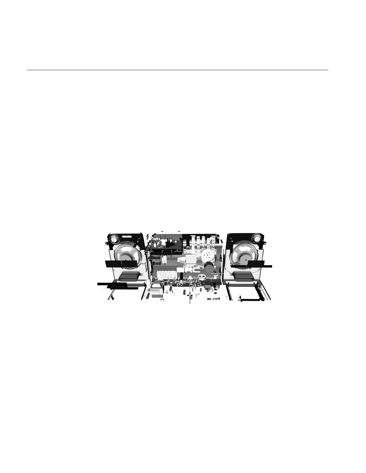
the OpenGL Optimizer library. Figure 1-1 shows the interior of a model that can be
manipulated with OpenGL Optimizer at interactive rates. The parts shown are those
hidden by the shell of the model; they are removed from the graphics pipeline by
occlusion culling when the model is viewed from outside.
Figure 1-1 Interior Parts From a CAD Model That Can Be Manipulated Interactively Using
OpenGL Optimizer (Data courtesy of SDRC™)
To accurately represent the surfaces in the design database requires selecting triangles
that provide appropriate detail without artificial cracks. To this end, OpenGL Optimizer
provides tools that provide controls over tessellation, mesh simplification, and surface
connectivity information, that is, topology.

How OpenGL Optimizer Helps
5
How OpenGL Optimizer Helps
OpenGL Optimizer provides tools to send only essential graphical information down the
graphics pipeline and to interact with the scene graph efficiently using multiple
processors.
To minimize the memory footprint of the scene graph, geometric objects can be
represented as abstract mathematical expressions. When you want to render them, you
can, for example, tessellate—that is, approximate them by sets of triangles—or simplify
them as your program proceeds. This mode of processing essentially substitutes CPU
cycles for limitations on the size of fast memory. The approach of the OpenGL Optimizer
toolkit is to treat a scene graph as a mutable object to be manipulated and altered
frequently; such calculations are essential to practical visualization of large CAD
datasets.
The basic OpenGL Optimizer elements are C++ classes that can be grouped roughly into
the general operations described this section, which contains the following subsections:
• “Graphics Pipeline” on page 6
• “Bottlenecks in the Pipeline” on page 7
• “Tools to Optimize the Generate Stage” on page 8
• “Tools to Optimize the Traversal Stage” on page 11
• “Tools to Optimize the Transform Stage” on page 12
• “Optimal Use of Rasterization Hardware” on page 15
The basic architectural modules, and their relations to lower-level software, are shown in
Figure 1-2.
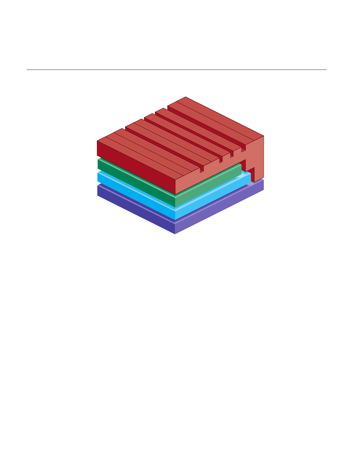
6
Chapter 1: Overview of OpenGL Optimizer
Figure 1-2 OpenGL Optimizer Architecture
Graphics Pipeline
You will more easily understand OpenGL Optimizer tools if you understand the generic
tasks of computer-generated graphics. These are the five fundamental stages in the
graphics pipeline, from host application to hardware display:
1. Generate and organize data to be displayed. The organizational structure for
OpenGL Optimizer applications is a Cosmo3D scene-graph. If you use abstract
surfaces to define objects, you must tessellate them before further processing.
OpenGL Optimizer tools facilitate these tasks.
2. Traverse the data and produce graphics data. For OpenGL Optimizer applications,
this typically means generating OpenGL commands, often guided by
considerations of interobject occlusion and represenational priority.
OpenGL Optimizer and Cosmo3D scene graph tools share these tasks.
OpenGL tools perform the last three tasks:
OpenGL
Cosmo 3D
OpenGL Optimizer
Operating System
Cullers
Simplifiers
MP Harness
Tessellators
Topology
Higher-Order Primitives
Lighting Effects
Traversers
Scene-Graph Manager

How OpenGL Optimizer Helps
7
3. Transform object-description coordinates into an appropriate viewing context; for
example, apply lighting effects, perform perspective transformations, and
transform these data into screen-space primitives (points, lines, and polygons).
4. Rasterize screen-space primitives into a frame buffer. Perform per-vertex and
per-pixel operations such as texture lookups, shading calculations, and depth
testing.
5. Display the contents of the frame buffer, typically on a monitor screen.
For further discussion of the graphics pipeline, see section 6.5, “Hardware for OpenGL,”
and section 6.6, “Maximizing OpenGL Performance,” in Programming OpenGL for the X
Window System. OpenGL Optimizer implements many of the tuning suggestions
discussed in section 6.6. See also the OpenGL Programming Guide.
Bottlenecks in the Pipeline
Ideally, your graphics software uses the hardware at its full potential so that processing
is not slowed by a bottleneck at any stage and data flows through the stages of the
pipeline at a uniform rate. There are three broad types of rendering bottlenecks:
1. Host: Generate- and traverse-stage limits are set by the efficiency of the software and
the performance of the CPU(s). The tasks of generating and organizing data for later
stages in the graphics pipeline, and scene graph traversal are CPU-intensive
operations.
2. Transform: Transform-stage limits are set by the rate at which the graphics hardware
(or software) can process vertices. For a single lighting source, the transformation
stage for one vertex takes approximately 100 floating-point operations.
3. Fill: Rasterize-stage limits are set by the rate at which the hardware can update the
frame buffer.
The term “host” refers to the first two stages of the graphics pipeline because OpenGL
defines a standard application program interface for the last three stages. Typical
machines running OpenGL Optimizer applications will have special-purpose graphics
hardware to implement the transform, rasterize, and display stages. In this manual, the
term “graphics hardware” is used to refer to only the OpenGL stages of the graphics
pipeline.
The nature of the graphics pipeline is such that rendering rate is controlled by the slowest
stage. Tuning a stage that is not a bottleneck will not affect performance. In fact, when

8
Chapter 1: Overview of OpenGL Optimizer
tuning an application, you might find that by adding processing to stages that are not
rate-controlling, you can improve the quality of images without affecting the rendering
rate.
The OpenGL Optimizer toolkit provides tools that typically minimize both host and
transform bottlenecks. In many cases the same tool will affect both a host bottleneck and
transform bottleneck. Typically large CAD applications are not fill limited.
Tools to Optimize the Generate Stage
OpenGL Optimizer provides the following tools:
• A powerful multiprocess control “harness,” which can be used independently of
any graphics application. All aspects of OpenGL Optimizer are designed to work
with this MP harness.
• Classes to facilitate multiprocess traversals of the scene graph with arbitrary
callbacks. These allow application speeds to scale with processor count.
• A transaction manager that coordinates scene graph modifications by several
processes and maintain logical consistency in a complex, multiprocessor context.
How OpenGL Optimizer Helps
9
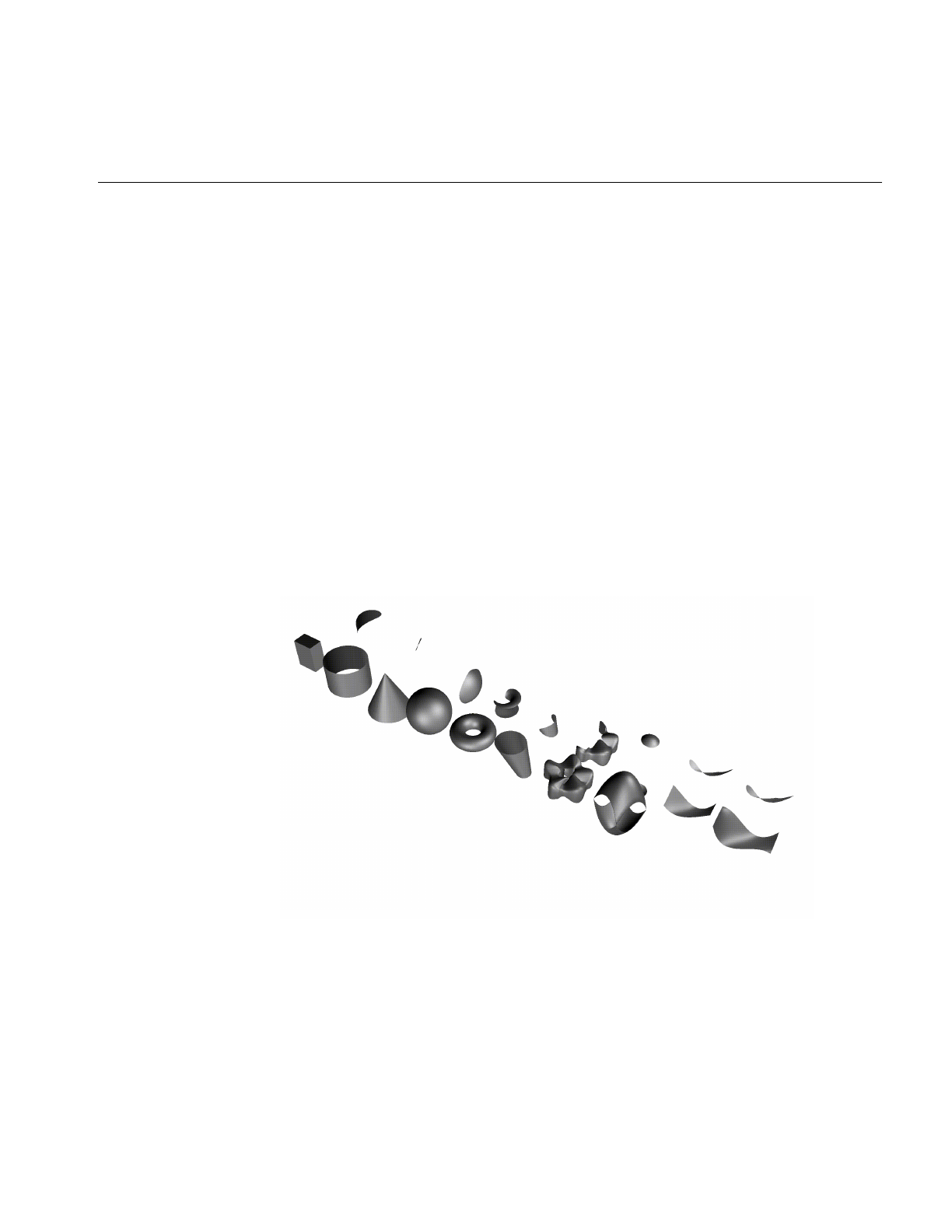
• Higher-order geometric primitives, called reps, that you can include in the scene
graph. shows the set of reps included in OpenGL Optimizer. From left to right, the
following reps are shown:
Cuboid
Cylinder
Cone
Sphere
Torus
Ruled Surface
Swept Surface (here with a superquadric curve for cross section)
Coons Patch
Hermite Spline Surface
NURBS Surface
Figure 1-3 Higher-Order Surface Representations With Trimmed Pieces
10
Chapter 1: Overview of OpenGL Optimizer
Higher-order surfaces are required to accurately represent CAD data. Direct support
for them allows OpenGL Optimizer applications to handle large design databases
without sacrificing design integrity, an unavoidable sacrifice if only vertex-based
data is used. Direct support for higher-order surfaces also facilitates alteration of
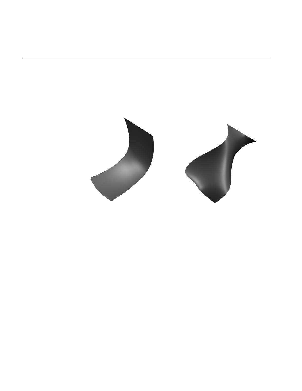
surface shapes, as illustrated in Figure 1-4, which shows NURBS surfaces that differ
by moving two control points.
Figure 1-4 NURBS Surfaces Deformed From One Another by Moving Two Control Points
• Tessellators for rendering higher-order geometric primitives. A tessellator in
OpenGL Optimizer is an independent object, not derived from a rep, that is applied
to a rep to produce a renderable object. The separation of tessellators from reps
allows your application to tessellate reps, and avoid storing large, renderable
objects. You can also apply one of several tessellators to a given rep, depending on
your need, or apply one tessellator to a set of reps.
• Topology data structures to easily maintain continuity of adjacent higher-order
surfaces as you modify your model and stitch surfaces together, thus preventing the
appearance of cracks during tessellation.

How OpenGL Optimizer Helps
11
Tools to Optimize the Traversal Stage
OpenGL Optimizer provides tools that perform these tasks:
• Organize a scene graph spatially, facilitating rapid culling operations and
interactions with the graph.
• Restructure the scene graph for efficient highlighting and picking.
• Subdivide large csGeoSets into smaller pieces defined by common rendering
features, such as proximity to each other or similarly oriented normal vectors.
• Sort the scene graph to minimize attribute-specification overhed in the graphics
hardware.
• Minimize the amount of data characterizing surface normals.
• Reduce OpenGL command overhead.
• Easily define arbitrary actions on a scene graph using the Visitor Behavioral Pattern
(see Design Patterns: Elements of Reusable Object-Oriented Software in “Recommended
Reference Materials” on page xxxi).
• Maintain both a spatial view needed for rapid display, and, for example, a logical
structure defined by design concerns.
12
Chapter 1: Overview of OpenGL Optimizer
Tools to Optimize the Transform Stage
Cosmo3D provides level-of-detail scene graph nodes and view-frustum culling. The
OpenGL Optimizer library adds the following tools to further accelerate the transform
stage:
• An occlusion culler to remove, before the transform stage, objects in the scene graph
that are occluded by closer objects. No preprocessing of the scene graph is required:
the culling is done automatically.
Figure 1-5 shows the exterior of a model containing many parts that have been
removed from the graphics pipeline by the occlusion culler. Only the shell needs to
be rendered; the culled geometry is shown in Figure 1-1.
Figure 1-5 Shell That Occludes the Objects Shown in Figure 1-1 (Data courtesy of SDRC™)
How OpenGL Optimizer Helps
13
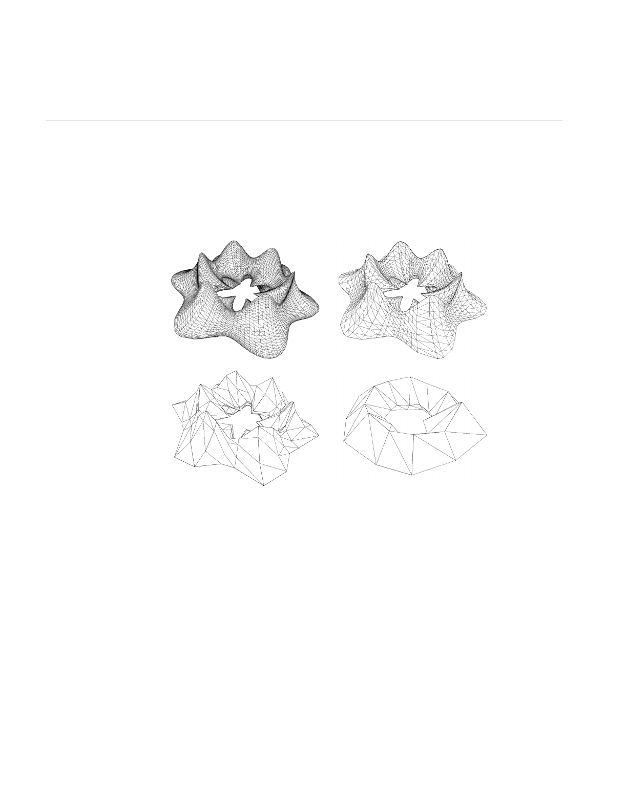
• Simplifiers to decimate the set of triangles that define a model image. OpenGL
Optimizer provides a new advanced simplification technology, known as the
Successive Relaxation Algorithm, which gives you control over high-quality
polygon mesh reduction. You can also use the faster, Rossignac simplification
algorithm if you are not greatly concerned about object distortion.
Figure 1-6 shows the effects of the Successive Relaxation Algorithm as the number
of triangles diminishes to nearly one tenth the original number. Essential structure
is preserved in the lowest resolution image, which is appropriate for use when the
object is viewed from greater distances.
Figure 1-6 Simplification From 4629 to 2002 to 483 Triangles
• Mesh optimizers to reduce the number of vertices that need to be processed to
render a given set of triangles. You can remove redundant vertex information by
combining adjacent triangles into triangle strips (tristrips), triangle fans (trifans) or a
combination of both.
14
Chapter 1: Overview of OpenGL Optimizer
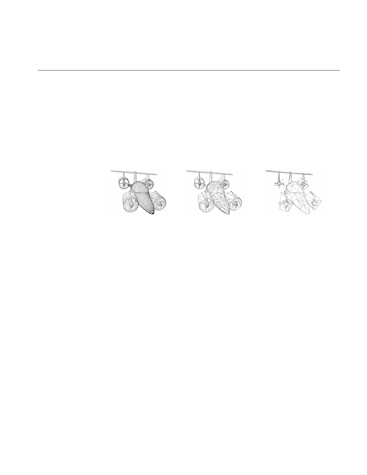
• Tessellators that can approximate higher-order geometric primitives with adjustable
levels of detail.
Figure 1-7 shows tessellations of a swept surface at varying levels of detail. The
number of triangles used to approximate the surface decreases from 16,544, to 5,400,
to 528, to 120.
Figure 1-7 Tessellations of a Higher-Order Surface: 16,544 to 120 triangles
• A scene-graph manipulation tool to insert level-of-detail nodes.
How OpenGL Optimizer Helps
15
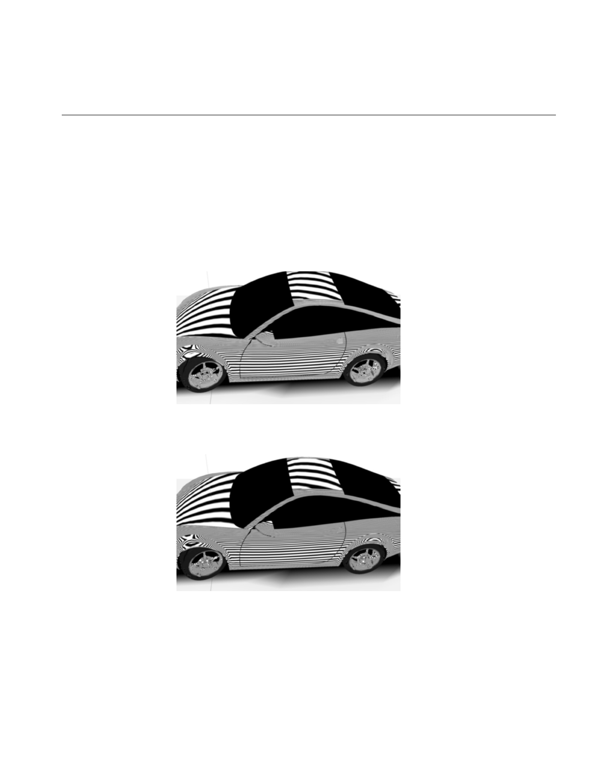
Optimal Use of Rasterization Hardware
For design and styling, where image quality and interactivity is essential, OpenGL
Optimizer also provides advanced shading and reflection mapping capabilities.
Figure 1-8 and illustrate tube-lighting effects, which simulate florescent lights in a
cylindrical room and are computed at interactive rates with OpenGL Optimizer
advanced lighting tools. Unfortunately, some aliasing was introduced in transfer from
original screen images to the images shown.
Figure 1-8 TubeLighting: Note Differences of Lights on Hood and Roof Compared to
Figure 1-9 (Data courtesy of Alias|Wavefront™)
Figure 1-9 TubeLighting: Note Differences of Lights on Hood and Roof Compared to
Figure 1-8 (Data courtesy of Alias|Wavefront)


17
Chapter 2
2. Installing, Compiling, and Running
This chapter describes installingand compiling an OpenGL Optimizer application,
presents brief descriptions of sample applications, which are ready to compile and run,
and lists a minimal OpenGL Optimizer application.
These are the sections in this chapter:
• “Installing the Library and Supporting Software” on page 17
• “Environment Variables to Set Before Compiling an Application” on page 19
• “Sample Applications” on page 20
• “Running a Sample Application” on page 20
• “Simple First Program” on page 24
Installing the Library and Supporting Software
The OpenGL Optimizer library can either be downloaded from the designated Web site
or from the release CD. In either case, use the Software Manager (swmgr) interface to
install the software.

18
Chapter 2: Installing, Compiling, and Running
In addition to the library, you need the software listed in Table 2-1, which also briefly
indicates why the software is needed and where to get it:
The installation overwrites previously installed Cosmo3D and OpenGL Optimizer
libraries and sample applications. To avoid overwriting any changed files during the
installation, save them in another directory.
Sample OpenGL Optimizer applications, file loaders and scene-graph viewers are in
/usr/share/Optimizer/. Sample Cosmo3D applications are in /usr/share/Cosmo3D. Use the
commands make ddso or make dso to build these Cosmo3D programs.
Table 2-1 Libaries Used by OpenGL Optimizer
Software Purpose Program Name Program Source
Compile and run C++ programs, use one of
the three.
c++_dev MIPSpro C++ 7.1 CD
c++_eoe IRIX™ 6.2 part 1 of 2 or IRIX 6.3
CD
compiler_dev 7.1 IDO package. The IDO
package contains 3 CDs, one
per IRIX platform.
Compile programs in the developer build
environment. dev IRIS® Developer’s Option CD
Load Inventor™ files: Inventor 2.1.1 or
higher. inventor_dev
and
inventor_eoe
IRIX 6.2 part 1 of 2 or IRIX 6.3
CD
To link with the Digital Media Execution
Environment. dmedia_eoe IRIX 6.2 part 1 of 2 or IRIX 6.3
CD
For reflection mapping: Image Format
Library. ifl_eoe Installable from Silcon SurfSM
as part of the ImageVision™
Runtimes 3.1.1

Environment Variables to Set Before Compiling an Application
19
Environment Variables to Set Before Compiling an Application
Before compiling an OpenGL Optimizer application, you should set several environment
variables.
• To specify which ABI to compile (o32, n32, or n64), enter this command:
setenv OBJECT_STYLE 32 or N32_M3 or 64
Note: For systems with IRIX 6.4, the compiler defaults to using n32. To force an o32
build enter this command:
setenv OBJECT_STYLE 32
• To designate linking with single or double-precision OpenGL Optimizer libraries,
edit the ‘OP_DOUBLE’ value set in /usr/share/Optimizer/src/opusercommondefs .
• To run-time load the debugging versions of the libraries, enter one of these
commands:
setenv LD_LIBRARY_PATH
/usr/lib/Optimizer/Debug:/usr/lib/Cosmo3D/Debug
setenv LD_LIBRARYN32_PATH
/usr/lib32/Optimizer/Debug:/usr/lib32/Cosmo3D/Debug
setenv LD_LIBRARY_PATH64
/usr/lib64/Optimizer/Debug:/usr/lib64/Cosmo3D/Debug
Note: For performance, do not set LD_LIBRARY_PATH to the
/usr/lib/{Optimizer,Cosmo3D}/Debug directories.
• If you see a compile-time warning that mentions incompatible versions for libifl.so
(sgi1.0), and your application does not use reflection mapping, you can enter the
this command
setenv _RLD_ARGS -ignore_all_versions
This error occus if you have a more recent version of libifl.so that ships with IRIX 6.3
or 6.4: Image Vision Runtimes 3.1.1.
You can avoid the error message by installing the IRIX 6.2 libifl.so into a different
directory than /usr/lib and set your LD_LIBRARY_PATH to point to that directory
first. For example, if you install libifl.so in /usr/tmp/ifllib, enter the following
command:
setenv LD_LIBRARY_PATH /usr/tmp/ifllib:/usr/lib
For further details, see “Compiler Warning Messages” on page 377 and the file
/usr/share/Optimizer/doc/Programming_tips/Compile_Notes.html.

20
Chapter 2: Installing, Compiling, and Running
Sample Applications
To help you get started, the library includes applications designed to illustrate OpenGL
Optimizer applications and the power of the OpenGL Optimizer and Cosmo3D toolkits.
These applications are in individual subdirectories of the /usr/share/Optimizer/src/sample
directory.
This section describes how to run the applications, and briefly describes each application,
which you can compile and run when you have the OpenGL Optimizer library properly
installed.
Running a Sample Application
The sample applications all run similarly. To see the command-line options that are
available, invoke the executable without any arguments. To print a list of interactive
program controls into your command shell while you run a sample application (except
for viewXmdemo, which provides different interface), place the mouse cursor in the
rendering window and enter h.
The applications have many command-line arguments; for example, viewDemo and
optimizeDemo both have over 20. Optional arguments for demonstration applications
should be placed after any required arguments when you invoke a sample application.
For example, viewDemo and optimizeDemo requre only filename arguments, so
command lines could look like the following:
%viewDemo xxx.csb -useDL
%optimizeDemo xxx.csb -batch test.csb
viewDemo Application
This application illustrates the basic structure of a fully developed OpenGL Optimizer
application that includes most of OpenGL Optimizer’s rendering tools. It uses the
graphical user interface tools in /usr/share/Optimizer/src/libopGUI. The important tools in
this library, opViewer and opDefDrawImpl are discussed in Chapter 3, “Basic I/O
Tools: The Application viewDemo.”
A line-by-line commentary on viewDemo appears in Chapter 3 in the section
“Application viewDemo: A First Look in the Toolkit” on page 42.

Sample Applications
21
The command-line options for this program appear in the file
/usr/share/Optimizer/src/sample/viewDemo/main.cxx. Interactive control options are defined
by the class opDefDrawImpl, which is in the /usr/share/Optimizer/src/libopGUI directory
and is discussed in in Chapter 3 in “Default opDrawImpl for opViewer:
opDefDrawImpl” on page 40.
viewXmDemo Application
This application illustrates the use of OpenGL Optimizer in a Motif™ application. It
essentially duplicates the functionality of viewDemo, but relies on different graphical
user interface tools; /usr/share/Optimizer/src/libopXmGUI is the motif version of
/usr/share/Optimizer/src/libopGUI, which is used by viewDemo.
viewXmDemo is a typical Motif application that creates a main window and a menu bar.
The application also creates an opXmViewer widget attached to the main window.
opXmViewer is the motif version of opViewer, discussed in “Viewing Class: opViewer”
on page 33. opXmViewer is a composite Motif widget consisting of a main drawing area,
an information area (for help text), and a user interface area.
viewXmDemo takes the same command-line options as viewDemo, with the exception
of occlusion culling and no-picking options: occlusion culling is not available and the
picking option is always on. Interactive controls are defined by the class
opXmDrawImpl, which is the Motif analog to a combination of opDefDrawImpl and
opPickDrawImpl, which are discussed in “Basic Tools for Rendering Implementations:
opKeyCallback and opDrawImpl” on page 38; and in “Interaction With a Rendered
Object: opPickDrawImpl” on page 156.
As in viewDemo, translation, rotation and zoom are done in viewXmDemo using the
mouse in the drawing area. Unlike viewDemo, the other interactions are controlled by
buttons in the user interface area, rather than by keyboard commands. Passing the cursor
over a button causes the help text associated with that button to be displayed in the
information area.
xdemo Application
This application illustrates how to render a Cosmo3D scene graph inside of an
X Window™. It presents a minimal OpenGL Optimizer application and emphasizes the
process of rendering. It includes the necessary routines from the following libraries:
X Window, OpenGL extensions to X, Cosmo3D, and OpenGL Optimizer.

22
Chapter 2: Installing, Compiling, and Running
optimizeDemo Application
This application uses most of the OpenGL Optimizer scene-graph-tuning tools and is
mainly for batch processing, although it also allows you to view the scene graph using
an opViewer (see “Viewing Class: opViewer” on page 33).
A line-by-line commentary appears in Chapter 4, “Scene Graph Tuning With the
optimizeDemo Application.” This application adds to viewDemo the command-line
options and keyboard controls that appear in the file
/usr/share/Optimizer/src/sample/optimizeDemo/main.cxx.
mergeLODDemo
This application is a specialized application of the OpenGL Optimizer
scene-graph-tuning tools; it places level-of-detail (LOD) nodes at leaf nodes and
provides fewer options than optimizeDemo, which places LOD nodes near the root of the
scene graph.
The tool included in this application that does not appear in optimizeDemo is one that
allows you to combine topologically identical scene graphs that contain leaf nodes with
differing levels of detail. See “Merging Graphs With Differing Levels of Detail:
opMergeScenes” on page 119.
repTest Application
This application for rendering higher-order reps provides an environment where you
can try your hand developing and rendering these objects.
This application is discussed in Chapter 11, “Higher-Order Geometric Primitives and
Discrete Meshes.” It adds to viewDemo the command-line options that appear in the file
/usr/share/Optimizer/src/sample/reptest/main.cxx.
topoTest Application
This application illustrates the use of the OpenGL Optimizer topology building tools to
“stitch” together surfaces “by hand.” It is designed to help you import surfaces whose
connectivity you know so that you can use the OpenGL Optimizer tessellators to get

Sample Applications
23
crack-free images. The application also illustrates an approach to developing trimmed
NURBS surfaces that is a somewhat different from that used in repTest.
The topology building tools are discussed in Chapter 12, “Creating and Maintaining
Surface Topology.”
opviz Application
This application illustrates how to use OpenGL Optimizer to visualize discrete scientific
and engineering data.
This application is discussed in the section “Sample Mesh Tessellation: opviz and
opVizViewer” on page 306. It adds to viewDemo the command-line options that appear
in the file /usr/share/Optimizer/src/sample/opviz/main.cxx, and the interactive commands
that appear in opVizViewer.cxx.
zebraFly Application
This application illustrates the use of reflection mapping to get tube-lighting effects,
which simulate lighting by florescent lights in a cylindrical room. The file
/usr/share/Optimizer/src/sample/zebrafly/README describes the basic controls for the
application, which is based on viewDemo.
Reflection mapping tools are discussed in Chapter 10, “Efficient High-Quality Lighting
Effects: Reflection Mapping.”

24
Chapter 2: Installing, Compiling, and Running
Simple First Program
The following simple program initializes the OpenGL Optimizer library with a call to
opInit(); an opArgParser interprets command-line arguments; an opGenLoader loads
data files, which it can tessellate if necessary by using an opTessParaSurfaceAction; and
anopViewer controls interaction with the scene graph. These tools are discussed in more
detail in Chapter 3 and in Chapter 13, “Rendering Higher-Order Primitives:
Tessellators.” Note that the program allows you to load a model that is included in
several files.
Simple Program Code
#include <stdio.h>
// you MUST include this file before csGroup.h
#include <Cosmo3D/csFields.h>
#include <Cosmo3D/csGroup.h>
#include <Optimizer/opArgs.h>
#include <Optimizer/opGenLoader.h>
#include <Optimizer/opInit.h>
#include <Optimizer/opTriStats.h>
#include <Optimizer/opViewer.h>
#include <Optimizer/opTessParaSurfaceAction.h>
int main(int argc, char *argv[])
{
opInit();
opArgParser args;
char *filename;
int numFiles;
int x=1280-600-10, y=0, w=600, h=600;
bool haveChordalTol = -1;
opReal chordalTol = 0.01; // 100th of meter if meters are the
// units of choice.
args.defRequired( “%s”,
“<filename>”,
&filename);
#ifdef OP_REAL_IS_DOUBLE
args.defOption( “-ctol %l”,
“-ctol <max chordal deviation>”,

Simple First Program
25
&haveChordalTol, &chordalTol );
#else
args.defOption( “-ctol %f”,
“-ctol <max chordal deviation>”,
&haveChordalTol, &chordalTol );
#endif
// Print out version of Optimizer
fprintf(stderr,”%s\n”,opVersion());
// Prepare to read filenames if more than one is supplied
numFiles = args.scanArgs(argc,argv);
// Create a tessellator
opTessParaSurfaceAction *tess;
tess = new opTessParaSurfaceAction;
// Set the chordal tolerance
tess->setChordalDevTol( chordalTol );
// Create a loader
opGenLoader *loader;
// Bind tessellator to loader so that
// tessellation is invoked at loading
loader = new opGenLoader( true, tess, false );
// Load the file on the command line and get a scene graph back
csGroup *obj = loader->load( filename );
if (numFiles)
{
// Loading more than one file
int i;
csGroup *grp = new csGroup;
if (obj)
{
grp->addChild(obj);
}
char **xtraFiles = args.getRemainingArgs();
for (i=0;i<numFiles;i++)
{
fprintf(stderr,”loading file %d %s\n”,i,xtraFiles[i]);
obj = loader->load(xtraFiles[i]);
if (obj)
{
grp->addChild(obj);

26
Chapter 2: Installing, Compiling, and Running
}
}
obj = grp;
}
// Throw the loader and tessellator away, we’re done with them
delete loader;
delete tess;
// If we got a scene graph draw it else end the program
if ( obj )
{
// Get stats on the scene graph
opTriStats stats;
stats.apply(obj);
printf(“Scene statistics:\n”);
stats.print();
opViewer *viewer = new opViewer(“Optimizer”, x, y, w, h);
viewer->addChild(obj);
viewer->setViewPoint(obj);
viewer->eventLoop();
}
}

Simple First Program
27
Compiling and Running the Simple Program
The easiest way to compile is to use one of the Makefiles in one of the
/usr/share/Optimizer/src/sample directories, and opusercommondefs shipped with the sample
code: copy and edit one of the sample Makefiles, then set the appropriate environment
variables: OPROOT, CSROOT, LD_LIBRARY_PATH, and OBJECT_STYLE. See
“Environment Variables to Set Before Compiling an Application” on page 19 and
/usr/share/Optimizer/doc/Programming_tips/Compile_Notes.html for more information.
Note: TheMakefile in the inst image is looking for the opusercommondefs to be in a specific
location:
include $(OPROOT)/usr/share/Optimizer/src/opusercommondefs
To run the simple program, enter commands such as the following:
viewDemo datafile.csb
viewDemo datafile.iv
Supplying an Inventor (.iv) file causes the program to use the tessellator.


29
Chapter 3
3. Basic I/O Tools: The Application viewDemo
To get you started with OpenGL Optimizer applications and to provide basic program
I/O, the library includes opViewer, an interactive scene graph viewer that uses OpenGL
and Cosmo3D calls to render a scene, and the base class opDrawImpl, which allows you
to control the rendering options. Analogous tools that use Motif calls can be found in
/usr/share/Optimizer/src/libopXmGUI.
These are the sections in this chapter:
• “Always First: Call opInit()” on page 29
• “Reading and Writing Scene-Graph Files: The Extendable Loading Class
opGenLoader” on page 30
• “Viewing Class: opViewer” on page 33
• “Basic Tools for Rendering Implementations: opKeyCallback and opDrawImpl” on
page 38
• “Application viewDemo: A First Look in the Toolkit” on page 42
Always First: Call opInit()
Every OpenGL Optimizer application must call opInit() once before calling any other
OpenGL Optimizer routine. You can terminate an OpenGL Optimizer application with a
call to opExit() or opNotify() (if the notification level is set to opFatal. See “Error
Handling and Notification” on page 366).
opInit provides the method opVersion(), which returns the OpenGL Optimizer version
string to use in correspondence concerning the specific OpenGL Optimizer library you
have installed. This string is defined by the following four definitions:
OP_MAJOR_VERSION
The major release number.

30
Chapter 3: Basic I/O Tools: The Application viewDemo
OP_MINOR_VERSION
The minor release number.
OP_RELEASE_TYPE
The type of release (apha, beta, MR, or unreleased).
OP_BUILD_VERSION
Build release number.
OP_BUILD_NUMBER
The unique build number.
Reading and Writing Scene-Graph Files: The Extendable Loading Class opGenLoader
The class opGenloader provides file-reading routines that create Cosmo3D scene graphs.
OpenGL Optimizer includes loaders for three file formats, and you can extend the class
to read any format.
The class provides loaders to read from the formats designated by the following file
extensions:.iv format, .csb, and .pfb. The .pfb, and .csb files are two highly efficient, binary
file formats used by OpenGL Optimizer and Cosmo3D.
• The .iv files are the format used by Open Inventor.
• The .pfb format allows you to interchange IRIS Performer readable data formats
with OpenGL Optimizer and Cosmo3D.
• The .csb format is used by Cosmo3D to efficiently store and transfer scene graphs.
As you load the contens of a file, you can flatten the scene graph (see “Simplifying a
Scene Graph: opFlattenScene()” on page 98), tessellate higher-order primitives (see
Chapter 13, “Rendering Higher-Order Primitives: Tessellators”), or perform an
incremental load. When you flatten a scene graph, you get a structure where all leaf
nodes are under one csGroup node.

Reading and Writing Scene-Graph Files: The Extendable Loading Class opGenLoader
31
Saving a Scene Graph to a File
To write a scene graph to a .csb file, you can use one of the following:
• Cosmo3D method csGlobal::storeFile()
• Cosmo3D function csdStoreFile_csb() (link to the Cosmo3D library libcscsb)
The latter method is used in the demonstration application optimizeDemo.
File Format Conversions
The natural format for OpenGL Optimizer is the .csb format. You can use opGenLoader
to read a file, in particular an .iv file, and convert it to the.csb format by using one of the
Cosmo3D file storing tools.
Class Declaration for opGenLoader
The following are the main methods in the class:
class opGenLoader
{
public:
opGenLoader();
opGenLoader( const bool _flatten, opTessellateAction* _tesselator,
const bool incremental );
~opGenLoader();
csGroup *load( const char *filename );
void addType( const char *ext, const char *tag );
void setDataFilePath( const char *path );
void setFlatten( const bool _flatten ) ;
void setTessellator( opTessellateAction *_tessellator );
void setIncremental( const bool _incremental );
char *getDataFilePath( );
bool getFlatten( );
opTessellateAction *getTessellator( );
bool getIncremental( );
}

32
Chapter 3: Basic I/O Tools: The Application viewDemo
Main Features of the Methods in opGenLoader
opGenLoader(_ flatten, _tesselator, _incremental )
Sets logical flags indicating whether the loader should, flatten the scene
graph, tessellate geometric primitives on the fly, or incrementally read
the graph.
addType( ext, tag )
Adds a loader that reads files with the extension ext. The name of the dso
containing the loader is tagLoader_sp.so or tagLoader_dp.so, depending
on whether you compile in single or double precision. The variable tag
can include a pathname.
load() Reads a data file, if it can find a DSO load routine.
setDataFilePath() and getDataFilePath()
Set the search paths for the DSO.
The class also includes accessor functions to set and get the flags for flattening and
incremental reads and to set and get the tessellator.
Adding a Scene Graph Loader
To develop your own scene graph loader, follow these steps:
1. Associate the label tag with filename extension ext by calling addType().
2. Name the DSO containing the load function tagLoader_sp.so or tagLoader_dp.so,
depending on whether you compile single or double precision.
3. Name the load function within the DSO tagLoad() using standard C naming
conventions.
4. Declare the load function as follows:
csGroup* tagLoad(const char * filename, const bool flatten,
opTessellateAction* tessellator, const bool incremental)
See, for example, ivLoad() in ivLoader.cxx in the /usr/share/Optimizer/src/loaders/iv
directory. The ivLoader creates nearly every type of node available in Cosmo3D.
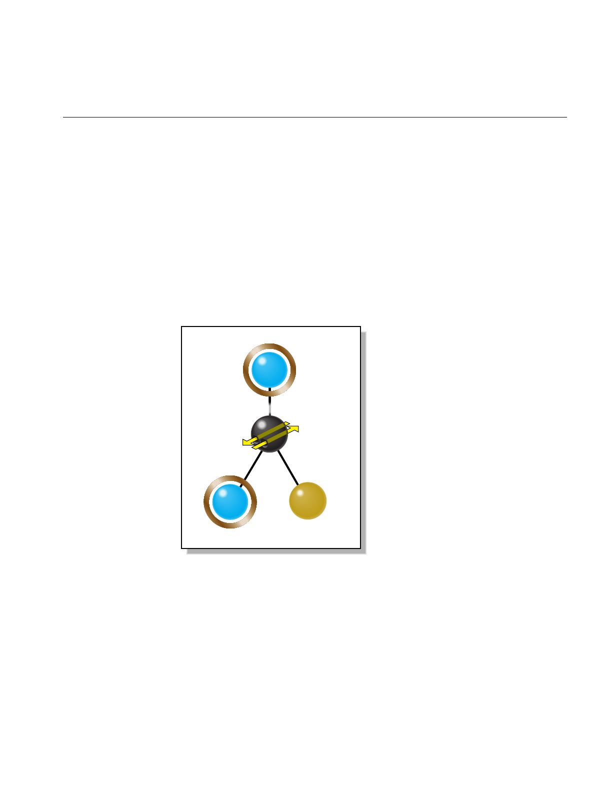
Viewing Class: opViewer
33
Viewing Class: opViewer
This class’s key operations are to add a data-model scene graph to a scene graph (as
shown in Figure 3-1) to facilitate interactions, and to register mouse and keyboard
controls for scene graph interaction. opViewer is designed to be extended by derivation.
Several features of the OpenGL Optimizer library were derived in this way, for example,
the class for scientific visualization, opVizViewer. The node opGLSpyNode,which
appears in Figure 3-1, is discussed in “Observing OpenGL Modes” on page 374.
To render using Motif library calls, see files in the directory
/usr/share/Optimizer/src/libopXmGUI. There you will find opXmViewer. The following
discussion should provide sufficient information to introduce you to the functionality of
that viewing class.
Figure 3-1 opViewer Scene Graph
root
csGroup
model
graph
root
node
csGroup
csTransform
opGLSpyNode
OpenGL
mode
watcher
pose

34
Chapter 3: Basic I/O Tools: The Application viewDemo
As for any OpenGL Optimizer application, an opViewer application begins by
initializing the library with a call to opInit(). Then the application need only instantiate
the viewer, load the scene graph, and call the event loop method. You can determine
interactions with the scene graph by setting drawing implementations (see “Basic Tools
for Rendering Implementations: opKeyCallback and opDrawImpl” on page 38). The
sample application viewDemo, discussed in “Application viewDemo: A First Look in the
Toolkit” on page 42, is an example of how to use an opViewer.

Viewing Class: opViewer
35
Class Declaration for opViewer
The following are the main methods in the class:
class opViewer
{
public:
// Creating and destroying
opViewer(const char *windowTitle=”unnamed”,
int x=0, int y=0, int w=512, int h=512,
int keyTableSize=512);
~opViewer();
// Accessor functions
csNode *getScene() const;
csNode *getRoot() const;
csLight *getLight() const;
csLight *getSecondLight() const;
csDrawAction *getDrawAction() const;
csContext *getContext() const;
csCamera *getCamera() const { return camera; }
int getWidth() const;
int getHeight() const;
void setViewPoint(csNode *n = NULL);
void setViewPoint(const csBoxBound &bbox, const csVec3f ¢er);
void setReflMap( opReflMap *rm );
opReflMap *getReflMap();
// Utility methods
void setFarClip(float farVal);
void setNearClip(float nearVal);
void enableClipPlanes () { clipPlanesEnabled = true; }
void disableClipPlanes () { clipPlanesEnabled = false; }
void setBackgroundColor( float r, float g, float b, float a );
void getBackgroundColor( float *r, float *g, float *b, float *a );
void setSaveImagePrefix( char *filename );
char *getSaveImagePrefix();
void setSaveImageSequenceNumber( int n );
int getSaveImageSequenceNumber();
void saveScreenImage();
void setClipPlanes();
void addChild(csGroup *g);
void addImmobileChild(csNode *);
void replaceChild(csGroup *oldGrp, csGroup *newGrp);

36
Chapter 3: Basic I/O Tools: The Application viewDemo
void eventLoop(void);
// Functions dealing with opDrawImpl’s
void setDrawImpl(opDrawImpl *di);
opDrawImpl *getDrawImpl() const;
// Methods for mode control
void setBackFaceMode( bool mode );
void setBoxBoundMode( bool mode );
void setPickMode( bool mode );
void setRotLightMode( bool mode );
void setTwoLightMode( bool mode );
void setLightsMode( bool mode );
void setModelRotation( float x, float y, float z, float angle );
void setModelTranslation( float x, float y, float z );
void getModelRotation( float *x, float *y, float *z, float *angle );
void getModelTranslation( float *x, float *y, float *z );
void setStatsDisplayMode( bool mode );
void setWireFrameMode( bool mode );
void setScribeMode( bool mode );
void setPreScribeLightMode( bool mode );
void setLODbias ( int bias );
void setStatsDisplayStyle(opStyle s);
bool getBackFaceMode() const;
bool getBoxBoundMode() const;
opGLSpyNode *getGLSpy() const;
bool getPickMode() const;
bool getRotLightMode() const;
bool getTwoLightMode() const;
bool getLightsMode() const;
bool getStatsDisplayMode() const;
bool getWireFrameMode() const;
bool getScribeMode() const;
bool getPreScribeLightMode() const;
int getLODbias() const;
opStyle getStatsDisplayStyle() const;
// Functions a user may call from an opDrawImpl
void clearWindow(void);
void drawScene(csNode *alt_root=NULL);
void drawStatistics(void);
void exit(int status=0);
void modelView(void);
void projection(void);
void printAppHelp(FILE *fp);
void printHelp(FILE *fp);

Viewing Class: opViewer
37
void reset();
void setMouseFocus (csTransform *new_pose);
void swapBuffers(void);
void update(void);
bool isSceneSpinning() const;
static int frameCallbackEntry(opViewer *);
};
Main Features of the Methods in opViewer
The names of the methods of opViewer are descriptive and often refer the OpenGL
Optimizer tools they control. Here are a few of the main methods:
addChild(g)Adds group g as child of the pose transform, shown in Figure 3-1.
eventLoop() Is the entry point for the X event loop for the window. eventLoop() starts
opViewer’s interactive mode. Perform all initializations of scene graph
data structures before calling eventLoop().
setDrawImpl() and getDrawImpl()
Set and get the opDrawImpl that currently controls scene graph
interactions. The constructor sets a default opDrawImpl, but you can
use others to allow, for example, highlighting and independent
manipulation of subgraphs (see Chapter 9, “Interactive Highlighting
and Manipulating”).
setLODbias() and getLODbias()
Set and get a bias for levels of detail when a scene is rotating.
A bias of i has the effect that, given a sequence of level-of-detail nodes
indexed by the integers 1 to nand arranged from highest to lowest level
of detail, after a level-of-detail calculation that would render node m,
the node m+i is rendered instead. This lightens the load on the graphics
hardware when you are not likely to need the most accurate object
representations.
setViewPoint() Sets the view frustum to contain the bounding box of the graph rooted
at node passed as an argument. If the argument is NULL, the bounding
box of the entire scene graph is used.
The class opViewer contains many more methods; consult the man page and source code
for more details.

38
Chapter 3: Basic I/O Tools: The Application viewDemo
Basic Tools for Rendering Implementations: opKeyCallback and
opDrawImpl
opViewer uses objects derived from opDrawImpl to control rendering details and the
effects of specific keyboard controls.
opViewer uses a C++ array of functions to organize the effects of a set of keyboard
commands, which can come from several opDrawImpls (however, you cannot have
more than one opDrawImpl active at any given time). The array is an opKeyCallback,
which is the following pointer-to-function type:
typedef bool (*opKeyCallback)(opDrawImpl *drawImpl,int key);
Class Declaration for opDrawImpl
The following are the main methods in the class:
class opDrawImpl
{
public:
opDrawImpl(opViewer *viewer); // Register keys and callbacks
virtual ~opDrawImpl();
void registerKey(int key, opKeyCallback keyCB,const char *helpMessage);
opViewer *getViewer() const;
// Callbacks to be implemented by the user.
virtual void draw(unsigned frame);
virtual void pick(bool mouseDown,const csHit& hit);
virtual void activated();
virtual void deactivated();
virtual void reset();
};

Viewing Class: opViewer
39
Main Features of the Methods in opDrawImpl
The methods of opDrawImpl do nothing. You create meaningful definitions in derived
classes. These are the intended uses of the member functions:
opDrawImpl(viewer)
Registers keys and their effects using the member function
registerKey().
registerKey(key, keyCB, helpmessage)
Registers a keyboard key and a callback function keyCB.keyCB becomes
a member of the opKeyCallback pointer-to-function array maintained
by the opViewer.keyCB interprets key in terms of the opDrawImpl’s
methods.
Each subclass defines at least one such member of opKeyCallback. The
subclasses of opDrawImpl in the OpenGL Optimizer library call this
defining function keyHandler() (see “Default opDrawImpl for
opViewer: opDefDrawImpl” on page 40, “Rendering With
View-Frustum and Occlusion Culling: opOccDrawImpl” on page 129,
and “Interaction With a Rendered Object: opPickDrawImpl” on
page 156).
Notice that different opDrawImpls cannot have different definitions
for one keyboard key. This allows you to include without ambiguity
several opDrawImpls in one opViewer and swtich among them. For
example you could select among the following opDrawImpls:
• Default: see “Default opDrawImpl for opViewer: opDefDrawImpl”
on page 40
• Picking: see “Interaction With a Rendered Object:
opPickDrawImpl” on page 156
• Occlusion culling: see “Rendering With View-Frustum and
Occlusion Culling: opOccDrawImpl” on page 129
pick() Allows you to define mouse interactions with a rendered object. See, for
example, the class opPickDrawImpl, which is discussed in “Interaction
With a Rendered Object: opPickDrawImpl” on page 156.
activated() and deactivated()
Define callbacks that are implemented when you switch to and from an
opDrawImpl using opViewer::setDrawImpl().
reset() Returns a scene to the default settings defined by this function.

40
Chapter 3: Basic I/O Tools: The Application viewDemo
Default opDrawImpl for opViewer: opDefDrawImpl
This class defines the default drawing options and their keybinding for opViewer().
If you want to use the Motif library, opXmViewer uses opXmDrawImpl, which has
methods analogous to a combination of opDrawImpl and opPickDrawImpl. The latter
is an opDrawImpl that allows manipulation of selected objects in a scene. See
“Interaction With a Rendered Object: opPickDrawImpl” on page 156
Class Declaration for opDefDrawImpl
The class declaration is nearly identical to that of opDrawImpl. The main difference is
the inclusion of a member of the opKeyCallback function array called keyHandler(),
which defines the effects of keyboard commands. This is the prototype for the member
function keyHandler():
static bool keyHandler(opDrawImpl *,int);
Main Features of the Methods in opDefDrawImpl
keyHandler() Defines the effects of the keyboard commands registered by calls to
registerKey().opDefDrawImpl has the keyboard controls described in
“opDefDrawImpl Keybindings” on page 41.
registerKey() Registers a keyboard command and specifies the function that interprets
the command. The function registerKey() is inherited from
opDrawImpl, which is discussed in “Basic Tools for Rendering
Implementations: opKeyCallback and opDrawImpl” on page 38. See the
file opDefDrawImpl.cxx for details.

Viewing Class: opViewer
41
opDefDrawImpl Keybindings
The class constructor for opDefDrawImpl uses the methods registerKey() and
keyHandler() to register the following keyboard commands (see the file
opDefDrawImpl.cxx):
bToggles back-face culling (see “Detail Culling” on page 135).
BToggles bounding-box display. Shows the csBoxBound of each
csGeoSet in the scene.
hPrints help message listing these key actions.
qQuits.
ESC Quits.
rResets scene to what it was at the start of the application.
lToggles the light-direction mode, which allows you to control the
location of the light source with your mouse.
LToggles a second light source opposite the first.
pPrints the scene graph.
sToggles status display.
tToggles reflection mapping illumination with the Gaussian map (see
Chapter 10, “Efficient High-Quality Lighting Effects: Reflection
Mapping”).
wToggles wire-frame mode, which shows the edges of the triangles that
define the objects in the scene.
WToggles hidden-line removal when in wire-frame mode.
SPACE Stops scene motion.
?Prints OpenGL status during the subsequent frame.
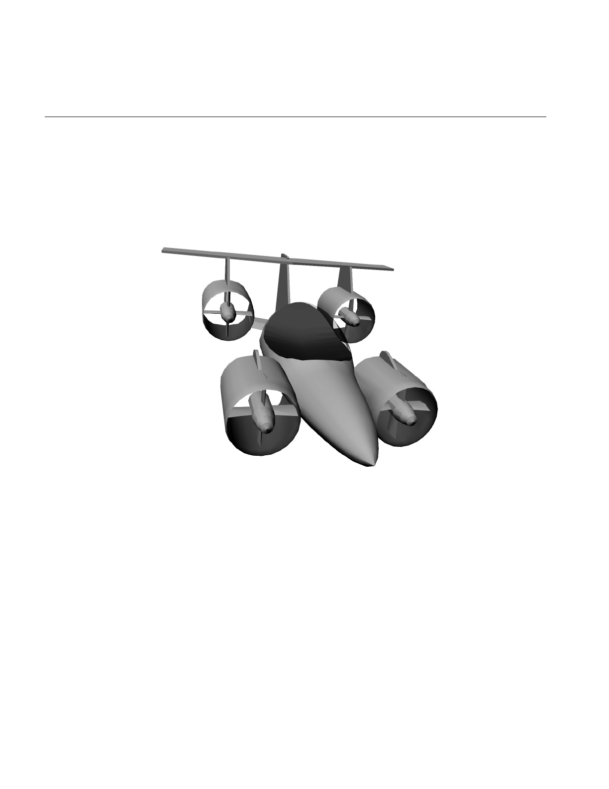
42
Chapter 3: Basic I/O Tools: The Application viewDemo
Application viewDemo: A First Look in the Toolkit
This application illustrates the basic structure of an OpenGL Optimizer opViewer
application that includes many of OpenGL Optimizer’s rendering tools. It is a working
application that allows you to use the rendering tools to manipulate complex models.
illustrates a model rendered by viewDemo.
Figure 3-2 A Model Rendered by the Application viewDemo
This section presents comments and lines of code essentially the same as that of
/usr/share/Optimizer/src/sample/viewDemo/main.cxx, briefly highlights OpenGL Optimizer
features, and refers to detailed discussions that appear in this guide. The code presented
here may not be exactly the same as the code that ships with OpenGL Optimizer, because
of late changes, but it should be close enough to orient you. The rest of this chapter is a
running commentary on the code in main.cxx.

Application viewDemo: A First Look in the Toolkit
43
These are the main tools omitted from viewDemo:
• Explicit mention of tools for tuning the scene-graph database, which are discussed
in Part II, “High-Level Strategic Tools for Fast RenderingChapter 8”
• Multiprocessing tools, which are discussed in Chapter 16, “Managing Multiple
Processors”
Analogous X Window and Motif Applications
If you are interested in developing a viewing application based directly on the X Window
library and OpenGL extensions to X, see the application xdemo in the
/usr/share/Optimizer/src/sample directory. The application xdemo does not use many of the
OpenGL Optimizer tools but emphasizes incorporating Cosmo3D rendering techniques
in an X window.
If you are interested in developing an application based on Motif, see viewXmDemo in
/usr/share/Optimizer/src/sample/viewXmDemo/main.cxx. This code is quite similar to
viewDemo.
Compiling and Running viewDemo
To compile viewDemo, enter the command make while in the directory
/usr/share/Optimizer/src/sample/viewDemo.
To run viewDemo, recall that command-line options are listed if you invoke the
application without any command-line arguments. To print a list of interactive program
controls into your command shell while you run viewDemo, place the mouse cursor in
the rendering window and enter h.

44
Chapter 3: Basic I/O Tools: The Application viewDemo
viewDemo Code
Inclusions
Besides the standard library, viewDemo requires
two base clases from the Cosmo3D library, and
header files from OpenGL Optimizer that provide
classes that provide the following features.
#include <stdio.h>
#include <Cosmo3D/csFields.h>
#include <Cosmo3D/csGroup.h>
You can set all csAppearances of the csShapes to
minimize mode switching. See “Avoiding OpenGL
Mode Switching” on page 96.
#include <Optimizer/opAppStats.h>
These two headers include the OpenGL Optimizer
command-line argument parser, which is discussed
in the section “Command-Line Parser:
opArgParser” on page 375; and the file loading
class, discussed in “Reading and Writing
Scene-Graph Files: The Extendable Loading Class
opGenLoader” on page 30.
#include <Optimizer/opArgs.h>
#include <Optimizer/opGenLoader.h>
This header includes the basic graphics acceleration
tools, most of which are discussed in Chapter 5,
“Sending Efficient Graphics Data to the Hardware.”
#include <Optimizer/opGFXSpeed.h>
The library initialization class is discussed in
“Always First: Call opInit()” on page 29. #include <Optimizer/opInit.h>
The basic control of interactive rendering, including
the control of occlusion culling or the ability to
manipulate selected portions of the scene graph is
provided by the classes in these files.These tools are
discussed in “Rendering With View-Frustum and
Occlusion Culling: opOccDrawImpl” on page 129,
and “Interaction With a Rendered Object:
opPickDrawImpl” on page 156.
#include <Optimizer/opOccDrawImpl.h>
#include <Optimizer/opPickDrawImpl.h>
OpenGL Optimizer provides several tools for
reflection mapping, discussed in Chapter 10,
“Efficient High-Quality Lighting Effects: Reflection
Mapping.”
#include <Optimizer/opReflMap.h>

Application viewDemo: A First Look in the Toolkit
45
Inclusions (cont.)
Traversal tools are discussed in Chapter 14,
“Traversing a Large Scene Graph.” #include <Optimizer/opTraverse.h>
You can collect statistics about the numbers of
vertices, triangles, and connected primitives in your
scene graph. See “Gathering Triangle Statistics” on
page 369.
#include <Optimizer/opTriStats.h>
The next file holds the basic rendering class
opViewer, discussed in “Viewing Class: opViewer”
on page 33.
#include <Optimizer/opViewer.h>
Initializations and main()
The tessellators convert abstract geometries into
renderable collections of vertices: see “Tessellating
Parametric Surfaces” on page 295.
#include <Optimizer/opTessParaSurfaceAction.h>
#include <Optimizer/opTessNurbSurfaceAction.h>
To guarantee consistent tessellations between
adjacent surfaces, that is rendered surfaces without
cracks, OpenGL Optimizer provides topology
maintenance tools. See Chapter 12, “Creating and
Maintaining Surface Topology.”
#include <Optimizer/opTopo.h>
You have three ways to develop surface connectivity
information. The values enumerated list from best
to worst. See Chapter 12, “Creating and
Maintaining Surface Topology.”
enum topologyOption {TOPO_TWO_PASS,
TOPO_ONE_PASS, TOPO_NO};
int main(int argc, char *argv[])
{
See “Always First: Call opInit()” on page 29. opInit();
Command-Line Control Parameters
The command-line control parameters are read
using the methods in the class opArgParser (see
“Command-Line Parser: opArgParser” on
page 375). The command-line parameters set
switches that allow you to control these features:
opArgParser args;
char *filename;

46
Chapter 3: Basic I/O Tools: The Application viewDemo
Command-Line Control Parameters (cont.)
The location on the screen (x, y) of the rendering
window, and the dimensions of the window (w,h).
The x-coordinate assumes a screen of width 1280,
and a rendering window of width 600 with a
10-pixel boundary.
bool haveX=-1, haveY=-1, haveW=-1,
haveH=-1, haveSize=-1;
int x=1280-600-10, y=0, w=600, h=600;
OpenGL display lists. See “Display Lists” on
page 94. bool haveDL;
bool haveFrameCount;
int frames = 0;
Print the scene graph. See “Viewing a Scene Graph”
on page 368. bool havePrint;
Flatten the scene graph, that is, placing all leaf nodes
directly under one group node. See “Main Features
of the Methods in opCollapseAppearance” on
page 97.
bool haveFlatten;
Use short representations of surface normal data.
See “Vertex Arrays” on page 95. bool haveShortNorms;
Introduce complex lighting effects with reflection
(or environment) maps. See Chapter 10, “Efficient
High-Quality Lighting Effects: Reflection
Mapping.”
bool haveReflMap;
char *reflMapFilename;
bool haveCeilingMap;
char *ceilingMapFilename;
bool haveCylinderMap;
bool haveGaussianMap;
int numFiles;
Set a bias for level-of-detail calculations when the
scene is moving. This feature of opViewer is
discussed in “Viewing Class: opViewer” on page 33.
bool haveLODbias;
int lodBias;
Specify the hint for maximum deviations of a
tessellation from the exact surface representation.
See “Tessellating Parametric Surfaces” on page 295.
bool haveChordalTol = -1;
opReal chordalTol = 0.01;
Specify the threshhold distance between points
below which they are considered identical when
building topology. See “Summary of Scene Graph
Topology: opTopo” on page 270.
bool haveTopoTol;
opReal topoTol;

Application viewDemo: A First Look in the Toolkit
47
Command-Line Control Parameters (cont.)
Specify the background color for the rendering
window and the model orientation. These settings
are controlled by opViewer options. See “Viewing
Class: opViewer” on page 33.
bool haveBackgroundColor;
float backgroundRed, backgroundGreen,
backgroundBlue, backgroundAlpha;
bool haveRotation;
float vx, vy, vz, angle;
bool haveTranslation;
float tx, ty, tz;
Specify the number of vertices in the tessellation of
surface boundaries. See “opTessParaSurfaceAction”
on page 295.
bool haveSamples;
int samples;
Specify the type of tessellator: a generic parametric
surface tessellator or a NURBS surface tessellator.
See “Tessellating Parametric Surfaces” on page 295.
bool haveTessType = -1;
char *tessType = NULL;
Specify rendering features: occlusion culling (see
“Occlusion Culling” on page 126) or interactive
manipulation (see Chapter 9, “Interactive
Highlighting and Manipulating”).
// --- Draw impl options
bool haveOccCull;
int nProcs = 2;
bool haveNoPick = false;
bool removeColors;
Play back a tour of the scene. See “Rendering With
View-Frustum and Occlusion Culling:
opOccDrawImpl” on page 129
// Option to playback recordings
bool havePath;
char *pathFile;
bool haveAutoPlay;
Control OpenGL mode switching by clamping the
first csAppearance encountered in the draw
traversal to all subsequent csShapes. See “Avoiding
OpenGL Mode Switching” on page 96.
bool haveOneAppearance;
By default, build the best topology. See Chapter 12,
“Creating and Maintaining Surface Topology.” bool isOnePass = false;

48
Chapter 3: Basic I/O Tools: The Application viewDemo
Get Command-Line Parameters
You must supply a file with the scene graph. All
other command-line control parameters are
optional and were described with the argument
declarations. See “Command-Line Parser:
opArgParser” on page 375.
args.defRequired( “%s”,
“<filename>”,&filename);
args.defOption( “-width %d”,
“-width <window width>”,
&haveW, &w );
args.defOption( “-height %d”,
“-height <window height>”,
&haveH, &h );
args.defOption( “-size %d”,
“-size <window width=hieght>”,
&haveSize, &w );
args.defOption( “-xpos %d”,
“-xpos <window x screen position>”,
&haveX, &x );
args.defOption( “-ypos %d”,
“-ypos <window y screen position>”,
&haveY, &y );
args.defOption( “-useDL”,
“-useDL”,
&haveDL );
args.defOption( “-frames %d”,
“-frames <n>”,
&haveFrameCount, &frames );
args.defOption( “-print”,
“-print”,
&havePrint );
args.defOption( “-flatten”,
“-flatten”,
&haveFlatten );

Application viewDemo: A First Look in the Toolkit
49
Get Command-Line Parameters (cont.)
args.defOption( “-shortNorms”,
“-shortNorms”,
&haveShortNorms );
args.defOption( “-reflmap %s”,
“-reflmap <filename>”,
&haveReflMap, &reflMapFilename );
args.defOption( “-ceilingmap %s”,
“-ceilingmap”,
&haveCeilingMap, &ceilingMapFilename );
args.defOption( “-cylindermap”,
“-cylindermap”,
&haveCylinderMap );
args.defOption( “-gaussianmap”,
“-gaussianmap”,
&haveGaussianMap );
args.defOption( “-occ %d”,
“-occ <nProcs>”,
&haveOccCull, &nProcs);
args.defOption( “-nopick”,
“-nopick”,
&haveNoPick);
args.defOption( “-lodBias %d”,
“-lodBias <integer>”,
&haveLODbias, &lodBias );
args.defOption( “-noColors”,
“-noColors removes color bindings from
csGeoSets”,
&removeColors);
args.defOption( “-path %s”,
“-path <filename>”,
&havePath, &pathFile );

50
Chapter 3: Basic I/O Tools: The Application viewDemo
Get Command-Line Parameters (cont.) args.defOption( “-autoplay”,
“-autoplay”,
&haveAutoPlay);
#ifdef OP_REAL_IS_DOUBLE
args.defOption( “-ctol %l”,
“-ctol <max chordal deviation>”,
&haveChordalTol, &chordalTol );
args.defOption( “-ttol %l”,
“-ttol <topology tolerance> [setting ttol
implies automatic topology building]”,
&haveTopoTol, &topoTol );
#else
args.defOption( “-ctol %f”,
“-ctol <max chordal deviation>”,
&haveChordalTol, &chordalTol );
args.defOption( “-ttol %f”,
“-ttol <topology tolerance> [asetting ttol
implies automatic topology building]”,
&haveTopoTol, &topoTol );
#endif
args.defOption( “-onePass”,
“-onePass [build topology while tessellating]”,
&isOnePass );
args.defOption( “-oneAppearance”,
“-oneAppearance”,
&haveOneAppearance );
args.defOption( “-ceilingmap %s”,
“-ceilingmap”,
&haveCeilingMap, &ceilingMapFilename );
args.defOption( “-tess %s”,
“-tess <gen[eral] nurb>”,
&haveTessType, &tessType );

Application viewDemo: A First Look in the Toolkit
51
Get Command-Line Parameters (cont.) // User defined background color
args.defOption( “-background %f %f %f %f”,
“-background <red> <green> <blue><alpha>”,
&haveBackgroundColor,
&backgroundRed,
&backgroundGreen,
&backgroundBlue,
&backgroundAlpha );
// User defined model orientation
args.defOption( “-rotation %f %f %f %f”,
“-rotation <vx> <vy> <vz> <angle>”,
&haveRotation, &vx, &vy, &vz, &angle );
args.defOption( “-translation %f %f %f”,
“-translation <tx> <ty> <tz>”,
&haveTranslation, &tx, &ty, &tz );
args.defOption( “-samples %d”,
“-samples <tessellator sample count>”,
&haveSamples, &samples);

52
Chapter 3: Basic I/O Tools: The Application viewDemo
Establish Status Information // Print out version of Optimizer
fprintf(stderr,”%s\n”,opVersion());
//set topoOption
topologyOption topoOption;
if (!haveTopoTol)
{
topoOption = TOPO_NO;
//don’t build topology
}
else if (isOnePass)
{
topoOption = TOPO_ONE_PASS;
//build topology while tessellating.
}
else
{
topoOption = TOPO_TWO_PASS;
//build topology in a seperate pass before
//tessellation
}
numFiles = args.scanArgs(argc,argv);
if (haveSize)h = w;

Application viewDemo: A First Look in the Toolkit
53
Create the Appropriate Tessellator
See Chapter 13, “Rendering Higher-Order
Primitives: Tessellators.”
// Create a tessellator
opTessParaSurfaceAction *tess;
if ( tessType == NULL )
tess = new opTessParaSurfaceAction;
else if ( strcmp( tessType, “gen” ) == 0 )
tess = new opTessParaSurfaceAction;
else if ( strcmp( tessType, “nurb” ) == 0 )
tess = new opTessNurbSurfaceAction;
else
tess = new opTessParaSurfaceAction;
// Set the chordal tolerance
tess->setChordalDevTol( chordalTol );
// Set the sample count if the user set them
if ( haveSamples )
tess->setSampling( samples );
Create the Topology Data Structures
See Chapter 12, “Creating and Maintaining Surface
Topology.”
//topology
opTopo *topo = new opTopo;
// Set the topology parameters
if ( haveTopoTol )
{
topo->setDistanceTol( topoTol, meter );
}

54
Chapter 3: Basic I/O Tools: The Application viewDemo
Load the Scene Graph Data
The loader manages topology in one of the
following ways:
• It anticipates the development of connectivity
information for all surfaces in the scene graph
followed by tessellating the surface. Code for these
steps appears later in the application.
• It develops connectivity information as surfaces
load, and tessellates them.
• It ignores connectivity: it simply tessellates
surfaces as they load without regard for adjacencies.
See “Reading and Writing Scene-Graph Files: The
Extendable Loading Class opGenLoader” on
page 30; Chapter 12, “Creating and Maintaining
Surface Topology”; and “Base Class
opTessellateAction” on page 289.
// Create a loader
opGenLoader *loader;
if(topoOption == TOPO_TWO_PASS)
//build topology before tessellating any
//surface.
{
loader = new opGenLoader( true, NULL, false );
//the tessellator is not bound to the loader so
//that there is no tessellation at loading. The
//reason is because tessellation has to wait
//until topology construction is completely done
//for all the surfaces
}
else if( topoOption == TOPO_ONE_PASS )
//build topology while tessellate
{
tess->setBuildTopoWhileTess(true);
//tell the tessellator to invoke topology
//construction at tessellation
tess->setTopo(topo);
//Sets the topology which will be used in the
//topology building tessellation.
loader = new opGenLoader( true, tess, false );
//bind tessellator to loader so that
//tessellation is invoked at loading
}
else //don’t build topology
{
//bind tessellator to loader so that
//tessellation is invoked at loading
loader = new opGenLoader( true, tess, false );
}
// Load the file on the command line and get a
// scene graph back
csGroup *obj = loader->load( filename );

Application viewDemo: A First Look in the Toolkit
55
Load the Scene Graph Data (cont.)
If there are several files making up the scene graph,
place them under a csGroup node.
if (numFiles)
{
int i;
csGroup *grp = new csGroup;
if (obj)
{
grp->addChild(obj);
}
char **xtraFiles =
args.getRemainingArgs();
for (i=0;i<numFiles;i++)
{
fprintf(stderr,”loading file
%d %s\n”,i,xtraFiles[i]);
obj = loader->load(xtraFiles[i]);
if (obj)
{
grp->addChild(obj);
}
}
obj = grp;
}
// Throw the loader away, we’re done with it
delete loader;
Build Topology and Tessellate
The most accurate topology, which yields crack-free
tessellations, is created by two traversals of the
scene graph: one to establish adjacencies of surfaces,
and the second to tessellate the surfaces. See
“Building Topology: Computing and Using
Connectivity Information” on page 273.
// Build topology if we haven’t done it and the
// user asks for it
if ( obj && topoOption == TOPO_TWO_PASS)
{
fprintf(stderr, “Building topology starts ...
\n”);
topo->buildTopologyTraverse( );
fprintf(stderr, “Building topology done\n”);
fprintf(stderr, “Tessellation starts ... \n”);
tess->apply( obj );
fprintf(stderr, “Tessellation done ... \n”);
}
delete tess;

56
Chapter 3: Basic I/O Tools: The Application viewDemo
Set Parameters to Draw the Scene
// If we got a scene graph draw it else end the
program
if ( obj )
{
See “Gathering Triangle Statistics” on page 369. // Get stats on the scene graph
opTriStats stats;
stats.apply(obj);
printf(“Scene statistics:\n”);
stats.print();
See “Avoiding OpenGL Mode Switching” on
page 96. if (haveOneAppearance)
{
opCollapseAppearances c;
c.apply(obj);
}
if (removeColors)
opRemoveColorBindings(obj);
See “Main Features of the Methods in
opCollapseAppearance” on page 97. // Optionally flatten the scene graph
if (haveFlatten)
obj = opFlattenScene(obj);
See “Vertex Arrays” on page 95. if (haveShortNorms)
opShortNormsScene(obj);
See “Viewing Class: opViewer” on page 33. // Note: viewer must be created before
// opDListScene.
opViewer *viewer =
new opViewer(“Optimizer”, x, y, w, h);
Set the background color. See “Viewing Class:
opViewer” on page 33. if ( haveBackgroundColor )
{
viewer->setBackgroundColor( backgroundRed,
backgroundGreen, backgroundBlue,
backgroundAlpha );
}
Set the bias for LOD calculations color. See
“Viewing Class: opViewer” on page 33. // Set the LOD bias
if (haveLODbias)
{
viewer->setLODbias( lodBias );
}

Application viewDemo: A First Look in the Toolkit
57
Set Parameters to Draw the Scene (cont.)
See “Basic Tools for Rendering Implementations:
opKeyCallback and opDrawImpl” on page 38;
“Rendering With View-Frustum and Occlusion
Culling: opOccDrawImpl” on page 129; and
“Interaction With a Rendered Object:
opPickDrawImpl” on page 156.
// Make Occ draw object the default.
opOccDrawImpl *occDrawImpl = NULL;
if (haveOccCull || havePath)
{
occDrawImpl = new opOccDrawImpl(viewer,nProcs);
viewer->setDrawImpl(occDrawImpl);
if (havePath)
occDrawImpl->loadRecording(pathFile);
}
opPickDrawImpl *pi = NULL;
if (! haveNoPick) // bad grammar, i know
{
pi = new opPickDrawImpl(viewer);
// Use default DrawImpl until pick invoked
}
See “Viewing a Scene Graph” on page 368 if (havePrint) opPrintScene(obj);
See “Viewing Class: opViewer” on page 9. viewer->addChild(obj);
viewer->setViewPoint(obj);

58
Chapter 3: Basic I/O Tools: The Application viewDemo
Set Parameters to Draw the Scene (cont.)
See Chapter 10, “Efficient High-Quality Lighting
Effects: Reflection Mapping.” // A new reflection map
opReflMap *rm = NULL;
if ( haveReflMap )
{
rm = new opReflMap( obj, reflMapFilename,
opReflMap::SPHERE );
}
else if ( haveGaussianMap )
{
rm = new opReflMap( obj, (char *)NULL,
opReflMap::GAUSSIAN | opReflMap::SPHERE );
}
else if ( haveCylinderMap )
{
rm = new opReflMap( obj, (char *)NULL,
opReflMap::CYLINDER );
}
else if ( haveCeilingMap )
{
rm = new opReflMap( obj, ceilingMapFilename,
opReflMap::CEILING );
}
viewer->setReflMap( rm );
// --- picker needs refl map for highlighting //
(could be passed into constructor also)
if (pi != NULL)
pi->setReflMap( rm );
See “Display Lists” on page 94. // Build display lists
// Note: this must be done after
// instantiating opReflMap and any
// other csGeometry changes.
if (haveDL)
{
printf(“Display listing scene.\n”);
opDListScene(obj);
}

Application viewDemo: A First Look in the Toolkit
59
Set Parameters to Draw the Scene (cont.)
Set orientation of model, if specified. See “Viewing
Class: opViewer” on page 33. if ( haveRotation )
{
viewer->setModelRotation( vx, vy, vz, angle );
}
if ( haveTranslation )
{
viewer->setModelTranslation( tx, ty, tz );
}
Draw the Scene if (haveFrameCount)
for (int i=0;i<frames;++i)
viewer->update();
else if (haveAutoPlay && havePath)
occDrawImpl->playback(true);
else
viewer->eventLoop();
}
}


61
Chapter 4
4. Scene Graph Tuning With the optimizeDemo
Application
The application optimizeDemo illustrates the basic structure of a scene-graph tuning
application. Scene-graph tuning is typically done before you begin rendering the model
for design work, so the main use of optimizeDemo is for batch processing. However,
optimizeDemo does allow scene-graph rendering interactions using an opViewer (see
“Viewing Class: opViewer” on page 33). The output of the application is typically a scene
graph that can be easily manipulated in an application like viewDemo, which was
discussed in Chapter 3.
This chapter presents lines of code that are essentially the same as those of
/usr/share/Optimizer/src/sample/optimizeDemo/main.cxx. Comments briefly highlight
OpenGL Optimizer features when they are referred to in the code, and direct you to
detailed discussions that appear in this guide. The code presented here may not be
exactly the same as what ships with OpenGL Optimizer, because of late changes, but it
is close and serves the purpose of presenting features of the OpenGL Optimizer toolkit.
The main tools not included in optimizeDemo are tools for multiprocessing, which are
discussed in Chapter 16, “Managing Multiple Processors.”

62
Chapter 4: Scene Graph Tuning With the optimizeDemo Application
General Features of Values Returned by Scene Graph Tools
As a general principle when you use OpenGL Optimizer methods that construct scene
graphs and csGeoSets, don’t use input pointers after the method call; the input objects
may change as a result of applying the method or they may be included in the output.
This may occur, for example, with the simplifiers, tessellators, and spatialization tools.
The problem that can arise if an input object is included in the output is that subsequent
changes to the original input may affect the output object. For example, if you generate
a level of detail node by simplifying a csGeoSet and you want color to distinguish the
levels of detail, but the simplifier could not change the input because of the criteria you
used, then a color change applied to input will also change the color of the output.
If you want to use an input scene graph or csGeoSet after a call to any modifying
method, make a copy first.
Compiling and Running optimizeDemo
To compile optimizeDemo, enter the command make while in the directory
/usr/share/Optimizer/src/sample/optimizeDemo.
To run optimizeDemo, recall that command-line options are listed if you invoke the
application without any command-line arguments. To print a list of interactive program
controls into your command shell while you run optimizeDemo, place the mouse cursor
in the rendering window and enter h.
Figure 4-1 illustrates using optimizeDemo to simplify a tessellation from 4629 to 2002 to
483 triangles. The three panels in the figure correspond, from left to right, to the
following three commands:
optimizeDemoaircar.iv-background 1 1 1 1 -rotation 0.190327 0.971742 0. 139621 1.866740
-translation -0.015904 -0.026498 -4.610418
optimizeDemo aircar.iv -background 1 1 1 1 -rotation 0.190327 0.971742 0.139621 1.866740
-translation -0.015904 -0.026498 -4.610418 -simpPercent 30. 10. -simplify -tristrip
optimizeDemo aircar.iv -background 1 1 1 1 -rotation 0.190327 0.971742 0.139621 1.866740
-translation -0.015904 -0.026498 -4.610418 -simpPercent 5. 100. -simplify -tristrip
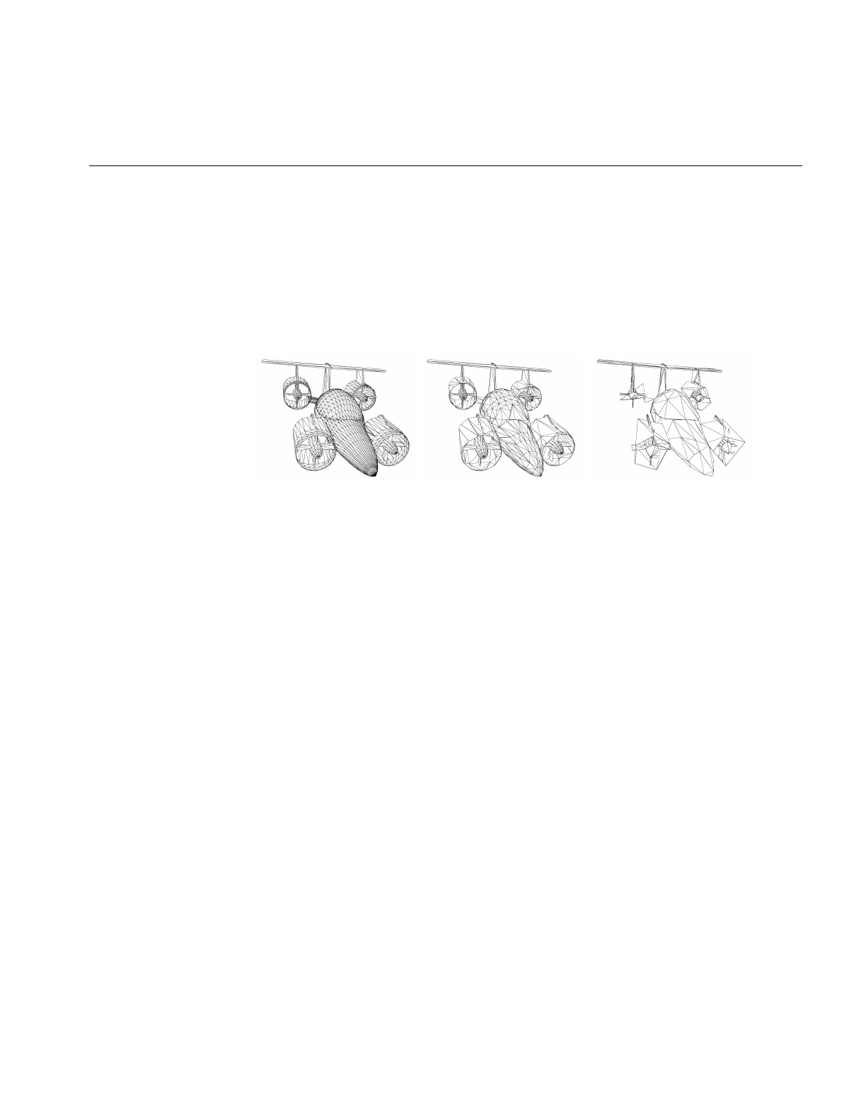
Compiling and Running optimizeDemo
63
The first command renders the model on a white background with a specific orientation.
The second command simplifies the model, as controlled by the -simpPercent 30. 10.
-simplify command-line options; and the third command simplifies the model further.
The simplifier used for these images is discussed in “Main Features of the Methods in
opSimplify:” on page 114.
In each case when the model was rendered, w was entered to yield the wire-frame views.
Figure 4-1 Simplifying a Model With optimizeDemo
The rest of this chapter is a running commentary on the code in main.cxx.

64
Chapter 4: Scene Graph Tuning With the optimizeDemo Application
optimizeDemo Code
Note: The sequence in which tools are applied to the scene graph in optimizeDemo is
not fundamental to a scene-graph tuning application; if you use optimizeDemo as a
template, other orderings may be more appropriate for your needs.
Inclusions
These headers include the necessary objects from
Cosmo3D. #include <stdio.h>
#include <Cosmo3D/csFields.h>
#include <Cosmo3D/csGroup.h>
#include <Cosmo3D/csCsb.h>
#include <Cosmo3D/csLOD.h>
#include <Cosmo3D/csTriStripSet.h>
#include <Cosmo3D/csTriFanSet.h>
#include <Cosmo3D/csTransform.h>
See “Command-Line Parser: opArgParser” on
page 375. #include <Optimizer/opArgs.h>
You can simplify the rendering task by culling
small features from the scene. See “Detail Culling”
on page 135.
#include <Optimizer/opDetailSimplify.h>
See “Reading and Writing Scene-Graph Files: The
Extendable Loading Class opGenLoader” on
page 30.
#include <Optimizer/opGenLoader.h>
This header provides various functions that
control specific features of the scene graph and
accelerate rendering. For example, see “Display
Lists” on page 94, “Vertex Arrays” on page 95,
and “Main Features of the Methods in
opCollapseAppearance” on page 97.
#include <Optimizer/opGFXSpeed.h>
See “Always First: Call opInit()” on page 29. #include <Optimizer/opInit.h>
See “Error Handling and Notification” on
page 366. #include <Optimizer/opNotify.h>

optimizeDemo Code
65
Inclusions (cont.)
The basic control of interactive rendering,
including keyboard commands and the ability to
manipulate selected portions of the scene graph,
are provided by the classes in these files. See
“Default opDrawImpl for opViewer:
opDefDrawImpl” on page 40 and “Interaction
With a Rendered Object: opPickDrawImpl” on
page 156.
#include <Optimizer/opDefDrawImpl.h>
#include <Optimizer/opPickDrawImpl.h>
To make scene graph traversals more efficient, you
can organize nodes spatially. See Chapter 8,
“Organizing the Scene Graph Spatially.”
#include <Optimizer/opSpatialize.h>
#include <Optimizer/opGeoSpatialize.h>
A sophisticated simplification tool is provided by
this file. See “Main Features of the Methods in
opSimplify:” on page 114.
#include <Optimizer/opSRASimplify.h>
You can collect statistics about the numbers of
vertices, triangles and connected primitives in
your scene graph. See “Gathering Triangle
Statistics” on page 369.
#include <Optimizer/opTriStats.h>
Includes classes to develop connected primitives
from a set of triangles in a csGeoSet. See “Merging
Triangles Into Both Strips and Fans:
opTriFanAndStrip” on page 107 and “Merging
Triangles Using Multiple Processors:
opMPTriFanAndStrip” on page 109.
#include <Optimizer/opTriFanAndStrip.h>
This file holds the basic rendering class opViewer,
discussed in “Viewing Class: opViewer” on
page 33.
#include <Optimizer/opViewer.h>

66
Chapter 4: Scene Graph Tuning With the optimizeDemo Application
Inclusions (cont.)
Tessellators convert abstract geometries into
renderable collections of triangles. See
“Tessellating Parametric Surfaces” on page 295.
This application focuses mainly on simplifying
the rendering task by using tessellations with
differing levels of resolution, by removing
triangles from tessellated objects, and by
reorganizing the distribution of triangles in the
scene graph.
#include <Optimizer/opTessParaSurfaceAction.h>
#include <Optimizer/opTessNurbSurfaceAction.h>
To guarantee consistent tessellations between
adjacent surfaces, that is, surfaces rendered
without cracks, OpenGL Optimizer provides
topology maintenance tools. See Chapter 12,
“Creating and Maintaining Surface Topology.”
#include <Optimizer/opTopo.h>
These files are in the optimizeDemo directory. #include “colorTag.h”
#include “deleteSurf.h”
#include “removeEmpty.h”
#include “simplify.h”
#include “convert.h”
Initialize
You can use either of the algorithms to remove
triangles from a mesh. See “Successive Relaxation
Algorithm: opSRASimplify” on page 115 and
“Rossignac Simplification Algorithm:
opLatticeSimplify” on page 118.
Here the application initializes the control
parameter for one of the simplification tools and
creates an instance of the other.
// Global simplifier paramaters for passing to
// app-defined key bindings
float gridSpacing = 0.08;
opSRASimplifier simplfier;
You have three ways to develop surface
connectivity information. The values enumerated
list from best to worst. See Chapter 12, “Creating
and Maintaining Surface Topology.”
int LODoffset;
enum opTopoOption
{TOPO_TWO_PASS, TOPO_ONE_PASS, TOPO_NO};

optimizeDemo Code
67
Define a Key Handler
The key handler extends the default keyboard
controls available during rendering. See “Default
opDrawImpl for opViewer: opDefDrawImpl” on
page 40.
// SimplifyViewer extends opViewer by adding new
// key bindings:
// ‘g’ : (go) simplify the scene graph
// ‘c’ : (go) tristrip the scene graph w/ random
// colors
// ‘C’ : (go) tristrip the scene graph w/o random
// colors
static bool keyHandler(opDrawImpl *di, int key)
{ opViewer *viewer = di->getViewer();
bool retVal = true;
switch(key)
{
See “Merging Triangles Into Strips: opTriStripper”
on page 105; and “Gathering Triangle Statistics”
on page 369.
case ‘c’:
case ‘C’:
// Show different colored tristrips
triStripTree( (csGroup *)viewer->getRoot(),
(key==’c’)?true:false);
{
opTriStats ts(8);
ts.apply(viewer->getRoot());
ts.print();
}
retVal = false;
break;

68
Chapter 4: Scene Graph Tuning With the optimizeDemo Application
Define a Key Handler (cont.)
See the file simplify.h and “Rossignac
Simplification Algorithm: opLatticeSimplify” on
page 118, and “Gathering Triangle Statistics” on
page 369.
case ‘G’:
opNotify(opInfo,opNull,
”Invoking Rossignac simplifier with gridSpacing =
%2.3f\n”,gridSpacing);
latticeSimplifySameTree(
(csGroup *)viewer->getRoot(), gridSpacing);
gridSpacing *= 2.0;
{
opTriStats ts(14);
ts.apply(viewer->getRoot());
ts.print();
}
break;
See the file simplify.h and “Successive Relaxation
Algorithm: opSRASimplify” on page 115, and
“Gathering Triangle Statistics” on page 369.
case ‘g’:
opNotify(opInfo,opNull,
”Invoking SRA simplifier.”);
simplifySameTree(
(csGroup *)viewer->getRoot(), &simplfier);
{
opTriStats ts(14);
ts.apply(viewer->getRoot());
ts.print();
}
retVal = false;
break;
The LOD offset adjusts the LOD calculation when
objects in the scene are moving. See “Viewing
Class: opViewer” on page 33.
case ‘+’:
changeLODOffset(
(csGroup *)viewer->getRoot(),++LODoffset);
retVal = false;
break;
case ‘-’:
changeLODOffset(
(csGroup *)viewer->getRoot(),--LODoffset);
retVal = false;
break;

optimizeDemo Code
69
Define a Key Handler (cont.)
This calls a Cosmo3D function to save a scene
graph to a file in .csb format. See “Reading and
Writing Scene-Graph Files: The Extendable
Loading Class opGenLoader” on page 30.
case ‘z’:
csdStoreFile_csb(
(csGroup *)viewer->getRoot(),”test.csb”);
break;
default:
break;
}
return retVal;
main()
See “Always First: Call opInit()” on page 29 and
“Command-Line Parser: opArgParser” on
page 375. int main(int argc, char *argv[])
{
opInit();
opArgParser args;
int numFiles;
char *filename,*outFile;
Command-Line Control Parameters
The location on the screen (x, y) of the rendering
window, and the dimensions of the window (w,h).
The default x-coordinate assumes a screen of
width 1280, and a rendering window of width 600
with a 10-pixel boundary. You can control these
parameters from the command line.
bool haveX=-1, haveY=-1, haveW=-1, haveH=-1,
haveSize=-1;
int x=1280-600-10, y=0, w=600, h=600;
If TRUE, the processed scene graph is written to a
.csb file and not rendered. See “Reading and
Writing Scene-Graph Files: The Extendable
Loading Class opGenLoader” on page 30.
bool writeCSB;
You can use several techniques to develop
connected primitives that accelerate the rendering
process. See “Creating OpenGL Connected
Primitives” on page 100.
bool doTriStrip, doTriFan, doTriFanStrip,
doMPTriFanStrip;
int minFanSize;
bool doRandomTriStrip;
// Color the tstrips with a random color

70
Chapter 4: Scene Graph Tuning With the optimizeDemo Application
Command-Line Control Parameters (cont.)
You can use either of two simplification
algorithms to remove triangles from a mesh. See
“Successive Relaxation Algorithm:
opSRASimplify” on page 115 and “Rossignac
Simplification Algorithm: opLatticeSimplify” on
page 118.
bool doSRASimplify;
bool SRApercent,SRAcount,SRAestimate;
float percent;
float fAngle;
int polyCount;
bool doLatticeSimplify;
There are several techniques to rearrange triangles
in a scene graph to reflect their positions in space
and facilitate cull traversals. See Chapter 8,
“Organizing the Scene Graph Spatially.”
bool combineGSet;
bool spatialize, geospatialize;
int minGoal,maxGoal;
bool writeOutput;
You can place simplified and unsimplified scene
graphs under a csLOD node. bool LODfiles, makeLOD;
See “Detail Culling” on page 135. bool doDetail;
float detail_ratio;
bool doRootRadius;
float root_radius;
bool doScale;
float scale_factor;
bool showDelete;
bool doDeleteSurf;
You can interactively assign colors to objects. See
“Interaction With a Rendered Object:
opPickDrawImpl” on page 156.
bool enableColoring;
char *colorTagFile;
char *colorTag;
bool doColorTag;
colorTable *cTable = NULL;
char *colorFile;
bool doRemoveEmptyGrp;
bool removeColors;

optimizeDemo Code
71
Get Command-Line Parameters
Specify the threshhold distance between points
below which they are considered identical when
building topology. See “Summary of Scene Graph
Topology: opTopo” on page 180.
bool haveTopoTol;
opReal topoTol;
Specify the background color for the rendering
window and the model orientation. These settings
are controlled by opViewer options. See “Viewing
Class: opViewer” on page 33.
bool haveBackgroundColor;
float backgroundRed, backgroundGreen,
backgroundBlue, backgroundAlpha;
bool haveRotation;
float vx, vy, vz, angle;
bool haveTranslation;
float tx, ty, tz;
Specify control parameters for tessellation, and
the type of tessellator (for example for general
parametric surfaces or for NURBS surfaces). See
“Tessellating Parametric Surfaces” on page 295.
If tessType is equal to zero, no tessellation is
performed. The main use for this option is in batch
mode to convert file formats and possibly store
topology information; you can read in a .iv file and
write the scene graph without tessellations to a
.csb file. Depending on the topology-build
command-line option, the output could have
topology information. See “Reading and Writing
Scene-Graph Files: The Extendable Loading Class
opGenLoader” on page 30.
bool haveChordalTol = -1;
opReal chordalTol = 0.01; bool haveSamples;
int samples;
bool haveTessType = -1;
char *tessType = NULL;
// Initialize this since cmdline args may modify
By default, build the best topology. See
Chapter 12, “Creating and Maintaining Surface
Topology.”
bool isOnePass = false;
You must supply a file with the scene graph. All
other command-line control parameters are
optional.
args.defRequired( “%s”,
“<filename>”,
&filename);

72
Chapter 4: Scene Graph Tuning With the optimizeDemo Application
Get Command-Line Parameters (cont.)
args.defOption( “-width %d”,
“-width <window width>”,
&haveW, &w );
args.defOption( “-height %d”,
“-height <window height>”,
&haveH, &h );
args.defOption( “-size %d”,
“-size <window width=hieght>”,
&haveSize, &w );
args.defOption( “-xpos %d”,
“-xpos <window x screen position>”,
&haveX, &x );
args.defOption( “-ypos %d”,
“-ypos <window y screen position>”,
&haveY, &y );
args.defOption( “-tristrip”,
“-tristrip”,
&doTriStrip );
args.defOption( “-trifan”,
“-trifan”,
&doTriFan);
args.defOption( “-trifanstrip %d”,
“-trifanstrip <min Fan length>”,
&doTriFanStrip, &minFanSize );
args.defOption( “-mptrifanstrip %d”,
“-mptrifanstrip <min Fan length>”,
&doMPTriFanStrip,&minFanSize );
args.defOption( “-detail %f”,
“-detail <detail ratio>”,
&doDetail, &detail_ratio);
args.defOption( “-rootRadius %f”,
“-rootRadius <radius>”,
&doRootRadius, &root_radius);
args.defOption( “-simplify”,
“-simplify”,
&doSRASimplify );

optimizeDemo Code
73
Get Command-Line Parameters (cont.)
args.defOption( “-rossignac %f”,
“-rossignac <gridSpacing>”,
&doLatticeSimplify,
&gridSpacing );
The target of the simplification can be specified as
a percentage of the original number of triangles,
or as a exact number. See “Successive Relaxation
Algorithm: opSRASimplify” on page 115.
args.defOption( “-simpPercent %f %f “,
“-simpPercent
<percent [0.0,100.0] of model desired>
<feature angle>”,
&SRApercent,
&percent,
&fAngle);
args.defOption( “-simpCount %d %f “,
“-simpCount <count per GeoSet> <feature angle>”,
&SRAcount,
&polyCount,
&fAngle);
args.defOption( “-simpEstimate”,
“-simpEstimate, for quick estimate of resulting
model”,
&SRAestimate);
You can render individual csTriStrips in differing
colors, to see their sizes.See “Creating OpenGL
Connected Primitives” on page 100; and “Specify
Coloring of New csGeoSets: opColorGenerator”
on page 332.
args.defOption( “-tristripRandom”,
“-tristripRandom, for random colors”,
&doRandomTriStrip);
args.defOption( “-scale %f”,
“-scale <scale factor>”,
&doScale, &scale_factor);
args.defOption( “-batch %s”,
“-batch <output filename>”,
&writeCSB,&outFile);
args.defOption( “-combine”,
“-combine”,
&combineGSet);
args.defOption( “-spatialize %d %d “,
“-spatialize <min tris> <max tris>”,
&spatialize,&minGoal,&maxGoal);

74
Chapter 4: Scene Graph Tuning With the optimizeDemo Application
Get Command-Line Parameters (cont.)
args.defOption( “-geospatialize %d %d “,
“-geospatialize <min tris> <max tris>”,
&geospatialize,&minGoal,&maxGoal);
args.defOption( “-LODfiles”,
“-LODfiles puts listed files as children under LOD
in given order”,
&LODfiles);
args.defOption( “-makeLOD”,
“-makeLOD creates simplified version from root
then adds both to LOD”,
&makeLOD);
args.defOption( “-writeSG”,
“-writeSG prints out entire contents of scene
graph”,
&writeOutput);
args.defOption( “-noColors”,
“-noColors removes color bindings from csGeoSets”,
&removeColors);

optimizeDemo Code
75
Get Command-Line Parameters (cont.)
#ifdef OP_REAL_IS_DOUBLE
args.defOption( “-ctol %l”,
“-ctol <max chordal deviation>”,
&haveChordalTol, &chordalTol );
args.defOption( “-ttol %l”,
“-ttol <topology tolerance> [setting ttol implies
automatic topology building]”,
&haveTopoTol, &topoTol );
#else
args.defOption( “-ctol %f”,
“-ctol <max chordal deviation>”,
&haveChordalTol, &chordalTol );
args.defOption( “-ttol %f”,
“-ttol <topology tolerance> [setting ttol implies
automatic topology building]”,
&haveTopoTol, &topoTol );
#endif
args.defOption( “-onePass”,
“-onePass [build topology while tessellating]”,
&isOnePass )
// Sets the type of tessellator used either by the
// loader or after building the topology.
args.defOption( “-tess %s”,
“-tess <gen[eral] nurb no>”,
&haveTessType, &tessType );
// Sets how many samples are used on trim curves
// during the tessellation.
args.defOption( “-samples %d”,
“-samples <tessellator sample count>”,
&haveSamples, &samples);

76
Chapter 4: Scene Graph Tuning With the optimizeDemo Application
Get Command-Line Parameters (cont.)
// enable feature to delete highlighted nodes with
‘X’ key
args.defOption( “-showDelete”,
“-showDelete use X key to delete highlighted
nodes to clean up dbase. Need to save SG for
permanent change.”,
&showDelete);
// enable feature to color highlighted subtrees
with number keys
args.defOption( “-enableColoring %s %s”,
“-enableColoring <output filename> <tag>”,
&enableColoring, &colorTagFile, &colorTag);
// Read in <filename>.delete to determine which
parts to delete from SG
args.defOption( “-delete”,
“-delete”,
&doDeleteSurf);
// User defined background color
args.defOption( “-background %f %f %f %f”,
“-background <red> <green> <blue><alpha>”,
&haveBackgroundColor, &backgroundRed,
&backgroundGreen, &backgroundBlue,
&backgroundAlpha );
// User defined model orientation
args.defOption( “-rotation %f %f %f %f”,
“-rotation <vx> <vy> <vz> <angle>”,
&haveRotation, &vx, &vy, &vz, &angle );
args.defOption( “-translation %f %f %f”,
“-translation <tx> <ty> <tz>”,
&haveTranslation, &tx, &ty, &tz );
// Use colortag file to determine which color to
apply to all parts
// in corresponding filename
// Assuming all nodes in file will be same color
args.defOption( “-colortag %s”, “-colortag
<filename>”, &doColorTag, &colorFile);
// Remove group nodes with no children
args.defOption( “-remove”,”-remove”,
&doRemoveEmptyGrp);

optimizeDemo Code
77
Get Command-Line Parameters (cont.)
numFiles = args.scanArgs(argc,argv);
//set topoOption
topologyOption topoOption;
if (!haveTopoTol)
{
topoOption = TOPO_NO;
//don’t build topology
}
else if (isOnePass)
{
topoOption = TOPO_ONE_PASS;
//build topology while tessellating.
}
else
{
topoOption = TOPO_TWO_PASS;
//build topology in a seperate pass before
//tessellation
}
Create the Appropriate Tessellator
See Chapter 13, “Rendering Higher-Order
Primitives: Tessellators.” // Create a tessellator
opTessParaSurfaceAction *tess;
if ( tessType == NULL )
tess = new opTessParaSurfaceAction;
else if ( strcmp( tessType, “gen” ) == 0 )
tess = new opTessParaSurfaceAction;
else if ( strcmp( tessType, “nurb” ) == 0 )
tess = new opTessNurbSurfaceAction;
else if ( strcmp( tessType, “no” ) == 0)
tess = NULL;
else
tess = new opTessParaSurfaceAction;
// Set the chordal tolerance
if(tess)
tess->setChordalDevTol( chordalTol );
// Set the sample count if the user set them
if ( haveSamples )
tess->setSampling( samples );

78
Chapter 4: Scene Graph Tuning With the optimizeDemo Application
Create the Topology Data Structures
See Chapter 12, “Creating and Maintaining
Surface Topology.” //topology
opTopo *topo = new opTopo;
// Set the topology parameters
if ( haveTopoTol )
{
topo->setDistanceTol( topoTol, meter );
}

optimizeDemo Code
79
Load the Scene Graph Data
The loader manages topology in one of the
following ways:
•It anticipates the development of connectivity
information for all surfaces in the scene graph
followed by tessellating the surface. Code for
these steps appears later in the application.
• It develops connectivity information as surfaces
load, and tessellates them.
• It ignores connectivity: it simply tessellates
surfaces as they load without regard for
adjacencies.
See “Reading and Writing Scene-Graph Files: The
Extendable Loading Class opGenLoader” on
page 30; Chapter 12, “Creating and Maintaining
Surface Topology”; and “Base Class
opTessellateAction” on page 289.
// Create a loader
opGenLoader *loader;
if(topoOption == TOPO_TWO_PASS)
//build topology before tessellating any
//surface.
{
loader = new opGenLoader( true, NULL, false );
//the tessellator is not bound to the loader so
//that there is no tessellation at loading. The
//reason is because tessellation has to wait
//until topology construction is completely done
//for all the surfaces
}
else if( topoOption == TOPO_ONE_PASS )
//build topology while tessellate
{
tess->setBuildTopoWhileTess(true);
//tell the tessellator to invoke topology
//construction at tessellation
//Sets the topology which will used in the
//topology building at tessellation.
tess->setTopo(topo);
loader = new opGenLoader( true, tess, false );
//bind tessellator to loader so that
//tessellation is invoked at loading
}
else //don’t build topology
{
//bind tessellator to loader so that
//tessellation is invoked at loading
loader = new opGenLoader( true, tess, false );
}
// Load the file on the command line and get a //
scene graph back
csGroup *obj = loader->load( filename );
csGroup *root = obj;

80
Chapter 4: Scene Graph Tuning With the optimizeDemo Application
Load the Scene Graph Data (cont.)
if (obj)
{
// Delete parts specified in corresponding
// *.delete
if (doDeleteSurf)
{
deleteSurfTree(obj,filename);
}
You can use a color tag file to specify the
appearance of different parts in the scene. The
format of the color tag file is:
• Comments (preceded by the pound sign, #).
• A line containing the number of colors.
• Lines containing the colors: five digits that
specify red, green, blue, alpha, and shininess
values. Currently, alpha is not used, but a
value must appear for the shininess parameter to
be properly interpreted.
• Part names and their associated colors.
See colorTable::colorTable() in
/usr/share/Optimizer/src/sample/optimizeDemo/
colorTag.cxx.
// Color the parts as specified in color file
if (doColorTag)
{
cTable = new colorTable(colorFile);
cTable->setColorTree(obj,filename);
}

optimizeDemo Code
81
Load the Scene Graph Data (cont.)
if (numFiles)
{
int i;
csGroup *grp;
if (LODfiles)
{
grp = (csGroup *)new csLOD;
} else
{
grp = new csGroup;
}
grp->addChild(obj);
char **xtraFiles = args.getRemainingArgs();
for (i=0;i<numFiles;i++)
{
opNotify( opNotice, opNull,
“Loading file %d %s\n”,i,xtraFiles[i]);
obj = loader->load(xtraFiles[i]);
if (obj)
{
if (doDeleteSurf)
{
deleteSurfTree(obj,xtraFiles[i]);
}
if (doColorTag)
{
cTable = new colorTable(colorFile);
cTable->setColorTree(obj,xtraFiles[i]);
}
grp->addChild(obj);
}
}

82
Chapter 4: Scene Graph Tuning With the optimizeDemo Application
Load the Scene Graph Data (cont.)
See addLOD.cxx.if (LODfiles)
{
setupLOD((csLOD *)grp,(csSwitch::SwitchEnum)0);
}
root = grp;
}
// Throw the loader away, we’re done with it
delete loader;
Build Topology and Tessellate
The most accurate topology, which yields
crack-free tessellations, is created by two
traversals of the scene graph: one to establish
adjacencies of surfaces, and the second to
tessellate the surfaces. See “Building Topology:
Computing and Using Connectivity Information”
on page 273.
//build topology if we haven’t done it
if ( obj && topoOption == TOPO_TWO_PASS)
{
fprintf(stderr, “Building topology starts ...
\n”);
topo->buildTopology( );
fprintf(stderr, “Building topology done\n”);
You can tesselate higher-order surface
representations and view the scene, or in batch
processing, not view the scene but write the scene
graph (possibly with topology information) to a
.csb file. See “Reading and Writing Scene-Graph
Files: The Extendable Loading Class
opGenLoader” on page 30.
if(tess)
{
fprintf(stderr, “Tessellation starts ... \n”);
tess->apply( obj );
fprintf(stderr, “Tessellation done ... \n”);
}
else
{
fprintf(stderr, “No tessellation is
performed\n”);
}
Remove Childless Nodes and Color Bindings
See the files removeEmpty.h and removeEmpty.cxx. // Run through the SG and remove groups with no
// children
if (doRemoveEmptyGrp)
{
obj = removeEmpty(root);
}

optimizeDemo Code
83
Remove Childless Nodes and Color Bindings
(cont.)
csType *type = csTriFanSet::getClassType();
if ( doTriStrip || doRandomTriStrip)
{
type = csTriStripSet::getClassType();
}
See “Removing Color Bindings” on page 96. if (removeColors)
opRemoveColorBindings(root);
Remove Small Objects from the Scene
You can remove small objects from the rendering
pipeline. See “Detail Culling” on page 135. csSphereBound sph;
root->getSphereBound (sph);
opNotify( opNotice, opNull,
“Root bounding sphere is %f\n”,sph.radius);
if (doDetail)
{
opDetailSimplify *dsimp = new opDetailSimplify;
// Compare radius of geosets to radius of overall
// model so more of the smaller pieces are culled.
if (doRootRadius)
{
dsimp->setRootRadius(root_radius);
}
dsimp->setSizeRatio (detail_ratio);
dsimp->apply (root);
}
Remove Childless Nodes After Detail Cull
See the files removeEmpty.h and removeEmpty.cxx. // Run through the SG and remove groups with no
children
if (doRemoveEmptyGrp)
{
root = removeEmpty(root);
}

84
Chapter 4: Scene Graph Tuning With the optimizeDemo Application
Spatialize the Scene Graph
If you have a scene graph with too many small
csGeosets, you can combine them and develop a
graph consisting of a root node with one child that
contains all of the triangles of the original graph.
See “Merging csGeoSets in a Scene Graph:
opCombineGeoSets” on page 147.
if (combineGSet)
{
// For now, don’t generate colors
root =
(csGroup *)opCombineGeoSets::convert(root,type);
}
Spatialize the Scene Graph (cont.)
You can re-organize existing nodes to reflect their
spatial relations (see “Spatializing a Scene Graph:
opGeoSpatialize” on page 144) or spatially
re-organize triangles in a csGeoSet (see
“Spatialization Tool: opSpatialize” on page 142).
The function geoSpatializeTree() is defined in
geoSpatialize.cxx and spatializeTree() is defined in
spatialize.cxx. These functions apply the
spatialization methods to the whole scene graph.
if (geospatialize)
{
// Spatialize based on combining everything below
// a particular group, then chop it up into smaller
// pieces if it exceeds maxGoal
geoSpatializeTree(root,minGoal,maxGoal,type);
} else if (spatialize)
{
spatializeTree(root,minGoal,maxGoal,type);
}
Print Scene Graph
This is the Cosmo3D method to write out the
scene graph. if (writeOutput)
{
csOutput *output = new csOutput(stdout);
output->write(root);
}

optimizeDemo Code
85
Remove Triangles and Create Levels of Detail
You can use either of two simplification
algorithms to remove triangles from a mesh. See
“Successive Relaxation Algorithm:
opSRASimplify” on page 115 and “Rossignac
Simplification Algorithm: opLatticeSimplify” on
page 118.
if ( doSRASimplify || makeLOD)
{
// Default is to use percentage
// of model as a target goal
if (SRAcount)
{
// Check if both -simpPercent and -simpCount
// options were used at the same time
if (SRApercent)
{
opNotify(opFatal,opUsage,”Can not use both
-simpPercent and -simpCount at the same
time. Using only -simpCount option\n”);
}
opTriStats stats;
stats.apply(root);
percent = 100.0*((float)polyCount/
(float)stats.getTriCount());
// User changes these settings
simplifier.setPercent(percent);
simplifier.setFAngle(fAngle);
} else if (SRApercent)
{ // User changes these settings
simplifier.setPercent(percent);
simplifier.setFAngle(fAngle);
}
if (SRAestimate)
{
simplifier.setAccurateMethod(false);
}

86
Chapter 4: Scene Graph Tuning With the optimizeDemo Application
Remove Triangles and Create Levels of Detail
The functions simplifyTree(),
simplifySameTree(), and
latticeSimplifySameTree() traverse the scene
graph and simplify all csGeoSets. See the files
simplify.h,simplify.cxx, and simplifySameTree.cxx.
if (makeLOD)
{
fprintf(stderr,”Simplifying ...”);
csGroup *simpObj =
simplifyTree(root, &simplifier);
fprintf(stderr,”Done\n”);
// Set child0 as default LOD to be drawn
root = addLODChild(root,simpObj,0);
} else
{
fprintf(stderr,”Simplifying ...”);
csGroup *simpObj =
simplifySameTree(root, &simplifier);
fprintf(stderr,”Done\n”);
root = simpObj;
}
}
else if (doLatticeSimplify)
{
opNotify(opInfo,opNull,
”Invoking Rossignac simplifier with
gridSpacing =%2.3f\n”,gridSpacing);
csGroup *simpObj =
latticeSimplifySameTree(root, gridSpacing);
gridSpacing *= 2;
fprintf(stderr,”Done\n”);
root = simpObj;
}

optimizeDemo Code
87
Create OpenGL Connected Primitives
To reduce the load on the graphics hardware, you
can reduce redundant vertex information by
combining triangles into fans of a minimum size,
and combining the remainder into triangle strips
(using either a single or multiple processors). See
“Merging Triangles Into Both Strips and Fans:
opTriFanAndStrip” on page 107 and “Merging
Triangles Using Multiple Processors:
opMPTriFanAndStrip” on page 109.
if (doTriFanStrip)
{
// Only create trifans if they can be of a minimum
// Fan Length.
opTriFanAndStrip tfs(minFanSize);
tfs.apply(root);
}
else if (doMPTriFanStrip)
{
// Only create trifans if they can be of a minimum
Fan Length.
opMPTriFanAndStrip tfs(minFanSize);
tfs.apply(root);
You can create just triangle strips to reduce
redundant vertex information, rather than create
both triangle fans and triangle strips. See
“Merging Triangles Into Strips: opTriStripper” on
page 105.
The methods of opTriStripper work only on a
csGeoSet. The function triStripTree() traverses
the whole scene graph, applying the methods of
opTriStripper to every csGeoSet (see triStrip.cxx).
} else if
((doTriStrip || doRandomTriStrip) && !combineGSet
)
{
bool useRandomColor;
fprintf(stderr,”TriStripping ...”);
if (doRandomTriStrip)
useRandomColor = true;
else
useRandomColor = false;
triStripTree( root,useRandomColor);
fprintf(stderr,”Done\n”);
You can create just triangle fans to reduce
redundant vertex information, rather than create
both triangle fans and triangle strips. See
“Merging Triangles Into Fans: opTriFanner” on
page 103.
The methods of opTriFanner work only on a
csGeoSet. The function triFanTree() traverses the
whole scene graph, applying the methods of
opTriFanner to every csGeoSet. (see triFan.cxx).
}else if (doTriFan && !combineGSet)
{
bool useRandomColor = false;
fprintf(stderr,”TriFanning ...”);
triFanTree( root,useRandomColor);
}

88
Chapter 4: Scene Graph Tuning With the optimizeDemo Application
Rescale Objects in Scene
if (doScale)
{
csGroup *newroot = new csGroup;
csTransform *xform = new csTransform;
xform->setScale
(scale_factor, scale_factor, scale_factor);
newroot->addChild (xform);
xform->addChild (root);
root = newroot;
}
Collect Vertex Statistics and Print Them
See “Error Handling and Notification” on
page 366 and “Getting Statistics About a Scene
Graph: opTriStats” on page 371.
// Get stats on the scene graph
opTriStats stats;
stats.apply(root);
opNotify( opNotice, opNull,
“Scene statistics:\n”);
stats.print();
Write Scene Graph to File
You can run optimizeDemo in batch mode
without viewing the effects of the scene-graph
manipulation tools.
if ( writeCSB)
{
csdStoreFile_csb(root,outFile);
}
else
{

optimizeDemo Code
89
Set Parameters to Draw the Scene
To see the effects of the scene-graph
manipulations, you can use an opViewer and
register the keyboard commands defined by the
keyHandler() with the interaction control class,
an opDrawImpl. See “Viewing Class: opViewer”
on page 33, “Basic Tools for Rendering
Implementations: opKeyCallback and
opDrawImpl” on page 38, and “Default
opDrawImpl for opViewer: opDefDrawImpl” on
page 40.
if (haveSize)
h = w;
opViewer *viewer =
new opViewer(filename, x, y, w, h);
opDefDrawImpl *di = new opDefDrawImpl( viewer );
if ( haveBackgroundColor )
{
viewer->setBackgroundColor(
backgroundRed,
backgroundGreen,
backgroundBlue,
backgroundAlpha );
}
di->registerKey(‘c’, keyHandler, “Tri-strip a
shape node (random colors)”);
di->registerKey(‘C’, keyHandler, “Tri-strip a
shape node (normal colors)”);
di->registerKey(‘g’, keyHandler,
“Go simplify single a shape node.” );
di->registerKey(‘G’, keyHandler,
“Go simplify single a shape node using Rossignac
algorithm.” );
di->registerKey(‘+’, keyHandler,
“See next LOD, less detail.” );
di->registerKey(‘-’, keyHandler,
“See previous LOD, more detail.” );
di->registerKey(‘z’, keyHandler,
“Save scene graph of model.” );
// Use default DrawImpl until pick invoked
opPickDrawImpl *pi = new opPickDrawImpl(viewer);
if (showDelete)
pi->enableDelete ();
if (enableColoring)
pi->enableColoring (colorTagFile, colorTag);

90
Chapter 4: Scene Graph Tuning With the optimizeDemo Application
Draw the Scene
You can set the model orientation. See “Viewing
Class: opViewer” on page 33. viewer->addChild(root);
viewer->setViewPoint(root);
if ( haveRotation )
{
viewer->setModelRotation( vx, vy, vz, angle );
}
if ( haveTranslation )
{
viewer->setModelTranslation( tx, ty, tz );
}
You can further reduce the load on the graphics
hardware by using OpenGL display lists. See
“Display Lists” on page 94.
opDListScene((csGroup*)viewer->getRoot());
viewer->eventLoop();
}
}
}

PART TWO
High-Level Strategic Tools for Fast
RenderingChapter 8 II
The first three chapters in this section discuss tools that help reduce the amount
of scene-graph data that the graphics hardware must process. With the exception
of the level-of-detail nodes, discussed in Chapter 6, all of these tools also reduce
the size of the host’s data management task.
Chapter 7 discusses organizing a scene graph to facilitate traversals, particularly
view frustum culling, picking and highlighting, and occlusion culling.
These are the titles of the chapters in this section:
Chapter 5, “Sending Efficient Graphics Data to the Hardware”
Chapter 6, “Rendering Appropriate Levels of Detail”
Chapter 7, “Culling Unneeded Objects From the Scene Graph”


93
Chapter 5
5. Sending Efficient Graphics Data to the Hardware
A potential bottleneck in the graphics pipeline is the transfer of rendering commands to
the graphics hardware. Generating a compact set of OpenGL commands not only
simplifies tasks for the host, it can accelerate later stages in the graphics pipeline.
For a discussion of techniques for developing an optimal set of OpenGL commands, see
sections 6.6.2, “Reducing OpenGL Command Overhead,” and section 6.6.3, “Minimize
OpenGL Mode Changes,” in Programming OpenGL for the X Window System (see
“Recommended Reference Materials” on page xxxi). This book is referred to in this
chapter as the Green book.
This chapter presents five of the six approaches to optimization mentioned in the Green
book sections 6.6.2 and 6.6.3: display lists, vertex arrays, short normals, connected
primitives, and avoiding mode switching. The sixth method described in the Green
book— using OpenGL evaluators— is a subtler task, addressed by OpenGL Optimizer
higher-order geometric primitives, and discussed in Part IV, “Managing and Rendering
Higher-Order Geometric Primitives.” OpenGL Optimizer also includes a tool for using
multiple processors to create connected primitives.
Also included in this chapter is a scene-graph-flattening tool, which simplifies a scene
graph.
The following list shows the main sections in this chapter.
• “Display Lists” on page 94 (see also the Green book)
• “Vertex Arrays” on page 95 (see also the Green book)
• “Avoiding OpenGL Mode Switching” on page 96 (see also the Green book)
• “Main Features of the Methods in opCollapseAppearance” on page 97
• “Creating OpenGL Connected Primitives” on page 100 (see also the Green book)

94
Chapter 5: Sending Efficient Graphics Data to the Hardware
Display Lists
A display list is a copy of the scene graph in a form optimized for the graphics pipeline.
On some machines, you can accelerate rendering by nearly a factor of 10 by making
OpenGL display lists. The speedup occurs largely where there is graphics hardware that
can hold display lists in a cache. For graphics hardware of this type, display lists are the
most efficient descriptions of objects in a scene. However, because display lists are a copy
they necessesarily cause more memory usage.
Display lists are useful when you can graphically treat all the objects in the list as a unit.
If you need to independently manipulate an element in the group, a display list is not
appropriate.
For more information on the advantages of using display lists, see the Green book; the
the Red book, particularly Chapter 4; and OpenGL on Silicon Graphics Systems,
particularly the sections “CPU Tuning: Basics” and “CPU Tuning: Display Lists” in
Chapter 12, “Tuning the Pipeline.” These books are all listed in “Recommended
Reference Materials” on page xxxi.
These two functions make OpenGL display lists:
opDListCSGeometry(g)
For a single csGeometry,g, compiles an OpenGL display list. This is the
declaration:
csGeometry *opDListCSGeometry(csGeometry *g)
opDListScene(root)
For each csGeometry in the scene graph below root, compiles an
OpenGL display list. This is the prototype:
void opDListScene(csNode *root);
See the reference page opGFXSpeed(3in) for more details.

Vertex Arrays
95
Vertex Arrays
For more efficient surface descriptions, you can convert csGeoSet attributes to OpenGL
1.1 vertex arrays, which provide an alternative to the main OpenGL approach of having
a procedure call for each piece of vertex data.
For more information on the advantages of using vertex arrays, see the Green book; the
the Red book, particularly the section “Vertex Arrays” in Chapter 2; and OpenGL on
Silicon Graphics Systems, particularly the section “The Vertex Array Extension” in Chapter
8. These books are all listed in “Recommended Reference Materials” on page xxxi.
These two functions make OpenGL vertex arrays:
opGLArrayEXTCSGeoSet()
Converts the attributes in a csGeoSet to the format appropriate for
glDrawArrays() and returns the modified csGeoSet. This is the
declaration for the conversion function:
csGeoSet *opGLArrayEXTCSGeoSet(csGeoSet *g)
opGLArrayEXTScene()
Converts the attributes in all the csGeoSets in a scene graph to the
format appropriate for glDrawArrays() and returns the root of modified
scene graph. This is the declaration for the conversion function:
void opGLArrayEXTScene(csNode *root);
These declarations appear in the file opGFXSpeed.h

96
Chapter 5: Sending Efficient Graphics Data to the Hardware
Shortening Representations of Surface Normal Data
Surface normals, which accurately represent a surface before tessellation, are usually
stored in a csGeoSet as csVec3fs, floating-point vectors, one for each vertex.
For all normal vectors in the scene graph below root, the function
opShortNormsScene(root) converts the data format from csVec3f to csVec3s, that is, to
short-integer vectors. This shortening of the memory segments holding surface normals
reduces the amount of data that must be sent from the host to the graphics pipeline by as
much as 25%.
Short normals provide faster rendering in situations where host-to-graphics-pipeline
bandwidth is the limiting factor. The reduced data volume also enhances performance
by allowing more of the scene to reside in the display-list cache.
Avoiding OpenGL Mode Switching
If the OpenGL machine state (or mode) differs between objects in a scene, rendering
speed, particularly the transformation and rasterization stages, can be slowed due to the
reconfiguration required.
Two OpenGL Optimizer classes allow you to inhibit mode changes during rendering.
You can inhibit a change to the color associated with a csShape or you can disable the
entire csAppearance associated with the shape. In either case the first values of states
that are encountered during the draw traversal are used for the entire scene.
Removing Color Bindings
You can accelerate the transform stage by disabling the current-color tests, which are
controlled by glColorMaterial(). Naturally this alters the color of objects. See the OpenGL
Programming Guide for more details.
The function opRemoveColorBindings() traverses a scene graph and sets the color
binding of each csGeoSet to NO_COLOR. This is the declaration of the function, which
appears in the file opGFXSpeed.h:
void opRemoveColorBindings(csNode *root);

Avoiding OpenGL Mode Switching
97
Removing csAppearance Effects
You can force all csShape nodes in a scene graph to have the same csAppearance, and
thus prevent mode switching by the OpenGL machine during rendering, by using the
class opCollapseAppearances, which is a csAction that traverses the scene graph and
sets all csAppearances to be the same as the first appearance encountered by the
traversal. However, be aware that existing csAppearances are lost.
Class Declaration for opCollapseAppearances
The following are the main methods in the class:
class opCollapseAppearances : public csAction
{
public:
opCollapseAppearances();
};
Main Features of the Methods in opCollapseAppearance
apply() Is inherited from csAction. When you call apply on a node, all csShapes
below it are set to have the same csAppearance as the first csShape
encountered by a traversal starting at the node.

98
Chapter 5: Sending Efficient Graphics Data to the Hardware
Simplifying a Scene Graph: opFlattenScene()
For many CAD data sets, scene-graph structure is likely to reflect useful data
organization. However, that organization can be a heavy computational overhead;
traversing a scene graph with a hierarchy containing many levels can slow rendering.
To eliminate the overhead incurred from scene graph hierarchy, the function
opFlattenScene() places all the csShape nodes in a scene (sub)graph below a single
csGroup node. Figure 5-1 shows the effects of flattening a simple scene graph. Notice
that the interior nodes are simply removed; in this figure, the removal of the csTransform
could alter the appearance of the scene. To avoid this distortion, before flattening a scene
graph, set the location and orientation of higher-order primitives using methods in
opRep (see “Geometric Primitives: The Base Class opRep and the Application repTest”
on page 189).
This is the prototype of opFlattenScene(), which appears in the file opGFXSpeed.h:
csGroup *opFlattenScene(csNode *node);
The argument node is the root of the scene graph. The returned value is a pointer to a
csGroup node, which has as children all the csShape nodes in the original graph.
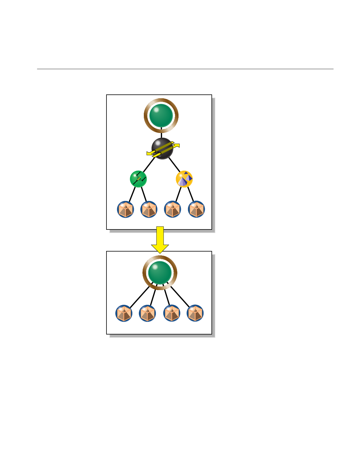
Simplifying a Scene Graph: opFlattenScene()
99
Figure 5-1 Flattening A Scene Graph Removes Interior Nodes
csGroup
csTransform
csLOD
csSwitch
csShape csShape csShape csShape
12 3 4
csGroup
csShape csShape csShape csShape
12 34

100
Chapter 5: Sending Efficient Graphics Data to the Hardware
Creating OpenGL Connected Primitives
OpenGL defines two useful geometric primitives to minimize the redundancy of vertex
information, and thus increase rendering performance: triangle fans (trifans) and triangle
strips (tristrips). These primitives take advantage of adjacency to eliminate vertex data
duplication along shared edges. Both of these primitives use the observation that, given
an existing triangle, one more vertex defines an adjacent triangle. A tristrip or trifan with
ntriangles is specified by n+2 vertices, which is typically significantly less than the 3n
vertices required to encode ntriangles independently. The construction algorithms for
these primitives are discussed in “Features of Trifans and Tristrips” on page 100.
Tristrips and trifans used in conjunction with display lists form a powerful combination
on machines with a display-list cache. Because of their compact representations, tristrips
and trifans allow the cache to hold more triangles.
The following sections discuss OpenGL Optimizer classes for creating trifans and
tristrips:
• “Features of Trifans and Tristrips” on page 100
• “Merging Triangles Into Fans: opTriFanner” on page 103
• “Merging Triangles Into Strips: opTriStripper” on page 105
• “Merging Triangles Into Both Strips and Fans: opTriFanAndStrip” on page 107
• “Merging Triangles Using Multiple Processors: opMPTriFanAndStrip” on page 109
• “Observing Trifans and Tristrips: opColorizeStrips()” on page 110
Features of Trifans and Tristrips
Reducing the number of vertices by collecting triangles into strips or fans mainly reduces
transform time— fewer vertices means fewer vertex transformations. Secondary benefits
of “tristripping” and “trifanning” are reductions in OpenGL function call overhead,
bandwidth requirements, memory consumption, and caching. Another benefit is fewer
glVertex*() calls and proportionally less bandwidth to the graphics hardware. Since
tristrips and trifans encode fewer vertices, they also require less memory than
independent triangles. On the host side, this translates into better locality of reference.
Fill-limited applications receive no benefit from tristripping or trifanning.

Creating OpenGL Connected Primitives
101
How Trifans and Tristrips Are Constructed
To construct a trifan, a new triangle is defined by a new vertex, the previous vertex, and
the first vertex, which is common to all the triangles in the fan (see Figure 5-2).
During the construction of a tristrip, a new triangle is defined by a new vertex the
previous two vertices added to the tristrip(see Figure 5-2).
Figure 5-2 Construction of Triangle Fan (left) and Triangle Strip (right)
How Attributes of Shared Vertices Are Managed
When a vertex defines a new triangle in a tristrip or trifan, it retains the attributes it had
as a member of the original triangle. When the vertex is subsequently shared with an
added triangle, in principle it has two sets of attributes. To resolve the ambiguity, the
vertex’s attributes that are associated with the most recently added triangle are lost.
You can set the maximum difference between the attributes of the vertex that come from
a prospective new triangle and those that it would have as a member of a tristrip or trifan.
If normals and colors associated with shared vertices of two adjacent triangles are too
different, you may see an unacceptable distortion of appearance; you control the
rendering artifacts that occur by specifying how great a difference is acceptable.
To illustrate the problem, consider the case of two adjacent triangles that lie on different
faces of a cube. The original normals associated with the shared vertices on the edge of
the cube are at right angles to each other. If these triangles are grouped into a tristrip, one
of the faces is lit as if it were a curved surface, because its original normal at the shared
vertex no longer controls the lighting calculation. Similarly, if you created a trifan with a
central vertex at the corner of a cube and triangles on all three adjacent faces, two of the
faces would appear curved.
0
12 2
3
3
4
4
5
6
7
0
1

102
Chapter 5: Sending Efficient Graphics Data to the Hardware
Strategies for Using Trifans, Tristips, or a Combination of Both
Trifanning algorithms often work well where tristripping algorithms work poorly, and
vice versa. Generating trifans is typically easier than generating good tristrips because a
good candidate for the first vertex in a fan is any vertex adjacent to a large number of
edges. Determining starting triangles for tristrips is more complicated. OpenGL
Optimizer provides classes for three ways to create trifans and tristrips:
• a trifan generator
• a tristrip generator
• an automatic combination of the two.
To tune your scene graph, try each technique, and use the one with the minimum number
of vertices (see “Gathering Triangle Statistics” on page 369).
Triangle fans are particularly useful when used with tessellations of trimmed NURBS
(see Part IV, “Managing and Rendering Higher-Order Geometric Primitives”) because
the tessellation process often generates large sets of triangles that can be represented by
fans.
Count Vertices, Not Triangles, to Assess Graphic Pipeline Load
To assess the benefits of tristrips or trifans when tuning your database, use the average
number of vertices per triangle as a metric. This is preferable to the average number of
triangles per trifan or tristrip, because it is proportional to the real computational load on
the transformation stage of the pipeline. To obtain triangle and vertex statistics, see
“Gathering Triangle Statistics” on page 369.

Creating OpenGL Connected Primitives
103
Merging Triangles Into Fans: opTriFanner
The main feature of this class is an overloaded method, convert(), which develops
csTriFanSets from triangle sets. A set of triangles can come from a csGeometry, from a
singly linked list of trifans that you create, or from an opGeoConverter, discussed in
“Decompose csGeoSets Into Constituent Triangles: opGeoConverter” on page 329. In
anticipation of possible derivations, the member function convert() is declared to accept
the parent class of csGeoSet,csGeometry.
Class Declaration for opTriFanner
The following are the main methods in the class:
class opTriFanner : public opTriFanSetBuilder
{
public:
opTriFanner(const opGeoConverter *gc);
~opTriFanner();
static csGeometry *convert(
const opGeoConverter *gc,
opColorGenerator *cg=opColorGenerator::noColors());
static csGeometry *convert(
csGeometry *geom,
opColorGenerator *cg=opColorGenerator::noColors());
};

104
Chapter 5: Sending Efficient Graphics Data to the Hardware
Main Features of the Methods in opTriFanner
The main feature of the class is the method convert(), which allows you to provide
contrasting colors for the new csTriStrips, to help you see the effects of the conversion.
These are the effects of the different argument types for convert():
opColorGenerator
convert()’s color options are controlled by the class opColorGenerator,
discussed in “Specify Coloring of New csGeoSets: opColorGenerator”
on page 332. The default is no color distinction, which renders quickly
but does not distinquish trifans.
csGeometry convert() takes a csTriSet,csTriStripSet, or csTriFanSet, and returns a
csTriFanSet. If the input is a csTriFanSet, the output may not have a
substantial effect on redundant vertices.
opGeoConverter
If you have previously used an opGeoConverter to develop hash tables
for a set of triangles, you can simply pass them to convert(). Otherwise,
convert() makes a new opGeoConverter. See “Decompose csGeoSets
Into Constituent Triangles: opGeoConverter” on page 329.

Creating OpenGL Connected Primitives
105
Merging Triangles Into Strips: opTriStripper
The second approach to control redundant vertex information is to organize triangles
into strips of adjacent triangles. Like opTriFanner, the important method for
opTriStripper is convert(), which takes three types of input data.
Class Declaration for opTriStripper
The following are the main methods in the class:
class opTriStripper : public opTriStripSetBuilder
{
public:
opTriStripper(const opGeoConverter *gc);
~opTriStripper();
static csGeometry *convert(
const opGeoConverter *gc,
opColorGenerator *cg = opColorGenerator::noColors());
static csGeometry *convert(
csGeometry *geom,
opColorGenerator *cg = opColorGenerator::noColors());
static csShape *convert(
csShape *s,
opColorGenerator *cg = opColorGenerator::noColors());
};
Main Features of the Methods in opTriStripper
The main feature of the class is the method convert(), which differs from
opTriFanner::convert() in the following way:
csGeometry convert() returns a csTriStripSet. If the input is a csTriStripSet, the
output may not be substantially different.

106
Chapter 5: Sending Efficient Graphics Data to the Hardware
Tuning Triangle Strips: Fixing Tristrips That Are Too Short
The effectiveness of triangle stripping depends on the length of the strips. Longer strips
imply fewer vertices per triangle, and thus a lighter rendering load. Typically, models
cannot be grouped into long strips using OpenGL Optimizer tristripping algorithms. In
general, the more uniform the tessellation, the longer the strips will be. When you see too
many vertices per triangle (see “Gathering Triangle Statistics” on page 369), check for the
following:
• The triangles may not actually be adjacent because of cracks. If the triangles were
generated by an OpenGL Optimizer tessellator, you may be able to eliminate the
cracks using the opTopo class (see Chapter 12, “Creating and Maintaining Surface
Topology”).
• Normals, colors, or texture coordinates may be too different to allow grouping. Try
relaxing tolerances if possible.
• The set of triangles may be too small for developing effective tristrips. Try
combining triangles from several csGeoSets (see “Merging csGeoSets in a Scene
Graph: opCombineGeoSets” on page 147).
• Some models cannot be grouped into long strips using the OpenGL Optimizer
algorithm. Try the trifanning algorithm, a different tristripping algorithm, or see if
you can generate a more uniform tessellation (see Chapter 13, “Rendering
Higher-Order Primitives: Tessellators”).

Creating OpenGL Connected Primitives
107
Merging Triangles Into Both Strips and Fans: opTriFanAndStrip
The class opTriFanAndStrip is a csAction that provides a a hybrid method to traverse a
scene graph and merge the triangles in each csGeoSet into trifans or tristrips.
The merging operation begins by making trifans. If a trifan has fewer than a minimum
number of triangles, the fan is not kept and the triangles are passed to the tristripper.
Class Declaration for opTriFanAndStrip
The following are the main methods in the class:
class OP_DLLEXPORT opTriFanAndStrip : public csAction
{
public:
// Input: csShape
// csGeometry, csGeoSet0, . . . csGeoSetN
// Output: csShape
// csGeometry, csTriStripSet, csTriFanSet
opTriFanAndStrip(int minFanSize,
opColorGenerator *cg=opColorGenerator::noColors());
virtual ~opTriFanAndStrip();
static csShape *convert(
csShape *,
int minFanSize=5,
opColorGenerator *cg=opColorGenerator::noColors());
};

108
Chapter 5: Sending Efficient Graphics Data to the Hardware
Main Features of the Methods in opTriFanAndStrip
apply(csNode *node)
Is inherited from csAction. It initiates the conversion traversal and
applies convert() to each csShape in the scene graph below node.
convert() Collects the csGeoSets in a csShape node and creates from all the
triangles a new csTriFanSet containing fans with at least minFanSize
triangles, and a csTriStripSet containing the remaining triangles.
convert() then places these new objects in the csShape. The remaining
csGeometrys are placed in a new csShape.
To control whether individual trifans and tristrips created by the apply() and convert()
functions are distinguished by color, use an opColorGenerator as for opTriFanner and
opTriStripper (see “Main Features of the Methods in opTriFanner” on page 104 and
“Specify Coloring of New csGeoSets: opColorGenerator” on page 332).

Creating OpenGL Connected Primitives
109
Merging Triangles Using Multiple Processors: opMPTriFanAndStrip
If your application runs on a machine with multiple processors, then you can use the
OpenGL Optimizer tool opMPTriFanAndStrip to accelerate generation of trifans and
tristrips.
The method apply(), which is inherited from csAction, performs the same conversion as
opTriFanAndStrip::apply(), but runs the procedure in parallel. The algorithm checks the
number of processors and reserves one for the thread manager; the remaining processors
manipulate the scene graph. For more information about OpenGL Optimizer
multiprocessing tools, see Chapter 16, “Managing Multiple Processors.”
Class Declaration for opMPTriFanAndStrip
The following are the main methods in the class:
class opMPTriFanAndStrip : public csAction
{
public:
opMPTriFanAndStrip(int minFanSize, opColorGenerator
*cg=opColorGenerator::noColors());
virtual ~opMPTriFanAndStrip();
void begin(csNode *node); // count shapes, allocate memory
csTravDirective preVisit(csNode *node); // collect shapes in list
void end(csNode *node); // convert shapes in parallel,
// replace in tree
};

110
Chapter 5: Sending Efficient Graphics Data to the Hardware
Main Features of the Methods in opMPTriFanAndStrip
apply(csNode *node)
Is inherited from csAction and initiates the conversion traversal, which
uses all but one of the available processors.
opMPTriFanAndStrip()
Sets the minimum allowable trifan size. Triangles from smaller fans
become parts of tristrips. To evaluate the effect of the trifan size, see
“Gathering Triangle Statistics” on page 369.
To control the scene graph traversal, the class defines the virtual functions inherited from
csAction:begin(),preVisit(), and end().
To control whether individual trifans and tristrips created by the apply() and convert()
functions are distinguished by color, use an opColorGenerator as you do for
opTriFanner and opTriStripper (see “Main Features of the Methods in opTriFanner” on
page 104 and “Specify Coloring of New csGeoSets: opColorGenerator” on page 332).
Observing Trifans and Tristrips: opColorizeStrips()
The convenience function opColorizeStrips() traverses a scene graph and applies
random colors to csTriStripSets, csTriFanSets, and csTriSets, allowing you to visualize
the effects of opTriFanner,opTriStripper,opTriFanAndStrip, or opMPTriFanAndStrip
algorithms. Notice that the convert() method for each of these classes also allows you to
apply random color to the output.
This is the declaration for the function, which appears in opGFXSpeed.h:
void opColorizeStrips(csNode *root)

111
Chapter 6
6. Rendering Appropriate Levels of Detail
Typically, a renderable object in an OpenGL Optimizer application is a csGeoSet that
approximates a surface with a mesh of triangles. Whether you create the set of triangles
with a tessellator (see Chapter 13, “Rendering Higher-Order Primitives: Tessellators”) or
import a model that already has a set of triangles, you do not always want to render
every triangle that you have.
For example, a nearby object requires many more triangles to approximate a smooth
appearance than the same object requires when further away, where it might cover only
a few pixels. Rendering the same set of vertices in both cases is an unnecessary load on
the graphics pipeline, particularly for the transform stage. It is also reasonable to use less
detail if an object is moving, when geometric details are less important.
The following sections in this chapter discuss the simplification tools:
• “Overview of Simplification Tools” on page 111
• “opSimplify: Base Class for Adding Level-of-Detail Nodes” on page 113
• “Successive Relaxation Algorithm: opSRASimplify” on page 115
• “Rossignac Simplification Algorithm: opLatticeSimplify” on page 118
• “Merging Graphs With Differing Levels of Detail: opMergeScenes” on page 119
Overview of Simplification Tools
The simplifier classes each act on a csGeoSet, creating another csGeoSet with fewer
triangles. OpenGL Optimizer does not provide tools to simplify multiple csGeoSets in a
scene graph, because there are too many possible context-dependent outputs for a
general tool. For one example of how to traverse a scene graph and simplify all the
csGeoSets in it, see the files /usr/share/Optimizer/src/sample/simplify.h and simplify.cxx. To
understand the traversers there, see Chapter 14, “Traversing a Large Scene Graph.”

112
Chapter 6: Rendering Appropriate Levels of Detail
Simplifier Classes
The base class opSimplify describes mesh simplifiers that create varying levels of detail
from a given csGeoSet and allow you to eliminate unnecessary triangles when
rendering. opSimplify is designed so you can derive your own simplifiers.
OpenGL Optimizer includes two opSimplify classes, opSRASimplify and
opLatticeSimplify, which provide different mesh-simplifying algorithms. The algorithm
available through opSRASimplify is more sophisticated and provides more detailed
control than is available through opLatticeSimplify, but the algorithm in
opLatticeSimplify is faster.
Levels of Detail
Typically you place a set of simplified objects below a level-of-detail node (a LOD), which
allows you to control the trade-off between interactivity and rendering accuracy; costly
detail is drawn only when you can see it.
The children of an LOD node represent objects with varying degrees of resolution, that
is, varying numbers of triangles. Typically, as the index of the child of an LOD increases,
resolution decreases and rendering rate, therefore, increases. In an extreme case, you may
not want to render an object at all. The tool for this operation is discussed in “Detail
Culling” on page 135.
Cosmo3D provides csLOD scene-graph nodes as a way, during a draw action, to set the
appropriate level of surface detail for a particular view. A csLOD is a switch node that
selects among its children based on the distance from the viewpoint. See the Cosmo 3D
Programmer’s Guide for more details.
When you decide where to place an LOD in a scene graph, consider how much
“popping” you can tolerate as the LOD switches between children during rendering. For
example, you could have one LOD near the root node, or many LODs, one above each
object in a scene.

opSimplify: Base Class for Adding Level-of-Detail Nodes
113
LOD Insertion Tools
You can insert a csLOD node below a csGroup node by calling the csGroup methods to
add or replace a child node. See the Cosmo 3D Programmer’s Guide for more details.
OpenGL Optimizer provides an example tool for inserting an LOD node
addLODChild(), which takes care of initializations required before you add a child with
the method from csGroup. The function addLODChild() is in
/usr/share/Optimizer/src/sample/optimizeDemo/addLOD.cxx.
The class opMergeScenes is a tool that lets you combine entire scene graphs that differ
only in the levels of detail in their csGeoSets.
opSimplify: Base Class for Adding Level-of-Detail Nodes
The functions in this class are not implemented, they are effectively virtual functions.
Asimplifier takes a scene graph as input and creates a modified scene graph that has
csLOD nodes with simplified children. From the opSimplify base class you can derive
your own simplifiers.
Class Declaration for opSimplify
The following are the main methods in the class:
class opSimplify
{
public:
opSimplify(void);
~opSimplify(void);
public:
// Which child in csGroup to simplify from
enum WhichSrcEnum
{
SRC, // Usually LOD 0
PREV // Usually coarsest LOD
};
void simplifyGraph( csNode *rootNode, int relativeDepth,
opLengthUnits units, int threadId );

114
Chapter 6: Rendering Appropriate Levels of Detail
// Simplify from the source
void simplifyFromSrc( int lodLevel );
// Simplify from the previous level
void simplifyFromPrev( int lodLevel );
// Simplifier precision parameter settings
void setRelativePercent( int lodLevel, opReal percent);
void setAbsolutePercent( int lodLevel,opReal percent);
void setRelativePolyCount( int lodLevel, int polyCount);
void setAbsolutePolyCount( int lodLevel, int polyCount);
void setAbsoluteTol( int lodLevel,opReal Tol);
void setRelativeTol( int lodLevel,opReal Tol );
opReal getRelativePercent( int lodLevel );
opReal getAbsolutePercent( int lodLevel );
int getRelativePolyCount( int lodLevel );
int getAbsolutePolyCount( int lodLevel );
opReal getAbsoluteTol( int lodLevel );
opReal getRelativeTol( int lodLevel );
};
Main Features of the Methods in opSimplify:
simplifyGraph()
Defines the graph to be simplified.
simplifyFromSrc()
Specifies that the simplifier work on the most detailed object.
simplifyFromPrev()
Specifies that the simplifier work on the previous level of detail.
The remaining methods set and get parameters that characterize the simplification
process.

Successive Relaxation Algorithm: opSRASimplify
115
Successive Relaxation Algorithm: opSRASimplify
The class opSRASimplify, which is derived from opSimplify, provides access to a
simplification algorithm that checks the amount of deviation of the simplified mesh from
the original, removes triangles with the least deviation, and stops simplifying when a
specified percentage of the original triangles remains.
For an example of using opSRASimplify to simplify all csGeoSets in a scene, see
“Sample Traversal Function From the Application optimizeDemo” on page 322 and the
file /usr/share/Optimizer/src/sample/optimizeDemo/simplify.cxx.
Class Declaration for opSRASimplify
The following are the main methods in the class:
class opSRASimplify : public opSimplify
{
public:
// Creating and destroying
opSRASimplify();
~opSRASimplify();
// Utility methods
csGeoSet *decimateGeoSet(csGeoSet *,int *status);
// Accessor functions
void setPercent(float percent);
void setFAngle(float fAngle);
void setAccurateMethod(bool enableFlag);
float getPercent(void);
float getFAngle(void);
bool getAccurateMethod(void);
};

116
Chapter 6: Rendering Appropriate Levels of Detail
Main Features of the Methods in opSRASimplify
decimateGeoSet()
Makes a copy of a csGeoSet and returns a simplified version in the
indexed csTriSet format. Note that, if the simplification criteria do not
allow any triangles to be removed, the returned csGeoSet is the input
csGeoSet.
The criteria for determining the effect of the simplification, are set by
the following parameters, which are set by the obvious methods
described below: percent, feature angle, and whether or not the
accurate method is used.
The algorithm seeks the specified percentage of the original model, but
the simplification can terminate early if any further decimation results
in a feature angle larger than the specified percent parameter.
setPercent() and getPercent()
Sets and gets the percent of the original set of triangles that should be in
the simplified csGeoSet. Values range from 0.0 to 100.0. The default
value is DEFAULT_SRASIMP_PERCENT.
setFAngle() and getFAngle()
Set and get the “feature angle,” which essentially controls small-scale
roughness. It describes the angle created by a line between a vertex v1
that might be removed and nearby vertex v2on the simplified mesh that
does not contain v1. A larger value allows coarser small-scale features.
The default value is DEFAULT_SRASIMP_FANGLE.
setAccurateMethod() and get AccurateMethod()
Set and gets a boolean parameter that selects between a quick, rough
estimate simplification, if the parameter is non zero, and the complete
algorithm, if the parameter is zero. The default value is true.
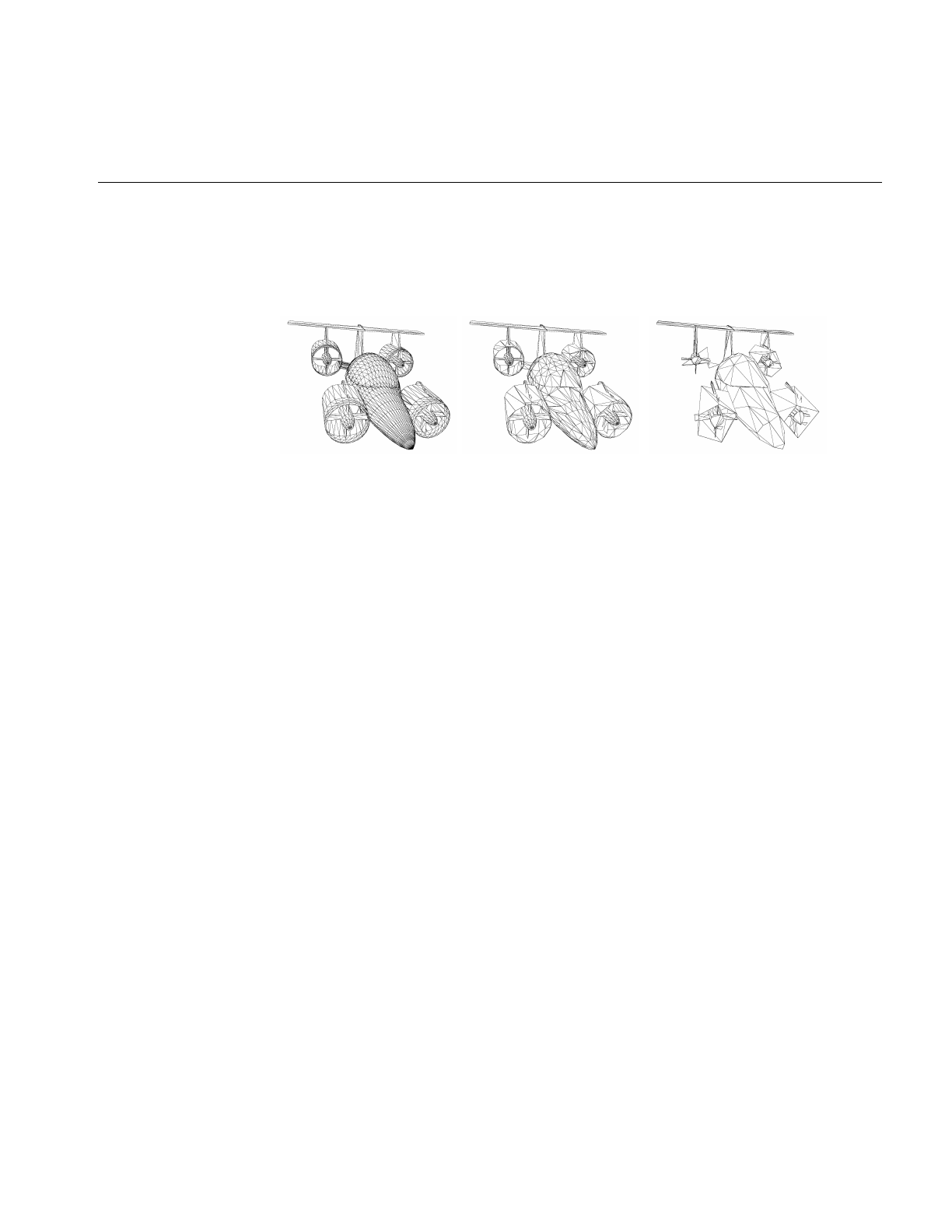
Successive Relaxation Algorithm: opSRASimplify
117
Figure 6-1 illustrates the effects of decimateGeoSet() for different simplification criteria.
These images were made using viewDemo, as discussed in “Compiling and Running
optimizeDemo” on page 62.
Figure 6-1 opSRASimplify: Original Model; A Target of 30% With a Feature Angle of 10°; A
Target of 5% With a Feature Angle of 100°.
Note: If you create several LODs from repeated calls decimateGeoSet(), processing is
faster if you take the output of a previous simplification as the input to create the next
lower level of detail. The output is the same as if you simplified from the original to
create each of the LODs. For example, if you called decimateGeoSet() twice, reducing the
number of triangles by 1/2 each time, the output of the second call is the same as if you
made one call to decimateGeoSet() to reduce the number of triangles to 1/4 of the
original.
Note: If you simplify a csGeoSet with two adjacent triangles that were originally
specified independently, cracks can appear in surfaces rendered after simplification. The
cracks result from shared vertices; they are not exactly the same, but form a closely
spaced pair due to small differences between finite-precision numbers that describe a
supposedly common position. The simplifier might eliminate one of the pair, but not the
other. The effect is an apparent tear or crack in the surface.

118
Chapter 6: Rendering Appropriate Levels of Detail
Rossignac Simplification Algorithm: opLatticeSimplify
The class opLatticeSimplify provides methods to apply the algorithm developed by
Jarek Rossignac to simplify a csGeoSet. The algorithm is less complex than that available
in opSRASimplify, so it is faster, but it gives a somewhat lumpy simplification. This
simplifier is most appropriate for low levels of detail.
The algorithm takes a grid in space and simply moves each vertex in a csGeoSet to the
nearest grid point. If the grid is too coarse, the result will strongly reflect the grid
structure.
Class Declaration for opLatticeSimplify
The following are the main methods in the class:
class opLatticeSimplify : public opSimplify
{
public:
opLatticeSimplify(float gridSpacing);
virtual ~opLatticeSimplify();
csGeoSet *simplify(csGeoSet *);
Main Features of the Methods in opLatticeSimplify
opLatticeSimplify()
Specifies the grid spacing used in the simplification.
simplify() Applies the Rossignac simplification to the specified csGeoSet.

Merging Graphs With Differing Levels of Detail: opMergeScenes
119
Merging Graphs With Differing Levels of Detail: opMergeScenes
If you simplify all the csGeoSets in a scene graph to varying levels of detail, and create
graphs that otherwise retain the identical structure, you can place the differing levels of
detail in one scene graph with the methods of opMergeScenes. The merged scene graph
has the following structure:
• Above nodes in the tree that you specify with a callback, the output graph is
identical to one of the input graphs.
• Below the specified nodes, a csLOD node is inserted, providing a switch between
the corresponding lower subgraphs of the input graphs.
Before the subgraphs are inserted, they are reorganized to reflect their relative positions
in space and facilitate rapid cull traversals. See “Spatializing a Scene Graph:
opGeoSpatialize” on page 144.
For an example of how to use an opMergeScenes, see the sample application
mergeLODDemo.
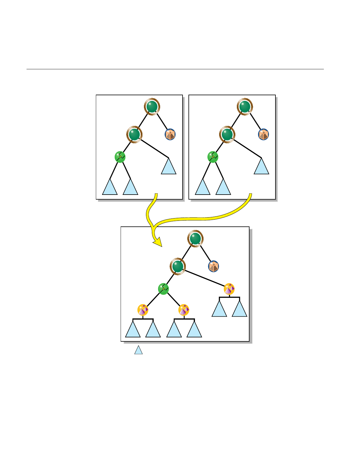
120
Chapter 6: Rendering Appropriate Levels of Detail
Figure 6-2 Merging Two Scene Graphs
csGroup
csGroup
csSwitch
csShape
AB
u
r
st
csShape
t
csGroup
csGroup
csSwitch u
r
s
C
csGroup
csGroup
csLOD
csSwitch
csLOD csLOD
csShape
w
S(A) S(B)
uv
r
s
x
t
S(D) S(E)
DE
F
S(C) S(F)
Subgraph S( ) Spatialization of subgraph

Merging Graphs With Differing Levels of Detail: opMergeScenes
121
Class Declaration for opMergeScenes
The following are the main methods in the class:
class opMergeScenes : public csAction
{
public:
typedef bool (*LODCallback)(csNode *);
opMergeScenes(int maxScenes,int goalMin,int goalMax,
opMergeScenes::LODCallback f);
~opMergeScenes();
void addScene(csNode *scene);
csNode *done();
void setGoalMin(int n) ;
void setGoalMax(int n) ;
void setLODInsert(LODCallback f) ;
int getGoalMin() ;
int getGoalMax() ;
LODCallback getLODInsert() ;
Main Features of the Methods in opMergeScenes
addScene() Adds a scene graph to the list of graphs to be merged.
apply() Is inherited from csAction and causes a traversal of the graph, merging
subgraphs according to the criteria specified by LODCallback(). The
first scene graph included by calling addScene() is the graph in which
thecsLod nodes and subgraphs are inserted.
done() Has the same effect as apply(), but returns the root node of the merged
graph. You do not need to call apply() if you call done().
opMergeScenes()
Specifies the following:
• the maximum number of scene graphs to merge
• the range of the number of triangles in the spatialized subgraphs
(see “Spatializing a Scene Graph: opGeoSpatialize” on page 144)

122
Chapter 6: Rendering Appropriate Levels of Detail
• a callback function that specifies when a node should have an LOD
node inserted below it that switches among the corresponding
subgraphs of the input graphs
setGoalMin(),getGoalMin(),setGoalMax(), and getGoalMax()
Set and get the parameters that control the spatialization routine. See
“Spatializing a Scene Graph: opGeoSpatialize” on page 144.
setLODInsert() and getLODInsert()
Set and get the callback function that determines which nodes should be
parents of the inserted LOD node(s) and subgraph children. Example
node-selection criteria are the depth of nodes from the top of the graph,
the height of nodes from the bottom of the graph, or specific node
names.
Note: The merged scene graph is created by modifying the first scene graph in the list
created by calls to addScene(); if you have further use for any of the graphs that you
merge, make copies before you merge them.

123
Chapter 7
7. Culling Unneeded Objects From the Scene Graph
With one exception, the tools discussed in this chapter reduce the number of objects and
vertices submitted to OpenGL processing. The tools cull unnecessary objects from the
scene graph before a draw traversal. This is in contrast to the tools discussed in the last
two chapters, which provide ways to minimize the number of vertices associated with a
given set of objects.
The following list shows the main culling topics discussed in this chapter:
• “View-Frustum Culling” on page 124
• “Occlusion Culling” on page 126
• “Rendering With View-Frustum and Occlusion Culling: opOccDrawImpl” on
page 129
• “Key Bindings for opOccDrawImpl” on page 132
• “Tuning Tips for Occlusion Culling” on page 134
• “Detail Culling” on page 135
• “Back-Face Culling” on page 137
The effect of these tools is to reduce the load on at least one of the transformation,
rasterization, and display stages of the graphics pipeline.

124
Chapter 7: Culling Unneeded Objects From the Scene Graph
View-Frustum Culling
View-frustum culling identifies csGeoSets in a scene graph whose geometry is not in the
viewing frustum, and prevents their further processing in the graphics pipeline, clearly
a potential benefit for all downstream resources.
Cosmo3D provides integrated, hierarchical view-frustum culling, which runs as part of the
rendering process. OpenGL Optimizer provides an additional method for multiprocess
view-frustum culling as part of the occlusion culler discussed in the next section.
When to Use View-Frustum Culling
View-frustum culling is beneficial if the viewpoint is near or inside a complex scene
where much of the scene is outside the viewing frustum, for example, during a
walkthrough of a building. A view-frustum test serves litle purpose if the scene fits in the
viewing frustum, for example, when you view an entire building from outside. The
hierarchical containment test used to implement view frustum culling in Cosmo3D
ensures that unneeded processing is avoided in such “all-visible” cases by detecting
geometry that is completely within the culling frustum and skipping subordinate
frustum tests.
View-Frustum Culling and Pipeline Load Balancing
View-frustum culling usually reduces the work done by the graphics hardware. But it
may either increase or decrease the load on the host, depending on whether the time
needed to perform the cull tests is greater or less than the time saved by eliminating
pieces of the scene graph from a draw traversal. To obtain a benefit to host processing,
you must spend less time culling than traversing the entire graph. A technique that
makes view-frustum culling more efficient is to create a spatialized scene graph, which
allows a single frustum intersection test to eliminate an entire subtree (see Chapter 8,
“Organizing the Scene Graph Spatially”).

View-Frustum Culling
125
Spatialization to Balance Pipeline Load When View-Frustum Culling
The average number of triangles in a csGeoSet, which OpenGL Optimizer spatialization
tools allow you to control, affects the impact of culling on different stages of the graphics
pipeline. If a scene graph has few csGeoSets with many triangles, a view-frustum cull
will be quite fast on the host, but unneeded triangles slow down the graphics hardware.
On the other hand, many smaller csGeoSets with fewer triangles result in more precise
culling and fewer unneeded triangles sent to the graphics hardware, because a larger
fraction of the member triangles are likely to intersect the view frustum. However, the
cost is a larger number of intersection tests. For optimal performance, adjust the
csGeoSet size to balance the time spent intersection testing with the time spent
transforming off-screen triangles. If the host is a bottleneck, all other things being equal,
you should send more triangles to the rendering hardware. If the rendering hardware is
the bottleneck, more precise culling might be a good use for the free CPU cycles.
To illustrate the load balancing issues, consider viewing a lug nut of a car for the
following two extreme scene graphs for rendering a car model. One graph consists of one
million triangles in one csGeoSet. No time would be spent on a view-frustum cull. When
rendering a close-up view of the lug nut, all one million triangles pass through the
graphics hardware, creating a transform bottleneck, because the few triangles making up
the lug nut were in the viewing frustum. Now consider a second graph for the same car
organized as one million csGeoSets, each containing a single triangle. After a
view-frustum cull, only the on-screen triangles go to the graphics hardware, minimizing
its load. However, the view-frustum cull test would cause a host bottleneck.
Since most data bases and views are not at these polar extremes, view frustum culling is
beneficial in nearly all cases: balancing the pipeline enhances the benefits.

126
Chapter 7: Culling Unneeded Objects From the Scene Graph
Occlusion Culling
Occlusion culling identifies triangles in a scene graph that are occluded by objects in the
foreground and prevents their further processing in the graphics pipeline.
You can control what you mean by “occluded”; the occlusion culler allows you to
eliminate objects for which a specified fraction of their bounding boxes are occluded by
foreground objects. This partial occlusion control allows you to further reduce the load
on the graphics pipeline; the efficacy of culling surges as you decrease of the fraction, but
at the possible cost of eliminating partially visible objects.
The default fraction for culling, 100%, is conservative in that the occlusion culler never
eliminates a visible triangle; however, it might not cull all occluded triangles. You can
change the fraction according to you needs, and update it dynamically in response to
graphics-pipeline load as a closed-loop frame rate control mechanism.
Rendering occluded triangles does not generate an incorrect image because the depth
buffer test eliminates occluded pixels, but that test occurs late in the rasterization stage
after vertices have been transformed, so relying on depth-buffer testing for occlusion
culling wastes graphics hardware processing cycles.
As for view-frustum culling, occlusion culling is clearly a potential benefit for all
downstream processing resources.
When to Use Occlusion Culling
Occlusion culling is appropriate for scenes with high depth complexity, that is, with
many objects that may be occluded. For example, 95% of the triangles in a typical view
of an automobile or other complicated mechanical assembly are occluded. Occlusion
culling provides less of a benefit for scenes with less depth complexity. In a visual
simulation application, where objects do not contain internal parts, more than half the
triangles are commonly visible. In this case, an occlusion culler would have a significant
effect on frame rate.
Figure 7-1 illustrates how view frustum and occlusion culling work together to greatly
reduce the amount of geometry that needs to be rendered. This is the first step in
high-fidelity, large-model visualization.
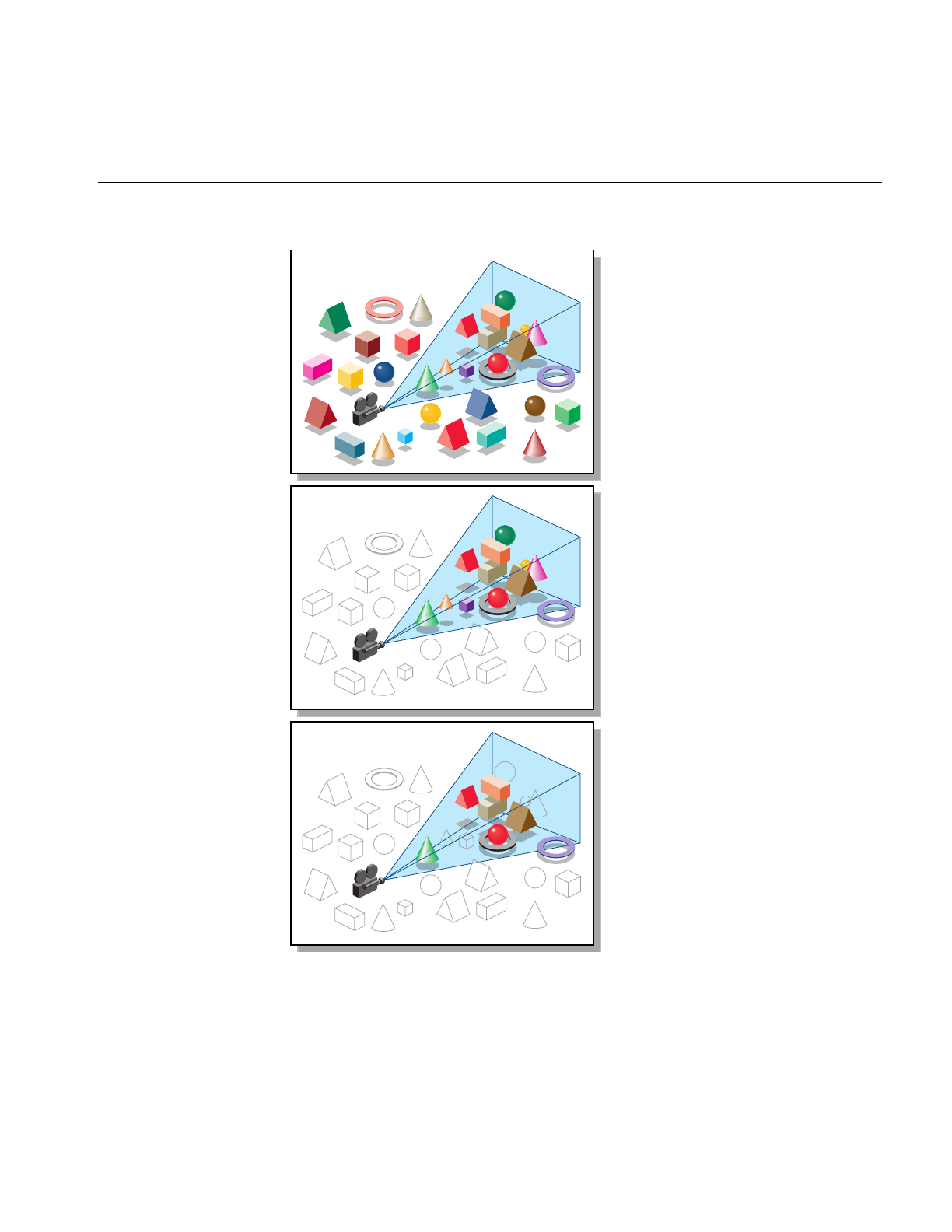
Occlusion Culling
127
Figure 7-1 Combined Effects of View Frustum and Occlusion Culling

128
Chapter 7: Culling Unneeded Objects From the Scene Graph
You can run the occlusion culler on multiple processes, and choose the number of
processes. Even on a single-processor machine, you may benefit from using multiple
processes because the host can cull while the OpenGL process is blocked, waiting for the
graphics FIFO to unclog.
Occlusion Culling and Pipeline Load Balancing
The occlusion culler performs view frustum culling before occlusion culling.
Consequently, all view frustum performance characteristics also apply to occlusion
culling.
As for view frustum culling, if the time required for occlusion culling is greater than the
rendering time saved, culling only moves a bottleneck to the host and increases the
processing time of the graphics pipeline. If occlusion culling takes less time than
drawing, you can use the extra time to eliminate more triangles from a scene graph, thus
further reducing the load on the graphics hardware and shifting the balance of tasks in
the graphics pipeline.
Note: You get lower quality culling if your scene occupies only a portion of the total
z-range of the depth buffer. For the best precision, set the z-clipping tightly around your
scene.
Spatialization to Balance Pipeline Load When Occlusion Culling
You can adjust the execution times of the host and the graphics hardware by controlling
the number of triangles in each csGeoSet (see Chapter 8, “Organizing the Scene Graph
Spatially”). Coarser granularities, which are characterized by a few large csGeoSets,
make culling run faster at the risk of drawing more occluded geometry. Finer
granularities give more precise culling at the cost of extra culling time.
The culler uses bounding boxes to determine whether a csGeoSet is occluded. Although
it may increase the time spent culling, creating smaller csGeoSets with tighter bounding
boxes may have a particularly dramatic impact on graphics hardware processing. For
example, in many tightly packed mechanical assemblies, the corner of a bounding box
may be visible, even though its enclosed csGeoSet is fully occluded; graphics hardware
is engaged in an unproductive rendering task. In summary, long csGeoSets are bad,
small rectangular ones are good.

Rendering With View-Frustum and Occlusion Culling: opOccDrawImpl
129
Changing the Fraction of the Bounding Box Required for Elimination
You can dynamically shift the load between the host and the OpenGL pipeline by
varying the fraction of a bounding box that must be occluded before it is eliminated from
the pipeline: thus you can create a closed-loop frame rate control mechanism.
Rendering With View-Frustum and Occlusion Culling: opOccDrawImpl
To use the occlusion-culling algorithm in a rendering application, you can register an
opOccDrawImpl in an opViewer. An example appears in the section “Application
viewDemo: A First Look in the Toolkit” on page 42.
The class opOccDrawImpl is an opDrawImpl, which is the base class for drawing
implementations discussed in “Basic Tools for Rendering Implementations:
opKeyCallback and opDrawImpl” on page 38.
opOccDrawImpl defines key bindings that control its rendering options in an opViewer
application, and that allow you to record a sequence of control operations so that you can
save a “tour” of a scene.

130
Chapter 7: Culling Unneeded Objects From the Scene Graph
Class Declaration for opOccDrawImpl
The following are the main methods in the class:
class opOccDrawImpl : public opDrawImpl
{
public:
opOccDrawImpl(opViewer *viewer,int nProcs = 2);
~opOccDrawImpl();
virtual void draw(unsigned frame);
virtual void pick(bool mouseDown,const csHit& hit);
virtual void activated();
virtual void deactivated();
virtual void reset();
static bool keyHandler(opDrawImpl *,int);
void setConservativeMode(bool enabled);
void setDrawCulledMode(bool enabled);
void setOCullMode(bool enabled);
void setVFCullMode(bool enabled);
bool getConservativeMode() const;
bool getDrawCulledMode() const;
bool getOCullMode() const;
bool getVFCullMode() const;
int loadRecording(const char *filename);
void saveRecording(const char *filename);
void beginRecording();
int endRecording();
void playback(bool playTwice=false);
};

Rendering With View-Frustum and Occlusion Culling: opOccDrawImpl
131
Main Features of the Methods in opOccDrawImpl
opOccDrawImpl()
Registers the occlusion culler with the opViewer, thus making key
bindings effective, and allocates the number of processors to use when
performing the occlusion or view-frustum culling.
draw()Is inherited from opDrawImpl and defined to implement occlusion culling for
each frame update in opViewer::eventLoop(). The other inherited
functions do nothing.
keyHandler()Defines the effects of the keyboard commands registered by calls to
registerKey(). An opOccDrawImpl has the keyboard control definitions
described in “Key Bindings for opOccDrawImpl” on page 132.
get...() and set...()
Provide interactions with the control parameters.
loadRecording(), and so on
Provide control over recording, writing, reading, and playing a
sequence of manipulations of your scene graph. You can store up to 1000
frames.
registerKey() Registers a keyboard command and specifies the function
(keyHandler()) that interprets the command.
The function registerKey() is inherited from opDrawImpl, which is
discussed in “Basic Tools for Rendering Implementations:
opKeyCallback and opDrawImpl” on page 38. See the file
opOccDrawImpl.cxx for details.

132
Chapter 7: Culling Unneeded Objects From the Scene Graph
Key Bindings for opOccDrawImpl
The class constructor for opOccDrawImpl uses the methods registerKey() and
keyHandler() to register the following keyboard commands (see the file
opOccDrawImpl.cxx):
cToggles “conservative” occlusion culling. If you use “non-conservative”
occlusion culling, the culler runs faster, but the screen may flash during
rendering; with conservative culling, no flashing occurs.
oToggles occlusion culling on and off. Initially, occlusion culling is
disabled and all geometry is rendered. The algorithm removes only
geometry that is not visible, so you do not see any change in the scene,
however, the frame rate increases.
OToggles rendering of occluded and foreground geometry. This feature
lets you see exactly which portions of your scene are completely
occluded. Note that all the occluded geometry is rendered when this
option is enabled, so for a scene with many layers, the occluded
geometry renders much more slowly than the foreground geometry.
vToggles view-frustum culling on and off. OpenGL Optimizer allows you
to use multiple processors to perform view-frustum culling.
+ - Allow you to increase and decrease the threshold fraction that specifies
how much of an object’s bounding box must be occluded to cull the
object.
[ Starts recording keyboard commands.
] Stops recording.
\ Playback last recording.
! Saves recording.

View-Frustum and Occlusion Cull Draw Traversal: opDrawAction
133
View-Frustum and Occlusion Cull Draw Traversal: opDrawAction
The class opDrawAction is a csDrawAction that allows you to traverse a scene graph
and draw the scene with occlusion culling, view-frustum culling, or both. You can also
set the background color for the scene by specifying RGBA values.
opOccDrawImpl uses opDrawAction to render the scene in an opViewer application.
The application xdemo illustrates rendering with an opDrawAction in an X Window
context (see /usr/share/Optimizer/src/sample/xdemo).
Class Declaration for opDrawAction
The following are the main methods in the class:
class opDrawAction : public csDrawAction
{
public:
opDrawAction(csLight *light1,csLight *light2,csNode *scene,
int nProcs=1,bool computeStats=false);
virtual ~opDrawAction();
void setFrameNumber(int f);
virtual csTravDirective apply(csNode *node);
virtual csTravDirective apply(csNode *node,
int width, int height, int frameNumber);
void updateMaxShapes(csNode *root);
void reset();
void setConservativeMode(bool enabled=true);
void setVFCullMode(bool enabled=true);
void setOCCullMode(bool enabled=true);
void setDrawCulledMode(bool enabled=true);
int getVFShapes();
int getVFTris();
int getShapesDrawn();
int getTrisDrawn();
void setBackgroundColor( float r, float g, float b, float a );
void getBackgroundColor( float *r, float *g, float *b, float *a );
};

134
Chapter 7: Culling Unneeded Objects From the Scene Graph
Main Features of the Methods in opDrawAction
apply() Traverses the scene graph, drawing it in a window width pixels wide and
height pixels high. The occlusion culler uses the framenumber to
determine if it was called on the previous frame.You can pass any
number initially, but all subsequent calls should increment framenumber.
The remaining methods allow you to control the types of culling applied, and to recover
statistics about the scene.
Tuning Tips for Occlusion Culling
The central concern for tuning occlusion culling is load balance. The goal is to have the
graphics hardware and all the general-purpose processors 100% busy and doing useful
work. Some tuning controls are the number of processors, the size of the csGeoSets,
spatialization, and the z-resolution of the frame buffer. Because every database is
different, you cannot effectively tune without taking performance measurements to
identify bottlenecks. Thus, consider optimizing dynamically: measure performance and
adjust tuning parameters as appropriate. The sections below describe some common
problems and their likely causes:
• “Culling Takes Longer Than Rendering” on page 134
• “Occluded Geometry Is Not Culled” on page 135
• “Very Small Speedup and Fast Culling” on page 135
Culling Takes Longer Than Rendering
Possible causes and solutions:
• Not enough geometry is being culled, either because most is visible, or because the
bounding boxes are too long.
• The csGeoSets are too small, so that the time required to cull one is longer than the
time required to draw it. To fix this, combine csGeoSets to make them bigger (see
“Merging csGeoSets in a Scene Graph: opCombineGeoSets” on page 147).
• Not enough processors. To fix this, increase the nProcs parameter for the constructor
opDrawAction() up to the number of processors on your system. On a single CPU
system, use the value 2; this allows the host to cull while the OpenGL process is
blocked, waiting for the graphics first-in-first-out queue to clear.

Detail Culling
135
Occluded Geometry Is Not Culled
Possible causes and solutions:
• Bounding boxes are not tight enough.
• Too much downsampling in x-y space.
• Not enough z-resolution.
• Geometry is actually visible through cracks in model.
Very Small Speedup and Fast Culling
Possible causes and solutions:
•csGeoSets are too big; nothing is culled. To fix this, use the spatialization tool to
break up the csGeoSets (see “Spatializing a Single csShape: opTriSpatialize” on
page 150).
• Too much downsampling in x-y space.
Detail Culling
While level-of-detail nodes are useful for adjusting the number of vertices associated
with any given object, a useful, logical extreme is simply not to render objects below a
certain size. The methods of opDetailSimplify allow you to remove geometry from
csShapes that are “small.” Small is determined by a threshhold for the ratio of shape size
to overall scene graph size, calculated from the radii of their respective bounding
spheres. You can explicitly set the large-scale dimension and thus have more direct
control over which objects are culled.
Notice that small csShape nodes are not removed from the graph, so the scene graph
structure remains the same. This allows you to use as an LOD a scene graph that has been
detail simplified.

136
Chapter 7: Culling Unneeded Objects From the Scene Graph
Class Declaration for opDetailSimplify
The following are the main methods in the class:
class opDetailSimplify
{
public:
opDetailSimplify (void)
~opDetailSimplify (void)
// --- ratio of shape size to overall size
void setSizeRatio (float ratio)
float getSizeRatio ()
// --- detail cull scene graph below root
void apply (csNode *root);
void setRootRadius(float radius)
};
Main Features of the Methods in opDetailSimplify
apply() Traverses the graph below root and culls small objects. Whether an object
is “small” is determined by the following:
• The radius of the bounding sphere of the object.
• The value set by setSizeRatio ().
• The radius of the bounding sphere of the root node. You can
explicitly set this maximum scale by calling setRootRadius().
setSizeRatio () and getSizeRatio()
Set and get the threshhold for culling small objects.
setRootRadius()Explicitly sets the dimension to which all objects are compared.
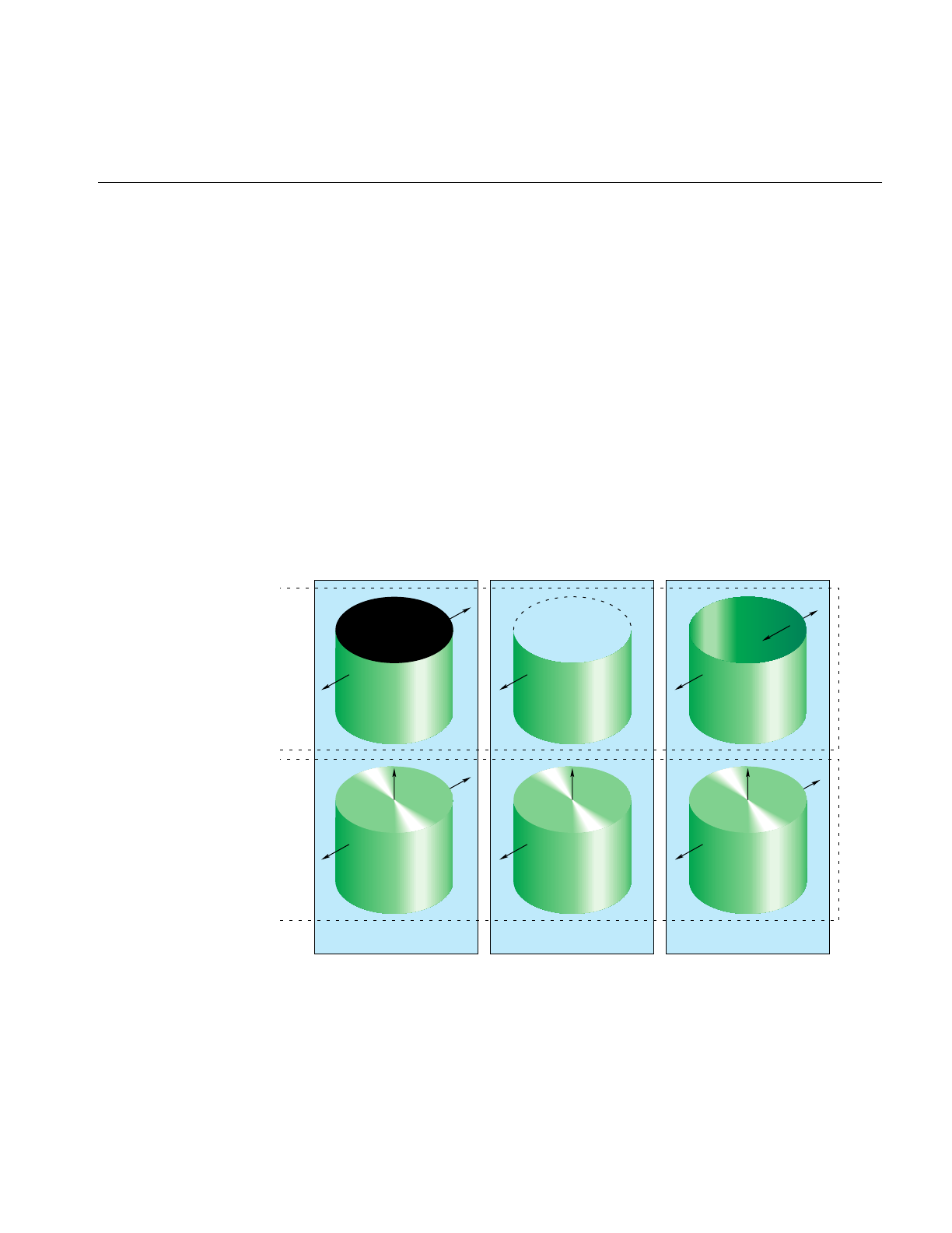
Detail Culling
137
Back-Face Culling
Typically, triangles should not be rendered when their front sides do not face the
viewpoint. Such pieces of a surface are called back faces. Figure 7-2 illustrates the back
faces of an open and a capped cylinder: the back faces are those for which the normals
point away from the viewpoint.
Back-face culling keeps these triangles from being rasterized, thus saving on pixel fill
time. Because the cull operation depends on the orientation of the triangles relative to the
viewer, back-face culling occurs in the graphics pipeline after the transform stage: only
rasterization and display stages are affected.
You need not always cull back faces. In general, if a surface has any holes, you should
render the back faces because they may be visible through the holes at certain viewing
angles. For example, if you can see into a pipe, render the pipe’s back face. Figure 7-2
illustrates this point by showing the effects of back-face culling on an open and a capped
cynlinder.
Figure 7-2 Back Faces, Back-Face Culling, and Two-Sided Lighting Effects
No back-face cull Back-face cull Two-light-source lighting
Without topWith top

138
Chapter 7: Culling Unneeded Objects From the Scene Graph
Two Lights Decreases Performance
Occasionally surface normals are inconsistent or inappropriate. For example, the
normals to a car body part might point towards the interior. Rather than maintain
consistent normals, many CAD applications ignore sidedness of surfaces and light
scenes with two lights pointing in opposite directions: the front and back sides of
triangles are made renderable that way. To make this work, materials must be set to be
two-sided. The rightmost panel in Figure 7-2 illustrates the effect.
Lighting with two lights is inefficient for two reasons. First, two-sided triangles do not
have a back face and so cannot be culled, even for only one light source. Second, the
levels of optimization may differ for the different rendering paths. For example, the
rendering path with a single light and single-sided material is on the optimized path in
Silicon Graphics machines, but rendering modes with two or more lights or with
two-sided materials are on the unoptimized path, which may run at half the speed of the
optimized path.
An OpenGL Optimizer tool that accomodates inconsistent normals and gives faster
rendering than two lights is the Gaussian light reflection map, discussed in “Gaussian
Map” on page 172.
Setting Backface Culling: opBackFaceCullScene()
It seems unlikely that you would build a database and not specify cull faces. However, if
you have such a scene graph, you have several options for how to control back-face
culling.
For a single csGeoSet, control rendering of the back face of a surface with the method
csGeoSet::setCullFace(). See the Cosmo 3D Programmer’s Guide for more information on
this feature.
For a scene (sub)graph, control rendering of the back faces of all objects with a call to
opBackFaceCullScene(root,enable), which is declared in the file opGFXSpeed.h. This
function traverses a scene graph and sets the rendering of every csGeoSet in the scene
graph below root. If enable is TRUE, the back faces of all csGeoSets are not rendered; if
FALSE, the back faces are rendered.
For an entire scene, use csContext if you want to set back face culling. See the Cosmo 3D
Programmer’s Guide for more information on this feature.

139
Chapter 8
8. Organizing the Scene Graph Spatially
To spatialize a scene graph means to structure the graph to reflect the spatial
relationships of objects in the scene. This simplifies searching for a node with a particular
location in space, and so increases the efficiency of view-frustum and occlusion culling,
as well as highlighting and picking.
These are the topics covered in this chapter:
• “Effect of Spatialization on Cull Traversals” on page 139
• “Granularity Tradeoffs” on page 140
• “When to Spatialize” on page 140
• “Spatialization Algorithm” on page 140
• “Spatialization Tool: opSpatialize” on page 142
• “Classes for Component Procedures of Spatialization” on page 143
Effect of Spatialization on Cull Traversals
As a view-frustum, cull, or highlighting traverser descends a spatialized graph, each
parent node effectively contains a “sign post,” the union of the bounding boxes of its
children, which directs the traverser towards a node of interest. More efficient traversal
results because the traverser does not need to test every node in the scene to check
whether a ray strikes an object; it can eliminate a subgraph with one node test. The
maximum number of tests is simply the depth of the tree. You control the depth of the
tree by how finely you subdivide the spatial volume, that is, the granularity of the
spatialization.

140
Chapter 8: Organizing the Scene Graph Spatially
Granularity Tradeoffs
Finer granularity for a scene graph reduces the load on the graphics hardware, but
increases traversal time by increasing the number of nodes in the graph. A coarse level
of granularity reduces traversal time, but slows the graphics pipeline because all the
vertices in large csGeoSets must be processed even if only a small portion is actually
visible. As discussed in the section “View-Frustum Culling” on page 124, an appropriate
level of granularity balances the amount of time spent on cull tests with the time saved
by eliminating unnecessary vertices from processing by the graphics hardware. In one
example, it was found that spatializing and defining appropriate granularity reduced
rendering time by a factor greater than ten.
When to Spatialize
Spatialization tools are useful when you have large objects in the viewing frustum, or
when you intend to interactively manipulate selected objects.
Spatialization takes time; it serves no purpose if you spend more time spatializing than
you would traversing and rendering without spatialization. Typically, spatializing
during a flythrough application is not useful, and may disrupt interactions with the
scene graph; similarly spatializing moving objects is not typically useful.
Spatialization Algorithm
The spatialization method used by OpenGL Optimizer classes is similar to the
development of an octree, a graph in which children correspond to iterated subdivisions
of a parent cube into eight equal cubes. For more information about octrees, see the book
Computer Graphics: Principles and Practice listed in “Recommended Reference Materials”
on page xxxi.
Octree spatial division is simple and efficient. However, the OpenGL Optimizer
spatializing tools subdivide space not by simply bisecting edges of a cube, as in an octree,
but by selecting planes for subdivisions such that the rendering loads of the resulting
volumes are similar; after each cut the number of triangles is approximately the same on
each side of the cutting plane.

Spatialization Algorithm
141
Spatialization Control Parameters
The main parameters you use to control spatialization are hints for the largest and
smallest sets of triangles in each csGeoSet of the spatialized graph. The spatializing tools
attempt to develop a scene graph with the number of triangles in each csGeoSet within
the prescribed range.
Spatialization Classes
OpenGL Optimizer provides a high-level tool that allows you to re-structure a scene
graph and its csGeoSets to get the desired number of triangles in each leaf node. You can
specify the leaf nodes to be trifans or tristrips. More details are provided in the section
“Spatialization Tool: opSpatialize” on page 142.
You can also use lower-level tools that perform the component procedures of this
process, tools that spatialize a set of triangles, reorganize an existing set of nodes, and
combinecsGeoSets. Combining csGeoSets is useful if the nodes in a scene graph are not
appropriate for spatial reorganization because, for example, they contain significantly
different numbers of triangles, or the graph simply has too many small csGeoSets. The
classes that provide these tools are discussed in the following sections:
• “Spatializing a Single csShape: opTriSpatialize” on page 150
• “Spatializing a Scene Graph: opGeoSpatialize” on page 144
• “Merging csGeoSets in a Scene Graph: opCombineGeoSets” on page 147

142
Chapter 8: Organizing the Scene Graph Spatially
Spatialization Tool: opSpatialize
You may not need another spatialization tool besides this class. opSpatialize has one
important method, convert(), which returns the root node of a new, spatialized scene
graph.convert() combines or divides, as necessary, all the csGeoSets in or below the root
node passed as an argument. Do not spatialize a scene graph that has LOD nodes or
transforms: spatializing csLOD siblings is a nonsensical operation, and the results of
splitting a csGeoSet under a transform node do not necessarily stay under the transform
node.
You control combining and dividing of csGeoSets by specifying a range of values for the
number of triangles in each leaf node. The method convert() also organizes the nodes in
the graph spatially such that the bounding box of each parent node is the union of the
bounding boxes of its children.
convert() is overloaded. If the argument of convert() is a csGeoSet, only it is effected. If
the argument is the root node of a scene, the entire graph is processed.
Class Declaration for opSpatialize
The following are the main methods in the class:
class opSpatialize
{
public:
static csNode *convert(
csNode *node,
int goalMin,int goalMax,
const csBoxBound& bbox,
csType *outType = csTriFanSet::getClassType(),
opColorGenerator *c = opColorGenerator::noColors());
};

Classes for Component Procedures of Spatialization
143
Main Features of the Methods in opSpatialize
These are the effects of the arguments for convert():
node Is the root node of the graph you want to spatialize.
bbox Defines the volume to be subdivided.
goalMax Is the target maximum number of triangles in any leaf node in the final
scene graph.
goalMin Is the minimum number of triangles in any leaf node in the final scene
graph.
outType Is the type of all the csGeoSets in the new, spatialized graph: either
csTriStrip or csTriFan.
convert()also allows you to provide contrasting colors for the csTriStrips or csTriFans in
the new graph by using opColorGenerator in exactly the same way as opTriFanner and
opTriStripper. See the section “Specify Coloring of New csGeoSets: opColorGenerator”
in Chapter 15 for more details.
Classes for Component Procedures of Spatialization
The method opSpatialize::convert() uses three component operations that are
implemented individually in three OpenGL Optimizer classes:
1. It uses the class opGeoSpatialize to organize the existing nodes in the scene graph.
2. It uses opCombineGeoSets to combine triangles from small leaf nodes, where
“small” means too few triangles.
3. It uses opTriSpatialize to subdivide large leaf nodes.
These classes are discussed in the following sections:
• “Spatializing a Scene Graph: opGeoSpatialize” on page 144
• “Merging csGeoSets in a Scene Graph: opCombineGeoSets” on page 147
• “Spatializing a Single csShape: opTriSpatialize” on page 150

144
Chapter 8: Organizing the Scene Graph Spatially
Spatializing a Scene Graph: opGeoSpatialize
The class opGeoSpatialize reorganizes existing nodes in a scene graph. Given a
bounding box and a scene-graph root node, convert() subdivides the box and
re-arranges the node hierarchy until there are approximately a specified number of
triangles in each of the resulting volumes.
The method convert() not only re-arranges existing nodes; it combines csGeoSets with
too few triangles into larger csGeoSets by using the class opCombineGeoSets
(see“Merging csGeoSets in a Scene Graph: opCombineGeoSets” on page 147).
Figure 8-1 illustrates the effects of opGeoSpatialize. The csGeoSets for three of the
tire-and-rim combinations (necessarily contained in csShape nodes) are placed
appropriately with respect to front or rear, and left or right. The csGeoSets for the fourth
tire and rim are combined in one csGeoSet, and placed appropriately in the graph. The
csGeoSet for the seat is placed in a portion of the graph for triangles in the center.
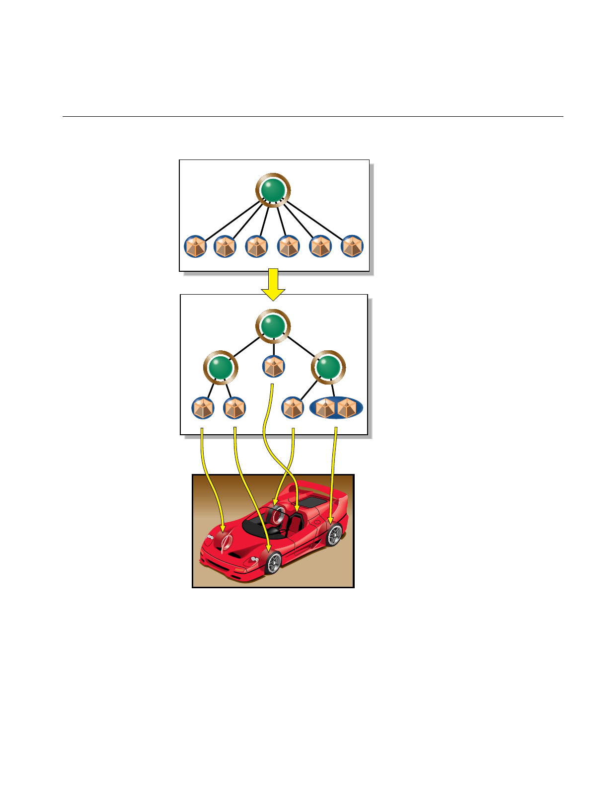
Classes for Component Procedures of Spatialization
145
Figure 8-1 Organizing and Combining csGeoSets With opGeoSpatialize
Car
csGroup
csShape
csShape csShape csShape csShape
LR
rim
RRLF SeatRF LR
tireRRLF SeatRF LR
rim LR
tire
csShape
csGroup
csGroup csGroup
LR
rim LR
tire
Front
wheels
Rear
wheels
LFRF RR
Seat
Front
wheels
Rear
wheels
LR
rim LR
tire
LFRF RR
Seat
Car
Car
Car
csShape csShape csShape csShape
csShape

146
Chapter 8: Organizing the Scene Graph Spatially
Class Declaration for opGeoSpatialize
The following are the main methods in the class:
class opGeoSpatialize : public opDFTravAction
{
public:
opGeoSpatialize(int goalMin,int goalMax, const csBoxBound& bbox);
~opGeoSpatialize();
opTravDisp preNode(csNode *&, const opActionInfo&);
opActionDisp end(csNode *&, const opActionInfo&)
;
void addShape(csShape *s);
csNode *done(csType *outType = csTriFanSet::getClassType(),
opColorGenerator *c = opColorGenerator::noColors());
static csNode *convert(
csNode *node,
int goalMin,int goalMax,
const csBoxBound& bbox,
csType *outType = csTriFanSet::getClassType(),
opColorGenerator *c = opColorGenerator::noColors());
};
Main Features of the Methods in opGeoSpatialize
The class appears somewhat complex, because it has several member functions needed
for a scene-graph traversal (see Chapter 14, “Traversing a Large Scene Graph” ).
To spatialize a scene graph, however, you do not need to concern yourself with most of
the member functions; simply call convert().
convert() Reorganizes the scene graph. It takes the same set of arguments as
opSpatialize::convert(). A call to convert() returns a root csNode for the
new graph. However, if the csNode argument is not the root of a
(sub)graph, convert() does nothing.
opGeoSpatialize uses an opGeoConverter to organize the triangles in the csNodes. See
“Decompose csGeoSets Into Constituent Triangles: opGeoConverter” on page 329.

Classes for Component Procedures of Spatialization
147
Merging csGeoSets in a Scene Graph: opCombineGeoSets
When you have a scene (sub)graph with too many small csGeosets, you can combine
them and develop a graph consisting of a root node with children each of which contains
all the triangles of the original graph that have the same appearance. You can specify
whether the output csGeoSets are csTriStripSets or csTriFanSets. You can subsequently
useopTriSpatialize on the combined triangles to further develop a scene graph structure
and adjust granularity; this is the approach taken by opSpatialize.
The result of combining csGeoSets is faster rendering, because of reduced traversal time
and the possibility of larger trifans or tristrips. In one case with too many small
csGeoSets, simply combining csGeoSets reduced rendering time by over two thirds.
Figure 8-2 illustrates the effects of combining csGeoSets. Notice that interior nodes of the
scene graph are lost: combine nodes before you create LODs or insert transform nodes.
Figure 8-2, which represents scene graph changes, shows the csShape nodes that contain
the csGeoSets.
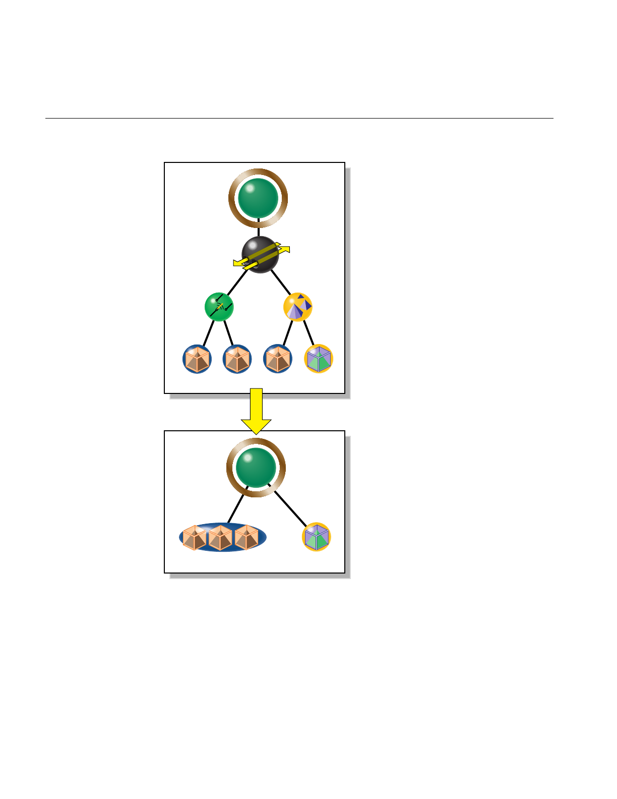
148
Chapter 8: Organizing the Scene Graph Spatially
Figure 8-2 Combining csGeoSets with opCombineGeoSets
csGroup
csTransform
csLOD
csSwitch
csShape csShape csShape csShape
12 3 4
csGroup
csShape csShape
1 42 3

Classes for Component Procedures of Spatialization
149
Class Declaration for opCombineGeoSets
The following are the main methods in the class:
class opCombineGeoSets : public opDFTravAction
{
public:
opCombineGeoSets();
~opCombineGeoSets();
opTravDisp preNode(csNode *&, const opActionInfo&);
opActionDisp end(csNode *&, const opActionInfo&);
void addGeoSet(csGeoSet *gs,csAppearance *app);
csNode *buildGraph(csType *outType=csTriFanSet::getClassType(),
opColorGenerator *c = opColorGenerator::noColors());
static csNode *convert(
csNode *root,
csType *outType=csTriFanSet::getClassType(),
opColorGenerator *c = opColorGenerator::noColors()
);
};
Main Features of the Methods in opCombineGeoSets
The class opCombineGeoSets appears somewhat complex, because it has several
methods needed for a scene-graph traversal (see Chapter 14, “Traversing a Large Scene
Graph” ).
However, to combine csGeoSets, you need not need concern yourself with most of the
methods; the function convert() handles the traversal details.
convert() Produces a new scene graph with csGeoSets combined wherever
possible. You can use an opColorGenerator to control coloring of the
new graph as you do with opSpatialize::convert().
Note that if the csMaterials associated with two csGeoSets do not
match, then they will not be combined.

150
Chapter 8: Organizing the Scene Graph Spatially
Spatializing a Single csShape: opTriSpatialize
The most elementary spatialization task successively subdivides a bounding box
containing a set of triangles until there are approximately a specified number of triangles
in each of the resulting volumes. Thus the loads on the graphics hardware are
approximately the same for all of the leaf nodes.
The main method of the class opTriSpatialize is the overloaded convert() function,
which redistributes triangles into csGeoSets containing similar numbers of triangles.
Except for the arguments that specify the set of triangles on which convert() acts, its
arguments are the same as for opSpatialize::convert() and have the same effects. You
specify the set of triangles to be manipulated by convert() with a csBoxBound and
csShape. Alternatively, you can use a csGeoSet and a csAppearance.
opTriSpatialize uses an opGeoConverter to manage the set of triangles and preserve
results for other operations. See “Decompose csGeoSets Into Constituent Triangles:
opGeoConverter” on page 329.
Figure 8-3 illustrates the effects of spatializing the set of triangles in one csGeoSet that
describes all four wheels of a car; a csGeoSet is created for each wheel and placed in a
csShape node corresponding to the spatial position of the wheels.
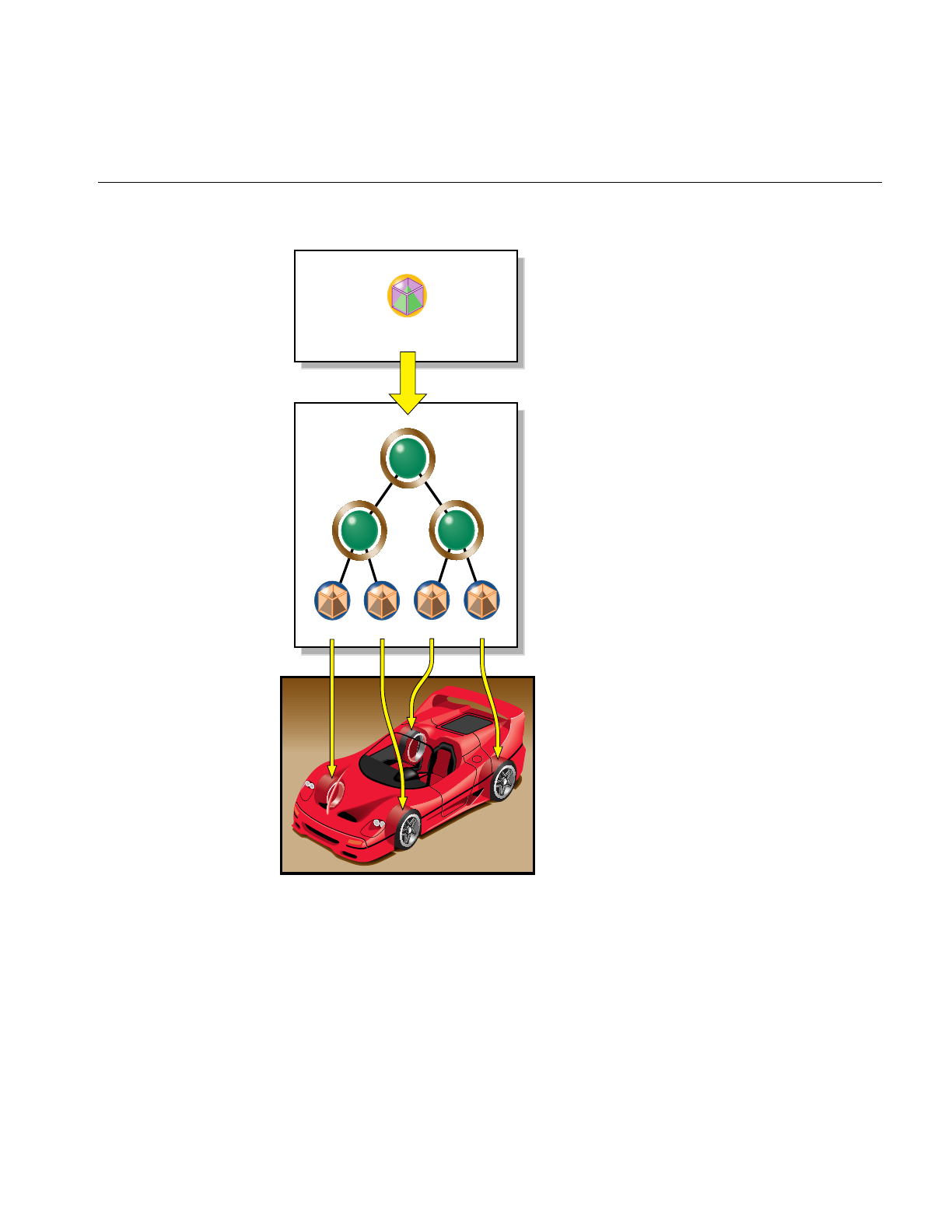
Classes for Component Procedures of Spatialization
151
Figure 8-3 Creating a Spatialized Graph From the csGeoSet in One csShape
csGroup
LFRF LRRR
csShape
4 wheels
csGroupcsGroup
Front Rear
Wheels
csShape csShape csShape csShape

152
Chapter 8: Organizing the Scene Graph Spatially
Class Declaration for opTriSpatialize
The following are the main methods in the class:
class opTriSpatialize
{
public:
opTriSpatialize(int goalMin,int goalMax,
const csBoxBound& bbox,
opGeoConverter *gc,
csAppearance *app);
~opTriSpatialize();
void addTriangle(const opTriangle *t);
csNode *done(csType *outType=csTriFanSet::getClassType(),
opColorGenerator *c = opColorGenerator::noColors());
static csNode *convert(
csGeoSet *gs, csAppearance *app,
int goalMin,int goalMax,
const csBoxBound& bbox,
csType *outType=csTriFanSet::getClassType(),
opColorGenerator *colors = opColorGenerator::noColors());
static csNode *convert(
csShape *shape,
int goalMin,int goalMax,
const csBoxBound& bbox,
csType *outType=csTriFanSet::getClassType(),
opColorGenerator *colors = opColorGenerator::noColors());
};

PART THREE
Specific Tools for Fast Rendering III
The tools discussed in the two chapters in this section address specific rendering
tasks: selecting and manipulating rendered objects independently while the
remaining objects in a scene remain stationary, and providing complex lighting
environments with which to examine your design.
Chapter 9, “Interactive Highlighting and Manipulating”
Chapter 10, “Efficient High-Quality Lighting Effects: Reflection Mapping”


155
Chapter 9
9. Interactive Highlighting and Manipulating
The tools discussed in this chapter enable you to highlight a portion of a rendered scene
and then pick and manipulate only the highlighted object(s). For example, you might
want to “pull” a piece off a car and examine and perhaps modify it, while the rest of the
vehicle remains stationary in the background. You can successively pick and move pieces
to disassemble a design.
These are the topics discussed in this chapter:
• “Overview of Highlighting and Picking” on page 155
• “Interaction With a Rendered Object: opPickDrawImpl” on page 156
• “Scene Graph Modification: opPick” on page 161
• “Node to Override Appearances: opHighlight” on page 167
Overview of Highlighting and Picking
During highlighting, a selected piece of the scene graph appears in a distinct color. When
you pick a highlighted object, subsequent interactions with the scene affect only the
picked object. You can expand or contract the picked portion of the scene graph available
for interaction by “climbing” or “descending” the scene graph from the picked node,
which corresponds to the csGeometry under the cursor. When you are finished, you can
undo interactions with a picked object, and return the object to its original position. You
can also tag certain types of nodes as unpickable and so force the selection to nodes
higher in the scene graph.

156
Chapter 9: Interactive Highlighting and Manipulating
How Picking Can Accelerate Rendering Rates
The independent manipulation of an object in a scene can help accelerate scene
transformations. You can pick a small key object that renders quickly, orient it as you like,
recover the net transformation developed during the interaction, and then apply the
transform to the whole scene. This obviates the intermediate steps required to
continuously manipulate a whole scene, thus lightening the traversal load on the host
and the load on the graphics pipeline until you are ready to change the view of the whole
scene.
Interaction With a Rendered Object: opPickDrawImpl
This class provides keyboard and mouse controls for picking and highlighting. It is
derived from opDrawImpl, which is the base class for the drawing implementations
discussed in “Basic Tools for Rendering Implementations: opKeyCallback and
opDrawImpl” on page 38.
If you want to use the Motif library, opXmViewer uses opXmDrawImpl, which has
methods analogous to a combination of opPickDrawImpl and opDefDrawImpl (see
“Default opDrawImpl for opViewer: opDefDrawImpl” on page 40).

Interaction With a Rendered Object: opPickDrawImpl
157
Class Declaration for opPickDrawImpl
The following are the main methods in the class:
class opPickDrawImpl : public opDrawImpl
{
public:
opPickDrawImpl(opViewer *viewer);
virtual ~opPickDrawImpl();
// --- redefined virtual functions
virtual void draw(unsigned frame);
virtual void pick(bool mouseDown, const csHit& hit);
virtual void reset();
static bool keyHandler(opDrawImpl *,int);
// --- Accessors
bool getDeleteEnabled()
bool enableDelete();
bool enableColoring(char *fname, char *tagname);
void decrementHLoffset()
void incrementHLoffset()
csNode *getHighlightedNode()
csNode *getPickRoot()
// --- cant always pass this to the constructor
void setReflMap(opReflMap *_rm)
};

158
Chapter 9: Interactive Highlighting and Manipulating
Main Features of the Methods in opPickDrawImpl
decrementHLoffset () and incrementHLoffset ()
Move you down or up in the scene graph hierarchy with respect to the
currently highlighted subgraph. Use the up- and down-arrow keys.
draw() Implements highlighting and picking for each frame update in
opViewer::eventLoop(). Enter i to toggle this rendering function.
enableColoring(fname, tagname)
Specifies a file containing, and registers keys to select, up to 20 colors
that can be applied to nodes whose names start with the string tagname.
The format of the file is as follows:
1. Comments (preceded by the pound sign, #).
2. A line containing the number of colors.
3. Lines containing the colors: five digits that specify red, green, blue,
alpha, and shininess values. Currently, alpha is not used, but a
value must appear for the shininess parameter to be properly
interpreted.
4. Part names and their associated colors (which are added to fname
during highlighting interactions). The color tag file is also used by
optimizeDemo to color parts, so you can use enableColoring() to
set colors for later viewing. See
/usr/share/Optimizer/src/sample/optimizeDemo/
The key bindings are to the numbers 0 to 9, corresponding the the first
ten colors in the file, and uppercase versions of these same keys for the
next ten colors.
getPickRoot () Returns the root node of the modified scene graph developed by
opPickDrawImpl(). Use the returned csNode to render the scene. For
example, viewer->drawScene (pick_root) appears in the code for
draw().
opPickDrawImpl(viewer)
Registers the picking and highlighting rendering features with an
opViewer, thus making the keybindings described above effective.
keyHandler() Defines the effects of the keyboard commands registered by calls to
registerKey().opDefDrawImpl has the keyboard controls described in
“Key Bindings for opPickDrawImpl” on page 160.

Interaction With a Rendered Object: opPickDrawImpl
159
pick() Sets a flag to switch interactive rendering only to picked objects. This is
the effect of pressing the Alt key and any mouse button.
registerKey() Registers a keyboard command and specifies the function that interprets
the command. The function registerKey() is inherited from
opDrawImpl, discussed in “Basic Tools for Rendering Implementations:
opKeyCallback and opDrawImpl” on page 38. See the file
opPickDrawImpl.cxx for details.
reset() Returns picked objects to their original position. Recall that
opDefDrawImpl defines lowercase “r” to reset the scene.
setReflMap() Sets the reflection map used to control the lighting effects. See
Chapter 10, “Efficient High-Quality Lighting Effects: Reflection
Mapping.”

160
Chapter 9: Interactive Highlighting and Manipulating
Key Bindings for opPickDrawImpl
opPickDrawImpl defines seven key bindings that control its options in an opViewer
application. These are the basic features:
• In highlight mode, object colors change to indicate which objects you can pick.
• The up- and down-arrow keys enlarge or shrink the set of selected objects.
• When you press the Alt key and any mouse button, the highlighted objects are
picked.
• Subsequent frames are rendered with all but the picked objects stationary—only
picked objects respond to opDefDrawImpl keyboard and mouse commands.
The class constructor for opPickDrawImpl uses the methods registerKey() and
keyHandler() to register the following keyboard commands, which you can change if
you make a subclass (see “Default opDrawImpl for opViewer: opDefDrawImpl” on
page 40 and the file opPickDrawImpl.cxx):
iToggles highlight and picking mode. opPickDrawImpl becomes the
opDrawImpl used by opViewer to control rendering. See “Basic Tools
for Rendering Implementations: opKeyCallback and opDrawImpl” on
page 38.
PPrint highlighted portion of the scene graph.
uDisable picking interaction. opDefDrawImpl becomes the
opDrawImpl used by opViewer to control rendering.
XDelete picked objects.
ALT-Any Mouse Button
Triggers picking, allowing you to move the highlighted object
independently of the rest of the scene.
UP ARROW Move highlight node up in scene-graph hierarchy, thus highlighting
more objects.
DOWN ARROW Move highlight node down in scene-graph hierarchy towards the
cursor, thus highlighting fewer objects.

Scene Graph Modification: opPick
161
Scene Graph Modification: opPick
The class opPick provides scene-graph modifying tools for picking and highlighting. It
uses the csCamera picking method, which returns a csHit that interactively identifies
objects in the scene graph.
A typical application that uses an opPick would include the following lines of code:
csCamera *camera = ....
opPick *picker = ...
csNode *root = picker->getRoot();
csHit hit;
if (camera->
pick (root, csWindow::getMouseX(), csWindow::getMouseY(), hit))
{
if (mouseDown)
picker->pickup (hit);
else
picker->highlight (hit);
}

162
Chapter 9: Interactive Highlighting and Manipulating
Class Declaration for opPick
The following are the main methods in the class:
class opPick
{
public:
// Creating and destroying
opPick (csGroup *root, opReflMap *rm=NULL);
~opPick ();
// Accessor functions
csNode *getHighlightedNode ()
csNode *getPickedNode ()
csTransform *getPickTransform ()
csGroup *getRoot ()
void setHighlightOffset (int _hl_offset)
int getHighlightOffset ()
void setHighlightColor (const csVec3f& _hl_color)
csVec3f getHighlightColor () const
void setInfoPosition (const csVec2f& _pos)
csVec2f getInfoPosition () const
void setReflMap (opReflMap *_rm)
PickBranch *getLodPath () const
// Utility methods
void highlight (const csHit& hit);
csTransform *pickupNode (const csHit& hit);
csTransform *pickupHighlightedNode ();
void drop ();
void removeHighlight ();
void reset ();
void ignoreType (csType *ignore_me);

Scene Graph Modification: opPick
163
Main Features of the Methods in opPick
drop () Leaves a picked object in its most recent position, by placing a new
csTransform in the scene graph above the picked node.
getHighlightedNode()
Returns the currently highlighted node.
getPickedNode()
Returns the currently picked node.
getPickTransform()
Returns the transform placed in the scene graph to manipulate the
picked subgraph. You manipulate the picked subgraph by changing this
matrix. See the example in “Sample Use of opPick” on page 165.
getRoot() Returns the root of the scene graph that you use for draw traversals
when picking and highlighting. opPick reorganizes the scene graph, so
use getRoot() to be sure you have the correct root node.
highlight() Highlights the node specified by the csHit argument returned by the
method csCamera::pick(). The highlighting is accomplished by
insertion of an opHighlight node (see “Node to Override Appearances:
opHighlight” on page 167).
You can prevent nodes from being highlighted by calling ignoreType().
ignoreType() Specifies node types that cannot be picked.
opPick () Constructs the class. If you use a reflection map to light the scene, pass
it to the constructor so that its effects will apply to highlighted nodes.
pickupHighlightedNode()
Picks up a currently highlighted node.
The return value is a csTransform that pickupHighlightedNode()
inserts into the scene graph above the picked node. The transform node
allows you to control manipulation of the picked subgraph.
pickupNode() Picks a node found with csCamera::pick(). You can use highlight offset
to define the picked node.
The return value is a csTransform that pickupNode() inserts into the
scene graph above the picked node. The transform node allows you to
control manipulation of the picked subgraph.
You can prevent nodes from being highlighted by calling ignoreType().

164
Chapter 9: Interactive Highlighting and Manipulating
removeHighlight()
Turns of highlighting.
reset() If a node is currently picked, puts the node back in its original place.
If a node is not currently picked, all previously picked nodes are
returned to their original position.
Notice that if you do a lot of picking, you will collect identity
csTransform nodes in your scene graph above all the nodes that you
pick.
setHighlightOffset() and getHighlightOffset()
Set and get the offset in the scene graph from the node originally
highlighted. The default value, 0, results in the leaf node of the scene
graph being picked. This node is typically a csShape.
setHighlightColor() and getHighlightColor()
Set and get the color of highlighted nodes. The default is yellow.
setInfoPosition() and getInfoPosition()
Set and get information about the placement of the opInfoNode that
displays the node name of the highlighted node. See “Example of Using
an opTriStats” on page 372.
setReflMap() Specifies the reflection map that sets the appearance properties of
highlighted nodes.

Scene Graph Modification: opPick
165
Sample Use of opPick
These lines of code sketch the use of an opPick in an opViewer application. Not all the
lines required for a working application are shown.
Create the opPick picker = new opPick
((csGroup *) viewer->getRoot());
TheopPick modifies the scene graph, and defines a new
root node for rendering. pick_root = picker->getRoot();
Highlight or Pick, Given a csHit
Here the code assumes it has a csHit named hit and uses
the keybindings of opPickDrawImpl to determine
highlighting or picking.
These lines of code mimic the lines of code in “Scene
Graph Modification: opPick” on page 161.
if (mouseDown && (state & INPICK_PICKREADY))
{
picker->pickupNode (hit);
}
else
picker->highlight (hit);
Set Highlight Offset
For either mode, use the highlight offset to define
exactly which nodes are affected. hl_offset = picker->getHighlighOffset();
Set Mouse Control of Object Manipulation
If in the pick mode, to specify that opViewer mouse
controls act on only the picked subgraph, set the pose
csTransform node shown in Figure 3-1 to be the picked
node’s transform.
viewer->setMouseFocus
(picker->get_pick_transform());
Draw
Specify rendering of the picked node in the definition of
opDrawImpl::draw()which is used by
opViewer::update().opPickDrawImpl provides one
specification.
See “Application viewDemo: A First Look in the
Toolkit” on page 42 for more on using the opDrawImpl
viewer->update (pick_root);

166
Chapter 9: Interactive Highlighting and Manipulating
Drop the Object, if Picked
When you are finished with the picked subgraph, leave
the objects where they are, or restore them to their
original position.
picker->drop ();
picker->reset ();
Clean up
If you want to delete the highlighted or picked subgraph
from the scene graph, include these lines of code.
Note that you should call either unhighlight() or drop()
before deleting, and be sure to remove the node from all
parents. In this sample there is only one parent.
csNode *hl_node = picker->getHighlighNode();
parent->removeChild (hl_node);

Node to Override Appearances: opHighlight
167
Node to Override Appearances: opHighlight
The lowest-level tool in the OpenGL Optimizer library for a highlighting and picking
application is the opHighlight class. This is a csGroup node that overrides the
appearance of its children during rendering. opPick uses opHighlight for its effects.
You can also override the rendering appearance of a selected subgraph with the
Cosmo3D functions csContext::pushOverrideAppearance() and
csContext::popOverrideAppearance(), but opHighlight is more convenient.
Class Declaration for opHighlight
The following are the main methods in the class:
class opHighlight : public csGroup
{
public:
// Creating and destroying
opHighlight (opReflMap *rm = NULL);
~opHighlight ();
// Accessor functions
csAppearance *getHighlightAppearance () const
void setHighlightAppearance (csAppearance *_hl_appear)
void setColor (const csVec3f& color);
csVec3f getColor () const
// Utility methods
virtual csTravDirective drawVisit (csDrawAction *da);
};
If you are using an opReflMap to light the scene, you must pass it to opHighlight() to
get appropriate lighting effects.

168
Chapter 9: Interactive Highlighting and Manipulating
Sample Use of opHighlight for Picking and Highlighting
The basic highlighting and picking operation inserts an opHighlight into the scene
graph between a selected node and the rest of the scene graph. The opHighlight then
controls rendering of the subgraph.
This example sketches the use of an opHighlight. It includes the insertion of a
csTransform node below the opHighlight, to allow manipulation of objects in the
subgraph. Not all the lines required for a working application are shown.
Create an opHighlight hl_node = new opHighlight ();
Create a csTransform to Manipulate With
To allow manipulation of the picked subgraph, create a csTransform
that will be the child of the opHighlight. For example, the csTransform
could be the pose transform in an opViewer scene graph; see
Figure 3-1.
xform = new csTransform;
Insert Nodes in Scene Graph and Draw
Place the highlight and transform nodes under the parent, and make
changling, which is the root of the highlighted subgraph, the child of the
transform node. This code uses methods in csGroups.
With this scene graph structure, rendering traversals of the scene graph
show a highlighted subgraph, with highlighted appearances
determined by the methods of opHighlight. If you change xform, you
can manipulate the subgraph.
hl_node->addChild (xform);
xform->addChild (changeling);
addChild (hl_node);
Clean Up
When you are finished, clean up the scene graph below the parent
csNode.xform->removeChild (changeling);
hl_node->removeChild (xform);
removeChild (changeling);
removeChild (hl_node);

169
Chapter 10
10. Efficient High-Quality Lighting Effects: Reflection
Mapping
OpenGL Optimizer supplements Cosmo3D lighting effects with reflection mapping, an
efficient technique for simulating a complex lighting environment. With reflection
mapping, also known as environment mapping, you treat a surface as a reflector and follow
one ray (from your eye and reflecting off the surface) to select a point on a texture image
that defines the visual environment. As an object rotates in the environment, the image
appears to move over the surface, in contrast to perhaps better-known texture-mapping
techniques that fix an image on a surface.
The reflection mappings available from OpenGL Optimizer form two groups:
• One group uses simple reflection maps, which have approximate lighting geometry
with credible sources and can be computed quickly. This group includes the sphere
and Gaussian map styles.
• The second group uses exact lighting geometry with relatively simple but useful
lighting sources that allow accurate visualization of curvature; they are useful for
designing smoothly curved surfaces, such as car bodies. This second group includes
the cylinder, floor, and ceiling mapping types.
OpenGL Optimizer adds a shininess threshold to the basic reflection mapping algorithm
so that selected objects, such as tires, do not reflect the environment image.
This chapter covers the principles underlying the different mapping methods, the basic
control parameters for each method, and the class opReflMap, which is the API for using
reflection maps. These topics are covered:
• “Simple Mapping: Remote View of a Remote Environment” on page 170
• “Gaussian Map” on page 172
• “Reflection-Mapping Class: opReflMap” on page 177

170
Chapter 10: Efficient High-Quality Lighting Effects: Reflection Mapping
For a more detailed introduction to reflection mapping, consult Advanced Animation and
Rendering Techniques: Theory and Practice and the section on “Interobject Reflections” in
Chapter 16 of Computer Graphics: Principles and Practice. Both of these books are listed in
“Recommended Reference Materials” on page xxxi.
Simple Mapping: Remote View of a Remote Environment
Two of opReflMap’s map types—sphere and Gaussian—use simple reflection mapping.
These map types are discussed in the following sections:
• “Sphere Map” on page 172
• “Gaussian Map” on page 172
Simple reflection maps determine coordinates for the texture image by assuming the
following:
• An image that lies on a sphere surrounding the scene.
•Aremote environment: The reflection geometry is simplified so that only the direction
of the reflection vector determines texture coordinates. Effectively, the texture map
is infinitely far away.
•Aremote viewer: The reflection geometry is further simplified by assuming that all
rays are parallel between the viewpoint and object’s surface. Effectively the
viewpoint is infinitely far away. The direction of the rays is from the viewpoint to
the center of the scene.
These three assumptions imply that the texture coordinates for any point on a surface are
determined by the viewing angle to the center of the scene and the vector normal to the
surface. For a tessellated surface, which includes correct surface-normal vectors only at
vertices, the rendering algorithm calculates the texture coordinates for a point inside a
triangular surface tile by interpolating the coordinates of the triangle’s three vertices. As
an object rotates, the directions of the normal vectors completely determine texture
coordinates; you do not have to calculate a new mapping from the surface to the texture
image.
You can simulate plausible complicated lighting environments at low computational cost
with a simple reflection map. However, reflection angles are not exact. For example, the
algorithm yields the same image point for every point on a large, flat surface. This effect
is illustrated in Figure 10-1, where collimating “lenses” indicate the effects of the remote
viewer and remote source approximations. Notice that the shading for all points on each
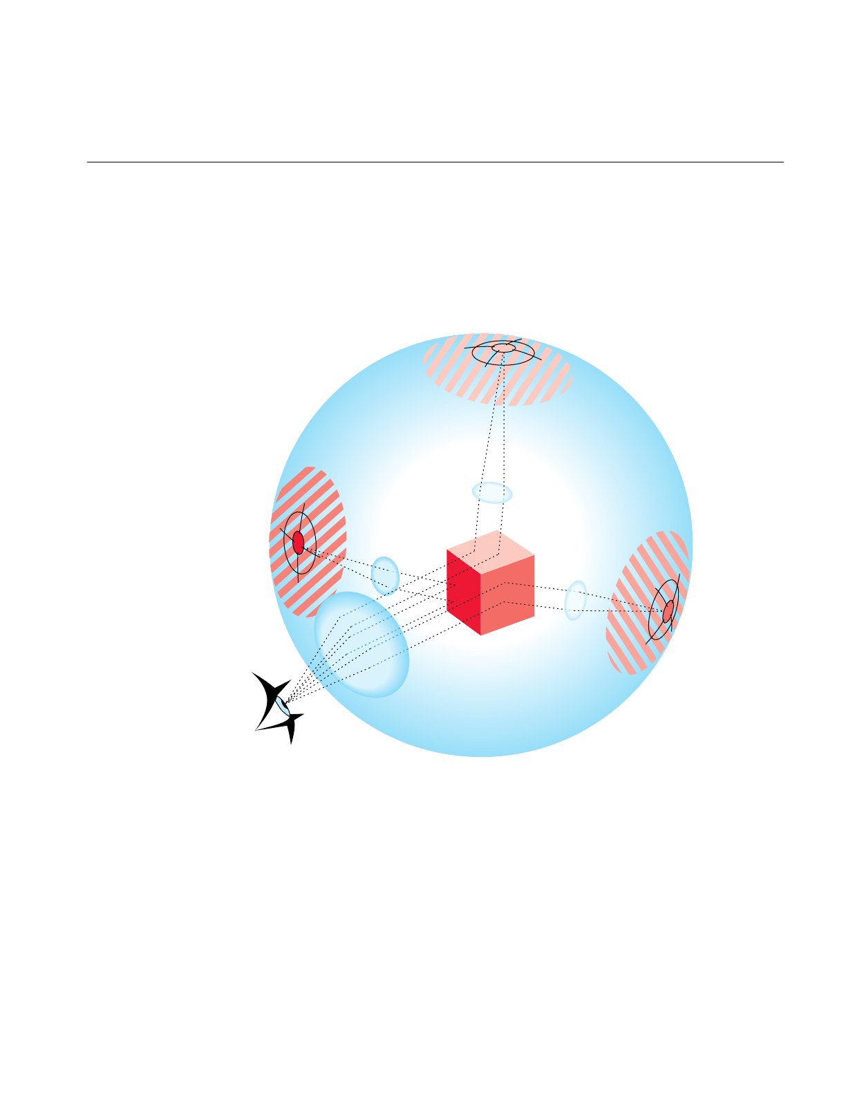
Simple Mapping: Remote View of a Remote Environment
171
face of the cube is determined by one point on the texture image, which is determined by
the normal to each surface. Furthermore, the texture image is usually blurred to avoid
problems that occur when the curvature of a surface can cause two points that are close
together to reflect widely separated points on the texture map, an effect called aliasing.
Thus you cannot closely examine reflection-map images to make accurate inferences
about a surface or its reflected environment.
Figure 10-1 Reflection-Map Geometry: Remote Viewer, Remote Environment

172
Chapter 10: Efficient High-Quality Lighting Effects: Reflection Mapping
Sphere Map
For this mapping type, you import a texture image, and opReflMap creates a lighting
environment for your scene by projecting the texture on a sphere that surrounds the
scene. The texture map first locates a point on the sphere using a remote viewer and
remote environment, and then projects the point onto the texture coordinate plane (a
plane through the equator) to determine the image point in the texture.
Thus, for a realistic image to appear on the surface, the texture image is a fish-eye image.
Mathematical details of the projection operation are in the discussion of the glTexGen()
functions in the OpenGL Reference Manual. Sphere mapping is discussed more intuitively
in the section “Environment Mapping“ in Chapter 9, “Texture Mapping,” of the OpenGL
Programming Guide.
Gaussian Map
This mapping creates an environment map on a sphere that simulates the effect of a light
source directed along the viewing direction at an imperfectly reflecting surface. It
provides efficient lighting effects for models with inconsistent normals; it is a faster
alternative to using two lights.
The mapping is a Phong-like illumination model characterized by a specularity
parameter that controls the amount of light that is imperfectly reflected. As the
specularity parameter increases, reflections become less diffuse and more mirror-like.
For more details on the Phong illumination model, see the book by van Dam and others
listed in the “Recommended Reference Materials” on page xxxi.

Accurate Mapping: Local View of a Local Environment
173
Accurate Mapping: Local View of a Local Environment
The cylinder reflection mapping creates a relatively simple lighting environment but with
a realistic reflection geometry. This map type assumes the following:
• A lighting geometry made of a cylindrical room with long narrow lights running
parallel to the cylinder’s axis and evenly distributed around the cylinder wall.
•Alocal environment: The radius of the room is finite; reflections do not depend solely
on the direction of the reflection angle. Reflections from a large flat surface vary;
they show the alternating lights in the room.
•Alocal viewer: The distance between the viewpoint and the surface is finite.
The texture coordinates depend on the complete ray-path geometry: the location of the
viewpoint and the location of the reflecting surface point and its normal. These
quantities, and the dimensions of the cylinder, define the point where a ray intersects the
cylinder and determine the point in the texture image (see Figure 10-2).
Unlike the remote viewer and environment configuration, a ray between the viewpoint
and the texture image changes as you bring the viewpoint closer to the surface or
translate the surface; the complete ray geometry determines the texture coordinates
associated with a point on a surface. For example, as you “walk” by a car, translating the
viewpoint of the scene, lines of lights slide over the car’s surface.
Figure 10-2 illustrates the general effects of a local viewer and local environment. To
simplify the comparison with the remote-viewer-remote-environment approximation,
the spherical texture image is the same as in Figure 10-1; the difference is that the
collimating lenses have been removed. Note how each point on the cube maps to a
different point on the texture map; the entire ray geometry determines the texture image
point and the size of the image on the cube.
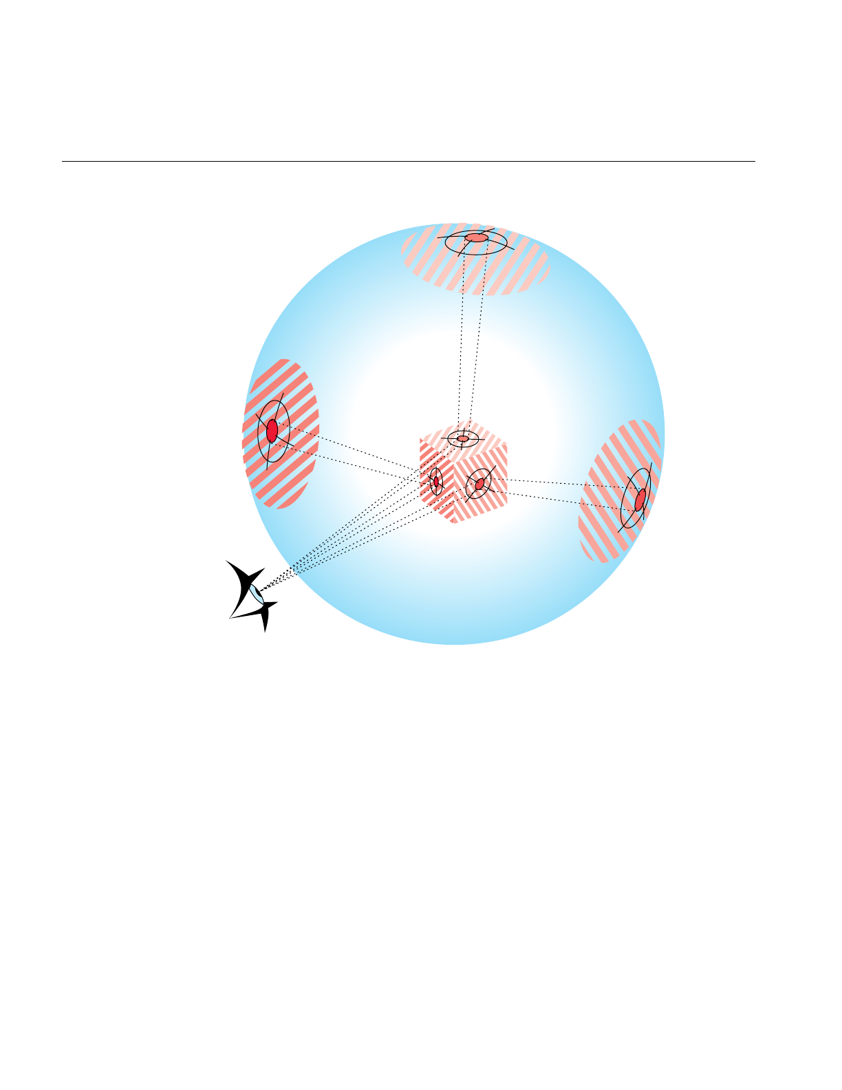
174
Chapter 10: Efficient High-Quality Lighting Effects: Reflection Mapping
Figure 10-2 Reflection-Map Geometry: Local Viewer, Local Environment
Any change in the scene or viewpoint requires a recomputation of the reflected ray, and
a new mapping of the surface to the texture image. The member function
updateViewInfo() calculates cylinder texture map coordinates for each frame. Clearly,
this is a greater processing burden than using a remote viewer in a remote environment.
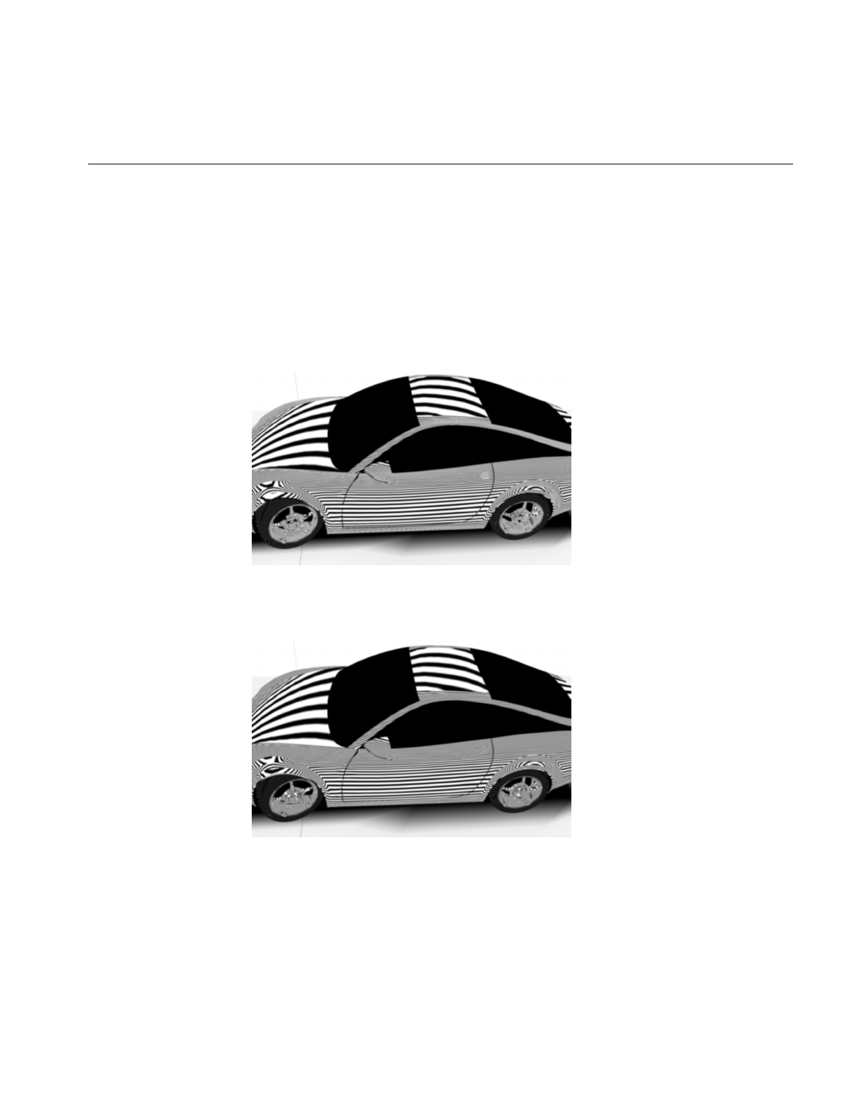
Accurate Mapping: Local View of a Local Environment
175
Cylinder Map
This reflection mapping style simulates tube lighting. The mapping assumes a local
viewer and a local environment; the x axis is the axis of a cylinder with lights that run
down the wall, parallel to the axis. As you move the viewpoint, the simulated lighting
tubes slide over the surface. Figure 10-3 and illustrate the effect. Note how the bands of
light shift on the surface of the car as the viewing angle changes. These images were
created with the sample application zebraFly (see “zebraFly Application” on page 23).
Figure 10-3 Cylinder-Map Images: Note How Lighting Differs From View in (Data courtesy of
Alias|Wavefront)
Figure 10-4 Cylinder-Map Images: Note How Lighting Differs From View in Figure 10-3 (Data
courtesy of Alias|Wavefront)
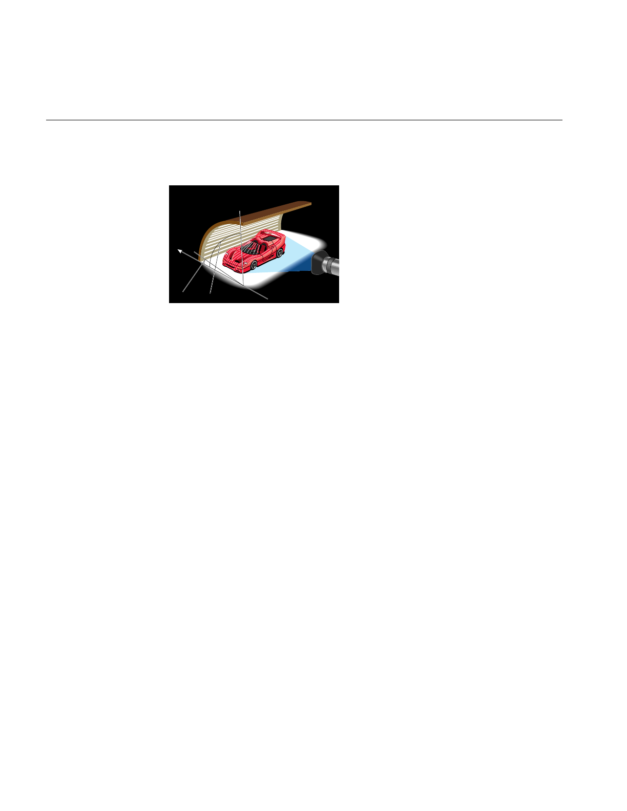
176
Chapter 10: Efficient High-Quality Lighting Effects: Reflection Mapping
Figure 10-5 illustrates the viewing configuration used for the cylinder map.
Figure 10-5 Viewing Configuration for the Cylinder Map
opReflMap has accessor methods to control parameters of the cylinder map, but you can
also use environment variables to set the radius of the cylinder and the size and the
spacing of the lights:
OP_REFL_MAP_RADIUS
Sets the radius of the cylinder.
OP_REFL_MAP_LIGHT_WIDTH
Is an angle, in radians, that specifies the width of the lights in the
cylinder.
OP_REFL_MAP_SPACE_WIDTH
Is an angle, in radians, that specifies the width of the space between the
lights in the cylinder.
y
Start angle End angle

Reflection-Mapping Class: opReflMap
177
Reflection-Mapping Class: opReflMap
This class provides the tools for the different reflection-mapping types discussed in this
section.
• Use any of the three simple reflection maps to rotate objects in the scene to observe
changing reflections.
• Use the more computationally expensive cylindrical environment map to more
realistically shift the lighting as you “walk” around a surface. The function
updateViewInfo() updates the texture coordinates as you walk around.
In addition to the constructor, opReflMap’s methods fall into three groups: those that are
independent of the type of reflection map set by the constructor, those that apply only to
the Gaussian map type, and those that apply only to the cylinder, floor, and ceiling maps.
No special function is needed to control the sphere map.
Class Declaration for opReflMap
The following are the main methods in the class:
class opReflMap
{
public:
opReflMap( csGroup *root, char *fileName, unsigned int mt );
opReflMap( csGroup *root, csImage *inputImage, unsigned int mt );
opReflMap( csGroup *root, opReal spec, unsigned int mt );
~opReflMap( void );
// Sets and gets
void setScene( csGroup *root ) ;
csGroup *getScene( ) ;
void setSpecularity( opReal spec );
opReal getSpecularity( );
void setScale( opReal _scale );
opReal getScale( );
void setXoffset( opReal offset );
opReal getXoffset( );

178
Chapter 10: Efficient High-Quality Lighting Effects: Reflection Mapping
void setYoffset( opReal offset );
opReal getYoffset( );
void setZoffset( opReal offset );
opReal getZoffset( );
void setStartAngle( opReal angle );
opReal getStartAngle( );
void setEndAngle( opReal angle );
opReal getEndAngle( );
void setMapType( uint mt );
unsigned int getMapType( );
void setShinyThreshold( float t );
float getShinyThreshold( );
void setXRes(int res);
int getXRes();
void setYRes(int res);
int getYRes();
csTexture *getTex()
csTexGen *getTexGen()
void setCBias(float bias)
float getCBias()
void setLightColor(float r, float g, float b)
void setSpaceColor(float r, float g, float b)
void setCylinderTexture( );
// Compute the new texture coordinates for a given geoset
void computeTexCoords( csTriStripSet *gs );
void computeTexCoords( csTriFanSet *gs );
// Run over the scene graph updating the texture coord
void computeAllTexCoords( );
// Tell the reflection map to update it’s viewing information
void updateViewInfo(
csCamera &camera, csTransform &transform, csVec3f ¢er );

Reflection-Mapping Class: opReflMap
179
// Enables the texture appearance on the scene graph’s shape nodes’
// apearances
void setTextureApp( bool enable );
};
Main Features of the Methods in opReflMap
These are the main features of the member functions of opReflMap that are independent
of mapping type:
opReflMap(root, fileName, mt),opReflMap(root, spec, mt), and
opReflMap( root, inputImage, mt )
Construct a reflection map of type mt, where mt is an element of an
enumerated type: SPHERE, GAUSSIAN, CYLINDER, FLOOR, or
CEILING. The argument mt must be SPHERE if you specify an
environment texture image with fileName or inputImage. If mt is
GAUSSIAN, spec is the specularity parameter; the default value is 2.0.
setMapType() and getMapType()
Set and get the map type, which is SPHERE, GAUSSIAN, CYLINDER,
FLOOR, or CEILING.
setScene() and getScene()
Get and set the scene graph for which opReflMap builds a reflection
mapping.
setShinyThreshold() and getShinyThreshold()
Get and set the threshold value for mapping a reflection from a surface.
The threshold is compared with the value of an object’s csMaterial
shininess parameter, which can vary from 0.0, for no reflections, to 1.0
for a perfect reflector. The default value is 0.0.
For GAUSSIAN reflection maps, you have the following specific methods:
setSpecularity() and getSpecularity()
Get and set the specularity parameter for the GAUSSIAN mapping, a
Phong-like illumination model. As the specularity parameter increases,
the surface appears more mirror like. The default value is 5.0.
For CYLINDER reflection maps, you have the following specific methods:
setScale() and getScale()
Get and set the radius for the CYLINDER mapping.

180
Chapter 10: Efficient High-Quality Lighting Effects: Reflection Mapping
setStartAngle() and getStartAngle()
Set and get the angular elevation, in radians, of the right edge of the light
cylinder as you look in the negative xdirection. The angle is measured
from the y axis in the z-y plane.
setEndAngle() and getEndAngle()
Set and get the angular elevation, in radians, of the left edge of the light
cylinder as you look down the center of the cylinder in the negative x
direction. The angle is measured from the y axis in the z-y plane.
computeTexCoords()
Computes texture coordinates for a particular csGeoSet, so you can
update the reflection map for a local viewer and environment when you
change the relative position of the viewpoint and the object.
updateViewInfo(camera, transform, center)
Translates the center of the scene to center, changes the viewing angle
according to the matrix transform, and computes new texture
coordinates for the entire scene graph. A simple rotation matrix gives
the best results. Use the center parameter to set the distance from the
center of the scene.

PART FOUR
Managing and Rendering Higher-Order
Geometric Primitives IV
The three chapters in this section discuss tools for creating higher-order
primitives, maintaining surface topology when primitives are adjacent, and
approximating a surface with a set of triangles, which define OpenGL primitives
suitable for rendering.
Chapter 11, “Higher-Order Geometric Primitives and Discrete Meshes”
Chapter 12, “Creating and Maintaining Surface Topology”
Chapter 13, “Rendering Higher-Order Primitives: Tessellators”


183
Chapter 11
11. Higher-Order Geometric Primitives and Discrete
Meshes
OpenGL Optimizer extends the set of geometric objects available through Cosmo3D
with a large set of higher-order primitives that you can include in a scene graph.
“Higher-order” means objects other than sets of triangles, and typically implies an object
that is defined mathematically.
Designs produced by CAD systems are defined by these types of surface representations.
By providing direct support for them, OpenGL Optimizer expands possible applications
from simple walkthrough ability to direct interaction with the design data base. When
combined with advanced rendering tools such as those discussed in “Occlusion Culling”
on page 126, higher-order surface representations provide visual access to very large
design data bases, with free-roaming interactivity.
OpenGL Optimizer also provides classes to define discrete curves, discrete surfaces, and
meshes. Meshes associate a vector with each mesh point and are useful for scientific
visualization.
The objects are discussed in the following sections:
• “Features and Uses of Higher-Order Geometric Primitives” on page 184
• “Necessary Objects Used by Reps” on page 185
• “Geometric Primitives: The Base Class opRep and the Application repTest” on
page 189
• “Planar Curves” on page 192
• “Spatial Curves” on page 214
• “Parametric Surfaces” on page 219
• “opCuboid” on page 260
• “Regular Meshes and Discrete Surfaces” on page 262

184
Chapter 11: Higher-Order Geometric Primitives and Discrete Meshes
Features and Uses of Higher-Order Geometric Primitives
Higher-order geometric primitives, called representations or simply reps, facilitate the
design process by providing a library of useful curves and surfaces that ease interactive
flexibility, accelerate scene-graph transformations, and reduce the memory footprint of
the scene graph. Reps yield these advantages by using parameters to describe objects.
Instead of a collection of vertices, each of which you must manipulate independently to
change a surface, reps define surfaces in terms of a relatively small set of control
parameters; they are more like pure mathematical objects.
Reps Relationship to the Rendering Process
OpenGL Optimizer allows you to interact with an abstract object and treat rendering as
a separate operation. A simple example of a representation is a sphere, defined by a
radius and a center. After defining a sphere, you can then implement rendering in several
ways: by tessellating, by a sphere-specific draw routine, or conceivably by hardware.
Member functions of geometric-primitive classes allow you to develop all these
implementations. The fundamental rendering step of tessellating a representation is
discussed in Chapter 13, “Rendering Higher-Order Primitives: Tessellators.”
Trimmed NURBS
NURBS curves and surfaces are included in the set of OpenGL Optimizer reps. OpenGL
also has these, but OpenGL Optimizer’s NURBS have two advantages; you can maintain
topology, so cracks do not appear at the boundaries of adjacent tessellations when they
are drawn, and you have better control over tessellation. See Chapter 12, “Creating and
Maintaining Surface Topology,” and “opTessNurbSurfaceAction” on page 301.

Necessary Objects Used by Reps
185
Necessary Objects Used by Reps
To use reps effectively, you need to understand the OpenGL Optimizer representations
of geometric points and the transformation matrices that are used by the methods of the
rep classes.
Pi
OpenGL Optimizer uses the value for π held in the variable M_PI, declared in csBasic.h:
3.14159265358979323846.
Classes for Points
The classes opVec2,opVec3, and opVec4 define two-, three-, and four-dimensional
vectors, respectively, and include common operations of vector algebra such as addition,
scalar multiplication, cross products, and so on. See the header file opVec.h for a list of
operations defined for each of the vectors.
The important distinction between these vector classes and csVec of Cosmo3D is that
OpenGL Optimizer vectors are declared opRealand so can be single or double precision,
depending on the version of the OpenGL Optimizer library you use.

186
Chapter 11: Higher-Order Geometric Primitives and Discrete Meshes
Classes for Scalar Functions
The class opScalar is the base class for defining scalar functions; it allows you to
conveniently read and write functions. The class provides a virtual evaluation method.
Class Declaration for opScalar
The following are the main methods in the class:
class opScalar : public csObject
{ public:
// Creating and destroying
opScalar();
virtual ~opScalar();
virtual opReal eval(opReal t) = 0;
};
The class opCompositeScalar allows you to define the functional composition of two
opScalars
Class Declaration for opCompositeScalar
The following are the main methods in the class:
class opCompositeScalar : public opScalar
{ public:
// Creating and destroying
opCompositeScalar( );
opCompositeScalar(opScalar *outFun, opScalar *inFun);
virtual ~opCompositeScalar();
// Accessor functions
opScalar *getOutF()
opScalar *getInF()
void setOutF(opScalar *outF);
void setInF (opScalar *inF);
opReal eval(opReal t);
};
Main Features of the Methods in opCompositeScalar
eval() Returns the value of outF(inF(t)).

Necessary Objects Used by Reps
187
Trigonometric Functions
OpenGL Optimizer provides classes for two trigonometric functions, opCosScalar and
opSinScalar. The class declarations have the same form as that of opScalar.
Polynomials
Polynomials of arbitrary degree are defined by the class opPolyScalar.
Class Declaration for opPolyScalar
The following are the main methods in the class:
class opPolyScalar : public opScalar
{
public:
// Creating and destroying
opPolyScalar( void );
opPolyScalar( int degree, opReal* coef);
virtual ~opPolyScalar();
// Accessor functions
void set( int degree, opReal* coef);
int getDegree()
opReal getCoef( int i)
// Evaluators
opReal eval(opReal u);
}:

188
Chapter 11: Higher-Order Geometric Primitives and Discrete Meshes
Matrix Class: opFrame
Each geometric primitive is defined with respect to its own coordinate system. The
elementary definition of an object gives a particular orientation and location with respect
to the origin. This reference frame can, in turn, be manipulated by a csTransform to place
it in a scene or manipulate it (see Chapter 9, “Interactive Highlighting and
Manipulating”).
However, to obviate insertion of csTransform nodes whenever you want to define the
location or orientation of an object or to change the shape of an objec, the base class for
higher-order primitives has functions that allow you to locate and orient a primitive with
respect to its own reference frame. The location is defined by an opVec2 or opVec3, and
the orientation is controlled by a 3 x 3 matrix, held in the class opFrame. If the matrix is
not a rotation matrix, you can change the shape of an object, for example, you can distort
a sphere into an ellipsoid.
Class Declaration for opFrame
The following are the main methods in the class:
class opFrame
{
public:
opReal m[3][3];
bool identity;
void setIdentity()
opFrame();
};

Geometric Primitives: The Base Class opRep and the Application repTest
189
Geometric Primitives: The Base Class opRep and the Application repTest
opRep is the base class for higher-order geometric primitives in a scene graph. An opRep
is derived from a csShape. Figure 11-1 shows the hierarchy of classes derived from
opRep.
The following sections discuss the subclasses of opRep:
• “Planar Curves” on page 192
• “Spatial Curves” on page 214
• “Parametric Surfaces” on page 219
• “opCuboid” on page 260
• “Regular Meshes and Discrete Surfaces” on page 262
To experiment with opReps, you can use and modify the application repTest in
/usr/share/Optimizer/src/sample/repTest, which provides sample instances of several
geometric representations, as well as the tessellation and Cosmo3D calls that render the
objects. Sample code from repTest is included with discussions of several of the classes
derived from opRep.
opRep has methods to orient the object in space, obviating the need to place a
csTransform node above each opRep to move it from its default position. opRep also has
a virtual drawing function that you can use to define an approach to rendering other than
via tessellation and a Cosmo3D draw action.
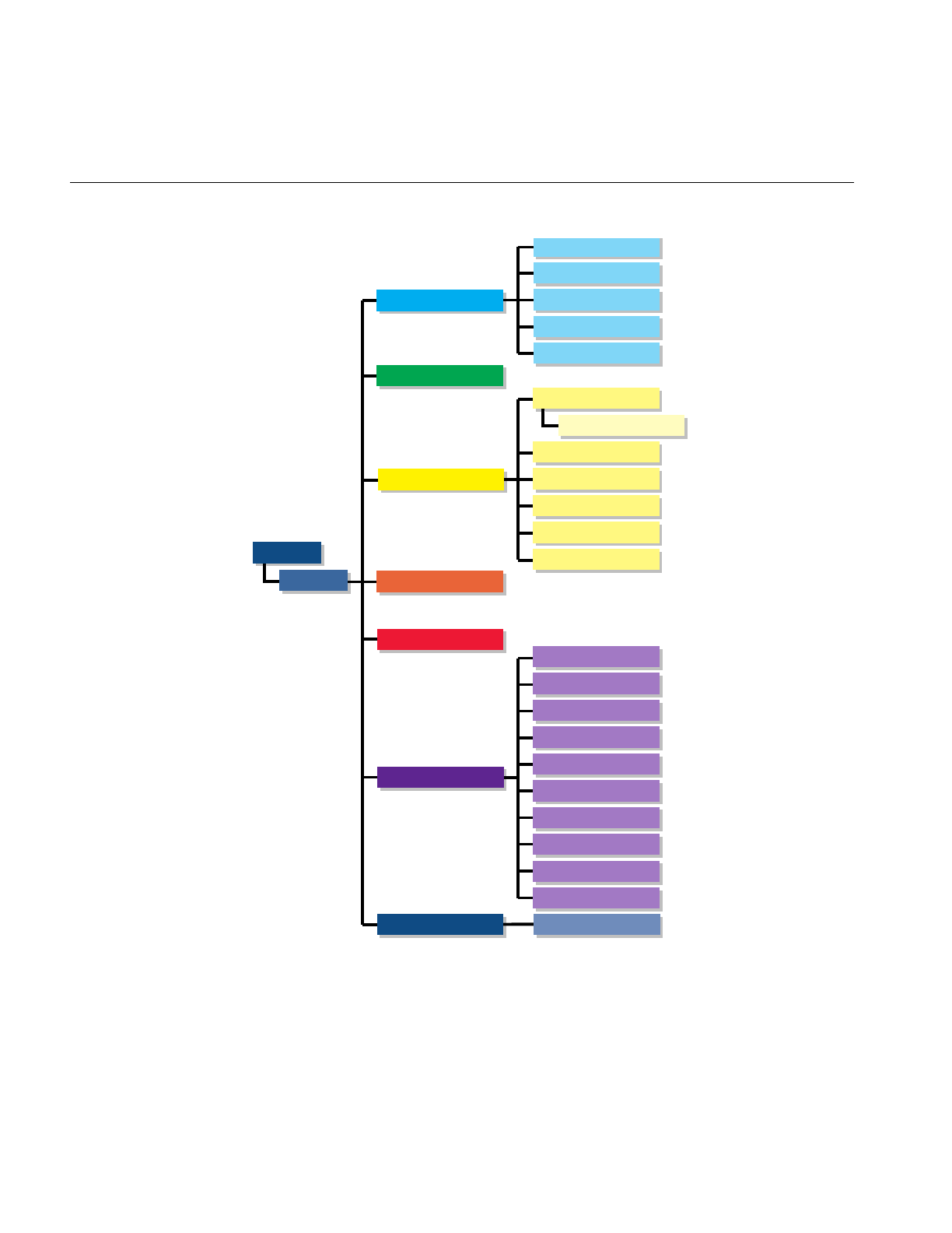
190
Chapter 11: Higher-Order Geometric Primitives and Discrete Meshes
Figure 11-1 Class Hierarchy for Higher-Order Primitives
opDisSurface
opCuboid
csShape
opCurve2d
opDisCurve2d
opCurve3d
opOrientedLine3d
opRep
opParaSurface
opLine2d
opCircle2d
opHsplineCurve2d
opSuperQuadCurve2d
opNurbCurve2d
opSuperQuadCurve3d
opLine3d
opCircle3d
opHsplineCurve3d
opNurbCurve3d
opCompositeCurve3d
opRegMesh
opTorus
opNurbSurfaceopNurbSurface
opPlane
opDisCurve3d
opSphere
opCylinder
opCone
opSweptSurface
opRuled
opCoons
opNurbSurface
opHsplineSurface

Geometric Primitives: The Base Class opRep and the Application repTest
191
Class Declaration for opRep
The following are the main methods in the class:
class opRep : public csShape
{
public:
opRep( );
virtual ~opRep( );
// Accessor functions
void setOrigin( const opVec3& org );
void setOrient( const opFrame& mat );
opVec3 getOrigin();
opFrame getOrient();
// Utility methods
virtual int getMemSize();
public:
// Comso3d virtual functions
virtual void draw();
};
Main Features of the Methods in opRep
setOrient() Sets the orientation of the representation with respect to the origin via a
matrix multiplication.
For a discussion of useful matrices, see the book Computer Graphics:
Principles and Practice in “Recommended Reference Materials” on
page xxxi.
setOrigin() Sets the location of the representation with respect to the origin. For
example, supplying the vector (1,0,0) shifts the location of the object 1
unit in the direction of the positive x axis.
opRep’s subclasses typically include evaluator methods to determine coordinates of
points, tangents, and normals. If you do not want the values corresponding to the defualt
position, do not call these methods before you use setOrient() and setOrigin() to locate
anopRep. Thus, for example, when defining points on a circle, first set the center and the
radius, then call setOrient() to set the orientation, and then evaluate points.

192
Chapter 11: Higher-Order Geometric Primitives and Discrete Meshes
Planar Curves
A parametric curve in the plane can be thought of as the result of taking a piece of the
real number line, twisting it, stretching it, maybe gluing the ends together, and laying it
down on the plane. The base class for parametric curves that lie in the x-y plane is the
class opCurve2d.
An important use of opCurve2d is to specify trim curves, which define boundaries for
surfaces. Surfaces are parameterized by part of a plane, which in OpenGL Optimizer is
referred to as the u-v plane. When an opCurve2d is used to define a trim curve, it is
treated as a curve in the u-v plane. This topic is discussed further in the section
“Parametric Surfaces” on page 219.
Another important use of opCurve2d is for specifying cross sections for swept surfaces.
See “Swept Surfaces” on page 240.
OpenGL Optimizer also provides a class to create discrete curves, opDisCurve2d.
The following sections discuss planar curve classes, most of which are derived from
opCurve2d:
• “Mathematical Description of a Planar Curve” on page 192
• “Lines in the Plane” on page 196
• “Circles in the Plane” on page 197
• “Superquadric Curves: opSuperQuadCurve2d” on page 199
• “Hermite-Spline Curves in the Plane” on page 202
• “NURBS Briefly” on page 204
• “NURBS Curves in the Plane” on page 208
• “Discrete Curves in the Plane” on page 211
Mathematical Description of a Planar Curve
Planar curves are made of sets of points, described by two-dimensional vectors, opVec2s.
They are parameterized by the opReal variable t;astvaries, a point “moves” along the
curve. tcan be thought of as the amount of time that has passed as a point moves along
the curve. Or, tcan measure the distance traveled.
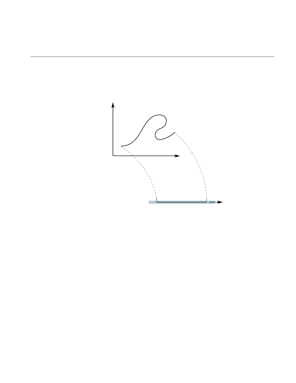
Planar Curves
193
More precisely, each component of a point on the curve is a function of t, which lies in the
parameter interval (t0,t1) on the real line. Points on the curve are described by a pair of
functions of t: (x(t), y(t)).
Figure 11-2 Parametric Curve: Parameter Interval (0,1).
Classes derived from opCurve2d inherit a set of evaluator functions which, for a given
value of t, evaluate a point on the curve, the tangent and normal vectors at the point, and
the curvature. Naturally, the base-class evaluator that locates points on the curve is a
pure virtual function.
To evaluate tangent and normal vectors at a point, opCurve2d provides virtual functions
that, by default, use finite-central-difference calculations. To compute the tangent to the
curve at p[t], a point on the curve, the tangent evaluator function takes the vector
connecting two “nearby” points on the curve, p[t+∆t]−p[t−∆t]where ∆tis “small,” and
divides by 2∆t. Similarly, a finite-central-difference calculation of the normal vector uses
the difference between two nearby tangent vectors: n[t]= (t[t+∆t] −t[t−∆t])/2∆t.
0.0 1.0
t
y
x
t=0.0
t=1.0
Object space
Parameter space

194
Chapter 11: Higher-Order Geometric Primitives and Discrete Meshes
Class Declaration for opCurve2d
The following are the main methods in the class:
class opCurve2d : public opRep
{
public:
// Creating and destroying
opCurve2d( );
opCurve2d( opReal beginT, opReal endT );
virtual ~opCurve2d();
// Accessor functions
void setBeginT( opReal beginT );
void setEndT( opReal endT );
opReal getBeginT();
opReal getEndT();
opVec2 getBeginPt();
opVec2 getEndPt();
opVec2 getBeginTan();
opVec2 getEndTan();
void setClosed( opLoop loopVal );
opLoop getClosed();
void setClosedTol( opReal tol );
opReal getClosedTol();
// Evaluators
virtual void evalPt( opReal t, opVec2 &pnt ) = 0;
virtual void evalTan( opReal t, opVec2 &tan );
virtual void evalNorm( opReal t, opVec2 &norm );
virtual void evalCurv( opReal t, opReal &curv );
virtual void eval( opReal t, opVec2 &pnt,
opVec2 &tan,
opReal &curv,
opVec2 &norm );
// Miscellaneous
virtual void copy( const opCurve2d& old );
};

Planar Curves
195
Main Features of the Methods in opCurve2d
opCurve2d(beginT,endT)
If you do not specify any arguments, then the parametric range of the
curve is [0.0,1.0].
eval() For a given t, returns the position, tangent, curvature, and normal
vectors.
evalPt() Is a pure virtual function to evaluate position on the curve.
evalTan(),evalCurv(), and evalNorm()
Evaluate the curve’s tangent, curvature, and normal vectors,
respectively. The default functions approximate these using central
differences taken about a small ∆t, given by (endT - beginT) * functionTol.
The latter is a static data element specified in the file opRep.H.
setBeginT() and setEndT(),getBeginPt() and getEndPt()
Set and get the parameter range for the curve. Whenever you set one of
these values, the endpoint of the curve changes. Therefore, each of these
functions also recomputes the endpoint, which is cached because it is
frequently used. Also, the functions recompute the ∆t used to
approximate derivatives.
Note that all planar curve classes derived from opCurve2d reuse
setBeginT() and setEndT() to define the extents of their curves.
setClosed() and getClosed()
Set and get whether a curve is closed.
A closed curve is one for which the endpoints match. Whether curves
are closed is determined automatically, but can be overridden by
setClosed().
setClosedTol() and getClosedTol()
Set and get the mismatch between endpoints that is allowed when
calculating whether curves are closed
To specify the origin used to locate an opCurve2d, use the first two components set by
the inherited function opRep::setOrigin().
196
Chapter 11: Higher-Order Geometric Primitives and Discrete Meshes
Lines in the Plane
Parametric lines in the plane are defined by beginning and ending points. The
parameterization is such that as t varies from t1 to t2, a point on the line “moves,” at a
uniform rate, from the beginning to the ending point.
Figure 11-3 Line in the Plane Parameterization
Class Declaration for opLine2d
The following are the main methods in the class:
class opLine2d : public opCurve2d
{
public:
// Creating and destroying
opLine2d();
opLine2d( opReal x1, opReal y1, opReal t1,
opReal x2, opReal y2, opReal t2 );
virtual ~opLine2d();
// Accessor functions
void setPoint1( opReal x1, opReal y1, opReal t1 );
void setPoint2( opReal x2, opReal y2, opReal t2 );
void getPoint1( opReal *x1, opReal *y1, opReal *t1 );
void getPoint2( opReal *x2, opReal *y2, opReal *t2 );
// Evaluators
void evalPt( opReal t, opVec2 &pnt );
};
y
x
t=t1
t=t2
(x1,y1)
(x2,y2)
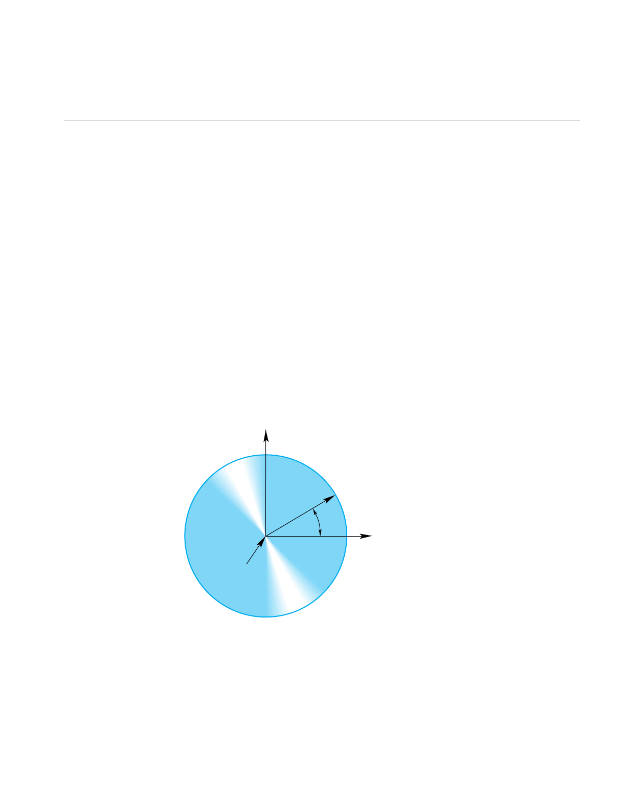
Planar Curves
197
Main Features of the Methods in opLine2d
opLine2d() Creates a parametric line with end points (0,0) and (1,0), and parameter
interval (0,1).
opLine2d(x1, y1, t1, x2, y2, t2)
Creates a parametric line starting at the point (x1, y1) and ending at
(x2,y2). The line is parameterized so that t=t1 corresponds to (x1, y1)
and t=t2 corresponds to (x2,y2).
evalPt() Is the only evaluator function defined for this object. The tangent vector
is (x2-x1, y2-y1) and the curvature is zero.
setPoint*() and getPoint*()
Set and get the endpoints of the line.
Circles in the Plane
Use the class opCircle2d to define a parametric circle in the plane. The parameterization
is such that t is the angular displacement, in radians, in a counterclockwise direction
from the x axis. Figure 11-4 illustrates the parameterization of the circle.
Figure 11-4 Circle in the Plane Parameterization
y
x
Origin
Radius
t

198
Chapter 11: Higher-Order Geometric Primitives and Discrete Meshes
Class Declaration for opCircle2d
The following are the main methods in the class:
class opCircle2d : public opCurve2d
{
public:
// Creating amd destroying
opCircle2d();
opCircle2d( opReal rad, opVec2 *org );
virtual ~opCircle2d();
// Accessor functions
void setRadius( opReal rad ) ;
opReal getRadius() ;
// Evaluator
void evalPt( opReal t, opVec2 &pnt );
void evalTan( opReal t, opVec2 &tan );
void evalCurv( opReal t, opReal &curv );
void evalNorm( opReal t, opVec2 &norm );
void eval( opReal t,
opVec2 &pnt,
opVec2 &tan,
opReal &curv,
opVec2& norm );
};
Main Features of the Methods in opCircle2d
The class opCircle2d inherits functions to set the range of parameter values from
opCurve2d.
opCircle2d(rad,org)
Creates an instance of a two-dimensional circle with radius rad centered
at org. The default circle has unit radius and origin (0,0). To change the
default position, use the methods setOrigin() and setOrient() inherited
from opRep.
setRadius() and getRadius()
Set and get the radius.
opCircle2d provides exact calculations for the evaluator functions inherited from
opCurve2d.

Planar Curves
199
Superquadric Curves: opSuperQuadCurve2d
The class opSuperQuadCurve2d provides methods to define a generalization of a circle
that, when used for constructing a swept surface, is convenient for generating rounded,
nearly square surfaces, or surfaces with sharp cusps (see “Swept Surfaces” on page 240).
Two examples of superquadrics appear in repTest. Position along the curve is specified
by an angle from the x axis, in the same was as for an opCircle2d; the shape of the curve
is controlled by a second parameter.
A superquadric is the set of points (x,y) given by the following equation that clearly
expresses the relationship to the equation of a circle:
The above equation can be written in a parametric form:
The family of curves generated by these equations as the quantity αvaries can be
described as follows (see Figure 11-5). Four points are always on the curve for any value
of α: (±r, 0) and (0, ±r). If α is 1, the curve is a circle of radius r; as α approaches zero, the
circle expands to fill a square of side 2r as if you were inflating a balloon in a box. As α
approaches infinity, the circle contracts towards the two diameters along the x and y axes,
approaching two orthogonal lines as if you deflated a balloon with two rigid orthogonal
sticks inside it.
x2
()
1α/y2
()
1α/
+r2
()
1α/
=
xt() rt[]cos αsign t[]cos[]=
yt() rt[]sin αsign t[]sin[]=
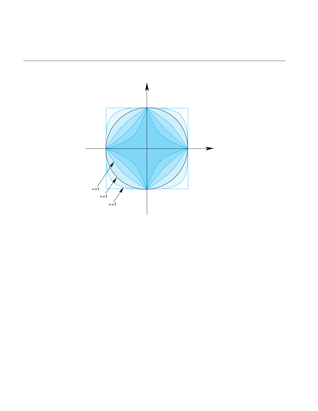
200
Chapter 11: Higher-Order Geometric Primitives and Discrete Meshes
Figure 11-5 Superquadric Curve’s Dependence on the Parameter α.
y
x

Planar Curves
201
Class Declaration for opSuperQuadCurve2d
The following are the main methods in the class:
class opSuperQuadCurve2d : public opCurve2d
{
public:
// Creating and destroying
opSuperQuadCurve2d();
opSuperQuadCurve2d( opReal _radius,
opVec2 *_origin,
opReal _exponent );
virtual ~opSuperQuadCurve2d();
// Accessor functions
void setRadius( opReal _radius );
opReal getRadius();
void setExponent( opReal _exponent );
opReal getExponent();
// Evaluator
void evalPt( opReal t, opVec2 &pnt );
};
Main Features of the Methods in opSuperQuadCurve2d
The accessor functions allow you to control the radius rand exponent αof the curve. To
change the default position, use the methods setOrigin() and setOrient() inherited from
opRep.
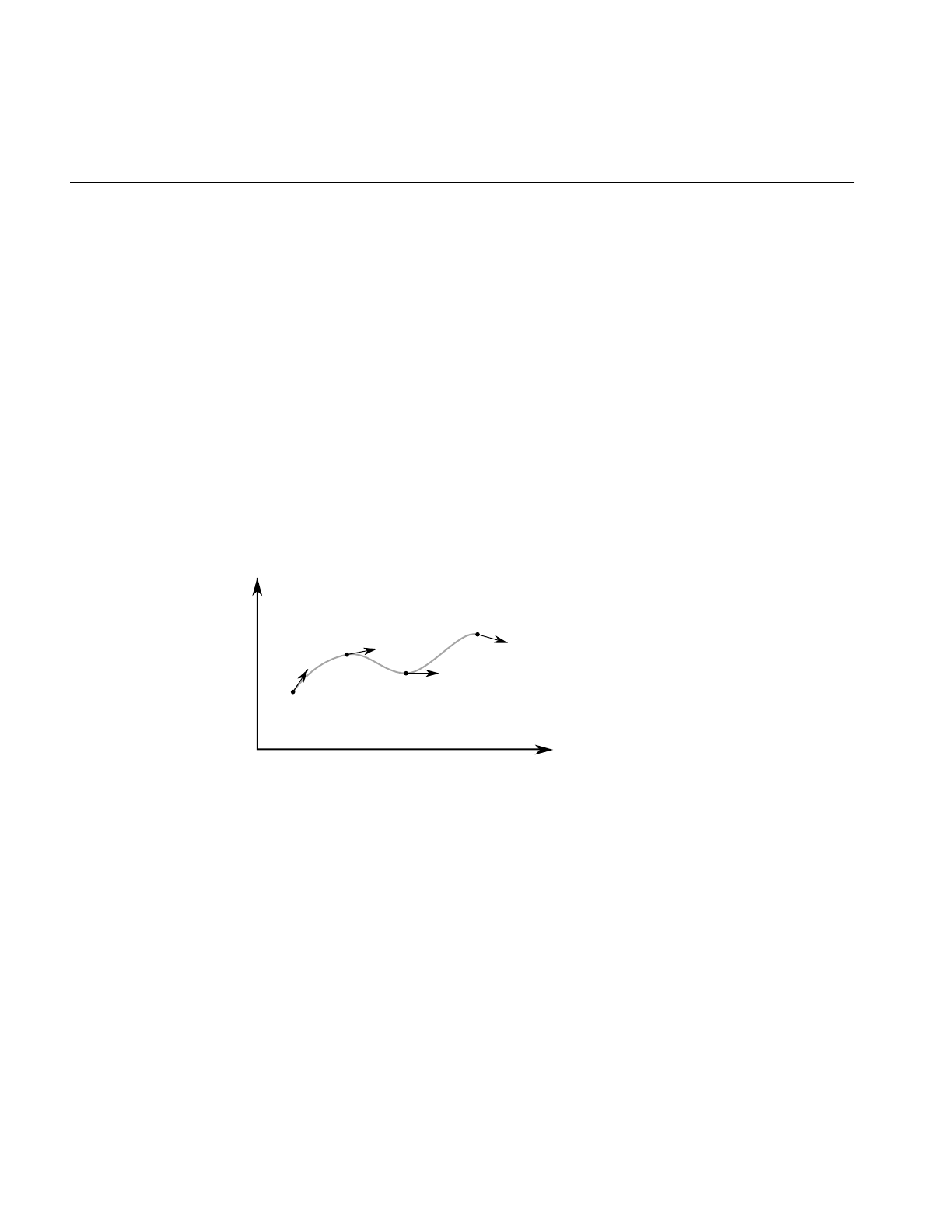
202
Chapter 11: Higher-Order Geometric Primitives and Discrete Meshes
Hermite-Spline Curves in the Plane
Asplineis a mathematical technique for generating a single geometric object from pieces.
An advantage of breaking a curve into pieces is greater flexibility when you have many
points controlling the shape: changes to one piece of the curve do not have significant
effects on remote pieces. To define a spline curve for a range of values for the parameter
t, say from 0 to 3, you “tie” together pieces of curves defined over intervals of values for
t. For example, you might assign curve pieces to the three intervals 0 to 1, 1 to 2, and 2 to
3. The four points in the set of parameters, 0, 1, 2, and 3, define the endpoints of the
intervals and are called knots.
AHermite-spline curve is a curve whose segments are cubic polynomials of the parameter
t, where the coefficients of the polynomials are determined by the position and tangent
to the curve at each knot point (see ). Thus the curve passes through each of a set of
specified points with a specified tangent vector. The set of knot points must be increasing
values of the parameter t.
Figure 11-6 Hermite Spline Curve Parameterization
y
x
t=t0
t=t1
t=t2
t=t3
p0
p1
tng0 tng1
p2 tng2
tng3
p3

Planar Curves
203
Class Declaration for opHsplineCurve2d
The class for creating Hermite spline curves is opHsplineCurve2d. The following are the
main methods in the class:
class opHsplineCurve2d : public opCurve2d
{
public:
// Creating and destroying
opHsplineCurve2d( opReal tBegin = 0.0, opReal tEnd = 1.0 );
virtual ~opHsplineCurve2d( );
// Accessor functions
void setPoint( int i, opVec2 &p );
void setTangent( int i, opVec2 &tng );
void setKnot( int i, opReal t );
opVec2* getPoint( int i );
opVec2* getTangent( int i );
opReal getKnot( int i );
virtual int getMemSize( );
// Evaluator
virtual void evalPt( opReal t, opVec2 &pnt );
};

204
Chapter 11: Higher-Order Geometric Primitives and Discrete Meshes
NURBS Briefly
The acronym NURBS stands for “nonuniform rational B-splines.” NURBS define a set of
curves and surfaces that generalizes Bezier curves. Both NURBS curves and Bezier
curves are “smooth” curves that are well suited for CAD design work. They are
essentially determined by a set of points that, although the points do not lie on the
curves, controls the shape of the curves.
Because NURBS properties are not widely known, a discussion of their features precedes
details of how to create instances of them. The discussion is necessarily brief and is
intended to provide the minimum amount of information needed to start using OpenGL
Optimizer NURBS classes.
This general discussion of NURBS is presented in the following sections:
• “OpenGL Optimizer NURBS Classes” on page 205
• “NURBS Control Parameters” on page 205
• “NURBS Elements That Determine the Control Parameters” on page 205
• “Knot Points” on page 206
• “Control Points” on page 206
• “Features of NURBS and Bezier Curves” on page 207
• “Weights for Control Points” on page 207
For more information, consult the following sources, which are listed in “Recommended
Reference Materials” on page xxxi:
• An intuitive introduction to NURBS curves and surfaces is Chapter 8 of The Inventor
Mentor.
• A more rigorous mathematical discussion appears in the book Curves and Surfaces
for Computer Aided Geometric Design: A Practical Guide.
• A discussion of NURBS also appears in Chapter 11 of the OpenGL Programming
Guide.

Planar Curves
205
OpenGL Optimizer NURBS Classes
The OpenGL Optimizer classes allow you to treat a NURBS object as a black box that
takes a set of control parameters and generates a geometric shape. A NURBS object’s
essential properties are rather straightforward, although the underlying mathematics are
complex. Unlike lines and circles, NURBS can represent a large set of distinct complex
shapes. Because of this flexibility, developing a NURBS object is often best done
interactively. In a plausible application, you could allow a user to design a curve using
an interface in which control parameters are changed by clicking and dragging and by
using sliders.
The class opNurbCurve2d generates curves in the plane, the simplest NURBS object
provided by OpenGL Optimizer. The class opNurbCurve3d generates NURBS curves in
three-dimensional space. The class opNurbSurface generates NURBS surfaces, which
extend the ideas underlying NURBS curves to two-dimensional objects. The principles
for controlling the shapes of these objects are all essentially the same.
NURBS Control Parameters
A discussion of the terms in the name “nonuniform rational B-splines” indicates the
nature of these objects and, perhaps more important, introduces the meanings of the
control parameters:
• “Knot Points” on page 206
• “Control Points” on page 206
• “Weights for Control Points” on page 207
NURBS Elements That Determine the Control Parameters
• splines, which introduce knot points and are discussed in “Hermite-Spline Curves
in the Plane” on page 202
• nonuniform knot points
• B-splines, which introduce control points
• rational B-Splines, which introduce weighting parameters for control points

206
Chapter 11: Higher-Order Geometric Primitives and Discrete Meshes
Knot Points
The first set of control parameters for a NURBS curve is the set of knots, which are
nondecreasing— but not necessarily uniformly spaced or distinct—values of the
parameter t for the curve. The knot points determine how and where the pieces of the
NURBS object are joined together. “Splines” and “nonuniform splines” are the concepts
that underly these control parameters.
nonuniform Indicates that the sequence of knots need not have uniform spacing in
the parameter interval. In fact, the mathematics of NURBS make it
possible and, perhaps, necessary to repeat knot values; that is knots can
appear with a certain multiplicity. The number of knot points is
determined by counting all the knot points, including all multiplicities.
For example, although the sequence (0,0,0,0,1,1,1,1) has only two
distinct knot points, the number of knot points is eight. This example
might seem contrived, but the sequence comes from a common
practical example: it is the set of knot points for a cubic Bezier curve
defined on the interval 0 to 1. How to determine the order of a NURBS
curve is discussed in “Features of NURBS and Bezier Curves” on
page 207.
Control Points
The second set of control parameters for a NURBS curve is the control hull, the set of all
points that determine the basic shape of NURBS object. The effect of the control hull is
determined by the concept of a “B-spline”:
B-spline Refers to basis splines, a set of special curves associated with a given
knot sequence from which you can generate all other spline curves
having the same knot sequence and control hull. For each interval
described by the knot sequence, the corresponding piece of a B-spline
curve is a Bezier curve.
B-spline curves are like Bezier curves in that they are defined by an
algorithm that acts on a sequence of control points, the control hull,
which lie in the plane or in three-dimensional space. For information on
this, consult the book Curves and Surface for Computer Aided Geometric
Design in “Recommended Reference Materials” on page xxxi.

Planar Curves
207
Weights for Control Points
The third set of control parameters for a NURBS curve is the set of weights associated
with the control points. The concept of rational B-spline determines the effects of the
weighting parameters:
rational Refers to spline curves made up of generalizations of Bezier curves that
have a weight associated with each control point. The individual pieces
of a NURBS curve usually are not Bezier curves but rational Bezier
curves. The values of the weights have no absolute meaning; they
control how “hard” an individual control point pulls on the curve
relative to other control points. If the weights for all the control points of
a rational Bezier curve are equal, then the curve becomes a simple Bezier
curve. Weights were introduced to allow construction of exact conic
sections, which cannot be made with simple Bezier curves. See Curves
and Surface for Computer Aided Geometric Design in “Recommended
Reference Materials” on page xxxi.
Features of NURBS and Bezier Curves
These are the important properties of Bezier curves:
• They are “nice” polynomial curves whose degree is one less than the number of
control points. A polynomial curve is one for which each of the components is a
polynomial function of the parameter t. The number of coefficients in the
polynomial, the order of the polynomial, is equal to the number of control points.
• The control points determine the shape of the Bezier curve, but they do not lie on
the curve, except the first and last control points.
NURBS curves differ in the following ways:
• The order of the polynomial pieces that make up the NURBS curve depends on the
number of control points and the number of knot points. The order of a NURBS
curve is the difference between the number of knots, accounting for multiplicity,
and the number of control points. That is,
order = number of knot points - number of control points
• The relationship between the curves and the control points is looser than for a
Bezier curve. It also depends on the knot sequence and the sequence of weights.

208
Chapter 11: Higher-Order Geometric Primitives and Discrete Meshes
NURBS Curves in the Plane
The class InNurbCurve2d defines a nonuniform rational B-spline curve in the plane, the
simplest NURBS object provided by OpenGL Optimizer.
Class Declaration for opNurbCurve2d
The following are the main methods in the class:
class opNurbCurve2d : public opCurve2d
{
public:
// Creating and destroying
opNurbCurve2d( opReal tBegin = 0.0, opReal tEnd = 1.0 );
virtual ~opNurbCurve2d( );
// Accessor functions
void setControlHull( int i, opVec2 &p );
void setControlHull( int i, opVec3 &p );
void setWeight( int i, opReal w );
void setKnot( int i, opReal t );
void setControlHullSize( int s );
void setBoxBound( const csBoxBound &newBox);
opVec2* getControlHull( int i );
opReal getWeight( int i );
int getControlHullSize( );
int getKnotCount( );
opReal getKnot( int i );
int getOrder( );
// Evaluator
virtual void evalPt( opReal t, opVec2 &pnt );
// Memory foot print
virtual int getMemSize( );
};

Planar Curves
209
Main Features of the Methods in opNurbCurve2d
opNurbCurve2d(tBegin,tEnd)
Creates a NURBS curve in the plane with the specified parameter
domain. The default parameter domain is 0.0 to 1.0.
evalPt() Is a pure virtual function inherited from opCurve2d, and produces
unpredictable results until you set the control parameters.
setControlHull(i,p)and getControlHull(i)
Set and get the two-dimensional control point with index ito the value
p. If you supply opVec3 arguments, the location of the control points is
set by the first two components; the last component is their weight.
setControlHullSize()
Gives a hint about how big the control hull array is. This is not
mandatory but uses time and space most efficiently.
setKnot(i,t) and getKnot(t)
Set and get the knot point with index iand the value t.
setWeight(i,w) and getWeight(i)
Set and get the weight of the control point with index iand weight w.

210
Chapter 11: Higher-Order Geometric Primitives and Discrete Meshes
The Equation Used to Calculate a NURBS Curve
The equation that defines the NURBS curve is
• is a point on the surface p(t)
• is the ith B-spline basis function of degree n
• is a control point
• is the weight for the control point
An Alternative Equation for a NURBS Curve
If you have a surface developed from the alternative expression for a NURBS surface:
you must change the coordinates of the control points to get the same surface from
OpenGL Optimizer; you convert the coordinates of the control points from (x,y,w) to
(wx,wy,w).
pt() Bint()Ci
i
∑
Bint()Wi
i
∑
----------------------------
=
pt()
Bint()
Ci
Wi
puv,() Binu()WiCi
i
∑
Binu()Wi
i
∑
-----------------------------------
=
Planar Curves
211
Discrete Curves in the Plane
The class opDisCurve2d is the base class for making a discrete curve from line segments
connecting a sequence of points in the plane. Because opDisCurve2d is not derived from
opCurve2d, it does not inherit that class’s finite difference functions for calculating
derivatives, therefore, opDisCurve2d includes member functions that calculate arc
length, tangents, principal normals, and curvatures using finite central differences.
Figure 11-7 illustrates the definition of the curve by a set of points.
Figure 11-7 Discrete Curve Definition
y
x
p0
p1
p2
p3
p4
pi=(points[2i], points[2i+1])

212
Chapter 11: Higher-Order Geometric Primitives and Discrete Meshes
Class Declaration for opDisCurve2d
The following are the main methods in the class:
class opDisCurve2d : public opRep
{
public:
// Creating and destroying
opDisCurve2d( void );
opDisCurve2d( int nPoints, opReal *points );
virtual ~opDisCurve2d( void );
// Accessor functions
opVec2 getBeginPt();
opVec2 getEndPt();
opLoop getClosed();
void setClosed( opLoop c );
void setPoint( int i, const opVec2& pnt );
opVec2 getPoint( int i);
int getPointCount();
opVec2 getTangent(int i);
opVec2 getNormal(int i);
opReal getCurvature(int i);
// Evaluators
void computeTangents( );
void computeNormals( );
void computeCurvatures( );
void computeDerivatives( );
};

Planar Curves
213
Main Features of the Methods in opDisCurve2d
opDisCurve2d(nPoints,points)
Creates a discrete curve from an array of point coordinates. The
constructor assumes that the coordinates of the points are stored in pairs
sequentially; thus the points array is nPoint*2 in length.
computeCurvatures()
Computes the curvature, which is the magnitude of the normal vector.
computeDerivatives()
Is a convenience function that calls (in order) the tangent, normal, and
curvature functions.
computeNormals()
Computes the principal normal at a point using finite central differences
and stores the result in the class member dvectorn. For the point p[i], the
normal vector is computed to be the difference vector between the
tangents at the two neighboring points, t[i+1]-t[i-1], divided by the sum
of the distances from p[i] to the two neighboring points.
computeTangents()
Computes the arc lengths of segments and then uses finite central
differences to compute the tangents. For the point p[i], the tangent
vector is computed to be the vector between its two neighboring points,
p[i+1]-p[i-1], divided by the sum of the distances from p[i]to the two
neighboring points. The tangents are stored in the dvector t, the arc
lengths in the dvector ds, and the total arc length in arcLength.
getCurvature() Returns the value of thecurvature at the ith point.
getNormal() Returns the value of the normal at the ith point.
getPoint() Returns the value of the ith point.
getPointCount()Returns the value of the ith point.
getTangent() Returns the value of the tangent at the ith point.

214
Chapter 11: Higher-Order Geometric Primitives and Discrete Meshes
Spatial Curves
The class opCurve3d is the base for parametric curves that lie in three-dimensional
space. Among other uses, a curve in space could locate a moving viewpoint in a CAD
walk-through.
The nature of these curves is essentially the same as those of opCurve2d curves, except
opCurve3d curves are made of points described by opVec3s. The components of the
points are assumed to be x,y, and zcoordinates. Refer to the section “Planar Curves” on
page 192 for a discussion of the basic features of parametric curves and references to
further reading.
This section parallels the discussion in “Planar Curves” on page 192, and emphasizes the
(not very great) differences that distinquish spatial curves:
• “Lines in Space” on page 214
• “Circles in Space” on page 215
• “Superquadrics in Space” on page 215
• “Hermite Spline Curves in Space” on page 216
• “NURBS Curves in Space” on page 216
• “Curves on Surfaces: opCompositeCurve3d” on page 216
• “Discrete Curves in Space” on page 217
The class declaration for opCurve3d is in the file
/usr/share/Optimizer/src/libop/opCurve3d.h. Its declaration is essentially identical to the
declaration for opCurve2d. The difference is that all opVec2 variables are replaced by
opVec3 variables.
Lines in Space
The base class for lines in space, opLine3d, is essentially the same as opLine2d, discussed
in “Lines in the Plane” on page 196.
The main differences are simply due to the need to manage three-dimensional vectors.
Thus all vector variables are opVec3 and the constructor takes six variables to define the
endpoints of the line.

Spatial Curves
215
The default orientation of the curve is identical to that for the planar curve opLine2d; you
can translate and rotate the line in three-dimensional space with the functions
setOrigin() and setOrient() inherited from opRep.
opOrientedLine3d
The class opOrientedLine3d is derived from opLine3d, and adds vectors to define a
moving three-dimensional reference frame for the line. This object is useful if you want
a straight-line path for an opFrenetSweptSurface (see “Swept Surfaces” on page 240
and, in particular, “Class Declaration for opFrenetSweptSurface” on page 244).
The methods of opOrientedLine3d add to the description of the line an “up” vector,
which you specify. The normal to the line is calculated from the direction of the line and
the up vector.
Circles in Space
The class opCircle3d defines a parametric circle with an arbitrary location and
orientation in space. The parameterization of the circle, before you change its location or
orientation, is such that tis the angular displacement, in radians, in a counterclockwise
direction from the xaxis.
The class declaration for opCircle3d is identical to that for opCircle2d, discussed in
“Circles in the Plane” on page 197, except for the obvious changes from opVec2 to
opVec3. The member functions perform the same operations. For more information, see
the discussion in the section “Circles in the Plane” on page 197.
If the matrix you use to orient an opCircle3d does not correspond to a rotation about an
axis—that is, the matrix is not orthonormal— you not only change the tilt of the plane in
which the circle lies but also change the radius, and may distort the circle into an ellipse.
For a discussion of useful matrices, see the book by J. D. Foley, et al., in “Recommended
Reference Materials” on page xxxi.
Superquadrics in Space
The class opSuperQuad3d provides methods to define a superquadric in space (see
“Superquadric Curves: opSuperQuadCurve2d” on page 199). The class declaration is

216
Chapter 11: Higher-Order Geometric Primitives and Discrete Meshes
identical to that for opSuperQuad2d except for the obvious difference that position on
the curve is defined by an opVec3.
The default orientation of the curve is identical to that for the planar curve
opSuperQuad2d; you can translate and rotate the curve in three-dimensional space with
the functions setOrigin() and setOrient() inherited from opRep.
Hermite Spline Curves in Space
The class opHsplineCurve3d provides methods to define a Hermite spline curve in
space. The definition of the curve is the same as that for a Hermite spline curve in the
plane, discussed in “Hermite-Spline Curves in the Plane” on page 202. The class
declaration is the same as that for opHsplineCurve2d, with the obvious difference that
the position and tangent vectors are opVec3s.
NURBS Curves in Space
The basic properties of NURBS are discussed in the section “NURBS Briefly” on
page 204. In an effort to keep things as simple as possible, the discussion there has a bias
toward curves in the plane. But the principles and, most importantly, the control
parameters are, with one difference, the same for NURBS curves in space.
The difference is that control points for NURBS curves in space can be anywhere in space
rather than only on a plane. The section “Examples of NURBS Curves” in Chapter 8 of
The Inventor Mentor present some illustrations of NURBS curves in space, along with
their control parameters.
The class opNurbCurve3d is the base class for NURBS curves in space. Its class
declaration is practically identical to that for opNurbCurve2d with the difference that all
occurrences of opVec2 are changed to opVec3. Also the vector argument of
setControlHull() can be an opVec3, if you just want to specify control point locations, or
an opVec4, if you want to append weighting information as a fourth component. See the
discussion in the section “NURBS Curves in the Plane” on page 208.
Curves on Surfaces: opCompositeCurve3d
Given a parameterized surface (see the section “Parametric Surfaces” on page 219), a
planar curve in the u-v plane describes a curve on the surface; each point on the curve in

Spatial Curves
217
the parameter plane is “lifted up” to the surface. Such curves are known as composite
curves because they are described mathematically as the composition of the function
describing the curve and the function describing the surface. The edge of a surface
defined by a trim curve is a composite curve.
opCompositeCurve3d is the base class for composite curves. This class is useful for
defining trim curves and surface silhouettes in the parametric surface’s coordinate
system.
Class Declaration for opCompositeCurve3d
The following are the main methods in the class:
class opCompositeCurve3d : public opCurve3d
{
public:
// Creating and destroying
opCompositeCurve3d( );
opCompositeCurve3d( opParaSurface *sur, opCurve2d *cur );
~opCompositeCurve3d( );
// Accessor functions
void set( opParaSurface *sur, opCurve2d *cur );
opParaSurface* getParaSurface() {return s;}
opCurve2d* getCurve2d() {return c;}
// Evaluator
void evalPt( opReal u, opVec3 &pnt );
};
Main Features of the Methods in opCompositeCurve3d
The constructor takes two arguments: the first is the surface on which the curve lies, the
second is the curve in the coordinate system of the surface. The returned object is a curve
in space.
Discrete Curves in Space
The class opDisCurve3d is the base class for making a discrete curve of line segments
connecting a sequence of points in space. Except for the obvious changes from opVec2 to
opVec3 parameters, the class declaration for opDisCurve3d is identical to that for

218
Chapter 11: Higher-Order Geometric Primitives and Discrete Meshes
opDisCurve2d, discussed in “Discrete Curves in the Plane” on page 211. The member
functions perform the same operations.
Example of Using opDisCurve3d and opHsplineCurve3d
A nice application of a opDisCurve3d and opHsplineCurve3d is to use them to
interactively specify routing for tubing. These are the operations to perform:
• Create a opDisCurve3d from a set of points. See “Discrete Curves in Space” on
page 217.
• Use the points and tangents to the discrete curve to create a continuous path with
an opHsplineCurve3d. See “Hermite Spline Curves in Space” on page 216
• Use the continuous path in an opFrenetSweptSurface with a circular cross section.
See “opFrenetSweptSurface” on page 244.

Parametric Surfaces
219
Parametric Surfaces
A parametric surface can be thought of as the result of taking a piece of a plane, twisting
and stretching it, maybe gluing edges of the piece together, and placing it in space.
The introductory discussion of parametric surfaces occurs in the following sections:
• “Mathematical Description of a Parametric Surface” on page 220
• “Defining Edges of a Parametric Surface: Trim Loops and Curves” on page 221
• “Adjacency Information: opEdge” on page 223
• “Base Class for Parametric Surfaces: opParaSurface” on page 224
The subclasses of opParaSurface are discussed in the subsequent sections:
• “opPlane” on page 228
• “opSphere” on page 231
• “Typical Instantance of a Trimmed Parametric Surface: an opSphere” on page 233
• “opCylinder” on page 234
• “opTorus” on page 236
• “opCone” on page 238
• “Swept Surfaces” on page 240
• “Ruled Surfaces” on page 246
• “Coons Patches” on page 248
• “NURBS Surfaces” on page 251
• “Hermite-Spline Surfaces” on page 258
Instances of most of the subclasses of opParaSurface appear in
/usr/share/Optimizer/src/sample/repTest/repTest.
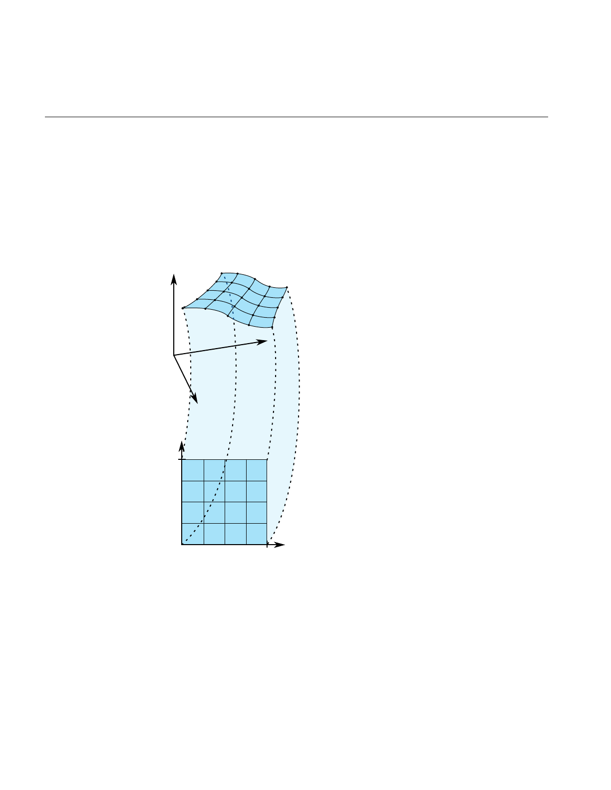
220
Chapter 11: Higher-Order Geometric Primitives and Discrete Meshes
Mathematical Description of a Parametric Surface
To locate a point on a parametric surface, you need two parameters, which in OpenGL
Optimizer are referred to as u and v. The set of u’s and v’s that describe the surface are
known as the parameter space, or coordinate system, of the surface (see Figure 11-8).
More precisely, the coordinates of the points in space that define a parametric surface are
described by a set of three functions of two parameters: ( x(u,v), y(u,v), z(u,v) ).
Figure 11-8 Parametric Surface: Unit-Square Coordinate System
Probably the best known example of a parametric surface is a sphere or a globe. On a
globe you can locate points with two parameters: latitude and longitude. The rectangular
grid of latitude and longitudes is the coordinate system that describes points on the
globe.
u
v
0.0 1.0
1.0
y
x
z

Parametric Surfaces
221
Defining Edges of a Parametric Surface: Trim Loops and Curves
Defining the extent of a parametric curve is not difficult: just pick an interval. But for
accurate trimming of a parametric surface, you need more complex tools. You are likely
to need edges for the surface other than those defined by the limits of the coordinate
system. For example, to define a pipe elbow, you might join two cylinders by a piece cut
from a torus. You are also likely to need to define holes in a surface, for example, to define
a T-joint intersection of pipes.
OpenGL Optimizer allows you to maintain curves to define the edges of a surface. These
curves are opCurve2d objects defined in the u-v plane that are “lifted” to the surface by
the parameterization. The main use of these curves is to eliminate a portion of the surface
on one side of the curve. The name of a curve in the coordinate system that is used to
define (possibly a piece of) such a surface edge is a trim curve. One or more trim curves
that are joined form a sequence called a trim loop. To be of use, trim curves should form
a closed loop or reach the edges of the coordinate system for the surface.
Which side of a trim loop is kept? The side on the left as you look down on the u-v plane
while a point moves along the curve in the direction of increasing t; you can hold on to
the surface with your left hand as you go along the trim loop. Thus a clockwise loop
removes a hole; a counterclockwise loop keeps the enclosed region and eliminates
everything outside. Do not create a trim loop that crosses itself like a figure eight.
Figure 11-9 illustrates trim loops and their effect on a surface.
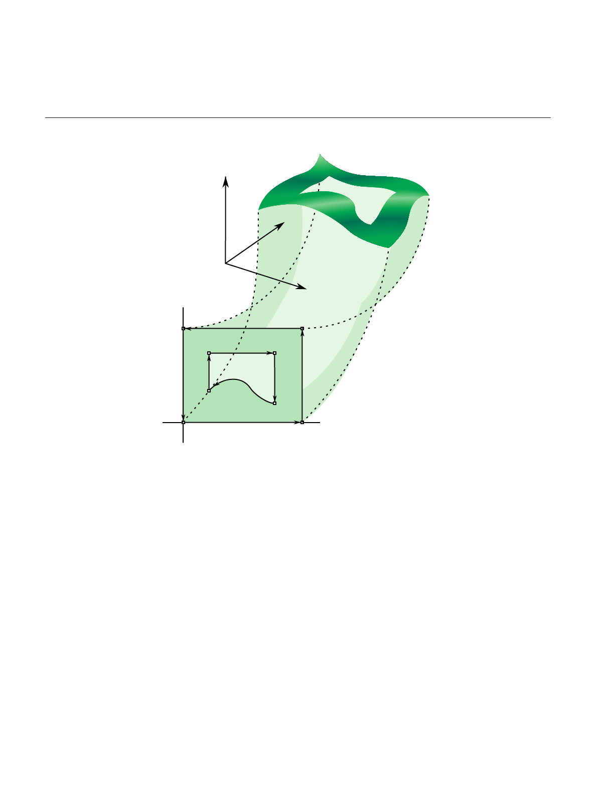
222
Chapter 11: Higher-Order Geometric Primitives and Discrete Meshes
Figure 11-9 Trim Loops and Trimmed Surface: Both Trim Loops Made of Four Trim Curves
u
Trim1
Trim2
Trim3
v
z
x
y

Parametric Surfaces
223
Adjacency Information: opEdge
An opEdge holds information about a surface’s adjacency. Each opEdge identifies an
opBoundary, which the class opTopo uses to keep track of connectivity of surfaces, and
continuous and discrete versions of the trim curve associated with the boundary. The
members of an opEdge are set by the toplogy building tools; the methods of opEdge
access the members. Topology building and the classes opTopo and opBoundary are
discussed further in Chapter 12, “Creating and Maintaining Surface Topology.”
The information held in opEdge allows tessellators to determine if a set of vertices has
already been developed for points shared with other surfaces. Also, you can find other
surfaces that have the same edge or trim-curve endpoint as that defined by a given trim
curve.
The set*() methods are mainly used when reading surface data from a file and creating
OpenGL Optimizer data structures.
Class Declaration for opEdge
The following are the main methods in the class:
class opEdge
{
public:
// Creating and destroying
opEdge();
~opEdge();
opCurve2d *getContCurve();
void setContCurve(opCurve2d *c);
opDisCurve2d *getDisCurve();
void setDisCurve( opDisCurve2d *d);
int getBoundary();
void setBoundaryDir( int dir );
int getBoundaryDir();

224
Chapter 11: Higher-Order Geometric Primitives and Discrete Meshes
Base Class for Parametric Surfaces: opParaSurface
opParaSurface is the base class for parametric surfaces in OpenGL Optimizer. As for the
base classes opCurve2d and opCurve3d,opParaSurfaceincludes a pure virtual function
to evaluate points on the surface and default evaluator functions that calculate
derivatives using finite central differences. The surface normal at a point is the cross
product of the partial derivatives.
As for parametric curves, whose extent is defined by the interval of values for t, the
extent of an opParaSurface is, initially, defined by all the points in its parameter space.
Class Declaration for opParaSurface
The following are the main methods in the class:
class opParaSurface : public opRep
{
public:
// Creating and destroying
opParaSurface();
opParaSurface( opReal _beginU = 0, opReal _endU = 1,
opReal _beginV = 0, opReal _endV = 1,
int _topoId = 0, int _solid_id = -1 );
~opParaSurface();
// Accessor functions
void setBeginU( opReal u );
void setEndU( opReal u );
void setBeginV( opReal v );
void setEndV( opReal v );
void setSolidId( int _solidId)
opReal getBeginU()
opReal getEndU()
opReal getBeginV()
opReal getEndV()
int getTrimLoopCount();
opLoop getTrimLoopClosed( int loopNum );
int getTrimCurveCount( int loopNum );
opEdge* getTrimCurve( int loopNum, int curveNum );
int getTopoId();

Parametric Surfaces
225
int getSolidId();
int getSurfaceId();
void setHandednessHint( bool _clockWise )
bool getHandednessHint()
void insertTrimCurve( int loopNum, opCurve2d *c, opDisCurve2d *d );
// Explicit add a trim curve to a trim loop
void addTrimCurve(int loopNum, opCurve2d *c, opDisCurve2d *d );
void setTrimLoopClosed( int loopNum, opLoop closed );
// Surface evaluators
virtual void evalPt( opReal u, opReal v, opVec3 &pnt ) = 0;
virtual void evalDu( opReal u, opReal v, opVec3 &Du );
virtual void evalDv( opReal u, opReal v, opVec3 &Dv );
virtual void evalDuu( opReal u, opReal v, opVec3 &Duu );
virtual void evalDvv( opReal u, opReal v, opVec3 &Dvv );
virtual void evalDuv( opReal u, opReal v, opVec3 &Duv );
virtual void evalNorm( opReal u, opReal v, opVec3 &norm );
// Directional derivative evaluators
virtual void evalD( opReal u, opReal v, opReal theta, opVec3 &D );
virtual void evalDD( opReal u, opReal v, opReal theta, opVec3 &DD );
virtual void eval( opReal u, opReal v,
opVec3 &p, // The point
opVec3 &Du, // The derivative in the u direction
opVec3 &Dv, // The derivative in the v direction
opVec3 &Duu, // The 2nd derivative in the u direction
opVec3 &Dvv, // The 2nd derivative in the v direction
opVec3 &Duv, // The cross derivative
opReal &s, // Texture coordinates
opReal &t );
};

226
Chapter 11: Higher-Order Geometric Primitives and Discrete Meshes
Main Features of the Methods in opParaSurface
addTrimCurve(j, curve, discurve)
Is a quick function for building a trim loop that assumes you know the
order of trim curves. It adds curveto the end of the list of continuous trim
curves for the jth trim loop, and adds discurve to the list of discrete trim
curves.
For example, you could build the trim loops in Figure 11-9 by starting
with one segment and successively adding segments. If the beginning
of curve does not match the end of the previously added curve, the list
of trim curves does not make sense; use insertTrimCurve(), which finds
the right place for the curve by assuming topological consistency.
eval() Returns all the evaluator functions. The last two arguments of eval() are
the same as the input coordinates u and v.
evalDu(),evalDv(),evalDuu(),evalDvv(), and evalDuv()
Are evaluator functions that use central differences to calculate the first
and second derivatives, identified by the lowercase u and vin the
function names, at a point on the surface.
evalD() and evalDD()
Calculate the first and second directional derivatives in the direction
given by an angle theta from the u axis in the parameter space.
evalNorm() Calculates the unit normal to the surface.
evalPt() Is a pure virtual function that you define to specify a surface.
opParaSurface()Contructs a parametric surface. You can specify to which topology the
surface belongs, and to which surface. See “Summary of Scene Graph
Topology: opTopo” on page 270.
insertTrimCurve(j, curve, discurve)
Is a slower function than addTrimCurve() for building a trim loop that
attempts to guarantee all curves form a sensible trim loop sequence. It
compares the ends of curve with the ends of the trim curves that are
already in the jth trim loop and inserts curve at the appropriate point in
the list. Similarly, addTrimCurve() inserts the discrete curve discurve. If
insertTrimCurve() cannot find an endpoint match, it adds curve to the
end of the list of trim curves. If you are building a trim loop by inserting
trim curves end to end, then addTrimCurve() gives the same result but
more quickly.

Parametric Surfaces
227
setBeginU(),setBeginV(), etc.
Set and get the start and ending values for the coordinate space of the
surface. The coordinate space is a rectangle in the u-v plane. The default
is the unit square; u and v both lie in the interval (0,1).
getTrimLoopCount()
Returns the number of trim loops for the opParaSurface.
getTrimLoopClosed() and setTrimLoopClosed()
Get and set the flag indicating whether a given trim loop is closed.
OpenGL Optimizer determines this for you, so use
setTrimLoopClosed() with caution; you could get a meaningless result.
getTrimCurveCount()
Returns the number of trim curves in the specified trim loop.
getTrimCurve(i,j)
Returns the opEdge for the trim curve with index iin the trim loop with
index j.
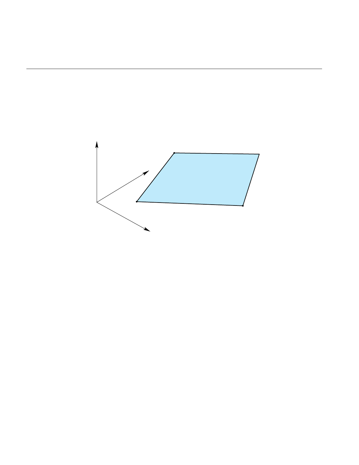
228
Chapter 11: Higher-Order Geometric Primitives and Discrete Meshes
opPlane
The simplest parametric surface is a plane. The class opPlane defines a plane by two
parameter intervals and three points that define the two coordinate directions.
Figure 11-10 illustrates the parameterization of an opPlane.
Figure 11-10 Plane Parameterization
y
x
z
(x1,y1,z1)
u=u1
v=v1
(x3,y3,z3)
u=u1
v=v3
(x2,y2,z2)
u=u2
v=v1

Parametric Surfaces
229
Class Declaration for opPlane
The following are the main methods in the class:
class opPlane : public opParaSurface
{
public:
// Creating and destroying
opPlane();
opPlane( opReal x1, opReal y1, opReal z1, opReal u1, opReal v1,
opReal x2, opReal y2, opReal z2, opReal u2,
opReal x3, opReal y3, opReal z3, opReal v3 );
virtual ~opPlane();
// Accessor functions
void setPoint1( opReal x1, opReal y1, opReal z1, opReal u1, opReal v1);
void setPoint2( opReal x2, opReal y2, opReal z2, opReal u2 );
void setPoint3( opReal x3, opReal y3, opReal z3, opReal v3 );
void getPoint1( opReal *x1, opReal *y1, opReal *z1,
opReal *u1, opReal *v1 );
void getPoint2( opReal *x2, opReal *y2, opReal *z2, opReal *u2 );
void getPoint3( opReal *x3, opReal *y3, opReal *z3, opReal *v3 );
// Evaluators
void evalPt( opReal u, opReal v, opVec3 &pnt );
void evalDu( opReal u, opReal v, opVec3 &Du );
void evalDv( opReal u, opReal v, opVec3 &Dv );
void evalNorm( opReal u, opReal v, opVec3 &norm );

230
Chapter 11: Higher-Order Geometric Primitives and Discrete Meshes
Main Features of the Methods in opPlane
opPlane() When you construct the class, you can specify the plane with three
points and two parameter intervals or you can use the setPoint*()
methods. Those parameters have the following meanings:
• the point (x1,y1,z1) and its parameter values, (u1,v1)
• the point (x2,y2,z2), which defines the u direction,
(x2-x1,y2-y1,z2-z1), and its parameter values (u2,v1)
• the point (x3,y3,z3), which defines the vdirection,
(x3-x1,y3-y1,z3-z1) and its parameter values (u1,v3).
setPoint*() and getPoint*()
Set and get each of the points that define the plane and their
corresponding parameter values (see opPlane()).
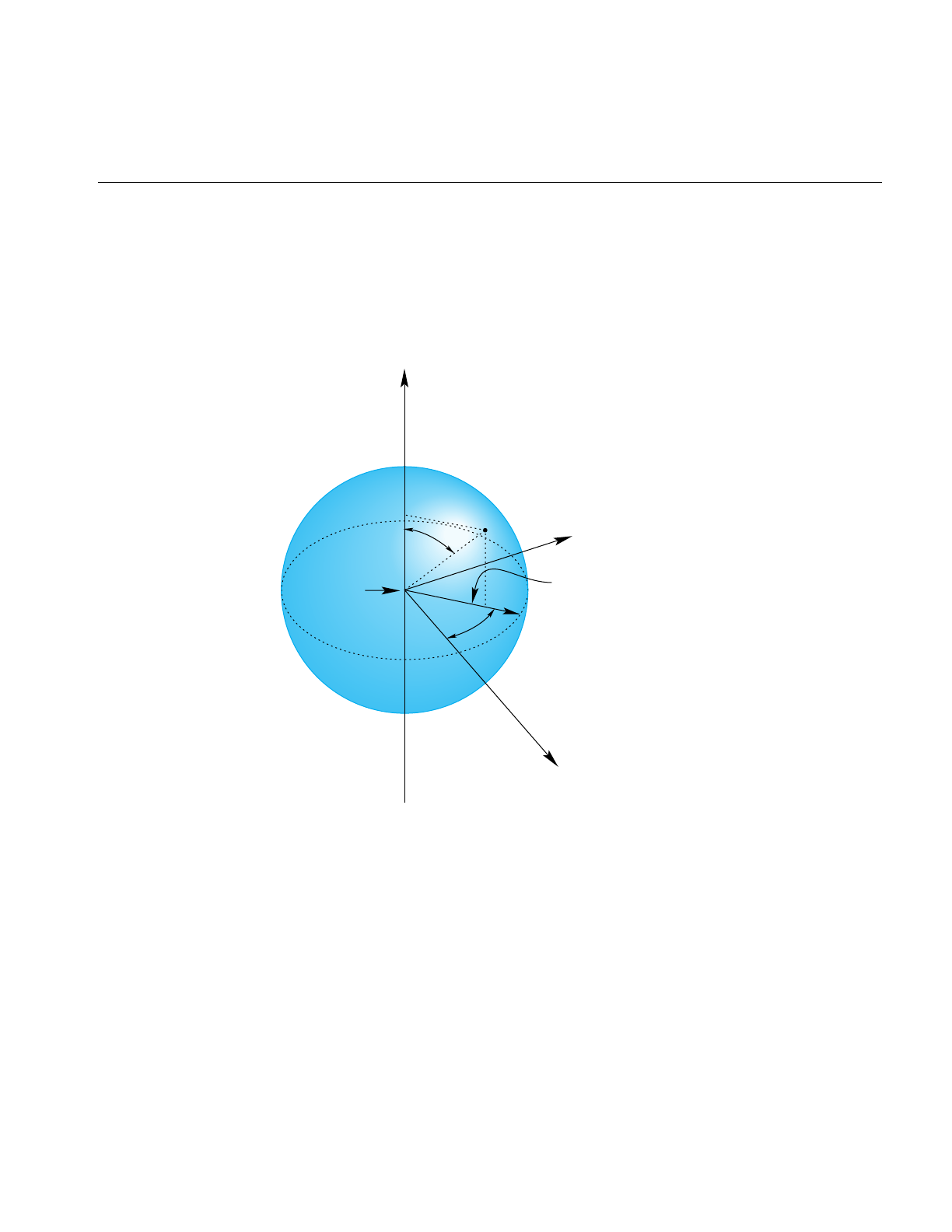
Parametric Surfaces
231
opSphere
The surface of the sphere is parameterized by angles, in radians, for latitude and
longitude; vcorresponds to longitude, uto latitude. Figure 11-11 illustrates the
parameterization of an opSphere.
Figure 11-11 Sphere Parameterization
pnt
v
u
Origin
y
x
z
Radius

232
Chapter 11: Higher-Order Geometric Primitives and Discrete Meshes
Class Declaration for opSphere
The following are the main methods in the class:
class opSphere : public opParaSurface
{
public:
// Creating and destroying
opSphere( );
opSphere( opReal radius );
~opSphere( );
// Accessor functions
void setRadius( opReal radiusVal )
opReal getRadius( )
// Evaluators
void evalPt( opReal u, opReal v, opVec3 &pnt );
void evalNorm( opReal u, opReal v, opVec3 &norm );
Main Features of the Methods in opSphere
The constructor defines a sphere centered on the origin with the specified radius. The
default radius is 1. The evaluator functions do not use finite-difference calculations for
derivatives.

Parametric Surfaces
233
Typical Instantance of a Trimmed Parametric Surface: an opSphere
An instance of an opSphere of radius three in repTest appears in the following lines of
code:
opSphere *sphere = new opSphere( 3 );
// under certain conditions, a trim curve is added that keeps only the
// portion of the surface above a circle
if ( nVersions <= 0 )
{
opCircle2d *trimCircle2d =
new opCircle2d( 1.0, new opVec2(M_PI/2.0,M_PI) );
sphere->addTrimCurve( 0, trimCircle2d );
}
setUpShape( sphere, OP_XDIST*numObject++, Y, OP_VIEWDIST );
setUpShape() locates the sphere in the scene, tessellates it, and places it in the scene
graph (see src/sample/repTest/repTest.cxx). Creating an instance of any opRep is basically
the same, as subsequent examples in the discussions of other opReps will show.
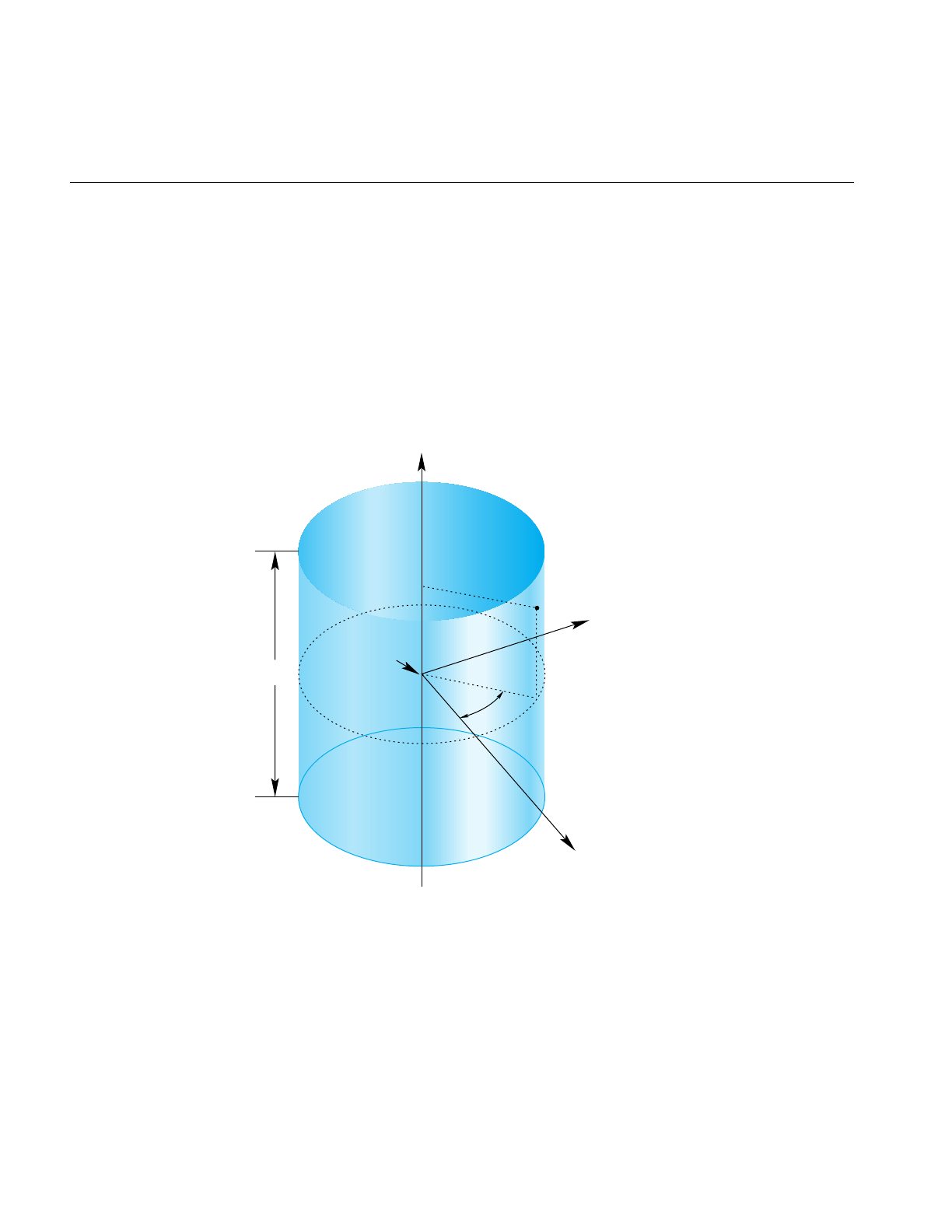
234
Chapter 11: Higher-Order Geometric Primitives and Discrete Meshes
opCylinder
This class provides functions to describe a cylinder.
A cylinder can be defined geometrically as the surface in space that is swept by moving
a circle along an axis that is perpendicular to the plane of the circle and passes through
the center of the circle.
The parametrization of an opCylinder is as follows: urepresents the position on the circle
and that vrepresents the position along the axis.
Figure 11-12 Cylinder Parameterization
y
x
z
pnt
v
u
Radius
Origin
Height

Parametric Surfaces
235
Class Declaration for opCylinder
The following are the main methods in the class:
class opCylinder : public opParaSurface
{
public:
// Creating and destroying
opCylinder( void );
opCylinder( opReal radius, opReal height );
~opCylinder();
// Accessor functions
void setRadius( opReal radiusVal ) ;
void setHeight( opReal heightVal );
opReal getRadius( )
opReal getHeight( )
// Evaluators
void evalPt( opReal u, opReal v, opVec3 &pnt );
void evalNorm( opReal u, opReal v, opVec3 &norm );
};
Main Features of the Methods in opCylinder
opCylinder( radius,height ) constructs a cylinder with the specified height and radius.
The default orientation is that the zaxis is the cylinder’s axis and the cylinder is centered
on the origin, extending in the positive and negative z directions for one-half the height.
For the default orientation, u measures the angle from the x-zplane in a counterclockwise
direction as you look down on the x-y plane and v measures the distance along the z-axis.
The default radius is 1 and the default height is 2.
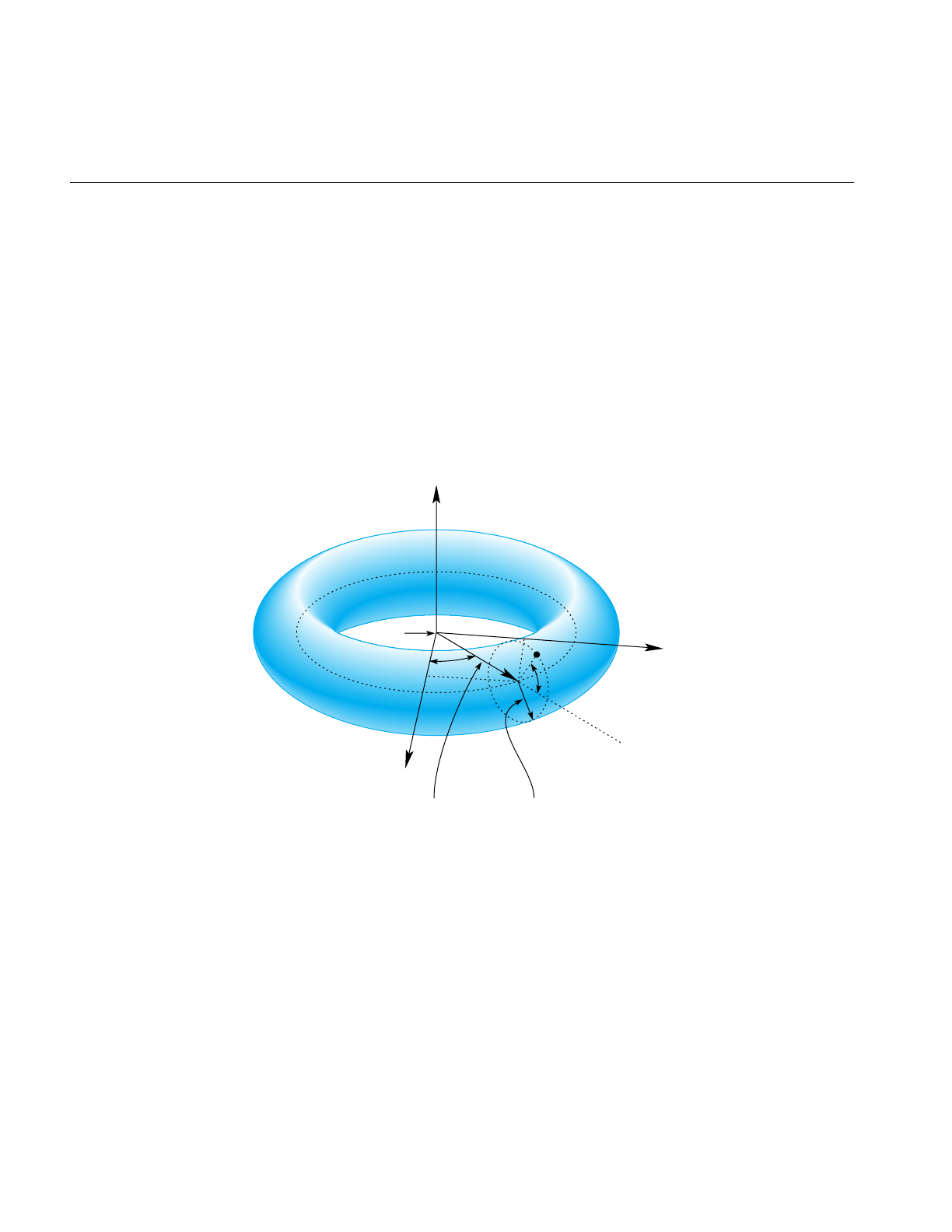
236
Chapter 11: Higher-Order Geometric Primitives and Discrete Meshes
opTorus
This class provides functions to describe a torus. Figure 11-13 illustrates a torus, and how
it is parameterized in opTorus.
A torus can be defined geometrically as the surface in space that is swept by moving a
circle, the minor circle, through space such that its center lies on a second circle, the major
circle, and the planes of the two circles are always perpendicular to each other, with the
plane of the minor circle aligned along radii of the major circle. The parametrization of
the surface is that urepresents a position on the major circle and vrepresents a position
on the minor circle.
Figure 11-13 Torus Parameterization
Major radius Minor radius
Origin
uv
y
x
z
pnt

Parametric Surfaces
237
Class Declaration for opTorus
The following are the main methods in the class:
class opTorus : public opParaSurface
{
public:
// Creating and destroying
opTorus( );
opTorus( opReal majorRadius, opReal minorRadius );
~opTorus();
// Accessor functions
void setMajorRadius( opReal majorRadiusVal )
void setMinorRadius( opReal minorRadiusVal )
opReal getMajorRadius( )
opReal getMinorRadius( )
// Evaluators
virtual void evalPt( opReal u, opReal v, opVec3 &pnt );
virtual void evalNorm( opReal u, opReal v, opVec3 &norm );
Main Features of the Methods in opTorus
The constructor opTorus( majorRadius,minorRadius ) defines a torus with the specified
radii such that the major circle is in the x-y plane and the minor circle is initially in the x-z
plane. The default value for the major radius is 1; the default for the minor radius is 0.1.
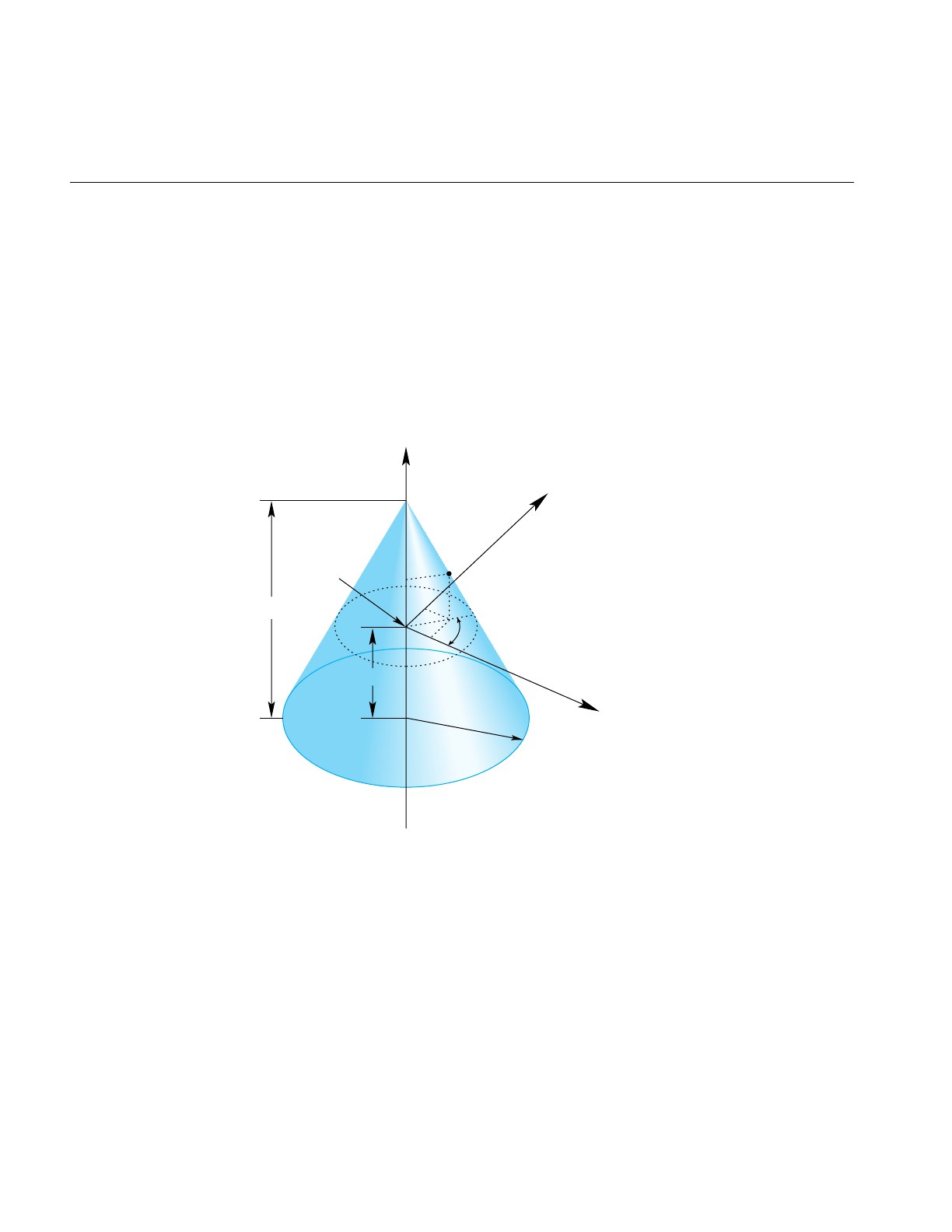
238
Chapter 11: Higher-Order Geometric Primitives and Discrete Meshes
opCone
You can define a cone geometrically by sweeping a circle along an axis in a way similar
to the way a cylinder is defined; however, as the circle is swept along the axis, the radius
changes linearly with distance.
The parameterization of a point on an opCone is that u measures the angle, in radians,
of the point on the circle, and that v measures the distance along the axis from the origin.
To truncate a cone, yielding a frustum, adjust the value for v.
Figure 11-14 Cone Parameterization
y
x
z
pnt
v
u
Radius
Origin
Height
Half-height

Parametric Surfaces
239
Class Declaration for opCone
The following are the main methods in the class:
class opCone : public opParaSurface
{
public:
// Creating and destroying
opCone( void );
opCone( opReal radius, opReal height );
~opCone();
// Accessor functions
void setRadius( opReal radius ) ;
void setHeight( opReal height );
opReal getRadius( )
opReal getHeight( )
// Evaluators
void evalPt( opReal u, opReal v, opVec3 &pnt );
void evalNorm( opReal u, opReal v, opVec3 &norm );
Main Features of the Methods in opCone
The constructor opCone( radius,height ) creates a parametric cone with the specified
height and a circular base with the specified radius. The default orientation is that the
base of the cone is parallel to the x-y plane and centered on the zaxis and the apex of the
cone is on the positive z-axis. The cone extends from the origin in the positive and
negativezdirections for one half the height. The default for the radius of the base is 1 and
the default height is 2.

240
Chapter 11: Higher-Order Geometric Primitives and Discrete Meshes
Swept Surfaces
The class opSweptSurface provides functions to describe a general swept surface. Three
examples of swept surfaces have been presented: a cylinder, a torus, and a cone. In the
first two cases a simple cross-section, a circle of constant radius, was swept along a path.
For a cone, the radius of the circle varied according to a simple profile.
To describe a swept surface, you specify a path, a cross section, and a coordinate frame in
which the graph of the cross section is drawn at each point on the path. The
parameterization of the surface is that u denotes the position along the path and v
denotes the position on the cross-section curve. You can also specify a profile, which
adjusts the size of the cross-section curve. Thus, for example, with a simple profile
function you could generate a sphere from a straight-line path and a circular cross
section. Figure 11-15 illustrates the feature of a swept surface.
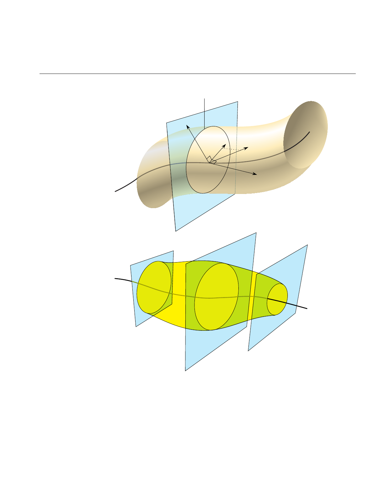
Parametric Surfaces
241
Figure 11-15 Swept Surface: Moving Reference Frame and Effect of Profile Function
P
a
t
h
C
ross sect
i
on
t
b
x
y

242
Chapter 11: Higher-Order Geometric Primitives and Discrete Meshes
Orientation of the Cross Section
Unlike the examples of the cylinder, torus, and cone, the cross-section in an
opSweptSurface generally is not necessarily perpendicular to the path. You set the
orientation of the cross-section with two additional instances of opCurve3d. For a point
on the path corresponding the parameter value t0, the vectors on these two additional
curves that have the same parameter value define the local coordinate system used to
draw the profile: one vector defines the normal to the plane of the graph, the second the
x axis for the graph, and their cross product determines the direction of the y axis for the
graph. For more details, see the discussion of the constructor below.
Class Declaration for opSweptSurface
The following are the main methods in the class:
class opSweptSurface : public opParaSurface
{
public:
// Creating and destroying
opSweptSurface( void );
opSweptSurface( opCurve3d *crossSection,
opCurve3d *_path,
opCurve3d *_t,
opCurve3d *_b,
opScalar *_profile );
~opSweptSurface( );
// Accessor functions
void setCrossSection( opCurve3d *_crossSection );
void setPath( opCurve3d *_path );
void setT( opCurve3d *_tng );
void setB( opCurve3d *_b );
void setProf( opScalar *_profile );
opCurve3d *getCrossSection() ;
opCurve3d *getPath() ;
opCurve3d *getT() ;
opCurve3d *getB() ;
opScalar *getProf();
// Evaluators
void evalPt( opReal u, opReal v, opVec3 &pnt );
};

Parametric Surfaces
243
Main Features of the Methods in opSweptSurface
opSweptSurface( crossSection,path, t, b, profile )
Defines a swept surface with the given path, cross section, and profile.
The arguments t and b are vector-valued functions of the path’s
parameter. They define the orientation of the profile at each point on the
path.
The orientation at a particular point on the curve is determined by
rendering the graph of crossSection in the coordinate plane
perpendicular to t, which locally defines the z axis of an x-y-z
coordinate system. The x axis is defined by the projection of b onto the
plane, and the y axis is that which forms a right-hand coordinate
system with the other two axes. The cross section is plotted in the x-y
plane.
If you specify a NULL value for profile,crossSection does not vary along
path.
evalPt( u,v,pnt )Calculates the point on the surface, pnt, as the vector sum of (a) the point
on the path corresponding to the value u and (b) the point on the cross
section corresponding to the value v. The vector locating the point on the
cross section is scaled by the value at uof the profile function, if profile is
not NULL.

244
Chapter 11: Higher-Order Geometric Primitives and Discrete Meshes
opFrenetSweptSurface
As a convenience, the class opFrenetSweptSurface allows you to use the Frenet frame of
the path to define the orientation vectors in a swept surface. The Frenet frame is defined
by the three unit vectors derived from the tangent, the principal normal, and their cross
product. This set of vectors facilitates orienting the cross section perpendicularly to the
path at every point.
Note: The path for an opFrenetSweptSurface must be at least a cubic to allow for the
principal normal calculation, which requires a second derivative.
Class Declaration for opFrenetSweptSurface
The following are the main methods in the class:
class opFrenetSweptSurface : public opSweptSurface
{
public:
// Accessor functions
opFrenetSweptSurface( void );
opFrenetSweptSurface( opCurve3d *crossSection,
opCurve3d *path,
opScalar *profile );
~opFrenetSweptSurface( );
// Accessor functions
void set( opCurve3d *crossSection,
opCurve3d *path,
opScalar *profile );
};
Main Features of the Methods in opFrenetSweptSurface
The arguments of the constructor for opFrenetSweptSurface are the same as for
opSweptSurface and have the same effects, except for the orientation vectors, which are
set to be the tangent and principal normal to path, and so do not appear as arguments.
Use the inherited method evalPt() to locate points on the surface.

Parametric Surfaces
245
Making a Modulated Torus With opFrenetSweptSurface
The following code uses an opFrenetSweptSurface to define a torus whose minor radius
varies with position on the ring. Other instances of opFrenetSweptSurface appear in
repTest.
// Scalar curve used by the swept surface primitive
static opReal profile( opReal t )
{
return 0.5*cos(t*5.0) + 1.25;
};
opCircle3d *cross =
new opCircle3d( 0.75, new opVec3( 0.0, 0.0, 0.0) );
opCircle3d *path =
new opCircle3d( 1.75, new opVec3( 0.0, 0.0, 0.0) );
opFrenetSweptSurface *fswept =
new opFrenetSweptSurface( cross, path, profile );
fswept->setHandednessHint( true );
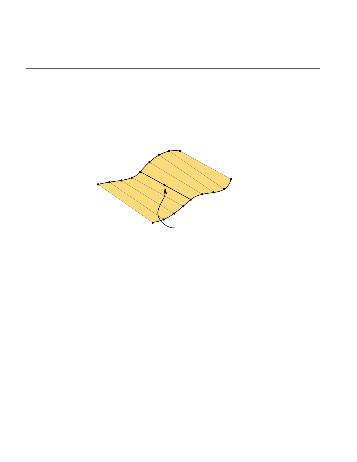
246
Chapter 11: Higher-Order Geometric Primitives and Discrete Meshes
Ruled Surfaces
A ruled surface is generated from two curves in space, both parameterized by the same
variable, u. A particular value of uspecifies a point on both curves. A ruled surface is
defined by connecting the two points with a straight line parameterized by v. The
parameterization of the resulting surface is always the unit square in the u-v plane,
regardless of the parameterizations of the original curves.
Figure 11-16 Ruled Surface Parameterization
A bilinear interpolation of four points is perhaps the simplest example of a ruled surface,
one for which the “curves” that define the surface are in fact straight lines. Thus, you
connect two pairs of points in space with lines and then develop the ruled surface. For a
bilinear interpolation, the parameterization by u and v is such that, if one of them is held
constant, a point “moves” along the connecting straight line at a uniform speed as the
other parameter is varied.
c2(u)
c1(u)
(1-v)c1(u) + v c2(u)

Parametric Surfaces
247
Class Declaration for opRuled
The following are the main methods in the class:
class opRuled : public opParaSurface
{
public:
// Creating and destroying
opRuled();
opRuled( opCurve3d *c1, opCurve3d *c2 );
~opRuled();
// Accessor functions
void setCurve1( opCurve3d *_c1 );
void setCurve2( opCurve3d *_c2 );
opCurve3d *getCurve1( )
opCurve3d *getCurve2( )
// Evaluators
void evalPt( opReal u, opReal v, opVec3 &pnt );
The constructor opRuled(c1,c2)creates an instance of a ruled surface defined by the two
curves c1 and c2.

248
Chapter 11: Higher-Order Geometric Primitives and Discrete Meshes
Coons Patches
A Coons patch is arguably the simplest surface you can define from four curves whose
endpoints match and form a closed loop. Think of the four curves as defining the four
sides of the patch, with one pair on opposite sides of the patch defining the top and
bottom curves and the other pair defining the left and right curves (see Figure 11-17). The
top and bottom curves are parameterized by u, and the left and right curves by v. Thus,
u is the “horizontal” coordinate and v the “vertical” coordinate.
The patch is made by
1. Adding the points on the ruled surface defined by the top and bottom curves to the
points on the ruled surface defined by the left and right curves.
2. Subtracting the bilinear interpolation of the four corner points.
Figure 11-17 illustrates the construction. To understand the result, notice that, after you
add the two ruled surfaces, each side of the boundary of the resulting surface is the sum
of the original bounding curve and the straight line connecting the bounding curve’s
endpoints. The straight line was introduced by the construction of the ruled surface that
did not include the boundary curve. Subtracting the bilinear interpolation eliminates the
straight-line components of the sum, leaving just the original four curves as the
boundary of the resulting surface.
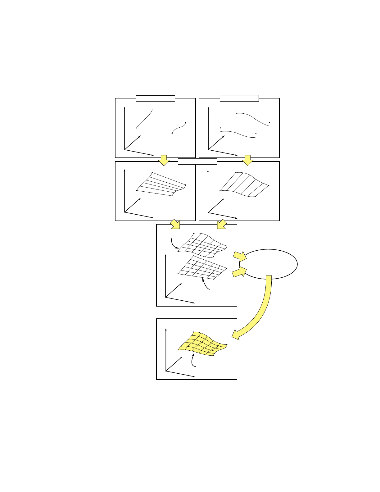
Parametric Surfaces
249
Figure 11-17 Coons Patch Construction
z3
z2
z4
z1
z3
z2
z4
z1
z3
z2
z4
z1
y
x
z
z3
z2
z4
z1
y
x
z
y
x
z
z3
z2
z4
z1
y
x
z
y
x
z
2z3
2z2
2z4
2z1
z3
z2
z4
z1
z1
y
x
z
Left & right curves Top & bottom curves
Ruled surfaces
Sum
Bilinear
interpolation
Subtract a bilinear
interpolation from the sum
of the ruled surfaces
Coons patch,bounded
by left, right, top &
bottom curves

250
Chapter 11: Higher-Order Geometric Primitives and Discrete Meshes
Class Declaration for opCoons
The following are the main methods in the class:
class opCoons : public opParaSurface
{
public:
opCoons( );
opCoons( opCurve3d *right, opCurve3d *left,
opCurve3d *bottom, opCurve3d *top );
~opCoons( );
// Accessor functions
void setRight( opCurve3d *right );
void setLeft( opCurve3d *left );
void setBottom( opCurve3d *bottom );
void setTop( opCurve3d *top );
opCurve3d* getTop() ;
opCurve3d* getBottom() ;
opCurve3d* getLeft() ;
opCurve3d* getRight() ;
// Surface point evaluator
void evalPt( opReal u, opReal v, opVec3 &pnt );
};
The constructor opCoons( right,left,bottom,top )creates an instance of a Coons patch
defined by the four curves right,left,bottom, and top. As mentioned above, the top and
bottom curves are parameterized by u and the left and right curves are parameterized by
v. For more details, see the book Curves and Surface for Computer Aided Geometric Design
listed in “Recommended Reference Materials” on page xxxi.

Parametric Surfaces
251
NURBS Surfaces
Just as a NURBS curve is made of Bezier curves, a NURBS surface is made of Bezier
surfaces. The set of control parameters is essentially the same for the curves and surfaces:
a set of knots, a control hull, and a set of weights. However, for a NURBS surface, the
knots form a grid in the coordinate system of the surface; that is, in the u-v plane and the
control hull is a grid of points in space that loosely defines the surface.
Understanding a Bezier surface helps you understand and use a NURBS surface, just as
understanding a Bezier curve helps you use a NURBS curve. A Bezier surface is defined
essentially as the surface formed by sweeping a Bezier cross section curve through space,
along a path defined by a Bezier curve. But, unlike an opSweptSurface, the shape of the
cross-section can be changed. More accurately, you define a Bezier surface by starting
with a Bezier curve in space: the cross section parameterized by u. Now define a family
of Bezier curves, a set of paths all of which are parameterized by v, that start at the control
points of the initial cross section. For each value of v, the set of control points defines a
Bezier curve. As v changes, the cross-sectional curve “moves” through space, changing
shape and defining a Bezier surface. A more rigorous discussion appears in the book
Curves and Surface for Computer Aided Geometric Design, listed in the section
“Recommended Reference Materials” on page xxxi.
A NURBS surface join Bezier surfaces in a smooth way, simlar to NURBS curves joining
Bezier curves. The class opNurbSurface provides functions to describe a NURBS
surface.

252
Chapter 11: Higher-Order Geometric Primitives and Discrete Meshes
Class Declaration for opNurbSurface
The following are the main methods in the class:
class opNurbSurface : public opParaSurface
{
public:
// Creating and destroying
opNurbSurface( void );
~opNurbSurface( void );
// Accessor functions
void setControlHull( int iu, int iv, opVec3 &p );
void setControlHull( int iu, int iv, opVec4 &p );
void setWeight( int iu, int iv, opReal w );
void setUknot( int iu, opReal u );
void setVknot( int iv, opReal v );
void setControlHullUSize( int s );
void setControlHullVSize( int s );
// Get the same parameters
opVec3& getControlHull( int iu, int iv) ;
int getControlHullUSize( void );
int getControlHullVSize( void );
opReal getWeight( int iu, int iv)
opReal& getUknot( int iu);
opReal& getVknot( int iv);
int getUknotCount( void );
int getVknotCount( void );
int getUorder( void ) ;
int getVorder( void ) ;
// Evaluator
virtual void evalPt( opReal u, opReal v, opVec3 &pnt );
virtual void evalDu( opReal u, opReal v, opVec3 &Du );
virtual void evalDv( opReal u, opReal v, opVec3 &Du );
virtual void evalNorm( opReal u, opReal v, opVec3 &norm );
// Memory footprint
int getMemSize();
};

Parametric Surfaces
253
Main Features of the Methods in opNurbSurface
The member functions are essentially the same as those for opNurbCurve3d (see
“NURBS Curves in Space” on page 216), with the generalization that the hull is a grid of
opVec3s indexed by i and j, the set of knots is defined by points on the u and vaxes, and
there are B-spline basis functions (of possibly differing orders) associated with each
coordinate direction.
Note: opNurbSurface redefines the virtual evaluators inherited from opParaSurface for
tangent and normal vectors; the methods use the the NURBS equation rather than finite,
central differences.
Indexing Knot Points and the Control Hull
The indexing of knot points in the coordinate space and control hull points in
three-dimensional space is illustrated in Figure 11-18. The indexing works as for
gluNurbsSurface, that is, as follows:
•iu indexes knots on the u axis. The correspondence is established by setUknot().
•iv indexes knots on the v axis.The correspondence is established by setVknot().
• Each (iu,iv) thus indexes a knot point in the u-v plane.
• Each (iu,iv) also indexes a point on the control hull in three-dimensional space. The
correspondence is established by setControlHull().
• Thus, setUknot(),setVknot(), and setControlHull() establish a correspondence
between an index pair (iu,iv) a knot point (uiu viv), and a point on the control hull in
three-dimensional space.
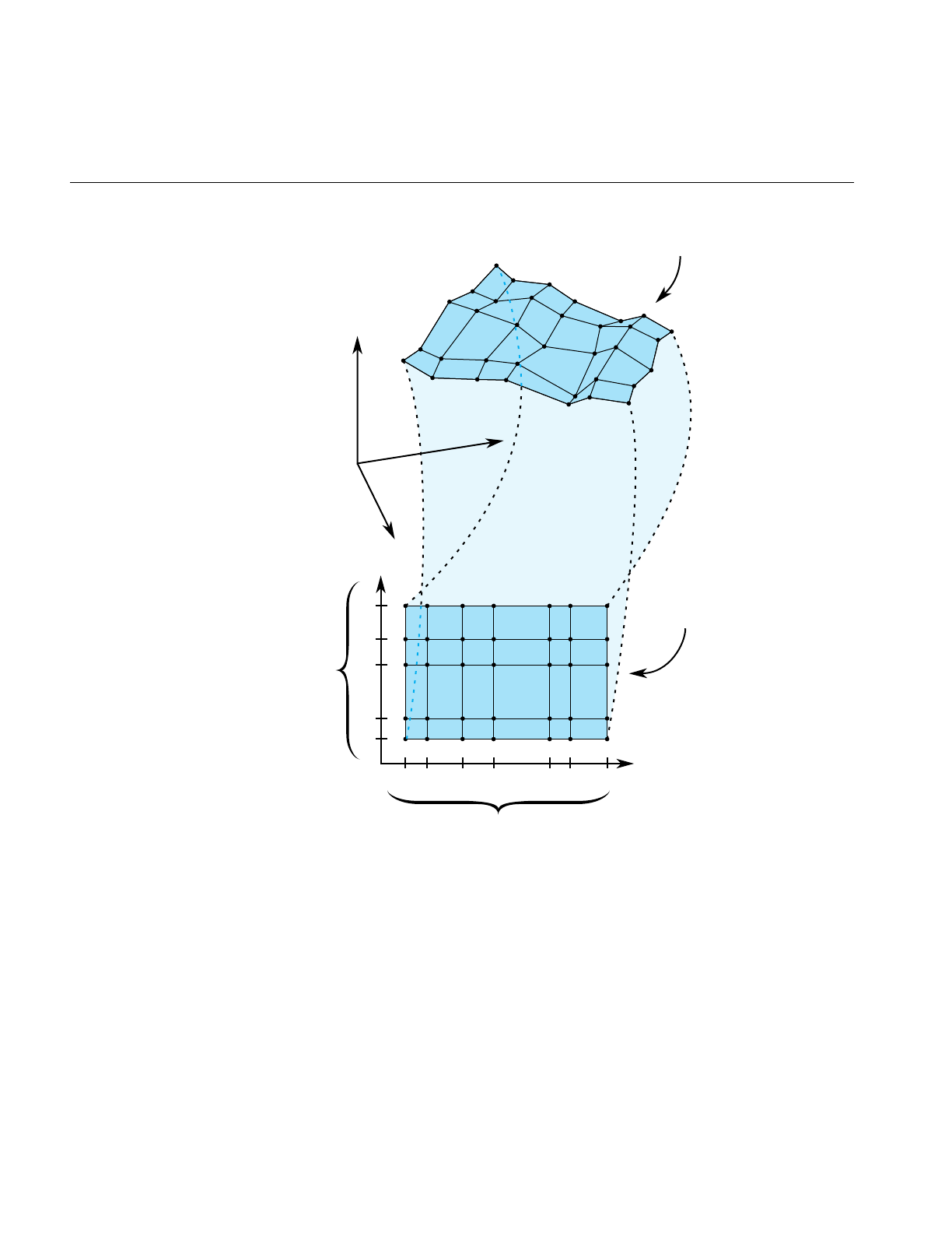
254
Chapter 11: Higher-Order Geometric Primitives and Discrete Meshes
Figure 11-18 Nurb Surface Control Hull Parameterization
u
v
u
1
u
2
u
3
u
4
u
0
u
5
u
6
(0,0)
(3,2)
(3,2)
(0,0)
v
4
v
3
v
2
v
1
v
0
y
x
z
iv
= 0,1,2,3...
iu
= 0,1,2,3...
setControlHull (
iu, iv, p
)
setUknot (
iu, u
)
setVknot (
iv, v
)

Parametric Surfaces
255
The Equation Used to Calculate a NURBS Surface
The indexing is determined by the following equation that OpenGL Optimizer uses to
calculate a NURBS surface (the index i corresponds to iu in the API, and j corresponds to
iv):
where
• is a point on the surface
• is the ith B-spline basis polynomial of degree m
• is a control point
• is the weight for the control point
An Alternative Equation for a NURBS Surface
If you have a surface developed from the following alternative expression for a NURBS
surface,
then you must change the coordinates of the control points to get the same surface from
OpenGL Optimizer; you convert the coordinates of the control points from (x,y,z,w) to
(wx,wy,wz,w).
puv,() Bimu()Bjnv()Cij
ij,
∑
Bimu()Bjnv()Wij
ij,
∑
---------------------------------------------
=
puv,()
Bimu()
Cij
Wij
puv,() Bimu()Bjnv()WijCij
ij,
∑
Bimu()Bjnv()Wij
ij,
∑
-----------------------------------------------------
=

256
Chapter 11: Higher-Order Geometric Primitives and Discrete Meshes
Sample of a Trimmed opNurbSurface From repTest
An instance of an opNurbSurface in repTest appears in the following lines of code.
Toward the end of this example, an optional opNurbCurve2d trim curve is created.
int i, j;
opNurbSurface *nurb = new opNurbSurface;
// Control hull dimensions
#define USIZE 4
#define VSIZE 5
// Set up the control hull size because we know a priori how big
// the nurb is. The next two lines are used for space
// efficiency but are functionally unnecessary.
nurb->setControlHullUSize(USIZE);
nurb->setControlHullVSize(VSIZE);
// Make the control hull be an oscillating grid
for ( i = 0; i < VSIZE; i++ )
{
opReal y = i/(float)(VSIZE - 1) * 2*M_PI - M_PI;
for ( j = 0; j < USIZE; j++ )
{
opReal x = j/(float)(USIZE - 1) * 2*M_PI - M_PI;
opReal val = 6*pow( cos(sqrt(x*x + y*y)), 2.0);
// Make the control hull a box, j maps to u and i maps to v
nurb->setControlHull( i, j, opVec3( x, y, val));
// Add the weights
nurb->setWeight( i, j, 1.0 );
}
}
// Add the knot points
nurb->setUknot( 0, 0.0 );
nurb->setUknot( 1, 0.0 );
nurb->setUknot( 2, 0.0 );
nurb->setUknot( 3, 0.0 );
nurb->setUknot( 4, 1.0 );
nurb->setUknot( 5, 1.0 );
nurb->setUknot( 6, 1.0 );

Parametric Surfaces
257
nurb->setUknot( 7, 1.0 );
nurb->setVknot( 0, 0.0 );
nurb->setVknot( 1, 0.0 );
nurb->setVknot( 2, 0.0 );
nurb->setVknot( 3, 0.0 );
nurb->setVknot( 4, 1.0 );
nurb->setVknot( 5, 1.0 );
nurb->setVknot( 6, 1.0 );
nurb->setVknot( 7, 1.0 );
// Only trim reps in the first row
if ( nVersions <= 0 )
{
// Add a super quadric trim curve
opSuperQuadCurve2d *trimCircle0 = new opSuperQuadCurve2d( 0.25, new
opVec2(0.25, 0.50), 2.0 );
nurb->addTrimCurve( 0, trimCircle0, NULL );
// make a 4-th order nurb trim curve
opNurbCurve2d *l = new opNurbCurve2d;
l->setKnot(0,0.0);
l->setKnot(1,0.0);
l->setKnot(2,0.0);
l->setKnot(3,0.0);
l->setKnot(4,1.0);
l->setKnot(5,1.0);
l->setKnot(6,1.0);
l->setKnot(7,1.0);
l->setControlHull(0,opVec2(0.50,0.50));
l->setControlHull(1,opVec2(0.90,0.10));
l->setControlHull(2,opVec2(0.90,0.90));
l->setControlHull(3,opVec2(0.50,0.50));
nurb->addTrimCurve( 1, l, NULL );
}
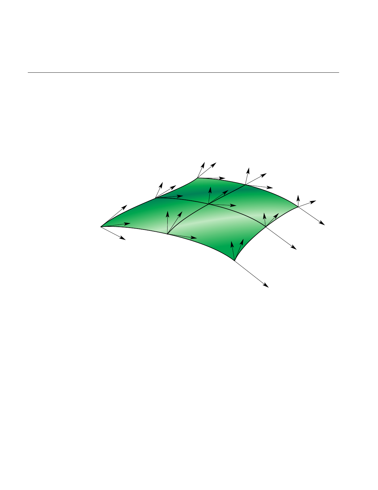
258
Chapter 11: Higher-Order Geometric Primitives and Discrete Meshes
Hermite-Spline Surfaces
Hermite-spline surfaces interpolate a grid of points; that is, they pass through the set of
specified points under the constraint that you supply the tangents at each point in the u
and vdirections and the mixed partial derivative at each point. This surface definition is
the natural generalization of Hermite-spline curves, discussed in “Hermite-Spline
Curves in the Plane” on page 202.
Figure 11-19 Hermite Spline Surface With Derivatives Specified at Knot Points
Hermite-spline surfaces are made of Hermite patches (see Figure 11-19). A bicubic
Hermite patch expands the definition of a bilinear interpolation to include specification of
first derivatives and mixed partial derivatives of the surface at each of the four corners.
The adjective “bicubic” in the name of the patches refers to the mathematical definition,
which includes products of the cubic Hermite polynomials that define a Hermite-spline
curve.
An advantage of including the derivatives to constrain the surface is that it is simple to
combine the patches into a smooth composite surface, that is, into a Hermite-spline surface.
A more formal discussion of these objects appears in the book Curves and Surface for
tv
tv
tv
tv
tu
tu
tu
tu
tuv
tv
tu
tuv
tuv
tv
tu
tuv
tv
tu
tuv
tuv
tuv
tv
tu
tuv
tv
tu
tuv

Parametric Surfaces
259
Computer Aided Geometric Design listed in the section “Recommended Reference
Materials” on page xxxi.
Class Declaration for opHsplineSurface
The following are the main methods in the class:
class opHsplineSurface : public opParaSurface
{
public:
// Creating and destroying
opHsplineSurface();
opHsplineSurface( opReal *_p,
opReal *_tu, opReal *_tv, opReal *_tuv,
opReal *_uu, opReal *_vv,
int uKnotCount, int vKnotCount );
~opHsplineSurface();
// Accessor functions
opVec3& getP( int i, int j );
opVec3& getTu( int i, int j );
opVec3& getTv( int i, int j );
opVec3& getTuv( int i, int j );
opReal getUknot( int i );
opReal getVknot( int j );
int getUknotCount();
int getVknotCount();
opReal getCylinderical();
void setAll( opReal *p,
opReal *tu,
opReal *tv,
opReal *tuv,
opReal *uu,
opReal *vv,
int uKnotCount,
int vKnotCount );
void setCylinderical(opReal cylinderical);
// Surface point evaluator
void evalPt( opReal u, opReal v, opVec3 &pnt );
};

260
Chapter 11: Higher-Order Geometric Primitives and Discrete Meshes
Main Features of the Methods in opHsplineSurface
The constructor’s arguments have the following effects:
_p Specifies the grid of points on the surface.
_tu,_tv, and _tuv
Specify, respectively, the corresponding tangents in the u and v
directions and the mixed partials.
The indexing of each of the arrays _p,_tu,_tv, and _tuv is as follows: the
x,y, and zcomponents of each vector are grouped in that order, and the
sequence of points is defined so that the vKnotCount index changes
more rapidly.
uKnotCount and vKnotCount
Specify the number of points in the grid. The surface is made of
(uKnotCount-1) ×(vKnotCount-1) Hermite patches.
_uu and _vv Define the knot points, the parameter values corresponding to the patch
corners; thus, they have uKnotCount and vKnotCount elements,
respectively.
setCylinderical() and getCylinderical()
Control the flag for whether the coordinates and derivatives are
assumed to be in cylindrical coordinates.
opCuboid
This class defines a simple closed surface, a box with a specified height, width, and
depth. It is not a parametric surface.
Class Declaration for opCuboid
The following are the main methods in the class:
class opCuboid : public opRep
{
public:
// Creating and destroying
opCuboid( );
opCuboid( opReal width, opReal height, opReal depth );
~opCuboid();

opCuboid
261
// Accessor functions
void setWidth( opReal widthVal);
opReal getWidth( )
void setHeight( opReal heightVal );
opReal getHeight( )
void setDepth( opReal depthVal );
opReal getDepth( )
};

262
Chapter 11: Higher-Order Geometric Primitives and Discrete Meshes
Regular Meshes and Discrete Surfaces
OpenGL Optimizer provides flexible tools to describe discrete objects in space. For
example, you can define a vector-valued function over a topologically regular mesh and
so visualize a fluid flow field.
Discrete Surface Base Class: opDisSurface
opDisSurface is the base for the all discrete surfaces and, more generally,
higher-dimensional meshes. A discrete surface is described as a set of discrete points
interconnected by a specific topology. An example of such a topology is a planar grid
structure. The base class provides functions only for discrete trim curves.
Making a Discrete Surface and Other Mesh Objects: opRegMesh
This template class describes a vector-valued function over a rectangular mesh. Thus, an
opRegMesh is the natural object for visualizing many data sets or scientific modeling
calculations.
The type of the template is determined by the return value of the mesh function you
define. For example, you can describe a discrete surface with a two-dimensional grid and
a mesh function that returns csVec3f positions of points on the surface. Thus the mesh
would be of type csVec3f. A surface tiling is developed by the member function evalPt(),
which interpolates values of the mesh function.
A mesh can have an arbitrary number of dimensions, although opRegMesh provides
special operations for two-, three-, or four-dimensional meshes. A mesh can have regular
or variable spacing in all dimensions. In general, if you specify a mesh by an array of grid
points, then the argument of the mesh function must be the same data type as the grid
points.

Regular Meshes and Discrete Surfaces
263
Class Declaration for opRegMesh
The following are the main methods in the class:
template <class T>
class opRegMesh : public opDisSurface
{
public:
opRegMesh( );
opRegMesh( int Xres, int Yres );
opRegMesh( int Xres, int Yres, int Zres );
opRegMesh( int Xres, int Yres, int Zres, int Tres );
opRegMesh( int d, int *res );
~opRegMesh( );
// Set and get the dimensionality of the mesh
void setDim (int _dim)
int getDim (void)
// Set and get the dimension of the mesh
void setRes( int Xres, int Yres );
void setRes( int Xres, int Yres, int Zres );
void setRes( int Xres, int Yres, int Zres, int Tres );
void setRes( int d, int *res );
int *getRes( ) ;
// Set and get the type
void setType( opRegMeshType meshType )
opRegMeshType getType( )
// Set and get the origin
void setOrigin( opReal *Origin )
opReal& getOrigin( )
// Set and get the delta spacing
void setSpacing( opReal *Delta );
opReal& getSpacing( ) ;
opReal& getSpacing( int i )
opReal& getSpacing( int i, int j );
opReal& getSpacing( int i, int j, int k );
opReal& getSpacing( int i, int j, int k, int l );

264
Chapter 11: Higher-Order Geometric Primitives and Discrete Meshes
// Arbitary indexing via an index vector
opReal& getSpacing( int *index );
// Set and get the mesh function
void setFunction( T *function )
T *getFunction( )
// Set and get variable spacing grid
// (memory maintained by calling program
// assumes sizeof(grid) =
// ndim*sizeof(opReal) * res[0]*res[1]*...*res[ndim-1]
void setGrid (opReal *_grid)
opReal *getGrid ()
// Single index subscripting operator
T& operator[]( int i );
// One, two, three and four dimensional indexing operators
T& operator()( int i );
T& operator()( int i, int j );
T& operator()( int i, int j, int k );
T& operator()( int i, int j, int k, int l );
// Arbitary indexing via an index vector
T& operator()( int *index );
// Point interpolated evaluators
void evalPt( T& pt, opReal x, opReal y );
void evalPt( T& pt, opReal x, opReal y, opReal z );
void evalPt( T& pt, opReal x, opReal y, opReal z, opReal t );
// Extract positional information out of grid
opReal gridVal ( int i );
csVec2f gridVal ( int i, int j );
csVec3f gridVal ( int i, int j, int k );
csVec4f gridVal ( int i, int j, int k, int l );
// Can set extents if you know them, or compute them
void setExtents (T _min, T _max);
void getExtents (T *_min, T *_max);
// compute min/max over all data points
bool computeExtents (bool force);
};

Regular Meshes and Discrete Surfaces
265
Main Features of the Methods in opRegMesh
opRegMesh() ( Xres, Yres ), ( Xres, Yres, Zres ),( Xres, Yres, Zres, Tres ), and
( d, res )
Create meshes of two, three, four, and d dimensions, respectively. The
numbers of points in each dimension are Xres, Yres, Zres, andTres,or are
given by the elements of the integer vector, res.
If parameters are supplied to the constructor, the value of
opRegMeshType is opConstant, indicating constant spacing along the
axes. See the discussion of the methods setType() and getType() for
more information about opRegMeshType.
computeExtents ()
Computes the maximum and minimum values of the mesh function.
evalPt(pt, x, y, ... )
Interpolates from neighboring mesh points the value of the mesh
function. pt is the interpolated value.
gridVal (i,j,...)Returns the grid point corresponding to the specified set of indices.
operator[] and operator()
Are the indexing operators that allow you to define an array of variables
with the same type as the class and use the indexing operator to return
values of the mesh function. For example, F(i,j,k) would give the value
of the grid function F(), for the point indexed by (i,j,k).
setDim () and getDim ()
Get and set the dimension of the mesh.
setExtents() and getExtents()
Set or get the maximum and minimum values of the mesh function. If
you know these values beforehand, use setExtents() rather than the
computationally more expensive computeExtents ().
setFunction( function ) and getFunction()
Set and get the mesh function. Define the mesh function before you
create an instance of opRegMesh. Recall that the return value of function
is the type of this template class.
setGrid ( _grid )and getGrid()
Get and set an array of grid points. _grid is a one-dimensional opReal
array. Coordinates of points on the grid are grouped, and the offsets of
the groups of coordinates are computed using the offset schemes
presented in the class declaration by the indexing operators (see

266
Chapter 11: Higher-Order Geometric Primitives and Discrete Meshes
opRegMesh.h). The offsets take into account the number of coordinates
associated with each point. Thus, for example, the first coordinate of the
point (i,j,k) in a three-dimensional grid constructed by
opRegMesh(Xres, Yres, Zres) is 3(i + j*Xres + k*Xres*Yres).
setRes() and getRes()
Set and get the number of mesh points.
setSpacing() and getSpacing()
Get and set the spacing of points for meshes with constant spacing along
each axis. Although the spacing along each axis is constant, the spacings
for the axes may differ. The argument for setSpacing() is an opReal
array specifying spacings for each axis.
setType() and getType()
Set and get the mesh type, which is a value of the enumerated type
opRegMeshType: opConstant, opVariable, and opCurviLinear.
An opConstant opRegMesh is defined by the number of points on
orthogonal axes and the spacing between the points on the axes.
An opVariable opRegMesh is defined with an explicit set of grid
points. The grid points must be topologically regular; that is, they can
be indexed with an integer vector that has the same dimension as the
grid points. Thus, for example, points on a three-dimensional grid can
be described by (i,j,k). See the discussions of setGrid() and operator[]
for more information about indexing.

Regular Meshes and Discrete Surfaces
267
An opConstant opRegMesh<opReal>: Data for opviz
An elementary instance of an opRegMesh<opReal>has a three-dimensional cubic mesh
of points with unit spacing in all three dimensions and a number assigned to each point.
The spacing of the mesh points determines that the mesh is opConstant.
For this example, make_data_cube() is the opReal-valued function. The program
computes the make_data_cube() values for the mesh points, stores them in an opReal
array called data, and loads data into the opRegMesh.
make_data_cube (&data, dims);
ndim = 3;
...
// Set origin and mesh spacing
opReal orig[3] = ;
opReal delta[3] = ;
// --- Allocate opRegMesh to contain raw data
opRegMesh<opReal> *rm = new opRegMesh<opReal>
// Load parameters of the opRegMesh rm:
rm->setType (opConstant);
rm->setRes (ndim, dims);
rm->setDim (ndim);
// do this after setRes, ‘cuz setRes(d,res) will reset dim=4
rm->setOrigin (orig);
rm->setSpacing (delta);
// Load function values:
rm->setFunction (data);

268
Chapter 11: Higher-Order Geometric Primitives and Discrete Meshes
An opVariable opRegMesh<opReal>: Data for opviz
This instance of an opRegMesh<opReal> has a mesh of three-dimensional points that
the application reads from a file and loads into the opReal array grid. Thus, the mesh is
opVariable.
The physical model for the real-valued mesh function is the distribution of material
density in space specified by the mesh density function real_rho.
When reading the grid array, the application also determines the number of points along
each grid axis and stores the values in an int array, dims. The application reads values for
the opReal-valued function from a second file and loads them in the array real_rho.
densityMesh = new opRegMesh<opReal>;
densityMesh->setType (opVariable);
densityMesh->setDim (3);
densityMesh->setRes (dims[0], dims[1], dims[2]);
densityMesh->setOrigin (orig);
densityMesh->setGrid (grid);
densityMesh->setFunction (real_rho);
An opVariable opRegMesh<csVec3f>: Data for opviz
This instance of an opRegMesh has the same mesh of three-dimensional points as in the
previous example, but the mesh function is vector-valued.
The physical model here is the distribution of momenta in space specified by the
vector-valued mesh function momentum. The application reads values for the
csVec3f-valued function from a file and loads them in the array momentum.
momentumMesh = new opRegMesh<csVec3f>;
momentumMesh->setType (opVariable);
momentumMesh->setDim (3);
momentumMesh->setRes (dims[0], dims[1], dims[2]);
momentumMesh->setOrigin (orig);
momentumMesh->setGrid (grid);
momentumMesh->setFunction (momentum);

269
Chapter 12
12. Creating and Maintaining Surface Topology
Most objects in a large model are made of many parametric surfaces. The OpenGL
Optimizer classes that describe the connectivity of parametric surfaces, that is, their
topology, allow you to “stitch” surfaces together by defining shared boundary curves,
and to propagate surface contact information.
The main purpose for shared-boundary information is to generate tessellations of
adjacent surfaces that are consistent, that is, no cracks develop between any pair of
rendered surfaces. Tessellations are discrete approximations of surfaces in terms of
renderable geometric primitives, typically triangles (see Chapter 13, “Rendering
Higher-Order Primitives: Tessellators”).
These topics are covered in this chapter:
• “Overview of Topology Tasks” on page 270
• “Summary of Scene Graph Topology: opTopo” on page 270
• “Consistent Vertices at Boundaries: opBoundary” on page 280
• “Collecting Connected Surfaces: opSolid” on page 283

270
Chapter 12: Creating and Maintaining Surface Topology
Overview of Topology Tasks
The topology classes provide definitions of boundary curves shared by adjacent
parametric surfaces. Discrete versions of these curves are used by tessellators to prevent
cracks. A rendered image can have artificial cracks essentially due to the following:
• the difficulty of sampling enough points on the boundary between two surfaces so
that mismatches of the tessellations are imperceptible
• the finite-precision mismatches between coordinates of ideally identical points, for
example at triple junctions where the edges of three surfaces meet at a point
Propagating surface contact information is useful for other tasks, such as
• maintaining consistent normal vectors for adjacent surfaces
• deforming a surface and consistantly deform an adjacent surface
• determineing whether an edge of a surface is in fact a shared boundary
• creating a mirror image of a compound surface; you can use topological
information to reorient the surface
Summary of Scene Graph Topology: opTopo
The class opTopo holds data that indicates whether, and how, two opParaSurfaces are in
contact. You can create several opTopos for a particular scene: for example, one each for
subassemblies. A static member of opTopo lists all the opTopos that you create.
opTopo maintains lists of surfaces and boundaries (opBoundarys) that are shared by an
arbitrary number of surfaces. Figure 12-1 illustrates how these data structures define
relations between opParaSurfaces.
When an edge has been tessellated, the associated opBoundary holds a discrete version
of the curve; this is necessary for consistent tessellations because it specifies one set of
boundary vertices for tessellating all the surfaces that share the boundary. The role of
opBoundary in determining a consistant tessellation is illustrated in Figure 12-2.
The classes opTopo and opBoundary are examples of b-reps, which identify objects in
terms of their bounding objects. opBoundary is also winged data structures, a particular
form of b-rep. For more information on these structures, see the book Computer Graphics:
Principles and Practice listed in “Recommended Reference Materials” on page xxxi.
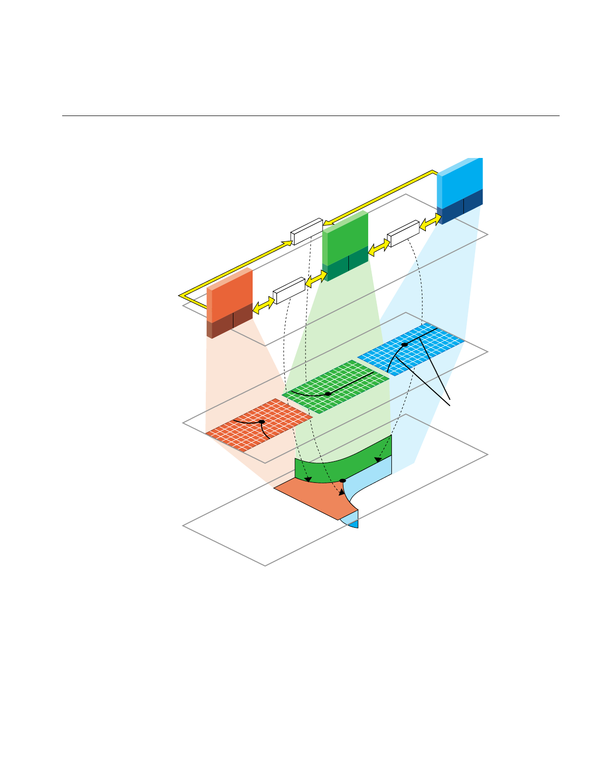
Summary of Scene Graph Topology: opTopo
271
Figure 12-1 Topological Relations Maintained by Topology Classes
u-v
coordinate
space
x-y-z
model
space
surfaces
Data
structure
2 Trim Curves
make up each
of theTrim Loops
in the figure
specified by
2 Edges
opParaSurface
opEdge opEdge opEdge opEdge
opParaSurface
opEdge opEdge
opParaSurface
opEdge opEdge
opParaSurface
opEdge opEdge
opBoundary opBoundary
opBoundary
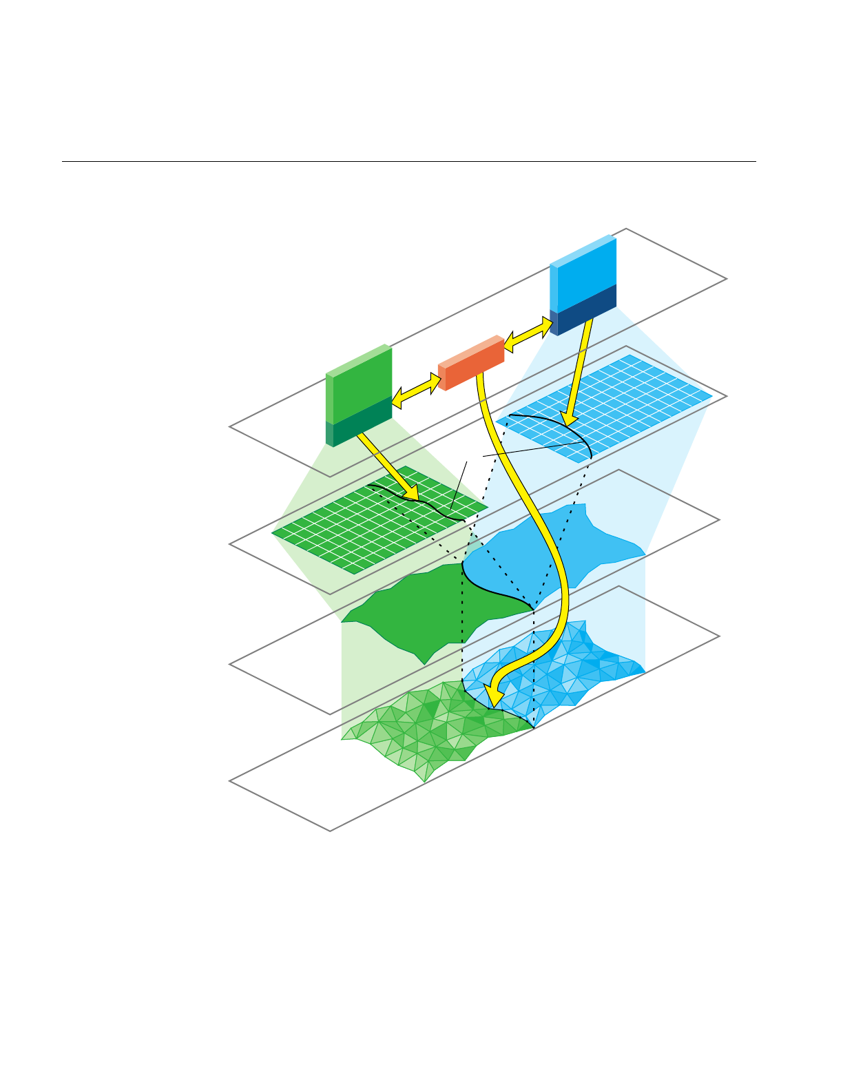
272
Chapter 12: Creating and Maintaining Surface Topology
Figure 12-2 Consistently Tessellated Adjacent Surfaces and Related Objects
Trim
curves
u-v
coordinate
space
x-y-z
model
space
surfaces
Discrete
surface
representation
(Edge consistent
tessellation)
opParaSurface opParaSurface
opEdge opBoundary
Data
structure
opEdge

Summary of Scene Graph Topology: opTopo
273
Building Topology: Computing and Using Connectivity Information
Given a set of opParaSurfaces in a scene graph, there are several ways to develop a set
of shared vertices to be held in opBoundarys. The following sections describe the
topology construction strategies (beyond the low-fidelity alternative of ignoring
topology):
• “Building Topology Incrementally: A Single-Traversal Build” on page 273
• “Building Topology From All the Surfaces in a Scene Graph: A Two-Traversal
Build” on page 274
• “Building Toplogy From a List of Surfaces” on page 274
• “Building Toplogy “by Hand”: Imported Surfaces” on page 274
• “Summary of Topology Building Strategies” on page 275
Building Topology Incrementally: A Single-Traversal Build
As each surface is tessellated during a traversal, the tessellator checks for previously
tessellated adjacent surfaces, uses existing vertices when it can, and adds necessary data
to topology data structures.
Although OpenGL Optimizer’s incremental toplogy building tools attempt to avoid
cracks, in principle they can appear because, when a surface is added, a new junction on
the boundary of an existing, tessellated surface may occur and the junction point may not
be in the existing tessellation. The tessellation of the added surface introduces the
junction point, necessarily at a finite distance from the existing tessellation, and a crack
appears between the newly and previously tessellated surfaces.

274
Chapter 12: Creating and Maintaining Surface Topology
Building Topology From All the Surfaces in a Scene Graph: A Two-Traversal Build
Topology built with two passes is very clean; unlike a single-pass build, in principle no
cracks due to unforeseen junctions can occur. The added cost of performing a
two-traversal build is slight; it is the recommended way to build topology and tessellate
if you want high-quality images. When building topology in two traversals, the
following steps occur:
1. Connectivity of all surfaces is calculated during a topology building traversal of the
scene graph, before a tessellation traversal.
2. The surfaces in the scene are tessellated during a second traversal.
Building Toplogy From a List of Surfaces
You can explicitly accumulate a list of surfaces for which to build topology and then
tessellate the surfaces. The result is clean tessellations of the surfaces on the list. Cracks
may appear if an adjacent surface was not included in the list.
Building Toplogy “by Hand”: Imported Surfaces
If you have a set of surfaces for which you know connectivity, you can explicitly develop
the appropriate topological data structures and develop consistent tessellations.
The presence of cracks will depend on how good your input trim curves are. If three
surfaces meet at a junction point that is not the shared endpoint of trim curves, a crack
may appear.

Summary of Scene Graph Topology: opTopo
275
Summary of Topology Building Strategies
Table 12-1 lists the methods required for each of the topology building strategies. See
“Base Class opTessellateAction” on page 289 for more information about the tessellation
methods listed.
Table 12-1 Topology Building Methods
Topology Building Strategy Methods
Ignore topology information and
let cracks appear as they will. 1. Do not create an opTopo or build topology.
2. opTessellateAction::setBuildTopoWhileTess(FALSE).
3. opTessellateAction::apply()
Build topology incrementally. 1. Create an opTopo.
2. opTessellateAction::setBuildTopoWhileTess(TRUE).
3. opTessellateAction::setTopo(topo).
4. opTessellateAction::apply(root).
Two-traversal build. 1. Create an opTopo.
2. opTopo::buildTopologyTraverse(root).
3. opTessellateAction::setBuildTopoWhileTess(FALSE).
4. opTessellateAction::apply(root).
Assemble a list of surfaces, build
the topology, and then tessellate. 1. Create an opTopo.
2. Assemble list of surfaces: opTopo::addSurface(surf).
3. opTopo::buildTopology().
4. opTessellateAction::setBuildTopoWhileTess(FALSE).
5. opTessellateAction::apply(shape).
Build the topology “by hand.”
See the file
src/sample/topoTest/topoTest.cxx
(step 7 does not appear in the code
because FALSE is the default).
1. Create an opTopo.
2. Assemble list of surfaces: opTopo::addSurface().
3. Create opBoundarys.
4. Add to list of boundaries: opTopo::addBoundary().
5. Add edges to boundaries: opBoundary::addEdge().
6. Set boundary orientation: opEdge::setBoundaryDir().
7. opTessellateAction::setBuildTopoWhileTess(FALSE).
8. opTessellateAction::apply(shape).

276
Chapter 12: Creating and Maintaining Surface Topology
Reading and Writing Topology Information: Using optimizeDemo
You can add topological information to an existing set of connected, higher-order
surfaces in a file—for example NURBS in an .iv file—and save the information for future,
crack-free surface rendering. This obviates the need for repeating the topology build. The
method opGenLoader::load() reads the topological information in a .csb file. See
“Reading and Writing Scene-Graph Files: The Extendable Loading Class opGenLoader”
on page 30.
Before you save the scene graph data, you can also add tessellations that use the topology
to give crack-free images (see Chapter 13, “Rendering Higher-Order Primitives:
Tessellators”).
The demonstration program optimizeDemo illlustrates how to perform these steps (see
Chapter 4, “Scene Graph Tuning With the optimizeDemo Application” and
/usr/share/Optimizer/src/sample/optimizeDemo).

Summary of Scene Graph Topology: opTopo
277
Table 12-2 shows three possible file conversions that you can apply to .iv or .csb files that
contain reps but no topology or tessellatione; they are listed with example
optimizeDemo command lines.
If you perform this processing, you may have files with or without tessellations.
Depending on which type of file you read, use one of the command lines in Table 12-3.
Note: If you attempt to load a tessellated surface, and do not switch off tessellation, you
will see two tessellations for each surface. The following command renders two
tessellations: optimizeDemo surTopTess.csb .
Table 12-2 Adding Topology and Tessellations to .iv and .csb Files
Conversion Example Command Line
Format change only. optimizeDemo sur.iv -tess no -batch sur.csb
Add topology
information to the
scene graph: save the
reps and topology
information but not
tessellations.
optimizeDemo sur.iv -tess no -ttol
topoTol -batch surTopo.csb
or
optimizeDemo sur.csb -tess no -ttol
topoTol -batch surTopo.csb
Add topology
information and
tessellations to the
scene graph: save the
reps, topology, and
tessellations.
optimizeDemo sur.iv -ttol topoTol
-batch surTopoTess.csb
or
optimizeDemo sur.csb -ttol topoTol
-batch surTopoTess.csb
Table 12-3 Reading .csb Files: With and Without Tessellations
To read a .csb file and perform
tessellation (without having to
build topology):
optimizeDemo surTopo.csb -ctol tessTol
To read a .csb file that already has
tessellations optimizeDemo surTopoTess.csb -tess no

278
Chapter 12: Creating and Maintaining Surface Topology
Class Declaration for opTopo
The following are the main methods in the class:
class opTopo : public csNode
{
public:
// Creating and destroying
opTopo( opReal tol = 1.0e-3,
opLengthUnits u = meter,
int sizeEstimate = 1024 );
~opTopo();
// Accessor functions
void setDistanceTol( opReal tol, opLengthUnits u )
opReal getDistanceTol( )
opParaSurface* getSurface( int i );
int getSurfaceCount( );
opBoundary* getBoundary( int i );
int getBoundaryCount( );
int getSolidCount()
opSolid* getSolid( int i )
//Adding topological elements
int addSurface( opParaSurface *sur );
int addBoundary( opBoundary *bnd );
//Topology construction
void buildTopology();
void buildTopologyTraverse(csNode *n);
int buildSolids();
static dvector<opTopo*> topology;
};

Summary of Scene Graph Topology: opTopo
279
Main Features of the Methods in opTopo
buildSolids() Collects connected surfaces in the opTopo into opSolids (see
“Collecting Connected Surfaces: opSolid” on page 283.
buildTopology()
Builds consistent set of boundaries from the list of surfaces accumulated
by calls to addSurface(). Previously developed boundaries are deleted.
buildTopologyTraverse()
Traverses a scene graph and builds a consistent set of boundaries for all
surfaces in the graph.
opTopo(tol,u) and opTopo(sizeEstimate)
Construct a topological data structure.
tol specifies a tolerance for calculating when points are close enough
together to be considered the same.
u specifies the system of units for tol.
The default values of u and tol are meters and 1 millimeter, respectively.
sizeEstimate specifies an estimate of the number of surfaces whose
topology needs to be maintained.
The static member topology is an array of all topologies that have been created.

280
Chapter 12: Creating and Maintaining Surface Topology
Consistent Vertices at Boundaries: opBoundary
This class is an element in the list maintained by opTopo of boundaries that are shared
by parametric surfaces. An opBoundary holds a curve that represents a common
boundary, and points to adjoining surfaces. Notice that an opBoundary can include any
number of surfaces that share a particular curve as a boundary, so it can represent the
intersection of several surfaces and allow you to describe a non-manifold surface
structure. An opBoundary can also hold just one surface, and thus represent a free edge.
The class opBoundary holds an opDisCurve3d xyzBoundary, which is derived from a
tessellation, to store a discrete version of a shared boundary. The unique discrete version
guarantees that tessellations of adjoining surfaces share the same vertices along the
boundary and so prevents the development of cracks.
In addition to information identifying each surface, opBoundary stores the index used
by each opParaSurface to identify the trim curve that defines the shared boundary.
Because a boundary may be made of several trim curves, it is possible for more than one
trim curve, and therefore more than one opBoundary, to define a geometric boundary
between two surfaces.
If you have an opParaSurface and want to identify adjacent surfaces, you have two
options. The simplest is to find the opSolid that holds the surface, using the
opParaSurface member _solid_id. At a lower level, you can identify each opBoundary
associated with the surface by using the boundary index that is stored in each of the
surface’sopEdgetrim curves. The boundaryindex identifies opBoundary members in the
opTopo list. From each member of the list, you can identify surfaces that share that
boundary. See the section “Parametric Surfaces” in Chapter 11 for more information
about opEdge.

Consistent Vertices at Boundaries: opBoundary
281
Class Declaration for opBoundary
The following are the main methods in the class:
class opBoundary
{
public:
opBoundary( );
~opBoundary( );
// Add a new edge to the end of the winged edge data structure
void addEdge( int i, int sur, int trimLoop, int trimCurve );
// Get data associated with this wing
void addEdge( int i, opParaSurface &sur, int trimLoop, int trimCurve );
int getSurface( int i );
int getLoop( int i );
int getTrimCurve( int i );
int getWingCount();
int getBoundaryId();
};

282
Chapter 12: Creating and Maintaining Surface Topology
Main Features of the Methods in opBoundary
opBoundary() Constructs an empty boundary.
wing Is a dvector composed of the surface and trim curve indices for one
surface associated with the boundary.
addEdge(i, sur, trimLoop, trimCurve)
“Attaches” the surface with index ito the boundary and identifies the
trim loop and trim curve that define the boundary in that surface. The
index sur is from the opTopo list of all opParaSurfaces. The indices
trimLoop and trimCurve are from the doubly indexed list in the
opParaSurface.
getSurface(i)Returns the opTopo index of the opBoundary surface with index i. The
other get*() functions return elements associated with the surface. See
“Parametric Surfaces” on page 219 for more details about the returned
objects.
xyzBoundary Is a discrete representation of the boundary curve. Notice that the curve
is not in the coordinate space of any of the surfaces but represents the
boundary as a curve in three-dimensional space. This curve defines the
set of vertices used in the tessellations of all surfaces that share this
boundary.
The methods set*(), which you can find in opBoundary.h, are mainly for use when reading
topological data from a file. For example, they are used by the .csb loader in
opGenLoader to create toplogical objects when reading a file (see “Reading and Writing
Scene-Graph Files: The Extendable Loading Class opGenLoader” on page 30).

Collecting Connected Surfaces: opSolid
283
Collecting Connected Surfaces: opSolid
To maintain consistent normals or propagate deformation information, organize
connected opParaSurfaces in an opSolid; with an opSolid, you can collect connected
surface patches in one object for convenient access and manipulation.
Despite the name of the class, the set of surfaces need not form a closed surface, that is
the boundary of a volume. They can be a set of patches joined to form a surface, for
example, you might generate a hood of a car from two opParaSurafaces that are mirror
images of each other.
To create solids, collect them in an opTopo and then call opTopo::buildSolid() (see
“Summary of Scene Graph Topology: opTopo” on page 270).
Class Declaration for opSolid
The following are the main methods in the class:
class opSolid
{
public:
// Creating and destroying
opSolid()
~opSolid()
// Accessor functions
int addSurface( opParaSurface *sur );
opParaSurface* getSurface( int i);
int getSurfaceCount( );
int getSolidId();
};
Main Features of the Methods in opSolid
Use the methods only after you have created an opSolid with opTopo::buildSolid().
Treat the method setSolidId() that appears in opSolid.h as private: it is used by
opTopo::buildSolid() when building the solid.


285
Chapter 13
13. Rendering Higher-Order Primitives: Tessellators
To render a higher-order primitive, you must develop an approximation that
“interprets” the primitive and makes a renderable “face” to present to the world. This
process is performed by a tessellator. The approximation is a collection of like primitives,
typically csTriFans or csTriStrips, for which Cosmo3D provides OpenGL rendering
calls. The interpretative aspect of tessellation lies in the nature of the approximation
developed; how big a deviation from the original surface will you allow? Or, a related
quantity, how many vertices do you want in the approximation? shows the hierarchy of
OpenGL Optimizer tessellator classes.
These topics are covered in this chapter:
• “Features of Tessellators” on page 286
• “Base Class opTessellateAction” on page 289
• “Tessellating Curves in Space” on page 292
• “Main Features of the Methods in opTessCurve3dAction” on page 293
• “Tessellating Parametric Surfaces” on page 295
• “Tessellating a Regular Mesh” on page 301
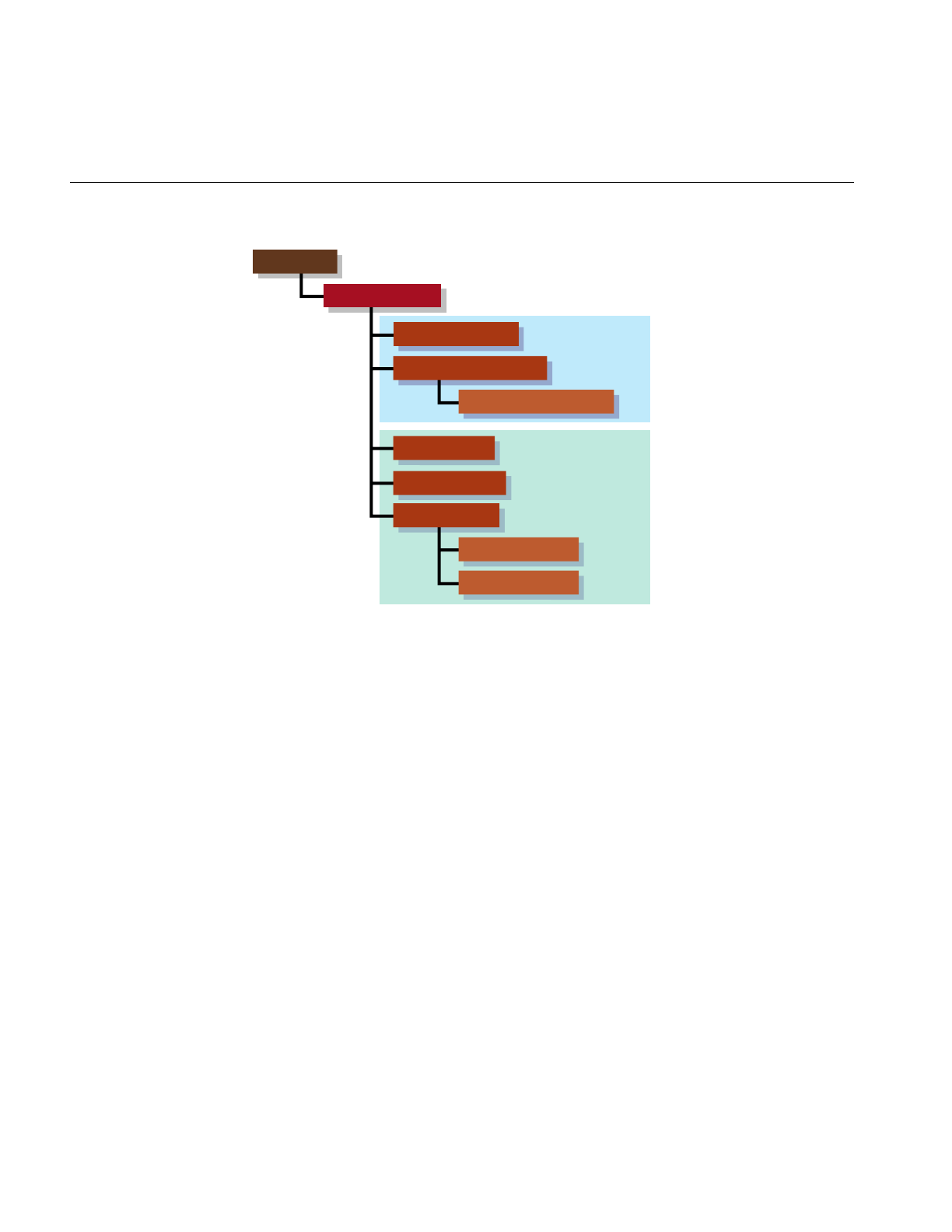
286
Chapter 13: Rendering Higher-Order Primitives: Tessellators
Figure 13-1 Class Hierarchy for Tessellators
Features of Tessellators
Tessellations necessarily burden the entire graphics pipeline; they provide a first
definition of the rendering task by specifying a maximal set of vertices to be sent to the
graphics hardware. You can redefine and simplify the rendering task by using the tools
discussed in Part II, “High-Level Strategic Tools for Fast RenderingChapter 8.”
Tessellators generate a sequence of straight-line segments to approximate an edge curve
of a surface, then cover the surface with triangular tiles. With each triangle vertex it
creates, a tessellator also stores the normal vector at the point from original surface. The
normal vectors are necessary for lighting and shading calculations.
opTessCuboidAction
opTessParaSurfaceAction
opTessIsoAction
opTessNurbSurfaceAction
opTessSliceAction
opTessVecAction
opTessVec3dAction
opTessVec2dAction
csDispatch
opTessellateAction
Tessellators for
continuous
surfaces
Tessellators for
regular meshes
Features of Tessellators
287
Tessellators for Varying Levels of Detail
Ideally you would quickly generate the simplest tessellation that adequately represents
surfaces of interest. “Adequate” depends on your particular rendering task. You may
want to generate several tessellations with varying degrees of complexity and accuracy
for one opRep and place them in level-of-detail nodes, as discussed in Chapter 6,
“Rendering Appropriate Levels of Detail.” The tessellators include accessor functions to
help you assess the load they create for the graphics hardware.
The control parameter for tessellations specifies the maximum deviation from the exact
surface. Figure 13-2 illustrates the effects of varying the deviation. The upper left image
is appropriate for accurate representation of the surface, the lower rightimage would be
appropriate if the object were in the distant background of a scene.
Figure 13-2 Tessellations Varying With Changes in Control Parameter

288
Chapter 13: Rendering Higher-Order Primitives: Tessellators
Details of Figure 13-2
The surface shown in Figure 13-2 was made with repTest using an
opFrenetSweptSurface as follows (see “opFrenetSweptSurface” on page 244 and
“repTest Application” on page 22):
opReal profile( opReal t ) { return 0.5*cos(t*6.0) + 1.25; };
opSuperQuadCurve3d *cross =
new opSuperQuadCurve3d( 0.75, new opVec3(0.0, 0.0, 0.0), 3.0 );
opCircle3d *path =
new opCircle3d( 1.75, new opVec3(0.0, 0.0, 0.0) );
opFrenetSweptSurface *fswept =
new opFrenetSweptSurface( cross, path, profile );
fswept->setHandednessHint( true );
The number of triangles in Figure 13-2 decreases as the maximum-deviation parameter
chordalDevTol varies from .001 to .01 to .1 to .5 (see “Tessellating Parametric Surfaces” on
page 295). These numbers should be compared to the scale of the object, which has a
maximum diameter of 6.125 = 2(1.75 +1.75 × .75), a minimum diameter of
.875 = 2(1.75 −1.75 ×.75), a maximum height of 2.625 = 2(1.75 ×.75), and a minimum
height of 1.125 = 2(.75 ×.75).
Tessellators Act on a Whole Graph or Single Node
You can apply a tessellator either to a scene graph or to just one node. The tessellators
produce from an opRep a csGeoSet and place it in the csShape that holds the opRep.
Tessellators and Topology: Managing Cracks
A tessellation begins with a discrete set of vertices at surface edges. To prevent cracks
from appearing between adjacent surfaces, the same set of vertices should be used to
tessellate both surfaces.
To address the crack problem, you have several options, which are discussed in
“Building Topology: Computing and Using Connectivity Information” on page 273.
”Table 12-1” on page 275, lists the different approaches to topology building, and the
methods to use for each.

Base Class opTessellateAction
289
Base Class opTessellateAction
The important methods of opTessellateAction are apply() and mpApply(), which
tessellate all opReps below the csNode that is their only argument. They perform,
respectively, a single-process or multiple-process traversal of the scene graph. If the
csNode is a csShape holding an opRep, then only that opRep is tessellated. If you supply
acsNode argument that is inappropriate for a particular opTessellateAction subclass,
nothing happens.
Subclasses of opTessellateAction, which are described in the subsequent sections of this
chapter, provide tessellators for specific opReps. All of these subclasses have a pair of
public functions, tessellate() and tessellator(), which implement a tessellation for a
specific opRep. Although these functions are public, you should have no need for them
if you use any OpenGL Optimizer opTessellateAction; call one of the apply functions,
apply() or mpApply(), to tessellate.
Tessellating a Scene Graph With Several Tessellators
If you create several subclasses of opTessellateAction and call
opTessellateAction::apply(), then for each surface encountered during the tessellation
traversal, the algorithm used to perform the tessellation is that of the most derived
instance of opTessellateAction that is appropriate for the surface. Thus, a call to the base
class method will do the right thing for each opParaSurface, if you create instances of
subclasses that provide the algorithms for doing so.

290
Chapter 13: Rendering Higher-Order Primitives: Tessellators
Class Declaration for opTessellateAction
The following are the main methods in the class:
class opTessellateAction : public csDispatch
{
public:
// Creating and destroying
opTessellateAction( void );
~opTessellateAction( void );
// Accessor functions
void setExtSize( int s );
int getExtSize( )
int getTriangleCount()
int getTriStripCount()
int getTriFanCount()
void setReverseTrimLoop( bool enable )
bool getReverseTrimLoop()
void setBuildTopoWhileTess(bool _buildTopoWhileTess)
bool getBuildTopoWhileTess()
void setTopo(opTopo * _topo)
opTopo *getTopo( void )
// Recursive action application
void apply ( csNode *node );
void mpApply( csNode *node );
};
Main Features of the Methods in opTessellateAction
apply() and mpApply()
Tessellate all opReps in a scene graph using a single-process or
multi-process traversal, respectively. Subclasses of opTessellateAction
define specific tessellation algorithms.
getTriangleCount()
Returns the number of all triangles generated by this instance of the
tessellator.

Base Class opTessellateAction
291
getTriStripCount() and getTriFanCount()
Return the number of tristrips or trifans in the tessellation.
setBuildTopoWhileTess() and getBuildTopoWhileTess()
Sets a flag whether surface connectivity is computed during the
tessellation traversal. Set the toplogy data structure to use with
setTopo().
If TRUE, before tessellating each surface, the connectivity of all
previously tessellated surfaces is used to avoid cracks when
tessellating. Notice that the final tessellations of the surfaces in the
scene graph may still have cracks because of unforeseen junctions
between surfaces.
If FALSE, no topology is constructed while tessellating. This leads to
two very different possible results:
• If topology information for the surfaces to be tessellated was
developed before the tessellation, by calling
opTopo::buildTopologyTraverse() or opTopo::buildTopology() or
by constructing topology by hand, the tessellator uses the
information and avoids cracks between surfaces. This option
provides the most crack-free tessellations possible.
• If topology information was not developed before the tessellation
traversal, then surfaces are tessellated without regard to
connectivity and cracks appear between all adjacent surfaces. This
option provides the least crack-free tessellations possible.
setExtSize() and getExtSize()
Set and return an estimate of how many surfaces you expect to tessellate
and thus allocate contiguous space in memory for dvectors that hold the
tessellation csGeoSet, a list of vertices, and a list of normals.
setReverseTrimLoop() and getReverseTrimLoop()
Set and recover the orientation of trim loops. Recall that the side of the
surface to the left of the trim loop is rendered (see the section
“Parametric Surfaces” on page 219).
setTopo() and getTopo()
Set and get the opTopo that holds the topology information used by the
tessellator (see “Summary of Scene Graph Topology: opTopo” on
page 270).

292
Chapter 13: Rendering Higher-Order Primitives: Tessellators
Tessellating Curves in Space
The class opTessCurve3dAction provides methods to develop a discrete approximation
to an opCurve3d.
Class Declaration for opTessCurve3dAction
The following are the main methods in the class:
class OP_DLLEXPORT opTessCurve3dAction : public opTessellateAction
{
public:
// Creating and destroying
opTessCurve3dAction( );
opTessCurve3dAction( opReal chordalDevTol,
bool scaleTolByCurvature,
int samples );
~opTessCurve3dAction();
// Accessor functions
void setChordalDevTol( const opReal chordalDevTol );
opReal getChordalDevTol( );
void setScaleTolByCurvature( const opReal scaleTolByCurvature );
bool getScaleTolByCurvature( );
void setSampling( const int samples );
int getSampling( );
};

Tessellating Curves in Space
293
Main Features of the Methods in opTessCurve3dAction
apply() and mpApply()
Are inherited from opTessellateAction. They tessellate individual
opCurve3ds or all opCurve3ds in a scene graph using a single-process
or multi-process traversal, respectively.
setChordalDevTol() and getChordalDevTol()
Set and get the maximum distance from the original surface to the edges
produced by the tessellation.
setSampling() and getSampling()
Set and get the hint for the number of vertices in the tessellation.
setScaleTolByCurvature() and getScaleTolByCurvature()
Set and get a flag to control whether the chordal deviation parameter
should be scaled by curvature. If non zero, the tessellation of highly
curved portions of a curve improves.

294
Chapter 13: Rendering Higher-Order Primitives: Tessellators
opTessCuboidAction
This class tessellates an opCuboid and is a minimal example of a tessellator.
Class Declaration for opTessCuboidAction
The following are the main methods in the class:
class opTessCuboidAction : public opTessellateAction
{
public:
opTessCuboidAction( );
~opTessCuboidAction( );
// Tessellate action
static void tessellate( csDispatch *action, csObject *object);
// The actual cuboid tessellator
void tessellator( opCuboid &c, csShape *shape );
};
Main Features of the Methods in opTessCuboidAction
apply() and mpApply()
Are inherited from opTessellateAction. They tessellate individual
opCuboids or all opCuboids in a scene graph using a single-process or
multi-process traversal, respectively.
The methods tessellate() and tessellator() occur for all subclasses of opTessellateAction;
you will rarely need to use them (see “Base Class opTessellateAction” on page 289 for
more details about these functions).

Tessellating Parametric Surfaces
295
Tessellating Parametric Surfaces
This section discusses the two classes OpenGL Optimizer provides for tessellating
parametric surfaces. The class opTessParaSurfaceAction has methods for any
parametric surface. The class opTessNurbSurfaceAction takes advantage of OpenGL
NURBS routines.
opTessParaSurfaceAction
This class develops tessellations of any opParaSurface. If a surface has boundary curves,
the tessellator starts there and specifies vertices at the edges of the surface. The tessellator
then covers the surface with csTriStripSets or csTriFanSets, using the boundary vertices
to “pin” the edges of the tessellation. If necessary, the tessellator creates edge vertices by
constructing a discrete version of the boundary curve associated with each of the
surface’s opEdges. An advantage of starting all tessellations at boundaries is easy
coordination of tessellations by several processors.
As part of the tessellation process, you can generate the u-v coordinates for each vertex
created by the tessellator.
To control the accuracy of a tessellation, you specify a chordal deviation parameter which
constrains the distance of edges in the tessellation from the original surface.

296
Chapter 13: Rendering Higher-Order Primitives: Tessellators
Class Declaration for opTessParaSurfaceAction
The following are the main methods in the class:
class opTessParaSurfaceAction : public opTessellateAction
{
public:
opTessParaSurfaceAction();
opTessParaSurfaceAction( opReal chordalDevTol,
bool scaleTolByCurvature, int samples);
~opTessParaSurfaceAction();
// Accessor functions
void setChordalDevTol( const opReal chordalDevTol );
opReal getChordalDevTol( );
void setScaleTolByCurvature( const opReal scaleTolByCurvature )
bool getScaleTolByCurvature()
void setSampling( const int samples )
int getSampling( )
void setGenUVCoordinates( const bool genUVCoordinates );
bool getGenUVCoordinates( );
bool capUbegin;
bool capUend;
bool capVbegin;
bool capVend;
};

Tessellating Parametric Surfaces
297
Main Features of the Methods in opTessParaSurface
apply() and mpApply()
Are inherited from opTessellateAction. They tessellate individual
opParaSurfaces orall opParaSurfaces in a scene graph using a
single-process or multi-process traversal, respectively.
opTessParaSurface()
Creates the class and provides a hint for the maximum deviation of the
tessellation from the original surface, indicates whether the tolerance
should be scaled by curvature, and provides a hint for how many
vertices to include in the tessellation.
setChordalDevTol() and getChordalDevTol()
Set and get the maximum distance from the original surface to the edges
produced by the tessellation.
setGenUVCoordinates() and getGenUVCoordinates()
Set and get a flag that indicates whether to generate u-v coordinates for
the vertices produced in the tessellation. The coordinates for each vertex
are stored as the vertex’s texture coordinates.
setSampling() and getSampling()
Set and get the hint for the number of triangle vertices in the tessellation
along each boundary of the surface. If the surface has no trim curves
defining its “outer” edges, then the sampling is along the edges of the
u-v rectangle that parameterizes the surface.
setScaleTolByCurvature() and getScaleTolByCurvature()
Set and get a flag to control whether the chordal deviation parameter
should be scaled by curvature. If non zero, the tessellation of highly
curved areas improves.
capUbegin,capUend,capVbegin,capVend
Define a rectangular region in the coordinate space and thus provide a
simple method to restrict tessellation to a portion of the surface.
The methods tessellate() and tessellator(), which are not shown in the declaration above,
occur for all subclasses of opTessellateAction; you will rarely need to use them (see
“Base Class opTessellateAction” on page 289 for more details about these functions).

298
Chapter 13: Rendering Higher-Order Primitives: Tessellators
Sample From repTest: Tessellating and Rendering a Sphere
The sample code in this section not only illustrates the main code elements for
tessellating an opParaSurface but describes the steps in the rendering process. The lines
of code perform the following procedures:
• Submitting the scene graph to an opViewer. This is part of the main program loop.
• Creating an instance of an opTessParaSurfaceAction.
• Creating and Tessellating an opSphere.
• Developing the Cosmo3D scene-graph nodes.
The code in this section comes mainly from the functions main(), in the file
/usr/share/Optimizer/src/sample/repTest/main.cxx, and makeShape() and makeObjects() in
the file /usr/share/Optimizer/sample/repTest/repTest.cxx.
From main()
The main routine of repTest, which is
similar to the application viewDemo,
creates an opViewer, calls makeObjects()
to get the tessellations, and starts the
rendering event loop.
makeObjects() makes the scene graph
full of tessellated reps. It calls
setupShape() to tessellate the reps.
opViewer *viewer = new
opViewer(“repTest”,x,y,w,h);
csGroup *obj = makeObjects();
viewer->addChild(obj);
viewer->setViewPoint(obj);
viewer->eventLoop();
Create Tessellators, Set Accuracy
tc is a tessellator included so
setupShape() can accept an opCuboid in
addition to an opParaSurface.
// Generic parametric surface
// tessellator
static opTessParaSurfaceAction *t
= new opTessParaSurfaceAction( );
// Set up the cuboid tessellator
static opTessCuboidAction *tc
= new opTessCuboidAction();
// Set the tolerance from the
// command line
t->setChordalDevTol( tol );

Tessellating Parametric Surfaces
299
Define setUpShape
The function setupShape() creates a new
csShape, applies an appearance, places
an opRep in the csShape, places the
csShape at a position specified by the
arguments, and tessellates the opRep.
// A helper function which attaches
// a rep to a newely created shape
// and attaches that shape to the
// scene graph
static void setUpShape(
opRep *rep,
opReal x,
opReal y,
opReal z )
{
// Get the current origin of the
// object
opVec3 org = rep->getOrigin();
// Add the incoming offest to it
org[0] += x;
org[1] += y;
org[2] += z;
// Now reset the origin to include
// the incoming offset
rep->setOrigin( org );
// Set the appearance of this shape
// to be a random color
csAppearance *c_app =
makeColor(
(float)rand()/((2<<15) - 1.0),
(float)rand()/((2<<15) - 1.0),
(float)rand()/((2<<15) - 1.0)
);
// Attach the geometry and
// appearance off of the shape
rep->setAppearance( c_app );
// Attach the shape to the scene
// graph
globalTransform->addChild( rep );
// Tessellate the invidual shape
t->apply(rep);
tc->apply(rep);
}

300
Chapter 13: Rendering Higher-Order Primitives: Tessellators
Define makeObjects()
The function makeObjects() sets up the
scene graph, defines and tessellates the
grid of reps, and places the tessellated
surfaces in the scene graph.
The code here shows the initial lines of
makeObjects() (skipping over the code
that controls the grid definition) and the
example of defining on opParaSurface, a
trimmed and untrimmed opSphere.
See the file
/usr/share/Optimizer/src/sample/repTest.cxx
for more details on the parameters
nVersions,OP_XDIST,OP_VIEWDIST,
and numObject.
csGroup *makeObjects()
{
...
// Scene’s global light
csPointLight *lt =
new csPointLight;
// Add the global light to the
// scene
sceneRootNode->addChild(lt);
// Attach the global transform
sceneRootNode->
addChild(globalTransform);
// Set the tolerance from the
// command line
t->setChordalDevTol( tol );
...
// Now all of the reps
...
/////////////////////////////////
// Sphere
/////////////////////////////////
opSphere *sphere =
new opSphere( 3 );
if ( nVersions <= 0 )
{
opCircle2d *trimCircle2d =
new opCircle2d( 1.0,
new opVec2(M_PI/2.0,M_PI)
);
sphere->
addTrimCurve( 0,
trimCircle2d,
NULL );
}
setUpShape( sphere,
OP_XDIST*numObject++,
Y,
OP_VIEWDIST );

Tessellating a Regular Mesh
301
opTessNurbSurfaceAction
This class tesselates surfaces using NURBS utilities in OpenGL. Thus, the tessellation
developed by opTessNurbSurfaceAction is well tuned for rendering. For more details
about the OpenGL utilities, see the section “The GLU NURBS Interface” in Chapter 11 of
the OpenGL Programming Guide.
The only member function of note is the constructor, which takes a chordal deviation
parameter that has the same effect as that for opTessParaSurfaceAction.
Tessellating a Regular Mesh
To facilitate visualization of discrete data sets, OpenGL Optimizer provides four
tessellators for various types of the template class opRegMesh. The tessellators accept
opRegMeshType opConstant and opVariable. These are brief descriptions of the
tessellation classes discussed in this section:
Visualizing Scalar-Valued Functions
opTessIsoAction
Acts on a surface determined by a constant value of an opReal-valued
function defined on a three-dimensional lattice. An opTessIsoAction
takes an opRegMesh<opReal> and a value for the mesh function and
returns a tessellation of the corresponding level surface, or iso-surface.
opTessSliceAction
Acts on planes that slice through a three-dimensional
opRegMesh<opReal> and, according to a simple “rainbow” scheme,
colors the values of the function at points that lie on the plane: red
corresponds to the minimum value of the mesh function, and blue
corresponds to the maximum value. The slicing planes are
perpendicular to the x, y, or z axes.

302
Chapter 13: Rendering Higher-Order Primitives: Tessellators
Visualizing Vector-Valued Functions
The last two mesh tessellators return what are known as “hedgehog” plots of the vector
fields. They are both trivial derivations of the base class opTessVecAction:
opTessVec2dAction
Acts on a two-dimensional vector field defined on a two-dimensional
grid. An opTessVec2d takes an opRegMesh<opVec2> and returns a set
of arrows on the x-y plane.
opTessVec3dAction
Acts on a three-dimensional vector field defined on a three-dimensional
grid. An opTessVec3d takes an opRegMesh<opVec3> and returns a set
of arrows distributed in space.
opTessIsoAction
This class interprets discrete versions of opReal-valued functions defined on
three-dimensional space. That is, opTessIsoActionacts on an opRegMesh<opReal> and
tessellates the mesh function’s iso-surfaces.
Class Declaration for opTessIsoAction
The following are the main methods in the class:
class opTessIsoAction : public opTessellateAction
{
public:
// Creating and destroying
opTessIsoAction ();
opTessIsoAction (opReal threshold, int stride = 1);
~opTessIsoAction ();
// Accessor functions
void setThreshold (opReal thresh)
opReal getThreshold ()
void setStride (int _stride)
int getStride ()
};

Tessellating a Regular Mesh
303
Main Features of the Methods in opTessIsoAction
apply() and mpApply()
Are inherited from opTessellateAction. They tessellate all
opRegMesh<opReal>s in a scene graph using a single-process or
multi-process traversal, respectively.
opTessIsoAction()
The variable threshold specifies the value of the mesh function on the
iso-surface. The variable stride specifies the sampling of the mesh by
specifying how to increment the mesh indices. For example, a stride
value of two takes every other point along the axes. The default values
of threshold and stride are 0 and 1, respectively.
opTessSliceAction
This class interprets discrete versions of opReal-valued functions defined on
three-dimensional space. That is, opTessSliceAction acts on an opRegMesh<opReal>
and shows, by a simple rainbow map, values of the functions that lie on a plane.
opTessSliceAction uses one of three possible planes perpendicular to the coordinate
axes.
Class Declaration for opTessSliceAction
The following are the main methods in the class:
class opTessSliceAction : public opTessellateAction
{
public:
opTessSliceAction();
opTessSliceAction (opReal position, char axis);
~opTessSliceAction();
// Accessor functions
void setPosition (opReal _position)
opReal getPosition ()
void setAxis (int _axis)
char getAxis ()
};

304
Chapter 13: Rendering Higher-Order Primitives: Tessellators
Main Features of the Methods in opTessSliceAction
apply() and mpApply()
Are inherited from opTessellateAction. They tessellate all
opRegMesh<opReal>s in a scene graph using a single-process or
multi-process traversal, respectively.
opTessSliceAction(position, axis)
Sets the slice plane perpendicular to axis. Values for axis are x, y, orz.The
argument position specifies the location of the slice plane: the point
where axis intersects the plane. The default position is 0.0, and the
default axis is the xaxis.
setAxis() and getAxis()
Set and get the current slice axis.
setPosition() and getPosition()
Set and get the current slice position along the currently defined axis.
The argument for setPosition() should be between zero and the mesh
resolution in the direction of axis.

Tessellating a Regular Mesh
305
opTessVecAction
This is the base class for the tessellators that act on an opRegMesh<opVec2> or an
opRegMesh<opVec3>. The latter are trivial derivations from an opTessVecAction.
Class Declaration for opTessVecAction
The following are the main methods in the class:
class opTessVecAction : public opTessellateAction
{
public:
opTessVecAction( );
~opTessVecAction( );
// --- Accessors
void setMagScale (opReal _scale)
void setInitialColor (csVec4f _iColor)
void setTerminalColor (csVec4f _tColor)
opReal getMagScale()
csVec4f getInitialColor()
csVec4f getTerminalColor()
};
Main Features of the Methods in opTessVecAction
setMagScale() and getMagScale()
Set and get the vector magnitude scale factor. This allows you to adjust
the length of the rendered vectors. The default value is 1.0.
setInitialColor() and getInitialColor()
Set and get the color to be used at the base of the vectors. The default
value is opaque white: (1.0, 1.0, 1.0, 1.0).
setTerminalColor() and getTerminalColor()
Set and get the color to be used at the tip of the vectors. The default value
is opaque white: (1.0, 1.0, 1.0, 1.0).

306
Chapter 13: Rendering Higher-Order Primitives: Tessellators
opTessVec2dAction and opTessVec3dAction
These classes provide tessellators for the two mesh classes opRegMesh<opVec2> and
opRegMesh<opVec3>. They are derived from opTessVecAction, and each contains no
public member functions other than a constructor, a destructor, and the necessary
tessellate() and tessellator() functions. If the opRep passed to one of the tessellators is
not of the correct type, the tesselator returns NULL.
apply() and mpApply()
Are inherited from opTessellateAction. They tessellate all
opRegMesh<opVec2>s or opRegMesh<opVec3>s in a scene graph
using a single-process or multi-process traversal, respectively.
Sample Mesh Tessellation: opviz and opVizViewer
The following discussion is not intended to provide all the details of the application
opviz but rather to highlight the basic structure of the program, to orient you when you
look at the source files.
The application opviz provides calls to OpenGL Optimizer’s three-dimensional
opRegMesh tessellators, and uses the class opVizViewer, which is derived from
opViewer, to control scene graph interactions and rendering. The application opviz can
read Plot3D data files, three samples of which are included in the OpenGL Optimizer
library to illustrate mesh tessellation. For more information on Plot3D data format, see,
for example, http://www.nas.nasa.gov/NAS/FAST/RND-93-010.walatka-clucas/htmldocs/
chp_21.formats.html.
The applcation opviz runs tessellators on an opThreadManager, which uses an
opFunctionAction to distribute tessellation tasks. For more information on
opThreadManager and opFunctionAction, see “Overview of the Thread Manager” on
page 341.
The following sections first present controls added to opViewer by the class
opVizViewer, and then cover these components of opviz:
• the main rendering routine and data loading
• creating a tessellator and a csShape to hold the tessellation
• applying the tessellator to an opRegMesh using an opThreadMgr

Tessellating a Regular Mesh
307
opVizViewer
This class extends the functionality of opViewer by defining the function
opVizViewer::keyHandler() to manipulate three tessellators.
Key Bindings for opVizViewer
The class opVizViewer allows you to perform these actions from the keyboard, in
addition to those provided by opViewer:
iRuns an opTessIso.
UP increases the function value used as a threshold and tessellates the
new isosurface.
DOWN decreases the function value and tessellates the new isosurface.
cRuns an opTessSlice.
RIGHT moves the slice plane, which is perpendicular to the x,y, or z axis,
in the positive direction along the appropriate axis, and tessellates the
new slice.
LEFT moves slice in the negative direction along the appropriate axis
and tessellates the new slice.
x sets the slice plane perpendicular to the xaxis.
y sets the slice plane perpendicular to the yaxis.
z sets the slice plane perpendicular to the yaxis.
gRuns an opTessVec3d.
+increases the size of plotted vectors.
- decreases the size of the plotted vectors.
0,1... Selects the mesh to act on.

308
Chapter 13: Rendering Higher-Order Primitives: Tessellators
opviz’s Main Routine
The application’s main loop parses command-line arguments, calls a data loader, and
then calls eventLoop(), which is inherited from opViewer, to handle interaction with the
data.
The data loader can read the three sample meshes (two scalar meshes and a vector mesh)
that are included in the library. These meshes are discussed in Chapter 11 in the sections
“An opConstant opRegMesh<opReal>: Data for opviz” on page 267, “An opVariable
opRegMesh<opReal>: Data for opviz” on page 268, and “An opVariable
opRegMesh<csVec3f>: Data for opviz” on page 268.
The data loader calls the opVizViewer methods addScalarMesh() and
addVectorMesh(), which bring in the mesh data and modify the scene graph for
convenient viewing. The add functions use the methods of the classes ScalarVizPacket
and VectorVizPacket to control the tessellators.
Initializing a Tessellator
The function ScalarVizPacket::init_isosurface(), from which the following lines are
taken, is an example of how to begin using a tessellator. To tessellate slices of a vector
field or a scalar mesh requires very similar lines of code.
Create the tessellator iso = new opTessIsoAction ();
Create a csShape node to hold the
tessellation.
For this application the node is placed
under the root node group:
material->
setShininess (.0078125f * 116.0f);
material->setTransparency (0.5);
material->
setDiffuseColor (0.08, 0.0, 1.0);
material->
setSpecularColor (0.75, 0.75, 1.0);
appear->setMaterial (material);
appear->setLightEnable (1);
appear->setTranspEnable (1);
appear->setTranspMode(
csContext::BLEND_TRANSP);
iso_shape->setAppearance (appear);
group->addChild (iso_shape);

Tessellating a Regular Mesh
309
opviz Tessellation and Thread Manager Calls
When you enter i after starting opviz, the application calls
ScalarVizPacket::run_isosurface(), which tessellates the sample data set. The
application opviz, via subsequent calls in eventLoop(), then renders the isosurface.
run_isosurface() uses the tessellator created by init_isosurface() and obtains tessellation
parameters from the data management structure developed by addScalarMesh().
Although run_isosurface() creates a multi-thread framework, opviz uses only one
thread. The application provides a framework that is easily extended to a multiprocess
tessellation controlled by an opMPFunListAction (see “opMPFunListAction: Many
Tasks, Many Processes” on page 351). For opviz, tessellations are performed by instances
of an opFunctionAction called IsoAction. See the section “opFunctionAction: One Task,
One Process” on page 348.
Create a Multi-Threaded
Environment
The function run_isosurface(), from
which this code is taken, provides a
multi-threaded environment.
The function checks the number of
available processors and creates an
opThreadManager, which runs only
one thread; see “Overview of the
Thread Manager” on page 341.
int numThreads =
opGetProcessorCount();
// ...error checking code deleted
tm = new opThreadMgr(numThreads);
// --- Create action array.
// Currently the action array only
// contains one action:
// isosurface generation
// create array
int numActions = 1;
opFunctionAction **actions =
(opFunctionAction **) new
opFunctionAction [ numActions ];
// insert action(s) in the array
for (int i=0; i < numActions; i++)

310
Chapter 13: Rendering Higher-Order Primitives: Tessellators
IsoAction is an opFunAction. Its
method function() performs the
tessellation.
See “opFunctionAction: One Task,
One Process” on page 348.
// the action objects take a mesh and
// tessellator
actions[i] =
new IsoAction (mesh, iso, iso_shape);
// --- the thread manager runs the
// action(s) on separate threads
tm->
SchedMPFunList (new opMPFunListAction(
numActions,
actions)
);
MP Tessellation
Because this procedure may occur
while another process is in a
rendering traversal, the code from
IsoAction::function() first removes
the iso_shape node from the scene
graph by submitting an
opTransaction::removeChild() to the
transaction manager. Then function()
tessellates iso_shape, and submits an
opTransaction::addChild() to the
transaction manager, placing the
newly tessellated shape back in the
scene graph. (See “opTransaction” in
Chapter 16).
Here shape is the member of
IsoAction that corresponds to
iso_shape in the lines of code above
from
ScalarVizPacket::init_isosurface()
and scalarMesh is the member that
corresponds to mesh.
int pc = shape->getParentCount();
for ( int i = 0; i < pc; i++ )
{
csGroup *parent =
(csGroup *)shape->getParent(i);
int place = parent->findChild (shape);
// --- extract existing geometry,
// delete and replace old one
opTransaction *trans1 =
new opTransaction;
trans1->removeChild(parent, shape);
opBlockingCommit(trans1);
isosurface->
tessellator(*scalarMesh, shape);
opTransaction *trans2 =
new opTransaction;
trans2->addChild(parent, shape);
opCommit(trans2);
}
To recover memory, function() has
the IsoAction deleted. return opDeleteThis;

PART FIVE
Traversers, Low-Level Geometry Processing, and
Multiprocessing V
Chapter 14, “Traversing a Large Scene Graph”
Chapter 15, “Manipulating Triangles and Rebuilding Renderable Objects”
Chapter 16, “Managing Multiple Processors”


313
Chapter 14
14. Traversing a Large Scene Graph
This and the following chapter discuss methods to efficiently manipulate (parts of) a
scene graph with extensible traversers. The OpenGL Optimizer tools fall in two general
categories:
• tools that essentially focus on the scene graph manipulation, which are discussed in
this chapter
• tools that coordinate scene-graph tasks as well as other tasks in a multiprocessor
environment, which are discussed in the next chapter
You define OpenGL Optimizer traversals with callbacks held in a traversal object. The
control provided by the callbacks allows you to do the following:
• Specify the effect when a traverser visits a node.
• Control the progress of the traversal, that is, which node to visit next.
• Delete the traversal object when you are through with it.
The following sections make up the rest of this chapter:
• “Traversals and Callbacks: General Features” on page 314
• “Controlling a Traversal With the Callback Return Value opTravDisp” on page 317
• “Depth-First Traversals: opDFTravAction” on page 318
• “Breadth-First Traversals: opBFTravAction” on page 320
• “Sample Traversal Function From the Application optimizeDemo” on page 322
• “Traversing a Scene Graph and Applying a csDispatch: opDispatchAction” on
page 325

314
Chapter 14: Traversing a Large Scene Graph
Traversals and Callbacks: General Features
Traversing a scene graph means “visiting” nodes in some sequence and invoking a
callback as each node is visited. Callbacks allow you to perform operations whenever a
node is visited during a traversal; for example, you can count nodes, render objects, or
compute the volume of objects in a scene.
OpenGL Optimizer provides tools for two scene-graph traversal sequences: depth first
or breadth first.
Depth-First Traversal Sequence
To picture depth-first traversals imagine the path you would take if the links between
nodes in a scene graph were hallways and you walk through the scene graph holding
your right hand on a wall. Nodes would be rooms, and you would continue to hold your
hand on the wall as you walked through the room. Callbacks are made each time you
enter a room, except when the hand-on-the-wall rule returns you to a parent node before
visiting all its children: a callback is made when you first “descend” into the parent node
and after you “ascend” from the last child.
Figure 14-1 shows a depth-first traversal of a simple scene graph. The solid circles in the
figure indicate pre-node callbacks, which are implemented when a traversal first visits a
node. The solid squares indicate post-node callbacks, which are implemented as a traversal
leaves a node.
Traversals and Callbacks: General Features
315
Figure 14-1 Depth-First, Left-to-Right Traversal of a Simple Scene Graph
Notice that a depth-first traversal visits each parent node twice, once before and once
after visiting its children. A depth-first traversal is inherently sequential and so cannot
be reasonably executed by more than one process; the ordering of actions, particularly
when parents are visited after their children, is best maintained by one process.
A
BE
CDF
A > B > C > D > B > E > F > E > A
316
Chapter 14: Traversing a Large Scene Graph
Breadth-First Traversal Sequence
The central concept of a breadth-first traversal is that the traverser visits the nodes at a
given level and proceeds to a lower level in the scene graph after all the nodes at a higher
level have been visited. Figure 14-2 shows a breadth-first traversal of a simple scene
graph. The solid circles in the figure indicate per-node callbacks, which are implemented
when a traverser first visits a node.
Figure 14-2 A Breadth-First Traversal of a Simple Scene Graph
There can be features that complicate the sequence of nodes visited in a bread-first
traversal, such as a multiprocess traversal or nodes with multiple parents, such that the
simple left-right, top-to-bottom sequence doesn’t hold exactly.
When a breadth-first traversal is executed by several processes or nodes in the graph
have several parents, a simple rule guarantees a reasonable sequence of events: the
traversal does not visit children until it visits at least one of the parents. Whenever a
parent node is encountered by a traverser, it places the node’s children at the end of the
processing queue.
A
BC
DEF
A > B > C > D > E > F

Controlling a Traversal With the Callback Return Value opTravDisp
317
Callbacks During a Traversal
These are the basic operations performed during a traversal and specified by an instance
of an action object:
1. Call a begin() method to establish any context you might want for the traversal.
2. Visit the scene-graph nodes in sequence.
3. Perform the appropriate callback at each node and determine how the traversal is to
proceed.
4. Delete or retain the action object as specified by the return value of the action
object’s member function end().
You have two controls over how a traversal proceeds:
• The return values of the node-visiting callbacks, which allow you to continue, stop,
or remove the children of a node from the traversal.
• The node argument of the callback, which is passed by reference, and provides
great freedom in determining the specific node that is next in the traversal.
Controlling a Traversal With the Callback Return Value opTravDisp
The possible return values of callbacks, and the method apply() which initiates a
traversal callback sequence, are set by the enumerated type opTravDisp whose values
correspond to whether the traversal should continue, skip over the children of the
current node, or stop.
This is the type definition for opTravDisp:
typedef enum {opTravCont=0, opTravPrune=1, opTravStop=2} opTravDisp;

318
Chapter 14: Traversing a Large Scene Graph
Specifying Deletion of Storage of Traversal Objects: opActionDisp
After you complete a traversal, you may want to keep the object for subsequent use, or
free storage assigned to the traversal object. For example, you might repeatedly use a cull
traverser, invoking it each frame, but you might perform a tessellation traversal only
once.
To specify whether a traversal object remains in memory after the traversal stops, specify
the return value of the last callback, end(). The possible values are set by the enumerated
type opActionDisp. This is the declaration for opActionDisp:
typedef enum {opDeleteThis, opKeepThis} opActionDisp;
Depth-First Traversals: opDFTravAction
The class opDFTravAction is used for a depth-first traversal of the scene graph. Parent
nodes get visited at least twice, before and after their children are visited with a different
callback for each visit (see “Depth-First Traversal Sequence” on page 314).
Class Declaration for opDFTravAction
The following are the main methods in the class:
class opDFTravAction : public opAction
{
public:
opDFTravAction();
virtual ~opDFTravAction();
opTravDisp apply(csNode *root);
virtual void begin (csNode *& , const &);
virtual opTravDisp preNode (csNode *&, const opActionInfo &);
virtual opTravDisp postNode(csNode *&, const opActionInfo &);
virtual opActionDisp end (csNode *&, const opActionInfo &);
};

Depth-First Traversals: opDFTravAction
319
Main Features of the Methods in opDFTravAction
apply() Initiates a traversal below root.
The callbacks are applied at these points of the traversal (see “Depth-First Traversal
Sequence” on page 314):
begin() Before the traverser visits any node. The csNode argument is the root of
the traversal. Note that if the argument equals NULL, the tree is empty
and no traversal will begin. The default for begin() does nothing.
preNode() Before visiting a node for the first time or for each visit to a node before
visiting its children. The latter case occurs, for example, when a parent
is itself the child of two parents; thus a traverser could visit the node
twice during a traversal and apply preNode() each time before visiting
the children. The default for preNode() returns opTravCont, and thus
simply continues the traversal.
postNode() After visiting a node’s children. The default for postNode() returns
opTravCont and thus simply continues the traversal.
end(node, info)Once the traversal is completed or halted by a callback.The argument
node is the root of the scene graph. The default for end() cleans up by
returning opDeleteThis, thus deleting the opDFTravAction. To avoid
deletion, define end() to return the value opKeepThis.
Note the following two features of the arguments you pass to preNode(),postNode(),
and end():
• The csNode pointer, which also appears as an argument for all of the callbacks, is
passed by reference; thus you can change its value. This is useful when the scene
graph changes during a traversal, typically when nodes have been added. The
traverser “decides” where to go next by assuming the traversal is complete up to
the current csNode.
• The class opActionInfo, which appears as an argument for all the callback
functions, is valid only if the traversal is initiated by the thread manager.
opActionInfo is discussed in the section“Difference Between Interprocess Control
Methods” on page 346.

320
Chapter 14: Traversing a Large Scene Graph
Breadth-First Traversals: opBFTravAction
The class opBFTravAction is for a breadth-first traversal, which can be performed on one
or several processors. All nodes are visited only once, typically, in contrast with an
opDFTravAction, for which parent nodes typically re visited at least twice.
Class Declaration for opBFTravAction
The following are the main methods in the class:
class opBFTravAction : public opAction
{
public:
opBFTravAction();
virtual ~opBFTravAction();
opTravDisp apply(csNode *root);
void applyMP(csNode *root,
opThreadMgr *tm,
const opTIDSet& tids = opTIDSet::opAllTIDs,
opPriority p = Optimizer::opDefaultPriority);
virtual void begin (csNode *&, const opActionInfo& );
virtual opTravDisp perNode(csNode *&, const opActionInfo& ):
virtual opActionDisp end (csNode *&, const opActionInfo& );
};

Breadth-First Traversals: opBFTravAction
321
Main Features of the Methods in opBFTravAction
apply() Initiates a traversal.
applyMP() Initiates a traversal on several threads using a thread manager. See
“Overview of the Thread Manager” on page 341.
The callbacks are applied at these points of the traversal (see “Breadth-First Traversal
Sequence” on page 316):
begin() Is applied before the traverser visits any node. It has the same effect as
opDFTravAction::begin(), discussed in “Depth-First Traversals:
opDFTravAction” on page 318.
perNode() Is applied as the traverser visits each node. A return value of opTravStop
stops the traversal at the current node. A return value of opTravStop is
equivalent to opTravPrune, thus eliminating from the traversal
whatever children the current node may have. The default for
perNode() returns opTravPrune and thus skips any of the node’s
children.
end(node, info)Once the traversal is completed or halted by a callback. It has the same
effect as opDFTravAction::end(), discussed in “Depth-First Traversals:
opDFTravAction” on page 318. The argument node is the root of the
scene graph. The default for end() cleans up by returning opDeleteThis,
thus deleting the opBFTravAction.To avoid deletion, define end() to
return the value opKeepThis.
As for an opDFTravAction, the scene-graph-node callback arguments can be modified to
change the course of the traversal and opActionInfo arguments are only valid if the
traversal is initiated in a multi-threaded context by a thread manager.

322
Chapter 14: Traversing a Large Scene Graph
Sample Traversal Function From the Application optimizeDemo
The following code illustrates the use of a traverser. The code is not a minimal example;
it serves a second purpose here: to illustrate a simplification traversal.
Because of the many possible simplification traversals, OpenGL Optimizer does not
provide a simplification traversal class. However, you are likely to need a simplification
traverser of some kind to meet particular needs. This code provides one approach to the
simplification traversal task. It defines a simplification traversal function that returns the
root of a new, simplified scene graph.
The main difference between this example and a minimal example is that it includes
some node-checking to determine whether a node is a csShape, and so could contain a
csGeoSet to simplify, and then code to further check whether the csShape actually
contains a csGeoSet. The particular checks performed reflect the needs of a simplifier,
but it would not be unusual for a traverser to test for particular node types.
These lines of code are taken from simplify.cxx and main.cxx in
/usr/share/Optimizer/src/sample/optimzeDemo to illustrate the procedure.
Create a Simplifier
See “Successive Relaxation Algorithm:
opSRASimplify” on page 115. static opSRASimplify simplifier;
Create a Traversal Object
Derive an opDFTravAction class SimplifyGeoSet : public opDFTravAction
{
public:
opTravDisp PreNode(csNode *&, const opActionInfo&);
opSRASimpParam *userData;
csGroup *simpObj;
};
Specify Effect of Callback
Define the callback preNode().opTravDisp SimplifyGeoSet::PreNode(
csNode *&node, const opActionInfo &)

Sample Traversal Function From the Application optimizeDemo
323
Specify Effect of Callback (cont.)
Set the return value to continue the
traversal, thus visiting every node. {
opTravDisp rv = opTravCont;
Test if a node is a csShape, and thus may
have a csGeoSet to simplify. if ((node->getType())->
isDerivedFrom(csShape::getClassType()))
{
Simplify all csGeoSets in the csShape by
using an opSRASimplify (see “Successive
Relaxation Algorithm: opSRASimplify” on
page 115).
csShape *shape = (csShape*)node;
for (int i = 0; i < shape->getGeometryCount(); i++)
{
csGeometry *g= shape->getGeometry(i);
if (
g &&
g->getType()->isDerivedFrom(
csGeoSet::getClassType()
)
)
{
csGeoSet *simpGSet, *gset = (csGeoSet*)g;
int status;
simplifier.settings(userData);
// If simplifier didn’t change input geoset,
// then original input geoset is returned.
simpGSet =
simplifier.DecimateGeoSet(gset, &status);
Place the simplifications in new csShapes
with the same appearance as the originals. // Whether or not the gset changed,
// add it to the group
// XXX Need clone since tree gets flattened
csShape *simpShape = (csShape *)new csShape;
simpShape->setAppearance(
shape->getAppearance()
);
// Add simplified geoset.
simpShape->setGeometry(i,simpGSet);
simpObj->addChild(simpShape);
}
}
}
return rv;
}

324
Chapter 14: Traversing a Large Scene Graph
Define the SimplifyTraversal Function
The application simplify then uses
SimplifyGeoSet() to define a
simplify-traversal function, simplifyTree().
csGroup *simplifyTree(csGroup *obj, opSRASimpParam
*userData)
{
csSphereBound sphere;
obj->getSphereBound(sphere);
csGroup *simpObj = new csGroup;
SimplifyGeoSet *action = new SimplifyGeoSet;
action->userData = userData;
action->simpObj = simpObj;
action->apply(obj);
return simpObj;
}
Use the Function: Here, Add Simplified
Graph to an LOD
The application optimizeDemo calls
simplifyTree() and adds the simplified
graph as a child of an LOD node.
addLODChild() is defined in
/usr/share/Optimizer/src/sample/optimizeDemo
/addLOD.cxx.
csGroup *simpObj = simplifyTree(root, parameters);
// Set child0 as default LOD to be drawn
root = addLODChild(root,simpObj,0);

Traversing a Scene Graph and Applying a csDispatch: opDispatchAction
325
Traversing a Scene Graph and Applying a csDispatch: opDispatchAction
The class opDispatchAction is a csAction that, as it traverses a scene graph, applies a
csDispatch to each node in a scene graph.
Recall that a csAction is a Cosmo3D object for traversing a scene-graph. The class
csDispatch is an object designed to follow the “Visitor Behavioral Pattern,” which
provides a convenient way to organize and define operations on scene graph elements.
The Visitor Behavioral Pattern is described in Design Patterns, listed in “Recommended
Reference Materials” on page xxxi. A csDispatch is a “Visitor,” and subclasses are
“Concrete Visitors.” This pattern is also used in Open Inventor; see The Inventor
Toolmaker. For more information about csAction and csDispatch, see Cosmo 3D
Programmer’s Guide.
An example of an opDispatchAction is the tool for gathering scene graph statistics; see
“Getting Statistics About a Scene Graph: opTriStats” on page 371.
Main Features of the Methods in opDispatchAction
apply(csNode *node)
Is inherited from csAction. A call to apply() traverses the scene graph
below node.
opDispatchAction(csDispatch *d)
Constructs the class and specifies the csDispatch to be applied during
the traversal begun by a call to apply().


327
Chapter 15
15. Manipulating Triangles and Rebuilding Renderable
Objects
The high-level scene graph tuning tools discussed in Chapter 5 and Chapter 8 provide
convenient interfaces, and probably meet most of your needs for manipulating triangles
in a scene graph. However, if you want lower-level control, for example, to develop your
own scene graph tuning application, you need the tools discussed in this chapter.
These are the sections in this chapter:
• “Overview of Low-Level Geometry Tools” on page 327
• “Decompose csGeoSets Into Constituent Triangles: opGeoConverter” on page 329
• “Specify Coloring of New csGeoSets: opColorGenerator” on page 332
• “Main Features of the Methods in opColorGenerator” on page 332
Overview of Low-Level Geometry Tools
The low-level geometry-building tools work with csGeoSets; they do not manipulate a
scene graph. They decompose csGeoSets into constituent triangles, or collect vertices
and triangles, and then rebuild the triangles into new csGeoSets. These are the basic
procedures of opSpatialize, which is discussed in the section “Spatialization Tool:
opSpatialize” on page 142. You can control color attributes of new csGeoSets by
specifying them for each primitive or triangle.
To apply these tools to a scene graph, incoporate them in a traversal; see Chapter 14,
“Traversing a Large Scene Graph” and Chapter 16, “Managing Multiple Processors.”
328
Chapter 15: Manipulating Triangles and Rebuilding Renderable Objects
Low-Level Tools Class Heirarchy
Figure 15-1 shows how the geometry-building classes fit into a class hierarchy.
Figure 15-1 Class Hierarchy of Geometry-Building Tools
The class hierarchy of opGeoBuilder and its children mimics the Cosmo3D hierarchy of
csGeoSet and its children, which are the classes for vertex-based geometries. The
methods in opGeoBuilder manipulate a vertex array developed from a csGeoSet. The
methods in its children manipulate objects in the corresponding descendents of
csGeoSet by using common functionality in opGeoBuilder. Thus, it is straightforward
to derive a class from opGeoBuilder to build a subclass of csGeoSet; for models, use the
classes opTriSetBuilder,opTriFanSetBuilder, and opTriStripSetBuilder.
This chapter discusses
•““““opGeoBuilder on page 333””””
•““““opTriFanSetBuilder on page 337””””
•““““opTriStripSetBuilder on page 338””””
Also, this chapter discusses in more detail opGeoConverter and opColorGenerator,
which were briefly mentioned in Chapter 5.
The classes opTriFannerandopTriStripper, which appear in Figure 15-1, were discussed
in “Creating OpenGL Connected Primitives” on page 100.
opGeoBuilder
opTriSetBuilder
opTriFanSetBuilder
opTriFanner
opTriStripSetBuilder
opTriStripper
opGeoTool
opGeoAttribs

Decompose csGeoSets Into Constituent Triangles: opGeoConverter
329
Decompose csGeoSets Into Constituent Triangles: opGeoConverter
You are likely to have csGeoSets whose triangles you want to reorganize when, for
example, you want to organize them spatially (see Chapter 8, “Organizing the Scene
Graph Spatially”). To reorganize a scene graph based on its renderable content, it is
valuable to have a database that provides convenient access to triangles, and avoids the
complexities of manipulating attributes.
The necessary data management is performed by the class opGeoConverter. It provides
methods to take the important csGeoSetscsTriSet,csTriStripSet, and csTriFanSet and
develop data structures—mainly hash tables—that hold the defining features of the
individual component triangles: vertices, normals, and colors. opGeoConverter
represents a set of input csGeoSets as concatenated lists of unique triangles.
The triangles from an opGeoConverter are used as inputs to opTriFanner and
opTriStripper (discussed in “Creating OpenGL Connected Primitives” on page 100) and
to the tools discussed below: opTriSetBuilder,opTriFanSetBuilder, and
opTriStripSetBuilder.

330
Chapter 15: Manipulating Triangles and Rebuilding Renderable Objects
Class Declaration for opGeoConverter
: The following are the main methods in the class:
class opGeoConverter
{
opGeoConverter(csGeoSet::NormalBindEnum nb = csGeoSet::NO_NORMAL,
csGeoSet::ColorBindEnum cb = csGeoSet::NO_COLOR,
csGeoSet::TexCoordBindEnum tb = csGeoSet::NO_TEX_COORD);
opGeoConverter(csGeoSet *g,
csGeoSet::NormalBindEnum nb = csGeoSet::NO_NORMAL,
csGeoSet::ColorBindEnum cb = csGeoSet::NO_COLOR,
csGeoSet::TexCoordBindEnum tb = csGeoSet::NO_TEX_COORD);
~opGeoConverter();
void addGeoSet(csGeoSet *g);
void done();
static bool isConvertable(csGeometry *g);
int getNTriangles() const;
opTriangle *getTriangle(int i) const;
int getNVertices() const;
csGeoSet::NormalBindEnum getNBind() const;
csGeoSet::ColorBindEnum getCBind() const;
csGeoSet::TexCoordBindEnum getTBind() const;
csVec3f *getOverallNormal() const;
csVec4f *getOverallColor() const;
};

Decompose csGeoSets Into Constituent Triangles: opGeoConverter
331
Main Features of the Methods in opGeoConverter
opGeoConverter()
Develops hash tables for its triangles and their associated data from the
csGeoSet submitted as an argument and sets default attribute values for
the triangles. If you do not provide a csGeoSet via the constructor, you
must provided them with addGeoSet().
addGeoSet(g)Adds the triangles in g to the data strucutre maintained by
opGeoConverter.
The accessor functions get the numbers of triangles and vertices, and the normal, color,
and texture bindings of the first csGeoset included in the hash tables. You can also test
whether a given csGeoSet can be converted; that is whether it is a csTriSet, a
csTriFanSet, or a csTriStripSet.
Since instances of opGeoConverter maintain tables of hashed attributes, memory
consumption can be reduced by destroying opGeoConverters that are no longer
required.

332
Chapter 15: Manipulating Triangles and Rebuilding Renderable Objects
Specify Coloring of New csGeoSets: opColorGenerator
If you use an opGeoConverter to break down csGeoSets, when you rebuild them you
can control the coloring of the new primitives by supplying an opColorGenerator to the
geometry building tools.
Class Declaration for opColorGenerator
The following are the main methods in the class:
class opColorGenerator
{
public:
opColorGenerator(const csVec4f *color=NULL);
void genOverallColor(const csVec4f *color=NULL);
void genPrimColor();
csGeoSet::ColorBindEnum getCBind() const;
const csVec4f *getOverallColor();
const csVec4f *getPrimColor();
Main Features of the Methods in opColorGenerator
opColorGenerator()
Provides the main functionality. If you supply a NULL argument, each
new primitive is assigned a random color. If you specify a color for the
constructor, all the new primitives are shades of that color. The default
setting is no color distinctions between primitives; this renders the
fastest.

Build New csGeoSets
333
Build New csGeoSets
Given the data held in an opGeoConverter, you can rebuild csGeoSets with the tools
discussed in this section. Or you can use the tools to build csGeoSets from individual
vertices and triangles.
Geometry-Building Base Class: opGeoBuilder
The class opGeoBuilder provides the common functionality needed by its children to
build csGeoSets. You are unlikely to use opGeoBuilder to build a csGeoSet, but rather
one of its children, opTriSetBuilder,opTriFanSetBuilder, or opTriStripSetBuilder.
opGeoBuilder is derived from the base class opGeoTool, which provides basic accessor
functions used by all geometry building classes, but which you should not use.
Class Declaration for opGeoBuilder
The following are the main methods in the class:
class opGeoBuilder : public opGeoTool
{
public:
opGeoBuilder(const opGeoConverter *gc=NULL);
virtual ~opGeoBuilder();
void setColorBind(csGeoSet::ColorBindEnum cBind);
void setNormalBind(csGeoSet::NormalBindEnum nBind);
void setTexCoordBind(csGeoSet::TexCoordBindEnum tBind);
void addVertex(const opVertex *v);
void finishPrim(const csVec4f *color,
const csVec3f *normal);
void finishSet( csGeoSet *geoSet,
const csVec4f *color,
const csVec3f *normal);
};

334
Chapter 15: Manipulating Triangles and Rebuilding Renderable Objects
Main Features of the Methods in opGeoBuilder
These are the important low-level member functions that are used by children of
opGeoBuilder:
addVertex() Adds a vertex to a primitive
setColorBind(),setNormalBind(), and setTexCoordBind()
Set the default bindings for a primitive.
finishPrim() Indicates when a set of vertices provided by addVertex() defines a
primitive. Optional arguments allow you to specify color and normals.
finishSet() Is called when a set of primitives defined by calls to finishPrim() is
complete. The function builds the new csGeoSet. Optional arguments
allow you to specify overall color and normals for the new csGeoSet.
If you have developed triangle data with an opGeoConverter, you can use it to supply
vertex data or default attribute settings to an opGeoBuilder.

Build New csGeoSets
335
Sets of Triangles From Individual Triangles: opTriSetBuilder
The class opTriSetBuilder is an opGeoBuilder that provides the necessary tools to build
acsTriSet from a set of triangles along with per-triangle attributes, or from the data in an
opGeoConverter.
Class Declaration for opTriSetBuilder
The following are the main methods in the class:
class opTriSetBuilder : public opGeoBuilder
{
public:
opTriSetBuilder(const opGeoConverter *gc=NULL);
virtual ~opTriSetBuilder();
// Add triangle with optional PER_PRIMATIVE
// attribute values.
void addTriangle( const opTriangle *t, const csVec3f *normal);
void addTriangle( const opTriangle *t, const csVec4f *color=NULL,
const csVec3f *normal=NULL);
// Finish set with option of passing OVERALL
// attribute values.
csTriSet *done( const csVec3f *normal);
csTriSet *done( const csVec4f *color=NULL, const csVec3f *normal=NULL);
static csTriSet *convert( const opGeoConverter *gc,
opColorGenerator *cg = opColorGenerator::noColors());
static csTriSet *convert( csGeometry *geom,
opColorGenerator *cg = opColorGenerator::noColors());
};

336
Chapter 15: Manipulating Triangles and Rebuilding Renderable Objects
Main Features of the Methods in opTriSetBuilder
In addition to the inherited member functions, opTriSetBuilder has the following
functions:
addTriangle() Is overloaded to allow you to specify normal and color bindings, or just
normal bindings, for each triangle included in the csTriSet.
done() Completes the process of making a csTriSet from the triangles brought
in by addTriangle(). This function is overloaded to allow you to specify
overall normal and color bindings, or just normal bindings.
convert() Is a convenience function that takes a set of triangles from either of two
sources, an opGeoConverter or a csGeometry, and develops a csTriSet.
addTriangel() Is overloaded to allow you to specify normal and color bindings, or just
normal bindings, for each triangle included in the csTriSet.
done() Completes the process of making a csTriSet from the triangles
brought in by addTriangle(). This function is overloaded to allow
you to specify overall normal and color bindings, or just normal
bindings.
convert() Is a convenience function that takes a set of triangles from either of
two sources, an opGeoConverter or a csGeometry, and develops a
csTriSet.

Build New csGeoSets
337
Sets of Triangle Fans From Triangles: opTriFanSetBuilder
The class opTriFanSetBuilder is an opGeoBuilder that provides the necessary tools to
build a csTriFanSet from a set of triangles along with per-triangle attributes or from the
data in an opGeoConverter.
Class Declaration for opTriFanSetBuilder
The following are the main methods in the class:
class opTriFanSetBuilder : public opGeoBuilder
{
public:
opTriFanSetBuilder(const opGeoConverter *gc=NULL);
virtual ~opTriFanSetBuilder();
// Add triangle with optional PER_PRIMATIVE
// attribute values.
void addTriangle(const opTriangle *t,
const csVec3f *normal);
void addTriangle(const opTriangle *t,
const csVec4f *color=NULL,
const csVec3f *normal=NULL);
// Finish fan with option of passing OVERALL
// attribute values.
void finishFan(const csVec3f *normal=NULL);
void finishFan(const csVec4f *color,const csVec3f *normal=NULL);
// Finish set with option of passing OVERALL
// attribute values.
csTriFanSet *done( const csVec3f *normal);
csTriFanSet *done( const csVec4f *color=NULL,
const csVec3f *normal=NULL);
};

338
Chapter 15: Manipulating Triangles and Rebuilding Renderable Objects
Main Features of the Methods in opTriSetBuilder
opTriFanSetBuilder is similar to opTriSetBuilder. However, it requires an intermediate
function to build primitives, which are no longer individual triangles but trifans.
finishFan() Defines data structures for each csTriFan that you build from a set of
triangles developed with calls to addTriangle() or from an
opGeoConverter.
done() Assembles the csTriFans into an output csTriFanSet.
Sets of Triangle Strips From Triangles: opTriStripSetBuilder
The class opTriStripSetBuilder is an opGeoBuilder that provides the necessary tools to
build a csTriStripSet either from a set of triangles along with per-triangle attributes or
from the data in an opGeoConverter.
Main Features of the Methods in opTriFanSetBuilder
With obvious differences in names, opTriStripSetBuilder has the same methods as
opTriFanSetBuilder, and one additional member function to control orientation of
triangles in the tristrip.
finishStrip() Defines the data structures for each csTriStrip that you build from a set
of triangles added by calls to addTriangle().
flipStrip() Sets a flag so that the vertices of subsequently added triangles are
re-ordered to change triangle orientation.

339
Chapter 16
16. Managing Multiple Processors
Although desirable, it is difficult to use all the processors all the time on a multiprocessor
machine. If you do not keep processors active, then you are not exploiting the advantages
of the machine; you won’t see execution speeds approach the ideal of a linear increase
with the number of processors. Even on a single-processor machine, you may benefit
from using multiple processes because, for example, the host can cull while the OpenGL
process is blocked, waiting for the graphics first-in-first-out queue to clear.
The tools in this chapter help you manage multiple processes. They provide an
infrastructure that simplifies the design of cooperative tasks. The tools fit into three
groups:
• general, high-level tools that schedule and manage tasks for multiprocess (MP)
programs
• tools that guarantee the orderly execution of changes to a scene graph when several
processes would make changes
• low-level multiprocess tools
These are the sections in this chapter:
• “MP Control Tasks and Related Classes” on page 340
• “Overview of the Thread Manager” on page 341
• “Thread Manager: opThreadMgr” on page 342
• “Difference Between Interprocess Control Methods” on page 346
• “Coordinating Threads That Change a Scene Graph: opTransactionMgr” on
page 353
• “Low-Level Multiprocess Tools” on page 358

340
Chapter 16: Managing Multiple Processors
MP Control Tasks and Related Classes
The following are the tasks and related classes discussed in this chapter:
• Thread management: The class opThreadMgr provides a convenient mechanism to
dispatch and synchronize tasks that run on a set of processes. opThreadMgr is a
general purpose multiprocessing “harness” that can be used independently of your
rendering needs.
• Action objects to define multithreaded tasks: opFunctionAction,
opMPFunListAction, and opMPFunAction provide callbacks to define the tasks.
• MP-safe scene-graph modification: The class opTransactionMgr coordinates
Cosmo3D function calls that alter the scene graph so that alterations attempted by
contemporaneous threads do not interfere with each other.
• Low-level MP operations: opTaskBlock,opLock,opSemaphore,opMutex, and
opBlockingCounter provide basic tools for managing more complex MP software
architectures in a manner consistent with the OpenGL Optimizer library.

Overview of the Thread Manager
341
Overview of the Thread Manager
The class opThreadMgrprovides an environment for submitting tasks to a set of threads
and monitoring and coordinating task execution.
Sequence of Events for Thread Management
To start a thread manager, supply an opThreadMgr with four parameters:
• the number of new processes to start
• the number of priority levels in the queue for each process
• how to prioritize the queues
• the maximum possible number of threads you can start
This is the sequence of events to specify and perform tasks managed by an
opThreadMgr:
1. Define callbacks for instances of action objects.
2. Pass the action objects to scheduling mehtods, which place the tasks in one or more
queues.
3. When an object reaches the head of its queue, it executes its tasks.
Managing Interprocess Dependencies
To design effective MP programs that keep processors occupied, you need to know when
tasks finish and you need tools to manage the order of their execution. For example, you
are likely to have process interdependencies such as “do A after B,” “wait for C,” and so
on. The opThreadMgr methods waitForRequests() and markRequests() allow you to
manage interprocess dependencies.
Note: When you use multiple processors, you cannot know in advance the order in
which tasks finish. opThreadMgr provides queueing and coordination tools, but be
cautious with programming assumptions about completion timings when you write MP
programs.

342
Chapter 16: Managing Multiple Processors
Classes for Scheduling and Defining Tasks
Three action objects define tasks scheduled by opThreadMgr’s three methods, which
distribute one task to one process, one task to many processes, and many tasks to many
processes. Table 16-1 summarizes the processing features of the three scheduling
functions and their action objects.
The callbacks for action objects are discussed after the class opThreadMgr and its
scheduling functions.
Thread Manager: opThreadMgr
The methods of opThreadMgr are largely self-explanatory, except the functions that
control scheduling action objects, which are discussed in “Scheduling Methods” on
page 344. The action objects themselves are discussed in “Difference Between
Interprocess Control Methods” on page 346.
Table 16-1 Modes of Executing Multithreaded Tasks and Their Action Objects
Function No. Tasks No. Processes Action Object
SchedSPFun() 11opFunctionAction
SchedMPFun() 1 many opMPFunAction
SchedMPFunList() many many opMPFunListAction

Thread Manager: opThreadMgr
343
Class Declaration for opThreadMgr
The following are the main methods in the class:
class opThreadMgr {
public:
// Constructor/Destructor
opThreadMgr( int initialNThreads = 2,
int prioritiesPerThread = 1,
opQDiscipline qd = opPreEmptive,
int maxNumberOfThreads = opThreadMgr::defaultMaxThreads);
~opThreadMgr( void );
/* Managing Threads */
// Thread parameter query and set
opTID addThread( int numberOfPriorities = 1,
opQDiscipline qd = opRoundRobin );
int getThreadCount( void ) const;
// The number of queues associated with a given thread.
int getPriorityCount( opTID tid ) const;
// Queue-discipline query and set.
void setQDiscipline( opTID tid, opQDiscipline qd );
opQDiscipline getQDiscipline( opTID tid ) const;
/* Scheduling Tasks */
// Enqueue a user function.
void schedMPFunList( opMPFunListAction* actions,
const opTIDSet& tids = opAllTIDs,
opPriority p = opDefaultPriority);
void schedMPFun( opMPFunAction* action,
const opTIDSet& tids = opAllTIDs,
opPriority p = opDefaultPriority);
void schedSPFun( opFunctionAction *action,
opTID tid = opDefaultTID,
opPriority priority = opDefaultPriority);
// Blocking calls that wait for queued requests to finish.
void waitForRequests(const opTIDSet& tids = opAllTIDs,
opPriority p = opAllLevels);
opBlockingCounter *markRequests(const opTIDSet& tids = opAllTIDs,
opPriority p = opAllLevels);
};

344
Chapter 16: Managing Multiple Processors
Main Features of the Methods in opThreadMgr
The main methods form two groups:
• Methods that schedule tasks. These methods are discussed in “Scheduling
Methods” on page 344.
• Methods that manage interprocess dependencies. These methods allow you to
guarantee that a task finishes before you start a second task that depends on the
first. The methods are discussed in “Managing Interprocess Dependencies” on
page 341.
Scheduling Methods
Once you have created an opThreadMgr, you can queue tasks with calls to one of the
three scheduling methods. Scheduling methods differ in the kind of action object they
accept and, therefore, the mode of execution of the action (see Table 16-1 for a summary
of the basic processing features of the scheduling functions).
Callbacks of the action objects define the tasks that are scheduled. Action objects are
discussed in “Difference Between Interprocess Control Methods” on page 346.
These are the three scheduling functions:
schedMPFun(opMPFunAction*actions, const opTIDSet&tids = opAllTIDs,opPriority p
=opDefaultPriority)
Places a single task described by the action object opMPFunAction on a
specified set of threads at a specified priority.
schedMPFunList(opMPFunListAction* actions, const opTIDSet&tids = opAllTIDs,
opPriority p = opDefaultPriority)
Places a set of independent tasks described by the action object
opMPFunListAction on a specified set of threads at a specified priority.
schedSPFun(opFunctionAction *action, opTID tid=opDefaultTID,
opPriority priority = opDefaultPriority)
Places a single task described by the action object opFunctionAction on
a single thread with a specified priority.

Thread Manager: opThreadMgr
345
Interprocess Control Methods
To allow you to control interprocess dependencies, opThreadMgr has the methods
markRequests() and waitForRequests().
waitForRequests() marks tasks by placing flags in process queues and immediately
stops the calling process until the tasks finish.
markRequests() marks tasks and allows you to have the calling process stop at some
later time and await completion of the tasks. markRequests() allows you to submit
subsequent tasks to the thread manager before you wait to get verification that the
marked tasks are finished, thus providing more programming flexibility.
More formally, this is how these methods work:
markRequests(tids, p)
Specifies tasks for a process to wait on but does not immediately block
the process.
When you call markRequests(), it returns an opBlockingCounter
initialized to count down from the number of tasks currently active on
the threads tids, and places in the queue of each thread an operator that
decrements the counter when the current task(s) on the thread finish
(see the section “Implementing a Condition Variable:
opBlockingCounter” on page 362) . Setting p to an integer value other
than opAllLevels restricts the set of marked tasks to those at level p.
To make a process wait until the tasks finish, call the function
opBlockingCounter::waitForZero(void).
waitForRequests(tids, p)
Blocks the calling process until all tasks finish that were active on the set
of threads tids at the time you called waitForRequests(). Setting p to an
integer value other than opAllLevelsrestricts the set of tasks waited on to
those at level p. A thread waiting for itself will deadlock.

346
Chapter 16: Managing Multiple Processors
Difference Between Interprocess Control Methods
Here is an example of the practical difference between markRequests() and
waitForRequests(). Suppose you have task B, which depends on the completion of task
A, and you have a set of other tasks, Q1,...QN, which B does not depend on and which do
not depend on A.
If you use markRequest(), you can.
1. Submit A to the thread manager.
2. Call markRequests().
3. Pass the returned opBlockingCounter to B.
4. Cubmit the tasks Q1,...QN.
5. Have B wait on A.
If you use waitForRequests(), you could do either of the following:
1. Submit A, have B wait for A complete.
2. Submit Q1,...QN, thus delaying Q1,...QN until both A and B finish.
Second option:
1. submit A and Q1,...QN.
2. Have B wait on all the tasks.
The method markRequests() provides greater flexibility in developing an execution
sequence, whatever the number of processes.

Defining Tasks for a Thread Manager
347
Defining Tasks for a Thread Manager
To specify the tasks managed by an opThreadMgr, pass one of the three action objects
opFunctionAction,opMPFunListAction, and opMPFunAction to the appropriate
scheduling function.
The scheduling functions place the action objects in thread queues. When an action object
reaches the head of the queue, it performs its tasks. You specify tasks by defining
callbacks, the appropriate virtual functions in the action object.
The following sections provide details about defining callbacks:
• “opActionInfo Holds Thread Information” on page 347
• “opFunctionAction: One Task, One Process” on page 348
• “opMPFunAction: One Task, Many Processes” on page 349
• “opMPFunListAction: Many Tasks, Many Processes” on page 351
opActionInfo Holds Thread Information
This class is an argument for any action-object callback. It provides information about the
callback’s opThreadMgr, the thread on which the callback is running, and the execution
priority of the callback.
Class Declaration for opActionInfo
The following are the main methods in the class:
class opActionInfo
{
public:
// Creating and destroying
opActionInfo(opThreadMgr *threadMgr, opTID tid, opPriority priority);
~opActionInfo() ;
// Accessors
opThreadMgr *getThreadManager(void) const;
opTID getTID(void) const;
opPriority getPriority(void) const;
};

348
Chapter 16: Managing Multiple Processors
opFunctionAction: One Task, One Process
opFunctionAction is the class for running one task on one thread in a multi-threaded
environment. To schedule an opFunctionAction, pass it to schedSPFunction().
Class Declaration for opFunctionAction
The following are the main methods in the class:
class opFunctionAction : public opAction
{
public:
opFunctionAction() ;
virtual ~opFunctionAction() ;
virtual opActionDisp function(const opActionInfo&);
};
Main Features of the Methods in opFunctionAction
You specify the action object’s task by defining the callback function() when you create
an opFunctionAction. The default return value causes the deletion of the class on return
from function(). The possible return values of the callback are discussed in “Controlling
a Traversal With the Callback Return Value opTravDisp” on page 317.

Defining Tasks for a Thread Manager
349
opMPFunAction: One Task, Many Processes
opMPFunAction is the class for running one task on a set of threads. For example, you
might submit a rendering action to four processes and divide the screen into four pieces.
You could submit one function to four processes and encode the portion of the screen
actually drawn by the function by using the thread identification number. To schedule an
opMPFunAction, pass it to schedMPFunction().
The thread manager processes an opMPFunAction in three steps:
1. A single thread applies the callback begin() to signal that processes are available for
the task.
2. Once begin() returns, each of the scheduled threads processes the callback
perThread().
3. The last thread to return from perThread() calls end() to signal that the action is
completed.
Class Declaration for opMPFunAction
The following are the main methods in the class:
class opMPFunAction : public opAction
{
public:
opMPFunAction() ;
virtual ~opMPFunAction() ;
virtual void begin(const opActionInfo&);
virtual void perThread(const opActionInfo&);
virtual opActionDisp end(const opActionInfo&);
};

350
Chapter 16: Managing Multiple Processors
Main Features of the Methods in opMPFunAction
begin(info)Is applied by the first thread scheduled to process an
opMPFunAction.The variable info describes the calling thread and
points to the controlling opThreadMgr. No thread executes the
perThread() callback until begin() returns. The default for begin() does
nothing.
end() Is applied after the last thread returns from perThread(). The default
return value, opDeleteThis, deletes the opMPFunAction. See
“Controlling a Traversal With the Callback Return Value opTravDisp”
on page 317.
perThread() Defines the task to be performed by the threads. Define this function
when you derive from opMPFunAction; the default for perThread()
does nothing.

Defining Tasks for a Thread Manager
351
opMPFunListAction: Many Tasks, Many Processes
This is the class for running several tasks on several threads. To schedule an
opMPFunListAction, pass it to an schedMPFunctionList().
The tasks of an opMPFunListAction are defined by a list of opFunctionActions. The
thread manager processes the list in three step:
1. A single thread applies the callback begin() to signal that processes are available for
the list of actions.
2. Once begin() returns, several threads perform the actions on the list.
3. When every action on the list has been performed, a single thread calls end() to
signal that the list of actions has been processed.
You may not always know the set of tasks you wish to implement when you construct an
opMPFunListAction. For example, you might want to render only visible surfaces, for
which you have an occlusion culling traverser. The methods setActionArray() and
addAction() allow you to build the list of functions before you begin the action.
Class Declaration for opMPFunListAction
The following are the main methods in the class:
class opMPFunListAction : public opAction
{
public:
opMPFunListAction(int nActions,opFunctionAction **actions);
virtual ~opMPFunListAction();
virtual void begin(const opActionInfo&);
virtual opActionDisp end(const opActionInfo&);
void setNumberOfActions(int numberOfActions);
int getNumberOfActions(void) ;
void setActionArray(opFunctionAction **actions);
opFunctionAction **getActionArray(void) ;
void addAction(opFunctionAction *action);
};

352
Chapter 16: Managing Multiple Processors
Main Features of the Methods in opMPFunListAction
addAction() Adds a new action to the end of the list of action objects and increments
the number of actions. The function assumes there is sufficient storage
in the action array for another element. A call to this function between
calls to begin() and end() causes an error.
begin(info)Is applied by the first thread to process an opMPFunListAction. The
variable info describes the calling thread and points to the controlling
opThreadMgr. None of theopFunctionActions is executed until begin()
returns. The default for begin() does nothing.
end() Is applied after all the callbacks have been completed. The default return
value, opDeleteThis causes the opMPFunListAction to be deleted after
returning from end(). See the section “Controlling a Traversal With the
Callback Return Value opTravDisp” on page 317 for a discussion of
opActionDisp return values.
opMPFunListAction(int nActions,opFunctionAction **actions)
Constructs the action object. You specify the number of members in an
opFunctionAction array that you have previously defined and provide
an array of pointers, thus defining the action array.
~opMPFunListAction()
Deletes the action object and the action pointer array but not the
opFunctionAction elements themselves. Delete each of the
opFunctionActions by specifying opDeleteThis as the return value of
each of the opFunctionAction::function() callbacks.
setActionArray()
Sets the action array with a pointer to the opFunctionAction objects. The
class destructor deletes this array; to avoid this, set the array to NULL.
A call to this function between calls to begin() and end() causes an error.

Coordinating Threads That Change a Scene Graph: opTransactionMgr
353
Coordinating Threads That Change a Scene Graph: opTransactionMgr
The class opTransactionMgr coordinates scene-graph–altering activities of several
threads by providing a “clearinghouse” where threads submit requested alterations.
Without an opTransactionMgr, or another process coordinating tool, threads could
perform simultaneous accesses to scene-graph elements and corrupt the scene graph.
The principle of the opTransactionMgr class is that a single process, usually the one
responsible for rendering, controls changes to the scene graph. Other processes read the
graph but do not change it directly. These processes initiate a change to the scene graph
by submitting to the transaction manager opTransaction objects, which consist of
sequences of deferred Cosmo3D function calls. The process that controls the scene graph
effects the queued changes by a call to a member function of opTransactionMgr.
The operations that send opTransaction objects to the queue are so common that you can
perform them by calls that do not refer to an opTransactionMgr class scope. These
functions are run by the default instance of opTransactionMgr, and you can call them
simply as opSync(),opCommit(), and opBlockingCommit().
The following sections provide details about multiprocess scene graph manipulations:
• “Class Declaration for opTransactionMgr” on page 354
• “Main Features of the Methods in opTransactionMgr” on page 355
• “opTransaction” on page 356
• “opCommit(), opBlockingCommit(), and opSync()” on page 357

354
Chapter 16: Managing Multiple Processors
Class Declaration for opTransactionMgr
The following are the main methods in the class:
class opTransactionMgr
{
public:
opTransactionMgr();
~opTransactionMgr();
void commit(opTransaction* transaction);
void blockingCommit(opTransaction *transaction);
void processTransactions(void);
// Sets the amount of time per frame that the main thread
// may spend processing pending transactions.
void setMergeTimeLimit(float seconds);
float getMergeTimeLimit(void);
void setMaxPending(int n);
int getMaxPending(void);
};

Coordinating Threads That Change a Scene Graph: opTransactionMgr
355
Main Features of the Methods in opTransactionMgr
commit() Sends a transaction to the queue. The calling process is not blocked
unless the queue is full. The size of the queue is set by setMaxPending().
blockingCommit()
Sends a transaction to the queue and blocks the calling process until the
transaction has been executed.
processTransactions()
Processes the queued transactions until the queue is empty or until the
merge time limit is reached. All transactions that are taken from the
queue are fully executed before processTransactions() returns; if a
process starts before the merge time limit, it finishes.
setMergeTimeLimit()
Sets the maximum amount of time allowed to the function
processTransactions().
getMergeTimeLimit()
Returns the current transaction-processing time limit.
setMaxPending()
Sets the length of the transaction queue, that is, the number of pending
transactions after which any process that commits a transaction to the
queue will be blocked
getMaxPending()
Returns the length of the transaction queue.

356
Chapter 16: Managing Multiple Processors
opTransaction
This class holds Cosmo3D functions that you can submit to the transaction manager.
Each of the opTransaction methods appends a token representing a Cosmo3D function
to the list to be submitted to the transaction manager.
Class Declaration for opTransaction
The following are the main methods in the class:
class opTransaction : public MPQElement
{
public:
opTransaction();
~opTransaction();
// csObject operations
void setUserData(csContainer *container, csData *data );
void unrefDelete(csObject *object);
// csGroup operations
void addChild (csGroup *parent,csNode *child);
void insertChild(csGroup *parent,int idx,csNode *child);
void removeChild (csGroup *parent,csNode *child);
void replaceChild(csGroup *parent,csNode *oldChild,
csNode *newChild);
// csShape operations
void setGeometry(csShape *shape, int i, csGeometry *geometry);
void setAppearance(csShape *shape,csAppearance *appearance);
// csMaterial operations
void setDiffuseColor(csMaterial *material,float r,float g,float b);
};

Coordinating Threads That Change a Scene Graph: opTransactionMgr
357
Main Features of the Methods in opTransaction
TheopTransaction methods correspond to methods of a Cosmo3D class according to the
following rules:
• The name of the opTransaction method corresponds to a method of the Cosmo3D
class.
• The Cosmo3D class is the first argument of each opTransaction method.
• The remaining arguments of the opTransaction method are the same as those for
the Cosmo3D class method.
For example, setUserData( base, data ) appends a token for the function
base->setUserData(data)to the list of transactions.
opCommit(), opBlockingCommit(), and opSync()
These functions correspond to the most commonly used opTransactionMgr methods.
They are defined so that you can use them without referring to a specific
opTransactionMgr scope; they are executed by the default instance of
opTransactionMgr, _opTransactionMgr, which is initialized by opInit.
The functions opCommit() and opBlockingCommit() have actions that correspond to
the like-named member functions of opTransactionMgr. The function opSync() calls an
opTransactionMgr::processTransactions() and returns a value of one.

358
Chapter 16: Managing Multiple Processors
Low-Level Multiprocess Tools
In addition to the high-level tools presented so far in this chapter, there are five OpenGL
Optimizer tools that you can use to spawn processes and coordinate their activities.
These tools typically use libc calls with similar names, but, to be consistent with the rest
of the library, use the OpenGL Optimizer versions. Do not use the libc functions fork()
and sproc() in an OpenGL Optimizer application.
The following sections provide details on low-level multiprocess tools:
• “opLock” on page 358
• “Mutual Exclusion Within a Code Block: opMutex” on page 359
• “opSemaphore” on page 360
• “Making Processes Wait on a Task: opTaskBlock” on page 361
• “Implementing a Condition Variable: opBlockingCounter” on page 362
opLock
This class implements a simple locking mechanism.
Class Declaration for opLock
The following are the main methods in the class:
class opLock
{
public:
// Allocates the lock from the arena that the opLock structure was
// allocated from.
opLock();
~opLock();
bool lock(void);
bool unlock();
};

Low-Level Multiprocess Tools
359
Main Features of the Methods in opLock
The member functions use the functions in ulocks.h; however, use opLock to be
compatible with the rest of the OpenGL Optimizer library. These are the essential
features of the two member functions:
lock() Blocks until a process acquires the lock. lock() returns true unless an
error occurs.
unlock() Releases a lock. unlock() returns false unless an error occurs.
Mutual Exclusion Within a Code Block: opMutex
This class provides a mechanism to simplify the control of mutual exclusion within a
block of code. An opMutex acquires and holds the lock passed to its constructor until
control exits the current scope. The lock is released when the destructor is called.
A typical use for opMutex is in conjunction with normal C++ scoping to make sure that
a lock is released when control leaves a block. This is particularly useful when an
exception could be thrown from within a block, or to guard against returning from the
middle of a locked block. See the reference page opLock(3in) for more details and an
illustrative piece of code. The file opMutex.h also contains an illustrative piece of code.

360
Chapter 16: Managing Multiple Processors
opSemaphore
To be compatible with the OpenGL Optimizer library, use the class opSemaphore to
control semaphores.
Class Declaration for opSemaphore
The following are the main methods in the class:
class opSemaphore
{
public:
// Allocates the lock from the arena that the opLock structure was
// allocated from.
opSemaphore(int count);
~opSemaphore();
bool p(void);
bool v(void);
void init(int count);
};
Main Features of the Methods in opSemaphore
opSemaphore(count)
Constructs an opSemaphore with the counter initialized to count. The
value of count reflects the number of resources available:
If count is greater than zero, there are count resources available.
If count is negative, then the absolute value of count is the number of
waiting processes.
p() Decrements the semaphore counter. If the count becomes negative, the
semaphore will block the calling process until the count is incremented
by a call to v() by another process. p() always returns a value of true.
v() Increments the semaphore counter. If there are any processes that have
been blocked and are waiting for the semaphore, the first one in the
queue begins execution.
The method names p() and v() were introduced by Edsgar Dijkstra when he developed
semaphores. His idea developed from the signalling strategy used by Dutch trains; the
names of the methods derive from the Dutch words “passern,” to pass (a train is

Low-Level Multiprocess Tools
361
passing); and “vrijgeven,” to give free (the track is free). See
http://www.kzoo.edu/~k087023/algor/bio/.
Making Processes Wait on a Task: opTaskBlock
The class opTaskBlock controls interprocess dependencies by making any number of
processes wait for the completion of a task.
These are the steps involved in using an opTaskBlock:
1. A blocking task establishes a block by creating an instance of opTaskBlock and
calling start().
2. Other processes wait until the blocking task finishes if they call the member
function waitUntilFinished().
3. When the blocking task finishes, it calls finish() and all the waiting processes begin
execution.
Class Declaration for opTaskBlock
The following are the main methods in the class:
class opTaskBlock
{
public:
opTaskBlock();
~opTaskBlock();
void start();
void finish();
void waitUntilFinished();
};
Main Features of the Methods in opTaskBlock
finish() Is called by the blocking task when it finishes, thus allowing waiting
processes to begin execution.
start() Is called by the blocking task to establish a block.
waitUntilFinished()
Is called by processes you want to await the completion of the blocking
task.

362
Chapter 16: Managing Multiple Processors
Implementing a Condition Variable: opBlockingCounter
This class implements the basic operation of opThreadMgr::markRequests(). It uses
opMutex and opSemaphore to implement a condition variable and provide more
refined control over execution dependency between processes than you have with
opTaskBlock.
To use an opBlockingCounter:
1. Create a opBlockingCounter initialized to count down from x:opBlockingCounter
C(x).
2. A process will block on a call to C.waitForZero() until C.decrement() has been
called x times. Naturally, calls to C.decrement() should correspond to the
completion of tasks you want to wait on.
Class Declaration for opBlockingCounter
The following are the main methods in the class:
class opBlockingCounter
{
public:
opBlockingCounter(int count);
~opBlockingCounter();
void decrement(void);
void waitForZero(void);
};
Main Features of the Methods in opBlockingCounter
• Once a process starts after a call to waitForZero(), the opBlockingCounter
reinitializes itself and is ready to receive waitForZero() calls from any process.
• If process P is blocked by a call to waitForZero(), a call to waitForZero() by a second
process R will block R until a call to decrement() after P starts.

PART SIX
Utilities and Troubleshooting VI
Chapter 17, “Utilities”
Chapter 18, “Troubleshooting”


365
Chapter 17
17. Utilities
This chapter describes tools that, although they are helpful in an OpenGL Optimizer
application, have little direct relationship to the main tasks discussed in previous
chapters. Below are the sections in this chapter:
• “Error Handling and Notification” on page 366
• “Performance Indicators” on page 367
• “dvector: A Template Class for Dynamic Arrays of Contiguous Elements” on
page 368
• “Viewing a Scene Graph” on page 368
• “Gathering Triangle Statistics” on page 369
• “Example of Using an opTriStats” on page 372
• “Observing OpenGL Modes” on page 374
• “Command-Line Parser: opArgParser” on page 375

366
Chapter 17: Utilities
Error Handling and Notification
You can control error handling by installing error-handling functions. You can also
control the level of importance of an error. The error-handling objects appear in the file
opNotify.h, along with useful comments.
These are the main error notification functions:
opSetNotifyHandler()
Installs an error-handling function.
opNotify() Generates a notification, which can be selectively suppressed,
depending on the notification threshold (a value of the enumerated type
opSeverity listed in Table 17-1).
opSetNotifyLevel()
Sets the threshold for error notification to one of the values that are listed
in Table 17-1 for the enumerated type opSeverity.
You can set the environment variable OP_NOTIFY_LEVEL to override the value
specified in opSetNotifyLevel(). If you do set OP_NOTIFY_LEVEL, you cannot change
the notification level in your application.
Once you set the notification threshold, only those messages with a priority greater than
or equal to the current level are printed or handed off to your program. Fatal errors cause
the program to exit unless you install a handler by calling opSetNotifyHandler().
Table 17-1 Error Priority Levels: Lowest to Highest
Value Meaning
opFPDebug Floating point debug information
opDebug Debug information
opInfo Information and floating-point exceptions
opNotice Warning
opWarn Serious warning
opFatal Fatal error
opAlways Always print regardless of notification level

Performance Indicators
367
The notification level to opFPDebug has the additional effect of trapping floating-point
exceptions such as overflows or operations on invalid floating-point numbers. It may be
a good idea to use a notification level of opFPDebug while testing your application, so
that you will be informed of all floating-point exceptions.
Performance Indicators
The classes opStopWatch and opPerfPlot provide tools to monitor the performance of an
application.
opStopWatch
This class allows you to observe elapsed times as a program runs. It is not safe to use in
a multi-threaded program.
These are the important methods of opStopWatch:
start() Starts or restarts the clock. The constructor calls Start(), so without
subsequent calls, all readings show elapsed time since construction of
the class.
read() Returns the elapsed time since the last call to Start().
getResolution()Returns the clock resolution in seconds.
opPerfPlot
This class allows you to graph timing measurements for events occurring in possibly
more than one process. However, the processes can run on only one processor.
The class opPerfPlot provides strip charts of elapsed times along with moving-average
and peak information. You can observe the output of an opPerfPlot by running the
application viewDemo, which uses the instance of opPerfPlot created by an opViewer to
monitor frame times.

368
Chapter 17: Utilities
dvector: A Template Class for Dynamic Arrays of Contiguous Elements
Instances of the template class dvector are common in OpenGL Optimizer classes. A
dvector provides a convenient, fast, and flexible device for storing and manipulating sets
of objects of any data type. The class defines a vector of arbitrary objects that you can treat
syntactically as you would any one-dimensional vector in C or C++.
dvector arrays grow dynamically, responding to the storage needs of your application.
You control the “step size” for data storage expansion with the constructor or with the
member function setExtension().The arrays extend such that the data elements of the
dvector are stored contiguously in memory. This allows you to pass—to a routine that is
expecting the address of an array—a pointer to an element in a dvector.
Nesteddvectors do not create a single multidimensional array of the template argument.
For example, a dvector<dvector<int> > is not one piece of two-dimensional integer
memory. Rather, nested dvectors create arrays of dvectors, and the nesting sequence
ends at one-dimensional arrays of dvectors.The example just given creates an array of
dvectors, and each lowest-level dvector is an array of integers. At every level in the
nesting sequence, each dvector is independently dynamic.
Viewing a Scene Graph
The function opPrintScene(), which is declared in opGFXSpeed.h, prints a textual listing
of the scene graph under a given a root node, provides some statistical details about
triangles held in each of the csGeometry nodes in the graph, and prints out csGeoSet
attribute bindings.

Gathering Triangle Statistics
369
Gathering Triangle Statistics
The two tools for gathering statistical information about triangles are
opTriStatsDispatch, which acts on one element in a scene graph, and opTristats, which
acts on the whole graph. The statistics accumulated by these classes help you tune a
scene graph and can, for example, help you assess the effect of simplification or
tristripping.
Getting Statistics About Individual Elements: opTriStatsDispatch
opTriStatsDispatch is a csDispatch that accumulates information about elements in a
scene graph: the output from each call to the method apply(), which is inherited from
csDispatch and thus acts on a node, is added to previously accumulated statistical
information. The method print() provides a table of the information. The methods get*()
provide individual values.
The traverser that accumulates triangle statistics is opTriStats, which is discussed in
“Getting Statistics About a Scene Graph: opTriStats” on page 371.

370
Chapter 17: Utilities
Class Declaration for opTriStatsDispatch
The following are the main methods in the class:
class opTriStatsDispatch : public csDispatch
{
public:
opTriStatsDispatch(int histogramSize = 0);
~opTriStatsDispatch();
void print();
void reset();
int getGeoSetCount();
int getTriSetCount();
int getTriStripSetCount();
int getTriFanSetCount();
int getQuadSetCount();
int getPolySetCount();
int getTriCount()
int getTriSetTriCount()
int getTriStripTriCount();
int getTriFanTriCount();
int getQuadTriCount();
int getPolyTriCount();
int getTriStripCount() ;
int getTriFanCount() ;
int getQuadCount();
int getPolyCount();
float getLengthsMean();
int getLengthsMedian();
int getLengthsMode();
};

Gathering Triangle Statistics
371
Main Features of the Methods in opTriStatsDispatch
apply() Is inherited from csDispatch. It accumulates the appropriate statistics
from any one of the the following objects supplied as its argument:
csNode, csShape, csGeometry, csTriSet, csTriStripSet, or csTriFanSet.
print() Prints a statistical summary for all the objects for which apply() was
called, providing the accumulated values in a self-descriptive listing.
reset() Sets all the accumulators to zero.
Getting Statistics About a Scene Graph: opTriStats
The class opTriStats is an opActionDispatch that traverses a scene graph applying an
opTriStatsDispatch to every node, thus accumulating statistics for a whole scene graph
(see “Traversing a Scene Graph and Applying a csDispatch: opDispatchAction” on
page 325).
Main Features of the Methods in opTriStats
The methods perform the operations that are established by opTriStatsDispatch (see
“Getting Statistics About Individual Elements: opTriStatsDispatch” on page 369).
apply( node)Traverses the scene graph below node, and accumulates scene graph
statistics. It is inherited from the grandparent of opTriStats,csAction,
rather than from csDispatch, which is the case for opTriStatsDispatch.

372
Chapter 17: Utilities
Example of Using an opTriStats
The following lines of code, taken from the application viewDemo, show a simple use of
an opTriStats.
Get a root node for the graph. Here
the graph comes from a file read by
an opGenLoader. See “Reading
and Writing Scene-Graph Files: The
Extendable Loading Class
opGenLoader” on page 30).
csGroup *obj = loader->load( filename );
Make an opTriStats.opTriStats stats;
Use the inherited function apply()
to get statistics on the scene graph. stats.apply(obj);
Print the results. printf(“Scene statistics:\n”);
stats.print();

Displaying Node Information
373
Displaying Node Information
The class opInfoNode provides a simple mechanism to present textual information
about nodes in the scene graph. For example, you might show a part name and number
of a picked or highlighted node.
Class Declaration for opInfoNode
The following are the main methods in the class:
class opInfoNode : public csNode
{
public:
// Creating and destroying
opInfoNode();
~opInfoNode();
// Accessor functions
void setText (const char *text);
const char *getText () const
void setTextPosition (const csVec2f& _pos)
csVec2f getTextPosition () const
// Utility methods
virtual csTravDirective drawVisit (csDrawAction *da);
};
Main Features of the Methods in opInfoNode
draw () Renders text set by setText().
setText() and getText ()
Set and get the text to be rendered, which is held in the private variable
info_textd.

374
Chapter 17: Utilities
Example of Using an opInfoNode
The few lines of code below illustrate how to use an opInfoNode to write the name of a
node.
A subsequent rendering traversal of the scene graph calls the opInfoNode draw method,
and places the node name on the screen.
Observing OpenGL Modes
The opGLSpyNode is a csShape that you can place in the scene graph and switch on to
monitor the current OpenGL status. When enabled, opGLSpyNode prints the
information for the current rendering traversal to the command shell, and switches itself
off.
Class Declaration for opGLSpyNode
The following are the main methods in the class:
class opGLSpyNode : public csShape
{
public:
// Creating and destroying
opGLSpyNode();
virtual ~opGLSpyNode();
void setOn(bool e) ;
void printStats();
};
Main Features of the Methods in opGLSpyNode
setOn() Toggles the reporting node.
printStats() Prints the current status.
Add an opInfoNode under a scene graph
root. infoNode = new opInfoNode ();
orig_root->addChild (infoNode);
Write the name of a node of interest. infoNode->setText
(node->getName());

Command-Line Parser: opArgParser
375
Example of Using an opGLSpyNode
The code from opViewer.cxx, shown below, illustrates how to use the reporting node.
Command-Line Parser: opArgParser
This class provides an optional command-line parser as a convenience that you can use
with OpenGL Optimizer applications. Although the parser is convenient, it’s syntax is
inconsistent with UNIX conventions, so you might prefer to write your own; the parser
is not central to the OpenGL Optimizer API, and will not be supported indefinitely.
From a shell, run a program that uses opArgParser by typing the program name,
followed by a number of required arguments, and then any optional arguments.
opArgParser makes programs easy to use because the syntax and documentation for
arguments can be defined in a few lines.
For more information, and an example of a simple application with opArgParser, see the
reference page opArgParser(3in). The header file inArgs.H also has extensive comments.
Create the node and place it in the scene
graph.
For this application, the node is a child of
thecsTransform that controls manipulation
of the scene (see Figure 3-1 for the basic
structure of an opViewer scene graph).
spy = new opGLSpyNode;
pose->addChild(spy);
Within opDefDrawImpl, the member
function of opViewer turns the node on. viewer->getGLSpy()->setOn(true);

376
Chapter 17: Utilities
Class Declaration for opArgParser
The following are the main methods in the class:
class opArgParser
{
public:
opArgParser();
~opArgParser();
void defRequired(char *format,char *documentation,...);
void defOption(char *format,char *documentation, bool *active,...);
void scanArgs(int argc,char **argv);
}
Main Features of the Methods in opArgParser
defRequired(format,documentation, ...)
Defines the syntax of required arguments. format is a string similar to
those used by printf(); the symbols %d, %f, and %s denote the types
integer, float, and string, respectively. The next parameter,
documentation, is a text string that describes the required arguments.
There follows a list of pointers to the variables that hold the
command-line values. You can call defRequired() only once.
defOption(format,documentation,active, ...)
Defines an optional argument, which may be a list of values and is
preceded by a keyword string. format and documentation are similar to
those used by defRequired(). The next parameter is a pointer to a
Boolean variable that is true if this option is found on the command line.
The remaining arguments are pointers to the variables that hold the
values of the arguments.
scanArgs(argc,argv)
Initiates parsing. scanArgs() returns only if the arguments match
definitions, in which case the arguments are initialized. If arguments do
not match the definitions, ScanArgs() prints a help message (based on
the defined syntax) to the stream stderr and aborts execution.

377
Chapter 18
18. Troubleshooting
This chapter presents some likely compile and run-time warnings with appropriate
responses, and provides general approaches to improving your application’s
performance. The topics covered in this chapter are:
• “Compiler Warning Messages” on page 377
• “Run-Time Warning Messages” on page 378
• “Tuning the Scene Graph Database” on page 378
Compiler Warning Messages
•Error Messages:
ld: ERROR 33: Unresolved text symbol “cos” -- 1st referenced by
repTest.o.
ld: ERROR 33: Unresolved text symbol “pow” -- 1st referenced by
repTest.o.
Solution: Enter the following command:
link -lm to the binary.
• Error Message:
ld: FATAL 9: I/O error (-lop_sp): No such file or directory
Solution: You don’t have the single-precision version of the OpenGL Optimizer
library installed. You probably have the double-precision version, so enter this
command:
setenv OP_DOUBLE yes

378
Chapter 18: Troubleshooting
Run-Time Warning Messages
•Problem: A warning about incompatible versions for libifl.so.
Solutions: You have two alternatives. You can enter this command:
setenv _RLD_ARGS -ignore_all_versions
Or you can install the 6.2 libifl.so into a directory different from /usr/lib and set your
LD_LIBRARY_PATH to point to that directory first:
setenv LD_LIBRARY_PATH /usr/tmp/inlib:/usr/lib
Tuning the Scene Graph Database
If you have a bottleneck on the host, tuning the database will help. This section lists
several approaches to tuning a large database. Details for most of the tools and
techniques discussed here appear in Part I, “Getting Started,” and Part II, “High-Level
Strategic Tools for Fast RenderingChapter 8.”
These are the approaches discussed in this section:
• “Reduce the Polygon Count” on page 379
• “Combine Small csGeoSets” on page 379
• “Spatialize to Facilitate View Frustum and Occlusion Culling” on page 380
• “Use Level-of-Detail Nodes” on page 381
• “Tessellation Problems” on page 382

Tuning the Scene Graph Database
379
Reduce the Polygon Count
Analysis: Use the application viewDemo to read in the dataset. Note how many
triangles are in the data set and whether the csGeoSets are in optimal
rendering form—csTriStrips or csTriFans. See “Creating OpenGL
Connected Primitives” on page 100 for more information.
Possible solution:
Use the application optimizeDemo to convert your scene graph. Go to
sample application directory, enter ./optimizeDemo for options, such
as simplifying, and write out result with the -batch option.
Evaluation: Compare the frame speed of the original and resulting dataset by
entering swhile in viewDemo.
Combine Small csGeoSets
Analysis: Print the scene hierarchy. Use the application viewDemo to read in the
dataset and either enter p, which is an opViewer command, or use
opPrintScene().
If the csGeoSets have very few triangles, consider combining
primitives into one csGeoSet. See the section on “Merging csGeoSets in
a Scene Graph: opCombineGeoSets” on page 147 for more information.
Possible solution:
Use the application optimizeDemo to convert your data. Use the
-combine option, which by default traverses the entire scene graph and
combines csGeoSets that have the same csAppearance (that is, color
and material.) Look at /usr/include/Cosmo3D/csAppearance.h for the
attributes. Write out the data into tristrips or trifans by using the -batch
option for optimizeDemo.
Note, however, that you may want to be selective when combining
csGeoSets because you lose hierarchy and text information from the
original scene graph when you combine. This may not be an option for
you, unless you add code to retain information in the node with the
combined csGeoSets.
Evaluation: Print out hierarchy again with new csGeoSet combinations to verify
that csGeoSets are larger. Compare frame speed.

380
Chapter 18: Troubleshooting
Spatialize to Facilitate View Frustum and Occlusion Culling
Analysis: If the database has large occluders or you tend to view the object close
to the viewpoint so that many parts are outside the viewing frustum,
then your database is a likely candidate for spatializing.
If you do not know if the scene graph is spatially organized, first print
the scene hierarchy. A simple way to do this is to use the application
viewDemo to read in the dataset and either enter p, which is
incorporated into opViewer, or use opPrintScene() in your own
application.
If you see a very flat structure without many csGroup nodes sectioning
off the csGeoSets, the database is probably not spatially organized. See
Chapter 8, “Organizing the Scene Graph Spatially,” for more
information.
Possible solution:
Use the application optimizeDemo with the options -combine and
either of the options -spatialize or -geospatialize. These options
combine the csGeoSets into larger, similar csGeoSets, and then
spatialize the results. With the -spatialize and -geospatialize options,
you include hints for the minimum and maximum number of triangles
in any leaf node of the new graph.
With the -spatialize option, optimizeDemo traverses the scene graph
looking for nodes that have greater than the maximum number of
triangles, and divides them into pieces with numbers of triangles
between the minimum and the maximum.
With the -geospatialize option, optimizeDemo combines all the
csGeoSets below a particular node, regardless of csAppearance, then
spatializes the result such that the leaf nodes have numbers of triangles
between the minimum and the maximum.
Evaluation: Print out the hierarchy again with the new csGeoSet combinations to
verify that csGeoSets have been spatialized. Compare the frame speed.

Tuning the Scene Graph Database
381
Use Level-of-Detail Nodes
Analysis: If you don’t need to see the entire database in fine detail all the time, then
use level-of-detail nodes (LODs). Chapter 6, “Rendering Appropriate
Levels of Detail” has more information.
Possible solution:
Simplify the scene graph by controlling the tessellation to produce fewer
triangles, by using a simplifier to reduce the number of existing
triangles, or by using a combination of the two.
For the tessellation approach, if your database has Inventor NURBS, try
different chordal deviation tolerances to control the quality of the
tessellation to see how well you can retain the shape, but with fewer
triangles. View the object in wireframe to see how well it is tessellated,
and look at the polygon count (printed by default). See Chapter 13,
“Rendering Higher-Order Primitives: Tessellators,” for more
information on controlling tessellation. After tessellating, consider
combining, spatializing, then simplifying the scene graph.
For the simplification approach, consider combining and spatializing
the scene graph before simplifying it. If you use the optimizeDemo
application with the -geospatialize option, try 5000 and 8000 for the
minimum and maximum parameters for this option; they usually give
reasonable results. View the object in wireframe to see how well it is
tessellated.
Add LODs to scene graph
After obtaining at least two versions of your scene with different levels
of detail that you want to view, add LODs to your scene graph.
There are two possible approaches to adding LODs to the scene graph:
use the application optimizeDemo, or create your own traversal. You
can use the optimizeDemo application to generate an LOD node with
the roots of the different versions of the scene graph as children. When
you create your own traversal to traverse the original scene graph, you
must create an LOD, and add the simplified version of the csGeoSet
from the simplified scene graph.
You may also want to adjust the LOD selection process by introducing a
bias when objects are moving, a feature of opViewer. See “Viewing
Class: opViewer” on page 33. The application viewDemo does this with
a command-line argument. See “Application viewDemo: A First Look
in the Toolkit” on page 42.

382
Chapter 18: Troubleshooting
Evaluation: When you are not viewing the highest level of detail on an object,
performance should improve to an extent that depends on how much
you simplified the scene graph.
Tessellation Problems
Two typical tessellation problems are covered in this section:
• “No Triangles” on page 382
• “Slow Processing” on page 382
No Triangles
Analysis: No triangles are generated when reading in Inventor *.iv files.
Solution: The tessellator generates triangles only for Inventor NURBS Surfaces. To
see if the Inventor models have NURBS surfaces, enter this command:
ivcat < filename.iv > /usr/tmp/junk. This gives you an ASCII
version of the file. Then enter: grep Surface /usr/tmp/junk .
Evaluation: If you still do not see any triangles, you may also have unsupported
Inventor primitives in your files.
Slow Processing
Analysis: Tessellation takes too long. Surfaces could be over tessellated.
Solution: Increase the chordal tolerance parameter for the tessellator.
To diagnose which particular surfaces may be causing problems, adjust
the range of the identification numbers of the NURBS objects to be
tessellated, or tessellate just one NURBS. The range is controlled by the
environment variables OP_TESS_BRANGE and OP_TESS_ERANGE,
whose values are inclusive. For tessellating NURBS 0 through 947,
enter
setenv OP_TESS_BRANGE 0
setenv OP_TESS_ERANGE 947
Or, to tessellate just NURBS 555, enter
setenv OP_TESS_BRANGE 555
setenv OP_TESS_ERANGE 555

383
Glossary
aliasing
In reflection mapping, a distortion in appearance resulting from two nearby vertices on
a surface that have very different normals, and hence very different texture images.
back faces
The portions of a surface where normals point away from the viewpoint.
highlighting
Rendering specific portions of a scene in a distinctive color, indicating a portion of the
scene graph that is ready to be picked and manipulated independently of other objects
in the scene.
LOD
Level of detail. Usually refers to a csLOD scene graph node, a subclass ofcsSwitch, that
allows you to select the accuracy with which you render an object. The csLOD node
selects amongst its children based on the distance from the viewpoint to the node. The
children are indexed by an integer. Typically, as the index increases, the rendering rate
also increases, and the amount of detail in the child decreases.
local environment
For reflection mapping, the distance to the the texture image environement map is finite;
reflections do not depend solely on the direction of the reflection angle. Reflections from
a large flat surface vary; they show the alternating lights in the room (see Figure 10-2).
local viewer
For reflection mapping, the distance between the viewpoint and the surface is finite. The
texture coordinates depend on the complete ray-path geometry: the location of the
viewpoint and the location of the reflecting surface point and its normal. These
quantities, and the distance to the texture image, define the point where a ray intersects
the cylinder (see Figure 10-2).

384
Glossary
occlusion culling
Eliminating from the graphics pipeline objects that cannot be seen from the viewpoint
because they are behind foreground objects.
picking
Selecting objects from a scene and manipulating them independently from the rest of the
objects in the scene. For example, removing a wheel from a rendered car and moving it
about on the screen.
post-node callback
A traversal callback implemented after a traverser leaves a node.
pre-node callback
A traversal callback implemented before a traverser enters a node.
reflection mapping
A method of simulating a complex lighting environment in which you treat a surface as
a reflector and follow one ray (from your eye and reflecting off the surface) to select a
point on a texture image that defines the visual environment. As an object rotates in the
environment, the image appears to move over the surface, in contrast to perhaps
better-known texture-mapping techniques, which fix an image on a surface.
remote environment
For reflection mapping, the reflection geometry is simplified so that only the direction of
the reflection vector determines texture coordinates. Effectively, the texture map is very
far away (see Figure 10-1).
remote viewer
For reflection mapping, the reflection geometry is simplified so that only the direction
from the viewpoint to the center of the scene determines the ray direction for every point
in the scene: all the rays from the viewpoint are parallel. Effectively, the viewer is very
far away (see Figure 10-1).
reps
Also known as representations; higher-order geometric primitives. That is, an object not
made simply from triangles. Typically a rep is more like a pure mathematical object and
must be tessellated with triangles before rendering.

Glossary
385
spatializing
Organizing a scene graph to reflect the spatial relationships of the objects in the scene.
stitch surfaces together
Defining a common boundary for two surfaces.
tessellator
An object that approximates a higher-order geometric surface (a rep) with a set of
triangles. Triangles are OpenGL primitives, but reps typically are not. Tessellation is a
way to render a rep.
texture image
An image that is used in texture or reflection mapping. These operations map each point
on the surface of an object to a point in the texture image. With a texture map, the
association is done once; the texture image is fixed on the surface, even when the surface
moves. With reflection mapping, the image appears as a reflection from a fixed
environment, and slides over a surface as it rotates.
trifans
Also known as triangle fans. A trifan is made of a set of adjacent triangles with one
common vertex. One vertex is required to add a triangle to a trifan. The other two vertices
of the triangle are the one common to all triangles in the fan, and a vertex shared with
only one other triangle. See Figure 5-2 on page 101.
tristrips
Also known as triangle strips. A tristrip is made of a series of adjacent triangles
developed iteratively from one triangle by adding a vertex and sharing two vertices with
a triangle already in the strip. See Figure 5-2 on page 101.
view-frustum culling
Eliminating from the graphics pipeline objects that cannot be seen from the viewpoint
because they are outside the viewing frustum, that is, outside the field of view.


387
Index
, 318
A
adding a scene graph loader, 32
appearances
overriding, 167
assessing graphics pipeline load, 102
B
back-face culling, 137
Bezier curves, 207
bilinear interpolation, 246
breadth-first traversal, 316
C
circles
in space, 215
in the plane, 197
color binding, 96
combining csGeoSets, 147
command-line parser, 375
compiler warning messages, 377
compiling, 17
composite curves, 216
cones, 238
connecting surface patches to form a solid, 283
control hull, NURBS, 206
Coons patch, 248
csAction, 325
.csb files, 30
csDispatch, 325
csDrawAction, 133
csLOD, 112
cuboids, 260
culling
back faces, 137, 138
detail, 135
occlusion, 126
view-frustum, 124
curves
in space, 214
in the plane, 192
cylinders, 234
D
default drawing options for opViewer, 40
depth-first traversal, 314
detail culling, 135
discrete curves
in space, 217
in the plane, 211
discrete surfaces, 262

388
: Index
display lists, 94
dvector, 368
dynamic arrays template, 368
E
efficient graphics data, 93
avoiding mode switching, 96
connected primitives, 100
display lists, 94
removing color bindings, 96
removing csAppearances, 97
short surface normals, 96
vertex arrays, 95
environment mapping, 169
See also reflection mapping
environment variables, 19
error handling and notification, 366
error priority levels, 366
example use
opDisCurve3d, 218
opFrenetSweptSurface, 218
opHsplineCurve3, 218
F
file formats, 30
conversions, 31
flattening a scene graph, 98
fork(), 358
Frenet frame, 244
<Function>opBFTravAction
declared, 320
<Function>opDFTravAction
declared, 318
functions
polynomials, 187
scalar, 186
trigonometric, 187
G
geometric primitives, 183
geometry tools
base class for building csGeoSets, 333
coloring csGeoSets, 332
csTriFanSets, 337
csTriStripSets, 338
decomposing csGeosets, 329
low level, 327
triangle sets, 335
glColorMaterial, 96
graphics data, efficient, 93
graphics pipeline, 6
bottlenecks, 7
H
Hermite spline
curves in space, 216
curves in the plane, 202
surfaces, 258
higher-order geometric primitives, 183
highlighting objects, 155
I
installing, 17
interprocess dependencies, 341, 345
.iv files, 30
K
keyboard control of rendering interaction, 39

389
: Index
keyHandler(), 40
knot points, 202
Hermite spline, 202
NURBS, 206
L
level-of-detail node, 112
inserting in a scene graph, 113, 119
levels of detail, 111, 381
libraries required, 18
lines
in space, 214
in the plane, 196
LOD, 112
M
matrices, 188
mergeLODDemo, 22
merging csGeoSets, 147
merging scene graphs, 119
meshes, 262
mode observation, 374
mode switching, 96
Motif viewing tools, 21, 33, 40, 156
multiprocessing
condition variables, 362
interprocess dependencies, 341, 345
locks, 358
low-level controls, 358
many tasks, many processes, 351
one task, many processes, 349
one task, one process, 348
scene-graph changes, 353
scheduling methods, 342, 344
semaphores, 360
tasks, 340, 347
thread management, 341
tools, 339
waiting on a task, 361
multiprocess merging of triangles, 109
N
node information display, 373
NURBS, 184, 204
curves in space, 216
curves in the plane, 208
equation for curve, 210
equation for surface, 255
surfaces, 251
control hull indexing, 253
O
occlusion culling, 126
load balancing, 128
rendering tool, 129, 133
spatialization, 128
tuning, 134
octrees, 140
OP_REFL_MAP_LIGHT_WIDTH, 176
OP_REFL_MAP_RADIUS, 176
OP_REFL_MAP_SPACE_WIDTH, 176
opActionDisp, 318
opActionInfo, 319, 321, 347
declared, 347
opArgParser
declared, 376
opBackFaceCullScene(), 138
opBFTravAction, 313, 320
opBlockingCommit(), 353, 357
opBlockingCounter, 340

390
: Index
declared, 362
opBoundary, 270, 280
declared, 281
opCircle2d
declared, 198
opCircle3d, 215, 287
opCollapseAppearances
declared, 97
opColorGenerator, 328
declared, 332
opColorizeStrips(), 110
opCombineGeoSets
declared, 149
opCommit(), 353, 357
opCompositeCurve3d
declared, 217
opCompositeScalar, 186
opCone
declared, 239
opCoons
declared, 250
opCosScalar, 187
opCuboid
declared, 260
opCurve2d, 192, 221, 223
declared, 194
opCurve3d, 214
opCylinder
declared, 235
opDefDrawImpl
keybindings, 41
opDetailSimplify
declared, 136
opDFTravAction, 313, 318, 322
opDisCurve2d
declared, 212
opDisCurve3d, 217, 280
example, 218
opDispatchAction, 325
opDisSurface, 262
opDListCSGeometry(), 94
opDListScene(), 94
opDrawAction
declared, 133
opDrawImpl
declared, 38
opEdge, 223, 280, 295
declared, 223
OpenGL mode observation, 374
opExit(), 29
opFlattenScene(), 98
opFrame, 188
opFrenetSweptSurface, 244, 287
declared, 244
example, 218
opFunctionAction, 306, 340, 347, 348
declared, 348
opGenLoader
declared, 31
opGeoBuilder, 328
declared, 333
opGeoConverter, 146, 150, 328, 329
declared, 330
opGeoSpatialize, 144
declared, 146
opGLArrayEXTCSGeoSet(), 95
opGLArrayEXTScene(), 95
opGLSpyNode
declared, 374
opHighlight, 167
declared, 167
opHsplineCurve2d, 203, 216
opHsplineCurve3d, 216
example, 218

391
: Index
opHsplineSurface
declared, 259
opInfoNode
declared, 373
opInit(), 29
opKeyCallback, 38, 39
opLatticeSimplify, 112, 118
declared, 118
opLine2d
declared, 196
opLine3d, 214
opLock, 340
declared, 358
opMergeScenes, 119
declared, 121
opMPFunAction, 340, 347, 349
declared, 349
opMPFunListAction, 340, 347, 351
declared, 351
opMPTriFanAndStrip, 109
opMutex, 340, 359, 362
opNotify(), 29, 366
opNurbCurve2d, 205, 208
declared, 208
opNurbCurve3d, 205, 216
opNurbSurface, 205, 251
declared, 252
opOccDrawImpl
declared, 130
keybindings, 132
opOrientedLine3d, 215
opParaSurface, 224, 280, 295
declared, 224
opPerfPlot, 367
opPick, 161
opPickDrawImpl, 160
key bindings, 160
opPlane
declared, 229
opPolyScalar, 187
opPrintScene(), 368, 379
opReal, 185
opReflMap, 169
declared, 177
opRegMesh, 262, 301
declared, 263
opRemoveColorBindings(), 96
opRep, 189
declared, 191
opRuled
declared, 247
opScalar, 186
opSemaphore, 340, 362
declared, 360
opSetNotifyHandler(), 366
opSetNotifyLevel(), 366
opShortNormsScene(), 96
opSimplify, 112
declared, 113
opSinScalar, 187
opSolid, 283
opSpatialize, 327
declared, 142
opSphere
declared, 232
opSRASimplify, 112, 115
declared, 115
opStopWatch, 367
opSuperQuad3d, 215
opSuperQuadCurve2d, 199
declared, 201
opSuperQuadCurve3, 287
opSweptSurface, 240
declared, 242

392
: Index
opSync(), 353, 357
opTaskBlock, 340, 361, 362
declared, 361
opTessCuboidAction, 294
opTessCurve3dAction, 292
opTessellateAction
declared, 290
opTessIsoAction, 301
declared, 302
opTessNurbSurfaceAction, 301
opTessParaSurface, 295
opTessParaSurfaceAction
declared, 296
opTessSliceAction, 301, 303
declared, 303
opTessVec2dAction, 302
opTessVec3dAction, 302
opTessVecAction, 305
delcared, 305
opThreadManager, 306
opThreadMgr, 340, 341
declared, 343
optimizeDemo, 22, 61, 379
sample command lines, 62
opTopo, 223, 270
declared, 278
opTorus
declared, 237
opTransaction, 353, 356
declared, 356
opTransactionMgr, 340, 353, 354
opTriFanAndStrip
declared, 107
opTriFanner
declared, 103
opTriFanSetBuilder, 328
declared, 337
opTriSetBuilder, 328
declared, 335
opTriSpatialize
declared, 152
opTriStats, 371
opTriStatsDispatch
declared, 370
opTriStripper
declared, 105
opTriStripSetBuilder, 328, 338
opVec2, 185
opVec3, 185
opVec4, 185
opVersion(), 29
opViewer, 33
declared, 35
drawing options, default, 40
opviz, 23, 267, 306, 308
opVizViewer, 306, 307
opXmDrawImpl, 21, 40
opXmViewer, 33, 40, 156
P
parametric surfaces, 219
base class, 224
performance indicators, 367
.pfb files, 30
pi, 185
picking objects, 155
planes, 228
Plot3D data, 306
points, 185
polynomials, 187
Programming OpenGL for the X Window System, 93

393
: Index
R
reading a scene graph file, 30
reflection mapping, 169
cylinder map, 175
Gaussian Map, 172
local environment, 173
local viewer, 173
remote environment, 170
remote viewer, 170
simple, 170
sphere, 172
tool, 177
removing color binding, 96
removing csAppearances, 97
rendering interaction keyboard control, 39
representations, 184
reps, 184
base class, 189
repTest, 22, 189, 219, 233, 256, 287, 298
required libraries, 18
return values of scene graph tools, 62
ruled surfaces, 246
run-time warning messages, 378
S
sample applications, 20
sample code
mergeLODDemo, 22, 119
opCircle3d, 287
opDFTravAction, 322
opFrenetSweptSurface, 245, 287
opHighlight, 168
opInfoNode, 374
opMutex, 359
opSuperQuadCurve3d, 287
opTessParaSurface, 298
optimizeDemo, 22, 61
opTriStats, 372
opviz, 23, 267, 306, 308
repTest, 22, 233, 256
simple first program, 24
simplification traversal, 322
tessellating an opRegMesh, 306
topoTest, 22
viewDemo, 20, 42
viewXmDemo, 21
xdemo, 21
zebraFly, 23
scalar functions, 186
see functions, 186
scalars, 185
scene graph
flattening, 98
printing, 368
simplification tools, 111
statistics, 369
scene graph file
reading, 30
writing, 31
scene graph loader, adding, 32
scene graph tools’ return values, 62
scientific visualization, 301
opVizViewer, 307
short surface normals, 96
simple first program, 24
simplification algorithm
lattice simplification, 118
successive relaxation algorithm, 115
simplifying all csGeoSets in a graph, 322
solids, 283
spatialization, 139, 142, 380
and octrees, 140
combining csGeoSets, 147
component procedures, 143
occlusion culling, 128

394
: Index
of a csShape, 150
of scene graph nodes, 144
tools, 141
spheres, 231
splines, 202
sproc(), 358
statistical data, 369
superquadric curves
in space, 215
in the plane, 199
surface edges, 223
surfaces
parametric, 219
swept surfaces, 240
T
tessellation, 285
base class, 289
controlling cracks, 288
curves, 292
meshes, 301
NURBS surfaces, 301
opCuboid, 294
parametric surfaces, 295
problems and solutions, 382
using several tessellators, 289
thread management, 341
topology
information, reading and writing, 276
solids, 283
tools, 270
topology-building
general tasks, 270
strategies, 273
topoTest, 22, 275
tori, 236
traversals, 313
applying a csDispatch, 325
breadth first, 316, 320
callbacks, 314
controls, callbacks, 317
depth first, 314, 318
post-node callbacks, 314
pre-node callbacks, 314
sample code, 322
triangle fans, 100
attribute sharing, 101
coloring, 110
construction, 101
triangle strips, 100
attribute sharing, 101
coloring, 110
construction, 101
tuning, 106
trigonometric functions, 187
trim loops and curves, 221
trouble shooting, 377
tuning scene graph data, 378
two-sided lighting(two lights), 138
two-sided materials, 138
U
utilities, 365
V
vectors, 185
dynamic array of arbitrary objects, 368
vertex arrays, 95
viewDemo, 20, 42, 379
view-frustum culling
rendering tool, 129, 133
viewXmDemo, 21, 43

395
: Index
visitor behavioral pattern, 325
W
warning messages
compiler, 377
run time, 378
weights for NURBS control points, 207
writing a scene graph file, 31
X
xdemo, 21, 43, 133
Y
You, 288
Z
zebraFly, 23, 175

Tell Us About This Manual
As a user of Silicon Graphics products, you can help us to better understand your needs
and to improve the quality of our documentation.
Any information that you provide will be useful. Here is a list of suggested topics:
• General impression of the document
• Omission of material that you expected to find
• Technical errors
• Relevance of the material to the job you had to do
• Quality of the printing and binding
Please send the title and part number of the document with your comments. The part
number for this document is 007-2852-001.
Thank you!
Three Ways to Reach Us
• To send your comments by electronic mail, use either of these addresses:
– On the Internet: techpubs@sgi.com
– For UUCP mail (through any backbone site): [your_site]!sgi!techpubs
•Tofax your comments (or annotated copies of manual pages), use this
fax number: 415-965-0964
• To send your comments by traditional mail, use this address:
Technical Publications
Silicon Graphics, Inc.
2011 North Shoreline Boulevard, M/S 535
Mountain View, California 94043-1389
