007 3214 004
User Manual: 007-3214-004
Open the PDF directly: View PDF ![]() .
.
Page Count: 756 [warning: Documents this large are best viewed by clicking the View PDF Link!]

MineSet™
User’s Guide
Document Number 007-3214-004

MineSet™ User’s Guide
Document Number 007-3214-004
CONTRIBUTORS
Written by Dieter Rathjens and Helen Vanderberg
Illustrated by Dany Galgani
Production by Kirsten Pekarek
Engineering contributions by Barry Becker, Dave Bouvier, Cliff Brunk, Eric Eros,
Ariel Faigon, Eben Haber, Georges Harik, John Hawkes, Andy Kar, Ed Karrels,
Ronny Kohavi, Alex Kozlov, Clay Kunz, Peter Rathmann, Dan Sommerfield,
Peter Welch, and Brett Zane-Ulman.
St. Peter’s Basilica image courtesy of ENEL SpA and InfoByte SpA. Disk Thrower
image courtesy of Xavier Berenguer, Animatica.
© 1998, Silicon Graphics, Inc.— All Rights Reserved
The contents of this document may not be copied or duplicated in any form, in whole
or in part, without the prior written permission of Silicon Graphics, Inc.
RESTRICTED RIGHTS LEGEND
Use, duplication, or disclosure of the technical data contained in this document by
the Government is subject to restrictions as set forth in subdivision (c) (1) (ii) of the
Rights in Technical Data and Computer Software clause at DFARS 52.227-7013
and/or in similar or successor clauses in the FAR, or in the DOD or NASA FAR
Supplement. Unpublished rights reserved under the Copyright Laws of the United
States. Contractor/manufacturer is Silicon Graphics, Inc., 2011 N. Shoreline Blvd.,
Mountain View, CA 94043-1389.
Silicon Graphics and the Silicon Graphics logo are registered trademarks, and
IRIX,MineSet and IRIS InSight are trademarks, of Silicon Graphics, Inc. Oracle is a
registered trademark, and SQL*Net is a trademark of Oracle Corporation.
INFORMIX is a registered trademark of Informix Software, Inc. Sybase is a registered
trademark, and SQL Server is a trademark of Sybase Inc. UNIX is a registered
trademark in the United States and other countries, licensed exclusively through
X/Open Company, Ltd. X Window System is a trademark of the Massachussetts
Institute of Technology.
The Tree Visualizer is patented under United States Patents No. 5,528,735, 5,555,354
and 5,671,381.

iii
Contents
List of Figures xxiii
List of Tables xxxi
About This Guide xxxiii
Audience for This Guide xxxiii
Structure of This Document xxxiv
Illustration in This Guide xxxvii
Typographical Conventions xxxvii
1. Getting Started 39
MineSet Tools Suite 39
Tool Manager 41
DataMover 41
Association Rules Generator 41
Automatic Binning 42
Clustering 42
Column Importance 42
Decision Table Inducer and Classifier 43
Decision Tree Inducer and Classifier 43
Evidence Inducer and Classifier 43
Option Tree Inducer and Classifier 44
Regression Tree Inducer and Regressor 44
Cluster Visualizer 44

iv
Contents
Decision Table Visualizer 45
Evidence Visualizer 45
Map Visualizer 45
Record Viewer 46
Rules Visualizer 46
Scatter Visualizer 46
Splat Visualizer 47
Statistics Visualizer 47
Tree Visualizer 47
Basic Tool Execution Scenario 48
2. Setting Up MineSet 51
Configuring the DataMover Server 51
The User Configuration File 51
File Handling 54
Mandatory Configuration File 54
Using MineSet With Existing Data Files 56
Using MineSet to Connect to Remote Databases 58
Loading Sample Datasets 59
3. The Tool Manager 63
Overview 63
Connecting to an Existing Data Source 64
Transforming the Data 64
Visualizing the Data on the Screen 65
Starting the Tool Manager 66
Choosing a Data Source 68
Choosing an Existing Data File 69
Choosing a Database Table 70

Contents
v
Transforming the Data 75
The Remove Column Button 76
The Bin Columns Button 77
Aggregation 83
The Filter Button 87
The Change Types Button 88
The Add Column Button 91
The Apply Model Button 92
The Sample Button 93
The Table History Buttons 94
The “Current view is” Field 94
The Prev and Next Buttons 94
Investigating the Data 99
Using Visualization Tools 99
Using Mining Tools 102
Using Data Files 107
Session Files 108
Pulldown Menus 109
The File Menu 109
The View Menu 111
The Visual Tools Menu 111
The Help Menu 112
The Tool Manager Options File 112
The Record Viewer 113
Color Options for the MineSet Visualizers 115
Choosing Colors 115
Using the Color Browser 117

vi
Contents
4. Using the Statistics Visualizer 119
Overview of the Statistics Visualizer 119
File Requirements 121
Starting the Statistics Visualizer 121
Starting the Statistics Visualizer 122
Working in the Statistics Visualizer’s Main Window 123
Pulldown Menus 123
The File Menu 123
The View Menu 124
The Help Menu 125
Sample Data Files 126
5. Using the Tree Visualizer 127
Overview of Tree Visualizer 127
File Requirements 129
Starting the Tree Visualizer 130
Configuring the Tree Visualizer Using the Tool Manager 132
Selecting the Tree Visualizer Tool 132
Undoing Mappings 134
Specifying Tool Options 134
Saving Tree Visualizer Settings 141
Invoking the Tree Visualizer 141
Working in the Tree Visualizer’s Main Window 142
Highlighting an Object or Node 143
Selecting an Object 144
Spotlighting an Object 144
Using the Right Mouse Button 145
Navigating With the Middle Mouse Button 146
External Controls 147
Buttons 147
Thumbwheels 149
Height Slider 150

Contents
vii
Pulldown Menus 150
The File Menu 151
The Show Menu 152
The Display Menu 165
The Selections Menu 166
The Go Menu 167
The Help Menu 169
Null Handling in the Tree Visualizer 170
Sample Configuration and Data Files 171
6. Using the Map Visualizer 173
Overview of Map Visualizer 173
File Requirements 176
Starting the Map Visualizer 178
Configuring the Map Visualizer Using the Tool Manager 180
Generating .gfx and .hierarchy Files 180
Selecting the Map Visualizer Tool 181
Mapping Columns to Visual Elements 182
Undoing Mappings 183
Slider Creation for Mapviz 183
Specifying Tool Options 184
Saving Map Visualizer Settings 189
Invoking the Map Visualizer 189
Working in the Map Visualizer’s Main Window 189
Viewing Modes 191
External Main Window Controls 194
Buttons 194
Height-Adjust Slider and Label 195
Thumbwheels 196
The Animation Control Panel 196
Sliders Controlling Independent Dimensions 197
The Summary Window 199
Animation Buttons and Sliders 201

viii
Contents
Pulldown Menus 204
The File Menu 204
The View Menu 204
The Selections Menu 208
The InterTool Menu 209
The Help Menu 209
Null Handling in the Map Visualizer 210
Sample Configuration and Data Files 211
7. Using the Scatter Visualizer 215
Overview of Scatter Visualizer 215
File Requirements 217
Starting the Scatter Visualizer 218
Configuring the Scatter Visualizer Using the Tool Manager 220
Selecting the Scatter Visualizer Tool 220
Mapping Requirements to Columns 221
Undoing Mappings 221
Slider Creation for Scatterviz 221
Specifying Tool Options 223
Invoking the Scatter Visualizer 229
Saving the Scatter Visualizer Settings 229
Null Handling in the Scatter Visualizer 229
Working in the Scatter Visualizer’s Main Window 230
Viewing Modes 232
External Controls 234
The Animation Control Panel 234
Sliders Controlling Independent Dimensions 234
The Summary Window 238
Animation Buttons and Sliders 239

Contents
ix
Pulldown Menus 241
The File Menu 241
The View Menu 241
The Selections Menu 244
The Help Menu 245
Sample Configuration and Data Files 245
8. Using the Splat Visualizer 249
Overview of the Splat Visualizer 249
Opacity 252
File Requirements 255
Starting the Splat Visualizer 255
Configuring the Splat Visualizer Using the Tool Manager 256
Selecting the Splat Visualizer Tool 257
Mapping Columns to Requirements 258
Undoing Mappings 258
Specifying Tool Options 258
Invoking the Splat Visualizer 262
Saving the Splat Visualizer Settings 262
Null Handling in the Splat Visualizer 263
Working in the Splat Visualizer’s Main Window 264
Viewing Modes 264
External Controls 267
The Animation Control Panel 267
Sliders Controlling Independent Dimensions 267
The Summary Window 271
Animation Buttons and Sliders 272
Pulldown Menus 276
The View Menu 276
The Selection Menu 279
Splat Type Menu 282
Sample Configuration and Data Files 283

x
Contents
9. Using the Rules Visualizer 287
Overview of Rules Visualizer 287
Data Conversion 290
Association Rules Generator 290
Rules Visualization 292
File Requirements 294
Starting the Rules Visualizer 295
Configuring the Rules Visualizer Using the Tool Manager 297
Setting Up Associations 297
Applying Association Rule Options 299
Mapping Columns to Association Items 300
Specifying Ruleviz Options 301
Mapping Columns to Visual Elements 304
Invoking the Rules Visualizer 305
Working in the Rules Visualizer’s Main Window 305
Viewing Modes 306
External Controls 308
The Height Slider 308
Pulldown Menus 309
The File Menu 309
The Filter Menu 310
The View Menu 312
The Help Menu 312
Sample Files 312
Sample Files for the Association Data Converter 312
Sample Files for the Association Rules Generator 313
Sample Files for the Rules Visualization Part 313

Contents
xi
10. MineSet Inducers and Classifiers 315
Classifiers 315
Decision Tree Classifiers 316
Option Tree Classifiers 317
Evidence Classifiers 319
Inducers 320
Training Set 322
Applying a Model 322
Error Estimation 324
Backfitting in Error Estimation 328
Confusion Matrices in Error Estimation 329
Lift Curves in Error Estimation 330
Learning Curves in Error Estimation 332
Advanced Options 335
Return-on-Investment Curves 338
Inducer Modes in Tool Manager 340
Error Options for Inducers 341
Backfitting 342
Confusion Matrices 343
ROI Option 343
Lift Curves 343
Loss Matrices 344
Weight Setting 344
Learning Curves 344
OK and Cancel Buttons 345
Go! Button 346

xii
Contents
The Status Window 346
Applying Models, Testing Models, and Fitting New Data 348
Apply Model 349
Test Model 349
Fit Data to Model 350
Special Options and Limitations 351
Setting Special Options 351
Default Limits and How to Override Them 352
Other Limitations 353
11. Inducing and Visualizing the Decision Tree Classifier 355
Overview 355
Inducing Decision Trees 356
File Requirements 357
Running the Decision Tree Inducer 357
Configuring the Decision Tree Inducer Using the Tool Manager 358
Discrete Labels 358
Classifier Name 359
Parallelization 359
Decision Tree Options 359
Working in the Tree Visualizer’s Main Window 363
Nodes 363
Lines 364
Using the Main Window to Classify Records 365
External Controls 365
Pulldown Menus 366
The Search and Filter Panels 366
Sample Files 368

Contents
xiii
12. Inducing and Visualizing the Option Tree Classifier 377
Overview 377
Inducing Option Trees 380
File Requirements 380
Running the Option Tree Inducer 380
Configuring the Decision Tree Inducer Using the Tool Manager 381
Discrete Labels 381
Parallelization 382
Classifier Name 382
Option Tree: Further Options 382
Working in the Tree Visualizer’s Main Window 385
Sample Files 385
13. Inducing and Visualizing the Evidence Classifier 389
Overview 389
Inducing Evidence Classifiers 397
File Requirements 398
Running the Evidence Inducer 398
Starting the Evidence Visualizer 399
Configuring the Evidence Inducer Using the Tool Manager 400
Discrete Labels 401
Classifier Name 401
Refining the Inducer With Further Options 401
Working in the Evidence Visualizer’s Panes 403
Viewing Modes 405
External Controls 415
Sliders 415
Pulldown Menus 416
The File Menu 416
The View Menu 417
The Nominal Order Menu 418
The Selection Menu 418
Sample Files 420

xiv
Contents
14. Inducing and Visualizing the Decision Table 431
Overview 431
Inducing Decision Tables 436
File Requirements 437
Running the Decision Table Inducer 437
Starting the Decision Table Visualizer 438
Configuring the Decision Table Inducer Using the Tool Manager 439
Discrete Labels 440
Classifier Name 440
Exploring Data by Mapping Columns to Axes 440
Decision Table Options 441
Working in the Decision Table Visualizer’s Main Window 442
Viewing Modes 444
External Main Window Controls 446
Sliders 446
Pulldown Menus 446
The File Menu 446
The View Menu 447
The Nominal Order Menu 447
The Selection Menu 448
The Help Menu 449
Sample Files 450
15. Inducing and Visualizing the Regression Tree 465
Overview 465
Running the Regression Tree Inducer 466
Configuring the Regression Tree Inducer Using the Tool Manager 467
Continuous Label 467
Regressor Name 468
Regression Tree Options 468
Error Estimation 471

Contents
xv
Visualizing the Regression Tree 472
Lines 473
Using the Main Window to Predict Values 473
External Controls 474
Pulldown Menus 474
Sample Files 474
16. Inducing and Visualizing Clustering 479
Overview of Clustering 479
Using Clustering and the Cluster Visualizer 482
Single k-Means Clustering Method 483
Iterative k-Means Clustering Method 484
Evaluation of Clustering 485
Using Attribute Weights 486
Further Clustering Options 488
Starting the Cluster Visualizer 489
File Requirements 490
Working in Cluster Visualizer Main Window 490
Pulldown Menus 492
Sample File 492
Alternative Visualization of Clustering 492
17. Column Importance 493
Finding Important Columns 493
Column Importance Notes 497
Column Importance and Relation to Classifiers 497
The Discretization Process 497
The Importance Function 498
Dependence on Other Attributes 498
Sample File 499

xvi
Contents
18. Selection and Drill-Through 501
Multiple Selection 501
Drill-Through 502
Tree Visualizer Specific Details 503
Map Visualizer Specific Details 504
Scatter Visualizer Specific Details 504
Splat Visualizer Specific Details 504
Rules Visualizer Specific Details 504
19. File Exchange Between MineSet and SAS 505
Overview 505
Converting MineSet Data Files to SAS Data Sets 505
The -names namefile Command Line Option 506
The -svsc Option 506
Converting SAS Data Sets Into MineSet Data Files 507
The -nolabel Option 507
The -names namefile Option 507
The -nodata Option 508
The -svsc Option 508
20. MineSet Web Extensions 509
Overview 509
MineSet Web Extension Files 510
scripts Subdirectory 510
examples Subdirectory 510
examples/rview_dir Subdirectory 511
MineSet Web Installation (Client) 511
MineSet Web Installation (Server) 512
Setting Up the Server 512
Local Installation 513
MineSet mtr Files 514
Creating mtr Files 514

Contents
xvii
MineSet Remote View 516
Installing MineSet Remote View 516
Configuring and Using rview_dir.cgi 516
Configuring and Using rview_file.cgi 519
MineSet Web Extension Security-Related Issues 520
A. Flat File Support for MineSet 521
The Data File 521
Data Types 522
Arrays 523
The .schema File 525
Variable Names 525
Strings and Characters 526
Comments 526
File Statements 526
Data Statements 526
Input Options 529
Exceptions 529
B. Creating Data and Configuration Files for the Tree Visualizer 531
The Data File 531
Data Types 532
Enumerations 533
Arrays 534
The Configuration File 536
Sections 536
Options Files 536
Statements 537
Variable Names 537
Option Statements 537
Include Statements 538
Sinclude Statements 538
Strings and Characters 538

xviii
Contents
Keywords 539
Expressions 540
The Input Section 541
File Statements 541
Data Statements 542
Input Options 544
The Expression Section 546
The Hierarchy Section 547
Levels Statements 547
Key Statements 548
Aggregate Subsection 551
Aggregate Base Subsection 552
Expressions Subsection 553
Sort Statements 553
Hierarchy Options 554
The View Section 555
Height Statements 556
Base Height Statements 558
Disk Height Statements 559
Color Statements 560
Base Color Statements 562
Disk Color Statements 563
Label Statements 563
Message Statements 563
The View Options 565

Contents
xix
C. Creating Data, Configuration, Hierarchy, and GFX Files for the Map Visualizer 573
The Data File 573
Data Types 574
Fixed Arrays 575
The Configuration File 576
Overview 576
Keywords 579
Expressions 580
The Input Section 581
The Expressions Section 587
The View Section 588
The Hierarchy File 595
The .gfx File 596
D. Creating Data and Configuration Files for the Scatter Visualizer 601
The Data File 601
Data Types 602
Arrays 603
Null Values 603
The Configuration File 604
Sections 604
Defaults Files 604
Statements 605
Variable Names 605
Options Statements 605
Include Statements 606
Sinclude Statements 606
Strings and Characters 606
Comments 606
Keywords 607
Expressions 608

xx
Contents
The Input Section 609
File Statements 610
Enumeration Statements 610
Data Statements 612
Input Options 614
The Expressions Section 614
The View Section 615
Slider Statement 616
Entity Statement 616
Size Statement 617
Color Statement 618
Axis Statement 621
Summary Statement 622
Message Statement 624
Execute Statement 625
The Filter Statement 625
View Options 626
E. Creating Data and Configuration Files for the Splat Visualizer 627
The Data File 627
Data Types 628
Null Values 629
The Configuration File 629
Sections 629
Defaults Files 630
Statements 630
Variable Names 630
Options Statements 631
Include Statements 631
Sinclude Statements 631
Strings and Characters 632
Comments 632
Keywords 632

Contents
xxi
The Input Section 633
File Statements 633
Enumeration Statements 634
Data Statements 636
Input Options 637
The View Section 637
Slider Statement 638
Opacity Statement 638
Color Statement 640
Axis Statement 643
Summary Statement 644
View Options 645
F. Creating Data and Configuration Files for the Rules Visualizer 647
The Association Data Converter 648
Association Data Converter File Requirements 648
Files Generated by the Association Data Converter 650
The Association Data Converter Command-Line Operation 650
Association Data Converter Examples 651
Association Rules Generator 652
Association Rules Generator Files Requirements 652
Association Rules Generator Command-Line Operation 652
Association Rule Examples 657
Rules Visualization 663
Rules Visualization File Requirements 663
G. Format of the Evidence Visualizer’s Data File 677
H. Creating Data and Configuration Files for the Decision Table Visualizer 681
Sample File 682

xxii
Contents
I. Command-Line Interface to MIndUtil: Analytical Data Mining Algorithms 683
MIndUtil Invocation and Options 683
General Options 687
Induction Modes 690
Decision Tree Inducer Options 692
Option Tree Inducer Options 693
Evidence Inducer Options 693
Decision Table Inducer Options 694
Regression Tree Inducer Options 695
Estimate Error 695
Learning Curve 696
Clustering 696
Discretization 697
Column Importance and Auto Selection 698
Fit-Data 699
MineSet-to-MLC, MLC-to-MineSet 699
Visualize 700
J. Nulls in MineSet 701
Semantics of Nulls 701
Representation of Nulls 702
Operations on Nulls 702
Arithmetic Expressions 702
Boolean Expressions 702
Relational Operations 703
Testing for Nulls 703
Aggregations in the Presence of Nulls 704
Sort Order for Nulls 705
Bins and Arrays With Nulls 705
K. Further Reading and Acknowledgments 707
Further Reading 707
Acknowledgments 711
Index 713

xxiii
List of Figures
Figure 1-1 Tool Execution Sequence 48
Figure 3-1 The Tool Manager Startup Window 67
Figure 3-2 File Pulldown Menu 68
Figure 3-3 Open New Data File Dialog Box 69
Figure 3-4 Choosing New Database Table Dialog Box 71
Figure 3-5 Specifying Server Name, Login, and Password 71
Figure 3-6 Sample Dialog Box Listing Available DBMS Names/Vendors 72
Figure 3-7 Dialog Box After Selecting Informix or Sybase DBMS 73
Figure 3-8 SQL Query Dialog Box 74
Figure 3-9 The Data Transformations Panel 75
Figure 3-10 Bin Columns Dialog Box 77
Figure 3-11 Binning With Automatically Computed Thresholds 79
Figure 3-12 Aggregate Dialog Box 86
Figure 3-13 Filter Dialog Box 87
Figure 3-14 Change Types Dialog Box 88
Figure 3-15 Types Popup List 89
Figure 3-16 The Add Column Dialog Box 91
Figure 3-17 Sampling Dialog Box 93
Figure 3-18 Table History Buttons 94
Figure 3-19 View History Dialog Box 96
Figure 3-20 Zoom Buttons 97
Figure 3-21 Overview Button 97
Figure 3-22 Vertical/Horizontal View Button 97
Figure 3-23 Data Destination Panel 100
Figure 3-24 Columns Mapped to Requirements 101
Figure 3-25 The Associations Tab 103
Figure 3-26 The Column Importance Tab 104

xxiv
List of Figures
Figure 3-27 Advanced Mode of Column Importance 105
Figure 3-28 The Data Files Panel 107
Figure 3-29 File Menu 109
Figure 3-30 View Menu 111
Figure 3-31 Sample Record Viewer Screen 114
Figure 3-32 Configuration Option With a Single Color Swatch 115
Figure 3-33 Color Browser 115
Figure 3-34 Multiple Colors Swatches 116
Figure 3-35 Scroll Arrows on Color Browser 116
Figure 3-36 Color Browser Out of Colors 116
Figure 4-1 Numeric Column Displayed by Statistics Visualizer 120
Figure 4-2 Discrete Column Displayed by Statistics Visualizer 120
Figure 4-3 File > Open Menu Selection for Statistics Visualizer 121
Figure 4-4 Data Destination Panel With Statistics Visualizer Selected 122
Figure 4-5 StatViz View Pulldown Menu 124
Figure 4-6 Statistics Visualizer Help Menu 125
Figure 5-1 Example Display in the Tree Visualizer’s Main Window 128
Figure 5-2 Tree Visualizer’s File Pulldown Menu 130
Figure 5-3 Data Destination Panel of Tool Manager With Tree
Visualizer Selected 133
Figure 5-4 Tree Visualizer’s Configuration Options Dialog Box 135
Figure 5-5 Tree Visualizer’s Initial View When Specifying store.treeviz 142
Figure 5-6 A Highlighted Object and the Information It Represents 143
Figure 5-7 Example of a Selected (Spotlighted) Object 145
Figure 5-8 Example of the Square as Navigational Base 146
Figure 5-9 Tree Visualizer’s External Button Controls 147
Figure 5-10 Tree Visualizer’s Thumbwheels 149
Figure 5-11 Tree Visualizer’s Height Slider 150
Figure 5-12 Tree Visualizer’s File Pulldown Menu With Options 151
Figure 5-13 Tree Visualizer’s Show Pulldown Menu With Options 152
Figure 5-14 Tree Visualizer’s Overview Window 153
Figure 5-15 Tree Visualizer’s Search Dialog Box 154
Figure 5-16 Sample Results of a Search in the Tree Visualizer 155

List of Figures
xxv
Figure 5-17 Detail of the Tree Visualizer’s Search Dialog Box 156
Figure 5-18 Tree Visualizer’s Filter Dialog Box 159
Figure 5-19 Tree Visualizer’s Marks Panel 163
Figure 5-20 Window Resulting From Clicking Mark Button 163
Figure 5-21 Main Window With Flags Representing Marks 164
Figure 5-22 Tree Visualizer’s Display Menu 165
Figure 5-23 Tree Visualizer’s Selection Menu 166
Figure 5-24 Tree Visualizer’s Go Pulldown Menu 167
Figure 5-25 Tree Visualizer’s Help Pulldown Menu 169
Figure 5-26 Representation of a Null Value Mapped to Height, Color,
Disk, and Label 171
Figure 6-1 Sample Map Visualizer Screen Showing 1990 U.S. Population 174
Figure 6-2 Sample Map Visualizer Screen Showing Relative Population
of Major U.S. Cities 175
Figure 6-3 Sample Map Visualizer Screen Showing the United States
With Specific Endpoints 176
Figure 6-4 Map Visualizer’s Startup Screen, With File Pulldown
Menu Selected 178
Figure 6-5 Data Destination Panel, With Map Visualizer Selected 182
Figure 6-6 Map Visualizer’s Options Dialog Box 185
Figure 6-7 Population.usa.mapviz Example With the Slider Moved to 1990 190
Figure 6-8 Highlighted Information in the Viewing Window and
Selected Information 192
Figure 6-9 Detail View of Top Right Buttons 194
Figure 6-10 Lower Half of Window With Thumbwheels 196
Figure 6-11 Map Visualizer’s Summary Window With Slider and
Animation Controls 197
Figure 6-12 Map Visualizer’s Summary Window With One Slider and
Animation Controls 198
Figure 6-13 If There Are No Independent Dimensions, No Animation
Control Panel Appears 199
Figure 6-14 Map Visualizer’s View Pulldown Menu 204
Figure 6-15 Map Visualizer Filter Panel 205
Figure 6-16 Map Visualizer Selections Menu 208

xxvi
List of Figures
Figure 6-17 Map Visualizer’s InterTool Pulldown Menu 209
Figure 6-18 Representation of a Null Value Mapped to Height
(Top Middle Object) and to Color (Bottom Right Object) 211
Figure 7-1 Sample Scatter Visualizer Screen 216
Figure 7-2 Scatter Visualizer Start-Up File Pulldown Menu Selected 219
Figure 7-3 Data Destination Panel With Scatter Visualizer Selected 220
Figure 7-4 Scatter Visualizer’s Options Dialog Box 224
Figure 7-5 Initial View When Specifying company.scatterviz 231
Figure 7-6 Displayed Information When Cursor is Over a Selected Entity 233
Figure 7-7 Animation Control Panel With Summary Window and Both
Slider Controls 235
Figure 7-8 Animation Control Panel With Summary Window and One
Slider Control 236
Figure 7-9 Scatter Visualizer With No Independent Dimension or
Animation Control Panel 237
Figure 7-10 Scatter Visualizer View Menu 241
Figure 7-11 Scatter Visualizer Filter Panel 242
Figure 7-12 The Scatter Visualizer Selections Menu 244
Figure 8-1 Sample Splat Visualizer With One Slider Control 250
Figure 8-2 Shape of Opacity Function For Low and High Values of u 252
Figure 8-3 Image Where u = 5.3, and u = 30 253
Figure 8-4 Data Destination Panel With Splat Visualizer Selected 257
Figure 8-5 Splat Visualizer’s Options Dialog Box 259
Figure 8-6 Pick Dragger Over Data 266
Figure 8-7 Animation Control Panel With Summary Window and
Both Slider Controls 268
Figure 8-8 Splat Visualizer Without Independent Dimension or An
Animation Control Panel 270
Figure 8-9 Changed Visualization as a Result of Moving the Slider
(Compare to Figure 8-1) 273
Figure 8-10 Splat Visualizer View Menu 276
Figure 8-11 Splat Visualizer Filter Panel 277
Figure 8-12 The Splat Visualizer’s Selection Menu 279

List of Figures
xxvii
Figure 8-13 Image With Fixed Selection Box (Gray) and Active Selection
Box (Yellow) 280
Figure 9-1 Execution Sequence of the Rules Visualizer 289
Figure 9-2 Detail View of the Rules Visualizer’s Main Window 293
Figure 9-3 Initial Tool Manager Window for Association Generation 298
Figure 9-4 Association Rule Options Dialog Box 299
Figure 9-5 Association Mappings Dialog Box 300
Figure 9-6 Rule Visualizer Options Dialog Box 301
Figure 9-7 The Rules Visualizer’s Mappings Panel 304
Figure 9-8 Initial Rules Visualizer View When Specifying group.ruleviz 305
Figure 9-9 Cursor Over a Rules Visualizer Object 307
Figure 9-10 Rules Visualizer’s Height Slider 308
Figure 9-11 Rules Visualizer File Menu 309
Figure 9-12 Rules Visualizer Filter Panel 310
Figure 9-13 Rules Visualizer View Menu 312
Figure 10-1 The Decision Tree Generated by the Decision Tree Inducer
for Churn Dataset 316
Figure 10-2 The Option Tree Generated by the Option Tree Inducer for
the Cars Dataset 317
Figure 10-3 Results of Evidence Inducer for Iris Dataset 319
Figure 10-4 Method for Building a Classifier 320
Figure 10-5 Using a Classifier to Label New Records 320
Figure 10-6 Tool Execution Sequence for Classifiers 321
Figure 10-7 Sample Records From a Training Set 322
Figure 10-8 Iris Dataset Misclassification, Example 1 323
Figure 10-9 Iris Dataset Misclassification, Example 2 324
Figure 10-10 Estimating the Classifier’s Accuracy 326
Figure 10-11 Classifier Cross-Validation (k=3) 327
Figure 10-12 Confusion Matrix for Iris Dataset 329
Figure 10-13 Lift Curve for the Churn Dataset 331
Figure 10-14 Learning Curve for the Churn Dataset 333
Figure 10-15 Learning Curve for the Adult Dataset With Label Set to Gross
Income Binned at $50,000 334

xxviii
List of Figures
Figure 10-16 Confusion Matrix for the Mushroom Dataset Using
Defaults Settings 335
Figure 10-17 Confusion Matrix for the Mushroom Dataset With Loss Matrix 336
Figure 10-18 Confusion Matrix for the Mushroom Dataset With Loss Matrix
Allowing Unknown Predictions 337
Figure 10-19 Options for Running the Inducer 340
Figure 10-20 Error Estimation Options With Holdout 341
Figure 10-21 Error Estimation Options With Cross Validation 342
Figure 10-22 Backfitting, Confusion Matrices, Lift Curve, and ROI
Curve Options 342
Figure 10-23 ROI Option for Generating a Return on Investment Curve 343
Figure 10-24 Enabling Loss Matrices and Setting the Weight Attribute 344
Figure 10-25 Learning Curve Options 345
Figure 10-26 The Status Window 346
Figure 10-27 The Test and Apply Model Dialog Box: Selecting a Classifier 348
Figure 10-28 The Apply Model Panel 349
Figure 10-29 The Test Model Panel 350
Figure 10-30 The Fit Data to Model Panel 351
Figure 11-1 Decision Tree for the Iris Dataset 356
Figure 11-2 Data Destination Panel in Tool Manager Showing Classifiers 358
Figure 11-3 Further Inducer Options 360
Figure 11-4 Tree Visualizer’s Search Dialog Box 366
Figure 12-1 Option Decision Tree for the Cars Dataset 379
Figure 12-2 Data Destination Panel in Tool Manager Showing Classifiers 381
Figure 12-3 Further Inducer Options 383
Figure 13-1 The Evidence Visualizer Applied to the Iris Dataset 390
Figure 13-2 Evidence Visualizer Showing Probabilities 391
Figure 13-3 Selecting sepal length < 5.45 and sepal width > 3.05 Using the
Iris Dataset 394
Figure 13-4 Selecting Two Contradictory Pies Results in a Gray Pie
on the Right 395
Figure 13-5 Veil-Color Attribute in the Mushroom Dataset 396
Figure 13-6 File > Open Menu Selection 399
Figure 13-7 Tool Manager With Data Destination Panel Showing Classifiers 400

List of Figures
xxix
Figure 13-8 Classification Options Dialog Box Without Accuracy Estimate 402
Figure 13-9 Evidence Visualizer Window for cars.eviviz 404
Figure 13-10 Label Value “Japan” Selected Using the Cars Dataset 406
Figure 13-11 Loss Matrix to Avoid Predicting Poisonous Mushrooms as
Being Edible 407
Figure 13-12 Loss Matrix Applied to Probabilities in the Label Probability Pane 408
Figure 13-13 Pie Charts With the First Binned Range of weightlbs Highlighted 409
Figure 13-14 Bar Chart With a Range Selected 411
Figure 13-15 Iris Dataset With the Value petal width .75 - 1.65 Selected 412
Figure 13-16 Bars Showing Evidence For iris-virginica 413
Figure 13-17 Bars Showing Evidence Against iris-virginica 414
Figure 13-18 Evidence Visualizer Height Scale Slider 415
Figure 13-19 Evidence Visualizer Detail Slider 416
Figure 13-20 Evidence Visualizer Percent Weight Threshold Slider. 416
Figure 13-21 Evidence Visualizer’s View Menu 417
Figure 13-22 Evidence Visualizer’s Nominal Order Menu 418
Figure 13-23 Evidence Visualizer’s Selection Menu 419
Figure 13-24 Filtered Adult Dataset With Multiple Selection 420
Figure 14-1 Decision Table for the Mushroom Dataset 432
Figure 14-2 Decision Table for the Mushroom Dataset, Showing Drill-Down 433
Figure 14-3 Mushroom Dataset Close-Up of “odor=none and
spore-print-color=white” 434
Figure 14-4 Data Destination Panel in Tool Manager Showing Classifiers 439
Figure 14-5 Further Inducer Options 441
Figure 14-6 Decision Table Showing Classifier Induced From adult94 Dataset 443
Figure 14-7 Example of Making Multiple Selections 445
Figure 14-8 Decision Table Visualizer’s View Menu 447
Figure 14-9 Decision Table Visualizer’s Nominal Order Menu 447
Figure 14-10 Decision Table Visualizer’s Selection Menu 448
Figure 14-11 Drilling Down on the Churn Dataset 451
Figure 14-12 Decision Table Visualizer Using the Adult Dataset 455
Figure 14-13 Closer Inspection of the Adult Dataset 457
Figure 15-1 Regression Tree for the Adult Dataset 466

xxx
List of Figures
Figure 15-2 Data Destination Panel in Tool Manager Showing Regressors 467
Figure 15-3 Further Inducer Options 469
Figure 16-1 Clustering Visualization on Adult Dataset 480
Figure 16-2 The Clustering Tab 481
Figure 16-3 Clustering Using Iterative K-Means 484
Figure 16-4 Clustering Options Dialog Box 487
Figure 16-5 Cluster Visualizer Main Window 491
Figure 17-1 The Column Importance Tab 494
Figure 17-2 Advanced Mode of Column Importance 495
Figure 18-1 Table of Values for Selected Objects 502

xxxi
List of Tables
Table 3-1 Aggregate Example 1 83
Table 3-2 Aggregate Example 2 83
Table 3-3 Aggregate Example 3 84
Table 3-4 Example of Binning 84
Table 3-5 Results When Making Total $ Spent an Array 84
Table 3-6 Results When Specifying Sex_bin 85
Table 3-7 Results of Making an Array by Age_bin and Sex_bin 85
Table 3-8 Results of Distributing Sex_bin and Indexing by Age_bin 85
Table 8-1 Ages 40 to 50 274
Table 8-2 Ages 50 to 60 274
Table 8-3 Interpolation Midway Between Table 1 and Table 2 275
Table 9-1 Association Rules Components 292
Table 9-2 Example of Hierarchical Levels 292
Table B-1 Keywords for the Tree Visualizer 539
Table C-1 Keywords for the Map Visualizer 579
Table C-2 Operators Used With Expressions 580
Table C-3 Characters That Can Follow the Percent Symbol in the
Format String 583
Table D-1 Scatter Visualizer Keywords 607
Table D-2 Operators Used With Expressions 608
Table D-3 Characters That Can Follow the Percent Symbol in the
Format String 611
Table E-1 Splat Visualizer Keywords 632
Table E-2 Characters That Can Follow the Percent Symbol in the
Format String 635
Table F-1 Single-Item Format 649
Table F-2 Multiple-Item Format 649
Table F-3 Options for the Association Data Converter 650

xxxii
List of Tables
Table F-4 Options for Controlling Rule Generation 653
Table F-5 Options for Restricting Generated Rules 654
Table F-6 Options for the mapassocgen Command 655
Table F-7 Example Hierarchy 656
Table F-8 Options Set 3 657
Table F-9 Data Example 2 658
Table F-10 Rule Generation Example 1 659
Table F-11 Example Hierarchy 660
Table F-12 Example of Rules at the Lowest Hierarchical Level 661
Table F-13 Second Example of Rules Generated at Lowest Hierarchical Level 663
Table F-14 Field Names and Types for Rules File 665
Table F-15 Operators Used With Expressions 666

xxxiii
About This Guide
The MineSet User’s Guide describes the features and capabilities of this suite of four
database mining and nine visualization tools. Current information about the MineSet
product can be found on the World Wide Web at
http://www.sgi.com/Products/software/MineSet
Audience for This Guide
If you are using the Tool Manager to extract data from a database into the MineSet tools,
you should understand database structures. It also would be helpful to know SQL.
If you are configuring the tools directly (through the configuration files, or through the
command line in the case of the association rules), you should have some knowledge of
UNIX as well as some programming experience.
Once the data has been loaded into the various visualization tools, you will not need a
database or programming background, although you will be able to interpret the
displays more easily if you have an understanding of the data and what it represents.

xxxiv
About This Guide
Structure of This Document
In addition to this preface, the documentation for MineSet consists of the following
chapters:
Chapter 1, “Getting Started”
This provides a brief overview of each MineSet tool and describes the processes that
occur when invoking and using a tool.
Chapter 2, “Setting Up MineSet”
This chapter describes how to set up MineSet by configuring the DataMover.
Chapter 3, “The Tool Manager”
This chapter describes the menus and functions of the initial interface for invoking tools
and tells how to produce their respective configuration files.
Chapter 4, “Using the Statistics Visualizer”
This chapter provides a description of the Statistics Visualizer. This tool is valuable for
comprehending variations in statistics by comparing box plots and histograms.
Chapter 5, “Using the Tree Visualizer”
This chapter provides a complete description of the Tree Visualizer tool interface. This
tool is valuable for visualizing hierarchical data.
Chapter 6, “Using the Map Visualizer”
This chapter provides a complete description of the Map Visualizer interface. This tool is
valuable for visualizing data that is connected with a geographical location.
Chapter 7, “Using the Scatter Visualizer”
This chapter provides a complete description of the Scatter Visualizer interface. This tool
is valuable for visualizing multidimensional data.
Chapter 8, “Using the Splat Visualizer”
This chapter provides a complete description of the Splat Visualizer. This tool, which is
particularly well suited for application to very large datasets, lets you visually analyze
relationships among several variables, either statically or by animation.
Chapter 9, “Using the Rules Visualizer”
This chapter provides a complete description of the Rules Visualizer. This tool is valuable
for mining large datasets and visualizing correlations in that data.

About This Guide
xxxv
Chapter 10, “MineSet Inducers and Classifiers”
This chapter provides a brief introduction to classifiers and regressors, and the
algorithms that generate them, called inducers. Specifically, it introduces the three
MineSet classifiers: Decision Tree, Option Tree and Evidence.
Chapter 11, “Inducing and Visualizing the Decision Tree Classifier”
This chapter describes how to generate and use the Decision Tree Classifier. This tool is
valuable for classifying data according to a set of attributes by making a series of
decisions based on those attributes.
Chapter 12, “Inducing and Visualizing the Option Tree Classifier”
This chapter describes how to generate and use the Option Tree Classifier. This tool
assigns each record to a class. Option trees can contain special option nodes that allow
the classifier to consider the influence of splitting on multiple attributes simultaneously.
Chapter 13, “Inducing and Visualizing the Evidence Classifier”
This chapter describes how to generate and use the Evidence Classifier. This tool is
valuable for classifying data by examining the probabilities of a specified result
occurring based on a given attribute.
Chapter 14, “Inducing and Visualizing the Decision Table”
This chapter describes how to generate and use the Decision Table Classifier. This tool is
useful for examining data and visualizing correlations between pairs of attributes.
Chapter 15, “Inducing and Visualizing the Regression Tree”
This chapter describes how to generate and use the Regression Tree Classifier. This tool
is useful for predicting attributes based on continuous values, such as occur in real life.
Chapter 16, “Inducing and Visualizing Clustering”
This chapter describes how to generate and use clustering to explore data. This tool is
useful to detect groups of records that have similar characteristics.
Chapter 17, “Column Importance”
This chapter provides a complete description of the column importance tool. It also
describes the relationship between column importance and the importance ranking in
the other data mining tools.
Chapter 18, “Selection and Drill-Through”
This chapter describes the how to use multiple selection in the MineSet tools, as well as
the concept of drill-through.

xxxvi
About This Guide
Chapter 19, “File Exchange Between MineSet and SAS”
This chapter describes the support for file exchanges between the MineSet and SAS
formats.
Chapter 20, “MineSet Web Extensions”
This chapter describes the MineSet extensions that are provided to let you create or view
visualizations and/or interact with MineSet over the web.
Appendix A, “Flat File Support for MineSet”
This appendix describes the .schema and the .data files that are required for MineSet to
read flat files.
Appendix B, “Creating Data and Configuration Files for the Tree Visualizer”
This appendix explains the required formats of the Tree Visualizer data and
configuration files.
Appendix C, “Creating Data, Configuration, Hierarchy, and GFX Files for the Map
Visualizer”
This appendix explains the required formats of the Map Visualizer data, configuration,
hierarchy, and .gfx files.
Appendix D, “Creating Data and Configuration Files for the Scatter Visualizer”
This appendix explains the required formats of the Scatter Visualizer data and
configuration files.
Appendix E, “Creating Data and Configuration Files for the Splat Visualizer”
This appendix describes the format of the Splat Visualizer’s data file.
Appendix F, “Creating Data and Configuration Files for the Rules Visualizer”
This appendix explains the required formats of the Rules Visualizer data and
configuration files.
Appendix G, “Format of the Evidence Visualizer’s Data File”
This appendix describes the format of the Evidence Visualizer’s data file.
Appendix H, “Creating Data and Configuration Files for the Decision Table Visualizer”
This appendix describes the format of the Decision Table’s data file.

About This Guide
xxxvii
Appendix I, “Command-Line Interface to MIndUtil: Analytical Data Mining
Algorithms”
This appendix describes how the server side of the MineSet images handles classifiers,
regressors, discretization, column importance, file conversions, and their options.
Appendix J, “Nulls in MineSet”
This appendix describes how MineSet supports nulls in the data access tools, the mining
tools, and the visualization tools.
Appendix K, “Further Reading and Acknowledgments”
This appendix lists reference sources for further reading about concepts and their
implementations used in the MineSet tools. It also lists acknowledgments for data
sources used in the examples provided with these tools.
Illustration in This Guide
The hard copy of this documentation provides all screen shots and illustrations in black
and white. The online version, however, provides these visuals in full, original color.
Thus, if you are reading the hard copy version and find a particular graphic or screen
shot difficult to see, go to the respective page of the online version for greater clarity.
Typographical Conventions
The following type conventions and symbols are used in this guide:
Italics Executable names, filenames, program variables, tools, utilities, variable
command-line arguments, and variables to be supplied by the user in
examples, code, and syntax statements.
Bold Keywords
Fixed-width type
On-screen command-line text and prompts.
Bold fixed-width type
User input, including keyboard keys (printing and non-printing);
literals supplied by the user in examples, code, and syntax statements.
[ ] Syntax statement arguments surrounded by square brackets denote that
these arguments are optional.


39
Chapter 1
1. Getting Started
This introduction provides an overview of MineSet™, an integrated suite of data mining
and visualization tools, and describes the basic tool execution scenario.
Note: Before using any of the MineSet tools, follow the installation and licensing
instructions in the MineSet release notes. Then your system administrator must set up
the DataMover configuration file. You also can choose to set up various options. The
setup details are described in Chapter 2.
MineSet Tools Suite
The MineSet suite of tools lets you mine and graphically display quantitative
information in ways that can help you better visualize, explore, and understand your
data. This suite of data mining and analysis tools can help you organize and examine
your data in new and meaningful ways. The mining tools automatically find patterns
and build models that can be viewed using the visualization tools. The visualization
tools can also be applied directly to the data for further insights. These tools provide an
enabling power that lets you gain a deeper, intuitive understanding of your data, and
helps you discover hidden patterns and important trends.
These tools provide a highly interactive, three-dimensional (3D) visual interface that lets
you manipulate visual objects on the screen, as well as search, filter and perform
animations. This ability to visualize and survey complex data patterns can prove
invaluable for decision support, in business intelligence and knowledge management.

40
Chapter 1: Getting Started
The MineSet suite consists of three basic components:
•a centralized control module, consisting of a graphical user interface tool called the
Tool Manager, and a process called the DataMover, which runs on the server part of
MineSet’s client/server architecture.
•analytical data mining, with nine data mining tools:
–Association Rules Generator
–Automatic Binning
–Cluster Generator
–Column Importance
–Decision Table Inducer and Classifier
–Decision Tree Inducer and Classifier
–Evidence Inducer and Classifier
–Option Tree Inducer and Classifier
–Regression Tree Inducer and Regressor
•visualization tools, which let you view your data using ten different visual
metaphors:
–Cluster Visualizer
–Decision Table Visualizer
–Evidence Visualizer
–Map Visualizer
–Record Viewer
–Rules Visualizer
–Scatter Visualizer
–Splat Visualizer
–Statistics Visualizer
–Tree Visualizer
The following sections provide a brief description of each of the above-mentioned
components.

MineSet Tools Suite
41
Tool Manager
Each of the mining and visualization tools described below can be configured and started
via a consistent graphical user interface known as the Tool Manager. The Tool Manager
•connects you to the server on which the analytical mining and transformations are
performed
•lets you access, query and transform data
•creates configuration files for each tool
DataMover
The DataMover is a process that runs on the server on behalf of the user. The DataMover
•connects to databases, flat files (ASCII or binary), and retrieves the data
•invokes the mining tools
•performs additional data manipulation such as binning and aggregation
•returns the data to the Tool Manager for distribution to the visualization tools
•can store the data in files on the server or client for future operations.
Association Rules Generator
The Association Rules Generator processes an input file, then generates an output file
consisting of rules. These rules indicate the frequency with which one item occurs in a
record along with another item. The strength of the association is quantified by three
numbers.
•The first number, the predictability of the rule, quantifies how often an item X and an
item Y occur together as a fraction of the number of records in which X occurs. For
example, given that someone has bought milk, how often do they also buy eggs.
•The second number, the prevalence of the rule, quantifies how often X and Y occur
together in the file as a fraction of the total number of records. For example, how
often were milk and eggs bought together.
•The third number is expected predictability. This gives an indication of what the
predictability would be if there were no relationship between the items in the
record. For example, how often were eggs bought, regardless of whether milk was
bought as well.

42
Chapter 1: Getting Started
Automatic Binning
Automatic Binning groups together closely spaced numerical data into discrete
categories. Some data mining algorithms, such as the Decision Tree Inducer, require
some discrete (categorical) data; similarly, visualization tools such as the Splat Visualizer
may need data categorized in this way.
MineSet can automatically determine these categories, or you can determine how you
need it done. Requirements can be as simple as dividing the data into three equal ranges;
or as complex as having MineSet choose ranges differentiated according to some chosen
attribute, at the same time discarding the outer five percent of the data as outliers.
Clustering
Clustering segments data into similar groups or clusters. For example, you can ask
MineSet to suggest a segmentation of customers into five distinct groups, without giving
any further parameters. Once the clustering operation has been run, you can view the
results in the Cluster Visualizer; or apply the clustering model to the current data, then
analyze the resulting clusters in any MineSet visualization or mining tool.
Column Importance
Column Importance determines how important various attributes are for determining
the value of a given label attribute. For example, you can ask MineSet to select
automatically the best three attributes that help determine whether someone is a good
credit risk. The system might select income, own-house, and car-cost. These attributes
can then be used to configure various visualizers.
Column Importance has an advanced mode that provides additional capabilities. First, it
lets you determine how important each of the attributes is. (For example, you could
determine that both income and salary are similar in importance in determining credit
risk. Although income might be slightly better in determining importance, you might
prefer to use salary because it is easier to obtain.) Second, once you explicitly choose an
attribute, you can determine what other attributes are important in conjunction with it.
(For example, if you have chosen salary rather than income, house-cost might become
more important than own-house, and income would have a very low importance.)

MineSet Tools Suite
43
Decision Table Inducer and Classifier
The Decision Table Classifier classifies data by making a series of consecutive decisions
leading to the classification based on a record’s attributes. It can be used to predict events
such as whether a bank customer is likely to default on a loan, or a homeowner is likely
to refinance their mortgage.
The Decision Table Inducer creates a Decision Table Classifier from the data. Attributes
are tested to classify the data, and you have the option to set the order in which the tests
are run as well. The resulting Decision Table Classifier can be viewed using the Decision
Table Visualizer, so you can simultaneously explore multiple attribute tests, two at a
time.
Decision Tree Inducer and Classifier
The Decision Tree Classifier classifies data according to a set of attributes by making a
series of decisions based on those attributes. Applying this classifier to determine the
profile of someone with credit worthiness, for example, a decision tree might determine
if someone who owns a home, owns a car that cost between $15,000 and $23,000, and has
two children, is a good credit risk.
The Decision Tree Inducer generates a Decision Tree Classifier, the structure of which is
displayed using the Tree Visualizer, each decision being represented by a node of the tree.
The graphical representation helps you understand the model, as well as gives valuable
insight into the data, by using visual searching and filtering.
Evidence Inducer and Classifier
The Evidence Classifier classifies data by examining the probabilities of a specified result
occurring based on a given attribute. For example, it might determine that someone who
owns a car that cost between $15,000 and $23,000 has a 70% chance of being a good credit
risk, and a 30% chance of being a bad credit risk. The classifier predicts the class with the
highest probability based on a simple probabilistic model.
The model is displayed using the Evidence Visualizer, which shows pie charts
illustrating the different probabilities. This graphical representation can help the user
understand the classification algorithm, as well as providing valuable insights into the
data and answering “what if” questions.

44
Chapter 1: Getting Started
Option Tree Inducer and Classifier
The Option Tree Classifier classifies data using a technique similar to the Decision Tree
Classifier. Unlike decision trees, option trees can contain special option nodes, which
allow the classifier to consider the influence of splitting on multiple attributes
simultaneously. For example, an option node in an option tree built to identify a car's
country of origin might choose miles per gallon, horsepower, number of cylinders, and
weight as informative attributes. In a decision tree, a node can choose at most one
attribute for consideration at a time. In an option tree, the results of all options are
“voted” when performing classification. Option trees are often more accurate than
decision trees; however, they generally are much larger.
The Option Tree Inducer generates an Option Tree Classifier from a training set in much
the same way that the Decision Tree inducer generates a Decision Tree. The induced
option tree is displayed using the Tree Visualizer. This visualization helps you
understand the classifier, and provides insight into which attributes are important in
determining the value of the label.
Regression Tree Inducer and Regressor
The Regression Tree Regressor predicts continuous attributes, in the same the way that
the Decision Tree and Option Tree Classifiers predict discrete attributes. While a classifier
predicts an event, such as whether a customer will churn (leave you) or not, a regressor
predicts specific numerical values, such as the profit margin for a business for the next
financial quarter.
The Regression Tree Inducer builds a Regression Tree Regressor model from your data.
As with Decision and Option Trees, this model can be viewed and analyzed using the
Tree Visualizer, so you can understand the basis from which its predictions are made.
Cluster Visualizer
The Cluster Visualizer displays statistics about the clusters or groups that are generated
by the clustering mining tool. It places these statistics side-by-side with those for the
entire data set, so that you can see which features make each cluster unique.
The Cluster Visualizer places the attributes in the display in the order of importance for
understanding the clustering. When you select one particular cluster, Cluster Visualizer
produces an ordering which is the most useful for discriminating between that cluster
and the remainder of the data set.

MineSet Tools Suite
45
Decision Table Visualizer
The Decision Table Visualizer allows you to view the distribution of data from a discrete
column at multiple levels of a hierarchy. For example, you can examine the profitability
of a business along dimensions of product class, geography, sales promotions and
sales-representative compensation plan. The Decision Table Visualizer distributes the
data two attributes at a time, allowing you to drill-down to further pairs of attributes at
each level.
The Decision Table Visualizer explores the results of the Decision Table Inducer, so that
the discrete column you examine is the label that the inducer classifies. When this is
done, the Decision Table Inducer arranges the attributes to determine which pair to
display first, and how to drill down from that top level to subsequent levels.
Evidence Visualizer
The Evidence Visualizer visually represents the model generated by the Evidence
Classifier. It initially shows cake charts that represent how the various attributes
contribute to the decision, and allow “what-if” analysis.
Map Visualizer
The Map Visualizer lets you visualize data relationships that exist across geographically
meaningful areas. For example, you can visualize different areas of a country, showing
the relative impact of a marketing program. The Map Visualizer’s drill-down capabilities
let you focus on designated regions and perform a more detailed analysis in smaller
geographical elements. One application might be analyzing how one or more products
are being sold across different geographies. A powerful animation feature, coupled with
a capability to connect different views of the same or related data, permits fast
comparisons and difference analyses. This tool lets you visually examine patterns in your
data that are difficult to detect when that data is shown in a tabular, two-dimensional
form.

46
Chapter 1: Getting Started
Record Viewer
The Record Viewer lets you view the data in the current table in a row/column
spreadsheet-like tool.
Rules Visualizer
The Rules Visualizer visually represents the model of the Association Rules Generator
mining tool. It provides detailed data analysis that lets you examine relationships across
data elements in new ways. In doing so, you might discover relationships that
significantly differ from what you might have expected; this, in turn, can lead to
important discoveries about your data or the processes behind that data. This tool’s
visualization capabilities let you discover additional patterns of co-occurrence between
these data elements. For example, you can use the analysis of products sold during the
last sales promotion to guide your advertising campaign for the next sales period. The
Rules Visualizer’s high performance would let you analyze the results from today’s sales
data in time to alter the advertising campaign for the future.
Scatter Visualizer
The Scatter Visualizer lets you examine the behavior of data across eight different
dimensions. The data is shown in a grid representing up to three dimensions. Extra
dimensions can map to the size, color, and label of each displayed entity. Two further
independent dimensions can be assigned as dynamic dimensions. A slider can be used
to select specific values along those dimensions, or a path can be traced through those
dimensions, for animation. During the path traversal, the display changes automatically
to reflect the change in the independent variables.

MineSet Tools Suite
47
Splat Visualizer
The Splat Visualizer produces 3D plots of very large data sets. Instead of showing
individual data points, it renders the density of data using varying opacity. It has many
of the same features as the Scatter Visualizer.
Statistics Visualizer
The Statistics Visualizer computes and displays summary information for the current
dataset (maximum, minimum, median, standard deviation, distinct values, and
quartiles).
Tree Visualizer
The Tree Visualizer helps you analyze data that has hierarchical relationships. It provides
an interactive “fly-through” capability for examining relationships among data at
different hierarchical levels. For example, the Tree Visualizer can be used to examine a
company’s product line, graphically displaying each product’s contribution to the
company’s total revenue. Each branch of the hierarchy displays information at increasing
levels of detail, breaking revenues down by product lines and, eventually, individual
products. Another example of using the Tree Visualizer is to show company sales
revenue, displaying a company-wide total as well as sub-totals at regional and other
levels. The fly-through capability in the Tree Visualizer lets you rapidly reposition your
view of the data. The Tree Visualizer’s filtering and searching capabilities let you focus
on specific data elements and queries.
The Tree Visualizer is also used to view the resulting models of the Decision Tree and
Option Tree Classifiers, and the Regression Tree Regressor; with each decision being
represented by a separate node in the tree. Each node also contains bars showing how the
data is modeled based on the decisions up to that point (for example, 73% of people who
own a home and have two children are good credit risks, while 27% are not).
48
Chapter 1: Getting Started
Basic Tool Execution Scenario
Each of the MineSet tools is started, configured, and run in a consistent manner. The
sequence of actions you follow at your MineSet client and at the MineSet server is shown
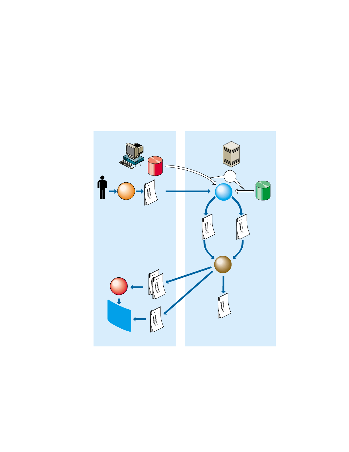
schematically in Figure 1-1. A description of the steps inherent in this figure follows.
Figure 1-1 Tool Execution Sequence
MineSet client MineSet server
Tool
manager
Configuration
file
Configuration
file
Visualization
tool
Visual
files
Data
file
DataMover User's
data
source
User
Visual
display
Inducer
(MIndUtil)
MODEL
Information & statistics
(error estimate)
OR

Basic Tool Execution Scenario
49
The following steps describe a “typical” interaction with a MineSet tool, and the
sequence of the tool’s actions. Depending on your requirements, some steps might be
skipped (for instance, if the data and configuration files have been generated in a
previous work session).
1. Start the Tool Manager, which is the graphical interface for generating and
specifying the configuration file, data file, and tools to be used. The Tool Manager
runs on your MineSet client.
2. The Tool Manager opens a network connection to the DataMover, which runs on the
MineSet server, which in some cases may be the same as your client workstation,
and in others is a separate machine.
3. Use the Tool Manager to specify
•the database and table, or a binary or ASCII flat file containing the data on
either the client or the server
•which mining or visualization tools are to be applied
•how that data is to be displayed, through tool options
•a session file to save the history of your work
Information retrieved via the DataMover is used to guide this interaction. As a
result, the Tool Manager generates a configuration file. This file contains the
user-defined parameters that determine the execution of the following steps.
4. The Tool Manager transmits a copy of the configuration file from step 3 to the
DataMover. The DataMover processes the file by
•accessing the database or flat file
•performing the specified data transformations
•running the mining tools when requested
•generating the visualization files when requested
These visualization files consist of your data in a specific format readable by the
MineSet tool. Then a copy of these visualization files is transferred to the MineSet
client.
5. The Tool Manager invokes the appropriate MineSet visualization tool.
6. The tool accesses the visualization files and displays the data.
7. If you generated a model, that model can be applied to additional data (see
Figure 10-5).

50
Chapter 1: Getting Started
Note: The MineSet client and server can run on different machines, using a network to
communicate. Because network bandwidth is often scarce, you should be cautious about
transferring large files between client and server regularly. If you are doing mining
operations on a large database or file, you can achieve greater efficiency by storing that
file on the server, where the DataMover runs, rather than on the client.

51
Chapter 2
2. Setting Up MineSet
This chapter describes how to set up MineSet, which requires configuring the
DataMover. The configuration has two parts:
•configuring the user’s account on the server (optional), and
•a global configuration, which usually is done by the system administrator
Parallelization is offered through the multiprocessor (n32) version of MineSet only. The
DataMover is a process that runs on the server, although it is not directly accessible to
users. The DataMover provides access to databases and data stored in flat files, and
transforms data for the mining and visualization tools. The last section of this chapter
describes how to load sample datasets into the supported relational databases.
Configuring the DataMover Server
In order to use the MineSet tools, two configuration files must be created on the server:
one by you, the other by the system administrator.
The User Configuration File
Note: You must have a UNIX account on every server you want to access.
The DataMover creates files on the server machine on behalf of each user. The
DataMover configuration file, .datamove, lets you control where these files are created and
whether different classes of files are saved or discarded. This file is located on the server,
in your home directory. A sample .datamove file called datamove.sample is located on the
server, in the /usr/lib/MineSet/datamove directory.

52
Chapter 2: Setting Up MineSet
If the .datamove file is absent, or if a particular entry is not present in the .datamove file, the
DataMover uses a default value for that entry.
Each entry in the DataMover’s configuration file must be on a separate line. For example:
file_cache = directory_name
where file_cache specifies the location in which the DataMover stores its output data files
and models resulting from mining algorithms. If the file_cache directory does not exist,
the DataMover attempts to create it on its first invocation. The default file_cache directory
is ./mineset_files/%U. The %U is a wildcard that is filled in with the user’s login name on
the client machine. This is useful in reducing contention if many users want to log in to
a common account on the server. If multiple sessions were simultaneously connected to
the same file_cache directory, they could overwrite each other’s server files, causing
incorrect and unexpected results. To prevent this, DataMover maintains a lock at the
file_cache directory level. The second and later attempts to connect to a particular
file_cache directory result in failure and an error message. The user can recover from such
a failure by killing one of the DataMover’s attempts to connect to a given file in the cache
directory.
The file_cache should be a directory in a file system with sufficient room to hold all of a
user’s output and temporary files. DataMover will create this directory if it doesn’t
already exist. These are deleted when the DataMover no longer needs them, unless one
of the following keep options is set:
keep_client_upload
keep_client_download
keep_classifier_files
keep_classifier_options_files
keep_mlc_input
use_ascii_mlc_input

Configuring the DataMover Server
53
Each of these entries is described below.
keep_client_upload (default no)
Keep files uploaded from the client for processing. If kept, they will be in the client_upload
subdirectory.
keep_client_download (default no)
Retain on the server a copy of data files and visualizations after they are downloaded to
the client. If kept, the files will be in the client_download subdirectory.
keep_classifier_files (default yes)
Keep the persistent classifiers (decision trees and so forth) generated by mining
operations. The tactic is generally useful.
keep_classifier_options_files (default no)
Keep the options file that is used when generating, or inducing the classifier. This tactic
is not useful. If kept, the files will be in the mlc_work subdirectory.
keep_mlc_input (default no)
Keep input files used for mining (MIndUtil or associations) operations. If kept, the files
will be in the mlc_work subdirectory.
use_ascii_mlc_input (default no)
Normally the DataMover creates MineSet binary files for MIndUtil input. If this option
is set, create ascii files instead.
aggregation_memory_limit (default 2147483647)
Memory limit (in bytes) for aggregation operations. This can be no larger than the
system-wide limit set in the dm_config file.
optimize_history=yes
The DataMover is able to rewrite histories to remove redundant computations. The
optimize_history parameter controls whether or not to do this. Since this rewriting can
speed up processing considerably, it is normally turned on.

54
Chapter 2: Setting Up MineSet
File Handling
A file in the file_cache directory is the result of a successful operation. If an operation
returns an error (that is, Tool Manager reports a message beginning “fatal error on
server,”) nothing should be changed in the file_cache directory. Two examples help
illustrate the point:
•Example 1: A user’sfile_cache directory contains the files cars.data and cars.schema,
both the result of a previous database query. The user then selects the same table,
and sets the output to server_file, filtering for examples with mpg>55. Since no
records in the dataset have mpg values this high, when the history executes, it
returns no rows, which is flagged as a fatal error. After this happens, the user’s
file_cache directory will still contain the old cars.schema and cars.data files.
•Example 2: A user’sfile_cache directory contains the files cars.data and cars.schema,
both the result of a previous database query. The user then selects the same table,
and sets the output to a visualization. The operation completes and the
visualization launches successfully. Once again, the user’sfile_cache directory still
contains the old cars.schema and cars.data files. The file_cache directory is not updated
unless the user specifically chooses server_file as the output.
Mandatory Configuration File
If you are using relational databases, the MineSet DataMover server must be configured
to find information in the databases. The DataMover works with Oracle® versions 7.2 or
later, INFORMIX®, and Sybase®.
The DataMover server reads the /usr/lib/MineSet/datamove/dm_config file during start up.
This file is not created by Inst during installation. It must be created by the system
administrator, who must log in as root to edit this file. It can be created via an editor such
as jot, vi, or Emacs. An example file can be found in
/usr/lib/MineSet/datamove/dm_config.sample. The format of this file is as follows:

Configuring the DataMover Server
55
Oracle {
"ORACLE_SID", "ORACLE_HOME";
}
Oracle_Remote {
“DATABASE_NAME”, “ADMIN_DIRECTORY”;
}
Informix {
"INFORMIXSERVER", "INFORMIXDIR";
}
Sybase {
"DSQUERY", "SYBASE";
}
Each optional entry describes the databases in use at your site. If your server is not
running any databases, that is, you intended to use MineSet with ASCII files only, simply
make an empty dm_config file.
The line "ORACLE_SID", "ORACLE_HOME" is filled in with the specific information and
repeated once for each Oracle database to be accessed via the DataMover. ORACLE_SID
and ORACLE_HOME are Oracle specific parameters defining an Oracle instance.
The Oracle_Remote section is for accessing remote Oracle databases via SQL*NET V2.
The DATABASE_NAME entry is a logical name for the remote database, as defined in a
tnsnames.ora file. The ADMIN_DIRECTORY entry is where DataMover searches for the
tnsnames.ora file. This file is described in Oracle’s SQL*NET documentation. Remote
access to databases is described in more detail in “Using MineSet to Connect to Remote
Databases” on page 58.
Each line in the Informix section defines a database server that, in turn, can contain
several databases. The server is checked at runtime to determine which databases it
contains, so there is no need to record the individual databases in the dm_config file. The
first entry is the INFORMIX server (corresponding to the INFORMIXSERVER
environment variable), and the second is the INFORMIX directory (corresponding to the
INFORMIXDIR environment variable).
Each entry in the Sybase section defines a database server (or, in Sybase terminology, an
SQL Server™). The first entry is the Sybase SQL Server name (corresponding to the
DSQUERY environment variable); the second is the Sybase home directory
(corresponding to the SYBASE environment variable).

56
Chapter 2: Setting Up MineSet
An example configuration file might be as follows:
Oracle {
"v73", "/usr/people/oracle/v73";
"wrhse", "/opt/oracle";
}
Oracle_Remote {
“lifeseq”, “/usr/lib/MineSet2/datamove/”;
}
Informix {
"learn_online", "/u5/informix";
}
Sybase {
"MINESET", "/usr/sybase/10.0.2.4";
}
This configuration file lets the DataMover access:
•three Oracle databases, one named v73 (installed in /usr/people/oracle/v73), another
named wrhse (installed in /opt/oracle), and a remote database named lifeseq,
•an INFORMIX Server;
•and a Sybase SQL Server.
Each of the INFORMIX and Sybase servers can, in turn, contain multiple databases.
For Sybase, DataMover uses vendor-supplied shared libraries as its connection to the
databases. One of the purposes of the dm_config file is to specify where DataMover must
look for its shared libraries. DataMover looks in the $SYBASE/lib/ directory for the
following shared libraries: libct.so,libcs.so,ibcomn.so,libintl.so,libtcl.so,libinsck.so.
Using MineSet With Existing Data Files
Sometimes it is convenient to use MineSet with data that is already stored as a file, but
requires further processing before it can be mined or visualized. In this case, the data file
can be made available (with a modest effort) to the Tool Manager/DataMover.
First, the data file must be in a tab-delimited format, with the same number of fields in
each line. A numeric or string field with a single “?” character appearing between
delimiters is loaded as a Null value.

Configuring the DataMover Server
57
For a detailed discussion of null values, refer to Appendix J, “Nulls in MineSet.”
The contents of the data file must be described to Tool Manager/DataMover via a file
with the .schema extension. The format of the .schema file is shown next:
#
# A line beginning with a "#" is a comment
#
input {
# The first line lists the data file which is described. It
# must be a simple filename, not a path.
file "carmodels.data";
# Fields are listed left to right in the line, legal
# types are float, double, int, string, date, fixedString and
# dataString
# Be sure to end every line with a semicolon ";"
float mpg;
int cylinders;
float cubicinches;
int horsepower;
int weightlbs;
double timeaccelerate;
date when_introduced;
string origin;
fixedString(3) manufacturer_code;
dataString model;
}
The schema and data files must be located in the same directory. If you prepare a dataset
in this fashion on the client machine, it can be opened with the Tool Manager’sFind File
dialog. If the file requires any additional processing, it is copied to the server. Sometimes
this is not convenient, especially if the file already exists on the server, or is large. In this
case, the .schema and .data files must be copied (or symbolically linked) into your file_cache
directory on the server. The directory used as the file cache is specified in your .datamove
file; the default is ./mineset_files/%U, where %U becomes your login name on the client
machine.
For a more extended description of MineSet .schema files see Appendix A.

58
Chapter 2: Setting Up MineSet
Using MineSet to Connect to Remote Databases
Sometimes it might not be feasible to install DataMover on the machine running the
database server. In this situation, DataMover can be installed on an intermediate server,
and DataMover then can use the database vendor’s networking facility to connect to the
remote database. (This sometimes is referred to as a three-tier architecture.)
Oracle
MineSet supports two ways to access remote Oracle databases:
•The remote database is specifically mentioned in the dm_config file. For this method,
add entries to the Oracle_Remote section of the dm_config file, as described in the
“Mandatory Configuration File” section, above. Every remote database named in
the dm_config file must be defined in the tnsnames.ora file. This file can be manually
edited, or, more commonly, generated automatically by a network administration
tool provided by Oracle. If this method is chosen, the only Oracle-specific file
needed on the DataMover server is tnsnames.ora; in particular, Oracle need not be
installed on this machine.
•A local Oracle install is used as a gateway to a remote database. In this case, the
dm-config file requires an entry for the local Oracle install, with ORACLE_HOME and
ORACLE_SID. This entry must be in the Oracle, not Oracle_remote section. Entries
for any remote databases must be added to the
$ORACLE_HOME/network/admin/tnsnames.ora file of the Oracle install on the
intermediate server.
Then, when users want to log in to user “system”, password “manager” at database
“remotedb”, they must provide the name of the intermediate server for the Tool
Manager “Log on to server...” dialog and select the intermediate server’s Oracle
database. When logging in to the database, use system@remotedb for the database
username, and manager for the password. (The added @remotedb specifies that
Oracle must use SQL*Net™ to connect to the remote database, instead of using a
local connection.)
Operating across SQL*Net is substantially slower than a local connection, especially for
queries that return a large amount of data. If possible, install DataMover on the same
machine as the Oracle server.

Loading Sample Datasets
59
Sybase
A Sybase installation is required on the intermediate DataMover server; this Sybase
installation need not be running an active database, but it is needed for access to the
shared libraries and the interfaces file.
In order to access the Sybase SQL server running on the remote machine, the interfaces
file on the DataMover server machine must have an entry for this Sybase SQL server.
Please refer to your Sybase manuals for the procedure for creating such entries. Also, the
name of this Sybase SQL server on the remote machine must be included in the dm_config
file on the intermediate DataMover server machine.
Once this setup is done, access to the Sybase SQL server on the remote machine is
handled transparently. The user can choose it and access data from it just like any other
database source, using the panels from the Tool Manager.
Loading Sample Datasets
This section describes how to load the sample datasets included with the MineSet
distribution into one of the supported relational databases.
Installed on the server in /usr/lib/MineSet/DBexamples are
•all the sample data, along with a brief description of what it contains.
•directions on how to load the data using the provided scripts.
Load the sample datasets into a database that has been set up on your server. The data
and these directions (README.server) are installed in /usr/lib/MineSet/DBexamples on the
server.
The /usr/MineSet/DBexamples directory contains scripts for loading the complete set of
data files into one of the supported databases. To load the complete set of data, run one
of the following loader scripts, depending on which database you have. (This assumes
your database and environment are already set up.)
sh load_all_Oracle.sh <userid> <passwd>
sh load_all_Sybase.sh <userid> <passwd>

60
Chapter 2: Setting Up MineSet
If you are going to work with an INFORMIX database, use the dbaccess interface to
select
create_all_Informix.sql
followed by
load_all_Informix.sql
Loading Individual Datasets
Alternatively, you can load, or reload, the sample data separately. Each data directory in
/usr/lib/MineSet/DBexamples on the server contains files necessary to load the data into
any of the supported databases. These files are:
README - explains the data
*.sql - sets up an Oracle table
*.ctl - control file for loading into Oracle
*_syb.sql - sets up a Sybase table
*.bcf.fmt - Sybase format file
*_inf.sql - sets up an INFORMIX table
*_load.sql - loads the data into the INFORMIX table
In the *.ctl file, the separator is declared in the line
" fields terminated by X'20' "
The separator is specified in ASCII hexadecimal; thus:
X'20' is used for ‘ ’
X'2c' is used for ‘,’
X'09' is used for ‘\t’

Loading Sample Datasets
61
Loading Into Oracle
Perform the following steps on the server with an Oracle database:
1. Ensure the following environment variables are set correctly:
ORACLE_HOME
ORACLE_SID
2. Type
sqlplus <userid>/<passwd>
SQL> @<dataset>.sql
Where dataset is the name of the dataset being loaded, and userid/passwd are your
assigned username and password for the Oracle database.
To delete an already existing table, type
SQL> drop table <dataset>;
3. Type
sqlload control = <dataset>.ctl userid = <userid>/<passwd>
log = /tmp/<dataset>.log direct = true
4. Check the resulting dataset.log to ensure the data was loaded correctly.
Loading Into Sybase
Perform the following steps on the server with a Sybase database:
1. Ensure that the following environment variables are set:
SYBASE
DSQUERY
2. To create the table, type
isql -U<userid> -P<passwd> -i <dataset>_syb.sql
Where dataset is the name of the dataset being loaded, and userid/passwd are your
assigned username and password for the Sybase database.
To delete an already existing table, type
isql -U<userid> -P<passwd>
drop table <dataset>
go

62
Chapter 2: Setting Up MineSet
3. To load the data, type
bcp <dataset> in <dataset>.data -U<userid> -P<passwd> -f
<dataset>.bcp.fmt
where dataset is the table name (created using <dataset>_syb.sql),in means
"load into the dbms," <dataset>.data refers to the name of the ASCII data file, and -f
points to the already-created format file. (When reading in from a file, the data types are
character.)
Loading Into INFORMIX
Perform the following steps on the server with an INFORMIX database:
1. Ensure the following environment variables are set:
ONCONFIG
INFORMIXSERVER
INFORMIXTERM
2. To create the table, type
dbaccess
3. If necessary, log into the appropriate database.
4. Choose Query-language, then choose the appropriate database from those listed.
5. Choose <dataset>_inf.sql, and run it.
6. Choose <dataset>_load.sql, and run it (where <dataset> is the name of the dataset
being loaded).

63
Chapter 3
3. The Tool Manager
This chapter discusses the functions of the Tool Manager, which is the graphical user
interface (GUI) that lets you specify data and configuration information for the MineSet
tools in this package. It provides an overview of this interface, then describes every
component of each panel that this interface displays for all MineSet tools.
Note: Any screens dedicated to a specific tool are discussed in the chapter for that tool;
for example, the screen for specifying the Tree Visualizer’s configuration file is discussed
in Chapter 5, “Using the Tree Visualizer.”
Overview
The Tool Manager is the initial graphical user interface (GUI) you use for most of your
interactions with the MineSet components. With Tool Manager you can select an existing
data source, transform or analyze that data, and visualize the results using any of the
MineSet individual tools. You can step through the process in these sections:
•“Connecting to an Existing Data Source”
•“Transforming the Data”
•“Visualizing the Data on the Screen”
Note: The Tool Manager generally does not support data files not created by the Tool
Manager without some manual work to make them compatible.

64
Chapter 3: The Tool Manager
Connecting to an Existing Data Source
You can specify the source of the data as being from a:
•database table
•database SQL query
•file
Transforming the Data
Often the original data is unsuitable for mining or visualization. It may contain irrelevant
or redundant columns, data types that are not applicable for viewing, or inconsistencies
that result in unhelpful visualization. You can transform the data with the Tool Manager
to display it in a useful form in any of these ways:
•mining tools—finds patterns in data
•binning variables—discretizes column values into groups, such as grouping years
by decade
•removing columns—excises unneeded columns to save space
•adding new columns—creates columns that are functions of existing columns
•aggregation—finds the average, sum, min, max, or counts of column values
•filtering—selects a subset of the data based on an expression using column values
•sampling—selects a random subset of the data
•making arrays—takes the values of one column and turns them into an array
indexed by discrete values in another column
•distributing columns—makes two or more new columns from a single column of
values, distributed by the discrete values of another column

Overview
65
Visualizing the Data on the Screen
The final step, having transformed the data, is to visualize the results.You can do this in
any of these ways; for example you can display the data on the screen as:
•a hierarchy (Tree Visualizer—Option, Decision, Regression)
•a map (Map Visualizer)
•a scatter plot showing relations of numerous independent variables (Scatter
Visualizer and Splat Visualizer)
•as associated rules (Rules Visualizer)
•as evidence and probability (Evidence Visualizer)
•as box plots and histograms (Statistics Visualizer and Cluster Visualizer)
•as layered tables or cakes (Decision Table)
With Tool Manager you can map data values to specific visual elements on the screen
such as:
•colors
•bars
•heights
Finally, Tool Manager lets you control those options not related to data, including:
•background colors
•grid spacing
•label sizes

66
Chapter 3: The Tool Manager
Starting the Tool Manager
You can run the Tool Manager in two modes:
•interactive mode—the Tool Manager provides windows, menus, buttons, and so on,
to let you access, mine, and visualize your data. Interactive mode also lets you save
a description of your actions to a “session file” for future use.
•batch mode—the Tool Manager performs all the actions described in a session file
without bringing up windows. For example, batch mode is useful for lengthy
computations that need to be done every night, so that the data can be fully
prepared each morning.
There are three ways to start the Tool Manager in interactive mode:
•Double-click the MineSet icon, which is in the Applications or the MineSet page of
the icon catalog. The Tool Manager starts with the same configuration used in the
last Tool Manager session.
•Double-click an icon representing a session file saved from a previous invocation of
the Tool Manager. This starts the Tool Manager with that session file.
•Start the Tool Manager from the UNIX shell command line by entering this
command at the prompt:
mineset [ sessionFile ]
Here, sessionFile is optional and specifies the name of the session file to use. If
you do not specify a configuration file, MineSet starts up with the configuration
most recently used.
To start the Tool Manager in batch mode, enter this command at the UNIX shell prompt:
mineset_batch [-s serverPassword -d databasePassword]sessionFile
The -s and -d options allow you to specify the password for logging into the server and
database respectively. If you do not specify these options, mineset_batch will ask you to
type in the passwords, thus these options are useful when running mineset_batch from a
shell script. To specify that there is no password for either the server or database, use -s
or -d followed by two double quotes, that is,
mineset_batch -s "" -d "" foo.mineset
If you specify one of the two passwords, you must specify both.
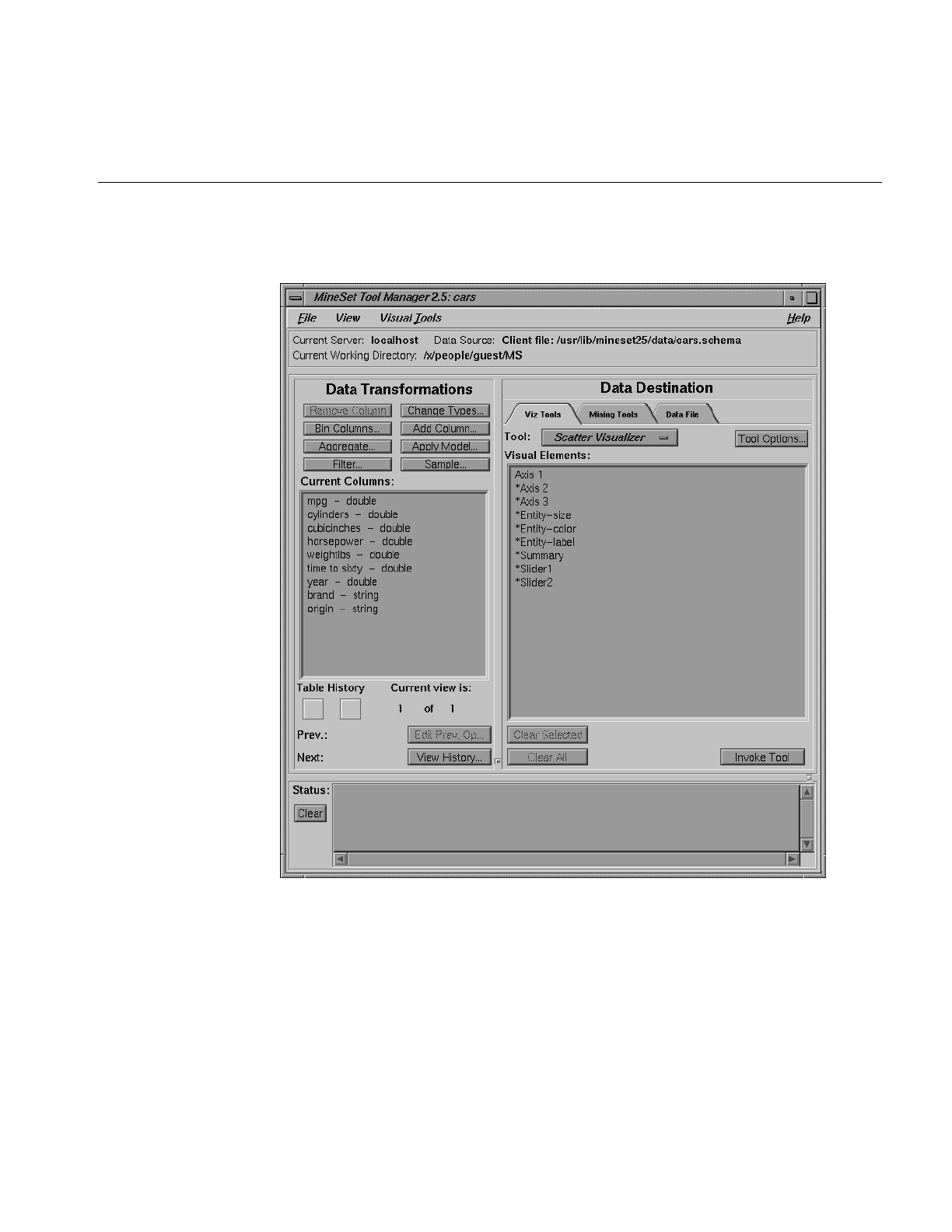
Starting the Tool Manager
67
Figure 3-1 shows the Tool Manager’s startup window.
Figure 3-1 The Tool Manager Startup Window
This window consists of two panels related to the specific dataset and tool chosen, and
two information sections. Specification of servers and data sources is done via popup
dialogs accessible from the File menu.
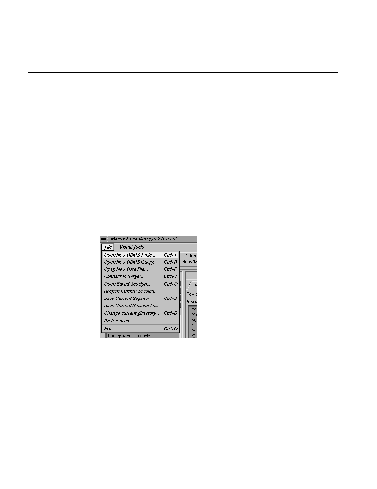
68
Chapter 3: The Tool Manager
The panels and information sections are
•Data Transformations, which lets you modify the data from your data source.
•Data Destination, which lets you create visualizations based on your data, save the
data to a file, mine the data for association rules, create classifiers based on the data,
or find important columns in the data.
•The top panel, which provides information on the currently selected data source.
•The bottom panel, which contains a stream of information on the status on certain
operations.
The following sections describe each panel of the main Tool Manager window.
Choosing a Data Source
Data sources are selected using the first set of menu items in the File menu.
Figure 3-2 File Pulldown Menu

Choosing a Data Source
69
The first three options in the File menu let you select the data source from a
•DBMS Table
•DBMS Query
•Data File
The fourth option, Connect to Server, lets you connect to a server without specifying the
data source.
You must connect to a server to get information from a database or mining tool, or to
apply transformations to an existing data file. It is not necessary if you plan to visualize
an existing client data file without transforming it.
Choosing an Existing Data File
Use the Open New Data File menu option to work with an existing data file. When you
select this option, the dialog in Figure 3-3 appears.
Figure 3-3 Open New Data File Dialog Box

70
Chapter 3: The Tool Manager
This dialog box, which is similar to a standard file selection dialog box, provides a toggle
at the top to select client versus server files; it also has a label indicating the name of the
current MineSet server, and a push button to let you log in to a new server. The radio
buttons at the top let you select files on your client machine (in any directory accessible
to you) or files that exist in your single cache on the DataMover server, (see “Configuring
the DataMover Server” in Chapter 2.)
When you select the name of a file from the list in the left window, the columns of that
data file are shown in the right window.
When you click the Change Server button, a dialog prompts you for a server name, login
name, and password to connect to the server (see Figure 3-5).
If you want to access a data file created outside of Tool Manager, you must create a
.schema file for it. This is a text file containing a configuration “input” section, which gives
the name of the data file and describes its layout. The Tool Manager supports input
sections similar to those for the Tree Visualizer (described in Appendix B), except that it
does not support variable length arrays or the monitor option.
Choosing a Database Table
Use the Open New DBMS Table menu option to work with tables in a DBMS. Selecting
this option causes the dialog box in Figure 3-4 to be displayed.
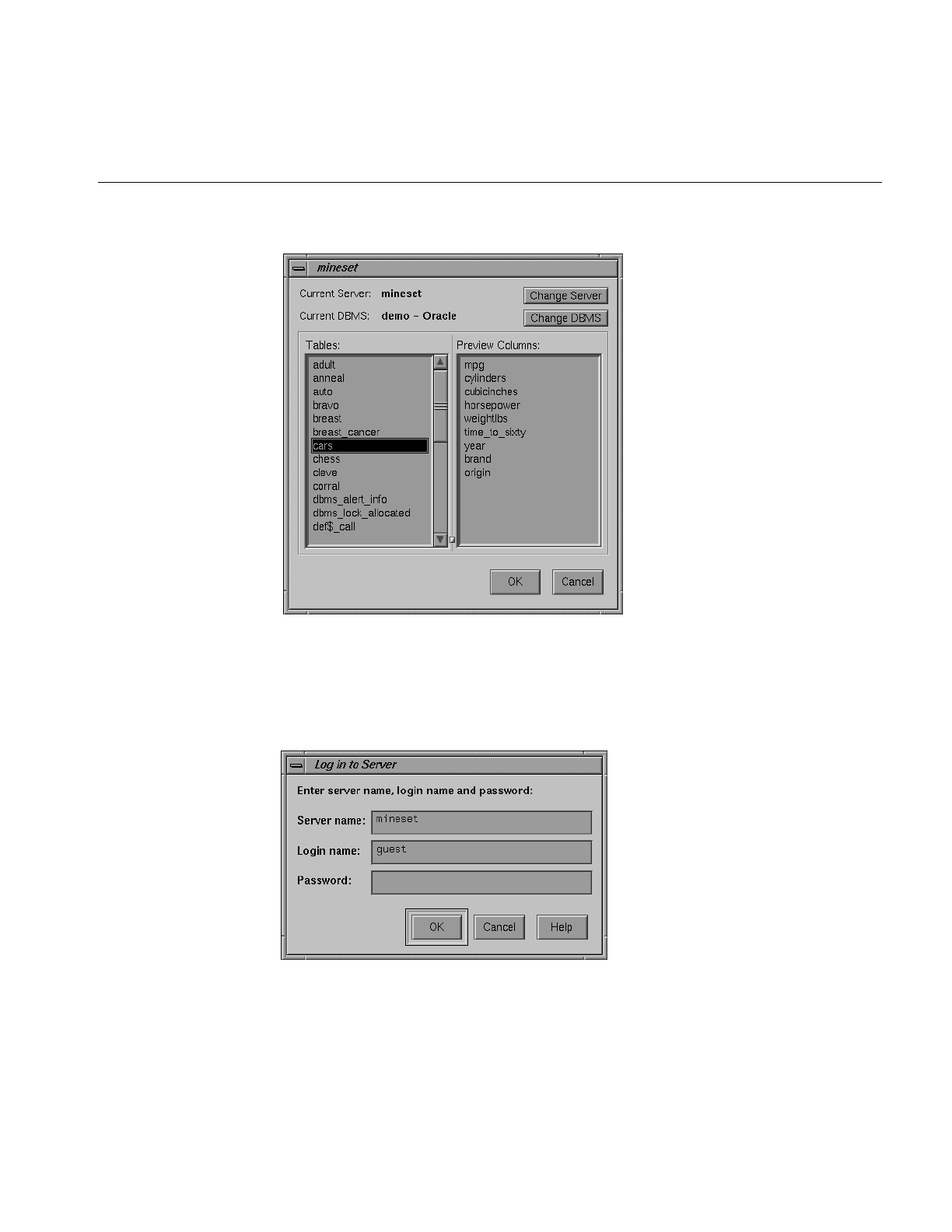
Choosing a Data Source
71
Figure 3-4 Choosing New Database Table Dialog Box
The name of the currently selected server appears to the left of the Change Server button.
If you click this button, the dialog box shown in Figure 3-5 appears. This lets you specify
a server name, login, and password.
Figure 3-5 Specifying Server Name, Login, and Password
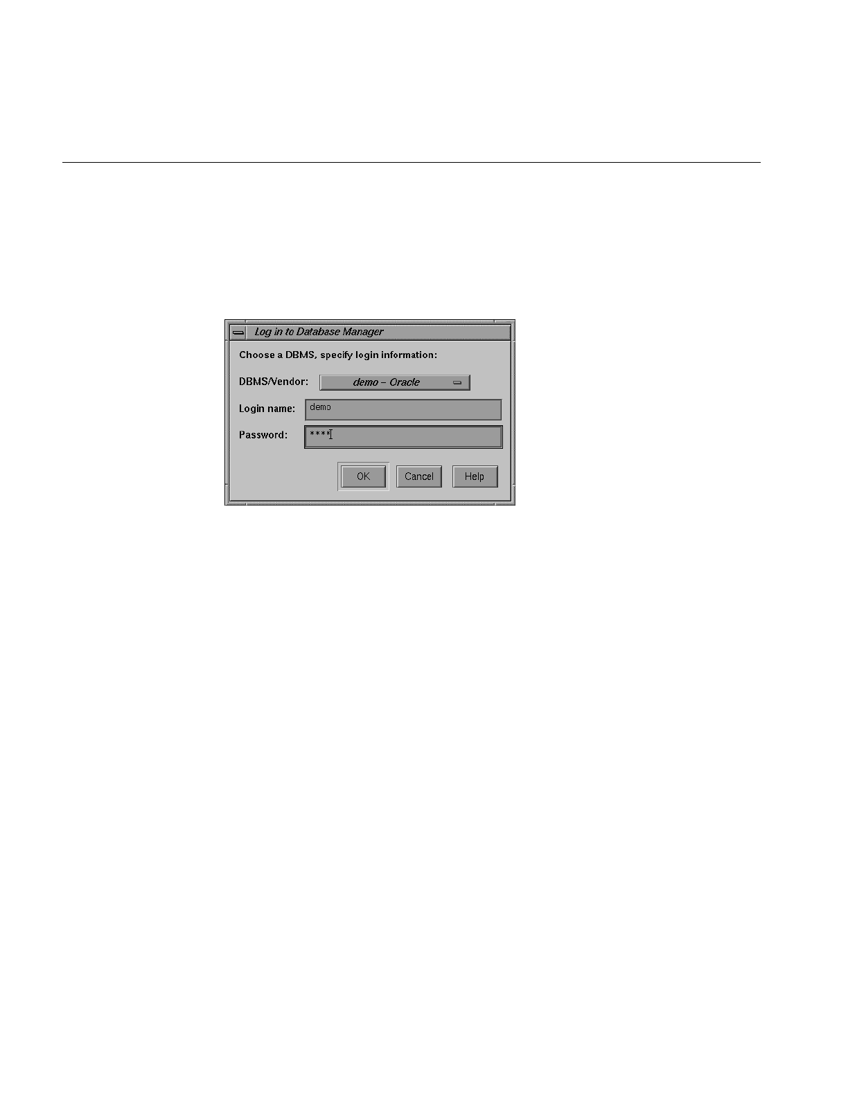
72
Chapter 3: The Tool Manager
Once you have logged in to a server, click the Change DBMS button to bring up a dialog
box that contains a popup menu listing DBMS names/vendors (see Figure 3-6). Select a
DBMS from the menu, and enter the login name and password to connect to the DBMS.
Note that the DBMS login and password are usually different from those required to
connect to the server.
Figure 3-6 Sample Dialog Box Listing Available DBMS Names/Vendors
If you have logged on to an Oracle DBMS, the dialog box appears as shown in Figure 3-4,
with a list of tables on the left. When you select a table, the columns for that table are
shown on the right.
If the DBMS is Informix or Sybase, the dialog box shown in Figure 3-7 appears, with a list
of databases for the DBMS. Select a database, and the list of tables in that database are
shown.
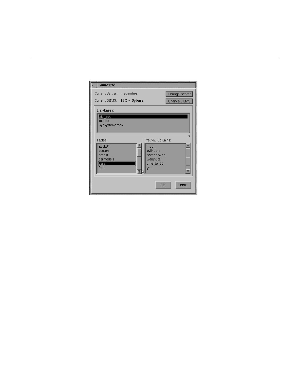
Choosing a Data Source
73
Figure 3-7 Dialog Box After Selecting Informix or Sybase DBMS
To use a certain table in the Tool Manager, select the table you want to use and click OK.
Running an SQL Query
Use the Open New DBMS Query menu option to work with tables created via SQL
queries against a DBMS. Selecting this option causes the dialog box in Figure 3-8 to
appear.
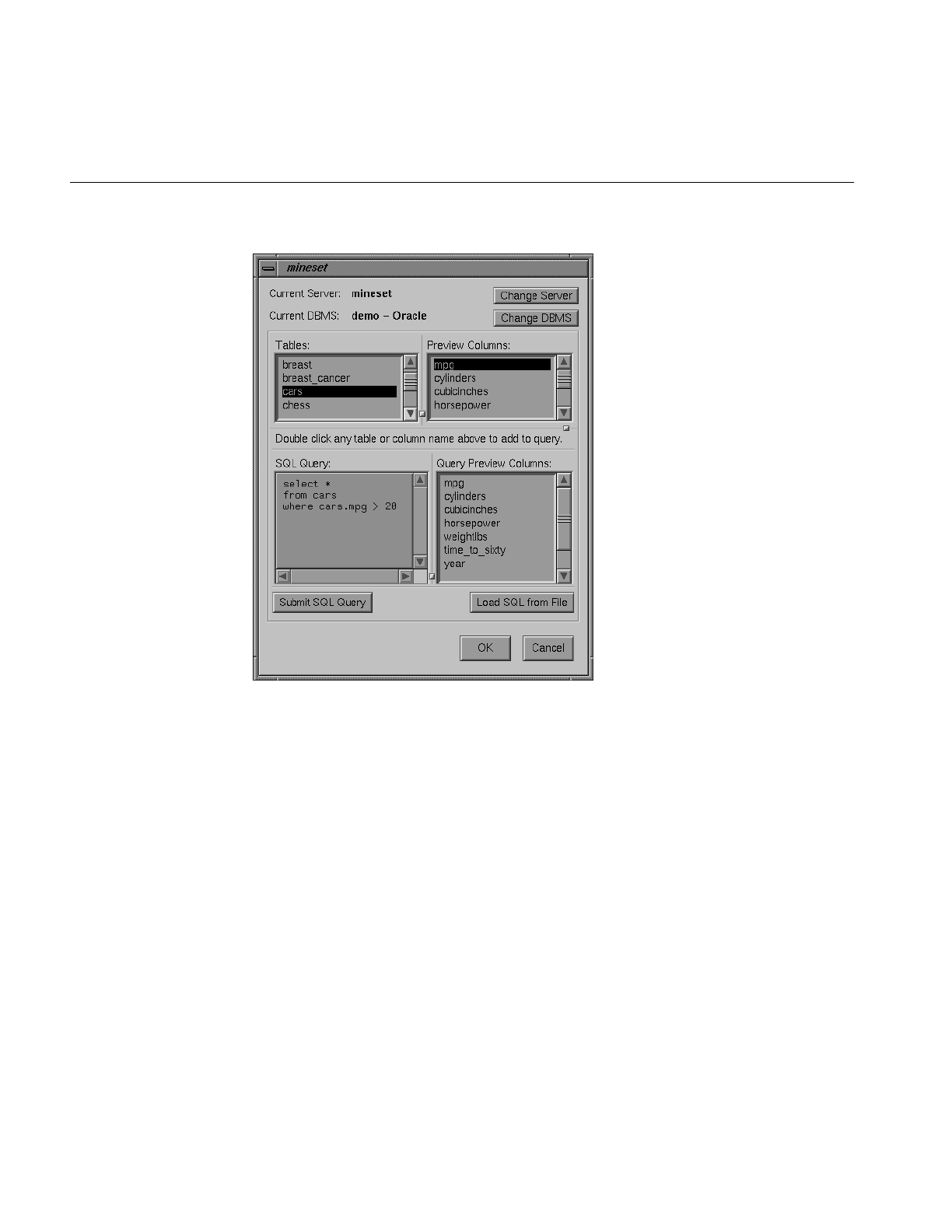
74
Chapter 3: The Tool Manager
Figure 3-8 SQL Query Dialog Box
Selecting a server and DBMS in this dialog box has the same effect as selecting those
items in the Open New DBMS Table dialog box.
The SQL query is shown in the panel at the lower left. You can enter the query there, or
load it from a disk file using the Load SQL from File button. The names of tables and
columns in the current DBMS are shown to help build queries. To have their names
transferred to the SQL query panel, double-click on them.
When you have entered the SQL query, click the Submit SQL Query button to send it to
the DBMS for execution. The table columns resulting from the query appears on the
right.
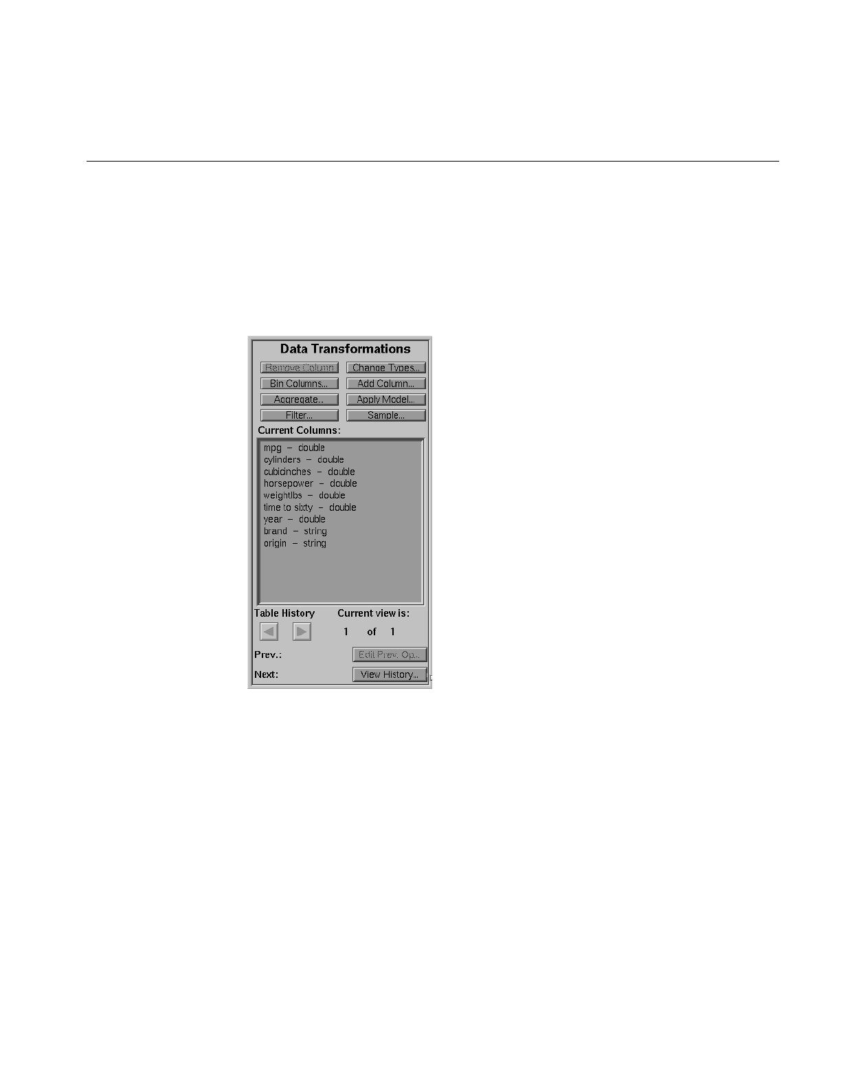
Transforming the Data
75
Transforming the Data
The Data Transformations panel lets you manipulate the tables with which you want to
work. After you have selected a table (via the File menu, described above), its column
headings appear in the Current Columns window of the Data Transformations panel
(Figure 3-9).
Figure 3-9 The Data Transformations Panel
The functions of the displayed options are:
•Remove Column—lets you delete one or more columns that are not relevant to the
current visualization or mining.
•Bin Columns—lets you assign each record to a group that falls within a certain range
(bin) of column values. For example, an age column may be binned into the ranges
(bins): 0-18, 19-25, 26-35, and so on.

76
Chapter 3: The Tool Manager
•Aggregate—adds columns of records (sum), creates a new column representing
maximum or minimum values, or makes an array from a column that is indexed by
other columns.
•Filter—lets you select a subset of the data based on an expression involving column
values, for example, leave only those records in which the age is less than 20.
•Change Types—lets you change a column’s name as well as its type.
•Add Column—lets you add a new column based on a mathematical expression. For
example, add a column “minor” based on the column “age,” using the expression:
“if age is less than or equal to 18 then minor is true; else minor is false.”
•Apply Model—lets you use a previously created classifier to label new records, to
estimate probabilities for label values, to test the classifier on new data, or to backfit
data to an existing classifier (see Chapter 10, “MineSet Inducers and Classifiers,” for
details).
•Sample—lets you select a random subset of the data. This is useful for very large
data sets.
The Remove Column Button
Remove Column lets you delete columns by selecting the column name or names in the
Current Columns panel, then clicking this button. The items in the Current Columns panel
change to show the new table columns. To choose multiple contiguous columns for
simultaneous removal, click and drag the mouse over the columns. To choose multiple
non-contiguous columns for simultaneous removal, hold down the Ctrl key while
selecting the additional columns.
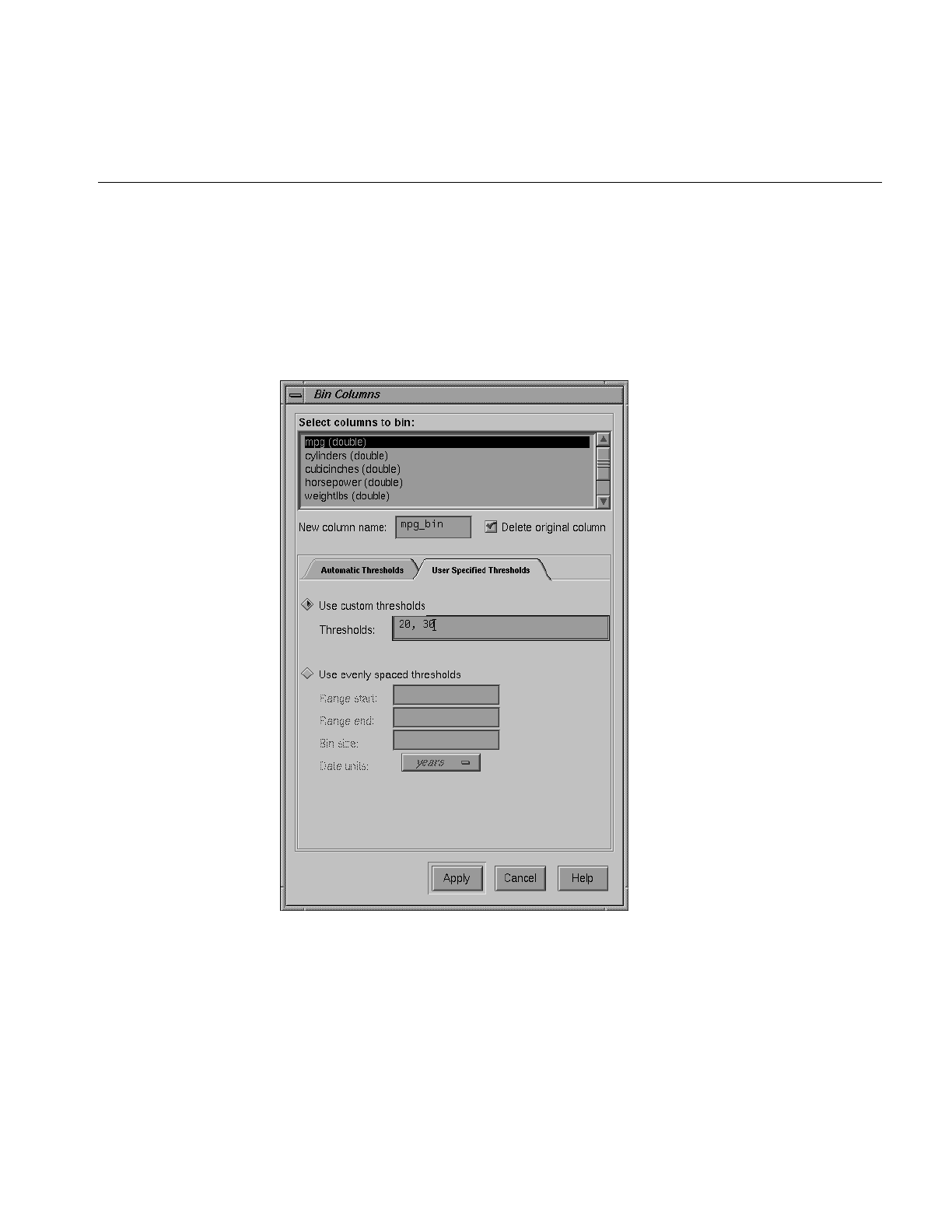
Transforming the Data
77
The Bin Columns Button
Binning lets you sort the information from one or more columns into groups in a new
column or columns (for example, with a range of ages, 0-18, 19-25, 26-35, and so on).
Click Bin Columns to get a dialog box that lets you specify the binning options
(Figure 3-10).
Figure 3-10 Bin Columns Dialog Box

78
Chapter 3: The Tool Manager
This dialog box lets you
•choose the column that is to be divided into bins
•specify the name of the new column to contain values for the bins
•set bin thresholds, or specify a range with thresholds at regular intervals
To specify binning options for one or more columns, select the column name(s), choose
the appropriate options below, and click the Apply button at the bottom of the dialog box.
If you select only one column for binning, the name of the resulting binned column
appears in the “New column name” box, and you can type in a new name if you like. In
the example shown in Figure 3-10, mpg_bin is the name for the new column; in this case,
it provides a range of fuel efficiencies. If you select more than one column for binning,
New column name stays inactive.
Next to New column name is a check box labeled “Delete original column”. When
chosen, this option automatically deletes the original column after binning. Click the
check box to turn this function on or off.
In the middle of the Bin columns dialogue box are two tabs for choosing Automatic
Thresholds or User Specified Thresholds. Choose Automatic Thresholds if you’d like the
computer to suggest the bins or User Specified Thresholds if you’d like to specify the
thresholds yourself.
Automatically Computed Thresholds
If you’ve chosen the Automatic Thresholds tab, the program can use machine learning to
suggest bins.
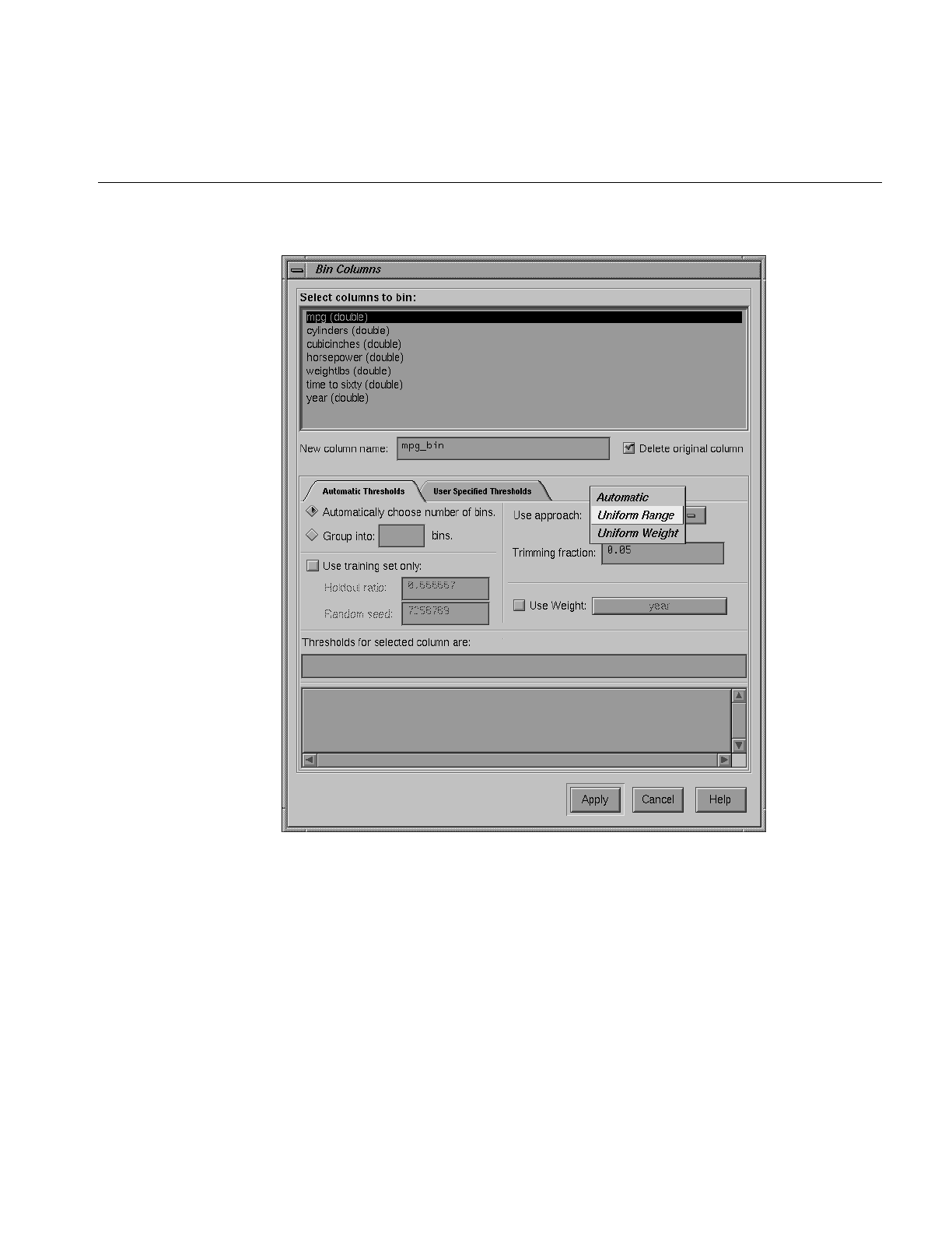
Transforming the Data
79
Figure 3-11 Binning With Automatically Computed Thresholds

80
Chapter 3: The Tool Manager
The first choice under Automatic Thresholds is between the Automatically choose number
of bins and the Group into: ___ bins buttons. Click Automatically choose number of bins to let
the computer decide the best number of bins. If you choose to specify the number of bins,
click Group into: ___ bins, and type the number of bins you want into the field.
There are three ways to categorize data into bins:
•Automatic—you must also select a discrete label. The thresholds are chosen so that
the distributions of labels within different bins are as different as possible. This
approach continues to create thresholds that split the range until no additional
interval is considered significant.
The “Min weight per bin” text field lets you specify the minimum weight in any bin;
this prevents the creation of bins with less weight than the number specified. No
interval is split if the two resulting subintervals do not each contain at least the
minimum weight you specify. By default, each instance has unit weight. In this
situation, specifying the Min weight per bin is the same as specifying the minimum
number of instances per bin.
Rather than specifying the minimum weight per bin, it is possible to have the
algorithm set that value automatically. The check box labeled Auto causes the
algorithm to calculate a value for the minimum weight per bin based on the total
weight of the instances: the more total weight, the higher the minimum weight per
bin (the relationship is logarithmic).
•Uniform Range—the algorithm divides the value range into the specified number of
uniformly sized subintervals. The upper and lower bounds for the extreme ranges
include any values outside the ranges observed in the data. For example, if the
values for an attribute are in the range 3-8, and you specify four bins, the thresholds
identified are 4.25, 5.5 and 6.75, corresponding to the ranges:
•≤4.25
•> 4.25 to 5.5
•> 5.5 to 6.75
•> 6.75
•Uniform Weight—the algorithm divides the value range into the specified number of
equal weight bins. Unlike Uniform Range, in which thresholds are identified that
separate the value range into intervals of equal size, Uniform Weight identifies
thresholds that group the instances into subsets of equal weight. By default, each
instance has unit weight. In this case, the Uniform Weight approach produces the
specified number of bins, each containing an approximately equal number of
instances.

Transforming the Data
81
Both Uniform Range and Uniform Weight let you specify a trimming fraction, which
indicates the fraction of extreme values to be excluded from the value range prior to
generating bins. The default trimming fraction is 0.05. This excludes the 5% of the
instances with the most extreme values (2.5% with the lowest values in the range, and
2.5% with the highest values in the range). Trimming tends to reduce the influence of
outliers on the generation of thresholds.
All of the approaches let you decide whether you want to specify the number of bins or
let the algorithm select the number automatically. For the Uniform Range and Uniform
Weight approaches, the automatic selection of the bins is based on the number of distinct
values: the more distinct values, the more bins are chosen (the relationship is
logarithmic).
Typically, all of the available instances are used when identifying thresholds. When
binned attributes are later used to induce a classifier, the error estimates for that classifier
tend to be overly optimistic. This is because distributional information from the test set
was used to identify thresholds. Use training set only prevents the binning approaches
from looking at the records in the test set when identifying thresholds. This tends to give
a more realistic estimate of the classifiers' error rate. Use training set only requires the user
to specify the same Holdout ratio and Random seed (see “Error Options for Inducers” in
Chapter 10) that are used to create the holdout set for estimating classifier error.
The Use Weight menu lets you weight the instances by any numeric attribute. Changing
instance weight affects both Automatic and Uniform Weight, but has no affect on the
Uniform Range.
If you click Apply, the Tool Manager picks bin thresholds and displays them in the
“Thresholds for selected column are” text field. The text field at the bottom of the Bin
Columns window shows the progress of the binning algorithm and any errors that occur.

82
Chapter 3: The Tool Manager
Specifying Thresholds
If you specify your own thresholds (as shown in Figure 3-10), you can choose between
Use custom thresholds or Use evenly spaced thresholds by clicking either button. When you
type in the thresholds, you must click Apply to make those thresholds effective for the
selected columns.
The Use custom thresholds text box lets you enter the range criteria. For example, you
could enter the numbers 18, 30, 50, 60. This results in the following ranges: 0-18, 19-30,
31-50, 51-60, 61+. Note that you enter only the digits and commas, not the ranges.
To specify equally spaced bins over a range of values, click the Equally Spaced Bins button.
This activates the three text fields below it. You can type the start of the binning range,
the end of the range, and the spacing of the bins, respectively, into these fields. If you are
binning a column that is a date, you can specify units of time for the bin spacing (using
the “Date units” popup menu under the text fields). This would permit you, for example,
to bin a time period into bins of three weeks. Dates entered into these fields must be
typed in the form “MM/DD/YY”. Possible time units are as follows:
•years
•quarters
•months
•days
•hours
•minutes
•seconds
The Use custom thresholds text box accepts dates either in double quotes (as shown below),
or without. If you enter dates without quotes, the quotes are added automatically.
"1/1/96", "2/1/96", "3/1/96", "4/1/96", "5/1/96", "6/1/96"
However, do not put quotes around dates used with Use evenly spaced thresholds.
Note: If you enter an invalid parameter, an error message is displayed after you click
Apply, informing you of the valid options and letting you either cancel the command or
return to the dialog box to make the appropriate changes.

Transforming the Data
83
Aggregation
Before describing the features and effects of the Aggregate button (see page 86), this
section provides an introduction to the concept of arrays and distribution as used in the
aggregation feature.
Introduction to Arrays and Distribution
The Aggregate button lets you perform simple aggregations (for example, sum, min, max,
and so on), make arrays, and distribute columns. (See Table 3-1)
If you make Total $ Spent into an array indexed by the binned column Age_bin, the
resulting table has only two columns:
In this case, making an array reduces the number of columns by one, and also reduces
the number of rows by four. Arrays are useful for the Tree Visualizer tool; they are
necessary if you want to use sliders in Scatter Visualizer and Map Visualizer displays.
Table 3-1 Aggregate Example 1
State Age_bin Total $ Spent
CA 0-20 $50
CA 21-40 $454
CA 41-60 $693
NY 0-20 $35
NY 21-40 $541
NY 41-60 $628
Table 3-2 Aggregate Example 2
State Total $ Spent [Age_bin]
CA [$50, $454, $693]
NY [$35, $541, $628]

84
Chapter 3: The Tool Manager
Distributing columns is similar, but different in several important ways. Instead of
producing a single new column holding many values, distributing produces one new
column for each value of the index. For example, if in the first table was not made an
array, but instead distributed by Age_bin, the result is:
Thus, distributing increases the number of columns but decreases the number of rows.
If you have more than one binned column (for example, Age_bin and Sex_bin), you can
make a two-dimensional array (indexed by combinations of Age_bin and Sex_bin). You
also can distribute and make an array at the same time.
This table has two binned columns: one for age, one for sex.:
If you make Total $ Spent an array indexed by age, and remove Sex_bin, the results are:
Table 3-3 Aggregate Example 3
State Total $_0-20 Total $_21-40 Total $_41-60
CA $50 $454 $693
NY $35 $541 $628
Table 3-4 Example of Binning
State Age_bin Sex_bin Total $ Spent
CA 0-20 1 $20
CA 0-20 2 $30
CA 21-40 1 $220
CA 21-40 2 $234
CA 41-60 1 $401
CA 41-60 2 $292
Table 3-5 Results When Making Total $ Spent an Array
State Total $ Spent [Age_bin]
CA [$50, $454, $693]

Transforming the Data
85
If you do not remove Sex_bin, the results are:
If you make an array by both Age_bin and Sex_bin, the results are:
Finally, if you distribute by Sex_bin and index by Age_bin, the results are:
The examples above (with the exception of Table 3-5) had exactly one relevant value for
each array element, and the distribution merely rearranged existing data values. For the
example in Table 3-5, there were two data values for each array element, and these were
summed. MineSet provides several aggregation options for datasets containing more
than one value to be distributed into a given output array element. The most common
option is to add the values (as done in Table 3-5). This is useful when accumulating
expenditures into budgets, for example. You also can take the minimum, maximum, and
average of the total number of values, as well as count them.
When distributing values for a given dataset, it is possible that there are no values
appropriate for a particular bin. In this case, for min, max, avg, and sum aggregations, the
DataMover fills in a value of NULL. For count aggregations, the DataMover fills in a
value of 0.
Table 3-6 Results When Specifying Sex_bin
State Sex_bin Total $ Spent [Age_bin]
CA 1 [$20, $220, $401]
CA 2 [$30, $234, $292]
Table 3-7 Results of Making an Array by Age_bin and Sex_bin
State Total $ Spent [Age_bin] [Sex_bin]
CA [$20, $220, $401, $30, $234, $292]
Table 3-8 Results of Distributing Sex_bin and Indexing by Age_bin
State Total $ Spent [Age_bin], Sex = 1 Total $ Spent [Age_bin], Sex = 2
CA [$20, $220, $401] [$30, $234, $292]
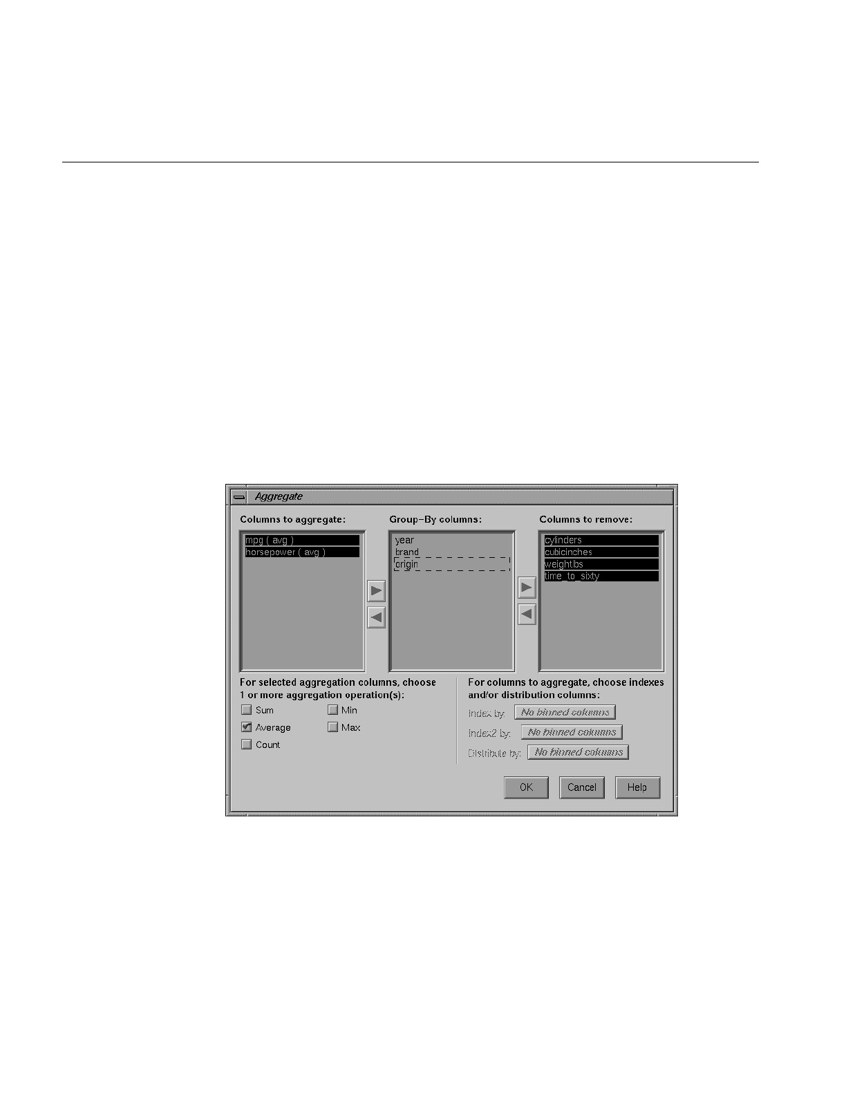
86
Chapter 3: The Tool Manager
The Aggregate Button
You can use the Aggregate button to create simple aggregations, make arrays, or
distribute columns. Clicking this button causes the Aggregate dialog box to appear
(Figure 3-12). It shows three lists, with the columns in the current table appearing in the
middle list. If you want to aggregate, distribute, or turn a column into an array, select the
name of the column, and click the left arrow button between the left and center lists.
Below are popup menus that let you specify indexes (if the result is to be an array) and a
distribution column (if the result is to be distributed). In addition, at the bottom of the
dialog box are five toggles that let you specify how different values are to be combined
when aggregated: either summed, averaged, the min or max value, or the count. When
you are aggregating number-valued columns, you can choose any combination of these
options. For other types, only count is permitted. If you choose more than one option,
you get more than one result. For example, selecting average and max gives you one
result with average values, and another one holding the max values.
Figure 3-12 Aggregate Dialog Box
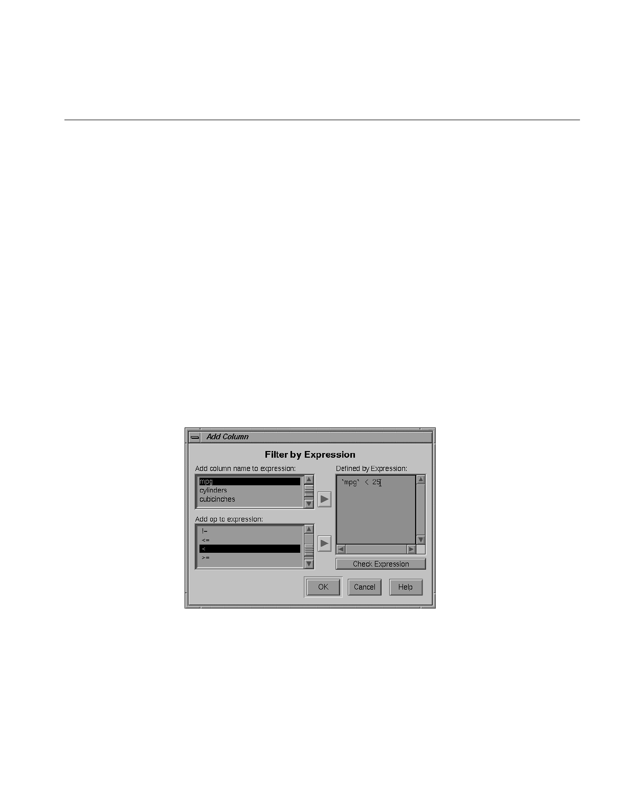
Transforming the Data
87
The three lists of column names are given below:
•Columns to aggregate.
•Group-By columns (the default); this keeps the columns unchanged throughout the
operation. For each set of records with the same combination of values in the Group
By columns, only one record is output in the resulting table, with values in the
aggregated columns summed, averaged, minned, maxed, or counted (depending
on the checkboxes at the bottom of the panel).
•Columns to remove, as can be seen with the Sex_bin column in Table 3-5
After you have finished with the additional aggregate criteria dialog box, the Current
Columns text box in the Table Processing window shows the new column names that
result from applying these criteria.
The Filter Button
This button lets you filter the data via a mathematical expression. The resulting table
includes only records for which the expression is true (or, if numerical, non-zero). When
you click Filter, the Filter dialog (Figure 3-13) appears.
Figure 3-13 Filter Dialog Box
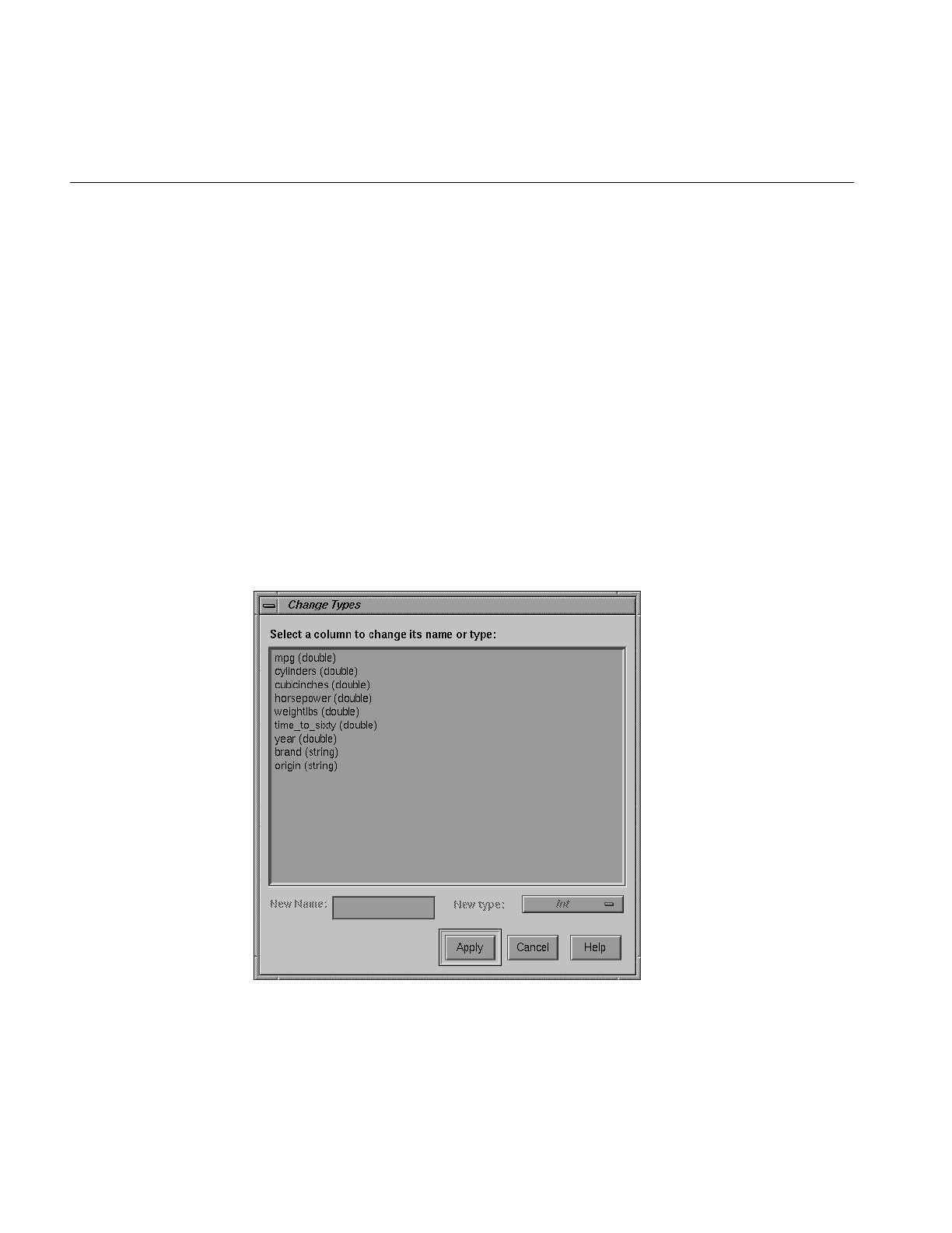
88
Chapter 3: The Tool Manager
This dialog box lets you select column names and operators on the left to build an
expression on the right. For a complete description of the expression definition language,
see “The Configuration File” in Appendix B.
The Change Types Button
This button lets you change the name of a column, as well as its type.
Changing a Column Type
Some databases store numerical values as strings. Oracle stores all numbers (both
integers and real numbers) in a single format, which defaults to the data type double in
the Tool Manager. You can use the Change Types button to ensure that these values are
processed correctly. To change the type of one or more columns, click the Change Types
button. A new dialog box appears (see Figure 3-14). This dialog box contains a window
with a list of column headings and their respective types.
Figure 3-14 Change Types Dialog Box
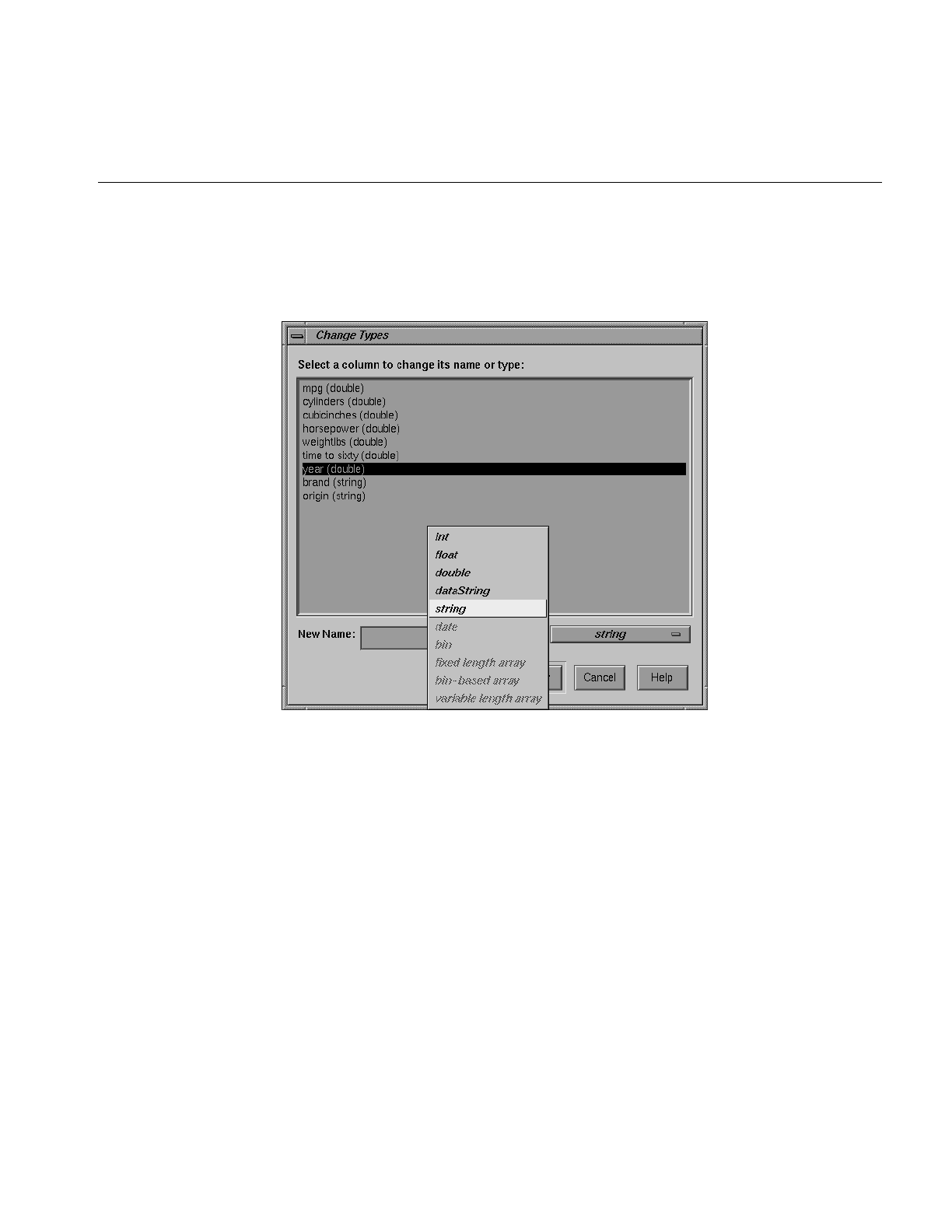
Transforming the Data
89
First select a column heading in the window. Then click the New type button. This
produces a popup list of the possible types (invalid types are grayed out), as shown in
Figure 3-15.
Figure 3-15 Types Popup List
•int—represents a 32-bit signed integer.
•float—represents a single-precision floating-point number. The decimal point is
optional when representing a floating-point number.
•double—represents a double-precision floating-point number. The decimal point is
optional when representing a floating-point number.
•dataString—represents a string that is unlikely to appear multiple times. If it
appears multiple times, several copies are made. A dataString can be used to store
an address. Addresses are unlikely to be compared, and each record can have a
different address.

90
Chapter 3: The Tool Manager
•string—represents a string of characters that can appear multiple times in the data
file. Unlike a dataString, only a single copy of a given string is stored in memory, no
matter how many times it appears in the data. This saves memory for strings
appearing many times.
Comparing strings is also much quicker than comparing dataStrings. However,
reading in strings can be slower than reading in dataStrings because it is necessary
to look for duplications. An example of string use would be for a division name that
appears once for each department in the division. If you are unsure whether to use a
string or a dataString, use a string.
•date—represents the date type from the database.
•bin—represents a column created by a binning operation.
•fixed-length array—an array of values of fixed size, not created by the Tool Manager.
•bin-base array—an array of values as can be created by the Tool Manager.
•variable-based array—an array of values of variable size, not created by the Tool
Manager.
After selecting a new type, click Apply to have the change take effect.
If you try to convert an inappropriate field (such as a name) to a number, the resulting
values are all zeroes.
Note: When the data source is an existing file, there are fewer possibilities available for
changing any given column.
Changing a Column Name
Select the original column, type a new name in the text field, and click Apply. Then click
Close.
To exit this dialog box, click Close.
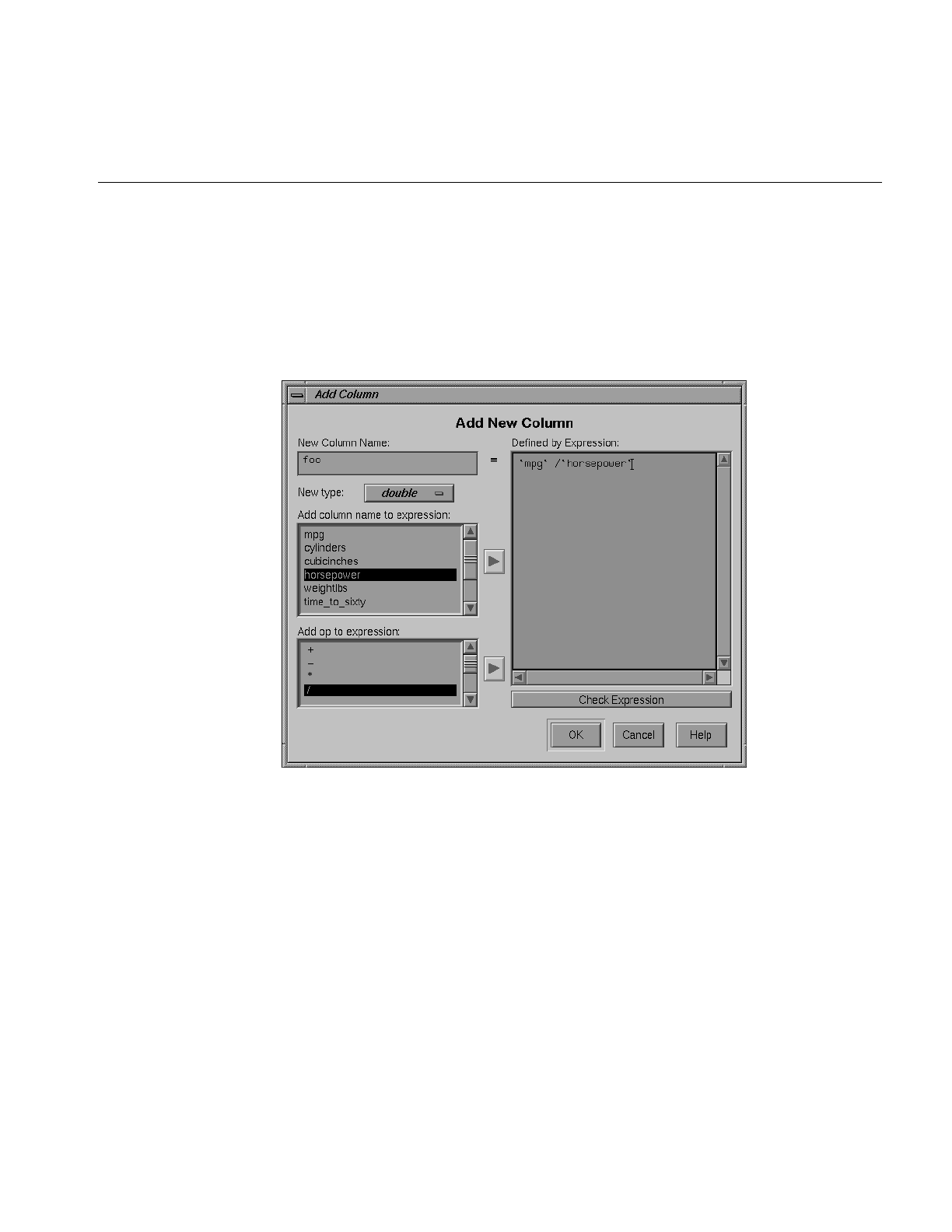
Transforming the Data
91
The Add Column Button
You can use the Add Column button to create a new column whose values are computed
based on a mathematical expression. For example, you could add a new column whose
values are the ratio of values from two existing columns. Click Add Column to get a dialog
box that lets you specify the new column name and expression (Figure 3-16).
Figure 3-16 The Add Column Dialog Box
In the upper left of this dialog box is a field for entering the new column’s name. Below
this is a popup menu that lets you specify the column type (integer, string, floating point,
and so on).

92
Chapter 3: The Tool Manager
The right-hand side of the dialog contains a large text entry area where you can type in
a definition of the expression (for a complete description of the expression definition
language, see “The Configuration File” in Appendix B). As a shortcut to typing column
names and operators, scrolled lists in the lower left of the dialog display all columns in
the current table and all possible operators. To insert a column name or operator into the
expression, either double-click it in its scrolled list, or select it and click the arrow button
to the right of the scrolled list.
To check the expression you have created, click the Check Expression button. If there is an
error, a dialog box appears, indicating what the error is and where it occurred. When you
click OK, the expression is automatically checked, and the dialog box is not removed
unless the expression is correct.
The Add Column dialog box checks for type compatibility: if you have assigned a
numerical expression to a string column (or vice versa), a warning message appears, and
the type of the new column is automatically changed to be correct.
The Apply Model Button
The Apply Model button lets you use a previously created model to label new records in
the current table, to estimate probabilities for a label value, to test the performance of the
model on the current table, or to backfit the current table onto an existing model. See
Chapter 10, “MineSet Inducers and Classifiers,” for details.
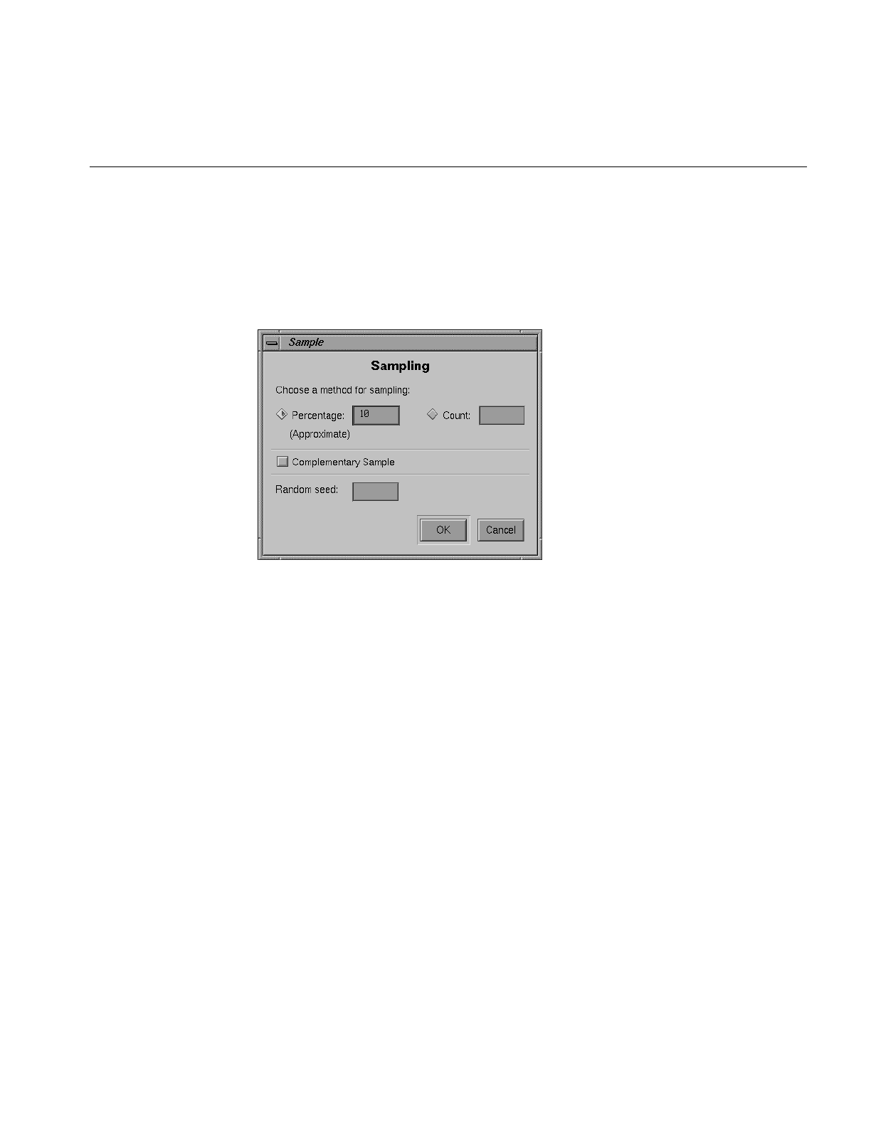
Transforming the Data
93
The Sample Button
This button lets you select a random subset of the data. This is useful for data sets that
are too large to work with efficiently. When you click Sample, the Sampling dialog box
(Figure 3-17) appears.
Figure 3-17 Sampling Dialog Box
You can sample two ways: as a percentage of the current table, or by setting the
maximum number of records to put in the sample. Percentage sampling is approximate,
you can get slightly more or slightly fewer records than the exact percentage would
indicate. The random sample is based on a numeric seed that can be specified in the
sampling dialog. If no seed is specified, the number 1 is used as the seed. If you want a
different random sample, specify a different random seed.
When you click the Complementary Sample toggle, you get all records except those that fall
in the random sample. That is, if you get a 10% sample with the Complementary Sample
not clicked, when you click it, you get the remaining 90% of the data.

94
Chapter 3: The Tool Manager
The Table History Buttons
Table processing is a series of operations performed by using the buttons described
above. To allow you to see this series of steps, and go back if you made a mistake, there
are two Table History buttons at the bottom of the Table Processing panel (Figure 3-18).
When you click the left arrow button, the columns window shows the table as it
appeared at an earlier step. Clicking the right arrow button returns the table to its current
state.
Figure 3-18 Table History Buttons
The “Current view is” Field
To the right of the history buttons is the information field Current view is, which counts
the changes you’ve made and indicates which step you are viewing. The two integers in
this field indicate which table view you’re looking at, out of the total number of table
views that exist. For example, if you’ve made two changes, you can view the original
table (1 of 3), the table after the first change (2 of 3), or the table after the second change
(3 of 3).
The Prev and Next Buttons
As you go back and forth using the Table History buttons to view earlier versions of the
table, the Prev: and Next: fields (under the arrow buttons) help you keep track of where
you are in the history of the table. For any table you view, the Prev: field tells you what
the previous change was, and the Next: field tells you the next change.

Transforming the Data
95
The Edit Prev. Op Button
The Edit Prev. Op. button allows you to edit the operation shown in the Prev. field. (This
button is not active when Current view is: 1 of some number, because that is the original
table, with no previous changes.) When you click the Edit Prev. Op. button, the dialog box
for the previous operation comes up, and you can make changes to that operation. For
example, if the previous operation was binning columns, when you click Edit Prev. Op.,
the Bin Columns dialog box appears.
Note that by changing a previous operation, you could affect operations you set up
subsequent to the current one. For example, if you delete a column that you used in a
subsequent binning operation, that binning operation becomes invalid. The Edit History
button can help you avoid such problems.
The View History Button
When you click the View History button, the panels showing the current column and data
destination are replaced by a panel showing you the complete history of the Data
Transformation table (Figure 3-19). Each version of the table appears as a box containing a
list of the columns, linked by a smaller box (indicating the operation performed on the
table) to the next version of it.
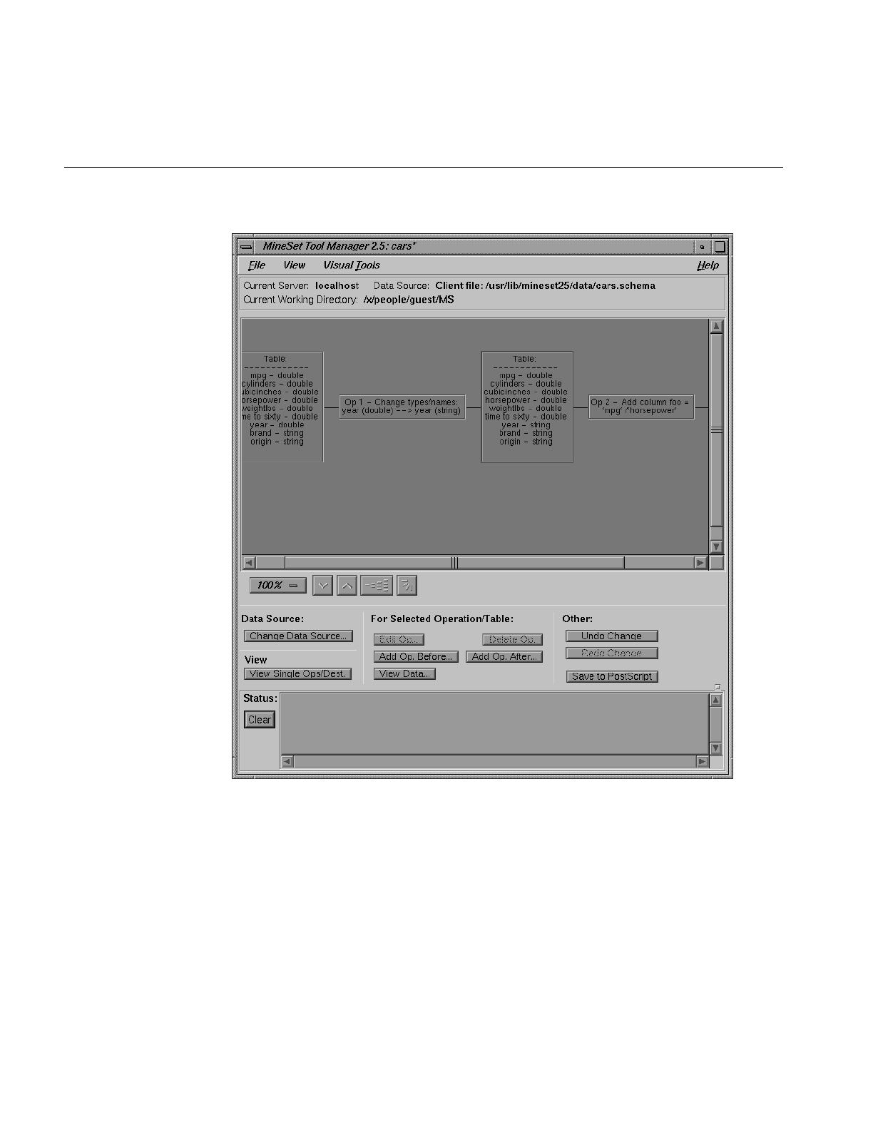
96
Chapter 3: The Tool Manager
Figure 3-19 View History Dialog Box
As with Edit Prev. Op, changing one operation usually affects (sometimes invalidates)
subsequent operations in the history. You can select a specific operation to edit, add, or
view. The View History dialog warns you when changes affect the history, shows you the
new history. The row of buttons beneath the diagram window of the View History panel
allows you to change the size and orientation of the diagram as detailed below.

Transforming the Data
97
Zoom Buttons
Under the window displaying this flow chart are the zoom buttons that let you view the
flow chart closer up or farther away (Figure 3-20). You can choose the zoom by using the
button indicating the percentage, or by clicking the arrow buttons to increase or decrease
the size. The increments of change are the same whether you use the percentage button
or the arrow buttons.
Figure 3-20 Zoom Buttons
Overview Button
This button (Figure 3-21) creates, in a separate window, an overview of the entire history
chart that is synchronized with the Edit History dialog. The overview window shows
you which part of the history is currently visible, and lets you pan to other parts of the
history.
Figure 3-21 Overview Button
Vertical/Horizontal View Button
Next to the zoom buttons is a toggle button that lets you view the flow chart vertically or
horizontally (Figure 3-22). Clicking the button switches you back and forth between the
two points of view.
Figure 3-22 Vertical/Horizontal View Button

98
Chapter 3: The Tool Manager
Data Source
Under the Data Source heading is the Change Data Source... button, which lets you change
the table on which the history operates. When you hold the button down, a menu
appears that lets you choose
•...to DBMS table
•...to DBMS query
•...to Data File
Selecting one of these items causes a dialog box to appear that lets you select the new data
source.
Note: As with editing the history, changing the data source can invalidate history
operations.
View
Under the indicator View is a View Single Ops/Dest button. When this button is pressed,
the panel showing the history is hidden, and the panels showing current columns and
data destinations return to view. The function of this button is the same as choosing the
Single Ops and Destination option from the View pulldown menu at the top of the
window.
For Selected Operation/Table
Under the indicator For Selected Operation are three rows of buttons that become active if
you click one of the operations or tables in the flow chart. Once you select an operation,
you can alter it.
•The Edit Op button brings up the dialog box for the selected operation, so you can
make changes to it.
•The Delete Op button removes the operation from the table history, and the elements
that follow in the flow chart move over when it disappears.
•The Add New Op. Before and Add New Op. After buttons let you insert a new
operation into the table history.
•The View Data button shows the data for any selected table in the history. When you
click this button, a menu is displayed enabling you to select the entire dataset, or a
random sample of 10, 100, or 1,000 records.

Investigating the Data
99
Other
Under the indicator Other there are three buttons that affect the total history file:
•Undo Change—undoes the most recent change to the history (except changes to the
data source)
•Redo Change—redoes any change you have undone.
•Save to PostScript—save a picture of the history flow chart to a file in PostScript
format.
Investigating the Data
The Data Destination panel (Figure 3-23) lets you direct your processed data to one of the
MineSet visualization or mining tools, or to a data file.
There are three tabs at the top of this panel:
•Viz Tools
•Mining Tools
•Data Files
These are the three possible destinations for your data. They are discussed in greater
detail in later chapters dealing with the Data Destination tools.
Using Visualization Tools
If you choose the Viz Tool tab, the visualization tool panel appears under Data
Destination (Figure 3-23).
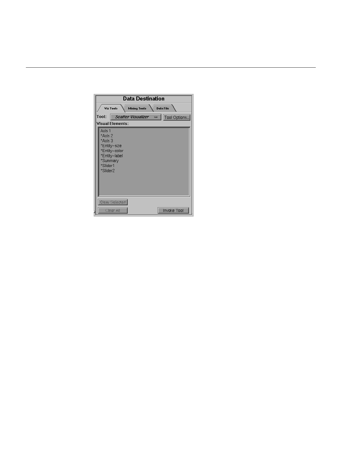
100
Chapter 3: The Tool Manager
Figure 3-23 Data Destination Panel
Viz Tool is a popup menu that lets you choose among Map Visualizer,Scatter Visualizer,
Splat Visualizer,Tree Visualizer,Statistics Visualizer and Record Viewer, to determine the type
of visual representation you want for your data.
The first five tools are described in their respective chapters.
The Record Viewer lets you view the data in the current table in a row/column
spreadsheet-like tool. To use the Record Viewer select it from the tool menu, and click
Invoke Tool.
•Tool Options—lets you further specify options you want to set in the specified tool’s
configuration file.
•Clear Selected—lets you undo the mapping to a selected Visual Element.
•Clear All—clears all mappings.
•Invoke Tool—lets you start the tool you specified (via the top button) using the
configuration file named in the Saved as text field.
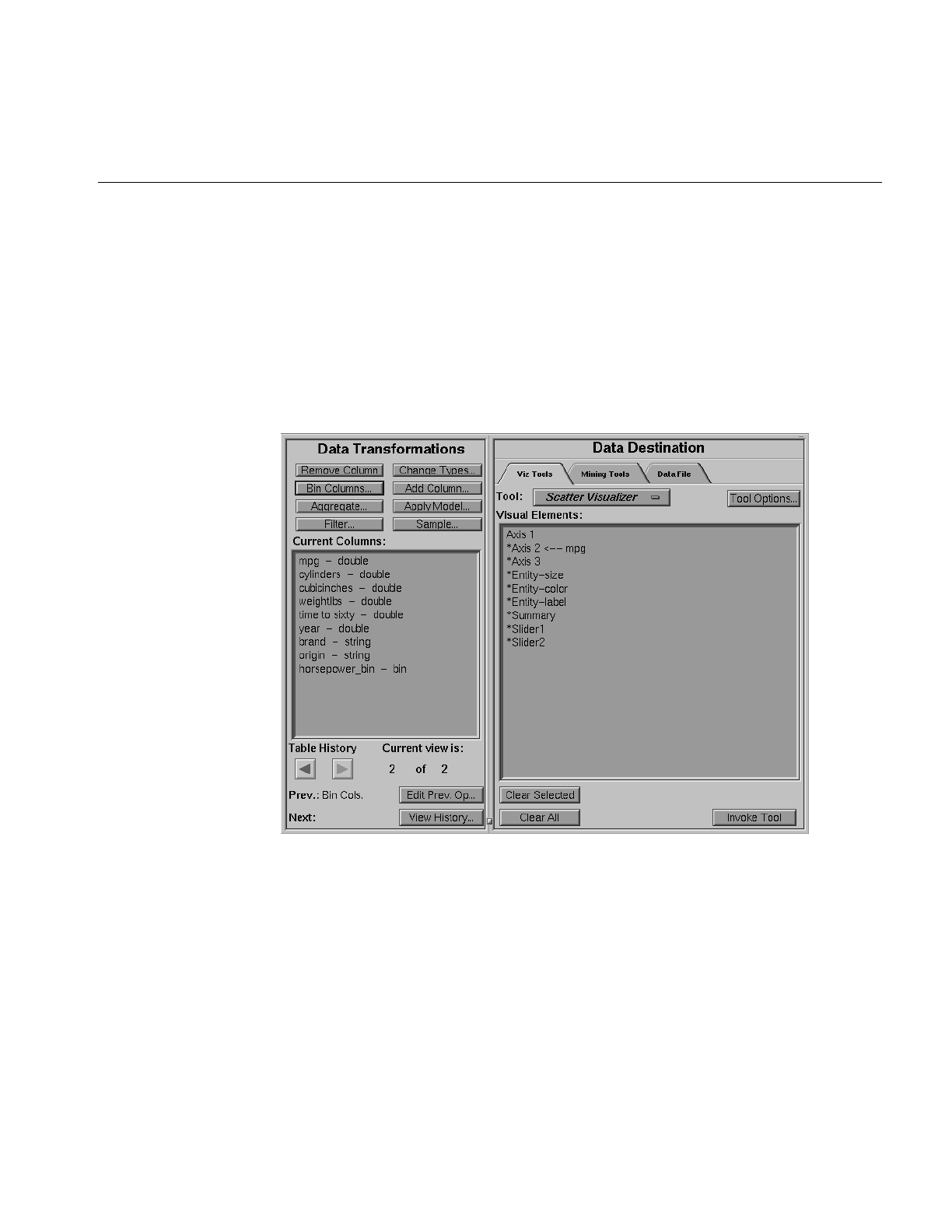
Investigating the Data
101
Each tool’s requirements are listed individually in the Visual Elements pane. This pane lets
you map a table column to a requirement. To do this,
1. Select a column by clicking its name in the Current Columns pane.
2. Select the requirement to which you want to map the column by clicking on that
requirement in the Visual Elements pane.
The Viz Tool panel now shows the Visual Element and the column to which it has been
mapped (see Figure 3-24).
Figure 3-24 Columns Mapped to Requirements

102
Chapter 3: The Tool Manager
You can clear the mapping at any time by selecting the requirement that has the mapping
you want to change, then clicking the Clear Selected button. You can clear all mappings
using the Clear All button.
If you want to specify other details to fine-tune your mappings or to change the settings
so that the data representations more clearly reflect your intentions, click the Tool Options
button. A dialog box specific to each MineSet tool appears, where you can manually
specify the options to use.
Note: For details on a specific tool’s options, see that tool’s chapter.
Using Mining Tools
The MineSet Classifiers are described in Chapter 10, “MineSet Inducers and Classifiers,”
Chapter 11, “Inducing and Visualizing the Decision Tree Classifier,” Chapter 12,
“Inducing and Visualizing the Option Tree Classifier,” Chapter 13, “Inducing and
Visualizing the Evidence Classifier,” Chapter 14, “Inducing and Visualizing the Decision
Table,” Chapter 15, “Inducing and Visualizing the Regression Tree.” Clustering is
described in Chapter 16, and Column Importance is described in Chapter 17.
Creating Associations for the Rule Visualizer
If you click the Mining Tools tab, then the Associations tab, the panel lets you take the data
file you created in Data Transformations and proceed to the Rule Visualizer. Each step of
the process is shown in the subpanels:
•Assoc Settings—creates rule generation options and mappings from the columns in
your table to elements of association rules
•Ruleviz Settings—provides options to tailor the representation of the association
rules in the Ruleviz tool
•Execution—a button to invoke the process of finding association rules and
visualizing them
If you don’t want to go through this process manually, click the Execution button, and the
computer will perform the process using defaults.
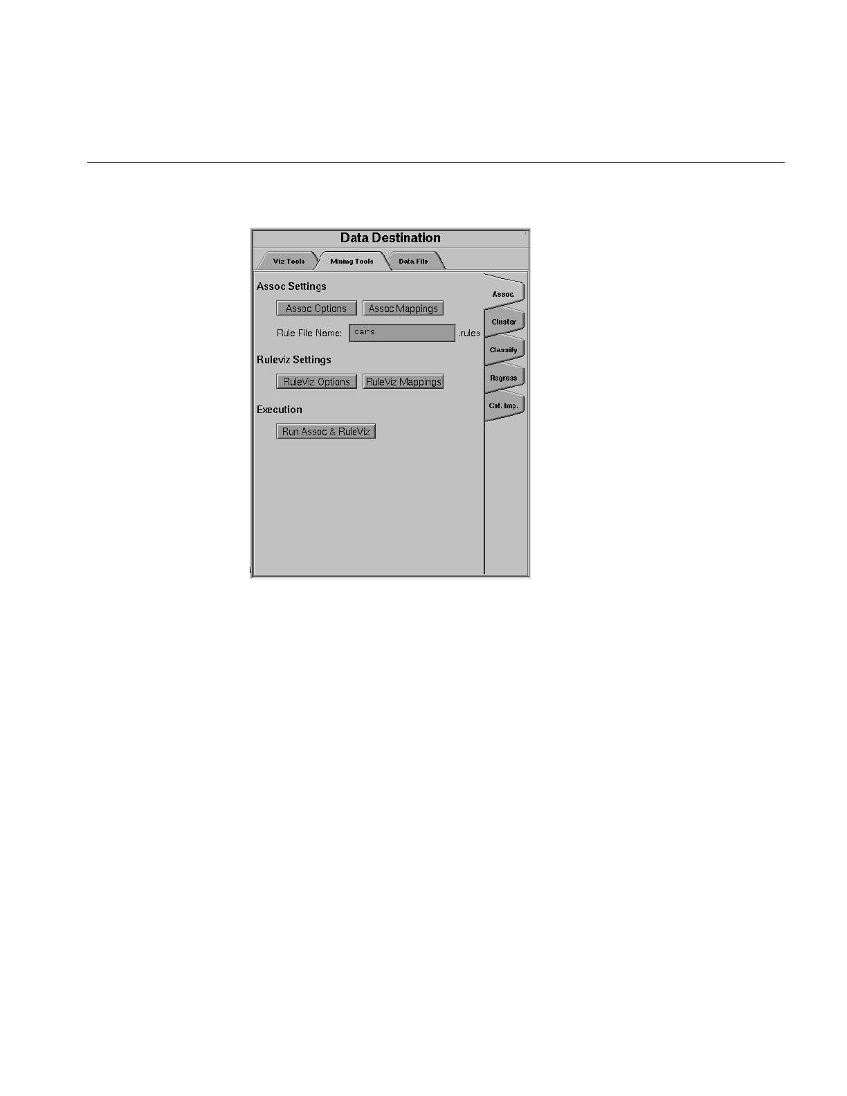
Investigating the Data
103
Figure 3-25 The Associations Tab
Finding Important Columns
The Column Importance (Figure 3-26) allows you to determine how important various
columns are in discriminating the different values of the label column you choose. You
might, for example, want to find the best three columns for discriminating the label good
credit risk so you can choose them for the Scatter Visualizer. When you select the label and
click Go!, a popup window appears with the three columns that are the best three
discriminators. A measure called “purity” (a number from 0 to 100) informs you how
well the columns discriminate the different labels. Adding more columns can only
increase the purity.
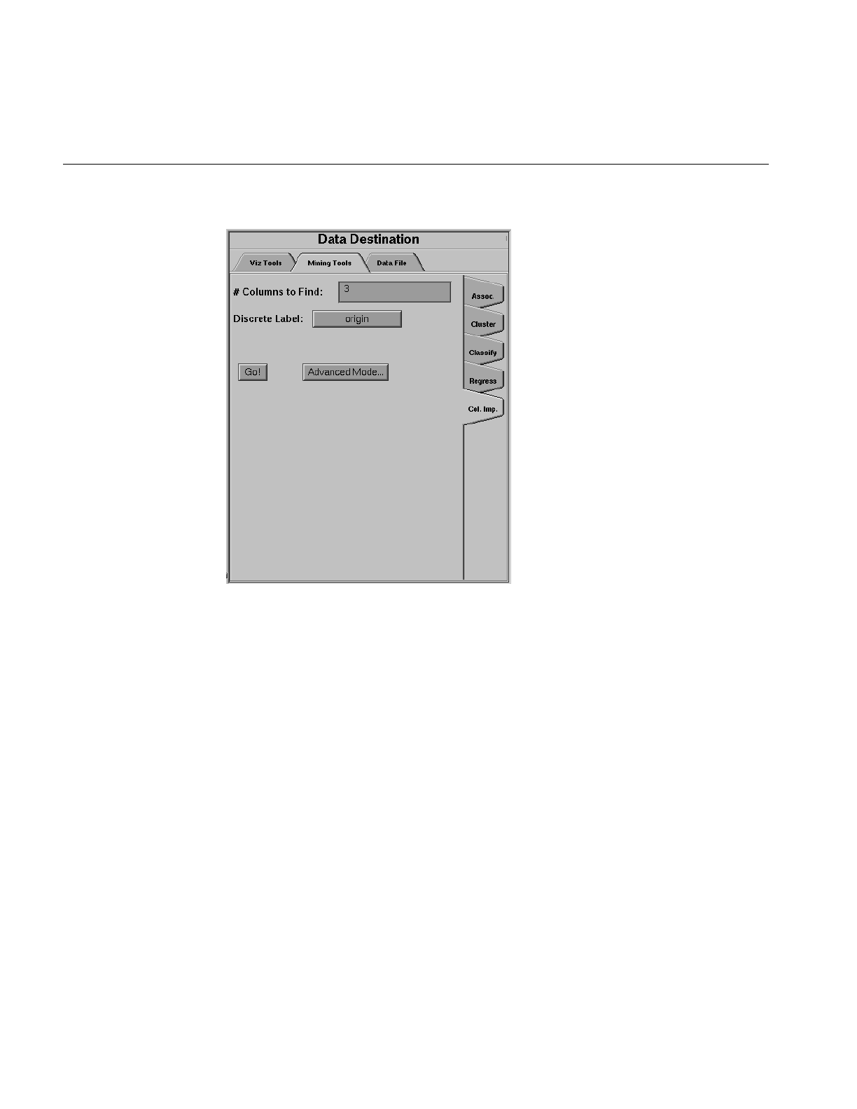
104
Chapter 3: The Tool Manager
Figure 3-26 The Column Importance Tab
There are two modes of column importance:
•Simple Mode
To invoke the simple mode, choose a discrete label from the popup menu, and
specify the number of columns you want to see.
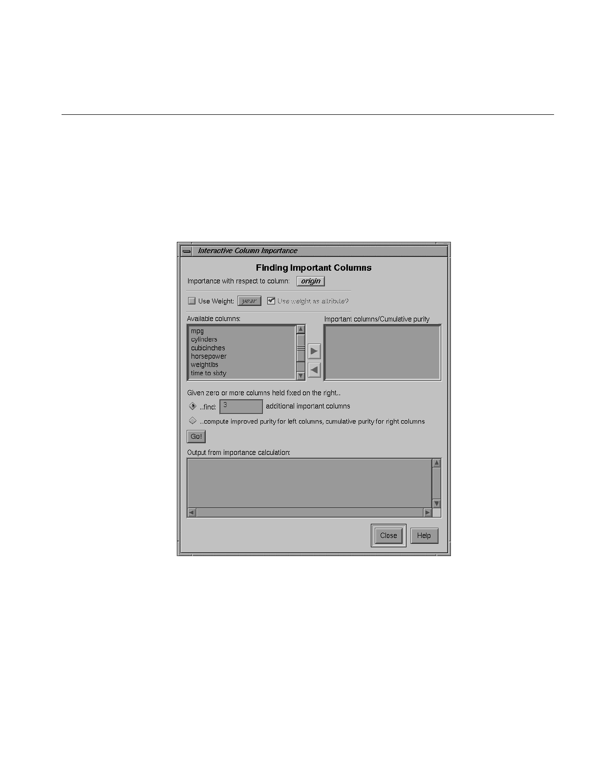
Investigating the Data
105
•Advanced Mode
Advanced mode lets you control the choice of columns. To enter advanced mode,
click Advanced Mode in the Column Importance panel. A dialog box appears, as
shown in Figure 3-27. The dialog box contains two lists of column names: the left
list contains available attributes, and the right list contains attributes chosen as
important (by either the user or the column importance algorithm).
Figure 3-27 Advanced Mode of Column Importance

106
Chapter 3: The Tool Manager
Advanced mode can work two different ways: finding several new important
attributes, or ranking available attributes.
•Finding Several Important Attributes
To enter this sub-mode, click the first of the two radio buttons at the bottom of
the dialog (...find [number] additional important columns). If you click Go! with no
further changes, the effect is the same as if you were in Simple Mode, finding
the specified number of important columns and automatically moving them to
the right column. Near each column, the cumulative purity is given (that is, the
purity of all the columns up to and including the one on the line). More
attributes can only increase the purity.
Alternatively, by moving columns names from the left list to the right list, you
can pre-specify columns that you want included and let the system add more.
For example, to select the age column and let the system find three more
columns, click the age column name, then click the right arrow.
Clicking Go! lets you see the cumulative purity of each column, together with
the previous ones in the list. A purity of 100 means that using the given
columns, you can perfectly discriminate the different label values.
•Ranking Available Attributes
Advanced Mode also lets you compute the change in purity that each column
would add to all those that were already selected. For example, you might
choose age, and then ask the system to compute the incremental improvement
in purity that each column would yield.
To enter this sub-mode, click the second of the two radio buttons at the bottom
of the dialog (...compute improved purity for left columns, cumulative purity for right
columns.). This sub-mode permits fine control over the process. If two columns
are ranked very closely, you might prefer one over the other (for example,
cheaper to gather, more reliable, easier to understand).
Column Importance Notes
Note that with other columns, the importance of features varies from their ranking alone.
For example, while net-income might be a good column individually, it might not be as
important together with salary because they are likely to be highly correlated. The best
set of three columns is not necessarily composed of the columns that rank highest
individually. If two columns give the income in dollars and in another currency, they are
ranked equally alone; however, once one of them is chosen, the other adds no
discriminatory power to the set of best features.
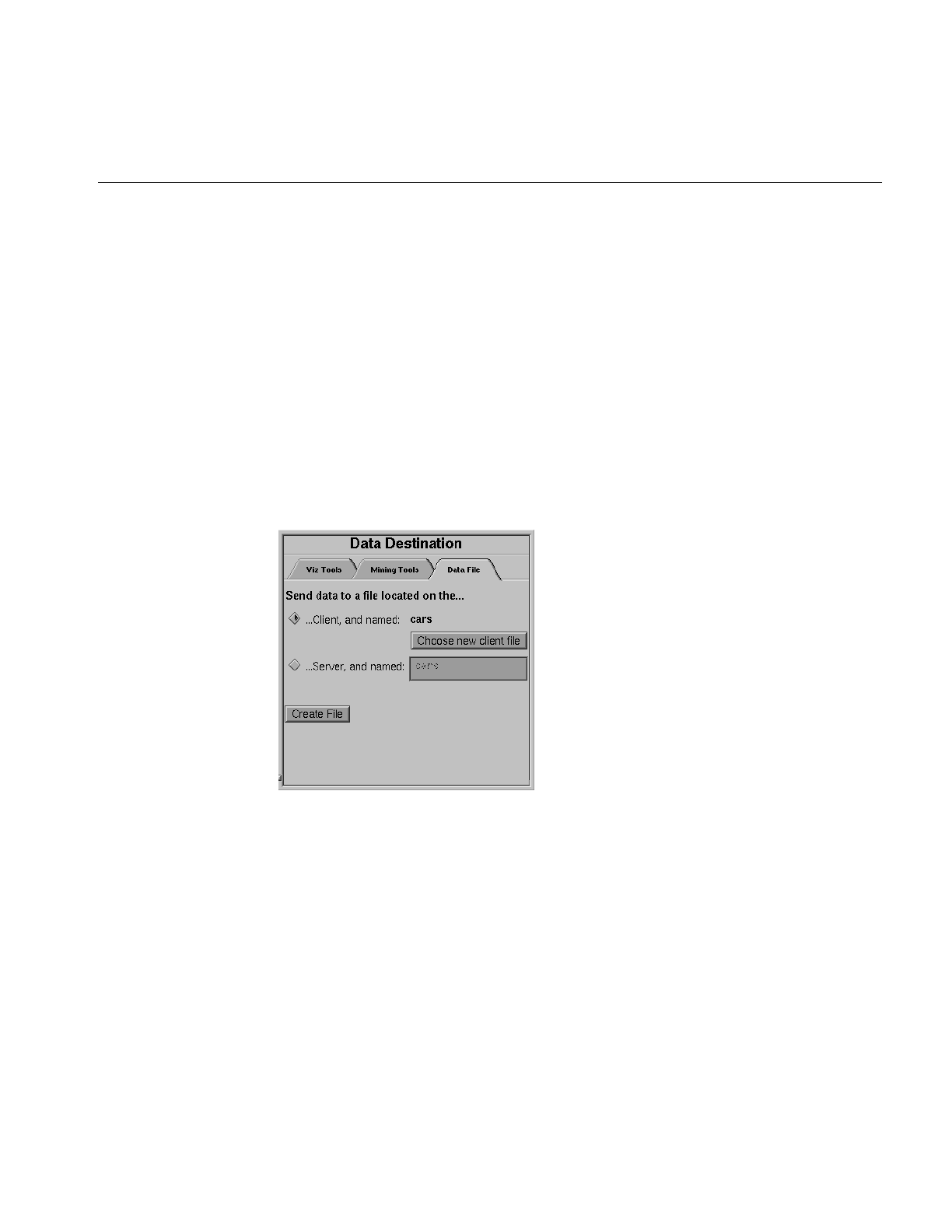
Investigating the Data
107
Column selection is useful for finding the best three axes for the Scatter Visualizer, as well
as for finding a good discriminatory hierarchy for the Tree Visualizer.
All floating point values (double or float) are pre-discretized using the automatic
discretization. If a column has no value given to it in the left list, the algorithm did not
consider it, because it either had a single value (for example, when it is discretized into
one interval), or the number of records that it would separate is not statistically
significant.
Using Data Files
The Tool Manager lets you save the manipulated table for future use in a data file on the
client or server. If you click the Data Files tab, the panel shown in Figure 3-28 appears.
Figure 3-28 The Data Files Panel
The two toggle buttons in this panel let you specify whether the file is to be saved on the
server or your client machine. The selected name for the client file appears next to the
Client checkbox. If you select Client, the Choose new client file button brings up a dialog for
you to choose the name for the client file. If you select Server, you can type the server
filename directly into the adjacent text field.
Note: Pathnames are not permitted for server files; all server files are stored in the
DataMover cache directory.

108
Chapter 3: The Tool Manager
Session Files
The Tool Manager can save a description of your work to a “session file” for future use.
A session file contains a description of the data source you selected, all the
transformations on the data, and the mining or visualization of the data. Each session file
can hold descriptions of only one data source and one data destination; thus, if you
change the destination visual tool or source data table, the session file loses its links to
any previous data source or destination.
Session files can be saved at any time through the entries in the File menu, described
below. The name of the current session appears in the window’s title bar. The Tool
Manager also keeps a parallel session file, called .latest.mineset, in your home directory. It
always has a record of your most recent actions in the Tool Manager. Whenever you start
the Tool Manager without a session file, it reads the contents of the .latest.mineset file to
return you to the state when you last ran MineSet.
Session files also can be used for running the Tool Manager in batch mode, by issuing this
command at the UNIX shell prompt:
mineset_batch [-s serverPassword -d databasePassword]sessionFile
The -s and -d options let you specify the password for logging into the server and
database respectively. If you do not specify these options, mineset_batch will ask you to
type in the passwords, thus these options are useful when running mineset_batch from a
shell script. To specify that there is no password for either the server or database, use -s
or -d followed by two double quotes, that is,
mineset_batch -s "" -d "" foo.mineset
If you specify one of the two passwords, you must specify both.
In batch mode, the Tool Manager does not bring up tools or windows; however, it creates
files for tools. For example, if the session file includes the Tree Visualizer as the data
destination, running the Tool Manager in batch mode produces files for running the Tree
Visualizer, but the Tool Manager does not invoke it.
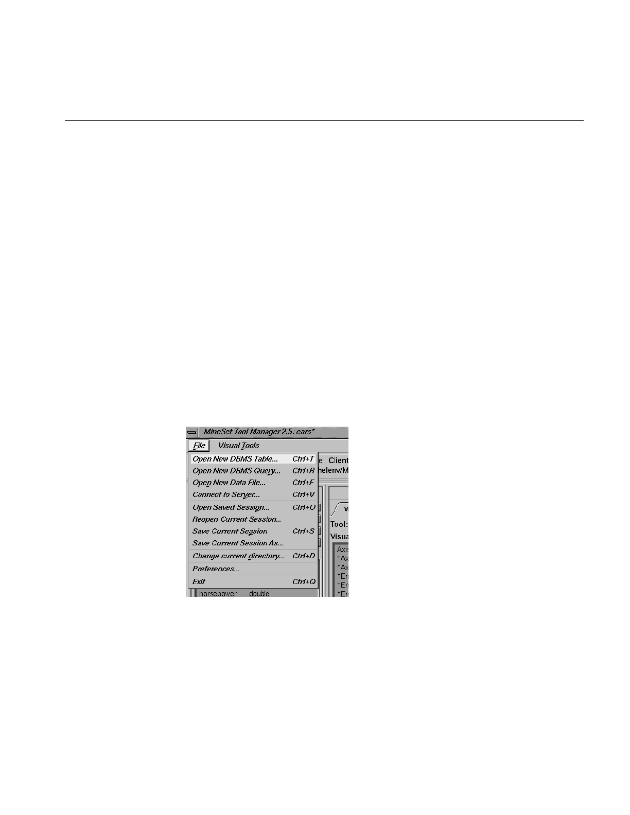
Pulldown Menus
109
Pulldown Menus
At the top of the Tool Manager window (see Figure 3-1 on page 67) are four pulldown
menus:
•File
•View
•Visual Tools
•Help
The following section describes each of these menus.
The File Menu
The File menu lets you choose what to do with your current session, which is one
complete session with a tool. This includes choosing the server, data source and table, all
the table manipulations, the mapping or classifying of the data, as well as opening or
saving a tool history, changing the working directory, and setting preferences.
Figure 3-29 File Menu

110
Chapter 3: The Tool Manager
The File menu provides five sets of functions:
•The first set is for selecting a data source.
–Open New DBMS Table—lets you select a single table from a DBMS.
–Open New DBMS Query—lets you make an SQL query against the DBMS.
–Open New Data File—lets you select a table from a data file on disk.
–Connect To Server—lets you open a connection to a MineSet server.
•The second set is for opening or saving .mineset files.
–Open Saved Session...—lets you open a .mineset file.
–Reopen Current Session —lets you reopen the current session file from the disk, in
case you do not want to save the current changes.
–Save Current Session—lets you save a currently open .mineset file.
–Save Current Session As...—lets you name (or rename) and save a currently open
history as a .mineset file.
•The third set is for changing the current directory.
–Change Current Directory—lets you specify the directory in which the Tool
Manager creates all data and visualization files.
•The fourth set is for setting preferences. Here you can specify whether to
–use ASCII or binary files
–include an entry for NULL values when creating arrays
–automatically load the most recent session when starting up the Tool Manager
–run MIndUtil in single- or multi-threaded mode; a slider allows you to select
how many threads to use.
•The last option, Exit, lets you end the current session and exit the Tool Manager.
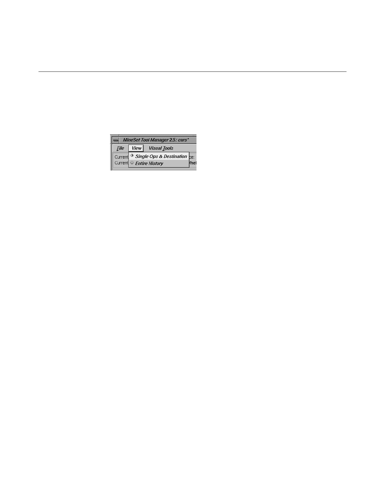
Pulldown Menus
111
The View Menu
The View Menu lets you select whether to see the history panel or the current columns
and data destination panels.
Figure 3-30 View Menu
•Single Ops and Destination—shows the current columns and data destination panels.
This menu option performs the same function as the View Single Ops/Dest button on
the history panel.
•Entire History—shows the history panel. This menu option performs the same
function as the View History button on the Data Transformations panel.
The Visual Tools Menu
The Visual Tool menu lets you invoke any of the following visual tools directly:
•Cluster
•Decision Table
•Evidence Visualizer
•Map Visualizer
•Rule Visualizer
•Scatter Visualizer
•Splat Visualizer
•Statistics Visualizer
•Record Viewer
•Tree Visualizer

112
Chapter 3: The Tool Manager
If you have created a file that runs within one of these tools, and you want to go back to
it, click the tool. From within the tool, use File > Open to open the data file. These viewers
are described in their respective chapters, except for Record Viewer, which is described
later in this chapter, in “The Record Viewer” on page 113.
The Help Menu
The Help menu provides information about the elements of the Tool Manager and how
they work:
•Click for Help—Gives help information about a particular item if you press Shift-F1,
then click the item for which you want help.
•Overview—Gives an overview of the online help and how to use it.
•Index—Provides an index of the complete help system. This option is currently
disabled.
•Keys & Shortcuts—Provides the keyboard shortcuts for all of the Tree Visualizer’s
functions that have accelerator keys.
•Product Information—Indicates what version of the Tool Manager you are using.
•MineSet User’s Guide—Invokes the IRIS Insight viewer with the online version of
this manual.
The Tool Manager Options File
The Tool Manager creates a .mineset file in your home directory. This is used to store the
preference indicating whether to restore the most recent session on startup, as well as the
default server name, login, and password. If you log in to the same server often, edit this
file and specify a server name and login as follows:
default_server_name: mineset
default_server_login: guest
default_server_password:
Whenever you try to log in to a server, these names appear as defaults.
Warning: Putting a password in a file is a great security risk. Do not place a
password in the Tool Manager options file unless you want other people to know that
password.

The Record Viewer
113
The Record Viewer
The Record Viewer lets you view MineSet data files in a format similar to spreadsheets.
There are five ways to start the Record Viewer.
•Use the Tool Manager to start the Record Viewer. This invokes the Record Viewer on
the data currently configured in the Tool Manager.
•Double-click on the Record Viewer icon, which is in the MineSet page of the icon
catalog. Since no .schema file is specified, you must select one by using File > Open.
•Double-click on any MineSet .schema file. This launches the Record Viewer on that
.schema file.
•Drag a .schema file onto the Record Viewer icon.
•Start the Record Viewer from the UNIX shell command line by entering this
command at the prompt:
recordview [ file.schema ]
where file.schema is optional and specifies the name of the .schema file to use. If
you do not specify a .schema file, you must use File|Open to specify one.
The Record Viewer shows the data specified by the .schema file in spreadsheet format (see
Figure 3-31).
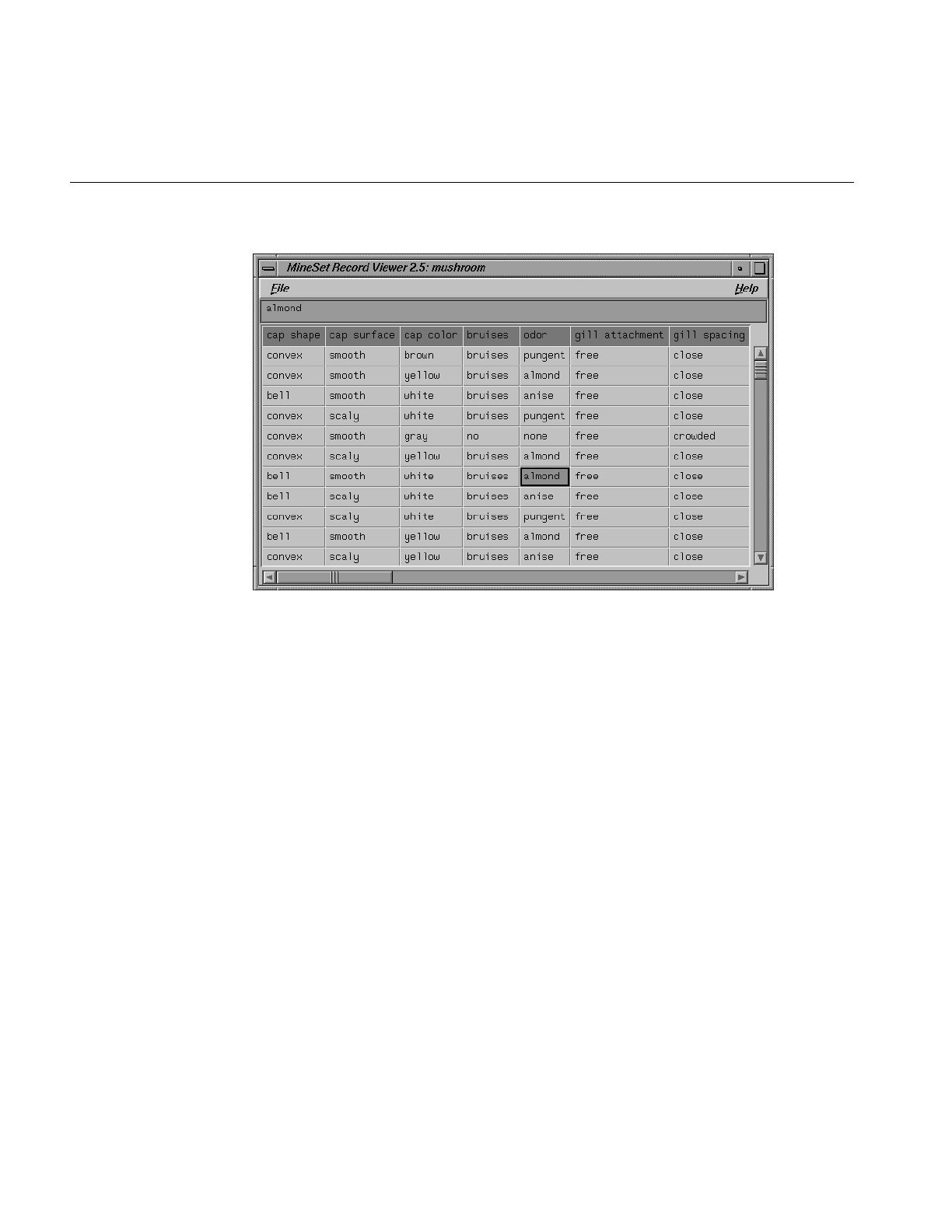
114
Chapter 3: The Tool Manager
Figure 3-31 Sample Record Viewer Screen
If a column is not wide enough to see a specific value, click on it to display that value at
the top of the Record Viewer. You also can change the width of columns by dragging the
separators between the columns.
To read a new .schema file into the Record Viewer, select File > Open. To close the Record
Viewer, select File > Exit.
Note that some of the visual tools also bring up record viewers to display the current
selections. These record viewers are built into the visual tools; while their behavior is the
same as the Record Viewer discussed above, they do not allow opening other .schema
files.
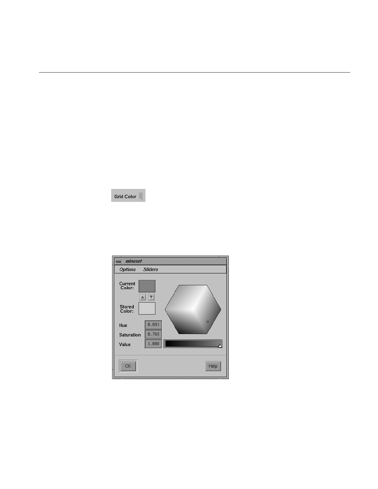
Color Options for the MineSet Visualizers
115
Color Options for the MineSet Visualizers
Many of the tool option dialogs have options for choosing colors. MineSet has a color list
chooser that uses color swatches. This section describes how to choose, apply, and
change color options for the MineSet Visualizers.
Choosing Colors
If only one color is to be chosen (for example a grid color), a single color swatch appears
(Figure 3-32).
Figure 3-32 Configuration Option With a Single Color Swatch
Clicking the swatch brings up a Color Browser that lets you change the color of that
swatch (Figure 3-33). The Color Browser is described in more detail in the “Using the
Color Browser” section, shown in Figure 3-33.
Figure 3-33 Color Browser

116
Chapter 3: The Tool Manager
If a list of color swatches is to be chosen, the list of swatches appears (these can be empty
initially), as shown in Figure 3-34.
Figure 3-34 Multiple Colors Swatches
To edit the color, click a swatch with the left mouse button. This also selects the swatch
for making changes to the colors with the buttons. If you click on the swatch with the
middle mouse button, the swatch is selected, but the color chooser does not appear.
Next to the list of swatches are four buttons. First is the Add button, labeled with a plus
sign (+), which adds a new color at the end of the list. A swatch is added, and the color
chooser appears, where you can select the color of that swatch. The Add button is
disabled if the maximum number of colors is already in the list.
Next to the Add button is a Delete button, labeled with a minus sign (-). This button
deletes the selected color. It is disabled if no swatch is selected, or if the list already has
the minimum number of colors.
Next to the Delete button are two buttons to shift the selected color right and left. These
buttons are disabled if no swatch is selected, or if the swatch is already at the end of the
list.
If there are more colors in the list than room to display them, scroll arrows are added at
each end of the list (Figure 3-35).
Figure 3-35 Scroll Arrows on Color Browser
If the hardware runs out of colors, the color swatches are replaced with text labels
showing the color in X notation (Figure 3-36).
Figure 3-36 Color Browser Out of Colors

Color Options for the MineSet Visualizers
117
Using the Color Browser
The Color Browser (Figure 3-33) appears when you click a color swatch or the add button
in the Colors panel of the visualizer’s Configuration Options panel.
To select a color using the Color Browser:
1. Move your mouse cursor on top of the small circle in the colored hexagon.
2. Press the left mouse button, and move your mouse around the hexagon. The color
beneath the small circle appears in the rectangle next to the Current Color label. This
rectangle acts as your color palette while you choose a color.
3. Release the mouse button when the small circle is on top of a color you want. The
selected swatch immediately takes on the chosen color.
You can edit several colors without dismissing the Color Browser; clicking any color
in the options panel lets you edit that color in the already posted Color Browser.
4. Click the OK button when you decide on a color. The Color Browser window closes.


119
Chapter 4
4. Using the Statistics Visualizer
This chapter discusses the features and capabilities of the Statistics Visualizer. It provides
an overview of this data visualization tool, then explains the Statistics Visualizer’s
functionality when working with the
•main window
•external controls
•pulldown menus
Finally, it lists and describes the sample files provided for this tool.
Overview of the Statistics Visualizer
The Statistics Visualizer lets you visualize statistics on columns. Statistics Visualizer
presents a window that contains one small panel for each column listed in the Current
Columns pane of Tool Manager. The Statistics Visualizer main window has a default size
and shows only a restricted number of column panels. If the number of columns is large,
scrollbars appear; alternatively, you can stretch the Statistics Visualizer window
horizontally or vertically to view more column panels.
The format of the column panel varies according to the column type, and the number of
distinct values that exist for that column. Columns are generally divided into two types:
numeric and discrete, shown as box plots and histograms, respectively.
Anumeric column has integer, float, double or date values. Each box plot panel shows
statistics about data from a single column, including the minimum, maximum, mean,
median, and two quartiles (25th and 75th percentiles) of these numeric values. These
values are shown as lines across a vertical bar in graduated shades of green, and the
standard deviation of the population is shown as a +/- value. The quartiles are shown
whenever there are fewer than 50,000 distinct values, (see Figure 4-1). If there are more
than 50,000 distinct values in the column, the statistics are shown as a gray vertical bar.
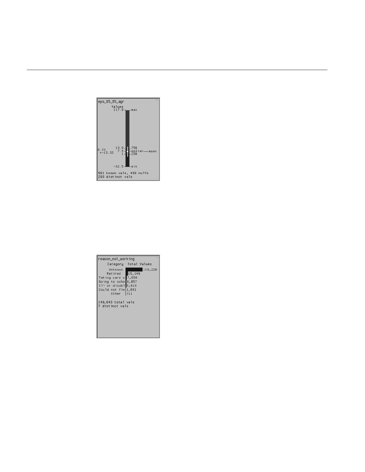
120
Chapter 4: Using the Statistics Visualizer
Figure 4-1 Numeric Column Displayed by Statistics Visualizer
Adiscrete (or nominal) column has non-numeric (string, bin, or enum) values shown as
histograms, (see Figure 4-2). The discrete column panel shows up to 100 distinct values,
as well as a histogram of the number of instances of this distinct value. The default
ordering of the discrete rows is by decreasing count, but you can use the View pulldown
menu to select an alternative sorting. If there are 100 or fewer distinct categories, then the
column panel also contains the count of distinct values.
Figure 4-2 Discrete Column Displayed by Statistics Visualizer
After creating a visualization of your data, the Statistics Visualizer lets you see truncated
textual information in the histograms with a brush highlighter. The brush highlighter
activates as you pass the mouse across a field without clicking.
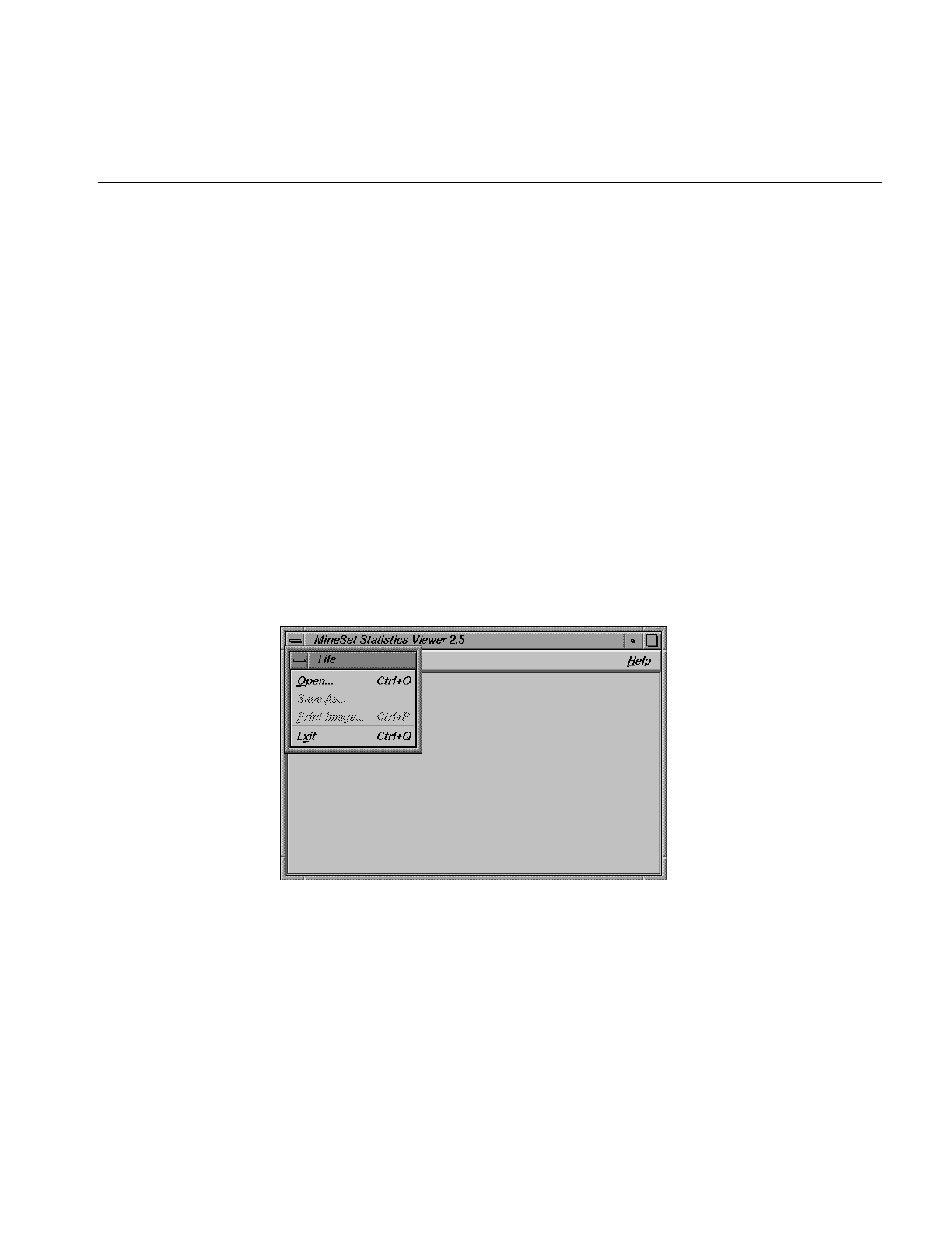
File Requirements
121
File Requirements
The Statistics Visualizer requires a data file, consisting of ASCII or binary fields. This file
is easily created when running the Tool Manager (see Chapter 3).
Starting the Statistics Visualizer
There are five ways to start the Statistics Visualizer:
•Use the Tool Manager to configure and start the Statistics Visualizer. See Chapter 3
for details on most of the Tool Manager’s functionality, which is common to all
MineSet tools.
•Double-click the Statistics Visualizer icon, which is in the MineSet page of the icon
catalog. The icon is labeled statviz. Since no configuration file is specified, the
start-up screen requires you to select one by using File > Open.
•Double-click the Statistics Visualizer icon on your Silicon Graphics desktop. The
startup screen requires you to select a data file by choosing File > Open.
Figure 4-3 File > Open Menu Selection for Statistics Visualizer
Starting the Statistics Visualizer from the icon activates only the File and Help
pulldown menus. For the main window to be fully functional, open a .statviz file by
selecting File > Open.
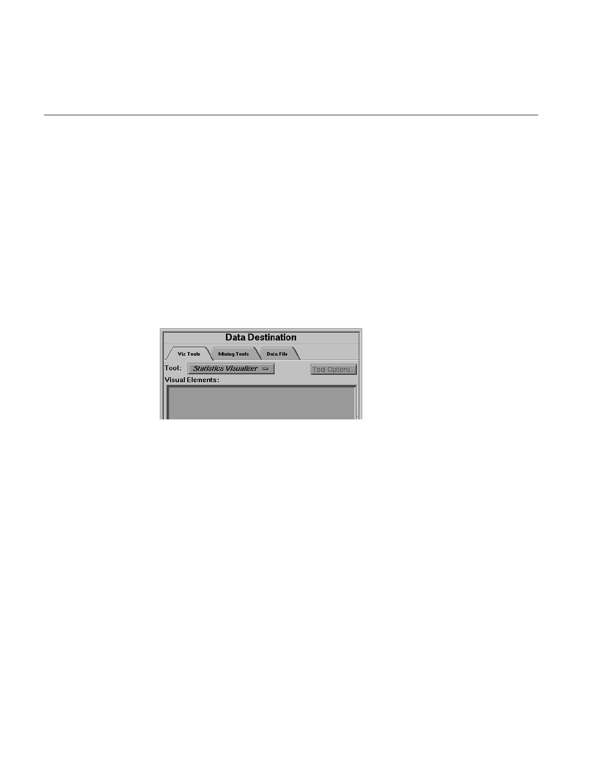
122
Chapter 4: Using the Statistics Visualizer
•If you know what .statviz file you want to use, double-click the icon for that file. This
starts the Statistics Visualizer and automatically loads the file you specified. This
works only if the filename ends in .statviz (which is always the case for data files
created for the Statistics Visualizer using the Tool Manager).
•Drag the .statviz file icon onto the Statistics Visualizer icon. This starts the Statistics
Visualizer and automatically loads the file you specified. This works even if the
configuration filename does not end in .statviz.
Starting the Statistics Visualizer
Select the Viz Tools tab in the Data Destination panel of the Tool Manager’s main screen
(Figure 4-4). From the popup list of tools, choose Statistics Visualizer.
Figure 4-4 Data Destination Panel With Statistics Visualizer Selected

Working in the Statistics Visualizer’s Main Window
123
Working in the Statistics Visualizer’s Main Window
If you started the Statistics Visualizer from the icon, the main window shows the
copyright notice and license agreement for the Statistics Visualizer. Only the File and
Help pulldown menus can be used. For the main window to show all menus and
controls, open a .statviz file. Use File > Open (Figure 4-3) to see a list of configuration files.
Pulldown Menus
Three pulldown menus let you access additional Statistics Visualizer functions. These are
labeled File, View, and Help. If you start the Statistics Visualizer without specifying a
configuration file, only the File and the Help menus are available.
The File Menu
The File pulldown menu for the Statistics Visualizer contains four options.
•Open loads and opens a file and displays it in the main window.
•Save As saves the current state of the Statistics Visualizer main window into an
image file
•Print Image captures the image of outputs the current state of the Statistics
Visualizer main window and prints it to a printer.
•Exit closes all windows and exits the application
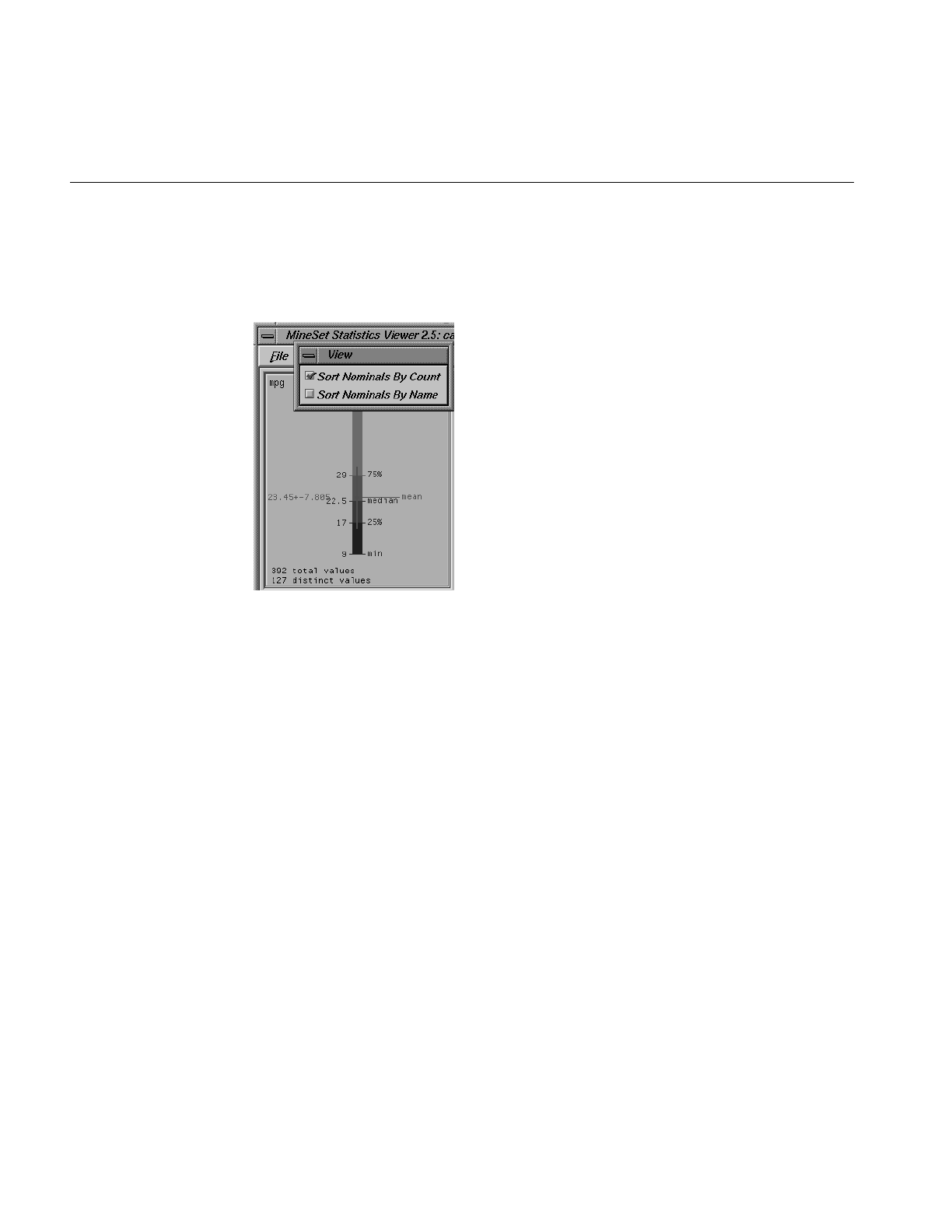
124
Chapter 4: Using the Statistics Visualizer
The View Menu
The Statistics Visualizer View pulldown menu (Figure 4-5) contains two options.
Figure 4-5 StatViz View Pulldown Menu
•Sort Nominals By Count specifies that the nominal (discrete) columns show the
histogram of values that is ordered by decreasing per-value counts.
•Sort Nominals By Name specifies that those same columns be ordered by the relative
alphabetical order of each data value name.
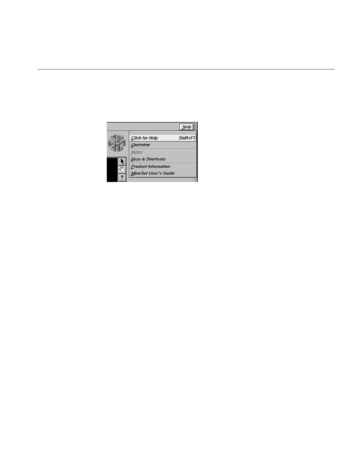
The Help Menu
125
The Help Menu
The Help menu provides access to five help functions (see Figure 4-6).
Figure 4-6 Statistics Visualizer Help Menu
•Click for Help turns the cursor into a question mark. Placing this cursor over an
object in the Statistics Visualizer’s main window and clicking the mouse causes a
help screen to appear; this screen contains information about that object. Closing the
help window restores the cursor to its arrow form and deselects the help function.
The keyboard shortcut for this function is Shift+F1. (Note that it also is possible to
place the arrow cursor over an object and press the F1 function key to access a help
screen about that object.)
•Overview provides a brief summary of the major functions of this tool, including
how to open a file and how to interact with the resulting view.
•Index provides an index of the complete help system. This option is currently
disabled.
•Keys & Shortcuts provides the keyboard shortcuts for all of the Statistics Visualizer’s
functions that have accelerator keys.
•Product Information brings up a screen with the version number and copyright notice
for the Statistics Visualizer.
•MineSet User’s Guide invokes the Insight viewer with the online version of this
manual.

126
Chapter 4: Using the Statistics Visualizer
Sample Data Files
The provided sample data files demonstrate the Statistics Visualizer’s features and
capabilities. The following files are in the /usr/lib/MineSet/statviz/examples directory:
mushroom.statviz
census95.statviz.

127
Chapter 5
5. Using the Tree Visualizer
This chapter discusses the features and capabilities of the Tree Visualizer. It provides an
overview of this visualization tool, discusses ways of invoking it, then explains the Tree
Visualizer’s functionality when working with the following elements.
•main window
•external controls
•pulldown menus
•overview window
Finally, this chapter lists and describes the sample files provided for this tool.
Overview of Tree Visualizer
The Tree Visualizer is a graphical interface that displays data as a three-dimensional
“landscape.” It presents your data as clustered, hierarchical blocks (nodes) and bars with
disks through which you can dynamically navigate, viewing part, or all, of the dataset.
As shown in Figure 5-1, the Tree Visualizer displays quantitative and relational
characteristics of your data by showing them as hierarchically connected nodes. Each
node contains bars whose height, color and disk correspond to aggregations of data
values. The lines connecting nodes show the relationship of one set of data to its subsets.
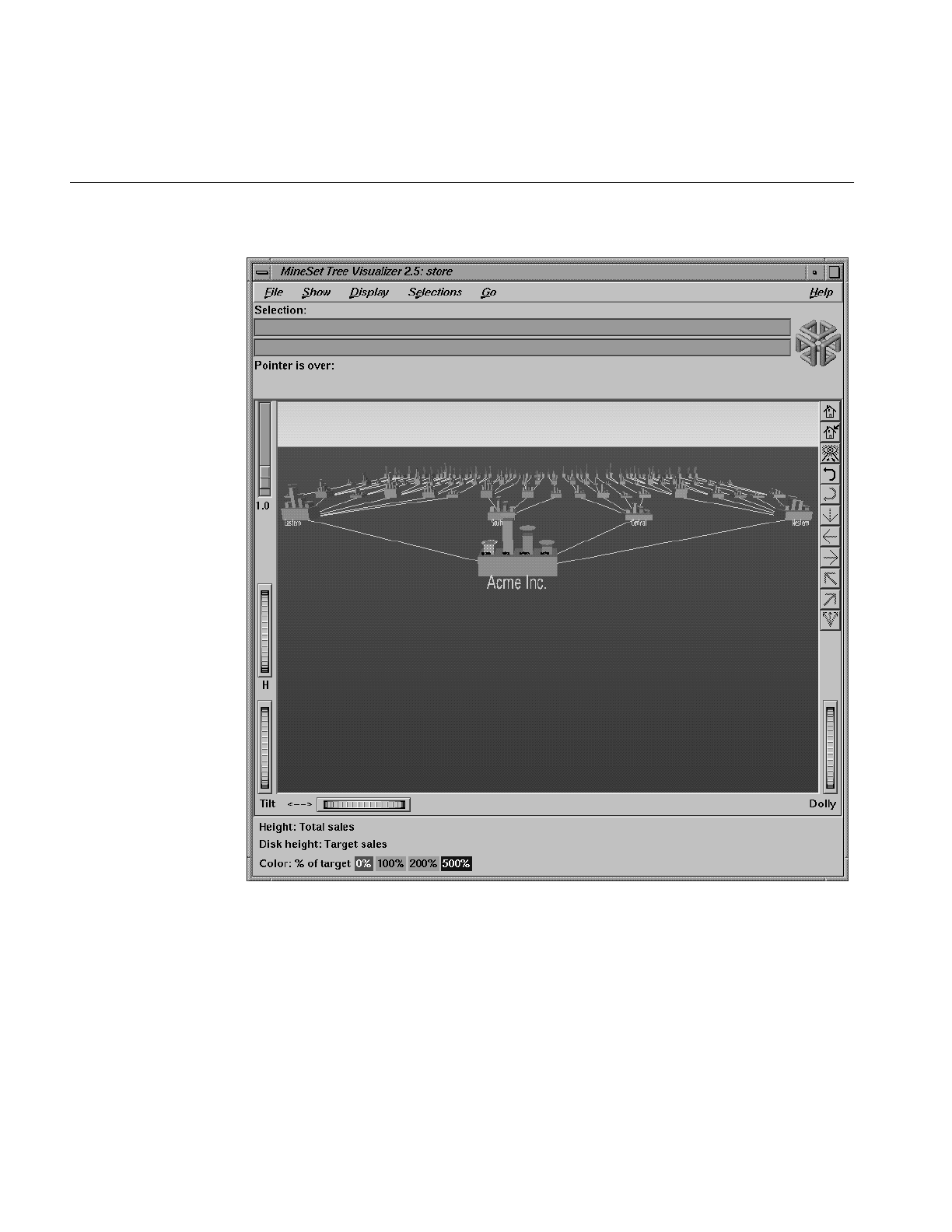
128
Chapter 5: Using the Tree Visualizer
Figure 5-1 Example Display in the Tree Visualizer’s Main Window

File Requirements
129
Values in subgroups can be summed and displayed automatically in the next higher
level. The base under the bars can provide information about the aggregate value of all
the bars. Bars representing negative values are shown below the top of the base. You can
see negative value bars more clearly by disabling the base height (see “The Display
Menu” on page 165, or the “Base Height Statements” section in Appendix B, “Creating
Data and Configuration Files for the Tree Visualizer”).
File Requirements
The Tree Visualizer requires the following files:
•Adata file consisting of rows of tab-separated fields. This file is easily created using
the Tool Manager (see Chapter 3). If you are generating this file yourself, see
Appendix B, “Creating Data and Configuration Files for the Tree Visualizer” for the
required file format.
Data files are generated by extracting data from a source (such as an Oracle,
INFORMIX, or Sybase database) and formatting it specifically for use by the Tree
Visualizer. Data files have user-defined extensions (the sample files provided with
the Tree Visualizer have a .data extension).
•Aconfiguration file describing the format of the input data and how these are
converted to a hierarchy. This file also is easily created using the Tools Manager (see
Chapter 3). You also can use an editor (such as jot, vi, or Emacs) to produce this file
(see Appendix B, “Creating Data and Configuration Files for the Tree Visualizer”).
Configuration files must have a .treeviz extension. When starting the Tree Visualizer,
or when opening a file, specify the configuration file, not the data file.

130
Chapter 5: Using the Tree Visualizer
Starting the Tree Visualizer
There are five ways to start the Tree Visualizer:
•Use the Tool Manager to configure and start the Tree Visualizer. (See Chapter 3 first
for details on most of the Tool Manager’s functionality, which is common to all
MineSet tools; see below for details about using the Tool Manager in conjunction
with the Tree Visualizer.)
•Double-click the Tree Visualizer icon, which is in the MineSet page of the icon
catalog. The icon is labeled treeviz. Since no configuration file is specified, the
start-up screen requires you to select one by using File|Open.
Starting the Tree Visualizer without specifying a configuration file causes the main
window to show the copyright notice for this tool. Only the File and Help pulldown
menus can be used. For the main window to be fully functional, open a
configuration file by selecting File|Open (Figure 5-2).
Figure 5-2 Tree Visualizer’s File Pulldown Menu
•If you know what configuration file you want to use, double-click the icon for that
file. This starts the Tree Visualizer and automatically loads the file you specified.
This only works if the filename ends in .treeviz (which is always the case for
configuration files created for the Tree Visualizer via the Tool Manager).

Starting the Tree Visualizer
131
•Drag the configuration file icon onto the Tree Visualizer icon. This starts the Tree
Visualizer and automatically loads the file you specified. This works even if the
filename does not end in .treeviz.
•Start the Tree Visualizer from the UNIX shell command line by entering this
command at the prompt:
treeviz [ configFile ]
where configFile is optional and specifies the name of the configuration file to use. If
you don’t specify a configuration file, you must use File > Open to specify one (see
Figure 5-2).
Options for Invoking the Tree Visualizer
There are a two options that affect how this tool is invoked:
•-warnexecute indicates that if you attempt to execute a command specified in an
execute statement, a warning is displayed and you are given the option to execute
the command or not. This is intended for an insecure environment, such as files
obtained from the Web, and is used automatically when commands are executed via
mtr files.
You can enable this option permanently by adding the line
*minesetWarnExecute:TRUE
to the user’s.Xdefaults file, or by setting the environment variable
MINESET_WARN_EXECUTE
•-quiet eliminates the dialogs that popup to indicate progress. You can enable this
option permanently by adding the line
*minesetQuiet:TRUE
to your .Xdefaults file.

132
Chapter 5: Using the Tree Visualizer
Configuring the Tree Visualizer Using the Tool Manager
This section describes how the Tree Visualizer can be configured using the Tool Manager.
Although the Tool Manager greatly simplifies the task of configuring the Tree Visualizer,
you can construct a configuration file manually for this tool using an editor (see
Appendix B, “Creating Data and Configuration Files for the Tree Visualizer”).
For the Tree Visualizer, the Tool Manager does not support the following:
•Non-aggregated hierarchies where the data is displayed directly without
aggregating it.
•Real-time monitoring.
•A number of very rarely used options (skip missing, overview, shrinkage, root label,
speed, climb speed, leaf margin, root leaf margin, leaf edge margin, initial position,
initial angle, bar label size, base label size, and lod). See Appendix B.
•Variable-length arrays.
•Expressions computed after creating the hierarchy. For example, if you are
computing a percentage, the percentage must be computed after the hierarchy
aggregation takes place, since it is not possible to aggregate the percentages.
Note that the steps required to connect to a data source are described in Chapter 3.
Selecting the Tree Visualizer Tool
Select the Viz Tools tab in the Data Destination panel of the Tool Manager’s main screen
(Figure 5-3). From the popup list of tools, select Tree Visualizer. The mapping
requirements for the Tree Visualizer are displayed in the window on the right side of this
panel. Items in the Visual Elements: list that are preceded by an asterisk are optional.
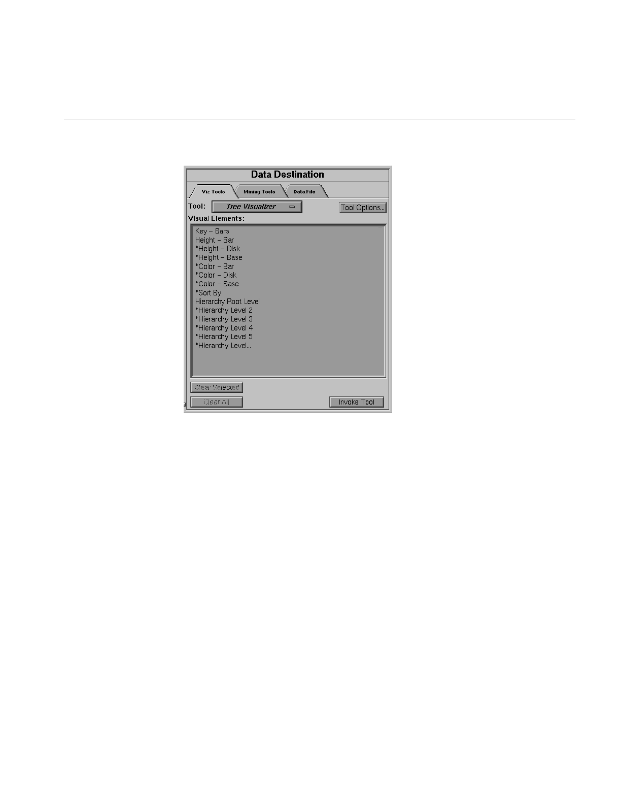
Configuring the Tree Visualizer Using the Tool Manager
133
Figure 5-3 Data Destination Panel of Tool Manager With Tree Visualizer Selected
Key - Bars lets you define what the bars shown in the Tree Visualizer main window
represent. For example, in a table representing the budget of the 50 United States, the
keys could be state names. If the first key is associated with Alabama, the first bar
represents the values for Alabama.
Height - Bar lets you specify what the bar heights represent. Typically, the higher the bar,
the greater the value represented.
Sort By lets you specify a column, the values of which are used to sort the layout of the
nodes. The sort order defaults to ascending from left to right.
Hierarchy Root Level lets you specify how the table from your data source is converted into
a hierarchy. The Visual Elements list defaults to six hierarchical levels. If you specify a
sixth hierarchy level, the Tree Visualizer automatically adds a seventh. With every extra
level you specify, the Tree Visualizer adds another one. You can specify as many
hierarchy levels as necessary.

134
Chapter 5: Using the Tree Visualizer
Height - Disk—lets you specify what the heights represent for optional disks placed at the
same location as the bar. If no mapping is specified, no disks are displayed.
Height - Base—lets you specify what the base heights represent. If no mapping is
specified, the bar height mapping is used.
Color - Bar—lets you specify what the bar colors represent. The specific colors must be
assigned via the Tool Manager’s Tool Options panel (see “Choosing Colors” and “Using
the Color Browser” in Chapter 3).
Color - Disk—lets you specify what the disk colors represent. This option has an effect
only if the disk height is specified (see “Choosing Colors” and “Using the Color Browser”
in Chapter 3).
Color - Base—lets you specify what the base colors represent. If no mapping is specified,
the bar color mapping is used (see “Choosing Colors” and “Using the Color Browser” in
Chapter 3).
Undoing Mappings
To undo any mapping, select that mapping in the Requirements: window, then click the
Clear Selected button. To undo all mappings, click the Clear All button.
Specifying Tool Options
Clicking the Tool Options button causes a new dialog box to be displayed (Figure 5-4).
This lets you change some of the Tree Visualizer options from their default values.
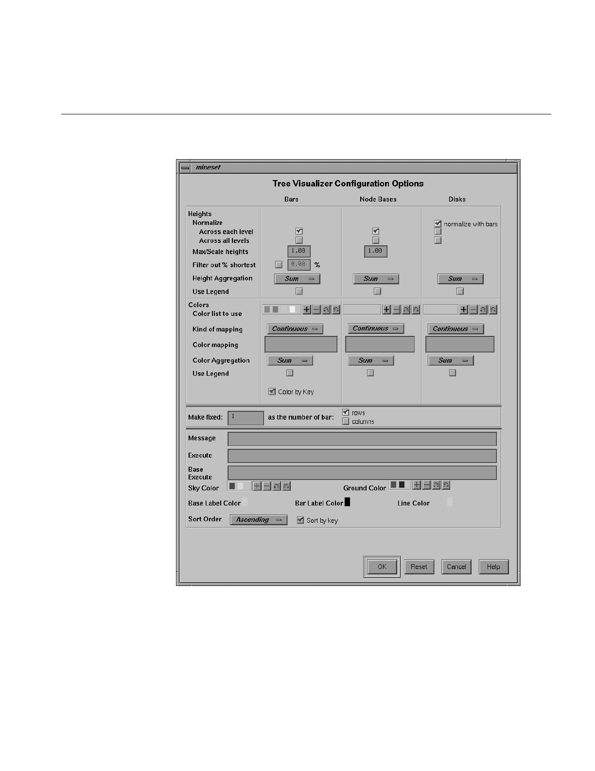
Configuring the Tree Visualizer Using the Tool Manager
135
Figure 5-4 Tree Visualizer’s Configuration Options Dialog Box
The top of the dialog box has three columns: Bars,Node Bases, and Disks.

136
Chapter 5: Using the Tree Visualizer
Normalize Heights
This option lets you normalize heights across each level of the hierarchy (or across all
levels) of bars, node bases, and disks. Normalizing the heights determines the maximum
value of the height variable; it normalizes all values relative to that height. Thus, if the
maximum value is 30.0, and the maximum bar height was set to 1.0 (in arbitrary units),
a value of 15.0 would be mapped to a value of 0.5.
Normalizing across each level independently normalizes each level of the hierarchy. This
option is most useful if data has been summed up the hierarchy, and prevents the top
level of the hierarchy from dwarfing items at the lowest level. Normalizing across all
levels normalizes everything together, regardless of the level in the hierarchy. If neither
box is checked for bars, no normalization takes place.
Node Bases are normalized independently of Bars. If no boxes are checked, the same
normalization method used for bars is used for node bases, although the values are
normalized independently.
If disks are present and normalize with bars is checked, the disks are normalized in
conjunction with the bars: a disk and a bar representing the same value have the same
height. If one of the other normalize boxes is checked in the Disks column, disks are
normalized independently of the bars: the highest disk and the tallest bar have the same
height, regardless of the actual values represented by them.
Max/Scale Heights
This option lets you specify the height of the tallest bars and node bases. The default is
1.0 (in arbitrary units). If after looking at the view, you see that the heights are too low or
too high, use this field to adjust them. For example, entering 2 in the field causes all bars
to be doubled in height; entering .5 makes all bars half as big.
If normalization was specified, this value represents the height of the tallest bar or base.
If normalization was not specified, all values are scaled by this amount. The latter can be
useful when comparing views of two different datasets.

Configuring the Tree Visualizer Using the Tool Manager
137
Filter out % shortest
This option lets you filter out nodes containing only short bars. First, the tallest bar in the
scene is calculated (if heights are normalized by level, then the tallest bar in each level).
Then only those nodes that contain at least one bar that is the appropriate percentage of
the tallest bar are shown. For example, if you enter 5% in this field, then only those nodes
containing at least one bar that is at least 5% of the height of the tallest bar are shown.
(Also shown are ancestors of such bars). This option is intended as a coarse way to filter
out small, uninteresting nodes. It is not intended as an exact mechanism of identifying
specific nodes of a certain value. Use of this option can accelerate the rendering of slow,
complex scenes, or reduce clutter resulting from many bars near zero height.
Although small nodes are filtered out, they are nonetheless counted in any cumulation
up the hierarchy.
Height Aggregation
By default, the height of the bars of the parent node is the sum of the height of all the bars
of the children; however, these heights can be average, max, min, count, or any of the
values that appear. This aggregation can be used for the values of the bar heights, base
heights, and disk heights.
Colors
This set of options lets you
•specify the list of colors to use
•specify the kind of mapping
•map colors to bars, node bases, and disks
To use these Colors options, you must have mapped a column to the *Color - Bar,
*Color - Disk, or *Color - Base requirements of the Data Destination panel. See
“Choosing Colors” and “Using the Color Browser” in Chapter 3 for a more detailed
explanation of how to choose and change colors.

138
Chapter 5: Using the Tree Visualizer
Color list to use lets you specify the color list using the + button next to the color list label.
This brings up a color editor that lets you specify a color to be added to the list.
Kind of mapping lets you specify whether the color change that is shown in the graphic
display is Continuous or Discrete. If you choose Continuous, the color values (of the bars,
node bases, or disks) shift gradually between the colors entered in the Color list to use
field as a function of the values that are mapped to those colors in the Color mapping field.
If you choose Discrete, the colors change only at the specified boundaries.
Color mapping lets you specify values to which the colors are mapped.
Example 5-1
If you
•used the Color Browser to apply red and green to bars
•selected Discrete for the Kind of mapping
•entered the values 0 100
then the display shows all bars (or node bases or disks) with values of less than 100 in
red, and all those with values greater than or equal to 100 in green.
Example 5-2
If you
•used the Color Browser to apply red and green to bars
•selected Continuous for the Kind of mapping
•entered the values 0 100
then the display shows all bars (or node bases or disks) with values less than or equal to
0 as completely red, those as greater than or equal to 100 as completely green, and those
between 0 and 100 as shadings from red to green.

Configuring the Tree Visualizer Using the Tool Manager
139
Color Aggregation
By default, the values of the colors of the bars of the parent node are the sum of the values
of all the bars of the children; however, these colors can be average, max, min, or any of
the values that appear. This aggregation can be used for the values of the bar colors, base
node colors, and disk colors.
Color by Key
This option lets you automatically color the bars by their key value. This option is
ignored if another coloring was specified. If you specify no color list, or specify
insufficient colors, additional colors are chosen at random. If extra colors are specified,
they are ignored.
Make Fixed
By default, this option places all bars across one row. This option allows changing the
number of rows or columns. If neither rows nor columns are selected, or the number is
set to 0, then neither rows nor columns are fixed, and the closest approximation to a
square is displayed.
Message
This option lets you type in any message you want. The message statement specifies the
message displayed when the pointer is moved over an object or when an object is
selected. By default, the same message is used for the base as for the bars. If no message
is specified, a default message containing the names and values of all the columns is
used.
The format of the message must match the type of data being used:
•Strings must use %s.
•Ints must use integer formats (like %d).
•Floats and doubles must used floating-point formats (like %f).
For a detailed description of the message field, see “Message Statements” in Appendix B.

140
Chapter 5: Using the Tree Visualizer
Execute and Base Execute
These options let you type in a UNIX command that is executed when double-clicking
on a bar or base. If only the Execute field is filled in, it applies to both bars and bases. If
both are filled in, Execute applies to bars, and Base Execute applies to bases. The format
is similar to the message statement. If no execute statement appears, double-clicking has
no effect.
For a detailed description of the Execute field, see “The Execute Statement” in
Appendix B.
Sky Color
You can specify either one or two colors. If only one color is specified, the sky is solid. If
two colors are specified, the sky is shaded between the colors. When specifying two
colors, the first color is for the top of the sky, the second for the bottom.
Ground Color
You can specify either one or two colors. If only one color is specified, the ground is solid.
If two colors are specified, the ground is shaded between the colors. For the ground, the
first color is for the far horizon, the second is for the near ground.
Base Label Color
You can specify the color of the labels on the front of the bases.
Bar Label Color
You can specify the color of the labels on the front of the bars.
Line Color
You can specify the color of the lines connecting the bases.

Configuring the Tree Visualizer Using the Tool Manager
141
Sort Order
If you select the Sort by Key checkbox, the nodes in the display are in sorted order. The
menu next to the checkbox lets you specify whether to sort in ascending or descending
order.
Resetting the Tool Options
If, after you have made changes to the Tool Options dialog box, you want to reset the
values of all options to their default values, click the Reset Options button.
Saving the New Tool Options
Once you have finished making changes to the Tool Options dialog box, click OK to
return to the Tool Manager’s main screen.
Saving Tree Visualizer Settings
The Tool Manager stores information for the Tree Visualizer in several files, all sharing
the same prefix:
•<prefix>.treeviz.data contains data.
•<prefix>.treeviz.schema describes the data file.
•<prefix>.treeviz contains information needed by the Tree Visualizer.
•<prefix>.mineset contains all the information needed to create the other files.
To specify a prefix, use the Save Current Session As ... menu option in the File menu of the
Tool Manager’s main window. If you do not specify a prefix, it is based on the data
source.
When you use the Invoke Tool button, the .data,.schema, and .treeviz files are updated, if
necessary.
Invoking the Tree Visualizer
To see the Tree Visualizer graphically represent your data, click the Invoke Tool button at
the bottom of the Data Destination panel.

142
Chapter 5: Using the Tree Visualizer
Working in the Tree Visualizer’s Main Window
A file’s hierarchy is visible only after a valid configuration file is specified. For example,
specifying store.treeviz results in Figure 5-5.
Figure 5-5 Tree Visualizer’s Initial View When Specifying store.treeviz

Working in the Tree Visualizer’s Main Window
143
The root node of the hierarchy is at the front of the scene, near the bottom of the Tree
Visualizer’s main window. In back of the root node are its descendents; each one consists
of a base with bars on it. You can change what the heights and colors of the bars represent
via the Tool Manager or by manually changing the .treeviz configuration file; usually, the
base represents the aggregate of all the bars. Bases are connected with lines representing
the connection of the nodes to their descendents.
Highlighting an Object or Node
To highlight an object, move the mouse over that object (either a base or a bar). This
causes information about that object to appear over the top left of the view area, under
the Pointer is over: label (Figure 5-6). To highlight a node and obtain information about
that node, place the pointer over a line leading to that node. This information appears in
the same place as that for an object.
Figure 5-6 A Highlighted Object and the Information It Represents

144
Chapter 5: Using the Tree Visualizer
Selecting an Object
To select an object and zoom to it, left-click the mouse on that object. Hold the Ctrl key
down while clicking to select the object without zooming to it. At the top of the window,
under the label “Selection:”, you see information about a selected object. The information
is the same as that shown when highlighting an object. As long as the object is selected,
the information is displayed. This lets you compare information about two objects by
selecting one, then highlighting the other. Using the mouse, you can cut and paste
selection information into other applications, such as reports or databases.
If you hold the Shift key while left-clicking on an object, the selection of that object is
toggled. If the object is currently not selected, it then is selected; conversely, if it is
currently selected, it then is deselected. Using this technique, it is possible to select
multiple objects simultaneously. While the information under the “Selection:” label only
shows the information on the last object selected, it is possible to see the values for all
selections by using Selections > Show Values or by drilling through to the original data
behind the selections (see “The Selections Menu” on page 166).
If an execute statement was specified via Tool Manager or the configuration file, then
double clicking on an object executes the appropriate command. If the -warnexecute
option was specified when invoking the Tree Visualizer, a warning is given first.
Spotlighting an Object
When you select an object, a white spotlight appears on it (Figure 5-7). A yellow spotlight
appears when you are searching (see “The Search Panel” on page 154). Spotlights are
visible even if the selected object is a descendent node in the far background.
The edges of spotlights are surrogates for an object: when you move the pointer over the
edge of a spotlight, the associated object is highlighted, and information about that object
appears above the top left of the view. Left-click the edge of a spotlight to select the
associated object and (if the Ctrl key is not held down) to zoom to it. The spotlight is
active only on the solid lines along the edges, not the translucent section in the center.
This lets you select objects behind the spotlight.
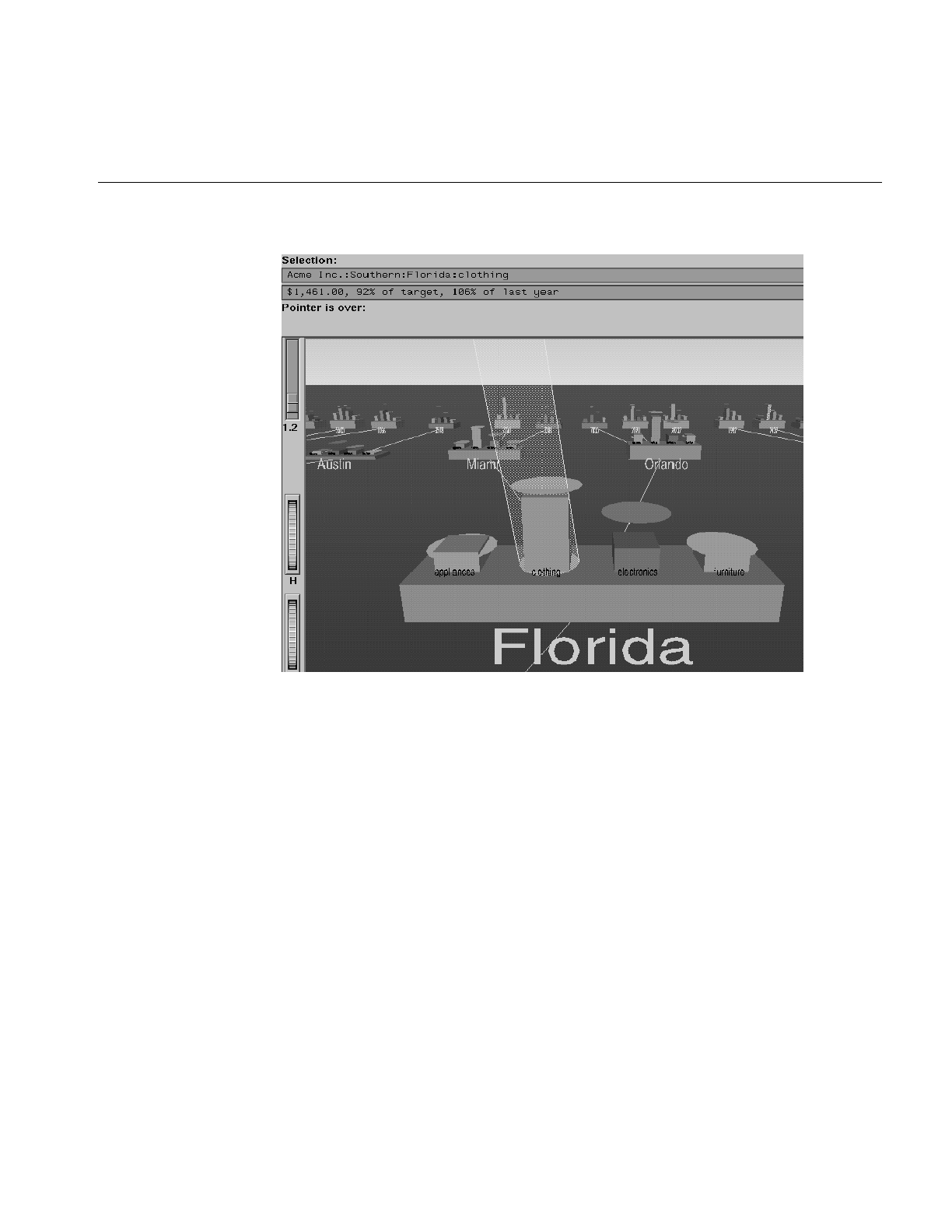
Working in the Tree Visualizer’s Main Window
145
Figure 5-7 Example of a Selected (Spotlighted) Object
Using the Right Mouse Button
When the cursor is in the main window, clicking the right mouse button (or, if the mouse
has been reconfigured, the third button) brings up a menu that lets you select the children
of a node. If you click on a node with children, it provides you with a list of the children.
This list is displayed as long as you hold the mouse button down. If you do not click on
a node, but one is selected, it provides you with a list of children of the selected node. If
nothing is selected, or if the selected node has no children, no menu is displayed.

146
Chapter 5: Using the Tree Visualizer
Navigating With the Middle Mouse Button
To navigate over the scene in the main window, use the middle mouse button. You also
can use external controls to perform all middle mouse button functions (see the “External
Controls” on page 147).
To move through the main window, click the middle mouse button. A small square
appears (see Figure 5-8). Move the cursor out of this square while pressing the mouse to
move your point of reference dynamically through the 3D landscape. The farther the
cursor is from the square, the faster your viewpoint moves. To move the viewpoint
forward, move the mouse up. To move the viewpoint back, move the mouse down.
Moving the mouse left and right causes the viewpoint to shift accordingly. You can move
in any direction as long as a part of your data is visible.
Figure 5-8 Example of the Square as Navigational Base
To move the viewpoint up and down, hold the Shift key down when pressing the middle
mouse button. To move the viewpoint up, move the mouse up. To move the viewpoint
down, move the mouse down. You cannot move below ground level.
To combine horizontal and vertical motion (that is, to move the viewpoint back and forth,
as well as up and down), hold the Alt key down when pressing the middle mouse button.
Note that while moving forward, the viewpoint also moves down, based on the current
tilt. Similarly, while moving backward, the viewpoint moves up, based on the tilt.
Note: You cannot turn from side to side. Tilting the viewpoint requires using external
controls.

External Controls
147
External Controls
Several external controls surround the graphics window. These consist of buttons and
thumbwheels.
Buttons
At the top right of the image area are eleven buttons as shown in Figure 5-9.
Figure 5-9 Tree Visualizer’s External Button Controls
•Home takes you to a designated location. Initially, this location is the first viewpoint
shown after invoking the Tree Visualizer and specifying a configuration file. If you
have been working with the Tree Visualizer and have clicked the Set Home button,
then clicking Home returns you to the viewpoint that was current when you last
clicked Set Home.
•Set Home makes your current location the Home location. Clicking the Home button
returns you to the last location where you clicked Set Home.
•View All lets you view the whole hierarchy, keeping the tilt of the camera. To get an
overhead view of the scene, tilt the camera to point straight down, then click the
View All button. To tilt the camera, see the description of the Tilt thumbwheel (see
“Thumbwheels” on page 149).
Home
Set Home
View All
Go Back
Go Forward
Parent
Move Left
Move Right
First Child
Last Child
Choose Child

148
Chapter 5: Using the Tree Visualizer
•Go Back lets you return to the previous location. If you have just started the Tree
Visualizer and have not moved from the home view, this button is grayed out.
•Go Forward lets you proceed to the location from which you clicked the Go Back
button. If you have not clicked the Go Back button, the Go Forward button is grayed
out.
•Parent is active only when you have an object selected. If a bar is selected, clicking
this button selects the base containing the bar. If a base is selected, clicking this
button moves up the hierarchy to the parent node. Once the root node has been
reached (highest level of the hierarchy), the Parent button is grayed out. Note that
when using Parent, the selected node is changed to the parent of the previously
selected one.
•Move Left lets you select the next sibling to the left. If a bar is selected, the bar to the
left of it is selected. If a base is selected, then, if the parent has another child to the
left, that is selected. This button is grayed out if nothing is selected, or if the current
selection has no sibling to the left.
•Move Right lets you select he next sibling to the right. If a bar is selected, the bar to
the right of it is selected. If a base is selected, then, if the parent has another child to
the right, that is selected. This button is grayed out if nothing is selected, or if the
current selection has no sibling to the right.
•First Child lets you select the first child of the current node. This button is grayed out
if there is no selection, if a bar is selected, or if the current selection has no children.
•Last Child lets you select the last child of the current node. This button is grayed out
if there is no selection, if a bar is selected, or if the current selection has no children.
•Choose Child produces a popup menu that lists all the children of the current node.
This button is grayed out if there is no selection, if a bar is selected, or if the current
selection has no children.
You also can perform these functions using the Go menu (see “The Go Menu” on
page 167.)
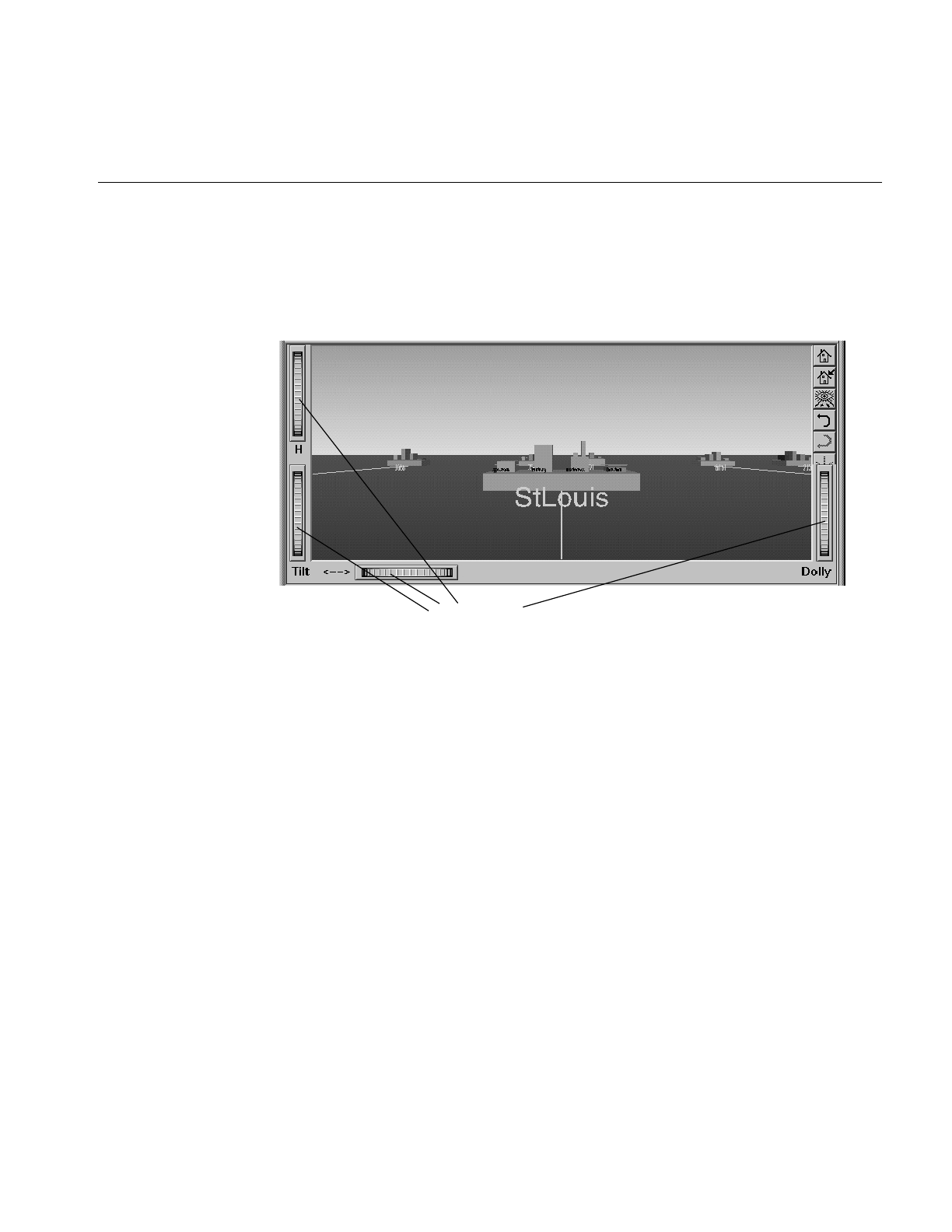
External Controls
149
Thumbwheels
Four thumbwheels appear around the lower part of the graphics window border (see
Figure 5-10). They let you dynamically move the viewpoint.
Figure 5-10 Tree Visualizer’s Thumbwheels
•The vertical H (height) thumbwheel, on the upper left, moves the camera up and
down. You cannot move the viewpoint below ground level.
•The vertical Tilt thumbwheel, at the bottom left, tilts the camera. You can tilt the
viewpoint to any position from straight ahead and straight down. You cannot tilt
the viewpoint to look up.
•The horizontal <--> (pan) thumbwheel, at the bottom left, moves the viewpoint
from left to right and back. You cannot rotate the viewpoint.
•The vertical Dolly thumbwheel, on the right, moves the viewpoint forward and
backward.
Thumbwheels

150
Chapter 5: Using the Tree Visualizer
Height Slider
A slider to the top left of the main window (Figure 5-11) lets you rescale all objects in the
window. Pushing the slider up to a value of 2.0 doubles the size of all objects in the main
window. Pulling the slider back down to a value of 1.0 returns the objects in the window
to their original heights.
Figure 5-11 Tree Visualizer’s Height Slider
Pulldown Menus
You also can access all of the Tree Visualizer’s functions via five pulldown menus. These
are labeled File, Show, Display, Go, and Help.
If you start the Tree Visualizer without specifying a configuration file, only the File and
the Help menus are available. The Show, Display, and Go menus are available after a
graph is loaded.
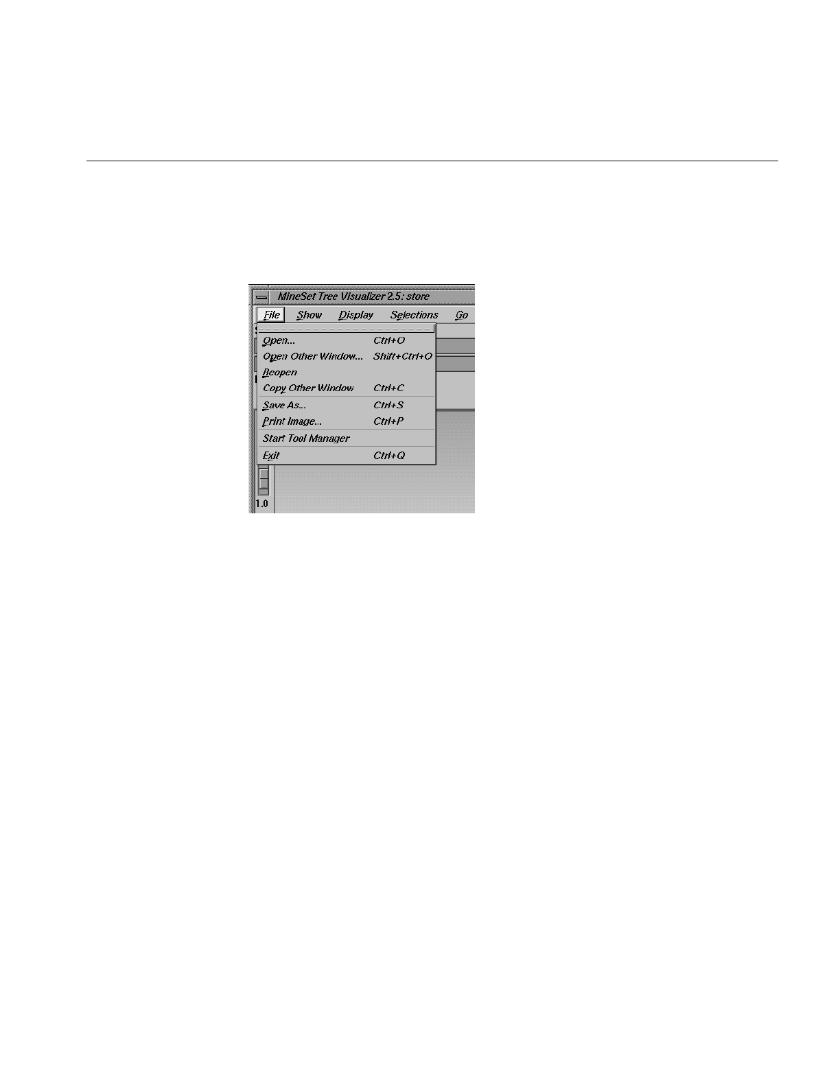
Pulldown Menus
151
The File Menu
The File menu (Figure 5-12) contains nine options.
Figure 5-12 Tree Visualizer’s File Pulldown Menu With Options
•Open loads and opens a configuration file, displaying it in the main window.
Previously displayed data is discarded. Use Open to view a new dataset, or to view
the same dataset after changing its configuration.
•Open Other Window opens a configuration file, but displays its results in a different
window. The current dataset remains open.
•Reopen reopens the currently opened file. This can be used after the configuration or
data file has been updated.
•Copy Other Window opens a new window that displays the same view of the current
dataset. You can interact with these windows independently.
•Save As saves the state of the current Tree Visualizer window into an image file. The
user specifies both the file name (default is treeviz.rgb), format (default is rgb), and
whether to save the entire window, including any legends, or just the main scene
with the graphical objects (default is the full window).

152
Chapter 5: Using the Tree Visualizer
•Print Image outputs the state of the current Tree Visualizer window to a printer. You
can specify the output printer using a Print dialog panel (default is your system's
default printer) and, like the Save As dialog, choose whether to print the entire
window or just the main scene window.
•Start Tool Manager starts the Tool Manager (if not already running), and restores it to
the state it was in when the Tree Visualizer was invoked.
•Close closes the current window (and all panels associated with it). If no other
windows are open, Close exits the application.
•Exit closes all windows and exits the application.
The Show Menu
The Show menu (Figure 5-13) contains four options:
•Overview
•Search Panel
•Filter Panel
•Marks Panel
Each of these options brings up another dialog box for interacting with the data.
Figure 5-13 Tree Visualizer’s Show Pulldown Menu With Options
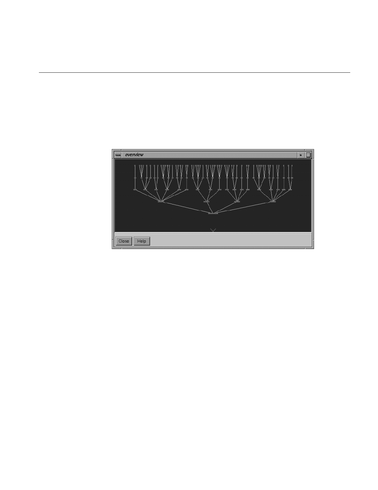
Pulldown Menus
153
The Overview Window
Select Overview in the Show menu to bring up a new window with an overhead view of
the complete hierarchy (Figure 5-14). If you want the Overview to be brought up
automatically each time the scene is viewed, set the Overview option in the configuration
file (see “Overview” on page 566).
Figure 5-14 Tree Visualizer’s Overview Window
The “X” in the Overview window shows your current location. The Overview helps you
keep track of your location and viewpoint in the entire scene. It can also help you quickly
go to a specific node.
To select an object in the Overview and have the main view zoom to it, left-click that
object. This is similar to left-clicking the object in the main view. Middle-clicking
anywhere in the overview zooms your viewpoint to that location, even if no object is at
that point.
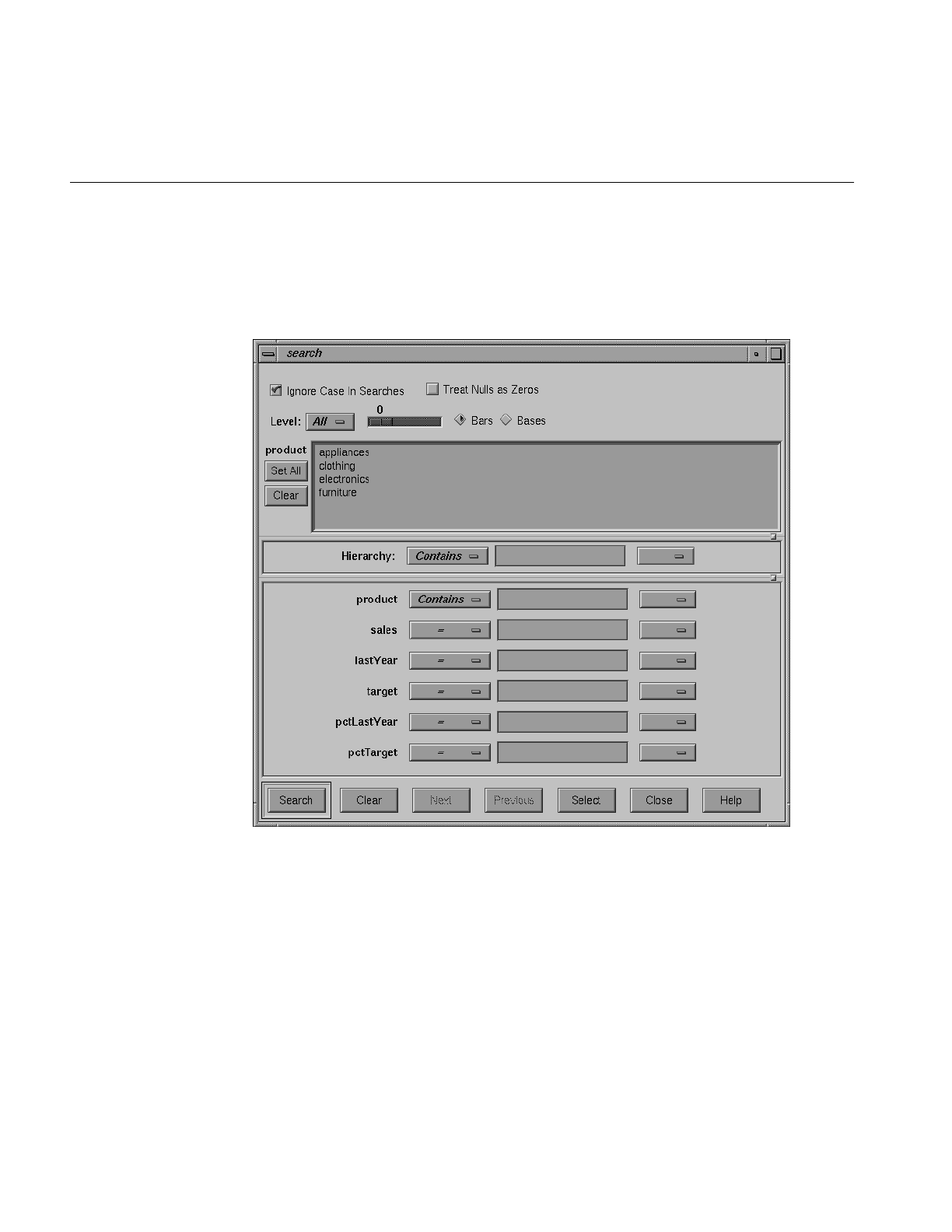
154
Chapter 5: Using the Tree Visualizer
The Search Panel
Select Search in the Show menu to bring up a dialog box that lets you specify criteria to
search for objects (Figure 5-15).
Figure 5-15 Tree Visualizer’s Search Dialog Box
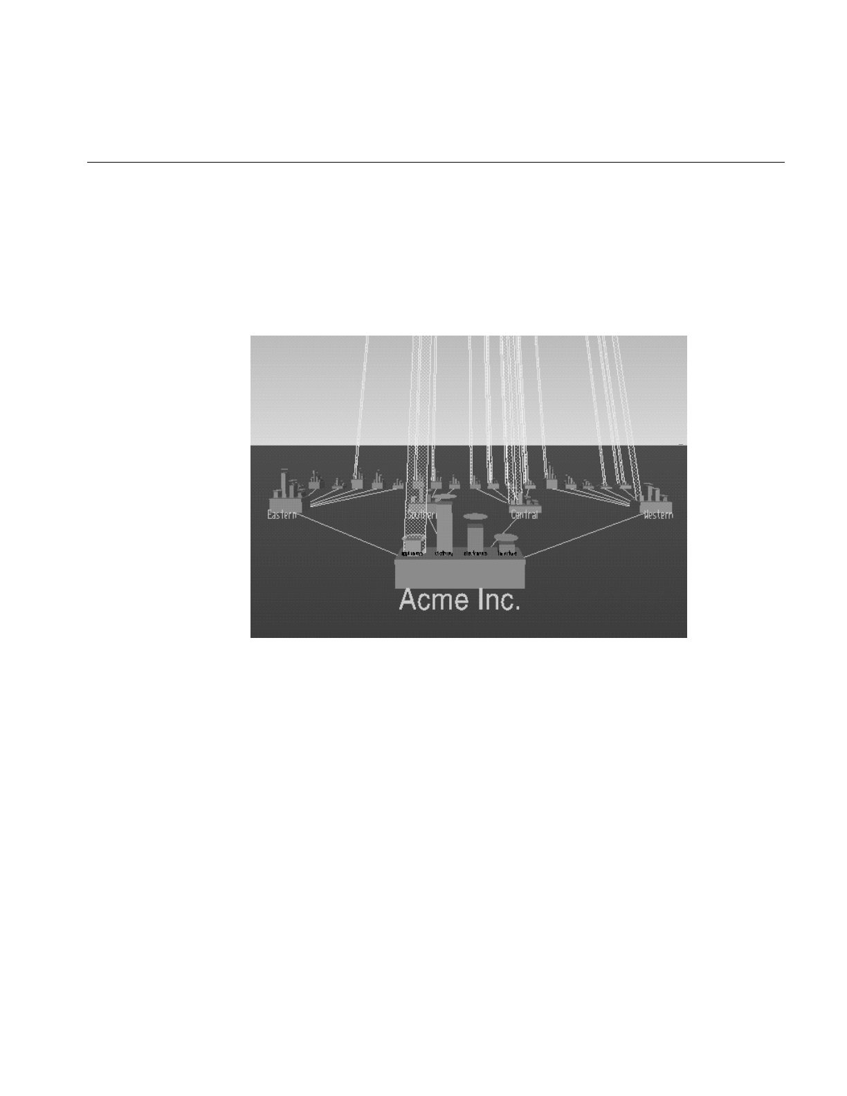
Pulldown Menus
155
Once the search is complete, yellow spotlights highlight objects matching the search
criteria (see Figure 5-16). To display information about an object under a yellow
spotlight, move the pointer over that spotlight; the information appears in the upper left
corner, under the label Pointer is over:. To select and zoom to an object under a yellow
spotlight, left-click the spotlight; if you press the Ctrl key while clicking, zooming does
not occur.
Figure 5-16 Sample Results of a Search in the Tree Visualizer
Items in the Search Panel
To specify whether a search is case-sensitive, click the Ignore Case In Searches checkbox, at
the top of the Search panel. For example, if this toggle is on (a check mark appears on that
button), the string “hello” is the same as “HellO.”
To the right of the case sensitivity checkbox is another, labeled Treat Nulls as Zeros. If this
checkbox is off (the default), comparisons involving nulls cannot return TRUE in a
search. If the it is on, nulls are treated as equal to zero.
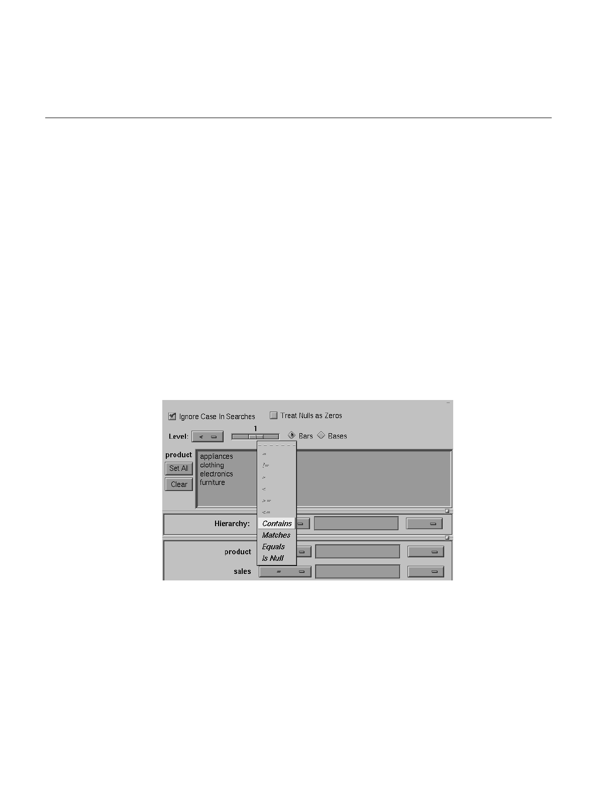
156
Chapter 5: Using the Tree Visualizer
Below the case-sensitivity checkbox are controls that let you specify the parts of the
hierarchy to be searched. By default, the whole hierarchy is searched. To limit the levels
searched, select a relational operator (such as <=) from the option menu that lets you
specify the operand for the level. Then use the slider to select the level to be searched.
Level 0 is the root of the hierarchy, level 1 is the level below that, and so forth. To search
the root and the two levels below that, for example, choose <= 2.
Checkboxes also let you choose whether to search the bars or the bases.
When searching through bars, the default is that all bars are searched. To search only a
specific list of bars, you must select them. The Set All button turns on all bars; this is
useful if most of the bars are to be searched, and only a few are to be turned off. The Clear
button turns off all bars. If no bar is selected, the bar list is ignored, and all bars are
searched.
Below the panel for bar labels is a Hierarchy field that lets you specify nodes to search
(Figure 5-17). Below the Hierarchy field are fields that let you specify search criteria for
individual columns (defined in the Current Columns: window of the Tool Manager’s
Table Processing pane, see “Selecting the Tree Visualizer Tool” on page 132).
Figure 5-17 Detail of the Tree Visualizer’s Search Dialog Box

Pulldown Menus
157
To search for numeric values, enter the value, and select a relational operation (=, !=, >,
<, >=, <=). To search for alphanumeric values, enter the string for which you want to
search. You can use any of three types of string comparisons:
•“Contains” indicates that it contains the appropriate string. For example, California
contains the strings Cal and forn.
•“Equals” requires the strings to match exactly.
•“Matches” allows wildcards:
–An asterisk (*) represents any number of characters.
–A question mark (?) represents one character.
–Square braces ([ ]) enclose a list of characters to match.
For example, California matches Cal*, Cal?fornia, and Cal[a-z]fornia.
In some cases (usually associated with binning in the Tool Manager), an option menu of
values appears, instead of a text field. To ignore that variable, select Ignored in the Option
menu. You can use relational operators (such as >=) with these options. This means that
the specified value as well as subsequent ones are selected.
In addition to numeric and string comparison operations, you can specify Is Null,
which is true if the value is null.
To the right of each search field is an additional option menu that lets you specify “And”
or “Or” options. For example, you could specify “sales > 20 And < 40.” You can have any
number of And or Or clauses for a given column, but cannot mix And and Or in a single
column.
Note that if different levels of the hierarchy are keyed by different types of data (for
example, the top level is selected by strings, while the second level is selected by
integers), then the “Hierarchy” search field is treated as a string and provides string
operations, not number operations.
If the Ignore Case In Searches checkbox is checked, the comparisons of all string searches
are case-insensitive.

158
Chapter 5: Using the Tree Visualizer
Six buttons are placed across the bottom of the Search panel:
•Search causes the search to be started. This button is automatically activated if the
Enter key is pressed and the panel is active.
•Clear turns off all search spotlights and erases the values from the search fields.
•Next selects and zooms to the next matched object, in left-to-right order. After the
last matched object is selected, clicking Next returns the view to the Home position.
Next is valid only after a search that has found matches.
•Previous selects and zooms in the opposite order from that of the Next button.
•Select causes all objects that matched the search criteria to be selected. The Selections
menu can then interact with these objects.
•Close closes the search window and turns off the search spotlights. If the Search
panel is reopened, it is in the same state as it was before the last Close; clicking Search
again repeats the last search.
The Filter Panel
The Filter panel filters out selected information, thus fine-tuning the displayed hierarchy.
You can use the Filter panel to emphasize specific information, or to shrink the amount
of data for better performance. Figure 5-18 shows a sample Filter panel.
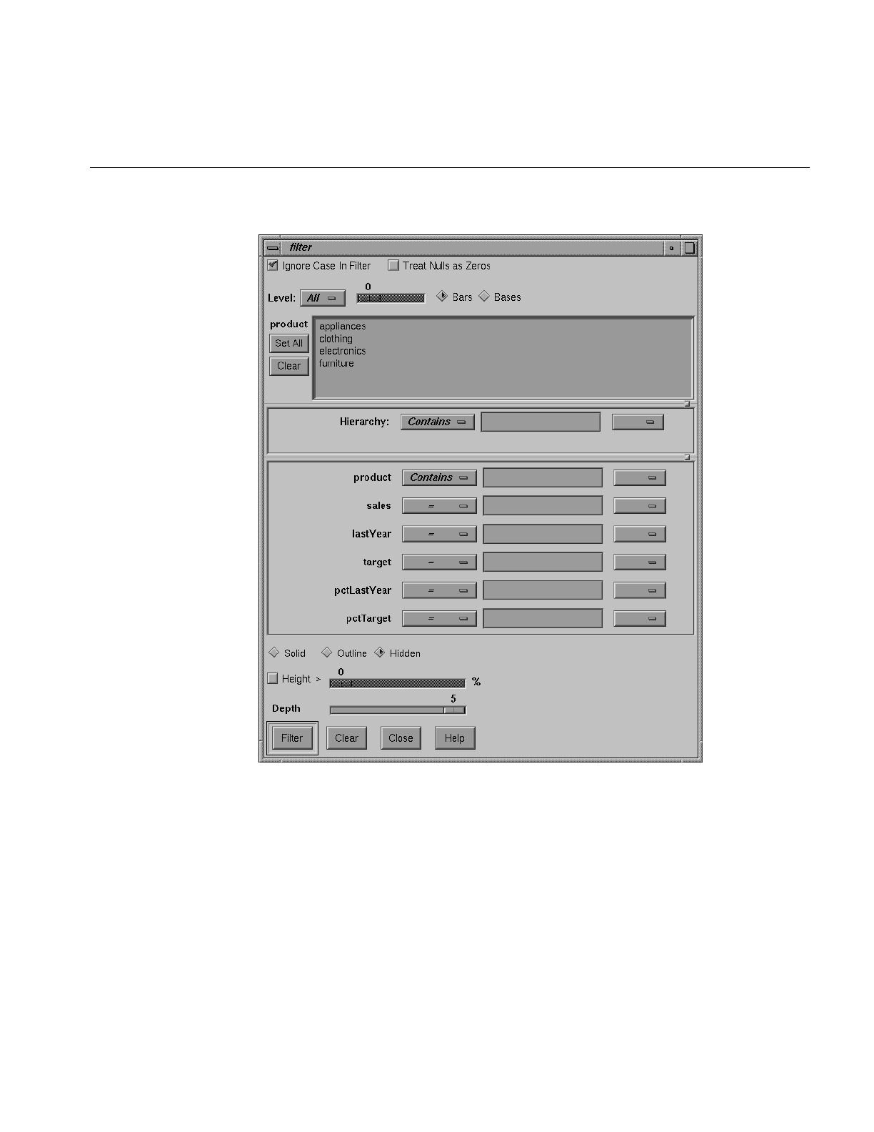
Pulldown Menus
159
Figure 5-18 Tree Visualizer’s Filter Dialog Box
To specify whether a filter is case-sensitive, click the Ignore Case In Filter checkbox, at the
top of the Filter panel. For example, if this toggle is on (a check mark appears on that
button), the string “hello” is the same as “HellO.”

160
Chapter 5: Using the Tree Visualizer
To the right of the case sensitivity checkbox is another, labeled Treat Nulls as Zeros. If this
checkbox is off (the default), comparisons involving nulls cannot return TRUE in a filter.
If the it is on, nulls are treated as equal to zero.
Below the case-sensitivity checkbox are controls that let you specify the parts of the
hierarchy to be filtered. By default, the whole hierarchy is filtered. To limit the levels
filtered, select a relational operator (such as <=) from the option menu that lets you
specify the operand for the level. Then use the slider to select the level to be filtered. Level
0 is the root of the hierarchy, level 1 is the level below that, and so forth. To filter the root
and the two levels below that, for example, choose <= 2.
Checkboxes also let you choose whether to filter the bars or bases.
When filtering bars, the default is that all bars are filtered. To filter only a specific list of
bars, you must select them. The Set All button turns on all bars; this is useful if most of
the bars are to be filtered, and only a few are to be turned off. The Clear button turns off
all bars. If no bar is selected, the bar list is ignored.
Filtering bars does not affect the information in the base, which continues to include the
summary of all bars.
Below the panel for bar labels is a Hierarchy field, which lets you specify nodes to filter.
Below the Hierarchy field are fields that let you specify filter criteria for individual
columns (defined in the Current Columns: window of the Tool Manager’s Table
Processing pane, see “Selecting the Tree Visualizer Tool” on page 132).
To filter for numeric values, enter the value, and select a relational operation (=, !=, >, <,
>=, <=). To filter for alphanumeric values, enter the string for which you want to filter.
You can use any of three types of string comparisons:
•“Contains” indicates that it contains the appropriate string. For example, California
contains the strings Cal and forn.
•“Equals” requires the strings to match exactly.
•“Matches” allows wildcards:
–An asterisk (*) represents any number of characters.
–A question mark (?) represents one character.
–Square braces ([ ]) enclose a list of characters to match.
For example, California matches Cal*, Cal?fornia, and Cal[a-z]fornia.

Pulldown Menus
161
In some cases (usually associated with binning in the Tool Manager), an option menu of
values appears, instead of a text field. To ignore that variable, select Ignored in the Option
menu. You can use relational operators (such as >=) with these options. This means that
the specified value as well as subsequent ones are selected.
In addition to numeric and string comparison operations, you can specify Is Null,
which is true if the value is null.
To the right of each filter field is an additional option menu that lets you specify “And”
or “Or” options. For example, you could specify “sales > 20 And < 40.” You can have any
number of And or Or clauses for a given column, but cannot mix And and Or in a single
column.
Note that if different levels of the hierarchy are keyed by different types of data (for
example, the top level is selected by strings, while the second level is selected by
integers), then the “Hierarchy” filter field is treated as a string and provides string
operations, not number operations.
If the Ignore Case In Filters checkbox is checked, the comparisons of all string filters are
case-insensitive.
If a node does not meet the filter criteria, has no bars that meet the criteria, and has no
children that meet the criteria, the node is not shown. There can be, however, cases in
which a specific object meets the filter criteria, but its ancestors up the tree do not. Also,
other bars in the same node might not meet the criteria. Since position is important in
interpreting context, it might not be good to eliminate those bars. Consequently, you are
given an option of selecting one of three radio buttons that control how these objects
should be drawn: Solid,Outline, and Hidden. Note, however, that if objects are drawn in
a less solid form due to the Display Zeros or Display Null menu, they are displayed
appropriately. For example, if Nulls are to be hidden, they are always hidden, regardless
of the filter criteria.
The exception to this is when filtering to specific bars. In such a case, the other bars are
eliminated and don’t take up space, regardless of the radio button settings.
The Height Filter slider lets you filter out those nodes containing only short bars. The size
of a value is shown as a percentage of the maximum height. First, the tallest bar in the
scene is calculated (if heights are normalized by level, then the tallest bar in each level).
Then only those nodes that contain at least one bar that is the appropriate percentage of
the tallest bar are shown.

162
Chapter 5: Using the Tree Visualizer
For example, if you enter 5% in this field, then only those nodes containing at least one
bar that is at least 5% of the height of the tallest bar are shown. (Also shown are ancestors
of such bars). This option is intended as a coarse way to filter out small, uninteresting
nodes. It is not intended as an exact mechanism of identifying specific nodes of a certain
value; use the search panel for that purpose. Use of this option can accelerate the
rendering of slow, complex scenes, or reduce clutter resulting from many bars near zero
height. You can also set this filtering option in the configuration file by using the Height
Filter command.
Although small nodes are filtered out, they are nonetheless counted in any cumulation
up the hierarchy.
The Depth slider, which is under the Height Filter slider, lets you display the hierarchy
so that only a given number of levels are displayed at any given time. When you are at
the top of the hierarchy, only the number of hierarchical levels specified by the slider is
seen. The nodes in the rows are arranged to optimize their visibility. When navigating to
nodes lower in the hierarchy, additional rows are made visible automatically. The nodes
above them automatically adjust their locations to accommodate the newly added nodes;
thus, some nodes might seem to move. Note that the overview shows all nodes in the
hierarchy, not just the top nodes; thus, the layout of the overview might not match the
layout of the main view. The X in the overview approximates the corresponding location
in the main view; there is no exact mapping between the two layouts.
•Click the Filter button to start filtering. If the Enter key is pressed while the panel is
active, filtering automatically starts.
•Click the Close button to close the panel.
The Marks Panel
The Marks panel, from the Tree Visualizer's Show Pulldown Menu (Figure 5-13,) lets you
name and store important locations (viewpoints) so that you can easily and quickly
return to them (see Figure 5-19). The location is stored relative to the currently selected
object. If no object is selected, the absolute location is recorded.
All marks can be indicated by colored flags in the main view. If the mark represents a
selected object, the flag is placed on that object. If it represents an absolute position, the
flag is placed at that position. To go to the mark, click the flag. All flags can be turned on
and off using the Mark Flags menu entry in the Display menu. (See Mark Flags in “The
Display Menu” on page 165).
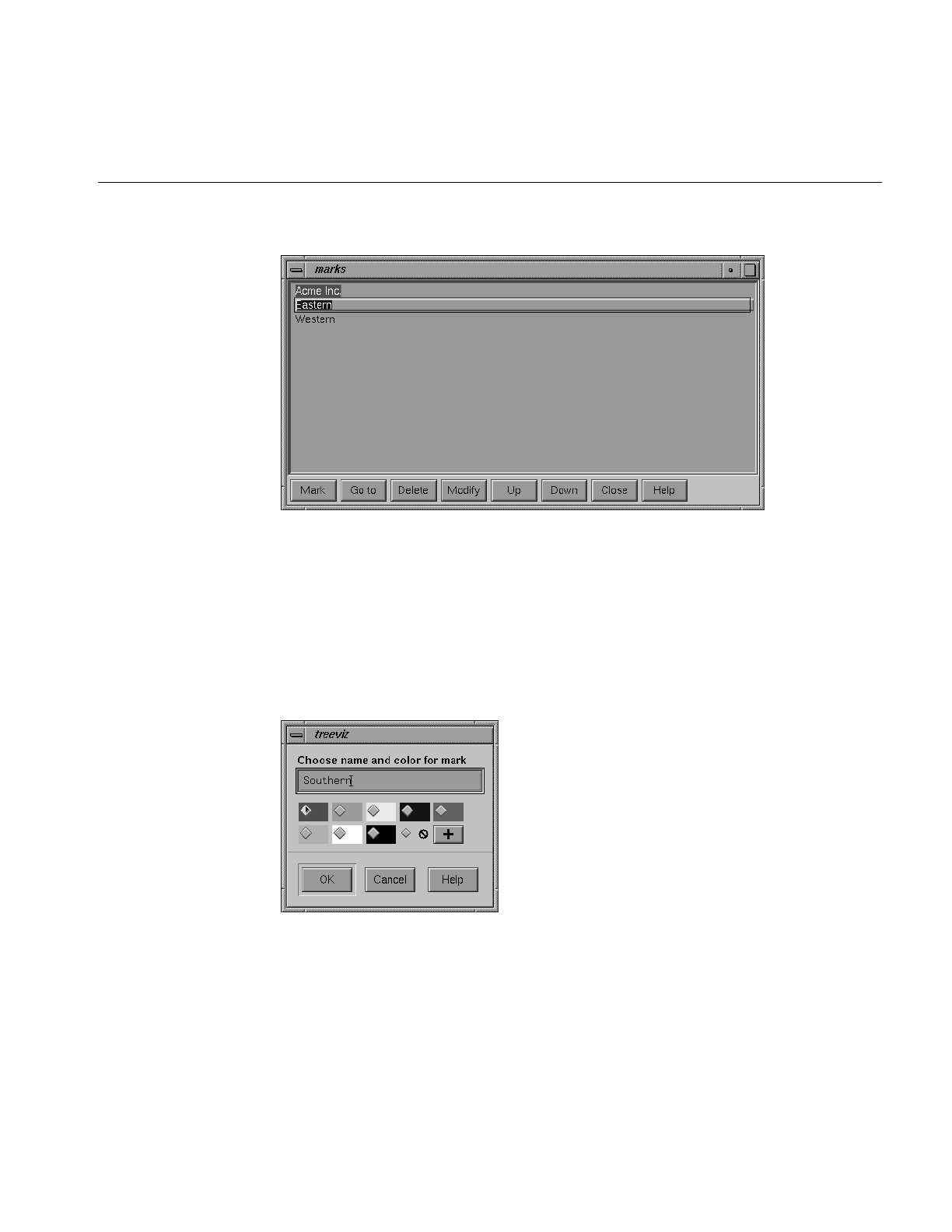
Pulldown Menus
163
Figure 5-19 Tree Visualizer’s Marks Panel
•Click the Mark button to mark the current location. Another dialog box appears (in
Figure 5-20) to prompt you for the name and color of the mark. The default name is
that of the currently selected object. The color controls the color of the flag
appearing in the main window and represents the mark. If you do not want a flag to
represent the mark, click the button with the “Not” symbol (slash through a circle).
To add another color to the palette, click the button with the plus symbol (+) to
bring up a color chooser.
Figure 5-20 Window Resulting From Clicking Mark Button

164
Chapter 5: Using the Tree Visualizer
Figure 5-21 shows a sample main window with flags representing the created marks.
Figure 5-21 Main Window With Flags Representing Marks
•Click the Go to button to go to the current location associated with the selected mark
in the panel. Double-clicking a mark has the same effect. If the object selected by
that mark no longer exists (because it was filtered out, or the data was changed
since the mark was created), the location shown is close to where the object would
have been.
•Click the Delete button to delete the selected mark in the panel.
•Click the Modify button to change the name or color of the selected mark in the
panel.
•Click the Up button to move the selected mark in the panel up the listing order.
•Click the Down button to move the selected mark in the panel down the listing
order.
•Click the Close button to exit the marks panel.
The file storing the marks information has the same name as the configuration file, with
a.marks suffix appended. Whenever a mark is changed, all marks are saved to that file.
If all marks are deleted, the .marks file is removed. If mark changes cannot be saved
(because of a permission error, for instance), a warning appears; this warning is not
repeated when subsequent mark changes are attempted.
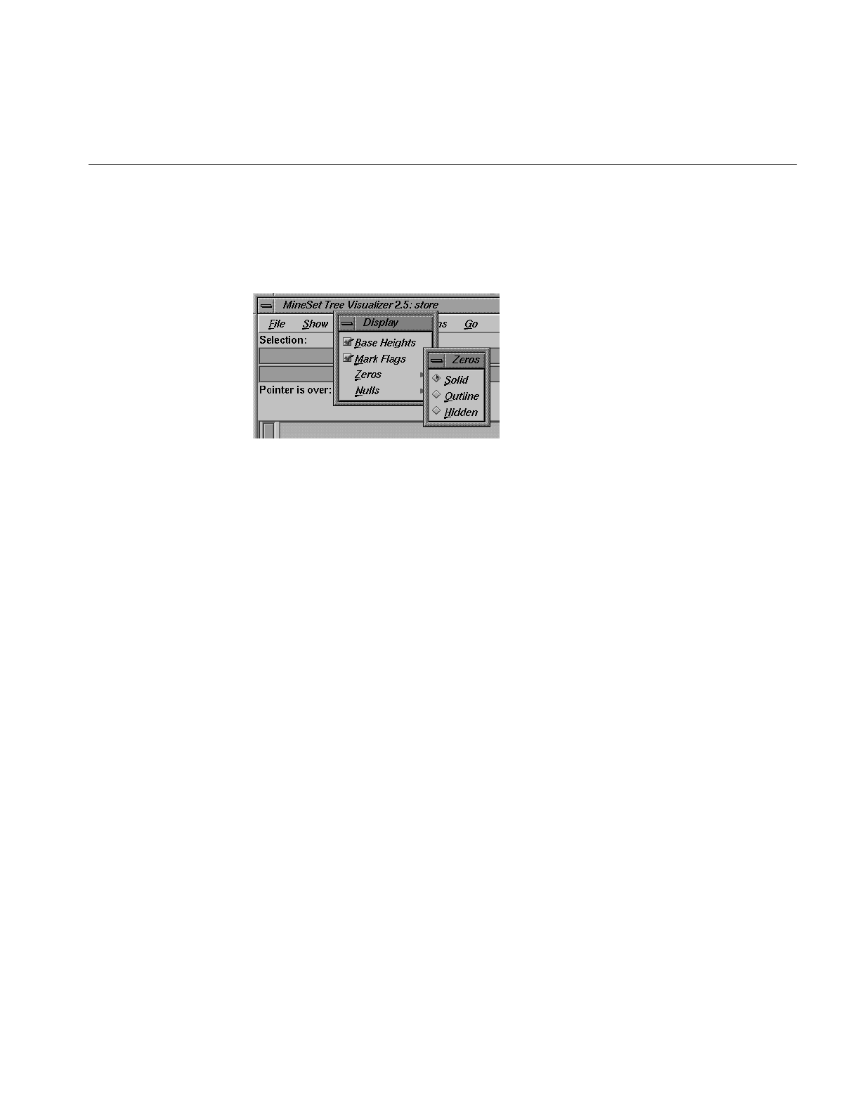
Pulldown Menus
165
The Display Menu
The Tree Visualizer's Display menu lets you control several display parameters.
Figure 5-22 Tree Visualizer’s Display Menu
Base Heights is a checkbox that lets you turn the heights of the bases on and off. To see
negative numbers, or to make it easier to compare the bar heights, turn this option off.
Turning it on provides summary information about all the bars. The initial value of this
toggle can be changed with the “base height” statement in the configuration file.
Mark Flags is a toggle option that lets you turn on or off the flags representing marks (also
see “The Marks Panel”).
Zeros is a submenu that controls how objects with zero height are displayed. By default,
they are shown like other objects: a solid cube of height zero (a plane). The submenu lets
you specify them to be displayed as outlines (appearing as a hollow square), or to be
hidden completely (not drawn). The initial value of this of this can be changed using the
“zero” option in the configuration file (see “Zero” on page 568).
Nulls is a submenu that controls how objects of null height are displayed. It has the same
options as the zero menu; however, the default for null options is to display the objects
as an outline. The initial value can be changed using the “null” option in the
configuration file (see “Null” on page 569).
!
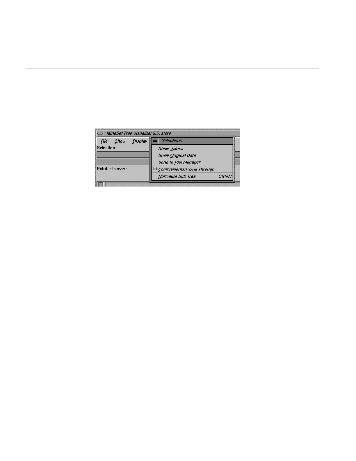
166
Chapter 5: Using the Tree Visualizer
The Selections Menu
The Selections menu lets you drill through to the underlying data. This menu has five
items (see Figure 5-23).
Figure 5-23 Tree Visualizer’s Selection Menu
•Show Values displays a table (Record Viewer) of the values for all selected objects.
•Show Original Data retrieves and displays the records corresponding to what has
been selected. The resulting records are shown in a table viewer.
•Send To Tool Manager inserts a filter operation, based on the current box selection(s),
at the beginning of the Tool Manager history. The actual expression used to do the
drill through is determined by extents of the current box selection(s). If nothing is
selected, a warning message appears.
•Complementary Drill Through causes the Show Original Data and Send To Tool Manager
selections, when used, to fetch all the data that are not selected.
•Normalize Subtree determines the maximum height of the elements in the subtree,
and normalizes all values relative to that height.
For further details on drill-through, see Chapter 18, “Selection and Drill-Through.”

Pulldown Menus
167
The Go Menu
The Go menu duplicates the functions of the buttons on the upper right-hand side of the
main window (see Figure 5-24). It also identifies keyboard shortcuts for some functions.
Figure 5-24 Tree Visualizer’s Go Pulldown Menu
•Home takes you to a designated location. By default, this location is the initial view
point of the scene. Initially, this location is the first viewpoint shown after invoking
the Tree Visualizer and specifying a configuration file. If you have been working
with the Tree Visualizer and have clicked the Set Home menu item, then clicking
Home returns you to the viewpoint that was current when you last clicked Set Home.
The keyboard shortcut for this function is Ctrl+H.
•Set Home changes the Home location to your current location. Clicking the Home
menu item then returns you to the viewpoint that was current when you last clicked
Set Home.

168
Chapter 5: Using the Tree Visualizer
•View All shows the whole hierarchy, keeping the tilt of the camera. To get an
overhead view of the scene, tilt the camera to point straight down, then click the
View All menu item. (To tilt the camera, see the description of the Tilt thumbwheel
in “Thumbwheels” on page 149.)
•Go Back lets you return to the previous location. If you have just started the Tree
Visualizer and have not moved from the home view, this menu item is grayed out.
The keyboard shortcut for this function is Ctrl+B.
•Go Forward lets you proceed to the location from which you clicked the Go Back
menu item. If you have not clicked the Go Back menu item, the Go Forward menu
item is grayed out. The keyboard shortcut for this function is Ctrl+R.
•Parent is active only when an object is selected. If a bar is selected, clicking this
menu item selects the base containing the bar. If a base is selected, clicking this
menu item moves up the hierarchy to the parent node. Once the root node has been
reached (highest level of the hierarchy), the Parent menu is grayed out. The
keyboard shortcut for this function is Ctrl+U.
•Move Left lets you select the next sibling to the left. If a bar is selected, the bar to the
left of it is selected. If a base is selected, then, if the parent has another child to the
left, that is selected. This button is grayed out if nothing is selected, or if the current
selection has no sibling to the left.
•Move Right lets you select the next sibling to the right. If a bar is selected, the bar to
the right of it is selected. If a base is selected, then, if the parent has another child to
the right, that is selected. This button is grayed out if nothing is selected, or if the
current selection has no sibling to the right.
•First Child lets you select the first child of the current node. This button is grayed out
if there is no selection, if a bar is selected, or if the current selection has no children.
•Last Child lets you select the last child of the current node. This button is grayed out
if there is no selection, if a bar is selected, or if the current selection has no children.
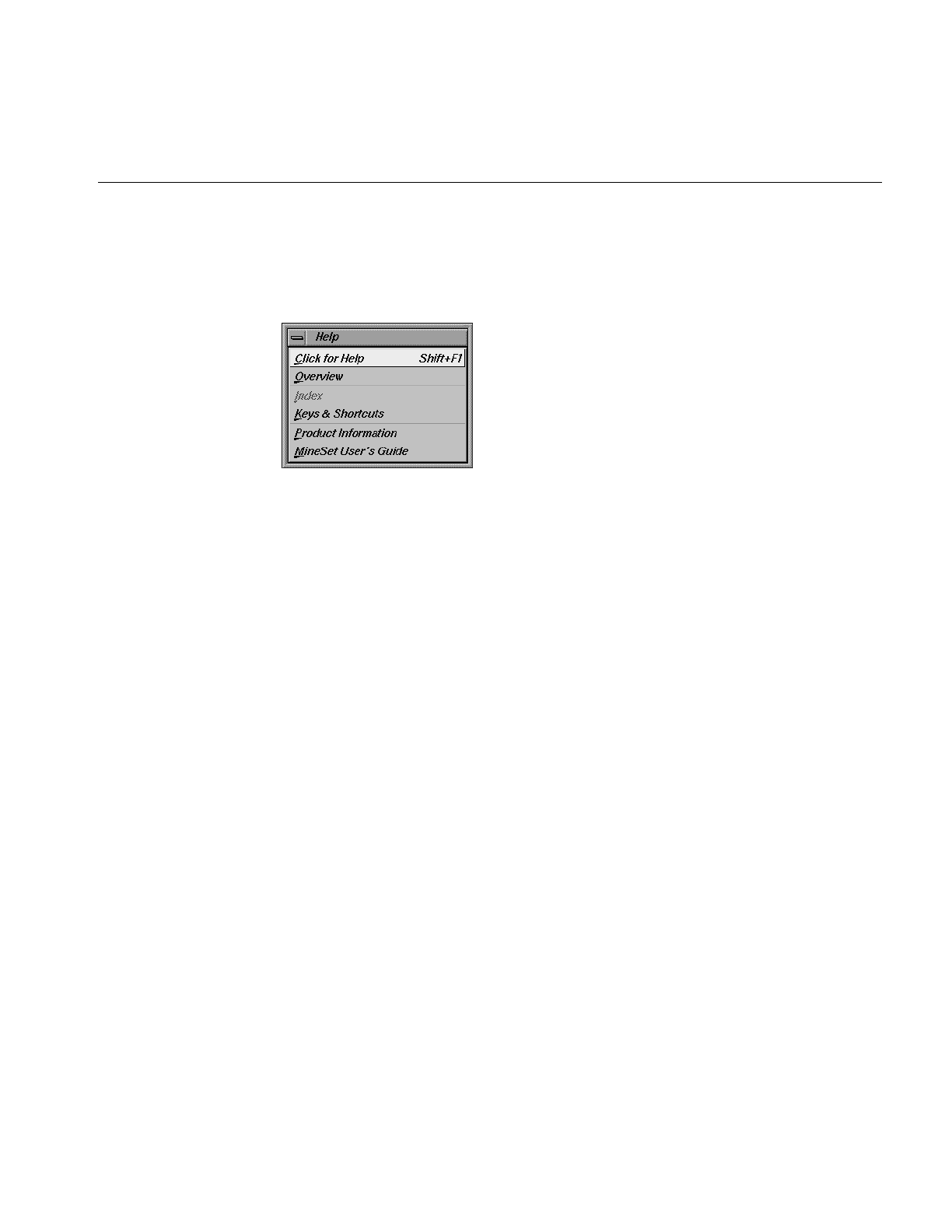
Pulldown Menus
169
The Help Menu
The Help menu (see Figure 5-25) provides access to six help functions.
Figure 5-25 Tree Visualizer’s Help Pulldown Menu
•Click for Help turns the cursor into a question mark. Placing this cursor over an
object in the main window and clicking the mouse causes a help screen to appear;
this screen contains information about that object. Closing the help window restores
the cursor to its arrow form and deselects the help function. The keyboard shortcut
for this function is Shift+F1. (Note that it also is possible to place the arrow cursor
over an object and press the F1 function key to access a help screen about that
object.)
•Overview provides a brief summary of the major functions of this tool, including
how to open a file and how to interact with the resulting view.
•Index provides an index of the complete help system. This option is currently
disabled.
•Keys & Shortcuts provides the keyboard shortcuts for all of the Tree Visualizer’s
functions that have accelerator keys.
•Product Information brings up a screen with the version number and copyright notice
for the Tree Visualizer.
•MineSet User’s Guide invokes the IRIS Insight viewer with the online version of this
manual.

170
Chapter 5: Using the Tree Visualizer
Null Handling in the Tree Visualizer
Nulls represent unknown data (see Appendix J, “Nulls in MineSet”).
In the Tree Visualizer, nulls can occur in the following cases:
•The database or data file contains a null value.
•The skipMissing option is not present in the configuration file (see skipMissing in
Appendix B,) and data is present for the key value in one node of the hierarchy, but
not in another. For example, in a representation of state budgets, if there is no record
for state income tax for Texas, Texas would have an income tax of null. This is
different than for the case where there is a record showing 0 as the income tax for
Texas, in which case it would show a tax of 0.
•When the Tool Manager is used to make an array based on bins and no data falls
into a specific bin, the value for that bin is null. For example, if there is no data for
30-40 year olds, that bin is null.
•When making an array in the Tool Manager and the null enum option is specified,
an extra array entry, corresponding to the first bar in each bar chart, is created to
represent the aggregation of all the values where the bin value is null (see
“Aggregations in the Presence of Nulls” in Appendix J). This bar is labeled with a
question mark (?), representing null. If there is no data for that null bin, the values
associated with it are null as well.
Note: if all values throughout the data associated with the null bin are null, the Tree
Visualizer ignores the null bin and does not display it.
•Expressions and aggregations of nulls can generate nulls (see Appendix J).
When a null value is mapped to a visual attribute, special representations are used in the
Tree Visualizer. If null is mapped to height, the object is normally drawn in outline mode
(although this is configurable through the Display menu (see the “The Display Menu”
section) or the configuration file (see “Null” in Appendix B). For a bar or a base, this looks
like an empty square. (It does not look like a cube, since it has no height.) For a disk, it
looks like a circle. If a null value is mapped to a color, it is drawn in a dark grey (see
Figure 5-26).

Sample Configuration and Data Files
171
Figure 5-26 Representation of a Null Value Mapped to Height, Color, Disk, and Label
When selecting an object with a null value, it is shown as a question mark (?) in the
selection field.
Sample Configuration and Data Files
The provided sample configuration and data files demonstrate the Tree Visualizer’s
features and capabilities. The following files are in the directory
/usr/lib/MineSet/treeviz/examples:
•store.data and store.treeviz
When graphically displayed, these files show hypothetical sales data for a store
chain. The hierarchy includes the entire chain, regions, states, cities, and individual
stores. Four products are shown for each level in the hierarchy. In this configuration,
heights represent sales in dollars; colors represent the percentage of the target dollar
amount.
•stateRevenue.data and stateRevenue.treeviz
When graphically displayed, these files show the revenue components of every
state’s budgets for 1992, as obtained from the United States Census Bureau (from
http://www.census.gov/govs/state/stfin92.dat). Heights represent the dollar
amounts in taxes. The descendent nodes in the background show the contribution
of various taxes to the total revenues shown in the root node.

172
Chapter 5: Using the Tree Visualizer
•beer.data and beer2.data, and beer.treeviz and beer2.treeviz
When graphically displayed, these files show fictitious data based on consumer
research of beer purchases. The hierarchy contains three levels:
1. The first is category (for example, beer or ale).
2. The second level is brand codes (randomly assigned).
3. The third is the individual product codes; for example, twelve-pack versus
six-pack (randomly assigned).
Each chart contains seven bars, representing seven age groups. Bar height
represents the total dollars spent by that age group. Colors represent the percentage
of dollars spent by males and females. Brands, products, and data used in these files
are samples only.
Both beer.treeviz and beer2.treeviz produce the same graphical output, but they have
been constructed differently. In beer.treeviz, each type of beer is represented by a
single record, with values for male and for female consumption; these values are
stored in an enumerated array (explained in Appendix B, “Creating Data and
Configuration Files for the Tree Visualizer”).
In beer2.treeviz, there are seven records for each beer, with each record representing
one age group. Note that in the beer file, the age groups are represented in the
configuration file; in the beer2 file, they are included in the data file.
The beer file requires less storage space than the beer2 file; however, the
configuration file is a little more complicated. In some cases, it might be easier to
produce data in the form used by the beer2 file.
Additional examples of the Tree Visualizer to visualize a Decision tree are provided in
Chapter 11.

173
Chapter 6
6. Using the Map Visualizer
This chapter discusses the features and capabilities of the Map Visualizer. It provides an
overview of this visualization tool, then explains the Map Visualizer’s functionality
when working with the following elements:
•main window
•viewing modes
•external controls
•pulldown menus
Finally, it lists and describes the sample files provided for this tool.
Overview of Map Visualizer
The Map Visualizer is a graphical interface that displays data as a three-dimensional
“landscape” of arbitrarily specified and positioned “bar chart” shapes. This tool displays
quantitative and relational characteristics of your geographically oriented data.
Data items are associated with graphical “bar chart” objects in the visual landscape.
However, the objects have recognizable geographical shapes and positions. The
landscape can consist of a collection of these geographical objects, each with individual
heights and colors (see Figure 6-1). You can dynamically navigate through this landscape
by
•panning
•rotating
•zooming to more clearly see areas of interest
•drilling down to see increased granularity of geographic details
•drilling up to aggregate data into coarser-grained graphical objects
•using animation to see how the data changes across one or two independent
dimensions.
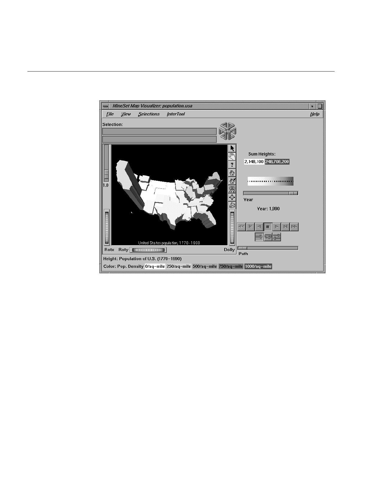
174
Chapter 6: Using the Map Visualizer
Figure 6-1 Sample Map Visualizer Screen Showing 1990 U.S. Population
The landscape can also consist of a flat plane of these geographical objects drawn as
simple outlines, with “bar chart” cylinders placed at specific locations (see Figure 6-2).

Overview of Map Visualizer
175
Figure 6-2 Sample Map Visualizer Screen Showing Relative Population of Major U.S. Cities
Another landscape possibility is lines with endpoints at specific point locations, all with
individual widths and colors (see Figure 6-3). Lines have width and color properties,
instead of the height and color properties of the arbitrarily shaped objects and cylinders.

176
Chapter 6: Using the Map Visualizer
Figure 6-3 Sample Map Visualizer Screen Showing the United States With Specific Endpoints
File Requirements
The Map Visualizer requires the following files:
•A data file consisting of rows of tab-separated fields. Typically, the Tool Manager
creates this file (see Chapter 3). You can also generate this file without using the Tool
Manager (for the required file format, see Appendix C, “Creating Data,
Configuration, Hierarchy, and GFX Files for the Map Visualizer”).
Data files are the result of extracting raw data from a source (such as an Oracle,
INFORMIX, or Sybase database) and formatting it specifically for use by the Map
Visualizer. Data files have user-defined extensions (the sample files provided with
the Map Visualizer have a .data extension).
•A gfx file consisting of a description of the shapes and locations of the 1-, 2-, or
3-dimensional objects to be displayed.
Gfx files must have a .gfx extension. MineSet includes various .gfx files, including
the United States to the granularity of counties, telephone area codes, and postal zip
codes, as well as Canada to the granularity of provinces. You can also manually
generate .gfx files (see Appendix C, “Creating Data, Configuration, Hierarchy, and
GFX Files for the Map Visualizer” for the required file format).

File Requirements
177
•A hierarchy file consisting of a description of
–the column names of the various graphical objects to be displayed
–the filenames of the .gfx files that describe the locations and shapes of the
graphical objects
–an optional description of the hierarchical relationship of the graphical objects,
which is used for the drill-down and drill-up functions.
Hierarchy files enable drill down and drill up. This means that information
associated with objects at one level can be aggregated (or, conversely, shown in
greater detail) and displayed at a different level. For example, a hierarchy file
defining the relationships between states and regions comprising multiple states
allows values such as population levels to be displayed at both the individual state
level as well as at regional levels. The gfx_files/usa.state.gfx file, for example,
describes the shapes of the 50 United States; the gfx_files/usa.state.hierarchy file
describes the hierarchy grouping individual states into regions, regions into
East-West areas, and the East-West areas into an aggregated United States.
For more information, see Appendix C, “Creating Data, Configuration, Hierarchy,
and GFX Files for the Map Visualizer”
•A configuration file describing the format of the input data and how these are to be
displayed. Typically, this file is created using the Tool Manager (see Chapter 3). You
also can use an editor (such as jot, vi, or Emacs) to produce this file without using
the Tool Manager (see Appendix C, “Creating Data, Configuration, Hierarchy, and
GFX Files for the Map Visualizer”).
Configuration files should have a .mapviz extension. If they do not, they are not
listed when selecting the Open option from the File pulldown menu. When starting
the Map Visualizer, or when opening a file, specify the configuration file, not the
data file.
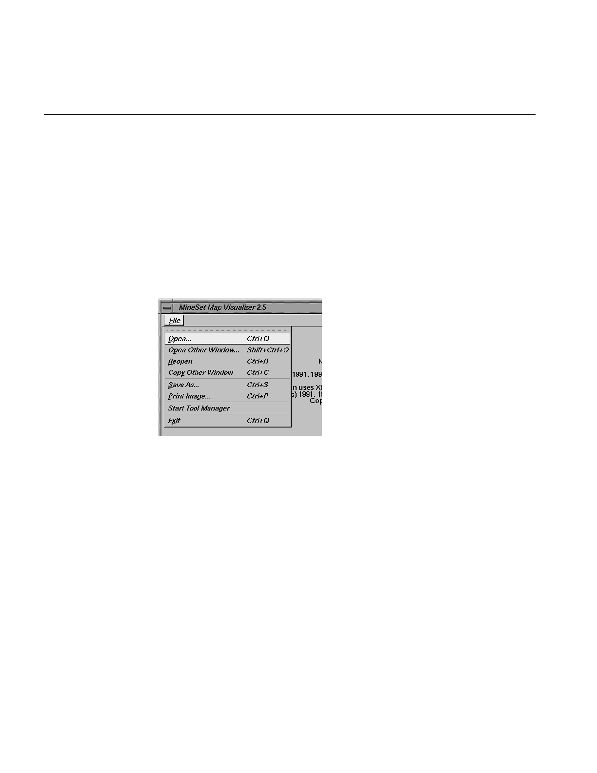
178
Chapter 6: Using the Map Visualizer
Starting the Map Visualizer
There are five ways to start the Map Visualizer:
•Use the Tool Manager to configure and start the Map Visualizer. See Chapter 3 first
for details on most of the Tool Manager’s functionality, which is common to all
MineSet tools; see below for details about using the Tool Manager in conjunction
with the Map Visualizer.
•Double-click the Map Visualizer icon, which is in the MineSet page of the icon
catalog. The icon is labeled mapviz. Since no configuration file is specified, the
start-up screen requires you to select one by using File > Open.
Figure 6-4 Map Visualizer’s Startup Screen, With File Pulldown Menu Selected
Starting the Map Visualizer without specifying a configuration file causes the main
window to show the copyright notice for this tool. Only the File and Help pulldown
menus can be used. For the main window to be fully functional, open a
configuration file by selecting File > Open (Figure 6-4).
•If you know what configuration file you want to use, double-click the icon for that
configuration file. This starts the Map Visualizer and automatically loads the
configuration file you specified. This only works if the configuration filename ends
in .mapviz (which is always the case for configuration files created for the Map
Visualizer using the Tool Manager).

Starting the Map Visualizer
179
•Drag the configuration file icon onto the Map Visualizer icon. This starts the Map
Visualizer and automatically loads the configuration file you specified. This works
even if the configuration filename does not end in .mapviz.
•Start the Map Visualizer from the UNIX shell command line by entering this
command at the prompt:
mapviz [ configFile ]
where configFile is optional and specifies the name of the configuration file to use. If
you don’t specify a configuration file, you must use File > Open to specify one (see
Figure 6-4).
Options for Invoking the Map Visualizer
There are a two options that affect how this tool is invoked:
•-warnexecute indicates that if you attempt to execute a command specified in an
execute statement, a warning is displayed and you are given the option to execute
the command or not. This is intended for an insecure environment, such as files
obtained from the Web, and is used automatically when commands are executed via
mtr files.
You can enable this option permanently by adding the line
*minesetWarnExecute:TRUE
to your .Xdefaults file, or by setting the environment variable
MINESET_WARN_EXECUTE
•-quiet eliminates the dialogs that popup to indicate progress. You can enable this
option permanently by adding the line
*minesetQuiet:TRUE
to your .Xdefaults file.

180
Chapter 6: Using the Map Visualizer
Configuring the Map Visualizer Using the Tool Manager
This section describes how the Map Visualizer can be configured using the Tool Manager.
Although the Tool Manager greatly simplifies the task of configuring the Map Visualizer,
you can construct a configuration file manually for this tool using a text editor (see
Appendix C, “Creating Data, Configuration, Hierarchy, and GFX Files for the Map
Visualizer”).
Note that the steps required to connect to a data source are described in Chapter 3.
Generating .gfx and .hierarchy Files
To use the Map Visualizer, you must provide the application with two files that define
the graphical objects to be displayed:
•One or more .gfx files, which define the shapes of the graphical objects displayed.
•A.hierarchy file, which describes the relationship of multiple, interrelated map (.gfx)
files.
These files are not created by the Tool Manager; they must already exist as part of
MineSet (residing in the /usr/lib/MineSet/mapviz/gfx_files directory), or they must be
created by the user. For instructions on their creation, see Appendix C, “Creating Data,
Configuration, Hierarchy, and GFX Files for the Map Visualizer”
The .gfx and .hierarchy files that are part of the MineSet package include
•the individual states of the United States
•the areas covered by the individual counties of the United States
•the areas covered by the individual five-digit ZIP codes of the United States
•the areas covered by the telephone area codes of the United States
•the individual provinces and territories of Canada
•the individual states of Mexico
•the individual states and territories of Australia
•the individual countries of Western and Central Europe
•regional subdivisions of both France and The Netherlands

Configuring the Map Visualizer Using the Tool Manager
181
The Map Visualizer requires a data file with
•One column indicating geographical objects (for example, states). Each row in this
column must indicate a unique geographical object (staying with the example, this
means one row for each state).
•At least one column with numeric values mapped (using arithmetic expressions) to
the heights and/or colors of each geographic bar. These columns can be scalar, a 1D
array, or a 2D array. If the column is an array, a slider must be used to select specific
data points for this mapping to heights and colors.
If both heights and colors are mapped to 1D or 2D arrays, the arrays must have the same
indexes (see Appendix C, “Creating Data, Configuration, Hierarchy, and GFX Files for
the Map Visualizer”).
Selecting the Map Visualizer Tool
Select the Viz Tools tab in the Data Destination panel of the Tool Manager’s main screen
(Figure 6-5). From the popup list of tools, select Map Visualizer. The window on the right
side of this panel displays the mapping requirements for the Map Visualizer. Items in the
Visual Elements list that are preceded by an asterisk are optional.
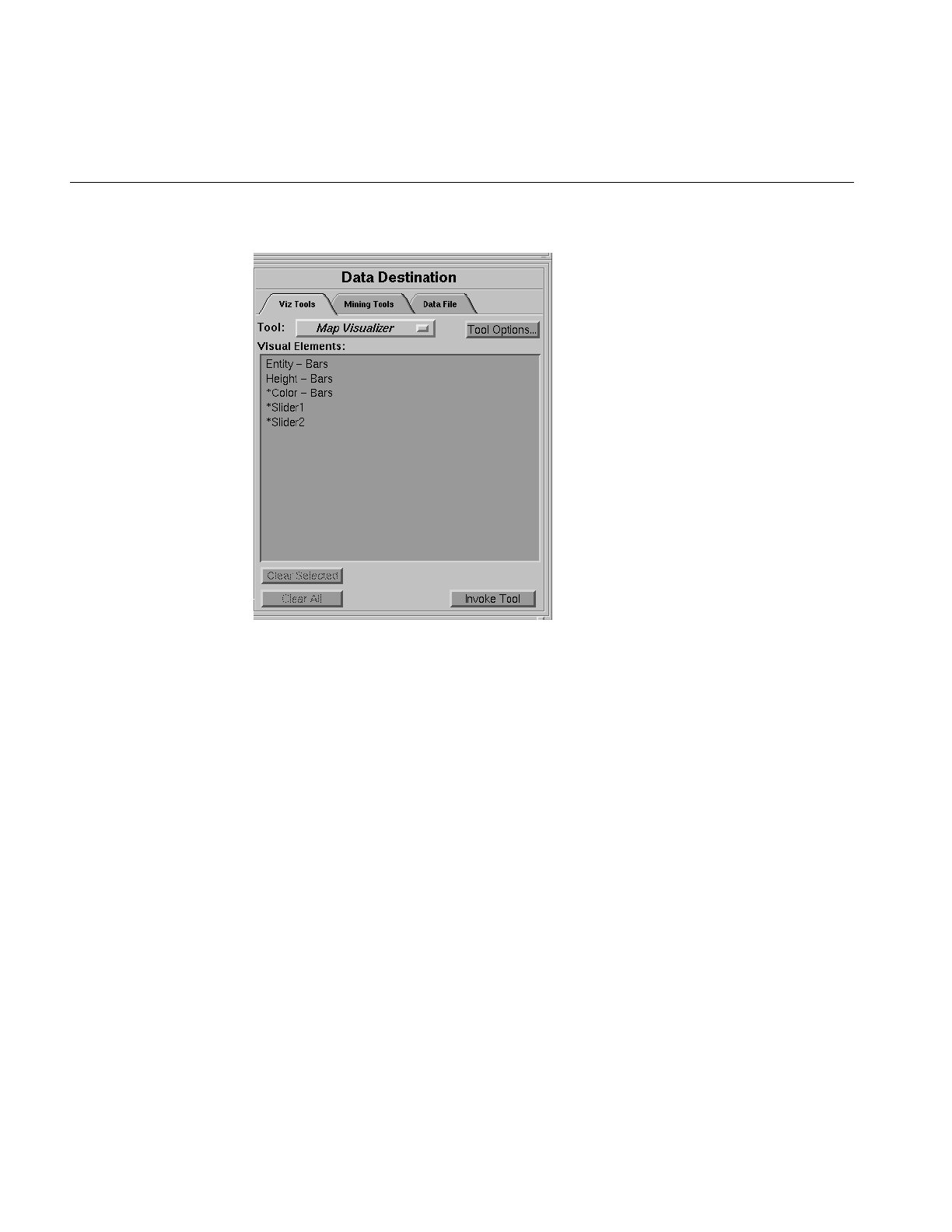
182
Chapter 6: Using the Map Visualizer
Figure 6-5 Data Destination Panel, With Map Visualizer Selected
•Entity - Bars lets you specify which column contains the keywords of the graphical
objects.
•Height - Bars lets you specify the heights of the geographic bars on the map.
•*Color - Bars lets you assign the colors of the geographic bars. See “Choosing
Colors” and “Using the Color Browser” in Chapter 3 for a more detailed
explanation of how to choose and change colors.
•*Slider1 and *Slider2 let you map columns directly to one or two animation Sliders
(see “Slider Creation for Mapviz,” below).
Mapping Columns to Visual Elements
A column in the Current Columns window should be mapped to the Visual Element
Height - Bars by clicking the column first, then Height - Bars. Optionally, another column
(perhaps even the same column) can be mapped to the Visual Element *Color - Bars.
Another column must be mapped to the Visual Element Entity. This must be a string
column.

Configuring the Map Visualizer Using the Tool Manager
183
Undoing Mappings
To undo a mapping, select the mapping in the Requirements: window, then click the
Clear Selected button. To undo all mappings, click the Clear All button.
Slider Creation for Mapviz
Sliders can be created manually or automatically. The following subsections describe
these methods.
Manual Slider Creation
Tool Manager generates sliders whenever there is an array column present in the current
table. The sliders correspond to the indices of the array columns. If the column has one
index (one-dimensional array), only one slider is created, but if the column has two
indices (two-dimensional array), both an X and a Y slider are created. The current slider
indices are indicated in the Tool Options dialog box from the Tool Manager.
Note that for a slider to be created, all array columns in the current table must have the
same indices. If array columns with differing indices exist in the current table, no slider
is created.
See “Aggregation” in Chapter 3 for more information on creating arrayed columns.
Automatic Slider Creation
If no arrayed columns are in the current table, Tool Manager can automatically generate
sliders by use of the Slider1 and Slider2 mappings. Sliders are created through a
combination of automatic binning and aggregation. These automatic operations occur
after clicking Invoke Tool. The operations do not affect the current history operations of
Tool Manager, but they do appear in the configuration files for the tool.
Columns mapped to Slider1 and Slider2 eventually form the indices for the sliders. These
columns must be either numeric (int, float, double) or binned. If a column mapped to a
slider is already binned, no automatic binning is needed for this column, and this column
is used as an index for a slider. However, if the column is not binned, a binned column is
created using the automatic binning options in the Tool Options dialog box.

184
Chapter 6: Using the Map Visualizer
The three methods of binning are:
•Selecting All Distinct Values creates a bin for every unique value of the column.
•Specify the number of bins you want to create. The thresholds for the bins are
determined using the Uniform Range approach.
•Selecting Automatic automatically determines the number of bins to create and
determines the bin thresholds using the Uniform Range approach.
(See “The Bin Columns Button” in Chapter 3 for more information about binning.) The
column used in forming the automatic bins is deleted from the current table.
The binned columns now form the indices of array columns. Note that if you want to
create only one slider, the index must be mapped to Slider1. Attempting to create only
one slider with a mapping to Slider2 is not allowed and generates a Tool Manager error.
Also, a column mapped to a slider cannot be mapped to any other mapping, since it is
removed during the aggregation process.
Once the slider indices are formed, the arrayed columns are created. This is done using
automatic aggregation. Any numeric columns mapped to Height or Color are
aggregated using the automatic aggregation options in the Tool Options dialog box. You
can either specify aggregating by Sum or by Average. The binned columns created from
the slider mappings form the indices for the aggregation. The column mapped to Entity
is the only Group-By column. Any remaining columns in the table are removed. (See
“Aggregation” in Chapter 3 for a description of the aggregation process.)
The aggregation step automatically forms the arrayed columns used for sliders. These
arrayed columns form the new tool mappings. For example, if the column “mpg” were
mapped to Height, a new column “avg_mpg[]” is formed and remapped to Height. The
progress of the automatic slider generation is displayed in the Tool Manager status
window.
Specifying Tool Options
Clicking the Tool Options button causes a new dialog box to be displayed (Figure 6-6).
This lets you change some of the Map Visualizer options from their default values.
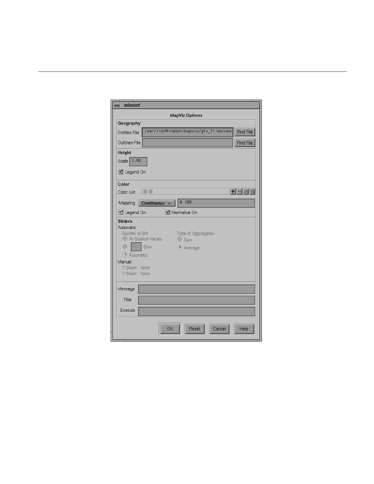
Configuring the Map Visualizer Using the Tool Manager
185
Figure 6-6 Map Visualizer’s Options Dialog Box
The following sections describe the buttons and fields of the Map Visualizer’s Options
dialog box.

186
Chapter 6: Using the Map Visualizer
Geography
The Entities File specifies a .hierarchy file to be used for the representation of the
geographical "entity" objects, in the Map Visualizer's main window.
The Outlines File specifies outline objects to draw, which appear as a flat plane on which
the 3-D entity objects are placed.
The Find File button lets you browse your files to find the .hierarchy file to be used.
Note that the Entities File and Outlines File fields are optional. If the Entities File is not
supplied, then the Map Visualizer creates graphical entity objects consisting of simple
rectangles that are arbitrarily sized and placed in the scene.
Height
This section specifies an initial height Scale value (default is 1.0) and whether to display
a height legend at the bottom of the Map Visualizer window.
Color
To use these Color options, you must have mapped a column to the *Color - Bars
requirement of the Data Destination panel. See “Choosing Colors” and “Using the Color
Browser” in Chapter 3 for a more detailed explanation of how to choose and change
colors.
Color List—You can specify the color list using the + button next to the color list label. This
brings up a color editor that lets you specify a color to be added to the list.
Mapping—You can specify whether the color change that is shown in the graphic display
is Continuous or Discrete. If you choose Continuous, the color values shift gradually
between the colors entered in the “Color List” field as a function of the values that are
mapped to those colors in the “Mapping” field.
The field to the right of the popup button lets you enter specific values to which the colors
are mapped. You must have the same number of values in this field as there are colors
entered in the “Color list to use” field.

Configuring the Map Visualizer Using the Tool Manager
187
Example 6-1
If you
•used the Color Browser to choose gray and red
•selected Discrete for the Mapping
•entered the values 0 150000
then the display shows the population of the United States across the time period
1770-1990. States with more than 150,000 square miles are shown in red, the rest are in
gray.
Example 6-2
If you
•used the Color Browser to choose gray and red
•selected Continuous for the Mapping
•entered the values 0 300000
then the display shows the population of the United States across the same time period.
The states’ colors vary from gray to red, depending on their size; the largest states are
shown with the greatest density of red.
You can enter as many colors into this field as necessary for your display. If the number
of values in the column that maps to *Color - Bars exceeds the number of distinct colors
you have chosen, the Map Visualizer adds an appropriate number of randomly chosen
colors at runtime.
Legend On—lets you determine whether a color legend is displayed or hidden.
Normalize On—lets you determine whether the Map Visualizer automatically scales the
colors between the color column's minimum and maximum values (this is called color
normalization), as opposed to you manually specifying threshold values. When
Normalize On is enabled, the threshold values must lie within the range 0 to 100,
representing a percentage of the color column's minimum to maximum numeric range.

188
Chapter 6: Using the Map Visualizer
Sliders
You can manually select a binned column to be associated with the slider(s), where the
binned column indexes an aggregated array that is mapped to height or color.
Alternatively, you can have the Tool Manager automatically perform the binning and
aggregations. For more details on the Slider options, see “Slider Creation for Mapviz” on
page 183.
Message Field
This lets you specify the message displayed when an entity is selected. For a listing and
description of format types that can be entered in this field, see the “Message Statement”
section in Appendix C, “Creating Data, Configuration, Hierarchy, and GFX Files for the
Map Visualizer”
Title field
This lets you specify a string that appears at the bottom of the Map Visualizer main
window. This string must be enclosed in double-quotes.
Execute Field
This option lets you type in a UNIX command that is executed when double-clicking on
an entity. The format is similar to the message statement. If no execute statement appears,
double-clicking has no effect.
For a detailed description of the Execute field, see “Execute Statement” in Appendix C.
Resetting the Tool Options
If, after making changes to the Tool Options dialog box, you want to reset the values of
all options to their default values, click the Reset Options button.
Accepting the Tool Options
Once you have finished making changes to the Tool Options dialog box, click OK to
return the Tool Manager’s main screen.

Working in the Map Visualizer’s Main Window
189
Saving Map Visualizer Settings
The Tool Manager stores information for the Map Visualizer in several files, all sharing
the same prefix:
•<prefix>.mapviz.data contains data.
•<prefix>.mapviz.schema describes the data file.
•<prefix>.mapviz contains information needed by the Map Visualizer.
•<prefix>.mineset contains all the information needed to create the other files.
To specify a prefix, use the Save ... menu option in the File menu of the Tool Manager’s
main window. If you do not specify a prefix, it is based on the data source.
When you use the Invoke Tool button, the .data,.schema, and .mapviz files are updated, if
necessary.
Invoking the Map Visualizer
To see the Map Visualizer graphically represent your data, click the Invoke Tool button at
the bottom of the Data Destination panel.
Working in the Map Visualizer’s Main Window
If you started the Map Visualizer without specifying a configuration file, the main
window shows the copyright notice for the Map Visualizer. Only the File and Help
pulldown menus can be used. For the main window to show all menus and controls,
open a configuration file. Use File > Open (Figure 6-4) to see a list of configuration files.
When a valid configuration file has been specified, its geographical landscape is visible.
For example, Figure 6-7 shows the results of specifying population.usa.mapviz and moving
the Year slider to the far right.

190
Chapter 6: Using the Map Visualizer
Figure 6-7 Population.usa.mapviz Example With the Slider Moved to 1990
This shows the population and population density for each state of the United States. The
population of each state is represented by the height of the state’s graphical shape.
Heights are relative to each other across the entire range of the animation controls.

Working in the Map Visualizer’s Main Window
191
Viewing Modes
The two modes of viewing are grasp and select. To toggle between these modes, move the
cursor into the main window, and press the Esc key. You can also change from one mode
to the other by clicking the appropriate button: to enter select mode, left-click the arrow
button (to the top-right of the main window); to enter grasp mode, left-click the hand
button (immediately below the arrow button, near the top right of the main window).
Grasp Mode
In grasp mode, the cursor appears as a hand. This mode supports panning, rotating, and
scaling the scene’s size in the main window.
•To pan the display, press the middle mouse button and drag it in the direction you
want the display panned.
•To rotate the display, press the left mouse button and move the mouse in the
direction you want to rotate.
•To move the viewpoint forward, press the left and middle mouse buttons
simultaneously and move the mouse downwards. To move the viewpoint
backward, press the left and middle mouse buttons simultaneously and move the
mouse upwards. This is equivalent to the functions provided by the Dolly
thumbwheel.
Select Mode
In select mode, you can highlight an object by positioning the cursor over that object.
Information about that object then appears at the top of the view area. This information
remains visible in the window only as long as the pointer cursor remains over the object.
If you position the pointer cursor over an object and click the left mouse button, the same
information appears in the Selection Window, which is above the main window, under
the “Selection” label (Figure 6-8).
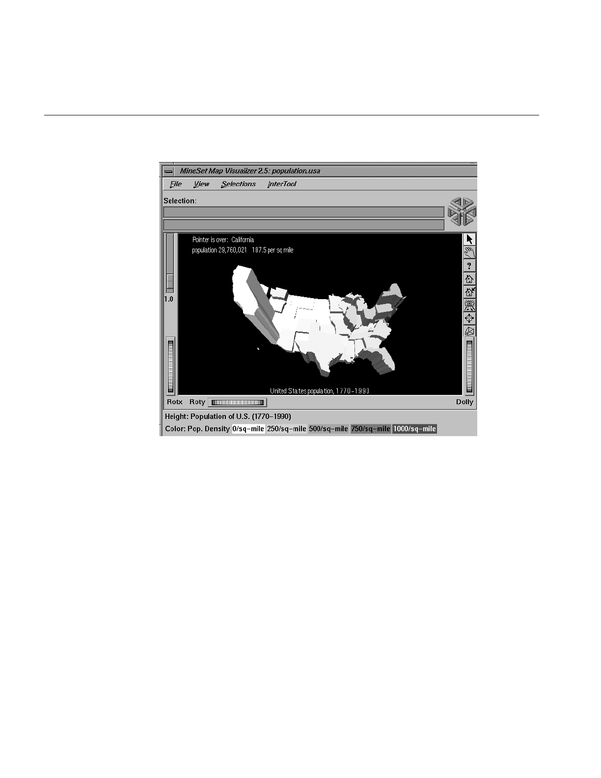
192
Chapter 6: Using the Map Visualizer
Figure 6-8 Highlighted Information in the Viewing Window and Selected Information
This Selection information remains visible until you select another object or click the
background. Using the mouse, you can cut and paste this text into other applications,
such as reports or databases.

Working in the Map Visualizer’s Main Window
193
Drilling Down and Drilling up
To view a finer level of geographical granularity for an object (if the .data and .hierarchy
files support it), click the right mouse button while the cursor is over that object. This is
called “drilling down.” You can repeat this down to the finest level of granularity
supported by the data. If the cursor is positioned over a specific object when drilling
down, only the more detailed sub-objects of that object appear. If, instead, the cursor is
positioned on the background at the time of the mouse click, then the more detailed
sub-objects of the entire set of objects appear. This might produce a display with a large
number of individual objects. The greater the number of objects, the longer the Map
Visualizer takes to construct the scene, and the slower the performance when moving the
animation controls.
To move up one level and view a coarser geographical granularity (“drill up”), click the
middle mouse button. If the cursor is positioned on the background when you click, all
the higher-level objects appear. If the cursor is positioned on a specific object in the scene,
then the scene “returns” to the group of higher-level objects visible when you last drilled
down with the right mouse button.
If an execute statement was specified via Tool Manager or the configuration file, then
double clicking on an object executes the appropriate command. If the -warnexecute
option was specified when invoking the Map Visualizer, a warning is given first.
Note: By default, the Map Visualizer initially displays objects at the lowest level of detail;
thus, initially, only drill-up (to coarser granularity) is active.

194
Chapter 6: Using the Map Visualizer
External Main Window Controls
Several external controls surround the graphics window. These consist of buttons,
sliders, and a summary window. Each of these controls is described in this section.
Buttons
At the top right of the image area are 11 buttons (see Figure 6-9).
Figure 6-9 Detail View of Top Right Buttons
•Arrow puts you in select mode, which lets you highlight entities in the main
window. When in this mode, the cursor shape is an arrow.
•Hand puts you in grasp mode, which lets you rotate, zoom, and pan the display in
the main window. When in this mode, the cursor shape is a hand.
•Viewer help brings up a help window describing the viewer itself.
Arrow
Hand
Viewer help
Home
Set Home
View All
Perspective
Seek
Top View
Front View
Right View

External Main Window Controls
195
•Home takes you to a designated location. Initially, this location is the first viewpoint
shown after invoking the Map Visualizer and specifying a configuration file. If you
have been working with the Map Visualizer and have clicked the Set Home button,
then clicking Home returns you to the viewpoint that was current when you last
clicked Set Home.
•Set Home makes your current location the Home location. Clicking the Home button
returns you to the last location where you clicked Set Home.
•View All lets you view the entire graphic display, without changing the angle of
view you had before clicking on this option. To get an overhead view of the scene,
rotate the camera so that you are looking directly down on the entities, then click
the View All button.
•Seek takes you to the point or object you click after selecting this button.
•Perspective is a toggle button that lets you view the scene in 3D perspective (closer
objects appear larger, farther object appear smaller). Clicking this button again turns
3D perspective off. If Perspective is off, the Dolly thumbwheel becomes the Zoom
thumbwheel
•Top View lets you view the scene from the top.
•Front View lets you view the scene from the front.
•Right View lets you view the scene from the right side.
Height-Adjust Slider and Label
To the left of the Map Visualizer’s main window is a vertical height adjust slider and,
below it, a label containing a numeric value between 0.1 and 100. This slider lets you
change the absolute heights of all the graphical objects in the main window. Moving the
slider up increases the heights of the objects; moving it down decreases their heights. The
numeric value in the label changes accordingly. This value indicates the height
multiplier, the default value of which is 1.0. The height adjust slider is useful for
accentuating relative height differences between objects in the view window.

196
Chapter 6: Using the Map Visualizer
Thumbwheels
Three thumbwheels appear around the lower part of the main window border (see
Figure 6-10). They let you dynamically move the viewpoint.
Figure 6-10 Lower Half of Window With Thumbwheels
•The vertical thumbwheel Rotx (rotate about the x axis), on the left, rotates the
display up and down.
•The horizontal thumbwheel Roty (rotate about the y axis), at the bottom left, rotates
the scene in the main window around its centerpoint left and right.
•The vertical Dolly thumbwheel, on the right, moves the viewpoint forward and
backward. Note that as you use the Dolly thumbwheel to magnify the scene in the
main window, additional detail can appear. This is not the case with the Zoom
slider, which merely enlarges the scene without adding detail.
The Animation Control Panel
To the right of the Map Visualizer’s main window are several external controls,
depending on the type of data being displayed (see Figure 6-11). These controls can
include
•sliders for independent dimensions
•a summary window containing a color density profile.
•a color legend showing the color density value limits
•buttons and sliders for animation
Thumbwheels
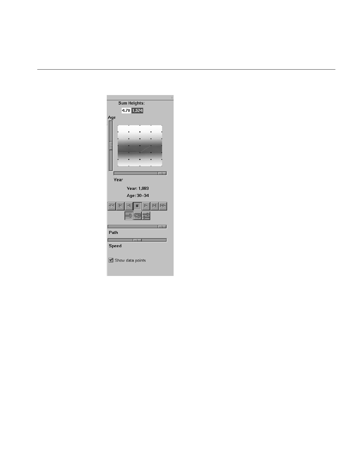
The Animation Control Panel
197
Figure 6-11 Map Visualizer’s Summary Window With Slider and Animation Controls
Sliders Controlling Independent Dimensions
The number of sliders appearing adjacent to the summary window is dependent on the
dataset displayed in the Map Visualizer’s main window. Datasets can have two, one, or
no independent dimensions.
Datasets With Two Independent Dimensions
If the dataset has two dimensions of independently varying data (such as
nl.births.mapviz), the animation control panel to the right of the main graphics window
becomes visible (as in Figure 6-11).
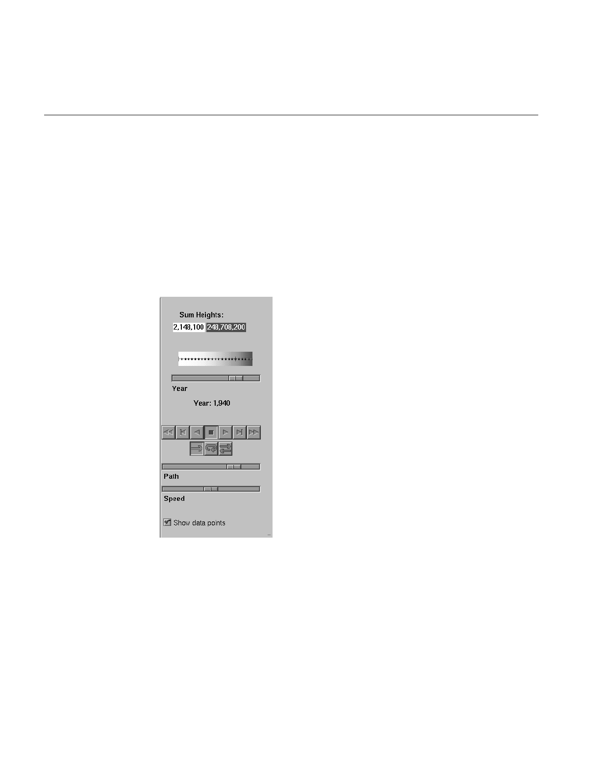
198
Chapter 6: Using the Map Visualizer
Within this animation control panel are the 2D summary window and two sliders. The
summary window has a horizontal slider below it for selecting data points of the first
independent dimension, and a vertical slider to the left for selecting data points of the
second independent dimension. The horizontal slider’s dimension is identified by a label
below it. The vertical slider’s dimension is identified by a label above it.
Datasets With One Independent Dimension
For datasets with one independent dimension (such as population.usa.mapviz), only the
slider below the summary window appears, and the summary window is compressed
(see Figure 6-12). This slider’s dimension is identified by a label below it.
Figure 6-12 Map Visualizer’s Summary Window With One Slider and Animation Controls
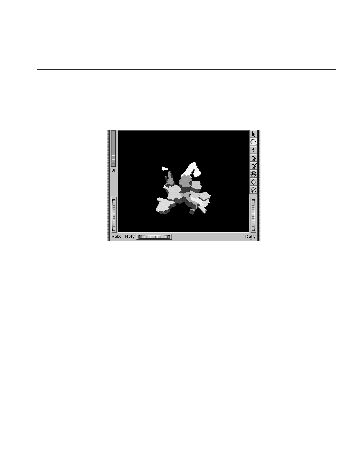
The Animation Control Panel
199
Datasets With No Independent Dimension
For datasets with no independent dimensions (such as population.europe.mapviz), no
animation control panel appears (see Figure 6-13).
Figure 6-13 If There Are No Independent Dimensions, No Animation Control Panel Appears
The Summary Window
The summary window provides a 2D representation of the aggregation of values that the
main window displays in 3D. Above this window is a label, Sum Heights, followed by
two rectangles: the first white, the second red. Within the rectangles are numbers; each is
the respective value for the maximum density of that color. This summary color legend
provides a visual and numeric comparison to the densities in the summary window.

200
Chapter 6: Using the Map Visualizer
The whiter the areas of the summary window, the lower the total values represented by
the heights of the objects in the main window. The greater the density of red shown in
areas of the summary window, the higher the total of those values. The density of these
colors in the summary window provides a summary of the data across the one or two
independent dimensions in the dataset, which is useful for guiding your exploration
through the data.
By default, the summary window also contains a set of black dots, evenly spaced across
the one or two dimensions of data. These dots indicate the precise positions of the
discrete datapoints of the data. You can turn off the dots using the View > Show Data
Points menu option.
Color Density Examples in the Summary Window
After opening the population.usa.mapviz file, for example, the 2D summary window
shows a color range from white (on the left) to red (on the right). White corresponds to
the low aggregate population in the early years of the United States; red represents the
higher aggregate population in later years. In this example, the greater the density of red,
the higher the total population of United States.
For a more complex example, open perhouse.perage.mapviz. This dataset has two
independent dimensions: time and age. The summary window displays these
dimensions as a complex pattern of colors. Place the cursor on the horizontal lines with
the greatest density of red, which runs horizontally across the summary window (this
means the age group making the greatest number of purchases). Click the left mouse
button. The information displayed in the field below the horizontal slider shows that this
represents purchases made by 30- to 39-year-olds.
Now place the cursor at the junction of the densest red horizontal (age group) and
vertical (time frame) parts of the summary window, and click the left mouse button. The
information displayed in the field below the horizontal slider shows that most purchases
were made by 30- to 39-year-olds in May-June 1989 and May-June 1990.

The Animation Control Panel
201
Creating a Path in the Summary Window
If the dataset loaded into the Map Visualizer has at least one independent dimension, it
is possible to view all or any part of that dataset via animation. This is done by first
creating a path in the summary window, then activating the animation controls
described in the next section.
The three ways to draw a path in the summary window are as follows:
•Define a starting point by clicking and holding down the left mouse button, then
draw a path by dragging the cursor over the window. The actual path passes
through intermediate discrete points closest to the path of the mouse. End the path
by releasing the left mouse button.
•Define a starting point by clicking the left mouse button, then define an endpoint by
moving the cursor to another part of the window and clicking the middle mouse
button. A path appears between those two endpoints, passing through the
intermediate discrete data point(s) that are closest to the hypothetical straight line
between the endpoints. To add more line segments, continue with repeated middle
mouse clicks.
•Define a starting point by clicking the left mouse button, then drag one of the
independent dimension sliders to draw a straight line along this dimension. If there
are two sliders, then using the second slider will continue to draw a straight line
along the axis controlled by this second slider.
The path you draw can only go through the well-defined discrete data points, identified
by the black dots in the summary window.
Animation Buttons and Sliders
Use the seven VCR-like buttons and two sliders (Path and Speed) below the 2D summary
window to control animation.

202
Chapter 6: Using the Map Visualizer
Animation Buttons
Once a path is drawn in the summary window (see “Creating a Path in the Summary
Window,” above), you can use the VCR-like buttons to control animation along this path.
The middle Stop button is highlighted in blue to indicate an initial state. Use the adjacent
Play Forward button (to the right of Stop) or Play Reverse (to the left) to begin simple
movement along the drawn path in a forward or reverse direction. Forward and Reverse
are defined by the sequence in which the path was drawn, not by a sense of left-to-right
or right-to-left movement.
To stop and restart the animation, click the Stop button, then use the Play Forward or
Reverse button. When you use the Stop button, the animation continues in the current
direction until the position falls on a discrete data point.
Adjacent to the Play buttons are the Single-Step buttons, also Forward and Reverse.
Clicking one of these buttons causes the current path position to change to the next
discrete data point.
On the outside are the Fast Forward and Fast Reverse buttons. Clicking one of these Fast
buttons while in Stop state changes the path position to the end (for Forward) or to the
beginning (for Reverse) of the path. Clicking a Fast button when in Play state increases the
animation speed.
Animation Flow
Below the Animation Buttons are the three Animation Flow buttons.
Play-once (default)—the animation moves either forward or in reverse until it reaches the
end of the path, then stops.
Loop—when the animation reaches the end of the path, it automatically resets to the
beginning and starts over again.
Swing—when the animation reaches the end of the path, it reverses direction and retraces
its path to the other end; upon reaching that end, the animation reverses direction again,
beginning the cycle again.

The Animation Control Panel
203
Animation Sliders
While animation is stopped, you can move the Path slider to reset the position along the
path. Note that when you use the Path slider, the cursor in the summary window moves
across the drawn path, and the 1D sliders (below and to the left of the drawing area)
move consistently with the cursor position. Then use the Play or Reverse button to restart
the animation from the newly specified point.
You can drag the Path slider to an arbitrary position on the path between discrete data
points; however, when you release the slider, the path position changes to a stop at the
nearest discrete data point.
Use the Speed slider to adjust the speed of the animation along the path.
Data Points and Interpolation
As animation proceeds, the variables mapped to height and color in the Map Visualizer
also change. However, the variables displayed in the Selection: message box show only
the data values of the nearest discrete data position, not intermediate (interpolated) data
values.
The animation is produced in the following manner: Assume you have data for 10 years,
on a per-year basis (that is, 10 data values) and that these correspond to the height of one
state in the Map Visualizer. The years are 1991 to 2000, the height for 1991 is 20, and the
height for 1992 is 40. As you move the year slider from 1991 to 1992, the height changes
by being uniformly interpolated between 20 and 40. For example, midway between 1991
and 1992, the height appears to be 30. As you approach 1992, the height approaches 40.
However, you cannot stop an animation between discrete data points, and you cannot
drag the Path slider to a stationary position between discrete data points.
The data points in the summary window represent the slider positions corresponding to
the actual data from the data file. For example, the heights 20 and 40 are representations
of actual data, but the height 30 is not. In this example, there would be data points in the
summary window at the slider positions corresponding to each year.
Note that not all variables are required to vary with a slider. For example, in the Map
Visualizer, the area and name of the state do not vary with the slider (for example, year).
If there are two sliders, some variables can vary with only one of the sliders, while other
variables vary with both.
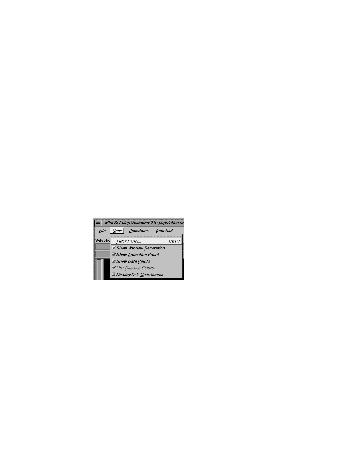
204
Chapter 6: Using the Map Visualizer
Pulldown Menus
Five pulldown menus let you access additional Map Visualizer functions. These are
labeled File, View, Selections, InterTool, and Help. If you start the Map Visualizer
without specifying a configuration file, only the File and the Help menus are available.
The View menu is available after a valid dataset is loaded.
The File Menu
The File menu is the same for all visualization tools; see “The File Menu” in Chapter 5.
The View Menu
The View menu (Figure 6-14) contains six options. This section describes those options
below.
Figure 6-14 Map Visualizer’s View Pulldown Menu
Filter Panel brings up a filter panel (Figure 6-15), which lets you reduce the number of
entities displayed in the main viewing area, based on one or more criteria. You can use
the filter panel to fine-tune the display, emphasize specific information, or simply shrink
the amount of information displayed. Scale to Filter lets you specify whether the heights
of the graphical objects are scaled across the entire dataset or just across the filtered data.
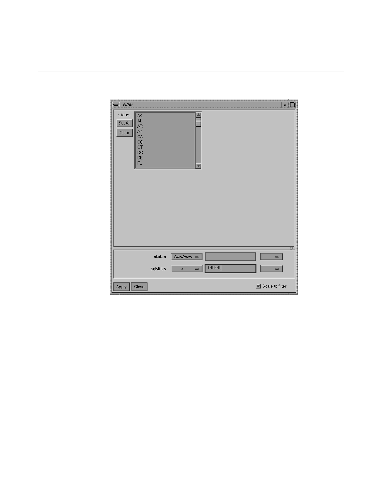
Pulldown Menus
205
Figure 6-15 Map Visualizer Filter Panel
The filter panel has two panes. The top pane lets you filter based on string variables. To
select all values of a variable, click Set All. To clear the current selections, click Clear. To
select a value, click it. To deselect a value, simply click it again.
The bottom pane lets you filter based on the values of both string and numeric variables.
Only variables whose values do not change as you navigate the slider can be used in
filtering.

206
Chapter 6: Using the Map Visualizer
To filter numeric values, enter the value, and select a relational operation (=, !=, >, <, >=,
<=). To filter alphanumeric values, enter the string. You can use any of three types of
string comparisons:
•Contains indicates that it contains the appropriate string. For example, California
contains the strings Cal and forn.
•Equals requires the strings to match exactly.
•Matches allows wildcards:
•An asterisk (*) represents any number of characters.
•A question mark (?) represents one character.
•Square braces ([ ]) enclose a list of characters to match.
For example, California matches Cal*, Cal?fornia, and Cal[a-z]fornia.
In some cases (usually associated with binning in the Tool Manager), an option menu of
values appears, instead of a text field. To ignore that variable, select Ignored in the Option
menu. You can use relational operators (such as >=) with these options. This means that
the specified value as well as subsequent ones are selected.
In addition to numeric and string comparison operations, you can specify Is Null,
which is true if the value is null.
To the right of each field is an additional option menu that lets you specify “And” or “Or”
options. For example, you could specify “sales > 20 And < 40.” You can have any number
of And or Or clauses for a given variable, but cannot mix And and Or in a single variable.
Click the Apply button to start filtering. If you press Enter while the panel is active,
filtering starts automatically.
Click the Close button to close the panel.
•Show Window Decoration causes the buttons around the main window to be
displayed. Default for this option is on. Toggle this option to make the window
decoration disappear.
•Show Animation Panel causes the animation control panel to be displayed to the right
of the main view. Click this option again to deselect it. When this option is
deselected, the animation panel is not displayed. Not displaying the animation
panel can be useful when you have applied the InterTool menu’sSynchronize All
Mapviz Sliders option (described in the “The InterTool Menu” on page 209) and need
only a single animation control panel on the screen.

Pulldown Menus
207
•Show Data Points causes a grid of black dots to appear (or disappear) in the 2D
summary window. Each dot denotes the precise position of a discrete data value in
the input dataset. For example, if the input dataset has 10 data values across one
independent dimension, then you see heights and colors of the graphical objects in
the main window vary continuously, based on data values that are interpolations
between these discrete data points. These data point dots in the summary window
help you better understand when the heights and colors are derived directly from
the input data values, and when they are derived indirectly from interpolated
values.
•Use Random Colors causes the configuration file’s color mapping specifications (for
example, white-to-red shadings representing population density) to be ignored.
Random, constant colors are assigned to the graphical objects. Click this option
again to deselect it.
•Display X-Y Coordinates puts the Map Visualizer into a special mode that lets you
identify X-Y vertex pairs at specific points of the scene in the main window. In this
mode, the Map Visualizer resets the cursor to select mode and displays 3D objects
as flat background lines. Clicking the left mouse button on various parts of the
displayed scene causes the corresponding X-Y vertex pair values to appear in the
Selection Details window. You can also enter the vertex pair points into the .gfx file
to identify point objects or the endpoints of line objects for subsequent display. Note
that displaying X-Y coordinates is used for developing and refining .gfx files, not for
data analysis.
When Display X-Y Coordinates mode is initially enabled, or when a point in the
background is selected, the selection window shows the minimum and maximum
X-Y pairs of the currently displayed image in the main window. Add these two
value pairs to the new .gfx file you are generating. The first record in the file
gfx_files/usa.cities.gfx shows an example of how the min-max pairs of the usa.sates.gfx
file were entered into the associated usa.cities.gfx file. This ensures that the X-Y
coordinate pairs in usa.cities.gfx share the same coordinate system as the X-Y
coordinate pairs in usa.sates.gfx.
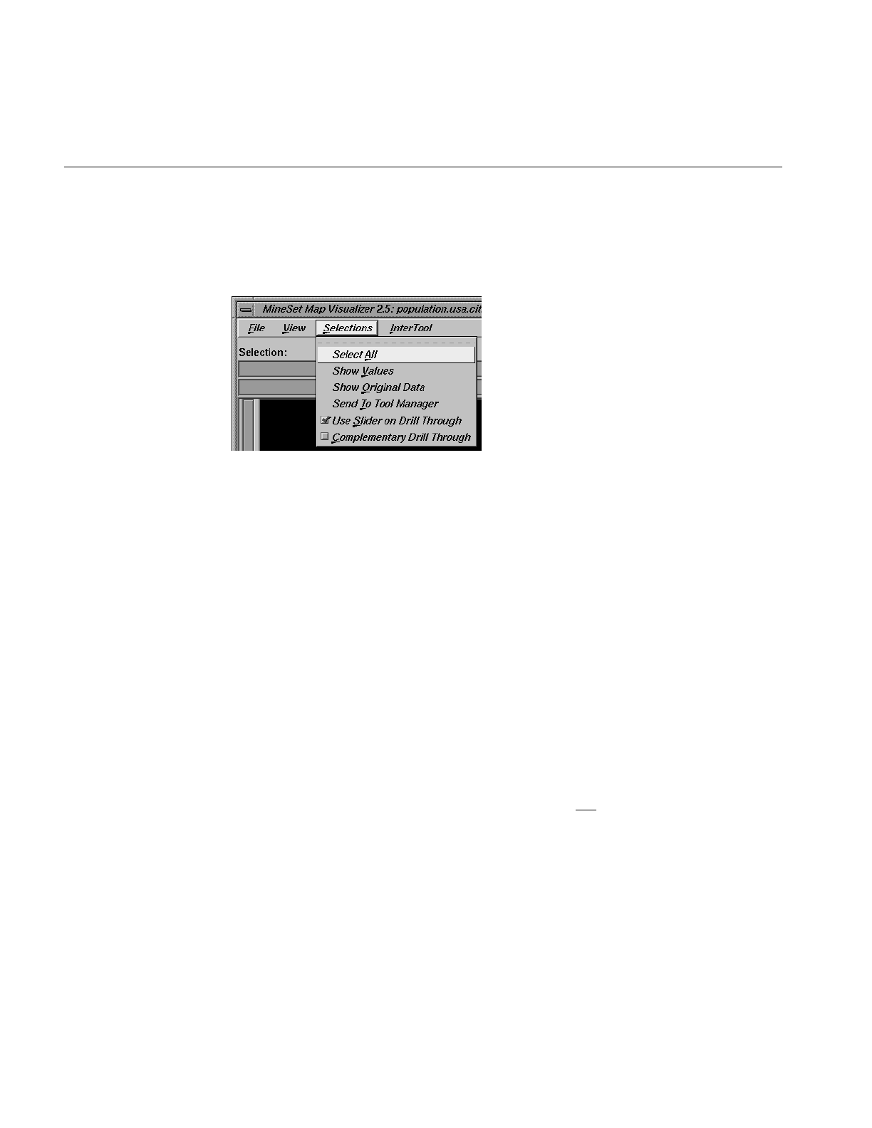
208
Chapter 6: Using the Map Visualizer
The Selections Menu
The Selection menu lets you drill through to the underlying data. The menu has six items.
Figure 6-16 Map Visualizer Selections Menu
•Select All performs the equivalent of selecting (with the mouse pointer) all the
visible graphical objects in the current scene.
•Show Values displays a table (Record Viewer) of the values for all selected objects.
•Show Original Data retrieves and displays the records corresponding to what has
been selected. The resulting records are shown in a table viewer.
•Send To Tool Manager inserts a filter operation, based on the current box selection(s),
at the beginning of the Tool Manager history. The actual expression used to do the
drill through is determined by extents of the current box selection(s). If nothing is
selected, a warning message appears.
•Use Slider On Drill Through determines whether or not to use the slider position
when creating the drill-through expression. If checked (default), an additional term
is added to the drill-through expression, limiting the drill-through to those records
defined by the slider’s position. If this option is not checked, no such limiting term
is added.
•Complementary Drill Through causes the Show Original Data and Send To Tool Manager
selections, when used, to fetch all the data that are not selected.
For further details on drill-through, see Chapter 18, “Selection and Drill-Through.”
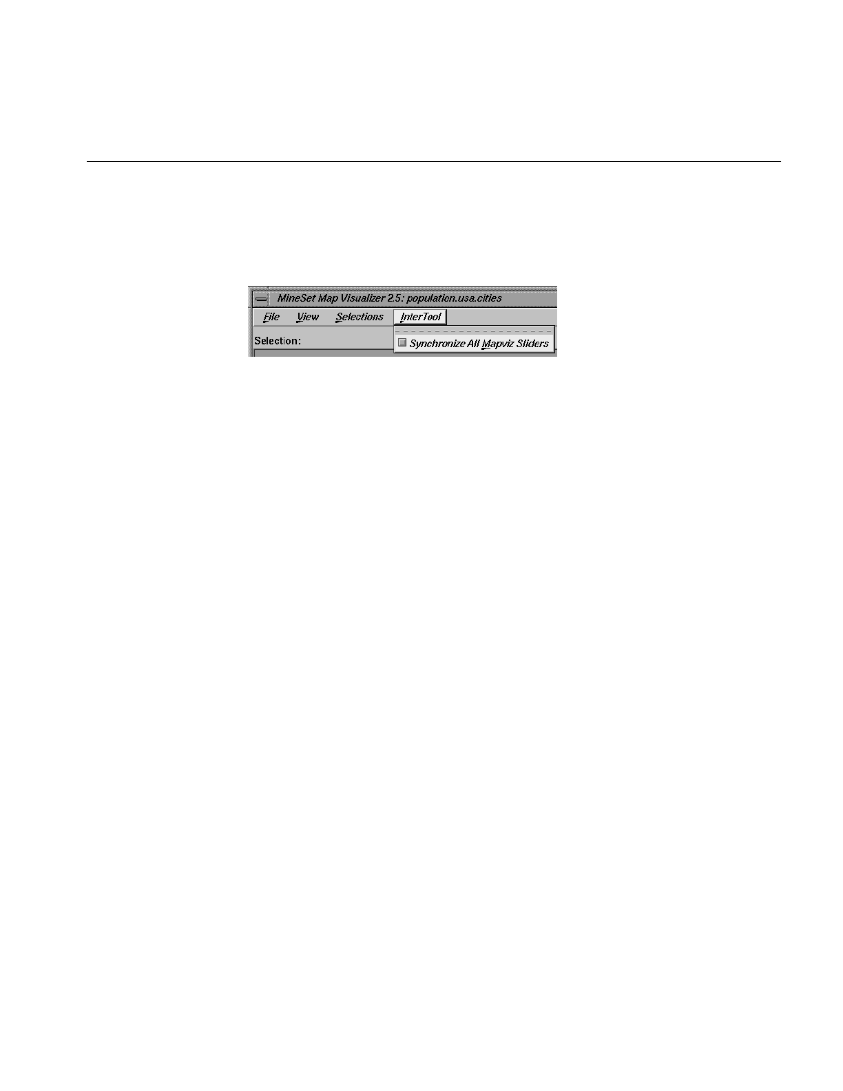
Pulldown Menus
209
The InterTool Menu
The InterTool menu has one option, as shown Figure 6-17.
Figure 6-17 Map Visualizer’s InterTool Pulldown Menu
Selecting Synchronize All Mapviz Sliders identifies this Map Visualizer window as one in
a “synchronized sliders” cooperative: changing the current slider positions in one Map
Visualizer window causes/produces the same change in all others currently open. Click
this option again to deselect it. This menu option must be selected in every Mapviz main
window that is to be part of the synchronization.
Note that currently only the sliders’ physical positions are synchronized, not the
underlying meanings of those positions. For example, synchronizing
population.usa.mapviz (with dates ranging from 1770 to 1990) and population.canada.mapviz
(with dates ranging from 1871 to 1991) probably is not useful, since the slider physical
midpoint position represents 1880 in the United States and 1931 in Canada. Generally,
synchronization is useful only when the sliders of each dataset represent the same range
of independent variables.
The Help Menu
The Help menu is the same for all visualization tools; see “The Help Menu” in Chapter 5.

210
Chapter 6: Using the Map Visualizer
Null Handling in the Map Visualizer
Nulls represent unknown data (see Appendix J, “Nulls in MineSet”).
In the Map Visualizer, nulls can occur when any of the following is true:
•The database or data file contains a null.
•The Tool Manager is used to make an array based on bins and no data falls into a
specific bin. For example, if there is no data for the 30-40-year-old population, that
bin is null.
•The Tool Manager is used to make an array and the null enum option is specified. In
this case, an extra array element is created to represent the aggregation of all the
values for which the bin value is null. The Tool Manager assigns the question mark
(?) character to this extra bin. To view the values of this bin, move the corresponding
slider to its left-most position. If there are no data for that null bin, the values
associated with it are null as well, and the Map Visualizer represents the
corresponding graphical object(s) as a “null object.”
•Expressions and aggregations of nulls can generate nulls (see Appendix J, “Nulls in
MineSet”).
•The Map Visualizer uses special representations when a null value is mapped to a
visual attribute. A null height results in a dark grey object with zero height; a null
color results in an object with appropriate height (as defined by the value mapped
to height), but with a dark gray color (see Figure 6-18).

Sample Configuration and Data Files
211
Figure 6-18 Representation of a Null Value Mapped to Height (Top Middle Object) and to
Color (Bottom Right Object)
When selecting an object with a null value, a question mark (?) is shown in the
selection field.
Sample Configuration and Data Files
The provided sample configuration and data files demonstrate the Map Visualizer’s
features and capabilities. The .data and .mapviz files are in the directory
/usr/lib/MineSet/mapviz/examples; the .gfx and .hierarchy files are in the directory
/usr/lib/MineSet/mapviz/gfx_files.
•blocks.mapviz,blocks.data,blocks.gfx, and blocks.hierarchy
This simple example shows four adjacent blocks. The height and color of each block
varies based on the underlying data in blocks.data. You can drill up using the middle
mouse button (see the “Select Mode” section) to see the upper pair and the lower
pair of blocks aggregate; then drill up again to see these upper and lower blocks
aggregate into a single block. You can drill down using the right mouse button to
see the objects of finer granularity reappear.

212
Chapter 6: Using the Map Visualizer
•population.australia.mapviz,population.australia.data,australia.states.gfx, and
australia.states.hierarchy
The data file contains one row for each Australian state and territory. Each row
contains three tab-separated items: a keyword name for the state or territory, the
population value, and the size of the territory.
This sample graphically displays the 1991 population and population density of the
Australian states and territories. Heights of the graphical objects represent the
relative population; color represents the relative population density. A legend at the
bottom of the display describes the color range and the associated values.
•population.canada.mapviz,population.canada.data,canada.provinces.gfx, and
canada.provinces.hierarchy
The data file contains one row for each Canadian province and territory. In this
example, each row contains 13 blank-separated values (one for each decade
between 1871 and 1991).
This sample graphically displays the population and population density of the
Canadian provinces and territories from 1871 to 1991, in 10-year increments. The
animation control panel lets you dynamically view the datasets across a range of
time. Animation operation is explained in “Sliders Controlling Independent
Dimensions” on page 197.
•population.europe.mapviz,population.europe.data,europe.countries.hierarchy, and
europe.countries.gfx
When graphically displayed, this shows the 1992 population and population
density of countries in Western and Central Europe.
•population.usa.mapviz,population.usa.data,usa.sates.gfx, and usa.sates.hierarchy
When graphically displayed, this shows the population and population density of
the United States from 1770 to 1990. The animation controls let you dynamically
view population and density changes across time.
•population.usa.cities.mapviz,population.usa.cities.data,usa.sates.gfx,usa.sates.hierarchy,
and usa.cities.gfx and usa.cities.hierarchy
The usa.sates.gfx file specifies the United States, which is displayed as a background.
The usa.cities.gfx file specifies the location of the cities on this background. The .data
file specifies the population of each city.
This sample graphically displays the population of the 48 largest U.S. cities from
1950 to 1990. No data has been mapped to the colors. The animation controls let you
dynamically view changes across time.

Sample Configuration and Data Files
213
•perhouse.perage.mapviz,perhouse.perage.data,usa.sates.gfx, and usa.sates.hierarchy
This sample graphically displays consumer household spending data from
July-August 1988 to May-June 1991. Color is mapped to the gender of the spending
household member; height represents the average dollar amount spent per
household for a given time period and age group. This data has two independent
dimensions: time and age. The highest spending is indicated in the summary
window (see “The Summary Window” on page 199) by the areas with the greatest
color density, namely “May-June 1989 (Age: 30-39)” and “May-June 1990 (Age:
30-39).”
•telecom.mapviz,telecom.data,usa.cities.lines.gfx,usa.cities.lines.hierarchy,usa.sates.gfx,
and usa.sates.hierarchy
This sample graphically displays a flat map with arched lines on it. These lines
connect two endpoints. The lines can have variable width and color. In this
example, the widths and colors are random; however, they could relate to the
volume and duration of the connections between the endpoints.
•fasta.m.data,fasta.m.mapviz,fasta.m.gfx, and fasta.m.hierarchy
The data file for this example contains the partial results of a full biological
sequence comparison between two complete genomes (courtesy of Dr. Tom Flores,
European Bioinformatics Institute). When graphically displayed, scientists can
quickly identify and locate the regions of similarity between the two genomes. The
ability to display such large amounts of information in a visual data exploration
method such as this could be extended to include much more information about the
individual genomes. Scientists could explore this data more easily and thereby
perhaps better understand the function and purpose of the similar genetic
sequences.
In this example, the “map” is the circular-shaped genome of a biological organism
called Mycoplasma genitalium (MG). The MG genome is divided into 500 equal
segments, each representing a 1000-nucleotide sequence in the genome. The slider
selects one of the segments of the second genome, called Haemophilus influenzae
(HI), for cross-comparison between the two genomes. The Summary Window in the
Animation Control Panel indicates which segments show the greatest similarities,
and you can move the slider to examine those particular segments of interest. The
bar heights and colors on the “map” therefore indicate the relative similarity of each
MG segment to each HI segment, where higher bars correspond to greater measures
of similarity. This similarity is measured by the “Reciprocal Evalues,” which ranges
from 0.0 to 1.0.


215
Chapter 7
7. Using the Scatter Visualizer
This chapter discusses the features and capabilities of the Scatter Visualizer. It provides
an overview of this database visualization tool, then explains the Scatter Visualizer’s
functionality when working with the
•main window
•external controls
•pulldown menus
Finally, it lists and describes the sample files provided for this tool.
Overview of Scatter Visualizer
The Scatter Visualizer lets you visually analyze relationships among several variables
(see Figure 7-1), either statically or by animation. It is particularly useful for seeing
individual data points when you do not have a large number of records. If your dataset
has a very large number of records consider using the Splat Visualizer. Analysis in the
Scatter Visualizer is done using
•a three-dimensional landscape
•an animation control panel that includes a two-dimensional slider
•graphical objects, called entities, that can be animated in the three-dimensional
landscape
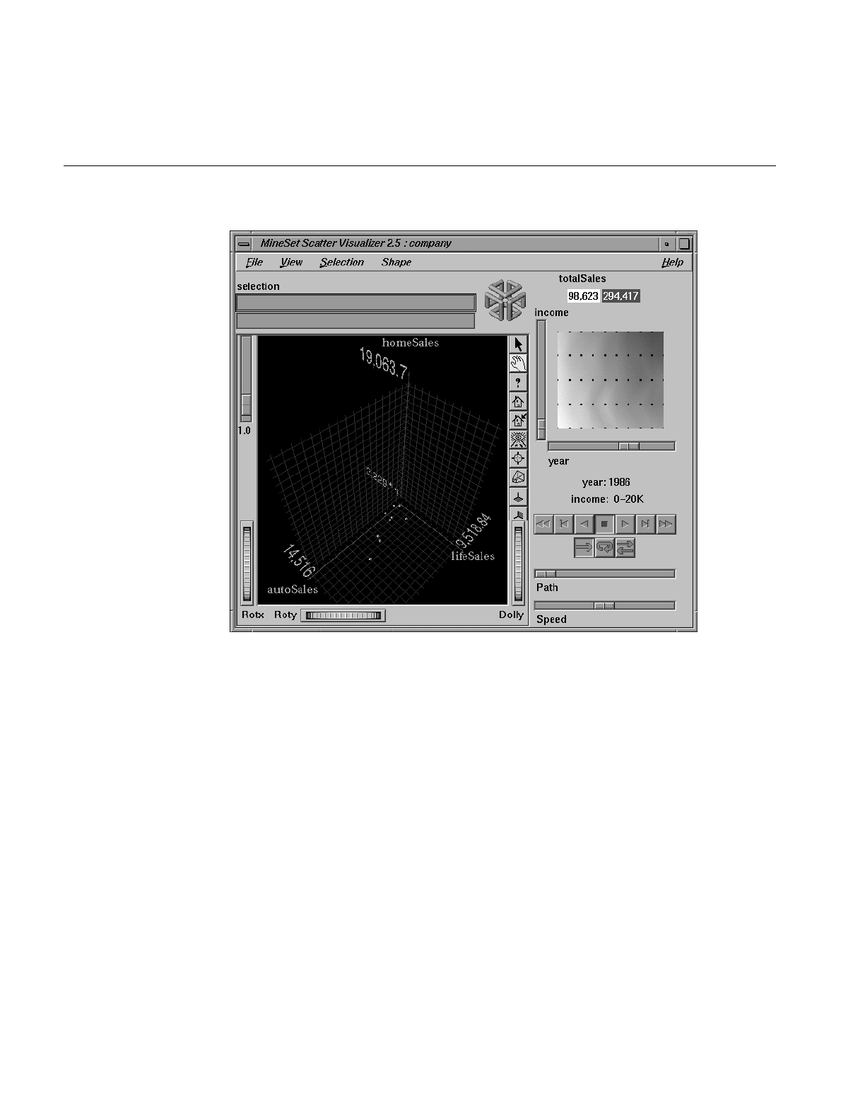
216
Chapter 7: Using the Scatter Visualizer
Figure 7-1 Sample Scatter Visualizer Screen
The Scatter Visualizer lets you visualize your data by mapping each record, or row, in the
dataset to an entity in the three-dimensional landscape. Variables in the data can be
mapped to the sizes, colors, and positions of the entities. Also, you can map one or two
numeric variables to the sliders in the animation control panel. If the variables mapped
to sizes, colors, or positions of the entities depend on the variables mapped to sliders, the
sliders can be used to drive an animation. For example, the data might represent the sales
of several companies over time. If the time variable is mapped to a slider and the sales
variable is mapped to size, then the entities grow or shrink as the time slider is animated.

File Requirements
217
After you create a visualization of your data, the Scatter Visualizer lets you analyze the
data in various ways. The animation control panel lets you trace animation paths in one
or two dimensions. By playing back the path you created, you can watch the size, color,
and motion of the entities for trends or anomalies. In the three-dimensional landscape,
you can orient the display to emphasize particular dimensions or a point of view. The
Scatter Visualizer lets you scale the values of variables to give them greater emphasis.
Also, you can filter the display to show only those entities meeting certain criteria.
File Requirements
The Scatter Visualizer requires the following files:
•A data file, consisting of rows of tab-separated fields. This file is easily created using
the Tool Manager (see Chapter 3). If you are generating this file yourself, see
Appendix D, “Creating Data and Configuration Files for the Scatter Visualizer” for
the required file format.
You can generate data files by extracting data from a source (such as a database) and
formatting it specifically for use by the Scatter Visualizer. Data files have
user-defined extensions (the sample files provided with the Scatter Visualizer have
a.data extension).
•A configuration file, describing the format of the input data and how it is to be
displayed. The Tool Manager can create this file (see Chapter 3), or you can use an
editor (such as jot, vi, or Emacs) to produce this file yourself (see Appendix D,
“Creating Data and Configuration Files for the Scatter Visualizer”).
Configuration files must have a .scatterviz extension. When starting the Scatter
Visualizer, or when opening a file, you must specify the configuration file, not the
data file.

218
Chapter 7: Using the Scatter Visualizer
Options for Invoking the Scatter Visualizer
There are a two options that affect how this tool is invoked:
•-warnexecute indicates that if you attempt to execute a command specified in an
execute statement, a warning is displayed and you are given the option to execute
the command or not. This is intended for an insecure environment, such as files
obtained from the Web, and is used automatically when commands are executed via
mtr files.
You can enable this option permanently by adding the line
*minesetWarnExecute:TRUE
to your .Xdefaults file, or by setting the environment variable
MINESET_WARN_EXECUTE
•-quiet eliminates the dialogs that popup to indicate progress. You can enable this
option permanently by adding the line
*minesetQuiet:TRUE
to your .Xdefaults file.
Starting the Scatter Visualizer
There are five ways to start the Scatter Visualizer:
•Use the Tool Manager to configure and start the Scatter Visualizer. (See Chapter 3
for details on most of the Tool Manager’s functionality, which is common to all
MineSet tools; see “Configuring the Scatter Visualizer Using the Tool Manager” on
page 220 for details about using the Tool Manager in conjunction with the Scatter
Visualizer.)
•Double-click the Scatter Visualizer icon, which is in the MineSet page of the icon
catalog. The icon is labeled scatterviz. Since no configuration file is specified, the
start-up screen requires you to select one by using File > Open.
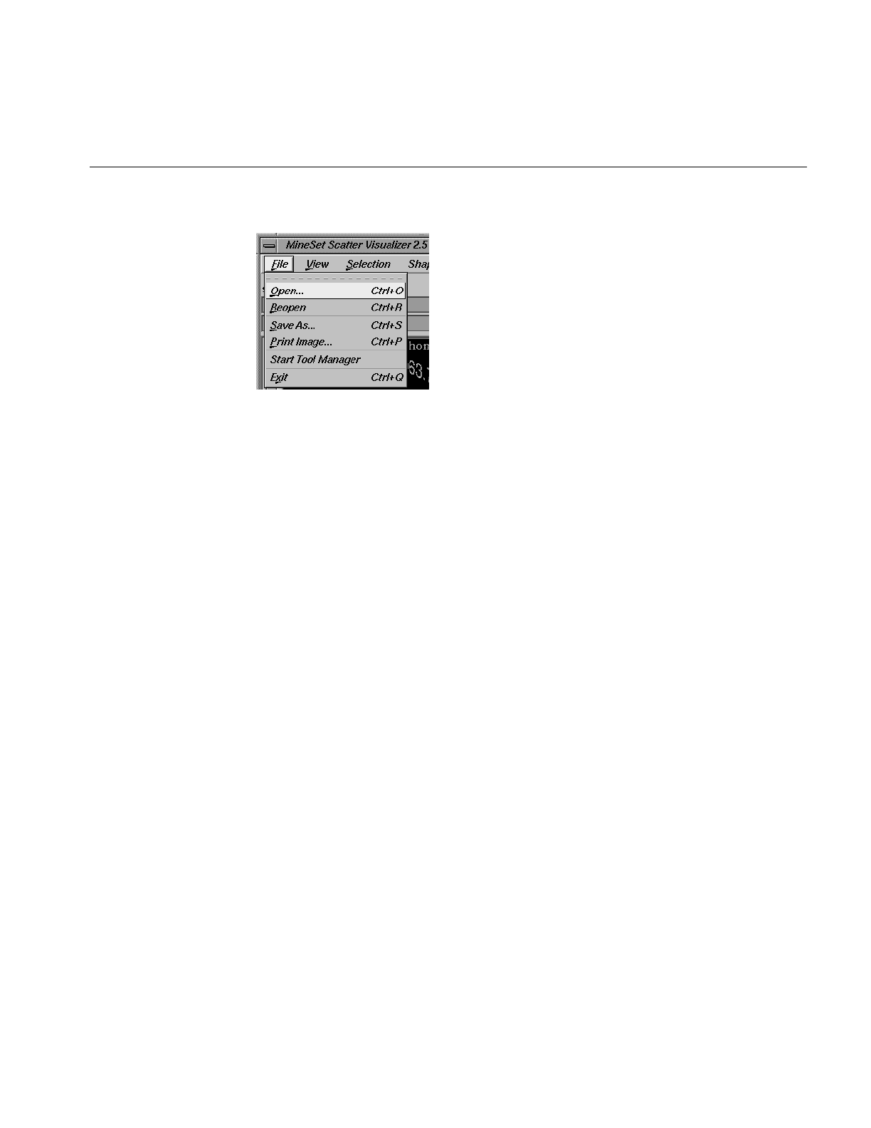
Starting the Scatter Visualizer
219
Figure 7-2 Scatter Visualizer Start-Up File Pulldown Menu Selected
Starting the Scatter Visualizer without specifying a configuration file causes the
main window to show the copyright notice and license agreement for this tool.
Only the File and Help pulldown menus can be used. For the main window to be
fully functional, open a configuration file by selecting File > Open.
•If you know which configuration file you want to use, double-click the icon for that
configuration file. This starts the Scatter Visualizer and automatically loads the
configuration file you specified. This works only if the configuration filename ends
in .scatterviz (which is always the case for configuration files created for the Scatter
Visualizer using the Tool Manager).
•Drag the configuration file icon onto the Scatter Visualizer icon. This starts the
Scatter Visualizer and automatically loads the configuration file you specified.
•Start the Scatter Visualizer from the UNIX shell command line by entering this
command at the prompt:
scatterviz [ configFile ]
configFile is optional and specifies the name of the configuration file to use. If you
don’t specify a configuration file, you must use File > Open to specify one (see
Figure 7-2).

220
Chapter 7: Using the Scatter Visualizer
Configuring the Scatter Visualizer Using the Tool Manager
This section describes how the Scatter Visualizer can be configured using the Tool
Manager. Although the Tool Manager greatly simplifies the task of configuring the
Scatter Visualizer, you can construct a configuration file manually for this tool using a
text editor (see Appendix D, “Creating Data and Configuration Files for the Scatter
Visualizer”).
The steps required to connect to a data source are described in Chapter 3.
Selecting the Scatter Visualizer Tool
Select the Viz Tools tab in the Data Destination panel of the Tool Manager’s main screen
(Figure 7-3). From the popup list of tools, select Scatter Visualizer. The mapping
requirements for the Scatter Visualizer are displayed in the window on the right side of
this panel. Items in the Visual Elements list that are preceded by an asterisk are optional.
Figure 7-3 Data Destination Panel With Scatter Visualizer Selected

Configuring the Scatter Visualizer Using the Tool Manager
221
•Axis 1,*Axis 2,*Axis 3 let you assign to the axes in the Scatter Visualizer’s main
window the data you want represented. Assigning data to Axis1 is required.
However, this alone does not produce a useful display. By assigning data to Axis 2,
you can create an XY chart. Assigning data to all three axes produces a 3-D chart.
•*Entity-size,*Entity-color,*Entity-label let you assign size, color, and label to the
entities appearing in the Scatter Visualizer’s main window.
•*Summary is the value mapped to the summary column, if you have a slider. It
determines the color of the slider’s background.
•*Slider1 and *Slider2 let you map columns directly to one or two animation Sliders
(see “Slider Creation for Scatterviz,” below).
Mapping Requirements to Columns
You can map requirements to columns by selecting a column name in the Current
Columns window of the Table Processing panel, then selecting a category in the Visual
Elements window.
Undoing Mappings
To undo a specific mapping, select that mapping in the Visual Elements window, then
click the Clear Selected button. To undo all mappings, click the Clear All button.
Slider Creation for Scatterviz
Sliders can be created manually or automatically. The following subsections describe
these methods.

222
Chapter 7: Using the Scatter Visualizer
Manual Slider Creation
Tool Manager generates sliders whenever there is an array column present in the current
table. The sliders correspond to the indices of the array columns. If the column has one
index (one-dimensional array), only one slider is created, but if the column has two
indices (two-dimensional array), both an X and a Y slider are created. The current slider
indices are indicated in the Tool Options dialog box from the Tool Manager. Array
columns can be created using the “index by” menus in the Tool Manager aggregation
panel (see “Aggregation” in Chapter 3).
Note that for a slider to be created, all array columns in the current table must have the
same indices. If array columns with differing indices exist in the current table, no sliders
are created.
Automatic Slider Creation
If no arrayed columns are in the current table, Tool Manager can automatically generate
sliders by use of the Slider1 and Slider2 mappings. Sliders are created through a
combination of automatic binning and aggregation. These automatic operations occur
after clicking Invoke Tool in the Data Destination Panel. The operations do not affect the
current history operations of Tool Manager, but they do appear in the configuration files
for the tool.
Columns mapped to Slider1 and Slider2 eventually form the indices for the sliders. These
columns must be either numeric (int, float, double) or binned. If a column mapped to a
slider is already binned, no automatic binning is needed for this column, and this column
is used as an index for a slider. However, if the column is not binned, a binned column is
created using the automatic binning options in the Tool Options dialog box.
The three methods of binning are:
•Selecting All Distinct Values creates a bin for every unique value of the column.
•Specify the number of bins you want to create. The thresholds for the bins are
determined using the Uniform Range approach.
•Selecting Automatic automatically determines the number of bins to create and
determines the bin thresholds using the Uniform Range approach.
(See “The Bin Columns Button” in Chapter 3 for more information about binning.) The
column used in forming the automatic bins is deleted from the current table.

Configuring the Scatter Visualizer Using the Tool Manager
223
The binned columns now form the indices of array columns. Note that if you want to
create only one slider, the index must be mapped to Slider1. Attempting to create only
one slider with a mapping to Slider2 is not allowed and generates a Tool Manager error.
Also, a column mapped to a slider cannot be mapped to any other mapping, since it is
removed during the aggregation process.
Once the slider indices are formed, the arrayed columns are created. This is done using
automatic aggregation. Any numeric columns mapped to Axis 1, Axis 2, Axis 3,
Entity-size, Entity-color, Entity-label, or Summary are aggregated using the automatic
aggregation options in the Tool Options dialog box. You can either specify aggregating
by Sum or by Average. The binned columns created from the slider mappings form the
indices for the aggregation, and any remaining columns in the table are Group-By
columns. (See “Aggregation” in Chapter 3 for a description of the aggregation process.)
Be sure to remove any columns you do not wish to use in the grouping process. If you
need different types of aggregates for different mappings, you must aggregate manually.
The aggregation step automatically forms the arrayed columns used for sliders. These
arrayed columns form the new tool mappings. For example, if the column “mpg” were
mapped to Axis 1, a new column “avg_mpg[]” is formed and remapped to Axis 1. The
progress of the automatic slider generation is displayed in the Tool Manager status
window.
Specifying Tool Options
Clicking the Tool Options button causes a new dialog box to be displayed (Figure 7-4).
This lets you change some of the Scatter Visualizer options from their default values.
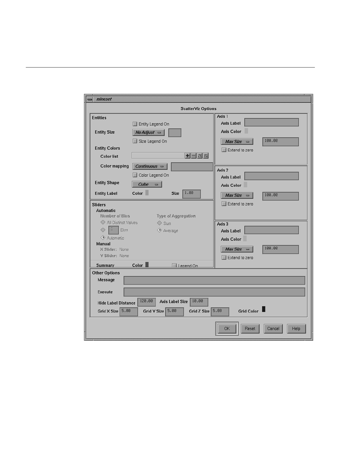
224
Chapter 7: Using the Scatter Visualizer
Figure 7-4 Scatter Visualizer’s Options Dialog Box

Configuring the Scatter Visualizer Using the Tool Manager
225
The Scatter Visualizer’s Options dialog box has four basic options blocks:
•Entities
•Sliders
•Axes
•Other
Entity Options
This option block lets you specify a number of characteristics for the entities that the
Scatter Visualizer then graphically displays.
•Entity Legend On—lets you determine whether the entity legend is displayed or
hidden.
•Entity Size—lets you scale the entity to a max size, a scale size, or a default (no
adjustment). You also can specify whether the legend for entity size is displayed or
hidden.
•Entity Colors—lets you control the colors in which entities are displayed. You can
–specify the list of colors to use
–specify the kind of mapping
–map the list of colors to a list of values
–specify whether the legend for color is displayed or hidden
–map colors to entities
•Entity Shape—lets you choose a visual representation for the entities: cubes, bars, or
diamonds.
To use these Colors options, you must have mapped a column to the *Entity-color
requirement of the Data Destination panel. See “Choosing Colors” and “Using the Color
Browser” in Chapter 3 for a more detailed explanation of how to choose and change
colors.
Color list to use lets you specify the color list using the + button next to the color list label.
This brings up a color editor that lets you specify a color to be added to the list.

226
Chapter 7: Using the Scatter Visualizer
Color mapping let you specify whether the color change that is shown in the graphic
display is Continuous or Discrete. If you choose Continuous, the color values shift
gradually between the colors entered in the Color list to use field as a function of the
values that are mapped to those colors in the Color mapping field.
The field to the right of the popup button lets you enter specific values for mapping the
colors. If you do not specify any mapping values, the range of values in the color variable
is used.
Example 7-1
If you
•used the Color Browser to apply red and green to bars
•selected Continuous for the Kind of mapping
•entered the values 0 100
then the display shows all entities with values less than or equal to 0 as completely red,
those as greater than or equal to 100 as completely green, and those between 0 and 100
as shadings from red to green.
Example 7-2
If you
•used the Color Browser to apply red and green to entities
•selected Discrete for the Kind of mapping
•entered the values 0 50
then the display shows all entities with values of less than 50 in red, and all those with
values greater than or equal to 50 in green.
•Entity Label Color lets you modify a label color by clicking on it. This causes the
Color Choose dialog box to appear, which lets you implement your color changes.
•Entity Label Size controls the size of the entity labels. A smaller number decreases
the size, a larger one increases it.

Configuring the Scatter Visualizer Using the Tool Manager
227
Summary Options
Summary options let you specify what color to use for the Summary window. You can
also specify whether the summary legend, which indicates what the values are, is
displayed or hidden.
If you have an array of values, you can specify an X or Y slider. The popup buttons next
to these options provide a list of available keys, and let you specify which to use as
sliders.
Slider Options
The Slider options control how the slider mappings are interpreted. For details see
“Slider Creation for Scatterviz” on page 221.
Axis Options
The Axis options let you specify the following, for each axis:
•A label. (If you leave this box blank, the Scatter Visualizer defaults to using the
column names for each axis.)
•A color
•A size type for each axis. (This can be Max Size,Scale Size, or No Adjustment.)
–Max Size lets you specify that an axis is scaled independently to a specified size.
If one axis has a Max Size that is twice as large as the other, it will be twice as
long, regardless of the data values. This option is most useful when comparing
axes that are in different units (for example, comparing income to age). This
option has no effect on non-numeric data.
–Scale Size lets you specify that the axis is scaled based on its maximum value. If
two axes have the same Scale Size, but one has a maximum that is twice the
value of the other, the former will be twice as long as the latter. This option is
useful for comparing axes with the same units (for example, income vs.
expenses). This option does affect the size of non-numeric axes.
–No Adjust is equivalent to a Scale Size of 1.0.
•A size value
•Whether the axis should be extended to include the value 0.

228
Chapter 7: Using the Scatter Visualizer
Other Options
The Other Options, at the bottom of the dialog box, include the following fields:
•Message lets you specify the message displayed when an entity is selected. For a
listing and description of format types that can be entered in this field, see the
“Message Statement” section in Appendix D, “Creating Data and Configuration
Files for the Scatter Visualizer”
•Execute lets you type in a UNIX command that is executed when double-clicking on
an entity. The format is similar to the message statement. If no execute statement
appears, double-clicking has no effect. For a detailed description of the Execute
field, see “Execute Statement” in Appendix D.
•Hide Label Distance controls the distance at which entity labels become invisible.
Smaller distances might improve performance, but the labels disappear more
quickly. The higher the number, the greater the distance at which labels are hidden.
•Axis Label Size controls the size of the axis labels. A smaller number decreases the
size, a larger one increases it.
•Grid (X, Y, Z) Size lets you specify the spacing between grid lines for the respective
axis. A smaller number decreases the size, a larger one increases it.
•Grid Color lets you modify a grid color by clicking on it. This causes the Color
Chooser dialog box to appear, which lets you implement your color changes.
Resetting the Tool Options
If you want to reset the values of all options to their default values, click the Reset Options
button.
Saving the New Tool Options
Once you have finished making changes to the Tool Options dialog box, click OK to
return to the Tool Manager’s main screen.

Configuring the Scatter Visualizer Using the Tool Manager
229
Invoking the Scatter Visualizer
To see Scatter Visualizer graphically represent your data, click the Invoke Tool button at
the bottom of the Data Destination panel.
Saving the Scatter Visualizer Settings
When you press Invoke Tool, the Tool Manager stores information for the Scatter
Visualizer in three files, all sharing the same prefix:
•<prefix>.scatterviz.data contains data.
•<prefix>.scatterviz.schema describes the data file.
•<prefix>.scatterviz contains information needed by the Scatter Visualizer.
To save the entire session along with the current tool options, use one of these menu
options from the File menu:
•Save Current Session... where the default prefix is based on the data source
•Save Current Session As... to specify your own prefix
The saved file is <prefix>.mineset, and contains all the information needed to return
MineSet to its current state.
Null Handling in the Scatter Visualizer
The Scatter Visualizer uses special representations when fields with unknown data
values, or nulls, are mapped to visual attributes. (For a discussion of null values, see
Appendix J, “Nulls in MineSet.”) When a null value is mapped to an entity’s size, the
entity is drawn as the outline of a cube. When a null value is mapped to an entity’s color,
it is drawn in dark grey. When a null value is displayed in the Selection Window or
“Pointer is Over” area, it is shown as a question mark (?). (The Selection Window and
“Pointer is Over” areas are discussed in the “Select Mode” section.)
If a null value is mapped to the x,y, or z position of an entity, the result depends on the
Show Entities with Null Positions option under the View Menu (see “The View Menu”
on page 241). If the option is set, the entity is shown just below the range of the
corresponding axis. If the option is not set, the entity is not shown.

230
Chapter 7: Using the Scatter Visualizer
Working in the Scatter Visualizer’s Main Window
If you started the Scatter Visualizer without specifying a configuration file, the main
window shows the copyright notice and license agreement for the Scatter Visualizer.
Only the File and Help pulldown menus can be used. For the main window to show all
menus and controls, open a configuration file. Use File > Open (Figure 7-2) to see a list of
configuration files.
When a valid configuration file has been selected, the 3D landscape it specifies is visible.
For example, selecting company-total.scatterviz gives results as shown in Figure 7-5.

Working in the Scatter Visualizer’s Main Window
231
Figure 7-5 Initial View When Specifying company.scatterviz
This shows the sales of life insurance, auto insurance, and home insurance with respect
to income brackets over time.

232
Chapter 7: Using the Scatter Visualizer
Viewing Modes
The two modes of viewing are grasp and select. To toggle between these modes, press the
Esc key or click the appropriate cursor button adjacent to the top-right of the viewing
area.
Grasp Mode
In grasp mode, the cursor appears as a hand. This mode supports panning, rotating, and
scaling the scene’s size in the main window.
•To pan the display, press the middle mouse button and drag it in the direction you
want the display panned.
•To rotate the display, press the left mouse button and move the mouse in the
direction you want to rotate. (Also see the thumbwheel controls Rotx and Roty,
described in “Thumbwheels” in Chapter 6.)
•To move the viewpoint forward, press the left and middle mouse buttons
simultaneously and move the mouse downwards. To move the viewpoint
backward, press the left and middle mouse buttons simultaneously and move the
mouse upwards. This is equivalent to the functions provided by the Dolly
thumbwheel.
Select Mode
In select mode, you can highlight an object by positioning the cursor over that object.
Information about that object then appears at the top of the view area, under the Pointer
is over: label (Figure 7-6). This information remains visible in the window only as long as
the pointer cursor remains over the object. Position the pointer cursor over an object and
click the left mouse button; the same information appears in the Selection Window, above
the main window. A white box appears around the entity, indicating it has been selected,
and a table viewer shows your current selection. Select several entities by holding down
the Shift key while clicking the left mouse button. The most recent selection is shown
under the Selection label at the top of the scene. All current selections are shown in the
Record Viewer. You can now drill-through on your selection (see “The Selection Menu”
on page 279 for the different drill-though options.)
This Selection information remains visible until another object is selected, or you click the
black background. Using the mouse, you can cut and paste this selection information into
other applications, such as reports or databases.
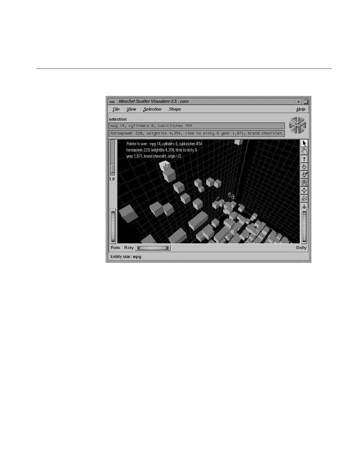
Working in the Scatter Visualizer’s Main Window
233
Figure 7-6 Displayed Information When Cursor is Over a Selected Entity
If an execute statement was specified using Tool Manager or the configuration file, then
double clicking on an object executes the appropriate command. If the -warnexecute
option was specified when invoking the Scatter Visualizer, a warning is given first.
Note: Users familiar with Open Inventor can configure the Scatter Visualizer so that the
right mouse button brings up the standard Inventor Menu. This provides additional
functions, such as stereo viewing and spin animation. These functions are provided by
the Open Inventor library. To enable the Open Inventor Menu, add the line
*minesetInventorMenu:TRUE
to your .Xdefaults file.

234
Chapter 7: Using the Scatter Visualizer
External Controls
Several external controls surround the main window, including buttons and
thumbwheels. These controls are substantially the same for most MineSet visualization
tools (see the descriptions “Buttons” in Chapter 6, and “Thumbwheels” in Chapter 6).
The Animation Control Panel
The animation control panel, which appears to the right of the main window, consists of
a summary window, with up to two adjacent sliders, an information field, animation
buttons, and animation sliders.
Sliders Controlling Independent Dimensions
The number of sliders appearing adjacent to the summary window is dependent on the
dataset displayed in the Scatter Visualizer’s main window. Datasets can have two, one,
or no independent dimensions.
Datasets With Two Independent Dimensions
If the dataset has two dimensions of independently varying data (such as
company.scatterviz), the controls to the right of the main graphics window become visible
(see Figure 7-7).

The Animation Control Panel
235
Figure 7-7 Animation Control Panel With Summary Window and Both Slider Controls
To the right of the main window are the summary window and slider controls. The
summary window has a horizontal slider below it for selecting data points of the first
independent dimension, and a vertical slider to the left for selecting data points of the
second independent dimension. The horizontal slider’s dimension is identified by a label
below it. The vertical slider’s dimension is identified by a label above it.
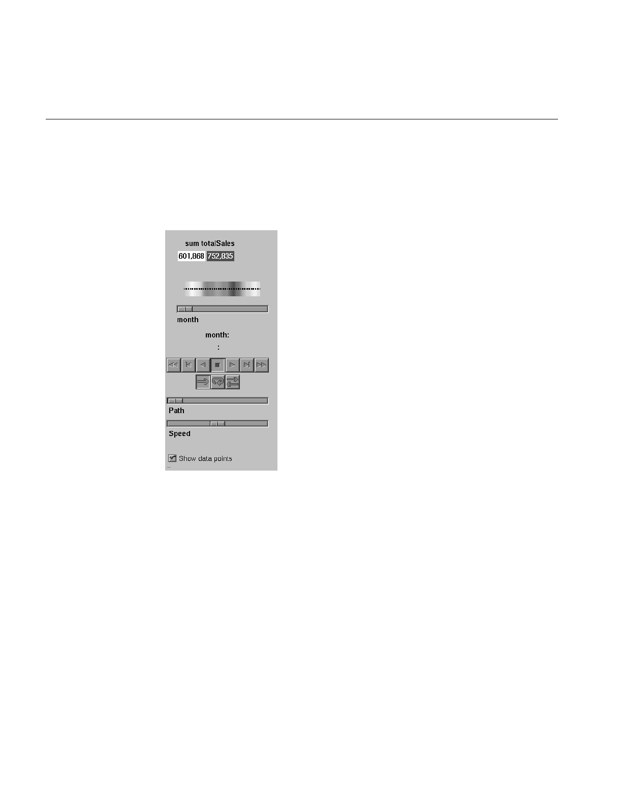
236
Chapter 7: Using the Scatter Visualizer
Datasets With One Independent Dimension
For datasets with one independent dimension (such as store-type.scatterviz), only the
slider below the summary window appears, and the summary window is compressed
(see Figure 7-8). This slider’s dimension is identified by a label below it.
Figure 7-8 Animation Control Panel With Summary Window and One Slider Control
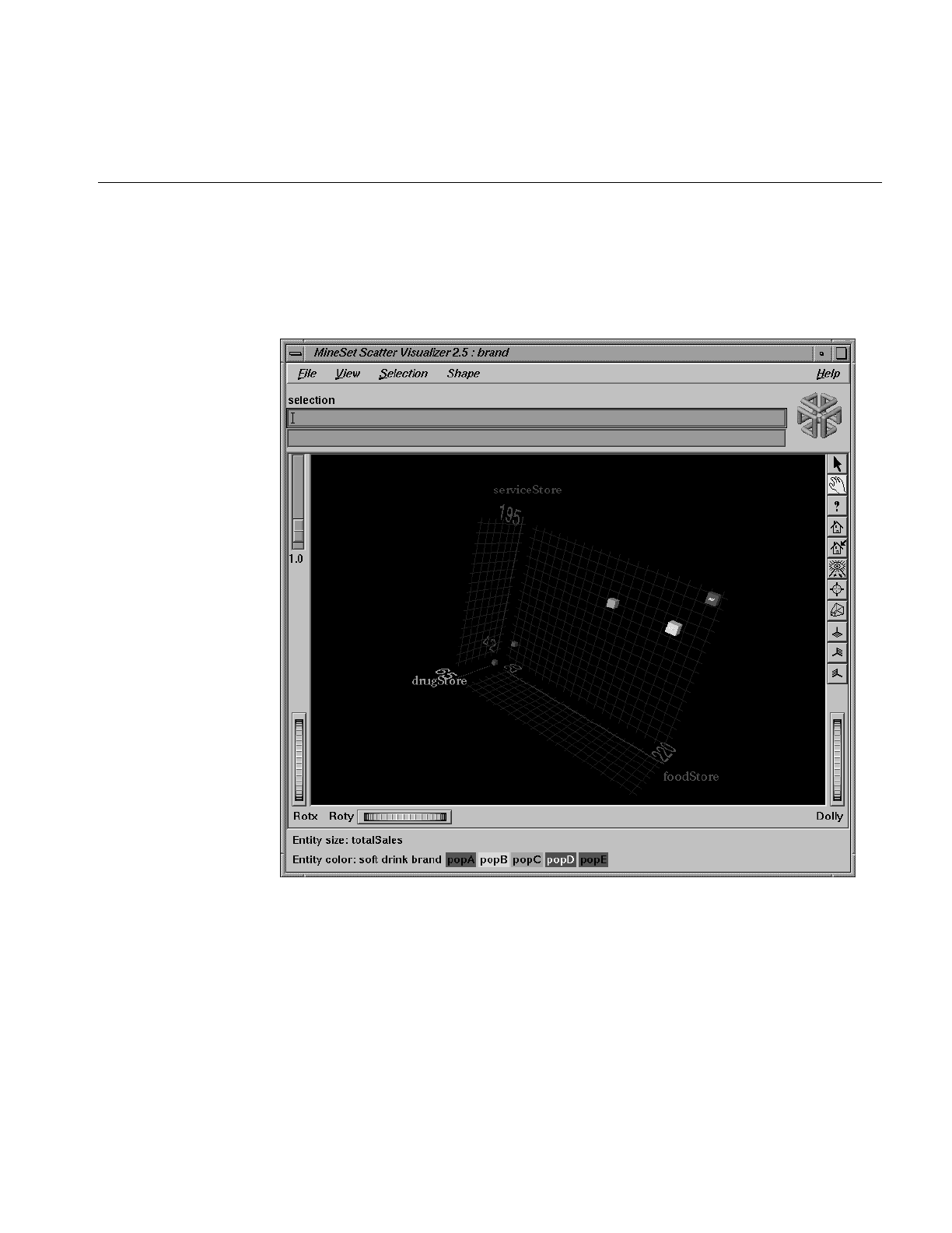
The Animation Control Panel
237
Datasets With No Independent Dimension
For datasets with no independent dimensions (such as brand.scatterviz), no slider control
appears (see Figure 7-9).
Figure 7-9 Scatter Visualizer With No Independent Dimension or Animation Control Panel

238
Chapter 7: Using the Scatter Visualizer
The Summary Window
The summary window provides a 2D representation of the aggregation of values that the
main window displays in 3D. The whiter the areas of the summary window, the lower
the total values represented by the entities in the main window. The greater the color
density in areas of the summary window, the higher the total of those values. The density
of these colors in the summary window provides a summary of the data across the one
or two independent dimensions in the dataset.
By default, the summary window also contains a set of black dots, evenly spaced across
the one or two dimensions of data. These dots indicate the precise positions of the
discrete datapoints. You can turn off these black dots using the View|Show Data Points
menu option.
Color Density Examples in the Summary Window
After opening the company.scatterviz file, for example, the 2D summary window shows a
color range from white (on the left) to red (on the right). White corresponds to a low sales
volume; red represents a higher aggregate sales volume. In this example, the greater the
density of red, the higher the total sales of life, auto, and home insurance.
Creating a Path in the Summary Window
If the dataset loaded into the Scatter Visualizer has at least one independent dimension,
it is possible to view all or any part of that dataset via animation. This is done by first
creating a path in the summary window (this path connects a sequence of data points),
then activating the animation controls described in the next section.
The three ways to draw a path in the summary window are as follows:
•Define a starting point by clicking and holding down the left mouse button, then
draw a path by dragging the cursor over the window. End the path by releasing the
left mouse button.
•Define a starting point by clicking the left mouse button, then define an endpoint by
moving the cursor to another part of the window and clicking the middle mouse
button. A line appears between those two points. To add more line segments,
continue with repeated middle mouse clicks.
•Define a starting point by clicking the left mouse button, then drag one of the
independent dimension sliders, thus drawing a straight line along this dimension.
If there are two sliders, use of the second slider causes a straight line to be drawn
along the axis controlled by this second slider.

The Animation Control Panel
239
Animation Buttons and Sliders
The seven VCR-like buttons and two sliders (Path and Speed) below the 2D summary
window let you control the animation.
Animation Buttons
Once a path is drawn in the summary window (see “Creating a Path in the Summary
Window,” above), you can use the VCR-like buttons to control animation along this path.
The middle Stop button is highlighted in blue, indicating an initial state. Use the adjacent
Play Forward button (to the right of Stop) or Play Reverse (to the left) to begin simple
movement along the drawn path in a forward or reverse direction. (Forward and Reverse
are defined by the sequence in which the path was drawn, not by the left-to-right or
right-to-left movement.)
To stop and restart the animation, click the Stop button, then use the Play Forward or
Reverse button again. Note that when you stop, the animation continues in the current
direction until the position falls upon a discrete data point.
Adjacent to the Play buttons are the Single-Step buttons, as well as Forward and Reverse.
Clicking on one of these buttons changes the current path position to the next discrete
data point.
On the outside are the Fast Forward and Fast Reverse buttons. Clicking one of these
buttons while in Stop state changes the path position to the end (for Forward) or to the
beginning (for Reverse) of the path. Clicking a Fast button when in Play state increases the
animation speed.
Animation Flow
Below the Animation Buttons are the three Animation Flow buttons.
Play-once (default)—the animation moves either forward or in reverse until it reaches the
end of the path, then stops.
Loop—when the animation reaches the end of the path, it automatically resets to the
beginning and starts over again.
Swing—when the animation reaches the end of the path, it reverses direction and retraces
its path to the other end; upon reaching that end, the animation reverses direction again,
beginning the cycle again.

240
Chapter 7: Using the Scatter Visualizer
Animation Sliders
While animation is stopped, you can move the Path slider to reset the position along the
path. Note that when you use the Path slider, the cursor in the summary window moves
across the drawn path, and the 1D sliders (below and to the left of the drawing area)
move consistently with the cursor position. Then use the Play or Reverse button to restart
the animation from the newly specified point. You can drag the Path slider to an arbitrary
position between discrete data points; however, when you release the slider, the path
position changes to the nearest discrete data point.
Use the Speed slider to adjust the speed of the animation along the path.
Data Points and Interpolation
As animation proceeds, the variables mapped to size, color, and axes (positions) in the
Scatter Visualizer change smoothly. However, the information displayed in the
“Selection:” message box and the Pointer is over: field show only the data values of the
nearest discrete data position; they do not show interpolated data values.
The animation is produced in the following manner: Assume you have data for 10 years,
on a per-year basis (that is, 10 data values) and that these correspond to the size of one
entity in the Scatter Visualizer. Assume further that the years are 1991 to 2000, the size for
1991 is 20, and the size for 1992 is 40. As you move the year slider from 1991 to 1992, the
size changes by being uniformly interpolated between 20 and 40. For example, midway
between 1991 and 1992, the size is 30. As you approach 1992, the size approaches 40.
However, you cannot stop an animation between discrete data points, and you cannot
drag the Path slider to a stationary position between discrete data points.
The data points in the summary window represent the slider positions corresponding to
the actual data from the data file. For example, sizes 20 and 40 are representations of
actual data, but size 30 is not. In this example, there would be data points in the summary
window at the slider positions corresponding to each year.
Note that not all variables are required to vary with a slider. If there are two sliders, some
variables can vary with only one of the sliders, while other variables vary with both.
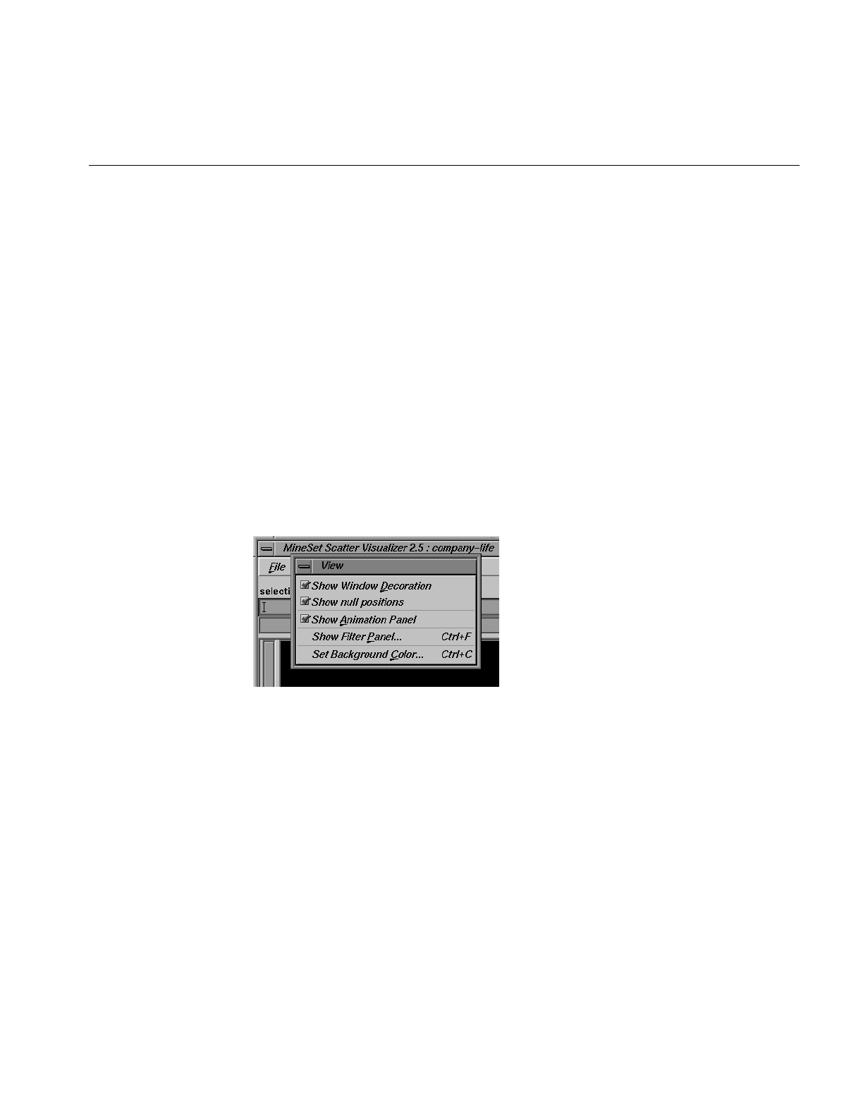
Pulldown Menus
241
Pulldown Menus
Four pulldown menus let you access additional Scatter Visualizer functions. These are
labeled File, View, Selections, and Help. If you start the Scatter Visualizer without
specifying a configuration file, only the File and the Help menus are available.
The File Menu
The File menu is the substantially the same for all visualization tools see “The File Menu”
in Chapter 5.
The View Menu
The View menu lets you control certain aspects of what is shown in the Scatter Visualizer
window (Figure 7-10).
Figure 7-10 Scatter Visualizer View Menu
•Show Window Decoration lets you hide or show the external controls around the
main window.
•Show null Positions lets you hide or show entities that have null or unknown
position values along one or more axes.
•Show Animation Panel lets you show or hide the animation control panel. This menu
item is disabled for datasets with no independent dimension.
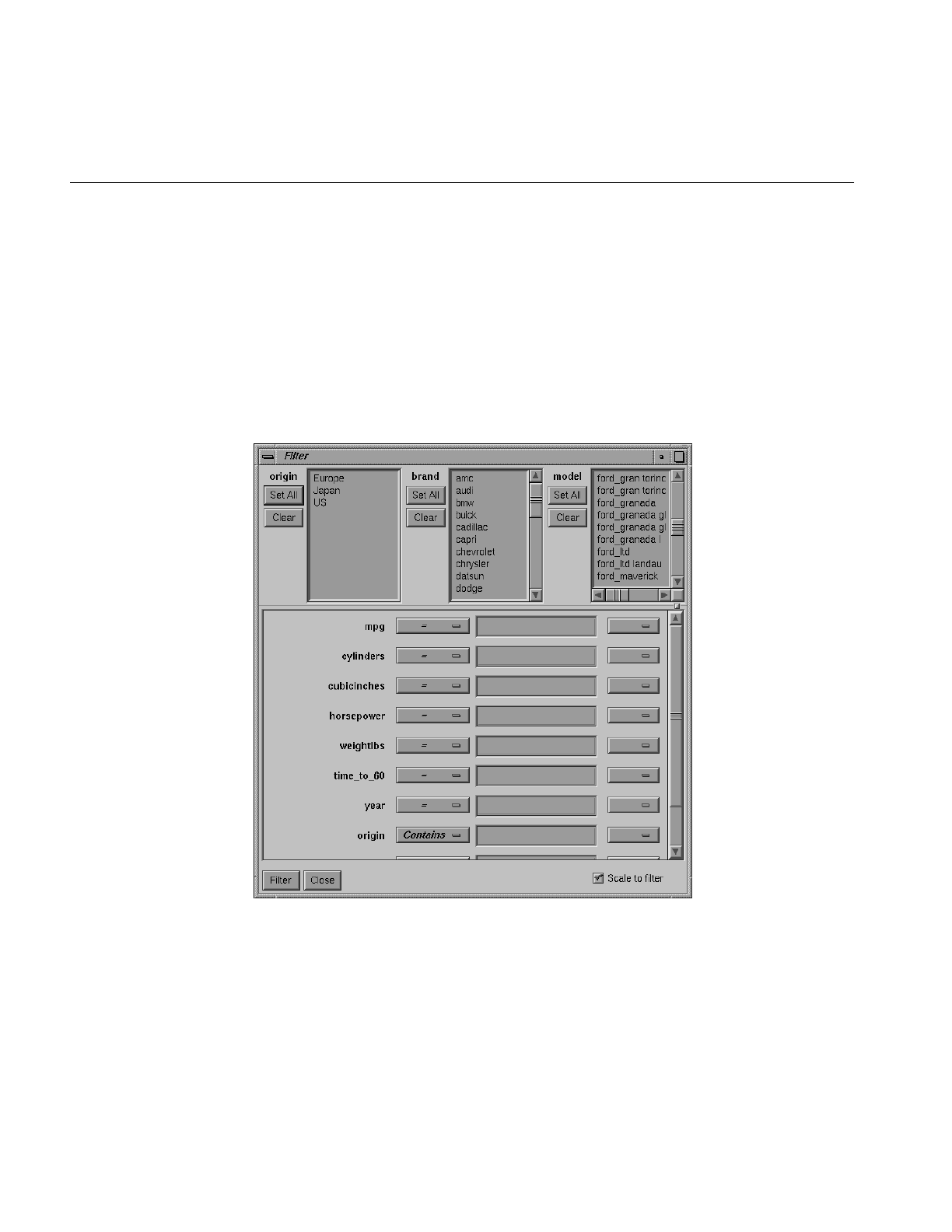
242
Chapter 7: Using the Scatter Visualizer
•Show Filter Panel lets brings up the Filter Panel. This panel (Figure 7-11) lets you
reduce the number of entities displayed in the main viewing area, based on one or
more criteria. You can use the filter panel to fine-tune the display, emphasize
specific information, or simply shrink the amount of information displayed. The Set
Landscape to Filter checkbox, which appears in the lower right of the filter panel,
lets you specify whether the landscape in the main window covers the entire
dataset or just the filtered data.
•Set Background Color brings up a color chooser to let you specify a new background
color.
Figure 7-11 Scatter Visualizer Filter Panel

Pulldown Menus
243
The Filter panel has two panes. The top pane lets you filter based on string columns.
To select all values of a column, click Set All. To clear the current selections, click
Clear. To select a value, click it. To deselect a value, simply click it again.
The bottom pane lets you filter based on the values of both string and numeric
columns.
To filter numeric values, enter the value, and select a relational operation (=, !=, >, <,
>=, <=). To filter alphanumeric values, enter the string. You can use any of three
types of string comparisons:
•Contains indicates that it contains the appropriate string. For example,
“California” contains the strings “Cal” and “forn”.
•Equals requires the strings to match exactly.
•Matches allows wildcards:
–An asterisk (*) represents any number of characters.
–A question mark (?) represents one character.
–Square braces ([ ]) enclose a list of characters to match.
For example, California matches Cal*, Cal?fornia, and Cal[a-z]fornia.
For columns which were binned, an option menu of values appears, instead of a
text field. To ignore that column, select Ignored in the Option menu. You can use
relational operators, such as >=, with these options. This means that the specified
value as well as subsequent ones are selected.
In addition to numeric and string comparison operations, you can specify Is Null,
which is true if the value is null.
To the right of each field is an additional option menu that lets you specify “And” or
“Or” options. For example, you could specify “sales > 20 And < 40.” You can have
any number of And or Or clauses for a given column, but cannot mix And and Or in
a single column.
Scale to Filter lets you specify whether the filtered landscape is rescaled to the size of
the filtered data or remains the size of the entire data set.
Click the Filter button to start filtering. If you press Enter while the panel is active,
filtering starts automatically.
Click the Close button to close the panel.

244
Chapter 7: Using the Scatter Visualizer
The Selections Menu
The Selections menu lets you drill through to the underlying data.
Figure 7-12 The Scatter Visualizer Selections Menu
•Create Box Selection creates a 3-D box selector that can be stretched and translated to
select regions of the volume. While active, a table in Record Viewer format is
opened showing information about all of the aggregated data that is represented by
the entities within it. Closing this window clears all current selections. Any entities
within the selection box or selected using Shift-click are shown in the table window.
To translate the selection box, click on one of the faces with the left mouse button,
and drag it in the desired direction. Holding the Shift key while dragging constrains
the motion to the axis to which the drag motion is closest. To change the extent of
the selection box, drag one of the gray scale tabs in the desired direction. Trying to
resize or translate beyond the bounds of the volume is not permitted. The gray scale
tabs constantly resize to maintain constant screen size. If at any time they appear
too big, you can zoom in closer, and they reduce their size relative to the box.
•Show Original Data retrieves and displays the records corresponding to what has
been selected. The resulting records are shown in a table viewer.
•Send To Tool Manager inserts a filter operation, based on the current box selection(s),
at the beginning of the Tool Manager history. The actual expression used to do the
drill through is determined by the extent of the current box selection. If nothing is
selected, a warning message appears.
•Complementary Drill Through causes the Show Original Data and Send To Tool Manager
selections, when used, to fetch all the data that are not selected.

Sample Configuration and Data Files
245
•Preferences brings up a panel that lets you select which columns are used in
drill-through. Unlike other visual tools, there are no specific columns in the data
that are designated as the key to the data. It is impossible for the Scatter Visualizer
to determine which columns the user desires in the drill-through expression. For
example, you might have cars data with brand, model, and weight. Perhaps you
want to drill through to the original data, and specify that brand and model should
be considered, but weight should not. By default, all columns that have been
mapped to graphical requirements are considered significant on drill-through. The
others are not, but may be made so by highlighting them in the Preferences dialog
box.
For further details on drill-through, see Chapter 18, “Selection and Drill-Through.”
The Help Menu
The Help menu is substantially the same for all visualization tools; see “The Help Menu”
in Chapter 6
Sample Configuration and Data Files
The provided sample data and configuration files demonstrate the Scatter Visualizer’s
features and capabilities. The following files are in the /usr/lib/MineSet/scatterviz/examples
directory:
•company.data
This file contains fictitious sales data of several insurance companies in three
product categories: life insurance, auto insurance, and home insurance. The data
span ten years (in increments of one year) and includes five income brackets (the
customer’s annual income).
•company.scatterviz
This file specifies that the years form one slider dimension and the income brackets
form the other slider. Sales of life insurance, auto insurance, and home insurance
become the three dimensions in the Scatter Visualizer landscape. The color density
in the slider summary window represents the total sales of all companies across all
categories of insurance.

246
Chapter 7: Using the Scatter Visualizer
•company-total.scatterviz
This file contains the same specifications as company.scatterviz, except that the size of
each company is determined by the total sales of that company across all the
categories of insurance.
•company-life.scatterviz
This file contains the same specifications as company.scatterviz, except that the color
of each object indicates the life insurance sales as a fraction of total sales.
•store-type.data and store-type.scatterviz
These files show sales of various product groups by store type during a three-year
period. The single independent variable for which a slider appears is time. Each
entity represents a store type (such as Food Store, Drug Store, Service Station, and
so forth). For each store type, the data file contains the total sales of several product
groups, such as alcoholic beverages, cereal, and so forth. The data spans 36 months,
in increments of one month.
The configuration file uses the month as the single slider dimension. One axis is
sales of alcoholic beverages, the other is sales of tobacco products. A third axis is not
used.
Note: The data file includes other categories. You can edit the configuration file to
use other product categories for the axes (see Appendix D, “Creating Data and
Configuration Files for the Scatter Visualizer”).
•brand.data and brand.scatterviz
These files show sales of several soft-drink brands in a variety of store types. In this
dataset the brands form the entities, and the store types are associated with the axes.
The total sales are mapped to the size of each brand. The color mapping is random.
Since there are no independent variables, no slider is present.
•cars.data and cars.scatterviz
These files show the weight, horsepower, model year, and acceleration of several car
models.
•people.data and people.scatterviz
These files show the height, weight, density, and cholesterol level for a population
sample.
•nl.births.data and nl.births.scatterviz
These files show birth patterns in the Netherlands. For each region, the population
density, birth rate, and population are shown. The animation sliders are mapped to
the age of the mother and the year.

Sample Configuration and Data Files
247
•adult94.data and adult94.scatterviz
These files show a complex example with scatterviz applied to
/usr/lib/MineSet/data/adult.data. The three axes in the visualization are avg_hrswk
(that is, average hours worked per week), avg_gross_income, and
avg_education_num. Unfortunately “education num” does not correspond exactly
to number of years of education, but it is close. The slider on the right side animates
across different age ranges. Each aggregate was created by grouping by occupation,
race and sex. This means that there is an entity for every combination of values for
these three attributes. The color shows different occupations, as shown in the
legend. The size of each entity corresponds to record counts. The summary slider is
also colored by data density. To find out how this visualization was created, you
may select Start Tool Manager from the File menu. This will bring up the Tool
Manager with the session used to create this example.
Initially the scene shows information for people under 20 years of age. Note that the
average hours worked (about 14) and the average income (about $4000) are low. If
you animate over age using the slider, and examine the scene from the three
orthogonal viewer (try using the lower 3 buttons to the right of the main window),
you will notice various trends emerge. For example, if you orient the scene so you
see only income by hours per week, you can see that people start to work longer
hours as they age, until about age 25, then they seldom work more that 49 hours per
week until they retire. Income, however, grows until people age 50, then plateaus,
then goes lower again. The actual trend depends somewhat on the career choice and
other factors.
Suppose you were interested in comparing trends between the occupations
craft-repair and prof-specialty. Open the Filter panel (View > Show Filter Panel) and
select just “craft-repair” and “prof-specialty” from the list of occupations. Now
when you animate, you can see that “prof-specialty” actually starts with lower
incomes, but quickly outpaces “craft-repair” as people age. “Prof-specialty” is much
higher on the education axis than “craft-repair”. You may wish to limit your filter
further by showing just females, or those of a certain race.


249
Chapter 8
8. Using the Splat Visualizer
This chapter discusses the features and capabilities of the Splat Visualizer. It provides an
overview of this database visualization tool, then explains the Splat Visualizer’s
functionality when working with the
•main window
•external controls
•pulldown menus
Finally, it lists and describes the sample files provided for this tool.
Overview of the Splat Visualizer
The Splat Visualizer lets you visually analyze relationships among several variables (see
Figure 8-1), either statically or by animation. It is particularly well-suited for application
to datasets with large numbers of records. Choose the Scatter Visualizer if you want to
see individual data points and do not have a large number of records. Data analysis is
done using
•a three-dimensional landscape
•an animation control panel that includes a two-dimensional slider
•graphical objects, called splats, which represent aggregates of datapoints. Color and
opacity of the splats can change during animation.
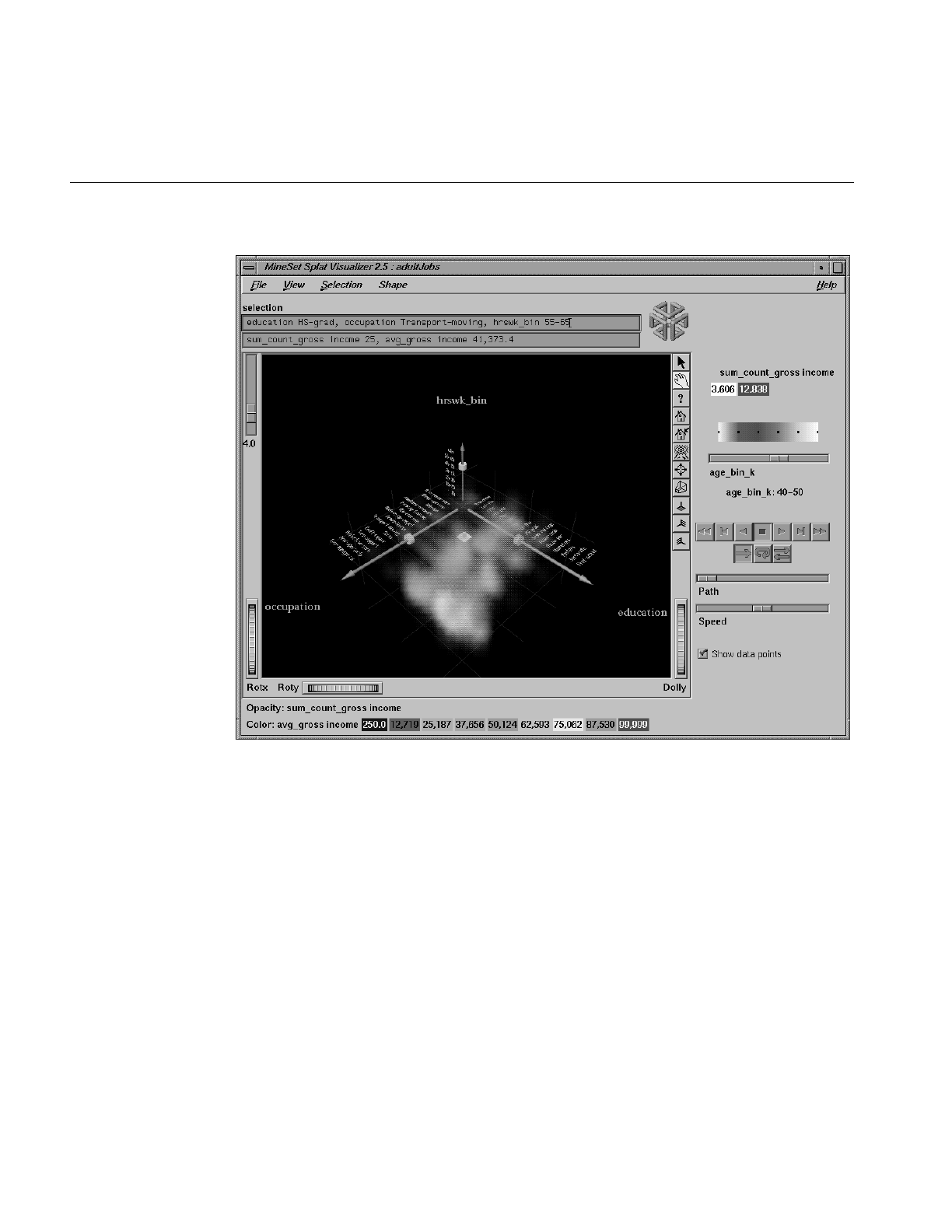
250
Chapter 8: Using the Splat Visualizer
Figure 8-1 Sample Splat Visualizer With One Slider Control
The Splat Visualizer lets you visualize your data by mapping columns to axes, sliders,
color, and opacity. The resulting three-dimensional landscape can be thought of as an
approximation to a scatterplot in which every datapoint is drawn separately. It is not
truly a scatterplot, because datapoints that are close together (fall in the same bin) are
aggregated and drawn as a single splat.

Overview of the Splat Visualizer
251
Each numeric column that is mapped to an axis or slider first must be binned. If this
binning step is skipped, the Tool Manager does it using automatic uniform binning (see
“The Bin Columns Button” in Chapter 3). String columns can be mapped directly to axes.
Any numeric column can be mapped to a color. The color of a splat is derived by
averaging the value of the column mapped to color for all the data points that fall in a
bin. The opacity of a splat is based on a weighting of the number of datapoints that fall
in a bin. If nothing is mapped to opacity, record counts are used to determine it. The
interactivity of the resulting visualization is independent of the number of data points
represented; it depends only on the number of bins in the axis dimensions. If your dataset
is very large, aggregate explicitly in the Tool Manager. This causes the server to perform
the processing, rather than having the entire dataset sent to the client and aggregated
there.
Up to two numeric columns can be mapped to the sliders in the animation control panel.
The splats change their color and opacity during animation as the sliders in the
animation panel are moved from point to point along the slider ‘s path. Unlike the Scatter
Visualizer, neither the position nor the size of the splats change; they are at fixed,
uniformly spaced positions. Only their color and opacity change, which can give the
illusion of actual movement.
After creating a visualization of your data, the Splat Visualizer lets you analyze the data
in various ways:
•The animation control panel lets you note global shifts and trends in the data.
•The three-dimensional landscape lets you orient the display to emphasize particular
dimensions or a point of view.
•You can use the scale slider (located to the left of the Main Window) to lower the
overall opacity of the splats, so only regions with dense data show up; conversely,
you can increase the scale slider so all regions having any data become visible. The
regions with dense data are likely to show less color variation, because the color is
based on the average of many values (see Figure 8-3).
•You can filter the display to show only those splats meeting certain criteria. You can
filter on the columns corresponding to axes, sliders, weight, and color.
•An opaque pick dragger lets you display textual information about individual
splats in the volume.
•A box selector lets you define a selected region for drilling through to the original
data or for sending to the Tool Manager.
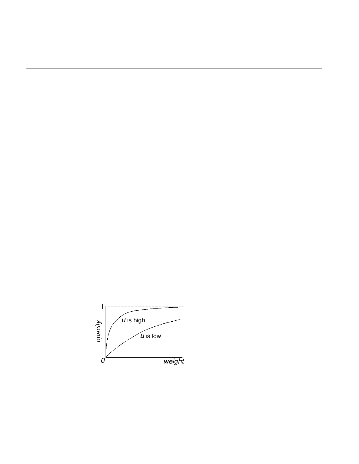
252
Chapter 8: Using the Splat Visualizer
If a string column is mapped onto an axis, binning is defined to be the distinct values of
that column. The order of the values along a string axis is automatically determined by
sorting the distinct values by the average aggregate value of the column mapped to color.
Looking at the color changes along a string-valued axis lets you see how well that
column correlates with the column mapped to color. The left axis in Figure 8-1 shows
occupations sorted by average income (the average income of everyone with that
occupation) along an axis. The occupation, executive-managerial, listed at the end of the
axis, has the highest average income. This ordering often presents a natural progression
for the values. For example, the ordering for the values of education (the right axis in
Figure 8-1) was generally from low to high; but, in a few cases, there were anomalies in
the order. This unexpected ordering might be interesting because it points out places
where the data does not agree with expectations.
Opacity
The column mapped to opacity should be record count or a column used to weight
record counts. A splat’s opacity, α, is based on this column according to the following
relation:
where count is the column mapped to opacity (or the record count if no such column was
mapped to opacity). The shape of this function is such that the opacity asymptotically
approaches 1 (totally opaque) as the value of weight becomes large. The variable u is what
is scaled when you adjust the opacity scale slider. Figure 8-2 shows the shape of this
function for low and high values of u. Figure 8-3 shows the same visualization with low
and high values of u.
Figure 8-2 Shape of Opacity Function For Low and High Values of u
α1eu weight⋅–
–=
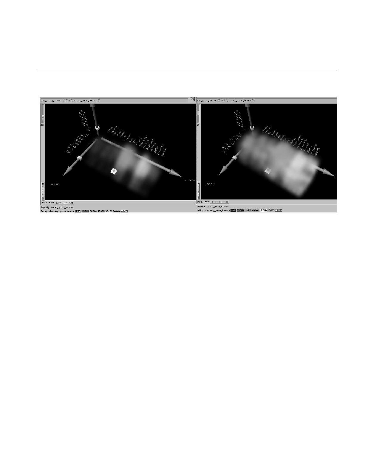
Overview of the Splat Visualizer
253
Figure 8-3 Image Where u = 5.3, and u = 30
If nothing is mapped to opacity, the Splat Visualizer generates a column of ones to
produce record counts when aggregating. This means all records are weighted equally.
A sum aggregation is done on this column, and an average aggregation is done on the
column mapped to color while grouping by all the axis and slider columns. All other
columns are unnecessary and removed. You do not need to map anything to opacity
unless you want each record to be weighted by something other than 1.
You can avoid processing on the client by aggregating in the Tool Manager. This also
avoids having to transfer a large dataset to the client. This is done by
1. Binning the numeric columns which are to be used for axes and sliders.
2. Aggregating the column to be mapped to color by count and average while
grouping by the axis and slider columns.
3. Mapping the resulting count aggregation to opacity.
4. Mapping the resulting average aggregation to color.

254
Chapter 8: Using the Splat Visualizer
For example, using the adult94 data (provided with the distribution):
1. Bin age and hours_per_week.
2. Aggregate gross_income using count and average. Keep education, occupation,
age_bin and hours_per_week_bin, in the group-by pane while removing all the
other columns.
3. Map education, occupation, and hours_per_week_bin to the axes.
4. Map avg_gross_income to color, count_gross_income to opacity, and age_bin to a
slider.
When you invoke the tool, note that all the processing is done on the server, and that the
datafile, adult94.splatviz.data, contains rows that are aggregates of rows in the original
data. This produces the same visualization as seen in Figure 8-1.
In some cases, you might have a column by which you want to weight the records. For
example, if you have a dataset for which one column was population and another was
average_salary (which you want to map to color), you can map population to opacity,
and average_salary to color; then have the Splat Visualizer do the aggregation. Its
aggregation groups-by the axis and slider columns, so that it sum aggregates the opacity
column (which, in this case, is population). The new column is called sum_population.
The average_salary column is revised, so that it is still average salary, but weighted by
each row’s population. In this way, the average salary column still shows the average
salary for all the people it represents.
Alternatively, if you want to avoid client-side processing and storage because of the size
of your dataset, you can perform the same aggregation in Tool Manager by doing the
following:
1. Create a new column, defining temp = population*avg_income.
2. Perform an aggregation: group-by axis and slider columns, sum aggregate
population, and sum aggregate temp.
3. create a new column, defining
avg_salary = sum_temp/sum_population
This creates the weighted average.
4. Now you can map sum_population to opacity, and avg_salary to color.
Note that these steps are the ones taken by the Splat Visualizer if you do not explicitly do
them in the Tool Manager.

File Requirements
255
File Requirements
The Splat Visualizer requires the following files:
•A data file, consisting of rows of tab-separated fields. This file is easily created using
the Tool Manager (see Chapter 3). If you are generating this file yourself, see
Appendix E, “Creating Data and Configuration Files for the Splat Visualizer” for
the required file format.
You can generate data files by extracting data from a source (such as a database) and
formatting it specifically for use by the Splat Visualizer. Data files have user-defined
extensions (the sample files provided with the Splat Visualizer have a .data
extension).
•A configuration file, describing the format of the input data and how it is to be
displayed. The Tool Manager can create this file (see Chapter 3), or you can use an
editor (such as jot, vi, or Emacs) to produce this file yourself (see Appendix E,
“Creating Data and Configuration Files for the Splat Visualizer”).
Configuration files must have a .splatviz extension. When starting the Splat
Visualizer, or when opening a file, you must specify the configuration file, not the
data file.
Starting the Splat Visualizer
There are five ways to start the Splat Visualizer:
•Use the Tool Manager to configure and start the Splat Visualizer. (See Chapter 3 for
details on most of the Tool Manager’s functionality, which is common to all MineSet
tools; see “Configuring the Splat Visualizer Using the Tool Manager” on page 256
for details about using the Tool Manager in conjunction with the Splat Visualizer.)
•Double-click the Splat Visualizer icon, which is in the MineSet page of the icon
catalog (or on your Indigo Magic desktop). The icon is labeled splatviz. Since no
configuration file is specified, the start-up screen requires you to select one by using
File > Open.
Starting the Splat Visualizer without specifying a configuration file causes the main
window to show the copyright notice and license agreement for this tool. Only the
File and Help pulldown menus can be used. For the main window to be fully
functional, open a configuration file by selecting File > Open.

256
Chapter 8: Using the Splat Visualizer
•If you know what configuration file you want to use, double-click the icon for that
configuration file. This starts the Splat Visualizer and automatically loads the
configuration file you specified. This works only if the configuration filename ends
in .splatviz (which is always the case for configuration files created for the Splat
Visualizer via the Tool Manager).
•Drag the configuration file icon onto the Splat Visualizer icon.
•Start the Splat Visualizer from the UNIX shell command line by entering this
command at the prompt:
splatviz [ configFile ]
configFile is optional and specifies the name of the configuration file to use. If you
don’t specify a configuration file, you must use File >Open to specify one.
Options for Invoking the Splat Visualizer
The -quiet option eliminates the dialogs that popup to indicate progress. You can enable
this option permanently by adding the line
*minesetQuiet:TRUE
to your .Xdefaults file.
Configuring the Splat Visualizer Using the Tool Manager
This section describes how the Splat Visualizer can be configured using the Tool
Manager. Although the Tool Manager greatly simplifies the task of configuring the Splat
Visualizer, you can construct a configuration file manually for this tool using a text editor
(see Appendix E, “Creating Data and Configuration Files for the Splat Visualizer”).
The steps required to connect to a data source are described in Chapter 3.
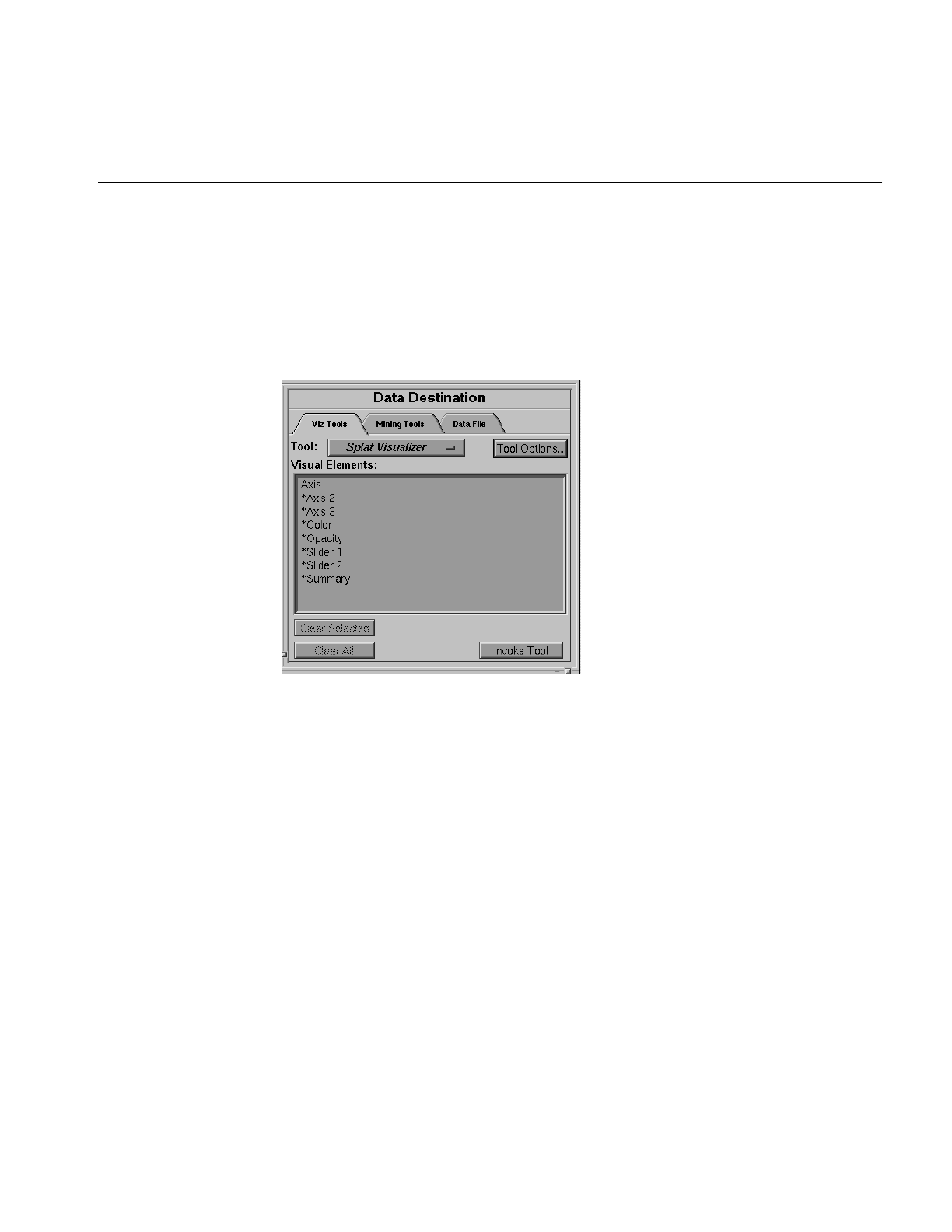
Configuring the Splat Visualizer Using the Tool Manager
257
Selecting the Splat Visualizer Tool
Select the Viz Tools tab in the Data Destination panel of the Tool Manager’s main screen
(Figure 8-4). From the popup list of tools, select Splat Visualizer. The mapping
requirements for the Splat Visualizer are displayed in the window on the right side of this
panel. Items in the Visual Elements list that are preceded by an asterisk are optional.
Figure 8-4 Data Destination Panel With Splat Visualizer Selected
•Axis 1, *Axis 2, *Axis 3 — determine which columns are assigned to the axes in the
Splat Visualizer’s main window. Assigning data to the first axis is required;
however, this alone does not usually produce a useful display. By assigning data to
Axis 2, you can create an XY chart. Assigning data to all three axes produces a 3-D
chart.
•*Color — Requires a numeric column used to determine the color of the splats.
If you have a two-valued string column, you can create a new numeric column
using an expression such as:
('stringCol'==”value1”)? 1:0
If nothing is mapped to color, the resulting scene is monochromatic.

258
Chapter 8: Using the Splat Visualizer
•*Opacity—the tool was designed to have the opacity based on a weighting of
records. If you do not aggregate in the Tool Manager, this requirement need not be
mapped; it will be determined automatically by the tool. If you do a count
aggregation in the Tool Manager, or there is a column in the data that already is
based on counts, use that column for this requirement.
•*Sliders — the summary slider dimensions. They must be numeric or binned.
•*Summary—this is the value to be shown in the summary slider. If no summary
column is mapped, count is used by default. If a summary column is mapped, a
weighted average value for that column is shown in the summary.
Mapping Columns to Requirements
You can map requirements to columns by selecting a column name in the Current
Columns window of the Table Processing panel, then selecting a category in the Visual
Elements window.
Undoing Mappings
To undo a specific mapping, select that mapping in the Requirements window, then click
the Clear Selected button. To undo all mappings, click the Clear All button.
Specifying Tool Options
Clicking the Tool Options button causes a new dialog box to be displayed (Figure 8-5).
This lets you change some of the default values of the Splat Visualizer options.
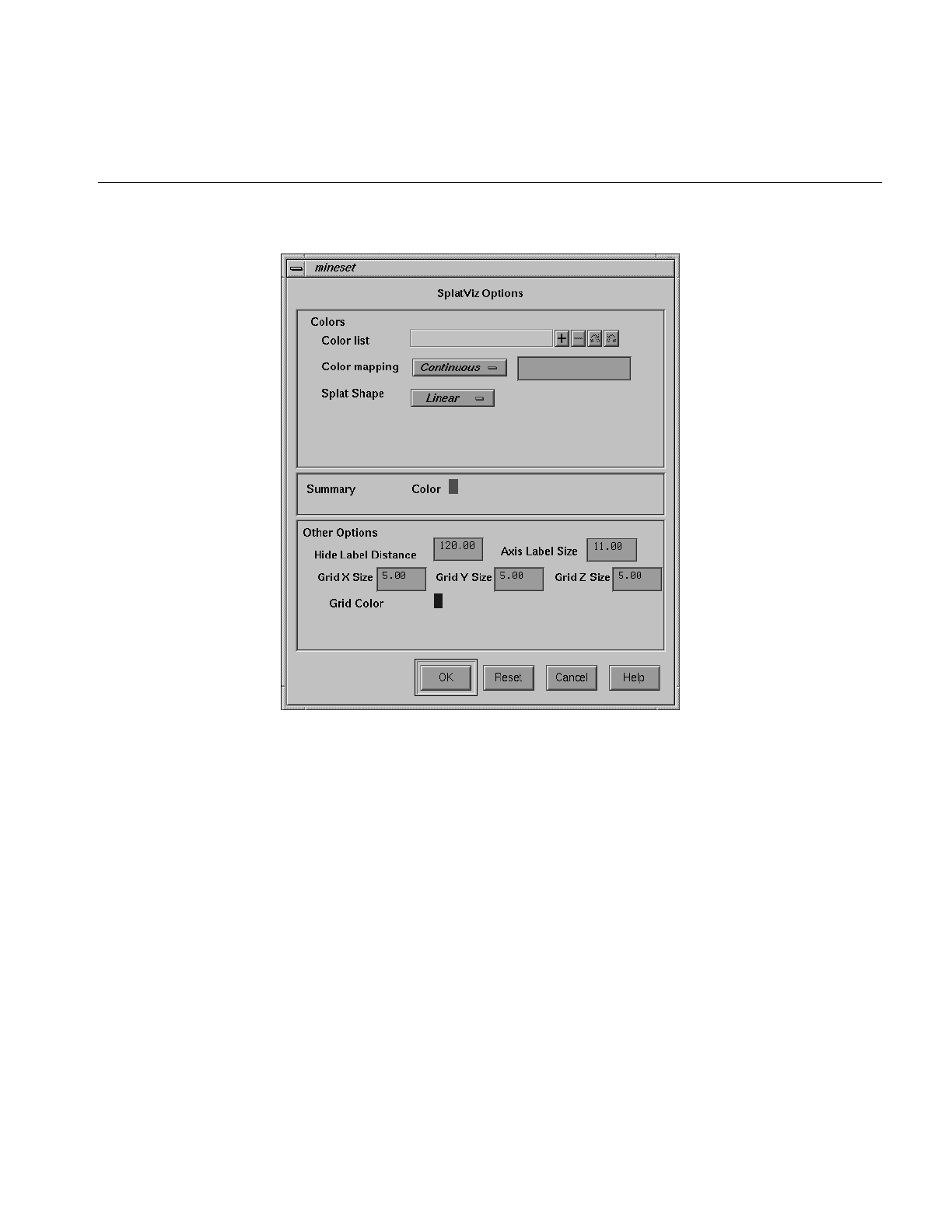
Configuring the Splat Visualizer Using the Tool Manager
259
Figure 8-5 Splat Visualizer’s Options Dialog Box
The Splat Visualizer’s Options dialog box has three basic options blocks:
•Splats
•Summary
•Other

260
Chapter 8: Using the Splat Visualizer
Splat Options
This option lets you specify a number of characteristics for the Splats that the Splat
Visualizer then graphically displays.
•Splat Colors—lets you control the colors used for the splats. You can
–specify the list of colors to use
–specify the kind of mapping
–map the list of colors to a list of values
•Splat Shape—lets you choose one of the following methods for drawing splats:
linear, gaussian, texture, sphere, cube, or diamond. See “Splat Type Menu” on
page 282 for a further explanation of each of these.
To use these Colors options, you must have mapped a column to the *color requirement
of the Data Destination panel. If nothing is entered in the color list, the default colormap
is used. The default colormap is a continuous spectrum from blue (lowest value) to red
(highest value). See “Choosing Colors” and “Using the Color Browser” in Chapter 3 for
a more detailed explanation of how to choose and change colors.
Color list—You can specify the color list using the + button next to the color list label.
This brings up a color editor that lets you specify a color to be added to the list.
Color mapping—You can specify whether the color change that is shown in the graphic
display is Continuous or Discrete. If you choose Continuous, the color values shift
gradually between the colors entered in the Color list to use field as a function of the
values that are mapped to those colors in the Color mapping field.
The field to the right of the popup button lets you enter specific values for mapping the
colors. If you do not specify any mapping values, the range of values in the color column
is used.

Configuring the Splat Visualizer Using the Tool Manager
261
Example 8-1
If you
•used the Color Browser to apply red and green to the splats
•selected Continuous for the Kind of mapping
•entered the values 0 100
the display shows all splats with values less than or equal to 0 as completely red, those
with values greater than or equal to 100 as completely green, and those between 0 and
100 have a color which results from a linear interpolation between red and green.
Example 8-2
If you
•used the Color Browser to apply red and green to the splats
•selected Discrete for the Kind of mapping
•entered the values 0 50
The display shows all splats with values of less than 50 in red, and all those with values
greater than, or equal to, 50 in green.
Summary Options
Summary options let you specify what color to use for the Summary window. This is
only applicable if you have mapped a column to the summary.

262
Chapter 8: Using the Splat Visualizer
Other Options
The Other Options, at the bottom of the dialog box, include the following fields:
•Hide Label Distance — controls the distance at which axis tick labels (for string
valued axes) become invisible. Increase this number to make the labels appear at
further distances. The higher the number, the greater the distance at which labels
are hidden.
•Axis Label Size — this controls the size of the axis labels. A smaller number decreases
the size, a larger one increases it.
•Grid Color — lets you modify a grid color by clicking on it. This causes the Color
Chooser dialog box to appear, which lets you implement your color changes.
•Grid (X, Y, Z) Size — lets you specify the spacing between grid lines for the
respective axis. A smaller number decreases the size, a larger one increases it. If the
Size is set to 0, there are no grid lines in that dimension.
Resetting the Tool Options
Clicking the Reset Options button resets the values of all options to their default values.
Invoking the Splat Visualizer
To see Splat Visualizer graphically represent your data, click Invoke Tool at the bottom of
the Data Destination panel.
Saving the Splat Visualizer Settings
When you press Invoke Tool, The Tool Manager stores information for the Splat Visualizer
in several files, all sharing the same prefix:
•<prefix>.splatviz.data contains data.
•<prefix>.splatviz.schema describes the data file.
•<prefix>.splatviz contains information required by the Splat Visualizer.

Configuring the Splat Visualizer Using the Tool Manager
263
To save the entire session along with the current tool options, use one of these menu
options from the File menu:
•Save Current Session... where the default prefix is based on the data source
•Save Current Session As... to specify your own prefix
The saved file is <prefix>.mineset, and contains all the information needed to return
MineSet to its current state.
When you use Invoke Tool, the .data,.schema, and .splatviz files are updated, if necessary.
Null Handling in the Splat Visualizer
The Splat Visualizer uses special representations when fields with unknown data values,
or nulls, are mapped to visual attributes. (For a discussion of null values, see Appendix J,
“Nulls in MineSet.”) When every record in a bin has a null value for the column mapped
to color, the resulting color for that splat is gray. If one or more records in the aggregate
have non-null values for the column mapped to colors, then that value is (or those values
are) used to compute the color. While the sum of a value and null is null, the average of
a value and null is the value (that is, value + Null = Null; avg(val, Null) = val).
When a null value is displayed in the Pick Window, Selection Window or “Pointer is
Over” area, it is shown as a question mark (?). (The Selection Window and “Pointer is
Over” areas are discussed in the “Select Mode” section.)
For numeric columns containing nulls which are mapped to axes, there is a special null
position below the range defined by the axis. This is to help show that the null value is
discontinuous with the other values. The null positions for numeric axes can be turned
off using the Show Null Positions option under the View Menu (see “The View Menu”
on page 276). For string-valued columns mapped to axes, nulls (represented by a ‘?’) are
treated as just another value.

264
Chapter 8: Using the Splat Visualizer
Working in the Splat Visualizer’s Main Window
If you started the Splat Visualizer without specifying a configuration file, the main
window shows the copyright notice and license agreement for the Splat Visualizer. Only
the File and Help pulldown menus can be used. For the main window to show all menus
and controls, open a configuration file. Use File > Open to see a list of configuration files.
When a valid configuration file has been selected, the 3-D landscape it specifies is visible.
Viewing Modes
The two modes of viewing are grasp and select. To toggle between these modes, press Esc,
or click the appropriate cursor button adjacent to the top-right of the viewing area.
Grasp Mode
In grasp mode, the cursor appears as a hand. This mode supports panning, rotating, and
scaling the scene’s size in the main window.
•To pan the display, press the middle mouse button and drag it in the direction you
want the display panned.
•To rotate the display, press the left mouse button and move the mouse in the
direction you want to rotate. (Also see the thumbwheel controls Rotx and Roty,
described in “Thumbwheels” in Chapter 6.)
•To move the viewpoint forward, press the left and middle mouse buttons
simultaneously and move the mouse downwards. To move the viewpoint
backward, press the left and middle mouse buttons simultaneously and move the
mouse upwards. This is equivalent to the functions provided by the Dolly
thumbwheel.

Working in the Splat Visualizer’s Main Window
265
Select Mode
In select mode, you can move a 3-D pick dragger through the volume in order to display
information about regions in the scene. This pick dragger is composed of a cylinder and
a square. If you pick on the cylinder and drag, motion is constrained to be parallel to the
cylinder’s axis. If you pick on the square and drag, motion is constrained to the plane
defined by the square. You can cycle through the three possible orientations of the pick
dragger by pressing the Control key with the cursor over the dragger. (You need not press
the mouse button.) In the case of dragging the square portion of the dragger, you can use
the Shift key to constrain the motion along one of the two axes within the plane.
Alternatively, each axis has a disk that aligns with the pick dragger position. Moving the
disk on an axis moves the dragger, and vice-versa.
The dragger lets you pick within a dense cloud of points, freeing you from the limitation
of having to pick regions on the surface.
When the pick dragger is over data, the cylinder changes its color to that of the splat
under it, and information about that region appears at the top of the view area
(Figure 8-6). If no data is present, the cylinder remains light gray, and information about
its position is displayed at the top of the render area for aid in navigation.
When you are finished dragging, and have released the mouse button, the message for
the splat you are currently over is shown in the Pick Window at the top. This pick
information is updated if the animation slider is moved. Using the mouse, you can cut
and paste this selection information into other applications, such as reports or databases.
The pick dragger may be removed from the scene by unchecking Selection > Show Pick
Dragger.
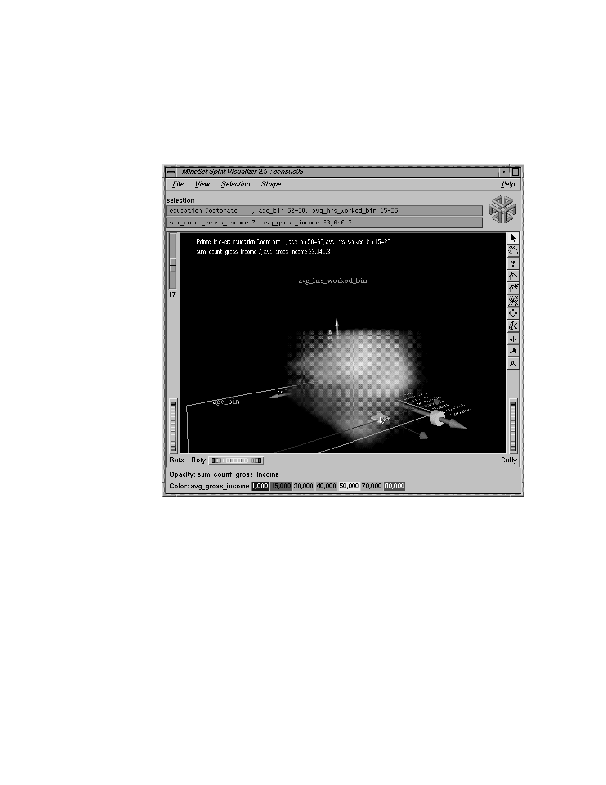
266
Chapter 8: Using the Splat Visualizer
Figure 8-6 Pick Dragger Over Data
The information is displayed when the pick dragger is over the object.
Note: Users familiar with Open Inventor can configure the Splat Visualizer so that the
right mouse button brings up the standard Inventor Menu. This provides additional
functions, such as stereo viewing and spin animation. These functions are provided by
the Open Inventor library. To enable the Open Inventor Menu, add the line
*minesetInventorMenu:TRUE
to your .Xdefaults file.

External Controls
267
External Controls
Several external controls surround the main window, including buttons and
thumbwheels. (These and the rest of the buttons are substantially the same as the other
MineSet visualization tools and are described in “Buttons” in Chapter 6, and
“Thumbwheels” in Chapter 6).
The Animation Control Panel
The animation control panel, which appears to the right of the main window, consists of
a summary window, with up to two adjacent sliders, an information field, animation
buttons, and animation sliders.
Sliders Controlling Independent Dimensions
The number of sliders appearing adjacent to the summary window is dependent on the
slider mappings specified in the configuration file. Datasets can have two, one, or no
independent dimensions.
Datasets With Two Independent Dimensions
If the dataset has two dimensions of independently varying data (such as
adultJobs2.splatviz), the controls to the right of the main graphics window become visible
(see Figure 8-7).
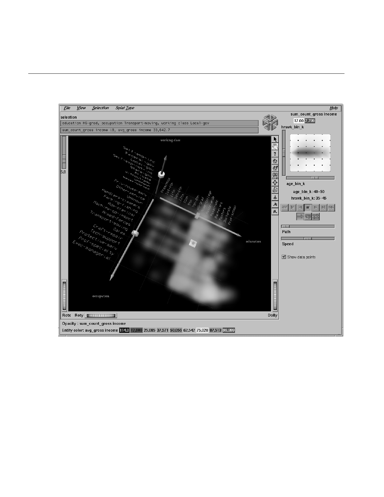
268
Chapter 8: Using the Splat Visualizer
Figure 8-7 Animation Control Panel With Summary Window and Both Slider Controls

The Animation Control Panel
269
To the right of the main window are the 2-D summary window and slider controls. The
summary window has a horizontal slider below it for selecting data points of the first
independent dimension, and a vertical slider to the left for selecting data points of the
second independent dimension. The horizontal slider’s dimension is identified by a label
below it. The vertical slider’s dimension is identified by a label above it.
Datasets with One Independent Dimension
For datasets with one independent dimension (such as adultJobs.splatviz), only the slider
below the summary window appears, and the summary window is compressed (see
Figure 8-1). This slider’s dimension is identified by a label below it.
Datasets With No Independent Dimension
For datasets with no independent dimensions (such as mushroom.splatviz), no slider
control appears (see Figure 8-8). In this example, the splats that are neither completely
red nor completely blue indicate that both poisonous and edible mushrooms are plotted
at that location.
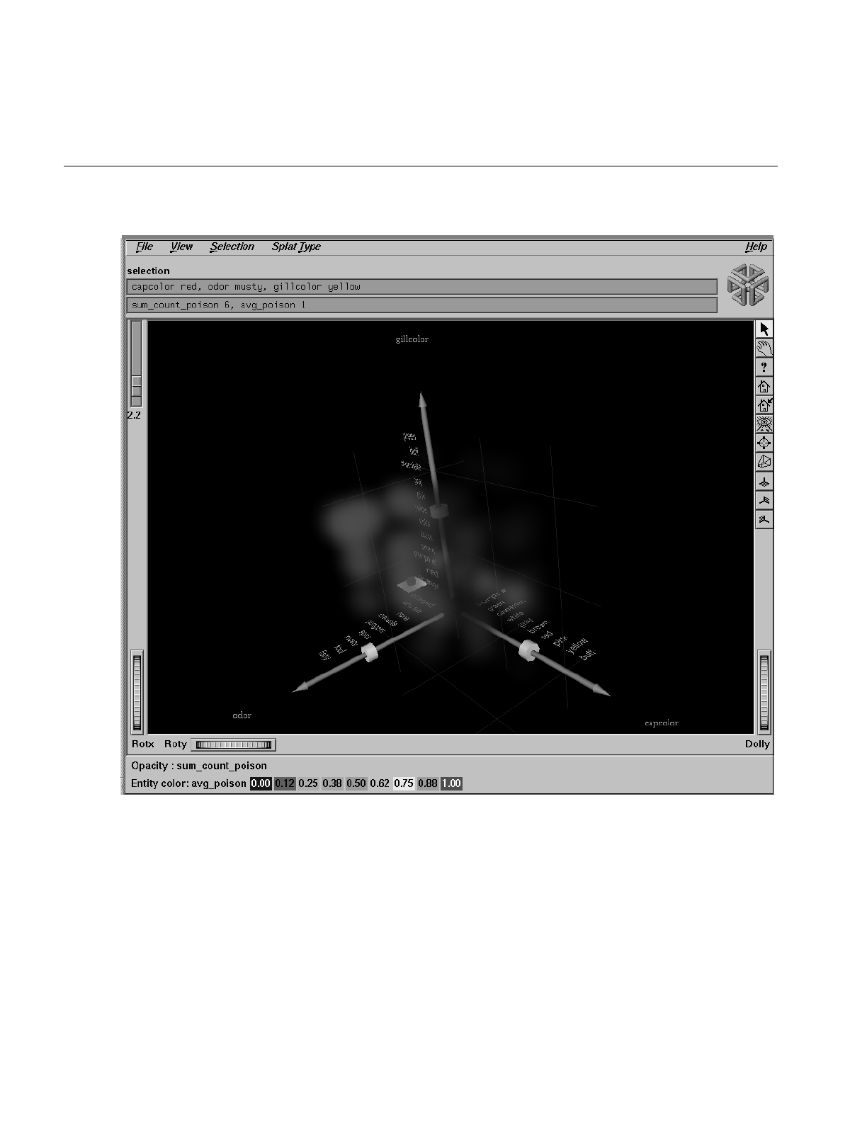
270
Chapter 8: Using the Splat Visualizer
Figure 8-8 Splat Visualizer Without Independent Dimension or An Animation Control Panel

The Animation Control Panel
271
The Summary Window
The summary window provides a 2-D representation of the aggregation of values that
the main window displays in 3-D. The whiter the areas of the summary window, the
lower the summary value represented by the splats in the main window. The greater the
color density in areas of the summary window, the higher the summary values. The
summary value is either the total weight of data at that slider position, or the weighted
average of the column that was mapped to summary. The density of these colors in the
summary window provides a summary of the data across the one or two independent
dimensions in the dataset. If no column is explicitly mapped to summary, count is used
to show which positions on the slider represent the most data.
By default, the summary window also contains a set of black dots, evenly spaced across
the one or two dimensions of data. These dots indicate the precise positions of the
discrete datapoints. You can turn off these black dots by unchecking the box at the
bottom of the summary slider window. Slider positions between these positions use
interpolation of the underlying data to produce an image.
Color Density in the Summary Window
After opening the adultJobs.splatviz file, for example, the 2-D summary window shows a
color range from white (on the left) to red (in the middle) to white (on the right). Red
represents more records (12,838 in this case), while white represents fewer records
(3,606). In this example, the greater the density of red in the middle of the slider, means
the highest concentration of people are in the 20-50 age range.
Creating a Path in the Summary Window
If the dataset loaded into the Splat Visualizer has at least one independent dimension, it
is possible to view all or any part of that dataset via animation. This is done by first
creating a path in the summary window (this path connects a sequence of data points),
then activating the animation controls described in the next section.

272
Chapter 8: Using the Splat Visualizer
The three ways to draw a path in the summary window are:
•Define a starting point by clicking and holding down the left mouse button, then
draw a path by dragging the cursor over the window. End the path by releasing the
left mouse button.
•Define a starting point by clicking the left mouse button, then define an endpoint by
moving the cursor to another part of the window and clicking the middle mouse
button. A path appears between those two endpoints. To add more line segments,
continue with repeated middle mouse clicks.
•Define a starting point by clicking the left mouse button, then drag one of the
independent dimension sliders, thus drawing a straight line along this dimension.
If there are two sliders, use of the second slider causes a straight line to be drawn
along the axis controlled by this second slider.
Animation Buttons and Sliders
The animation panel is identical to that of the Map Visualizer, see “Animation Buttons
and Sliders” in Chapter 6. The following section is different, however.
Slider Data Points and Interpolation
As animation proceeds, the size and color of the splats change smoothly. The information
displayed in the message box field shows the interpolated data values. When the slider
motion stops, the slider position snaps to the nearest discrete data position where
interpolated data values are not used.
There is a table for each binned position on the summary slider. Each row in one of these
tables (which is an aggregate of original data) defines a splat in the scene. Tables
corresponding to adjacent bins on the summary need not have the same number of rows
because of the differences in data distribution from one position to the next. For example,
if we change the visualization in Figure 8-1 from showing 40-50 year-olds to one showing
50-60 year-olds by moving the slider one notch to the right (see Figure 8-9), some
positions might show splats where there were none before, and vice versa.
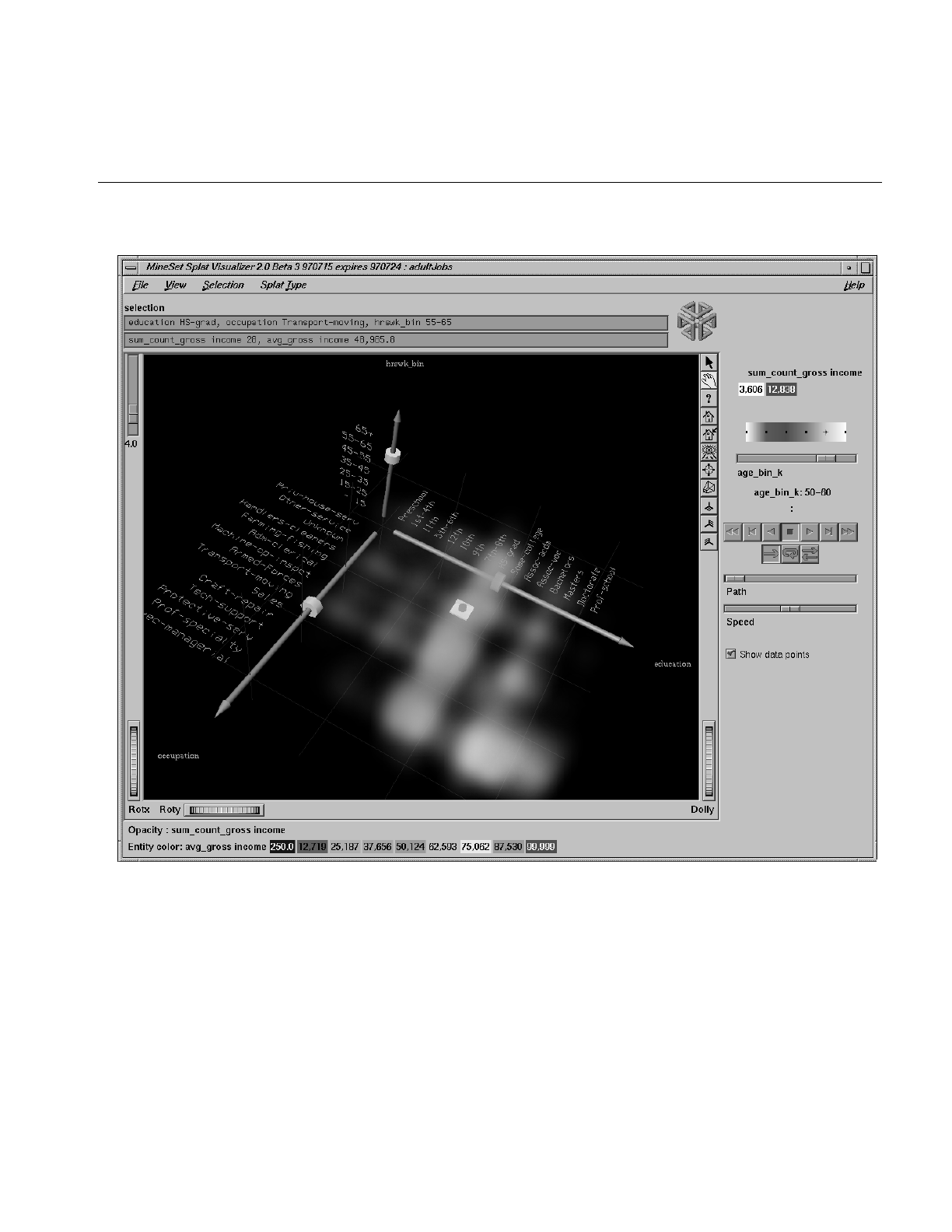
The Animation Control Panel
273
Figure 8-9 Changed Visualization as a Result of Moving the Slider (Compare to Figure 8-1)

274
Chapter 8: Using the Splat Visualizer
For interpolation on a one dimensional slider, two adjacent tables are merged, then
aggregated using the spatial columns as unique keys. The count is simply interpolated
(0 count is assumed if one of the tables lacks a particular row). The average value used
for color is also interpolated, but weighted by the count.
Example 8-3
(This example describes technical details of the interpolation process.) Suppose we want
to show an image that represents an interpolation between the tables for the 40-50
year-olds and the 50-60 year-olds on the external slider. Let Table 8-1 and Table 8-2 be the
tables for age=40-50 and age=50-60, respectively, for the two slider positions.
This is how the Splat Visualizer performs the interpolation. For Table 8-1, a new count
column equal to (1-t)count and a new weighted value column equal to (1-t) (count) (value)
are added. For Table 2, a new count column equal to (t)(count), and a new weighted value
column equal to (t) (count) (value) are added. The two tables are merged together.
The merged table is aggregated using the spatial axes columns as keys, and sum
aggregating the two new columns. This ensures that no two rows have the same binned
values for all the spatial axes. Finally, divide the summed value by the summed count to
get the interpolated values. In this case, the interpolated values are for income. If t=.5, the
resulting table would be Table 8-3.
Table 8-1 Ages 40 to 50
education occupation hours_worked income count
HS-grad
HS-grad
Masters
Exec-Man.
Mach-op
Technician
15-25
15-25
25-35
25000
30000
35000
2
1
3
Table 8-2 Ages 50 to 60
education occupation hours_worked income count
HS-grad
Vocational
Exec-Man.
Mach-op
15-25
35-45
70000
40000
1
2

The Animation Control Panel
275
If the external query slider has two dimensions, bilinear interpolation is used.
This census dataset contains nearly 150,000 rows. The purpose of the external slider is to
allow navigation through, and show summary info for additional dimensions in the
data. The red regions represent places where the summary value is high; white shows
areas where it is low. When the slider is positioned over a black point, the image shows
uninterpolated data. One can trace a path on the slider and animate it using the VCR
control panel below the slider.
To show how animation is produced, assume you have data for 8 years, 1990-1997 (that
is, eight data points in the summary window). Lets examine how one splat changes as
the slider is moved from one year to the next. Assume that in 1990 a splat at a given
position has value of 20 (to be mapped to color) and a count of 2. Assume further that in
1991 that same splat has a value of 40 and a count of 200. The splat in year 1991 is much
more opaque than the one in 1990 because it represents an aggregation of many more
records (or of much more heavily weighted records). As you move the year slider from
1990 to 1991, the count changes by being linearly interpolated between 2 and 200. The
value is computed by taking an average of the two values weighted by records counts (or
weights). For example, midway between 1990 and 1991, the count is 101, and the value
is ((1-.5)*2*20+.5*200*40)/((1-.5)*2+.5*200) = 39.8. As you approach 1992, the size
approaches 40. You cannot stop an animation between discrete data points, and you
cannot drag the Path slider to a stationary position between discrete data points.
The data points in the summary window represent the slider positions corresponding to
the actual data from the data file. For example, values 20 and 40 represent aggregations
of actual data, but the value 39.8 does not.
Table 8-3 Interpolation Midway Between Table 1 and Table 2
education occupation hours_worked income count
HS-grad
HS-grad
Masters
Vocational
Exec-Man.
Mach-op
Technician
Mach-op
15-25
15-25
25-35
35-45
40000
30000
35000
40000
1.5
.5
1.5
1

276
Chapter 8: Using the Splat Visualizer
Pulldown Menus
Five pulldown menus let you access additional Splat Visualizer functions. These are
labeled File, View, Selection, Splat Type, and Help. If you start the Splat Visualizer
without specifying a configuration file, only the File and the Help menus are available.
The File and Help menus are the same as found in other MineSet visualization tools. For
a description see “The File Menu” in Chapter 5, and “The Help Menu” in Chapter 5.
The View Menu
The View menu lets you control certain aspects of what is shown in the Splat Visualizer
window.
Figure 8-10 Splat Visualizer View Menu
•Show Window Decoration lets you hide or show the external controls around the
main window.
•Show Null Positions lets you hide or show splats that have null or unknown position
values along one or more axes.
•Show Animation Panel lets you show or hide the animation control panel. This menu
item is disabled for datasets with no independent dimension.
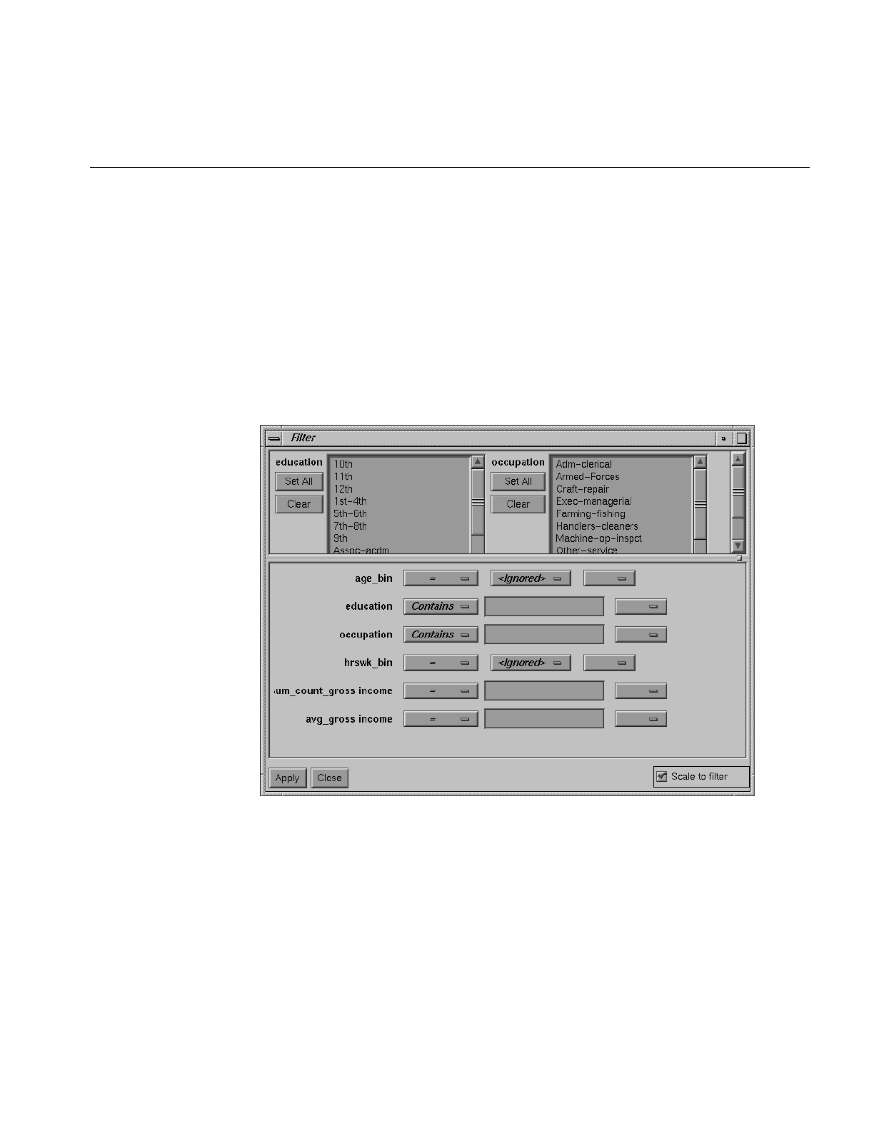
Pulldown Menus
277
•Show Filter Menu brings up a filter panel (Figure 8-11) that lets you reduce the
number of splats displayed in the main viewing area, based on one or more criteria.
You can use the filter panel to fine-tune the display, emphasize specific information,
or simply shrink the amount of information displayed. Columns other than those
mapped to axes, sliders, opacity, and color are not available for filtering because
they are removed during aggregation. The Scale to filter checkbox, which appears in
the lower right of the filter panel, lets you specify whether the landscape in the main
window covers the entire dataset or just the filtered data.
•Set Background Color brings up a color chooser to let you specify a new background
color.
Figure 8-11 Splat Visualizer Filter Panel

278
Chapter 8: Using the Splat Visualizer
The Filter panel has two panes. The top pane lets you filter based on string columns.
To select all values of a column, click Set All. To clear the current selections, click
Clear. To select a value, click it. To deselect a value, simply click it again.
The bottom pane lets you filter based on the values of both string and numeric
columns.
To filter numeric values, enter the value, and select a relational operation (=, !=, >, <,
>=, <=). To filter alphanumeric values, enter the string. You can use any of three
types of string comparisons:
•Contains indicates that it contains the appropriate string. For example,
“California” contains the strings “Cal” and “forn”.
•Equals requires the strings to match exactly.
•Matches allows wildcards:
–An asterisk (*) represents any number of characters.
–A question mark (?) represents one character.
–Square braces ([ ]) enclose a list of characters to match.
For example, California matches Cal*, Cal?fornia, and Cal[a-z]fornia.
For columns which were binned, an option menu of values appears, instead of a
text field. To ignore that column, select Ignored in the Option menu. You can use
relational operators, such as >=, with these options. This means that the specified
value as well as subsequent ones are selected.
In addition to numeric and string comparison operations, you can specify Is Null,
which is true if the value is null.
To the right of each field is an additional option menu that lets you specify “And” or
“Or” options. For example, you could specify “sales > 20 And < 40.” You can have
any number of And or Or clauses for a given column, but cannot mix And and Or in
a single column.
Scale to Filter lets you specify whether the filtered landscape is rescaled to the size of
the filtered data or remains the size of the entire data set.
Click the Filter button to start filtering. If you press Enter while the panel is active,
filtering starts automatically.
Click the Close button to close the panel.
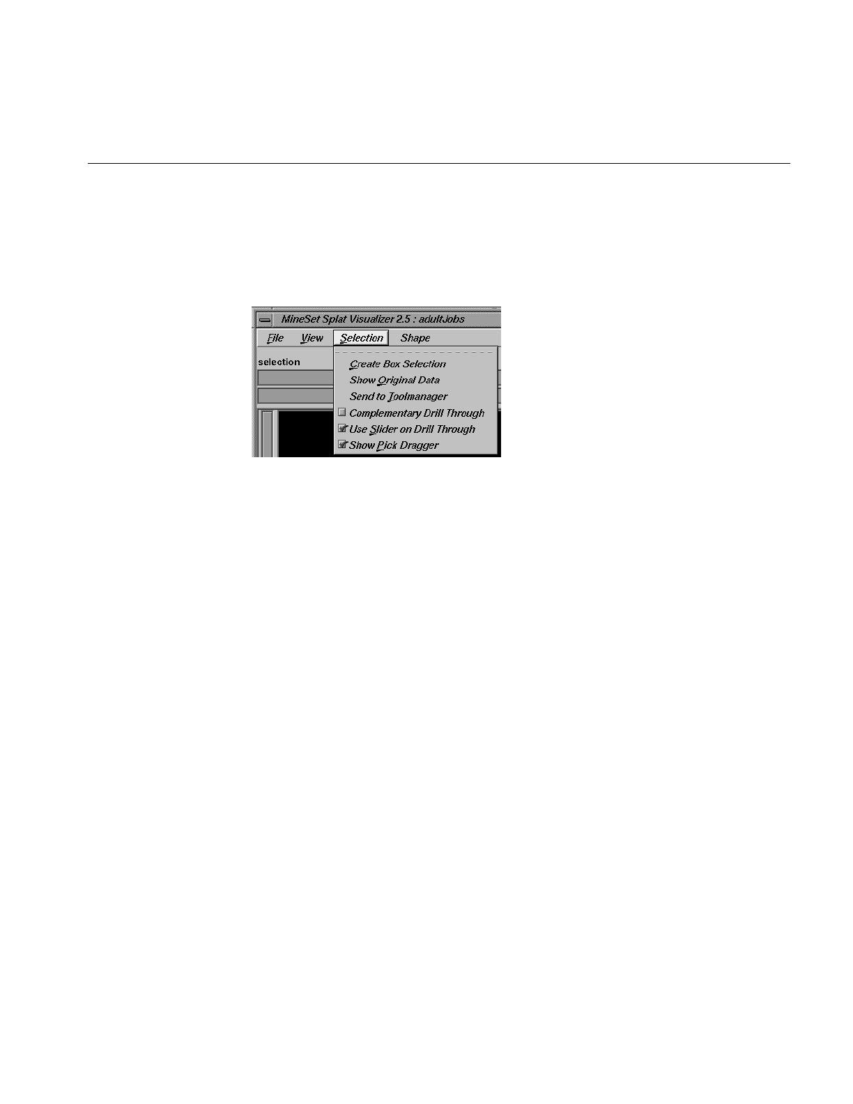
Pulldown Menus
279
The Selection Menu
The Selection menu (Figure 8-12) lets you drill through to the underlying data. The menu
has six items.
Figure 8-12 The Splat Visualizer’s Selection Menu
•Create Box Selection creates a 3-D box selector that can be stretched and translated to
select regions of the volume. While the box selector is active, a window in Record
Viewer format is opened showing information about all of the aggregated data that
is represented by the splats within it (see top of Figure 8-13). Closing this window
clears the current box selection(s). Selecting this option again creates a new box
selection, making the previous selection fixed. The fixed-selection boxes are gray,
while the active one is light yellow (see Figure 8-13). The selected bins, shown in the
selection window, are the bins enclosed by the union of all the selection boxes.
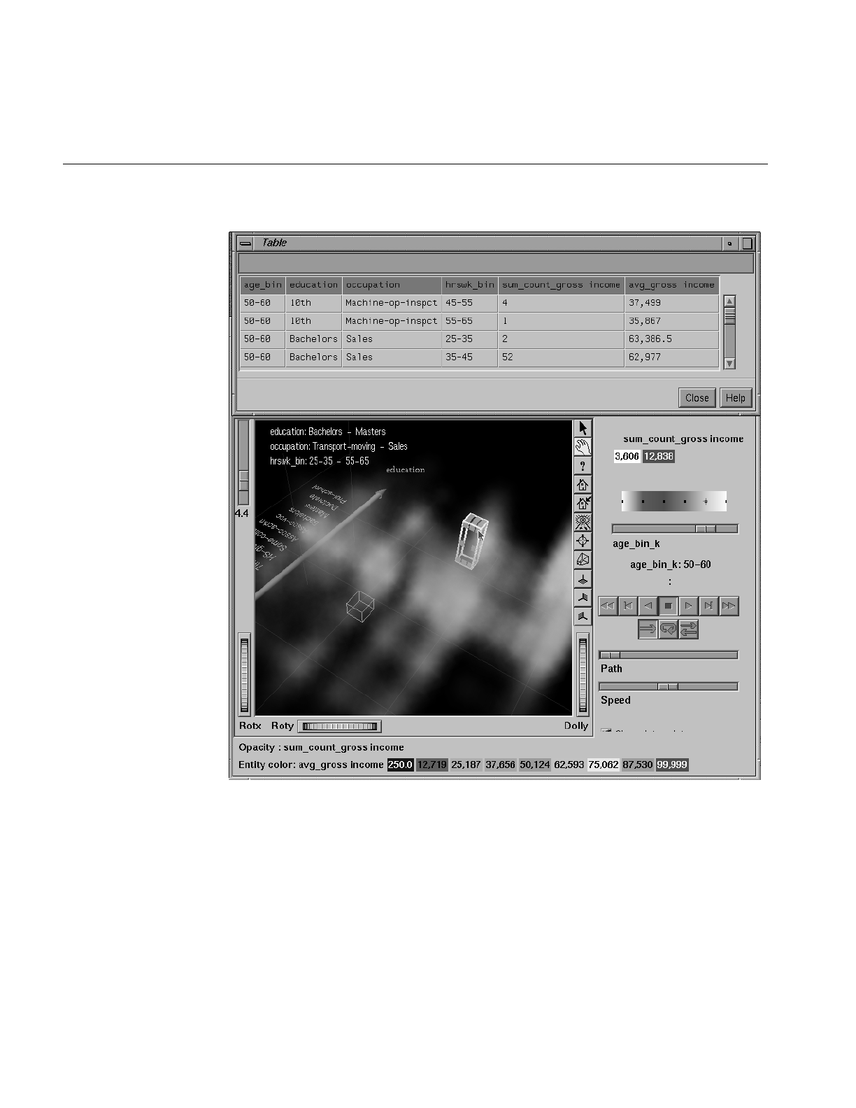
280
Chapter 8: Using the Splat Visualizer
Figure 8-13 Image With Fixed Selection Box (Gray) and Active Selection Box (Yellow)

Pulldown Menus
281
To translate the active selection box, click on one of the faces with the left mouse
button, and drag it in the desired direction. Holding the Shift key while dragging
constrains the motion to the axis to which the drag motion is closest. To change the
extent of the selection box, drag one of the gray scale tabs in the desired direction.
Trying to resize or translate beyond the bounds of the volume is not permitted. The
gray scale tabs constantly resize to maintain constant screen size. If at any time they
appear too big, you can zoom in closer, and they reduce their size relative to the
box.
•Show Original Data retrieves and displays the records corresponding to what has
been selected via Box Selection(s). The resulting records are shown in a table viewer.
•Send To Tool Manager inserts a filter operation, based on the current box selection(s),
at the beginning of the Tool Manager history. The actual expression used to do the
drill through is determined by extents of the current box selection(s). If nothing is
selected, a warning message appears.
•Use Slider On Drill-Through determines whether or not to use the slider position
when creating the drill-through expression. If checked (default), an additional term
is added to the drill-through expression, limiting the drill-through to those records
defined by the slider’s position. If this option is not checked, no such limiting term
is added.
•Complementary Drill Through causes the Show Original Data and Send To Tool Manager
selections, when used, to fetch all the data that are not selected.
•Show Pick Dragger toggles the visibility of the pick dragger (on by default). The pick
dragger is removed when a box selection is started, but it can be made active at the
same time that a box selection is active.
For further details on drill-through, see Chapter 18, “Selection and Drill-Through.”

282
Chapter 8: Using the Splat Visualizer
Splat Type Menu
Splats are used in this tool to model clouds of small points (see Lee Westover, “Footprint
Evaluation for Volume Rendering” in Proceedings of SIGGRAPH ‘90, Vol. 24, No. 4, pages
367-376).
The Splat Type menu lets you change the method for drawing the splats. You can choose
to exchange accuracy for interactivity. Texture splats are the most accurate representation
of ideal Gaussian density that is approximated in every approach. Since most computers
support hardware-assisted texturing well, the texture splat is usually the best choice.
Among SGI platforms, only the Indy or earlier systems are restricted to the slower
software implementation. The three splat types are:
•Linear draws a small set of triangles to give a linear approximation to a Gaussian
splat.
•Gaussian draws a large set of triangles to approximate a Gaussian splat.
•Texture uses a texture mapped rectangle to give the most accurate representation.
This can be very slow on machines that don’t support hardware-assisted texture
mapping.
Alternatively, the following opaque primitives are allowed.
•Sphere draws an opaque sphere, the radius for which varies with the cube root of the
count (or weight).
•Cube draws a large set of triangles to approximate a Gaussian splat.
•Diamond uses a texture-mapped rectangle to give the most accurate representation.
This can be very slow on machines that don’t support hardware-assisted texture
mapping.

Sample Configuration and Data Files
283
Sample Configuration and Data Files
The provided sample data and configuration files demonstrate the Splat Visualizer’s
features and capabilities. The following files are in the /usr/lib/MineSet/splatviz/examples
directory:
•mushroom
The mushroom.data file contains pre-aggregated data concerning more than 5,000
mushrooms. The group by columns were: odor, gill_color, and cap_color. For every
combination of these three columns in the original data, there is a count and an
average edibility, where 0 is edible, and 1 is poisonous. An average edibility
between 0 and 1 means some of the mushrooms in that aggregate are edible and
some are poisonous, since mushrooms can not be partially poisonous.
The visualization (Figure 8-8) shows that the unique values for each of these
columns have been sorted along the axes according to average edibility. Odor is
clearly the best determinant of edibility. Also note that most splats are either all 0 or
all 1, meaning these three columns are useful in segmenting the two classes of
mushrooms. Lower the opacity slider to determine which splats have the highest
counts. The most opaque splat represents 288 mushrooms having common values
for odor, gill_color, and cap_color. To confirm this try filtering based on
sum_count_poison>280 and picking on the remaining splats to see their counts.
Note that all mushrooms with gill_color=buff are poisonous.
•adultJobs
The adultJobs.data file was derived from adult94, a dataset provided with the
distribution. It was created using an aggregation that grouped by education,
occupation, hrs_worked_per_week(binned), and age (binned). The gross_income
column was aggregated by count and average. For a display using the Splat
Visualizer (Figure 8-1), age_bin was mapped to a slider, while the other group-by
columns were mapped to axes. The count_gross_income column was mapped to
opacity, and avg_gross_income was mapped to color.
When the slider is in the left-most position, the color of the plot is almost entirely
blue. This means that regardless of occupation, education, or number of hours
worked, people younger than 20 have low incomes. Move the slider to the right,
and note how incomes rise faster for higher education and occupations toward the
end of the axis. By the opacity variation you can see that the most common types of
education are HS, some college and Bachelors degree.
Moving the Summary slider shows how the distribution of income changes with
respect to the axis columns as people age.

284
Chapter 8: Using the Splat Visualizer
•adultJobs2
The adultJobs2 file is also based on the adult94 dataset. Here, the axis columns are
working_class, education, and occupation. The two columns mapped to sliders are
age(binned) and hours_worked_per_week(binned). Again, income was aggregated
by count and average for use with opacity and color, respectively. Since there are
more positions on the 2D slider, there are fewer records represented by each
position. This causes greater variation of color and opacity. The red region in the
center of the hrs_per_week dimension of the Summary slider shows that nearly
everyone works between 35 and 45 hours per week (see Figure 8-7). Note that some
occupations are aligned with specific working classes. For example, everyone in the
Armed-forces has Fed-Government for their working class.
•censusIncome
This example is based on a dataset similar to adult94, but was not included with the
distribution because of its size. In attempt to understand the differences between
gross income and total income, gross_income, total_income, and hrs_per_week
have been mapped to axes. Color shows age. By studying the image we can learn
that there are many records where total_income=gross_income, but there are also a
larger portion of records with high total_income, but 0 gross_income. It is
surprising that in many cases gross_income is greater that total_income.
Note where the people of different ages are concentrated. Many old people (yellow)
are in the hrs_per_wk=0 plane. They are probably retirees. Many children and
young adults (blue) are in the line gross_income=total_income=0. Note the fairly
opaque splats near the outside edges of the volume. These positions include all
points that fell in the maximum bin shown for an axis. For example, the highest bin
for total_income is 70300+. Any point higher than 70300 goes in this bin.
To better see the varying density, adjust the opacity slider. At low opacity scales, the
diagonal lines show that for most people gross_income=total_income, or they have
just total_income and no gross_income. As you raise the scale, you can see that
almost the entire volume contains data. This dataset contains 150,000 records.

Sample Configuration and Data Files
285
•churn
Churn is when a customer leaves one company for another. This example shows
customer churn for a telephone company. The data used to generate this example is
in /usr/lib/MineSet/data/churn.schema.
Using column importance, we found that total_day_charge,
number_customer_service_calls, and international_plan were important
discriminators. These columns were mapped to axes. We then created a new
numeric column, churn, which equals churned==Yes, and mapped it to color.
In the resulting visualization, red areas of the volume indicate high churn. The area
corresponding to three or more customer service calls and low total_day charge
corresponds to high churn. You might want to weight big-spending customers more
heavily than others. To do this, create a new column, total_charge, equal to
`total_day_charge`+`total_eve_charge`+`total_night_charge`
or some power of this sum. Then map this total_charge column to opacity. This
means every record is weighted by total_charge. Now the visualization shows
additional areas of interest near the high end of the total_day_charge axis.


287
Chapter 9
9. Using the Rules Visualizer
This chapter discusses the components and capabilities of the Rules Visualizer. It first
provides an overview of this data mining and visualization tool, then it explains this
tool’s functionality when working with the
•main window
•external controls
•pulldown menus
Finally, it lists and describes the provided sample files for these tools.
Overview of Rules Visualizer
The Rules Visualizer gives you the power to mine data by constructing, verifying, and
graphically representing models of patterns in large databases. These patterns are
expressed via association rules, which indicate the frequency of items occurring together
in a database.
Discovering and graphically displaying association rules can be relevant to many
enterprises, including supermarket inventory planning, shelf planning, and attached
mailing in direct marketing.
The tool execution scenario described in Chapter 1 of this document (see Figure 1-1) is
slightly modified for the Rules Visualizer. First, the “raw” data in your database must be
converted into a specially formatted file that can be processed by the association rules
generator part of the Rules Visualizer. When the association rules generator has
processed this file, the results can be displayed by the rules visualizer part of this tool.

288
Chapter 9: Using the Rules Visualizer
Thus, the Rules Visualizer consists of three operations:
1. Data conversion. The association data converter processes a “raw” data file and
creates a file usable by the association rules generator.
2. Association rules generation. The data file created by the association data converter
is processed by the association rules generator, which creates a file usable by the
rules visualizer.
3. Rules visualization. This operation displays the generated association rules.
In addition to the input data and rules file requirements, each operation requires a
configuration file that specifies operational parameters.
The sequence of actions by the user, at the user’s workstation, and at the host server is
shown schematically in Figure 9-1. The phases indicated at the right of the illustration
correlate to the operations listed above.
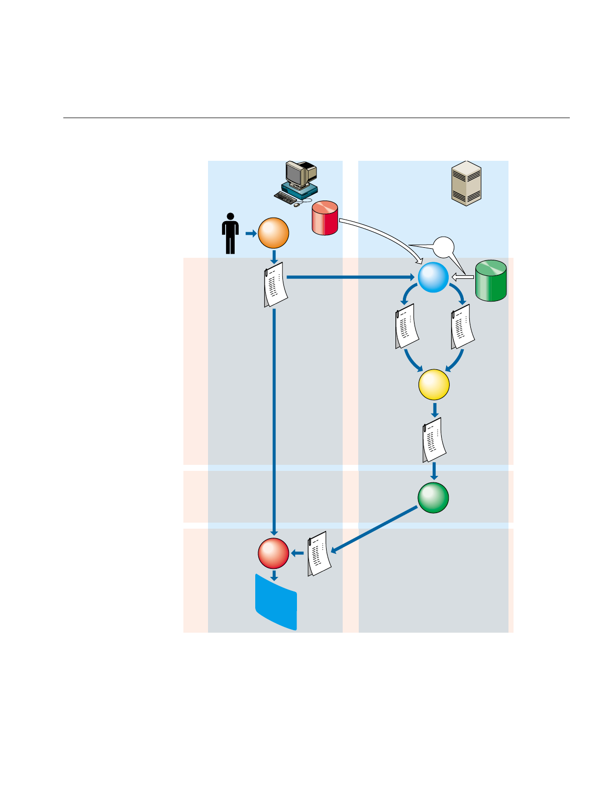
Overview of Rules Visualizer
289
Figure 9-1 Execution Sequence of the Rules Visualizer
User's
data source
Data Mover
Client
workstation Host server
Tool
manager
Format
file
Rules
Visualizer
Rules file
Configuration
file
Binary (flat)
data file
Association
data
converter
Association
rules
generator
"Raw"
data file
User
Visual
display
Data conversionRules visualization Rules
generation
OR

290
Chapter 9: Using the Rules Visualizer
Data Conversion
The association data converter takes a “raw” data file, such as one resulting from a
database query, and creates a binary data file in the format used by the association rules
generator. The internal format of this generated file allows optimum processing by the
rules generator. The data converter also accepts input from flat files as well as databases.
Association Rules Generator
One example of applying the association rules generator is to obtain “market basket”
data for customer buying patterns. Here, “market basket” is the set of items bought by
each customer on a single visit to a store. An example rule in this context might be: “80%
of the people that buy diapers buy baby powder.” This percentage is known as the
predictability of the rule.
In the example, “diapers” is the item on the left-hand side (LHS) of the rule, and “baby
powder” is the item on the right-hand side (RHS) of the rule.
Some applications of these rules are as follows:
•If “Fizzy Pop” appears on the RHS, the LHS can help us determine what the store
should do to boost sales of this beverage.
•If “Bagels” appears on the LHS, the RHS can help us determine what products
might be affected if the store no longer sells bagels.
The association rules generator part of this tool processes an input file, then generates an
output file consisting of the rules. If X and Y are items in a record, then a rule such as
X ⇒ Y
indicates that whenever X occurs in a record, expect Y to occur with some frequency.

Overview of Rules Visualizer
291
Components of a Generated Association Rule
The strength of the association is quantified by three numbers. The first number, the
predictability of the rule, quantifies how often X and Y occur together as a fraction of the
number of records in which X occurs. For example, if the predictability is 50%, X and Y
occur together in 50% of the records in which X occurs. Thus, knowing that X occurs in
a record, expect that 50% of the time Y occurs in that record.
The second number, the prevalence of the rule, quantifies how often X and Y occur
together in the file as a fraction of the total number of records. For example, if the
prevalence is 1%, X and Y occur together in 1% of the total number of records.
You can specify a minimum prevalence threshold for the generated rules. The default
minimum prevalence threshold is 1%. The lower the minimum prevalence, the more
rules are generated, and the slower the performance of the tool might be. You can also
specify a minimum predictability threshold for the generated rules. The minimum
predictability threshold default is 50%.
Rules that meet a minimum prevalence threshold are important for two reasons:
1. A rule might have business value only if a reasonably significant fraction of records
support the rule. For example, if everyone who buys caviar also buys vodka, the
rule Caviar ⇒Vodka has 100% predictability. However, if only a handful of people
buy caviar, the rule might be of limited value to the retailer.
2. A rule might not be statistically significant if a very small number of records
support the rule. The rule might be due to chance, and it would not be prudent to
make decisions based on such a rule.
The third number is expected predictability. The expected predictability is the frequency of
occurrence of the RHS items. So the difference between expected predictability and
predictability is a measure of the change in predictive power due to the presence of the
LHS rule. Expected predictability gives an indication of what the predictability would be
if there were no relationship between the items.
The Association Rules generator does not report rules in which the predictability is less
than the expected predictability. In other words, a rule such as A->B is not reported if the
frequency of A and B occurring together is less than the frequency of B alone.
Note: Given just Y and a rule of the form X ⇒ Y, nothing is known about X. Rules specify
implications only from the LHS to the RHS.

292
Chapter 9: Using the Rules Visualizer
Table 9-1 summarizes the three numbers that quantify the strength of each association
rule.
Hierarchical Data
The rules generator also works on hierarchical data, which includes a component that
relates (or maps) data to new data at varying degrees of generality. The ability to handle
hierarchical data allows rules to be generated at the desired level of generality.
For example, consider the hierarchy shown in Table 9-2. This hierarchical information, in
addition to the “market basket” data that lists the products purchased in each record,
allows rules to be generated at four levels. In contrast to rules learned at the lowest level,
which relate specific products to each other, a rule at the highest level might be “Milk
implies Bread.”
Rules Visualization
The rules visualization part lets you graphically display and explore the generated
association rules. The rules are presented on a grid landscape, with left-hand side (LHS)
items on one axis, and right-hand side (RHS) items on the other. As shown in Figure 9-2,
attributes of a rule are displayed at the junction of its LHS and RHS item. The display can
include bars, disks, and labels.
Table 9-1 Association Rules Components
Measure Description
Prevalence Frequency of LHS and RHS occurring together.
Predictability Fraction of RHS out of all items with LHS, or the prevalence
divided by the frequency of occurrence of LHS items.
Expected Predictability Frequency of occurrence of RHS items.
Table 9-2 Example of Hierarchical Levels
Level Example
Product Group Milk
Category Non-Refrigerated Milk
Brand Lucerne®
Product ID (UPC/SKU Code) 1 pint can of Premium Condensed Milk
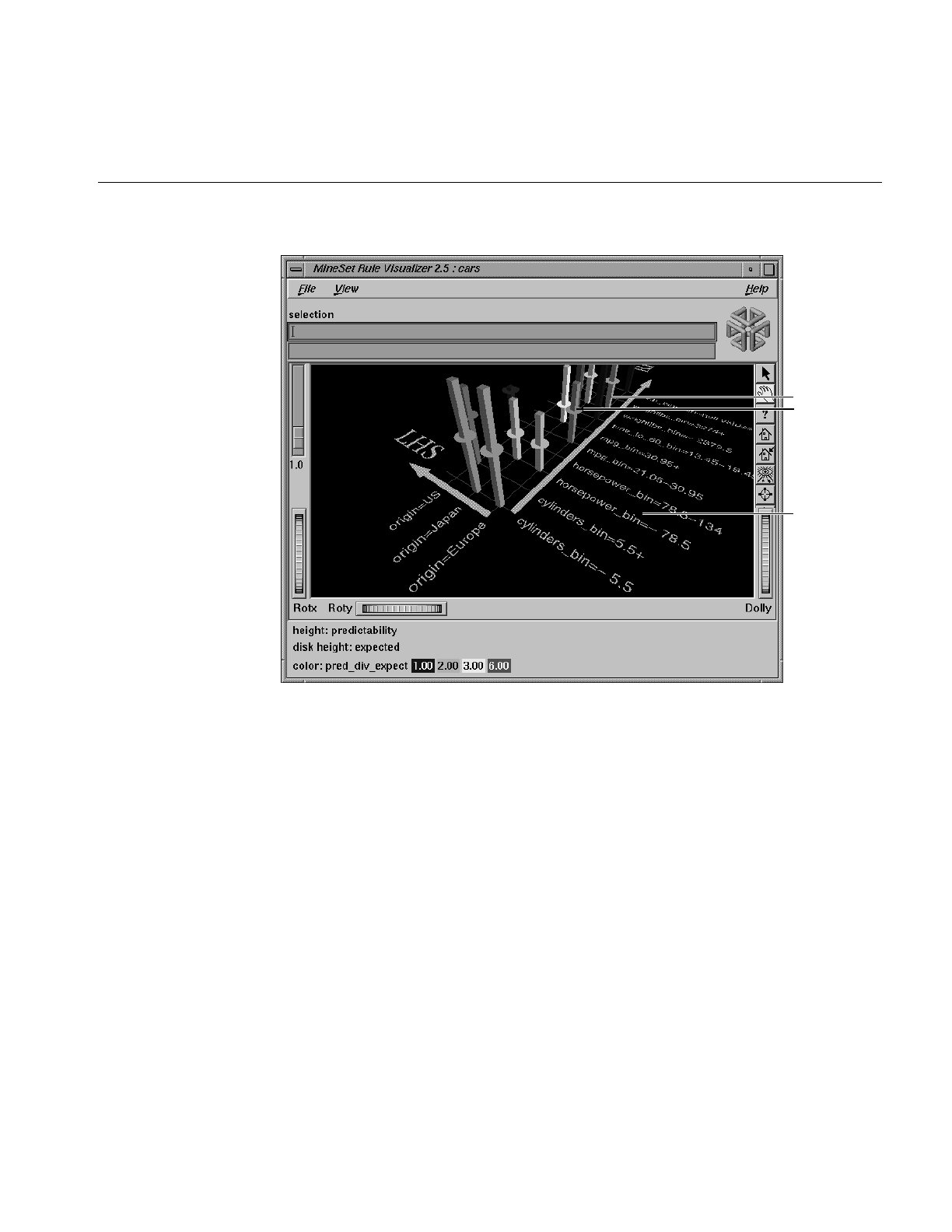
Overview of Rules Visualizer
293
Figure 9-2 Detail View of the Rules Visualizer’s Main Window
If the displayed view is too small, item labels do not appear on the side of the axes. You
can zoom in on the view until the item labels appear (see the Dolly description in
“Thumbwheels” in Chapter 6).
A legend indicating the mapping between displayed attributes (such as bar heights and
colors) and the values associated with the underlying rules (such as predictability and
prevalence) can be displayed at the bottom of the main window.
The Tool Manager interface for associations allows you to run the Rule Visualizer
without running associations, by using the Visual Tools menu from Tool Manager’s main
window.
Disk
Label
Bar

294
Chapter 9: Using the Rules Visualizer
File Requirements
Each of the Rules Visualizer’s three components has its own file requirements. These are
detailed in the following subsections.
Files Required by the Association Data Converter Part
•A “raw” data file that results from extracting raw data from a source (such as a
relational database). This file is processed by the association data converter to
produce the internal binary data file used by the association rules generator.
•A format file that specifies the format of the data file. If the internal binary data file
(see next subsection) is created via the Tool Manager, this format file is created
automatically. If the internal binary data file is created via the command line, this
format file must be created manually (see Appendix F, “Creating Data and
Configuration Files for the Rules Visualizer”).
Files Required by the Association Rules Generator Part
•An internal binary data file, which results from running the association data
converter on your original data.
If you have hierarchical data, the association rules generator also requires the
following two files:
•A mapping file, which specifies the mapping between hierarchical levels.
•A description file, which specifies a string description for each item at a specific
hierarchical level.
Files Required by the Rules Visualization Part
•A rules file that results from running the association rules generator.
•A.ruleviz configuration file that specifies parameters used by the rules visualizer
program (such as mapping colors to prevalence values) when displaying the
generated rules. This file is easily created using the Tool Manager (see Chapter 3).
You also can use an editor (such as jot, vi, or Emacs) to produce this file (see
Appendix F, “Creating Data and Configuration Files for the Rules Visualizer”).
These configuration files must have a .ruleviz extension.

Starting the Rules Visualizer
295
Starting the Rules Visualizer
The Rules Visualizer has three components. The following subsections describe the
procedure for starting each one.
Starting the Association Data Converter Part
There are two ways to start the association data converter part of the Rules Visualizer:
•Use the Tool Manager to configure and start the data converter. (See Chapter 3 first
for details on most of the Tool Manager’s functionality, which is common to all
MineSet tools; see below for details about using the Tool Manager in conjunction
with the data converter.)
•Enter the following command at the UNIX shell command-line prompt:
assoccvt parameters
The parameters are described in Appendix F, “Creating Data and Configuration Files
for the Rules Visualizer.”
Starting the Association Rules Generator Part
There are two ways to start the association rules generator part of the Rules Visualizer:
•Use the Tool Manager to configure and start the association rules generator. (See
Chapter 3 first for details on most of the Tool Manager’s functionality, which is
common to all MineSet tools; see below for details about using the Tool Manager in
conjunction with the association rules generator.)
•If the data with which you are working is non-hierarchical, enter this command at
the UNIX shell command line prompt:
assocgen parameters
If your data is hierarchical, enter this command at the UNIX shell command-line
prompt:
mapassocgen parameters
The parameters for both instances are described in Appendix F, “Creating Data and
Configuration Files for the Rules Visualizer.”

296
Chapter 9: Using the Rules Visualizer
Starting the Rules Visualization Part
There are five ways to start the rules visualization part of this tool:
•Use the Tool Manager to configure and start the Rules Visualizer. (See Chapter 3
first for details on most of the Tool Manager’s functionality, which is common to all
MineSet tools; see below for details about using the Tool Manager in conjunction
with the Rules Visualizer.)
•Double-click the Rules Visualizer icon, which is in the MineSet page of the icon
catalog. The icon is labeled ruleviz. Since no configuration file is specified, the
start-up screen requires you to select one by using File > Open.
•If you know what configuration file you want to use, double-click the icon for that
configuration file. This starts the Rules Visualizer and automatically loads the
configuration file you specified. This only works if the configuration filename ends
in .ruleviz (which is always the case for configuration files created for the Rules
Visualizer via the Tool Manager).
•Drag the configuration file icon onto the Rules Visualizer icon. This starts the Rules
Visualizer and automatically loads the configuration file you specified. This works
even if the configuration filename does not end in .ruleviz.
•Enter this command at the UNIX shell command-line prompt:
ruleviz [ configFilename ]
When starting the rules visualization part of this tool, you must specify the configuration
file, not the data or rules file.
Option for Invoking the Rules Visualizer
The -quiet option eliminates the dialogs that popup to indicate progress. You can enable
this option permanently by adding the line
*minesetQuiet:TRUE
to your .Xdefaults file.

Configuring the Rules Visualizer Using the Tool Manager
297
Configuring the Rules Visualizer Using the Tool Manager
This section describes how the components of the Rules Visualizer can be configured
using the Tool Manager. Although the Tool Manager greatly simplifies the task of
configuring the Rules Visualizer, you can construct a configuration file for this tool using
an editor (see Appendix F, “Creating Data and Configuration Files for the Rules
Visualizer”).
Note that the steps required to connect to a data source are described in Chapter 3.
The sections below follow the configuration and invocation of the Rules Visualizer
components in the conventional order:
•creating a file for the association rules generator
•generating rules
•displaying rules
Setting Up Associations
To show how to set up associations, the following example uses the cars database table.
Assume that you want to find out if there is an association between miles per gallon,
horsepower, and the year the car was built. For example, did mileage improve over time?
Did engines become less powerful? The following steps (and Figure 9-3) show you how
to set up the associations and map table columns to the data you want to study.
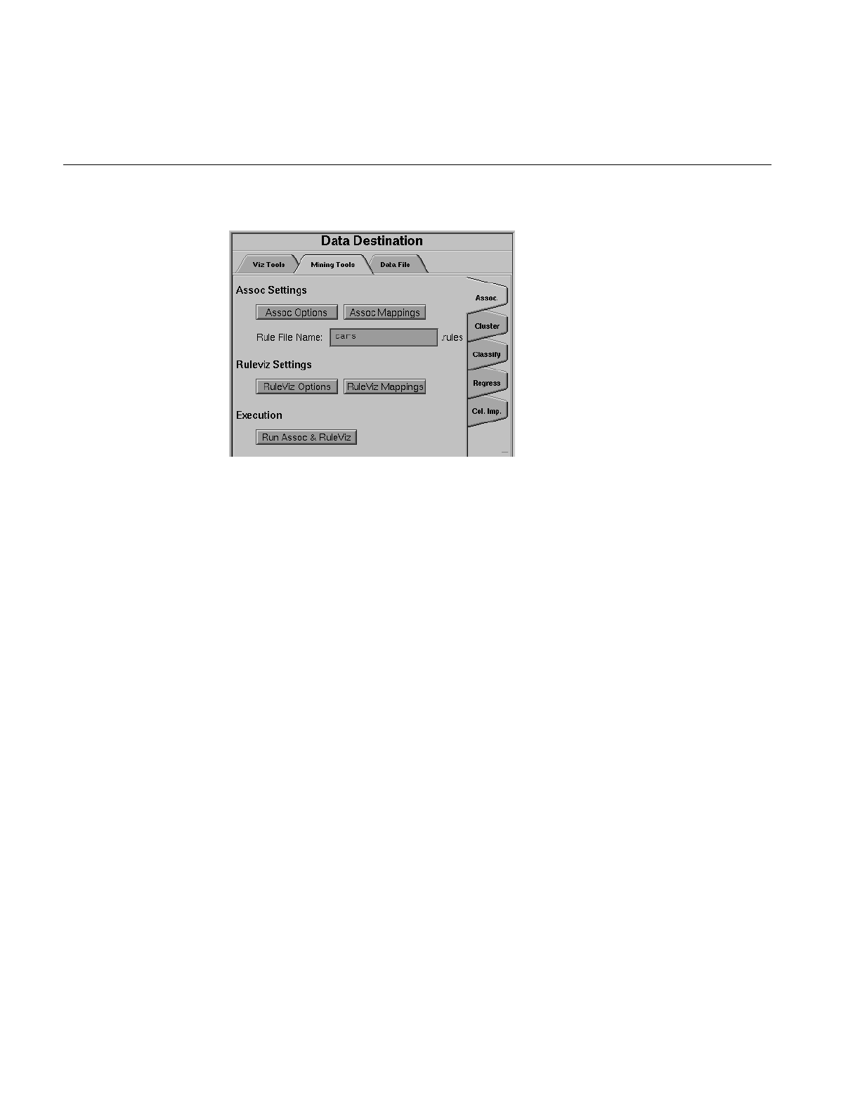
298
Chapter 9: Using the Rules Visualizer
Figure 9-3 Initial Tool Manager Window for Association Generation
1. Connect to a MineSet server. Refer to Chapter 2, “Setting Up MineSet,”if you need
help.
2. Open a data source.
3. (Optional step) In the Data Transformations tab you can choose the transformations
you want do on the data before you give it to the associations engine. One
recommended transformation is to create bins for numeric data. (The binning
operation and the options available for it are described in detail in Chapter 3.) This
leads to more “meaningful” rules from the association engine. For example, instead
of using discrete values for the weightlbs attribute in the “cars” table such as 3504,
3693, 3436, 3433, and so on, it may be more meaningful to give weightlbs_bin value
ranges such as 1600-2500, 2501-3500, and so on.
For this example, click on the Bin Columns button, and select all the columns in the
Bin Column window for binning.
Note: If you run associations without binning any of the numerical columns (ints,
floats, doubles) you get the warning message
Running associations on unbinned non-categorical data. Binning is
recommended for producing more useful results.
4. Choose the Mining Tools tab from the Data Destination tab.
5. Choose the Assoc. tab (abbreviation for Associations) from the Mining Tools tab.
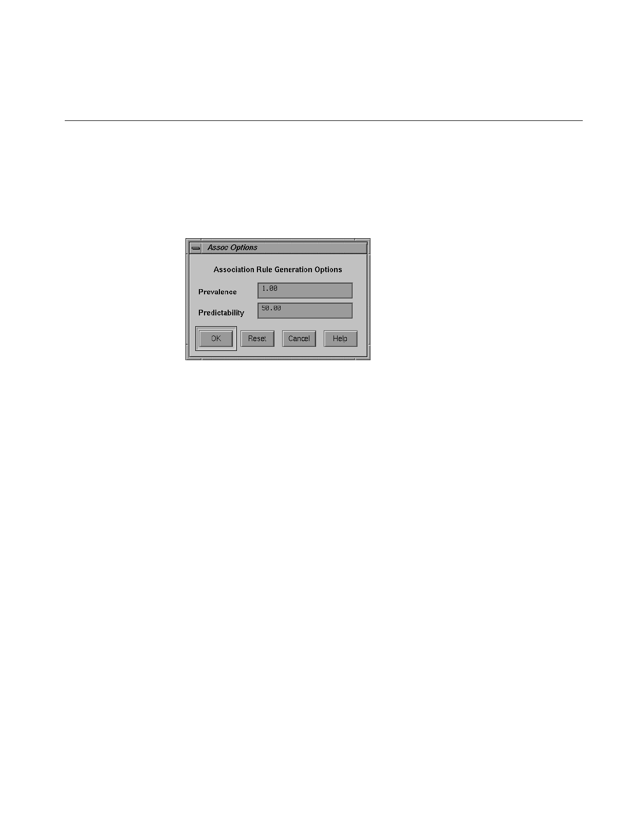
Configuring the Rules Visualizer Using the Tool Manager
299
Applying Association Rule Options
After selecting a data source, you can run the Association Rules generator. You can
choose options for this by clicking on the Assoc Options button. This causes the dialog box
in Figure 9-4 to be displayed.
Figure 9-4 Association Rule Options Dialog Box
Prevalence—lets you specify the minimum prevalence threshold as a percentage of the
total number of records. Rules with a prevalence below this value are not generated. The
default is 1%. The possible values are 0–100.
Predictability—lets you specify the minimum predictability threshold for rules. Rules
with a predictability below this value are not generated. The default is 50%. The possible
values are 0–100.
6. Once you have made your association rule options selections, click the OK button.
This returns you to the Tool Manager startup screen.
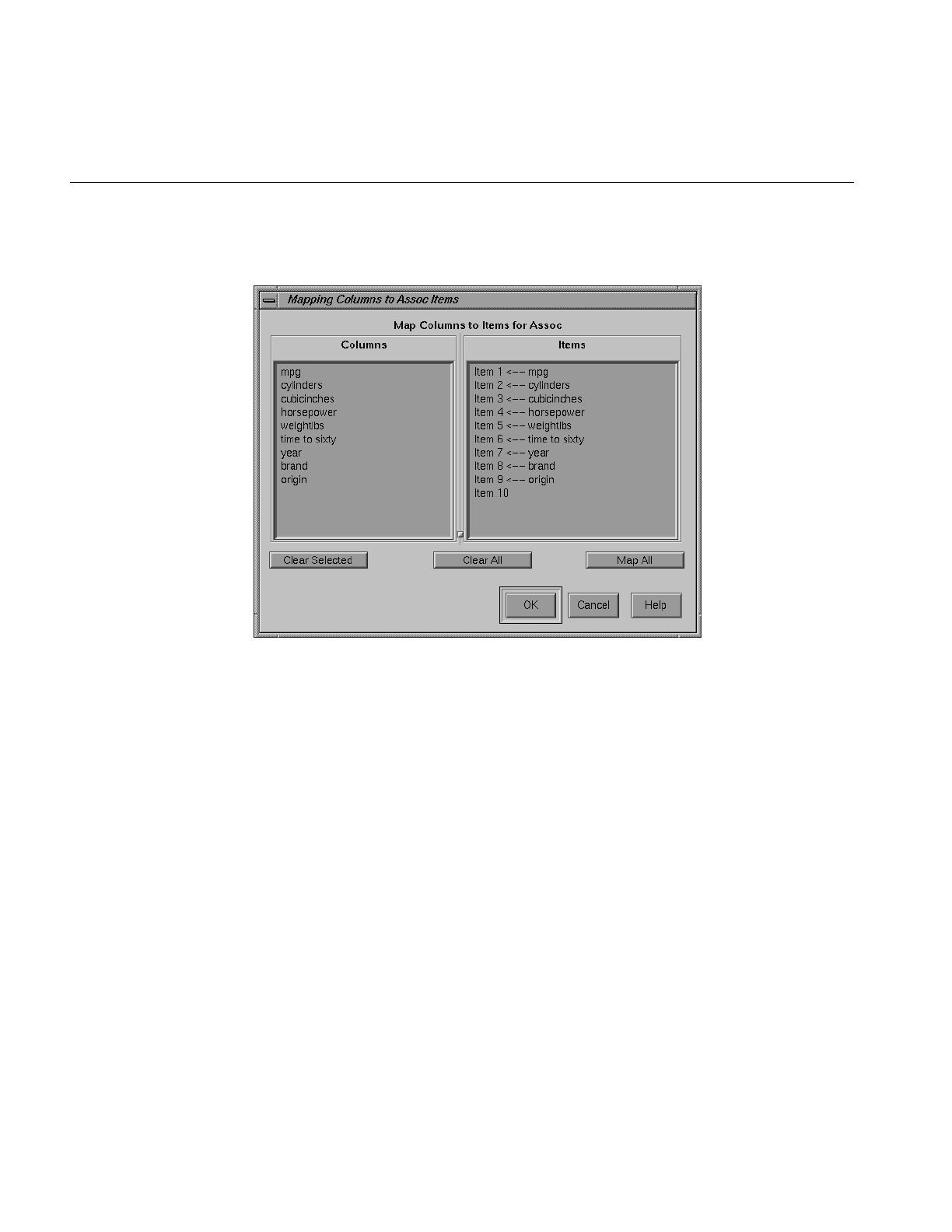
300
Chapter 9: Using the Rules Visualizer
Mapping Columns to Association Items
Figure 9-5 Association Mappings Dialog Box
The database in the Current Columns text panel can contain multiple table columns. By
mapping specific columns to association rules, the association rules generator can find
the association between any possible pair of those items.
1. Click on Assoc. Mappings button to open the Mapping Columns to Assoc Items
dialog box.
The Mapping Columns to Assoc Items window shows two panels:
•Columns shows the columns in the data
•Items shows the mapping between columns in the data and items
The Map All button on this window can be used to map all the attributes in the data
source to items for the associations engine. The Clear All and Clear Selected buttons
can be used to clear/change the mapping between columns and items.
2. The default behavior is to map all columns to items. Therefore, if you omit this step
or if you open this window, you find all columns mapped. For this example, click
OK.
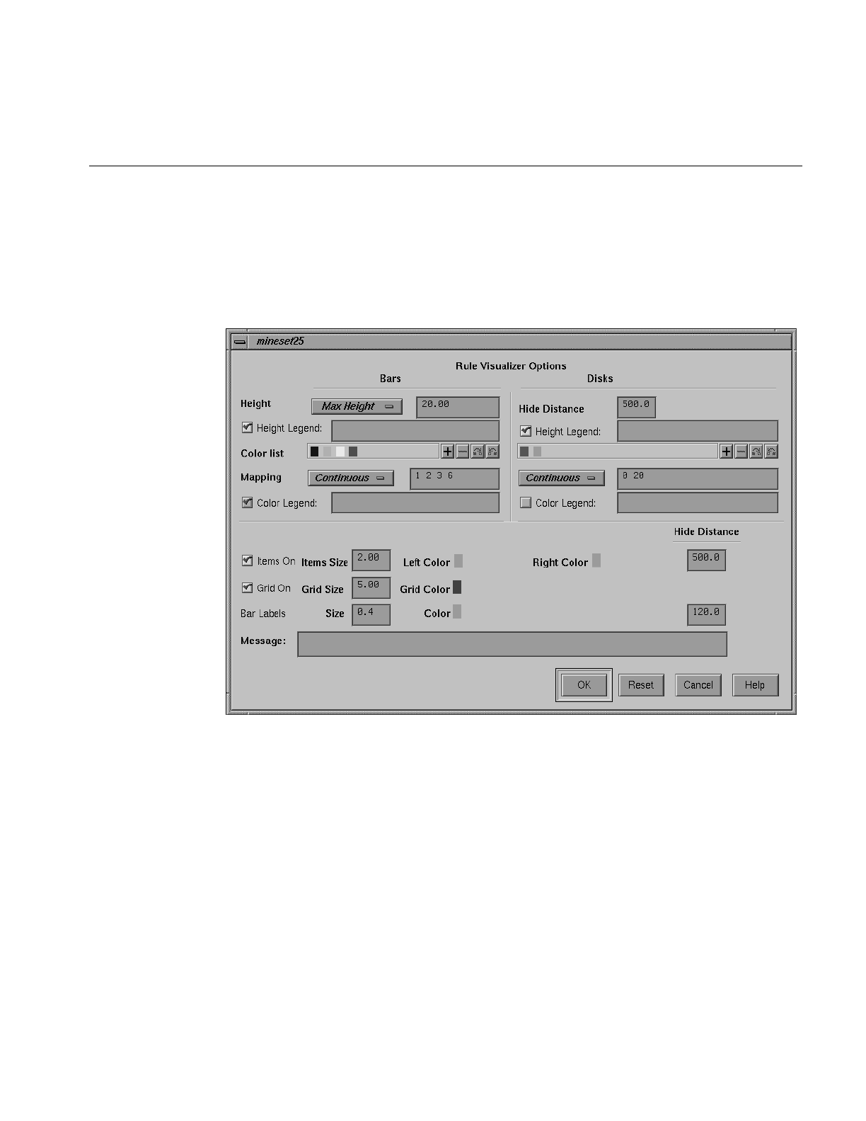
Configuring the Rules Visualizer Using the Tool Manager
301
Specifying Ruleviz Options
Clicking on the Ruleviz Options button causes a new dialog box to be displayed
(Figure 9-6). This lets you change some of the Rules Visualizer options from their default
values.
Figure 9-6 Rule Visualizer Options Dialog Box
This dialog box has two panels: the top one lets you set options for bars and disks; the
bottom one lets you specify options for items, the grid, and labels.

302
Chapter 9: Using the Rules Visualizer
Items in the top panel are listed below:
•Height button—lets you specify whether the bars and disk heights are to be
normalized so that the tallest bar equals the height field value (Max Height), or
whether they are to be scaled by the height field value (Scale Height).
•Height field—lets you enter the maximum or scale value for bar and disk heights.
•Hide Distance—lets you specify the distance at which disks are not graphically
represented. Smaller numbers in this field specify a shorter distance; this means
fewer disks are shown and performance is greater. Larger numbers indicate a
greater distance; this means disks further away remain visible.
•Legends—lets you enter a text string that appears as mapping information displayed
at the bottom of the main Rules Visualizer window. This is information about
mapping between display entities and data values (for example, bar height
corresponds to predictability values).
•Color list—lets you add or edit a color. To add a color to the list, click the + button. To
edit a color, click the color. See “Choosing Colors” and “Using the Color Browser”
in Chapter 3 for a more detailed explanation of how to choose and change colors.
•Mapping—lets you specify whether the color change that is shown in the graphic
display is Continuous or Discrete. If you choose Continuous, the color values (of the
bars or disks) shift gradually between the colors entered in the Color list field as a
function of the values that are mapped to those colors in the Color list field.
Example 9-1
If you
•used the Color Browser to apply red and green (for bars and/or disks)
•selected Discreet for the Mapping
•entered the values 0 100
then the display shows all bars and/or disks with values of less than 50 in red, and all
those with values greater than or equal to 50 in green.

Configuring the Rules Visualizer Using the Tool Manager
303
Example 9-2
If you
•used the Color Browser to apply red and green (for bars and/or disks)
•selected Continuous for the Mapping
•entered the values 0 100
then the display shows all bars and/or disks with values less than or equal to 0 as
completely red, those as greater than or equal to 100 as completely green, and those
between 0 and 100 as shadings from red to green.
If no mapping and values are specified, a continuous mapping is used, and values are
generated automatically from the minimum value to the maximum value in the data.
Items in the bottom panel are as follows:
•Items On and Grids On checkbox buttons let you determine whether items (the
names on the side of the grid) are displayed or hidden.
•Size (for Items, Grid, and Bar Labels) lets you specify the size for items, the grid, and
bar labels. If you mapped a column value to bar labels in the Requirements panel of
the Tool Manager startup screen, you can specify a size for those labels.
•Color (for Left-Hand Items, Right-Hand Items, Grid, and Bar Labels) lets you specify
the color for LHS and RHS items, the grid, and bar labels. If you mapped a column
value to bar labels in the Requirements panel of the Tool Manager startup screen,
you can specify a size for those labels.
•Hide Distance lets you specify the distance at which the LHS items, RHS items, grid,
or labels become invisible. Smaller distances might improve performance, but the
objects disappear more quickly. The higher the number, the greater the distance at
which labels are hidden.
•Message lets you specify the message displayed when the pointer is moved over an
object or when an object is selected. (See Figure 9-8.) The syntax of the message
string is the same as for the mapviz message string. See the Message Statement
section in Appendix C, “Creating Data, Configuration, Hierarchy, and GFX Files for
the Map Visualizer.”
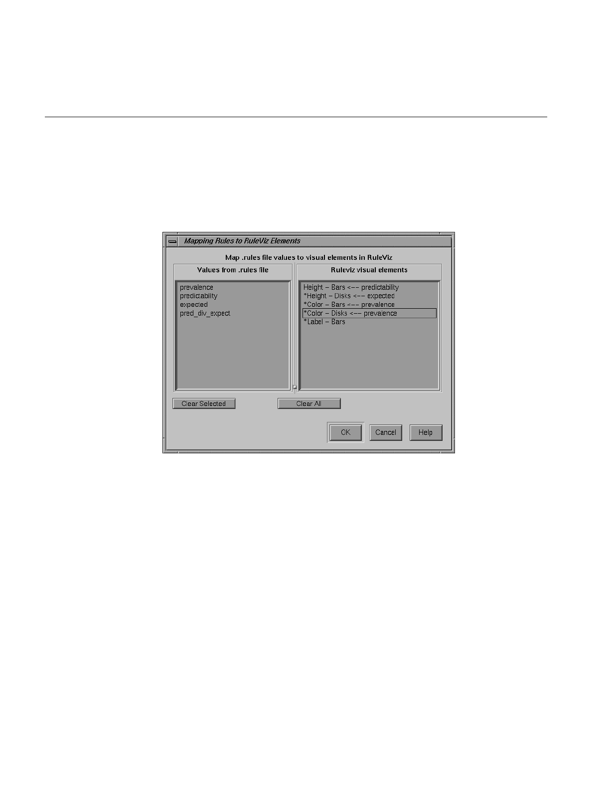
304
Chapter 9: Using the Rules Visualizer
Mapping Columns to Visual Elements
The Rules Visualizer lets you map attributes of the rules to visual elements of the display.
Clicking on the RuleViz Mappings button brings up the Ruleviz Mappings panel shown in
Figure 9-7.
Figure 9-7 The Rules Visualizer’s Mappings Panel
The visual elements that can be mapped are listed below, where the items with “*” are
optional:
•Height - Bars—lets you specify what the bar heights represent.
•*Height - Disks—lets you specify what the disk heights represent.
•*Color - Bars—lets you specify what the bar colors represent.
•*Color - Disks—lets you specify what the disk colors represent.
•*Label - Bars—lets you specify what the bar labels represent.

Working in the Rules Visualizer’s Main Window
305
The default mappings are as follows:
•predictability to bar heights
•expected predictability to disk heights
•lift to bar and disk colors
Lift is the predictability divided by the expected predictability.
Invoking the Rules Visualizer
To see the Rules Visualizer graphically represent your data, click the Run Assoc & Rules
button at the bottom of the Associations tab in the Data Destination panel of the main
Tool Manager window.
Working in the Rules Visualizer’s Main Window
The Rules Visualizer part of this tool graphically displays the data in a rules file using the
specifications of a valid configuration file. For example, specifying group.ruleviz results in
the image shown in Figure 9-8.
Figure 9-8 Initial Rules Visualizer View When Specifying group.ruleviz

306
Chapter 9: Using the Rules Visualizer
The rules are presented on a grid, initially displayed with left-hand side (LHS) items
displayed on the left side of the window and right-hand side (RHS) items on the right. A
rule is displayed at the junction of its LHS and RHS items. The display can include bars,
disks, and labels.
When the scene is close enough, the LHS and RHS axes are labeled with the item names,
unless this has been turned off in the configuration file. (To view the grid and rules at
closer range, use the Dolly thumbwheel, described in the “Thumbwheels” in Chapter 6.)
You can change the labels as well as what the heights and colors of the bars and disks
represent by modifying the configuration file via the Tool Manager (see Chapter 3) or
using an editor to change the configuration file.
For example, in Figure 9-8, bar heights correspond to predictability values, bar colors
correspond to prevalence values, and disk heights correspond to expected predictability.
Viewing Modes
The two modes of viewing are grasp and select. To toggle between these modes, press the
Esc key. You also can change from one mode to the other by clicking the appropriate
button: to enter select mode, left-click the arrow button (to the top right of the main
window); to enter grasp mode, left-click the hand button (immediately below the arrow
button, near the top right of the main window as shown in Figure 9-2).
Grasp Mode
In grasp mode the cursor appears as a hand. This mode supports panning, rotating, and
scaling the scene’s size in the main window.
•To rotate the display, press the left mouse button and move the mouse in the
direction you want to rotate. (Also see the rotating controls Rotx and Roty described
in “Thumbwheels” in Chapter 6.)
•To pan the display, press the middle mouse button and drag it in the direction you
want the display panned.
•To move the viewpoint forward, press the left and middle mouse buttons
simultaneously and move the mouse downwards. To move the viewpoint
backward, press the left and middle mouse buttons simultaneously and move the
mouse upwards. This is equivalent to the functions provided by the Dolly
thumbwheel.
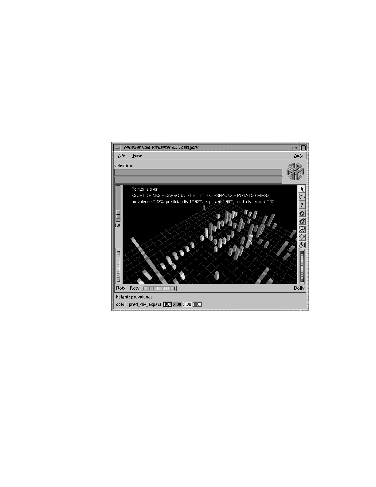
Working in the Rules Visualizer’s Main Window
307
Select Mode
In select mode, you can obtain additional information about a rule by placing the cursor
over a bar. This highlights the selected bar and causes information about the rule
represented by that bar to appear at the top of the main window.
Figure 9-9 Cursor Over a Rules Visualizer Object
The information is displayed as long as the cursor remains over the object. If you position
the pointer cursor over an object and click the left mouse button, that same information
appears in the Selection Window, which is above the main window, under the
“Selection” label.
This Selection information remains visible until another object is selected, or until no
object is selected (if you click the black background). Using the mouse, you can cut and
paste this text into other applications, such as reports or databases.)

308
Chapter 9: Using the Rules Visualizer
External Controls
Several external controls surround the main window, including buttons and
thumbwheels. (These and the rest of the buttons are the same as the other MineSet
visualization tools and are described in “Buttons” in Chapter 6, and “Thumbwheels” in
Chapter 6)
The Height Slider
The Height slider, at the upper left corner of the main window, lets you scale the heights
of objects (bars and disks) in the main window.
Figure 9-10 Rules Visualizer’s Height Slider
Height slider
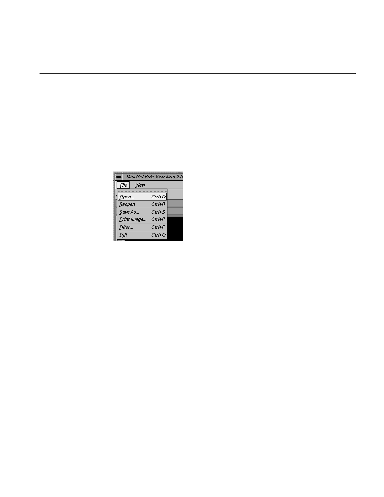
Pulldown Menus
309
Pulldown Menus
The Rules Visualizer has three pulldown menus, labeled File, View, and Help.
The File Menu
The File menu (Figure 9-11) contains six options.
Figure 9-11 Rules Visualizer File Menu
•Open loads and opens a configuration file, displaying it in the main window.
Previously displayed data is discarded.
•Reopen reloads the current configuration file. This is useful if either the
configuration file or data file has changed.
•Save As... allows uyou to save the file under a different file name
•Print Image... allows you to print the image from the screen
•Filter....allows you to filter the data.
•Exit closes the current window and exits the application.
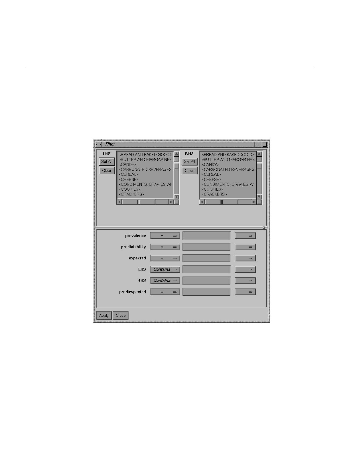
310
Chapter 9: Using the Rules Visualizer
The Filter Menu
The Filter menu brings up a Filter panel (Figure 9-12) that lets you reduce the number of
rules displayed in the main viewing area, based on one or more criteria. You can use the
filter panel to fine-tune the display, emphasize specific information, or simply shrink the
amount of information displayed.
Figure 9-12 Rules Visualizer Filter Panel

Pulldown Menus
311
The top pane lets you filter based on string variables, such as LHS and RHS. To select all
values of a variable, click Set All. To clear the current selections, click Clear. To select a
value, click it. To deselect a value, click it again.
The bottom pane lets you filter based on the values of both string and numeric variables.
To filter numeric values, enter the value, and select a relational operation (=, !=, >, <, >=,
<=). To filter alphanumeric values, enter the string. You can use any of three types of
string comparisons:
•Contains indicates that it contains the appropriate string. For example, California
contains the strings Cal and forn.
•Equals requires the strings to match exactly.
•Matches allows wildcards:
–An asterisk (*) represents any number of characters.
–A question mark (?) represents one character.
–Square braces ([ ]) enclose a list of characters to match.
For example, California matches Cal*, Cal?fornia, and Cal[a-z]fornia.
In addition to numeric and string comparison operations, you can specify Is Null.
Currently, this option does not match any rules, resulting in an empty display.
To the right of each field is an additional option menu that lets you specify “And” or “Or”
options. For example, you could specify “sales > 20 And < 40.” You can have any number
of And or Or clauses for a given variable, but cannot mix And and Or in a single variable.
Click the Filter button to start filtering. If you press Enter while the panel is active,
filtering starts automatically.
Click the Close button to close the panel.
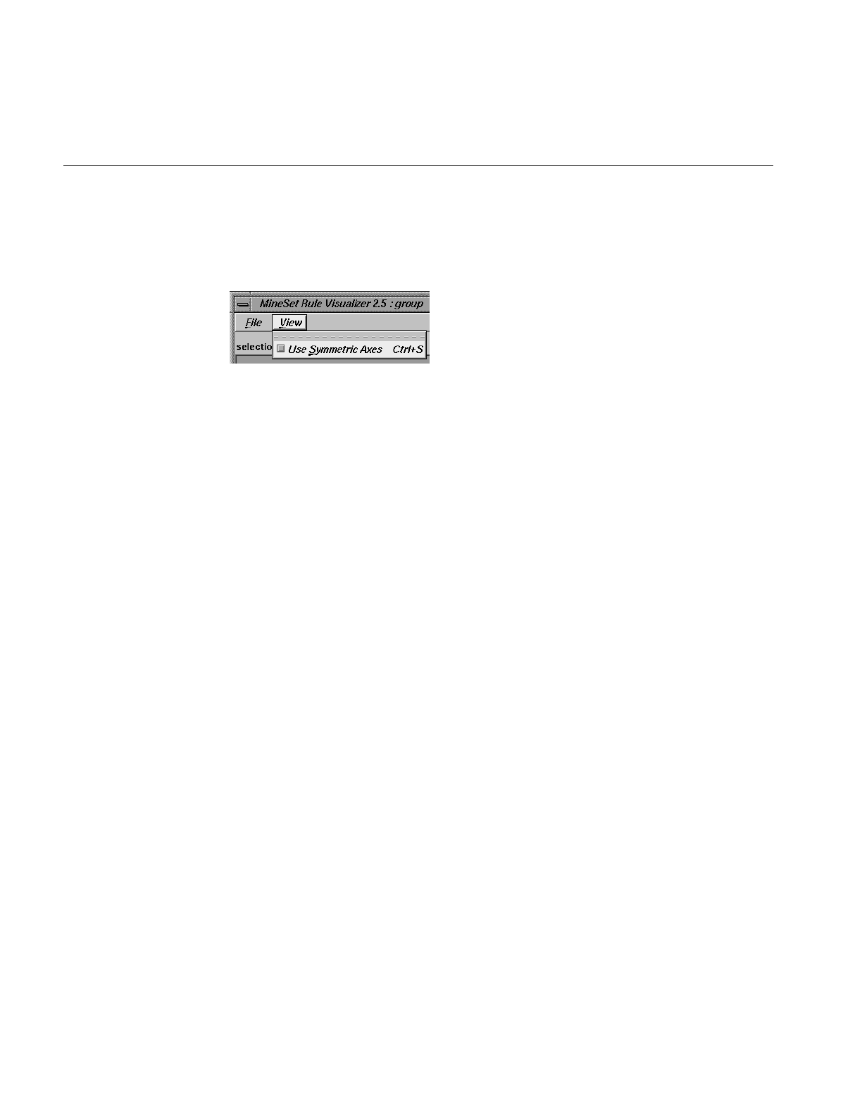
312
Chapter 9: Using the Rules Visualizer
The View Menu
The View menu (Figure 9-13)contains one option.
Figure 9-13 Rules Visualizer View Menu
Use Symmetric Axes controls how items are displayed along the left- and right-hand side
axes. If enabled, every item appears on both axes, making the axes identical. Otherwise,
only the required items appear on each axis.
The Help Menu
The Help menu is the same for all MineSet Visualization tools, (see “The Help Menu” in
Chapter 5 for a complete description).
Sample Files
The provided sample data, rules, and configuration files demonstrate the features and
capabilities of the Rules Visualizer.
Sample Files for the Association Data Converter
There are two sample files provided for each of the two formats of the association data
converter. These files are located in the /usr/lib/MineSet/assoccvt/examples directory.
•sing.dat and sing.fmt
The sing.dat file is a “raw” data file type, as described in the “Files Required by the
Association Data Converter Part” on page 294. The sing.fmt file is the format file
described in the same section. Both files are of the single-item-per-record format.
•mult.dat and mult.fmt
The mult.dat file is a “raw” data file type, as described in the “Files Required by the
Association Data Converter Part” on page 294. The mult.fmt file is the format file
described in the same section. Both files are of the multiple-item-per-record format.

Sample Files
313
Sample Files for the Association Rules Generator
These files are located in the /usr/lib/MineSet/assocgen/examples directory. Except for the
synthn.dsc file, the sample files for the association rules generator are provided in 2-byte
and 4-byte integer versions. The difference between the respective files is that the 4-byte
integer version requires twice the amount of storage space of the 2-byte integer version.
•synthn.dsc
This is a description file for items at the nth level of the hierarchy. For example, if n
is 0, this file describes the lowest level; if n = 1, the file describes the next higher
level of the hierarchy, and so forth. Description files are common to both 2-byte and
4-byte integer files.
Two-byte Integer Version
•synths.dat
This is a data file with 2-byte integers. It corresponds to the data shown in Table F-9
on page 658.
•synths.map
This is a 2-byte integer mapping file for hierarchical data.
Four-byte Integer Version
•synthb.dat
This is a data file with 4-byte integers. It corresponds to the data shown in Table F-9
on page 658.
•synthb.map
This is a 4-byte integer mapping file for hierarchical data.
Sample Files for the Rules Visualization Part
The following sample rules and configuration files are provided for use with the rules
visualization part of this tool. These files correspond to the hierarchical datasets. Rules
files contain the generated rules obtained by running the association rules generator part
of the Rules Visualizer. Rules files must have a .rules extension. Each configuration file
specifies how the corresponding rules file is displayed. Configuration files must have a
.ruleviz extension. The files mentioned in this subsection are in the
/usr/lib/MineSet/ruleviz/examples directory.

314
Chapter 9: Using the Rules Visualizer
•group.rules and group.ruleviz
These files provide the generated rules and configuration specifications for product
groups, such as bread and baked goods, dairy milk, and carbonated beverages.
•category.rules and category.ruleviz
These files provide the generated rules and configuration specifications for product
categories within product groups, such as refrigerated or non-refrigerated milk.
•people94.rules and people94.ruleviz
These files provide the generated rules and configuration specifications for a census
database, showing associations among marital status, education level, age, income,
and other variables.
•germanCredit.rules and germanCredit.ruleviz
These files provide the generated rules and configuration specifications for a credit
database from Germany, showing associations among credit history, employment,
savings, and other variables.
See /usr/lib/MineSet/ruleviz/examples/README for additional information on the files in
that directory.

315
Chapter 10
10. MineSet Inducers and Classifiers
This chapter provides an introduction to classifiers and the algorithms that build them,
called inducers. MineSet provides three inducer-classifier pairs:
•Decision Tree
•Option Tree
•Evidence
The information in this chapter is equally applicable to all the MineSet classifiers and
inducers. The chapter consists of two parts: the first part introduces the basic concepts,
and the second part details how to apply those concepts via the Tool Manager.
Detailed descriptions of the MineSet inducers and classifiers are provided in Chapter 11,
“Inducing and Visualizing the Decision Tree Classifier,” Chapter 12, “Inducing and
Visualizing the Option Tree Classifier,” and Chapter 13, “Inducing and Visualizing the
Evidence Classifier.”
Classifiers
A classifier predicts one attribute of a set of data, given several other attributes. For
example, if you have data on customers of a telecommunications company, a classifier
can be generated to predict whether the customer will churn (leave the company) given
information such as whether the customer has voice mail, an international plan or not,
and how much time they spend on the phone. The attribute being predicted is called the
label, and the attributes used for prediction are called the descriptive attributes.
MineSet can build a classifier automatically from a training set. The training set consists
of records in the data for which the label has been supplied. For example, you supply a
database table with one column for each descriptive attribute (such as the presence of a
voice mail plan, the average number of calling minutes per day), and one column for the
label (churned or not). An algorithm that automatically builds a classifier from a training
set is called an inducer.
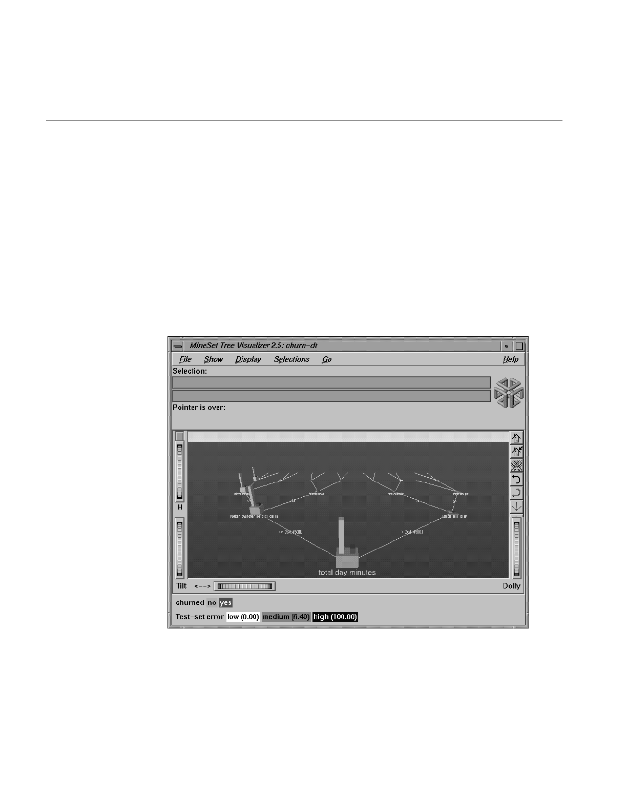
316
Chapter 10: MineSet Inducers and Classifiers
When a classifier is generated, MineSet also generates a visualization that can help you
understand how the classifier operates. This visualization can also provide valuable
insight into the data itself. Once a classifier is generated, it can be used to classify records
that do not contain the label attribute. This value is predicted by the classifier.
Note: See Appendix K for a list of further readings about classifiers as well as
acknowledgements for the datasets used in MineSet sample files.
Decision Tree Classifiers
Figure 10-1 shows the Decision Tree generated by the Decision Tree Inducer for the churn
dataset.
Figure 10-1 The Decision Tree Generated by the Decision Tree Inducer for Churn Dataset

Classifiers
317
To understand how the Decision Tree classifier assigns a label to each record, look at the
attributes tested at the nodes and the values on the connecting lines. In the Decision Tree
shown in Figure 10-1, the first test (at the root of the tree) is for total day minutes. There
are two branches from this root. If the total day minutes is <= 264.45, the left branch is
taken; otherwise the right branch is taken. The process is repeated until a leaf (node with
no branches) is reached. The leaf is labeled with the predicted class. The leaf represents
a rule that is the conjunction of all tests from the root to the leaf. For example, the right
most leaf, labeled No, matches the rule
total day minutes > 264.45 and voice mail plan = yes and
international plan = yes and total day minutes > 276.3
Option Tree Classifiers
Figure 10-2 shows an Option Tree generated by the Option Tree inducer.
Figure 10-2 The Option Tree Generated by the Option Tree Inducer for the Cars Dataset

318
Chapter 10: MineSet Inducers and Classifiers
The top node in this figure is an “Option node,” which indicates that several good
attributes can be chosen at the root. A Decision Tree Inducer picks the single “best”
attribute for each subtree; however, there might be several good attributes on which to
split. In such cases, an Option Tree can create option nodes. In the example dataset
(Figure 10-2), the task is to predict whether a car is manufactured in Europe, Japan, or the
US. The Decision Tree Inducer picks cubic inches for the root. The Option Tree inducer
chooses several options: cubic inches, cylinders, weight, mpg, and brand are all good
choices for the root.
Option nodes can appear elsewhere besides the root. With the default settings, however,
they appear only at the root or one level below the root (after a single test node).
Option Trees usually take 10 to 15 times longer to build than do Decision trees, but they
provide two significant advantages:
1. Comprehensibility — Option nodes let you see several likely options. Instead of
having to settle for a single attribute, option nodes let you choose from several.
When you fly over the tree, you can choose to follow an option that you believe is
easier to understand or that you believe is better for predictions based on your
background knowledge of the problem.
2. Accuracy — In many cases, Option Trees are more accurate (have lower error-rates)
than Decision Trees. Option Trees classify by letting each option “vote” for each
label value, then average the votes. This is similar to having a series of “experts,”
each one attempting to predict the label based on a different main criterion. The
option node averages all these experts’ votes. Just as distributing stock investments
reduces the risk, using a mixture of options usually results in a more stable, less
risky classifier.
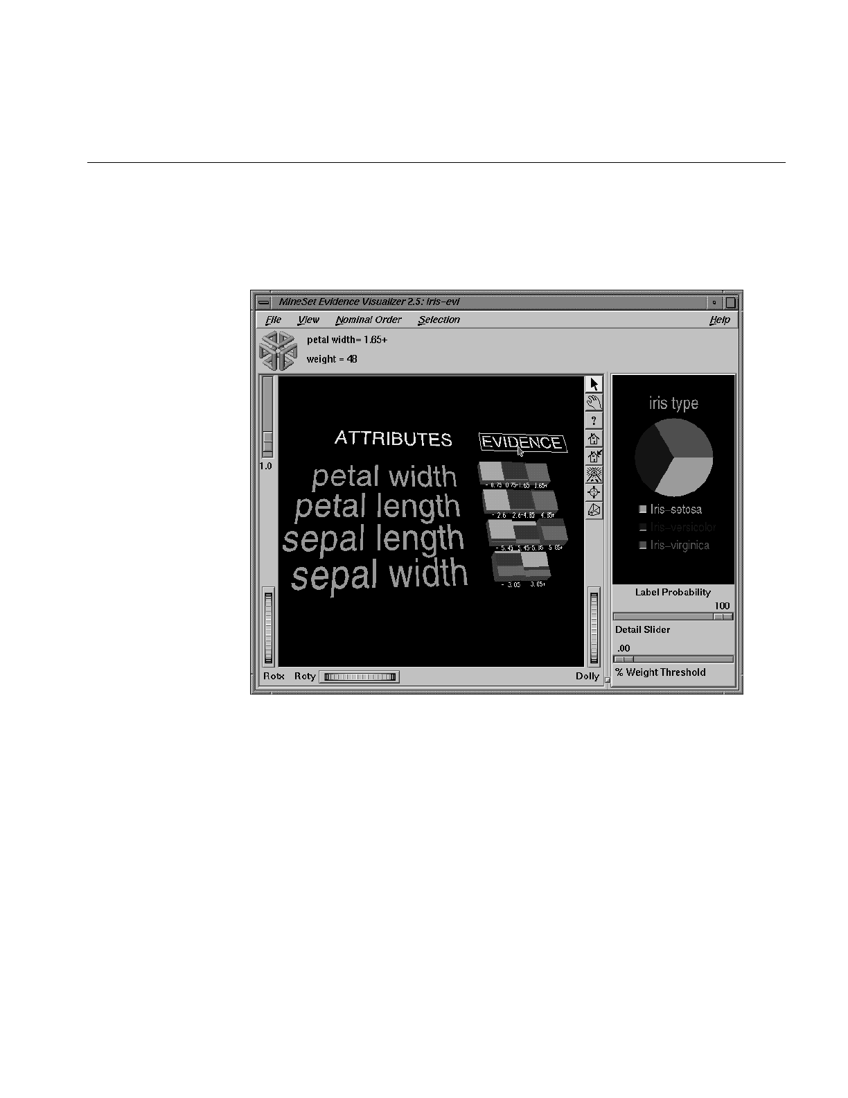
Classifiers
319
Evidence Classifiers
Figure 10-3 shows the evidence information generated by the Evidence Inducer.
Figure 10-3 Results of Evidence Inducer for Iris Dataset
The right window of the screen shows the distribution of the classes in the training set.
The left side shows rows of cake charts, one for each attribute. For every value of an
attribute in the data, there is one chart matching it in the row for the attribute. Given a
record with an attribute value corresponding to a chart, the chart represents how much
evidence the classifier “adds” to each possible label value. For example, in Figure 11-3, a
record with total day minutes < 175 shows much evidence for the No label value, and
little evidence for the Yes label value. After evidence is accumulated from all the
attributes, the label value with the most evidence is predicted.
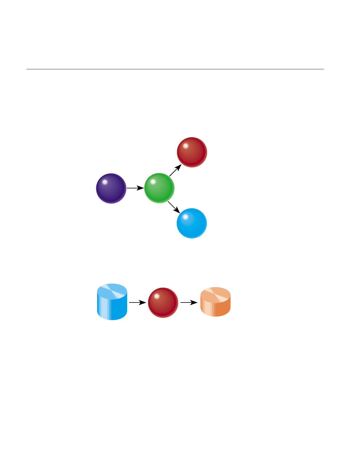
320
Chapter 10: MineSet Inducers and Classifiers
Inducers
An inducer is an algorithm that builds a classifier from a training set, which consists of
records with labels. The training set is used by the inducer to “learn” how to construct
the classifier, as shown in Figure 10-4.
Figure 10-4 Method for Building a Classifier
Once the classifier is built, its structure can be visualized or used to classify unlabeled
records, as shown in Figure 10-4 and Figure 10-5.
Figure 10-5 Using a Classifier to Label New Records
Running inducers can be a CPU- and I/O-intensive process. For this reason, the MineSet
inducers run on the MineSet server, rather than on the MineSet client (see Figure 10-6).
Training Set
(records with
labels)
Classifier
Inducer
Visualization
files
Classifier
Records
without
labels Labels

Inducers
321
Figure 10-6 Tool Execution Sequence for Classifiers
MineSet client MineSet server
Tool
manager
Configuration
file
Configuration
file
Visualization
tool
Visual
files
Data
file
DataMover User's
data
source
User
Visual
display
Inducer
(MIndUtil)
Classifier
Information & statistics
(error estimate)
OR
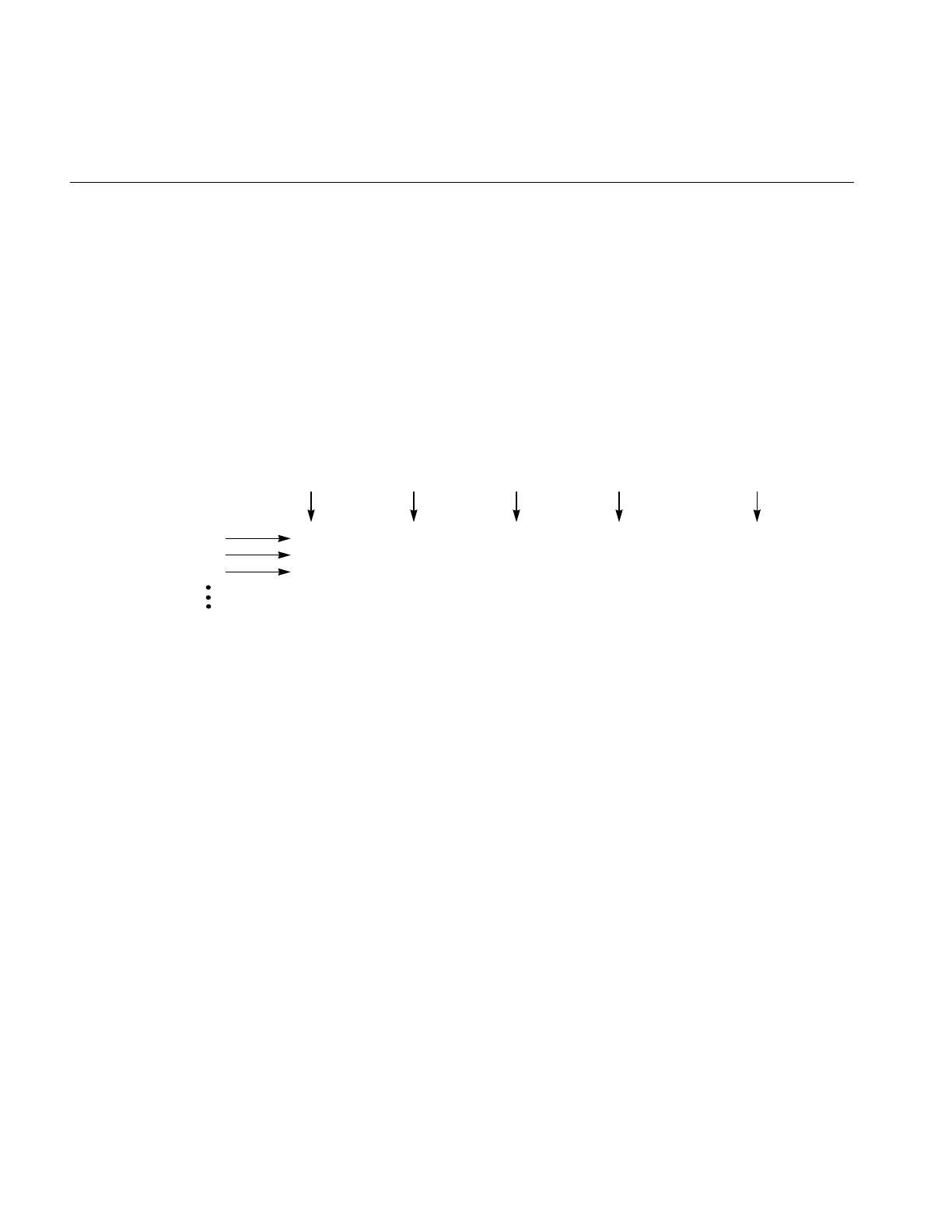
322
Chapter 10: MineSet Inducers and Classifiers
Training Set
Inducers require a training set, which is a table containing attributes, one of which is
designated as the class label. The label attribute type must be discrete (binned values,
character string values, or a few integers). The number of possible values for the label
attribute should be small, preferably two or three values. Let’s look at an example where
the goal is to classify the type of an iris flower (iris-setosa, iris-versicolor, or iris-virginica)
given as descriptive attributes its sepal length, sepal width, petal length and petal width.
Figure 10-7 shows several records from a sample training set for this problem.
Figure 10-7 Sample Records From a Training Set
Once a classifier is built, it can classify new records as belonging to one of the above
classes (see Figure 10-5). These new records must be in a table that has all the attributes
used by the classifier with the same name and type as they were in the training set. The
table need not contain the label attribute. If it exists, it is ignored during classification.
Applying a Model
After building a classifier, you can apply it to records to predict their label. For example,
if you built a classifier for predicting iris type, you can apply the classifier to records
containing only the descriptive attributes, and a new column is added with the predicted
iris type.
In a marketing campaign, for example, a training set can be generated by running the
campaign at one city and generating label values according to the responses in that city.
A classifier can then be induced and campaign mail can then be sent only to people who
are labeled by the classifier as likely to respond, thus saving mailing costs.
5.1 3.5 1.4 0.2 Iris-setosa
5.9 3 5.1 1.8 Iris-virginica
6.5 2.8 4.6 1.5 Iris-versicolor
6.3 2.9 5.6 1.8 Iris-virginica
6.5 3 5.8 2.2 Iris-virginica
Record 1
Record 2
Record 3
sepal length sepal width petal length petal width iris type
Descriptive Attributes Label
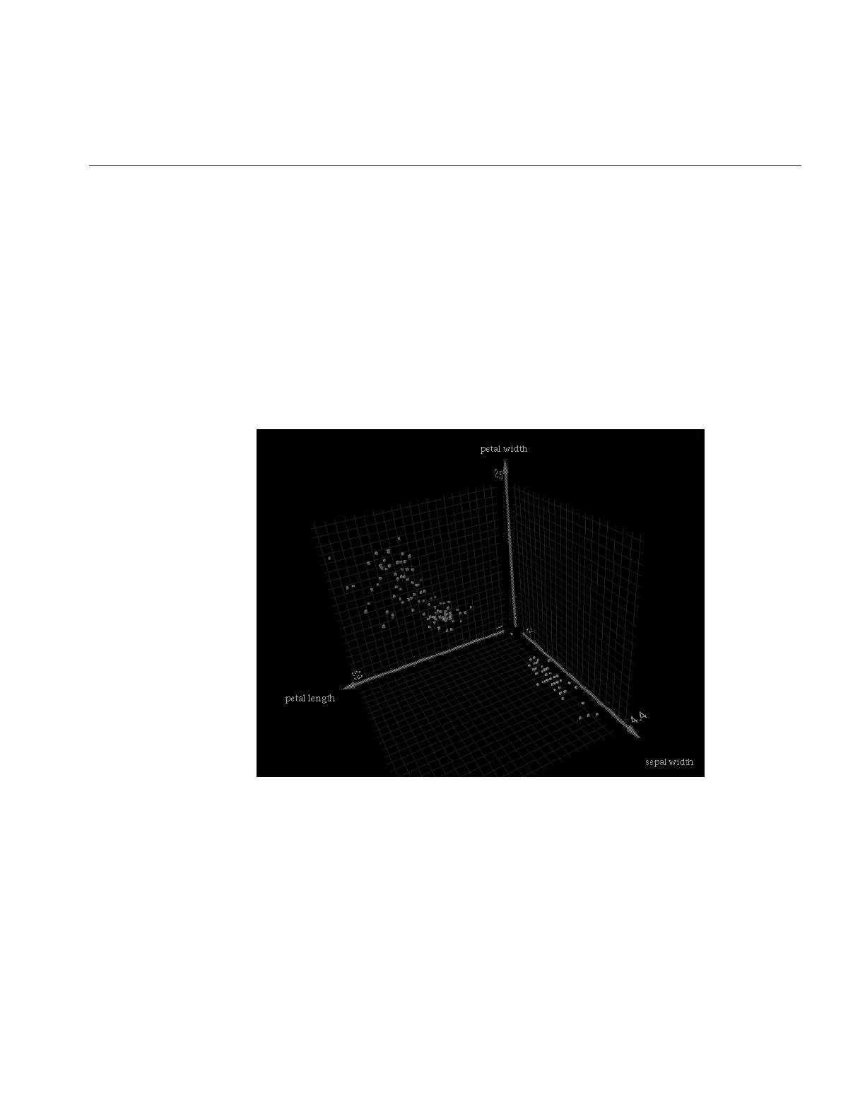
Training Set
323
As an example of using mining tools for ensuring data quality, after building a classifier
you can apply it to the training set in order to identify records that are mislabeled by the
classifier. Such records might warrant closer investigation. Perhaps they are “noise,” or
they might yield special insights. If, for example, you have a Decision Tree for the iris
dataset induced using the Classify Only mode, by applying the classifier, you get a new
column (iris type_1) containing the predicted labels. You can then add a column that is
defined as type int with the expression (iris type != iris type_1). The new column has a 1
whenever the classifier misclassifies, and a zero when it correctly classifies. Figure 10-8
shows a Scatter Visualizer plot of the data where the new column is mapped to color with
the colors set such that green is 0 (OK) and 1 is red (error). By looking at the plot, it is
possible to determine where mistakes are being made.
Figure 10-8 Iris Dataset Misclassification, Example 1
Another alternative is to define the new column as a float with the expression
(iris type != iris type_1) + 0.01. The Scatter Visualizer can then be used with the original
label mapped to color, and this new column mapped to size. Incorrect predictions are
shown as big cubes; correct predictions are shown as small cubes (see Figure 10-9).
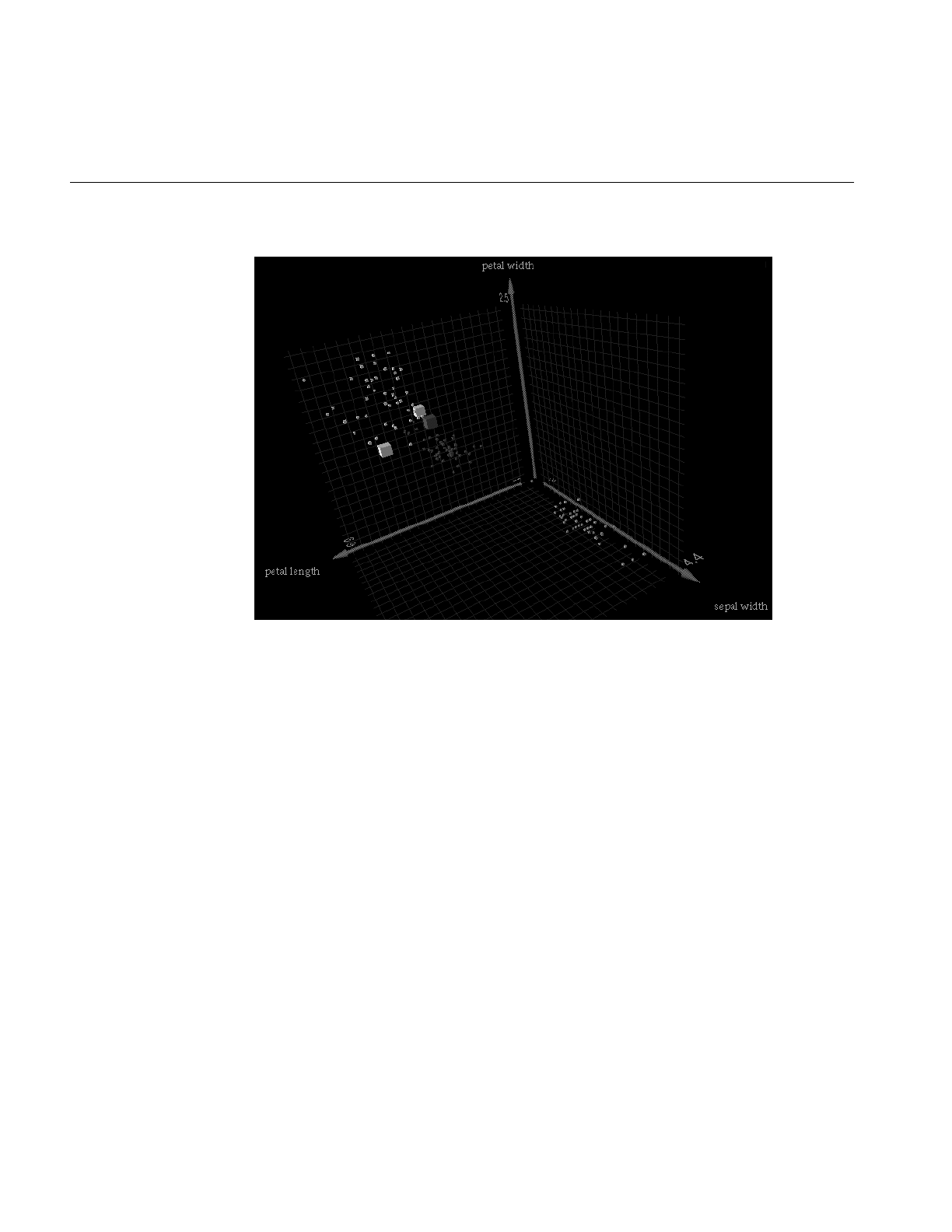
324
Chapter 10: MineSet Inducers and Classifiers
Figure 10-9 Iris Dataset Misclassification, Example 2
Error Estimation
When a classifier is built, it is useful to know how well you can expect it to perform in
the future (what is the classifier’s error-rate). Factors affecting classification error-rate
include:
•The number of records available in the training set.
Since the inducer must learn from the training set, the larger the training set, the
more reliable the classifier should be; however, the larger the training set, the longer
it takes the inducer to build a classifier. The improvement to the error-rate decreases
as the size of the training set increases (this is a case of diminishing returns).

Error Estimation
325
•The number of attributes.
More attributes mean more combinations for the inducer to compute, making the
problem more difficult for the inducer and requiring more time. Note that
sometimes random correlations can lead the inducer astray; consequently, it might
build less accurate classifiers (technically, this is known as “overfitting”). If an
attribute is irrelevant to the task, remove it from the training set (this can be done
using the Tool Manager).
•The information in the attributes.
Sometimes there is not enough information in the attributes to correctly predict the
label with a low error-rate (for example, trying to determine someone’s salary based
on their eye color). Adding other attributes (such as profession, hours per week,
and age) might reduce the error-rate.
•The distribution of future unlabeled records.
If future records come from a distribution different from that of the training set, the
error-rate probably will be high. For example, if you build a classifier from a
training set containing family cars, it might not be useful when attempting to
classify records containing many sport cars, because the distribution of attribute
values might be very different.
The two common methods for estimating the error-rate of a classifier are described
below. Both of these assume that future records will be sampled from the same
distribution as the training set.
•Holdout: A portion of the records (commonly two-thirds) is used as the training set,
while the rest is kept as a test set. The inducer is shown only two-thirds of the data
and builds a classifier. The test set is then classified using the induced classifier, and
the error-rate or loss on this test set is the estimated error-rate or estimated loss.
Figure 10-10 shows this error estimation method.
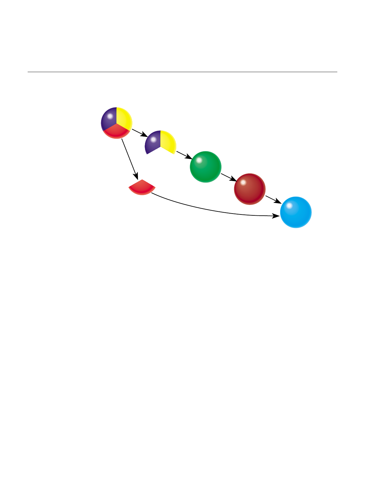
326
Chapter 10: MineSet Inducers and Classifiers
Figure 10-10 Estimating the Classifier’s Accuracy
This method is fast, but since it uses only two-thirds of the data for building the
classifier, it does not make efficient use of the data for learning. If all the data were
used, it is possible that a more accurate classifier could be built.
•Cross-validation: The data is split into k mutually exclusive subsets (folds) of
approximately equal size. The inducer is trained and tested k times; each time, it is
trained on all the data minus a different fold, then tested on that holdout fold. The
estimated error-rate is then the average of the errors obtained. Figure 10-11 shows
cross-validation with k=3 (note that the default value is k=10).
Cross-validation can be repeated multiple times (t). For a t times k-fold
cross-validation, k*t classifiers are built and evaluated. This means the time for
cross-validation is k*t times longer. By default, k=10 and t=1, so cross-validation
takes approximately 10 times longer than building a single classifier.
Increasing the number of repetitions (t) increases the running time and improves
the error estimate and the corresponding confidence interval.
You can increase or decrease k. Reducing it to 3 or 5 shortens the running time;
however, estimates are likely to be biased pessimistically because of the smaller
training set sizes. You can increase k, but this is recommended only for very small
datasets.
Evaluation
(percent
incorrect
predictions)
Classifier
Inducer
Training Set
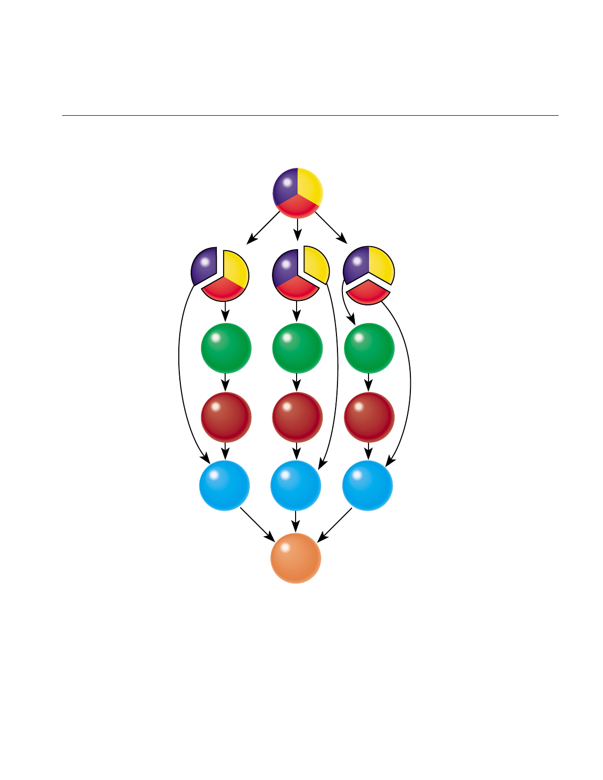
Error Estimation
327
Figure 10-11 Classifier Cross-Validation (k=3)
Generally, a holdout estimate should be used at the exploratory stage, as well as on
datasets of over 5,000 records. Cross-validation should be used for the final classifier
building phase, as well as on small datasets.
Average
Evaluation
Classifier
Inducer
Classifier
Inducer
Classifier
Inducer
Training Set
Evaluation Evaluation

328
Chapter 10: MineSet Inducers and Classifiers
Backfitting in Error Estimation
An inducer builds a classifier, which has two parts:
•Structure — For Decision Trees and Option Trees, the structure is the shape of the
tree. For evidence, the structure is the number of bins for every attribute and the
thresholds if the attribute is numeric.
•Probability estimates — Each part of the structure estimates the probability of each
class. These estimates are commonly based on the counts of training records at
different points in the structure. For Decision Trees, the probabilities are determined
by the weight of records at the leaves. For the Evidence classifier, the probabilities
are determined by the conditional probabilities for every attribute value or range.
Backfitting a classifier with a set of records does not alter the structure of the classifier,
but updates the probability estimates based on the given data. Backfitting is useful for
several reasons:
1. A structure can be built from a small training set, then backfitted with a big dataset
to improve the probability estimates in the structure. Backfitting is a faster process
than inducing the classifier's structure.
2. When holdout error estimation is used, a portion of the data is left out for testing.
Once the classifier structure is induced and the error estimated, it is possible to
backfit all of the data through the structure, which can reduce the error of the final
classifier. When counts, weights, and probabilities are shown in the classifier's
structure, they reflect all the data, not just the training set portion.
When using drill-through from the visualizers, you can see data corresponding to the
weights shown, which reflect the whole dataset. If backfitting is not used, the weights
shown represent only the training set.
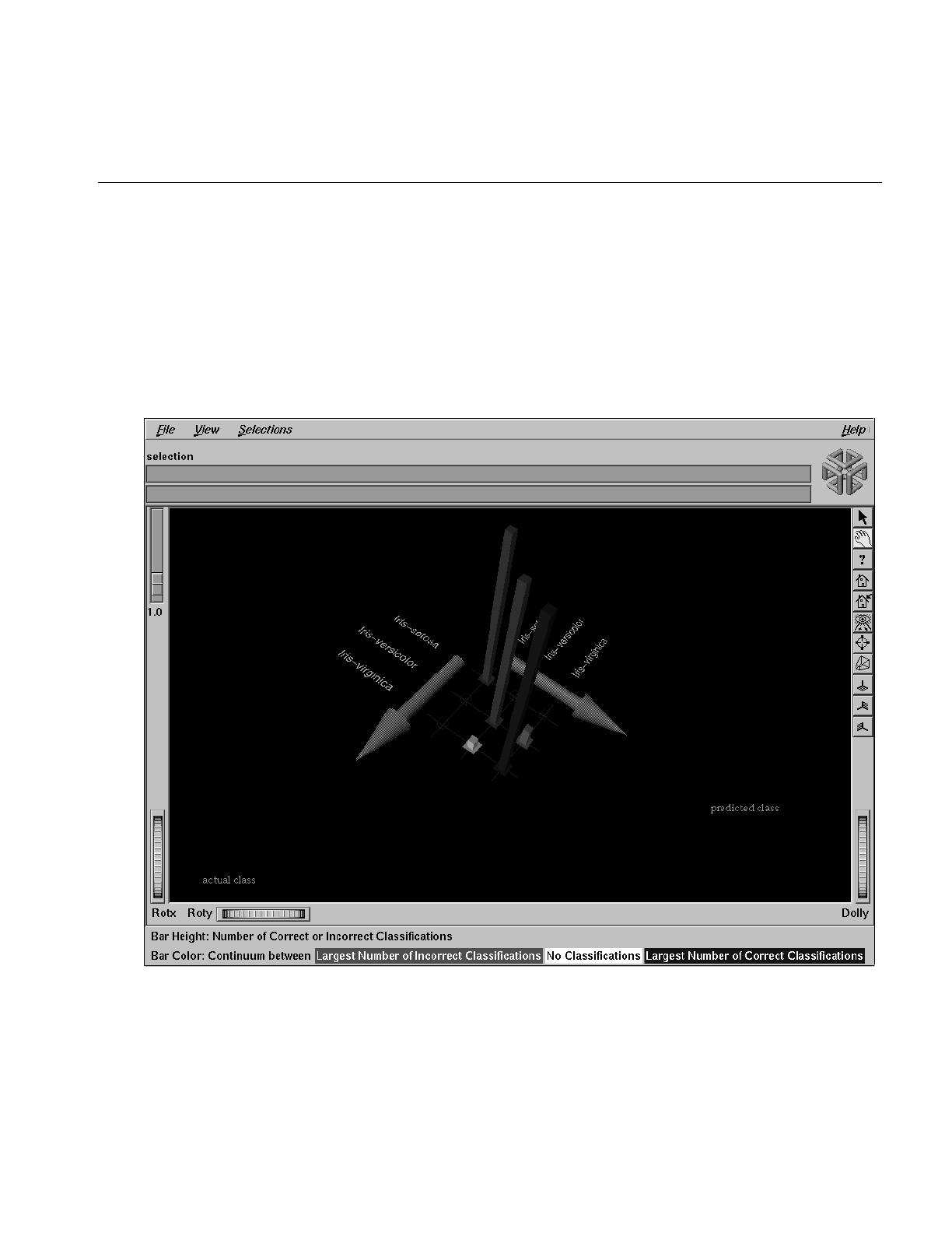
Error Estimation
329
Confusion Matrices in Error Estimation
Confusion matrices give a more detailed picture of the errors made by a classifier. Instead
of simply analyzing the number of correct and incorrect predictions, the confusion
matrix shows the type of errors being made.
Figure 10-12 shows a confusion matrix for a Decision Tree that was induced on the iris
dataset.
Figure 10-12 Confusion Matrix for Iris Dataset

330
Chapter 10: MineSet Inducers and Classifiers
The two axes represent:
•the class values predicted by the classifier, and
•the actual class values given in the test set (holdout set).
Entries on the diagonal are correct predictions. Entries off the diagonal indicate incorrect
predictions. This representation shows that iris-versicolor and iris-virginica are frequently
confused, but iris-setosa is always predicted correctly.
When the cost of making different types of mistakes is uneven, it is frequently useful to
understand the type of errors that are being made (see loss matrices below).
Note: The confusion matrix shows the errors made on the test set; thus, it represents the
expected true distribution of errors in an actual situation if the underlying distribution
of the data does not change significantly. The confusion matrix in MineSet is computed
prior to backfitting and is the same whether or not backfitting is applied.
Lift Curves in Error Estimation
A lift curve is a graph that plots the cumulative weight of the records from a specified
label value as a function of the weight of all the records. The order in which the records
occur determines the slope of the curve. Typically, a lift curve plots the difference
between randomly ordered records and records sorted based on a classifier's predictions.
For example, in telecommunications, it is valuable to be able to predict which customers
are likely to switch providers (churn). In the dataset churn, about 13.5% of the customers
are likely to switch provider. Figure 10-13 shows the lift curve obtained by using a
Decision Tree classifier on this dataset.
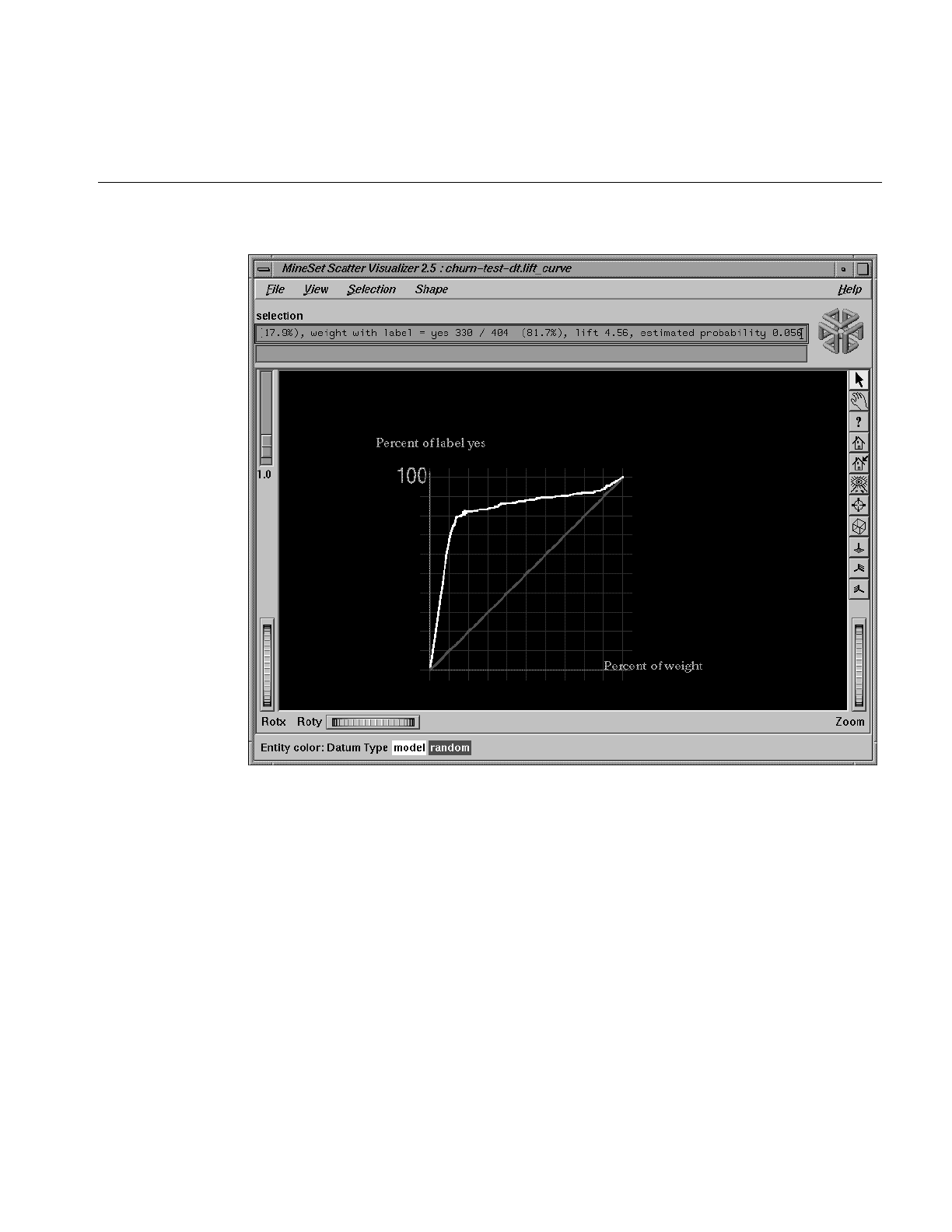
Error Estimation
331
Figure 10-13 Lift Curve for the Churn Dataset
The X axis shows the number of records sampled; the Y axis shows the number of records
corresponding to customers who churn. The lower curve (red) shows the number of
customers expected to churn given a random ordering of the records. The upper curve
(white) shows the percentage of customers that churn when ordered according to the
classifier's score (probability estimate) for each record. Records representing customers
that the classifier identifies as most likely to churn appear first; those less likely to churn
appear last. The lift that the classifier ordering provides can be seen by the difference
between the classifier curve and the random curve.

332
Chapter 10: MineSet Inducers and Classifiers
If some action should be taken before customers churn, it should be prioritized according
to the classifier's score. If the action costs money (for example, an operator contacting the
customer or a mailing), lift curves can help identify a cutoff point that maximizes returns.
Note: The lift curve shows lift on the test set; thus, it represents the expected true lift in
actual situations if the underlying distribution of the data does not change significantly.
The lift curve in MineSet is computed prior to backfitting and is the same whether or not
backfitting is applied.
Learning Curves in Error Estimation
A learning curve is a graph that shows the error of the classifier generated by an inducer
as a function of the number of records used to create the classifier. Typically, the more
records used to generate the classifier, the lower its error.
A learning curve is created by generating the specified number of classifiers for each of
the points on the curve. Each classifier is generated using a random sample of the
records, and its error is estimated using the rest of the records (those not used for
training).
Figure 10-14 shows a learning curve for the Decision Tree Inducer on the churn dataset.
Figure 10-15 shows a learning curve for the Decision Tree Inducer on the adult dataset
with the label set to gross income binned at $50,000 (so one class is gross income less than
or equal to $50,000 and the other class is gross income >$50,000). The X axis shows the
number of records used for training the inducer; the Y axis shows the error. The graph
consists of four type of points:
•The yellow points are the actual error estimates taken from the runs.
•The white points are averages.
•The blue points interpolate between the white points.
•The red points show a 95% confidence interval about the average based on actual
error estimates for each run.
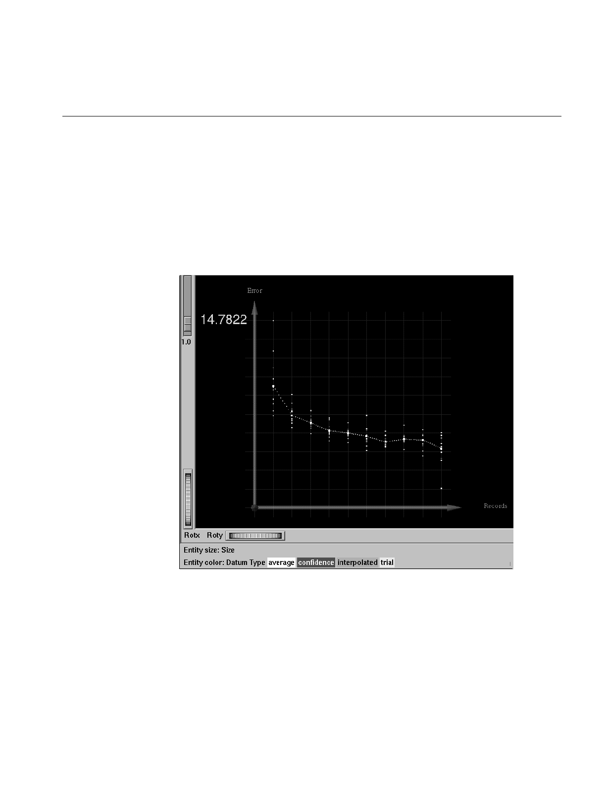
Error Estimation
333
The more runs that are requested, and the bigger the test set (portion used to test), the
smaller the confidence interval. The error is generally reduced as more records are used
for training.
We can see that for the churn dataset, the error continues to decrease as the training set
size grows, while for the adult dataset, there is little advantage to training on the whole
dataset. The third point represents about 13,000 records and has an estimated error of
16.96%, while the last point represents about 44,000 records and has an estimated error
of 16.85%.
Figure 10-14 Learning Curve for the Churn Dataset
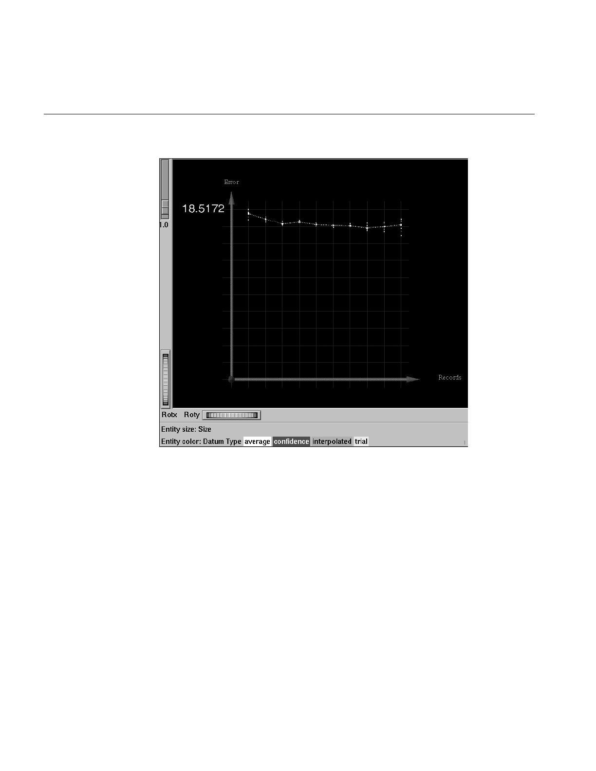
334
Chapter 10: MineSet Inducers and Classifiers
Figure 10-15 Learning Curve for the Adult Dataset With Label Set to Gross Income
Binned at $50,000
A small sample might suffice for most of the study, with the full data used only for the
final runs. In many cases, a small sample can result in a sufficiently accurate classifier,
with the error reducing only slightly if the number of records is increased (diminishing
returns). Once a learning curve is seen, the desired sampling point can be determined,
and the “sample” transformation in Tool Manager can be used to generate a sample of
this size (see “The Sample Button” in Chapter 3). Small samples reduce the time needed
to build a classifier and make the knowledge discovery process more interactive.

Error Estimation
335
Advanced Options
MineSet supports several advanced options for all inducers. These let you take into
account different costs for making mistakes and to take into account an experimental
design that has a non-uniform sampling process (that is, some parts of the true
population are sampled more heavily than others). Another option lets you create more
complicated classifiers which may have better accuracy, at the expense of added compute
time.
Loss Matrices: Not All Mistakes Were Created Equally
Suppose you are trying to classify mushrooms as poisonous or edible. Classifying a
mushroom that is actually edible as poisonous might cost you $2, since you are not eating
it; however, classifying a poisonous mushroom as edible (that is, eating it) might incur a
$10,000 operation.
Figure 10-16 shows a confusion matrix for the mushroom dataset with the Decision Tree
Inducer when only a ratio of 0.1 (10%) was used for a training set.
Figure 10-16 Confusion Matrix for the Mushroom Dataset Using Defaults Settings

336
Chapter 10: MineSet Inducers and Classifiers
Eight records, representing poisonous mushrooms, were classified as edible (0.1%); 15
records, representing edible mushrooms, were classified as poisonous (0.2%). 3793
edible mushrooms and 3496 poisonous mushrooms were correctly classified. While the
error-rate for the classifier is only 0.31% (less than one percent), our estimated loss would
be $10000*8 + $2*15 = $80,030.
Figure 10-17 shows a confusion matrix for the same dataset, but with the Decision Tree
Inducer run using a loss matrix representing the above costs. The new classifier is very
conservative and makes no mistakes in classifying a poisonous mushroom as edible; but
it makes 1558 mistakes (1543+8) in classifying edible mushrooms as poisonous. The total
estimated loss we would incur is thus $10000*0 + $2*1558 = $3116, only 3% of the cost of
the classifier that did not take losses into account.
Figure 10-17 Confusion Matrix for the Mushroom Dataset With Loss Matrix

Error Estimation
337
Loss matrices also allow predicting unknown (null values), which are shown as question
marks (?). For example, suppose it costs us $1 to ask an outside expert whether a
mushroom is poisonous or edible. In that case, some classifications result in an unknown
prediction. Running the Decision Tree Inducer yields the confusion matrix shown in
Figure 10-18, where there are 1551 unknowns, and only 15 edible mushrooms are
classified as poisonous. The overall cost is thus $10000*0 + $1*1551 + $15*2 = $1581
Figure 10-18 Confusion Matrix for the Mushroom Dataset With Loss Matrix Allowing
Unknown Predictions
Note that loss matrices are based on probability estimates made at the leaves of the tree.
For reliable estimates:
1. Raise the "split lower bound" in Further Options of Decision Trees and Option Trees
from the default value to a higher value (for example: 5). In general, the larger and
noisier the training set size, the higher this value should be.
2. Use large training sets. You might need large training sets to get reliable estimates
when the costs are not as extreme as in this example.
3. Use Option Trees. While they do not always help, they usually provide better
probability estimates that tend to reduce the loss. For example, running the above
example with $10000 changed to $100 with unknowns not allowed, yields an
estimated loss of $1464 for Decision Trees and an estimated loss of $662 for Option
Trees.

338
Chapter 10: MineSet Inducers and Classifiers
Return-on-Investment Curves
A Return-on-Investment (ROI) curve is similar to a Lift Curve, but displays accuracy in
terms of loss rather than in terms of error; taking into account the Loss Matrix used. The
points in an ROI curve are ordered by the expected loss for each record, were they to be
labeled by the chosen label value. Similarly, the height of each point in the curve indicates
the cumulative profit (inverse loss), rather than the cumulative accuracy (inverse error)
of all records up to this point. The expected loss is computed by multiplying entries in
the Loss Matrix, under the chosen labels column (see “Loss Matrices,” under “Advanced
Options,” below) by the probabilities assigned to the corresponding classes, for the
classes by the classifier. Hence, if the classifier is very sure about its prediction, the
expected loss will be low, and the record will appear near the left side of the ROI curve.
The idea behind the ROI curve is that the user will take an action for each individual
record in the dataset. That action will be the one associated with the chosen label value.
For example, in the churn dataset, the action associated with the label Yes, might be to
send that person some marketing material. This might stop the person from churning;
but the action is costly if done indiscriminately. The peak of the ROI curve shows
approximately how much money would have been saved on the test set, if the classifier
was used to predict whether or not to send the mailing to a particular person.
Special care needs to be taken when filling out a Loss Matrix for use with a Loss Curve.
The column under a certain predicted label determines the resulting ROI curve for that
label value. The entries in this column need to represent the expected gain or loss for
taking the action associated with that label value, on all of the possible classes. For
example, the entry under the column “prediction yes” in churn, under the row “actual
value no”, may contain the value 2 to indicate that the cost of mailing a brochure (the
action associated with “yes”) to someone who was not going to churn, is 2 dollars. On
the other hand, the entry under the column yes, row yes, may have a value of -10 to
indicate that a customer was prevented from churning, saving the company ten dollars
over the cost of the mailing.
Record Weighting: Not All Records Were Sampled Equally
In certain experimental designs, portions of the true population are sampled more
frequently than others. For example, while you might want a 1% sample of some
population, a small minority that is already 0.1% of the population results in a 0.001%
sample, which might be too small (for instance, you might get two people). Record
weighting lets you give each record a weight; thus, a subpopulation that was sampled
twice as frequently might get a weight of 0.5, while the rest of the population is given a
weight of 1.

Error Estimation
339
As another example, a phone company stores all fraudulent phone calls in the dataset,
while storing only a small fraction of non-fraudulent calls. By using record weighting, it
is possible give each record its true portion of the population.
Finally, some datasets are already aggregated, and the records have a natural “count”
associated with them (for example, statistics about cities in the U.S. usually have an
associated count of the population). This count attribute can be mapped to weight, which
is equivalent to replicating each record by the number of counts.
The semantics of record weighting is that a record weight of 2 is equivalent to two records
with a record weight of 1. Floating point weights are allowed.
Boosting: Accuracy is Sometimes Crucial
In some cases, the most important issue in creating a classifier is its error rate. For
example, suppose you have analyzed a dataset for churn prediction to a point that you
are satisfied with, and are ready to create a classifier that will predict which of your
customers are the most likely to churn. At this point, you are no longer interested in
visualizing your classifier, since you have a reasonably good understanding of the factors
that are involved. You also want to achieve the best classification accuracy possible. In
this case, you might want to enable Boosting, which is an algorithm that creates several
different classifiers and combines their predictions using a weighted voting scheme.
Boosted classifiers often improve classifier accuracy, by focusing the induction process
on examples in the data which are harder to model than others.
Boosting will not always increase accuracy, but it often does. Boosted classifiers cannot
be visualized, though you can still see confusion matrices, lift curves, learning curves
and ROI curves for boosted classifiers. Boosting is a computationally intensive process,
often taking 25 times longer to run than the corresponding inducer without Boosting.
Backfitting does not work with Boosted classifiers, because of the special way Boosting
weights multiple classifiers and the records used to train them.
The theory behind boosting has not been generalized past two-class problems. MineSet
2.5 and later versions, however, allow you to use boosting with labels that have any
number of values. Boosting will not always improve the error rate of induced classifiers;
this is especially stressed for problems that have more than two label values.
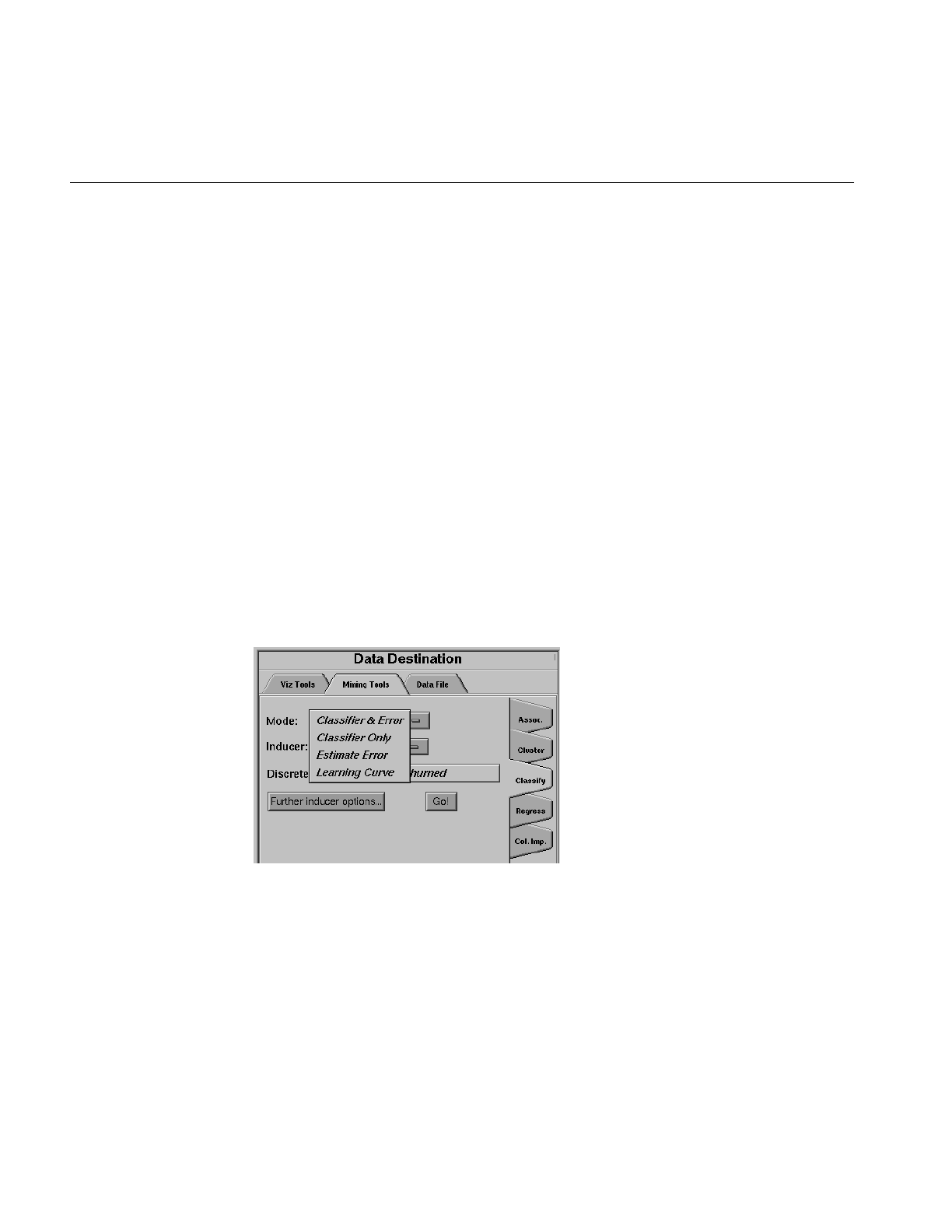
340
Chapter 10: MineSet Inducers and Classifiers
Boosting works by repeatedly assigning new weight distributions to the training set and
inducing classifiers on the reweighted sets. The number of times this occurs is limited by
the BOOST_NUM_TRIALS option, which can be set using the .mineset-classopt files on
the client (see Appendix I, “Command-Line Interface to MIndUtil: Analytical Data
Mining Algorithms,”for more information about the .mineset-classopt file). The number of
classifiers generated may be lower than this parameter if the training set error rate drops
to zero before this many classifiers are generated.
The following section describes the options provided for the classifiers by the Tool
Manager.
Inducer Modes in Tool Manager
There are four modes for running an inducer (shown in Figure 10-19).
•Classifier and Error
•Classifier Only
•Estimate Error
•Learning Curve
Figure 10-19 Options for Running the Inducer
The Classifier and Error mode uses a holdout method to build a classifier: a random
portion of the data is used for training (commonly two-thirds) and the rest for testing.
This holdout proportion can be set in Further Inducer Options (see “Error Estimation” on
page 324). This method is the default mode and is recommended for initial explorations.
It is fast and provides an error estimate.

Error Options for Inducers
341
The Classifier Only mode uses all the data to build the classifier. There is no error
estimation. Use this mode when there is little data or when you build the final classifier.
The Estimate Error mode assesses the error of a classifier that would be built if all the data
were used (as with Classifier Only mode). Estimate Error uses cross-validation, resulting
in long running times. Cross-validation splits the data into k folds (commonly 10) and
builds k classifiers. The process can be repeated multiple times to increase the reliability
of the estimate. You can set the number k and the number of times in Further Inducer
Options, as explained in “Error Options for Inducers,” below. Use this method when
there is little data. The induced classifier is exactly the same as the one induced by the
Classifier Only mode.
The Learning Curve mode assesses the effect of training set size on the error of a
classifier.
Error Options for Inducers
The following options are available to fine tune the error estimation for the inducers. The
Error Options available to you depend on the mode you have chosen.
In both Classifier & Error and Estimate Error, you can set a random seed that determines
how the data is split into training and testing sets. Changing the random seed causes a
different split of the data into training and test sets. If the error estimate varies
appreciably, the induction process is not stable.
In Classifier & Error (see Figure 10-20), you can set the Holdout Ratio of records to keep
as the training set. This defaults to 0.666667 (two-thirds). The rest of the records are used
for assessing the error.
Figure 10-20 Error Estimation Options With Holdout
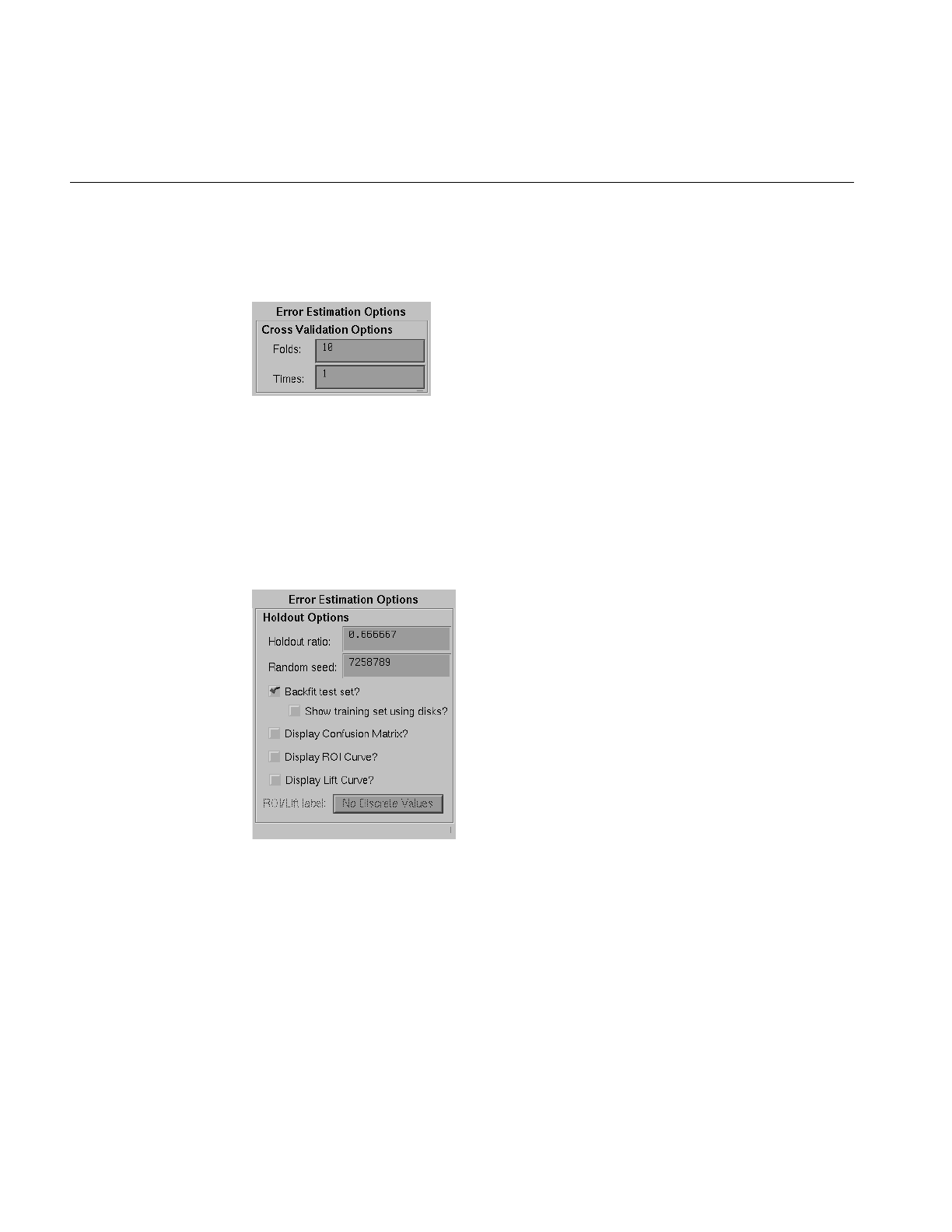
342
Chapter 10: MineSet Inducers and Classifiers
In Estimate Error (see Figure 10-21), you can set the number of folds in cross validation
and the number of times to repeat the process.
Figure 10-21 Error Estimation Options With Cross Validation
Backfitting
The Backfit test set option is a checkmark that can be found under Further Options for all
inducers when using Classifier & Error mode, and is shown in Figure 10-22. The backfit
checkmark is disabled when Boosting is enabled.
Figure 10-22 Backfitting, Confusion Matrices, Lift Curve, and ROI Curve Options

Error Options for Inducers
343
Confusion Matrices
The Display Confusion Matrix option is checkmark under Further Options for all inducers
when using Classifier & Error mode is shown in Figure 10-22.
ROI Option
The Display ROI Curve option is a checkmark under Further Options for all inducers when
the classifier and Error mode is shown in Figure 10-23. An ROI curve requires a label
value to be chosen. An ROI curve is then generated and displayed for that label value.
Figure 10-23 ROI Option for Generating a Return on Investment Curve
Lift Curves
The Display Lift Curve option is a checkmark under Further Options for all inducers when
using Classifier & Error mode is shown in Figure 10-22. A Lift Curve requires a label
value to be chosen. A lift curve is generated and displayed for that label value.
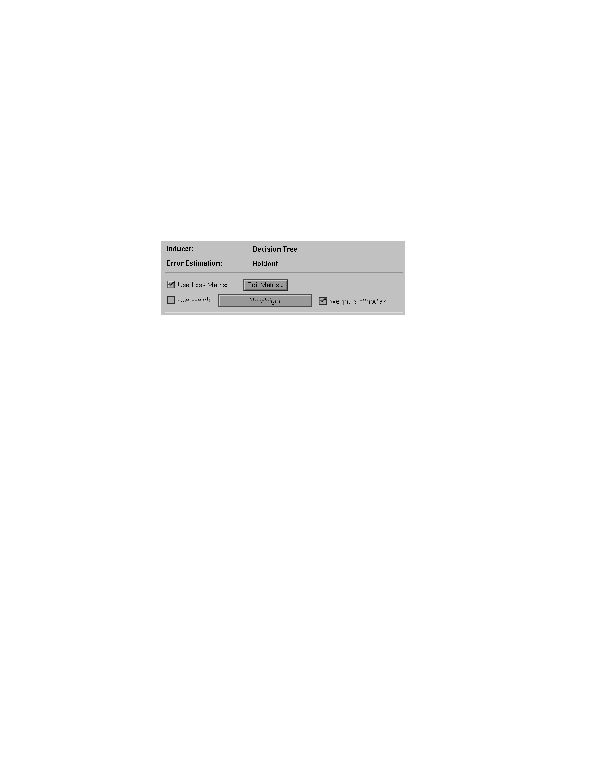
344
Chapter 10: MineSet Inducers and Classifiers
Loss Matrices
The Use Loss Matrix option is a checkmark under Further Options for all inducers (See
Figure 10-24). The Edit matrix button can then be used to define the loss matrix. To avoid
unknowns from being predicted, fill the unknown prediction column with the highest
value in the matrix.
Figure 10-24 Enabling Loss Matrices and Setting the Weight Attribute
Weight Setting
The Use Weight option is a checkmark under Further Options for all inducers (See
Figure 10-24). Choose the column for the weight. The Weight is Attribute option
determines whether the inducer can use this attribute for classification purposes or not.
In certain cases where the weight is a result of a stratified sample that is part of the
experimental design, the classifier should not be given access to the weight column as it
is not a property of the real-word entity.
Learning Curves
Learning Curve is a mode in the Classify menu of the Mining Tools tab. It can be used
with any of the inducers. When the Learning Curve mode is selected, the Further Options
dialog box lets you specify Learning Curve Options (shown in Figure 10-25), including:
•the number of points in the learning curve,
•the number of runs per point, and
•the number of records to use at the start and end points.
The number of records to use at each intermediate point is calculated automatically.

Error Options for Inducers
345
Figure 10-25 Learning Curve Options
The number of points in the learning curve must be specified; also, it must be greater than
or equal to 1. The number of records for the starting and ending points can be specified
to allow generating a learning curve for a specific range of the training set. If either of
these options are left blank, they are calculated automatically based on the number of
points in the learning curve and the total number of records in the training set. This
default covers the entire range of the training set. For instance, assume a file containing
80,000 records. If you specified 3 points in the learning curve, the algorithm generates
points at 20,000, 40,000 and 60,000 records. Often it is useful to “zoom in” on a smaller
range. For example, a learning curve might be generated only for a range of 1000 to
10,000 records.
Generating a learning curve takes a significant amount of CPU time. If tiis the time to
train an inducer on training set i (where i ranges from 1 to the number of points), and
there are k runs per point, the total time is . Increasing the number of runs per
point increases the running time proportionally, but improves the estimate of the
average. The default value of the number of runs is 3.
The Scatter Visualizer’s filter panel can be used to filter some of the data types shown
(average points, confidence intervals, interpolated points, or actual trials). For example,
you might want to remove the data points for the trials and confidence intervals and
show only the averages and interpolated points.
OK and Cancel Buttons
Once you have specified the Classification Options, click OK to have these options take
effect and to return to the Data Destination panel. To return to the Data Destination panel
without having changes to the options take effect, click Cancel.
k*Σti
i

346
Chapter 10: MineSet Inducers and Classifiers
Go! Button
After you have set the options, click the Go! button in the Data Destination panel to run
the inducer. The appropriate visualizer will automatically be launched.
The Status Window
After you press Go! in the Data Destination panel, the Status Window at the bottom of
the Tool Manager’s main window shows the inducer’s progress and the output
classifier’s statistics. It displays specific information for the induced classifier. For
example, for Decision Trees it shows the number of nodes, the number of leaves, and the
depth of the Decision Tree (Figure 10-26). This information is saved automatically on
your workstation under the session file name with a -dt.out, -odt.out, or -eviviz.out
extension, depending on whether a Decision Tree, Option Tree, or Evidence Inducer was
executed.
For Classifier & Error, the first series of dots represent reading the file, then information
about the classifier build progress is shown, then the test set classification progress is
shown.
For Classifier Only mode, there is no test set classification phase.
For Estimate Error, the times and folds are shown.
For Learning curves, each average point on the x-axis will be described on a line and each
run for that average point will be represented by a dot.
Figure 10-26 The Status Window

The Status Window
347
When you have selected the Classifier & Error mode, the Status window contains the
following information:
•The random seed used to split the data into training and test sets.
•The number of records used for training the inducer.
•The number of records used for evaluating the resulting classifier; of the test
records, how many were seen during training, excluding the label attribute. It is
possible to have duplicate records (“seen”) in a dataset; some records can be in both
the training and test set. A large value of seen records indicates that there are many
duplicate records. If their labels are contradictory, it might be impossible to achieve
high accuracy without adding more attributes to the dataset.
•The number of correct and incorrect predictions made.
•The average normalized mean squared error represents the accuracy of the
probability estimates. For each test record, the mean squared error is the square of
one minus the probability estimate for the correct label value, plus the sum of the
squares of the probability estimates for the other (incorrect) label values. The
normalized mean squared error is half the mean squared error, which is a value
between zero and one. The average normalized mean squared error is the
normalized mean squared error averaged over all the records in the test set by their
appropriate weights (weighted average).
•The classification error, which is the percent of incorrect predictions.
•Both the average mean squared error and the classification error show the standard
deviation of the mean and the confidence interval for the mean. This is the range
you can expect from the classifier if the data comes from the same distribution. For
error estimates (not losses), a more accurate formula than the usual two-standard
deviation rule is used.
When you have selected the Estimate Error mode, the Status window contains the
following information:
•The number of cross-validation folds and times.
•The random seed.
•The estimated accuracy with standard deviation.
•The 95% confidence interval for the estimated accuracy.
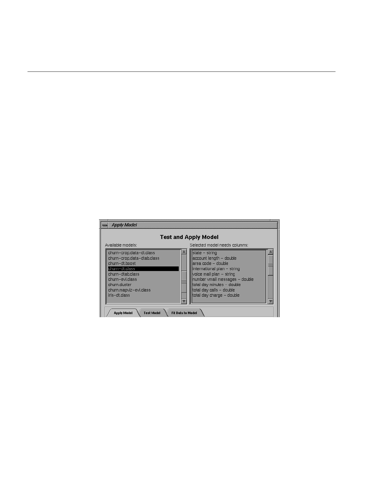
348
Chapter 10: MineSet Inducers and Classifiers
Applying Models, Testing Models, and Fitting New Data
The Apply Model button in the Data Transformations panel lets you:
•take a previously created classifier and apply it to new data.
•test a previously created classifier’s performance on the current table.
•fit the current table into a previously created classifier’s structure.
On the top left of this dialog box (Figure 10-27) is a list of all classifiers currently available
on the server. If you select a classifier, the right-hand side lists the column names and
types required by that classifier. If these requirements match the current table, a message
at the bottom states this, and the buttons on the bottom (OK,Run Test, or Fit Data) is
activated. If the current table does not have all the columns required for the selected
classifier, the message at the bottom states this, the columns that are missing are selected
in the list on the right, and the button on the bottom is deactivated.
Figure 10-27 The Test and Apply Model Dialog Box: Selecting a Classifier
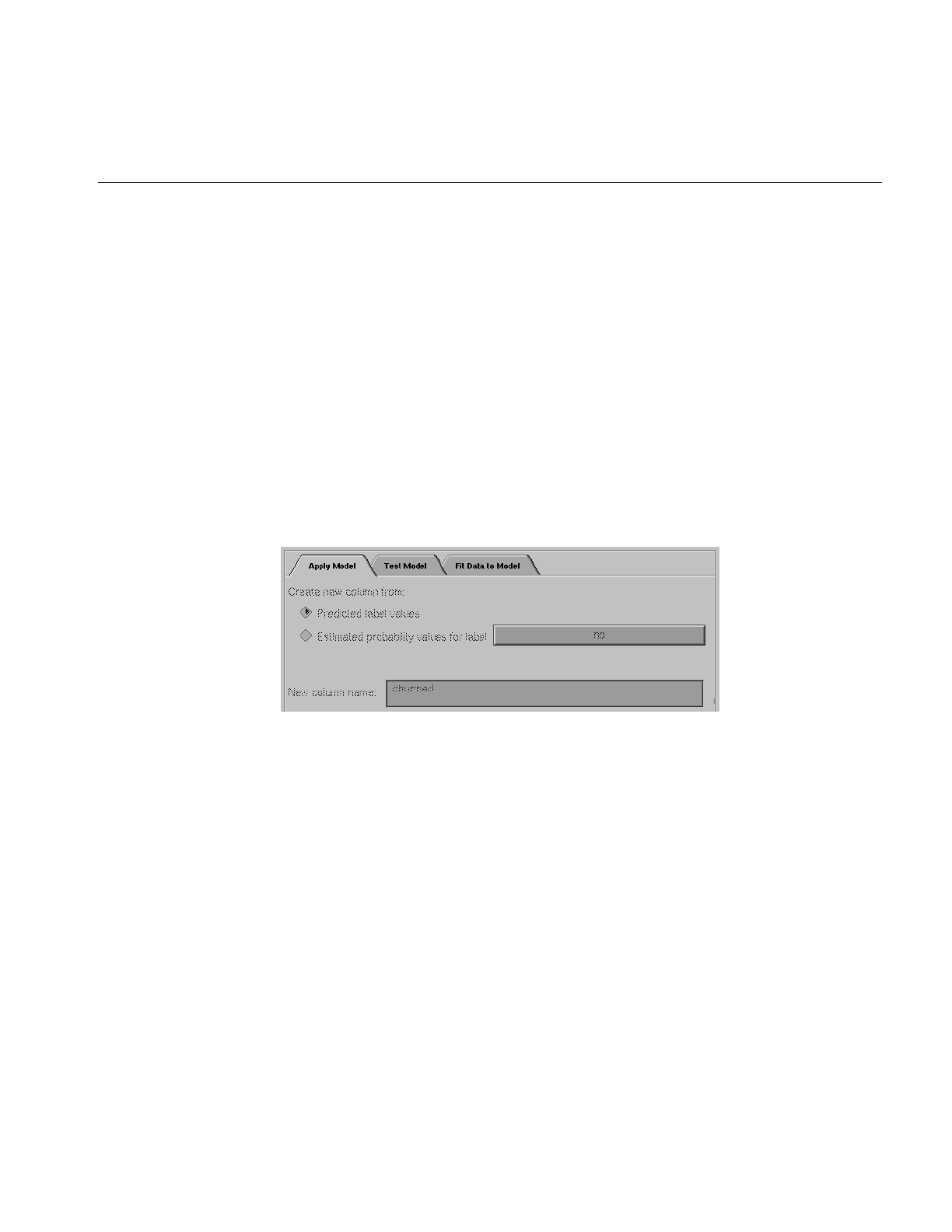
Applying Models, Testing Models, and Fitting New Data
349
Apply Model
The Apply Model panel is used to apply a previously created classifier to the current
table, as shown in Figure 10-28. There are two modes of application for the classifier:
•To Predict discrete label values for the records in the current table. For example, if you
created a classifier to determine churn, you can use this option to add a column that
labels each customer as either likely to churn or not likely to churn.
•To generate Estimated probability values for a specified label value. Instead of using
the classifier to predict the label value of each record, it is used to estimate the
probability that each record has a specified label value (for example, churn = yes).
Given the classifier created to determine churn, you can use this option to add a
column that indicates the probability that each customer is likely to churn.
The New column name text field lets you specify the name of the new column.
Figure 10-28 The Apply Model Panel
Test Model
The Test Model panel is used to test a previously created classifier on the current table,
as shown in Figure 10-29. The table must contain columns with the names and types
required by the selected classifier. Unlike Apply Model, Test Model also requires the
table to contain a label column with the same name and type as the label column used
when building the classifier.
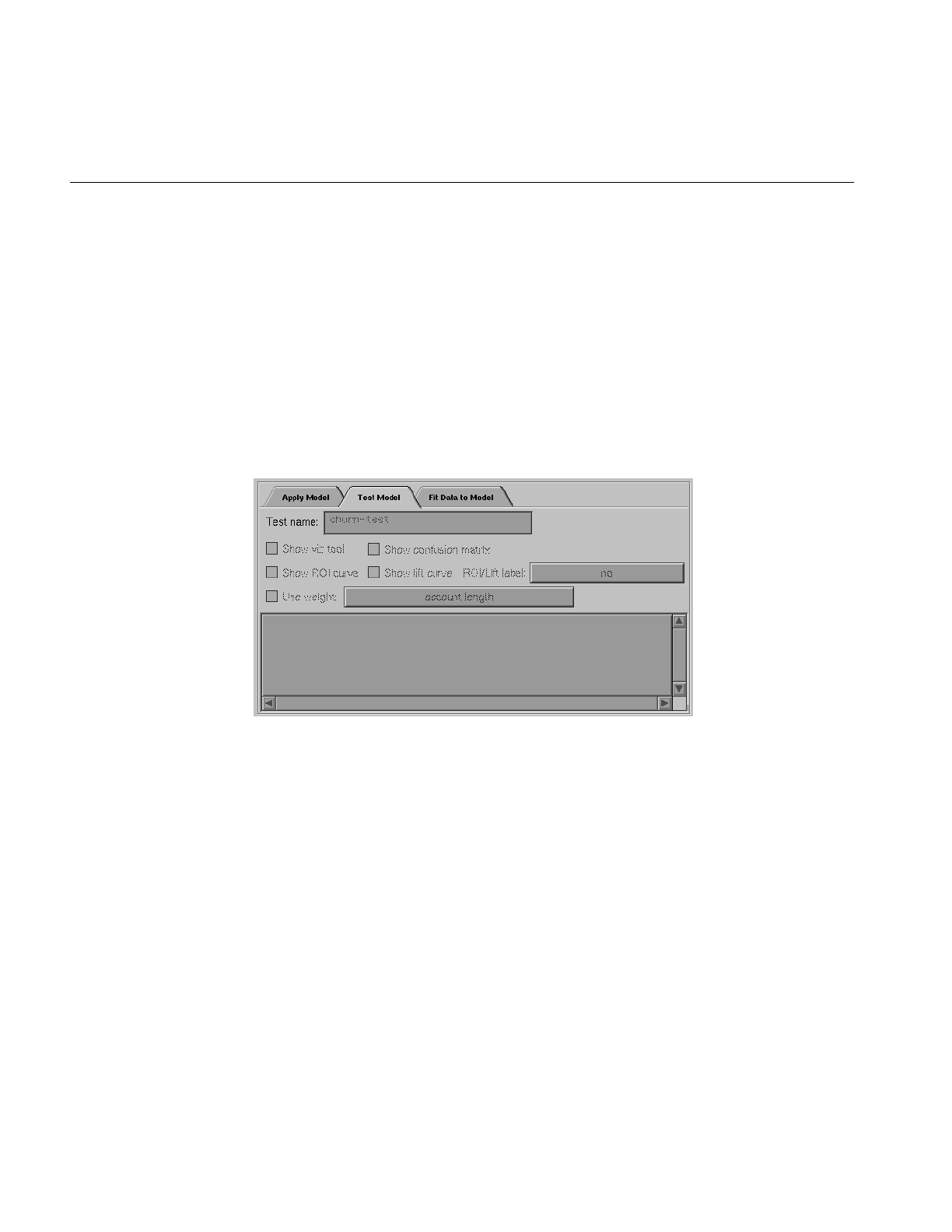
350
Chapter 10: MineSet Inducers and Classifiers
The Test Model panel has options that lets you
•show the confusion matrix of the classifier on the table records
•show the lift curve of the classifier for a specified label value
•show the ROI curve of the classifier for a specified label value
•show a visualization of the classifier with the table used as the test-set (this is only
relevant for Decision Tree and Option Tree classifiers)
•select an attribute to use as the record weight
The text field at the bottom of the Test Model panel shows the results.
Figure 10-29 The Test Model Panel
Fit Data to Model
The Fit Data to Model panel is used to fit the data in the current table to a previously
created classifier, as shown in Figure 10-30. This produces a new classifier with the same
structure as the original one; however, the new one uses the data from the table to update
the probability estimates (see “Backfitting in Error Estimation” on page 328). Because all
of the data from the table is being fit into the structure of the classifier, there is no error
estimation. Fit Data to Model cannot be used on classifiers that were built using boosting.
Use Test Model to evaluate the performance of the new classifier on a separate test set
(disjoint from the fit data).
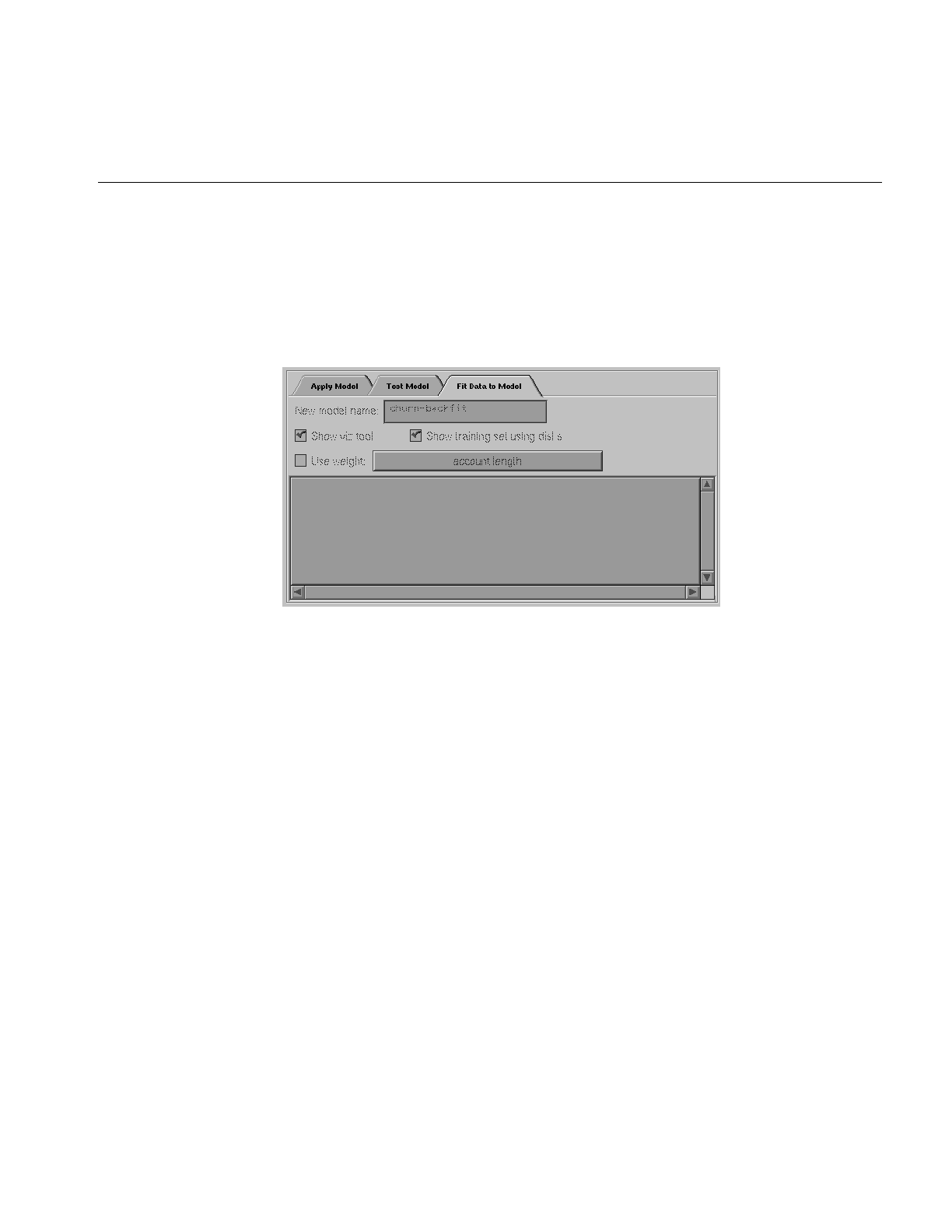
Special Options and Limitations
351
The Fit Data to Model panel has options that lets you
•show a visualization of the new classifier
•specify a name for the new classifier
•select an attribute to use as the record weight
Figure 10-30 The Fit Data to Model Panel
Special Options and Limitations
The following subsections describe how to set special options and the limitations of the
inducers.
Setting Special Options
When the Tool Manager runs an inducer on the server (the MIndUtil program), it passes
certain options to the inducers. Not all options are controlled through the Tool Manager
GUI. Those options not controlled by Tool Manager take on their default values and can
be overridden by setting them in a special file, called .mineset-classopt. Tool Manager
prepends this file to the options sent. This file is optional. Tool Manager looks for it first
in the current directory, then in your home directory. See Appendix I, “Command-Line
Interface to MIndUtil: Analytical Data Mining Algorithms” for more details about the
options.

352
Chapter 10: MineSet Inducers and Classifiers
The file should contain one line per option, in the following format:
<OPTION>=<value>
For example, the special option LOGLEVEL increases the amount of information shown
during the induction process. The default of zero shows very little information. Level 1
shows other options and slightly more information. Level 2 and higher show large
amounts of information about the induction process. These levels are appropriate only if
you have a firm understanding of the induction process. (See Appendix K, “Further
Reading and Acknowledgments.”)
Note that these options are not part of the saved session. If you send files to other users,
you might have to send this file separately to them.
Default Limits and How to Override Them
Three limits and their respective options are as follows:
•Discrete attributes are ignored if they have more than 100 values. Discrete attributes
with many values are usually inappropriate for classification. For example, first
names and street addresses are unlikely to form predictive patterns.
To speed up the induction process, attributes with over 100 values are ignored.
You can override this value by setting MAX_ATTR_VALS to a higher number. For
example, your .mineset-classopt file could contain the line
MAX_ATTR_VALS=500
•Discrete labels with over 25 values are not allowed by default. Automatically
induced classifiers are rarely appropriate for predicting one of a large number of
label values. You should limit the label to a few values (preferably two or three).
You can override this default limit by setting the option MAX_LABEL_VALS to a
higher value in your .mineset-classopt file.
•Boosting works by repeatedly assigning new weight distributions to the training set
and inducing classifiers on the reweighted sets. The number of times this occurs is
limited by the BOOST_NUM_TRIALS option, which can be set by the
.mineset-classopt file on the client. The number of classifiers generated may be lower
than this parameter if the training set error rate drops to zero before this many
classifiers are generated.

Special Options and Limitations
353
Other Limitations
There are three further limitations:
•Floating point numbers are read into MIndUtil as floats (4 bytes) even if they are
represented as doubles (8 bytes) in the database, in the ASCII file, or in the binary
file. This limits the precision and magnitude of the representations allowed.
•Attributes of type arrays are always ignored.
•Dates are considered strings. Unless there are few dates, such attributes are usually
ignored because of the limit on discrete attributes. You should bin dates before
running an inducer.


355
Chapter 11
11. Inducing and Visualizing the Decision Tree Classifier
This chapter discusses the features and capabilities of the Decision Tree Inducer. Its
associated visualizer, the Tree Visualizer, is described in Chapter 5. This chapter provides
an overview of this tool and discusses the ways of using it to generate Decision Tree
classifiers. It then explains the Tree Visualizer’s functionality when working with the
main window. Finally, it lists and describes the sample files provided for this tool.
Note: It is assumed that you have read Chapter 10, “MineSet Inducers and Classifiers,”
before proceeding with this chapter.
Overview
A Decision Tree classifier assigns each record to a class. The underlying structure used
for classification is a Decision Tree, such as the one shown in Figure 11-1.
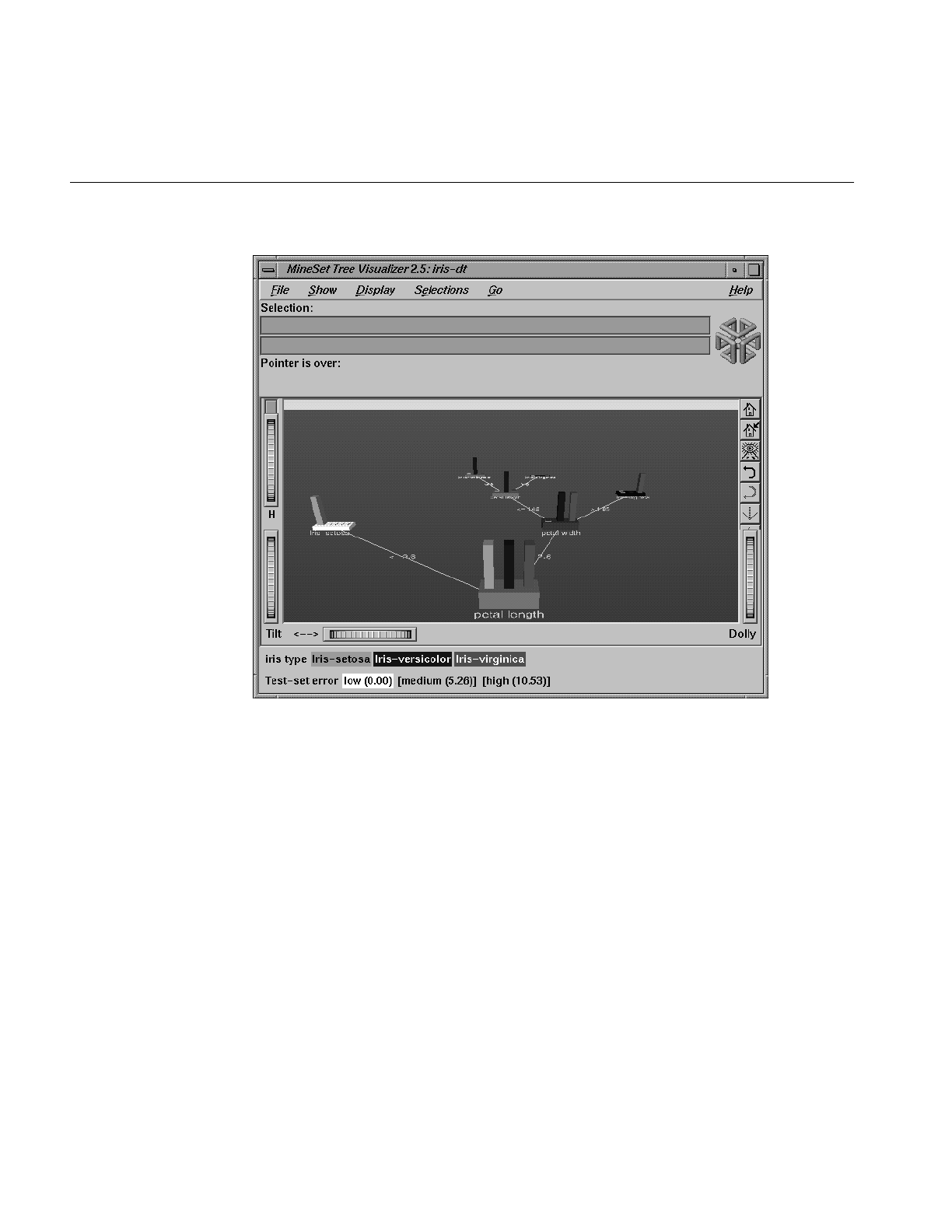
356
Chapter 11: Inducing and Visualizing the Decision Tree Classifier
Figure 11-1 Decision Tree for the Iris Dataset
Inducing Decision Trees
A Decision Tree classifier is induced (generated) automatically from data. The data,
which is made up of records and a label associated with each record, is called the training
set (see Chapter 10, “MineSet Inducers and Classifiers”).

File Requirements
357
File Requirements
The Decision Tree Inducer requires a training set, as described in the “Training Set” in
Chapter 10. Files are generated by extracting data from a source (such as a MineSet ASCII
or binary file, or a table in an Oracle, INFORMIX, or Sybase database). To apply the
generated classifier, you should have a dataset of records with the attributes used by the
classifier, except that the label need not be present.
Running the Decision Tree Inducer
There are two ways to run the Decision Tree inducer:
•From the Tool Manager.
Connect to the server and select a data source (see “Choosing a Data Source” in
Chapter 3).
From the File menu, choose Open New Data File. Log in to a server, and enter the
filename. For the example shown here, the filename entered would be
/usr/lib/MineSet/data/iris.schema as the filename. You’ll see four continuous
attributes and one discrete attribute in the Data Transformation panel. Since there is
only one discrete attribute, the label option automatically shows it. Select the
Decision Tree inducer, and ensure you have selected the Classifier & Error mode. To
run the Inducer, click Go!.
The status window will show the progress, statistics, and the Tree Visualizer will be
launched automatically.
•From the command line.
To induce a Decision Tree classifier from the command line, refer to Appendix I,
“Command-Line Interface to MIndUtil: Analytical Data Mining Algorithms.”
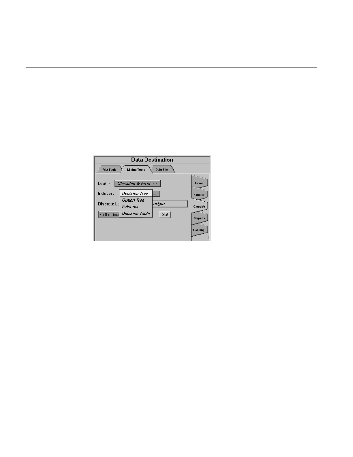
358
Chapter 11: Inducing and Visualizing the Decision Tree Classifier
Configuring the Decision Tree Inducer Using the Tool Manager
To access the options for configuring the Decision Tree inducer, select the Mining Tools
tab on the Data Destination panel (Figure 11-2). From the tabs at the right, select Classify.
Ensure that the inducer you select is Decision Tree (the default). Your selections in the
Mode and Inducer menus determine the options available in the Further Inducer
Options menu. After you have made your selections in these menus, click Go! to run the
inducer, which, in turn, creates the classifier.
Figure 11-2 Data Destination Panel in Tool Manager Showing Classifiers
Discrete Labels
The Discrete Labels menu provides a list of possible discrete labels. Discrete attributes
(binned values, character string values, or a few integers) have a limited number of
values. You should select a label attribute with few values; for instance, two or three (see
“Training Set” in Chapter 10). If there are no discrete attributes, the menu shows No
Discrete Label, and the Go! button is disabled. You then must create a discrete attribute by
binning or adding a new column using the Tool Manager’s Data Transformations panel.

Configuring the Decision Tree Inducer Using the Tool Manager
359
Classifier Name
The generated classifier is named with the prefix of the session filename (as determined
in Tool Manager) and the suffix-dt.class. By default, all classifiers are stored on the server
in the file_cache directory, which defaults to mineset_files. These classifiers can be used for
future classification of unlabeled records; that is, they can be used to predict the labels for
unlabeled datasets (see “Applying a Model” and “Backfitting in Error Estimation” in
Chapter 10).
Parallelization
If you have installed the multiprocessor version of MineSet, it is possible to compute
tree-based algorithms in parallel whenever a branch contains over 1000 records. Each
node on the tree estimates the best possible split on the corresponding level, and these
tasks are performed in parallel. The maximum number of threads a program can spawn
is determined automatically by default. You can control the number of threads by
changing the parallelization mode in the Preferences panel of Tool Manager (see“The File
Menu” in Chapter 3). Parallelization may cause memory fragmentation, causing the
largest data sets that can be computed in parallel to be smaller than the largest data sets
that can be computed on a uniprocessor.
Decision Tree Options
Selecting Further Classifier Options causes the Classifier Options dialog box
(Figure 11-3) to appear. This dialog box consists of four panels:
•The top panel indicates the choices you made in the Tool Manager’s Data
Destination panel.
•The second pane from the top lets you set the loss matrix and the weight attribute.
See “Loss Matrices” and “Weight Setting” in Chapter 10.
•The bottom-left panel lets you specify further Inducer Options.
•The bottom-right panel lets you specify the Error Estimation Options (unless the
mode you chose in the Data Destination panel was Classifier Only, in which case
this area is empty). The options shown in this panel depend on the type of Error
Estimation you chose (see “Applying Models, Testing Models, and Fitting New
Data” in Chapter 10).

360
Chapter 11: Inducing and Visualizing the Decision Tree Classifier
Figure 11-3 Further Inducer Options
Decision Tree Inducer Options
To fine-tune the Decision Tree induction algorithm, you can change the following
Decision Tree inducer options (see Figure 11-3).

Configuring the Decision Tree Inducer Using the Tool Manager
361
•Limit tree height by
By default, there is no limit to the height (number of levels) in the Decision Tree.
Limit the height by clicking the checkbox and typing a number for the limit.
Limiting the number of levels speeds up the induction and is useful for studying
the Decision Tree without the distraction of too many nodes. Note that restricting
the size decreases the run time but might increase the error rate. Setting this option
does not affect the attributes chosen at levels before the maximum level.
•Splitting criterion
This option offers three splitting criteria selections. The definitions below are
technical. For a given problem, it is difficult to know which criteria will be best. Try
them all, and select the one that leads to the lowest error estimate - or to a Decision
Tree you find easiest to understand.
Mutual Info is the change in purity (that is, the entropy) between the parent node and
the weighted average of the purities of the child nodes. The weighted average is
based on the number of records at each child node.
Normalized Mutual Info (the default) is the Mutual Info divided by the log (base 2) of
the number of child nodes.
Gain Ratio is the Mutual Info divided by the entropy of the split while ignoring the
label values.
Normalized Mutual Info and Gain Ratio give preference to attributes with few values.
•Split lower bound
This is a lower bound on the weight (normally the number of records if weight was
not set) that must be present in at least two of the node’s children. The default for
this option is 2. For example, if there is a three-way split in the node, at least two out
of the three children must have a weight of two or more (two records or more if
weight is not set). This provides another method of limiting the size of the Decision
Tree.
Increasing the split lower bound tends to increase the reliability of the probability
estimates, because the number of records at each leaf is larger. It also creates smaller
trees and decreases the induction time. If you expect the data to contain noise
(errors or anomalies), or if you use the tree for estimating probabilities (see
“Applying a Model” in Chapter 10), increase the split lower bound to 5 or more. If
your dataset is very small (< 100 records), you might want to decrease this number
to 1.

362
Chapter 11: Inducing and Visualizing the Decision Tree Classifier
•Pruning factor
A Decision Tree is built based on the limits imposed by Limit Tree Height and Split
Lower Bound. Statistical tests are then made to determine when some subtrees are
not significantly better than a single leaf node in which case those subtrees are
pruned.
The default pruning factor of 0.7 indicates the recommended amount of pruning to
be applied to the Decision Tree. Higher numbers indicate more pruning; lower
numbers indicate less pruning. If your data might contain noise (errors or
anomalies), increase this number to create smaller trees. The lowest possible value is
0 (no pruning); there is no upper limit.
Pruning is slower than limiting the tree height or increasing the split lower bound
because a full tree is built and then pruned. Pruning, however, is done selectively,
resulting in a more accurate classifier
•Boosting
Boosting is employed to improve accuracy of classification, although it is a
time-intensive process. Visualization is not performed during boosting.
The estimated error appears in the status window, as the process runs. This
estimated error is the result of the algorithm repeatedly assigning new weight
distributions to the training set, and inducing a classifier on the reweighted sets.
Estimating error in this manner is normally done after you have done a
visualization to gain insight into the dataset. See “Boosting: Accuracy is Sometimes
Crucial” in Chapter 10 for more information on boosting.
•Allow one-off splits
Clicking this checkbox allows the inducer to make two-way splits on nominal
attributes that have more than two values. Normally, splits on nominal attributes
have as many lines as they have values (see the section on Decision Nodes, below).
For example, a split on the attribute “color” might have lines for red, green, yellow,
and blue. If one-off splits are enabled, then the inducer can also make splits with
just two lines, for example red, and not red. One-off splits isolate exactly one of the
possible values that the column can have. These kinds of splits may be useful when
the data contains attributes with many possible values, some of which are
exceptionally good at discriminating the label.

Working in the Tree Visualizer’s Main Window
363
Working in the Tree Visualizer’s Main Window
The Tree Visualizer’s main window shows the Decision Tree. This Decision Tree consists
of nodes connected by lines (see Figure 11-1).
Nodes
There are two types of nodes:
•decision
•leaf
Decision Nodes
Decision nodes specify the attribute that is tested at the node. Values (or ranges of values)
against which the attributes are tested are shown at the lines. Each possible value for the
attribute matches exactly one line. For example, the root of the Decision Tree in
Figure 11-1 tests the attribute petal_length; the two lines emanating from the node
specify the ranges of values for that attribute (< = 2.6 and >2.6,) so that every possible
value matches either the right branch or the left branch. If the value is unknown and
there is no line labeled with a question mark (?), the majority class of the current node is
predicted.
Leaf Nodes
Leaf nodes in a Decision Tree specify a class. Follow the left branch in Figure 11-1 from
the root to a leaf labeled iris-setosa. Note that the Decision Tree classifier classifies all
records with petal_length < = 2.6 inches as belonging to the class iris-setosa.
Node Information
The vertical bars atop each node show the distribution of the classes at the node. The base
of each node has a height and a color. The height corresponds to the weight of the
training set records that have reached this node (this is the number of records if weight
was not set). In general, the higher the weight, the more reliable the class distribution at
every node.

364
Chapter 11: Inducing and Visualizing the Decision Tree Classifier
The color of the base indicates the error estimate of the subtree: indigo shows high error,
grey indicates medium, white indicates low error. The color of the base is black if no test
set records reached a node; thus, there is no error estimate.
Pointing to a node causes the following information to be displayed:
•Subtree weight — The weight of the training set records in the subtree below the
node pointed to. This value is mapped to the height of the base.
•Test set error/loss — An estimate of the subtree error (or loss if a loss matrix was
given). The number after the +/- is the standard deviation of the estimate. The
higher the standard deviation, the less accurate the error estimate. The error/loss
estimate and the standard deviation are less reliable for leaves with few records or
when the test set error is close to 0% or 100%.
•Test set weight — The weight of records from the test set that reached the node
(number of records if weight was not set).
•Purity — A number from 0 to 100 indicating the skewness of the label value
distribution at the node. If a node has records from a single class, the purity is 100. If
the label values have the same weight, the purity is 0. The purity is computed after
backfitting.
When backfitting is enabled and Display training set as disks checked on, the vertical bars
show the distribution of the training set as disks. The heights of the disks are on the same
scale as the heights of the bars. You should expect the disks to appear about as high on
the bars as the value used for the Holdout ratio in Further inducer options.
Note that only Classify & Error yields the test set error/loss and weight. You can use the
Test Classifier option (see “Applying Models, Testing Models, and Fitting New Data” in
Chapter 10) to generate a visualization based on an existing classifier and a test set.
Lines
All possible outcomes are marked on the horizontal lines emanating from each decision
node. Each line indicates the value (or range of values) against which the attribute of that
node was tested.

External Controls
365
Using the Main Window to Classify Records
To classify a record, start at the root, and test how to branch at every decision node. By
following the appropriate lines based on the record’s attribute values, you reach a leaf
node. The label, or class, associated with the leaf node is the predicted classification of
the record.
Some decisions are quickly made and take a shorter path (for example, petal_length
<=2.6 implies iris-setosa). Other decisions can take a longer path (for example, the right
branches, petal_length > 2.6 and petal_width > 1.65). In general, every leaf corresponds
to a rule that is the conjunction of all tests at the decision nodes and all the values (or
ranges of values) on the lines leading to it from the root.
In the root of the tree shown in Figure 11-1, the error rate is 6%, with a standard deviation
of 3.39%. The standard deviation is high because the file is small, and the test set only has
50 records. The purity is 0.0, indicating that the distribution is uniform.
The left child of the root has 0 test set error and a purity of 100 because all records with
petal_length <=2.6 inches are of the iris-setosa class; thus, the prediction of iris-setosa is
likely to be very accurate for all records with petal_length <=2.6 inches. The right child
of the root has an estimated error of 8.57%. In this child, which matches records whose
petal_length > 2.6 inches, there are no records belonging to the iris-setosa class; thus, the
class is more likely to be iris-versicolor or iris-virginica. Because only two possibilities
exist at this node, there is a higher purity than at the root (36.91).
The Decision Tree leaves segment the data into clusters sharing the same classification
rule (path that leads to each leaf). By looking at the leaves, it is possible to see clusters
that share the same set of properties.
External Controls
The external controls for the visualizer associated with the Decision Tree classifier are the
same as those for the Tree Visualizer. For a description of these controls, see “External
Controls” in Chapter 5.
One particularly useful control for decision trees is to click the right mouse button when
pointing to a node. This shows the list of children of that node.
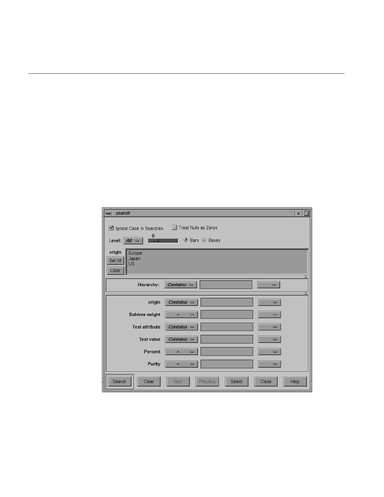
366
Chapter 11: Inducing and Visualizing the Decision Tree Classifier
Pulldown Menus
The pulldown menus for the visualizer associated with the Decision Tree classifier are the
same as those for the Tree Visualizer. For a description of these menus, see “External
Controls” in Chapter 5.
The Search and Filter Panels
Select Search Panel and Filter Panel in the Show menu to bring up a dialog box that lets
you specify criteria to search/filter for objects (Figure 11-4). The panels are the same ones
described in “The Search Panel” in Chapter 5; however, the item choices for decision
trees are always the same. These are described below.
Figure 11-4 Tree Visualizer’s Search Dialog Box

Pulldown Menus
367
The search/filter can be restricted to specific class labels, either by selecting the values in
the class list or by using the class item, which allows more powerful comparison
operators (such as Matches). Other items are described below:
•Subtree weight lets you restrict the search/filter to bars or bases (depending on the
choice of the radio button bars/bases) with a given weight (number of records if
weight is not set) for the subtree. For example, you can restrict the search to bars
containing a weight of at least 50.
•Test attribute lets you restrict the search/filter to nodes labeled by the given value
that the node is testing. Note that decision node labels represent the test attribute,
while leaf node labels show the predicted label. For example, if you select Test
attribute contains age, only nodes that test the value of age are considered.
•Test value lets you restrict the search/filter to nodes having an incoming line labeled
with a value you specify.
•Percent lets you restrict the search/filter to bars representing a percentage of the
overall weight at a node. For example, you might want to find all nodes such that a
given class accounts for more than 80 percent of the weight. To do this, click the
class label, and select Percent > 80. Setting this item is meaningless if you select
bases and not bars (the value for the bases is 0).
•Purity lets you restrict the search/filter to nodes with a range of purity levels. For
example, if you want to look at pure nodes (with one class predominant), you can
select Purity > 90.
•Test-set subtree weight lets you restrict the search/filter to subtrees with a given
test-set weight (number of test-set records if weight is not set).
•Test set error/loss lets you restrict the search/filter to nodes with a range of estimated
error/loss.
•Mean error/loss standard deviation lets you restrict the search/filter to nodes with a
range of estimated standard deviation for the test set error/loss.
•Level lets you restrict the search/filter to a specific level or range of levels. For
example, you can search only the first five levels.
The following items and options are less useful for decision trees.
•Hierarchy finds all the nodes and lines that match the given value at the tail of the
path from the root. It then marks the children of these nodes.
•Treat Nulls as Zeros is not used by the Decision Tree inducer because there are no null
items generated for decision trees.

368
Chapter 11: Inducing and Visualizing the Decision Tree Classifier
Once the search is complete, yellow spotlights highlight objects matching the search
criteria. To display information about an object under a yellow spotlight, move the
pointer over that spotlight; the information appears in the upper left corner, under the
label “Pointer is over:.” To select and zoom to an object under a yellow spotlight,
left-click the spotlight; if you press the Shift key while clicking, zooming does not occur.
Once the filtering is complete, the scene shows only nodes matching the filtering criteria.
Sample Files
The following examples illustrate cases in which the Decision Tree inducer can be useful.
Each of these examples is associated with a sample data file provided with MineSet. By
running the inducer, you can generate the -dt.treeviz files described below.
Note: The data files, which have a .schema extension, are located in /usr/lib/MineSet/data
on the client workstation. The classifier visualization files, which have a -dt.treeviz
extension, reside on the client workstation in /usr/lib/MineSet/treeviz/examples.
Churn
When customers change their phone carrier from one telecommunications company to
another, this is termed “churning.” This is a common problem in the telecommunications
industry. The file /usr/lib/MineSet/treeviz/examples/churn-dt.treeviz shows a Decision Tree
classifier induced for this problem. The file was generated by running the inducer on
/usr/lib/MineSet/data/churn.schema with the label set to churn (yes, no). The file given is
fictitious, but based on patterns found in real data.
Note that in this tree the root split is on the amount of time the customers talk during the
day (total day minutes). Customers who talk more than 264 minutes per day churn at a
significantly higher rate than those who don’t (60% versus 11%). These also are probably
the most profitable customers.
The left subtree represents customers who talk less than 264 minutes per day. They have
a churn rate of 11%; but if they make more than three customer service calls, the churn
rate increases to 49%.
The right subtree represents customers who talk over 264 minutes per day. They have a
churn rate of 59%; but if they have a voice-mail plan, the rate decreases to 9.3%. If they
do not have a voice-mail plan, the churn rate is almost 75%.

Sample Files
369
Origin of Cars
The cars dataset contains information about different models of cars from the 1970s and
early 1980s. Attributes include weight, acceleration, and miles per gallon (mpg). The file
/usr/lib/MineSet/treeviz/examples/cars-dt.treeviz shows the Decision Tree classifier induced
for this problem. This file was generated by running the inducer on
/usr/lib/MineSet/data/cars.schema with the label set to origin (Japan, U.S., Europe). If you
have a dataset of car attributes, you might want to know what characterizes cars of
different origins.
Note that in the tree the left split is on brand. The root split is not brand because the
Decision Tree inducer penalizes multi-way splits; and the split on cubic_inches was
deemed a better discriminator. You can use the Tool Manager Remove Column
transformation to hide the brand, thus making the problem more interesting.
In the Decision Tree, you can see that cubic inches is an excellent discriminator for
U.S.-made cars. Cars with large engines (>169.5 cubic inches) are all made in the U.S., but
smaller cars are made everywhere. By choosing Selections > Show Original Data, you can
see that the one car with a big engine that was not made in the US is a Mercedes. Note
that in this tree, the root node (that is, the entire training dataset) has many more U.S. cars
(62.50%), yet after a single split on the cubic inches attribute, it is more difficult to predict
the origin of cars with small engines. The purity of the root is 16.2 showing that there is
one class (U.S., in this case) that is dominant. The right node (cubic inches > 169.5) has
purity 96.81, indicating that we have identified a very pure subpopulation (almost all
cars with large engines were made in the U.S.). Indeed, the error rate for the right subtree
is estimated at 0% (green base). The left node from the root has purity 0.23 and a much
higher error rate of 31.25% (orange base). This subproblem is much harder than the
original one: the number of records for each class is approximately the same.
Gender Attribution
The adult dataset contains information about working adults. This dataset was extracted
from the U.S. Census Bureau. It contains data about people older than 16, with a gross
income of more than $100 per year who work at least one hour a week. You might want
to know how to characterize males and females. The file
/usr/lib/MineSet/treeviz/examples/adult-sex-dt.treeviz shows the Decision Tree classifier
induced for this problem. This file was generated by running the inducer on
/usr/lib/MineSet/data/adult.schema, with the label set to sex. Note that this dataset contains
almost 50,000 records; thus, running the Decision Tree Inducer can take several minutes
when you run this on your workstation.

370
Chapter 11: Inducing and Visualizing the Decision Tree Classifier
The resulting visualization provides the following insights:
•Relationship is a giveaway attributes for some values. Husbands usually are male.
(Interestingly, there is one husband that is a female, showing data quality problems
at the Census Bureau, which does not recognize same-sex marriages.) Similarly, if
the person is a wife, the person is usually a female, except for three records that
show otherwise.
To make the problem more interesting, remove the relationship attribute and generate a
new Decision Tree. Note that
•The most important attribute is marital status.
•From the height of the bases, most people are either divorced, married to a civilian
spouse, or never married. Few are married with spouse absent, separated, married
to armed-forces spouse, or widowed.
•The distribution at the root shows more males in this dataset. (This database
contains information about working adults and is not representative of the entire
population.)
•The left-most node contains divorced working adults. We can see that the
distribution is more balanced than at the root (60% female, 40% male). The second
node contains married working adults. We can see that 89% are males. The third
node contains working adults that have never married. Their numbers are
approximately equal to those in the divorced group, with slightly more males. The
right-most node contains working widowed adults, of which 81% are females
(probably because of their higher life expectancy).
If you want to target working females for a new product, you can use the search panel to
identify segments that have a large population of females. You can do this by choosing
•sex matches female (click female on the top portion of the window).
•subtree weight > 1000
•percent > 80
Three yellow spotlights show the matching nodes. Since two are on one path, look at the
node closest to the root (on the right). The paths translate into the rules
marital status = Widowed implies that 81.23% are female
marital status = Divorced and occupation =
administrative clerical implies that 87.67% are female
In this training set, 1233 (widowed) and 1045 (divorced and occupation) females satisfy
these rules out of 16,192 at the root. This simple segment contains over 14% of working
women.

Sample Files
371
Salary Factors
If you have a dataset of working adults, you might want to find out what factors affect
salary. You might then divide the records into two classes: those adults earning ≤ $50,000
a year, and those earning more. Each record then has an attribute with two values: “−
50,000” and “50,000+”. You can run a MineSet classifier to help determine what factors
influence salary. The file /usr/lib/MineSet/treeviz/examples/adult-salary-dt.treeviz shows the
Decision Tree classifier induced for this problem. This file was generated by running the
inducer on /usr/lib/MineSet/data/adult.schema with gross_income binned at the
user-specified threshold of 50000 and the label set to gross_income_bin.
The resulting visualization provides the following insights:
•The root, which represents the entire training set, shows 76.07% of the working
adults earn ≤$50,000.
•Age is the most important factor. Only 3.07% of the people under 27 years old earn
more than $50,000. Note that the base color is green, indicating a very accurate rule
(about 3% error rate).
•Education is an important factor for predicting salary for people over 27 years old.
The Census Bureau assigns education levels to each person. The Decision Tree
classifier splits on 12.5; the level 13 matches a Bachelor’s degree. People with a
Bachelor’s degree or higher, go right to the node where about 55% earn over
$50,000.
•Of the segment that is older than 27 years and well educated, relationship is an
important predictor of salary. For those persons that are married, chances of earning
$50,000 or more increase to 73% for husbands and 75% for wives. (Note, however,
that the node containing wives has a small base, indicating that few females match
this rule.) If the person in this group is not married, chances of earning $50,000 or
more decrease to 27% for males and 25% for females.
Iris Classification
In this dataset, each record describes four characteristics of iris flowers: petal width, petal
length, sepal width, and sepal length. Each iris was further classified into the types
iris-setosa, iris-versicolor, or iris-virginica. The goal is to understand what characterizes
each iris type.
Before running a classifier, click the Importance tab in the Tool Manager’s Classifiers tab;
then click Go!. You obtain a ranking of the importance of the features: petal_width,
petal_length, and sepal_length. You can map these to the axes in the Scatter Visualizer,
with the iris_type mapped to the color, and see the clusters.

372
Chapter 11: Inducing and Visualizing the Decision Tree Classifier
The file /usr/lib/MineSet/treeviz/examples/iris-dt.treeviz shows the Decision Tree classifier
induced for this problem. This file was generated by running the inducer on
/usr/lib/MineSet/data/iris.schema.
Running the Tree Visualizer, you can see that the root has 6% error rate, even though the
purity is very low (0). The purity measures the skewness of the distribution, and, at the
root, the distribution is perfectly uniform: 50 records for each label value. The left branch
(petal-length <= 2.6 inches) goes to a green node (zero error) containing only iris-setosas.
The other branches are also quickly able to separate the classes using another test on the
petal_width. The path petal-length > 2.6 and petal-width £ 1.65 and petal-length > 5 ends
with an impure leaf containing 4 records. There are three records of type iris-virginica
and one of iris-versicolor. The Decision Tree did not split this node because it was
deemed insignificant (by default, every split must contain two children with at least a
weight of two). The node color is also black, indicating that no test instances reach this
node, so we do not have an estimated error rate for it.
To summarize: the flowers with petal length £ 2.6 inches are predicted as iris-setosa,
those with petal length > 2.6 inches and <=5 inches and petal width £1.65 inches are
predicted as iris-versicolor, and those with a petal length >2.6 inches and a petal width >
1.65 or petal length > 5 inches and petal width <= 1.65 are predicted as iris-virginica.
Note that because the Decision Tree makes binary splits on continuous attributes while
Column Importance discretizes the data, the root split of the tree is different from the first
attribute in column importance (see Chapter 17 for more details).
Mushroom Classification
The file /usr/lib/MineSet/treeviz/examples/mushroom-dt.treeviz shows the Decision Tree
classifier induced for the classification of mushrooms. This file was generated by running
the inducer on /usr/lib/MineSet/data/mushroom.schema.
The goal is to understand which mushrooms are edible and which are poisonous, given
this dataset. There are over 8000 records in this set; thus, running this inducer might take
several minutes.
Each mushroom has many characteristics, including cap color, bruises, and odor. If you
build a Decision Tree classifier, you can see that using only the odor attribute lets you
determine in 50% of the cases whether the mushroom is poisonous or edible. If the
mushroom has no odor, there is a 3.4% chance it is poisonous. The next attribute to look
at is the shape of the stalk. If it tapers, the mushroom is edible; but if it enlarges, there is
a 11.6% chance the mushroom is poisonous. There are 1032 mushrooms that reach this
node. You can follow the tree down further nodes to see what other attributes to consider.

Sample Files
373
Party Affiliation
This dataset consists of voting records. The goal is to identify the party a congressperson
belongs to given data about key votes. The dataset includes votes for each member of the
U.S. House of Representatives on the 16 key votes identified by the Congressional
Quarterly Almanac (CQA). The CQA lists nine types of votes: voted for, paired for, and
announced for (these three are simplified to yes); voted against, paired against, and
announced against (these three are simplified to no); voted present, voted present to
avoid conflict of interest, and did not vote or otherwise make a position known (these
three are simplified to an unknown disposition).
Before running a classifier, look at the 16 votes to see if you can perceive which features
are important. Then run the Decision Tree classifier.
The file /usr/lib/MineSet/treeviz/examples/vote-dt.treeviz shows the Decision Tree classifier
induced for this problem. This file was generated by running the inducer on
/usr/lib/MineSet/data/vote.schema.
Breast Cancer Diagnosis
The breast cancer dataset contains information about females undergoing breast cancer
diagnosis. Each record is a patient with attributes such as cell size, clump thickness, and
marginal adhesion. The final attribute is whether the diagnosis is malignant or benign.
The file /usr/lib/MineSet/treeviz/examples/breast-dt.treeviz shows the Decision Tree classifier
induced for this problem. This file was generated by running the inducers on
/usr/lib/MineSet/data/breast.schema.
The Decision Tree shows that uniformity_of_cell_size is a very strong discriminatory
attribute. While the root distribution is about 65% versus 35% (purity is 7.07), the two
children of the root are much more skewed, with the left node having an error rate of only
1.29%. The root alone is an excellent discriminator: if you limit the tree height to a single
level (see “Decision Tree Inducer Options”), the error rate is 7.3%.
Hypothyroid Diagnosis
The hypothyroid diseases dataset is similar to the one for breast cancer. The file
/usr/lib/MineSet/treeviz/examples/hypothyroid-dt.treeviz shows the Decision Tree classifier
induced for this problem. This file was generated by running the inducer on
/usr/lib/MineSet/data/hypothyroid.schema.

374
Chapter 11: Inducing and Visualizing the Decision Tree Classifier
There are 3163 records in this dataset and most of them do not have hypothyroid
(95.23%). While this means that one can predict “negative” and be correct with high
probability, it’s those people that have hypothyroid that we are most worried about: the
false negatives are very important. By selecting a confusion matrix from Further Inducer
Options, you’ll see that there are five patients with Hypothyroid who were misclassified.
Looking at the Decision Tree, you can see that the root node is “green” (highly accurate).
The single attribute on “fti” at the root shows that it is relatively easy to identify many of
the negative diagnosis. People with high fti are 99.7% negative, and all those where the
value is unknown are also negative (perhaps the doctor decided not to measure this
attribute because something else was obvious), but the rest (218 people) are hard cases
(node base is colored orange). We started with 3163 records, but only 218 are really
“interesting” to mine because it was very easy to determine the classification of most
cases. In this example most of the data is uninteresting and you want to concentrate on a
small part quickly. Of the 218 people, you can see that about 66% are positive and 34%
negative.
As you move down the tree, increase the height scale (slider on the top left of the
visualizer) to see the different heights. The node that catches most of the people with
hypothyroid has the conditions “fti <= 64.5 and tsh > 5.95.” It contains 140 of the 151
records that have hypothyroid.
Pima Diabetes Diagnosis
This dataset is a diagnosis problem for diabetes using statistics gathered from a Native
American tribe in Phoenix, Arizona. The task is to determine whether a patient has
diabetes, given some medical attributes, such as blood pressure, body mass, glucose
level, and age.
The file /usr/lib/MineSet/treeviz/examples/pima-dt.treeviz shows the Decision Tree classifier
induced for this problem. This file was generated by running the inducer on
/usr/lib/MineSet/data/pima.schema.

Sample Files
375
DNA Boundaries
There are 3,186 records in this DNA dataset. The domain is drawn from the field of
molecular biology. Splice junctions are points on a DNA sequence at which
“superfluous” DNA is removed during protein creation. The task is to recognize
exon/intron boundaries, referred to as EI sites; intron/exon boundaries, referred to as IE
sites; or neither. The IE borders are referred to as “acceptors” and the EI borders are
“donors.” The records were originally taken from GenBank 64.1 (genbank.bio.net). The
attributes provide a window of 60 nucleotides. The classification is the middle point of
the window, thus providing 30 nucleotides at each side of the junction.
In this example, the root of the Decision Tree shows the distribution of the three classes.
By pointing to the bars, you can see that the composition is about 24% exon/intron, 24%
intron/exon, and 52% none. The “left_01” in front of the root node indicates that this is
an important attribute to look at first. The “left_01” notation refers to the first nucleotide
found to the left of the splice junction in question. The choices of attribute values for this
first nucleotide (and all nucleotides in general) are the “A”, “G”, “T”, and “C”
nucleotides. If the “left_01” nucleotide is a “G”, then the “G” branch is taken and
followed to the next node, where the distribution now shows that such a nucleotide is
more likely to be an “exon/intron” or an “intron/exon” than at the root: the distribution
is 34% for “exon/intron,” 42% for “intron/exon”, and 24% for “none.” If the “left_01”
nucleotide is an “A”, “T”, or “C”, then the corresponding “A”, “T”, or “C” branch is
taken instead and in all three cases, the probability of “none” increases dramatically
(87%, 87%, and 95% respectively). This testing and branching process is repeated until
the final node with the predicted class (“exon/intron”, “intron/exon”, or “none”) is
reached.
For this dataset, the Evidence Classifier (Chapter 13) is more appropriate than a Decision
Tree due to the probabilistic nature of this domain. This can be verified by comparing the
estimated error rates.


377
Chapter 12
12. Inducing and Visualizing the Option Tree Classifier
This chapter discusses the features and capabilities of the Option Tree inducer. This
chapter provides an overview of this tool and discusses methods for using it to generate
Option Tree classifiers. The Option Tree Visualizer’s functionality is the same as for
Decision Trees and was described in Chapter 11. Finally, it lists and describes the sample
files provided for this tool.
Note: It is assumed that you have read Chapter 10, “MineSet Inducers and Classifiers,”
and Chapter 11, “Inducing and Visualizing the Decision Tree Classifier” before
proceeding with this chapter.
Overview
An Option Tree classifier assigns each record to a class. The underlying structure used for
classification is a Decision Tree, as described in Chapter 11. Figure 12-1 shows an Option
Tree where the goal is to predict for the cars dataset the origin of a car built in the 1970’s
or early 1980’s (the origin points being the U.S., Japan, or Europe). Option Trees extend
a regular Decision Tree classifier by allowing Option Nodes. An Option Node shows
several options that can be chosen at a decision node in the tree. For example, in
Figure 12-1, the root is an option node with five options:
1. cubicinches
2. cylinders
3. weightlbs
4. mpg
5. brand

378
Chapter 12: Inducing and Visualizing the Option Tree Classifier
Option nodes serve two purposes:
1. They enhance comprehensibility of the factors affecting the determination of class
label by showing several choices that can be made. Instead of using a single
attribute at a node, an option node provides you with several options. When flying
over the tree, you can choose to follow an option that
•you believe is easier to understand, or
•you believe is better for predictions based upon your previous experience, or
•you select based on the error estimate
In the cars dataset shown in Figure 12-1, you can fly down the cylinders subtree
because it has few values, or you can fly down to the weightlbs subtree because its
estimated error is lower (1.53). Note that error estimates are only estimates;
generally, if the error difference between two options is less than twice their mean
standard deviation, then statistically the errors are not different.
2. They reduce the risk of making a mistake by averaging the votes made by the
options below. Every option leads to a subtree that can be thought of as an “expert.”
The option node averages these experts’ votes. Such averaging can lead to a better
classifier with a lower error rate.
In the cars dataset, shown in Figure 12-1, the root node has an estimated error rate
of 0.76%, which is lower than any of its children! Note that while brand might seem
like a “giveaway” attribute for this task, the training set might not contain all
brands (in fact, it does not contain all of them). For an unseen brand, the Decision
Tree guesses the majority class (U.S.) and makes two errors. However, when there
are other options, they are averaged, and, indeed, the error is reduced.
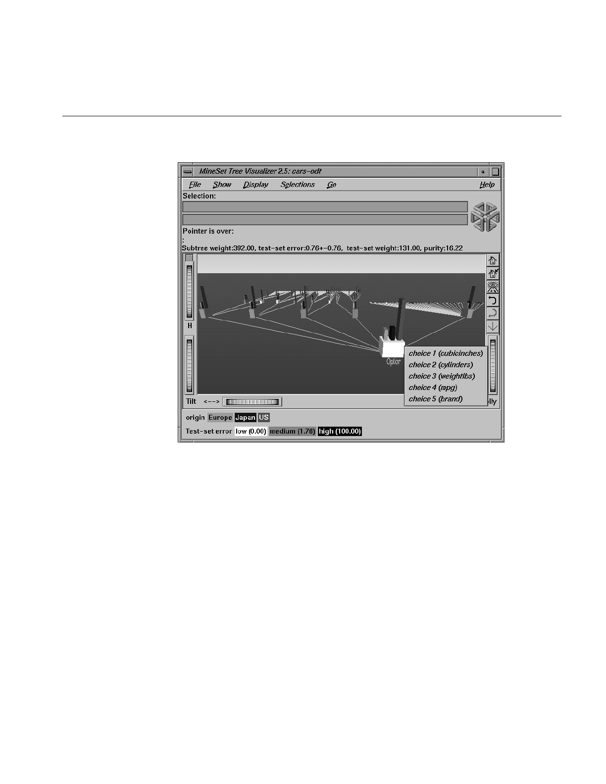
Overview
379
Figure 12-1 Option Decision Tree for the Cars Dataset
Option Trees, however, have two disadvantages:
1. The time necessary to build an Option Tree under the default setting is about 10 to
15 times longer than that needed to build a Decision Tree.
2. The Tree Visualizer file that is created is more complex, containing 10 to 15 times as
many nodes.
Run the Option Tree inducer on your dataset to determine whether the advantages in
comprehensibility and error rates justify the longer induction time. You might gain
additional insight as to which attributes to remove or use when building a Decision Tree.

380
Chapter 12: Inducing and Visualizing the Option Tree Classifier
Inducing Option Trees
An Option Tree classifier is induced (generated) automatically from data. The data,
which is made up of records and a label associated with each record, is called the training
set (see Chapter 10, “MineSet Inducers and Classifiers”).
File Requirements
The Option Tree inducer requires a training set, as described in the “Training Set” in
Chapter 10. Files are generated by extracting data from a source (such as a MineSet ASCII
or binary file, or a table in an Oracle, INFORMIX, or Sybase database). To apply the
generated classifier, you should have a dataset of records with the attributes used by the
classifier, except that the label need not be present.
Running the Option Tree Inducer
There are two ways to run the Option Tree inducer:
•From the Tool Manager.
Connect to the server and select a data source (see “Choosing a Data Source” in
Chapter 3). Enter the filename. For the example shown here, the filename entered
would be /usr/lib/MineSet/data/cars.schema as the filename. You’ll see several
attributes in the Data Transformation panel. Verify that origin is shown as the
discrete label. Select the Option Tree inducer, and ensure you have selected the
Classifier & Error mode. To run the Inducer, click Go!.
•From the command line.
To induce an Option Tree classifier from the command line, refer to Appendix I,
“Command-Line Interface to MIndUtil: Analytical Data Mining Algorithms.”

Configuring the Decision Tree Inducer Using the Tool Manager
381
Configuring the Decision Tree Inducer Using the Tool Manager
To access the options for configuring the Option Tree inducer, select the Mining Tools tab
on the Data Destination panel (Figure 12-2). From the tabs at the right, select Classify.
Ensure that the inducer you select is Option Tree. Your selections in the Mode and
Inducer menus determine the options available in the Further Inducer Options menu
(Figure 12-3). After you have made your selections in these menus, click Go! to run the
inducer, which, in turn, creates the classifier.
Figure 12-2 Data Destination Panel in Tool Manager Showing Classifiers
Discrete Labels
The Discrete Labels menu provides a list of possible discrete labels. Discrete attributes
(binned values, character string values, or a few integers) have a limited number of
values. You should select a label attribute with few values; for instance, two or three (see
“Training Set” in Chapter 10). If there are no discrete attributes, the menu shows No
Discrete Label, and the Go! button is disabled. You then must create a discrete attribute by
binning or adding a new column using the Tool Manager’s Data Transformations panel.

382
Chapter 12: Inducing and Visualizing the Option Tree Classifier
Parallelization
If you have installed the multiprocessor version of MineSet, it is possible to compute
tree-based algorithms in parallel whenever a branch contains over 1000 records. Each
node on the tree estimates the best possible split on the corresponding level, and these
tasks are performed in parallel. The maximum number of threads that a program can
spawn is determined automatically by default. You can control the number of threads
changing the parallelization mode in the Preferences panel of Tool Manager (see “The
File Menu” in Chapter 3). Parallelization may cause memory fragmentation, causing the
largest data sets that can be computed in parallel to be smaller than the largest data sets
that can be computed on a uniprocessor.
Classifier Name
The generated classifier is named with the prefix of the session filename (as determined
in Tool Manager) with the suffix-odt.class. By default, all classifiers are stored on the
server in the file_cache directory, which defaults to mineset_files. These classifiers can be
used for future classification of unlabeled records; that is, they can be used to predict the
labels for unlabeled datasets (see “Applying a Model” and “Backfitting in Error
Estimation” in Chapter 10).
Option Tree: Further Options
Selecting Further Classifier Options causes the Further Inducer Options dialog box to
appear. This dialog box consists of four panels:
•The top panel indicates the choices you made in the Tool Manager’s Data
Destination panel.
•The second pane from the top lets you set the loss matrix and the weight attribute.
See “Loss Matrices: Not All Mistakes Were Created Equally” and “Record
Weighting: Not All Records Were Sampled Equally” in Chapter 10.
•The bottom-left panel lets you specify further Inducer Options.
•The bottom-right panel lets you specify the Error Estimation Options (unless the
mode you chose in the Data Destination panel was Classifier Only, in which case
this area is empty). The options shown in this panel depend on the type of Error
Estimation you chose (see “Error Estimation” in Chapter 10).
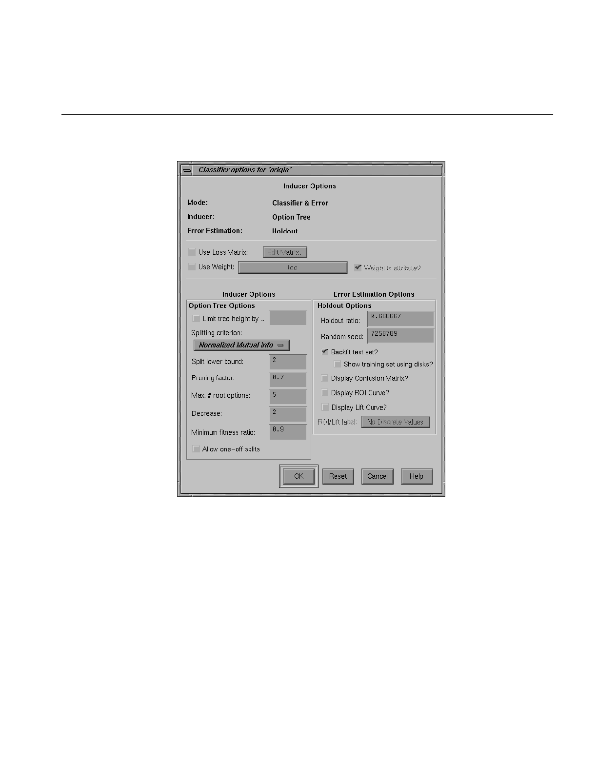
Configuring the Decision Tree Inducer Using the Tool Manager
383
Figure 12-3 Further Inducer Options

384
Chapter 12: Inducing and Visualizing the Option Tree Classifier
Option Tree Inducer Further Options
To fine-tune the Option Tree induction algorithm, you can change any of the options for
Decision Trees described in Chapter 11. In addition, the following new options are
provided (see Figure 12-3).
•Max # root options
This integer, which defaults to 5, restricts the maximum number of options that may
be created at the root. While the inducer might not allow this number of options
because other attributes are inferior, many natural datasets will have many good
attributes that could be chosen.
•Decrease
This integer, which defaults to 2, defines the amount by which the number of
options decreases at every level. With the default of 5 for Max # root options, it
implies that there are at most three options (5-2=3) for the second level of decision
nodes. The third level of decision nodes is restricted to a single option (3-2=1).
Levels further down are similarly restricted to a single option.
•Min fitness ratio
This ratio determines when to exclude attributes as options. When the inducer gives
a fitness score to each attribute, it chooses the best attribute as well as other
attributes that might also be good as options. The fitness ratio determines how good
those other options must be, to be chosen. A factor value of f implies that to be
considered an option, an attribute must rank at least (1-f)*b, where b is the score for
the best attribute. A fitness ratio of 1 picks all the attributes (so the limiting options
described above are reached if there are attributes on which to split). A fitness ratio
of 0 causes a regular Decision Tree to be created (no option nodes).
The time to induce an Option Tree is closely related to the number of option nodes
created. Because option nodes usually are created near the top (where they are most
useful for both comprehensibility and error reduction), a good approximation for the
time to induce an Option Tree is: the number of options created that have no children
options times the time to build a Decision Tree. Under the default setting, the root node
can have up to five options, and each child can have up to three options. The total options
then can be up to 15 (3 times 5). If the option Max # root options is increased to 6, the
number of options then is limited by 48 (6*4*2); if it is increased to 7, the number of
options is then limited by 105 (7*5*3). Keeping the Max # root options to 5, but changing
the decrease to 1, limits the options by 120 (5*4*3*2). The expected induction time for the
last example, thus, is two orders of magnitude longer than for a regular Decision Tree.
Decreasing the Min fitness ratio option usually results in fewer options than the limiting
factor, thus reducing induction time.

Working in the Tree Visualizer’s Main Window
385
Working in the Tree Visualizer’s Main Window
The Tree Visualizer’s main window shows the Option Tree. The navigation is the same
as for decision trees. One feature that is very useful for option trees is clicking the right
mouse button on an option node. This presents the list of children, which are the options.
Note that:
•The left-most option would have been the only option chosen by the Decision Tree
inducer. As you go right, the options are ranked in decreasing order by the fitness
scoring. Sometimes, it is interesting to see that the fitness scores do not necessarily
match the test-set error shown. This is expected, as the inducer is using a
non-perfect scoring function. The test-set estimate also has natural variability: the
larger the test-set, the more accurate the estimate.
•The option node can have a different error rate than every one of its children.
Because the option node averages the children’s predictions, its error rate can be
different. In some cases, its error is strictly lower than that of every child, showing
that averaging helps.
•The distribution of instances (shown in bars) at every child of an option node is
exactly the same as that of the option node itself. This is because there was no
decision made by the option node: options are being presented as children.
Sample Files
The following examples show cases in which the Option Tree inducer can be useful. Each
of these examples is associated with a sample data file provided with MineSet. By
running the inducer, you can generate the -odt.treeviz files described below. The text
describing the scenario and goal for each task is described in “Sample Files” in
Chapter 11. Here we describe the specific advantages and disadvantages of Option Trees
for several of the example datasets.
Note: The data files, which have a .schema extension, are located in /usr/lib/MineSet/data
on the client workstation. The classifier visualization files, which have a -odt.treeviz
extension, reside on the client workstation in /usr/lib/MineSet/treeviz/examples.

386
Chapter 12: Inducing and Visualizing the Option Tree Classifier
Churn
The Option Tree for this dataset shows that total day charge, total day minutes, and
customer service calls are all good attributes for the root: they all have approximately the
same estimated error rate. You can choose to fly down to one subtree or another, based
on your preferences and understanding of the data. Note that while the right subtree
starts with customer service calls, the second test is on total daily charge or total daily
minutes (as the root’s left option). However, because a split already occurred on an
attribute, the thresholds are different.
Origin of Cars
The Option Tree for this dataset shows several good attributes for the root, including:
cubic inches, cylinders, weight lbs, mpg, and brand. Note that the root has a lower
estimated error rate than any of the children.
Iris Classification
This is an example where Option Trees seem to be performing worse than Decision Trees.
The root for the Decision Tree shows 6% error and the root for the Option Tree shows 8%
error, so it seems that Option Trees perform worse. Be cautioned about making inferences
regarding the error rates:
•The standard deviation of the error estimate is fairly high: 3.88% and 3.39%. A rule
of thumb in statistics is that if the difference is less than two standard deviations,
the difference is not statistically significant at the 95% confidence level. A difference
of 2% is not larger than even a single standard deviation; hence, the classifier error
rates are not statistically different at the 95% confidence level
•For small files (Iris has 150 records), different random seeds give different results.
For example, changing the seed to 3 improves the Option Tree classifier’s error from
8% to 4% without changing the Decision Tree classifier’s error rate (remember to
reset the seed). This does not imply that a more accurate classifier has been
generated, rather that the error estimate is not stable. Because only 50 records are
used for testing, each mistake is 2%. The difference between 4% and 8% is making
two more mistakes.

Sample Files
387
•For small files (Iris has 150 records), use the “Estimate Error” option in MineSet. It
results in better estimates that have narrower confidence intervals. When you run
this mode, the status window shows that the Decision Tree classifier has an
estimated error of 4.67% +/- 1.73%, and the Option Tree classifier has an estimated
error of 4.00% +/- 1.61%. The difference is not significant in this case either, but the
Option Tree is slightly superior.
•Even if the error rate is higher for Option Trees, they might be (and usually are)
better at assigning probability estimates. For this dataset, the estimated mean
squared error for Decision Trees is 3.94; for Option Trees it is 3.67 (although the
difference is not significant at the 95% confidence level).
Mushroom Classification
The Option Tree for this dataset shows that all five options chosen at the root have zero
error rate estimates. Looking at the result, you might prefer the left option (bruises)
because it is as accurate but is easier to measure than odor (the root test of the induced
Decision Tree). You might want to remove odor and gill size, then build a regular
Decision Tree that turns out to be just as accurate (0% estimated error rate).
Note, however, that removal of a root option to have a sibling option selected by the
Decision Tree might not necessarily result in the same accurate classifier that is shown in
the Option Tree. The removed attribute might have been used lower down in the tree. For
example, removing brand from the cars dataset significantly increases the error rate,
even though four out of five options do not use it at the root.
Party Affiliation
This dataset behaves very similarly to the Iris dataset. The Option Tree has the same error
rate as the Decision Tree. Under “Estimate error,” the cross-validated estimate shows that
it is slightly better than the Decision Tree (but not significantly so at the 95% level) both
on error rate and on mean squared error.
Breast Cancer Diagnosis
The error rate for Option Trees is slightly lower than that for Decision Trees, both for
Classifier & Error and for Estimate Error; however, the difference is not significant (at 95%).

388
Chapter 12: Inducing and Visualizing the Option Tree Classifier
Hypothyroid Diagnosis
The error rates for this dataset are very low (less than 1%), but this is because most people
who were tested for hypothyroid (95%) did not suffer from it. If we use a loss matrix that
attempts to avoid false negatives (by penalizing by 100 a prediction of negative when the
actual value is hypothyroid), we can see that the loss for Option Trees is significantly
lower than that of Decision Trees: 182 versus 523 (total), or 0.17 versus 0.5 (per record).
This difference is significant at the 95% confidence level.
DNA Boundaries
For this dataset, the Option Tree is slightly more accurate than the Decision Tree;
however, looking at the root options, you might notice that it chooses left 1,2, and right
1,2,5. Given the background knowledge that attributes closer to the boundary can be
more important, you might want to exclude the option split on right 5. After updating the
maximum number of root options to 4 (down from 5), the error rate increases from 5.65%
to 6.59%. This might be surprising, given that the root no longer uses right 5 as an option;
another effect of changing the number of root options from 5 to 4 was to also reduce the
number of options that appear further down the tree (because of the decrease parameter).
This caused the individual error rates for each of the other 4 subtrees to increase. Still, the
option tree’s error rate is significantly better (at the 95% confidence level) than the
Decision Tree error rate of 7.06% +/- 0.79%.

389
Chapter 13
13. Inducing and Visualizing the Evidence Classifier
This chapter discusses the features and capabilities of the Evidence Classifier and
Visualizer. It provides an overview of this classification tool as well as the inducer that
generates it. It describes the ways of invoking this tool. It then explains the Evidence
Visualizer’s functionality when working with the
•Label Probability Pane
•Main Window
Finally, it lists and describes the sample files provided for this tool.
Note: It is assumed that you have read Chapter 10, “MineSet Inducers and Classifiers,”
before proceeding with this chapter.
Overview
The Evidence Classifier assigns each record in a dataset to a class. The Evidence
Visualizer displays the structure of an evidence classifier (Figure 13-1). The visualizer
can help you understand the importance of specific attribute values for classification.
Also, it can be used to gain insight into how classification is done, as well as to answer
“what if” questions.
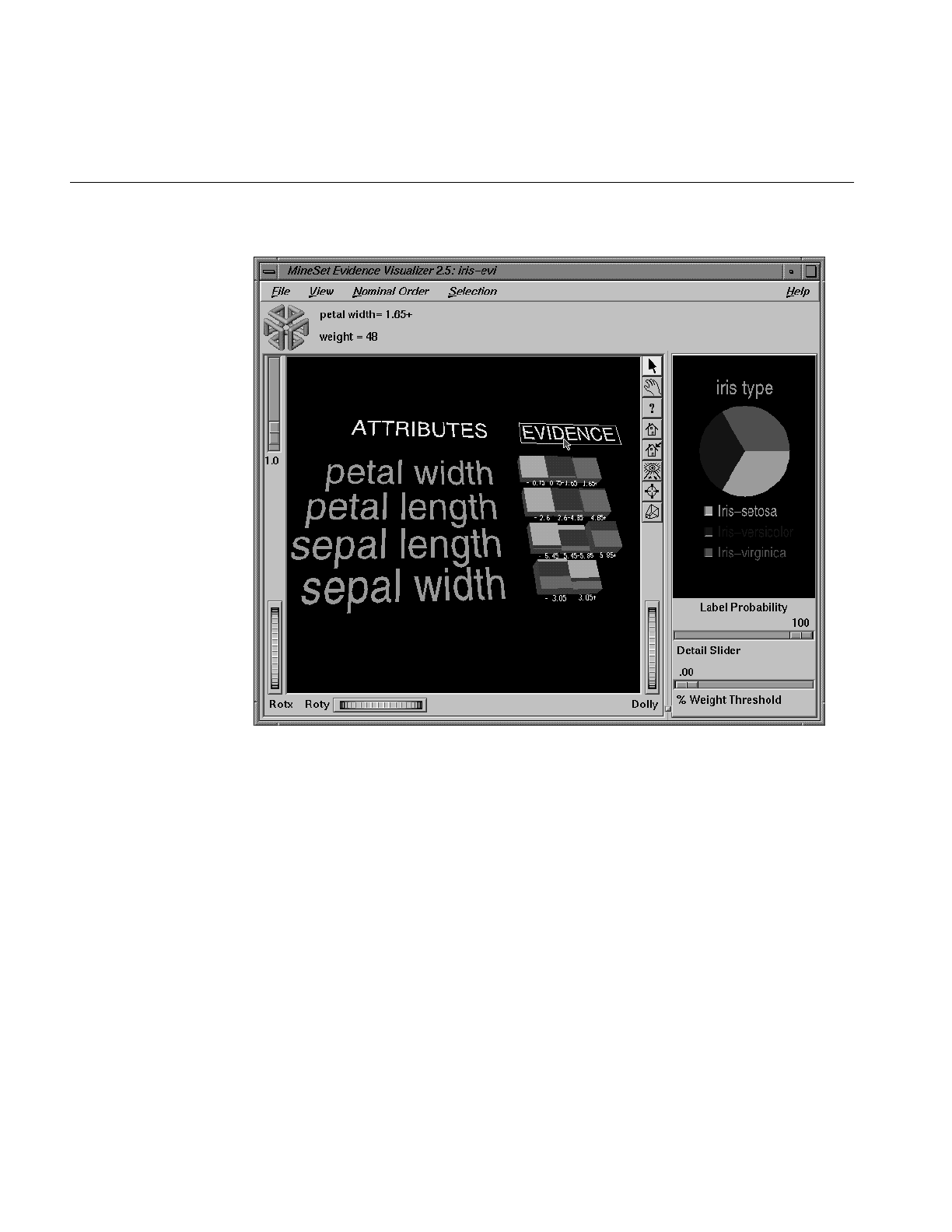
390
Chapter 13: Inducing and Visualizing the Evidence Classifier
Figure 13-1 The Evidence Visualizer Applied to the Iris Dataset
The Main Window (left) contains rows of cake charts, pie charts, or bars for each attribute
used by the classifier. Initially rows of cake charts are shown (as in Figure 13-1). A cake
chart resembles a pie chart in that it shows proportions, but it is square with rectangular
slices. To toggle between cakes, representing evidence, and pies, representing
probabilities, click on the boxed title “Evidence,” and the display shown in Figure 13-2
appears. To characterize a particular class label select one of the values in the Label
Probability Pane (right).
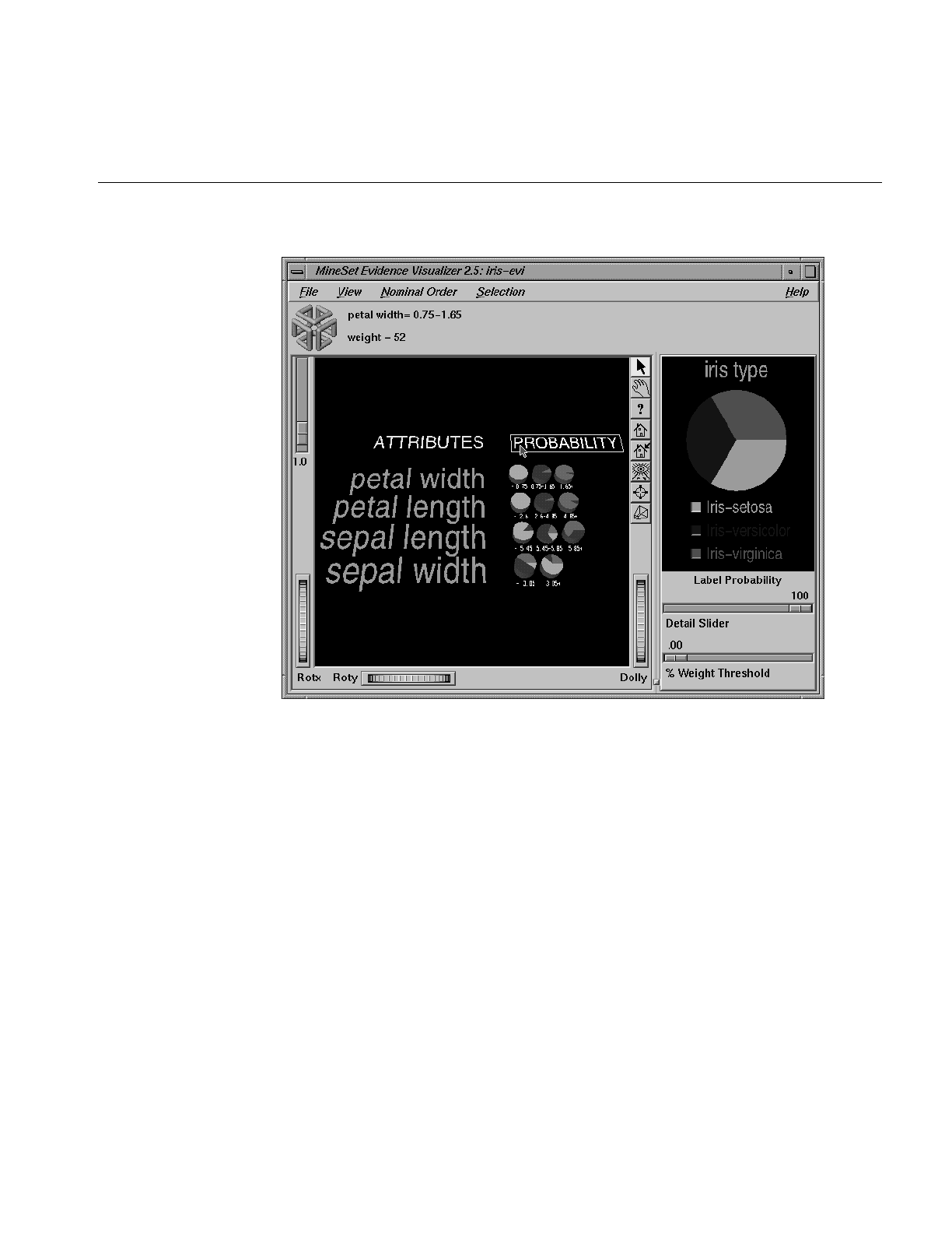
Overview
391
Figure 13-2 Evidence Visualizer Showing Probabilities
There is one chart or bar for each discrete value of the attribute. In the case where the
attributes are not discrete, the continuous range has been discretized (binned) in a way
that maximizes the differences between adjacent charts. A chart’s height is proportional
to the weight of records having that attribute value. (If no weight attribute is set, the
height represents the number of records.) If no filtering is done, the sum of the chart
heights for every row is the same because it is equal to the total weight of the dataset.
The height of the graphical objects can be scaled to exaggerate the differences between
the charts. You can adjust a Detail slider in order to reduce the number of attributes
shown starting with the ones that are less useful for classification.
By adjusting the percent weight threshold, all values having counts below a certain
percentage of the total are filtered out.

392
Chapter 13: Inducing and Visualizing the Evidence Classifier
The kinds of questions you might answer by using the Evidence Visualizer are as follows:
•What is the likelihood that a new record, for which you know only the values for a
few attributes, has a certain label?
•Which values of which attributes are the most useful for classifying the label?
•What is the distribution of records by attribute values?
•What are the characteristics of records that have a certain label?
•What is the probability that an attribute takes on a certain value given that it has a
specific label value?
The prior probability for each class label is depicted in the pie chart in the Label Probability
Pane, on the right of the screen. The prior probability for a class label is the probability of
seeing this label in the data for a randomly chosen record, ignoring all attribute values.
Mathematically, this is the number of records with the class label divided by the total
number of records.
The conditional probabilities, depicted by cake charts in the Main Window on the left of the
screen, show the relative probability of each attribute value given (conditioned on) each
label value. The size of a cake slice indicates the amount of evidence the classifier adds
to the prior probability after taking into account a given attribute value in a record. If the
size of the slices are equal, the value is irrelevant, and the classifier adds the same amount
of evidence to all classes.
The probability distribution for each value, depicted by pie charts representation in the
Main Window on the left of the screen, show the proportion of records in each class
considering only records having that particular value. This distribution is arrived at by
multiplying the conditional probabilities for the value by the prior probability, then
normalizing so that they sum to one. These probabilities are precise for the data given
(Figure 13-2). You may toggle between the cakes and pies representation by clicking on
the boxed title “Evidence” or “Probabilities” in the scene.
By default, values of nominal attributes are sorted by the size of the slices corresponding
to one of the classes. This aids in identifying important values. If the label is a binned
attribute, the class that is the highest bin is used. If the label is nominal, then the class
with the largest slice in the prior probability pie is used. If a particular class is selected,
and then a sort by label probability is requested, the selected class is used for determining
the ordering. Alternatively, the values of the nominal attributes can be sorted
alphabetically or by weight. Binned attributes never change their ordering.

Overview
393
Technically, the slice of the chart represents the normalized conditional probability of an
attribute value A, given the class label L. The conditional probability, P(A|L), is the
probability that a random record chosen only from records with label L takes the value
A. Under the default settings, the probability is computed based on record weights. For
example, P(0.75 < petal width < 1.65 | iris-versicolor) is 91.6, because there are 36
records with label iris-versicolor, and 33 of them have a petal width in this range.
The Evidence Inducer, sometimes called Naive-Bayes (or Simple Bayes), builds a model
that assumes the probabilities of each attribute value are independent given the class. For
example, this assumes that the four attributes (sepal length, sepal width, petal length,
and petal width) are independent for each class of iris (iris-setosa, iris-versicolor, and
iris-virginica). While this simplistic model is rarely true, the model is excellent for initial
explorations of data and its classification prediction performance is very good in
practical applications.
Each attribute value, or range of values, (for binned continuous attributes), defines
exactly one chart, which, in turn, gives the conditional probabilities for each class label.
To classify a given record, one computes the probability of each class by multiplying its
prior probability by the appropriate conditional probability from each row in the matrix.
The final product gives the relative probability for each class and the highest value is the
predicted class. If an attribute has an unknown value, it is ignored. These NULL values
are represented by charts that are slightly offset from the rest of the charts and are on the
left. For example, stalk root in Figure 13-5 has a null value.
This process of classification can be done interactively using the Evidence Visualizer.
Simply select all the values for the attributes that you know. The probability pie on the
right changes to show the distribution you would expect, given the attribute values you
selected on the left. For example, selecting the chart for sepal length < 5.45 inches and the
chart for sepal width > 3.05 inches shows that an iris with these characteristics belongs
almost certainly to the class iris-setosa (see Figure 13-3).The behavior is the same
whether you are using the cake, pie, or bar mode.
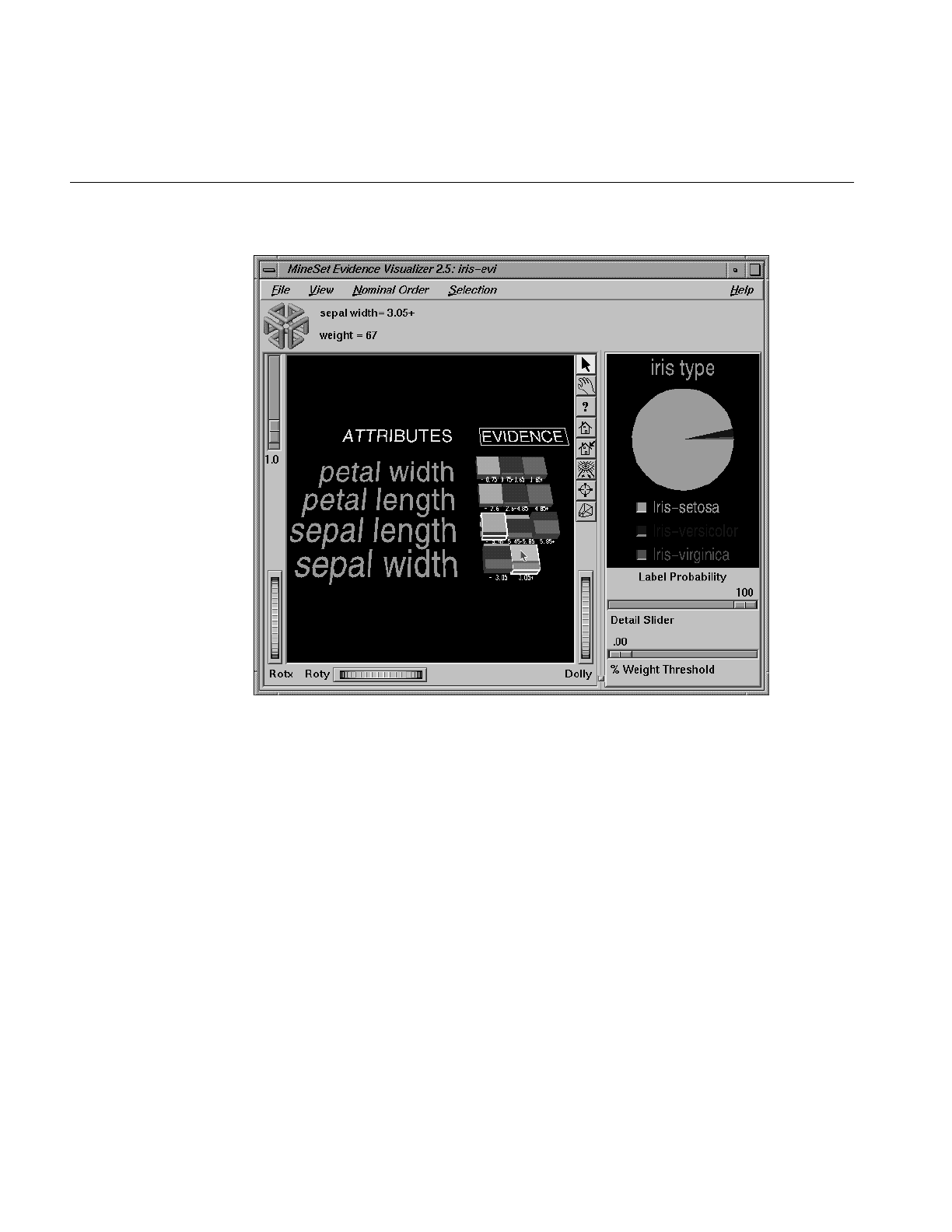
394
Chapter 13: Inducing and Visualizing the Evidence Classifier
Figure 13-3 Selecting sepal length < 5.45 and sepal width > 3.05 Using the Iris Dataset
If the classes listed under the pie chart on the right are not numerical, they are shown in
order of slice size. The class with the largest probability is at the top. As values on the left
are selected, this order changes to reflect the changing probability pie. If the label is a
binned attribute, the values are not reordered, and colors are assigned according to a
continuous spectrum: the highest bin is red; otherwise, random colors are used.
For some combinations of selected values, the probability pie on the right turns
completely gray. This occurs when the values selected are contradictory according to the
model. For example, in iris.eviviz there are no iris flowers that have petal width <.75
inches and petal length > 4.85 inches. Thus, selecting the two charts on the left
representing these two values results in a gray chart on the right (see Figure 13-4).
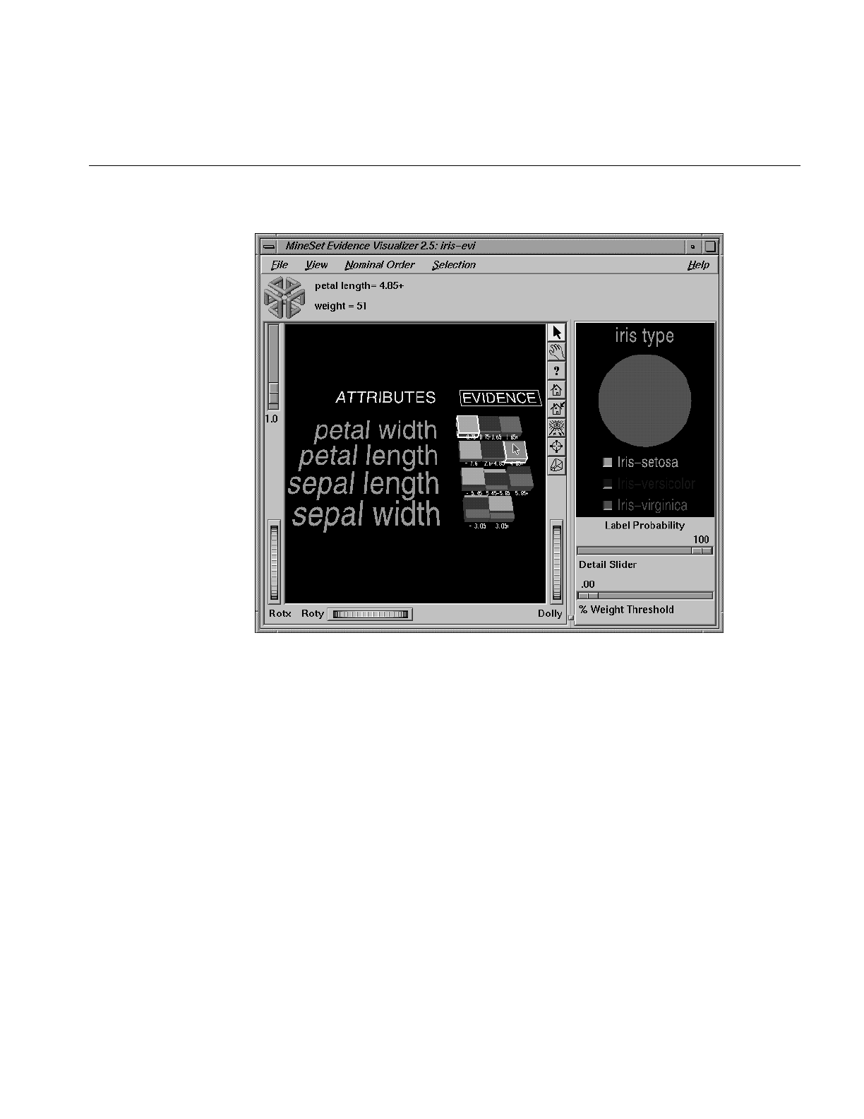
Overview
395
Figure 13-4 Selecting Two Contradictory Pies Results in a Gray Pie on the Right
You can eliminate the possibility of getting a grey pie by using the Laplace correction
option (see “Evidence Inducer Options” on page 402). If Laplace correction is not used,
clicking more than one chart on the left yields exact posterior proportions on the right.
After selecting charts with more than one attribute on the left, the posterior probability
pie might not reflect exactly the true proportions in the original data; however, it is a
good estimate. Laplace correction can be toggled on or off from within the tool by
checkmarking View > Use Laplace Correction. Even if a value for the Laplace correction
was not specified in the further inducer options, a default value for it will be used if this
menu item has a check mark.
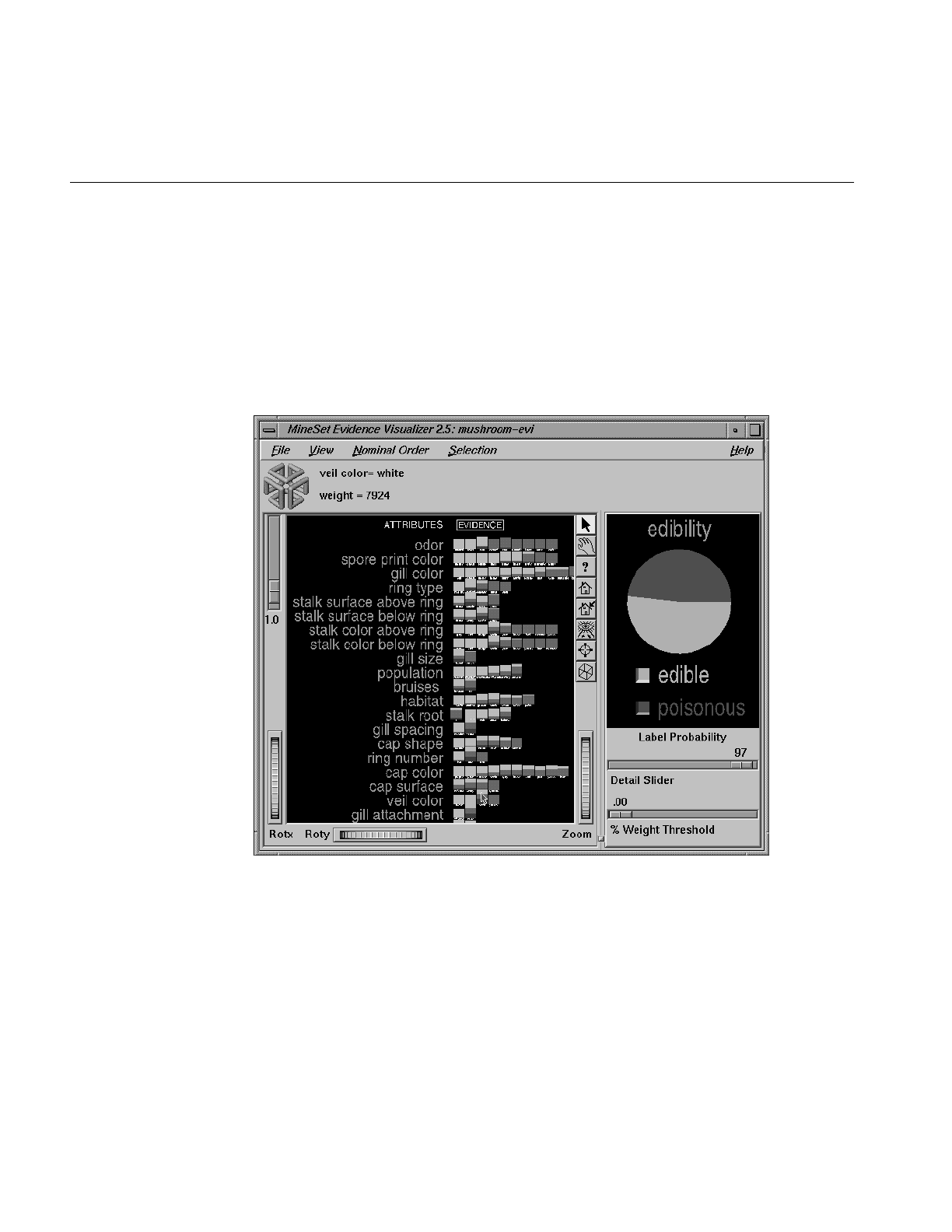
396
Chapter 13: Inducing and Visualizing the Evidence Classifier
Importance is a measure of predictive power with respect to a label. The Main Window
provides valuable insight not only into the importance of each attribute value affecting
the class value, but also into the importance of specific attribute values. For example, in
the mushroom dataset (described in “Mushroom Classification” on page 426), the
veil-color attribute has little importance because its attribute value usually is white (see
Figure 13-5) and does not add much evidence to either class. The importance assigned to
each attribute is a number between 1 and 100. It is possible to see the value at the top by
selecting the attribute name in the scene.
Figure 13-5 Veil-Color Attribute in the Mushroom Dataset
However, if the veil color is brown or orange, the mushroom is likely to be edible, while
if it is yellow, it is likely to be poisonous. Similarly, a “test for AIDS” might not be an
important attribute for determining whether a patient has a deadly disease because most
people would not test positive. However, the value “positive” for this test is highly
informative because most patients that test positive do have a deadly disease.

Inducing Evidence Classifiers
397
Inducing Evidence Classifiers
The automatic induction of Evidence classifiers is a process whereby counts (or weights)
are used to calculate the probabilities. Evidence classifiers are automatically induced
(generated) from data. The data, which is made up of records and a label associated with
each record, is called the training set (see Chapter 10).
The probabilities are generated using the following method:
1. All continuous attributes are discretized (binned), such that class distributions in
these ranges are as different as possible. The number of ranges is determined
automatically, which invokes parallelization so that attributes are binned in parallel,
if the multiprocessor version of MineSet is installed on your system. The automatic
binning for any attribute may be overridden by explicitly performing the binning
operation in Tool Manager.
2. The prior probabilities are the proportions of each class in the training set.
3. The conditional probabilities are the probabilities of each attribute value
conditioned on each class label in the training set. (The charts show them
normalized for each attribute value.)
The number of charts in a row is the number of discrete ranges produced by the inducer.
If there is just one range, it means that this attribute by itself was not useful in predicting
the label. Initially, the prior probabilities of the labels are displayed in the Label
Probability Pane.
An optional Auto Column selection mode removes attributes that are not useful or that
increase the error rate.
An optional Laplace correction can be applied to the probabilities, which avoids extreme
probabilities (for example, probabilities of zeros and ones). We may prefer not to assign
a probability of 1 to the event “a patient tested positive for AIDS has a deadly disease.”
We may want to assign a probability close to 1 (but not 1), in order to allow for errors or
unrepresentative samples.
Note that the Evidence Visualizer shows the probabilities of classes. The classifier can
have a Loss Matrix. In the visualization the Loss Matrix (if present) may be applied by
clicking the button to the lower right of the pie in the label probability pane. The
predicted class is the one with the least expected loss under the probability estimates.The
Loss Matrix button will only appear if it has been specified in the .eviviz file (see
Appendix G, “Format of the Evidence Visualizer’s Data File.”

398
Chapter 13: Inducing and Visualizing the Evidence Classifier
File Requirements
The Evidence Visualizer requires a training set, as described in “Training Set” on
page 322 of Chapter 10, “MineSet Inducers and Classifiers.” Files are generated by
extracting data from a source (such as a MineSet ASCII or binary file, or a table in an
Oracle, INFORMIX, or Sybase database). The Evidence Visualizer data file is output as a
result of running the Evidence Inducer. The format of this file, which has a .eviviz
extension, is described in Appendix G. When starting the Evidence Visualizer or when
opening a file, you must specify the data filename. To apply the generated classifier, you
should have a dataset of records with the same attributes and type as those used by the
classifier, except that the label need not be present.
Running the Evidence Inducer
There are two ways to run the evidence inducer:
•From the Tool Manager
Connect to the server and select a data source (see “Choosing a Data Source” in
Chapter 3).
From the File menu, choose Open New Data File. Log in to a server, and type
/usr/lib/MineSet/data/iris.schema as the filename. You’ll see four continuous
attributes and one discrete attribute in the Data Transformation panel. Since there is
only one discrete attribute, the label option automatically shows it. Select the
Evidence Inducer, and ensure that you have selected the Classifier & Error mode. To
run the Inducer, click Go!.
The Status window shows the progress and resulting statistics.
•From the command line
To induce an evidence classifier from the command line, refer to Appendix I,
“Command-Line Interface to MIndUtil: Analytical Data Mining Algorithms.”
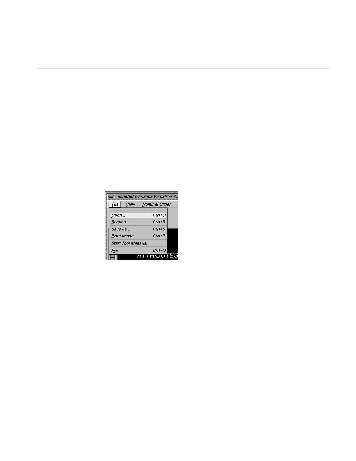
Starting the Evidence Visualizer
399
Starting the Evidence Visualizer
There are six ways to start the Evidence Visualizer:
•Run the Evidence Inducer from the Tool Manager under the Classify tab. After the
inducer builds the classifier, it automatically invokes the Evidence Visualizer. See
below for details about using the Tool Manager in conjunction with the Evidence
Visualizer.
•Use the Tool Manager to start the Evidence Visualizer from the Visual Tools menu.
(See Chapter 3 for details on the Tool Manager’s functionality, which is common to
all MineSet tools.)
•Double-click the Evidence Visualizer icon on your Indigo Magic desktop. The
startup screen requires you to select a data file by choosing File > Open.
Figure 13-6 File > Open Menu Selection
•If you know what configuration file you want to use, double-click the icon for that
configuration file. This starts the Evidence Visualizer and automatically loads the
configuration file you specified. This works only if the configuration filename ends
in .eviviz (which is always the case for configuration files created for the Evidence
Visualizer via the Tool Manager).
•If you know what configuration file you want to use, drag its icon onto the Evidence
Visualizer icon. This starts the Evidence Visualizer and automatically loads the
configuration file you specified.
•Start the Evidence Visualizer from the UNIX shell command line by entering this
command at the prompt:
eviviz [ dataFile ]
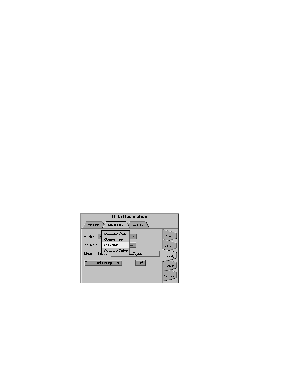
400
Chapter 13: Inducing and Visualizing the Evidence Classifier
Here, dataFile is optional and specifies the name of the configuration file to use. If
you don’t specify a configuration file, you then must use File > Open to specify one
(see Figure 13-6).
Options for Invoking the Evidence Visualizer
The -quiet option eliminates the dialogs that popup to indicate progress. You can enable
this option permanently by adding the line
*minesetQuiet:TRUE
to your .Xdefaults file.
Configuring the Evidence Inducer Using the Tool Manager
To access the options for configuring the Evidence Inducer, select the Mining Tools tab on
the Data Destination panel (Figure 13-7). From the subsequent tabs, select Classify.
Ensure that the inducer you select is Evidence. Your selections in the Mode menu
determines the options available in the Further Inducer Options menu. After you have
made your selections in these menus, click Go! to run the inducer, which, in turn, creates
the classifier.
Figure 13-7 Tool Manager With Data Destination Panel Showing Classifiers

Configuring the Evidence Inducer Using the Tool Manager
401
Discrete Labels
The Discrete Labels menu provides a list of possible discrete labels. Discrete attributes
(binned values, character string values, or integers) can have a number of values. Select
a label attribute (see “Training Set” in Chapter 10). If there are no discrete attributes, the
menu shows No Discrete Label, and the Go! button is disabled. You then must create a
discrete attribute by binning or adding a new column using the Tool Manager’s Data
Transformations panel.
Classifier Name
The generated classifier is named with the prefix of the session filename (as determined
in Tool Manager) and the suffix-evi.class. By default, all classifiers are stored on the
server. These classifiers can be used for future classification of unlabeled records; that is,
they can be used to predict the labels for unlabeled datasets (see “The Apply Model
Button” in Chapter 3).
Refining the Inducer With Further Options
Selecting Further Inducer Options causes the Inducer Options dialog box to appear (see
Figure 13-8). This dialog box consists of three panels:
•The top panel shows the choices you made in the Tool Manager’s Data Destination
panel. The type of Error Estimation is determined by the model.
•The bottom-left panel lets you specify further Inducer Options.
•The bottom-right panel lets you specify the Error Estimation Options (unless the
mode you chose in the Data Destination panel was Classifier Only, in which case
this area is empty). The options shown in this panel depend on the type of Error
Estimation you chose (see “Error Estimation” in Chapter 10).
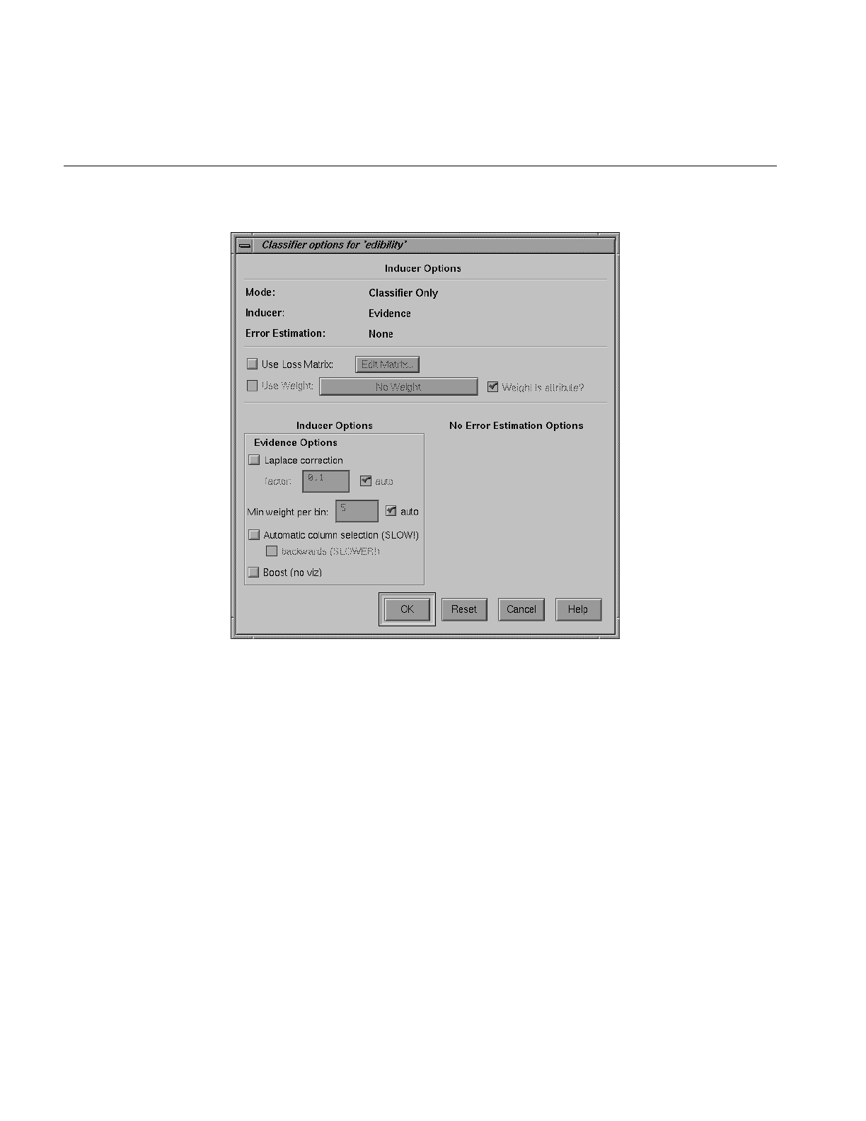
402
Chapter 13: Inducing and Visualizing the Evidence Classifier
Figure 13-8 Classification Options Dialog Box Without Accuracy Estimate
Evidence Inducer Options
By choosing Further Inducer Options, you can fine-tune the Evidence inducer.
•Laplace Correction
This biases the probabilities towards the average, thus avoiding extreme numbers
(such as 0 and 1). This means every chart in the Main Window has a non-zero slice
for each class. The fewer the records in a bin, the more it is changed towards the
average. If the Laplace correction is checked, and the factor is left empty or set to 0,
an automatic Laplace correction is applied, using a heuristic that applies a factor of
1/training-set-weight.

Working in the Evidence Visualizer’s Panes
403
•Set Minimum Weight per Bin
The Evidence Inducer discretizes all continuous attributes. This option lets you
define the minimum number of instances per bin. The automatic setting has a
heuristic that sets this number based on the dataset size: the larger the dataset, the
greater the minimum number of records allowed in the bin, and the smaller the
width of the bin, in general. If your dataset is very large, you might obtain more
discrete ranges than you want. To reduce the number of bins, raise this value.
•Automatic column selection
This applies a process that chooses only those columns that help prediction the
most. Because extra columns can degrade the predictive accuracy of the evidence
classifier, this process searches for a good subset of the columns automatically. Only
those columns found to be useful are used. This process can take a long time,
especially if there are many columns. It is useful for eliminating highly correlated
columns that could degrade accuracy. Automatic column selection and Boosting
cannot both be enabled, as together they would take far too long to complete.
Automatic column selection conducts a search for the best set of columns that
reduce the error of the classifier. The selection of these columns is done by
estimating the error of different attribute sets using the wrapper approach (see
Appendix K, “Further Reading and Acknowledgments”). Each feature subset is
evaluated by estimating the classifier's error using cross-validation. Columns are
added or removed based on the error estimates using a best-first search mechanism.
In the default mode, the search begins with an empty set of features. By selecting
the Backwards option, the search starts with the full set of options; this is slower,
since larger models are initially built.
Working in the Evidence Visualizer’s Panes
If you started the Evidence Visualizer without specifying a configuration file, the main
screen shows the copyright notice for the Evidence Visualizer. Only the File and Help
pulldown menus are available. To view all menus and controls in the Main Window,
open a configuration file. Use File > Open (see Figure 13-6) to see a list of configuration
files.
When a valid configuration file is specified, the two panes in the main screen display
graphics. For example, specifying cars.eviviz results in the output displayed in
Figure 13-9.

404
Chapter 13: Inducing and Visualizing the Evidence Classifier
Figure 13-9 Evidence Visualizer Window for cars.eviviz
In the Main Window on the left, one row of cake charts appears for each attribute in the
dataset that the classifier is using. Each chart corresponds to a value for the attribute
associated with the row. In the Label Probability Pane on the right, a list of all class labels
appears under a large pie chart of the prior probability distribution. Note that the color
of the slices correspond to the color associated with each class label. This prior
probability represented by the pie shows the proportion of data with each class label.

Working in the Evidence Visualizer’s Panes
405
Viewing Modes
Both of the Evidence Visualizer’s window panes has two modes of viewing: grasp and
select.
Viewing Modes in the Label Probability Pane
The Label Probability Pane is located on the right of the Evidence Visualizer’s Main
Window. The top two buttons of those aligned vertically between the panes toggle
between the grasp and select modes. Alternatively, the Esc key also toggles the viewing
mode for both panes.
In grasp mode, the cursor appears as a hand that lets you pan and scale the scene’s size.
•To move the display within the pane, press the middle mouse button and drag it in
the direction you want the display moved.
•To enlarge the scene, press the left mouse button, and drag the mouse downward.
•To shrink the scene, press the left mouse button, and move the mouse upward.
Viewing Modes in the Main Window
The Main Window is located on the left of the Evidence Visualizer’s display window. The
top two buttons of those aligned vertically between the panes toggle between the grasp
and select modes. Alternatively, the Esc key also toggles the viewing mode for both
panes.
In grasp mode, the cursor appears as a hand, so you can pan, rotate, and scale the scene’s
size. (The Label Probability pane contains only 2D geometry; thus, rotation is disabled.)
•To rotate the display, press the left mouse button and move the mouse in the
direction you want.
•To move the display within the pane, press the middle mouse button, and drag it in
the direction you want the display moved.
•To enlarge the viewpoint, simultaneously press the left and middle mouse buttons
and move the mouse downward. To shrink the viewpoint, simultaneously press the
left and middle mouse buttons, and move the mouse upward. This is equivalent to
the functions provided by the Dolly thumbwheel.
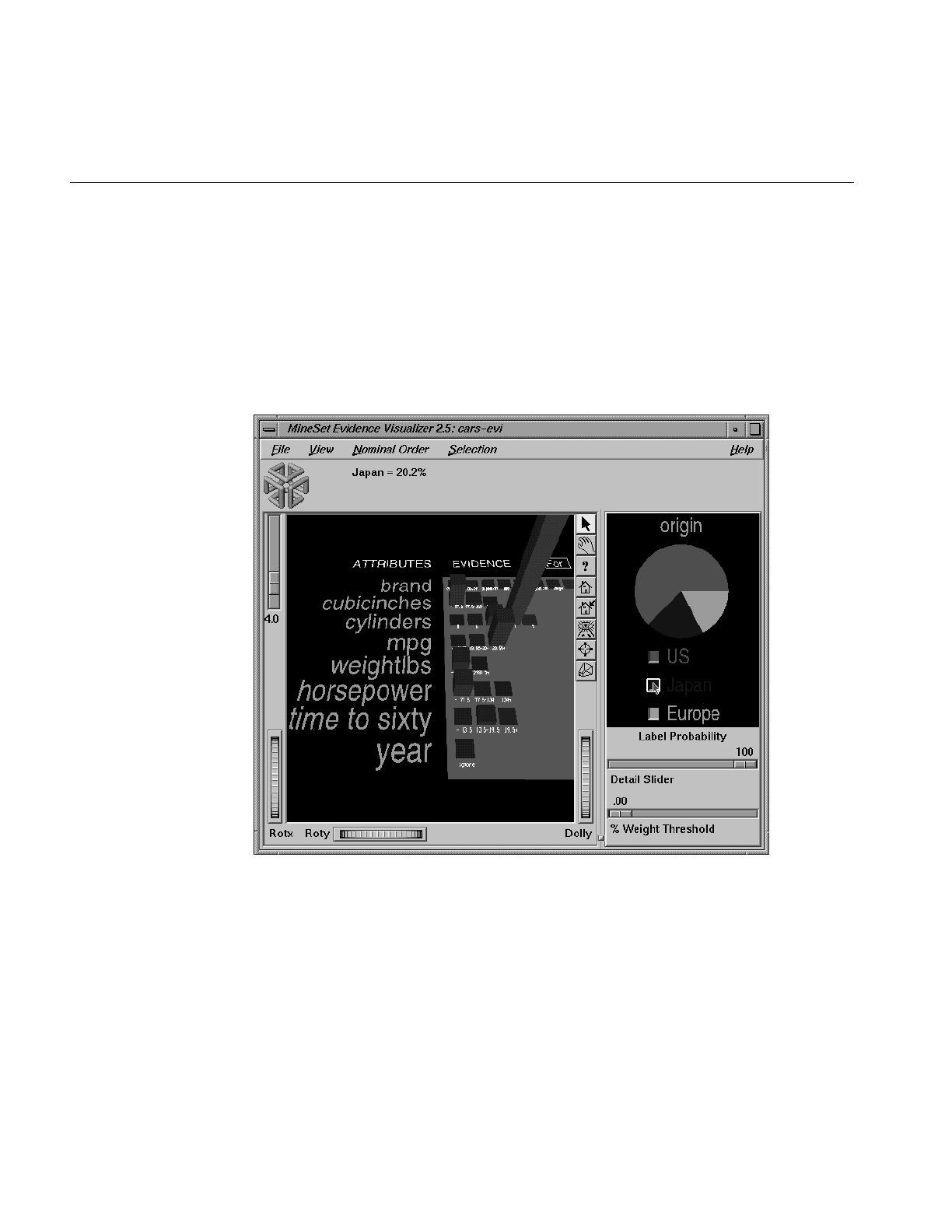
406
Chapter 13: Inducing and Visualizing the Evidence Classifier
Selecting Items in the Label Probability Pane
In select mode, the cursor appears as an arrow. If you then click the button to the left of
one of the class labels, a white box appears around the button next to the label (see
Figure 13-10). The size of that slice (the probability of predicting that label value) appears
in the text output line at the top. To deselect a class label, click on it again. Moving the
mouse over the button next to a class label, in select mode, causes the size of that slice (in
percentage terms) to appear in the output line at the top.
Figure 13-10 Label Value “Japan” Selected Using the Cars Dataset
If no label is selected, the Main Window on the left displays cake or pie charts (see
Figure 13-10).
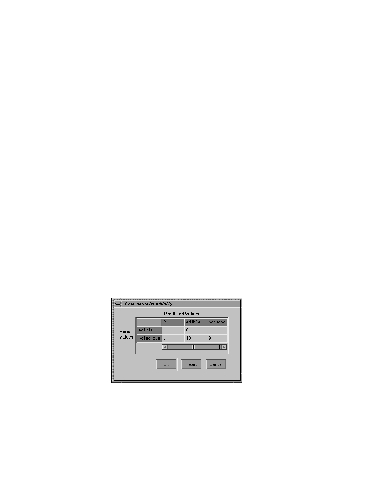
Working in the Evidence Visualizer’s Panes
407
If a label is selected, the representation on the left displays bar charts (see Figure 13-10).
The height of each bar shows the evidence in favor of the selected label value. Evidence
for is the negative log of the quantity one, minus the size of the slice matching the selected
label, in the corresponding chart representation.
The grayness of the bars is based on the 95% confidence interval. This, in turn, depends
on the weight for that value. Hence, bars that are nearly gray have low weight and a large
confidence interval. The height of gray bars is not likely to be very accurate. Conversely,
the height and corresponding evidence value for a fully saturated bar can be relied on
because it is based on large weight, representing many records. The exact number of
records (weight) is reflected in the text output line when that bar is highlighted.
As the default, the amount of evidence common to all the labels is subtracted. This means
that the height of a bar for each value is reduced by the height representing the label for
which the evidence is smallest. If you select a different label, the bars and their colors
change to represent the new class label. Selecting the same label again deselects it, and
the Main Window again displays the cake or pie charts. Uncheck the View > Subtract
minimum evidence option if you do not want to subtract the common evidence.
If a Loss Matrix has been specified in the Further Inducer options, a button labelled Use
Loss Matrix appears to the lower right of the probability pie. When selected (the default)
the Loss Matrix is used to adjust the probabilities shown. The largest slice shown is the
class that takes into account the Loss Matrix. To see what the probabilities would be
without using the Loss Matrix, deselect the Use Loss Matrix button. When using the Loss
Matrix, a gray slice may be present because there was a column for predicting null when
you edited it. If the gray slice is the largest slice, the classifier predicts null.
Figure 13-11 Loss Matrix to Avoid Predicting Poisonous Mushrooms as Being Edible
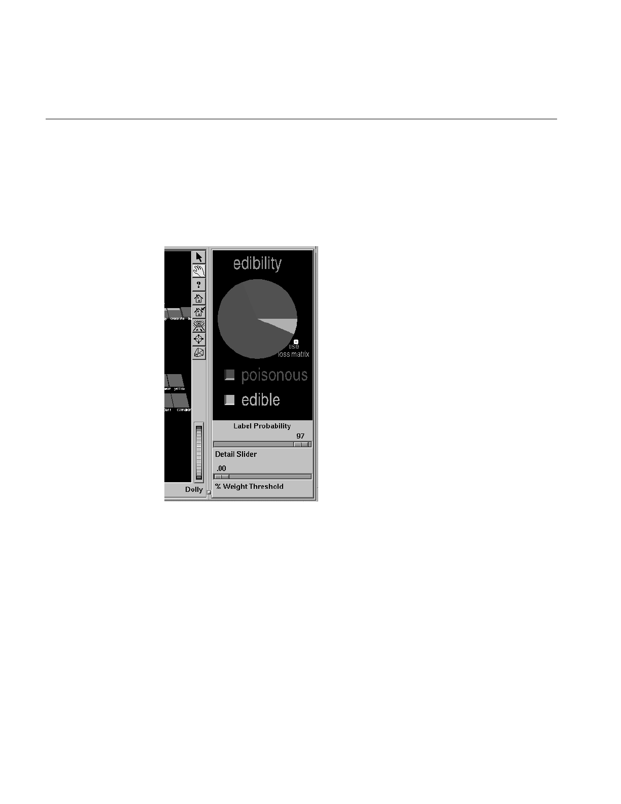
408
Chapter 13: Inducing and Visualizing the Evidence Classifier
Figure 13-11 shows a Loss Matrix that has been edited to reduce the likelihood of
predicting a mushroom edible when it is really poisonous. Figure 13-12 shows the initial
state of the Label Probability pane for the resulting Evidence Visualizer. Normally the
prior probability on the right shows slices of almost equal sizes for edible and poisonous
mushrooms. Using this Loss Matrix, however, we csn be much more cautious about
predicting that a mushroom is edible.
Figure 13-12 Loss Matrix Applied to Probabilities in the Label Probability Pane
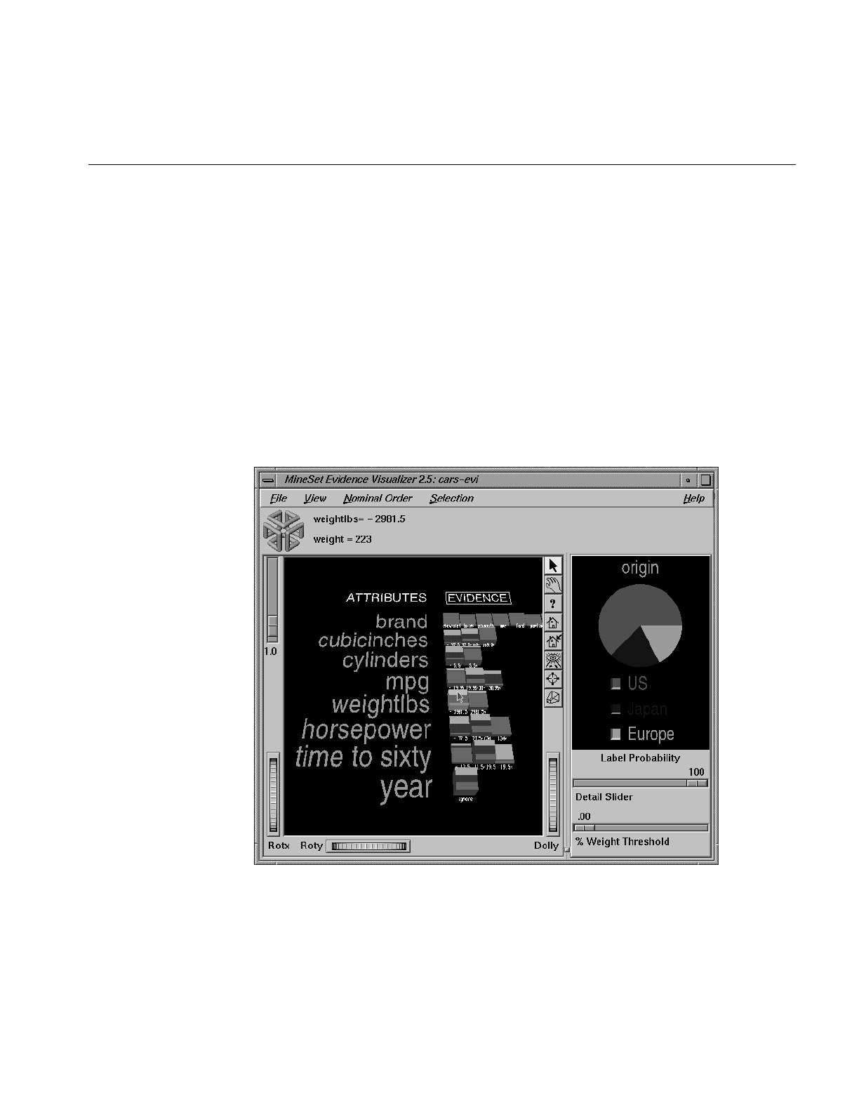
Working in the Evidence Visualizer’s Panes
409
Selecting Items in the Main Window
In select mode, the cursor appears as an arrow. You can highlight an object (either a pie
chart or a bar) by moving the cursor over that object. Information about that object then
appears above the Main Window. The information is displayed as long as the cursor is
over the object.
•If the object is a pie chart, then the message takes this format:
<attribute name>: <value or range>
weight = <weight>
Here, weight is the total weight of the data points that fall in that range or have that
value for that attribute (see Figure 13-13). The chart height is proportional to this
number. Unless record weighting is used, the weight shows record counts.
Figure 13-13 Pie Charts With the First Binned Range of weightlbs Highlighted

410
Chapter 13: Inducing and Visualizing the Evidence Classifier
•If the object is a bar, then the message takes this format:
(<attribute> = <value>) ==> Prob(<selected label>) = x%
[low%-high%] Evidence=z
<selected label> ==> Prob(<attribute> = <value>) = y% [low%-high%]
weight = <weight>
See Figure 13-14.
Here, x is the probability that a record has the selected label given that it has the
highlighted attribute value. The bracketed range, [low%-high%] gives the 95%
confidence interval. Similarly, y% is the probability that a record has the highlighted
attribute value given the selected label (see Figure 13-14). Note that the height of the
bar shows evidence, not probability. The amount of evidence, z, is directly related to
the bar heights. Evidence can be summed in order to determine which class is
predicted (unlike probability, which must be multiplied). Weight is the weight of
data points having that value.
Technically, evidence for is defined as
while evidence against is defined as
A is the attribute value, L is the selected label value, and N is the number of label
values. When computing the bar heights, a very small number is added inside the
brackets of the above expressions to prevent the bars from becoming infinitely tall.
The word “for” or “against” in the Main Window has a box around it to indicate
that it may be clicked on. Click on the box to toggle the representation.
The height of the gray rectangular base (on which the bars stand) represents the
amount of evidence contributed by the prior probability. For example, if the label is
car cylinders, there are very few three cylinder cars, so the base is low when evidence
for is showing, and high when evidence against is showing. You can add to this height
the height of individual bars that are on top.
Evidence for can be useful in determining which values are the most helpful in
predicting a particular label value.
1 −
P(A|Li)
P(A|L)
-log Σ
i=1
N
P(A|Li)
P(A|L)
-log Σ
i=1
N

Working in the Evidence Visualizer’s Panes
411
The amount of evidence (bar height) is not derived directly from either probability
shown while highlighting. Instead, the evidence depends on the conditional
probability relative to the other probabilities for all the other label values according
to the equation above.
Figure 13-14 Bar Chart With a Range Selected
You can also select any number of values from an attribute row by clicking the left mouse
button while the cursor is over one of the attribute values. This causes the object to be
drawn with a white bounding box surrounding it (see Figure 13-14). The large pie chart
in the Label Probability Pane on the right changes to reflect items you select; it now
shows the posterior probability, given the attribute values just selected. Note that the
classes remain ordered, so the one corresponding to the largest slice is at the top of the
list on the right. The Evidence Visualizer arrives at the new posterior probability
distribution by multiplying the conditional probabilities for each attribute together, then
multiplying this result by the prior probability and normalizing to one.
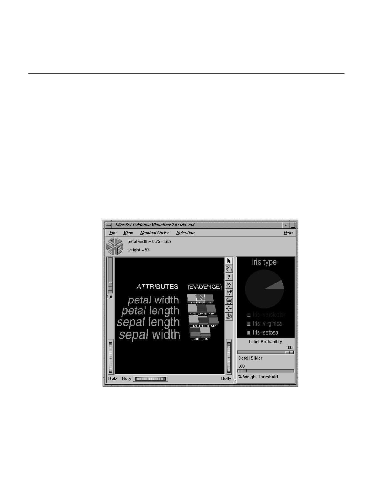
412
Chapter 13: Inducing and Visualizing the Evidence Classifier
This multiplication corresponds to a conditional independence assumption. When this
assumption is violated, and multiple values for attributes are chosen, the predicted class
probabilities are likely to be too extreme, although the final classification might be
correct. The estimated error shown in the Status window when you run the inducer can
help you determine how reasonable this assumption is. If the error rate/loss is low, the
assumption is reasonably robust in the domain.
Before clicking on a square chart, the Evidence Visualizer appears as shown in
Figure 13-1. This shows that given no additional information, there is an approximately
equal likelihood that an iris will be designated type iris-setosa, iris-versicolor, or
iris-virginica. If you click a chart for petal width .75 - 1.65, the pie on the right changes to
that shown in Figure 13-15. This indicates that if the petal width is between .75 and 1.65,
the iris probably belongs to the class iris-versicolor. You then can select additional values
to further change the distribution. The order in which you select charts or bars does not
matter.
Figure 13-15 Iris Dataset With the Value petal width .75 - 1.65 Selected
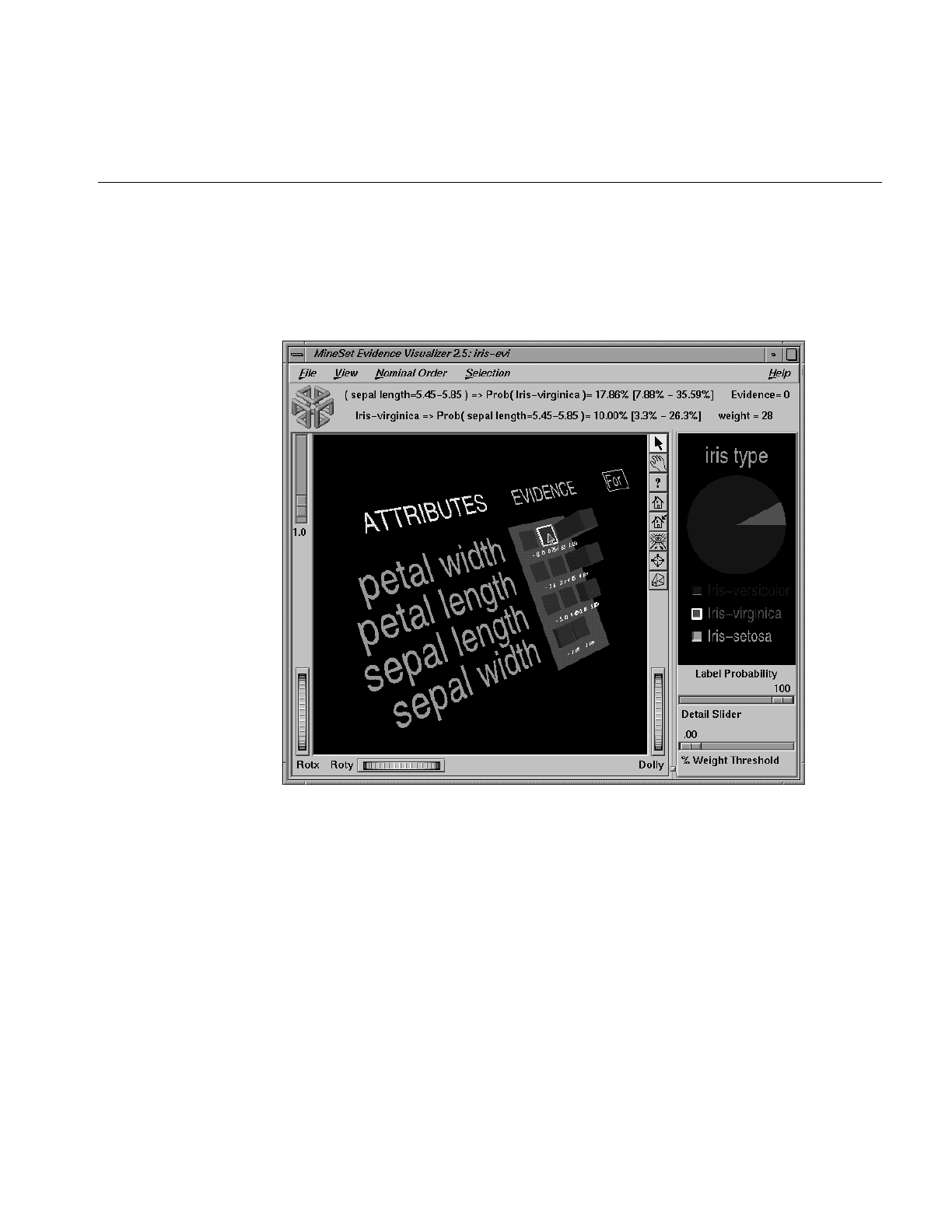
Working in the Evidence Visualizer’s Panes
413
When a particular label has been selected in the Label Probability Pane, the Main
Window shows bars rather than cakes or pies for each value of an attribute. The title over
the bars reads “Evidence For.” The box around the “For” indicates that it can be selected
(Figure 13-16).
Figure 13-16 Bars Showing Evidence For iris-virginica
Clicking the “For” in the “Evidence For” title toggles it to display “Against”. As a result,
the bar heights change to show evidence against the label (Figure 13-17).
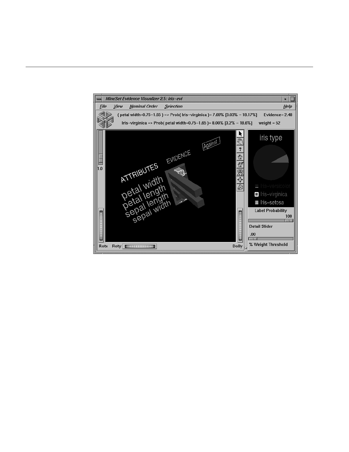
414
Chapter 13: Inducing and Visualizing the Evidence Classifier
Figure 13-17 Bars Showing Evidence Against iris-virginica
Selecting bars has the same effect on the large probability pie in the Label Probability
Pane to the right as did selecting cakes or pies. The bar height indicates the amount of
evidence for or against the selected label contributed by that selected value. Since log
probabilities are used to represent evidence, the bar heights are added to accumulate
evidence (whereas probabilities must be multiplied).

External Controls
415
External Controls
The external controls for the visualizer associated with the Decision Table classifier are
the same as those for the Map Visualizer. For a description of these controls, see “External
Controls” in Chapter 5.
Sliders
The Evidence Visualizer contains three sliders: Height Scale, Detail Slider, and Percent
Weight Threshold.
The Height Scale Slider (Figure 13-18), which is located in the upper left of the Evidence
Visualizer, scales the height of the charts and bars. You can use this slider to magnify
small differences.
Figure 13-18 Evidence Visualizer Height Scale Slider
The Detail Slider, located at the bottom right of the Evidence Visualizer window
(Figure 13-19), filters out attributes that are not as useful for classifying the selected label.
This quality, assigned a value between 0 and 100 by the inducer, is called importance. This
measure is on an absolute scale. To understand how importance is calculated, see
“Column Importance and Relation to Classifiers” on page 497. As the slider is moved to
the right, attributes that fall below the requisite importance value are removed from the
scene. If the attributes are sorted by importance (the default), then the ones at the bottom
are the first to be removed.
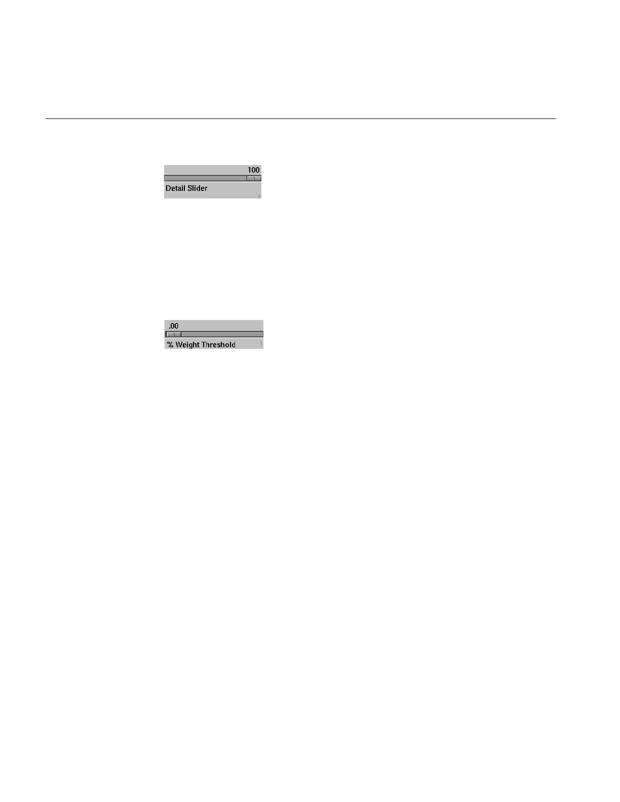
416
Chapter 13: Inducing and Visualizing the Evidence Classifier
Figure 13-19 Evidence Visualizer Detail Slider
The Percent Weight Threshold Slider, located at the bottom right of the Evidence
Visualizer window (Figure 13-20), filters out values having counts less than the
percentage indicated by the slider (up to a maximum of 2%). This slider helps visualize
attributes that have a large number of values, many of which occur infrequently (and,
hence, are not as useful). For example, if an attribute has 101 values, removing values
with counts less than 1% of the total might remove all values, and must remove at least 2.
Figure 13-20 Evidence Visualizer Percent Weight Threshold Slider.
Pulldown Menus
Five pulldown menus let you access additional Evidence Visualizer functions: File, View,
Selection, Nominal Order and Help. If you start the Evidence Visualizer without
specifying a configuration file, only the File and the Help menus are available.
The File Menu
The File menu lets you open a new configuration file, reopen the current configuration
file, save an image of a current display, send an image of the display to the printer, start
the Tool Manager, or exit the Evidence Visualizer.
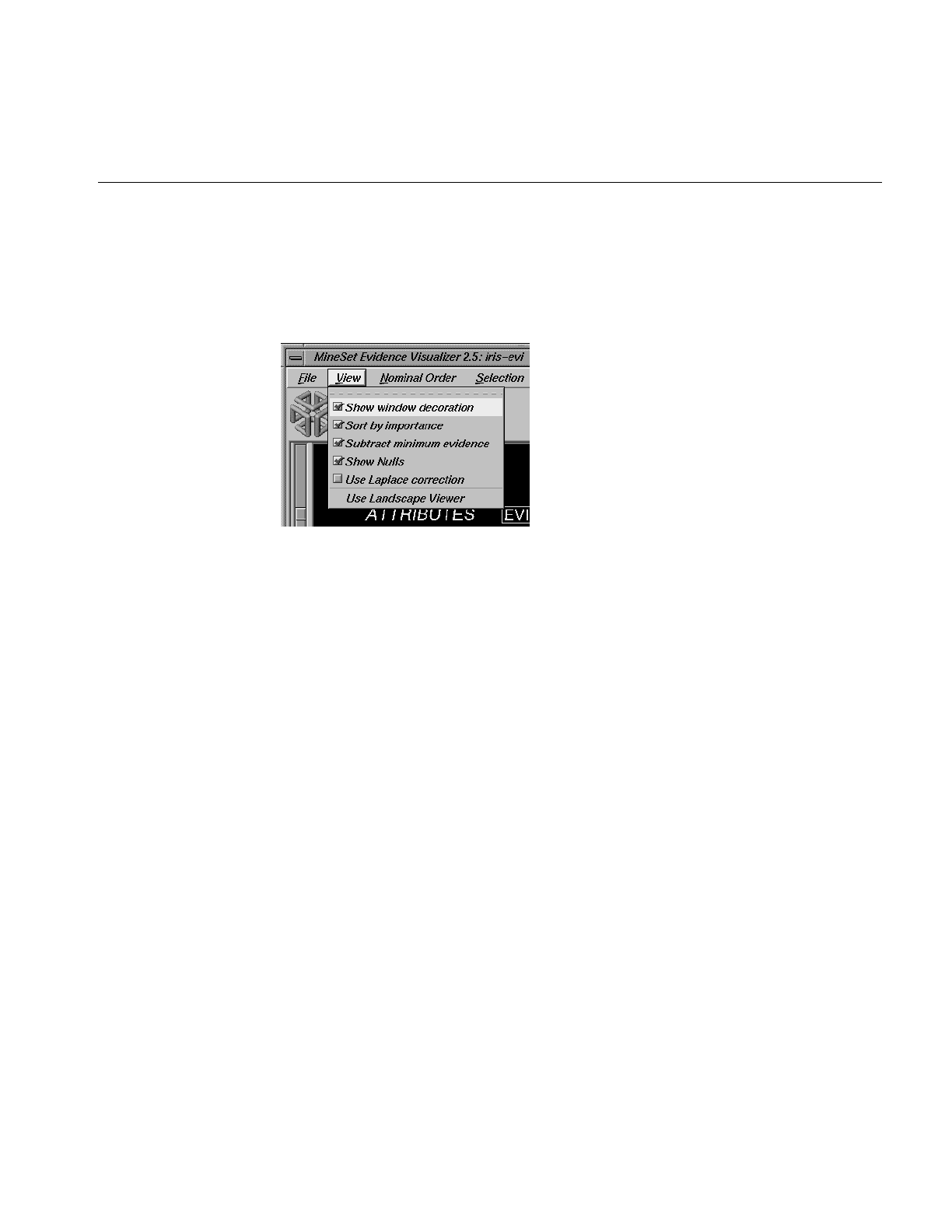
Pulldown Menus
417
The View Menu
The View menu lets you control certain aspects of what is shown in the Evidence
Visualizer pane (Figure 13-21).
Figure 13-21 Evidence Visualizer’s View Menu
This menu contains six options:
•Show Window Decoration lets you hide or show the external controls around the
display window.
•Sort By Importance lets you display the attributes sorted according to their
usefulness in classifying with respect to the chosen label. If this option is turned off,
then the attributes will appear in the same order they did under “Current Columns”
in the Tool Manager.
•Subtract Minimum Evidence applies only when a label has been selected and the bars
are shown. With this option on (the default), the height that is the minimum over all
the label values is subtracted. This amount may be different for each value of each
attribute, but for a given attribute value, the amount subtracted is constant across
label values. Activating this option magnifies small differences by subtracting the
least common denominator among all the label values.
•Show Nulls toggles the display of null values. Null values, if present, are shown as
the first value, offset slightly from other non-Null values.
•Use Laplace Correction toggles the use of Laplace correction. If a specific Laplace
correction was specified in the further inducer options dialog box, then that value
gets used, otherwise a default value is provided.
•Use Landscape Viewer (or Use Examiner Viewer) switches to an alternative mode of 3D
navigation. To understand navigation using the Landscape viewer see “Navigating
With the Middle Mouse Button” in Chapter 5.
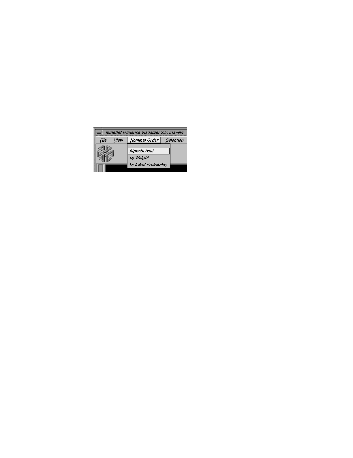
418
Chapter 13: Inducing and Visualizing the Evidence Classifier
The Nominal Order Menu
The Nominal Order menu lets you control how values for nominal attributes are ordered
(Figure 13-22).
Figure 13-22 Evidence Visualizer’s Nominal Order Menu
The three choices are:
•Alphabetical implies values for nominal attributes are sorted from left to right, in
alphabetical order.
•by Weight sorts values from left to right, with those having the largest number of
records appearing toward the left.
•by Label Probability (the default) sorts the values of nominal attributes by the size of
the slices corresponding to one of the classes. If the label is a binned attribute, the
highest bin is used by default. If the label is nominal, then whatever class has the
largest slice in the prior probability pie is used by default. If a particular class is
selected, and then sort by label probability is requested, the selected class is used for
determining the ordering. In all cases, if there is a NULL value, it remains at the far
left.
The Selection Menu
The Selection menu allows drill-through to the underlying data (Figure 13-23). To do a
drill-through, first select some combination of values and/or a class, then chose one of
the two methods of drilling-through to the underlying records.
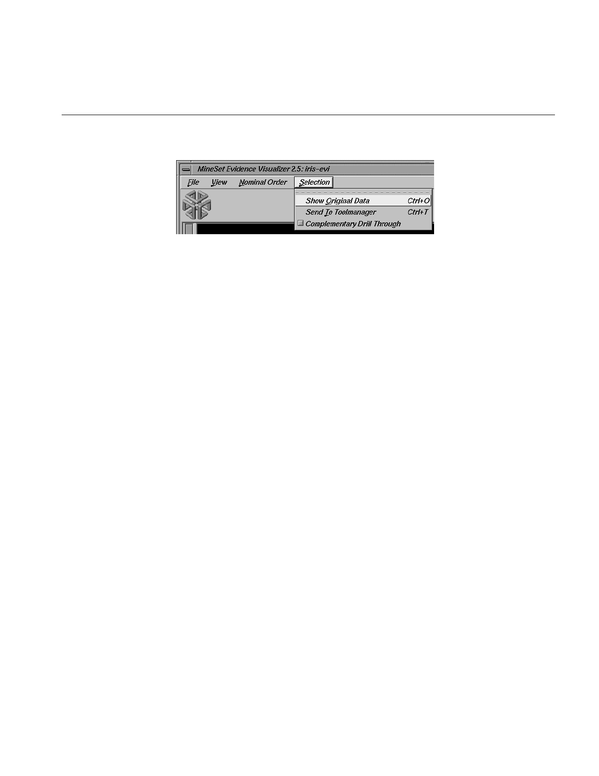
Pulldown Menus
419
Figure 13-23 Evidence Visualizer’s Selection Menu
There are three menu items:
•Show Original Data causes the records corresponding to the selected item to be
displayed in a record viewer.
•Send to Tool Manager causes a filter operation to be inserted at the beginning of the
Tool Manager history. The actual expression used to do the drill-through is
determined by
–the values selected in the Main Window, and
–the class(optionally) selected on the right.
All selected values within a single attribute are ORed together. These terms for each
attribute are then ANDed along with the class selection, if present, to form a
drill-through expression that is used to do the filtering in Tool Manager. If nothing
is currently selected, a warning message appears.
For Figure 13-24 the filter expression would be:
(`gross income`>60000.0) &&
((`occupation`==”Protective-serv”)||(`occupation`==”Tech-support”))
&&(`education`==”Masters”)
&&(`sex`==”Female”)
•Complementary Drill Through uses the complement of the expression defined by the
selected objects for drill-through.
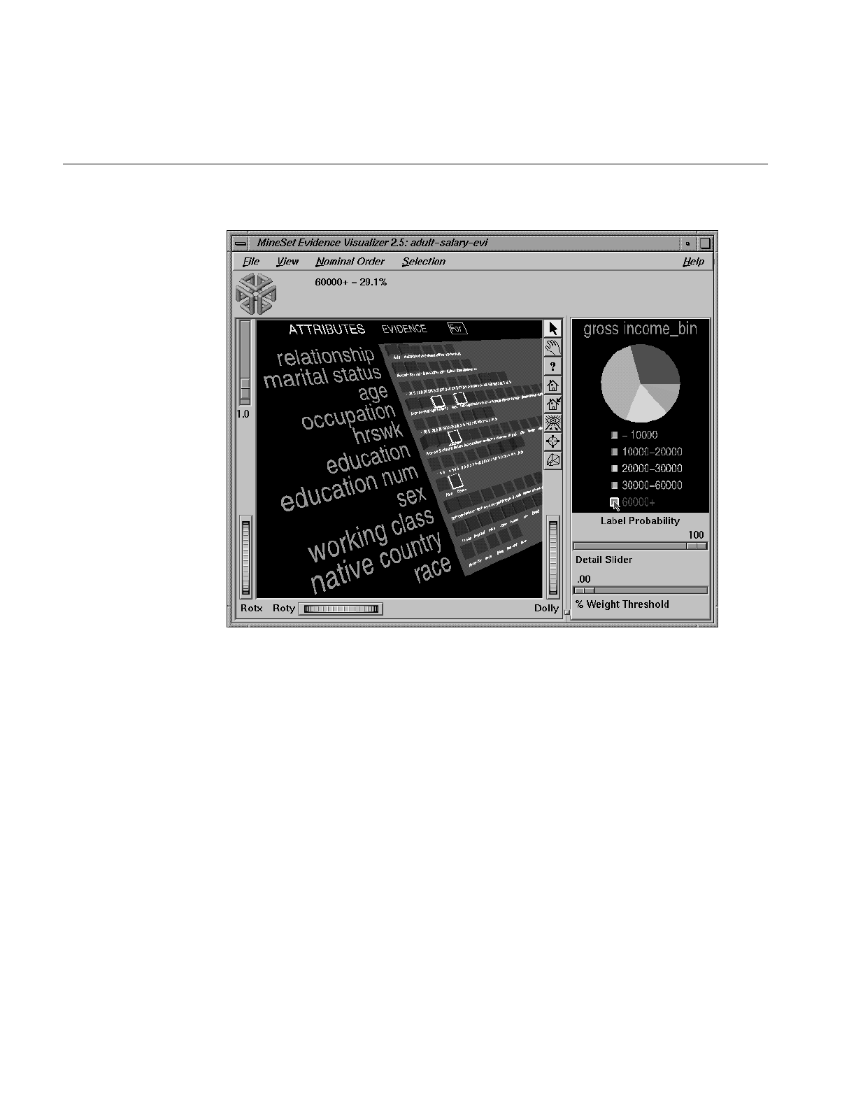
420
Chapter 13: Inducing and Visualizing the Evidence Classifier
Figure 13-24 Filtered Adult Dataset With Multiple Selection
Sample Files
The following examples show cases in which classifiers might be useful. Each of these
examples is associated with a sample dataset provided with MineSet. By running the
inducer, you can generate the .eviviz files described below.
Note: The data files, which have a .schema extension, are located in /usr/lib/MineSet/data
on the client workstation. The classifier visualization files, which have a .eviviz extension,
reside on the client workstation in /usr/lib/MineSet/eviviz/examples.

Sample Files
421
Churn
Churn is when a customer leaves one company for another. This example shows what
causes customer churn for a telephone company. The data used to generate this example
is in /usr/lib/MineSet/data/churn.schema. The file
/usr/lib/MineSet/eviviz/examples/churn.eviviz shows the structure of the classifier induced
using the attribute churned as the label. The error rate for this classifier is 12%. 14.1% of
the records represent customers who churned. The two most important attributes,
total_day_minutes and total_day_charge, are clearly correlated. A more accurate
classifier can be induced if one of these attributes is removed first (the error rate becomes
11%). If you run the inducer after selecting Automatic Feature Selection from the Further
Inducer Options, the error-rate drops to 10.5% using only 4 attributes (total day charge,
number of service calls, voice mail plan, and number of voice mail messages). All 29
customers who had a total_day_charge above 53.78 churned.
A high number of customer service calls is a predictor of churn. Many customer service
calls might indicate frustration in using a complicated equipment or receiving unreliable
service. Customers with the International plan are also more likely to churn. The people
in some states were much more likely to churn than those in others; for example,
California and New Jersey have the most churn, Virginia the least. To see just those states
that have more than 2% of the total number of records, slide the % Weights Threshold
slider all the way to the right. This eliminates most of the values for state from the
display. If you also select Nominal Order > Weight, then the state with the most records,
West Virginia (WV), is left-most. Many of the attributes (at the bottom of the list) are not
useful in discriminating churn. Note that day_charge is a great predictor, but
night_charge is not.
Origin of Cars
The cars dataset contains information about different models of cars from the 1970s and
early 1980s. Attributes include weight,acceleration, and miles per gallon (mpg). The file
/usr/lib/MineSet/eviviz/examples/cars.eviviz shows the structure of the Evidence Classifier
induced for this problem. This file was generated by running the inducer on
/usr/lib/MineSet/data/cars.schema with the label set to origin (Japan, U.S., Europe) and the
cylinders column changed to type string. The cylinders were changed to type string in
order to see all values and avoid the automatic discretization.

422
Chapter 13: Inducing and Visualizing the Evidence Classifier
If you have a dataset of car attributes, you might want to know what characterizes cars
of different origins. From the distribution of label values in the pie on the right we can
see that most cars in this dataset were made in the U.S. (62.5%) and a smaller number in
Japan (20.2%) and Europe (17.3%). Clearly brand is the best predictor of origin, since each
brand is associated with only one country of origin. For this reason, it has the highest
importance and is at the top of the list. By looking at the height of the pies, it can be seen
that many cars have four cylinders, most weigh less that 3000 lbs and most can reach 60
miles per hour in less than 20 seconds but more than 13.
Look at the distribution of slices for individual attribute values. If a car has an engine size
>169 cubic inches, it is almost certainly made in the U.S.; it certainly was not made in
Japan. Other pies show that U.S. cars generally have six or eight cylinders, low miles per
gallon, high horsepower (over 134), heavy weight (over 2981 lbs), and fast acceleration.
Japanese cars have better gas mileage, three or four cylinders (and a few six cylinders),
and smaller engines. If you click “Europe” in the Label Probability Pane, you can see bars
representing evidence for a car being European. For example, five cylinders strongly
indicates that a car is European. The height of the corresponding pie, however, shows
that there were only three cars with five cylinders in the data. If a car’s mileage is good,
there is much evidence for it being European. If a car’s mileage is > 41, then there is an
83% chance that it’s European. If a car is European, there is only a 10.4% chance that its
mileage is better than 41 mpg. But only 2% of Japanese cars—and no U.S. cars—have
mpg in this range, so Europe gets the most evidence.
Suppose you wanted to predict where a car came from knowing only that it got 40 mpg
and weighed 3000 lbs. Select the appropriate pies (or bars): mpg=30.95-41.15 and
weightlbs=2981.5+. The resulting probability distribution on the right shows 84% U.S.,
16% European. There is no possibility it is Japanese because there were no Japanese cars
in the training set with weightlbs>2981.5. If you run the inducer again with Laplace
correction turned on (with a value of .5), you get a different answer: 16% chance for
European, 82% chance for U.S., and a 2% chance for Japanese. This is because Laplace
correction prevents any slice in the pies from going completely to 0. Certainly, there is no
fundamental reason why the Japanese could not make a car that weighs more than
2981lbs; hence, when the probabilities (pies) are multiplied together, the possibility of
predicting a Japanese car is not eliminated.

Sample Files
423
Gender Attribution
The adult dataset contains information about working adults. This dataset was extracted
from the U.S. Census Bureau. It contains data about people older than 16, with a gross
income of more than $100 per year who work at least one hour a week. You might want
to know how to characterize males and females. The file
/usr/lib/MineSet/eviviz/examples/adult-sex.eviviz shows the structure of the Evidence
Classifier induced for this problem. This file was generated by running the inducer on
/usr/lib/MineSet/data/adult.schema, with the label set to sex, after removing the relationship
column (which would have made the classifier trivial).
In the Evidence Visualizer, the Label Probability Pane shows that the prior probability of
working males is higher than that of females.
•Marital status is the most important predictor of gender. If a worker is a
married-civilian-spouse there is a greater probability of being male. A worker who
is widowed and working, however, is much more likely to be female.
•The second attribute listed shows occupation. Study this to learn which occupations
are popular with a particular gender. The various occupations are listed from left to
right in order of decreasing male dominance: Armed forces (100%), Craft-repair
(95%), Transport-moving (95%), and Farming-fishing (94%). Female trades are
Private-house-service (94%) and Adm-clerical (67%). By clicking on the button next
to “Female” in the Label Probability Pane, and then moving the mouse over
occupation = Adm-clerical, one can see that 23% of females have an Adm-clerical
job. Conversely, given that one’s job is Adm-clerical, there is a 67% chance that the
gender is Female.
Suppose you wanted to find out the probability of being female given that a person
is widowed and has occupation = Adm-clerical. This can be done by clicking on the
values and reading 95% from the text at the top when you move the mouse over the
box next to “Female” (in select mode).
•If the working class is either self-employed-incorporated or
self-employed-not-incorporated, the probability that the person is a male is higher.
Conversely, if the working class is state-gov, the conditional probability that the
person is a female is higher, but the posterior probability (after taking into account
the prior probability) is not higher (click it and look at the posterior probability on
the right). The size of the female slice increased by selecting state-gov, but not so
much that it would lead you to predict that a person was female, given only that
they worked for the state.
By rotating the view, you can see that most people work in private industry by
looking at the height of the charts.

424
Chapter 13: Inducing and Visualizing the Evidence Classifier
•By looking at the gross-income attribute, you can see that the higher the income
range, the higher the probability of being male.
•Education generally does not indicate much about gender, except for doctorate
degrees, where you are more likely to find males.
•Different occupations have different distributions for males and females.
•The race attribute shows that African-Americans have a higher percentage of
females working than the percentage of other races in the conditional probability.
Click the value to see that the posterior is about equal between males and females.
•Males in this dataset work more hours per week than do females.
Salary Factors
If you have a dataset of working adults, you might want to find out what factors affect
salary. First bin gross_income into five bins, with thresholds at 10,000, 20,000, 30,000, and
60,000. Each record then has an attribute with one of five values. You can run a MineSet
classifier to help determine what factors influence salary. The file
/usr/lib/MineSet/eviviz/examples/adult-salary.eviviz shows the Evidence classifier induced
for this problem. This file was generated by running the inducer on
/usr/lib/MineSet/data/adult.schema with gross_income divided into five bins using
user-specified thresholds.
The attributes in the Evidence Visualizer are ranked by importance; thus, relationship,
marital status, age, occupation, education, hours per week, and sex are considered most
important. Since the label is numeric, a continuous spectrum is used to assign colors to
each class. Red is assigned to the highest bin (60,000+). The class labels are listed in the
Label Probability Pane according to slice size. As you click on values in the Main
Window, the order of the class labels changes to keep the label for the largest predicted
class at the top.
•Relationship shows that husbands and wives are likely to make more money than
unmarried workers or workers not in a family. Wives have slightly higher incomes
than husbands.
•Marital status shows that most people are married (the second chart from the left is
tall). Married workers earn more money than unmarried people.
•Age shows that age is a crucial factor. Until the age of 61, when many people retire,
the probability of making over $50,000 increases as workers get older.

Sample Files
425
•Different occupations yield different probabilities. Executive and professional jobs
raise the evidence for making over $60,000 per year.
•Education is an important factor. When considering just education, the highest
evidence for earning over $60,000 is given to workers whose educational level
includes a masters or doctoral degree, or matriculation from professional schools.
•Hours per week show that the more hours worked, the higher the evidence for
earning more money.
•Sex shows that being a female gives evidence for making less than $60,000 per year.
•Adjust the Percent Weights slider to remove values of native_country, education and
occupation with low weights are removed.
Iris Classification
In this dataset, each record describes four characteristics of iris flowers: petal width, petal
length, sepal width, and sepal length. Each iris was further classified into the types
iris-setosa, iris-versicolor, or iris-virginica. The goal is to understand what characterizes
each iris type.
Before running a classifier, click the Column Importance tab in the Tool Manager’s
Classifiers tab; then click Go! You obtain a ranking of the importance of the features: petal
width, petal length, and sepal length. You can map these to the axes in the Scatter
Visualizer, with the iris_type mapped to the color and see the clusters.
The file /usr/lib/MineSet/eviviz/examples/iris.eviviz shows the structure of the Evidence
Classifier induced for this problem. This file was generated by running the inducer on
/usr/lib/MineSet/data/iris.schema.
In the Evidence Visualizer, we can see that petal length and petal width are excellent
discriminatory attributes, while sepal length and sepal width are not as good. Move the
importance threshold slider to the right to see that the sepal-based attributes disappear
first.

426
Chapter 13: Inducing and Visualizing the Evidence Classifier
Mushroom Classification
The file /usr/lib/MineSet/eviviz/examples/mushroom.eviviz shows the structure of the
Evidence Classifier induced for this problem. This file was generated by running the
inducer on /usr/lib/MineSet/data/mushroom.schema.
The goal is to understand which mushrooms are edible and which ones are poisonous,
given this dataset. There are over 8000 records in this set; thus, running this inducer
might take several minutes. Note that under the default mode of the one-third holdout
for accuracy estimation, a third of the records are kept for testing.
Each mushroom has many characteristics, including cap color, bruises, and odor. The
Evidence Visualizer orders attributes by importance (that is, usefulness in predicting the
label). Odor and spore print color appear at the top of the list because the distributions
in the pies is most different from value to value for these attributes. Since all the attributes
in this dataset are nominal, all the values are sorted from left to right by how well they
predict edibility. You might want to order the values alphabetically or by weight
(prevalence). To do this, select the appropriate method from the nominal order menu.
You can see a characterization of poisonous mushrooms by changing the pointer to an
arrow (click the arrow icon at the top right of the main screen), then clicking the button
by that class label in the right pane. High bars are associated with values that indicate the
mushrooms are poisonous.
In the Evidence Visualizer, move the Detail slider to the right. The attributes with the
lowest importance are removed from the scene. The most important attribute by far is
odor, as its importance is 92; all other attributes have importance less than 48. Almost all
values are good discriminators, but if there is no odor (none), then there is a mix of both
classes. The Evidence Visualizer lets you see specific values that might be critical, even if
the attribute itself is not always important. For example, stalk_color_below_ring is not a
good discriminatory attribute because most of the time it takes on the value white. White
offers no predictive power because there are equal amounts of edible and poisonous
mushrooms with this value. When stalk_color_below_ring takes the value gray or buff,
it provides excellent discrimination, but there are very few mushrooms with these
values.

Sample Files
427
Party Affiliation
This dataset consists of voting records. The goal is to identify the party a congressperson
belongs to given data about key votes. The dataset includes votes for each member of the
U.S. House of Representatives on the 16 key votes identified by the Congressional
Quarterly Almanac (CQA). The CQA lists nine types of votes: voted for, paired for, and
announced for (these three are simplified to yes), voted against, paired against, and
announced against (these three are simplified to no), voted present, voted present to
avoid conflict of interest, and did not vote or otherwise make a position known (these
three are simplified to an unknown disposition).
Before running a classifier, look at the 16 votes to see if you can perceive which features
are important. Then run the Evidence Visualizer. For this dataset, you might want to
order the values alphabetically, so that all no votes are on the left, undecided is in the
middle, and yes is on the right.
Some issues clearly define one’s party affiliation. Democrats tended to vote for a
physician fee freeze and aid for El Salvador, while Republicans voted for adoption of a
budget resolution and aid to the Contras in Nicaragua.
Immigration was an issue not split along party lines; nevertheless, politicians had strong
positions on it because only 7 out of the 235 were undecided on this issue.
The file /usr/lib/MineSet/eviviz/examples/vote.eviviz shows the structure of the Evidence
Classifier induced for this problem. This file was generated by running the inducer on
/usr/lib/MineSet/data/vote.schema.
Breast Cancer Diagnosis
The breast cancer dataset contains information about females undergoing breast cancer
diagnosis. Each record represents a patient with attributes such as cell size, clump
thickness, and marginal adhesion. The final attribute is whether the diagnosis is
malignant or benign. The file /usr/lib/MineSet/eviviz/examples/breast.eviviz shows the
structure of the Evidence Classifier induced for this problem. This file was generated by
running the inducer on /usr/lib/MineSet/data/breast.schema.
In the Evidence Visualizer, you can see that sample_code_number was discretized into
one range that is equally split, meaning that it does not indicate whether the breast cancer
is benign or malignant.

428
Chapter 13: Inducing and Visualizing the Evidence Classifier
Hypothyroid Diagnosis
The hypothyroidism dataset is similar to the one for breast cancer. The file
/usr/lib/MineSet/eviviz/examples/hypothyroid.eviviz shows the structure of the Evidence
Classifier induced for this problem. This file was generated by running the inducer on
/usr/lib/MineSet/data/hypothyroid.schema.
There are 3163 records in this dataset and most of them do not have hypothyroidism
(95.45%). While this means that one can predict “negative” and be correct with high
probability, it’s those people that have hypothyroidism that we are most worried about.
In technical terms, the false negatives are very important.
Look at the pie for “tsh” between 6.35 and 27.5. It shows much evidence for
hypothyroidism. When you click on it, however, the posterior pie still predicts
“negative” because the prior probability for “negative” was so great.
This is a case where you might want to adjust the Loss Matrix to skew the posterior
probability toward predicting hypothyroidism in order to avoid false negatives. There
might be a high cost associated with predicting that someone is healthy when they
actually have the disease; predicting them sick when they are actually healthy means
they take a more accurate test or a treatment they do not need.
In the Evidence Visualizer, you can see that “fti” is very important. The first two ranges
(besides the unknown) give a lot of evidence for hypothyroidism.
Pima Diabetes Diagnosis
This dataset is a diagnosis problem for diabetes using statistics gathered from an Indian
tribe in Phoenix Arizona. The task is to determine whether a patient has diabetes, given
some medical attributes, such as blood pressure, body mass, glucose level, and age.
The file /usr/lib/MineSet/eviviz/examples/pima.eviviz shows the structure of the Evidence
Classifier induced for this problem. This file was generated by running the inducer on
/usr/lib/MineSet/data/pima.schema.
In the Evidence Visualizer, you can see that many attributes are irrelevant by themselves.
As plasma_glucose increases, the probability of having diabetes increases. The number
of pregnancies is also a good indicator when it is high (above 6), as is age (above 27).

Sample Files
429
DNA Boundaries
The file /usr/lib/MineSet/eviviz/examples/dna.eviviz shows the structure of the Evidence
Classifier induced for this problem. This file was generated by running the inducer on
/usr/lib/MineSet/data/dna.schema.
There are 3,186 records in this DNA dataset. The domain is drawn from the field of
molecular biology. Splice junctions are points on a DNA sequence at which
“superfluous” DNA is removed during protein creation. The task is to recognize
exon/intron boundaries, referred to as EI sites; intron/exon boundaries, referred to as IE
sites; or neither. The IE borders are referred to as “acceptors” and the EI borders are
“donors.” The records were originally taken from GenBank 64.1 (genbank.bio.net). The
attributes provide a window of 60 nucleotides. The classification is the middle point of
the window, thus providing 30 nucleotides at each side of the junction.
From the Evidence Visualizer, you can see that attributes near the center are chosen as
very important. Attributes further away from the splice junction are less important.
If you click and select the charts in the left pane corresponding to “left_01: G” and
“left_02: A”, then the pie chart in the label probability pane on the right will change to
show the probability distribution of each class as predicted by the evidence classifier.
Given these two values, the pie chart shows that the evidence model built assigns the
highest probability to “intron/exon”, followed by “exon/intron” and “none”.
The accuracy improves slightly if you invoke automatic feature selection, although
running time increases dramatically (sometimes hours). In such cases, run feature
selection once, and continue mining only with the chosen features.


431
Chapter 14
14. Inducing and Visualizing the Decision Table
This chapter discusses the features and capabilities of the Decision Table Visualizer,
provides an overview of this tool, and discusses the methods of inducing Decision
Tables. It then explains the Decision Table Visualizer’s functionality when working with
the
•Label Probability Pane
•Main Window
Finally, it lists and describes the sample files provided for this tool.
Note: It is assumed that you have read Chapter 10, “MineSet Inducers and Classifiers,”
before proceeding with this chapter.
Overview
The Decision Table presents correlations between pairs of attributes, and can be used as
a visualizer alone, or as a classifier and visualizer, in the same manner as MineSet’s other
inducers and visualizers. The underlying structure used for classification is a Decision
Tree which splits on a single attribute at each level of the tree hierarchy. Such a structure
is called an Oblivious Decision Tree. That attribute is rendered discrete in an identical
manner across the whole level. Accuracy is inhibited to a small degree by representing
the Decision Tree in this way, but the advantage is a uniform structure in a compact
tabular form, which can easily show correlations between pairs of attributes at adjacent
levels in the tree.
The method of classification used by Decision Tables is similar to that of a Decision Tree.
Classification is done by picking the majority class of the region in which the example is
found. If a record to be classified falls in a region where no training data occurred,
classification is done by picking the predominant class one level up in the table hierarchy.
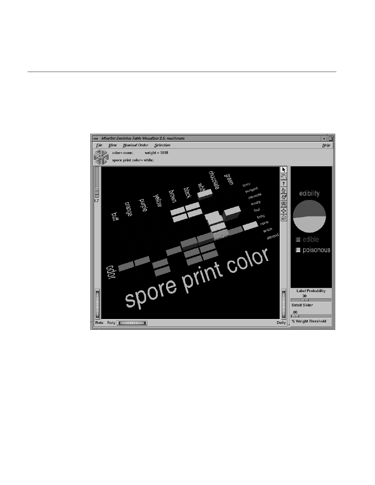
432
Chapter 14: Inducing and Visualizing the Decision Table
An example Decision Table is shown in Figure 14-1 for the mushroom dataset. It is
hierarchical in structure like a Decision Tree, but breaks the data down by two attributes
at each level instead of one. Decision Tables do not assume that the attributes are
independent.
Figure 14-1 Decision Table for the Mushroom Dataset

Overview
433
You might, for example create a Decision Table from the mushroom dataset to determine
mushroom edibility (see Figure 14-1). The Main Window (on left) shows the top level of
detail for a Decision Table induced from the mushroom dataset. Odor and
spore-print-color were chosen to be at the top level because doing so improves the
accuracy of the underlying classifier. In this dataset a dependence is shown between odor
and spore-print-color at the top level. There is only one top level block with any
ambiguity, meaning more than one class is present. It is the block with odor=none and
spore-print-color=white. When you drill down to the next level (by clicking the right
mouse button over the chart) the attributes habitat and population are shown at the next
lower level (see Figure 14-2). The result of zooming in close to this drilled-down region
is shown in Figure 14-3.
Figure 14-2 Decision Table for the Mushroom Dataset, Showing Drill-Down
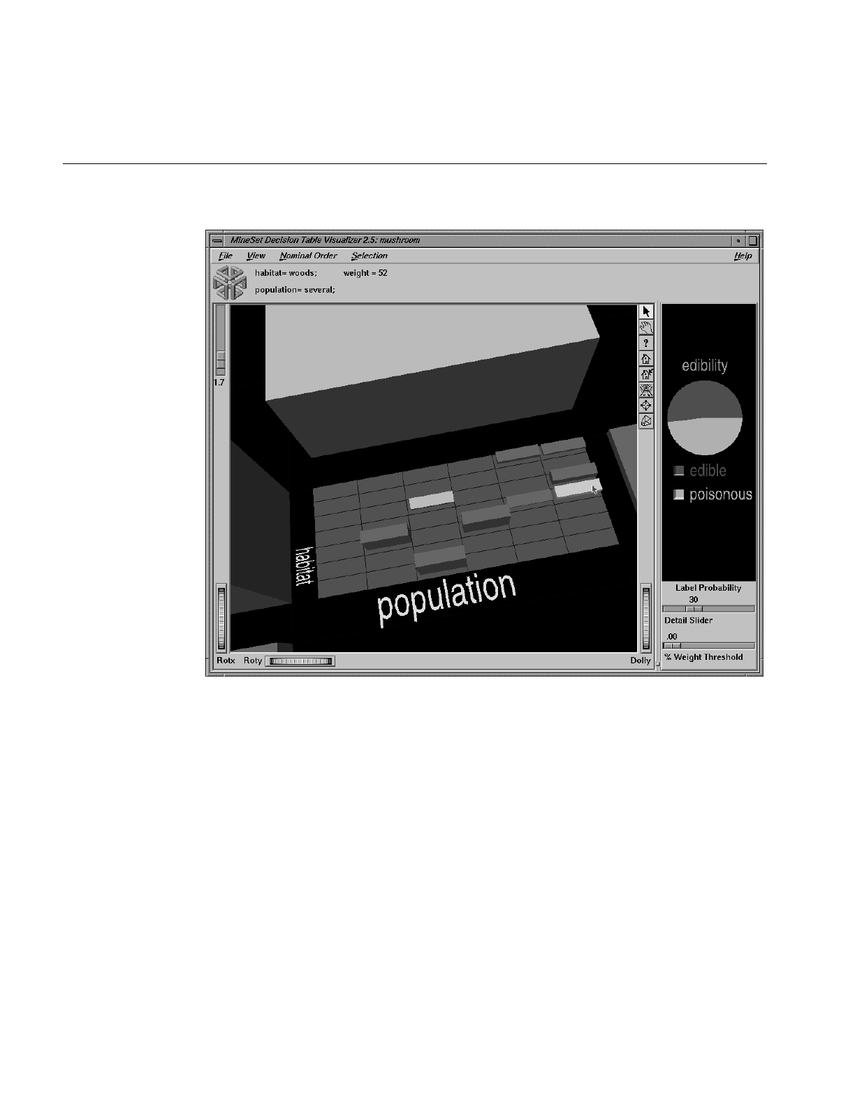
434
Chapter 14: Inducing and Visualizing the Decision Table
Figure 14-3 Mushroom Dataset Close-Up of “odor=none and spore-print-color=white”
The Decision Table Visualizer may be used to answer questions such as:
•When you know the values for only a few attributes, what can you predict for a new
record? If the attributes for which you know the values appear in the top levels of
the hierarchy, then this question is answered precisely, instead of approximately, as
with the Evidence Visualizer.
•How are the records distributed with respect to the label for the combination of
attribute values that you are interested in?

Overview
435
The prior probability for each class label is depicted in the pie chart in the Label Probability
Pane, on the right of the screen. The prior probability for a class label is the probability of
seeing this label in the data for a randomly chosen record, ignoring all attribute values.
Mathematically, this is the number of records with the class label divided by the total
number of records.
The probability distribution for each rectangular block or cake in the Main Window on the
left, shows the proportion of records in each class considering only records having that
particular combination of values. These probabilities are precise for the data given.
By default, values of nominal attributes are sorted by how well they predict one of the
classes. This helps identify important values. If the label is a binned attribute, the class
that is the highest bin is used. If the label is nominal, then the class with the largest slice
in the prior probability pie is used. When you select a particular class, and request a sort
by label probability (nominal ordering > sort by label probability), that class determines the
order of the result. Alternatively, the values of the nominal attributes can be sorted
alphabetically or by weight. Values of binned attributes are always shown in their
natural order.
When you drill down into a rectangular cake (using the right mouse button) the data
represented by that cake is redisplayed in a new matrix of cakes where the attributes
assigned to that level of detail are used as the axes. The cake charts sit on top of a gray
base. If the base is completely covered with cakes, then every combination of values at
this level is represented by the data. Often much of the base is uncovered. This shows
regions where no data exists. In a very sparse dataset there are large regions that are
empty. Picking or selecting a gray base has the same effect as selecting the cake that was
one level up in level of detail. Drilling down on a base causes every cake sitting on top of
it to expand to the next level of detail.
If an attribute has unknown (NULL) values, then the unknown values are denoted by a
question mark (?). The NULL always appears as the first value if present and does not
get sorted with the rest. It is possible to toggle the display of NULL values using View >
Show Null Values.
If a cake is selected (left mouse click) on the left, then the probability pie on the right will
show a posterior probability distribution which exactly matches that shown by the cake.
When more than one cake chart on the left is selected (Shift-left mouse click), then the pie
on the right will show the probability distribution (with respect to the label) for the set of
records defined by the selected cakes. It is also possible to select a whole group of cakes
by selecting the gray base below them. This has the same effect as selecting the cake one
level up in the hierarchy.

436
Chapter 14: Inducing and Visualizing the Decision Table
Classes are listed under the pie chart on the right, and are in order of slice size. The class
with the largest probability is at the top. As values on the left are selected, this order
changes to reflect the changing probability pie. The class that would be predicted given
current selections is shown at the top. If the label is a binned attribute the order of the
classes is not changed on slice size. In addition, if the label is a binned attribute, colors
are assigned according to a continuous spectrum: the highest bin is red; otherwise,
random colors are used.
Inducing Decision Tables
A Decision Table classifier can be induced, or generated automatically, from data. The
data is made up of records, and a label associated with each record. (See Chapter 10,
“MineSet Inducers and Classifiers”)
The automatic induction of Decision Table classifiers is a process in which record counts
(or more generally record weights) are used to calculate the probabilities using the
following method:
1. All continuous attributes are separated into discrete bins, so that class distributions
in these ranges are as different as possible. The number of ranges is determined
automatically. You can override automatic binning for any attribute by explicitly
binning using Tool Manager.
2. The prior probabilities are the proportions of each class in the training set.
The number of cakes in any row along one of the axes (attribute) pairs shows the number
of discrete ranges produced by the inducer. If there is just one range, it means that this
attribute by itself was not useful in predicting the label. Initially, the prior probabilities
of the labels are displayed in the Label Probability Pane.
There are three ways to assign attributes to X and Y axes at every level in the Decision
Table hierarchy: manually, automatically, and automatically with feature search.
The classifier can have a loss matrix. When the classifier is applied, the loss matrix skews
the predictions. In the visualization, the loss matrix can be used to adjust the posterior
probability distribution.

File Requirements
437
File Requirements
The Decision Table Inducer requires the following files:
•A data file (.data) consisting of rows of tab-separated fields.
•A .dtableviz file containing the schema.The format of this schema is the same as
described in “The .schema File” in Appendix A.
•A training set, as described in “Training Set” in Chapter 10. Files are generated by
extracting data from a source (such as a MineSet ASCII or binary file, or a table in an
Oracle, INFORMIX, or Sybase database).
To apply the generated classifier, you should have a dataset of records with the attributes
used by the classifier, except that the label need not be present.
Running the Decision Table Inducer
There are two ways to run the Decision Table inducer:
•From the Tool Manager
Connect to the server and select a data source (see “Choosing a Data Source” in
Chapter 3).
From the File menu, choose Open New Data File. Log in to a server, and enter the
filename. For the example shown here, the filename entered is
/usr/lib/MineSet/data/mushroom.schema. In the Data Transformation panel you see 23
discrete attributes. Select the Mining Tools tab in the Data Destination panel and
click the Classify tab. Select edibility as the discrete label. Select the Decision Table
inducer, and ensure you have selected the Classifier & Error mode. To run the
Inducer, click Suggest then click Go!.
The status window shows the progress and statistics, and the Decision Table
Visualizer is launched automatically. You can also interrupt the automatic attribute
suggestion process by selecting Cancel or Show Viz Now in the progress dialog.
Selecting Show Viz Now stops the current server computation and uses the
intermediate result to construct the Decision Table for the columns mapped so far.
Alternatively you may manually map columns to the X and Y requirements as
described in the next section.
•From the command line
To induce a Decision Table classifier from the command line, refer to step 6 in
“Starting the Decision Table Visualizer” on page 438.

438
Chapter 14: Inducing and Visualizing the Decision Table
Starting the Decision Table Visualizer
As with the other visualization tools, there are six ways to start the Decision Table
Visualizer:
1. Run the Decision Table Inducer from the Tool Manager under the Classify tab. After
the inducer builds the classifier, it automatically invokes the Decision Table
Visualizer. See below for details about using the Tool Manager in conjunction with
the Decision Table Visualizer.
2. Use the Tool Manager to start the Decision Table Visualizer from the Visual Tools
menu. (See Chapter 3 for details of the Tool Manager’s functions, which are
common to all MineSet tools.)
3. Double-click the Decision Table Visualizer icon on your Silicon Graphics desktop.
The startup screen requires you to select a data file by choosing File > Open.
4. If you know what configuration file you want to use, double-click the icon for that
configuration file. This starts the Decision Table Visualizer and automatically loads
the configuration file you specified. This works only if the configuration filename
ends in .dtableviz. (Configuration files created for the Decision Table Visualizer with
Tool Manager all carry the .dtableviz suffix.)
5. If you know what configuration file you want to use, drag its icon onto the Decision
Table Visualizer icon. This starts the Decision Table Visualizer and automatically
loads the configuration file you specified.
6. Start the Decision Table Visualizer from the UNIX shell command line by entering
this command at the prompt:
dtableviz [dataFile]
Here, dataFile is optional and specifies the name of the configuration file to use. If
you don’t specify a configuration file, you then must use File> Open to specify one.
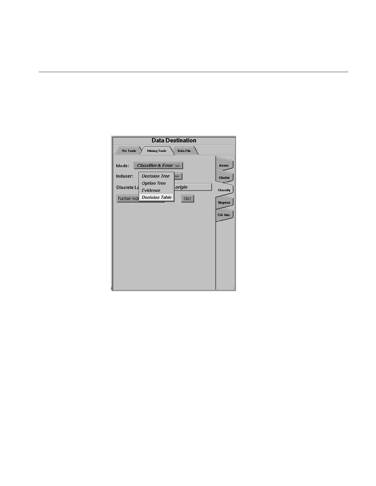
Configuring the Decision Table Inducer Using the Tool Manager
439
Configuring the Decision Table Inducer Using the Tool Manager
To access the options for configuring the Decision Table inducer, select the Mining Tools
tab on the Data Destination panel, shown in Figure 14-4.
Figure 14-4 Data Destination Panel in Tool Manager Showing Classifiers
From the tabs at the right, select Classify. Ensure that the inducer you select is Decision
Table. Your selections in the Mode and Inducer menus determine the options available
in the Further Inducer Options menu. After you have made your selections in these
menus, click Go! to run the inducer, which, in turn, creates the classifier. Or you can
simply click Suggest and then Go!

440
Chapter 14: Inducing and Visualizing the Decision Table
Discrete Labels
The Discrete Labels menu provides a list of available discrete labels selected from the
dataset you chose. Discrete attributes (binned values, character string values, or a few
integers) have a limited number of values. You should select a label attribute with few
values—two or three (see “Training Set” in Chapter 10). If there are no discrete attributes,
the menu shows No Discrete Label, and the Go! button is disabled. You then must create a
discrete attribute by binning or adding a new column, using the Tool Manager’s Data
Transformations panel.
Classifier Name
The generated classifier is named with the prefix of the session filename (as determined
in Tool Manager) and the suffix-dtable.class. By default, all classifiers are stored on the
server in the file_cache directory, which defaults to mineset_files. These classifiers can be
used for future classification of unlabeled records; that is, they can be used to predict the
labels for unlabeled datasets (see “Applying a Model” and “Backfitting in Error
Estimation” in Chapter 10).
Exploring Data by Mapping Columns to Axes
You can explore the relationships between attributes in data by mapping columns to X
and Y axes. Select a column name in the Current Columns panel of the Data
Transformations pane of Tool Manager window, then select an item in the X-axis or Y-axis
windows. The first two columns mapped are shown at the top level, and subsequent
mappings descend through the levels. If you map an odd number of attributes, the last
level of detail shows a single column of cakes corresponding to the values of that odd
attribute. If an interaction between two attributes is suspected, map one attribute to the
X axis and the other to the Y axis. If you have no idea which attribute to map to which
axis, simply click the Suggest and Go button.
There are two different ways to Suggest: with or without feature subset search in the
further inducer options turned on:
•Checkbox Off runs Column Importance to find the features. Column Importance is
described further in Chapter 17, “Column Importance.”
•Checkbox On begins with Column Importance, then runs through all possible orders,
beginning with the order recommended by Column Importance. An error estimate
is run at every stage, and each option is explored. Predictably, this can be a tedious
process, and if you become impatient you can click Stop at any time. The longer the
feature search continues, the more accurate the resulting classifier.
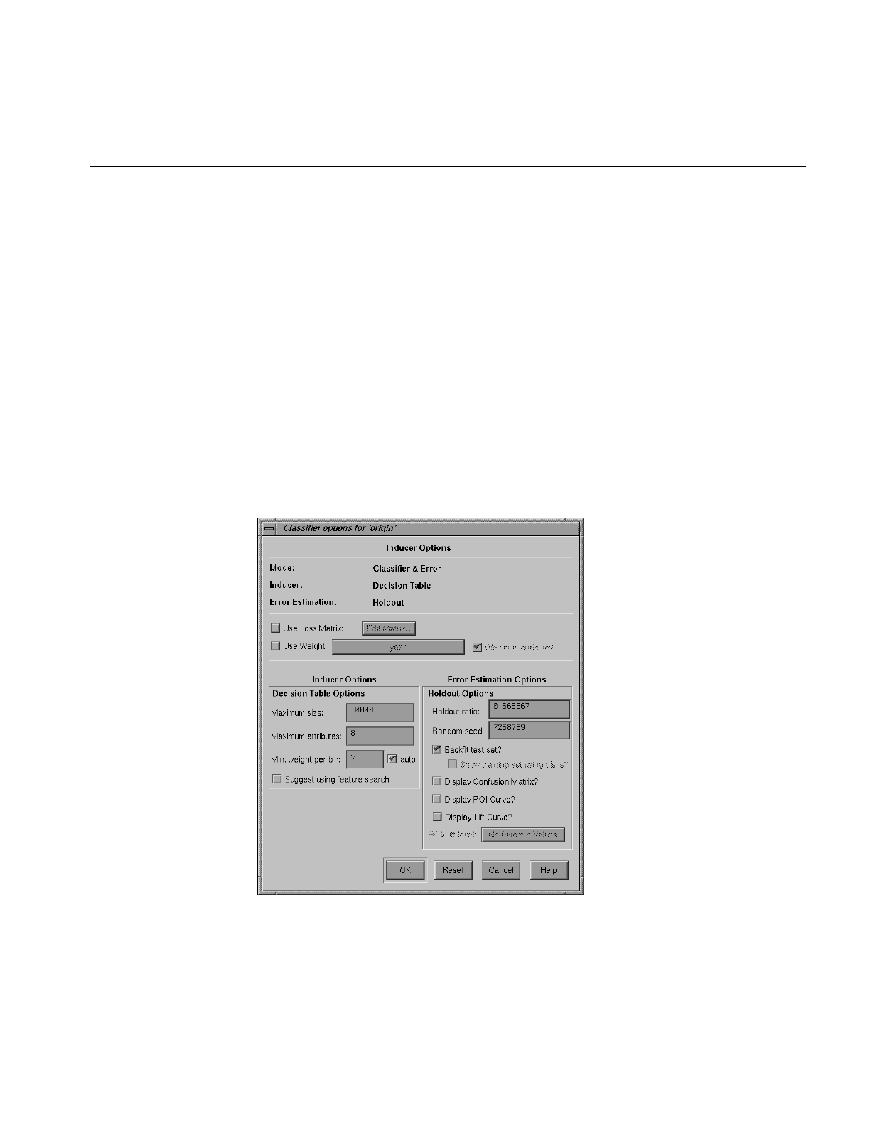
Configuring the Decision Table Inducer Using the Tool Manager
441
Decision Table Options
Selecting Further Inducer Options causes the Inducer Options dialog box (Figure 14-5) to
appear. This dialog box consists of four panels:
•The top panel indicates the choices you made in the Tool Manager’s Data
Destination panel.
•The second pane from the top lets you set the loss matrix and the weight attribute.
See “Loss Matrices” and “Weight Setting” in Chapter 10.
•The bottom-left panel lets you specify further Inducer Options.
•The bottom-right panel lets you specify the Error Estimation Options (unless the
mode you chose in the Data Destination panel was Classifier Only, in which case
this area is empty). The options shown in this panel depend on the type of Error
Estimation you chose (see “Applying Models, Testing Models, and Fitting New
Data” in Chapter 10).
Figure 14-5 Further Inducer Options

442
Chapter 14: Inducing and Visualizing the Decision Table
Decision Table Inducer Options
To fine-tune the Decision Table induction algorithm, you can change the following
Decision Table inducer options (see Figure 14-5).
•Maximum size
This is particularly useful when you have a large dataset. By default, there is a limit
of 10000 nodes (these nodes correspond exactly to the cakes in the visualization).
Limit the size by clicking the checkbox and typing a number for the limit. Limiting
the number speeds up induction and limits the storage required. Although
restricting the size decreases the run time, it might increase the error rate.
•Maximum Attributes
This option determines how many different columns you allow to participate in the
Decision Table when searching. Limiting the attributes simplifies the result and
speeds its arrival. This limit affects only columns added by the Suggest mode.
Columns added manually are not subject to the limit.
•Minimum Weight per Bin
The Decision Table inducer discretizes all continuous attributes. This option lets
you define the minimum number of instances per bin. The automatic setting
calculates this number based on the dataset size: the larger the dataset, the larger
the bin size. If your dataset is very large, you might obtain more discrete ranges
than you want. To reduce the number of bins, raise this value.
Working in the Decision Table Visualizer’s Main Window
If you started the Decision Table Visualizer without specifying a configuration file, the
main screen shows the copyright notice for the Decision Table Visualizer. Only the File
and Help pulldown menus are available. To view all menus and controls in the main
window, open a configuration file. Use File > Open to see a list of configuration files.
When a valid configuration file is specified, the two panes in the main screen display
graphics. For example, specifying /usr/lib/mineset/dtableviz/examples/adult.dtableviz results
in the output displayed in Figure 14-6.
In the Main Window pane on the left is shown the Decision Table. The elements in this
Decision Table may be further subdivided into smaller and smaller cake charts (see
Figure 14-6). Each chart shows the same information as a pie chart, but with rectangular
slices, rather than wedges.
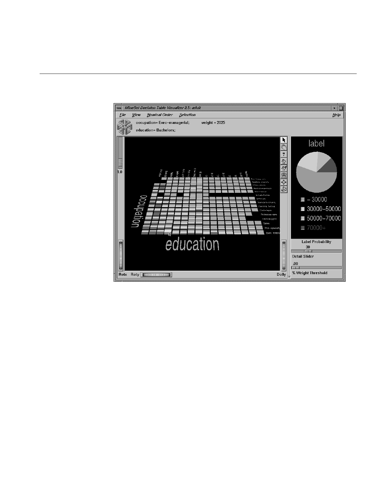
Working in the Decision Table Visualizer’s Main Window
443
Figure 14-6 Decision Table Showing Classifier Induced From adult94 Dataset
In the Label Probability Pane on the right, a list of all class labels appears under a large
pie chart of the prior probability distribution. The color of the slices corresponds to the
color associated with each class label; the size of the slices shows the proportion of data
with each class label.
If you pick an object (place the cursor over it without clicking), you can see the values of
the two attributes at that level of detail. The weight of records represented is proportional
to the height of the cake. Picking a base (the gray block under the cake) shows the values
for the two attributes for the cake one level higher in the hierarchy, together with the
weight of records.
To see the values that define a particular chart, start by picking the base at the coarsest
level of detail, and continue through the next most detailed base until you reach the base
immediately below the chart of interest. The relevant value pair is then displayed at the
top for each level of detail.

444
Chapter 14: Inducing and Visualizing the Decision Table
At each level of detail the attribute names are shown to the left and bottom of the array
of charts; their values are shown to the right and top, respectively. If there is an odd total
number of attributes, the lowest level shows only one attribute.
Viewing Modes
Both of the Decision Table Visualizer’s window panes have two modes of viewing: grasp
and select. Methods of viewing are the same as those for the Evidence Visualizer, see
“Viewing Modes” in Chapter 13, and “Viewing Modes in the Main Window” in
Chapter 13.
Selecting Items in the Label Probability Pane
In select mode, the cursor appears as an arrow. You can then select one of the class labels
by clicking the button to the left of it. Once a class label is selected, a white box appears
around the button next to the label (see Figure 14-6). The size of that slice (the probability
of predicting that label value) appears as text at the top of the display. To deselect a class
label, click on it again. When you move the mouse over the button next to a class label in
pick mode, the size of that slice (in percentage terms) appears in the top display.
If you select one of the classes in the Label Probability pane (on the right), and then select
a cake chart on the left, you see probabilities and confidence intervals for that class
shown in the top display, together with attribute values and weight. To select multiple
charts on the left, hold down the Shift key while clicking the left mouse button.
For example, choose the /usr/lib/MineSet/dtableviz/examples/adult.dtableviz dataset. Select
“class 70,000+” on right, then select a cake chart. The display at the top shows something
like:
marital-status= Husband; weight = 484
occupation= Exec-Manag; Prob(70000+) = 15%[12%, 18%]
The numbers in brackets, [12%, 18%], indicate a 95% confidence interval. That is, we
are 95% confident that the actual percentage of likelihood that a husband executive
manager earns over 70,000 is between 12% and 18%, assuming our dataset is a true
random sample of the desired population.
Selecting Items in the Main Window Pane
Select an object using the left mouse button. Select multiple objects using Shift-select, in
the same way you do for other tools. For example, you can select a number of cakes at
different levels of detail in the scene as shown in Figure 14-7. On the right the distribution
for the classes shows just the records described by the multiple selections.
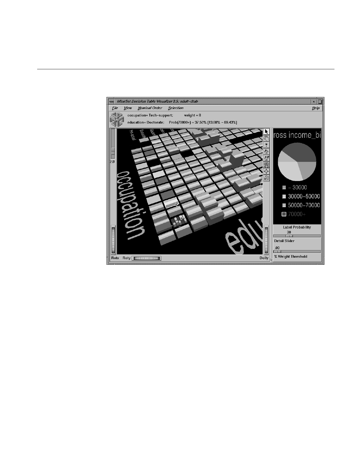
Working in the Decision Table Visualizer’s Main Window
445
Figure 14-7 Example of Making Multiple Selections
Drilling Down and Drilling Up
Drill down and drill up operate the same as in mapviz. (See“Drilling Down and Drilling
up” in Chapter 6.) Drill down by clicking the right mouse button on one of the cakes. This
replaces the one cake with smaller cakes which show the data broken down by the pair
of attributes for the next level down. If the cursor is positioned on the background,
clicking the right mouse drills down or up globally on all cakes. If the cursor is positioned
on a gray base, clicking the right mouse button drills down on all cakes on that base. To
drill up, click the middle mouse button when over a cake, a gray base, or the background.

446
Chapter 14: Inducing and Visualizing the Decision Table
External Main Window Controls
The external controls for the visualizer associated with the Decision Table classifier are
the same as those for the Map Visualizer. For a description of these controls, see “External
Controls” in Chapter 5.
Sliders
The Decision Table Visualizer contains three sliders: Height Scale, Detail Slider, and
Percent Weight Threshold. The function of these sliders is the same as for the Evidence
Visualizer. See “Sliders” in Chapter 13 for an explanation.
In using the Percent Weight Threshold Slider, the rectangular slices atop each cake show
the distribution of the classes for the records represented by that cake. The height
corresponds to the weight of the training set records that have reached this node (this is
the number of records if weight was not set). In general, the higher the weight, the more
reliable the class distribution the cake.
Pulldown Menus
Four pulldown menus let you access additional Decision Table Visualizer functions: File,
View, Selection, and Help. If you start the Decision Table Visualizer without specifying a
configuration file, only the File and the Help menus are available.
The File Menu
The File menu lets you open a new configuration file, save under a new name, print an
image of the current display, start the Tool Manager, reopen the current configuration file,
or exit the Decision Table Visualizer.
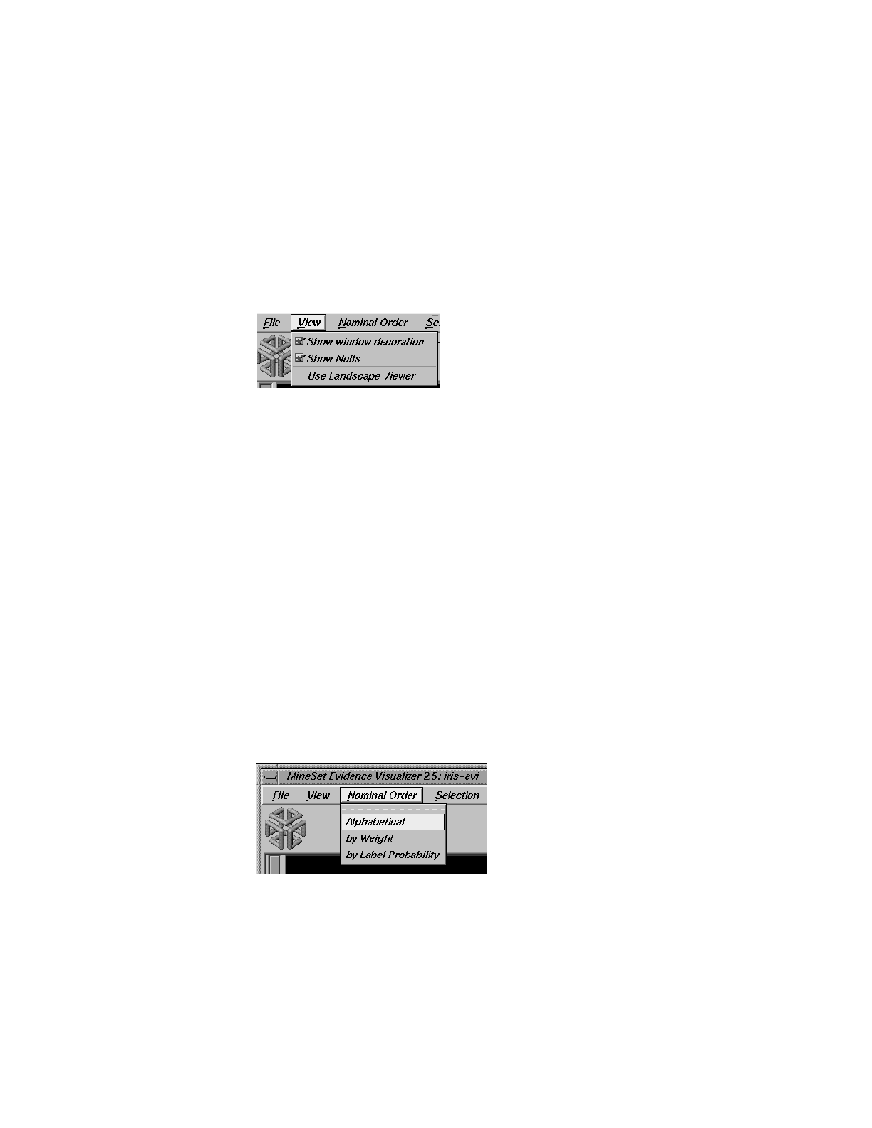
Pulldown Menus
447
The View Menu
The View menu lets you control certain aspects of what is shown in the Main Window
(Figure 14-8).
Figure 14-8 Decision Table Visualizer’s View Menu
This menu contains three options:
•Show Window Decoration lets you hide or show the external controls around the
main window.
•Show Nulls toggles the display of null values. Null values, if present, are shown as
the first value, offset slightly from other non-Null values.
•Use Landscape Viewer (or Use Examiner Viewer) switches to an alternative mode of 3D
navigation. To understand navigation using the Landscape viewer see “Navigating
With the Middle Mouse Button” in Chapter 5. Note that since the middle mouse
button is used for navigation in the Landscape viewer, to drill-up you must click the
middle mouse button while holding down the Ctrl key.
The Nominal Order Menu
The Nominal Order menu lets you control how values for nominal attributes are ordered
(Figure 14-9).
Figure 14-9 Decision Table Visualizer’s Nominal Order Menu
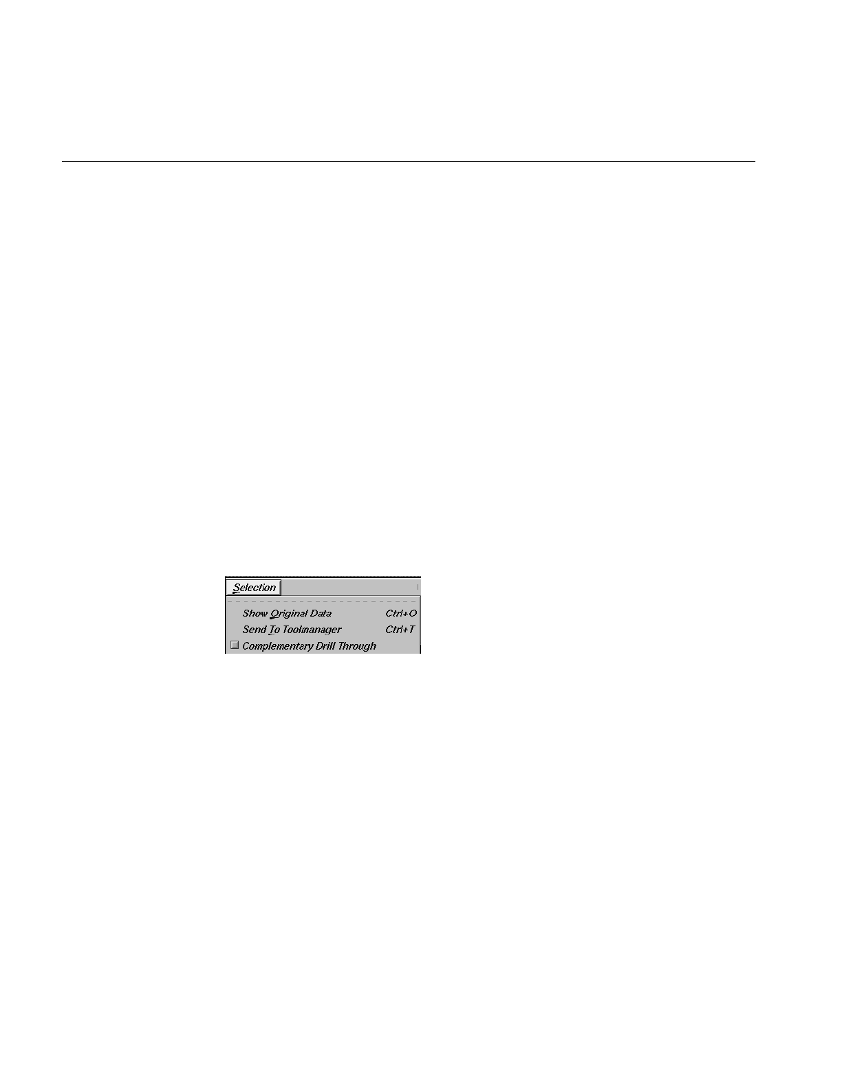
448
Chapter 14: Inducing and Visualizing the Decision Table
The three choices are:
•Alphabetical implies attributes with nominal values are sorted from left to right (or
bottom to top) alphabetically.
•Weight sorts values from left to right, with those having the largest weight of
records appearing toward the left.
•Label Probability (the default) sorts the values of nominal attributes by the size of the
slices corresponding to one of the classes. If the label is a binned attribute, the
highest bin is used by default. If the label is nominal, then whatever class has the
largest slice in the prior probability pie is used by default. If a particular class is
selected, and then sort by label probability is requested, the selected class is used for
determining the ordering. In all cases, if there is a NULL value, it remains the first
value.
The Selection Menu
The Selection menu allows drill-through to the underlying data (Figure 14-10). To do a
drill-through first select some combination of values and/or a class, then chose one of the
two methods of drilling-through to the underlying records.
Figure 14-10 Decision Table Visualizer’s Selection Menu

Pulldown Menus
449
There are three menu items:
•Show Original Data causes the records corresponding to the selected item to be
displayed in a record viewer.
•Send to Tool Manager causes a filter operation to be inserted at the beginning of the
Tool Manager history. The actual expression used to do the drill-through is
determined by
–the cakes selected in the Main Window, and
–the class (optionally) selected on the right.
Selected cakes are ORed together and then ANDed with the selected class, if
present, to form a drill-through expression to do the filtering in Tool Manager. If
nothing is selected, a warning message appears.
For example, for figure 14-10, the filter expression corresponding to the selections is:
(`gross income`>70000.0) &&
((`occupation`==”Tech-support”)&&(`education`==”Doctorate”)) ||
(
(`occupation`==”Prof-specialty”)&&(`education`==”Doctorate”)&&
(`sex`==”Female”)&&(`race`==”Amer-Indian-Eskimo”)
)
The three major terms in this expression correspond to the selected class on the
right, the selected cake at the top level, and the selected cake at the second level,
respectively.
•Complementary Drill Through uses the complement of the expression defined by the
selected objects for drill-through.
The Help Menu
The Help menu provides access to six help functions. These are the same for all MineSet
tools (see“The Help Menu” in Chapter 6.)

450
Chapter 14: Inducing and Visualizing the Decision Table
Sample Files
The following examples show cases in which the Decision Table can be useful. Each of
these examples is associated with a sample data file provided with MineSet. By running
the Decision Table inducer (with suggest using feature search turned on in the further
inducer options), you can generate the -dtab.dtableviz and -dtab.dtableviz.data files
described below.
Note: The data (.data) and accompanying schema (.schema) files are located in
/usr/lib/MineSet/data on the client workstation. The classifier visualization files, which
have a -dtab.dtableviz extension, reside on the client workstation in
/usr/lib/MineSet/dtableviz/examples.
Churn
Churn is when a customer leaves one company for another. This example shows what
causes customer churn for a telephone company. The data used to generate this example
is in /usr/lib/MineSet/data/churn.schema.
The file /usr/lib/MineSet/dtableviz/examples/churn-dtab.dtableviz shows the structure of the
classifier induced using the attribute churned as the label. The error rate for this classifier
is 5.5%. Of the records, 14.3% represent customers who churned. The two attributes
selected for the first level of detail were number_of_customer_service_calls and
total_day_charge. By looking at the distribution over these two attributes, you can see
that churn increases as total day charge increases, except when the total day charge is <
29.75, then the churn is high if the number of service calls is > 3. About 3/4 of the records
have total day charge less than 38 and 3 or fewer customer service calls.
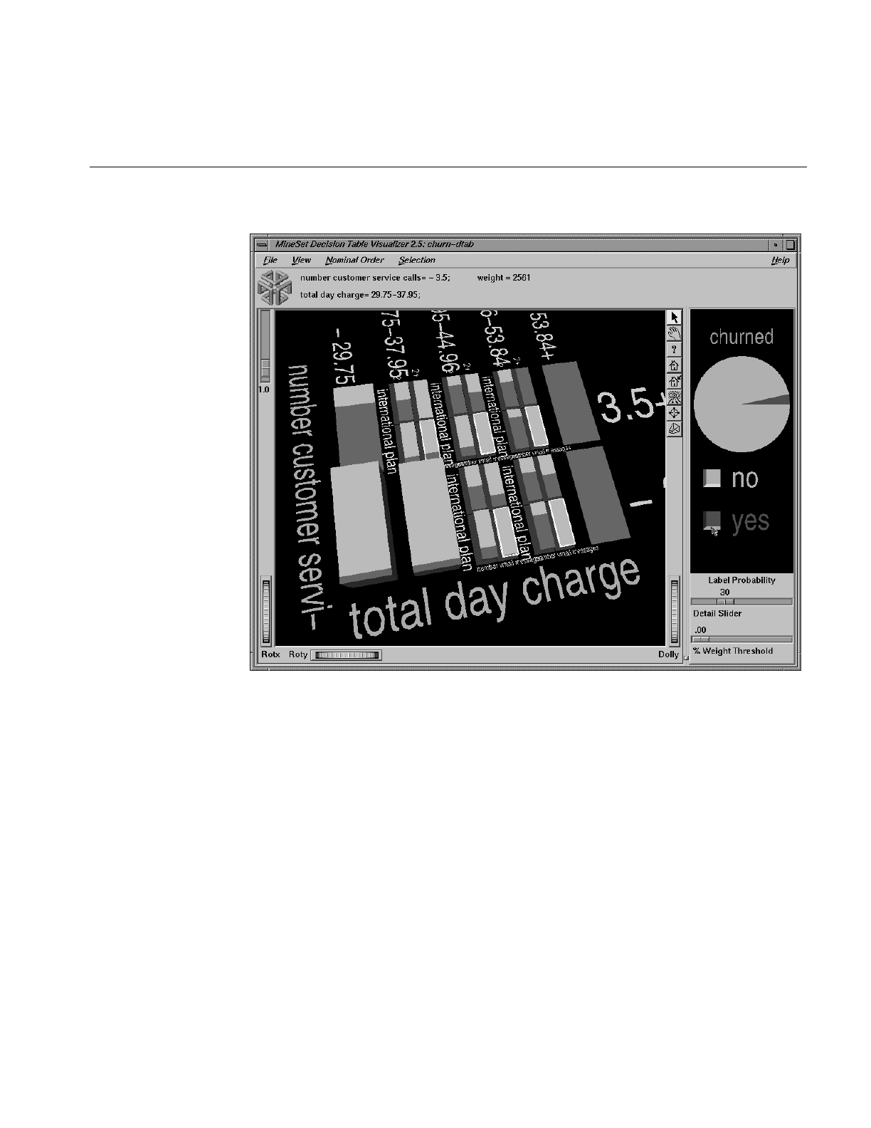
Sample Files
451
Figure 14-11 Drilling Down on the Churn Dataset
Begin to drill down on regions where its not clear when a customer churns. Figure 14-11
shows drilling down on all cakes in which there was not a clear majority class. The next
attributes considered are international_plan and number_of_vmail_messages. Among
those with heavy day charge, it appears clear that having the international plan and
having few vmail messages correlates well with customer churn. Selecting the lower
right cake in each of the drill-down regions, and then brushing with the mouse across the
box next to “churned=yes” in the probability pane on the right, shows that only 3.4
percent of the customers in the selected regions churned.

452
Chapter 14: Inducing and Visualizing the Decision Table
Now drill down further on the cake in the upper left of each previous drill-down region.
Doing so shows a very similar distribution for each. The consistent pattern shows: high
total_evening_charge and high total_international_charge correlate well with churn. You
can even drill-down another level to see the effect of total_international_calls, but doing
so leaves so few records from which to draw conclusions, you could not be confident of
the distributions seen. If you are interested in how total_international_calls affects churn
and how it correlates with other variables, return to the Tool Manager and explicitly map
total_international_calls to a higher level in the hierarchy, and rerun the decision table.
Although “state” is fairly well correlated with churn, it was not selected because the
algorithm has a built-in preference for variables with few values. This prevents the
algorithm from selecting attributes like social security number which uniquely identify
each record, thus yielding high training set accuracy, but are not useful for classifying
future unlabeled data.
Origin of Cars
The cars dataset contains information about different models of cars from the 1970s and
early 1980s. Attributes include weight, acceleration, and miles per gallon (mpg). The file
/usr/lib/MineSet/dtableviz/examples/cars-dtab.dtableviz shows the structure of the Decision
Table Classifier induced for this dataset. This file was generated by running the inducer
on /usr/lib/MineSet/data/cars.schema with the label set to “origin” (Japan, U.S., Europe).
Since the brand attribute uniquely determines the origin, the structure of the classifier is
extremely simple. The only two attributes shown are brand and cylinders. It is interesting
to see which brands tend toward high or low cylinder types. For example, there are 21
different models of Mazda, and 18 models of Honda, but they all have 5 or fewer
cylinders. Conversely, Cadillac only makes cars with six or more cylinders.
This example could probably be made more interesting by first removing the brand
attribute. Another useful transformation might be to convert cylinders to string so each
unique cylinder value is shown, rather than a bin. Alternatively, one can create
additional levels of detail beyond brand and cylinder, by mapping them explicitly.

Sample Files
453
Gender Attribution
The adult dataset contains information about working adults. This dataset was extracted
from the U.S. Census Bureau. It contains data about people older than 16, with a gross
income of more than $100 per year who work at least one hour a week. You might want
to know how to characterize males and females.
The file /usr/lib/MineSet/dtableviz/examples/adult-sex-dtab.dtableviz shows the structure of
the Decision Table Classifier induced for this problem. This file was generated by
running the inducer on /usr/lib/MineSet/data/adult.schema, with the label set to sex, after
removing the relationship column (which would have made the classifier trivial). To
make it easier to see the distribution of records for each combination of values, you can
scale the cake heights using the scale slider on the left.
In the Decision Table Visualizer, the Label Probability Pane shows that the prior
probability of working males is higher than that of females. The Evidence Visualizer
showed us that marital_status and occupation are very important attributes for
determining gender, however, it did not show us the dependencies between these two
attributes. The top level shows several interactions. For example, most people with
occupation craft repair are married civilian spouses (more specifically 98.6 of them are
husbands), while most people with occupation “Other-service” have “Never-married”
(48% male).
At first it may seem odd that most of the people with “marital_status =
Married-civilian-spouse” are male, but once you consider that this data was probably
gathered from tax returns, it seems reasonable that the wives of these males are not
working but filing jointly with their husbands.
The divorce rate seems highest among those with ”occupation = Admin-clerical”. Those
in “Other-service” also have high divorce rates, but they seem to prefer separation, as the
number who are separated is even greater than that of “Admin-clerical”.
Suppose you wanted to find out the probability of being female given that a person is
“widowed” and has “occupation=Adm-clerical”. In the evidence visualizer one can get
an approximate answer (94.7% female) for this by clicking on these two attribute values.
Here we can get the exact answer by clicking the left mouse on the cake at the intersection
of these two values (95.2% female).
Drill down to the lowest level on the cake for “Married-civilian-spouse” and
“Occupation= Unknown.” There is a pattern evident here more than any of the other
combinations of occupation and marital status. For this cake, the younger members tend
to be women, and the older members tend to be men.

454
Chapter 14: Inducing and Visualizing the Decision Table
Salary Factors
For a dataset of working adults, you might want to find out what factors affect salary.
First bin gross_income into two bins, those that earn less that 50,000, and those earning
over 50,000. You can run a MineSet classifier to help determine what factors influence
salary. The file /usr/lib/MineSet/dtableviz/examples/adult-salary-dtab.dtableviz shows the
Decision Table classifier induced for this problem. This file was generated by running the
inducer on /usr/lib/MineSet/data/adult.schema with gross_income divided into five bins
using user-specified thresholds.
Since the label is numeric, a continuous spectrum is used to assign colors to each class.
Also the classes in the probability pane on the right are not sorted by slice size because
they have a numeric order. Red is assigned to the highest bin (50,000+).
The two attributes chosen at the top of the hierarchy are relationship and
education_num. The attribute education_num is not particularly useful because it is
simply an enumeration of the different educations possible, not years of education, as
you might think. However there is an approximate correlation. Replace this column with
education if you prefer to see the actual string values. If you simply remove the column,
education_num, and rerun using feature search, the algorithm may not pick education at
the top of the hierarchy because it has so many values.
The order of the attributes in this model were selected automatically to increase accuracy.
Often a model in which domain knowledge is used to perform the mappings can give a
more useful visualization. Such a model is provided in
/usr/lib/MineSet/dtableviz/examples/adult-salary3-dtab.dtableviz, and shown in Figure 14-12.
Here the salary has first been binned into 3 ranges (20000, and 60000 are the thresholds).
The attributes mapped at level one are: relationship and sex; level two has education and
occupation; and level 3 has hrswk (hours worked per week) and age.
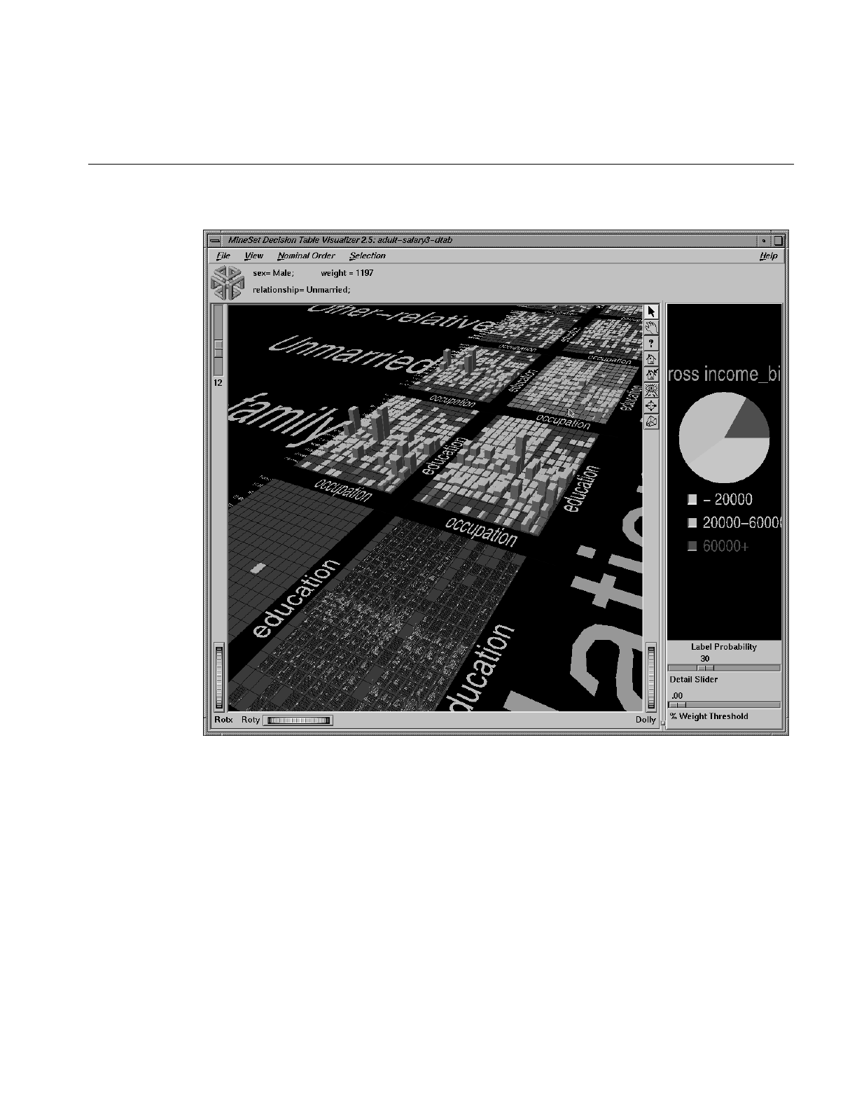
Sample Files
455
Figure 14-12 Decision Table Visualizer Using the Adult Dataset

456
Chapter 14: Inducing and Visualizing the Decision Table
At the top level we know “relationship” and “sex” have a strong correlation. Of course
we expect all husbands to be male, and wives to be female, but we can see right away this
is not the case. By brushing on the cake for male wives we see that there are 3 of them
and all their salaries fall in the 20,000-60,000 range. Drilling down on these cakes reveals
more information about these anomalous records. You may wish to select these cakes
(using the left mouse button) and drill through to the underlying data so you can find the
values of all the other fields.
Click the right mouse on the background; this will drill down globally to the next level.
Every cake is now replaced with a matrix for every combination of education and
occupation. The ordering is the same for every matrix, and overall the ordering is by
correlation with income. If you choose Nominal Order > by Weight from the pulldown
menu the overall ordering will be by record weights. The most popular occupations and
education levels will appear in the lower left corner of each matrix. High school grads is
the most prevalent education level, and Professional-specialty is the most common
occupation, but there are not many high school graduates whose occupation is
professional specialty.

Sample Files
457
Figure 14-13 Closer Inspection of the Adult Dataset

458
Chapter 14: Inducing and Visualizing the Decision Table
Returning to ordering of nominals by income, you can see distinct distributions for each
combination of sex and relationship. There is not much difference between males and
females whose relationship is not-in-family. The difference between unmarried males
and females, however, is very pronounced. (See Figure 14-13). There is a very distinctive
cluster of red cakes in the lower left of male matrix that does not exist in the female
matrix. By scaling up the heights somewhat, you will notice that the female matrix has
obvious spikes at occupation = “admin clerical” and “other service”. No such spikes are
visible in the corresponding male matrix.
Click with the right mouse button on the most populous cake (male husbands). This
operation may take a minute to perform because the visualizer needs to construct all the
geometry for the next level for this cake. The geometry is constructed on demand because
the time needed to create it all at the beginning would be excessive, and wasteful since
the user rarely explorers most of the high detail regions. If you click on the background
by mistake you may be forced to wait a very long time if the amount of detail at the next
level is very long - as it is in this case. Figure 14-12 shows the result of drilling down on
the male husband base.
Consider the many age by hrswk distributions that are displayed for every combination
of occupation and education. The first surprising fact is that, in spite of the many
hundreds of cakes shown, there is a single spike at that accounts for 2.5% of all husbands!
(SeeFigure 14-13) If you had to pick characteristics for a typical husband, it would be
reasonable to say he is a HS-grad doing craft-repair, aged between 41 and 59 and working
between 38 and 41 hours a week.
Compare the salary distributions for husbands who are HS-grads in sales with those who
are HS-grads and executive managers. Although the distribution of age and hours
worked is similar, the probability of being in the income greater than 60,000 class is 34%
for this group of managers, compared with 27% for the salesmen. To see these
probabilities shown at the top, first click the button next to the 60000+ income class in the
label probability pane on the right, then brush over cakes on the left.

Sample Files
459
Iris Classification
In this dataset, each record describes four characteristics of iris flowers: petal width, petal
length, sepal width, and sepal length. Each iris was further classified into the types
iris-setosa, iris-versicolor, or iris-virginica. The goal is to understand what characterizes
each iris type.
Before running a classifier, click the Column Importance tab in the Tool Manager’s
Classifiers tab; then click Suggest then Go!. You obtain a ranking of the importance of the
features: petal_width, petal_length, and sepal_length. You can map these to the axes in
the Scatter Visualizer, with the iris_type mapped to the color and see the clusters.
The file /usr/lib/MineSet/dtableviz/examples/iris-dtab.dtablerviz shows the structure of the
Decision Table Classifier induced for this problem. This file was generated by running
the inducer on /usr/lib/MineSet/data/iris.schema.
In the Decision Table Visualizer, we can see that petal_width is an excellent
discriminatory attribute. When you add sepal_width you see that all instances of
“iris_versicolor” appear in the sepal width<3.05 bin for those records which have petal
width= 0.75-1.65.
Drill down on the three cakes which are not 100% pure. The top two cakes each contain
a single instance of iris-versicolor which prevent them from being pure. For the
sepal_width<3.05 cake it is very difficult to isolate the anomalous “iris-versicolor”. For
the sepal_width>3.05 cake, however, the iris_versicolor is isolated by using petal_length.
Mushroom Classification
The file /usr/lib/MineSet/dtableviz/examples/mushroom-dtab.dtableviz shows the structure of
the Decision Table Classifier induced for this problem. This file was generated by
running the inducer on /usr/lib/MineSet/data/mushroom.schema.
The goal is to understand which mushrooms are edible and which ones are poisonous,
given this dataset. There are over 8000 records in this set; thus, running this inducer
might take several minutes. Note that under the default mode of the one-third holdout
for accuracy estimation, a third of the records are kept for testing.

460
Chapter 14: Inducing and Visualizing the Decision Table
Each mushroom has many characteristics, including cap-color, bruises, and odor. In the
Decision Table Visualizer odor and stalk-shape appear at the top level. Note that odor
alone does an excellent job of discriminating edibility. Only when the “odor=none” and
the stalk-shape is “enlarging” is there any ambiguity. So naturally we drill down on this
lone cake. Now we see just the records with these 2 values broken down by their values
for bruises and gill-size. Notice the interaction between gill-size and bruises. This
interaction is nearly impossible to discern using any other classifier.
Since all the attributes in this dataset are nominal, all the values are sorted from by how
well they predict edibility. You might want to order the values alphabetically or by
weight (prevalence). To do this, select the appropriate method from the nominal order
menu. If you considered either bruises or gill_size alone you would not be able to predict
large classes of completely edible or poisonous mushrooms, but by considering them
together, we see that if there are no bruises and the gill-size is broad, then all 814
mushrooms of this type are edible. Conversely, if there are bruises and the gill-size is
narrow, then all 11 mushrooms of this type are poisonous. To disambiguate the other two
cases we would have to drill down further.
There is actually a mapping which can completely discriminate among all the examples
in our training set using only 2 levels. The attributes for these to levels are: odor,
spore_print_color and habitat, population. The reason the automatic suggestion did not
use this mapping was because of the preference for attributes with fewer numbers of
values.
In the Decision Table Visualizer, move the % Weight Threshold slider to the right.
Eventually the “odor=musty” will be deleted from the scene. The reason for this is that
there are fewer than 1% of the records with odor=musty.
Party Affiliation
This dataset consists of voting records. The goal is to identify the party a congressperson
belongs to given data about key votes. The dataset includes votes for each member of the
U.S. House of Representatives on the 16 key votes identified by the Congressional
Quarterly Almanac (CQA). The CQA lists nine types of votes: voted for, paired for, and
announced for (these three are simplified to yes), voted against, paired against, and
announced against (these three are simplified to no), voted present, voted present to
avoid conflict of interest, and did not vote or otherwise make a position known (these
three are simplified to an unknown disposition).

Sample Files
461
Before running a classifier, look at the 16 votes to see if you can perceive which features
are important. Then run the Decision Table Visualizer. For this dataset, you may wish to
order the values alphabetically, so that all “yes” votes appear in the upper right and “no”
votes appear in the lower left.
A the top level we see synfuels_corporation_cutback and physician_fee_freeze. There is
a fascinating relationship between these variable that would be next to impossible point
out with any other model. Everyone (but 3) who voted against physicians was a
democrat. Nearly every democrat that voted against physicians also voted against the
synfuels cutback (only 3 of 206 did not fit this pattern). Surprisingly, nearly every (all but
5) republican that voted for the physicians, voted against the synfuels cutback.This odd
relationship between these very different issues hints that these bills may have been
connected in ways that would require further investigation.
Most of the cakes at the top level are nearly pure except for the middle one (which
contains only 6 records) and the one where the representatives voted yes on both issues.
Here we can drill-down another level to discriminate the political affiliation of the
representatives in this group. Doing so uses “anti-satellite test ban” and “adoption of the
budget resolution” to further discriminate among the 55 representatives in this group.
The file /usr/lib/MineSet/dtableviz/examples/vote-dtab.dtableviz shows the structure of the
Decision Table Classifier induced for this problem. This file was generated by running
the inducer on /usr/lib/MineSet/data/vote.schema.
Breast Cancer Diagnosis
The breast cancer dataset contains information about females undergoing breast cancer
diagnosis. Each record represents a patient with attributes such as cell size, clump
thickness, and marginal adhesion. The final attribute is whether the diagnosis is
malignant or benign. The file /usr/lib/MineSet/dtableviz/examples/breast-dtab.dtableviz
shows the structure of the Decision Table Classifier induced for this problem. This file
was generated by running the inducer on /usr/lib/MineSet/data/breast.schema.
In the Decision Table Visualizer, mitosis and uniformity of cell shape are shown at the top
of the hierarchy. If both attributes have low values at the same time the given sample is
99.2% likely to be benign. On the other hand, 100% of the training records that had high
values for both, were malignant.

462
Chapter 14: Inducing and Visualizing the Decision Table
Drill-down on the four cakes that are not so pure. Now marginal adhesion and
bare-nuclei are used to discriminate. There are far fewer records in each cake at this level;
as a result there is more noise, and trends are more difficult to detect. High values for
both marginal-adhesion and bare-nuclei seem to contribute to malignancy, but its
uncertain. Note that the first value of bare-nuclei is null. The distributions for these null
cakes are more suspect than others so you may wish to hide them by unchecking View >
Show Nulls.
If you drill down globally two more levels, you can note a few interesting features. The
cakes get very small, and there are large regions of the multi-dimensional space which
are empty. There are a few tiny regions where many records are clustered. There is one
huge spike (100% benign) where all the values are low This spike alone accounts for
about 20% of the data.
Hypothyroid Diagnosis
The hypothyroidism dataset is similar to the one for breast cancer. The file
/usr/lib/MineSet/dtableviz/examples/hypothyroid-dtab.dtableviz shows the structure of the
Decision Table Classifier induced for this problem. This file was generated by running
the inducer on /usr/lib/MineSet/data/hypothyroid.schema.
There are 3,163 records in this dataset and most of them do not have hypothyroidism
(95.45%). While this means that one can predict “negative” and be correct with high
probability, it’s those people that have hypothyroidism that we are most worried about.
In technical terms, the false negatives are very important.
This is a case where you might want to adjust the loss matrix to skew the posterior
probability toward predicting hypothyroidism in order to avoid false negatives. There
might be a high cost associated with predicting that someone is healthy when they
actually have the disease; predicting them sick when they are actually healthy means
they take a more accurate test or a treatment they do not need.
Using the Decision Table Visualizer on this dataset, we note:
•If fti is null then tbg is not null and t3 is almost always null (drilling down-one more level).
•Except for 2 instances, the only time t4u is null is when fti is null.
•Hypothyroidism is more prevalent for lower values of for fti

Sample Files
463
Pima Diabetes Diagnosis
This dataset is a diagnosis problem for diabetes using statistics gathered from an Indian
tribe in Phoenix Arizona. The task is to determine whether a patient has diabetes, given
some medical attributes, such as blood pressure, body mass, glucose level, and age.
The file /usr/lib/MineSet/dtableviz/examples/pima-dtab.dtableviz shows the structure of the
Decision Table Classifier induced for this problem. This file was generated by running
the inducer on /usr/lib/MineSet/data/pima.schema.
Using the Decision Table Visualizer we note:
•At the second level of detail you can see that few women under 28 have more than 6
pregnancies (only 4 do). You may wish to drill-through to these records to get all the
information available for these 4.
•High values of plasma glucose, body mass, indicate a greater likelihood of diabetes.
DNA Boundaries
The file /usr/lib/MineSet/dtableviz/examples/dna-dtab.dtableviz shows the structure of the
Decision Table Classifier induced for this problem. This file was generated by running
the inducer on /usr/lib/MineSet/data/dna.schema.
There are 3,186 records in this DNA dataset. The domain is drawn from the field of
molecular biology. Splice junctions are points on a DNA sequence at which
“superfluous” DNA is removed during protein creation. The task is to recognize
exon/intron boundaries, referred to as EI sites; intron/exon boundaries, referred to as IE
sites; or neither. The IE borders are referred to as “acceptors” and the EI borders are
“donors.” The records were originally taken from GenBank 64.1 (genbank.bio.net). The
attributes provide a window of 60 nucleotides. The classification is the middle point of
the window, thus providing 30 nucleotides at each side of the junction.
From the Decision Table Visualizer, you can see a surprising pattern not nearly as evident
in any other classifier model. At the top level there is a pronounced interaction between
left_01 and right_02. Exon/intron is only present if right_02 = T. Intron/extron is only
present if left_01=G. For other values of left_01 and right_01 there are very few splice
junctions.
Drill down globally to the next level (left_02 and right_01). Among the records where
right_02 = T and left_01 = G we see a pattern which is consistent with the patterns along
each edge.


465
Chapter 15
15. Inducing and Visualizing the Regression Tree
This chapter discusses the features and capabilities of the Regression Tree Inducer. Its
associated visualizer, the Tree Visualizer, is described in Chapter 5. This chapter provides
an overview of this tool and discusses methods of using it to generate Regression Trees.
It then explains the Tree Visualizer’s functionality when working with regression trees.
Finally, it lists and describes the sample files provided for this tool.
Note: It is assumed that you have read Chapter 10, “MineSet Inducers and Classifiers,”
before proceeding with this chapter.
Overview
Regression is the task of predicting a continuous label value, given a set of descriptive
attributes. A regressor is a predictive model that performs regression. Regression and
classification are similar, the difference being that in classification the predicted label can
take on only a small number of discrete values. For example, an iris may be classified by
type as either iris-setosa, iris-versicolor, or iris-virginica. In regression, the predicted
label can be any value in a continuous range, for example, an individual’s annual income
may be any amount greater than zero.
MineSet can build a regressor automatically from a training set using an algorithm called
an inducer. The training set consists of records in the database for which the continuous
label is known. For example, you could supply a database table with columns (such as
age, education, occupation, hours worked per week, and so forth), and one column
containing descriptive attributes (gross income). An algorithm called an inducer
automatically builds a regressor from a training set.
When a regressor is generated, MineSet also generates a visualization. This visualization
can help you understand the regressor and how it makes predictions. In addition, it can
provide valuable insight into the data itself. Once generated, a regressor can be used to
predict the label value for unlabeled records.
The underlying structure used for regression is a Regression Tree, such as the one shown
in Figure 15-1.

466
Chapter 15: Inducing and Visualizing the Regression Tree
Figure 15-1 Regression Tree for the Adult Dataset
Running the Regression Tree Inducer
There are two ways to run the Regression Tree Inducer:
•From the Tool Manager.
Connect to the server and select a data source (see “Choosing a Data Source” in
Chapter 3).
From the File menu, choose Open New Data File. Log in to a server, and enter the
filename. For the example shown here, the filename entered would be
/usr/lib/MineSet/data/adult.schema. In the Continuous Label popup menu of the Data
Destination pane you see a list of continuous attributes. Of the several continuous
attributes available, one is automatically selected as the label option. You may
change this. Regression Tree Inducer is automatically shown as the inducer. To run
the Inducer, click Go!.
The status window shows the progress and statistics, and the Tree Visualizer is
launched automatically.
•From the command line.
To induce a Regression Tree classifier from the command line, refer to Appendix I,
“Command-Line Interface to MIndUtil: Analytical Data Mining Algorithms.”
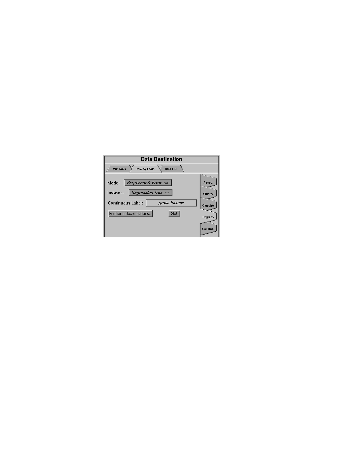
Configuring the Regression Tree Inducer Using the Tool Manager
467
Configuring the Regression Tree Inducer Using the Tool Manager
To access the options for configuring the Regression Tree Inducer, select the Mining Tools
tab on the Data Destination panel (Figure 15-2). From the tabs at the right, select Regress.
The selected inducer is the Regression Tree, the only regression model currently available
in MineSet. Your selections in the Mode menu determines the options available in the
Further Inducer Options menu. After you have made your selections in these menus,
click Go! to induce the regressor.
Figure 15-2 Data Destination Panel in Tool Manager Showing Regressors
Continuous Label
The Continuous Label menu provides a list of possible continuous labels. This list
includes all attributes that take on numeric values. Select the label attribute you wish to
model. For instance, to generate a regressor for predicting gross income, select “gross
income”. (See “Training Set” in Chapter 10). If there are no continuous attributes, the
menu shows No Continuous Label, and the Go! button is disabled. Regressors can only be
generated for continuous attributes. If the dataset does not contain a continuous attribute
you may add a new continuous column using the Tool Manager’s Data Transformations
panel.

468
Chapter 15: Inducing and Visualizing the Regression Tree
Regressor Name
The generated regressor is named with the prefix of the session filename (as determined
in Tool Manager) and the suffix-rt.regress. By default, all regressors are stored on the
server in the file_cache directory, which defaults to mineset_files.
These regressors can be used to predict the labels for unlabeled datasets. To apply a
stored regressor, you need to select a dataset of records with the attributes used by the
regressor. The regressor will predict a new continuous label value for each record. See
“Applying a Model” and “Backfitting in Error Estimation” in Chapter 10.
Regression Tree Options
Selecting Further Inducer Options displays the Inducer Options dialog box (Figure 15-3).
to appear. This dialog box consists of four panels:
•The top panel indicates the choices you made in the Tool Manager’s Data
Destination panel.
•The second panel from the top lets you set the weight attribute. See “Weight
Setting” in Chapter 10.
•The bottom-left panel lets you specify other Inducer Options.
•The bottom-right panel lets you specify the Error Estimation Options (unless the
mode you chose in the Data Destination panel was Classifier Only, in which case
this area is empty). The options shown in this panel depend on the type of Error
Estimation you chose (see “Error Options for Inducers” in Chapter 10).
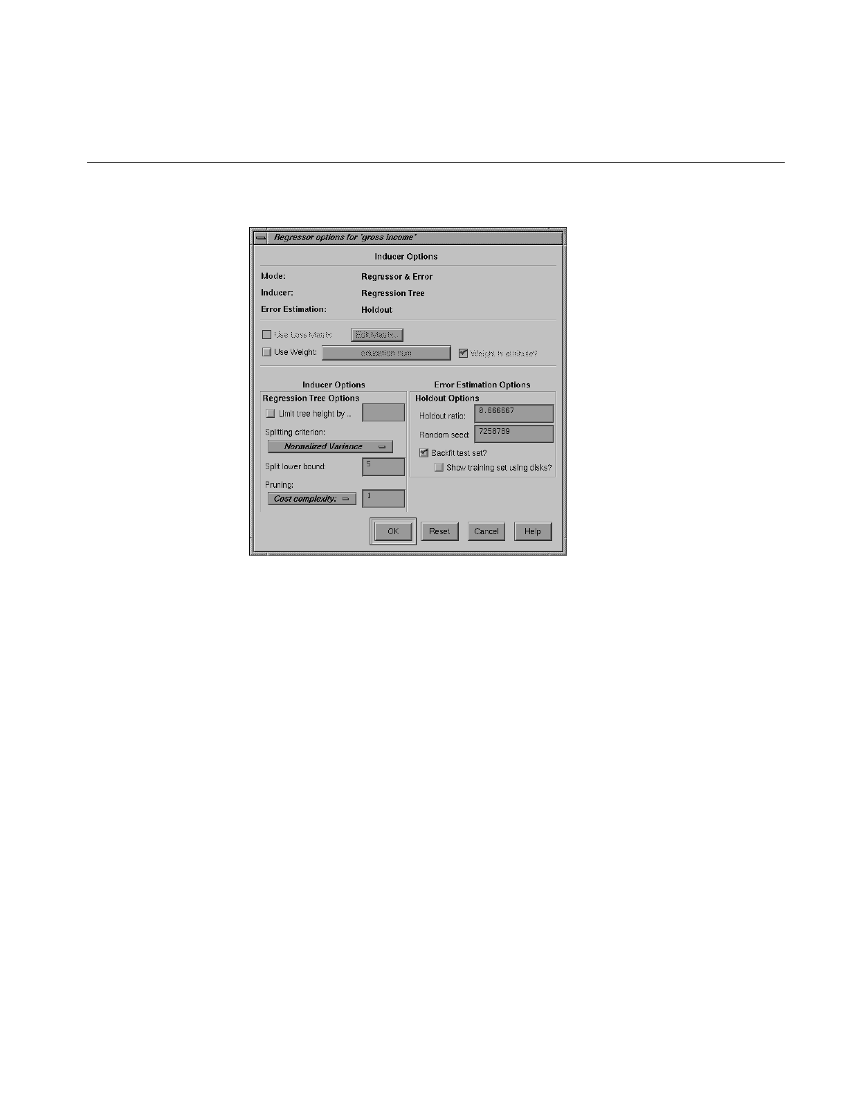
Configuring the Regression Tree Inducer Using the Tool Manager
469
Figure 15-3 Further Inducer Options
Regression Tree Inducer Options
To fine-tune the Regression Tree induction algorithm, you can change the following
Regression Tree Inducer options (see Figure 15-3).
•Limit tree height by
By default, there is no limit to the height (number of levels) in the Regression Tree.
You can limit the height by clicking the check box and typing a number for the limit.
Limiting the number of levels speeds up the induction and is useful for studying
the Regression Tree without the distraction of too many nodes. Note that restricting
the size decreases the run time, but may increase the error rate. Setting this option
does not affect the attributes chosen at levels before the maximum level.

470
Chapter 15: Inducing and Visualizing the Regression Tree
•Splitting criterion
This option allows you to specify which criterion will be used to select among
competing attribute splits during tree induction. For regression trees, MineSet
supports four splitting criteria:
Variance chooses splits that minimize the within-node variance at each point in the
tree. When generating a leaf, the prediction at the leaf is the mean of the label values
of the records reaching that leaf. Variance is the squared difference between each of
the values in the set, divided by the total number of elements or values. This mode
is most commonly used statistically.
Absolute Deviation chooses splits that minimize the absolute deviation within the
node at each point in the tree. When generating a leaf, the prediction at the leaf is
the median of the label values of the records reaching that leaf.
Normalized Variance (the default) is variance divided by the log (base 2) of the
number of child nodes.
Normalized Absolute Deviation is absolute deviation divided by the log (base 2) of the
number of child nodes.
For a given problem, it is difficult to know which criterion will be best. Try each,
and select the one that leads to the lowest error estimate, or the Regression Tree you
find easiest to understand.
•Split lower bound
This is a lower bound on the weight (or the number of records if weight was not set)
that must be present in at least two of the node’s children. The default for this
option is 5. For example, if there is a three-way split in the node, at least two out of
the three children must have a weight of five or more. This provides another
method of limiting the size of the Regression Tree.
Increasing the split lower bound tends to increase the reliability of the probability
estimates, because the number of records at each leaf is larger. It also creates smaller
trees and decreases the induction time. If you expect the data to contain noise
(errors or anomalies), increase the split lower bound. If your dataset is very small (<
100 records), you might want to decrease the split lower bound.

Configuring the Regression Tree Inducer Using the Tool Manager
471
•Cost Complexity Pruning
Cost complexity pruning attempts to generate optimally sized trees by trading off
the error rate of the tree (its cost) and the number of leaves in the tree (its
complexity). During cost complexity pruning the training set is partitioned into a
learning set and a pruning set. The learning set is used to grow a pruning tree. This
tree is pruned to generate a sequence of trees with decreasing complexity. The
pruning set is then used to identify the minimum cost tree in this sequence. The size
of the minimum cost tree is noted. The learning and pruning sets are recombined
and used to grow a tree. This tree is then pruned to the size of the minimum cost
tree.
The cost complexity pruning parameter allows you to select trees smaller than the
minimum cost tree. The parameter indicates the number of standard errors more
costly than the minimum cost tree that you are willing to accept. Setting the
parameter to zero selects the minimum cost tree; setting the parameter to 0.5 selects
the minimum size tree that had an error rate no more than 0.5 standard errors worse
than the minimum cost tree. The default setting, 1, selects the minimum size tree
that has an error rate no more than one standard error worse than the minimum
cost tree. Higher numbers indicate more pruning. If your data may contain noise
(errors and anomalies), increase the number to create smaller trees. If the tree is
pruned back to a single node, decrease the number to decrease the amount of
pruning and show more of the trees structure.
Pruning is slower than limiting the tree height or increasing the split lower bound
because a full tree is built and then pruned. Pruning, however, is done selectively,
resulting in a more accurate regressor.
Error Estimation
When evaluating a classifier the natural metric is error (the number of examples for
which the classifier predicts the wrong label). When a loss matrix is supplied, different
types of misclassification errors may have different associated costs. In this situation loss
is a natural measure.
For regression, where the task is to predict a real value there is no single natural
evaluation metric. The two measures that are frequently used are mean squared error and
mean absolute error. In Mean Squared Error, the mean of the squared difference between
the predicted label value and the actual label value is used. In mean absolute error, the
mean of the absolute value of the difference between the predicted label value and the
actual label value is used.

472
Chapter 15: Inducing and Visualizing the Regression Tree
Visualizing the Regression Tree
A Regression Tree visualization is similar to Decision Tree visualization. Like a Decision
Tree, a Regression Tree consists of nodes connected by lines (see Figure 15-1).
There are two types of nodes: decision nodes and leaf nodes.
Decision Nodes
Decision nodes specify the attribute that is tested at the node. Values (or ranges of values)
against which the attributes are tested are shown at the lines. Each possible value for the
attribute matches exactly one line. For example, the root of the Regression Tree in
Figure 15-1 tests the attribute age; the two lines emanating from the node partition values
for that attribute (< 27.5, => 27.5) so that every possible value matches either the right
branch or the left branch. If the value is unknown and there is no line labeled with a
question mark, the mean or median label values at the current node is predicted.
Leaf Nodes
Leaf nodes in a Regression Tree predict a value. Follow the left-most branch in
Figure 15-1 from the root to the leaf labeled 5540.038. Note that the Regression Tree
predicts that people under 23.5 who work less than 35.5 hours per week will average a
gross income of $5540.40.
Node Information
The bars atop nodes in a Regression Tree are different than the bars atop nodes in a
Decision Tree. In a Decision Tree each bar corresponds to a specific discrete label value.
In a Regression Tree each bar corresponds to a subrange of continuous label values. In a
Decision Tree the bars have a simple mapping throughout the entire tree. For example,
in Figure 11-1 of Chapter 11, “Inducing and Visualizing the Decision Tree Classifier,” the
leftmost bar of each node indicates the weight (number) of records with the iris-setosa
label. By contrast, in a Regression Tree the range of continuous label values covered by
each node can be different. The bars at each node form a histogram indicating how the
weight (number) of records is distributed over this range. The leftmost bar always shows
the weight (number) of records with the lowest label values. But the size of that subrange
and its midpoint maybe different at every node. In a Decision Tree, the color of a bar
indicates the discrete class label. In a Regression Tree, the color of a bar indicates the
midpoint of the subrange that bar covers.

Visualizing the Regression Tree
473
In the Decision Tree, each bar corresponds to a label value. The height of the bar indicates
the total weight of records with that label value at that node. The bars are consistent
throughout the entire tree. For example, if you run the Regression Tree on the iris dataset
the leftmost bar at the root node indicates the weight (number) of records with the
iris-setosa label. The left most bar at each node indicates the weight (number) of records
with the label iris-setosa.
In a Regression Tree, the set of bars on a node collectively form a histogram of the label
values at that node. The number of bars is determined by the weight of records at the
root. The color of the bars indicates of the range. The maximum range is indicated by blue
on the left and red on the right. A node which only covers records with a limited range
of label values will have a histogram that doesn’t range from blue to red.
The base of each node has a height. The height corresponds to the weight of the training
set records that have reached this node (this is the number of records if weight was not
set). In general, the higher the weight, the more reliable the distribution at a node.
Pointing to a node causes the following information to be displayed:
•Subtree weight—The weight of the training set records in the subtree below the node
pointed to. This value is mapped to the height of the base.
–Mean: the mean of the continuous label
–Standard deviation: the standard deviation of the continuous label. The higher
the standard deviation, the less reliable the model.
–Median: the median of continuous label.
–Absolute deviation: absolute deviation of the continuous label. The higher the
absolute deviation, the less reliable the model.
Lines
All possible outcomes are marked on the horizontal lines emanating from each decision
node. Each line indicates the value (or range of values) against which the attribute of that
node was tested.
Using the Main Window to Predict Values
To predict a value for a record, start at the root, and test how to branch at every decision
node. By following the appropriate lines based on the record’s attribute values, you reach
a leaf node. The label, or prediction, associated with the leaf node is the predicted value
of the record.

474
Chapter 15: Inducing and Visualizing the Regression Tree
External Controls
The external controls for the visualizer associated with a Regression Tree are the same as
those for the Tree Visualizer. For a description of these controls, see “External Controls”
in Chapter 5.
One particularly useful control for regression trees is to select a node, and from the menu
Selections select the menu item Normalize Sub Tree (or press Ctrl-N). This will normalize
the height and color range of the tree using the current node. By default the tree is
normalized to the root node.
Another useful control is to click the right mouse button when pointing to a node. This
shows the list of children of that node.
Pulldown Menus
The pulldown menus for the visualizer associated with a Regression Tree are the same as
those for the Tree Visualizer. For a description of these menus, see “Pulldown Menus” in
Chapter 5, and “The Search and Filter Panels” in Chapter 11.
Sample Files
The following examples show cases in which regression might be useful and highlight
some of the capabilities of the Regression Tree Inducer. Each of these examples is
associated with a sample data file provided with MineSet. By running the inducer, you
can generate the -rt.regress files described below.
Note: The data files, which have a .schema extension, are located in /usr/lib/MineSet/data
on the client workstation; and the regressor visualization files, with a -rt.treeviz extension,
reside on the client workstation in /usr/lib/MineSet/treeviz/examples.

Sample Files
475
Churn
The churn dataset contains generated information on the calling patterns of a
telecommunication company’s customers. In the classification examples, this dataset is
used to determine which factors lead a customer to churn, or leave the company for one
of its competitors. In this regression example, we will try to determine what factors
influence how much the company charges each customer per day.
The file churn-rt.treeviz shows the Regression Tree generated on this data set to predict
the total day charge. Interestingly, the tree branches on only one attribute throughout,
total day minutes, continuously dividing this attribute further and further into
progressively smaller ranges. This is because the relationship between total day minutes
and total day charge is completely deterministic—the customers are charged only for the
minutes they use the system. The Regression Tree is quickly able to locate and capitalize
on this fact.
Car Mileage
The cars dataset contains information about different models of cars from the 1970s and
the early 1980s. Attributes in this data set include weight, acceleration and miles per
gallon. The file cars-rt.treeviz shows the Regression Tree regressor induced on this data
set, using miles per gallon as the continuous label.
By clicking on the top node, we see that the average mpg of cars in this dataset is around
23.5. The first split in the Regression Tree for this dataset shows that the most important
factor contributing to the mileage of a car is its weight. The Regression Tree has
discovered that heavier cars get lower mileage, a fact that may be obvious to a human
observer, but is insightful for an automated discovery program. By looking at the two
children of the base node, we note that the right child is bluer than the left one, that is it
gets fewer miles per gallon. By highlighting the nodes, we see that cars that weigh less
than 3018 lbs. get around 28.3 mpg, while cars weighing more get around 16.6 mpg.
Heading over to the heavier cars, we see that the next split is on the horsepower of the
car, and that more powerful cars tend to get lower mileage. The split at the next level that
is on the year the car was made, with newer cars getting better mileage. Now, let’s look
for an unusual car. Using the filter panel, let’s try and find a node with a mean mpg < 24
but with a maximum > 30. Doing this filter, we quickly reduce the tree to one node, cars
weighing less than 3018 lbs, with more than 77 horsepower, and made before 1980. In this
category, there is an unusual car; by selecting the rightmost bar on that node and sending
this information to the Tool Manager via the Selections > Show Original Data menu item,
we see that this car is a 1978 Dodge, weighing around 2000 lbs, with 83 hp, but getting a
high 33.5 miles per gallon.

476
Chapter 15: Inducing and Visualizing the Regression Tree
Salary Factors
The adult dataset contains information about working adults, extracted from the U.S.
Census Bureau. It contains data about people older than 16, with a gross income of more
than $100 per year, who work at least one hour a week. We can use the Regression Tree
Inducer to determine which factors influence a person’s salary; as well as to give a rough
prediction of what that person’s salary would be, given the other information.
The file adult-rt.treeviz shows the Regression Tree regressor induced on the adult dataset,
using gross income as the continuous label. Note that this data set is large (around 50000
records), and therefore inducing the regressor on this data set may take a few minutes on
your workstation.
The bars at the top node provide a histogram of salary values in the Census Bureau’s
data. Note that the amount of data available decreases as the salary level increases. We
have a lot of data for people earning around $3,000 a year, but less so as that figure
increases. This trend is reversed in the last part of the histogram that indicates a sizeable
amount of data on people earning roughly $100,000 per year. This discrepancy might be
the result of either a genuine trend in the data, or a biased sampling.
The first division in the Regression Tree is on the age attribute. As expected, younger
people generally make less money than older people. Brushing the top node and its two
children nodes, we can see some summary statistics for these three groupings of people.
We note that the mean salary for everyone in this study is around $33,500, while the mean
salary of people under 27 is around $14,300; and the mean salary of those over 27 is
around $40,000.
Following the next two divisions of people under 27, we see that the tree again splits
them into two categories: those 23 and under, and those over 23. Interestingly, the split
past these two divisions is the same, and on the hours per week attribute, indicating that
for both age ranges the more hours worked, the higher one’s gross income.
Now, focusing on those over 27, we find that the tree splits immediately on the amount
of education a person has had. Those with an education number 13 and over (which
corresponds to a bachelor’s degree), tend to make more money. By looking over the two
children of the education number split, we can see that most of the people making
around $90,000 a year have at least some advanced education.

Sample Files
477
We can use the filter panel, to quickly locate those categories of people making on
average over $50,000 a year. In the filter panel, select mean > 50000. Top level nodes
disappear in this filter, as making that amount of money is a rare occurrence. People with
a bachelor’s degree who are over 27 fall in this category. By following the left branch of
the first split to the end, we find another group of people in this category: married men
over 36 years old, who work over 35 hours a week and have a good education (10 years
or more).
If we revisit the filter, and look for nodes with an absolute deviation of larger than
$25,000, we can find those people whose economic condition offers the widest variability.
The first remaining node in this filter is those people over 27 and with a bachelor’s
degree. The histogram above this node shows a distribution centered around its mean,
but with an unusual number of people making around $100,000 a year.
Iris
Each record in this dataset describes five characteristics of iris flowers, petal width, petal
length, sepal width, sepal length, and iris type. Our goal in this regression is to predict
the petal width based on the other characteristics. The file iris-rt.treeviz shows the results
of the Regression Tree Inducer run on this dataset in order to predict petal width.
Looking at the top node, we see a gap in the petal width values, where no flowers exist.
The Regression Tree Inducer splits on this data set first using the petal length variable. If
the petal length is less than 2.6, only a restricted set of petal widths seems possible. On
the other hand, petal length values greater than 2.6 indicate a more even distribution
with larger corresponding petal lengths. The mean petal width for those irises with petal
lengths less than 2.6 is 0.24, while the corresponding mean petal width for those with
lengths greater than 2.6 is 1.68. Following the large petal length irises, we see that the tree
splits again on petal length, this time on the value 4.85. These two consecutive splits on
the same variable point to some kind of restricted functional relationship between these
two variables.
Going back to those irises with a petal width less than 2.6, we see that the following split
is on the sepal width attribute. Interestingly, the values in this part of the tree seem
segregated, with those irises with sepal width less than 3.25 taking on values in three
narrow but separated ranges.

478
Chapter 15: Inducing and Visualizing the Regression Tree
Pima
This dataset is a diabetes diagnosis problem using statistics gathered from an Indian tribe
in Phoenix, Arizona. The file pima-rt.treeviz shows the results of running the Regression
Tree Inducer on this dataset, using the plasma glucose level as the predicted continues
variable.
The first split in this tree is on the diabetes indicator, showing that people with diabetes
tend to have a higher plasma glucose level than those without (141 versus 110). The next
split is the 2-hour serum insulin attribute, where values greater than 125 lead to higher
plasma glucose.
The Regression Tree predicts by following the decisions at each of the nodes from the top
node, while examining new records. For example a diabetic patient with 2-hour serum
insulin of 110 would have a predicted plasma glucose level of 105.

479
Chapter 16
16. Inducing and Visualizing Clustering
This chapter discusses the features and capabilities of the Clustering mining tool, and the
selection of parameters by which to run clustering in relationship to the other data
mining tools. Sample files, provided with MineSet, is discussed at the end of this chapter.
Note: This chapter assumes that you have read Chapter 10, “MineSet Inducers and
Classifiers.”
Overview of Clustering
The Clustering mining tool is useful for exploring a dataset which is not well known.
Because clustering is a descriptive mining task similar to the discovery of association
rules, you do not need to designate a specific column as a label. In addition, the dataset
is never split into training and test sets; clustering models are always built from an
evaluated on the full dataset.
A clustering model is stored as a set of prototypical records, one per cluster. These
represent a weighted average of all data in the cluster and are known as Cluster centers or
centroids. Unlike standard database records, Cluster centers maintain a distribution for
each column in the form of summary statistics for numerical columns or histograms for
categorical columns.
Once the clustering operation has been run, you can view the Cluster centers directly
using the Cluster Visualizer as shown in Figure 16-1. Alternatively, you can use the apply
model facility (see “Applying a Model” in Chapter 10) directly on the training data to
assign a cluster to each record. You can then use many of the other tools in MineSet to
explore the resulting clusters.
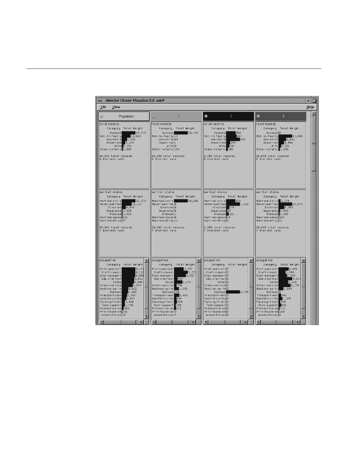
480
Chapter 16: Inducing and Visualizing Clustering
Figure 16-1 Clustering Visualization on Adult Dataset
Clustering is run from the Mining tab in the Data Destinations panel of Tool Manager.
The purpose of clustering is to determine what if any characteristics in the dataset are
similar. You then look at the resulting clusters and experiment with different parameters.
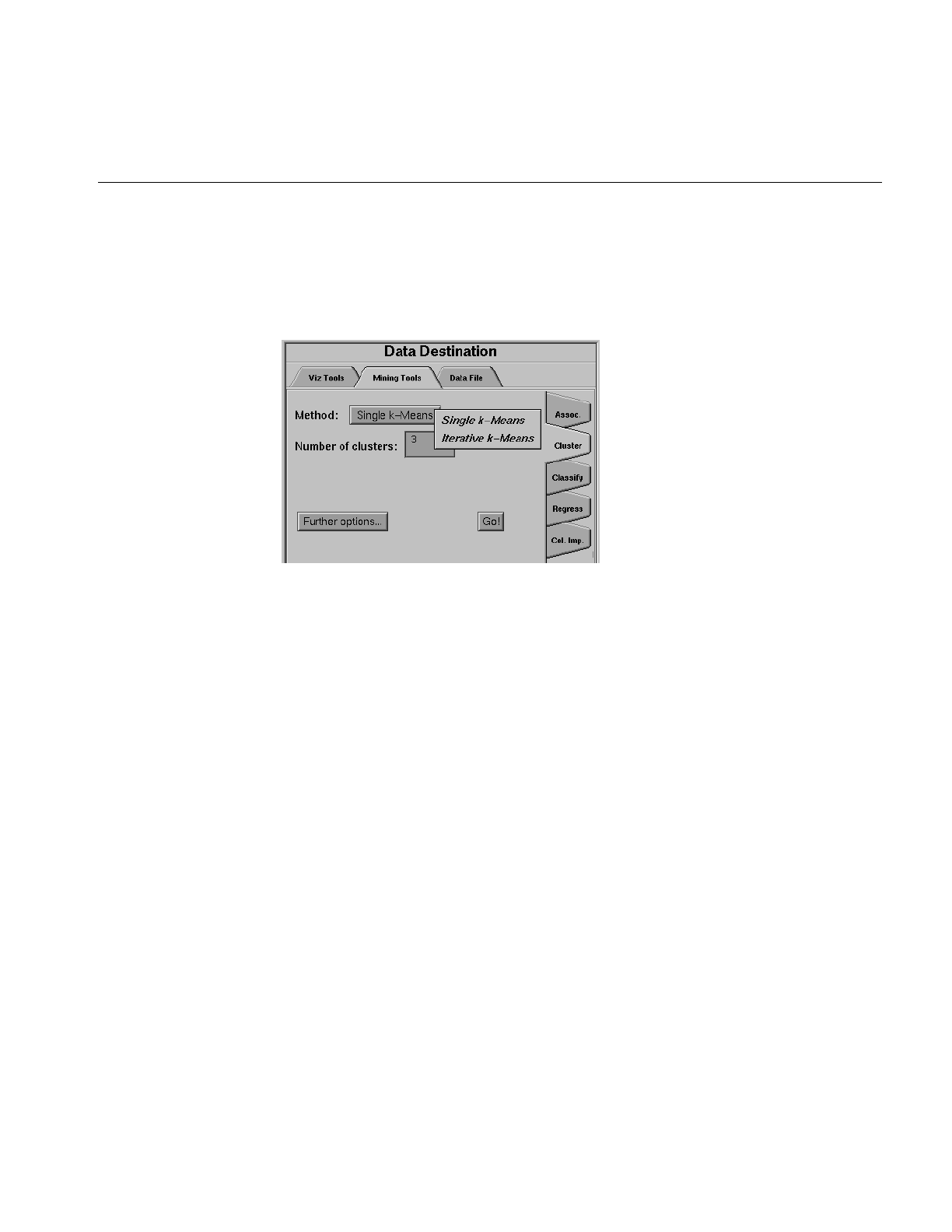
Overview of Clustering
481
All clustering in MineSet uses a combinatorial algorithm based on the k-means objective
function; the algorithm forms clusters by grouping similar records together, aiming to
maximize the overall similarity within each group. MineSet provides two distinct modes
of clustering, single and iterative, both of which are discussed below.
Figure 16-2 The Clustering Tab
There are two methods of clustering
•Single k-means
The term k-means refers to the objective function determining possible good
clustering based on similarity between records.
•Iterative k-means
This method requires three parameters: a lower boundary, an upper boundary, and
a choice point. The algorithm will pick a number of clusters somewhere between
the lower and upper boundary which is appropriate for the dataset. The choice
point is a value between zero and one which guides the selection of the number of
clusters; higher choice points suggest larger numbers of clusters while lower choice
points suggest smaller numbers. A choice point of 1.0 will always pick the upper
boundary. For example, if your boundaries are one and five clusters, a choice point
of 0.4 might pick two clusters while a choice point of 0.8 will pick four. A choice
point of 1.0 will always pick five.

482
Chapter 16: Inducing and Visualizing Clustering
Using Clustering and the Cluster Visualizer
Select the Mining Tools tab in the Data Destination panel of the Tool Manager main
window. From the subsequent tabs select Cluster. This will expose the main clustering
panel.
You can begin the clustering process by clicking Go! from the main Cluster panel (see
Figure 16-2; there are no required options. By default, you will use the single k-means
clustering method to discover three clusters in the data. Once the clustering is complete,
you will see an evaluation of the clustering (see “Evaluation of Clustering” on page 485),
and then the Cluster Visualizer will appear. The Cluster panel provides the following
options:
•Method—Allows you to choose between the single k-means and iterative k-means
methods. The default is single k-means. Both methods are described in detail below.
•Number of clusters—For the single k-means method only, you must specify the
number of clusters to find. The default is 3.
•Number of clusters range—For the iterative k-means method only, you must specify
lower and upper bounds on the possible number of clusters. The default is 1 ... 10.
•Choice point—For the iterative k-means method only, you must specify a choice
point. This is a value between 0 and 1 which helps choose the final number of
clusters. See “Iterative k-Means Clustering Method” on page 484.The default is 0.5.
Note: Clustering is a computationally intensive operation and will take some time to
complete on larger datasets, especially when running iterative k-means mode. We
suggest clustering a sample of the data if your dataset has more than 10000 records.

Using Clustering and the Cluster Visualizer
483
Single k-Means Clustering Method
This method is the simplest form of clustering in MineSet. You specify the desired
number of clusters, and the algorithm groups the records in the data to minimize the
overall dispersion within each cluster. Dispersion refers to the cohesiveness of a cluster;
the higher the dispersion, the farther each record falls from the cluster center. Technically,
dispersion is measured as the root mean squared distance from each record to the center
of the cluster to which it is assigned.
The algorithm itself is iterative and proceeds as follows:
1. You select, for example, five clusters to find.
2. The five cluster centers are initialized to be in random positions in the space of all
records. Different choices of the random seed parameter will produce different
starting positions.
3. Each record in the data is assigned to the cluster whose center is closest to it. The
cluster centers are then recomputed based on the new data in each cluster.
The next step is run repeatedly until no improvement can be made:
4. If there are any records which are closer to the center of a different cluster than they
are established in already, these records are moved to the closer clusters. Then the
cluster centers are recomputed based on the new data in each cluster.
This algorithm is guaranteed to terminate in a finite number of iterations.
Step 4 dominates the running time of clustering. Therefore, the progress window will
show one progress bar for each run of step 4, combined with a note on how many
iterations have been run so far. You can set a limit on the maximum number of iterations
(runs of step 4) allowed before the algorithm stops. The default is 20.
Clusters are assigned sequential numerical names starting from 1. Although cluster
names are represented by numbers, there is no ordering to the clusters.
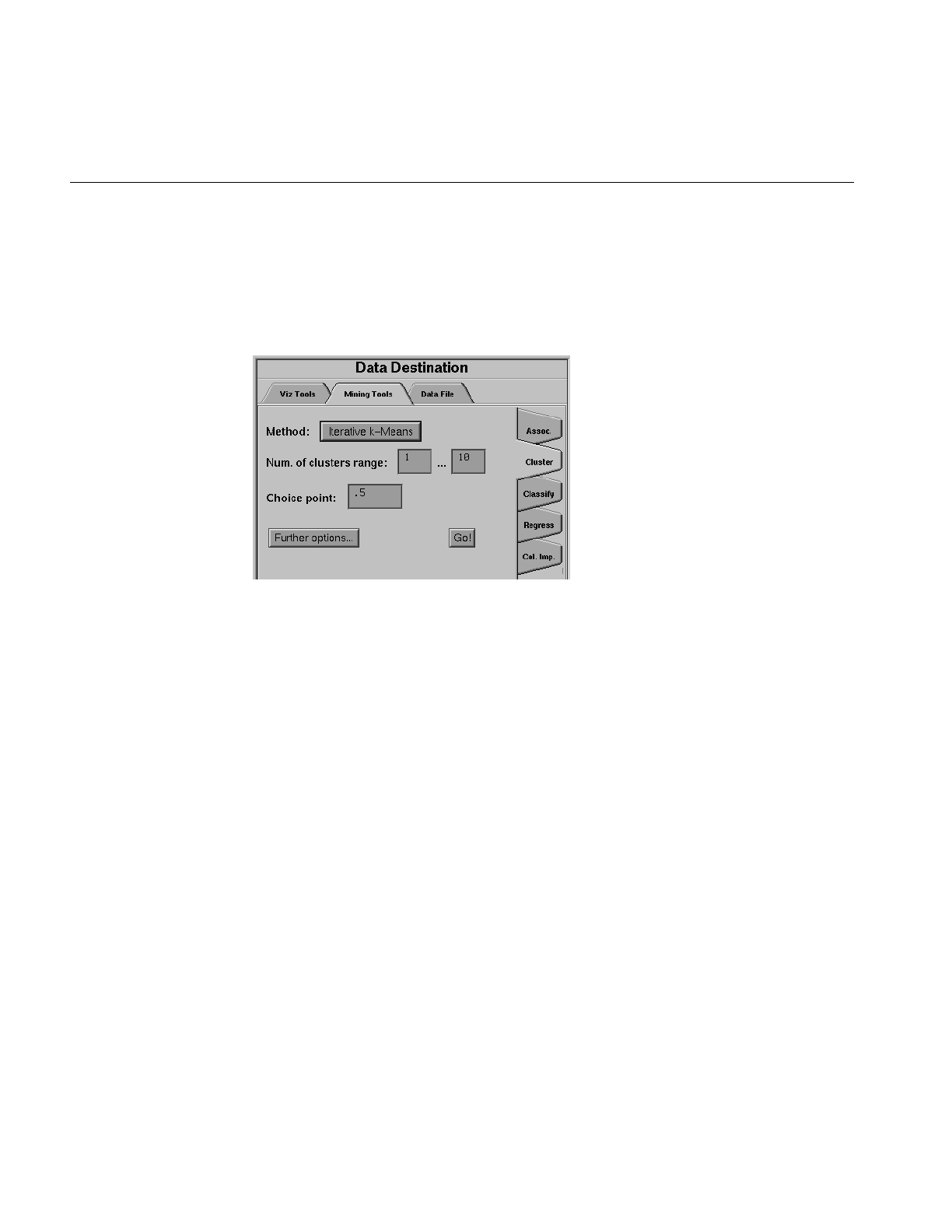
484
Chapter 16: Inducing and Visualizing Clustering
Iterative k-Means Clustering Method
The iterative k-means clustering method is a more complex extension to the single
k-means clustering method. Unlike single k-means, it does not require the specification
on an exact number of clusters to create.
Figure 16-3 Clustering Using Iterative K-Means
To run iterative k-means, you select three parameters: a lower bound on the number of
clusters (default 1), an upper bound on the number of clusters (default 10), and a choice
point (default 0.5). See Figure 16-3. Given these parameters, the algorithm proceeds as
follows:
1. Use the minimum number of clusters for a run of the single k-means algorithm.
This will produce an initial clustering.
The next steps are run repeatedly until the maximum number of clusters has been
reached:
2. Find the cluster with the greatest dispersion and split it in half, creating two new
clusters. Half of the records in the original cluster will be distributed to one of the
new clusters and the other half will be distributed to the other new cluster.
Recompute the centers of the new clusters based on the data they contain.
3. If there are any records which are closer to the center of a different cluster than that
they are currently in, those records are moved to the closer clusters. The cluster
centers are then recomputed based on the new data in each cluster. This is the same
as step 4 of the single k-means method. As in the single k-means algorithm, this step
is repeated until either no records need to be moved or until it has been run the
maximum number of times allowed, as determined by the maximum iterations
parameter (default 20).

Evaluation of Clustering
485
This process has the effect of producing a range of clusterings between the minimum and
maximum numbers of clusters.
The final clustering you are presented with is determined using the choice point
parameter (default 0.5) as follows:
Each clustering is evaluated by measuring the average dispersion of each cluster. As the
number of clusters increases, the average dispersion always decreases. However, it does
not decrease uniformly. The choice point selects the desired degree of dispersion,
measured as the proportion from the dispersion of the minimum number of clusters to
the dispersion of the maximum number of clusters. The clustering with a measured
dispersion closest to this value is chosen as the final clustering. Note that a choice point
of 1.0 will always pick the maximum number of clusters, and a choice point of 0.0 will
always pick the minimum.
Clusters are named based on their derivation during the splitting process. The initial
clustering (based on the minimum number of clusters) is named using sequential
numbers, just as in single k-means. Every time a cluster is split, the two new clusters are
given the name of the split cluster, but with an “A” or a “B” appended. For example, the
cluster named “2-B-A” was derived from cluster 2 in the initial clustering, and was split
twice. We built three clusters using the single k-means algorithm with all default options
except that we set the attribute weight for iris_type to zero.
Evaluation of Clustering
When a clustering model is built, you will be presented with the following display of
statistics in the status window:
This example is from the iris dataset, available in /usr/lib/MineSet/data.
Result of clustering:
-----------------------------------------
Overall root-mean-squared distance from record to centroid: 0.216 +-
0.0928 RMS distance from records to each centroid:
Cluster 1: 0.2306 +- 0.09484
Cluster 2: 0.1921 +- 0.09932
Cluster 3: 0.2247 +- 0.08058
Model saved as iris.cluster
The numbers are measures of the dispersion of each cluster, as well as the overall
excellence of fit of the clustering, dispersions from clusterings based on different datasets
or different numbers or different numbers of clusters are not immediately comparable.

486
Chapter 16: Inducing and Visualizing Clustering
Using Attribute Weights
The k-means clustering algorithm relies on computing the distance between records and
the center of a cluster. Each column in the data is treated as a separate dimension in a
multi-dimensional space of all records. By default, each column in the data has an equal
influence on the final distance. However, you may change the influence of each column,
or attribute, by specifying Attribute Weights in the Clustering Options dialog box for
clustering, see Figure 16-4.
The attribute weight of a column is a value greater than or equal to zero, which
determines the column’s influence in the distance computations of the clustering
algorithm. Setting an attribute's weight to 1 gives it an average influence. Setting it to 2
gives it the influence of two copies of exactly the same column. Setting it to 0 causes the
column to have no effect on the clustering (the clustering proceeds as if you had removed
the column from the data before running clustering). Attribute weights need not be
integral and may be less than one.
To set attribute weights, first click on the Further options button in the main clustering
panel. The top portion of the Further Options dialog box (illustrated in Figure 16-4)
shows the current attribute weights, which all default to 1. To change one or more
weights, select the column(s) whose weights you wish to change (use Shift-click to select
or deselect a range, and Ctrl-click to select or deselect more than one value at once). Now
type the new weight value into the Selected weights field. Finally, click the Set button and
the selected weights will change to the new value. You may select and set all weights at
once using the Select All button.
You will need to adjust attribute weights to help discover a more understandable
clustering. Guidelines for weighting are:
•String or enum type columns with large numbers of values should generally get
low weight (often 0). While such columns will heavily skew the clustering if used
by the algorithm, they can help explain the clustering later.
•If you have detected several columns which correlate strongly, adjust the weights so
that the TOTAL WEIGHT of this set of columns is 1. Otherwise these columns may
excessively drive the clustering.
•Since distances between categorical (string or enum) columns tend to be greater, it is
often useful to give them lower weights than real-valued columns.
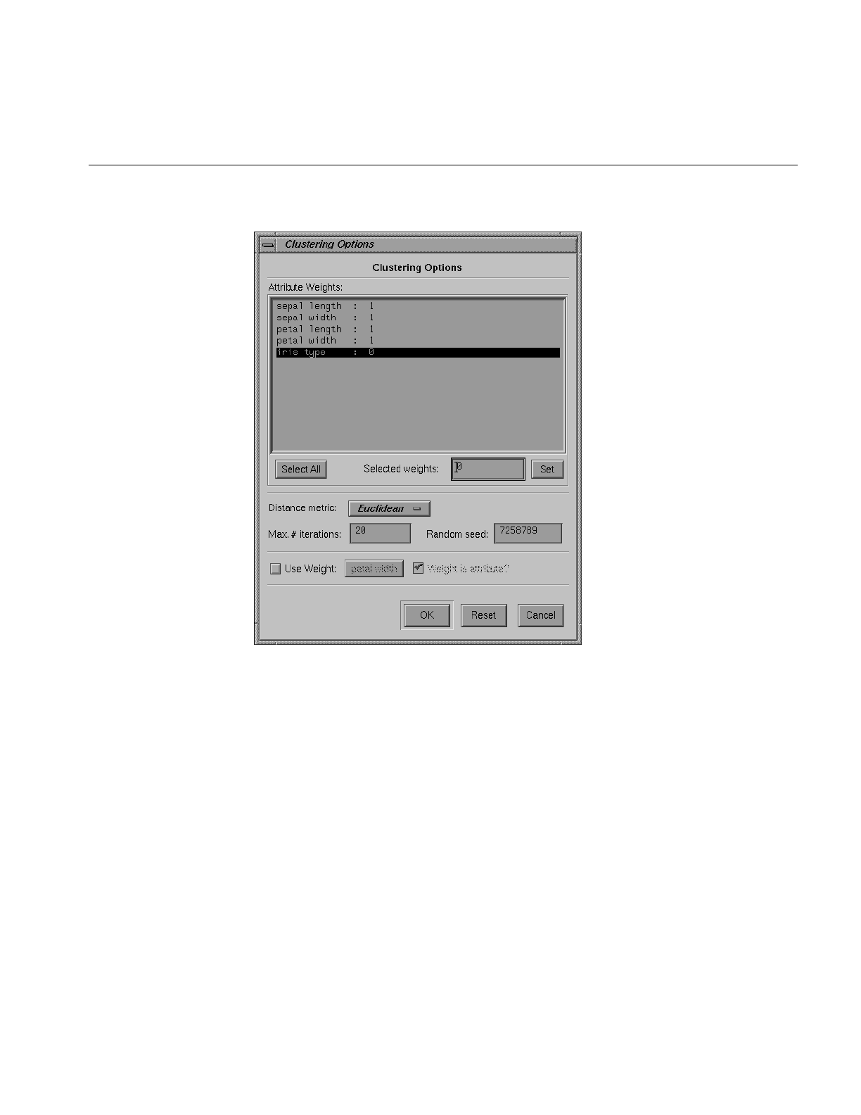
Evaluation of Clustering
487
Figure 16-4 Clustering Options Dialog Box

488
Chapter 16: Inducing and Visualizing Clustering
Further Clustering Options
•Attribute Weights
Clustering gives the opportunity to weight the value of each attribute in the dataset
differently. See “Using Attribute Weights” for more information about this option.
•Distance Metric
This metric determines the way in which distances between records and cluster
centers should be measured. The default choice is Euclidean distance, which
measures distance along a straight line in multidimensional space, with one
dimension per column in the data. The popup menu provides an alternate choice,
Manhattan. Manhattan distance is computed by adding the distance along the axis
of each dimension. This metric gets its name from the way one traverses street
blocks in Manhattan: it is not possible to go straight from point A to point B because
travel may only proceed along paths parallel to the axes (streets).
•Max. # Iterations
This option sets a limit on the number of passes through the dataset the clustering
algorithm may use. More specifically, it limits the number of runs of Step 4 in the
single k-means algorithm. See the section on the k-means method.
•Random Seed
Different random seeds will result in different starting points for the initial cluster
centers. See the section on the k-means method.
•Use Weight
Like most mining tools in MineSet, Clustering supports record weights. This option
allows you to specify a column (which must have a numerical value) which will
specify the weight of each record in the data.
•Weight is Attribute
If this box is selected, the designated weight column will also be used as a normal
attribute by the clustering algorithm. If this box is unchecked, the designated
weight column will not be used as an attribute; it will also disappear from the
attribute weights section (it is given an implicit weight of zero).

Starting the Cluster Visualizer
489
Starting the Cluster Visualizer
There are six ways to start the Cluster Visualizer:
•Use the Tool Manager to configure and start the Cluster Visualizer. (See Chapter 3
for details on most of the Tool Manager’s functionality, which is common to all
MineSet tools; see “Working in Cluster Visualizer Main Window” on page 490 for
details about using the Tool Manager with the Cluster Visualizer.)
•Double-click the Cluster Visualizer icon, which is in the MineSet page of the icon
catalog. The icon is labeled clusterviz. Since no configuration file is specified, the
start-up screen requires you to select one by using File > Open.
•Double-click the Cluster Visualizer icon on your Silicon Graphics desktop. The
startup screen requires you to select a data file by choosing File > Open.
Starting the Cluster Visualizer without specifying a configuration file displays the
copyright notice and license agreement for this tool. Only the File and Help
pulldown menus can be used. For the main window to be fully functional, open a
configuration file by choosing File > Open.
•If you know which configuration file you want to use, double-click the icon for that
configuration file. This starts the Cluster Visualizer and automatically loads the
configuration file you specified. This works only if the configuration filename ends
in .clusterviz (which is always the case for configuration files created for the Cluster
Visualizer using the Tool Manager).
•Drag the configuration file icon onto the Cluster Visualizer icon. This starts the
Cluster Visualizer and automatically loads the configuration file you specified. This
works even if the configuration filename does not end in .clusterviz.
•Start the Cluster Visualizer from the UNIX shell command line by entering this
command at the prompt:
clusterviz [ configFile ]
configFile is optional and specifies the name of the configuration file to use. If you
don’t specify a configuration file, you must use File > Open to specify one.
Options for Invoking the Cluster Visualizer
The -quiet option eliminates the dialogs that pop up to indicate progress. You can
enable this option permanently by adding the line
*minesetQuiet:TRUE
to your .Xdefaults file.

490
Chapter 16: Inducing and Visualizing Clustering
File Requirements
The Cluster Visualizer requires the following files:
•A data file consisting of rows of tab-separated fields. This file is easily created using
the Tool Manager (see Chapter 3).
You can generate data files by extracting data from a source (such as a database) and
formatting it specifically for use by the Cluster Visualizer. Data files have
user-defined extensions (the sample files provided with the Cluster Visualizer have
.clusterviz.data extension)
•A configuration file, describing the format of the input data and how it is to be
displayed. The Tool Manager can create this file (see Chapter 3), or you can use an
editor (such as jot, vi, or Emacs) to produce this file yourself.
Configuration files must have a .clusterviz.extension. When starting the Cluster
Visualizer, or when opening a file, you must specify the configuration file, not the
data file.
Working in Cluster Visualizer Main Window
Cluster Visualizer illustrated in Figure 16-5 bears a resemblance to Statistics Visualizer
(StatViz) with its box plots and histograms. Unlike in StatViz, the box plots are arranged
in rows and columns. ClusterViz shows one row for each attribute in the data, and one
column for each cluster. At the top of each cluster is a pane containing the name of the
cluster. There is one additional column with the title “population”. This column displays
statistics for the dataset as a whole and is equivalent to a StatViz view of the data.
Clusters are named based on the mode used to create them. Clusters created using single
k-means are numbered sequentially. Clusters created using iterative k-means are
numbered according to the process used to create them. In this example the clusters are
simply numbered sequentially. The algorithm has no way of detecting what the clusters
represent, and human interpretation is required. Each box plot shows statistics about
data from a single column, including the minimum, maximum, mean, median, and two
quartiles (25th and 75th percentiles). These values are shown as lines, and the standard
deviation is shown as a value.
The order in which attributes are displayed in the Cluster Visualizer window is
significant; by default, attributes are displayed in order of importance for discriminating
between the clusters (this is the same importance ordering as shown in the Evidence
Visualizer). Clicking on the pane containing the name of a cluster will redisplay the
attributes in order of importance for discriminating that cluster from all others. Clicking
on the pane containing “population” will restore the default ordering.
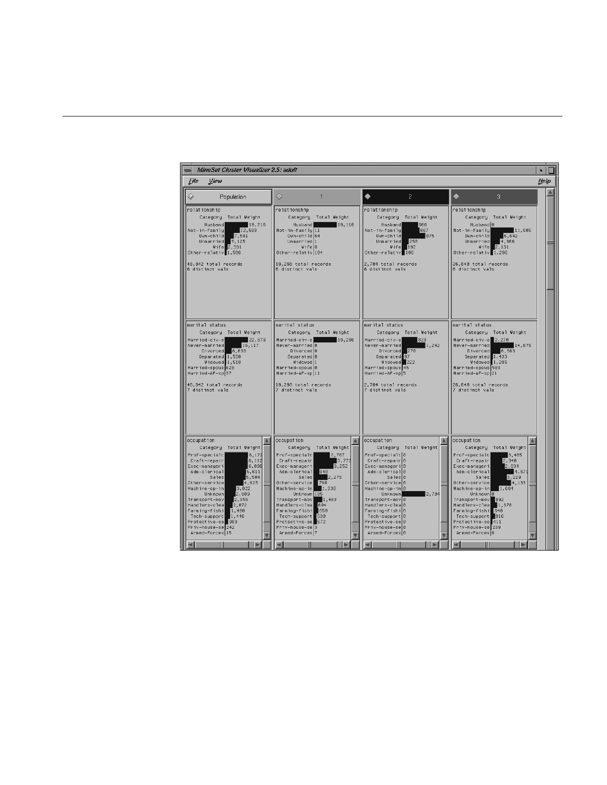
Working in Cluster Visualizer Main Window
491
Figure 16-5 Cluster Visualizer Main Window

492
Chapter 16: Inducing and Visualizing Clustering
Pulldown Menus
The Cluster Visualizer has three pulldown menus, labeled File, View and Help. These are
similar to menus in the Evidence Visualizer (see“Pulldown Menus” in Chapter 13.)
Sample File
The following example shows a case in which clustering might be useful. This example
is associated with a sample dataset provided with MineSet. It shows how to work with
the Clustering mining tool, and explains the different outcomes and options.
The cars dataset is relatively simple, dealing with familiar concepts of horsepower,
vehicle weight, and time required to reach 60 mph.
In working with the Cluster Visualizer window, when you select cluster 1, that cluster
controls the priority ordering of attributes represented by the bar charts and histograms.
The order of attributes in other clusters is based on cluster 1. For example, if you click on
cluster 1, the attribute importance is cylinders, weight, then miles per gallon. This
ordering of importance is a controlling cluster only as far as the visualization goes. You
can compare the same row across the other clusters to see how that attribute differs from
cluster to cluster. When you select cluster 2, you see a differentiation in the order of
attributes at a lower level. In this case, origin is more important, then cylinder, then
horsepower, then miles per gallon.
Alternative Visualization of Clustering
The Cluster Visualizer provides an easy-to-use basic visualization of the clustering.
However, it is not the only way to visualize clustering. An example of transferring the
results of clustering into a display using the Scatter Visualizer is shown in MineSet 2.5
Tutorial.

493
Chapter 17
17. Column Importance
This chapter discusses the features and capabilities of the Column Importance mining
tool, and the relationship between column importance and the importance ranking in the
other data mining tools. Because of the differences in representation for classification
models, different attributes may be judged more important for different models. A
sample file, provided with MineSet, is discussed at the end of this chapter.
Note: This chapter assumes that you have read Chapter 10, “MineSet Inducers and
Classifiers.”
Finding Important Columns
Column Importance is run from the tab labelled Col. Imp. on the Mining Tools panel
(Figure 17-1). It determines how important various columns are in discriminating the
different values of the label column you choose. You might, for example, want to find the
best three columns for discriminating the label good credit risk so you can choose them for
mapping to axes the Scatter Visualizer. When you select the label and click Go!, a popup
window appears with the three columns that are the best three discriminators. A
measure called “purity” (a number from 0 to 100) informs you how well the columns
discriminate the different labels. Adding more columns can only increase the purity.
Purity is a measure of the skewness of the label value distribution. The cumulative purity
measure is a measure of the purity of partioning the data. The data is partioned using
columns found as importand in the same way data is partitioned in a Decision Tree. Each
set in the partition has its own purity measure, and the purity measure within the partion
is a combination of these individual measures. For a given set in the partition, the purity
is 0 if each class has equal representation, and 100 if every record is of the same class.
Similarly, the cumulative purity will be 0 if each set in the partition has an equal
representation of classes, and 100 if each set in the partition contains record that all have
the same class.
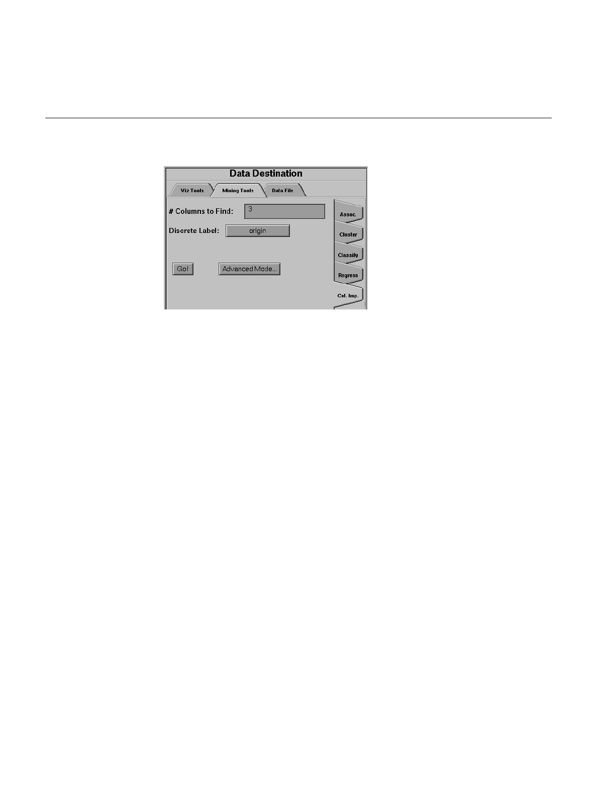
494
Chapter 17: Column Importance
Figure 17-1 The Column Importance Tab
There are two modes of Column Importance:
•Simple Mode
To invoke the Simple mode, choose a discrete label from the popup menu, and
specify the number of columns you want to see, then click Go!.
•Advanced Mode
Advanced mode lets you control the choice of columns. To enter Advanced mode,
click Advanced Mode in the Column Importance panel. A dialog box appears, as
shown in Figure 17-2. As with Further Inducer Options (see Chapter 10, “MineSet
Inducers and Classifiers”), you can select a weight attribute and decide whether it
behaves as a regular attribute for determining importance. The dialog box contains
two lists of column names: The left list contains the available attributes and the right
list contains attributes chosen as important (by either the user or the Column
Importance algorithm).

Finding Important Columns
495
Figure 17-2 Advanced Mode of Column Importance

496
Chapter 17: Column Importance
Advanced mode can work two different ways: finding several new important
attributes or ranking available attributes.
•Finding Several Important Attributes
To enter this submode, click the first of the two radio buttons in the middle of
the dialog (...find [number] additional important attributes). If you click Go! with no
further changes, the effect is the same as if you were in Simple mode, finding
the specified number of important columns and automatically moving them to
the right column. Near each column, the cumulative purity is given (that is, the
purity of all the columns up to and including the one on the line.)
Alternatively, by moving column names from the left list to the right list, you
can prespecify columns that you want included and let the system add more.
For example, to select the cylinders column and let the system find three more
columns, click the cylinders column name, then click the right arrow between
the lists.
Clicking Go! lets you see the cumulative purity of each column, together with
the previous ones in the list. A purity of 100 means that using the given
columns, you can perfectly discriminate the different label values in the dataset.
•Ranking Available Attributes
Advanced mode also lets you compute the change in purity that each column
would add to all those that were already marked important, that is, they are in
the list on the right. For example, you might move cylinders to the list on the
right, and then ask the system to compute the incremental improvement in
purity that each column remaining in the left column would yield. The
cumulative purity is computed for columns on the right (already marked
important).
To enter this submode, click the second of the two radio buttons at the bottom
of the dialog (...compute improved purity for left columns, cumulative purity for right
columns.). This submode permits fine control over the process. If two columns
are ranked very closely, you might prefer one over the other (for example,
because it is cheaper to gather, more reliable, or easier to understand).

Column Importance Notes
497
Column Importance Notes
The importance of a column depends on the columns previously marked as important.
For example, while net-income might be a good column individually, it might not be as
important together with salary because they are likely to be highly correlated. The best
set of three columns is not necessarily composed of the columns that rank highest
individually. If two columns give the income in dollars and in another currency, they are
ranked equally alone; however, once one of them is chosen, the other adds no
discriminatory power to the set of best features.
Column selection is useful for finding the best three axes for Scatter Visualizer and Splat
Visualizer. It is also useful for finding a good discriminatory hierarchy (hierarchy that
separates different label values) for the Tree Visualizer when you select the label to be the
key used in the Tree Visualizer.
All floating point values (doubles or floats) are prediscretized using automatic
discretization (see Chapter 3, “The Tool Manager”). If a column has no value given to it
in the left list, the algorithm did not consider it; this is because it either had a single value
(for example, when it is discretized into one interval), or the number of records that it
would separate is not statistically significant.
Column Importance and Relation to Classifiers
This section describes the differences among Column Importance, the importance
ranking chosen by the Evidence Inducer, and the splits chosen by the Decision Tree
Inducer. As Column Importance uses all of the data, these descriptions assume that you
are running the inducers in “Classifier Only” mode, so that the inducers are using all of
the data as well.
The Discretization Process
The Column Importance algorithm and the Evidence Inducer discretize all continuous
attributes using the automatic discretization algorithm (the same algorithm that is
applied in automatic binning in the Tool Manager). The Decision Tree algorithm does not
pre-discretize attributes (columns) and finds thresholds as the tree is built.
The main advantage of the automatic discretization is that it discretizes the continuous
range into several intervals at once, while the Decision Tree makes only binary splits.

498
Chapter 17: Column Importance
The main advantage of the Decision Tree algorithm is that it discretizes subsets of the
data (those that reach a specific node where a test is done). Thus the discretization is
“local” to those records as opposed to a “global” discretization.
The Importance Function
The Evidence Inducer and Column Importance rank attributes based on “mutual
information” as the purity measure. The Decision Tree Inducer, Option Tree Inducer, and
Decision Table Inducer defaults to “normalized mutual information,” which penalizes
multi-way splits (see the description of splitting criterion in Chapter 11, “Inducing and
Visualizing the Decision Tree Classifier”). Thus, the Decision Tree Inducer prefers an
attribute with few values over attributes with many values. The default for Decision
Trees can be changed to “mutual information.”
Dependence on Other Attributes
The Evidence Inducer ranks each attribute independently. If several attributes are highly
correlated, they have similar ranking. If you use the Advanced mode from Column
Importance, and the “...compute improved purity” option without any attributes chosen
as important (that is, moved to the list on the right), the attribute ranking shown matches
the sort order chosen by the Evidence Inducer.
The Column Importance tool, the Decision Tree Inducer, and the Decision Table Inducer
all provide more powerful importance capabilities than the Evidence Inducer. All choose
an importance ranking with respect to other columns.
In Column Importance, columns are judged as important relative to the set of columns
in the list on the right. If two columns are highly correlated and one is chosen, the other
will probably never be chosen; each column is chosen for its ability to provide more
information about the label than is already present.
In the Decision Table Inducer, the Suggest button provides an importance facility similar
to the column importance tool. Columns are judged as important relative to the set of
columns already present in the mapping box. There are three major differences, however,
between the Decision Table Inducer's suggest mode and the column importance tool.
First, the Decision Table Inducer penalizes multi-way splits. Second, the Decision Table
Inducer is capable of performing a more exhaustive search to find a better column
ordering. Finally, the Decision Table Inducer does not report any purity scores—it merely
ranks the columns.

Sample File
499
The Decision Tree Inducer provides a more flexible importance ranking because different
columns can be selected at different subtrees. For example, one column can be chosen for
the left child of the root and another for the right child of the root. While this is
appropriate for a Decision Tree, it is inappropriate for choosing a small set of columns to
show in the Scatter Visualizer or Splat Visualizer. For these cases, the Column
Importance tool is superior because it builds an “oblivious” Decision Tree in which every
level of the tree tests the same column across the nodes. With Column Importance, a
single column must be chosen for all combinations of the previously chosen columns.
Sample File
The following example shows a case in which Column Importance might be useful. This
example is associated with a sample dataset provided with MineSet. It shows how to
work with the Column Importance mining tool, and explains the different outcomes and
options.
When customers change their phone carrier from one telecommunications company to
another, this is termed “churning.” This is a common problem in the telecommunications
industry. The data used to generate this example is in /usr/lib/MineSet/data/churn.schema.
The Column Importance mining tool lets you look at properties of this file.
Running the simple Column Importance mode yields the following three attributes:
•Total Day Charge.
•Number of customer service calls.
•State.
By running “compute improved purity” from the advanced mode, you can see that Total
Day Charge and Total Day Minutes have the same purity ranking (48.67). By moving one
of them to the right (for example, Total Day Minutes) and rerunning Compute Improved
Purity, you can see that there is no value to the other (Total Day Charge). These two
attributes are highly correlated.

500
Chapter 17: Column Importance
Looking at the attributes when Total Day Minutes is on the right, we can see that the
following are good:
•International plan (4.1)
•Number of Customer Service Calls (8.1).
•State (4.7)
You can choose to move International Plan to the right, because this information is
readily available and easy to measure.
The other two attributes (Number of Customer Service Calls and State) remain highly
important (in fact, their importance increases), so they are apparently not correlated with
the International Plan.
By looking at the importance of attributes this way, you can determine which ones can
be substituted with others that are equally good (or almost as good), but are easier to
measure or understand. By looking at the purity, you can determine how much the
additional attributes help. For example, in the above scenario, state significantly
improves the purity. In the iris dataset, the third attribute chosen (sepal length) raises the
purity only slightly higher. In some cases, the simpler, two-dimensional scatterplot
might be easier to understand.

501
Chapter 18
18. Selection and Drill-Through
This chapter provides an introduction to selection and drill-through. With these features,
you can select graphical objects in the visual tools, show the data associated with that
tool, and send your selection to the Tool Manager to view the original data or to analyze
it using another tool.
These features are common to all tools in MineSet, although certain tools have additional
behavioral characteristics. Tool-specific details are provided at the end of this chapter.
Multiple Selection
In most of the tools, selection is done using Shift-Mouse 1. Clicking mouse button 1 on an
object without pressing Shift, selects the object under the cursor while deselecting all
other previously selected objects. Holding down Shift while clicking mouse button 1
toggles the selection of that object without affecting any other selections. (Note that the
Splat Visualizer has a different interface, described at the end of this chapter.)
When you select an item, a message describing that item appears in the tool's main
window; by default, the visual tools only show information on the last object selected. A
separate Record Viewer window displays a table, which shows the values for all
selections. In the Tree and Map Visualizers, choose the Selection > Show Values to see
this. Figure 18-1 shows an example of the selected values in the Record Viewer. See also
“The Record Viewer” in Chapter 3.

502
Chapter 18: Selection and Drill-Through
Figure 18-1 Table of Values for Selected Objects
If a message has been set for the particular tool, that message also appears in the table.
Columns in this table can be resized by dragging the separators between the columns.
You also can click on a value to display the complete text of that value at the top of the
table.
Drill-Through
It is often useful to see or manipulate the original data from the data source that resulted
in the current selections. This is referred to as drill-through. There are two entries on the
Selections menu that perform drill-through:
•Send to Tool Manager — When this is selected, the history of operations that
produced the visualization is placed in the Tool Manager. A filter operation
corresponding to the user's selection in the visual tool is added to the history. The
filter is placed as early in the history as possible, given the restrictions described
below.
•Show Original Data — As with Send to Tool Manager, this option starts with the
history of operations used to produce the visualization, and adds a filter operation
as early as possible in the history. All non-filter operations coming after the filter in
the history are removed. This new history is used to produce a table shown in the
Record Viewer. If the filter can be placed at the beginning of the history, the data
shown are the original records; otherwise, a warning is issued, indicating that the
data are not totally original. The state of the Tool Manager is not altered (unless it is
currently not running).

Drill-Through
503
In either case, the Tool Manager performs the operation. If the Tool Manager is not
running, it is started automatically.
Only visualizations generated using the Tool Manager can be used for drill-through.
Each .schema file for these visualizations includes a history section that informs the Tool
Manager how that file was generated. A few special-purpose mining visualizations such
as Learning Curves, Confusion Matrices, Lift Curves, and the Rules Visualizer do not
include a history and do not support drill-through.
When you select objects for drill-through, you are implicitly specifying a filter statement
based on the visualized table. If the table was transformed before visualization, the Tool
Manager might have to change the filter to place it earlier in the history. For example, if
the filter is based on a binned column, the Tool Manager must change it so it refers to the
pre-binned column.
The filter cannot always be placed at the beginning of the history because the Tool
Manager cannot adjust the filter for all operations. Specifically, if the filter refers to any
column created via Add Column,Aggregate, or Apply Model, the filter cannot be placed
earlier in the history than the operation that created the column. Furthermore, the Tool
Manager can never move a filter earlier than an existing Sample operation, since that
would dramatically change the output of the sampling.
The Show Original Data mode tries to truncate the history to show the records from as
early a stage as possible. To prevent this mode from showing more records than were
selected, however, the truncation does not remove any other existing filter operations
(either user-created or the result of previous drill-through).
Tree Visualizer Specific Details
The Tree Visualizer selects drill-through criteria based on the location in the hierarchy
and, if appropriate, the bar selected on that node. For example, in a sales hierarchy with
region, city, and store, and with bars representing products, selecting the furniture bar
for a particular city can generate a drill-through request selecting everything for which
region=Western and city=Mountain View and product=furniture.
In the Decision Tree, the drill-through request is based on the decision criteria. For
example, for an automobile decision tree, a drill-through request might be:
“cubicinches <= 170 and mpg>20 and origin=US.” In both cases, selecting the top node
of the tree generates a drill-through of the entire dataset. For both Decision Trees and
normal hierarchies, selecting the top node of the tree generates a drill-through of the
entire dataset.

504
Chapter 18: Selection and Drill-Through
Map Visualizer Specific Details
Drill-through in the Map Visualizer is based on the regions selected.
Scatter Visualizer Specific Details
The Scatter Visualizer uses a selection box in addition to Shift-select. From the Selection
menu select Create Box Selection. The box has tabs that can be used to resize or move it.
You can not create more than one box.
The Scatter Visualizer does not have a key with which to select columns used for
drill-through. The default is to use all non-array columns that have been mapped to
graphical requirements (such as axes, size, color and sliders). From the Selections
pull-down menu, the Preferences panel lets you select an alternate list of columns to be
used in the drill-through.
A Record Viewer appears whenever a selection has been made. It shows the current
selections. If the Record Viewer is closed, the selections are cleared.
Splat Visualizer Specific Details
The Splat Visualizer uses a Selection box rather than Shift-click to select multiple objects.
From the Selection menu select Create Box Selection. The box has tabs that can be used
to resize it, or it can be moved. You can create more than one box.
The Record Viewer is tied to the Selection box; when the Record Viewer is dismissed, the
selections are cleared. Drill-through is based on where the box is within the axes, and,
optionally, on the sliders, if the Use Slider on Drill Thru item on the Selection menu is
checked.
Rules Visualizer Specific Details
Selection and drill-through are not implemented in the Rules Visualizer.

505
Chapter 19
19. File Exchange Between MineSet and SAS
This chapter describes the support for file exchanges between MineSet and SAS.
Overview
Exchanging data sets between MineSet and SAS is done through two utilities: mineset2sas
and sas2mineset. To convert a MineSet .schema and .data file pair into a SAS data set, use
mineset2sas. To convert a SAS data set into MineSet .schema and .data files, use sas2mineset.
Both mineset2sas and sas2mineset invoke the SAS executable; thus, SAS must be installed
on the machine on which these conversion utilities are used.
Converting MineSet Data Files to SAS Data Sets
Use mineset2sas to convert MineSet data files into SAS data sets. The syntax for this is
mineset2sas <MineSet file> <SAS libref.datafile> [options]
Options are
•-svsc to save the script sent to SAS. The script normally is deleted after use.
•-names <namefile> to save trimmed column names in <namefile>. The script
normally is deleted after use.
For example:
mineset2sas cars sasuser.cars -svsc -names cars.names
mineset2sas converts the MineSet .schema and .data files (in this case, cars.schema and
cars.data) into a SAS data file. Currently, only string and numeric data types are
supported. The MineSet .data file must be in ASCII format; binary format is not
supported. To save MineSet data files in ASCII, deselect Use binary data files in Tool
Manager Preferences.

506
Chapter 19: File Exchange Between MineSet and SAS
SAS column names (or, in SAS terminology, variable names) can consist of only letters,
and underscore characters. The first character in a column name cannot be a number.
Furthermore, SAS column names can be up to eight characters long. Since any character
string can be a legal MineSet column name, mineset2sas maps MineSet column names to
legal SAS column names. The rules for this mapping are:
•Any invalid character is replaced with an underscore.
•If the first character is a digit, an underscore is prepended to the column name.
•Column names are truncated to eight characters. If this truncation results in
non-unique column names, the ends of the conflicting column names are replaced
with sequential numbers, thus creating unique column names.
To preserve as much of the full column names as possible, mineset2sas also saves the first
40 characters of each column name as the column label.
The -names namefile Command Line Option
To get a listing of the column names before and after conversion into SAS format, specify
the -names <namefile> command line option. When mineset2sas executes, it writes out a
mapping of the column name changes to the specified file. For example:
`date of birth` -> `date_of_`
`92census` -> `_92censu`
`# of days to end of quarter` -> `__of_da0`
`# of days to end of year` -> `__of_da1`
`# of davenports` -> `__of_da2`
The -svsc Option
The mineset2sas utility reads the schema for the specified data file, and writes a
customized SAS script. SAS, which must be installed in /usr/sbin/sas, is invoked with this
script to read and convert the data. The script sent to SAS is normally deleted after use.
With the -svsc option, the script is saved as the file mineset2sas.sas. If there is an error in
the script processing, the SAS error log is saved as mineset2sas.log.

Converting SAS Data Sets Into MineSet Data Files
507
Converting SAS Data Sets Into MineSet Data Files
Use sas2mineset to convert SAS data sets into MineSet data files. The syntax for this is
sas2mineset <SAS libref.datafile> <MineSet file> [options]
Options are
•-nodata creates only a .schema file, no .data file.
•-svsc saves the scripts sent to SAS.
•-nolabel indicates that you do not want labels used for column names.
•-names <namefile> restores long column names from <namefile>, created by
mineset2sas.
For example,
sas2mineset sasuser.houses -svsc -names houses.names
The sas2mineset utility converts a SAS data file into MineSet .schema and .data files.
Currently, this utility supports only string, numeric, and date data types.
The -nolabel Option
SAS only supports eight-character long column names, but allows optional 40 character
labels for each column. MineSet sets no limit on the column name length, so, by default,
sas2mineset uses the column labels to name the columns in the output file, if labels have
been defined. To force sas2mineset to use the SAS column name for each column, even if
a label is specified, add the -nolabel option to the command line.
The -names namefile Option
If a MineSet data file is converted into SAS with mineset2sas and then back to MineSet
format with sas2mineset, a column name map file can be created to keep track of the
original column names. To have sas2mineset use a name map file created by mineset2sas,
add the -names <namefile> option to the command line, and specify the same map file as
specified when the file was converted into SAS format with mineset2sas. This option is
useful only for data files with column names longer than 40 characters, since mineset2sas
saves up to 40 characters in the column label.
Note that the -name <namefile> option overrides the -nolabel option.

508
Chapter 19: File Exchange Between MineSet and SAS
The -nodata Option
To create just a MineSet schema file without downloading the data from a SAS data file,
add the -nodata option to the command line.
The -svsc Option
The sas2mineset utility writes two customized SAS scripts to retrieve the specified data
file. The first script extracts column descriptions; the second extracts the data. The scripts
are normally deleted after use. With the -svsc option, the scripts are saved as
getschema.sas and getdata.sas, respectively. If there is an error in the script processing, the
SAS error logs are saved as getschema.log and getdata.log, respectively.

509
Chapter 20
20. MineSet Web Extensions
This chapter describes the MineSet extensions that are provided to let you create or view
visualizations and/or interact with MineSet over the web.
Overview
MineSet Web extension allows visualizing files and data generated by MineSet software
over the Web. This can be done in two ways.
•MineSet mtr extension
MineSet mtr extension lets you place MineSet configuration, schema and data files
into an archive file, which can be embedded in a web page as an html tag. Once the
user clicks on the hyperlink in Netscape, the browser automatically invokes the
mineset_weblaunch program. This brings up the MineSet visual tool. The machine
that the browser is running on must have the MineSet client software installed.
•MineSet Remote View
MineSet Remote View extension allows machines that do not have MineSet
software installed to view visualizations through the Web. This is done via two cgi
scripts that are included with the MineSet software distribution. The cgi scripts
must be configured properly and installed in the Web Server machine. The cgi script
rview_file.cgi must get called from a .html file with a MineSet visual tool file as an
argument. The cgi script rview_dir.cgi provides the client (user who accesses the
script) with a list of available visualizations. The user then can select any file via
multiple popup menus and click on the invoke button to launch the MineSet tool.

510
Chapter 20: MineSet Web Extensions
MineSet Web Extension Files
All MineSet Web Extension files are located in the /usr/lib/MineSet/www directory, which
contains three subdirectories.
scripts Subdirectory
examples Subdirectory
Script Purpose
mineset_webinstall_server This program configures the httpd server. Use it to configure the server and the MineSet
Remote View Program. If the web server is a remote machine, copy this file along with
mineset_wsf.tar to the remote machine.
mineset_webinstall_client This program configures the Web browser (Netscape). Use it to configure the client.
mineset_weblaunch This program is invoked by the web browser (Netscape). It un-archives the mtr file and brings
up the appropriate viewer.
mineset_makemtr This program creates one or more mtr files from files created either by Tool Manager or created
manually. The mtr file is sent over the network and is used by mineset_weblaunch to invoke
MineSet visual tools.
mineset_wsf.tar This is a tar file of various files needed by mineset_webinstall_server. If the web server is a
remote machine, copy this file along with mineset_webinstall_server to the remote machine.
File Purpose
index.html This file provides an index of all the mtr files supplied with MineSet.
rview_file.html This file illustrates how you should embed hyperlinks to invoke mineset_rview on files and
directories.
adult-salary.eviviz.mtr mtr file of /usr/lib/MineSet/eviviz/examples/adult-salary.eviviz.
nl.births.mapviz.mtr mtr file of /usr/lib/MineSet/mapviz/examples/nl.births.mapviz.
company.scatterviz.mtr mtr file of /usr/lib/MineSet/scatterviz/examples/company.scatterviz.
cars-dt.treeviz.mtr mtr file of /usr/lib/MineSet/treeviz/examples/cars-dt.treeviz.
cars-odt.treeviz.mtr mtr file of /usr/lib/MineSet/treeviz/examples/cars-odt.treeviz.
churn-dt.treeviz.mtr mtr file of /usr/lib/MineSet/treeviz/examples/churn-dt.treeviz.

MineSet Web Installation (Client)
511
examples/rview_dir Subdirectory
MineSet Web Installation (Client)
During the MineSet client installation the client part of the web extension is
automatically installed under most circumstances. To see whether it was automatically
installed run the following command.
sh -c "grep mineset /usr/local/lib/netscape/mime.types > /dev/null ;
echo $?"
If the output is 0 then you don't need to do the client installation. If the output is not 0
then you need to install the MineSet web-client extension. A program is provided for the
MineSet Web installation. Before you start the installation you must make sure that
MineSet Client is installed in the machine you're trying to configure. If it is not installed
please install the MineSet software before you try to configure the MineSet Web
Extension.
To configure the client, run the following command.
cd /usr/lib/MineSet/www/scripts ; ./mineset_webinstall_client
The program prompts you for the location of the files mailcap and mime.types. After you
provide the correct names, the program adds the corresponding entries to the files.
File Purpose
*.treeviz.* Treeviz configuration and data files to be dynamically indexed by rview_dir.cgi.
*.mapviz.* Mapviz configuration and data files to be dynamically indexed by rview_dir.cgi.
*.eviviz.* Eviviz configuration and data files to be dynamically indexed by rview_dir.cgi.
*.scatterviz.* Scatterviz configuration and data files to be dynamically indexed by rview_dir.cgi.
*.ruleviz.* Ruleviz configuration and data files to be dynamically indexed by rview_dir.cgi.
*.dtableviz.* Decision Table configuration and data files to be dynamically indexed by rview_dir.cgi.
*.clusterviz.* Clusterviz configuration and data files to be dynamically indexed by rview_dir.cgi.

512
Chapter 20: MineSet Web Extensions
MineSet Web Installation (Server)
A program is provided for the MineSet Web installation. Before you start the installation
you must make sure the following software, listed below is installed. If you are not
familiar with the details contact your system administrator or webmaster and request
that the installation be done for you.
For MineSet Web installation to work properly, you need
•a Netscape browser
•an httpd server
Setting Up the Server
The server can be running on either the local machine or a remote machine. You must
know:
•the name of the machine on which your httpd server runs, and
•the directory where the publicly accessible .html files are stored
Typically the files are located under /var/www/htdocs. The machine name is included
between http:// and the first /. If you are accessing files by using
http://some-machine.xxx.com/file.html, then some-machine is the name of the machine, and
xxx.com is the domain name. An httpd daemon must be installed and running on
some-machine.
You also must know where the httpd configuration files are stored in the server. If you
are running the Netscape fast-track server, the configuration files usually are in
/usr/ns-home/httpd-machine/config, where machine is the name of your machine. If you are
running a version of ncsa-httpd or apache, the files might be located in
/usr/local/etc/httpd/conf or /var/www/server/conf. If you are not sure where the config files
are located, contact your system administrator or webmaster.
Once you know where your Server configuration files are located, you need the
following two files to perform the installation
•mineset_webinstall_server
•mineset_wsf.tar

MineSet Web Installation (Server)
513
Local Installation
A script is provided with MineSet that helps with the MineSet installation. Since
configuration of Web Servers varies from machine to machine, the program prompts you
for the location of files. It tries to make a reasonable guess and provides defaults;
however, it is better if you know where the files are located before you supply them to
the program.
Configuring MineSet Web Extensions for the Local Server
To start the installation, enter the following
cd /usr/lib/MineSet/www/scripts
./mineset_webinstall_server -s
You are prompted for the location of your server mime.types file. Once you give the
correct file name, it adds an entry and tries to restart the httpd daemon. If it can not
restart your daemon, you must do it manually. If you're not sure about how to restart the
httpd daemon, ask your system administrator or webmaster.
Configuring MineSet Web Extensions for a Remote Server
First copy over the following two files to the server
•mineset_webinstall_server
•mineset_wsf.tar
Once you're copied them over, cd to the directory where you copied the files. Then start
the installation by entering
./mineset_webinstall_server -s
It prompts you for the location of your server mime.types file. Once you give the correct
file name, it adds an entry and tries to restart the httpd daemon. If it can not restart your
daemon, you must do it manually. If you're not sure about how to restart the httpd
daemon, ask your system administrator or webmaster.

514
Chapter 20: MineSet Web Extensions
MineSet mtr Files
For MineSet mtr extension to work, you must have MineSet software installed in your
machine or the machine where the Netscape browser is installed. MineSet mtr files are
archives of MineSet files generated by the Tool Manager or created manually. Creating
an mtr file is very easy. Once created, it can be used as a hyperlink in an html page. The
mtr files are very effective in sharing multiple visualizations over the web, eliminating
the need for attaching huge files in mails, remote copies, or file transfers (ftp).
Since mtr files are in a compressed format and use the underlying http protocol, the
transfer of an mtr file is very fast and does not require a cumbersome setup on the part
of administrators.
Creating mtr Files
An mtr file can be created in the following ways.
1. From Files created by Tool Manager
Once you have launched a tool from the Tool Manager, go to the directory from
where you launched the Tool Manager and invoke mineset_makemtr using the name
of the file(s) as the arguments. For example, if you have launched the Tree
Visualizer and the Rule Visualizer from Tool Manager, then to create mtr files use
the following command.
% mineset_makemtr foo.treeviz foo.ruleviz
This creates two files called foo.treeviz.mtr and foo.ruleviz.mtr.
2. Mapviz files with .gfx extensions
If you have generated a Mapviz visualization that uses the .gfx extension, you must
use the -f option of mineset_makemtr, and mention all the files that you want to
include in the archive. For example, you can use the following command
% mineset_makemtr -f sales.mapviz sales.mapviz.schema
sales.mapviz.data sales.hierarchy sales.gfx

MineSet mtr Files
515
3. From Files not created by Tool Manager
If you've created some files without using Tool Manager, you still can create a mtr
file from those files. You must use the -l option of mineset_makemtr. Suppose you
want to create a mtr file from the MineSet scatterviz example directory, use the
following command.
% mineset_makemtr -l
/usr/lib/Mineset/scatterviz/examples/company.scatterviz
4. Creating an mtr file from given files
Under certain circumstances, you might want to generate an mtr file while
bypassing the checks performed by mineset_makemtr. If the checks are not
performed, you are not guaranteed that the mtr file will work. You must check its
usability by launching it from the web. You also must use the -f option of
mineset_makemtr. Suppose you want to create an mtr file from the following files:
foo.treeviz,foo.treeviz.schema, and foo.treeviz.data, then use the following command.
% mineset_makemtr -f foo.treeviz foo.treeviz.schema
foo.treeviz.data
Unlike the other options, this one can create only one mtr file.
5. Creating a hyperlink to the mtr file
After the mtr file is created, it should be moved to the directory containing all your
.html files. For Netscape to launch an mtr file, you can invoke it directly by entering
http://yourserver/directory/foo.treeviz.mtr
in the Netscape Location window; or you can make a link to it from a page by
adding the following line in the .html file for that page.
<A HREF="foo.treeviz.mtr">foo.treeviz.mtr </A>
After you launch a visualization via the Web browser from an mtr file, a temporary
directory is created to store the files. These files are deleted after the visualization tools
are launched. If you want to save these files, set the environment variable
MINESET_MTR_FILE_SAVE to TRUE;mineset_weblaunch then prompts you if want to
save or delete the file. If you click Save, the files are saved; otherwise, they are deleted.

516
Chapter 20: MineSet Web Extensions
MineSet Remote View
MineSet remote view lets you view MineSet visual tools over the web on any UNIX
platform and on PCs. The X Server running on the UNIX machine must be
OpenGL-enabled. The PCs must be running an OpenGL-enabled X server, such as
HummingBird Exceed 3D. You also should have:
•Perl version 5.002 or greater installed on your (server) machine
•the CGI.pm module version 2.35 or greater. The CGI.pm module is included with
the MineSet distribution and is installed in the proper place during Remote View
Installation.
Installing MineSet Remote View
First you must copy over mineset_webinstall_server and mineset_wsf.tar to the machine on
which you are going to install Remote view. To do this, enter
% cd /usr/lib/MineSet/www/scripts
% ./mineset_webinstall_server -r
You are prompted for the location of your Perl binary, the Perl library and your Perl
version. It provides reasonable defaults. If the default is correct, you can hit Enter to
install MineSet Remoteview in the proper place. If you are not sure about some of the
answers, ask your system administrator or webmaster.
Configuring and Using rview_dir.cgi
The rview_dir.cgi program that is supplied with the MineSet distribution is generic and
must be configured properly. By default, it works only for example files installed under
/usr/lib/MineSet/www/examples. Here are the steps you must follow to configure
rview_dir.cgi.

MineSet Remote View
517
1. Rename the rview_dir.cgi program
Copy the program and rename it with a unique suffix, such as rview_<login>.cgi
where <login> is your login name. Since rview_<login>.cgi indexes one directory at a
time, you must have multiple copies of the script with the $DIR entry set to a
particular directory to have multiple directories indexed. To set the $DIR entry
properly, edit the rview_<login>.cgi program, and look for the following line
############# EDIT THE LINE BELOW ################
$DIR="/usr/lib/MineSet/www/rview_dir"
##################################################
Replace /usr/lib/MineSet with the full pathname of the directory that will contain
your visualization files. This directory must be available and readable by the user id
(uid) under which the httpd daemon is running. Suppose your files reside in
/usr/people/jdoe/mineset_files, then the $DIR entry in rview_jdoe looks like
############# EDIT THE LINE BELOW ################
$DIR="/usr/people/jdoe/mineset_files"
##################################################
There are several other options that you can set in both rview_dir.cgi and in
rview_file.cgi.
Variable Purpose
$BODY_FILE Default is /usr/lib/MineSet/www/examples/rview_file_body.txt. This file contains the text that will be
displayed when the cgi script is invoked. This file can contain embedded html tags.
$PR_KILL Default is OFF
This variable specifies whether a visual tool invoked by the user will get killed after a certain period of
time. This is a useful feature to avoid overloading the server. To turn this feature on, set
$PR_KILL="ON".
$TIMEOUT Default is 10 minutes
If $PR_KILL is "ON" then the processes will get killed after this number of minutes.

518
Chapter 20: MineSet Web Extensions
2. Invoke rview_dir.cgi
rview_dir.cgi is invoked in the following way
http://yourserver/cgi-bin/rview_dir.cgi
When invoked, rview_dir reads the text from the file specified in $BODY_FILE; it
then creates a web page with popup menus and an Invoke button for each of the
visual tools. A user can choose any file. Clicking on the Invoke Viztool button invokes
the selected visual tool.
$LOGGING Default is ON
This variable, if set to "ON, " provide detailed logging information. The information is in the following
format.
display user time program filename
where
display = name of the display the user entered
user = name of the user if available
time = time the program was launched
program = name of the launched visual tool
filename = name of the file that was viewed
$LOGFILE Default is /usr/tmp/rview-log
If $LOGGING is ON then the logfile where the entries will get recorded is specified in $LOGFILE. The
log file should reside in a secure place. The file must be writable by the userid under which the cgi scripts
are run. This is generally nobody.
$THIS_URL Default is http://localhost/cgi-bin/rview_dir.cgi
This entry should be set to the full URL entry an user uses to access the script.
$RESTRICT Default is OFF
This is available only in rview_file.cgi. If it is on, files only in the directory $RESTRICT_DIR are shared. If
$RESTRICT is set to ON and $RESTRICT_DIR="public_html, then files residing in public_html for any
user can be accessed over the web. This is for security reason; you can turn it off if you are sure there are
no confidential files in your directory.
$RESTRICT_DIR Default is public_html
This entry should be set to a directory name where users store their.html files.
Variable Purpose

MineSet Remote View
519
Configuring and Using rview_file.cgi
The rview_file.cgi takes a file name as an argument so once the script is installed properly
in cgi-bin it can handle any request. The user does not need to change the script, only
enter the location of the file in a .html file. All the variables (listed above) that are set in
rview_dir.cgi are supported in rview_file.cgi. A single file can embed links to multiple
visualizations via different submit buttons. A sample file, rview_file.html, is included with
the distribution. It is located in the /usr/lib/MineSet/www/examples directory. For each
visual file you embed, there must be two entries. If you want the user to see the
visualization generated by the Scatter Visualizer on the iris dataset, add the following
lines to a .html file
<INPUT NAME="View Scatterviz" TYPE="hidden"
VALUE="/usr/lib/MineSet/examples/iris.scatterviz">
Clicking on the following button will bring up a view of the iris
dataset. The tool that will be launched is scatterviz.
<INPUT TYPE="submit" NAME="button" value="View Scatterviz">
For the script to work properly, the quoted string after the NAME= entry on the first line
must be exactly equal to the quoted string after the value= entry on the last line. For
example, the entry View Scatterviz appears both after the <INPUT NAME= entry in the
first line, and <INPUT TYPE="submit" NAME="button value=" in the fourth line.
Also ensure that
•the following line appears in the .html file
<form method=post action="/cgi-bin/rview_file.cgi">
•you have a text box to which the user can set the DISPLAY. For example
DISPLAY <INPUT TYPE="TEXT" NAME="DISPLAY" SIZE=30>
•you add a line asking the user to give the program access to the Xserver. You can
put the following lines in your html page
Since the visual tools will run on this server, you need to grant
us access to your DISPLAY. You can do this easily by executing the
command <b>xhost + machine</b>
Replace "machine" with the name of the machine on which the cgi script resides.
The easiest way to create a customized .html file that includes all of the above is to copy
rview_file.html and edit it as necessary.

520
Chapter 20: MineSet Web Extensions
MineSet Web Extension Security-Related Issues
It is very important to understand the security implications before installing MineSet
Web Extensions. The following security concerns should be addressed before you install
the web extensions.
•MineSet mtr file extensions
When you publish an mtr file, the files that are included in it are sent to the client
and can be saved by the user.
•For rview_login to work, you (the client) must use the command xhost + machine.
This allows the server to use your X display and compromises security. This is a
limitation of the X protocol and not of MineSet Web Extensions. If you enter the
command xhost + machine to invoke a visual tool, then xhost - machine as soon as
you quit the MineSet visual tool.
•Most MineSet visualization tools support an -execute option in the configuration
files. Double-clicking on an object executes the command listed in the -execute
option. This can be used maliciously to embed arbitrary commands in the
configuration file, which then are triggered when a user double-clicks on an object.
To prevent this, a warning message appears, asking whether the user really wants
to execute this command. This feature can be turned off by setting the environment
variable MINESET_IGNORE_WARN_EXECUTE to TRUE. Set this variable only if
you're going to launch mtr files from trusted machines.

521
Appendix A
A. Flat File Support for MineSet
This appendix describes the .schema and the .data files that are required to define the
MineSet flat files. The Tool Manager also generates .schema files to include the .schema
files for Tree Visualizer, Map Visualizer, Scatter Visualizer, and Splat Visualizer.
This appendix first discusses the. data file (the data file), then the .schema file; the final
section notes the exceptions to the descriptions for these files for some tools.
The Data File
In its simplest form, the data file consists of a list of lines, each containing a set of fields,
each separated by one tab. (Other separators are also allowed—see “Input Options” on
page 529—but only one, per file, may can separate each field). All lines must contain the
same fields. (The interpretation of the fields is specified by the .schema file, described in
the next section.) For example, the first few lines of retail store data might look like this:
Eastern Maryland Baltimore 1816 appliances 72 115 138
Eastern Maryland Baltimore 1816 clothing 355 344 395
Eastern Maryland Baltimore 1816 electronics 156 182 209
Eastern Maryland Baltimore 1816 furniture 78 75 82
Eastern Massachusetts Boston 1331 appliances 48 68 81
Eastern Massachusetts Boston 1331 clothing 307 258 296
Eastern Massachusetts Boston 1331 electronics 38 183 210
Eastern Massachusetts Boston 1331 furniture 52 69 75
Eastern Massachusetts Boston 1220 appliances 37 63 75
Eastern Massachusetts Boston 1220 clothing 233 240 276
Eastern Massachusetts Boston 1220 electronics 175 208 239
Eastern Massachusetts Boston 1220 furniture 35 53 58
In this example, the first five columns are strings: region, state, city, store ID, and product.
These are followed by three numbers, representing current sales, last year’s sales, and the
sales target.

522
Appendix A: Flat File Support for MineSet
The data file cannot contain blank lines or comments. Missing or extra data on a line
causes an error.
Note: One tab (the default separator) separates each field. Do not insert multiple tabs to
line up the fields visually; doing so generates blank fields. It is possible to use other
characters, such as a colon (:), as a separator. In this case, the first line appears as:
Eastern:Maryland:Baltimore:1816:appliances:72:115:138
The order of the columns must match the format of the .schema file. For some visual tools,
the order of the rows can affect the layout of the final graphic. See the tool-specific
appendices for details.
Any field in the data can also be a “?”, indicating that the data is null (unknown). See
Appendix J, “Nulls in MineSet.”
Note: MineSet also supports a binary format, which currently is not documented.
Data Types
MineSet supports integer, floating-point number, and string data types, as well as arrays
of these types. The following data types are supported:
•int represents a 32-bit signed integer.
•float represents a single-precision floating point number. The decimal point is
optional. Numbers in exponential “e” notation are also accepted.
•double represents a double-precision floating point number. The decimal point is
optional when representing a floating point number. Numbers in exponential “e”
notation are also accepted. The superior precision of double can be useful for
accurately representing large numbers, since float can represent only seven or eight
significant digits accurately. This superior accuracy, however, consumes twice the
memory space of float.

The Data File
523
•dataString represents a string that is unlikely to appear multiple times. If it appears
multiple times, several copies are made. A dataString can be used to store a
memory address. Addresses are unlikely to be compared, and each record can have
a different address.
•string represents a string of characters that can appear multiple times in the data
file. Unlike a dataString, only a single copy of a given string is stored in memory, no
matter how many times it appears in the data. This saves memory for strings
appearing many times.
Comparing strings is also much quicker than comparing dataStrings. Reading in
strings can be slower than reading in dataStrings because it is necessary to look for
duplications. An example of string use is a division name that appears once for each
department in the division. If you are unsure whether to use a string or a
dataString, use a string.
•fixed string represents a string of fixed length. Like a dataString, if a fixed string
appears multiple times, multiple copies are made. In general, fixed strings are used
internally for representations of data from data bases, and are generally better to
use than strings or dataStrings.
•date represents a date and time. In the data file, a date appears with the format
MM/DD/YYYY HH:MM:SS. Output from MineSet always represents dates with
four-digit years, although two-digit years are acceptable for input. MineSet follows
the X-OPEN standard for interpreting two-digit years. Fields with values 69 or
greater are considered to be from the 20th century (1969-1999), and values from 0 to
68 are considered to be from the 21st century (2000 - 2068).
Arrays
In MineSet, you can use one-dimensional or two-dimensional arrays of fixed or variable
size.
In a fixed-sized array, all entries of the given type have the same number of values. For
example, the budgets of the 50 United States, can be represented by a separate float
column for each state, or by a single array with 50 floats.
A special form of a fixed array is an “enumerated array.” Like the normal fixed array,
there are a fixed number of values in the array; however, the values are associated with
an enumeration. For each value in the enumeration, there is a single entry in the array.

524
Appendix A: Flat File Support for MineSet
For example, if there is an enumeration representing the 50 states, an enumerated array
based on this enumeration has 50 values.
A variant of the “enumerated array” is the “null enumerated array,” which has an
additional entry at the beginning for null (represented as a “?” ). For example, with the
enumeration of the 50 states, the null enumerated array has 51 values, one for NULL, and
the remaining 50 for the 50 states. The null array element could be used for entries where
the state is unknown.
The tree visualizer also supports variable length arrays (see Appendix B, “Creating Data
and Configuration Files for the Tree Visualizer,” for details).
As with the columns, arrays are represented as values separated by tabs or other
separators. For a fixed-sized array, the same separator can be used for columns and for
individual array elements (in which case, array elements are not visually distinguished
from separate columns). You can also define a different separator. In the sales example
(in “The Data File” on page 521), for example, you can treat the location as a four-element
array, rather than as four columns. It then could be represented like this:
Eastern:Maryland:Baltimore:1816 appliances 72 115 138
Here, the array is separated by colons, and the columns are separated by tabs. (For clarity,
the rest of this document uses tabs to separate columns, and colons to separate array
elements.)
For a variable-length array, you must use different separators for the array and for the
columns; otherwise, it is impossible to determine where the variable-length array ends
and the other columns begin.
Null Values
Any field or array element in the data file can also have the value “?” (question mark),
indicating an unknown or null value (see the discussion of nulls in Appendix J).

The .schema File
525
The .schema File
The schema file consists of an input section, which defines the name and format of the
file. (The .schema files generated by the Tool Manager can also contain a history section,
which is a copy of the .mineset file. This section is used by drill-through and would
normally not be present in manually generated .schema files.)
A typical input section might look like this:
input {
file "store";
string region;
string state;
string city;
string storeId;
string product;
float sales;
float lastYear;
float target;
options separator ‘:’;
}
This example states that the input file is called store, and that there are eight fields: five of
type string, three of type float.
Variable Names
A variable name can appear in two formats:
•In the first format, it is a letter followed by a number of letters, digits, or
underscores. It cannot be a keyword, and should not be quoted.
•In the alternate form, the variable name should be surrounded by back quotes (‘).
In this form, the variable name can match a keyword, and can contain even
non-alphanumeric characters. The primary purpose of this second form is for
.schema files generated automatically by the Tool Manager.
There is no scoping of variable names; a given variable name can only be declared once
in the .schema file.

526
Appendix A: Flat File Support for MineSet
Strings and Characters
Strings and characters in the .schema file follow C-language conventions. Strings are in
double quotation marks ("), and characters are in single quotation marks (’). All standard
backslash conventions are followed (for example, \n represents a new line).
Comments
Comments begin with a pound (#) symbol at the beginning of a line; anything after this
symbol to the end of the line is ignored, up to the end of the line.
File Statements
The file statement names the data file to be read. This statement is required. Its syntax is:
file "filename";
Filename must be in double quote marks. If it is a relative pathname (no leading slash), it
is first sought in the directory containing the current .schema file. If it is not found in the
current .schema file’s directory, the file is sought in the current directory.
Data Statements
The data statements declare the columns in the data file. The columns must be declared
in the order they appear in the data file. The format of most data statements is
type name;
where type is int,float,double string,dataString,date, and fixedString(n), where n is an
integer representing the width of the string; name is the variable name. Unlike in C, only
one variable can be declared per statement.

The .schema File
527
Enumerations
The syntax for declaring an enumeration is:
enum type name { value,value...};
For example:
enum string state {
"Alabama",
"Alaska",
...
“Wyoming"
};
The word “string” indicates that the enumeration maps integers to strings; they can also
be mapped to other types.
Note that for compatibility with MineSet 1.0, “enum” can be replaced with “key.”
Once an enumeration is declared, a column can be declared to be of that enumeration
using the following syntax:
enum enumname columnname;
For example:
enum state st;
declares st to be a variable of state enumeration. The input file corresponding to this
column must contain values from 0-49 (or “?” representing null); however, the output
shows the state name.
Enumerations also can be used to declare enumerated arrays (see “Enumerated Arrays”).
Fixed Arrays
Arrays are also declared using data declarations. The simplest form is the fixed array. The
declaration syntax is
type name [ number ] ;
For example:
float revenue [50];

528
Appendix A: Flat File Support for MineSet
You can also override the separator by declaring it as
type name [ number ] separator ‘char’;
For example:
float revenue [50] separator ‘:’;
If no separator is specified, the default column separator (usually a tab) is used.
Enumerated Arrays
To declare an enumerated array, first declare the enumeration (see the “Enumerations”
subsection on page 527). Then declare the array using the following syntax:
type name [ enum keyname ];
or
type name [enum keyname ] separator ‘char’;
For example:
float revenue [enum state];
As with the normal fixed array, you can also specify a separator. Note that for
compatibility with MineSet 1.0, the word "enum" can be omitted from within the
brackets. To declare a null enumerated array, use the syntax:
type name [ null enum keyname ];
or
type name [ null enum keyname ] separator `char';
For example:
float revenue [null enum state];
indicates that the array contains one additional value at the beginning, corresponding to
null.

Exceptions
529
Input Options
The input section of a data file has several options. All options statements begin with the
word options and have one or more comma-separated options.
•The separator option defines the separator between columns in the data file. The
default separator is a tab. The syntax is:
options separator ‘char’;
For example:
options separator ‘:’;
Note: Arrays can override the separator.
•The backslash option controls whether backslashes in the input data are treated
specially or like other characters. The syntax is:
options backslash off;
options backslash on;
The default is off. If backslash processing is on, separators in the input data
preceded by backslashes are treated as regular characters rather than separators.
Also, within strings, standard C-style backslash processing is done.
Exceptions
The following exceptions apply to the .schema and .data files:
•The Tree Visualizer supports only one-dimensional arrays.
•The Tree Visualizer supports variable-length arrays.
•The Map Visualizer and the Scatter Visualizer support a special enum format for
dates.
•The Tree Visualizer and the Map Visualizer support the Monitor option.
Note: These exceptions are discussed in detail in the respective tool’s appendix.


531
Appendix B
B. Creating Data and Configuration Files for the Tree
Visualizer
The first part of this appendix describes the types and formats of data supported by the
Tree Visualizer. Data input to the Tree Visualizer must be provided as a single file
containing raw data, usually in a tab-separated ASCII text form.
The second part discusses the configuration file, which describes how the Tree Visualizer
reads in, and graphically displays, the data file.
Note that both the data and configuration files can be generated automatically by the
Tool Manager (see Chapter 3).
Note: Read Chapter 5, “Using the Tree Visualizer,” before using this appendix.
The Data File
In its simplest form, the data file consists of a list of lines, each containing a set of fields,
each separated by one tab. (Other separators are also allowed—see “Input Options” on
page 544—but only one, per file, can separate each field). All lines must contain the same
fields. (The interpretation of the fields is specified by the configuration file, described in
the next section.) For example, using the retail store data (store.treeviz file) provided as
part of the Tree Visualizer package, the first few lines of the input file look like this:
Eastern Maryland Baltimore 1816 appliances 72 115 138
Eastern Maryland Baltimore 1816 clothing 355 344 395
Eastern Maryland Baltimore 1816 electronics 156 182 209
Eastern Maryland Baltimore 1816 furniture 78 75 82
Eastern Massachusetts Boston 1331 appliances 48 68 81
Eastern Massachusetts Boston 1331 clothing 307 258 296
Eastern Massachusetts Boston 1331 electronics 38 183 210
Eastern Massachusetts Boston 1331 furniture 52 69 75
Eastern Massachusetts Boston 1220 appliances 37 63 75
Eastern Massachusetts Boston 1220 clothing 233 240 276
Eastern Massachusetts Boston 1220 electronics 175 208 239
Eastern Massachusetts Boston 1220 furniture 35 53 58

532
Appendix B: Creating Data and Configuration Files for the Tree Visualizer
In this example, the first five columns are strings: region, state, city, store ID, and product.
These are followed by three numbers, representing current sales, last year’s sales, and the
sales target. (The specific mapping to those values is defined in the configuration file,
described in the section “The Configuration File.”)
The data file cannot contain blank lines or comments. Missing or extra data on a line
causes an error.
Note: One tab (the default separator) separates each field. Do not insert multiple tabs to
line up the fields visually; doing so generates blank fields. It is possible to use other
characters, such as a colon (:), as a separator. In this case, the first line appears as:
Eastern:Maryland:Baltimore:1816:appliances:72:115:138
The order of the columns must match the format of the configuration file. The order of
the rows affects the layout of the final graphic, unless the configuration file specifies
sorting. Generally, objects appearing earlier in the file appear to the left of objects
appearing later in the file.
Any field in the data can also be a “?”, indicating that the data is null (unknown). See
Appendix J, “Nulls in MineSet.”
Data Types
The Tree Visualizer supports integer, floating-point number, and string data types, as
well as arrays of these types. The following data types are supported:
•int represents a 32-bit signed integer.
•float represents a single-precision floating point number. The decimal point is
optional. Numbers in exponential “e” notation are also accepted.
•double represents a double-precision floating point number. The decimal point is
optional when representing a floating point number. Numbers in exponential “e”
notation are also accepted. The superior precision of double can be useful for
accurately representing large numbers, since float can represent only seven or eight
significant digits accurately. This superior accuracy, however, consumes twice the
memory space of float.

The Data File
533
•dataString represents a string that is unlikely to appear multiple times. If it appears
multiple times, several copies are made. A dataString can be used to store a
memory address. Addresses are unlikely to be compared, and each record can have
a different address.
•string represents a string of characters that can appear multiple times in the data
file. Unlike a dataString, only a single copy of a given string is stored in memory, no
matter how many times it appears in the data. This saves memory for strings
appearing many times.
Comparing strings is also much quicker than comparing dataStrings. Reading in
strings can be slower than reading in dataStrings because it is necessary to look for
duplications. An example of string use is a division name that appears once for each
department in the division. If you are unsure whether to use a string or a
dataString, use a string.
•fixed string represents a string of fixed length. Like a dataString, if a fixed string
appears multiple times, multiple copies are made. In general, fixed strings are used
internally for representations of data from data bases, and are generally better to
use than strings or dataStrings.
•date represents a date and time. In the data file, date must appear in the format
MM/DD/YY HH:MM:SS.
Enumerations
You can create a special data type that maps consecutive integers to strings. These types
are referred to as enumerations, or enums. For example, you can create a state enum that
maps 0 to Alabama, 1 to Alaska, and so on. Often, enums are created by the Tool Manager
to represent bins. For example, 0 might map to a bin representing <10, 1 to the bin 10-20,
and so on.

534
Appendix B: Creating Data and Configuration Files for the Tree Visualizer
Arrays
With the Tree Visualizer, you can use one-dimensional arrays of fixed or variable size.
In a fixed-sized array, all entries of the given type have the same number of values. For
example, the budgets of the 50 United States can be represented by a separate float
column for each state, or by a single array with 50 floats.
A special form of a fixed array is an “enumerated array.” Like the normal fixed array,
there are a fixed number of values in the array; however, the values are associated with
an enumeration. For each value in the enumeration, there is a single entry in the array.
For example, if there is an enumeration representing the 50 states, an enumerated array
based on this enumeration has 50 values. (Note that in MineSet release 1.0, the
enumerated array was referred to as a “keyed fixed array.”)
A variant of the “enumerated array” is the “null enumerated array.” This is a variant of
the enumerated array with an additional entry at the beginning for null (represented as
a “?” ). For example, with the enumeration of the 50 states, the null enumerated array has
51 values, one for NULL, and the remaining 50 for the 50 states. The null array element
could be used for entries where the state is unknown.
A variable-length array can have a different number of entries in each instance of the
array. Often this is useful for representing organizations in which different parts have
different depths. For example, one department could be represented by
Gomez:Shapiro:Lacy (three entries), while another is Gomez:Wong:McMartin:Singe
(four entries).
A variable-length entry with zero values can also be declared by passing an empty string.
This can be used to specify data for the top level of a hierarchy.
When representing an organization with variable-length arrays, be careful. The Tree
Visualizer computes the height for each level of the hierarchy separately, giving the
highest bar on each level a user-specified height and normalizing the other bars
accordingly. For example: Imagine a U.S.-based organization with a domestic and an
international sales force. Domestic sales are divided up into states, which are further
divided into cities. International sales are divided into continents, which are then
divided into countries and cities. You can have locations such as
domestic:California:Mountain View, and international:Europe:Italy:Rome. When
displaying organizational hierarchies of this type, it is best to normalize heights at each
level. If this is not done, small parts of the organization (for example, Mountain View)
would be dwarfed by large parts of the organization (for example, domestic).

The Data File
535
When the system tries to match up the levels, the normalization process might introduce
anomalies. Usually, this is not the case at the highest level (domestic is matched with
international); however, at lower levels this correspondence is no longer valid. Domestic
cities (for example, Mountain View) are at the third level, but the third level for
international is a country (for example, Italy). Comparing domestic cities against foreign
countries usually has little validity. In this case, it is recommended that you introduce
artificial levels to balance the hierarchies (for example,
domestic:USA:California:Mountain View), thus matching cities.
Variable-length arrays might also be useful when some of the regions being compared
are subdivided further than others. For example, an organization might have
USA:California:San Francisco and USA:California:Los Angeles, but only USA:Wyoming.
There is no need to construct an artificial third level just to keep the arrays balanced, as
long as each level in the array matches the same level in other arrays.
Starting up the Tree Visualizer takes longer when variable-length arrays are read in than
when fixed-length arrays or individual columns are read in. Unless the data is variable
length, it is best not to use variable-length arrays.
As with the columns, arrays are represented as values separated by tabs or other
separators. For a fixed-sized array, the same separator can be used for columns and for
individual array elements (in which case, array elements are not visually distinguished
from separate columns). You can also define a different separator. In the sales example
(in “The Data File” on page 531), for example, you can treat the location as a four-element
array, rather than as four columns. It then could be represented like this:
Eastern:Maryland:Baltimore:1816 appliances 72 115 138
Here, the array is separated by colons, and the columns are separated by tabs. (For clarity,
the rest of this document uses tabs to separate columns, and colons to separate array
elements.)
For a variable-length array, you must use different separators for the array and for the
columns; otherwise, it is impossible to determine where the variable-length array ends
and the other columns begin.

536
Appendix B: Creating Data and Configuration Files for the Tree Visualizer
The Configuration File
The configuration file format is flexible. Words in it must be separated by spaces, and it
is case-sensitive. Except for the include statement and text within quoted strings, spacing
and line breaks are irrelevant.
Comments begin with a pound (#) symbol at the beginning of a line; anything after this
symbol to the end of the line is ignored.
Sections
The configuration file consists of a series of sections, each of which has this syntax:
sectionKeyword
{
statements...
}
where sectionKeyword names the section. A semicolon (;) can follow the closing brace (})
but is not required. The order of the sections is significant, since sections can refer to
variables defined in previous sections.
Options Files
As each section is encountered, a special configuration file (referred to as an “options
file”) is also read in. Options files have names in the form:
sectionName.treeviz.options
Options files normally contain options statements. These files are read in the following
order:
1. The directory /usr/lib/MineSet/treeviz. This directory usually contains system
defaults.
2. The ~/.MineSet directory (where the tilde, ~, indicates your home directory). You can
set up personal defaults in this directory.
3. The current directory. This lets you set up defaults for each directory.
Files with the same name can appear in more than one of the above-named directories;
in this case, the order given is the one in which the directories are read. If the same option
is found in multiple files, the last option read is used. Note that the appropriate section
in the configuration file is read after all the options files have been read in; thus, options
in the configuration file override those in the options files.

The Configuration File
537
Statements
A statement has the following syntax:
statementKeyword info ;
where statementKeyword defines the statement, and info varies according to the keyword.
A statement can be another section (using the brace format defined under “Sections”).
Variable Names
A variable name can appear in two formats:
•In the first format, it is a letter followed by a number of letters, digits, or
underscores. It cannot be a keyword (defined later in this appendix), and should not
be placed in quotation marks.
•In the alternate form, the variable name should be surrounded by back quotes (‘).
In this form, the variable name can match a keyword, and can contain even
non-alphanumeric characters. The primary purpose of this second form is for
configuration files generated automatically by the Tool Manager.
There is no scoping of variable names; a given variable name can be declared only once
in the configuration file.
Option Statements
Many sections have options statements, which have this syntax:
options key info, key info... ;
where key defines the specific option, and info depends on the key. In some cases, the key
can be more than one word. To maximize the number of allowable variable names, most
option keys are meaningful only within the appropriate option statement; keys do not
conflict with variable names. You can declare several options on the same line, separating
them by commas or placing them in several options statements. For example, the
following two examples are equivalent:
options home angle 30, shrinkage 10.0;
and
options home angle 30;
options shrinkage 10.0;
If two conflicting values for the same option appear, the last value is taken.

538
Appendix B: Creating Data and Configuration Files for the Tree Visualizer
Include Statements
The configuration file can contain lines of the form:
include "filename"
These lines can appear anywhere in the configuration file, but each must be on its own
line. The filename must be in quotation marks; anything after the closing quotation mark
is ignored. Include statements can be nested. If a relative pathname (one not beginning
with a slash) is specified, the file is first sought relative to the directory containing the
current configuration file. (If include statements are present, this might not be the same
as the initially loaded configuration file.) If it is not found in the directory containing the
current configuration file, the include file is sought in the current directory. If the file is
not found, an error message appears.
Sinclude Statements
A statement similar to an include is sinclude, which has the syntax:
sinclude "filename"
This is identical to the include statement, except that no error appears if the file does not
exist; instead, the sinclude statement is ignored.
Strings and Characters
Strings and characters in the configuration file follow C language conventions. Strings
are in double quotes ("), and characters are in single quotation marks (‘). All standard
backslash conventions are followed (for example, \n represents a new line).

Keywords
539
Keywords
The currently recognized keywords are listed in Table B-1. Variables cannot have these
names unless they are surrounded by back quotes (‘). Tokens appearing only in option
statements are not keywords, and can be used for variable names.
Table B-1 Keywords for the Tree Visualizer
aggregate disk int normalize
any divide isSummary off
ascending double key on
average enum label options
back execute landscape scale
base expressions legend separator
buckets file levels sort
color filter max string
colors float message sum
count height min view
dataString hierarchy modulus
descending input none

540
Appendix B: Creating Data and Configuration Files for the Tree Visualizer
Expressions
Expressions are accepted in several places in the input. Expressions follow standard C
syntax. The following operations are supported:
+ - * / % == != > < >= <= && || ! & | ^ ?:
Also, the following functions are available:
•divide(x, y, z) divides x by y, unless y is zero. If y is zero, the result is z; this is
equivalent to the C construct y==0 ? z : x/y.
•modulus(x, y, z) is similar to divide, but for modulus.
•hierarchy(string) is valid only within a hierarchy. It produces a string describing the
components of the hierarchy, separated by string. For example:
hierarchy(":")
might produce
Western:California:Mountain View
The hierarchy function is most useful in the execute statement, passing the
hierarchy information to the command being executed.
•isSummary() returns 1 if the expression is being applied to base information;
otherwise, it returns zero. Often, this is useful with the ?: operator, particularly in
message and execute statements.
Type handling is similar to that in C. Expressions using int and float promote both sides
to float. Expressions using int and double, or float and double promote both sides to
double. The result of a relational expression (for example, ==, <) is always an int. Type
casting is also supported.
Unlike in C, strings can be compared using relational expressions; the strings are
compared lexicographically.

The Input Section
541
The Input Section
The first section of a data file is normally the input section. It defines the name and format
of the file. A typical input section might look like this:
input {
file "store";
string region;
string state;
string city;
string storeId;
string product;
float sales;
float lastYear;
float target;
options separator ‘:’;
}
This example states that the input file is called store, and that there are eight fields: five of
type string, three of type float.
When the input section is entered, the options file, input.treeviz.options, is read in.
File Statements
The file statement names the data file to be read. This statement is required. Its syntax is:
file "filename";
Filename must be in double quote marks. If it is a relative pathname (no leading slash), it
is first sought in the directory containing the current configuration file. If include
statements are present, this might not be the same as the initially loaded configuration
file. If it is not found in the current configuration file’s directory, the file is sought in the
current directory.

542
Appendix B: Creating Data and Configuration Files for the Tree Visualizer
Data Statements
The data statements declare the columns in the data file. The columns must be declared
in the order they appear in the data file. The format of most data statements is
type name;
where type is int,float,double string,dataString,date, and fixedString(n), where n is an
integer representing the width of the string; name is the variable name. Unlike in C, only
one variable can be declared per statement.
Enumerations
The syntax for declaring an enumeration is:
enum type name { value,value...};
For example:
enum string state {
"Alabama",
"Alaska",
...
“Wyoming"
};
The word “string” indicates that the enumeration maps integers to strings; they can also
be mapped to other types.
Note that for compatibility with MineSet 1.0, “enum” can be replaced with “key.”
Once an enumeration is declared, a column can be declared to be of that enumeration
using the following syntax:
enum enumname columnname;
For example:
enum state st;
declares st to be a variable of state enumeration. The input file corresponding to this
column must contain values from 0-49 (or “?” representing null); however, the output
shows the state name.
Enumerations also can be used to declare enumerated arrays (see “Enumerated Arrays”).

The Input Section
543
Fixed Arrays
Arrays are also declared using data declarations. The simplest form is the fixed array. The
declaration syntax is
type name [ number ] ;
For example:
float revenue [50];
You can also override the separator by declaring it as
type name [ number ] separator ‘char’;
For example:
float revenue [50] separator ‘:’;
If no separator is specified, the default column separator (usually a tab) is used.
Enumerated Arrays
To declare an enumerated array, first declare the enumeration (see the “Enumerations”
subsection). Then declare the array using the following syntax:
type name [ enum keyname ];
or
type name [enum keyname ] separator ‘char’;
For example:
float revenue [enum state];
As with the normal fixed array, you can also specify a separator. Note that for
compatibility with MineSet 1.0, the word "enum" can be omitted from within the
brackets. To declare a null enumerated array, use the syntax:
type name [ null enum keyname ];
or
type name [ null enum keyname ] separator `char';
For example:
float revenue [null enum state];
indicates that the array contains one additional value at the beginning, corresponding to
null.

544
Appendix B: Creating Data and Configuration Files for the Tree Visualizer
Variable-Length Arrays
To declare a variable-length array, do not include a number in the brackets ( [ ] ). With a
variable-length array, you must include a separator that is different from the one
specified as a column separator. The syntax is:
type name [] separator ‘char’;
For example:
string category [] separator ‘:’;
Input Options
The input section of a data file has several options. All options statements begin with the
word options and have one or more comma-separated options.
•The separator option defines the separator between columns in the data file. The
default separator is a tab. The syntax is:
options separator ‘char’;
For example:
options separator ‘:’;
Note: Arrays can override the separator.
•The monitor option allows a dynamic update of the data displayed. When the
specified file is changed (for example, through the touch command), the data file
(not the configuration file) is reread. The data file should not be used to trigger the
updates. This prevents the data file being read at the same time it is being updated.
The syntax of the monitor option is
options monitor "filename";
options monitor "filename"timeout;
where filename is the file to watch, and the optional timeout specifies the number of
seconds to wait after the file changes. If the user interacts with the application in
any way during this timeout (via the mouse or keyboard), the timeout restarts.
Updating the file can take a few seconds. By specifying a timeout, the chances of an
update occurring while the user is interacting with the tool are minimized (but the
update is delayed). If no timeout is specified, the update occurs immediately.

The Input Section
545
The file being monitored must exist at the start of the program. When this file is
being updated, it must not be removed and re-created; instead, only its modify time
should be updated (for example, through the touch command). If the file is deleted,
subsequent updates are not shown.
Suppose a program extractor extracts data from a database into a data file. If you
want the program to update the data file every 10 minutes, the script might look
like this:
extractor > dataFile; # create first data file
touch trigger; # create the trigger file
while (sleep 600) # sleep 10 minutes
do
extractor > dataFile; # create new data file
touch trigger; # force a reread
done & # this loop goes in the
# background
treeviz configFile; # run treeviz
kill $! # when treeviz exits, kill the
# update loop
The monitor option can be used only if the file alteration monitor /usr/etc/fam is
installed (this can be found in the subsystem desktop_eoe.sw.fam).
The input section of a configuration file might look like this:
input
{
file "dataFile"
#data declarations here
options monitor "trigger" 15;
}
•The backslash option controls whether backslashes in the input data are treated
specially or like other characters. The syntax is:
options backslash off;
options backslash on;
The default is off. If backslash processing is on, separators in the input data
preceded by backslashes are treated as regular characters rather than separators.
Also, within strings standard C-style backslash processing is done.

546
Appendix B: Creating Data and Configuration Files for the Tree Visualizer
The Expression Section
The expression section of a data file lets you define additional columns that are
expressions of existing columns. For example, one column can be defined as the sum of
two other columns. The expressions are calculated before the definition of the hierarchy.
In many cases, it is more appropriate to apply the expressions after creating the
hierarchy; the expressions then should be defined within the hierarchy section (described
later), and the expressions section can be omitted.
The following is a sample expression section. This section assumes two existing columns
of type float, “male” and “female”; these represent spending by males and females on
various goods. Two columns are added: “total” represents the total dollars spent, and
“pctFemale” represents the percentage of dollars spent by females.
expressions
{
float total = male+female;
float pctFemale = divide (female*100, total, 50.0);
}
Note: The pctFemale calculation uses “total,” defined in the previous statement. Also,
note the use of the divide function rather than the / operator. This results in 50% for the
case where there are no dollars spent at all; using the / operator generates a divide by zero
error in such a case.
The format of the expressions section is:
expressions
{
expressionDeclaration;
...
}
where expressionDeclaration has the following syntax:
type name = expression ;
Since the expressions section has no options, no options file is read in for it.

The Hierarchy Section
547
The Hierarchy Section
The hierarchy section of a data file describes how the previously read table is converted
into a hierarchy. Here is a sample hierarchy section:
hierarchy
{
levels region, state, city, storeId;
key product;
aggregate
{
sum sales;
sum lastYear;
sum target;
}
expressions
{
float pctLastYear = divide(sales*100, lastYear, 100.0);
float pctTarget = divide(sales*100, target, 100.0);
}
}
The parts of the hierarchy section are described below.
When entering the hierarchy section, the hierarchy.treeviz.options options file is read in.
Levels Statements
The levels statement defines how the table is converted into a hierarchy. The format is:
levels name,name...;
where name represents a column previously defined in the input or the expressions
section. How the hierarchy is created depends on the types of the columns defined.
If the columns represent simple types (for example, strings or numbers), each column is
converted into a single level of the hierarchy. The top level of the hierarchy is a single,
all-inclusive node. The next level contains one node for each unique value in the first
column. The third level contains one node for each unique value in the second column,
and so on. Hierarchies created in this way are always balanced: All branches in the
hierarchy go to the same depth (namely one greater than the number of columns
specified in the levels statement).

548
Appendix B: Creating Data and Configuration Files for the Tree Visualizer
In the case where the column is an array, there can be only a single column specified in
the levels statement. Each value in the array is mapped to one level in the hierarchy. The
top level is a single node representing the total aggregation. The next level contains one
node for each unique value of the first value in the array; the third level contains one
node for each unique value of the first two values of the array, and so on.
If the array is of fixed type, this hierarchy is balanced. If a variable array is used, the
hierarchy is not necessarily balanced (some branches can go deeper than others).
A variable-length array can be used to specify the hierarchy, even if the hierarchy is
balanced to a fixed depth. When using columns or fixed arrays to specify the levels, you
can specify data associated only with those levels at the bottom (or leaf) nodes. In this
case, all higher nodes in the hierarchy must be aggregated. However, rather than relying
on automatic aggregation, you might want to supply your own data for each level of the
hierarchy (if, for example, the calculation can not be done automatically by the Tree
Visualizer). In that case, use variable-length arrays to specify levels and provide separate
data for each level.
For example, the data file might contain lines such as:
Domestic:Western 43
Domestic:Eastern 57
Domestic 85
Intl:Europe 52
Intl:Asia 39
Intl 94
133
Note: The last line has an empty value for the location; the number 133 is translated to
the top of the hierarchy.
Key Statements
The key statement specifies those keys that are used to select the bars at each node in the
hierarchy. The key corresponds to the bars displayed in the final view. The syntax of the
key statement is:
key name [sort [ascending|descending]};
where name is the name of one of the previously defined columns. It cannot be the name
of a column used in the levels statement. Only a single key statement can be made.

The Hierarchy Section
549
By default, the bars generated by the key statement appear in the order first encountered.
If the key is an enumerated array, the bars appear in the order of the enumeration;
otherwise they appear in the order in which values are first encountered in the data file.
Adding the word sort at the end of the key statement sorts the bars. Sorting depends on
the type: Strings are sorted alphabetically, and numbers are sorted numerically.
Enumerations are sorted on the index of the enumeration, not the string that the
enumeration refers to. If, however, the key is an enumerated array, the sorting takes place
according to the enumeration string (to sort based on the enumeration index, leave it
unsorted). Optionally, the word sort can be followed by ascending or descending to
specify the sort order; the default is ascending.
If the key column is a simple type (for example, a string), the unique values of that key
are looked up in the original table. The order of the values is the same as the one in which
the key values appear in the original input table. Although it is not required, the same
keys are often repeated in the same order. For example, in the following table, the fifth
column is the key, and has the values “appliances,” “clothing,” “electronics,” and
“furniture.”
Eastern Maryland Baltimore 1816 appliances 72 115 138
Eastern Maryland Baltimore 1816 clothing 355 344 395
Eastern Maryland Baltimore 1816 electronics 156 182 209
Eastern Maryland Baltimore 1816 furniture 78 75 82
Eastern Massachusetts Boston 1331 appliances 48 68 81
Eastern Massachusetts Boston 1331 clothing 307 258 296
Eastern Massachusetts Boston 1331 electronics 38 183 210
Eastern Massachusetts Boston 1331 furniture 52 69 75
Eastern Massachusetts Boston 1220 appliances 37 63 75
Eastern Massachusetts Boston 1220 clothing 233 240 276
Eastern Massachusetts Boston 1220 electronics 175 208 239
Eastern Massachusetts Boston 1220 furniture 35 53 58
The key can also be any column of the enumerated array type. In this case, the
enumeration is used as the key for specifying the bars. Other columns in the input can
also be enumerated array types, as long as they use the same enumeration. For example,
this table can also be input as
Eastern Maryland Baltimore 1816
72:355:156:78 115:344:182:75 138:395:209:82
Eastern Massachusetts Boston 1331
48:307:38:52 68:258:183:69 81:296:210:75
Eastern Massachusetts Boston 1200
837:233:175:35 63:240:208:53 75:276:239:58

550
Appendix B: Creating Data and Configuration Files for the Tree Visualizer
For clarity, each line has been wrapped onto two lines; however, in the file these should
be on single lines. The input section for this data appears as
input
{
file "...";
key string product {
"appliances", "clothing", "electronics", "furniture"
}
string region;
string state;
string city;
string storeId;
float sales [ enum product ] separator ‘:’ ;
float lastYear [ enum product ] separator ‘:’ ;
float target [ enum product ] separator ‘:’ ;
}
Note: Since the arrays are fixed, the use of a colon separator for the arrays is not required;
however, it might make it easier for a human to read the input.
In this example, the hierarchy section appears as follows:
hierarchy
{
levels region, state, city, storeId;
key sales;
...
}
Since sales is an enumerated array, it used its key type (product) as the key to generating
the bars; thus, each graph in the final view has four bars. Note that lastYear and target
must use the same key type for their array.
Arrays other than enumerated arrays can not be specified as the key.

The Hierarchy Section
551
Aggregate Subsection
The aggregate subsection of the hierarchy section describes how values are aggregated
at higher levels of the hierarchy. An example is:
aggregate
{
sum sales;
sum lastYear;
sum target;
}
This indicates that sales,lastYear, and target are to be summed at higher levels of the
hierarchy (each level summing the values in the level below it). In addition to the sum
aggregation, the aggregations average,min,max,count, and any are allowed. All are
self-explanatory, except for any, which indicates that any of the values can be used. This
aggregation is used if you expect the same value (for example, a string) to appear
everywhere in the hierarchy and if you just want it to populate the entire hierarchy.
A special case is when the key is an enumerated array. Here, the key is normally also
aggregated.
In the case where a variable-length array specifies data for all levels of the hierarchy
simultaneously (as opposed to merely specifying the data at the leaf nodes), the
aggregate section cannot be used.
The two forms an aggregate statement can take are
agg name;
name1 = agg name2;
In both cases, the aggregate (agg) is one of sum,average,min,max,count, and any. The
first form was illustrated above; it aggregates a column, and the result is given the same
name as the original column being aggregated. The second form aggregates the column
name2, but gives the result the name name1. This second form is useful if the same value
is being aggregated multiple times. Since using the first form creates two aggregations
with the same name, the second form can be used to differentiate the aggregations.

552
Appendix B: Creating Data and Configuration Files for the Tree Visualizer
For example, if you have a column named expenses and want to aggregate it to show the
maximum and minimum expenses, you can use
aggregate
{
maxExpenses = max expenses;
minExpenses = min expenses;
}
Aggregate Base Subsection
This subsection specifies how values in the base are aggregated. It can be used only if the
aggregate subsection is not present. (If the aggregate section is present, the base is
aggregated using the aggregations specified in it).
A sample aggregate base subsection is:
aggregate base
{
sum sales;
sum lastYear;
}
An aggregate statement takes the form
agg name;
where the aggregate (agg) is one of sum, average, min, max, count, and any, (similar to the
aggregate section). The aggregation is applied to all the bars on that base to give the
appropriate value for the base. After the base is aggregated, its values correspond to all
of the columns used in specifying the bars. Any column not specified in the aggregate
base section has a value of zero. Because the base values correspond to the bar values, the
second form of the aggregate statement (using the =), cannot be used in the aggregate
base section.

The Hierarchy Section
553
Expressions Subsection
An expressions subsection of the hierarchy section is similar to the expressions section
described earlier, except that it is applied after the hierarchy is created and aggregated.
The syntax is identical, but it is declared within the hierarchy section, not external to it.
To give an example of the difference between calculating the expressions before and after
creating the hierarchy, take the example of male and female dollars spent. Assume you
want to calculate the percentage of dollars spent by women. The expressions might be:
expressions
{
float total = male+female;
float pctFemale = divide (female*100, total, 50.0);
}
Assume you calculated these variables before creating the hierarchy. Then, when
aggregating the data up the hierarchy, summing the percentages is not useful. Averaging
the percentages results in a believable number; however, it averages percentages of large
dollars with percentages of small dollars, and produces incorrect results. (To make this
clearer, suppose that on one product, males spent $99, and females spent $0. On another
product, males spent $0, and females spent $1. On the first product females spent 0%, and
on the second they spent 100%. Averaging these gives 50%, but in reality, females spent
only 1% of the dollars spent on the two products combined.)
The base data should be aggregated first, then the expressions should be applied. (In the
example, after aggregating, the result is a combined spending of $99 for males, and $1 for
females; if the percentage is calculated after the aggregation, the correct value of 1%
results.)
Sort Statements
By default, the order of the nodes within each level of the hierarchy is based on the order
of the data in the input file. However, sometimes it is desirable to sort the hierarchy. The
sort statement can appear in one of two forms:
sort name [, ascending|descending];
sort key [, ascending|descending];

554
Appendix B: Creating Data and Configuration Files for the Tree Visualizer
In the first form, one column name (not used in the level statement) is used for sorting.
The column can be the result of an aggregation or an expression. In the second form, the
value used in the level statement is the one used in laying out the hierarchy.
The hierarchy can be sorted in ascending or descending order. If neither option is
specified, the default is descending order if the first form of the sort is used (this places
the largest columns on the left); the default is ascending order if the second form is used
(this typically sorts alphabetically).
Note that sort statements affect the sorting of only the branches of the hierarchy; they do
not affect the bars within each node of the hierarchy.
Hierarchy Options
There are two options in the hierarchy section: skipMissing and organization. The format
for the skipMissing option is
options skipMissing;
If this option is off (the default) and some values of the key are not present for a given
hierarchy node, dummy entries are created with values of 0. This guarantees that all
graphs in the hierarchy have the same number of bars, and the same layout. If this option
is on, no such entries are generated. This results in variable-length tables in the hierarchy,
and bars exist only for items in the input. The position of these bars, however, is not
meaningful. This option is not useful if the key is an enumerated array (for which all
values are supplied).
The skipMissing option increases memory usage and should be avoided, if possible.
The format for the organization option is
options organization same;
options organization contains;
options organization unknown;

The View Section
555
The organization option provides hints about the hierarchy organization that allow for
more efficient algorithms. This option is most useful if no hierarchy aggregation is done.
The same value specifies that all nodes in the hierarchy contain entries for the same item
(for example, all nodes could contain “appliances,” “clothing,” “electronics,” and
“furniture”). The contains value indicates that a parent node contains entries for all values
that its children contain. For example, if a node contains “appliances,” its parent node
must also contain “appliances,” although not all of its child nodes must contain
appliances. The unknown value means that no assumptions are to be made regarding the
contents of individual nodes.
If no organization is specified, the Tree Visualizer determines the organization as follows.
•If there is no aggregate subsection, unknown is used.
•If there is an aggregate section, but the skipMissing option is provided, contains is
used; otherwise, same is used. Since this is normally correct when an aggregate
subsection is provided (unless skipMissing is used but nothing is missing), there
normally is no need to provide an organization if the aggregate subsection is
present.
If the organization specified does not match the data, the results are unspecified. For
example, same should not be specified, unless all nodes have the same entries.
The View Section
The view section of a data file describes how the hierarchy is displayed, including the
mapping of heights, colors, labels, and so forth. A sample view section is:
view hierarchy landscape
{
height sales, normalize levels, max 2.0;
height legend label "Height: Total sales";
base height max 1.0;
disk height target, legend label "Disk height: Target
sales";
color pctTarget, scale 0 100 200 500;
color colors "red" "gray" "green" "blue";
color legend label "Color: % of target" "0%" "100%"
"200%" "500%";
options columns 4;
message "$%,.2f, %.0f%% of target, %.0f%% of last year",
sales, pctTarget, pctLastYear;
}

556
Appendix B: Creating Data and Configuration Files for the Tree Visualizer
The first words of the view section (before the opening brace) describe the type of view.
The only view type supported is view hierarchy landscape; thus, these words must
introduce the view section.
When entering the view section, the viewHierarchyLandscape.treeviz.options options file is
read in. Note that there is not a simple view.treeviz.options options file, the full name
viewHierarchyLandscape must be used.
Height Statements
The height statement describes how the columns are mapped to the height of objects. It
consists of a series of clauses separated by commas. Alternatively, it can be specified as
multiple height statements. Thus: the following three examples are equivalent:
•height sales, normalize levels, max 2.0;
•height sales;
height normalize levels;
height max 2.0;
•height sales, normalize levels;
height max 2.0;
The first clause normally contains the name of a column that is to be mapped to height
(“sales,” in the example). The column must be of a number type (int,float, or double);
float is the most efficient. If no height column is specified, all bars are flat, and the
remaining height clauses have no effect.
Normalize Clause
The normalize clause determines the maximum value of the height variable; it
normalizes all values relative to that height. Thus, if the maximum value is 30.0, and that
bar was given a height of 1.0 (in arbitrary units), a value of 15.0 would be mapped to a
value of 0.5.
The syntax of the normalize clause can be
normalize This normalizes all values against one another, throughout the
hierarchy.
normalize levels
This performs independent normalization at each level of the hierarchy.
normalize none
This performs no normalization, and is the default.

The View Section
557
The second form is particularly useful in cases where the data is aggregated up the
hierarchy. For example, assume the sales data is aggregated up the company. Comparing
the sales of the company as a whole to the sales of a single individual has little meaning;
in a large company, the heights of the bars for the individuals are so small as to be
indistinguishable from zero. It makes more sense to compare sales people to sales people,
offices to offices, regions to regions, and so on. Normalizing levels does this.
Regardless of which form of normalization is used, the base (if shown) is always
normalized independently of the bars. By default, the same normalization mechanism
for the bars is used for the base.
The scale Clause
The scale clause scales the height of all objects; all values are multiplied by the scale. The
syntax of the scale clause is:
scale float
where float is a floating point number (the decimal point is optional). For example, to
double the heights, specify
scale 2
The filter Clause
Large datasets can contain many graphics. This results in poor performance. In many
cases, the data values are small and of little informative value. The filter clause prefilters
the data based on the height variable, so that only the nodes with the highest bars are
shown. The syntax of the filter clause is:
filter > float%
The > and % characters must be typed literally. For example:
filter > 5%
This example filters out all charts containing no bars greater than 5% of the maximum
bar height, except for those containing descendants in the hierarchy containing such
bars. Note that if a chart contains just one bar that meets this criterion, the entire chart is
shown.
The filter value can be changed interactively through the filter panel (see “The Filter
Panel” in Chapter 5).
The filter clause is permitted only on the height statement.

558
Appendix B: Creating Data and Configuration Files for the Tree Visualizer
The legend Clause
The legend clause defines the meaning of the height mappings. Any string can be placed
in the height legend. The legend clause has the following syntaxes:
legend off This turns off the height legend (this is the default).
legend on This turns on the height legend.
legend label string
This changes the legend. If legend label is used, legend on is
unnecessary.
By default, the legend has the following syntax:
height:varname
where varname is the name of the variable that is mapped to height.
It is possible to declare separate legends for the height, the base height, and the disk
height.
Base Height Statements
The base height statement specifies how the height of the base is calculated. The format
is similar to the height statement, except that it is preceded by the word “base.” If the
base height statement is omitted, the height of the base is calculated using the same
values as in the height statement (the same variable, normalization mechanism, max
value, and so on). You also can specify only some of the clauses for the base, in which
case everything else is the same as the height statement. For example:
height sales, normalize levels, max 2.0;
base height max 1.0;
In this case, the base height is based on sales, and it is normalized by levels. The maximum
height, however, is only 1.0 instead of 2.0. Usually, the visual effect is better if the base
height max is less than the max for the bars.
The filter clause is not permitted on the base height statement.

The View Section
559
The on and off Clauses
The initial value of the base height can be turned on and off via the on and off clauses. To
turn it off, use
base height off
To turn it on, use the default:
base height on
The base height can be changed interactively using the Base Height option in the Display
menu. The on and off clauses are valid only with base height. Do not use them with the
height or disk height statements.
Disk Height Statements
You can place a disk on each bar to indicate an additional item of data. This is done with
the disk height statement. The disk height statement’s syntax is similar to that of the
height statement, but it is preceded by the word “disk.” For a disk to be displayed, there
must be a clause specifying the column to be mapped to the disk. Other clauses are
optional; if these are omitted, the height statement’s defaults are used.
If the height statement has a normalize clause, and the disk height statement has no
normalize or max clause, then the disks are normalized with the bars (they are drawn to
the same scale). If the disk height statement has either a normalize clause or a max clause,
the disks are normalized independently of the bars. For example:
height sales, normalize levels, max 2.0;
disk height target;
In this case, the bars are mapped to the variable “sales,” and the disks are mapped to
“target.” Both are normalized, with the maximum value of sales or target on each level
mapped to a value of 2.0. If instead this example is written as
height sales, normalize levels, max 2.0;
disk height target, normalize levels;
the bars are mapped so the highest bar at each level is 2.0, and the highest disk on each
level is 2.0, but the bars and disks are not mapped to the same scale. This can be used, for
example, if the bars represent dollars and the disks represent head count.
The filter clause is not permitted on the disk height statement.

560
Appendix B: Creating Data and Configuration Files for the Tree Visualizer
Color Statements
The color statement describes how values are mapped to colors. The format is similar to
that of the height statement, consisting of several clauses that can be separated by
commas or entered as multiple statements.
Color Naming
Color names follow the conventions of the X Window System™, except that the names
must be in quotation marks. Examples of valid colors are “green,” “Hot Pink,” and
“#77ff42.” The last one is in the form “#rrggbb”, in which the red, green, and blue
components of the color are specified as hexadecimal values. Pure saturation is
represented by ff, a lack of color by 00. For example, “#000000” is black, “#ffffff” is white,
“#ff0000” is red, and “#00ffff” is cyan. (A list of available colors is found in the file
/usr/lib/X11/rgb.txt.)
The Color Variable
As with height, you also can specify a single column to be mapped to a color. The column
must be a number type. Unlike for height, there is no normalization of colors.
The key Clause
Instead of specifying a variable, the word key can be specified. This assigns a different
color based on each key, normally for each bar. For example, if the 50 states were the keys,
key assigns a different color to the bar for each state. Since the base is not keyed, when
the key clause is used, the base is always gray.
The colors Clause
The colors clause specifies the colors to be used. The colors clause syntax is:
colors "colorname" "colorname"...
The format for colorname is described “Color Naming.” Note that there are no commas
between the colors. This is because commas are used to separate clauses in the color
statement. A sample colors clause is
colors "red" "gray" "blue"

The View Section
561
Colors in the list are subsequently referred to by their index, starting at zero. In the above
example, red is color 0, gray is color 1, and blue is color 2.
If there is no colors statement, colors are chosen randomly; however, if there is a colors
statement, at least as many colors must be specified as are to be mapped. If a key is used,
there must be one color for each key value.
The scale Clause
The scale clause allows assignment of values to a continuous range of colors. For
example, when displaying a percentage, red can be assigned to 0%, gray to 50%, and blue
to 100%. Intermediate values are interpolated; for example, 25% is pinkish, and 55% is a
slightly bluish gray.
The syntax for the scale clause is
scale float float ...
The first value is mapped to color 0, the second to color 1, and so forth. The colors
statement must contain at least as many colors as are to be mapped to the largest index.
Values in this statement must be in increasing order. Any value less than the first color is
assigned the value of the first color. Any value greater than the last value is assigned the
last color. Intermediate values are interpolated.
For example, assume the pctFemale column indicates what percentage of the group is
female, and you want to map a group that is 100% female to red, 100% male to blue, and
50% each to gray. The colors statement for this is:
colors pctFemale, colors "blue" "gray" "red", scale 0 50 100;
The buckets Clause
The buckets clause is similar to the scale clause without interpolation. All values are
rounded down to the highest value in the clause, and that exact color is used. Values less
than the first value use the first color.
The syntax for the buckets clause is
buckets float float ...
The syntax and assignment of colors is the same as for the scale clause.

562
Appendix B: Creating Data and Configuration Files for the Tree Visualizer
If, in the pctFemale example, you used the buckets clause instead of the scale clause, the
statement would be
colors pctFemale, colors "blue" "gray" "red", buckets 0 50 100;
All values greater or equal to 100 are colored red. Values greater than or equal to 50, but
less than 100, are gray. All other values are blue.
The legend Clause
The legend clause creates a legend of the colors. By default, a legend is on for the bar
colors, and off for base and disk colors, although separate legends are permitted for each.
The legend clause syntax can be any of the following:
legend off
legend on
legend "string" "string" ...
legend label "string"
legend "string" "string" ... label "string"
The legend off clause turns the legend off. The legend on clause turns the legend on. It
can be omitted if other legend statements are included. Specifying only legend on
generates the default legend.
The default legend includes a single label to the left (with the name of the column that is
mapped to color), and a list of colored labels on the right (with values obtained from the
scale clause, the buckets clause, or from the keys). To override the strings in the colored
labels, specify the strings as: legend "string" "string.
To override the label on the left, specify it following the word label. To eliminate this
label, specify an empty string; that is:
legend label ""
Base Color Statements
The base color statement controls the color of the base. Its syntax is similar to the color
statement, except that it is preceded by the word “base.” If this word is omitted, the base
has the same color as the bars. If the base color statement is present, any omitted clauses
default to the values of the color statement.

The View Section
563
Disk Color Statements
The disk color statement controls the color of the disk. The syntax is similar to the color
statement, except that it is preceded by the word “disks.” If the disk color statement is
omitted, the disk has the same color as the bars. If the statement is present, any omitted
clauses default to the values of the color statement.
Since disks are drawn only if a disk height statement is present, a disk color statement
has no effect without a disk height statement.
Label Statements
Label statements specify the labels used when labeling objects in the scene. Normally,
these statements can be omitted. By default, each bar is labeled with its key; each base is
labeled with its position in the hierarchy. The syntaxes of the label statements are:
label name
base label name
line label name
back label name
where name is the name of the column to be used as the label. The first form is used as the
label on the bars. The second form is the label on the bases. The third form labels the lines
connecting the bases. The fourth places labels behind the bases. (Note that bases often
obscure the back labels, so this form is less useful; however, there might be occasions
where it is appropriate.)
Message Statements
The message statement specifies the message displayed when the pointer is moved over
an object or when an object is selected. The syntax is similar to that of the C printf
statement. A sample message statement is
message "%s: $%f, %.0f%% of target, %.0f%% of last year",
product, sales, pctTarget, pctLastYear;
This could produce the following message:
furniture: $2425.37, 23% of target, 87% of last year

564
Appendix B: Creating Data and Configuration Files for the Tree Visualizer
The formats must match the type of data being used:
•Strings must use %s.
•Ints must use integer formats (such as %d).
•Floats and doubles must use floating point formats (such as %f).
For details of the printf format, see the printf (1) reference (man) page (type man printf
at the shell prompt).
A special format type has been added to printf. If the percent sign is followed by a
comma (for example, “%,f”), commas are inserted in the number for clarity. Currently,
only the United States convention of d,ddd,ddd.dddd is supported, with the decimal
point represented by a period, and commas separating every three places to the left of
the decimal point. For example, if the above format were:
message "%s: $%,f, %,.0f%% of target, %,.0f%% of last year”,
product, sales, pctTarget, pctLastYear;
it would produce the message:
furniture: $2,425.37, 23% of target, 87% of last year
The $, *, h, l, ll, L, and n printf format options are not supported.
All values, including the format string, are expressions. Thus, if you had a pctFemale
column, but wanted a more gender-neutral message, you could use
message pctFemale>50?"%f%% females":"%f%% males",
pctFemale>50?pctFemale:100-pctFemale;
If pctFemale is 70, the message “70% females” is displayed; if pctFemale is 30, the
message “70% males” is displayed. In this case, you can also achieve the same result with
a single format string:
message "%f%% %s", pctFemale>50?pctFemale:100-pctFemale,
pctFemale>50?"females":"males";
By default, the same message is used for the base as for the bars. It is possible to specify
a different message by using a base message statement, which has the same syntax.
If no message is specified, a default message containing the names and values of all the
columns is used.

The View Section
565
The Execute Statement
The execute statement lets you execute a shell command by double-clicking an object.
The syntax is similar to that of the message command; however, since hierarchy
information is not displayed on a separate line, it is useful to include the hierarchy
information and to pass the key information as arguments.
Here is a sample execute statement that uses xconfirm to show a window with
information about the item. (The first line, the string, is broken into multiple lines to fit
into a single page. In an actual file, it should be on a single line. Multi-line strings are not
supported.
execute "xconfirm -t ‘%s’ -t ‘sales of %s’ -t ‘$%,.0f’
-t ‘target $%,.0f (%.0f%% of target)’
-t 'last year $%,.0f, %.0f%% of last year'>/dev/null",
hierarchy(" "), isSummary()?"everything":product,
sales, target, pctTarget, lastYear, pctLastYear;
This might produce a dialog with the message
Eastern Connecticut Milford
sales of clothing
$348
target $427 (81% of target)
last year $372 (94% of target)
Note the use of hierarchy(" ") to produce a blank-separated description of the hierarchy.
Also note the isSummary()?”everything”:product; this produces the word “everything”
if the base was selected, but otherwise produces the product. An alternative to this is
using separate execute and base execute statements.
If there is no execute statement, double-clicking an object has the same effect as
single-clicking it.
The View Options
The view section has many options. Like other options statements, the options can be
separated by commas, or they can appear in separate lines.

566
Appendix B: Creating Data and Configuration Files for the Tree Visualizer
Sky and Ground Colors
The sky and ground color can be specified using the following syntax:
options sky color colorname
options sky color colorname colorname
options ground color colorname
options ground color colorname colorname
The syntax for color names is the same as that for color naming.
For both the sky and the ground it is possible to specify either one or two colors. If only
one color is specified, the sky or ground is solid. If two colors are specified, the sky or
ground is shaded between the colors. For the sky, the first color is for the top of the sky,
the second for the bottom. For the ground, the first color is for the far horizon, the second
for the near ground.
For example, to have a solid black background, specify:
options sky color "black", ground color "black";
Bar Layout
By default, bars in each chart are laid out as close to a square as possible. You can override
this using either the rows or the columns option:
options rows number
options columns number
Only one of these can be specified.
Overview
Although the overview can be brought up using the Show menu, it can also be
configured to come up automatically at startup. The overview syntax is:
options overview on
options overview off
The first form causes the overview to be displayed at startup. The second form (the
default) turns the overview off. Regardless of the setting, the overview can be invoked
from the Show menu.

The View Section
567
Shrinkage
Hierarchies normally have a large aspect ratio, having greater width than depth. In their
unaltered form, it is impossible to view the entire hierarchy, except from such a far
distance that no detail would be visible. To see the hierarchy more clearly, distant objects
can be shrunk more than perspective normally dictates. The shrinkage option lets you
control the shrinkage for a given graph. The shrinkage option syntax is any of the
following:
options shrinkage auto
options shrinkage float
options shrinkage off
The first form (the default) automatically calculates a shrinkage value. Its results are
usually reasonable, but not necessarily optimal in unusual hierarchical layouts. Thus,
you might want to explicitly set the shrinkage using the second form. For hierarchies in
which some parts are deeper than others, automatic calculation does not work well. The
best shrinkage value depends on the graph being displayed, as well as various layout
options such as margins. You should experiment with each graph. Start with a value of
10.0, then make adjustments. Smaller values result in a narrower hierarchy and increased
distortion. The shrinkage value must be positive; avoid values smaller than 5.0.
Shrinkage can be turned off. This is recommended only for very small hierarchies, as it
produces hierarchies with very large aspect ratios.
Root Label
By default, the root node of the hierarchy gets a label based on the name of the
configuration file. You can override this by using the root label option. The format is
options root label string
This option also affects the string displayed when an object is selected, as well as the
result of the of hierarchy() function.
Note that the root label option has no effect if the base label statement was used (that
statement defines the base label for the root as well as for all other bases).

568
Appendix B: Creating Data and Configuration Files for the Tree Visualizer
Font
The font option controls the font used for drawing the labels. The syntax is
options font "fontname"
where fontname can be any font in the directory /usr/lib/DPS/outline/base.
It also can be the string default. This attempts to use Helvetica (if available), or the default
Inventor font (if Helvetica is not available). Note that different systems can have different
fonts installed.
Base Label Color
The base label color option controls the color of the labels in front of the bases. The syntax
is
options base label color "color"
Bar Label Color
The bar label color option controls the color of the labels in front of the bars. The syntax is
options bar label color "color"
Line Color
The line color option controls the color of the lines connecting the nodes in the hierarchy.
The syntax is
options line color "color"
Zero
The zero option lets you determine whether bars, disks, and bases of height zero are
drawn solid, as an outline, or hidden completely. In the last case, space is left for the
object, but it is not drawn. The default value is solid. This option can be changed at run
time using the Display menu (see “The Display Menu” in Chapter 5).

The View Section
569
The syntax for the zero option is
options zero solid
options zero outline
options zero hidden
Null
The null option lets you determine whether bars, disks, and bases of height null (see
Appendix J, “Nulls in MineSet”) are drawn solid, outline, or hidden completely. In the
last case, space is left for the object, but it is not drawn. The default value is outline. This
option can be changed at run time using the Display menu (see “The Display Menu” in
Chapter 5). The syntax is
options null solid
options null outline
options null hidden
Other Options
There are 10 other options to control the layout of the display, level of detail, and other
parameters. Generally, it is not necessary to adjust these parameters. The values of many
of the options are in arbitrary units. Adjust the options by increasing or decreasing the
value. For the default values of these parameters, see the file
/usr/lib/MineSet/treeviz/viewHierarchyLandscape.
•options speed float
Controls the speed during free-form (middle-mouse) horizontal navigation
(forward, backward, and side to side). The larger the value, the faster the motion.
•options climb speed float
Controls the speed when moving up and down using Shift + middle mouse. The
larger the value, the faster the motion.
•options leaf leaf margin float
Controls the distance between adjacent nodes in the hierarchy. Larger values move
the nodes farther away.

570
Appendix B: Creating Data and Configuration Files for the Tree Visualizer
•options root leaf margin float
Controls the distance between a node and its children. Larger values move the
nodes farther away.
•options leaf edge margin float
Adds margin space next to nodes at the edge of a subhierarchy.
•options initial position float float float
Provides the initial x,y, and z position from which the scene is viewed. A value of 0
0 0 positions the viewer at the root of the hierarchy; since the user is looking
forward, the root probably is not visible. Increasing x,y, and z moves the camera to
the right, up, and back, respectively. A typical position has a zero x, positive y, and
positive z. If unspecified, the initial position depends on the layout of the hierarchy.
•options initial angle float
Provides the initial angle, measured in degrees, from which the hierarchy is viewed.
The value must be between 0 and 90. A value of 0 looks at the scene horizontally; a
value of 90 looks straight down.
•options bar label size float
Specifies the size of the labels in front of the bars. Larger values result in larger
labels.
•options base label size float
Specifies the size of the labels in front of the bases. Larger values result in larger
labels.
•options lod [bar float float] [bar label float [float]]
[base float float] [base label float [float]] [disk float]
[motion float]
Controls the level of detail. The parameters can appear in any order, be omitted, or
placed in multiple lod options. These options control the changing form, or
disappearance of, objects, thus providing better system performance.
Except for the motion parameter, all float values represent the size of the object when the
form change or disappearance takes place. The smaller the value specified, the smaller
and farther away the object is when the change takes place. Smaller values provide nicer
graphics but slower system performance. The numbers of the different parameters
cannot be compared directly because the size of the object also determines when the
change takes place. A value of 0.0 means no level of detail changes for that parameter.
This setting can significantly slow the rendering process.

The View Section
571
bar controls when a bar is drawn with less detail. The first value specifies when the object
is drawn as a pair of planes; the second value specifies when the object is drawn as a
single line.
bar label controls when the labels on the bars disappear. If two values are specified, the
first value specifies when the label is drawn in a lower-quality, fast font; the second value
controls when it disappears.
base controls when the bases, and the bar charts in front on top of them, disappear. The
first number is based on the width of the base; the second on the height of the base plus
the tallest bar on it.
base label controls when the label in front of the base disappears. If two values are
specified, the first value specifies when the label is drawn in a lower-quality, fast font; the
second value controls when it disappears.
initial depth controls the initial depth to which the hierarchy is viewed. When you are at
the top of the hierarchy, you see only the number of hierarchical levels specified by the
slider. The nodes in the rows are arranged to optimize their visibility. When navigating
to nodes lower in the hierarchy, additional rows are made visible automatically. The
nodes above them automatically adjust their locations to accommodate the newly added
nodes; thus, some nodes might seem to move. Note that the overview shows all nodes in
the hierarchy, not just the top nodes, so the layout of the overview might not match the
layout of the main view. The X in the overview approximates the corresponding location
in the main view; there is no exact mapping between the two layouts.
An initial depth of zero, or one greater than the depth of the hierarchy, shows the entire
hierarchy.
Once the Tree Visualizer is running, the depth can be changed through the filter panel.
disk controls when the disk disappears.
motion controls changes in some of the level of detail calculations when the scene is
animated. A value greater than 1.0 defaults to 1.0. A value of 1.0 specifies that motion has
no effect on the level of detail. Smaller values change the level of detail at a proportional
distance. For example, a value of 0.5 means that during animation, level of detail changes
occur at half the normal distance.


573
Appendix C
C. Creating Data, Configuration, Hierarchy, and GFX Files
for the Map Visualizer
The first part of this appendix describes the types and formats of data supported by the
Map Visualizer. Data input to the Map Visualizer must be provided as a single file
containing raw data, usually in a tab-separated ASCII text form.
The second part discusses the configuration file, which describes how the Map Visualizer
reads in, and displays, the data file.
Both the data and configuration files can be generated automatically by the Tool Manager
(see Chapter 3).
Note: Read Chapter 6, “Using the Map Visualizer,” before using this appendix.
The Data File
In its simplest form, the data file consists of a list of lines, each containing a set of fields
separated by one tab. (Other separators are also allowed, but only one can separate each
field. See “Input options” on page 585.) All lines must contain the same fields. The
interpretation of the fields is specified by the configuration file, described in “The
Configuration File” on page 576. Using the U.S. population data
(examples/population.usa.data file), provided as part of the Map Visualizer package, the
first few lines of this input file appear as shown below:
AL 0 0 0 1000 9000 127901 309527 590756 771623 964201 996992
1262505 1513401 1828697 2138093 2348174 2646248 2832961 3061743
3266740 3444354 3894025 4040587 51705
AR 0 0 0 0 1000 14000 30000 98000 210000 435000 484000 803000
1128000 1312000 1574000 1752000 1854000 1949000 1910000 1786000
1923000 2286000 2351000 53187
AZ 0 0 0 0 0 0 0 0 0 0 10000 40000 88000 123000 204000 334000
436000 499000 750000 1302000 1775000 2717000 3665000 114000
CA 0 0 0 0 0 0 0 0 93000 380000 560000 865000 1213000 1485000
2378000 3427000 5677000 6907000 10586000 15717000 19971000 23668000
29760021 158706

574
Appendix C: Creating Data, Configuration, Hierarchy, and GFX Files for the Map Visualizer
In this example, the first column is a two-character string identifying the graphical
object—the state. (This string locates a record in a .gfx file containing information about
the shape of the graphical object.) The tab separator is followed by a grouping of 23
numeric values, which represent the state’s population from 1770 through 1990, in
10-year increments. The next tab separator is followed by a single numeric value, which
specifies the state’s area in square miles.
The data file cannot contain blank lines or comments. Missing or extra data on a line
causes an error.
Note: One tab (the default separator) separates each field. Do not insert multiple tabs to
line up the fields visually; this generates blank fields. The order of the columns must
match the format specified by the configuration file.
Any field in the data can also be a “?”, indicating that the data is null (unknown). See
Appendix J, “Nulls in MineSet.”
Data Types
The Map Visualizer supports integer, floating point number, and string data types, as
well as arrays of these types. The following data types are supported:
•int represents a 32-bit signed integer.
•float represents a single-precision floating point number. The decimal point is
optional. Numbers in exponential “e” notation are also accepted.
•double represents a double-precision floating point number. The decimal point is
optional when representing a floating point number. Numbers in exponential “e”
notation are also accepted. The superior precision of double can be useful for
accurately representing large numbers, since float can represent only seven or eight
significant digits accurately. This superior accuracy, however, consumes twice the
memory space of float.

The Data File
575
•dataString represents a string that is unlikely to appear multiple times. If it appears
multiple times, multiple copies are made.
•string represents a string of characters that can appear multiple times in the data
file. Unlike a dataString, only a single copy of a given string is stored in memory, no
matter how many times it appears in the data. This saves memory for strings
appearing many times.
Comparing strings is also much quicker than comparing dataStrings. Processing is
somewhat slower when looking for duplicate strings as they are read in. An
example of string use is for a division name that appears once for each department
in the division. If you are unsure whether to use a string or a dataString, use a
string.
•fixed string represents a string of fixed length. Like a dataString, if a fixed string
appears multiple times, multiple copies are made. In general, fixed strings are used
internally for representations of data from data bases, and are generally better to
use than strings or dataStrings.
•date represents a date and time. In the data file, date must appear in the format
MM/DD/YY HH:MM:SS.
Fixed Arrays
With the Map Visualizer, you can use one- or two-dimensional arrays of fixed size. In a
fixed-sized array, all entries of the given type have the same number of values. Arrays
contain the data values across one or two independent variables, that is, those
dimensions controlled by the sliders.
A variant of the “enumerated array” is the “null enumerated array.” This is a variant of
the enumerated array with an additional entry at the beginning for null, which is
represented by “?”. See “Enumerated Arrays” in Appendix B for a discussion of
enumerated arrays.

576
Appendix C: Creating Data, Configuration, Hierarchy, and GFX Files for the Map Visualizer
The Configuration File
The configuration file format is flexible. Words in it must be separated by spaces, and it
is case-sensitive. Except for the include statement and text within quoted strings, spacing
and line breaks are irrelevant.
Overview
The configuration file’s structure and grammar are explained in the following sections.
Sections
The configuration file consists of a series of sections, each of which has the following
syntax:
sectionKeyword
{
statements...
}
where sectionKeyword names the section. A semicolon (;) can follow the closing brace (})
but is not required. The order of the sections is significant, since sections can refer to
variables defined in previous sections.
Defaults Files
As each section is encountered, a special configuration file (referred to as a defaults file) is
also read in. The defaults file has the same name as the section. Defaults files contain
options statements. These files are searched in the following order, as specified by the
X-resource Mapviz*configPath in the file /usr/lib/X11/app-defaults/Mapviz.
1. The directory /usr/lib/MineSet/mapviz. This directory contains system defaults.
2. The ~/.MineSet directory (where the tilde, ~, indicates your home directory). You can
set up personal defaults in this directory.
3. The current directory. This lets you set up defaults for each directory.
Files with the same name can appear in more than one of the above-named directories;
in this case, the order given is the one in which the directories are read. If the same option
is found in multiple files, the last option read is used. Note that the appropriate section
in the configuration file is read after all the defaults files; thus, options in the
configuration file override those in the defaults files.

The Configuration File
577
Statements
A statement has the following syntax:
statementKeyword info ;
where statementKeyword defines the statement, and info varies according to the keyword.
A statement can be another section (using the brace format defined under “Sections” on
page 576).
Variable Names
A variable name can appear in two formats:
•In the first format, it is a letter followed by a number of letters, digits, or
underscores. It cannot be a keyword, and should not be placed in quotation marks.
•In the alternate form, the variable name should be surrounded by back quotes (‘).
In this form, the variable name can match a keyword, and can contain even
non-alphanumeric characters. The primary purpose of this second form is for
configuration files generated automatically by the Tool Manager.
There is no scoping of variable names; a given variable name can be declared only once
in the configuration file.
Option Statements
Many sections have options statements, which have the syntax:
options key info, key info... ;
where key defines the specific option, and info depends on the key. In some cases, the key
can be more than one word. To maximize the number of allowable variable names, most
option keys are meaningful only within the appropriate option statement; keys do not
conflict with variable names. You can declare several options on the same line, separating
them by commas or placing them in several options statements. If two conflicting values
for the same option appear, the last value is taken.

578
Appendix C: Creating Data, Configuration, Hierarchy, and GFX Files for the Map Visualizer
Include Statements
The configuration file may contain lines of the form
include "filename"
These lines can appear anywhere in the configuration file, but each must be on its own
line. The filename must be in quotes; anything after the closing quote is ignored. The
number of nested includes is unlimited. If a relative pathname (one not beginning with
a slash) is specified, the file is first sought in the directory containing the current
configuration file. If include statements are present, this might not be the same as the
initially loaded configuration file. If it is not found in the directory containing the current
configuration file, the include file is sought in the current directory. If the file is not found,
an error message appears.
Sinclude Statements
A statement similar to an include is sinclude, which has the syntax:
sinclude "filename"
This is identical to the include statement, except that no error is given if the file does not
exist; instead, the sinclude statement is ignored.
Strings, Characters, and Comments
Strings and characters in the configuration file follow C conventions. Strings are in
double quotation marks (“), and characters are in single quotation marks (’). All standard
backslash conventions are followed (for example, \n represents a new line).
Comments begin with a pound (#) symbol at the beginning of a line; anything after this
symbol to the end of the line is ignored.

The Configuration File
579
Keywords
The currently recognized keywords are listed below. Variables can not have these names
unless they are surrounded by back quotes (‘). Tokens appearing only in option
statements are not keywords, and can be used for variable names.
Table C-1 Keywords for the Map Visualizer
buckets expressions level outlines
color file map scale
colors float message separator
datapoints from modulus slider
dataString height monitor string
date input null summary
divide int objects title
double key off to
enum label on view
execute legend options

580
Appendix C: Creating Data, Configuration, Hierarchy, and GFX Files for the Map Visualizer
Expressions
Expressions are accepted in several places in the input. Expressions follow standard
C-language syntax The operations and their expressions are listed in Table C-2:
Table C-2 Operators Used With Expressions
Operator Description
+Addition
-Subtraction
*Multiplication
/Division
%Modulus
== Equals
!= Not equals
>Greater than
<Less than
>= Greater than or equal to
<= Less than or equal to
&& AND
|| OR
!NOT
&Bitwise AND
|Bitwise OR
^Bitwise XOR
A?B:C If (A), then B else C

The Configuration File
581
Also, the following functions are available:
•divide(x, y, z) divides x by y, unless y is zero. If y is zero, the result is z; this is
equivalent to y==0 ? z : x/y.
•modulus(x, y, z) is similar to divide, but for modulus.
Type handling is similar to that in C. Expressions using int and float promote both sides
to float. Expressions using int and double, or float and double promote both sides to
double. The result of a relational expression (for example, ==, <) is always an int. Type
casting is also supported.
Unlike in C, strings can be compared using relational expressions; the strings are
compared lexicographically.
The following sections explain the use and syntax of the Map Visualizer configuration
file’s input, expression, and view geography sections.
The Input Section
The first section of a data file is normally the input section. It defines the name and
format of the data file. A typical input section might look like this:
input
{
file
"/usr/lib/MineSet/mapviz/examples/population.usa.data";
enum int Year from 1770 to 1990 by 10;
string states;
float population[enum Year] separator ' ';
float sqMiles;
}
This example specifies that the input data file is called population.usa.data, and that there
are three tab-separated (the default) fields as follows:
•one of type string
•one a fixed-length vector of type float, with each value separated by a space
•one a scalar value of type float
When the input section is entered, the defaults file,
/usr/lib/MineSet/mapviz/input.mapviz.options, is read in.

582
Appendix C: Creating Data, Configuration, Hierarchy, and GFX Files for the Map Visualizer
File Statements
The file statement names the data file to be read. This statement is required. Its syntax is
file "filename";
The file name must be in double quotation marks. If it is a relative pathname (no leading
slash), it is first sought in the directory containing the current configuration file. If include
statements are present, this might not be the same as the initially loaded configuration
file. If it is not found in the current configuration file’s directory, the file is sought in the
current directory.
Enum Statements
Enum statements declare enumeration variables that index into array fields. The enum
statement has three forms.
•The first form is
enum type name from value1 to value2 by increment;
This declares an enum with values starting at value1 and incremented by increment
until they reach or exceed value2. For example, the statement:
enum int age from 20 to 70 by 10;
declares age as an array dimension with the values 20, 30, 40, 50, 60, and 70.
Type must be a number type (int,float, or double) or date (see “Dates” on page 583).
•The second enum statement form is
enum type name from value1 to value2 across numberOfValues;
This declares an enum with values ranging from value1 to value2. The
numberOfValues is an integer specifying the number of values. For example, the
statement
enum int age from 20 to 70 across 6;
declares age as an enum with the values 20, 30, 40, 50, 60, and 70.
Type must be a number type (int,float, or double) or date (see “Dates” on page 583).
•The third enum statement explicitly lists the enumeration values. Its form is
enum type name { value1,value2, ..., valueN };
Type can be any type or date (see “Dates” on page 583).

The Configuration File
583
Dates
The enum statement includes special support for a date type that handles date and time
values starting Jan 1, 1753. The date type is valid only within enum statements. A date
enum statement can have the following syntaxes:
enum date “format”name from “value1” to “value2” across
numberOfValues;
enum date “format”name { value1,value2, ..., valueN };
enum date “format”name from “value1” to “value2” by
“increment”;
The format string specifies the format of the values; it is useful for controlling how dates
are displayed in the animation control panel. The syntax of the format string is similar to
the scanf function in C. Various units of time are represented by special characters
preceded by the percent symbol (%). For example:
enum date cq “Calendar Q%Q, %Y” from “Calendar Q1, 1980” to “Calendar
Q3, 1985” by “1 quarter”;
The “Calendar Q” in the format string matches the “Calendar Q” in value1 and value2. The
%Q in the format string indicates that the next number in value1 and value2 is the calendar
quarter. The comma and space in the format string match the commas and spaces in the
values. Finally, the %Y in the format string specifies that the year values are next.
Table C-3 lists the characters that can follow the percent symbol and the units of time
they represent.
Table C-3 Characters That Can Follow the Percent Symbol in the Format String
Character Time Unit Precision
Y year 4
Q calendar quarter 1
M month 2
N month name >= 3
D day 2
h hour 2
m minute 2
s second 2

584
Appendix C: Creating Data, Configuration, Hierarchy, and GFX Files for the Map Visualizer
With the exception of N, each character matches an integer of the specified precision. N
matches 3 or more characters giving the English name of the month.
The from-to-by form of the enum statement includes an increment value. For dates, the
increment is a quoted string containing an integer, an optional space, and one of the
special characters in Table C-3 or one of the symbols year,quarter,month,day,hour,
minute, and second. The plural forms of these symbols are also accepted. Note that these
symbols are not keywords, since they have special meaning only in the increment string.
The following are examples of valid increments:
“1 year”
“7 days”
“4h”
Data Statements
The data statements declare the columns in the data file. The columns must be declared
in the order they appear in the data file. The format of most data statements is
type name;
where type is int,float,double string,dataString,date, and fixedString(n), where n is an
integer representing the width of the string; name is the variable name. Unlike in C, only
one variable can be declared per statement.
Fixed Arrays
Fixed arrays can also be declared using simple numeric data declarations; however, if
you also are going to declare a slider, you must use the enum declaration form. The
declaration syntax is
type name [ number ] ;
For example:
float revenue [50];
You can also override the separator by declaring it as
type name [ number ] separator ’char’;
For example:
float revenue [50] separator ’:’;
If no separator is specified, the default separator (usually a tab) is used.

The Configuration File
585
Fixed arrays can also be two-dimensional, such as
enum string products {“bread”,“milk”,”cheese”,”cereal”,
”apples”,”lettuce”,”juice”,”toothpaste”,”soap”,”eggs”};
enum year from 1985 to 1994 by 1;
float prices[enum products][enum year];
or
float prices[10][20];
which might be used for an array of prices for a set of 10 products over a 20-year period.
Using the prices array, for example, if you specified in the Tool Manager that data was to
be retrieved from the database in "wide" mode (with a bin for null values), the
enumerated products are declared as:
float prices[null enum products][enum year];
and the first column contains the prices for unknown products (products not in the
enumerated list of ten known products) declared in the enum string products statement.
Input options
The input section of a data file has several options. All options statements begin with the
word “options” and have one or more comma-separated options.
•The separator option defines the separator between columns in the data file. The
default separator is a tab. The syntax is
options separator ’char’;
For example:
options separator ’:’;
Note: Arrays can override the separator.
•The monitor option allows a dynamic update of the data displayed. When the
specified file is changed (for example, through the UNIX touch command), the data
file (not the configuration file) is reread. Note that although the data file could be
used to trigger the updates, it is better to use a different file so that the data file is
not read while it is being updated. The syntax of the monitor option is:
options monitor "filename";
options monitor "filename"timeout;

586
Appendix C: Creating Data, Configuration, Hierarchy, and GFX Files for the Map Visualizer
where filename is the file to watch, and the optional timeout specifies the number of
seconds to wait after the file changes. If the user interacts with the application in
any way during this timeout (via the mouse or keyboard), the timeout restarts.
Updating the file can take a few seconds. By specifying a timeout, the chances of an
update occurring while the user is interacting with the tool are minimized. This
might delay the update. If no timeout is specified, the update occurs immediately.
The file being monitored must exist at the start of the program. When this file is
being updated, it must not be removed and re-created; instead, only its modify time
should be updated (for example, through the touch command). If the file is deleted,
subsequent updates are not shown.
Suppose a program extractor extracts data from a database into a data file. If you
want the program to update the data file every 10 minutes, the script you write
might look like this:
extractor > dataFile; # create first data file
touch trigger; # create the trigger file
while (sleep 600) # sleep 10 minutes
do
extractor > dataFile; # create new data file
touch trigger; # force a reread
done & # this loop goes in the
# background
mapviz configFile; # run mapviz
kill $! # when mapviz exits, kill
# the update loop
The monitor option can be used only if the file alteration monitor /usr/etc/fam is
installed (this can be found in the subsystem desktop_eoe.sw.fam).
The input section of configuration file might look like this:
input
{
file "dataFile:
#data declarations here
options monitor "trigger" 15;
}
•The backslash option controls whether backslashes in the input data are treated
specially or like other characters. The syntax is:
options backslash off;
options backslash on;
The default is off. If backslash processing is on, separators in the input data
preceded by backslashes are treated as regular characters rather than separators.
Also, within strings standard C-style backslash processing is done.

The Configuration File
587
The Expressions Section
The expressions section pf a data file lets you define additional columns that are
expressions of existing columns. For example, one column can be defined as the sum of
two other columns. The following is a sample expression section. This section assumes
two existing fixed-length columns of type double: “male” and “female”; these represent
spending by males and females on various goods across time (one independent
dimension). Two columns are added: “total” represents the total dollars spent, and
“pctFemale” represents the percentage of dollars spent by females.
expressions
{
double total[enum month] = male+female;
double pctFemale[enum month] = divide(female*100,total,50.0);
}
Note: The pctFemale calculation uses “total,” defined in the previous section. Also, note
the use of the divide function rather than the / operator. This results in 50% for the case
where there are no dollars spent at all; using the / operator generates a divide by zero
error in such a case. (The divide function is described in the “Expressions” section.)
The format of the expressions section is
expressions
{
expressionDeclaration;
...
}
where expressionDeclaration has the following syntax:
type name = expression ;
The format of expression has already been described.
Since the expressions section has no options, no defaults file is read in for it.

588
Appendix C: Creating Data, Configuration, Hierarchy, and GFX Files for the Map Visualizer
The View Section
The view section of a data file describes how the graphic objects are displayed, including
the mapping of heights, colors, labels, and so forth. A sample view section is
view map
{
map objects "usa.states.hierarchy";
slider Year;
height population;
height legend label "Height: U.S. Population (1770-1990)";
color density, scale 0 250 500 750 1000;
color colors "white" "#ffc0c0" "#ff8080" "#ff4040" "red";
color legend label "Color: Pop. Density" "0/sq-mile"
"250/sq-mile" "500/sq-mile" "750/sq-mile"
"1000/sq-mile";
message "population %,.0f %,.1f per sq mile",
population, density;
execute "xconfirm -t 'Population %,.0f'
-t 'averaging %,.1f per sq mile'
-t 'across %,.0f sq-miles' > /dev/null",
population, density, sqMiles;
}
The first words of the view section (before the opening brace) describe the type of view.
The only view type supported is view map; thus, these words must introduce the view
section.
When entering the view section, the viewMap.mapviz.options defaults file is read in. Note
that there is no simple view defaults file, so the full name viewMap.mapviz.options must
be used.
Title Statement
The title statement inserts a title string at the bottom of the main window. The syntax is
title string;
where string is a string enclosed by double- quotation makes.

The Configuration File
589
Map Statement
The map statement specifies how the graphical objects are to be drawn in the main
window. The map statement has three possible syntaxes: one required, the other two
optional. The required syntax is
map objects hierarchy_filename;
where “objects” is a keyword, and hierarchy_filename is a filename enclosed in double
quotation marks. This statement names the .hierarchy file describing the 3D graphical
objects that exhibit heights and colors.
The following map statements are optional:
•map outlines hierarchy_filename;
Declares graphical objects that are drawn as flat lines on which the map objects
objects are placed. See the samples provided in examples/population.usa.cities.mapviz.
•map level column_name;
Specifies an alternative level of the geographical hierarchy for initial display. For
example, in the examples/population.usa.mapviz file, the unstated default is
map level states;
and the main window initially displays individual states. If, instead, the
configuration file specified
map level eastWest;
the main window initially displays the United States as two halves: East and West.
Slider Statement
The slider statement identifies a key to be used as a slider dimension. Its syntax is
slider [enum] enumName;
where enumName is the name of an enum variable declared in the input section. Note that
the enum keyword is optional.
There can be 0, 1, or 2 slider statements. The first slider statement applies to the
horizontal slider. The second slider statement applies to the vertical slider. If there is no
slider statement, the resulting display does not include animation.

590
Appendix C: Creating Data, Configuration, Hierarchy, and GFX Files for the Map Visualizer
No slider statement is required if “height” and “color” map to non-array variables. One
slider statement can be included if “height” and “color” map to one-dimensional arrays.
Two slider statements can be included if “height” and “color” map to:
•two-dimensional arrays, or
•one-dimensional arrays, where dimensions are enum variable names that one of the
sliders controls.
Height Statement
The height statement describes how the columns of data are mapped to the height of
objects. It consists of a series of clauses separated by commas. The first clause normally
contains the name of a column to be mapped to height (“population,” in the example in
the section “The View Section” on page 588). The column must be of a number type (int,
float, or double), of which float is the most memory-efficient. If the column is a
fixed-length array, the view section also must contain at least one, and no more than two,
slider statements.
If no height column is specified, all bars are flat, and the remaining height clauses have
no effect.
The scale clause lets you scale the height values. Normally, the height variable is mapped
directly to the height of the graphical objects, so that the tallest object (with the largest
numeric value) rises towards the top of the view window. With the optional scale clause,
all values are multiplied by the scale. The scale clause syntax is
scale float
The legend clause defines the meaning of the height mappings. Any string can be placed
in the height legend. The legend clause has the following syntaxes:
legend off This turns off the height legend (this is the default).
legend on This turns on the height legend. The legend can be changed by using the
legend label form, in which case legend on is unnecessary. The legend’s
default syntax is
height:varname
where varname is the name of the variable that is mapped to height.
legend label string
where string is the name of the variable that is mapped to height. The
legend can be changed by using the legend label form. If legend label is
used, legend on is unnecessary.

The Configuration File
591
Color Statement
The color statement describes how values are mapped to colors. The format is similar to
that of the height statement, consisting of several clauses that can be separated by
commas or entered as multiple statements.
Color naming follows the conventions of the X Window System, except that the names
must be in quotation marks. Examples of valid colors are “green,” “Hot Pink,” and
“#77ff42.” The last one is in the form “#rrggbb”, in which the red, green, and blue
components of the color are specified as hexadecimal values. Pure saturation is
represented by ff, a lack of color by 00. For example, “#000000” is black, “#ffffff” is white,
“#ff0000” is red, and “#00ffff” is cyan.)
The color variable lets you specify a single column to be mapped to a color (as with
height). The column must be a number type.
The colors clause specifies the colors to be used. The colors clause’s syntax is
colors "colorname" "colorname"...
The format for colorname is described above. Note that there are no commas between the
colors. This is because commas are used to separate clauses in the color statement. A
sample colors clause is
colors "red" "gray" "blue"
Colors in the list are subsequently referred to by their index, starting at zero. In the above
example, red is color 0, gray is color 1, and blue is color 2.
If there is no colors statement, colors are chosen randomly; however, if there is a colors
statement, at least as many colors must be specified as are to be mapped.
The scale clause allows assignment of values to a continuous range of colors. For
example, when displaying a percentage, red can be assigned to 0%, gray to 50%, and blue
to 100%. Intermediate values are interpolated; for example 25% is pinkish, and 55% is a
slightly bluish gray.
The syntax for the scale clause is
scale float float ...
The first value is mapped to color 0, the second to color 1, and so forth. The colors
statement must contain at least as many colors as are to be mapped to the largest index.

592
Appendix C: Creating Data, Configuration, Hierarchy, and GFX Files for the Map Visualizer
Values in this statement must be in increasing order. Any value less than the first color is
assigned the value of the first color. Any value greater than the last value is assigned the
last color. Intermediate values are interpolated.
For example, assume the pctFemale column indicates what percentage of the group is
female, and you want to map a group that is 100% female to red, 100% male to blue, and
50% each to gray. The colors statement for this is:
colors pctFemale, colors "blue" "gray" "red", scale 0 50 100;
The buckets clause is similar to the scale clause without interpolation. All values are
rounded down to the highest value in the clause, and that exact color is used. Values less
than the first value use the first color.
The syntax for the buckets clause is
buckets float float ...
The syntax and assignment of colors is the same as for the scale clause.
If, in the pctFemale example, you used the buckets clause instead of the scale clause, the
statement would be:
colors pctFemale, colors "blue" "gray" "red", buckets 0 50 100;
All values greater or equal to 100 are colored red. Values greater than or equal to 50, but
less than 100, are gray. All other values are blue.
The normalize clause controls a form of color normalization, analogous to height
normalization. By default, color normalization is off. The syntax is
normalize off;
normalize on;
When color normalization is on, the color scale (or buckets) list of values must range
between 0 and 100. These color values then represent relative percentages of the range
from the minimum to the maximum for a given viewed scene. For example,
color totalSales;legend off
color scale 0 100, colors “white” “red”, normalize on;
generates colors in the range of “white” to “red,” where “white” corresponds to the
minimum “totalSales” and “red” corresponds to the maximum “totalSales” for the
particular set of graphical objects being viewed. See
/usr/lib/MineSet/mapviz/examples/variations.articles.france.mapviz for a more elaborate
example.

The Configuration File
593
The legend clause creates a legend of the colors. By default, the color legend is off. The
legend clause syntax can be any of the following:
legend off
legend on
legend "string" "string" ...
legend label "string"
legend "string" "string" ... label "string"
The legend off clause turns the legend off. The legend on clause turns the legend on. It
can be omitted if other legend statements are included. Specifying only legend on
generates the default legend.
The default legend includes a single label to the left (with the name of the column that is
mapped to color), and a list of colored labels on the right (with values obtained from the
scale clause, the buckets clause, or from the keys). To override the strings in the colored
labels, specify the strings as:
legend "string" "string
To override the label on the left, specify it following the word label. To eliminate this
label, specify an empty string; that is
legend ""
Message Statement
The message statement specifies the message displayed when an object is selected. The
syntax is similar to the C printf statement. A sample message statement is
message "%s: $%f, %.0f%% of target, %.0f%% of last year",
product, sales, pctTarget, pctLastYear;
This could produce the following message:
furniture: $2425.37, 23% of target, 87% of last year
The formats must match the type of data being used:
•Strings must use %s.
•Ints must use integer formats (such as %d).
•Floats and doubles must use floating point formats (such as %f).
For details of the printf format, see the printf (1) reference (man) page (type man printf
at the shell prompt).

594
Appendix C: Creating Data, Configuration, Hierarchy, and GFX Files for the Map Visualizer
A special format type has been added to printf. If the percent sign is followed by a
comma (for example, “%,f”), commas are inserted in the number for clarity. Currently,
only the United States convention of d,ddd,ddd.dddd is supported, with the decimal
point represented by a period, and commas separating every three places to the left of
the decimal point. For example, if the above format were:
message "%s: $%,f, %,.0f%% of target, %,.0f%% of last year",
product, sales, pctTarget, pctLastYear;
it would produce the message:
furniture: $2,425.37, 23% of target, 87% of last year
The $, *, h, l, ll, L, and n printf format options are not supported.
All values, including the format string, are expressions. Thus, if you had a pctFemale
column, but wanted a more gender-neutral message, you can use:
message pctFemale>50?"%f%% females":"%f%% males",
pctFemale>50?pctFemale:100-pctFemale;
If pctFemale is 70, the message “70% females” is displayed; if pctFemale is 30, the
message “70% males” is displayed. In this case, you can also achieve the same result with
a single format string:
message "%f%% %s", pctFemale>50?pctFemale:100-pctFemale,
pctFemale>50?"females":"males";
If no message is specified, a default message containing the names and values of all the
columns is used.
Execute Statement
The execute statement lets you execute a shell command by double-clicking an object.
The syntax is similar to that of the message command.
Here is a sample execute statement that uses xconfirm to show a window with
information about the item. Note that the command line (string) is shown as three lines.
In an actual file, this should be on a single line. Multi-line strings are not supported.
execute "xconfirm -t '%s' -t 'population %,.0f' -t '%,.0f per
sq mile' -t '%,.0f sq-miles' > /dev/null", states,
population, density, sqMiles;

The Hierarchy File
595
This might produce a dialog with the message:
CA
64 per sq mile
266,807 sq-miles
If there is no execute statement, double-clicking an object has the same effect as
single-clicking it.
Summary Statement
The summary statement specifies the initial setting of the Show Data Points pulldown
menu option. The syntax is
summary datapoints on;
or
summary datapoints off;
The summary statement is optional, and the default setting is off.
The Hierarchy File
The hierarchy file defines the object hierarchy, allowing objects to be displayed at
different levels of aggregation. It enables the drill up and drill down capabilities of the
Map Visualizer (see “File Requirements” in Chapter 6). The hierarchy file is specified in
the .mapviz configuration file with the map object hierarchy_filename statement (see
“The View Section” on page 588 and “Map Statement” on page 589).
Here are the first few lines of the usa.states.hierarchy file:
states regions eastWest USA
usa.states.gfx usa.states.gfx
usa.states.gfx usa.states.gfx
AL E_S_CENTRAL USA_E USA_ALL
AR W_S_CENTRAL USA_W USA_ALL
AZ MOUNTAIN USA_W USA_ALL
CA PACIFIC USA_W USA_ALL
CO MOUNTAIN USA_W USA_ALL
CT NEW_ENGLAND USA_E USA_ALL
DE MID_ATLANTIC USA_E USA_ALL
This defines how states combine into regions, sectors, and into a single object
encompassing all states.

596
Appendix C: Creating Data, Configuration, Hierarchy, and GFX Files for the Map Visualizer
The first record is a list of column names of the hierarchy; each name must be separated
by a single tab (‘\t’) character. One of the column names must match a type string
column in the data file, as declared in the configuration file’sinput section in “The Input
Section” on page 581. In this example, the first column name, states, is also the name of a
data column in the example population.usa.mapviz. The number of column names in this
record must be the same as the number of columns of hierarchy data, beginning at the
third record of the .hierarchy file. If there is only one column name (for example,
gfx_files/canada.provinces.hierarchy), then there are only two records in the .hierarchy file.
The second record is a list of .gfx file pathnames, where each pathname is separated by a
single tab (‘\t’) character. Each column name in the first record must have a matching .gfx
file pathname.
If there is a single column name (and .gfx file pathname), then only these two records
must be in the file. If there are multiple column names and pathnames, then starting at
the third record in the .hierarchy file is an N-column table of keywords of graphical
objects, where N is the number of column names in the first record. Looking at the
sample file, the first column contains “states” keywords, the second column “regions”
keywords, the third the “eastWest” keywords, and the fourth the “USA” keyword. The
matching .gfx files contain the positions and shapes of each of the column’s graphical
objects.
The third and remaining records in the hierarchy file are the hierarchy data. These
records define how objects at one level correspond to objects at other levels.
The .gfx File
The .gfx files define the geometry of each object used by the Map Visualizer when
displaying the objects. Each .gfx file contains multiple records, one for each object being
displayed. Each record contains:
•the gfx keyword name
•the gfx full name
•the vertex pair count
•the shape hint
•the vertex pairs
The following steps guide you through the procedure for building .gfx files.

The .gfx File
597
1. Using a digitizing scanner, convert a geographical image into an RGB image file
format. Note that the image itself is not used by the Map Visualizer; it is just used as
a template for defining the graphical objects in Step 6 on page 597.
2. Launch the i3dm application in /usr/demos/bin/. (If this application is not currently
installed, it can be installed from the IRIX™ 5.3 or 6.2 distribution, in the subsystem
demos.sw.tools.) This creates windows on your screen: a Menu window on the left,
an Input window across the bottom, and four windows (labeled TOP,Pers,Front,
and Right) on the right. All i3dm windows must remain displayed (not iconified) for
i3dm to work.
3. Move the cursor to the Front window.
4. Press the right mouse button to display options. Continue holding the right mouse
button, and scroll to the Image Background option, then to the Load Image option.
The Input window (at the bottom of your screen) prompts you for a name to apply
to this image.
5. Enter the name of the RGB image file. The image appears in the Front window.
6. Delineate the shape of each object in the image by pointing and clicking at
significant points on the boundary of each object. Do this in a clockwise sequence
for each object. Each identified point is called a “vertex” and is represented by
numeric x- and y-axis values. These values are assigned by the i3dm application
and exist in a relative frame of reference for that RGB image file. The following
procedure is used to delineate each object’s shape:
■Use the middle mouse button to drag the image in the Front window so that the
object you are going to delineate is completely exposed. If this is not possible,
see step 8.
■Go to the Menu window, and click the right mouse button on the Create
pulldown menu.
■Choose the Line option.
■Start the point-and-click process of selecting vertices with the left mouse button
in the Front window. Note that the greater the number of vertices you identify,
the more accurate the resulting graphical image is.
■Note the red line crosshairs as you move the cursor over the image. As you click
the left mouse button to declare each vertex, a small red box appears at that
point. The box of the previous vertex changes to a small “x,” and a yellow line
connects the new vertex to the previous vertices. As you move clockwise
around the object, stop selecting vertices immediately before you are about to
close the shape (that is, before clicking on the first vertex you selected when
starting to delineate the object).

598
Appendix C: Creating Data, Configuration, Hierarchy, and GFX Files for the Map Visualizer
■Go to the Menu window, and click the right mouse button on the Attrib
pulldown menu.
■Scroll to the Name option. The Input window (at the bottom of your screen)
prompts you for a name.
■Enter a unique identifier for the object you have just delineated. Do not use
spaces. The becomes the object’s gfx keyword name. For example, in
population.usa.mapviz the gfx column is specified as the first column in the data
file. This first column contains strings such as “CA” and “NY.” These are the
keyword names for the states. These keyword names are the gfx keyword
names in the associated gfx file.
■Go to the Menu window, and click the right mouse button on Done.
7. Repeat Step 6 for every other object in the same image. If the object adjoins a
previously identified object, you must reuse common vertices by selecting them
with the middle mouse button instead of the left mouse button. Using the middle
mouse button while the crosshairs are positioned close to a previously selected
vertex ensures that the newly selected vertex is identical to the previously selected
one.
Caution: If a graphical object is too large to fit into the Front window, you must
identify the vertices in sections. After all the objects are declared and the vertex
information written to an ASCII file, you must edit this output file to join the sections
of each subdivided object.
8. When all objects are identified, save the recorded vertices in a file. To do this:
■Go to the Menu window and press the right mouse button on the File pulldown
menu.
■Scroll down to the File i3dm format option and choose it. The Input window (at
the bottom of your screen) prompts you for a filename.
■Enter a filename, specifying the .i3dm suffix.
9. Exit the i3dm application. To do this
■Go to the Menu window, and choose the File pulldown menu.
■Scroll to the Exit option, and choose it.
10. Convert the i3dm format file into a gfx file format by using the convert.i3dm utility,
using the following syntax:
/usr/lib/MineSet/mapviz/convert.i3dm inputFilename
outputFilename.gfx

The .gfx File
599
For each object, the utility prompts you to
•confirm the object’s keyword name (which defaults to the Attrib name you
supplied in Step 6, substep 6, above, when identifying the vertices)
•declare the object’s full name (which is the name the user sees in the Map
Visualizer’s Selection window when using the mouse to select a geographical
object)
•declare if the object has a concave shape that requires special handling
Note: Declaring an object to be concave results in an accurate graphical display, but
at the cost of slower performance. One strategy is to declare no objects as concave,
examine the display to determine which objects are inaccurately drawn, then
manually edit the gfx files for those objects, changing the string “convex” to
“concave.” Another strategy is to declare all objects as “concave” (assuming there are
few objects), then determine if the resulting performance is acceptable.


601
Appendix D
D. Creating Data and Configuration Files for the Scatter
Visualizer
The first part of this appendix describes the types and formats of data supported by the
Scatter Visualizer. Data input to the Scatter Visualizer must be provided as a single file
containing raw data, usually in a tab-separated ASCII text form.
The second part discusses the configuration file, which describes how the Scatter
Visualizer reads in, and displays, the data file.
Both the data and configuration files can be generated automatically by the Tool Manager
(see Chapter 3).
Note: Read Chapter 7, “Using the Scatter Visualizer,” before using this appendix.
The Data File
In its simplest form, the data file consists of a list of lines, each containing a set of fields,
each separated by one tab. (Other separators are also allowed, but only one per file can
separate each field. See “Input Options” on page 614.) All lines must contain the same
fields. The interpretation of the fields is specified by the configuration file, described in
the next section. Using the store sales data provided as part of the Scatter Visualizer
package (file /usr/lib/MineSet/scatterviz/examples/store-type.data), the first few lines of the
input file appear as:
LIQUOR STORE 4300,4460,4800,4900,4700,4200,4250,4200
2700,2800,2750,3000,2900,2600,2500,2650
1600,1650,1900,1950,2000,2200,2300,2300
GROCERY STORE 700,900,600,800,877,755,800,600
3000,2900,3100,2800,2899,2950,3400,3300
10000,11000,9000,9800,9700,9650,9770,9700

602
Appendix D: Creating Data and Configuration Files for the Scatter Visualizer
In this sample file listing, each line consists of four fields, separated by tabs. The first field
is a string that identifies a store type. The second field is an array of eight numbers,
separated by commas, which might be sales of alcohol over an eight-day period. The
third and fourth fields are also arrays of eight numbers that could represent sales of
tobacco and food, respectively, over the same eight-day period.
The sample data file has other fields in the same format, but these are not shown. These
additional fields correspond to sales of other products (see the configuration file
/usr/lib/MineSet/scatterviz/examples/store-type.scatterviz for a listing of all the fields).
The data file cannot contain blank lines or comments. Missing or extra data on a line
causes an error.
Note: One tab (the default separator) separates each field. Do not insert multiple tabs to
line up the fields visually; this generates blank fields. The order of the fields must match
the format specified by the configuration file.
Data Types
The Scatter Visualizer supports integer, floating-point number, and string data types, as
well as arrays of these types. The following data types are supported:
•int represents a 32-bit signed integer.
•float represents a single-precision floating point number. The decimal point is
optional. Numbers in exponential “e” notation are also accepted.
•double represents a double-precision floating point number. The decimal point is
optional when representing a floating point number. Numbers in exponential “e”
notation are also accepted. The superior precision of double can be useful for
accurately representing large numbers, since float can represent only seven or eight
significant digits accurately. This superior accuracy, however, consumes twice the
memory space of float.

The Data File
603
•dataString represents a string that is unlikely to appear multiple times. If it appears
multiple times, several copies are made. A dataString is typically used to store an
memory address. Addresses are unlikely to be compared, and each record can have
a different address.
•string represents a string of characters that can appear multiple times in the data
file. Unlike a dataString, only a single copy of a given string is stored in memory, no
matter how many times it appears in the data. This saves much memory for strings
appearing many times.
Comparing strings is also much quicker than comparing dataStrings. Processing is
somewhat slower when looking for duplicate strings as they are read in. An
example of string use is for a division name that appears once for each department
in the division. If you are unsure whether to use a string or a dataString, use a
string.
•fixed string represents a string of fixed length. Like a dataString, if a fixed string
appears multiple times, multiple copies are made. In general, fixed strings are used
internally for representations of data from data bases, and are generally better to
use than strings or dataStrings.
•date represents a date and time. In the data file, date must appear as in the format
MM/DD/YY HH:MM:SS.
Arrays
With the Scatter Visualizer, you can use fields that are one- or two-dimensional arrays of
fixed size. In a fixed-sized array field, all entries of the given field are arrays with the
same number of values. Arrays contain the data values across one or two independent
variables (those dimensions controlled by the sliders). In the listing from the file
store-type.data, the second, third, and fourth fields are arrays.
Null Values
Any field or array element in the data file can also have the value “?” (question mark),
indicating an unknown or null value (see the discussion of nulls in Appendix J).

604
Appendix D: Creating Data and Configuration Files for the Scatter Visualizer
The Configuration File
The configuration file format is flexible. Words in it must be separated by spaces, and it
is case-sensitive. Except for the include statement and text within quoted strings, spacing
and line breaks are irrelevant.
Sections
The configuration file consists of a series of sections, each of which has the form:
sectionKeyword
{
statements...
}
where sectionKeyword names the section. The order of the sections is significant, since
sections can refer to variables defined in previous sections.
Defaults Files
As each section is encountered, a special configuration file (referred to as a defaults file) is
also read in. Defaults files normally contain options statements. These files are read in the
following order:
1. The directory /usr/lib/MineSet/scatterviz. This directory usually contains system
defaults.
2. The ~/.MineSet directory (where the tilde, ~, indicates your home directory). You can
set up personal defaults in this directory.
3. The current directory. This lets you set up defaults for each directory.
Files with the same name can appear in more than one of the above-named directories;
in this case, the order given is the one in which the directories are read. If the same option
is found in multiple files, the last option read is used. Note that the appropriate section
in the configuration file is read after all the defaults files; thus, options in the
configuration file override those in the defaults files.

The Configuration File
605
Statements
A statement has the following form:
statementKeyword info ;
where statementKeyword defines the statement, and info varies according to the keyword.
Variable Names
A variable name can appear in two formats:
•In the first format, it is a letter followed by a number of letters, digits, or
underscores. It cannot be a keyword, and should not be quoted.
•In the alternate form, the variable name should be surrounded by back quotes (‘).
In this form, the variable name can match a keyword, and can contain even
non-alphanumeric characters. The primary purpose of this second form is for
configuration files generated automatically by the Tool Manager.
There is no scoping of variable names; a given variable name can only be declared once
in the configuration file.
Options Statements
Many sections have options statements, which have the form
options optionName info,optionName info... ;
where optionName defines the specific option, and info depends on the option. In some
cases, optionName can be more than one word. To maximize the number of allowable
variable names, most option names are meaningful only within the appropriate options
statement; option names do not conflict with variable names. You can declare several
options on the same line, separating them by commas or placing them in several options
statements. If two conflicting values for the same option appear, the last value is taken.

606
Appendix D: Creating Data and Configuration Files for the Scatter Visualizer
Include Statements
The configuration file can contain lines of the form
include "filename"
These lines can appear anywhere in the configuration file, but each must be on its own
line. The filename must be in quotation marks; anything after the closing quote is
ignored. The number of nested includes is unlimited. If a relative pathname (one not
beginning with a slash) is specified, the file is first sought in the directory containing the
current configuration file. If include statements are present, this might not be the same as
the initially loaded configuration file. If it is not found in the directory containing current
configuration file, the include file is sought in the current directory.
Sinclude Statements
A statement similar to an include is sinclude, which has the form
sinclude "filename"
This is identical to the include statement, except that no error is given if the file does not
exist; instead, the sinclude statement is ignored.
Strings and Characters
Strings and characters in the configuration file follow C conventions. Strings are in
double quotation marks ("), and characters are in single quotation marks (’). All standard
backslash conventions are followed (for example, \n represents a new line).
Comments
Comments begin with a pound (#) symbol at the beginning of a line; anything after this
symbol to the end of the line is ignored, up to the end of the line.

The Configuration File
607
Keywords
The keywords recognized by the Scatter Visualizer are listed in Table D-1. Variables
cannot have these names unless they are surrounded by back quotes (‘). Tokens
appearing only in option statements are not keywords, and can be used for variable
names.
Currently, the keywords execute,min,monitor, and time are not used by the Scatter
Visualizer.
Table D-1 Scatter Visualizer Keywords
across average axis buckets
by color colors dataString
date divide double entity
execute expressions file float
from include input int
key label legend max
message min modulus monitor
off on options scale
separator sinclude size slider
string sum summary time
to view

608
Appendix D: Creating Data and Configuration Files for the Scatter Visualizer
Expressions
Expressions are accepted in several places in the input. Expressions follow the syntax of
C. The following operations and their symbols are listed in Table D-2.
Table D-2 Operators Used With Expressions
Operator Description
+Addition
-Subtraction
*Multiplication
/Division
%Modulus
== Equals
!= Not equals
>Greater than
<Less than
>= Greater than or equal to
<= Less than or equal to
&& AND
|| OR
!NOT
&Bitwise AND
|Bitwise OR
^Bitwise XOR
A?B:C If (A), then B else C

The Input Section
609
Also, the following functions are available:
•divide(x, y, z) divides x by y, unless y is zero. If y is zero, the result is z; this is
equivalent to y==0 ? z : x/y.
•modulus(x, y, z) is similar to divide, but for modulus.
Type handling is similar to that in C. Expressions using int and float promote both sides
to float. Expressions using int and double, or float and double promote both sides to
double. The result of a relational expression (for example, ==, <) is always an int. Type
casting is also supported.
Unlike in C, strings can be compared using relational expressions; the strings are
compared lexicographically.
The Input Section
The first section of a configuration file is normally the input section. It defines the name
and format of the data file. A typical input section might look like this:
input {
file "company.data";
string company;
slider int income from 20000 to 60000 by 10000;
slider date “%N %Y” purchaseDate from “Jan 1990” to “Dec
1992” by “1 month”;
options array separator ‘,’;
float lifeSales[income][purchaseDate];
float autoSales[income][purchaseDate];
float homeSales[income][purchaseDate];
string location;
}
This example states that the input file is called company.data, and that there are five fields:
company,lifeSales,autoSales,homeSales, and location. The company and location fields are of
type string, while the other three fields are two-dimensional arrays of type float. Two
slider dimensions are declared:
•income, which is of type int, ranges from 20000 to 60000 in increments of 10000; and
•purchaseDate, which is of type date and ranges from January 1990 to December 1992
in increments of 1 month.
The arrays lifeSales,autoSales, and homeSales contain values for each income and purchase
date. Individual values within the arrays are separated by commas.
When the input section is entered, the defaults file inputDefaults is read in.

610
Appendix D: Creating Data and Configuration Files for the Scatter Visualizer
File Statements
The file statement names the data file to be read. This statement is required. Its form is:
file "filename";
filename must be in double quotation marks. If it is a relative pathname (no leading slash),
it is first sought in the directory containing the current configuration file. If include
statements are present, this might not be the same as the initially loaded configuration
file. If it is not found in the current configuration file’s directory, the file is sought in the
current directory.
Enumeration Statements
Enumeration statements declare enumerations, or enums, that index into array fields.
The enum statement has three forms.
•The first enum statement form is
enum type name from value1 to value2 by increment;
This declares an enum with values starting at value1 and incremented by increment
until they reach or exceed value2. For example, the statement
enum int age from 20 to 70 by 10;
declares age as an enum with the values 20, 30, 40, 50, 60, and 70.
Type must be a number type (int,float, or double) or date (see “Dates” on page 611).
•The second enum statement form is
enum type name from value1 to value2 across numberOfValues;
This declares an enum with values ranging from value1 to value2. The
numberOfValues is an integer specifying the number of values. For example, the
statement:
enum int age from 20 to 70 across 6;
declares age as an enum with the values 20, 30, 40, 50, 60, and 70.
Type must be a number type (int,float, or double) or date (see “Dates” on page 611).
•The third enum statement explicitly lists the enum values. Its form is:
enum type name {value1,value2, ..., valueN };
Type can be any type or date (see “Dates” on page 611).

The Input Section
611
Dates
The enum statement includes special support for a date type that handles date and time
values starting Jan 1, 1753. The date type is valid only within enum statements. A date
enum statement can have the following syntaxes:
enum date “format”name from “value1” to “value2” across
numberOfValues;
enum date “format”name { value1,value2, ..., valueN };
enum date “format”name from “value1” to “value2” by
“increment”;
The format string specifies the format of the values; it is useful for controlling how dates
are displayed in the animation control panel. The syntax of the format string is similar to
the scanf function in C. Various units of time are represented by special characters
preceded by the percent symbol (%). For example,
enum date cq “Calendar Q%Q, %Y” from “Calendar Q1, 1980” to “Calendar
Q3, 1985” by “1 quarter”;
The “Calendar Q” in the format string matches the “Calendar Q” in value1 and value2. The
%Q in the format string indicates that the next number in value1 and value2 is the calendar
quarter. The comma and space in the format string match the commas and spaces in the
values. Finally, the %Y in the format string specifies that the year values are next.
Table D-3 lists the characters that can follow the percent symbol and the units of time
they represent.
Table D-3 Characters That Can Follow the Percent Symbol in the Format String
Character Time Unit Precision
Y year 4
Q calendar quarter 1
M month 2
N month name >= 3
D day 2
h hour 2
m minute 2
s second 2

612
Appendix D: Creating Data and Configuration Files for the Scatter Visualizer
With the exception of N, each character matches an integer of the specified precision. N
matches 3 or more characters giving the English name of the month.
The from-to-by form of the enum statement includes an increment value. For dates, the
increment is a quoted string containing an integer, an optional space, and one of the
special characters in Table D-3 or one of the symbols year,quarter,month,day,hour,
minute, and second. The plural forms of these symbols are also accepted. Note that these
symbols are not keywords, since they have special meaning only in the increment string.
The following are examples of valid increments:
“1 year”
“7 days”
“4h”
Data Statements
The data statements declare the fields in the data file. The fields must be declared in the
order they appear in the data file. The format of most data statements is
type name;
where type is int,float,double string,dataString,date, and fixedString(n), where n is an
integer representing the width of the string; name is the variable name. Unlike in C, only
one variable can be declared per statement.
A data field can also be based on an enumeration. The syntax is
enum enumName name;
The field must contain ints corresponding to the values of the enum. For example, if the
enum ageGroup is declared as
enum string ageGroup {"below 30", "30-39", "40-49", "50-59",
"60 or above"};
the field age can be declared as
enum ageGroup age;
The field should contain ints between 0 and 4, where 0 is displayed as “below 30,” 1 as
“30-39”, and so forth.
Only one variable can be declared per statement.

The Input Section
613
Arrays
Arrays are also declared using data declarations. The declaration syntax for
one-dimensional arrays is one of the following:
type name [ number ] ;
type name [ enumName ] ;
type name [ null enumName ] ;
For example:
float revenue [50];
The declaration syntax for two-dimensional arrays is one of the following:
type name [ number1 ][ number2 ] ;
type name [ enumName1 ][ enumName2 ] ;
type name [ null enumName1 ][ null enumName2 ] ;
For example:
float revenue [50][10];
When enums are used, the number of values in the array is taken from the declaration of
the enum. For example, given the statements
enum int age from 20 to 70 by 10;
float clothingPurchases[age];
the array clothingPurchases must have six values, corresponding to the enum values 20,
30, 40, 50, 60, and 70.
The keyword null indicates an extra value at the beginning of the array, corresponding
to null. Thus, the statements
enum int age from 20 to 70 by 10;
float clothingPurchases[null age];
declare clothingPurchases as an array with seven values: the first value corresponding to
null or unknown age values, and the remaining six values corresponding to age values
20, 30, 40, 50, 60, and 70.
You can override the separator between values in an array by declaring it as:
type name [ number ] separator ‘char’;
For example:
float revenue [50][10] separator ‘:’;
If no separator is specified, the default separator (usually a tab) is used.

614
Appendix D: Creating Data and Configuration Files for the Scatter Visualizer
Input Options
All options statements begin with the word “options” and have one or more
comma-separated options.
•The separator option defines the separator between fields in the data file. The
default separator is a tab. The syntax is
options separator ‘char’;
For example:
options separator ‘:’;
Note: The separator is used also to separate values within arrays; however, arrays
can override the separator.
•The backslash option controls whether backslashes in the input data are treated
specially or like other characters. The syntax is:
options backslash off;
options backslash on;
The default is off. If backslash processing is on, separators in the input data
preceded by backslashes are treated as regular characters rather than separators.
Within strings, this causes standard C-style backslash processing.
The Expressions Section
The expressions section of a configuration file lets you define additional fields that are
expressions of existing fields. For example, one field can be defined as the sum of two
other fields.
The format of the expressions section is
expressions
{
expressionDeclaration;
...
}
where expressionDeclaration has the following form:
type name = expression ;

The View Section
615
The following is a sample expression section. This section assumes two existing array
fields of type double: “male” and “female”; these represent spending by males and
females on various goods across time (one independent dimension). Two fields are
added: “total” represents the total dollars spent, and “pctFemale” represents the
percentage of dollars spent by females.
expressions
{
double total[36] = male+female;
double pctFemale[36] = divide (female*100, total, 50.0);
}
Note: The pctFemale calculation uses “total,” defined in the previous statement. Also,
note the use of the divide function rather than the / operator. This results in 50% for the
case where there are no dollars spent at all; using the / operator generates a divide by zero
error.
The expressions section has no options; thus, no defaults file is read in for it.
The View Section
The view section of a configuration file describes how the data is displayed, including
the mapping of sizes, colors, axes, and so on. The default values for these options are in
/usr/lib/MineSet/scatterviz/view.scatterviz.options. Its form is
view
{
viewStatement;
...
}
A sample view section is
view {
slider month;
entity brand;
axis male$, color “blue”;
axis female$, color “red”;
size total$, max 5;
color pctFemale, scale 0 50 100, colors “blue” "gray"
"red";
message "brand %s, total sales %,.0f",brand, total$;
}
When entering the view section, the viewDefaults file is read in.

616
Appendix D: Creating Data and Configuration Files for the Scatter Visualizer
Slider Statement
The slider statement identifies an enum to be used as a slider dimension. Its syntax is one
of the following:
slider enumName;
slider null enumName;
The enum name is declared in the input section. If the keyword null is present, the slider
includes a position at the beginning corresponding to null or unknown values of the
enum. Arrays indexed by the slider must be declared to match the null in the slider
statement.
There can be 0, 1, or 2 slider statements. The first slider statement applies to the
horizontal slider, the second to the vertical slider. If there is no slider statement, the
resulting display does not include animation.
Entity Statement
The entity statement lets you specify a variable that uniquely identifies the entities in the
display. The entity statement consists of a series of clauses, separated by commas:
entity clause1, clause2,...
Alternatively, the clauses can be given in separate entity statements.
The Entity Variable
The first clause of the entity statement normally contains the name of the entity variable
(brand in the example on page 615).
The Label Clause
This clause defines how the entities are labeled. It has the following forms:
•label off
This turns off the labels.
•label on
This turns on the labels. The default labels use the entity variable as the label for
each entity.
•label variable
This turns on the labels and uses the given variable to label the entities. When this
form is used, it is not necessary to specify label on.

The View Section
617
The Label Color Clause
This clause turns on the labels and specifies their color. It has the form:
label color “colorname”
where colorname is the name of a color in a special format. (Color naming is explained in
“Color Statement” on page 618.) The default label color is gray.
The Legend Clause
The legend clause explains what the entities are. Any string can be placed in the entity
legend. The legend clause has the following forms:
•legend off
This turns off the entity legend.
•legend on
This turns on the entity legend (this is the default). The default legend is
Entity: varname
where varname is the name of the entity variable.
•legend label “string”
This turns the legend on and explicitly sets the legend string. If this form is used,
legend on is unnecessary.
Size Statement
The size statement describes how a field of data is mapped to the sizes of entities. The
size statement consists of a series of clauses, separated by commas:
size clause1, clause2,...
Alternatively, the clauses can be given in separate size statements.
The Size Variable
The first clause normally contains the name of a field to be mapped to size (total$, in the
view example in “The View Section” on page 615). The field must be of a number type
(int,float, or double), of which float is the most efficient. The field can be an array that is
indexed by slider dimensions. If no size field is specified, all entities are the same size.

618
Appendix D: Creating Data and Configuration Files for the Scatter Visualizer
The Max Clause
Normally, the size variable is mapped to the size of the entities, so that the biggest entity
has a size of 5. This size can be changed by specifying a different value. If there is no size
variable, the default maximum size is 2.5. The max clause has the form
max float
The Scale Clause
Instead of using the max clause to affect size values, the scale clause can be used to scale
these values; all values are multiplied by the scale. The scale clause’s syntax is
scale float
The Legend Clause
The legend clause defines the meaning of the size mappings. Any string can be placed in
the size legend. The legend clause has the following forms:
•legend off
This turns off the size legend.
•legend on
This turns on the size legend (this is the default). The default legend is:
size:varname
where varname is the name of the variable that is mapped to size.
•legend label “string”
This turns the legend on and explicitly sets the legend string. If this form is used,
legend on is unnecessary.
Color Statement
The color statement describes how values are mapped to colors. The format is similar to
the size statement, consisting of several clauses that can be separated by commas, or
entered as multiple statements. The syntax is:
color clause1, clause2,...

The View Section
619
Color Naming
Color names follow the conventions of the X window system, except that the names must
be in quotes. Examples of valid colors are “green,” “Hot Pink,” and “#77ff42.” The latter
is in the form “#rrggbb”, in which the red, green, and blue components of the color are
specified in hexadecimal value. Pure saturation is represented by ff, a lack of color by 00.
For example,”#000000” is black, “#ffffff” is white, “#ff0000” is red, and “#00ffff” is cyan.
The Color Variable
As with size, you also can specify a single field to be mapped to an entity color. The field
can be an array that is indexed by slider dimensions. If the field is an array, it must be a
number type. If the field is a number type, the scale and buckets clauses described below
can be used to map a range of colors to the values of the field. If the field is not a number
type, it is sorted, and each unique value is assigned a color.
The colors Clause
The colors clause specifies the colors to be used. The colors clause’s syntax is:
colors "colorname" "colorname"...
The format for colorname is described in “Color Naming” on page 619. Note that there are
no commas between the colors, because commas are used to separate clauses in the color
statement. A sample colors clause is:
colors "red" "gray" "blue"
Colors in the list are subsequently referred to by their index, starting at zero. In the above
example, red is color 0, gray is color 1, and blue is color 2.
If there is no colors statement, colors are chosen randomly. If there is a colors statement,
at least as many colors must be specified as are to be mapped.
The scale Clause
The scale clause allows assignment of values to a continuous range of colors. For
example, when displaying a percentage, red can be assigned to 0%, gray to 50%, and blue
to 100%. Intermediate values are interpolated; for example 25% is pinkish, and 55% is a
slightly bluish gray.

620
Appendix D: Creating Data and Configuration Files for the Scatter Visualizer
The syntax for the scale clause is
scale float float ...
The first value is mapped to color 0, the second to color 1, and so forth. The colors
statement must contain at least as many colors as are to be mapped to the largest index.
Values in this statement must be in increasing order. Any value less than the first color is
assigned the value of the first color. Any value greater than the last value is assigned the
last color. Intermediate values are interpolated.
For example, assume the pctFemale field indicates what percentage of the group is
female, and you want to map a group that is 100% female to red, 100% male to blue, and
50% each to gray. The colors statement for this is:
colors pctFemale, colors "blue" "gray" "red", scale 0 50 100;
Use the scale clause only in conjunction with a numeric color variable.
The buckets Clause
The buckets clause is similar to the scale clause without interpolation. All values are
rounded down to the highest value in the clause, and that exact color is used. Values less
than the first value use the first color.
The syntax for the buckets clause is
buckets float float ...
The syntax and assignment of colors is the same as for the scale clause.
If, in the above example, you used the buckets clause instead of the scale clause, the
statement would be:
colors pctFemale, colors "blue" "gray" "red", buckets 0 50 100;
All values greater than or equal to 100 are colored red. Values greater than, or equal to,
50 but less than 100, are gray. All other values are then blue.
Use the buckets clause only with a numeric color variable.

The View Section
621
The legend Clause
The legend clause creates a legend of the colors. The legend clause syntax can be any of
the following:
legend off
legend on
legend "string" "string" ...
legend label "string"
The legend off clause turns the legend off. The legend on clause turns the legend on. It
can be omitted if other legend statements are included. Specifying only legend on
generates the default legend.
The default legend includes a single label to the left (with the name of the field that is
mapped to color), and a list of colored labels on the right (with values obtained from the
scale clause, the buckets clause, or from the field). To override the strings in the colored
labels, specify the strings as:
legend "string" "string"
To override the label on the left, specify it following the word label. To eliminate this label,
specify an empty string; that is:
legend label ""
Axis Statement
The axis statement causes a variable to be used as an axis in the 3D landscape. The
variable’s values determine where the entities are positioned on the axis. There can be up
to three axis statements. Like the size and color statements, the axis statement contains a
series of comma-separated clauses, but all of them must be specified in a single
statement.
axis clause1, clause2,...
The Axis Variable
As with size and color, you can specify a field to be used as an axis. The field can be an
array that is indexed by slider dimensions. If the field is an array, it must be of type
number. If the field is not of type number, it is sorted, and each unique value is assigned
a position along the axis.

622
Appendix D: Creating Data and Configuration Files for the Scatter Visualizer
The Label Clause
The label clause has the form:
label "string"
The string is used to label the axis. It appears in the landscape, at the end of the axis line.
The default label is the name of the axis variable.
The Max Clause
Normally, the axis variable is mapped directly to the position of the entities along the
axis0. The max clause lets you normalize the values of the axis variable, so that the
maximum value is mapped to the specified max. The max clause’s syntax is:
max float
The Scale Clause
Instead of using the max clause to affect position values, the scale clause can be used to
scale the values. All values are multiplied by the scale. The scale clause syntax is
scale float
The Color Clause
The color clause specifies the color used for the axis line and label. It has the form:
color "colorname"
The Extend Clause
The extend clause specifies whether the axis should be extended automatically to include
the value zero. It has the form:
extend on
extend off
Summary Statement
The summary statement specifies a summation to be calculated over all the entities. The
summary is used to color the drawing window in the animation control panel. Like the
size and color statements, the summary statement has several clauses that can be
specified in one statement, separated by commas, or in separate statements.
summary clause1, clause2,...

The View Section
623
The Summary Variable
You can specify the variable to be used in the summary. This variable must be of number
type. Typically, the summary variable is an array indexed by slider dimensions, so that
the summary value varies across the slider dimensions.
The Color Clause
The color clause specifies the color used to display the summary values in the drawing
window. It has the form
color “colorname”
Various shades of the color, from white to the specified color, are used to represent
summary values. The minimum summary value is mapped to white, while the
maximum summary value is mapped to the specified color. The default summary color
is red.
The Legend Clause
The legend clause creates a legend of the summary colors. The legend clause syntax can
be any of the following:
legend off
legend on
legend label "string"
The legend off clause turns the legend off. The legend on clause turns the legend on. It
can be omitted if other legend statements are included. Specifying only legend on
generates the default legend.
The legend includes a single label to the left (which defaults to the aggregation function
and variable used in the summary), and two colored labels on the right (with the
minimum and maximum summary values). To override the label on the left, specify it
following the word label. To eliminate this label, specify an empty string; that is
legend label ""

624
Appendix D: Creating Data and Configuration Files for the Scatter Visualizer
Message Statement
The message statement specifies the message displayed when an entity is selected. The
syntax is similar to that of the C printf statement. A sample message statement is
message "%s: $%f, %.0f%% of target, %.0f%% of last year",
product, sales, pctTarget, pctLastYear;
This could produce the following message:
furniture: $2425.37, 23% of target, 87% of last year
The formats must match the type of data being used:
•Strings must use %.
•Ints must use integer formats (such as %d).
•Floats and doubles must use floating point formats (such as %f).
For details of the printf format, see the printf (1) reference (man) page (type man printf
at the shell prompt).
A special format type has been added to printf. If the percent sign is followed by a
comma (for example, “%,f”), commas are inserted in the number for clarity. Only the
United States convention of d,ddd,ddd.dddd is supported, with the decimal point
represented by a period, and commas separating every three places to the left of the
decimal point. For example, if the above format were:
message "%s: $%,f, %,.0f%% of target, %,.0f%% of last year",
product, sales, pctTarget, pctLastYear;
it would produce the message:
furniture: $2,425.37, 23% of target, 87% of last year
The $, *, h, l, ll, L, and n printf format options are not supported.
All values, including the format string, are expressions. Thus, if you had a pctFemale
field, but wanted a more gender-neutral message, you could use:
message pctFemale>50?"%f%% females":"%f%% males",
pctFemale>50?pctFemale:100-pctFemale;

The View Section
625
If pctFemale is 70, the message “70% females” is displayed; if pctFemale is 30, the
message “70% males” is displayed. In this case, you can also achieve the same result with
a single format string:
message "%f%% %s", pctFemale>50?pctFemale:100-pctFemale,
pctFemale>50?"females":"males";
If no message is specified, a default message containing the names and values of all the
fields is used.
Execute Statement
The execute statement lets you execute a shell command by double-clicking an object.
The syntax is similar to that of the message command.
Here is a sample execute statement that uses xconfirm to show a window with
information about the item. Note that the command line (string) is shown as three lines.
In an actual file, this should be on a single line. Multi-line strings are not supported.
execute "xconfirm -t '%s' -t 'population %,.0f' -t '%,.0f per
sq mile' -t '%,.0f sq-miles' > /dev/null", states,
population, density, sqMiles;
This might produce a dialog with the message:
CA
64 per sq mile
266,807 sq-miles
If there is no execute statement, double-clicking an object has the same effect as
single-clicking it.
The Filter Statement
The filter statement specifies that only entities meeting certain filter criteria are displayed
initially (see “The View Menu” on page 242 of Chapter 7). The filter criteria are in the
form of expressions whose values must all be true or nonzero for an entity to be
displayed (expressions are described in “Expressions” on page 608).
The syntax of the filter statement is
filter expression,expression,...

626
Appendix D: Creating Data and Configuration Files for the Scatter Visualizer
For example, the statement
filter state == "CA" || state == "WA", sales > 9000, pctTarget >= 90;
specifies that only records from California or Washington state, with sales greater than
9000 and a pctTarget value greater than or equal to 90 should be displayed initially.
After the Scatter Visualizer is invoked, the filter criteria can be changed or removed
interactively using the filter panel.
View Options
The view section of the configuration file has several options for controlling parameters
of the display. These options can appear in a single options statement, separated by
commas, or in separate options statements. The syntax of the options statement is
options option, option,...
The following options are available:
•entity label size float
controls the size of the entity labels.
•axis label size float
controls the size of the axis labels.
•hide entity label distance float
controls the distance at which entity labels become invisible. Smaller distances
might improve performance, but the labels disappear more quickly.
•grid color “colorname”
controls the color of the grid.
•grid size float float float
controls the spacing between grid lines. It applies the three values to grid lines
along the x, y, and z axes, respectively.
•entity shape shapeName
specifies the shape used to display entities. shapeName can be “cube,” “bar,” or
“diamond.”

627
Appendix E
E. Creating Data and Configuration Files for the Splat
Visualizer
The first part of this appendix describes the types and formats of data supported by the
Splat Visualizer. Data input to the Splat Visualizer must be provided as a single file
containing raw data, in a tab-separated ASCII text.
The second part discusses the configuration file, which describes how the Splat
Visualizer reads in, and displays, the data file.
Both the data and configuration files can be generated automatically by the Tool Manager
(see Chapter 3).
Note: Read Chapter 8, “Using the Splat Visualizer,” before using this appendix.
The Data File
In its simplest form, the data file consists of a list of lines, each containing a set of fields,
each separated by one tab. (Other separators are also allowed, but only one per file can
separate each field. See “Input Options” on page 637.) All lines must contain the same
fields. The interpretation of the fields is specified by the configuration file, described in
the next section. Using the adultJobs data file provided as part of the Splat Visualizer
package (file /usr/lib/MineSet/splatviz/examples/adultJobs.data), the first few lines of the
input file appear as:
BachelorsAdm-clerical3351189.4869565217115
BachelorsExec-managerial2570722.627118644159
BachelorsAdm-clerical2337876.328358209134
BachelorsExec-managerial3034436.85
Bachelors Tech-support1237583.666673
Bachelors Tech-support1313711.333333
Bachelors Tech-support1429878.7419331

628
Appendix E: Creating Data and Configuration Files for the Splat Visualizer
In this sample file listing, each line consists of six fields, separated by tabs. The first field
is a string that identifies level of education. The second field is a string which identifies
occupation. The third field identifies the age bin. The fourth field identifies the number
of hours per week worked bin. The fifth field quantifies the average gross income. The
sixth field is the weight of records in the aggregate (ie the record count, unless record
weighting has been used). This data file was derived from
/usr/lib/MineSet/data/adult94.data by performing Tool Manager operations (specifically
binning and aggregation).
The data file cannot contain blank lines or comments. Missing or extra data on a line
causes an error.
Note: One tab (the default separator) separates each field. Do not insert multiple tabs to
line up the fields visually; this generates blank fields. The order of the fields must match
the format specified by the configuration file.
Data Types
The Splat Visualizer supports the following seven data types:
•int represents a 32-bit signed integer.
•float represents a single-precision floating point number. The decimal point is
optional. Numbers in exponential “e” notation are also accepted.
•double represents a double-precision floating point number. The decimal point is
optional when representing a floating point number. Numbers in exponential “e”
notation are also accepted. The superior precision of double can be useful for
accurately representing large numbers, since float can represent only seven or eight
significant digits accurately. This superior accuracy, however, consumes twice the
memory space of float.
•dataString represents a string that is unlikely to appear multiple times. If it appears
multiple times, several copies are made. A dataString is typically used to store an
address. Addresses are unlikely to be compared, and each record can have a
different address.

The Configuration File
629
•string represents a string of characters that can appear multiple times in the data
file. Unlike a dataString, only a single copy of a given string is stored in memory, no
matter how many times it appears in the data. This saves much memory for strings
appearing many times.
Comparing strings is also much quicker than comparing dataStrings. Processing is
somewhat slower when looking for duplicate strings as they are read in. An
example of string use is for a division name that appears once for each department
in the division. If you are unsure whether to use a string or a dataString, use a
string.
•fixed string represents a string of fixed length. Like a dataString, if a fixed string
appears multiple times, multiple copies are made. In general, fixed strings are used
internally for representations of data from data bases, and are generally better to
use than strings or dataStrings.
•date represents a date and time. In the data file, date must appear in the format
MM/DD/YY HH:MM:SS.
Null Values
Any field element in the data file can also have the value “?” (question mark), indicating
an unknown or null value (see the discussion of nulls in Appendix J).
The Configuration File
The configuration file format is flexible. Words in it must be separated by spaces, and it
is case-sensitive. Except for the include statement and text within quoted strings, spacing
and line breaks are irrelevant.
Sections
The configuration file consists of a series of sections, each of which has the form:
sectionKeyword
{
statements...
}
where sectionKeyword names the section. The order of the sections is significant, since
sections can refer to variables defined in previous sections.

630
Appendix E: Creating Data and Configuration Files for the Splat Visualizer
Defaults Files
As each section is encountered, a special configuration file (referred to as a defaults file) is
also read in. Defaults files normally contain options statements. These files are read in the
following order:
1. The directory /usr/lib/MineSet/splatviz. This directory usually contains system
defaults.
2. The ~/.MineSet directory (where the tilde [~] indicates your home directory). You
can set up personal defaults in this directory.
3. The current directory. This lets you set up defaults for each directory.
Files with the same name can appear in more than one of the above-named directories;
in this case, the order given is the one in which the directories are read. If the same option
is found in multiple files, the last option read is used. Note that the appropriate section
in the configuration file is read after all the defaults files; thus, options in the
configuration file override those in the defaults files.
Statements
A statement has the following form:
statementKeyword info ;
where statementKeyword defines the statement, and info varies according to the keyword.
Variable Names
A variable name can appear in two formats:
•In the first format, it is a letter followed by a number of letters, digits, or
underscores. It cannot be a keyword, and should not be quoted.
•In the alternate form, the variable name should be surrounded by back quotes (‘).
In this form, the variable name can match a keyword, and can contain even
non-alphanumeric characters. Configuration files generated automatically by the
Tool Manager use this form.
There is no scoping of variable names; a given variable name can only be declared once
in the configuration file.

The Configuration File
631
Options Statements
Many sections have options statements, which have the form
options optionName info,optionName info... ;
where optionName defines the specific option, and info depends on the option. In some
cases, optionName can be more than one word. To maximize the number of allowable
variable names, most option names are meaningful only within the appropriate options
statement; option names do not conflict with variable names. You can declare several
options on the same line, separating them by commas or placing them in several options
statements. If two conflicting values for the same option appear, the last value is taken.
Include Statements
The configuration file can contain lines of the form
include "filename"
These lines can appear anywhere in the configuration file, but each must be on its own
line. The filename must be in quotation marks; anything after the closing quote is
ignored. The number of nested includes is unlimited. If a relative pathname (one not
beginning with a slash) is specified, the file is first sought in the directory containing the
current configuration file. If include statements are present, this might not be the same as
the initially loaded configuration file. If it is not found in the directory containing the
current configuration file, the include file is sought in the current directory.
Sinclude Statements
A statement similar to an include is sinclude, which has the form
sinclude "filename"
This is identical to the include statement, except that no error is given if the file does not
exist; instead, the sinclude statement is ignored.

632
Appendix E: Creating Data and Configuration Files for the Splat Visualizer
Strings and Characters
Strings and characters in the configuration file follow C conventions. Strings are in
double quotation marks ("), and characters are in single quotation marks (’). All standard
backslash conventions are followed (for example, \n represents a new line).
Comments
Comments begin with a pound (#) symbol at the beginning of a line; anything after this
symbol to the end of the line is ignored, up to the end of the line.
Keywords
The keywords recognized by the Splat Visualizer are listed in Table E-1. Variables cannot
have these names unless they are surrounded by back quotes (‘). Tokens appearing only
in option statements are not keywords, and can be used for variable names.
Currently, the keywords execute,monitor,weight, and time are not used by the Splat
Visualizer.
Table E-1 Splat Visualizer Keywords
across average axis buckets
by color colors weight
dataString date divide double
execute expressions file float
from include input int
key label legend max
message min modulus monitor
off on options opacity
scale separator sinclude size
slider string sum summary
time to view background

The Input Section
633
The Input Section
The first section of a configuration file is normally the input section. It defines the name
and format of the data file. A typical input section might look like this:
input {
file "adultJobs.data";
enum string `age_bin_k` {"- 20", "20-30", "30-40",
"40-50", "50-60", "60-70", "70+"};
enum string `hours_per_week_bin_k` {"- 20", "20-25", "25-30",
"30-35", "35-40", "40-45", "45-50", "50-55", "55-60", "60-65",
"65-70", "70+"};
string `education`;
string `occupation`;
enum `age_bin_k` `age_bin`;
enum `hours_per_week_bin_k` `hours_per_week_bin`;
double `avg_gross_income`;
int `count_gross_income`;
}
This example states that the input file is called adultJobs.data, and that there are six fields:
education, occupation, age_bin, hours_per_week_bin, avg_gross_income, and
count_gross_income. The education and occupation fields are of type string. The age_bin
and hours_per_week_bin are of type enum, where the values of these enums is defined
by age_bin_k and hours_per_week_bin_k respectively. The column avg_gross_income is
of type double and the field count_gross_income is of type int.
When the input section is entered, the defaults file inputDefaults is read in.
File Statements
The file statement names the data file to be read. This statement is required. Its form is:
file "filename";
filename must be in double quotation marks. If it is a relative pathname (no leading slash),
it is first sought in the directory containing the current configuration file. If include
statements are present, this might not be the same as the initially loaded configuration
file. If it is not found in the current configuration file’s directory, the file is sought in the
current directory.

634
Appendix E: Creating Data and Configuration Files for the Splat Visualizer
Enumeration Statements
Enumeration statements declare enumerations, or enums. The enum statement has three
forms.
•The first enum statement form is
enum type name from value1 to value2 by increment;
This declares an enum with values starting at value1 and incremented by increment
until they reach or exceed value2. For example, the statement
enum int age from 20 to 70 by 10;
declares age as an enum with the values 20, 30, 40, 50, 60, and 70.
Type must be a number type (int,float, or double) or date (see “Dates” on page 634).
•The second enum statement form is
enum type name from value1 to value2 across numberOfValues;
This declares an enum with values ranging from value1 to value2. The
numberOfValues is an integer specifying the number of values. For example, the
statement:
enum int age from 20 to 70 across 6;
declares age as an enum with the values 20, 30, 40, 50, 60, and 70.
Type must be a number type (int,float, or double) or date (see “Dates” on page 634).
•The third enum statement explicitly lists the enum values. Its form is:
enum type name {value1,value2, ..., valueN };
Type can be any type or date (see “Dates” on page 634).
Dates
The enum statement includes special support for a date type that handles date and time
values starting Jan 1, 1753. The date type is valid only within enum statements. A date
enum statement can have the following syntaxes:
enum date “format”name from “value1” to “value2” across
numberOfValues;
enum date “format”name { value1,value2, ..., valueN };
enum date “format”name from “value1” to “value2” by
“increment”;

The Input Section
635
The format string specifies the format of the values; it is useful for controlling how dates
are displayed in the animation control panel. The syntax of the format string is similar to
the scanf function in C. Various units of time are represented by special characters
preceded by the percent symbol (%). For example,
enum date cq “Calendar Q%Q, %Y” from “Calendar Q1, 1980” to “Calendar
Q3, 1985” by “1 quarter”;
The “Calendar Q” in the format string matches the “Calendar Q” in value1 and value2. The
%Q in the format string indicates that the next number in value1 and value2 is the calendar
quarter. The comma and space in the format string match the commas and spaces in the
values. Finally, the %Y in the format string specifies that the year values are next.
Table E-2 lists the characters that can follow the percent symbol and the units of time they
represent.
With the exception of N, each character matches an integer of the specified precision. N
matches 3 or more characters giving the English name of the month.
Table E-2 Characters That Can Follow the Percent Symbol in the Format String
Character Time Unit Precision
Y year 4
Q calendar quarter 1
M month 2
N month name >= 3
D day 2
h hour 2
m minute 2
s second 2

636
Appendix E: Creating Data and Configuration Files for the Splat Visualizer
The from-to-by form of the enum statement includes an increment value. For dates, the
increment is a quoted string containing an integer, an optional space, and one of the
special characters in Table E-2 or one of the symbols year,quarter,month,day,hour,
minute, and second. The plural forms of these symbols are also accepted. Note that these
symbols are not keywords, since they have special meaning only in the increment string.
The following are examples of valid increments:
“1 year”
“7 days”
“4h”
Data Statements
The data statements declare the fields in the data file. The fields must be declared in the
order they appear in the data file. The format of most data statements is
type name;
where type is int,float,double string,dataString,date, and fixedString(n), where n is an
integer representing the width of the string; name is the variable name. Unlike in C, only
one variable can be declared per statement.
A data field can also be based on an enumeration. The syntax is
enum enumName name;
The field must contain ints corresponding to the values of the enum. For example, if the
enum ageGroup is declared as
enum string ageGroup {"below 30", "30-39", "40-49", "50-59",
"60 or above"};
the field age can be declared as
enum ageGroup age;
The field should contain ints between 0 and 4, where 0 is displayed as “below 30,” 1 as
“30-39”, and so forth.
Only one variable can be declared per statement.

The View Section
637
Input Options
All options statements begin with the word “options” and have one or more
comma-separated options.
•The separator option defines the separator between fields in the data file. The
default separator is a tab. The syntax is
options separator ‘char’;
For example:
options separator ‘:’;
•The backslash option controls whether backslashes in the input data are treated
specially or like other characters. The syntax is:
options backslash off;
options backslash on;
The default is off. If backslash processing is on, separators in the input data
preceded by backslashes are treated as regular characters rather than separators.
Within strings, this causes standard C-style backslash processing.
The View Section
The view section of a configuration file describes how the data is displayed, including
the mapping of sizes, colors, axes, and so on. The default values for these options are in
/usr/lib/MineSet/splatviz/view.splatviz.options. Its form is
view
{
viewStatement;
...
}

638
Appendix E: Creating Data and Configuration Files for the Splat Visualizer
A sample view section is
view {
slider `age_bin`;
opacity `count_gross_income`;
color `avg_gross_income`;
axis `education`, color "grey";
axis `occupation`, color "grey";
axis `hours_per_week_bin`, max 100, color "grey";
options grid size 0 0 0;
summary `count_gross_income`, color "red";
}
When entering the view section, the viewDefaults file is read in.
Slider Statement
The slider statement identifies an enum column to be used as a slider dimension. Its
syntax is one of the following:
slider columnName;
The columnName name is declared in the input section. If this column contains nulls, the
slider includes a beginning position corresponding to those null values.
There can be 0, 1, or 2 slider statements. The first slider statement applies to the
horizontal slider, the second to the vertical slider. If there is no slider statement, the
resulting display does not include animation.
Opacity Statement
In the Splat Visualizer, the opacity is based on counts or record weights. If a column is
mapped to this requirement, it is used to weight each record (rather than using 1), when
computing a value for the opacity. Thus, if you had a column with values for population,
density, or the result of a count aggregation, you might want to map this column to the
opacity (weight) requirement. If you had no such column, the requirement is left
unmapped, and a column of 1's is used by default.

The View Section
639
•An opacity type for each axis. (This can be Max Opacity, or Scale Opacity.)
–Max Opacity lets you specify that an axis is scaled independently to a specified
opacity. If one axis has a Max Opacity that is twice as opaque as the other, it will
be twice as opaque, regardless of the data values. This option is most useful
when comparing axes that are in different units (for example, comparing
income to age). This option has no effect on non-numeric data.
–Scale Opacity lets you specify that the axis is scaled based on its maximum
value. If two axes have the same Scale Opacity, but one has a maximum that is
twice the value of the other, the former will be twice as opaque as the latter. This
option is useful for comparing axes with the same units (for example, income
vs. expenses). This option does affect the opacity of non-numeric axes.
In the Splat Visualizer, this column (if present) is sum aggregated, and its name is
prepended with "sum_". If no column is present, the record count is used. In either case,
the values of this column are used to compute opacity. The legend at the bottom of the
main window shows this column name after "opacity:".
The opacity statement describes how a column is mapped to the opacity of the splats.
The opacity statement consists of a series of clauses, separated by commas:
opacity clause1, clause2,...
Alternatively, the clauses can be given in separate opacity statements.
The Opacity Variable
The first clause normally contains the name of a field to be mapped to opacity
(count_gross_income, in the view example in “The View Section” on page 637). The field
must be of a number type (int,float, or double).

640
Appendix E: Creating Data and Configuration Files for the Splat Visualizer
The Legend Clause
The legend clause defines the meaning of the opacity mapping. The legend clause has
the following forms:
•legend off
This turns off the opacity legend.
•legend on
This turns on the opacity legend (this is the default). The default legend is:
opacity:count
where count is a column that the tool has created by counting the number of
records in each aggregate. If a column was mapped to opacity, the name of this
column prepended with "sum_" is shown in the legend. This new column is
computed by sum aggregating the column mapped to the opacity requirement.
•legend label “string”
This turns the legend on and explicitly sets the legend string. If this form is used,
legend on is unnecessary.
Color Statement
The color statement describes how values are mapped to colors. The format is similar to
the opacity statement, consisting of several clauses that can be separated by commas, or
entered as multiple statements. The syntax is:
color clause1, clause2,...
Color Naming
Color names follow the conventions of the X window system, except that the names must
be in quotes. Examples of valid colors are “green,” “Hot Pink,” and “#77ff42.” The latter
is in the form “#rrggbb”, in which the red, green, and blue components of the color are
specified in hexadecimal value. Pure saturation is represented by ff, a lack of color by 00.
For example,”#000000” is black, “#ffffff” is white, “#ff0000” is red, and “#00ffff” is cyan.

The View Section
641
The Color Variable
As with opacity, you also can specify a column to be mapped to splat color. If the column
is a number type, the scale and buckets clauses described below can be used to map a
range of colors to the values of the field.
The colors Clause
The colors clause specifies the colors to be used. The colors clause’s syntax is:
colors "colorname" "colorname"...
The format for colorname is described in “Color Naming” on page 640. Note that there are
no commas between the colors, because commas are used to separate clauses in the color
statement. A sample colors clause is:
colors "red" "gray" "blue"
Colors in the list are subsequently referred to by their index, starting at zero. In the above
example, red is color 0, gray is color 1, and blue is color 2.
If there is no colors statement, colors are chosen randomly. If there is a colors statement,
at least as many colors must be specified as are to be mapped.
The scale Clause
The scale clause allows assignment of values to a continuous range of colors. For
example, when displaying a percentage, red can be assigned to 0%, gray to 50%, and blue
to 100%. Intermediate values are interpolated; for example 25% is pinkish, and 55% is a
slightly bluish gray.
The syntax for the scale clause is
scale float float ...
The first value is mapped to color 0, the second to color 1, and so forth. The colors
statement must contain at least as many colors as are to be mapped to the largest index.
Values in this statement must be in increasing order. Any value less than the first color is
assigned the value of the first color. Any value greater than the last value is assigned the
last color. Intermediate values are interpolated.

642
Appendix E: Creating Data and Configuration Files for the Splat Visualizer
For example, assume the pctFemale field indicates what percentage of the group is
female, and you want to map a group that is 100% female to red, 100% male to blue, and
50% each to gray. The colors statement for this is:
colors pctFemale, colors "blue" "gray" "red", scale 0 50 100;
Use the scale clause only in conjunction with a numeric color variable.
The buckets Clause
The buckets clause is similar to the scale clause without interpolation. All values are
rounded down to the highest value in the clause, and that exact color is used. Values less
than the first value use the first color.
The syntax for the buckets clause is
buckets float float ...
The syntax and assignment of colors is the same as for the scale clause.
If, in the above example, you used the buckets clause instead of the scale clause, the
statement would be:
colors pctFemale, colors "blue" "gray" "red", buckets 0 50 100;
All values greater than or equal to 100 are colored red. Values greater than, or equal to,
50 but less than 100, are gray. All other values are then blue.
Use the buckets clause only with a numeric color variable.
The legend Clause
The legend clause creates a legend of the colors. The legend clause syntax can be any of
the following:
legend off
legend on
legend "string" "string" ...
legend label "string"
The legend off clause turns the legend off. The legend on clause turns the legend on. It
can be omitted if other legend statements are included. Specifying only legend on
generates the default legend.

The View Section
643
The default legend includes a single label to the left (with the name of the field that is
mapped to color), and a list of colored labels on the right (with values obtained from the
scale clause, the buckets clause, or from the field). To override the strings in the colored
labels, specify the strings as:
legend "string" "string"
To override the label on the left, specify it following the word label. To eliminate this label,
specify an empty string; that is:
legend label ""
Axis Statement
The axis statement causes a variable to be used as an axis in the 3D landscape. The
variable’s values determine where the entities are positioned on the axis. There can be up
to three axis statements. Like the size and color statements, the axis statement contains a
series of comma-separated clauses, but all of them must be specified in a single
statement.
axis clause1, clause2,...
The Axis Variable
As with size and color, you can specify a field to be used as an axis. The field can be an
array that is indexed by slider dimensions. If the field is an array, it must be of type
number. If the field is not of type number, it is sorted, and each unique value is assigned
a position along the axis.
The Label Clause
The label clause has the form:
label "string"
The string is used to label the axis. It appears in the landscape, at the end of the axis line.
The default label is the name of the axis variable.
The Color Clause
The color clause specifies the color used for the axis line and label. It has the form:
color "colorname"

644
Appendix E: Creating Data and Configuration Files for the Splat Visualizer
Summary Statement
The summary statement specifies aggregate information to be calculated for all data
defined by the slider position. The summary is used to color the drawing window in the
animation control panel. Like the opacity and color statements, the summary statement
has several clauses that can be specified in one statement, separated by commas, or in
separate statements.
summary clause1, clause2,...
The Summary Variable
You can specify the variable to be used in the summary. This variable must be of number
type. If no summary variable is specified, sum of counts is used. If a variable is specified,
then the weighted average of that variable (for all the data at the slider location) is used.
The Color Clause
The color clause specifies the color used to display the summary values in the drawing
window. It has the form
color “colorname”
Various shades of the color, from white to the specified color, are used to represent
summary values. The minimum summary value is mapped to white, while the
maximum summary value is mapped to the specified color. The default summary color
is red. If no slider variable is specified, this statement has no effect.
The Legend Clause
The legend clause creates a legend of the summary colors. The legend clause syntax can
be any of the following:
legend off
legend on
legend label "string"
The legend off clause turns the legend off. The legend on clause turns the legend on. It
can be omitted if other legend statements are included. Specifying only legend on
generates the default legend.

The View Section
645
The legend includes a single label to the left (which defaults to the aggregation function
and variable used in the summary), and two colored labels on the right (with the
minimum and maximum summary values). To override the label on the left, specify it
following the word label. To eliminate this label, specify an empty string; that is
legend label ""
View Options
The view section of the configuration file has several options for controlling parameters
of the display. These options can appear in a single options statement, separated by
commas, or in separate options statements. The syntax of the options statement is
options option, option,...
The following options are available:
•axis label size float
controls the size of the axis labels.
•background color “colorname”
controls the initial color of the background..
•hide label distance float
controls the distance at which axis labels become invisible. Smaller distances might
improve performance, but the labels disappear more quickly.
•grid color “colorname”
controls the color of the grid.
•grid size float float float
controls the spacing between grid lines. It applies the three values to grid lines
along the x, y, and z axes, respectively.
•shape splatType
specifies the type of splat used. The shapeName can be “constant,” “linear,”
"gaussian","texture", or “sphere.”


647
Appendix F
F. Creating Data and Configuration Files for the Rules
Visualizer
This appendix describes
•data and configuration files
•command-line operation
•example files and commands
for each of the three components of the Rules tool (association data converter, association
rules generator, and rule visualizer).
The Rules tool is completely operable via the Tool Manager (see Chapter 3).
Alternatively, all components of the Rules tool can be invoked via the command-line
interface and/or files created with a text editor, such as jot, vi, or Emacs. This second
mode of operation lets you create configuration files needed for the association data
converter and the association rules generator. It also lets you set up a process (using
standard UNIX facilities) to run the association data converter and the association rules
program nightly on new data using those configuration files.
The examples used in the following sections can be found in the
/usr/lib/MineSet/assoccvt/examples/ and /usr/lib/MineSet/assocgen/examples/ directories.
Descriptions and instructions for use can be found in the README file in these
directories.
Note: Read Chapter 9, “Using the Rules Visualizer,” before using this appendix.

648
Appendix F: Creating Data and Configuration Files for the Rules Visualizer
The Association Data Converter
The association data converter converts a raw data file (such as a user’s ASCII data file)
into a file of the format used by the association rule generator program. The association
data converter requires as input a raw data file and a format file. Its output is a specially
formatted data file for use by the association rules generator. Note that the process
described below is for preparing data files for use by the associations program manually
(that is, via the command line). When the associations program is run via the Tool
Manager, this process is done automatically.
In the following description, %s denotes a string-valued input, %f denotes a
floating-point number input, and %d denotes an integer number input.
Association Data Converter File Requirements
The association data converter requires:
•araw data file (this is the user’s data for running associations) in one of two accepted
formats.
•aformat file, which describes the raw data file’s format.
The Raw Data File
The raw data file input from the association data converter can be in one of two formats:
•Single-item format
–Each record has one item and an identifier.
–All items with the same identifier are grouped on successive lines in the file
(they need not be sorted, just grouped.)
–Each record has the same length.
•Multiple-item format
–Each record has multiple items and an identifier.
–All items associated with the same identifier are in a single record.
–Each record has the same length.

The Association Data Converter
649
The Format File
The format file specifies the format of the raw data file to the association data converter.
The format file follows one of the forms listed in Table F-1 or Table F-2, depending on the
raw data file’s format (single or multiple item).
Table F-1 Single-Item Format
List of required items in the format file (Format 1)
Letter “S” to indicate single-item format file
Number of bytes in each record (excluding record separator, such as LF)
Number of fields that make up the identifier
Total number of bytes in the identifier
Offset and length in bytes for each field that makes up the identifier
Number of fields that make up the item
Total number of bytes in the item
Offset and length in bytes for each field that makes up the item
Description flag indicating if descriptions should be produced along with names
(either a 0 [meaning No] or 1 [meaning Yes])
If the description flag is 1, the following are required:
Number of fields that make up the description
Total number of bytes in the description
Offset and length in bytes for each field that makes up the description
Table F-2 Multiple-Item Format
List of required items in the format file (Format 2)
The letter “M” to indicate multiple-item format file
Number of bytes in each record (excluding record separator such as LF)
Number of items in each record
For each item:
Name of the item (column name/domain)
Number of fields of the record that make up the item
Total number of bytes in the item
Number of buckets (discrete bins or categories); 0 for categorical items
Offset and length in bytes for each field that makes up item

650
Appendix F: Creating Data and Configuration Files for the Rules Visualizer
Files Generated by the Association Data Converter
The association data converter generates two files:
•The output data file contains the converted data from the raw data file in a format
required by the association rules generator.
•The output names file contains auxiliary descriptor information used by the
association rules generator.
The Association Data Converter Command-Line Operation
Table F-3 lists the set of options for controlling the association data converter. A
description of each option follows the table. An example of invoking the program is:
assoccvt -ifile sing.data -ofile sing.bin sing.format sing.names
Options for controlling data conversion from raw to internal format are listed below. A
description of each option follows the table.
-ifile %s
Specifies the name of the raw data file, which serves as input to the association data
converter. This file contains the data to be converted.
-ofile %s
Specifies the name of the file that contains the data converted by the association data
converter.
-isize %d
Specifies the binary integer size in the output data file.
Table F-3 Options for the Association Data Converter
Option Format Required Default Value Comments
-ifile %s no stdin Name of raw data file (input)
-ofile %s no stdout Name of output data file
-isize %d no 4 Size of binary numbers in output
file

The Association Data Converter
651
There are two required arguments on the association data converter command line:
•The name of the format file to be used by the association data converter
•The name of the file containing the description of the integer codes in the output
data file
Association Data Converter Examples
The following commands illustrate the use of the association data converter on the
example files in /usr/lib/MineSet/assoccvt/examples. The file sing.data is an example of data
in the single item format and has some simple grocery store transactions. Each line has a
transaction number and the name of an item bought in that transaction. The format of
this file is described by sing.format. The file mult.data is an example about automobiles
and has data about cars of different origin (American, Japanese, European) regarding
attributes such as mpg, weight, etc. The values for these attributes are in discrete ranges
rather than exact numbers. The format of this file is described by the file mult.format.
assoccvt -ifile sing.data -ofile sing.bin sing.format sing.names
assoccvt -ifile mult.data -ofile mult.bin mult.format mult.names
To test whether the files for data conversion are correctly installed, run any or all of the
following commands from the shell command line. Then, using the UNIX diff command,
compare the files created to those with the same name in
/usr/lib/MineSet/assoccvt/examples.
Then compare sing.bin with /usr/lib/MineSet/assoccvt/examples/sing.bin, and compare
sing.names with /usr/lib/MineSet/assoccvt/examples/sing.names.
Enter:
assoccvt -ifile mult.data -ofile mult.bin mult.format mult.names
Then compare mult.bin with /usr/lib/MineSet/assoccvt/examples/mult.bin; and compare
mult.names with /usr/lib/MineSet/assoccvt/examples/mult.names.

652
Appendix F: Creating Data and Configuration Files for the Rules Visualizer
Association Rules Generator
The association rules generator generates association rules among items in a set of data.
Its required inputs are described in the following subsections. Its output is a specially
formatted rules file, which can be used by the rule visualization part of the Rules
Visualizer (see Chapter 9).
Association Rules Generator Files Requirements
The association rules generator programs, assocgen and mapassocgen, require:
•adata file in the internally required format
•aconfiguration file, which specifies various program parameters
•(for mapassocgen only) a mapping file, which specifies the mapping between
hierarchical levels
•(for mapassocgen only) a description file, which specifies a string description for each
item at a specific hierarchical level
Association Rules Generator Command-Line Operation
Rules are generated by applying one of two commands, along with one or more
parameters. The command used depends on whether the data for which rules are to be
generated are non-hierarchical or hierarchical (see “Starting the Association Rules
Generator Part” in Chapter 9). The commands are:
•assocgen—which generates rules based on nonhierarchical data.
•mapassocgen—which generates rules based on hierarchical data.
Numerous options control the rule-generation process. Many of these are common to
both the assocgen and mapassocgen commands. Options fall into one of the following
categories:
•Rule Generation Options— control the process of rule generation.
•Rule Restriction Options—place restrictions on the set of generated rules.
•Hierarchical Data Options—define parameters used only when generating rules from
hierarchical data (using mapassocgen.)

Association Rules Generator
653
The -ropts string separates the first two sets of options. This string is required if there are
any options from the second or third set.
The -vopts string separates the second and third sets of options. This string is required if
there are any options from the third set.
An example rule generation command line (for which the parameters are explained in
the following sections) might be:
assocgen -prev 20 -tran mult.bin -ropts -names mult.names
-rout -mult.rules
Rule Generation Options Common to assocgen and mapassocgen
Table F-4 lists the set of options for controlling the rule-generation process. A description
of each option follows the table.
-tran %s
Specifies the path for the file. By default, the file is read from stdin.
-prev %f
Specifies the minimum prevalence threshold as a percentage of the total number of
records. The default is 1.0%. If the prevalence threshold results in a minimum count less
than 3, an error message is displayed, and no rules are generated.
-uniq %d
Specifies the number of unique or distinct items across all records (if known). Specifying
this (or an upper bound) speeds processing.
Table F-4 Options for Controlling Rule Generation
Option Format Default Value Comments
-tran %s (stdin) Data file path
-prev %f (1.0) Prevalence threshold (as a percentage)
-uniq %d Number of items in dataset
-dir %s (/usr/tmp) Directory for temporary files
-tprefix %s (A_) Prefix for temporary files
-msg %s (assocgen.msg) Message file

654
Appendix F: Creating Data and Configuration Files for the Rules Visualizer
-dir %s
Specifies the directory to store temporary files, including the message file (see -msg,
below). The default is ./ .
-tprefix %s
Specifies the prefix to be used for temporary files, except the message file (see -msg,
below). The default prefix is A_.
-msg %s
Specifies the message file. The default is assocgen.msg.
Rule Restriction Options Common to assocgen and mapassocgen
Table F-5 lists the set of options for restricting generated rules. Options in this set are used
after those listed in Table F-4 and separated on the command line from the former
options by -ropts. A description of each option follows the table.
-pred %f
Specifies the minimum predictability threshold for rules. Rules with a predictability
below this value are not generated. The default is 50%.
-rnum
Output only the number of rules generated, not the rules themselves.
Table F-5 Options for Restricting Generated Rules
Option Format Default Value Comments
-pred %f (50.0) Minimum predictability (as a percentage)
-rnum (FALSE) Print only the number of rules generated
-rsort %d [%s]+ (4 RHS PRED PREV LHS) Field sorting order. Fields can be all or any
subset. PRED and PREV are sorted in
descending order.
-names %s Name of file containing item descriptions
-rout %s (stdout) Name of file in which to output rules

Association Rules Generator
655
-rsort %d [%s]+
Specifies the sort order for rules. The first number denotes the number of sorting fields
specified; the second field of the option specifies the fields to be sorted. The four keys for
sorting rules are (in order):
•RHS—items on right-hand side of rule
•PRED—predictability of rule
•PREV—prevalence of rule
•LHS—items on left-hand side of rule
-names %s
Specifies the name of the file which contains the descriptions of the items. This is
typically the names file created during the assoccvt step.
-rout %s
Specifies the name of the file to which rules are to be written. If this is not specified, rules
are written to stdout.
Hierarchical Data Options Common to assocgen and mapassocgen
There are no hierarchical data options common to both assocgen and mapassocgen. See
“Hierarchical Data Options for mapassocgen Only” on page 657.
Rule-Generation Options for mapassocgen Only
In addition to the options provided by the assocgen program, the mapassocgen program
provides two additional options (Table F-6). These options are rule-generation options
and thus must be specified in the first set of options (the set before the -ropts string). A
description of each option follows the table.
Table F-6 Options for the mapassocgen Command
Option Format Comments
-agg %d Hierarchical level for which rules are to be obtained.
-map %d [%d]+ %s File for mapping lowest hierarchical level to level for
which rules are to be obtained.

656
Appendix F: Creating Data and Configuration Files for the Rules Visualizer
-agg %d
Specifies the level of the hierarchy at which the rules are desired. Level 0 is the lowest
level of the hierarchy, level 1 is the next level up in the hierarchy, and so on.
-map %d [%d]+ %s
Specifies a file that allows the mapassocgen program to map the lowest level in the
hierarchy (present in the data) to the level at which the rules are desired. The first number
specifies the total number of levels of aggregation. Next, for each level, a number denotes
the size in bytes for the mapping value for that level. Finally, the path is given for the map
file.
The values at the lowest level are the integers 0, 1, 2, 3, and so on. The map file lists the
values at the new level (or levels) in the same order. First list the value(s) corresponding
to level 1, then the value(s) corresponding to value 2, and so on. The values at the lowest
level (level 0) are omitted because the list of values is in the implicit order 0, 1, 2, 3, and
so forth.
Table F-7 provides an example from the dataset used in the “Hierarchical Data Example”
section. This example has two hierarchical levels:
Table F-7 Example Hierarchy
Level 0 Level 1
Milk Dairy
Chips Snack
Coffee Beverage
Eggs Dairy
Tea Beverage
Soda Snack
Cheese Dairy
Butter Dairy

Association Rules Generator
657
The first line in the mapping file (/usr/lib/MineSet/assocgen/examples/synth.map) indicates
that the value “0” at the lowest level is mapped to value “1” at the next level; the second
line indicates that the value “1” at the lowest level is mapped to value “0” at the next
level; and so forth.
Rule Restriction Options for mapassocgen Only
There are no rule restriction options specific to mapassocgen only. See “Rule Restriction
Options Common to assocgen and mapassocgen” on page 654.
Hierarchical Data Options for mapassocgen Only
The option used for hierarchical data is listed in Table F-8. A description follows the table.
-lvldesc %d %s
Specifies the hierarchical level and the corresponding string description file. Each string
description file must be on a separate line. The strings are mapped, in order, to items 0,
1, 2, 3, and so forth, at the hierarchy level.
This option follows all other options and must be separated from them by -vopts.
Association Rule Examples
Assume you have the data listed in Table F-9. This example is based on the data in the
file /usr/lib/MineSet/assoccvt/examples/synth.data. In this example, each row represents one
transaction, and the transaction id is implicit.
Table F-8 Options Set 3
Option Comments
-lvldesc %d %s Hierarchical level, string description file

658
Appendix F: Creating Data and Configuration Files for the Rules Visualizer
After using assocgen on the file produced by running the sample data in Table F-9 through
assoccvt, the rule file that is output has the following format:
1 1 30.0000 75.00 60.00 Item=Chips Item=Milk
The first pair of numbers denotes the number of items on the LHS and RHS of the rule,
respectively. These are always 1’s, since only a single item is supported for the LHS and
the RHS. The next three numbers denote (in percentages) the prevalence, predictability,
and expected predictability. Then the LHS item is listed, followed by the RHS item. In the
example above, the LHS is item “Item=Chips”, the RHS is item “Item=Milk.”
The expected predictability is the frequency of occurrence of the RHS items. The
difference between expected predictability and observed predictability is a measure of
the increase in predictive power due to the presence of the LHS rule. Expected
predictability gives an indication of what the predictability would be if there were no
relationship between the items.
Table F-9 Data Example 2
Item Item Item
Milk Chips Coffee
Milk Chips Eggs
Milk Chips Coffee
Chips Coffee Eggs
Milk Coffee Cheese
Milk Eggs Cheese
Milk Tea Butter
Eggs Tea Soda
Eggs Tea Soda
Eggs Tea Soda

Association Rules Generator
659
Nonhierarchical Data Example
Assume the minimum prevalence threshold is 30% (3 records out of 10 in the example
below). With a default minimum predictability threshold of 50%, and given the input file
described above, the assocgen program generates the set of rules shown in Table F-10.
The fields in each line correspond to
•the number of items on the LHS of the rule (always 1)
•the number of items on the RHS of the rule (always 1)
•the prevalence
•the predictability
•the expected predictability (explained in the following section)
•the name (or code) of the item on the LHS
•the name (or code) of item on the RHS
Table F-10 Rule Generation Example 1
1 1 30.0000 75.00 60.00 Item=Chips Item=Milk
1 1 30.0000 75.00 60.00 Item=Coffee Item=Milk
1 1 30.0000 75.00 40.00 Item=Coffee Item=Chips
1 1 30.0000 50.00 40.00 Item=Milk Item=Chips
1 1 30.0000 75.00 40.00 Item=Chips Item=Coffee
1 1 30.0000 50.00 40.00 Item=Milk Item=Coffee
1 1 30.0000 100.00 60.00 Item=Soda Item=Eggs
1 1 30.0000 75.00 60.00 Item=Tea Item=Eggs
1 1 30.0000 100.00 40.00 Item=Soda Item=Tea
1 1 30.0000 50.00 40.00 Item=Eggs Item=Tea
1 1 30.0000 75.00 30.00 Item=Tea Item=Soda
1 1 30.0000 50.00 30.00 Item=Eggs Item=Soda

660
Appendix F: Creating Data and Configuration Files for the Rules Visualizer
Hierarchical Data Example
Using the example dataset in “Nonhierarchical Data Example” on page 659, Table F-11
shows the mapping of the values at the lowest level to the highest level. The first column
represents data at the lowest hierarchical level, while the values Snack, Dairy, and
Beverage in the second column represent a higher hierarchical level.
In this example, value “Milk” is mapped to “Dairy”, value “Chips” is mapped to
“Snack”, and so on. “Snack”, “Dairy”, and “Beverage” can be represented as integers 0,
1, and 2 in the mapping file. Then, the -map option can be specified as
-map 2 4 synth.map
where 2 indicates two levels in the hierarchy, 4 indicates a 4-byte integer for each value
in the map file, and synth.map is the name of the map file. The binary file synth.map for
our running example can be found in /usr/lib/MineSet/assocgen/examples and contains the
following values (for purposes of illustration, numbers are provided in decimal rather
than binary form):
1 0 2 1 2 0 1 1
Table F-11 Example Hierarchy
Level 0 Level 1
Milk Dairy
Chips Snack
Coffee Beverage
Eggs Dairy
Tea Beverage
Soda Snack
Cheese Dairy
Butter Dairy

Association Rules Generator
661
To obtain rules at the lowest hierarchical level, specify -agg 0. The program output for
this is shown in Table F-12.
When listing each item, the program shows the complete hierarchical description. For
example, 0|1 indicates that item 1 (“Chips”) is mapped to value 0 (“Snack”) at the next
higher level in the hierarchy. If you specify -agg 1, you get the rules at the next higher
level of the hierarchy (which, for this example, is the top level):
1 1 80.0000 80.00 80.00 1 0
1 1 80.0000 100.00 100.00 0 1
To see the strings “Snack,” “Beverage,” and “Dairy” instead of values 0, 1, and 2 at the
top-level hierarchy, specify a third set of options (described in the “Example of Applying
Description Files” on page 662).
Table F-12 Example of Rules at the Lowest Hierarchical Level
1 1 30.0000 75.00 60.00 0 | 1 1 | 0
1 1 30.0000 75.00 60.00 2 | 2 1 | 0
1 1 30.0000 75.00 40.00 2 | 2 0 | 1
1 1 30.0000 50.00 40.00 1 | 0 0 | 1
1 1 30.0000 75.00 40.00 0 | 1 2 | 2
1 1 30.0000 50.00 40.00 1 | 0 2 | 2
1 1 30.0000 100.00 60.00 1 | 7 1 | 3
1 1 30.0000 75.00 60.00 0 | 5 1 | 3
1 1 30.0000 100.00 40.00 1 | 7 0 | 5
1 1 30.0000 50.00 40.00 1 | 3 0 | 5
1 1 30.0000 75.00 30.00 0 | 5 1 | 7
1 1 30.0000 50.00 30.00 1 | 3 1 | 7

662
Appendix F: Creating Data and Configuration Files for the Rules Visualizer
Example of Applying Description Files
Using the example in “Hierarchical Data Example” on page 660, you can specify a
description file for the top-level hierarchy (level 1) as follows:
mapassocgen -tran <dataFileName> -agg 1 -map 2 4
<hierarchyMappingFileName> -ropts -vopts
-lvldesc 1 <level1descriptionFileName>
-rout <rulesFileName>
The description file level1descriptionFileName now looks like this:
Snack
Dairy
Beverage
The rules at level 1 of the hierarchy then appear like this:
1 1 80.0000 80.00 80.00 Dairy Snack
1 1 80.0000 100.00 100.00 Snack Dairy
Similarly, you can specify a description file for the items at the lowest level. If the
description file, synth0.names, looks like this:
Milk
Chips
Coffee
Eggs
Tea
Soda
Cheese
Butter
then item 0 is mapped to “Milk,” item 1 is mapped to “Chips,” and so on. Then if you
specify the options string
-lvldesc 1 synth1.names -lvldesc 0 synth0.names
after -vopts, the rules generated at the lowest hierarchical level are shown in Table F-13.

Rules Visualization
663
Rules Visualization
The rules visualization part of the Rules Visualizer graphically displays rules resulting
from the association rules generator.
Rules Visualization File Requirements
The rules visualization requires:
•arules file in the internally required format.
•aconfiguration file, which specifies various display parameters.
Table F-13 Second Example of Rules Generated at Lowest Hierarchical Level
1 1 30.0000 75.00 60.00 Snack | Chips Dairy | Milk
1 1 30.0000 75.00 60.00 Beverage | Coffee Dairy | Milk
1 1 30.0000 75.00 40.00 Beverage | Coffee Snack | Chips
1 1 30.0000 50.00 40.00 Dairy | Milk Snack | Chips
1 1 30.0000 75.00 40.00 Snack | Chips Beverage | Coffee
1 1 30.0000 50.00 40.00 Dairy | Milk Beverage | Coffee
1 1 30.0000 100.00 60.00 Dairy | Butter Dairy | Eggs
1 1 30.0000 75.00 60.00 Snack | Soda Dairy | Eggs
1 1 30.0000 100.00 40.00 Dairy | Butter Snack | Soda
1 1 30.0000 50.00 40.00 Dairy | Eggs Snack | Soda
1 1 30.0000 75.00 30.00 Snack | Soda Dairy | Butter
1 1 30.0000 50.00 30.00 Dairy | Eggs Dairy | Butter

664
Appendix F: Creating Data and Configuration Files for the Rules Visualizer
The Rules File
The rules file is generated by the association rules generator (See “Association Rules
Generator” on page 652).
The Configuration File
The configuration file describes how the data from the rules file is to be displayed. This
file consists of three sections:
•The input section—specifies the rules file to be used.
•The expressions section (optional)—creates new viewing parameters.
•The view section—specifies how the data is presented.
An example configuration file, group.ruleviz, is
input {
file “group.rules”;
}
expressions {
float ratio = expected / predictability;
}
view {
height predictability, max 10, legend on;
disk height expected, legend on;
color prevalence, scale 0 10, colors “white” “purple”,
legend on;
options grid size 6;
message “LHS: %s\nRHS: %s\npredictability: %.2f
expected: %.2f prevalence: %.2f”,
LHS, RHS, predictability, expected, prevalence;
}

Rules Visualization
665
Input Section
The input section has the form:
input { file “rulesFilename”; }
The file statement specifies the rules file. It is the only statement in the input section.
Expressions
The expressions section of the configuration file defines field names to be used
subsequently in both this section itself and in the view section. This section specifies new
fields in terms of the fields in the rules file. For example, the following line specifies the
ratio between predictability and expected predictability:
expressions { float ratio = predictability / expected; }
The expression section uses field names defined in the rules file. These field names and
their types are listed in Table F-14.
Table F-14 Field Names and Types for Rules File
Rules File Field Name Type Notes
numLHS int Always 1.
numRHS int Always 1.
prevalence float
predictability float
expected float
LHS string
RHS string

666
Appendix F: Creating Data and Configuration Files for the Rules Visualizer
Expressions are defined with a combination of field names and operators. The operations
and their symbols are listed in Table F-15.
Also, the following functions are available:
•divide(x, y, z) divides x by y, unless y is zero. If y is zero, the result is z; this is
equivalent to y==0 ? z : x/y.
•modulus(x, y, z) is similar to divide, but for modulus.
Table F-15 Operators Used With Expressions
Operator Description
+Addition
-Subtraction
*Multiplication
/Division
%Modulus
== Equals
!= Not equals
>Greater than
<Less than
>= Greater than or equal to
<= Less than or equal to
&& AND
|| OR
!NOT
&Bitwise AND
|Bitwise OR
^Bitwise XOR
A?B:C If (A), then B else C

Rules Visualization
667
The following sample code illustrates some of the possible expressions:
float variable0 = expected / predictability;
float variable1 = prevalence +1;
float variable2 = variable1 - 1;
float variable3 = variable1 * 3;
float variable5 = 10 % 4;
float variable6 = variable1;
float variable7 = variable1 || 87;
float variable8 = variable1 && 34;
float variable9 = (7 < 5 ? 4 : 3);
float variable10 = divide(15,8,9);
float variable11 = modulus(15,0,9);
float variable12 = (“abc” < “def” ? 1 : 2);
int variable 13 = (int) variable 12;
Expressions using int and float promote both sides to float. Expressions using int and
double, or float and double, promote both sides to double. The result of a relational
expression (for example, ==, <) is always an int. Type casting is also supported.
Strings can be compared using relational expressions; the strings are compared
lexicographically.
View Section
The view section describes how data is presented. A rule is displayed at the junction of
its left-hand-side and right-hand-side items. The view section lets you specify what is
shown at the junctions.
The view section has the form:
view { viewStatement; ... }
You can view bars, disks, and labels at the junctions. The bars and disks have heights and
colors.

668
Appendix F: Creating Data and Configuration Files for the Rules Visualizer
Height Statement
The height statement describes how the rules are mapped to the heights of bars and
disks. The height statement consists of a series of clauses, separated by commas.
Alternatively, it can be specified as multiple height statements.
height sales, max 2.0;
or
height sales;
max 2.0;
The first clause normally contains the name of a column that is to be mapped to bar
height (sales, in the example). The column must be of a number type (int, float, or
double); float is the most efficient. If no height column is specified, all bars are flat, and
the remaining height clauses have no effect.
The max clause specifies the height of the tallest bars. If no max clause is specified, the
height is 1.0 in arbitrary units. If, after looking at the view, you see that the heights are
too low or too high, use the max clause to adjust them. The syntax of the max clause is
max float
where float is a floating point number (the decimal point is optional). For example, to
specify the maximum height as 2, enter:
max 2
The scale clause scales the arbitrary height values; all values are multiplied by the scale.
The syntax of the scale clause is
scale float
Do not use the scale clause with the max clause.

Rules Visualization
669
The legend clause specifies whether mapping information is displayed in the lower
window pane. This information is about mapping between display entities and data
values (for example, bar height corresponds to predictability values). The legend clause
has the following syntaxes:
•legend off
This turns off the height legend (this is the default).
•legend on
This turns on the height legend. The legend can be changed by using the legend
label form, in which case legend on is unnecessary. By default, the legend has the
following syntax:
height:varname
where varname is the name of the variable that is mapped to height.
•The legend can be changed by using the legend label form:
legend label "string"
If legend label is used, legend on is unnecessary.
By default, the height statement affects bars. To specify disks, begin the statement with
disk height:
disk height sales, max 2.0;
If no max or scale clause is specified for disk heights, the disks inherit the clause specified
for bars.
Color Statement
The color statement describes how values are mapped to colors. The format is similar to
the height statement, consisting of several clauses that can be separated by commas, or
entered as multiple statements.
Color names must be in quotation marks. Examples of valid colors are “green,” “Hot
Pink,” and “#77ff42.” The last one is in the form “#rrggbb”, in which the red, green, and
blue components of the color are specified as hexadecimal values. Pure saturation is
represented by ff, a lack of color by 00. For example, “#000000” is black, “#ffffff” is white,
“#ff0000” is red, and “#00ffff” is cyan. You can use the colorview program to determine
the names of the colors available on your workstation.

670
Appendix F: Creating Data and Configuration Files for the Rules Visualizer
The color variable lets you map a column to a color. The column must be a number type.
There is no normalization of colors.
The colors clause specifies the colors to be used. The colors clause syntax is:
colors "colorname" "colorname"...
The format for colorname has been described above. Note that there are no commas
between the colors. This is because commas are used to separate clauses in the color
statement. A sample colors clause is
colors "red" "gray" "blue"
Colors in the list are subsequently referred to by their index, starting at zero. In the above
example, red is color 0, gray is color 1, and blue is color 2.
If there is no colors statement, all bars have the same color.
The scale clause allows assignment of values to a continuous range of colors. For
example, when displaying a percentage, red can be assigned to 0%, gray to 50%, and blue
to 100%. Intermediate values are interpolated; for example, 25% is pinkish, and 55% is a
slightly bluish gray.
The syntax for the scale clause is
scale float float ...
The first value is mapped to color 0, the second to color 1, and so forth. The colors
statement must contain at least as many colors as are to be mapped to the largest index.
Values in the scale clause must be in increasing order. Any value less than the first color
is assigned the value of the first color. Any value greater than the last value is assigned
the last color. Intermediate values are interpolated.
For example, assume the pctFemale column indicates what percentage of the group is
female, and you want to map a group that is 100% female to red, 100% male to blue, and
50% each to gray. The colors statement for this is:
colors pctFemale, colors "blue" "gray" "red", scale 0 50 100;
The buckets clause is similar to the scale clause without interpolation. All values are
rounded down to the highest value in the clause, and that exact color is used. Values less
than the first value use the first color.

Rules Visualization
671
The syntax for the buckets clause is
buckets float float ...
The syntax and assignment of colors is the same as for the scale clause.
If, in the above example, you use the buckets clause instead of the scale clause, the
statement is:
colors pctFemale, colors "blue" "gray" "red", buckets 0 50 100;
All values greater or equal to 100 are colored red. Values greater than or equal to 50, but
less than 100, are gray. All remaining values is blue.
If a color variable is specified, but neither a scale clause nor a buckets clause is given, a
default scale clause is used. The values are generated automatically, ranging from the
minimum value to the maximum value in the data.
The Legend Clause
The legend clause creates a legend of the colors. The legend clause syntax can be any of
the following:
legend off
legend on
legend "string" "string" ...
legend label "string"
The legend off clause turns the legend off. The legend on clause turns the legend on. It
can be omitted if other legend statements are included. Specifying only legend on
generates the default legend.
The default legend includes a single label to the left (with the name of the field that is
mapped to color), and a list of colored labels on the right (with values obtained from the
scale clause or the buckets clause). To override the strings in the colored labels, specify
the strings as shown:
legend "string" "string"
To override the label on the left, specify it following the word label. To eliminate this label,
specify an empty string; that is:
legend label ""

672
Appendix F: Creating Data and Configuration Files for the Rules Visualizer
By default, the color statement affects bars. To affect disks, begin the statement with disk
color:
disk color pctFemale;
If no colors, scale, or buckets clause is given for disk colors, the disks inherit the clauses
given for bars.
Label Statement
You can specify a variable name and a color for labels to appear in front of the bars, at the
base. By default, no labels appear. The color is a single color (unlike the bars and disks).
For example, the following line displays the numeric predictability value in red at the
base of each bar:
label predictability, color “red”;
Message Statement
The message statement specifies the message displayed when the pointer is moved over
an object or when an object is selected. The syntax is similar to that of the C printf
statement. A sample message statement is
message "LHS: %s\NRHS: %s\npredictability/expected: %.2f",
LHS, RHS, predictability/expected;
This could produce the following message:
LHS: milk
RHS: bread
predictability/expected: 2.00
The formats must match the type of data being used:
•Strings must use %s.
•Ints must use integer formats (such as %d).
•Floats and doubles must use floating point formats (such as %f).
For details of the printf format, see the printf (1) reference (man) page (type man printf
at the shell prompt).

Rules Visualization
673
A special format type has been added to printf. If the percent sign is followed by a
comma (for example, %,f), commas are inserted in the number for clarity. Currently, only
the United States convention of d,ddd,ddd.dddd is supported, with the decimal point
represented by a period, and commas separating every three places to the left of the
decimal point. For example, if the above format were:
message "LHS: %s\nRHS: %s\npredictability/expected: %.2f",
LHS, RHS, predictability/expected;
it would produce the message:
LHS: milk
RHS: bread
predictability/expected: 1,000.00
The $, *, h, l, ll, L, and n printf format options are not supported.
All values, including the format string, are expressions. Thus, if want to distinguish rules
with predictability greater than twice the expected, you can use
message predictability > expected*2 ? "LHS: %s\nRHS:
%s\npredictability/expected: HIGH" : "LHS: %s\nRHS:
%s\npredictability/expected: LOW" , LHS, RHS;
This could produce the message
LHS: milk
RHS: bread
predictability/expected: LOW
or:
LHS: milk
RHS: cake
predictability/expected: HIGH
You could also achieve the same result with a single format string:
message "LHS: %s\nRHS: %s\npredictability/expected: %s",
LHS, RHS, predictability > expected*2 ? "HIGH" : "LOW";
If no message is specified, a default message is used.

674
Appendix F: Creating Data and Configuration Files for the Rules Visualizer
Item Statement
An item statement describes the item names displayed along the LHS and RHS axes. An
item statement has the form
item colors <colorLeft> <colorRight>;
The colors are absolute colors, like the label color. There is also a statement to turn on/off
the item names:
item <off|on>;
Display axes may be customized using the syntax:
item labels <leftLabel> <rightLabel;
For example
item labels “LHS” “RHS”;
produces the same as the default found in the examples file
/usr/lib/MineSet/ruleviz/examples/category.ruleviz.
Grid Statement
The grid statement describes the grid on which the rules are displayed. A grid statement
has the form
grid color <color>;
or
grid <off|on>;
The color is a single color.

Rules Visualization
675
Options
The options statement lets you fine-tune certain parameters of the display. When the
view section is first entered, options are loaded from the defaults file
/usr/lib/MineSet/ruleviz/view.ruleviz.options. This file is searched for in the following
directories, in the order listed:
•/usr/lib/MineSet/ruleviz
•~/.MineSet (where ~ is your home directory)
•the current directory
The file is not required to be present.
Options specified directly in the configuration file override those in the defaults files. The
syntax of the options statement is
options option,option, ...
The following options are available:
•bar label size
•hide bar label distance
•hide disk distance
•grid size
•item size
•hide item distance
•font

676
Appendix F: Creating Data and Configuration Files for the Rules Visualizer
The following is a description of each option.
•options bar label size float
Specifies the size of the labels in front of the bars. Larger values result in larger
labels.
•options hide bar label distance float
Specifies the distance at which the bar labels are not drawn. Smaller distances
improve performance, but the labels might not be visible.
•options hide disk distance float
Specifies the distance at which disks are not drawn. Smaller distances improve
performance, but the disks might not be visible.
•options grid size float
Specifies the width and depth of grid cells.
•options item size float
Specifies the size of the items.
•options hide item distance float
Specifies the distance at which the items are not drawn. Smaller distances improve
performance, but the items might not be visible.
•options font ”fontName”
Specifies the font used for items and bar labels.

677
Appendix G
G. Format of the Evidence Visualizer’s Data File
The purpose of this appendix is to describe the Evidence Visualizer’s input data file. This
file is a textual representation of the evidence classifier. The data file is generated
automatically through the Tool Manager. In some instances one may wish to edit this file
in order to alter label, attribute, or value names.
The Evidence Visualizer requires a data file containing the label and attributes, along
with weights and probabilities. These are used to create the graphics. It is output as a
result of running the Evidence Inducer through the Tool Manager. The format of the data
file is:
#MineSet 2.5
<type> "<label>" <L>
"<label1>" <weight1> <probability1>
"<label2>" <weight2> <probability2>
:
"<labelL>" <weightL> <probabilityL>
<M>
<type> "<attrib1>" <N1> <importance1>
"<value1_1>" <weight1_1_1> <prob1_1_1> ... <weight1_1_L> <prob1_1_L>
"<value1_2>" <weight1_2_1> <prob1_2_1> ... <weight1_2_L> <prob1_2_L>
:
"<value1_N1>" <weight1_N1_1> <prob1_N1_1> ... <weight1_N1_L> <prob1_N1_L>
<type> "<attrib2>" <N2> <importance2>
"<value2_1>" <weight2_1_1> <prob2_1_1> ... <weight2_1_L> <prob2_1_L>
"<value2_2>" <weight2_2_1> <prob2_2_1> ... <weight2_2_L> <prob2_2_L>
:
"<value2_N2>" <weight2_N2_1> <prob2_N2_1> ... <weight2_N2_L> <prob2_N2_L>
:
:
:

678
Appendix G: Format of the Evidence Visualizer’s Data File
"<attribM>" <NM> <importanceM>
"<valueM_1>" <weightM_1_1> <probM_1> ... <weightM_1_L> <probM_1_L>
"<valueM_1>" <weightM_2_1> <probM_2_2> ... <weightM_2_L> <probM_2_L>
:
"<valueM_NM>" <weightN1_NM_1> <probM_NM_1> ... <weightM_NM_L> <probM_NM_L>
history {
:
:
}
Where L is the number of label values, M is the number of attributes, and N is the number
of values or bins for attribute i. The <>’s indicate variables. The actual file has numbers
or strings. A NULL is considered a unique value if it is present in an attribute. If NULLs
exist for an attribute they always appear as the first value (i.e., the first line following the
attribute header) and are represented by "?".
The <type> can be
•NOMINAL, which currently implies a string valued attribute (or an integer
attribute which is used for the label).
•ENUM, which is used for attributes binned in Tool Manager.
•AUTO-ENUM, which is used for attributes that have been discretized automatically
by the inducer. If a type is not present, AUTO-ENUM is assumed.
Lines beginning with # are comments (and ignored by the program).
An optional history section can be included at the end of the file. It is used by Tool
Manager for drill-through. Without this section, drill-through is not possible (in the
Evidence Visualizer or any other MineSet tool).
The weights are the number of records (or sum of weights) in the table with that particular
attribute value (or range of values); hence, the sum of the weights for each attribute
equals the total number of records in the table (unless record weighting was used). The
probability is the number of weights for that attribute value divided by the total number
of weights. If the data file was generated with Laplace correction turned on, the probability
is only approximately the number of weights for that attribute value divided by the total
number of weights (see “Refining the Inducer With Further Options” in Chapter 13).
Thus, the probability value indicates the proportion of records with a particular label that
have this attribute value instead of another value.
Data files must have a .eviviz extension. When starting the Evidence Visualizer, or when
opening a file, you must specify the data file.

679
A sample Evidence Visualizer data file, /usr/lib/MineSet/eviviz/examples/cars.eviviz,
follows.
#MineSet 2.5
#automatically generated
NOMINAL "origin" 3
"Europe" 73 0.179803
"Japan" 79 0.194581
"US" 254 0.625616
6
AUTO_ENUM "mpg" 5 25.448
"?" 3 0.0410959 0 0 5 0.019685
"- 16.1" 0 0 0 0 87 0.34252
"16.1-21.05" 10 0.136986 5 0.0632911 77 0.30315
"21.05-30.95" 43 0.589041 28 0.35443 67 0.26378
"30.95+" 17 0.232877 46 0.582278 18 0.0708661
NOMINAL "cylinders" 5 29.1759
"8" 0 0 0 0 108 0.425197
"4" 66 0.90411 69 0.873418 72 0.283465
"6" 4 0.0547945 6 0.0759494 74 0.291339
"3" 0 0 4 0.0506329 0 0
"5" 3 0.0410959 0 0 0 0
AUTO_ENUM "horsepower" 4 22.3514
"?" 2 0.0273973 0 0 4 0.015748
"- 78.5" 40 0.547945 46 0.582278 25 0.0984252
"78.5-134" 31 0.424658 33 0.417722 131 0.515748
"134+" 0 0 0 0 94 0.370079
AUTO_ENUM "weightlbs" 4 28.5157
"- 2379.5" 43 0.589041 57 0.721519 30 0.11811
"2379.5-2959.5" 18 0.246575 22 0.278481 57 0.224409
"2959.5-3274" 9 0.123288 0 0 29 0.114173
"3274+" 3 0.0410959 0 0 138 0.543307
AUTO_ENUM "time_to_60" 3 10.0055
"- 13.45" 3 0.0410959 3 0.0379747 78 0.307087
"13.45-19.45" 52 0.712329 75 0.949367 162 0.637795
"19.45+" 18 0.246575 1 0.0126582 14 0.0551181
AUTO_ENUM "year" 1 2.84217e-14
"ignore" 73 1 79 1 254 1
Note that the sum of the probabilities corresponding to a particular label value for a
given attribute always equals 1. Consider the attribute weightlbs, for label value US (the
first one), we have .11811+.224409+.114173+.543307=1.0 . Also note that attributes mpg
and horsepower have NULL values.
The eviviz datafile (*.eviviz) also accommodates loss matrices and optionally included
Laplace factor. The next example .eviviz file contains both of these.

680
Appendix G: Format of the Evidence Visualizer’s Data File
MineSet 2.5
# MLC++ generated file for MineSet Evidence Visualizer.
NOMINAL “edibility” 2
“edible” 5 0.621212121212
“poisonous” 3 0.378787878788
TOTAL 8
LAPLACE yes 0
LOSS
10 0 20
10 10000 0
3
NOMINAL “cap-shape” 6 47.6129309656
“bell” 1 0.195652173913 0 0.0333333333333
“conical” 0 0.0217391304348 0 0.0333333333333
“convex” 2 0.369565217391 2 0.566666666667
“flat” 2 0.369565217391 0 0.0333333333333
“knobbed” 0 0.0217391304348 1 0.3
“sunken” 0 0.0217391304348 0 0.0333333333333
NOMINAL “cap-surface” 4 27.8397591211
“fibrous” 2 0.386363636364 0 0.0357142857143
“grooves” 0 0.0227272727273 0 0.0357142857143
“scaly” 1 0.204545454545 2 0.607142857143
“smooth” 2 0.386363636364 1 0.321428571429
NOMINAL “cap-color” 10 47.6129309656
“brown” 1 0.18 1 0.264705882353
“buff” 0 0.02 0 0.0294117647059
“cinnamon” 0 0.02 0 0.0294117647059
“gray” 0 0.02 1 0.264705882353
“green” 0 0.02 0 0.0294117647059
“pink” 1 0.18 0 0.0294117647059
“purple” 0 0.02 0 0.0294117647059
“red” 1 0.18 0 0.0294117647059
“white” 1 0.18 1 0.264705882353
“yellow” 1 0.18 0 0.0294117647059
The LaPlace matrix follows the form shown in the GUI (see the description in “Loss
Matrices” in Chapter 10.)

681
Appendix H
H. Creating Data and Configuration Files for the Decision
Table Visualizer
The purpose of this appendix is to describe the Decision Table Visualizer's data and
configuration files. The *.dtableviz file contains a schema and optional history section, and
the *.data file contains the data. The format of these two files is almost exactly that
described in Appendix A.
The Decision Table Visualizer's *.dtableviz file must contain a schema of the form: some
number of columns of type string or enum; followed by a float column containing the
weight of records; followed by a vector column, indexed by an enum containing possible
classes, and containing the proportion of the weight of records in each class. The
*.dtableviz and *.data files are automatically generated by the Tool Manager, and you
should not normally need to modify them.
There are two extra key-words that the schema in the *.dtableviz file uses that are not
present in other schemas. They are "auto", and "nominal". The Decision Table Visualizer
must be able to differentiate between different types of enums. For example, enums that
have been automatically rendered discrete by mining are handled differently in
drill-through, than enums that have been binned by the user in Tool Manager. Hence the
keyword "auto" is used to distinguish columns that have been binned by mining.
The label may be a binned column, or it may be string column. Either way it appears as
an enum in the schema, so that the final probs[] column can be indexed by it. If the label
is string valued, the "enum" keyword is predicated with "nominal" to distinguish it.

682
Appendix H: Creating Data and Configuration Files for the Decision Table Visualizer
Sample File
An example configuration file created from the adult dataset follows:
MineSet 2.5
input {
file "adult-tmbin-dtab.dtableviz.data";
enum string `hours_per_week_bin_k` {"- 20", "20-28", "28-36",
"36-44", "44-52", "52-60", "60+"};
enum `hours_per_week_bin_k` `hours_per_week_bin`;
auto enum string `gross_income_k` {"- 9598", "9598-14579",
"14579-24794.5", "24794.5-24806", "24806-29606", "29606-42049.5",
"42049.5-46306.5", "46306.5-64885", "64885+"};
enum `gross_income_k` `gross_income`;
auto enum string `final_weight_k` {"- 223033", "223033+"};
enum `final_weight_k` `final_weight`;
float `weight`;
nominal enum string `label` {"Female ", "Male "}; # the
label values
float `probs[]`[ enum `label` ]; # and probabilities
}
history {
:
:
}
In this example, the name of the data file is adult-tmbin-dtab.dtableviz.data. The first three
columns are attributes from the data. The first one, hours_per_week_bin has been binned
by the user using Tool Manager. The second two, gross_income, and final_weight were
binned automatically by the mining. Note the use of the auto keyword in their enum
definition. The fourth column gives the weight of records having the values given by the
first three columns.
The last column, probs[], is a vector valued column which gives the probability of each
class, computed by dividing the number of records for each class by the value in the
weight column. The sum of the entries of this vector must add to 1. Note that the
definition of the index label includes the keyword nominal to show that the class values
are not numeric, and hence do not have an implied ordering. The nominal keyword
would not be present had the label been a binned numeric attribute.

683
Appendix I
I. Command-Line Interface to MIndUtil: Analytical Data
Mining Algorithms
The first part of this appendix describes the MIndUtil program and its options. The
second part lists and describes the general options for MIndUtil. The final part describes
the specific modes available. The MIndUtil program comes with the server side of the
MineSet images and is invoked automatically by DataMover on the server when
working through Tool Manager. MIndUtil provides extra functionality not directly
available from Tool Manager and may be easier to use in a batch environment (for
example, when you use cron jobs).
MIndUtil Invocation and Options
MIndUtil provides the MineSet inducers and additional mining utilities, such as
discretization (binning). It also provides features for file conversions. In the following
description, all examples assume the UNIX shell is csh or tcsh. Users of sh and ksh can
transform setenv ENV val into ENV=val; export ENV.
MIndUtil is shorthand for one of two programs, MIndUtil_p and MIndUtil_s.
MIndUtil_p is the multi-threaded version of the program, while MIndUtil_s is the
single-threaded version. The number of threads spawned by MIndUtil_p is controlled by
the NUM_THREADS option (see below for how to set options). In the invocation
examples below, replace MIndUtil with whichever version of the program that you
intend to use. The Tool Manager parallelization preference determines which version of
the program Datamove invokes.
The syntax for invoking MIndUtil is:
MIndUtil [-s] [-o <optionfile>] [-O <option>=<value>]
where the -s option suppresses environment options (described below). The -o option
allows reading options from an ASCII option specification file containing one
<option>=<value> per line. By convention, MineSet uses the suffix.classify-opt for such
option files. The -O option (uppercase) allows setting a specific option by following it

684
Appendix I: Command-Line Interface to MIndUtil: Analytical Data Mining Algorithms
with the option name, an equal sign, and the value. The -o and -O can be repeated
multiple times. If an option is set more than once, the last time it is set determines its
value. For example, if it is set through an option file and then set again through using the
-O flag, the latter one determines its value.
Each option has a unique name; all option names are written in uppercase letters. If you
want to set up the .datamove file to keep data and classifier option files on the server, the
following lines must be in the .datamove file:
keep_data_files=yes
keep_classifier_options_files=yes
This ensures that the option specification files ending with the .classify-opt extension
(consisting of the options passed to MIndUtil via the Tool Manager) are not erased from
the server after you invoke inducers through Tool Manager.
Example With MIndUtil Options
A typical file (iris-dt.classify-opt) might contain the following lines:
MODE=classify-and-error
LABEL=iris_type
ALGORITHM=decision-tree
DT_SPLIT_BY=normalized-mutual-info
DT_LBOUND_MIN_SPLIT=2
DT_PRUNING_FACTOR=0.7
DT_MAX_LEVEL=0
CLASSIFIER_NAME=iris-dt.class
VIZ_NAME=iris-dt.treeviz
HOLDOUT_PERCENT=0.666667
RANDOM_SEED=7258789
BACKFIT_TEST_SET=Yes
DISP_CONFUSION_MAT=No
DISP_LIFT_CURVE=No
Given a schema file (iris.schema, which references iris.data), you can run MIndUtil from
the command line to induce a decision tree by using the options file as follows:
MIndUtil -o iris-dt.classify-opt -O FLAT_FILE=iris-dt.schema
This is exactly the way MIndUtil is invoked by DataMover.

MIndUtil Invocation and Options
685
Options in MIndUtil can be set through a hierarchy of levels. An option set at a higher
level (see below) overrides any setting from a lower level. The levels are:
•Hard-coded default—Many options have a hard-coded default value. If the value is
not overridden in any of the higher levels, the hard-coded default is used.
•Environment option—An environment variable can contain the option’s value. You
can set the environment variable with the same name as the option itself. For
example,
setenv FLAT_FILE iris-dt.schema
sets the FLAT_FILE option to iris.schema.
An environment variable takes precedence over hard-coded defaults. The
command-line option -s suppresses environment variables.
•Command-line options—You can set specific options with -O <option>=<value>
For example, to generate a decision tree from iris.classify-opt, set the pruning factor
to 0, and set the minimum records in a split to 1, use:
MIndUtil -o iris-dt.classify-opt \
-O FLAT_FILE=iris-dt.schema\
-O DT_PRUNING_FACTOR=0 \
-O DT_LBOUND_MIN_SPLIT=1
This induces a larger tree for the iris dataset. Command-line options take
precedence over environment variables and hard-coded defaults.
The order of command line arguments is important: Options to the right override
earlier options to their left. Thus, the -O options override the values set in the
iris.classify-opt file.
•User input—If an option is required but the option was not set using any of the
above levels in the hierarchy, you are prompted for the option, and you can type a
value.
If you type ?, a help string appears to explain the meaning of the option. User input
has the highest precedence and given values override command line options,
environment variables, and hard-coded defaults.

686
Appendix I: Command-Line Interface to MIndUtil: Analytical Data Mining Algorithms
A special environment variable, called PROMPTLEVEL, determines when to prompt the
user for an option. The variable has three possible values:
•Required-only prompts you for required options only. There are no prompts for
options with a hard-coded default value. This is the lowest level prompting mode
and the default.
•Basic prompts you for basic options (each option is hard-coded as basic or not),
whether or not they have a default value. Some options are defined as “nuisance”
(non-basic) options and are not prompted for by this mode. The purpose of this
mode is to prompt for the most commonly used options.
If the option has a default, you can change it to be a nuisance option by setting the
option value to an exclamation mark (“!”). A nuisance option can be changed to a
non-nuisance option by setting its value to be a question mark (“?”). For example,
you can type:
setenv PROMPTLEVEL basic
MIndUtil -o iris-dt.classify-opt -O DT_MAX_LEVEL="?"
You now are prompted for most options (non-nuisance) with defaults taken from
iris.classify-opt. To accept the default, press Enter. Since FLAT_FILE is not defined in
iris.classify-opt and is a required option, you are prompted for FLAT_FILE without a
default. DT_MAX_LEVEL is a nuisance option, but setting it to a question mark
specifies to prompt for it.
•All prompts you for all options, regardless of their nuisance setting.
When MIndUtil is executed from Tool Manager, all options except the schema filename
are passed from the client through an options file <file>.classify-opt. On the server, the
DataMover invokes MIndUtil with the options file and the appropriate schema file.
Tool Manager prepends any options it finds in .mineset-classopt on the client workstation.
The file is searched first in the current directory, then in the home directory. The first one
found is used.
When an option requires one of a given set of values (for instance, an enumerated
option), a prefix of the desired option value can be used, and comparison is
case-insensitive. If there are multiple values with the given prefix, the first one in the list
is chosen. For example, the first option in MIndUtil is MODE, which takes on one of the
following values: classify-only, classify-and-error, estimate-error, learning-curve, discretize,
auto-select, compute-importance, test-classifier, fit-data, mineset-to-mlc, mlc-to-mineset, score,
upload-mlc, upload-mineset, visualize. Setting the option to “c” selects classify-only. In
scripts, use the full option name for future compatibility.

General Options
687
To facilitate repeat runs of a program under the same options, these can be saved in a file.
The name of the file can be set through the environment variable OPTIONS_FILE. For
example, if you run MIndUtil as
MIndUtil -o iris-dt.classify-opt \
-O FLAT_FILE=iris-dt.schema\
-O DT_MAX_LEVEL=1 \
-O OPTIONS_FILE=foo.opt
the options will be saved in the file foo.opt, which you can edit and rerun by typing:
MIndUtil -o foo.opt
General Options
MIndUtil is written using MLC++, the machine learning library in C++ (see
http://www.sgi.com/Technology/mlc). More options can be used for those familiar
with MLC++. Here are the important ones shared by many modes.
All filename specifications require the file suffix, except where detailed below.
•MODE is an enumerated option containing one of the following: classify-only,
classify-and-error, estimate-error, learning-curve, discretize, auto-select,
compute-importance, test-classifier, assoc, cluster, fit-data, mineset-to-mlc, mlc-to-mineset,
score, upload-mlc, upload-mineset, visualize.
•Classify-only builds a classifier using all the data.
•Classify-and-error splits the data into a training set and a test set; a classifier is
built from the training set and evaluated on the test set. If the classifier is a
decision tree or option tree, the error estimates are added at the tree nodes for
the visualization.
•Estimate-error performs cross-validation to estimate the error of a classifier
built using the induce option.
•Learning-curve generates a learning curve.
•Discretize allows discretizing continuous attributes.

688
Appendix I: Command-Line Interface to MIndUtil: Analytical Data Mining Algorithms
•Auto-select allows finding a set of important attributes together with
prespecified attributes.
•Compute-importance computes the importance of each attribute as if it were
used individually with a prespecified set of attributes.
•Test-classifier evaluates a previously induced classifier on new data. If a
decision tree or option tree is used, the error estimates are added at the tree
nodes for the visualization.
•Assoc runs an association rules generator over the data and produces a file for
the Rule Visualizer.
•Cluster invokes the various modes of clustering that are available. It produces a
file for the Cluster Visualizer.
•Fit-data allows fitting new data to the structure of an existing classifier
(backfitting).
•MineSet-to-MLC and MLC-to-MineSet allow converting files from MLC++
format to MineSet format and vice versa.
•Score generates a label values for each record, performing the same function as
apply-classifier in the data-transformation panel of Tool Manager. This option is
not supported and not documented further.
•upload-MLC and upload-MineSet allow uploading a file in either MLC++ or
MineSet format to a database. This option is not supported and not documented
further. There may be loss of type information when files are uploaded, since
MLC++ supports a smaller set of types than MineSet.
•Visualize allows converting a classifier to a visualization.
The details of each mode are described in the next section.
•FLAT_FILE is a string defining the MineSet schema file to use. The file specification
must be complete (that is, with the .schema extension) and the file can be either a
MineSet ASCII or binary file. See “Using MineSet With Existing Data Files” in
Chapter 2 for a description of schema files.

General Options
689
•LOSS_FILE is the name of the loss matrix file. The loss file is optional. If it is
supplied the format should be as follows:
nodefault.
?,Iris-setosa: 10
Iris-setosa,Iris-setosa: 0
Iris-versicolor,Iris-setosa: 1
Iris-virginica,Iris-setosa: 1
?,Iris-versicolor: 10
Iris-setosa,Iris-versicolor: 1
Iris-versicolor,Iris-versicolor: 0
Iris-virginica,Iris-versicolor: 1
?,Iris-virginica: 1
Iris-setosa,Iris-virginica: 1
Iris-versicolor,Iris-virginica: 1
Iris-virginica,Iris-virginica: 0
endloss
where each line other than the first and the last contain the predicted and the actual
label values followed by a colon and the loss. The first line may be default, in which
case all unspecified entries are zero on the diagonal and one off the diagonal. If
nodefault is used, all matrix entries must be specified.
•LABEL is the name of the column or attribute that is to be used as the label
whenever it is needed. The label name must be one of the columns in the schema
file.
•WEIGHT is the name of the attribute that should determine the weight of each
instance. It must be an integer or a floating point attribute and should be part of the
schema.
•WEIGHT_IS_ATTRIBUTE is a Boolean option that determines whether the weight
attribute can be used by the classifier as a regular attribute. In certain cases where
the weight is a result of a stratified sample that is part of the experimental design,
the classifier should not be given access to the weight column as it is not a property
of the real-word entity.
•DISC_TYPE is an enumerated option taking on the value uniform-weight,
uniform-range, or entropy. It determines the discretization mode: uniform-weight
invokes uniform binning by record weights (ranges are not uniform); uniform-range
invokes uniform binning by range, while entropy invokes automatic, nonuniform
binning based on minimizing entropy (see “The Bin Columns Button” in
Chapter 3). The default is entropy.

690
Appendix I: Command-Line Interface to MIndUtil: Analytical Data Mining Algorithms
•DISC_MIN_SPLIT is an floating point value specifying the minimum weight of
instances that must be in each bucket when discretization is being done. A value of
zero automatically determines a value for DISC_MIN_SPLIT that grows slowly as
the weight of the dataset grows.
•LOGLEVEL is an integer >= 0 defining the amount of logging information to print
during the run. The default is zero. This option is hidden; you are not prompted for
it.
•DRIBBLE is a Boolean operation defining whether to dribble output during
processing in order to show progress. The default is TRUE. This option is hidden;
you are not prompted for it.
•LINE_WIDTH is an integer > 1 defining the line width for the output. Automatic
wrapping occurs to break words before this width. Wrapped lines begin with the
WRAP_PREFIX string. The default line width is 79. This option is hidden; you are
not prompted for it.
Induction Modes
This section describes the options for induction modes: classify-only, classify-and-error,
estimate-error, and learning-curve. The classify-only mode induces a classifier using the
whole dataset. The classify-and-error mode induces a classifier on a portion of the
dataset and tests it on the remainder of the dataset. The estimate-error mode performs
cross-validation using the full dataset for a more robust error estimate. The
learning-curve mode induces many classifiers using differently sized samples of the
dataset to estimate the effect of sampling on the error rate.
All modes require specifying an ALGORITHM option, which determines the type of
classifier or regressor to build. Note that in MIndUtil (unlike in the Tool Manager)
regression models are treated as a type of classification model. The available values for
the ALGORITHM option are decision-tree,option-tree,evidence,decision-table, and
regression-tree. The following options are common to all algorithms:
•VIZ_NAME is a string defining the visualization name whenever appropriate. For
the decision tree, option tree, and regression tree inducers, this option specifies the
full name of the configuration file to be generated for the Tree Visualizer
(recommended suffix is .treeviz). For the decision table inducer, this option specifies
the full name of the configuration file to be generated for the Decision Table
Visualizer (recommended suffix is .dtableviz). For the evidence inducer, this option
specifies the full name of the Visualizer file (recommended suffix is .eviviz). For all
inducers except the evidence inducer, a data file with an extra .data suffix will be
generated automatically.

Induction Modes
691
•CLASSIFIER_NAME is a string defining the name of the model which will be
generated. This options is not applicable in the learning-curve mode.
•BACKFIT_TEST_SET is a Boolean option determining whether to backfit the test set
data into the classifier’s structure (see “Boosting: Accuracy is Sometimes Crucial” in
Chapter 10).
•DISP_CONFUSION_MAT is a Boolean defining whether to display a confusion
matrix (see “Confusion Matrices in Error Estimation” in Chapter 10). If this is set to
yes, the option CONFUSION_MAT_SCATTERVIZ_NAME is needed, which
determines the fully specified scatterviz file name (recommended suffix .scatterviz).
This option is only applicable in the classify-and-error mode. It is not applicable to
the regression-tree inducer.
•DISP_LIFT_CURVE is a Boolean defining whether to display a lift curve (see “Lift
Curves in Error Estimation” in Chapter 10). If this is set to yes, the following options
are needed: LIFT_CURVE_LABEL_VALUE, identifying the label value for which to
generate the lift curve, and LIFT_CURVE_SCATTERVIZ_NAME, which determines
the fully specified scatterviz file name (recommended suffix .scatterviz).This option
is only applicable in the classify-and-error mode. It is not applicable to the
regression-tree inducer
•DISP_ROI_CURVE is a Boolean defining whether to display a return-on-investment
(ROI) curve (see “ROI Curves” in Chapter 11). If this is set to yes, the option
ROI_CURVE_SCATTERVIZ_NAME is needed, which determines the fully specifies
scatterviz file name (recommended suffix .scatterviz). This option is only applicable
in the classify-and-error mode. It is not applicable to the regression-tree inducer.
•BOOST_INDUCER is a Boolean defining whether to apply a boosting algorithm in
conjunction with the Inducer to improve accuracy. (See “Boosting: Accuracy is
Sometimes Crucial” in Chapter 10). There are a number of restrictions imposed if
you turn on this option:
–no visualization is produced (the VIZ_NAME option is ignored).
–you cannot use the regression-tree inducer.
–you MUST set BACKFIT_TEST_SET to FALSE (or you will get an error).
–you MUST set EVI_AUTO_FEATURE_SELECTION to FALSE if running the
evidence inducer.
•HOLDOUT_PERCENT is a floating point number between 0 and 1. It determines
what ratio of the records to use as a training set. The rest are used as a test set. The
default is two-thirds.
•RANDOM_SEED is an integer serving as the seed for the random-number
generator used to split the records into training and test sets.

692
Appendix I: Command-Line Interface to MIndUtil: Analytical Data Mining Algorithms
Decision Tree Inducer Options
The following options are available for decision trees (ALGORITHM = decision-tree):
•DT_MAX_LEVEL, an integer >=0, limits the number of levels to grow the decision
tree. The default of zero implies no limit.
•DT_PRUNING_FACTOR, a floating point number >=0, determines the pruning
factor. Zero implies no pruning. The default is 0.7.
•DT_LBOUND_MIN_SPLIT, a float that provides a lower bound on the weight of
records required to trickle down to at least two branches in a given node. No split
will be made otherwise. The default is 2.
•DT_MIN_SPLIT_WEIGHT, a floating point number >=0, is the minimum ratio of
training records divided by the number of classes that are required to trickle down
to at least two branches in a given node. The default is 0.1. This option is not
controllable from Tool Manager.
•DT_SPLIT_BY is an enumerated option taking one of the following values:
mutual-info,normalized-mutual-info,gain-ratio. It specifies the evaluation criterion for
choosing the attribute to split on at every node (see Chapter 11 for details). The
default is normalized-mutual-info.
•DT_ADJUST_THRESHOLDS is a Boolean operator determining whether splits on
continuous attributes have thresholds that are midpoints between two data points
or whether the thresholds should be actual data values. The default is FALSE (that
is, not to adjust the thresholds to data values). This option is not controllable from
Tool Manager.
This option is useful when you want to avoid splits on fractional values if attributes
take on only integer values.

Induction Modes
693
Option Tree Inducer Options
The following options are available for the option tree inducer (ALGORITHM =
option-tree) in addition to the options listed above for decision trees, which are all
applicable to option trees too:
•ODT_ROOT_OPTIONS is an integer option determining the maximum number of
splits at the root. The default is five.
•ODT_OPTION_CHANGE is an integer option determining the change in the
maximum width allowed at every level of the tree. The default is -2. With the
default ODT_OPTION_CHANGE of 5, option nodes will only be generated for the
root (up to 5) and for the second level (up to 3). All levels below will have no option
nodes.
•ODT_INIT_FITNESS is a floating point value which determines when to exclude
attributes as options. When the inducer gives a fitness score to each attribute, it
chooses the best attribute and other attributes that might also be good as options.
The fitness ratio determines how good those other options must be. A factor value
of f implies that to be considered an option, an attribute must rank at least(1- f)*b
from the best scoring node, where b is the score for the best attribute. A fitness ratio
of 1 picks all the attributes (so the limiting options described above are reached if
there are attributes on which to split). A fitness ratio of 0 causes a regular decision
tree to be created (no option nodes).
Evidence Inducer Options
The following options are available for the evidence inducer (ALGORITHM= evidence):
•EVI_LAPLACE_CORRECTION is a Boolean determining whether to apply the
Laplace correction (see Chapter 13). The default is false.
•EVI_LAPLACE_FACTOR specifies the correction factor to be applied during
Laplace correction (see Chapter 13). The default is 0, which chooses a value
automatically based on the data.
•EVI_AUTO_FEATURE_SELECTION is a Boolean determining whether to apply
feature subset search along with the induction. (See Chapter 10). This may improve
performance, but can be slow. You cannot set this option to TRUE if
BOOST_INDUCER is set.
•EVI_FSS_BACKWARDS is a Boolean determining whether to run the feature subset
search starting from the full set of columns. Doing so may perform better but is
even slower than a regular feature subset search.

694
Appendix I: Command-Line Interface to MIndUtil: Analytical Data Mining Algorithms
Decision Table Inducer Options
The following options are available for the decision table inducer
(ALGORITHM=decision-table)
•DTAB_X_NUM_ATTRS
•DTAB_X_ATTR_n
•DTAB_Y_NUM_ATTRS
•DTAB_Y_ATTR_n are options which specify the initial column mappings for the
Decision Table Inducer. They should be used as follows:
–set DTAB_X_NUM_ATTRS to the number of columns you wish to map to the X
axis.
–set DTAB_Y_NUM_ATTRS to the number of columns you wish to map to the Y
axis.
–columns are numbered starting with 0. For each column n on the X axis, set
DTAB_X_ATTR_n to the name of the column.
–For each column n on the Y axis, set DTAB_Y_ATTR_n to the name of the
column.
Here is an example showing how to set the mappings for a sample file (cars.data from
/usr/lib/MineSet/data):
DTAB_X_NUM_ATTRS=1
DTAB_X_ATTR_0=time_to_sixty
DTAB_Y_NUM_ATTRS=0
This example maps a single column to the X axis and no columns to the Y axis.
•DTAB_FEATURE_SELECTION is a Boolean determining whether to automatically
select column mappings for the induction. Setting this option is equivalent to using
the Suggest then Go button in the Tool Manager. See Chapter 14, “Inducing and
Visualizing the Decision Table.”
•DTAB_FEATURE_SEARCH is a Boolean determining whether to run a search over
the space of column orderings to determine a better mapping ordering. If
DTAB_FEATURE_SELECTION is also turned on, the feature selection process will
be used to select the initial state for the search. Otherwise the search proceeds based
on the column mappings. Checking the search box in Tool Manager and using the
Suggest then the Go button will turn both this option and
DTAB_FEATURE_SELECTION on.

Estimate Error
695
•DTAB_MAX_NUM_ATTRS is an integer which limits the number of columns
which may be suggested when DTAB_FEATURE_SELECTION is turned on. This
option is ignored unless DTAB_FEATURE_SELECTION is turned on.
•DTAB_MAX_NUM_NODES is an integer which limits the total size of the decision
table. See Chapter 14, “Inducing and Visualizing the Decision Table.”
Regression Tree Inducer Options
The following options are available for the Regression Tree Inducer
(ALGORITHM=regression-tree):
•RT_SPLIT_BY is an enumerated option which specifies the split criterion to use for
regression tree generation. Allowable values are: variance,absolute-deviation,
normalized-variance, and normalized-absolute-deviation.
•RT_SPLIT_LOWER_BOUND is a floating point option which specifies the
minimum weight of instances allowed in one particular branch of a split.
•RT_PRUNING_METHOD is an enumerated option that specifies the pruning
method to use for regression trees. This option currently allows only one value:
cost_complexity.
•RT_PRUNING_FACTOR is a floating point option which specifies the number of
standard errors worse than the minimum cost tree is acceptable. A value of 0 will
return the minimum cost tree. This value may be any floating point number greater
or equal to zero.
•RT_MAX_LEVELS is an integer option which limits the maximum depth of the tree.
Set to zero to disable the depth limit.
Estimate Error
If the MODE is estimate-error, cross-validation will be performed. The following options
are available:
•CV_FOLDS is an integer determining the number of cross-validation folds. The
default is 10. See Chapter 10 for details.
•CV_TIMES is an integer determining the number of times to repeat
cross-validation. The default is 1. See Chapter 10 for details.
All other options are the same as for the induction modes.

696
Appendix I: Command-Line Interface to MIndUtil: Analytical Data Mining Algorithms
Learning Curve
If MODE is learning-curve, a learning curve is generated (see “Learning Curves in Error
Estimation” in Chapter 10). All the options for the inducer modes are the same, plus the
following:
•LEARN_CURVE_NUM_POINTS is an integer >0 that determines the number of
points on the learning curve,
•LEARN_CURVE_RUNS_PER_POINT is an integer > 0 that determines how many
times to run the inducer for each point on the learning curve. The more runs, the
better the error estimate and the narrower the confidence interval.
•LEARN_CURVE_MIN_RECORDS is an integer that determines the minimum
number of records, or what value for the x-axis should the learning curve start at. A
value of -1 invokes an automatic heuristic.
•LEARN_CURVE_MAX_RECORDS is an integer that determines the maximum
number of records, or what value for the x-axis should the learning curve end at. A
value of -1 invokes an automatic heuristic.
Clustering
If MODE is cluster, MIndUtil will invoke the clustering algorithm. Clustering behaves
similarly to an inducer, except that no label is required (the LABEL option is ignored).
Clustering uses the following options:
•CLUSTER_METHOD is an enumerated option taking on one of two values: single,
or iterative. This option selects between the single k-means and iterative k-means
clustering methods. (See Chapter 16, “Inducing and Visualizing Clustering.”).
•CLUSTER_NUM is an integer which specifies the number of clusters to find in the
data. It is only used if CLUSTER_METHOD is set to single.
•CLUSTER_LOW is an integer which specifies the lower bound on the number of
clusters to find in the data. It is only used if CLUSTER_METHOD is set to iterative.
•CLUSTER_HIGH is an integer which specifies the upper bound on the number of
clusters to find in the data. It is only used if CLUSTER_METHOD is set to iterative.
•CLUSTER_CHOICE_POINT is a floating point number between 0.0 and 1.0 which
is used to determine the final number of clusters. It is only used if
CLUSTER_METHOD is set to iterative. For more details see Chapter 16, “Inducing
and Visualizing Clustering.”

Discretization
697
•CLUSTER_DISTANCE_TYPE is an enumerated option taking on one of two values:
euclidean and manhattan. This option chooses the distance metric used by Clustering.
See Chapter 16, “Inducing and Visualizing Clustering.”
•CLUSTER_NUM_ITERATIONS is an integer which specifies the limit on the
number of iterations the clustering algorithm may use. This is equivalent to the max
# iters parameter in the Tool Manager. See Chapter 3, “The Tool Manager.”
•RANDOM_SEED specifies a unique random initial starting position for the
clustering algorithm. Different values of this option may produce different
clusterings. See Chapter 16, “Inducing and Visualizing Clustering.”
•CLASSIFIER_NAME is a string defining the name of the clustering model to be
built. Suggested suffix: .cluster.
•VIZ_NAME is a string defining the name of the visualization files. This option
should be set to the name of the file to generate for the Cluster Visualizer (suggested
suffix: .clusterviz). A data file with an additional .data suffix will be automatically
generated.
Discretization
If MODE is discretize, discretization (binning) of attributes is performed and thresholds
are determined. The following options are available:
•OUTPUT_NAME is the name of the file to contain the results.
•DISC_TRAIN_ONLY is a Boolean option that determines whether only the training
set should be used for determining the discretization intervals. If a model is built
and tested, it is important that the test set not be used for any part of the induction
process. If this option is yes, HOLDOUT_PERCENT and RANDOM_SEED will be
requested (see “Induction Modes” on page 690).
•ATTR_X, where X starts at 0 and increases. This defines the names of the attributes
that you would like discretized.
•BINS_X, where X starts at 0 and increases. This specifies the number of bins to
discretize ATTR_X into. Note that this is an upper bound and entropy binning may
choose a lower number of bins. If the number of bins is zero, automatic heuristics
are used.

Example: A discretization of two attributes, sepal width and petal length, according to
label iris type, such that the number of bins is automatically determined, and only the
training set portion of the dataset is used, can be done using the following options:
MODE=discretize
ATTR_0=sepal width
BINS_0=0
ATTR_1=petal length
BINS_1=0
DISC_TRAIN_ONLY=Yes
HOLDOUT_PERCENT=0.666667
RANDOM_SEED=7258789
DISC_TYPE=entropy
DISC_MIN_SPLIT=0
LABEL=iris type
WEIGHT=sepal length
WEIGHT_IS_ATTRIBUTE=Yes
OUTPUT_NAME=iris.disc
Column Importance and Auto Selection
If MODE is auto-select or compute-importance, corresponding to the Find Importance
and Compute Importance modes in the Tool Manager’s Column Importance, the
following options are available:
•OUTPUT_FILE is the name of the file to contain the results.
•ATTR_X, where X starts at 0 and increases. This defines the names of preselected
attributes. All other attributes are candidates for auto-selection or are ranked if
column importance is chosen.
•SELECT_N, an integer that determines the number of attributes to automatically
select in auto-select mode, which corresponds to the non-Advanced mode and the
advanced “find...” mode in column importance in the Tool Manager.

Fit-Data
699
Example:To choose three attributes that can be used together with petal width to classify
iris type, the following options can be used:
MODE=auto-select
LABEL=iris type
SELECT_N=3
ATTR_0=petal length
DISC_TYPE=entropy
DISC_MIN_SPLIT=0
OUTPUT_NAME=feature.fss
In this example, the discretization mode was entropy and the minimum number of
instances in a bin was set to 0, indicating automatic MIN_SPLIT.
Fit-Data
If the MODE is fit-data, the following options are available:
•TEST_CLASSIFIER_IN determines the input classifier, which usually contains a
.class suffix.
•TEST_CLASSIFIER_OUT is the name of the generated classifier (the .class suffix is
recommended).
•TEST_SHOW_VIZ is a Boolean option that determines if a visualization should also
be generated. If the option’s value is yes or true, VIZ_NAME must be supplied as
the file name to output the visualization.
MineSet-to-MLC, MLC-to-MineSet
These modes provide facilities to convert from MLC++ format to MineSet format and
vice versa (see http://www.sgi.com/Technology/mlc). They can be used to convert UC
Irvine (http://www.ics.uci.edu/~mlearn/MLRepository.html) formatted files or C4.5
formatted files, which are common in the machine learning community.
MineSet-to-MLC provides the following options:
•SPLIT_TRAIN_TEST, whether to split the data into two files: a training set and a
test set.
•MLCFILE, the filename to export to. Suffixes of .names,.data, and .test are appended
to this stem if SPLIT_TRAIN_TEST is true; otherwise, the suffixes are .names and
.all. You can then run MLC++ inducers on these files, independent of MineSet.

700
Appendix I: Command-Line Interface to MIndUtil: Analytical Data Mining Algorithms
MLC-to-MineSet provides the following options:
•DATAFILE, the file to import. If no suffix is given, it is assumed to be .data. It is
recommended that you concatenate the training and test sets into a .all file and use
that for importing.
•NAMESFILE, the names file describing the DATAFILE. A reasonable default is
automatically suggested based on the DATAFILE option.
•OUTPUT_DATA, a MineSet output file. This should have a .data suffix.
•OUTPUT_SCHEMA, a MineSet schema file. This should have a .schema suffix.
•OUTPUT_LABEL, a string indicating what name to use for the label attribute.
•REMOVE_UNKNOWN_INST, a Boolean option indicating whether to remove
records that have attributes with unknown values. The default is FALSE.
Visualize
This mode lets you generate visualization files from classifiers. The following options are
available:
•CLASSIFIER_NAME is the name of the classifier, including the file suffix.
•VIZ_NAME is a string defining the visualization name. For the decision tree
inducer, this fully specified file name will be the name of the configuration file
(recommended suffix is .treeviz) and a suffix of .data will be automatically added to
the data file needed. For the evidence inducer, only one file name is needed
(recommended suffix is .eviviz).
Note that the classifier does not contain error estimation information, so decision trees
and option trees will just show the structure and distributions, not error estimates. You
can use the test-classifier option within the apply-classifier option in ToolManager to
generate a visualization that contains error estimates.

701
Appendix J
J. Nulls in MineSet
Nulls represent unknown data. MineSet supports nulls in the data access tools, the
mining tools, and the visualization tools. The purpose of this appendix is to give you a
better understanding of the way MineSet handles nulls.
Semantics of Nulls
Unknown data values are often represented as nulls in data sources. While it is possible
to associate different semantics with nulls, the most common is that nulls represent
missing or unknown values. For example, if a data record is made up of fields
representing firstname,middlename, lastname, and if a person’smiddlename is not known,
it can be represented by the null value.
Nulls can occur in data for a variety of reasons: They can occur naturally in data as a
means of representing unknown data, or they can come about as the result of doing
certain kinds of aggregations. For example, if there are no flights between San Francisco
and MineSet City, a query such as "find the average flight time from San Francisco to
MineSet City" yields a null value.
MineSet generally follows the semantics of relational databases when dealing with nulls,
and treats them as unknown values.
Some databases, such as Oracle RDBMS, do not distinguish between null and empty
strings. In such a case, it is not possible to distinguish between an unknown middle name
and a person who does not have a middle name. On the other hand, Sybase RDBMS
distinguishes between null and empty strings. Hence MineSet can distinguish empty
and null strings when reading from Sybase, but not from Oracle.

702
Appendix J: Nulls in MineSet
Representation of Nulls
In data files, as well as in the visual tools, nulls are represented by the string "?" (question
mark). Thus, if Joe Miner’s middle name is unknown, his name is represented in our
example data file (having schema firstname,middlename, lastname) as:
Joe ? Miner
In general, the color gray is often associated with null values in the visualizations. The
graphical representation of nulls varies from tool to tool. See the chapters on the
individual tools for a discussion of how they represent them graphically.
Operations on Nulls
Given that nulls represent unknown values, it becomes straightforward to give meaning
to expressions involving nulls.
Arithmetic Expressions
Arithmetic operations involving nulls always give a null result. For example:
(5 + ?) evaluates to ? (adding 5 to an unknown yields yet another unknown);
(6 / ?) evaluates to ?
Boolean Expressions
In addition to taking on the values of TRUE and FALSE, Boolean variables can also be
null. If a Boolean valued variable has a null (unknown) value, the result of combining it
with another Boolean variable in an expression is also unknown, unless it is possible to
determine just from the known value what the result is. In particular:
"? AND FALSE is FALSE", because FALSE ANDed with anything is always FALSE
"? AND TRUE is ?"

Operations on Nulls
703
"? OR FALSE is ?"
"? OR TRUE is TRUE", because TRUE ORed with anything is always TRUE
"NOT ? is ?"
Relational Operations
Relational operations (==, !=, <, >, <=, and >=) involving nulls always evaluate to null.
Some particular cases worth emphasizing are:
"? == ? "evaluates to ?, not TRUE
"? != ?" evaluates to ?, not FALSE
"? != x"evaluates to ?, not FALSE
Given two unknown values, it is unknown whether the two are equal or unequal. This
behavior can be confusing when using a search panel. For example, when searching for
all values not equal to 0, nulls do not show up, yet neither do they show up when
searching for values equal to 0. Because of this, search panels provide the ability to search
explicitly for nulls. (Some search panels provide the option of treating nulls as zeros; see
the individual tool discussions for more information.)
Testing for Nulls
The function isNull() can determine whether or not a variable has the value null. For
example:
isNull(X) evaluates to TRUE if variable X has the null value
isNull(X) evaluates to FALSE if variable X has a non-null value

704
Appendix J: Nulls in MineSet
Aggregations in the Presence of Nulls
MineSet stays close to the semantics of SQL and relational databases when aggregating
columns that might have null values. Thus, null values are ignored when computing
SUM, AVG, MIN, MAX, and COUNT. This is best illustrated by an example. Consider a
data file having records representing the number of pets a person has. The schema of this
record is name,num_pets, and null (unknown) values are represented by "?".
Then,
SUM(NUM_PETS) = 4
COUNT(NUM_PETS) = 3 (and not 5, even though there are 5 rows of data)
AVG(NUM_PETS) = 1.33
MAX(NUM_PETS) = 3
MIN(NUM_PETS) = 0
In these aggregations, null values are basically ignored (note that the value 0 is different
from ?, and is not ignored).
A special case of this is an aggregation where all the values being aggregated are
themselves null. An even more specialized case is when there are no values being
aggregated: for instance, when summing an empty column. In both these cases, the sum,
average, min, and max are ?, while the count is 0.
Name NUM_PETS
Tesler 3
Rathmann ?
Haber 1
Bhargava 0
Sangudi ?

Sort Order for Nulls
705
Sort Order for Nulls
In an ascending sorted sequence, null values always appear before non-null values. In a
descending sorted sequence, null values always appear after non-null values.
Bins and Arrays With Nulls
MineSet lets you bin numeric data into bins or discrete intervals. It also lets you (via the
aggregation panel in the Tool Manager) create arrays on these bins. When a column of
values is binned, all null values are put in a bin labeled "?". Such a bin label is always
created, whether or not the data being binned has nulls in it. You have control over
whether to use this bin for nulls in your application. You can do so by allowing arrays to
ignore or keep bins for nulls by setting the desired option in the Tool Manager’s
Preferences dialog. For example, if you know that the column being binned has no nulls,
or you intend to study the data corresponding to non-null values only, you can choose to
ignore the bin for nulls.


707
Appendix K
K. Further Reading and Acknowledgments
Some datasets were taken from the UCI repository (Merz, C. J., and Murphy, P. M. (1996).
UCI Repository of machine learning databases, Irvine, CA: University of California,
Department of Information and Computer Science) found at
http://www.ics.uci.edu/~mlearn/MLRepository.html
Further Reading
Several papers describing the technology used in MineSet are available at
http://mineset.sgi.com/tech
An excellent, non-technical introduction to data mining techniques is:
•Michael Berry and Gordon Linoff. Data Mining Techniques. New York: John Wiley &
Sons, 1997. ISBN 0-471-17980-9. See
http://www.data-miners.com/
A comparative study of data mining tools, including MineSet, was done by the Two
Crows Corporation. It contains a good introduction to data mining.
•Two Crows Corporation. Data Mining: Products, Applications & Technologies.
Ordering information is available at
http://www.twocrows.com
A paper describing MLC++, the underlying analytical engine used in MineSet, is
described in:
•Kohavi, R., Sommerfield, D., Dougherty, J., Data Mining using MLC++, a Machine
Learning Library in C++. International Journal of Artificial Intelligence Tools, Vol. 6,
No. 4, 1997, p. 537-566. See http://robotics.stanford.edu/users/ronnyk/

708
Appendix K: Further Reading and Acknowledgments
A general and easy-to-read introduction to machine learning is:
•Weiss, S. M., and C. A. Kulikowski. Computer Systems that Learn. San Mateo, CA:
Morgan Kaufmann Publishers, Inc., 1991.
A general comparison of algorithms and descriptions is provided in:
•Taylor, C., D. Michie, and D. Spiegalhalter. Machine Learning, Neural and Statistical
Classification. Paramount Publishing International, 1994.
An easy-to-read introduction to decision tree induction is:
•Quinlan, J. R. C4.5: Programs for Machine Learning. Los Altos, CA: Morgan Kaufmann
Publishers, Inc., 1993.
An excellent book on decision trees from a statistical perspective is:
•Breiman, L., J. H. Friedman, R. A. Olshen, and C.J. Stone. Classification and Regression
Trees. Wadsworth International Group, 1984.
A good edited volume of machine learning techniques is:
•Dietterich, T. G. and J. W. Shavlik (Eds). Readings in Machine Learning. Morgan
Kaufmann Publishers, Inc., 1990.
A summary of accuracy estimation techniques is given in:
•Kohavi, R. A study of cross-validation and bootstrap for accuracy estimation and model
selection. In Proceedings of the 14th International Joint Conference on Artificial
Intelligence, edited by C. S. Mellish. Morgan Kaufmann Publishers, Inc., 1995.
Available at
http://robotics.stanford.edu/users/ronnyk/
The following paper describes the decision table metaphor:
•Kohavi, R., The Power of Decision Tables. In The European Conference on Machine
Learning, 1995.
A good reference to a paper explaining that no classifier can be “best” is:
•Schaffer, C. A conservation law for generalization performance. In Machine Learning:
Proceedings of the Eleventh International Conference, 259-265. Morgan Kaufmann
Publishers, Inc., 1994. Available at
http://wwwcs.hunter.cuny.edu/faculty/schaffer/papers/list.html

Further Reading
709
Further Readings About Option Trees
MineSet uses an advanced version of the Option Trees described in:
•Ron Kohavi and Clayton Kunz. Option Decision Trees with Majority Votes. Machine
Learning: Proceedings of the Fourteenth International Conference”, Morgan
Kaufmann Publishers, Inc., 1997. (See http://robotics.stanford.edu/users/ronnyk).
The option trees used in MineSet average the predictions and do not simply vote
them as described in this paper. Option Trees were first introduced by Wray Buntine
in his thesis A Theory of Learning Classification Rules, 1992, School of Computing
Science, University of Technology, Sydney.
Further Readings About the Evidence Inducer
The following paper describes the wrapper method used to select the features for the
Evidence Classifier:
•Kohavi, R., Sommerfield, D. (1995). Feature Subset Selection Using the Wrapper Model:
Overfitting and Dynamic Search Space Topology. The First International Conference on
Knowledge Discovery and Data Mining, pp. 192-197. Available at:
http://robotics.stanford.edu/users/ronnyk/
An excellent introduction to the Evidence Classifier (Naive-Bayes) is:
•Kononenko, I. (1993). Inductive and Bayesian Learning in Medical Diagnosis. Applied
Artificial Intelligence, pp. 7:317-337.
The following paper describes conditions under which the Evidence Inducer is optimal:
•Domingos, P., Pazzani, M., Beyond Independence: Conditions for the Optimality of the
Simple Bayes Classifier. Machine Learning, Volume 29, No. 2/3, Nov/Dec 1997, pp.
103-130.
The following paper describes the use of the wrapper method in the Evidence Inducer:
•Kohavi, R., John, G., Wrappers for Feature Subset Selection. In Artificial Intelligence
Journal, special issue on relevance, Vol. 97, Nos 1-2, pp. 273-324.
The following paper describes the Laplace correction option:
•Cestnik, B. (1990). Estimating Probabilities: A Crucial Task in Machine Learning.
Proceedings of the Ninth European Conference on Artificial Intelligence, pp.
147-149.

710
Appendix K: Further Reading and Acknowledgments
The following paper describes the automatic Laplace correction used in MineSet:
•Kohavi R., Becker B., and Sommerfield D., Improving Simple Bayes, European
Conference on Machine Learning, 1997 (poster). Available at
http://robotics.stanford.edu/users/ronnyk/
The following paper describes the Evidence Classifier (Naive-Bayes):
•Langley, P., Iba, W., Thompson, K. (1992). An Analysis of Bayesian Classifiers.
Proceedings of the Tenth National Conference on Artificial Intelligence, pp. 223-228.
Available at
http://www.isle.org/~langley/pubs.html
Simple Bayesian Classifier. To appear in Lecture Notes in Computer Science:Issues in the
Integration of Data Mining and Data Visualization, Springer Verlag, 1998.
The following books describe the Evidence Classifier:
•Good, I. J. The Estimation of Probabilities: An Essay on Modern Bayesian Methods. MIT
Press, 1965.
•Duda, R., Hart, P. Pattern Classification and Scene Analysis, Wiley, 1973.
The following paper shows that while the conditional independence assumption can be
violated, the classification accuracy of the evidence classifier (called Simple Bayes in this
paper) can be good:
•Domingos P., Pazzani M (1996). Beyond Independence: Conditions for the Optimality of
the Simple Bayesian Classifier. Machine learning, Proceedings of the 13th International
Conference (ICML ’96), pp. 105-112. Available at
http://www.ics.uci.edu/~pedrod/
Further Readings About the Splat Visualizer
The following paper describes and provides further references for the technical details of
the Splat Visualizer.
•Becker, Barry G, Volume Rendering for Relational Data, to appear in Proceedings of
Information Visualization '97, IEEE Computer Society Press, Los Alamitos CA,
October 19-24, 1997.
The following paper explains how to use Gaussian splats for volume rendering.
•Westover, Lee, Footprint Evaluation for Volume Rendering in Proceedings of
SIGGRAPH ‘90, Vol. 24, No. 4, pages 367-376)

Acknowledgments
711
Acknowledgments
The iris database (described in Chapter 10, “MineSet Inducers and Classifiers”) was
originally used in Fisher, R. A. 1936. The use of multiple measurements in taxonomic
problems. Annals of Eugenics 7(1):179-188. It is a classical problem in many statistical
texts.
The breast cancer database was obtained from Dr. William H. Wolberg, L. Mangasarian,
and W. H. Wolberg. Cancer diagnosis via linear programming. SIAM News 23(5):1 & 18.
University of Wisconsin Hospitals, Madison, September 1990.
The data for the mushroom sample file comes from: Audubon Society Field Guide to North
American Mushrooms. New York: Alfred A. Knopf, 1981.
The data on congressional voting was taken from the Congressional Quarterly Almanac,
98th Congress, 2nd session 1984, Volume XL, Congressional Quarterly Inc.: Washington,
D.C., 1985.
The adult dataset was derived from the US Census Bureau survey in 1994
(http://www.census.gov/ftp/pub/DES/www/welcome.html).


713
Index
Symbols
“, 446
# symbol (configuration files), 526, 536, 578, 606, 632
% (percent) character, 557
% shortest option, 137
% symbol (configuration files)
enum statements, 583, 611, 635
message statements, 564, 594, 624, 673
" (double quote) vs. ’ (single quote), 538
* wildcard, 157, 160, 206, 243, 278, 311
; symbol (configuration files), 536, 576
> (greater than) symbol, 557
<--> thumbwheel, 149
? character, 702
? cursor, 169
? wildcard, 157, 160, 206, 243, 278, 311
[] wildcard, 157, 160, 206, 243, 278, 311
\ (backslash) sequences, 526, 538, 578, 606, 632
\ characters, 529, 545
\n sequence, 538
} symbol (configuration files), 536, 576
’ (single closing quotation) characters, 539
Numbers
2D aggregation, 199, 238, 271
2-dimensional arrays, 575, 585, 603
declaring, 609
3D charts, 221, 257, 621, 643
3D landscapes, 127, 173, 250
3D views, 195
A
accelerator keys, 169
accessing help screens
Tree Visualizer, 169
accuracy
boosting, 339
accuracy (classifiers), 324
testing, 341
Add Column button, 91
Add Column dialog box, 91, 92
Add Column option, 76
Add New Op. After button, 98
Add New Op. Before button, 98
addresses, 523, 533
adultJobs.data, 283
adult-salary.dtableviz, 454
adult-salary-dt.treeviz, 371
adult-salary.eviviz, 424
adult-salary.schema, 371, 424, 454
adult.schema, 369, 423, 453
adult-sex.dtableviz, 453
adult-sex-dt.treeviz, 369
adult-sex.eviviz, 423
Advanced mode, 494-496
Advanced Mode button, 494
-agg %d command-line option, 656
Aggregate button, 83, 86
Aggregate dialog box, 86
aggregate keyword, 551
Aggregate option, 76

714
Index
aggregation, 83-87, 129
bar heights, 137
bases, 552
color values, 139
data points, 249, 253, 254
hierarchies, 548, 551, 555, 557
null values and, 701, 704
options, 86, 87
two-dimensional, 199, 238, 271
algorithms, 315
adjusting, 360, 384
aligning fields in data files, 522, 532
Alphabetical command, 418, 448
alphabetical comparisons, 540
alphanumeric values
filtering, 206, 243, 278, 311
searching for, 157, 160
analyzing
patterns and trends, 251, 287
relationships, 127, 173, 215, 249
And operations, 157, 206, 243, 278, 311
AND operator, 580, 608, 666
animation, 173, 249
animation control panel (Map Visualizer), 196-203
buttons, 202, 239
displaying dates, 583
hiding data points, 207
sliders, 203
starting animation, 202, 239
stopping animation, 202, 239
summary window, 198, 199-201
creating paths, 201
viewing data, 197-199
animation control panel (Scatter Visualizer), 234-240
buttons, 239
displaying, 241
summary window, 227, 236, 238
coloring, 622
creating paths, 238
viewing dates, 611
animation control panel (Splat Visualizer), 267-270
displaying, 276
summary window, 261, 269, 271
coloring, 644
creating paths, 271
viewing dates, 635
Animation Flow buttons, 202, 239
animations, 39
annotating data points, 162
any keyword, 551, 552
color values and, 139
Apply button, 206
Apply Classifier button, 92, 348
Apply Classifier dialog box, 348
Apply Classifier option, 76
Apply Model
Estimated probability values mode, 349
Predict discrete label values mode, 349
Apply Model panel, 349
arithmetic functions, 540, 581, 609, 666
arithmetic operators, 580, 608, 666
null values and, 702
Arrays
necessary for Scatter Visualizer and Map
Visualizer, 83
arrays, 83, 523-524, 534-535, 575, 603
converting columns to, 86
declaring, 527, 534, 543, 584, 609, 613
defining keys, 549, 551, 610, 613, 634
enumerating, 523-524, 534
geographic locations, 181
hierarchies and, 548, 551, 554
inducers and, 353
null values and, 524, 528, 534, 543, 575, 705
separators, 524, 535, 544
overriding, 528, 543, 584, 613
sliders and, 227
zero values and, 534

715
Index
Arrow button, 194
ascending keyword, 549
ascending sort order, 141
hierarchies, 554
keys, 549
null values, 705
ASCII files, 55
aspect ratios, 567
assoccvt command-line option, 295, 650
assocgen command-line option, 295, 652
assocgen program, 652
examples, 313
generation options, 653
restriction options, 654
starting, 295, 652
association data converter, 290, 648-651
command-line options, 650-651
examples, 651
file requirements, 648
output, 650
sample files, 312
starting, 295
testing files, 651
Association Rule Options dialog box, 299
association rules, 290-292
displaying, 303, 306, 667
examples, 657-663
filtering, 310-311
generating, 652
mapping data to, 300, 304-305, 668
predictability, 290, 291, 658
expected, 291, 658
minimum threshold, 291, 299, 654
prevalence, 291, 658
minimum threshold, 291, 299, 653
sorting, 655
visualizing, 292, 312
association rules generator, 290-292, 300, 652-663
command-line options, 652-657
displaying legends, 293
file requirements, 652
output, 290, 654
overview, 41
sample files, 313, 314
setting options, 299
starting, 295
associations, 41, 102, 297-300
Associations tab, 102
attaching to servers, 49
attributes, 42, 315, 322, 358, 381
availability, 325
discretization algorithm, 497
options, 352
removing, 397
testing, 363, 367
Attribute Weights in clustering, 488
Australian maps, 180, 212
australia.states.gfx, 212
australia.states.hierarchy, 212
Auto Column selection mode, 397
automatically computed thresholds, 78
Automatic column selection option, 403
automatic discretization algorithm, 497
Automatic Thresholds
Uniform Range, 81
Uniform Weight, 80, 81
automatic thresholds
Uniform Range, 80
Automatic Thresholds Computation, 80
Automatic Thresholds tab, 78
avg keyword, 551, 552
color values and, 139
null values and, 704

716
Index
axes
assigning values, 221, 257, 621-622, 643
display options, 227
invisible labels, 262
labeling, 228, 262, 622, 626, 643, 645
color options, 622, 643
normalizing, 622
scaling values, 622
zero values and, 622
Axes requirement, 257
Axis 1 requirement, 221
axis keyword, 621, 643
Axis Label Size option, 228, 262
Axis Options
No Adjust, 227
Scale Size, 227, 639
Axis options, 227
Max Size, 227, 639
axis statements, 621-622, 643
axis variable, 621, 643
B
Backfit test set option, 342
backfitting classifiers, 328, 342
backslash characters, 529, 545
backslash keyword, 614, 637
backslash sequences, 526, 538, 578, 606, 632
bar charts, 173
Bar Label Color option, 140
bars, 127, 133
color options, 134, 139, 302
based on keys, 139, 560
labels, 140, 568
mapping to, 138
decision trees and, 363
equalizing, 554
fixed, 139
generating, 548
geographic regions, 182
heights, 136, 302, 308, 668
adjusting, 556
aggregating, 137
normalizing, 556, 558
labeling, 303, 563, 672, 676
colors, 140, 568
font options, 676
size, 570
laying out, 566
negative values and, 129
null values and, 569
scaling, 136, 302, 308
searching, 156, 160
sorting, 549
zero values and, 568
base color statements, 562
Base Execute option, 140
Base Heights command, 165
base height statements, 558
base keyword, 552, 562
Base Label Color option, 140
base message statements, 564
bases, 129, 134, 143
aggregation and, 552
color options, 134, 139, 562
labels, 140, 568
lines, 140
mapping to, 138
decision trees and, 363
heights, 558
legends and, 558
labeling, 140, 568
size, 570
null values and, 569
scaling, 136
selecting, 168
zero values and, 568

717
Index
batch mode, 66
beer2.data, 172
beer2.treeviz, 172
beer.data, 172
beer.treeviz, 172
bibliography, 708
binary files, 290, 294
binary formats, 522
bin-based array types, 90
Bin Column button, 77
Bin Columns dialog box, 77-78
Bin Columns option, 75
binned columns
make 2-d array, 84
Binning
with Automatically Computed Thresholds, 79
binning, 77
binning options, 78
bins, 77, 78
assigning dates, 82
creating automatically, 78
creating manually, 82
null values and, 705
range criteria, 82
bin type, 90
bitwise operators, 580, 608, 666
blank fields, 522, 532, 574, 602, 628
blank lines, 522, 532, 574, 602, 628
blocks.data, 211
blocks.gfx, 211
blocks.hierarchy, 211
blocks.mapviz, 211
Boolean expressions, 702
BOOST_NUM_TRIALS option, 352
Boosting, 339
brand.data, 246
brand.scatterviz, 246
Breast Cancer Diagnosis dataset, 373, 387, 427, 461
breast.dtableviz, 461
breast-dt.treeviz, 373
breast.eviviz, 427
breast.schema, 427, 461
buckets keyword, 561, 592, 620, 642, 670
budgets, 85, 171
buttons
Map Visualizer
animation control panel, 202, 239
Tree Visualizer, 147-148
search dialog box, 158
window control, 194-195
C
calculated columns, 546, 587, 614
calendar quarters, 583, 611, 635
canada.provinces.gfx, 212
canada.provinces.hierarchy, 212
Canadian maps, 180, 212
cars.data, 246, 297
cars.dtableviz, 452
cars-dt.treeviz, 369
cars.eviviz, 421
cars.scatterviz, 246
cars.schema, 369, 421, 452
case-insensitive filters, 161
case-insensitive searches, 157
case-sensitive filters, 159
case-sensitive searches, 155
category.rules, 314
category.ruleviz, 314
census95 data file, 126
census database, 314

718
Index
censusIncome data file, 284
Change DBMS button, 72
Change Server button, 70
Change Types Button, 88
Change Types button, 88
Change Types option, 76, 88
changing colors, 116
changing marks, 164
character strings, 90, 523, 533, 575, 603, 629, 632
configuration files, 526, 538, 578, 606, 632
filtering, 206, 243, 278, 311
searching, 157, 160
charts, 173, 221, 257
labeling, 622, 626, 643, 645
normalizing axes, 622
plotting values, 621-622, 643
zero values and, 622
Check Expression button, 92
child nodes
option trees and, 385
selecting, 145, 148, 168
viewing, 148
Choose Child button, 148
choosing colors, 115, 117
Churn dataset, 285, 368, 386, 421, 450, 499
learning curve for, 333
churn.dtableviz, 450
churn-dt.treeviz, 368
churn.eviviz, 421
churn.schema, 285, 421, 450
classes
assigning records, 355, 377, 389
specifying, 363
classification rules, 365
classification types, 325, 326
Classifier & Error mode, 340, 341, 342, 343
viewing output, 346, 347
Classifier only mode, 341, 346
Classifier Options dialog box, 359
classifiers, 315, 315-319
accuracy, 324
testing, 341
applying to records, 328
backfitting, 328, 342
column importance and, 497
confusion matrices, 329-330, 343
defined, 315
generating, 316, 356, 380, 397
learning curves, 332-334
options, 344-345
viewing output, 346
lift curves, 330-332, 343
loading pre-existing, 92, 348
loss matrices, 335-337, 344, 397
naming, 359, 382, 401
predicting unknown values, 337
record weighting, 328, 338, 344
plotting cumulative weights, 330
return on investment curves, 343
selecting, 348
viewing output, 346
class labels, 322
searching, 367
selecting, 406, 444
Clear All button, 102, 134, 300
Clear button
filter dialog, 160
search dialog, 156, 158
Clear Selected button, 102, 134, 300
Click for Help command, 169
Close button
filter dialogs, 164
search dialogs, 158
Close command, 152
clustering algorithms
iterative k-means, 484
single-k means, 483

719
Index
Cluster Visualizer
starting, 489
.clusterviz.data files, 490
Color Aggregation options, 139
Color - Bar requirement, 134
Color - Bars requirement, 182
Color - Base requirement, 134
Color Browser, 117
opening, 115
Color by Key option, 139
Color Choose dialog box, 228, 262
Color - Disk requirement, 134
color editor, 138, 186
color keyword, 617, 618, 640
color list, 138, 186, 225, 260, 302
Color mapping option, 138, 226, 260
color mappings
Map Visualizer, 186-187, 591
overriding, 591
Rules Visualizer, 302, 669
overriding, 670
Scatter Visualizer, 226, 618-621
overriding, 620
Splat Visualizer, 257, 260-261, 640-643
overriding, 641
Tree Visualizer, 138, 560-563
null values and, 170
overriding, 561
color names, 560, 591, 619, 640, 669
Color requirement, 257
colors, 115-117, 137
bars, 134, 139, 302
based on keys, 139, 560
labels, 140, 568
bases, 134, 139, 562
labels, 140, 568
changing, 116
continuous ranges, 561, 619, 641
decision trees, 364
disks, 134, 139, 302, 563
entities, 225-226
filling by key, 139, 560
geographic regions, 182
grids, 228, 262, 303, 626, 645
ground, 140, 566
labels, 303, 617, 622, 643
bars, 140, 568
bases, 140, 568
legends, 562, 593, 621, 671
displaying for, 642
lines, 140
nodes, 568
normalizing, 592
sky, 140, 566
splats, 251, 257, 260
summary values, 623, 644
colors keyword, 560, 591, 619, 641, 670
Colors option, 137
color statements
Map Visualizer, 591-593
Rules Visualizer, 669-672
Scatter Visualizer, 618-621
Splat Visualizer, 640-643
Tree Visualizer, 560-562
color swatches, 115, 116
color variable, 560, 591, 619, 641, 670
column importance algorithm, 497
Column Importance option, 103-107
modes, 104
Column Importance tool, 493-500
dependence, 498
discrete attributes and, 497
importance ranking, 498
modes, 494-496
purity measure, 498
sample files, 499-500

720
Index
columns, 42, 526, 542, 584, 612, 636
aggregation options, 86, 87, 551
calculated, 546, 587, 614
changing types, 88
computed, 91
converting to arrays, 86
defining, 521, 529, 531, 544
deleting, 76
mapping to, 221, 250, 258, 556, 590
naming, 91
retrieving, 300
selecting, 493, 497
viewing, 75
Columns to aggregate option, 87
Columns to remove option, 87
Column Type
changing, 88
command-line options
data converter, 650-651
rules generator, 652-657
startup
Evidence Visualizer, 399
Map Visualizer, 179
Rules Visualizer, 295, 296
Scatter Visualizer, 219
Splat Visualizer, 256
Tree Visualizer, 131
commas, adding to numbers, 564, 594, 624, 673
comments
configuration files, 526, 536, 578, 606, 632
data files, 522, 532, 574, 602, 628
company.data, 245
company-life.scatterviz, 246
company.scatterviz, 245
company-total.scatterviz, 246
comparing
datasets, 136
locations, 535
regions, 535
strings, 581, 609, 667
alphabetically, 540
dataString vs. string types, 523, 533
filtering types, 243, 278
filtering types and, 206, 311
comparing strings, 90
Complementary Drill Through command, 166, 208,
244, 281, 419, 449
computed columns, 91
conditional probabilities, 392, 397
configuration files, 49
comments, 526, 536, 578, 606, 632
data files and, 522, 532
DataMover, 51-57
Evidence Visualizer
loading, 399
mandatory, 54
Map Visualizer, 177, 576
loading, 178
sample, 211, 212
naming variables, 525, 537, 577, 605, 630
option files and, 536
Rules Visualizer, 294, 652, 664
loading, 296, 309
sample, 314
Scatter Visualizer, 217, 219, 604
formatting, 604
loading, 219
sample, 245, 246
Splat Visualizer, 255, 629
formatting, 629
loading, 256
Tree Visualizer, 129, 536
loading, 130, 151
sample, 171, 172

721
Index
configuring
DataMover, 51-59
Decision Tree Inducer, 358-362
Evidence Visualizer, 400-403
Map Visualizer, 576-595
Tool Manager and, 180-189
Option Tree inducer, 381
Rules Visualizer, 664-676
Tool Manager and, 297-305
Scatter Visualizer, 604-626
Tool Manager and, 220-229
Splat Visualizer, 629-645
Tool Manager and, 256-262
Tree Visualizer, 536-571
Tool Manager and, 132-141
confusion matrices, 329-330, 343
confusion matrix, 350
connections, 49, 52, 55
remote, 58-59
consecutive integers, 533
Constant command, 282
consumer research sample files, 172
consumer spending sample files, 213
Contains search option, 157, 160, 206, 243, 278, 311
Continuous color setting, 138, 186, 226, 260, 302
controls
Map Visualizer, 194-196
hiding, 206
Rules Visualizer, 308-??
Scatter Visualizer, 234
hiding, 241, 242
Splat Visualizer, 267
hiding, 276
Tree Visualizer, 147-150
copying data files, 57
Copy Other Window command, 151
COUNT aggregations, 85
count keyword, 551, 552
null values and, 704
Create Box Selection command, 279
credit database, 314
cross-validation classification, 326, 342
Current Columns text box, 87
Current Columns window, 75
current views, 94
cursor
hand, 191, 232, 264, 306, 405
question mark, 169
cutting selection information, 144, 192, 232, 265, 307
D
database mining tools, 40
database servers
connecting to, 49
data/breast.schema, 373
Data Destination panel, 68, 99
data exchanges, 505
.data filename extensions, 129, 176, 217, 255
data files, 521-524
aligning fields, 522, 532
comments, 522, 532, 574, 602, 628
configuration files and, 522, 532
copying, 57
Decision Tree Inducer, 357
Evidence Visualizer, 398, 677
Map Visualizer, 176, 181, 573-575
naming, 581
reading, 582
sample, 211, 212
null values and, 702
Option Tree inducer, 380
pre-existing, 56
reading, 526
Rules Visualizer, 294, 648, 650, 652
sample, 312, 313

722
Index
Scatter Visualizer, 217, 601-603
naming, 609
reading, 610
sample, 245, 246
selecting, 69
Splat Visualizer, 255, 627-629
naming, 633
reading, 633
sample, 283
Tree Visualizer, 129, 531-535
naming, 541
reading, 541
sample, 171, 172
Data Files panel, 107
Data Files tab, 107
.datamove files, 51
DataMover, 40, 41, 51-59
connecting to, 49
pre-existing data files and, 56
remote connections, 58-59
startup config file, 54
data points, 203, 240, 272
aggregating, 249, 253, 254
annotating, 162
hiding, 207
multi-dimensional, 235, 269
one-dimensional, 236, 269
datasets
classifying, 43, 44, 355, 377, 389
comparing, 136
displaying data, 174, 175, 197
3D landscapes, 127, 173, 250
animation control panel, 234-240, 267-270
drilling through, 502-504
restrictions, 503
filtering, 137, 158-162, 557
finding specific values, 154-158, 366-368
geographic regions and, 197-199
hierarchical, 292, 656
accessing, 295
example, 660-661
options, 657
sample files, 313
loading sample, 59
predictions, 315
confusion matrices and, 329
sampling, 340
SAS formats and, 505-508
saving, 107
selecting multiple values, 501
unlabeled, 359, 382
updating, 544, 585
data sources, 68
null values and, 701
data statements, 526
Map Visualizer, 584-585
Scatter Visualizer, 612-613
Splat Visualizer, 636
Tree Visualizer, 542-544
dataString, 89
dataString types, 523, 533, 575, 603, 628
Data Transformations panel, 68, 75
data types, 89, 522
changing, 88
invalid, 89
Map Visualizer, 574-575, 581, 584
Rules Visualizer, 665, 667
Scatter Visualizer, 602-603, 609, 612
Splat Visualizer, 628-629, 636
Tree Visualizer, 532-535, 540, 542
user-defined, 533
dates, 583-584, 611-612, 634-636
assigning to bins, 82
formatting, 583, 611, 635
incrementing, 583, 611, 634
inducers and, 353
date types, 90, 583, 611, 629, 634

723
Index
days, 583, 611, 635
decimal points, 564, 594, 624, 673
double types, 522, 532
float types, 522, 532
decision nodes, 363
Decision Table Visualizer, 431-463
menus, 446-449
sample files, 450-463
selecting items, 444
viewing modes, 444
Decision Tree Classifier, 316-317
controls, 365
generating, 356
menus, 366
naming, 359
overview, 43, 355
searching for objects, 366-368
Decision Tree Inducer, 43, 355-375
adjusting induction algorithm, 360
classification rules, 365
Column Importance tool and, 498
configuring, 358-362
overview, 355
required files, 357
sample files, 368-375
starting, 357
viewing node information, 364
decision trees
classifying records, 365
displaying, 346, 363-364, 385
drilling through, 503
error/loss estimates, 364, 367
filtering, 366
generating, 43
measure of purity, 364, 367
nodes, 363-364
viewing information, 364
null values and, 367
pruning, 362
searching, 366-368
setting options, 359-362, 382-384
splitting, 361
testing attributes, 363
declaring
arrays, 527, 534, 543, 584, 609, 613
data types, 542, 584, 612, 636
enumerations, 527, 542
keys, 549, 551, 610, 613, 634
sliders and, 589
variables, 526, 537, 542, 577, 584, 612, 636
Decrease option, 384
default directories, 536, 576, 604, 630
default mappings, 300, 305
defaults, resetting
Map Visualizer, 184
Rules Visualizer, 301
Scatter Visualizer, 223
Splat Visualizer, 258, 262
Tree Visualizer, 134
defaults files, 536, 576, 604, 630
views, 588, 615, 638
default sort order, 554
Delete button, 164
Delete Op button, 98
deleting columns, 76
deleting marks, 164
Depth slider, 162
descendent nodes, 143
descending keyword, 549
descending sort order, 141
hierarchies, 554
keys, 549
null values, 705
description files, 294, 652, 657
sample, 313
specifying, 662
Detail Slider, 415
Diabetes Diagnosis dataset, 374, 428, 463

724
Index
diff command (UNIX), 651
-dir %s command-line option, 654
disabling progress dialogs, 131, 179, 218, 296
discrete attributes, 352, 358, 381, 497
Discrete color setting, 138, 186, 226, 260, 302
discrete labels, 352, 358, 381, 401
Discrete Labels menu, 358, 381, 401
discretization algorithm, 497
disk color statements, 563
disk height statements, 559
disk keyword, 559, 563
disks, 134
color options, 134, 139, 302, 563, 672
mapping to, 138
distance between, 302, 676
heights, 136, 308, 559
legends and, 558
normalizing, 559
null values and, 569
size, 669
zero values and, 568
Display confusion matrix option, 343
displaying
animation control panel, 241, 276
association rules, 303, 306, 667
child nodes, 148
classifier output, 346
data, 127, 173, 174, 175, 197, 250
animation control panel, 234-240, 267-270
overhead projections, 153, 566
decision tree nodes, 364
decision trees, 346, 363-364, 385
entities, 225, 626
hierarchies, 142, 555, 567
labels, 228, 262, 303, 616, 622, 643
messages, 502
Map Visualizer, 188, 593
Rules Visualizer, 303, 672
Scatter Visualizer, 228, 624
Tree Visualizer, 139, 563
option trees, 318, 385
selected objects, 501
splats, 260
Display lift curves option, 343
Display menu (Tree Visualizer), 165
display options
Map Visualizer, 184-188
Rules Visualizer, 301-303, 675
Scatter Visualizer, 223-228, 626
Splat Visualizer, 258-262, 645
Tree Visualizer, 134-141, 565
display parameters, 165
Display X-Y Coordinates command, 207
Distance Metric in clustering, 488
distributions, 83, 84, 85
divide by zero errors, 546
divide function, 540, 581, 609, 666
/ operator vs., 546, 587, 615
dm_config file, 54, 56
remote connections and, 58, 59
DNA Boundaries dataset, 388
DNA dataset, 375, 429, 463
dna.dtableviz, 463
dna.eviviz, 429
dna.schema, 429, 463
documentation, xxxiv
typographic conventions, xxxvii
Dolly thumbwheel, 149, 196
double, 89
double-precision floating-point numbers, 522, 532,
574, 602, 628
double quotes vs. single quotes, 538
double types, 522, 532, 574, 602, 628
Down button, 164
downloading Internet files, 131, 179, 218
drill-down functions, 193
drilling preferences, 245

725
Index
drilling through datasets, 502-504
restrictions, 503
drill-up functions, 193
-dt.class files, 359
.dtableviz file, 681
-dt.out filename extension, 346
E
editing, 95, 98
colors, 116
Edit matrix button, 344
Edit Op button, 98
editors, 647
Edit Prev. Op. button, 95
empty strings, 534
null values vs., 701
endpoints, 175
sample files, 213
e notation, 522, 532, 574, 602, 628
entities, 616
color options, 225-226
displaying, 225, 626
filtering, 625
labeling, 226, 616, 626
legends, 618
null values and, 229, 241
selecting, 228, 624
size, 225, 617-618
unknown positions, 241
Entities File field, 186
entity
assigning color, 221
assigning label, 221
assigning size, 221
Entity - Bars requirement, 182
Entity Colors option, 225
entity keyword, 616
Entity Label Color option, 226
Entity Label Size option, 226
Entity Legend On option, 225
Entity Options option, 225
Entity requirement, 258
Entity Shape option, 225
Entity Size option, 225
entity statements, 616-617
entity variable, 616
enumerated arrays, 523-524, 534
declaring, 528, 543
hierarchies and, 554
keys as, 549, 551
enumerated values, 582, 610, 634
dates, 583, 611, 634
enumerations, 533
declaring, 527, 542
sliders and, 616, 638
enum keyword, 527, 542, 582, 583, 610, 611, 634
enum statements, 582-584, 610-612, 634-636
equality, 580, 608, 666
Equally Spaced Bins button, 82
Equals search option, 157, 160, 206, 243, 278, 311
Error Estimate mode, 341
viewing output, 347
Error Estimate Options
mean absolute error, 471
mean square error, 471
Error Estimation
Regression Tree Inducer, 471
error/loss estimate, 364, 367
error options (inducers), 341-346
error rate
boosting accuracy, 339
error rate (option trees), 385
Estimated probability values mode, 349

726
Index
Estimate Error mode, 342
viewing output, 346
European maps, 180, 212
europe.countries.gfx, 212
europe.countries.hierarchy, 212
-evi.class files, 401
Evidence Classifier, 319, 389
generating, 43, 397
loss matrix, 397
naming, 401
Evidence Inducer
Column Importance tool and, 497, 498
running, 398
setting options, 402
Evidence Pane, 405
selecting items, 409
Evidence Visualizer, 43, 389-429, 677
configuring, 400-403
controls, 415-416
history logs, 678
main window, 403-414
menus, 416-419
overview, 45, 389
predictions, 396
probabilities, 392, 397
correcting, 397, 402
required files, 398
sample files, 420-429
selecting items, 406, 409
starting, 399-400
from UNIX prompt, 399
startup options, 400
viewing modes, 405
Evidence Visualizer icon, 399
-evi.out filename exension, 346
eviviz command-line option, 399
.eviviz filename extensions, 678
example files
loading, 59
examples directory, 171, 211, 245, 283
association rules, 312, 313
exceptions, 529
exchanging data, 505
execute keyword, 565
Execute option, 140, 188, 228
execute statements
Map Visualizer, 594
enabling warnings, 179
running, 179
Scatter Visualizer, 625
enabling warnings, 218
running, 218
Tree Visualizer, 565
enabling warnings, 131
running, 131, 144
executing queries, 73
executing shell commands, 565, 594, 625
executing UNIX commands, 140, 188, 228
Execution button, 102
Exit command, 152, 309
exiting
Rules Visualizer, 309
Scatter Visualizer, 241
Tree Visualizer, 152
expected predictability, 291, 658
expenditures, 85
exponential notation, 522, 532, 574, 602, 628
expressions, 92, 540, 580, 608
defining, 546, 587, 614, 666
hierarchies and, 553
null values and, 702-703
expressions keyword, 546, 587, 614, 665
expressions sections
Map Visualizer, 587
Rules Visualizer, 665-667
Scatter Visualizer, 614
Tree Visualizer, 546

727
Index
extend keyword, 622
extension files (Web), 510
external controls
Decision Tree Classifier, 365
Evidence Visualizer, 415-416
Map Visualizer, 194-196
hiding, 206
Regression Tree Visualizer, 474
Scatter Visualizer, 234
hiding, 241, 242
Splat Visualizer, 267
hiding, 276
Tree Visualizer, 147-150
F
far horizon, 140
fasta.m.data, 213
fasta.m.gfx, 213
fasta.m.hierarchy, 213
fasta.m.mapviz, 213
Fast Forward button (Map Visualizer), 202, 239
Fast Reverse button (Map Visualizer), 202, 239
field names, 91
fields, 573, 601, 627
aligning, 522, 532
assigning colors, 560, 591, 619, 641
charts and, 621, 643
data files, 521, 529, 531, 544
defining, 546, 587, 614
data type, 526, 542, 584, 612, 636
input sections, 525, 541
entity size and, 617-618
format files, 649
rules files, 665
field separators, 573, 601, 627
default, 522, 532
file_cache setting, 52
file alteration monitor, 545, 586
file caches, 57
file keyword, 526, 541, 582, 610, 633
File menu, 68
Decision Table Visualizer, 446
Evidence Visualizer, 416
Rules Visualizer, 309
Scatter Visualizer, 241
Tree Visualizer, 151
filenames
include statements, 538, 578, 606, 631
option files, 536
Rules Visualizer, 294, 313
Scatter Visualizer, 217
Splat Visualizer, 255
Tree Visualizer, 129, 176
file requirements
Decision Tree Inducer, 357
Evidence Visualizer, 398
Map Visualizer, 176
Option Tree inducer, 380
Rules Visualizer, 294, 648, 652, 663
Scatter Visualizer, 217
Splat Visualizer, 255
Tree Visualizer, 129
files, including, 538, 578, 606, 631
file statements, 526
Filter Button, 87
Filter button, 243, 278, 311
filter dialog box, 159
filtering
association rules, 310-311
data, 137, 158-162, 557
decision trees, 366
entities, 625
maps, 204
splats, 242-243, 277-278
filter keyword, 557, 625
Filter menu
Rules Visualizer, 310

728
Index
Filter option, 76
Filter Out % Shortest option, 137
Filter panel
Map Visualizer, 204-206
Rules Visualizer, 310-311
Scatter Visualizer, 243
Splat Visualizer, 243, 278
Tree Visualizer, 158-162
Filter Panel command, 158, 204, 366
filter statement, 625
Find File button, 186
Find File dialog box, 57
finding specific values, 154-158
decision trees, 366-368
First Child button, 148
First Child command, 168
fiscal year quarters, 583, 611, 635
Fit Data to Model, 350
Fit Data to Model mode, 350
Fit Data to Model Panel, 351
fixed-length array types, 90
fixed-sized arrays, 523, 534, 575, 603
declaring, 527, 543, 584, 609, 613
hierarchies and, 548
separators, 524, 535
fixed strings, 523, 533, 575, 603, 629
flat maps, 213
flat planes, 174
float, 89
floating-point numbers, 497, 522, 532, 574, 602, 628,
665
inducers and, 353
float types, 522, 532, 574, 602, 628, 665
fonts, 568, 676
format files, 294, 649
formats
configuration files, 536, 576, 604, 629
data files, 521, 531, 573, 601, 627, 677
data converter, 648
messages, 139
numbers, 564, 594, 624, 673
format strings
dates/time, 583, 611, 635
messages, 564, 593, 624, 672
For Selected Operation options, 98
Front View button, 195
Further Classifier Options command, 359, 382, 401
Further Inducer Options dialog box, 382
Further Inducer Options option, 402
further readings, 708
G
Gain Ratio option, 361
Gaussian command, 282
Gender attribution dataset, 369, 423, 453
generalities, 292
geographical objects, 176, 186
geographic regions, 173, 180, 589
assigning keywords, 182
bar heights, 182
color options, 182
displaying, 596
granularity, 193
legends, 187, 590
messages, 188
scaling, 186, 590
vertical height, 195
Geography File option, 186
germanCredit.rules, 314
germanCredit.ruleviz, 314

729
Index
gfx files, 176, 596-599
generating, 180-181
samples, 211, 212
Web environments, 514
Go Back button, 148
Go Back command, 168
Go Forward button, 148
Go Forward command, 168
Go menu (Tree Visualizer), 167
Go to button, 164
graphical user interface, 63
graphs, 173, 221, 257
labeling, 622, 626, 643, 645
normalizing axes, 622
plotting values, 621-622, 643
zero values and, 622
grasp mode
Evidence Visualizer, 405
Map Visualizer, 191, 194
Rules Visualizer, 306
Scatter Visualizer, 232
Splat Visualizer, 264
greater than symbol (>), 557
Grid (X, Y, Z) Size option, 228, 262
Grid Color option, 228, 262
grid keyword, 674
grids
association rules, 674, 676
color options, 228, 262, 303, 626, 645
labeling, 303
line spacing, 228, 262
grid statements, 674
ground colors, 140, 566
Group-By columns option, 87
group.rules, 314
group.ruleviz, 314
H
Hand button, 194
hand cursor, 191, 232, 264, 306, 405
Height-adjust slider, 195
Height Aggregation option, 137
Height - Bar requirement, 133
Height - Bars requirement, 182
Height - Base requirement, 134
Height button, 302
Height - Disk requirement, 134
Height field, 302
Height filter slider, 161
height keyword, 556, 668, 669
height multiplier, 195
Height Scale slider, 415
Height slider, 150, 308
height statements
Map Visualizer, 590
Rules Visualizer, 668-669
Tree Visualizer, 556-558
Help menu
Map Visualizer, 209
Rules Visualizer, 312
Scatter Visualizer, 245
Tree Visualizer, 169
help screens, accessing, 169
help windows
Scatter Visualizer, 194
hexadecimal color values, 560, 591, 619, 640, 669
Hidden option, 161
Hide Distance option, 302
Hide Label Distance option, 228, 262
hiding
data points, 207
labels, 228, 262, 303, 616

730
Index
hierarchical data, 292, 656
accessing, 295
example, 660-661
options, 657
sample files, 313
hierarchies, 127, 547
aggregating, 551, 555, 557
assigning values, 133
defining keys, 548, 554
displaying, 142, 555, 567
getting descriptions, 565
moving through, 168
normalizing heights, 556
populating, 551
setting options, 554
sorting, 553
Hierarchy field, 156, 160
hierarchy files, 177, 595-596
generating, 180-181
samples, 212
specifying, 186
hierarchy function, 540, 567
hierarchy keyword, 547
Hierarchy option, 367
Hierarchy Root Level requirement, 133
hierarchy sections, 547-555
key statements, 548-550
levels statements, 547-548
options, 554
sort statements, 553
hierarchy.treeviz.options, 547
highlighting objects
Map Visualizer, 191, 208, 232
Rules Visualizer, 307
Scatter Visualizer, 232, 244
Splat Visualizer, 265
Tree Visualizer, 143
history sections, 678
history window, 95
removing items, 98
holdout classification, 325, 341
holdout ratio, 341
Home button, 147, 195
Home command, 167
home locations, 147, 167, 195
setting, 147, 167, 195
horizontal sliders, 589, 616, 638
hours, 583, 611, 635
H thumbwheel, 149
Hypothyroid Diagnosis dataset, 373, 388, 428, 462
hypothyroid.dtableviz, 462
hypothyroid-dt.treeviz, 373
hypothyroid.eviviz, 428
hypothyroid.schema, 373, 428, 462
I
icons, 66
-ifile %s command-line option, 650
Ignore Case In Filter option, 159
Ignore Case In Filters option, 161
Ignore Case In Searches option, 155, 157
importance (defined), 396
importance ranking, 498
include keyword, 538, 578, 606, 631
include statements, 631
Map Visualizer, 578
Scatter Visualizer, 606
Tree Visualizer, 538
incrementing dates, 583, 611, 634
incrementing numeric values, 582, 610, 634
Index command, 169
indexes, 84
color values and, 561, 591, 619, 620, 641, 670
defining keys, 548, 554, 610, 613, 634
Inducer Options dialog box, 401

731
Index
inducers, 315, 320-321
adjusting information levels, 352
class labels, 322
error options, 341-346
execution modes, 340-341
limitations, 351-353
overriding, 352
running, 340, 346
setting options, 335, 351-353
tracking progress, 346
induction algorithms, 315
adjusting, 360, 384
INFORMIX tables, 54, 55, 60
loading, 62
input keyword, 525, 541, 581, 609, 633, 665
input sections, 525-529
Map Visualizer, 581-586
data statements, 584-585
enum statements, 582-584
file statements, 582
options, 585
Rules Visualizer, 665
Scatter Visualizer, 609-614
data statements, 612-613
enum statements, 610-612
file statements, 610
options, 614
Splat Visualizer, 633-637
data statements, 636
enum statements, 634-636
file statements, 633
options, 637
Tree Visualizer, 541-545
data statements, 542-544
file statements, 541
options, 544
input transaction files, 290
insurance sample files, 245
int, 89
integers, 522, 532, 574, 602, 628, 665
mapping consecutive, 533
interactive mode, 66
Internet files, 131, 179, 218
InterTool menu, 209
int types, 522, 532, 574, 602, 628, 665
invalid parameters, 82
invalid types, 89
invisible labels, 228, 262
invoking
Cluster Visualizer, 489
Decision Table Inducer, 436
Decision Tree Inducer, 357
Evidence Visualizer, 399-400
from UNIX prompt, 399
Map Visualizer, 178-179, 189
from UNIX prompt, 179
multi-threaded mode, 683
Option Tree inducer, 380
Rules Visualizer, 295-296, 305
Scatter Visualizer, 217, 218-219, 229
from UNIX prompt, 219
single-threaded mode, 683
Splat Visualizer, 255-256, 262
from UNIX prompt, 256
resetting defaults and, 262
Tool Manager, 49, 66-68
from UNIX prompt, 66
Tree Visualizer, 130-131, 132, 141
from UNIX prompt, 131
Iris classification dataset, 371, 386, 425, 459
iris.dtableviz, 459
iris-dt.treeviz, 372
iris.eviviz, 425
iris.schema, 372, 425, 459
isize %d command-line option, 650
isNull function, 243, 278, 703
Is Null operator, 157, 206, 311

732
Index
isSummary function, 540
item keyword, 674
item statements, 674
iterative k-means clustering, 484
K
keep_classifier_files setting, 52
keep_classifier_options_files setting, 52
keep_client_download setting, 52
keep_client_upload setting, 52
keep_mlc_input setting, 52
Key - Bars requirement, 133
keyboard shortcuts, 169
key keyword, 548, 613
color statements and, 560
keys, 133
arrays, 549, 551, 554, 610, 613, 634
coloring bars and, 139, 560
geographic regions, 182
hierarchies, 548, 554
setting options, 537, 577
sliders, 589
Keys & Shortcuts command, 169
key statements, 548-550
keywords, 539, 579, 607, 632, 681
Kind of mapping color option, 138
L
label keyword, 643
Rules Visualizer, 672
Scatter Visualizer, 616, 622
Tree Visualizer, 563
Label Probability command, 418, 448
Label Probability Pane, 405
selecting items, 406, 444
labels
axes, 228, 262, 622, 626, 643, 645
bars, 303, 563, 672, 676
colors, 140, 568
size, 570
bases, 140, 568
size, 570
color options, 303, 617, 622, 643
bars, 140, 568
bases, 140, 568
distance between, 228, 262, 303
entities, 226, 616, 626
grids, 303
inducers and, 322, 352, 358, 381, 401
main windows, 188, 588
nodes, 567
resizing, 226
setting fonts, 568, 676
size, 626, 676
splats, 262, 643
label statements
Rules Visualizer, 672
Tree Visualizer, 563
landscapes, 127, 173, 250
Laplace correction, 395, 397
Laplace correction option, 402
large numbers, 522, 532, 574, 602, 628
Last Child button, 148
Last Child command, 168
leaf nodes, 363
Learning Curve mode, 344
learning curves, 332-334
options, 344-345
viewing output, 346
legend keyword, 590, 593
Rules Visualizer, 669, 671
Scatter Visualizer, 617, 618, 621, 623
Splat Visualizer, 640, 642, 644
Tree Visualizer, 558, 562

733
Index
Legend On option, 187
legends
association rules, 293
color values, 562, 593, 621, 642, 671
entities, 225, 302, 617, 618
geographic regions, 187, 590
height mappings, 558
splats, 640, 642, 644
summary, 227, 623, 644
Legends option, 302
Level option, 367
levels keyword, 547
levels statements, 547-548
LHS (defined), 655
libraries, 56
lift curve, 350
lift curves, 330-332, 343
Limit tree height to option, 361
Linear command, 282
line breaks, 536
Line Color option, 140
line colors, 140
line spacing (grids), 228, 262
loading example files, 59
loading files
Map Visualizer, 178, 179
Rules Visualizer, 299, 309
Scatter Visualizer, 217
Splat Visualizer, 255-256
Tree Visualizer, 129, 131, 151, 296
loading tables
sample, 61, 62
Load SQL from File button, 74
locations
comparing, 535
marking, 162-164
loding files
Cluster Visualizer, 490
lod options, 570
LOGLEVEL option, 352
Loop button, 202, 239
loss matrix, 335-337, 344, 397
-lvldesc %d %s command-line option, 657
M
main window
Statistics Visualizer, 123
main windows
Cluster Visualizer, 490-491
Decision Table, 442-445
Evidence Visualizer, 403-414
Map Visualizer, 189-193
labeling, 188, 588
Regression Tree, 472-473
Rules Visualizer, 293, 305-307
displaying legends, 302, 669
Scatter Visualizer, 230-233
Splat Visualizer, 264-266
Tree Visualizer, 128, 142-146
Make Fixed option, 139
-map %d command-line option, 656
Map All button, 300
mapassocgen command-line option, 295, 652
mapassocgen program, 652
generation options, 653, 655
hierarchical data options, 657
restriction options, 654
starting, 295, 652
map keyword, 589
mapping
sliders, 182, 221
mapping files, 294, 652, 656
sample, 313
Mapping option, 186

734
Index
mapping requirements
Map Visualizer, 181-183
Scatter Visualizer, 220-221
Splat Visualizer, 252, 257-258
Tree Visualizer, 132-134
mappings, 99-102, 555
association rules and, 300, 304-305, 668
consecutive integers, 533
default, 300, 305
entity size and, 617-618
geographic locations, 181
hierarchical data, 292
legends and, 558
null values and, 170, 229
strings, 252
table columns, 221, 250, 258, 556, 590
undoing, 102
Map Visualizer, 173-213
animation control panel, 196-203
buttons, 202, 239
displaying dates, 583
summary window, 198, 199-201
viewing data, 197-199
color mappings, 186-187, 591
configuring, 576-595
Tool Manager and, 180-189
data files, 176, 181, 573-575
naming, 581
reading, 582
data input, 573
data types, 574-575, 581
declaring, 584
displaying data, 173, 174, 175, 197, 588
gfx files and, 596
drilling through, 504
external controls, 194-196
hiding, 206
file requirements, 176
filter panel, 204-206
fine-tuning granularity, 193
geographic locations, 180
assigning keywords, 182
getting information, 191, 232
help with, 209
keywords, 579
loading files, 178, 179
main window, 189-193
labeling, 188, 588
manipulating views, 191
mapping requirements, 181-183
undoing, 183
menus, 204-209
moving through views, 195
null values and, 210
options, 184-189
resetting, 188
saving, 188
startup, 179
overview, 45, 173
resetting defaults, 184
sample files, 211-213
saving defaults, 189
selecting objects, 191, 208, 232
sliders, 240
starting, 178-179, 189
from UNIX prompt, 179
startup options, 179
startup screen, 178
synchronizing sliders, 209
viewing modes, 191, 194
Map Visualizer’s Options dialog box, 185-188
Map Visualizer icon, 178
mapviz command-line option, 179
.mapviz extensions, 177
Mark button, 163
Mark Flags command, 165
Marks command, 162
.marks filename extensions, 164
Marks panel, 162-164
getting current location, 164
Matches search option, 157, 160, 206, 243, 278, 311
mathematical expressions, 91

735
Index
mathematical functions, 540, 581, 609, 666
Max # root options, 384
MAX_ATTR_VALS option, 352
MAX_LABEL_VALS option, 352
max keyword, 551, 552
color values and, 139
null values and, 704
Rules Visualizer, 668
Scatter Visualizer, 618, 622
Max/Scale Heights option, 136
Mean error/loss standard deviation option, 367
mean squared error, 471
measure of purity, 364, 367
memory, 523, 533, 575, 603, 629
menus
Cluster Visualizer, 492
Decision Table Visualizer, 446-449
Decision Tree Classifier, 366
Evidence Visualizer, 416-419
Map Visualizer, 204-209
Regression Tree Visualizer, 474
Rules Visualizer, 309-312
Scatter Visualizer, 241-245
Splat Visualizer, 276-282
Statistics Visualizer, 123-125
Tool Manager, 109-112
Tree Visualizer, 150-169
message files, 654
message keyword, 563, 593, 624, 672
Message option, 139, 188
messages, 502
Map Visualizer, 188, 593
Rules Visualizer, 303, 672
Scatter Visualizer, 228, 624
Tree Visualizer, 139, 563
message statements
Map Visualizer, 593-594
Rules Visualizer, 672-673
Scatter Visualizer, 624-625
Tree Visualizer, 563-565
MineSet, 39
multi-threaded, 683
setting up, 51-59
tools, xxxiii
overview, 39-49
mineset_batch command-line option, 66
mineset_makemtr command-line option, 514
mineset_makemtr script, 510
MINESET_WARN_EXECUTE variable, 131, 179, 218
mineset_webinstall_client script, 510
mineset_webinstall_server script, 510
mineset_weblaunch script, 510
mineset_wsf.tar script, 510
mineset2sas command-line option, 505
mineset2sas utility, 505
running, 505
startup options, 506
.mineset-classopt file, 351
mineset command-line option, 66
MineSet icon, 66
MineSet mtr extension, 509, 514-515
publishing files, 520
startup options, 514, 515
MineSet Remote View, 509, 516-519
installing, 516
MineSet User’s Guide command, 169
Min fitness ratio, 384
minimum predictability threshold, 291, 299, 654
minimum prevalence threshold, 291, 299, 653
min keyword, 551, 552
color values and, 139
null values and, 704
minutes, 583, 611, 635
missing data values, 701
models
applying to records, 322-324
modifing marks, 164

736
Index
Modify button, 164
modifying colors, 116
modulus function, 540, 581, 609, 666
monitor keyword, 544, 585
months, 583, 611, 635
Move Left button, 148
Move Left command, 168
Move Right button, 148
Move Right command, 168
Move Up command, 168
moving through views, 94
-msg %s command-line option, 654
mtr files, 131, 179, 218, 514
publishing, 520
mult.dat, 312
mult.fmt, 312
multi-dimensional data points, 235, 269
multiple objects, selecting, 144
multiple users, 52
multiple values, 501
multiprocessor version, 51, 359, 382
multi-threaded mode
MIndUtil_p, 683
setting, 110
Mushroom classification dataset, 283, 372, 387, 426,
459
confusion matrix for, 335, 336, 337
mushroom.data, 283
mushroom.dtableviz, 459
mushroom-dt.treeviz, 372
mushroom.eviviz, 426
mushroom.schema, 372, 426, 459
Mutual Info option, 361
N
Naive-Bayes, 393
-names command-line option, 507
-names %s command-line option, 655
naming
classifiers, 359, 382, 401
columns, 91
data files, 541, 581, 609, 633
variables, 525, 537, 577, 605, 630
keywords and, 539, 579, 607, 632
viewpoints, 162
negative values, 129
nesting include statements, 538, 578, 606, 631
network connections, 49
New column name text field, 349
New Database Table dialog box, 71
New Data File dialog box, 69
new lines, 538
New type button, 89
Next button, 158
Next field, 94
nl.births.data, 246
nl.births.scatterviz, 246
-nodata command-line option, 508
nodes, 127, 143
base heights, 136
decision trees, 363-364
viewing information, 364
disk heights, 136
distance between, 569
filtering, 161
finding specific, 156, 160
labeling, 567
line options, 568
option trees, 385
populating, 555
regression trees, 472
selecting child, 145, 148, 168
viewing child, 148

737
Index
-nolabel command-line option, 507
Nominal Order menu, 418, 447
Normalized Mutual Info option, 361
Normalize Heights option, 136
normalize keyword, 556, 592
Normalize On option, 187
Normalize Subtree command, 166
normalizing axes values, 622
normalizing colors, 592
normalizing heights, 136
bars, 556, 558
disks, 559
normalizing trees, 534
NOT operator, 580, 608, 666
null enumerated arrays, 524, 534, 575
declaring, 528, 543
Nulls command, 165
null values, 170, 210, 229, 524, 701
arrays and, 524, 528, 534, 543, 575
binning, 705
decision trees and, 367
defining, 702
display options, 241, 569
empty strings vs., 701
in expressions, 702-703
mapping, 170, 229
objects and, 165
predicting, 337
sorting, 705
splats and, 263
testing for, 703
treating as zeros, 160
numbers, 522, 532, 574, 602, 628, 665
as filters, 311
filtering, 206, 243, 278, 311
formatting, 564, 594, 624, 673
incrementing, 582, 610, 634
searching for, 157, 160
sorting, 549
O
objects
displaying messages
Map Visualizer, 188, 593
Rules Visualizer, 303, 672
Scatter Visualizer, 228, 624
Tree Visualizer, 139, 563
geographical, 176, 186
null heights and, 165
searching for, 154-158, 366-368
selecting
Map Visualizer, 191, 195, 208, 232
null values and, 171, 211
Rules Visualizer, 307
Scatter Visualizer, 232
Splat Visualizer, 265
Tree Visualizer, 143, 144, 153, 155
viewing selected, 501
zero heights and, 165
observed predictability, 658
-odt.class files, 382
-odt.out filename extension, 346
-ofile %s command-line option, 650
one-dimensional arrays, 534, 575, 603
declaring, 613
one-dimensional data points, 236, 269
opacity, 252, 258
opacity keyword, 639
Opacity requirement, 258
opacity statements, 638-640
opacity variable, 639
Open command, 151, 309
opening database tables, 70
opening files
Map Visualizer, 178, 179
Rules Visualizer, 299, 309
Scatter Visualizer, 217
Splat Visualizer, 255-256
Tree Visualizer, 129, 131, 151, 296

738
Index
Open New Data File command, 69
Open New DBMS Query command, 73
Open New DBMS Table command, 70
Open Other Window command, 151
operators, 540, 580, 608, 666
relational, 157, 160
filtering data, 206, 243, 278, 311
optional mappings
Map Visualizer, 181
Scatter Visualizer, 220
Tree Visualizer, 132
Option Nodes, 318, 378, 384
defined, 377
ranking, 385
options files, 536
hierarchies, 547, 556
options keyword, 529
Map Visualizer, 577, 585
Rules Visualizer, 675
Scatter Visualizer, 605, 614, 626
Splat Visualizer, 631, 637, 645
Tree Visualizer, 537, 544, 565
options statements, 529, 536, 537, 577, 605, 631
defaults files and, 576, 604, 630
tokens and, 539, 579, 607, 632
views, 565, 626, 645
Option Tree Classifier
overview, 44
Option Tree classifier, 317, 377
generating, 380
naming, 382
Option Tree Inducer, 44
Option Tree inducer, 377-388
adjusting induction algorithm, 384
configuring, 381
Decision Tree vs., 379
displaying option trees, 318, 385
error rates, 385
overview, 377-379
required files, 380
sample files, 385-388
starting, 380
Option Tree Visualizer, 44
Oracle tables, 54, 55, 60
loading, 61
remote servers and, 58
organizational hierarchies, 534
organization option, 554
Origin of cars dataset, 369, 386, 421, 452
Or operations, 157, 206, 243, 278, 311
OR operator, 580, 608, 666
Other Options option, 228, 262
Outline option, 161
outlines, 165
Outlines File field, 186
output files
data converter, 650
rules generator, 290
Overview command, 153, 169
Overview window (Tree Visualizer), 153, 566
P
panning views
Map Visualizer, 191
Rules Visualizer, 306
Scatter Visualizer, 232
Splat Visualizer, 264
pan thumbwheel, 149
parallel computing, 359, 382
parallelization, 51, 683
parameters, 82
assoccvt command-line options, 650
assocgen command-line options, 653, 654
display options, 165
mapassocgen command-line options, 655, 657
mineset2sas command-line options, 506
sas2mineset command-line options, 507

739
Index
Parent button, 148, 168
Party affiliation dataset, 373, 387, 427, 460
pasting selection information, 144, 192, 232, 265, 307
pathnames, 582, 610, 633
data files, 526, 541
include files, 538, 578, 606, 631
Path slider (Map Visualizer), 203, 240
patterns, 251, 287
people94.rules, 314
people94.ruleviz, 314
people.data, 246
people.scatterviz, 246
percentages, 557
Percent option, 367
percent symbol (%) in configuration files
enum statements, 583, 611, 635
message statements, 564, 594, 624, 673
perhouse.perage.data, 213
perhouse.perage.mapviz, 213
Perspective button, 195
pick dragger, 265, 281
pima.dtableviz, 463
pima-dt.treeviz, 374
pima.eviviz, 428
pima.schema, 374, 428, 463
Play Forward button (Map Visualizer), 202, 239
Play-once button, 202, 239
Play Reverse button (Map Visualizer), 202, 239
population.australia.data, 212
population.australia.mapviz, 212
population.canada.data, 212
population.canada.mapviz, 212
population.europe.data, 212
population.europe.mapviz, 212
population sample files, 212
population sampling, 338
population.usa.cities.data, 212
population.usa.cities.mapviz, 212
population.usa.data, 212
population.usa.mapviz, 212
pound symbol (#) in configuration files, 526, 536,
578, 606, 632
-pred %f command-line option, 654
PRED (defined), 655
predictability, 290, 291, 658
expected, 291, 658
minimum threshold, 291, 299, 654
Predictability option, 299
Predict discrete label values mode, 349
predicting unknown values, 337
predictions, 315, 396
confusion matrices and, 329
pre-existing data files, 56
Preferences command, 245
-prev %f command-line option, 653
PREV (defined), 655
prevalence, 291, 658
minimum threshold, 291, 299, 653
Prevalence option, 299
Prev field, 94
Previous button, 158
printed documentation, xxxiv
typographic conventions, xxxvii
printf manual page, 564, 593, 624, 672
Print Image command, 152
prior probability, 392, 397
probabilities, 392
correcting, 397, 402
generating, 397
probability estimates, 328
product categories sample files, 314
product group sample files, 314
Product Information command, 169

740
Index
progress dialogs, disabling, 131, 179, 218, 296, 400
Pruning factor option, 362
purity, 103, 364, 367, 493
testing, 496
purity measure, 498
Purity option, 367
Q
quantities, 127, 173
quarters (calendar), 583, 611, 635
queries
running, 73
question mark (?), 702
question mark cursor, 169
-quiet option, 131, 179, 218, 296, 400
quitting
Rules Visualizer, 309
Scatter Visualizer, 241
Tree Visualizer, 152
quotation marks, 82
R
random colors, 207, 561, 591, 619, 641
random samples, 340
random seeds, 341
range criteria, 82
range of values, 82
raw data, 531, 573, 601, 627
raw data files, 294
formats, 648
sample, 312
reading
arrays, 535
strings, 523, 533
README files, 60, 314
reassigning data types, 88
records
assigning to classes, 355, 377, 389
availability, 324
classifiers and, 328
classifying, 365
format files, 649
models and, 322-324
raw data files, 648
unlabeled, 325
Record Viewer, 504
record weighting, 328, 338, 344
plotting cumulative weights, 330
splats and, 252
Redo Change button, 99
references, 708
regions, comparing, 535
Regression Tree
starting, 466
Regression Tree Inducer, 465-478
error estimation, 471
options, 468
Cost Complexity Pruning, 471
Limit tree height by, 469
Split lower bound, 470
Splitting criterion, 470
overview, 465
Regression Tree Visualizer
controls, 474
menus, 474
regressor, 465
relational expressions, 540, 581, 609, 667
null values and, 703
strings, 540, 581, 609, 667
relational operators, 157, 160
filtering data, 206, 243, 278, 311
relationships, analyzing, 127, 173, 215, 249

741
Index
relative pathnames, 582, 610, 633
data files, 526, 541
include files, 538, 578, 606, 631
remote server connections, 58-59
Remove Column button, 76
Remove Columns option, 75
Reopen command, 151, 309
required files
Decision Table, 437
Decision Tree Inducer, 357
Evidence Visualizer, 398
Map Visualizer, 176
Option Tree inducer, 380
Rules Visualizer, 294, 648, 652, 663
Scatter Visualizer, 217
Splat Visualizer, 255
Statistics Visualizer, 121
Tree Visualizer, 129
Reset Options button, 141, 188, 228, 262
resetting defaults
Map Visualizer, 184
Rules Visualizer, 301
Scatter Visualizer, 223
Splat Visualizer, 258, 262
Tree Visualizer, 134
resetting tool options
Map Visualizer, 188
Scatter Visualizer, 228
Splat Visualizer, 262
Tree Visualizer, 141
resizing labels, 226
Return-on-Investment curve, 338
revenue sample files, 171
RHS (defined), 655
Right View button, 195
-rnum command-line option, 654
ROI curve, 338
ROI Curve option, 343
root nodes, 143
labeling, 567
-ropts command-line option, 653
rotating views
Map Visualizer, 191
Rules Visualizer, 306
Scatter Visualizer, 196, 232
Splat Visualizer, 264
Rotx thumbwheel, 196
Roty thumbwheel, 196
-rout %s command-line option, 655
-rsort %d command-line option, 655
.rules filename extensions, 313
rules files, 294, 664
sample, 314
Rules Visualizer, 287-314, 647
color mappings, 302, 669
components, 288
configuring, 664-676
Tool Manager and, 297-305
controls, ??-308
converting data, 290, 297-300, 648
creating associations, 102
current columns, 300
data files, 294, 648, 650, 652
data types, 665, 667
default mappings, 300, 305
displaying rules, 292, 303, 306, 312, 667
drilling through, 504
exiting, 309
external controls, 308
file requirements, 294, 648, 652, 663
filtering association rules, 310-311
generating association rules, 290-292, 652
minimum predictability threshold, 291, 299, 654
minimum prevalence threshold, 291, 299, 653
setting options, 299
getting information, 307
help with, 312

742
Index
loading files, 299, 309
main window, 293, 305-307
displaying legends, 302, 669
manipulating views, 306, 308
menus, 309-312
options, 301-305
startup, 296
overview, 46, 287
resetting defaults, 301
sample files, 312-314
selecting objects, 307
setting up associations, 297-300
starting, 295-296, 305
startup options, 296
viewing modes, 306
Rules Visualizer icon, 296
Rule Visualizer Options dialog box, 301-303
ruleviz command-line option, 296
.ruleviz filename extensions, 294
Ruleviz Mappings panel, 304
running clustering, 484
running execute statements
Map Visualizer, 179
Scatter Visualizer, 218
Tree Visualizer, 131, 144
running queries, 73
running shell commands, 565, 594, 625
running UNIX commands, 140, 188, 228
rview_dir.cgi program, 516
configuring, 519
running, 518
rview_login program, 520
S
Salary Factors dataset, 371, 424, 454
sales sample files, 171, 246
sample files
association rules generator, 313
Cluster Visualizer, 492
Column Importance, 499-500
Decision Table, 682
Decision Table Visualizer, 450-463
Decision Tree Inducer, 368-375
Evidence Visualizer, 420-429
loading, 59
Map Visualizer, 211-213
Option Tree inducer, 385-388
Regression Tree Visualizer, 474-478
Rules Visualizer, 312-314
Scatter Visualizer, 245-247
Splat Visualizer, 283-285
Statistics Visualizer, 126
Tree Visualizer, 171-172
Web extensions, 510
Sample option, 76
sas2mineset command-line option, 507
sas2mineset utility, 505
running, 507
SAS datasets, 505-508
SAS executables, 505
Save As command, 151
Save Current History As command, 141
Save to PostScript button, 99
saving data, 107
saving tool options
Map Visualizer, 188
Scatter Visualizer, 228
Tree Visualizer, 141

743
Index
scale keyword, 557, 590, 591
Rules Visualizer, 668, 670
Scatter Visualizer, 618, 619, 622
Splat Visualizer, 641
Tree Visualizer, 561
Scale to Filter command, 204
scaling
axes values, 622
bars, 136, 302, 308, 668
bases, 136
colors, 561, 591, 619, 641, 670
disks, 308, 668
entities, 225, 618
geographic regions, 186, 590
main windows
Map Visualizer, 191
Rules Visualizer, 306
Scatter Visualizer, 196, 232
Splat Visualizer, 264
scatterplots, 250
Scatter Visualizer, 215-247
animation control panel, 234-240
displaying, 241
summary window, 227, 236, 238, 622
viewing dates, 611
color mappings, 226, 618-621
configuring, 604-626
Tool Manager and, 220-229
data files, 217, 601-603
naming, 609
reading, 610
data input, 601
data types, 602-603, 609
declaring, 612
displaying data, 238, 615
drilling preferences, 245
drilling through, 504
exiting, 241
external controls, 234
hiding, 241, 242
file requirements, 217
filtering data, 242-243, 625
getting information, 232
help with, 194, 245
keywords, 607
loading files, 217
main window, 230-233
manipulating views, 196, 232
mapping requirements, 220-221
undoing, 221
menus, 241-245
null values and, 229
options, 223-228
resetting, 228
saving, 228
startup, 218
overview, 46, 47, 215
resetting defaults, 223
sample files, 245-247
saving defaults, 229
selecting columns, 497
selecting objects, 195, 232, 244
starting, 217, 218-219, 229
from UNIX prompt, 219
startup options, 218
startup screen, 219
viewing modes, 232
Scatter Visualizer icon, 218
scatterviz command-line option, 219
.scatterviz filename extensions, 217
ScatterViz Options dialog box, 225-228
.schema files, 57, 70, 525-529
Search button, 158
Search command, 154
Search dialog box, 154, 155-158, 366
searches, 154-158, 366-368
specifying search criteria, 157, 160
wildcards, 157, 160, 206, 243, 278, 311
Search Panel command, 366

744
Index
search paths
data files, 526, 541, 582, 610, 633
defaults files, 604, 630
include files, 538, 578, 606, 631
options files, 536, 576
search spotlights, 155
turning off, 158
seconds, 583, 611, 635
sections (configuration files), 536, 576, 604, 629
security, 520
Seek button, 195
Select All command, 208
Select button, 158
selecting bases, 168
selecting classifiers, 348
selecting colors, 115, 117
selecting data files, 69
selecting entities, 228, 624
selecting multiple values, 501
selecting objects
Map Visualizer, 191, 195, 208, 232
null values and, 171, 211
Rules Visualizer, 307
Scatter Visualizer, 232, 244
Splat Visualizer, 265
Tree Visualizer, 143, 144, 155
Overview window, 153
Selection menu
Decision Table Visualizer, 448
Evidence Visualizer, 418
Map Visualizer, 208
Scatter Visualizer, 244
Splat Visualizer, 279
Tree Visualizer, 166
select mode
Decision Table Visualizer, 444
Evidence Visualizer, 406, 409
Map Visualizer, 191, 232
Rules Visualizer, 307
Scatter Visualizer, 194, 232
Splat Visualizer, 265
semicolons (;) in configuration files, 536, 576
Send To Tool Manager command, 166, 208, 244, 281
Send to Tool Manager command, 419, 449, 462
usage discussed, 502
separator keyword, 528, 529, 637
Map Visualiser, 584, 585
Scatter Visualizer, 613, 614
Tree Visualizer, 543, 544
separators, 585
arrays, 524, 535, 544
overriding, 528, 543, 584, 613
data files, 521, 529, 531, 544, 573, 601, 627
default character, 522, 532
fields, 573, 601, 627
numeric formats, 564, 594, 624, 673
server connections, 52, 55
remote, 58-59
servers
connecting to, 49
Set All button
filter dialog, 160
search dialog, 156
Set Home button, 147, 195
Set Home command, 167
Set Minimum Weight per Bin option, 403
setting run modes, 110
shared libraries, 56
shell commands, 565, 594, 625
shortcut keys, 169
Show Animation Panel command, 206, 241, 276

745
Index
Show Data Points command, 207
specifying initial settings, 595
Show Entities with Null Positions command, 241
Show Filter Menu command, 277
Show menu (Tree Visualizer), 152
Show Null Positions command, 276
Show Original Data command, 166, 208, 244, 281,
419, 449, 462, 463
usage discussed, 502
Show Pick Dragger command, 281
Show Values command, 166, 208, 244
Show Window Decoration command, 206, 241, 242,
276, 417, 447
shrinking aspect ratios, 567
signed integers, 522, 532, 574, 602, 628
Simple Bayes, 393
Simple mode, 494
sinclude keyword, 538, 578, 606, 631
sinclude statements, 631
Map Visualizer, 578
Scatter Visualizer, 606
Tree Visualizer, 538
sing.dat, 312
sing.fmt, 312
single closing quotation marks, 539
single k-means clustering, 483
single quotes vs. double quotes, 538
Single-Step buttons (Map Visualizer), 202, 239
single-threaded mode
MIndUtil_s, 683
setting, 110
size keyword, 617
size statements, 617-618
size variable, 617
skipMissing option, 554, 555
sky colors, 140, 566
slider
creation, 183, 221
creation, automatic, 183, 222
creation,manual, 183, 222
mapping options, 227
slider controls
Evidence Visualizer, 415
Map Visualizer, 195, 197, 240
animation control panel, 203
declaring, 584
synchronizing, 209
Rules Visualizer, 308
Scatter Visualizer, 234-237
Splat Visualizer, 267-269
Tree Visualizer, 150
slider keyword, 589, 616, 638
Slider options, 227
sliders
assigning keys, 589
defining dimensions, 589, 603, 609, 616, 638
geographic regions, 188
mapping, 182, 221
summary values, 221
Sliders requirement, 258
small values, filtering out, 161
Solid option, 161
Sort By Importance command, 417
Sort by Key option, 141
Sort By requirement, 133
sorting, 77, 141, 549
association rules, 655
hierarchies, 553
sort keyword, 554
sort order, 549
null values, 705
specifying, 141
sort statements, 553

746
Index
Specifying Thresholds, 82
Use custom thresholds, 82
Use evenly spaced thresholds, 82
Speed slider (Map Visualizer), 203, 240
Sphere command, 282
Splat Colors option, 260
splats
color options, 251, 257, 260
defined, 249
displaying, 260
drawing options, 260, 282
filtering, 242-243, 277-278
labeling, 262, 643
legends, 640, 642, 644
record weighting and, 252
summary values, 258
Splat Shape option, 260
Splats option, 260
Splat Type menu, 282
Splat Visualizer, 249-285
aggregating data points, 249, 253, 254
analyzing data, 251
animation control panel, 267-270
displaying, 276
summary window, 261, 269, 271, 644
viewing dates, 635
color mappings, 257, 260-261, 640-643
configuring, 629-645
Tool Manager and, 256-262
data files, 255, 627-629
naming, 633
reading, 633
data input, 627
data types, 628-629
declaring, 636
displaying data, 250, 271, 279, 282, 637
drilling through, 504
external controls, 267
hiding, 276
file requirements, 255
filtering data, 277-278
getting information, 265
interpolation, 272-275
keywords, 632
loading files, 255-256
main window, 264-266
manipulating views, 264
mapping requirements, 252, 257-258
undoing, 258
menus, 276-282
null values and, 263
options, 258-262
resetting, 262
overview, 249
resetting defaults, 258, 262
sample files, 283-285
selecting objects, 265
starting, 255-256, 262
from UNIX prompt, 256
resetting defaults and, 262
startup options, 256
viewing modes, 264
Splat Visualizer icon, 255
Splat Visualizer Options dialog box, 259-262
splatviz command-line option, 256
.splatviz.data files, 262
.splatrviz extensions, 255
.splatviz.schema files, 262
Split Lower Bound option, 361
Splitting criterion option, 361
spotlights, 144, 155
turning off, 158
SQL queries
running, 73
SQL Query dialog box, 74
standard deviation, 367
Starting, 219

747
Index
starting
Cluster Visualizer, 489
Decision Table Inducer, 436
Decision Tree Inducer, 357
Evidence Visualizer, 399-400
from UNIX prompt, 399
Map Visualizer, 178-179, 189
from UNIX prompt, 179
Option Tree inducer, 380
Regression Tree, 466
Rules Visualizer, 295-296, 305
Scatter Visualizer, 217, 218-219, 229
from UNIX prompt, 219
Splat Visualizer, 255-256, 262
from UNIX prompt, 256
resetting defaults and, 262
Statistics Visualizer, 121
Tool Manager, 49, 66-68
from UNIX prompt, 66
Tree Visualizer, 130-131, 132, 141
from UNIX prompt, 131
Start Tool Manager command
Tree Visualizer, 152
startup window, 67
Map Visualizer, 178
Scatter Visualizer, 219
Tree Visualizer, 130
statements (configuration files), 537, 577, 605, 630
stateRevenue.data, 171
stateRevenue.treeviz, 171
statics, 249
Stop button (Map Visualizer), 202, 239
store.data, 171
store.treeviz, 171
store-type.data, 246
store-type.scatterviz, 246
storing
data locations, 162
strings, 523, 533, 575, 603, 629
temporary files, 654
string, 90
string function, 540
strings, 90, 523, 533, 575, 603, 628, 632
as filters, 311
comparing, 90, 206, 243, 278, 311, 581, 609, 667
alphabetically, 540
dataString vs. string types, 523, 533
configuration files, 526, 538, 578, 606, 632
empty, 534, 701
filtering, 206, 243, 278, 311
hierarchies and, 540
mapping, 252
searching, 157, 160
sorting, 549
storing, 523, 533, 575, 603, 629
zero values and, 534
string types, 523, 533, 575, 603, 629, 665
Submit SQL Query button, 74
Subtract Minimum Evidence command, 417
Subtree weight option, 367, 473
sum keyword, 551, 552
null values and, 704
summary keyword, 595, 622, 644
summary legends, 227, 623, 644
Summary options, 227, 261
Summary requirement, 182, 221, 258
summary statements
Map Visualizer, 595
Scatter Visualizer, 622-623
Splat Visualizer, 644-645
summary values, 129
color options, 623, 644
hierarchies, 551
sliders and, 221
splats, 258
summary variable, 623, 644
summary window (Map Visualizer), 198, 199-201
creating paths, 201

748
Index
summary window (Scatter Visualizer), 227, 236, 238
creating paths, 238
summary window (Splat Visualizer), 261, 269, 271
creating paths, 271
-svsc command-line option, 506, 508
Swing button, 202, 239
Sybase tables, 54, 55, 60
loading, 61
remote servers and, 59
shared libraries and, 56
Synchronize All Mapviz Sliders command, 209
syntax (configuration files), 536, 537, 576, 604, 629
axis statements, 621, 643
base color statements, 562
base height statements, 558
color statements, 560, 591, 618, 640, 669
buckets clause, 561, 592, 620, 642, 671
colors clause, 560, 591, 619, 641, 670
key clause, 560
legend clause, 562, 593, 621, 642, 671
normalize clause, 592
scale clause, 561, 591, 620, 641, 670
disk color statements, 563
disk height statements, 559
entity statements, 616
enum statements, 610, 634
expressions sections, 546, 587, 614, 665
filter statements, 625
grid statements, 674
height statements, 556, 590, 668, 669
filter clause, 557
legend clause, 558, 590
normalize clause, 556
scale clause, 557, 590
hierarchy sections, 547, 554
aggregate statements, 551, 552
key statements, 548
levels statements, 547
sort statements, 554
include statements, 538, 578, 606, 631
input sections, 525, 541, 581, 609, 633, 665
data statements, 526, 542, 584, 612, 636
enum statements, 582, 583, 611, 634
file statements, 526, 541, 582, 610, 633
options, 585
item statements, 674
label statements, 563, 672
message statements, 563, 593, 624, 672
execute clause, 565
opacity statements, 639
options statements, 537, 577, 585, 605, 631
input sections, 529, 544
sinclude statements, 538, 578, 606, 631
size statements, 617
summary statements, 595, 622, 644
view sections, 555, 588, 615, 637, 667
map statements, 589
options, 566, 567, 568, 569, 626, 645, 675
slider statements, 589, 616, 638
title statements, 588
syntax (data files), 522, 532, 573, 601, 627, 677
synthb.dat, 313
synthb.map, 313
synthn.dsc, 313
synths.dat, 313
synths.map, 313
system defaults, 536, 576, 604, 630
T
tab character, 522, 532
Table History buttons, 94
Table history dialog box, 96
Table Processing window, 87

749
Index
tables
accessing data, 51
classifiers and, 322
deleting columns, 76
hierarchies and, 547, 554
loading
sample, 61, 62
mapping to columns, 221, 250, 258, 556, 590
opening, 70
processing options, 75
retrieving columns, 300
saving data, 107
variable-length, 554
viewing current states, 94
telecom.data, 213
telecom.mapviz, 213
temporary files, 654
storing, 654
Test attribute option, 367
testing classifier accuracy, 341
Test Model
confusion matrix, 350
lift curve, 350
Test Model Panel, 350
Test Model panel, 349
Test set error/loss option, 367
Test value option, 367
text editors, 647
text field
Thresholds for selected column are, 81
text files, 55
Texture command, 282
three-dimensional charts, 221, 257, 621, 643
three-dimensional landscapes, 127, 173, 250
three-dimensional views, 195
thresholds, 78, 82
thumbwheels
Scatter Visualizer, 196
Tree Visualizer, 149
Tilt thumbwheel, 149
time, 583-584, 611-612, 634-636
bin values, 82
formatting, 583, 611, 635
timeout options, 544
title keyword, 588
tnsnames.ora, 58
tokens, 539, 579, 607, 632
Tool Manager, xxxiii, 41, 63-117
configuration options
Decision Tree Inducer, 358-362
Evidence Visualizer, 400-403
Map Visualizer, 180-189
Option Tree inducer, 381
Rules Visualizer, 297-305
Scatter Visualizer, 220-229
Splat Visualizer, 256-262
Tree Visualizer, 132-141
inducers and, 351
menus, 109-112
nonsupported options, 63
overview, 63
running in batch mode, 66
starting, 49, 66-68
from UNIX prompt, 66
startup window, 67
tool options
Map Visualizer, 184-189
Rules Visualizer, 301-305
Scatter Visualizer, 223-228
Splat Visualizer, 258-262
Tree Visualizer, 134-141
Tool Options button, 102
tools, xxxiii
invoking, 100
multiple selection and, 501
overview, 39-49
requirements, 101
Top View button, 195

750
Index
-tprefix %s command-line option, 654
training sets, 322-323
-tran %s command-line option, 653
Treat Nulls as Zeros option, 160, 367
Tree Visualizer, 127-172
classifiers and, 346
color mappings, 138, 560-563
configuring, 536-571
Tool Manager and, 132-141
data files, 129, 531-535
naming, 541
reading, 541
data input, 531
data types, 532-535, 540
declaring, 542
decision trees and, 363, 385
displaying child nodes, 148
displaying hierarchies, 142, 555, 567
drilling through, 503
exiting, 152
external controls, 147-150
file requirements, 129
filtering data, 137, 158-162, 557
getting information, 143, 144, 155, 169
keywords, 539
loading files, 129, 131, 151, 296
main window, 128, 142-146
manipulating views, 146, 149, 569, 570
mapping requirements, 132-134
undoing, 134
marking viewpoints, 162-164
menus, 150-169
moving through, 146, 147, 167
nonsupported options, 132
null values and, 170
opening multiple windows, 151
options, 134-141
resetting, 141
saving, 141
startup, 131
overview, 47, 127
printing, 152
resetting defaults, 134
sample files, 171-172
saving defaults, 141
searching for objects, 154-158
selecting child nodes, 145, 148, 168
selecting columns, 497
selecting objects, 143, 144, 153, 155
null values and, 171, 211
spotlighting information, 144, 155, 158
starting, 130-131, 132, 141
from UNIX prompt, 131
startup options, 131
startup screen, 130
Tree Visualizer icon, 130
Tree Visualizer Options dialog box, 134
treeviz command-line option, 131
.treeviz extensions, 129
trends, 251, 287
two-dimensional aggregation, 199, 238, 271
two-dimensional arrays, 575, 585, 603
declaring, 609, 613
type casting, 540, 581, 609, 667
typographic conventions, xxxvii
U
u, 241
Undo Change button, 99
undoing mappings, 102
Map Visualizer, 183
Scatter Visualizer, 221
Splat Visualizer, 258
Tree Visualizer, 134
-uniq %d command-line option, 653
UNIX accounts, 51
UNIX commands, 140, 188, 228

751
Index
UNIX diff command, 651
UNIX startup commands
Evidence Visualizer, 399
Map Visualizer, 179
Rules Visualizer, 295, 296
Scatter Visualizer, 219
Splat Visualizer, 256
Tree Visualizer, 131
unknown data values, 701
unlabeled datasets, 359, 382
unlabeled records, 325
Up button, 164
updating data, 544, 585
usa.cities.gfx, 212
usa.cities.hierarchy, 212
usa.cities.lines.gfx, 213
usa.cities.lines.hierarchy, 213
usa.states.gfx, 212, 213
usa.states.hierarchy, 212, 213, 595
use_ascii_mlc_input, 52
Use approach menu, 80
Auto, 80
Automatic, 80
Min weight per bin, 80
Use custom thresholds text box, 82
Use loss matrix option, 344
Use Random Colors command, 207
user-defined data types, 533
user interface, 63
User Specified Thresholds tab, 78, 82
Use Slider On Drill Through command, 208
Use Slider On Drill-Through command, 281
Use Symmetric Axes command, 312
Use Weight in clustering, 488
Use Weight menu, 81
Use Weight option, 344
US maps, 180, 212
usr/lib/MineSet/datamove, 51
usr/lib/MineSet/DBexamples, 59
usr/lib/MineSet/mapviz, 576
usr/lib/MineSet/scatterviz, 604
usr/lib/MineSet/splatviz, 630
usr/lib/MineSet/treeviz, 536
usr/lib/MineSet/www, 510
V
values, selecting multiple, 501
variable-based array types, 90
variable-length arrays, 534-535
declaring, 544
hierarchies and, 548, 551
separators, 524, 535
variables, 536
as filters, 205, 311
axes values and, 621, 643
axis, 621, 643
color, 560, 591, 619, 641, 670
declaring, 526, 537, 542, 577, 584, 612, 636
entity, 616
naming, 525, 537, 577, 605, 630
keywords and, 539, 579, 607, 632
null values and, 703
opacity, 639
size, 617
summary, 623, 644
variants, 524, 534
Vertical/Horizontal View button, 97
vertical sliders, 589, 616, 638
View All button, 147, 195
View All command, 168
Viewer button, 194
viewHierarchyLandscape.treeviz.options, 556

752
Index
View History button, 95
viewing modes
Decision Table Visualizer, 444
Evidence Visualizer, 405
Map Visualizer, 191, 194
Rules Visualizer, 306
Scatter Visualizer, 232
Splat Visualizer, 264
view keyword, 555, 667
viewMap.mapviz.options, 588
View menu
Decison Table Visualizer, 447
Evidence Visualizer, 417
Map Visualizer, 204
Rules Visualizer, 312
Scatter Visualizer, 241
Splat Visualizer, 276
viewpoints, 162
manipulating, 146, 149, 569, 570
view.ruleviz.options, 675
views
current, 94
Map Visualizer, 173, 174, 175
display options, 184-188
moving through, 195
panning, 191
rotating, 191
moving through, 94
Rules Visualizer, 293
display options, 301-303, 675
panning, 306
rotating, 306
Scatter Visualizer
display options, 223-228, 626
panning, 232
rotating, 196, 232
Splat Visualizer
display options, 258-262, 645
panning, 264
rotating, 264
Tree Visualizer, 555
display options, 134-141, 565
moving through, 146, 147, 167
opening multiple, 151
overhead projections, 153, 566
spotlighting information, 144, 155, 158
view.scatterviz.options, 615
view sections
See also configuration files
Map Visualizer, 588-595
color statements, 591-593
execute statements, 594
height statements, 590
map statements, 589
message statements, 593-594
slider statements, 589
title statements, 588
Rules Visualizer, 667-676
color statements, 669-672
grid statements, 674
height statements, 668-669
item statements, 674
label statements, 672
message statements, 672-673
options, 675-676
Scatter Visualizer, 615-626
axis statements, 621-622
color statements, 618-621
entity statements, 616-617
execute statements, 625
message statements, 624-625
options, 626
size statements, 617-618
slider statements, 616
summary statements, 622-623
Splat Visualizer, 637-645
axis statements, 643
color statements, 640-643
opacity statements, 638-640
options, 645
slider statements, 638
summary statements, 644-645

753
Index
Tree Visualizer, 555-571
base color statements, 562
base height statements, 558
color statements, 560-562
disk color statements, 563
disk height statements, 559
height statements, 556-558
label statements, 563
message statements, 563-565
options, 565-571
viewsMap Visualizer
three-dimensional, 195
view.splatviz.options, 637
Visual Element Height - Bars option, 182
Visual Elements pane, 101
visualization tools, 40
Viz Tool menu, 100
Viz Tool panel, 99-102
-vopts command-line option, 653
vote.dtableviz, 461
vote-dt.treeviz, 373
vote.eviviz, 427
vote.schema, 373, 427, 461
voting records example, 373, 387, 427, 460
W
-warnexecute option, 131, 179, 218
warnings, 131, 179, 218
Web environments, 509-520
client installation, 511
extension files, 510
overview, 509
sample files, 510
security, 520
server installation, 512-513
locally, 513
remote systems, 513
Web files, 131, 179, 218
Weight command, 418, 448
Weight is Attribute in clustering, 488
Weight is Attribute option, 344
“what if” questions, 389
wildcards, 243, 278
Map Visualizer, 206
Rules Visualizer, 311
Tree Visualizer, 157, 160
X
xconfirm command, 565, 594, 625
X coordinates (maps), 207
.Xdefaults files, 131, 179, 218
X sliders, 227
XY charts, 221, 257
X-Y vertex pairs, 207
Y
Y coordinates (maps), 207
years, 583, 611, 635
Y sliders, 227
Z
Zeros command, 165
zero values, 534
display options, 568
graphing, 622
nulls as, 160
objects and, 165
returning, 540


Tell Us About This Manual
As a user of Silicon Graphics products, you can help us to better understand your needs
and to improve the quality of our documentation.
Any information that you provide will be useful. Here is a list of suggested topics:
•General impression of the document
•Omission of material that you expected to find
•Technical errors
•Relevance of the material to the job you had to do
•Quality of the printing and binding
Please send the title and part number of the document with your comments. The part
number for this document is 007-3214-004.
Thank you!
Three Ways to Reach Us
•To send your comments by electronic mail, use either of these addresses:
–On the Internet: techpubs@sgi.com
–For UUCP mail (through any backbone site): [your_site]!sgi!techpubs
•To fax your comments (or annotated copies of manual pages), use this
fax number: 650-932-0801
•To send your comments by traditional mail, use this address:
Technical Publications
Silicon Graphics, Inc.
2011 North Shoreline Boulevard, M/S 535
Mountain View, California 94043-1389

