10 GCLC 2015 Manual
User Manual:
Open the PDF directly: View PDF ![]() .
.
Page Count: 109 [warning: Documents this large are best viewed by clicking the View PDF Link!]
- Briefly About GCLC
- Quick Start
- GCLC Language
- Graphical User Interface
- Exporting Options
- Theorem Prover
- xml Support
- List of Errors and Warnings
- Version History
- Additional Modules
- Acknowledgements
- Examples
2
Contents
1 Briefly About GCLC 5
1.1 Comments and Bugs Report ..................... 7
1.2 Copyright Notice ........................... 7
2 Quick Start 9
2.1 Installation .............................. 9
2.2 First Example ............................. 10
2.3 Basic Syntax Rules .......................... 11
2.4 Basic Objects ............................. 11
2.5 Geometrical Constructions ...................... 12
2.6 Basic Ideas .............................. 12
3 GCLC Language 15
3.1 Basic Definition Commands ..................... 16
3.2 Basic Constructions Commands ................... 16
3.3 Transformation Commands ..................... 18
3.4 Calculations, Expressions, Arrays, and Control Structures . . . . 19
3.5 Drawing Commands ......................... 23
3.6 Labelling and Printing Commands ................. 29
3.7 Low Level Commands ........................ 31
3.8 Cartesian Commands ......................... 33
3.9 3D Cartesian Commands ...................... 37
3.10 Layers ................................. 39
3.11 Support for Animations ....................... 40
3.12 Support for Theorem Provers .................... 40
4 Graphical User Interface 43
4.1 An Overview of the Graphical Interface .............. 43
4.2 Features for Interactive Work .................... 44
5 Exporting Options 49
5.1 Export to Simple L
A
T
E
X format ................... 49
5.1.1 Generating L
A
T
E
X Files and gclc.sty ........... 50
5.1.2 Changing L
A
T
E
X File Directly ................ 50
5.1.3 Handling More Pictures on a Page ............. 51
5.1.4 Batch Processing ....................... 51
5.2 Export to PSTricks L
A
T
E
X format .................. 52
5.3 Export to TikZ L
A
T
E
X format .................... 53
3

4 CONTENTS
5.4 Export to Raster-based Formats and Export to Sequences of Images 54
5.5 Export to eps Format ........................ 54
5.6 Export to svg Format ........................ 55
5.7 Export to xml Format ........................ 55
5.8 Generating PostScript and pdf Documents ........... 55
6 Theorem Prover 57
6.1 Introductory Example ........................ 58
6.2 Basic Sorts of Conjectures ...................... 58
6.3 Geometry Quantities and Stating Conjectures ........... 59
6.4 Area Method ............................. 62
6.4.1 Underlying Constructions .................. 62
6.4.2 Integration of Algorithm and Auxiliary Points . . . . . . 62
6.4.3 Non-degenerative Conditions and Lemmas ......... 63
6.4.4 Structure of Algorithm .................... 63
6.4.5 Scope ............................. 65
6.5 Wu’s Method and Gr¨obner Bases Method ............. 65
6.6 Prover Output ............................ 65
6.6.1 Prover’s Short Report .................... 65
6.6.2 Controlling Level of Output ................. 66
6.6.3 Proofs in L
A
T
E
X format ................... 66
6.6.4 Proofs in xml format .................... 68
6.7 Automatic Verification of Regular Constructions ......... 69
7xml Support 73
7.1 xml .................................. 73
7.2 xml Suite ............................... 74
7.3 Using xml Tools ........................... 75
A List of Errors and Warnings 77
B Version History 79
C Additional Modules 85
D Acknowledgements 87
E Examples 89
E.1 Example (Simple Triangle) ..................... 89
E.2 Example (Conics) ........................... 90
E.3 Example (Parametric Curves) .................... 92
E.4 Example (While-loop) ........................ 94
E.5 Example (Ceva’s theorem) ...................... 96
Chapter 1
Briefly About GCLC
What is GCLC? GCLC (from “Geometry Constructions →L
A
T
E
X converter”)
is a tool for visualizing and teaching geometry, and for producing mathe-
matical illustrations. Its basic purpose is converting descriptions of math-
ematical objects (written in the gcl language) into digital figures. GCLC
provides easy-to-use support for many geometrical constructions, isomet-
ric transformations, conics, and parametric curves. The basic idea behind
GCLC is that constructions are formal procedures, rather than drawings.
Thus, in GCLC, producing mathematical illustrations is based on “de-
scribing figures” rather than of “drawing figures”. This approach stresses
the fact that geometrical constructions are abstract, formal procedures
and not figures. A figure can be generated on the basis of abstract de-
scription, in Cartesian model of a plane. These digital figures can be
displayed and exported to L
A
T
E
X or some other format.
Although GCLC was initially built as a tool for converting formal descrip-
tions of geometric constructions into L
A
T
E
X form, now it is much more than
that. For instance, there is support for symbolic expressions, for drawing
parametric curves, for program loops, user-defined procedures, etc; built-
in theorem provers can automatically prove a range of complex theorems;
the graphical interface makes GCLC a tool for teaching geometry, and
other mathematical fields as well.
The main purposes of GCLC:
•producing digital mathematical illustrations of high quality;
•usage in mathematical education and as a research tool;
•storing mathematical contents;
•studies of automated geometrical reasoning.
The main features of GCLC:
•freely available;
•support for a range of elementary and advanced constructions, and
isometric transformations;
•support for symbolic expressions, second order curves, parametric
curves, loops, user-defined procedures, etc.

6 1 Briefly About GCLC
•user-friendly interface, interactive work, animations, tracing points,
watch window (“geometry calculator”), and other tools;
•easy drawing of trees;
•built-in theorem provers, capable of proving many complex theorems
(in traditional geometry style or in algebraic style);
•very simple, very easy to use, very small in size;
•export of high quality figures into L
A
T
E
X, eps,svg, bitmap format;
•import from JavaView JVX format;
•available from http://www.matf.bg.ac.rs/~janicic/gclc and from
EMIS (The European Mathematical Information Service) servers:
http://www.emis.de/misc/software/gclc/.
Implementation and platforms: There are command-line versions and ver-
sions with graphical user interface (GUI) of GCLC for Windows and
for Linux. The version with graphical user interface provides a range of
additional functionalities, including interactive work, animations, traces,
“watch window”, etc. It gives GCLC a new, graphic user-friendly in-
terface, and introduces some new features which are not available in the
command-line version. It is a kind of an “Integrated Development Envi-
ronment” or IDE for GCLC. The version of GCLC with GUI for Win-
dows is called WinGCLC.
GCLC can be also used via GeoThms (joint work with Pedro Quaresma,
University of Coimbra), a web-based framework for constructive geometry
(http://hilbert.mat.uc.pt/~geothms).
GCLC program is implemented in the C++ programming language.
Author: GCLC is being developed at the Faculty of Mathematics, University
of Belgrade, by Predrag Janiˇci´c and, in some parts, by Predrag Janiˇci´c
and his collaborators:
•Ivan Trajkovi´c (University of Belgrade, Serbia) — a co-author of the
graphical interface for WinGCLC 2003;
•prof. Pedro Quaresma (University of Coimbra, Portugal) — a co-
author of the theorem prover based on the area method built into
GCLC.
•Goran Predovi´c (University of Belgrade, Serbia) — the main author
of the theorem prover based on the Wu’s method and Gr¨obner based
method built into GCLC.
•prof. Pedro Quaresma (University of Coimbra, Portugal), Jelena To-
maˇsevi´c (University of Belgrade, Serbia), and Milena Vujoˇsevi´c-Janiˇci´c
(University of Belgrade, Serbia) — co-authors of the xml support for
GCLC.
•Luka Tomaˇsevi´c (University of Belgrade, Serbia) — the main author
of the support for graph drawing.
•prof. Konrad Polthier and Klaus Hildebrandt (Technical University,
Berlin, Germany) — coauthors of JavaView →GCLC converter).
1.1 Comments and Bugs Report 7
Version history: GCLC programs is under development since 1996. and had
several releases since then. It has thousands of users and has been used for
producing digital illustrations for a number of books and journal volumes
and in a number of different high-school and university courses.
What others said about GCLC/WinGCLC: “... program WinGCLC...
is a very useful, impressive professional academic geometry program.”
(from an anonymous review for “Teaching Mathematics and its Appli-
cations”)
References: More on the background of GCLC can be found in [6,9,5,10,
7,8].
1.1 Comments and Bugs Report
Please send your comments and/or noticed bugs to the following e-mail address:
janicic@matf.bg.ac.rs. Your feedback would be very much appreciated and
would help in improving the future releases of GCLC.
1.2 Copyright Notice
This software is protected by the Creative Commons licence CC BY-ND
(https://creativecommons.org/licenses/by-nd/4.0/) Attribution-NoDeri-
vatives 4.0 International. This license allows for redistribution, commercial and
non-commercial, as long as it is passed along unchanged and in whole, with
credit to the author.
You may install and run GCLC without any restrictions.
All output of this software is your property. You are free to use it in teaching,
studying, research, and in producing digital illustrations.
THIS SOFTWARE IS PROVIDED ”AS IS” AND WITHOUT ANY EX-
PRESS OR IMPLIED WARRANTIES, INCLUDING, WITHOUT LIMITA-
TION, THE IMPLIED WARRANTIES OF MERCHANTABILITY AND FIT-
NESS FOR A PARTICULAR PURPOSE.
If you use GCLC, please let me know by sending an e-mail to Predrag
Janiˇci´c (janicic@matf.bg.ac.rs). You will be put on the GCLC mailing list
and be informed about new releases of GCLC.
If you used GCLC for producing figures for your book, article, thesis, I
would be happy to hear about that.
Your feedback would be very much appreciated and would help in improving
the future releases of GCLC.

8 1 Briefly About GCLC
Chapter 2
Quick Start
In GCLC one describes mathematical objects in the gcl language. This de-
scription can be visualized within the version with GUI (or within view pre-
viewer, see p 85) or can be converted into some other format, e.g., L
A
T
E
X format.
In this chapter, we describe how to run GCLC and we give one very simple
figure description and discuss how it can be processed and give an illustration
in L
A
T
E
X format.
2.1 Installation
There is no installation required for GCLC— just unzip the distribution archive
(to a folder of your choice) and you can run the program. For convenience, you
can add the path to this folder to the system path, so you can run GCLC from
any folder. You can associate GCLC (GUI version) with .gcl files, so you can
always open them with GCLC.
When the archive is unpacked, in the root folder there will be executable
programs – a command line version and a version with GUI, and L
A
T
E
X packages
gclc.sty and gclcproofs.sty for processing figures and proofs generated by
GCLC. In addition, there will be the following folders:
•manual with the manual file and additional reference papers;
•samples with a range of .gcl samples, organized in the following subfold-
ers:
–basic_samples with basic samples for GCLC;
–samples_prover with samples for the theorem prover;
–samples_gui with samples specific for GUI version;
•tools with additional tools (view and jv2gcl) (not included in the version
for Linux);
•working_example with a self-contained example ready to be processed by
L
A
T
E
X;
•LaTeX_packages with L
A
T
E
X packages (developed by other authors) re-
quired for the prover output or for support for colors.

10 2 Quick Start
•XML_support xml suite for different processing of xml files generated by
GCLC.
2.2 First Example
Using GCLC is very simple. Like many other programs, GCLC has its docu-
ment type — *.gcl document type. *.gcl file is nothing more than a plain text
file (it has no special formatting inside), containing a list of gcl commands.
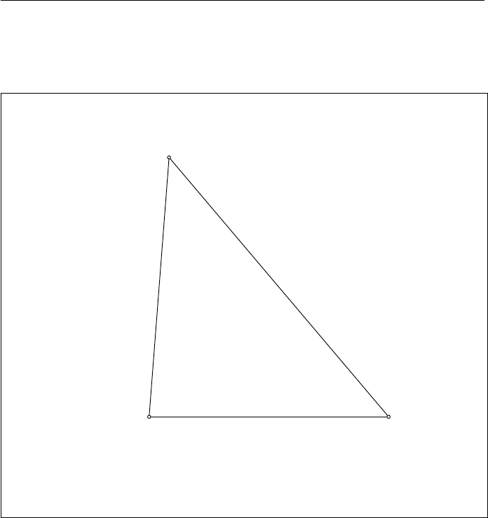
Consider the following text:
point A 40 85
point B 35 20
point C 95 20
cmark_lt A
cmark_lb B
cmark_rb C
drawsegment A B
drawsegment B C
drawsegment C A
It describes a triangle ABC via gcl commands. The command point A 40 85
introduces a point Awith coordinates (40,85). The command cmark_lt A de-
notes the point Aby a small circle and prints its name in left-top direction.
The command drawsegment A B draws the segment AB. More details on gcl
commands can be found in Chapter 3
If you are using the command-line version of GCLC, type the above text
(gcl code) in any text editor and save it under the name, say, quick.gcl. The
figure in L
A
T
E
X format can be generated using the following command:
> gclc quick.gcl quick.pic
where quick.pic is the name of a resulting file.
Within the GUI version, you can type the above code directly to the built-
in editor, save the file under the name, say, quick.gcl, and press the button
Build in the toolbar (or choose the option Picture/Build from the menu). Then,
you can export the picture to L
A
T
E
X format by selecting the option File/Export
to.../LaTeX (and choosing the name, say, quick.pic).1More details about the
GUI version can be found in Chapter 4.
The picture (contained in quick.pic) can be included in your L
A
T
E
X docu-
ment using the command:
\input{quick.pic}
in an appropriate position in your L
A
T
E
X document. In addition, you have to
include (by the L
A
T
E
X command \usepackage{gclc}) the package gclc (pro-
vided within the gclc distribution) in the preamble of your document,2and
1Within this chapter, we comment only on the simple L
A
T
E
X format, supported by
gclc.sty. However, GCLC can export to other L
A
T
E
X formats, see Chapter 5.
2You also have to put the file gclc.sty (providing the gclc package) in the current folder
(where your L
A
T
E
X document is) or in the folder with other L
A
T
E
X packages.
2.3 Basic Syntax Rules 11
then you can process your L
A
T
E
X document as usual. If everything is ok, within
your L
A
T
E
X document you will get the illustration as shown in Figure 2.1. More
details about export to L
A
T
E
X can be found in Chapter 5.
A
B C
Figure 2.1: Illustration generated from the given GCLC code
2.3 Basic Syntax Rules
The syntax of the gcl language is very simple. Commands, identifiers, constants
etc. must be separated by at least one tab or space symbol or a new line.
Usually, each new command (with its argument) is in separate line and empty
lines separate different parts of the construction.
2.4 Basic Objects
There are five types of objects in the gcl language: number,point,line,
circle and conic. They are represented in the following manner:
number n(n)
point (x, y) (x, y)
line ax +by +c= 0 (a, b, c)
circle (x−x0)(x−x0)+(y−y0)(y−y0) = r2(x0, y0, r)
conic ax2+ 2bxy +cy2+ 2dx + 2ey +f= 0 (a, b, c, d, e, f)

12 2 Quick Start
While processing an input file, GCLC generates the transcript file gclc.log
(in the current directory) with the list of all warnings and the list of all defined
objects (with their names and parameters). Instead of writing to the log file,
the GUI version shows this list in its output window.
2.5 Geometrical Constructions
Geometrical constructions are the main area of GCLC. A geometrical con-
struction is a sequence of specific, primitive construction steps. These primitive
construction steps are also called elementary constructions and they are:
•construction (by ruler) of a line such that two given points belong to it;
•construction of a point such that it is the intersection of two lines (if such
a point exist);
•construction (by compass) of a circle such that its center is one given point
and such that the second given point belongs to it;
•construction of intersections between a given line and a given circle (if
such points exist).
By using the set of primitive constructions, one can define more involved,
compound constructions (e.g., construction of right angle, construction of the
segment midpoint, construction of the segment bisector etc.). In describing
geometrical constructions, it is usual to use higher level constructions as well as
the primitive ones.
GCLC follows the idea of formal constructions. It provides easy-to-use sup-
port for all primitive constructions, but also for a range of higher-level construc-
tions. (Although motivated by the formal geometrical constructions, GCLC
provides a support for some non-constructible objects too — for instance, in
GCLC it is possible to determine/use a point obtained by rotation for 1◦,
although it is not possible to construct that point by ruler and compass).
2.6 Basic Ideas
There is a need of distinguishing abstract (i.e., formal, axiomatic) nature of
geometrical objects and their usual models. A geometrical construction is a mere
procedure of abstract steps and not a picture. However, for each (Euclidean)
construction, there is its counterpart in the standard Cartesian model. While a
construction is an abstract procedure, in order to make its usual representation
in Cartesian model of Euclidean plane, we still have to make some link between
these two. For instance, given three vertices of a triangle we can construct a
center of its inscribed circle (by using primitive constructions), but in order to
represent this construction in Cartesian plane, we have to take three particular
Cartesian points as vertices of the triangle. A figure description in GCLC is
usually made by a list of definitions of several fixed points (defined in terms
of Cartesian plane, i.e., by pairs of coordinates) and then a list of construction
steps based on these points. Normally, there should be very few such fixed points
and all other points should depend on them. Afterwards, if one wants to vary a

2.6 Basic Ideas 13
figure, he/she would usually change only coordinates of fixed points and all other
objects will be recalculated automatically. For instance, if points Aand Bare
given by their coordinates, never introduce their midpoint Malso by coordinates,
but always via the command midpoint M A B. This would give your GCLC
descriptions flexibility and would better reflect the mathematical/geometrical
meaning of the figure.

14 2 Quick Start
Chapter 3
GCLC Language
In the gc language, there are several entities: commands (source code state-
ments), objects (scalar, point, line, conic), and constants. A source code line
will generally have a command and identifiers (as handles for an object or vari-
able) and possibly constants (including constant text enclosed by brackets). The
syntax requires that entities be separated by at least one tab or space symbol.
Commands should be separated by at least one tab or space symbol, or, for
better readability, by new line.
The commands fall into ten categories, and the identifiers will be one of five
types of objects in GCLC:number,point,line,circle, and conic. The
types are not attached to variables explicitly, but implicitly (with respect to the
given context).
Notation conventions. This document uses the following notation to clarify
that an identifier is of a particular type. When writing the source code, always
leave out the <and >marks.
•<n_id> a constant (a decimal number) or a simple numerical variable (of
type number);
•<p_id> an identifier associated with a point;
•<l_id> an identifier associated with a line;
•<circle_id> an identifier associated with a circle;
•<conic_id> an identifier associated with a conic;
•<text> Constant text string beginning with the symbol {and ending with
the symbol }.
•<exp> denotes an arbitrary expression.
Identifiers can be one to 99 characters. Underscores, single-quotes or braces
are permissible, but not white spaces. Identifiers are case-sensitive. Names like
A_1 or Q_{a}’ (in usual T
E
X form) can be used.

16 3 GCLC Language
3.1 Basic Definition Commands
The first parameter for each of these commands is the identifier, the rest are
constants or variables. The identifier <id> can have a previous definition which
is ignored, it just gets a new type and new value.
•number <n_id0> <n_id1>: Definition of a number. The object <n_id0>
is defined or re-defined as type number, and can be used in commands as a
segment length, measure of an angle (in degrees) or as a command specific
parameter (but cannot be used where a point,line,circle or conic
is expected). The variable’s value can be changed by another number
command, or by expression command. <n_id1> can be a constant or
another number identifier. Example: number left_bottom_x 80.
•point <p_id> <n_id1> <n_id2>: Definition of a point. <p_id> is defined
or re-defined as type point, where its x-coordinate value becomes <n_id1>
and its y-coordinate value becomes <n_id2>.<n_id1> and <n_id2> can
be constants or number variables.
•point <p_id> <n_id1> <n_id2> <n_id3> <n_id4>: Extended definition
of a point within support of animations (relevant only for GUI version,
see 3.11), where (<n_id1>,<n_id2>) is the starting location for the point,
and (<n_id3>,<n_id4>) is the final location. <n_id1>,<n_id2>,<n_id3>,
<n_id4> can be constants or number variables.
•line <l_id> <p_id1> <p_id2>: Definition of a line. Identifier <l_id>
gets type line, determined by (already defined) points <p_id1> and <p_id2>.
•circle <c_id> <p_id1> <p_id2>: Definition of a circle. Identifier <c_id>
gets type circle, and represents a circle determined by two points: the
first point (<p_id1>) is the center and the second (<p_id2>) is anywhere
on the circle.
•set_equal <id1> <id2>: The object <id1> gets the type and the value
of the object <id2>.
3.2 Basic Constructions Commands
•intersec <p_id> <l_id1> <l_id2> The object with the specified iden-
tifier <p_id> becomes point and gets coordinates of the intersection of
two given lines.
This command can also be used in this form:
intersec <p_id> <p_id1> <p_id2> <p_id3> <p_id4>
The object with the specified identifier <p_id> becomes point and gets co-
ordinates of the intersection of two given lines given by <p_id1> <p_id2>
and by <p_id3> <p_id4>.
The full name, intersection, can also be used for this command.
•intersec2 <p_id1> <p_id2> <id1> <id2> The objects with the speci-
fied identifiers <p_id1> and <p_id2> become points and get coordinates

3.2 Basic Constructions Commands 17
of the intersection of two given circles, of a given circle and a line, or of a
given line and a circle.
The full name, intersection2, can also be used for this command.
•midpoint <p_id> <p_id1> <p_id2> The object with the specified iden-
tifier <p_id> becomes point and gets coordinates of the midpoint of the
segment determined by two given points.
•med <l_id> <p_id1> <p_id2> The object with the specified identifier
<l_id> becomes line and gets the parameters of the line that bisects (and
is perpendicular to) the segment determined by the two given points.
The full name, mediatrice, can also be used for this command.
•bis <l_id> <p_id1> <p_id2> <p_id3> The object with the specified
identifier <l_id> becomes line and gets the parameters of the line that
bisects the angle determined by three given points. Example:
bissABC
makes object sto become line with parameters of the bisector of the
angle 6ABC.
The full name, bisector, can also be used for this command.
•perp <l_id> <p_id1> <l_id1> The object with the specified identifier
<l_id> becomes line and gets the parameters of the line that is perpen-
dicular to the given line and contains the given point.
The full name, perpendicular, can also be used for this command.
•foot <p_id> <p_id1> <l_id1> The object with the specified identifier
<p_id> becomes point and gets the parameters of the foot of the perpen-
dicular from the point <p_id1> to the line <l_id1>.
•parallel <l_id> <p_id1> <l_id1> The object with the specified iden-
tifier <l_id> becomes line and gets the parameters of the line that is
parallel to the given line and contains the given point.
•getcenter <p_id> <c_id> The object with the specified identifier <p_id>
becomes point and gets the parameters of the center of the given circle.
•onsegment <p_id> <p_id1> <p_id2> The object with the specified iden-
tifier <p_id> becomes point, placed randomly on the line segment deter-
mined by the two given points.
•online <p_id> <p_id1> <p_id2> The object with the specified identifier
<p_id> becomes point, placed randomly on the line determined by the
two given points (more precisely, a random point is chosen between points
Xand Ysuch that Xis symmetrical to <p_id1> with respect to <p_id2>
and Yis symmetrical to <p_id2> with respect to <p_id1>). (This com-
mand is suitable for describing constructions with properties to be proved
by the theorem provers.)

18 3 GCLC Language
•oncircle <p_id> <p_id1> <p_id2> The object with the specified iden-
tifier <p_id> becomes point, placed randomly on the circle with cen-
ter <p_id1> and with the point <p_id2>. (This command is suitable
for describing constructions with properties to be proved by the theorem
provers.)
3.3 Transformation Commands
•translate <p_id> <p_id1> <p_id2> <p_id3> The object with the spec-
ified identifier <p_id> becomes point and gets the parameters of the point
that is an image of the third point (<p_id3>) in a translation for the vector
determined by the first and the second given point. Example:
translate A2 X Y A1
makes object A2 to become point such that T(A1)=A2, where Tis trans-
lation for the vector XY.
•rotate <p_id> <p_id1> <n> <p_id2> The object with the specified iden-
tifier <p_id> becomes point and gets the parameters of the point that
is an image of the second given point in a rotation around the first given
point and for the given (positive or negative) angle (determined by the
given constant or number). Example:
rotate A2 O 90 A1
makes object A2 to become point such that R(A1)=A2, where Ris rota-
tion around the point Ofor the angle of 90◦.
•rotateonellipse <p_id> <p_id1> <p_id2> <p_id3> <n> <p_id4> The
object with the specified identifier <p_id> becomes point and gets the
parameters of the point Ysuch that the angle X <p_id1> Y is equal to
n, where Xis the intersection of the half-line <p_id1> <p_id4> and the
ellipse determined by <p_id1> <p_id2> <p_id3>.
•sim <p_id> <id1> <p_id> The object with the specified identifier <p_id>
becomes point and gets the parameters of the point that is an image of
the given point in a half-turn, line-reflection or inversion (depending of
the type (point,line, or circle) of the second argument). Example:
If lis line,
sim A2 l A1
makes object A2 to become point such that S(A1)=A2 where Sis line
reflection determined by the line l.
The full name, symmetrical, can also be used for this command.
•turtle <p_id> <p_id1> <p_id2> <n1> <n2> The object with the spec-
ified identifier <p_id> becomes point. Its segment length from <p_id2>
will be <n2>. The segment determined by <p_id> and <p_id2> will make
an angle <n1> (in degrees) with the segment from <p_id1> to <p_id2>.
Example:
turtle A X Y 90 10.00
makes object Ato become point such that YA=10.00 and 6XYA=90◦.

3.4 Calculations, Expressions, Arrays, and Control Structures 19
•towards <p_id> <p_id1> <p_id2> <n1> The object with the specified
identifier <p_id> becomes point, placed on the line determined by the
two given points. The distance from <p_id1> to the new point <p_id>
is a fraction <n1> of the distance from <p_id1> to <p_id2>. Thus, if
0<<n1> <1, then the point <p_id> will be between points <p_id1>
and <p_id1>; if <n1> >1, the point <p_id2> will be between points
<p_id1> and <p_id>; if <n1> <0, the point <p_id1> will be between
points <p_id2> and <p_id>. Example:
towards O A B 0.9
makes object Oto become point such that AO=0.9 ·AB and Ois between
Aand B.
3.4 Calculations, Expressions, Arrays, and Con-
trol Structures
•getx <n_id> <p_id>: The object with the specified identifier <n_id> be-
comes number and gets the value of the x-coordinate of the given point
<p_id>.
•gety <n_id> <p_id> The object with the specified identifier <n_id> be-
comes number and gets the value of the y-coordinate of the given point
<p_id>.
•distance <n_id> <p_id1> <p_id2>: The object with the specified iden-
tifier <n_id> becomes number and gets the value of the distance between
two given points.
•angle <n_id> <p_id1> <p_id2> <p_id3>: The object with the specified
identifier <n_id> becomes number and gets the measure of the angle
determined by three given points. Example:
angle alpha A B C
makes object alpha to get type number and its value will be the measure
of the (oriented) angle 6ABC (in degrees).
•angle_o <n_id> <p_id1> <p_id2> <p_id3>: The same as the command
angle, but takes orientation into account, so the angle can have positive
and negative values. Therefore, this version is compatible with the com-
mand rotate.
•random <n_id> The object with the specified identifier <n_id> gets type
number and gets a (pseudo)random value between 0 and 1.
•expression <n_id> {exp}: The object with the specified identifier <n_id>
gets type number and gets the value of the expression exp. Example:
expression e {sin(3)*(5+2)}
After the above command, ewill have the value 0.366352.
Defined variables of the type number can be used in expressions. No
other variables can be used in expressions. For instance,

20 3 GCLC Language
expression e {n+5}
makes object eto become number equal to n+5, if nis of the type num-
ber.
The following standard functions, operators and relations are supported in
expressions: +(addition), -(subtraction), *(multiplication), /(division),
== (equality), != (inequality), <,<=,>,>=,&& (and), || (or), abs,ceil
(rounding up), floor (rounding down), sin,cos,tan (with arguments
expressed in radians), sinh,cosh,tanh,asin,acos,atan,sqrt,exp,pow
(exponentiation), log,log10,min (two arguments), max (two arguments).
For example,
expression m { pow(n+1,2)}
makes object mequal (n+1)2(note that the operator ^is not used for
exponentiation).
The ite operator (from if-then-else) is also supported. For example,
expression E {ite(n>0,1,2)}
makes object Eto become number equal to 1 if nis greater than zero,
and 2 otherwise.
Blank spaces in expressions are allowed and ignored.
•array <c_id> { <n_id0> <n_id1> ... <n_idk> }: Definition of an (mul-
tidimensional) array. The values <n_id0> <n_id1> ... <n_idk> are di-
mensions of the array. There can be up to 10 dimensions. All elements of
the array initially have type number and value 0. Indexing is 1-based, i.e.,
the first element of the array has all indices equal 1. Indices are written
in separate angle brackets.
Examples:
array A { 4 3 }
defines 4 ×3 = 12 elements of the array A—A[1][1], A[1][2], . . .,A[4][3].
All these elements initially have the type number and value 0, but both
of these can be changed, as for any other variable. So, different elements
of the same array can have different types.
Indices of an array element can be arbitrary expressions, that can also in-
volve other array elements (of type number). For instance, if all elements
of an (one-dimensional) array Aare numbers, one can use the following
construction: A[5 + A[5]] (in any position that requires a number).
An array with the same name can be defined more than once. If the num-
bers of dimensions are same, and if all dimensions are same, then all old
elements are reset to have type number and value 0. If some dimensions
are different, new elements may be added (if some new dimensions are
greater then the old ones), but old elements (those not covered by the
new definition) are never destroyed (even if some new dimensions are less
then the old ones). If the numbers of dimensions (in two definitions) are
different, then these two arrays are considered different and there are no
resetting of the old elements.

3.4 Calculations, Expressions, Arrays, and Control Structures 21
•while {<exp>} { <while-block> }:<while-block> is a sequence of
commands. This sequence will be repeatedly executed as long as <exp>
condition is true (nonzero). Example:
point A 0 0
number n 0
while { n<30 }
{
point B n 30
drawsegment A B
expression n { n+1 }
}
Both syntax and run-time errors encountered within a while-block are
reported only as Invalid while block error and no other (more detailed)
information on the error is provided. Also, all warnings encountered within
a while-block are suppressed and are not written to the log.
The sequence of commands in the while-block behaves as any GCLC
sequence. It shares the defined variables and the environment (defined
by commands ang_picture and ang_origin etc) with the outer GCLC
context.
If the <exp> condition is never fulfilled, this leads to non-termination (i.e.,
infinite loop). In order to prevent this, the system enables only a limited
number (10000) of executions of blocks within while-loops. If this number
is exceeded, then the error Too many while-block executions (more
than 10000). Possible infinite loop is reported and the processing
is stopped.
Procedures cannot be defined within while-blocks.
•if_then_else {<exp>} { <then-block> } { <else-block> }:
<then-block> is a sequence of commands. This sequence will be executed
if <exp> condition is true (nonzero). <else-block> is a sequence of com-
mands. This sequence will be executed if <exp> condition is false (zero).
Example:
distance d1 C A
distance d2 C B
if_then_else { d1<d2 }
{
drawsegment A C
}
{
drawsegment B C
}

22 3 GCLC Language
Both syntax and run-time errors encountered within <then-block> and
<else-block> are reported only as Invalid if-then-else block error
and no other (more detailed) information on the error is provided. Also,
all warnings encountered within a if-then-else-block are suppressed and
are not written to the log.
The sequence of commands in the blocks behaves as any GCLC sequence.
It shares the defined variables and the environment (defined by commands
ang_picture and ang_origin etc) with the outer GCLC context.
Procedures cannot be defined within if-then-else-blocks.
•procedure <name> { <arguments> } { <block of commands> }:
<name> is the name of the procedure. <arguments> is a list of the proce-
dure’s arguments. Arguments are separated by blank spaces. In GCLC,
arguments are passed by their names, which means that they may be
changed by the procedure. <block of commands> is a sequence of com-
mands. It inherits the environment form the outer context, but not the
variables from the outer context. Within a block, only arguments and
variables defined within it can be used. The definition of a procedure
must precede calling it. Procedures cannot be defined within while-blocks
or within definitions of other procedures.
Example:
procedure drawtriangle { X Y Z }
{
drawsegment X
drawsegment Y
drawsegment Z
}
•call <name> { <arguments> } <name> is the name of the procedure.
<arguments> is a list of the arguments that will be passed to the proce-
dure. Arguments are separated by blank spaces. In GCLC, variables are
passed to procedures as arguments by names and they may be changed by
a procedure. Argument of a procedure call can also be a constant (and, of
course, it is passed by value). If a variable that is argument is not defined
before (i.e., with an intention that it receives the resulting value of the
function), by default it get the type number and the value 0. If a single
variable is used for several arguments, it will get the value of the last of
such arguments (when returning from the procedure).
Procedures can be called from other procedures.
Example:
call drawtriangle { A B C }

3.5 Drawing Commands 23
•include <file_name> Reads/consults the contents of another .gcl file.
After this command, variables and procedures defined in that another file
can be used (as they were defined within the current file). Both syntax and
run-time errors encountered within the consulted file are reported only as
Invalid include file error and no other (more detailed) information on
the error is provided. Also, all warnings encountered within the consulted
file are suppressed and are not written to the log.
3.5 Drawing Commands
All drawn figures are clipped against the defined picture area. The current area
can be changed by the area command.
•drawpoint <p_id> Generates a (export–specific) command for drawing
the specified point.
•drawsegment <p_id1> <p_id2> Generates a command for drawing the
segment determined by endpoints named <p_id1> and <p_id2>.
•drawdashsegment <p_id1> <p_id2> Generates commands for drawing
the dashed segment connecting points named <p_id1> and <p_id2>. The
length of dashes can be changed by the dash command.
•drawline <l_id> Generates a command for drawing the given line.
•drawline <p_id1> <p_id2> Generates a command for drawing the line
determined by the points <p_id1> and <p_id2>.
•drawdashline <l_id> Generates a command for drawing the given line
dashed.
•drawdashline <p_id1> <p_id2> Generates a command for drawing the
dashed line determined by the points <p_id1> and <p_id2>.
•drawvector <p_id1> <p_id2> Generates a command for drawing the
vector determined by points <p_id1> and <p_id2>.
•drawarrow <p_id1> <p_id2> <n> Generates commands for drawing an
arrow on the line segment <p_id1> <p_id2> (the line segment itself is not
drawn). The ratio between the distance from <p_id1> to the end of the
arrow and the distance from <p_id1> to <p_id2> is equal to <n>. The
default shape of the arrow can be changed by the command arrowstyle.
•drawcircle <c_id> Generates commands for drawing the given circle.
In figures exported to the simple L
A
T
E
X format, GCLC draws circles and
arcs segment by segment. The number of segments can be changed by
the circleprecision command. By the default, a circle of radius 10mm
has 72 segments, while the number of segments depends (linearly) on the
circle size.

24 3 GCLC Language
•drawcircle <p_id1> <p_id2> Generates commands for drawing the cir-
cle determined by center <p_id1> and one point <p_id2>.
In figures exported the simple L
A
T
E
X format, GCLC draws circles and
arcs segment by segment. The number of segments can be changed by the
circleprecision command.
•drawdashcircle <p_id1> <p_id2> Generates commands for drawing the
circle determined by center <p_id1> and one point <p_id2>, and made
of dashes. In this mode, GCLC draws circles arc by arc and every third
arc will not be drawn, so the length of these arcs can be changed by the
circleprecision command.
•drawarc <p_id1> <p_id2> <n> Generates commands for drawing the arc
determined by center <p_id1>, one point <p_id2> and the measure of
angle equal <n> (<n> is constant or number).
•drawarc_p <p_id1> <p_id2> <n> The same as drawarc, but always draws
the arc in positive (counterclockwise) direction.
•drawdasharc <p_id1> <p_id2> <n> Generates commands for drawing
the dashed arc determined by center <p_id1>, one point <p_id2> and
the measure of angle equal <n> (<n> is constant or number). GCLC
draws arcs segment by segment and by this command every third segment
will not be drawn, so the length of dashes by command circleprecision.
•drawdasharc_p <p_id1> <p_id2> <n> The same as drawdasharc, but
always draws the arc in positive (counterclockwise) direction.
•drawellipse <p_id1> <p_id2> <p_id3> Generates commands for draw-
ing the ellipse determined by center <p_id1> and two points <p_id2> and
<p_id3>, such that a line determined by points <p_id1> and <p_id2> is
one of the ellipse’s axis. GCLC draws ellipses segment by segment. The
number of segments can be changed by the circleprecision command.
•drawdashellipse <p_id1> <p_id2> <p_id3> Generates commands for
drawing the dashed ellipse determined by center <p_id1> and two points
<p_id2> and <p_id3>, such that a line determined by points <p_id1>
and <p_id2> is one of the ellipse’s axis. Picture of ellipse is made of dash
segments. GCLC draws circles and ellipses segment by segment and for
this dash command every third segment will not be drawn, so the length
of dashes can be changed by the circleprecision command.
•drawellipsearc <p_id1> <p_id2> <p_id3> <n> Generates commands
for drawing the arc (with a starting point <p_id2>) of the ellipse deter-
mined by center <p_id1> and two points <p_id2> and <p_id3>, such that
a line determined by points <p_id1> and <p_id2> is one of the ellipse’s
axis and <n> is the measure of the angle (<n> is constant or number).
There is a similar command drawellipsearc1.
•drawdashellipsearc <p_id1> <p_id2> <p_id3> <n> Generates commands
for drawing the arc (with a starting point <p_id2>) of the ellipse deter-
mined by center <p_id1> and two points <p_id2> and <p_id3>, such that
a line determined by points <p_id1> and <p_id2> is one of the ellipse’s axis

3.5 Drawing Commands 25
and <n> is the measure of the angle (<n> is constant or number). GCLC
draws arcs segment by segment and in this arc every third segment will not
be drawn, so the length of dashes can be changed by the circleprecision
command. There is a similar command drawdashellipsearc1.
•drawellipsearc1 <p_id1> <p_id2> <p_id3> <p_id4> <n> Generates com-
mands for drawing the arc (with a starting point <p_id4>) of the ellipse
determined by center <p_id1> and two points <p_id2> and <p_id3>, such
that a line determined by points <p_id1> and <p_id2> is one of the el-
lipse’s axis and <n> is the measure of the angle (<n> is constant or con-
stant).
•drawdashellipsearc1 <p_id1> <p_id2> <p_id3> <p_id4> <n> Gener-
ates commands for drawing the arc (with a starting point <p_id4>) of
the ellipse determined by center <p_id1> and two points <p_id2> and
<p_id3>, such that a line determined by points <p_id1> and <p_id2> is
one of the ellipse’s axis and <n> is the measure of the angle (<n> is con-
stant or number). GCLC draws arcs segment by segment and in this
arc every third segment will not be drawn, so the length of dashes can be
changed by the circleprecision command.
•drawellipsearc2 <p_id1> <p_id2> <p_id3> <n1> <n2> Generates com-
mands for drawing the elliptical arc X Y, where Xand Yare points on the
ellipse determined by the points <p_id1> <p_id2> <p_id3>, the angle
<p_id2> <p_id1> X is equal to n1, and the angle Y <p_id1> X is equal
to n2.
•drawdashellipsearc2 <p_id1> <p_id2> <p_id3> <p_id4> <n> Gener-
ates commands for drawing the elliptical arc X Y, where Xand Yare
points on the ellipse determined by <p_id1> <p_id2> <p_id3>, the angle
<p_id2> <p_id1> X is equal to n1, the angle Y <p_id1> X is equal to
n2.GCLC draws arcs segment by segment and in this arc every third
segment will not be drawn, so the length of dashes can be changed by the
circleprecision command.
•drawbezier3 <p_id1> <p_id2> <p_id3> Generates commands for draw-
ing the quadratic B´ezier curve determined by points <p_id1>,<p_id2>,
<p_id3> (it goes from <p_id1> to <p_id3>, while <p_id2> is a control
point). GCLC draws B´ezier curves segment by segment. The number of
segments can be changed by the bezierprecision command.
•drawdashbezier3 <p_id1> <p_id2> <p_id3> Generates commands for
drawing the quadratic B´ezier curve determined by points <p_id1>,<p_id2>,
<p_id3> (it goes from <p_id1> to <p_id3>, while <p_id2> is a control
point). GCLC draws B´ezier curves segment by segment and in this mode
every third segment will not be drawn, so the length of dashes can be
changed by the bezierprecision command.
•drawbezier4 <p_id1> <p_id2> <p_id3> <p_id4> Generates commands
for drawing the cubic B´ezier curve determined by points <p_id1>,<p_id2>,
<p_id3>,<p_id4> (it goes from <p_id1> to <p_id4>, while <p_id2> and

26 3 GCLC Language
<p_id3> are control points). GCLC draws B´ezier curves segment by seg-
ment. The number of segments can be changed by the bezierprecision
command.
•drawdashbezier4 <p_id1> <p_id2> <p_id3> <p_id4> Generates com-
mands for drawing the cubic B´ezier curve determined by points <p_id1>,
<p_id2>,<p_id3>,<p_id4> (it goes from <p_id1> to <p_id4>, while
<p_id2> and <p_id3> are control points). GCLC draws B´ezier curves
segment by segment and in this mode every third segment will not be
drawn, so the length of dashes can be changed by the bezierprecision
command.
•drawpolygon <p_id> <p_id> <n> Generates commands for drawing the
regular polygon determined by center <p_id1>, one vertex <p_id2>, and
number of sides <n> (<n> is constant or number).
•drawtree <p_id> <n1> <n2> <n3> <n4> <tree_description> Genera-
tes commands for drawing the tree with the given point <p_id> as a root.
The numerical parameters <n1> and <n2> give the width and height of
the tree (in millimeters), <n3> determines the style for drawing tree, and
<n4> gives a rotation angle (in degrees) with the root as a center, and
a vertical, top-down direction as a reference direction (corresponding the
angle 0◦). There are four drawing styles (1,2,3and 4).
A tree description is of the form { node_name <subtree_1> ... <subtree_n>.
All node names are printed in appropriate positions. If a tree node should
not be labelled, its name should start with the symbol _. Empty subtree,
written { } is not drawn or labelled, but it takes one position of subtrees
in the same level.
All tree nodes are defined as points and get names built from the name
of the reference point and their label. In the example given below, one
can use points Proot,Pleft, etc.
Example:
drawtree P 90 70 1 10
{
root
{ left
{ }
{ left-right }
}
{ right
{ _
{a}
{b}
{c}
}
{ right-right }
}
}

3.5 Drawing Commands 27
•drawgraph_a <p_id> <n1> <n2> <list_of_nodes> <list_of_edges>
Generates commands for drawing the graph using the arc-layered method.1
The given reference point <p_id> will be the center of the graph image.
The numerical parameter <n1> gives the width of the graph image, while
<n2> gives a rotation angle (in degrees) with the point <p_id> as the
center.
The list of nodes <list_of_nodes> is of the form
{ node_name1 node_name2 ... node_name_n }. All node names in the
figure are printed in left-top positions. If a graph node should not be
labelled, its name should start with the symbol _.
The list of edges <list_of_edges> is of the form
{ node_name1_1 node_name1_2 ... node_name_n_1 node_name_n_2 },
where all node names must already appear in the list of nodes.
If the graph is not connected, then none of its nodes or edges will not be
drawn.
All graph nodes are defined as points and get names built from the name
of the reference point and their label. In the example given below, one
can use points P_a,Pb, etc.
Example:
point P 30 50
drawgraph_a P 40 0
{_abcde}
{
_a b
_a c
_a d
b d
b e
}
•drawgraph_b <id> <list_of_nodes> <list_of_edges> Generates com-
mands for drawing the graph using the barycenter method. The given
reference name <id> is used just to identify graph nodes, it does not need
to refer to any point or other object.
The list of nodes <list_of_nodes> is of the form
{ node_name1 p_id1 node_name2 p_id2 ... node_name_n p_id_n}.
The node names represent the names of the graph nodes, while the point
identifiers associate graph nodes to already defined points. If a graph
node is not initially associated to an already defined point, then the point
identifier should be _, or can begin with _. The set of used defined points
(serving as fixed nodes) must form a convex polygon.
All node names in the figure are printed in left-top positions. If a graph
node should not be labelled, its name should start with the symbol _.
1The main author of support for graph drawing is Luka Tomaˇsevi´c (University of Belgrade).

28 3 GCLC Language
The list of edges <list_of_edges> is of the form
{ node_name1_1 node_name1_2 ... node_name_n_1 node_name_n_2 },
where all node names must already appear in the list of nodes.
If the graph is not connected, then none of its nodes or edges will not be
drawn.
All graph nodes are defined as points and get names built from the name
of the reference point and their label. In the example given below, one
can use points P_a,Pb, etc.
Example:
point A 80 50
point B 100 50
point C 90 55
drawgraph_b G
{ _a A
b B
c C
d _
}
{
_a b
_a c
_a d
b d
b c
}
•filltriangle <p_id1> <p_id2> <p_id3> Fills the triangle determined
by the given points with the current color. This command is ignored when
exporting to the simple L
A
T
E
X format.
•fillrectangle <p_id1> <p_id2> Fills the rectangle determined by the
given points (<p_id1> is the left-bottom corner, p_id2 is the right-top
corner) with the current color. This command is ignored when exporting
to the simple L
A
T
E
X format.
•fillcircle <c_id> Fills the circle <c_id> with the current color. This
command is ignored when exporting to the simple L
A
T
E
X format.
•fillcircle <p_id1> <p_id2> Fills the circle determined by the given
points (<p_id1> is the center, p_id2 lies on the circle) with the current
color. This command is ignored when exporting to the simple L
A
T
E
X for-
mat.
•fillellipse <p_id1> <p_id2> <p_id3> Fills the ellipse determined by
the given points (<p_id1> is the center, <p_id1> <p_id2> is one of the
ellipse’s axis) with the current color. This command is ignored when
exporting to the simple L
A
T
E
X format.

3.6 Labelling and Printing Commands 29
•fillarc <p_id1> <p_id2> <n> Fills the circular arc determined by the
given points (<p_id1> is the center, p_id2 lies on the circle, nis the
measure of the angle) with the current color. This command is ignored
when exporting to the simple L
A
T
E
X format.
•fillarc0 <p_id1> <p_id2> <n> The same as fillarc, except that the
area determined by the circle center and the arc endpoints is not filled.
•fillellipsearc <p_id1> <n1> <n2> <n3> <n4> Fills the elliptical arc
determined by the given points (<p_id1> is the center of the ellipse with
axes parallel to coordinate axes, <n1> is the half-width, <n2> is the half-
height of the ellipse, n3 is the start central angle, and n4 is the measure
of the angle that corresponds to the arc). This command is ignored when
exporting to the simple L
A
T
E
X format.
•fillellipsearc0 <p_id1> <n1> <n2> <n3> <n4> This command has the
same effect as fillellipsearc, except that the area determined by the
ellipse center and the arc endpoints is not filled.
3.6 Labelling and Printing Commands
•cmark <p_id> Denotes the given point by a small empty circle (with ra-
dius 0.4mm) at its coordinates.
•cmark_lt <p_id>
cmark_l <p_id>
cmark_lb <p_id>
cmark_t <p_id>
cmark_b <p_id>
cmark_rt <p_id>
cmark_r <p_id>
cmark_rb <p_id>
Generates commands for denoting the given point by its name and by
small empty circle (with radius 0.4mm) at its coordinates. The name of
the point is written (in L
A
T
E
X mode — in size \footnotesize) in one of
eight directions (left-top, left, left-bottom, top, bottom, right-top, right,
right-bottom).
•mark <p_id> Generates commands for printing the name of the given
point at its coordinates (without denoting it by a circle).
•mark_lt <p_id>
mark_l <p_id>
mark_lb <p_id>
mark_t <p_id>
mark_b <p_id>
mark_rt <p_id>

30 3 GCLC Language
mark_r <p_id>
mark_rb <p_id>
Generates commands for printing the name of the given point at its coor-
dinates (without denoting it by a circle) in one of eight directions. These
commands could be used for denoting lines and circles, too (of course,
first, some point with a line or circle name has to be defined).
•printat <p_id> <text> Generates commands for printing given text
at coordinates of the given point. Text must begin with symbol {and
end with symbol }. These two symbols are not part of the text and will
not be printed. Text can have at most 100 characters. Text can include
all characters including {,}and blank space. In L
A
T
E
X mode, the text is
printed in math mode, so for ordinary text, L
A
T
E
X command \mbox{...}
should be used.
printat_lt <p_id> <text>
printat_l <p_id> <text>
printat_lb <p_id> <text>
printat_t <p_id> <text>
printat_b <p_id> <text>
printat_rt <p_id> <text>
printat_r <p_id> <text>
printat_rb <p_id> <text>
Generates commands for printing given text in one of eight directions with
respect to the given point. Example:
printat_l A {A=S_a(B) \mbox{($a$ is the bisector of $AB$)}}
will generate a command for printing the given text left from the point A.
•printvalueat <p_id> <id> Generates commands for printing value of a
given object <id> at coordinates of the given point <p_id>. The object
<id> can be of any type. The value is printed in the format given in
Section 2.4. In L
A
T
E
X mode, the text is printed in math mode, so for
ordinary text, L
A
T
E
X command \mbox{...} should be used.
printvalueat_lt <p_id> <id>
printvalueat_l <p_id> <id>
printvalueat_lb <p_id> <id>
printvalueat_t <p_id> <id>
printvalueat_b <p_id> <id>
printvalueat_rt <p_id> <id>
printvalueat_r <p_id> <id>
printvalueat_rb <p_id> <id>
Generates commands for printing value of a given object <id> in one of
eight directions with respect to the given point <p_id>. Example:
printvalueat_b A A

3.7 Low Level Commands 31
will generate a command for printing the coordinates of the point Aon
bottom from the point A.
3.7 Low Level Commands
•%A comment is marked by the symbol %(like in T
E
X). Characters in the
line after the symbol %will not be read.
•dim <n1> <n2> Defines dimensions of the picture. This command can
be at any position in the figure description file. If there is more than
one occurrence of this command, only the first one is used. The default
dimensions of a picture are 140mm×100mm. The rectangle defined by
this command also defines the visible area.
•area <n1> <n2> <n3> <n4> Defines the visible area of the picture. The
area is defined by the lower-left corner (the first two numbers) and its
upper-right corner (the second pair of numbers). There is always at most
one active area. All objects are clipped with respect to the active, current
area. If there is no defined area, the default area is the whole of the
picture.
•color <n1> <n2> <n3> Changes the current color. The parameters are
rgb (red/green/blue) components of the color. Each of them should
range between 0 and 255. For instance, 255 0 0 defines (pure) red color,
0 255 0 defines (pure) green color, 0 0 255 defines (pure) blue color,
255 255 0 defines yellow, 255 0 255 defines magenta, 0 255 255 defines
cyan, 127 127 127 defines grey color, 000defines black and 255 255 255
white color.
Figures using this command exported to L
A
T
E
X require using the package
color in your L
A
T
E
X document. Note that this support for colors might
not work properly in conjunctions with some L
A
T
E
X distributions (i.e.,
with some dvi drivers).
•background <n1> <n2> <n3> Sets the background color. The parameters
are rgb (red/green/blue) components of the color. This command is
ignored when exporting to the simple L
A
T
E
X format.
•fontsize <n> Changes the current font size. Font size is given in pts.
The default value is 8. In export to L
A
T
E
X, this command can change the
current fontsize to one of the values: \tiny (1pt-5pt), \scriptsize (6pt-
7pt), \footnotesize (8pt), \small (9pt), \normalsize (10pt), \large
(11pt-12pt), \Large (13pt-14pt), \LARGE (15pt-17pt), \huge (18pt-20pt),
\Huge (over 21pt).
•arrowstyle <n1> <n2> <n3> Defines a shape of arrows drawn by the
command drawarrow. The angle between outer line segments in arrows
is given, in degrees, by <n1> (the default value is 15◦, maximal value is
180◦). The length of outer line segments is given, in millimeters, by <n2>
(the default value is 3). Inner line segments meet the central line at the
point that is determined by <n3> — if Xis the intersection of the central
line with the line determined by the endpoints of the outer line segments,

32 3 GCLC Language
if Ythe point where the inner line segments meet the central line, and if
Zis the endpoint of the arrow, then XY/XZ =<n3> (the default value
is 0.667).
•circleprecision <n> When exporting to L
A
T
E
X, GCLC draws circles
and ellipses segment by segment. The default value is 72 segments for
a circle of a radius 10mm, more for larger circles (while there is linear
dependency). The number of segments can be changed by this command.
It will linearly depend on the circle radius, but it will be no less than the
given value <n>. This command is irrelevant for export into formats other
than L
A
T
E
X.
•bezierprecision <n> GCLC draws B´ezier curves segment by segment.
The default value is 36 segments for a curve. The number of segments can
be changed by this command.
•linethickness <n> The line thickness can be changed by this command.
Thickness is expressed in millimeters. The default value is 0.16mm. If the
given value is negative, then the line thickness is product of the absolute
value of the argument and the default value.
•double This command makes all subsequent lines to be drawn with double
thickness.
•normal This command makes all subsequent lines to be drawn with normal
thickness.
•dash <n> The length of dash lines (in dash drawn lines and line segments)
can be changed by this command. Length is expressed in millimeters.
The default value is 1.5mm. The length of space between dash lines is
<n>/2. This command cancels the effect of previous dash and dashstyle
commands.
•dashstyle <n1> <n2> <n3> <n4> This command provides more expres-
sive way of describing dashed lines and segments layout than given by the
command dash. The pattern defined by this command is as follows: <n1>
dash line — <n2> empty space — <n3> dash line — <n4> empty space. All
lengths are expressed in millimeters. The default values are: 1.5 0.75 1.5
0.75. This command cancels the effect of previous dash and dashstyle
commands.
•dmc <n> The distance between point and its name or associated text can
be changed by this command. The default value is 1mm.
•mcr <n> The radius of circle marking point can be changed by this com-
mand. The default value is 0.4mm.
•mcp <n> When exporting to the simple L
A
T
E
X format, draws circles mark-
ing points segment by segment. The default value is 9 segments for a
circle. The number of segments can be changed by this command. This
command is irrelevant for export into formats other than L
A
T
E
X.

3.8 Cartesian Commands 33
•mcp <n> When exporting to the simple L
A
T
E
X format, draws circles mark-
ing points segment by segment. The default value is 9 segments for a
circle. The number of segments can be changed by this command. This
command is irrelevant for export into formats other than L
A
T
E
X.
•export_to_latex {<text>} When exporting to the simple L
A
T
E
X format,
PSTricks L
A
T
E
X format, or TikZ L
A
T
E
X format, the given text is directly
exported to the output file (normally this should be a sequence of L
A
T
E
X
commands).
•export_to_latex {<text>} When exporting to the simple L
A
T
E
X format,
PSTricks L
A
T
E
X format, or TikZ L
A
T
E
X format, the given text is directly
exported to the output file (normally this should be a sequence of L
A
T
E
X
commands).
•export_to_simple\_latex {<text>} When exporting to the simple L
A
T
E
X
format, the given text is directly exported to the output file.
•export_to_pstricks {<text>} When exporting to PSTricks L
A
T
E
X for-
mat, the given text is directly exported to the output file.
•export_to_tikz {<text>} When exporting to TikZ L
A
T
E
X format, the
given text is directly exported to the output file.
•export_to_eps {<text>} When exporting to eps format, the given text
is directly exported to the output file.
•export_to_svg {<text>} When exporting to svg format, the given text
is directly exported to the output file.
3.8 Cartesian Commands
•ang_picture <n1> <n2> <n3> <n4> Defines a rectangular area for Carte-
sian picture (ang is from “ANalytical Geometry”). The first two parame-
ters determine its lower left corner, and last two parameters determine its
upper right corner. If there is no defined area, the default area is empty
(i.e., it is defined by lower left and upper right corner equal to (0,0)). This
area is relevant only for Cartesian commands (ang_...).
•ang_origin <n1> <n2> Defines an origin of the coordinate system. The
default value is (0,0).
•ang_unit <n> Defines the unit of the coordinate system in millimeters.
The default value is 10mm.
•ang_scale <n1> <n2> Defines the scale between yand xcoordinates.
The parameter <n1> determines if the coordinate system is regular (value
1) or logarithmic (value 2). In logarithmic system, xaxis is set on y= 1.
The parameter <n2> determines the multiplication factor for ycoordinates.
It must be positive. If a negative value or zero is given, the value 1 is
assumed.

34 3 GCLC Language
These values determines the coordinate system and all consequent draw-
ings. The default values are 1 and 1.
Note that, if logarithmic system is used, the commands doing with lines
(ang_tangent,ang_drawline,ang_drawline_p) will not work properly.
Other commands (including, for instance, commands ang_drawdashconic
and ang_draw_parametric_curve) can be used.
•ang_drawsystem_p <n1> <n2> <n3> <n4> <n5> Generates commands
for drawing coordinate axes.
The parameter <n1> controls denoting the integer points on the axes: with
parameter value 1, integer points are denoted by small circles, with value
2 by small dashes, and with value 3 they are not denoted at all.
The parameter <n2> controls the step for denoting integer points on x
axis. For instance, if <n2> is equal to 1, then each integer point on xaxis
is denoted (in a way defined by the parameter <n1>); if <n2> is equal to
2, then every second integer point is denoted.
The parameter <n3> controls the step for denoting integer points on y
axis.
The parameter <n4> controls denoting the axes: with parameter value
1, the axes are denoted by xand y, and with value 2 the axes are not
denoted.
The parameter <n5> controls drawing arrows at the endpoints of the sys-
tem: with parameter value 1, there are arrows at both positive and nega-
tive endpoints, with parameter value 2, there are arrows only at positive,
and with parameter value 3, there are no arrows at all.
This command can replace all other variants of ang_drawsystem... com-
mands (however, they are kept for simplicity and for the reasons of vertical
compatibility).
•ang_drawsystem Generates commands for drawing the axes and denotes
(by small circles) integer points on them.
•ang_drawsystem0 Generates commands for drawing the axes and doesn’t
denote integer points on them.
•ang_drawsystem1 Generates commands for drawing the axes and denotes
by small dashes integer points on them.
•ang_drawsystem_a Same as ang_drawsystem, but denotes the axes by x
and y.
•ang_drawsystem0_a Same as ang_drawsystem0, but denotes the axes by
xand y.
•ang_drawsystem1_a Same as ang_drawsystem1, but denotes the axes by
xand y.
•ang_point <p_id> <n1> <n2> Definition of an ang point. A difference
from the standard command point is that the ang_point command in-
troduces point by coordinates given with respect to a defined origin and
unit of Cartesian system.

3.8 Cartesian Commands 35
•ang_getx <n_id> <p_id> The object with the specified identifier <n_id>
becomes number and gets the value of the x-coordinate of the given point
<p_id> in the active Cartesian system (<p_id> was not necessarily defined
by the command ang_point).
•ang_gety <n_id> <p_id> The object with the specified identifier <n_id>
becomes number and gets the value of the y-coordinate of the given point
<p_id> in the active Cartesian system (<p_id> was not necessarily defined
by the command ang_point).
•ang_line <l_id> <n1> <n2> <n3> Introduces a line <l_id> by given pa-
rameters in the form ax +by +c= 0, with respect to a defined origin and
unit.
•ang_conic <conic_id> <n1> <n2> <n3> <n4> <n5> <n6> Definition of
a conic. A conic <conic_id> is determined by the given parameters a,b,
c,d,eand fin the following form: ax2+ 2bxy +cy2+ 2dx + 2ey +f= 0,
with respect to a defined origin and unit. An object defined in such a
manner gets type conic, and can not be used as number,point,line
or circle (unless its type is changed by another definition).
•ang_intersec2 <p_id1> <p_id2> <l_id> <conic_id>
ang_intersec2 <p_id1> <p_id2> <conic_id> <l_id>
Objects with specified identifiers <id1> and <id2> become points and
get coordinates of the intersection of a given line and a conic, or of a given
conic and line. If there is just one intersection point, then both <id1> and
<id2> have the same value. If there are no intersection points, then the
program reports a run-time error.
The full name, ang_intersec2, can also be used for this command.
•ang_tangent <l_id> <p_id> <conic_id> Introduces a line <l_id> which
is tangent to a conic <conic_id> at a point <p_id>.
•ang_drawline <l_id> Generates commands for drawing a line <l_id>
within the defined area.
•ang_drawline_p <p_id1> <p_id2> Generates commands for drawing the
line determined by points <p_id1> and <p_id2>, within the defined area.
•ang_drawconic <conic_id>
Generates commands for drawing the conic <conic_id>.
•ang_drawdashconic <conic_id>
Generates commands for drawing the conic <conic_id> and made of dash
segments. GCLC draws conics segment by segment and by this command
every third segment will not be drawn, and you can change length of dash
segments by the command ’conicprecision’. The default number of
segments is 144 on x-axis.
•ang_draw_parametric_curve <id>
{<exp1>;<exp2>;<exp3>}{<exp4>;<exp5>}

36 3 GCLC Language
The object with the specified identifier <id> becomes number and serves
as a (iterating) curve parameter. A curve is being drawn in iterations.
<exp1> is the initial value for the parameter, <exp2> is the (while) condi-
tion that the (changing) parameter has to meet, and <exp2> is the expres-
sion for recalculating the parameter in each iteration. The pair <exp4>,
<exp5> determines the pair (x, y) of coordinates of a point on the curve.
In building expressions, one can use the same functions, operators and
relations as in command expression, described in §3.4.
Examples:
ang_draw_parametric_curve x {-5;x<10;x+0.1}{x;x*sin(x)}
ang_draw_parametric_curve t {0;t<30;t+0.3}{sin(t)*t;-cos(t)*t}
The curve drawing is reset if in some iteration an undefined expression is
encountered. For instance,
ang_draw_parametric_curve x {-5;x<10;x+0.1}{x;d/x}
will produce two pieces of a line with the discontinuity point at (0,0).
However,
ang_draw_parametric_curve x {-5;x<10;x+0.3}{x;d/x}
will produce a single line since the discontinuity point (0,0) is missed. The
system does not determine parameter values for which a resulting point
is undefined, but can only detect such situation if encountered in some
iteration. However, in order to provide expected output, the system does
not draw segment between subsequent point on the line if both of them
are out of the picture area.
As explained above, the system skips points in which expressions giving
(x, y) is not defined. So, it is not reported if one of these expressions is not
defined in some iterations. Moreover, it is also not reported if expressions
involve undefined functions or are ill-formed. Because of that, in case of
a problem, it is a good practice to check the expressions separately, as
arguments to the expression command.
•ang_conicprecision GCLC draws conics segment by segment. The de-
fault value is 144 segments on x-axis. This number can be changed by
this command.
•ang_plot_data <n> { <sequence of coordinates> } Draws the graph
of the function given by its points. The number <n> is equal to 0 if the
points are not to be denoted, and is equal to 1 if the points are to be
denoted by small circles. The points are given as a sequence of their
coordinates.
Example:
ang_plot_data 1
{
1.0 1.0
2.0 1.0
3.0 2.0
}

3.9 3D Cartesian Commands 37
3.9 3D Cartesian Commands
•ang3d_picture <n1> <n2> <n3> <n4> Defines a rectangular area for 3D
Cartesian picture. The first two parameters determine its lower left corner,
and last two parameters determine its upper right corner. If there is no
defined area, the default area is empty (i.e., it is defined by lower left and
upper right corner equal to (0,0)).
•ang3d_origin <n1> <n2> <n3> <n4> Defines a 3D Cartesian coordinate
system, shown using normal projection. <n1> and <n2> give a position of
the origin of the system. The default value is (0,0). <n3> and <n4> give
the angles (in radians) that determine the viewing angle to the coordinate
system. In the default position of the system, xaxis is screen-horizontal
with respect to the screen, yaxis is perpendicular to the screen, zaxis is
screen-vertical. This default position corresponds to the values 0 and 0
of <n3> and <n4>. For other values, the rotation around the zaxis, for
<n3> radians, is first applied (the new and the old xaxes build the angle
<n3>). After that, the rotation around the default xaxis, for <n4> radians
is applied (the new and the old zaxes build the angle <n4>).
•ang3d_unit <n> Defines the unit of the coordinate system in millimeters.
The default value is 10mm.
•ang3d_scale <n1> <n2> <n3> Defines the scale between yand xcoordi-
nates and between zand xcoordinates.
The parameter <n1> determines if the coordinate system is regular (value
1) or logarithmic (value 2). In logarithmic system, xand yaxes are set
on z= 1.
The parameter <n2> determines the multiplication factor for ycoordinates.
It must be positive. If a negative value or zero is given, the value 1 is
assumed.
The parameter <n3> determines the multiplication factor for zcoordinates.
It must be positive. If a negative value or zero is given, the value 1 is
assumed.
These values determines the coordinate system and all consequent draw-
ings. The default values are 1, 1, and 1.
Note that, if logarithmic system is used, the commands doing with lines
will not work properly.
•ang3d_axes_drawing_range <n1> <n2> <n3> <n4> <n5> <n6> Sets the
range for drawing awes. On xaxis the interval [¡n1¿ ¡n2¿] will be drawn,
on yaxis the segment [¡n3¿ ¡n4¿], and on zaxis the segment [¡n5¿ ¡n6¿].
This command should be used before drawing the system (i.e., before the
command ang3d_drawsystem_p.
•ang3d_drawsystem_p <n1> <n2> <n3> <n4> <n5> <n6> Generates com-
mands for drawing coordinate axes.
The parameter <n1> controls denoting the integer points on the axes: with
parameter value 1, integer points are denoted by small circles, with value
2 by small dashes, and with value 3 they are not denoted at all.

38 3 GCLC Language
The parameter <n2> controls the step for denoting integer points on x
axis. For instance, if <n2> is equal to 1, then each integer point on xaxis
is denoted (in a way defined by the parameter <n1>); if <n2> is equal to
2, then every second integer point is denoted.
The parameter <n3> controls the step for denoting integer points on y
axis.
The parameter <n4> controls the step for denoting integer points on z
axis.
The parameter <n5> controls denoting the axes: with parameter value 1,
the axes are denoted by x,y, and z, and with value 2 the axes are not
denoted.
The parameter <n6> controls drawing arrows at the endpoints of the sys-
tem: with parameter value 1, there are arrows at both positive and nega-
tive endpoints, with parameter value 2, there are arrows only at positive,
and with parameter value 3, there are no arrows at all.
•ang3d_point <p_id> <n1> <n2> <n3> Definition of an ang3d point by
coordinates in the current 3D Cartesian system.
•ang3d_getx <n_id> <p_id> The object with the specified identifier <n_id>
becomes number and gets the value of the x-coordinate of the given point
<p_id> in the 3D Cartesian system (and it gets the value 0 if <p_id> was
not defined by the command ang3d_point).
•ang3d_gety <n_id> <p_id> The object with the specified identifier <n_id>
becomes number and gets the value of the y-coordinate of the given point
<p_id> in the 3D Cartesian system (and it gets the value 0 if <p_id> was
not defined by the command ang3d_point).
•ang3d_getz <n_id> <p_id> The object with the specified identifier <n_id>
becomes number and gets the value of the z-coordinate of the given point
<p_id> in the 3D Cartesian system (and it gets the value 0 if <p_id> was
not defined by the command ang3d_point).
•ang3d_drawline_p <p_id1> <p_id2> Generates commands for drawing
the line determined by points <p_id1> and <p_id2>, within the defined
area.
•ang3d_draw_parametric_surface <id1> <id2>
{<exp1>;<exp2>;<exp3>}
{<exp4>;<exp5>;<exp6>}
{<exp7>;<exp8>;<exp9>}
This commands draws a surface given by two parameters. The objects
with the specified identifiers <id1> and <id2> become numbers and serve
as a (iterating) surface parameters. A surface is drawn in iterations. For
the first parameter (id1), <exp1> is the initial value, <exp2> is the (while)
condition that the (changing) parameter has to meet, and <exp2> is the
expression for recalculating the parameter in each iteration. For the sec-
ond parameter (id2), <exp4> is the initial value, <exp5> is the (while)
condition that the (changing) parameter has to meet, and <exp6> is the

3.10 Layers 39
expression for recalculating the parameter in each iteration. The triple
<exp7>,<exp8>,<exp9> determines the triple (x, y, z) of coordinates of
a point on the surface. In building expressions, one can use the same
functions, operators and relations as in command expression, described
in §3.4.
Example (drawing a torus):
ang3d_draw_parametric_surface u v
{0; u<=6.43; u+0.15}
{0; v<=6.43; v+0.15}
{ (4+2*sin(v))*cos(u); (4+2*sin(v))*sin(u); b*cos(v) }
Drawing of the surface is reset if in some iteration an undefined expression
is encountered (see explanation for ang_draw_parametric_curve com-
mand)
•ang3d_draw_parametric_curve <id>
{<exp1>;<exp2>;<exp3>}{<exp4>;<exp5>;<exp6>}
The object with the specified identifier <id> becomes number and serves
as a (iterating) curve parameter. A curve is being drawn in iterations.
<exp1> is the initial value for the parameter, <exp2> is the (while) condi-
tion that the (changing) parameter has to meet, and <exp2> is the expres-
sion for recalculating the parameter in each iteration. The triple <exp4>,
<exp5>,<exp6> determines the triple (x, y, z) of coordinates of a point
on the curve. In building expressions, one can use the same functions,
operators and relations as in command expression, described in §3.4.
Example:
ang3d_draw_parametric_curve u
{0; u<=5; u+0.05}
{ u*sin(u*u); u*cos(u*u); u }
Drawing of the curve reset if in some iteration an undefined expression
is encountered (see explanation for ang_draw_parametric_curve com-
mand)
3.10 Layers
•layer <n> Declares the layer: all subsequent drawing, labelling com-
mands, commands for changing color or line thickness, etc. will be con-
sidered to belong to this layer. Layers are irrelevant for construction
commands. The parameter <n> can have values between 0 and 1000.
•hide\_layer <n> Hides contents of the layer <n> will not be shown. The
parameter <n> can have values between 0 and 1000.
•hide_layers_from <n> Hides contents of all layers higher than <n>, in-
cluding the layer <n>.

40 3 GCLC Language
•hide_layers_to <n> Hides contents of all layers lower than <n>, including
the layer <n>.
3.11 Support for Animations
Animations are supported in GUI version of GCLC version only.
Within animations, the entire gcl descriptions runs for every frame. The
only difference between frames occurs with moving points. If the animation is
defined to have, say, 100 frames, then there will be 100 runs of the script with
100 tuples of values for moving points. The first run (giving the first frame) will
give the output for the initial values for all points. The 100th run will give the
output for the ending values for all points. Each moving point moves uniformly
and linearly from its initial to its ending position. Having all frames built, they
are just shown one by one.
•animation_frames <n1> <n2> Defines the total number of frames in the
animation and the number of frames per second. The default value for the
total number of frames is 0. This command is ignored when producing
e.g.,L
A
T
E
X or bitmap images. The command is used only in animation
mode in WinGCLC version. In other modes/releases this command has
no effects.
This command should not be used within while-blocks.
•point <p_id> <n1> <n2> <n3> <n4> This is a five-arguments version of
the point command. The point will move from the position determined
by the first pair of coordinates to the position determined by the second
pair of coordinates. The command is used in this form only in animation
mode in the GUI version. In other modes, the last two arguments are
ignored.
trace <p_id> <n1> <n2> <n3> Defines the point for which the trace (or
locus) will be drawn during the animation. The three given numbers give
rgb components of the color for the trace.
The command is used only in animation mode in the GUI version. In
other modes/releases this command has no effects.
Tracing spans all animation frames so it can have only a global scope.
Thus, it is ignored if invoked within an user-defined procedure or a con-
ditional block of commands.
Traces for a selected frame are also exported to output files.
3.12 Support for Theorem Provers
Theorem proving is supported in both the command-line and in GUI version.
There are several automated theorem provers built-in GCLC, the specific prover
is selected either by a command line parameter (for GCLC) or by appropriate
button (in the GUI version).
•prove { <statement> } After the processing of construction description,
the theorem prover will be called on the given statement. The output of

3.12 Support for Theorem Provers 41
the prover will be exported to L
A
T
E
X format or to xml format, in the
current directory.
•prooflevel <n> Controls the output level of the prover. A level can be
an integer between 0 and 7. The default value is 1.
•prooflimit <n> Controls the maximal number of proof steps. The default
value is 10000.
•prover_timeout <n> Sets the time (in seconds) available to the prover.
The default value is 10 seconds.
•theorem_name <n> Sets the name of the theorem (it is used in prover’s
output documents).
More detailed description of the build-in theorem provers are given in Chap-
ter 6.

42 3 GCLC Language
Chapter 4
Graphical User Interface
The graphical user interface for GCLC does not provide only a a new, user-
friendly interface, but also introduces some features which are not available in
command-line version (e.g., moving points, building and playing animations,
tracing points, watch window etc). It is a kind of an “Integrated Development
Environment” or IDE for GCLC.
4.1 An Overview of the Graphical Interface
The graphical interface consists of these main parts (see Figure 4.1):
1 Editor window.
2 Picture window
3 Debug/Log window
4 Menus and toolbar
5 Status bar
6 Watch window
Editor window is provided here for writing source files (i.e., descriptions of a
geometric construction) in it. It has standard features which are expected
from an text editor, find/replace, and some additional features like coloring
syntax and error/warning locating.
The Picture window is used for showing the processed figure. One can inter-
actively work in this window by selecting and moving fixed points, zooming
the picture, etc. (Note: “Fixed point” is a point defined by gcl command
point.)
Debug/Log window is a notifying window. It displays messages about the
status of the most recent operation such as compiling, exporting etc.
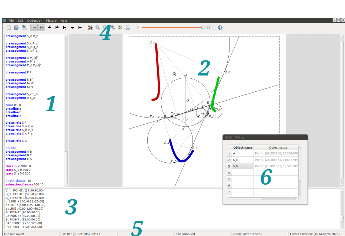
44 4 Graphical User Interface
Figure 4.1: Screenshot of the program with GUI
Menus and toolbars are standard parts of almost every program with GUI
program. There is a standard menu with a toolbar that provides shortcuts
for menu items. Most items on the menu have an equivalent on some
toolbar. The menu items can also be activated by appropriate keyboard
shortcuts — for instance, Build (compiles a picture or builds animation)
can be activated by the keys Ctrl+B.
•The toolbar has a number of items, including those for creating,
opening and saving files, for zooming picture in and out, for theo-
rem proving (for turning on and off the prover based on the area
method, for turning on and off the prover based on Wu’s method, for
turning on and off the prover based on Gr¨obner bases method, for
turning deduction control on and off, for generating proofs in L
A
T
E
X,
for generating proofs in xml.
•The status bar displays some real-time information like current line
and column in editor window, current xand ycoordinates of the
mouse pointer in the picture window, whether the file has been saved
or processed, and the zoom factor.
4.2 Features for Interactive Work
Creating/Opening: In the beginning, one can created a new or open an ex-
isting *.gcl file. From the File menu, select the item New and the blank
new document window should appear. Type a few gcl commands in the
editor window. For instance, try this set of commands:
point A 20 20
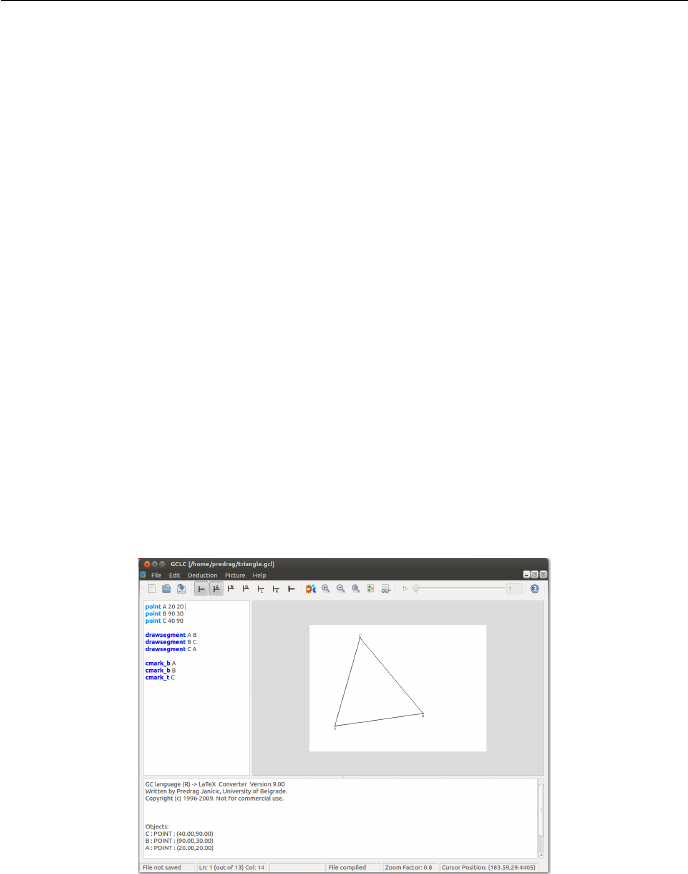
4.2 Features for Interactive Work 45
point B 90 30
point C 40 90
drawsegment A B
drawsegment B C
drawsegment C A
cmark_b A
cmark_b B
cmark_t C
If you are not familiar with gcl, explore some of the samples and learn
about commands of gcl.
Editing: You can type gcl commands in the editor window just like in any
other programming language.
Building: After entering of the source, select the item Build from the Picture
menu and start the compilation and building of the picture. If there were
no errors, a figure corresponding to the description given by the source
code will appear in the picture window (see Figure 4.2).
Figure 4.2: After building the image
Modifying the picture: Modifying the figure can be achieved by editing the
source manually (which gives more control over the picture), or by moving
“free” points directly on the picture. After successful compilation, you can
select the item Show Free Points from the Picture menu. Now, every free
point will have a green circular mark which can be selected (picked-up)
and dragged to another position (also changing the coordinates of the
point in the editor). In a similar way, destination points for animations
can be dragged (while they have orange circular marks) (see Figure 4.3).
Export: GUI GCLC can export a compiled picture (or a particular frame from
an animation) to the following formats:
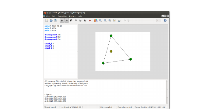
46 4 Graphical User Interface
Figure 4.3: Moving a fixed point
•simple L
A
T
E
X format (supported by gclc.sty
•PSTricks L
A
T
E
X format
•TikZ L
A
T
E
X format
•Bitmap
•eps (Encapsulated PostScript)
•svg (Scalable Vector Graphics)
•raster formats: bitmap, PNG, JPG
•xml (textual description of the figure given as xml file).
Also, an animation can be exported to a sequence of bitmaps (which can
be further used for making animations by some other tool). These features
are available in the File/Export menu. More about export options can be
found in Chapter 5.
Import: GUI GCLC can import JavaView .jvx files. This feature is available
in the File/Import from menu.
Theorem proving: Options for the built-in theorem proving can be accessed
via the option group Source or via the Source toolbar. If the source file
contains a conjecture, GCLC will automatically invoke the built-in the-
orem prover, if the option Theorem proving is checked (i.e., if this button
is turned on). If the option Deductive control is checked, when a run-time
error occurs (during processing the source), GCLC will run the prover
to check whether this error occurs in all situations (i.e., whether it is a
deductive consequence of the given construction) (see Section 6.7). The-
orem prover can generate proofs in L
A
T
E
X and in xml form. If at least
one of the options Theorem proving and Deductive control is checked, then
the options Generate Proofs in L
A
T
E
Xand Generate Proofs in xml can
be selected. If neither of these two options were selected, then the prover
works without generating files with the proofs. More about the theorem
proving and the deduction control can be found in Chapter 6.

4.2 Features for Interactive Work 47
Miscellaneous: GUI GCLC provides some additional useful features, includ-
ing
•Watch window: Gives information about type and values of specified
objects in the generated picture or in any particular animation frame.

48 4 Graphical User Interface
Chapter 5
Exporting Options
On the basis of a (valid) figure description in the file in.gcl, a figure can be
generated by the command-line version of GCLC using the following command:
> gclc in.gcl out.pic -option
where out.pic is the name of a resulting file (it can have any extension, not
necessarily .pic), and -option controls the output format. If the option is
omitted, the output format is the simple L
A
T
E
X format (supported by gclc.sty).
For PSTricks L
A
T
E
X format, -pst is used, for TikZ L
A
T
E
X format, -tikz is used,
for eps,-eps is used, for svg,-svg is used, and for xml, the option -xml is
used. Command line version of GCLC does not support export to bitmap.
Within the GUI version of GCLC, a picture exported in some of supported
formats can be obtained by selecting one of the option available in the group
File/Export to... (see Chapter 4). When exporting a particular frame from an
animation, traces are also saved to output files.
File exported to vector formats (L
A
T
E
X, svg,xml) contain comments —
explanations for portions of code for easier understanding and modifying.
By using the export_to... GCLC commands, arbitrary text can be ex-
ported directly to files containing specific vector formats (L
A
T
E
X, svg,xml).
Note that mathematical formulae written within a GCLC file will be for-
matted properly only when exported to L
A
T
E
X formats. If a figure is exported
to, say, eps format, it will not have properly formatted formulae. In order to
obtain an eps file with properly formatted formulae, one must first export the
file to L
A
T
E
X, then process a L
A
T
E
X file that contains only this figure, then export
the obtain document to a ps document, and then finally, convert the ps to a
eps file.
When exported to L
A
T
E
X, the text is printed in math mode and in the size
footnotesize.
5.1 Export to Simple L
A
T
E
X format
By ”simple export L
A
T
E
X format“ we mean the format based on the gclc.sty
package. Good sides of this choice are: there is just one file required (gclc.sty),
it can be stored in standard folder for L
A
T
E
X packages or in the current folder,
it can be easily shared with others to make L
A
T
E
X documents portable, or it can

50 5 Exporting Options
even be copied to L
A
T
E
X documents (since it is just few lines long). This package
insignificantly slows down processing L
A
T
E
X documents that use it. Bad sides
of choosing this L
A
T
E
X format are: in most systems producing pdf documents
has to be performed via PostScript format. In addition, this format does not
support some features of GCLC, like filling polygons.
5.1.1 Generating L
A
T
E
X Files and gclc.sty
On the basis of a (valid) figure description in the file in.gcl, a picture in
L
A
T
E
X format can be generated by the command-line version of GCLC using
the following command:
> gclc in.gcl out.pic
where out.pic is the name of a resulting file (it is not necessary for it to have
the extension .pic). If the extension of the input file is not given, then the
assumed extension is .gcl. If the name of the output file is not given, then the
assumed name is built from the input file name (e.g., in.pic).
Within the GUI version of GCLC, a picture exported in L
A
T
E
X format can
be obtained by selecting the option File/Export to.../LaTeX.
The picture can be included in a L
A
T
E
X document using the command:
\input{out.pic}
in appropriate position in your L
A
T
E
X document.
The package gclc must be included (by \usepackage{gclc}) in the pream-
ble of your document, or you can add the following lines in the preamble:
\def\gclcpicture#1{%
\def\gclcline##1##2##3##4##5##6##7{%
\put(##1,##2){\special{em:point #1##3}}%
\put(##4,##5){\special{em:point #1##6}}%
\special{em:line #1##3,#1##6,##7mm}}}
\gclcpicture{1}
If the command color is used in the gcl file, a L
A
T
E
X document including
the corresponding picture (.pic file) should also use the package color.1
5.1.2 Changing L
A
T
E
X File Directly
A position of the picture in your document can be changed by changing (within
any editor) appropriate parameters in the GCLC output file. For example,
\begin{picture}(140.00,100.00)
can be changed to
\begin{picture}(180.00,100.00)(10.00,10.00)
in order to change picture dimensions and its position. (All values in both input
and output file are expressed in units of 1 millimeter.)
1For convenience, the package color.sty (developed by other authors), is distributed with
GCLC.

5.1 Export to Simple L
A
T
E
X format 51
5.1.3 Handling More Pictures on a Page
If you want to put two or more pictures generated by GCLC on one page, you
might need to take care about point numbers, otherwise dvi... programs might
report the warning duplicate point numbers and only your first picture on a
page will be drawn correctly. This is so because (many) dvi programs can (in
an appropriate mode) address a limited number of points each of which has its
own index. These indices can go from 1 to 32767. If there are several pictures,
each of their points should have an index which is unique; indices of points in
different pictures thus could differ in the first digit. So, before each, there should
be one \gclcpicture command with the number of the picture (you can omit
\gclcpicture{1} before the first picture):
\input{sample1.pic}
\gclcpicture{1}
\input{sample2.pic}
This way, point indices are built by concatenating picture indices and original
point indices. Add command \gclcpicture{1} after a sequence of pictures
supposed to be on the same page. Note that if pictures have thousands of
points this approach can fail (for instance, if there are three pictures on a page,
each with 3000 points).
There is also another solution for this problem: GCLC can create pictures
with indices of points starting with a given number. Therefore, for example,
if GCLC reports Ending point number: 99 after successfully processing an
input file, starting point number for the second picture should be 100 or more:
> gclc in.gcl out.pic 100
If this parameter is omitted, the starting point number is 1.
5.1.4 Batch Processing
If GCLC (the command line version) is called the option -b, then the batch
processing is used. It expects a L
A
T
E
X file with blocks of GCLC commands,
given in gclc environment, and it outputs a single L
A
T
E
X file with GCLC
commands replaced by corresponding L
A
T
E
X drawing commands (based on the
gclc.sty style). This output file then should be processed (only) by L
A
T
E
X
processor. If the option -b is used, then all other options are ignored (the
theorem prover and deduction control are off, and only exporting to L
A
T
E
X is
enabled).
The batch processing is used as in the following example:
> gclc in.tex out.tex -b
If the extension of the input file is not given, then the assumed extension is
.tex. If the option -b is used and if the name of the output file is not given,
then the assumed name is built from the input file name (e.g., in-gclc.tex).
For example, an input L
A
T
E
X file (in.tex) can be

52 5 Exporting Options
\documentclass{article}
\usepackage{gclc}
\begin{document}
Here goes a triangle...
\begin{figure}[h]
\begin{gclc}
dim 100 35
point A 10 10
point B 80 10
point C 30 30
drawsegment A B
drawsegment A C
drawsegment B C
\end{gclc}
\caption{Triangle}
\end{figure}
...and here goes a parametric curve...
\begin{gclc}
dim 100 35
ang_picture 0 0 100 35
ang_origin 10 10
ang_drawsystem
ang_draw_parametric_curve x
{ 0; x<8; x+0.05}
{ x; sin(pow(x,2))*cos(x) }
\end{gclc}
\end{document}
5.2 Export to PSTricks L
A
T
E
X format
PSTricks is a collection of PostScript-based T
E
X macros that is compatible with
L
A
T
E
X (but also most T
E
X macro packages, including plaint T
E
X). It enables
creating high quality graphics in an inline manner. PSTricks package is not
distributed with GCLC.2Good sides of PSTricks choice are: it is very popular,
very expressive, it is understandable and can be relatively easily modified by
hand. Bad sides of choosing this L
A
T
E
X format are: it takes several megabytes,
it required installing dozens of L
A
T
E
X packages, it is impossible to share L
A
T
E
X
documents with those who do not have PSTricks installed, it slows down a bit
processing L
A
T
E
X documents that use it, in order to produce pdf document, an
intermediate PostScript document has to be generated.
On the basis of a (valid) figure description in the file in.gcl, a picture in
PSTricks format can be generated by the command-line version of GCLC using
2It can be found on http://tug.org/PSTricks.

5.3 Export to TikZ L
A
T
E
X format 53
the following command:
> gclc in.gcl out.pst -pst
where out.pst is the name of a resulting file. If the extension of the input file
is not given, then the assumed extension is .gcl. If the option -pst is used and
if the name of the output file is not given, then the assumed name is built from
the input file name (e.g., in.pst).
Within the GUI version of GCLC, a picture exported in PSTricks format
can be obtained by selecting the option File/Export to.../LaTeX-PSTricks.
A picture in PSTricks format can be included in a L
A
T
E
X document using
the command:
\input{out.pst}
in appropriate position in your L
A
T
E
X document or the whole picture in PSTricks
format can be copied to the document (the package pstricks must be included.
Batch processing is supported for this format. If GCLC (the command line
version) is called the option -b, then the batch processing is used. It expects a
L
A
T
E
X file with blocks of GCLC commands, given in gclc environment, and it
outputs a single L
A
T
E
X file with GCLC commands replaced by corresponding
L
A
T
E
X PSTricks drawing commands. This output file then should be processed
(only) by L
A
T
E
X processor. If the option -b is used, then all other options are
ignored (the theorem prover and deduction control are off).
The batch processing is used as in the following example:
> gclc in.tex out.tex -b -pst
5.3 Export to TikZ L
A
T
E
X format
The pgf package (pgf is supposed to mean ,,portable graphics format“), is
a package for creating graphics in an inline manner. It defines a number of
T
E
X commands that draw graphics. TikZ is the natural frontend for pgf. It
gives access to all features of pgf, but it is intended to be easy to use. The
syntax is a mixture of metafont and pstricks and some additional ideas. The
pgf package, supporting TikZ format, is not distributed with GCLC.3Good
sides of TikZ choice are: it is very expressive, it is understandable and can be
relatively easily modified by hand, it enables directly producing pdf documents
with figures directly from the L
A
T
E
X source (there is no need for PostScript
intermediate step). Bad sides of choosing this L
A
T
E
X format are: it takes several
megabytes, it required installing dozens of L
A
T
E
X packages, it is impossible to
share L
A
T
E
X documents with those who do not have pgf installed, it slows down
processing L
A
T
E
X documents that use it.
On the basis of a (valid) figure description in the file in.gcl, a picture in
TikZ format can be generated by the command-line version of GCLC using the
following command:
> gclc in.gcl out.tkz -tikz
3It can be found on http://sourceforge.net/projects/pgf.

54 5 Exporting Options
where out.tkz is the name of a resulting file. If the extension of the input file
is not given, then the assumed extension is .gcl. If the option -tikz is used
and if the name of the output file is not given, then the assumed name is built
from the input file name (e.g., in.tkz).
Within the GUI version of GCLC, a picture exported in TikZ format can
be obtained by selecting the option File/Export to.../LaTeX-TikZ.
A picture in TikZ format can be included in a L
A
T
E
X document using the
command:
\input{out.tkz}
in appropriate position in your L
A
T
E
X document or the whole picture in TikZ
format can be copied to the document (the package tikz must be included).
Batch processing is supported for this format. If GCLC (the command line
version) is called the option -b, then the batch processing is used. It expects a
L
A
T
E
X file with blocks of GCLC commands, given in gclc environment, and it
outputs a single L
A
T
E
X file with GCLC commands replaced by corresponding
L
A
T
E
X TikZ drawing commands. This output file then should be processed (only)
by L
A
T
E
X processor. If the option -b is used, then all other options are ignored
(the theorem prover and deduction control are off).
The batch processing is used as in the following example:
> gclc in.tex out.tex -b -tikz
5.4 Export to Raster-based Formats and Export
to Sequences of Images
Within WinGCLC, there is available export to bitmap format (option File/Export
to.../LaTeX). The picture can be generated for the following resolutions 75, 150,
300 and 600 dpi. The new GUI version supports also export to JPEG and PNG
formats.
Within the GUI version, an animation can be exported to a sequence of
bitmaps (option File/Export to...) which can be further used for making ani-
mations by some other tool.
5.5 Export to eps Format
On the basis of a (valid) figure description in the file in.gcl, a picture in eps
(Encapsulated PostScript Format) format can be generated by the command-
line version of GCLC using the following command:
> gclc in.gcl out.eps -eps
where out.eps is the name of a resulting file. If the extension of the input file
is not given, then the assumed extension is .gcl. If the option -eps is used and
if the name of the output file is not given, then the assumed name is built from
the input file name (e.g., in.eps).
Within the GUI version of GCLC, a picture exported in eps format can be
obtained by selecting the option File/Export to.../EPS.

5.6 Export to svg Format 55
A picture in eps format can be included in a L
A
T
E
X document using the
command:
\includegraphics[width=0.5\textwidth]{out.eps}
in appropriate position in your L
A
T
E
X document (the package graphicx must
be included (by \usepackage{graphicx}) in the preamble of your document).
5.6 Export to svg Format
On the basis of a (valid) figure description in the file in.gcl, a picture in
svg (Scalable Vector Graphics) format can be generated by the command-line
version of GCLC using the following command:
> gclc in.gcl out.svg -svg
where out.svg is the name of a resulting file. If the extension of the input file
is not given, then the assumed extension is .gcl. If the option -svg is used and
if the name of the output file is not given, then the assumed name is built from
the input file name (e.g., in.svg).
Within the GUI version of GCLC, a picture exported in svg format can
be obtained by selecting the option File/Export to.../SVG. A picture in svg
format can be directly open by modern web browsers. For more details about
xml and svg see Chapter 7.
5.7 Export to xml Format
On the basis of a (valid) figure description in the file in.gcl, a textual descrip-
tion as xml file can be generated by the command-line version of GCLC using
the following command:
> gclc in.gcl out.xml -xml
where out.xml is the name of a resulting file. If the extension of the input file
is not given, then the assumed extension is .gcl. If the option -xml is used and
if the name of the output file is not given, then the assumed name is built from
the input file name (e.g., in.xml).
Within the GUI version of GCLC, a figure description exported in xml
format can be obtained by selecting the option File/Export to.../XML. A figure
description in xml format can be directly open by modern web browsers. For
more details about xml and svg see Chapter 7.
5.8 Generating PostScript and pdf Documents
L
A
T
E
X files with figures generated by GCLC should be normally converted to
dvi format (by the L
A
T
E
X processor), and then to PostScript (by some dvi
to PostScript converter, e.g., dvi2ps).

56 5 Exporting Options
L
A
T
E
X files with figures generated by GCLC might not properly get con-
verted to pdf documents in some environments (neither by L
A
T
E
X to pdf pro-
cessor, nor by dvi to pdf converter, e.g., dvi2pdf). If this is the case, then first
produce the dvi file, then convert it to PostScript, and then, finally, to pdf
(by some PostScript to pdf converter, e.g., ps2pdf).

Chapter 6
Theorem Prover
There are three theorem provers built into GCLC:
•a theorem prover based on the Chou’s area method1[3]; the prover pro-
duces traditional (i.e., geometric, not algebraic, coordinate-based), read-
able proofs; the proofs are expressed in terms of higher-level geometry
lemmas and expression simplifications.
•theorem provers based on the Wu’s method [12,4] and on the Gr¨obner
bases method [1,2];2these provers are algebraic theorem provers; they are
based on manipulating polynomials and they do not produce traditional
geometrical proofs.
The theorem prover to be used is selected in the following way:
•in the command line version, by an appropriate parameter: -a for the
area method (default), -w for the Wu’s method, -g for the Gr¨obner bases
method.
•in the GUI version, the theorem prover is selected by checking appropriate
button in the toolbar or by checking the option Deduction Control.
All provers can prove a range of non-trivial theorems, including theorems
due to Ceva, Menelaus, Gauss, Pappus, Thales etc, but they are still a subject
of further improvements.
Support for the provers involves only a few commands:
•prove (for providing a conjecture);
•prooflevel (for setting the level of proof details);
•prooflimit (for setting maximal size of a proof).
•prover_timeout (for setting the timeout for the prover).
1This theorem prover based on the area method was developed in collaboration with
prof. Pedro Quaresma, Department of Mathematics, University of Coimbra, Portugal. This
work was partially supported by CISUC/FCT, Centro International de Matem´atica (CIM),
under the programme “Research in Pairs”, while on visit to Coimbra University under the
Coimbra Group Hospitality Scheme.
2The main author of these theorem provers is Goran Predovi´c (University of Belgrade).

58 6 Theorem Prover
•theorem_name (for setting the theorem’s name).
The provers work in both command line version and in GUI version (and
they do not use any specific functionalities of the GUI). Proofs of theorems
can be generated in L
A
T
E
X or in xml form and saved in a file. For the area
method, each deduction step is accompanied by its semantics counterpart —
corresponding numeric values in Cartesian plane.
The theorem provers are very efficient. Many conjectures are proved in
only milliseconds. However, some conjecture may take several seconds, several
minutes, or in some specific cases even several hours. The maximal number of
proof steps can be set by the command prooflimit. The default value is 10000
proof steps.3If the prover perform more proof steps, the proving process is
stopped. Similarly, the time available to the prover (in seconds) can be set by
the command prover_timeout. The default value is 10 seconds.
6.1 Introductory Example
The theorem prover is tightly integrated into GCLC. This means that one
can use the prover to reason about a GCLC construction (i.e., about objects
introduced in it), without any required adaptations required for the deduction
process. Of course, only the conjecture itself has to be added.
The example GCLC code given in Figure 6.1 describes a triangle and mid-
points of two of triangle’s sides. This GCLC code produces the Figure 6.2.
It holds that the lines AB and A1B1are parallel and this can be proved by
the theorem prover. The conjecture ,,AB and A1B1are parallel“ is given as
argument to the prove command in the following way:
prove { parallel A B A_1 B_1 }
At the end of the processing of the GCLC file, the theorem prover is invoked;
it can produce a proof in L
A
T
E
X and in xml form (in the current directory) and,
within the GCLC report, a report about the proving process: whether the
conjecture was proved or disproved, data about CPU time spent, etc.
6.2 Basic Sorts of Conjectures
Statements for the basic sorts of conjectures are given in the following table:
points Aand Bare identical: identical A B
points A,B,Care collinear: collinear A B C
AB is perpendicular to CD:perpendicular A B C D
AB is parallel to CD:parallel A B C D
Ois the midpoint of AB:midpoint O A B
AB has the same length as CD:same_length A B C D
points A,B,C,Dare harmonic: harmonic A B C D
All these sorts of conjectures can also be expressed in terms of geometry
quantities. Geometry quantities provide more general way for stating conjec-
tures.
3On a modern PC computer, 10000 steps are performed in less then 1 minute.

6.3 Geometry Quantities and Stating Conjectures 59
point A 20 10
point B 70 10
point C 35 40
midpoint B_1 B C
midpoint A_1 A C
drawsegment A B
drawsegment A C
drawsegment B C
drawsegment A_1 B_1
cmark_b A
cmark_b B
cmark_t C
cmark_l A_1
cmark_r B_1
prove { parallel A B A_1 B_1 }
Figure 6.1: Description of a triangle and midpoints of two of triangle’s sides and
the conjecture of midpoint theorem
6.3 Geometry Quantities and Stating Conjec-
tures
The theorem prover deals with the following geometry quantities:
ratio of directed segments: for four collinear points P,Q,A, and Bsuch
that A6=B, it is the ratio
−−→
P Q
−−→
AB ;
signed area: it is the signed area SABC of a triangle ABC or the signed area
SABCD of a quadrilateral ABCD;
Pythagoras difference: for three points, PABC is defined as follows:
PABC =AB2+CB2−AC2.
Pythagoras difference for four points, PABCD is defined as follows:
PABCD =PABD −PCBD .
real number: it is a real number, constant.
In GCLC, geometry quantities are written as in the following examples:
60 6 Theorem Prover
A B
C
AlBl
Figure 6.2: Illustration generated from the GCLC code from Figure 6.1
ratio of directed segments
−−→
P Q
−−→
AB sratio P Q A B
signed area (arity 3) SABC signed_area3 A B C
signed area (arity 4) SABCD signed_area4 A B C D
Pythagoras difference (arity 3) PABC pythagoras_difference3 A B C
Pythagoras difference (arity 4) PABCD pythagoras_difference4 A B C D
A conjecture to be proved is given as argument to the prove command. It
has to be some of the basic sorts of conjectures (see Section 6.2), or it has to be of
the form L=R, where Land Rare expressions over geometry quantities. The
conjecture can involve geometry quantities (only) over points already introduced
(by a subset of commands) within the current construction. Geometry quantities
can be combined together into more complex terms by operators for addition,
multiplication and division. Operators are written in textual form as in the
following table:
= equality
+ sum
·mult
/ratio
The conjecture and all its subterms are written in prefix form, with brackets
if needed. For instance,
SA1B1A=SA1B1B
is given to be proved in the following way:
prove { equal { signed_area3 A_1 B_1 A }
{ signed_area3 A_1 B_1 B }
}
and −→
AF
−−→
F B ·
−−→
BD
−−→
DC !·
−−→
CE
−→
EA != 1
is given to be proved in the following way:

6.3 Geometry Quantities and Stating Conjectures 61
prove { equal { mult { mult { sratio A F F B }
{sratioBDDC}}
{sratioCEEA}}
1 }
A range of geometry conjectures can be stated in terms of geometry quan-
tities. The representations for the basic sorts of conjectures is are given in the
following table:
points Aand Bare identical iff PABA = 0
points A,B,Care collinear iff SABC = 0
AB is perpendicular to CD iff PACD =PBCD
AB is parallel to CD iff SACD =SBCD
Ois the midpoint of AB iff
−→
AO
−−→
OB = 1
AB has the same length as CD iff PABA =PCDC
points A,B,C,Dare harmonic iff
−→
AC
−−→
CB =
−−→
DA
−−→
DB
Note that the command
prove { parallel A B A_1 B_1 }
(from Section 6.1) is equivalent to
prove { equal { signed_area3 A_1 B_1 A }
{ signed_area3 A_1 B_1 B }
}
The prover transforms the basic sorts of conjectures into statements given
in terms of geometric quantities: if a conjecture of a basic sort is given, the very
first step in the proof is its formulation in terms of geometric quantities.
The conjecture can involve geometry quantities only over points and lines
already introduced within the current construction, and by using (only) the
following commands:
•point
•line
•intersec
•midpoint
•med
•perp
•foot
•parallel
•translate
•towards

62 6 Theorem Prover
•online
The prover cannot prove conjectures about object constructed by using some
other commands. For instance, if a line ais constructed by the command
bis, then the prove cannot prove conjectures involving aor involving points
constructed by using a.
6.4 Area Method
One of the theorem prover built into GCLC is based on the algorithm described
in [3]. The basic idea of the algorithm is to express a theorem in terms of
geometry quantities, to eliminate (by appropriate lemmas) all occurrences of
constructed point and to simplify the expression, yielding a trivial equality.
6.4.1 Underlying Constructions
In [3], a construction is expressed in terms of commands INTER,PRATIO,TRATIO
and FOOT:
INTER Y ln1 ln2 : Point Yis the intersection of line ln1and line ln2.
PRATIO Y W U V r : Point Yis a point such that W Y =rUV , where ris a real
number.
TRATIO Y U V r : Point Yis a point on line l, such that r=U Y
UV , where ris a
real number and lis a line such that Ulies on land lis perpendicular to
UV .
FOOT Y P U V : Point Yis a foot from Pto line UV (i.e., Y P is perpendicular
to UV and Ylies on UV .
For each point Xconstructed by the above constructions and for each ge-
ometry quantity ginvolving X, there is a suitable lemma that enables replacing
gby an expression with no occurrences of X. Thanks to these lemmas, all
constructed points can be eliminated from the conjecture.
6.4.2 Integration of Algorithm and Auxiliary Points
In order to be tightly integrated into GCLC, the prover uses standard GCLC
construction commands and, if needed, transforms them internally into form
required by the algorithm and/or introduces some auxiliary points:
midpoint is expressed in terms of PRATIO, it does not introduce new points;
foot is expressed in terms of FOOT, it does not introduce new points;
med introduces two auxiliary points: for instance, med m A B introduce a point
Mmas the midpoint of AB and a point Tmon the bisector of AB (such
that TRATIO TmMmA 1); the line mis then determined by the points Mm
and Tm;

6.4 Area Method 63
perp introduces one auxiliary point: if Alies on the line q, then perp p A q in-
troduces a point Tpon a line perpendicular to q(such that TRATIO TpA Q11;
where the line qis determined by points Q1and Q2); in this case, the line
pis determined by the points Aand Tp; if Adoes not lie on the line q,
then perp p A q introduce a point Fpwhich is a foot of the normal from
Ato the line q; in this case, the line pis determined by the points Aand
Fp;
parallel introduces one auxiliary point: for instance, parallel p A q intro-
duces a point Ppon a line parallel to q(such that PRATIO PpA Q1Q21;
the line pis then determined by the points Aand Pp;
translate is expressed in terms of PRATIO, it does not introduce new points;
towards is expressed in terms of PRATIO, it does not introduce new points;
online is expressed in terms of PRATIO, it does not introduce new points, but
introduces a (indeterminate) constant r: for instance, online X A B is
interpreted as PRATIO X A A B r.
Definitions of auxiliary points are given at the beginning of the proof.
6.4.3 Non-degenerative Conditions and Lemmas
Some constructions are possible only if certain conditions are met. For instance,
the construction inter X a b is possible only if the lines aand bare not parallel.
For such constructions non-degenerative conditions are store for future possible
use and listed at the end of the proof.
Some non-degenerative conditions can also be introduced during the proving
process:
•some lemmas have two cases (for instance, ,,if Abelongs to CD“ and ,,if
Adoes not belong to CD“); if a condition for one case can be proved (as a
lemma), then that case is applied, otherwise, a condition for one case (the
one of the form L6=R) is assumed and introduced as a non-degenerative
condition.
•in the cancellation rule, if all summands on both sides of the equality have
the same multiplication factor X, the rule tries to prove (as a lemma) that
X= 0; if this fails, a condition X6= 0 is assumed and introduced as a
non-degenerative condition and the equality is cancelled by X.
Lemmas are being proved as separate conjectures, but, of course, sharing
the construction and non-degenerative conditions with outer context.
6.4.4 Structure of Algorithm
The algorithm has one main while loop — it process the sequence of all (relevant)
constructions in backward manner (from last to first construction step) and
transforms the current goal as follows:
•the current goal is initially the given conjecture;

64 6 Theorem Prover
•while there are construction steps do:
–apply geometric simplifications to the current goal;
–apply algebraic simplifications to the current goal;
–if the current construction step introduce a new point P, then elim-
inate (using the elimination rules) one of occurrences of P(from the
current goal) and go to the top of the while loop; otherwise, go to
next construction step.
•apply geometric simplifications to the current goal;
•apply algebraic simplifications to the current goal.
•if the current goal is a equality trivially true, then the conjecture has been
proved, if the current goal is a equality trivially false, then the conjecture
has been disproved, otherwise, the conjecture has been neither proved nor
disproved.
The reasoning steps, as seen from the above overall algorithm, are divided
into three groups:
algebraic simplifications: applies simplification rewrite rule (not directly re-
lated to geometry) such as:
x+ 0 →x
0 + x→x
x·1→x
x·0→0
x
y+u
v→x·v+u·y
y·v
. . .
geometric simplifications: applies simplification rewrite rule, directly related
to geometry quantities such as:
SAAB →0
SABC →SBCA
PAAB →0
. . .
elimination simplifications: applies elimination lemmas for eliminating con-
structed points for the current goal; for instance, if the point Yis intro-
duced by as the intersection of lines l1(determined by Uand V) and l2
(determined by Pand Q), then Ycan be eliminated from expression of
the form
−→
AY
−−→
CD using the following equality:
−→
AY
−−→
CD =(SAP Q
SCP DQ ,if A∈UV
SAUV
SCUDV ,if A6∈ UV

6.5 Wu’s Method and Gr¨obner Bases Method 65
Full details about all used lemmas and rewrite rules are given in the techni-
cal report “Framework for constructive geometry (based on the area method)”
(written by Pedro Quaresma and Predrag Janiˇci´c) [11]. This technical report is
a part of GCLC distribution.
6.4.5 Scope
The theorem prover can prove any geometry theorem expressed in terms of ge-
ometry quantities, and involving only points introduced by using the commands
point,line,intersec,midpoint,med,perp,foot,parallel,translate,
towards,online. This can be proved following the ideas from [3]. However,
some of the proofs can be very long and can take lot of time.
6.5 Wu’s Method and Gr¨obner Bases Method
One of the theorem prover built into GCLC is based on the Wu’s method
[12,4] and one is based on the Gr¨obner bases method [1,2]. These methods
are algebraic methods and they prove geometrical statements by manipulating
polynomials corresponding to the constructions and given conjectures. These
methods can also detect non-degenerative conditions, described in Section 6.4.
6.6 Prover Output
Whenever there was a conjecture given in the input gcl file, the prover produces
a short report. The prover can also generate proofs in L
A
T
E
X format, or in xml
format. The level of details given in generated proof can be controlled by the
user.
6.6.1 Prover’s Short Report
The prover produces a short report (if there was a conjecture given in the gcl
file). In the command line version, this short report is shown and written in the
log file, while the GUI version shows this report in its output window. For the
area method, this report consists of information on number of steps performed,
on CPU time spent and whether or not the conjecture has been proved. For
example:
Number of elimination proof steps: 3
Number of geometric proof steps: 6
Number of algebraic proof steps: 23
Total number of proof steps: 32
Time spent by the prover: 0.002 seconds
The conjecture successfully proved.
The prover output is written in the file ceva_proof.tex.

66 6 Theorem Prover
6.6.2 Controlling Level of Output
For the area method, the level of generated proof output is controlled by the
command prooflevel. This command has one argument (an integer from 0 to
7) which provides the output level:
0 : no output (except the statement);
1 : elimination steps plus grouped geometric steps and algebraic steps;
2 : elimination steps plus geometric steps plus grouped algebraic steps;
3 : as level 2, plus statements of lemmas;
4 : as level 3, plus elimination steps plus grouped geometric steps and alge-
braic steps in lemmas;
5 : as level 4, plus geometric steps in lemmas;
6 : as level 5, plus algebraic steps at proof level 0;
7 : as level 6, plus algebraic steps in lemmas.
The default output level is 1.
For the algebraic theorem provers, the output is always given in a standard
form and the command prooflevel is ignored.
6.6.3 Proofs in L
A
T
E
X format
The proof in L
A
T
E
X form is generated by the command line version of GCLC, if
the option -eps (for export to eps format) is used, or, if there no export option
is used (when the figure is exported to L
A
T
E
X format).
The proof in L
A
T
E
X form is generated by the GUI version of GCLC, if the
option Deduction/Proof Export to LaTeX is checked.
In these cases, the proof is exported to the file name_proof.tex (in the
current directory, name is the name of the input file). If there is no prove
command within the construction, then the file with a proof will not be created.
For proofs generated by the area method, at the beginning of the proof, the
auxiliary points are defined, for instance:
Let M0
abe the midpoint of the segment BC.
Let T1
abe the point on bisector of the segment BC (such that TRATIO T1
a
M0
aB1).
The proof consists of proof steps. In each proof step, the current goal is
changed. For each proof step, there is an explanation and (optionally) its se-
mantics counterpart. This semantic information is calculated for concrete points
used in the construction (note that these coordinates are never used in the proof
itself); it can serve as a semantic test, especially for conjectures for which is not

6.6 Prover Output 67
known whether or not they are theorems. Proof step are enumerated. For
example:
−→
AF
−−→
F B ·
−−→
BD
−−→
DC ·
−−→
CE
−→
EA = 1 by the statement (value 1=1)
−1·
−→
AF
−−→
BF ·
−−→
BD
−−→
DC ·
−−→
CE
−→
EA = 1 by geometric simplifications (value 1=1)
Lemmas are proved within the main proof (making nested proof levels), and
the beginning and the end of a proof for a lemma is marked by a horizontal
solid line.
At the end of a proof, it is reported if the conjecture is proved (“Q.E.D.”
— lat. Quod Erat Demonstrandum — which was required to prove), if the
conjecture is disproved (if it was shown that it is invalid), or neither of these
two.
At the end of the main proof all non-degenerative conditions are listed. For
instance:
SM0
aM2
bT3
b6=ST1
aM2
bT3
bi.e., lines M0
aT1
aand M2
bT3
bare not parallel (construc-
tion based assumption)
For proofs generated by the Wu’s and Gr¨obner bases method, the output
consist of a summary of processing steps over the relevant set of polynomials.
See one complete example in the appendix (Section E.5).
Modifying L
A
T
E
X Output
The prover exports proofs in L
A
T
E
X form. These L
A
T
E
X files require L
A
T
E
X pack-
age gclcproof.sty.
Once generated, the proof in L
A
T
E
X form can still be parameterized. Namely,
data in the file can be formatted in several ways, giving different layouts. Also,
semantics part can be omitted. Parameters for proof formatting are given as
options for the package gclcproof.sty. There are three parameters:
style: defines the layout; available choices are:
•portrait — uses the package longtable to generate a multi-page
table.4
•portraitbreqn — uses the package breqn to try to break the equa-
tions. Problems with extra large fractions.
•landscape — uses the packages lscape,amsmath (with option leqno),
and breqn, to generate the list of equations in landscape mode, with
numbers on the left, and with automatic equation breaking.
The default value for style is portrait.
size: defines the font size in the proof. It uses the L
A
T
E
X font size names of,
from tiny up to large. The default value is small.
4For convenience, the required packages breqn.sty,flexisym.sty,mathstyle.sty,
cmbase.sim (developed by other authors), are distributed with GCLC. The packages
longtable.sty,lscape,sty,amsmath.sty (developed by other authors) are not distributed
with GCLC, but are widely available, most often as part of a T
E
X distribution.

68 6 Theorem Prover
semantic values: controls if the semantics values will be shown. If the option
semantics is used, the semantic values of both sides of equations will be
shown. The default value is NULL, i.e., without any value. The semantics
values are only generated by the area method.
According to the above,
\usepackage{gclcproof}
is equivalent to
\usepackage[portrait,small]{gclcproof}
(which gives a proof in portrait style, small size, without semantics style).
For example,
•\usepackage[tiny]{gclcproof}
retains the portrait mode (default value), but decrease the size of the fonts
used in the proof to tiny. No semantic values displayed.
•\usepackage[portraitbreqn,sematics]{gclcproof}
uses the breqn package of the AMSTeX to try to break automatically
the equations. Portrait form, small size fonts, semantic values displayed.
Note: the breqn package may fail (not being able to process the document)
if the proof contains large fractions, breqn it is unable to break them into
lines.
•\usepackage[landscape]{gclcproof}
uses the packages lscape,amsmath (with option leqno), and breqn to
produce a proof in landscape mode. It is the mode that provides the larger
environment for proofs, so in some proofs it will be the only one to be able
to display the proofs without overlapping of the different elements. Note:
the rotation of the proof to landscape mode it is done with Postscript
specials, so it may not display properly in some viewers. The size of the
fonts it is small, and the sematic values are not displayed.
In the generated proofs, there is always \usepackage{gclcproof} used (in
the preamble) and the layout can be changed by using options for this command,
as discussed above.
6.6.4 Proofs in xml format
The proof in xml form is generated by the command line version of GCLC, if
the option -xml (for export to xml format) or if the option -svg (for export to
svg format) is used.
The proof in xml form is generated by the GUI version of GCLC, if the
option Deduction/Proofs Export to XML is checked.
In these cases, the proof is exported to the file name_proof.xml (in the
current directory, name is the name of the input file). If there is no prove
command within the construction, then the file with a proof will not be created.
Proofs stored in xml are formatted analogously as in L
A
T
E
X format.
The proofs in xml format fulfil restrictions posed by GeoCons_proof.dtd (as
stated in the line <!DOCTYPE figure SYSTEM "GeoCons_proof.dtd"> in each
of these files). For any xml file, it can be checked if it meets these restrictions.

6.7 Automatic Verification of Regular Constructions 69
It can be done using a xml processor, such as AltovaXML (copyrighted by Altova
GmbH). For instance:
> AltovaXML /v GeoCons_proof.dtd thm_proof.xml
verifies if the file thm_proof.xml is valid.
A proof in xml format (valid with respect to GeoCons_proof.dtd) can be
converted to a html form, for example:
>AltovaXML.exe /xslt1 GeoCons_proof.xsl /in thm_proof.xml /out thm_proof.html
A file with a proof in xml format can also be open directly by web browsers.
See one example in the appendix (Section E.5).
For more details about proofs represented in xml format, see Chapter 7.
6.7 Automatic Verification of Regular Construc-
tions
A geometrical construction is associated with some fixed points (with concrete
Cartesian coordinates). In such environments, some constructions (e.g., if they
attempt to use intersection of parallel lines), but the question if such construc-
tion is always illegal or it is illegal only for given particular fixed points is not
trivial (if a construction is never illegal, i.e., if it is always possible, we will call
it regular). For answering such question, one has to use deductive reasoning,
and not only semantic check for the special case. Consider one simple example:
given (by Cartesian coordinates) three fixed distinct points A,B,C, we can
construct a point Das an image of the point Cin translation TAB (in terms
of GCLC commands: translate D A B C); later on, if we try to construct an
intersection of lines AC and BD, we will discover that there is no such intersec-
tion (since these two lines are parallel). This holds not for some specific points
A,B,C, with Ddetermined as above, but for all triples of points A,B,C. So,
this construction is illegal, and moreover, it is illegal not only for a given special
case, but always.
The system for automated testing whether a construction is regular or illegal
is built into GCLC and is based on the built-in theorem provers. All built-in
theorem provers can be used for this purpose. This verification mechanism can
be switched on or off:
•in the command line version, the verification mechanism is turned on by
using the option -d.
•in the GUI version, the verification mechanism is turned on by check-
ing the button Deduction Control in the toolbar or the option Deduc-
tion/Deduction Control.
If the verification mechanism is turned on, while processing the input file
(with a description of a geometrical construction), GCLC provides to the the-
orem prover all construction steps performed. When GCLC encounters a con-
struction step that cannot be performed (e.g., two identical points do not de-
termine a line), it reports that the step is illegal with respect to a given set
of fixed points, and then it invokes the theorem prover. The prover is run on

70 6 Theorem Prover
the critical conjecture (e.g., it tries to prove that two points are identical) and,
if successful, it reports that the construction step is always illegal/impossible.
The prover generates the proof for the critical construction:
•in the command line version: in the format selected for conjectures (see
Chapter 5);
•in the GUI version: in L
A
T
E
X and xml format if the options, respectively,
Proof Export to L
A
T
E
Xand Proof Export to xml are checked.
Realm. The verification deductive-check system currently covers the following
critical commands and constructions:
line — construction of a line given two points (error if the two points are
identical);
med — construction of a segment-bisector given two endpoints (error if the two
points are identical);
bis — constructing an angle-bisector of the angle determined by three points
A,B,C(error if Aand B, or Cand Bare identical);
intersec — constructing an intersection of lines aand b(error if the two lines
are parallel);
angle — calculating an angle determined by three points A,B,C(error if A
and B, or Cand Bare identical);
Geometry objects that are subject to deductive verification have to be made
within using the following commands:
•point
•line
•intersec
•midpoint
•med
•perp
•foot
•parallel
•translate
•towards
•online

6.7 Automatic Verification of Regular Constructions 71
which are internally transformed into primitive constructions of the area method.
For more details see [11].
It is worth pointing out that although GCLC has support for a large num-
ber of constructions, only few of them can be illegal. The above list of critical
constructions almost exhaust them. The only possible illegal constructions that
are not covered by the current version of our system are constructions of in-
tersection points of circle and line, and of two circles. Corresponding geometry
conjectures cannot be generally handled by the area method and the built-in
theorem prover.

72 6 Theorem Prover

Chapter 7
xml Support
GCLC has xml support, both for processing figures and proofs.1xml is format
suitable for storing descriptions of geometrical constructions and proofs and as
interchange format:
•instead of raw, plain text representation, geometrical constructions are
stored in strictly structured files; these files are easy to parse, process,
and convert into different forms and formats;
•input/output tasks are supported by generic, external tools and different
geometry tools will communicate easily;
•growing corpora of geometrical constructions will be unified and accessible
to users of different geometry tools;
•easier communication and exchange of material with the rest of mathe-
matical and computer science community;
•there is a wide and growing support for xml;
•different sorts of presentation (text form, L
A
T
E
X form, html) easily en-
abled;
•strict content validation of documents with respect to given restrictions.
7.1 xml
Extensible Markup Language (xml) is a simple, very flexible text format derived
from SGML (ISO 8879) and with data structured using tags. Originally designed
to meet the challenges of large-scale electronic publishing, xml is also playing
an increasingly important role in the exchange of a wide variety of data on the
Web and elsewhere2. It is called extensible because it is not a fixed format
like html (a single, predefined markup language), instead the tags indicate the
semantic structure of the data, rather than only its layout in a browser.
1xml support was developed in collaboration with prof. Pedro Quaresma, Department of
Mathematics, University of Coimbra, Portugal, Jelena Tomaˇsevi´c (University of Belgrade,
Serbia), and Milena Vujoˇsevi´c-Janiˇci´c (University of Belgrade, Serbia).
2http://www.w3.org/XML/

74 7 xml Support
However, xml is not just for Web pages: it can be used to store any kind
of structured information, and to enclose or encapsulate information in order
to pass it between different computing systems. An xml document can carry
both presentation (i.e., plausible visualisation) and content information. xml is
a project of the World Wide Web Consortium (W3C) and is a public format —
it is not a proprietary development of any company. Almost all browsers that
are currently in use support xml natively.
Data type definitions (dtds) provide a formal specification of the constraints
on the structure of data presented in xml form. A dtd is given as a formal
description in xml declaration syntax. It sets out what names are to be used
for the different types of element, where they may occur, and how they all fit
together. This formal description enables automatic verification (“validation”)
of whether a given document meets the given syntactical restrictions. This way,
groups sharing data with similar meanings can agree on different sets of tags
and dtds for representing different kinds of data.
Extensible stylesheet language transformation (xslt) is a document process-
ing language that is used to transform the input xml documents i.e., the input
files to the desired output documents. An xslt style-sheet declares a set of rules
(templates) for an xslt processor to use when interpreting the contents of an
input xml document. These rules tell the xslt processor how that data should
be presented — as an xml document, as an html document, as plain text, or
in some other form.
Scalable Vector Graphics (svg) is a language for describing two-dimensional
graphics and graphical applications in xml3. As xml,svg is a W3C recom-
mendation.
7.2 xml Suite
GCLCxml suite for geometrical constructions and geometrical proofs consists
of the following components and tools:
•xml-based format for representing geometrical constructions with corre-
sponding dtd,GeoCons.dtd;
•the option for conversion GCLC files to xml-based form;
•the option for generating figures from GCLC in svg form;
•the converter (implemented as xslt file, GeoConsGCLC.xlst) from xml-
based form to GCLC format;
•the converter (implemented as a xslt file, GeoConsHTML.xlst) from xml-
based form to a simple, readable html form (with syntax colouring fea-
tures, provided for better readability);
•the converter (implemented as a xslt file, GeoConsNL.xlst) from xml-
based form to a natural language form (currently, only for English lan-
guage);
3http://www.w3.org/Graphics/SVG/

7.3 Using xml Tools 75
•the xml-based format for representing proofs of properties of geometrical
constructions with a corresponding dtd,GeoCons_proof.dtd; the format
is adapted for the area-method;
•the option for generating proofs in xml-based form;
•the converter (implemented as a xslt file, GeoCons_proof.xslt) for proofs
from xml-based form to a simple, readable html form (with syntax
colouring features, and other features for better readability).
7.3 Using xml Tools
A regular .gcl file (file without errors) can be converted to xml form in the
following way:
•in the command-line version — using the option -xml:
> gclc example.gcl example.xml -xml
•in the GUI version of GCLC, by selecting the option File/Export to.../XML.
Note that the xml file obtained in this way is not an image file, but also
textual representation of the construction described in the input file.
xml files obtained this way fulfil restrictions posed by GeoCons.dtd (as
stated in the line <!DOCTYPE figure SYSTEM "GeoCons.dtd"> in each of these
files). For any xml, it can be checked if it meets these restrictions. It can be
done using a xml processor, such as AltovaXML (copyrighted by Altova GmbH).
For instance:
> AltovaXML /v GeoCons.dtd example.xml
verifies if the file example.xml is valid.
Axml file with geometrical contents (valid with respect to GeoCons.dtd)
can be converted to
•GCLC format, for example:
>AltovaXML.exe /xslt1 GeoConsGCLC.xsl /in example.xml /out example1.gcl
•to a simple, readable html form, for example:
>AltovaXML.exe /xslt1 GeoConsHTML.xsl /in example.xml /out example.html
•to a natural language (English) form (formatted in html):
>AltovaXML.exe /xslt1 GeoConsNL.xsl /in example.xml /out example.html
The geometrical xml files can be open directly by web browsers: For in-
stance, if the second line in the xml file reads:
<?xml-stylesheet href="GeoConsNL.xsl" type="text/xsl"?>
then the web-browser will render the contents of the file according to the file
GeoConsNL.xsl (see the example given in Figure 7.1).
GCLC files can be used for generating figures in svg format:
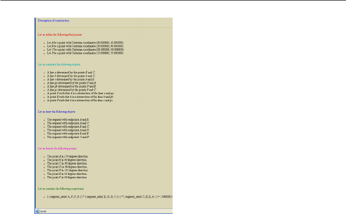
76 7 xml Support
Figure 7.1: Natural language presentation of a figure description stored in xml
form
•in the command-line version — using the option -svg:
> gclc example.gcl example.svg -svg
•in the GUI version of GCLC, by selecting the option File/Export to.../SVG.
A picture in svg format can be directly open by modern web browsers.
For .gcl files with conjectures, GCLC can generate proofs in xml form:
•in the command-line version — if the option -xmls or the option -svg is
used;
•in the GUI version of GCLC, by checking the option Source/Generate
proof in XML or the corresponding button in the source toolbar.
The xml files obtained in the above described way fulfil restrictions posed by
GeoCons_proof.dtd (as stated in the line <!DOCTYPE figure SYSTEM "GeoCons_proof.dtd">
in each of these files). For any xml, it can be verified if it meets these restrictions
(by analogy with verifying files with constructions).
Axml file with a proof contents (valid with respect to GeoCons_proof.dtd)
can be converted to a html form, using GeoCons_proof.xsl, for example:
>AltovaXML.exe /xslt1 GeoCons_proof.xsl /in proof.xml /out proof.html
xml files with proofs can be also open directly by web browsers see one
example in the appendix (Section E.5).
Appendix A
List of Errors and Warnings
Syntax error: Number expected.
Syntax error: Two decimal points in number.
Syntax error: Identifier expected.
Syntax error: Identifier or number expected.
Syntax error: Undefined variable.
Syntax error: Wrong variable type.
Syntax error: Symbol ’{’ expected.
Syntax error: Symbol ’}’ expected.
Syntax error: Unrecognized definition or command.
Invalid or non-defined expression.
Symbol ’;’ expected.
Invalid while block.
Invalid if-then-else block.
Invalid procedure definition.
Too many while-block executions (more than 10000). Possible infinite loop.
The conjecture given to prove is ill-formed or includes a point
that is not constructed by commands supported by the prover.
Syntax error: Unknown procedure.
Syntax error: Parameters lists not matched.
Syntax error: Procedures cannot be defined within while-blocks or procedures
Syntax error: Invalid tree description.
Syntax error: Invalid graph description.
Invalid include file.
Input error: Invalid input.
Run-time error: Bad definition. Can not determine line.
Run-time error: Bad definition. Circle radius too small.
Run-time error: Bad definition. Can not determine intersection.
Run-time error: Bad definition. Can not determine angle.
Run-time error: Bad definition. Cannot determine ellipse.
Run-time error: Cannot export data.
Memory error: Cannot allocate enough memory.

78 A List of Errors and Warnings
Warning: Changing variable value
Warning: Changing variable type
Appendix B
Version History
1996 First release of GCLC (GCLC v1.0) ( c
1996-2009 Predrag Janiˇci´c);
1998 GCLC v2.0 : Cartesian commands (including conics) added. Full vertical
compatibility.
2000 GCLC v2.1 : Several bugs fixed.
2003 GCLC v3.0 : Commands
dim,
area,
color,
drawline,
getx,
gety,
fontsize,
animation_frames,
trace
added. Full vertical compatibility (for input format). New export format
and new L
A
T
E
X style is used (gclc.sty). Since this version, commands
cmark do not have to precede other drawing commands.
WinGCLC— first release (graphical interface: c
2003-2009 Ivan Tra-
jkovi´c, Predrag Janiˇci´c);
2004 GCLC v3.1: Several small bugs fixed.
WinGCLC 2004: export now supports exporting an animation to a se-
quence of bitmaps, which can then be used for generating animated gif
(by some other tool) or the animation in some other format. Import from
JavaView .jvx format is integrated in WinGCLC.
2005 GCLC v4.0: Commands
expression,
while,

80 B Version History
random,
ang_draw_parametric_curve,
ang_drawsystem1,
ang_drawsystem_a,
ang_drawsystem0_a,
ang_drawsystem1_a
added. Full vertical compatibility. A bug in drawing negative arcs fixed.
WinGCLC 2005: no changes in the Windows interface.
2006 GCLC v5.0: Theorem prover tightly built-in. Full vertical compatibility.
The commands
foot,
online,
angle_o,
drawdashline
ang_drawsystem_p,
ang_scale,
prove,
prooflevel,
prooflimit,
added. If not defined, area (a visible part of the picture) is, by default, the
whole of the picture (which is relevant for drawline and drawdashline
as they are applied only if there is defined area — now always). There
is support for colors for L
A
T
E
X files, i.e., the command color is relevant
for exporting to L
A
T
E
X too (not only for exporting to bitmap). The new
manual and the help file.
WinGCLC 2006: The behavior of changing line thickness (by the com-
mands linethickness,normal,double) is fixed and improved for WinG-
CLC and for export to bitmap. New application icon and new file type
icon.
2006 GCLC v6.0: Full vertical compatibility. Added options for export to
eps (Encapsulated PostScript) and svg. Full support for xml (both for
construction descriptions and proofs). Added options for deductive veri-
fication of constructions.
The following commands were added:
procedure
call
(providing support for user-defined procedures),
ang3d_picture,
ang3d_origin,
ang3d_unit,

Version History 81
ang3d_scale,
ang3d_point,
ang3d_axes_drawing_range,
ang3d_drawline_p,
ang3d_drawsystem_p,
ang3d_draw_parametric_surface,
ang3d_draw_parametric_curve,
(providing support for 3D Cartesian system) and
drawarc_p
dradashwarc_p
set_equal
printvalueat_rb <p_id> <id>
background
ang_plot_data.
For the commands intersec,intersec2,bis,perp,med,sim,ang_intersec2,
full names (intersection,intersection2,bisector,perpendicular,
mediatrice,symmetrical,ang_intersection2) can also be used.
Using the theorem prover is simpler. Instead of stating conjectures in
terms of geometric quantities, one can also use the following basic sorts of
conjectures: identical A B,collinear A B C,perpendicular A B C D,
parallel A B C D,midpoint O A B,same_length A B C D,harmonic A B C D.
The sequence of commands in while-blocks now shares both the defined
variables and the environment with the outer context (In previous versions,
the environment, defined by commands ang_picture and ang_origin etc)
was reset in while-blocks).
In WinGCLC, there are new icons for easier use of the theorem prover.
In WinGCLC viewer and bitmap images (as well as in newly supported
formats, eps and svg) circles and arcs are not represented by small seg-
ments, but by proper circles and arcs.
WinGCLC 2006.1: New icons for easier using of the theorem prover.
When exporting a particular frame from an animation, traces are also
saved to output files.
2007 GCLC 7.0: Several small fixes were made and the following commands
were added:
drawtree
if_then_else
WinGCLC 2007: no changes in the Windows interface.
Support for hyperbolic geometry (through Poincar´e disc model) is given
via a sample file, as illustration of the mechanism of user-defined proce-
dures (sample21_hyp.gcl).

82 B Version History
2007.1 GCLC 7.1: Several small fixes were made.
Support for arrays (and the command array) added.
Support for export to another L
A
T
E
X formats — PSTricks and TikZ.
Support for including other files (and the command include) added.
Arguments for procedure calls can now also be constants.
If a tree node should not be labelled, its name should start with the symbol
_(in the previous version, its name had to be just the symbol _). All tree
nodes introduced by drawtree can be used as points.
If there is no defined area for ang_picture (or ang3d_picture), the de-
fault area is empty.
File exported to vector formats (L
A
T
E
X, svg,xml) contain comments —
explanations for portions of code for easier understanding and modifying.
In the command line version, assumed file names are supported.
The batch processing option added.
The following commands were added:
filltriangle
fillrectangle
fillcircle
fillellipse
fillarc
fillellipsearc
dashstyle
drawarrow
arrowstyle
drawbezier3
drawdashbezier3
drawbezier4
drawdashbezier4
bezierprecision
drawellipsearc1
drawdashellipsearc1
drawellipsearc2
drawdashellipsearc2
rotateonellipse
onsegment
oncircle
mcp
WinGCLC 2007.1: no changes in the Windows interface.

Version History 83
2008 GCLC 8.0:
New theorem provers added: one based on the Wu’s method and one based
on the Gr¨obner bases method.
New form of intersection command (intersection of lines determined by
the given four points).
The following commands were added:
prover_timeout
theorem_name
layer
hide_layer
hide_layers_from
hide_layers_to
ang_getx
ang_gety
ang3d_getx
ang3d_gety
ang3d_getz
fillellipsearc0
fillarc0
Several bugs fixed.
WinGCLC 2008: New buttons added for additional theorem provers.
2008 GCLC 8.1:
The following commands were added:
drawgraph_a
drawgraph_b
2009 GCLC 9.0:
Several small fixes were made.
The following commands were added:
getcenter
export_to_latex
export_to_simple_latex
export_to_pstricks
export_to_tikz
export_to_eps
export_to_svg
New version of support for hyperbolic geometry (through Poincar´e disc
model) is given via a new version of the sample file sample21_hyp.gcl
(co-authored with Zoran Luˇci´c).
WinGCLC 2009: no changes in the Windows interface.

84 B Version History

Appendix C
Additional Modules
There are several additional modules that going with the basic GCLC program:
•WinGCLC (c
2003-2015 Predrag Janiˇci´c, Windows interface: Ivan Tra-
jkovi´c): MS Windows version of GCLC; user-friendly multi-document
interface, support for animations, traces, export to bitmaps etc.
•Command line version of GCLC for Linux ( c
1996-2005 Predrag Janiˇci´c).
•Simple previewer view for GCLC output files (there is no need to “latex”
them) ( c
1996-2003 Predrag Janiˇci´c). Supports both output formats (old,
based on emlines.sty and new, based on gclc.sty). A picture out.pic
generated by GCLC can be seen by:
> view out.pic
Program view has the following commands (they are similar to commands
in T
E
X viewers):
–→right ;
–←left ;
–↑up ;
–↓down ;
–+ zoom-in ;
–−zoom-out ;
–Cincrease step ;
–Fdecrease step ;
–Qquit.
•JavaView to GCLC converter jv2gcl (c
2002 Predrag Janiˇci´c): con-
verts files from JavaView to GCLC format.1
1This program was developed in collaboration with prof. Konrad Polthier and Klaus Hilde-
brandt from Mathematical Institute, Technical University, Berlin. This work was partially
supported by daad grant form my visit to Technical University, Berlin (2003).

86 C Additional Modules
Appendix D
Acknowledgements
I am grateful to:
•Prof. Mirjana Djori´c for the initial discussion which led to the first version
of GCLC (1996);
•Ivan Trajkovi´c, the main author of the Windows interface in WinGCLC
(2003);
•Prof. Neda Bokan and other members of the Group for geometry, edu-
cation and visualization with applications (mostly based at the Faculty
of Mathematics, University of Belgrade) for their invaluable support in
developing the WinGCLC package (2003);
•daad (Germany) for funding my visit to Konrad Polthier’s group at Math-
ematical Institute of TU Berlin (2003), which I used for making a JavaView
→GCLC converter. I also thank prof. Konrad Polthier and Klaus Hilde-
brandt for their hospitality and their collaboration in developing this con-
verter;
•cim/cisuc (University of Coimbra, Portugal) for funding my visit to the
Department of Mathematics, University of Coimbra (2005), which I used
for developing the geometry theorem prover built into GCLC. I also thank
prof. Pedro Quaresma for his warm hospitality and his collaboration in
developing this prover;
•Prof. Pedro Quaresma (University of Coimbra), Jelena Tomaˇsevi´c, and
Milena Vujoˇsevi´c-Janiˇci´c, coauthors of the xml support for GCLC (2006);
•Prof. Bruno Buchberger (RISC, University of Linz, Austria), for kindly
inviting me to visit RISC and to present GCLC there (2006).
•emis (The European Mathematical Information Service) for mirroring
GCLC web page at http://www.emis.de/misc/software/gclc/ and
other emis locations.
•James Fry (New Albany, Indiana, USA) for careful revision of the GCLC/-
WinGCLC manual and help file and for many useful insights and com-
ments (2005);

88 D Acknowledgements
•Aleksandar Samardˇzi´c for his advices in making Linux release of GCLC
(2003/2005/2006);
•Goran Predovi´c (University of Belgrade, Serbia and Microsoft Develop-
ment Center Belgrade) — the main author of the theorem provers based
on the Wu’s method and Gr¨obner based method (2008).
•Luka Tomaˇsevi´c (University of Belgrade, Serbia) — the main author of
the support for graph drawing (2008).
•Prof. Stefano Marchiafava (University ,,La Sapienza“, Rome, Italy), for
kindly inviting me to visit the University ,,La Sapienza“ and to present
GCLC there (2008).
•Colleagues who gave contributions and suggestions in earlier stages of de-
velopment of WinGCLC: Nenad Dedi´c, Miloˇs Utvi´c, Nikola Begovi´c, Ivan
Elˇci´c, Jelena Grmuˇsa, Aleksandra Nenadi´c, Marijana Luki´c, Srdjan Vuk-
mirovi´c, Goran Terzi´c, Milica Labus, and Aleksandar Gogi´c (1999/2003);
•Konrad Polthier (TU Berlin), Zach (Temple University, USA), Vladimir
Balti´c (University of Belgrade), Hristos Bitos (Greece), Aleksandar Gogi´c
(DTA, Belgrade), Bob Schumacher (Cedarville University, Ohio, USA),
Pedro Quaresma (University of Coimbra, Portugal), Zoran Luˇci´c (Univer-
sity of Belgrade), Biljana Radovanovi´c (University of Belgrade), Nedeljko
Stefanovi´c (University of Belgrade), Milan Mitrovi´c (Slovenia), Thomas
Speziale (USA), Ania Piktas (Poland), Bojan Radusinovi´c (Serbia), Pierre
Larochelle (Florida Institute of Technology, USA), Robert Hartmann (TU
Clausthal, Clausthal-Zellerfeld, Germany), and Xavier Allamigeon for use-
ful feedback and suggestions on different versions of GCLC/WinGCLC.
•All GCLC users for their support, feedback and suggestions.

Appendix E
Examples
E.1 Example (Simple Triangle)
point A 50 45
point B 45 15
point C 90 15
cmark_lt A
cmark_lb B
cmark_rb C
drawsegment A B
drawsegment B C
drawsegment C A
med a C B
med b A C
intersec O a b
drawcircle O A
A
B C

90 E Examples
E.2 Example (Conics)
ang_picture 0 0 80 80
ang_origin 20.0 35.0
ang_drawsystem
ang_conic h 0 0 1 -1 0 -3
ang_conicprecision 75
ang_point A1 2 2
ang_point A2 3 2
line l A1 A2
ang_intersec2 P P2 h l
cmark_t P
ang_tangent p P h
color 32 192 32
ang_drawline p
color 32 32 192
ang_drawconic h
color 0 0 0
% --------------------------------------------------
ang_unit 5
ang_picture 85 5 140 100
ang_origin 115.0 45.0
ang_drawsystem
ang_conic h -1 0.5 1 -1 0 -3
ang_conicprecision 50
ang_point A1 2 2
ang_point A2 3 2
line l A1 A2
ang_intersec2 P P2 h l
cmark_t P
ang_tangent p P h
color 32 192 32
ang_drawline p
color 192 32 32
ang_drawdashconic h

E.2 Example (Conics) 91
0 1234−1
1
2
3
4
−1
−2
−3
P
0 1234−1−2−3−4−5−6
1
2
3
4
5
6
7
8
9
10
−1
−2
−3
−4
−5
−6
−7
−8
P

92 E Examples
E.3 Example (Parametric Curves)
ang_picture 5 5 112 92
ang_origin 45 35
ang_drawsystem_a
point X -0.5 0 0.5 0
point O 0 0
distance d X O
color 255 0 0
ang_draw_parametric_curve x {-3;x<8;x+0.1}{x;d/x}
color 0 0 255
ang_draw_parametric_curve x {-3;x<8;x+0.1}{x;d*x*sin(10*d*x)}
color 100 200 100
ang_draw_parametric_curve t {0;t<30;t+0.3}{sin(d*t)*t/6;-cos(d*t)*t/6}
animation_frames 50 5

E.3 Example (Parametric Curves) 93
x
y
0 123456−1−2−3−4
1
2
3
4
5
−1
−2
−3

94 E Examples
E.4 Example (While-loop)
dim 120 80
ang_picture 5 5 115 70
ang_origin 45 25
ang_drawsystem_a
ang_draw_parametric_curve x {-3;x<5;x+0.05}{x;0.3*x*sin(3*x)}
% while loop in conjunction with parametric curves
number x -3
while { x<5 }
{
ang_picture 10 10 100 70
ang_origin 45 25
expression y { 0.3*x*sin(3*x) }
ang_point A x 0
ang_point B x y
drawsegment A B
expression x { x+0.05}
}

E.4 Example (While-loop) 95
x
y
0 1234567−1−2−3−4
1
2
3
4
−1
−2

96 E Examples
E.5 Example (Ceva’s theorem)
point A 30 10
point B 80 10
point C 60 90
point P 55 55
line a B C
line b A C
line c A B
line pa P A
line pb P B
line pc P C
intersec D a pa
intersec E b pb
intersec F c pc
drawsegment A B
drawsegment A C
drawsegment B C
drawsegment A D
drawsegment B E
drawsegment C F
cmark_b A
cmark_b B
cmark_t C
cmark_rt D
cmark_b F
cmark_lt E
cmark_r P
prove { equal { mult { mult { sratio A F F B }
{sratioBDDC}}
{sratioCEEA}}
1 }

E.5 Example (Ceva’s theorem) 97
A B
C
D
F
E
P
Figure E.1: Output for Example E
L
A
T
E
X output of the prover based on the area method:
−→
AF
−−→
F B ·
−−→
BD
−−→
DC !·
−−→
CE
−→
EA !=1by the statement
(value 1=1) (0)
−1·
−→
AF
−−→
BF !·
−−→
BD
−−→
DC !·
−−→
CE
−→
EA !=1by geometric simplifi-
cations (value 1=1) (1)
−1· −→
AF
−−→
BF · −−→
BD
−−→
DC ·
−−→
CE
−→
EA !!! =1by algebraic simplifica-
tions (value 1=1) (2)
−1· SAP C
SBP C
· −−→
BD
−−→
DC ·
−−→
CE
−→
EA !!! =1
by Lemma 8 (point
Feliminated) (value
1=1)
(3)
−1· SAP C
SBP C
· −−→
BD
−−→
DC · −1·
−−→
CE
−→
AE !!!!=1by geometric simplifi-
cations (value 1=1) (4)

98 E Examples
SAP C ·−−→
BD
−−→
DC ·
−−→
CE
−→
AE
SBP C
=1by algebraic simplifica-
tions (value 1=1) (5)
SAP C ·−−→
BD
−−→
DC ·SCP B
SAP B
SBP C
=1
by Lemma 8 (point
Eeliminated) (value
1=1)
(6)
SAP C ·−1·
−−→
BD
−−→
CD ·SCP B
SAP B
(−1·SCP B )
=1by geometric simplifi-
cations (value 1=1) (7)
SAP C ·
−−→
BD
−−→
CD
SAP B
=1by algebraic simplifica-
tions (value 1=1) (8)
SAP C ·SBP A
SCP A
SAP B
=1
by Lemma 8 (point
Deliminated) (value
1=1)
(9)
SAP C ·SBP A
(−1·SAP C )
(−1·SBP A)
=1by geometric simplifi-
cations (value 1=1) (10)
1=1by algebraic simplifica-
tions (value 1=1) (11)
Q.E.D.
NDG conditions are:
SBP A 6=SCP A i.e., lines BC and P A are not parallel (construction based
assumption)
SAP B 6=SCP B i.e., lines AC and P B are not parallel (construction based
assumption)
SAP C 6=SBP C i.e., lines AB and P C are not parallel (construction based
assumption)
PF BF 6= 0 i.e., points Fand Bare not identical (conjecture based assump-
tion)
PDCD 6= 0 i.e., points Dand Care not identical (conjecture based assump-
tion)
PEAE 6= 0 i.e., points Eand Aare not identical (conjecture based assump-
tion)
Number of elimination proof steps: 3
Number of geometric proof steps: 6
Number of algebraic proof steps: 23
Total number of proof steps: 32
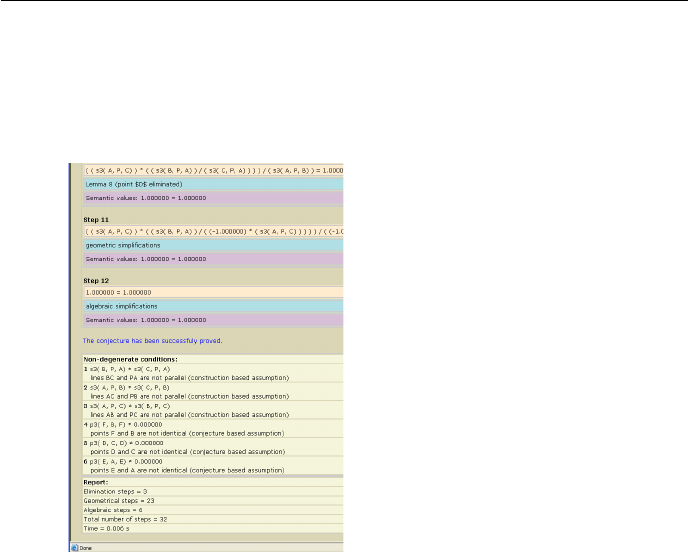
E.5 Example (Ceva’s theorem) 99
Time spent by the prover: 0.002 seconds
A fragment of the xml output of the prover based on the area method:
A fragment of the L
A
T
E
X output of the prover based on the Wu’s method:
Creating polynomials from hypotheses
•Point A
no condition
•Point B
no condition
•Point C
no condition
•Point P
no condition
•Line a:B C
–point Bis on the line (B,C)
no condition
–point Cis on the line (B,C)
no condition
•Line b:A C
–point Ais on the line (A,C)
no condition

100 E Examples
–point Cis on the line (A,C)
no condition
•Line c:A B
–point Ais on the line (A,B)
no condition
–point Bis on the line (A,B)
no condition
•Line pa:P A
–point Pis on the line (P,A)
no condition
–point Ais on the line (P,A)
no condition
•Line pb:P B
–point Pis on the line (P,B)
no condition
–point Bis on the line (P,B)
no condition
•Line pc:P C
–point Pis on the line (P,C)
no condition
–point Cis on the line (P,C)
no condition
•Intersection of lines, D:a pa
–point Dis on the line (B,C)
p33 =−u3x2+ (u2−u1)x1+u3u1
–point Dis on the line (P,A)
p34 =u5x2−u4x1
•Intersection of lines, E:b pb
–point Eis on the line (A,C)
p35 =−u3x4+u2x3
–point Eis on the line (P,B)
p36 =u5x4+ (−u4+u1)x3−u5u1
•Intersection of lines, F:c pc
–point Fis on the line (A,B) — true by the construction
no condition
–point Fis on the line (P,C)
p37 = (u5−u3)x6+ (−u5u2+u4u3)

E.5 Example (Ceva’s theorem) 101
Creating polynomial from the conjecture
•Processing given conjecture(s).
Conjecture 1:
p38 =−2x6x3x1+u3x6x3+u3x6x1+u1x3x1−u3u1x3
Invoking the theorem prover
The used proving method is Wu’s method.
The input system is:
p0=−u3x2+ (u2−u1)x1+u3u1
p1=u5x2−u4x1
p2=−u3x4+u2x3
p3=u5x4+ (−u4+u1)x3−u5u1
p4= (u5−u3)x6+ (−u5u2+u4u3)
Triangulation, step 1
Choosing variable: Trying the variable with index 6.
Variable x6selected: The number of polynomials with this variable is 1.
Single polynomial with chosen variable: No reduction needed.
The triangular system has not been changed.
Triangulation, step 2
Choosing variable: Trying the variable with index 5.
Choosing variable: Trying the variable with index 4.
Variable x4selected: The number of polynomials with this variable is 2.
Minimal degrees: 3 polynomials with degree 1 and 2 polynomials with degree
1.
Polynomial with linear degree: Removing variable x4from all other poly-
nomials by reducing them with polynomial p3.
Finished a triangulation step, the current system is:
p0=−u3x2+ (u2−u1)x1+u3u1
p1=u5x2−u4x1
p2= (u5u2−u4u3+u3u1)x3−u5u3u1
p3=u5x4+ (−u4+u1)x3−u5u1
p4= (u5−u3)x6+ (−u5u2+u4u3)

102 E Examples
Triangulation, step 3
Choosing variable: Trying the variable with index 3.
Variable x3selected: The number of polynomials with this variable is 1.
Single polynomial with chosen variable: No reduction needed.
The triangular system has not been changed.
Triangulation, step 4
Choosing variable: Trying the variable with index 2.
Variable x2selected: The number of polynomials with this variable is 2.
Minimal degrees: 1 polynomials with degree 1 and 0 polynomials with degree
1.
Polynomial with linear degree: Removing variable x2from all other poly-
nomials by reducing them with polynomial p1.
Finished a triangulation step, the current system is:
p0= (u5u2−u5u1−u4u3)x1+u5u3u1
p1=u5x2−u4x1
p2= (u5u2−u4u3+u3u1)x3−u5u3u1
p3=u5x4+ (−u4+u1)x3−u5u1
p4= (u5−u3)x6+ (−u5u2+u4u3)
Triangulation, step 5
Choosing variable: Trying the variable with index 1.
Variable x1selected: The number of polynomials with this variable is 1.
Single polynomial with chosen variable: No reduction needed.
The triangular system has not been changed.
The triangular system is:
p0= (u5u2−u5u1−u4u3)x1+u5u3u1
p1=u5x2−u4x1
p2= (u5u2−u4u3+u3u1)x3−u5u3u1
p3=u5x4+ (−u4+u1)x3−u5u1
p4= (u5−u3)x6+ (−u5u2+u4u3)

E.5 Example (Ceva’s theorem) 103
Final remainder
Final remainder for conjecture 1
Calculating final remainder of the conclusion:
g=−2x6x3x1+u3x6x3+u3x6x1+u1x3x1−u3u1x3
with respect to the triangular system.
1. Pseudo remainder with p4over variable x6:
g= (−2u5u2+u5u1+ 2u4u3−u3u1)x3x1+
(u5u3u2−u5u3u1−u4u2
3+u2
3u1)x3+ (u5u3u2−u4u2
3)x1
2. Pseudo remainder with p3over variable x4:
g= (−2u5u2+u5u1+ 2u4u3−u3u1)x3x1+
(u5u3u2−u5u3u1−u4u2
3+u2
3u1)x3+ (u5u3u2−u4u2
3)x1
3. Pseudo remainder with p2over variable x3:
g= (u2
5u3u2
2−2u2
5u3u2u1+u2
5u3u2
1−2u5u4u2
3u2+
2u5u4u2
3u1+u5u2
3u2u1−u5u2
3u2
1+u2
4u3
3−u4u3
3u1)x1+
(u2
5u2
3u2u1−u2
5u2
3u2
1−u5u4u3
3u1+u5u3
3u2
1)
4. Pseudo remainder with p1over variable x2:
g= (u2
5u3u2
2−2u2
5u3u2u1+u2
5u3u2
1−2u5u4u2
3u2+
2u5u4u2
3u1+u5u2
3u2u1−u5u2
3u2
1+u2
4u3
3−u4u3
3u1)x1+
(u2
5u2
3u2u1−u2
5u2
3u2
1−u5u4u3
3u1+u5u3
3u2
1)
5. Pseudo remainder with p0over variable x1:
g= 0
Prover report
Status: The conjecture has been proved.
Space Complexity: The biggest polynomial obtained during proof process
contained 13 terms.
Time Complexity: Time spent by the prover is 0.053 seconds.
NDG conditions are:
•PF BF 6= 0 i.e., points Fand Bare not identical (conjecture based
assumption).
•PDCD 6= 0 i.e., points Dand Care not identical (conjecture based
assumption).
•PEAE 6= 0 i.e., points Eand Aare not identical (conjecture based
assumption).

104 E Examples
Bibliography
[1] B. Buchberger. An Algorithm for finding a basis for the residue class ring
of a zero-dimensional polynomial ideal. PhD thesis, Math. Inst. University
of Innsbruck, Austria, 1965.
[2] B. Buchberger and F. e. Winkler. Gr¨obner Bases and Applications. Cam-
bridge University Press, 1998.
[3] C. C. Chou, O. X. S. Gao, and J. Z. Zhang. Automated production of
traditional proofs for constructive geometry theorems. In Eighth Annual
IEEE Symposium on Logic in Computer Science, 1993.
[4] S.-C. Chou. Mechanical Geometry Theorem Proving. D.Reidel Publishing
Company, Dordrecht, 1988.
[5] M. Djori´c and P. Janiˇci´c. Constructions, instructions, interactions . Teach-
ing Mathematics and its Applications, 23(2):69–88, 2004.
[6] P. Janiˇci´c. GCLC – A Tool for Constructive Euclidean Geometry and More
than That. In N. Takayama, A. Iglesias, and J. Gutierrez, editors, Pro-
ceedings of International Congress of Mathematical Software (ICMS 2006),
volume 4151 of Lecture Notes in Computer Science, pages 58–73. Springer-
Verlag, 2006.
[7] P. Janiˇci´c and P. Quaresma. System description: Gclcprover + GeoThms.
In U. Furbach and N. Shankar, editors, International Joint Conference
on Automated Reasoning (IJCAR-2006), volume 4130 of Lecture Notes in
Artificial Intelligence, pages 145–150. Springer-Verlag, 2006.
[8] P. Janiˇci´c. Geometry Constructions Language. Journal of Automated Rea-
soning, 2009. to appear.
[9] P. Janiˇci´c and I. Trajkovi´c. WinGCLC — a Workbench for Formally De-
scribing Figures. In Proceedings of the 18th Spring Conference on Computer
Graphics (SCCG 2003), pages 251–256, Budmerice, Slovakia, April, 24-26
2003. ACM Press, New York, USA.
[10] P. Quaresma and P. Janiˇci´c. Integrating dynamic geometry software, de-
duction systems, and theorem repositories. In J. Borwein and W. Farmer,
editors, Mathematical Knowledge Management (MKM-2006), volume 4108
of Lecture Notes in Artificial Intelligence, pages 280–294. Springer-Verlag,
2006.

106 BIBLIOGRAPHY
[11] P. Quaresma and P. Janiˇci´c. Framework for the Constructive Geometry.
Technical Report TR2006/001, Center for Informatics and Systems of the
University of Coimbra, 2006.
[12] W.-T. Wu. On the decision problem and the mechanization of theorem
proving in elementary geometry. Scientia Sinica, 21:157–179, 1978.
Index
%,31
ang3d axes drawing range,37
ang3d draw parametric curve,39
ang3d draw parametric surface,38
ang3d drawline p,38
ang3d drawsystem p,37
ang3d getx,38
ang3d gety,38
ang3d getz,38
ang3d origin,37
ang3d picture,37
ang3d point,38
ang3d scale,37
ang3d unit,37
ang conic,35
ang conicprecision,36
ang draw parametric curve,35
ang drawconic,35
ang drawdashconic,35
ang drawline,35
ang drawline p,35
ang drawsystem,34
ang drawsystem0,34
ang drawsystem0 a,34
ang drawsystem1,34
ang drawsystem1 a,34
ang drawsystem a,34
ang drawsystem p,34
ang getx,34
ang gety,35
ang intersec2,35
ang intersection2,35
ang line,35
ang origin,33
ang picture,33
ang plot data,36
ang point,34
ang scale,33
ang tangent,35
ang unit,33
angle,19
angle o,19
animation frames,40
area,31
array,20
arrowstyle,31
background,31
batch processing, 51,53,54
bezierprecision,32
bis,17
bisector,17
bitmap, 46,49
call,22
circle,16
circleprecision,32
cmark,10,29
color,31
comments, 31,49
control structures, 5
dash,32
dashstyle,32
deductive verification, 69
dim,31
distance,19
dmc,32
double,32
dradashwarc p,24
drawarc,24
drawarc p,24
drawarrow,23
drawbezier3,25
drawbezier4,25
drawcircle,23
drawdasharc,24
drawdashbezier3,25
drawdashbezier4,26
drawdashcircle,24
drawdashellipse,24

108 INDEX
drawdashellipsearc,24
drawdashellipsearc1,25
drawdashellipsearc1,25
drawdashline,23
drawdashsegment,23
drawellipse,24
drawellipsearc,24
drawellipsearc1,25
drawellipsearc2,25
drawgraph a,27
drawgraph b,27
drawline,23
drawpoint,23
drawpolygon,26
drawsegment,10,23
drawtree,26
drawvector,23
eps,33,46,49,54,66
export, 49
to L
A
T
E
X, 46,49,52,53,66
to bitmap, 46,54
to PSTricks, 52
to TikZ, 46,53
to eps,46,54,66
to svg,46,55,68
to xml,46,55,68
export to eps,33
export to latex,33,49
export to pstricks,33
export to simple latex,33
export to svg,33
export to tikz,33
expression,19
fillarc,28
fillarc0,29
fillcircle,28
fillellipse,28
fillellipsearc,29
fillellipsearc0,29
fillrectangle,28
filltriangle,28
fontsize,31
foot,17,61
getcenter,17
getx,19
gety,19
hide layer,39
hide layer from,39
hide layers to,39
if then else,21
import
from JavaView, 6,46
include,22
installation, 9
intersec,16,61
intersec2,16
intersection,16
intersection2,16
JavaView, 6,46,79,85
L
A
T
E
X, 5,9,10,33,44,46,47,49–54,
66,69
L
A
T
E
X
package, 9,11,31,50,53–55,67
layer,39
line,16,61
linethickness,32
log file, 12
loops, 5,20
mark,29
mcp,32
mcr,32
med,17,61
mediatrice,17
midpoint,17,61
normal,32
number,16
oncircle,17
online,17,61
onsegment,17
parallel,17,61
pdf,55
perp,17,61
perpendicular,17
point,10,16,34,40,43,61,65
PostScript,55
printat,30
printvalueat,30
procedure,22
procedures, 5,22
prooflevel,41,57,66
prooflimit,41,57

INDEX 109
prove,40,57,58,66,68
prover timeout,41,57
PSTricks, 33,46,49,52
Q.E.D.,67
random,19
rotate,18
rotateonellipse,18
samples, 9
set equal,16
sim,18
svg,33,46,49,55,68
symbolic expressions, 5,16,19
symmetrical,18
theorem prover, 5,40,57
area method, 57,62
Gr¨obner bases method, 57,65
Wu’s method, 57,65
theorem name,41,57
TikZ, 33,46,49,53
towards,18,61
trace,40
translate,18,61
turtle,18
view, 9,85
while,20
WinGCLC,5,9,43
xml,44,46,47,49,55,68,69,73
xml validation, 74
