1 CALISTA USER MANUAL
User Manual:
Open the PDF directly: View PDF ![]() .
.
Page Count: 38

1
CALISTA: User Manual
Version 1.2.0 (1 December 2018)
Authors: Nan Papili Gao and Rudiyanto Gunawan
Institute for Chemical and Bioengineering
ETH Zurich
Contact e-mail: nanp@ethz.ch and rgunawan@buffalo.edu
Table of contents
1!Overview ........................................................................................................... 2!
2!System requirements ........................................................................................ 2!
3!CALISTA package ............................................................................................ 2!
4!Examples ........................................................................................................... 3!
4.1!Example 1. iPSC differentiation into mesodermal and endodermal cells ........................ 3!
4.1.1!Data Import and Preprocessing .................................................................................... 3!
4.1.2!Single-cell clustering ................................................................................................... 4!
4.1.3!Reconstruction of lineage progression .......................................................................... 5!
4.1.4!Determination of transition genes ................................................................................ 7!
4.1.5!Pseudotemporal ordering of cells ................................................................................. 8!
4.1.6!Path analysis ............................................................................................................... 8!
4.2!Example 2. Hematopoietic stem cell differentiation ....................................................... 10!
4.2.1!Data Import and Preprocessing .................................................................................. 10!
4.2.2!Single-cell clustering ................................................................................................. 10!
4.2.3!Reconstruction of lineage progression ........................................................................ 11!
4.2.4!Determination of transition genes .............................................................................. 12!
4.2.5!Pseudotemporal ordering of cells ............................................................................... 12!
4.2.6!Path analysis ............................................................................................................. 13!
4.3!Example 3. Mouse embryonic fibroblast differentiation into neurons (Manual data
import) ........................................................................................................................................ 13!
4.3.1!Data Import and Preprocessing .................................................................................. 13!
4.3.2!Single-cell clustering ................................................................................................. 16!
4.3.3!Reconstruction of lineage progression ........................................................................ 17!
4.3.4!Determination of transition genes .............................................................................. 17!
4.3.5!Pseudotemporal ordering of cells ............................................................................... 17!
4.4!Example 4. Human embryonic stem cell differentiation into endodermal cells ............. 18!
4.4.1!Data Import and Preprocessing .................................................................................. 18!
4.4.2!Single-cell clustering ................................................................................................. 18!
4.4.3!Reconstruction of lineage progression ........................................................................ 19!
4.4.4!Determination of transition genes .............................................................................. 21!
4.4.5!Pseudotemporal ordering of cells ............................................................................... 21!
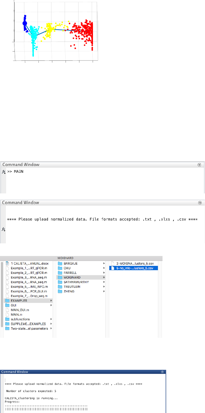
4.5!Example 5. Running CALISTA without time or cell stage information ........................ 22!
4.5.1!Data Import and Preprocessing .................................................................................. 22!
4.5.2!Single-cell clustering ................................................................................................. 22!
4.5.3!Reconstruction of lineage progression and pseudotemporal ordering of cells .............. 23!
4.6!Example 6. Removing undesired clusters ....................................................................... 25!
4.6.1!Data Import and Preprocessing .................................................................................. 25!
4.6.2!Single-cell clustering ................................................................................................. 25!
4.6.3!Single-cell clustering after removing undesired clusters ............................................. 26!
4.6.4!Reconstruction of lineage progression ........................................................................ 27!
4.6.5!Determination of transition genes .............................................................................. 28!
4.6.6!Pseudotemporal ordering of cells ............................................................................... 28!
4.7!Running CALISTA GUI ................................................................................................. 28!
4.7.1!Data Import and Preprocessing .................................................................................. 28!

2
4.7.2!Single-cell clustering ................................................................................................. 29!
4.7.3!Reconstruction of lineage progression ........................................................................ 30!
4.7.4!Determination of transition genes .............................................................................. 31!
4.7.5!Pseudotemporal ordering of cells ............................................................................... 32!
4.8!Example 8. Reconstruction of developmental trajectories during zebrafish
embryogenesis ............................................................................................................................ 32!
4.8.1!Data Import and Preprocessing .................................................................................. 32!
4.8.2!Single-cell clustering ................................................................................................. 33!
4.8.3!Reconstruction of lineage progression ........................................................................ 34!
4.8.4!Determination of transition genes .............................................................................. 34!
4.8.5!Pseudotemporal ordering of cells ............................................................................... 34!
4.8.6!Path analysis ............................................................................................................. 35!
4.9!Example 9. Identification of mouse spinal cord neurons activity during behavior ....... 35!
4.9.1!Data Import and Preprocessing .................................................................................. 35!
4.9.2!Single-cell clustering ................................................................................................. 36!
4.10!Example 9. Analysis of peripherical blood mononuclear cells (PBMCs) ....................... 37!
4.10.1!Data Import and Preprocessing .................................................................................. 37!
4.10.2!Single-cell clustering ................................................................................................. 37!
5!Questions and comments .................................................................................38!
1 Overview
This user manual is for the MATLAB distribution of CALISTA (Clustering And Lineage Inference in Single Cell
Transcriptional Analysis).
CALISTA provides a user-friendly toolbox for the analysis of single cell expression data. CALISTA accomplishes
three major tasks:
(1) Identification of cell clusters in a cell population based on single-cell gene expression data;
(2) Reconstruction of lineage progression and produce transition genes;
(3) Pseudotemporal ordering of cells along any given developmental paths in the lineage progression.
For detailed information about CALISTA, please refer to the following manuscript.
Papili Gao N., Hartmann T, Fang T., and Gunawan R., CALISTA: Clustering and lineage inference in single-
cell transcriptional analysis, bioRxiv, 2018. https://doi.org/10.1101/257550
2 System requirements
This distribution of CALISTA is written for and developed in MATLAB
1
.
CALISTA has been successfully tested on MATLAB 2016b, 2017a, 2018a and 2018b.
3 CALISTA package
CALISTA package contains the following files and folders:
1. This CALISTA_USER_MANUAL.doc file
2. License.txt modified BSD license for CALISTA
3. MAIN.m CALISTA main script (use this script to run CALISTA on your own dataset)
4. MAIN_GUI.m GUI version of CALISTA (use this script to run CALISTA_GUI on your own
dataset)
5. Example scripts on how to use CALISTA subroutines and GUI version of CALISTA
6. Save_to_matlab.R R script describing how to convert the dataset (especially large text
files) in Matlab files
1
http://www.mathworks.com
3
7. The folder Two-state model parameters containing:
a. Parameters.mat steady-state distribution functions of mRNA level
8. The folder subfunctions containing the following main subroutines (and other
subroutines):
a. import_data.m : upload single-cell expression data and perform preprocessing.
b. CALISTA_clustering_main.m: single-cell clustering in CALISTA.
c. CALISTA_transition_main.m: infer lineage progression among cell
clusters.
d. CALISTA_transition_genes_main.m: identify the key genes in lineage
progression.
e. CALISTA_ordering_main.m: perform pseudotemporal ordering of cells.
f. CALISTA_landscape_plotting_main.m: landscape plots of single
cells in the dataset based on cell-likelihood values
g. CALISTA_path_main.m: perform post-analysis along developmental path(s).
9. The folder EXAMPLES containing single-cell expression datasets used in the examples
below.
10. The folder GUI containing the subroutines used in MAIN_GUI.m
11. The folder SUPPLEMENTARY EXAMPLES containing the additional analysis
For further information on running the main subroutines in CALISTA, please use Matlab ‘help’
command followed by function_name(for example ‘help import_data’).
4 Examples
In the following, we describe the main steps of CALISTA applied to publicly available single-cell gene
expression data. For each dataset, ONLY the most important results are reported. Please refer to the file
MAIN.m for an example MATLAB script of CALISTA implementation.
4.1 Example 1. iPSC differentiation into mesodermal and endodermal cells
Analysis of RT-qPCR data of Bargaje et al. (Bargaje, et al, Cell population structure prior to bifurcation predicts
efficiency of directed differentiation in human induced pluripotent cells. Proc. Natl. Acad. Sci. U. S. A. 114, 2271–
2276 (2017)).
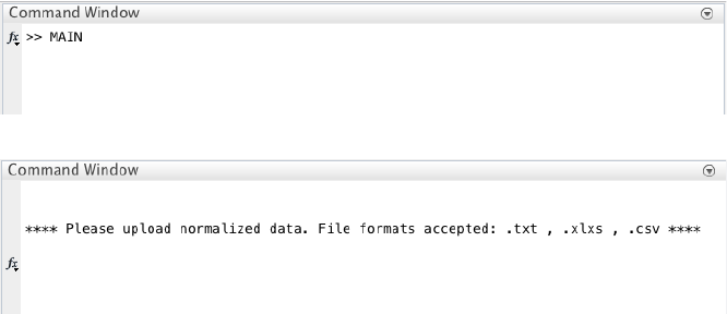
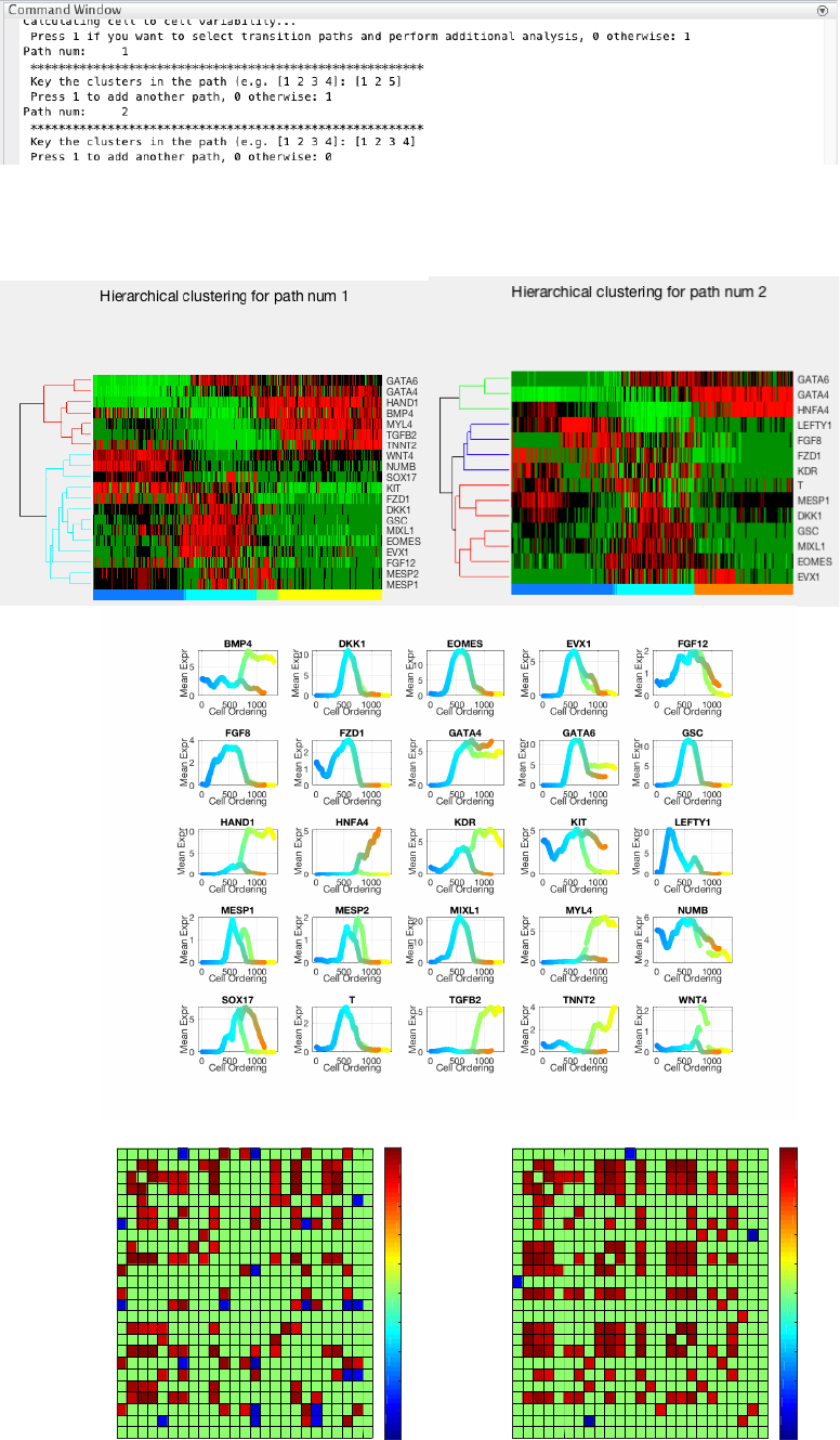
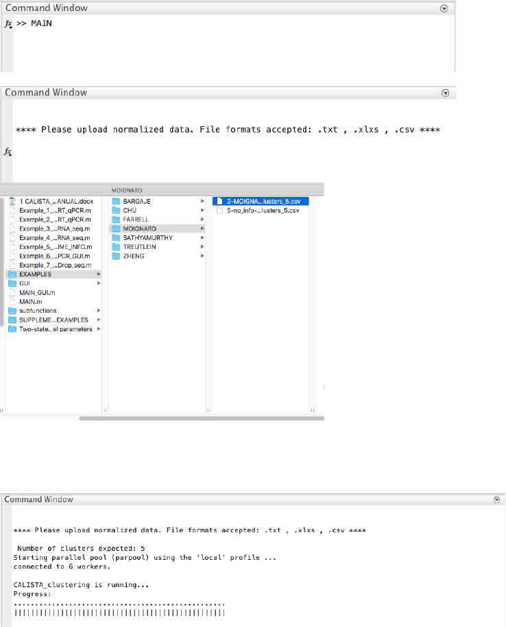
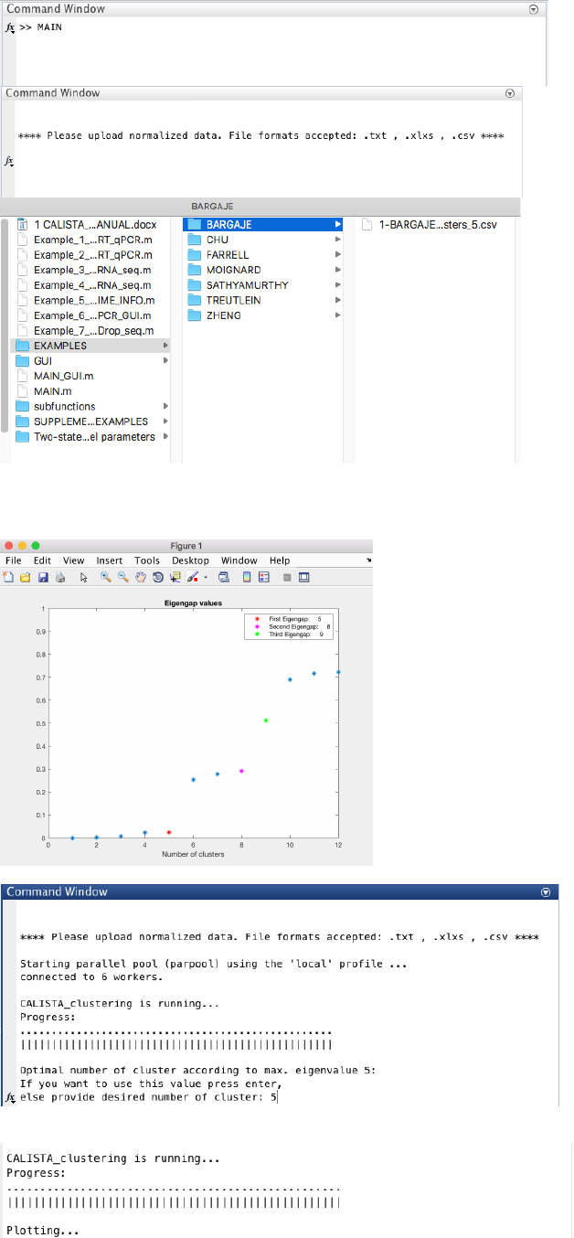
4.1.1 Data Import and Preprocessing
We begin with changing the current directory in MATLAB to the CALISTA folder. Then, we run
Example_1_BARGAJE_scRT_qPCR.m script in the main folder of CALISTA and import Bargaje dataset
(available in the subfolder EXAMPLES/BARGAJE).
The following are screenshots from running CALISTA on MATLAB.
4
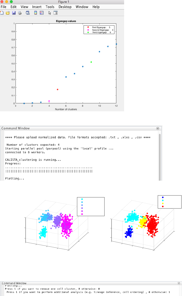
4.1.2 Single-cell clustering
In this case, the number of clusters is determined using the eigengap plot. According to the eigengap plot below,
we set the number of clusters to 5. The following are screenshots from CALISTA single-cell clustering analysis.
5
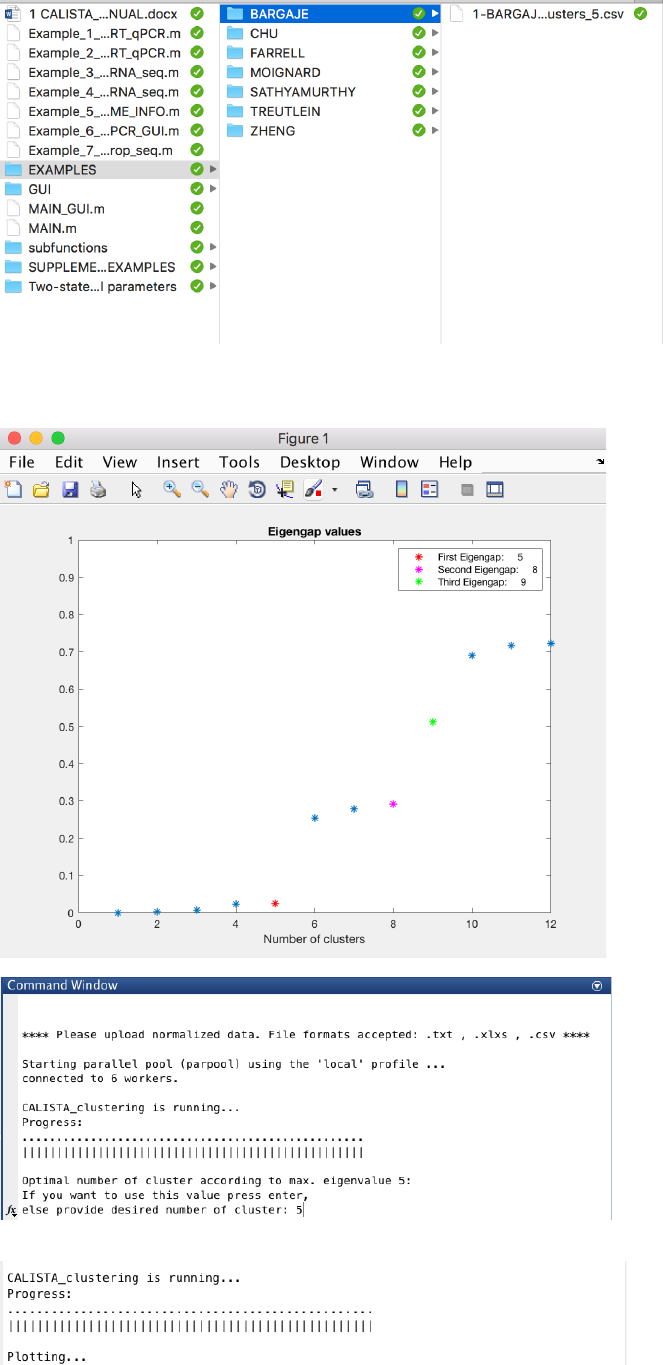
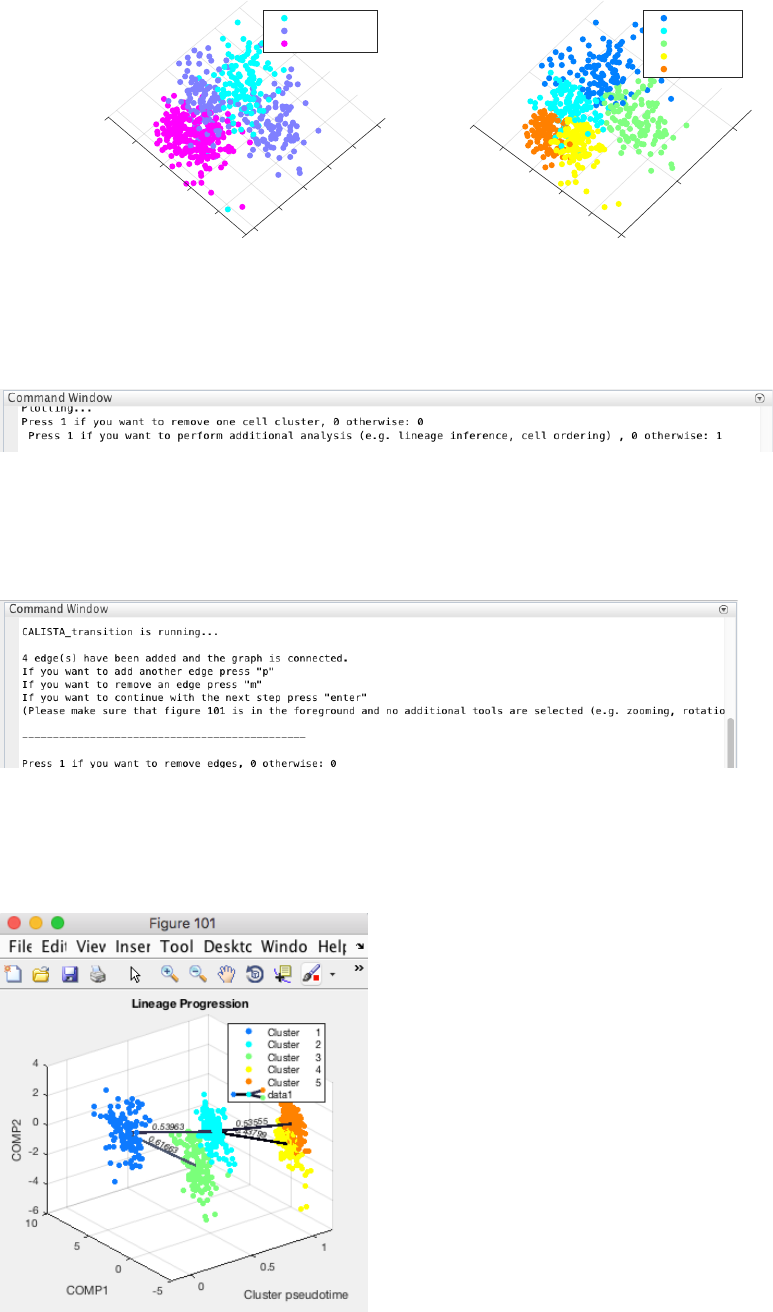
If desired, users can remove cells from specific clusters from further analysis. In this example, we do not want to
remove any clusters. Hence, we enter 0 (no cluster removal) and then 1 to proceed with lineage inference.
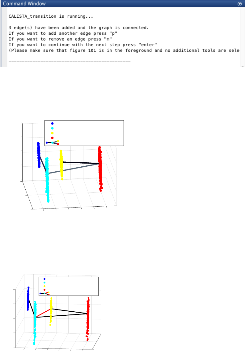
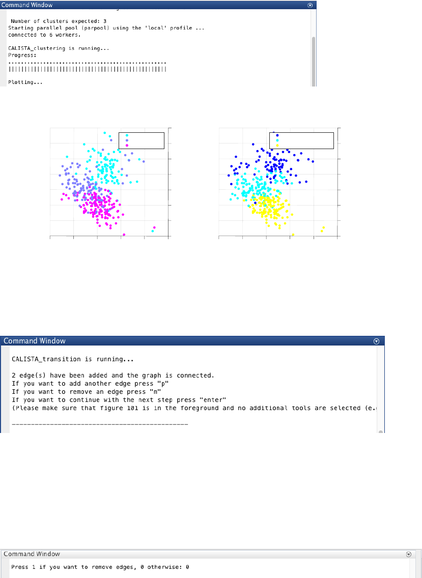
4.1.3 Reconstruction of lineage progression
During the lineage inference step, CALISTA automatically generates and displays a lineage graph, obtained by
adding an edge between two clusters in increasing cluster distances, until all clusters are connected to at least one
other cluster. Subsequently, users can manually add or remove one edge at time based on the cluster distances.
ATTENTION: to add an edge (press “p”), remove an edge (press “m”) or finalize the lineage progression graph
(press “enter”), the MATLAB figure of the graph must appear in foreground without any modification (e.g.,
zooming, rotation). Note that the addition/removal of the edges are performed according to increasing/decreasing
order of cluster distance.
ATTENTION: the final graph must be connected (i.e. there exists a path from any node/cluster to any other
node/cluster in the graph), otherwise a warning will be returned.
Original time/cell stage info
-2
-4
5
0
2
10
4
15 PC1
-5
6
0
8
-10 -15
-6
10
-8
PC2
Time/Stage 0
Time/Stage 24
Time/Stage 36
Time/Stage 48
Time/Stage 60
Time/Stage 72
Time/Stage 96
Time/Stage 120
Cell Clustering
PC2
10
8
6
4
0
-2
-4
-6
-8
PC1
15 10 50-5 -10 -15
2
Cluster 1
Cluster 2
Cluster 3
Cluster 4
Cluster 5
6
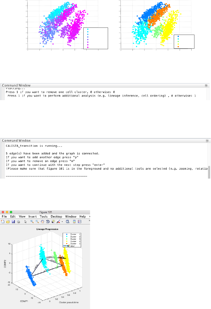
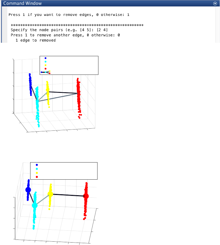
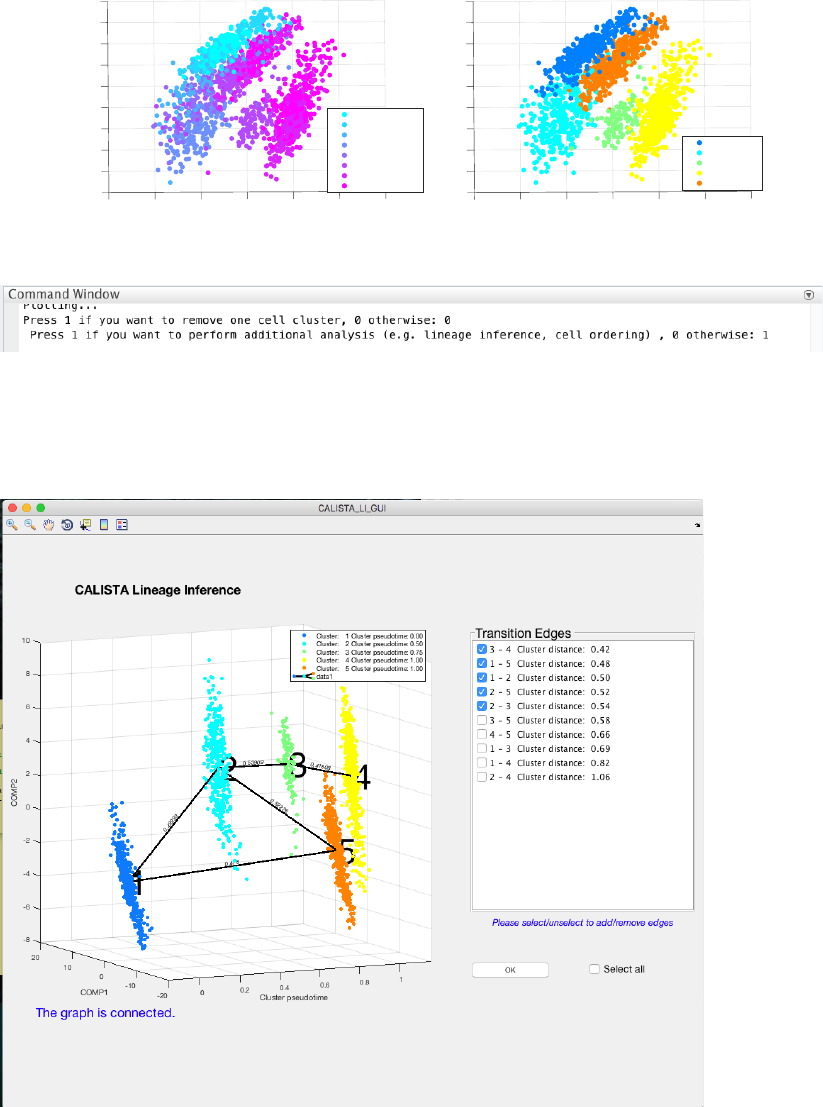
Since the transition from cluster 1 to cluster 5 is inconsistent with the capture time info (i.e. cluster pseudotime
values for cluster 1 and 5 are 0 and 1 respectively) we remove the spurious edge between cluster 1 and 5, by
entering 1 and entering [1 5], upon the following query.
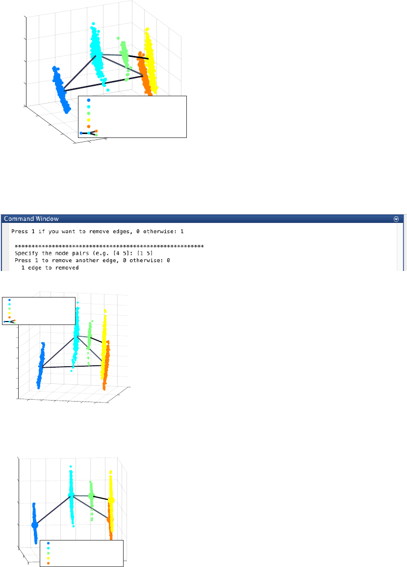
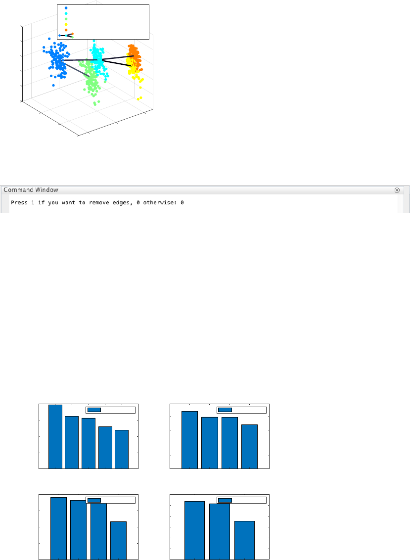
The final inferred lineage relationships are displayed below.
In addition, CALISTA provides the following.
- Cell clustering plot based on the cluster pseudotime
-10
20
-5
0
COMP2
10
0.52226
5
0.478
10
0.49993
0.53909
COMP1
Lineage Progression
0
0.41808
1
0.8
Cluster pseudotime
-10 0.6
0.4
0.2
-20 0
Cluster: 1 Cluster pseudotime: 0.00
Cluster: 2 Cluster pseudotime: 0.50
Cluster: 3 Cluster pseudotime: 0.75
Cluster: 4 Cluster pseudotime: 1.00
Cluster: 5 Cluster pseudotime: 1.00
data1
20
1
0.49993
2
0.53909
0.478
0.52226
Lineage Progression
COMP1
0
5
3
0.41808
4
-8
-6
-4
-2
0
2
COMP2
4
Cluster pseudotime
6
8
10
00.2 0.4 -20
0.6 0.8 1
Cluster: 1 Cluster pseudotime: 0.00
Cluster: 2 Cluster pseudotime: 0.50
Cluster: 3 Cluster pseudotime: 0.75
Cluster: 4 Cluster pseudotime: 1.00
Cluster: 5 Cluster pseudotime: 1.00
data1
-10
-5
0
5
10
20
PC2
2
0.49993
0.52226
15
0.53909
0
PC1
Lineage Progression
3
0.41808
4
1
0.8
0.6
0.4
Cluster pseudotime
0.2
0
-20
Cluster: 1 Cluster pseudotime: 0.00
Cluster: 2 Cluster pseudotime: 0.50
Cluster: 3 Cluster pseudotime: 0.75
Cluster: 4 Cluster pseudotime: 1.00
Cluster: 5 Cluster pseudotime: 1.00
7
- Boxplot, mean, median entropy values calculated for each cluster
- Plot of mean expression values for each gene based on cell cluster expression level
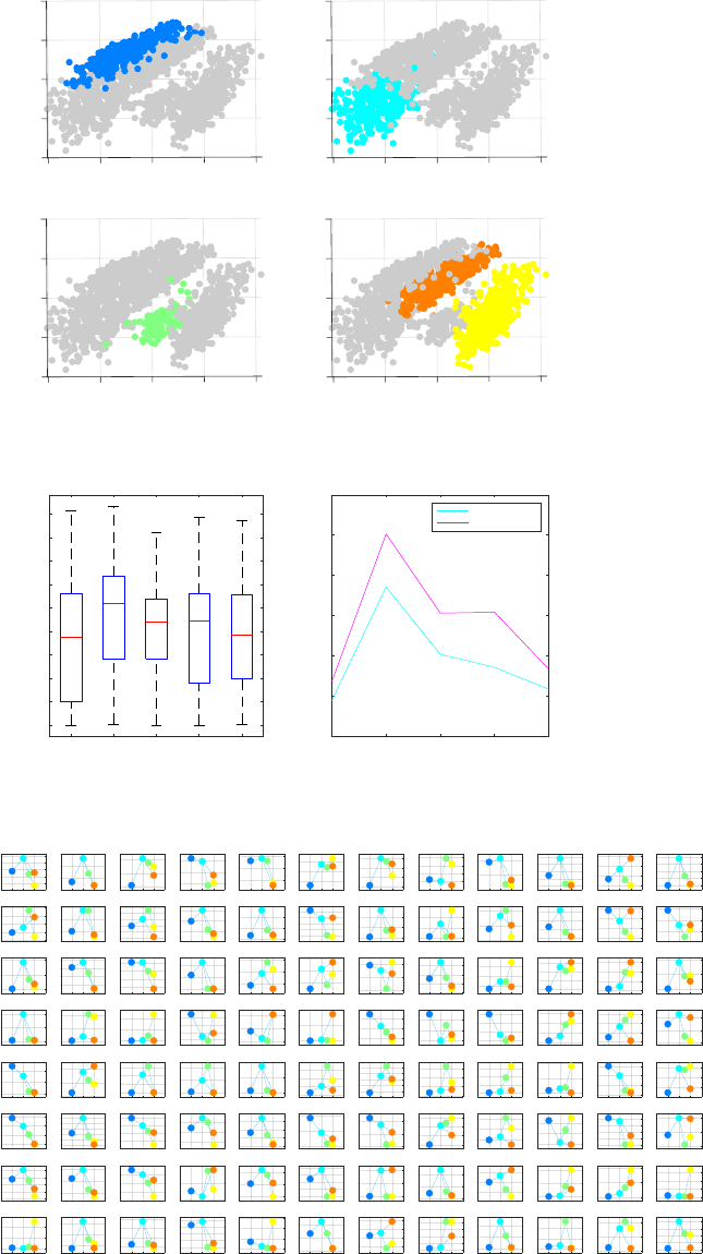
4.1.4 Determination of transition genes
After reconstructing the lineage progression, we identify the key transition genes for any two connected clusters in
the graph, based on the gene-wise likelihood difference between having the cells separately as two clusters and
together as a single cluster. Larger differences in the gene-wise likelihood point to more informative genes. The
transition genes are selected as those whose gene-wise likelihood differences make up to more than a certain
CALISTA cluster pseudotime 0
PC2
10
5
-5
-10
PC1
10 50-5 -10
0
CALISTA cluster pseudotime 0.5
PC2
10
5
0
-5
-10
PC1
10 50-5 -10
CALISTA cluster pseudotime 0.75
PC2
10
5
0
-5
-10
PC1
10 50-5 -10
CALISTA cluster pseudotime 1
-10
PC1
10
-5
50-5 -10
0
10
PC2
5
12345
Cluster
0
0.5
1
1.5
2
2.5
3
3.5
4
4.5
Entropy
Boxplot for the entropy
12345
Cluster
1.6
1.8
2
2.2
2.4
2.6
2.8
Entropy value
Entropy Mean and Median
MeanEntropy
MedianEntropy
-0.5 0 0.5 1 1.5
1.5
2
2.5
3
3.5
ACVR1B
-0.5 0 0.5 1 1.5
3
4
5
ACVR2A
-0.5 0 0.5 1 1.5
0
0.1
0.2
ACVRL1
-0.5 0 0.5 1 1.5
1
2
3
ALCAM
-0.5 0 0.5 1 1.5
0.8
1
1.2
ANF
-0.5 0 0.5 1 1.5
5
6
7
BAMBI
-0.5 0 0.5 1 1.5
0
2
4
6
BMP2
-0.5 0 0.5 1 1.5
2
4
6
8
BMP4
-0.5 0 0.5 1 1.5
4
6
8
BMPR1A
-0.5 0 0.5 1 1.5
3
4
5
6
7
BMPR2
-0.5 0 0.5 1 1.5
1
2
3
4
CXCR4
-0.5 0 0.5 1 1.5
0
2
4
6
8
DKK1
-0.5 0 0.5 1 1.5
0
0.2
0.4
0.6
0.8
DLL1
-0.5 0 0.5 1 1.5
1
2
3
DLL3
-0.5 0 0.5 1 1.5
0.2
0.4
0.6
0.8
1
1.2
EMILIN2
-0.5 0 0.5 1 1.5
1
2
3
ENG
-0.5 0 0.5 1 1.5
0
5
10
15
EOMES
-0.5 0 0.5 1 1.5
2
4
6
8
10
EPCAM
-0.5 0 0.5 1 1.5
0
2
4
6
EVX1
-0.5 0 0.5 1 1.5
0
0.5
1
1.5
FGF10
-0.5 0 0.5 1 1.5
0
1
2
FGF12
-0.5 0 0.5 1 1.5
0
1
2
3
FGF8
-0.5 0 0.5 1 1.5
4
6
8
10
FGFR1
-0.5 0 0.5 1 1.5
5
6
7
FGFR2
-0.5 0 0.5 1 1.5
0
1
2
FOXC1
-0.5 0 0.5 1 1.5
3
4
5
6
7
FOXH1
-0.5 0 0.5 1 1.5
8
9
10
11
FSTL1
-0.5 0 0.5 1 1.5
0
1
2
FZD1
-0.5 0 0.5 1 1.5
2
4
6
FZD2
-0.5 0 0.5 1 1.5
2
3
4
FZD4
-0.5 0 0.5 1 1.5
1
1.5
2
FZD6
-0.5 0 0.5 1 1.5
4
6
8
10
FZD7
-0.5 0 0.5 1 1.5
0.5
1
1.5
GAS1
-0.5 0 0.5 1 1.5
0
2
4
6
GATA4
-0.5 0 0.5 1 1.5
0
0.2
0.4
0.6
GATA5
-0.5 0 0.5 1 1.5
0
5
10
GATA6
-0.5 0 0.5 1 1.5
0
5
10
GSC
-0.5 0 0.5 1 1.5
0
5
10
HAND1
-0.5 0 0.5 1 1.5
0
2
4
HAND2
-0.5 0 0.5 1 1.5
0.4
0.6
0.8
1
1.2
HEY1
-0.5 0 0.5 1 1.5
0
0.5
1
HHIP
-0.5 0 0.5 1 1.5
0
2
4
HNFA4
-0.5 0 0.5 1 1.5
1
2
3
HRT2
-0.5 0 0.5 1 1.5
0
0.2
0.4
INHBA
-0.5 0 0.5 1 1.5
0
0.1
0.2
0.3
IRX4
-0.5 0 0.5 1 1.5
0
1
2
3
ISL1
-0.5 0 0.5 1 1.5
0
2
4
6
KDR
-0.5 0 0.5 1 1.5
0
2
4
KIT
-0.5 0 0.5 1 1.5
0
2
4
LEFTY1
-0.5 0 0.5 1 1.5
2.4
2.6
2.8
LTBP1
-0.5 0 0.5 1 1.5
0
0.5
1
1.5
MESP1
-0.5 0 0.5 1 1.5
0
1
2
MESP2
-0.5 0 0.5 1 1.5
0
10
20
MIXL1
-0.5 0 0.5 1 1.5
0
1
2
3
MSX1
-0.5 0 0.5 1 1.5
1
2
3
4
5
MSX2
-0.5 0 0.5 1 1.5
0
0.2
0.4
0.6
MYL3
-0.5 0 0.5 1 1.5
0
2
4
6
MYL4
-0.5 0 0.5 1 1.5
0
2
4
MYOCD
-0.5 0 0.5 1 1.5
2
4
6
8
NANOG
-0.5 0 0.5 1 1.5
0.2
0.4
0.6
0.8
NKX2.5
-0.5 0 0.5 1 1.5
1
2
3
4
NOTCH1
-0.5 0 0.5 1 1.5
1.8
2
2.2
2.4
2.6
2.8
NOTCH2
-0.5 0 0.5 1 1.5
3
4
5
6
7
NOTCH3
-0.5 0 0.5 1 1.5
3
4
5
NUMB
-0.5 0 0.5 1 1.5
3
4
5
6
PARD3
-0.5 0 0.5 1 1.5
0
2
4
PDGFA
-0.5 0 0.5 1 1.5
0
0.5
1
PDGFB
-0.5 0 0.5 1 1.5
0
2
4
6
PDGFRA
-0.5 0 0.5 1 1.5
1
2
3
PDGFRB
-0.5 0 0.5 1 1.5
4
6
8
PTCH1
-0.5 0 0.5 1 1.5
0.5
1
1.5
2
2.5
PTX1
-0.5 0 0.5 1 1.5
0
1
2
PTX2
-0.5 0 0.5 1 1.5
3
4
5
6
7
RCOR2
-0.5 0 0.5 1 1.5
10
15
20
RPL35A
-0.5 0 0.5 1 1.5
0.2
0.3
0.4
0.5
SERCA
-0.5 0 0.5 1 1.5
2
4
6
SFRP1
-0.5 0 0.5 1 1.5
0
0.01
0.02
SHH
-0.5 0 0.5 1 1.5
0.4
0.6
0.8
1
1.2
SIRPA
-0.5 0 0.5 1 1.5
0
2
4
SOX17
-0.5 0 0.5 1 1.5
0
1
2
T
-0.5 0 0.5 1 1.5
0.2
0.4
0.6
TBX1
-0.5 0 0.5 1 1.5
0
1
2
TBX2
-0.5 0 0.5 1 1.5
0
2
4
TBX20
-0.5 0 0.5 1 1.5
0
0.5
1
1.5
TBX5
-0.5 0 0.5 1 1.5
0
2
4
TGFB2
-0.5 0 0.5 1 1.5
4
6
8
TGFB1
-0.5 0 0.5 1 1.5
4
5
6
7
TGFBR1
-0.5 0 0.5 1 1.5
0.6
0.8
1
1.2
1.4
TGFBR2
-0.5 0 0.5 1 1.5
0
1
2
3
TNNT2
-0.5 0 0.5 1 1.5
15
20
25
TUBB
-0.5 0 0.5 1 1.5
2
3
4
5
VEGFA
-0.5 0 0.5 1 1.5
0
0.2
0.4
0.6
0.8
WNT11
-0.5 0 0.5 1 1.5
0
0.05
0.1
WNT3A
-0.5 0 0.5 1 1.5
0
1
2
3
WNT4
-0.5 0 0.5 1 1.5
0
2
4
WNT5A
-0.5 0 0.5 1 1.5
0.1
0.2
0.3
0.4
0.5
WNT5B
8
percentage of the cumulative sum of the likelihood differences of all genes – set by
INPUTS.thr_transition_genes.
4.1.5 Pseudotemporal ordering of cells
For pseudotemporal ordering of cells, CALISTA performs maximum likelihood optimization for each cell using a
linear interpolation of the cell likelihoods between any two connected clusters. The pseudotimes of the cells are
computed by linear interpolation of the cluster pseudotimes, and correspond to the maximum point of the
likelihood optimization above. Cells are subsequently assigned to the edges in the lineage progression graph. The
following screenshot gives the results of this cell-to-edge assignment.
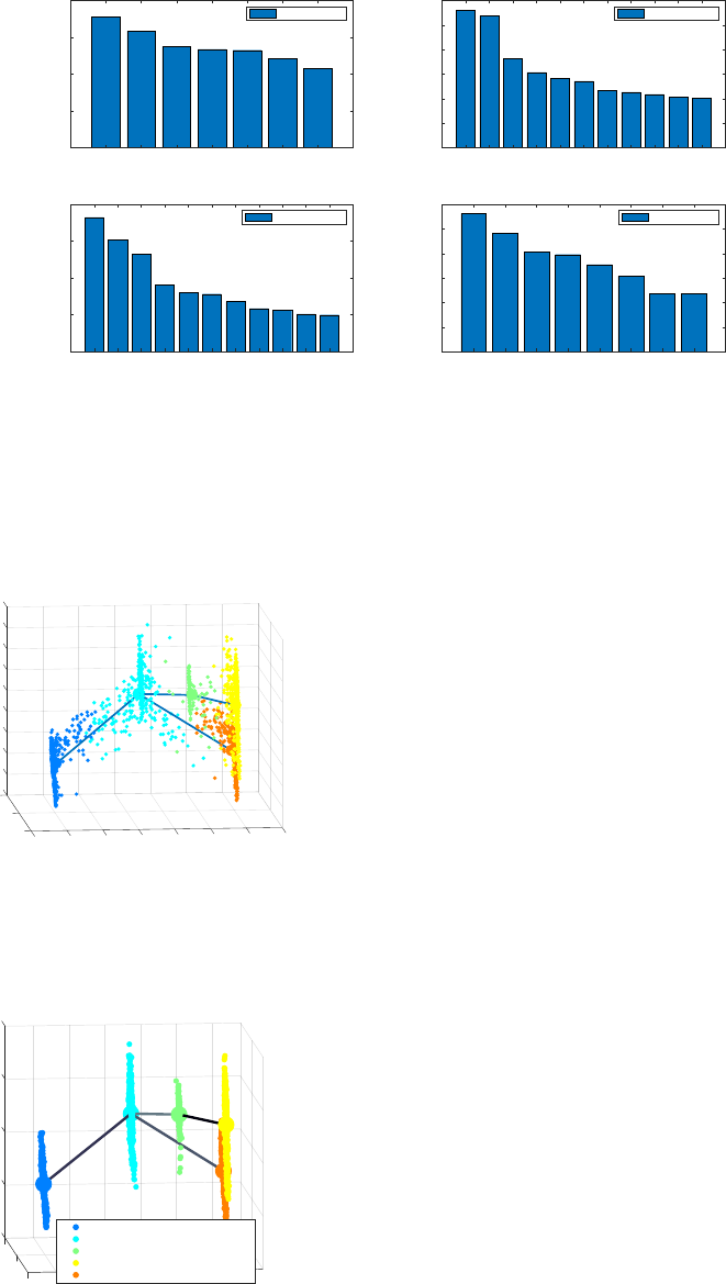
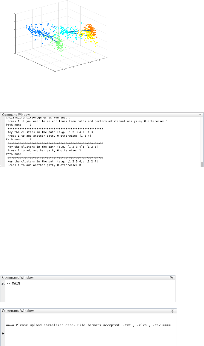
4.1.6 Path analysis
To perform path-specific analysis, users can enter 1 upon queried. In the following, we input two developmental
paths of interest: [1 2 3 4] (mesodermal fate) and [1 2 5] (endodermal fate).
1 - 2
GATA6
GSC
EOMES
MIXL1
DKK1
GATA4
EVX1
0
200
400
600
800
vg
j k
7 transition genes
2 - 3
GSC
MIXL1
HAND1
EOMES
WNT4
FZD1
MYL4
NUMB
BMP4
SOX17
KIT
0
50
100
150
200
250
300
vg
j k
11 transition genes
2 - 5
MIXL1
GSC
EOMES
FZD1
FGF8
DKK1
HNFA4
KDR
LEFTY1
MESP1
T
0
200
400
600
800
vg
j k
11 transition genes
3 - 4
WNT4
MESP2
MESP1
DKK1
TGFB2
FGF12
TNNT2
EOMES
0
50
100
150
200
250
300
vg
j k
8 transition genes
-8
-6
-4
-2
0
2
4
6
8
10
20
PC2
PC1
0
Cell Ordering
Cell Ordering
-20 1.2
1
0.8
0.6
0.4
0.2
0
-0.2
-10
-5
0
5
10
20
PC2
2
0.49993
0.52226
15
0.53909
0
PC1
Lineage Progression
3
0.41808
4
1
0.8
0.6
0.4
Cluster pseudotime
0.2
0
-20
Cluster: 1 Cluster pseudotime: 0.00
Cluster: 2 Cluster pseudotime: 0.50
Cluster: 3 Cluster pseudotime: 0.75
Cluster: 4 Cluster pseudotime: 1.00
Cluster: 5 Cluster pseudotime: 1.00
9
For each path, the post-analysis in CALISTA generates Clustergrams, moving-averaged gene expression profiles
and co-expression networks for the transition genes detected previously based on cell orderings.
Path num 1
BMP4
DKK1
EOMES
EVX1
FGF12
FGF8
FZD1
GATA4
GATA6
GSC
HAND1
HNFA4
KDR
KIT
LEFTY1
MESP1
MESP2
MIXL1
MYL4
NUMB
SOX17
T
TGFB2
TNNT2
WNT4
Target Gene j
BMP4
DKK1
EOMES
EVX1
FGF12
FGF8
FZD1
GATA4
GATA6
GSC
HAND1
HNFA4
KDR
KIT
LEFTY1
MESP1
MESP2
MIXL1
MYL4
NUMB
SOX17
T
TGFB2
TNNT2
WNT4
Source Gene i
-1
-0.8
-0.6
-0.4
-0.2
0
0.2
0.4
0.6
0.8
1 Path num 2
BMP4
DKK1
EOMES
EVX1
FGF12
FGF8
FZD1
GATA4
GATA6
GSC
HAND1
HNFA4
KDR
KIT
LEFTY1
MESP1
MESP2
MIXL1
MYL4
NUMB
SOX17
T
TGFB2
TNNT2
WNT4
Target Gene j
BMP4
DKK1
EOMES
EVX1
FGF12
FGF8
FZD1
GATA4
GATA6
GSC
HAND1
HNFA4
KDR
KIT
LEFTY1
MESP1
MESP2
MIXL1
MYL4
NUMB
SOX17
T
TGFB2
TNNT2
WNT4
Source Gene i
-1
-0.8
-0.6
-0.4
-0.2
0
0.2
0.4
0.6
0.8
1
10
4.2 Example 2. Hematopoietic stem cell differentiation
Analysis of RT-qPCR data in Moignard et al., Characterization of transcriptional networks in blood stem and
progenitor cells using high-throughput single-cell gene expression analysis, Nat. Cell Biol. 15, 363–72 (2013).
4.2.1 Data Import and Preprocessing
We start by changing the current directory in MATLAB to the CALISTA folder. We run
Example_2_MOIGNARD_scRT_qPCR.m script in the main folder of CALISTA and load Moignard dataset (in
subfolder EXAMPLES/MOIGNARD).
4.2.2 Single-cell clustering
Following the original publication, we set the number of clusters equals to 5.
CALISTA single-cell clustering results are as follow.
11
In this case, we do not need to remove any clusters (by pressing 0 upon queried). Then we proceed with further
analysis (by pressing 1 upon queried).
4.2.3 Reconstruction of lineage progression
During the lineage inference step, CALISTA automatically generates and displays a lineage graph, obtained by
adding an edge between two clusters in increasing cluster distances, until all clusters are connected to at least one
other cluster. Subsequently, users can manually add or remove one edge at time based on the cluster distances.
ATTENTION: to add an edge (press “p”), remove an edge (press “m”) or finalize the lineage progression graph
(press “enter”), the MATLAB figure of the graph must appear in foreground without any modification (e.g.,
zooming, rotation). Note that the addition/removal of the edges are performed according to increasing/decreasing
order of cluster distance.
ATTENTION: The final lineage progression graph must be connected (i.e. there is a path from any node/cluster
to any other node/cluster in the graph) otherwise a warning will be returned.
Original time/cell stage info
-4 PC1
6
4
-2
0
2
4
2
0
-2
-4
PC2
-6
Time/Stage 1
Time/Stage 2
Time/Stage 3
Cell Clustering
-2
-4 PC1
0
5
2
0
-5
4
-6
PC2
Cluster 1
Cluster 2
Cluster 3
Cluster 4
Cluster 5
12
Here, we do not need to remove any spurious edges, and hence we enter 0 upon queried.
In addition, CALISTA gives (not shown):
- Cell clustering plot based on the cluster pseudotime
- Boxplot, mean, median entropy values calculated for each cluster
- Plot of mean expression values for each gene based on cell cluster expression level
4.2.4 Determination of transition genes
After reconstructing the lineage progression, we identify the key transition genes for any two connected clusters in
the graph, based on the gene-wise likelihood difference between having the cells separately as two clusters and
together as a single cluster. Larger differences in the gene-wise likelihood point to more informative genes. The
transition genes are selected as those whose gene-wise likelihood differences make up to more than a certain
percentage of the cumulative sum of the likelihood differences of all genes – set by
INPUTS.thr_transition_genes.
4.2.5 Pseudotemporal ordering of cells
For pseudotemporal ordering of cells, CALISTA performs maximum likelihood optimization for each cell using a
linear interpolation of the cell likelihoods between any two connected clusters. The pseudotimes of the cells are
computed by linear interpolation of the cluster pseudotimes, and correspond to the maximum point of the
likelihood optimization above. Cells are subsequently assigned to the edges in the lineage progression graph. The
following screenshot gives the results of this cell-to-edge assignment.
-6
10
-4
-2
COMP2
5
0
1
0.61663
Lineage Progression
COMP1
0.43799
2
Cluster pseudotime
4
0.5
0
0.53555
0.53963
0
-5
Cluster: 1 Cluster pseudotime: 0.00
Cluster: 2 Cluster pseudotime: 0.50
Cluster: 3 Cluster pseudotime: 0.50
Cluster: 4 Cluster pseudotime: 1.00
Cluster: 5 Cluster pseudotime: 1.00
data1
1 - 2
Meis1
Gata2
Nfe2
Fli1
Erg
0
20
40
60
80
vg
j k
5 transition genes
1 - 3
Mitf
Gfi1
Meis1
Lmo2
0
20
40
60
80
100
vg
j k
4 transition genes
2 - 4
Meis1
Nfe2
Lmo2
Gata2
0
20
40
60
80
vg
j k
4 transition genes
2 - 5
Meis1
Gfi1b
Lmo2
0
20
40
60
80
100
120
vg
j k
3 transition genes
13
4.2.6 Path analysis
Finally, we perform post-analysis by entering 1 upon queried. Here, we input three developmental paths: [1 3], [1
2 5], and [1 2 4].
For each path, the post-analysis in CALISTA generates Clustergrams, moving-averaged gene expression profiles
and co-expression networks for the transition genes detected previously based on cell orderings (not shown).
4.3 Example 3. Mouse embryonic fibroblast differentiation into neurons (Manual data
import)
Analysis of RNA-seq data in Treutlein et al., Dissecting direct reprogramming from fibroblast to neuron using
single-cell RNA-seq, Nature 534, 391–395 (2016).
**Please unzip the file “3-TREUTLEIN_data_type_3_format_data_5_clusters_4.txt.zip” in
EXAMPLES/TREUTLEIN/ before running CALISTA**
4.3.1 Data Import and Preprocessing
Again, we change the current directory in MATLAB to the CALISTA folder. Here, we run
Example_3_TREUTLEIN_scRNA_seq.m script in the main folder of CALISTA and load Treutlein dataset (in
subfolder EXAMPLES/TREUTLEIN).
-6
10
-4
-2
1.2
PC2
5
0
1
Cell Ordering
PC1
2
0.8
Cell Ordering
0.6
4
00.4
0.2
-5 0
14
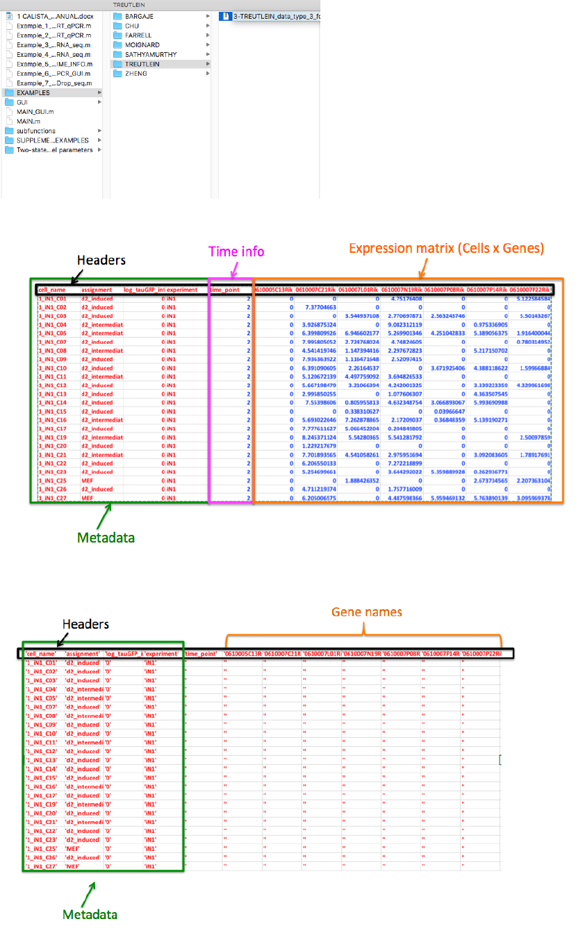
The text file containing the original dataset can be summarized as follows (preview with the first 25 rows and 12
column):
CALISTA imports the dataset by splitting the text data from the expression (numbers) data. In particular we define
the “imported text data” as:
and “imported expression data” as:
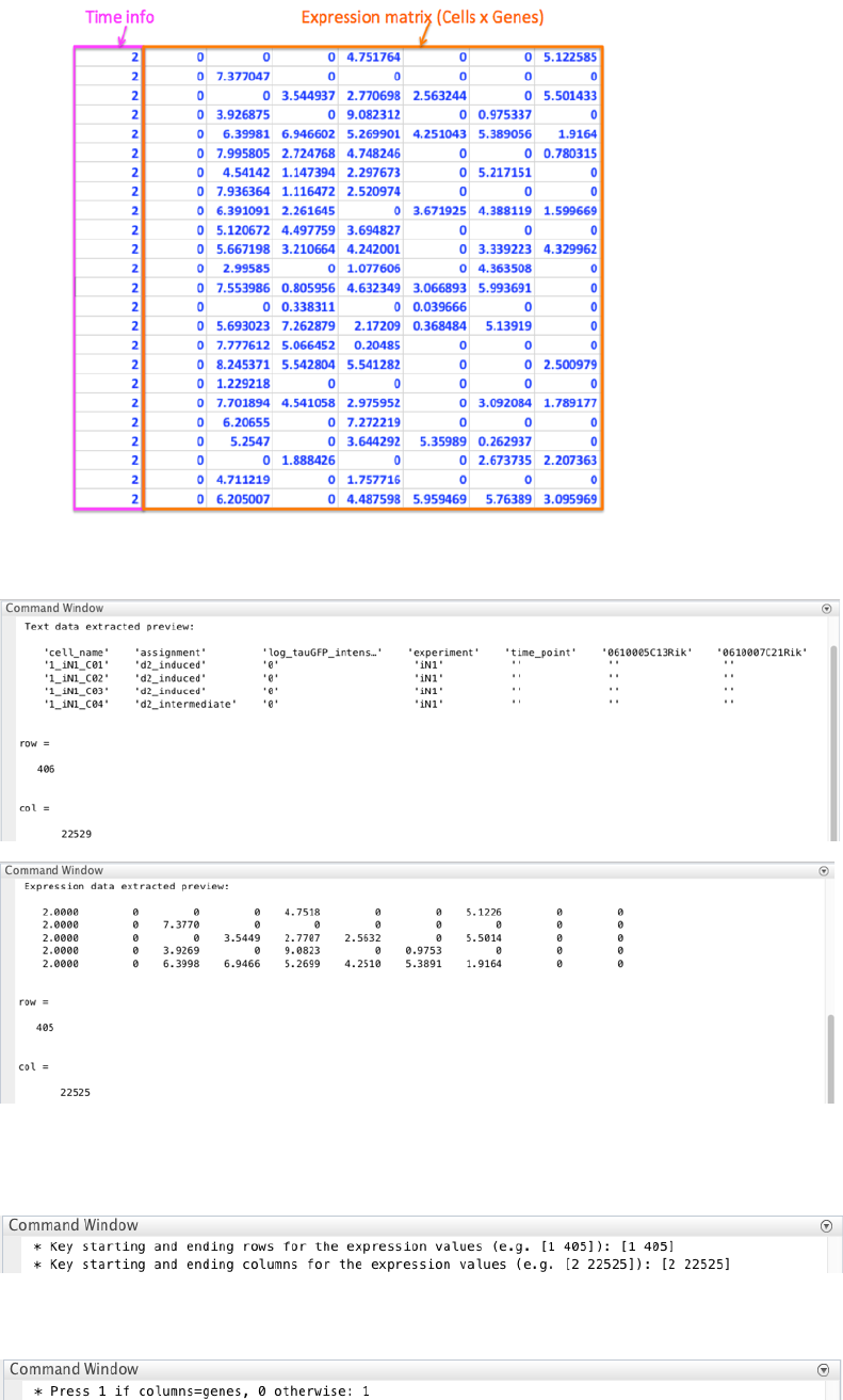
15
CALISTA provides a preview and the dimensions of both imported text and expression data.
Based on the expression data preview, we set the starting and ending rows and columns for the expression values:
as [1 405] and [2 22525], respectively, when queried. We exclude the capture time info in the first column.
We press 1 since columns refer genes and rows refer cells.
We define the gene’s names using the text data preview [6 22529] (starting and ending columns).
16
We load the capture time/cell stage by pressing 1 (i.e. time/cell stage information is in expression data matrix is)
and selecting column 1 in the data matrix.
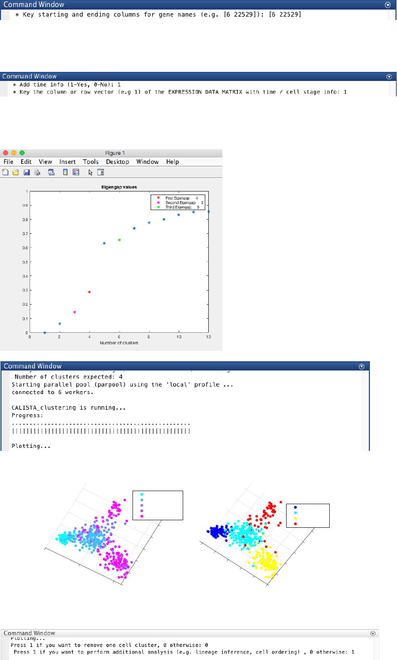
4.3.2 Single-cell clustering
In this case, the number of clusters is determined using the eigengap plot. According to the eigengap plot below,
we set the number of clusters to 4.
CALISTA single-cell clustering results are as follow.
We do not need to remove any cluster (by entering 0 upon queried), and continue with further analysis (by entering
1 upon queried):
Original time/cell stage info
-4
-2
0
2
PC1 5
4
0
-5
6
PC2
Time/Stage 0
Time/Stage 2
Time/Stage 5
Time/Stage 20
Time/Stage 22
Cell Clustering
2
0
-2
-4
PC1
6
6
2
0
-2
PC2
-4 4
4
Cluster 1
Cluster 2
Cluster 3
Cluster 4
17
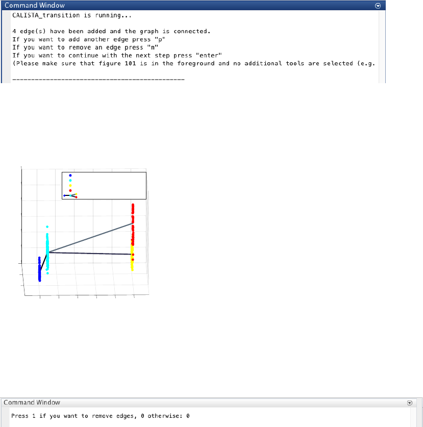
4.3.3 Reconstruction of lineage progression
During the lineage inference step, CALISTA automatically generates and displays a lineage graph, obtained by
adding an edge between two clusters in increasing cluster distances, until all clusters are connected to at least one
other cluster. Subsequently, users can manually add or remove one edge at time based on the cluster distances.
ATTENTION: to add an edge (press “p”), remove an edge (press “m”) or finalize the lineage progression graph
(press “enter”), the MATLAB figure of the graph must appear in foreground without any modification (e.g.,
zooming, rotation). Note that the addition/removal of the edges are performed according to increasing/decreasing
order of cluster distance.
ATTENTION: the final graph must be connected (i.e. there is a path from any node/cluster to any other
node/cluster in the graph) otherwise a warning will be returned.
Here, we do not need to remove any spurious edges, and hence we enter 0 upon queried.
In addition, CALISTA returns (not shown):
- Cell clustering plot based on the cluster pseudotime
- Boxplot, mean, median entropy values calculated for each cluster
- Plot of mean expression values for each gene based on cell cluster expression level
4.3.4 Determination of transition genes
After reconstructing the lineage progression, we identify the key transition genes for any two connected clusters in
the graph (results not shown here), based on the gene-wise likelihood difference between having the cells
separately as two clusters and together as a single cluster. Larger differences in the gene-wise likelihood point to
more informative genes. The transition genes are selected as those whose gene-wise likelihood differences make
up to more than a certain percentage of the cumulative sum of the likelihood differences of all genes – set by
INPUTS.thr_transition_genes.
4.3.5 Pseudotemporal ordering of cells
For pseudotemporal ordering of cells, CALISTA performs maximum likelihood optimization for each cell using a
linear interpolation of the cell likelihoods between any two connected clusters. The pseudotimes of the cells are
computed by linear interpolation of the cluster pseudotimes, and correspond to the maximum point of the
-4
-2
0
10
2
4
6
COMP2
8
5
3
COMP1
0.91266
Lineage Progression
0
2
1.3114
4
0.54478
Cluster pseudotime
1
1
0.8
0.6
0.4
0.2
0
Cluster: 1 Cluster pseudotime: 0.00
Cluster: 2 Cluster pseudotime: 0.09
Cluster: 3 Cluster pseudotime: 1.00
Cluster: 4 Cluster pseudotime: 1.00
data1
18
likelihood optimization above. Cells are subsequently assigned to the edges in the lineage progression graph. The
following screenshot gives the results of this cell-to-edge assignment.
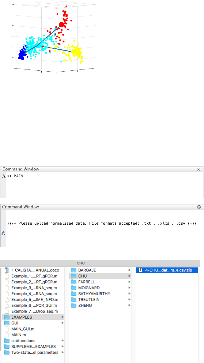
4.4 Example 4. Human embryonic stem cell differentiation into endodermal cells
Analysis of RNA-seq data in Chu et al., Single-cell RNA-seq reveals novel regulators of human embryonic stem
cell differentiation to definitive endoderm, Genome Biol. 17, 173 (2016).
**Please unzip the file “4-CHU__data_type_4_format_data_2_clusters_4.csv.zip” in EXAMPLES/CHU/
before running CALISTA**
4.4.1 Data Import and Preprocessing
We first change the current directory in MATLAB to the CALISTA folder. We edit the
Example_4_CHU_scRNA_seq.m script in the main folder of CALISTA and import Chu dataset (in subfolder
EXAMPLES/CHU):
4.4.2 Single-cell clustering
In this case, the number of clusters is determined using the eigengap plot. According to the eigengap plot below,
we set the number of clusters to 4.
10 0
5
PC1 Cell Ordering
0.5
0
PC2
8
6
Cell Ordering
4
1
2
0
-2
-4
19
NOTE: CALISTA automatically returns the optimal number of clusters based on the MAXIMUM eigengap value.
However, the user might choose the number of clusters to adopt based on the FIRST eigengap.
CALISTA single-cell clustering result is shown below.
We do not need to remove any clusters (by entering 0 upon queried), and continue with further analysis (by
entering 1 upon queried).
4.4.3 Reconstruction of lineage progression
During the lineage inference step, CALISTA automatically generates and displays a lineage graph, obtained by
adding an edge between two clusters in increasing cluster distances, until all clusters are connected to at least one
other cluster. Subsequently, users can manually add or remove one edge at time based on the cluster distances.
5
10 10
0
PC3
5
0
PC1
-5
Original time/cell stage info
-5
-10 0
PC2
-10
Time/Stage 0
Time/Stage 12
Time/Stage 24
Time/Stage 36
Time/Stage 72
Time/Stage 96
5
0
10
PC3
10
5
0
Cell Clustering
PC1
-5
-5
-10 0
PC2
-10
Cluster 1
Cluster 2
Cluster 3
Cluster 4
20
ATTENTION: to add an edge (press “p”), remove an edge (press “m”) or finalize the lineage progression graph
(press “enter”), the MATLAB figure of the graph must appear in foreground without any modification (e.g.,
zooming, rotation). Note that the addition/removal of the edges are performed according to increasing/decreasing
order of cluster distance.
ATTENTION: the final graph must be connected (i.e. there is a path from any node/cluster to any other
node/cluster in the graph), otherwise a warning will be returned.
Since the transition from cluster 4 to cluster 3 is inconsistent with the capture time info (i.e. cluster pseudotime
values for cluster 4 and 3 are 1 and 0.38 respectively), we add one further edge to produce the following lineage
progression graph by pressing “p” and then “enter”:
Based on our definition of branching point, we consider the previous inferred lineage graph still linear, since there
is only one final cell cluster (cluster 4). Moreover, since the transition from cluster 2 to cluster 4 bypasses a cluster
with intermediate pseudotime (i.e. cluster 3), we remove the spurious edge between cluster 2 and 4, by entering 1
and entering [2 4], upon the following query:
-10
-5
20
0
5
COMP2
10
COMP1
0
0.522290.522290.522290.52229
1.4041.404
Lineage Progression
0.883660.883660.88366
Cluster pseudotime
-20 1
0.8
0.6
0.4
0.2
0
Cluster: 1 Cluster pseudotime: 0.00
Cluster: 2 Cluster pseudotime: 0.12
Cluster: 3 Cluster pseudotime: 0.38
Cluster: 4 Cluster pseudotime: 1.00
data1
20
COMP1
0
1.404
0.52229
Lineage Progression
1.8736
0.88366
-10
Cluster pseudotime
-5
-20
0
COMP2
0
5
0.2 0.4 0.6
10
0.8 1
Cluster: 1 Cluster pseudotime: 0.00
Cluster: 2 Cluster pseudotime: 0.12
Cluster: 3 Cluster pseudotime: 0.38
Cluster: 4 Cluster pseudotime: 1.00
data1
21
The final inferred lineage relationships is shown below.
In addition, CALISTA returns (not shown):
- Cell clustering plot based on the cluster pseudotime
- Boxplot, mean, median entropy values calculated for each cluster
- Plot of mean expression values for each gene based on cell cluster expression level
4.4.4 Determination of transition genes
After reconstructing the lineage progression, we identify the key transition genes for any two connected clusters in
the graph (results not shown here), based on the gene-wise likelihood difference between having the cells
separately as two clusters and together as a single cluster. Larger differences in the gene-wise likelihood point to
more informative genes. The transition genes are selected as those whose gene-wise likelihood differences make
up to more than a certain percentage of the cumulative sum of the likelihood differences of all genes – set by
INPUTS.thr_transition_genes.
4.4.5 Pseudotemporal ordering of cells
For pseudotemporal ordering of cells, CALISTA performs maximum likelihood optimization for each cell using a
linear interpolation of the cell likelihoods between any two connected clusters. The pseudotimes of the cells are
computed by linear interpolation of the cluster pseudotimes, and correspond to the maximum point of the
likelihood optimization above. Cells are subsequently assigned to the edges in the lineage progression graph. The
following screenshot gives the results of this cell-to-edge assignment.
-10
-5
20
0
5
COMP2
10
4
1.404
3
0.52229
COMP1
0
Lineage Progression
1.8736
2
0.88366
1
Cluster pseudotime
1
0.8
0.6
-20 0.4
0.2
0
Cluster: 1 Cluster pseudotime: 0.00
Cluster: 2 Cluster pseudotime: 0.12
Cluster: 3 Cluster pseudotime: 0.38
Cluster: 4 Cluster pseudotime: 1.00
data1
10
0
PC1
4
0.52229
-10
3
1.8736
2
Lineage Progression
-10
0.88366
Cluster pseudotime
0
1
-20
0.2 0.4 0.6 0.8 1
-5
0
PC2
5
10
Cluster: 1 Cluster pseudotime: 0.00
Cluster: 2 Cluster pseudotime: 0.12
Cluster: 3 Cluster pseudotime: 0.38
Cluster: 4 Cluster pseudotime: 1.00
22
4.5 Example 5. Running CALISTA without time or cell stage information
Analysis of RT-qPCR data in Moignard et al. “Characterization of transcriptional networks in blood stem and
progenitor cells using high-throughput single-cell gene expression analysis”. Nat. Cell Biol. 15, 363–72 (2013).
Here, we report only the main steps of the analysis. For the complete analysis please check Example 4.2.
4.5.1 Data Import and Preprocessing
We change the current directory in MATLAB to the CALISTA folder.
We then edit the Example_5_MOIGNARD_scRT_qPCR_NO_TIME_INFO.m script in the main folder of
CALISTA and load Moignard dataset (in subfolder EXAMPLES/MOIGNARD):
4.5.2 Single-cell clustering
Following the original publication, we set the number of clusters equals to 5.
-10
-5
20
0
5
PC2
10
PC1
0
Cell Ordering
Cell Ordering
-20
1
0.8
0.6
0.4
0.2
0
23
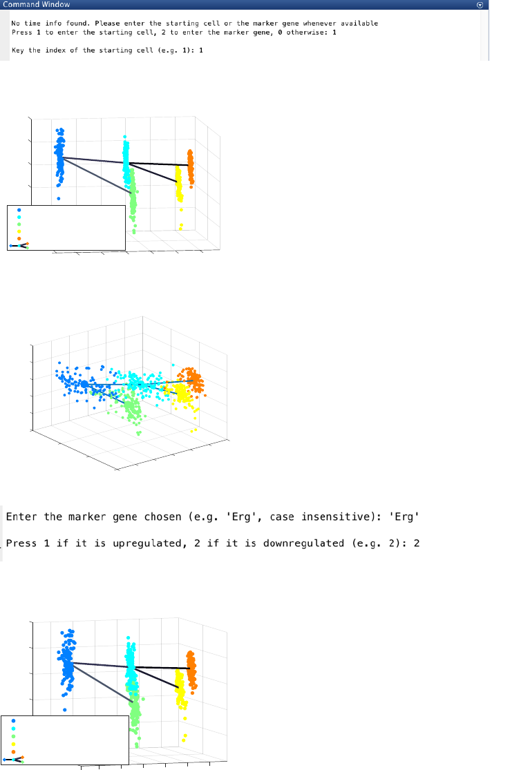
4.5.3 Reconstruction of lineage progression and pseudotemporal ordering of cells
We follow the steps as outlined in the other examples above to infer the lineage progression and carry out
pseudotemporal ordering of single cells.
Without the time or cell stage info, CALISTA is still able to recover the cluster progression based on:
a. The specification of the starting cell (e.g. cell 1):
The final inferred lineage relationships are as follow.
CALISTA pseudotemporal ordering gives the following outcome.
b. The specification of a marker gene (e.g. ‘Erg’) which is downregulated (press 2):
The final inferred lineage relationships:
CALISTA pseudotemporal ordering of cells gives the following result.
-6
-4
-2
0
2
4
10
COMP2
3
0.61663
1
COMP1
0
Plot after cluster relabelling
0.53963
24
0.53555
0.43799
5
Cluster pseudotime
-10 1
0.8
0.6
0.4
0.2
0
Cluster: 1 Cluster pseudotime: 0.00
Cluster: 2 Cluster pseudotime: 0.50
Cluster: 3 Cluster pseudotime: 0.57
Cluster: 4 Cluster pseudotime: 0.91
Cluster: 5 Cluster pseudotime: 1.00
data1
-6
10
-4
-2
1.2
PC2
5
0
1
Cell Ordering
PC1
2
0.8
Cell Ordering
0.6
4
00.4
0.2
-5 0
-6
-4
-2
0
2
10
4
COMP2
3
0.61663
4
Plot after cluster relabelling
1
0.53963
0.53555
5
0.43799
2
0
COMP1
1
0.8
0.6
Cluster pseudotime
0.4
0.2
0
-10
Cluster: 1 Cluster pseudotime: 0.00
Cluster: 2 Cluster pseudotime: 0.50
Cluster: 3 Cluster pseudotime: 0.57
Cluster: 4 Cluster pseudotime: 0.91
Cluster: 5 Cluster pseudotime: 1.00
data1
24
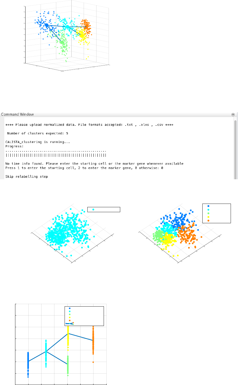
Without any information of the time information, cell stage, starting cell and marker genes, CALISTA is still able
to find the topology of the lineage graph, but the edges are undirected.
CALISTA single-cell clustering result is as follows.
The final inferred lineage relationships are shown below.
Therefore, CALISTA performs the pseudotemporal ordering of cells as follows:
-6
-5
-4
-3
-2
10
-1
0
1
PC2
2
3
4
Cell Ordering
1.5
5
PC1
1
Cell Ordering
00.5
-5 0
Original time/cell stage info
-4 PC1
6
4
-2
0
2
4
2
0
-2
-4
PC2
-6
Time/Stage 0
Cell Clustering
2
0
-2
PC2
6
-4 PC1
4
2
0
-2
-4
-6
4
Cluster 1
Cluster 2
Cluster 3
Cluster 4
Cluster 5
-0.2 0 0.2 0.4 0.6 0.8 1 1.2
Cluster progression
-6
-4
-2
0
2
4
6
8
COMP1
5
1
-0.61663
Plot after cluster relabelling
-0.43799
3
-0.53555
2
-0.53963
4
K= 1 pseudo-stage 1
K= 2 pseudo-stage 2
K= 3 pseudo-stage 3
K= 4 pseudo-stage 4
K= 5 pseudo-stage 5
data1
25
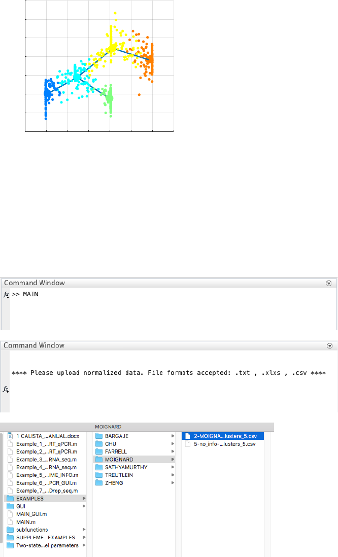
4.6 Example 6. Removing undesired clusters
Analysis of RT-qPCR data in Moignard et al., Characterization of transcriptional networks in blood stem and
progenitor cells using high-throughput single-cell gene expression analysis, Nat. Cell Biol. 15, 363–72 (2013).
4.6.1 Data Import and Preprocessing
We change the current directory in MATLAB to the CALISTA folder. We run
Example_1_MOiGNARD_scRT_qPCR_GUI.m script in the main folder of CALISTA and load Moignard
dataset (in subfolder EXAMPLES/RT-qPCR):
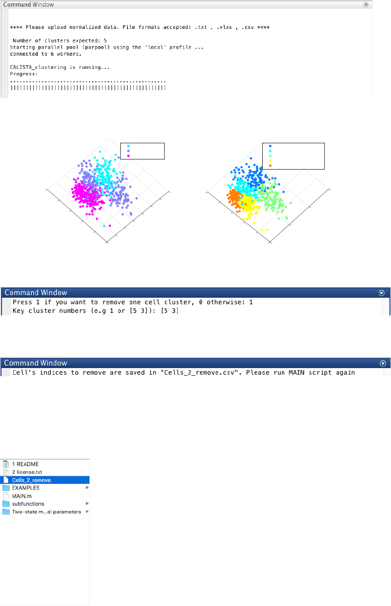
4.6.2 Single-cell clustering
We set the number of clusters equals to 5 following the original publication.
-0.2 0 0.2 0.4 0.6 0.8 1 1.2
Cell Ordering
-6
-4
-2
0
2
4
6
8
PC1
Cell Ordering
26
CALISTA single-cell clustering result is shown below.
Let us proceed with removing cluster 3 and 5, by entering 1 and type [5 3] upon queried.
The indices of cells to remove are saved in a csv file.
We then edit MAIN.m script again, but we set the INPUTS as described previously except:
INPUTS.cells_2_cut=0; % Manual removal of cells
We run MAIN.m once more from the workspace and import Moignard dataset (in subfolder EXAMPLES/RT-
qPCR). We also upload the csv file containing cell’s indices to remove.
4.6.3 Single-cell clustering after removing undesired clusters
We now set the number of clusters equals to 3.
Original time/cell stage info
2
-6
4
6
8
COMP1
0
-4
-6
-4
-2
0
2
4
COMP2
-2
Time/Stage 1
Time/Stage 2
Time/Stage 3
Cell Clustering
-6
-4
-2
PC1
10
2
5
0
-5
4
PC2
0
K= 1 pseudo-stage 1
K= 2 pseudo-stage 2
K= 3 pseudo-stage 2
K= 4 pseudo-stage 3
K= 5 pseudo-stage 3
27
We obtain the following clustering results.
4.6.4 Reconstruction of lineage progression
We continue with lineage inference step. During the lineage inference step, CALISTA provides the minimal
connected graph (with nodes = cell clusters and edges = state transitions) as starting prediction for the
developmental hierarchy. In addition, the user can also manually add or remove one edge at time based on the
cluster distance values:
ATTENTION: to add an edge (press “p”), remove an edge (press “m”) or finalize the lineage progression graph
(press “enter”), the MATLAB figure of the graph must appear in foreground without any modification (e.g.,
zooming, rotation). Note that the addition/removal of the edges are performed according to increasing/decreasing
order of cluster distance.
ATTENTION: the final graph must be connected (i.e. there exists a path from any node/cluster to any other
node/cluster in the graph), otherwise a warning will be returned.
We do not need to remove spurious edges (entering 0 upon queried)
The final inferred lineage relationship is shown below
Original time/cell stage info
-4
0
-2
6
8
2
4
-6
COMP1
COMP2
4-6
20-2
-4
Time/Stage 1
Time/Stage 2
Time/Stage 3
Cell Clustering
PC1
8
4
2
0
-2
-4
4
-6
-6
PC2 -4
-2
0
2
6
K= 1 pseudo-stage 1
K= 2 pseudo-stage 2
K= 3 pseudo-stage 3
28
In addition, CALISTA returns (not shown):
- Cell clustering plot based on the cluster pseudotime
- Boxplot, mean, median entropy values calculated for each cluster
- Plot of mean expression values for each gene based on cell cluster expression level
4.6.5 Determination of transition genes
After reconstructing the lineage progression, we identify the key transition genes for any two connected clusters in
the graph (results not shown here), based on the gene-wise likelihood difference between having the cells
separately as two clusters and together as a single cluster. Larger differences in the gene-wise likelihood point to
more informative genes. The transition genes are selected as those whose gene-wise likelihood differences make
up to more than a certain percentage of the cumulative sum of the likelihood differences of all genes – set by
INPUTS.thr_transition_genes.
4.6.6 Pseudotemporal ordering of cells
For pseudotemporal ordering of cells, CALISTA performs maximum likelihood optimization for each cell using a
linear interpolation of the cell likelihoods between any two connected clusters. The pseudotimes of the cells are
computed by linear interpolation of the cluster pseudotimes, and correspond to the maximum point of the
likelihood optimization above. Cells are subsequently assigned to the edges in the lineage progression graph. The
following screenshot gives the results of this cell-to-edge assignment.
4.7 Running CALISTA GUI
Analysis of RT-qPCR data of Bargaje et al. (Bargaje, et al, Cell population structure prior to bifurcation predicts
efficiency of directed differentiation in human induced pluripotent cells. Proc. Natl. Acad. Sci. U. S. A. 114, 2271–
2276 (2017)).
Here, we report only the main steps of the analysis. For the complete analysis please check Example 4.1.
4.7.1 Data Import and Preprocessing
We begin with changing the current directory in MATLAB to the CALISTA folder. Then, we edit the
Example_6_BARGAJE_scRT_qPCR_GUI.m script in the main folder of CALISTA and import Bargaje dataset
(available in the subfolder EXAMPLES/MOIGNARD).
The following are screenshots from running CALISTA on MATLAB.
-6
-4
10
-2
0
COMP2
2
4
COMP1
0
0.49935
Lineage Progression
0.48732
Cluster pseudotime
-10
1
0.8
0.6
0.4
0.2
0
Cluster: 1 Cluster pseudotime: 0.00
Cluster: 2 Cluster pseudotime: 0.50
Cluster: 3 Cluster pseudotime: 1.00
data1
-6
10
-4
-2
1.5
PC2
0
Cell Ordering
PC1
2
01
Cell Ordering
4
0.5
-10 0
29
4.7.2 Single-cell clustering
In this case, the number of clusters is determined using the eigengap plot. According to the eigengap plot below,
we set the number of clusters to 5. The following are screenshots from CALISTA single-cell clustering analysis.
30
If desired, users can remove cells from specific clusters from further analysis. In this example, we do not want to
remove any clusters. Hence, we enter 0 (no cluster removal) and then 1 to proceed with lineage inference.
4.7.3 Reconstruction of lineage progression
During the lineage inference step, CALISTA automatically generates and displays a lineage graph, obtained by
adding an edge between two clusters in increasing cluster distances, until all clusters are connected to at least one
other cluster. Subsequently, users can manually add or remove one edge at time based on the cluster distances.
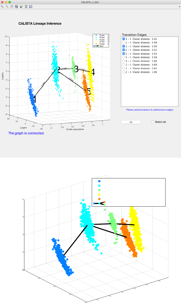
ATTENTION: select (or unselect) checkboxes to add (or remove) specific edges. To select (or unselect) all edges
use the “Select all” checkbox.
ATTENTION: to finalize the lineage progression (by pressing the “OK” button), the final graph must be
connected (i.e. there exists a path from any node/cluster to any other node/cluster in the graph).
Since the transition from cluster 1 to cluster 5 is inconsistent with the capture time info (i.e. cluster pseudotime
values for cluster 1 and 5 are 0 and 1 respectively) we remove the spurious edge between cluster 1 and 5, by
unselecting the second checkbox:
Original time/cell stage info
-2
-4
5
0
2
10
4
15 PC1
-5
6
0
8
-10 -15
-6
10
-8
PC2
Time/Stage 0
Time/Stage 24
Time/Stage 36
Time/Stage 48
Time/Stage 60
Time/Stage 72
Time/Stage 96
Time/Stage 120
Cell Clustering
PC2
10
8
6
4
0
-2
-4
-6
-8
PC1
15 10 50-5 -10 -15
2
Cluster 1
Cluster 2
Cluster 3
Cluster 4
Cluster 5
31
We press the “OK” button to confirm and the final inferred lineage relationships are displayed below.
In addition, CALISTA gives (not shown):
- Cell clustering plot based on the cluster pseudotime
- Boxplot, mean, median entropy values calculated for each cluster
- Plot of mean expression values for each gene based on cell cluster expression level
4.7.4 Determination of transition genes
After reconstructing the lineage progression, we identify the key transition genes for any two connected clusters in
the graph (results not shown here), based on the gene-wise likelihood difference between having the cells
separately as two clusters and together as a single cluster. Larger differences in the gene-wise likelihood point to
more informative genes. The transition genes are selected as those whose gene-wise likelihood differences make
-10
20
0.52226
-5
10
0
COMP2
1
0.41808
0.53909
Lineage Progression
5
0.8
COMP1
0.49993
00.6
Cluster pseudotime
10
0.4
-10 0.2
0
-20
Cluster: 1 Cluster pseudotime: 0.00
Cluster: 2 Cluster pseudotime: 0.50
Cluster: 3 Cluster pseudotime: 0.75
Cluster: 4 Cluster pseudotime: 1.00
Cluster: 5 Cluster pseudotime: 1.00
data1
32
up to more than a certain percentage of the cumulative sum of the likelihood differences of all genes – set by
INPUTS.thr_transition_genes.
4.7.5 Pseudotemporal ordering of cells
For pseudotemporal ordering of cells, CALISTA performs maximum likelihood optimization for each cell using a
linear interpolation of the cell likelihoods between any two connected clusters. The pseudotimes of the cells are
computed by linear interpolation of the cluster pseudotimes, and correspond to the maximum point of the
likelihood optimization above. Cells are subsequently assigned to the edges in the lineage progression graph. The
following screenshot gives the results of this cell-to-edge assignment.
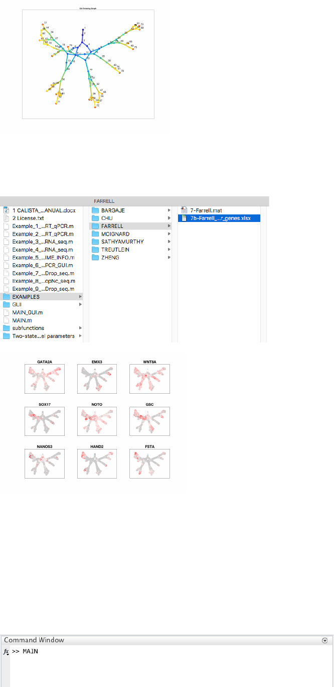
4.8 Example 8. Reconstruction of developmental trajectories during zebrafish embryogenesis
Analysis of Drop-seq data of Farrell et al. (Farrell, J. A. et al. Single-cell reconstruction of developmental
trajectories during zebrafish embryogenesis. Science 360, eaar3131 (2018)).
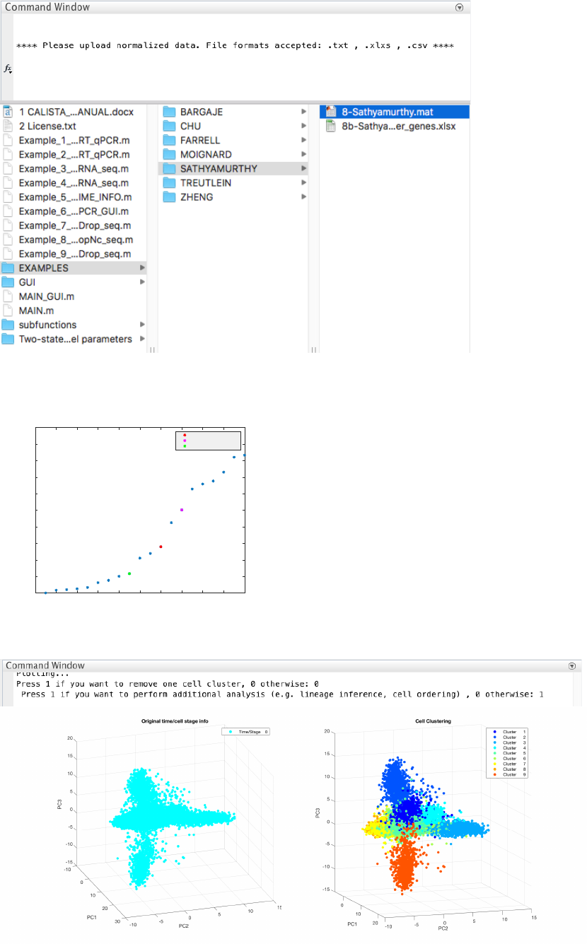
4.8.1 Data Import and Preprocessing
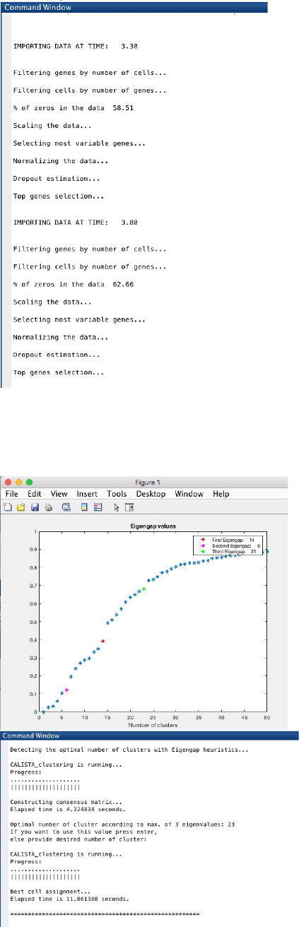
We begin with changing the current directory in MATLAB to the CALISTA folder. Then, we run
Example_7_FARRELL_scDrop_seq.m script in the main folder of CALISTA and import Farrell dataset
(available upon request due to the large file size OR run save_to_matlab.R in R to convert the original data into
Matlab file).
The following are screenshots from running CALISTA on MATLAB.
CALISTA processes the data from each time point separately:
33
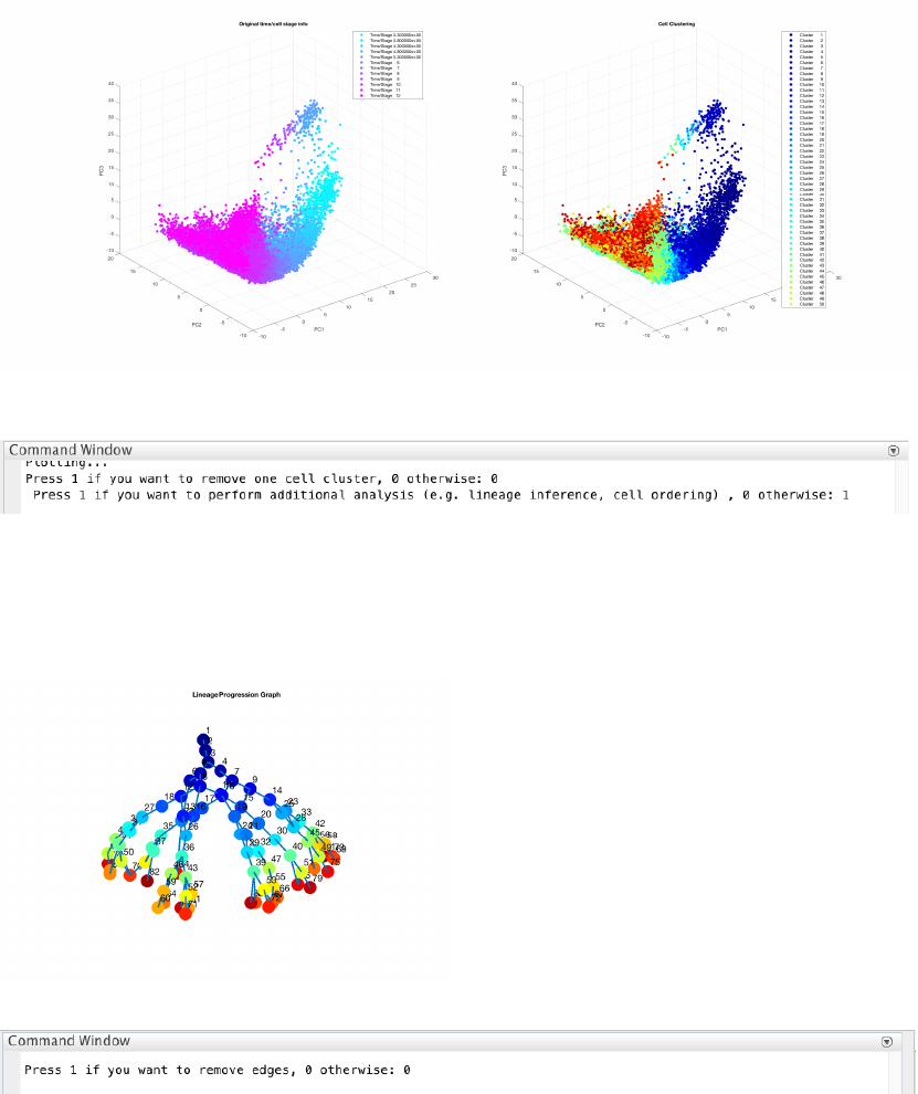
4.8.2 Single-cell clustering
We run a CALISTA clustering for each data point as follows. First, the number of clusters at the final time point is
determined using the eigengap plot. According to the eigengap plot below, we set the number of clusters to 23.
The following are screenshots from CALISTA single-cell clustering analysis.
Then CALISTA will automatically detect the optimal number of clusters for the remaining time points.
34
If desired, users can remove cells from specific clusters from further analysis. In this example, we do not want to
remove any clusters. Hence, we enter 0 (no cluster removal) and then 1 to proceed with lineage inference.
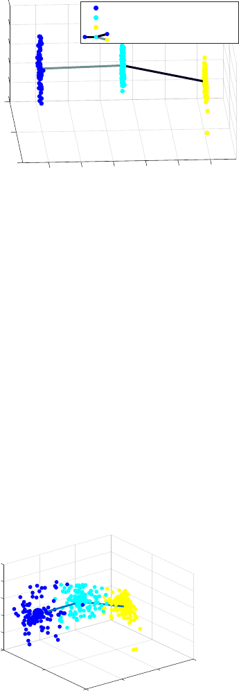
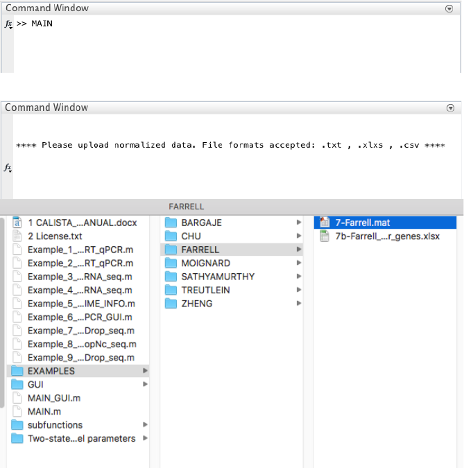
4.8.3 Reconstruction of lineage progression
During the lineage inference step for time series Drop-seq data, CALISTA automatically generates and displays a
lineage graph, obtained by calculating the shortest path between each cluster at the final cluster progression time
and the starting cluster. The inferred lineage is represented by a tree-based graph:
Here, we do not need to remove any spurious edges, and hence we enter 0 upon queried.
4.8.4 Determination of transition genes
After reconstructing the lineage progression, we identify the key transition genes for any two connected clusters in
the graph, based on the gene-wise likelihood difference between having the cells separately as two clusters and
together as a single cluster. Larger differences in the gene-wise likelihood point to more informative genes. The
transition genes are selected as those whose gene-wise likelihood differences make up to more than a certain
percentage of the cumulative sum of the likelihood differences of all genes – set by
INPUTS.thr_transition_genes.
4.8.5 Pseudotemporal ordering of cells
For pseudotemporal ordering of cells, CALISTA performs maximum likelihood optimization for each cell using a
linear interpolation of the cell likelihoods between any two connected clusters. The pseudotimes of the cells are
computed by linear interpolation of the cluster pseudotimes, and correspond to the maximum point of the
likelihood optimization above. Cells are subsequently assigned to the edges in the lineage progression graph. The
following screenshot gives the results of this cell-to-edge assignment.
35
4.8.6 Path analysis
To plot the expression of marker genes along each path, users can enter 1 upon queried and load the excel file
containing the list of genes if interest. In this case the file is in EXAMPLES/FARRELL:
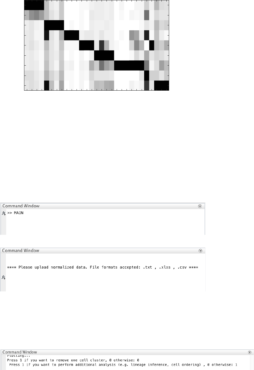
4.9 Example 9. Identification of mouse spinal cord neurons activity during behavior
Analysis of snRNA-seq data of Sathyamurthy et al. (Sathyamurthy, A. et al. Massively Parallel Single
Nucleus Transcriptional Profiling Defines Spinal Cord Neurons and Their Activity during Behavior.
Cell Rep. 22, 2216–2225 (2018)).
4.9.1 Data Import and Preprocessing
We begin with changing the current directory in MATLAB to the CALISTA folder. Then, we run
Example_8_SATHYAMURTHY_DropNc_seq.m script in the main folder of CALISTA and import Farrell
dataset (available upon request due to the large file size).
The following are screenshots from running CALISTA on MATLAB.
36
4.9.2 Single-cell clustering
The number of clusters is determined using the eigengap plot. According to the eigengap plot below, we set the
number of clusters to 9. The following are screenshots from CALISTA single-cell clustering analysis.
If desired, users can remove cells from specific clusters from further analysis. In this example, we do not want to
remove any clusters. Hence, we enter 0 (no cluster removal) and then 1 to proceed with lineage inference.
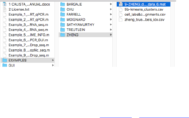
We can load the list of marker genes and visualize the mean expression of each predicted cluster:
0 2 4 6 8 10 12 14 16 18 20
Number of clusters
0
0.1
0.2
0.3
0.4
0.5
0.6
0.7
0.8
0.9
1Eigengap values
First Eigengap: 12
Second Eigengap: 14
Third Eigengap: 9
37
4.10 Example 9. Analysis of peripherical blood mononuclear cells (PBMCs)
Analysis of Drop-seq data of Zheng et al. (Zheng, G. X. Y. et al. Massively parallel digital transcriptional
profiling of single cells. Nat. Commun. 8, 14049 (2017).).
4.10.1 Data Import and Preprocessing
We begin with changing the current directory in MATLAB to the CALISTA folder. Then, we run
Example_8_SATHYAMURTHY_DropNc_seq.m script in the main folder of CALISTA and import Farrell
dataset (available upon request due to the large file size).
The following are screenshots from running CALISTA on MATLAB.
4.10.2 Single-cell clustering
Following the clustering analysis of the original publication, We set the number of clusters to 10. The following
are screenshots from CALISTA single-cell clustering analysis.
If desired, users can remove cells from specific clusters from further analysis. In this example, we do not want to
remove any clusters. Hence, we enter 0 (no cluster removal) and then 1 to proceed with lineage inference.
Snap25
Syp
Rbfox3
Snhg11
Mbp
Mobp
Mog
Plp1
Mpz
Pmp22
Prx
Dcn
Col3a1
Igf2
Aqp4
Atp1a2
Gja1
Slc1a2
Flt1
Pecam1
Tek
Myl9
Pdgfrb
Cspg4
Gpr17
Pdgfra
Ctss
Itgam
Ptprc
Neuron 1
Neuron 2
Oligo
Schwann
Meningeal
Astrocyte
Vascular
OPC
Microglia
38
5 Questions and comments
Please address any problem or comment to: nanp@ethz.ch or rudiyant@buffalo.edu.
