181015_MBD_TU2_Solar_PA_Guidelines 181015 MBD TU2 Solar Cell Guide
User Manual:
Open the PDF directly: View PDF ![]() .
.
Page Count: 7
A. Steinhuber WS2018 1
ENGINEERING
ECEMBD:TrainingUnit2
Solar Cell Modelling
During these exercises you will be trained how to implement equations within Simulink, how to run and treat
different experiments as well as how to display the outcome of those experiments.
Check list: After these exercises, you should be capable to convert and implement equations in Simulink-like
blocks, to prepare scripts for post processing and to handle algebraic loops.
Preparation
As a preparation for this Training Unit (TU), please read the presentation and the lecture notes available
at the e-learning platform (Moodle).
Laboratory
work
In this TU, a solar cell model will be implemented within the Simulink environment.
Description of solar cell model
A solar cell is a large semiconductor area with similar electrical properties to a diode, such as the photovoltaic
effect. This effect allows creating an electrical current from semiconductor material exposed to light, if the circuit
is closed by means of an electrical load. For obtaining a higher voltage/current the cells can be connected in series
or/and parallel to form a solar panel.
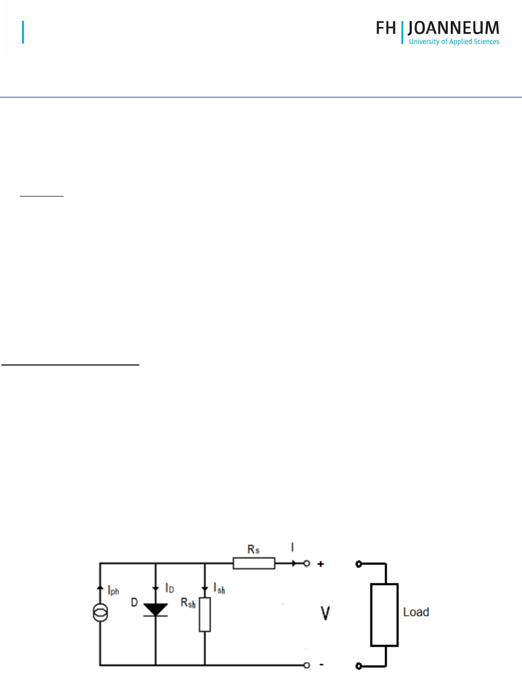
An ideal solar cell can be modelled by a current source connected in parallel with a diode (D). The current source
provides a current I
ph
(photo) directly proportional to the irradiance G. However, in a real solar cell some losses
are present. First, voltage losses occur at the boundary and at external contacts and second, leakage currents are
present throughout the cell. Voltage losses can be represented with a series resistance R
s
(series) and leakage
currents with a parallel resistance R
sh
(shunt). The resulting equivalent circuit of a solar cell is shown in Figure 1.
Figure 1: Equivalent Circuit/Model of Solar Cell

A. Steinhuber WS2018 2
ENGINEERING
The solar cell is described by the following equations, according to the representation above.
shDph
IIII −−=
(1)
I
:
output current (A)
I
ph
: photo generated current (A)
I
D
: diode current (A)
I
sh
: shunt current (A)
The currents within equation (1) are obtained by means of the following formulas:
n
scph
G
G
AJI ⋅⋅=
(2)
J
sc
:
short circuit current density (A/cm
2
)
G : actual irradiance (W/m
2
)
Gn : nominal irradiance (1000 W/m
2
)
A : cell area (cm
2
)
−⋅=
⋅
⋅+
1
0
T
S
Vm
RIV
D
eII
(3)
Note: For simplicity, temperature effect
influence is not considered. Therefore constant
nominal temperature is assumed at 300 K.
I
0
:
reverse saturation
current (A)
V
T
: thermal voltage (25.85 mV at 300 K)
V: voltage at the solar cell (V)
m : diode ideal factor (1 for an ideal diode)
sh
s
sh
R
RIV
I
⋅
+
=
(4)
R
s
:
series resistance
(Ohm)
R
sh
: parallel shunt resistance (Ohm)
The above represented equations are completely describing the solar cell to be developed within this TU. For the
implementation it will be required to modify and adapt the equations in a way to get them to an input/output
relation. [3][4]
Consider the following Steps
1. Model development
Based on the equations for the solar-cell, build the model within the Simulink environment [1] [2].
For the
implementation you will require standard blocks like: the gain, multiplications, divide, exponential, constants,
and sum. Select a suiting solver as learned within the previous lecture and lab.
A. Steinhuber WS2018 3
ENGINEERING
1.1. Parameters
a) Allocate the following variables at the workspace, using a parameter file (script)
b) Use a structure as done for PED (p.SolarCell.Rs)
c) Create a “.mat” file from the actual parameters
d) What are the reasons for storing the data within a “.mat” instead of an “.m” explain the difference?
1.2. Interfaces
Consider that the solar cell will be connected to a battery
a) Which signals (interfaces) do you consider as
Input
Output
b) Explain your decision?
1.3. Model design
a) Create a subsystem containing your model of the solar cell
b) Define constant values for irradiance and voltage and simulate your model. Check the messages in
the Diagnostic Viewer, is everything fine?
If Yes, everything is fine
If Not, report the warning and how it could be solved?
Check list: After this exercise you should be capable to convert and implement equations in Simulink
2. Model testing
In order to check if your model is correctly implemented consider the following steps, set the irradiance to
1000W/m².
2.1. Short circuit:
a) Which voltage has to be applied to the solar cell?
b) Which current value the solar cell is providing, what does this current stand for?
Choose a further value for irradiance and report your result
2.2. Open circuit:
a) Which voltage has to be applied to the solar cell?
b) What happens if the voltage is raised further?
c) Which current value the solar cell is providing?
Choose a further value for irradiance and report your result
R
s
= 1e
-
6 Ohm
A = 126.6 cm2
I
0
=
2.8e
-
9 A
Vt = 25.85e
-
3 V
R
sh
= 1000 Ohm
J
sc
= 0.0343 A/cm
²
Gn= 1000W/m²
m = 1
A. Steinhuber WS2018 4
ENGINEERING
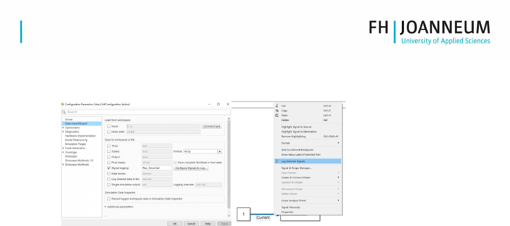
2.3. Storing of simulation results
a) Configure the model for data logging and select the signals of interest
Figure 1: Signal logging
b) Start the simulation and analyze the newly gathered data structure
e.g.: Res_SolarCell.get('G').Values.Data
2.4. Characteristic curves of the solar cell:
Replace the constant input voltage by a variable load resistor (Consider Ohm’s law). Cover the
whole operating range of the solar cell.
a) Prepare the graphs for following signals via a script
• Cell current [A]
• Voltage at cell [V]
• Load resistance [Ohm]
• Power of cell [W]
Use a subplot with four separate plots, consider also labeling and explain your observations
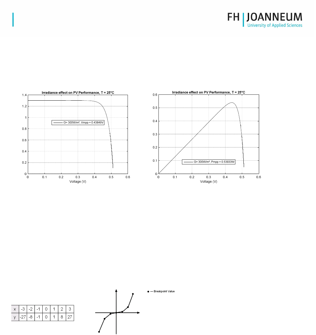
3. Irradiance effect on solar cell performance
Prepare the characteristic curves of the solar cell by preparing an m-script
3.1. Test configuration
a) Set the temperature to 25°C.
b) Vary the value of irradiance G=400, 600, 800, 1000, 1200 [W/m²]
c) In order to make an automate process you can use the “sim” command for running the different
simulations.
d) Store the gathered data within different variables after each run
3.2. Results plotting
a) Current over voltage (XY)
b) Power over voltage (XY)
A. Steinhuber WS2018 5
ENGINEERING
c) Plot the results of the different runs within a single plot for comparison reasons
3.3. Maximum power point
a) Identify the MPPT for each curve via command
b) Integrate the MPPT value to your figure
Figure 2: Example result
4. Lookup table creation:
Based on the previously created model prepare a lookup table, which could be used instead of the detailed
model. A lookup table block uses an array of data to map input values to output values, approximating a
mathematical function. Given input values, Simulink® performs a “lookup” operation to retrieve the
corresponding output values from the table. If the lookup table does not define the input values, the block
estimates the output values based on nearby table values [5]. The following table and graph illustrate the
input/output relationship:
Figure 3: Lookup Table Example [5]
a) Prepare a new model containing the lookup version
b) Consider the Voltage as the input for the table, and the current as the output
Explain the process for gathering the look up table
c)
Prepare a script for comparing the required simulation time of the models developed (using the
equations versus the lookup table)
What difference you observe?
Current (A)
Power (W)
A. Steinhuber WS2018 6
ENGINEERING
d) What are possible reasons for making a look up table?
e) In case a dynamic system based on ODEs shall be converted which restrictions occur?
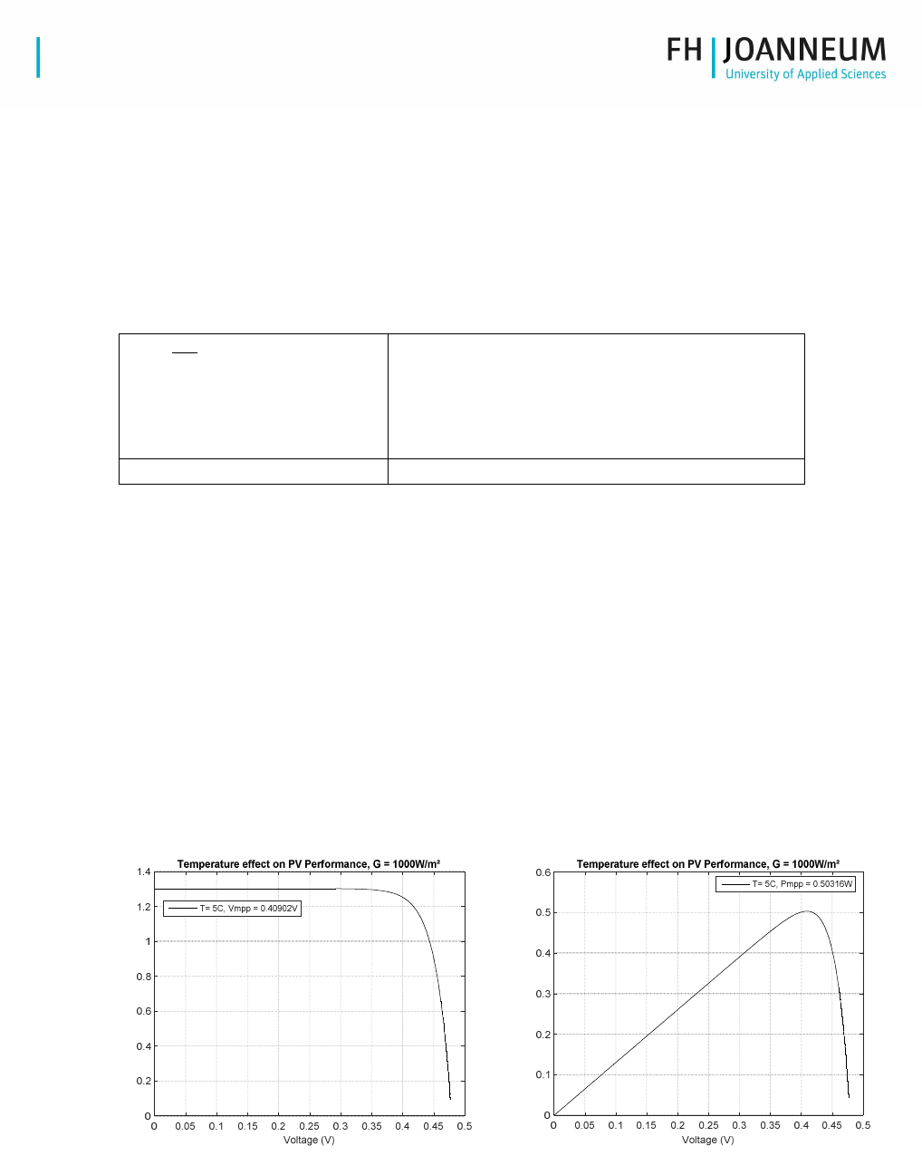
5. Temperature Effect on PV Performance:
5.1. Update the Model
a) In order to demonstrate the influence of the cell temperature on the cell voltage, include the
equation of the thermal voltage to your system.
=
∗
(5)
k
:
Boltzmann constant (J/K)
T : Temperature (K)
q : electron charge (C)
k
= 1.38064852*10^
-
23
q = 1.602176565*10^
-
19
5.2. Test Configuration
a) Repeat the test like in (3) with the irradiance set to 1000 [W/m²] (for all tests)
b) Vary the temperature T=15, 20, 30, 40, 50 [°C]
5.3. Prepare the curves for
a) Current over voltage (XY)
b) Power over voltage (XY)
c) Use the hold function for plotting the different curves within one figure.
5.4. Maximum power point
a) Identify the MPPT for each curve via command
b) Integrate the MPPT value to your figure
Figure 4: Example result
Current (A)
Power (W)

A. Steinhuber WS2018 7
ENGINEERING
Check list: After this exercise you should be capable of manipulating the model and handling
results.
Additional references:
For particular information about solving of algebraic loops in MATLAB/Simulink, I strongly recommend to look at
the following links:
https://de.mathworks.com/help/simulink/ug/algebraic-loops.html
References
[1]
Guzzella, L.; Sciarretta, A. “Vehicle Propulsion Systems: Introduction to Modeling and Optimization”, 3
rd
Edition, Springer
[2] Chaturvedi. "Modeling and Simulation of System Using Matlab and Simulink", CRC Press
[3] E.M.G. Rodrigues, R. Melicio, V.M.F. Mendes and J.P.S Catalao, “Simulation of a Solar Cell considering Single-
Diode Equivalent Circuit Model”; Source: http://www.icrepq.com/icrepq%2711/339-rodrigues.pdf
[4] IEEE TRANSACTIONS ON POWER ELECTRONICS, VOL. 24, NO. 5, MAY 2009 Marcelo Gradella Villalva, Jonas
Rafael Gazoli, and Ernesto Ruppert Filho, “Comprehensive Approach to Modelling and Simulation of Photovoltaic
Arrays”; Source: http://ieeexplore.ieee.org/stamp/stamp.jsp?tp=&arnumber=4806084
[5] Mathworks Block Description, “Matlab Simulink Help”
