259246271 Digital Signal Processing Solution Manual 3rd Edition By Mitra
User Manual:
Open the PDF directly: View PDF ![]() .
.
Page Count: 581 [warning: Documents this large are best viewed by clicking the View PDF Link!]
- M 12.5 MATLAB code is shown below:
- M 12.6 %Program_M12_6.m
- M12.7
- M12.8 The parallel form I and II structures used for the si
- The MATLAB program below can be used to simulate a 4-th orde
- M 12.9 The scaled Gray-Markel cascaded lattice structure us
- The MATLAB program that can be used to simulate the Gray-Mar
- M12 .10 (a) (b)
SOLUTIONS MANUAL
to accompany
Digital Signal Processing:
A Computer-Based Approach
Third Edition
Sanjit K. Mitra
Prepared by
Chowdary Adsumilli, John Berger, Marco Carli,
Hsin-Han Ho, Rajeev Gandhi, Chin Kaye Koh,
Luca Lucchese, and Mylene Queiroz de Farias
Not for sale. 1
Chapter 2
2.1 (a) ,81.4,1396.9,85.22 1
2
1
1
1=== ∞
xxx
(b) .48.3,1944.7,68.18 2
2
2
1
2=== ∞
xxx
2.2 Hence, Thus,
⎩
⎨
⎧<
≥
=µ .0,0
,0,1
][ n
n
n⎩
⎨
⎧≥
<
=−−µ .0,0
,0,1
]1[ n
n
n].1[][][ −−µ+µ
=
nnnx
2.3 (a) Consider the sequence defined by If n < 0, then k = 0 is not included
in the sum and hence, x[n] = 0 for n < 0. On the other hand, for k = 0 is included
in the sum, and as a result, x[n] =1 for Therefore,
.][][ ∑δ=
−∞=
n
k
knx
,0≥n
.0≥n
].[
,0,0
,0,1
][][ n
n
n
knx
n
k
µ=
⎩
⎨
⎧<
≥
=
∑δ=
−∞=
(b) Since it follows that Hence,
⎩
⎨
⎧<
≥
=µ ,0,0
,0,1
][ n
n
n⎩
⎨
⎧<
≥
=−µ .1,0
,1,1
]1[ n
n
n
].[
,0,0
,0,1
]1[][ n
n
n
nn δ=
⎩
⎨
⎧≠
=
=−µ−µ
2.4 Recall ].[]1[][ nnn δ=−
µ
−µ Hence,
]3[4]2[2]1[3][][
−
δ
+
−
δ−−δ+δ= nnnnnx
])4[]3[(4])3[]2[(2])2[]1[(3])1[][(
−
µ
−−µ
+
−
µ
−
−
µ
−
−
µ
−
−µ+−µ−µ= nnnnnnnn
].4[4]3[6]2[5]1[2][
−
µ
−
−
µ
+
−µ−−µ+µ= nnnnn
2.5 (a) },4512302{]2[][
−
−
−
=+−= ↑
nxnc
(b) },006310872{]3[][ ↑
−
−
−=−−= nynd
(c) },003221025{][][ ↑
−
−=−= nwne
(d) },27801332154{]2[][][ −
−
−
−
=−+= ↑
nynxnu
(e) },040342150{]4[][][
−
−
=+⋅= ↑
nwnxnv
(f) },221000543{]4[][][
−
−
−
=+−= ↑
nwnyns
(g) }.75.248.205.35.1021{][5.3][
−
−
−== ↑
nynr
2.6 (a) ],3[2]1[3][2]1[]2[5]3[4][ −
δ
+
−
δ
−
δ
−
+
δ
+
+
δ++
δ
−= nnnnnnnx
],5[2]4[7]3[8]1[][3]1[6][
−
δ
−
−
δ
+
−
δ
+
−
δ−δ−+δ= nnnnnnny
],8[5]7[2]5[]4[2]3[2]2[3][ −
δ
+
−
δ
−
−
δ
−
−
δ
+
−δ+−δ= nnnnnnnw
(b) Recall ].1[][][
−
µ−µ=δ nnn Hence,
])[]1[(])1[]2[(5])2[]3[(4][ nnnnnnnx µ
−
+
µ
+
+
µ
−
+
µ
+
+µ−+µ−=
])4[]3[(2])2[]1[(3])1[][(2
−
µ
−
−
µ
+
−
µ
−
−
µ−−µ−µ− nnnnnn
Not for sale. 2
],4[2]3[2]2[3]1[][3]1[4]2[9]3[4
−
µ
−−µ
+
−
µ
+
−
µ
−
µ
−
+
µ
−+µ++µ−= nnnnnnnn
2.7 (a)
z
1
_
z
1
_
+
+
h[0] h[1] h[2]
x
[n]
y[n]
x[n-1] x[n-2]
From the above figure it follows that ].2[]2[]1[]1[][]0[][ −+
−
+
=
nxhnxhnxhny
(b)
h[0]
z1
_
z1
_
+
+
z1
_
z1
_
+
+
11
β12
β
22
β
21
β
x
[n]y[n]
x[n 1]
_
x[n 2]
_
w[n 1]
_
w[n 2]
_
w[n]
From the above figure we get ])2[]1[][](0[][ 2111 −
β
+
−
β
+
=
nxnxnxhnw and
].2[]1[][][ 2212
−
β
+−
β
+= nwnwnwny Making use of the first equation in the second
we arrive at
])2[]1[][](0[][ 2111
−
β
+
−β+= nxnxnxhny
])3[]2[]1[](0[ 211112
−
β
+
−
β
+
−
β+ nxnxnxh
])4[]3[]2[](0[ 211122
−
β
+
−
β
+
−
β+ nxnxnxh
]2[)(]1[)(][]0[ 221112211211
(−β+ββ+β+−β+β+= nxnxnxh
.]4[]3[)( )
212211222112 −ββ+−ββ+ββ+ nxnx
(c) Figure P2.1(c) is a cascade of a first-order section and a second-order section. The
input-output relation remains unchanged if the ordering of the two sections is
interchanged as shown below.
z
1
_
z
1
_
+
++
+
0.6
0.3
0.2
_
0.8
0.5
_
y[n]
w[n 1]
_
w[n 2]
_
w[n]
z
1
_
+
0.4
x
[n]u[n]y[n+1]
Not for sale. 3
The second-order section can be redrawn as shown below without changing its input-
output relation.
z1
_
z1
_
+
++
+
0.6
0.3
0.2
_0.8
0.5
_
w[n 1]
_
w[n 2]
_
w[n]
x
[n]
y[n]
z1
_
+
0.4
u[n]y[n+1]
z1
_
z1
_
The second-order section can be seen to be cascade of two sections. Interchanging their
ordering we finally arrive at the structure shown below:
z1
_
z1
_
+
+
+
+
0.6
0.3
0.2
_0.8
0.5
_
x
[n]
y[n]
z1
_
+
0.4
u[n]y[n+1]
z1
_
z1
_
x[n 1]
_
x[n 2]
_
u[n 1]
_
u[n 2]
_
s[n]
Analyzing the above structure we arrive at
],2[2.0]1[3.0][6.0][
−
+
−
+
=
nxnxnxns
],2[5.0]1[8.0][][
−
−
−
−
=
nununsnu
].[4.0][]1[ nynuny
+
=
+
From Substituting this in the second equation we get after some
algebra
].[4.0]1[][ nynynu −+=
].2[8.0]1[18.0][4.0][]1[
−
+
−
−
−=+ nynynynsny Making use of the first
equation in this equation we finally arrive at the desired input-output relation
].3[2.0]2[3.0]1[6.0]3[2.0]2[18.0]1[4.0][
−
+−
+
−
=
−
−
−
+−+ nxnxnxnynynyny
(d) Figure P2.19(d) is a parallel connection of a first-order section and a second-order
section. The second-order section can be redrawn as a cascade of two sections as
indicated below:
z1
_
z1
_
+
+
+
0.3
0.2
_0.8
0.5
_
w[n 1]
_
w[n 2]
_
w[n]
x
[n]
z1
_
z1
_
y [n]
2
Not for sale. 4
Interchanging the order of the two sections we arrive at an equivalent structure shown
below:
q[n]
z1
_
z1
_
+
+
_
0.8
0.5
_
x
[n]
+
0.3
0.2
z1
_
z1
_
y [n]
2
y [n 1]
_
2
_
y [n 2]
2
Analyzing the above structure we get
],2[2.0]1[3.0][
−
+
−
=
nxnxnq
].2[5.0]1[8.0][][ 222
−
−
−
−
=
nynynqny
Substituting the first equation in the second we have
].2[2.0]1[3.0]2[5.0]1[8.0][ 222 −
+
−
=
−
+
−
+nxnxnynyny (2-1)
Analyzing the first-order section of Figure P2.1(d) given below
0.6
x
[n]z1
_
+
0.4
u[n]y [n]
1
u[n 1]
_
we get
],1[4.0][][
−
+
=
nunxnu
].1[6.0][
1
−
=
nuny
Solving the above two equations we have
].1[6.0]1[4.0][ 11
−
=
−
−
nxnyny (2-2)
The output of the structure of Figure P2.19(d) is given by ][ny
].[][][ 21 nynyny
+
=
(2-3)
From Eq. (2-2) we get ]2[48.0]2[32.0]1[8.0 11
−
=
−
−
−
nxnyny and
].3[3.0]3[2.0]2[5.0 11
−
=
−−− nxnyny Adding the last two equations to Eq. (2-2) we
arrive at ]3[2.0]2[18.0]1[4.0][ 1111
−
−
−
+
−+ nynynyny
].3[3.0]2[48.0]1[6.0
−
+
−
+
−
=nxnxnx (2-4)
Similarly, from Eq. (2-1) we get
].3[08.0]2[12.0]3[2.0]2[32.0]1[4.0 222 −
−
−
−
=
−
−
−−−− nxnxnynyny Adding this
equation to Eq. (2-1) we arrive at
]3[2.0]2[18.0]1[4.0][ 2222
−
−
−
+−+ nynynyny
].3[08.0]2[08.0]1[3.0 −
−
−
+
−
=
nxnxnx (2-5)
Adding Eqs. (2-4) and (2-5), and making use of Eq. (2-3) we finally arrive at the input-
output relation of Figure P2.1(d) as:
].3[22.0]2[56.0]1[9.0]3[2.0]2[18.0]1[4.0][
−
+−
+
−
=
−
−
−
+
−
+nxnxnxnynynyny
Not for sale. 5

2.8 (a)
},137235241{][
*
1jjjjjnx −−−−+−−−=
↑
Therefore
}.415223371{][
*
1jjjjjnx −−−+−−−−=−
↑
(
)
},....{][][][ *
,515435451
1
1
2
1
1jjjjnxnxnx cs −−−+−=−+= ↑
(
)
}.....{][][][ *
,5214522452521
11
2
1
1jjjjjnxnxnx ca +−+−−++=−−=
↑
(b) Hence, and thus,
Therefore,
.][ 3/
2nj
enx π
=3/
*
2][ nj
enx π−
=].[][ 2
3/
*
2nxenx nj ==− π
(
)
],[][][][ /
*
,nxenxnxnx nj
cs 2
32
22
2
1
2==−+= π and
(
)
.][][][ *
,0
22
2
1
2=−−= nxnxnx ca
(c) Hence, and thus,
Therefore,
.][ 5/
3nj
ejnx π−
=5/
*
3][ nj
ejnx π
−=
].[][ 3
5/
*
3nxejnx nj −=−=− π−
(
)
,][][][ *
,0
33
2
1
3=−+= nxnxnx cs and
(
)
.][][][][ /
*
,5
333
2
1
3nj
ca ejnxnxnxnx π−
==−−=
2.9 (a) }.2032154{][
−
−−= ↑
nx Hence, }.4512302{][
−
−−
=
−
↑
nx
Therefore, }2524252{])[][(][ 2
1
2
1−−−−−=−+= ↑
nxnxnxev
}15.21215.21{
−
−
−
−
−= ↑
and }6540456{])[][(][ 2
1
2
1−−−=−−= ↑
nxnxnxod
}.35.22025.23{
−
−
−= ↑
(b) }.27801360000{][
−
−
−
=↑
ny Hence,
}.00006310872{][ ↑
−
−−=−ny
Therefore, }15.3405.235.2045.31{])[][(][ 2
1−−−=−+= ↑
nynynyev
and }.15.3405.305.3045.31{])[][(][ 2
1−−−−=−−= ↑
nynynyod
(c) }.52012230000000000{][ −
−
=↑
nw Hence,
}.00000000003221025{][ ↑
−−=−nw Therefore
])[][(][ 2
1nwnwnwev −+=
Not for sale. 6

}5.2105.0115.10005.1115.0015.2{ −
−
−−= ↑ and
])[][(][ 2
1nwnwnwod −−=
}.5.2105.0115.10005.1115.0015.2{ −
−
−
−
−−= ↑
2.10 (a) Hence,
].2[][
1+µ= nnx ].2[][
1
+
−
µ
=
−
nnx Therefore,
⎪
⎩
⎪
⎨
⎧
≤− ≤≤− ≥
=+−µ++µ=
,3,2/1
,22,1
,3,2/1
])2[]2[(][ 2
1
,1 n
n
n
nnnx ev and
⎪
⎩
⎪
⎨
⎧
≤−− ≤≤− ≥
=+−µ−+µ=
.3,2/1
,22,0
,3,2/1
])2[]2[(][ 2
1
,1 n
n
n
nnnx od
(b) Hence, Therefore,
].3[][
2−µα= nnx n].3[][
2−−µα=− −nnx n
()
⎪
⎪
⎩
⎪
⎪
⎨
⎧
≤−α
≤≤−
≥α
=−−µα+−µα=
−
−
,3,
,22,0
,3,
]3[]3[][
2
1
2
1
2
1
,2
n
n
n
nnnx
n
n
nn
ev and
()
⎪
⎪
⎩
⎪
⎪
⎨
⎧
≤−α
≤≤−
≥α
=−−µα−−µα=
−
−
−
.3,
,22,0
,3,
]3[]3[][
2
1
2
1
2
1
,2
n
n
n
nnnx
n
n
nn
od
(c) Hence, Therefore,
].[][
3nnnx nµα= ].[][
3nnnx n−µα−=− −
()
n
nn
ev nnnnnnx α=−µα−+µα= −
2
1
][)(][][ 2
1
,3 and
()
.][)(][][ 2
1
2
1
,3
n
nn
od nnnnnnx α=−µα−−µα= −
(d) .][
4
n
nx α= Hence, ].[][ 44 nxnx nn =α=α=− − Therefore,
n
ev nxnxnxnxnxnx α==+=−+= ][])[][(])[][(][ 444
2
1
44
2
1
,4 and
.0])[][(])[][(][ 44
2
1
44
2
1
,4 =−=−−= nxnxnxnxnx od
2.11
()
.][][][ 2
1nxnxnxev −+= Thus,
()
].[][][][ 2
1nxnxnxnx evev =+−=− Hence, is
an even sequence. Likewise,
][nxev
()
.][][][ 2
1nxnxnxod −−= Thus,
()
].[][][][ 2
1nxnxnxnx odod −=−−=− Hence, is an odd sequence. ][nxod
Not for sale. 7

2.12 (a) Thus, ].[][][ nxnxng evev
=].[][][][][][ ngnxnxnxnxng evevevev =
=
−
−
=
−
Hence,
is an even sequence. ][ng
(b) Thus, ].[][][ nxnxnu odev
=
(
)
].[][][][][][ nunxnxnxnxnu odevodev −=
−
=
−
−
=
−
Hence, is an odd sequence.
][nu
(c) Thus, ].[][][ nxnxnv odod
=
(
)( )
][][][][][ nxnxnxnxnv odododod −
−
=
−
−
=
−
Hence, is an even sequence. ].[][][ nvnxnx odod == ][nv
2.13 (a) Since is causal,
][nx .0,0][
<
=
nnx Also, .0,0][ >
=
−
nnx Now,
()
.][][][ 2
1nxnxnxev −+= Hence,
()
]0[]0[]0[]0[ 2
1xxxxev =+= and
.0],[][ 2
1>= nnxnxev Combining the two equations we get
⎪
⎩
⎪
⎨
⎧
<
=
>
=
.0,0
,0],[
,0],[2
][
n
nnx
nnx
nx ev
ev
Likewise,
()
.][][][ 2
1nxnxnxod −−= Hence,
()
0]0[]0[]0[ 2
1=−= xxxod and
.0],[][ 2
1>= nnxnxod Combining the two equations we get
⎩
⎨
⎧
≤
>
=.0,0
,0],[2
][ n
nnx
nx ev
(b) Since is causal, ][ny .0,0][
<
=
nny Also, .0,0][ >
=
−
nny Let
where and are real causal sequences. ],[][][ njynyny imre += ][nyre ][nyim
Now,
(
)
.][][][ 2
1nynynyca −−= ∗ Hence,
(
)
]0[]0[]0[]0[ 2
1
imca jyyyy =−= ∗ and
.0],[][ 2
1>= nnny y
ca Since is not known, cannot be fully recovered from
.
]0[
re
y][ny
][nyca
Likewise,
(
)
.][][][ 2
1nynynycs −+= ∗ Hence,
(
)
]0[]0[]0[]0[ 2
1
recs yyyy =+= ∗ and
.0],[][ 2
1>= nnny y
cs Since is not known, cannot be fully recovered from
.
]0[
im
y][ny
][nycs
2.14 Since is causal,
][nx .0,0][
<
=nnx From the solution of Problem 2.13 we have
].[][)cos(2
,0,0
,01
,0),cos(2
,0,0
,0],[
,0],[2
][ nnn
n
n
nn
n
nnx
nnx
nx o
o
ev
ev δ−µω=
⎪
⎩
⎪
⎨
⎧
<
=
>ω
=
⎪
⎩
⎪
⎨
⎧
<
=
>
=
2.15 (a) where }{]}[{ n
Anx α=
A
and
α
are complex numbers with .1<α Since for
n
nα< ,0 can become arbitrarily large, is not a bounded sequence.
]}[{ nx
Not for sale. 8

(b) where
⎩
⎨
⎧
<
≥α
=µα= ,0,0
,0,
][][ n
nA
nAny n
n
A
and
α
are complex numbers with
.1<α Here, .0,1 ≥≤α n
n Hence Any ≤][ for all values of Hence, is a
bounded sequence.
.n]}[{ ny
(c) where and ][]}[{ nCnh nµβ= C
β
are complex numbers with .1>β Since for
n
nβ> ,0 can become arbitrarily large, is not a bounded sequence.
]}[{ nh
(d) Since ).cos(4]}[{ nng o
ω= 4][ ≤ng for all values of is a bounded
sequence.
]}[{, ngn
(e) ⎪
⎩
⎪
⎨
⎧
≤
≥
⎟
⎠
⎞
⎜
⎝
⎛−
=
.0,0
,1,1
][ 2
1
n
n
nv n Since 1
2
1<
n for and
1>n1
2
1=
n for ,1=n1][ <nv for
all values of Thus is a bounded sequence.
.n]}[{ nv
2.16 ].1[
)1(
][
1
−µ
−
=+
n
n
nx
n Now .
1)1(
][
11
1∞=
∑
=
∑−
=
∑∞
=
∞
=
+
∞
−∞= nn
n
nnn
nx Hence is
not absolutely summable.
]}[{ nx
2.17 (a) Now ].1[][
1−µα= nnx n∞<
α−
α
=
∑α=
∑α=
∑∞
=
∞
=
∞
−∞= 1
][
11
2
n
n
n
n
n
nx , since
.1<α Hence, is absolutely summable.
]}[{ 1nx
(b) Now ].1[][
2−µα= nnx n∑α=
∑α=
∑∞
=
∞
=
∞
−∞= 11
2][
n
n
n
n
n
nnnx ,
)1( 2∞<
α−
α
= since
.1
2<α Hence, is absolutely summable.
]}[{ 2nx
(c) Now
].1[][ 2
3−µα= nnnx nn
nn
n
n
nnnx α
∑
=
∑α=
∑∞
=
∞
=
∞
−∞= 1
2
1
2
3][
K+α+α+α+α= 4
2
3
2
2
2432
)(5)(3)( 543432432 KKK +α+α+α++α+α+α++α+α+α+α=
Not for sale. 9

)(7 654 K+α+α+α+ = K+
α−
α
+
α−
α
+
α−
α
+
α−
α
1
7
1
5
1
3
1
432
⎟
⎟
⎠
⎞
⎜
⎜
⎝
⎛∑α−
∑α
α−
=
⎟
⎟
⎠
⎞
⎜
⎜
⎝
⎛∑α−
α−
=∞
=
∞
=
∞
=111
2
1
1
)12(
1
1
n
n
n
n
n
nnn ⎟
⎟
⎠
⎞
⎜
⎜
⎝
⎛
α−
α
−
α−
α
α−
=1
)1(
2
1
1
2
.
)1(
)1(
3∞<
α−
α+α
= Hence, is absolutely summable. ]}[{ 3nx
2.18 (a) ].[
2
1
][ nnx n
aµ= Now .2
1
1
2
1
2
1
][
2
1
00
∞<=
−
=
∑
=
∑
=
∑∞
=
∞
=
∞
−∞= nn
nn
n
anx Hence,
is absolutely summable. ]}[{ nxa
(b) ].[
)2)(1(
1
][ n
nn
nxbµ
++
= Now ∑++
=
∑∞
=
∞
−∞= 0)2)(1(
1
][
nn
bnn
nx
.1
5
1
4
1
4
1
3
1
3
1
2
1
2
1
1
2
1
1
1
0
∞<=+
⎟
⎠
⎞
⎜
⎝
⎛−+
⎟
⎠
⎞
⎜
⎝
⎛−+
⎟
⎠
⎞
⎜
⎝
⎛−+
⎟
⎠
⎞
⎜
⎝
⎛−=
∑⎟
⎠
⎞
⎜
⎝
⎛
+
−
+
=∞
=
K
nnn Hence,
is absolutely summable. ]}[{ nxb
2.19 (a) A sequence is absolutely summable if
][nx .][ ∞<
∑
∞
−∞=n
nx By Schwartz inequality
we have .][][][ 2∞<
⎟
⎟
⎠
⎞
⎜
⎜
⎝
⎛∑
⎟
⎟
⎠
⎞
⎜
⎜
⎝
⎛∑
≤
∑∞
−∞=
∞
−∞=
∞
−∞= nnn
nxnxnx Hence, an absolutely summable
sequence is square summable and has thus finite energy.
Now consider the sequence ].1[][ 1−µ= nnx n The convergence of an infinite series can
be shown via the integral test. Let ),(xfan
=
where a continuous, positive and
decreasing function is for all Then the series and the integral
both converge or both diverge. For
.1≥x∑
∞
=1n
n
a∫
∞
1
)( dxxf
.)(, 11
xn
nxfa == But ∞=−∞==
∫∞
∞
0)(ln 1
1
1xdx
x.
Hence, ∑
=
∑∞
=
∞
−∞= 1
1
][
nn
n
nx does not converge. As a result, ]1[][ 1−µ= nnx n is not
absolutely summable.
Not for sale. 10

(b) To show that is square-summable, we observe that here
]}[{ nx 2
1
n
n
a=, and thus,
.)( 2
1
x
xf = Now, .11
11
1
1
1
2=+
∞
−=
⎟
⎠
⎞
⎜
⎝
⎛−=
∫
∞
∞
x
dx
x Hence, ∑
∞
=1
1
2
nnconverges, or in other
words, ]1[][ 1−µ= nnx n is square-summable.
2.20 See Problem 2.19, Part (a) solution.
2.21 ].1[
cos
][
2−µ
π
ω
=n
n
n
nx c Now, .
1
cos
][
122
1
2
2
2∑π
≤
∑⎟
⎠
⎞
⎜
⎝
⎛
π
ω
=
∑∞
=
∞
=
∞
−∞= nn
c
nn
n
n
nx Since,
,
6
2
1
1
2
π
=
∑
∞
=nn .
6
1
cos
1
2
≤
∑⎟
⎠
⎞
⎜
⎝
⎛
π
ω
∞
=
n
c
n
n Therefore is square-summable.
][
2nx
Using the integral test (See Problem 2.19, Part (a) solution) we now show that is
not absolutely summable. Now,
][
2nx
∞
∞ω⋅
ω
π
ω
⋅
π
=
∫π
ω
1
1
)int(cos
cos
cos
1
cos x
x
x
x
dx
x
x
c
c
c
c where
is the cosine integral function. Since
intcos dx
x
x
c
∫π
ω
∞
1
cos diverges, ∑π
ω
∞
=1
cos
n
c
n
n also
diverges. Hence, is not absolutely summable.
][
2nx
2.22
()
∑+=
∑
=∞
−∞=
+
∞→
−=
+
∞→ K
odev
K
K
K
Kn
K
K
xnxnxnx 2
12
1
2
12
1][][lim][limP
()
∑++=
−=
+
∞→
K
Kn
odevodev
K
K
nxnxnxnx ][][2][][lim 22
12
1
()(
][][][][lim 12
1
2
1nxnxnxnx
K
Kn
K
K
xx odev −−
∑−+++=
−=
+
∞→
PP
)
odev
n
K
Kn
odev xx
nxnx
K
K
xx PPPP +=++= ⎟
⎟
⎠
⎞
⎜
⎜
⎝
⎛∑−−
∑
⋅
+
∞→
∞
−∞=−=
][][
2
1
12
122
lim
as Now for the given sequence,
∑−
∑=
−=−=
K
Kn
K
Kn
nxnx ].[][ 22
∑
+
∞→
=
+
∞→
−=
+
∞→ =
⎟
⎠
⎞
⎜
⎝
⎛
=
∑⎟
⎠
⎞
⎜
⎝
⎛
=
∑
=K
n
od K
K
K
n
K
K
K
Kn
od
K
K
xnx
0
1
12
1
6
3
1
0
6
3
1
12
1
2
12
1limlim][limP
.lim
6
3
1
2
1
12
1
6
3
1⎟
⎠
⎞
⎜
⎝
⎛
⎟
⎠
⎞
⎜
⎝
⎛
==
+
+
∞→ K
K
K Hence, .10
6
3
1
2
1⎟
⎠
⎞
⎜
⎝
⎛
−=−= odev xxx PPP
Not for sale. 11

2.23 .10),/2sin(][
−
≤
≤π= NnNknnx Now )/2(sin][
1
0
2
1
0
2Nknnx
N
n
N
n
xπ
∑
=
∑
=−
=
−
=
E
()
.)/4cos()/4cos(1
1
0
2
1
2
1
0
2
1∑π−=
∑π−= −
=
−
=
N
n
N
N
n
NknNkn Let and
∑π= −
=
1
0
)/4cos(
N
n
NknC
Then .)/4sin(
1
0
∑π= −
=
N
n
NknS .0
1
1
/4
4
1
0
/4 =
−
−
=
∑
=+ π−
π−
−
=
π−
Nkj
knj
N
n
Nknj
e
e
ejSC This implies
Hence
.0=C.
2
N
x=E
2.24 (a) Then ].[][ nAnx µ= α.
1
][ 2
2
0
22
2
α−
=
∑α=
∑
=∞
=
∞
−∞=
A
Anx
n
n
n
axa
E
(b) ].1[][ 2
1−µ= nnx
n
b Then ∑
=
∑
=
∑∞
=
∞
=
∞
−∞= 1
1
1
1
2
4
2
][
nn
nn
n
bx nx
b
E.
90
4
π
=
2.25 (a) Then average power .)1(][
1n
nx −=
,1)12(
12
1
lim][lim 2
1
12
1
1=+
+
=
∑
=∞→
−=
+
∞→ K
K
nx
K
K
Kn
K
K
x
P and energy
.1][ 2
1
1∞=
∑
=
∑
=∞
−∞=
∞
−∞= nn
xnxE
(b) Then average power
].[][
2nnx µ=
,
2
1
12
1
lim1
12
1
lim][
12
1
lim
0
2
2
2=
+
+
=
∑
+
=
∑
+
=∞→
=
∞→
−=
∞→ K
K
K
nx
KK
K
n
K
K
Kn
K
x
P and energy
.1][
0
2
2
2∞=
∑
=
∑
=∞
=
∞
−∞= nn
xnxE
(c) Then average power ].[][
3nnnx µ=
,
6
)12)(1(
lim
12
1
lim][
12
1
lim
1
2
2
3
3∞=
++
=
∑
+
=
∑
+
=∞→
=
∞→
−=
∞→
KKK
n
K
nx
KK
K
n
K
K
Kn
K
x
P
and energy .][
0
2
2
3
3∞=
∑
=
∑
=∞
=
∞
−∞= nn
xnnxE
(d) Then average power
.][ 0
04 nj
eAnx ω
=∑
+
=
−=
∞→
K
Kn
K
xnx
K
P2
4][
12
1
lim
4
Not for sale. 12

,)12(
12
1
lim
12
1
lim
12
1
lim 2
0
2
0
2
0
2
00AKA
K
A
K
eA
KK
K
Kn
K
K
Kn
nj
K
=+⋅
+
=
∑
+
=
∑
+
=∞→
−=
∞→
−=
ω
∞→
and energy .][ 2
0
2
0
2
30
3∞=
∑
=
∑
=
∑
=∞
−∞=
∞
−∞=
ω
∞
−∞= nn
nj
n
xAeAnxE
(e) .cos][ 2
5⎟
⎠
⎞
⎜
⎝
⎛φ+= π
M
n
Anx Note is a periodic sequence. Then average power ][
5nx
.1cos
2
1
cos
1
][
11
0
2
4
2
1
0
2
2
1
0
2
5
5∑⎟
⎠
⎞
⎜
⎝
⎛+
⎟
⎠
⎞
⎜
⎝
⎛
⋅=
∑⎟
⎠
⎞
⎜
⎝
⎛φ+=
∑
=−
=
φ+
π
−
=
π
−
=
M
nM
n
M
nM
n
M
n
x
A
M
A
M
nx
M
P
Let ∑⎟
⎠
⎞
⎜
⎝
⎛φ+= −
=
1
0
42cos
M
nM
πn
C and .2cos
1
0
4
∑⎟
⎠
⎞
⎜
⎝
⎛φ+= −
=
M
nM
πn
S Then
.0
1
1
/4
4
2
1
0
/42
1
0
2
4
=
−
−
⋅=
∑
=
∑
=+ π
π
φ
−
=
πφ
−
=
⎟
⎠
⎞
⎜
⎝
⎛φ+
π
Mj
j
j
M
n
Mnjj
M
n
j
e
e
eeeejSC M
n
Hence Therefore
.0=C.
2
1
2
12
1
0
2
5
AA
M
P
M
n
x=
∑
⋅= −
=
Since is a periodic sequence, it has infinite energy. ][
5nx
2.26 In each of the following parts, denotes the fundamental period and
N
r
is a positive
integer.
(a) Here and
).5/2cos(4][
~1nnx π= N
r
must satisfy the relation .2
5
2rN π=⋅
π
Among all positive solutions for
N
and r, the smallest values are and
5=N.1
=
r
Hence the average power is given by
.8cos4
5
1
][
~
12
4
05
2
1
0
2
1
1=
∑⎟
⎠
⎞
⎜
⎝
⎛
=
∑
=
=
π
−
=n
n
N
n
xnx
N
P
(b) Here and
).5/3cos(3][
~2nnx π= N
r
must satisfy the relation .2
5
3rN π=⋅
π
Among all positive solutions for
N
and r, the smallest values are and
10=N.3
=
r
Hence the average power is given by
.5.4cos3
10
1
][
~
12
9
05
3
1
0
2
2
2=
∑⎟
⎠
⎞
⎜
⎝
⎛
=
∑
=
=
π
−
=n
n
N
n
xnx
N
P
(c) Here and ).7/3cos(2][
~3nnx π= N
r
must satisfy the relation .2
7
3rN π=⋅
π
Among all positive solutions for and
N
r
, the smallest values are and
14=N.3
=
r
Hence the average power is given by
.2cos2
14
1
][
~
12
13
07
3
1
0
2
3
3=
∑⎟
⎠
⎞
⎜
⎝
⎛
=
∑
=
=
π
−
=n
n
N
n
xnx
N
P
Not for sale. 13

(d) Here and
).3/5cos(4][
~4nnx π= N
r
must satisfy the relation .2
3
5rN π=⋅
π
Among all positive solutions for and
N
r
, the smallest values are and
6=N.5
=
r
Hence the average power is given by
.8cos4
6
1
][
~
12
5
03
5
1
0
2
4
4=
∑⎟
⎠
⎞
⎜
⎝
⎛
=
∑
=
=
π
−
=n
n
N
n
xnx
N
P
(e) ).5/3cos(3)5/2cos(4][
~5nnnx
π
+π= We first determine the fundamental period
of Here and
1
N).5/2cos( nπ1
N
r
must satisfy the relation .2
1
5
2rN π=⋅
π Among all
positive solutions for and , the smallest values are
1
Nr5
1
=
N and We next
determine the fundamental period of
.1=r
2
N).5/3cos( n
π
Here and r must satisfy the
relation
2
N
.2
2
5
3rN π=⋅
π Among all positive solutions for and
2
N
r
, the smallest values
are and The fundamental period of is then given by
10
2=N.3=r][
~5nx
.10)10,5(),( 21
=
=LCMNNLCM
Hence the average power is given by
2
4
05
3
5
2
1
0
2
5cos3cos4
10
1
][
~
1
5∑⎟
⎠
⎞
⎜
⎝
⎛
+
⎟
⎠
⎞
⎜
⎝
⎛
=
∑
=
=
ππ
−
=n
nn
N
n
xnx
N
P
.5.1205.48coscos24cos9cos16
10
111
05
3
5
2
5
3
11
0
2
5
2
11
0
2=++≅
⎟
⎟
⎠
⎞
⎜
⎜
⎝
⎛∑⎟
⎠
⎞
⎜
⎝
⎛
⎟
⎠
⎞
⎜
⎝
⎛
+
⎟
⎠
⎞
⎜
⎝
⎛
∑
+
⎟
⎠
⎞
⎜
⎝
⎛
∑
=
=
πππ
=
π
=n
nnn
n
n
n
(f) ).5/3cos(3)3/5cos(4][
~6nnnx
π
+π= We first determine the fundamental period
of Here and r must satisfy the relation
1
N).3/5cos( nπ1
N.2
1
3
5rN π=⋅
π Among all
positive solutions for and , the smallest values are
1
Nr6
1
=
N and We next
determine the fundamental period of
.5=r
2
N).5/3cos( n
π
Here and r must satisfy the
relation
2
N
.2
2
5
3rN π=⋅
π Among all positive solutions for and r, the smallest values
are and The fundamental period of is then given by
2
N
10
2=N.3=r][
~6nx
.30)10,6(),( 21
=
=LCMNNLCM
Hence the average power is given by
2
29
05
3
3
5
1
0
2
6cos3cos4
30
1
][
~
1
6∑⎟
⎠
⎞
⎜
⎝
⎛
+
⎟
⎠
⎞
⎜
⎝
⎛
=
∑
=
=
ππ
−
=n
nn
N
n
xnx
N
P
.5.1205.48coscos24cos9cos16
30
129
05
3
3
5
5
3
30
0
2
3
5
29
0
2=++≅
⎟
⎟
⎠
⎞
⎜
⎜
⎝
⎛∑⎟
⎠
⎞
⎜
⎝
⎛
⎟
⎠
⎞
⎜
⎝
⎛
+
⎟
⎠
⎞
⎜
⎝
⎛
∑
+
⎟
⎠
⎞
⎜
⎝
⎛
∑
=
=
πππ
=
π
=n
nnn
n
n
n
2.27 Now , from Eq. (2.38) we have Therefore .][][
~∑+= ∞
−∞=k
kNnxny
Not for sale. 14
.][][
~∑++=+ ∞
−∞=k
NkNnxNny Substituting 1
+
=
kr we get
].[
~
][][
~nyrNnxNny
r
=
∑+=+ ∞
−∞= Hence is a periodic sequence with a period
][
~ny .N
2.28 (a) Now The portion of in the range
.5=N.]5[][
~∑+= ∞
−∞=n
pknxnx ][
~nx p40
≤
≤
n is
given by }15400{]5[][]5[
−
=
+
++− nxnxnx
.40},17432{}00000{}02032{ ≤≤
−
−
−
=
+−−+ n
Hence, one period of is given by
][
~nx p.40},17432{ ≤≤
−
−
−
n
Now The portion of in the range is given by .]5[][
~∑+= ∞
−∞=n
pknyny ][
~nyp40 ≤≤ n
}60000{]5[][]5[
=
+++− nynyny
.40},138015{}00002{}78013{ ≤≤
−
−
=
−
+−−+ n
Hence, one period of is given by
][
~ny p.40},138015{ ≤≤
−
−
n
Now The portion of in the range is given by .]5[][
~∑+= ∞
−∞=n
pknwnw ][
~nw p40 ≤≤ n
}00000{]5[][]5[
=
+++− nwnwnw
.40},27101{}05201{}22300{ ≤≤
−
=
−
−++ n
Hence, one period of is given by
][
~nw p.40},27101{ ≤
≤
−
n
(b) .7=
N
Now The portion of in the range .]7[][
~∑+= ∞
−∞=n
pknxnx ][
~nx p60
≤
≤n is
given by }1540000{]7[][]7[
−
=
+
++− nxnxnx
}0000000{}0002032{
+
−−+
.60},1542032{
≤
≤
−−−= n Hence, one period of is given by
][
~nx p
.60},1542032{
≤
≤
−−− n
Now The portion of in the range is given by .]7[][
~∑+= ∞
−∞=n
pknyny ][
~nyp60 ≤≤ n
}6000000{]7[][]7[
=
+++− nxnxnx
}0000000{}0278013{
+
−−−+
.60},6278013{
≤
≤
−−−= n Hence, one period of is given by
][
~ny p
.60},6278013{
≤
≤
−−− n
Now The portion of in the range is given by .]7[][
~∑+= ∞
−∞=n
pknwnw ][
~nw p60 ≤≤ n
}0000000{]7[][]7[
=
+++− nwnwnw
}0000052{}0122300{
−
+
−+
Not for sale. 15
.60},0122352{
≤
≤
−−= n Hence, one period of is given by
][
~nw p
.60},0122352{
≤
≤
−− n
2.29 ).cos(][
~φ+ω= nAnx o
(a) }.11111111{][
~
−
−
−−=nx Hence .4/,2/,2 π=φπ=ω= o
A
(b) }.30303030{][
~−−=nx Hence ,3=A ,2/
π
=ωo
.2/π=φ
(c) }.366.1366.01366.1366.01{][
~
−
−
−=nx Hence ,2=A ,3/
π
=
ωo
.4/π=φ
(d) }.02020202{][
~
−
−=nx Hence .0,2/,2 =φπ=
ω
=
o
A
2.30 The fundamental period of a periodic sequence with an angular frequency
No
ω
satisfies Eq. (2.47a) with the smallest value of and .
Nr
(a) Here Eq. (2.47a) reduces to .5.0 π=ωorN
π
=
π
25.0 which is satisfied with
.1,4 == rN
(b) Here Eq. (2.47a) reduces to .8.0 π=ωorN
π
=
π
28.0 which is satisfied with
.2,5 == rN
(c) We first determine the fundamental period of In
this case, Eq. (2.47a) reduces to
1
N).2.0cos(}Re{ 5/ ne nj π=
π
11 22.0 rN
π
=
π
which is satisfied with .1,10 11
=
=rN
We next determine the fundamental period of In this
case, Eq. (2.47a) reduces to
2
N).1.0sin(Im{ 10/ nje nj π=
π
22 21.0 rN
π
=
π
which is satisfied with .1,20 22
=
=rN
Hence the fundamental period of is given by
N][
~nx c
.20)20,10(),( 21
=
=LCMNNLCM
(d) We first determine the fundamental period of In this case, Eq.
(2.47a) reduces to
1
N).3.1cos(3 nπ
11 23.1 rN
π
=
π which is satisfied with .13,20 11 =
=
rN We next
determine the fundamental period of
2
N).5.05.0sin(4
π
+
π
n In this case, Eq. (2.47a)
reduces to which is satisfied with
22 25.0 rN π=π .1,4 22
=
=
rN Hence the
fundamental period of is given by
N][
~4nx .20)4,20(),( 21 =
=
LCMNNLCM
(e) We first determine the fundamental period of In this
case, Eq. (2.47a) reduces to
1
N).75.05.1cos(5 π+πn
11 25.1 rN
π
=
π
which is satisfied with .3,4 11
=
=rN We
next determine the fundamental period of
2
N).6.0cos(4 n
π
In this case, Eq. (2.47a)
reduces to which is satisfied with
22 26.0 rN π=π .3,10 22
=
=
rN We finally
determine the fundamental period of
3
N).5.0sin( n
π
In this case, Eq. (2.47a) reduces
to which is satisfied with
33 25.0 rN π=π .1,4 33
=
=
rN Hence the fundamental period
N
of is given by ][
~5nx .20)4,10,4(),,( 321
=
=
LCMNNNLCM
2.31 The fundamental period
N
of a periodic sequence with an angular frequency o
ω
satisfies Eq. (2.47a) with the smallest value of
N
and . r
Not for sale. 16

(a) Here Eq. (2.47a) reduces to .6.0 π=ωorN
π
=
π
26.0 which is satisfied with
.3,10 == rN
(b) Here Eq. (2.47a) reduces to .28.0 π=ωorN
π
=
π
228.0 which is satisfied with
.7,50 == rN
(c) Here Eq. (2.47a) reduces to .45.0 π=ωorN
π
=
π
245.0 which is satisfied with
.9,40 == rN
(d) Here Eq. (2.47a) reduces to .55.0 π=ωorN
π
=
π
255.0 which is satisfied with
.11,40 == rN
(e) Here Eq. (2.47a) reduces to .65.0 π=ωorN
π
=
π
265.0 which is satisfied with
.13,40 == rN
2.32 Here Eq. (2.47a) reduces to .08.0 π=ωorN
π
=
π
208.0 which is satisfied with
For a sequence .1,25 == rN )sin(][
~22 nnx
ω
=
with a fundamental period of 25
=
N,
Eq. (2.47a) reduces to .225 2r
π
=
ω
For example, for 2
=
r
we have
Another sequence with the same fundamental period is obtained
by setting which leads to
.16.025/4
2π=π=ω
3=r.24.025/6
3
π
=
π
=
ω
The corresponding periodic
sequences are therefore )16.0sin(][
~2nnx
π
=
and ).24.0sin(][
~3nnx π
=
2.33 The three parameters and ,, o
AΩ
φ
of the continuous-time signal can be
determined from
)(txa
)cos()(][
φ
+
Ω
=
=nTAnTxnx oa by setting 3 distinct values of
For example
.n
,cos]0[ α=φ= Ax
,sin)sin(cos)cos()cos(]1[ β=
φ
Ω
+
φ
Ω
=
φ+Ω−=− TATATAx ooo ,
.sin)sin(cos)cos()cos(]1[
γ
=
φ
Ω
−
φ
Ω
=φ+Ω= TATATAx ooo
Substituting the first equation into the last two equations and then adding them we get
α
γ
+β
=Ω 2
)cos( T
o which can be solved to determine o
Ω
. Next, from the second
equation we have ).cos(cos)cos(sin TTAA oo
Ω
α
−
β
=
φ
Ω
−
β
=
φ Dividing this
equation by the last equation on the previous page we arrive at T
T
o
o
Ωα
Ω
α−β
=φ sin(
)cos(
tan
which can be solved to determine .
φ
Finally, the parameter is determined from the first
equation of the last page.
Not for sale. 17

Now consider the case .2
2
oT TΩ=
π
=Ω In this case
β
=φ+π
=
)cos(][ nAnx and
()
β
=
φ
+
π
=
φ
+π+=+ )cos()1(cos]1[ nAnAnx . Since all sample values are equal, the
three parameters cannot be determined uniquely.
Finally consider the case .2
2
oT TΩ<
π
=Ω In this case )cos(][
φ
+
Ω
=
nTAnx o
implying )cos( φ+ω= nA o.
π
>
Ω
=
ω
T
oo As explained in Section 2.2.1, a digital
sinusoidal sequence with an angular frequency o
ω
greater than assumes the identity
of a sinusoidal sequence with an angular frequency in the range . Hence,
cannot be uniquely determined from
π
.0 π<ω≤
o
Ω)cos(][ φ
+
Ω
=
nTAnx o.
2.34 If is periodic with a period , then ).cos(][ nTnx o
Ω= ][nx N
()
).cos(][cos][ 000 nTnxNTnTNnx
Ω
=
=
Ω+Ω=+ This implies rNT
o
π
=Ω 2with
r
any nonzero positive integer. Hence the sampling rate must satisfy the relation
If i.e., ./2 NrT o
Ωπ= ,20=Ωo,8/
π
=
T then we must have rN π=
π
⋅2
8
20 . The
smallest value of and r satisfying this relation are
N4
=
N and The
fundamental period is thus
.5=r
4
=
N.
2.35 (a) For an input the output is ,2,1],[ =inxi
.2,1],2[]1[]2[]1[][][ 21210 =−
+
−
+
−
+
−
+= inyanyanxbnxbnxbny iiiiii Then, for
an input the output is
],[][][ 21 nBxnAxnx += ])[][(][ 210 nBxnAxbny +
=
])1[]1[(])2[]2[(])1[]1[( 211212211
−
+−
+
−
+
−
+
−+
−
+nBynAyanBxnAxbnBxnAxb
])2[]2[( 211
−
+
−
+nBynAya ]1[]2[]1[][( 11121110
−
+−
+
−
+
=
nyanxbnxbnxbA
])2[]1[]2[]1[][(])1[ 222123222122
−
+−
+
−
+
−
+
+−+ nxanxanxbnxbnxbBnya
].[][ 21 nBynAy += Hence, the system of Eq. (2.18) is linear.
(b) For an input the output is ,2,1],[ =inxi⎩
⎨
⎧±±=
=otherwise.,0
,2,,0],/[
][ LLLnLnx
ny i
i
For an input ],[][][ 21 nBxnAxnx
+
= the output for K,2,,0 LLn
±
±
=
is
][][]/[]/[]/[][ 2121 nBynAyLnBxLnAxLnxny
+
=
+
== . For all other values of
Hence the system of Eq. (2.20) is linear.
.000][, =⋅+⋅= BAnyn
(c) For an input the output is ,2,1],[ =inxi.2,1],/[][ =
=
iMnxny ii Then, for an input
the output is
],[][][ 21 nBxnAxnx += ].[][]/[]/[][ 2121 nBynAyMnBxMnAxny
+
=
+
=
Hence the system of Eq. (2.21) is linear.
Not for sale. 18

(d) For an input the output is ,2,1],[ =inxi∑=−= −
=
1
0
.2,1],[
1
][
M
k
ii iknx
M
ny Then, for
an input the output is
],[][][ 21 nBxnAxnx +=
()
∑−+−= −
=
1
0
21 ][][
1
][
M
k
knBxknAx
M
ny
].[][][
1
][
1
21
1
0
2
1
0
1nBynAyknx
M
Bknx
M
A
M
k
M
k
+=
⎟
⎟
⎠
⎞
⎜
⎜
⎝
⎛∑−+
⎟
⎟
⎠
⎞
⎜
⎜
⎝
⎛∑−= −
=
−
= Hence the system of
Eq. (2.61) is linear.
(e) The first term on the RHS of Eq. (2.65) is the output of a factor-of-2 up-sampler.
The second term on the RHS of Eq. (2.65) is simply the output of an unit delay
followed by a factor-of-2 up-sampler, whereas, the third term is the output of an unit
advance operator followed by a factor-of-2 up-sampler. We have shown in Part (b) that
the up-sampler is a linear system. Moreover, the unit delay and the unit advance
operator are linear systems. A cascade of two linear systems is linear and the linear
combination of linear systems is also linear. Hence, the factor-of-2 interpolator of Eq.
(2.65) is a linear system.
(f) Following the arguments given in Part (e), we can similarly show that the factor-of-
3 interpolator of Eq. (2.66) is a linear system.
2.36 (a) For an input ].[][ 3nxnny =,2,1],[
=
inxi the output is
Then, for an input
.2,1],[][ 3== inxnny ii
],[][][ 21 nBxnAxnx
+
= the output is
Hence the system is linear.
()
][][][ 21
3nBxnAxnny +=
].[][ 21 nBynAy +=
For an input the output is the impulse response As
for and the system is causal.
],[][ nnx δ= ].[][ 3nnnh δ=
0][ =nh ,0<n
Let 1 for all values of Then ][ =nx .n3
][ nny = and as Since a
bounded input results in an unbounded output, the system is not BIBO stable.
∞→][ny .∞→n
Finally, let
and be the outputs for inputs and respectively. If ][ny ][
1ny ][nx ],[
1nx
then However, ][][
1o
nnxnx −= ].[][][ 3
1
3
1o
nnxnnxnny −==
=
−][ o
nny
Since
].[)( 3oo nnxnn −− ],[][
1o
nnyny
−
≠
the system is not time-invariant.
(b) For an input .])[(][ 5
nxny =,2,1],[
=
inxi the output is
.2,1,])[(][ 5== inxny ii
Then, for an input ],[][][ 21 nBxnAxnx
+
= the output is
Hence the system is nonlinear.
()
5
21 ][][][ nBxnAxny +=
.])[(])[( 5
2
5
1nxBnxA +≠
For an input the output is the impulse response As
for and the system is causal.
],[][ nnx δ= .])[(][ 5
nnh δ=
0][ =nh ,0<n
Not for sale. 19

For a bounded input ,][ ∞<≤ Bnx the magnitude of the output samples are
.][])[(][ 5
5
5∞<≤== Bnxnxny As the output is also a bounded sequence, the
system is BIBO stable.
Finally, let and be the outputs for inputs and respectively. If ][ny ][
1ny ][nx ],[
1nx
][][
1o
nnxnx −= then
(
)
].[][])[(][ 5
5
11 oo nnynnxnxny −=−== Hence, the system
is time-invariant.
(c) with
∑−+β=
=
3
0
][][
l
lnxny
β
a nonzero constant. For an input the
output is Then, for an input
the output is
,2,1],[ =inxi
.2,1,][][
3
0
=
∑−+β=
=
inxny ii
l
l],[][][ 21 nBxnAxnx +=
()
∑−+
∑−+β=
∑−+−+β=
===
3
0
2
3
0
1
3
0
21 ][][][][][
lll
llll nBxnAxnBxnAxny
].[][ 21 nBynAy +≠ Hence the system is nonlinear.
For an input the output is the impulse response As
for the system is noncausal.
],[][ nnx δ= .][][
0
∑−δ+β= ∞
=l
lnnh
0][ ≠nh ,0<n
For a bounded input ,][ ∞<≤ Bnx the magnitude of the output samples are
.4][ ∞<+β≤ Bny As the output is also a bounded sequence, the system is BIBO
stable.
Finally, let and be the outputs for inputs and respectively. If ][ny ][
1ny ][nx ],[
1nx
][][
1o
nnxnx −= then Hence, the system is
time-invariant.
].[][][
3
0
1oo nnynnxny −=
∑−−+β=
=l
l
(d)
(
.][2ln][ nxny +=
)
For an input ,2,1],[
=
inxi the output is
()
,][2ln][ nxny ii +=
.2,1=i Then, for an input ],[][][ 21 nBxnAxnx
+
=
the output is
()
].[][][][2ln][ 2121 nBynAynBxnAxny +≠++= Hence the system is nonlinear.
For an input the output is the impulse response ],[][ nnx δ=
()
][2ln][ nnh δ++ .
For Hence, the system is noncausal.
.0)2ln(][,0 ≠=< nhn
For a bounded input ,][ ∞<≤ Bnx the magnitude of the output samples are
()
.2ln][ ∞<+≤ Bny As the output is also a bounded sequence, the system is BIBO
stable.
Finally, let and be the outputs for inputs and respectively. If ][ny ][
1ny ][nx ],[
1nx
Not for sale. 20

][][
1o
nnxnx −= then
(
)
].[][2ln][
1oo nnynnxny −=−+= Hence, the system is
time-invariant.
(e) with a nonzero constant. For an input the output
is Then, for an input
],2[][ +−α= nxny ,2,1],[ =inxi
],2[][ +−α= nxny ii .2,1=i],[][][ 21 nBxnAxnx +
=
the output is
].[][]2[]2[][ 2121 nBynAynxBnxAny
+
=
+
−
α++−α= Hence the system is linear.
For an input the output is the impulse response For ],[][ nnx δ= ].2[][ +−αδ= nnh
,0<n.0][
=
nh Hence, the system is causal.
For a bounded input ,][ ∞<≤ Bnx the magnitude of the output samples are
.][ ∞<α= Bny As the output is also a bounded sequence, the system is BIBO stable.
Finally, let and be the outputs for inputs and respectively. If ][ny ][
1ny ][nx ],[
1nx
][][
1o
nnxnx −= then ].[]2)([]2[][ 11 oo nnynnxnxny −=
+
−
−
α
=
+
−
α
=
Hence, the
system is time-invariant.
(f) For an input
].4[][ −= nxny ,2,1],[
=
inxi the output is .2,1],4[][
=
−= inxny ii
Then, for an input ],[][][ 21 nBxnAxnx
+
= the output is ]4[]4[][ 21
−
+−
=
nBxnAxny
].[][ 21 nBynAy += Hence the system is linear.
For an input the output is the impulse response For ],[][ nnx δ= ].4[][ −δ= nnh ,0
<
n
.0][ =nh Hence, the system is causal.
For a bounded input ,][ ∞<≤ Bnx the magnitude of the output samples are
.][ ∞<= Bny As the output is also a bounded sequence, the system is BIBO stable.
Finally, let and be the outputs for inputs and respectively. If ][ny ][
1ny ][nx ],[
1nx
][][
1o
nnxnx −= then ].[]4[][
1oo nnynnxny
−
=
−
−
=
Hence, the system is time-
invariant.
2.37 Let and be the outputs of a median filter of length for inputs
and , respectively. If
][ny ][
1ny 12 +K][nx
][
1nx ][][
1o
nnxnx
−
=
, then
}][,],1[],[],1[,],[{med][ 111111 KnxnxnxnxKnxny +
+
−
−= KK
}][,],1[],[],1[,],[{med KnnxnnxnnxnnxKnnx ooooo
+
−
+
−
−
−
−
−−= KK
].[ o
nny −= Hence, the system is time-invariant.
2.38 ].1[][2]1[][
−
+−+= nxnxnxny For an input ,2,1],[
=
inxi the output is
.2,1],1[][2]1[][
=
−
+
−+= inxnxnxny iiii Then, for an input ],[][][ 21 nBxnAxnx
+
=
the output is
]1[]1[][2][2]1[]1[][ 212121 −+
−
+
−
−
+
++= nBxnAxnBxnAxnBxnAxny
].[][ 21 nBynAy += Hence the system is linear.
If then ],[][
1o
nnxnx −= ].[]1[][2]1[][
1oooo nnynnxnnxnnxny
−
=−−
+
−
−
+
−
=
Hence, the system is time-invariant.
Not for sale. 21

The impulse response of the system is ]1[][2]1[][ −
δ
+
δ
−
+
δ
=
nnnnh . Now
.1]0[]1[ =δ=−h Since 0][
≠
nh for all values of ,0
<
n the system is noncausal.
2.39 For an input ].1[]1[][][ 2+−−= nxnxnxny ,2,1],[
=
inxi the output is
.2,1],1[]1[][][ 2=+−−= inxnxnxny iiii Then, for an input the
output is
],[][][ 21 nBxnAxnx +=
()
(
)
(
)
]1[]1[]1[]1[][][][ 2121
2
21 +++−+−−+= nBxnAxnBxnAxnBxnAxny
Hence the system is nonlinear.
].[][ 21 nBynAy +≠
If then
],[][
1o
nnxnx −= ]1[]1[][][ 11
2
11 +−−= nxnxnxny
]1[]1[][
2+−−−−−= ooo nnxnnxnnx ].[ o
nny
−
=
Hence, the system is time-
invariant.
The impulse response of the system is Since
for all values of
].[]1[]1[][][ 2nnnnnh δ=+δ−δ−δ=
0][ =nh ,0
<
n the system is causal.
2.40 .
]1[
][
]1[
2
1
][ ⎟
⎟
⎠
⎞
⎜
⎜
⎝
⎛
−
+−= ny
nx
nyny Now for an input ],[][ nn
x
α
µ
=
the output
converges to some constant
][ny
K
as .
∞
→n The input-output relation of the system as
reduces to
∞→n⎟
⎠
⎞
⎜
⎝
⎛α
+= K
KK 2
1 from which we get or in other words
α=
2
K
.α=K
For an input the output is ,2,1],[ =inxi.2,1,
]1[
][
]1[
2
1
][ =
⎟
⎟
⎠
⎞
⎜
⎜
⎝
⎛
−
+−= i
ny
nx
nyny
i
i
ii Then,
for an input ],[][][ 21 nBxnAxnx
+
= the output is .
]1[
][][
]1[
2
1
][ 21 ⎟
⎟
⎠
⎞
⎜
⎜
⎝
⎛
−
+
+−= ny
nBxnAx
nyny
On the other hand,
⎟
⎟
⎠
⎞
⎜
⎜
⎝
⎛
−
+−=+ ]1[
][
]1[
2
1
][][
1
1
121 ny
nAx
nAynBynAy ].[
]1[
][
]1[
2
1
2
2
2ny
ny
nBx
nBy ≠
⎟
⎟
⎠
⎞
⎜
⎜
⎝
⎛
−
+−+
Hence the system is nonlinear.
If then ],[][
1o
nnxnx −= ].[
]1[
][
]1[
2
1
][
1
11 o
onny
ny
nnx
nyny −=
⎟
⎟
⎠
⎞
⎜
⎜
⎝
⎛
−
−
+−= Hence, the
system is time-invariant.
2.41 ].1[]1[][][ 2−+−−= nynynxny
For an input the output is
Then, for an input
,2,1],[ =inxi.2,1],1[]1[][][ 2=−+−−= inynynxny iiii
],[][][ 21 nBxnAxnx
+
= the output is
].1[]1[][][][ 2
21 −+−−+= nynynBxnAxny On the other hand,
][][ 21 nBynAy +
Not for sale. 22

].[]1[]1[][]1[]1[][ 2
2
221
2
11 nynBynBynBxnAynAynAx ≠−+−−+−+−−= Hence the
system is nonlinear.
Let be the output for an input , i.e., Then, for an
input the output is given by , or
in other words, the system is time-invariant.
][ny ][nx ].[][][][ 1
2−+−= nynynxny
][o
nnx −][][][][ 11
2−−+−−−−=− oooo nnnnynnxnny
Now, for an input ][][ nnx
α
µ= , the output converges to some constant K as
][ny
∞
→n.
The difference equation describing the system as
∞
→n reduces to or
i.e.,
,KKK +−α= 2
,α=
2
K.α=K
2.42 The impulse response of the factor-of-3 interpolator of Eq. (2.66) is the output for an
input and is given by ][][ nnxuδ=
])2[]2[(])1[]1[(][][ 3
1
3
2+δ+−δ++δ+−δ+δ= nnnnnnh or equivalently by
{
}
.22,,,1,]}[{ 3
1
3
2
3
2
,
3
1≤≤−= nnh
2.43 The input-output relation of a factor-of-
L
interpolator is given by
(
.][][][][
1
1
knxknx
L
kL
nxny uu
L
k
u++−
∑−
+= −
=
)
Its impulse response is the output for
an input and is thus given by ][][ nnxuδ=
()
][][][][
1
1
knkn
L
kL
nnh
L
k
+δ+−δ
∑−
+δ= −
=
or equivalently by
{
}
.11,,,,,,1,,,,,]}[{ 1
2211221 −≤≤+−= −−−− LnLnh
L
LL
L
L
L
L
L
L
L
LL
KK
2.44 The impulse response of a causal discrete-time system satisfies the difference
equation
][nh
].[]1[][ nnhanh
δ
=
−− Since the system is causal, we have for
Evaluating the above difference equation for
0][ =nh
.0<n,0
=
n we arrive at
and thus 1]1[]0[ =−− ahh .1]0[
=
h Next, for 1
=
n, we have and thus
Continuing we get for
0]0[]1[ =− hah
.]1[ ah =0]1[]2[,2
=
−
=
ahhn , i.e., Assume
.]1[]2[ 2
aahh ==
with From the difference equation we then have
, i.e., Since the last equation holds for
by induction, it holds for
1
]1[ −
=− n
anh .0>n
0]1[][ =−− nhanh .]1[][ n
anahnh =−=
,2,1,0=n.3≥n
2.45 As and are right-sided sequences, assume
][nx ][nh 0][
=
nx for all and
and Hence,
1
Nn <
0][ =nh .
2
Nn <0][O][][ *
=
=
nxnhny for all and thus
21 NNn +<
Not for sale. 23

is also a right-sided sequence. Therefore, ][ny ][O][][ *
2121
nxnhny
NNnNNn
∑
=
∑∞
+=
∞
+=
∑−
∑
=
∑∑ −=
∑∑ −= ∞
+=
∞
=
∞
=
∞
+=
∞
+=
∞
=212221212
][][][][][][
NNnNkNkNNnNNnNk
knxkhknxkhknxkh
as
∑∑
=
∑∑
=∞
=
∞
=
∞
−+=
∞
=12212
][][][][
NmNkkNNmNk
mxkhmxkh 0][
=
mx for all . Hence,
1
Nm <
.][][][ ⎟
⎟
⎠
⎞
⎜
⎜
⎝
⎛∑
⎟
⎟
⎠
⎞
⎜
⎜
⎝
⎛∑∑ =
nnn
nxnhny
2.46 (a)
⎩
⎨
⎧
<
≥
∑α
=
∑−µα=−µ
∑µα=µµα =
∞
=
∞
−∞= ,,
,,
][][][][O][ *00
0
0
0n
n
knknknn n
k
k
k
k
k
kn
].[n
nµ
⎟
⎟
⎠
⎞
⎜
⎜
⎝
⎛
α−
α−
=+
1
11
(b)
⎩
⎨
⎧
≤
>
∑α
=
∑−µα=−µ
∑µα=µµα =
∞
=
∞
−∞= .0,0
,0,
][][][][O][ 0
0
*n
nk
knkknkknnn n
k
k
k
k
k
kn
2.47 Now from Eq. (2.72) an arbitrary input can be expressed as
which can be rewritten using Eq. (2.41b) as
][nx
∑−δ= ∞
−∞=k
knkxnx ][][][
()
∑−−µ−−µ= ∞
−∞=k
knknkxnx ]1[][][][ ∑−µ= ∞
−∞=k
knkx ][][ .]1[][
∑−−µ− ∞
−∞=k
knkx
Since is the response of an LTI system for an input
][ns ],[n
µ
is the response
for an input and
][ kns −
][ kn −µ ]1[
−
−
kns is the response for an input Hence,
the output for an input is given by
].1[ −−µ kn
∑−µ
∞
−∞=k
knkx ][][ ∑−−µ− ∞
−∞=k
knkx ]1[][
].1[O]1[][O][]1[][][][][ ** −−−=
∑−−−
∑−= ∞
−∞=
∞
−∞=
nsnxnsnxknskxknskxny
kk
2.48 Hence,
Thus, is also a
periodic sequence with a period
.][
~
][][ ∑−= ∞
−∞=m
mnxmhny
].[][][][
~
][][ nymnxmhmkNnxmhkNny
mm
=
∑∑
−=−+=+ ∞
−∞=
∞
−∞=
][ny
.
N
2.49 In this problem we make use of the identity ].[][O][ *rmnrnmn −−δ=
−
δ
−
δ
Not for sale. 24
(a)
(
)
(
)
]1[2][4]2[O]1[2]2[3][O][][ *
1
*
11
−
δ+δ
+
+
δ
−
+
δ
−
−
δ
=
=nnnnnnhnxny
]1[O]2[6][O]2[12]2[O]2[3 ***
−
δ
−
δ
−
δ
−
δ
++δ−δ−= nnnnnn ]2[O]1[2 *
+
δ+δ
+
nn
]1[O]1[4][O]1[8 **
−
δ
+δ+δ+δ− nnnn . Hence
][4]1[8]3[2]3[6]2[12][3][
1nnnnnnny δ
+
+
δ
−
+
δ
+
−
δ
−
−δ+δ−=
].3[6]2[12][]1[8]3[2
−
δ
−
−
δ
+
δ++δ−+δ= nnnnn
(b)
(
)
(
)
]1[]2[5.1]4[3O]1[2]3[5][O][][ *
2
*
22
+
δ
−−δ
+
−
δ
+
δ
+
−
δ
=
=nnnnnnhnxny
]4[O]1[6]1[O]3[5]2[O]3[5.7]4[O]3[15 ****
−
δ
+δ+
+
δ
−
δ
−
−
δ
−
δ
+−δ−δ= nnnnnnnn
]1[O]1[2]2[O]1[3 **
+
δ
+
δ−−δ+δ+ nnnn ]2[5]5[5.7]7[15 −δ−−
δ
+
−
δ
=
nnn
].2[2]1[3]3[6
+
δ
−−δ+−δ+ nnn
(c)
(
)
(
)
]1[]2[5.1]4[3O]1[2]2[3][O][][ *
2
*
13
+
δ
−
−δ+
−
δ
+
δ
−
−
δ
−
=
=nnnnnnhnxny
]4[O]1[6]1[O]2[3]2[O]2[5.4]4[O]2[9 ****
−
δ
+δ−
+
δ
−
δ
−
−
δ
−
δ
+−δ−δ= nnnnnnnn
]1[O]1[2]2[O]1[3 **
+
δ
+
δ+−δ+δ− nnnn ]1[3]4[5.4]6[9 −δ−
−
δ
+
−
δ
=
nnn
]2[2]1[3]1[3]3[6
+
δ
+
−
δ
−−δ−−δ− nnnn ]3[6]1[6]2[2 −δ−
−
δ
−
+
δ
=
nnn
].6[9]4[5.4 −δ+−δ+ nn
(d)
(
)
(
)
]1[2][4]2[O]1[2]3[5][O][][ *
1
*
24
−
δ−δ
+
+
δ
−
+
δ
+
−
δ
=
=nnnnnnhnxny
]2[O]1[2]1[O]3[10][O]3[20]2[O]3[5 ****
+
δ
+δ−
−
δ
−
δ
−
δ
−
δ
++δ−δ−= nnnnnnnn
]1[O]1[4][O]1[8 **
−
δ
+δ−δ+δ+ nnnn ]3[2]4[10]3[20]1[5
+
δ
−
−δ−
−
δ
+
−
δ
−
=
nnnn
][4]1[8 nn δ−+δ+ ].4[10]3[20]1[5][4]1[8]3[2
−
δ
−−δ
+
−
δ
−
δ
−
+
δ
+
+
δ−= nnnnnn
2.50 (a)
][O][][ *nynxnu =
.84},4,14,22,17,42,25,66,23,45,20,5,42,24{
≤
≤−−
−
−
−
−−−−= n
(b)
][O][][ *nwnxnv =
.111},10,4,15,6,13,30,28,3,16,10,5,7,12{ ≤≤
−
−
−
−
−
−−−= n
(c)
][O][][ *nynwng =
.131},10,39,26,14,16,11,60,26,25,14,3,3,18{ ≤≤
−
−
−
−
−= n
Not for sale. 25
2.51 Now,
.][][][ 2
1
∑−= =
N
Nm mnhmgny ][ mnh
−
is defined for . Thus,
for is defined for
21 MmnM ≤−≤
][,
1mnhNm −= 211 MNnM
≤
−
≤
, or equivalently, for
. Likewise, for
1211 NMnNM +≤≤+ ][,
2mnhNm
−
=
is defined for
, or equivalently, for
221 MNnM ≤−≤ .
2221 NMnNM
+
≤
≤
+
For the specified
sequences .6,2,4,3 2121
=
=
=−= MMNN (a) The length of is ][ny
121)3(2461
1122
=
+
−
−
−
+
=+−−+ NMNM . (b) The range of for
n0][
≠
ny is
),max(),min( 22112211 NMNMnNMNM
+
+
≤
≤
++ , i.e.,
For the specified sequences the range of is
.
2211 NMnNM +≤≤+ n.101
≤
≤
−n
2.52 Now,
Let
∑−== ∞
−∞=k
kxknxnxnxny ].[][][O][][ 212
*
1
∑−−−=−−= ∞
−∞=k
NkxkNnxNnxNnxn ].[][][O][][ 221122
*
11
v.
2mNk
=
−
Then
∑−−=−−−= ∞
−∞=m
NNnymxmNNnxn ].[][][][ 212211
v
2.53 ][O][][O][O][][ 3
*
3
*
2
*
1nxnynxnxnxng
=
= where ].[O][][ 2
*
1nxnxny
=
Now
].[O][][ 22
*
11 NnxNnxnv
−
−
= Define ].[O][][ 33
*Nnxnvnh
−
=
Then from the
results of Problem 2.52, ].[][ 21 NNnynv
−
−
=
Hence,
].[O][][ 33
*
21 NnxNNnynh
−
−−= Therefore, making use of the results of Problem
2.52 again we get ].[][ 321 NNNnynh
−
−
−
=
2.54 Substituting by
∑−== ∞
−∞=k
khknxnhnxny ].[][][O][][ *kmn
−
in this expression, we
get Hence the convolution operation is
commutative.
∑=−= ∞
−∞=m
nxnhmnhmxny ].[O][][][][ *
Let
() (
∑+−=+= ∞
−∞=k
khkhknxnhnhnxny ][][][][][O][][ 2121
*
)
Hence the
convolution operation is also distributive.
∑+
∑=−+−= ∞
−∞=
∞
−∞=kk
nhnxnhnxkhknxkhknx ].[O][][O][][][][][ 2
*
1
*
21
2.55 As is an unbounded
sequence, the result of this convolution cannot be determined. But
]).[O][(O][][O][O][ 1
*
2
*
31
*
2
*
3nxnxnxnxnxnx =][O][ 1
*
2nxnx
Not for sale. 26

]).[O][(O][][O][O][ 1
*
3
*
21
*
3
*
2nxnxnxnxnxnx = Now for all values
of , and hence the overall result is zero. As a result, for the given sequences
0][O][ 1
*
3=nxnx
n
≠][O][O][ 1
*
2
*
3nxnxnx ][O][O][ 1
*
3
*
2nxnxnx
2.56 Define
].[O][O][][ ** ngnhnxnw =∑−
=
=
k
knhkxnhnxny ][][][O][][ * and
.][][][O][][ *∑
−
==
k
knhkgngnhnf Consider ][O])[O][(][ **
1ngnhnxnw
=
].[][][][O][ *kmnhkxmgngny
km
−
−
∑∑
== Now consider
])[O][(O][][ **
2ngnhnxnw =
].[][][][O][ *mknhmgkxnfnx
mk
−
−
∑∑
== The difference between the
expressions for and is that the order of the summations is changed.
][
1nw ][
2nw
A) Assumptions: and are causal sequences, and for This
implies Thus,
][nh ][ng 0][ =nx .0<n
⎩
⎨
⎧
≥
∑
<
==.0fork],-x[k]h[m
,0for,0
][ m0k m
m
my ∑−=
=
n
m
mnymgnw
0
][][][
∑−−
∑
=−
==
mn
k
n
m
kmnhkxmg
00
].[][][ All sums have only a finite number of terms. Hence,
the interchange of the order of the summations is justified and will give correct results.
B) Assumptions: and are stable sequences, and is a bounded sequence
with
][nh ][ng ][nx
. Here,
⎟
⎠
⎞
⎜
⎝
⎛∑−=
∑−= =
∞−∞= 2
1
][][][][][ k
kk
kkmxkhkmxkhmy
∞<≤ Bnx ][
][
21 ,m
kk
ε+ with .][
21 ,Bm nkk ε≤ε In this case, all sums have effectively only a finite
number of terms and the error ][
21 ,m
kk
ε can be reduced by choosing and
sufficiently large. As a result, in this case the problem is again effectively reduced
to that of the one-sided sequences. Thus, the interchange of the order of the
summations is again justified and will give correct results.
1
k
2
k
Hence, for the convolution to be associative, it is sufficient that the sequences be stable
and single-sided.
2.57 Since is of length .][][][ ∑−= ∞−∞=kkhknxny ][kh
M
and defined for ,10
−
≤
≤Mk
the convolution sum reduces to will be nonzero for
all those values of and for k which
.][][][ )1(
0
∑−= −
=
M
kkhknxny ][ny
nkn
−
satisfies .10 −≤
−
≤
Nkn Minimum
value of and occurs for lowest at
0=− kn n0
=
n and .0
=
k Maximum value of
and occurs for maximum value of at
1−=− Nkn k .1
−
M Thus 1
−
=− Mkn
Hence the total number of nonzero samples
.2−+=⇒ MNn .1−+= MN
Not for sale. 27
2.58 The maximum value of occurs at when all
product terms are present. The maximum value is given by
.][][][ 1
0
∑−= −
=
N
kkxknxny ][ny 1−= Nn
.]1[ 1
01
∑
=− −
=−−
N
kkkN aaNy
2.59 The maximum value of occurs at when all
product terms are present. The maximum value is given by
.][][][ 1
0
∑−= −
=
N
kkhknxny ][ny 1−= Nn
.]1[ 1
01
∑
=− −
=−−
N
kkkN baNy
2.60 (a) Now,
Replace by
∑−== ∞−∞=
kevevevev kgknhnhngny ].[][][O][][ *
∑−−=− ∞−∞=kevev kgknhny ].[][][ k.k
−
Then the summation on the left
becomes
∑∑
−−−=−+−=− ∞−∞= ∞−∞=kk
evevevev kgknhkgknhny ][)]([][][][
].[ny= Hence is an even sequence.
][O][ *nhng evev
(b) Now,
∑−== ∞−∞=
kevododev kgknhnhngny ].[][][O][][ *
∑−+−=
∑−−=− ∞−∞=
∞−∞= kevod
kevod kgknhkgknhny ][][][][][
].[][][][)]([ nykgknhkgknh kevod
kevod −=
∑−−=
∑−−−= ∞−∞=
∞−∞=
Hence is an odd sequence.
][O][ *nhng odev
(c) Now,
∑−== ∞−∞=
kodododod kgknhnhngny ].[][][O][][ *
∑−+−=
∑−−=− ∞−∞=
∞−∞= kodod
kodod kgknhkgknhny ][][][][][
].[][][][)]([ nykgknhkgknh kodod
kodod =
∑−=
∑−−−= ∞−∞=
∞−∞=
Hence is an even sequence.
][O][ *nhng odod
2.61 The impulse response of the cascade is given by ][O][][ 2
*
1nhnhnh
=
where
and Hence, ][][
1nnh nµα= ].[][
2nnh nµβ=
(
)
].[][ 0nnh n
k
knk µ
∑βα= =−
2.62 Now Therefore ].[][ nnh nµα= ][][][][ 0knxknxkhny kk
k−
∑α=
∑−= ∞=
∞−∞=
].1[][]1[][][][ 01 −α+=
∑−−αα+=
∑−α+= ∞=
∞=nynxknxnxknxnx kk
kk
Hence, ].1[][][
−
α−= nynynx Thus the inverse system is given by
The impulse response of the inverse system is given by
].1[][][ −α−= nxnxny
.10},,1{][ ≤≤α= nnh
2.63 From the results of Problem 2.62 we have
(
)
].[][ 0nnh n
k
knk µ
∑βα= =− Now,
Not for sale. 28

][][][][][][
000
knxknxmkhknxny
k
k
m
mkm
k
k
m
mkm
k
−
∑⎟
⎟
⎠
⎞
⎜
⎜
⎝
⎛∑βα=−µ
∑⎟
⎟
⎠
⎞
⎜
⎜
⎝
⎛∑βα=
∑−= ∞
==
−
∞
−∞==
−
∞
−∞=
Substituting
].[][
10
knxnx
k
k
m
mkm −
∑⎟
⎟
⎠
⎞
⎜
⎜
⎝
⎛∑βα+= ∞
==
−1
−
=
kr in the last expression we get
]1[][]1[][][
0
1
0
1
0
1
0
1−−
∑⎟
⎟
⎠
⎞
⎜
⎜
⎝
⎛α+
∑βα+=−−
∑⎟
⎟
⎠
⎞
⎜
⎜
⎝
⎛∑βα+= ∞
=
+
=
−+
∞
=
+
=
−+ rnxnxrnxnxny
r
r
r
m
mrm
r
r
m
mrm
]1[]1[][
0
1
00
−−
∑α+−−
∑⎟
⎟
⎠
⎞
⎜
⎜
⎝
⎛∑βαβ+= ∞
=
+
∞
==
−rnxrnxnx
r
r
r
r
m
mrm
.]3[]2[]1[]1[][ 32 K+−α+−α+−α+−β+= nxnxnxnynx The inverse system is
therefore given by ].2[]1[)(][][
−
α
β
+
−
β
+
α
−
=nynynynx
2.64 (a) ].[O][][O][][O][O][O][][ 4
*
32
*
13
*
3
*
2
*
1nhnhnhnhnhnhnhnhnh
+
+
=
(b) .
][O][O][1
][O][O][
][][
5
*
2
*
1
3
*
2
*
1
4nhnhnh
nhnhnh
nhnh −
+=
2.65 Now
].[][O][][ 32
*
1nhnhnhnh +=
])2[2]1[(O])1[3]2[2(][O][ *
2
*
1
+
δ
+
−
δ
+
δ
−
−δ= nnnnnhnh
][O][][O][][O][][O][ **** 22132222113122
+
δ
+δ−
+
δ
−
δ
+
−
δ
+
δ−−δ−δ= nnnnnnnn
=][][][][ 364332
+
δ
−
δ+δ−−δ nnnn and
].[][][][][][ 13123755
3
+
δ
+
δ
−
−
δ
+
−δ+−δ= nnnnnnh Therefore,
][][][][][][][][][][ 13123755364332
+
δ
+
δ
−−δ+
−
δ
+
−
δ
+
+
δ
−
δ
+δ−
−
δ= nnnnnnnnnnh
].[][][][][ 3613123955
+
δ
−
+
δ
+
−
δ
+−δ+−δ= nnnnn
2.66 (a) The length of is
][nx .5148
=
+
−
Using ⎭
⎬
⎫
⎩
⎨
⎧∑−−=
=
3
0
][][][
]0[
1
][
k
knxkhny
h
nx we
arrive at .40},2,1,0,2,3{]}[{
≤
≤
−= nnx
(b) The length of is
][nx .4147
=
+
−
Using ⎭
⎬
⎫
⎩
⎨
⎧∑−−=
=
3
0
][][][
]0[
1
][
k
knxkhny
h
nx we
arrive at .30},4,3,2,1{]}[{
≤
≤
=nnx
(c) The length of is
][nx .4158
=
+
−
Using ⎭
⎬
⎫
⎩
⎨
⎧∑−−=
=
4
0
][][][
]0[
1
][
k
knxkhny
h
nx we
arrive at .30},1,3,2,1{]}[{
≤
≤
−
−= nnx
Not for sale. 29
2.67 ].[]1[][ nbxnayny +
−
= Hence, ].0[]1[]0[ bxayy
+
−
=
Next,
Continuing further in a similar
way we obtained
]1[]0[]1[ bxayy +=
()
].1[]0[]1[]1[]0[]1[ 2bxabxyabxbxaya ++−=++−=
.][]1[][ 0
1∑
+−= =−+ n
k
knn kbxayany
(a) Let be the output due to an input Then
If
][
1ny ].[
1nx
.][]1[][ 01
1
1∑
+−= =−+ n
k
knn kbxayany ],[][
1o
nnxnx
−
=
then
However,
.][]1[][]1[][ 0
1
0
1
1∑
+−=
∑−+−= −
=−−
+
=−+ oo
nn
r
rnn
n
n
ko
knn rbxayankbxayany
.][]1[][]1[][ 00
1
1∑∑
+−=−+−=− =−
=−−+−
−+ n
knn
r
rnnnn
o
knn
oooo rbxayankbxayanny
Hence if ][][
1o
nnyny −≠ ,0]1[
≠
−
y i.e., the system is time-variant. The system is
time-invariant if and only if ,0]1[
=
−
y as then ][][
1o
nnyny
−
=
.
(b) Let and be the outputs due to inputs and , respectively.
Let be the output due to an input
][
1ny ][
1ny ][
1nx ][
1nx
][ny ].[][ 21 nxnx
β
+
α
However,
=
β
+α ][][ 21 nyny
whereas,
,][][]1[]1[ 02
01
11 ∑
β+
∑
α+−β+−α =−
=−++ n
k
kn
n
k
knnn kbxakbxayaya
Hence, the system is
nonlinear if and is linear if and only if
.][][]1[][ 02
01
1∑
β+
∑
α+−= =−
=−+ n
k
kn
n
k
knn kbxakbxayany
0]1[ ≠−y.0]1[
=
−
y
(c) Generalizing the above result it can be shown that an –th order causal discrete-
time system is linear and time-invariant if and only if
N
.1,0][ Nrry ≤≤
=
−
2.68 ]1[]1[][][ 110
−
−
−+= nydnxpnxpny leads to ],1[]1[][][
0
1
0
1
0
1−−−+= nxnynynx p
p
p
d
p
which is the difference equation characterizing the inverse system. In other words, simply
solve the equation for x[n] in terms of present and past values of y[n] and x[n].
2.69 and
,0],[][][][ 00 ≥
∑
=
∑−µ= == nkhknkhns n
k
n
k.0,0][
<
=
nns Since is
nonnegative, is a monotonically increasing function of for , and is not
oscillatory. Hence, there is no overshoot.
][kh
][ns n0≥n
2.70 (a) ].2[]1[][
−
+−= nfnfnf Let then the difference equation reduces to ,][ n
rnf α=
0
21 =α−α−α −− nnn rrr which reduces further to resulting in
01
2=−− rr
.
2
51±
=r Thus, .][ 2
51
1
2
51
1
nn
nf ⎟
⎠
⎞
⎜
⎝
⎛
α+
⎟
⎠
⎞
⎜
⎝
⎛
α= −+
As hence
,0]0[ =f.0
21
=
α
+α Also ,1]1[
=
f, and hence
.15 22
2121 =
⎟
⎠
⎞
⎜
⎝
⎛
+
⎟
⎠
⎞
⎜
⎝
⎛α−αα+α Solving for 1
α
and ,
2
α
we get .
5
1
21 =α−=α Hence,
Not for sale. 30

.][ 2
51
5
1
2
51
5
1nn
nf ⎟
⎠
⎞
⎜
⎝
⎛
−
⎟
⎠
⎞
⎜
⎝
⎛
=−+
(b) ].1[]2[]1[][
−
+
−+−= nxnynyny As the system is LTI, the initial conditions are
equal to zero. Let ].[][ nnx
δ
= Then ].1[]2[]1[][ −δ
+
−
+
−
=
nnynyny Hence,
0]2[]1[]0[ =−+−= yyy and .1]0[]2[]0[]1[
=
δ
+
−
+
=
yyy For the
corresponding difference equation is
,1>n
]2[]1[][
−
+
−
=
nynyny with initial conditions
and which are the same as those for the solution of the Fibonacci’s
sequence. Hence
0]0[ =y,1]1[ =y
.][ 2
51
5
1
2
51
5
1nn
ny ⎟
⎠
⎞
⎜
⎝
⎛
−
⎟
⎠
⎞
⎜
⎝
⎛
=−+ Thus denotes the impulse
response of a causal LTI system described by the difference equation
].1[]2[]1[][
−
+−+−= nxnynyny
2.71 Denoting
].[]1[][ nxnyny +−α= ],[][][ nyjnyny imre
+
=
and ,bja +=
α
we get
].[])1[]1[)((][][ nxnyjnybjanyjny imreimre
+
−
+
−
+=+ Equating the real and the
imaginary parts, and noting that is real, we get
][nx
],[]1[]1[][ nxnbynayny imrere
+
−
−−= ].1[]1[][ −
+
−
=
naynbyny imreim From the
second equation we have ].1[][]1[ 1−−=− nynyny re
a
b
im
a
im Substituting this
equation in the top left equation we arrive at
],[]1[][]1[][
2
nxnynynayny re
a
b
im
a
b
rere +−+−−= from which we get
].1[]2[)(]1[]1[ 22 −+−++−−=− naxnybanaynby rereim Substituting this equation
in the equation ][]1[]1[][ nxnbynayny imrere
+
−
−
−
= we arrive at
]1[][]2[)(]1[2][ 22 −−+−+−−= naxnxnybanayny rerere which is a second-order
difference equation representing in terms of ][nyre ].[nx
2.72 The first-order causal LTI system is characterized by the difference equation
].1[]1[][][ 110
−
−
−+= nydnxpnxpny Letting ][][ nnx
δ
=
we obtain the difference
equation representation of its impulse response ].1[]1[][][ 110
−
−−δ
+
δ
=
nhdnpnpnh
Solving it for we get
,2,1,0=n,]0[]1[,]0[ 011110 pdphdphph −
=
−
=
=
and
).(]1[]2[ 011011 pdppdhdh
−
−=−= Solving these equations we get ],0[
0hp =
,
]1[
]2[
1h
h
d−= and .]1[ ]1[
]0[]2[
1h
hh
hp −=
2.73 Let .][][
00
∑−=
∑−
==
N
k
k
M
k
kknydknxp ].[][ nnx
δ
=
Then .][][
00
∑−=
∑−δ
==
N
k
k
M
k
kknhdknp
Thus, Since the system is assumed to be causal,
∑−= =
N
kkr krhdp 0].[ 0][
=
−krh
Not for sale. 31

for all
Hence,
.rk >∑∑
=−= ==
−
N
kN
kkrkr dkhkrhdp 00
.][][
2.74 For a filter with a complex-valued impulse response, the first part of the proof is the
same as that for a filter with a real-valued impulse response. From
we get
∑−= ∞−∞=kknxkhny ][][][ ∑−≤
∑−= ∞−∞=
∞−∞= kk knxkhknxkhny ][][][][][ .
Since the input is bounded .][ x
Bnx ≤ Therefore .][][ ∑
≤∞−∞=
k
xkhBny So if
,][ ∞<=
∑∞−∞= Skh
kthen SBny x
≤][ indicating that is also bounded. ][ny
To prove the converse we need to show that if a bounded input is produced by a
bounded input then Consider the following bounded input defined by
.∞<S
.
][
][*
][ nh
nh
nx −
−
=Then .][
][
][][*
][ Skh
kh
khkh
ny
kk
=
∑
=
∑−
=∞
−∞=
∞
−∞= Now since the output
is bounded, Thus for a filter with a complex impulse response is BIBO stable if
.∞<S
and only if .][ ∞<=
∑∞−∞= Skh
k
2.75 The impulse response of the cascade is Thus .][][][ 21
∑−= ∞−∞=krhrkhkg
.][][][][][ 2121 ⎟
⎟
⎠
⎞
⎜
⎜
⎝
⎛∑
⎟
⎟
⎠
⎞
⎜
⎜
⎝
⎛∑
≤
∑∑ −=
∑∞
−∞=
∞
−∞=
∞
−∞=
∞
−∞=
∞
−∞= rkkrk
rhkhrhrkhkg Since
][
1nh and are stable,
][
2nh ∑∞<
k
kh ][
1and .][
2
∑∞<
k
kh Hence ∑∞<
k
kg ][ and as a
result, a cascade of two stable LTI systems is also stable.
2.76 The impulse response of the parallel structure is ].[][][ 21 nhnhng
+
=
Now,
.][][][][][ 2121 ∑∑
+≤
∑+=
∑∞
−∞=
∞
−∞=
∞
−∞=
∞
−∞= kkkk
khkhkhkhkg Since and
are stable,
][
1nh
][
2nh ∑∞<
k
kh ][
1and .][
2
∑∞<
k
kh Hence ∑∞<
k
kg ][ and as a result, a
parallel connection of two stable LTI systems is also stable.
2.77 Consider a cascade connection of two passive LTI systems with an input and an
output Let and be the outputs of the two systems for the input
Now
][nx
].[ny ][
1ny ][
2ny
].[nx ∑
≤
∑∞−∞=
∞−∞= nn nxny 22
1][][ and .][][ 22
2∑
≤
∑∞−∞=
∞−∞= nn nxny Let
satisfying the above inequalities. Then
and as a result,
][][][ 21 nxnyny == ][][][ 21 nynyny +=
][2 nx=222 ][][4][ ∑
>
∑
=
∑∞−∞=
∞−∞=
∞−∞= nnn nxnxny . Hence, the
parallel connection of two passive LTI systems may not be passive.
2.78 Consider a parallel connection of two passive LTI systems with an input and an
output Let and be the outputs of the two systems for the input
][nx
].[ny ][
1ny ][
2ny
Not for sale. 32

].[nx Now ∑
≤
∑∞−∞=
∞−∞= nn nxny 22
1][][ and .][][ 22
2∑
≤
∑∞−∞=
∞−∞= nn nxny Let
satisfying the above inequalities. Then
and as a result,
][][][ 21 nxnyny == ][][][ 21 nynyny +=
][2 nx=222 ][][4][ ∑
>
∑
=
∑∞−∞=
∞−∞=
∞−∞= nnn nxnxny . Hence, the
parallel connection of two passive LTI systems may not be passive.
2.79 Let the difference equation represents the
causal IIR digital filter. For an input
∑−+=
∑−=
=N
kk
M
kkknydnyknxp 1
0][][][
],[][ nnx
δ
=
the corresponding output is then
the impulse response of the filter. As the number of coefficients is
and the number of coefficients is
],[][ nhny =}{ k
p
1+M}{ k
d
N
, there are a total of 1
+
+MN
unknowns. To determine these coefficients from the impulse response samples, we
compute only the first 1
+
+
MN impulse response samples. To illustrate the method,
without any loss of generality, we assume .3
=
=
MN Then, from the difference
equation we arrive at the following 71
=
+
+
MN equations:
,]0[ 0
ph =
,]0[]1[ 11 pdhh =
+
,]0[]1[]2[ 221 pdhdhh
=
++
,]0[]1[]2[]3[ 2221 pdhdhdhh
=
+
++
,0]1[]2[]3[]4[ 221
=
+
++ dhdhdhh
,0]2[]3[]4[]5[ 221
=
+
++ dhdhdhh
.0]3[]4[]5[]6[ 221
=
+
++ dhdhdhh
Writing the last three equations in matrix form we arrive at
,
0
0
0
]3[]4[]5[
]2[]3[]4[
]1[]2[]3[
]6[
]5[
]4[
3
2
1
⎥
⎥
⎦
⎤
⎢
⎢
⎣
⎡
=
⎥
⎥
⎦
⎤
⎢
⎢
⎣
⎡
⎥
⎥
⎦
⎤
⎢
⎢
⎣
⎡
=
⎥
⎥
⎦
⎤
⎢
⎢
⎣
⎡
d
d
d
hhh
hhh
hhh
h
h
h and hence, .
]6[
]5[
]4[
]3[]4[]5[
]2[]3[]4[
]1[]2[]3[ 1
3
2
1
⎥
⎥
⎦
⎤
⎢
⎢
⎣
⎡
⎥
⎥
⎦
⎤
⎢
⎢
⎣
⎡
−=
⎥
⎥
⎦
⎤
⎢
⎢
⎣
⎡−
h
h
h
hhh
hhh
hhh
d
d
d
Substituting these values in the first four equations written in matrix form we get
.
1
]0[]1[]2[]3[
0]0[]1[]2[
00]0[]1[
000]0[
3
2
1
3
2
1
0
⎥
⎥
⎥
⎦
⎤
⎢
⎢
⎢
⎣
⎡
⎥
⎥
⎥
⎦
⎤
⎢
⎢
⎢
⎣
⎡
=
⎥
⎥
⎥
⎦
⎤
⎢
⎢
⎢
⎣
⎡
d
d
d
hhhh
hhh
hh
h
p
p
p
p
2.80 .]1[]1[][]1[][]1[][ 2
)1(
000
+
=== +−
∑=+−
∑=µ+−
∑=+−= nn
nnn yyyxyny lll llll
(a) For .][,0]1[ 2
)1( +
==− nn
nyy
(b) For .2][,2]1[ 2
4
2
)1( 2−++ =+−=−=− nnnn
nyy
Not for sale. 33

2.81
()
(
)
(
)
.)1()1()()1()( )1( TnxTTnydxTnynTy nT
Tn −⋅+−
∫=ττ+−= − Therefore, the
difference equation representation is given by ]1[]1[][ −⋅
+
−
=
nxTnyny where
and
)(][ nTyny =).(][ nTxnx =
2.82 ∑≥+
∑== −
== 1
1
11
1
1.1],[][][][ n
nn
n
nnnxxxny ll ll Now ∑≥=− −
=
−
1
1
1
1,1],[]1[ n
nnxny ll i.e,
Thus, the difference equation representation is given by
∑−−=
−
=1
1].1[)1(][
nnynx
ll
].[]1[][ 1
1nxnyny n
n
n+−
⎟
⎠
⎞
⎜
⎝
⎛
=−
2.83 with
][4.2]1[35.0][ nnyny µ=−− .3]1[
=
−
y The total solution is given by
],[][][ nynyny pc += where is the complementary solution and is the
particular solution.
][nyc][ny p
][nyc is obtained by solving .0]1[35.0][
=
−
−
nyny cc To this end we set
which yields resulting in the solution
,][ n
cny λ=
035.0 1=λ−λ −nn .35.0
=
λ
Hence
.)35.0(][ n
cny α=
For the particular solution we choose .][
β
=
ny p Substituting this solution in the
difference equation representing the system we get ].[4.235.0 nµ
=
β
−
β
For 0
=
n we
get , i.e.,
4.235.0 =β−β 4.2)35.01(
=
β
−
and hence .13/4865.0/4.2 =
=
β
Therefore .0,)35.0(][][][ 13
48 ≥+α=+= nnynyny n
pc For ,1−
=
n we thus have
13
48
1
)35.0(3]1[ +α==− −
y implying .2423.0
−
=
α
The total solution is thus given by
.0,)35.0(2423.0][ 13
48 ≥+−= nny n
2.84 with ][3]2[04.0]1[3.0][ nnynyny nµ=−−−− 2]1[
=
−
y and The total
solution is given by
.1]2[ =−y
],[][][ nynyny pc
+
=
where is the complementary solution
and is the particular solution.
][nyc
][ny p
][nyc is obtained by solving .0]2[04.0]1[3.0][ =
−
−
−
−
nynyny ccc To this end we
set which yields resulting in the solutions
or Hence
,][ n
cny λ= 004.03.0 21 =λ−λ−λ −− nnn
4.0=λ .1.0−=λ .)1.0()4.0(][ 21 nn
cny −α+α=
For the particular solution we choose Substituting this solution in the
difference equation representing the system we get
For
.)3(][ n
pny β=
].[3)3(04.0)3(3.0)3( 21 n
nnnn µ=β−β−β −− 0
=
n we have
which yields 1)3(04.0)3(3.0 21 =β−β−β −− .1166.1
=
β
Therefore
Not for sale. 34
.0,)3(1166.1)1.0()4.0(][][][ 21 ≥+−α+α=+= nnynyny nnn
pc For and
we thus have and
1−=n
2−=n2)3(1166.1)1.0()4.0(]1[ 11
2
1
1=+−α+α=− −−−
y
.1)3(1166.1)1.0(2)4.0(]2[ 22
2
1
1=+−α+α=− −−−
y Solving these two equations we
get and
5489.0
1=α .0255.0
2
−
=
α Hence,
.0,)3(1166.1)1.0(0255.0)4.0(5489.0][ ≥+−−= nny nnn
2.85 ]1[2][]2[04.0]1[3.0][
−
+
=
−
−−− nxnxnynyny with ],[3][ nnx nµ= 2]1[
=
−y and
The total solution is given by
.1]2[ =−y],[][][ nynyny pc
+
=
where is the
complementary solution and is the particular solution. From the solution of
Problem 2.84, the complementary solution is of the form
][nyc
][ny p
.)1.0()4.0(][ 21 nn
cny −α+α=
To determine we observe that the it is given by the sum of the particular solution
of the difference equation
and the particular solution of the difference equation
From the solution of
Problem 2.84, we have Hence,
Therefore,
][ny p
][
1ny p][3][]2[04.0]1[3.0][ 111 nnxnynyny nµ==−−−−
][
2nyp
].1[32]1[2]2[04.0]1[3.0][ 1
222 −µ⋅=−=−−−− −nnxnynyny n
.)3(][
1n
pny β= .)3(2]1[2][ 1
12 −
β=−= n
pp nyny
].1[32][3)3(2)3(][2][][ 11
21 −µ⋅+µ=β+β=+= −− nnnynyny nnnn
ppp
For the above equation reduces to
1=n.2323
+
=
β
+
β
Thus, Therefore, the
total solution is given by
For
.1=β
.0,)3(2)3()1.0()4.0(][][][ 1
21 ≥++−α+α=+= −nnynyny nnnn
pc 1
−
=
n and
we thus have and
2−=n2)3(2)3()1.0()4.0(]1[ 211
2
1
1=++−α+α=− −−−−
y
.1)3(2)3()1.0()4.0(]2[ 322
2
2
1=++−α+α=− −−−−
y Solving these two equations we
get and
0.4883
1=α .0.0224
2
−
=
α Hence,
.0,)3(2)3()1.0(0.0224)4.0(0.4883][ 1≥++−−= −nny nnnn
2.86 The solution is given by ].[]1[35.0][ nnhnh δ=−− ],[][][ nhnhnh pc +
=
where
is the complementary solution and is the particular solution. If is the
impulse response, then
][nhc
][nhp][nh
.0][
=
nhp From Problem 2.83 we note that .)35.0(][ n
cnh α=
Thus, .1]0[]1[35.0]0[
=
=−− hhh This implies .1
=
α
Hence, .0,)35.0(][ ≥= nnh n
2.87 The overall system can be regarded as the cascade of two causal LTI systems:
S1: ][]2[04.0]1[3.0][ 1nxnynyny
=
−
−−− and S2: ]1[2][][
1−+
=
nxnxnx .
Not for sale. 35

The impulse response of the system S1 can be found by solving the
complementary solution of
][
1nh
][]2[04.0]1[3.0][ 111 nnhnhnh
δ
=
−
−
−
−
. Let the
complementary solution be , we have
hence . Therefore, the impulse response is given by
. Solving constants we get
n
cnh λ=][
1004.03.0 21 =λ−λ−λ −− nnn
{
1.0,4.0 −=λ
}
][
1nh
0,)1.0()4.0(][][ 11 ≥−+== nBAnhnh nn
c,, BA 8.0
=
A
and Hence .
.2.0=B.0,)1.0(2.0)4.0(8.0][
1≥−+= nnh nn
The impulse response of the system S2 is given by
][
2nh ].1[2][][
2−δ+δ
=
nnnh .
The impulse response of the overall system is ][nh
(
)
(
)
]1[)1.0(2.0)4.0(8.02][)1.0(2.0)4.0(8.0][*][][ 11
21 −µ−++µ−+== −− nnnhnhnh nnnn
].1[)1.0(38.0]1[)4.0(92.1][ 11 −µ−+−µ+δ= −− nnn nn
2.88 Step response is then given by .10],[)(][ <α<µα−= nnh n][O][][ *nnhns µ=
⎩
⎨
⎧
<
≥
∑α−
=−µ
∑µα−=µµα−= =
∞
−∞= 0,0
,0,)(
][][)(][O][)( 0
*n
n
knknn n
k
k
k
kn
⎪
⎩
⎪
⎨
⎧
<
≥
=α+
α−− +
.0,0
,0
,
1
)(1 1
n
n
n
2.89 Let .)( n
i
K
nnA λ= Then .
1
1i
K
n
n
n
n
A
Aλ
+
=
+ Now .1
1
lim =
+
∞→
K
nn
n Since there
exists a positive integer such that for all
o
N.1
2
1
0, 1<
λ+
<<> +i
n
n
oA
A
Nn Hence
converges.
∑∞=0nn
A
2.90 ,33},2,0,3,2,1,5,4{]}[{
≤
≤
−
−−−= nnx
,51},2,7,8,0,1,3,6{]}[{
≤
≤
−
−
−−= nny
.82},5,2,0,1,2,2,3{]}[{
≤
≤
−
−= nnw
(a) .66,][][][ 33≤≤−
∑−= −= lll n
xx nxnxr
,66},8,10,14,11,23,11,59,11,23,11,14,10,8{]}[{
≤
≤
−−
−
−
−
−
−
−−= ll
xx
r
.66,][][][ 5
5≤≤−
∑−= −= lll n
yy nynyr
,66},12,48,29,31,30,27,163,27,30,31,29,48,12{]}[{
≤
≤
−
−
−
−
−
−
−= ll
yy
r
.66,][][][ 6
6≤≤−
∑−= −= lll n
ww nwnwr
,66},15,4,6,12,6,2,47,2,6,12,6,4,15{]}[{ ≤≤
−
−
−
−
−= ll
ww
r
Not for sale. 36

(b)
.48,][][][ 3
5≤≤−
∑−= −= lll n
xy nynxr
,48},12,6,20,3,31,43,68,30,4,51,1,38,8{]}[{ ≤≤−
−
−
−
−
−
−= ll
xy
r
.111,][][][ 38≤≤−
∑−= −= lll n
xw nynxr
,111},6,4,5,14,7,12,12,7,24,8,5,33,20{]}[{
≤
≤−
−
−
−
−
−
−
−
=ll
xw
r
2.91 (a) ].[][
1nnx nµα= ][][][][][ 11
11 lll l−µαµ
∑α=−
∑
=−
∞−∞=
∞−∞= nnnxnxr n
nn
n
xx
⎪
⎩
⎪
⎨
⎧
≥
∑α
<
∑α
=−µ
∑α= ∞=−
∞=−
∞=−
,0,
,0,
][ 2
02
0
2
l
l
l
l
l
l
l
nn
nn
nnn
⎪
⎪
⎩
⎪
⎪
⎨
⎧
≥
<
=
α−
α
α−
α−
.0,
,0,
2
2
1
1
l
l
l
l
Note for ,][,0 2
11 1α−
α
=≥
l
ll xx
r and for .
12
11 ][,0 α−
α−
=<
l
ll xx
r Replacing l with l
−
in the second expression we get .
11
][][ 11
22
)(
11 ll
ll
xxxx rr =
α−
α
α−
α==− −− Hence,
is an even function of Maximum value of occurs at since is a
decaying function for increasing when
][
11 l
xx
r
.l][
11 l
xx
r0=ll
α
.1<α
(b) Now where
Therefore,
⎩
⎨
⎧−≤≤
=otherwise.,0
,10,1
][
2Nn
nx ,][][ 1
02
22 ∑−= −
=
N
n
xx nxr ll
⎩
⎨
⎧+−≤≤
=− otherwise.,0
,1,1
][
2
ll
lNn
nx
⎪
⎪
⎩
⎪
⎪
⎨
⎧
−>
−≤−<−
=
≤≤−−+
−−<
=
.1for,0
,10for,
,0for,
,0)1(for,
),1(for,0
][
22
N
NNN
N
NN
N
rxx
l
ll
l
ll
l
l
It follows from the above that is a triangular function of , and hence is an
even function with a maximum value of at
][
22 l
xx
rl
N.0
=
l
2.92 (a) ⎟
⎠
⎞
⎜
⎝
⎛
=π
M
n
nx cos][
1 where
M
is a positive integer. Period of is , and
hence
][
1nx M2
⎟
⎠
⎞
⎜
⎝
⎛+π
∑⎟
⎠
⎞
⎜
⎝
⎛π
=
∑+= −
=
−
=M
n
M
n
M
nxnx
M
r
M
n
M
n
xx
)(
coscos
2
1
][][
2
1
][
12
0
12
0
22
11
l
ll
∑⎭
⎬
⎫
⎩
⎨
⎧⎟
⎠
⎞
⎜
⎝
⎛π
⎟
⎠
⎞
⎜
⎝
⎛π
−
⎟
⎠
⎞
⎜
⎝
⎛π
⎟
⎠
⎞
⎜
⎝
⎛π
⎟
⎠
⎞
⎜
⎝
⎛π
=−
=
12
0
sinsincoscoscos
2
1M
nMM
n
MM
n
M
n
M
ll
.coscos
2
112
0
2
∑⎟
⎠
⎞
⎜
⎝
⎛π
⎟
⎠
⎞
⎜
⎝
⎛π
=−
=
M
nM
n
MM
l
Not for sale. 37

Now
∑⎟
⎠
⎞
⎜
⎝
⎛π
+=
∑⎭
⎬
⎫
⎩
⎨
⎧⎟
⎠
⎞
⎜
⎝
⎛π
+=
∑⎟
⎠
⎞
⎜
⎝
⎛π
=
∑⎟
⎠
⎞
⎜
⎝
⎛π−
=
−
=
−
=
−
=
1
0
1
0
1
0
2
12
0
2.
4
cos
2
1
2
4
cos1
2
14
coscos
N
n
N
n
N
n
M
nN
nN
N
n
N
n
M
n
Let ∑⎟
⎠
⎞
⎜
⎝
⎛π
=−
=
1
0
4
cos
N
nN
n
C and .
4
sin
1
0
∑⎟
⎠
⎞
⎜
⎝
⎛π
=−
=
N
nN
n
S Then
∑
=+ −
=
π
1
0
)/4(
N
n
Nnj
ejSC
.0
1
1
/4
4=
−
−
=π
π
Nj
j
e
e This implies .0
=
C Thus .
2
cos
12
0
2M
N
M
n
M
n
==
∑⎟
⎠
⎞
⎜
⎝
⎛π
−
=
Hence, .cos
2
1
cos
2
][
11 ⎟
⎠
⎞
⎜
⎝
⎛π
=
⎟
⎠
⎞
⎜
⎝
⎛π
=MMM
M
rxx
ll
l
(b)
{} { }
.50,5,4,3,2,1,0][ 62
≤
≤
=〉〈= nnnx It is a periodic sequence with a
period Thus,
.6 .50,][][][ 62
502
6
1
22 ≤≤〉+〈
∑
==lll nxnxr n
xx is also a
periodic sequence with a period
][
22 l
xx
r
.6
()
,]5[]5[]4[]4[]3[]3[]2[]2[]1[]1[]0[]0[]0[ 6
55
222222222222
6
1
22 =+++++= xxxxxxxxxxxxr xx
( )
,]0[]5[]5[]4[]4[]3[]3[]2[]2[]1[]1[]0[]1[ 6
40
222222222222
6
1
22 =+++++= xxxxxxxxxxxxr xx
( )
,]1[]5[]0[]4[]5[]3[]4[]2[]3[]1[]2[]0[]2[ 6
32
222222222222
6
1
22 =+++++= xxxxxxxxxxxxr xx
( )
,]2[]5[]1[]4[]0[]3[]5[]2[]4[]1[]3[]0[]3[ 6
28
222222222222
6
1
22 =+++++= xxxxxxxxxxxxr xx
( )
,]4[]3[]2[]4[]1[]3[]0[]2[]5[]1[]4[]0[]4[ 6
31
222222222222
6
1
22 =+++++= xxxxxxxxxxxxr xx
( )
.
6
40
222222222222
6
1]4[]5[]3[]4[]2[]3[]1[]2[]0[]1[]5[]0[]5[
22 =+++++= xxxxxxxxxxxxr xx
(c) is a periodic sequence with a period Thus,
n
nx )1(][
3−= .2
.10],[][][ 3
103
2
1
33 ≤≤+
∑
==lll nxnxr n
xx Hence,
()
,1]1[]1[]0[]0[]0[ 3333
2
1
33 =+= xxxxr xx
()
.1]0[]1[]1[]0[]1[ 3333
2
1
33 −=+= xxxxr xx
][
33 l
xx
r is also a periodic sequence with a period
.2
M2.1 (a) The input data entered during the execution of Program 2_2.m are:
Type in real exponent = -1/12
Type in imaginary exponent = pi/6
Type in gain constant = 1
Type in length of sequence = 41
(b) The input data entered during the execution of Program 2_2.m are:
Type in real exponent = -1/12
Type in imaginary exponent = pi/6
Type in gain constant = 1
Type in length of sequence = 41
Not for sale. 38
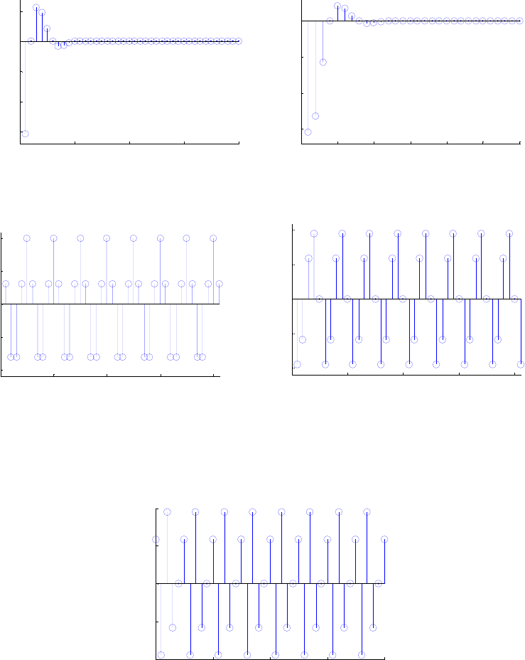
010 20 30 40
-1.5
-1
-0.5
0
0.5
Time index n
A
mp
lit
u
d
e
Real part
0 5 10 15 20 25 30
-1.5
-1
-0.5
0
Time index n
A
mp
lit
u
d
e
Imaginary part
M2.2 (a) The plots generated using Program 2_2.m are shown below:
.][
~4.0 nj
aenx π−
=
010 20 30 40
-1
-0.5
0
0.5
1
Time index n
A
mp
lit
u
d
e
Real part
010 20 30 40
-1
-0.5
0
0.5
1
Time index n
A
mp
lit
u
d
e
Imaginary part
(b) The code fragment used to generate )8.08.0sin(][
~π
+
π
=
nnx b is as follows:
x = sin(0.8*pi*n + 0.8*pi);
The plot of the periodic sequence is given below:
010 20 30 40
-1
-0.5
0
0.5
1
n
A
mp
lit
u
d
e
(c) The code fragment used to generate
(
)
(
)
10/5/ ImRe][
~njnj
ceenx ππ += is as
follows:
x = real(exp(i*pi*n/5)+ imag(exp(i*pi*n/10);
The plot of the periodic sequence is given below:
Not for sale. 39
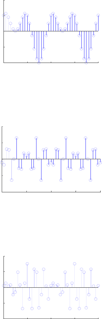
010 20 30 40
-2
-1
0
1
2
n
Amplitude
(d) The code fragment used to generate )5.05.0sin(4)3.1cos(3][
~
π
+π
−
π
=
nnnx d is as
follows:
x = 3*cos(1.3*pi*n)-4*sin(0.5*pi*n+0.5*pi);
The plot of the periodic sequence is given below:
010 20 30 40
-10
-5
0
5
10
n
Amplitude
(e) The code fragment used to generate
)5.0sin()6.0cos(4)75.05.1cos(5][
~nnnnx e
π
−
π
+
π
+π= is as follows:
x = 5*cos(1.5*pi*n+0.75*pi)+4*cos(0.6*pi*n)-sin(0.5*pi*n);
The plot of the periodic sequence is given below:
010 20 30 40
-10
-5
0
5
10
n
Amplitude
M2.3 (a) L = input('Desired length = ');
A = input('Amplitude = ');
omega = input('Angular frequency = ');
phi = input('Phase = ');
n = 0:L-1;
Not for sale. 40
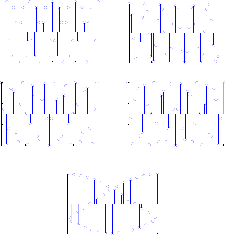
x = A*cos(omega*n + phi);
stem(n,x);
xlabel('Time Index'); ylabel('Amplitude');
title(['\omega_{o} = ',num2str(omega/pi),'\pi']);
(b)
010 20 30 40
-1.5
-1
-0.5
0
0.5
1
1.5
Time Index
A
mp
lit
u
d
e
ω
o
=
0
.
6
π
010 20 30 40
-1.5
-1
-0.5
0
0.5
1
1.5
Time Index
A
mp
lit
u
d
e
ω
o =
0
.
28
π
010 20 30 40
-1.5
-1
-0.5
0
0.5
1
1.5
Time Index
A
mp
lit
u
d
e
ω
o
=
0
.
45
π
010 20 30 40
-1.5
-1
-0.5
0
0.5
1
1.5
Time Index
A
mp
lit
u
d
e
ω
o
=
0
.
55
π
010 20 30 40
-1.5
-1
-0.5
0
0.5
1
1.5
Time Index
A
mp
lit
u
d
e
ω
o
=
0
.
65
π
M2.4 t = 0:0.001:1;
fo = input('Frequency of sinusoid in Hz = ');
FT = input('Sampling frequency in Hz = ');
g1 = cos(2*pi*fo*t);
plot(t,g1,'-');
xlabel('time'); ylabel('Amplitude'); hold
n = 0:1:FT;
gs = cos(2*pi*fo*n/FT);
plot(n/FT,gs,'o'); hold off
M2.5 t = 0:0.001:0.85;
Not for sale. 41
g1 = cos(6*pi*t); g2 = cos(14*pi*t); g3 =
cos(26*pi*t);
plot(t/0.85,g1,'-', t/0.85, g2, '--', t/0.85, g3,':');
xlabel('time'); ylabel('Amplitude'); hold
n = 0:1:8; gs = cos(0.6*pi*n); plot(n/8.5,gs,'o');
hold off
M2.6 As the length of the moving average filter is increased, the output of the filter gets more
smoother. However, the delay between the input and the output sequences also
increases (This can be seen from the plots generated by Program 2_4.m for various
values of the filter length.)
M2.7 alpha = input('Alpha = ');
y0 = 1; y1 = 0.5*(y0 + (alpha/y0));
while abs(y1-y0)>0.00001
y2 = 0.5*(y1+(alpha/y1));
y0 = y1; y1 = y2;
end
disp('Squre root of alpha is'); disp(y1);
M2.8 format long
alpha = input('Alpha = ');
y0 = 0.3; y = zeros(1,61);
L = length(y) - 1;
y(1) = alpha - y0*y0 + y0; n = 2;
while abs(y(n-1) - y0) > 0.00001
y2 = alpha - y(n-1)*y(n-1) + y(n-1);
y0 = y(n-1); y(n) = y2;
n = n+1;
end
disp('Square root of alpha is');disp(y(n-1));
m = 0:n-2;
err = y(1:n-1) - sqrt(alpha);
stem(m,err);
axis([0 n-2 min(err) max(err)]);
xlabel('Time index n'); ylabel('Error');
title(['\alpha = ',num2str(alpha)]);
The displayed out is
Square root of alpha is
0.84178104293115
Not for sale. 42
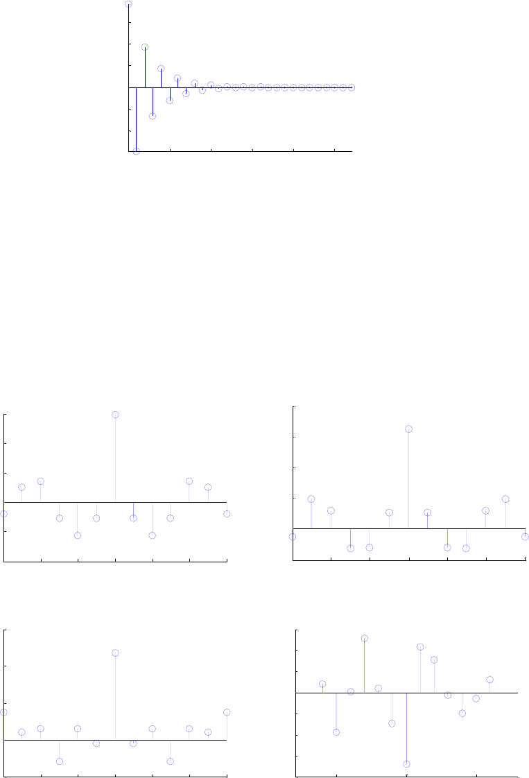
0 5 10 15 20 25
-0.04
-0.02
0
0.02
0.04
0.06
Time index n
Error
α
= 0.7086
M2.9 ,33},2,0,3,2,1,5,4{]}[{
≤
≤
−
−
−−= nnx
,51},2,7,8,0,1,3,6{]}[{
≤
≤
−
−
−−= nny
.82},5,2,0,1,2,2,3{]}[{
≤
≤
−
−= nnw
.66},8,10,14,11,23,11,59,11,23,11,14,10,8{]}[{ ≤≤−−−−−−−−−= nnrxx
.66},12,48,29,31,30,27,163,27,30,31,29,48,12{]}[{ ≤≤−−−−−−−−−= nnryy
.66},15,10,6,12,6,2,47,2,6,12,6,4,15{]}[{ ≤≤−−−−−= nnrww
-6 -4 -2 0 2 4 6
-40
-20
0
20
40
60
La
g
index
Amplitude
r
xx
[
n
]
-6 -4 -2 0 2 4 6
-50
0
50
100
150
200
La
g
index
A
mp
li
tu
d
e
r
yy
[
n
]
-6 -4 -2 0 2 4 6
-20
0
20
40
60
La
g
index
Amplitude
r
ww
[
n
]
-5 0 5
-80
-60
-40
-20
0
20
40
60
La
g
index
Amplitude
r
xy
[
n
]
Not for sale. 43
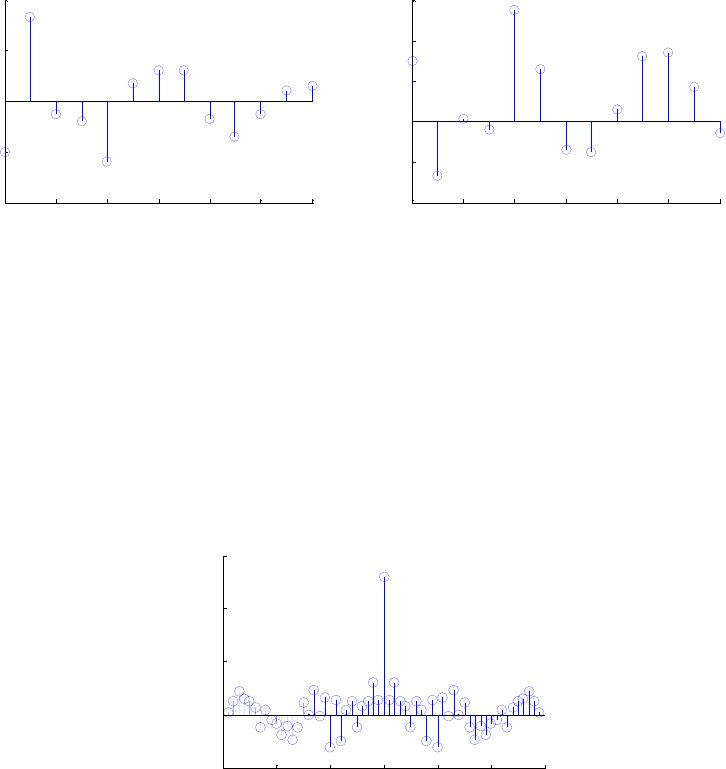
-6 -4 -2 0 2 4 6
-40
-20
0
20
40
La
g
index
Amplitude
r
xw
[
n
]
-6 -4 -2 0 2 4 6
-40
-20
0
20
40
60
La
g
index
Amplitude
r
yw
[
n
]
M2.10 N = input('Length of sequence = ');
n = 0:N-1;
x = exp(-0.8*n);
y = rand(1,N)-0.5+x;
n1 = length(x)-1;
r = conv(y,fliplr(y));
k = (-n1):n1;
stem(k,r);
xlabel('Lag_index'); ylabel('Amplitude');
-30 -20 -10 010 20 30
-1
0
1
2
3
La
g
index
Amplitude
Not for sale. 44

Chapter 3
3.1 Now,
.)()( ∫
=Ω ∞
∞−
Ω− dtetxjX tj
aa .)( ∞<
∫
∞
∞
−
dttxa Hence,
≤
∫
=Ω ∞
∞−
Ω− dtetxjX tj
aa )()( ∫
∞
∞
−
Ω− dtetx tj
a)( .)( ∞<
∫
≤∞
∞
−
dttxa
3.2 (a)
()
dtdtetjY tj
t
o
jt
o
jeee
tj
oa ∫+
∞
∞−
Ω− ∞−
∞−
Ω−
Ω−Ω
=
∫Ω=Ω 2
1
)cos()(
()
)()(
2
1
oo Ω+Ωδ+Ω−Ωδ= .
(b) dteedteedteejU tjttjttj
t
aΩ−
∞α−Ω−
∞−
αΩ−
∞
∞−
α− ∫
+
∫
=
∫
=Ω
0
0
)(
[]
[
]
.
21111
22
0
)(
0
)(
Ω+α
α
=
Ω+α
+
Ω−α
=⋅
Ω+α
−⋅
Ω−α
=∞−
Ω+α−
∞−
Ω−α
jj
e
j
e
j
tjtj
(c) ).()( )( o
tj
tj
tj
adtedteejV oo Ω−Ωδ=
∫
=
∫
=Ω ∞
∞
−
Ω−Ω−
∞
∞−
Ω−
Ω
(d) using the
linearity property of the CTFT. Next, using the shifting property of the CTFT we get
which can be alternately expressed in the form
∑⎟
⎟
⎠
⎞
⎜
⎜
⎝
⎛∫−δ=
∫⎟
⎟
⎠
⎞
⎜
⎜
⎝
⎛∑−δ=Ω ∞
−∞=
∞
∞−
Ω−Ω−
∞
∞−
∞
−∞= ll
ll dteTtdteTtjP tjtj
a)()()(
∑
=Ω ∞
−∞=
Ω−
l
lTj
aejP )(
)
2
(
2
)( ∑π
−Ωδ
π
=Ω ∞
−∞=l
l
TT
jPa making use of the results of Problem 3.2(c).
3.3 (a)
).()( Ωδ=
∫
=Ω ∞
∞−
Ω− dtejV tj
a
(b) µ)(
1
)()()( Ωπδ+
Ω
=
∫⎟
⎟
⎠
⎞
⎜
⎜
⎝
⎛∫ττδ=
∫µ=Ω Ω−
∞
∞−∞−
∞
∞−
Ω−
j
dteddtetj tj
t
tj .
(c) The function is also denoted by Thus,
)(txa).(rect tdtetxjX tj
aa ∫
=Ω ∞
∞−
Ω−
)()(
()
).2/(sinc
2/
)2/sin()2/sin(21 2/2/
2/1
2/1
Ω=
Ω
Ω
=
Ω
Ω
=−
Ω
−=
∫
=ΩΩ−
−
Ω− jjtj ee
j
dte
Not for sale 45

(d) ⎩
⎨
⎧
≥
<−
=.5.0,0
,5.0,21
)( t
tt
tya A more convenient way to determine the CTFT of
is to differentiate it twice with respect to
)(ty a
t
, determine the CTFT of 2
2)(
dt
tyd a and then
make use of the time-differentiation property given in Problem 3.6(e) and time-shifting
property given in Problen 3.6(a). Now, ⎩
⎨
⎧
≥−
<
=.5.0,2
,5.0,2
)(
t
t
dt
dyat As dt
tdya)( has jump
discontinuities with a positive jump of value 2 at ,5.0
±
=
t a negative jump of value 4
−
at and zero everywhere else, ,0=t2
2)(
dt
tyd a has only impulses of strength 2 at ,5.0
±
=
t
and an impulse of strength 4
−
at ,0
=
ti.e., ).5.0(2)(4)5.0(2
2
)( −δ+δ−+δ= ttt
dt
tya
2
d If
denotes the CTFT of , then using of the time-differentiation property we
have
)( ΩjYa)(ty a
).()( 2
CTFT
)(
2
2ΩΩ↔ jYj a
dt
tyd a Using the time-shifting property, we arrive at the
CTFT of 2
2)(
dt
tyd a given by Therefore = .242 2/2/ Ω−Ω +− jj ee )()( 2ΩΩ jYj a
=ΩΩ− )(
2jYa
(
)
1)2/cos(4242 2/2/ −Ω=+− Ω−Ω jj ee , i.e,
()
.sincsin1)2/cos()( 4
2
2
1
4
2
84
22 ⎟
⎠
⎞
⎜
⎝
⎛
=
⎟
⎠
⎞
⎜
⎝
⎛
=−Ω−=Ω ΩΩ
ΩΩ
jYa
3.4 .
2
1
)( 22 2/)( σµ−−
⋅
πσ
=t
eth Thus, .
2
1
)( 22 2/)( dteejH tjt
∫⋅
πσ
=Ω ∞
∞
−
Ω−σµ−−
Making a change of variable
τ
=
µ
−
t
we get τ
∫
πσ
=Ω ∞
∞
−
µ+τΩ−στ− deejH j)(2/ 22
2
1
)(
2/2/ 2222 2
2
1
2
1Ωσ−µΩ−
∞
∞−
τΩ−στ−µΩ− ⋅πσ⋅⋅
πσ
=τ
∫
πσ
=eedeee jjj
.
)
2
(
22 µΩ+
Ωσ
−
=j
e For a zero mean impulse response, we then have the CTFT pair
2/
CTFT
2/ 2222 2Ωσ−σ− πσ
↔ee t.
3.5
(
)
.
)sin(
2
1
2
1
)(
2
1
)( 1
1t
t
ee
tj
dedejXtx jjtjtj
aπ
=−
π
=Ω
∫
π
=Ω
∫Ω
π
=Ω−Ω
−
Ω
∞
∞−
Ω
Not for sale 46

3.6 (a) τ
∫τ=
∫−+τΩ−
∞
∞
−
Ω−
∞
∞−
dexdtettx o
tj
a
tj
oa )(
)()( obtained using a change of variable
Therefore
.τ=− o
tt ).()()( Ω=τ
∫τ=
∫−Ω−
τΩ−
∞
∞
−
Ω−
Ω−
∞
∞−
jXedexedtettx a
tj
j
a
tj
tj
oa oo
(b)
()
.)()()( )( o
tj
a
tj
tj
ajXdtetxdteetx oo Ω−Ω=
∫
=
∫Ω−Ω−
∞
∞
−
Ω−
∞
∞−
Ω
(c) .)(
2
1
)( Ω
∫Ω
π
=∞
∞−
ΩdejXtx tj
aa Therefore .)()(2 Ω
∫Ω=−π ∞
∞
−
Ω− dejXtx tj
aa
Interchanging
t
and Ω we get .)()(2 dtejtXx tj
aa ∫
=Ω−π ∞
∞
−
Ω−
(d) For a positive real constant the CTFT of is given by
a)(atxa
).()()( 1
)/(
1
a
a
a
aj
a
a
tj
ajXdexdteatx Ω
∞
∞−
τΩ−
∞
∞−
Ω− =τ
∫τ=
∫ In a similar manner we
can show that for a negative constant the CTFT of is given by
a)(atxa).(
1
a
a
ajX Ω
−
Therefore .)( 1⎟
⎠
⎞
⎜
⎝
⎛
↔Ω
a
a
a
CTFT
ajXatx
(e) Differentiating both sides of Ω
∫Ω
π
=∞
∞
−
ΩdejXtx tj
aa )(
2
1
)( get
.)(
2
1
)( ΩΩ
∫Ω
π
=Ω
∞
∞−
dejXj
dt
tdx tj
a
a Therefore ).(
)( CTFT ΩΩ
↔jXj
dt
tdx
a
a
3.7 ,)()()( )(Ωθ
Ω−
∞
∞−
Ω=
∫
=Ω a
j
a
tj
aa ejXdtetxjX where
{
.)(arg)( Ω
}
=
Ω
θ
jXaa Thus,
.)()( dtetxjX tj
aa Ω
∞
∞
−∫
=Ω− If is a real function of then it follows from the
definition of and the expression for
)(txa
)( ΩjXa)(
Ω
−
jXa that and )( ΩjXa)(
Ω
−
jXa are
complex conjugates. Therefore )()( Ω=Ω− jXjX aa and ).()( Ωθ−=Ω
−
θ
aa Or in
other words, for a real , the magnitude spectrum )( ΩjXa is an even function of
Ω
and
the phase spectrum is an odd function of
)(Ωθa.
Ω
3.8
Not for sale 47

3.9 where
.)()()(
ˆττ
∫τ−= ∞
∞−
dxthtx HT )(thH
T
is the impulse response of the Hilbert
transformer. Taking the CTFT of both sides we get )()()(
ˆΩΩ=Ω jXjHjX
HT
where
and )(
ˆΩjX )( ΩjHH
T
denote the CTFTs of and
)(
ˆtx ),(thH
T
respectively. Rewriting
(
)
).()()()()()(
ˆΩ+Ω−=Ω+ΩΩ=Ω jXjjXjjXjXjHjX npnpHT As the magnitude and
phase of are an even and odd function, is seen to be real signal. Consider
the complex signal
)(
ˆΩjX )(
ˆtx
)(
ˆ
)()( txjtxty
+
=. Its CTFT is then given by
).(2)(
ˆ
)()( Ω=Ω+Ω=Ω jXjXjjXjY p
3.10 The total energy ε
[
]
.1
2/1
2
1
0
2
2
1
2
2=
=α
α
∞
α−
α−
∞
∞
−
α−
∞
∞−
α− ==
∫
=
∫
=ttt
xedtedte
The total energy can also be computed using using the Parsevals’ theorem
ε.
22
1
2
1Ω
∫
=∞
∞− Ω+α
πd
x
Therefore, the 80% bandwidth c
Ω
can be found by evaluating Ω
∫
Ω
Ω− Ω+α
πd
c
c
22
1
2
1
2/1
1
tantantantan 1
11
2
1
1
1
2
1
=α
−⎟
⎟
⎠
⎞
⎜
⎜
⎝
⎛
α
Ω
⋅
πα
=
⎥
⎦
⎤
⎢
⎣
⎡
⎟
⎟
⎠
⎞
⎜
⎜
⎝
⎛
α
Ω
−
−
−
⎟
⎟
⎠
⎞
⎜
⎜
⎝
⎛
α
Ω
−
πα
Ω
Ω−
α
Ω
−
απ =
⎥
⎦
⎤
⎢
⎣
⎡⎟
⎠
⎞
⎜
⎝
⎛
⋅= ccc
c
c
8.0)2(tan 1
2=Ω
−
π
=c. Therefore, .5388.1tan 2
8.0
2
1=
⎟
⎠
⎞
⎜
⎝
⎛
⋅=Ω π
c
3.11 where
],[][][][ nynynny odev +=µ= ][])[][(][ 2
1
2
1
2
1nnynynyev δ+=−+= and
].[][])[][(])[][(][ 2
1
2
1
2
1
2
1nnnnnynynyod δ−µ=−µ−µ=−−= − Now,
.
2
1
)2(
2
1
)2(2
2
1
)( +
∑π+ωδπ=+
⎥
⎦
⎤
⎢
⎣
⎡∑π+ωδπ= ∞
−∞=
∞
−∞=
ω
kk
j
ev kkeY Since
],[][][ 2
1
2
1nnnyod δ−µ= − ].1[]1[]1[ 2
1
2
1−δ−−µ=− −nnnyod As a result,
()
.
2
1
2
1
2
1]1[][][]1[]1[][]1[][ −δ+δ=δ−δ−−µ−µ=−− +nnnnnnnyny odod
Taking the DTFT of both sides of the above equation, we get
(
)
ω−ωω−ω +=− jj
od
jj
od eeYeeY 1)()( 2
1 or .
2
1
1
1
1
1
2
1
)( −=
⎟
⎠
⎞
⎜
⎝
⎛
=ω−
ω−
ω−
−
−
+
ω
j
j
j
e
e
e
j
od eY
Hence, .)2()()()(
1
1∑π+ωδπ+=+= ∞
−∞=
ω−
−
ωωω
k
j
e
j
od
j
ev
jkeYeYeY
3.12 The inverse DTFT of is given by
∑π+ωπδ= ∞
−∞=
ω
k
jkeX )2(2)(
Not for sale 48

.1
2
2
)(2
2
1
][ =
π
π
=
∫ωωπδ
π
=π
π−
ωdenx nj
3.13 nj
n
n
jeeY ω−
∞
−∞=
ω∑α=)( with .1<α Rewriting we get
nj
n
nj
n
nj
n
nnj
n
nj eeeeeY )()()( ω−
∞
=
ω
∞
=
ω−
∞
=
ω−
−
−∞=
−ω ∑α+
∑α=
∑α+
∑α=
010
1
.
cos21
1
1
1
12
2
α+ωα−
α−
=
α−
+
α−
α
=ω−ω
ω
jj
j
ee
e
3.14 ).(1
)sin(
][)( ωω−
∞
−∞=
ω−=
∑⎟
⎠
⎞
⎜
⎝
⎛
π
ω
−δ= j
LP
nj
n
c
jeHe
n
n
neG
G(e )
jω
ωc
1
ωc
_0ω
π
π
_
3.15 .)(
2
1
][ ω
∫
π
=ω
π
π−
ωdeeXnx njj Hence, .)(*
2
1
][* ω
∫
π
=ω−
π
π−
ωdeeXnx njj
(a) Since is real and even, we have Thus
][nx ).(*)( ωω =jj eXeX
.)(
2
1
][ ω
∫
π
=− ω−
π
π−
ωdeeXnx njj Therefore,
.)cos()(
2
1
])[][(
2
1
][ ωω
∫
π
=−+= π
π−
ωdneXnxnxnx j As is even,
As a result, the term inside the above integral is even, and hence
][nx ).()( ω−ω =jj eXeX
)(cos)( nneX jω
ω
.)cos()(
1
][
0
ωω
∫
π
=πωdneXnx j
(b) Since is real and odd, we have
][nx ][][ nxnx
−
−
=
and Thus, ).()( ω−ω −= jj eXeX
.)sin()(
2
])[][(
2
1
][ ∫ωω
π
=−−= π
π−
ωdneX
j
nxnxnx j As a result, the term )sin()( neX jω
ω
inside the above integral is even, and hence .)sin()(
2
][
0
∫ωω
π
=πωdneX
j
nx j
Not for sale 49

3.16 ][
2
][)sin(][ 00
0n
j
eeee
AnnAnx
j
nj
j
nj
nn µ
⎟
⎟
⎠
⎞
⎜
⎜
⎝
⎛−
α=µφ+ωα= φ−
ω−
φ
ω
()
(
)
].[
2
][
2
00 nee
j
A
nee
j
An
j
j
n
j
jµα−µα= ω−
φ−
ω
φ Therefore, the DTFT of is given
by
][nx
.
1
1
2
1
1
2
)(
00 ω−
ω
φ−
ω
ω
φω
α−
−
α−
=j
j
j
j
j
jj
ee
e
j
A
ee
e
j
A
eX
3.17 Let with
]1[][ nnx nµα= .1<α Its DTFT was computed in Example 3.6 and is given by
.
1
1
)( ω−
ω
α−
=j
j
e
eX
(a) with
]1[][
1−µα= nnx n.1<α Its DTFT is given by
nj
n
nj eeX ω−
∞
=
ω∑α=
1
1)(
.
1
1
1
1
1)()(
01 ω−
ω−
ω−
ω−
∞
=
ω−
∞
=α−
α
=−
α−
=−
∑α=
∑α= j
j
j
nj
n
nj
ne
e
e
ee
(b) with
][][
2nnnx nµα= .1<α Note ][][
2nxnnx
=
. Therefore, using the
differentiation-in-frequency property in Table 3.4 we get
.
)1(1
1)(
)( 2
2ω−
ω−
ω−
ω
ω
α−
α
=
⎟
⎟
⎠
⎞
⎜
⎜
⎝
⎛
α−
ω
=
ω
=j
j
j
j
j
e
e
e
d
d
j
d
edX
jeX
(c) with
]1[][
3+µα= nnx n.1<α Its DTFT is given by
.
1
1
1
1
)( 1
0
1
1
3⎟
⎟
⎠
⎞
⎜
⎜
⎝
⎛
α−
α−
α
=
α−
+α=
∑α+α=
∑α= ω−
ω
ω−
ω−ω−
∞
=
ω−ω−
∞
−=
ω
j
j
j
jnj
n
njnj
n
nj
e
e
e
eeeeeX
(d) with ]2[][
4+µα= nnnx n.1<α Its DTFT is given by
From the results of Part
(b) we observe that
.2)( 122
02
4ω−ω−ω−
∞
=
ω−
∞
−=
ωα−α−
∑α=
∑α= jjnj
n
nnj
n
nj eeeneneX
.
)1( 2
0ω−
ω−
ω−
∞
=α−
α
=
∑αj
j
nj
n
n
e
e
en Hence,
.2
)1(
)( 122
2
4ω−ω−
ω−
ω−
ωα−α−
α−
α
=jj
j
j
jee
e
e
eX
(e) with ]1[][
5−−µα= nnnx n.1>α Its DTFT is given by
Not for sale 50

.1
1
1
1)( 1
01
1
5ω
ω
ω−
ω
∞
=
−ω
∞
=
−ω−
−
−∞=
ω
−α
=−
α−
=−
∑α=
∑α=
∑α= j
j
j
mj
m
mmj
m
mnj
n
nj
e
e
e
eeeeX
(f) ⎪
⎩
⎪
⎨
⎧≤α
=.otherwise,0
,,
][
6Mn
nx
n Its DTFT is given by
.
1
1
1
1
)(
)1(1)1(1
1
0
6ω−
+ω−+
ω
ω−
+ω−+
−
−=
ω−−
=
ω−ω
α−
α−
⋅α+
α−
α−
=
∑α+
∑α= j
MjM
MjM
j
MjM
Mn
njn
M
n
njnj
e
e
e
e
e
eeeX
3.18 (a) Let denote µ the DTFT of ].5[][][ −µ−µ= nnnxa)( ωj
e].[n
µ
Using the time-
shifting property of the DTFT given in Table 3.4, the DTFT of is thus given by
][nxa
µ. From Table 3.3, we have
µ
)1()( 5ω−ω −= jj
aeeX )( ωj
e
.)2(
1
1
)( ∑π+ωπδ+
−
=∞
−∞=
ω
ω
k
j
jk
e
e Therefore, .
1
1
)(
5
ω
ω
ω
j
j
j
ae
e
eX −
−
=−
(b) Let with
]).8[][(][ −µ−µα= nnnx n
b]1[][ nnx nµα= .1<α Its DTFT was
computed in Example 3.6 and is given by .
1
1
)( ω−
ω
α−
=j
j
e
eX Now
Using the time-shifting property of the DTFT given in Table
3.4, the DTFT of is thus given by
].8[][][ −−= nxnxnxb
][nxa.
1
1
)()1()(
8
8
ω−
ω−
ωω−ω
α−
−
=−= j
j
jjj
be
e
eXeeX
(c) with ][][][)1(][ nnnnnnx nnn
cµα+µα=µα+= .1>α We can rewrite it as
].[][][ 2nxnxnxc+= The DTFT of was computed in Problem 3.17(b) and is
given by
][
2nx
2
2)1(
)( ω−
ω−
ω
α−
α
=j
j
j
e
e
eX and the DTFT of was computed in Example 3.6
and is given by
][nx
.
1
1
)( ω−
ω
α−
=j
j
e
eX Therefore
)()()( 2ωωω += jjj
ceXeXeX
.
)1(
1
1
1
)1( 22 ω−ω−ω−
ω−
α−
=
α−
+
α−
α
=jjj
j
eee
e
3.19 (a) Then
⎩
⎨
⎧≤≤−
=otherwise.,0
,,1
][
1NnN
ny ⎟
⎟
⎠
⎞
⎜
⎜
⎝
⎛
−
−
=
∑
=ω−
+ω−
ω−
−=
ω−ω
j
Nj
Nj
N
Nn
njj
e
e
eeeY
1
1
)(
)12(
1
.
)2/sin(
][sin 2
1
ω
⎟
⎠
⎞
⎜
⎝
⎛+ω
=
N
Not for sale 51

(b) Then
⎩
⎨
⎧≤≤
=otherwise.,0
,0,1
][
2Nn
ny ω−
+ω−
=
ω−ω
−
−
=
∑
=j
Nj
N
n
njj
e
e
eeY
1
1
)(
)1(
0
2
⎟
⎟
⎠
⎞
⎜
⎜
⎝
⎛
ω
+ω
=ω−
)2/sin(
)2/]1[sin(
2/ N
eNj .
(c) ⎪
⎩
⎪
⎨
⎧≤≤−−
=
otherwise.,0
,,1
][
3NnN
ny N
n
Assume to be odd. Then we can express
N
][O][][ 0
*
0
1
3nynyny N
= where ⎪
⎩
⎪
⎨
⎧≤≤−
=−−
otherwise.,0
,,1
][ 2
1
2
1
0
NN n
ny Therefore,
).()()()( 2
0
1
00
1
3ωωωω == j
N
jj
N
jeYeYeYeY Now, from the results of Part (a), we have
()
.
)2/sin(
2/sin
)(
0ω
ω
=
ωN
eY j Hence,
(
)
.
)2/(sin
2/sin1
)( 2
2
3ω
ω
⋅=
ωN
N
eY j
Note: The above result also holds for
N
even.
(d) ],[][
otherwise,,0
,,1
][ 314 nNyny
NnNnN
ny +=
⎩
⎨
⎧≤≤−−+
= where is the sequence
considered in Part (a) and is the sequence considered in Part (c). Hence,
][
1ny
][
3ny
()
.
)2/(sin
2/sin
)2/sin(
][sin
)()()( 2
2
2
1
314 ω
ω
ω
ω
ωωω N
N
eYNeYeY jjj +
⎟
⎠
⎞
⎜
⎝
⎛+
=⋅+=
(e) Then
⎩
⎨
⎧≤≤−π
=otherwise.,0
,),2/cos(
][
5NnNNn
ny
∑
+
∑
=
−=
ω−π
−=
ω−π−ω N
Nn
njNnj
N
Nn
njNnjj eeeeeY )2/()2/(
52
1
2
1
)(
(
)
()
(
)
()
.
sin
sin
2
1
sin
sin
2
1
2
1
2
1
2/)(
)((
2/)(
)((
2
)
2
1
2
2
)
2
1
222
N
N
N
NNN NN
N
Nn
nj
N
Nn
nj
ee π
π
π
π
ππ
+ω
++ω
−ω
+−ω
−=
⎟
⎠
⎞
⎜
⎝
⎛+ω−
−=
⎟
⎠
⎞
⎜
⎝
⎛−ω− ⋅+⋅=
∑
+
∑
=
3.20 Denote ][
)!1(!
)!1(
][ n
mn
mn
nx n
mµα
−
−+
= with .1<α We shall prove by induction that the
DTFT of is given by ][nxm.
)1(
1
)( mj
j
me
eX ω−
ω
α−
= From Table 3.3, it follows that
it holds for Let
.1=m.2
=
m Then
].[][][)1(][
!
)!1(
][ 1112 nxnnxnxnn
n
n
nx n+=+=µα
+
= Therefore,
Not for sale 52

,
)1(
1
1
)1(
)( 22
2ω−
ω−
ω−
ω−
ω
α−
=α−+
α−
α
=j
j
j
j
j
e
e
e
e
eX and it also holds for .2
=
m
Now, assume that it holds for Consider next
.m][
)!(!
)!(
][
1n
mn
mn
nx n
mµα
+
=
+
].[][
1
][][
)!1(!
)!1( nxnxn
m
nx
m
mn
n
mn
mn
m
mn
mmm
n+⋅⋅=
⎟
⎠
⎞
⎜
⎝
⎛+
=µα
−
−+
⎟
⎠
⎞
⎜
⎝
⎛+
= Hence,
mjmj
j
mjmj
j
mee
e
ee
d
d
j
m
eX
)1(
1
)1()1(
1
)1(
11
)( 1
1ω−+ω−
ω−
ω−ω−
ω
+α−
+
α−
α
=
α−
+
⎟
⎟
⎠
⎞
⎜
⎜
⎝
⎛
α−
ω
=
.
)1(
1
1+ω−
α−
=mj
e
3.21 (a) Hence, .)2()( ∑π+ωδ= ∞
−∞=
ω
k
j
akeX .1)(
2
1
][ =ω
∫ωδ
π
=ω
π
π−
denx nj
a
(b)
(
)
.
1
1
)( 1
0
∑
=
−
−
=−
=
ωω
ω
ωω
ωN
n
njj
j
Njj
j
bee
e
ee
eX Let .nm
−
=
.)( 1
0
∑
=+−
=
ω−ωω N
m
mjjj
beeeX
Consider the DTFT Its inverse is given by
Therefore, by the time-shifting property of the DTFT, the
inverse DTFT of is given by
.)( 1
0
∑
=+−
=
ω−ω N
m
mjj eeX
⎩
⎨
⎧≤≤−−
=otherwise.,0
,0)1(,1
][ nN
nx
)()( ωωω =jjj
beXeeX ⎩
⎨
⎧−≤≤−
=+= otherwise.,0
,1,1
]1[][ nN
nxnxb
(c) Hence, .2)cos(21)(
0
∑
+=
∑ω+=
−=
ω−
=
ωN
N
j
N
j
ceeX
l
l
l
l
⎪
⎩
⎪
⎨
⎧
≤<
=
=
otherwise.,0
,0,1
,0,3
][ Nn
n
nxc
(d) 2
)1(
)( ω
ω−
ω
−α−
α−
=j
j
j
dje
e
eX with .1<α We can rewrite as
)( ωj
deX
ω
=
ω
ω
d
edX
eX
j
o
j
d
)(
)( where .
1
1
)( ω−
ω
α−
=j
j
oe
eX From Table 3.3, the inverse
DTFT of is given by From Table 3.4, using the
differentiation-in-frequency property the inverse DTFT of is thus given by
)( ωj
deX ].[][ nnx n
oµα=
)( ωj
deX
].[][][ nnnxnnx n
od µα==
Not for sale 53

3.22 (a) .)4sin()( 4
2
1
4
2
1
2
44 ω−ω
−
ω−==ω= ω−ω j
j
j
jj
ee
j
aeeeH
jj Therefore,
.44},5.0,0,0,0,0,0,0,0,5.0{][
≤
≤
−
−= njjnha
(b) .5.05.0)4cos()( 44
2
44 ω−ω
+
ω+==ω= ω−ω jj
ee
j
beeeH
jj Therefore,
.44},5.0,0,0,0,0,0,0,0,5.0{][
≤
≤
−
=nnhb
(c) .)5sin()( 5
2
1
5
2
1
2
55 ω−ω
−
ω−==ω= ω−ω j
j
j
jj
ee
j
ceeeH
jj Therefore,
.55},5.0,0,0,0,0,0,0,0,0,0,5.0{][ ≤≤
−
−= njjnhc
(d) .5.05.0)5cos()( 55
2
55 ω−ω
+
ω+==ω= ω−ω jj
ee
j
deeeH
jj Therefore,
.55},5.0,0,0,0,0,0,0,0,0,0,5.0{][ ≤
≤
−
=nnhd
3.23 (a) ⎟
⎠
⎞
⎜
⎝
⎛
+
⎟
⎠
⎞
⎜
⎝
⎛
+=ω+ω+= ω−ωω−ω ++
ω
22
1
22
321)2cos(3)cos(21)( jjjj eeee
j
eH
Therefore, .5.15.11 22 ω−ωω−ω ++++= jjjj eeee
.22},5.1,1,1,1,5.1{]}[{ 1
≤
≤
−
=nnh
(b)
()
2/
2
2cos)2cos(4)cos(23)( ω−
ω
ω⎟
⎠
⎞
⎜
⎝
⎛
ω+ω+= jj eeH
2/
222
2/2/22
423 ω−
+++ ⎟
⎠
⎞
⎜
⎝
⎛
⎥
⎦
⎤
⎢
⎣
⎡⎟
⎠
⎞
⎜
⎝
⎛
+
⎟
⎠
⎞
⎜
⎝
⎛
+= ω−ωω−ωω−ω j
eeeeee e
jjjjjj
()
(
)
ω−ω−ωω−ω +++++= jjjjj eeeee 1223
2
122
.5.125.12 322 ω−ω−ωω−ω +++++= jjjjj eeeee Hence,
.32},1,5.1,2,2,5.1,1{]}[{ 2
≤
≤
−
=nnh
(c)
[]
)sin()2cos(2)cos(43)(
3ωω+ω+=
ωjeH j
⎟
⎠
⎞
⎜
⎝
⎛
⎥
⎦
⎤
⎢
⎣
⎡⎟
⎠
⎞
⎜
⎝
⎛
+
⎟
⎠
⎞
⎜
⎝
⎛
+= ω−ωω−ωω−ω −++
j
eeeeee jjjjjj
j222
22
243
(
)
)(223 22
2
1ω−ωω−ωω−ω −++++= jjjjjj eeeeee
.5.05.0223 22 ω−ωω−ω ++++= jjjj eeee Hence,
.22},5.0,2,3,2,5.0{]}[{
≤
≤
−
=nnhc
Not for sale 54

(d)
[]
2/
4)2/sin()2cos(3)cos(24)( ωω ωω+ω+= jj ejeH
2/
222
2/2/22
324 ω−
−++ ⎟
⎠
⎞
⎜
⎝
⎛
⎥
⎦
⎤
⎢
⎣
⎡⎟
⎠
⎞
⎜
⎝
⎛
+
⎟
⎠
⎞
⎜
⎝
⎛
+= ω−ωω−ωω−ω j
j
eeeeee ej
jjjjjj
(
)
(
)
ω−ω−ωω−ω −++++= jjjjj eeeee 15.15.14 22
2
1
.75.05.05.15.125.05.1 322 ω−ω−ωω−ω −−+−−= jjjjj eeeee Hence,
.23},3,5.0,3,3,5.0,5.1{]}[{ 4
≤
≤
−
−
−
−−−= nnh
3.24 Let and denote the DTFTs of the sequences and , respectively. )( ωj
eH )( ωj
eG ][nh ][ng
(a) Linearity Theorem: F
{}
∑β+α=β+α ∞
−∞=
ω−
n
nj
engnhngnh ])[][(][][
∑
β+
∑
α= ∞
−∞=
ω−
∞
−∞=
ω−
n
nj
n
nj engenh ][][ ).()( ωω β+α= jj eGeH
(b) Time-reversal Theorem: ).(][][ ω−
∞
−∞=
ω
∞
−∞=
ω− =
∑
=
∑−j
m
mj
n
nj eHemhenh
(c) Time-shifting Theorem:
∑
=
∑−∞
−∞=
+ω−
∞
−∞=
ω−
m
nmj
n
nj
oo
emhennh )(
][][
).(][ ω
ω−
∞
−∞=
ω−
ω− =
∑
=j
nj
m
mj
nj eHeemhe oo
(d) Frequency-shifting Theorem:
(
)
∑
=
∑∞
−∞=
ω−ω−
∞
−∞=
ω−
ω
n
nj
n
nj
nj oo enhenhe )(
][][
)( )( o
j
eH ω−ω
=.
3.25 Let = F and = F )(
1ωj
eH
{
][
1nh
}
)(
2ωj
eH
{
}
.][
2nh From Example 3.8 we have
∑⎟
⎠
⎞
⎜
⎝
⎛
π
ω
=∞
−∞=
ω
n
j
n
n
eH )sin(
)( 2
2
⎩
⎨
⎧
π≤ω<ω
ω≤ω≤
=.,0
,0,1
2
2 From the result of Problem 3.14 we get
⎩
⎨
⎧
π≤ω<ω
ω≤ω≤
=
∑⎟
⎠
⎞
⎜
⎝
⎛
π
ω
−δ= ω−
∞
−∞=
ω
.,1
,0,0
)sin(
][)(
1
1
1
1nj
n
je
n
n
neH
As the impulse response of the cascade is given by ][O][][ 2
*
1nhnhnh
=
, using the
convolution theorem we obtain the DTFT of the cascade: )()()( 21 ωωω =jjj eHeHeH
Not for sale 55
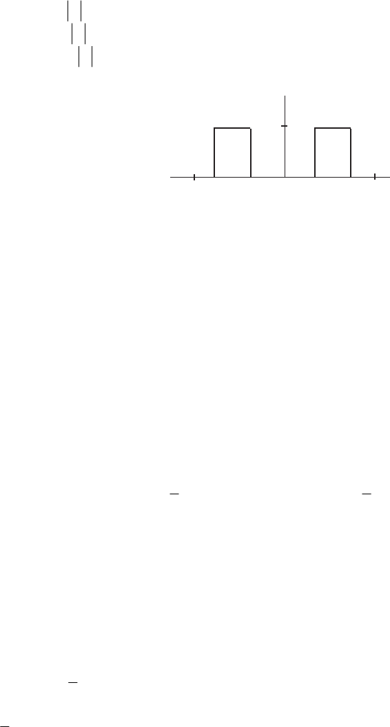
⎪
⎩
⎪
⎨
⎧
π≤ω<ω
ω≤ω≤ω
ω<ω≤
=
.,0
,,1
,0,0
2
21
1
H(e )
jω
ω1
1
0
ω
π
π
__ω2ω2
ω1
_
3.26
(
)
.)()()( 44 ωωω == jjj eXeXeY Now, Hence, .][)( ∑
=∞
−∞=
ω−ω
n
njj enxeX
(
)
.]4/[)(][)(][)( 44 ∑
=
∑
==
∑
=∞
−∞=
ω−
∞
−∞=
ω−ω
∞
−∞=
ω−ω
m
mj
n
njj
n
njj emxenxeXenyeY
Therefore
⎩
⎨
⎧±±±=
=otherwise.,0
,16,8,4,0],[
][ Knnx
ny
3.27 Therefore, and .][)( ∑
=∞
−∞=
ω−ω
n
njj enxeX ∑
=∞
−∞=
ω−ω
n
njj enxeX )2/(2/ ][)(
Thus, we can write .)1(][)( )2/(2/ ∑−=− ∞
−∞=
ω−ω
n
njnj enxeX
{
}
(
)
.)1]([][)()(][)( )2/(
2
1
2/2/
2
1∑∑ ∞
−∞=
ω−ωω
∞
−∞=
ω−ω −+=−+==
n
njnjj
n
njj enxnxeXeXenyeY
Thus, Hence,
⎪
⎩
⎪
⎨
⎧
=∑
∞
−∞=
ω−
odd.for,0
,evenfor,][
][
)2/(
n
nenx
ny n
nj
⎩
⎨
⎧
=.oddfor,0
,evenfor],2[
][ n
nnx
ny
3.28 F
{}
=− ][* nx ∑
=
∑−∞
−∞=
ω
∞
−∞=
ω−
n
nj
n
nj enxenx ][*][* .)()][( *
*ω
∞
−∞=
ω− =
∑
=j
n
nj eXenx
3.29
[
]
=−= ω−ωω )()()( *
2
1jjj
ca eXeXeX
⎟
⎟
⎠
⎞
⎜
⎜
⎝
⎛∑
−
∑
−
∑
+
∑
=∞
−∞=
ω−
∞
−∞=
ω−
∞
−∞=
ω−
∞
−∞=
ω−
n
nj
im
n
nj
re
n
nj
im
n
nj
re enxjenxenxjenx ][][][][
2
1
,ω=
∑
=∞
−∞=
ω−
n
nj
im enxj ][ F
{
}
.][nxj im
3.30
Not for sale 56
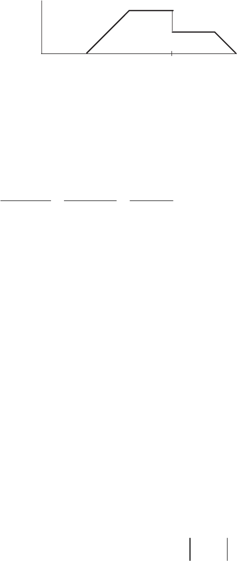
00.6π1.4π2π
|X(e )|
jω
3.31 From Table 3.2 we observe that an even real-valued sequence has a real-valued DTFT
and an odd real-valued sequence has an imaginary-valued DTFT.
(a) Since is an odd sequence, it has an imaginary-valued DTFT.
][
1nx
(b) Since is an even sequence, it has a real-valued DTFT.
][
2nx
(c) ].[
)sin()sin()sin(
][ 33 nx
n
n
n
n
n
n
nx ccc =
π
ω
=
π−
ω
−
=
π−
ω−
=− Since, is an even
sequence, it has a real-valued DTFT.
][
3nx
(d) Since is an odd sequence, it has an imaginary-valued DTFT.
][
4nx
(e) Since is an odd sequence, it has an imaginary-valued DTFT. ][
5nx
3.32 From Table 3.2 we observe that an even real-valued sequence has a real-valued DTFT
and an odd real-valued sequence has an imaginary-valued DTFT.
(a) Since is a real-valued function of )(
1ωj
eY ,
ω
its inverse is an even sequence.
(b) Since is an imaginary-valued function of )(
2ωj
eY ,
ω
its inverse is an odd sequence.
(c) Since is an imaginary-valued function of
)(
3ωj
eY ,
ω
its inverse is an odd sequence.
3.33 (a) Since is a real-valued function of )(
1ωj
eH ,
ω
its inverse is an even sequence.
(b) Since is a real-valued function of )(
2ωj
eH ,
ω
its inverse is an even sequence.
3.34 Let and let and denote the DTFTs of and
respectively. From the convolution property of the DTFT given in Table 3.4, the DTFT
],[][ *nxnu −= )( ωj
eX )( ωj
eU ][nx ],[nu
of is given by From Table 3.1,
][O][][ *nunxny =).()()( ωωω =jjj eUeXeY )( ωj
eU
Therefore, ).(
*ω
=j
eX
2
*)()()()( ωωωω == jjjj eXeXeXeY which is a real-valued
function of
.ω
3.35 From the frequency-shifting property of the DTFT given in Table 3.4,
F A sketch of this DTFT is shown below ).(}][{ )3/(3/ π+ωπ− =jnj eXenx
Not for sale 57

π
0
π
_
X(e )
j(ω+π/3)
_π
2
3
π
3
_
ω
3.36 .)(]}1[{
0
1
1
1∑⎟
⎠
⎞
⎜
⎝
⎛
α−=
∑α−=
∑α−==−−µα− ∞
=α
ω−ω
∞
=
−ω−
−
−∞=
ωω
n
n
e
jnj
n
nnj
n
njn j
eeeeXn
For ,1>α .
1
1
)/(1
1
1
)( ωω α−α−
ω−ω =α−= jj ee
jj eeX .)( )cos(21
1
2
2ωα−α+
ω=⇒ j
eX
From Parseval’s relation, .][)(
2
12
2∑
=ω
∫
π
∞
−∞=
π
π−
ω
n
jnxdeX
(a) .)( )cos(45
1
2
ω+
ω=
j
eX Hence .2
−
=
α
Therefore, ].1[)2(][ −−µ−= nnx n
Now, ∑−π=
∑
π=ω
∫
=ω
∫−
−∞=
∞
−∞=
π
π−
ω
πω12
2
2
0
2)2(4][4)(2)(4
n
n
n
jj nxdeXdeX
.4 3
4
04
1
14
1π
∞
=
∞
=
=
∑⎟
⎠
⎞
⎜
⎝
⎛
π=
∑⎟
⎠
⎞
⎜
⎝
⎛
π=
n
n
n
n
(b) .)( )cos(325.3
1
2
ω−
ω=
j
eX Hence .5.1
=
α
Therefore, ].1[)5.1(][ −−µ−= nnx n
Now, ∑
π=
∑
π=ω
∫
=ω
∫−
−∞=
∞
−∞=
π
π−
ω
πω12
2
2
0
2)5.1(][)(
2
1
)(
n
n
n
jj nxdeXdeX
.
5
4
5
9
9
4
09
4
9
4
19
4ππ
∞
=
π
∞
=
=⋅=
∑⎟
⎠
⎞
⎜
⎝
⎛
=
∑⎟
⎠
⎞
⎜
⎝
⎛
π=
n
n
n
n
(c) Using the differentiation-in-frequency property of the DTFT as given in Table 3.4,
the inverse DTFT of 2
)1(
1
1
)( ω−
ω−
ω− α−
α
α−
ω=
⎟
⎟
⎠
⎞
⎜
⎜
⎝
⎛
ω
=j
j
je
e
e
j
d
d
jeX is
Hence, the inverse DTFT of
].1[][ −−µα−= nnnx n
2
)1(
1
ω−
α− j
e
is ].1[)1( −−µα+− nn n
.
)45(
1
2
2
)( ω−
−
ω=j
e
j
eY Hence .2
=
α
Therefore, . ]1[2)1(][ −−µ+−= nnny n
Now, n
nn
jj nnxdeXdeX 2
12
2
2
0
22)1(4][4)(2)(4 ⋅
∑+π=
∑
π=ω
∫
=ω
∫−
−∞=
∞
−∞=
π
π−
ω
πω
Not for sale 58

.4
16/9
4/9
0
2
4
1π=π=
∑⋅
⎟
⎠
⎞
⎜
⎝
⎛
π= ∞
=n
n
n
3.37 .152][2][2 6
3
22
)( 2
π=
∑
π=
∑
π=ω
∫−
∞
∞−
π
π− ω
ω
nxnnxnd
d
edX j (Using Parseval’s relation with
differentiation-in-frequency property)
3.38 (a) .10][][)( 6
2
0=
∑
=
∑
=
−=
∞
−∞= nn
jnxnxeX
(b) .6][][)( 6
2
−=
∑
=
∑
=
−=
ππ
∞
−∞=
π
n
njnj
n
jenxenxeX
(c)
.2]0[2)( π−=π=
∫ω
π
π−
ωxdeX j
(d) .120][2][2)( 6
2
22
2π=
∑
π=
∑
π=
∫ω
−=
∞
−∞=
π
π−
ω
nn
jnxnxdeX
(e) .][][
)( π=
∑
π=
∑
π=ω
∫−
∞
∞−
π
π− ω
ω172422 6
2
22
2
nxnnxnd
d
edX j
3.39 (a) .12][][)( 2
6
0=
∑
=
∑
=
−=
∞
−∞= nn
jnxnxeX
(b) .12][][)( 2
6
−=
∑
=
∑
=
−=
ππ
∞
−∞=
π
n
njnj
n
jenxenxeX
(c)
.4]0[2)( π−=π=
∫ω
π
π−
ωxdeX j
(d) .160][2][2)( 2
6
22
2π=
∑
π=
∑
π=
∫ω
−=
∞
−∞=
π
π−
ω
nn
jnxnxdeX
(e) .136][2][2 2
6
22
)( 2
π=
∑
π=
∑
π=ω
∫−
∞
∞−
π
π− ω
ω
nxnnxnd
d
edX j
3.40 From the differentiation-in-frequency property of the DTFT given in Table 3.4 we
have ω
=
∑
ω
∞
−∞=
ω−
d
edX
jenxn
j
n
nj )(
][ where F Therefore, =
ω)( j
eX ]}.[{ nx
.][
0
)(
=ω
ω
∞
−∞=
ω
=
∑d
edX
n
j
jnxn From the definition of the DTFT
∑
=∞
−∞=
ω−ω
n
njj enxeX ][)(
Not for sale 59

it follows that Therefore, .)(][ 0
∑=
∞
−∞=n
j
eXnx .
)( 0
0
)(
j
d
edX
geX
j
C
j
=ω
ω
ω
=
From Table 3.3, F =
ω)( j
eX .1,]}[{ 1
1<α=µα ω−
α− j
e
nn As a result,
22 )1(
0
)1(
0
)(
α−
α
=ω
α−
α
=ω
ω== ω−
ω−
ω
j
j
j
e
e
d
edX
j and .
1
1
0)( α−
=
j
eX Hence, .
1α−
α
=
g
C
3.41 Let F =
ω)(
1j
eG ]}.[{ 1ng
(b) Note ].4[][][ 112
−
+= ngngng Hence, F )(]}[{ 22 ω
=j
eGng
)()( 1
4
1ωω−ω += jjj eGeeG
(
)
).(1 1
4ωω−
+= jj eGe
(c) Note ].4[)]3([][ 113
−
+
−−= ngngng Now, F Hence, ).(]}[{ 11 ω−
=− j
eGng
F
)(]}[{ 33 ω
=j
eGng ).()( 1
4
1
3ωω−ω−ω− += jjjj eGeeGe
(d) Note )].7([][][ 114
−
−
+= ngngng Hence, F )(]}[{ 44 ω
=j
eGng
).()( 1
7
1ω−ω−ω += jjj eGeeG
3.42 i.e., ),()()( 21 ωωω =jjj eXeXeY .][][][ 21 ⎟
⎟
⎠
⎞
⎜
⎜
⎝
⎛∑
⎟
⎟
⎠
⎞
⎜
⎜
⎝
⎛∑
=
∑∞
−∞=
ω−
∞
−∞=
ω−
∞
−∞=
ω−
n
nj
n
nj
n
nj enxenxeny
(a) Setting in the above we get
0=ω .][][][ 21 ⎟
⎟
⎠
⎞
⎜
⎜
⎝
⎛∑
⎟
⎟
⎠
⎞
⎜
⎜
⎝
⎛∑
=
∑∞
−∞=
∞
−∞=
∞
−∞= nnn
nxnxny
(b) Setting we get
π=ω .][)1(][)1(][)1( 21 ⎟
⎟
⎠
⎞
⎜
⎜
⎝
⎛∑−
⎟
⎟
⎠
⎞
⎜
⎜
⎝
⎛∑−=
∑−∞
−∞=
∞
−∞=
∞
−∞= n
n
n
n
n
nnxnxny
3.43 .1],[][ <αµα= nnx nFrom Table 3.3, F ω
α−
ω== j
e
j
eXnx
1
1
)(]}[{ . The total energy
of is E
][nx .
3
4
)(
2/1
2
1
1
0
2
2
1
1
2
1==
∑α=ω
∫
=
=α
α−
∞
=
π
π− ω−
α−
πn
n
j
e
xd To determine the
80% bandwidth of the signal, we set E8.0
2
1
1
2
1
80, =ω
∫
=ω
ω− ω−
α−
πd
c
c
j
e
xE3
4
8.0 ⋅=
x
and solve for , i.e., set E
c
ω3
2.3
2/1
2
sin)cos1(
1
2
1
80, 22 =
⎥
⎥
⎦
⎤
⎢
⎢
⎣
⎡ω
∫
=
=α
ω
ω− ωα+ωα−
πd
c
c
x.
A numerical solution of the above equation yields .5081.0
π
=
ω
c
Not for sale 60

3.44 Recall where ],[][][ nxnxnx odev += ])[][(][ 2
1nxnxnxev −+= and As is causal,
for and
][nx
0][ =nx 0<n0][
=
−nx for Hence, there is no overlap between the
nonzero portions of and
.0>n
][nx ][ nx
−
except at ,0
=
n and we have
][]0[][][2][ nxnnxnx evev
δ
−µ= and ].[]0[][][2][ nxnnxnx odod δ
+
µ
=
Moreover, since
is real, it follows from Table 3.2 that F and
][nx )(]}[{ ω
=j
reev eXnx
F Taking the DTFT of
).(]}[{ ω
=j
imev eXjnx ][]0[][][2][ nxnnxnx evev δ−
µ
=
we
arrive at
∫
=π
π−
ν
π
ω)()( 1j
re
jeXeX µ ].0[)( )( xde j−ν
ν−ω
From Table 3.3 we have
µ F=
ω)( j
e∑π+ωπδ+
⎟
⎠
⎞
⎜
⎝
⎛−
∑=π+ωπδ+=µ ∞
−∞=
ω
∞
−∞=
−ω− kk
e
kjkn j).2()cot(1)2(]}[{ 22
1
1
1
Substituting the above in the equation preceding it we get
ν
⎥
⎦
⎤
⎢
⎣
⎡⎟
⎠
⎞
⎜
⎝
⎛⎟
⎠
⎞
⎜
⎝
⎛
−
∫
=ν−ω
π
π−
ν
π
ωdjeXeX j
re
j
2
2
11 cot1)()(
()
]0[2)()( xdkeX
k
j
re −νπ+ν−ωδ
∑∫
+∞
−∞=
π
π−
ν
].0[)(cot)(
2
)(
2
1
2xeXdeX
j
deX j
re
j
re
j
re −+
∫ν
⎟
⎠
⎞
⎜
⎝
⎛
π
−
∫ν
π
=ω
π
π−
ν−ω
ν
π
π−
ν
Comparing the last equation with we arrive at ),()()( ωωω += j
im
j
re
jeXjeXeX
.cot)(
2
1
)( 2
∫ν
⎟
⎠
⎞
⎜
⎝
⎛
π
−= π
π−
ν−ω
νω deXeX j
re
j
im
Likewise, taking the DTFT of ][]0[][][2][ nxnnxnx odod
δ
+
µ
=
we get
∫
=π
π−
ν
π
ω)()( j
im
j
jeXeX µ ].0[)( )( xde j+ν
ν−ω
Substituting the expression for µ given earlier in the above equation we get )( ωj
e
ν
⎥
⎦
⎤
⎢
⎣
⎡⎟
⎠
⎞
⎜
⎝
⎛⎟
⎠
⎞
⎜
⎝
⎛
−
∫
=ν−ω
π
π−
ν
π
ωdjeXeX j
im
j
j
2
2
1cot1)()(
()
]0[2)()( xdkeXj
k
j
im +νπ+ν−ωδ
∑∫
+∞
−∞=
π
π−
ν
].0[)(cot)()( 2
2
1
2xejXdeXdeX j
im
j
im
j
im
j++
∫ν
⎟
⎠
⎞
⎜
⎝
⎛
+
∫ν= ω
π
π−
ν−ω
ν
π
π
π−
ν
π
Comparing the last equation with we arrive at
),()()( ωωω += j
im
j
re
jeXjeXeX
Not for sale 61

.]0[cot)(
2
1
)( 2
∫+ν
⎟
⎠
⎞
⎜
⎝
⎛
π
=π
π−
ν−ω
νω xdeXeX j
im
j
re
3.45 If is the input to the LTI discrete-time system, then its output is given by
n
znu =][
).(][][][][][ zHzzkhzzkhknukhny n
k
kn
k
kn
k
=
∑
=
∑
=
∑−= ∞
−∞=
−
∞
−∞=
−
∞
−∞=
where Hence is an eigenfunction of the system. .][)( ∑
=∞
−∞=
−
k
k
zkhzH
If is the input to the LTI discrete-time system, then its output is given by ][][ nznv nµ=
.][][][][][][ ∑
=
∑−µ=
∑−=
−∞=
−
∞
−∞=
−
∞
−∞=
n
k
kn
k
knn
k
zkhzzknkhzknvkhny
Since in this case the summation depends upon is not an eigenfunction of the system.
3.46 F F== ω)(]}[{ 11 j
eHnh ,5.01]}1[][{ 2
1ω−
+=−δ+δ j
enn
F F== ω)(]}[{ 22 j
eHnh ,25.05.0]}1[][{ 4
1
2
1ω−
−=−δ−δ j
enn
F
F
== ω)(]}[{ 33 j
eHnh ,2]}[2{
=
δ
n
F
F== ω)(]}[{ 44 j
eHnh .
5.01
2
]}[2{ 2
1
ω−
−
−
=µ
⎟
⎠
⎞
⎜
⎝
⎛
−j
n
e
n
The overall frequency response of the structure of Figure 2.35 is given by
)()()()()()( 42321 ωωωωωω ++= jjjjjj eHeHeHeHeHeH
.1
5.01
)25.05.0(2
)25.05.0(25.01 =
−
−
−−++= ω−
ω−
ω−ω−
j
j
jj
e
e
ee
3.46 Denote F =
ω)( j
ieH .51]},[{ 1
≤
≤
inh
(a) The overall frequency of Figure P2.2(a) is then given by
).()()()()()()()()( 53214321 ωωωωωωωωω ++= jjjjjjjjj
ieHeHeHeHeHeHeHeHeH
(b) The structure of Figure P2.2(b) can be redrawn as shown below
+
h[n]
oh[n]
3
h[n]
4
where the block with an impulse response represents the part of Figure P2.2(b) with a
feedback loop as shown below
Not for sale 62

h[n]
1h2[n]
5
h[n]
+
u[n]v[n]
w[n]
Let F F and F Then we have =
ω)( j
eU ]},[{ nu =
ω)( j
eV ]},[{ nv =
ω)( j
eW ]}.[{ nw
)()()()( 3ωωωω += jjjj eVeHeUeW and
Eliminating from these two equations we get
).()()()( 21 ωωωω =jjjj eWeHeHeV
)( ωj
eW
(
)
)()()()()()()(1 21521 ωωωωωωω =− jjjjjjj eUeHeHeVeHeHeH
which leads to the frequency response of the feedback structure given by
)()()(1
)()(
)(
)(
)(
521
21
ωωω
ωω
ω
ω
ω
−
== jjj
jj
j
j
j
oeHeHeH
eHeH
eU
eV
eH
The overall frequency of Figure P2.2(a) is thus given by
.
)()()(1
)()(
)()()()()(
521
21
434 ωωω
ωω
ωωωωω
−
+=+= jjj
jj
jjj
o
jj
eHeHeH
eHeH
eHeHeHeHeH
3.48 F F == ω)(]}[{ 11 j
eHnh ,32]}1[3]2[2{ 2ωω− −=+δ−−δ jj eenn
F F == ω)(]}[{ 22 j
eHnh ,2]}2[2]1[{ 2ωω− +=+δ+−δ jj eenn
F
F
== ω)(]}[{ 33 j
eHnh ]}1[3][]1[2]3[7]5[5{ +δ+
δ
−
−
δ
+
−
δ
+
−
δ
nnnnn
.31275 35 ωω−ω−ω− +−++= jjjj eeee
The overall frequency of Figure P2.3 is given by
=+= ωωωω )()()()( 213 jjjj eHeHeHeH ωω−ω−ω− +−++ jjjj eeee 31275 35
(
)
(
)
.63295232 33522 ωωω−ω−ω−ωω−ωω− −+++=+−+ jjjjjjjjj eeeeeeeee
3.49 Now, is the inverse DTFT of Rewriting we get ][nhev ).( ωj
re eH
⎟
⎟
⎠
⎞
⎜
⎜
⎝
⎛
+
⎟
⎟
⎠
⎞
⎜
⎜
⎝
⎛
+
⎟
⎟
⎠
⎞
⎜
⎜
⎝
⎛
+= ω−
+
ωω−
+
ωω−
+
ω
ω
2
33
2
22
24321)( j
e
j
e
j
e
j
e
j
e
j
e
j
re eH
Its inverse DTFT is
.225.15.11 3322 ω−ωω−ωω−ω ++++++= jjjjjj eeeeee
].3[2]3[2]2[5.1]2[5.1]1[]1[][][ −δ++
δ
+
−
δ
+
+
δ
+
−
δ++δ+δ= nnnnnnnnhev
Since is real and causal, and its DTFT exists, it is also absolutely
summable. Hence, we can reconstruct from as
][nh )( ωj
eH
][nh ][nhev
][]0[][][2][ nhnnhnh evev
δ
−µ=
(
)
][]3[2]2[5.1]1[][2 nnnnn δ−−δ
+
−
δ
+
−
δ
+
δ
=
].3[4]2[3]1[2][
−
δ
+
−
δ
+
−δ+δ= nnnn
Not for sale 63
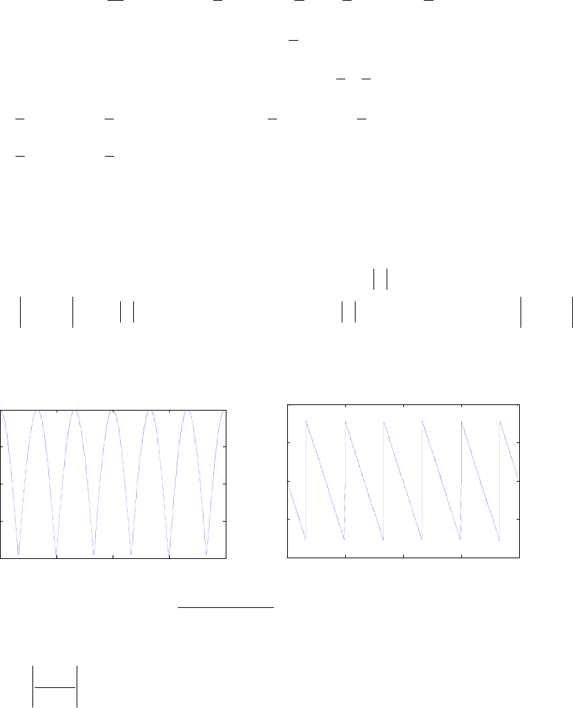
3.50 (a) .)(sin)(sin)cos(sin][ 32
1
32
1
3⎟
⎠
⎞
⎜
⎝
⎛−ω−
⎟
⎠
⎞
⎜
⎝
⎛+ω=ω
⎟
⎠
⎞
⎜
⎝
⎛
=ππ
πnnnny ooo
n
a Hence, the angular
frequencies present in the output are .)( 3n
o
π
±ω
(b) )cos()2cos()cos()(cos)(cos][ 2
1
2
1
23 nnnnnny ooooob ω
⎥
⎦
⎤
⎢
⎣
⎡ω+=ωω=ω=
[
]
)cos()3cos()cos()cos()2cos()cos( 4
1
2
1
2
1
2
1nnnnnn oooooo ω+ω+ω=ωω+ω=
).3cos()cos( 4
1
4
3nn oo ω+ω= Hence, the angular frequencies present in the output are
and
o
ω3 .
o
ω
(c) Hence, the angular frequency present in the output is ).3cos(][ nny oc ω= o
ω
3.
3.51 F Let .1)(]}[][{ Rjj eeHRnn ω−ω α−==−αδ−δ .
φ
α=α j
e Then the maximum value
of )( ωj
eH is α+1 and the minimum value is .1 α− There are
R
peaks of )( ωj
eH
located at ,10,/2
−
≤
≤π=ω RkRk and
R
dips located at
,/)12( Rk π+=ω 10
−
≤≤ Rk in the frequency range .20
π
<
ω
≤
00.5 11.5 2
0
0.5
1
1.5
2
/
Magnitude
00.5 11.5 2
-2
-1
0
1
2
/
Phase, in radians
3.52 .
1
1
)( 1
0ω−
ω−
ω−
−
=
ω
α−
α−
=
∑α= j
MjM
nj
M
n
nj
e
e
eeG Note for In order )()( ωω =jj eHeG .1=α
to have the impulse response should be multiplied by a factor where ,1)( 0=
j
eG ,K
.
1
1
M
Kα−
α−
=
3.53
[]
[
]
.)sin()()2sin()cos()()2cos()( 3213321 ω−+ω−++ω++ω=
ωaaajaaaaeH j
The frequency response will have zero-phase for 32 aa
=
and .
0
1=a
3.54
ω−ω−ω−ω−ω ++++= 4
5
3
4
2
321
)( jjjjj eaeaeaeaaeH
(
)
(
)
.
2
3
2
42
22
5
2
1ω−ω−ω−ωω−ω−ω ++++= jjjjjjj eaeeaeaeeaea
Not for sale 64

If and then we can rewrite the above equation as
51 aa =,
42 aa =
which is seen to have a linear phase.
[
ω−ω +ω+ω= 2
321 )cos(2)2cos(2)( jj eaaaeH
]
3.55
ω−−ω−−ω−ωω +++= )3(
1
)2(
2
)1(
21
)( kjkjkjjkj eaeaeaeaeH
)( 3
1
2
221 ω−ω−ω−ω +++= jjjjk eaeaeaae
[]
.)()( 2/2/
2
2/32/3
1
)( 2
3ω−ωω−ω
ω− +++= jjjj
kj eeaeeae Hence, will be a
real function of if in which case we have
)( ωj
eH
ω,2/3=k
).()()( 2/2/
2
2/32/3
1ω−ωω−ωω +++= jjjjj eeaeeaeH
3.56 F ,)(]}2[]1[][{ 2
1ω−ω−ω ++==−δ+−δ+δ jjj eebaeHnnbna
F ,
1
1
)(]}[{ 2ω−
ω
−
==µ j
jn
ec
eHnc and F .
1
1
)(]}[{ 3ω−
ω
−
==µ j
jn
ed
eHnd
The overall frequency response is then
)()()()( 321 ωωωω =jjjj eHeHeHeH
.
)1)(1(
2
ω−ω−
ω−ω−
−−
++
=jj
jj
edec
eeba Therefore,
)1)(1()1)(1(
)(
22
2
ωω
ωω
ω−ω−
ω−ω−
ω
−−
++
−−
++
=jj
jj
jj
jj
j
edec
eeba
edec
eeba
eH
(
)
(
)
22
22
)cos(21)cos(21
)2cos(2)cos()1(2)1(
ddcc
aabba
+ω−+ω−
ω+ω++++
=
.
)2cos(2)cos()1)((2)21(
)2cos(2)cos()1(2)1(
2222
22
ω+ω++−++++
ω+ω++++
=
cdcddccddcdc
aabba Hence,
,1)( 2=
ωj
eH if
,211 222222 cddcdcba ++++=++
),1)(()cos()1( cddcab
+
+−=ω+ and .cda
=
Substituting cda
=
in the equation on the
left we get
).( dcb +−=
3.57 .)()( )(arg ω
α
ωω =j
eXjjj eeXeY Therefore, .)(
)(
)(
)( 1−α
ω
ω
ω
ω== j
j
j
jeX
eX
eY
eH
Since is real function of )( ωj
eH ,
ω
it has zero-phase.
3.58 ].[][][
R
nyn
x
ny −α−= Taking the DTFT of both sides we get
Hence, ).()()( ωω−ωω α−= jRjjj eYeeXeY .)( 1
1
)(
)(
Rjj
j
eeX
eY
j
eH ω−ω
ω
α+
ω==
Not for sale 65
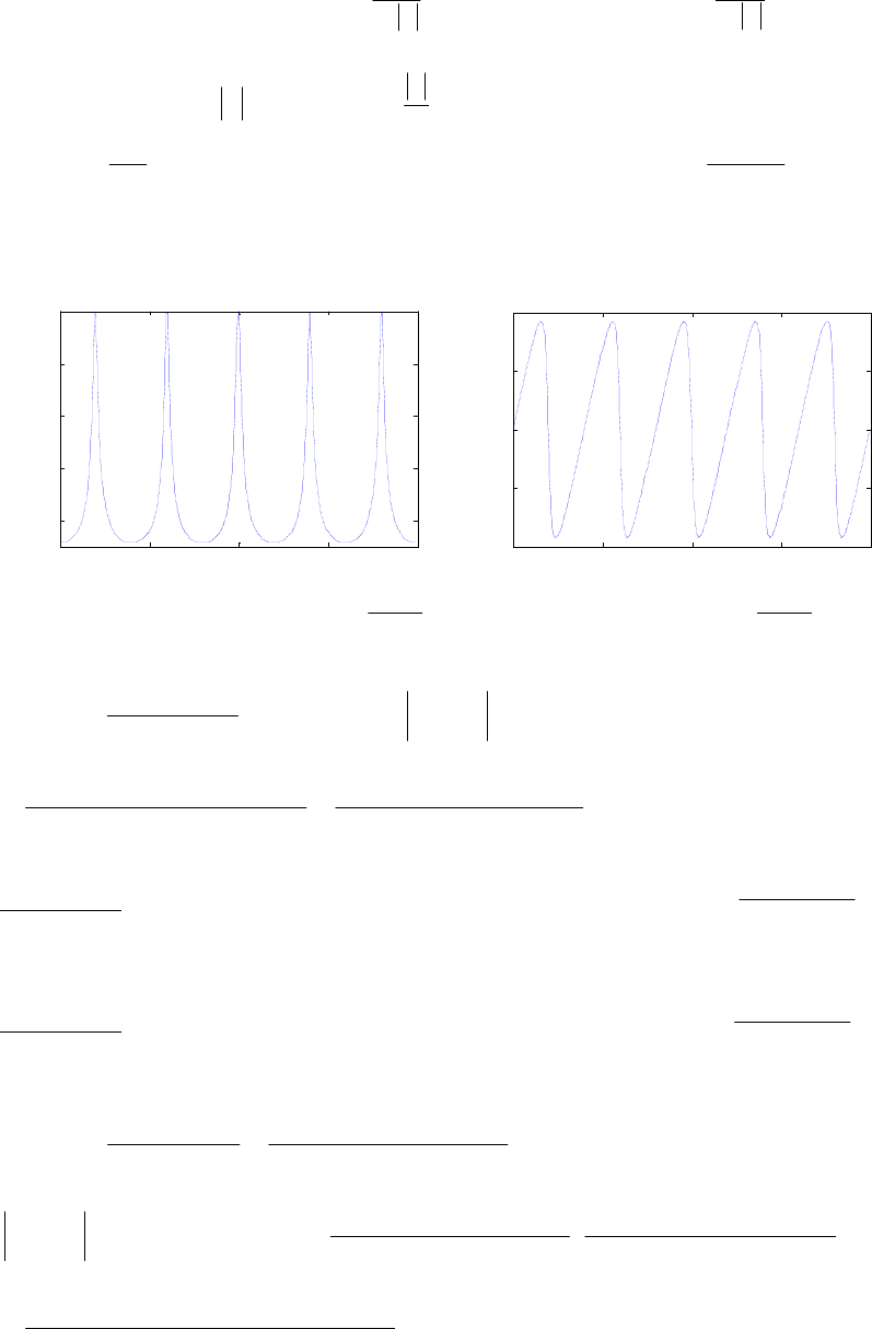
The maximum value of is )( ωj
eH α−1
1 and the minimum value is .
1
1
α+ There are
peaks and dips in the range .20
π
<
ω
≤
The locations of the peaks and the dips are given
by α±=α− ω− 11 Rj
e or .
α
α
ω− ±=
Rj
e The locations of the peaks are given by
R
k
k
π
=ω=ω 2 and the locations of the dips are given by .10,
)12( −≤≤
+π
=ω=ω Rk
R
k
k
Plots of the magnitude and the phase responses of for )( ωj
eH 8.0=
α
and 5
=
R are
shown below:
00.5 11.5 2
1
2
3
4
5
/
Magnitude
00.5 11.5 2
-1
-0.5
0
0.5
1
/
Ph
ase,
i
n ra
di
ans
In this case the maximum value is 5
8.01
1=
− and the minimum value is 0.5556.
8.01
1=
+
3.59 .
1
)(
1
10
ω−
ω−
ω
+
+
=j
j
j
ea
ebb
eA Thus, we set )()()(*)()( 2ω−ωωωω == jjjjj eAeAeAeAeA
.1
)cos(21
)cos(2
)1)(1(
))((
1
2
1
10
2
1
2
0
11
1010 =
ω++
ω++
=
++
++
=ωω−
ωω−
aa
bbbb
eaea
ebbebb
jj
jj
Solution #1: and 1
0±=b.)sgn( 101 abb
=
In which case ,1
1
1
)(
1
1=
+
+
±= ω−
ω−
ω
j
j
j
ea
ea
eA a
trivial solution.
Solution #2: and
1
1±=b.)sgn( 110 abb
=
In which case .
1
)(
1
1
ω−
ω−
ω
+
+
±= j
j
j
ea
ea
eA
3.60 .
11
)(
1
10
1
10 1
0
ω−θ
ω−
φ
φ
ω−
ω−
ω
+
+
=
+
+
=jj
j
j
j
j
j
j
eeA
eeBeB
ea
ebb
eA Thus, we set
ωθ−
ω
φ−
φ−
ω−θ
ω−
φ
φ
ωωω
+
+
⋅
+
+
== jj
j
j
j
jj
j
j
j
jjj
eeA
eeBeB
eeA
eeBeB
eAeAeA
1
10
1
10
2
11
)(*)()( 1
0
1
0
.1
)cos(21
)cos(2
1
2
1
0110
2
1
2
0=
θ−ω++
φ+φ−ω++
=
AA
BBBB
Not for sale 66

Solution #1: .,)sgn(,1 011010
θ
=
φ
−
φ
=±= ABBB In which case
00
00
1
1
1
)(
1
1
1
1
)( φ
ω−θ
ω−θ
φ
ω−θ
ω−
θ+φφ
ω±=
⎟
⎟
⎠
⎞
⎜
⎜
⎝
⎛
+
+
±=
+
±±
=j
jj
jj
j
jj
j
jj
je
eeA
eeA
e
eeA
eeAe
eA
implying
A trivial solution. .
0π±=φ
Solution #2: .,)sgn(,1 011101
θ
=
φ
−
φ
=±= ABBB In which case
11
1
1
1
1
)(
1
11
)( φ
ω−θ
ω−θ−
φ
ω−θ
ω−
θ−φ
ω±=
⎟
⎟
⎠
⎞
⎜
⎜
⎝
⎛
+
+
±=
+
±±
=j
jj
jj
j
jj
j
j
je
eeA
eeA
e
eeA
eeA
eA implying .
1
π
±
=
φ
Hence, a non-trivia solution is .
1
)(
1
*
1⎟
⎟
⎠
⎞
⎜
⎜
⎝
⎛
+
+
=ω−
ω−
πω
j
j
jj
ea
ea
eeA
3.61 (a) )sin(
)cos(
)2/sin(
)2/cos(
)cot(cot)(cosec)( 2ω
ω
−
ω
ω
=ω−
⎟
⎠
⎞
⎜
⎝
⎛
=ω= ω
ωj
aeH
)(
)(
)(
)(
2/2/
2/2/
ω−ω
ω−ω
ω−ω
ω−ω
−
+
−
−
+
=jj
jj
jj
jj
ee
eej
ee
eej
))((
))(())((
2/2/
2/2/2/2/
ω−ωω−ω
ω−ωω−ωω−ωω−ω
−−
+−−−+
=jjjj
jjjjjjjj
eeee
eeeeeeee
j
.
1
234
2
⎟
⎟
⎠
⎞
⎜
⎜
⎝
⎛
+−−
−
=ω−ω−ω−
ω−ω−
jjj
jj
eee
ee
j Therefore, the input-output relation is given by
].2[2]1[2]3[]2[]1[][
−
−
−
=
−
+−−−− nxjnxjnynynyny
(b) .
1
22
)cos(
1
)(sec)( 2ω−
ω−
ω−ω
ω
+
=
+
=
ω
=ω= j
j
jj
j
be
e
ee
eH Therefore, the input-output
relation is given by ].1[2]2[][
−
=
−
+nxnyny
(c) ω−
ω−ωω−
ω−ω
ω−ω
ω−ω
ω−ω
−
+
−
+
−
+
ω==
⎟
⎟
⎠
⎞
⎜
⎜
⎝
⎛
=
ω
ω
=ω= 2
1
)()(
)sin(
)cos(
)(cot)( j
jjj
jj
jj
jj
jj
e
eeej
ee
eej
ee
ee
j
cjeH
.
1
)1(
2
2
ω−
ω−
−
+
=j
j
e
ej Therefore, the input-output relation is given by
].2[][]2[][
−
+=−− nxjnxjnyny
(d) .
1)1(
1
)
2/
(
22/
2/2/
)2/cos(
)2/sin(
tan)( ω−
ω−
ω−
ω−
ω
ω−ω
+
+−
=
+
−
ω−
+
−ω
ω===
ω
ω
=
⎟
⎠
⎞
⎜
⎝
⎛
=j
j
j
j
j
jj
e
ejj
ej
e
j
eej
ee
j
deH
Therefore, the input-output relation is given by ].1[][]1[][
−
+
−
=
−
+
nxjnxjnyny
3.62 From Eq. (2.20), the input-output relation of a factor-of-
L
up-sampler is given by
The DTFT of is thus given by
⎩
⎨
⎧±±±=
=otherwise.,0
,3,2,,0],/[
][ KLLLnLnx
ny ][ny
Not for sale 67

where
),(][]/[][)( ωω−
∞
−∞=
ω−
∞
=−∞=
ω−
∞
−∞=
ω=
∑
=
∑
=
∑
=jLmLj
m
nj
mLn
n
nj
n
jeXemxeLnxenyeY
F =
ω)( j
eX ]}.[{ nx
3.63 .1,
1
1
)( <α
α−
=ω−
ω
jL
j
e
eG Thus, we can write where ),()( ωω =jLj eXeG
.
1
1
)( ω−
ω
α−
=j
j
e
eX From Table 3.3, the inverse DTFT of is
Hence, from the results of Problem 3.62, it follows that
)( ωj
eX ].[][ nnx nµα=
⎩
⎨
⎧±±±=
=otherwise.,0
,3,2,,0],/[
][ KLLLnLnx
ng
3.64 From Table 3.3, .
5.01
1
)( ω−
ω
−
=j
j
e
eH Thus, )cos(25.1
1
)( ω−
=
ωj
eH and
.
)cos(5.01
)sin(5.0
tan)()}(arg{ 1⎟
⎟
⎠
⎞
⎜
⎜
⎝
⎛
ω−
ω−
=ωθ= −ωj
eH Therefore .6664.03504.1)( 5/ jeH jm=
π±
5059.1)( 5/ =
π± j
eH and 4585.0)5/( m
=
π
±
θ
radians.
Now, for an input ],[)sin(][ nnnx o
µ
ω
= the steady-state output is given by
()
.)(sin)(][ oo
jneHny oωθ+ω= ω For ,5/
π
=
ω
o the steady-state output is therefore
given by .4585.0sinsin5059.1)(sin)(][ 555
5/ ⎟
⎠
⎞
⎜
⎝
⎛−=
⎟
⎠
⎞
⎜
⎝
⎛θ+= πππ
πnneHny j
3.65
ω−ω−ω−ω−ω ++=++= jjjjj ehehehehheH ]1[)1](0[]0[]1[]0[)( 22
We require
()
.]1[)cos(]0[2 hhe j+ω= ω− 0]1[)3.0cos(]0[2)( 3.0 =+= hheH j
and .1]1[)6.0cos(]0[2)( 6.0 =+= hheH j Solving these two equations we get
and 8461.3]0[ =h.3487.6]1[ −=h
3.66 ω−ω−ω ++= jjj eheheH ]1[)1](0[)( 2
(
)
.]1[)cos(]0[2 hhe j+ω= ω− We require
1]1[)3.0cos(]0[2)( 3.0 =+= hheH jand .0]1[)6.0cos(]0[2)( 6.0 =+= hheH j Solving
these two equations we get 8461.3]0[
−
=
h and .3487.7]1[
=
h
3.67
3.68
ω−ω−ω−ω−ω ++++= 234 ]2[)(]1[)1](0[)( jjjjj eheeheheH
Not for sale 68

We require
()
.]2[)cos(]1[2)2cos(]0[2
2hhhe j+ω+ω= ω−
,0]2[]1[)2.0cos(2]0[)4.0cos(2)( 2.0 =++= hhheH j
,1]2[]1[)5.0cos(2]0[)0.1cos(2)( 5.0 =++= hhheH j
.0]2[]1[)8.0cos(2]0[)6.1cos(2)( 8.0 =++= hhheH j Solving these three equations we
get ,8089.63]2[,228.45]1[,4866.13]0[
−
=
=−= hhh i.e.,
.20},8089.63,228.45,4866.13{]}[{
≤
≤
−
−= nnh
3.69 Therefore, .]3[]2[]1[]0[)( 32 ω−ω−ω−ω +++= jjjj ehehehheH
,2]3[]2[]1[]0[)( 0=+++= hhhheH j
2/32/2/ ]3[]2[]1[]0[)( π−π−π−π +++= jjjj ehehehheH
,37]3[]2[]1[]0[ jhjhhjh
−
=
+
−−=
Since the impulse response is real, the value of
at
.0]3[]2[]1[]0[)( =−+−=
πhhhheH j
)( ωj
eH 2/3π
=
ω is the conjugate of its value at ,2/
π
=
ω
i.e.,
)(*)( 2/2/3 ππ =jj eHeH .37]3[]2[]1[]0[ jhjhhjh
+
=
−
−
+
= Writing the four
equations in matrix form we get
,
1
3
2
4
37 0
37 2
11 1111
11 1111
4
1
37 0
37 2
11 1111
11 1111
]3[
]2[
]1[
]0[ 1
⎥
⎥
⎥
⎦
⎤
⎢
⎢
⎢
⎣
⎡
−
−
=
⎥
⎥
⎥
⎦
⎤
⎢
⎢
⎢
⎣
⎡
+
−
⎥
⎥
⎥
⎦
⎤
⎢
⎢
⎢
⎣
⎡
−− −−
−−
=
⎥
⎥
⎥
⎦
⎤
⎢
⎢
⎢
⎣
⎡
+
−
⎥
⎥
⎥
⎦
⎤
⎢
⎢
⎢
⎣
⎡
−− −−
−−
=
⎥
⎥
⎥
⎦
⎤
⎢
⎢
⎢
⎣
⎡−
j
j
jj
jj
j
j
jj
jj
h
h
h
h
and
hence .30},1,3,2,4{][{
≤
≤
−
−= nnh
3.70 (a)
ω−ω−ω−ω +++= 32 ]3[]2[]1[]0[)( jjjj ehehehheH
Therefore, .]0[]1[]1[]0[ 32 ω−ω−ω− −−+= jjj ehehehh
2/32/2/ ]0[]1[]1[]0[)( π−π−π−π −−+= jjjj ehehehheH
,22]0[]1[]1[]0[ jhjhhjh
+
−
=
−
+−=
Solving these two equations we get .8]0[]1[]1[]0[)( =+−−=
πhhhheH j
and Hence, 1]0[ =h.3]1[ −=h.30},1,3,3,1{]}[{ pnnh
≤
−
−
=
3.71 (a) The two
conditions to be satisfied by the filter are:
.]0[]1[]0[]2[]1[]0[)( 22 ω−ω−ω−ω−ω ++=++= jjjjj ehehhehehheH
and 0]0[]1[]0[)( 8.04.04.0 =++= π−π−π jjj ehehheH
Solving these two equations we get and .1]0[]1[]0[)( 0=++= hhheH j7236.0]0[ =h
.4472.0]1[ −=h
(b) .7236.04472.07236.0)( 2ω−ω−ω +−= jjj eeeH
Not for sale 69
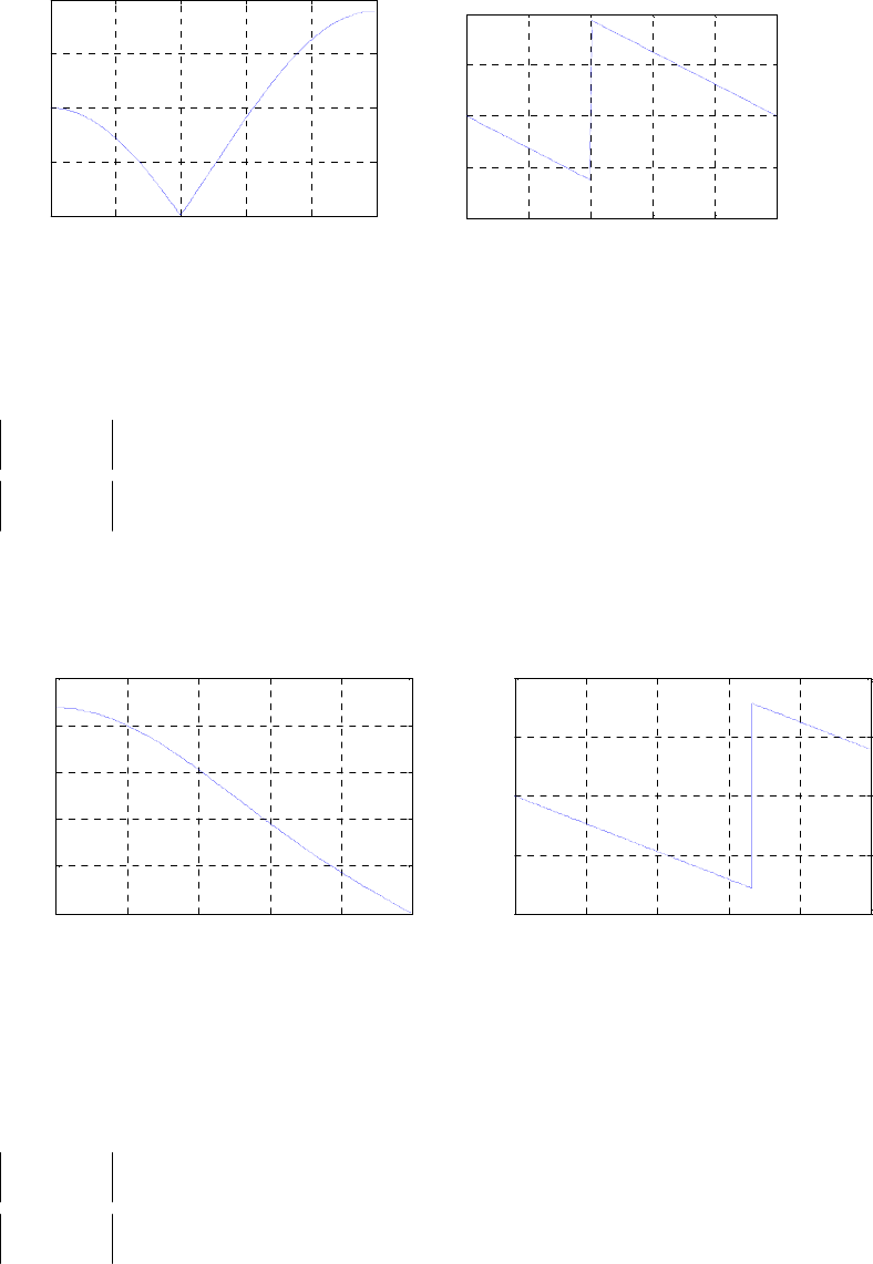
00.2 0.4 0.6 0.8 1
0
0.5
1
1.5
2
ω
/p
i
Magnitude
00.2 0.4 0.6 0.8 1
-2
-1
0
1
2
ω
/
p
i
Phase, radians
3.72 (a)
ω−ω−ω−ω +++= 32 ]3[]2[]1[]0[)( jjjj ehehehheH
(
)
.)2/cos(]1[2)2/3cos(]0[2]0[]1[]1[]0[ 2/332 ω+ω=+++= ω−ω−ω−ω− hheehehehh jjjj
The two conditions to be satisfied by the filter are:
,8.0)1.0cos(]1[2)3.0cos(]0[2)( 2.0 =π+π=
πhheH j
.5.0)25.0cos(]1[2)75.0cos(]0[2)( 5.0 =π+π=
πhheH j Solving these two equations we
get and 0414.0]0[ =h.395.0]1[
=
h
(b) .0414.0395.0395.00414.0)( 32 ω−ω−ω−ω +++= jjjj eeeeH
00.2 0.4 0.6 0.8 1
0
0.2
0.4
0.6
0.8
1
ω
/p
i
Magnitude
00.2 0.4 0.6 0.8 1
-4
-2
0
2
4
ω
/p
i
Phase, radians
3.73 (a)
ω−ω−ω−ω +++= 32 ]3[]2[]1[]0[)( jjjj ehehehheH
(
)
.)2/sin(]1[2)2/3(sin]0[2]0[]1[]1[]0[ 2/332 ω+ω=−−+= ω−ω−ω−ω− hshejehehehh jjjj
The two conditions to be satisfied by the filter are:
,2.0)25.0(sin]1[2)75.0sin(]0[2)( 5.0 =π+π=
πshheH j
.7.0)4.0cos(]1[2)2.1sin(]0[2)( 8.0 =π+π=
πhheH j Solving these two equations we get
and 14.0]0[ −=h.2815.0]1[ =h
(b) .14.02815.02815.014.0)( 32 ω−ω−ω−ω +−+−= jjjj eeeeH
Not for sale 70
00.2 0.4 0.6 0.8 1
0
0.2
0.4
0.6
0.8
1
ω
/
π
Magnitude
00.2 0.4 0.6 0.8 1
-4
-3
-2
-1
0
1
ω
/
π
Phase, radians
3.74 (a)
ω−ω−ω−ω−ω ++++= 432 ]4[]3[]2[]1[]0[)( jjjjj ehehehehheH
(
)
.)sin(]1[2)2(sin]0[2]0[]1[]1[]0[ 243 ω+ω=−−+= ω−ω−ω−ω− hshejehehehh jjjj
The two conditions to be satisfied by the filter are:
,8.0)4.0(sin]1[2)8.0sin(]0[2)( 5.0 =π+π=
πshheH j
.2.0)8.0cos(]1[2)6.1sin(]0[2)( 8.0 =π+π=
πhheH j Solving these two equations we get
and 112.0]0[ =h.3514.0]1[ =h
(b) .112.03514.03514.0112.0)( 43 ω−ω−ω−ω −−+= jjjj eeeeH
00.2 0.4 0.6 0.8 1
0
0.2
0.4
0.6
0.8
1
ω
/
π
Magnitude
00.2 0.4 0.6 0.8 1
-4
-2
0
2
4
ω
/
π
Phase, radians
3.75 (a) .3.03.0)(,3.03.0)( 22 ω−ω−ωω−ω−ω ++=+−= jjj
B
jjj
A
eeeHeeeH
Not for sale 71
00.2 0.4 0.6 0.8 1
0
0.5
1
1.5
2
ω
/
π
Magnitude
|H
A
(e
j
ω
)|
00.2 0.4 0.6 0.8 1
0
0.5
1
1.5
2
ω
/
π
Magnitude
|H
B
(e
j
ω
)|
It can be seen from the above plots that )( ωj
A
eH is a highpass filter, whereas
is a lowpass filter.
)( ωj
BeH
(b) ).()()( )( π+ωωω == j
A
j
B
j
CeHeHeH
3.76
(
.]1[][5.0]1[][
)
−
++−= nxnxnyny Taking the DTFT of both sides we get
(
)
.)()(5.0)()( ωω−ωωω−ω ++= jjjjjj eXeeXeYeeY Hence, the frequency response is
given by .
1
1
2
1
)(
)(
)( ⎟
⎟
⎠
⎞
⎜
⎜
⎝
⎛
−
+
== ω−
ω−
ω
ω
ω
j
j
j
j
j
trap e
e
eX
eY
eH
3.77
()
.]2[]1[4][]2[][ 3
1−+−++−= nxnxnxnyny Hence,
.
1
41
)( 2
2
3
1
⎟
⎟
⎠
⎞
⎜
⎜
⎝
⎛
−
++
=ω−
ω−ω−
ω
j
jj
j
simpson e
ee
eH
00.2 0.4 0.6 0.8 1
0
0.5
1
1.5
2
ω
/
π
Magnitude
Trapezoidal
Simpson
Note: To compare the performances of the Trapezoidal numerical integration formula
with that of the Simpson’s formula, we first observe that if the input is then
the result of integration is
,)( tj
aetx ω
=
.)( 1tj
j
aety ω
ω
= Thus, the desired ideal frequency response is
Not for sale 72

.)( 1
ω
ω=j
j
eH Hence, we take the ratio of the frequency responses of the approximation
to the ideal, and plot the two curves as indicated on the previous page. From this plot, it
is evident that the Simpson’s formula amplifies high frequencies, whereas, the
trapezoidal formula attenuates them. In the very low frequency range, both formulae
yield results close to the ideal. However, Simpson’s formula is reasonably accurate for
frequencies close to the midband range.
3.78
ω−ω−ω−ω +++= 3
3
2
210
)( jjjj egegeggeG
(
)
2/3
0
2/
2
2/
1
2/3
0
2/3 ω−ω−ωωω− +++= jjjjj egegegege
)2/3sin()2/3cos()2/3sin()2/3cos([ 3300
2/3 ω−+ω−+ω+ω= ω− jggjgge j
)]2/sin()2/cos()2/sin()2/cos( 2211 ω−
+
ω
−
+
ω
+ω+ jggjgg ]
)2/cos()()2/3cos()[( 2130
2/3 ω++ω+= ω− gggge j
)].2/cos()()2/3sin()( 2130
ω
−
+
ω
−+ ggjggj
Thus, if and then
which has a linear phase
30 gg =,
21 gg =
)]2/cos()()2/3cos()[()( 2130
2/3 ω++ω+= ω−ω ggggeeG jj
,)( 2
3ω
−=ωθ and hence, a constant group delay.
Alternately, if and
30 gg −= ,
21 gg
−
=
then
which has a linear phase
)]2/sin()()2/3sin()[()( 2130
2/3 ω++ω+= ω−ω ggggejeG jj
,)( 22
3π
+
ω
−=ωθ and hence, a constant group delay.
3.79 (a) Thus,
.sincos)( ω−ω+=+= ω−ω bjbaebaeH jj
a⎟
⎟
⎠
⎞
⎜
⎜
⎝
⎛
ω+
ω−
=ωθ −
cos
sin
tan)( 1
ba
b
a
H.
Hence, ⎟
⎠
⎞
⎜
⎝
⎛
ω+
ω−
ω
⋅
⎟
⎠
⎞
⎜
⎝
⎛
ω+
ω−
+
−=
ω
ω
θ
−=ωτ cos
sin
cos
sin
1
1
)(
)( 2ba
b
d
d
ba
b
d
da
a
H
H
222
2
)cos(
)sin)(sin(cos)cos(
)sin()cos(
)cos(
ω+
ω−ω−−ωω+−
⋅
ω+ω+
ω+
−=
ba
bbbba
bba
ba
.
cos2
cos
sincos2cos
sincoscos
22
2
22222
2222
ω++
ω+
=
ω+ω+ω+
ω−ω−ω−
−=
abba
abb
babba
bbab
Not for sale 73

(b) Let From the results of Part (a) we
have
.sincos11)( ω−ω+=+= ω−ω cjceceG jj
b
.
cos21
cos
)( 2
2
ω++
ω+
=ωτ
cc
cc
b
G Since ,
1
1
)(
1
)( ω−ω
ω
+
== jj
b
j
beceG
eH
we have
),()( ωθ−=ωθ bb GH .
cos21
cos
)()( 2
2
ω++
ω+
−=ωτ−=ωτ
cc
cc
bb GH
(c) ),()(
1
)( ωω
ω−
ω−
ω=
+
+
=j
b
j
a
j
j
j
ceHeH
ec
eba
eH where is the frequency
response of Part (a) and is the frequency response of Part (b). Thus,
)( ωj
aeH
)( ωj
beH
),()()(
ω
θ+ωθ=ωθ bac HHH and therefore, )()()( ωτ+
ω
τ
=
ω
τ
bac HHH
.
cos21
cos
cos2
cos
2
2
22
2
ω++
ω+
−
ω++
ω+
=
cc
cc
abba
abb
(d) ),()(
1
1
1
1
)( ωω
ω−ω−
ω=
+
⋅
+
=j
e
j
b
jj
j
deHeH
edec
eH where is the
frequency response of Part (b) and is similar in form to . Thus,
)( ωj
beH
)( ωj
eeH )( ωj
beH
),()()(
ω
θ+ωθ=ωθ edd HHH and therefore, )()()( ωτ+
ω
τ
=
ω
τ
ebd HHH
.
cos21
cos
cos21
cos
2
2
2
2
ω++
ω+
+
ω++
ω+
=
dd
dd
cc
cc
3.80 The group delay of a causal LTI discrete-time system with a frequency response
)(
)()( ωθωω =jjj eeHeH is given by .
)(
)(
ω
ω
θ
−=ωτ d
d
g Now,
.
)(
)(
)(
)( )()(
ω
ωθ
+
ω
=
ω
ωθω
ω
ωθ
ω
d
d
eeHj
d
eHd
e
d
edH jj
j
j
j Hence,
,
)(
)(
)(
)( )()(
ω
−
ω
=
ω
ωθ
−ω
ω
ωθωθω
d
edH
d
eHd
e
d
d
eeHj
j
j
jjj or, equivalently,
ω
⋅−
ω
⋅=
ω
ωθ
−ω
ωθω
ω
ωθω
ωθ
d
edH
eeHj
d
eHd
eeHj
e
d
dj
jj
j
jj
j)(
)(
1
)(
)(
)(
)()(
)(
.
)(
)(
1
)(
)(
1
ω
⋅+
ω
⋅= ω
ω
ω
ωd
edH
eH
j
d
eHd
eHj
j
j
j
j The first term on the right-
hand side of the above equation is purely imaginary. Hence,
Not for sale 74

.
)(
Re
)(
)(
)(
⎪
⎭
⎪
⎬
⎫
⎪
⎩
⎪
⎨
⎧
=
ω
ωθ
−=ωτ ω
ω
ω
j
d
edH
geH
j
d
d
j
3.81 Since is the Fourier transform of )( ωj
eG ],[nng .
)(
)( ω
=ω
ω
d
edH
jeG
j
j Rewriting Eq.
(3.127) we get
⎪
⎪
⎭
⎪
⎪
⎬
⎫
⎪
⎪
⎩
⎪
⎪
⎨
⎧
⎟
⎟
⎟
⎟
⎠
⎞
⎜
⎜
⎜
⎜
⎝
⎛
+=ωτ ω
ω
ω
ω
ωω *
)()(
)()(
2
1
)( j
d
edH
j
d
edH
geH
j
eH
j
jj
⎪
⎪
⎭
⎪
⎪
⎬
⎫
⎪
⎪
⎩
⎪
⎪
⎨
⎧
⎟
⎟
⎠
⎞
⎜
⎜
⎝
⎛
+= ω
ω
ω
ω
ω
ω
)()(
2
1
*
*
)(
)(
j
d
edH
j
d
edH
eH
j
eH
j
j
j
⎪
⎪
⎭
⎪
⎪
⎬
⎫
⎪
⎪
⎩
⎪
⎪
⎨
⎧
⎟
⎟
⎠
⎞
⎜
⎜
⎝
⎛
+
=ω
ω
ω
ω
ω
ωω
2
*
)(
*
)(
)(
)()(
2
1
j
j
d
edH
j
d
edH
eH
eHjeHj
jj
()
(
)
*
2)()()()(
)(2
1[ωωωω
ω++= j
im
j
re
j
im
j
re
j
eHjeHeGjeG
eH
()
(
)
]
*
)()()()( ωωωω +++ j
im
j
re
j
im
j
re eHjeHeGjeG
[]
)()(2)()(2
)(2
1
2
ωωωω
ω+= j
im
j
im
j
re
j
re
j
eHeGeHeG
eH
.
)(
)()()()(
2
ω
ωωωω +
=
j
j
im
j
im
j
re
j
re
eH
eHeGeHeG
3.82 (a) and thus,
ω−ω+=+= ω−ω sin4.0cos4.014.01)( jeeH jj
a
{
}
ω+=
ωcos4.01)(Re j
aeH and
{
}
.sin4.0)(Im ω−=
ωj
aeH .
.sin4.0cos4.0)4.0(
)(
)( ω−ω=−=
ω
=ω−
ω
ωjejj
d
edH
jeG j
j
a
j
a Thus,
{
}
ω=
ωcos4.0)(Re j
aeG and
{
}
.sin4.0)(Im ω−=
ωj
aeG . Therefore, using Eq. (3.128) we
get )(ωτ a
H22
2
)sin4.0()cos4.01(
)sin4.0()cos4.0)(cos4.01(
ω−+ω+
ω−+ωω+
=
.
cos8.016.1
cos4.016.0
cos8.0sin16.0cos16.01
cos4.0sin16.0cos16.0
22
22
ω+
ω+
=
ω+ω+ω+
ω+ω+ω
=
Not for sale 75

(b) Let .6.01
)(
1
)( ω−
ω
ω+== j
j
b
j
be
eH
eG Then ).()( ω
τ
−
=
ω
τ
bb HG Then using the
same procedure as in Part (a) we get .
cos2.136.1
cos6.036.0
)( ω+
ω
+
=ωτ b
G Therefore,
.
cos2.136.1
cos6.036.0
)( ω+
ω+
−=ωτ b
H
(c) Let ),()(
3.01
1
)5.01()( ωω
ω−
ω−ω =
⎟
⎟
⎠
⎞
⎜
⎜
⎝
⎛
+
−= j
b
j
a
j
jj
ceGeG
e
eeH where
and
ω−ω −= jj
aeeG 5.01)( .
3.01
1
)( ω−
ω
+
=j
j
be
eG Therefore,
Then using the same procedure as in Part (a) we get
).()()( ωτ+ωτ=ωτ bac GGH
ω−
ω−
=ωτ cos25.1
cos5.025.0
)(
a
G and using the same procedure as in Part (b) we get
.
cos6.009.1
cos3.009.0
)( ω+
ω+
−=ωτ b
G Hence, .
cos6.009.1
cos3.009.0
cos25.1
cos5.025.0
)( ω+
ω
+
−
ω−
ω
−
=ωτ c
H
(d) Let ),()(
5.01
1
3.01
1
)( ωω
ω−ω−
ω=
⎟
⎟
⎠
⎞
⎜
⎜
⎝
⎛
+
⎟
⎟
⎠
⎞
⎜
⎜
⎝
⎛
−
=j
b
j
a
jj
j
deGeG
ee
eH where
ω−
ω
−
=j
j
ae
eG
3.01
1
)( and .
5.01
1
)( ω−
ω
+
=j
j
be
eG Therefore,
).()()( ωτ+ωτ=ωτ bad GGH Then using the same procedure as in Part (b) we get
ω−
ω+−
=ωτ cos6.009.1
cos3.009.0
)(
a
G and .
cos25.1
cos5.025.0
)( ω+
ω
−
−
=ωτ a
G Hence,
.
cos25.1
cos5.025.0
cos6.009.1
cos3.009.0
)( ⎟
⎟
⎠
⎞
⎜
⎜
⎝
⎛
ω+
ω+
+
ω−
ω−
−=ωτ a
G
3.83 From Table 3.3, .
sin5.0cos5.01
1
5.01
1
)( ω−ω+
=
+
=ω−
ω
j
e
eH j
j Thus,
ω+
=
ω+ω+
=
ω
cos25.1
1
)sin5.0()cos5.01(
1
)( 22
j
eH and
.
cos5.01
sin5.0
tan
cos5.01
sin5.0
tan)()}(arg{ 11 ⎟
⎟
⎠
⎞
⎜
⎜
⎝
⎛
ω+
ω
=
⎟
⎟
⎠
⎞
⎜
⎜
⎝
⎛
ω+
ω−
−=ωθ= −−ωj
eH Now
.0.1427j + 0.6821
)5/sin(5.0)5/cos(5.01
1
)( 5/ =
π−π+
=
π
j
eH j Therefore,
Not for sale 76
0.6969)( 5/ =
πj
eH and 0.2063
6821.0
1427.0
tan)5/()}(arg{ 15/ =
⎟
⎠
⎞
⎜
⎝
⎛
=πθ= −πj
eH radians.
Since for a frequency response with real coefficient impulse response, )( ωj
eH is an
even function of and is an odd function of
ω)(ωθ ,
ω
we have 0.6969)( 5/ =
π− j
eH and
0.2063.)5/( −=π−θ
Now, for an input ],[)sin(][ nnnx o
µ
ω
= the steady-state output is given by
()
.)(sin)(][ oo
jneHny oωθ+ω= ω Thus, for ,5/
π
=
ω
o the steady-state output is given
by .2063.0sin6969.0)5/(sin)(][ 55
5/ ⎟
⎠
⎞
⎜
⎝
⎛+=
⎟
⎠
⎞
⎜
⎝
⎛πθ+= ππ
πnneHny j
3.84
(
)
(
)
.]1[cos]0[2]1[1]0[)( 2hheeheheH jjjj +ω=++= ω−ω−ω−ω We require
and
1]1[)3.0cos(]0[2 =+ hh .0]1[)7.0cos(]0[2
=
+
hh Solving these two equations we
get and 2.6248]0[ =h4.015.]1[
−
=
h
00.2 0.4 0.6 0.8 11.2
0
0.5
1
1.5
2
2.5
ω
Magnitude
Not for sale 77
M3.1
75.0,9.0 =θ=r
00.5 1
-2
0
2
4
6
8
Real part
ω
/
π
Amplitude
00.5 1
-8
-6
-4
-2
0
2
Imaginary part
ω
/
π
Amplitude
00.5 1
0
2
4
6
8
Magnitude Spectrum
ω
/
π
Magnitude
00.5 1
-2
-1.5
-1
-0.5
0
0.5
Phase Spectrum
ω
/
π
Phase, radians
5.0,7.0 =θ=r
00.5 1
0
1
2
3
4Real part
ω
/
π
Amplitude
00.5 1
-3
-2
-1
0Imaginary part
ω
/
π
Amplitude
00.5 1
0
1
2
3
4
5Magnitude Spectrum
ω
/
π
Magnitude
00.5 1
-1.5
-1
-0.5
0Phase Spectrum
ω
/
π
Phase, radians
M3.2 It should be noted that Program 3_1.m uses the function freqz to determine the
samples of a DTFT that is rational function in i.e., a ratio of polynomials in
. Their inverse DTFTs are two-sided sequences. However, all sequences of
,
ω− j
e
ω− j
e
Not for sale 78
Problem 3.19 except that in Part (b) are two-sided finite-length sequences of length
, and their DTFTs have both positive and negative powers of As a result,
12 +N.
ωj
e
the frequency sample computed using freqz should be multiplied by the vector
evaluated at the frequency points
Nj n
eωn
ω
used in freqz. In Parts (a), (c) and (d),
the phase spectra are the plots of the unwrapped phase obtained using the function
unwrap.
Moreover, the DTFTs of the sequences in Parts (a), (c) and (d) are real functions of
ω
and thus have zero phase. More accurate plots of the DTFTs are obtained using the
function zerophase.
(a)
⎩
⎨
⎧≤≤−
=otherwise,,0
,1010,1
][
1n
ny =
ω)(
1j
eY
(
)
.
)2/sin(
2/21sin
ω
ω
The plots obtained using
Program 3_1.m are shown below:
00.5 1
-10
0
10
20
30 Real part
ω
/
π
Amplitude
00.5 1
-2
-1
0
1
2x 10
-14
Imaginary part
ω
/
π
Amplitude
00.5 1
0
5
10
15
20
25
Magnitude Spectrum
ω
/
π
Magnitude
00.5 1
-8
-6
-4
-2
0
2
Phase Spectrum
ω
/
π
Phase, radians
The plot obtained using the function zerophase is shown below:
00.2 0.4 0.6 0.8 1
-5
0
5
10
15
20
25
ω
/
π
Amplitude
Not for sale 79
(b) Then
⎩
⎨
⎧≤≤
=otherwise.,0
,0,1
][
2Nn
ny )(
2ω
j
eY ⎟
⎟
⎠
⎞
⎜
⎜
⎝
⎛
ω
+ω
=ω−
)2/sin(
)2/]1[sin(
2/ N
eNj . The plots
obtained using Program 3_1.m are shown below:
00.5 1
-5
0
5
10
15
Real part
ω
/
π
Amplitude
00.5 1
-2
0
2
4
6
8
Imaginary part
ω
/
π
Amplitude
00.5 1
0
5
10
15
Magnitude Spectrum
ω
/
π
Magnitude
00.5 1
-2
-1
0
1
2
3
Phase Spectrum
ω
/
π
Phase, radians
(c) ⎪
⎩
⎪
⎨
⎧≤≤−−
=
otherwise.,0
,,1
][
3NnN
ny N
n
(
)
.
)2/(sin
2/sin1
)( 2
2
3ω
ω
⋅=
ωN
N
eY j The plots obtained
using Program 3_1.m are shown below:
00.5 1
-5
0
5
10 Real part
ω
/
π
Amplitude
00.5 1
0
0.5
1
1.5 Imaginary part
ω
/
π
Amplitude
00.5 1
0
2
4
6
8
10 Magnitude Spectrum
ω
/
π
Magnitude
00.5 1
0
1
2
3
4Phase Spectrum
ω
/
π
Phase, radians
Not for sale 80
The plot obtained using the function zerophase is shown below:
00.2 0.4 0.6 0.8 1
-5
0
5
10
15
20
25
ω
/
π
Amplitude
(d) ⎪
⎩
⎪
⎨
⎧≤≤−−+
=
otherwise.,0
,,1
][
4NnNN
ny N
n
()
.
)2/(sin
2/sin1
)2/sin(
][sin
)( 2
2
2
1
4ω
ω
⋅+
ω
⎟
⎠
⎞
⎜
⎝
⎛+ω
⋅=
ωN
N
N
NeY j
00.5 1
-10
0
10
20
30
40
Real part
ω
/
π
Amplitude
00.5 1
-2
-1
0
1
2x 10
-14
Imaginary part
ω
/
π
Amplitude
00.5 1
0
10
20
30
40
Magnitude Spectrum
ω
/
π
Magnitude
00.5 1
-10
-5
0
5
Phase Spectrum
ω
/
π
Phase, radians
The plot obtained using the function zerophase is shown below:
00.2 0.4 0.6 0.8 1
-5
0
5
10
15
20
25
ω
/
π
Amplitude
Not for sale 81
(e)
⎩
⎨
⎧≤≤−π
=otherwise.,0
,),2/cos(
][
5NnNNn
ny
(
)
()
(
)
()
.
sin
sin
2
1
sin
sin
2
1
)(
2/)(
)((
2/)(
)((
5
2
)
2
1
2
2
)
2
1
2
N
N
N
NNN
j
eY π
π
π
π
+ω
++ω
−ω
+−ω
ω⋅+⋅= The plots obtained using
Program 3_1.m are shown below:
00.5 1
-5
0
5
10
15 Real part
ω
/
π
Amplitude
00.5 1
-0.5
0
0.5
x 10
-14
Imaginary part
ω
/
π
Amplitude
00.5 1
0
5
10
15 Magnitude Spectrum
ω
/
π
Magnitude
00.5 1
-5
0
5
10
15 Phase Spectrum
ω
/
π
Phase, radians
The plot obtained using the function zerophase is shown below:
00.2 0.4 0.6 0.8 1
-5
0
5
10
15
20
25
ω
/
π
Amplitude
M3.3 (a) ω−ω−ω−ω−
ω−ω−ω−ω−
ω
++++
++−+
=432
432
4153.01393.08258.02386.01
)139.03519.0139.01(2418.0
)( jjjj
jjjj
j
eeee
eeee
eX
The plots obtained using Program 3_1.m are shown below:
Not for sale 82
00.5 1
-0.5
0
0.5
1
Real part
ω/π
Amplitude
00.5 1
-1
-0.5
0
0.5
1
Imaginary part
ω/π
Amplitude
00.5 1
0
0.2
0.4
0.6
0.8
1
Magnitude Spectrum
ω/π
Magnitude
00.5 1
-4
-2
0
2
4
Phase Spectrum
ω/π
Phase, radians
(b) .
1205.07275.01454.11
)0911.00911.01(1397.0
)( 32
32
ω−ω−ω−
ω−ω−ω−
ω
+++
−+−
=jjj
jjj
j
eee
eee
eX
The plots obtained using Program 3_1.m are shown below:
00.5 1
-0.2
0
0.2
0.4
0.6
0.8 Real part
ω
/
π
Amplitude
00.5 1
-0.2
0
0.2
0.4
0.6 Imaginary part
ω
/
π
Amplitude
00.5 1
0
0.2
0.4
0.6
0.8 Magnitude Spectrum
ω
/
π
Magnitude
00.5 1
-1
0
1
2
3Phase Spectrum
ω
/
π
Phase, radians
M3.4 % Property 1
Not for sale 83
N = 8; % Number of samples in sequence
gamma = 0.5; k = 0:N-1;
x = exp(-j*gamma*k); y = exp(-j*gamma*fliplr(k));
% r = x[-n] then y = r[n-(N-1)]
% so if X1(exp(jw)) is DTFT of x[-n], then
% X1(exp(jw)) = R(exp(jw)) = exp(jw(N-1))Y(exp(jw))
[Y,w] = freqz(y,1,512);
X1 = exp(j*w*(N-1)).*Y;
m = 0:511; w = -pi*m/512;
X = freqz(x,1,w);
% Verify X = X1
% Property 2
k = 0:N-1; y = exp(j*gamma*fliplr(k));
[Y,w] = freqz(y,1,512);
X1 = exp(j*w*(N-1)).*Y;
[X,w] = freqz(x,1,512);
% Verify X1 = conj(X)
% Property 3
y = real(x);
[Y3,w] = freqz(y,1,512);
m = 0:511; w0 = -pi*m/512;
X1 = freqz(x,1,w0);
[X,w] = freqz(x,1,512);
% Verify Y3 = 0.5*(X+conj(X1))
% Property 4
y = j*imag(x); [Y4,w] = freqz(y,1,512);
% Verify Y4 = 0.5*(X-conj(X1))
% Property 5
k = 0:N-1; y = exp(-j*gamma*fliplr(k));
xcs = 0.5*[zeros(1,N-1) x] + 0.5*[conj(y) zeros(1,N-1)];
xacs = 0.5*[zeros(1,N-1) x] - 0.5*[conj(y) zeros(1,N-1)];
[Y5,w] = freqz(xcs,1,512);
[Y6,w] = freqz(xacs,1,512);
Y5 = Y5.*exp(j*w*(N-1));
Y6 = Y6.*exp(j*w*(N-1));
% Verify Y5 = real(X) and Y6 = j*imag(X)
M3.5 N = 8; % Number of samples in sequence
gamma = 0.5; k = 0:N-1;
x = exp(gamma*k); y = exp(gamma*fliplr(k));
xev = 0.5*([zeros(1,N-1) x] + [y zeros(1,N-1)]);
xod = 0.5*([zeros(1,N-1) x] - [y zeros(1,N-1)]);
[X,w] = freqz(x,1,512);
[Xev,w] = freqz(xev,1,512);
[Xod,w] = freqz(xod,1,512);
Xev = exp(j*w*(N-1)).*Xev;
Not for sale 84
Xod = exp(j*w*(N-1)).*Xod;
% Verify real(X) = Xev, and j*imag(X) = Xod
M3.5 N = input('The length of the seqeunce = ');
k = 0:N-1; gamma = -0.5;
g = exp(gamma*k);
% g is an exponential seqeunce
h = sin(2*pi*k/(N/2));
% h is a sinusoidal sequence with period = N/2
[G,w] = freqz(g,1,512); [H,w] = freqz(h,1,512);
% Property 1
alpha = 0.5; beta = 0.25;
y = alpha*g+beta*h; [Y,w] =
freqz(y,1,512);
% Plot Y and alpha*G+beta*H to verify that they are equal
% Property 2
n0 = 12; % Sequence shifted by 12 samples
y2 = [zeros(1,n0) g];
[Y2,w] = freqz(y2,1,512);
G0 = exp(-j*w*n0).*G;
% Plot G0 and Y2 to verify they are equal
% Property 3
w0 = pi/2; % the value of omega0 = pi/2
r = 256; % the value of omega0 in terms of number of
samples
k = 0:N-1; y3 = g.*exp(j*w0*k);
[Y3,w] = freqz(y3,1,512);
k = 0:511;
w = -w0+pi*k/512; % creating G(exp(w-w0))
G1 = freqz(g,1,w);
% Compare G1 and Y3
% Property 4
k = 0:N-1; y4 = k.*g;
[Y4,w] = freqz(y4,1,512);
% To compute derivative we need sample at pi
y0 = ((-1).^k).*g;
G2 = [G(2:512)' sum(y0)]';
delG = (G2-G)*512/pi;
% Compare Y4, delG
% Property 5
y5 = conv(g,h);
[Y5,w] = freqz(y5,1,512);
% Compare Y5 and G.*H
% Property 6
Not for sale 85
y6 = g.*h;
[Y6,w] = freqz(y6,1,512,'whole');
[G0,w] = freqz(g,1,512,'whole');
[H0,w] = freqz(h,1,512,'whole');
% Evaluate the sample value at w = pi/2
% and verify with Y6 at pi/2
H1 = [fliplr(H0(1:129)') fliplr(H0(130:512)')]';
val = 1/(512)*sum(G0.*H1);
% Compare val with Y6(129) i.e., sample at pi/2
% Can extend this to other points similarly
% Parsevals theorem
val1 m = sum(g.*conj(h)); val2 = sum(G0.*conj(H0))/512;
% Compare val1 with val2
M3.7 The DTFT of is ][nnh .
)(
ω
ω
d
edH j
j Hence, the group delay )(
ω
τ
g can be computed at a
set of
N
discrete frequency points ,10,/2
−
≤
≤
π
=
ω
NkNk
k as follows:
,Re)( ]}[{
]}[{ ⎟
⎠
⎞
⎜
⎝
⎛
=ωτ nhDFT
nhnDFT
kg
where all DFTs are –points in length with greater than or equal to the length of
N N
]}.[{ nh
M3.8 h = [3.8461 -6.3487 3.8461];
[H,w] = freqz(h,1,512);
plot(w/pi,abs(H)); grid
xlabel('\omega/\pi'); ylabel('Magnitude');
00.2 0.4 0.6 0.8 1
0
5
10
15
ω
/
π
Magnitude
M3.9 h = [-13.4866 45.228 -63.8089 45.228 -13.4866];
[H,w] = freqz(h,1,512);
plot(w/pi,abs(H)); grid
xlabel('\omega/\pi'); ylabel(Magnitude);
Not for sale 86
00.2 0.4 0.6 0.8 1
0
50
100
150
200
ω
/
π
M
agn
i
tu
d
e
Not for sale 87

Chapter 4
4.1 Let be an arbitrary continuous-time function with a CTFT
)(tφ),( Ω
Φ
j where
Let denote the periodic continuous-
time function with a period T obtained by a periodic extension of Note that
is also given by the convolution of
.)()( dtetj tj
∫φ=ΩΦ ∞
∞−
Ω− ∑+φ=φ ∞
−∞=n
TnTtt )()(
~
).(tφ
)(
~t
T
φ)(t
φ
with the periodic impulse train
i.e.,
∑+δ= ∞
−∞=n
nTttp ),()( .)()()(
~ττ−
∫τφ=φ ∞
∞
−
dtpt
T
Tthe CTFT of is then given by F{ F { } )(
~t
T
φ ⋅ΩΦ=φ )()}(
~jt
T)(tp
() (
,)()()()( 2
2
TT
nT
n
T
Tnjjnnjj Ω−ΩδΩΦ
∑
=
∑Ω−Ωδ⋅ΩΦ= ∞
−∞=
π
∞
−∞=
π
)
(4-1)
where .
2
T
T
π
=Ω
Now, the Fourier series expansion of is given by
A CTFT of both sides of this equation is then
∑+φ=φ ∞
−∞=n
TnTtt )()(
~
.)(
~∑
=φ ∞
−∞=
Ω
n
tjn
nT T
eat
F (4-2)
()
.)(2)}(
~
{T
n
nT njat Ω−Ωπδ⋅
∑
=φ ∞
−∞=
Comparing Eqs. (4-1) and (4-2) we arrive at ).(
1
T
T
njna ΩΦ= Substituting this
expression in the Fourier expansion of )(
~t
T
φ we therefore arrive at the Poisson’s sum
formula .)()()(
~1tjn
n
T
T
n
TT
ejnnTtt Ω
∞
−∞=
∞
−∞= ∑ΩΦ=
∑+φ=φ
4.2 Consider the continuous-time signal )sin()( ttg ma
Ω
=
which is bandlimited to
If we sample at a rate
.
m
Ω)(tga mT
Ω
=
Ω
2 starting at 0
=
t, then all its samples
are zero. Hence, cannot be recovered from its samples obtained by sampling
it at the Nyquist rate
)(tga
mT
Ω
=Ω 2. As a result, )sin()( ttg ma
Ω
=
must be sampled
at a rate to recover it fully from its samples.
mT Ω>Ω 2
4.3 (a) Now, the CTFT of is given by
)(
1ty )(O)()( *
2
1
1ΩΩ=Ω πjGjGjY aa where
denotes the CTFT of and denotes the frequency-domain
convolution. The highest frequency present in is therefore twice that of
and hence, the Nyquist frequency of is
)( ΩjGa)(tga*
O
)(
1ty
)(tga)(
1ty .2 m
Ω
Not for sale 86

(b) The CTFT of is given by
)(
2ty dtegjY tj
t
aΩ−
∞
∞
−
∫
=Ω )()( 3
2
The highest frequency present in is
therefore one-third of that of and hence, the Nyquist frequency of is
).3(3)(3 3Ω=τ
∫τ= τΩ−
∞
∞−
jGdeg a
j
a)(
2ty
)(tga)(
2ty
.3/
m
Ω
(c) The CTFT of is given by
)(
3ty dtetgjY tj
aΩ−
∞
∞
−
∫
=Ω )3()(
3
).()( 33
1
3/
3
1Ω
τΩ−
∞
∞−
=τ
∫τ= jGdeg a
j
a The highest frequency present in is )(
3ty
therefore three times of that of and hence, the Nyquist frequency of is
)(tga)(
3ty
.3 m
Ω
(d) The CTFT of is given by
)(
4ty
τ
∫⎥
⎦
⎤
⎢
⎣
⎡∫τ−τ=
∫⎥
⎦
⎤
⎢
⎣
⎡∫τττ−=Ω ∞
∞−
∞
∞−
Ω−Ω−
∞
∞−
∞
∞−
ddtetggdtedgtgjY tj
aa
tj
aa )()()()()(
4
).()()()()()( ΩΩ=τ
∫τΩ=τΩ
∫τ= ∞
∞
−
τΩ−
∞
∞−
τΩ− jGjGdegjGdjGeg aa
j
aaa
j
a The
highest frequency present in is therefore the same as that of and hence,
the Nyquist frequency of is
)(
4ty )(tga
)(
4ty .
m
Ω
(e) Now .)()( 2
1Ω
∫Ω= Ω
∞
∞−
πdejGtg tj
aa Differentiating both sides of this equation
we get .)(
2
1
)( Ω
∫ΩΩ= Ω
∞
∞−
πdejGj tj
a
dt
tdga Hence, it follows that the CTFT of
dt
tdga
ty )(
5)( = is simply ).(
Ω
ΩjGj a The highest frequency present in is
therefore the same as that of and hence, the Nyquist frequency of is
)(
5ty
)(tga)(
5ty
.
m
Ω
4.4 By Parseval’s relation, the total energy of is given by
E
)(tga
Ω
∫Ω=
∫
=∞
∞
−
π
∞
∞−
djGdttgt aaga
2
2
1
2)()()( .)( 2
2
1Ω
∫Ω=
Ω
Ω−
πdjG
m
m
a Likewise, the
total energy of is given by E ][ng ω
∫
=
∑
=π
π−
ω
π
∞
∞−
deGng j
ng
2
2
1
2
][ )(][
Not for sale 87

Ω
∫Ω=Ω
∫Ω=Ω
∫Ω=
Ω
Ω−
π
π
π−
π
π
π−
πdjGdjGTdjG
m
m
a
T
T
T
a
T
T
T
a
T
2
2
1
/
/
2
2
1
/
/
2
1
2
1)()()()(
T
1
=E
.
)(tga
4.5 Sampling period == 5000
5.2
T sec. Hence, the sampling frequency is
2000
1== T
T
F Hz. Therefore, the highest frequency component that could be
present in the continuous-time signal has a frequency 1000
2
20000 = Hz.
4.6 Since the continuous-time signal is being sampled at kHz rate, the sampled
version of its -th sinusoidal component with a frequency will generate discrete-
time sinusoidal signals with frequencies
)(txa2
ii
F
.,2000
∞
<
<
∞
−
±
nnF i Hence, the
frequencies generated in the sampled version associated with the sinusoidal
components present in are as follows:
im
F
300
1=F Hz K,2300,1700,300
1
=
⇒m
FHz
500
2=F Hz K,2500,1500,500
2
=
⇒m
FHz
1200
3=F Hz K,3200,800,1200
3
=
⇒m
FHz
2150
4=F Hz K,4150,150,2150
4
=
⇒m
FHz
3500
5=F Hz K,7500,500,5500,1500,3500
5
=
⇒m
FHz
After filtering by a lowpass filter with a cutoff at 900 Hz, the frequencies of the
sinusoidal components in are Hz.
)(tya800,500,300,150
4.7 One possible set of values for the frequencies present in are: Hz,
Hz, Hz, and
)(tya350
1=F
575
2=F815
3=F9650
4
=
F Hz. Another possible set of values for
the frequencies present in are:
)(tya350
1
=
F Hz, 575
2
=
F Hz, Hz,
and Hz. Hence, the solution is not unique.
815
3=F
10575
4=F
4.8 .
50
n
nTt == Therefore,
⎟
⎠
⎞
⎜
⎝
⎛
+
⎟
⎠
⎞
⎜
⎝
⎛
+
⎟
⎠
⎞
⎜
⎝
⎛
−
⎟
⎠
⎞
⎜
⎝
⎛
=ππππ
50
176
50
120
50
24
50
20 cos2sin3cos5sin4][ nnnn
nx
⎟
⎠
⎞
⎜
⎝
⎛
+
⎟
⎠
⎞
⎜
⎝
⎛
+
⎟
⎠
⎞
⎜
⎝
⎛
−
⎟
⎠
⎞
⎜
⎝
⎛
=π−π+ππ
25
)12100(
5
)210(
25
12
5
2cos2sin3cos5sin4 nnnn
.cos2sin3cos5sin4 25
12(
5
2
25
12
5
2⎟
⎠
⎞
⎜
⎝
⎛
+
⎟
⎠
⎞
⎜
⎝
⎛
+
⎟
⎠
⎞
⎜
⎝
⎛
−
⎟
⎠
⎞
⎜
⎝
⎛
=ππππ nnnn
Not for sale 88
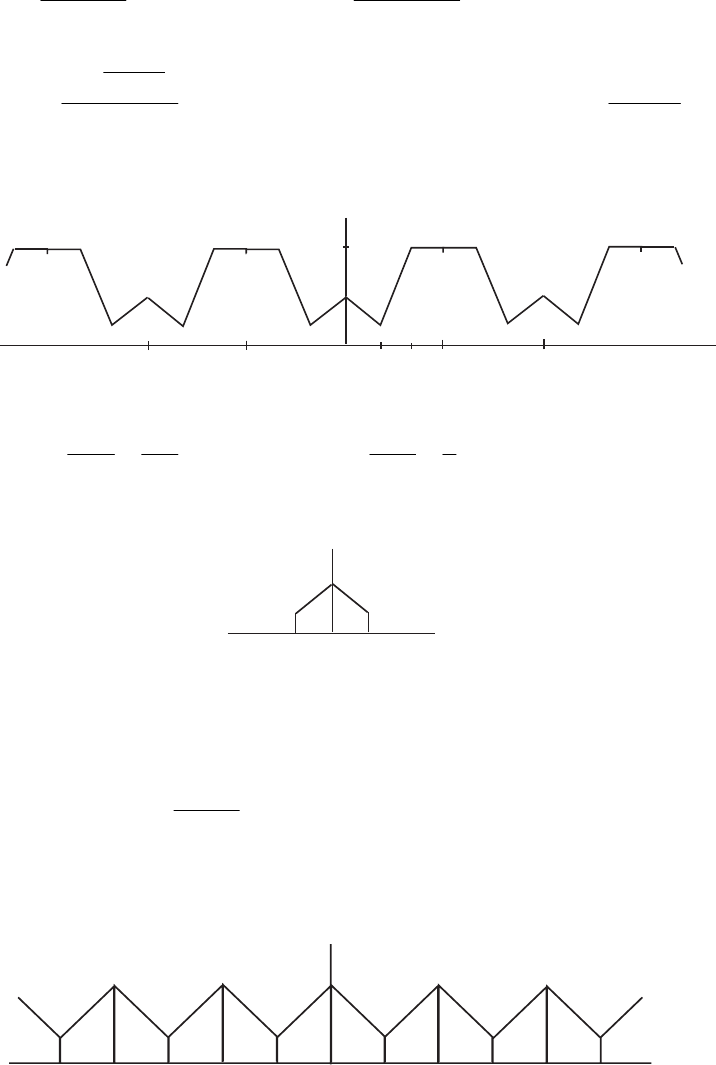
4.9 Both channels are being sampled at kHz. Therefore, there are a total of
samples/sec. Each sample is quantized using 12 bits. Hence,
the total bit rate of the two channels after sampling and digitization is 108 kpbs.
45
90000450002 =×
4.10 .
2/
)sin(
)( t
t
th
T
c
rΩ
Ω
= Therefore, .
2/
)sin(
)( nT
nT
nTh
T
c
rΩ
Ω
= Since ,/2
T
TΩπ
=
we have
.
sin
)(
2
n
nTh T
cn
rπ
⎟
⎠
⎞
⎜
⎝
⎛
=Ω
Ωπ
For ,2/
Tc
Ω
=
Ω
we thus have ].[
)sin(
)( n
n
n
nThrδ=
π
π
=
4.11 The spectrum of the sampled signal is as shown below:
0
X (jΩ)
p
Ω
Ω
_m
Ωm
Ωm
__
3
Ωm
2
Ωm
2
_
1/T
1/2T
Now, .
2
2
mm
TΩ
π
Ω
π== As a result, .
33
π
Ω
πΩ ==ω
m
m
c Hence after lowpass filtering
the spectrum of the output continuous-time signal will be as shown below: )(tya
0
Y (jΩ)
a
Ω
Ωm
__
3
Ωm
__
3
_
4.12 (a) .150,100 11 π=Ω
π
=Ω Thus, .50
12
π
=
Ω
−
Ω
=
∆
Ω Note is an integer
multiple of Hence, we choose the sampling angular frequency as
∆Ω
.
2
Ω
,1002 1502
M
T
π×
=π=∆Ω=Ω which is satisfied for .3
=
M The sampling
frequency is therefore 50 Hz. The CTFT )(
Ω
jX pof the sampled sequence and the
frequency response )(
Ω
jHr of the desired reconstruction filter are shown below.
X (jΩ)
p
1/T
0 100π150π200π
Ω
50π
_
50π
_
200π100π
_
150π
_
M = 3
Not for sale 89
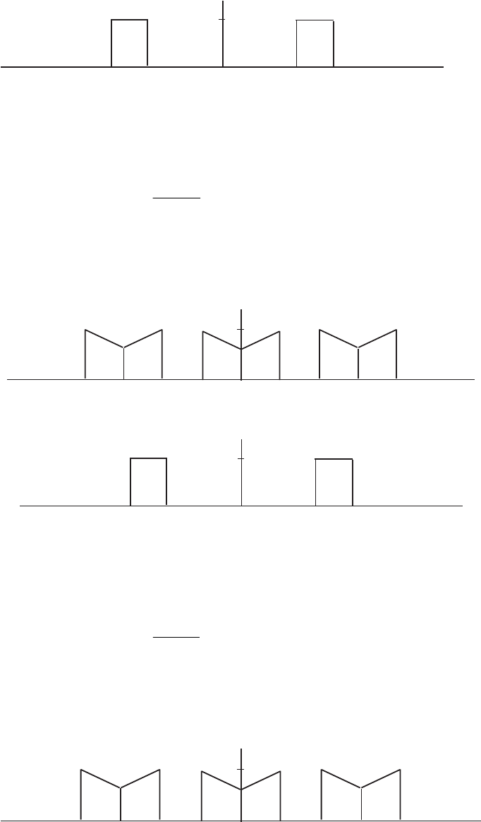
Ω
T
H (jΩ)
r
0 100π150π
100π
_
150π
_
(b) Thus,
.250,160 11 π=Ωπ=Ω .90
12
π
=
Ω
−
Ω
=
∆
Ω Note is not an
integer multiple of Hence, we extend the bandwidth to the left by assuming
the lowest frequency to be
∆Ω
.
2
Ω
0
Ω
and choose the sampling angular frequency as
,)(22 2502
02 M
T
π×
=Ω−Ω=∆Ω=Ω which is satisfied for π
=
Ω
125
0 and .2
=
M
The sampling frequency is therefore 125 Hz. The CTFT )(
Ω
jX pof the sampled
sequence and the frequency response )(
Ω
jHr of the desired reconstruction filter
are shown below.
Ω
1/T
0 160π250π
160π
_
250π
_
90π
90π
_
340π
340π
_
X (jΩ)
p
Ω
T
H (jΩ)
r
0 160π250π
160π
_
250π
_
(c) Thus,
.180,110 11 π=Ωπ=Ω .70
12
π
=
Ω
−
Ω
=
∆
Ω Note
∆
Ω is not an
integer multiple of Hence, we extend the bandwidth to the left by assuming
the lowest frequency to be
.
2
Ω
0
Ω
and choose the sampling angular frequency as
,)(22 1802
02 M
T
π×
=Ω−Ω=∆Ω=Ω which is satisfied for π
=
Ω
90
0 and
The sampling frequency is therefore Hz. The CTFT
.2=M
90 )(
Ω
jX pof the sampled
sequence and the frequency response )(
Ω
jHr of the desired reconstruction filter
are shown below.
Ω
1/T
0110π180π
110π
_
180π
_
70π
70π
_
250π
250π
_
X (jΩ)
p
Not for sale 90

Ω
T
H (jΩ)
r
0 110π180π
110π
_
180π
_
4.13 dB and
)1(log20 10 pp δ−−=α ss
δ
−
=
α
10
log20 dB. Therefore,
and
20/
101 p
p
α−
−=δ .10 20/
s
sα−
=δ
(a) dB and
21.0=α p52
=
αs dB. Hence, 0239.0
=
δ
p and .025.0=δs
(b) dB and
03.0=α p69
=
αs dB. Hence, 0034.0
=
δ
p and .00355.0=δs
(c) dB and
33.0=α p57
=
αs dB. Hence, 0373.0
=
δ
p and .0014.0=δs
4.14 .)( as
a
sHa+
= Thus, ,)( aj
a
jHa+Ω
=Ω and hence,
.)()()( 22
2
2
a
a
aj
a
aj
a
aaa jHjHjH +Ω
+Ω−+Ω =⋅=Ω−Ω=Ω As Ω increases from
to ∞, it can be seen that the square-magnitude function
02
)Ωj(Ha and hence,
the magnitude function )( ΩjHa 22 a
a
+Ω
=decreases monotonically from
1)0( j=Ha to .0)( =∞jHa Let c
Ω
denote the 3–dB cutoff frequency. Then
,
2
1
2
22
2
)( ==Ω +Ω a
a
ca
c
jH which implies .a
c
=
Ω
4.15 .)( as
s
sGa+
= Thus, ,)( aj
j
jGa+Ω
Ω
=Ω and hence,
.)()()( 22
2
2
a
aj
j
aj
j
aaa jGjGjG +Ω
Ω
+Ω−
Ω−
+Ω
Ω=⋅=Ω−Ω=Ω As increases from
to ∞, it can be seen that the square-magnitude function
Ω
02
)( ΩjGa and hence,
the magnitude function )( ΩjGa 22 a+Ω
Ω
=increases monotonically from
0)0j(=Ga to .1)( =∞jGa Let c
Ω
denote the 3–dB cutoff frequency. Then
,
2
1
2
22
2
)( ==Ω +Ω
Ω
a
ca
c
c
jG which implies .a
c
=
Ω
4.16
()
)()(
2
1
1
2
1
)( 21 sAsA
as
as
as
a
sHa−=
⎟
⎠
⎞
⎜
⎝
⎛
+
−
−=
+
= and as
s
sGa+
=)(
()
,)()(
2
1
1
2
1
21 sAsA
as
as +=
⎟
⎠
⎞
⎜
⎝
⎛
+
−
+= where 1)(
1
=
sA and .)(
2as
as
sA +
−
= Now,
Not for sale 91

1)(
1=ΩjA and 1)( 2
2=
−Ω
+
Ω
⋅
+Ω
−
Ω
=
+Ω−
−
Ω
−
⋅
+Ω
−
Ω
=Ω aj
aj
aj
aj
aj
aj
aj
aj
jA for all
values of and are allpass functions.
,Ω)(
1sA )(
2sA
4.17 .)( 22 o
abss
bs
sH Ω++
= Thus, 22
)( Ω−Ω+Ω
Ω
=Ω
o
ajb
jb
jH and hence,
2222
2)()()( Ω−Ω+Ω−
Ω
−
⋅
Ω−Ω+Ω
Ω
=Ω−Ω=Ω
oo
aaa jb
jb
jb
jb
jHjHjH
.
)( 22222
22
Ω+Ω−Ω
Ω
=
b
b
o
At ,0
=
Ω
,0)0( =jHa at ,
∞
=
Ω
,0)( =∞jHa and at
,
o
Ω=Ω )( ΩjHa has the maximum value of Now,
.1
()
.
)(
2
)))((
2
22222
22222
2
Ω+Ω−Ω
Ω+ΩΩ−ΩΩ
=
b
b
o
oo
(
Ω
Ω
d
jHd a It therefore follows that in the
frequency range ,0 o
Ω
<Ω≤ ,0
)( 2
>
Ω
Ω
d
jHd a and in the frequency range
,∞<Ω<Ωo.0
)( 2
<
Ω
Ω
d
jHd a Hence, in the frequency range ,0 o
Ω<Ω≤
2
)( ΩjHa is a monotonically increasing function of
Ω
and in the frequency range
,∞<Ω<Ωo
2
)( ΩjHa is a monotonically decreasing function of Or in other
words, has a bandpass magnitude response. The –dB cutoff frequencies
are given by the solution of
.Ω
)(sHa3
,
2
1
)( 22222
22
=
Ω+Ω−Ω
Ω
cco
c
b
b or,
i.e., Substituting
in the last equation we get Let and
be the two roots of this quadratic equation. Then,
and Therefore, From the last two
equations we get
Hence,
,2)( 2222222
ccco bb Ω=Ω+Ω−Ω .0)2( 42224 =Ω+ΩΩ+−Ω ococ b
2
c
xΩ= .0)2( 4222 =Ω+Ω+− oo xbx 2
11 Ω=x
2
22 Ω=x42
2
2
121 o
xx Ω=ΩΩ=
.2 222
2
2
121 o
bxx Ω+=Ω+Ω=+ .
2
21 o
Ω=ΩΩ
.22)(2 22222
1221
2
2
2
1bb oo =Ω−Ω+=Ω−Ω=ΩΩ−Ω+Ω
.
12 b=Ω
−
Ω
Not for sale 92

4.18 .)( 22
22
o
o
abss
s
sG Ω++
Ω+
= Thus, 22
22
)( Ω−Ω+Ω
Ω−Ω
=Ω
o
o
ajb
jG and hence,
22
22
22
22
2)()()( Ω−Ω+Ω−
Ω−Ω
⋅
Ω−Ω+Ω
Ω−Ω
=Ω−Ω=Ω
o
o
o
o
aaa jbjb
jGjGjG
.
)(
)(
22222
222
Ω+Ω−Ω
Ω−Ω
=
b
o
o Note 1)()0( =∞= jGjG aa and .0)( =Ωoa jG
Now,
()
.
)(
)(2
)(
2
22222
2232
2
Ω+Ω−Ω
Ω−ΩΩ
=
Ω
Ω
b
b
d
jGd
o
o
a It therefore follows that in the
frequency range ,0 o
Ω
<Ω≤ ,0
)( 2
<
Ω
Ω
d
jGd a and in the frequency range
,∞<Ω<Ωo.0
)( 2
>
Ω
Ω
d
jGd a Hence, in the frequency range ,0 o
Ω<Ω≤
2
)( ΩjGa is a monotonically decreasing function of
Ω
and in the frequency
range ,∞<Ω<Ωo
2
)( ΩjGa is a monotonically increasing function of Or in
.Ω
other words, has a bandstop magnitude response.
)(sGa
The
3–dB cutoff frequencies are given by the solution of ,
2
1
)(
)(
22222
222
=
Ω+Ω−Ω
Ω−Ω
cco
co
b
or, i.e., This
last equation is exactly the same as in solution of Problem 4.18 from which we get
and
,
22222222
2(Ω)() ccoco bΩ+Ω−Ω=Ω− .0)2( 42224 =Ω+ΩΩ+−Ω ococ b
2
21 o
Ω=ΩΩ .
12 b
=
Ω−Ω
4.19
()
)()(
2
1
1
2
1
)( 21
22
22
22 sAsA
bss
bss
bss
bs
sH
o
o
o
a−=
⎟
⎟
⎠
⎞
⎜
⎜
⎝
⎛
Ω++
Ω+−
−=
Ω++
= and
()
,)()(
2
1
1
2
1
)( 21
22
22
22
22
sAsA
bss
bss
bss
s
sG
o
o
o
o
a+=
⎟
⎟
⎠
⎞
⎜
⎜
⎝
⎛
Ω++
Ω+−
+=
Ω++
Ω+
= where
and
1)(
1=sA .)( 22
22
2
o
o
bss
bss
sA Ω++
Ω+−
= Now, 1)(
1=ΩjA and 2
2)( ΩjA
=Ω−Ω= )()( 22 jAjA ,1
22
22
22
22
=
Ω+Ω−Ω−
Ω+Ω+Ω−
⋅
Ω+Ω+Ω−
Ω+Ω−Ω−
o
o
o
o
jb
jb
jb
jb for all values of
and are allpass functions.
,Ω)(
1sA )(
2sA
Not for sale 93

4.20 (a) Let .)(
*
i
i
is
s
sA λ−
λ+
= Since the pole of is strictly in the left-half –plane
and hence, is causal and stable. Now
)(sAis
)(sAi)()()( *
2ΩΩ=Ω jAjAjA iii
.1
*
*
*
*
=
λ+Ω
λ−Ω
⋅
λ−Ω
λ+Ω
=
λ−Ω−
λ+Ω−
⋅
λ−Ω
λ+Ω
=
i
i
i
i
i
i
i
i
j
j
j
j
j
j
j
j Hence, is an allpass
function. Since, it is a product of causal, stable allpass functions,
and as a result, is also a causal, stable allpass function.
)(sAi
∏
=
=
N
i
isAsA
1
),()(
(b) *
*
*
2
*
*
)()()(
i
i
i
i
iii s
s
s
s
sAsAsA λ−
λ+
⋅
λ−
λ+
== .
}*Re{2
}Re{2
22
22
ii
ii
ss
ss
λ−λ+
λ+λ+
= Let
Ω+σ= js and Then .
iii jba +=λ .
2)2(
2)2(
)( 22
22
2
iii
iii
i
abs
abs
sA σ−Ω−λ+
σ+Ω−λ+
=
Since it follows from the above that
,0<
i
a1)( 2<sAi for ,0>
σ
1)( 2=sAi
for and ,0=σ 1)( 2>sAi for .0
<
σ
4.21 .
)/(1
1
)( 2
2
N
c
ajH ΩΩ+
=Ω Define .)/(1
)(
1
)( 2
2
N
c
ajH
DΩΩ+=
Ω
=Ω It
follows then .)12()12(2
)(
2
2
N
c
kN
k
k
kNNN
d
Dd
Ω
Ω
+−−=
Ω
Ω−
L Therefore,
0
)(
0
=
Ω
Ω
=Ω
k
k
d
Dd for ,1,,2,1
−
=
Nk K or, equivalently, 0
)(
0
=
Ω
Ω
=Ω
k
a
k
d
jHd
for
.1,,2,1 −= Nk K
4.22 .25.0
1
1
log10 2
10 −=
⎟
⎟
⎠
⎞
⎜
⎜
⎝
⎛
ε+ Therefore, Next, from
0.0593.110 025.02 =−=ε
,25
1
log10 2
10 −=
⎟
⎟
⎠
⎞
⎜
⎜
⎝
⎛
A
we get Now,
316.2278.10 5.22 ==A4
5.1
61 ==
Ω
Ω
=
p
s
k
and .72.9381
0593.0
2278.31511
2
2
1
==
ε
−
=A
k Hence, 3.0943.
)/1(log
)/1(log
10
110 == k
k
N
We choose as the filter order.
4=N
To verify using MATLAB, we use the code fragment
[N,Wn]=buttord(2*pi*1500,2*pi*6000,0.25,25,'s');
Not for sale 94

which yields N = 4 and Wn = 18365.51286.
4.23 The poles are given by Hence,
.61,
/)25( ≤≤= +π l
l
lj
ep
,0.7071 + 0.7071 ,9659.02588.0 )12/9(
2
)12/7(
1jepjep jj −==+−== ππ
,2588.09659.0 0.2588, + 0.9659 *
3
)12/11(
4
)12/9(
3jpepjep jj −−===−== ππ
,7071.07071.0
*
2
)12/13(
5jpep j−−=== π.9659.02588.0
*
1
)12/15(
6jpep j−−=== π
The poles can also be determined in MATLAB using the statement
[z,p,k]=buttap(6) which yields
p =
-0.2588 + 0.9659i
-0.2588 - 0.9659i
-0.7071 + 0.7071i
-0.7071 - 0.7071i
-0.9659 + 0.2588i
-0.9659 - 0.2588i
4.24 From Eq. (4.41) of text, ),()(2)( 21
Ω
−
Ω
Ω
=
Ω
−− NNN TTT where is defined in Eq.
(4.40).
)(Ω
N
T
Case 1: .1≤Ω Making use of Eq. (4.40) in Eq. (4.41) we get
(
)
(
)
Ω⋅−−Ω⋅−Ω=Ω −− 11 cos)2(coscos)1(cos2)( NNTN
(
)
(
)
Ω−Ω−Ω−ΩΩ= −−−− 1111 cos2coscoscoscoscos2 NN
[
]
)sin(cos)cossin()cos(cos)coscos(2 1111 ΩΩ+ΩΩΩ= −−−− NN
[
]
)cos2sin()cossin()cos2cos()coscos( 1111 ΩΩ+ΩΩ− −−−− NN
)cos2cos()coscos()cos(cos)coscos(2 1111 ΩΩ−ΩΩΩ= −−−− NN
[
]
1)(coscos2)coscos()coscos(2 12112 −ΩΩ−ΩΩ= −−− NN
[
]
).coscos(122)coscos( 1221 Ω=+Ω−ΩΩ= −− NN
Case 2: .1>Ω Making use of Eq. (4.40) in Eq. (4.41) we get
(
)
(
)
.cosh)2(coshcosh)1(cosh2)( 11 Ω⋅−−Ω⋅−Ω=Ω −− NNTN Using the trigonometric
identities
),sinh()sinh()cosh()cosh()cosh( BABABA
−
=− ),cosh()sinh(2)2sinh( AAA
=
and
and following a similar algebra as in Case 1, we can show ,1)(cosh2)2cosh( 2−= AA
).coshcosh()( 1Ω=Ω −
NTN
4.25 From the solution of Problem 4.22, we have 4
1=
k and 72.9381.
1
1
=
k Hence,
Not for sale 95

.2.4151
)/1(cosh
)/1(cosh
1
1
1== −
−
k
k
N We choose the filter order as .3
=
N
The filter order obtained using the MATLAB statement
[N,Wn]=cheb1ord(2*pi*1500,2*pi*6000,0.25, 25, 's') results in N=3.
4.26 ,25.0
1
1
log10 2
10 −=
⎟
⎟
⎠
⎞
⎜
⎜
⎝
⎛
ε+ which yields 0.2434.
=
ε
,25
1
log10 2
10 −=
⎟
⎟
⎠
⎞
⎜
⎜
⎝
⎛
A which
yields Now,
316.2278.
2=A25.0
6000
1500 ==
Ω
Ω
=
s
p
k and ==
−
ε
=2278.315
2434.0
1
2
1
A
k
0.0137.= Substituting the value of in Eq. (4..55a) we get Then from Eq.
(4.55b) we get Substituting the value
k0.9682.
'=k
.0.004
0=ρ 0
ρ
in Eq. (4.55c) we get 0.004.
=
ρ
Finally, from Eq. (4.54) we arrive at 2.0591.
=
N We choose the next higher integer as the
filter order
.3=N
The filter order obtained using the MATLAB statement
[N,Wn]=ellipord(2*pi*1500,2*pi*6000,0.25, 25, 's') results in N=3.
4.27 where
),()()12()( 2
2
1sBssBNsB NNN −− +−= 1)(
1
+
=
ssB and .33)( 2
2++= sssB
(a) Thus,
,15156)1()33(5)()(5)( 2322
1
2
23 +++=++++=+= ssssssssBssBsB
)33()15156(7)()(7)( 2223
2
2
34 ++++++=+= sssssssBssBsB
.1051054510 234 ++++= ssss
(b)
)15156()1051054510(9)()(9)( 232234
3
2
45 ++++++++=+= sssssssssBssBsB
.94594542010515 2345 +++++= sssss
4.28 and The mapping is thus
24.02 ×π=Ω p.32
ˆ×π=Ω p.
ˆ
72.04
ˆ
ˆ2
ss
spp ×π
=
ΩΩ
=
Denote Hence, the desired highpass transfer function is given
by
28.4245.72.04 2=×π=K
102835.9309.4
10
)()
ˆ
(
ˆ
2
ˆ
3
ˆ
ˆ
/+
⎟
⎠
⎞
⎜
⎝
⎛
+
⎟
⎠
⎞
⎜
⎝
⎛
+
⎟
⎠
⎞
⎜
⎝
⎛
== =
s
K
s
K
s
K
sKs
LPHP sHsH
3223
3
ˆ
10
ˆ
2835.9
ˆ
309.4
ˆ
10
ssKsKK
s
+++
=
22966s
ˆ
3481.5s
ˆ
263.8785s
ˆ
10
s
ˆ
10
23
3
+++
=
.
2296.6s
ˆ
348.15s
ˆ
26.38785s
ˆ
s
ˆ
23
3
+++
=
4.29 and The mapping is thus
9.02 ×π=Ω p.32
ˆ×π=Ω p.
ˆ
7.24
ˆ
ˆ2
ss
spp ×π
=
ΩΩ
= Denote
Hence, the desired lowpass transfer function is given by
106.5917.7.24 2=×π=K
Not for sale 96

100087.40238.9
)()(
ˆ
2
ˆ
3
ˆ
3
ˆ
ˆ
/+
⎟
⎠
⎞
⎜
⎝
⎛
+
⎟
⎠
⎞
⎜
⎝
⎛
+
⎟
⎠
⎞
⎜
⎝
⎛
⎟
⎠
⎞
⎜
⎝
⎛
== =
s
K
s
K
s
K
s
K
sKs
LPLP sHsH
3223
3
ˆ
100
ˆ
087.40
ˆ
238.9 ssKsKK
K
+++
=
.
12110.735s
ˆ
1049.602s
ˆ
42.729s
ˆ
12110.735
23 +++
=
4.30 The mapping is thus
.)5.0(2
ˆˆ
,632
ˆ
,5.025.02 12 π=π=Ω−Ωπ=×π=Ωπ=×π=Ω ppop
.
ˆ
2
36
ˆ
ˆ
36
ˆ
5.0
)
ˆˆ
(
ˆ
ˆ
ˆ2222
12
22
s
s
s
s
s
s
s
pp
o
p
π+
=
⎟
⎟
⎠
⎞
⎜
⎜
⎝
⎛
π
π+
π=
Ω−Ω
Ω+
Ω=
sss
LPBP sHsH ˆ
2/)36
ˆ
(22
)()
ˆ
(π+=
=
895.3269.2
93.36701.0
ˆ
2
36
ˆ
2
ˆ
2
36
ˆ
2
ˆ
2
36
ˆ
2222
22
+
⎟
⎟
⎠
⎞
⎜
⎜
⎝
⎛
+
⎟
⎟
⎠
⎞
⎜
⎜
⎝
⎛
⎥
⎥
⎦
⎤
⎢
⎢
⎣
⎡+
⎟
⎟
⎠
⎞
⎜
⎜
⎝
⎛
=
π+π+
π+
s
s
s
s
s
s
.
18.126242
ˆ
38.1612
ˆ
19.726
ˆ
538.4
ˆ
)18.126242
ˆ
33.2182
ˆ
(01.0
234
24
++++
++
=
ssss
ss
4.31 and
3
105.62
ˆ××π=Ω p.105.12
ˆ3
××π=Ωs
,5.0log10 2
1
1
10 −=
⎟
⎠
⎞
⎜
⎝
⎛
ε+ and hence,
.122.0110 05.02 =−=ε
,40log10 2
1
10 −=
⎟
⎠
⎞
⎜
⎝
⎛
A
and hence, Therefore,
.1042 =A286.2632.
11
2
2
1
=
ε
−
=A
k
Set Then
.1=Ω p.
3
13
5.1
5.6
ˆ
ˆ==
Ω
Ω
=Ω
s
p
s Thus, .
3
131 =
Ω
Ω
=
p
s
k The order of the
prototype lowpass filter is thus given by .8579.3
)/1(log
)/1(log
10
110 == k
k
N As a result, we
choose the filter order as .4
=
N
The order of the prototype lowpass filter obtained using the MATLAB statement
[N,Wn]=buttord(1,13/3,0.5, 40, 's') results in N=4.
The order of the desired highpass filter is also
.4
4.32 and Thus, ,1010
ˆ
,1045
ˆ
,1020
ˆ3
1
3
2
3
1×=×=×= spp FFF .1050
ˆ3
2×=
s
F
Not for sale 97
8
21 109
ˆˆ ×=
pp FF and Since we can either
increase left stopband edge or decrease the left passband edge to make
We choose to increase to a new value given by in
which case The center angular frequency of the
bandpass filter is therefore The passband width is
.105.7
ˆˆ 8
21 ×=
ss FF ,
ˆˆˆˆ 2121 sspp FFFF >
1
ˆs
F1
ˆp
F
.
ˆˆˆˆ 2121 sspp FFFF =1
ˆs
F,1018
ˆ3
1×=
s
F
.109
ˆˆˆˆˆ 82
2121 ×=== osspp FFFFF
.10302
ˆ3
××π=Ωo
.10252
ˆˆ 3
21 ××π=Ω−Ω= pp
w
B
To determine the bandedges of the prototype lowpass filter we set and thus,
1=Ω p
.28.1
2518
1830
ˆ
ˆˆ 22
1
2
1
2
=
×
−
=
Ω
Ω−Ω
Ω=Ω
ws
so
ps B
Now, .78125.0
28.1
1==
Ω
Ω
=
s
p
k Hence, .62421826.01' 2=−= kk
Next, 25.0
1
1
log10 2
10 −=
⎟
⎟
⎠
⎞
⎜
⎜
⎝
⎛
ε+ or equivalently, which yields
025.0)1(log 2
10 =ε+
50.05925372110 025.02 =−=ε or .0.243421
=
ε
Likewise, 50
1
log10 2
10 −=
⎟
⎟
⎠
⎞
⎜
⎜
⎝
⎛
A
or, equivalently, which yields Therefore,
5)(log 2
10 =A.1000001052 ==A
.058635856.0
)'1(2
'1
,1069768.7
1
0
4
2
1=
+
−
=ρ×=
−
ε
=−
k
k
A
k As a result,
.058637246.0)(150)(15)(2 13
0
9
0
5
00 =ρ+ρ+ρ+ρ=ρ Hence,
.0328.6
)/1(log
)/4(log2
10
110 =
ρ
=k
N We choose 7
=
N as the order of the prototype lowpass
filter.
Note that the order can also estimated using the specifications of the bandpass filter. To
this end, the statement to use is
[N,Wn]=ellipord([20 45],[15 50],0.25,50,'s') which also yields N=7 as
the order of the prototype lowpass filter. The order of the desired bandpass filter is
therefore
.1427 =×
4.33 and Thus, ,1020
ˆ
,1070
ˆ
,1010
ˆ6
1
6
2
6
1×=×=×= spp FFF .1045
ˆ6
2×=
s
F
and Since we can either
increase left passband edge or decrease the left stopband edge to make
We choose to increase to a new value given by
13
21 1070
ˆˆ ×=
pp FF .1090
ˆˆ 13
21 ×=
ss FF ,
ˆˆˆˆ 2121 sspp FFFF <
1
ˆp
F1
ˆs
F
.
ˆˆˆˆ 2121 sspp FFFF =1
ˆp
F
Not for sale 98

,108571.12
ˆ
ˆˆ
ˆˆ 6
2
21
21 ×==
p
ss
pp F
FF
FF in which case .10700
ˆˆˆˆ 122
2121 ×=== osspp FFFFF
The width of the stopband is and the center angular
frequency of the stopband is
6
12 10252
ˆˆ ××π=Ω−Ω= ssw
B
.107004 1222 ××π=Ωo
To determine the bandedges of the prototype lowpass filter we set resulting in its
passband edge
1=Ωs
.4375.0
ˆˆ
ˆ
21
2
1=
Ω−Ω
Ω
Ω=Ω
po
wp
pp
B
Now, 5.0
1
1
log10 2
10 −=
⎟
⎟
⎠
⎞
⎜
⎜
⎝
⎛
ε+ or equivalently, which yields
05.0)1(log 2
10 =ε+
or
1220184543.0110 05.02 =−=ε .349114.0
=
ε
Likewise, 30
1
log10 2
10 −=
⎟
⎟
⎠
⎞
⎜
⎜
⎝
⎛
A
or, equivalently, which yields Therefore,
3)(log 2
10 =A.10001032 ==A
2.2857
4375.0
11 ==
Ω
Ω
=
p
s
k and .90.4836236
349114.0
99911 2
1
==
ε
−
=A
k
Substituting the values of k
1 and
1
1
k in Eq. (4.43) we get
.5408.3
)2857.2(cosh
)4836236.90(cosh
1
1== −
−
N We therefore choose 4
=
N as the order of the
prototype lowpass filter. The order of the desired bandstop filter is thus
.8
Using the statement [N,Wn]=cheb1ord(0.4375,1,0.5,30,'s') we get N=4.
Note that the order can also estimated using the specifications of the bandstop filter. To
This end, the statement to use is
[N,Wn]=cheb1ord([10 70],[20 45],0.5,30,'s') which also yields N=4 as
the order of the prototype lowpass filter.
4.34 From Eq. (4.71), the difference in dB in the attenuation levels at and is given by
Hence, for
p
Ωs
Ω
)./(log20 10 sp
NΩΩ ,2 po
Ω
=
Ω
the attenuation difference in dB is equal to
Likewise, for .0206.62log20 10 NN =,3 po
Ω
=
Ω
the attenuation difference in dB is
equal to Finally, for .5424.93log20 10 NN =,4 po
Ω
=
Ω
the attenuation difference in
dB is equal to .0412.124log20 10 NN
=
4.35 The equivalent representation of the D/A converter of Figure 4.48 reduces to the circuit
shown below if -th bit is ON and the remaining bits are OFF, i.e., and
j1=
j
a
.,0 jkak≠=
Not for sale 99
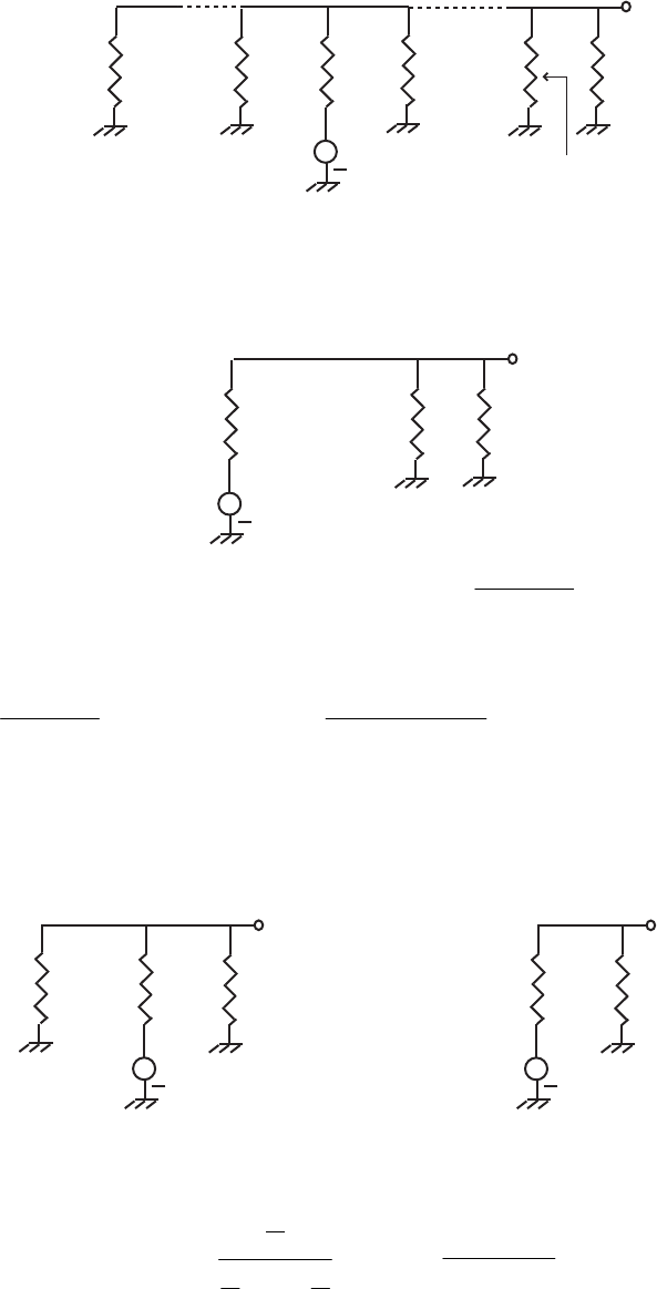
+
a V
R
j
in
Y
G
L
V
o,
j
2
N 1
_
2
j 2
_
2
j0
2
2
j 1
_
In the above circuit, is the total conductance seen by the load conductance
in
Y
L
G which is
given by The above circuit can be redrawn as indicated below: .122
1
0
−=
∑
=−
=
N
N
i
i
in
Y
+
a V
R
j
G
L
V
o,j
2
j 1
_
Y
in
_2
j 1
_
Using the voltage-divider relation we then get .
21
,Rj
Lin
j
jo Va
GY
V⋅
+
=− Using the
superposition theorem, the general expression for the output voltage is thus given by
o
V
.
)12(1
2
2
1
1
1
1
R
L
N
L
j
N
j
j
N
j
Rj
Lin
j
oV
R
R
aVa
GY
V⎟
⎟
⎠
⎞
⎜
⎜
⎝
⎛
−+
∑
=
∑⋅
+
=
=
−
=
−
4.36 The equivalent representation of the D/A converter of Figure 4.49 reduces to the circuit
shown below on the left if -th bit is ON and the remaining bits are OFF, i.e.,
N1
=
N
aand
,,0 Nkak≠=
+
a V
R
N
GL
Vo,N
G
2
__
G
2
__
+
a V
R
N
GL
Vo,N
G
2
__
G
2
__
+
which simplifies to the circuit shown above on the right.
Using the voltage-divider relation we then get
.
)(2
22
2
,RN
L
L
RN
G
G
G
G
No Va
RR
R
VaV
L
⋅
+
=⋅
++
=
The equivalent representation of the D/A converter of Figure 4.49 reduces to the circuit
shown below on the left if )1(
−
N-th bit is ON and the remaining bits are OFF, i.e.,
and 1
1=
−N
a,1,0
−
≠= Nkak
Not for sale 100
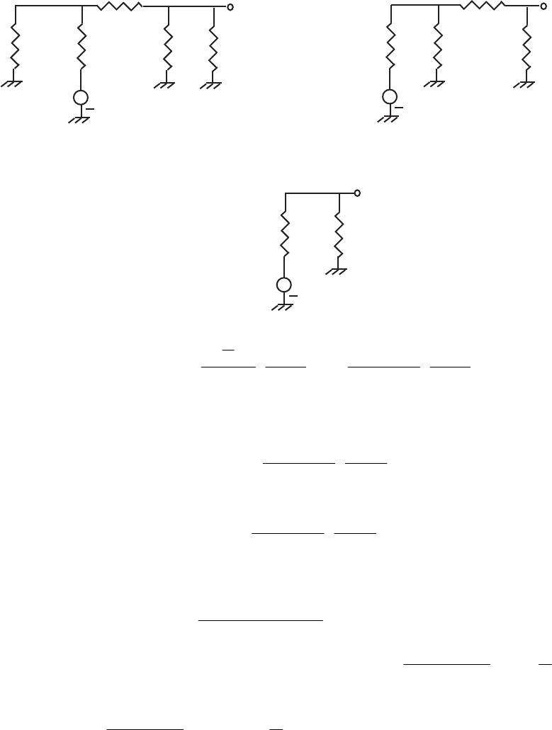
+
GL
G
2
__
G
2
__
G
2
__
G
R
a V
_
N 1
Vo,N 1
_
GL
G
2
__
G
+
G
2
__
R
a V
_
N 1
Vo,N 1
_
G
2
__
+
which simplifies to the circuit shown above on the right.
Its Thevenin equivalent circuit is indicated below:
+
GL
G
2
__
G
2
__
+
V
o,N 1
_
a
N1
_
___
2
R
V
from which we readily obtain
.
2)(22
11
2
1, R
N
L
L
R
N
L
G
No V
a
RR
R
V
a
GG
V−−
−⋅
+
=⋅
+
=
Following the same procedure we can show that if the –th bit is ON and the remaining
bits are OFF, i.e., and
l
,1=
l
a,,0 l
≠
=
kak then
.
2
)(2
,R
N
L
L
oV
a
RR
R
Vl
l
l−
⋅
+
=
Hence, in general we have
.
2
)(2
1
∑⋅
+
=
=−
N
R
N
L
L
oV
a
RR
R
V
ll
l
4.37 From the input-output relation of the first-order hold, we get the expression for the impulse
response as .)1(),(
)()(
)()( TntnTnTt
T
TnTnT
nTth f+<≤−
−
δ
−
δ
+δ= In the range
the impulse response is given by ,0 Tt <≤ .1
)()0(
)0()( T
t
t
T
T
th f+=
−δ
−
δ
+δ=
Likewise, in the range ,2TtT
<
≤ the impulse response is given by
.1)(
)0()(
)()( T
t
Tt
T
T
Tth f−=−
δ−δ
+δ= Outside these two ranges, Hence we
have
.0)( =th f
Not for sale 101
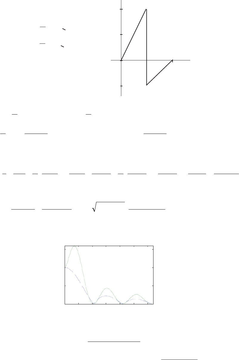
T2T
0
t
1
2
1
_
h (t)
f
otherwise.,0
,2,1
,0,1
)( TtT
T
t
Tt
T
t
th
f
=
{
+
_
<
<
<
<
Using the step function we can write
)]2()([1)]()([1)( TtTt
T
t
Ttt
T
t
th f−µ−−µ
⎟
⎠
⎞
⎜
⎝
⎛−+−µ−µ
⎟
⎠
⎞
⎜
⎝
⎛+=
).2(2)2(
)2(
)2()(2)(
)(2
)()( TtTt
T
Tt
TtTtTt
T
Tt
t
T
t
t−µ+−µ
−
+−µ−−µ−−µ
−
−µ+µ=
Taking the Laplace transform of the above equation we arrive at the transfer function
.
11
2
1
2
211
)(
2
2
2
22
22 ⎟
⎟
⎠
⎞
⎜
⎜
⎝
⎛−
⎟
⎠
⎞
⎜
⎝
⎛+
=+⋅+−−⋅−+= −−−−−−
s
e
T
sT
s
e
s
e
Ts
e
s
e
s
e
T
Ts
s
sH
sTsTsTsTsTsT
f
Hence, the frequency response is given by
.
2/
)2/sin(2
1
11
)( 1
tan
2
22
2
TjTj
Tj
fee
T
T
TT
j
e
T
Tj
jH ΩΩ−
Ω− −
⎟
⎠
⎞
⎜
⎝
⎛
Ω
Ω
Ω+=
⎟
⎟
⎠
⎞
⎜
⎜
⎝
⎛
Ω
−
⎟
⎠
⎞
⎜
⎝
⎛Ω+
=Ω A
plot of the magnitude responses of the zero-order hold and the first-order hold is shown
below:
00.5 11.5 22.5 3
0
0.5
1
1.5
Ω
Amplitude
←
zero-order hold
←
first-order hold
4.37 From the input-output relation of thelinear interpolator, we get the expression for the
impulse response as .)1(),(
)()(
)()( TntnTnTt
T
TnTnT
TnTth f+<≤−
−
δ
−
δ
+−δ= In the
range the impulse response is given by ,0 Tt <≤ .
)()0(
)()( t
T
T
Tth f
−δ−δ
+−δ= Likewise,
Not for sale 102
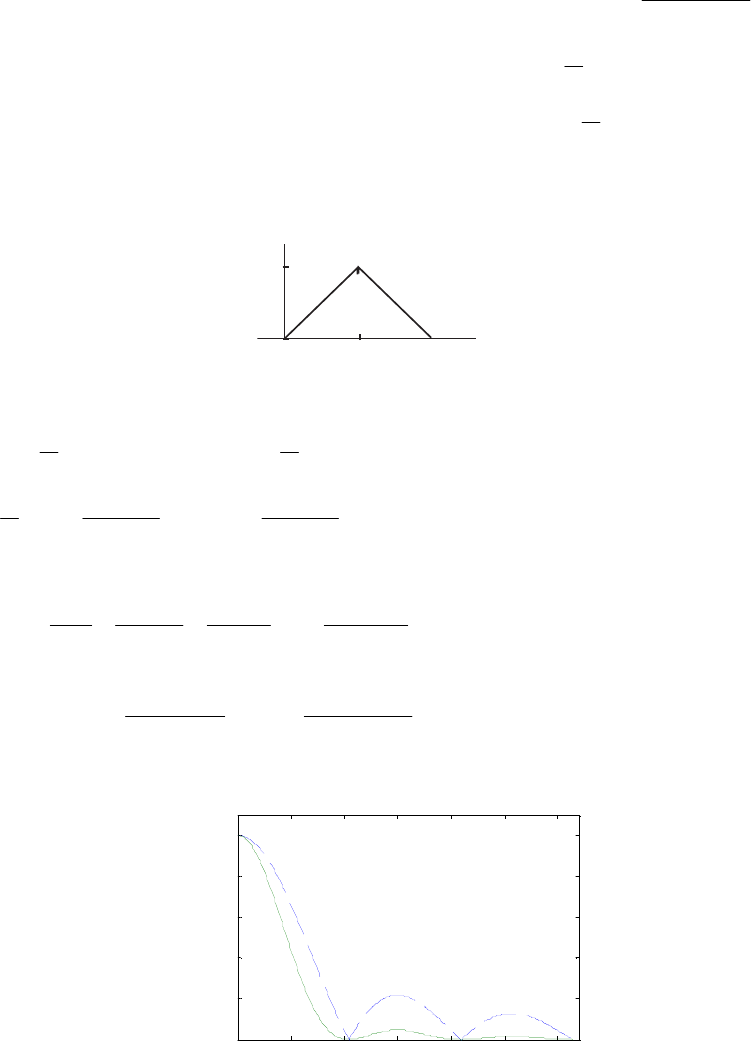
in the range the impulse response is given by ,2TtT <≤ ).(
)0()(
)0()( Tt
T
T
th f−
δ
−δ
+δ=
Outside these two ranges, .0)(
=
th f Hence we have
⎪
⎪
⎪
⎩
⎪
⎪
⎪
⎨
⎧
<≤−
<≤
=
otherwise.,0
,2,2
,0,
)( TtT
T
t
Tt
T
t
th f
T2T
0
t
1
h (t)
f
Using the step function we can write
)]2()([2)]()([)( TtTt
T
t
Ttt
T
t
th f−µ−−µ
⎟
⎠
⎞
⎜
⎝
⎛−+−µ−µ=
).2(
)2(
)(
)(2
)( Tt
T
Tt
Tt
T
Tt
t
T
t−µ
−
+−µ
−
−µ=
Taking the Laplace transform of the above equation we arrive at the transfer function
.
121
)(
2
2
2
22 ⎟
⎟
⎠
⎞
⎜
⎜
⎝
⎛−
=+−= −−−
sT
e
T
Ts
e
Ts
e
Ts
sH
sTsTsT
f Hence, the frequency response is given
by .
2/
)2/sin(1
)(
2
2
Tj
Tj
fe
T
T
T
Tj
e
TjH Ω−
Ω−
⎟
⎠
⎞
⎜
⎝
⎛
Ω
Ω
=
⎟
⎟
⎠
⎞
⎜
⎜
⎝
⎛
Ω
−
=Ω A plot of the magnitude
responses of the ideal filter, zero-order hold and the first-order hold is shown below:
00.5 11.5 22.5 3
0
0.2
0.4
0.6
0.8
1
Ω
Amplitude
←
zero-order hold
←
linear interpolator
M4.1 We use N = 4 and Wn = 18365.512865 computed in Problem 4.22 and use omega
= 0:2*pi:2*pi*10000; to evaluate the frequency points. The gain plot obtained using
Program 4_2 is shown below.
Not for sale 103
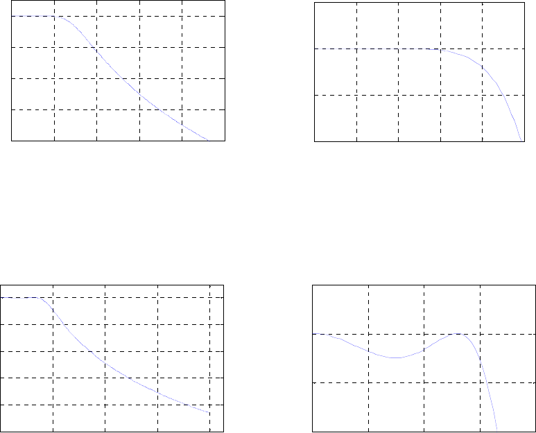
02000 4000 6000 8000 10000
-40
-30
-20
-10
0
Fre
q
uenc
y
, Hz
Gain, dB
Analog Lowpass Filter
0500 1000 1500 2000 2500
-1
-0.5
0
0.5
Fre
q
uenc
y
, Hz
G
a
i
n,
dB
Passband Details
M4.2 We use N = 3 computed in Problem 4.23 and Fp = 2*pi*1500 and Rp = 0.25
and use omega = 0:2*pi:2*pi*10000; to evaluate the frequency points. The gain plot
obtained using Program 4_3 is shown below.
02000 4000 6000 8000
-50
-40
-30
-20
-10
0
Fre
q
uenc
y
, Hz
Gain, dB
Analog Lowpass Filter
0500 1000 1500 2000
-1
-0.5
0
0.5
Fre
q
uenc
y
, Hz
G
a
i
n,
dB
Passband Details
M4.3 We replace the statement
Fp = input('Passband edge frequency in Hz = '); with
Fs = input('Stopband edge frequency in Hz = '); replace
Rp = input('Passband ripple in dB = ');
with Rs = input('Minimum stopband attenuation in dB = '); and
replace [num,den] = cheby1(N,Rp,Fp,'s'); with [num,den] =
cheby2(N,Rs,Fs,'s'); to modify Program 4_3.
Next, we run the modified program using N = 3 and Rs = 25, and Fs = 2*pi*6000. The
gain response plot generated by the modified program is shown below.
Not for sale 104
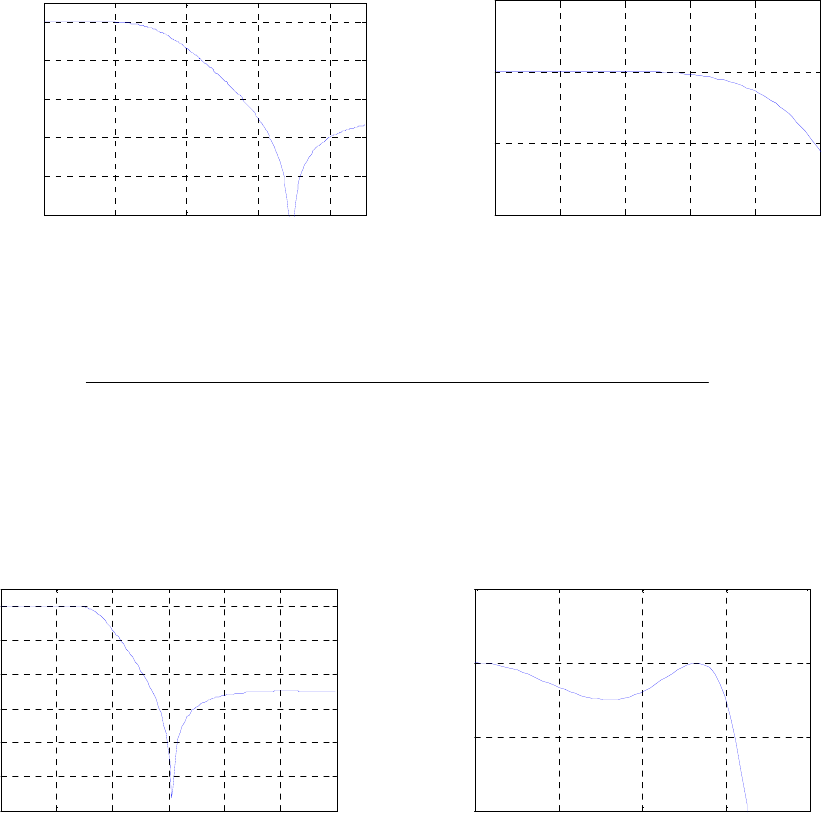
02000 4000 6000 8000
-50
-40
-30
-20
-10
0
Fre
q
uenc
y
, Hz
Gain, dB
Analog Lowpass Filter
0500 1000 1500 2000 2500
-1
-0.5
0
0.5
Fre
q
uenc
y
, Hz
G
a
i
n,
dB
Passband Details
The numerator and the denominator coefficients of the 3rd order Type 2 Chebyshev lowpass
filter can be obtained by typing num and den in the command window:
10723
102
104.866329410542.4198332257030.25552
104.866329410138.1864
)( ×+×++
×+
=
sss
s
sH LP .
M4.4 We use N = 3 and Wn = 9424.777960769379 computed in Problem 4.26 in
Program 4_4 and use omega = [0: 200: 12000*pi]; to evaluate the frequency points. The
gain plot generated by running this program is shown below:
01000 2000 3000 4000 5000 6000
-60
-50
-40
-30
-20
-10
0
Fre
q
uenc
y
, Hz
Gain, dB
Analog Lowpass Filter
0500 1000 1500 2000
-1
-0.5
0
0.5
Fre
q
uenc
y
, Hz
G
a
i
n,
dB
Passband Details
M4.5 The MATLAB program used is as given below:
[N,Wn]=buttord(1,13/3,0.5, 40, 's');
[B,A] = butter(N,Wn,'s');
[num,den]=lp2hp(B,A,2*pi*6500);
figure(1)
[h,w]=freqs(B,A);gain = 20*log10(abs(h));
plot(w,gain);grid
xlabel('\Omega');ylabel('Gain, dB');
title('Analog Lowpass Filter');
figure(2)
[h,w]=freqs(num,den);gain = 20*log10(abs(h));
plot(w/(2*pi),gain);grid
xlabel('Frequency, Hz');ylabel('Gain, dB');
title('Analog Highpass Filter');
Not for sale 105
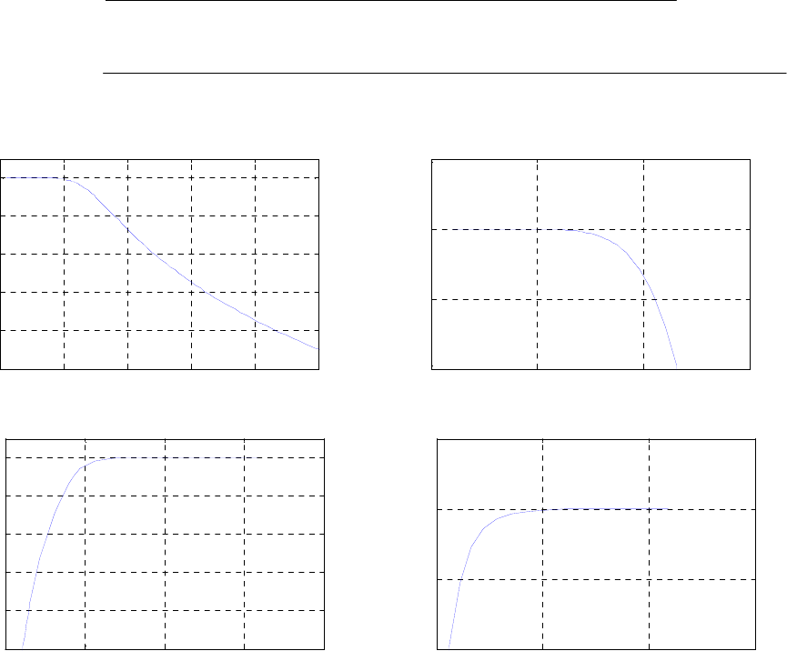
,
3.5262257s6.72423556s6.411294643.58086432
3.5262257
)( 234 ++++
=
ss
sHLP
.
107.8897418106.91763168103.03264857.7880
)( 17132934
4
×+×+×++
=
ssss
s
sHHP
0 1 2 3 4 5
-50
-40
-30
-20
-10
0
Ω
Gian, dB
Prototype Lowpass Filter
00.5 11.5
-1
-0.5
0
0.5
Ω
Gi
an,
dB
Passband Details
00.5 11.5 2
x 10
4
-50
-40
-30
-20
-10
0
Frequency, Hz
Gain, dB
Analog Highpass Filter
0.5 11.5 2
x 10
4
-1
-0.5
0
0.5
Frequency, Hz
G
a
i
n,
dB
Passband Details
M4.6 The MATLAB program used is given below:
[N,Wn] = ellipord(1,1.28,0.25,50,'s');
[B,A] = ellip(N,0.25,50,Wn,'s');
[num,den] = lp2bp(B,A,2*pi*30e3,2*pi*25e3);
figure(1)
omega = [0:0.01:10];
h = freqs(B,A,omega);
gain = 20*log10(abs(h));
plot(omega,gain); grid; axis([0 5 -80 5]);
xlabel('\Omega'); ylabel('Gain, dB');
title('Analog Lowpass Filter');
figure(2)
omega = [0:200:100e3*2*pi];
h = freqs(num,den,omega);
gain = 20*log10(abs(h));
Not for sale 106
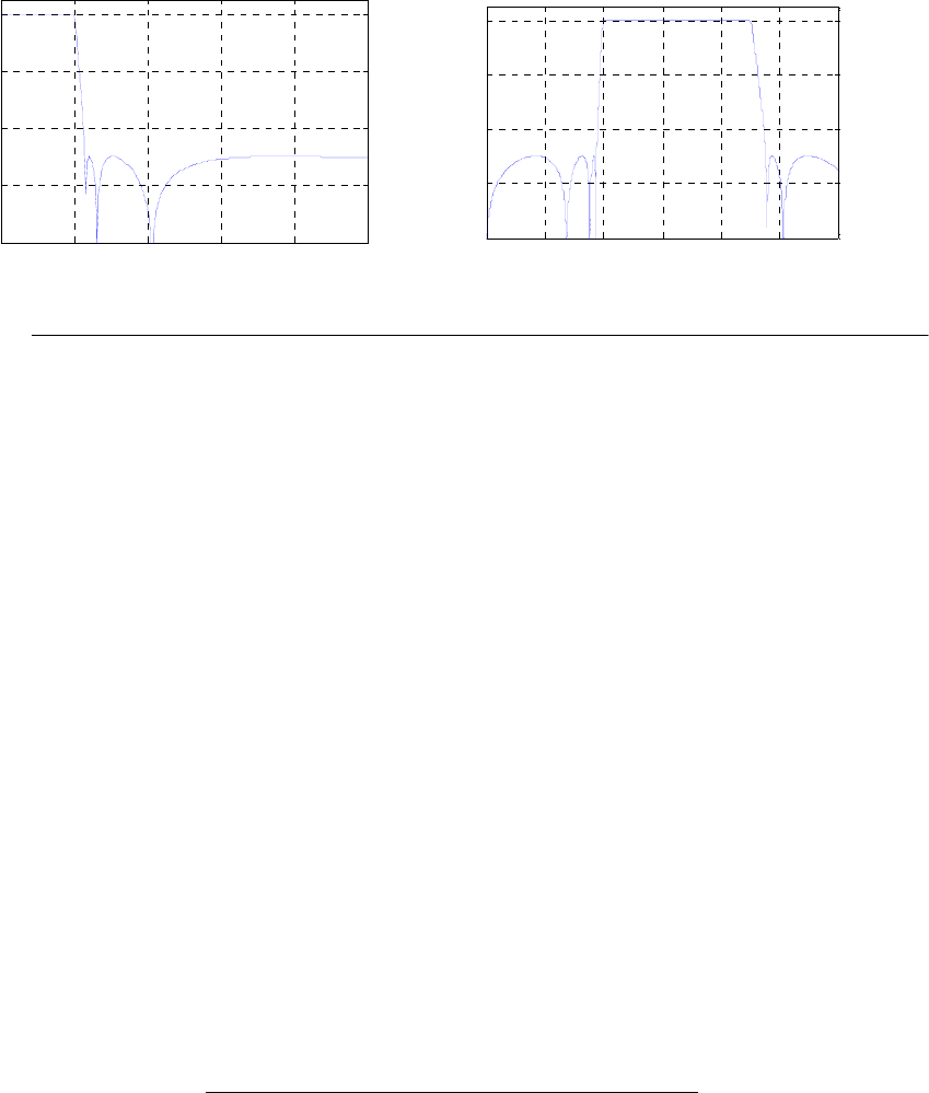
plot(omega/(2*pi),gain); grid; axis([0 60e3 -80 5]);
xlabel('Frequency in Hz'); ylabel('Gain, dB');
title('Analog Bandpass Filter');
0 1 2 3 4 5
-80
-60
-40
-20
0
Ω
Gain, dB
Analog Lowpass Filter
0 1 2 3 4 5 6
x 10
4
-80
-60
-40
-20
0
Frequency in Hz
Gain, dB
Analog Bandpass Filter
.
0.1868s0.7275s1.56215s2.70025s2.7545s2.9795s1.36426s
0.186835s0.2887s0.1364s0.0185
)( 234567
246
+++++++
+++
=sHLP
The numerator and denominator coefficients of can be obtained by typing num and den in
the Command Window.
M4.7 The MATLAB program used is given below:
[N,Wn] = cheb1ord(0.3157894, 1, 0.5, 30,'s');
[B,A] = cheby1(N,0.5, Wn,'s');
[num,den] = lp2bs(B,A,2*pi*sqrt(700)*10^6, 2*pi*15e6);
figure(1)
omega = [0:0.01:10];
h = freqs(B,A,omega);
gain = 20*log10(abs(h));
plot(omega, gain); grid; axis([0 4 -70 5]);
xlabel('\Omega'); ylabel('Gain, dB');
title('Analog Lowpass Filter');
figure(2)
omega = [0:10000:160e6*pi];
h = freqs(num,den,omega);
gain = 20*log10(abs(h));
plot(omega/(2*pi), gain); grid; axis([0 80e6 -70 5]);
xlabel('Frequency in Hz'); ylabel('Gain, dB');
title('Analog Bandstop Filter');
.
0.02253823s0.1530643s0.3956566
0.02253823
)( 23 +++
=
s
sHLP
Not for sale 107
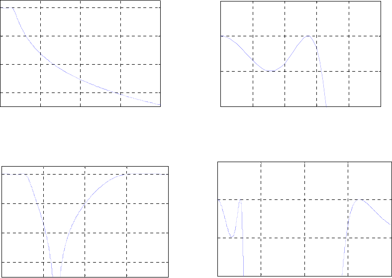
0 1 2 3 4
-60
-40
-20
0
Ω
Gain, dB
Analog Lowpass Filter
00.1 0.2 0.3 0.4 0.5
-1
-0.5
0
0.5
Ω
G
a
i
n,
dB
Passband Details
0 2 4 6 8
x 10
7
-60
-40
-20
0
Frequency in Hz
Gain, dB
Analog Bandstop Filter
0 2 4 6 8
x 10
7
-1
-0.5
0
0.5
Frequency in Hz
G
a
i
n,
dB
Stopband Details
M4.8 The MATLAB program to generate the plots of Figure 4.56 is given below:
% Droop Compensation
w = 0:pi/100:pi;
h1 = freqz([-1/16 9/8 -1/16],1,w);
h2 = freqz(9, [8 1], w);
w1 = 0;
for n = 1:101;
h3(n) = sin(w1/2)/(w1/2);
w1 = w1 + pi/100;
end
m1 = 20*log10(abs(h1));
m2 = 20*log10(abs(h2));
m3 = 20*log10(abs(h3));
plot(w/pi,m3,’-’,w/pi,m1+m2,’--’,w/pi,m2+m3,’-.’);grid
xlabel(‘Normalized frequency’);ylabel(Gain, dB’);
Not for sale 108

Chapter 5
5.1 Let Then Since is
periodic in with a period Therefore
hence is also periodic in with a period
∑−= −
=
1
0
].[
~
][
~
][
~N
r
rnhrxny ∑−+=+ −
=
1
0
].[
~
][
~
][
~N
r
rkNnhrxkNny ][
~nh
n].[
~
][
~
,rnhrkNnhN −=−+ ][
~kNny +
∑=−= −
=
1
0
],[
~
][
~
][
~
N
r
nyrnhrx ][
~ny n.N
5.2 (a)
,13]1[
~
]4[
~
]2[
~
]3[
~
]3[
~
]2[
~
]4[
~
]1[
~
]0[
~
]0[
~
][
~
][
~
]0[
~4
0
−=++++=
∑−=
=
hxhxhxhxhxrhrxy
r
,13]2[
~
]4[
~
]3[
~
]3[
~
]4[
~
]2[
~
]0[
~
]1[
~
]1[
~
]0[
~
]1[
~
][
~
]1[
~4
0
−=++++=
∑−=
=
hxhxhxhxhxrhrxy
r
,13]3[
~
]4[
~
]4[
~
]3[
~
]0[
~
]2[
~
]1[
~
]1[
~
]2[
~
]0[
~
]2[
~
][
~
]2[
~4
0
−=++++=
∑−=
=
hxhxhxhxhxrhrxy
r
,13]4[
~
]4[
~
]0[
~
]3[
~
]1[
~
]2[
~
]2[
~
]1[
~
]3[
~
]0[
~
]3[
~
][
~
]3[
~4
0
−=++++=
∑−=
=
hxhxhxhxhxrhrxy
r
.13]0[
~
]4[
~
]1[
~
]3[
~
]2[
~
]2[
~
]3[
~
]1[
~
]4[
~
]0[
~
]4[
~
][
~
]4[
~4
0
−=++++=
∑−=
=
hxhxhxhxhxrhrxy
r
Therefore, .40},,13,13,13,13,13{][
~
≤
≤
−
−
−
−−= nny
(b) .40},,1,1,1,1,1{][
~
≤
≤
=nny
5.3 Since hence all the terms which are not in the range
],[
~
][
~nrNn kk ψ=+ψ ,1,,1,0
−
NK
can be accumulated to where ],[
~n
k
ψ.10
−
≤
≤
Nk Hence, in this case the Fourier
series representation involves only
N
complex exponential sequences. Let
,][
~
1
][
~1
0
/2
∑
=−
=
π
N
k
Nknj
ekX
N
nx then
.][
~
1
][
~
1
][
~1
0
/)(2
1
0
1
0
1
0
/)(2
1
0
/2 ⎟
⎟
⎠
⎞
⎜
⎜
⎝
⎛∑∑
=
∑∑
=
∑−
=
−π
−
=
−
=
−
=
−π
−
=
π− N
n
Nnrkj
N
k
N
n
N
k
Nnrkj
N
n
Nrnj ekX
N
ekX
N
enx
Now, from Eq. (5.11), the inner summation is equal to
N
if ,rk
=
otherwise it is equal
to Thus, Next, we observe
.0 ].[
~
][
~
1
0
/2 rXenx
N
n
Nrnj =
∑
−
=
π− ][
~NkX l+
].[
~
][
~
][
~
][
~1
0
/22
1
0
/2
1
0
/)(2 kXenxeenxenx
N
n
Nknjnj
N
n
Nknj
N
n
NnNkj =
∑
=
∑
=
∑
=−
=
π−π−
−
=
π−
−
=
+π− ll
Not for sale. 109

5.4 (a)
{}
.cos][
~4/4/
2
1
4
1njnj
neenx π−π
π+=
⎟
⎠
⎞
⎜
⎝
⎛
= The period of is
][
~
1nx .8=N
⎭
⎬
⎫
⎩
⎨
⎧∑
+
∑
=
=
π−π−
=
π−π 7
0
8/28/2
7
0
8/28/2
12
1
][
~
n
knjnj
n
knjnj eeeekX
.
2
17
0
8/)1(2
7
0
8/)1(2
⎭
⎬
⎫
⎩
⎨
⎧∑
+
∑
=
=
+π−
=
−π−
n
knj
n
knj ee Now, from Eqn. (5.11) we observe
and
⎩
⎨
⎧=
=
∑
=
−π−
,otherwise,0
,1for,8
7
0
8/)1(2 k
e
n
knj
⎩
⎨
⎧=
=
∑
=
+π−
.otherwise,0
,7for,8
7
0
8/)1(2 k
e
n
knj
Hence,
⎩
⎨
⎧=
=otherwise.,0
,7,1for,4
][
~
1
k
kX
(b) }.{}{cos3sin][
~4/4/
2
3
3/3/
2
1
43
2njnjnjnj
j
nn eeeenx π−ππ−π
ππ ++−=
⎟
⎠
⎞
⎜
⎝
⎛
+
⎟
⎠
⎞
⎜
⎝
⎛
= The
period of
(
)
3
sin n
π
is and the period of
6
(
)
4
cos n
π
is Hence, the period of is the
GCM of and is
.8 ][
~2nx
)8,6( .24
⎭
⎬
⎫
⎩
⎨
⎧∑
−
∑
=
=
π−π−
=
π−π 23
0
24/224/8
23
0
24/224/8
22
1
][
~
n
knjnj
n
knjnj eeee
j
kX
⎭
⎬
⎫
⎩
⎨
⎧∑
−
∑
+
=
π−π−
=
π−π 23
0
24/224/6
23
0
24/224/6
2
3
n
knjnj
n
knjnj eeee
⎭
⎬
⎫
⎩
⎨
⎧∑
−
∑
=
=
+π−
=
−π− 23
0
24/)3(2
23
0
24/)3(2
2
1
n
knj
n
knj ee
j
.
2
323
0
24/)4(2
23
0
24/)4(2
⎭
⎬
⎫
⎩
⎨
⎧∑
−
∑
+
=
+π−
=
−π−
n
knj
n
knj ee Hence
⎪
⎩
⎪
⎨
⎧
=
=
=−
=
otherwise.,0
,20,4,36
,21,12
,3,12
][
~
2k
kj
kj
kX
5.5 Let denote the coefficients of the Fourier series representation of Since
is periodic with a period
][
~kP ].[
~np
][
~np ,
N
then from Eq. (5.185b), we have
Hence, from Eq. (5.185a) we get
.1][
~
][
~1
0
/2 =
∑
=−
=
π−
N
n
Nknj
enpkP
.
1
][
~
1
][
~1
0
/2
1
0
/2 ∑
=
∑
=−
=
π
−
=
πNNnj
NNnj e
N
eP
N
np
l
l
l
l
l
5.6 .,][)()(][
~/2/2
/2
∞<<∞−
∑
=== ∞
−∞=
π−π
π=ω
ωkenxeXeXkX
n
NkjNkj
Nk
j
Now,
].[
~
)()()(][
~/2/2/)(2 kXeXeeXeXNkX NkjjNkjNNkj ====+ πππ+π ll
l
Not for sale. 110

Likewise, Nknj
N
k
Nnj
N
k
Nknj eex
N
ekX
N
nx /2
1
0
/2
1
0
/2 ][
1
][
~
1
][
~π
−
=
∞
−∞=
π−
−
=
π∑⎟
⎟
⎠
⎞
⎜
⎜
⎝
⎛∑
=
∑
=
l
l
l
.][
11
0
/)(2
∑∑
=−
=
∞
−∞=
−π
N
k
Nnkj
ex
Nl
l
l Let .rNn
+
=
l Then
.][
1
][
~1
0
2
∑⎟
⎟
⎠
⎞
⎜
⎜
⎝
⎛∑
+= ∞
−∞=
−
=
π−
r
N
k
krj
erNnx
N
nx But Hence, .
1
0
2Ne
N
k
krj =
∑
−
=
π−
.][][
~∑+= ∞
−∞=
r
rNnxnx
5.7 (a) Now, .][
~
][
~
][
~
][
~1
0
/2
1
0
/2 ∑
=
∑
=−
=
π−
−
=
π− N
n
Nknj
N
n
Nknj enynxengkG
.][
~
1
][
~1
0
/2
∑
=−
=
π−
N
r
Nrnj
erX
N
nx Therefore,
∑∑
=
∑∑
=−
=
−π−
−
=
−
=
−π−
−
=
1
0
/)(2
1
0
1
0
/)(2
1
0
][][
~
1
][][
~
1
][
~N
r
Nnrkj
N
n
N
n
Nnrkj
N
r
enyrX
N
enyrX
N
kG tt
.][
~
][
~
11
0
∑−= −
=
N
r
rkYrX
N
(b) ∑∑
=
∑
=−
=
−
=
−π
−
=
π1
0
1
0
/)(2
1
0
/2 ][
~
][
~
1
][
~
][
~
1
][
~N
k
N
r
Nrnkj
N
k
Nknj ekYrx
N
ekYkX
N
nh
.][
~
][
~
][
~
1
][
~1
0
1
0
1
0
/)(2 ∑−=
∑⎟
⎟
⎠
⎞
⎜
⎜
⎝
⎛∑
=−
=
−
=
−
=
−π N
r
N
r
N
k
Nrnkj rnyrxekY
N
rx
5.8 (a) ).()/2sin(][ /2/2
2
1NnjNnj
j
aeeNnnx π−π −=π= Therefore,
Nknj
N
n
NnjNknj
N
n
Nnj
aee
j
ee
j
kX /2
1
0
/2/2
1
0
/2
2
1
2
1
][ π−
−
=
π−π−
−
=
π∑
−
∑
=
.
2
1
2
11
0
/)1(2
1
0
/)1(2 ∑
−
∑
=−
=
+π−
−
=
−π− N
n
Nnkj
N
n
Nnkj e
j
e
j From Eq. (5.11), the first sum is
equal to
N
when and othereise. Likewise, from Eq. (5.11), the second sum is
equal to when and otherwise. Therefore,
1=k0
N1−= Nk 0
⎪
⎩
⎪
⎨
⎧−=−
=
=
otherwise.,0
,1,2/
,1,2/
][ NkjN
kjN
kXa
(b) .coscos][ 4
2
1
2
1
2
2⎟
⎠
⎞
⎜
⎝
⎛
+=
⎟
⎠
⎞
⎜
⎝
⎛
=ππ
N
n
N
n
bnx Now the –point DFT of
N2
1 is 2
N for
and 0 otherwise. From Example 5.2, the
0=k
N
–point DFT of
(
)
N
nπ4
cos is 2
N for
and and 0 otherwise. Therefore,
2=k2−= Nk
Not for sale. 111

⎪
⎩
⎪
⎨
⎧−= =
=
otherwise.,0
,2,2,4/
,0,2/
][ NkN
kN
kXb
(c) .coscoscos][ 2
4
3
6
4
1
2
3⎟
⎠
⎞
⎜
⎝
⎛
+
⎟
⎠
⎞
⎜
⎝
⎛
=
⎟
⎠
⎞
⎜
⎝
⎛
=πππ
N
n
N
n
N
n
cnx From Example 5.2, the –point
DFT of
N
⎟
⎠
⎞
⎜
⎝
⎛π
N
n6
cos is 2
N for 3
=
k and 3
−
=
Nk and 0 otherwise. Likewise, from
Example 5.2, the –point DFT of
N⎟
⎠
⎞
⎜
⎝
⎛π
N
n2
cos is 2
N for 1
=
k and and
otherwise. Therefore,
1−= Nk 0
⎪
⎩
⎪
⎨
⎧−=
−=
=
otherwise.,0
,1,1,8/3
,3,3,8/
][ NkN
NkN
kXc
5.9 (a) .
1
1
1
1
)(][
1
0
1
0k
N
k
N
kN
N
N
n
nk
N
N
n
kn
N
n
aWW
W
WWkY α−
α−
=
α−
α−
=
∑α=
∑α= −
=
−
=
(b) Assume first is even, i.e., Then
.32][
oddeven
∑
−
∑
=
k
kn
N
k
kn
Nb WWkY N.2LN =
()
.0
1
1
323232][ 1
0
2
1
0
1
0
)12(
2
1
0
2
2=
⎟
⎟
⎠
⎞
⎜
⎜
⎝
⎛
−
−
−=
∑
−
∑
=
∑
−
∑
=−
=
−
=
−
=
+
−
=k
L
kL
L
k
N
L
r
kr
L
k
L
L
r
kr
L
L
r
rk
L
L
r
rk
Lb W
W
WWWWWWkY
Next, assume
N
is odd, i.e., .12
+
=
LN Then
∑
−
∑
=−
=
+
=
1
0
)12(
2
0
2
232][
L
r
rk
L
L
r
rk
Lb WWkY
.2
1
1
2
1
1
3
1
1
232 2
)1(
1
0
2
0
=
⎟
⎟
⎠
⎞
⎜
⎜
⎝
⎛
−
−
=
⎟
⎟
⎠
⎞
⎜
⎜
⎝
⎛
−
−
−
⎟
⎟
⎠
⎞
⎜
⎜
⎝
⎛
−
−
=
∑
−
∑
=
+
−
== k
L
k
L
k
L
kL
L
k
L
k
L
Lk
L
L
r
kr
L
k
L
L
r
kr
LW
W
W
W
W
W
W
WWW
5.10 .10),()cos(][ 2
1−≤≤+=ω= ω−ω Nneennx njnj
ooo Therefore,
∑−+
∑
=−
=
π−
ω
−
=
π−
ω1
0
/2
1
0
/2
2
1
2
1
][
N
n
Nknj
nj
N
n
Nknj
nj ejeeekX oo
∑
+
∑
=−
=
ω−
−
=
ω−− +
ππ 1
0
)(
1
0
)( 22
2
1
2
1N
n
nj
N
n
nj o
N
k
o
N
k
ee
⎟
⎠
⎞
⎜
⎝
⎛
−
⎟
⎠
⎞
⎜
⎝
⎛
−
⎟
⎠
⎞
⎜
⎝
⎛
−
⎟
⎠
⎞
⎜
⎝
⎛
−
ω+
π
ω+
π
ω−
π
ω−
π
−
−
⋅+
−
−
⋅=
o
N
k
o
N
k
o
N
k
o
N
k
j
Nj
j
Nj
e
e
e
e
2
2
2
2
1
1
2
1
1
1
2
1
Not for sale. 112

(
)
()
(
)
()
.
sin
sin
2
1
sin
sin
2
1
2
2
2
12
2
2
2
12
o
N
k
N
o
N
o
N
k
o
N
k
N
o
N
o
N
kk
e
k
e
jj
ω
+
π
ω
−
ω+
π
ωπ
ω
−
ω−
π+π
⋅+
−
−π
⋅= ⎟
⎠
⎞
⎜
⎝
⎛
⎟
⎠
⎞
⎜
⎝
⎛
−
⎟
⎠
⎞
⎜
⎝
⎛
⎟
⎠
⎞
⎜
⎝
⎛
−
5.11
∑++
∑
=
∑
=−
=
+
−
=
−
=
1)2/(
0
)12(
1)2/(
0
2
1
0
]12[]2[][][
N
r
kr
N
N
r
rk
N
N
n
nk
NWrxWrxWnxkX
∑++
∑
=−
=
−
=
1)2/(
02/
1)2/(
02/ ]12[]2[
N
r
rk
N
k
N
N
r
rk
NWrxWWrx
∑
+
∑
=
−
=
−
=
1)2/(
02/1
1)2/(
02/0 ][][
N
r
rk
N
k
N
N
r
rk
NWrxWWrx
.10],[][ 2/12/0 −≤≤〉〈+〉〈= NkkXWkX N
k
NN
5.12
∑
+
∑
=
∑
=−
=
−
=
−
=
1
2/
1)2/(
0
1
0
][][][][
N
Nn
nk
N
N
n
nk
N
N
n
nk
NWnxWnxWnxkX
∑++
∑
=−
=
−
=
1)2/(
02
)2/(
1)2/(
0
][][
N
n
nk
N
N
kN
N
N
n
nk
NWnxWWnx
∑⎟
⎠
⎞
⎜
⎝
⎛+−+= −
=
1)2/(
0
]
2
[)1(][
N
n
nk
N
kWn
N
xnx . For ,2l
=
k we get
][]
2
[][]
2
[][]2[ 0
1)2/(
02/
1)2/(
0
2ll ll XWn
N
xnxWn
N
xnxX
N
n
n
N
N
n
n
N=
∑⎟
⎠
⎞
⎜
⎝
⎛++=
∑⎟
⎠
⎞
⎜
⎝
⎛++= −
=
−
=
and for we get
12 += lk∑⎟
⎠
⎞
⎜
⎝
⎛+−=+ −
=
+
1)2/(
0
)12(
]
2
[][]12[
N
n
n
N
Wn
N
xnxX l
l
][]
2
[][ 1
1)2/(
02/ l
lXWWn
N
xnx
N
n
n
N
n
N=
∑⋅
⎟
⎠
⎞
⎜
⎝
⎛++= −
= where .1
2
0−≤≤ N
l
5.13 .1
22
1
2
10]),12[]2[(][]),12[]2[(][ −≤≤+−=++= N
nnxnxnhnxnxng Solving for
and we get ]2[ nx ],12[ +nx ][][]2[ nhngnx
+
=
and ].[][]12[ nhngnx −
=
+
Therefore,
∑++
∑
=
∑
=−
=
+
−
=
−
=
1)2/(
0
)12(
1)2/(
0
2
1
0
]12[]2[][][
N
r
kr
N
N
r
rk
N
N
n
nk
NWrxWrxWnxkX
∑++
∑
=−
=
−
=
1)2/(
02/
1)2/(
02/ ]12[]2[
N
r
rk
N
k
N
N
r
rk
NWrxWWrx
∑−+
∑+= −
=
−
=
1)2/(
02/
1)2/(
02/ ])[][(])[][(
N
r
rk
N
k
N
N
r
rk
NWnhngWWnhng
∑
−+
∑
+= −
=
−
=
1)2/(
02/
1)2/(
02/ ][)1(][)1(
N
r
rk
N
k
N
N
r
rk
N
k
NWnhWWngW
Not for sale. 113

.10],[)1(][)1( 2/2/ −≤≤〉〈−+〉〈+= NkkHWkGW N
k
NN
k
N
5.14 ,1
2
4321 0],12[]2[][],12[]2[][ −≤≤+−=++= N
nnxanxanhnxanxang with
Solving for and .
3241 aaaa ≠]2[ nx ],12[
+
nx we get
3241
24 ][][
]2[ aaaa
nhanga
nx −
−
= and
.
][][
]12[
3241
13
aaaa
nhanga
nx −
+−
=+ Therefore,
∑++
∑
=
∑
=−
=
+
−
=
−
=
1)2/(
0
)12(
1)2/(
0
2
1
0
]12[]2[][][
N
r
kr
N
N
r
rk
N
N
n
nk
NWrxWrxWnxkX
∑++
∑
=−
=
−
=
1)2/(
02/
1)2/(
02/ ]12[]2[
N
r
rk
N
k
N
N
r
rk
NWrxWWrx
∑⎟
⎟
⎠
⎞
⎜
⎜
⎝
⎛
−
+−
+
∑⎟
⎟
⎠
⎞
⎜
⎜
⎝
⎛
−
−
=−
=
−
=
1)2/(
02/
3241
13
1)2/(
02/
3241
24 ][][
][][ N
r
rk
N
k
N
N
r
rk
NW
aaaa
nhanga
WW
aaaa
rharga
()
.10,][)(][)(
1
2/122/34
3241
−≤≤〉〈+−+〉〈−
−
=NnkHWaakGWaa
aaaa N
k
NN
k
N
5.15 (a) For even, i.e., .][][ 1
02
∑
=−
=
N
n
nk
N
WnxkG k,2l
=
k
∑
=−
=
1
0
2
2
][]2[
N
n
n
N
WnxG l
l
.10],[][
1
02−≤≤=
∑
=−
=
NXnx
N
n
n
Nll
l
(b) Let .][][ 12
2
∑−= −
=
N
Nn
nk
N
WNnxkH Nnm
−
=
or .Nmn
+
=
Then
For even, i.e.,
.][)1(][][ 1
02
1
0
)(
2∑
−=
∑
=−
=
−
=
+N
m
mk
N
k
N
m
kNm
NWmxWmxkH k,2l=k
.10],[][][]2[ 1
0
1
0
2
2−≤≤=
∑
=
∑
=−
=
−
=
NXWnxWnxH
N
n
n
N
N
n
n
Nlll ll
5.16 For even, i.e.,
].[][])[][(][][ 12
02
12
02kHkGWnhngWnykY
N
n
nk
N
N
n
nk
N+=
∑+=
∑
=−
=
−
=
k
,2l=k.10],[2]2[]2[]2[
−
≤
≤
=
+= NXHGY lllll
For odd, i.e., and
k,12 += lk∑
=
∑
=+ −
=
−
=
+1
02
1
0
)12(
2][][]12[
N
n
n
N
n
N
N
n
n
NWWnxWnxG l
l
l
.10,]12[][][]12[ 1
02
1
0
)12(
2−≤≤
∑+−=−=
∑
−=+ −
=
−
=
+NGWWnxWnxH
N
n
n
N
n
N
N
n
n
Nlll l
l
Hence, for ,12 += lk.10,0]12[]12[]12[ −≤
≤
=
+
−
+
=
+
NGGY llll
Not for sale. 114

5.17 Thus,
.][][][ 1
0
1
0
∑
=
∑
=−
=
−
=
N
n
nk
MN
MN
n
nk
MN WnxWnykY
].[][][][ 1
0
1
0
kXWnxWnxkMY
N
n
nk
N
N
n
nkM
MN =
∑
=
∑
=−
=
−
=
5.18
5.19 (a) Now, Hence if ].[)1(][]2/[ 1
0
1
0
2/ nxWnxNX
N
n
n
N
n
nN
N∑−=
∑
=−
=
−
=
]1[][ nNxnx
−
−=
and is even, then
N.0][)1(]2/[ 1
0
=
∑−= −
=
nxNX
N
n
n
(b) Hence if .][]0[ 1
0
∑
=−
=
N
n
nxX ],1[][ nNxnx
−
−
−
=
then .0]0[
=
X
(c)
∑
+
∑
=
∑
=−
−=
−
=
−
=
1
1)2/(
2
1)2/(
0
2
1
0
2][][][]2[
N
Nn
n
N
N
n
n
N
N
n
n
NWnxWnxWnxX lll
l
()
.][][][][
1
0
2
2
1)2/(
0
2
1)2/(
0
2
2∑++=
∑++
∑
=−
=
−
=
−
=
M
n
n
M
N
n
n
N
N
n
n
NWMnxnxWnxWnx Nlll Hence if
],[][
M
n
x
n
x
+−= then 0]2[
=
lX for .10
−
≤
≤
Ml
5.20
∑
+
∑
=
∑
=−
=
−
=
−
=
1
2/
2
1)2/(
0
2
1
0
2][][][]2[ N
Nn
mn
N
N
n
mn
N
N
n
mn
NWnxWnxWnxmX
∑++
∑
=−
=
−
=
12/
0
2
2
1)2/(
0
2][][ N
n
mN
N
mn
N
N
N
n
mn
NWWnxWnx ,0[][
1)2/(
0
2
2=
∑⎟
⎠
⎞
⎜
⎝
⎛++= −
=
N
n
mn
N
NWnxnx
.10 2−≤≤ N
m This implies .0][][ 2=++ N
nxnx
5.21 (a) Using the circular convolution property of the DFT given in Table 5.3, we get
and
][}[{DFT 1
1kXWmnx km
N
N=〉−〈 ].[}[{DFT 2
2kXWmnx km
N
N=〉−〈
Hence,
].[)(][][]}[{DF][ 1121 kXWWkXWkXWnwTkW km
N
km
N
km
N
km
N+=+==
(b)
(
)
(
)
.][][][)1(][][ )2/(
2
1
2
1nxWnxnxnxng nN
N
n−
+=−+= Using the circular
convolution property of the DFT given in Table 5.3, we get
{
}
.[][]}[{DFT][ 22
1
N
N
kXkXngkG 〉−〈+==
(c) Using the circular convolution property of the DFT given in Table 5.3, we get
].[][][]}[{DF][ 2kXkXkXnyTkY =⋅==
Not for sale. 115

5.22 (a)
{
}
].[)1(][[DFT )2/(
2kXkXWnx k
Nk
N
N
N−==〉−〈 Hence,
{}
⎩
⎨
⎧
=−−=〉−〈−== .evenfor,0
,oddfor],[2
][)1(][[][DFT]}[{DFT][ 2k
kkX
kXkXnxnxnukU k
N
N
(b) ].[2][][]
2
N
[][DFT]}[{DFT][ kXkXkXnxnxnvkV =+=
⎭
⎬
⎫
⎩
⎨
⎧−−==
(c) Hence, using the circular frequency-shifting
property of the DFT given in Table 5.3, we get
].[][)1(][ )2/( nxWnxny nN
N
n=−=
{
}
].[][DFT]}[{DFT][ 2
)2/( N
N
nN
NkXnxWnykY 〉−〈===
5.23 (a) From the circular frequency-shifting property of the DFT given in Table 5.3, we get
and Hence,
][}[{IDFT 1
1nxWmkX nm
N
N
−
=〉−〈 ].[}[{IDFT 2
2nxWmkX nm
N
N
−
=〉−〈
}[}[{IDFT]}[{IDFT][ 21 NN mkXmkXkWnw 〉
−
〈
+
〉
−
〈
== βα
].[)(][][ 2121 nxWWnxWnxW nm
N
nm
N
nm
N
nm
N
−
−
−− +=+= βαβα
(b)
(
)
.][][])[)1(][(][ )2/(
2
1
2
1kXWkXkXkXkG kN
N
k−
+=−+= Using the circular
time-shifting property of the DFT given in Table 5.3, we get
.[][]}[{IDFT][ 22
1⎟
⎠
⎞
⎜
⎝
⎛〉−〈+== N
N
nxnxkGng
(c) Using the modulation property of the DFT given in Table 5.3, we get
].[][][]}[{IDFT][ 2nxNnxnxNkYny ⋅=⋅⋅==
5.24 (a)
∑
+
∑
=
∑
=−
=
−
=
−
=
1
2/
2
1)2/(
0
2
1
0
2][][][]2[ N
Nn
mn
N
N
n
mn
N
N
n
mn
NWnxWnxWnxmX
∑++
∑
=−
=
+
−
=
12/
0
)(2
2
1)2/(
0
22
][][ N
n
nm
N
N
N
n
mn
N
N
WnxWnx
mn
N
N
n
mn
N
N
N
n
mn
NWWnxWnx ∑++
∑
=−
=
−
=
12/
0
2
2
1)2/(
0
2][][
∑⎟
⎠
⎞
⎜
⎝
⎛++= −
=
1)2/(
0
2
2][][
N
n
mn
N
NWnxnx
()
.10,0][][ 2
1)2/(
0
2−≤≤=
∑−= −
=
N
N
n
mn
NmWnxnx
(b)
∑
=−
=
1
0
4
][]4[ N
n
n
N
WnxX l
l
∑
+
∑
+
∑
+
∑
=−
=
−
=
−
=
−
=
1
4/3
4
1)4/3(
2/
4
1)2/(
4/
4
1)4/(
0
4][][][][ N
Nn
n
N
N
Nn
n
N
N
Nn
n
N
N
n
n
NWnxWnxWnxWnx llll
Not for sale. 116

∑⎟
⎟
⎟
⎠
⎞
⎜
⎜
⎜
⎝
⎛++++++=
−
=
+++
1
0
)(4
4
3
)(4
2
)(4
4
4
44
3
24 ][][][][
NNNN
n
n
N
N
n
N
N
n
N
N
n
NWnxWnxWnxWnx
lll
l
∑⎟
⎠
⎞
⎜
⎝
⎛++++++=
−
=
1
0
43
4
3
2
24
4][][][][
N
n
n
N
n
N
N
n
N
N
n
N
NWWnxWnxWnxnx llll
0])[][][][(
1
0
4
4=
∑−+−=
−
=
N
n
n
N
WnxnxnXnx l as .1
32 === N
N
N
N
N
NWWW lll
5.25 (a) ].[*][][][ 1
0
1
0
)( kXWnxWnxkNX N
n
kn
N
N
n
nkN
N+
∑
=
∑
=− −
=
−
−
=
−
(b) which is real.
∑∑
=−
=
−
=
1
0
1
0
0][][]0[ N
n
N
nNnxWnxX
(c) ][)1(][][ 1
0
1
0
)2/(
2nxWnxX N
n
n
N
n
nN
N
N∑−=
∑
=−
=
−
= which is real.
5.26 .][][ 1
0
∑
=−
=
N
n
nk
N
WnxkX
(a) Replacing by .][*][* 1
0
∑
=−
=
−
N
n
nk
N
WnxkX nnN
−
in the summation we obtain
Thus, .][*][*][* 1
0
1
0
)( ∑−=
∑−= −
=
−
=
−− N
n
nk
N
N
n
knN
NWnNxWnNxkX
].[*}[*{DFT]}[*DFT{ kXnxnNx N
=
〉
〈
−=−
(b) ]}.[*][{]}[Re{ 2
1nxnxnx += Taking the DFT of both sides and using the results
of Part (a) we get
{}{}
.[*][]}[Re{DFT 2
1
N
kXkXnx 〉〈−+=
(c) ]}.[*][{]}[Im{ 2
1nxnxnxj −= Thus,
{}{}
.[*][]}[Im{DFT 2
1
N
kXkXnxj 〉〈−−=
(d) ]}.[*][{][ 2
1
Ncs nxnxnx 〉〈−+= Using the linearity property and results of Part (b)
we get ]}.[Re{]}[*][{]}[{DFT 2
1kXkXkXnxcs =+=
(e) ]}.[*][{][ 2
1
Nca nxnxnx 〉〈−−= Using the linearity property and results of Part (b)
we get ]}.[Im{]}[*][{]}[{DFT 2
1kXjkXkXnxca =−=
Not for sale. 117
5.27 Since for a real sequence, ],[*][ nxnx
=
taking the DFT of both sides we get
This implies
].[*][ N
kXkX 〉〈−=
]}.[Im{]}[Re{]}[Im{]}[Re{ NN kXjkXkXjkX 〉
〈
−
−
〉
〈
−=+
Comparing real and imaginary parts we get ]}[Re{]}[Re{ N
kXkX 〉
〈
−
=
and
]}.[Im{]}[Im{ N
kXkX 〉〈−−=
Also, 22 ]})[(Im{]})[(Re{][ kXkXkX +=
][]})[(Im{]})[(Re{ 22 NNN kXkXkX 〉〈−=〉〈−+〉〈−= and
]}.[arg{
]}[Re{
]}[Im{
tan
]}[Re{
]}[Im{
tan]}[arg{ 11 N
N
NkX
kX
kX
kX
kX
kX 〉〈−−=
⎟
⎟
⎠
⎞
⎜
⎜
⎝
⎛
〉〈−
〉〈−−
=
⎟
⎟
⎠
⎞
⎜
⎜
⎝
⎛
=−−
5.28 (a) ].[}351221534{][ 191 nxnx
=
−
−
−
−=〉〈− Thus, is a
circular even sequence and hence, it has a real-valued 9-point DFT.
][
1nx
(b) ].[}514334150{][ 292 nxnx
−
=
−
−
−
−=〉〈− Thus, is a
circular odd sequence and hence, it has an imaginaryl-valued 9-point DFT.
][
2nx
(c) }524334150{][ 93
−
−
−
−
−=〉〈−nx which is neither equal to
nor equal to Thus, has a complex-valued 9-point DFT.
][
3nx ].[
3nx−][
3nx
(d) ].[}522442255{][ 494 nxnx
=
−
−
−=〉〈− Thus, is a
circular even sequence and hence, it has a real-valued 9-point DFT.
][
4nx
5.29 (a) Hence, ].5[][ 8
〉−〈= ngnh ][][][][ 4/58/105
8kGekGekGWkH kjkjk ππ === −
),6.25.3(),4.12.4(),7.23(,1.46.2 4/152/54/5
{jejejej jjj −+−−+= πππ
.)6.13(),6.14.2(),4.43.1(),5.0( }
4/352/154/255 jejejee jjjj +−−+ ππππ
(b) Hence, ].3[][ 8
〉+〈= kGkH ][][][][ 4/38/63
8ngengengWnh njnj ππ −− ===
),2.21.1(),7.02(),3.1(,7.01.0{ 4/92/34/3 jejejej jjj +++−−= −−− πππ
)}.5.1(),1.32.1(),1.04.3(),2.08.0( 4/212/94/153 jejejeje jjjj ππππ −−−− +−−+−
5.30 (a) Therefore,
].[][][ nhngny βα +=
].[][][][][][ 1
0
1
0
1
0
kHkGWnhWngWnykY N
n
nk
N
N
n
nk
N
N
n
nk
Nβαβα +=
∑
+
∑
=
∑
=−
=
−
=
−
=
(b) Therefore, ].[][ No
nngnx 〉−〈= nk
NN
N
noWnngkX ][][ 1
0
〉
∑−〈= −
=
Not for sale. 118

nk
N
N
nn o
nk
N
n
noWnngWnnNg
o
o][][ 1
1
0∑−+
∑−+= −
=
−
=
].[][][][ 1
0
)(
1
0
)(
1kGWWngWWngWng kn
N
N
n
nk
N
kn
N
knn
N
nN
no
kNnn
N
N
nNn
oooo
o
=
∑
=
∑
+
∑
=−
=
+
−−
=
−+
−
−=
(c) Therefore, ].[][ ngWnu nk
No
−
=∑
=
∑
=−
=
−
−
=
1
0
)(
1
0][][][ N
n
nkk
N
N
n
kn
No
WngWnukU
⎪
⎪
⎩
⎪
⎪
⎨
⎧
<
∑
≥
∑
=−
=
−+
−
=
−
.if,][
,if,][
1
0
)(
1
0
)(
o
N
n
nkkN
N
o
N
n
nkk
N
kkWng
kkWng
o
o
Thus,
].[
,if],[
,if],[
][ No
oo
oo kkG
kkkkNG
kkkkG
kU 〉−〈=
⎩
⎨
⎧
<−+
≥−
=
(d) Therefore,
].[][ nGnh =∑
=
∑
=−
=
−
=
1
0
1
0][][][ N
n
nk
N
N
n
nk
NWnGWnhkH
.][][ 1
0
1
0
)(
1
0
1
0∑∑
=
∑∑
=−
=
−
=
+
−
=
−
=
N
r
N
n
nrk
N
kr
N
N
n
N
r
nr
NWrgWWrg The second sum is nonzero only if
or else if and
0== rk kNr −= .0
≠
k Hence,
].[
,0if],[
,0if],0[
][ N
kNg
kkNNg
kNg
kH 〉〈−=
⎩
⎨
⎧
>−
=
=
(e) Therefore, ].[][][ 1
0
∑〉−〈−= −
=
N
m
N
mnhmgnu nk
N
N
n
N
m
NWmnhmgkU ][][][ 1
0
1
0
∑∑ 〉−〈−= −
=
−
=
].[][][][][][ 1
0
1
0
1
0
kGkHWkHmgWmnhmg mk
N
N
m
nk
N
N
m
N
n
N=
∑
=
∑∑ 〉−〈−= −
=
−
=
−
=
5.31 ∑∑
=
∑∑
=
∑−
=
−
=
−
−
=
−
=
−
−
=
1
0
1
0
1
0
1
0
1
0
][*][
1
][*][
1
][*][
N
k
N
n
nk
N
N
n
N
k
nk
N
N
n
WnhkG
N
nhWkG
N
nhng
∑
=−
=
1
0
].[*][
1N
k
kHkG
N
5.32 r R r
{DFT =]}[l
xy ∑
=−
=
1
0
][
N
xy
l
lk
Nxy Wl
l][ k
N
NN
n
NWnynx l
l
l
∑⎟
⎟
⎠
⎞
⎜
⎜
⎝
⎛∑〉+〈= −
=
−
=
1
0
1
0
[][
∑⎟
⎟
⎠
⎞
⎜
⎜
⎝
⎛∑
=
∑⎟
⎟
⎠
⎞
⎜
⎜
⎝
⎛∑〉+〈= −
=
−
=
−
−
=
−
=
1
0
1
0
)(
1
0
1
0
][][][][
N
n
Nnm
N
N
n
Nk
NN WmynxWnynx
l
l
l
l
l
Not for sale. 119

].[][*][][
1
0
1
0
kYkXWmyWnx
N
n
Nm
N
nk
N=
∑⎟
⎟
⎠
⎞
⎜
⎜
⎝
⎛∑
=−
=
−
=
−
l
l
5.33 Note is the –point DFT of the sequence obtained from ][kX MN ][nxe][n
x
by
appending it with zeros. Thus, the length- sequence is given by
)1( −NM MN ][ny
Taking the –DFT of both sides we
get
.10],[][ 1
0
−≤≤〉−〈
∑
=−
=
MNnNnxny MN
M
el
l
MN
].[][][ 1
0
1
0
kXWkXWkY
Mk
N
MNk
MN ⎟
⎟
⎠
⎞
⎜
⎜
⎝
⎛∑
=
⎟
⎟
⎠
⎞
⎜
⎜
⎝
⎛∑
=−
=
−
=l
l
l
l
5.34 (a) .30][]0[ 9
0
=
∑
=
=n
nxX
(b) .0][)1(]5[ 9
0
=
∑−=
=
nxX
n
n
(c) .30]0[10][
9
0
−=
∑⋅=
=k
xkX
(d) The inverse DFT of is
][
5/2 kXe kj π− ].2[ 10
〉
−
〈
nx Thus, ][
9
0
5/2 kXe
k
kj
∑
=
π−
.100]8[10]20[10 10
−
=
⋅=〉−〈⋅= xx
(e) From Parseval’s relation, 38600.][10][ 9
0
2
9
0
2=
∑
⋅=
∑== nk
nxkX
5.35 ,2]5[*]7[*]7[ 12 jXXX
−
=
=〉〈−= ,23]4[*]8[*]8[ 12 jXXX −−=
=
〉
〈
−
=
,36]3[*]9[*]9[ 12 jXXX
−
=
=〉〈−= ,121]2[*]10[*]10[ 12 jXXX +=
=
〉
〈
−
=
.28]1[*]11[*]11[ 12 jXXX
+
=
=〉〈−=
(a) ,5.4][
12
1
]0[ 11
0
=
∑
=
=k
kXx
(b) ,8333.0][)1(
12
1
]6[ 11
0
−=
∑−=
=k
kkXx
(c) ,11]0[][
11
0
==
∑
=
Xnx
n
(d) Let Then, ].[][][ 4
12
3/2 nxWnxeng nnj −π == ].4[]}[{DFT 12
4
12 〉−〈=
−kXnxW n
Thus, ,23]8[]40[][][ 12
11
0
3/2
11
0
jXXnxeng
n
nj
n
−−==〉−〈=
∑
=
∑=
π
=
(e) From Parseval’s relation, .8333.74][
12
1
][ 11
0
2
11
0
2=
∑
=
∑== kn
kXnx
Not for sale. 120
5.36 Now, Hence, .][][][ 6
07
∑〉−〈=
=l
ll nhgnyC
],1[]6[]2[]5[]3[]4[]4[]3[]5[]2[]6[]1[]0[]0[]0[ hghghghghghghgyC+
+
+
+
+
+=
],2[]6[]3[]5[]4[]4[]5[]3[]6[]2[]0[]1[]1[]0[]1[ hghghghghghghgyC+
+
+
+
+
+=
],3[]6[]4[]5[]5[]4[]6[]3[]0[]2[]1[]1[]2[]0[]2[ hghghghghghghgyC+
+
+
+
+
+=
],4[]6[]5[]5[]6[]4[]0[]3[]1[]2[]2[]1[]3[]0[]3[ hghghghghghghgyC+
+
+
+
+
+=
],5[]6[]6[]5[]0[]4[]1[]3[]2[]2[]3[]1[]4[]0[]4[ hghghghghghghgyC+
+
+
+
+
+=
],6[]6[]0[]5[]1[]4[]2[]3[]3[]2[]4[]1[]5[]0[]5[ hghghghghghghgyC+
+
+
+
+
+=
].0[]6[]1[]5[]2[]4[]3[]3[]4[]2[]5[]1[]6[]0[]6[ hghghghghghghgyC+
+
+
+
+
+=
Likewise, Hence, ].[][][ 6
0
ll
l
−
∑
=
=
nhgnyL
],0[]0[]0[ hgy
L
=
],0[]1[]1[]0[]1[ hghgy
L
+=
],0[]2[]1[]1[]2[]0[]2[ hghghgy
L
+
+=
],0[]3[]1[]2[]2[]1[]3[]0[]3[ hghghghgy
L
+
+
+=
],0[]4[]1[]3[]2[]2[]3[]1[]4[]0[]4[ hghghghghgy
L
+
+
+
+=
],0[]5[]1[]4[]2[]3[]3[]2[]4[]1[]5[]0[]5[ hghghghghghgy
L
+
+
+
+
+=
],0[]6[]1[]5[]2[]4[]3[]3[]4[]2[]5[]1[]6[]0[]6[ hghghghghghghgy
L
+
+
+
+
+
+=
],1[]6[]2[]5[]3[]4[]4[]3[]5[]2[]6[]1[]7[ hghghghghghgy
L
+
+
+
+
+=
],2[]6[]3[]5[]4[]4[]5[]3[]6[]2[]8[ hghghghghgy
L
+
+
+
+=
],3[]6[]4[]5[]5[]4[]6[]3[]9[ hghghghgy
L
+
+
+=
],4[]6[]5[]5[]6[]4[]10[ hghghgy
L
+
+=
],5[]6[]6[]5[]11[ hghgy
L
+=
].6[]6[]12[ hgy
L
=
Comparing with ][nyC][ny
L
we observe that
],7[]0[]0[ LLC yyy +=
],8[]1[]1[ LLC yyy +=
],9[]2[]2[ LLC yyy +=
],10[]3[]3[ LLC yyy +=
],11[]4[]4[ LLC yyy +=
],12[]5[]5[ LLC yyy +=
].6[]6[ LC yy =
5.37 Since ][n
x
is a length-9 real sequence, its DFT satisfies ].[*][ 9
〉〈−
=
kXkX Therefore,
,2.37.7]8[*]1[*]1[ 9jXXX
+
−
=
=〉〈−=
Not for sale. 121

,6.96.8]6[*]3[*]3[ 9jXXX
+
=
=〉〈−=
,3.55.3]4[*]5[*]5[ 9jXXX
−
−
=
=〉〈−=
.1.42.1]2[*]7[*]7[ 9jXXX
+
=
=〉〈−=
5.38 ,6.15.4]8[*]1[*]1[ 9jXXX
−
=
=〉〈−=
,2.81.3]5[*]4[*]4[ 9jXXX
−
−
=
=〉〈−=
,1.42.7]3[*]6[*]6[ 9
+
−
=
=〉〈−= XXX
.3.22.1]2[*]7[*]7[ 9jXXX
+
=
=〉〈−=
5.39 Since the DFT is real-valued, ][kX ][n
x
is a circularly even sequence, i.e.,
Therefore,
].[][ 12
〉〈−= nxnx
,2]11[]1[]1[ 12 −==〉〈−= xxx
,3.9]8[]4[]4[ 12 ==〉〈−= xxx
,1.4]5[]7[]7[ 12 ==〉〈−= xxx
,25.3]3[]9[]9[ 12 −==〉〈−= xxx
.7.0]2[]10[]10[ 12 ==〉〈−= xxx
5.40 Since the DFT is imaginary-valued, ][kX ][n
x
is a circularly odd sequence, i.e.,
Therefore,
].[][ 12
〉〈−−= nxnx
,3.9]5[]7[]7[ 12
=
−=〉〈−−= xxx
,87.2]4[]8[]8[ 12
−
=
−=〉〈−−= xxx
,1.4]3[]9[]9[ 12
−
=
−=〉〈−−= xxx
,25.3]2[]10[]10[ 12
=
−=〉〈−−= xxx
.7.0]1[]11[]11[ 12
−
=
−=〉〈−−= xxx
5.41 ].174[*][*][ 174 kXkXkX
−
=〉〈−=
9.54.3]165[*]9174[*]9[ jXXX
+
−
=
=−= .9.54.3]165[ jX
−
−
=
⇒
6.15]123[*]51174[*]51[ jXXX
−
=
=−= .6.15]123[ jX
+
=
⇒
9.47.8]61[*]113174[*]113[ jXXX
−
=
=−= .9.47.8]61[ jX
+
=
⇒
4.21.7]12[*]162174[*]162[ jXXX
−
=
=−= .4.21.7]12[ jX
+
=
⇒
.9.54.3][,6.15][,9.47.8][,4.21.7][ 4321 jkXjkXjkXjkX −−
=
+
=
+
=+=
(a) Comparing these 4 DFT samples with the DFT samples given above we conclude
.165,123,61,12 4321
=
=== kkkk
(b) dc value of .11]0[]}[{
=
=Xnx
(c) }]51[Re{2}]9[Re{2]0[
174
1
][
174
1
][ 51
174
9
174174
173
0
(nnkn
k
WXWXXWkXnx −−−
=
++=
∑
=
)}]162[Re{2}]113[Re{2]87[ 162
174
113
174
87
174 nnn WXWXWX −−− +++
Not for sale. 122

(d) 86.0279.][
174
1
][ 173
0
2
173
0
2=
∑
=
∑== kn
kXnx
5.42 ].126[*][*][ 126 kXkXkX
−
=〉〈−=
.8.12]0[ α+= jX
2.27.3]113[*]13126[*]13[ jXXX
+
−
=
=−= .2.27.3]113[ jX −
−
=
⇒
7.1]75[*]51126[*]51[ jXXX
−
=
=−= .7.1]75[ jX
=
⇒
2.27.3]113[*]13126[*]13[ jXXX
+
−
=
=−= .2.27.3]113[ jX −
−
=
⇒
4.51.9]126[*][ 11 jkXkX
−
=−= .4.51.9]126[ 1jkX
+
=
−
⇒
3.23.6]126[*][ 22 jkXkX
+
=−= .3.23.6]126[ 2jkX
−
=
−
⇒
7.1]126[*][ 33 jkXkX
+
γ
=−= .7.1]126[ 3jkX
−
γ
=
−
⇒
2.27.3]126[*][ 44 jkXkX
−
−=−= .2.27.3]126[ 4jkX
+
−
=
−
⇒
(a) (b) Since ][n
x
is a real-valued sequence of length and must be
real. Thus,
,126 ]0[X]63[X
0
=
α and As
.0=β ]126[ 1
kX
−
and have the same imaginary
part, and
]108[X
1.9=ε .18108126
1
=
−
=k Likewise, as and have the same
real part,
][ 2
kX ]79[X
3.2
−
=δ and .4779126
2
=
−
=
k Similarly, as and have
the same imaginary part,
]126[ 3
kX −]51[X
0
=
γ and .7551126
3
=
−
=
k Finally, as
],113[][ 4XkX =.113
4=k
(c) dc value of ][n
x
is .8.12]0[
=
X
(d) }]13[Re{2]0[
126
1
][
126
1
][ 126/26
126
125
0126 (n
k
kn WXXWkXnx π−
=
−+=
∑
=
nnn WXWXWX π−π−π− +++ 63
126
126/94
126
126/36
126 ]63[}]47[Re{2}]18[Re{2
.}]113[Re{2}]75[Re{2 )
126/226
126
126/150
126
nn WXWX π−π− ++
(e) 5.767.][
126
1
][ 125
0
2
125
0
2=
∑
=
∑== kn
kXnx
5.43 Therefore,
].[][][ 6
9
2
3kXWkXWkY kk −− == ].6[][ 9
〉
−
〈
=
nxny Thus,
,2]7[]4[,2]6[]3[,5]5[]2[,3]4[]1[,4]3[]0[
−
==
−
=
=
=
=
−
=
=== xyxyxyxyxy
.1]2[]8[,5]1[]7[,3]0[]6[,4]8[]5[
=
=
=
=
=
=== xyxyxyxy
5.44 ].9[*][*][ 9kXkHkH
−
=〉〈−= Hence, ,4883.11876.6]4[*]5[ jHH −
−
=
=
,957.10346.6]2[*]7[,6603.8]3[*]6[ jHHjHH
+
=
=
−==
.0572.68414.6]1[*]8[ jHH +==
Not for sale. 123
Now Therefore,
Thus,
].[][][][ 6
9
9/63/2 nhWnhenheng nnjnj −ππ ===
.80],6[][ 9≤≤〉−〈= kkHkG ,6603.8]3[]6[]0[ 9jHHG
=
=
〉
〈
−
=
,4883.11876.6]4[]61[]1[ 9jHHG
−
−
==〉−〈=
,4883.11876.6]4[*]5[]62[]2[ 9jHHHG
+
−
=
=
=〉−〈=
,6603.8]3[*]6[]63[]3[ 9jHHHG
−
=
=
=〉−〈=
,957.10346.6]2[*]7[]64[]4[ 9jHHHG
+
=
=
=〉−〈=
,0572.8414.6]1[*]8[]65[]5[ 9jHHHG
+
=
=
=〉−〈=
,15]0[]66[]6[ 9
=
=〉−〈= HHG
,0572.68414.6]1[]67[]7[ 9jHHG
−
=
=〉−〈=
.957.10346.6]2[]68[]8[ 9jHHG
−
=
=〉−〈=
5.45 (a) ,4]0[]0[]0[ −== hgy
L
,10]0[]1[]1[]0[]1[
=
+= hghgy
L
,6]0[]2[]1[]1[]2[]0[]2[
−
=
+
+= hghghgy
L
8,]1[]2[]2[]1[]3[]0[]3[
=
+
+= hghghgy
L
7,]2[]2[]3[]1[]4[
=
+= hghgy
L
.3]3[]2[]5[ −== hgy
L
(b) ]1[]3[]2[]2[]3[]1[]0[]0[]0[ hghghghgy eeeeC
+
+
+=
,3]2[]2[]3[]1[]0[]0[
=
+
+
=hghghg
]2[]3[]3[]2[]0[]1[]1[]0[]1[ hghghghgy eeeeC
+
+
+=
,7]3[]2[]0[]1[]1[]0[
=
+
+
=hghghg
]3[]3[]0[]2[]1[]1[]2[]0[]2[ hghghghgy eeeeC
+
+
+=
,6]0[]2[]1[]1[]2[]0[
−
=
+
+
=hghghg
]0[]3[]1[]2[]2[]1[]3[]0[]3[ hghghghgy eeeeC
+
+
+=
.8]1[]2[]2[]1[]3[]0[
=
+
+
=hghghg
(c)
,
1
6
1
4
0
3
1
2
11
1111
11
1111
]3[
]2[
]1[
]0[
⎥
⎥
⎥
⎦
⎤
⎢
⎢
⎢
⎣
⎡
−−
+−
=
⎥
⎥
⎥
⎦
⎤
⎢
⎢
⎢
⎣
⎡−
⎥
⎥
⎥
⎦
⎤
⎢
⎢
⎢
⎣
⎡
−−−
−−
=
⎥
⎥
⎥
⎦
⎤
⎢
⎢
⎢
⎣
⎡
j
j
jj
jj
G
G
G
G
e
e
e
e
.
54
3
54
3
1
2
4
2
11
1111
11
1111
]3[
]2[
]1[
]0[
⎥
⎥
⎥
⎦
⎤
⎢
⎢
⎢
⎣
⎡
+− −
−−
=
⎥
⎥
⎥
⎦
⎤
⎢
⎢
⎢
⎣
⎡
−
−
⎥
⎥
⎥
⎦
⎤
⎢
⎢
⎢
⎣
⎡
−−−
−−
=
⎥
⎥
⎥
⎦
⎤
⎢
⎢
⎢
⎣
⎡
j
j
jj
jj
H
H
H
H
Therefore
.
9
18
9
12
]3[]3[
]2[]2[
]1[]1[
]0[]0[
]3[
]2[
]1[
]0[
⎥
⎥
⎥
⎦
⎤
⎢
⎢
⎢
⎣
⎡
−
−
+
=
⎥
⎥
⎥
⎦
⎤
⎢
⎢
⎢
⎣
⎡
=
⎥
⎥
⎥
⎦
⎤
⎢
⎢
⎢
⎣
⎡
j
j
HG
HG
HG
HG
Y
Y
Y
Y
e
e
e
e
C
C
C
C
Not for sale. 124

.
8
6
7
3
9
18
9
12
11
1111
11
1111
4
1
]3[
]2[
]1[
]0[
⎥
⎥
⎥
⎦
⎤
⎢
⎢
⎢
⎣
⎡
−
=
⎥
⎥
⎥
⎦
⎤
⎢
⎢
⎢
⎣
⎡
−
−
+
⎥
⎥
⎥
⎦
⎤
⎢
⎢
⎢
⎣
⎡
−− −−
−−
=
⎥
⎥
⎥
⎦
⎤
⎢
⎢
⎢
⎣
⎡
j
j
jj
jj
y
y
y
y
C
C
C
C
(d)
[]
[
]
.0,0,1,2,4,2][,0,0,0,3,1,2][
−
−
=
−= nhng ee
]1[]5[]2[]4[]3[]3[]4[]2[]5[]1[]0[]0[]0[ eeeeeeeeeeeeC hghghghghghgy +
+
+
+
+=
],0[4]0[]0[
L
yhg
=
−
=
=
]2[]5[]3[]4[]6[]3[]5[]2[]0[]1[]1[]0[]1[ eeeeeeeeeeeeC hghghghghghgy +
+
+
+
+=
],1[10]0[]1[]1[]0[
L
yhghg
=
=
+
=
]3[]5[]4[]4[]5[]3[]0[]2[]1[]1[]2[]0[]2[ eeeeeeeeeeeeC hghghghghghgy +
+
+
+
+=
],2[6]0[]2[]1[]1[]2[]0[
L
yhghghg
=
−
=
+
+
=
]4[]5[]5[]4[]0[]3[]1[]2[]2[]1[]3[]0[]3[ eeeeeeeeeeeeC hghghghghghgy +
+
+
+
+=
],3[8]1[]2[]2[]1[]3[]0[
L
yhghghg
=
=
+
+
=
]5[]5[]0[]4[]1[]3[]2[]2[]3[]1[]4[]0[]4[ eeeeeeeeeeeeC hghghghghghgy
+
+
+
+
+=
],4[7]2[]2[]3[]1[
L
yhghg
=
=
+
=
]0[]5[]1[]4[]2[]3[]3[]2[]4[]1[]5[]0[]5[ eeeeeeeeeeeeC hghghghghghgy
+
+
+
+
+=
].5[3]3[]2[
L
yhg
=
−
=
=
5.46 We need to show Let
and
].[][][][ NN OO ngnhnhng =
∑〉−〈== −
=
1
0
][][][][][ N
ON
m
N
mnhmgnhngnx
∑〉−〈== −
=
1
0
][][][][][ N
ON
m
N
mngmhngnhny ∑−++
∑−= −
+==
1
10
][][][][
N
nm
n
m
mnNgmhmngmh
].[][][][][][][ 1
0
1
10
nxmgmnhmgmnNhmgmnh
N
m
N
N
nm
n
m
=
∑〉−〈=
∑−++
∑−= −
=
−
+==
5.47 (a) Thus, .][][][][][ 1
02121 N
O∑〉−〈== −
=
N
m
N
mnxmxnxnxny
.][][][][][ 1
02
1
01
1
0
1
01
1
0⎟
⎟
⎠
⎞
⎜
⎜
⎝
⎛∑
⎟
⎟
⎠
⎞
⎜
⎜
⎝
⎛∑
=
∑〉−〈
∑
=
∑−
=
−
=
−
=
−
=
−
=
N
n
N
n
N
n
N
N
m
N
n
nxnxmnxmxny
(b)
Replacing n by
∑−〉−〈
∑
=
∑−−
=
−
=
−
=
1
0
1
01
1
0
)1]([][][)1(
N
n
n
N
N
m
N
n
nmnxmxny
.)1]([)1]([][ 1
0
1
22
1
01⎟
⎟
⎠
⎞
⎜
⎜
⎝
⎛∑∑
−−+−−+
⎟
⎟
⎠
⎞
⎜
⎜
⎝
⎛∑
=−
=
−
=
−
=
m
n
N
mn
nn
N
m
nmxnmNxmx
Not for sale. 125

mn
N
−+ in the first sum on the right-hand side and by mn
−
in the second sum on
the right-hand side we obtain
⎟
⎟
⎠
⎞
⎜
⎜
⎝
⎛∑∑
−+−
⎟
⎟
⎠
⎞
⎜
⎜
⎝
⎛∑
=
∑−−
=
−
=
++−
−
=
−
=
1
0
1
22
1
01
1
0
)1]([)1]([][][)1(
m
n
N
mn
mnmNn
N
m
N
n
nnxnxmxny
.][)1(][)1( 1
02
1
01⎟
⎟
⎠
⎞
⎜
⎜
⎝
⎛∑−
⎟
⎟
⎠
⎞
⎜
⎜
⎝
⎛∑−= −
=
−
=
N
n
n
N
n
nnxnx
5.48 .10],3[][ 3−≤≤= N
nnxny Therefore, .]4[][][
1
3/
1
3/
33 ∑
=
∑
=
−
=
−
=
NN
n
nk
N
n
nk
NWnxWnykY
Now, .][
1
][
1
][ 1
03/
1
0
3∑
=
∑
=−
=
−
−
=
−N
m
mn
N
N
m
mn
NWmX
N
WmX
N
nx Hence,
.][
1
][
1
][
1
0
1
0
)(
3/
3/
1
0
1
03/
33 ∑∑
=
∑∑
=−
=
−
=
−
−
=
−
=
−N
mn
nmk
N
nk
N
n
N
m
mn
N
NN
WmX
N
WWmX
N
kY Since
⎪
⎩
⎪
⎨
⎧+++=
=
∑
−
=
−
elsewhere.,0
,,,,, 3
2
33
1
0
)(
3/
3Nkkkkm
W
NNN
n
nmk
N
N
Thus,
.][][][][
3
1
][ 3
2
3⎟
⎠
⎞
⎜
⎝
⎛++++++= NkXkXkXkXkY NN
5.49 ].[][][ njyn
x
nv += Hence, ]}[*][{][ 8
2
1〉〈−+= kVkVkX is the 8–point DFT of ][n
x
and ]}[*][{][ 8
2
1〉〈−−= kVkVkY j is the 8–point DFT of ].[ny
[]
.83,4,23,25,94,51,62,73][ jjjjjjjjkV −−
−
+
−
−
+−+=
[
]
.62,51,94,25,23,4,83,73][* 8jjjjjjjjkV
−
−+
+
−
+
−
+
−+=〉〈−
Therefore,
,7,5,7,73][ 2
5
,
2
9
2
1
,
2
7
2
7
,
2
7
2
7
,
2
9
2
1
2
5
⎥
⎦
⎤
⎢
⎣
⎡−+−+= −−+−+ jjjkX jjjj
.1,2,1,0][ 2
1
,
2
1
2
1
,
2
1
2
11
,
2
1
2
11
,
2
1
2
1
2
1
⎥
⎦
⎤
⎢
⎣
⎡+−−−−−−−= ++−− jjkY jjjj
The IDFT of obtained using MATLAB is given by ][kV
Columns 1 through 4
1.3750 - 0.6250i -0.8044 + 1.7223i -1.7500 + 1.2500i
-0.9331 - 0.1187i
Columns 5 through 8
0.8750 + 2.6250i 2.5544 - 0.2223i 3.5000 + 1.2500i
-1.8169 + 1.1187i
Not for sale. 126

The same result is obtained by computing the IDFT ][n
x
of and the IDFT
of using MATLAB and then forming
][kX ][ny
][kY ].[][ njyn
x
+
5.50
[]
.,23,41,22][][][ jjjjnhjngnv
−
+
+
−
−=+= Therefore,
i.e., ,
56
36
34
34
23
41
22
11
1111
11
1111
]3[
]2[
]1[
]0[
⎥
⎥
⎥
⎦
⎤
⎢
⎢
⎢
⎣
⎡
−−
−
−
+
=
⎥
⎥
⎥
⎦
⎤
⎢
⎢
⎢
⎣
⎡
−
+
+−
−
⎥
⎥
⎥
⎦
⎤
⎢
⎢
⎢
⎣
⎡
−− −−
−−
=
⎥
⎥
⎥
⎦
⎤
⎢
⎢
⎢
⎣
⎡
j
j
j
j
j
j
j
j
jj
jj
V
V
V
V
[]
.56,36,34,34][ jjjjkV
−
−
−
−+=
Thus,
[]
.34,36,56,34][* 4jjjjkV
+
+
+
−
+=〉〈− Therefore,
()
[]
jjkVkVkG −−+−=〉〈−+= 1,6,1,4][*][][ 4
2
1 and
()
[]
.54,3,54,3][*][][ 4
2
1jjkVkVkH j+−−−−=〉〈−−=
5.51 Let Thus,
]}.[{IDFT][ kPnp =
⎥
⎥
⎥
⎦
⎤
⎢
⎢
⎢
⎣
⎡−
−
=
⎥
⎥
⎥
⎦
⎤
⎢
⎢
⎢
⎣
⎡
−−
+− −
⎥
⎥
⎥
⎦
⎤
⎢
⎢
⎢
⎣
⎡
−− −−
−−
=
⎥
⎥
⎥
⎦
⎤
⎢
⎢
⎢
⎣
⎡
25.0
75.0
75.4
25.1
52
4
52
5
11
1111
11
1111
4
1
]3[
]2[
]1[
]0[
j
j
jj
jj
p
p
p
p
.
3
3
2
1
4
7
4
3
11
1111
11
1111
4
1
]3[
]2[
]1[
]0[
⎥
⎥
⎥
⎦
⎤
⎢
⎢
⎢
⎣
⎡
−
=
⎥
⎥
⎥
⎦
⎤
⎢
⎢
⎢
⎣
⎡
−
−
+
⎥
⎥
⎥
⎦
⎤
⎢
⎢
⎢
⎣
⎡
−− −−
−−
=
⎥
⎥
⎥
⎦
⎤
⎢
⎢
⎢
⎣
⎡
j
j
jj
jj
d
d
d
d
Therefore,
.
3321
25.075.075.425.1
)( 32
32
ω−ω−ω−
ω−ω−ω−
ω
+−+
++−−
=jjj
jjj
j
eee
eee
eX
5.52 Let Thus,
]}.[{IDFT][ kPnp =
⎥
⎥
⎥
⎦
⎤
⎢
⎢
⎢
⎣
⎡
−
−
=
⎥
⎥
⎥
⎦
⎤
⎢
⎢
⎢
⎣
⎡
+− −
−−
⎥
⎥
⎥
⎦
⎤
⎢
⎢
⎢
⎣
⎡
−− −−
−−
=
⎥
⎥
⎥
⎦
⎤
⎢
⎢
⎢
⎣
⎡
25.0
75.3
75.5
25.1
65
3
65
8
11
1111
11
1111
4
1
]3[
]2[
]1[
]0[
j
j
jj
jj
p
p
p
p
.
75.1
25.3
75.3
75.2
4
7
4
3
11
1111
11
1111
4
1
]3[
]2[
]1[
]0[
⎥
⎥
⎥
⎦
⎤
⎢
⎢
⎢
⎣
⎡
−
−
−
=
⎥
⎥
⎥
⎦
⎤
⎢
⎢
⎢
⎣
⎡
−
−
+
⎥
⎥
⎥
⎦
⎤
⎢
⎢
⎢
⎣
⎡
−− −−
−−
=
⎥
⎥
⎥
⎦
⎤
⎢
⎢
⎢
⎣
⎡
j
j
jj
jj
d
d
d
d
Therefore,
.
75.125.375.375.2
25.075.375.5425.1
)( 32
32
ω−ω−ω−
ω−ω−ω−
ω
−−−
−++−
=jjj
jjj
j
eee
eee
eX
5.53 and Now,
∑
=−
=
ω−ω 1
0
][)(
N
n
njj enxeX .][][
ˆ1
0
/2
∑
=−
=
π−
N
n
Mknj
enxkX
Not for sale. 127

∑∑
=
∑
=−
=
−
=
−π−
−
=
−1
0
1
0
/2
1
0
][
1
][
ˆ
1
][
ˆM
k
N
m
nk
M
Mkmj
M
k
nk
MWemx
M
WkX
M
nx
∑∑
+=
∑
=−
=
∞
−∞=
−
=
−π−
1
0
1
0
/)(2 ].[][
1N
mr
N
k
Mnmkj rMnxemx
M
Thus, is obtained by shifting ][
ˆnx ][n
x
in multiples of
M
and adding the shifted
copies. Since the new sequence is obtained by shifting in multiples of hence, to recover
the original sequence take any consecutive
N
samples in the range 10
−
≤≤ Nn for
any value of .
r
This would be true only if the shifted copies of ][n
x
did not overlap
with each other, that is, if and only if
.NM ≥
5.54 (a) Therefore, Hence, .][)( 8
0
∑
=
=
ω−ω
n
njj enxeX .][][ 8
0
12/2
1∑
=
=
π−
n
knj
enxkX
∑⎟
⎟
⎠
⎞
⎜
⎜
⎝
⎛∑
=
∑
=
=
π
=
π
=
π11
0
12/2
8
0
12/2
11
0
12/2
1][
12
1
][
12
1
][
k
knj
m
kmj
k
knj eemxekXnx
∑+=
∑∑
=∞
−∞===
−π
rmk
mnkj rnxemx ]12[][
12
18
0
11
0
12/)(2 using the results of Problem 5.53.
Since 12=M and and hence,
,,9 NMN >= ][n
x
is recoverable from In fact
].[
1nx
,110},0,0,0,1,2,3,4,5,4,3,2,1{][
1≤≤
−
−
−−= nnx and ][n
x
is
given by the first samples of
9].[
1nx
(b) Here, Hence, .][][ 8
0
8/2
2∑
=
=
π−
n
knj
enxkX
∑⎟
⎟
⎠
⎞
⎜
⎜
⎝
⎛∑
=
∑
=
=
π
=
π
=
π7
0
8/2
8
0
8/2
7
0
8/2
1][
8
1
][
8
1
][
k
knj
m
kmj
k
knj eemxekXnx
∑+=
∑∑
=∞
−∞===
−π
rmk
mnkj rnxemx ]8[][
8
18
0
7
0
8/)(2 using the results of Problem 5.53.
Since and
8=M,,9 NMN
<
= and hence, ][n
x
is not recoverable from In
fact
].[
1nx
[]
.100,1,1,2,2,3,4,5,4,3,2,2][
2≤≤
−
−
−
−
−= nnx
5.55 .][
1
][ 1
0
∑
=−
=
−
N
k
kn
N
WkX
N
nx Let .mNn
−
=
Then,
N
WkX
N
WkX
N
mx
N
k
km
N
N
k
mNk
N
1
][
1
][
1
][ 1
0
1
0
)( =
∑
=
∑
=−
=
−
=
−− F Therefore,
]}.[{ kX
N
nNx 1
][ =− FN
kX 1
]}[{ = F{F or, F{F
]}},[{ nx ].[]}}[{ nNxNnx −⋅
=
Hence,
F{F{F{F ].[]}}}}[{ 2nNxNnx −⋅=
Not for sale. 128

5.56 .][][][][][][][O][][ 36
17
100
0
100
0
*∑−=
∑−=
∑−==
=== kkk
knxkhknxkhknhkxnhnxny
.][][][][][][][ 36
17 51
50
051
N
O∑〉−〈=
∑〉−〈==
== kk
knxkhknxkhnhnxnu
Now, for ].[][,36 51 knxknxn
−
=
〉−〈≥ Thus, ][][ nuny
=
for
.5036 ≤≤ n
5.57 (a) Overlap-add method: Since the impulse response is of length and the DFT size to
be used is hence, the number of data samples required for each convolution will be
Thus the total number of DFTs required for the length-1300 data
sequence is
,128
.19109128 =−
.69
19
1300 =
⎥
⎥
⎤
⎢
⎢
⎡ Also, the DFT of the impulse response needs to be computed
once. Hence, the total number of DFTs used are .70169
=
+
=
The total number of
IDFTs used are
.69=
(b) Overlap-save method: In this case, since the first 1091110
=
−
points are lost, we
need to pad the data sequence with 109 zeros for a total length of Again, each
convolution will result in
.1409
19109128
=
−
correct values. Thus the total number of
DFTs required for the data are .75
19
1409 =
⎥
⎥
⎤
⎢
⎢
⎡ Again, 1 DFT is required for the impulse
response. The total number of DFTs used are .76175
=
+
The total number of IDFTs
used are
.75=
5.58 (a)
⎩
⎨
⎧−=
=elsewhere.,0
,)1(,,2,,0],/[
][ LNLLnLnx
ny K
For let .][][][][ 1
0
1
0
1
0
∑
=
∑
=
∑
=−
=
−
=
−
=
N
n
nk
N
N
n
nLk
NL
NL
n
nk
NL WnxWnxWnykY ,Nk ≥rNkk o
+
=
where Then,
.
No kk 〉〈= ∑
=
∑
=+= −
=
−
=
+1
0
1
0
)( ][][][][
N
n
nk
N
N
n
rNkn
N
ooo WnxWnxrNkYkY
].[][ No kXkX 〉〈==
(b) Since for ][][ 5
〉〈= kXkY ,200
≤
≤
k a sketch of is thus as shown below. ][kY
5.59 ],2[]12[][],2[]12[][],2[]12[][ 010 nynynynxnxnxnxnxnx ++
=
−
+
=
++= and
.10],2[]12[][ 2
1−≤≤−+= N
nnynyny Since ][n
x
and are real, symmetric
sequences, it follows that and are real, symmetric sequences, and
and are real, antisymmetric sequences. Now, consider the
][ny
][
0nx ][
0ny ][
1nx
][
1ny 2
N–length sequence
(
.][][][][][ 0110 nynxjnynxnu
)
+
++= Its conjugate sequence is given by
(
.][][][][][* 0110 nynxjnynxnu
)
+
−+= Next, we observe that
(
)
][][][][][ 2/02/12/12/02/ NNNNN nynxjnynxnu 〉〈−
+
〉
〈
−
+
〉
〈
−
+
〉〈−=〉〈−
Not for sale. 129

(
.][][][][ 0110 nynxjnynx
)
+
−+−= Its conjugate sequence is given by
(
)
.][][][][][* 01102/ nynxjnynxnu N
+
−
−
−=〉〈−
By adding the last 4 sequences we get
].[*][][*][][4 2/2/0 NN nununununx 〉
〈
−
+
〉〈−++=
From Table 5.3, if then
]},[{DFT][ nukU =]},[*{DFT][* 2/ nukU N
=
〉
〈
−
and
]},[*{DFT][* 2/N
nukU 〉〈−= ]}.[{DFT][ 2/2/ NN nukU 〉
〈
−
=
〉
〈
− Thus,
()
.][*][][*][]}[{DFT][ 2/2/
4
1
00 kUkUkUkUnxkX NN +〉〈−+〉〈−+== Similarly,
].[*][][*][][4 2/2/1 NN nununununxj 〉
〈
−
+
〉
〈
−−−= Hence,
()
.][*][][*][]}[{DFT][ 2/2/
4
1
11 kUkUkUkUnxkX NN
j+〉〈−−〉〈−−== Likewise,
].[*][*][][][4 2/2/1 NN nununununy 〉
〈
−
−
+
〉〈−−= Thus,
()
.][*][*][][]}[{DFT][ 2/2/
4
1
11 kUkUkUkUnykY NN −〉〈−+〉〈−−== Finally,
].[*][*][][][4 2/2/0 NN nununununyj 〉
〈
−
−
−
〉〈−+= Hence,
()
.][*][*][][]}[{DFT][ 2/2/
4
1
00 kUkUkUkUnykY NN
j−〉〈−−〉〈−+==
5.60 .][],,[
1
0
))((2
∑
=−
=
++π
−
N
n
N
bkan
j
GDFT enxbakX
N
bkan
j
N
k
N
r
N
bkar
j
N
k
N
bkan
j
eerx
N
ekX
N
nx
))(2
1
0
1
0
))(2
1
0
))((2
][
1
][
1
][
++π
−
=
−
=
++π
−
−
=
++π
∑∑
=
∑
=
∑∑
=
∑∑
=−
=
−
=
+−π
−
=
−
=
+−−+π 1
0
1
0
))((2
1
0
1
0
))((2
][
1
][
1N
k
N
r
N
bkrn
j
N
k
N
r
N
bkaran
j
erx
N
erx
N
],[][
1
][
11
0
1
0
))((2
nxNnx
N
erx
N
N
r
N
k
N
bkrn
j=⋅⋅=
∑∑
=−
=
−
=
+−π
as from Eq. (5.23)
⎩
⎨
⎧=
=
∑
−
=
+−π
otherwise.,0
,if,
1
0
))((2
rnN
e
N
k
N
bkrn
j
5.61 (a) Thus,
].[][][ nhngnx β+α=
()
∑⎟
⎠
⎞
⎜
⎝
⎛
β+α
∑=
⎟
⎠
⎞
⎜
⎝
⎛
=−
=
+π
−
=
+π 1
02
)12(
1
02
)12(
DCT cos][][cos][][
N
nN
nk
N
nN
nk nhngnxkX
].[][cos][cos][ DCTDCT
1
02
)12(
1
02
)12( kHkGnhng
N
nN
nk
N
nN
nk β+α=
∑⎟
⎠
⎞
⎜
⎝
⎛
β+
∑⎟
⎠
⎞
⎜
⎝
⎛
α= −
=
+π
−
=
+π
Not for sale. 130

(b) ∑⎟
⎠
⎞
⎜
⎝
⎛
=
∑⇒
⎟
⎠
⎞
⎜
⎝
⎛
=−
=
+π
−
=
+π 1
02
)12(
*
1
02
)12(
DCT .cos][*][cos][][ DCT
N
nN
nk
N
nN
nk ngkGngkG
Therefore,
].[][* *
DCT
DCT kGng ↔
(c) Note that ⎪
⎩
⎪
⎨
⎧≠=
==
=
⎟
⎠
⎞
⎜
⎝
⎛
∑⎟
⎠
⎞
⎜
⎝
⎛+π
−
=
+π
otherwise.,0
,0andif/2,
,0if,
coscos 2
)12(
1
02
)12( kmkN
mkN
N
nm
N
nN
nk Now,
.coscos][][][][][*][ 2
)12(
2
)12(
*
DCT
1
0
1
0DCT
1
2⎟
⎠
⎞
⎜
⎝
⎛
⎟
⎠
⎞
⎜
⎝
⎛
∑∑ αα= +π+π
−
=
−
=N
kn
N
kn
N
k
N
m
N
mGkGmkngng
Thus,
.coscos][][][][][ 1
02
)12(
2
)12(
*
DCT
1
0
1
0DCT
1
1
0
2
2∑⎟
⎠
⎞
⎜
⎝
⎛
⎟
⎠
⎞
⎜
⎝
⎛
∑∑ αα=
∑−
=
+π+π
−
=
−
=
−
=
N
nN
kn
N
kn
N
k
N
m
N
N
n
mGkGmkng
Using the orthogonality property mentioned earlier we get
.][][][ 1
0
2
DCT
2
1
1
0
2∑α=
∑−
=
−
=
N
k
N
N
n
kGkng
5.62 (a) The matrix is orthogonal if
where is the identity matrix and is a constant. Now,
.
717177
13131313
177717
13131313
⎥
⎥
⎥
⎥
⎦
⎤
⎢
⎢
⎢
⎢
⎣
⎡
−−
−−
−−
=
N
HN
HIHH c
T
NN =
I44 ×c
=
T
NN HH .
676000
067600
006760
000676
7131713
1713713
1713713
7131713
717177
13131313
177717
13131313
⎥
⎥
⎥
⎦
⎤
⎢
⎢
⎢
⎣
⎡
=
⎥
⎥
⎥
⎦
⎤
⎢
⎢
⎢
⎣
⎡
−− −− −−
⎥
⎥
⎥
⎦
⎤
⎢
⎢
⎢
⎣
⎡
−− −− −−
Hence, the matrix is orthogonal and all its rows have the same L-norm.
2
(b) Next, we observe
which shows that
the rows of are orthogonal but do not have the same L2-norms.
.
1221
1111
2112
1111
⎥
⎥
⎥
⎥
⎦
⎤
⎢
⎢
⎢
⎢
⎣
⎡
−−
−−
−−
=
N
G
⎥
⎥
⎥
⎦
⎤
⎢
⎢
⎢
⎣
⎡
=
⎥
⎥
⎥
⎦
⎤
⎢
⎢
⎢
⎣
⎡
−− −−− −−
⎥
⎥
⎥
⎦
⎤
⎢
⎢
⎢
⎣
⎡
−− −− −−
=
10000
0400
00100
0004
1121
2111
2111
1121
1221
1111
2112
1111
T
N
NGG
N
G
Not for sale. 131

5.63 (a) Now, .
11
11
2⎥
⎦
⎤
⎢
⎣
⎡−
=
H.
10
01
11
11
11
11 2
2
1
22
2
1IHH =
⎥
⎦
⎤
⎢
⎣
⎡
=
⎥
⎦
⎤
⎢
⎣
⎡−
⎥
⎦
⎤
⎢
⎣
⎡−
=
t
Thus,
.
22
22
4⎥
⎦
⎤
⎢
⎣
⎡−
=HH
HH
H
.
1000
0100
0010
0001
44
44
4
22
22
4
1
22
22
22
22
4
1
44
4
1I
II
II
HH
HH
HH
HH
HH =
⎥
⎥
⎥
⎦
⎤
⎢
⎢
⎢
⎣
⎡
=
⎥
⎦
⎤
⎢
⎣
⎡
=
⎥
⎦
⎤
⎢
⎣
⎡−
⎥
⎥
⎦
⎤
⎢
⎢
⎣
⎡
−
=tt
tt
t
⎥
⎦
⎤
⎢
⎣
⎡−
⎥
⎥
⎦
⎤
⎢
⎢
⎣
⎡
−
=
2/2/
2/2/
2/2/
2/2/
11
NN
NN
t
N
t
N
t
N
t
N
N
N
t
N
NHH
HH
HH
HH
HH .
2/2/
2/2/
1
N
NN
NN
NNN
NN I
II
II =
⎥
⎦
⎤
⎢
⎣
⎡
=
(b) From Eq. (5.172), ⎟
⎠
⎞
⎜
⎝
⎛
⎟
⎠
⎞
⎜
⎝
⎛
==
∑
−
=Haar
t
N
N
t
Haar
t
N
N
t
N
n
nx XHXHxx 11
1
0
2
][
∑
=== −
=
1
0
2
111 ][
2
N
k
Haar
N
Haar
t
Haar
N
Haar
t
NN
t
Haar
N
kXXXXHHX as from Eq.
(5.171)
.N
t
NN +HH
5.64 .sincos][][ 1
0
22
DHT ∑⎟
⎠
⎞
⎜
⎝
⎛⎟
⎠
⎞
⎜
⎝
⎛
+
⎟
⎠
⎞
⎜
⎝
⎛
=−
=
ππ
N
nN
nk
N
nk
nxkX Now,
⎟
⎠
⎞
⎜
⎝
⎛⎟
⎠
⎞
⎜
⎝
⎛
+
⎟
⎠
⎞
⎜
⎝
⎛ππ
N
mk
N
mk
kX 22
DHT sincos][
.sincossincos][ 22
1
0
22 ⎟
⎠
⎞
⎜
⎝
⎛⎟
⎠
⎞
⎜
⎝
⎛
+
⎟
⎠
⎞
⎜
⎝
⎛
∑⎟
⎠
⎞
⎜
⎝
⎛⎟
⎠
⎞
⎜
⎝
⎛
+
⎟
⎠
⎞
⎜
⎝
⎛
=ππ
−
=
ππ
N
mk
N
mk
N
nN
nk
N
nk
nx Therefore,
∑⎟
⎠
⎞
⎜
⎝
⎛⎟
⎠
⎞
⎜
⎝
⎛
+
⎟
⎠
⎞
⎜
⎝
⎛
−
=
ππ
1
0
22
DHT sincos][
N
kN
mk
N
mk
kX
.sincossincos][
1
0
22
1
0
22
∑⎟
⎠
⎞
⎜
⎝
⎛⎟
⎠
⎞
⎜
⎝
⎛
+
⎟
⎠
⎞
⎜
⎝
⎛
∑⎟
⎠
⎞
⎜
⎝
⎛⎟
⎠
⎞
⎜
⎝
⎛
+
⎟
⎠
⎞
⎜
⎝
⎛
=−
=
ππ
−
=
ππ
N
nN
mk
N
mk
N
kN
nk
N
nk
nx
It can be shown that ⎪
⎩
⎪
⎨
⎧
−=
≠=
==
=
∑⎟
⎠
⎞
⎜
⎝
⎛
⋅
⎟
⎠
⎞
⎜
⎝
⎛
−
=
ππ
otherwise,,0
,if,2/
,0if,2/
,0if,
coscos
1
0
22
nNmN
nmN
nmN
N
kN
mk
N
nk
⎪
⎩
⎪
⎨
⎧
−=−
≠=
==
=
∑⎟
⎠
⎞
⎜
⎝
⎛
⋅
⎟
⎠
⎞
⎜
⎝
⎛
−
=
ππ
otherwise,,0
,if,2/
,0if,2/
,0if,
sinsin
1
0
22
nNmN
nmN
nmN
N
kN
mk
N
nk
.0sincoscossin 1
0
22
1
0
22 =
∑⎟
⎠
⎞
⎜
⎝
⎛
⋅
⎟
⎠
⎞
⎜
⎝
⎛
=
∑⎟
⎠
⎞
⎜
⎝
⎛
⋅
⎟
⎠
⎞
⎜
⎝
⎛−
=
ππ
−
=
ππ N
kN
mk
N
nk
N
kN
mk
N
nk
Hence, .sincos][
1
][ 1
0
22
DHT
∑⎟
⎠
⎞
⎜
⎝
⎛⎟
⎠
⎞
⎜
⎝
⎛
+
⎟
⎠
⎞
⎜
⎝
⎛
=−
=
ππ
N
nN
mk
N
mk
nX
N
mx
Not for sale. 132

5.65 (a)
⎩
⎨
⎧
−≤≤−
−≤≤+−
=〉−〈= .1],[
,10],[
][][ Nnnnnx
nnNnnx
nnxny
oo
oo
No
∑⎟
⎠
⎞
⎜
⎝
⎛⎟
⎠
⎞
⎜
⎝
⎛
+
⎟
⎠
⎞
⎜
⎝
⎛
=−
=
ππ
1
0
22
DHT sincos][][
N
nN
nk
N
nk
nykY
∑⎟
⎠
⎞
⎜
⎝
⎛⎟
⎠
⎞
⎜
⎝
⎛
+
⎟
⎠
⎞
⎜
⎝
⎛
−+
∑⎟
⎠
⎞
⎜
⎝
⎛⎟
⎠
⎞
⎜
⎝
⎛
+
⎟
⎠
⎞
⎜
⎝
⎛
+−= −
=
ππ
−
=
ππ 122
1
0
22 sincos][sincos][
N
nn N
nk
N
nk
o
n
nN
nk
N
nk
o
o
onnxNnnx .
Replacing by in the first sum and
Nnn o+− no
nn
−
by n in the second sum we get
∑⎟
⎠
⎞
⎜
⎝
⎛⎟
⎠
⎞
⎜
⎝
⎛
+
⎟
⎠
⎞
⎜
⎝
⎛
=−
−=
+π+π
1)(2)(2
DHT sincos][][
N
nNn N
knn
N
knn
o
oo
nxkY
∑⎟
⎠
⎞
⎜
⎝
⎛⎟
⎠
⎞
⎜
⎝
⎛
+
⎟
⎠
⎞
⎜
⎝
⎛
+−
=
+π+π
1
0
)(2)(2 sincos][
ooo
n
nN
knn
N
knn
nx
∑⎟
⎠
⎞
⎜
⎝
⎛⎟
⎠
⎞
⎜
⎝
⎛
+
⎟
⎠
⎞
⎜
⎝
⎛
=−
=
+π+π
1
0
)(2)(2 sincos][
N
nN
knn
N
knn oo
nx
∑⎟
⎠
⎞
⎜
⎝
⎛⎟
⎠
⎞
⎜
⎝
⎛
+
⎟
⎠
⎞
⎜
⎝
⎛
⎟
⎠
⎞
⎜
⎝
⎛
=−
=
ππ
π1
0
22
2sincos][cos
N
nN
nk
N
nk
N
kn nx
o
∑⎟
⎠
⎞
⎜
⎝
⎛⎟
⎠
⎞
⎜
⎝
⎛
−
⎟
⎠
⎞
⎜
⎝
⎛
⎟
⎠
⎞
⎜
⎝
⎛
+−
=
ππ
π1
0
22
2sincos][sin
N
nN
nk
N
nk
N
kn nx
o
].[sin][cos DHT
2
DHT
2kXkX N
kn
N
kn oo −
⎟
⎠
⎞
⎜
⎝
⎛
+
⎟
⎠
⎞
⎜
⎝
⎛
=ππ
(b) The
N
–point DHT of ][ N
nx 〉
〈
− is ][
DHT kX
−
.
(c) ×
∑∑∑=
=
−
=
−
=
][][
1
][ DHT
1
0
1
0DHT
2
1
0
2l
l
XkX
N
nx
N-
k
NN
n
.sincossincos
1
0
2222 ⎟
⎟
⎠
⎞
⎜
⎜
⎝
⎛∑⎟
⎠
⎞
⎜
⎝
⎛⎟
⎠
⎞
⎜
⎝
⎛
+
⎟
⎠
⎞
⎜
⎝
⎛
⎟
⎠
⎞
⎜
⎝
⎛⎟
⎠
⎞
⎜
⎝
⎛
+
⎟
⎠
⎞
⎜
⎝
⎛
−
=
ππππ
N
nN
n
N
n
N
nk
N
nk ll
Using the orthogonality property, we observe that the above product is equal to
N
if
and is equal to zero if
l=k.l
≠
k Hence,
()
∑∑ =−
=
−
=
1
0
2
DHT
1
0
2.][
1
][
N
k
N
n
kX
N
nx
5.66
()
nk
N
nk
N
N
nk WW +=
⎟
⎠
⎞
⎜
⎝
⎛−
π
2
1
2
cos and
(
)
.sin 2
1
2nk
N
nk
N
j
N
nk WW −=
⎟
⎠
⎞
⎜
⎝
⎛−
π Therefore,
()
∑+−+= −
=
−−
1
0
2
1
DHT ][][
N
n
nk
N
nk
N
nk
N
nk
NWjWjWWnxkX
2
1
=
()
.][][][][ kXjkNXjkXkNX
+
−
−
+
−
Not for sale. 133

5.67 Thus,
].[][][ N
Ongnxny =∑⎟
⎠
⎞
⎜
⎝
⎛⎟
⎠
⎞
⎜
⎝
⎛
+
⎟
⎠
⎞
⎜
⎝
⎛
=−
=
ππ
1
0
22
DHT sincos][][
N
nN
nk
N
nk
nykY
.sincos][][
1
0
1
0
22
∑∑ ⎟
⎠
⎞
⎜
⎝
⎛⎟
⎠
⎞
⎜
⎝
⎛
+
⎟
⎠
⎞
⎜
⎝
⎛
〉−〈= −
=
−
=
ππ
N
r
N
nN
nk
N
nk
N
rngrx
From the results of Problem 5.65 we have
⎟
⎠
⎞
⎜
⎝
⎛⎟
⎠
⎞
⎜
⎝
⎛
〉〈−+
⎟
⎠
⎞
⎜
⎝
⎛
∑
=ππ
−
=N
k
N
N
k
N
kGkGxkY ll
l
l2
DHT
2
DHT
1
0
DHT sin][cos][][][
⎟
⎠
⎞
⎜
⎝
⎛
∑
〉〈−+
⎟
⎠
⎞
⎜
⎝
⎛
∑
=π
−
=
π
−
=N
k
N
N
N
k
N
xkGxkG l
l
l
l
ll 2
1
0
DHT
2
1
0
DHT sin][][cos][][
()
][][][ DHTDHTDHT
2
1
N
kXkXkG 〉〈−+=
()
][][][ DHTDHTDHT
2
1
NN kXkXkG 〉〈−−〉〈−+
()
][][][ DHTDHTDHT
2
1
N
XkGkGk 〉〈−+=
()
][][][ DHTDHT
2
1
NNDHT
XkGkGk 〉〈−−〉〈−+ .
5.68 (a) ][)(][ DCFT2
1
01kXWWny nk
N
nk
N
N
k
β+
∑β= −
−
=
)(][ )(
21
)(
21
)(
22
)(
1
011
1
0
knm
N
knm
N
knm
N
knm
N
N
k
N
m
WWWWmx −−++−−
−
=
−
=
βα+βα+βα+
∑βα
∑
=
()
∑−+δ++δβα+βα+−δβα+βα= −
=
1
021122211 ])[][)((][)(][
N
m
NnmnmnmNmx
(
)
[]
.][1]([][][)(][)( 21122211 nnNxnnxnxN δ
−
−
+
δ
β
α
+
β
α
+βα+βα=
If we require
,10],[][
−
≤
≤
=
Nnnxny
then the following conditions must be satisfied:
,0
2112
=
β
α
+
β
α
(5-1)
and
.1)( 2211
=
β
α
+
β
α
N (5-2)
(b) Let Solving for .0
2
2
2
1≠α−α 1
β
and 2
β
in Eqs. (5-1) and (5-2) we arrive at
.
)(
,
)( 2
2
2
1
2
2
2
2
2
1
1
1α−α
α−
=β
α−α
α
=β
NN
Then, the inverse DCFT is given by
.10],[)(
)(
1
][ DCFT2
1
01
2
2
2
1
−≤≤α−
∑α
α−α
=−
=
−NnkXWW
N
nx nk
N
N
k
nk
N
(c) If with
imre
*
21 α+α=α=α j0
re
≠
α
and ,0
i
m
≠
α
the expression for
reduces to
][
DCFT kX
Not for sale. 134

][sin2cos2][ 1
0
2
im
2
reDCFT nxkX
N
nN
nk
N
nk
∑⎟
⎠
⎞
⎜
⎝
⎛⎟
⎠
⎞
⎜
⎝
⎛
α+
⎟
⎠
⎞
⎜
⎝
⎛
α= −
=
ππ
which is real. The inverse DCFT is then given by
].[sin2cos2
4
1
][ DCFT
1
0
2
re
2
im
21
kX
N
nx
N
kN
nk
N
nk
∑⎟
⎠
⎞
⎜
⎝
⎛⎟
⎠
⎞
⎜
⎝
⎛
α+
⎟
⎠
⎞
⎜
⎝
⎛
α
αα
=−
=
ππ
(d) It can be easily shown that the discrete Hartley transform (DHT) of Eq. (5.192) is a
special case of the real DCFT with .
2
1
imre N
=α=α
5.69 (a) and
,
1111
1111
1111
1111
,
11
11 42
⎥
⎥
⎥
⎦
⎤
⎢
⎢
⎢
⎣
⎡
−− −− −−
=
⎥
⎦
⎤
⎢
⎣
⎡−
=HH
.
1111
1111
1111
1111
1111
1111
1111
1111
1111
1111
1111
1111
1111
1111
1111
1111
8
⎥
⎥
⎥
⎥
⎥
⎥
⎥
⎦
⎤
⎢
⎢
⎢
⎢
⎢
⎢
⎢
⎣
⎡
−− −− −− −−−−
−− −− −−
−− −− −−
−− −− −−
=H
(b) From the structure of and it can be seen that
and
,, 42 HH ,
8
H,
22
22
4⎥
⎦
⎤
⎢
⎣
⎡−
=HH
HH
H
.
44
44
8⎥
⎦
⎤
⎢
⎣
⎡−
=HH
HH
H
(c) Therefore, Hence, .
NHT xHX =.
*1 HTNHT
T
NHTN NN XHXHXHx ⋅=⋅== −
where is the i–th bit in the binary
representation of
,)1]([][
1
0
)()(
1
0
∑
−
=
−
=
−
∑
=
l
i
ii kbnb
N
k
HT knx X)(rbi
.
r
M5.1 (a) N = input('The value of N = ');
k = -N:N;
y = ones(1,2*N+1);
w = 0:2*pi/255:2*pi;
Y = freqz(y, 1, w);
Ydft = fft(y);
n = 0:1:2*N;
plot(w/pi,abs(Y),n*2/(2*N+1),abs(Ydft),'o');
xlabel('\omega/\pi'),ylabel('Amplitude');
Not for sale. 135
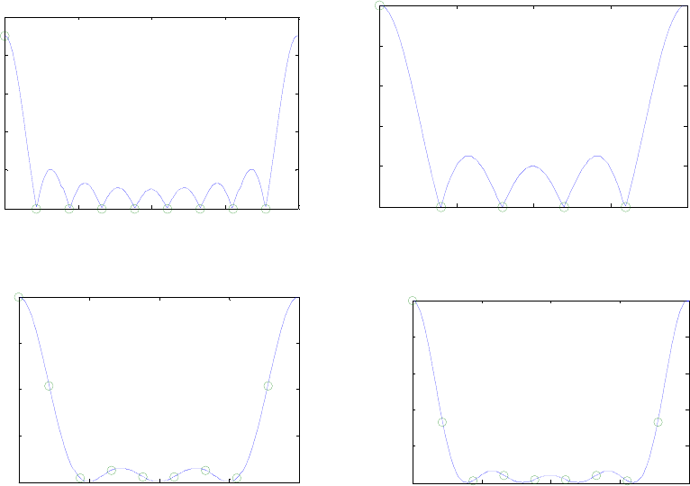
(b) Replace the statement k = -N:N; with k = 0:N;, y = ones(1,2*N+1);
with y = ones(1,N+1); the statement n = 0:1:2*N; with n = 0:N;, and
the statement plot(w/pi,abs(Y),n*2/(2*N+1),abs(Ydft),'o');
with plot(w/pi,abs(Y),n*2/(N+1),abs(Ydft),'o');,in the program of
Part (a).
(c) Add the statement y = y – abs(k)/N; below the statement y =
ones([1,2*N+1]); in the program of Part (a).
(d) Replace the statement y = ones(1,2*N+1); with y = N +
ones(1,2*N+1) – abs(k); in the program of Part (a).
(e) Replace the statement y = ones(1,2*N+1); with y = cos(pi*k/(2*N));
in the program of Part (a).
The plots generated for 4
=
N are shown below where the circles denote the DFT
samples.
(a) (b)
00.5 11.5 2
0
2
4
6
8
10
ω
/
π
Amplitude
00.5 11.5 2
0
1
2
3
4
5
ω
/
π
Amplitude
(c) (d)
00.5 11.5 2
0
1
2
3
4
ω
/
π
Amplitude
00.5 11.5 2
0
5
10
15
20
25
ω
/
π
Amplitude
(e)
Not for sale. 136
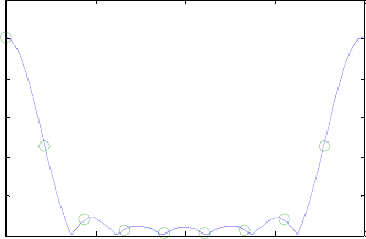
00.5 11.5 2
0
1
2
3
4
5
6
ω
/
π
Amplitude
M5.2 The code fragments to be used are as follows:
Y = fft(g).*fft(h);
y = iift(Y);
(a) The output generated using the above code fragments is
].[][][ 6
Onhngny =
y =
-6 9 -16 20 -4 45
(b) The output generated using the above code fragments is
].[][][ 5
Onvnxnw =
w =
Columns 1 through 3
11.0000 +25.0000i -9.0000 +48.0000i 3.0000 +17.0000i
Columns 4 through 5
29.0000 + 0.0000i -10.0000 +12.0000i
(c) The output generated using the above code fragments is
].[][][ 5
Onynxnu =
u =
-23.0000 -69.0000 35.0000 105.0000 73.0000
M5.3 N = 8; % sequence length
gamma = 0.5;
k = 0:N-1;
x = exp(-gamma*k);
X = fft(x);
% Property 1
X1 = fft(conj(x));
G1 = conj([X(1) X(N:-1:2)]);
% Verify X1 = G1
% Property 2
x2 = conj([x(1) x(N:-1:2)]);
X2 = fft(x2);
Not for sale. 137
% Verify X2 = conj(X)
% Property 3
x3 = real(x);
X3 = fft(x3);
G3 = 0.5*(X+conj([X(1) X(N:-1:2)]));
% Verify X3 = G3
% Property 4
x4 = j*imag(x);
X4 = fft(x4);
G4 = 0.5*(X-conj([X(1) X(N:-1:2)]));
% Verify X4 = G4
% Property 5
x5 = 0.5*(x+conj([x(1) x(N:-1:2)]));
X5 = fft(x5);
% Verify X5 = real(X)
% Property 6
x6 = 0.5*(x-conj([x(1) x(N:-1:2)]));
X6 = fft(x6);
% Verify X6 = j*imag(X)
M5.4 N = 8;
k = 0:N-1;
gamma = 0.5;
x = exp(-gamma*k);
X = fft(x);
% Property 1
xpe = 0.5*(x+[x(1) x(N:-1:2)]);
xpo = 0.5*(x-[x(1) x(N:-1:2)]);
Xpe = fft(xpe);
Xpo = fft(xpo);
% Verify Xpe = real(X) and Xpo = j*imag(X)
% Property 2
X2 = [X(1) X(N:-1:2)];
% Verify X = conj(X2);
% real(X) = real(X2) and imag(X) = -imag(X2)
% abs(X)= abs(X2) and angle(X) = -angle(X2)
M5.5 N = 8; % N is length of the sequence(s)
gamma = 0.5;
k = 0:N-1;
g = exp(-gamma*k); h = cos(pi*k/N);
G = fft(g); H=fft(h);
% Property 1
Not for sale. 138
alpha=0.5; beta=0.25;
x1 = alpha*g+beta*h;
X1 = fft(x1);
% Verify X1=alpha*G+beta*H
% Property 2
n0 = N/2; % n0 is the amount of shift
x2 = [g(n0+1:N) g(1:n0)];
X2 = fft(x2);
% Verify X2(k)= exp(-j*k*n0)G(k)
% Property 3
k0 = N/2;
x3 = exp(-j*2*pi*k0*k/N).*g;
X3 = fft(x3);
G3 = [G(k0+1:N) G(1:k0)];
% Verify X3=G3
% Property 4
x4 = G;
X4 = fft(G);
G4 = N*[g(1) g(8:-1:2)]; % This forms N*(g mod(-k))
% Verify X4 = G4;
% Property 5
% To calculate circular convolution between
% g and h use eqn (3.67)
h1 = [h(1) h(N:-1:2)];
T = toeplitz(h',h1);
x5 = T*g';
X5 = fft(x5');
% Verify X5 = G.*H
% Property 6
x6 = g.*h;
X6 = fft(x6);
H1 = [H(1) H(N:-1:2)];
T = toeplitz(H.', H1); % .' is the nonconjugate transpose
G6 = (1/N)*T*G.';
% Verify G6 = X6.'
M5.6 g = input('Type in first sequence = ');
h = input('Type in second sequence = ');
x = g +i*h;
XF = fft(x);
XFconj = conj(XF);
N = length(g);
YF = zeros(N-1,1)';
for k = 1:N-1;
YF(k) = XFconj(mod(-k,N)+1);
Not for sale. 139
end
YF1 = [XFconj(1) YF];
GF = (XF + YF1)/2;
HF = (XF - YF1)/2;
M5.7 x = [-3 5 45 -15 -9 -19 -8 21 -10 23];
XF = fft(x);
k =0:9; YF = exp(-i*2*pi*k/5).*XF;
output = [XF(1) XF(6) sum(XF) sum(YF)];;
disp(output)
disp(sum(abs(XF).*abs(XF))
The output data generated by this program is
30 0 -30-0.0000i -100-0.0000i
38600
M5.8 X = [11 8-i*2 1-i*12 6+i*3 -3+i*2 2+i 15];
k = 8:12; XF(k)=conj(X(mod(-k+2,12)));
XF = [X XF(8:12)];
x = ifft(XF);
n = 0:11; y = exp(i*2*pi*n/3).*x;
output = [x(1) x(7) sum(x) sum(y)];
disp(output)
disp(x.*x)
The output data generated by this program is
4.5000 -0.8333 11.0000 -3.0000-2.0000i
74.8333
M5.9 n=0:255;
x = 0.1*n.*exp(-0.03*n);
plot(n,x);axis([0 255 0 1.3]);
xlabel('n');ylabel('Amplitude');
title('Original signal');
pause
z = [zeros(1,50) ones(1,156) zeros(1,50)];
y = 4*rand(1,256)-1;
YF = z.*fft(y);
yinv = ifft(YF);
s = x + yinv;
plot(n,s);axis([0 255 -2 4]);
xlabel('n');ylabel('Amplitude');
title('Noise corrupted signal');
pause
zc = [ones(1,50) zeros(1,156) ones(1,50)];
SF = zc.*fft(s);
xr = ifft(SF);
plot(n,xr);axis([0 255 0 1.3]);
xlabel('n');ylabel('Amplitude');
Not for sale. 140
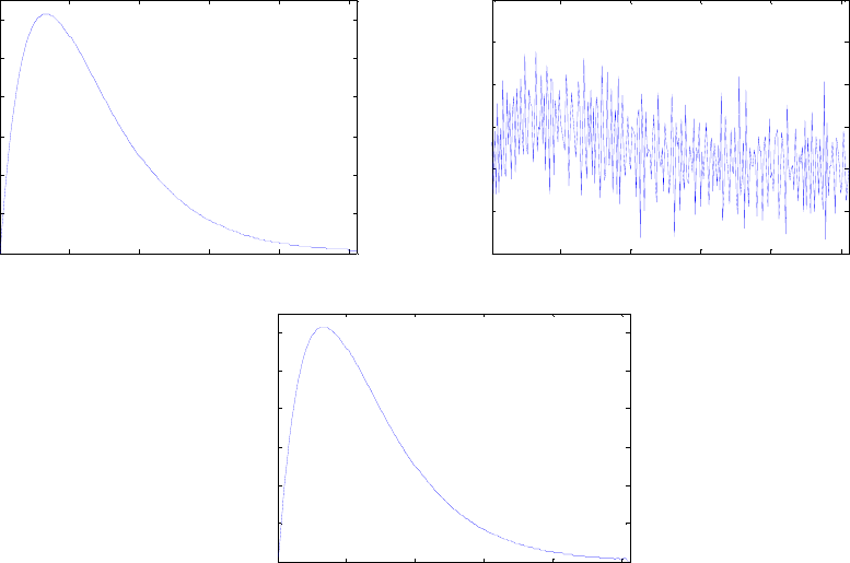
title('Signal after Fourier-domain filtering');
050 100 150 200 250
0
0.2
0.4
0.6
0.8
1
1.2
Amplitude
Original signal
050 100 150 200 250
-2
-1
0
1
2
3
4
Amplitude
Noise corrupted signal
050 100 150 200 250
0
0.2
0.4
0.6
0.8
1
1.2
Amplitude
Signal after Fourier-domain filtering
M5.10 function y = overlapsave(x,h)
X = length(x); %Length of longer sequence
M = length(h); %length of shorter sequence
flops(0);
if (M > X) %Error condition
disp('error');
end
%clear all
temp = ceil(log2(M)); %Find length of circular
convolution
N = 2^temp; %zero padding the shorter sequence
if(N > M)
for i = M+1:N
h(i) = 0;
end
end
m = ceil((-N/(N-M+1)));
while (m*(N-M+1) <= X)
if(((N+m*(N-M+1)) <= X)&((m*(N-M+1)) > 0))
for n = 1:N
x1(n) = x(n+m*(N-M+1));
end
end
if(((m*(N-M+1))<=0)&((N+m*(N-M+1))>=0))
%underflow adjustment
Not for sale. 141
for n = 1:N
x1(n) = 0;
end
for n = m*(N-M+1):N+m*(N-M+1)
if(n > 0)
x1(n-m*(N-M+1)) = x(n);
end
end
end
if((N+m*(N-M+1)) > X) %overflow adjustment
for n = 1:N
x1(n) = 0;
end
for n = 1:(X-m*(N-M+1))
x1(n) =x (m*(N-M+1)+n);
end
end
w1 = circonv1(h,x1); %circular convolution using DFT
for i = 1:M-1
y1(i) = 0;
end
for i = M:N
y1(i) = w1(i);
end
for j = M:N
if((j+m*(N-M+1)) < (X+M))
if((j+m*(N-M+1)) > 0)
yO(j+m*(N-M+1)) = y1(j);
end
end
end
m = m+1;
end
%disp('Convolution using Overlap Save:');
y = real(yO);
function y = circonv1(x1,x2)
L1 = length(x1); L2 = length(x2);
if L1 ~= L2,
error('Sequences of unequal lengths'),
end
X1 = fft(x1);
X2 = fft(x2);
X_RES = X1.*X2;
y = ifft(X_RES);
The MATLAB program for performing convolution using the overlap-save method is
h = [1 1 1]/3;
R = 50;
Not for sale. 142
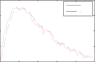
d = rand(1,R) - 0.5;
m = 0:1:R-1;
s = 2*m.*(0.9.^m);
x = s + d;
%x = [x x x x x x x];
y = overlapsave(x,h);
k = 0:R-1;
plot(k,x,'r-',k,y(1:R),'b--');
xlabel('Time index n');ylabel('Amplitude');
legend('r-', 's[n]','b--','y[n]');
The output plot generated by the above program is shown below:
010 20 30 40 50
0
2
4
6
8
Time index n
Amplitude
s[n]
y[n]
Not for sale. 143

Chapter 6
6.1 Therefore,
.][][)(
0
∑
=
∑
=∞
=
−
∞
−∞=
−
n
n
n
nznxznxzX ∑
=∞
=
−
∞→∞→ 0
][lim)(lim
n
n
zz
znxzX
].0[][lim]0[lim
1
xznxx
n
n
zz
=
∑
+= ∞
=
−
∞→∞→
6.2 (a) Z which converges everywhere in the –plane.
,1]0[][]}{[ ==
∑
=∞
−∞=
−δδδ
n
n
znn z
(b) From Table 6.1,
Z
].[][ nnx nµα=
.,
1
1
][)(]}[{ 1α
α
>
−
=
∑
== −
∞
−∞=
−z
z
znxzXnx
n
n Let ].[][ nn
x
ng
=
Then,
Z Now,
.][)(]}[{ n
n
znnxzGng −
∞
−∞=
∑
== .][
)( 1
∑
−= ∞
−∞=
−−
n
n
znng
dz
zdX Hence,
),(][
)( zGznnx
dz
zdX
z
n
n−=
∑
−= ∞
−∞=
− or, .,
)1(
)(
)( 21
1
α
α
α>
−
=−= −
−
z
z
z
dz
zdX
zzG
(c) ].[)(
2
][)sin(][ nee
j
r
nnrnx njnj
n
o
noo µµωωω −
−== Using the results of Example
6.1 and the linearity property of the –transform we get
z
Z⎟
⎟
⎠
⎞
⎜
⎜
⎝
⎛
−
⎟
⎟
⎠
⎞
⎜
⎜
⎝
⎛
=−− −
−− 11 1
1
2
1
1
1
2
1
]}[)sin({
z
j
er
j
z
j
er
j
o
n
oo
nnr ωω
µω
221
1
221
1
2
)cos(21
)sin(
)(1
)(
−−
−
−−
−
−
−
+−
=
++−
−
=
zrzr
zr
zrzeer
zee
o
o
jj
jj
j
r
oo
oo
ω
ω
ωω
ωω
, .rz >∀
6.3 (a) Note, is a right-sided sequence. Hence, the ROC of its
–transform is exterior to a circle. Therefore,
].2[][
1−= nnx nµα][
1nx
zn
n
nn
n
nzznzX −
∞
=
−
∞
−∞= ∑
=−
∑
=
2
1]2[)( αµα
Simplifying we get 1
22
1
1
11
1
1
1
)( −
−
−
−−
=−−
−
=
z
z
z
z
zX
α
α
α
α
whose ROC is given by
.α>z
(b) Note, is a left-sided sequence. Hence, the ROC of ].3[][
2−−−= nnx nµα][
2nx
its –transform is interior to a circle. Therefore,
z
∑
−=
∑
−=
∑
−=−−
∑
−= ∞
=
∞
=
−−
−
−∞=
−
∞
−∞= 33
3
2)/(]3[)(
m
mm
m
mn
n
nn
n
nzzzznzX αααµα
Not for sale. 147

Simplifying we get )/(1
)/(
)( 3
2
α
α
z
z
zX −
= whose ROC is given by .α<z
(c) Note, is a right-sided sequence. Hence, the ROC of its
–transform is exterior to a circle. Therefore,
].4[][
3+= nnx nµα][
3nx
zn
n
nn
n
nzznzX −
∞
−=
−
∞
−∞= ∑
=+
∑
=
4
3]4[)( αµα
Simplifying we get )/(1
)/(
)( 4
3z
z
zX
α
α
−
=
−
whose ROC is given by .α>z
(d) Note, is a left-sided sequence. Hence, the ROC of its
–transform is interior to a circle. Therefore,
].[][
4nnx n−= µα][
4nx
zn
n
nn
n
nzznzX −
−∞=
−
∞
−∞= ∑
=−
∑
=0
4][)( αµα
.1/,
)/(1
1
0
<
−
=
∑
=∞
=
−α
α
αz
z
zm
m
m Therefore the ROC of is given by
)(
4zX .α<z
6.4 Z;4.0,
4.01
1
]}[)4.0{( 1>
−
=−z
z
n
nµ Z;6.0,
6.01
1
]}[)6.0{( 1>
+
=− −z
z
n
nµ
Z;4.0,
4.01
1
]}1[)4.0{( 1<
−
−=−− −z
z
n
nµ
Z;6.0,
6.01
1
]}1[)6.0{( 1<
+
−=−−− −z
z
n
nµ
(a) Z.6.0,
)6.01)(4.01(
2.01
6.01
1
4.01
1
]}[{ 11
1
11
1>
+−
+
=
+
+
−
=−−
−
−− z
zz
z
zz
nx
(b) Z.6.04.0,
)6.01)(4.01(
2.01
6.01
1
4.01
1
]}[{ 11
1
11
2<<
+−
+
=
+
+
−
=−−
−
−− z
zz
z
zz
nx
(c) Z.4.0,
)6.01)(4.01(
2.01
6.01
1
4.01
1
]}[{ 11
1
11
3<
+−
+
=
+
+
−
=−−
−
−− z
zz
z
zz
nx
(d) Z.
)6.01)(4.01(
2.01
6.01
1
4.01
1
]}[{ 11
1
11
4−−
−
−− +−
+
=
+
+
−
=
zz
z
zz
nx Since the ROC of
the first term is 4.0<z and that of the second term is 6.0>z. Hence, the –
transform of does not converge.
z
][
4nx
6.5 (a) The ROC of Z is
]}[{ 1nx ,3.0>z the ROC of Z is
]}[{ 2nx ,7.0>z the ROC of
Z is ]}[{ 3nx ,4.0>z and the ROC of Z is
]}[{ 4nx .4.0<z
(b) (i) The ROC of Z is
]}[{ 1ny ,7.0>z
(ii) The ROC of Z is
]}[{ 2ny ,4.0>z
Not for sale. 148

(iii) The ROC of Z is ]}[{ 3ny ,4.03.0 << z
(iv) The ROC of Z is
]}[{ 4ny ,7.0>z
(v) The ROC of Z is
]}[{ 2nx ,7.0>z whereas, the ROC of Z is
]}[{ 4nx .4.0<z
Hence, the -transform of does not converge.
z][
5ny
(vi) The ROC of Z is ]}[{ 3nx ,4.0>z whereas, the ROC of Z is
]}[{ 4nx .4.0<z
Hence, the -transform of does not converge.
z][
6ny
6.6 ].1[][][ −−+== −nnnv nn
nµαµαα Now, Z.,
1
1
]}[{ 1α
α
µα>
−
=−z
z
n
n (See Table
6.1) and Z∑−
−
=−
∑
==
∑
=−− ∞
=
∞
=
−
−∞=
−−−
10
11
1
1
1]}1[{
mm
mmmm
n
nnn
z
zzzn α
αααµα
.1,
1<
−
=z
z
zα
α
α Therefore, ))(1(
)1(
1
1
)(]}[{ 11
12
11 αα
α
α
α
α−−
−
=
−
+
−
== −−
−
−− zz
z
zz
zVnv
with its ROC given by ./1 αα << z
6.7 (a) with ]2[]2[][
1+++= nnnx nn µβµα.αβ > Note that is a right-sided
sequence. Hence, the ROC of its –transform is exterior to a circle. Now,
][
1nx
z
Z
∑++=
∑
=+ ∞
=
−−−
∞
−=
−
0
21
2
)/()/(]}2[{
n
nn
n
nnn zzzzn ααααµα
)/(1
)/(
)/()/(
)/(1
12
21
z
z
zz
zα
α
αα
α−
=++
−
=−
−− with its ROC given by .α>z Likewise,
Z)/(1
)/(
]}2[{
2
z
z
n
n
β
β
µβ−
=+ − with its ROC given by .β>z Hence,
Z)/(1
)/(
)/(1
)/(
)(]}[{
22
11 z
z
z
z
zXnx β
β
α
α
−
+
−
== −−
)1)(1(
)()(
112
12222
−−−
−−−−−
−−
+−+
=
zzz
z
βα
βααββα with its ROC given by .β>z
(b) with ]1[]2[][
2−+−−= nnnx nn µβµα.αβ > Note that is a two-sided
sequence. Now,
][
2nx
Z
2
02
2)/()/(1)/(]}2[{ αααααµαzzzzzn
m
m
m
mm
n
nnn −−−
∑
=
∑
=
∑
=−− ∞
=
∞
=
−
−
−∞=
−
)/(1
)/( 3
α
α
z
z
−
=with its ROC given by .α<z Likewise,
Not for sale. 149

Z1
1
1
01 1
1
1
1
1]}1[{ −
−
−
∞
=
−
∞
=
−
−
=−
−
=−
∑
=
∑
=−
z
z
z
zzn
n
nn
n
nnn
β
β
β
ββµβ with its ROC
given by .β>z Since the two ROCs do not intersect, Z does not converge.
]}[{ 2nx
(c) with ]2[]1[][
3−−++= nnnx nn µβµα.αβ > Note that is a two-sided
sequence. Now,
][
3nx
Z
2
02
2)/()/(1)/(]}2[{
βββββµβ
zzzzzn
m
m
m
mm
n
nnn −−−===−− ∑∑∑ ∞
=
∞
=
−
−
−∞=
−
)/(1
)/( 3
β
β
z
z
−
=with its ROC given by .
β
<z Likewise,
Z1
1
1
01 1
1
1
1
1]}1[{ −
−
−
∞
=
−
∞
=
−
−
=−
−
=−==− ∑∑ z
z
z
zzn
n
nn
n
nnn
α
α
α
ααµα
with its ROC given by
.
α
>z
6.8 The denominator factor has poles at )3.0)(6.0()18.03.0( 2−+=−+ zzzz 6.0
−
=z and
at and the factor has poles with a magnitude Hence, the four
ROCs are defined by the regions: R
,3.0=z)42( 2+− zz .2
:
1,3.00 << z R:
2,6.03.0 << z
R,26.0
3<<= zand R
:
4.2>z The inverse –transform associated with the ROC
R 1 is a left-sided sequence, the inverse –transforms associated with the ROCs
Rand R3 are two-sided sequences, and the inverse –transform associated with the
ROC Ris a right-sided sequence.
z
z
2z
4
6.9 Z with an ROC given by R. Using the conjugation property of the –
transform given in Table 6.2, we observe that Z
=)(zX ]}[{ nx x
*)(*]}[*{ zXnx
=
whose ROC is
given by R. Now,
x]).[*][(]}[Re{ 2
1nxnxnx += Hence, Z
]}[{Re nx
(
)(*)(
2
1zXzX +=
)
whose ROC is also R. Likewise,
x]).[*][(]}[Im{ 2
1nxnxnx j−=
Thus, Z
]}[{Im nx
(
)(*)(
2
1zXzX
j−=
)
whose ROC is again R.
x
6.10 .62},4,2,1,3,4,0,1,3,2{]}[{
≤
≤
−
−
−= nnx Then,
.)()()(][
~
6/2
6/23/ k
j
ezez eXzXzXkX kjkj πω
ω
ππ =
== === Note that is a
periodic sequence with a period Hence, from Eq. (5.49), the inverse of the discrete
Fourier series is given by
][
~kX
.6
][
~kX ]6[][]6[]6[][ +++−=
∑+= ∞
−
∞
=
nxnxnxrnxnx
r
t for
Let
.50 ≤≤ n.62],6[][]6[][
≤
≤
−
+
+
+
−
=nnxnxnxny Now,
Not for sale. 150

}1,3,2,0,0,0,0,0,0{]}6[{
−
=−nx and
Therefore,
}.0,0,0,0,0,0,4,2,1{]6[{ =+nx
.62},3,5,3,3,4,0,3,5,3{]}[{
≤
≤
−
−
=nny Hence,
.50},5,3,3,4,0,3{]}[
~
{
≤
≤
−= nnx
6.11 .26},2,4,2,1,3,5,1,2,4{]}[{
≤
≤
−
−
−
−= nnx Then,
.)()()(][
~
6/2
6/23/ k
j
ezez eXzXzXkX kjkj πω
ω
ππ =
== === Note that is a
periodic sequence with a period Hence, from Eq. (5.49), the inverse of the discrete
Fourier series is given by
][
~kX
.6
][
~kX ]6[][]6[]6[][ +++−=
∑+= ∞
−
∞
=
nxnxnxrnxnx
r
t for
Let
.50 ≤≤ n.56],6[][]6[][
≤
≤
−
+
+
+
−
=nnxnxnxny Now,
,56},1,3,5,1,2,4,0,0,0,0,0,0{]}6[{ ≤≤−
−
−
=− nnx
.56},0,0,0,0,0,0,0,0,0,2,4,2{]6[{ ≤≤
−
−=+ nnx
Therefore, .56},1,3,5,6,2,1,3,5,1,6,2{]}[{ ≤≤−
−
−
=nny
Hence, .50},1,3,5,1,6,2{]}[
~
{
≤
≤
−
=nnx
6.12 .80,][)(][.][)( 11
0
9/2
0
11
0
9/2( ≤≤
∑
==
∑
=
=
−
=
=
−kenxzXkXznxzX
n
knj
ez
n
nkπ
π
Therefore, 9/2
8
0
11
0
9/2
9
1
8
0
9/2
0
9
1
0][][][ knj
kr
krj
k
knj eerxekXnx πππ ∑⎟
⎟
⎠
⎞
⎜
⎜
⎝
⎛∑
=
∑
=
==
−
=
.][][][ 11
0
9
0
)(
9
9
1
11
0
9
0
9/)(2
9
1
8
0
11
0
9/)(2
9
1∑∑
=
∑∑
=
∑∑
=
==
−−
==
−
==
−
rk
knr
rk
rnkj
kr
rnkj Wrxerxerx ππ
From Eq. (5.11), ⎩
⎨
⎧=−
=
∑
−
−−
otherwise.,0
,9for,1
8
0
)(
9
9
1inr
W
k
knr Hence,
i.e.,
⎩
⎨
⎧=+
=otherwise,],[
0for],9[]0[
][
0nx
nxx
nx
.80},102181991545520{]}[{ 0≤
≤
−
−
−
−
−= nnx
6.13 (a) Hence, Define
a new sequence We can then express
.][)( ∑
=∞
−∞=
−
n
n
znxzX .]3/[][)(
3
33 ∑
=
∑
=∞
−∞=
−
∞
−∞=
−
=rm
r
m
n
nzmxznxzX
⎩
⎨
⎧±±=
=otherwise.,0
,,6,3,0],3/[
][ Kmmx
mg
Not for sale. 151

.][)( 3∑
=∞
−∞=
−
n
n
zngzX Thus, the inverse –transform of is given by
For
z)( 3
zX ].[ng
],[)5.0(][ nnx nµ−= ⎪
⎩
⎪
⎨
⎧=−
=otherwise.,0
,,6,3,0,)5.0(
][
3/ Kn
ng
n
(b) Therefore, ).()()()1()( 31331 zXzzXzXzzY −− +=+=
=][ny Z Z Z where =
−)}({
1zY +
−)( 31 zX ],1[][)( 311 −+=
−− ngngzXz
=
][ng
Z. From Part (a), Hence,
Therefore,
)( 31 zX
−
⎪
⎩
⎪
⎨
⎧=−
=otherwise.,0
,,6,3,0,)5.0(
][
3/ Kn
ng
n
⎪
⎩
⎪
⎨
⎧=−
=− −
otherwise.,0
,,7,4,1,)5.0(
]1[
3/)1( Kn
ng
n
⎪
⎪
⎩
⎪
⎪
⎨
⎧
=−
=−
=−
otherwise.,0
,,7,4,1,)5.0(
,,6,3,0,)5.0(
][ 3/)1(
3/
K
K
n
n
ny n
n
6.14 (a) Z=)(zXa1
5
1
5
11
1
11
1
]}5[][{ −
−
−
−
−−
−
=
−
−
−
=−−
z
z
z
z
z
nn µµ
. Since has all poles at the origin, the ROC is the entire
–plane except the point
4321
1−−−− ++++= zzzz
z0
=
z, and hence includes the unit circle. On the unit circle,
)()( ω
ωj
a
ez
aeXzX j=
=.
1
1
1
5
432
ω
ω
ωωωω
j
j
jjjj
e
e
eeee −
−
−−−−
−
−
=++++=
(b) .1],8[][][ <−−= αµαµαnnnx nn
b From Table 6.1,
.
1
1
11
1
)( 1
8
1
8
1−
−
−
−
−−
−
=
−
−
−
=
z
z
z
z
z
zXbααα
The ROC is exterior to the circle at
.1<= αz Hence, the ROC includes the unit circle. On the unit circle,
.
1
1
)()(
8
ω
ω
ω
α
ωj
j
j
b
ez
be
e
eXzX j−
−
==
=
(c) .1],[][][)1(][ <+=+= αµαµαµαnnnnnnx nnn
c From Table 6.1,
.
1
1
1
1
1
)( 1
1
11
1
−
−
−−
−
−
+
=
−
+
−
=
z
z
zz
z
zXcα
α
αα
α The ROC is exterior to the circle at
.1<= αz Hence, the ROC includes the unit circle. On the unit circle,
.
1
1
)( ω
ω
ωα
j
j
j
ce
e
eX −
+
=
Not for sale. 152

6.15 (a) .
)1(
1
)( 1
)12(
2
0
1−−
+−
=
−
−=
−
−
−
=
⎟
⎟
⎠
⎞
⎜
⎜
⎝
⎛∑
=
∑
=
zz
z
zzzzY N
N
N
n
nN
N
Nn
n has poles at
and poles at
)(
1zY N
0=zN.
∞
=z Hence, the ROC is the entire –plane excluding the
points and
z
0=z,∞=
z
and includes the unit circle. On the unit circle,
.
)2/sin(
)(sin
)1(
1
)()( 2
1
)12(
11 ω
ω
ωω
ω
ω
ω
⎟
⎠
⎞
⎜
⎝
⎛+
=
−
−
== −−
+
=
N
ee
e
eYzY jjN
Nj
j
ez j
(b) .
1
1
)( 1
)1(
0
2−
+−
=
−
−
−
=
∑
=
z
z
zzY
N
N
n
n has
)(
2zY
N
poles at .0
=
z Hence, the ROC
is the entire z–plane excluding the point .0
=
z On the unit circle,
.
)2/sin(
sin
1
1
)()( 2
1
2/
)1(
22 ω
ω
ω
ω
ω
ω
ω
⎟
⎠
⎞
⎜
⎝
⎛
=
−
−
==
+
−
−
+
=
N
N
j
Nj
j
ez e
e
e
eYzY j
(c) ⎪
⎩
⎪
⎨
⎧≤≤−−
=
otherwise.,0
,,1
][
3NnN
ny N
n Now, where
][][][ 0
*
03 Onynyny =
⎪
⎩
⎪
⎨
⎧≤≤−
=
otherwise.,0
,,1
][ 22
0
NN n
ny Therefore, .
)1(
)1(
)()( 21
2)1(
2
03 −−
+−
−
−
==
zz
z
zYzY N
N
)(
3zY has 2
N poles at and
0=z2
N poles at .
∞
=
z Hence, the ROC is the entire –
plane excluding the points
z
0
=
z and ,
∞
=
z
and includes the unit circle. On the unit
circle, .
)2/(sin
sin
)()( 2
2
1
2
2
03 ω
ω
ωω ⎟
⎠
⎞
⎜
⎝
⎛⎟
⎠
⎞
⎜
⎝
⎛
==
+N
jj eYeY
(d) ],[][
otherwise,,0
,,1
][ 314 nyNny
NnNnN
ny ⋅+=
⎩
⎨
⎧≤≤−−+
= where is the
sequence of Part (a) and is the sequence of Part (c). Therefore,
][
1ny
][
3ny
N
zz
z
zYNzYzY N
N+
−
−
=⋅+= −−
+−
)1(
1
)()()( 1
)12(
314 21
2)1(
)1(
)1(
−−
+−
−
−
zz
z
N
N. Since the ROCs of
both and include the unit circle, the ROC of also includes the unit
)(
1zY )(
3zY )(
4zY
circle. On the unit circle, .
)2/(sin
sin
)2/sin(
)(sin
)( 2
2
1
2
2
1
4ω
ω
ω
ω
ω⎟
⎠
⎞
⎜
⎝
⎛⎟
⎠
⎞
⎜
⎝
⎛
+
⎟
⎠
⎞
⎜
⎝
⎛+
=
+N
jN
eY
(e) Therefore,
⎩
⎨
⎧≤≤−
=otherwise.,0
,),2/cos(
][ NnNNn
ny f
π
Not for sale. 153

n
N
Nn
Nnjn
N
Nn
Nnj
fzezezY −
−=
−
−=
−∑
+
∑
=)2/()2/(
2
1
2
1
)( ππ
⎟
⎟
⎠
⎞
⎜
⎜
⎝
⎛
−
−
=−−
+−+−
1)2/(
)12()2/)(12()2/(
1
1
2ze
zeze
Nj
NNNjNj
π
ππ
⎟
⎟
⎠
⎞
⎜
⎜
⎝
⎛
−
−
+−
+−+−
1)2/(
)12()2/)(12()2/(
1
1
2ze
zeze
Nj
NNNjNj
π
ππ .
)(zY f has poles at
N0
=
z and poles at
N.
∞
=
z Hence, the ROC is the entire –
plane excluding the points
z
0
=
z and ,
∞
=
z
and includes the unit circle. On the unit
circle, .
2/sin
sin
2
1
2/sin
sin
2
1
)(
2
2
1
2
2
2
1
2
⎟
⎠
⎞
⎜
⎝
⎛⎟
⎠
⎞
⎜
⎝
⎛+
⎟
⎠
⎞
⎜
⎝
⎛⎟
⎠
⎞
⎜
⎝
⎛+
⎟
⎠
⎞
⎜
⎝
⎛+
+
⎟
⎠
⎞
⎜
⎝
⎛⎟
⎠
⎞
⎜
⎝
⎛−
⎟
⎠
⎞
⎜
⎝
⎛⎟
⎠
⎞
⎜
⎝
⎛+
⎟
⎠
⎞
⎜
⎝
⎛−
=
N
N
N
N
j
f
NN
eY π
π
π
π
ω
ω
ω
ω
ω
6.16 ,27836)(,23254)( 54313123 −−−−−− −++−−=+−−++−= zzzzzzYzzzzzzX
.52223)( 875432 −−−−−− +−−++= zzzzzzzW
(a)
)()()( zYzXzU =
)27836)(23254( 54313123 −−−−−− −++−−+−−++−= zzzzzzzzzz
54321234 1742256623452054224 −−−−− −−−++−−−+−= zzzzzzzzz
.41422 876 −−− −++ zzz Hence,
.84},4,14,22,17,42,25,66,23,45,20,5,42,24{]}[{
≤
≤
−−
−
−
−
−
−−−= nnu
(b)
)()()( zWzXzV =
)52223)(23254( 8754323123 −−−−−−−− +−−+++−−++−= zzzzzzzzzzz
87654321 6133028316105712 −−−−−−−− −++−−−+++−= zzzzzzzzz
.10415 11104 −−− +−− zzz Hence,
.111},10,4,15,6,13,30,28,3,16,10,5,7,12{]}[{
≤
≤−
−
−
−
−
−
−
−= nnv
(c)
)()()( zYzWzG =
)27836)(52223( 5431875432 −−−−−−−−−− −++−−+−−++= zzzzzzzzzzz
10987654321 141611602625143318 −−−−−−−−−− −−−+++−++= zzzzzzzzzz
Hence,
.103926 131211 −−− −++ zzz
.131},10,39,26,14,16,11,60,26,25,14,3,3,18{]}[{ ≤≤
−
−
−
−
−= nng
6.17 and
n
N
n
N
m
LzmnhmxzY −
−
=
−
=
∑⎟
⎟
⎠
⎞
⎜
⎜
⎝
⎛∑−= 12
0
1
0
][][)( .][][)( 1
0
1
0
n
N
n
N
m
NC zmnhmxzY −
−
=
−
=
∑⎟
⎟
⎠
⎞
⎜
⎜
⎝
⎛∑〉−〈=
Not for sale. 154

Now, )(zY
L
can be rewritten as
n
N
Nn
N
m
n
N
n
N
m
LzmnhmxzmnhmxzY −
−
=
−
=
−
−
=
−
=∑⎟
⎟
⎠
⎞
⎜
⎜
⎝
⎛∑−+
∑⎟
⎟
⎠
⎞
⎜
⎜
⎝
⎛∑−= 121
0
1
0
1
0
][][][][)(
.][][][][ )(
1
0
1
0
1
0
1
0
Nk
N
k
N
m
n
N
n
N
m
zNmkhmxzmnhmx −−
−
=
−
=
−
−
=
−
=∑⎟
⎟
⎠
⎞
⎜
⎜
⎝
⎛∑−−+
∑⎟
⎟
⎠
⎞
⎜
⎜
⎝
⎛∑−= Therefore,
=〉〈 −
−)1(
)( N
z
LzY k
N
k
N
m
N
n
N
n
N
m
zmkhmxzmnhmx −
−
=
−
=
−
−
=
−
=∑⎟
⎟
⎠
⎞
⎜
⎜
⎝
⎛∑〉−〈+
∑⎟
⎟
⎠
⎞
⎜
⎜
⎝
⎛∑−1
0
1
0
1
0
1
0
][][][][
).(][][
1
0
1
0
zYzmnhmx C
n
N
n
N
m
N=
∑⎟
⎟
⎠
⎞
⎜
⎜
⎝
⎛∑〉−〈= −
−
=
−
=
6.18 Now, .242)(,32)( 32121 −−−−− −++−=+−= zzzzHzzzG
)242)(32()()()( 32121 −−−−− −++−+−== zzzzzzHzGzY
L
.3786104 54321 −−−−− −++−+−= zzzzz Therefore,
.50},3512264{][
≤
≤
−
−= nny
L
Using the MATLAB statement y = conv([2 -1 3], [-2 4 2 -1]); we
obtain
y =
-4 10 -6 8 7 -3
which is seen to be the same result as given above.
)1(
54321
)1( 44 3786104)()( −
−−−−−
−−− 〉−++−+〈−=〉〈= zz
CC zzzzzzYzY
.86733786104 3211321 −−−−−−− +−+=−++−+−= zzzzzzz Therefore,
.30},12231{][
≤
≤
=nnyC
Using the MATLAB statement y = circonv([2 -1 3 0],[-2 4 2 -1]);
we obtain
y =
3 7 -6 8
which is seen to be the same result as given above.
6.19 .
)()1(
)(
)(
)(
)( 1zRz
zP
zD
zP
zG −
−
==
l
λ The residue of at the pole is given by
l
ρ)(zG
.
)(
)(
l
l
λ
ρ
=
=
z
zR
zP Now,
1
1
1
)]()1[(
)(
)(' −
−
−
−
==
dz
zRzd
dz
zdD
zD l
λ.
)(
)1()( 1
1
−
−
−+−=
dz
zdR
zzR ll λλ Hence,
.)()(' l
llλ
λλ=
=−= z
zzRzD Therefore, .
)('
)(
l
ll
λ
λρ
=
−=
z
zD
zP
Not for sale. 155

6.20 (a) ,
3.016.01)3.01)(6.01(
3
)3.0)(6.0(
3
)( 1
2
1
1
11
1
−−−−
−
−
+
+
=
−+
=
−+
=
zzzz
z
zz
z
zXa
ρρ
where ,
3
10
9.0
3
3.0
3
6.0
1−=
−
=
−
=
−=z
z
ρ .
3
10
9.0
3
6.0
3
3.0
2==
+
=
=z
z
ρ
Therefore, .
3.01
3/10
6.01
3/10
)( 11 −− −
+
+
−=
zz
zXa
There are three ROCs - R,3.0:
1<z R,6.03.0:
2<< z R.6.0:
3>z
The inverse –transform associated with the ROC is a left-sided sequence:
z1
R
].1[)3.0()6.0(][)}({ 3
10
1−−µ−−== ⎟
⎠
⎞
⎜
⎝
⎛
−nnxzX nn
aa
Z
The inverse –transform associated with the ROC is a two-sided sequence:
z2
R
].[)3.0(]1[)6.0(][)}({ 3
10
3
10
1nnnxzX nn
aa µ+−−µ−−==
−
Z
The inverse –transform associated with the ROC is a right-sided sequence:
z3
R
(
)
].[)3.0()6.0(][)}({ 3
10
1nnxzX nn
aa µ+−−==
−
Z
(b) .
)3.01(3.016.01)3.01)(6.01(
87.01.03
)( 21
2
1
1
1
1
211
321
−−−−−
−−−
−
γ
+
−
γ
+
+
ρ
+=
−+
++
=
zzz
K
zz
zzz
zXb
,0)0( == b
XK 2.7279,
)3.01(
87.01.03
6.0
21
321
1=
−
++
=ρ
−=
−
−−−
z
z
zzz
0.6190,
6.01
87.01.03
3.0
1
321
2=
+
++
=γ
=
−
−−−
z
z
zzz
3.0
1
321
1
16.01
87.01.03
3.0
1
=
−
−−−
−⎟
⎟
⎠
⎞
⎜
⎜
⎝
⎛
+
++
⋅
−
=γ
z
z
zzz
dz
d0.3469.
−
=
Hence,
.
)3.01(
61900
3.01
34690
6.01
72792
)( 2111 −−− −
+
−
−
+
=
z
.
z
.
z
.
zXb
There are three ROCs - R,3.0:
1<z R,6.03.0:
2<< z R.6.0:
3>z
The inverse –transform associated with the ROC is a left-sided sequence:
z1
R
Z
][).(.][)}({ 16072792
1−−µ−==
−nnxzX n
bb
()
].1[)3.0()1(6190.03469.0 −−µ++−+ nn n
The inverse –transform associated with the ROC is a two-sided sequence:
z2
R
Z
][).(.][)}({ 16072792
1−−µ−==
−nnxzX n
bb
()
].[)3.0()1(6190.03469.0 nn nµ++−+
The inverse –transform associated with the ROC is a right-sided sequence:
z3
R
Not for sale. 156

(
)
].[)3.0()1(6190.03469.0][)6.0(7279.2][)}({
1nnnnxzX nn
bb µ++−+µ−==
−
Z
6.21 .
1
)(
)(
)( 1
1
1
10
N
N
M
M
zdzd
zpzpp
zD
zP
zG −−
−−
+++
+++
==
L
L Thus, .
)(
)(
)( ∞
∞
=∞ D
P
G Now, a partial-
fraction expansion of in is given by
)(zG 1−
z,
1
)(
11
∑−
=
=−
N
z
zG
ll
l
λ
ρ from which we obtain
.)(
0
0
1d
p
G
N=
∑
=∞
=l
l
ρ
6.22 .0,
cos21
1
)( 221 >>
+−
=−− rz
zrzr
zH
θ By using partial-fraction expansion we write
.
11
sin2
1
11)(
1
)( 1111 ⎟
⎟
⎠
⎞
⎜
⎜
⎝
⎛
−
−
−
=
⎟
⎟
⎠
⎞
⎜
⎜
⎝
⎛
−
−
−−−
=−−
−
−−−
−
−zre
e
zre
e
zre
e
zre
e
jee
zH j
j
j
j
j
j
j
j
jj θ
θ
θ
θ
θ
θ
θ
θ
θθ θ
Thus,
()
][
2sin
][][
sin2
1
][
)1()1(
n
j
eer
neerneer
j
nh
njnjn
jnjnjnjn µ
θ
µµ
θ
θθ
θθθθ ⎟
⎟
⎠
⎞
⎜
⎜
⎝
⎛−
=−= +−+
−−
()
].[
sin
)1(sin n
nr n
µ
θ
θ
+
=
6.23 (a) 1)/()/(]1[)(
011
1−
∑α=
∑α=
∑α=
∑α=−−µ
∑α= ∞
=
∞
=
∞
=
−−
−
−∞=
−
∞
−∞= m
m
m
mm
m
mn
n
nn
n
nzzzzznzX
.,
1
1
)/(1
/
1α<
α−
=
α−
α
=−z
z
z
z
(b) Using the differentiation property, we obtain from Part (a),
.,
)1(
)(
]}[{ 21
1α<
α−
α
=−= −
−
z
z
z
dz
zdX
znnxZ Therefore,
]}[][{Z]}[{ nxnnxnyZ +=
.,
)1(
1
1
1
)1( 21121
1α<
α−
=
α−
+
α−
α
=−−−
−
z
zzz
z
6.24 (a) Expanding in a power series we get
)(
1zX .1,)(
0
3
1>
∑
=∞
=
−zzzX
n
n Thus,
Alternately, using partial-fraction expansion we get
⎩
⎨
⎧≥=
=otherwise.,0
,0and3if,1
][
1
nkn
nx
.
)(1)(1
11
1
)( 11
13
1
2
3
2
1
3
1
2
3
2
1
3
1
3
1
−−
−− −+
+
++
+
−
=
−
=
zjzj
zz
zX Therefore,
Not for sale. 157

][][][][ 2
3
2
1
3
1
2
3
2
1
3
1
3
1
1njnjnnx µµµ ⎟
⎠
⎞
⎜
⎝
⎛−+
⎟
⎠
⎞
⎜
⎝
⎛−−+= +
].[)3/2cos(][][][][ 3
2
3
1
3
1
3
1
3
13/23/2 nnnnenen njnj µπµµµµ ππ +=++= − Thus,
⎩
⎨
⎧≥=
=otherwise.,0
,0and3if,1
][
1
nkn
nx
(b) Expanding in a power series we get
)(
2zX .1,)(
0
4
2>
∑
=∞
=
−zzzX
n
n Thus,
⎩
⎨
⎧≥=
=otherwise.,0
,0and4if,1
][
2
nkn
nx Alternately, using partial-fraction expansion we get
.
)(1)(1
11
)( 11
11
2
2
3
2
1
4
1
2
3
2
1
4
1
4
1
4
1
−−
−− −+
+
++
+
+
+
−
=
zjzj
zz
zX Thus,
][][][)1(][][ 2
3
2
1
4
1
2
3
2
1
4
1
4
1
4
1
2njnjnnnx nµµµµ ⎟
⎠
⎞
⎜
⎝
⎛−+
⎟
⎠
⎞
⎜
⎝
⎛−−+−+= +
][][][)1(][ 3/23/2
4
1
4
1
4
1
4
1nenenn njnjn µµµµ ππ ++−+= −
].[)3/2cos(][)1(][ 2
1
4
1
4
1nnnn nµπµµ +−+= Thus,
⎩
⎨
⎧≥=
=otherwise.,0
,0and4if,1
][
2
nkn
nx
6.25 (a) .),1log()( 1
1αα >−= −zzzX Expanding in a power series we get
)(
1zX
.
32
)(
1
3322
1
1n
n
n
z
n
zz
zzX −
∞
=
−−
−∑
−=−−−−= ααα
αK Therefore,
].1[][
1−−= n
n
nx
n
µ
α
(b)
(
)
.,)(1loglog)( 1
1
2αα
α
α<−=
⎟
⎟
⎠
⎞
⎜
⎜
⎝
⎛−
=−
−
zz
z
zX Expanding in a power series
we get
)(
2zX
.
)(
3
)(
2
)(
)()(
1
32
1
2∑
−=−−−−= ∞
=
−−−
−
n
n
n
zzz
zzX ααα
αK Therefore,
].1[][
2−−= −
n
n
nx
n
µ
α
(c) .,
1
1
log)( 1
3α
α
>
⎟
⎟
⎠
⎞
⎜
⎜
⎝
⎛
−
=−z
z
zX Expanding in a power series we get )(
3zX
.
32
)(
1
3322
1
3n
n
n
z
n
zz
zzX −
∞
=
−−
−∑
=++= ααα
αK Therefore, ].1[][
3−= n
n
nx
n
µ
α
Not for sale. 158

(d)
(
)
.,)(1loglog)( 1
1
4αα
α
α<−−=
⎟
⎟
⎠
⎞
⎜
⎜
⎝
⎛
−
=−
−zz
z
zX Expanding in a power
series we get
)(
4zX
.
)(
3
)(
2
)(
)()(
1
32
1
4∑
=−++= ∞
=
−−−
−
n
n
n
zzz
zzX ααα
αK Therefore,
].1[][
4−= −
n
n
nx
n
µ
α
6.26 ,
5.013.01)5.01)(3.01(
7.1
)( 1
2
1
1
11
21
−−−−
−−
+
+
−
+=
+−
+
=
zz
k
zz
zz
zH ρρ where ,
3
34
)0( −== Hk
.3
3.01
7.1
,
3
25
5.01
7.1
5.0
1
21
2
3.0
1
21
1=
−
+
==
+
+
=
−=
−
−−
=
−
−−
zz z
zz
z
zz ρρ
The statement [r,p,k]=residuez([0 1 1.7],conv([1 -0.3],[1 0.6]);
yields
r =
3.0000
8.3333
p =
-0.5000
0.3000
k =
-11.3333
Thus, .
5.01
3
3.01
3/25
3
34
)( 11 −− +
+
−
+−=
zz
zH Hence, its inverse –transform is given by
z
].[)5.0(3][)3.0(
3
25
][
3
34
][ nnnnh nn µµδ−++−=
6.27 with a ROC given by and
with a ROC given by
∑
== ∞
−∞=
−
n
n
zngngzG ][][{)( Zg
R∑
== ∞
−∞=
−
n
n
znhnhzH ][][{)( Z
.
h
R
(a) and Therefore,
∑
=∞
−∞=
−
n
n
zngzG *)]([*)(* .][**)(* ∑
=∞
−∞=
−
n
n
zngzG
*)(*]}[*{ zGng =
Z
with a ROC given by
.
g
R
(b) Replace n by in the sum defining Then
m−).(zG
)./1()/1]([][ zGzmgzmg
m
m
m
m=
∑−=
∑−∞
−∞=
−
∞
−∞= Thus, )./1(]}[{ zGng
=
−
Z
Since has
been replaced by the ROC of is given by
z
,/1 z./1 g
R
Not for sale. 159

(c) Let Then
].[][][ nhngny βα +=
][{][{][][{)( nhngnhngzY
Z
Z
Z
βαβα
+
=+= ).()( zHzG βα
+
=
In this case will
converge wherever both and converge. Hence the ROC of is
)(zY
)(zG )(zH )(zY
.
hg RR ∩
(d) Hence,
].[][ o
nngny −=
∑
=
∑−=
∑
=∞
−∞=
+−
∞
−∞=
−
∞
−∞=
−
m
nm
n
n
n
no
zmyznngznyzY )(
0][][][)(
).(][ zGzzngz oo n
m
m
n−
∞
−∞=
−
−=
∑
= In this case, the ROC of is same as that of
except for the possible addition or elimination of the point
)(zY )(zG
0
=
z or (due to the
factor of ).
∞=z
o
n
z−
(e) Hence, ].[][ ngny n
α=∑
=
∑
=
∑
=∞
−∞=
−
∞
−∞=
−
∞
−∞=
−
n
n
n
n
n
nzngzngznyzY )/]([][][)( αα
)./( αzG= The ROC of is
)(zY .
g
Rα
(f) Hence, Now, ].[][ ngnny =.][][)( ∑
=
∑
=∞
−∞=
−
∞
−∞=
−
n
n
n
nznngznyzY
.][)( ∑
=∞
−∞=
−
n
n
zngzG Thus, .][
)( 1−−
∞
−∞=
∑
−= n
n
znng
dz
zdG Hence,
.][
)( 1−−
∞
−∞=
∑
=− n
n
znng
dz
zdG
z Thus, .
)(
]}[{ dz
zdG
nngY(z) −== Z In this case, the ROC of
is same as that of except possibly the point
)(zY )(zG 0
=
z or .
∞=z
6.28 From Eq. (6.111), for we get ,3=N
The determinant of is given by
.
1
1
1
2
2
1
2
2
1
1
1
2
0
1
0
3
⎥
⎥
⎥
⎥
⎦
⎤
⎢
⎢
⎢
⎢
⎣
⎡
=
−−
−−
−−
zz
zz
zz
D3
D
2
0
2
2
1
0
1
2
2
0
2
1
1
0
1
1
2
0
2
2
1
0
1
2
2
0
2
1
1
0
1
1
2
0
1
0
2
2
1
2
2
1
1
1
2
0
1
0
3
0
0
1
1
1
1
)det( −−−−
−−−−
−−−−
−−−−
−−
−−
−−
−−
−−
−−
=
−−
−−==
zzzz
zzzz
zzzz
zzzz
zz
zz
zz
zz
D
))()((
1
1
))(( 1
1
1
2
1
0
1
2
1
0
1
1
1
0
1
2
1
0
1
1
1
0
1
2
1
0
1
1−−−−−−
−−
−−
−−−− −−−=
+
+
−−= zzzzzz
zz
zz
zzzz
.)(
02
11
∏−=
≥≥≥
−−
l
l
k
kzz
From Eq. (6.111), for we get ,4=N
Not for sale. 160

.
1
1
1
1
3
3
2
3
1
3
3
2
2
2
1
2
3
1
2
1
1
1
3
0
2
0
1
0
4
−−−
−−−
−−−
−−−
=
zzz
zzz
zzz
zzz
D The determinant of is given by
4
D
3
0
3
3
2
0
2
3
1
0
1
3
3
0
3
2
2
0
2
2
1
0
1
2
3
0
3
1
2
0
2
1
1
0
1
1
3
0
2
0
1
0
3
3
2
3
1
3
3
2
2
2
1
2
3
1
2
1
1
1
3
0
2
0
1
0
4
0
0
0
1
1
1
1
1
)det(
−−−−−−
−−−−−−
−−−−−−
−−−
−−−
−−−
−−−
−−−
−−−
−−−
−−−
==
zzzzzz
zzzzzz
zzzzzz
zzz
zzz
zzz
zzz
zzz
D
2
0
3
3
2
0
2
3
1
0
1
3
2
0
3
2
2
0
2
2
1
0
1
2
2
0
3
1
2
0
2
1
1
0
1
1
−−−−−−
−−−−−−
−−−−−−
−−−
−−−
−−−
=
zzzzzz
zzzzzz
zzzzzz
2
0
1
0
1
3
2
3
1
0
1
3
2
0
1
0
1
2
2
2
1
0
1
2
2
0
1
0
1
1
2
1
1
0
1
1
1
0
1
3
1
0
1
2
1
0
1
1
1
1
1
))()((
−−−−−−
−−−−−−
−−−−−−
−−−−−−
+++
+++
+++
−−−=
zzzzzz
zzzzzz
zzzzzz
zzzzzz
))((0
))((0
1
))()((
1
0
1
1
1
3
1
0
1
3
1
0
1
3
1
0
1
1
1
2
1
0
1
2
1
0
1
2
2
0
1
0
1
1
2
1
1
0
1
1
1
0
1
3
1
0
1
2
1
0
1
1−−−−−−−
−−−−−−−
−−−−−−
−−−−−−
++−−
++−−
+++
−−−=
zzzzzzz
zzzzzzz
zzzzzz
zzzzzz
))((
))((
))()(( 1
0
1
1
1
3
1
1
1
3
1
1
1
3
1
0
1
1
1
2
1
1
1
2
1
1
1
2
1
0
1
3
1
0
1
2
1
0
1
1−−−−−−−
−−−−−−−
−−−−−−
++−−
++−−
−−−=
zzzzzzz
zzzzzzz
zzzzzz
))()()()()(( 1
2
1
3
1
1
1
3
1
1
1
2
1
0
1
3
1
0
1
2
1
0
1
1−−−−−−−−−−−− −−−−−−= zzzzzzzzzzzz
∏−=
≥≥≥
−−
03
11 )(
l
l
k
kzz . Hence, in the general case, It follows
from this expression that the determinant is non-zero, i.e., is non-singular, if
the sampling points are distinct.
.)()det(
01
11
∏−=
≥≥≥−
−−
l
l
kN
kN zzD
)det( N
DN
D
k
z
6.29 Thus, .4321)( 321 −−− −+−= zzzzX
,498443414321)(]0[
3
2
1
2
2
1
1
2
1
0NDFT =⋅+⋅++=
⎟
⎠
⎞
⎜
⎝
⎛−−
⎟
⎠
⎞
⎜
⎝
⎛−+
⎟
⎠
⎞
⎜
⎝
⎛−−==
−
−
−
zXX
,24321)(]1[ 1NDFT
−
=
−
+−== zXX
=
⎟
⎠
⎞
⎜
⎝
⎛
−
⎟
⎠
⎞
⎜
⎝
⎛
+
⎟
⎠
⎞
⎜
⎝
⎛
−==
−
−
−
3
2
1
2
2
1
1
2
1
2NDFT 4321)(]2[ zXX ,23844341 −=⋅−⋅
+
−
.86274933214321)(]3[
3
3
1
2
3
1
1
3
1
3NDFT −=⋅−⋅+⋅−=
⎟
⎠
⎞
⎜
⎝
⎛
−
⎟
⎠
⎞
⎜
⎝
⎛
+
⎟
⎠
⎞
⎜
⎝
⎛
−==
−
−
−
zXX
Not for sale. 161

,10)(1)1)(1)(1()( 2
1
0
3
6
1
21
6
11
1
3
1
1
2
1
1
0=−⇒−+−=−−−= −−−−−− IzzzzzzzI
,
2
1
)1(1)1)(1)(1()( 1
3
12
1
2
4
1
1
3
1
1
3
1
1
2
1
1
2
1
1=⇒+−−=−−+= −−−−−− IzzzzzzzI
,
3
2
)(1)1)(1)(1()( 2
1
2
3
6
1
2
3
1
1
6
5
1
3
1
11
2
1
2−=⇒+−−=−−+= −−−−−− IzzzzzzzI
.
2
5
)(1)1)(1)(1()( 3
1
3
3
4
1
2
4
1
11
2
1
11
2
1
3=⇒+−−=−−+= −−−−−− IzzzzzzzI
Therefore, )(
2/5
86
)(
3/2
23
)(
2/1
2
)(
10
49
)( 3210 zIzIzIzIzX
−
+
−
−
+
−
+=
.4321)(4.34)(5.34)(4)(9.4 321
3210 −−− −+−=−+−= zzzzIzIzIzI
6.30 (a) Let Thus, .][)( ∑
=∞
−∞=
−
n
n
znxzX .)())(log()(
ˆ)(
ˆzX
ezXzXzX =⇒=
.)( )(
ˆω
ωj
eXj eeX =
(b)
()
.)(log
2
1
][
ˆω
π
ω
π
π
ωdeeXnx njj
∫
=
− If ][n
x
is real, then ).(*)( ωω jj eXeX −
=
Therefore,
(
)
(
)
.)(*log)(log ωω jj jeXeX −= .
()
(
)
ω
π
ω
π
ω
π
π
ωω
π
π
ωdeeXdeeXnx njjnjj −
−
−−
−∫
=
∫
=)(log
2
1
)(*log
2
1
][*
ˆ
(
)
].[
ˆ
)(log
2
1nxdeeX njj =
∫
=
−
ω
π
ω
π
π
ω
(c)
(
)
ω
π
ωω
π
π
ωd
ee
eX
nxnx
nx
njnj
j
ev ⎟
⎟
⎠
⎞
⎜
⎜
⎝
⎛+
∫
=
−+
=−
−2
)(log
2
1
2
][
ˆ
][
ˆ
][
ˆ
(
)
.)cos()(log
2
1ωω
π
π
π
ωdneX j
∫
=
−
Similarly,
(
)
ω
π
ωω
π
π
ωd
ee
eX
nxnx
nx
njnj
j
ev ⎟
⎟
⎠
⎞
⎜
⎜
⎝
⎛−
∫
=
−−
=−
−2
)(log
2
1
2
][
ˆ
][
ˆ
][
ˆ
(
)
.)sin()(log
2ωω
π
π
π
ωdneX
jj
∫
=
−
6.31 Thus, Also, ].1[][][ −+= nbnanx δδ .]}[{)( 1−
+== bzanxzX Z
.
)/(
)1()log()/1log()log()log()(
ˆ111 n
n
n
nz
n
ab
aazbabzazX −
∞
−∞=
−−− ∑−+=++=+=
Not for sale. 162

Therefore,
⎪
⎪
⎩
⎪
⎪
⎨
⎧
>−
=
=−
otherwise.,0
,0for,
)/(
)1(
,0if),log(
][
ˆ1n
n
ab
na
nx
n
n
6.32 (a) )1log()1log()log()(
ˆ
1
1
1
zzKzX
N
k
k
N
k
k∑−+
∑−+=
=
−
=
γ
αγα )1log( 1
1
−
=
∑−− z
N
k
k
β
β)1log(
1
z
N
k
k
∑−−
=
δδ
.)log(
11111111
n
N
kn
n
k
n
N
kn
n
k
n
N
kn
n
k
n
N
kn
n
kz
n
z
n
z
n
z
n
K∑∑
−
∑∑
−
∑∑
−
∑∑
−=
=
∞
=
−
=
∞
==
∞
=
−
=
∞
=
δ
β
λα δβγα
Thus,
⎪
⎪
⎪
⎪
⎩
⎪
⎪
⎪
⎪
⎨
⎧
<
∑∑ ∑ ∑
−
>
∑∑ ∑ ∑
−
=
=
=
∞
==
∞
=
−−
=
∞
==
∞
=
.0,
,0,
,0),log(
][
ˆ
11 1 1
11 1 1
n
nn
n
nn
nK
nx
N
kn
N
kn
n
k
n
k
N
kn
N
kn
n
k
n
k
γδ
βα
δγ
αβ
(b) n
r
Nnx
n
<][
ˆ as where r is the maximum value of and for all
values of and is a constant. Thus, is a decaying bounded sequence as
,∞→n,,, kkk γβα k
δ
,kN][
ˆnx .
∞
→n
(c) From Part (a) if ,0
=
=kk βα then 0][
ˆ
=
nx for all and is thus anti-causal. ,0>n
(d) If then ,0== kk δγ 0][
ˆ
=
nx for all ,0
<
n and is thus causal.
6.33 If has no poles and zeros on the unit circle, then from Part (b) of Problem 6.32,
then for all
)(zX
,0== kk δγ 0][
ˆ=nx .0
<
n
Therefore,
(
.)(log)(
ˆzXzX =
)
.
)(
)(
1)(
ˆ
dz
zdX
zXdz
zXd = Thus, .
)(
ˆ
)(
)(
dz
zXd
zzX
dz
zdX
z=
Taking the inverse –transform we get Or, .0,][][
ˆ
][
0
≠
∑−=
=
nknxkxknnx
n
k
].0[][
ˆ
][][
ˆ
][ 1
0
xnxknxkx
n
k
nx
n
k
+
∑−= −
= Hence, .0,
]0[
][][
ˆ
]0[
][
][
ˆ1
0
≠
−
∑⎟
⎠
⎞
⎜
⎝
⎛
−= −
=
n
x
knxkx
n
k
x
nx
nx
n
k
For ]).0[log()()(
ˆ
]0[
ˆ
,0 xzXzXxn zz ==== ∞=∞= Thus,
Not for sale. 163

⎪
⎪
⎩
⎪
⎪
⎨
⎧
>
∑−
⎟
⎠
⎞
⎜
⎝
⎛
−
=
<
=
−
=
.0,
]0[
][][
ˆ
]0[
][
,0]),0[log(
,0,0
][
ˆ
1
0
n
x
knxkx
n
k
x
nx
nx
n
nx
n
n
6.34
H(e )
j5ω
| |
ω
ππ
5
_
0
5
3π
__
0.02π0.06π
6.35 Given the real part of a real, stable transfer function
,
)(
)(
)cos(
)cos(
)(
0
0
ω
ω
ω
ω
ω
j
j
N
ii
N
ii
j
re eB
eA
ib
ia
eH =
∑
∑
=
=
= (6-1)
the problem is to determine the transfer function .
)(
)(
)(
0
0
∑
∑
==
=−
=−
N
ii
i
N
ii
i
zp
zp
zD
zP
zH
(a) )]()([)](*)([)( 2
1
2
1
re ωωωωω jjjjj eHeHeHeHeH −
+=+=
.)]()([ 1
2
1
ωj
ez
zHzH =
−
+=
Substituting in the above we get
)(/)()( zDzPzH =
,
)()(
)()()()(
2
1
)( 1
11
re
ω
ω
j
ez
j
zDzD
zDzPzDzP
eH
=
−
−− +
= (6-2)
which is Eq. (6.117).
(b) Comparing Eqs. (6-1) and (6-2) we get ,)()()( 1
ω
ω
j
ez
jzDzDeB =
−
= (6-3)
.)]()()()([)( 11
2
1
ω
ω
j
ez
jzDzPzDzPeA =
−− += (6-4)
Now, is of the form (6-5)
)(zD ∏−=
=
−N
i
i
NzzKzzD
1
),()(
where the s are the roots of '
i
z
ze
j
j
eBzB =
=ω
ω)()( inside the unit circle and
K
is a scalar
constant. Putting in Eq. (6-3) we get or
0=ω,)]1([)1( 2
DB =).1()1( 1
∏−= =
N
ii
zKB
Hence,
).1(/)1( 1
∏−= =
N
ii
zBK (6-6)
Not for sale. 164

(c) By analytic continuation, Eq. (6-4) yields )].()()()([)( 11
2
1zDzPzDzPzA −− += (6-7)
Substituting )(
2
1
)(
0
ii
N
i
izzazA −
=
+
∑
= and the polynomial forms of and we get
)(zP ),(zD
⎟
⎟
⎠
⎞
⎜
⎜
⎝
⎛∑
⎟
⎟
⎠
⎞
⎜
⎜
⎝
⎛∑
+
⎟
⎟
⎠
⎞
⎜
⎜
⎝
⎛∑
⎟
⎟
⎠
⎞
⎜
⎜
⎝
⎛∑
=+
∑−
===
−
=
−
=
i
N
i
i
i
N
i
i
i
N
i
i
i
N
i
i
ii
N
i
izdzpzdzpzza
00000
)( and equating the coefficients
of on both sides, we arrive at a set of equations which can be solved for the
numerator coefficients of
)( ii zz −
+N
i
p).(zH
For the given example, i.e., ,
)2cos(817
)2cos()cos(1
)( ω+−
ω
+
ω
+
=eHre we observe
).()(1)( 22
2
1
1
2
1−− ++++= zzzzzA (6-8)
Also, which has roots at ),(417)( 22 −
+−= zzzB 2
1
±=z and .2±
=
z Hence,
.)())(()( 2
4
1
2
2
1
2
1
2−− −=+−= zzKzzKzzD (6-9)
Also, from Eq. (6-6) we have ,4)1/(817 4
1=−−=K so that .4)( 2−
−= zzD
Substituting Eqs. (6-8), (6-9) and in Eq. (6-7) we get
2
2
1
10
)( −− ++= zpzppzP
[
]
.)4)(()4)(()()(1 22
210
22
2
1
10
22
2
1
1
2
1−−−−− −+++−++=++++ zzpzppzzpzppzzzz
Equating the coefficients of on both sides we get
,20,2/)( ≤≤+ −izz ii
,14 20 =− pp .14,13 021
=
−
=ppp Solving these equations we then arrive at
Therefore, .3/1
210 === ppp .
)4(3
1
)( 2
21
−
−−
−
++
=
z
zz
zH
6.36 1)1(
1
)( 1
1
1
1
1
1
1
1=⇒
++++
++++
=−+−
−
−
−+−−
−A
zdzdzd
zzdzdd
zA M
M
M
M
MM
MM
L
L and if
1)1( −=−A
M
is odd.
In which case, and
)1()1( HG =).1()1(
−
=
−
HG If is even, then and
.
)1()1( HG =
).1()1( HG =−
6.37
)9.05.21.4)(7.03.32.1()()()()( 2121
321 −−−− +−−++=+= zzzzzHzHzHzH
.63.022.124.923.1262.28.03.43.2 432121 −−−−−− ++−−−=+++ zzzzzz
6.38 (a) ⇒−++=++− −−−−−− )()244.15.95()()49.014.01.01( 321321 zXzzzzYzzz
Not for sale. 165
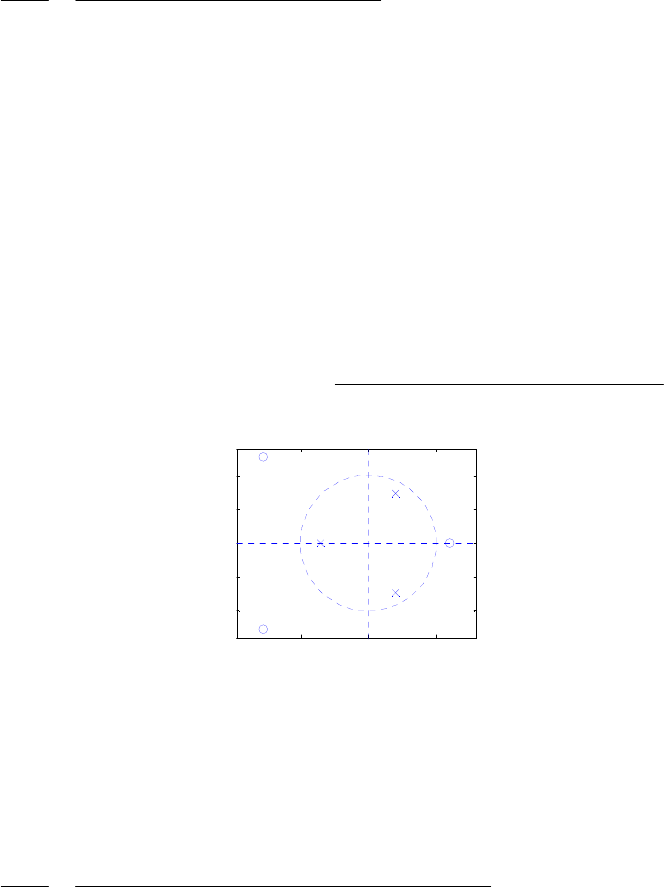
.
49.014.01.01
244.15.95
)(
)(
)( 321
321
−−−
−−−
++−
−++
==
zzz
zzz
zX
zY
zH Using Program 6_1.m we factorize
and develop is pole-zero plot shown below:
)(zH
Numerator factors
1.00000000000000 3.10000000000000 4.00000000000000
1.00000000000000 -1.20000000000000 0
Denominator factors
1.00000000000000 -0.80000000000000 0.70000000000000
1.00000000000000 0.70000000000000 0
Gain constant
5
The factored form of is thus
)(zH
)7.01)(7.081.01(
)2.11)(41.31(5
)( 121
121
−−−
−−−
++−
−++
=
zzz
zzz
zH
-1 0 1
-1
-0.5
0
0.5
1
Real Part
Imaginary Part
As all poles are inside the unit circle, is BIBO stable.
)(zH
(b)
)()0936.03.01.05.01( 4321 zYzzzz −−−− −++−
⇒−−++= −−−− )()6.334.227.145.165( 4321 zXzzzz
.
0936.03.01.05.01
6.334.227.145.165
)(
)(
)( 4321
4321
−−−−
−−−−
−++−
−−++
==
zzzz
zzzz
zX
zY
zH Using Program 6_1.m we
factorize and develop is pole-zero plot shown below:
)(zH
Numerator factors
1.00000000000000 -1.20000000000000 0
1.00000000000000 3.10000000000001 4.00000000000001
1.00000000000000 1.39999999999999 0
Denominator factors
1.00000000000000 0.59950918226500 0
1.00000000000000 -0.80131282790906 0.52021728677142
1.00000000000000 -0.29819635435594 0
Not for sale. 166
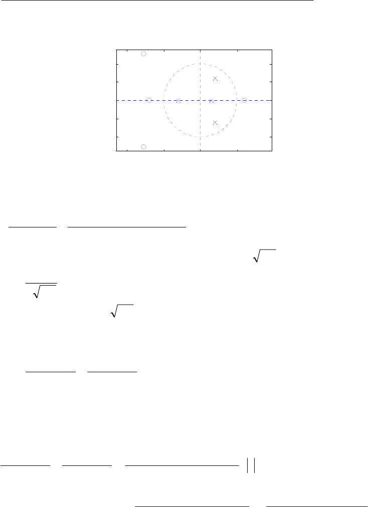
Gain constant
5
The factored form of is thus
)(zH
)2982.01)(520217.0801313.01)(5995.01(
)4.11)(41.31)(2.11(5
)( 1211
1211
−−−−
−−−−
−+−+
+++−
=
zzzz
zzzz
zH
As all poles are inside the unit circle, is BIBO stable.
)(zH
-2 -1 0 1
-1
-0.5
0
0.5
1
Real Part
I
mag
i
nary
P
ar
t
6.39 A partial-fraction expansion of in using the M-file residuez yields
)(zH 1−
z
.
3.05.01
)0.817811(212122
401
212121
)( 21
1
1−−
−
−++
−
+
−
−=
zz
z.
z.
.
zH Comparing the denominator of the
quadratic factor with we get
221
)cos(21 −− +ω− zrzr o0.547723.0 ==r and
,
3.02
5.0
)cos( −=ωo or 2.04478.
=
ωo Hence, from Table 6.1 we have
].[)2.04478cos()3.0(][)4.0(21212.1][ nnnnh nn µ+µ−=
6.40 (a) A partial-fraction expansion of in using the M-file residuez yields
)(zH 1−
z
.
3.01
2
6.01
5
2)( 11 −− −
−
+
+−=
zz
zH Hence, from Table 6.1 we have
].[)3.0(2][)6.0(5][2][ nnnnh nn µ−µ−+δ−=
(b) Its –transform is thus given by ].[)3.0(3.0][)4.0(1.2][ nnnx nn µ−+µ= z
.4.0,
)3.01)(4.01(
51.04.2
3.01
3.0
4.01
1.2
)( 11
1
11 >
+−
+
=
+
+
−
=−−
−
−− z
zz
z
zz
zX The –transform of
the output is then given by
z
.
18.03.01
36.03.31
)3.01)(4.01(
51.04.2
)( 21
21
11
1
⎥
⎥
⎦
⎤
⎢
⎢
⎣
⎡
−+
+−
⋅
⎥
⎥
⎦
⎤
⎢
⎢
⎣
⎡
+−
+
=−−
−−
−−
−
zz
zz
zz
z
zY
A partial-fraction expansion of in using the M-file residuez yields
)(zY 1−
z
Not for sale. 167

.6.0,
0.3z1
2.4
0.3z1
12.3
z4.01
16.8
0.6z1
9.3
)( 1111 >
+
−
−
+
−
−
+
=−−−− zzY Hence, from Table 6.1
we have
(
)
].[)3.0(4.2)3.0(3.12)4.0(8.16)6.0(3.9][ nny nnnn µ−−+−−=
6.41 (a) .4.0,
2.01
1
]}[{)(,4.0,
4.01
1
]}[{)( 11 >
−
==>
+
== −− z
z
nxzXz
z
nhzH ZZ Thus,
.4.0,
)2.01)(4.01(
1
)()()( 11 >
−+
== −− z
zz
zXzHzY A partial-fraction expansion of
using the M-file residuez yields .
2.01
3/1
4.01
3/2
)( 11 −− −
+
+
=
zz
zY Hence, from Table 6.1
].[)2.0(][)4.0(][ 3
1
3
2nnny nn µµ +−=
(b) .4.0,
2.01
1
]}[{)(,2.0,
2.01
1
]}[{)( 11 >
+
==>
+
== −− z
z
nxzXz
z
nhzH ZZ Thus,
.2.0,
)2.01(
1
)()()( 21 >
+
== −z
z
zXzHzY Hence, from Table 6.1,
].[)2.0)(1(][ nnny nµ−+=
6.42 .2.0,
6.01
4
]}[{)(,3.0,
3.01
2
]}[{)( 11 >
−
==>
+
== −− z
z
nxZzXz
z
nyzY Z Thus,
.3.0,
3.01
)6.01(5.0
)(
)(
)( 1
1>
+
−
== −
−
z
z
z
zX
zY
zH A partial-fraction expansion of using the M-file
residuez yields .
3.01
5.1
1)( 1−
+
+−=
z
zH Hence, from Table 6.1,
].[)3.0(5.1][][ nnnh nµδ−+−=
6.43 (a) Taking the –transform of both sides of the difference equation we get
Hence, ).(2)(08.0)(2.0)( 21 zXzYzzYzzY ++= −− .
08.02.01
2
)(
)(
)( 21 −− −−
==
zz
zX
zY
zH
(b) A partial-fraction expansion of using the M-file residuez yields
.
2.01
3/2
4.01
3/4
)( 11 −− +
+
−
=
zz
zH Hence, from Table 6.1,
].[)2.0(][)4.0(][ 3
2
3
4nnnh nn µµ −+=
(c) Now .
)1)(08.02.01(
2
]}[{)(]}[{)( 121 −−− −−−
=⋅==
zzz
nzHnszS µ
ZZ
Not for sale. 168

A partial-fraction expansion of using the M-file residuez yields
.
2.01
11110
4.01
88890
1
77782
)( 111 −−− +
+
−
−
−
=
z
.
z
.
z
.
zS Hence, from Table 6.1,
].[)2.0(1111.0][)4.0(8889.0][7778.2][ nnnns nn µµµ −+−=
6.44 .
)cos()1(1
1
)( 21
2
−−
−
α+ωα+−
−
=
zz
z
zH
c
Thus,
.
)cos()1(1
1
)( 2
2
ω−ω−
ω
ω
α+ωα+−
−
=jj
c
j
j
ee
e
eH
ωα+ω−ωα+α+α+ω+
ω
−
=
ω
cos)1(cos22cos2)1()(cos1
)2cos1(2
)( 2222
2
cc
j
eH
.
sin)1()cos(cos)1(
sin4
222
2
ωα−+ω−ωα+
ω
=
c
Note that 2
)( ωj
eH is maximum when
i.e, Then ,coscos c
ω=ω .
c
ω=ω ,
)1(
4
sin)1(
sin4
)( 222
2
2
α−
=
ωα−
ω
=
ω
c
c
jc
eH and hence,
).1/(2)( α−=
ωc
j
eH
6.45 Then, ⇒α−= −R
zzH 1)( .1)( Rjj eeH ωω α−
−= .)cos(21( 2ReH jωα−α+=
ω
ωj
eH( is maximum when 1)cos(
−
=
ω
R and is minimum when The
maximum value of
.1)cos( =ωR
)( ωj
eH is ,1 α+ and the minimum value is .1 α− ωj
eH( has
R
peaks and
R
dips in the range .20
π
<
ω
≤
The peaks are located at R
k
k
π
=ω=ω 2 and the dips are located at ,
)12(
R
k
k
π
+
=ω=ω
.10 −≤≤ Rk
00.5 11.5 2
0
0.5
1
1.5
2
ω
/
π
Amplitude
Magnitude Response
00.5 11.5 2
-1
-0.5
0
0.5
1
ω
/
π
Ph
ase, ra
di
ans
Phase Response
6.46
(
)
.)1()()( 3
3Rjjj eeHeG ωωω α−==
Not for sale. 169
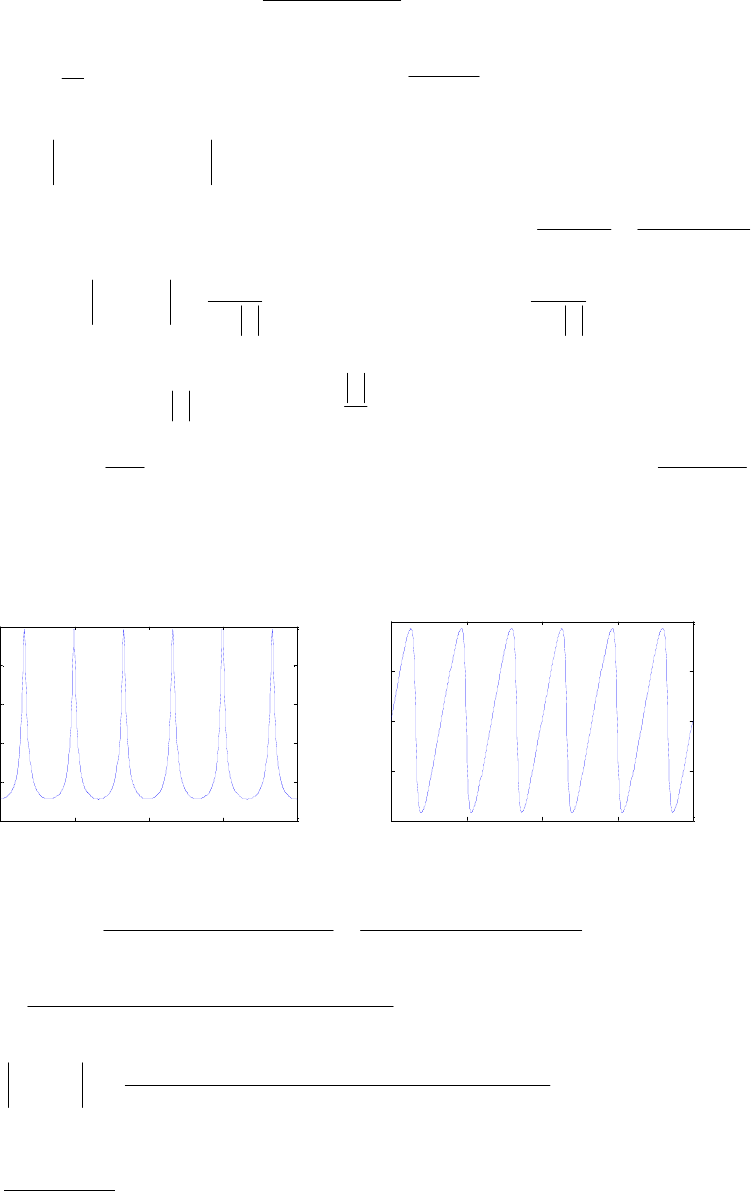
6.47 .
1
1
)( 1
0ω
ω
ωω
α
α
αj
MjM
nj
M
n
nj
e
e
eeG −
−
−
−
=−
−
=
∑
= Note that for )()( ωω jj eHeG =
.10,
1−≤≤= Mn
M
n
α Now, .
1
1
)( 0
α
α
−
−
=M
j
eG Hence, to make the dc value of the
magnitude response equal to unity, the impulse response should be multiplied by a constant
.)1/()1( M
Kαα −−=
6.48 Hence, ).()()( ωωωω αjRjjj eYeeXeY −
+= .
1
1
)(
)(
)( Rjj
j
j
eeX
eY
eH ω−ω
ω
ω
α−
== Maximum
value of )( ωj
eH is α−1
1 and the minimum value is .
1
1
α+ There are
R
peaks and dips
in the range The locations of the peaks and dips are given by
.20 πω ≤≤
αα ω±=− −11 Rj
e or, .
α
α
ω±=
−Rj
e The locations of the peaks are given by
R
k
k
π
ωω 2
== and the locations of the dips are given by ,
)12(
R
k
k
+
== π
ωω
Plots of the magnitude and phase responses of for and
are shown below:
.10 −≤≤ Rk )( ωj
eH 8.0=α
6=R
00.5 11.5 2
0
1
2
3
4
5
ω
/
π
Amplitude
Magnitude Response
00.5 11.5 2
-1
-0.5
0
0.5
1
ω
/
π
Ph
ase, ra
di
ans
Phase Response
6.49
12
120
2
21
2
210
)(
)(
1
)(
aeae
bebeb
eaea
ebebb
eA jj
jj
jj
jj
j
++
++
=
++
++
=−
−
−−
−−
ωω
ωω
ωω
ωω
ω
.
sin)1(cos)1(
sin)(cos)(
221
20201
ωω
ωω
ajaa
bbjbbb
−+++
−
+++
= Therefore,
[]
[]
.1
sin)1(cos)1(
sin)(cos)(
)( 22
2
2
2
21
22
20
2
2
201
2=
−+++
−+++
=
ωω
ωω
ω
aaa
bbbbb
eA j Hence, at we have ,0=ω
and at )],1([)( 21201 aabbb ++±=++ ,2/πω
=
we have ).1( 220 abb −±=
−
Solution #1: Consider .1 220 abb
−
=
− Choose ,1,1 220 abb
−
=
−
=
and
.
22 ab =
Substituting these values in )],1([)( 21201 aabbb
+
+
±
=
+
+
we get In this case,
.
11 ab =
Not for sale. 170

,1
1
1
)( 2
21
2
21 =
++
++
=−−
−−
ωω
ωω
ω
jj
jj
j
eaea
eaea
eA a trivial solution.
Solution #2: Consider .1
220
−
=
−abb Choose 20 ab
=
and Substituting these
values in
.1
2=b
we get .
11 ab
=
In this case, )],1([)( 21201 aabbb
+
+
±=++
.
1
)( 2
21
2
12
ωω
ωω
ω
jj
jj
j
eaea
eeaa
eA −−
−−
++
++
=
6.50 From Eq. (2.20), the input-output relation of a factor-of-2 up-sampler is given by
⎩
⎨
⎧±±=
=otherwise.,0
,4,2,0],2/[
][ Knnx
nxu
The DTFT of is therefore given by ][nxu
where
is the DTFT of
)(][]2/[][)( 22
even
ωωωωω jmj
m
nj
n
n
nj
n
jeXemxenxenyeY =
∑
=
∑
=
∑
=−
∞
−∞=
−
∞
−∞=
−
∞
−∞= )( ωj
eX
].[n
x
6.51 .
sin5.0cos5.01
1
5.01
1
)( ωω
ω
ω
j
e
eH j
j
+−
=
−
=− Thus,
.1.19070.6512
0.35360.6464
1
)4/sin(5.0)4/cos(5.01
1
)( 4/ j
jj
eH jm=
±
=
±+±−
=
±
ππ
π
Therefore, 1.3572)( 4/ =
±πj
eH and 1.0703.)4/()}(arg{ 4/ m=±=
±πθ
πjeH j
Now, for an input the steady-state output is given by ],[)sin(][ nnnx oµω=
()
)(sin)(][ oo
jneHny oωθω
ω+= which for 4/πω
=
o reduces to
.0703.1sin3572.1)4/(sin)(][ 44
4/ ⎟
⎠
⎞
⎜
⎝
⎛−=
⎟
⎠
⎞
⎜
⎝
⎛+= nneHny jππ
ππθ
6.52 To guarantee the stability of the transformation should be such that the
unit circle remains inside the ROC after the mapping. If the points inside the unit circle
after the mapping remains inside the unit circle, will be causal and stable. On the
other hand, if the points inside the unit circle after the mapping move outside the unit
circle, will be stable but anti-causal. For example, the mapping will ensure
that will be causal and stable, whereas, the mapping will result in a
that is stable, but anti-causal.
),(zG )(zFz →
)(zG
)(zG zz −→
)(zG 1−
→zz )(zG
6.53
Not for sale. 171

6.54 .][95.0][
0
2
0
2∑
=
∑∞
== n
K
n
nhnh Since Thus, ].[)(][),1/(1)( 1nnhzzH nµββ =−= −
.
1
95.0
1
1
22
2
ββ
β
−
=
−
−K
Solving this equation for we get .
)log(
)05.0log(
5.0 α
=K
6.55 Let the output of the predictor of Figure P6.3(a) be denoted by Then analysis of this
structure yields
).(zE
[
]
)()()()( zEzUzPzE
+
= and ).()()( zEzXzU
−
=
From the first equation
we have )(
)(1
)(
)( zU
zP
zP
zE −
= which when substituted in the second equation yields
).(1
)(
)(
)( zP
zX
zU
zH −==
Analyzing Figure P6.3(b) we get )()()()( zYzPzVzY
+
=
which leads to
,
)(1
1
)(
)(
)( zPzV
zY
zG −
== which is seen to be the inverse of
).(zH
For and
1
1
1
11)(,)( −− −== zhzHzhzP .
1
1
)( 1
1−
−
=
zh
zG Similarly, for
and
2
2
1
1
2
2
1
11)(,)( −−−− −−=+= zhzhzHzhzhzP .
1
1
)( 2
2
1
1−− −−
=
zhzh
zG
6.56
[
).()()()()()( 0000 zXzFzHzFzHzY
]
−
−−= Since the output is a delayed replica of the
input, we must have But, Hence,
.)()()()( 0000 r
zzFzHzFzH −
=−−− .1)( 1
0−
+= zzH α
Let This implies,
.)()1()()1( 0
1
0
1r
zzFzzFz −−− =−−−+ αα .)( 1
100 −
+= zaazF
.)(2 1
10 r
zzaa −− =+α
The solution is therefore, 1
=
r and .1)(2 10
=
+
aa α One possible solution is thus
and Hence, 2/1
0=a.4/1
1=a).1(25.0)( 1
0−
+= zzF
6.57 =
−
−
+
+== −− 11
11 2.01
6.0
5.01
5.0
2.1]}[{)(
zz
nhzH Z.
1.03.01
12.004.01.1
21
21
−−
−−
−+
−−
zz
zz The transfer
function of the inverse transform is thus
21
21
1
212.004.01.1
1.03.01
)(
1
)( −−
−−
−−
−+
==
zz
zz
zH
zH .
)312601)(34901(1.1
)2.01)(5.01(
11
11
−−
−−
+−
−+
=
z.z.
zz As both
poles are inside the unit circle, is stable and causal with an ROC
)(
2zH .349.0>z A
partial-fraction expansion in obtained using the M-file residuez is
Not for sale. 172

.
31261.01
42224464.0
34897.01
498.0
)( 11
2.1
1
2−− +
−
−
+=
zz
zH Hence,
].[)31261.0(42224464.0][)34897.0(498.0][][ 2.1
1
2nnnnh nn µµδ−−+=
6.58 Now, .)()()( )(ωθωω
===
ωjjj
ez eeHeHzH j Denote .
)(
)(' dz
zdH
zH =
From the above we get ).()(ln)(ln ωθ+= ω
=ωjeHzH j
ez j Therefore,
).(
)(
/)(
)(
)(
/)(
)(
)(' ωτ−
ω
=
ω
ωθ
+
ω
=
ω
⋅ω
ω
ω
ω
=ωg
j
j
j
j
ez
j
eH
deHd
d
d
j
eH
deHd
d
dz
zH
zH
j (6-A)
Hence,
)(
/)(
)(
)('
)( ω
ω
=
ω
−−=ωτ ωj
j
ez
geH
deHd
j
zH
zH
z
j. (6-B)
Replacing by in Eq, (6-A) we arrive at
.
)(
/)(
)(
)('
)( 1
ω
ω
=
−ω
+−=ωτ ωj
j
ez
geH
deHd
j
zH
zH
z
j (6-C)
Adding Eqs. (6-B) and (6-C), and making use of the notation )(
)('
)( zH
zH
zzT = we finally get
.
2
)()(
)(
1
ω
=
−
+
−=ωτ
j
ez
g
zTzT
M6.1 (a) The output data generated by Program 6_1 is as follows:
Numerator factors
1.00000000000000 -2.10000000000000 5.00000000000000
1.00000000000000 -0.40000000000000 0.90000000000000
Denominator factors
1.00000000000000 2.00000000000000 4.99999999999999
1.00000000000000 -0.20000000000000 0.40000000000001
Gain constant
0.50000000000000
Hence, .
)4.02.01)(521(
)9.021)(51.21(5.0
)( 2121
2121
1−−−−
−−−−
+−++
+++−
=
zzzz
zzzz
zG
The pole-zero plot of is given below:
)(
1zG
Not for sale. 173
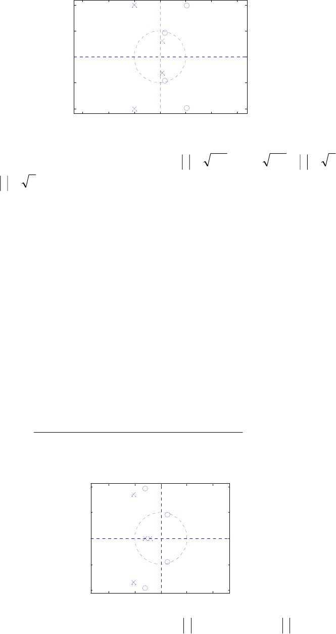
-3 -2 -1 0 1 2 3
-2
-1
0
1
2
Real Part
Imaginary Part
There are 3 ROCs associated with :
)(
1zG ,4.0:
1<zR ,54.0:
2<< zR
and .5:
3>zR The inverse –transform corresponding to the ROC is a left-
sided sequence, the inverse –transform corresponding to the ROC is a two-sided
sequence, and the inverse –transform corresponding to the ROC is a right-sided
sequence.
z1
R
z2
R
z3
R
(b) The output data generated by Program 6_1 is as follows:
Numerator factors
1.00000000000000 1.20000000000000 3.99999999999999
1.00000000000000 -0.50000000000000 0.90000000000001
Denominator factors
1.00000000000000 2.10000000000000 4.00000000000001
1.00000000000000 0.60000000000003 0
1.00000000000000 0.39999999999997 0
Gain constant
1
Hence, )4.01)(6.01)(41.21(
)9.05.01)(42.11(
)( 1121
2121
2−−−−
−−−−
++++
+−++
=
zzzz
zzzz
zG
The pole-zero plot of is given below:
)(
2zG
-2 -1 0 1 2
-2
-1
0
1
2
Real Part
Imaginary Part
There are 4 ROCs associated with :
)(
2zG ,4.0:
1<zR ,6.04.0:
2<< zR
Not for sale. 174

,26.0:
3<< zR and .2:
4>zR The inverse –transform corresponding to the ROC
is a left-sided sequence, the inverse z–transform corresponding to the ROC is a
two-sided sequence, the inverse –transform corresponding to the ROC is a two-
sided sequence, and the inverse –transform corresponding to the ROC is a right-
sided sequence.
z
1
R2
R
z3
R
z4
R
M6.2 (a) The output data generated by Program 6_3 is as follows:
Residues
-3.33333333333333 3.33333333333333
Poles
-0.60000000000000 0.30000000000000
Constants
0
Hence, the partial-fraction expansion of is given by )(zXa
.
3.01
3/10
6.01
3/10
)( 11 −− −
+
+
−=
zz
zXa The –transform has poles at and at
Thus, it is associated with ROCs as given in the solution of Problem 6.20 which
also shows their corresponding inverse –transform.
z6.0−=z
.3.0=z
z
(b) The output data generated by Program 6_3 is as follows:
Residues
Columns 1 through 2
2.33333333333333 -3.66666666666667 + 0.00000008829151i
Column 3
4.33333333333333 - 0.00000008829151i
Poles
Columns 1 through 2
-0.60000000000000 0.30000000000000 - 0.00000000722385i
Column 3
0.30000000000000 + 0.00000000722385i
Constants
Hence, the partial-fraction expansion of is given by )(zXb
.
)3.01(
4.33333
3.01
3.66666
6.01
3333.2
)( 2111 −−− −
+
−
−
+
=
zzz
zXb The –transform has two poles
at and one at
z
6.0−=z.3.0
=
z Thus, it is associated with ROCs as given in the solution
of Problem 6.20 which also shows their corresponding inverse –transform.
z
M6.3 (a) .
)6/1(1
6/7
)5/1(1
5/4
3
6
7
5
4
3)( 1111
1−−−− +
−
+
−=
+
−
+
−=
zzzz
zX
Not for sale. 175

The output data generated by Program 6_4 is as follows:
Numerator polynomial coefficients
1.03333333333333 0.73333333333333 0.1000000000000
Denominator polynomial coefficients
1.00000000000000 0.36666666666667 0.03333333333333
Hence, .
1130
32231
)( 21
21
1−−
−−
++
++
=
zz
zz
zX
(b) 2
1
1
26.01
4.1
4.01
3
5.2)( −
−
−+
+
−
+
+−=
z
z
z
zX
111 90.774596661
67964549722437.0
90.774596661
67964549722437.0
4.01
3
5.2 −−− +
+
−
−
−
−
+
+−=
zj
j
zj
j
z
.
The output data generated by Program 6_4 is as follows:
Numerator polynomial coefficients
-0.9000 -2.5600 -0.1000 -0.6000
Denominator polynomial coefficients
1.0000 0.4000 0.6000 0.2400
Hence, .
24.06.04.00.1
6.01.056.29.0
)( 321
321
−−−
−−−
+++
+++
−=
zzz
zzz
zXb
(c) 2111
3)24(
4
24
6
64.01
5
)( −−− +
−
+
+
+
+
=
zzz
zX
.
)5.01(
25.0
5.01
5.1
64.01
5
2111 −−− +
−
+
+
+
+
=
zzz
The output data generated by Program 6_4 is as follows:
Numerator polynomial coefficients
6.2500 6.5500 1.7300 0
Denominator polynomial coefficients
1.0000 1.6400 0.8900 0.1600
Hence, .
16.089.064.11
73.155.625.6
)( 321
21
3−−−
−−
+++
++
=
zzz
zz
zX
(d) 21
1
1
49.03434
2
5)( −−
−
−++
+
+
+−=
zz
z
z
zX
.
j0.2905) 0.3750(1
0.4303
j0.2905) - 0.3750(1
0.4303
75.01
5.0
5111 −−− ++
+
+
−
+
+−=
z
j
z
j
z
The output data generated by Program 6_4 is as follows:
Numerator polynomial coefficients
Not for sale. 176

-4.5000 -6.8750 -3.6375 -0.8438
Denominator polynomial coefficients
1.0000 1.5000 0.7875 0.1688
Hence, .
16875.07875.05.11
84375.06375.3875.65.4
)( 321
321
4−−−
−−−
+++
+++
−=
zzz
zzz
zX
M6.4 (a) The inverse –transform of from it partial-fraction expansion form is thus
z)(zXa
].[)6/1(][)5/1(][3][ 6
7
5
4nnnnx nn
aµµδ−−−−= The first 10 samples of obtained
by evaluating this expression in MATAB are given by
][nxa
Columns 1 through 4
1.0333333333 0.3544444444 -0.0644074074 0.0118012345
Columns 5 through 8
-0.0021802057 0.0004060343 -0.0000762057 0.0000144076
Columns 9 through 10
-0.0000027426 0.0000005254
The first
10 samples of the inverse z–transform of the rational form of obtaining
using the M-file impz are identical to the samples given above.
)(zXa
(b) The inverse z–transform of from it partial-fraction expansion form is thus )(zXb
][)4177459666920)(6796454972243.07.0(][)4.0(3][5.2][ n.jjnnnx nn
bµµδ−−−+−=
. ][)4177459666920)(6796454972243.07.0( n.jj nµ−+−
The first
10 samples of obtained by evaluating this expression in MATAB are
given by
][nxb
Columns 1 through 4
-0.900000000 -2.200000000 1.320000000 0.408000000
Columns 5 through 8
-0.427200000 -0.390720000 0.314688000 0.211084800
Columns 9 through 10
-0.179473920 -0.130386432
The first
10 samples of the inverse z–transform of the rational form of obtaining
using the M-file impz are identical to the samples given above.
)(zXb
(c) The inverse –transform of from it partial-fraction expansion form is thus
z)(zXc
].[)5.0)(1(25.0][)5.0(5.1][)64.0(5][ nnnnnx nnn
cµ−+−µ−+µ−=
The first 10 samples of obtained by evaluating this expression in MATAB are
given by
][nxc
Not for sale. 177

Columns 1 through 5
6.250000000 -3.700000000 2.235500000 -1.373220000
0.854485800
Columns 6 through 10
-0.536870912 0.3396911337 -0.215996076 0.137807801
-0.0881188675
The first 10 samples of the inverse z–transform of the rational form of obtaining
using the M-file impz are identical to the samples given above.
)(zXc
(d) The inverse z–transform of from it partial-fraction expansion form is thus )(zXd
][)290473750375.0(4303314830][)75.0(5.05][
4n.j.jnnx nn µµ +−−−+−=
].[)290473750375.0(4303314830 n.j.j nµ−−+
The first 10 samples of obtained by evaluating this expression in MATAB are
given by
][nxd
Columns 1 through 5
4.50000000000000 -0.12499999991919 0.09374999993940 -
0.12656249997773 0.13710937500069
Columns 6 through 10
-0.12181640625721 0.09610839844318 -0.07136938476820
0.05192523193410 -0.03790274963350
The first 10 samples of the inverse z–transform of the rational form of obtaining
using the M-file impz are identical to the samples given above.
)(zXd
M6.5 To verify using MATLAB that 21
21
212.004.01.1
1.03.01
)( −−
−−
−−
−+
=
zz
zz
zH is the inverse of
,
1.03.01
12.004.01.1
)( 21
21
1−−
−−
−+
−−
=
zz
zz
zH we determine the first 20 samples of and ,
and then form the convolution of these two sequences using the M-file conv. The first
samples of the convolution result are as follows:
][
1nh ][
2nh
Columns 1 through 9
1.0000 0 0.0000 0.0000 0.0000 0.0000 0.0000 0.0000 -0.0000
Columns 10 through 18
0.0000 -0.0000 -0.0000 -0.0000 -0.0000 0.0000 -0.0000 0.0000 0.0000
Columns 19 through 21
-0.0000 -0.0000 -0.0000
M6.6 % As an example try a sequence x = 0:24;
% calculate the actual uniform dft
Not for sale. 178
% and then use these uniform samples
% with this ndft program to get the
% original sequence back
% [X,w] = freqz(x,1,25,’whole’);
% use freq = X and points = exp(j*w)
freq = input(‘The sample values = ‘);
points = input(‘Frequencies at which samples are taken = ‘);
L = 1;
len = length(points);
val = zeros(size(1,len));
L = poly(points);
for k = 1:len
if (freq(k) ~= 0)
xx = [1 –points(k)];
[yy, rr] = deconv(L,xx);
F(k,:) = yy;
Down = polyval(yy,points(k))*(points(k))*(points(k)^(-len+1));
F(k,:) = freq(k)/down*yy;
val = val+F(k,:);
end
end
coeff = val;
Not for sale. 179

Chapter 7
7.1 Impulse response of the moving average filter is: ⎪
⎩
⎪
⎨
⎧−≤≤
=otherwise.,0
,10,
][
1Mn
nh M
Its frequency response is: .
)2/sin(
)2/sin(1
1
11
)( 2/ω
ω
ω
ω
ω
ωjM
j
jM
je
M
M
e
e
M
eH −
−
−⋅=
⎟
⎟
⎠
⎞
⎜
⎜
⎝
⎛
−
−
=
Now, for a BR transfer function, .,1)( ω
ω∀≤
j
eH For the moving-average filter,
.
)2/sin(
)2/sin(1
)( ω
ω
=
ωM
M
eH j We shall show by induction that
.,1
)2/sin(
)2/sin(1 ω∀≤
ω
ωM
M Now, for
,2=M.,1)2/cos(
)2/sin(
)2/cos()2/sin(2
2
1
)2/sin(
)sin(
2
1
)( ω∀≤ω=
ω
ωω
=
ω
ω
=
ωj
eH
We assume next that 1
)2/sin(
)2/sin(1 ≤
ω
ωm
m for .11
−
≤
≤
Mm We can express
()
(
)
)2/sin(
)2/sin(2/)1(cos)2/cos(2/)1(sin1
)2/sin(
)2/sin(1
ω
ωω−+ωω−
=
ω
ωMM
M
M
M
() ()
.2/)1(cos)2/cos(
)2/sin(
2/)1(sin1 ⎥
⎦
⎤
⎢
⎣
⎡ω−+ω
ω
ω−
≤M
M
M Now,
()
12/cos ≤ωm for
all values of Hence,
.m)2/sin(
)2/sin(1
ω
ωM
M
[]
.111
1≤+−≤ M
M
7.2 .
)*)((
*)1)(1(
)(*)()(.
1
)( *
11
1
*
1
2
1
*
1
dzdz
zdzd
zAzAzA
dz
zd
zA −−
−−
==
−
−
= Therefore,
)*)((
*)1)(1()*)((
)(1 *
11
1
*
1
*
11
2
dzdz
zdzddzdz
zA −−
−−−−−
=−
.
)1)(1(
)*)((
*1*
2
1
2
1
2
*
11
*
11
22
1
*
11
2
1
2
dz
dz
dzdz
zdzdzdzdzddz
−
−−
=
−−
++−−−−+
= Hence,
⎪
⎩
⎪
⎨
⎧
<<
==
>>
−
.1,0
,1
,1,0
)(1 2
1
z
z
z
zA
if
if0,
if
Thus, ⎪
⎩
⎪
⎨
⎧
<>
==
><
.1,1
,1
,1,1
)( 2
1
z
z
z
zA
if
if1,
if
Thus, Eq. (7.20) holds
for any first-order allpass function. A higher-order allpass function can br factored
into a product of first-order allpass functions. Since, Eq. (7.20) holds true each of
these factors individually, hence, it also holds true for the product.
Not for sale 177

7.3 An
m–th order stable, real allpass transfer function can be expressed as a product
of first-order allpass transfer functions of the form .
1
)(
*
i
i
idz
zd
zA −
−
= If is
complex, then has another factor of the form
i
d
)(zA .
1
)(' *
i
i
idz
zd
zA −
−
= Now,
.
)1)(1(
)1)(1(1
)( *
***
ωω
ωω
ω
ω
ω
ω
j
i
j
i
j
i
j
i
j
i
j
j
i
j
ieded
eded
e
de
ed
eA −−
−−
=
−
−
=−
− Let .
θθ αjj
ii eedd ==
Then, .
)]cos(21[
)1(
)( 2
2
ωθαα
αωθ
ωω
−−+
−
=−
−jj
jj
i
ee
eeA Therefore,
{
}
{
}
)1(arg2)1(arg)}(arg{ 2ωθωθω αωαω jjjjj
ieeeeeA −− −+−=−+−=
.
)cos(1
)sin(
tan2 1⎥
⎦
⎤
⎢
⎣
⎡
−−
−
+−= −
ωθα
ωθα
ω We can show similarly,
.
)cos(1
tan2)}('arg{ 1⎢
⎣
⎡
−
+−= −α
ω
ωj
ieA )sin( ⎥
⎦
⎤
+
+
ωθα
ωθ
If α is real, then
=
i
d.
cos1
sin
tan2)}(arg{ 1⎥
⎦
⎤
⎢
⎣
⎡
−
+−= −
ωα
ωα
ω
ωj
ieA Now for real
For
complex
,
i
d
.)}0(tan2{)}0(tan20{)}(arg{)}(arg{ 110 ππ
π=−+−−−+−=− −−j
i
j
ieAeA
,
i
d=−−+ )}('arg{)}(arg{)}('arg{)}(arg{ 00 ππ j
i
j
i
j
i
j
ieAeAeAeA
⎥
⎦
⎤
⎢
⎣
⎡
−
−
+−
⎥
⎦
⎤
⎢
⎣
⎡
−
+−= −−
θα
θα
θα
θα
cos1
sin
tan20
cos1
sin
tan20 11
.2
cos1
sin
tan2
cos1
sin
tan2 11 π
θα
θα
π
θα
θα
π=
⎥
⎦
⎤
⎢
⎣
⎡
+
−+
⎥
⎦
⎤
⎢
⎣
⎡
+
−+ −− Now,
(
.)}(arg{)( ω
ω
ωτ j
eA
d
d
−=
)
Therefore,
Since
it follows then
).(arg{)(arg{)}]([arg{)( 0
00
π
πω
π
ωωτ jjj eAeAeAdd −=
∫
−=
∫
,)(arg{)(arg{
1
∑
=
=
m
i
j
i
jeAeA ωω .)(
0
πωωτ
π
md =
∫
7.4 ].2[]1[][]1[]2[][ 54321
+
−
+
+
−
−−−= nanananananh δδδδδ Therefore,
ωωωωω 2
5432
2
1
)( −− −+−−= eaeaaeaeaeH jjjj
)sin(cos)sin(cos)2sin2(cos 4311 ωωωωωω jaajaja
−
+
−
+
−+=
)2sin2(cos)sin(cos 543 ωωωω jajaa
−
−−+−
(
)
.sin)(2sin)(cos)(2cos)( 134251 ωω ajaaaaa 425 ωω aaa +
−
+
+
−
−−−= To
Not for sale 178

have a zero-phase frequency response, the imaginary part of must be equal to zero
for all values of Hence, for a zero-phase response,
.ω51 aa
−
=
and
.
42 aa −=
7.5 and
],[][][ nhnxnv *
O
−= ].[][][][ nhnxnvnu
−
=
−
=
*
O Hence,
Therefore, Thus, the
equivalent frequency response is real and has zero phase.
].[])[][(][ nxnhnhny *
O
−+= ).(*)()( ωωω jjj eHeHeG +=
7.6 Now, ,
)(
*)/1(
)(
*
zD
zDz
zA
M
M
M
M
−
±= where
.1)( 2
2
1
1M
M
MzdzdzdzD −−− ++++= L
.1
*)/1(
)(
)(
*)/1(
*)/1()()( *
*
*
2=⋅==
zD
zD
zD
zD
zAzAzA
M
M
M
M
MMM
7.7 Consider the first-order factor Its square-magnitude function is given by
.1 1−
+az
.cos2)1()1)(1( 21 ω
ωaaazaz j
ez
++=++ =
− We thus rewrite the given square-
magnitude function as
.
)](8.064.1)][(6.036.1[
)](7.049.1)][(25.00625.1[9
)()()( 11
11
1
2
ω
ω
ω
j
j
ez
ez
j
zzzz
zzzz
zHzHeH
=
−−
−−
=
−
++++
+−++
==
Therefore, .
)8.01)(8.01)(6.01)(6.01(
)7.01)(7.01)(25.01)(25.01(9
)()( 11
11
1
−−
−−
−
++++
−−++
=
zzzz
zzzz
zHzH
As can be seen, there are 4 possible causal, stable transfer functions:
(i) ,
)8.01)(6.01(
)7.01)(25.01(3
)( 11
11
−−
−−
++
−+
=
zz
zz
zH (ii) ,
)8.01)(6.01(
)7.01)(25.01(3
)( 11
1
−−
−
++
−+
=
zz
zz
zH
(iii) ,
)8.01)(6.01(
)7.01)(25.01(3
)( 11 −− ++
−
+
=
zz
zz
zH (iv) )8.01)(6.01(
)7.01)(25.01(3
)( 11
1
−−
−
++
−+
=
zz
zz
zH .
The zero locations of the four FIR transfer functions are given below:
-1 -0.5 00.5 1
-1
-0.5
0
0.5
1
Real Part
Imaginary Part
(i)
-4 -3 -2 -1 0 1
-1.5
-1
-0.5
0
0.5
1
1.5
Real Part
I
mag
i
nary
P
ar
t
(ii)
Not for sale 179

-4 -3 -2 -1 0 1
-1.5
-1
-0.5
0
0.5
1
1.5
Real Part
I
mag
i
nary
P
ar
t
(iii)
-1 -0.5 00.5 11.5
-1
-0.5
0
0.5
1
Real Part
I
mag
i
nary
P
ar
t
(iv)
The zeros of the transfer function of a linear-phase FIR filter exhibits mirror-image
symmetry with respect to the unit circle. The zeros of the transfer function of a
minimum-phase FIR filter are all inside the unit circle and that of a maximum-phase
FIR filter are outside the unit circle.
(a) The transfer functions of (iii) and (iv) have linear-phase as their zeros exhibit
mirror-image symmetry.
(b) The transfer function of (i) is minimum-phase as its zeros are inside the unit
circle.
(c) The transfer function of (ii) is maximum-phase as its zeros are inside the unit
circle.
7.9
)5.01)(8.01)(5.21(6)5.01)(27.11(6)( 111121 −−−−−− −−+=−−+= zzzzzzzG
.61.172.76 321 −−− +−+= zzz
(a) Other transfer functions having the same magnitude responses are:
(i) ⎟
⎟
⎠
⎞
⎜
⎜
⎝
⎛
−−+= −
−
+
+
−−−
1
1
5.21
5.2
111
2)5.01)(8.01)(5.21(6)(
z
z
zzzzG
(ii)
.4.28.15.1315)5.01)(8.01)(5.2(6 321111 −−−−−− +−−=−−+= zzzzzz
⎟
⎟
⎠
⎞
⎜
⎜
⎝
⎛
−−+= −
−
−
+−
−−−
1
1
8.01
8.0
111
3)5.01)(8.01)(5.21(6)(
z
z
zzzzG
(iii)
.56.7186.38.4)5.01)(8.0)(5.21(6 321111 −−−−−− −+−−=−+−+= zzzzzz
⎟
⎟
⎠
⎞
⎜
⎜
⎝
⎛
−−+= −
−
−
+−
−−−
1
1
5.01
5.0
111
4)5.01)(8.01)(5.21(6)(
z
z
zzzzG
(iv)
.12428.169.03)5.0)(8.01)(5.21(6 321111 −−−−−− −++−=+−−+= zzzzzz
⎟
⎟
⎠
⎞
⎜
⎜
⎝
⎛
⎟
⎟
⎠
⎞
⎜
⎜
⎝
⎛
−−+= −
−
−
−
−
+−
+
+
−−−
1
1
1
1
8.01
8.0
5.21
5.2
111
5)5.01)(8.01)(5.21(6)(
z
z
z
z
zzzzG
.39.02.1612)5.01)(8.0)(5.2(6 321111 −−−−−− −++−=−+−+= zzzzzz
Not for sale 180

(v) ⎟
⎟
⎠
⎞
⎜
⎜
⎝
⎛
⎟
⎟
⎠
⎞
⎜
⎜
⎝
⎛
−−+= −
−
−
−
−
+−
−
+−
−−−
1
1
1
1
5.01
5.0
8.01
8.0
111
6)5.01)(8.01)(5.21(6)(
z
z
z
z
zzzzG
(vi)
.155.138.14.2)5.0)(8.0)(5.21(6 321111 −−−−−− +−−=+−+−+= zzzzzz
⎟
⎟
⎠
⎞
⎜
⎜
⎝
⎛
⎟
⎟
⎠
⎞
⎜
⎜
⎝
⎛
−−+= −
−
−
−
−
+−
+
+
−−−
1
1
1
1
5.01
5.0
5.21
5.2
111
7)5.01)(8.01)(5.21(6)(
z
z
z
z
zzzzG
(vii)
.8.46.3185.7)5.0)(8.01)(5.2(6 321111 −−−−−− −−+−=+−−+= zzzzzz
⎟
⎟
⎠
⎞
⎜
⎜
⎝
⎛
⎟
⎟
⎠
⎞
⎜
⎜
⎝
⎛
⎟
⎟
⎠
⎞
⎜
⎜
⎝
⎛
−−+= −
−
−
−
−
−
−
+−
−
+−
+
+
−−−
1
1
1
1
1
1
5.01
5.0
8.01
8.0
5.21
5.2
111
8)5.01)(8.01)(5.21(6)(
z
z
z
z
z
z
zzzzG
.62.71.176)5.0)(8.0)(5.21(6 321111 −−−−−− ++−−=+−+−+= zzzzzz
(b) The minimum phase filter is as all its zeros inside the unit circle.
Likewise, the maximum phase filter is as all its zeros outside the unit circle.
),(
2zG
),(
6zG
(c) The partial energy of impulse responses of each of the above transfer functions
for different values of k are given by:
k = 0 k = 1 k = 2 k = 3
G1(z) 36 87.84 380.25 416.25
G2(z) 225 407.25 410.49 416.25
G3(z) 23.04 36 360 416.25
G4(z) 9 9.81 272.25 416.25
G5(z) 144 406.44 407.25 416.25
G6(z) 5.76 9 191.25 416.25
G7(z) 56.25 380.25 393.25 416.25
G8(z) 36.00 328.41 380.25 416.25
The partial energy remains the same for values of From the above table it
can be seen that
.3≥k
,][][
0
2
2
0
2∑
≤
∑==
n
m
n
m
kmgmg and
,25.416][][
0
2
2
0
2=
∑
=
∑∞
=
∞
=mm
kmgmg ,81
≤
≤
k where is the minimum
phase transfer function. Likewise,
)(
2zG
,][][
0
2
6
0
2∑
≥
∑==
n
m
n
m
kmgmg where
is the maximum phase transfer function.
,81 ≤≤ k
)(
6zG
7.9
7654321
11.02.0125.025.04.08.05.01)( −−−−−−− −+−+−+−= zzzzzzzzH
Not for sale 181

).5.01)(5.01)(5.01)(8.01( 121212 −−−−−− −+−++−= zzzzzz
7654321
22.06.075.075.0425.04.025.05.0)( −−−−−−− −+−+−++= zzzzzzzzH
).5.01)(5.01)(5.0)(8.01( 121212 −−−−−− −+−++−= zzzzzz
7654321
34.06.09.045.07.0175.025.025.0)( −−−−−−− +−+−+++−= zzzzzzzzH
).5.0)(5.01)(5.0)(8.01( 121212 −−−−−− +−+−++−= zzzzzz
7654321
42.01.025.0125.08.04.05.0)( −−−−−−− +−+−+−+−= zzzzzzzzH
).5.0)(5.01)(5.01)(8.01( 121212 −−−−−− +−+−++−= zzzzzz
7654321
55.08.04.025.0125.02.01.0)( −−−−−−− +−+−+−+−= zzzzzzzzH
).()5.0)(5.0)(5.0)(8.0( 1
1
7121212 −−−−−−−− =+−+−+++−= zHzzzzzzz
Each factor of has roots inside the unit circle. Hence, is a minimum-
phase transfer function. Since is a mirror-image of , it has all zeros
outside the unit circle and is thus a maximum-phase transfer function.
)(
1zH )(
1zH
)(
5zH )(
1zH
There are 11 other length- FIR filters having the same magnitude responses as that
of the above filters.
7.11 ωωωωωω 5
6
4
5
3
4
2
321
)( jjjjjj eaeaeaeaeaaeH −−−−− +++++=
[
]
)()()( 2/
4
2/
3
2/3
5
2/3
2
2/5
6
2/5
1
2/5 ωωωωωωω jjjjjjj eaeaeaeaeaeae −−−− +++++=
+
⎟
⎠
⎞
⎜
⎝
⎛
−+
⎟
⎠
⎞
⎜
⎝
⎛
+= −
2
5
61
2
5
61 sin)(cos)[(2
2
5
ωω
ω
aajaae j
]sin)(cos)(sin)(cos)( 2
43
2
43
2
3
52
2
3
52 ⎟
⎠
⎞
⎜
⎝
⎛
−+
⎟
⎠
⎞
⎜
⎝
⎛
++
⎟
⎠
⎞
⎜
⎝
⎛
−+
⎟
⎠
⎞
⎜
⎝
⎛
++ ωωωω aajaaaajaa
It follows from the above that will have linear-phase, i.e., constant group
delay, if the imaginary parts inside the square brackets are zero. Hence, for a
constant group delay we must have
)( ωj
eH
,, 5261 aaaa
=
=
and .
43 aa
=
7.12 The frequency response of the LTI discrete-time system is given by
ωωωωω )4(
1
)3(
2
)1(
21
)( −−− −+−= kjkjkjjkj eaeaeaeaeH
)]()([ 2
22
1
)2( ωωωωω jjjjkj eeaeeae −−−− −+−=
].sin)2sin([2]sin)2sin([2 21
)2(
21
)2( 2ωωωω ω
ω
π
aaeaaje kj
kj +−=+−= −−−
−−
So, for ,2 2
π
−=kthe system will have a frequency response that is a real function
of .
ω
Not for sale 182

7.13 and
ωω βα jj eeH −
+=)(
1.
1
1
)(
2ω
ω
γj
j
e
eH −
+
= Thus,
.
1
)()()( 21 ω
ω
ωωω
γ
βα
j
j
jjj
e
e
eHeHeH −
−
−
+
==
2
2
22
2
cos21
cos2
11
)()()( K
e
e
e
e
eHeHeH j
j
j
j
jjj =
−+
++
=
−
+
⋅
−
+
== −
−
−
ωγγ
ωαββα
γ
βα
γ
βα
ω
ω
ω
ω
ωωω
if and i.e., )1( 2222 γβα +=+ K,
2γαβ K−= .)1()( 222 γβα −=+ K
7.14 .)()( )(arg ω
α
ωω j
eXjjj eeXeY = Hence, .)(
)(
)(
)( )1( −
== α
ω
ω
ω
ωj
j
j
jeX
eX
eY
eH Since
is a real function of it has zero phase. )( ωj
eH ,ω
7.15
(
)
]1[)](0[]1[)1](0[)( 2heeheeheheH jjjjjj ++=++= −−−− ωωωωωω
Thus, we require
]).1[cos]0[2( hhe j+= −ω
ω1]1[)3.0cos(]0[2)( 3.0 =+= hheH j
and .0]1[)6.0cos(]0[2)( 6.0 =+= hheH j Solving these two equations we get
and 8461.3]0[ =h.3487.6]1[ −=h
7.16 (a)
ωωωω 43 ]0[]1[]1[]0[)( jjjj ehehehheH −−− −−+=
(
)
)](1[)](0[ 222 ωωωωω jjjjj eeheehe −−− −+−=
Therefore,
()
.)sin(]1[)2sin(]0[2 2ωω
ωhhej j+= −
()
.)sin(]1[)2sin(]0[2)( ωω
ωhheH j+= Thus,
()
3.0)3.0sin(]1[)6.0sin(]0[2)( 3.0 =+= hheH j and
(
.8.0)6.0sin(]1[)2.1sin(]0[2)( 6.0 =+= hheH j
)
Solving these two equations we get
and 9873.0]1[ −=h.5686.2]0[ =h
(b) The plot of the magnitude
and phase responses are shown below.
()
.)sin(9873.0)2sin(5686.22)( 2ωω
ωω −= −jj ejeH
7.17 (a)
ωωωω 32 ]0[]1[]1[]0[)( jjjj ehehehheH −−− −−+=
(
)
)](1[)](0[ 2/2/2/32/32/3 ωωωωω jjjjj eeheehe −−− −+−=
()
.)2/sin(]1[)2/3sin(]0[2 2/3 ωω
ωhhej j+= − Therefore,
()
.)2/sin(]1[)2/3sin(]0[2)( ωω
ωhheH j+= Thus,
Not for sale 183
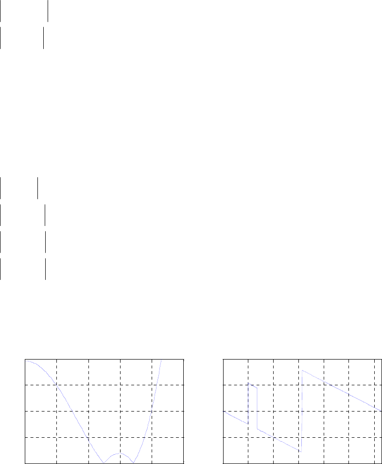
()
2.0)125.0sin(]1[)375.0sin(]0[2)( 25.0 =+= hheH j and
(
.8.0)4.0sin(]1[)2.1sin(]0[2)( 8.0 =+= hheH j
)
Solving these two equations we get
and 2573.6]1[ =h.8569.1]0[ −=h
(b)
)( ωj
eH
()
.)2/sin(2573.6)2/3sin(8569.12 2/3 ωω
ω+−= −j
ej
7.18 (a)
ωωωωω 432 ]0[]1[]2[]1[]0[)( jjjjj ehehehehheH −−−− ++++=
(
)
]2[)](1[)](0[ 222 heeheehe jjjjj ++++= −−− ωωωωω
. Therefore,
()
]2[cos]1[2)2cos(]0[2
2hhhe j++= −ωω
ω
].2[cos]1[2)2cos(]0[2)( hhheH j++= ωω
ω Thus,
,][).cos(][).cos(][)( .1230126002
30 =++= hhheH j
,][).cos(][).cos(][)( .0250120102
50 =++= hhheH j and
.][).cos(][).cos(][)( .1280126102
80 =++= hhheH j Solving these three equations
we get ,][,][ 58.7339117.77610
−
=
=hh and .][ 83.87862
=
h
(b) The plot of the
magnitude and phase responses are shown below.
()
.cos)cos()( 83.8786117.4677235.5522
2+ω−ω= ω−ω jj eeH
00.2 0.4 0.6 0.8 1
0
0.5
1
1.5
2
ω
Magnitude
00.5 11.5 22.5 3
-4
-2
0
2
4
ω
Phase, in radians
7.19 and Using the symmetry
property of the DTFT of a real sequence, we observe
Thus, the –point DFT of the length-
,43)(,13)( 4/30 jeHeH jj −−== π.3)( −=
πj
eH
.43)(*)( 4/34/ jeHeH jj +−== ππ 4][kH 4
Not for sale 184
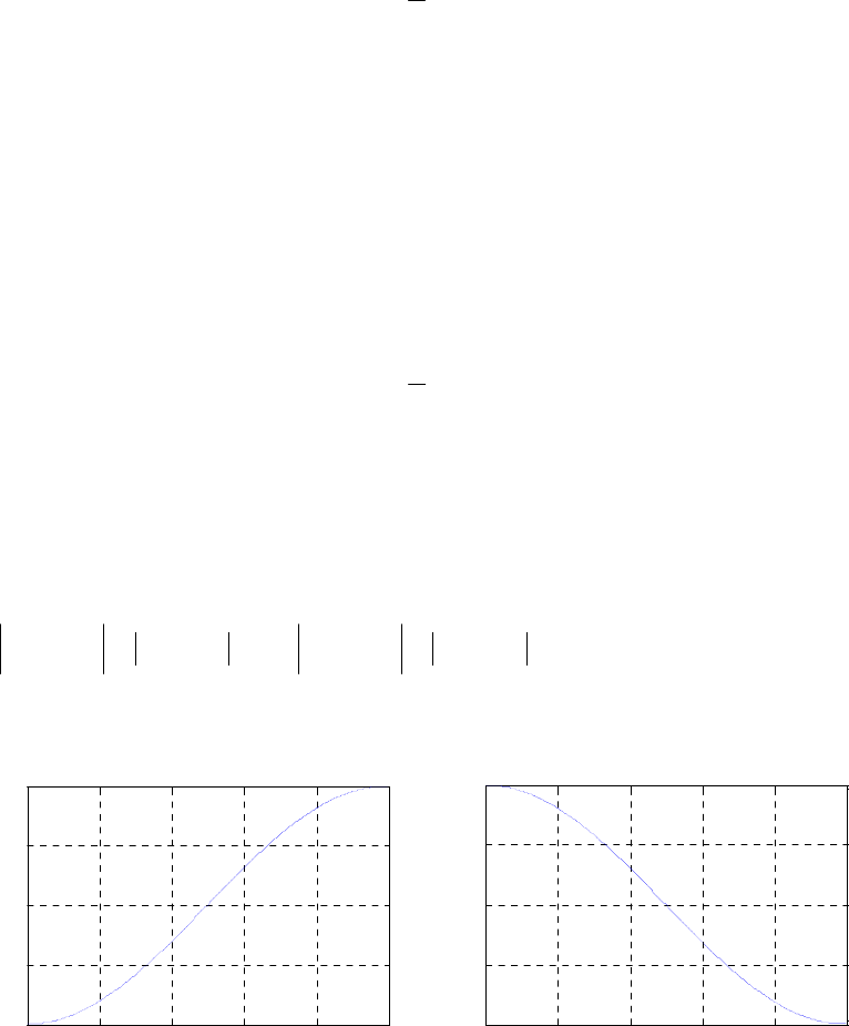
sequence
{
is given by
}
][nh
{
}
}.43,3,43,13{][ jjkH
−
−
−
+
−
=
Its –point
inverse DFT is thus given by
4
.
6
4
2
1
43
3
43
13
11
1111
11
1111
4
1
]3[
]2[
]1[
]0[
⎥
⎥
⎥
⎥
⎦
⎤
⎢
⎢
⎢
⎢
⎣
⎡
=
⎥
⎥
⎥
⎥
⎦
⎤
⎢
⎢
⎢
⎢
⎣
⎡
−−
−
+−
⎥
⎥
⎥
⎥
⎦
⎤
⎢
⎢
⎢
⎢
⎣
⎡
−−
−−
−−
=
⎥
⎥
⎥
⎥
⎦
⎤
⎢
⎢
⎢
⎢
⎣
⎡
j
j
jj
jj
h
h
h
h
Hence, .6421)( 321 −−− +++= zzzzH
7.20 Now, for a real, anti-symmetric sequence of even length,
Using the symmetry property of the DTFT of a real sequence, we observe also
Hence, the –point DFT of the length- 4
sequence is given by
]}[{ nh .0)( 0=
j
eH
.55)(*)( 4/34/ jeHeH jj +−== ππ 4
]}[{ nh }.55,20,55,0{]}[{ jjkH
−
−
+
−
=
Its –point 4
inverse DFT is thus given by .
5.7 5.2 5.75.2
55
20
550
11 1111
11 1111
4
1
]3[
]2[
]1[
]0[
⎥
⎥
⎥
⎦
⎤
⎢
⎢
⎢
⎣
⎡
−
−
=
⎥
⎥
⎥
⎦
⎤
⎢
⎢
⎢
⎣
⎡
−−
+−
⎥
⎥
⎥
⎦
⎤
⎢
⎢
⎢
⎣
⎡
−− −−
−−
=
⎥
⎥
⎥
⎦
⎤
⎢
⎢
⎢
⎣
⎡
j
j
jj
jj
h
h
h
h
Hence, .5.75.25.75.2)( 321 −−− +−−= zzzzH
7.21 (a) )1(cos5.05.0)( 2−=+−= −−− ω
ωωωω jjjj
A
eeeeH and
Hence, ).1(cos5.05.0)( 2+=++= −−− ω
ωωωω jjjj
BeeeeH
1cos)( −ω=
ωj
AeH and .1cos)( +ω=
ωj
BeH Plots of these two magnitude
functions is given below:
00.2 0.4 0.6 0.8 1
0
0.5
1
1.5
2
ω
/
π
Magnitude
H
A
(e
jω
)
00.2 0.4 0.6 0.8 1
0
0.5
1
1.5
2
ω
/
π
Magnitude
H
B
(e
jω
)
As can be seen from the above plots, is a highpass filter and
][nhA][nh
B
is a
lowpass filter.
(b) Hence,
is a shifted version of
].[][)1(][ nhnhnh BA
n
C=−= ).()()( )( ωπωω j
B
j
A
j
CeHeHeH == +
)( ωj
CeH )( ωj
A
eH shifted by
π
radians.
Not for sale 185

7.22 Thus, ].[][ nNhnh −=
).(][][][)( 1
1
0
)(
1
0
1
0
−−
−
=
−−
−
=
−
−
=
−=
∑
=
∑−=
∑
=zHzzkhznNhznhzH N
N
k
kN
N
n
n
N
n
n As
has zeros in a mirror-image symmetry in the –plane, will
have poles outside the unit circle making it unstable.
)(zH z)(/1)( zHzG =
7.23 (a) Since is a minimum-phase FIR transfer function, any other FIR transfer
function with the same magnitude response as that of can be expressed
as where is an allpass function. Now,
Thus,
)(zH
)(zG )(zH
)()()( zAzHzG =)(zA ).(lim]0[ zGg
z∞→
=
|)(lim||)(lim||)()(lim||)(lim|]0[ zAzHzAzHzGg
zzzz ∞→∞→∞→∞→ ⋅===
as
|,)(lim| zH
z∞→
≤1|)(lim|
<
∞→ zA
z (see Eq. (7.20)). Hence, .]0[]0[ hg ≤
(b) If is a zero of then
1
λ),(zH ,1
1<λ since is a minimum-phase causal
stable transfer function with all zeros inside the unit circle. Let
It follows that is also a minimum-phase causal transfer
function.
)(zH
).1)(()( 1
1−
−= zzBzH λ
Now, consider the transfer function .
1
)())(()( 1
1
1*
1
1*
1⎟
⎟
⎠
⎞
⎜
⎜
⎝
⎛
−
−
=−= −
−
−
z
z
zHzzBzF
λ
λ
λ If
and denote, respectively, the inverse –transform of and
then we get
],[],[ nbnh ][nf ),(),( zBzH
),(zF
⎩
⎨
⎧
≥−−
=
=,1],1[][
,0],0[
][
1nnbnb
nb
nh λ and
⎪
⎩
⎪
⎨
⎧
≥−−
=
=.1],1[][
,0],0[
][ *
1
*
1
nnbnb
nb
nf
λ
λ
Consider
.][][]0[]0[][][
1
2
1
22
2
*
1
2
0
2
0
2∑
−
∑
+−=
∑
−
∑
=
====
m
n
m
n
m
n
m
n
nfnhbbnfnh λε Now,
],[]1[*][*]1[]1[][][ *
11
22
1
22 nbnbnbnbnbnbnh −−−−−+= λλλ and
].[]1[*][*]1[]1[][][ *
11
222
1
2nbnbnbnbnbnbnf −−−−−+= λλλ
Hence, ∑⎟
⎠
⎞
⎜
⎝
⎛−−+−=
=
m
n
nbnbbb
1
22
1
222
1
2]1[][]0[]0[ λλε
.][1]1[][ 22
1
1
222
1mbnbnb
m
n
⎟
⎠
⎞
⎜
⎝
⎛−=
∑⎟
⎠
⎞
⎜
⎝
⎛−−−
=
λλ
Since ,0,1
1>< ελ i.e., .][][
0
2
0
2∑
>
∑==
m
n
m
n
nfnh Hence, .][][
0
2
0
2∑
≥
∑==
m
n
m
n
ngnh
Not for sale 186

7.24 (a) )8.05.0)(32(
)2678.20867.0)(0867.3(
)8.05.0)(32(
723
12
2
2
23
)( +++
+−+
+++
+++ ==
zzz
zzz
zzz
zzz
zH has a pole at
,
2
3
−=z which is outside the unit circle. Hence, is not a stable transfer
function. To arrive at a stable transfer function with an identical magnitude
response, we multiply with the allpass function
)(
1zH
)(
1zH z
z
32
32
+
+ resulting in
.
)8.05.0)(32(
723
32
32
)8.05.0)(32(
723
2
23
2
23
+++
+++
=
+
+
+++
+++ ⋅
zzz
zzz
z
z
zzz
zzz
(b) )7.03.0)(0817.1)(0817.3(5.1
)(6338.14181.0(4
)7.03.0)(535.1(
6524
22
2
22
23
)( +−−+
−++
+−−+
−+− ==
zzzz
zz
zzzz
zzz
zH 0.9181) has
two poles outside the unit circle at 0817.3
−
=
z and 0817.1
=
z. Hence, is
not a stable transfer function. To arrive at a stable transfer function with an
identical magnitude response, we multiply with the allpass function
)(
2zH
)(
2zH
13.07.0
7.03.0
2
2
+−
+−
zz
zz resulting in 13.07.0
7.03.0
)7.03.0)(535.1(
6524
2
2
22
23
+−
+−
+−−+
−+− ⋅
zz
zz
zzzz
zzz
.
)7.03.0)(5.135(
6524
22
23
+−−+
−+−
=
zzzz
zzz
7.25 The transfer function of the simplest notch filter is given by
In the steady-state,
the output for an input is given by
where
.)cos(21)1)(1()( 2111 −−−
−
−+−=−−= zzzezezH o
jj oo ω
ωω
)cos(][ nnx o
ω=
()
)(cos)(][ oo
jneHny oωθω
ω+=
)].(arg[)( o
j
oeH ω
ωθ =
(a) Comparing with as given above we conclude
21
1)( −− +−= zzzH )(zH
,)cos( 2
1
=
o
ω or .
3
π
ω=
o Here,
ooo jjj eeeH ωωω 2
11)( −− +−=
.0)866.05.0()866.05.0(11 3/23/ =+−++−=+−= −− jjee jj ππ
Hence,
(
)
.0)(cos)(][ 1=+= oo
jneHny oωθω
ω
(b) Comparing with as given above we conclude
or Here,
21
28.01)( −− +−= zzzH )(zH
4.0)cos( =
o
ω.πω 0.369=
o
ooo jjj eeeH ωωω 2
21)( −− +−= .0)7332.068.0()7332.032.0(1 =+
−
+
+
−
=
jj
Hence,
(
)
.0)(cos)(][ 2=+= oo
jneHny oωθω
ω.
Not for sale 187
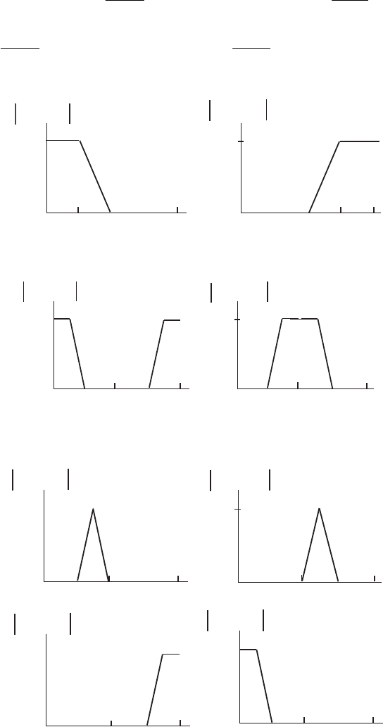
(c) Comparing with as given above we conclude
or Here,
21
36.11)( −− +−= zzzH )(zH
8.0)cos( =
o
ω.πω 0.2048=
o
ooo jjj eeeH ωωω 2
21)( −− +−= .0)9599.02801.0()9599.02891.1(1
=
+
+
+
−
=
jj
Hence,
(
)
.0)(cos)(][ 3=+= oo
jneHny oωθω
ω
7.26 From the figure, ),()(
)(
)(
)( 2
0
0zGzG
zX
zY
zH HL
== ),()(
)(
)(
)( 2
1
1zGzG
zX
zY
zH HH
==
),()(
)(
)(
)( 2
2
2zGzG
zX
zY
zH LH
== ).()(
)(
)(
)( 2
3
3zGzG
zX
zY
zH LL
==
For the magnitude responses of )(zG
L
and shown below
)(zGH
Ljω
1
00π
/
2πω
π
/
4
G
(
e
) Hjω
1
0
0π
/
2πω
3π/
4
G
(
e
)
the magnitude responses of )( 2
zG
L
and )( 2
zG
H
are as shown below
1
00π/2πω
π/4
L
j2ω
G (e )
1
0
0π/2πω
3π
/4
Hj2ω
G (e )
Hence, the magnitude responses of the casacaded filters ,30),(
≤
≤
izHi are as indicated
below:
1
00π
/
2πω
π
/
4
1
0
0π
/
2πω
3π
/
4
jω
H (e )
0jω
H (e )
1
1
00π
/
2πω
π
/
4
jω
H (e )
2
1
00π
/
2πω
π
/
4
jω
H (e )
3
Not for sale 188
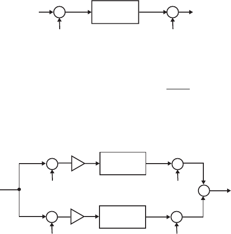
7.27 Since,
Hence, is a highpass filter with a cutoff
frequency given by
).()( )( ωπω −
=j
LP
jeHeG ⎩
⎨
⎧
<≤
<≤
=,,0
,0,1
)( πωω
ωω
ω
c
c
j
LP eH
⎩
⎨
⎧
<≤−
−<≤
=.,1
,0,0
)( πωωπ
ωπω
ω
c
c
j
eG )( ωj
eG
.
co ωπω
−
= Also, since ),()( zHzG
L
P
−
=
we have
].[)1(][ nhng LP
n
−=
7.28 Hence,
).()()( zeHzeHzG oo j
LP
j
LP ωω −
+= nj
LP
nj
LP oo enhenhng ωω ][][][ += −
).cos(][2 nnh oLP ω= Thus, is a real coefficient bandpass filter with
a center frequency at and a passband width of
)(zG
o
ω.2 p
ω
7.29 Hence,
).()()()( zHzeHzeHzF LP
j
LP
j
LP oo ++= −ωω
Thus, is a real coefficient bandstop filter with
()
].[)cos(21][ nhnnf LPo
ω+= )(zF
a center frequency at and a stopband width of
o
ω.2/)3( p
ω
−
π
7.30
+
+
( 1)
_n
( 1)
_n
LP
h [n]
X
(z)Y(z)
U(z)
V(z)
From the above figure, we get ),()()(),()( zXzHzUzXzV
L
P
−
=
−
=
and
).()()()( zXzHzUzY
L
P−=−= Hence, ),(
)(
)(
)( zH
zX
zY
zH LPeq −== which is the
highpass filter of Problem 7.27.
7.31
+
+
LP
h [n]
+
+
LP
h [n]
+
2
2
cos(ω n)
o
cos(ω n)
o
o
sin(ω n)
o
sin(ω n)
X
(z)Y(z)
V (z)
0
V (z)
1
U (z)
0
U (z)
1
From the above figure, we have
or, Likewise,
We also have
njnj
ooo enxenxnnxnu ω−ω +=ω= ][][)cos(][2][
0
).()()( )()(
0oo jj
jeXeXeU ω−ωω+ω
ω+=
).()()( )()(
1oo jj
jeXjeXjeU ω−ωω+ω
ω−=
Not for sale 189

and
Therefore,
),()()()()(
0oo j
LP
j
LP ezXzHezXzHzV ω−ω +=
).()()()()(
1oo j
LP
j
LP ezXzHjezXzHjzV ω−ω −=
(
)
(
)
,)()()()()( 11
2
1
00
2
1oooo jjjj ezVezVjezVezVzY ω−ωω−ω −++= which after
simplification yields
)()()()()()()( 2
4
1{zXezHzXezHezXezHzY oooo j
LP
j
LP
jj
LP ω−ωωω ++=
)()()()()()( 2
4
1
2{} zXezHezXezHezXezH ooooo j
LP
jj
LP
jj
LP ωωωω−ω− −+
−
Hence,
}.)()()()( 2ooo jj
LP
j
LP ezXezHzXezH ω−ω−ω− ++
{
}
).()()()( 2
1zXezHezHzY oo j
LP
j
LP ω−ω += Therefore,
{
}
.)()()( 2
1oo j
LP
j
LPeq ezHezHzH ω−ω += Thus, the structure of Figure P7.4
implements the bandpass filter of Problem 7.28.
7.32
Not for sale 190
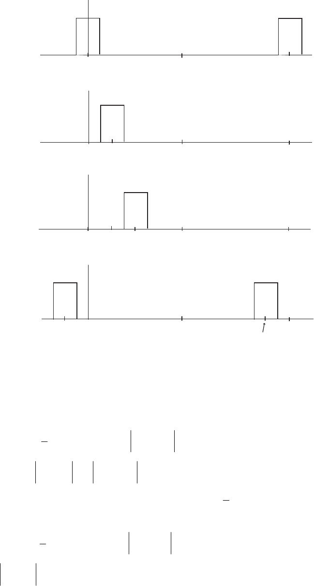
|H (e )|
jω
1
|H (e )|
jω
2
|H (e )|
jω
0
π
M
__
π
M
___ 0π2
ω
π2π2π
2π
π
π
ω
ω
0
0
2π
M
__
4π
__
M
jω
|H (e )|
M 1
_
2π
π
ω
0
_____
2( 1)πM_
M
2π
M
___
The output of the k–th filter is a bandpass signal occupying a bandwidth of
and centered at In general, the –th filter has a complex
impulse response generating a complex output sequence. To realize a real
coefficient bandpass filter, one can combine the outputs of and
M/2π
./ Mkπ=ω k)(zHk
)(zHk).(zH kM −
7.33 ).1()( 1
2
1
0−
+= zzH Thus, ).2/cos()(
0ω
ω=
j
eH Now,
Hence,
()
.)()( 0M
zHzG =
()
.)2/cos()()( 2
2
0
2M
M
jj eHeG ω
ωω == The 3–dB cutoff frequency
of is thus given by
(
c
ω)(zG
)
.)2/cos( 2
1
2=
M
c
ω Hence,
).2(cos2 2/11 M
c−−
=ω
7.34 ).1()( 1
2
1
1−
−= zzH Thus, ).2/(sin)( 2
2
1ω
ω=
j
eH Let, Then,
()
.)()( 0M
zHzF =
()
.)2/sin()( 2
2M
j
eF ω
ω= The 3–dB cutoff frequency of is thus given
c
ω)(zF
Not for sale 191

by
()
,
2
1
2
)2/sin( =
M
c
ω which yields,
).2(sin2 2/11 M
c−−
=ω
7.35 .
1
1
2
1
)( 1
1
⎟
⎟
⎠
⎞
⎜
⎜
⎝
⎛
−
+−
=−
−
z
z
zH LP α
α Note that )(zH
L
P is stable if .1<α Now,
)2/(sin)2/(cos
)2/cos()2/sin(2)2/(sin)2/(cos
)cos(
)sin(1
22
22
cc
cccc
c
c
ωω
ωωωω
ω
ω
α−
−+
=
−
=
.
)2/tan(1
)2/tan(1
)2/sin()2/cos(
)2/sin()2/cos(
c
c
cc
cc
ω
ω
ωω
ωω
+
−
=
+
−
= (7-a)
If then Hence,
,0 πω <≤ .0)2/tan( ≥
c
ω.1<α
7.36 From Eq. (7-a), .
)2/tan(1
)2/tan(1
c
c
ω
ω
α+
−
= Hence, .
1
1
)2/tan( α
α
ω
+
−
=
c
7.37 (a) From Eq.(7.73b), we get .5275.0
)6.0cos(
)6.0sin(1 =
−
=α Substituting this value of α
in Eq.(7.71), we arrive at .
5275.01
1
2363.0)( 1
1
⎟
⎟
⎠
⎞
⎜
⎜
⎝
⎛
−
+
=−
−
z
z
zH LP
(b) From Eq.(7.73b), we get .0787.0
)45.0cos(
)45.0sin(1 =
−
=α Substituting this value of
α in Eq.(7.71), we arrive at .
0787.01
1
4607.0)( 1
1
⎟
⎟
⎠
⎞
⎜
⎜
⎝
⎛
−
+
=−
−
z
z
zH LP
7.38 .
1
1
2
1
)( 1
1
⎟
⎟
⎠
⎞
⎜
⎜
⎝
⎛
−
−+
=−
−
z
z
zHHP α
α Thus, .
1
1
2
1
)( ⎟
⎟
⎠
⎞
⎜
⎜
⎝
⎛
−
−+
=−
−
ω
ω
ω
α
α
j
j
j
HP e
e
eH Thus,
.
)cos(21
)cos(22
2
1
)( 2
2
2
⎟
⎟
⎠
⎞
⎜
⎜
⎝
⎛
−+
−
⎟
⎠
⎞
⎜
⎝
⎛+
=
ωαα
ωα
ωj
HP eH At –dB cutoff frequency ,
c
ω
2
1
)( 2=
c
j
HP eH ω which yields .
1
2
)cos( 2
α
α
ω+
=
c
7.39 (a) From Eq.(7.73b), we get .5275.0
)6.0cos(
)6.0sin(1 =
−
=α Substituting this value of
in Eq.(7.74), we arrive at
α⎟
⎟
⎠
⎞
⎜
⎜
⎝
⎛
−
+
=−
−
1
1
5275.01
1
7637.0)(
z
z
zHHP .
(b) From Eq.(7.73b), we get .0787.0
)45.0cos(
)45.0sin(1 =
−
=α Substituting this value of
Not for sale 192
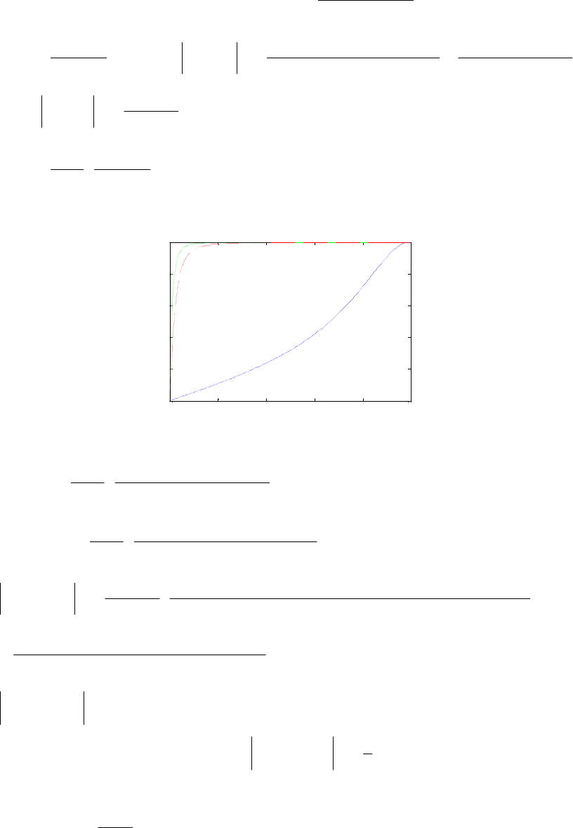
α in Eq.(7.74), we arrive at .
0787.01
1
5394.0)( 1
1
⎟
⎟
⎠
⎞
⎜
⎜
⎝
⎛
−
+
=−
−
z
z
zHHP
7.40 .
1
1
)( 1
1
−
−
−
−
=
kz
z
zH Hence, .
cos21
cos22
sin)cos1(
sin)cos1(
)( 2222
22
2
ω
ω
ωω
ωω
ω
kkkk
eH j
−+
−
=
+−
+−
=
Now, .
)1(
4
)( 2
2
k
eH j
+
=
π Thus, the scaled transfer function is given by
.
1
1
2
1
)( 1
1
⎟
⎟
⎠
⎞
⎜
⎜
⎝
⎛
−
−+
=−
−
kz
zk
zH A plot of the magnitude responses of the scaled transfer
function for and
,9.0,95.0=k5.0
−
are given below:
00.2 0.4 0.6 0.8 1
0
0.2
0.4
0.6
0.8
1
ω
/p
i
Magnitude
←
k=0.95
←
k=0.9 k=-0.5
→
7.41 .
)1(1
1
2
1
)( 21
2
⎟
⎟
⎠
⎞
⎜
⎜
⎝
⎛
++−
−−
=−−
−
zz
z
zH BP ααβ
α Thus,
.
)1(1
1
2
1
)( 2
2
⎟
⎟
⎠
⎞
⎜
⎜
⎝
⎛
++−
−−
=−−
−
ωω
ω
ω
ααβ
α
jj
j
j
BP ee
e
eH Hence,
(
)
)cos()1(2)2cos(2)1(1
)2cos(212
2
)1(
)( 2222
2
2
ωαβωαααβ
ωα
ω
+−++++
−
⋅
−
=
j
BP eH
.
sin)1()(cos)1(
sin)1(
2222
22
ωα−+β−ωα+
ωα−
= At the center frequency ,
o
ω
.1)( 2=
o
j
BP eH ω Hence, or
0)(cos 2=−βωo.cos βω
=
o
At the
3–dB bandedges and
1
ω,
2
ω
.2,1,)( 2
1
2==
ωieH i
j
BP This imples
(7-c) ,sin)1()(cos)2
1( 222 ii ωα−=β−ωα+
or, .2,1),(cos
1
1
sin =β−ω
⎟
⎠
⎞
⎜
⎝
⎛
α−
α+
±=ω i
ii Since, ,
21
ω
<
ω
<
ω
o must have
positive sign and must have negative sign, because otherwise,
1
sinω
2
sinω0sin 2<ω
Not for sale 193

for in Now, Eq. (7-c) can be rewritten as
Hence,
2
ω).,0( π
.0)1()1(cos)1(2cos)1(2 222222 =α−−α+β+ωα+β−ωα+ ii
,
1
)1(
coscos 2
2
21 α+
α+
β=ω+ω and .
)1(2
)1()1(
))(cos(cos 2
222
21 α+
α−−α+β
=ωω
Denote Then
.
123 ω−ω=ω dB 12123 sinsincoscoscos ω
ω
+
ω
ω
=
ω
dB
()
.
1
2
)cos(coscoscos
1
1
coscos 2
12
2
12
2
12 α+
α
=ω+ωβ+ωω
⎟
⎠
⎞
⎜
⎝
⎛
α−
α+
−ωω=
7.42 (a) Using Eq.(7.76), we get .1564.0)55.0cos(
−
=
π
=
β
Next, from Eq.(7.78), we
get ,7071.0)25.0cos(
1
2
2=π=
α+
α or, equivalently,
Solution of this quadratic equation yields
.07071.027071.0 2=+α−α
4142.2
=
α
and .4142.0
=
α
Substituting and
4142.2=α .1564.0
−
=
β
in Eq.(7.77) we arrive at the
denominator polynomial of the transfer function )(zH
B
Pas
Comparing with Eq. (7.136) we note
and Since the condition of Eq. (7.139) is not satisfied,
the corresponding
.4142.25340.01)( 21 −− ++= zzzD
5340.0
1=d.4142.2
2=d
)(zH
B
P is unstable.
Substituting and
4142.0=α .1564.0
−
=
β
in Eq.(7.77) we arrive at the
denominator polynomial of the transfer function )(zH
B
Pas
Comparing with Eq. (7.136) we note
and Since the conditions of Eqs. (7.139) and (7.141) are
satisfied, the corresponding
.4142.02212.01)( 21 −− ++= zzzD
2212.0
1=d.4142.0
2=d
)(zH
B
P is a stable transfer function. Hence, the desired
transfer function is .
4142.02212.01
)1(2929.0
)( 21
2
−−
−
++
−
=
zz
z
zHBP
(b) Using Eq.(7.76), we get .5878.0)3.0cos(
=
π
=
β
Next, from Eq.(7.78), we get
,5878.0)3.0cos(
1
2
2=π=
α+
α or, equivalently,
Solution of this quadratic equation yields
.05878.025878.0 2=+α−α
0766.3
=
α
and .3249.0
=
α
Substituting and
0766.3=α .5878.0
=
β
in Eq.(7.77) we arrive at the denominator
polynomial of the transfer function )(zH
B
Pas
Comparing with Eq. (7.136) we note
.788.03968.21)( 21 −− ++= zzzD
3968.2
1
=
d and .788.0
2
=
d Since the
condition of Eq. (7.141) is not satisfied, the corresponding )(zH
B
P is unstable.
Substituting and
3249.0=α .5878.0
=
β
in Eq.(7.77) we arrive at the denominator
polynomial of the transfer function )(zH
B
Pas .3249.07788.01)( 21 −− ++= zzzD
Not for sale 194

Comparing with Eq. (7.136) we note 2212.0
1
=
d and .4142.0
2
=
d Since the
conditions of Eqs. (7.139) and (7.141) are satisfied, the corresponding )(zH
B
P is a
stable transfer function. Hence, the desired transfer function is
.
3249.07788.01
)1(3376.0
)( 21
2
−−
−
++
−
=
zz
z
zHBP
7.43 .
)1(1
21
2
1
)( 21
21
⎟
⎟
⎠
⎞
⎜
⎜
⎝
⎛
α+α+β−
+β−α+
=−−
−−
zz
zz
zH BS Thus,
)cos()1(2)2cos(2)1(1
)2cos(2)cos(842
2
1
)( 2222
2
2
2
ωα+β−ωα+α+α+β+
ω+ωβ−β+
⋅
⎟
⎠
⎞
⎜
⎝
⎛α+
=
ωj
BS eH
.
sin)1()(cos)1(
)(cos)1(
2222
22
ωα−+β−ωα+
β−ωα+
= At the center frequency ,
o
ω
.0)( 2=
ωo
j
BS eH Hence, or
0)(cos 2=−βωo.cos βω
=
o At the 3–dB
bandedges and
1
ω,
2
ω.2,1,)( 2
1
2==
ωieH i
j
BP This leads to Eq. (7-c) given in
the solution of Problem 7.41. Hence, as in the solution of Problem 7.41,
2
31
2
α+
α
=ω dB .
7.44 (a) Using Eq.(7.76), we get .454.0)35.0cos(
=
π
=
β
Next, from Eq.(7.78), we get
,809.0)2.0cos(
1
2
2=π=
α+
α or, equivalently, Solution
of this quadratic equation yields
.0809.02809.0 2=+α−α
9627.1
=
α
and .3249.0
=
α
Substituting
and in Eq.(7.80) we arrive at the denominator polynomial of
the transfer function as Since the
condition of Eq. (7.139) is not satisfied, the corresponding is unstable.
9627.1=α 454.0=β
)(zH BS .9627.13451.11)( 21 −− +−= zzzD
)(zH BS
Substituting and
3249.0=α 454.0
=
β
in Eq.(7.80) we arrive at the denominator
polynomial of the transfer function as Since
the conditions of Eqs. (7.139) and (7.141) are satisfied, the corresponding is a
stable transfer function. Hence, the desired transfer function is
)(zH BS .3249.06015.01)( 21 −− ++= zzzD
)(zH BS
.
3249.06015.01
)908.01(6624.0
)( 21
21
−−
−−
++
+−
=
zz
zz
zH BS
(b) Using Eq.(7.76), we get .309.0)6.0cos(
−
=
π
=
β
Next, from Eq.(7.78), we get
,891.0)15.0cos(
1
2
2=π=
α+
α or, equivalently, Solution
.0891.02891.0 2=+α−α
Not for sale 195

of this quadratic equation yields 6319.1
=
α
and 6128.0
=
α
.
Substituting and
6319.1=α 309.0
−
=
β
in Eq.(7.80) we arrive at the denominator
polynomial of the transfer function as
Since the condition of Eq. (7.139) is not satisfied, the corresponding is
unstable.
)(zH BS .6319.1345.21)( 21 −− ++= zzzD
)(zH BS
Substituting and
6128.0=α 309.0
−
=
β
in Eq.(7.80) we arrive at the denominator
polynomial of the transfer function as
Since the conditions of Eqs. (7.139) and (7.141) are satisfied, the
corresponding is a stable transfer function. Hence, the desired transfer
function is
)(zH BS .6128.04974.01)( 21 −− ++= zzzD
)(zH BS
.
6128.04984.01
)618.01(564.0
)( 21
21
−−
−−
++
++
=
zz
zz
zH BS
7.45 .2
)cos21(2
)cos1()1( /1
2
2K
c
c−
=
ωα−α+
ω+α− Let Simplifying the first equation
.
/)( KK
C1
2−
=
we then get
Solving the quadratic equation for
.cos)coscos()(cos 01121
2=−ω++ω−ω+α−−+ωα CCC cccc
α
we obtain
()()
)cos
−1
(
)cos(cos)(cos)(
C
CCC
c
ccc
−ω+
−ω+−ω+±ω−+
=α 12
1414112 2
2
()
(
)
C
CCCC
c
cccc
−ω+
ω−ω−−ω+±ω−+
=cos
)cos()coscos(cos)(
1
12211
.
cos
sincos)(
C
CCC
c
cc
−ω+
−ω±ω−+
=1
211 2
For stability we require ,1<α hence the
desired solution is .
cos
cos)( Cc
+
ω−+
=α 1
11 sin
C
CC
c
c
−ω
−ω− 22
7.46 .
1
1
2
1
)( 1
1
⎟
⎟
⎠
⎞
⎜
⎜
⎝
⎛
α−
−α+
=−
−
z
z
zHHP .
1
1
2
1
)(
2
2
2
ω−
ω−
ω
α−
−
⎟
⎠
⎞
⎜
⎝
⎛α+
=j
j
j
HP e
e
eH
.
)cos21(
)cos1(2
2
1
1
1
2
1
)( 2
2
2
2
2
K
KK
K
K
j
j
K
K
j
HP e
e
eH ωα−α+
ω−
⎟
⎠
⎞
⎜
⎝
⎛α+
=
α−
−
⎟
⎠
⎞
⎜
⎝
⎛α+
=ω−
ω−
ω At
the –dB cutoff frequency .)(, 2
1
2=ω ωK
j
HPc c
eH Let
Simplifying the above equation we get
Solving the
quadratic equation for α we obtain
.
/)( KK
C1
2−
=
.cos)coscos()cos( 01121
2=−ω−+ω+ω−α−−ω−α CCC cccc
Not for sale 196

.
)cos(
)cos()coscos()coscos(
C
CCC
c
ccccc
−ω−
−ω−−ω+ω−±ω+ω−−
=α 12
11212 22
For stability we require ,1<α hence the desired solution is
.
cos
)coscos(sin
C
CCC
c
ccc
−ω−
ω+ω−−−ω
=α 1
12 2
7.47 (a) Analyzing Figure P7.6(a) we get
()()
).()(1)(1)( 1
2
1
2
1zXzzzY K
⎥
⎦
⎤
⎢
⎣
⎡−++= AA
Hence, ).(
2
1
2
1
)(
)(
)( 1z
KK
zX
zY
zH A
⎟
⎠
⎞
⎜
⎝
⎛−
+
⎟
⎠
⎞
⎜
⎝
⎛+
==
(b) Analyzing Figure P7.6(b) we get ).()(
2
1
)(
2
1
)( 1zXz
K
zX
K
zY A
⎟
⎠
⎞
⎜
⎝
⎛−
+
⎟
⎠
⎞
⎜
⎝
⎛+
=
Hence, ).(
2
1
2
1
)(
)(
)( 1z
KK
zX
zY
zH A
⎟
⎠
⎞
⎜
⎝
⎛−
+
⎟
⎠
⎞
⎜
⎝
⎛+
==
7.48 (a) Analyzing Figure P7.6(a) we get
()
).()(1
2
)()( 1zXz
K
zXzY A++=
Therefore, ).(
22
1
)(
)(
)( 1z
KK
zX
zY
zH A
⎟
⎠
⎞
⎜
⎝
⎛
+
⎟
⎠
⎞
⎜
⎝
⎛+
==
(b) Analyzing Figure P7.6(b) we get
()
).()(1
2
)()( 1zXz
K
zXzY A−+= Therefore,
).(
22
1
)(
)(
)( 1z
KK
zX
zY
zH A
⎟
⎠
⎞
⎜
⎝
⎛
−
⎟
⎠
⎞
⎜
⎝
⎛+
==
7.49 ⎪
⎩
⎪
⎨
⎧
π<ω≤ω
ω≤ω≤
ω≤ω≤ω
=
ω
.
,0
,0
,0
,,1
)(
2
1
21
s
s
pp
j
eH This implies that the
frequency response of is a shifted version of the frequency response of
, shifted by radians. Therefore,
),()( )( ω−πω =jj eHeG
)( zH −
)(zH π
⎪
⎩
⎪
⎨
⎧
π<ω≤ω−π
ω−π≤ω≤
ω−π≤ω≤ω−π
== ω−πω
.
,0
,0
,0
,,1
)()(
1
2
12
)(
s
s
pp
jj eHeG Hence, is also a
bandpass filter with passband edges at
)( zH −
2p
ω
−
π
and 1p
ω
−
π
, and stopband edges at
and with
2s
ω−π 1s
ω−π .
1112 spps
ω
−
π
<
ω
−
π
<
ω
−
π
<
ω
−
π
7.50 .
1
1
2
1
)(,
1
1
2
1
)( 1
1
1
1
⎟
⎟
⎠
⎞
⎜
⎜
⎝
⎛
+
−−
=
⎟
⎟
⎠
⎞
⎜
⎜
⎝
⎛
−
+−
=−
−
−
−
z
z
zG
z
z
zH HPLP α
α
α
α Let Then,
.αβ −=
Not for sale 197
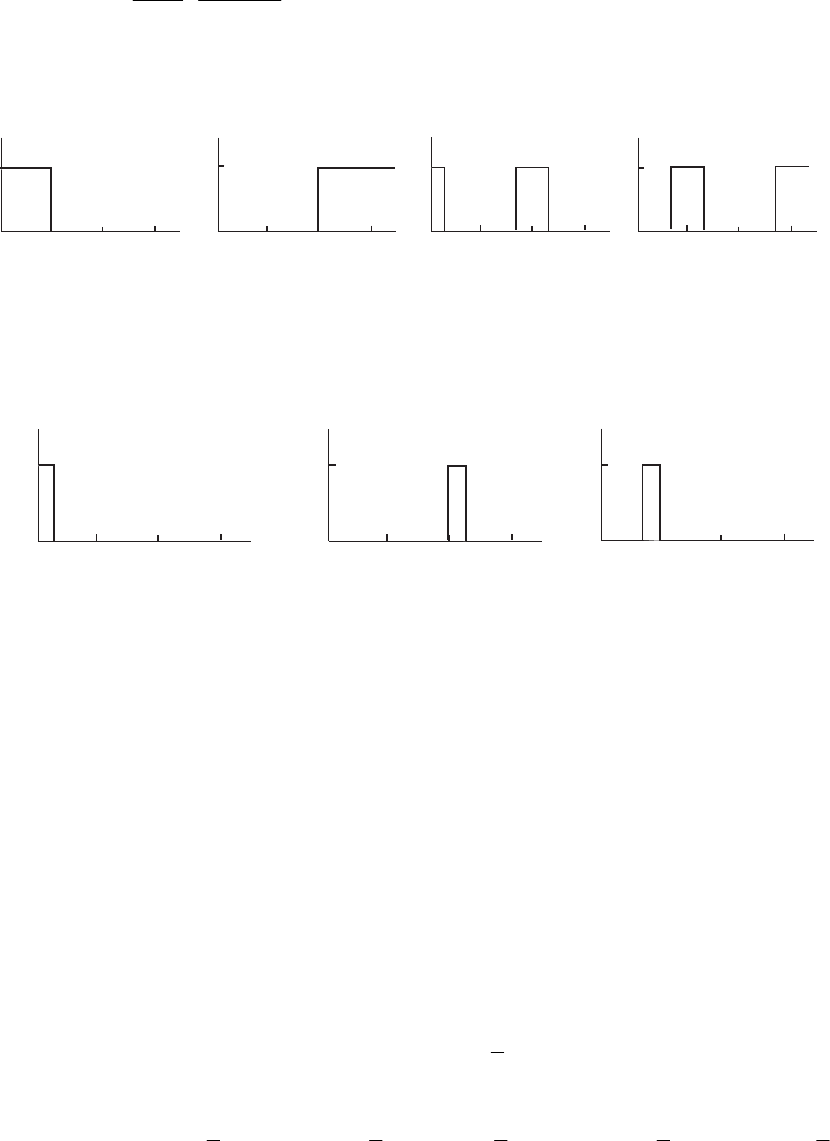
.
1
1
2
1
)( 1
1
⎟
⎟
⎠
⎞
⎜
⎜
⎝
⎛
−
−+
=−
−
z
z
zGHP β
β Therefore,
).(cos)(cos 11 αβω −== −−
c
7.51 The magnitude responses of and are shown below: ),(),(),( 3
zHzHzH −)( 3
zH −
|H(e )|
jω
1
0π
3
__
ω
π
3
__
2π
1
0π
3
__
ω
π
3
__
2π
_
|H( e )|
jω|H(e )|
j3ω
1
0π
3
__
ω
π
3
__
2π
|H( e )|
j3ω
_
1
0π
3
__
ω
π
3
__
2π
9
__
5π
9
__
7π
9
__
8π
9
__
4π
9
__
2π
π
9
__
The magnitude responses of and are shown
below:
),()(),()( 33 zHzHzHzH −)()( 3
zHzH −
1
0
π
3
__
ω
π
3
__
2π
π
9
__
|H(e )H(e )|
j3ω
jω
1
0
π
3
__
ω
π
3
__
2π
9
__
2π
|H(e )H( e )|
j3ω
_
jω
1
0
π
3
__
ω
π
3
__
2π
|H( e )H(e )|
j3ω
_
jω
9
__
7π
7.52 From Eq. (7.49) we observe that the amplitude response )(ωH
(
of a Type 1 FIR
transfer function is a function of Thus,
).cos( nω)2( kH πω +
(
will be a function of
()
).cos()2sin()sin()2cos()cos()2cos()2(cos nknnknnknnnk ωπωπωπωπω =
−
=
+=+
Hence, )(ωH
(
is a periodic function in with a period
ω.2π
Likewise, from Eq. (7.53) we observe that the amplitude response )(ωH
(
of a Type
3 FIR transfer function is a function of Thus,
).sin( nω)2( kH πω +
(
will be a
function of
()
)2cos()sin()2sin()2(sin knnknnnk πωπωπω
=
+
=
+
. Hence,
)sin()2sin()cos( nknn ωπω =+ )(ωH
(
is a periodic function in with a
period
ω
.2π
Next, from Eq. (7.52) we observe that the amplitude response )(ωH
(
of a Type 2
FIR transfer function is a function of .)(cos 2
1⎟
⎠
⎞
⎜
⎝
⎛−n
ω Thus, )4( kH πω +
(
will be a
function of
⎟
⎠
⎞
⎜
⎝
⎛−
⎟
⎠
⎞
⎜
⎝
⎛−=
⎟
⎠
⎞
⎜
⎝
⎛−+−=
⎟
⎠
⎞
⎜
⎝
⎛−+ )(4cos)(cos)(4)(cos))(4(cos 2
1
2
1
2
1
2
1
2
1nknnknnk πωπωπω
Not for sale 198

⎟
⎠
⎞
⎜
⎝
⎛−=
⎟
⎠
⎞
⎜
⎝
⎛−
⎟
⎠
⎞
⎜
⎝
⎛−− )(cos)(4sin)(sin 2
1
2
1
2
1nnkn ωπω as 1)(4cos 2
1=
⎟
⎠
⎞
⎜
⎝
⎛−nkπ and
.0)(4sin 2
1=
⎟
⎠
⎞
⎜
⎝
⎛−nkπ Hence, )(ωH
(
is a periodic function in with a period
ω.4π
Finally, from Eq. (7.54) we observe that the amplitude response )(ωH
(
of a Type
4 FIR transfer function is a function of .)(sin 2
1⎟
⎠
⎞
⎜
⎝
⎛−n
ω Thus, )4( kH πω +
(
will be a
function of
⎟
⎠
⎞
⎜
⎝
⎛−
⎟
⎠
⎞
⎜
⎝
⎛−=
⎟
⎠
⎞
⎜
⎝
⎛−+−=
⎟
⎠
⎞
⎜
⎝
⎛−+ )(4cos)(sin)(4)(sin))(4(sin 2
1
2
1
2
1
2
1
2
1nknnknnk πωπωπω
⎟
⎠
⎞
⎜
⎝
⎛−=
⎟
⎠
⎞
⎜
⎝
⎛−
⎟
⎠
⎞
⎜
⎝
⎛−+ )(sin)(4sin)(cos 2
1
2
1
2
1nnkn ωπω as 1)(4cos 2
1=
⎟
⎠
⎞
⎜
⎝
⎛−nkπ and
.0)(4sin 2
1=
⎟
⎠
⎞
⎜
⎝
⎛−nkπ Hence, )(ωH
(
is a periodic function in with a period
ω.4π
7.53 The remaining zeros are at: ;25.1
8.0
11
1
5=== z
z
;
*
26 jzz == ;22
*
37 jzz +==
;25.025.0
22
11
3
8j
jz
z+=
−
==
;25.025.0
*
89 jzz −== ;3.05.0
*
410 jzz −−==
.
34.0
3.0
34.0
5.0
,
34.0
3.0
34.0
5.0
3.05.0
11 *
1112
4
11 jzzj
jz
z−−==+−=
+−
==
4321
12
1
1
16432.50226.117576.16088.21)1()( −−−−
=
−+++−=
∏−= zzzzzzzH
k
k
1098765 7576.10226.116432.52166.247711.92166.24 −−−−−− +++−+− zzzzzz
.6088.2 1211 −− +− zz
7.54 The remaining zeros are at: ,3226.0
1.3
11
1
4=== z
z
,42
*
25 jzz −−==
,2.01.0
42
11
2
6j
jz
z−−=
+−
== ,2.01.0
7jz
−
−
=
,4.08.0
*
38 jzz −== ,5.01
4.08.0
11
3
9j
jz
z−=
+
== .1,5.01 1110 −=
+
=
zjz
43211
11
1
219.1824635.791039.78226.11)1()( −−−−−
=
+−+−=
∏−= zzzzzzzH
k
k
.8226.11039.74635.7919.1822306.1112306.111 111098765 −−−−−−− +−+−+−− zzzzzzz
Not for sale 199

7.55 The remaining zeros are at: ,599.01.0
*
14 jzz +==
1.6242, j+ 0.2711=
−
== 599.01.0
11
1
5jz
z
1.6242, j- 0.2711== *
56 zz
,4.03.0
*
27 jzz −−== 1.6, j 1.2 −−==
2
8
1
z
z
1.6, j 1.2 +−== *
89 zz
.1,1,5.0
1
,2 1110
3
103 −===== zz
z
zz
54321
32533.173338.15294.60076.12423.01)( −−−−− −+−+−= zzzzzzH
.2423.00076.15294.63338.12533.17 121110987 −−−−−− −+−+−+ zzzzzz
7.56 The remaining zeros are at: 0.2073, 0.1341 j
z
zjz −==−=
1
54
1
,4.32.2
0.2073, 0.1341 jzz +== *
56
,9.06.0,9.06.0 *
272 jzzjz −==+= 0.7692, 0.5128 j
z
z−==
2
8
1
0.7692, 0.5128 jzz +== *
89 .1,2
1
,5.0 11
3
103 =−==−= z
z
zz
54321
47073.1198577.510838.5446.193939.51)( −−−−− +−−+−= zzzzzzH
.3939.5446.190838.58577.517073.119 11109876 −−−−−− −+−++− zzzzzz
7.57 The magnitude responses of (solid line) and (dashed line) are shown
below:
)( M
zH )(
1zF
1
0
ω
M
ω
p
__ M
ω
s
__
M
2π
__
M
4π
__
M
ω
s
__
2π
_
H(e )|
jMω
|
F (e )|
jω
|
1
Hence, is a lowpass filter with a unity passband magnitude,
passband edge at and stopband edge at
)()()( 11 zFzHzG M
=
M
p/ω./ M
s
ω
The magnitude responses of (solid line) and (dashed line) are shown
below:
)( M
zH )(
2zF
Not for sale 200
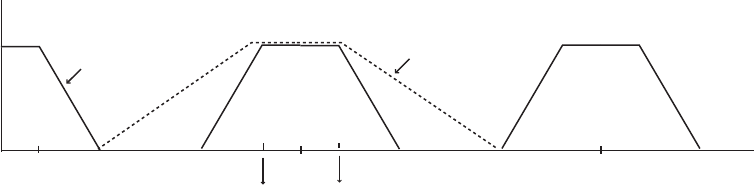
1
0
ω
M
ω
p
__ M
ω
s
__
M
2π
__
M
4π
__
M
ω
s
__
2π
_
H(e )|
jMω
|F (e )|
jω
|
2
M
ω
s
__
4π
_
M
ω
s
__
2π +
M
ω
p
__
2π
_
+
M
ω
p
__
2π
Hence, is a bandpass filter with a unity passband magnitude,
passband edges at and
)()()( 22 zFzHzG M
=
M
p/)2( ωπ −,/)2( M
p
ωπ
+
and stopband edges at
and M
s/)2( ωπ −./)2( M
s
ωπ +
7.58 and The frequency response will
exhibit generalized linear phase if it can be expressed in the form
∑
=
=
−
N
n
n
znhzH
0
][)( .][)(
0
∑
=
=
−
N
n
njj enheH ωω
)( ωj
eH
,)( βαω
ωjj eeH −−
=
(
where ),(ωH
(
the amplitude function, is a real function of ω
and α and are constants. We need to examine the case when the order
β
N
is
even and when
N
is odd separately. Without any loss of generality, assume first
Then and
. It follows then that if
.5=N,][)( 5
0
∑
=
=
−
n
n
znhzH
ωωωωωω 5432 ]5[]4[]3[]2[]1[]0[)( jjjjjj ehehehehehheH −−−−− +++++=
2/2/32/32/52/52/5 ]2[]4[]1[]5[]0[(ωωωωωω jjjjjj ehehehehehe ++++= −−−
)2/3cos(])4[]1[()2/5cos(])5[]0[(]3[ [) 2/52/3 ωω
ωω hhhheeh jj +++=+ −−
)2/3sin(])4[]1[()2/5sin(])5[]0[()2/3cos(])3[]2[( [] 2/5 ωω ωhhhhjehh j−+−+++ −
])2/3cos(])3[]2[( ωhh −+
ω
,50],5[][ ≤≤
−
=
nnhnh we
have ),()( 2/5ωω HeeH jj ω
(
−
= where
),2/cos(]2[2)2/3cos(]1[2)2/5cos(]0[2)( ωωωω hhhH ++=
(
which is a real
function of and as a result, has generalized phase. )( ωj
eH
Alternately, if ,50],5[][
≤
≤
−
−= nnhnh then we have
),()()( 2/52/5 ωω πωωω HeeHjeeH jjjj
(
(
−− == where,
),2/sin(]2[2)2/3sin(]1[2)2/5sin(]0[2)( ωωωω hhhH ++=
(
which is a real
function of and as a result, has generalized phase. )( ωj
eH
Next, assume Then and
.6=N,][)( 6
0
∑
=
=
−
n
n
znhzH ωω jj ehheH −
+= ]1[]0[)(
Not for sale 201
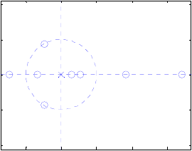
ωωωωω 65432 ]6[]5[]4[]3[]2[ jjjjj eheheheheh −−−−− +++++
][ ]3[)cos(])4[]2[()2cos(])5[]1[()3cos(])6[]0[(
3hhhhhhhe j++++++= −ωωω
ω
].[ )sin(])4[]2[()2sin(])5[]1[()3sin(])6[]0[(
3ωωω
ωhhhhhhje j−+−+−+ −
Hence, it follows that if ,60],6[][
≤
≤
−
=
nnhnh then ),()( 3ω
ωω HeeH jj
(
−
=
where ],3[)cos(]2[2)2cos(]1[2)3 hh ++ ωωcos(]0[2)( hhH += ωω
(
which is a real
function of and as a result, has generalized phase. )( ωj
eH
Alternately, if ,50],6[][
≤
≤
−
−= nnhnh then we have
),()()( 33 ωω πωωω HeeHjeeH jjjj
(
(
−− == where,
),sin(]2[2)2sin(]1[2)3sin(]0[2)( ωωωω hhhH ++=
(
which is a real function of and
as a result, has generalized phase. )( ωj
eH
7.59 Type 1:
{}
.][ abcdedcbanh
−
−
−−=
Type 2:
{}
.][ abcdeedcbanh
−
−
−−=
Type 3:
{}
.0][ abcdeedcbanh
−
−
−
−−=
Type 4:
{}
.][ abcdeedcbanh
−
−
−
−−=
7.60 (a) Type 1:
{}
.134686431]}[{
−
−
−
−=nh Hence,
.34686431)( 87654321 −−−−−−−− +−−+++−−= zzzzzzzzzH
The zero plot obtained using the M-file zplane is shown below:
-1 0 1 2 3
-2
-1
0
1
2
8
Real Part
Imaginary Part
It can be seen from the above that a complex-conjugate zero pair on the unit circle
appear singly and real zeros appear in mirror-image symmetry. There are no zeros
at
.1=z
(b) Type 2:
{}
.1346886431]}[{
−
−
−
−=nh Hence,
.346886431)( 987654321 −−−−−−−−− +−−++++−−= zzzzzzzzzzH
The zero plot obtained using the M-file zplane is shown below:
Not for sale 202
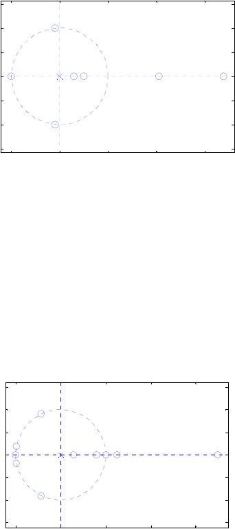
-1 0 1 2 3
-1.5
-1
-0.5
0
0.5
1
1.5
39
Real Part
I
mag
i
nary
P
ar
t
From the above zero plot it can be seen that complex-conjugate zero pairs on the
unit circle appear singly and real zerosappear in mirror-image symmetry. There are
3 zeros at
.1−=z
(c) Type 3:
{}
.13468086431]}[{
−
−
−
−
−=nh Hence,
.346886431)( 1098764321 −−−−−−−−− −++−−++−−= zzzzzzzzzzH
The zero plot obtained using the M-file zplane is shown below:
-1 0 1 2 3
-1.5
-1
-0.5
0
0.5
1
1.5
10
Real Part
I
mag
i
nary
P
ar
t
From the above zero plot it can be seen that complex-conjugate zero pairs on the
unit circle appear singly and real zeros appear in mirror-image symmetry. There is
one zero at and one zero at
.1−=z.1
=
z
(d) Type 4:
{}
.1346886431]}[{
−
−
−
−
−=nh Hence,
.346886431)( 987654321 −−−−−−−−− +−−++++−−= zzzzzzzzzzH
The zero plot obtained using the M-file zplane is shown below:
Not for sale 203
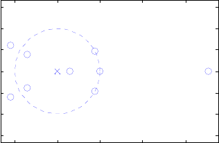
-1 0 1 2 3
-1.5
-1
-0.5
0
0.5
1
1.5
9
Real Part
I
mag
i
nary
P
ar
t
From the above zero plot it can be seen that complex-conjugate zeros appear in
mirror-image symmetry, a complex-conjugate zero pair on the unit circle appear
singly, and real zeros appear in mirror-image symmetry. There is one zero at .1
=
z
7.61 is of Type 1 and hence, it has a symmetric impulse response of odd length
)(
1zH
Let α be the constant term of Then, the coefficient of the highest
.12 +N).(
1zH
power of of is also
1−
z)(
1zH .α
)(
2zH is of Type 2 and hence, it has a symmetric impulse response of even length
Let be the constant term of Then, the coefficient of the highest
.2Mβ).(
2zH
power of of is also .
1−
z)(
2zH β
is of Type 3 and hence, it has an anti-symmetric impulse response of odd
length Let
)(
3zH
.12 +R
γ
be the constant term of Then, the coefficient of the
highest power of of is
).(
3zH
1−
z)(
3zH .γ
−
)(
4zH is of Type 4 and hence, it has an anti-symmetric impulse response of even
length Let be the constant term of Then, the coefficient of the
highest power of of is
.2Kδ).(
4zH
1−
z)(
4zH .δ
−
(a) The length of is
)()( 11 zHzH 141)12()12(
+
=
−
+
+
+
NNN which is odd.
The constant term of is and the coefficient of the highest power of
of is also . Hence, is of Type 1.
)()( 11 zHzH 2
α
1−
z)()( 11 zHzH 2
α)()( 11 zHzH
(b) The length of is
)()( 21 zHzH )(21)2()12( MNMN
+
=
−
+
+
which is even.
The constant term of is and the coefficient of the highest power of
of is also . Hence, is of Type 2.
)()( 21 zHzH αβ
1−
z)()( 21 zHzH αβ )()( 21 zHzH
(c) The length of is )()( 31 zHzH 1)(21)12()12( +
+
=
−
+
+
+
RNRN which is
odd. The constant term of is )()( 31 zHzH α
γ
and the coefficient of the highest
power of of is
1−
z)()( 31 zHzH .αγ
−
. Hence, is of Type 3. )()( 31 zHzH
Not for sale 204
(d) The length of is
)()( 41 zHzH )(21)2()12( KNKN
+
=
−
+
+
which is even.
The constant term of is and the coefficient of the highest power of
of is . Hence, is of Type 4.
)()( 41 zHzH αδ
1−
z)()( 41 zHzH αδ−)()( 41 zHzH
(e) The length of is
)()( 22 zHzH 141)2()2(
−
=
−
+
MMM which is odd. The
constant term of is and the coefficient of the highest power of
of is also . Hence, is of Type 1.
)()( 22 zHzH 2
β
1−
z)()( 22 zHzH 2
β)()( 22 zHzH
(f) The length of is )()( 33 zHzH 141)12()12(
+
=
−
+
+
+
RRR which is odd. The
constant term of is and the coefficient of the highest power of
of is also . Hence, is of Type 1.
)()( 33 zHzH 2
γ
1−
z)()( 33 zHzH 2
γ)()( 33 zHzH
(g) The length of is
)()( 44 zHzH 141)2()2(
−
=
−
+
KKK which is odd. The
constant term of is and the coefficient of the highest power of
of is also . Hence, is of Type 1.
)()( 44 zHzH 2
δ
1−
z)()( 44 zHzH 2
δ)()( 44 zHzH
(h) The length of is )()( 32 zHzH )(21)12()2( RMRM
+
=
−
+
+
which is even.
The constant term of is and the coefficient of the highest power of
of is . Hence, is of Type 4.
)()( 32 zHzH βγ
1−
z)()( 32 zHzH βγ−)()( 32 zHzH
(i) The length of is )()( 43 zHzH )(21)2()12( KRKR
+
=
−
+
+
which is even. The
constant term of is and the coefficient of the highest power of
of is also . Hence, is of Type 2.
)()( 43 zHzH γδ
1−
z)()( 43 zHzH γδ )()( 43 zHzH
7.62 (a) has complex
conjugate zeros at
).2667.11(1.22.45.31.2)( 2121
1−−−− +−=+−= zzzzzF )(
1zF
.1426.18333.0 jz
±
= To generate a linear-phase transfer
function , we need to multiply with the factor which has
complex-conjugate zeros situated in the –plane with a mirror-image symmetry
with respect to the zeros of . Hence, resulting in
)(zH )(
1zF )(
2zF
z
)(
1zF ,667.12)( 21
2−− +−= zzzF
)257778.752(1.2)()()( 4321
21 −−−− +−+−== zzzzzFzFzH
.2.45.103333.165.102.4 4321 −−−− +−+−= zzzz
(b)
321
13.32.22.54.1)( −−− +−+= zzzzF
has complex conjugate zeros ).3571.25714.17143.31(4.1 321 −−− +−+= zzz )(
1zF
Not for sale 205

at .7035.00.2524 jz
±
=and a real zero at 4.2192.
−
To generate a linear-phase
transfer function , we need to multiply with the factor which has
situated in the –plane with a mirror-image symmetry with respect to the zeros of
. Hence, resulting in
)(zH )(
1zF )(
2zF
z
)(
1zF ,7143.35714.13571.2)( 321
2−−− ++−= zzzzF
321
21 8214.228265.51837.73571.2(4.1)()()( −−− +−+== zzzzFzFzH
)3571.21837.78265.5 654 −−− ++− zzz 321 95.311671.80571.103.3 −−− +−+= zzz
.3.30571.101571.8 654 −−− ++− zzz
7.63 We rewrite the polynomial in the form . Its
)(zH ∏
=
−λ−= N
i
i
NzKzzf
1
)()(
logarithmic differential is given by ∑
=λ−
+−= N
ii
zz
N
zf
zf
1
'1
)(
)( or
∑∑ == λ−
+−=
λ−
+−= N
ii
N
iiz
N
z
z
N
zf
zf
z
11
'
)/(1
1
)(
)( .
For any we can expand the above in a Taylor series as
||max|| i
i
zλ>
[]
∑
=
+λ+λ+λ++−=
′N
i
iii zzzN
zf
zf
z
1
32 ...)/()/()/(1
)(
)( , or
...)/()/()/(
)(
)( 3
3
2
21 +++++−=
′zSzSzSNN
zf
zf
z (1)
where
.
1
∑
=
λ= N
i
m
im
S
Now set So that .][...]2[]1[]0[)( 21 N
zNhzhzhhzf −−− ++++=
N
N
zNhzhzhh
zNNhzhzh
zf
zf
z−−−
−
−
−
++++
+++
−=
′
][...]2[]1[]0[
][...]2[2]1[
)(
)(
21
21 . (2)
Equations (1) and (2) pertain to the same quantity hence identically the right hand
sides are the same. Thus the following convolution holds true
{}
{
}
{
}
][,],2[2],1[,,,,0O][,],2[],1[],0[ 321
*nNhhhSSSNhhhh KKK
−
=
Hence the Newton Identities.
7.64 The root moments of of are defined as
m
S)1()1()( 1
1
1
1
21 −
=
−
=∏∏ β−α−= zzKzH
n
i
i
n
i
i
Not for sale 206

For real the complex roots occur in conjugate pairs .
21
11
∑∑ ==
β+α= n
i
m
i
n
i
m
im
S),(zH
and hence, their corresponding powers are also in this form, thereby making their
sum entirely real.
(a) If is minimum-phase, then
)(zH 0
=
β
i for all and
,i.1<αi Therefore as
will decrease exponentially.
m
Sm ,∞→
(b) Write and then expand
in a Laurent series. The second summation can be re-expressed as
)1ln()1ln(ln)(ln 1
1
1
1
21 −
=
−
=∑−+
∑−+= zzKzH
n
i
i
n
i
iβα
)(ln zH
.1)ln()1ln( 1
1
1
1
22
⎟
⎟
⎠
⎞
⎜
⎜
⎝
⎛−−=− −
=
−
=∑∑
i
n
i
i
n
i
i
z
zz β
ββ Hence,
)ln(ln)(ln 2
1
∑
=
−+= n
i
i
KzH β).1()1(ln 21
1
1
1
2
i
n
i
n
i
i
z
zzn β
α∑∑ =
−
=
−+−+− Now, appear
in complex conjugate pairs, hence, can be written as where
is real.
i
β
)ln(ln 2
1
∑
=
−+ n
i
i
Kβ1
ln K
1
K
However, ⎥
⎥
⎦
⎤
⎢
⎢
⎣
⎡+++−=− −−
−− L
3
)(
2
)(
)1ln(
3121
11 zz
zz ii
ii
αα
αα and
.
3
)/(
2
)/(
1ln
32
⎥
⎥
⎦
⎤
⎢
⎢
⎣
⎡+++−=
⎟
⎟
⎠
⎞
⎜
⎜
⎝
⎛−L
ii
ii
zz
zz ββ
ββ These two Taylor series expansions are
valid since 1
1<
−
z
i
α and 1/ <
i
zβ on .1=z Thus,
∑
∞
=
−
−⎟
⎟
⎠
⎞
⎜
⎜
⎝
⎛+−=
1
1
21
ln)(ln
m
m
N
m
m
N
mz
m
S
z
m
S
KzH where and
On
∑
=
=1
1
1
n
i
m
i
N
m
Sα.
1
2
1
∑
=
−
−=n
i
m
i
N
m
Sβ
1=z we have )(
)()( ωθ
ω
ωj
ez eHzH j
(
=
= and therefore,
).(ln)()(ln 2
11
1
21
ωωθω ωω jne
m
S
e
m
S
KjH
mm
jm
N
m
jm
N
m−+
⎟
⎟
⎠
⎞
⎜
⎜
⎝
⎛∑∑
+−=+ ∞
=
∞
=
−
−
(
On equating real and imaginary parts of the equation we arrive at
),cos(ln)(ln
1
1
21
ωω m
m
SS
KH
m
N
m
N
m
∑⎟
⎟
⎠
⎞
⎜
⎜
⎝
⎛+
−= ∞
=
−
(
).sin()(
1
2
21
ωωωθ m
m
SS
n
m
N
m
N
m
∑⎟
⎟
⎠
⎞
⎜
⎜
⎝
⎛−
+−= ∞
=
−
Not for sale 207

(c) From the expression for the phase as given above, it can be seen that the second
term contributes non-linear components to the phase, whilst the only term which is
linear is the first Thus to have linear phase we must have (1) and (2)
The second condition means that the zeros of outside the unit circle
must be the same in number as those inside the unit circle and the zeros outside must be
at locations of the zeros inside the unit circle.
).( 2ωn−0
2≠n
.
21 N
m
N
mSS −
=)(zH
7.65 (a) .
1
)( 1
1
1
1
1−
−
+
+
=
zd
zd
zA Thus, 2/
1
2/
2/2/
1
1
1
11
)( ωω
ωω
ω
ω
ω
jj
jj
j
j
j
ede
eed
ed
ed
eA −
−
−
−
+
+
=
+
+
=
,
2β
β
β
α
αj
j
j
e
e
e== − where
Therefore, phase is given by
)
2/2/
1ωωβ
αjjj eede −
+=
).2/sin()1()2/cos()1( 11 ωω −++= djd
.)2/tan(
1
1
tan22)(
1
1
1⎟
⎟
⎠
⎞
⎜
⎜
⎝
⎛
+
−
−== −ωβωθ d
d Now, for small values of and
Hence, the approximate expression for the phase at low frequencies
is given by
xxx ≅)tan(,
.)(tan 1xx ≅
−
.
1
1
21
1
2)(
1
1
1
1ω
ω
ωθ ⎟
⎟
⎠
⎞
⎜
⎜
⎝
⎛
+
−
−=
⎟
⎟
⎠
⎞
⎜
⎜
⎝
⎛
+
−
−≅ d
d
d
d Therefore, the approximate
expression for the phase delay is given by
1
1
1
1)(
)( d
d
p+
−
≅=−= δ
ω
ωθ
ωτ samples.
(b) For samples,
5.0=δ.
3
1
5.1
5.0
1
1
1=== +
−
δ
δ
d Then, .
1
)( 1
1
1
3
1
3
1
−
−
+
+
=
z
z
zA Thus, the
exact phase delay is given by ω
ωθ
ωτ )(
)( −=
p⎟
⎠
⎞
⎜
⎝
⎛
=+
−
)2/tan(
1
1
1
1
2ω
ωd
d
()
.)2/tan(5.0
2ω
ω
=
For a sampling rate of 20 kHz, the normalized angular frequency equivalent to 1
kHz is .05.0
20
1=
1020
10
3
3== ×
o
ω The exact phase delay at is thus
o
ω
500078.0)025.0tan(5.0()2/tan(5.0()( 05.0
22 === oop o
ωωτ ω samples, which is
seen to be very close to the desired phase delay of samples.
5.0
00.2 0.4 0.6 0.8 1
0.5
0.6
0.7
0.8
0.9
1
ω
/
π
Phase delay, in samples
00.05 0.1 0.15 0.2
0.4
0.45
0.5
0.55
ω
/
π
Ph
ase
d
e
l
ay,
i
n samp
l
es
Not for sale 208

7.66 ωω
ωω
ωω
ωω
ω
jj
jj
jj
jj
j
edde
eded
eded
eedd
eA −
−
−−
−−
++
++
=
++
++
=
21
12
2
21
2
12
21
)(
(
)
()
.
sin)1(cos)1(
sin)1(cos)1(
)sin(sin)coscos(
)sinsin()coscos(
221
221
221
221
ωω
ωω
ωωωω
ωωωω
−−++
−+
+
+
=
−+++
+
+++
=djdd
djdd
djdd
djdd
Therefore, .tan2)( cos)1(
sin)1(
1
21
2⎟
⎠
⎞
⎜
⎝
⎛
=ωθ ω++
ω−
−
dd
d Now,
ω
−=
ω
ωθ
−=ωτ 2
)(
)(
p⎟
⎠
⎞
⎜
⎝
⎛
ω++
ω−
−
cos)1(
sin)1(
1
21
2
tan dd
d. For ωωω
=
≅
sin,0 and
Then,
.1cos =ω.tan)( )1(
)1(
1
2
21
2⎟
⎠
⎞
⎜
⎝
⎛
−=ωτ ++
ω−
−
ωdd
d
p Also, for
Hence,
.tan,0 1xxx ≅≅ −
.)( 1
)1(2
)1(
)1(
2
21
2
21
2
++
−
++
ω−
ω−=−=ωτ dd
d
dd
d
p Now, substituting ⎟
⎠
⎞
⎜
⎝
⎛
=δ+
δ−
1
2
12d and
,
)1)(2(
)1)(2(
2δ+δ+
δ−δ−
=d we can easily show that .
1
21
)1
2
(2 δ=− ++
−
dd
d
7.67 Since is non-minimum phase but causal, it will have some zeros outside the
unit circle. Let be one such zero. We can then write
)(zG
α=z)1)(()( 1−
−= zzPzG α
.)*)((
)*(
1
1
1
1
⎟
⎟
⎠
⎞
⎜
⎜
⎝
⎛
+α−= −
−
+α−
α−
−
z
z
zzP Note that ⎟
⎟
⎠
⎞
⎜
⎜
⎝
⎛
−
−
+α−
α−
)*(
1
1
1
z
z is a stable first-order
allpass function. If we carry out this operation for all zeros of that are outside
the unit circle, we can write
)(zG
)()()( zAzHzG
=
where will have all zeros inside
the unit circle and will thus be a minimum phase function and will be a product of
stable first-order allpass functions, and hence an allpass function.
)(zH
7.68 .
)48.0)(65.0(
)55.2)(1.23(
)(
2
+−
++−
=zz
zzz
zH In order to correct for magnitude distortion we
require the transfer function to satisfy the following property
)(zG
.
)(
1
)( ω
ω
j
j
eH
eG = Hence, one possible solution is
.
)55.2)(1.23(
)48.0)(65.0(
)(
1
)( 2++−
+
−
==
zzz
zz
zH
zGd Note that the coefficients of the pole
factor in the denominator of do not satisfy the condition of
Eq. (7.139) and hence, has roots outside the unit circle making unstable.
)55.2( 2++ zz )(zGd
)(zGd
To develop a stable transfer function with magnitude response same as , we
multiply it with the stable allpass function
)(zGd
15.25
55.2
2
2
++
++
zz
zz resulting in the transfer
Not for sale 209

function )15.25)(1.23(
)48.0)(65.0(
)( 2++−
+
−
=
zzz
zz
zG which is the desired stable solution
satisfying the condition .1)()( =
ωω jj eHeG
7.69 (a) where is an allpass function. Then,
Hence,
),()()( zAzHzG =)(zA ).(lim]0[ zGg
z∞→
=
|)(lim||)(lim||)(lim||)()(lim||)(lim|]0[ zHzAzHzAzHzGg
zzzzz ∞→∞→∞→∞→∞→ ≤===
because
|)(lim| zH
z∞→
≤1|)(lim|
<
∞→ zA
zbecause of Property 2 of stable allpass
function (see Eq. (7.20)). Hence, .]0[]0[ hg ≤
(b) If is a zero of then
1
λ),(zH ,1
1<λ since is a minimum-phase causal
stable transfer function. As has all zeros inside the unit circle, we can write
It follows that is also a minimum-phase causal
transfer function.
),(zH
)(zH
).1)(()( 1
1−
−= zzBzH λ)(zB
Now consider the transfer function .
1
)())(()( 1
1
1*
1
1*
1⎟
⎟
⎠
⎞
⎜
⎜
⎝
⎛
−
−
=−= −
−
−
z
z
zHzzBzF
λ
λ
λ If
and denote, respectively, the inverse –transforms of
and then we get and
],[],[ nbnh ][nf z),(),( zBzH
),(zF ⎩
⎨
⎧
≥−−
=
=,1],1[][
,0],0[
][
1nnbnb
nb
nh λ
⎪
⎩
⎪
⎨
⎧
≥−−
=
=.1],1[][
,0],0[
][ *
1
*
1
nnbnb
nb
nf
λ
λ
Consider .][][]0[]0[][][
1
2
1
22
2
*
1
2
0
2
0
2∑
−
∑
+−=
∑
−
∑
=
====
m
n
m
n
m
n
m
n
nfnhbbnfnh λε
Now, ],[]1[*][*]1[]1[][][ *
11
22
1
22 nbnbnbnbnbnbnh −−−−−+= λλλ and
].[]1[*][*]1[]1[][][ *
11
222
1
2nbnbnbnbnbnbnf −−−−−+= λλλ Hence,
∑⎟
⎠
⎞
⎜
⎝
⎛−−−
∑⎟
⎠
⎞
⎜
⎝
⎛−++−=
==
m
n
m
n
nbnbnbnbbb
1
222
1
1
22
1
222
1
2]1[][]1[][]0[]0[ λλλε
.][)1( 22
1mbλ−= Since ,0,1
1>< ελ i.e., .][][
0
2
0
2∑
>
∑==
m
n
m
n
nfnh Hence,
.][][
0
2
0
2∑
≥
∑==
m
n
m
n
ngnh
Not for sale 210

7.70 )6.0)(4.0(
)14)(32(
)( −+
−+
=zz
zz
zH has a zero at 2
3
=z which is outside the unit circle and is
thus a non-minimum phase transfer function. To develop a minimum phase transfer
function such that
)(zG ,)()( ωω jj eHeG = we multiply with an allpass function
32
23
+
+
z
z and arrive at )6.0)(4.0(
)14)(23(
)( −+
−
+
=zz
zz
zG which is minimum phase.
The first 5 impulse response of are
)(zH
,40},904.0032.324.16.118{]}[{
≤
≤
=nnh and
The first
5 impulse response of are
)(zG
.40},016.1248.236.24.712{]}[{
≤
≤
=nng
210.4154209.3831204.3296198.76144
210.1078209.2906200.0976198.56
m
n
m
n
ng
nh
m
0
2
0
2
][
64][
43210
Σ
Σ
=
=
It follows from the above that ∑
>
∑==
m
n
m
n
nhng
0
2
0
2][][ for
.1≥m
7.71 See Example 7.14.
(a) .)1()( 22
4
1−
+= zzHBS Thus, .)1()1()( 22
4
1
22
4
1
2−−− −−=+−= zzzzHBP
(b) ).61)(1()( 422
16
1−−− −+−+= zzzzHBS Thus,
)4641()61)(1()( 8642
16
1
422
16
1
4−−−−−−−− +−+−=−+−+−= zzzzzzzzzHBP
.)1(
16
142−
−=z
(c) ).3143()1()( 4222
32
1−−− −+−+= zzzzHBS Thus,
).381083()3143()1()( 8642
32
1
4222
32
1
4−−−−−−−− +−+−=−+−+−= zzzzzzzzzHBP
7.72 and ),()()( 100 zAzAzH += ),()()( 101 zAzAzH
−
=
where and are
allpass functions of orders
)(
0zA )(
1zA
M
and ,
N
respectively. Hence, the orders of
and are Now, we can write
)(
0zH
)(
1zH .NM +)(
)(
)(
0
1
0
0zD
zDz
zA
M
−
−
= and
Not for sale 211

.
)(
)(
)(
1
1
1
1zD
zDz
zA
N−−
= Then,
)()(
)()()()(
)(
)(
)(
10
1
101
1
0
0zDzD
zDzDzzDzDz
zD
zP
zH
NM
−
−
−− +
== and
.
)()(
)()()()(
)(
)(
)(
10
1
101
1
0
1zDzD
zDzDzzDzDz
zD
zQ
zH
NM
−
−
−− −
== Since is of degree
)(zP
N
M
+and
[
]
)()()()()( 1
1
0
1
10
)(1)( zDzDzzDzDzzzPz NMNMNM −−+−−+− +=
Hence, is symmetric.
Similarly, one can show that is anti-symmetric.
).()()()()( 1
101
1
0zPzDzDzzDzDz NM =+= −−−− )(zP
)(zQ
7.73 )]()([)( 10
2
1
0zAzAzH += and )].()([)( 10
2
1
1zAzAzH −= Thus,
)()()()( 1
11
1
00 −− +zHzHzHzH )]()()][()([ 1
1
1
010
4
1−− ++= zAzAzAzA
)]()()][()([ 1
1
1
010
4
1−− −−+ zAzAzAzA
)]()()()()()()()([ 1
11
1
01
1
10
1
00
4
1−−−− +++= zAzAzAzAzAzAzAzA
)]()()()()()()()([ 1
11
1
01
1
10
1
00
4
1−−−− +−−+ zAzAzAzAzAzAzAzA
.1)]()()()([ 1
11
1
00
2
1=+= −− zAzAzAzA Thus, 1)()( 2
1
2
0=+ ωω jj eHeH
implying that and form a power-complementary pair. )(
0zH )(
1zH
7.74 )()()()()()()( *
10
*
01
*
00
4
1
2
0{ωωωωωωω jjjjjjj eAeAeAeAeAeAeH ++=
Since and are allpass functions,
and Therefore,
.)()( }
*
11 ωω jj eAeA+)(
0zA )(
1zA
)(
00
)( ωφ
ωj
jeeA =.)( )(
11ωφ
ωj
jeeA =
{}
12
4
1
2
0))(
1
)(
0
())(
1
)(
0
(
)( ≤+++ −−−
=ωφωφωφωφ
ωjj ee
j
eH as maximum values of
and are is stable since and
are stable allpass functions. Hence, is BR.
))(
1
)(
0
(ωφωφ −j
e))(
1
)(
0
(ωφωφ −− j
e.1 )(
0zH )(
0zA )(
1zA
)(
0zH
7.75 ∑
=−
=
1
0
).(
1
)( M
k
kzA
M
zH Thus, ∑∑
=−
=
−
=
−− 1
0
1
0
1
2
1.)()(
1
)()( M
k
M
r
rk zAzA
M
zHzH Hence,
.1
1
)( 1
0
1
0
))()((
2
2≤
∑∑
=−
=
−
=
−
M
r
M
k
j
jrk
e
M
eH ωφωφ
ω Also, is stable since
are stable allpass functions. Hence, is BR.
)(zH
,10),( −≤≤ MizAi)(zH
Not for sale 212

7.76 )](1[)( 2
1zAzHBP −= and )](1[)( 2
1zAzHBS += where
21
21
)1(1
)1(
)( −−
−−
++−
++−
=
zz
zz
zA
ααβ
αβα is an allpass function. Note
and from the solution of Problem 7.73, )()()( zAzHzH BSBP =+
.1)()( 22 =+ ωω j
BS
j
BP eHeH Hence, )(zH
B
P and are doubly-
complementary pair.
)(zHBS
7.77 On the unit circle, this reduces to
or, equivalently,
.)()()()( 11 KzHzHzHzH =−−+ −−
,)()()()( KeHeHeHeH jjjj =−−+ −− ωωωω
,)()( 22
KeHeH jj =−+ ωω as is a real-coefficient transfer function. Now,
)(zH
.)()( 2
)(
2ωπω +
=− jj eHeH Hence, for ,2/πω
=
the power-symmetric condition
reduces to .)()( 2
)2/(
2
2/ KeHeH jj =+ +πππ Since is a real-coefficient
transfer function,
)(zH
2
)( ωj
eH is an even function of and thus, ,ω
.)()( 2
)2/2(
2
2/ πππ −
=jj eHeH As a result, ,)(2 2
2/ KeH j=
π from which we
obtain ,log10)(log202log10 10
2/
1010 KeH j=+ π or,
3log10)(log20 10
2/
10 −= KeH jπ dB.
7.78 Therefore,
).()()( 2
1
12
0zAzzAzH −
+=
)]()([)]()([)()()()( 2
1
2
0
2
1
12
0
11 −−−−− ++=−−+ zzAzAzAzzAzHzHzHzH
)]()([)]()([ 2
1
2
0
2
1
12
0)()()()( zAzzAzAzzA −−−−−−+ −
)()()()()()()()( 2
1
2
1
2
1
2
0
2
0
2
1
12
0
2
0−−−−− +++= zAzAzAzAzzAzAzzAzA
as
,4)()()()()()()()( 2
1
2
1
2
1
2
0
2
0
2
1
12
0
2
0=+−−+ −−−−− zAzAzAzAzzAzAzzAzA
.1)()()()( 2
1
2
1
2
0
2
0== −− zAzAzAzA
Not for sale 213

7.79 42
54321
2.01.01
1.05.005.005.05.01.0
)( −−
−−−−−
−+
−++++−
=
zz
zzzzz
zH ],)([ 12
2
1−
+= zzA
where 21
21
2.01.01
1.02.0
)( −−
−−
−+
++−
=
zz
zz
zA is a stable allpass function. Thus,
])(][)([)()()()( 212
4
1
11 zzAzzAzHzHzHzH ++=−−+ −−−−
.1])(][)([ 212
4
1=−−+ −− zzAzzA
7.80 (a) Thus,
.5.065.421)( 54321 −−−−− ++++−= zzzzzzHa)()( 1−
zHzH aa
)5.065.421)(5.065.421( 543254321 zzzzzzzzzz ++++−++++−= −−−−−
.5.025.65.225.625.2225.65.0 53135 −−− ++++++= zzzzzz
Next, we compute
=−− −)()( 1
zHzH aa
)5.065.421)(5.065.421( 543254321 zzzzzzzzzz −+−++−+−++= −−−−−
.5.025.65.225.625.2225.65.0 53135 −−− −−−+−−−= zzzzzz
Hence,
.125)()()()( 11 =−−+ −− zHzHzHzH aaaa
(b) .21)( 542
4
15
1
2
1−−−− +−++= zzzzzHb Thus,
)()( 1−
zHzH aa
⎟
⎠
⎞
⎜
⎝
⎛+−++
⎟
⎠
⎞
⎜
⎝
⎛+−++= −−−−− 542
4
15
2
1
542
4
15
1
2
1
12121)()( zzzzzzzzzHzH bb
.27375.03125.20375.072 53135 −−− ++++++= zzzzzz
Next, we compute
=−− −)()( 1
zHzH bb
)275.35.01)(275.35.01( 5425421 zzzzzzzz −−+−−−+−= −−−−
.27375.03125.20375.072 53135 −−− −−−+−−−= zzzzzz
Hence,
.625.40)()()()( 11 =−−+ −− zHzHzHzH aaaa
7.81 .)1()1)(1()()( 112222121 −−−− ++=+++=++= czdczbzababzabzbzazHzH
Thus, and Now,
bac 2
=).1( 22 bad += )()()()( 11 −− −−+ zHzHzHzH
Therefore, This
condition is satisfied by
.2
11 dczdczczdcz =−+−++ −− .1)1(22 22 =+= bad
.
)1(2
1
2
b
a
+
= For .,1 2
1
== ab Other solutions include
,,1 2
1
=−= ab and .,10 10
1
== ab
Since is a first-order causal FIR transfer function, is
also a first-order causal FIR transfer function. Now,
)(zH )()( 11 −− −−= zHzzG
Not for sale 214

)]()][([)()()()()()( 11111 zzHzHzzHzHzGzGzHzH −−−−+=+ −−−−−
Hence, and are power
complementary.
.1)()()()( 11 =−−+= −− zHzHzHzH )(zH )(zG
7.82 ])1()1()1()[()()( 2
2
1
21
2
2
2
121
2
2
11 −−−− ++++++++++= zdzddddzddzdczdczzHzH
Thus, )1(2)1(2)()()()( 21
2
2
2
21
11 [dcdzddzdcdzHzHzHzH ++++=−−+ −−
Hence, we require .1)1()1( ]
2
21
2
2
2
2
2
1=++++++ −− zdcdzddddd
and Solving these two
equations we arrive at
0)1( 212 =++ dcddd .1)1()1(2 2
2
2
121 =+++++ ddddcd
)12)(1( 2
2
2
1222
2
ddddd
d
c−−−+
=, and
.
12
1
2
2
2
12 ddd
d−−−
−= For ,1
21
=
=
dd we get 2
1
−=c and
.1=d
Since is a third-order causal FIR transfer function, is
also a third-order causal FIR transfer function. Now,
)(zH )()( 13 −− −−= zHzzG
)]()][([)()()()()()( 313111 zHzzHzzHzHzGzGzHzH −−−−+=+ −−−−−
Hence, and are power
complementary.
.1)()()()( 11 =−−+= −− zHzHzHzH )(zH )(zG
7.83 )]()([)( 10
2
1
0zAzAzH += and )],()([)( 10
2
1
1zAzAzH −= where and
are stable allpass transfer functions. From these two equations we obtain
)(
0zA )(
1zA
),()()( 010 zAzHzH =+ and ).()()( 110 zAzHzH
=
−
Moreover, we have
.1)()( 2
1
2
0=+ ωω jj eHeH Choose and
)()( 2
00 zHzG =).()( 2
11 zHzG −=
Hence, 1)()()()( 2
1
2
010 =+=+ ωωωω jjjj eHeHeGeG .
7.84 (a) ).31()( 1
4
1
1−
+= zzH Therefore, ⇒++= −− )31)(31()()( 1
16
1
1
11 zzzHzH
.
16
cos610
)( 2
1
ω
ω+
=
j
eH Thus, 0sin)( 8
3
2
1<−=
⎟
⎟
⎠
⎞
⎜
⎜
⎝
⎛ω
ω
ωj
eH
d
d for
Thus,
.0 πω <≤
)(
1ωj
eH is a montonically decreasing function of .
ω
The maximum value
of 1)(
1=
ωj
eH is at and the minimum value is at ,0=ω.
π
ω
=
Hence, is
BR.
)(
1zH
(b) ).2.11()( 1
2.2
1
2−
−= zzH Therefore, ⇒−−= −− )2.11)(2.11()()( 1
84.4
1
1
22 zzzHzH
Not for sale 215

.
84.4
cos4.244.2
)( 2
2
ω−
=
ωj
eH Thus, 0sin)( 84.4
4.2
2
2>ω=
⎟
⎟
⎠
⎞
⎜
⎜
⎝
⎛
ω
ωj
eH
d
d for
Thus,
.0 πω <≤ )(
2ωj
eH is a montonically increasing function of The
maximum value of
.ω
1)(
2=
ωj
eH is at ,
π
=
ω
and the minimum value is at
Hence, is BR.
.0=ω
)(
2zH
(c) ),()(
)1)(1(
)1)(1(
)( 21
11
3zGzG
zz
zH =
β+α+
β−α+
=−− where α+
α+
=−
1
1
)(
1
1
z
zG and
.
1
1
)(
1
2β+
β−
=−
z
zG Now, .
)1(
cos21
)( 2
2
2
1α+
ωα+α+
=
ωj
eG Thus,
0
)1(
sin2
)( 2
2
1<
α+
ωα
−=
⎟
⎟
⎠
⎞
⎜
⎜
⎝
⎛
ω
ωj
eG
d
d for
π
<
ω
≤
0 as .0>
α
As a result, )(
1ωj
eG is
a monotonically decreasing decreasing function of .
ω
The maximum value of
1)(
1=
ωj
eG is at and the minimum value is at ,0=ω.
π
ω
=
Hence, is BR.
Likewise,
)(
1zG
.
)1(
cos21
)( 2
2
2
2β+
ωβ−β+
=
ωj
eG Thus, 0
)1(
sin2
)( 2
2
2>
β+
ωβ
=
⎟
⎟
⎠
⎞
⎜
⎜
⎝
⎛
ω
ωj
eG
d
d
for as Thus,
π<ω≤0.0>β )(
2ωj
eH is a montonically increasing function of
The maximum value of
.ω1)(
2=
ωj
eG is at ,
π
=
ω
and the minimum value is at
Hence, is BR. Therefore,
.0=ω )(
2zG )()()( 233 zGzGzH
=
is also BR.
(d) ⎟
⎟
⎠
⎞
⎜
⎜
⎝
⎛−
⎟
⎟
⎠
⎞
⎜
⎜
⎝
⎛+
⎟
⎟
⎠
⎞
⎜
⎜
⎝
⎛−
=
−+−
=−−−−−−
5.1
5.01
2.1
2.01
3.1
3.01
34.2
)5.01)(2.01)(3.01(
)(
111111
4
zzzzzz
zH .
Since each individual factor on the right-hand side is BR, is BR.
)(
4zH
7.85 (a)
()
,)()(
2
1
2.4
2.41
1
2
1
2.4
6.26.2
)( 10
1
1
1
1
1zAzA
z
z
z
z
zH +=
⎟
⎟
⎠
⎞
⎜
⎜
⎝
⎛
+
+
+=
+
+
=−
−
−
− where
and 1)(
0=zA 1
1
12.4
2.41
)( −
−
+
+
=
z
z
zA are stable allpass transfer functions. Therefore,
is BR (See solution of Problem 7.74).
)(
1zH
Not for sale 216

(b)
()
,)()(
2
1
2.4
2.41
1
2
1
2.4
6.16.1
)( 10
1
1
1
1
2zAzA
z
z
z
z
zH −=
⎟
⎟
⎠
⎞
⎜
⎜
⎝
⎛
+
+
−=
+
−
=−
−
−
− where
and 1)(
0=zA 1
1
12.4
2.41
)( −
−
+
+
=
z
z
zA are stable allpass transfer functions. Therefore,
is BR (See solution of Problem 7.74).
)(
2zH
(c) ⎟
⎟
⎠
⎞
⎜
⎜
⎝
⎛
++
++
−=
++
−
=−−
−−
−−
−
21
21
21
2
38.04.01
4.08.0
1
2
1
8.04.01
)1(1.0
)(
zz
zz
zz
z
zH
()
)()(
2
1
10 zAzA −= , where 1)(
0
=
zA and 21
21
18.04.01
4.08.0
)( −−
−−
++
++
=
zz
zz
zA are stable
allpass transfer functions. Therefore, is BR (See solution of Problem 7.74). )(
3zH
(d) ⎟
⎟
⎠
⎞
⎜
⎜
⎝
⎛
++
++
+=
++
++
=−−
−−
−−
−−
21
21
21
21
4425
524
1
2
1
425
5.425.4
)(
zz
zz
zz
zz
zH
()
)()(
2
1
10 zAzA += ,
where and 1)(
0=zA 21
21
1425
524
)( −−
−−
++
++
=
zz
zz
zA are stable allpass transfer functions.
Therefore, is BR (See solution of Problem 7.74).
)(
4zH
7.86 Since and are LBR,
)(
1zA )(
2zA 1)(
1=
ωj
eA and .1)(
2=
ωj
eA Thus,
and Now,
)(
11
)( ωφ
ω=j
jeeA .)( )(
22ωφ
ω=j
jeeA
()
.
)(
1)(
1
2
12ωφ−
ω=
⎟
⎟
⎠
⎞
⎜
⎜
⎝
⎛j
jeA
eA
A
Thus,
(
)
.1
)(
12=
ωφ− j
eA Thus, ⎟
⎟
⎠
⎞
⎜
⎜
⎝
⎛
)(
1
2
1zA
A is LBR.
7.87 .
)(1
)(
)( ⎟
⎟
⎠
⎞
⎜
⎜
⎝
⎛
α+
α+
=zG
zG
zzF Thus, ⎟
⎟
⎠
⎞
⎜
⎜
⎝
⎛
α+
α+
=
⎟
⎟
⎠
⎞
⎜
⎜
⎝
⎛
α+
α+
=ωφ
ωφ
ω
ω
ω
ωω
)(
)(
1)(1
)(
)( j
j
j
j
j
jj
e
e
e
eG
eG
eeF
since is LBR. Therefore,
)(zG
2
)(
)(
2
1
)( ωφ
ωφ
ω
α+
α+
=j
j
j
e
e
eF
()()
()()
.1
)(cos(21
)(cos(21
)(sin()(cos(1
)(sin()(cos(
2
2
22
22 =
α+ωφα+
α+ωφα+
=
ωφα+ωφα+
ωφ+α+ωφ
= Let be a pole
of Then
λ=z
).(zF ,
1
)(
)(
)( α
−=
α−
α−
=
λ=
λ= z
zzFz
zzF
zG or, ./1)( α=λG If ,1<α then
Not for sale 217

,1)( >λG which is satisfied by the LBR if
)(zG .1<λ Hence, is LBR. The
order of is same as that of
)(zF
)(zF ).(zG
can be realized in the form of a two-pair constrained by the transfer function
as shown below:
)(zG
)(zF
F(z)
G(z)
X
1
Y
1
X
2
Y
2
To this end, we express in terms of arriving at
)(zG )(zF
,
)(
)(
)(1
)(
)( 1
1
zFBA
zFDC
zFz
zFz
zG +
+
=
α−
+α−
=−
− where and are the chain
parameters of the two-pair. Comparing the above two expressions we get
and The corresponding transfer parameters are
given by and
,,, CBA D
,1=A
,,
1α−=α−= −CzB .
1−
=zD
12
122111 )1(,1, −
α−==α−= zttt .
1
22 −
α= zt
7.88 Let .)( )(
1⎟
⎠
⎞
⎜
⎝
⎛
=zA
GzF Now, being LBR, Thus,
)(zA .)( )(ωφω =jj eeA
).()( )(
)(
1ωφ−ω =
⎟
⎟
⎠
⎞
⎜
⎜
⎝
⎛
=ω
j
eA
jeGGeF j Since is a BR function,
)(zG .1)( ≤
ωj
eG
Hence, .1)(
)(
1≤
⎟
⎟
⎠
⎞
⎜
⎜
⎝
⎛
=ω
ω
j
eA
jGeF
Let be a pole of . Hence, will be a BR function if
ξ=z)(zF )(zF .1<ξ Let
be a pole of Then this pole is mapped to the location of by
the relation
λ=z).(zG ξ=z)(zF
,
)(
1λ=
ξ=z
zA or .
1
)( λ
=ξA Hence, 1
1
)( >
λ
=ξA because of Eq.
(7.20). This implies, .1<λ Thus, is a BR function.
)(zG
7.89 (a) .
2.4
)1(6.1
)(,
2.4
)1(6.2
)( 1
1
1
1
−
−
−
−
+
−
=
+
+
=
z
z
zG
z
z
zH Now,
.1
2.4
2.4
2.4
)1(6.1
2.4
)1(6.2
)()( 1
1
1
1
1
1=
+
+
=
+
−
+
+
+
=+ −
−
−
−
−
−
z
z
z
z
z
z
zGzH Next,
z
z
z
z
z
z
z
z
zGzGzHzH +
−
⋅
+
−
+
+
+
⋅
+
+
=+ −
−
−
−
−−
2.4
)1(6.1
2.4
)1(6.1
2.4
)1(6.2
2.4
)1(6.2
)()()()( 1
1
1
1
11
.1
2.464.182.4
2.464.182.4
2.464.182.4
)56.212.556.2()76.652.1376.6(
11
11
11
11 =
++
++
=
++
−+−+++
=−−
−−
−−
−−
zz
zz
zz
zzzz
Not for sale 218

Thus, .1)()( 22 =+ ωω jj eGeH Hence, and are both allpass-
complementary and power complementary. As a result, they are doubly
complementary.
)(zH )(zG
(b) .
8.04.01
9.04.09.0
)(,
8.04.01
)1(1.0
)( 21
21
21
2
−−
−−
−−
−
++
++
=
++
−
=
zz
zz
zG
zz
z
zH Now,
21
21
21
21
21
2
8.04.01
4.08.0
8.04.01
9.04.09.0
8.04.01
)1(1.0
)()( −−
−−
−−
−−
−−
−
++
++
=
++
++
+
++
−
=+
zz
zz
zz
zz
zz
z
zGzH
implying that and are allpass complementary. Next, )()()()( 11 −− +zGzGzHzH
2
2
21
21
2
2
21
2
8.04.01
9.04.09.0
8.04.01
9.04.09.0
8.04.01
)1(1.0
8.04.01
)1(1.0
zz
zz
zz
zz
zz
z
zz
z
++
++
⋅
++
++
+
++
−
⋅
++
−
=−−
−−
−−
−
212
21222
8.072.08.172.08.0
)81.072.078.172.081.0()01.002.001.0(
−−
−−−
++++
+++++−+−
=
zzzz
zzzzzz
.1
8.072.08.172.08.0
8.072.08.172.08.0
212
212 =
++++
++++
=−−
−−
zzzz
zzzz Hence and are also
power complementary. As a result, they are doubly complementary.
)(zH )(zG
7.90 (a)
[
)(1
2
1
325
)22(2
)( 21
21
zA
zz
zz
zHa+=
++
++
=−−
−−
]
where 21
21
325
523
)( −−
−−
++
++
=
zz
zz
zA is an
allpass function. Hence, the power complementary transfer function of is
given by
)(zHa
[]
.
325
1
325
523
1
2
1
)(1
2
1
)( 21
2
21
21
−−
−
−−
−−
++
−
=
⎥
⎥
⎦
⎤
⎢
⎢
⎣
⎡
++
++
−=−=
zz
z
zz
zz
zAzGa
(b) )24)(5.01(2
35.75.73
488
35.75.73
)( 211
321
321
321
−−−
−−−
−−−
−−−
+++
+++
=
+++
+++
=
zzz
zzz
zzz
zzz
zHb
[]
)()(
2
1
10 zAzA += where 21
21
024
421
)( −−
−−
++
++
=
zz
zz
zA and 1
1
15.01
5.0
)( −
−
+
+
=
z
z
zA are
allpass functions. Hence, the power complementary transfer function of is
given by
)(zHb
[]
.
488
5.25.21
)()(
2
1
)( 321
321
10 −−−
−−−
+++
++−−
=−=
zzz
zzz
zAzAzGb
7.91 From Eq. (7.126) we have ., 221221 DXCYYBXAYX
+
=
+
=
From the first
equation, .
1
212 X
A
B
X
A
Y−= Substituting this in the second equation we get
Not for sale 219

.
1
212211 X
A
BCAD
X
A
C
DXX
A
B
X
A
CY −
+=+
⎟
⎠
⎞
⎜
⎝
⎛−= Comparing the last two
equations with Eq. (7.123) we arrive at .,
1
,, 22211211 A
B
t
A
t
A
BCAD
t
A
C
t−==
−
==
From Eq. (7.123) we have ., 22212122121111 XtXtYXtXtY
+
=
+
=
From the
second equation we get .
1
2
21
2
21
22
1Y
t
X
t
t
X+−= Substituting this in the first
equation we get
.
1
2
21
22112112
2
21
11
2122
21
2
21
22
111 X
t
tttt
Y
t
t
XtY
t
X
t
t
tY −
+=+
⎟
⎟
⎠
⎞
⎜
⎜
⎝
⎛+−= Comparing the
last two equations with Eq. (7.126) we arrive at ,,
1
21
22
21 t
t
B
t
A−==
.,
21
22112112
21
11
t
tttt
D
t
t
C−
==
7.92 From Eq. (7.128a) we note A
BCAD
t
−
=
12 and .
1
21 A
t= Hence, imply
2112 tt =
.1=− BCAD
7.93 where =
. The transfer matrices of the two two-pairs are given by
τ and τ The corresponding chain
matrices are obtained using Eq. (7.128b) and are given by Γ and
Γ Therefore, the chain matrix of the Γ-cascade is given by
,
1
)1(
,
1
)1(
"
2
"
1
1
2
12
22
"
2
"
1
'
2
'
1
1
1
12
11
'
2
'
1
⎥
⎥
⎦
⎤
⎢
⎢
⎣
⎡
⎥
⎥
⎦
⎤
⎢
⎢
⎣
⎡
−
−
=
⎥
⎥
⎦
⎤
⎢
⎢
⎣
⎡
⎥
⎥
⎦
⎤
⎢
⎢
⎣
⎡
⎥
⎥
⎦
⎤
⎢
⎢
⎣
⎡
−
−
=
⎥
⎥
⎦
⎤
⎢
⎢
⎣
⎡
−
−
−
−
X
X
zk
zkk
Y
Y
X
X
zk
zkk
Y
Y
⎥
⎥
⎦
⎤
⎢
⎢
⎣
⎡
"
2
"
1
X
X
⎥
⎥
⎦
⎤
⎢
⎢
⎣
⎡
'
2
'
1
Y
Y
⎥
⎥
⎦
⎤
⎢
⎢
⎣
⎡
−
−
=−
−
1
1
12
11
11
)1(
zk
zkk .
1
)1(
1
2
12
22
2⎥
⎥
⎦
⎤
⎢
⎢
⎣
⎡
−
−
=−
−
zk
zkk
⎥
⎥
⎦
⎤
⎢
⎢
⎣
⎡
=−
−
1
1
1
1
11
zk
zk
.
1
1
2
1
2
2⎥
⎥
⎦
⎤
⎢
⎢
⎣
⎡
=−
−
zk
zk
Γ1Γ Next using Eq.
(7.128a) we arrive at the transfer matrix of the Γ-cascade as
.
111
21
21
1
21
1
1
1
2
1
21
1
2
1
2
1
1
1
1
2⎥
⎥
⎦
⎤
⎢
⎢
⎣
⎡
++
++
=
⎥
⎥
⎦
⎤
⎢
⎢
⎣
⎡
⎥
⎥
⎦
⎤
⎢
⎢
⎣
⎡
=−−−
−−−
−
−
−
−
zzkkzkk
zkzkzkk
zk
zk
zk
zk
Not for sale 220

τ .
1
)(
1
1
1
)1)(1(
1
1
21
1
12
1
1
21
1
21
2
2
2
1
2
1
21
1
21
⎥
⎥
⎥
⎥
⎥
⎦
⎤
⎢
⎢
⎢
⎢
⎢
⎣
⎡
+
+
+
+
−−
+
+
=
−
−−
−
−
−
−
−
zkk
zkkz
zkk
zkk
kkz
zkk
zkk
7.94 where The
chain matrices of the two two-pairs are given by Γ and
Γ The corresponding transfer matrices are obtained using Eq.
(7.128a) and are given by τ and τ The
transfer matrix τ of the τ-cascade is therefore given by
,
11
"
2
"
2
1
2
1
2
"
1
"
1
'
2
'
2
1
1
1
1
'
1
'
1
⎥
⎥
⎦
⎤
⎢
⎢
⎣
⎡
⎥
⎥
⎦
⎤
⎢
⎢
⎣
⎡
=
⎥
⎥
⎦
⎤
⎢
⎢
⎣
⎡
⎥
⎥
⎦
⎤
⎢
⎢
⎣
⎡
⎥
⎥
⎦
⎤
⎢
⎢
⎣
⎡
=
⎥
⎥
⎦
⎤
⎢
⎢
⎣
⎡
−
−
−
−
X
Y
zk
zk
Y
X
X
Y
zk
zk
Y
X.
"
1
"
1
'
2
'
2
⎥
⎥
⎦
⎤
⎢
⎢
⎣
⎡
=
⎥
⎥
⎦
⎤
⎢
⎢
⎣
⎡
Y
X
X
Y
⎥
⎥
⎦
⎤
⎢
⎢
⎣
⎡
=−
−
1
1
1
1
11
zk
zk
.
1
1
2
1
2
2⎥
⎥
⎦
⎤
⎢
⎢
⎣
⎡
=−
−
zk
zk
⎥
⎥
⎦
⎤
⎢
⎢
⎣
⎡
−
−
=−
−
1
1
12
11
11
)1(
zk
zkk .
1
)1(
1
2
12
22
2⎥
⎥
⎦
⎤
⎢
⎢
⎣
⎡
−
−
=−
−
zk
zkk
τ2τ
Using Eq. (7.128b) we thus
arrive at the chain matrix of the τ-cascade as
=
1⎥
⎥
⎦
⎤
⎢
⎢
⎣
⎡
−
−
−
−
1
2
12
22
1
)1(
zk
zkk
⎥
⎥
⎦
⎤
⎢
⎢
⎣
⎡
−
−
−
−
1
1
12
11
1
)1(
zk
zkk
.
)1()1(
)1()1()1(
22
12
12
1
11
21
2
21
22
12
12
2
1
21
⎥
⎥
⎦
⎤
⎢
⎢
⎣
⎡
=−+−−
−−−−+
−−−−
−−−
zkkzkzzkk
kkzkkzkzkk
Γ = .
)1(
)1(
1
1
21
2
1
21
2
2
1
21
1
21
12
1
1
21
1
21
⎥
⎥
⎥
⎥
⎥
⎦
⎤
⎢
⎢
⎢
⎢
⎢
⎣
⎡
−−
−+
−
−+−
−
−
−
−
−
−
−−
−
zkk
z
zkk
kzkk
zkk
zkzkk
zkk
7.95 (a) Analyzing Figure P7.10(a) we obtain and
Hence, the transfer matrix is given by τ Using Eq. (7.128b)
we then arrive at the chain matrix Γ
2
1
12 XzkXY m−
−=
.)1()( 2
12
12
1
2
1
12
1
21 XzkXkXzXzkXkXzYkY mmmmm −−−− −+=−=+=
.
1
)1(
1
12
⎥
⎥
⎦
⎤
⎢
⎢
⎣
⎡
−
−
=−
−
zk
zkk
m
mm
.
1
1
1
⎥
⎥
⎦
⎤
⎢
⎢
⎣
⎡
=−
−
zk
zk
m
m
Not for sale 221

(b) Labeling the output variable of the top left adder connected to input we
then analyze Figure P7.10(b) and obtain
and Hence,
the transfer matrix of the two-pair is given by τ Using
Eq. (7.128b) we then arrive at the chain matrix Γ
1
V1
X
1112
1
11 ),( XVYXzXkV m+=−= −
,)1( 2
1
1XzkXk mm −
−+= .)1( 2
1
12
1
12 XzkXkXzVY mm −− −+=+=
.
)1(
1
1
1
⎥
⎥
⎦
⎤
⎢
⎢
⎣
⎡
−
−+
=−
−
zkk
zkk
mm
mm
.
1
1
)1(
11
⎥
⎥
⎥
⎥
⎦
⎤
⎢
⎢
⎢
⎢
⎣
⎡
−
−
−
−
=
−
mm
m
m
m
m
kk
k
k
zk
k
7.96 Solving )](1[
)(
)( 1zHkz
kzH
zG
m
m
−
−
=− for we get
)(zH .
)(1
)(
)( 1
1
zGzk
zGzk
zH
m
m
−
−
+
+
=
For the constrained two-pair .
)(
)(
)( zGBA
zGDC
zH ⋅+
⋅
+
= Comparing the last two
equations we thus get Substituting these
values of the chain parameters in Eq. (7.128a) we get
,1,, 1=== −AzDkC m.
1−
=zkB m
.,1
1
),1(, 1
2221
21
1211 −− −=−===−=
−
=== zk
A
B
t
A
tkz
A
BCAD
tk
A
C
tmmm
7.97 (a) .
)(1
)(
)( 1
1
zGz
zGz
zH −
−
+
+
=
α
α For the constrained two-pair .
)(
)(
)( zGBA
zGDC
zH ⋅+
⋅+
=
Comparing the last two equations we thus get .,1,, 11 −− ==== zBAzDC αα
(b)
7.98 From the results of Problem 7.95, Part (a), we observe that the chain matrix of the
-th lattice two-pair is given by Γ Thus, the chain matrix
of the cascade of the three lattice two-pairs is given by
i.3,2,1,
1
1
1=
⎥
⎥
⎦
⎤
⎢
⎢
⎣
⎡
=−
−
i
zk
zk
i
i
i
Γ
⎥
⎥
⎦
⎤
⎢
⎢
⎣
⎡
⎥
⎥
⎦
⎤
⎢
⎢
⎣
⎡
⎥
⎥
⎦
⎤
⎢
⎢
⎣
⎡
=−
−
−
−
−
−
1
3
1
3
1
2
1
2
1
1
1
11
11
zk
zk
zk
zk
zk
zk
cascade
.
)()()()1(
)()(1
2
32
11
2
1
31
1
32
11
321
2
32
1
1
1
2
1
3
1
32
1
1
1
32
⎥
⎥
⎦
⎤
⎢
⎢
⎣
⎡
++++++
++++++
=−−−−−−−
−−−−−−−
zkkzzkzkkzkkzzkkk
zkkzkzkzkzkkzkzkk
From Eq. (7.135a) we obtain BA
DC
zA +
+
=)(
3
Not for sale 222

32
32132
1
3212311
3
1
2
321231
1
32132
)()(
)()(1
−−−
−−−
+++++++
+++++++
=
zzkkkkkzkkkkkkk
zkzkkkkkkzkkkkk which is seen to be
an allpass function.
7.99 Let
Thus, and
.)(1)1)(1(1)( 2
21
1
21
1
2
1
1
2
2
1
1−−−−−− ++−=−−=++= zzzzzdzdzD λλλλλλ
212 λλ=d).( 211 λλ
+
−
=d For stability, .2,1,1 =< i
i
λ As a result,
.1
212 <= λλd
Case 1: Complex poles: In this case, Now,
.0
2>d.
*
12 λλ =
.
2
4
,2
2
11
21
ddd −±−
=
λλ Hence, and will be complex, if In
this case,
1
λ2
λ.4 2
2
1dd <
.4
22
2
12
1
1dd
j
d−+−=λ Thus,
(
)
.14 2
2
12
2
1
4
1
2
1<=−+= ddddλ
Consequently, if the poles are complex and ,1
2
<
d then they are inside the unit
circle.
Case 2: Real poles. In this case we get .2,1,11
=
<
<
−
i
i
λ Since, ,1<
i
λ it follows
then .2
211 <+< λλd Now, ,1
2
4
12
2
11 <
−±−
<− ddd or
.24 12
2
1ddd +<−± It is not possible to satisfy the inequality on the right hand
side with a minus sign in front of the square root as it would imply then
Therefore,
.2
1−<d
,24 12
2
1ddd +<− or or ,444 1
2
12
2
1dddd ++<− .1 21 dd +
<
−
(7-x)
Similarly, ,1
2
42
2
11 −<
−±− ddd or .24 12
2
1ddd +−>−± Again it is not
possible to satisfy the inequality on the right hand side with a plus sign in front of
the square root as it would imply then Therefore,
.2
1>d,24 12
2
1ddd +−>−−
or ,24 12
2
1ddd −<− or or equivalently, ,444 1
2
12
2
1dddd −+<−
.1 21 dd
+
<
(7-y)
Combining Eqs. (7-x) and (7-y) we get .1 21 dd +<
7.100 (a) Since
.5.0,75.0)25.075.01(4)( 21
21 ==⇒++= −− ddzzzDa
15.0
2<=d and .175.0,5.11 212 ddd +<==+ Hence, both roots of are
inside the unit circle.
)(zDa
Not for sale 223

(b) Since .5.0,5.0)5.05.01(2)( 21
21 ==⇒++= −− ddzzzDb15.0
2<=d and
.15.0,5.11 212 ddd +<==+ .175.0,5.11 212 ddd +<==+ Hence, both
roots of are inside the unit circle. )(zDb
(c) .,)1(3)( 3
4
2
3
4
1
2
3
4
1
3
4−==⇒−+= −− ddzzzDc Since ,1
3
4
2>=d at least
one root of is outside the unit circle. )(zDc
(d) .,)1(3)( 3
1
2
6
1
1
2
3
1
1
6
1−=−=⇒−−= −− ddzzzDd Since 1
3
1
2<=d and
.1,1 2
3
1
1
3
2
2ddd +<==+ Hence, both roots of are inside the unit circle. )(zDd
7.101 (a) .
25.05.075.01
75.05.025.0
)( 321
321
3−−−
−−−
+++
+++
=
zzz
zzz
zA Note .125.0
3<=k Using Eq.
(7.148) we arrive at .
1
)( 2
3
1
1
3
2
21
3
2
3
1
2−−
−−
++
++
=
zz
zz
zA Here, .1
3
1
2<=k Continuing this
process we get .
5.01
5.0
)( 1
1
1−
−
+
+
=
z
z
zA Finally, .15.0
1<=k Since ,3,2,1,1 =< iki
is stable. )(zH a
(b) .
1
)( 3
3
1
2
3
2
1
3
2
32
3
2
1
3
2
3
1
3−−−
−−−
−−+
++−−
=
zzz
zzz
zA Note .1
3
1
3<=k Using Eq. (7.148) we
arrive at .
5.05.01
5.05.0
)( 21
21
2−−
−−
−+
++−
=
zz
zz
zA Here, .15.0
2<=k Continuing this
process we get .
1
1
)( 1
1
1−
−
+
+
=
z
z
zA Finally, .1
1=k Since 1
k is not less than 1,
is not stable. )(zH b
(c) .
1
)( 4
6
1
3
2
1
2
3
2
1
3
2
43
3
2
2
3
2
1
2
1
6
1
4−−−−
−−−−
+
−+++
+++−
=
zzzz
zzzz
zA Note .1
6
1
4<=k Using Eq. (7.148)
we get .
1
)( 321
321
3−−−
−−−
+++
+++
=
zzz
zzz
zA 0.62860.80.7714
0.77140.80.6286 Note .16286.0
3<=k
Using Eq. (7.148) we next get .
1
)( 21
21
2−−
−−
++
++
=
zz
zz
zA 0.52090.444
0.4440.5209 Here,
Not for sale 224

.1209.0
2<=k Continuing this process we get .
1
)( 1
1
1−
−
+
+
=
z
z
zA 0.2919
0.2919 Finally,
.12919.0
1<=k Since ,4,3,2,1,1 =< iki is stable. )(zH c
(d) .
2.04.06.08.01
8.06.04.02.0
)( 4321
43
3
2
21
4−−−−
−−−−
+
++++
+++
=
zzzz
zzzz
zA Note .12.0
4<=k Using
Eq. (7.148) we get .
1
)( 321
321
3−−−
−−−
+++
+++
=
zzz
zzz
zA 0.250.50.75
0.750.50.25 Note .125.0
3<=k
Using Eq. (7.148) we next get .
1
)( 2
3
1
1
3
2
21
3
2
3
1
2−−
−−
++
++
=
zz
zz
zA Here, .1
3
1
2<=k
Continuing this process we get .
1
)( 1
1
1−
−
+
+
=
z
z
zA 0.5
0.5 Finally, .15.0
1<=k Since
,4,3,2,1,1 =< iki is stable. )(zH d
(e) .
1.02.03.05.07.01
7.05.03.02.0
)( 54321
54321
1.0
5−−−−−
−−−−−
+
+++++
++++
=
zzzzz
zzzzz
zA Note .11.0
5<=k
Using Eq. (7.148) we get
.
1
)( 4321
4321
4−−−−
−−−−
+
++++
+++
=
zzzz
zzzz
zA 0.13130.25250.47470.6869
0.68690.47470.25250.1313 Note
.101313
4<=k Using Eq. (7.148) we next get
.
1
)( 321
321
3−−−
−−−
+++
+++
=
zzz
zzz
zA 0.16520.41960.6652
0.66520.41960.1652 Note .11652.0
3<=k Using
Eq. (7.148) we next get .
1
)( 21
21
2−−
−−
++
++
=
zz
zz
zA 0.31850.6126
0.61260.3185 Here,
.13185.0
2<=k Continuing this process we get .
1
)( 1
1
1−
−
+
+
=
z
z
zA 0.4646
0.4646 Finally,
.14646.0
1<=k Since ,5,4,3,2,1,1 =< iki is stable. )(zH e
7.102 (a) .
1.02.04.06.08.01
8.06.04.02.0
)( 54321
54321
1.0
5−−−−−
−−−−−
+
+++++
++++
=
zzzzz
zzzzz
zA Note
.11.0
5<=k Using Eq. (7.148) we get
.
1
)( 4321
4321
4−−−−
−−−−
+
++++
+++
=
zzzz
zzzz
zA 0.12120.34340.56570.7879
0.78790.56570.34340.1212 Note
.11211.0
4<=k Using Eq. (7.148) we next get
Not for sale 225

.
1
)( 321
321
3−−−
−−−
+++
+++
=
zzz
zzz
zA 0.25160.50450.7574
0.75740.50450.2516 Note .12516.0
3<=k Using
Eq. (7.148) we next get .
1
)( 21
21
2−−
−−
++
++
=
zz
zz
zA 0.33510.6730
0.67300.3351 Here,
.13351.0
2<=k Continuing this process we get .
1
)( 1
1
1−
−
+
+
=
z
z
zA 0.5041
0.5041 Finally,
.15041.0
1<=k Since ,5,4,3,2,1,1 =< iki has all roots inside the unit
circle..
)(zDa
(b) .
25.05.01
875.075.05.025.0
)( 54321
54321
5−−−−−
−−−−−
+
−++++
++++−
=
zzzzz
zzzzz
zA 0.6250.750.875
0.625 Note
.125.0
5<=k Using Eq. (7.148) we get
.
1
)( 4321
4321
4−−−−
−−−−
+
++++
+++
=
zzzz
zzzz
zA 0.76670.86670.96671.0667
1.06670.96670.86670.7667 Note
.17667.0
4<=k Using Eq. (7.148) we next get
.
1
)( 321
321
3−−−
−−−
+++
+++
=
zzz
zzz
zA 0.11860.54720.9757
0.97570.54720.1186 Note .1
3<= 0.1186k Using
Eq. (7.148) we next get .
1
)( 21
21
2−−
−−
++
++
=
zz
zz
zA 0.43760.9238
0.92380.4376 Here,
.14376.0
2<=k Continuing this process we get .
1
)( 1
1
1−
−
+
+
=
z
z
zA 0.6426
0.6426 Finally,
.1
1<= 0.6426k Since ,5,4,3,2,1,1 =< iki has all roots inside the unit
circle..
)(zDb
M7.1 The MATLAB code fragments used to simulate the FIR filter are
b = [3.8461 -6.3487 3.8461];zi = [0 0];
n=0:49;x1 = cos(0.3*n);x2=cos(0.6*n);
y = filter(b,1,x1+x2,zi);
The plot generated by the above program is shown below:
010 20 30 40
-1
-0.5
0
0.5
1
1.5
2
Time index n
A
mp
lit
u
d
e
y[n]
x1[n]
x2[n]
Not for sale 226
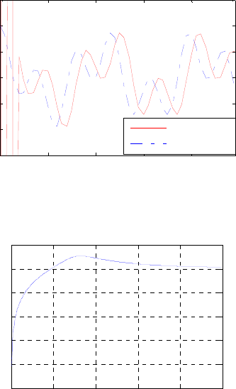
M7.2 The MATLAB code fragments used to simulate the FIR filter are:
b =[17.7761 -58.7339 83.8786 -58.7339 17.7761];
n = 0:49; x1 = cos(0.3*n);x2=cos(0.5*n);x3=cos(0.8*n);
y = filter(b,1,x1+x2+x3);
The plot generated by the above program is shown below:
010 20 30 40
-3
-2
-1
0
1
2
3
Time index n
Amplitude
y[n]
x1[n]+x3[n]
M7.3 The gain response of is shown below:
)(zH
00.2 0.4 0.6 0.8 1
-100
-80
-60
-40
-20
0
20
ω
/
π
Gain, dB
M7.4 (a) The MATLAB code fragments used to evaluate is
shown below:
)()()()( 11 −− −−+ zHzHzHzH
n = [1 -2 3.5];n = [n fliplr(n)];
d = [8 0 -2 0 -1 0];
k = 0:5;n1 = (-1).^k.*n;
a = conv(n,fliplr(n))+conv(n1,fliplr(n1));
b = conv(d,fliplr(d));
The numerator and denominator of are given by
the vectors and :
)()()()( 11 −− −−+ zHzHzHzH
ab
a =
0 -8 0 -14 0 69 0 -14 0 -8 0
b =
0 -8 0 -14 0 69 0 -14 0 -8 0
Hence verifying the power-complementary
property of and
1)()()()( 11 =−−+ −− zHzHzHzH
)(zH ).( zH
−
Not for sale 227
(b) The MATLAB code fragments used to evaluate is
shown below:
)()()()( 11 −− −−+ zHzHzHzH
n = [1 1.5 5.25 7.25];n = [n fliplr(n)];
d = [12 0 13 0 4.5 0 0.5 0];
k = 0:7;n1 = (-1).^k.*n;
a = conv(n,fliplr(n))+conv(n1,fliplr(n1));
b = conv(d,fliplr(d));
The numerator and denominator of are given by
the vectors and :
)()()()( 11 −− −−+ zHzHzHzH
ab
a =
Columns 1 through 10
0 6.0000 0 60.5000 0 216.7500
0 333.5000 0 216.7500
Columns 11 through 15
0 60.5000 0 6.0000 0
b =
Columns 1 through 10
0 6.0000 0 60.5000 0 216.7500
0 333.5000 0 216.7500
Columns 11 through 15
0 60.5000 0 6.0000 0
Hence verifying the power-complementary
property of and
1)()()()( 11 =−−+ −− zHzHzHzH
)(zH ).( zH
−
M7.5 The magnitude and phase responses of are shown below:
)(zH
00.2 0.4 0.6 0.8 1
0
0.2
0.4
0.6
0.8
1
ω
/
π
Magnitude
00.2 0.4 0.6 0.8 1
-4
-2
0
2
4
ω
/
π
phase, radians
From the magnitude response plot given above it can be seen that represents a
highpass filter. The difference equation representation of is given by
)(zH
]3[2004.0]2[7976.0]1[7074.0][
−
+
−
+−+ nynynyny
].3[2031.0]2[2588.0]1[2588.0][2031.0 −
−
−
+
−
−= nxnxnxnx
M7.6 The magnitude and phase responses of are shown below:
)(zH
Not for sale 228
00.2 0.4 0.6 0.8 1
0
1
2
3
4
5
ω
/
π
Magnitude
00.2 0.4 0.6 0.8 1
-4
-2
0
2
4
ω
/
π
phase, radians
From the magnitude response plot given above it can be seen that represents a
bandpass filter. The difference equation representation of is given by
)(zH
][.][.][.][.][ 470150353540274971164020 −
+
−
+
−
+−+ nynynynyny
].3[2031.0]2[2588.0]1[2588.0][2031.0 −
−
−
+
−
−= nxnxnxnx
M7.7 Here Using Eq. (7.85) we obtain first
.5=K1.7411.
=
C Then using Eq. (7.84)
we obtain From Eq. (7.71) we get the transfer function of the
lowpass filter as
0.3779.−=α
.
)
)( 1
-1
0.37791
z0.6889(1
−
−
+
=
z
zH LP A plot of the gain response of a
cascade of 5 lowpass filters is shown below:
00.2 0.4 0.6 0.8 1
-30
-25
-20
-15
-10
-5
0
5
ω
/
π
Gain, in dB
0.4 0.42 0.44 0.46 0.48 0.5 0.52
-5
-4
-3
-2
-1
ω
/
π
Gain, in dB
Passband Details
M7.8 From the solution of Problem 7.46 we observe
,
cos
)coscos(sin
C
CCC
c
ccc
−ω−
ω+ω−−−ω
=α 1
12 2
where
Substituting in the second equation we get
.
/)( KK
C1
2−
=
6=K1.7818.
=
C Next, substituting
this value of C and
π
=ω 40.
c in the first equation we arrive at
From Eq. (7.74) we get the transfer function of the lowpass filter as
0.5946.=α
.
)
)( 1
-1
0.59461
0.7973(1
−
z
−
−
=
z
zH HP A plot of the gain response of a cascade of 6
highpass filters is shown below:
Not for sale 229
00.2 0.4 0.6 0.8 1
-30
-25
-20
-15
-10
-5
0
5
ω
/
π
Gain, in dB
0.2 0.3 0.4 0.5 0.6
-12
-10
-8
-6
-4
-2
ω
/
π
Gain, in dB
Passband Details
M7.9 Using Eq. (7.73b) we obtain 0.1584.
−
=
α
Sunstituting this value of α in Eqs.
(7.71) and (7.74) we get 1
-1
0.15841
z0.5792(1
−
−
+
=
z
zH LP
)
)( and .
)
)( 1
-1
0.15841
z0.4208(1
−
−
−
=
z
zH HP
Plots of the magnitude responses of )(zH
LP
and )(zH
HP
along with the plot of
the magnitude response of )()( zHzH
HP
LP
+
and plot of
22 )()( ωω +j
HP
j
LP eHeH are shown below verifying the doubly complementary
property of )(zH
LP
and ).(zH
HP
00.2 0.4 0.6 0.8 1
0
0.2
0.4
0.6
0.8
1
ω
/
π
Magniitude
H
LP
(z) H
HP
(z)
00.2 0.4 0.6 0.8 1
0
0.2
0.4
0.6
0.8
1
ω
/
π
Magniitude
|HLP(ejω)+HHP(ejω)|
00.2 0.4 0.6 0.8 1
0
0.2
0.4
0.6
0.8
1
ω
/
π
Square Magniitude
|H
LP
(e
jω
)|
2
+|H
HP
(e
jω
)|
2
M7.10 From Eq. (7.78) we arrive at the quadratic equation whose
solution yields and
012.8284
2=+α−α
0.4142=α 2.4142.
=
α
A stable bandpass and bandstop
transfer function requires .1<α Hence we choose 0.4142.
=
α
Next, from Eq.
Not for sale 230
(7.76) we get Substituting these two parameters in Eqs. (7.77) and
(7.80) we obtain
0.3090.=β
21
2
0.4142437001
)1(29290
−−
−
+−
−
=
zz.
z.
zH BP )( and
21
21
0.4142437001
)6180010.7071(
−−
−
+−
+−
=
zz.
zz.
zH
-
BS )( . Plots of the magnitude responses of
)(zH B
P
and along with the plot of the magnitude response of
and plot of
)(zH BS
)()( zHzH BSBP +22 )()( ωω +j
BS
j
BP eHeH are shown below
verifying the doubly complementary property of )(zH B
P
and ).(zH BS
00.2 0.4 0.6 0.8 1
0
0.2
0.4
0.6
0.8
1
ω
/
π
Magniitude
H
BP
(z) H
BS
(z)
00.2 0.4 0.6 0.8 1
0
0.2
0.4
0.6
0.8
1
ω
/
π
Magniitude
|H
BP
(e
jω
)+H
BS
(e
jω
)|
00.2 0.4 0.6 0.8 1
0
0.2
0.4
0.6
0.8
1
ω
/
π
Square Magniitude
|H
BP
(e
jω
)|
2
+|H
BS
(e
jω
)|
2
M7.11 From Eq. (7.78) we arrive at the quadratic equation whose
solution yields and
012.4721
2=+α−α
0.5095=α 1.9626.
=
α
A stable bandpass transfer function
requires .1<α Hence we choose 0.5095.
=
α
Next, from Eq. (7.76) we get
Substituting these two parameters in Eqs. (7.77) we obtain
0.3090.−=β
.)( 21
2
0.50950.46651
)10.2453(
−−
−
++
−
=
zz
z
zH BP A plot of the magnitude response of
)(zH B
P
is shown below:
Not for sale 231
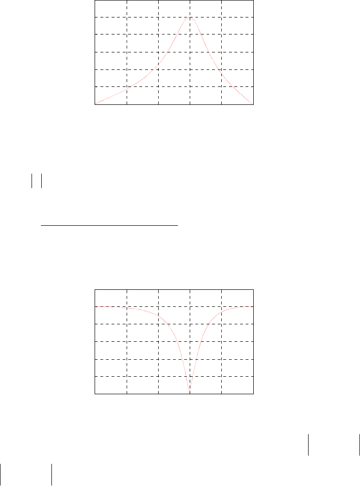
00.2 0.4 0.6 0.8 1
0
0.2
0.4
0.6
0.8
1
ω
/
π
Magniitude
M7.12 From Eq. (7.78) we arrive at the quadratic equation whose
solution yields and
012.4721
2=+α−α
0.5095=α 1.9626.
=
α
A stable bandstop transfer function
requires .1<α Hence we choose 0.5095.
=
α
Next, from Eq. (7.80) we get
Substituting these two parameters in Eqs. (7.77) we obtain
0.3090.−=β
.)( 21
21
0.50950.46651
)0.618010.7548(
−−
−
−
++
++
=
zz
zz
zH BS A plot of the magnitude response of
is shown below:
)(zH BS
00.2 0.4 0.6 0.8 1
0
0.2
0.4
0.6
0.8
1
ω
/
π
Magniitude
M7.13 A plot of the magnitude response of )()( zHzH BSBP
+
and plot of 2
)( ωj
BP eH
2
)( ω
+j
BS eH are shown below verifying the doubly complementary property of
)(zH B
P
and ).(zH BS
Not for sale 232

00.2 0.4 0.6 0.8 1
0
0.2
0.4
0.6
0.8
1
ω
/
π
Magniitude
|H
BP
(e
j
ω
)+H
BS
(e
j
ω
)|
00.2 0.4 0.6 0.8 1
0
0.2
0.4
0.6
0.8
1
ω
/
π
Square Magniitude
|H
BP
(e
j
ω
)|
2
+|H
BS
(e
j
ω
)|
2
M7.14 (a)
00.2 0.4 0.6 0.8 1
0
0.2
0.4
0.6
0.8
1
ω
/
π
Magnitude
|H(e
jω
)+G(e
jω
)|
00.2 0.4 0.6 0.8 1
0
0.2
0.4
0.6
0.8
1
ω
/
π
Square Magnitude
|H(e
jω
)|
2
+|G(e
jω
)|
2
A plot of the magnitude response of )()( zGzH
+
and plot of 2
)( ωj
eH
2
)( ωj
eG+ are shown above verifying the doubly complementary property of
and
)(zH
).(zG
(b)
00.2 0.4 0.6 0.8 1
0
0.2
0.4
0.6
0.8
1
ω
/
π
Magnitude
|H(e
jω
)+G(e
jω
)|
00.2 0.4 0.6 0.8 1
0
0.2
0.4
0.6
0.8
1
ω
/
π
Square Magnitude
|H(e
jω
)|
2
+|G(e
jω
)|
2
A plot of the magnitude response of )()( zGzH
+
and plot of 2
)( ωj
eH
2
)( ωj
eG+ are shown above verifying the doubly complementary property of
and
)(zH
).(zG
Not for sale 233
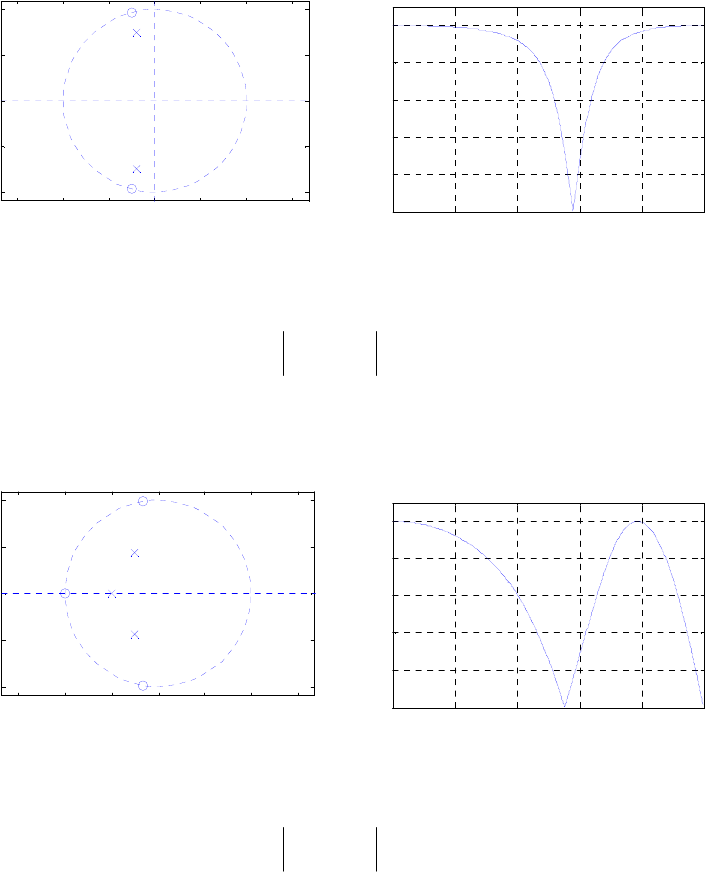
M7.15 (a) The pole-zero plot obtained using the M-file zplane is shown below:
-1.5 -1 -0.5 00.5 11.5
-1
-0.5
0
0.5
1
Real Part
I
mag
i
nary
P
ar
t
00.2 0.4 0.6 0.8 1
0
0.2
0.4
0.6
0.8
1
ω
/
π
Magnitude
H
a
(z)
It can be seen from the above pole-zero plot that the two poles of are
inside the unit circle and hence is stable. From the magnitude response
plot given above, we observe that
)(zH a
)(zHa
1≤
ω)( j
aeH and hence, is a BR
function.
)(zH a
(b) The pole-zero plot obtained using the M-file zplane is shown below:
-1.5 -1 -0.5 00.5 11.5
-1
-0.5
0
0.5
1
Real Part
I
mag
i
nary
P
ar
t
00.2 0.4 0.6 0.8 1
0
0.2
0.4
0.6
0.8
1
ω
/
π
Magnitude
H
b
(z)
It can be seen from the above pole-zero plot that the three poles of are
inside the unit circle and hence is stable. From the magnitude response
plot given above, we observe that
)(zHb
)(zHb
1≤
ω)( j
aeH and hence, is a BR
function.
)(zH a
M7.16 (a) The power-complementary transfer function )(/)()( zDzQzGa
=
to the
transfer function satisfy the relation
or equivalently the relation
Here, and
)(/)()( zDzPzHa=)()( 1−
zGzG aa
),()(1 1−
−= zHzH aa )()()()( 11 −− =zDzDzQzQ
).()( 1−
−zPzP 21 6.04.01)( −− ++= zzzD
.8.04.08.0)( 21 −− ++= zzzP
(b)
Not for sale 234
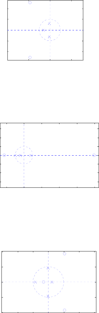
M7.17 (a) The pole-zero plot of obtained using the M-file zplane is shown
below. From this plot it can be seen that all 3 poles of are inside the unit
circle, and hence, is a stable transfer function.
)(zH a
)(zH a
)(zH a
-2 0 2
-2
-1
0
1
2
Real Part
Imaginary Part
H
a
(z)
(b) The pole-zero plot of obtained using the M-file zplane is shown
below. From this plot it can be seen that one pole of is on the unit circle,
and hence, is an unstable transfer function.
)(zHb
)(zHb
)(zHb
-2 0 2 4 6 8
-3
-2
-1
0
1
2
3
Real Part
Imaginary Part
H
b
(z)
(c) The pole-zero plot of obtained using the M-file zplane is shown
below. From this plot it can be seen that all 4 poles of are inside the unit
circle, and hence, is a stable transfer function.
)(zHc
)(zH c
)(zH c
-3 -2 -1 0 1 2 3
-2
-1
0
1
2
Real Part
Imaginary Part
H
c
(z)
Not for sale 235
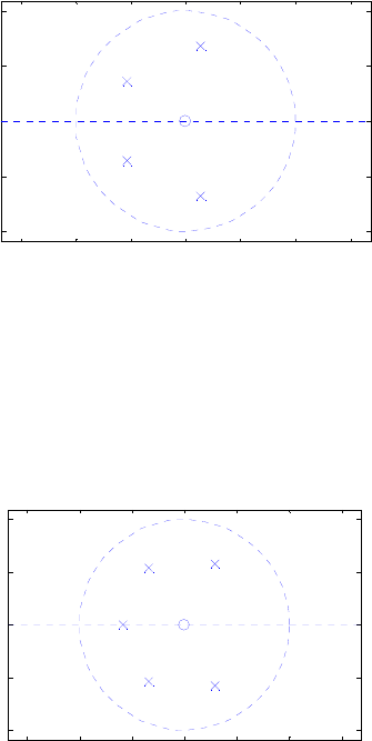
(d) The pole-zero plot of obtained using the M-file zplane is shown
below. From this plot it can be seen that all 4 poles of are inside the unit
circle, and hence, is a stable transfer function.
)(zH d
)(zHd
)(zHd
-1.5 -1 -0.5 00.5 11.5
-1
-0.5
0
0.5
1
4
Real Part
I
mag
i
nary
P
ar
t
H
d
(z)
(e) The pole-zero plot of obtained using the M-file zplane is shown
below. From this plot it can be seen that all 5 poles of are inside the unit
circle, and hence, is a stable transfer function.
)(zHe
)(zHe
)(zHe
-1.5 -1 -0.5 00.5 11.5
-1
-0.5
0
0.5
1
5
Real Part
I
mag
i
nary
P
ar
t
H
e
(z)
M7.18 (a) The output data generated by running Program 7_2 are:
The stability test parameters are
0.2500 0.3333 0.5000
stable =
1
Hence, is a stable transfer function.
)(zH a
(b) The output data generated by running Program 7_2 are:
The stability test parameters are
-0.3333 -0.5000 1.0000
stable =
0
Not for sale 236
Hence, is an unstable transfer function.
)(zHb
(c) The output data generated by running Program 7_2 are:
The stability test parameters are
-0.1667 0.6286 0.5209 0.2919
stable =
1
Hence, is a stable transfer function.
)(zH c
(d) The output data generated by running Program 7_2 are:
The stability test parameters are
0.2000 0.2500 0.3333 0.5000
stable =
1
Hence, is a stable transfer function.
)(zH d
(e) The output data generated by running Program 7_2 are:
The stability test parameters are
0.1000 0.1313 0.1652 0.3185 0.4646
stable =
1
Hence, is a stable transfer function.
)(zHe
M7.19 (a) The output data generated by running Program 7_2 are:
The stability test parameters are
0.1000 0.1212 0.2516 0.3351 0.5041
stable =
1
Hence, all roots of are inside the unit circle. )(zDa
(b) The output data generated by running Program 7_2 are:
(c)
The stability test parameters are
-0.2500 0.7667 0.1186 0.4376 0.6426
stable =
1
Hence, all roots of are inside the unit circle.
)(zDb
Not for sale 237
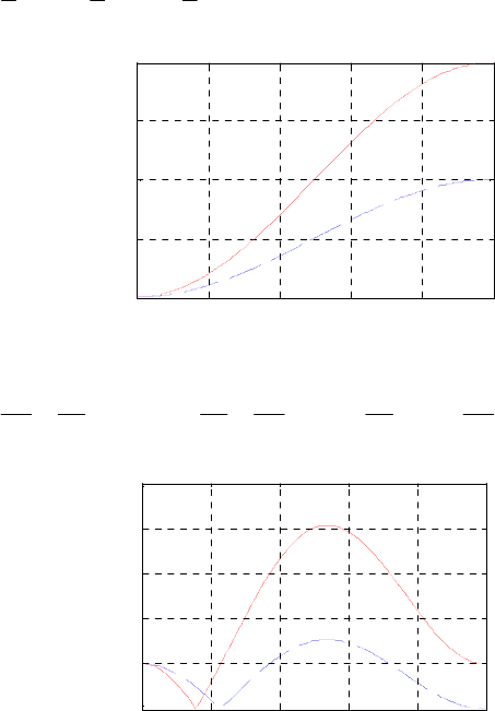
M7.20 .1)( 2
4
1
44
−− −
⎟
⎠
⎞
⎜
⎝
⎛++−= zzzH kkk
00.2 0.4 0.6 0.8 1
1
1.5
2
2.5
3
ω
/
π
Magnitude
k=2
k=1
M7.21 .
4444
1
44
)( 4
2
3
1
2
21
1
12 −−−− −+
⎟
⎠
⎞
⎜
⎝
⎛+−++−= z
k
z
k
z
kk
z
kk
zH
00.2 0.4 0.6 0.8 1
0
1
2
3
4
5
ω
/
π
Magnitude
k
1
=2, k
2
=-4
k
1
=1, k
2
=-2
Not for sale 238
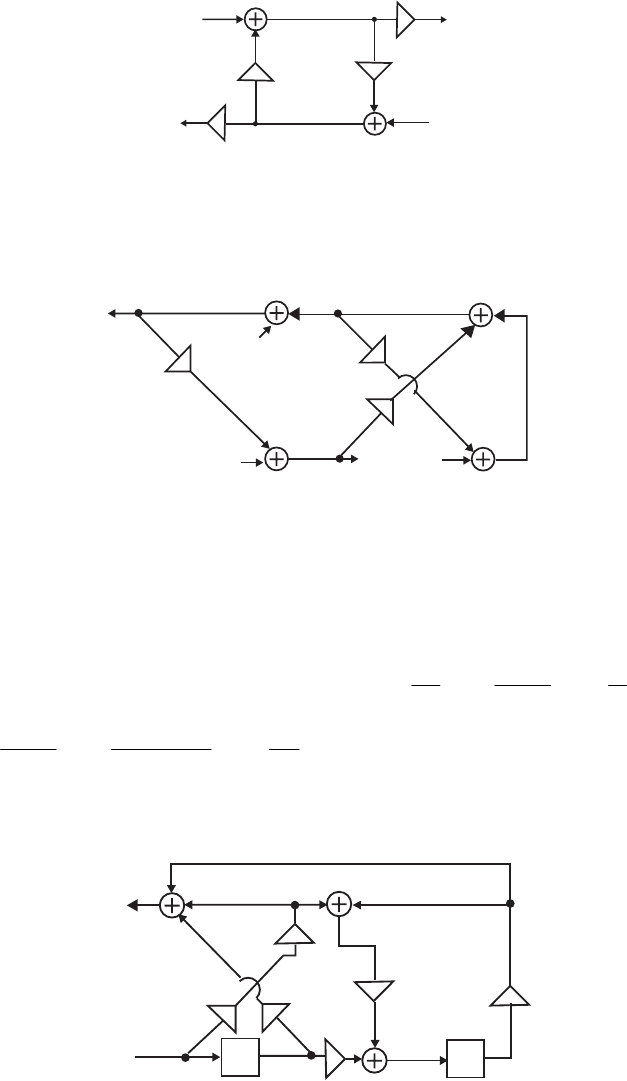
Chapter 8
8.1 Analyzing Figure P8.1, we get
(
)
][][][ nCDunXAnw
+
=
and
A direct implementation of these two equations leads to
the structure shown below which has no delay-free loop.
(
.][][][ nunABxCny +=
)
x[n]
y
[n]
w[n]
u[n]
A
C
AB
CD
8.2 (a) Figure P8.2(a) with input and output nodes removed and delays removed is as
shown below. There are two delay-free loops in the reduced structure shown
below. Analysis of this structure yields
k1
k2
α
1
1
W
2
W
3
W
1
U
2
U
3
U
(1): ,
231 UWW
+
= (2): ,
1112 UWW
+
α
=
(3): .
222313 UWkWkW +
+
=
From Eq. (3) we get (4): ,)( 22231
1UWkWk
=
−
−
and from Eq. (1) we get
Substituting the last equation in Eq. (4) we get .
213 UWW −=
3212211 11 UUkWkWk
+
−=−− )()( and from Eq. (2) we have .
1211 UWW
=
+α
−
Solving the last two equations we arrive at 32
1
1
2
1
1
1UU
k
U
k
W∆
+
∆
−
+
∆
= and
.
)(
3
1
2
11
1
1
2
11 UU
k
U
k
W∆
α
+
∆
−α
+
∆
−
= A realization based on the above two
equations after insertion of the input and output nodes and the delays is shown
below which has no delay-free loops.
X(z)
Y(z)
α
z1
_z1
_
α2
1
∆
1
_
(1 k )/
∆
1
_
(1 k )/
k2∆
/∆1/
U1
W1
U2
W2U3
Not for sale 239
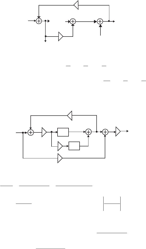
(b) Figure P8.2(b) with input and output nodes removed and delays removed is as
shown below. There is one delay-free loop in the reduced structure shown below.
Analysis of this structure yields
β
δ
U
1
W
1
U
2
U
3
W
2
(1): and (2):
,
211 WUW δ+= .
3122 UWUW
+
β
+
=
Substituting Eq. (1) in Eq. (2)
we get after some algebra (3): ,
3212
11 UUUW
∆
+
∆
+
∆
β
= where
Substituting Eq. (3) in Eq. (1) we get (5):
.βδ−=∆ 1
.
32111 UUUUW ∆
δ
+
∆
δ
+
∆
β
δ
+= A
realization based on Eqs. (3) and (5) after insertion of the input and output nodes
and the delays is shown below which has no delay-free loop.
β
δ
U
1
W
1
U
2
W
2
z
_1
z
_1
1/∆
1/∆
γ
U
3
X
(z)Y(z)
8.3 Analysis yields
(
)
.)()()()()( zYzCzXzGzY
−
= Hence,
.
)(
)()(
)(
)(
)(
)( 1
321
2
1−
++
=
+
==
zK
zCzG
zG
zX
zY
zH The overall transfer function has
a pole at .
K
z21
3
+
−= Thus, the system is stable if ,1
21
3<
+K or, 1>
K
or
.2−<K
8.4 From the results of Problem 8.3, we have )()(
)(
)( zCzG
zG
zH +
=1 which can be
solved yielding .
)()(
)()(
)( zHzG
zHzG
zC
−
= Substituting the expressions for and
in this expression we get
)(zG
)(zH
Not for sale 240
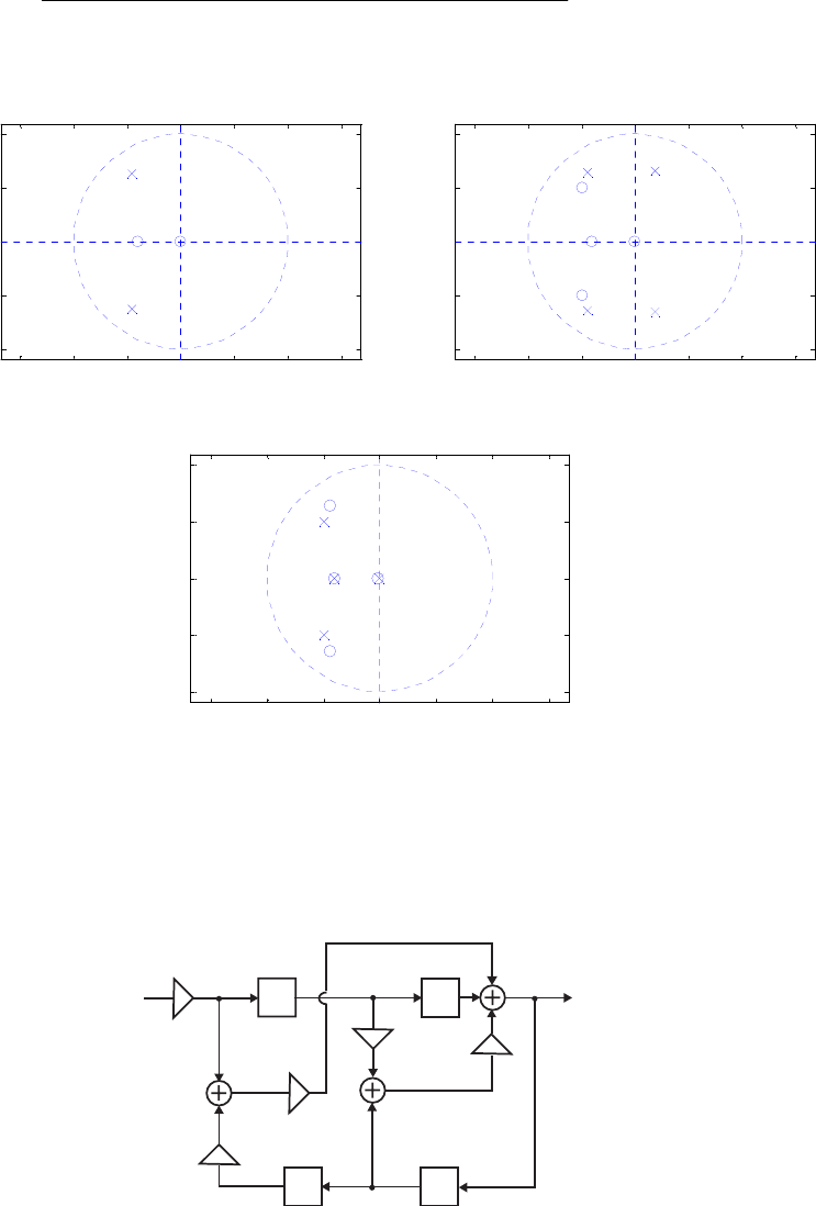
.
)....(.
).....(
)( 4321
43211
080560461811040
0408418761907
−−−−
−−−−−
++++
++++
−=
zzzz
zzzzz
zC Pole-zero plots of
and obtained using zplane are shown below:
),(),( zCzG )(zH
-1.5 -1 -0.5 00.5 11.5
-1
-0.5
0
0.5
1
Real Part
I
mag
i
nary
P
ar
t
G(z)
-1.5 -1 -0.5 00.5 11.5
-1
-0.5
0
0.5
1
Real Part
I
mag
i
nary
P
ar
t
H(z)
-1.5 -1 -0.5 00.5 11.5
-1
-0.5
0
0.5
1
2
Real Part
I
mag
i
nary
P
ar
t
C(z)
Ac can be seen from the above ploe-zero plots, and are stable
transfer functions.
),(),( zCzG )(zH
8.5 The structure with internal variables is shown below. Analysis of this structure yields
_1
z
_1
z
_1
z
_1
z
X
(z)Y(z)
K
1
_
1
_
α
β
W (z)
1W (z)
2
and
Substituting the first two equations into the
third, and rearranging we get
),()()(),()()( zYzzXKzzWzYzzXKzW 11
2
2
1−−− +−=−=
).()()()( zXKzzWzWzY 2
21 −
+α+β=
).()()()( zXzzKzYzz 2121
1−−−− +α−β=β+α−
Not for sale 241
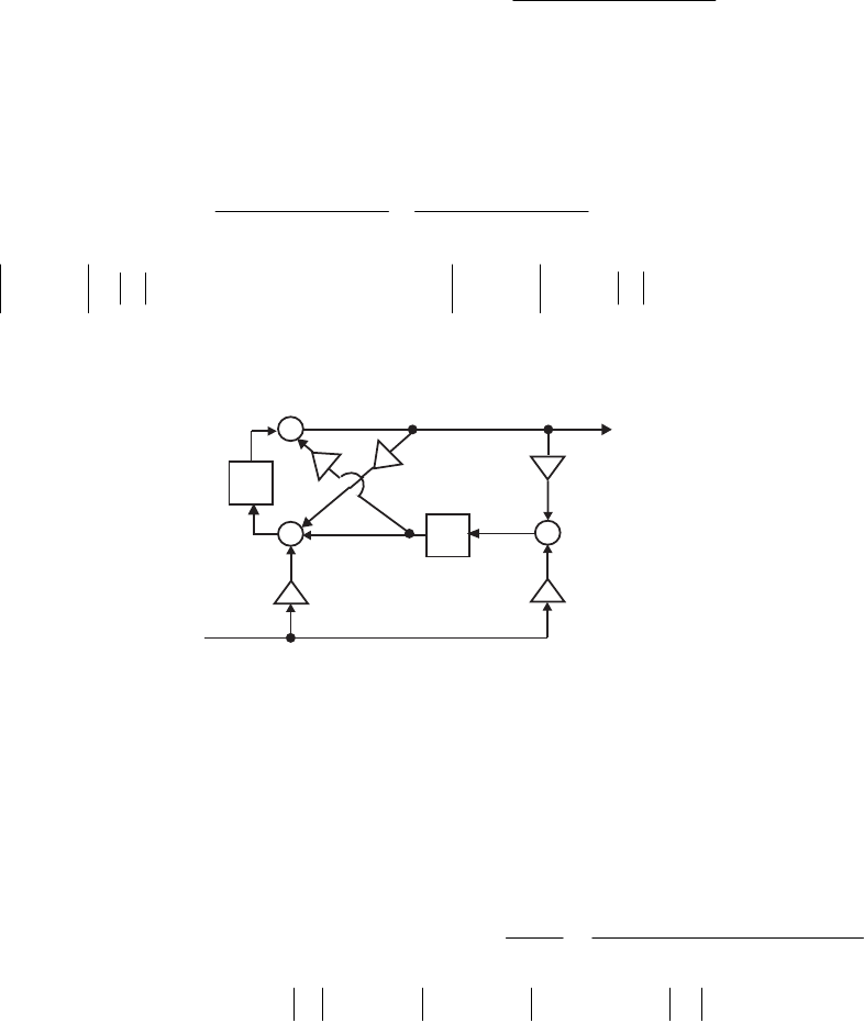
Hence, the transfer function is given by .
)(
)( 21
21
1−−
−−
β+α−
+α−β
=
zz
zzK
zH
(a) Since the structure employs 2 delays and has a second order transfer function, it
is a canonic structure.
(b) and (c) We form
.)()( 2
12
12
21
21
21 1
1
K
zz
zz
zz
zz
KzHzH =
⎟
⎟
⎠
⎞
⎜
⎜
⎝
⎛
β+α−
+α−β
⎟
⎟
⎠
⎞
⎜
⎜
⎝
⎛
β+α−
+α−β
=−−
−−
−−
−−
− Therefore,
KeH j=
ω)( for all values of .
ω
Hence, 1=
ω)( j
eH if .1=K
8.6 The structure with internal variables is shown below. Analysis of this structure yields
z
1
_
z
1
_
+
+
+
_
k
1
k
2
k
2
_
1
γ
2
γ
X
(z)
Y(z)
1
W (z)
2
W (z)
and
Substituting the second equation in the first and
rearranging we get Substituting this
equation and the second equation in the third equation we get after some
rearrangement
Hence, the transfer function is given by
),()()(),()()()( zYkzXzWzWzzYkzXzW 1122
1
221 −γ=++γ= −
).()()( zWzkzWzzY 2
1
21
1−− −=
).()()()()( zYzkkzXzzW 1
12
1
121 −− −+γ+γ=
).(])[()(])([ zXzzkzYzkzkk 2
1
1
122
2
1
1
21 11 −−−− γ+γ−γ=++−
.
)(
)(
)(
)(
)( 2
1
1
21
2
1
1
122
11 −−
−
−
++−
γ+γ−γ
==
zkzkk
zzk
zX
zY
zH
For stability, we must have 1
1<k and ,)( 121 11 kkk +<+ or .1
2<k
8.7 The structure with internal variables is shown on next page. Analysis of this structure
yields
and Eliminating and
),()()(),()()(),()()( zSzzSazSzSzzSzzSzSzXzS 2
1
0325
1
2
1
110 −−− −=+=−=
),()()(),()()(),()()( zSzzSazSzSzzSzSzSzzSazS 5
1
4153
1
043
1
533 −−− −=+=−=
).()( zSazY 44
=)(),(),(),(),( zSzSzSzSzS 43210 )(zS5
from these equations we get after some algebra
Not for sale 242
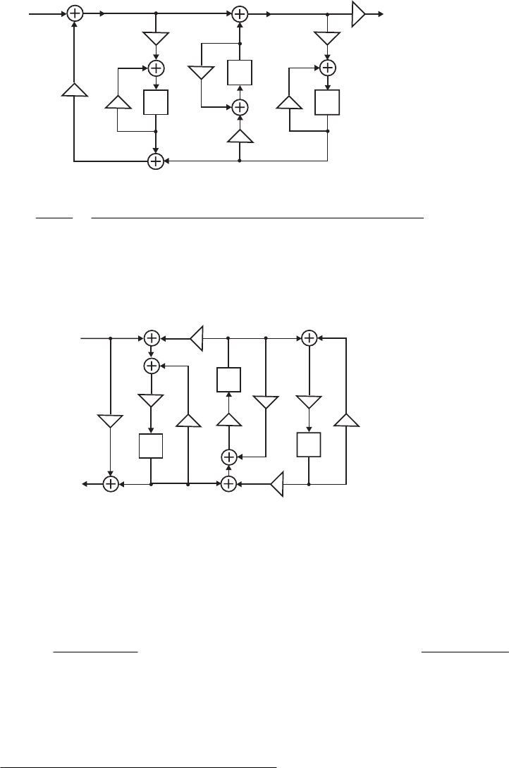
_1
z
_1
z
_1
z
X
(z)Y(z)
1
_
1
_
1
_
1
_
a
1
a
2
a
3
a
4
S (z)
2
S (z)
3
S (z)
4
S (z)
5
1
S (z)
S (z)
0
.
)(
)()(
)(
)(
)(
)(
3
3212131
2
2131
1
31
31
4
1
22331
1
−
−−
−
−−+++
−++++++
+
==
zaaaaaaa
zaaaazaa
za
zX
zY
zH
8.8 The structure with internal variables is shown below. Analysis of this structure yields
_1
z
_1
z
_1
z
X
(z)
Y(z)1
_
1
_
0
α
3
α
1
α
2
α
1
β
3
β
2
β
R (z)
2
1
R (z)
1
W (z)
2
W (z)
3
W (z)
),()()(),()()( zRzzXzWzRzzXzY 2
1
211
1
10 −− β−=β+α=
),()()(),()()( zWzzRzzWzRzzWzR 3
1
31
1
121
1
1111 −−− β−β=βα+=
).()()(),()()( zWzzRzzWzRzzWzR 3
1
332
1
232
1
2222 −−− βα+β=βα+=
From the third equation we get From the sixth equation
we get
).()()( zRzzW 1
1
111 1−
βα−=
.
)(
)( 1
33
2
1
2
3−
−
βα
β
=
z
zRz
zW From the fifth equation we get .
)(
)( 1
22
2
21−
βα−
=
z
zW
zR
Rewriting the fourth equation we get in which we
substitute the expressions for and resulting in after some algebra
),()()( zRzzWzzW 1
1
13
1
32 −− β=β+
)(zW3)(zW1
).(
))((
)(
)( zR
zzz
zz
zR 1
1
33
1
22
1
32
1
33
1
1
211
1
−−−
−−
βα−βα−+ββ
βα−β
= Substituting this expression
for and the expression for in the second equation we arrive at
)(zR2)(zW1
Not for sale 243
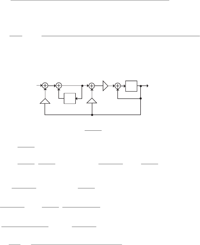
).(
)(
))()(()(
))((
)( zX
zz
zzzzz
zzz
zR
1
33
2
21
1
33
1
22
1
11
1
11
2
32
1
33
1
22
2
32
1
1
1111
11
−−
−−−−−
−−−
βα−ββ
βα−βα−βα−+βα−ββ
βα−βα−+ββ
=
Substituting the above in the first equation we finally arrive at
.
)(
)())()((
))((
)(
)(
)(
1
33
2
21
1
11
2
32
1
33
1
22
1
11
1
33
1
22
1
1
3
321
0
1
1111
11
−−
−−−−−
−−−−
βα−ββ
βα−ββ+βα−βα−βα−
βα−βα−β+βββ
+α==
zz
zzzzz
zzzz
zX
zY
zH
8.9 The structure with internal variables is shown below. Analysis of this structure yields
k1k2
–
z 1
–
z 1
k1
_
X
(z)Y(z)
W(z)U(z)
(1): (2):
),()()( 1zYkzXzW += ),()(
1
1
)( 2
1zYkzW
z
zU +
−
=− and
(3): ).(
1
)( 1
1zU
z
k
zY −
−
−
= Substituting Eq. (2) in Eq. (3) we get
(4): ).(
1
)(
)1(
)()(
1
1
1
)( 1
21
21
1
2
11
1zY
z
kk
zW
z
k
zYkzW
zz
k
zY −−−− −
−
−
−
=
⎟
⎟
⎠
⎞
⎜
⎜
⎝
⎛+
−−
−
=
Substituting Eq. (1) in Eq. (4) we then get
)(
1
)]()([
)1(
)( 1
21
1
21
1zY
z
kk
zYkzX
z
k
zY −− −
−+
−
−=
),(
11
)(
)1( 1
1
221
1
1
21
1zY
z
zkkk
z
k
zX
z
k
⎥
⎥
⎦
⎤
⎢
⎢
⎣
⎡
−
−+
−
−
−
−= −
−
−− or,
).(
)1(
)(
)1(
)(
121
1
21
1
2211 zX
z
k
zY
z
zkkkk
−−
−
−
−=
⎥
⎥
⎦
⎤
⎢
⎢
⎣
⎡
−
−+
+ Hence,
.
)2()](1[
)(
)(
)( 21
21211
1
−− ++−++
−==
zzkkkkk
k
zX
zY
zH
8.10 (a) A direct form realization of 4321 944.132.44.56.31)(
−
−
−
−
+−+−= zzzzzH
and its transformed structure are shown on next page:
65 0467.04666.0 −− +− zz
Not for sale 244
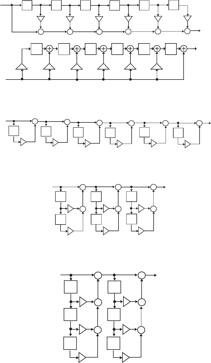
z
1
_
z
1
_
z
1
_
++
+
x
[n]
y[n]
z
1
_
+
z
1
_
+
z
1
_
+
3.6
_
5.4
_
4.32 1.944 0.4666
_
0.0467
x
[n]
y[n]
z–1 z–1 z–1 z–1
z–1
z–1
_
3.6
5.4
4.32
_
1.944
_
0.4666
0.0467
(b) A cascade realization of
)6.01)(6.01)(6.01)(6.01)(6.01)(6.01()( 111111 −
−
−
−
−
−−−−−−−= zzzzzzzH is
shown below:
z
1
_
+
z1
_
+
z1
_
+
x
[n]y[n]
z1
_
+
z
1
_
+
z1
_
+
_0.6 _0.6 _0.6 _0.6 _0.6 _0.6
(c) A cascade realization of
)36.02.11)(36.02.11)(36.02.11()( 212121 −
−
−
−
−− +−+−+−= zzzzzzzH is shown
below:
z
1
_
z
1
_
+
+
z
1
_
z
1
_
+
+
z
1
_
z
1
_
+
+
x
[n]y[n]
0.36
0.2
_
0.2
_
0.2
_
0.36 0.36
(d) A cascade realization of
)216.008.18.11)(216.008.18.11()( 321321 −
−
−
−
−− −+−−+−= zzzzzzzH is shown
below:
+
z
1
_
+
z
1
_
+
+
x
[n]y[n]
z
1
_
z
1
_
+
z
1
_
z
1
_
+
1.08
1.8
_
0.216
_
1.8
_
1.08
0.216
_
Not for sale 245
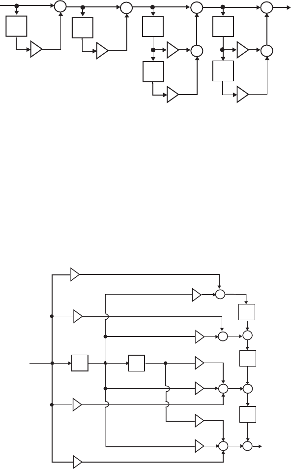
(e) A cascade realization of
)36.02.11)(36.02.11)(6.01)(6.01()( 212111 −
−
−
−
−
−+−+−−−= zzzzzzzH is shown
below:
z1
_
z1
_
+
+
z1
_
z1
_
+
+
z1
_
+
x
[n]y[n]
0.2
_
0.2
_
0.36 0.36
z1
_
+
_0.6 _0.6
All realizations given above require 6 multipliers and 6 two-input adders.
8.11 (a) A four branch polyphase decomposition is given by
,)()()()()( 34
3
24
2
14
1
4
0
−
−
−+++= zzEzzEzzEzEzH where
,][][][)(,][][][)( 21
1
21
0951840 −−−− ++=++= zhzhhzEzhzhhzE
,]6[]2[)( 1
2−
+= zhhzE .]7[]3[)( 1
3
−
+= zhhzE
(b) A canonic four-branch polyphase realization of the above transfer function is
shown below:
z
1
_
z
1
_
z
4
_
++
+
+
+
h[0]
h[1]
h[2]
h[3]
h[4]
h[5]
h[6]
h[7]
h[8]
z
4
_
h[9]
+
z
1
_
+
x
[n]
y[n]
8.12 (a) A three branch polyphase decomposition is given by
,)()()()( 23
2
13
1
3
0
−
−++= zzEzzEzEzH where
,]7[]4[]1[)(,]9[]6[]3[]0[)( 21
1
321
0−
−
−
−
−++=+++= zhzhhzEzhzhzhhzE
.]8[]5[]2[)( 21
2
−
−++= zhzhhzE
Not for sale 246
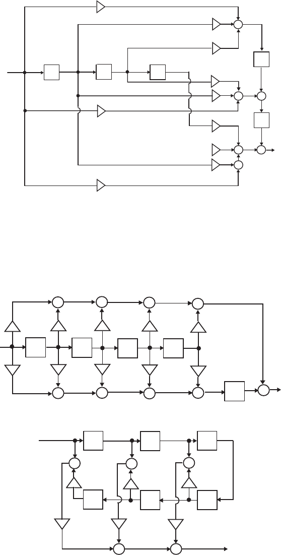
(b) A canonic three branch polyphase realization of the above transfer function is
shown below:
+
z
1
_
z
1
_
z
3
_
++
+
+
z
3
_
h[0]
h[1]
h[2]
h[3]
h[4]
h[5]
h[6]
h[7]
h[8]
z
3
_
h[9]
+
8.13 (a) A two branch polyphase decomposition is given by ,)()()( 12
1
2
0
−
+= zzEzEzH
where ,]8[]6[]4[]2[]0[)( 4321
0
−
−
−
−
++++= zhzhzhzhhzE
.]9[]7[]5[]3[]1[)( 4321
1
−
−
−
−++++= zhzhzhzhhzE
(b) A canonic two branch polyphase realization of the above transfer function is shown
below:
z1
_
h[0]
h[1]
h[2]
h[3]
h[4]
h[5]
h[6]
h[7] h[9]
z2
_z2
_z2
_z2
_
+
+
+
+
+
+
+
+
+
h[8]
x
[n]
y[n]
8.14
z1
_
+
h[0] h[1] h[2]
z1
_z1
_z1
_
z1
_
z1
_
++
++
x
[n]
y[n]
1
_1
_1
_
8.15
Not for sale 247
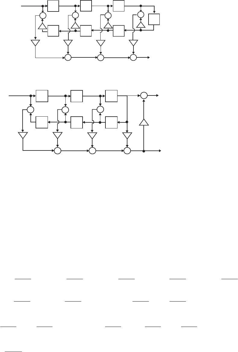
z
1
_
h[0] h[1] h[2] h[3]
z
1
_
z
1
_
z
1
_
z
1
_
z
1
_
+
z
1
_
++ +
+++
_
1
_
1
_
1
_
1
8.16 A canonic realization of both and is shown below
for
).()( 2/ zHzzG N−= −)(zG )(zH
.6=N
z1
_
+
h[0] h[1] h[2] h[3]
z1
_z1
_z1
_
z1
_
z1
_
+
+++
+
+
1
_
G(z)
H(z)
8.17 Without any loss of generality, assume 5
=
M which means .11
=
N In this case, the
transfer function is given by
)(zH
[
]
.)](0[)](1[)](2[)](3[)](4[]5[ 5544332215
−
−
−
−
−− ++++++++++= zzhzzhzzhzzhzzhhz
Now, the recursion relation for the Chebyshev polynomial is given by
2),()(2)( 21 ≥−= −
−
rxTxTxxT rrr with 1)(
0
=
xT and .)(
1xxT
=
Hence,
We can thus rewrite the expression inside the square brackets given above as
,12)()(2)( 2
012 −=−= xxTxTxxT
,34)12(2)()(2)( 32
123 xxxxxxTxTxxT −=−−=−=
,188)12()34(2)()(2)( 2423
234 +−=−−−=−= xxxxxxxTxTxxT
.52016)34()188(2)()(2)( 35324
345 xxxxxxxxxTxTxxT +−=−−+−=−=
⎟
⎠
⎞
⎜
⎝
⎛
+
⎟
⎠
⎞
⎜
⎝
⎛
+
⎟
⎠
⎞
⎜
⎝
⎛
+
⎟
⎠
⎞
⎜
⎝
⎛
+
⎟
⎠
⎞
⎜
⎝
⎛
+−−−−− +++++
2
5
2
4
2
3
2
2
2
1
11111 ]0[2]1[2]2[2]3[2]4[2]5[ zzzzzzzzzz ThThThThThh
⎥
⎥
⎦
⎤
⎢
⎢
⎣
⎡⎟
⎠
⎞
⎜
⎝
⎛
−
⎟
⎠
⎞
⎜
⎝
⎛
+
⎥
⎥
⎦
⎤
⎢
⎢
⎣
⎡−
⎟
⎠
⎞
⎜
⎝
⎛
+
⎟
⎠
⎞
⎜
⎝
⎛
+= −−−− ++++
2
3
2
2
22
1111 34]2[212]3[2]4[2]5[ zzzzzzzz hhhh
⎥
⎥
⎦
⎤
⎢
⎢
⎣
⎡⎟
⎠
⎞
⎜
⎝
⎛
+
⎟
⎠
⎞
⎜
⎝
⎛
−
⎟
⎠
⎞
⎜
⎝
⎛
+
⎥
⎥
⎦
⎤
⎢
⎢
⎣
⎡+
⎟
⎠
⎞
⎜
⎝
⎛
−
⎟
⎠
⎞
⎜
⎝
⎛
+−−−−− +++++
2
3
2
5
2
2
2
4
2
11111 52016]0[2188]1[2 zzzzzzzzzz hh
,][
5
02
1
∑
=
+⎟
⎠
⎞
⎜
⎝
⎛
=−
n
n
zz
na where ],0[10]2[6]4[2]1[],1[2]3[2]5[]0[ hhahhha +− h
=
+
−
=
],1[16]4[],1[40]2[8]3[],1[16]3[4]2[ hha hahha
=
−
=−= and A
realization of
].0[32]5[ ha =
Not for sale 248
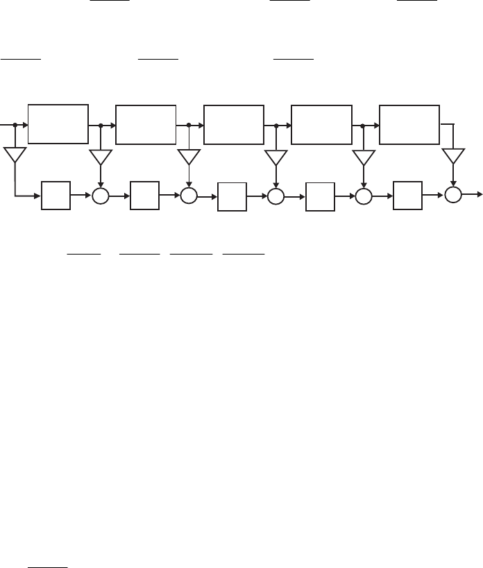
4
2
1
5
5
02
521 ]1[]0[][)( −
+
−
=
+
−⎟
⎠
⎞
⎜
⎝
⎛
+=
⎟
⎠
⎞
⎜
⎝
⎛
=−−
∑zazanazzH z
n
n
zz 3
2
2
12
]2[ −
+⎟
⎠
⎞
⎜
⎝
⎛
+−za z
5
2
1
1
4
2
1
2
3
2
1222 ]5[]4[]3[ ⎟
⎠
⎞
⎜
⎝
⎛
+
⎟
⎠
⎞
⎜
⎝
⎛
+
⎟
⎠
⎞
⎜
⎝
⎛
+−−− +
−
+
−
+zzz azaza is shown below:
a[0] a[1] a[2] a[3]
1 + z
2
______
_2
1 + z
2
______
_2
1 + z
2
______
_2
1 + z
2
______
_2
1 + z
2
______
_2
+++ + +
z
1
_
z
1
_
z
1
_
z
1
_
z
1
_
a[4] a[5]
x
[n]
y[n]
8.18 Consider .
)(
)(
)(
)(
)(
)(
)(
)(
)(
3
3
2
2
1
1
zD
zP
zD
zP
zD
zP
zD
zP
zH ⋅⋅== Assume all zeros of and
are complex. Note that the numerator of the first stage can be one of the 3 factors,
and Likewise, the numerator of the second stage can be one of the
remaining 2 factors, and the numerator of the third stage is the remaining factor.
Similarly, that the denominator of the first stage can be one of the 3 factors,
and Likewise, the denominator of the second stage can be one
of the remaining 2 factors, and the denominator of the third stage is the remaining
factor. Hence, there are different types of cascade realizations.
)(zP )(zD
),(
1zP ),(
2zP ).(
3zP
),(
1zD ),(
2zD ).(
3zD
36)!3( 2=
If the zeros of and are all real, then has 6 real zeros and has 6
real zeros. In this case, then there are different types of cascade
realizations.
)(zP )(zD )(zP )(zD
518400)!6( 2=
8.19 .
)(
)(
)(
1
∏
=
=
K
ii
i
zD
zP
zH Here, the numerator of the first stage can be chosen in ways,
the numerator of the second stage can be chosen in ways, and so on, until there
is only one possible choice for the numerator of the
⎟
⎠
⎞
⎜
⎝
⎛
1
K
⎟
⎠
⎞
⎜
⎝
⎛−
1
1
K
K
–th stage. Likewise, the
denominator of the first stage can be chosen in ways, the denominator of the
second stage can be chosen in ways, and so on, until there is only one possible
choice for the denominator of the
⎟
⎠
⎞
⎜
⎝
⎛
1
K
⎟
⎠
⎞
⎜
⎝
⎛−
1
1
K
K
–th stage. Hence, the total number of possible
cascade realizations are equal to
L
2
1
2
2
1
1
2
1⎟
⎠
⎞
⎜
⎝
⎛
⎟
⎠
⎞
⎜
⎝
⎛
⎟
⎠
⎞
⎜
⎝
⎛−− KKK .)!( 2
2
1
1
2
1
2K=
⎟
⎠
⎞
⎜
⎝
⎛
⎟
⎠
⎞
⎜
⎝
⎛
Not for sale 249
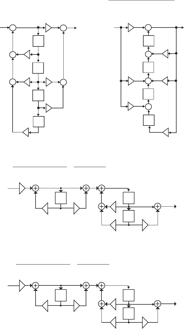
8.20 A canonic direct form II realization of 421
32
6341
353
−−−
−−
++−
+−
=
zzz
zz
zH )( is shown below
on the left. Its transposed realization is shown below on the right.
++
z1
_
z1
_
z1
_
+
+
+
x
[n]y[n]
z1
_
_6
_3
4
2
_5
3
+
+
z
1
_
+
z
1
_
+
z
1
_
x
[n]y[n]
z
1
_
2
_
5
3
4
_
3
_
6
8.21 (a) A cascade canonic realization of based on the decomposition
)(
1zH
⎟
⎟
⎠
⎞
⎜
⎜
⎝
⎛
−
−
⎟
⎟
⎠
⎞
⎜
⎜
⎝
⎛
+−
+
=−
−
−−
−−
1
1
21
21
17501
801
12611
3
30
z
z
zz
zz
zH .
.
..
.)( is shown below:
z–1 z–1
z–1
0.3
0.75 0.8
_1.6
_2.1 3
x
[n]
y[n]
An alternate cascade canonic realization of based on the decomposition
)(
1zH
⎟
⎟
⎠
⎞
⎜
⎜
⎝
⎛
−
+
⎟
⎟
⎠
⎞
⎜
⎜
⎝
⎛
+−
−
=−
−
−−
−−
1
1
21
21
17501
31
12611
80
30
z
z
zz
zz
zH ...
.
.)( is shown below:
z–1 z–1
z–1
0.3
0.75
0.8
_
1.6
_2.1
3
x
[n]
y[n]
Not for sale 250
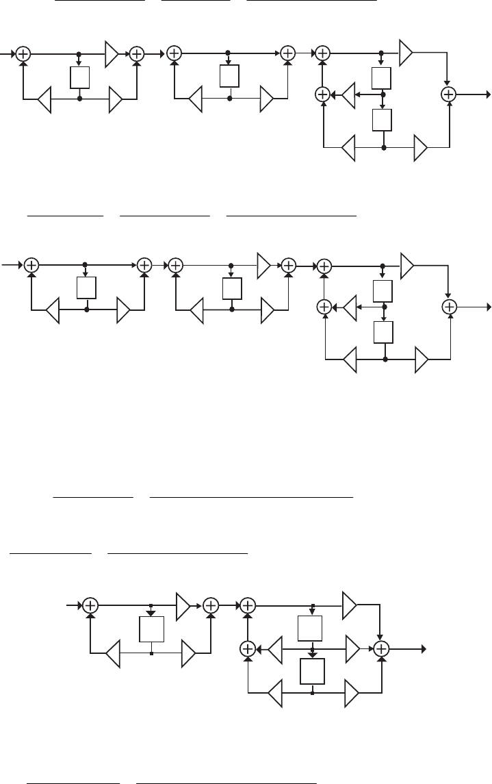
(b) A cascade canonic realization of based on the decomposition
)(
2zH
⎟
⎟
⎠
⎞
⎜
⎜
⎝
⎛
++
−
⎟
⎟
⎠
⎞
⎜
⎜
⎝
⎛
+
−
⎟
⎟
⎠
⎞
⎜
⎜
⎝
⎛
−
+
=−−
−
−
−
−
−
21
2
1
1
1
1
21.05.01
5.03
2.01
5.41
15.01
85.01.3
)(
zz
z
z
z
z
z
zH is shown below:
z
–1
x
[n]
y[n]
z
–1
z
–1
z
–1
3.1
0.85
0.15
3
4.5
_
0.2
_
0.1
_
0.5
_
0.5
_
An alternate cascade canonic realization of based on the decomposition
)(
2zH
⎟
⎟
⎠
⎞
⎜
⎜
⎝
⎛
++
−
⎟
⎟
⎠
⎞
⎜
⎜
⎝
⎛
+
+
⎟
⎟
⎠
⎞
⎜
⎜
⎝
⎛
−
−
=−−
−
−
−
−
−
21
2
1
1
1
1
21.05.01
5.03
2.01
85.01.3
15.01
5.41
)(
zz
z
z
z
z
z
zH is shown below:
z–1
x
[n]
y[n]
z–1
z–1
3.1
0.85
0.15
3
4.5
_0.2
_
0.1
_
0.5
_
0.5
_
z–1
(c) The factored form of the denominator of is given by: )(
3zH
).3754.01)(0246.21)(1.31( 111
−
−
−−−+ zzz A cascade canonic realization of
based on the decomposition
)(
3zH
⎟
⎟
⎠
⎞
⎜
⎜
⎝
⎛
−−
+−
⎟
⎟
⎠
⎞
⎜
⎜
⎝
⎛
+
+
=−−
−−
−
−
)3754.01)(0246.21(
74.82.5
1.31
7.05.1
)( 11
21
1
1
3zz
zz
z
z
zH
⎟
⎟
⎠
⎞
⎜
⎜
⎝
⎛
+−
+−
⎟
⎟
⎠
⎞
⎜
⎜
⎝
⎛
+
+
=−−
−−
−
−
21
21
1
1
760421
74825
131
7051
zz
zz
z
z
..
..
.
.. is shown below:
z–
1
x
[n]
y[n]
z–
1
z–
1
1.5
0.7
_
3.1
2.4
0.76
_
5.2
8.4
_
7.0
An alternate cascade canonic realization of based on the decomposition )(
3zH
⎟
⎟
⎠
⎞
⎜
⎜
⎝
⎛
−+
+−
⎟
⎟
⎠
⎞
⎜
⎜
⎝
⎛
−
+
=−−
−−
−
−
)3754.01)(1.31(
74.82.5
0246.21
7.05.1
)( 11
21
1
1
3zz
zz
z
z
zH
Not for sale 251
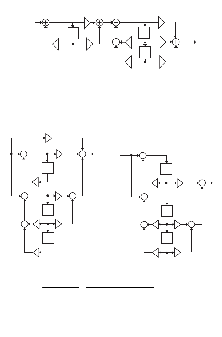
⎟
⎟
⎠
⎞
⎜
⎜
⎝
⎛
−+
+−
⎟
⎟
⎠
⎞
⎜
⎜
⎝
⎛
−
+
=−−
−−
−
−
11
21
1
1
1637.17246.21
74.82.5
0246.21
7.05.1
zz
zz
z
z is shown below:
z–1
x
[n]
y[n]
z–1
z–1
1.5
0.7
5.2
8.4
_
7.0
2.024
_
2.7246
1.1637
8.22 (a) A partial fraction expansion of in
)(
1zH 1
−
z obtained using the M-file residuez
is given by .
1.26.11
9878.04059.0
75.01
0513.0
4571.0)( 21
1
1
1−−
−
−+−
+−
+
−
−
+=
zz
z
z
zH The Parallel Form I
realization based on this expansion is shown on the next page on the left side.
z
1
_
z
1
_
z
1
_
+
+
++
+
0.4571
_
0.0513
0.75
_
0.4059
0.9878
1.6
2.1
_
x
[n]y[n]
z
1
_
z
1
_
z
1
_
+
+
+
+
+
0.75
_
0.0385
1.6
2.1
_
0.3385
_
0.8523
x
[n]
y[n]
A partial fraction expansion of in obtained using the M-file residue is
given by
)(
1zH z
.
1.26.11
8523.03385.0
75.01
0385.0
)( 21
21
1
1
1−−
−−
−
−
+−
−
+
−
−
=
zz
zz
z
z
zH The Parallel Form II
realization based on this expansion is shown above on the right side.
(b) A partial fraction expansion of in
)(
2zH 1
−
z obtained using the M-file residuez
is given by .
1.05.01
8813.794905.261
15.01
6.238
2.01
71.146
5.637)( 21
1
11
2−−
−
−− ++
+
+
−
+
+
+−=
zz
z
zz
zH The
Parallel Form I realization based on this expansion is shown on the next page on the left
side.
Not for sale 252
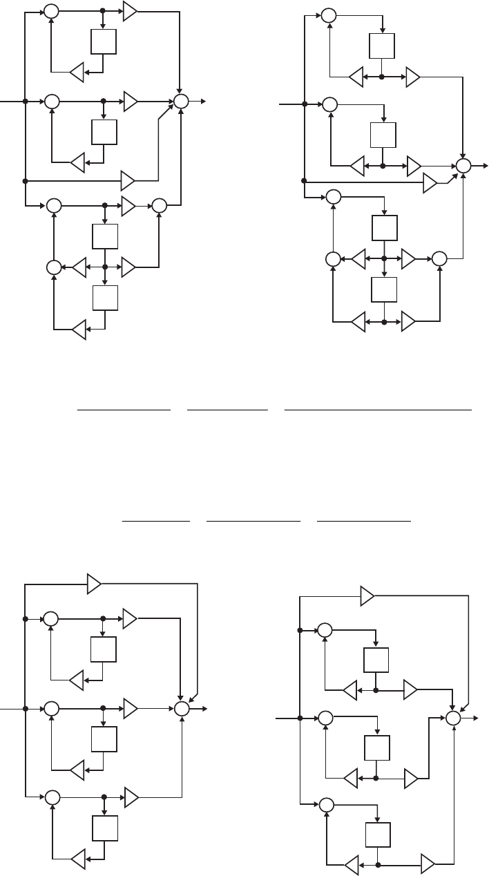
z
1
_
z
1
_
+
+
+
+
z
1
_
+
z
1
_
+
_
637.5
146.71
_
0.2
0.15
261.4905
79.8813
_
0.5
_
0.1
x
[n]y[n]
238.6
z
1
_
z
1
_
+
+
+
+
z
1
_
+
x
[n]
y[n]
z
1
_
+
9.3
_
0.2 29.3414
_
35.7904
0.15
50.8639
_
_
26.1491
_
0.5
_
0.1
A partial fraction expansion of in obtained using residue is given by
)(
2zH z
.
1.05.01
1491.268639.50
15.01
7904.35
2.01
3414.29
3.9)( 21
21
1
1
1
1
2−−
−−
−
−
−
−
++
−−
+
−
+
+
−
+=
zz
zz
z
z
z
z
zH The
Parallel Form II realization based on this expansion is shown above on the right side.
(c) A partial fraction expansion of in )(
3zH 1
−
z obtained using residuez is given
by .
3754.01
6884.2
0246.01
4696.2
1.31
939.5
0798.2)( 111
3−−− −
−
+
−
+
+
+=
zzz
zH The Parallel Form I
realization based on this expansion is shown below on the left side.
+
x
[n]y[n]
z
1
_
+
z
1
_
+
z
1
_
+
2.0798
5.939
2.4696
2.6884
_
_
3.1
0.0246
0.3754
+
x
[n]y[n]
z
1
_
+
z
1
_
+
z
1
_
+
_
3.1
0.0246
0.3754
7.8
5.0
_
18.4109
1.0092
_
Not for sale 253
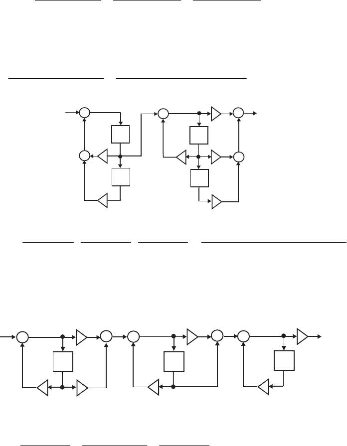
A partial fraction expansion of in obtained using residue is given by )(
3zH z
.
3754.01
0092.1
0246.01
0.5
1.31
4109.18
8.7)( 1
1
1
1
1
1
3−
−
−
−
−
−
−
−
+
−
+
+
−
+=
z
z
z
z
z
z
zH The Parallel Form II
realization based on this expansion is shown on the previous page on the right side.
8.23 A cascade realization of based on the factored form given by
⎟
⎟
⎠
⎞
⎜
⎜
⎝
⎛
−
++
⎟
⎟
⎠
⎞
⎜
⎜
⎝
⎛
++
=−
−−
−−
−
1
21
21
1
4.01
02.0362.044.0
5.08.01
)(
z
zz
zz
z
zH is shown below:
_
0.8
z
1
_
z
1
_
++
+
z
1
_
+
+
z
1
_
_
0.5
0.4
0.44
0.362
0.02
x
[n]y[n]
8.24 (a) .
1.065.04.11
9.064.54.2
5.01
3
4.01
4.0
5.01
3.02
)( 321
21
11
1
1
1
−−−
−−
−−
−
−
−
+++
−+
=
+
⋅
+
+
⋅
+
−
=
zzz
zz
zz
z
z
z
zH
(b) ].3[1.0]2[65.0]1[4.1]2[9.0]1[64.5][4.2][
−
−−
−
−
−
−
−
−
+= nynynynxnxnxny
(c) A cascade realization of is shown below:
)(zH
z
1
_
++
z
1
_
++
z
1
_
+
0.5
_
0.5
_
32 0.4
_
0.4
_
0.3
x
[n]y[n]
(d) A partial-fraction expansion of in
)(zH 1
−
z obtained using residuez is given by
1211 4.01
2.277
)5.01(
4.62
5.01
342
)( −−− +
−
+
+
−
+
+
=
zzz
zH . The Parallel Form I realization
based on this expansion is shown on the next page.
(e) The inverse –transform of the partial-fraction of given in Part (d) yields
z)(zH
].[)4.0(2.277][)5.0)(1(4.62][)5.0(342][ nnnnnh nnn µµµ −−−+−−=
Not for sale 254
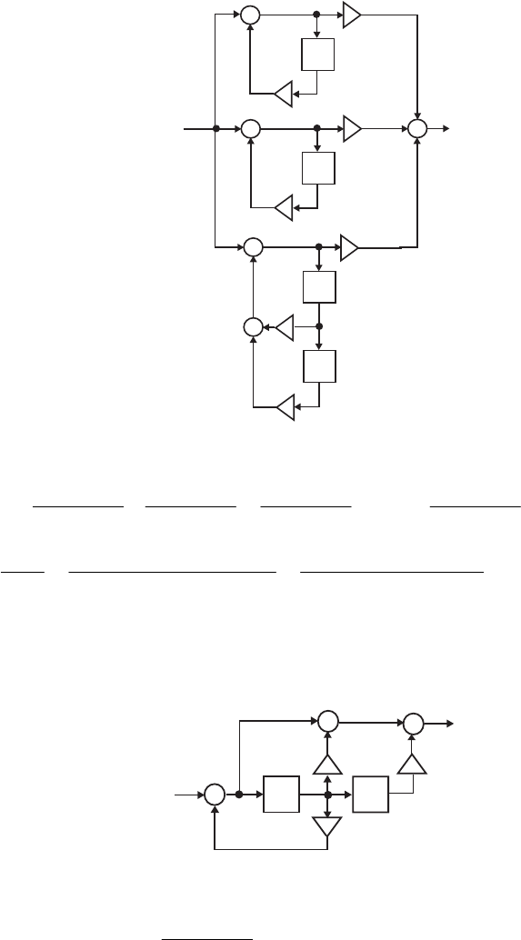
z1
_
z1
_
+
+
+
z1
_
+
0.4
_
z1
_
+
0.5
_
0.25
_
342
277.2
_
_62.4
_1
x
[n]y[n]
8.25 (a) .
2.01
1
)(,
4.01
3.01
4.01
3.0
4.01
1
)( 11
1
1
1
1−−
−
−
−
−−
=
−
−
=
−
−
−
=
z
zX
z
z
z
z
z
zY Thus,
.
4.01
06.05.01
4.01
)2.01)(3.01(
)(
)(
)( 1
21
1
11
−
−−
−
−−
−
+−
=
−
−−
==
z
zz
z
zz
zX
zY
zH
(b) ].1[4.0]2[06.0]1[5.0][][
−
+
−
+
−−= nynxnxnxny
(c)
z1
_
+
+
z1
_
+
0.4
_0.5 0.06
x
[n]
y[n]
(d) A partial-fraction expansion of in
)(zH 1
−
z using residuez is given by
1
1
4.01
125.0
15.0875.0)( −
−
−
+−=
z
zzH whose realization yields the Parallel Form I
structure as indicated on the next page.
(e) The inverse -transform of yields
z)(zH
].[)4.0(125.0][15.0]1[875.0][ nnnnh nµδδ +−−=
Not for sale 255

z
1
_
+
z
1
_
0.4
x
[n]y[n]
0.875
0.125
_
0.15
+
(f) .
3.01
4.01
3.01
4.0
3.01
1
)( 1
1
1
1
1−
−
−
−
−−
−
=
−
−
−
=
z
z
z
z
z
zX Therefore,
)()()( zXzHzY =
,2.01
3.01
4.01
4.01
)2.01)(3.01( 1
1
1
1
11 −
−
−
−
−− −=
⎟
⎟
⎠
⎞
⎜
⎜
⎝
⎛
−
−
⎟
⎟
⎠
⎞
⎜
⎜
⎝
⎛
−
−−
=z
z
z
z
zz whose inverse -transform
yields
z
].1[2.0][][
−
−= nnny δδ
8.26 Figure P8.12 can be seen to be a Parallel Form II structure. A partial-fraction
expansion of 2.16.2
6.182.32
)( 2
2
−−
−−
=
zz
zz
zH in obtained using the M-file residue is
given by
z
.
4.01
5
31
3
2)( 1
1
1
1
−
−
−
−
+
+
−
−
+=
z
z
z
z
zH Comparing the coefficients of the
expansion with the corresponding multiplier coefficients in Figure P8.12 we conclude
that the multiplier coefficient 5
−
in the feed forward path should be and the
multiplier coefficient in the feedback path should be replaced with
5
5.0−.4.0−
8.27 Figure P8.13 can be seen to be a Parallel Form I structure. A partial-fraction expansion
of 08.02.0
6.54
)( 2
2
−+
−
=
zz
zz
zH in 1
−
z obtained using the M-file residuez is given by
.
2.01
1
4.01
5.1
8
2.01
8
4.01
12
)( 1111 ⎟
⎟
⎠
⎞
⎜
⎜
⎝
⎛
−
+
+
−
−=
−
−
+
+
=−−−− zzzz
zH Comparing the
coefficients of the expansion with the corresponding multiplier coefficients in Figure
P8.12 we conclude that the multiplier coefficient
A
has a value equal to and the
multiplier coefficient has a value equal to
8−
B.4.0
−
8.28 (a) The difference equation corresponding to the transfer function )(
)(
)( zX
zY
zH =
2
2
1
1
21
21
1
)21)(1(
−−
−
−
+−
++++
=
zz
zz
αα
αα is given by
]),2[]1[2][)(1(]2[]1[][ 2121 −
+
−
+
+
+
=
−−−+ nxnxnxnynyny αααα which can be
rewritten as ])2[]1[2][]1[(])2[]1[2][(][ 1
−
−−−
−
−
+
−
+
−
+= nxnxnxnynxnxnxny α
]).2[]1[2][]2[(
2
−
−
−
−−−− nxnxnxnyα Denoting ],2[]1[2][][
−
+−+
=
nxnxnxnw
the difference equation representation becomes
Not for sale 256
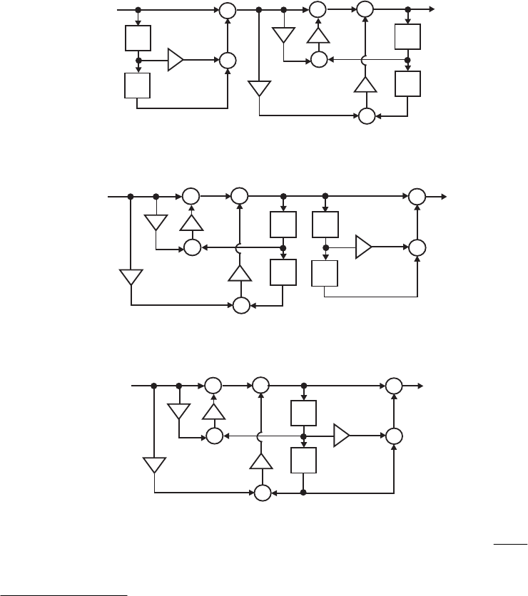
]).[]2[(])[]1[(][][ 21 nwnynwnynwny
−
−
−
−−+= αα A realization of based on the
last two equations is as indicated below:
)(zH
+
z1
_
w[n]
+
z1
_
y[n]
+
+
1
_
1
_
1
α
_2
α
+
z1
_
+
x
[n]
z1
_
2
An interchange of the two stages leads to an equivalent realization shown below:
y[n]
+
z1
_
+
z1
_
+
+
1
_
1
_
1
α
_2
α
x
[n]+
z1
_
+
z1
_
2
Finally, by delay sharing the above structure reduces to the canonic realization shown
below:
y[n]
+
z
1
_
+
z
1
_
+
+
1
_
1
_
1
α
_2
α
x
[n]+
+
2
(b) The difference equation corresponding to the transfer function )(
)(
)( zX
zY
zH =
2
2
1
1
2
2
1
)1)(1(
−−
−
+−
−−
=
zz
z
αα
α is given by
])2[][)(1(]2[]1[][ 221
−
−
−
=
−+−− nxnxnynyny ααα which can be rewritten as
]2[]2[][][]2[]1[][ 2221
−
+
−
−
−
+
−−−= nxnxnxnxnynyny αααα
]).2[][(])2[]2[][(]1[ 21
−
−
+
−
+
−
−−−= nxnxnynxnxny αα Denoting
we can rewrite the last equation as
],2[][][ −−= nxnxnw
].[])2[][(]1[][ 21 nwnynwnyny
+
−
+
−−= αα
A realization of based on the last two equations is as shown on next page.
)(zH
Not for sale 257
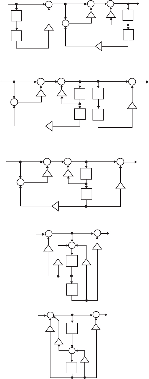
+
z
1
_
w[n]
+
y[n]
+
1
_
1
_
1
α
_2
α
+
z
1
_
x
[n]
z1
_z1
_
An interchange of the two stages leads to an equivalent realization shown below:
y[n]
x
[n]
1
_
+
z
1
_
z
1
_
+
z
1
_
+
+
1
_
1
α
_2
α
z
1
_
Finally, by delay sharing the above structure reduces to a canonic realization as shown
below:
y[n]
x
[n]
1
_
+
+
z
1
_
+
+
1
_
1
α
_2
α
z
1
_
8.29 (a)
z1
_
++
+
z1
_
α1α2
α3α4
X
1Y
1
(b)
z
1
_
++
+
α
1
α
2
α
4
α
3
z
1
_
Y
1
X
1
Not for sale 258

8.30 (a) From the structure of Figure P8.14 it follows that ,
)(
)(
)(
1
1
1
1
zHBA
zHDC
X
Y
zH
N
N
N−
−
⋅+
⋅+
==
from which we get .
)(
)(
)(
1DzHB
zHAC
zH
N
N
N−⋅
⋅
−
=
− Substituting the expression for we
then arrive at
)(zHN
⎟
⎠
⎞
⎜
⎝
⎛+−
⎟
⎠
⎞
⎜
⎝
⎛
⎟
⎠
⎞
⎜
⎝
⎛
−
⎟
⎠
⎞
⎜
⎝
⎛+
=∑∑
∑∑
=−
=
== −
−N
i
i
i
N
ii
N
ii
N
i
i
i
N
zdDpB
pAzdC
zH
10
01
1
1
1
)(
.
)()()()(
)()()()(
1
11
1
110
1
11
1
110
N
NN
N
NN
N
NN
N
NN
zDdBpzDdBpzDdBpDBp
zApCdzApCdzApCdApC
−+−
−−
−
−+−
−−
−
−+−++−+−
−+−++−+−
=
L
K
Substituting the values ,,,1 0
1pCzdBA N===
−
and ,
1
−
=zpD N we get )(
1zH N−
1
11
2
11
1
0
0
1
110
1
11000
)(
)()()(
)()()()(
−−
−
−−
−−
−+−
−−
−
−+
−++−+−
−+−++−+−
=
N
NNNN
N
NNNNNNNN
N
NN
N
NN
zdppd
zdppdzdppdzppd
zpdpzpdpzpdppp
L
L
1
11
1
110
1
0
2
110110
)()()(
)()()(
+−
−−
−
+−+−
−−
−++−+−
−+−++−
=N
NNNNNNNN
N
NN
N
NN
zdppdzdppdppd
zpdpzpdppdp
L
L
1
'1
2
'2
1
'
1
1
'1
2
'2
1
'
1
'
0
1+−
−
+−
−
−
+−
−
+−
−
−
++++
++++
=N
N
N
N
N
N
N
N
zdzdzd
zpzpzpp
L
L where
,10,
0
11
'−≤≤
−
−
=++ Nk
pdp
pdp
p
NN
kkk
k and .11,
0
'−≤≤
−
−
=Nk
pdp
dpdp
d
NN
kNNk
k
(b) From the chain parameters, we obtain for the first stage ,
011 p
A
C
t==
.,1
1
,)( 1
2221
1
012 −− −=−===−=
−
=zd
A
B
t
A
tzdpp
A
BCAD
tNNN The
corresponding input-output relations of the two-pair are given by
,)()( 2
1
2
1
102
1
0101 XzpXzdXpXzdppXpY NNNN −
−
−
+−=−+=
Substituting the second equation into the first we rewrite it as
A realization of the two-pair based on the last two equations is
therefore as indicated below:
.
2
1
12 XzdXY N−
−=
.
2
1
201 XzpYpY N−
+=
z–1
p
0
d
N
_
X
1
Y
1
X
2
Y
2
p
N
Not for sale 259
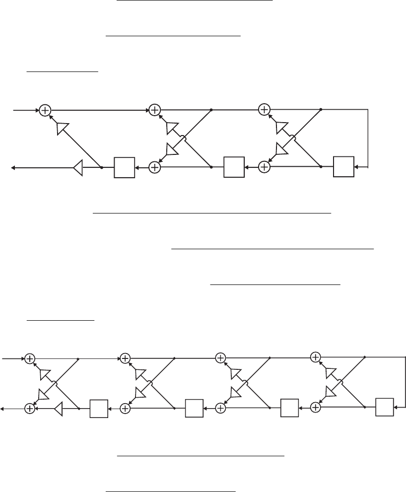
(c) Except for the first stage, all other stages require 2 multipliers. Hence, the total number
of multipliers needed to implement an –th order transfer function is
N)(zHN.12
+
N
The total number of 2-input adders required is while the overall realization is canonic
requiring delays.
,2N
N
8.31 (a) From 321
321
13 575.13.335.21
72.066.03.0
)()( −−−
−−−
−+−
−+
==
zzz
zzz
zHzG , using Eq. (8.132a) and
(8.132b) we get .
8562.10063.31
9167.04167.0
)( 21
21
2−−
−−
+−
+−−
=
zz
zz
zG Repeating the procedure we get
.
7357.01
2232.1
)( 1
1
1−
−
−
+−
=
z
z
zG From and we arrive at the cascaded lattice
realization shown below:
),(),( 23 zGzG ),(
1zG
z–1 z–1 z–1
_
0.72
1.575 1.8562
_
_
0.4167 1.2232
_
0.7357
(b) From ,
003.001.0095.055.01
9125.155.6025.133.393.9
)()( 4321
4321
24 −−−−
−−−−
−−++
++−−
==
zzzz
zzzz
zHzG using Eq.
(8.132a) and (8.132b) we get .
00027.00735.04813.01
4235.31679.78896.22
)( 321
321
3−−−
−−−
+++
++−−
=
zzz
zzz
zG
Repeating the procedure twice we get 21
21
20721.04803.01
0744.58259.3
)( −−
−−
++
++
=
zz
zz
zG and
.
1579.01
4704.4
)( 1
1
1−
−
+
+
=
z
z
zG From and we arrive at the cascaded
lattice realization shown below:
),(),(),( 234 zGzGzG ),(
1zG
z–1 z–1 z–1 z–1
9.3
1.9125
0.003
_22.8896
_0.00027
3.8259
_0.0721
0.9179
4.7915
(c) From 321
321
33 356.268.67.01
92.462.496.88.7
)()( −−−
−−−
+−+
++−
==
zzz
zzz
zHzG , using Eq. (8.132a) and
(8.132b) we get .
2364.38209.11
209.407.1
)( 21
21
2−−
−−
+−
+−
=
zz
zz
zG Repeating the procedure we get
Not for sale 260
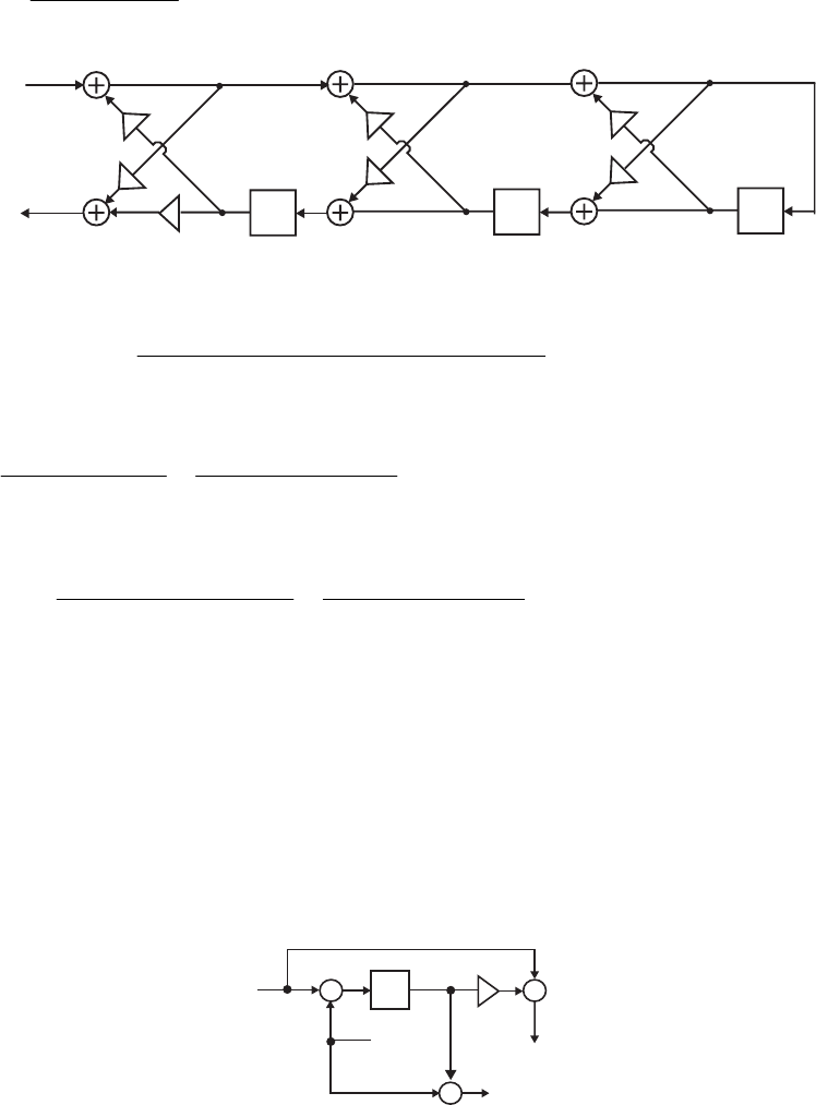
.
7915.41
9179.0
)( 1
1
1−
−
−
+
=
z
z
zG From and we arrive at the cascaded lattice
realization shown below:
),(),( 23 zGzG ),(
1zG
z–1 z–1 z–1
7.8
4.92
_2.356
1.07
3.2364
_4.7915
0.9179
8.32 When is an allpass transfer function of the form )(zHN
,
1
)()( 1
1
1
1
1
1
1
1
N
N
N
N
NN
NN
NN zdzdzd
zzdzdd
zAzH −+−
−
−
−+−−
−
++++
++++
==
L
L then from Eq. (8.132a), the
numerator coefficients of are given by )(
1zH N−
,
1
2
11
0
110
'−
−
=
−
−
=−−+++
N
kNkN
NN
kk
kd
ddd
pdp
pdp
p and from Eq. (8.132b) the denominator
coefficients of are given by )(
1zH N−
,
1
'
2
11
0
11
'1k
N
kNNk
NN
kNNkN
kN p
d
ddd
pdp
ddp
d=
−
−
=
−
−
=−−+−−−−
−− implying is an
allpass transfer function of order
)(
1zH N−
.1
−
N Since here 1
=
N
p and the lattice
structure of Problem 8.30 then reduces to the lattice structure employed in the Gray-Markel
realization procedure.
,
0N
dp =
8.33 (a) Consider the realization of Type 1B allpass structure. From its transfer parameters
given in Eq. (8.50b) we arrive at ,)()1( 221
1
2
1
1
1
1XXXzXzXzY ++=++=
−
−
−
and
).()1( 21
1
12
1
1
1
2XXzXXzXzY +−=−−=
−
−− A realization of the two-pair based on
these two equations is as shown below which leads to the structure of Figure 8.24(b).
z
1
_
+ +
1
_
1
X
1
Y
+
2
X
2
Y
(b) From the transfer parameters of Type 1At allpass given in Eq. (8.50c) we obtain
and
,
21
1
1XXzY += −.)()1( 1
1
121
11
12
1
1
2
2YzXXXzzXXzXzY
−
−
−
−
−
−=+−=−−=
A realization of the two-pair based on these two equations is as shown on next page which
leads to the structure of Figure 8.24(c).
Not for sale 261
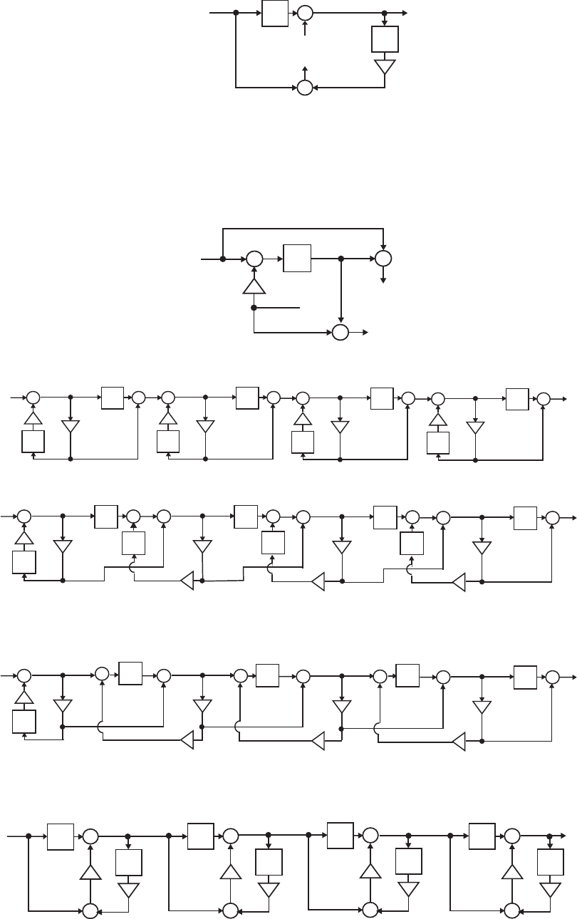
z
1
_
+
1
_
1
X
1
Y
+
z
1
_
2
X
2
Y
(c) From the transfer parameters of Type 1At allpass given in Eq. (8.50d) we obtain
,)()1( 221
1
2
1
1
1
1XXXzXzXzY +−=−+=
−
−− and 2
1
1
1
2)1( XzXzY −
−
−+=
A realization of the two-pair based on these two equations is as
shown below which leads to the structure of Figure 8.24(d).
).( 21
1
1XXzX −+= −
z
1
_+
1
X
1
Y
+
+
1
_
X
2
2
Y
8.34 (a) A cascade connection of 4 Type 1A first-order allpass networks is shown below:
z
1
_
z
1
_
++
1
_
z
1
_
z
1
_
++
1
_
z
1
_
z
1
_
++
1
_
z
1
_
z
1
_
++
1
_
abcd
Simple block diagram manipulation of the above structure leads to:
z
1
_
z
1
_
+ +
1
_
z
1
_
+ +
1
_
z
1
_
z
1
_
+ +
1
_
z
1
_
z
1
_
+ +
1
_
d
az
1
_
bc
Finally, by delay sharing between adjacent allpass sections we arrive at the following
equivalent realization requiring now 5 delays compared to 8 delays in the direct realization
shown on the previous page.
z
1
_
z
1
_
++
1
_
z
1
_
+ +
1
_
z
1
_
+ +
1
_
z
1
_
+ +
1
_
d
abc
(b) A cascade connection of 4 Type 1At first-order allpass networks is shown below which
requires 8 delays.
z
1
_
+
1
_
+
z
1
_
z
1
_
+
1
_
+
z
1
_
z
1
_
+
1
_
+
z
1
_
z
1
_
+
1
_
+
z
1
_
abcd
Not for sale 262
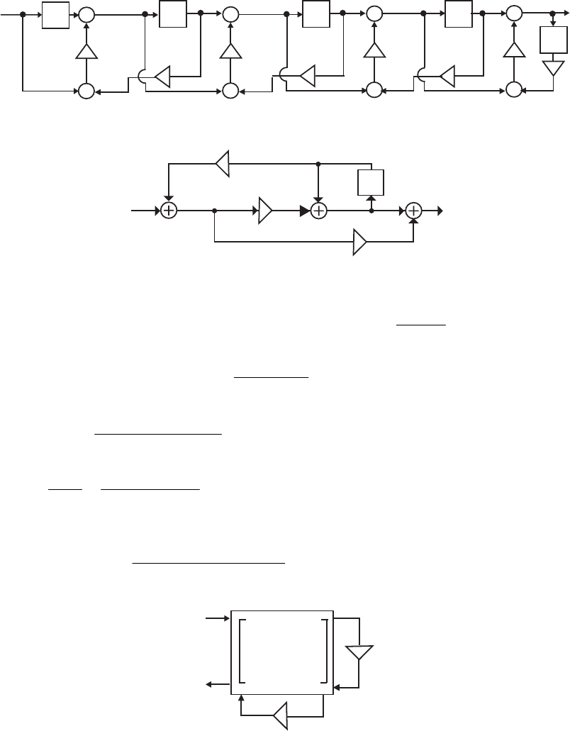
By delay sharing between adjacent allpass sections we arrive at the following equivalent
realization requiring now 5 delays.
z
1
_
+
1
_
+
z
1
_
+
1
_
+
z
1
_
+
1
_
+
z
1
_
+
1
_
+
z
1
_
abcd
8.35 The structure of Figure P8.15 with internal variables labeled is shown below:
z
–1
–1
–1
a
W(z)U(z)
X
(z)Y(z)
Its analysis yields (1): ),()()( 1zUzzXzW
−
−= (2): and (3):
From Eq. (2) we obtain (4):
),()()( 1zUzzWazU −
+=
).()()( zUzWzY +−= ).(
1
)( 1zW
z
a
zU −
−
= Substituting Eq.
(4) in Eq. (3) we get (5): ).(
1
1
)( 1
1
zW
z
za
zY ⎟
⎟
⎠
⎞
⎜
⎜
⎝
⎛
−
−−
−= −
− Substituting Eq. (4) in Eq. (1) we get
:)6( ).(
1
1
)( 1
11
zW
z
zaza
zX ⎟
⎟
⎠
⎞
⎜
⎜
⎝
⎛
−
+−−
=−
−− Finally, from Eqs. (5) and (6) we arrive at
.
)1(1
)1(
)(
)(
)( 1
1
−
−
−−
+−−
==
za
za
zX
zY
zH
8.36 We realize 2
21
1
1
21
121
21
)( −−
−
−
+++
++
=
zddzd
zzddd
zA in the form of a constrained three-pair as
indicated below:
t
11
t
12
t
13
t
21
t
22
t
23
t
32
t
31
t
33
1
X
1
Y
2
X
3
X
2
Y
3
Y
d
1
_
d
2
From the above figure, we have and
,
3
2
1
333231
232221
131211
3
2
1
⎥
⎥
⎥
⎦
⎤
⎢
⎢
⎢
⎣
⎡
⎥
⎥
⎥
⎦
⎤
⎢
⎢
⎢
⎣
⎡
=
⎥
⎥
⎥
⎦
⎤
⎢
⎢
⎢
⎣
⎡
X
X
X
ttt
ttt
ttt
Y
Y
Y
,
212 YdX −=
Not for sale 263

From these equations, we get after some algebra .
323 YdX =,
)(
)(
)(
1
1
2zD
zN
X
Y
zA == where
),(1)( 3322322321332221 ttttddtdtdzD
−
+−+= and
)()()( 31133311221122211111 ttttdttttdtzN
−
−
−+=
{}
.)()()( 33223223112312132231321333122121 tttttttttttttttdd
−
+
−
+
−+
Comparing the denominator of the desired allpass transfer function with we get
)(zD
.,0, 2
322333
1
22
−
−=== ztttzt Next, comparing the numerator of the desired allpass
transfer function with we get
)(zN ,0),1(, 3113
21
2112
2
11 =−==
−
−
−
ttzzttzt and
.1)()( 23121322311321231132
=
−
+− tttttttttt Substituting the appropriate transfer
parameters from the previous equations into the last equation we simplify it to
.1
4
231231322113 −=+ −
ztttttt
Since either ,0
3113 =tt ,0
13
=
t or .0
31
=
t (Both cannot be simultaneously equal to zero,
as this will violate the condition 231231322113 tttttt
+
.1
4−=
−
z
Consider the case Then the above equation reduces to From
this equation and
.0
13 =t.1
4
231231 −= −
zttt
,
2
3223
−
=ztt it follows that 1,1, 4
123123
2
32 −=== −
−
ztttzt
There are four possible realizable sets of values of and
satisfying the last equation and
).1)(1)(1( 211 ++−= −−− zzz 21
t
31
t).1( 21
2112 −=
−
−
zztt These lead to 4 different
realizable transfer matrices for the three-pair: Type 2A:
Type 2B: Type 2C:
Type 2D: A realization of each of the above Type 2 allpass
structures is obtained by implementing its respective transfer matrix, and then constraining
the and variables through the multiplier and constraining the and
variables through the multiplier
,
01
1
01
22
11
22
⎥
⎥
⎥
⎦
⎤
⎢
⎢
⎢
⎣
⎡
+
−
−−
−−
−−
zz
zz
zz
,
0)1)(1(
1)1(
01
212
111
12
⎥
⎥
⎥
⎦
⎤
⎢
⎢
⎢
⎣
⎡
−+
−
+
−−−
−−−
−−
zzz
zzz
zz
,
0)1)(1(
1)1(
01
212
111
12
⎥
⎥
⎥
⎦
⎤
⎢
⎢
⎢
⎣
⎡
++
+
−
−−−
−−−
−−
zzz
zzz
zz
.
01
1)1(
01
24
121
2
⎥
⎥
⎥
⎦
⎤
⎢
⎢
⎢
⎣
⎡
−
−
−−
−−−
−
zz
zzz
z
2
Y2
X1
d3
Y3
X
2
d
−
resulting in the four structures shown in Figure 8.25
of the text.
It can be easily shown that the allpass structures obtained for the case are precisely
the transpose of the structures of Figure 8.25.
0
31 =t
8.37 A cascade of two Type 2D second-order allpass networks is shown below which requires 8
delays.
Not for sale 264
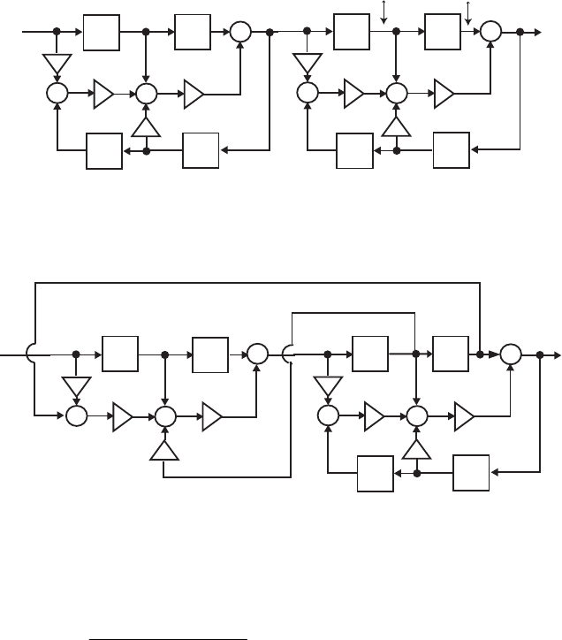
z
1
_
z
1
_
+
+
+
z
1
_
z
1
_
1
_
1
_
z
1
_
z
1
_
+
+
+
z
1
_
z
1
_
1
_
1
_
abcd
w[n]
x
[n]y[n]
w[n ]
1
_
w[n ]
1
_
w[n ]
2
_
w[n ]
2
_
By delay sharing between adjacent allpass sections we arrive at the following equivalent
realizations requiring now 6 delays.
+
+
1
_ab
z1
_z1
_
z1
_
+
+
+
z1
_
1
_
1
_
cd
z1
_z1
_
+
1
_
w[n]
x
[n]y[n]
w[n ]
1
_
w[n ]
2
_
The minimum number of delays needed to implement a cascade of Type 2D second-order
allpass sections is thus ).1(2)1(24
+
=
−
+MM
8.38 We realize 2
2
1
1
21
12
21
)( −−
−
−
++
++
=
zdzd
zzdd
zA in the form of a constrained three-pair as indicated
in the solution of Problem 8.36. Comparing the numerator and the denominator of the
Type 3 allpass transfer function with and given in the solution of Problem 8.36
we arrive at
)(zN )(zD
),1(,,,,, 21
21212
3
3223
2
33
2
22
1
22
2
11 −====== −−
−
−
−
−− zzttzttztztztzt
).1()1(,1 4123
232113322113
4
3113 −+−=+−=
−
−
−
−
−zzzzttttttztt
To solve the last four equations to arrive at a set of realizable set of values for the transfer
parameters, and we need to pre-select and satisfying the
condition and then determine realizable values for the other transfer
parameters.
,,,,, 2331132112 ttttt ,
32
t23
t32
t
,
3
3223 −
=ztt
(a) Let There are 4 possible realizable sets of values of
and satisfying the constraints given above resulting in the following transfer matrices
of the three-pair:
., 2
32
1
23 −− == ztzt ,,, 132112 ttt
31
t
Not for sale 265
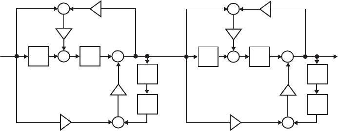
Type 3A: Type 3B: ,
1
11
222
111
222
⎥
⎥
⎥
⎦
⎤
⎢
⎢
⎢
⎣
⎡
+
−−
−−−
−−−
−−−
zzz
zzz
zzz
,
)1)(1(
)1(
11
2221
1111
112
⎥
⎥
⎥
⎦
⎤
⎢
⎢
⎢
⎣
⎡
+−
−
++
−−−−
−−−−
−−−
zzzz
zzzz
zzz
Type 3C: Type 3D: ,
)1)(1(
)1(
11
2221
1111
112
⎥
⎥
⎥
⎦
⎤
⎢
⎢
⎢
⎣
⎡
++
+
−−
−−−−
−−−−
−−−
zzzz
zzzz
zzz
.
1
)1(
11
224
1121
2
⎥
⎥
⎥
⎦
⎤
⎢
⎢
⎢
⎣
⎡
−
−
−−−
−−−−
−
zzz
zzzz
z
(b) This leads to 4 new realizations which are transpose of the 4
structures developed in Case (a).
., 1
32
2
23 −− == ztzt
(c) Here also there are 4 different realizations whose transfer matrices
are as given below:
.,1 3
3223 −
== ztt
Type 3E: ,
1
1
1)1(
232
11
2212
⎥
⎥
⎥
⎦
⎤
⎢
⎢
⎢
⎣
⎡
+
−−
−−−
−−
−−−−
zzz
zz
zzzz
Type 3F: ,
)1)(1(
11
1)1(
2321
11
1112
⎥
⎥
⎥
⎦
⎤
⎢
⎢
⎢
⎣
⎡
+−
−
++
−−−−
−−
−−−−
zzzz
zz
zzzz
Type 3G: Type 3H: ,
)1)(1(
11
1)1(
2321
11
1112
⎥
⎥
⎥
⎦
⎤
⎢
⎢
⎢
⎣
⎡
++
+
−−
−−−−
−−
−−−−
zzzz
zz
zzzz
.
1
11
1
234
12
12
⎥
⎥
⎥
⎦
⎤
⎢
⎢
⎢
⎣
⎡
−
−
−−−
−−
−−
zzz
zz
zz
(d) This leads to 4 new realizations which are transpose of the 4
structures developed in Case (b).
.1, 32
3
23 == −tzt
8.39 A cascade of two Type 3B second-order allpass networks is shown below which requires 8
delays.
z
1
_
+
+
+
+
z
1
_
z
1
_
z
1
_
_
1
_
1
z
1
_
+
+
+
+
z
1
_
z
1
_
z
1
_
_
1
_
1
a
b
c
d
w[n]
x
[n]y[n]
w[n ]
1
_
w[n ]2
_
Not for sale 266
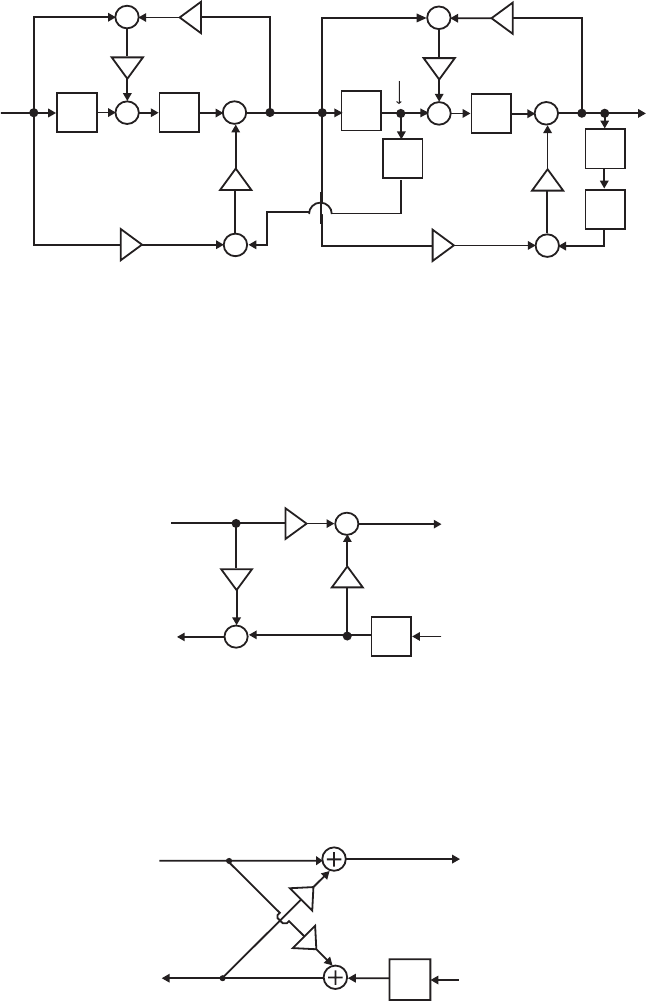
By delay sharing between adjacent allpass sections we arrive at the following equivalent
realizations requiring now 7 delays.
+
+
+
+
z1
_z1
_
_1
_1
z1
_
+
+
+
+
z1
_
z1
_
_1
_1
a
b
c
d
w[n]
x
[n]y[n]
w[n ]
1
_
w[n ]2
_
z1
_
z1
_
The minimum number of delays needed to implement a cascade of Type 3B second-order
allpass sections is thus ).1(3)1(34
+
=
−
+MM
8.40 From the transfer parameters given in Eq. (8.50d) we arrive at the input-output relations of
the two-pair as (1): ,
2
1
11 XzXkY m
−
+= and (2): A three-
multiplier realization based on these two equations is shown below:
.)1( 2
1
1
2
2XzkXkY mm −
−−=
_
1
2
m
k
+
1
X
1
Y
+
z
1
_
m
k
2
Y
X
2
m
k
_
8.41 Eq. (2) in the solution of Problem 8.40 can be rewritten as:
).( 2
1
112
1
1
2
12 XzXkkXXzkXkXY mmmm
−
−+−=−−= Substituting Eq. (1) of the
solution of Problem 8.40 in this equation we then get (3): .
112 YkXY m
−
=
A
realization of the two-pair based on Eq. (3) and Eq. (1) of the solution of Problem 8.40
results in the lattice structure shown below:
z–1
km
km
_
X1
Y
1X2
Y2
From Eqs. (1) and (2) of the solution of Problem 8.40 we arrive at the transfer
parameters of the lattice two-pair given by ,1,, 2
21
1
1211 mm ktztkt −===
−
The corresponding chain parameters are obtained using Eq. (7.128b)
.
1
22 −
−= zkt m
Not for sale 267
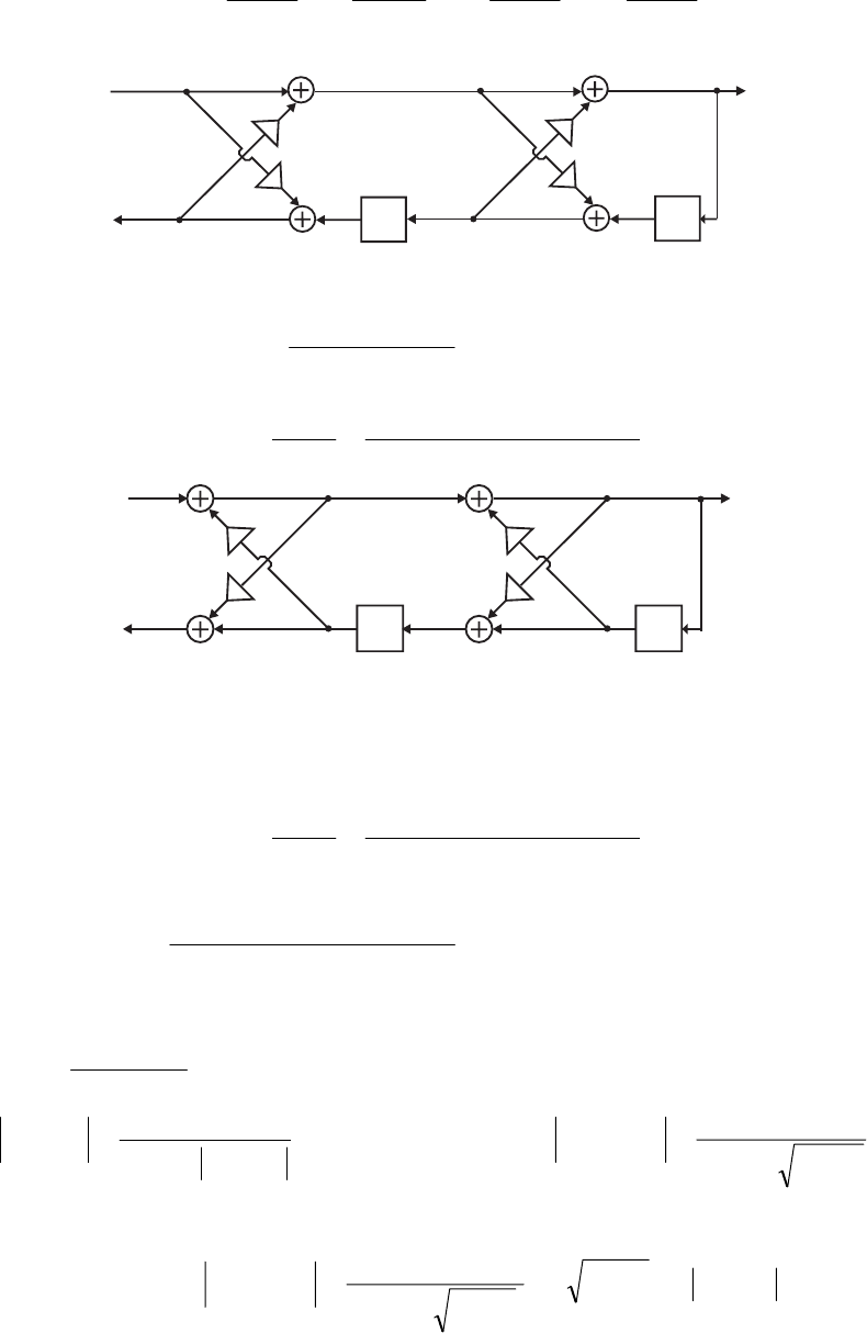
and are given by .
1
,
1
,
1
,
1
1
2
1
22
1
2mm
m
m
m
mk
z
D
k
k
C
k
zk
B
k
A−
=
−
=
−
=
−
=−
−
z–1
k2
k1
_
z–1
X
(z)
1
Y (z)
1
W (z)
1
k2
_
k1
S (z)
1
Hence, the input-output relation of the all-pole cascade lattice structure given above can
be expressed as: ,
)(
)(
11
)1)(1(
1
)(
)(
1
1
1
1
1
1
1
2
1
2
2
1
2
2
1
1⎥
⎦
⎤
⎢
⎣
⎡
⎥
⎥
⎦
⎤
⎢
⎢
⎣
⎡
⎥
⎥
⎦
⎤
⎢
⎢
⎣
⎡
−−
=
⎥
⎦
⎤
⎢
⎣
⎡
−
−
−
−
zS
zW
zk
zk
zk
zk
kk
zY
zX from
which we obtain .
)1(1
)1)(1(
)(
)(
)( 2
2
1
21
2
1
2
2
1
1
−− +++
−−
==
zkzkk
kk
zX
zW
zHr
z–1
k
1
k
1
_
z–1
k
2
_
k
2
X (z)
1
Y (z)
1
W (z)
1
S (z)
1
Likewise, from Section 8.8.1, we arrive at input-output relation of the all-pole cascade
lattice structure given above as: from
which we obtain
,
)(
)(
11
)(
)(
1
1
1
1
1
1
1
2
1
2
1
1⎥
⎦
⎤
⎢
⎣
⎡
⎥
⎥
⎦
⎤
⎢
⎢
⎣
⎡
⎥
⎥
⎦
⎤
⎢
⎢
⎣
⎡
=
⎥
⎦
⎤
⎢
⎣
⎡
−
−
−
−
zS
zW
zk
zk
zk
zk
zY
zX
.
)1(1
1
)(
)(
)( 2
2
1
21
1
1
−− +++
==
zkzkk
zX
zW
zHs
Now a second-order all-pole transfer function can also be expressed in terms of its
poles as .
)cos(21
1
)( 221 −− +−
=
zrzr
zH
o
ω Comparing the denominator of with that
of and we observe and )(zHs),(zHr2
2rk =).cos(2)1( 21 o
rkk ω
−
=
+
As ,1
≅
r
).cos(
1
)cos(2
2
1o
o
r
r
kω
ω−≅
+
−= At the true resonance peak, we have
.
)sin()1(
1
)( 2o
r
eH r
ω
ω
−
= Likewise, at ,
r
ωω
=
.
1)1(
1
)( 2
1
2kk
eH r
j
s=−
=
ω As
and
Hence, at
,1,1 2
2→=→ rkr ).1)(1(2)1)(1)(1()1)(1( 2
2
1
22
2
1
2
2
2
1kkkkkkk −−≅+−−=−−
,
r
ωω =.)sin(212
1)1(
)1)(1(2
)( 2
1
2
1
2
2
2
1r
j
rk
kk
kk
eH rω
ω=−=
−−
−−
≅ This
indicates that the gain at the peak resonance is approximately independent of the pole
Not for sale 268
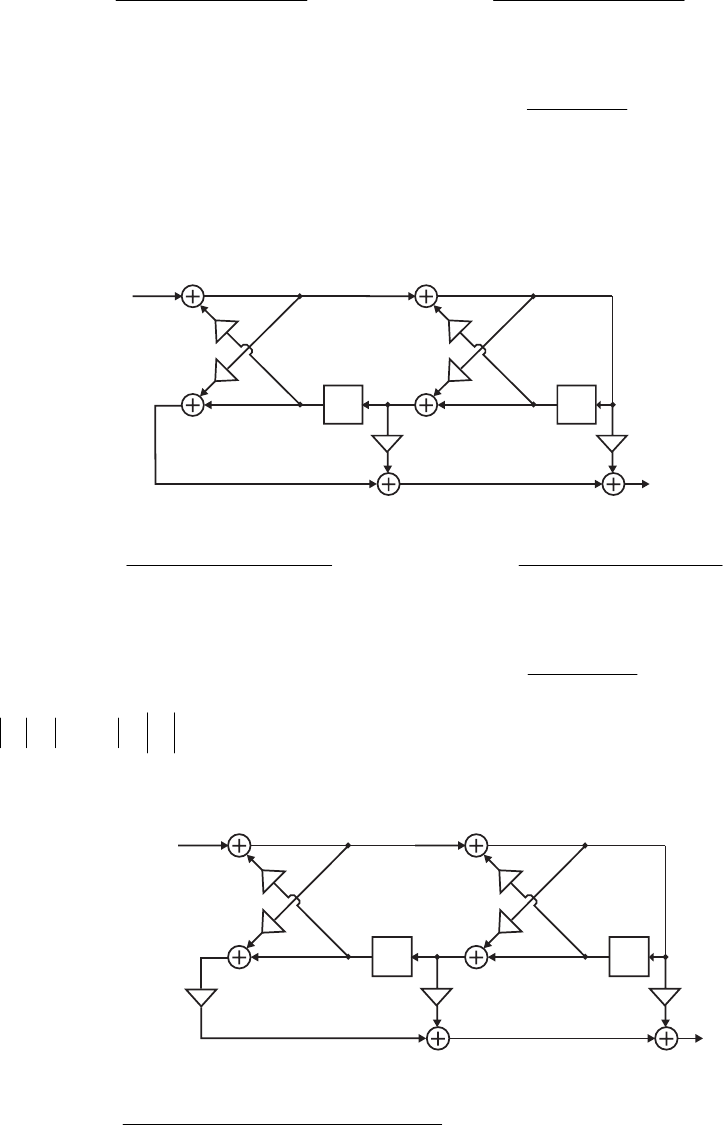
radius as long as the pole angle is constant and the radius is close to 1.
8.42 (a) .
5.03.01
3.29.3
)( 21
21
1−−
−−
++
++
=
zz
zz
zH Choose .
5.03.01
3.05.0
)( 21
21
2−−
−−
++
++
=
zz
zz
zA Note
Using Eq. (8.45) we next determine the coefficient of
the allpass transfer function arriving at
.15.0)( 222 <==∞= dAk '
1
d
)(
1zA 1
1
12.01
2.0
)( −
−
+
+
=
z
z
zA . Here,
Therefore, and hence, is stable.
.12.0)( '
111 <==∞= dAk )(
2zA )(
1zH
The feed-forward coefficients are given by ,0.2,0.1 111221 =−
=
=
=
dpp ααα
Final realization of is as shown below:
.0.3
'
122103 =−−= ddp ααα )(
1zH
z–1
z–1
_
1
X
o
Y
0.5 _
0.5
0.2
0.2
23
(b) .
4.042.01
374.06.2
)( 21
21
2−−
−−
+−
++
=
zz
zz
zH Choose .
4.042.01
42.04.0
)( 21
21
2−−
−−
+−
+−
=
zz
zz
zA Note
Using Eq. (8.45) we next determine the coefficient of
the allpass transfer function arriving at
.14.0)( 222 <==∞= dAk '
1
d
)(
1zA 1
1
13.01
3.0
)( −
−
−
+−
=
z
z
zA . Here,
.13.0)( '
111 <==∞= dAk Therefore, and hence, is stable.
)(
2zA )(
2zH
The feed-forward coefficients are given by ,0.2,0.3 111221 =−
=
=
=
dpp ααα
Final realization of is as shown below:
.0.2
'
122103 =−−= ddp ααα )(
2zH
z–1 z–1
_
1
X
o
Y
_0.4
0.4
2
32
0.3
0.3
(c) .
4.0056.028.01
256.3192.53
)( 321
321
3−−−
−−−
++−
+−+−
=
zzz
zzz
zH Choose
Not for sale 269
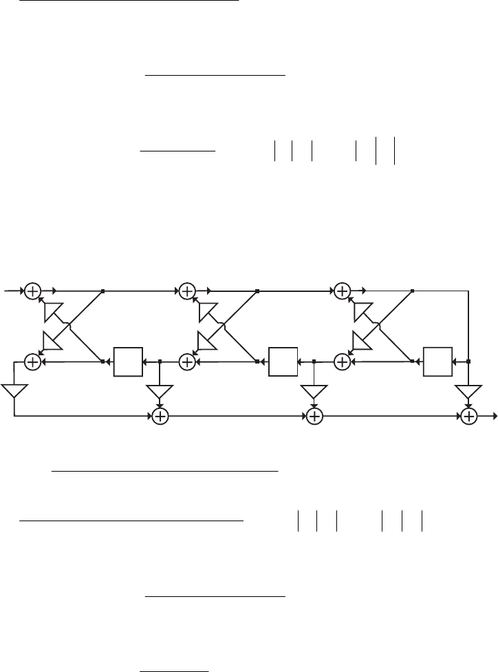
321
321
34.0056.028.01
28.0056.04.0
)( −−−
−−−
++−
+−+
=
zzz
zzz
zA Note .14.0)( 333 <=
=
∞
=
dAk Using
Eq. (8.45) we next determine the coefficient and of the allpass transfer function
arriving at
'
1
d'
2
d
)(
2zA .
2.036.01
36.02.0
)( 21
21
2−−
−−
+−
+−
=
zz
zz
zA Now .12.0)( 222
<
==∞
=
dAk
Using Eq. (8.45) we next determine the coefficient of the allpass transfer function
arriving at
"
1
d
)(
1zA 1
1
13.01
3.0
)( −
−
−
+−
=
z
z
zA . Here, .13.0)( '
111 <==∞= dAk Therefore,
and hence, is stable. )(
3zA )(
3zH
The feed-forward coefficients are given by ,0.3,0.2 112231 −=−
=
=
=
dpp ααα
Final realization
of is as shown below:
,0.4
'
122113 =−−= ddp ααα .0.2
"
13
'
223104 −=−−−= dddp αααα
)(
3zH
Yo
X
1
z
1
_
z
1
_
z
1
_
_0.4
0.4
_0.2
0.2
0.3
0.3
_
23
_42
_
(d) .
3.0056.042.01
284.0112.363.1
)( 321
321
4−−−
−−−
−++
+++
=
zzz
zzz
zH Choose
321
321
33.0056.042.01
42.0056.03.0
)( −−−
−−−
−++
+++−
=
zzz
zzz
zA Note .13.0)( 333 <==∞= dAk Using
Eq. (8.45) we next determine the coefficients and of the allpass transfer function
arriving at
'
1
d'
2
d
)(
2zA .
2.048.01
48.02.0
)( 21
21
2−−
−−
++
++
=
zz
zz
zA Now .12.0)( 222
<
==∞
=
dAk
Using Eq. (8.45) we next determine the coefficient of the allpass transfer function
arriving at
"
1
d
)(
1zA 1
1
14.01
4.0
)( −
−
+
+
=
z
z
zA . Here, Therefore,
and hence, is stable.
.14.0)( '
111 <==∞= dAk
)(
3zA )(
4zH
The feed-forward coefficients are given by ,0,0.2 112231 =−
=
=
=
dpp ααα
Final realization
of is as shown on the next page.
,0.3
'
122113 =−−= ddp ααα .0.1
"
13
'
223104 =−−−= dddp αααα
)(
3zH
Not for sale 270
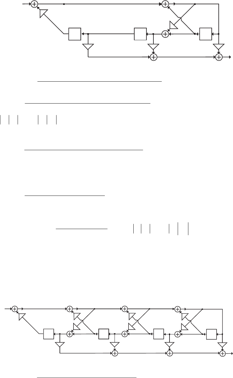
Yo
X
1
z
1
_
z
1
_
z
1
_
_
_
1
0.4
0.6 2.2 3.2
(e) .
08.008.018.01.01
3.06.02
)( 4321
321
5−−−−
−−−
−++−
+−+
=
zzzz
zzz
zH Choose
.
08.008.018.01.01
1.018.008.008.0
)( 4321
4321
4−−−−
−−−−
−++−
+−++−
=
zzzz
zzzz
zA Note
.108.0)( 444 <==∞= dAk Using Eq. (8.45) we next determine the coefficients
and of the allpass transfer function arriving at
,
'
1
d'
2
d'
3
d)(
3zA
.
0725.01957.00942.01
0942.0195.00725.0
)( 321
321
3−−−
−−−
++−
+−+
=
zzz
zzz
zA Now
Using Eq. (8.45) we next determine the coefficients
and of the allpass transfer function arriving at
.10725.0)( '
333 <==∞= dAk "
1
d
"
2
d)(
2zA
.
2035.01090.01
1090.02035.0
)( 21
21
2−−
−−
+−
+−
=
zz
zz
zA Now Using Eq.
(8.45) we next determine the coefficient of the allpass transfer function
arriving at
..)( "120350
222 <==∞= dAk
'''
1
d)(
1zA
1
1
10905.01
009058.0
)( −
−
−
+−
=
z
z
zA . Here, .10905.0)( '''
111 <==∞= dAk
Therefore, and hence, is stable.
)(
4zA )(
5zH
The feed-forward coefficients are given by ,3.0,0 113241 −=−
=
=
=
dpp ααα
,0283.1
'
122123 −=−−= ddp ααα
Final realization of is as
shown below:
,.
"' 54670
13223114 =α−α−α−=α dddp
.2805.2
'''
14
"
23
'
324105 =−−−−= ddddp ααααα )(
5zH
Yo
X
1
z
1
_
z
1
_
z
1
_
z
1
_
0.08 _0.0725
0.0725
_0.2035
0.2035
0.0905
_0.0905
_0.3 _1.0283 0.5467 2.2805
8.43 (a) .
575.136.335.21
72.066.032.0
)( 321
321
1−−−
−−−
−+−
−+
=
zzz
zzz
zH Choose
Not for sale 271
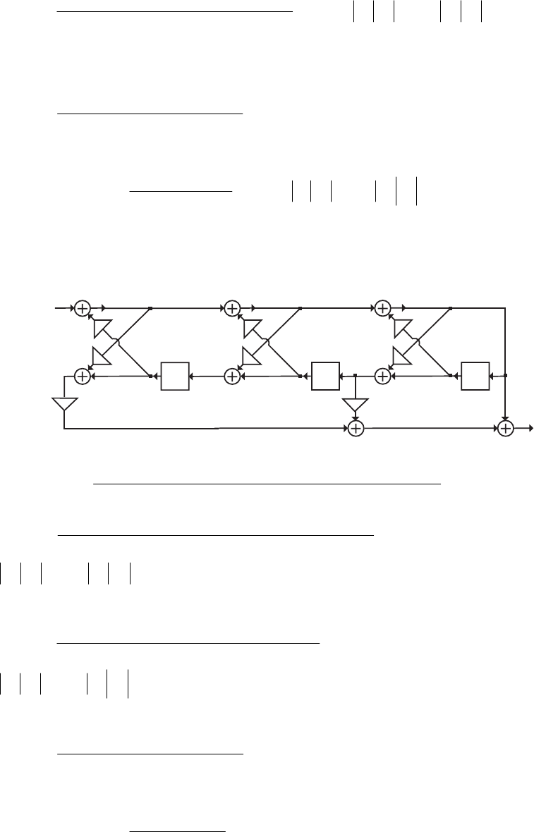
321
321
3575.136.335.21
35.236.3575.1
)( −−−
−−−
−+−
+−+−
=
zzz
zzz
zA . Note .1575.1)( 333 >==∞= dAk
Therefore, and hence, is unstable. Using Eq. (8.45) we next determine
the coefficients and of the allpass transfer function arriving at
)(
3zA )(
3zH
'
1
d'
2
d)(
2zA
.
5105.36308.21
6308.25105.3
)( 21
21
2−−
−−
+−
+−
=
zz
zz
zA Now .15105.3)( 222 >
=
=
∞
=
dAk Using Eq.
(8.45) we next determine the coefficient of the allpass transfer function
arriving at
"
1
d)(
1zA
1
1
15833.01
5833.0
)( −
−
−
+−
=
z
z
zA . Here, .15833.0)( "
111 <==∞= dAk
The feed-forward coefficients are given by ,0,0.2 112231 =−
=
=
=
dpp ααα
Final realization
of is as shown below:
,0.3
'
122113 =−−= ddp ααα .0.1
"
13
'
223104 =−−−= dddp αααα
)(
3zH
Y
o
X
1
z
1
_
z
1
_
z
1
_
23
1.575
_
1.575
_
3.5105
3.5105
0.5833
_
0.5833
(b) .
003.001.0095.055.01
9125.1552.6025.133.393.9
)( 4321
4321
2−−−−
−−−−
−−++
++−−
=
zzzz
zzzz
zH Choose
.
003.001.0095.055.01
55.0095.001.0003.0
)( 4321
4321
4−−−−
−−−−
−−++
+++−−
=
zzzz
zzzz
zA Note
.1003.0)( 444 <==∞= dAk Using Eq. (8.45) we next determine the coefficients
and of the allpass transfer function arriving at
,
'
1
d'
2
d'
3
d)(
3zA
.
0084.00953.055.01
55.00953.00084.0
)( 321
321
3−−−
−−−
−++
+++−
=
zzz
zzz
zA Now
.10084.0)( '
333 <==∞= dAk Using Eq. (8.45) we next determine the coefficients
and of the allpass transfer function arriving at
"
1
d"
2
d)(
2zA
.
0999.05508.01
5508.00999.0
)( 21
21
2−−
−−
++
++
=
zz
zz
zA Now .10999.0)( 222 <
=
=
∞
=
dAk Using Eq.
(8.45) we next determine the coefficient of the allpass transfer function
arriving at
"
1
d)(
1zA
1
1
15088.01
5088.0
)( −
−
+
+
=
z
z
zA . Here, As a result,
, and hence, is stable.
.15088.0)( "
111 <==∞= dAk
)(
3zA )(
2zH
Not for sale 272
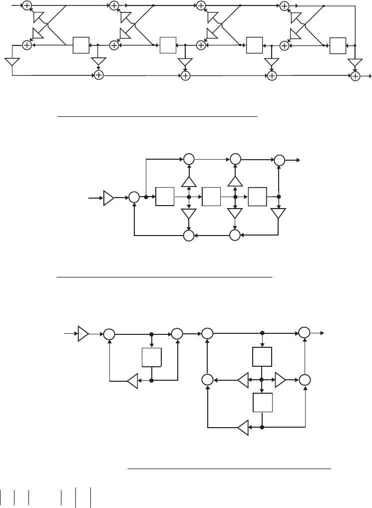
The feed-forward coefficients are given by
,.,. 5001591251 113241
=
α
−
=α==α dpp ,.
'231616
122123 −=α−α−=α ddp
Final realization of is as
shown below:
,.
"' 864430
13223114 −=α−α−α−=α dddp
..
'''"' 429526
4433324105 =α−α−α−α−=α ddddp )(zH2
Y
o
X
1
z
1
_
z
1
_
z
1
_
z
1
_
1.9125 5.5001
_
16.2316
_
30.8644 26.4295
_
0.003
0.003
_
0.0084
0.0084
_
0.0999
0.0999
_
0.5088
0.5088
8.44 (a) .
...
)..(.
)( 321
321
1574071980189101
6985169851125450
−−−
−−−
−+−
+++
=
zzz
zzz
zH A direct form II realization of
is shown below:
)(zH
z
1
_
+
+
+
+
z
1
_
z
1
_
+
+
x
[n]
y[n]
0.1891
_
0.7198 0.1574
0.2545 1.6985 1.6985
(b) .
)7258.00278.01)(2169.01(
)6985.01)(1(2545.0
)( 2
2
11
11
−
−
++−
+++
=−−
−−
zzz
zzz
zH A cascade realization of
is shown below:
)(zH
z1
_
z1
_z1
_
+
+
++
+
0.2169
+
0.2545
0.6985
0.7285
_
_0.0278
x
[n]y[n]
(c) We first form .
1574.07198.01891.01
1891.071985.01574.0
)( 321
321
3−−−
−−−
−+−
+−+−
=
zzz
zzz
zA Now
.11574.0)( '
333 <==∞= dAk Using Eq. (8.45) we next determine the coefficients
and of the allpass transfer function arriving at
"
1
d"
2
d)(
2zA
Not for sale 273
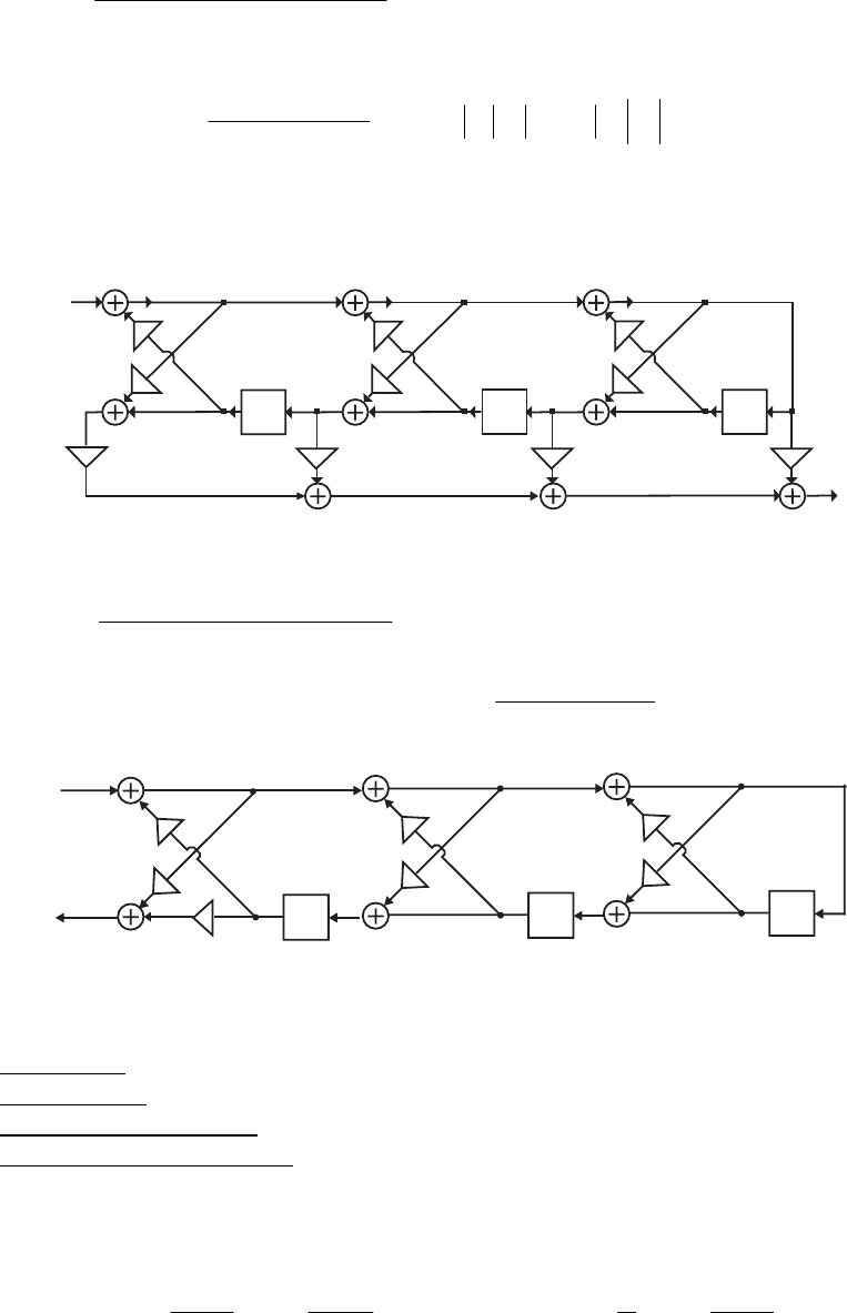
.
7075.00777.01
0777.07075.0
)( 21
21
2−−
−−
+−
+−
=
zz
zz
zA Now .17075.0)( 222 <
=
=
∞
=
dAk Using Eq.
(8.45) we next determine the coefficient of the allpass transfer function
arriving at
"
1
d)(
1zA
1
1
10455.01
0455.0
)( −
−
−
+−
=
z
z
zA . Here, .10455.0)( "
111 <==∞= dAk
The feed-forward coefficients are given by ,4804.0,2545.0 112231
=
−=
=
=
dpp ααα
The
Gray-Markel realization of is as shown below:
,2864.0
'
122113 =−−= ddp ααα .0323.0
"
13
'
223104 −=−−−= dddp αααα
)(zH
Yo
X1
z 1
_z 1
_
z 1
_
_0.1574 _0.0455
_0.7075
0.1574
0.7075
0.0455
0.2545 0.4804 0.2864 _0.0323
(d) Using Eqs. (8.132a) and (8.132b) we determine the coefficients of
:)(
2zH
.
8529.00676.01
8456.06309.1
)( 21
21
2−−
−−
++
++
=
zz
zz
zH Next, using Eqs. (8.132a) and (8.132b) we
determine the coefficients of
:)(
1zH .
6718.11
8808.1
)( 1
1
1−
−
+
+−
=
z
z
zH A cascaded lattice
realization of using the method of Problem 8.30 is thus as shown below:
z–1 z–1 z–1
_1.6718
_0.8529
_1.8808
0.1574
0.2545 1.6309
X1
Y10.2545
A comparison of the hardware requirements of the four realizations is as follows:
Direct form: No. of multipliers = 7 and no. of 2-input adders = 6,
Cascade form: No. of multipliers = 10 and no. of 2-input adders = 9,
Gray-Markel realization: No. of multipliers = 5 and no. of 2-input adders = 6,
Cascaded lattice realization: No. of multipliers = 6 and no. of 2-input adders = 6.
Hence, the Gray-Markel realization has the smallest hardware requirements.
8.45 (a) A partial-fraction expansion of is of the form
)(zG
.)(
2/
1*
*
2/
1
∑∑ == −
+
−
+=
N
ii
i
N
ii
i
z
z
dzG λ
υ
λ
υ If we define ,
2
)(
2/
1
∑
=−
+=
N
ii
i
z
d
zH λ
υ then we can
Not for sale 274
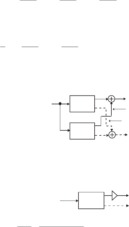
write where represents the transfer function obtained from
by conjugating its coefficients.
),()()( *zHzHzG += )(
*zH
)(zH
(b) In this case, the partial-fraction expansion of is of the form
)(zG
,)(
2/
1*
*
2/
11
∑∑∑ === −
+
−
+
−
+= cc
rN
ii
i
N
ii
i
N
ii
i
z
zz
dzG
λ
υ
λ
υ
ξ
ρ where and are the number
of real poles ’s and complex poles ’s, respectively, with residues ’s and ’s.
We can thus decompose as
r
Nc
N
i
ξi
λi
ρi
υ
)(zG ),()()( *zHzHzG
+
=
where
.
2/
2
)(
2/
11
∑∑ == −
+
−
+= c
rN
ii
i
N
ii
i
zz
d
zH λ
υ
ξ
ρ
(c) An implementation of real coefficient is thus simply a parallel connection of
two complex-coefficient filters characterized by transfer functions and as
indicated in the figure below:
)(zG
)(zH )(
*zH
H(z)
H (z)
*
x
[n]x[n]
= 0
real
imaginary
However, for a real-valued input ],[n
x
the output of is the complex conjugate of
that of As a result, two times the real part of the output of is the desired
real-valued output sequence indicating that a single complex-coefficient filter
is sufficient to realize as indicated below:
)(zH
).(
*zH )(zH
][ny
)(zH )(zG
H(z)
x
[n]y[n]
2
8.46 From ,
)(1
)(
)(
)( 1−
++
+
==
zj
jBA
zX
zY
zH
βα we arrive at the difference equation
representation
(
)
],[][]1[]1[)(][][ njBxnAxnyjnyjnyjny imreimre ++
−
+
−
+
−
=
+βα
which is equivalent to a set of two difference equations involving all real variables and
real multiplier coefficients: ][]1[]1[][ nxAnynyny imrere
+
−
+
−
−
=
βα and
].[]1[]1[][ nxBnynyny imreim
+
−
−−−= αβ A realization of based on the last
two equations is shown on next page.
)(zH
To determine the transfer function we take the -transform of the last
two difference equations and arrive at
),(/)( zXzYre z
)()()()1( 11 zXAzYzzYz imre =−+
−
−
βα and
Solving these two equations we get
).()()1()( 11 zXBzYzzYz imre =++ −− αβ
Not for sale 275

,
)(21
)(
)(
)(
2221
1
−−
−
+++
++
=
zz
zBAA
zX
zYre
βαα
βα which is seen to be a second-order transfer
function.
z–1
x
[n]
z–1
y [n]
re
y [n]
im
_α
_α
_β
β
A
B
To determine the transfer function we take the -transform of the last
two difference equations and arrive at
),(/)( zXzYre z
)()()()1( 11 zXAzYzzYz imre =−+
−
−
βα and
Solving these two equations we get
).()()1()( 11 zXBzYzzYz imre =++ −− αβ
,
)(21
)(
)(
)(
2221
1
−−
−
+++
++
=
zz
zBAA
zX
zYre
βαα
βα which is seen to be a second-order transfer
function.
8.47 An -th order complex allpass function is given by
m
.
1
)( 1
1
2
2
1
1
1
*
1
1
*1
*
m
m
m
m
mm
mm
mzzzz
zzz
zA −+−
−
−−
−+−−
−
++++++
++++
=
αααα
ααα
L
L To generate an )1(
−
m–th
order allpass function, we use the recursion .
)(1
)(
)(
)(
)(
*
1
1
1⎥
⎥
⎦
⎤
⎢
⎢
⎣
⎡
−
−
==
−
−
−zAk
kzA
z
zD
zP
zA
mm
mm
m
m
m
Substituting the expression for in the above equation we obtain after some
algebra
)(zAm
mm
mmmm zzzzzzP −
+
−
−
−
−
−− +++++= 1
*
1
2
*2
1
*1
*
1[)( αααα L
)]1( 1
1
2
2
1
1
*m
m
m
mm zzzz −+
−
−
−
−
+++++− ααααα L
,)1()()()( 1
2
2
1
**
1
1
2
** 21
** 1+−+−
−
−
−− −+−++−+−= m
m
m
mmmmmm zzz αααααααααα L
and m
m
m
mm zzzzzD
−
+
−
−
−
−
−+++++= αααα 1
1
2
2
1
11 1)( L
)( 1
*
1
1
*1
*mm
mmm zzz −+
−
−
−++++− αααα L
.)()()()1( 1
*
11
2
*22
1
*11
2+−
−
−
−
−
−−++−+−+−= m
mmmmmmm zzz αααααααααα L
Thus, is a complex allpass function of order )(
1zAm−1
−
m and given by
Not for sale 276
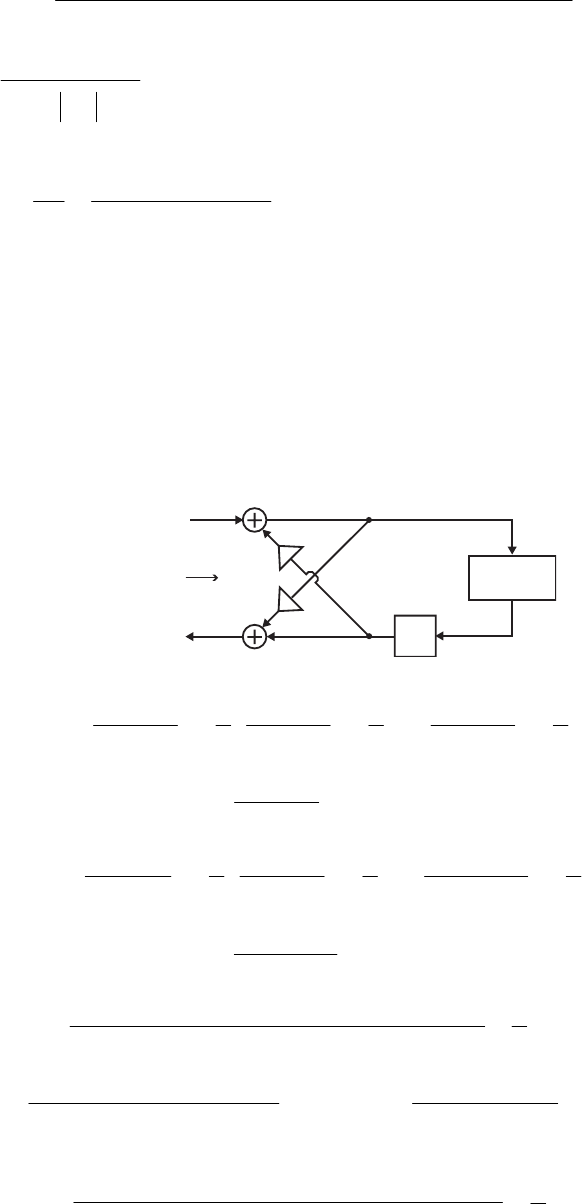
,
1
)( 1
1
2
2
2
2
1
1
12
*
1
1
*2
*1
1+−
−
+−
−
−−
+−+−−
−−
−+++++
++++
=m
m
m
m
mm
mm
mzzzz
zzz
zA
ββββ
βββ
L
L where
,
12
*
m
kmmk
kα
ααα
β−
−
=− .11
−
≤
≤mk
To develop a realization of we express in terms of )(zAm)(zAm:)(
1zAm−
,
)(1
)(
)(
1
1
1
1
*
1
1
zAzk
zAzk
X
Y
zA
mm
mm
m−
−
−
−
+
−
== and compare it with Eq. (8.47) resulting in the
following expressions for the transfer parameters of the two-pair:
and
,
*
11 m
kt =
,
1
22 −
−= zkt m.)1( 1*
2112
−
−= zkktt mm As in the case of the realization of a real
allpass function, there are many possible choices for and We choose
The corresponding input-output relations of the two-pair
are:
12
t.
21
t
.1,)1( 21
1*
12 =−= −tzkkt mm
2
1
2
1
1
*
2
1*
1
*
1)()1( XzXzkXkXzkkXkY mmmmm
−
−
−
+−=−+= and
A realization of based on the above two-pair relations is
indicated below:
.
2
1
12 XzkXY m−
−= )(zAm
z–1
k
m
k
m
_
X
1
Y
1
X
2
Y
2
A (z)
m1
_
*
A
(z)
m
8.48 (a)
()
,)()(
2
1
35
53
1
2
1
35
88
2
1
35
1
4)( 10
1
1
1
1
1
1
1zAzA
z
z
z
z
z
z
zH +=
⎟
⎟
⎠
⎞
⎜
⎜
⎝
⎛
+
+
+=
⎟
⎟
⎠
⎞
⎜
⎜
⎝
⎛
+
+
=
⎟
⎟
⎠
⎞
⎜
⎜
⎝
⎛
+
+
=−
−
−
−
−
−
where and 1)(
0=zA .
35
53
)( 1
1
1−
−
+
+
=
z
z
zA
(b)
()
,)()(
2
1
23
32
1
2
1
23
55
2
1
46
55
)( 10
1
1
1
1
1
1
2zAzA
z
z
z
z
z
z
zH −=
⎟
⎟
⎠
⎞
⎜
⎜
⎝
⎛
−
+−
−=
⎟
⎟
⎠
⎞
⎜
⎜
⎝
⎛
−
−
=
⎟
⎟
⎠
⎞
⎜
⎜
⎝
⎛
−
−
=−
−
−
−
−
−
where and 1)(
0=zA .
23
32
)( 1
1
1−
−
−
+−
=
z
z
zA
(c)
[]
,)()(
2
1
)9061.0004.01)(1768.01(
)0757.01)(1(5414.0
)( 10
211
211
3zAzA
zzz
zzz
zH −=
+−−
+−−
=−−−
−−− where
21
21
09061.0004.01
004.09061.0
)( −−
−−
+−
+−
=
zz
zz
zA and .
1768.01
1768.0
)( 1
1
1−
−
−
+−
=
z
z
zA
(d) )8482.00377.01)(0712.01(
)2859.01)(1(4547.0
)( 211
211
4−−−
−−−
+−+
+−+
=
zzz
zzz
zH
[]
)()(
2
1
10 zAzA −= , where
Not for sale 277

1
1
00712.01
0712.0
)( −
−
+
+
=
z
z
zA and .
8482.00377.01
0377.08482.0
)( 21
21
1−−
−−
+−
+−
=
zz
zz
zA
8.49 (a) From the given equation we get
].52[]5[]42[]4[]32[]3[]22[]2[]12[]1[]2[]0[]2[
−
+−
+
−
+
−
+
−
+= lllllll xhxhxhxhxhxhy
].42[]5[]32[]4[]22[]3[]12[]2[]2[]1[]12[]0[]12[
−
+−
+
−
+
−
+
++=+ lllllll xhxhxhxhxhxhy
Rewriting the above equations in matrix form we arrive at
⎥
⎦
⎤
⎢
⎣
⎡
−
−
⎥
⎦
⎤
⎢
⎣
⎡
+
⎥
⎦
⎤
⎢
⎣
⎡
+
⎥
⎦
⎤
⎢
⎣
⎡
=
⎥
⎦
⎤
⎢
⎣
⎡
+]12[
]22[
]2[]3[
]1[]2[
]12[
]2[
]0[]1[
0]0[
]12[
]2[
l
l
l
l
l
l
x
x
hh
hh
x
x
hh
h
y
y
,
]12[
]2[
00
]5[0
]32[
]42[
]4[]5[
]3[]4[ ⎥
⎦
⎤
⎢
⎣
⎡
+
⎥
⎦
⎤
⎢
⎣
⎡
+
⎥
⎦
⎤
⎢
⎣
⎡
−
−
⎥
⎦
⎤
⎢
⎣
⎡
+l
l
l
l
x
xh
x
x
hh
hh
which can be alternately expressed as ,
3322110 −−− +
+
+
=
lllll XHXHXHXHY
where
,
]2[]3[
]1[]2[
,
]0[]1[
0]0[
,
]12[
]2[
,
]12[
]2[
10 ⎥
⎦
⎤
⎢
⎣
⎡
=
⎥
⎦
⎤
⎢
⎣
⎡
=
⎥
⎦
⎤
⎢
⎣
⎡
+
=
⎥
⎦
⎤
⎢
⎣
⎡
+
=hh
hh
hh
h
x
x
y
yHHXY
l
l
l
l
ll
.
00
]5[0
,
]4[]5[
]3[]4[
32 ⎥
⎦
⎤
⎢
⎣
⎡
=
⎥
⎦
⎤
⎢
⎣
⎡
=h
hh
hh HH
(b) Here we have
].53[]5[]43[]4[]33[]3[]23[]2[]13[]1[]3[]0[]3[
−
+−
+
−
+
−
+
−+= lllllll xhxhxhxhxhxhy
],43[]5[]33[]4[]23[]3[]13[]2[]3[]1[]13[]0[]13[
−
+−
+
−
+
−
+
++=+ lllllll xhxhxhxhxhxhy
].33[]5[]23[]4[]13[]3[]3[]2[]13[]1[]23[]0[]23[
−
+−
+
−
+
+
+
++=+ lllllll xhxhxhxhxhxhy
Rewriting the above equations in matrix form we arrive at
⎥
⎥
⎥
⎦
⎤
⎢
⎢
⎢
⎣
⎡
−
−
−
⎥
⎥
⎥
⎦
⎤
⎢
⎢
⎢
⎣
⎡
+
⎥
⎥
⎥
⎦
⎤
⎢
⎢
⎢
⎣
⎡
+
+
⎥
⎥
⎥
⎦
⎤
⎢
⎢
⎢
⎣
⎡
=
⎥
⎥
⎥
⎦
⎤
⎢
⎢
⎢
⎣
⎡
+
+
]13[
]23[
]33[
]3[]4[]5[
]2[]3[]4[
]1[]2[]3[
]23
[
]13[
]3[
]0[]1[]2[
0]0[]1[
00]0[
]23[
]13[
]3[
l
l
l
l
l
l
l
l
l
x
x
x
hhh
hhh
hhh
x
x
x
hhh
hh
h
y
y
y
,
]43[
]53[
]63[
000
]2[00
]1[]2[0
⎥
⎥
⎥
⎦
⎤
⎢
⎢
⎢
⎣
⎡
−
−
−
⎥
⎥
⎥
⎦
⎤
⎢
⎢
⎢
⎣
⎡
+
l
l
l
x
x
x
h
hh
which can be alternately expressed as ,
22110 −−
+
+
=
llll XHXHXHY where
,
]3[]4[]5[
]2[]3[]4[
]1[]2[]3[
,
]0[]1[]2[
0]0[]1[
00]0[
,
]23[
]13[
]3[
,
]23[
]13[
]3[
10
⎥
⎥
⎥
⎦
⎤
⎢
⎢
⎢
⎣
⎡
=
⎥
⎥
⎥
⎦
⎤
⎢
⎢
⎢
⎣
⎡
=
⎥
⎥
⎥
⎦
⎤
⎢
⎢
⎢
⎣
⎡
+
+=
⎥
⎥
⎥
⎦
⎤
⎢
⎢
⎢
⎣
⎡
+
+=
hhh
hhh
hhh
hhh
hh
h
x
x
x
y
y
y
HHXY
l
l
l
l
l
l
ll
Not for sale 278
and
.
000
]2[00
]1[]2[0
2
⎥
⎥
⎥
⎦
⎤
⎢
⎢
⎢
⎣
⎡
=h
hh
H
(c) Following a procedure similar to that outlined in Parts (a) and (b) above, we can
show that here ,
22110 −−
+
+
=llll XHXHXHY where
,
]34[
]24[
]14[
]4[
,
]34[
]24[
]14[
]4[
⎥
⎥
⎥
⎥
⎦
⎤
⎢
⎢
⎢
⎢
⎣
⎡
+
+
+
=
⎥
⎥
⎥
⎥
⎦
⎤
⎢
⎢
⎢
⎢
⎣
⎡
+
+
+
=
l
l
l
l
l
l
l
l
ll
x
x
x
x
y
y
y
y
XY
,
]0[]1[]2[]3[
0]0[]1[]2[
00]0[]1[
000]0[
0
⎥
⎥
⎥
⎥
⎦
⎤
⎢
⎢
⎢
⎢
⎣
⎡
=
hhhh
hhh
hh
h
H
.
0000
0000
0000
]5[000
,
]4[]5[00
]3[]4[]5[0
]2[]3[]4[]5[
]1[]2[]3[]4[
21
⎥
⎥
⎥
⎥
⎦
⎤
⎢
⎢
⎢
⎢
⎣
⎡
=
⎥
⎥
⎥
⎥
⎦
⎤
⎢
⎢
⎢
⎢
⎣
⎡
=
h
hh
hhh
hhhh
hhhh
HH
8.50 (a) ]42[]32[]22[]12[]2[ 43210
−
+
−
+
−
+−+ lllll ydydydydyd
],42[]32[]22[]12[]2[ 43210
−
+
−
+
−
+
−
+
=lllll xpxpxpxpxp
]32[]22[]12[]2[]12[ 43210
−
+
−
+
−
+++ lllll ydydydydyd
].32[]22[]12[]2[]12[ 43210
−
+
−
+
−
+
+
+
=lllll xpxpxpxpxp
Rewriting the above equations in matrix form we arrive at
⎥
⎦
⎤
⎢
⎣
⎡
−
−
⎥
⎦
⎤
⎢
⎣
⎡
+
⎥
⎦
⎤
⎢
⎣
⎡
−
−
⎥
⎦
⎤
⎢
⎣
⎡
+
⎥
⎦
⎤
⎢
⎣
⎡
+
⎥
⎦
⎤
⎢
⎣
⎡
]32[
]42[
0
]12[
]22[
]12[
]2[
0
4
34
23
12
01
0
l
l
l
l
l
l
y
y
d
dd
y
y
dd
dd
y
y
dd
d
The above matrix equation can be alternately expressed as
.
]32[
]42[
0
]12[
]22[
]12[
]2[
0
4
34
23
12
01
0⎥
⎦
⎤
⎢
⎣
⎡
−
−
⎥
⎦
⎤
⎢
⎣
⎡
+
⎥
⎦
⎤
⎢
⎣
⎡
−
−
⎥
⎦
⎤
⎢
⎣
⎡
+
⎥
⎦
⎤
⎢
⎣
⎡
+
⎥
⎦
⎤
⎢
⎣
⎡
=l
l
l
l
l
l
x
x
p
pp
x
x
pp
pp
x
x
pp
p
,
2211022110 −−−−
+
+
=
++ llllll XPXPXPYDYDYD where
,
and
,
]12[
]2[ ⎥
⎦
⎤
⎢
⎣
⎡
+
=l
l
ly
y
Y
=
⎥
⎦
⎤
⎢
⎣
⎡
=
⎥
⎦
⎤
⎢
⎣
⎡
+
=1
01
0
0,
0
,
]12[
]2[ DDX
dd
d
x
x
l
l
l⎥
⎦
⎤
⎢
⎣
⎡
23
12
dd
dd ,
04
34
2⎥
⎦
⎤
⎢
⎣
⎡
=d
dd
D
,,
0
23
12
1
01
0
0⎥
⎦
⎤
⎢
⎣
⎡
=
⎥
⎦
⎤
⎢
⎣
⎡
=pp
pp
pp
pPP
=
2
P⎥
⎦
⎤
⎢
⎣
⎡
4
34
0p
pp .
(b)
⎥
⎥
⎥
⎦
⎤
⎢
⎢
⎢
⎣
⎡
−
−
−
⎥
⎥
⎥
⎦
⎤
⎢
⎢
⎢
⎣
⎡
+
⎥
⎥
⎥
⎦
⎤
⎢
⎢
⎢
⎣
⎡
+
+
⎥
⎥
⎥
⎦
⎤
⎢
⎢
⎢
⎣
⎡
]13[
]23[
3]3[
0]23[
]13[
]3[
0
00
34
234
123
012
01
0
l
l
l
l
l
l
y
y
y
dd
ddd
ddd
y
y
y
ddd
dd
d
⎥
⎥
⎥
⎦
⎤
⎢
⎢
⎢
⎣
⎡
−
−
−
⎥
⎥
⎥
⎦
⎤
⎢
⎢
⎢
⎣
⎡
+
]43[
]53[
]63[
000
000
00 4
l
l
l
y
y
yd
Not for sale 279
⎥
⎥
⎥
⎦
⎤
⎢
⎢
⎢
⎣
⎡
−
−
−
⎥
⎥
⎥
⎦
⎤
⎢
⎢
⎢
⎣
⎡
+
⎥
⎥
⎥
⎦
⎤
⎢
⎢
⎢
⎣
⎡
+
+
⎥
⎥
⎥
⎦
⎤
⎢
⎢
⎢
⎣
⎡
=
]13[
]23[
3]3[
0]23[
]13[
]3[
0
00
34
234
123
012
01
0
l
l
l
l
l
l
x
x
x
pp
ppp
ppp
x
x
x
ppp
pp
p
⎥
⎥
⎥
⎦
⎤
⎢
⎢
⎢
⎣
⎡
−
−
−
⎥
⎥
⎥
⎦
⎤
⎢
⎢
⎢
⎣
⎡
+
]43[
]53[
]63[
000
000
00 4
l
l
l
x
x
xp
,
which can be alternately expressed as
=
++ −− 22110 lll YDYDYD ,
22110 −−
+
+
lll XPXPXP where
and
,
]23[
]13[
]3[
0
⎥
⎥
⎥
⎦
⎤
⎢
⎢
⎢
⎣
⎡
+
+=
l
l
l
y
y
y
D
,
]23[
]13[
]3[
0
⎥
⎥
⎥
⎦
⎤
⎢
⎢
⎢
⎣
⎡
+
+=
l
l
l
x
x
x
P,0
00
012
01
0
0
⎥
⎥
⎥
⎦
⎤
⎢
⎢
⎢
⎣
⎡
=
ddd
dd
d
D,
034
234
123
1
⎥
⎥
⎥
⎦
⎤
⎢
⎢
⎢
⎣
⎡
=
dd
ddd
ddd
D,
000
000
00 4
2
⎥
⎥
⎥
⎦
⎤
⎢
⎢
⎢
⎣
⎡
=
d
D
,0
00
012
01
0
0
⎥
⎥
⎥
⎦
⎤
⎢
⎢
⎢
⎣
⎡
=
ppp
pp
p
P,
034
234
123
1
⎥
⎥
⎥
⎦
⎤
⎢
⎢
⎢
⎣
⎡
=
pp
ppp
ppp
P.
000
000
00 4
2
⎥
⎥
⎥
⎦
⎤
⎢
⎢
⎢
⎣
⎡
=
p
P
(c)
⎥
⎥
⎥
⎥
⎦
⎤
⎢
⎢
⎢
⎢
⎣
⎡
−
−
−
−
⎥
⎥
⎥
⎥
⎦
⎤
⎢
⎢
⎢
⎢
⎣
⎡
+
⎥
⎥
⎥
⎥
⎦
⎤
⎢
⎢
⎢
⎢
⎣
⎡
+
+
+
⎥
⎥
⎥
⎥
⎦
⎤
⎢
⎢
⎢
⎢
⎣
⎡
]14[
]24[
]34[
]44[
000
00
0
]34[
]24[
]14[
]4[
0
00
000
4
34
234
1234
0123
012
01
0
l
l
l
l
l
l
l
l
y
y
y
y
d
dd
ddd
dddd
y
y
y
y
dddd
ddd
dd
d
,
]14[
]24[
]34[
]44[
000
00
0
]34[
]24[
]14[
]4[
0
00
000
4
34
234
1234
0123
012
01
0
⎥
⎥
⎥
⎥
⎦
⎤
⎢
⎢
⎢
⎢
⎣
⎡
−
−
−
−
⎥
⎥
⎥
⎥
⎦
⎤
⎢
⎢
⎢
⎢
⎣
⎡
+
⎥
⎥
⎥
⎥
⎦
⎤
⎢
⎢
⎢
⎢
⎣
⎡
+
+
+
⎥
⎥
⎥
⎥
⎦
⎤
⎢
⎢
⎢
⎢
⎣
⎡
=
l
l
l
l
l
l
l
l
x
x
x
x
p
pp
ppp
pppp
x
x
x
x
pppp
ppp
pp
p
which can be
alternately written as ,
2211022110 −−−− +
+
=
+
+
llllll XPXPXPYDYDYD where
and
,
]34[
]24[
]14[
]4[
,
]34[
]24[
]14[
]4[
⎥
⎥
⎥
⎥
⎦
⎤
⎢
⎢
⎢
⎢
⎣
⎡
+
+
+
=
⎥
⎥
⎥
⎥
⎦
⎤
⎢
⎢
⎢
⎢
⎣
⎡
+
+
+
=
l
l
l
l
l
l
l
l
ll
x
x
x
x
y
y
y
y
XY ,
0
00
000
0123
012
01
0
0
⎥
⎥
⎥
⎥
⎦
⎤
⎢
⎢
⎢
⎢
⎣
⎡
=
dddd
ddd
dd
d
D
,
000
00
0
4
34
234
1234
1
⎥
⎥
⎥
⎥
⎦
⎤
⎢
⎢
⎢
⎢
⎣
⎡
=
d
dd
ddd
dddd
D,
0
00
000
0123
012
01
0
0
⎥
⎥
⎥
⎥
⎦
⎤
⎢
⎢
⎢
⎢
⎣
⎡
=
pppp
ppp
pp
p
P.
000
00
0
4
34
234
1234
1
⎥
⎥
⎥
⎥
⎦
⎤
⎢
⎢
⎢
⎢
⎣
⎡
=
p
pp
ppp
pppp
P
8.51 We first rewrite the second-order block difference equation
,
2211022110 −−−−
+
+
=
++ llllll XPXPXPYDYDYD
as two separate equations: ,
22110 −−
+
+
=
llll XPXPXPW and
Not for sale 280
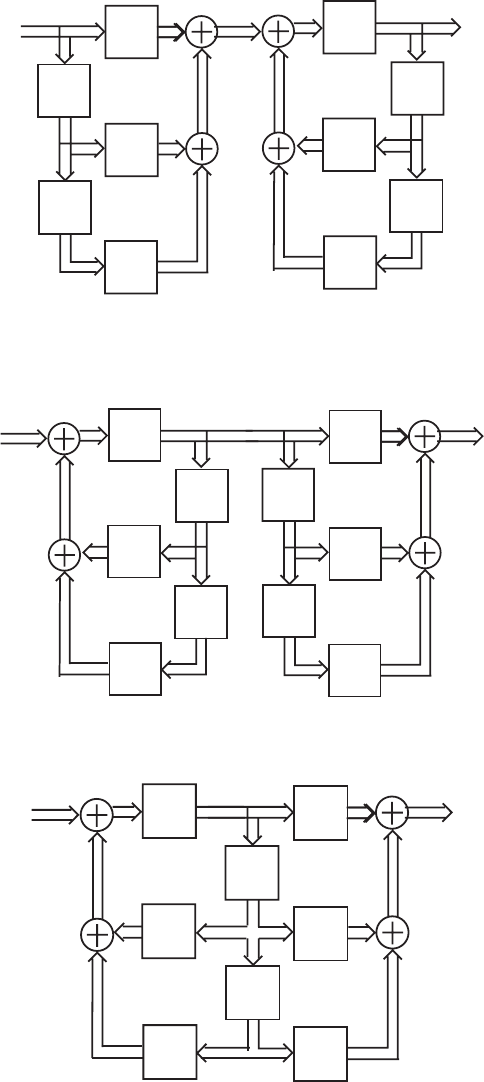
.
1
0
22
1
0
11
1
0llll WDYDDYDDY
−
−
−
−
−+−−= As cascade realization of the IIR block
digital filter based on the last two equations is thus as shown below:
∆∆
∆∆
2
P
1
P
0
P
0
1
_
D
1
D
2
D
X
k
Y
k
W
k
By interchanging the locations of the two block sections in the above structure we arrive at
an equivalent realization as indicated below:
X
k
∆
∆
0
1
_
D
1
D
2
D
∆
∆
2
P
1
P
0
PY
k
Finally, by delay-sharing the above structure reduces to a canonic realization as shown
below:
X
k0
1
_
D
1
D
2
D
∆
∆
2
P
1
P
0
PY
k
8.51 By setting in Eq. (8.125), the state-space description of the sine-cosine
θβα sin±=
Not for sale 281
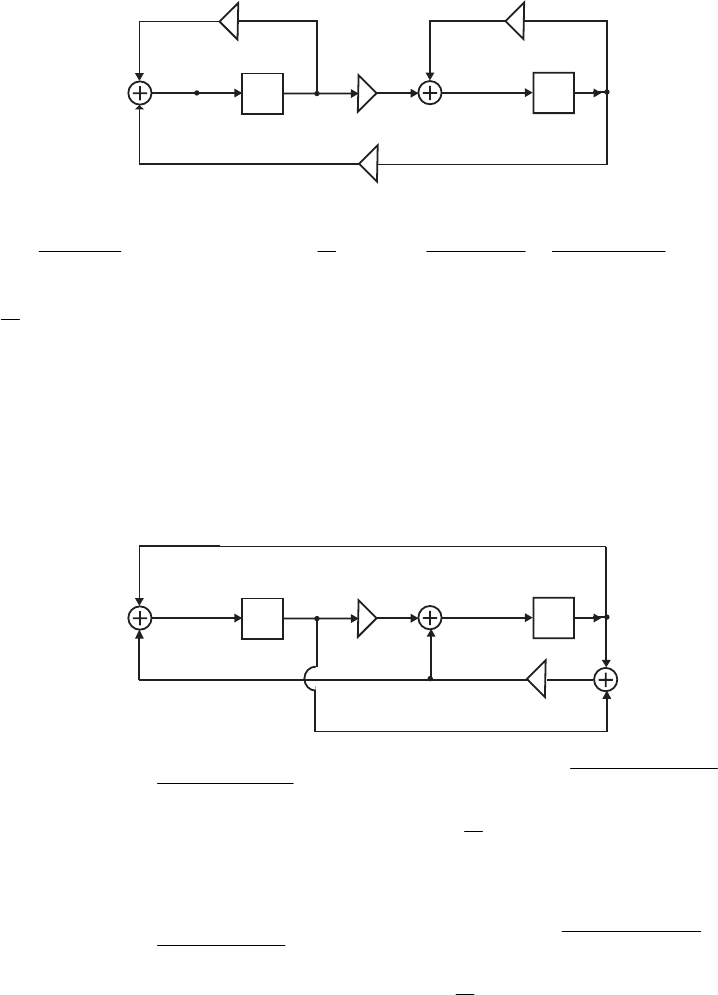
generator reduces to which leads to the three-
multiplier realization shown below:
,
][
][
cos
sincos
]1[
]1[
2
1
2
2
1⎥
⎦
⎤
⎢
⎣
⎡
⎥
⎥
⎦
⎤
⎢
⎢
⎣
⎡±
=
⎥
⎦
⎤
⎢
⎣
⎡
+
+
ns
ns
ns
ns
o
oo
ω
ωω
m
z
1
_
z
1
_
s [n]
1
s [n]
2
s [n+1]
2
s [n+1]
1
cosω
o
sin ω
o
2
+
_
+
_
cosω
o
8.53 Let .cos1
sin
o
oω
α
ωβ +=− Then ,1cos
1cos
1cos
1cos
sin
sin
22 −=
+
−
=
+
−
=o
o
o
o
o
oω
ω
ω
ω
ω
ω
β
α and
.1cossin +=− oo ωω
α
β Substituting these values in Eq. (8.125) we arrive at
These equations can be alternately written
as
.
][
][
cos1cos
1coscos
]1[
]1[
2
1
2
1⎥
⎦
⎤
⎢
⎣
⎡
⎥
⎦
⎤
⎢
⎣
⎡
+
−
=
⎥
⎦
⎤
⎢
⎣
⎡
+
+
ns
ns
ns
ns
oo
oo
ωω
ωω
()
],[][][cos]1[ 2211 nsnsnsns o
−
+
=+ ω and
()
].[][][cos]1[ 2212 nsnsnsns o
+
+
=
+
ω
A realization based on the last two equations results in a single-multiplier structure as
indicated below:
z
1
_
z
1
_
s [n]
1
s [n]
2
s [n+1]
2s [n+1]
1
cosωo
1
_
8.54 ⎥
⎦
⎤
⎢
⎣
⎡
⎥
⎥
⎥
⎥
⎦
⎤
⎢
⎢
⎢
⎢
⎣
⎡
−
−
+
⎥
⎦
⎤
⎢
⎣
⎡
+
+
⎥
⎥
⎦
⎤
⎢
⎢
⎣
⎡−
=
⎥
⎦
⎤
⎢
⎣
⎡
+
+
][
][
cossin
sin
)cos1(
]1[
]1[
00
sin
)cos(
0
]1[
]1[
2
1
2
1
2
1
ns
ns
C
C
ns
ns
C
ns
ns
oo
o
o
o
o
ωω
α
β
ωβ
ωα
ωβ
ωα
. If
then ,1=C
.
][
][
cossin
sin
)cos11(
1
]1[
]1[
00
sin
)cos1(
0
]1[
]1[
2
1
2
1
2
1⎥
⎦
⎤
⎢
⎣
⎡
⎥
⎥
⎥
⎥
⎦
⎤
⎢
⎢
⎢
⎢
⎣
⎡
−
−
+
⎥
⎦
⎤
⎢
⎣
⎡
+
+
⎥
⎥
⎦
⎤
⎢
⎢
⎣
⎡−
=
⎥
⎦
⎤
⎢
⎣
⎡
+
+
ns
ns
ns
ns
ns
ns
oo
o
o
o
o
ωω
α
β
ωβ
ωα
ωβ
ωα
Choose Then the above equation reduces to
.sin o
ωβα =
.
][
][
cos1
cos11
]1[
]1[
00
cos10
]1[
]1[
2
1
2
1
2
1⎥
⎦
⎤
⎢
⎣
⎡
⎥
⎦
⎤
⎢
⎣
⎡
−
−
+
⎥
⎦
⎤
⎢
⎣
⎡
+
+
⎥
⎦
⎤
⎢
⎣
⎡−
=
⎥
⎦
⎤
⎢
⎣
⎡
+
+
ns
ns
ns
ns
ns
ns
o
o
o
ω
ω
ω
A two-multiplier realization of the above equation is shown below:
Not for sale 282
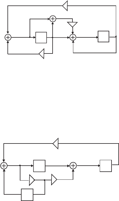
z
1
_
s [n]
1
s [n]
2
s [n+1]
2
1
_
cosω
o
1
_
cosω
o
s [n+1]
1
z
1
_
To arrive at a one-multiplier realization we observe that the two equations describing the
sine-cosine generator are given by
],[)cos(][][)cos(][ nsnsnsns oo 2121 1111
ω
−
+
+
+
ω−=+ and
].[cos][][ nsnsns o212 1
⋅
ω+−=+ Substituting the second equation in the first we arrive at
an alternate description in the form ],[][cos][ nsnsns o221 11 +
+
⋅
ω
−
=
+
and
].[cos][][ nsnsns o212 1
⋅
ω+−=+ A realization of these two equations leads to the single-
multiplier structure shown below:
z
1
_
s [n]
1
s [n]
2
1
_
cosω
o
z
1
_
z
1
_
1
_
s [n+1]
1
s [n+1]
2
8.55 From Figure P8.18(a), the input-output relation of the channel is given
by Likewise, the input-output relation of the
channel separation circuit of Figure P8.18(b) is given by
Hence, the overall system is characterized by
.
)(
)(
1)(
)(1
)(
)(
2
1
21
12
2
1⎥
⎦
⎤
⎢
⎣
⎡
⎥
⎦
⎤
⎢
⎣
⎡
=
⎥
⎦
⎤
⎢
⎣
⎡
zX
zX
zH
zH
zY
zY
.
)(
)(
1)(
)(1
)(
)(
2
1
21
12
2
1⎥
⎦
⎤
⎢
⎣
⎡
⎥
⎦
⎤
⎢
⎣
⎡
−
−
=
⎥
⎦
⎤
⎢
⎣
⎡
zY
zY
zG
zG
zV
zV
⎥
⎦
⎤
⎢
⎣
⎡
⎥
⎦
⎤
⎢
⎣
⎡
⎥
⎦
⎤
⎢
⎣
⎡
−
−
=
⎥
⎦
⎤
⎢
⎣
⎡
)(
)(
1)(
)(1
1)(
)(1
)(
)(
2
1
21
12
21
12
2
1
zX
zX
zH
zH
zG
zG
zV
zV
.
)(
)(
)()(1)()(
)()()()(1
2
1
21122121
12121221 ⎥
⎦
⎤
⎢
⎣
⎡
⎥
⎦
⎤
⎢
⎣
⎡
−−
−−
=zX
zX
zGzHzGzH
zGzHzGzH
The cross-talk is eliminated if is a function of either or and similarly,
if is a function of either or From the above equation it follows that if
and
)(
1zV )(
1zX ),(
2zX
)(
2zV )(
1zX ).(
2zX
),()( 1212 zGzH =),()( 2121 zGzH
=
then
(
)
),()()(1)( 112211 zXzGzHzV
−
=
and
Alternately, if
(
).()()(1)( 221122 zXzGzHzV −=
)
),()( 1
21
12 zHzG
−
= and ),()( 1
12
21 zHzG
−
=
Not for sale 283
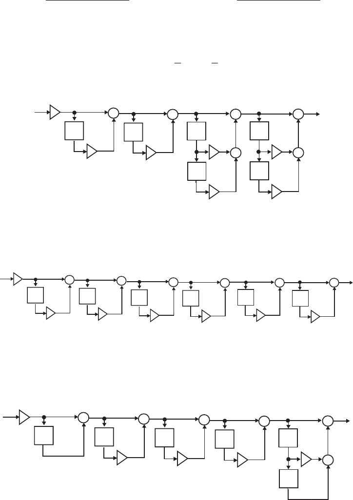
then ),(
)(
1)()(
)( 2
21
2112
1zX
zH
zHzH
zV ⎟
⎟
⎠
⎞
⎜
⎜
⎝
⎛−
= and ).(
)(
1)()(
)( 1
12
2112
2zX
zH
zHzH
zV ⎟
⎟
⎠
⎞
⎜
⎜
⎝
⎛−
=
M8.1 (a) Using the M-file factor, we factorize resulting in
)(
1zH
).6.08.01)(1)(4.01)(5.21(24.0)( 212
3
6
1
3
4
11
1−−−−−− ++++−−−= zzzzzzzH
A cascade realization of based on the above factored form is shown below:
)(
1zH
z
1
_
z
1
_
+
+
z
1
_
z
1
_
+
+
z
1
_
+
x
[n]y[n]
z
1
_
+
_
0.24
_
0.5
_
2.5 4/3
6/3
0.8
0.6
(b) Using the M-file factor, we factorize resulting in
)(
2zH
).2597.01)(649.01)(4.01)(5403.11)(5.21)(8508.31(4)( 111111
2
−
−
−
−
−
−−−+−+−= zzzzzzzH
A cascade realization of based on the above factored form is shown below:
)(
2zH
z1
_
+
z1
_
+
z1
_
+
x
[n]y[n]
z1
_
+
z1
_
+
z1
_
+
_3.8508 _1.5403 _0.649 _0.2597
2.5 0.4
4
(c) Using the M-file factor, we factorize resulting in )(
3zH
).3488.11)(71306.01)(4024.11)(1)(1(24.0)( 211111
3
−
−
−
−
−
−++−−−+−= zzzzzzzH
A cascade realization of based on the above factored form is shown below: )(
3zH
z1
_
z1
_
+
+
z1
_
+
x
[n]y[n]
1.4024
_
0.71306
_
z1
_
+
_0.24
_1
z1
_
+
z1
_
+
1.3488
(d) Using the M-file factor, we factorize resulting in
)(
4zH
).4675.11)(214.01)(6735.41)(1)(1(4)( 211111
4−−
−
−
−− ++−−−+= zzzzzzzH
A cascade realization of based on the above factored form is shown below:
)(
4zH
Not for sale 284
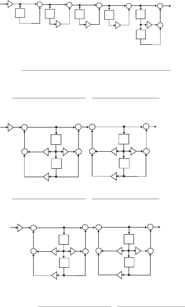
z1
_
z1
_
+
+
z1
_
+
x
[n]y[n]
4.6735
_
z1
_
+
_0.214
_1
z1
_
+
z1
_
+
1.4675
4
M8.2 (a) Using the M-file factor, we factorize the numerator and the denominator of
resulting in
)(zG
)..)(..(
).)(.(.
)( 2121
2121
222805653017042600614701
15820148911139010
−−−−
−−−−
+++−
++++
=
zzzz
zzzz
zG .
(b) We can write
.
..
.
..
.
.)( ⎟
⎟
⎠
⎞
⎜
⎜
⎝
⎛
++
++
⎟
⎟
⎠
⎞
⎜
⎜
⎝
⎛
+−
++
=−−
−−
−−
−−
21
21
21
21
22280565301
158201
7042600614701
489111
39010
zz
zz
zz
zz
zG A
cascade realization of based on the above decomposition is shown on next page:
)(zG
z1
_
z1
_
+
++
+
z1
_
z1
_
+
++
+
1.4891
0.3901
0.56527
_0.1582
_0.70426
0.06147
0.2228
_
x
[n]y[n]
Alternately, we can write
.
..
.
..
.
.)( ⎟
⎟
⎠
⎞
⎜
⎜
⎝
⎛
++
++
⎟
⎟
⎠
⎞
⎜
⎜
⎝
⎛
+−
++
=−−
−−
−−
−−
21
21
21
21
22280565301
489111
7042600614701
158201
39010
zz
zz
zz
zz
zG
A cascade realization of based on the above decomposition is shown below:
)(zG
z1
_
z1
_
+
++
+
z1
_
z1
_
+
++
+
1.4891
0.3901
0.56527
_
0.1582
_0.70426
0.06147
0.2228
_
x
[n]y[n]
(c) A partial-fraction expansion of in
)(zG 1
−
z obtained using the M-file residuez is
given by .
..
..
..
..
.)( 21
1
21
1
22280565301
4094074811
7042500614701
11128034810
48632 −−
−
−−
−
++
+−
+
+−
−−
+=
zz
z
zz
z
zG
Not for sale 285
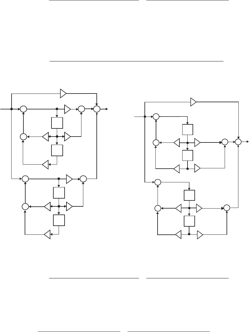
A Parallel Form I realization of based on the above expansion is shown on the left
side top of next page.
)(zG
(d) A partial-fraction expansion of in obtained using the M-file residue is given
by
)(zG z
.
..
..
..
..
.)( 21
21
21
11
22280565301
3895057870
7042500614701
2451013270
39010 −−
−−
−−
−−
++
+
+
+−
+−
+=
zz
zz
zz
zz
zG A
Parallel Form II realization of based on the above expansion is shown on the right
side top of next page.
)(zG
M8.3 (a) Using the M-file factor, we factorize the numerator and the denominator of
resulting in
)(zH
)..)(..(
).)(.(.
)( 2121
2121
5681063130198450620901
031690159580135490
−−−−
−−−−
++++
+−++
=
zzzz
zzzz
zH .
z
1
_
z
1
_
+
+ +
+
_
1.7481
0.5653
_
0.11128
_
0.3481
_
z
1
_
z
1
_
+
++
2.4863
0.4094
0.06147
_
0.70425
0.2228
_
x
[n]y[n]
z
1
_
z
1
_
+
+
++
0.5653
_
0.1327
_
z
1
_
z
1
_
+
+
_
0.70425
0.2228
_
x
[n]
y[n]
+
0.06147
0.2451
0.5787
0.3895
0.3901
(b) We can write
.
..
.
..
.
.)( ⎟
⎟
⎠
⎞
⎜
⎜
⎝
⎛
++
+−
⎟
⎟
⎠
⎞
⎜
⎜
⎝
⎛
++
++
=−−
−−
−−
−−
21
21
21
21
56830631301
0316901
9845062098601
595801
35490
zz
zz
zz
zz
zH
A cascade realization of based on the above decomposition is shown on top of the
next page.
)(zH
Alternately, we can write
.
..
.
..
.
.)( ⎟
⎟
⎠
⎞
⎜
⎜
⎝
⎛
++
++
⎟
⎟
⎠
⎞
⎜
⎜
⎝
⎛
++
+−
=−−
−−
−−
−−
21
21
21
21
56830631301
595801
98450620901
0316901
35490
zz
zz
zz
zz
zH
Not for sale 286
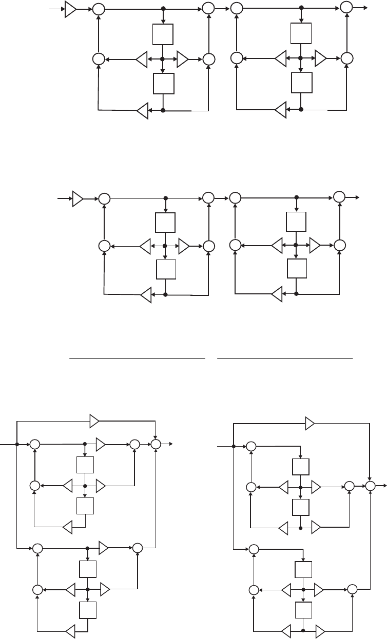
z
1
_
z
1
_
+
++
+
z
1
_
z
1
_
+
++
+
0.3549
_
0.6209
x
[n]y[n]
0.9845
_
0.6313
_
0.5683
_
0.5958
0.03169
_
A cascade realization of based on the decomposition given at the bottom of the
previous page is shown below:
)(zH
z1
_
z1
_
+
++
+
z1
_
z1
_
+
++
+
0.3549
_0.6209
x
[n]y[n]
0.9845
_
0.6313
_
0.5683
_
0.5958
0.03169
_
(c) A partial-fraction expansion of in
)(zG 1
−
z obtained using the M-file
residuez is given by
.
..
..
..
..
.)( 21
1
21
1
56830631301
4299026610
98450620901
0094001330
63430 −−
−
−−
−
++
−−
+
++
+−
+=
zz
z
zz
z
zH A Parallel
Form I realization of based on the above expansion is shown below on the left side.
)(zG
z1
_
z1
_
+
++
0.6313
_
0.6209
_
z1
_
z1
_
+
+
_0.9845
0.5683
_
x
[n]y[n]
+
+
0.0133
_
0.0094
0.2661
_
0.4299
_
0.6343
z
1
_
z
1
_
+
+
++
0.6313
_
0.6209
_
z
1
_
z
1
_
+
+
_
0.9845
0.5683
_
x
[n]
y[n]
+
0.3549
0.0177
0.1512
0.0131
0.2619
_
Not for sale 287
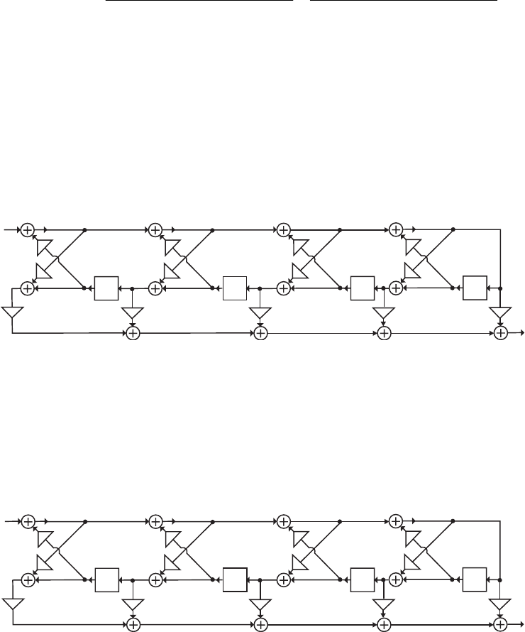
(d) A partial-fraction expansion of in obtained using the M-file residue is given
by
)(zG z
.
..
..
..
..
.)( 21
21
21
11
56830631301
1512026190
98450620901
0131001770
35490 −−
−−
−−
−−
++
+−
+
++
+−
+=
zz
zz
zz
zz
zG A Parallel
Form II realization of based on the above expansion is shown at the bottom of the
previous page on the right side.
)(zG
M8.4 Lattice parameters are
0.1393 0.6973 0.3131 0.1569
Feedforward multipliers are
0.3901 0.4461 0.3212 0.0727 -0.0488
The Gray-Markel tapped cascaded lattice realization of is shown on next page:
)(zG
z
1
_
z
1
_
z
1
_
z
1
_
0.1569
_
0.1569
_
0.3131
0.3131
_
0.6973
0.6973
_
0.1393
0.1393
0.3901 0.4461 0.3212 0.0727
_
0.0488
x[n]
y[n]
M8.5 Lattice parameters are
0.3171 0.9949 0.3986 0.5595
Feedforward multipliers are
03549 -0.2442 0.2642 -0.0082 -0.0066
The Gray-Markel tapped cascaded lattice realization of is shown below:
)(zH
z
1
_
z
1
_
z
1
_
z
1
_
0.5595
_
0.5595
_
0.3986
0.3986
_
0.9949
0.9949
_
0.3171
0.3171
0.3549 0.2642
_
0.0066
x[n]
y[n]
_
0.0082
_
0.2442
M8.6 (a) (b) Program 8_7 generated the following error messages for the FIR transfer functions
of Parts (a) and (b):
??? Error using ==> signal\private\levdown
At least one of the reflection coefficients is equal to one.
The algorithm fails for this case.
(c) (d) Program 8_7 generated the following error messages for the FIR transfer functions
of Parts (c) and (d):
Warning: Divide by zero.
Lattice coefficients are
Not for sale 288
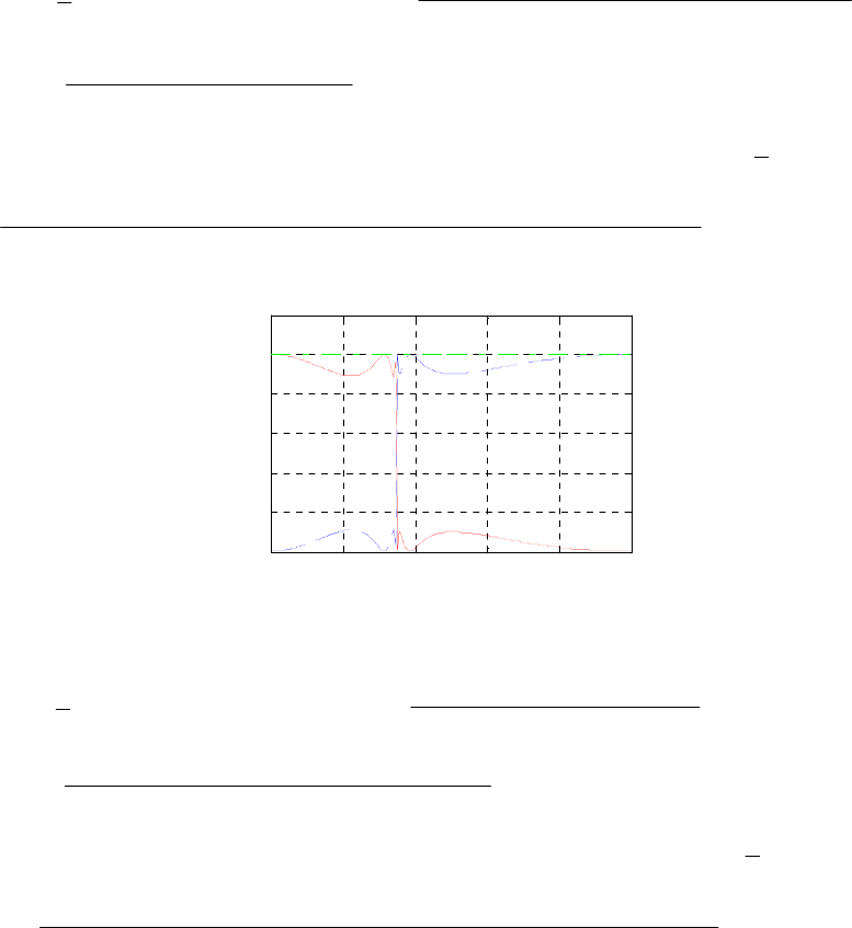
-1 NaN NaN NaN NaN NaN
M8.7 (a) Using the M-file tf2ca we arrive at the parallel allpass decomposition of as:
)(zG
[]
,)()()( zAzAzG 10
2
1+= where 321
321
02440020921143611
143612092124400
−−−
−−−
−+−
+−+−
=
zzz
zzz
zA ...
...
)( and
21
21
180410817101
8171080410
−−
−−
+−
+−
=
zz
zz
zA ..
..
)( .
(b) The power-complementary transfer function is then given by
[]
)()()( zAzAzH 10
2
1−=
.
.....
....(.
54321
54321
19610171311511294732960611
0011399484994840011315240
−−−−−
−−−−−
−+−+−
−+−+−
=
zzzzz
zzzzz
(c)
00.2 0.4 0.6 0.8 1
0
0.2
0.4
0.6
0.8
1
|G(ejω)|2|H(ejω)|2
|G(ejω)|2+|H(ejω)|2
ω
/
π
Magnitude Square
M8.8 (a) Using the M-file tf2ca we arrive at the parallel allpass decomposition of as:
)(zG
[]
,)()()( 10
2
1zAzAzG −= where 21
21
09077.06205.01
6205.09077.0
)( −−
−−
++
++
=
zz
zz
zA and
321
321
13325.02027.19522.01
9522.02027.13325.0
)( −−−
−−−
+++
+++
=
zzz
zzz
zA .
(b) The power-complementary transfer function is then given by
[]
)()()( 10
2
1zAzAzH +=
.
.....
....(
54321
54321
3018029791943117122572711
333427759377593333421
−−−−−
−−−−−
+++++
+++++
=
zzzzz
zzzzz
(c)
Not for sale 289
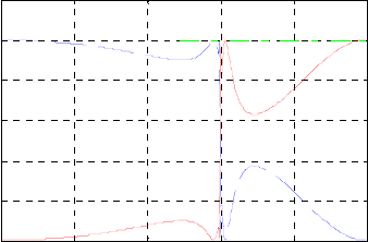
00.2 0.4 0.6 0.8 1
0
0.2
0.4
0.6
0.8
1
ω
/
π
Magnitude Square
|G(e
jω
|
2
|H(e
jω
|
2
|G(e
jω
|
2
+|H(e
jω
|
2
M8.9 The transfer function given cannot be realized as a parallel connection of two real allpass
sections as the degree difference between the two allpass transfer functions must be 2.
M8.10 The MATLAB program for the simulation of the sine-cosine generator of Problem 8.53
is given below:
s10 = 0.1; s20 = 0.1; a = 0.8;
y1 = zeros(1,50); y2 = y1;
for n = 1:50;
y1(n) = a*(s10 + s20) - s20;
y2(n) = a*(s10 +s20) + s10;
s10 = y1(n);
s20 = y2(n);
end
y1max = max(y1);y2max = max(y2);
k = 1:50;
stem (k-1,y1/y1max);
xlabel('Time index n');ylabel('Amplitude');
title('y_1[n]');
pause
stem(k-1,y2/y2max);
xlabel('Time index n');ylabel('Amplitude');
title('y_2[n]');
The plots generated by the above program for initial conditions s1[-1] s2[-1] =
0.1 are shown below:
Not for sale 290
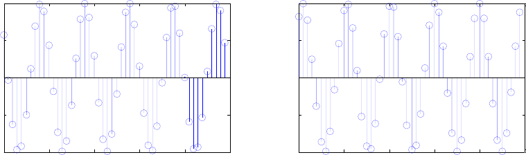
010 20 30 40 50
-1
-0.5
0
0.5
1
Time index n
A
mp
lit
u
d
e
y
1
[n]
010 20 30 40 50
-1
-0.5
0
0.5
1
Time index n
A
mp
lit
u
d
e
y
2
[n]
The outputs are zero for zero initial conditions. Non-zero initial conditions of equal values
appear to have no effects on the outputs. However, unequal initial conditions have effects
on the amplitudes and phases of the two output sequences.
M8.11 The MATLAB program for the simulation of the sine-cosine generator of Problem 8.53
is given below:
s10 = 0.1; s20 = 1; a = 0.8;
y1 = zeros(1,50); y2 = y1;
for n = 1:50;
y1(n) = -s20 +a*s10;
y2(n) = -a*y1(n) + s10;
s10 = y1(n); s20 = y2(n);
end
y1max = max(y1);y2max = max(y2);
k = 1:50;
stem (k-1,y1/y1max);
xlabel('Time index n');ylabel('Amplitude');
title('y_1[n]');
pause
stem(k-1,y2/y2max);
xlabel('Time index n');ylabel('Amplitude');
title('y_2[n]');
The plots generated by the above program for initial conditions s1[-1] s2[-1] =
0.1 are shown on top of the next page.:
The outputs are zero for zero initial conditions. Non-zero initial conditions of equal values
appear to have no effects on the outputs. However, unequal initial conditions have effects
on the amplitudes and phases of the two output sequences.
Not for sale 291
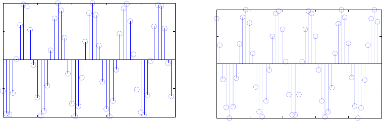
010 20 30 40 50
-1
-0.5
0
0.5
1
Time index n
A
mp
lit
u
d
e
y1[n]
010 20 30 40 50
-1
-0.5
0
0.5
1
Time index n
A
mp
lit
u
d
e
y
2
[n]
Not for sale 292
Chapter 9
9.1 We obtain the solutions by using Eq. (9.3) and Eq. (9.4).
(a)
0022.01010,0239.0101101 20/53
20/
20/21.0
20/ ===δ=−=−=δ −
α−
−
α− s
psp
(b)
.
,0194.0101101 20/17.0
20/ =−=−=δ −
α− p
p
420/78
20/ 1026.11010 −−
α− ×===δ s
s
9.2 We obtain the solutions by using Eq. (9.3) and Eq. (9.4).
(a)
(
)
dB,1755.0)02.01(log201log20 1010
=
−
−
=
δ−−=α pp
()
(
)
dB.458.3003.0log20log20 1010
=
−=δ−=α ss
(b)
(
)
dB,4914.0)055.01(log201log20 1010
=
−
−
=
δ−−=α pp
()
(
)
dB.630.29033.0log20log20 1010
=
−=δ−=α ss
9.3 or equivalently,
),()( 2zHzG =).()( 2ωω =jj eHeG
2
2)()()( ωωω == jjj eHeHeG .
Let and denote the passband and stopband ripples of , respectively. Also,
let and denote the passband and stopband ripples of ,
respectively. Then and For a cascade of
p
δs
δ)( ωj
eH
,2, 2pp δ=δ 2,s
δ)( ωj
eG
,)1(1 2
2, pp δ−−=δ .)( 2
2, ss δ=δ
M
sections,
and
,)1(1
,M
pMp δ−−=δ .)(
,M
sMs δ=δ
9.4
HLP(e j )
p
s
š
– p
– s
–
s
1
p
1– p
0
HHP (e j )
š–
s
1
p
1– p
p
s
–( – s)
–( – p)
0
Therefore, the passband edge and the stopband edge of the highpass filter are given by
and
,
,pHPp ω−π=ω ,
,sHPs respectively.
ω
−
π
=
ω
9.5 Note that is a complex bandpass filter with a passband in the range
)(zG
π
≤
ω≤0. Its
passband edges are at ,
,poBPp
ω
±
ω
=
ωand stopband edges at .
,soBPs
ω
±ω=
ω
A real
coefficient bandpass transfer function can be generated according to
Not for sale 293
which will have a passband in the range
)()()( –zeHzeHzG oo j
LP
j
LPBP ωω +=
π
≤
ω
≤
0
and another passband in the range .0–
≤
ω
≤
π
However because of the overlap of the two
spectra a simple formula for the bandedges cannot be derived.
HLP (e j )
p
s
š
– p
– s
–
s
1
p
1– p
0
G(ej )
š
–
s
1
p
1– p
0 o
o s
o p
o p
o
s
9.6 (a) where Thus, h.
We also have, g[ Now, H and
Comparing the above expression with G( we
conclude that G(
)()()( tpthth ap ⋅= ∑−δ= ∞
−∞=n
nTttp ).()( p(t) ha(nT) (t nT)
n
n] ha(nT). a(s) ha(t) e st
dt
Hp(s) hp(t)e st
dt ha(nT) (t nT)e st
dt
n
ha(nT)e snT
n
.
z) g[n]z n
n
ha(nT)z n
n
,
z) Hp(s) s
1
Tln z .
We can also show that a Fourier series expansion of p(t) is given by
p(t)
1
Te j(2 kt / T).
k
Therefore,
hp(t)
1
Te j(2 kt / T)
k
ha(t)
1
Tha(t)
k
e j(2 kt / T). Hence,
Hp(s)
1
THa
k
s j2 kt
T
. As a result, we have
G(z)
1
THa
k
s j2 kt
T
s
1
Tln z . (7-1)
(b) The transformation from the -plane to -plane is given by z If we express
then we can write z
s z esT .
s
o j o, re
j
e e
oT
j
oT. Therefore,
Not for sale 294
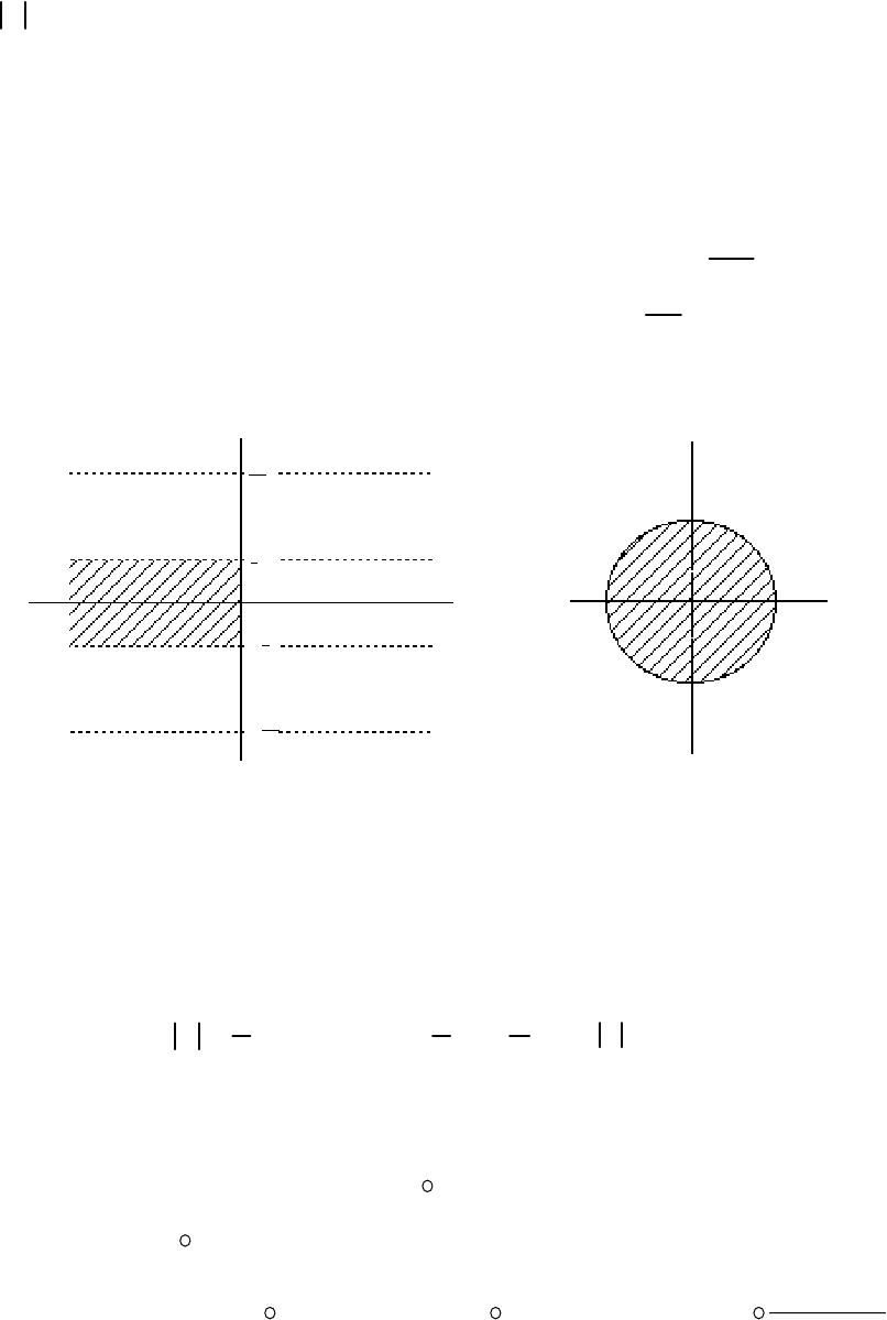
z
o
1, for o 1,
1, for o 1.
1, for 1,
z s
z
Or in other words, a point in the left-half -plane is mapped onto
a point inside the unit circle in the -plane, a point in the right-half -plane is mapped
onto a point outside the unit circle in the -plane, and a point on the
s
j
-axis in the -
plane is mapped onto a point on the unit circle in the -plane. As a result, the mapping has
the desirable properties enumerated in Section 9.1.3.
s
z
(c) However, all points in the -plane defined by s
s
o j o j2 k
T,
k
0, ,1, 2,K, are
mapped onto a single point in the z-plane as z e oTe
j( o
2
k
T)T
e oTej oT. The
mapping is illustrated in the figure below
1
1
j z
Im
zRe
z-plane-plane
s
T
3š
š
T
–T
3š
–š
T
Note that the strip of width T/2
π
in the -plane for values of in the range
s s
/
T
/
Tz
T/2π
is mapped into the entire -plane, and so are the adjacent strips of
width . The mapping is many-to-one with infinite number of such strips of width
.
T/2π
It follows from the above figure and also from Eq. (7-1) that if the frequency response
for
Ha(j ) 0
T
, then G( )
T
1Ha(jT), for ,and there is no aliasing.
ej
(d) For z e
j
e
j
T. Or equivalently, T.
9.7 Assume is causal. Now,
)(tha
∫
=.)()( dsesHth st
aa Hence,
.)()(][ dsesHnThng aa ∫
== snT Therefore,
ds
ze
sH
dsezsHdszesHzngzG sT
a
snT
n
n
a
n
nsnT
a
n
n∫∫ ∑∑∫
∑−
∞
=
−
∞
=
−
∞
=
−
−
==== 1
000 1
)(
)()(][)( .
Not for sale 295

Hence .
1
)(
Residues)(
)(ofpolesall 1
∑⎥
⎦
⎤
⎢
⎣
⎡
−
=−
sH sT
a
aze
sH
zG
9.8 α+
=s
A
sHa)( . The transfer function has a pole at .
α
−
=
s Now
.
11)1)((
Residue)( 1
–
11
–at −α−
α=
−−
α= −
=
−
=
⎥
⎥
⎦
⎤
⎢
⎢
⎣
⎡
−α+
=
ze
A
ze
A
zes
A
zG T
s
sTsT
s
9.9 (a)
()
)2(
62
)2(
62
2
4
)54)(2(
)73(4
2js
j
js
j
s
sss
s
sHa−+
+
+
++
−
+
+
−
=
+++
+
=
()
(
)
()
(
)
()
.
12
112
12
24
2
4
12
44
2
4
2
2
2
2
2
2
2++
⋅−
+
++
+
+
+
−
=
++
−
+
+
−
=
ss
s
s
s
s
s
Using Eqs. (9.58), (9.60), and (9.62), we get
()
(
)
(
)
()
2421
21
12 cos21
cos14
1
4
−−−−
−−
−− +−
−
+
−
−
=
zeTez
Tez
ze
zG TT
T
T
a
(
)
()
2421
21
cos21
sin
−−−−
−−
+−
+
zeTez
Tez
TT
T
,
where T = 0.3. Therefore,
()
(
)
21
1
13012.00486.11
5243.014
5488.01
4
−−
−
−+−
−
+
−
−
=
zz
z
z
zGa21
1
3012.00486.11
1622.0
−−
−
+−
+
zz
z
.
3012.00486.11
935.14
5488.01
4
21
1
1−−
−
−+−
−
+
−
−
=
zz
z
z
(b)
()
(
)
()
()()()
js
js
js
j
s
sss
ss
sHb31
5.0
31
5.03
4
2
4102
56378
2
2
−+
−
+
++
+
+
+
=
+++
++
=
()
(
)
()
(
)
()
.
31
33
31
16
4
2
91
96
4
2
2
2
2
22 ++
+
++
+
+
+
=
++
+
+
+
=
ss
s
s
s
s
s
Using Eqs. (9.58), (9.60), and (9.62), we get
()
(
)
()
221
1
14 3cos21
3cos1
6
1
2
−−−−
−−
−− +−
−
+
−
=
zeTez
Tez
ze
zG TT
T
T
b
(
)
()
221
1
3cos21
3sin
3−−−−
−−
+−
+
zeTez
Tez
TT
T
,
where T = 0.3. Therefore,
()
(
)
(
)
21
1
21
1
15489.09210.01
5803.03
5489.09210.01
4605.016
3012.01
4
−−
−
−−
−
−+−
+
+−
−
+
−
=
zz
z
zz
z
z
zGb
Not for sale 296

21
1
15489.09210.01
0221.16
3012.01
4
−−
−
−+−
−
+
−
=
zz
z
z
(c)
()
(
)
(
)
(
)
(
)
4
23
52
14
452
146
2222
23
++
+−
+
++
+
=
++++
+++
=
ss
s
ss
s
ssss
sss
sHc
()
()
()
()
(
)
()
()
(
)
()
()
.
2/155.0
2/1515/7
2/155.0
5.03
12
17
12
24
2
2
2
2
2
2
2
2++
+
++
+−
+
++
−
+
++
+
=
ss
s
ss
s
Using Eqs. (9.58), (9.60), and (9.62), we get
() ()
(
)
() () ()
()
2412
12
2412
12
cos21
sin
7
cos21
cos1
4−−−−
−−
−−−−
−−
+−
−+
+−
−
=
zezTe
zTe
zezTe
zTe
zG TT
T
TT
T
c
()
()
() () ()
()
,
2/15cos21
2/15sin
15/7
2/15cos21
2/15cos1
3212
12/
212
12/
−−−−
−−
−−−−
−−
+−
+
+−
−
−+
zezTe
zTe
zezTe
zTe
TT
T
TT
T
where T = 0.3. Hence,
()
(
)
21
1
21
1
3012.00486.11
1353.1
3012.00486.11
5243.014
−−
−
−−
−
+−
−
+−
−
=
zz
z
zz
z
zGc
(
)
21
1
21
1
7408.04390.11
8538.0
7408.04390.11
7195.013
−−
−
−−
−
+−
+
+−
−−
zz
z
zz
z.
9.10 (a)
()
.
43
21
21
8.15.1 TT
aez
zA
ez
zA
ez
z
ez
z
zG α−α−−− −
+
−
=
−
+
−
=
Since T = 0.2, 4,3,9,5.7 2121
=
=
=AA
α
α
, it follows
()
.
9
4
5.7
3
+
+
+
=ss
sHa
(b)
()
(
)
()
(
)
()
.
cos2
sin
5.1cos2
5.1sin
224.22.12
2.1
TT
T
beTzez
Tze
ezez
ze
zG β−β−
β−
−−
−
+λ−
λ
=
+−
=
Since T = 0.2, it follows
,6,5.7 =β=λ
() ()
2
25.76
5.7
++
=
s
sHb
9.11 (a)
() ()
()
.
9115475
4316
2
2
6
1
1
44
1
1
410
4
1
1
43
1
1
44
1
1
42
2
++
++
=
⎥
⎦
⎤
⎢
⎣
⎡⎟
⎠
⎞
⎜
⎝
⎛
⎥
⎦
⎤
⎢
⎣
⎡⎟
⎠
⎞
⎜
⎝
⎛
⎥
⎦
⎤
⎢
⎣
⎡⎟
⎠
⎞
⎜
⎝
⎛
⎥
⎦
⎤
⎢
⎣
⎡⎟
⎠
⎞
⎜
⎝
⎛
==
+
−
+
+
−
+
+
−
+
+
−
+
⎟
⎠
⎞
⎜
⎝
⎛
−
+
=ss
ss
zGsH
s
s
s
s
s
s
s
s
s
s
z
aa
(b)
() ()
⎟
⎟
⎠
⎞
⎜
⎜
⎝
⎛
⎥
⎦
⎤
⎢
⎣
⎡⎟
⎠
⎞
⎜
⎝
⎛
⎥
⎦
⎤
⎢
⎣
⎡⎟
⎠
⎞
⎜
⎝
⎛
⎟
⎠
⎞
⎜
⎝
⎛⎥
⎦
⎤
⎢
⎣
⎡⎟
⎠
⎞
⎜
⎝
⎛
⎥
⎦
⎤
⎢
⎣
⎡⎟
⎠
⎞
⎜
⎝
⎛
⎥
⎦
⎤
⎢
⎣
⎡⎟
⎠
⎞
⎜
⎝
⎛
⎥
⎦
⎤
⎢
⎣
⎡⎟
⎠
⎞
⎜
⎝
⎛
==
+
−
+
−
−
+
+
−
+
+
−
+
+
−
+
+
−
+
⎟
⎠
⎞
⎜
⎝
⎛
−
+
=
8
1
1
44
1
1
4121
1
1
43
18
1
1
426
1
1
462
1
1
454
1
1
42
23
s
s
s
s
s
s
s
s
s
s
s
s
s
s
z
bb zGsH
Not for sale 297

(
)
(
)
()
(
)
.
23462711134
45784642535
2
2
+++
+++−
=
sss
sss
9.12 For the impulse invariance design:
(
)
(
)
π=××π=π=Ω=ω −27.0103.01045.022 33
TFT ppp
For the bilinear transformation method:
()
(
)
π=π⋅×⋅×=π=
⎟
⎟
⎠
⎞
⎜
⎜
⎝
⎛Ω
=ω −−−− 2554.0103.01045.0tan2tan2
2
tan2 33111 TF
T
p
p
p
9.13 For the impulse invariance method: ⇒
×
π
=
ω
=π −3
102.0
56.0
2T
Fp
p
kHz4.1=
p
F
For the bilinear transformation method:
(
)
kHz.923.1
102.0
1
2
56.0
tan
1
2
tan 3=
×π
⋅
⎟
⎠
⎞
⎜
⎝
⎛π
=
π
⋅
⎟
⎟
⎠
⎞
⎜
⎜
⎝
⎛ω
=−
T
Fp
p
9.14 The passband and the stopband edges of the analog lowpass filter are assumed to
and . The requirements to be satisfied by the analog
lowpass filter are thus
π=Ω 25.0
ps 0.55
5.0)25.0(log20 10 −≥πjHa dB and
15)55.0(log20 10 −≤πjHa dB.
From 5.0)1(log20 2
10 =ε+=α p we obtain . From
we obtain A. From Eq. (4.32), the inverse
discrimination ratio is given by
20.1220184543
s 10 log10 (A ) 15
2231.6227766
841979.15
11 2
1
=
−
=ε
A
k and from Eq. (4.31) the inverse
transition ratio is given by 2.2
1=
Ω
Ω
=
p
s
k. Substituting these values in Eq. (4.35) we
obtain .503885.3
)2.2(log)/1(log 10
10
10
110 === k
N)841979.15(log)/1(log k We choose N = 4.
From Eq. (4.33) we have .
2
2
ε=
⎟
⎟
⎠
⎞
⎜
⎜
⎝
⎛
Ω
ΩN
c
p Substituting the values of , N, and we get
p
2
.021612.1)(3007568.1 =Ω=Ω
,9239.03827.0 jp +
pc
Using the statement [z,p,k] = buttap(4) we get the poles of the 4-th order
Butterworth analog filter with a 3-dB cutoff at 1 rad/s as 1
−
=
,9239.03827.0
2jp −−= ,3827.09239.0 jp3 and .3827.09239.0
4jp
+
−
=
−
−
=
Therefore,
Not for sale 298

)18478.1)(17654.0(
1
))()()((
1
)( 22
4321 ++++
=
−−−−
=
ssss
pspspsps
sH an .
Next we expand in a partial-fraction expansion using the M-file residue and
arrive at
)(sH an
18478.1
7071323.19238729.0
17654.0
7071323.09238729.0
)( 22 ++
+
++
=
ss
s
ss
s
sHan
+
−−
)(sH
. We next
denormalize to move the 3-dB cutoff frequency to using the M-file
lp2lp resulting in
an c1.021612
⎟
⎠
⎞
⎜
⎝
⎛
=021612.1
)( s
HsH ana
0437074244.1887749436.10437074244.1781947948.0 22 ++
78174665.1943847.0738039.0943847.0
+
+
++
=
ssss
−− ss
2222 )39090656.0()94387471.0(
78174665.1943847.0
)9438467.0()390974.0(
738039.0943847.0
++
+
++
=
s
s
s
s+−−
Making use of the M-file bilinear we finally arrive at
1514122.077823439.0
25640047.0943847.0
4575139.0363567724.1
68178386.0943847.0
)( 22 +−
−
+
+−
+−
=
zz
zz
zz
zz
zG
22
.
9.15 The mapping is given by )1( 1
1−
−= zs T or equivalently, by .
1
1
sT
z−
= For
,
o
js oΩ+= σ.
1TjT
z
oo Ω−−
=σ
1 Therefore, .
)()1( 22
2
TT
z
oo Ω+−
=
σ
1 Hence,
1<z for As a result, a stable results in a stable after the
transformation. However, for
o 0. )(sHa)(zH
,0
=
o
σ2
2
)(1 T
z
o
Ω+
=1
.0=
Ω0
which is equal to 1 only for
Hence, only the point
o
=
o
Ω on the -axis in the -plane is mapped onto the
point on the unit circle. Consequently, this mapping is not useful for the design of
digital filters via analog filter transformation.
Ωs
1=z
j
9.16 For no aliasing .
c
TΩ
π
≤ Figure below shows the magnitude responses of the digital filters
and
H.
)(zH )(z
1 2
H1(ej )H2(e j )
1
2
00–š –šš š
Not for sale 299

(a) The magnitude responses of the digital filters and are shown below:
)(
1zG )(
2zG
1
00–š –ššš
3/2
G2(e j)
G1(ej )
(b) As can be seen from the above is a multi-band filter, whereas, is a
highpass filter.
)(
1zG )(
2zG
9.17 is causal and stable and )(sHa)(sHa 1, s, Now, ⎟
⎟
⎠
⎞
⎜
⎜
⎝
⎛
=−
−
−
−
=
1
1
1
1
2
)()(
z
z
T
s
asHzG . Thus,
is causal and stable. Now,
)(zG
).2/tan(()()()( 2
)2/tan(
2
1
1
2ω
ω
ω
ω
ωT
a
js
a
s
a
jjHsHsHeG
T
j
e
j
e
T
=== =
⎟
⎟
⎠
⎞
⎜
⎜
⎝
⎛
=+
−
Therefore, 1)2/tan(()( 2≤= ω
ω
T
a
jjHeG for all values of Hence, is a BR
function.
.)(zG
9.18 .
)1(1
21
2
1
)( 21
21
−−
−−
++−
+−
⋅
+
=
zz
zz
zG
ααβ
βα For ,cos o
ωβ
=
the numerator of becomes
)(zG
1 2cos 0z z (1 e
1 2
j
01
j
01
z ) which has roots at z e
z )(1 e
j
0
N
. The
numerator of G( is then given by (1z) e
j
0N
z )(1 e
j
0N
N
z ) whose roots are
obtained by solving the equation z e
j
0,and are given by z e
j
(2 n 0)
/
N
N
2 n
,
Hence G( has N complex conjugate zero-pairs located on the unit
circle at angles of
0 n N 1. z)
0
N radians, 0 n N 1.
0
/
2, there are 2N equally spaced zeros on the unit circle starting at
/
2N.
9.19 (a) .
)(
)(
)](1[)( 4
2
1
zD
zN
zAzH =+= We can write ,
)(
)(
)(
)(
)(
2
1
2
2
1
1
1
2
4zD
zDz
zD
zDz
zA
−−−− ⋅= where
and Therefore,
2
1
1
111 )1(1)( −− ++−= zzzD ααβ .)1(1)( 2
2
1
222 −− ++−= zzzD ααβ
[
]
.)()()()()( 1
2
1
1
4
21
2
1−−−
+= zDzDzzDzDzN Now,
Not for sale 300

[
]
).()()()()()( 21
1
2
1
1
4
2
1
14 zNzDzDzDzDzzNz =+= −−−−− Hence, is a symmetric
polynomial. It follows then
)(zN
(
)
(
)
21
222
21
111
2
1)1()1()( [−−−− ++−++−= zzzzzP αβααβα
(
)
(
)
]
222111 )1(1)1(1 ++−++−+ ααβααβ zzzz 2
121 −
−−−
2
21
212121
1
21
212121
1
)]1)(1([2
1
))(1)(1(
1
2
1[−−
αα+
α+α+ββ+α+α
+
αα+
β+βα+α+
−
αα+
=zz
]
43
21
2121
1
))(1)(1( −− +
αα+
−zz
β+βα+α+ ),1( 33
1
2
2
1
1−−−− ++++= zzbzbzba
where ,
1
))(1)(1(
21
2121
1αα
ββαα
+
+++
−=b (7-a)
,
1
)]1)(1([2
21
212121
2αα
ααββαα
+
=b++++ (7-b)
(b) .
2
121αα+
=a (7-c)
(c) for we can write
Now, for
,
ω
=j
ez )1()( 43
1
2
21 ω−ω−ω−ω−ω ++++= jjjjj eebebebaeN
).2cos2cos2( 12 ω+ω+= bbae 2ω− jωj0)( =eN .2,1
=
i For we get
,1=i
,02cos2cos2 1112
=
ω
+
ω
+
bb (7-d)
for we get ,2=i,02cos2cos2 2212
=
ω
+
ω
+
bb (7-e)
Solving Eqs. (7-d) and (7-e) we get )cos(cos2 211
ω
+
ω
−
=
b (7-f)
and ).1coscos2(2 212
+
ω
ω
=
b (7-g)
From Eqs. (7-a) and (7-f) we have ),cos(cos2
1
))(1)(1(
21
21
1121 ω+ω=
αα+
β+βα+α+ (7-h)
and from Eqs. (7-b) and (7-g) we have
).1coscos2(2
1
)]1)(1([2
21
21
212121 +ωω=
αα+
α+α+ββ+α+α (7-i)
Substituting )2/tan(1
)2/tan(1
1
1
1B
B
+
−
=α and ,
)2/tan(1
)2/tan(1
2
2
2B
B
+
=α − and after rearrangement we get
,)]2/tan()2/tan(1)[cos(cos 1212121 θ
∆
+ω+ω=β+β =
BB (7-j)
Not for sale 301
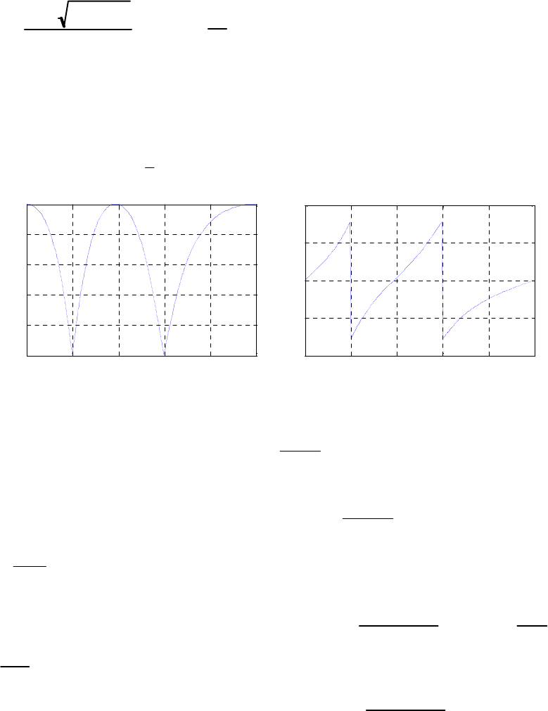
and .coscos)]2/tan()2/tan(1[ 2212121 θ
∆
ωω+=ββ =
BB (7-k)
The above two nonlinear equations can be solved yielding
1
1
1
2
4 2
2 and 2
2
1
.
(d) For the double notch filter with the following specifications:
π
ω
2.0
1=,
, and
π=ω 6.0
2,2.0
1π=B
π
=
25.0
2
B we get the following values for the
parameters of the notch filter transfer function:
,7628.0,1491.0,5673.0,4142.0,5095.0 12121
=
β
−
=
θ
=
θ
=α=α and
.
1955.0
2−=β
() ()
[]
zAzH 4
2
11+= :
00.2 0.4 0.6 0.8 1
0
0.2
0.4
0.6
0.8
1
ω
/
π
Magnitude
00.2 0.4 0.6 0.8 1
-2
-1
0
1
2
ω
/
π
Phase, radians
9.20 A zero (pole) of )(zH
L
P is given by the factor ).( k
zz
−
After applying the lowpass-to-
lowpass transformation, this factor becomes k
z
z−
−
z
−
ˆ
1α
ˆα, and hence the new location of the
zero (pole) is given by the roots of the equation
0)(
ˆ
)1(
ˆˆ
=
+
−
+=+−− kkkk zzzzzzz αααα or .
1
ˆ
k
k
kz
zα+
z
α
+
= For ,1−=
k
z
.1
1
ˆ−=
−
=a
zk
1
−a
9.21 The lowpass-to-bandpass transformation is given by z
b aˆ
z ˆ
z
2
1 aˆ z bˆ z
2 where a
2
1 and
b
1
1. A zero (pole) of )(zH
L
P is given by the factor ).( k
zz
−
. After applying the
lowpass-to-bandpass transformation, this factor becomes ˆ ˆ
2
b az z
1 aˆ z bˆ z
2 zk, and hence, the
new location of the zero (pole) of the bandpass transfer function is given by the roots of the
Not for sale 302

equation (1 or bz
k)z2
a(1 zk)z (b zk) 0, z2
k
1 bz
k
a(1 z)z
k
1 bzk
b z
0, whose
solution is given by ˆ
z
k
a(1 zk)
2(1 bzk)
a(1 zk)
2(1 bzk)
b zk
1 bzk
2
. For z
k 1, ˆ
z
k1.
9.22
()
()
21
2
1
1776.01842.01
13404.0
−−
−
++
+
=
zz
z
zGLP , with .55.0
π
=
ω
c
()
zH
L
P for π=ω 42.0
ˆc
2030.0
sin
sin
tantan
tantan
2
42.055.0
2
42.055.0
2
42.0
2
55.0
2
42.0
2
55.0
=
⎟
⎠
⎞
⎜
⎝
⎛
⎟
⎠
⎞
⎜
⎝
⎛
=
⎟
⎠
⎞
⎜
⎝
⎛
+
⎟
⎠
⎞
⎜
⎝
⎛
⎟
⎠
⎞
⎜
⎝
⎛
−
⎟
⎠
⎞
⎜
⎝
⎛
=+
−
ππ
ππ
ππ
ππ
α
() ()
2
1
ˆ
1
1
ˆ
1
ˆ
1
1
ˆ
2
1
ˆ
1
1
ˆ
1
ˆ
1
ˆ
1776.01842.01
3404.0
1
1
1
⎟
⎟
⎠
⎞
⎜
⎜
⎝
⎛
+
⎟
⎟
⎠
⎞
⎜
⎜
⎝
⎛
+
⎟
⎟
⎠
⎞
⎜
⎜
⎝
⎛
==
−
−
−
−
−
−
−
−
−
−
−
−
+
−
−
=−
−
−
z
z
z
z
z
z
z
z
z
LPLP zGzH
α
α
α
α
α
α
α
α
21
21
ˆ
181416.0
ˆ
2863.096993.0
ˆ
21623.0
ˆ
43245.021623.0
−−
−−
+−
++
=
zz
zz .
00.2 0.4 0.6 0.8 1
-50
-40
-30
-20
-10
0
G
a
i
n
i
n
dB
G
ain Responses
HLP(z)
GLP(z)
9.23 .0317.0
cos
cos
2
47.055.0
2
47.055.0
=
⎟
⎠
⎞
⎜
⎝
⎛
⎟
⎠
⎞
⎜
⎝
⎛
−
=−
+
ππ
ππ
α
() ()
.
ˆ
1728.0
ˆ
1097.09943.0
ˆ
3192.0
ˆ
6383.03192.0
21
21
ˆ
1
ˆ
1
1
1−−
−−
⎟
⎟
⎠
⎞
⎜
⎜
⎝
⎛
α+
α+
−= +−
+−
==
−
−
−
zz
zz
zGzH
z
z
z
LPHP
Not for sale 303
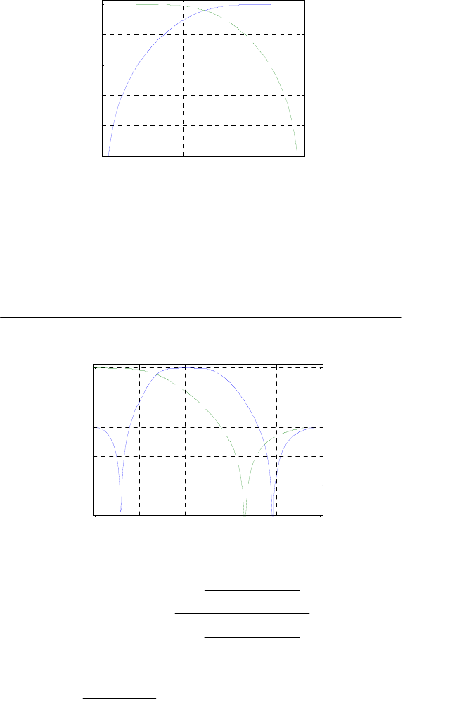
00.2 0.4 0.6 0.8 1
-50
-40
-30
-20
-10
0
ω /π
Gain
,
dB
Gain Responses
HHP(z) GLP(z)
9.24 , and
12 ˆˆ ccc ω−ω=ω
(
)
2790.0
ˆ
cos
=
ω
=α c
1
21
1
1
11
ˆ
2790.01
ˆˆ
2790.0
ˆ
1
ˆ
ˆ−
−−
−
−
−−
−
−
=
⎟
⎟
⎠
⎞
⎜
⎜
⎝
⎛
α−
α−
−=
z
zz
z
z
zz .
()
4321
4321
ˆˆ
2546.1
ˆ
046.3
ˆ
6824.25588.3
ˆ
6918.0
ˆ
1968.0
ˆ
6234.0
ˆ
1968.06918.0
−−−−
−−−−
+−+−
+−−−
=
zzzz
zzzz
zH BP .
00.2 0.4 0.6 0.8 1
-50
-40
-30
-20
-10
0
ω
/
π
Gain, dB
Gain Responses
HBP(z)
GLP(z)
9.25 and
,45.0
ˆπ=ωp.52.0
π
=ωp .1099.0
2
45.052.0
sin
2
45.052.0
sin
=
⎟
⎠
⎞
⎜
⎝
⎛π+π
⎟
⎠
⎞
⎜
⎝
⎛π−π
=λ
() ()
321
321
ˆ
1099.01
1099.0
ˆ
ˆˆ
711.6
ˆ
5359.17623.9
ˆ
874.2
ˆ
629.5
ˆ
622.5873.2
1
1
−−−
−
−
−
−
−
=++−
−+−
==
−
−
zzz
zzz
zGzH
z
z
z
HPHP .
Not for sale 304
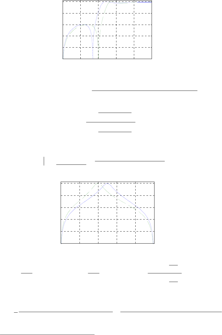
00.2 0.4 0.6 0.8 1
-50
-40
-30
-20
-10
0
ω
/
π
Gain in dB
Gain Responses
H
HP
(z)
G
HP
(z)
9.26 Eq. (7.79):
()
.
726542528.053353098.01
1
136728736.0 21
2
⎟
⎟
⎠
⎞
⎜
⎜
⎝
⎛
+−
−
=−−
−
zz
z
zH BP
and ,5.0
ˆ0π=ω .4.0
0π=ω 1584.0
2
4.05.0
sin
2
4.05.0
sin
−=
⎟
⎠
⎞
⎜
⎝
⎛+
⎟
⎠
⎞
⎜
⎝
⎛−
=
ππ
ππ
λ
() ()
.
ˆ
667122.0933718.0
ˆ
1333.01333.0
2
2
ˆ
1584.01
1584.0
ˆ
1
1
1−
−
+
+
=+
−
==
−
−
−
z
z
zHzG
z
z
z
BPBP
00.2 0.4 0.6 0.8 1
-50
-40
-30
-20
-10
0
ω
/
π
Gain in dB
Gain Responses
HBP(z)
GBP(z)
9.27 π=
⎟
⎠
⎞
⎜
⎝
⎛
π=ω 4.0
400
80
2
0, .025.0
400
5
2π=
⎟
⎠
⎞
⎜
⎝
⎛
π=
ω
B 9244.0
tan1
tan1
2
2=
⎟
⎠
⎞
⎜
⎝
⎛
+
⎟
⎠
⎞
⎜
⎝
⎛
−
=α ω
ω
B
B
()
.3090.0cos 0=ω=β
() ()()
(
)
()
(
)
21
21
21
21
2
1
9244.05946.01
9244.11893.19244.15.0
11
1121
−−
−−
−−
−−
+−
+−
=
α+α+β−
α++α+β−α+
=
zz
zz
zz
zz
zG
.
9244.05946.01
9622.059465.09622.0
21
21
−−
−−
+−
+−
=
zz
zz
Not for sale 305

.2738.0
sin
sin
2
ˆ
2
ˆ
00
00
=
⎟
⎠
⎞
⎜
⎝
⎛
⎟
⎠
⎞
⎜
⎝
⎛
=α ω+ω
ω−ω
.25.02
400
50
ˆ0π=π
⎟
⎠
⎞
⎜
⎝
⎛
=ω
() ()
1
1
1
ˆ
1
ˆ
−
−
−
α−
α−
=
=
z
z
z
BSBS zGzH 21
21
ˆˆ
45674.106017.1
ˆ
0301.1
ˆ
45679.10301.1
−−
−−
+−
+−
=
zz
zz .
00.2 0.4 0.6 0.8 1
-50
-40
-30
-20
-10
0
ω
/
π
Gain in dB
Gain Responses
H
BS
(z) G
BS
(z)
9.28 and
π=ω 45.0
ˆp.52.0
π
=ωp
()
(
)
321
321
179.07459.03272.01
5858.15858.112397.0
−−−
−−−
+++
−+−
=
zzz
zzz
zGHP
.0474.0
cos
cos
2
ˆ
2
ˆ
−=
⎟
⎠
⎞
⎜
⎝
⎛
⎟
⎠
⎞
⎜
⎝
⎛
−
=α ω−ω
ω+ω
pp
pp
() ()
1
1
1
ˆ
1
ˆ
−
−
−
α+
α−−
=
=
z
z
z
HPLP zGzH 321
321
ˆˆ
7756.3
ˆ
52265.272684.4
ˆ
03399.1
ˆ
45578.1
ˆ
45578.103399.1
−−−
−−−
+−+−
−−−−
=
zzz
zzz
00.2 0.4 0.6 0.8 1
-50
-40
-30
-20
-10
0
ω
/
π
Gain, dB
Gain Responses
HLP(z) GHP(z)
9.29 , hence,
9231.6=D.6=N
()
(
)
()
.
16
zD
zDz
zA
−−
=
Not for sale 306
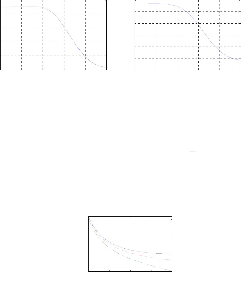
00.2 0.4 0.6 0.8 1
0.55
0.6
0.65
0.7
0.75
0.8
ω
/
π
Magnitude
Magnitude response
00.2 0.4 0.6 0.8 1
3
3.5
4
4.5
5
5.5
6
ω
/
π
Delay, in radians
Group delay
9.30 From Eq. (2.141) which
reduces to
() ()(
,)1()1()()1()(
)1(
TnxTTnydxTnynTy
nT
Tn
−⋅+−=ττ+−= ∫
−
)
].1[]1[][
−
⋅
+−= nxTnyny Hence, the corresponding transfer function is
given by .
1
)( 1
1
−
−
−
=
z
Tz
zH R From Eq. (2.120)
()
]1[][
2
]1[][ −++−= nxnx
T
nyny .
Hence, the corresponding transfer function is given by .
1
1
2
)( 1−
−
+
⋅=
z
zT
zHT
1−
)(zH
(
From the
plot given below it can be seen that the magnitude response of lies between that
of
int
)zH
R
and )(zH
T
.
0.2 0.4 0.6 0.8 1
0
0.5
1
1.5
HT(z)
HR(z)
Hint(z)
ω
/
π
Magnitude
9.31 ).()()( 4
1
4
3zHzHzH TRN += From the plot given below it can be seen that the magnitude
response of lies between that of )(zHN)(zH
R
and )(zH
T
, and is much closer to that of
. )(
int zH
Not for sale 307
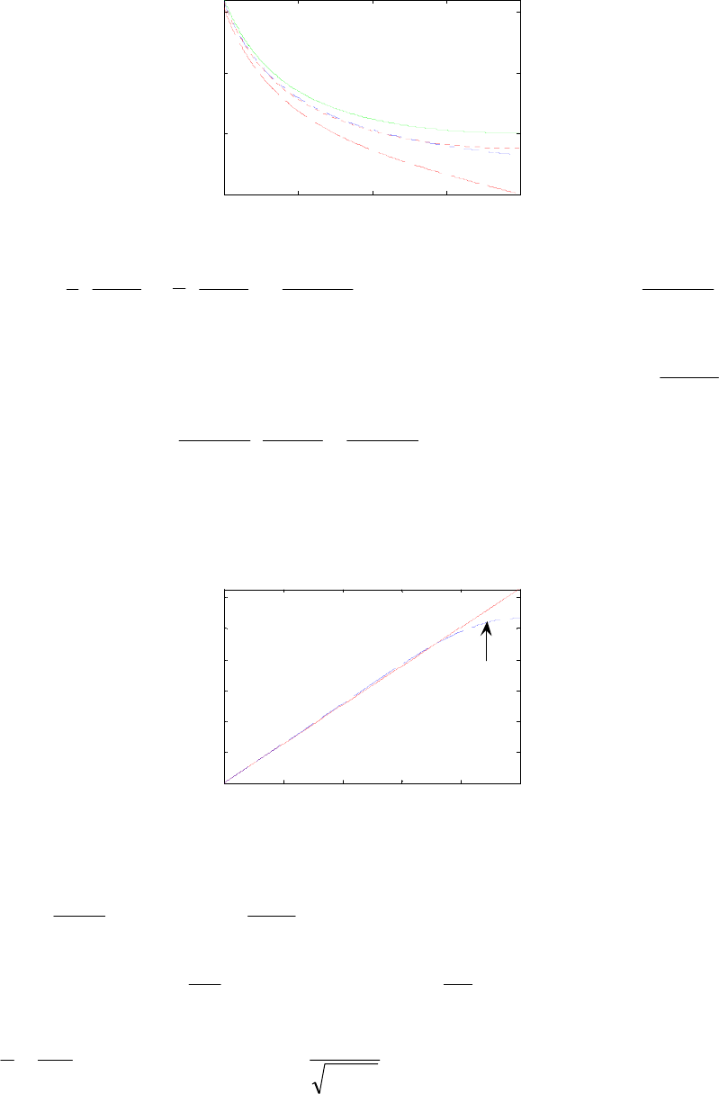
0.2 0.4 0.6 0.8 1
0
0.5
1
1.5
HT(z)
HR(z)
HN(z)
Hint(z)
ω
/
π
Magnitude
9.32 .
8
1
)(
)1(8
71
1
1
1
4
3
1
1
1
1
1
1
−
−
−
−
−
−
−
+
−
+
−=
⎟
⎟
⎠
⎞
⎜
⎜
⎝
⎛
+
⎟
⎟
⎠
⎞
⎜
⎜
⎝
⎛
=
z
z
z
z
z
z
NzH Its inverse is given by ,)( 1
1
71
)1(8
−
−
+
−
=
z
z
zH
which is unstable as it has a pole at .7
−
=
z
A stable transfer function with the same
magnitude response is obtained by multiplying with an allpass function
)(zH 1
7
71
−
+
+
z
z1−
resulting in .)( 1
1
1
1
7
)1
7
1
71
)1(8
−
−
−
−
+
−
+
+
⋅
+
−
=
z
z
z
z
IIR zH 1
1(87
−
−=
z
z A plot of the ideal differentiator
)(zH
D
I
F
with a frequency response given by Eq. (7.68) and that of the IIR differentiator
)(zH
I
IR is given below. As can be seen the magnitude response of )(zH
I
IR is very close
to that )(zH
D
I
F
.
00.2 0.4 0.6 0.8 1
0
0.5
1
1.5
2
2.5
3H
IIR
(z)
→
H
DIF
(z)
ω
/
π
Magnitude
M9.1 kHz30 & dB, 50 kHz,10 dB, 4.0 kHz,100
=
=
α
=
=α= ssppT FFF ,
,628.0
2=
π
=ω
T
p
pF
F .885.1
2=
π
=ω
T
s
sF
F
Let
T = 2. ,376.1
2
tan =
⎟
⎟
⎠
⎞
⎜
⎜
⎝
⎛ω
=Ω p
p and .376.1
2
tan =
⎟
⎠
⎞
⎜
⎝
⎛ω
=Ω s
s Therefore,
.235.4
1=
Ω
Ω
=
p
s
k Now, .4.0
1
1
log20 2
10 −=
⎟
⎟
⎠
⎞
⎜
⎜
⎝
⎛
ε+
Hence,
.096.0
2=ε
Not for sale 308

From 50
1
log20 10 −=
⎟
⎠
⎞
⎜
⎝
⎛
A we obtain Therefore,
or
.000,100
2=A
,10798.9 4
1−
×=k.62.1020
1
1
=
k As a result,
()
()
.580.4
/1log
/1log
10
110 →== k
k
N Next, solving 999,991
2
10
=−=
⎟
⎟
⎠
⎞
⎜
⎜
⎝
⎛
Ω
ΩA
c
s we get
435.0316.0
999,99 10/1 =Ω=
Ω
=Ω s
s
c
Using the M-file buttap, we determine the normalized analog Butterworth
transfer function of 5th order with a 3-dB cutoff frequency at 1=
Ω
c, which is:
() ()
(
)
(
)
.
1618.11618.01
1
22 +++++
=
sssss
sHan
Denormalize to move
()
sHan c
Ω
to 0.316:
() ()
)172.328.5)(142.128.5(130.2
1
22
435.0 +++++
=
⎟
⎠
⎞
⎜
⎝
⎛
=
sssss
HsH s
ana
5432 12.6430.9058.6366.2744.71
1
sssss
+
+
+
+
+
=.
() ()
⎟
⎟
⎠
⎞
⎜
⎜
⎝
⎛
−
+
−
−
=
=
1
1
1
1
2
z
z
T
s
asHzG
54321
54321
0637.04865.05492.16139.23617.21
0039.00197.00394.00394.00197.00039.0
−−−−−
−−−−−
−+−+−
+++++
=
zzzzz
zzzzz .
Matlab code is as follows:
% Program M9.01
N = 5;
[z, p, k] = buttap(N);
[num, den] = zp2tf(z, p, k);
% s -> s/0.435
den = [64.12 90.30 63.58 27.66 7.44 1];
num = [0 0 0 0 0 1];
% compute z, p, and k
[z, p, k] = tf2zp(num, den);
% perform bilinear transformation with T = 2;
[zd, pd, kd] = bilinear(z, p, k, 1/2);
% get the digital transfer function
[n2, d2] = zp2tf(zd, pd, kd);
% get the frequency response
[h, w] = freqz(n2, d2, 512);
figure(1);
plot(w/pi, 20*log10(abs(h))); grid;
axis([0 1 -60 5]);
xlabel('\omega/\pi'); ylabel('Gain, dB');
Not for sale 309
title('Gain response');
figure(2);
plot(w/pi, unwrap(angle(h))); grid;
axis([0 1 -8 1]);
xlabel('\omega/\pi'); ylabel('Phase, radians');
title('Phase response');
00.2 0.4 0.6 0.8 1
-60
-50
-40
-30
-20
-10
0
ω
/
π
Gain, dB
Gain response
00.2 0.4 0.6 0.8 1
-8
-6
-4
-2
0
ω
/
π
Phase, radians
Phase response
M9.2 % Problem M9.02
Fp = input('Passband edge frequency in Hz = ');
Fs = input('Stopband edge frequency in Hz = ');
FT = input('Sampling frequency in Hz = ');
Rp = input('Passband ripple in dB = ');
Rs = input('Stopband minimum attenuation in dB = ');
Wp = 2*Fp/FT;
Ws = 2*Fs/FT;
[N, Wn] = buttord(Wp, Ws, Rp, Rs)
[b, a] = butter(N, Wn);
disp('Numerator polynomial');
disp(b)
disp('Denominator polynomial');
disp(a)
[h, w] = freqz(b, a, 512);
plot(w/pi, 20*log10(abs(h))); grid
axis([0 1 -60 5]);
xlabel('\omega/\pi'); ylabel('Magnitude, dB');
pause
plot(w/pi, unwrap(angle(h))); grid
axis([0 1 -8 1]);
xlabel('\omega/\pi'); ylabel('Phase, radians');
M9.3 % Program #M9.03
close all;
clear;
clc;
% (a.) Ft = 1Hz;
[B, A] = besself(5, 0.5);
Not for sale 310
[BZ,AZ] = impinvar(B,A,1);
[h, w] = freqz(BZ, AZ, 512);
[Gd,W] = grpdelay(BZ,AZ,512);
figure(1);
plot(w/pi, 20*log10(abs(h)));
title('Gain response, , Sampling rate = 1 Hz');
xlabel('\omega/\pi'); ylabel('Gain, in dB');
figure(2);
plot(W/pi, (Gd));
title('Group delay, Sampling rate = 1 Hz');
xlabel('\omega/\pi'); ylabel('Delay, in samples');
% (b.) Ft = 2Hz;
[B, A] = besself(5, 0.5);
[BZ,AZ] = impinvar(B,A,2);
[h, w] = freqz(BZ, AZ, 512);
[Gd,W] = grpdelay(BZ,AZ,512);
figure(3);
plot(w/pi, 20*log10(abs(h)));
title('Gain response, Sampling rate = 2 Hz');
xlabel('\omega/\pi');ylabel('gain response');
figure(4);
plot(W/pi, (Gd));
title('Group delay, Sampling rate = 2 Hz');
xlabel('\omega/\pi'); ylabel('Delay, in samples');
(a) FT = 1 Hz
00.2 0.4 0.6 0.8 1
-80
-60
-40
-20
0
20
Gain response, Sampling rate = 1 Hz
ω
/
π
Gain, in dB
00.2 0.4 0.6 0.8 1
-4
-2
0
2
4
6
8
Group delay, Sampling rate = 1 Hz
ω
/
π
Delay, in samples
(b) FT = 2 Hz
Not for sale 311
00.2 0.4 0.6 0.8 1
-80
-60
-40
-20
0
20
Gain response, Sampling rate = 2 Hz
ω
/
π
Gain, in dB
00.2 0.4 0.6 0.8 1
-5
0
5
10
15
20
Group delay, Sampling rate = 2 Hz
ω
/
π
Delay, in samples
M9.4
,628.0=ωp.885.1=ωs
(
)
(
)
.50log20,4.0log20 885.1
10
628.0
10 −≤−≥ jj eGeG
Impulse invariance method, let T = 1 and assume no aliasing. Then
⇒−=
⎟
⎟
⎠
⎞
⎜
⎜
⎝
⎛
ε+
4.0log20 2
1
1
10 ,
096.0
2=ε
⇒−=
⎟
⎠
⎞
⎜
⎝
⎛50
1
log20 10 A .
000,100
2=A
62.1020
11
2
2
1
=
ε
−
=A
k, 3
628.0
885.11 ==
k. Hence,
73.6
log
log
1
10
1
10 1→=
⎟
⎠
⎞
⎜
⎝
⎛
⎟
⎠
⎞
⎜
⎝
⎛
=
k
k
N
999,991
2
10
=−=
⎟
⎟
⎠
⎞
⎜
⎜
⎝
⎛
Ω
ΩA
c
s or
(
)
596.0
110/1
2
=
−
Ω
=Ω
A
s
c.
Using the M-file butter, we get the analog Butterworth transfer function
(
)
sHa
of 7th order with a 3-dB cutoff frequency at c
Ω
.
()
sHa is then transformed into a digital transfer function using the M-file
impinvar, which yields:
()
.
07.066.077.257.655.954.838.41
0003.00023.00034.0001.0
7654321
5432
−−−−−−−
−−−−
−+−+−+−
+++
=
zzzzzzz
zzzz
zG
% Problem M9.04
[B, A] = butter(7, 0.596, 's');
[num, den] = impinvar(B, A, 1);
Not for sale 312
% get the frequency response
[h, w] = freqz(num, den, 512);
plot(w/pi, 20*log10(abs(h))); grid;
axis([0 1 -60 5]);
xlabel('\omega/\pi'); ylabel('Gain, in dB');
title('Gain response');
00.2 0.4 0.6 0.8 1
-60
-50
-40
-30
-20
-10
0
ω
/
π
Gain, in dB
Gain response
M9.5 dB 50 dB, 4.0 kHz,30 kHz,10 kHz,100
=
α
=
α
=
== spspT FFF
,2.0
2π=
π
=ω
T
p
pF
F and . .6.0
2π=
π
=ω
T
s
sF
F
(
)
(
)
.50log20,4.0log20 885.1
10
628.0
10 −≤−≥ jj eGeG
Impulse invariance method:
Let T = 1 and assume no aliasing. In this case, the specifications for are
same as that for i.e.,
()
sHa
()
,zG
,885.1,628.0 =Ω=Ω sp
()
(
)
.50885.1log20,4.0628.0log20 1010 −≤−≥ jHjH aa
Now, ⇒−=
⎟
⎟
⎠
⎞
⎜
⎜
⎝
⎛
ε+
4.0log20 2
1
1
10 , and
096.0
2=ε
⇒−=
⎟
⎠
⎞
⎜
⎝
⎛50log20 1
10 A . Hence,
000,100
2=A
62.1020
11
2
2
1
=
ε
−
=A
k and 3
628.0
885.11 ==
k.
Order of the Type I Chebyshev filter is
(
)
()
5324.4
/1cosh
/1cosh
1
1
1→== −
−
k
k
N
Bilinear transformation method:
. Here, 235.4
1=
Ω
Ω
=
p
s
k, and
376.1,325.0
=
Ω=
Ω
sp
Let T = 2.
Not for sale 313

000,100,096.0 22 ==ε A. Thus, 62.1020
1
1
=
k.
Order of the Type I Chebyshev filter is
(
)
()
.459.3
/1cosh
/1cosh
1
1
1→== −
−
k
k
N
Both designs meet the specifications, while the bilinear transformation method
meets with a filter of lower order. MATLAB code is as follows:
% Problem #M9.05
% Impulse invariance method
[z, p, k] = cheb1ap(5, 0.4);
[B, A] = zp2tf(z, p, k);
[BT, AT] = lp2lp(B, A, 0.628);
[num, den] = impinvar(BT, AT, 1);
[h, w] = freqz(num, den, 512);
figure(1);
plot(w/pi, 20*log10(abs(h))); grid;
axis([0 1 -60 5]);
xlabel('\omega/\pi'); ylabel('Gain, in dB');
title('Impulse Invariance Method');
figure(2);
plot(w/pi, unwrap(angle(h))); grid
axis([0 1 -8 1]);
xlabel('\omega/\pi'); ylabel('Phase, in radians');
title('Impulse Invariance Method');
% Bilinear transformation method
[z, p, k] = cheb1ap(4, 0.4);
[B, A] = zp2tf(z, p, k);
[BT, AT] = lp2lp(B, A, 0.325);
[num, den] = bilinear(BT, AT, 0.5);
[h, w] = freqz(num, den, 512);
figure(3);
plot(w/pi, 20*log10(abs(h))); grid;
axis([0 1 -60 5]);
xlabel('\omega/\pi'); ylabel('Gain, in dB');
title('Bilinear Transformation Method');
figure(4);
plot(w/pi, unwrap(angle(h))); grid
axis([0 1 -8 1]);
xlabel('\omega/\pi'); ylabel('Phase, in radians');
title('Bilinear Transformation Method');
Impulse Invariance Method:
Not for sale 314
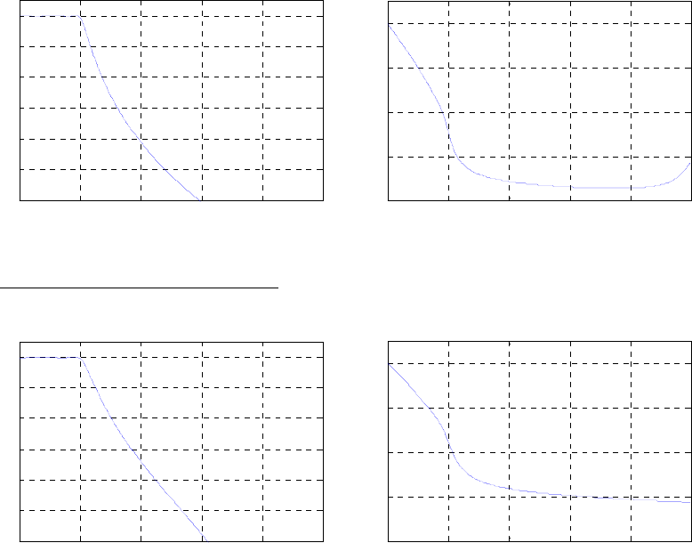
00.2 0.4 0.6 0.8 1
-60
-50
-40
-30
-20
-10
0
ω
/
π
Gain, in dB
Impulse Invariance Method
00.2 0.4 0.6 0.8 1
-8
-6
-4
-2
0
ω
/
π
Phase, in radians
Impulse Invariance Method
Bilinear Transformation Method:
00.2 0.4 0.6 0.8 1
-60
-50
-40
-30
-20
-10
0
ω
/
π
Gain, in dB
Bilinear Transformation Method
00.2 0.4 0.6 0.8 1
-8
-6
-4
-2
0
ω
/
π
Phase, in radians
Bilinear Transformation Method
M9.6 % Problem M9.06
Wp = input('Normalized passband edge = ');
Ws = input('Normalized stopband edge = ');
Rp = input('Passband ripple in dB = ');
Rs = input('Minimum stopband attenuation in dB = ');
[N, Wn] = cheb1ord(Wp, Ws, Rp, Rs);
[b, a] = cheby1(N, Rp, Wn);
[h, omega] = freqz(b,a,256);
figure(1);
plot(omega/pi, 20*log10(abs(h)));grid;
xlabel('\omega/\pi'); ylabel('Gain, in dB');
title('Type I Chebyshev Filter');
axis([0 1 -60 5]);
figure(2);
plot(omega/pi, unwrap(angle(h))); grid
axis([0 1 -8 1]);
xlabel('\omega/\pi'); ylabel('Phase, in radians');
title('Type I Chebyshev Filter');
Not for sale 315
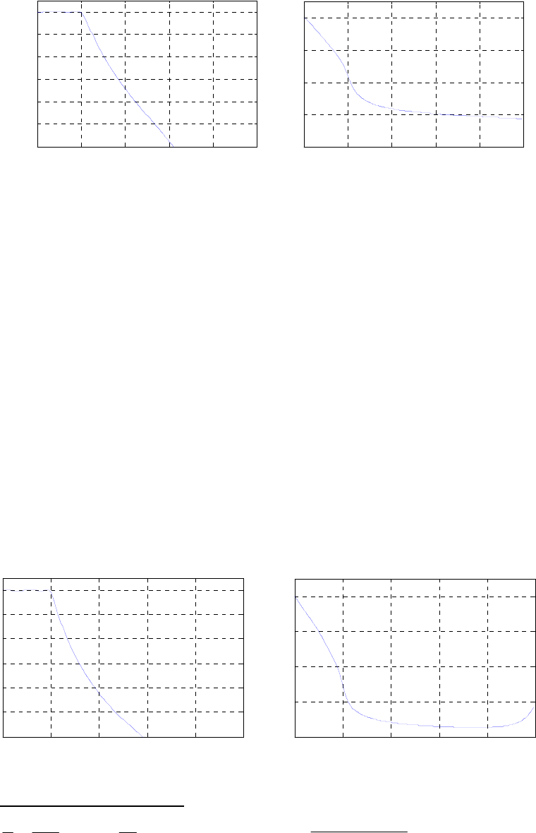
00.2 0.4 0.6 0.8 1
-60
-50
-40
-30
-20
-10
0
ω
/
π
Gain, in dB
Type I Chebyshev Filter
00.2 0.4 0.6 0.8 1
-8
-6
-4
-2
0
ω
/
π
Phase, in radians
Type I Chebyshev Filter
M9.7 % Problem M9.07
Wp = input(' Passband edge in radians = ');
Ws = input(' Stopband edge in radians = ');
Rp = input('Passband ripple in dB = ');
Rs = input('Stopband minimum attenuation in dB = ');
[N, Wn] = cheb1ord(Wp,Ws,Rp,Rs, 's');
[B, A] = cheby1(N, 0.5, Wn, 's');
[num, den] = impinvar(B, A, 1);
[h, omega] = freqz(num,den,256);
figure(1);
plot(omega/pi, 20*log10(abs(h)));grid;
xlabel('\omega/\pi'); ylabel('Gain, in dB');
title('Type I Chebyshev Filter');
axis([0 1 -60 5]);
figure(2);
plot(omega/pi, unwrap(angle(h))); grid
axis([0 1 -8 1]);
xlabel('\omega/\pi'); ylabel('Phase, in radians');
title('Type I Chebyshev Filter');
00.2 0.4 0.6 0.8 1
-60
-50
-40
-30
-20
-10
0
ω
/
π
Gain, in dB
Type I Chebyshev Filter
00.2 0.4 0.6 0.8 1
-8
-6
-4
-2
0
ω
/
π
Phase, in radians
Type I Chebyshev Filter
M9.8 Impulse invariance method:
Hence,
(
)
()
ρ/1log
/4log2
10
110 k
N≈, where
.62.1020
1
,00.3
1
1
=== kk p
s
Ω
Ω
Not for sale 316
()
,
'12
'1
,1' 0
2
k
k
kk +
−
=−= ρ
.150152 13
0
9
0
5
00 ρρρρρ +++= In our case,
,943.0' =k ,0073.0
0=ρ0073.0
=
ρ. Hence, 438.3 →
≈
N
Bilinear transformation method:
.235.4
1
,376.1,325.0 ====
p
s
sp kΩ
Ω
ΩΩ .62.1020
1
1
=
k
,972.0' =k , 0036.0
0=ρ0036.0
=
ρ. Hence, 396.2 →
≈
N
We note that the filter design using the impulse invariance method does not meet
the specifications due to aliasing. Increasing N from 4 to 6 will meet the
specifications.
% Problem M9_08
% Impulse Invariance Method
[z, p, k] = ellipap(4, 0.4, 50);
[B, A] = zp2tf(z, p, k);
[BT, AT] = lp2lp(B, A, 0.628);
[num, den] = impinvar(BT, AT, 1);
[h, omega] = freqz(num,den,256);
figure(1);
plot(omega/pi, 20*log10(abs(h)));grid;
xlabel('\omega/\pi'); ylabel('Gain, in dB');
title('Impulse Invariance Method');
axis([0 1 -60 5]);
figure(2);
plot(omega/pi, unwrap(angle(h))); grid
axis([0 1 -8 1]);
xlabel('\omega/\pi'); ylabel('Phase, in radians');
title('Impulse Invariance Method');
% Bilinear Transformation Method
[z, p, k] = ellipap(4, 0.4, 50);
[B, A] = zp2tf(z, p, k);
[BT, AT] = lp2lp(B, A, 0.325);
[num, den] = bilinear(BT, AT, 0.5);
[h, omega] = freqz(num,den,256);
figure(3);
plot(omega/pi, 20*log10(abs(h)));grid;
xlabel('\omega/\pi'); ylabel('Gain, in dB');
title('Bilinear Transformation Method');
axis([0 1 -60 5]);
figure(4);
plot(omega/pi, unwrap(angle(h))); grid
axis([0 1 -8 1]);
xlabel('\omega/\pi'); ylabel('Phase, in radians');
Not for sale 317
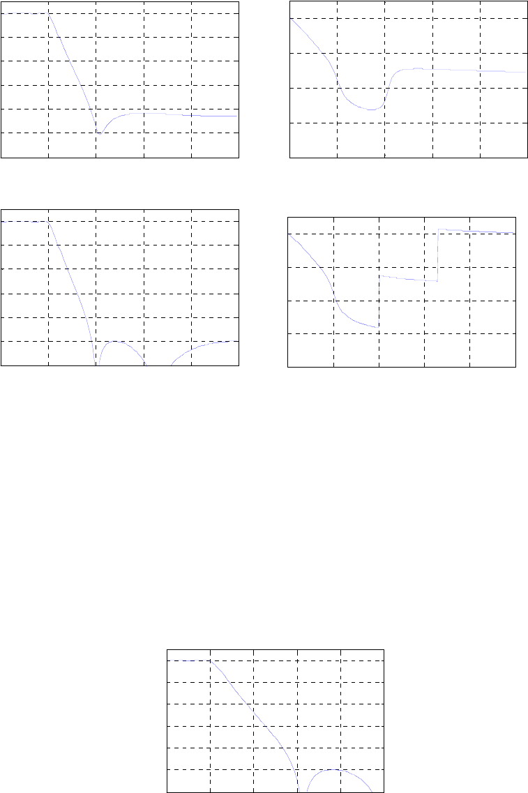
title('Bilinear Transformation Method');
00.2 0.4 0.6 0.8 1
-60
-50
-40
-30
-20
-10
0
ω
/
π
Gain, in dB
Impulse Invariance Method
00.2 0.4 0.6 0.8 1
-8
-6
-4
-2
0
ω
/
π
Phase, in radians
Impulse Invariance Method
00.2 0.4 0.6 0.8 1
-60
-50
-40
-30
-20
-10
0
ω
/
π
Gain, in dB
Bilinear Transformation Method
00.2 0.4 0.6 0.8 1
-8
-6
-4
-2
0
ω
/
π
Phase, in radians
Bilinear Transformation Method
M9.9 % Program M9_09
Wp = input('Normalized passband edge = ');
Ws = input('Normalized stopband edge = ');
Rp = input('Passband ripple in dB = ');
Rs = input('Stopband ripple in dB = ');
[N, Wn] = ellipord(Wp, Ws, Rp, Rs);
[b, a] = ellip(N, Rp, Rs, Wn);
[h, omega] = freqz(b, a, 256);
plot(omega/pi, 20*log10(abs(h)));grid;
xlabel('\omega/\pi'); ylabel('Gain, in dB');
title('IIR Elliptic Lowpass Filter');
axis([0 1 -60 5]);
00.2 0.4 0.6 0.8 1
-60
-50
-40
-30
-20
-10
0
ω
/
π
Gain, in dB
IIR Elliptic Lowpass Filter
M9.10 kHz. kHz, MHz, 2106005.1
=
== spT FFF
Not for sale 318

.
dB dB, 454.0 == sp αα
(a) .880.0
2
,513.2
2====
F
s
s
T
p
pF
F
F
Fπ
ω
π
ω
.471.0tan
ˆ
,076.3tan
ˆ
22 =
⎟
⎠
⎞
⎜
⎝
⎛
==
⎟
⎠
⎞
⎜
⎝
⎛
=s
psp
ω
ωΩΩ
Analog highpass specifications are thus:
dB dB, 454.0,471.0
ˆ
,076.3
ˆ==== spsp ααΩΩ
(b) 531.6
ˆ
ˆ
,1 ===
s
p
sp Ω
Ω
ΩΩ
% Problem M9.10
close all;
clear;
clc;
[N, Wn] = ellipord(1, 6.531, 0.4, 45, 's');
[B, A] = ellip(N, 0.4, 45, Wn, 's');
[BT, AT] = lp2hp(B, A, 3.076);
[num, den] = bilinear(BT, AT, 0.5);
[h, omega] = freqz(num, den, 256);
figure(1);
plot(omega/pi, 20*log10(abs(h)));grid;
xlabel('\omega/\pi'); ylabel('Gain, in dB');
title('Elliptic Highpass Filter');
axis([0 1 -60 5]);
00.2 0.4 0.6 0.8 1
-60
-50
-40
-30
-20
-10
0
ω
/
π
Gain, in dB
Elliptic Highpass Filter
(c) Analog lowpass transfer function coefficient are obtained by displaying B and A:
.
8329.06434.1s3314.1s
0.8329s0.0556
)( 23
2
+++
+
=
s
sHLP
Analog highpass transfer function coefficient are obtained by displaying BT and AT:
Not for sale 319

.
9438.341254.150693.6
6315.0
)( 23
3
+++
+
=
sss
ss
sHHP
Digital highpass transfer function coefficient are obtained by displaying num and
den:
:.
4356.05613.19407.11
0286.00415.00415.00286.0
)( 321
321
−−−
−−−
+++
−+−
=
zzz
zzz
zGHP
M9.11 ,3,650,2.2,2.1,9 2121 kHzFHzFkHzFkHzFkHzF ssppT
=
=
=
==
dBdB sp 31,8.0 == αα
(a) 8378.0
21
1=
π
=ω
T
p
pF
F, 536.1
22
2=
π
=ω
T
p
pF
F, 4538.0
21
1=
π
=ω
T
s
sF
F, and
094.2
22
2==
T
s
sF
F
π
ω, with
445.0
2
tan
ˆ1
1=
⎟
⎟
⎠
⎞
⎜
⎜
⎝
⎛
=p
p
ω
Ω, 966.0
2
tan
ˆ2
2=
⎟
⎟
⎠
⎞
⎜
⎜
⎝
⎛
=p
p
ω
Ω, 231.0
2
tan
ˆ1
1=
⎟
⎠
⎞
⎜
⎝
⎛
=s
s
ω
Ω,
and 731.1
2
tan
ˆ2
2=
⎟
⎠
⎞
⎜
⎝
⎛
=s
s
ω
Ω.
,521.0
ˆˆ 12 =−= pp
BΩΩ
ω
40.0
ˆˆ
430.0
ˆˆˆ 2121
2
0=≠== sspp ΩΩΩΩΩ
Therefore, we choose to lower the stopband edge to: 13.3
ˆ
ˆˆ
1
2
1
2
0=
⋅
−
=
ω
B
s
s
sΩ
ΩΩ
Ω
(b) The analog lowpass specifications are thus:
1=Ω p rad, rad, 13.3=
s
Ω8.0
=
α
pdB, 31
=
α
sdB.
% Problem M9.11
[N, Wn] = cheb1ord(1, 3.13, 0.8, 31, 's');
[B, A] = cheby1(N, 0.8, Wn, 's');
[BT, AT] = lp2bp(B, A, sqrt(0.43), 0.521);
[num, den] = bilinear(BT, AT, 0.5);
[h, omega] = freqz(num, den, 256);
plot(omega/pi, 20*log10(abs(h)));grid;
xlabel('\omega/\pi'); ylabel('Gain,in dB');
title('Chebyshev I Bandpass Filter');
axis([0 1 -60 5]);
Not for sale 320

00.2 0.4 0.6 0.8 1
-60
-50
-40
-30
-20
-10
0
ω
/
π
Gain,in dB
Chebyshev I Bandpass Filter
(c) Analog lowpass transfer function coefficient are obtained by displaying B and A:
.
5559.03244.10719.1
5559.0
)( 23 +++
=
sss
sHLP
Analog bandpass transfer function coefficient are obtained by displaying BT and AT:
.
0795.01033.07093.05589.06495.15584.0
0786.0
)( 23456
3
++++++
=
ssssss
s
sH BP
Digital bandpass transfer function coefficient are obtained by displaying den and
num:
.
476.01983.16191.21443.33196.39799.11
0169.00506.00506.00169.0
)( 654321
642
−−−−−−
−−−
+++−+−
−+−
=
zzzzzz
zzz
zGBP
M9.12 8=
T
F kHz, kHz,
9.0
1=
p
F1.2
2
=
p
F kHz, 6.0
1
=
s
F kHz, kHz, 3
2=
s
F
5.1=α p dB, dB 30=αs
(a) 707.0
21
1==
T
p
pF
F
π
ω
, 649.1
22
2==
T
p
pF
F
π
ω
, 471.0
21
1==
T
s
sF
F
π
ω
, and
356.2
22
2==
T
s
sF
F
π
ω
, with
369.0
2
tan
ˆ1
1=
⎟
⎟
⎠
⎞
⎜
⎜
⎝
⎛
=Ω p
p
ω
, 081.1
2
tan
ˆ2
2=
⎟
⎟
⎠
⎞
⎜
⎜
⎝
⎛
=Ω p
p
ω
, 240.0
2
tan
ˆ1
1=
⎟
⎠
⎞
⎜
⎝
⎛
=Ω s
s
ω
,
and 414.2
2
tan
ˆ2
2=
⎟
⎠
⎞
⎜
⎝
⎛
=Ω s
s
ω
.
174.2
ˆˆ 12 =Ω−Ω= ss
B
ω
579.0
ˆˆ
399.0
ˆˆˆ 2121
2
0=ΩΩ≠=ΩΩ=Ω sspp
Therefore, we choose to lower the passband:
Not for sale 321

536.0
ˆ
ˆˆ
ˆ
2
12
1=
Ω
ΩΩ
=Ω
p
ss
p
The analog bandstop filter specifications are thus:
536.0
ˆ1=Ω p rad, rad, rad, rad, 081.1
ˆ2=Ω p240.0
ˆ1=Ωs414.2
ˆ2=Ωs
5.1=
p
α
dB, 30=
s
α
dB.
(b) Analog prototype LP filter:
rad, 995.3
ˆˆ
ˆ
21
2
0
1=
−
⋅
=
p
p
p
B
ΩΩ
Ω
Ωω rad, 5.1
=
p
α
dB, 30
=
s
α
dB.
1
=Ωs
% Problem M9.12
close all;
clear;
clc;
[N, Wn] = ellipord(3.995, 1, 1.5, 30, 's');
[B, A] = ellip(N, 1.5, 30, Wn, 's');
[BT, AT] = lp2bs(B, A, sqrt(0.579), 2.174);
[num, den] = bilinear(BT, AT, 0.5);
[h, omega] = freqz(num, den, 256);
plot(omega/pi, 20*log10(abs(h)));grid;
xlabel('\omega/\pi'); ylabel('Gain, in dB');
title('Elliptic Bandstop Filter');
axis([0 1 -60 5]);
00.2 0.4 0.6 0.8 1
-60
-50
-40
-30
-20
-10
0
ω
/
π
Gain, in dB
Elliptic Bandstop Filter
(c) Analog lowpass transfer function coefficient are obtained by displaying B and A:
.
059.156122.3
6706.120316.0
)( 2
2
++
+
=
ss
s
sHLP
Analog bandstop transfer function coefficients are obtained by displaying BT and
AT:
.
3352.03019.04719.15215.0
2821.09843.08414.0
)( 234
24
++++
++
=
ssss
ss
sH BS
Not for sale 322

Digital bandstop transfer function coefficients are obtained by displaying num
and den:
.
5464.06115.03959.18534.01
5806.06163.03145.16163.05806.0
)( 4321
4321
−−−−
−−−−
+−+−
+−+−
=
zzzz
zzzz
zGBS
M9.13 % Program M9.13
close all;
clear;
clc;
Wp = 0.7; Ws = 0.5;
Rp = 1; Rs = 32;
[N,Wn] = cheb1ord(Wp,Ws,Rp,Rs);
[b,a] = cheby1(N,Rp,Wn,'high');
[h,omega] = freqz(b,a,256);
plot (omega/pi,20*log10(abs(h)));grid;
xlabel('\omega/\pi'); ylabel('Gain, in dB');
title('Type I Chebyshev Highpass Filter');
[GdH,w] = grpdelay(b,a,512);
plot(w/pi,GdH); grid
xlabel('\omega/\pi'); ylabel('Delay, in samples');
title('Original Filter Group Delay');
F = 0.7:0.001:1;
g = grpdelay(b,a,F,2); % Equalize the passband
Gd = max(g)-g;
% Design the allpass delay equalizer
[num,den,tau] = iirgrpdelay(2*N, F, [0.7 1], Gd);
[GdA,w] = grpdelay(num,den,512);
plot(w/pi,GdH+GdA); grid
xlabel('\omega/\pi');ylabel('Delay, in samples');
title('Group Delay Equalized Filter');
00.2 0.4 0.6 0.8 1
0
10
20
30
40
ω
/
π
Delay, in samples
Group Delay Equalized Filter
M9.14 % Program M9.14
close all;
clear;
Not for sale 323
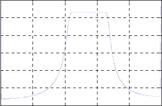
clc;
Wp = [0.45 0.65]; Ws = [0.3 0.75];
Rp = 1; Rs = 40;
[N,Wn] = buttord(Wp, Ws, Rp, Rs);
[b,a] = butter(N,Wn);
[h,omega] = freqz(b,a,256);
gain = 20*log10(abs(h));
plot (omega/pi,gain);grid;
xlabel('\omega/\pi'); ylabel('Gain, in dB');
title('IIR Butterworth Bandpass Filter');
[GdH,w] = grpdelay(b,a,512);
plot(w/pi,GdH); grid
xlabel('\omega/\pi'); ylabel('Delay, in samples');
title('Original Filter Group Delay');
F = 0.45:0.001:0.65;
g = grpdelay(b,a,F,2); % Equalize the passband
Gd = max(g)-g;
% Design the allpass delay equalizer
[num,den,tau] = iirgrpdelay(2*N, F, [0.45 0.65], Gd);
[GdA,w] = grpdelay(num,den,512);
plot(w/pi,GdH+GdA); grid
xlabel('\omega/\pi');ylabel('Delay, in samples');
title('Group Delay Equalized Filter');
00.2 0.4 0.6 0.8 1
0
10
20
30
40
50
60
ω
/
π
Delay, in samples
Group Delay Equalized Filter
Not for sale 324

Chapter 10
10.1 To compute the filter orders, we use Kaiser’s formula of Eq. (10.3), Bellanger’s formula
of Eq. (10.4), and Hermann’s formula of Eq. (10.5).
Filter #1:
Kaiser’s formula -
(
)
()
158097.157
2/10625.014375.06.14
1300012.00224.0log20 10 ≈=
−
−⋅−
=πππ
N
Bellanger’s formula -
(
)
()
163575.1621
2/10625.014375.03
000112.00224.010log2 10 ≈=−
−
⋅
⋅
−
=πππ
N
Hermann’s formula -
()
()
(
)
[
]
()()
[]
8326.24278.00224.0log5941.00224.0log00266.0
000112.0log4761.00224.0log07114.00224.0log005309.0,
10
2
10
1010
2
10
=++
−⋅−+=
∞sp
D
δδ
(
)
[
]
1913.12000112.0log0224.0log51244.001217.11, 1010
=
−
+=
sp
F
δ
δ
()
[]
()
1518434.150
2/10625.014375.0
2/10625.014375.01913.128326.2 2≈=
−
−−
=πππ
πππ
N
Filter #2:
Kaiser’s formula -
(
)
()
34186.33
2/2075.02875.06.14
13034.0017.0log20 10 ≈=
−
−⋅−
=πππ
N
Bellanger’s formula -
(
)
()
373012.361
2/2075.02875.03
034.0017.010log2 10 ≈=−
−
⋅
⋅
−
=πππ
N
Hermann’s formula -
()
()
(
)
[
]
()()
[]
474777.14278.0017.0log5941.0017.0log00266.0
034.0log4761.0017.0log07114.0017.0log005309.0,
10
2
10
1010
2
10
=++
−⋅−+=
∞sp
D
δδ
(
)
[
]
85791019.10034.0log017.0log51244.001217.11, 1010
=
−
+=
sp
F
δ
δ
()
[
]
()
37435.36
2/2075.02875.0
2/2075.02875.085791019.10474777.1 2≈=
−
−−
=πππ
πππ
N
Filter #3:
Kaiser’s formula -
(
)
()
126107.11
2/345.0575.06.14
130137.00411.0log20 10 ≈=
−
−⋅−
=
πππ
k
N
Bellanger’s formula -
(
)
()
1304.121
2/345.0575.03
0137.00411.010log2 10 ≈=−
−
⋅
⋅
−
=πππ
N
Hermann’s formula -
Not for sale 324

()
()
(
)
[
]
()()
[]
4424.14278.00411.0log5941.00411.0log00266.0
0137.0log4761.00411.0log07114.00411.0log005309.0,
10
2
10
1010
2
10
=++
−⋅−+=
∞sp
D
δδ
(
)
[
]
256666.110137.0log0411.0log51244.001217.11, 1010
=
−
+=
sp
F
δ
δ
()
[]
()
12248.11
2/345.0575.0
2/345.0575.0256666.114424.1 2≈=
−
−−
=πππ
πππ
N
10.2 and
75=N
π
ω
ω
05.0=− ps and we assume .
ps
δ
δ
=
(a) Using Kaiser’s formula of Eq. (10.3):
[]
375.40009577.010 20
132/05.06.1475
=∴== ⎟
⎠
⎞
⎜
⎝
⎛
−
+⋅
ss αδ
ππ
dB.
(b) Using Bellanger’s formula of Eq. (10.4):
5.380119.0101.0
2/1
2
2/05.0376
=∴=
⎟
⎟
⎟
⎠
⎞
⎜
⎜
⎜
⎝
⎛
⋅= ⎟
⎠
⎞
⎜
⎝
⎛⋅⋅−
ss αδ
ππ
dB.
(c) Using Hermann’s formula of Eq. (10.5):
()
()
(
)
[
]
2
11 2/2/
πωωπωωδ
pspss bNDbF −+−=∴= ∞
() ( )
(
)
[
]
(
)
()()
[]
()()()()
()()
()()()()()()
61053
2
1042
3
101
6105
2
104
103
2
102
3
101
6105
2
104
103102
2
101
logloglog
loglog
logloglog
loglog
logloglog
aaaaaaD
aaa
aaaD
aaa
aaaD
ssss
ss
ssss
ss
ssss
−−+−+=
−−
−++=
++
−++=
∞
∞
∞
δδδδ
δδ
δδδδ
δδ
δδδδ
Let
(
s
x
)
δ
10
log=, and thus
()
875697.14278.00702.106848.0005309.0 23 =−−+=
∞xxxD s
δ
Solving for x gives us three possible solutions:
4263.10,94654.1,3787.21
=
−=−= xxx
The most reasonable solution is the second. Therefore,
93.380113.0 =∴= ss
α
δ
10.3 and
75=N
ω
π
ω
ω
∆
=
=− 05.0
ps
()
9.348285.2 =+
∆
=N
s
ω
α
dB.
10.4 The ideal
L
-band digital filter )(zH
M
L has a frequency response given by
for
,)( k
j
ML AeH =
ω,
1kk ωωω
≤
≤
−,1 Lk
≤
≤
and can be considered as sum of
L
ideal
bandpass filters with cutoff frequencies at and where
and Now from Eq. (10.47) the impulse response of an ideal bandpass filter is
1
1−
=k
k
cωω ,
2k
k
cωω =0
0
1=
c
ω
.
2π=
L
c
ω
Not for sale 325

given by .
)sin()sin(
][ 12
n
n
n
n
nh cc
BP π
ω
π
ω−= Therefore ,
n
n
n
n
nh kk
k
BP π
ω
π
ω)sin()sin(
][ 1−
−= . Hence,
∑∑ =
−
=
⎟
⎠
⎞
⎜
⎝
⎛−==
L
k
kk
k
L
k
k
BPML n
n
n
n
Anhnh
1
1
1
)sin()sin(
][][ π
ω
π
ω
∑∑ −
=
−
−
=
⎟
⎠
⎞
⎜
⎝
⎛−−+
⎟
⎠
⎞
⎜
⎝
⎛−=
1
2
1
1
2
1
1
)sin()sin()sin(
)0sin(
)sin( L
k
kk
k
L
k
k
kn
n
n
n
A
n
n
A
n
n
n
n
Aπ
ω
π
ω
π
ω
ππ
ω
⎟
⎠
⎞
⎜
⎝
⎛−+ −
n
n
n
n
ALL
Lπ
ω
π
ω)sin()sin( 1
n
n
A
n
n
A
n
n
A
n
n
AL
L
L
k
L
k
k
k
k
kπ
ω
π
ω
π
ω
π
ω)sin(
)sin()sin(
)sin( 1
1
2
1
2
1
1
1−
−
=
−
=
−−−+= ∑∑
.
)sin()sin(
1
12
1
∑∑
−
==
−
−=
L
k
L
k
k
k
k
kn
n
A
n
n
Aπ
ω
π
ω
Since ,π=
L
ω .0)sin(
=
n
L
ω We add a term n
n
AL
Lπ
ω)sin( to the first sum in the above
expression and change the index range of the second sum, resulting in
.
)sin()sin(
][
1
1
1
1
∑∑
=
−
=
+
−=
L
k
L
k
k
k
k
kML n
n
A
n
n
Anh π
ω
π
ω
Finally, since ,0
1=
+
L
A we can add a term n
n
AL
Lπ
ω)sin(
1+ to the second sum. This leads to
.
)sin(
)(
)sin()sin(
][
11 1
11
∑∑ ∑
== =
++ −=−=
L
k
L
k
L
k
k
kk
k
k
k
kML n
n
AA
n
n
A
n
n
Anh π
ω
π
ω
π
ω
10.5 Therefore,
⎩
⎨
⎧
<<−
<<−
=.0,
,0,
)( πω
ωπ
ω
j
j
eH j
HT
∫∫ π
−π
+
π
=
0
0
)(
2
1
)(
2
1
][ ωω ωω
π
ωω deeHdeeHnh njj
HT
njj
HTHT
()
n
n
n
n
djedje njnj
π
π
π
π
ωω ω
π
ω)2/(sin2
)cos(1
2
2
2
1
2
12
0
0
=−=
π
−
π
=∫∫ π
−
if
.0≠n
For ,0=n.0
2
1
2
1
]0[
0
0
=
π
−
π
=∫∫ π
−
ωω
π
jdjdhHT
Not for sale 326
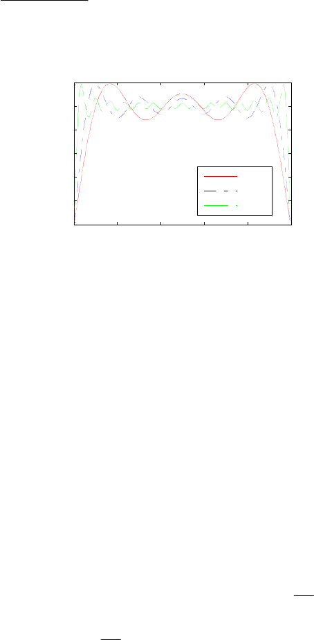
Hence, ⎪
⎩
⎪
⎨
⎧
≠
π
π
=
=.,
)/(
,,
][ 0if
22sin
0if0
2
n
n
n
n
nh HT
Since ],[][ nhnh H
T
H
T
−−= and the length of the truncated impulse response is odd, it is a Type
3 linear-phase FIR filter.
00.2 0.4 0.6 0.8 1
0
0.2
0.4
0.6
0.8
1
ω
/
π
Magnitude
N=11
N=21
N=61
From the frequency response plots given above, we observe the presence of ripples at the
bandedges due to the Gibbs phenomenon caused by the truncation of the impulse response.
10.6 . Hence,
∑
∞
−∞=
−=
k
HT kxknhnx ][][]}[{H
{}
{}
)()(][ ωω jj
H
TeXeHnx =HF
⎪
⎩
⎪
⎨
⎧
<<−
<<−
=.0),(
,0),(
πω
ωπ
ω
ω
j
j
ejX
ejX
(a) Let
{
}
{{}{}
.][ ][nxny HHHH=
}
Hence,
Therefore,
).(
,0),()(–
,0),(
)( 4
4ω
ω
ω
ω
πω
ωπ j
j
j
jeX
eXj
eXj
eY =
⎪
⎩
⎪
⎨
⎧
<<
<<−
=
].[][ n
x
ny =
(b) Define and
{
,][][ nxng H=
}
].[][* nxnh
=
Then
But from the Parseval's' relation in Table 3.4,
{}
.][*][][][ –– ∑∑ ∞
∞=
∞
∞= =ll llll hgxxH
.)()(
2
1
][*][ –
–ω
ωω deGeGhg jj
∫
∑π
∞
∞= π
=
lll π
Therefore,
{}
ω
ωωω deXeXeHxx jjj
HT )()()(
2
1
][][ –
–∫
∑π−
∞
∞= π
=
lllHπ
where
Since the integrand
⎩
⎨
⎧
<<−
<<−
=.0,
,0,
)( πω
ωπ
ω
j
j
eH j
HT )()()( –ωωω jjj
H
TeXeXeH is an odd
function of As a result, ,ω.0)()()( –=
∫π
π− ω
ωωω deXeXeH jjj
HT
{}
.0][][
–=
∑∞
∞=lll xxH
Not for sale 327
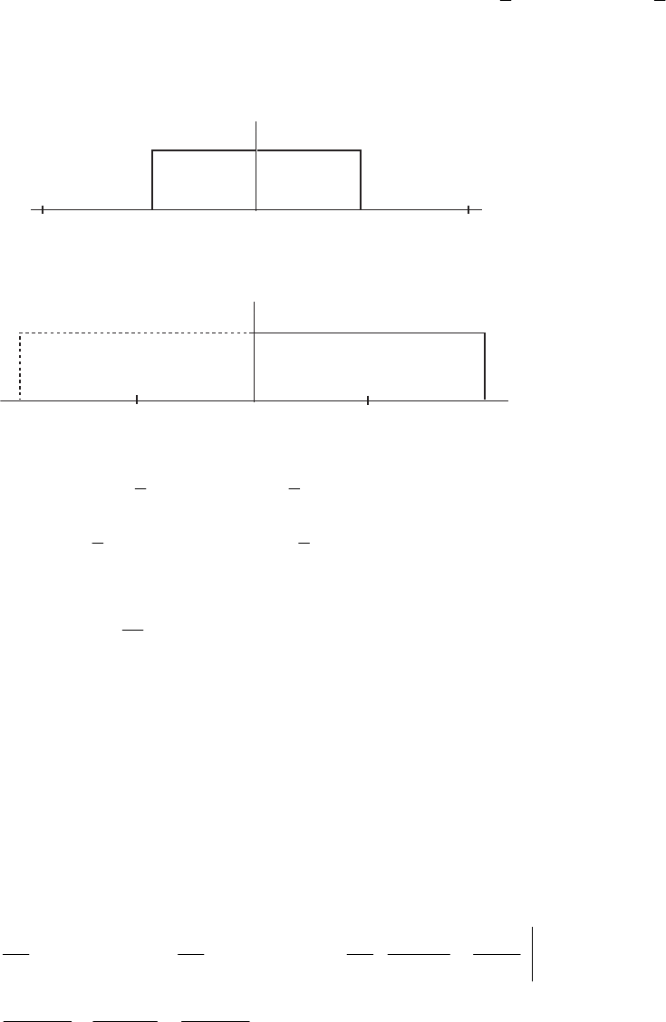
10.7 Its frequency response
.][)( ∑
=
−
=N
n
n
LPLP znhzH
0
)(ωj
L
P
eH is shown in Figure (a)
below. A plot of the frequency response =
ω)( j
H
TeH )()( )()( 22
ππ +ω−ω +j
L
P
j
L
P
eHeH
is shown in Figure (b) below. It is evident from this figure that )(ωj
H
TeH is the
frequency response of an ideal Hilbert transformer. Therefore, we have
0π
ω
1
_
π
jω
H (e )
LP
2
__
π
_
2
__
π
(a)
0π
ω
1
_π
2
__
π
_
2
__
π
H (e )
LP j(ω )
2
__
π
_
j(ω + )
2
__
π
H (e )
LP
jω
H (e )
HT
(b)
)()()( )()( 22
ππ −ω+ω
ω+= j
L
P
j
L
P
j
H
TeHeHeH
()
22
000
22 //
)()( ][][][ ππ−ω−
==
−ω−
=
+ω− +=+= ∑∑∑
ππ
jnjnjn
N
n
LP
N
n
jn
LP
N
n
jn
LP eeenhenhenh
()
.cos][ 2
0
2π
=
ω−
∑
=n
N
n
jn
LP enh Now, for odd,
n02
=
ω
)/cos(n and hence, we can drop all
odd terms in the above expression. Let MN 2
=
with even and let Then, we
can rewrite the above equation as The
corresponding transfer function of the Hilbert transformer is therefore given by
N.nr 2=
.)cos(][)( ω−
=
ωπ= ∑rj
M
r
LP
j
HT errheH 2
0
22
.][)()cos(][)( ∑∑ =
−
=
−−=π= M
n
n
LP
n
M
n
n
LPHT znhznnhzH
0
2
0
221222
10.8 Hence,
.)( ω
ωjeH j
DIF =
.
222
1
][ 2
π
π
ωω
ωω ω
ωωωω −
⎟
⎟
⎠
⎞
⎜
⎜
⎝
⎛+
π
=
π
=
π
=∫∫ π
π−
π
π− n
e
jn
e
j
de
j
dejnh
njnj
njnj
DIF Therefore,
,
)cos()sin()cos(
][ 2n
n
n
n
n
n
nhDIF
πππ =
π
−= if .0
≠
n
Not for sale 328
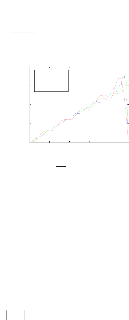
For ,
0=n.0
2
1
]0[ =
π
=∫
−
π
π
ωωdjhDIF
Hence, ⎪
⎩
⎪
⎨
⎧
>
π=
=.0||,
)cos(
,0,0
][ n
n
n
n
nhDIF Since ],[][ nhnh
D
I
F
D
I
F
−
−
=
the truncated impulse
response is a Type 3 linear-phase FIR filter. The magnitude responses of the above
differentiator for several values of
M
are given below:
00.2 0.4 0.6 0.8 1
0
1
2
3
4
ω
/
π
Magnitude
M=10
M=20
M=30
10.9
.12 += MN
()
⎪
⎪
⎪
⎩
⎪
⎪
⎪
⎨
⎧
<≤≠
−
−
−
=−
=
otherwise.
0,
if
for
,0,,
)(
)(sin
,,1
][
ˆNnMn
mn
mn
Mn
nh c
c
HP π
ω
π
ω
Now,
∑∑∑∑ −
=
−
−
=
−
∞
−∞=
−
∞
−∞=
−+=+=+
1
0
1
0
][
ˆ
][
ˆ
][
ˆ
][
ˆ
)(
ˆ
)(
ˆN
n
n
LP
N
n
n
HP
n
n
LP
n
n
HPLPHP znhznhznhznhzHzH
()
.][
ˆ
][
ˆ
1
0
∑
−
=
−
+=
N
n
n
LPHP znhnh
But ][
ˆ
][
ˆnhnh
L
P
H
P+ = ,
⎩
⎨
⎧≠≤≤
=+ .
1,0
][
ˆ
][
ˆ
n=M
M, nN–n
nhnh LPHP 1,
,0
Hence, ,)(
ˆ
)(
ˆ–M
LP
H
PzzHzH =+ i.e. the two filters are delay-complementary.
10.10 ⎩
⎨
⎧<
=otherwise.
,0
,,
)( c
j
LLP eH ωωω
ω Therefore,
Not for sale 329

⎟
⎟
⎟
⎠
⎞
⎜
⎜
⎜
⎝
⎛
+−
π
=∫∫
−
c
c
dedenh njnj
LLP
ω
ω
ω
ωωωωω
0
0
2
1
][
⎟
⎟
⎟
⎠
⎞
⎜
⎜
⎜
⎝
⎛
⎥
⎥
⎦
⎤
⎢
⎢
⎣
⎡++
⎥
⎥
⎦
⎤
⎢
⎢
⎣
⎡+−
π
=
c
c
n
e
jn
e
n
e
jn
enjnjnjnj ω
ωω
ω
ωω ωω
0
2
0
–
2
2
1
⎟
⎟
⎠
⎞
⎜
⎜
⎝
⎛−+
+
−
π
=
−
−
2
2
2
1
n
ee
jn
ee njnj
nj
c
nj
ccc
cc ωω
ωω ωω .
1)cos(
)sin( 2
n
n
n
n
c
c
c
π
−
+= ω
ω
π
ω
10.11 ⎩
⎨
⎧<
=.,0
,,
)( otherwise
c
j
BLDIF eH ωωω
ω Hence,
⎟
⎟
⎟
⎠
⎞
⎜
⎜
⎜
⎝
⎛
⎥
⎥
⎦
⎤
⎢
⎢
⎣
⎡+
π
=
π
=
−
−∫
c
c
c
cn
e
jn
e
denh
njnj
nj
BLDIF
ω
ω
ωω
ω
ω
ωω
ωω 2
2
1
2
1
][
).sin(
1
)cos(–
2
1
22 n
n
jn
n
j
n
ee
jn
ee
cc
c
njnj
nj
c
nj
ccc
cc
ω
π
ω
π
ωωω ωω
ωω
+=
⎟
⎟
⎠
⎞
⎜
⎜
⎝
⎛−
+
+
π
=
−
−
10.12 The frequency response of a causal ideal notch filter can thus be expressed as
)(
)()( ωθω ωj
notch
j
notch eHeH
(
=where )(ω
notch
H
(
is the amplitude response which can
be expressed as It follows then that
⎩
⎨
⎧
<<−
≤≤
=.,1
,0,1
)( πωω
ωω
ω
o
o
notch
H
(
)(ω
notch
H
(
is
related to the amplitude response )(ω
LP
H
(
of the ideal lowpass filter with a cutoff at
through
o
ω
].1)(2[)( −±= ωω LP
HHnotch
(
(
Hence, the impulse response of the ideal
notch filter is given by
[
]
,][][2][ nnhnh LPnotch δ
−
±
=
where
.,
)sin(
][ ∞<<∞−= n
n
n
nh o
LP π
ω The magnitude responses of a length 41 notch filter
with a notch frequency at = 0.4π and its associated length-41 lowpass filter are shown
below.
o
ω
Not for sale 330

0
0.2
0.4
0.6
0.8
1
0
0.5
1
1.5
/
Amplitude
o = 0.4š
10.13
() ()
∫
−
−=
π
π
ωω ω
πdeHeH j
d
j
tR
2
2
1
Φ, where
(
)
[]
.
∑
−=
−
=
M
Mn
nj
t
j
tenheH ωω
Using Parseval’s relation, we can write
[] []
∑
∞
−∞=
−=
n
dtR nhnh 2
Φ
[] [] [] []
∑∑∑
−=
∞
+=
−−
−∞=
++−=
M
MnMn
d
M
n
ddt nhnhnhnh
1
2
12
2.
Now,
[] [] []
∑
∞
−∞=
−⋅=
n
dHanndHaan nhnwnh 2
Φ
[] [] [] []
∑∑∑ ∞
+=
−−
−∞=−=
++−
⎟
⎟
⎠
⎞
⎜
⎜
⎝
⎛⎟
⎠
⎞
⎜
⎝
⎛
+
+=
1
2
12
2
12
2
cos
2
1
2
1
Mn
d
M
n
d
M
Mn
dd nhnhnh
M
n
nh π
Hence,
HaanRExcess ΦΦΦ −=
[] [] [] [] []
∑∑ −=−=
−
⎟
⎟
⎠
⎞
⎜
⎜
⎝
⎛⎟
⎠
⎞
⎜
⎝
⎛
+
+⋅−−⋅=
M
Mn
dd
M
Mn
dRd nh
M
n
nhnhnwnh
2
2
12
2
cos
2
1
2
1π
[] []
∑
−=
−
⎟
⎠
⎞
⎜
⎝
⎛
+
−=
M
Mn
dd nh
M
n
nh 2
212
2
cos
2
π
()
2
1
12
2
cos21
2
1−
⎟
⎠
⎞
⎜
⎝
⎛
+
+= M
M
Mπ.
10.14
[] []
∑
∞
−∞=
−=Φ
n
dtR nhnh 2and
[] [] []
.
2
∑
∞
−∞=
−⋅=
n
dHammdHamm nhnwnhΦ
Therefore, HammRExcess ΦΦΦ
−
=
[]
∑
−= ⎟
⎟
⎠
⎞
⎜
⎜
⎝
⎛−
⎟
⎠
⎞
⎜
⎝
⎛
+
−=
M
Mn
dM
n
nh
2
46.0
12
2
cos46.0 π
[]
∑
−= ⎟
⎟
⎠
⎞
⎜
⎜
⎝
⎛−
⎟
⎠
⎞
⎜
⎝
⎛
+
−=
M
Mn
dM
n
nh
2
1
12
2
cos46.0 π
()
.1
12
2
cos1246.0
2
−
⎟
⎠
⎞
⎜
⎝
⎛
+
+= M
M
Mπ
Not for sale 331
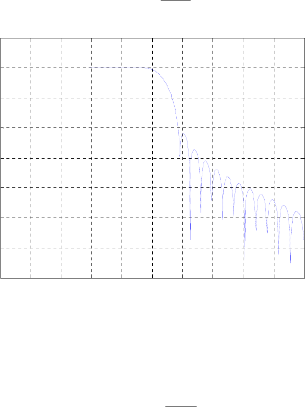
10.15 (a)
π
ω
47.0=
p,
π
ω
59.0=
s,001.0
=
p
δ
, 007.0
=
s
δ
,
π
ω
12.0
=
∆
,
1.43log20 10 =−= ss
δ
α
dB
From Table 10.2, we see that for fixed-window functions, we can achieve the minimum
stopband attenuation by using Hann, Hamming, or Blackman windows. Hann will have
the lowest filter length.
⎡⎤
5312 =+= MN Haan since .917.25
12.0
11.3 == π
π
M
00.1 0.2 0.3 0.4 0.5 0.6 0.7 0.8 0.9 1
-140
-120
-100
-80
-60
-40
-20
0
20
ω
/
π
Magnitude Response
Lowpass filter using Hann window
(b)
π
ω
61.0=
p ,
π
ω
78.0=
s,001.0
=
p
δ
, 002.0
=
s
δ
,
π
ω
17.0
=
∆
,
54log20 10 =−= ss
δ
α
dB
From Table 10.2, we see that for fixed-window functions, we can achieve the minimum
stopband attenuation by using either Hamming, or Blackman windows. Hamming will
have the lowest filter length.
⎡⎤
4112 =+= MN Hamm since 53.19
17.0
32.3 ==
π
π
M.
Not for sale 332
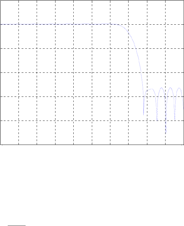
00.1 0.2 0.3 0.4 0.5 0.6 0.7 0.8 0.9 1
-100
-80
-60
-40
-20
0
20
ω
/
π
Magnitude Response
Lowpass filter using Hamming window
10.16
π
ω
45.0
1=
p,
π
ω
65.0
2=
p,
π
ω
3.0
1
=
s,
π
ω
8.0
2
=
s,
π
ω
ω
15.0
21 =
∆
=
∆
,
01.0=
p
δ
,008.0
1=
s
δ
,05.0
2
=
s
δ
42log20 1101 =−= ss
δ
α
dB, 26log20 2102
=
−
=
ss
δ
α
dB
From Table 10.2, we see that the Hann window will have minimum length and meet the
minimum stopband attenuation.
.21
15.0
11.3 == π
π
M Therefore, 43
=
N.
Not for sale 333
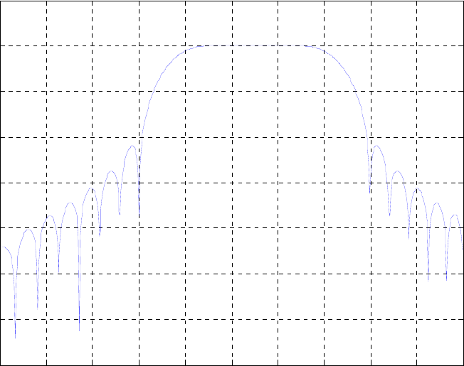
00.1 0.2 0.3 0.4 0.5 0.6 0.7 0.8 0.9 1
-140
-120
-100
-80
-60
-40
-20
0
20
ω/π
Magnitude Response
Bandpass filter using Hann window
10.17
π
ω
3.0
1=
p,
π
ω
8.0
2=
p,
π
ω
45.0
1
=
s,
π
ω
65.0
2
=
s,
π
ω
ω
15.0
21 =
∆
=
∆
,
05.0
1=
p
δ
,009.0
2=
p
δ
,02.0
=
s
δ
,
34log20 10 =−= ss
δ
α
dB
From Table 10.2, we see that the Hann window will have minimum length and meet the
minimum stopband attenuation.
Not for sale 334
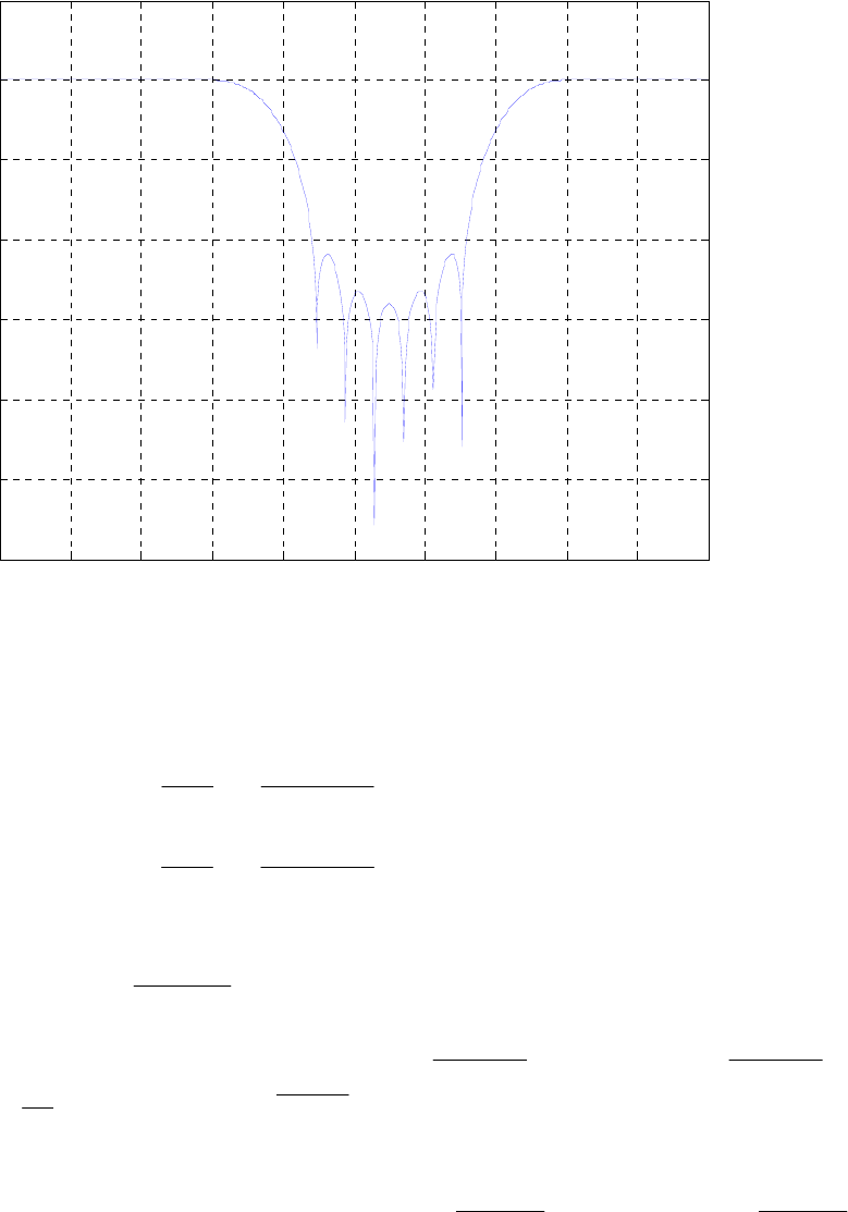
00.1 0.2 0.3 0.4 0.5 0.6 0.7 0.8 0.9 1
-120
-100
-80
-60
-40
-20
0
20
ω/π
Magnitude Response
Bandstop filter using Hann window
10.18 Consider another filter with a frequency response given by )( ωj
eG
⎪
⎪
⎪
⎩
⎪
⎪
⎪
⎨
⎧
−≤≤−
⎟
⎟
⎠
⎞
⎜
⎜
⎝
⎛+
−
≤<
⎟
⎟
⎠
⎞
⎜
⎜
⎝
⎛−
−
≤≤
=
elsewhere.,0
,,
)(
sin
2
,,
)(
sin
2
,0,0
)(
ps
p
sp
p
p
j
eG
ωωω
ω
ωωπ
ω
π
ωωω
ω
ωωπ
ω
π
ωω
ω
∆∆
∆∆
Clearly .
)(
)( ω
ω
ω
d
edH
eG
j
j= Now,
∫
−
=
π
π
ωω ω
πdeeGng njj )(
2
1
][ ⎜
⎜
⎜
⎜
⎜
⎝
⎛
−
−
=∫∫ ⎟
⎟
⎠
⎞
⎜
⎜
⎝
⎛−
−
⎟
⎟
⎠
⎞
⎜
⎜
⎝
⎛−
s
p
s
p
deedee
j
nj
p
j
nj
p
jω
ω
ω
ω
ωωπ
ω
ω
ω
ω
ωωπ
ωω
ωπ
π∆∆
∆
)()(
8
⎟
⎟
⎟
⎟
⎠
⎞
−+ ∫∫
−
−
⎟
⎟
⎠
⎞
⎜
⎜
⎝
⎛+
−
−
−
⎟
⎟
⎠
⎞
⎜
⎜
⎝
⎛+
p
s
p
s
deedee nj
p
j
nj
p
jω
ω
ω
ω
ωωπ
ω
ω
ω
ω
ωωπ
ωω ∆∆
)()(
Not for sale 335

⎜
⎜
⎜
⎜
⎜
⎝
⎛
⎥
⎥
⎥
⎥
⎦
⎤
⎢
⎢
⎢
⎢
⎣
⎡
⎟
⎠
⎞
⎜
⎝
⎛−
−
−
⎥
⎥
⎥
⎥
⎦
⎤
⎢
⎢
⎢
⎢
⎣
⎡
⎟
⎠
⎞
⎜
⎝
⎛+
−−
=
⎟
⎠
⎞
⎜
⎝
⎛−
⎟
⎠
⎞
⎜
⎝
⎛−
−
⎟
⎠
⎞
⎜
⎝
⎛+
⎟
⎠
⎞
⎜
⎝
⎛+
−
ω
π
ω
π
ω
ω
π
ω
ω
π
ω
ω
πω
ω
π
ω
ω
π
ω
ω
πω
∆∆
∆
∆∆
∆
∆∆
∆
nj
ee
e
nj
ee
e
j
njnj
j
njnj
jps
p
ps
p)
8
1
⎟
⎟
⎟
⎟
⎟
⎠
⎞
⎥
⎥
⎥
⎥
⎦
⎤
⎢
⎢
⎢
⎢
⎣
⎡
⎟
⎠
⎞
⎜
⎝
⎛−
−
−
⎥
⎥
⎥
⎥
⎦
⎤
⎢
⎢
⎢
⎢
⎣
⎡
⎟
⎠
⎞
⎜
⎝
⎛+
−
+
⎟
⎠
⎞
⎜
⎝
⎛−−
⎟
⎠
⎞
⎜
⎝
⎛−−
−
⎟
⎠
⎞
⎜
⎝
⎛+−
⎟
⎠
⎞
⎜
⎝
⎛+−
ω
π
ω
π
ω
π
ω
ω
π
ω
ω
πω
ω
π
ω
ω
π
ω
ω
πω
∆∆
∆∆
∆
∆∆
∆
nj
ee
e
nj
ee
e
njnj
j
njnj
jsp
p
sp
p
⎟
⎟
⎟
⎟
⎠
⎞
⎜
⎜
⎜
⎜
⎝
⎛
⎟
⎠
⎞
⎜
⎝
⎛−
−−
−
⎟
⎠
⎞
⎜
⎝
⎛+
−−
−
=
ω
π
ωω
ω
π
ωω
ω
∆∆
∆n
nn
n
nn
j
psps )sin()sin()sin()sin(
4
1
()
⎟
⎟
⎟
⎟
⎟
⎠
⎞
⎜
⎜
⎜
⎜
⎜
⎝
⎛
−
−
+
=
2
2
2
/2
4
)sin()sin(
ω
π
ωπ
ω
ωω
∆
∆
∆
n
j
nn ps
()
.
)/(1
1
)2/cos()sin(
22 ⎟
⎟
⎠
⎞
⎜
⎜
⎝
⎛
−
=
n
j
nn
c
πωπ
ω
ωω
∆
∆
∆
Now, ].[][ ng
n
j
nh = Therefore, .
)sin(
)/(1
)2/cos(
][ 22 ⎟
⎠
⎞
⎜
⎝
⎛
⎟
⎟
⎠
⎞
⎜
⎜
⎝
⎛
−
=n
n
n
n
nh c
π
ω
πω
ω
∆
∆
10.19 ][
12
4
cos
12
2
cos][ nw
M
n
M
n
nw RGC ⎥
⎦
⎤
⎢
⎣
⎡⎟
⎠
⎞
⎜
⎝
⎛
+
+
⎟
⎠
⎞
⎜
⎝
⎛
+
+= π
γ
π
βα
][22 12
4
12
4
12
2
12
2
nweeee R
M
n
j
M
n
j
M
n
j
M
n
j
⎥
⎥
⎥
⎦
⎤
⎢
⎢
⎢
⎣
⎡
⎟
⎟
⎟
⎠
⎞
⎜
⎜
⎜
⎝
⎛
++
⎟
⎟
⎟
⎠
⎞
⎜
⎜
⎜
⎝
⎛
++= ⎟
⎠
⎞
⎜
⎝
⎛
+
−
⎟
⎠
⎞
⎜
⎝
⎛
+
⎟
⎠
⎞
⎜
⎝
⎛
+
−
⎟
⎠
⎞
⎜
⎝
⎛
+
ππππ
γβα
Hence, ⎟
⎟
⎟
⎠
⎞
⎜
⎜
⎜
⎝
⎛
+
⎟
⎟
⎟
⎠
⎞
⎜
⎜
⎜
⎝
⎛
+= ⎟
⎠
⎞
⎜
⎝
⎛
+
+
⎟
⎠
⎞
⎜
⎝
⎛
+
−12
2
12
2
22)()( M
j
R
M
j
R
j
R
j
GC eeee
π
ω
π
ω
ωω ββα ΨΨΨΨ
.22 12
4
12
4
⎟
⎟
⎟
⎠
⎞
⎜
⎜
⎜
⎝
⎛
+
⎟
⎟
⎟
⎠
⎞
⎜
⎜
⎜
⎝
⎛
+⎟
⎠
⎞
⎜
⎝
⎛
+
+
⎟
⎠
⎞
⎜
⎝
⎛
+
−M
j
R
M
j
Ree
π
ω
π
ω
γγ ΨΨ
For the Hann window : = 0.5, = 0.5 and = 0. Hence,
⎟
⎟
⎟
⎠
⎞
⎜
⎜
⎜
⎝
⎛
+
⎟
⎟
⎟
⎠
⎞
⎜
⎜
⎜
⎝
⎛
+= ⎟
⎠
⎞
⎜
⎝
⎛
+
+
⎟
⎠
⎞
⎜
⎝
⎛
+
−12
2
12
2
2)(5.0)( M
j
R
M
j
R
j
R
j
Haan eeee
π
ω
π
ω
ωω βΨΨΨΨ
Not for sale 336

.
122
sin
122
)12(sin
122
sin
122
)12(sin
)2/sin(
2
)12(
sin
5.0
⎟
⎠
⎞
⎜
⎝
⎛
+
+
⎟
⎟
⎠
⎞
⎜
⎜
⎝
⎛⎟
⎠
⎞
⎜
⎝
⎛
+
++
+
⎟
⎠
⎞
⎜
⎝
⎛
+
−
⎟
⎟
⎠
⎞
⎜
⎜
⎝
⎛⎟
⎠
⎞
⎜
⎝
⎛
+
−+
+
⎟
⎠
⎞
⎜
⎝
⎛+
=
M
M
M
M
M
M
M
πω
πω
πω
πω
ω
ω
For the Hamming window, = 0.54, = 0.46, and = 0. Hence,
⎟
⎟
⎟
⎠
⎞
⎜
⎜
⎜
⎝
⎛
+
⎟
⎟
⎟
⎠
⎞
⎜
⎜
⎜
⎝
⎛
+= ⎟
⎠
⎞
⎜
⎝
⎛
+
+
⎟
⎠
⎞
⎜
⎝
⎛
+
−12
2
12
2
min 92.092.0)(54.0)( M
j
R
M
j
R
j
R
j
gHam eeee
π
ω
π
ω
ωω ΨΨΨΨ
.
122
sin
122
)12(sin
92.0
122
sin
122
)12(sin
92.0
)2/sin(
2
)12(
sin
54.0
⎟
⎠
⎞
⎜
⎝
⎛
+
+
⎟
⎟
⎠
⎞
⎜
⎜
⎝
⎛⎟
⎠
⎞
⎜
⎝
⎛
+
++
+
⎟
⎠
⎞
⎜
⎝
⎛
+
−
⎟
⎟
⎠
⎞
⎜
⎜
⎝
⎛⎟
⎠
⎞
⎜
⎝
⎛
+
−+
+
⎟
⎠
⎞
⎜
⎝
⎛+
=
M
M
M
M
M
M
M
πω
πω
πω
πω
ω
ω
F
or the Blackmann window = 0.42, = 0.5 and = 0.08
⎟
⎟
⎟
⎠
⎞
⎜
⎜
⎜
⎝
⎛
+
⎟
⎟
⎟
⎠
⎞
⎜
⎜
⎜
⎝
⎛
+= ⎟
⎠
⎞
⎜
⎝
⎛
+
+
⎟
⎠
⎞
⎜
⎝
⎛
+
−12
2
12
2
)(42.0)( M
j
R
M
j
R
j
R
j
Blackman eeee
π
ω
π
ω
ωω ΨΨΨΨ
⎟
⎟
⎟
⎠
⎞
⎜
⎜
⎜
⎝
⎛
+
⎟
⎟
⎟
⎠
⎞
⎜
⎜
⎜
⎝
⎛
+⎟
⎠
⎞
⎜
⎝
⎛
+
−
⎟
⎠
⎞
⎜
⎝
⎛
+
−12
4
12
4
16.016.0 M
j
R
M
j
Ree
π
ω
π
ω
ΨΨ
⎟
⎠
⎞
⎜
⎝
⎛
+
+
⎟
⎟
⎠
⎞
⎜
⎜
⎝
⎛⎟
⎠
⎞
⎜
⎝
⎛
+
++
+
⎟
⎠
⎞
⎜
⎝
⎛
+
−
⎟
⎟
⎠
⎞
⎜
⎜
⎝
⎛⎟
⎠
⎞
⎜
⎝
⎛
+
−+
+
⎟
⎠
⎞
⎜
⎝
⎛+
=
122
sin
122
)12(sin
122
sin
122
)12(sin
)2/sin(
2
)12(
sin
42.0
M
M
M
M
M
M
M
πω
πω
πω
πω
ω
ω
.
12
2
2
sin
12
2
2
)12(sin
16.0
12
2
2
sin
12
2
2
)12(sin
16.0
⎟
⎠
⎞
⎜
⎝
⎛
+
−
⎟
⎟
⎠
⎞
⎜
⎜
⎝
⎛⎟
⎠
⎞
⎜
⎝
⎛
+
−+
+
⎟
⎠
⎞
⎜
⎝
⎛
+
−
⎟
⎟
⎠
⎞
⎜
⎜
⎝
⎛⎟
⎠
⎞
⎜
⎝
⎛
+
−+
+
M
M
M
M
M
M
πω
πω
πω
πω
10.20 (a)
()
[] [] [] [] [ ]
∑
=
−−−−− ++++=≈= N
n
NnD zNhzhzhhznhzzH
0
21 210 L
We see that if then
() ()
[
,
ˆ
2
1
∑
−=
+=
N
Nk
ka knxtPtx
]
()
∏
≠
−= ⎟
⎟
⎠
⎞
⎜
⎜
⎝
⎛
−
−
=2
1
N
kl
Nl lk
l
ktt
tt
tP for 21 NkN
≤
≤
−.
Not for sale 337

Here, we have and the solution follows if
()
[]
∑
=
−
=
N
n
n
znhzH
0
ˆ
()
[]
nhtPk=, , ,
0
1=N NN =
2nk
=
,Dt
=
,ktl
=
, and ntk
=
Therefore, we have
[]
∏
≠
=−
−
=
N
nk
kkn
kD
nh
0
for Nn
≤
≤
0.
(b) N = 21, D = 90/13, L = 22. , where
()
[]
∑
=
−
≈
21
0n
n
znhzH
[]
∏
≠
=−
−
=
21
0
13/90
nk
kkn
k
nh .
% Problem #10.20
D = 90/13;
N = 21;
for n = 0:N,
for k = 0:N,
if n ~= k,
tmp(n+1,k+1) = (D-k)/(n-k);
else
tmp(n+1,k+1) = 1;
end
end
end
h = prod(tmp');
[Gd,W] = grpdelay(h,1,512);
[H, w] = freqz(h,1,512);
figure(1);
plot(W/pi, Gd);
xlabel('\omega/\pi');
ylabel('Group Delay');
title('Group delay of z^-^D');
grid;
figure(2);
plot(w/pi, (abs(H)));
xlabel('\omega/\pi');
ylabel('Magnitude');
title('Magnitude response of z^-^D');
grid;
Not for sale 338
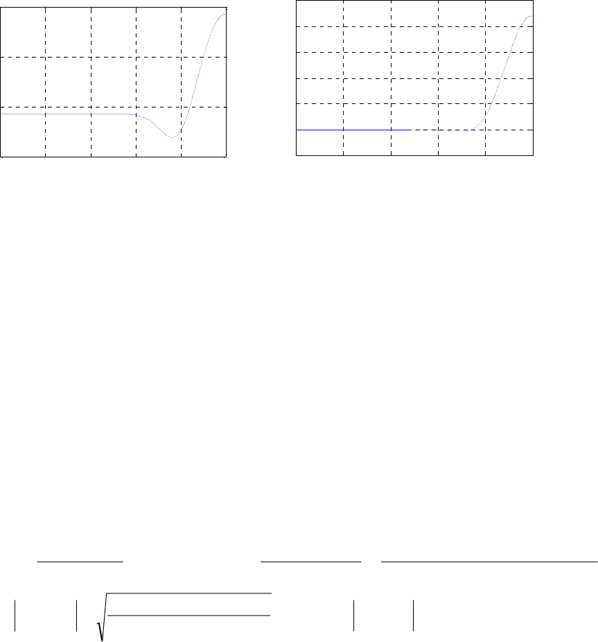
00.2 0.4 0.6 0.8 1
6.5
7
7.5
8
ω
/
π
Group Delay
Group delay of z
-D
00.2 0.4 0.6 0.8 1
0.9
1
1.1
1.2
1.3
1.4
1.5
ω
/
π
Magnitude
Magnitude response of z
-D
10.21 (a) where is the desired signal and
is the harmonic interference with fundamental
frequency . Now,
],[][)sin(][][
0
nrnsnkAnsnx ko
M
k
k+=++= ∑
=
φω ][ns
)sin(][
0
ko
M
k
knkAnr φω += ∑
=
o
ω])(sin[][
0
ko
M
k
kDnkADnr φω +−=− ∑
=
].[)2sin(
0
nrknkA ko
M
k
k=−+= ∑
=
πφω
(b) ][][][][][][][][][][][ n
r
Dnsn
r
nsDn
r
Dnsn
r
nsDn
x
n
x
ny
−
−
−+
=
−
−
−
−
+
=
−−=
Hence, does not contain any harmonic disturbances.
].[][ Dnsns −−= ][ny
(c) .
1
1
)( DD
D
cz
z
zH −−
−
−
−
=
ρ
Thus, ω
ω
ω
ρjDD
jD
j
ce
e
eH −−
−
−
−
=
1
1
)(
()
(
)
.
)sin()cos(1
)sin()cos(1
ωρωρ
ωω
DjD
DjD
DD +−
+
−
=
Then,
(
)
.
)cos(21
)cos(12
)( 2DD
j
cD
D
eH
ρωρ
ω
ω
+−
−
= A plot of )( ωj
ceH for πω 22.0
=
o and
is shown below:
99.0=ρ
Not for sale 339
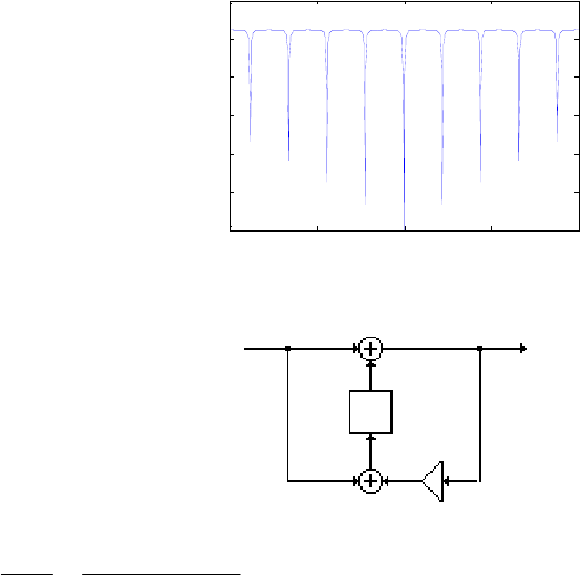
-1 -0.5 00.5 1
0
0.2
0.4
0.6
0.8
1
ω
/
π
Amplitude
(d) x[n]
y
[n]
+
–
z–D
10.22 )(98.01
)(1
)(
)(
)( zN
zN
zQ
zP
zH D
c−
−
== , with ππ 18.0/2
=
D, N = 18, and 98.0=
ρ
.
% Problem #10.23
close all;
clear;
clc;
D = 2/.18;
N = 18;
rho = 0.98;
for n = 0:N,
for k = 0:N,
if n ~= k,
tmp(n+1,k+1) = (D-k)/(n-k);
else
tmp(n+1,k+1) = 1;
end
end
end
h = prod(tmp');
[H,w] = freqz(h,1,1024);
Hc = (1-H)./(1-(rho^D)*H);
x = sqrt((2*(1-cos(D*w)))./(1-
2*(rho^D)*cos(D*w)+rho^(2*D)));
%plot(w/pi, abs(Hc));
plot(w/pi, x); grid;
xlabel('\omega/\pi');
ylabel('Magnitude');
title(‘Comb filter using FIR fractional delay');
Not for sale 340
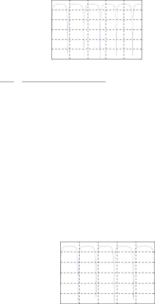
00.2 0.4 0.6 0.8 1
0
0.2
0.4
0.6
0.8
1
ω
/
π
Magnitude
Comb filter using FIR fractional delay
10.23 )(98.0)(
)()(
)(
)(
)( 11113/90
111
−−
−−
−
−
== zDzzD
zDzzD
zQ
zP
zHc, with 11.1118.0/2 =
=
π
π
Dand N = 11.
% Problem #10.23
close all;
clear;
clc;
D = 2/0.18;
rho = 0.98;
N = floor(D);
for k = 1:N,
for n = 0:N,
p(n+1) = (D-N+n)/(D-N+k+n);
end
d(k) = ((-1)^k)*nchoosek(N,k)*prod(p);
end
[H,w] = freqz(fliplr(d)-d, fliplr(d)-(rho^D).*d , 512);
plot(w/pi, abs(H));grid;
xlabel('\omega/\pi');
ylabel('Magnitude');
title(Comb filter using allpass IIR fractional delay');
00.2 0.4 0.6 0.8 1
0
0.2
0.4
0.6
0.8
1
ω
/
π
Magnitude
Comb filter using allpass IIR fractional delay
Not for sale 341

10.24
⎪
⎪
⎪
⎪
⎩
⎪
⎪
⎪
⎪
⎨
⎧
≤<−
⎟
⎟
⎠
⎞
⎜
⎜
⎝
⎛
−
+
+
≤<
⎟
⎟
⎠
⎞
⎜
⎜
⎝
⎛
−
−
−
≤≤−
=
elsewhere.,0
,,1
,,1
,,1
)(
ps
ps
p
sp
ps
p
pp
j
LP eH
ωωω
ωω
ωω
ωωω
ωω
ωω
ωωω
ω
Now, for ,0≠n∫
−
=
π
π
ωω ω
πdeeHnh njj
LPLP )(
2
1
][
⎥
⎥
⎥
⎦
⎤
⎢
⎢
⎢
⎣
⎡
⎟
⎟
⎠
⎞
⎜
⎜
⎝
⎛+
++
⎟
⎟
⎠
⎞
⎜
⎜
⎝
⎛−
−+= ∫∫∫
−
−−
s
p
p
s
p
p
dedede nj
p
nj
p
nj
ω
ω
ω
ω
ωω
ω
ω
ωω
ω
ωω
ω
ω
ωω
ω
π∆∆ 11
2
1
⎥
⎥
⎥
⎦
⎤
⎢
⎢
⎢
⎣
⎡+
+
−
−= ∫∫∫
−
−−
s
p
p
s
s
s
dedede nj
p
nj
p
nj
ω
ω
ω
ω
ωω
ω
ω
ωω
ω
ωω
ω
ω
ωω
ω
π∆∆2
1
⎪
⎪
⎭
⎪
⎪
⎬
⎫
⎪
⎪
⎩
⎪
⎪
⎨
⎧
⎥
⎥
⎦
⎤
⎢
⎢
⎣
⎡+
+
+
⎥
⎥
⎦
⎤
⎢
⎢
⎣
⎡+
−
−=
p
s
s
p
n
e
jn
e
n
e
jn
e
n
nnj
nj
p
nj
nj
p
s
ω
ω
ω
ω
ω
ω
ω
ωωω
ω
ωω
ωπ
ω
π
–
–
22
)(
1
)(
1
)sin(2
2
1
∆∆
⎪
⎭
⎪
⎬
⎫
⎪
⎩
⎪
⎨
⎧
⎥
⎥
⎦
⎤
⎢
⎢
⎣
⎡−
−
−
+
−
+−=
−
−
−
22
1
)sin(2
2
1
n
ee
jn
e
n
ee
jn
e
n
nnj
nj
nj
nj
nj
nj
ss
p
s
p
s
sω
ω
ω
ω
ω
ωωω
ωπ
ω
π
∆∆
∆
⎪
⎭
⎪
⎬
⎫
⎪
⎩
⎪
⎨
⎧
⎥
⎥
⎦
⎤
⎢
⎢
⎣
⎡−
+−= 2
)cos()cos(
)sin(
2
)sin(2
2
1
n
nn
n
n
n
nps
ss ωω
ωω
ωπ
ω
π
∆
∆
⎪
⎭
⎪
⎬
⎫
⎪
⎩
⎪
⎨
⎧−= 22
)cos(
)cos(
1
n
n
n
ns
p
π
ω
π
ω
ω
∆ ⎭
⎬
⎫
⎩
⎨
⎧+
−
−
=22
))2/cos(())2/cos((
1
n
n
n
ncc
π
ωω
π
ωω
ω
∆∆
∆
.
)sin(
)2/sin(2
n
n
n
nc
π
ω
ω
ω
∆
∆
=
Next, for ,0
=
n π
ω
π
π
π
ω
2
1
)(
2
1
]0[ == ∫
−
deHh j
LPLP (area under the curve)
(
)
.
22
1
π
ωc
ps =
π
=2ωω +
Not for sale 342

Hence, ⎪
⎩
⎪
⎨
⎧
≠
=
=
0. if
2sin(
0, if
n
n
n
n
n
n
nh
c
c
LP
,
)sin(
)2/
,
][
π
ω
ω
ω
π
ω
∆
∆
An alternate approach to solving this problem is as follows. Consider the frequency response
⎪
⎪
⎪
⎩
⎪
⎪
⎪
⎨
⎧
−<<−
<<
≤≤−
==
elsewhere.,0
,,
1
,,
1
–
,,0
)(
)(
ps
sp
pp
j
LP
j
d
eHd
eG
ωωω
ω
ωωω
ω
ωωω
ω
ω
ω
∆
∆
Its inverse DTFT is given by
∫
π
π
π
=
–
)(
2
1
][ ω
ωω deeGng njj ω
ω
ω
ω
ω
ω
ω
ω
ω
ω
dede njnj s
p
p
s
∫∫ π
−
π
=∆∆
1
2
11
2
1–
–
⎟
⎟
⎟
⎟
⎠
⎞
⎜
⎜
⎜
⎜
⎝
⎛
−
π
=
−
−jn
nj
e
jn
nj
es
p
p
s
ωω
ω
ω
ω
ω
ω
∆2
1
(
)
)cos()cos(
1nn
nj sp ωω
ω−
π
=∆.
Thus, ][][ ng
n
j
nhLP =
(
)
)cos()cos(
1
2nn
nsp ωω
ω
−
π
=
∆
⎥
⎦
⎤
⎢
⎣
⎡⎟
⎟
⎠
⎞
⎜
⎜
⎝
⎛⎟
⎠
⎞
⎜
⎝
⎛+−
⎟
⎟
⎠
⎞
⎜
⎜
⎝
⎛⎟
⎠
⎞
⎜
⎝
⎛−
π
=nn
nsc 2
cos
2
cos
1
2
ω
ω
ω
ω
ω
∆∆
∆
.0,
)sin(
)2/sin(2 ≠
π
⋅= nfor
n
n
n
nc
ω
ω
ω
∆
∆
For ,0=n.][ π
=c
LP nh ω
10.25 Consider the case when the transition region is approximated by a second order spline. In
this case the ideal frequency response can be constructed by convolving an ideal, no-
transition-band frequency response with a triangular pulse of width ps ωωω
−
=∆,
which in turn can be obtained by convolving two rectangular pulses of width . In
the time domain this implies that the impulse response of a filter with transition band
approximated by a second order spline is given by the product of the impulse response of
an ideal low pass filter with no transition region and square of the impulse response of a
rectangular pulse. Now,
2/ω∆
Not for sale 343
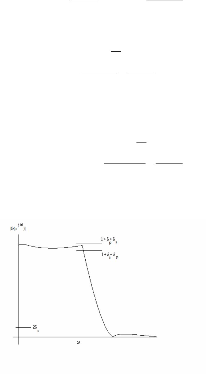
n
n
nH c
idealLP
π
ω)sin(
][
)( = and 4/
)4/sin(
][ n
n
nHrec ω
ω
∆
∆
=. Hence,
.
()
)( ][][][ nHnHnH recidealLPLP =2
Thus for a lowpass filter with a transition region approximated by a second order spline
⎪
⎪
⎩
⎪
⎪
⎨
⎧
⎟
⎠
⎞
⎜
⎝
⎛
=
otherwise.
sin(
0,=n if
,
)sin(
4/
)4/
,
][ 2
n
n
n
n
nh
c
c
LP
π
ω
ω
ω
π
ω
∆
∆
Similarly the frequency response of a lowpass filter with the transition region specified by a
-th order spline can be obtained by convolving in the frequency domain an ideal filter with no
transition region with rectangular pulses of width Hence,
, where the rectangular pulse is of width Thus
P
P./ Pω∆
(
P
recidealLPLP nHnHnH ][][][ )(
=
)
./ Pω∆
⎪
⎪
⎩
⎪
⎪
⎨
⎧
⎟
⎠
⎞
⎜
⎝
⎛
=
otherwise.
sin(
if
,
)sin(
2/
)2/
0,
][
n
n
Pn
Pn
,= n
nh
c
P
c
LP
π
ω
ω
ω
π
ω
∆
∆
10.26 From Step 2, we have .)()()( )( ωωωω ωδω jNjNjNj eFeeGeG F
s−−− +==
(
(
The amplitude response )(ωG
(
has been obtained by raising the amplitude response
)(ωF
(
by and hence, the filter has double zeros in the stopband.
()
F
s
δ
)(zG
Not for sale 344
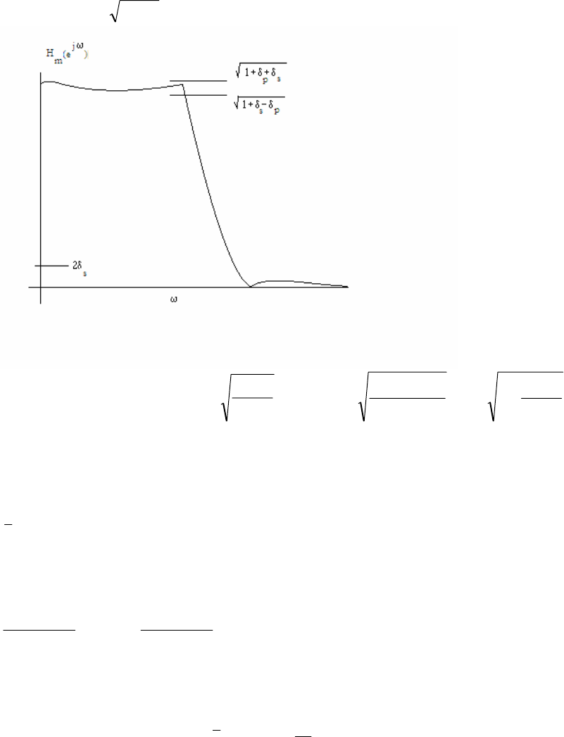
We may factorize as follows: where is a real-coefficient
minimum-phase FIR lowpass filter with half the degree of the original Since,
),()()( 1−−
=zHzHzzG mm
N)(zHm
).(zH ,0)( ≥ωG
(
the amplitude response )(ω
m
H
(
of the minimum-phase filter does not oscillate about
unity in the passband. Since the original frequency response was raised by
)(zHm
()
,
F
s
δ
)(ω
m
H
(
must be
normalized by a factor .1 s
δ
+ Therefore,
For )(ω
m
H
(
, we can see
()
s
s
F
sδ
δ
δ+
=1
2and
()
1
1
11
1
1−
+
+=−
+
++
=
s
p
s
sp
F
pδ
δ
δ
δδ
δ.
10.27 (a) N = 1 and hence, .)( 10 ttxaαα
+
=
Without any loss of generality, for .5
=
Lwe first
fit the data set ,55]},[{
≤
≤
−kkx by the polynomial ttxa10
)( αα +
=
with a minimum
mean-square error at ,5,,1,0,1,,4,5 KK
−
−
−
=t, and then replace with a new value ]0[x
.)0(]0[ 0
α
=
=xx
Now, the mean-square error is given by We set
()
.][),(
5
5
2
1010 ∑
−=
−−=
k
kkx ααααε
0
),(
0
10 =
α
αα
ε
∂
∂
and 0
),(
1
10 =
α
αα
ε
∂
∂
which yields and
∑
=
∑
+
−=−=
5
5
5
5
10 ],[11
kk
kxkαα
∑
=
∑
+
∑−=−=−=
5
5
5
5
2
1
5
5
0].[
kkk
kxkkk αα
From the first equation we get ∑
−=
==
5
5
0].[
11
1
]0[
k
kxx α In the general case we thus
Not for sale 345

have ∑
−=
==
5
5
0][
11
1
][
k
kxnx α which is a moving average filter of length 11.
(b) and hence, Here, we fit the data set
by the polynomial with a minimum mean-square
error at and then replace with a new value
,2=N.)( 2
210 tttxaααα ++= ]},[{ kx
,55 ≤≤− k2
,5,,1,0,1,,4,5 KK −− ]0[x
210
)( tttxaααα ++=
−=t
.)0( 0
α=
a
x]0[ =x
5
The mean-square error is now given by
We set
()
()
.][,,
5
2
2
210210 ∑
−=
−−−=
k
kkkx ααααααε,0
),,(
0
210 =
α
ααα
ε
∂
∂
,0
1
210 =
α
∂
),,( ααα
ε
∂
and ,0
2
210 =
α
∂
),,( ααα
ε
∂
which yields
From the
first and the third equations we then get
∑
−=
=+
5
5
20 ],[11011
k
kxαα ∑
−=
=
5
5
1],[110
k
kxkα∑
−=
=+
5
5
2
20 ].[1958110
k
kxkαα
2
5
5
2
5
5
0)110()111958(
][110][1958
−×
−
=
∑∑ −=−= kk
kxkkx
α
()
].[589
429
15
5
2kxk
k
∑
−=
−=
Hence, here we replace ][n
x
with a new value 0
][ α
=
nx which is a weighted combination of
the original data set :55]},[{
≤
≤
−
kkx
()
][589
429
1
][
5
5
2knxknx
k
−−= ∑
−=
][89]1[84]2[69]3[44]4[9]5[36
429
1(nxnxnxnxnxnx ++++++++++−=
.]5[36]4[9]3[44]2[69]1[84 )−−
−
+
−
+
−
+
−+ nxnxnxnxnx
(c) The impulse response of the FIR filter of Part (a) is given by
{}
,11111111111
11
1
][
1=nh
whereas, the impulse response of the FIR filter of Part (b) is given by
{}
.36944698489846944936
429
1
][
1−−=nh
The corresponding frequency responses are given by
,
11
1
)(
5
5
1∑
−=
−
=
k
kjj eeH ωω and
()
.589
429
1
)(
5
5
2
2∑
−=
−
−=
k
kjj ekeH ωω
Not for sale 346
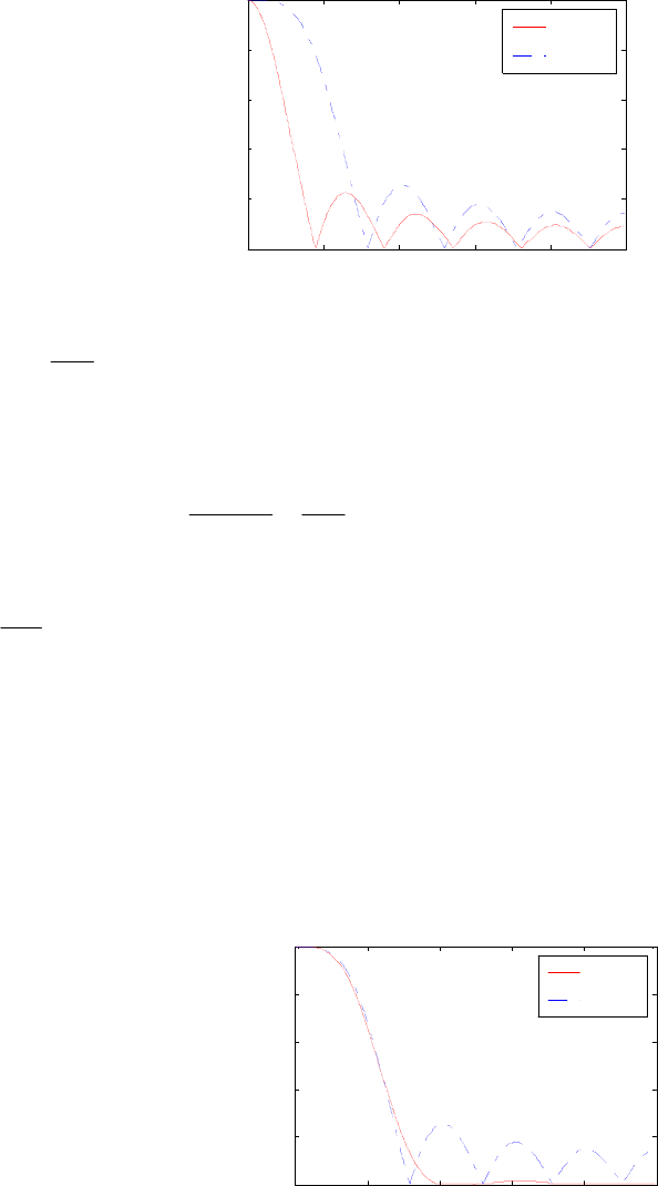
A plot of the magnitude responses of these two filters are shown below from which it can
be seen that the filter of Part (b) has a wider passband and thus provides smoothing over a
larger frequency range than the filter of Part (a).
00.2 0.4 0.6 0.8 1
0
0.2
0.4
0.6
0.8
1
ω
/
π
Magnitude
H
1
(z)
H
2
(z)
10.28 ]2[46]3[21]4[3]5[5]6[6]7[3
320
1
][ {−+−+−+−−−−−−= nxnxnxnxnxnxny
]4[3]3[21]2[46]1[67][74]1[67 ++
+
+
+
+
+
+
+−+ nxnxnxnxnxnx
.]7[3]6[6]5[5 }+−−−++ nxnxnx
Hence,
{
ωωωωω
ω
ω
ω34567
3213563
320
1
)(
)(
)( jjjjj
j
j
jeeeee
eX
eY
eH −−−−− ++−−−==
}
ωωωωωωωωω 7654322 3653214667746746 jjjjjjjjj eeeeeeeee −−−++++++ −− .
{ }
)7cos(3–)6cos(6–)5cos(5–)4cos(3)3cos(21)2cos(46cos6774
160
1ωωωωωωω ++++=
}
.)7cos(3–)6cos(6–)5cos(5– ωωω
The magnitude response of the above FIR filter is plotted below (solid line) along
with that of the FIR filter of Part (b) of Problem 10.27 (dashed line). Note that
both filters have roughly the same passband but the Spencer's filter has very large
attenuation in the stopband and hence it provides better smoothing than the filter of Part
(b).
)(
3zH
)(
2zH
00.2 0.4 0.6 0.8 1
0
0.2
0.4
0.6
0.8
1
ω
/
π
Magnitude
H
3
(z)
H
2
(z)
Not for sale 347

10.29 (a) . Now
.3=L3
3
2
21
)( xxxxP ααα ++= 0)0(
=
P is satisfied by the way has
been defined. Also to ensure
)(xP
1)1(
=
P we require 1
321 =
+
+
ααα . Choose 1
=
m and
Since
.1=n,0
)(
0
=
=x
dx
xdP hence ,032 0
2
321 =++ =x
xx ααα implying 0
1
=
α. Also
since ,0
)(
1
=
=x
dx
xdP hence 032 321
=
+
+
ααα . Thus solving the three equations:
,,and
1
321 =++ ααα 0
1=α032 321
=
+
+
ααα
we arrive at , , and
1 02 33
–
2. Therefore, .23)( 32 xxxP −=
(b) Hence, . Choose and
.4=L4
4
3
3
2
21
)( xxxxxP αααα +++= 2=m1
=
n
(alternatively one can choose 1
=
m2
and
=
n
⇒=
for better stopband performance ). Then,
1)1(P.1
4321
=
+
++ αααα Also,
,04 3
4x
α
320
)(
0
2
321
0
=+++⇒= =
=x
x
xx
dx
xdP ααα
,012620
)(
0
2
432
0
2
2=++⇒= =
=
x
x
xx
dx
xPd ααα
.04320
)(
4321
1
=+++⇒=
=
αααα
x
dx
xdP
Solving the above four simultaneous equations we get and
10, 2 0, 3 4, 4
–
3.
Therefore, .34)( xxxP −= 43
(c) Hence Choose and
.5=L.)( 5
5
4
4
3
3
2
21 xxxxxxP ααααα ++++= 2=m2
=
n.
Following a procedure similar to that in parts (a) and (b) we get
and
1 0, 0, 10,
–15, 6.
2 3
4 5
10.30 From Eq. (7.102) we have Now
∑
=
=
M
k
kkcH
1
).sin(][)( ωω
(
()
∑∑∑ =
+
==
−=−=−=−
M
k
k
M
k
M
k
kkckkkckkcH
1
1
11
).()1]([)cos()(sin][)(sin][)( ωπωωπωπ
(
Thus, )()( ωπω −= HH
(
(
implies or
equivalently, which in turn implies that
∑∑
==
+
−=
M
k
M
k
kkkckkc
11
1),sin()1(][)sin(][ ωω
()
∑
=
+=−−
M
k
kkkc
1
1,0)sin(][)1(1 ω0][
=
kc for
.,6,4,2 K=k
Not for sale 348

But from Eq. (7.103) we have ,1],[2][ MkkMhkc
≤
≤
−
=
or, ].[][ 2
1kMckh −= For k even,
i.e., 0]2[]2[,2 2=−== RMcRhRk 1 if M is even.
10.31 (a) Thus, .10),()(][ /2 −≤≤== MkeHeHkH Mkj
jkπ
ω,][
1
][
1
0
∑
−
=
−
=
M
k
kn
M
WkH
M
nh
where
.
/2 Mkj
MeW π−
=
Now, .][
1
][
1
][)(
1
0
1
0
1
0
1
0
1
0∑∑∑∑∑−
=
−
=
−−
−
=
−
−
=
−
−
=
−⎟
⎟
⎠
⎞
⎜
⎜
⎝
⎛
===
M
k
M
n
nkn
M
M
n
n
M
k
kn
M
M
n
nzWkH
M
zWkH
M
znhzH
We can write
∑∑∑ ∞
=
−−
∞
=
−−
−
=
−− −=
Mn
nkn
M
n
nkn
M
M
n
nkn
MzWzWzW
0
1
0
()
.
1
1
11
000 −−
−
∞
=
−−−
∞
=
−−−−
∞
=
−−
−
−
=−=−= ∑∑∑ zW
z
zWzzWzWzW k
M
M
n
nkn
M
M
n
nkn
M
MkM
M
n
nkn
M
Therefore, .
1
][1
)(
1
01
∑
−
=−−
−
−
−
=
M
kk
M
M
zW
kH
M
z
zH
(b) H[0]
M
H[1]
M
H[M 1]
M
x[n] y[n]
1
1 z 1
1
1 z 1ej2 /M
1
1 z 1ej2 (M 1)/ M
1 z M
(c) Note .][
1
1
][1
)(
1
0
1
0
1
01∑∑∑−
=
−
=
−−
−
=−−
−
⎟
⎟
⎠
⎞
⎜
⎜
⎝
⎛
=
−
−
=
M
k
M
n
nkn
M
M
kk
M
M
zWkH
M
zW
kH
M
z
zH
Not for sale 349

On the unit circle the above reduces to .][
1
)(
1
0
1
0
∑∑
−
=
−
=
−− ⎟
⎟
⎠
⎞
⎜
⎜
⎝
⎛
=
M
k
M
n
njkn
M
jeWkH
M
eH ωω For
we then get from the above
,/2 Mj lπω =∑∑
= =
−− ⎟
⎟
⎠
⎞
⎜
⎜
⎝
⎛
=
0 0
/2/2 1
][)(
k n
Mnkn
M
Mj eW
M
kHeH ll ππ
− −1 1M M
∑∑
= =
−⎟
⎟
⎠
⎞
⎜
⎜
⎝
⎛
=
0 0
1
][
k n
n
M
kn
MWW
M
kH l
− −1 1M M
.
1
][
0 0
)(
∑∑
= =
−−
⎟
⎟
⎠
⎞
⎜
⎜
⎝
⎛
=
k n
nk
M
W
M
kH l
1 1− −M M
Using the identity of Eq.
(5.23) of text we observe that ⎩
⎨
⎧=
=
∑
=
−−
otherwise.,0
,if,1
1
0
)( k
W
Mn
nk
M
l
l
−1M
Hence,
].[)( /2 l
lHeH Mj =
π
10.32 (a) For Type 1 FIR filter, .)()( 2
)1(
ω
ω
ωj
M
j
jeHeeH
−
−
= Since in the frequency
sampling approach we sample the DTFT at
)( ωj
eH
M
points given by ,
2
M
kπ
ω=
therefore ,10 −≤≤ Mk ,)()(][ /)1(2/2/2 MMkjMkj
d
Mkj eeHeHkH −
== πππ
Since the filter is of Type 1,
.10 −≤≤ Mk 1
−
M is even, thus, .
Moreover, being real, Thus,
.1
2/)1(2 =
−Mkj
eπ
][nh ).(*)( ωω jj eHeH =,)()( 2/)1( ωωω jMjj eHeeH −
=
Hence,
.2πωπ <≤
⎪
⎩
⎪
⎨
⎧=
=
−
++
=
−−−
−
−−
.1,,
2
3
2
1
2/)1)((2/2
,
2
1
2/)1(2/2
,)(
,,2,1,0,)(
][
M
MM
k
MMkMjMkj
d
M
MMkjMkj
d
eeH
keeH
kH
K
K
ππ
ππ
(b) For the Type 2 FIR filter
⎪
⎪
⎩
⎪
⎪
⎨
⎧
−+=
=
=
=
−−−
−
−−
.1,,1,)(
,,0
,,2,1,0,)(
][
2
2/)1)((2/2
2
,
2
1
2/)1(2/2
MkeeH
k
keeH
kH
M
MMkMjMkj
d
M
M
MMkjMkj
d
K
K
ππ
ππ
10.33 (a) The frequency spacing between 2 consecutive DFT samples
is given by
.72788.155.0 == πωp
.3307.0
19
2=
π The desired passband edge is between the frequency samples at
19
5
2πω =and .
19
6
2πω = Therefore, the 19-point DFT is given by
Not for sale 350
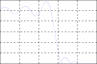
⎩
⎨
⎧
=
=
=−
.12,,6,0
,18,,14,13,5,,1,0,
][ 9)19/2(
K
KK
k
ke
kH
kj π
A 19-point IDFT of the above DFT samples yields the impulse response coefficients
given below in ascending powers of :
1−
z
Columns 1 through 10
-0.0037 -0.0022 0.0224 -0.0211 -0.0231 0.0674
-0.0316 -0.1128 0.2888 0.6316
Columns 11 through 19
0.2888 -0.1128 -0.0316 0.0674 -0.0231 -0.0211
0.0224 -0.0022 -0.0037
(b)
00.2 0.4 0.6 0.8 1
0
0.2
0.4
0.6
0.8
1
ω
/
π
Magnitude
% Problem #10.33
close all;
clear;
clc;
ind = 1;
for k = 0:5,
H(ind) = exp(-i*2*pi*9*k/19);
ind = ind + 1;
end
for k = 6:12,
H(ind) = 0;
ind = ind + 1;
end
for k = 13:18,
H(ind) = exp(-i*2*pi*9*k/19);
ind = ind + 1;
end
h = ifft(H);
figure(1);
stem(real(h));
[FF, w] = freqz(h, 1, 512);
Not for sale 351

figure(2);
plot(w/pi, abs(FF)); axis([0 1 0 1.2]);grid;
ylabel('Gain, in dB'); xlabel('\omega/\pi');
10.34 (a) The frequency spacing between 2 consecutiveDFT samples
is given by
.09956.135.0 == πωp
.1611.0
39
2=
π The desired passband edge is between the frequency samples
at 39
6
2πω =and 39
7
2πω =. Therefore, the 39-point DFT is given by
⎩
⎨
⎧
=
=
=−
.31,,7,0
,38,,33,32,6,,1,0,
][ 19)39/2(
K
KK
k
ke
kH
kj π
A 39-point IDFT of the above DFT samples yields the impulse response coefficients
given below in ascending powers of :
1−
z
Columns 1 through 10
0.0006 0.0031 0.0017 -0.0054 -0.0091 -0.0010
0.0128 0.0146 -0.0034 -0.0237
Columns 11 through 20
-0.0192 0.0134 0.0405 0.0227 -0.0362 -0.0753
-0.0249 0.1222 0.2870 0.3590
Columns 21 through 30
0.2870 0.1222 -0.0249 -0.0753 -0.0362 0.0227
0.0405 0.0134 -0.0192 -0.0237
Columns 31 through 39
-0.0034 0.0146 0.0128 -0.0010 -0.0091 -0.0054
0.0017 0.0031 0.0006
(b)
00.2 0.4 0.6 0.8 1
0
0.2
0.4
0.6
0.8
1
ω
/
π
Magnitude
% Problem #10.34
close all;
clear;
clc;
ind = 1;
for k = 0:6,
Not for sale 352

H(ind) = exp(-i*2*pi*19*k/39);
ind = ind + 1;
end
for k = 7:31,
H(ind) = 0;
ind = ind + 1;
end
for k = 32:38,
H(ind) = exp(-i*2*pi*19*k/39);
ind = ind + 1;
end
h = ifft(H);
figure(1);
stem(real(h));
[FF, w] = freqz(h, 1, 512);
figure(2);
plot(w/pi, abs(FF)); axis([0 1 0 1.2]); grid;
xlabel('\omega/\pi'); ylabel('Gain, dB');
10.35 By expressing where Tn(x) is the -th order Chebyshev
polynomial in
),(cos)cos( ωω n
Tn =)(xTnn
,
x
we first rewrite Eq. (10.48) in the form:
.)(cos)cos(][)(
00 ∑∑ ==
==
M
n
n
n
M
n
nnaH ωαωω
(
Therefore, we can rewrite Eq. (10.70) repeated below for convenience
[]
,21,)1()()()( +≤≤−=− MiDHP i
iii εωωω
in a matrix form as
.
)(
)(
)(
)(
)(/)1()(cos)cos(1
)(/)1()(cos)cos(1
)(/1)(cos)cos(1
)(/1)(cos)cos(1
2
1
2
1
1
0
2
1
22
111
222
111
⎥
⎥
⎥
⎥
⎥
⎥
⎦
⎤
⎢
⎢
⎢
⎢
⎢
⎢
⎣
⎡
=
⎥
⎥
⎥
⎥
⎥
⎥
⎦
⎤
⎢
⎢
⎢
⎢
⎢
⎢
⎣
⎡
⎥
⎥
⎥
⎥
⎥
⎥
⎦
⎤
⎢
⎢
⎢
⎢
⎢
⎢
⎣
⎡
−
−
−
+
+
+
+
++
+++
M
M
M
M
M
M
M
M
M
M
M
M
M
M
M
D
D
D
D
P
P
P
P
ω
ω
ω
ω
ε
α
α
α
ωωω
ωωω
ωωω
ωωω
M
L
L
MMOMM
L
L
Note that the coefficients are different from the coefficients of Eq. (10.70). To
determine the expression of we use Cramer's rule arriving at
}{ i
α]}[{ ia
, where
,
)(/)1()(cos)cos(1
)(/)1()(cos)cos(1
)(/1)(cos)cos(1
)(/1)(cos)cos(1
det
2
1
22
111
222
111
+
+
++
+++
−
−
−
=
M
M
M
M
M
M
M
M
M
M
M
M
P
P
P
P
ωωω
ωωω
ωωω
ωωω
L
L
MMOMM
L
L
∆ and
Not for sale 353

.
)()(cos)cos(1
)()(cos)cos(1
)()(cos)cos(1
)()(cos)cos(1
222
111
222
111
+++
+++
=
MM
M
M
MM
M
M
M
M
D
D
D
D
ωωω
ωωω
ωωω
ωωω
ε
L
L
MMOMM
L
L
∆.
Expanding both determinants using the last column we get and
)( 1
2
1
+
+
=
∑
=i
M
i
iDb ω
ε
∆
,
)(
)1( 1
2
1i
i
M
i
iP
bω
−
+
=
−
=∑
∆ where
.
)(cos)(cos)cos(1
)(cos)(cos)cos(1
)(cos)(cos)cos(1
)(cos)(cos)cos(1
)(cos)(cos)cos(1
det
22
2
2
11
2
1
11
2
1
22
2
2
11
2
1
+++
+++
−−−
=
M
M
MM
i
M
ii
i
M
ii
M
M
i
b
ωωω
ωωω
ωωω
ωωω
ωωω
L
MOMMM
L
L
MOMMM
L
L
The above matrix is seen to be a Vandermonde matrix and is determinant is given by
Define
).cos(cos
,
,
l
l
ll
ωω −= ∏
≠>≠
ik
kk
ki
b.
2
1
∏
+
≠
=
=M
ir
r
r
i
i
b
b
c It can be shown by induction that
.
coscos
1
1
∏
≠
=−
=
in
nni
i
cωω
2+M
Therefore,
)(
)1(
)(
2
1
1
i
i
M
i
i
i
ii
P
b
Db
ω
ω
ε−
=
∑
∑
+
=
=
2
M+
.
)(
)1(
)()(
)()()(
2
1
2
2
2
1
1
222211
+
+
+
++
−
++−
+++
=
M
M
M
MM
P
c
P
c
P
c
DcDcDc
ωωω
ωωω
L
L
10.36
()
⎪
⎩
⎪
⎨
⎧
∈
∈
=stopband.
passband,1
ω
δ
δ
ω
ω
s
p
W
()
⎩
⎨
⎧
≤≤
≤≤
=.55.05.4
,45.001
πωπ
πω
ωW
Not for sale 354

10.37
()
⎪
⎩
⎪
⎨
⎧
∈
∈
=stopband.
passband,1
ω
δ
δ
ω
ω
s
p
W
()
⎩
⎨
⎧
≤≤
≤≤
=.7.04.3
,55.001
πωπ
πω
ωW
10.38
()
⎪
⎩
⎪
⎨
⎧
≤≤
≤≤
≤≤
=
⎪
⎪
⎪
⎩
⎪
⎪
⎪
⎨
⎧
≤≤
≤≤
≤≤
=
.82.05
,7.055.01
,44.0043.1
,
,1
,0
2
2
21
1
1
πωπ
πωπ
πω
πωω
δ
δ
ωωω
ωω
δ
δ
ω
s
s
p
pp
s
s
p
W
10.39 It follows from Eq. (10.22) that the impulse response of an ideal Hilbert transformer is an
antisymmetric sequence. If we truncate it to a finite number of terms between MnM
≤
≤
−
the impulse response is of length )12(
+
M which is odd. Hence the FIR Hilbert transformer
obtained by truncation and satisfying Eq. (10.90) cannot be satisfied by a Type 4 FIR filter.
10.40 (a) Thus, .][)(
1
0
∑
−
=
−
=
N
n
n
znxzX
,
)(
)(
1
][)()(
1
01
1
11
1
1zD
zP
z
z
nxzXzX
N
n
z
z
z(
(
(
(
(
(
(=
⎟
⎟
⎠
⎞
⎜
⎜
⎝
⎛
−
+−
== ∑
−
=−
−
−
+−
=−
−
−α
α
α
α where
,)()1]([][)( 111
1
0
1nnN
N
n
zznxznpzP −−−−
−
=
−+−−== ∑∑ (((( αα and
.)1(][)( 11
1
0
−−
−
=
−−== ∑N
N
n
nzzndzD ((( α
(b) ,
][
][
)(
)(
)(][ /2
/2 kD
kP
zD
zP
zXkX Nkj
ez
Nkj
ez (
(
(
(
(
(
(
(===
=
=π
πwhere Nkj
ez
zPkP /2
)(][ π
=
=(
(
(
is
the -point DFT of the sequence
N][n
p
and Nkj
ez
zDkD /2
)(][ π
=
=(
(
(
is the -point DFT
of the sequence
N
].[nd
(c) Let and
[]
T
Nppp ]1[]1[]0[ −= LP
[
]
.]1[]1[]0[ T
Nxxx −= LX Without
any loss of generality, assume 4
=
N in which case
∑
=
−
=
0
][)(
n
n
znpzP (( 3
(
)
]3[]2[]1[]0[ xxxx ααα −+−= 32
(
)
1222 ]3[3]2[)2(]1[)21(]0[3
−
++−++−+ zxxxx
(
ααααα
(
)
2222 ]3[3]2[)21(]1[)2(]0[3
−
−+++−+ zxxxx
(
ααααα
Not for sale 355
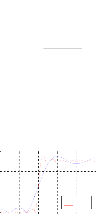
(
)
.]3[]2[]1[]0[ 323
−
+−+−+ zxxxx
(
αααα Equating like powers of 1−
z
(
we can write
where
,XQP ⋅=
[]
,]3[]2[]1[]0[ T
pppp=P
[
]
T
xxxx ]3[]2[]1[]0[=Xand
.
1
321)2(3
3)2(213
1
223
222
222
⎥
⎥
⎥
⎥
⎥
⎦
⎤
⎢
⎢
⎢
⎢
⎢
⎣
⎡
−−
−++−
+−+−
−−
=
ααα
ααααα
ααααα
ααα
Q
32
It can be seen that the elements ,3,0,
,
≤
≤
srq sr q, of the 4 matrix Q can be
determined as follows:
r,s 4
(i) The first row is given by
,)(
,0 s
s
qα−=
(ii) The first column is given by ,)(
)!3(!
!3
)(
3
0, rr
rr rr
Cq αα −
−
=−= and
(iii) the remaining elements can be obtained using the recurrence relation
.
,11,1,1, srsrsrsr qqqq −−−−
+
−= αα
In the general case, we only change the computation of the elements of the first column
using the relation .)(
)!1(!
)!1(
)(
1
0, rr
r
N
rrNr
N
Cq αα −
−−
−
=−= −
M10.1 The impulse response coefficients of the truncated FIR highpass filter with cutoff
frequency at can be generated using the following MATLAB statements:
π4.0
n = -M:M;
num = -0.4*sinc(0.4*n);
num(M+1) = 0.6;
The magnitude responses of the truncated FIR highpass filter for two values of M are
shown below:
00.2 0.4 0.6 0.8 1
0
0.2
0.4
0.6
0.8
1
ω
/
π
Magnitude
M=5
M=20
Not for sale 356
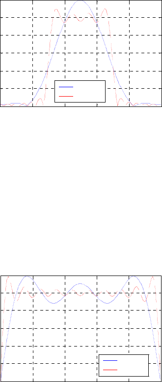
M10.2 The impulse response coefficients of the truncated FIR bandpass filter with cutoff
frequencies at 0.7π and 0.3π can be generated using the following MATLAB statements:
n = -M:M;
num = 0.7*sinc(0.7*n) - 0.3*sinc(0.3*n);
The magnitude responses of the truncated FIR bandpass filter for two values of M are shown
below:
00.2 0.4 0.6 0.8 1
0
0.2
0.4
0.6
0.8
1
ω
/
π
Magnitude
M=5
M=20
M10.3 The impulse response coefficients of the truncated Hilbert transformer can be generated
using the following MATLAB statements:
n = 1:M;
c = 2*sin(pi*n/2).*sin(pi*n/2);b = c./(pi*n);
num = [-fliplr(b) 0 b];
The magnitude responses of the truncated Hilbert transformer for two values of M are
shown below:
00.2 0.4 0.6 0.8 1
0
0.2
0.4
0.6
0.8
1
ω
/
π
Magnitude
M=5
M=20
M10.4
% Problem #M10.4
% Cascade of 2 boxcar filters of length 4
K = 2;N = 4;b = firgauss(K,N);
figure(1);
stem(b);xlabel(‘n’);ylabel(‘h[n]’);
title('Cascade of 2 boxcar filters of length 4');
Not for sale 357
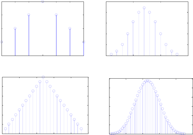
% Cascade of 4 boxcar filters of length 4
K = 4;N = 4;b = firgauss(K,N);
figure(2);
stem(b);xlabel(‘n’);ylabel(‘h[n]’);
title('Cascade of 4 boxcar filters of length 4');
% Cascade of 2 boxcar filters of length 12
K = 2;N = 12;b = firgauss(K,N);
figure(3);
stem(b);xlabel(‘n’);ylabel(‘h[n]’);
title('Cascade of 2 boxcar filters of length 12');
% Cascade of 4 boxcar filters of length 12
K = 4;N = 12;b = firgauss(K,N);
figure(4);
stem(b);xlabel(‘n’);ylabel(‘h[n]’);
title('Cascade of 4 boxcar filters of length 12');
1 2 3 4 5 6 7
0
1
2
3
4
n
h[n]
Cascade of 2 boxcar filters of length 4
0 5 10 15
0
10
20
30
40
50
n
h[n]
Cascade of 4 boxcar filters of length 4
0 5 10 15 20 25
0
2
4
6
8
10
12
n
h[n]
Cascade of 2 boxcar filters of length 12
010 20 30 40 50
0
200
400
600
800
1000
1200
n
h[n]
Cascade of 4 boxcar filters of length 12
We can see that by increasing either K or N, the approximation to a Gaussian function
gets better. It is noted that increasing the number of boxcar filters K to a number greater
than 3 greatly affects the Gaussian shape of the impulse response.
M10.5 % Problem #M10.05
N = 36;fc = 0.2*pi;
M = N/2;
n = -M:1:M;t = fc*n;
lp = fc*sinc(t);
Not for sale 358
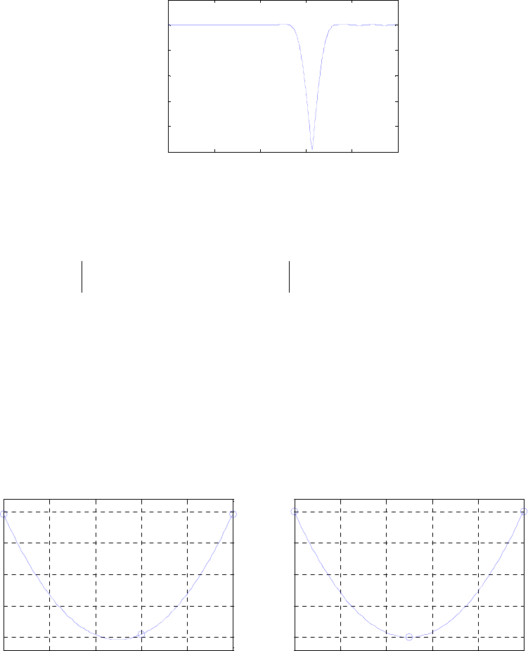
b = 2*[lp(1:M) (lp(M+1) - 0.5) lp((M+2):N+1)];
bw = b.*hamming(N+1)';
[h2, w] = freqz(bw, 1, 512);
plot(w/pi, abs(h2));axis([0 1 0 1.2]);
xlabel('\omega/\pi');ylabel('Magnitude');
title(['\omega_c = ', num2str(fc), ', N = ', num2str(N)]);
00.2 0.4 0.6 0.8 1
0
0.2
0.4
0.6
0.8
1
ω
/
π
Magnitude
ω
c
= 0.62832, N = 36
M10.6 Its approximation over the range ....)( 5505423 2−+= xxxD 23 ≤≤
−
x is given by
We want to minimize the peak value of the absolute error, i.e.,
minimize
.)( xaaxA 10 +=
....max xaaxx
x10
2
23 5505423 −−−+
≤≤− Since there are 3 unknowns,
and we need 3 extremal points on , which we arbitrarily choose as
,,10 aa
,εx,3
1
−
=x,0
2
=
x
and We then solve the 3 linear equations:
This leads to whose solution yields
.2
3=x.,,),()( 3211
10 ==ε−−+ l
l
lxDxaa
,
.
.
.
⎥
⎥
⎦
⎤
⎢
⎢
⎣
⎡−=
⎥
⎥
⎦
⎤
⎢
⎢
⎣
⎡
ε
⎥
⎥
⎦
⎤
⎢
⎢
⎣
⎡−
−
415 55
1511
121 101 131
1
0
a
a
,.,. 85014 10
=
=aa
and A plot of the corresponding error is shown
below in Figure (c).
..69=ε 692323 2
1...)( −+= xxxE
-3 -2 -1 0 1 2
-10
-5
0
5
10
x
Error
Result of first guess
-3 -2 -1 0 1 2
-10
-5
0
5
10
x
Error
Result of second guess
(c) (d)
Not for sale 359
After looking at , we move the second extremal point to the location where
)(x
1
E2
x
is a minimum. The next extrtemal points are therefore given by
)(x
1
E,3
1
−
=x
and The new values of the unknowns are obtained by solving
,.50
2−=x.2
3=x
,
which yields
.
.
.
.⎥
⎥
⎦
⎤
⎢
⎢
⎣
⎡−=
⎥
⎥
⎦
⎤
⎢
⎢
⎣
⎡
ε
⎥
⎥
⎦
⎤
⎢
⎢
⎣
⎡−−
−
4157256 1511
121 1501 131
1
0
a
a
,.,. 85073 10
=
=
aa and A plot
of the corresponding error is shown on the previous page in
Figure (d).
.10=ε
292323 2
2...)( −+= xxxE
% Problem #M10.06
x = [-3 0 2];
d = 3.2.*x.^2 + 4.05.*x-5.5;
D = d';
A = [1 -3 1;1 0 -1;1 2 1];
C = inv(A)*D;
y = -3:0.05:2;
E = 3.2.*y.^2 + 4.05.*y - 5.5 - C(1) - C(2).*y;
% Results of first guess
figure(1);
plot(y,E);
axis([-3 2 -12 12]);
xlabel('x');
ylabel('Error');
title('Result of first guess');
hold on;
plot([-3 -3], [E(1) E(1)], 'o');
plot([2 2], [E(end) E(end)], 'o');
plot([0 0], [E(61) E(61)], 'o');
hold off;
x = [-3 -0.5 2];
d = 3.2.*x.^2 + 4.05.*x-5.5;
D = d';
A = [1 -3 1;1 -0.5 -1;1 2 1];
C = inv(A)*D;
y = -3:0.05:2;
E = 3.2.*y.^2 + 4.05.*y - 5.5 - C(1) - C(2).*y;
% Results of second guess
figure(2);
plot(y,E);
axis([-3 2 -12 12]);
xlabel('x');
ylabel('Error');
Not for sale 360
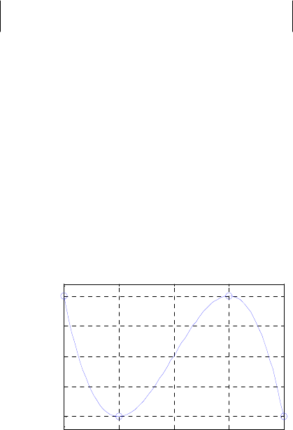
title('Result of second guess');
hold on;
plot([-3 -3], [E(1) E(1)], 'o');
plot([2 2], [E(end) E(end)], 'o');
plot([-0.5 -0.5], [E(51) E(51)], 'o');
hold off;
M10.7 . Its approximation over the range is given by
We want to minimize the peak value of the absolute error, i.e.,
minimize
()
558205 23 .. ++−−= xxxxD 22 ≤≤− x
.)( 2
210 xaxaaxA ++=
...max 2
210
23
22 558205 xaxaaxxx
x
−−−++−−
≤≤− Since there are 4
unknowns, and
,,, 210 aaa ,
ε
we need 4 extremal points on , which we arbitrarily
choose as
x
,2
1−=x,1
2−=x,1
3
=
x and .2
4
=
x We then solve the 4 linear equations:
This leads to
whose solution yields
.,,,),()( 43211
2
210 ==ε−−++ l
l
lxDxaxaa
,
.
.
.
.
⎥
⎥
⎥
⎦
⎤
⎢
⎢
⎢
⎣
⎡
−
=
⎥
⎥
⎥
⎦
⎤
⎢
⎢
⎢
⎣
⎡
ε
⎥
⎥
⎥
⎦
⎤
⎢
⎢
⎢
⎣
⎡
−
−−
−
319
38 32 728
1421 1111 1111 1421
2
1
0
a
a
a
,.,,. 20755 210
−
=
−=
=
aaa
and A plot of the corresponding error is shown below in
Figure (e). We observe that these values maximize the error (
ε
= 10).
.10=ε xxx 155 3
1+−=)(E
-2 -1 0 1 2
-10
-5
0
5
10
x
Error
Result of first guess
% Problem #M10.07
x = [-2 -1 1 2];
d = -5.*x.^3 - 0.2.*x.^2 + 8.*x + 5.5;
D = d';
A = [1 -2 4 1;1 -1 1 -1;1 1 1 1;1 2 4 -1];
C = inv(A)*D;
y = -2:0.05:2;
E = -5.*y.^3 - 0.2.*y.^2 + 8.*y + 5.5 - C(1) - C(2).*y -
C(3).*y.^2;
% Results of first guess
figure(1);
Not for sale 361

plot(y,E);
axis([-2 2 -12 12]);
xlabel('x');
ylabel('Error');
title('Result of first guess');
hold on;
plot([-2 -2], [E(1) E(1)], 'o');
plot([2 2], [E(end) E(end)], 'o');
plot([-1 -1], [E(21) E(21)], 'o');
plot([1 1], [E(1) E(1)], 'o');
hold off;
M10.8 18
8π
=ω p,18
12π
=ωs,18
10
π
=ωT
% Problem #M10.8
wp = 4*(2*pi)/18;
ws = 6*(2*pi)/18;
wc = (wp + ws)/2;
dw = ws - wp;
% Hamming
M = ceil(3.32*pi/dw);N = 2*M+1;n = -M:M;
num = (6/18)*sinc(6*n/18);
wh = hamming(N)';b = num.*wh;
figure(1);
k=0:2*M:stem(k,b);
title('Impulse Response Coefficients');
xlabel('Time index n'); ylabel('Amplitude');
figure(2);
[h, w] = freqz(b,1,512);
plot(w/pi, 20*log10(abs(h))); grid;
xlabel('\omega/\pi'); ylabel('Gain, in dB');
title('Lowpass filter designed using Hamming window');
axis([0 1 -80 10]);
% Hann
M = ceil(3.11*pi/dw);N = 2*M+1;n = -M:M;
num = (6/18)*sinc(6*n/18);
wh = hann(N)';b = num.*wh;
figure(3);
k=0:2*M:stem(k,b);
title('Impulse Response Coefficients');
xlabel('Time index n'); ylabel('Amplitude');
figure(4);
[h, w] = freqz(b,1,512);
plot(w/pi, 20*log10(abs(h)));grid;
xlabel('\omega/\pi');ylabel('Gain, in dB');
Not for sale 362
title('Lowpass filter designed using Hann window');
axis([0 1 -80 10]);
% Blackman
M = ceil(5.56*pi/dw);N = 2*M+1;n = -M:M;
num = (6/18)*sinc(6*n/18);
wh = blackman(N)';b = num.*wh;
figure(5);
k=0:2*M:stem(k,b);
title('Impulse Response Coefficients');
xlabel('Time index n'); ylabel('Amplitude');
figure(6);
[h, w] = freqz(b,1,512);
plot(w/pi, 20*log10(abs(h)));grid;
xlabel('\omega/\pi');ylabel('Gain, in dB');
title('Lowpass filter designed using Blackman window');
axis([0 1 -80 10]);
Lowpass filter design using Hamming window: N = 31
0 5 10 15 20 25 30
-0.1
0
0.1
0.2
0.3
0.4
Impulse Response Coefficients
Time index n
A
mp
lit
u
d
e
00.2 0.4 0.6 0.8 1
-80
-60
-40
-20
0
ω
/
π
Gain, in dB
Lowpass filter designed using Hamming window
Lowpass filter design using Hann window: N = 29
0 5 10 15 20 25
-0.1
0
0.1
0.2
0.3
0.4
Impulse Response Coefficients
Time index n
M
agn
it
u
d
e
00.2 0.4 0.6 0.8 1
-80
-60
-40
-20
0
ω
/
π
Gain, in dB
Lowpass filter designed using Hann window
Lowpass filter design using Blackman window: N = 53
Not for sale 363
010 20 30 40 50
-0.1
0
0.1
0.2
0.3
Impulse Response Coefficients
Time index n
M
agn
it
u
d
e
00.2 0.4 0.6 0.8 1
-80
-60
-40
-20
0
ω
/
π
Gain, in dB
Lowpass filter designed using Blackman window
Comments: The Hann window method results in using the lowest filter order. All filters
meet the requirements of the specifications.
M10.9 ,42=
s
α
()
(
)
631.3214207886.021425842.0 4.0 =−+−=βusing Eq. (10.41).
⎟
⎠
⎞
⎜
⎝
⎛
−
=
18
2
285.2
842
π
Nusing Eq. (10.42).
N = 42.627 43 and we choose 44 since N must be even. M = 22. ≥
% Problem #M10.9
beta = 3.631;N = 44;n = -N/2:N/2;
num = (6/18)*sinc(6*n/18);
wh = kaiser(N+1,beta)';b = num.*wh;
figure(1);
stem(b);
title('Impulse Response Coefficients');
xlabel('Time index n');ylabel('Amplitude')
figure(2);
[h, w] = freqz(b,1,512);
plot(w/pi, 20*log10(abs(h)));grid;
xlabel('\omega/\pi');ylabel('Gain, in dB');
title('Lowpass filter designed using Kaiser window');
axis([0 1 -80 10]);
010 20 30 40
-0.1
0
0.1
0.2
0.3
0.4
Impulse Response Coefficients
Time index n
A
mp
lit
u
d
e
00.2 0.4 0.6 0.8 1
-80
-60
-40
-20
0
ω
/
π
Gain, in dB
Lowpass filter designed using Kaiser window
Not for sale 364
M10.10 ,
πω 4.0=
p
π
ω
6.0=
s,42
=
s
α
dB,
π
ω
5.0
=
c,
π
ω
2.0
=
∆
We will use the Hann window since it meets the requirements and has the lowest order
from Table 10.2.
.321655.15
11.3 =⇒→== NM ω
π
∆
% Problem M10.10
n = -16:16;
lp = 0.5*sinc(0.5*n);wh = hanning(33);
b = lp.*wh';
figure(1);
k=0:2*n;stem(k,b);
title('Impulse Response Coefficients');
xlabel('Time index n');ylabel(‘Amplitude');
figure(2);
[h, w] = freqz(b,1,512);
plot(w/pi, 20*log10(abs(h)));grid;
xlabel('\omega/\pi');ylabel('Gain, in dB');
title('Lowpass filter designed using Hann window');
axis([0 1 -80 10]);
0 5 10 15 20 25 30
-0.1
0
0.1
0.2
0.3
0.4
0.5
Impulse Response Coefficients
Time index n
A
mp
lit
u
d
e
00.2 0.4 0.6 0.8 1
-80
-60
-40
-20
0
ω
/
π
Gain, in dB
Lowpass filter designed using Hann window
M10.11 We use the same specifications from Problem M10.10, but we use the Dolph-Chebyshev
window.
()
()
748
202852
416420562 .
..
.. =
π
−
=N. We use N = 50, which is a much higher order
than in Problem M10.10.
% Problem M10.11
n = -25:25;
lp = 0.5*sinc(0.5*n);wh = chebwin(51,42);
b = lp.*wh';
figure(1);
stem(b);
title('Impulse Response Coefficients');
xlabel('Time index n');ylabel('Amplitude');
figure(2);
[h, w] = freqz(b,1,512);
Not for sale 365
plot(w/pi, 20*log10(abs(h)));grid;
xlabel('\omega/\pi');ylabel('Magnitude');
title('Filter designed using Dolph-Chebyshev window');
axis([0 1 -80 10]);
010 20 30 40 50
-0.2
0
0.2
0.4
0.6
Impulse Response Coefficients
Time index n
A
mp
lit
u
d
e
00.2 0.4 0.6 0.8 1
-80
-60
-40
-20
0
ω
/
π
Magnitude
Filter designed using Dolph-Chebyshev window
M10.12 n = -16:16;
b = fir1(32, 0.5, hanning(33));
figure(1);
stem(b);
title('Impulse Response Coefficients');
xlabel('Time index n');ylabel('Amplitude');
figure(2);
[h, w] = freqz(b,1,512);
plot(w/pi, 20*log10(abs(h)));
grid;
xlabel('\omega/\pi');ylabel('Magnitude');
title(' Lowpass filter designed using Hann window');
axis([0 1 -80 10]);
0 5 10 15 20 25 30
-0.2
0
0.2
0.4
0.6
Impulse Response Coefficients
Time index n
A
mp
lit
u
d
e
00.2 0.4 0.6 0.8 1
-80
-60
-40
-20
0
ω
/
π
Magnitude
Lowpass filter designed using Hann window
M10.13 N = 35;
for k = 1:N+1,
w(k) = 2*pi*(k-1)/(N+1);
if(w(k) >= 0.45*pi & w(k) <= 1.45*pi) H(k) = 1;
else H(k) = 0;
end
if (w(k) <= pi) phase(k) = i*exp(-i*w(k)*N/2);
else phase(k) = -i*exp(i*(2*pi-w(k))*N/2);
Not for sale 366
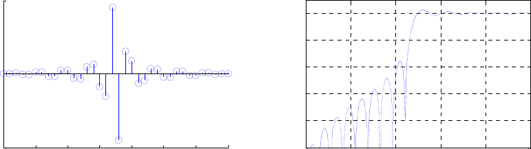
end
end
H = H.*phase;
f = ifft(H);
[FF, w] = freqz(f, 1, 512);
k = 0:N;
figure(1);
stem(k, real(f));
xlabel('Time index n');ylabel('Amplitude');
figure(2);
plot(w/pi,20*log10(abs(FF)));grid
xlabel('\omega/\pi');ylabel('Gain, dB');
axis([0 1 -50 5]);
0 5 10 15 20 25 30 35
-0.5
0
0.5
Time index n
A
mp
lit
u
d
e
00.2 0.4 0.6 0.8 1
-50
-40
-30
-20
-10
0
ω
/
π
Gain, dB
M10.14 N = 45;
L = N + 1;
for k = 1:L,
w = 2*pi*(k-1)/L;
if (w >= 0.5*pi & w <= 0.7*pi) H(k) = i*exp(-i*w*N/2);
elseif (w >= 1.3*pi & w <= 1.5*pi) H(k) = -
i*exp(i*(2*pi-w)*N/2);
else H(k) = 0;
end
end
f = ifft(H);
[FF, w] = freqz(f, 1, 512);
k = 0:N;
figure(1);
stem(k, real(f));
xlabel('Time index, n');ylabel('h[n]');
figure(2);
plot(w/pi, 20*log10(abs(FF)));grid;
ylabel('Gain, dB');xlabel('\omega/\pi');
axis([0 1 -50 5]);
Not for sale 367
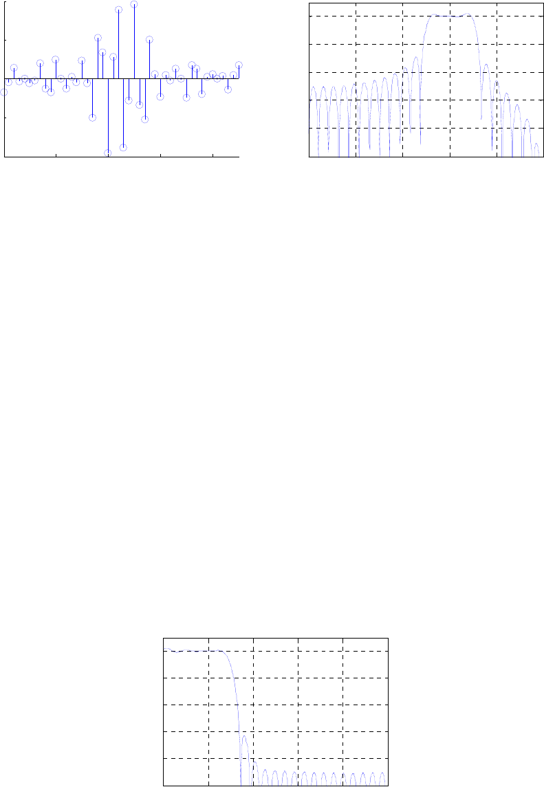
010 20 30 40
-0.2
-0.1
0
0.1
0.2
Time index, n
h[
n
]
00.2 0.4 0.6 0.8 1
-50
-40
-30
-20
-10
0
Gain, dB
ω
/
π
M10.15 ind = 1;
for k = 0:6,
H(ind) = exp(-i*2*pi*19*k/39);
ind = ind + 1;
end
k = 7;
H(ind) = 0.5*exp(-i*2*pi*19*k/39);
ind = ind + 1;
for k = 8:30,
H(ind) = 0;
ind = ind + 1;
end
k = 31;
H(ind) = 0.5*exp(-i*2*pi*19*k/39);
ind = ind + 1;
for k = 32:38,
H(ind) = exp(-i*2*pi*19*k/39);
ind = ind + 1;
end
h = ifft(H);
[FF, w] = freqz(h, 1, 512);
plot(w/pi, 20*log10(abs(FF)));grid;
xlabel('\omega/\pi');ylabel('Gain, dB');
axis([0 1 -50 5]);
00.2 0.4 0.6 0.8 1
-50
-40
-30
-20
-10
0
ω
/
π
Gain, dB
M10.16 ind = 1;
Not for sale 368
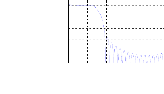
for k = 0:6,
H(ind) = exp(-i*2*pi*19*k/39);
ind = ind + 1;
end
k = 7;
H(ind) = (2/3)*exp(-i*2*pi*19*k/39);
ind = ind + 1;
k = 8;
H(ind) = (1/3)*exp(-i*2*pi*19*k/39);
ind = ind + 1;
for k = 9:29,
H(ind) = 0;
ind = ind + 1;
end
k = 30;
H(ind) = (1/3)*exp(-i*2*pi*19*k/39);
ind = ind + 1;
k = 31;
H(ind) = (2/3)*exp(-i*2*pi*19*k/39);
ind = ind + 1;
for k = 32:38,
H(ind) = exp(-i*2*pi*19*k/39);
ind = ind + 1;
end
h = ifft(H);
[FF, w] = freqz(h, 1, 512);
plot(w/pi, 20*log10(abs(FF)));grid;
xlabel('\omega/\pi');ylabel('Gain, dB');
axis([0 1 -50 5]);
00.2 0.4 0.6 0.8 1
-50
-40
-30
-20
-10
0
ω
/
π
Gain, dB
M10.17 18
8π
=ω p,18
12π
=ωs,18
10
π
=ωc,18
4
π
=ω∆
wp = 4*(2*pi)/18;
ws = 6*(2*pi)/18;
wc = (wp + ws)/2;
dw = ws - wp;
% Hamming
M = ceil(3.32*pi/dw);
N = 2*M;
b = fir1(N, ws/(2*pi));
Not for sale 369
[H, w] = freqz(b,1,512);
figure(1);
stem(b);
title('Impulse Response Coefficients');
xlabel('Time index n');ylabel('h[n]');
figure(2);
plot(w/pi, 20*log10(abs(H)));grid;
xlabel('\omega/\pi');ylabel('Gain, dB');
title('Lowpass filter designed using Hamming window');
axis([0 1 -80 10]);
% Hann
M = ceil(3.11*pi/dw);
N = 2*M;
b = fir1(N, ws/(2*pi), hanning(N+1));
[H, w] = freqz(b,1,512);
figure(3);
stem(b);
title('Impulse Response Coefficients');
xlabel('Time index n');ylabel('h[n]');
figure(4);
plot(w/pi, 20*log10(abs(H)));grid;
xlabel('\omega/\pi');ylabel('Gain, dB');
title('Lowpass filter designed using Hann window');
axis([0 1 -80 10]);
% Blackman
M = ceil(5.56*pi/dw);
N = 2*M;
b = fir1(N, ws/(2*pi), blackman(N+1));
[H, w] = freqz(b,1,512);
figure(5);
stem(b);
title('Impulse Response Coefficients');
xlabel('Time index n');ylabel('h[n]');
figure(6);
plot(w/pi, 20*log10(abs(H)));
grid;
xlabel('\omega/\pi');ylabel('Gain, dB');
title('Lowpass filter designed using Blackman window');
axis([0 1 -80 10]);
% Kaiser
beta = 3.631;
N = 44;
b = fir1(N, ws/(2*pi), kaiser(N+1, beta));
[H, w] = freqz(b,1,512);
figure(7);
stem(b);
title('Impulse Response Coefficients');
Not for sale 370
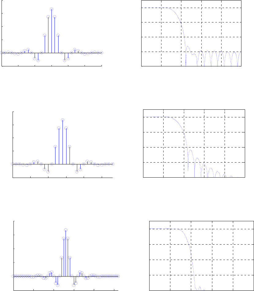
xlabel('Time index n');ylabel('h[n]');
figure(8);
plot(w/pi, 20*log10(abs(H)));grid;
xlabel('\omega/\pi');ylabel('Gain, dB');
title('Lowpass filter designed using Kaiser window');
axis([0 1 -80 10]);
(a) Hamming window using fir1
0 5 10 15 20 25 30
-0.1
0
0.1
0.2
0.3
0.4
Impulse Response Coefficients
Time index n
h[
n
]
00.2 0.4 0.6 0.8 1
-80
-60
-40
-20
0
ω
/
π
Gain, dB
Lowpass filter designed using Hamming window
(b) Hann window using fir1
0 5 10 15 20 25
-0.1
0
0.1
0.2
0.3
0.4
Impulse Response Coefficients
Time index n
h[
n
]
00.2 0.4 0.6 0.8 1
-80
-60
-40
-20
0
ω
/
π
Gain, dB
Lowpass filter designed using Hann window
(c) Blackman window using fir1
010 20 30 40 50
-0.1
0
0.1
0.2
0.3
0.4
Impulse Response Coefficients
Time index n
h[
n
]
00.2 0.4 0.6 0.8 1
-80
-60
-40
-20
0
ω
/
π
Gain, dB
Lowpass filter designed using Blackman window
(d) Kaiser window using fir1
Not for sale 371
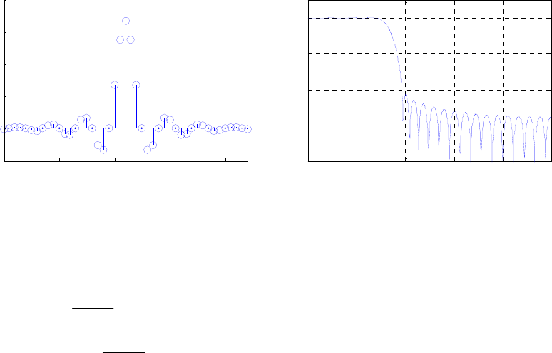
010 20 30 40
-0.1
0
0.1
0.2
0.3
0.4
Impulse Response Coefficients
Time index n
h[
n
]
00.2 0.4 0.6 0.8 1
-80
-60
-40
-20
0
ω
/
π
Gain, dB
Lowpass filter designed using Kaiser window
M10.18 , ,π=ω 40.
sπ=ω 550.
p10.
=
α
pdB, 42
=
α
sdB, π
=
ω
∆
150.,
π
=ω 4750.
c
(a) Hamming: use Eq. (10.33): 4622313322
150
323 ==∴→=
π
π
=MNM .
.
.
(b) Hann: 4222173320
150
113 ==∴→=
π
π
=MNM .
.
.
(c) Blackman: 7623806737
150
565 ==∴→=
π
π
=MNM .
.
.
(d) Kaiser: 00794010 20 .
/==δ α− s
s
% Hamming
N = 46;
b = fir1(N, 0.475, 'high');
[H,w] = freqz(b,1,512);
figure(1);
stem(b);
title('Impulse Response Coefficients');
xlabel('Time index n');ylabel('h[n]');
figure(2);
plot(w/pi, 20*log10(abs(H)));grid;
xlabel('\omega/\pi');ylabel('Gain, dB');
title('Highpass filter designed using Hamming window');
axis([0 1 -80 10]);
% Hann
N = 42;
b = fir1(N, 0.475, 'high', hanning(N+1));
[H,w] = freqz(b,1,512);
figure(3);
stem(b);
title('Impulse Response Coefficients');
xlabel('Time index n');ylabel('h[n]');
figure(4);
plot(w/pi, 20*log10(abs(H)));grid;
xlabel('\omega/\pi');ylabel('Gain, dB');
title('Highpass filter designed using Hann window');
axis([0 1 -80 10]);
Not for sale 372
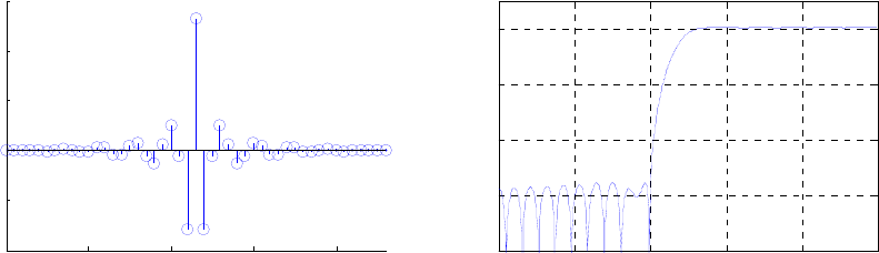
% Blackman
N = 76;
b = fir1(N, 0.475, 'high', blackman(N+1));
[H,w] = freqz(b,1,512);
figure(5);
stem(b);
title('Impulse Response Coefficients');
xlabel('Time index n');ylabel('h[n]');
figure(6);
plot(w/pi, 20*log10(abs(H)));grid;
xlabel('\omega/\pi');ylabel('Gain, dB');
title('Highpass filter designed using Blackman window');
axis([0 1 -80 10]);
% Kaiser
ds = 0.00794;
[N,Wn,beta,type] = kaiserord([0.4 0.55],[1 0],[ds ds]);
b = fir1(N, 0.475,'high',kaiser(N+1,beta));
[H,w] = freqz(b,1,512);
figure(7);
stem(b);
title('Impulse Response Coefficients');
xlabel('Time index n');ylabel('h[n]');
figure(8);
plot(w/pi, 20*log10(abs(H)));grid;
xlabel('\omega/\pi');ylabel('Gain, dB');
title('Highpass filter designed using Kaiser window');
axis([0 1 -80 10]);
(a) Hamming window using fir1
010 20 30 40
-0.4
-0.2
0
0.2
0.4
0.6
Impulse Response Coefficients
Time index n
h[
n
]
00.2 0.4 0.6 0.8 1
-80
-60
-40
-20
0
ω
/
π
Gain, dB
Highpass filter designed using Hamming window
(b) Hann window using fir1
Not for sale 373
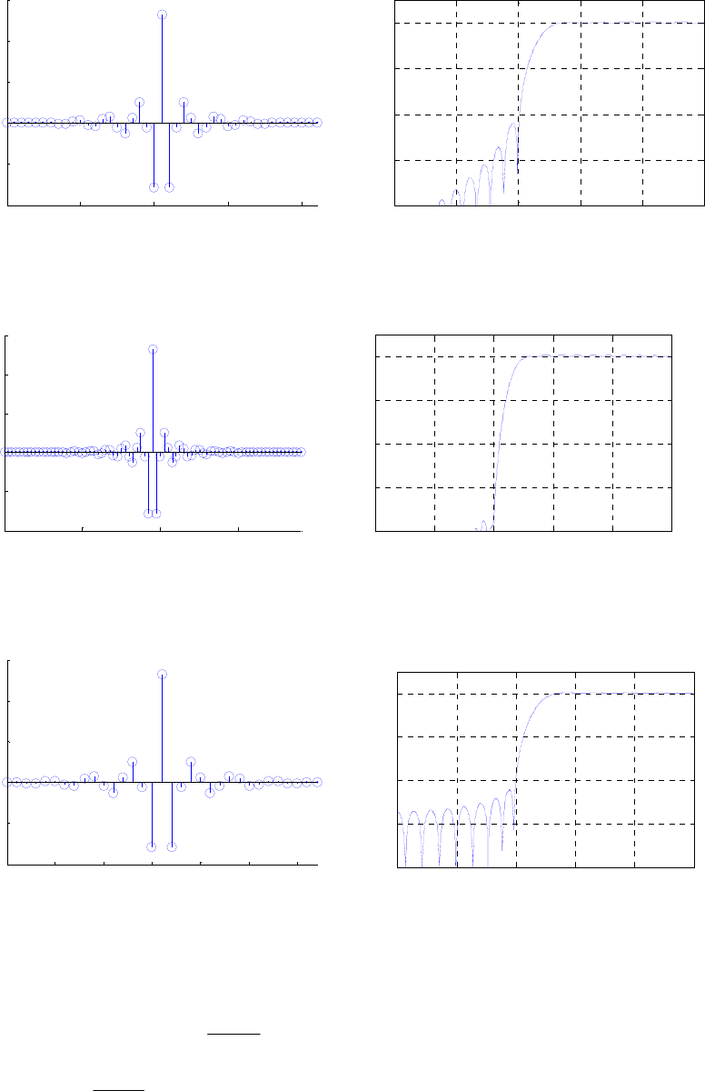
010 20 30 40
-0.4
-0.2
0
0.2
0.4
0.6
Impulse Response Coefficients
Time index n
h[
n
]
00.2 0.4 0.6 0.8 1
-80
-60
-40
-20
0
ω
/
π
Gain, dB
Highpass filter designed using Hann window
(c) Blackman window using fir1
020 40 60
-0.4
-0.2
0
0.2
0.4
0.6
Impulse Response Coefficients
Time index n
h[
n
]
00.2 0.4 0.6 0.8 1
-80
-60
-40
-20
0
ω
/
π
Gain, dB
Highpass filter designed using Blackman window
(d) Kaiser window using fir 1
0 5 10 15 20 25 30
-0.4
-0.2
0
0.2
0.4
0.6
Impulse Response Coefficients
Time index n
h[
n
]
00.2 0.4 0.6 0.8 1
-80
-60
-40
-20
0
ω
/
π
Gain, dB
Highpass filter designed using Kaiser window
M10.19 , ,
πω 65.0
1=
pπω 85.0
2=
pπω 55.0
1
=
s,πω 75.0
2
=
s,2.0
=
p
αdB, dB 42=
s
α
πωωω 1.0
111 =
−
=sp
∆, ωπωωω ∆∆
=
=
−
=
1.0
222 sp
(a) Hamming window: 682342.33
1.0
32.3 ==∴→== MNM π
π
(b) Hann: 642321.31
1.0
11.3 ==∴→== MNM π
π
Not for sale 374

(c) Blackman: 1122566.55
1.0
56.5 ==∴→== MNM π
π
(d) Kaiser: , 00794.010 20/ == −s
sα
δ97724.010 20/ == −p
p
α
δ
% Problem #M10.19
% Hamming
N = 68;
b = fir1(N, [0.6 0.8]);
[H, w] = freqz(b,1,512);
figure(1);
stem(b);
title('Impulse Response Coefficients');
xlabel('Time index n');ylabel('h[n]');
figure(2);
plot(w/pi, 20*log10(abs(H)));grid;
xlabel('\omega/\pi');ylabel('Gain, dB');
title('Bandpass filter designed using Hamming window');
axis([0 1 -80 10]);
% Hann
N = 64;
b = fir1(N, [0.6 0.8], hanning(N+1));
[H, w] = freqz(b,1,512);
figure(3);
stem(b);
title('Impulse Response Coefficients');
xlabel('Time index n');ylabel('h[n]');
figure(4);
plot(w/pi, 20*log10(abs(H)));grid;
xlabel('\omega/\pi');ylabel('Gain, dB');
title('Bandpass filter designed using Hann window');
axis([0 1 -80 10]);
% Blackman
N = 112;
b = fir1(N, [0.6 0.8], blackman(N+1));
[H, w] = freqz(b,1,512);
figure(5);
stem(b);
title('Impulse Response Coefficients');
xlabel('Time index n');ylabel('h[n]');
figure(6);
plot(w/pi, 20*log10(abs(H)));grid;
xlabel('\omega/\pi');ylabel('Gain, dB');
title('Bandpass filter designed using Blackman window');
axis([0 1 -80 10]);
% Kaiser
[N, Wn, beta, type] = kaiserord([0.6 0.8], [1 0], [0.97724
0.00794]);
Not for sale 375
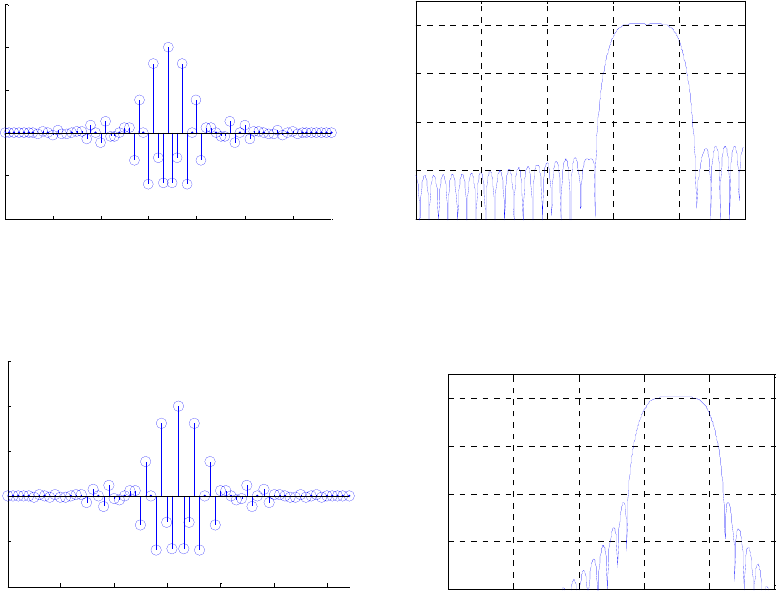
b = fir1(2*N, [0.6 0.8], kaiser(2*N+1, beta));
[H, w] = freqz(b,1,512);
figure(7);
stem(b);
title('Impulse Response Coefficients');
xlabel('Time index n');ylabel('h[n]');
figure(8);
plot(w/pi, 20*log10(abs(H)));grid;
xlabel('\omega/\pi');ylabel('Gain, dB');
title('Bandpass filter designed using Kaiser window');
axis([0 1 -80 10]);
(a) Hamming window using fir1
010 20 30 40 50 60
-0.2
-0.1
0
0.1
0.2
0.3
Impulse Response Coefficients
Time index n
h[
n
]
00.2 0.4 0.6 0.8 1
-80
-60
-40
-20
0
ω
/
π
Gain, dB
Bandpass filter designed using Hamming window
(b) Hann window using fir1
010 20 30 40 50 60
-0.2
-0.1
0
0.1
0.2
0.3
Impulse Response Coefficients
Time index n
h[
n
]
00.2 0.4 0.6 0.8 1
-80
-60
-40
-20
0
ω
/
π
Gain, dB
Bandpass filter designed using Hann window
(c) Blackman window using fir1
Not for sale 376
020 40 60 80 100
-0.2
-0.1
0
0.1
0.2
Impulse Response Coefficients
Time index n
h[
n
]
00.2 0.4 0.6 0.8 1
-80
-60
-40
-20
0
ω
/
π
Gain, dB
Bandpass filter designed using Blackman windo
w
(d) Kaiser window using fir1
010 20 30 40
-0.2
-0.1
0
0.1
0.2
0.3
Impulse Response Coefficients
Time index n
h[
n
]
00.2 0.4 0.6 0.8 1
-80
-60
-40
-20
0
ω
/
π
Gain, dB
Bandpass filter designed using Kaiser window
M10.20 π
π
ω4286.0
70
152 =
⋅
=
c
% Problem #M10.20
N = 31;
d1 = fir1(N-1,0.4286);d2 = fir1(N-1,0.4286,'high');
[h1,w] = freqz(d1,1,512);h2 = freqz(d2,1,w);
plot(w/pi,20*log10(abs(h1)),'-r',w/pi,20*log10(abs(h2)),'--
b');grid;
xlabel('\omega/\pi');ylabel('Gain, dB');
title('Crossover pair');
axis([0 1 -80 10]);
00.2 0.4 0.6 0.8 1
-80
-60
-40
-20
0
ω
/
π
Gain, dB
Crossover pair
Not for sale 377
M10.21 , 2494.0
1=
c
ω5442.0
2=
c
ω
% Problem #M10.21
N = 32;
d1 = fir1(N, 0.2494, hanning(33));
d2 = fir1(N, 0.5442, 'high', hanning(33));
d3 = -d1-d2;
d3(17) = 1-d1(17)-d2(17);
[h1,w] = freqz(d1,1,512);h2 = freqz(d2,1,w);h3 =
freqz(d3,1,w);
g1 = 20*log10(abs(h1))); g2 = 20*log10(abs(h2)));
g3 = 20*log10(abs(h3)));
plot(w/pi, g1,’—-b’,w/pi,g2,’-.g’,w/pi,g3,’-r’);grid;
xlabel('\omega/\pi');ylabel('Gain, dB');
title('Crossover triple');
axis([0 1 -80 10]);
00.2 0.4 0.6 0.8 1
-80
-60
-40
-20
0
ω
/
π
Gain, dB
Crossover triple
M10.22 % Problem #M10.22
fpts = [0 0.35 0.4 0.7 0.72 1];
mval = [0.2 0.2 1 1 0.6 0.6];
b = fir2(70, fpts, mval);
[H,w] = freqz(b,1,512);
figure(1);
plot(w/pi,abs(H));grid;
xlabel('\omega/\pi');ylabel('Magnitude');
title('Multilevel FIR filter');
axis([0 1 0 1.2]);
00.2 0.4 0.6 0.8 1
0
0.2
0.4
0.6
0.8
1
ω
/
π
Magnitude
Multilevel FIR filter
Not for sale 378

M10.23 From Problem 10.36,
π=ω 450.
p, ,π=ω 60.
s20430.
=
δ
p,04540.
=
δ
sand we assume that
.2=
T
F Therefore, 450
2
450 .
.=
π
⋅π
=T
p
F
Fand ..60
=
s
F
(
)
9851120 10 .log =δ−−=α pp dB,
(
)
8582620 10 .log
=
δ
−
=
α
ss dB.
After obtaining the length N using ‘remezord’, the specifications of the filter were not
met. We increased N to 11 to meet the specifications.
% Program #M10.23
Ft = 2;Fp = 0.45;Fs = 0.6;
ds = 0.0454;dp = 0.2043;
F = [Fp Fs];A = [1 0];DEV = [dp ds];
[N,Fo,Ao,W] = remezord(F,A,DEV,Ft);
b = remez(N,Fo,Ao,W);
[H,w] = freqz(b,1,512);
figure(1);
plot(w/pi, 20*log10(abs(H)));
xlabel('\omega/\pi');ylabel('Gain, dB');title('N = 9');
%axis([0 0.45 -3 3]);
N = 11;
b = remez(N,Fo, Ao, W);
[H,w] = freqz(b,1,512);
figure(2);
plot(w/pi, 20*log10(abs(H)));
xlabel('\omega/\pi');ylabel(Gain, dB);title('N = 11');
Using remezord, we get N = 9. The corresponding gain response is shown in Figure (e)
below:
00.2 0.4 0.6 0.8 1
-80
-60
-40
-20
0
20
ω
/
π
Gain, dB
N = 9
00.2 0.4 0.6 0.8 1
-80
-60
-40
-20
0
20
ω
/
π
Gain, dB
N = 11
(e) (f)
However, specifications are not met in the passband with this filter, so we increase N to
11. The corresponding gain response is shown in Figure (f) above. The specifications
are now met.
Not for sale 379
M10.24 From problem 10.37,
π=ω 70.
p, ,π=ω 550.
s038080.
=
δ
p,01120.
=
δ
sand we assume that
.2=
T
F Therefore, 70
2
70 .
.=
π
⋅π
=T
p
F
Fand ..550
=
s
F
(
)
33720120 10 .log =δ−−=α pp dB,
(
)
0163920 10 .log
=
δ
−
=
α
ss dB.
Using ‘remezord’, we get an estimate of N = 20. However, using this order, the
specifications are not met in the stopband, so we need to increase N up to 23 to meet the
specifications.
% Program #M10.24
Ft = 2;Fp = 0.7;Fs = 0.55;
ds = 0.0112;dp = 0.03808;
F = [Fs Fp];A = [0 1];DEV = [ds dp];
[N,Fo,Ao,W] = remezord(F,A,DEV,Ft);
b = remez(N,Fo,Ao,W);
[H,w] = freqz(b,1,512);
figure(1);
plot(w/pi, 20*log10(abs(H)));
xlabel('\omega/\pi');ylabel('Gain, dB');title('N = 20');
N = 23;
b = remez(N,Fo,Ao,W);
[H,w] = freqz(b,1,512);
figure(2);
plot(w/pi,20*log10(abs(H)));
xlabel('\omega/\pi');ylabel('Gain,dB ');title('N = 23');
00.2 0.4 0.6 0.8 1
-80
-60
-40
-20
0
ω
/
π
Gain, dB
N = 20
00.2 0.4 0.6 0.8 1
-80
-60
-40
-20
0
ω
/
π
Gain, dB
N = 24
Note: As odd order symmetric FIR filters must have a gain of zero at the Nyquist
frequency. The order has been increased by one by remez.
M10.25 From Problem 10.38,
π=ω 550
1.
p, ,
π=ω 70
2.
p
π
=
ω
440
1.
s,
π
=
ω
820
2.
s,010.
=
δ
p,,
.
0070
1.=δs
0020
2.=δs
(
)
0870120 10 .log
=
δ
−
−=α pp dB,
Not for sale 380
()
4320 1101 =δ−=α ss log dB,
(
)
5420 2102
=
δ
−
=
α
ss log dB.
% Program #M10.25
Ft = 2;Fp1 = 0.55;Fp2 = 0.7;Fs1 = 0.44;Fs2 = 0.82;
ds1 = 0.007;ds2 = 0.002;dp = 0.01;
F = [Fs1 Fp1 Fp2 Fs2];A = [0 1 0];DEV = [ds1 dp ds2];
[N,Fo,Ao,W] = remezord(F,A,DEV,Ft);
b = remez(N,Fo,Ao,W);
[H, w] = freqz(b, 1, 512);
figure(1);
plot(w/pi,20*log10(abs(H)));grid;
xlabel('\omega/\pi');ylabel('Gain, dB');title('N = 39');
axis([0 1 -80 10]);
N = 41;
b = remez(N, Fo, Ao, W);
[H, w] = freqz(b, 1, 512);
figure(2);
plot(w/pi, 20*log10(abs(H)));
xlabel('\omega/\pi');ylabel('Gain, dB');title('N = 41');
axis([0 1 -80 10]);
Using remezord, we estimate the filter length to be N = 39. However, the minimum
stopband attenuation specifications are not met in both stopbands, so we increase N to 41
00.2 0.4 0.6 0.8 1
-80
-60
-40
-20
0
ω
/
π
Gain, dB
N = 39
00.2 0.4 0.6 0.8 1
-80
-60
-40
-20
0
ω
/
π
Gain, dB
N = 41
.
M10.26 % Program #M10.26
b = remez(29, [0 1], [0 pi], 'differentiator');
[H, w] = freqz(b, 1, 512);
plot(w/pi,abs(H));grid
xlabel('\omega/\pi');ylabel('Magnitude');
axis([0 1 0 pi]);
The magnitude response of the differentiator is given below:
Not for sale 381
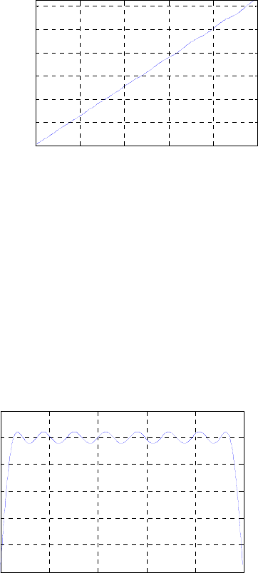
00.2 0.4 0.6 0.8 1
0
0.5
1
1.5
2
2.5
3
ω
/
π
Magnitude
M10.27 % Program #M10.27
f = [0.02 0.05 0.07 0.95 0.97 1];
m = [0 0 1 1 0 0];
wt = [1 60 1];
b = remez(30, f, m, wt, 'hilbert');
[H,w] = freqz(b,1,512);
plot(w/pi,abs(H));grid
xlabel('\omega/\pi');ylabel('Magnitude');
axis([0 1 0 1.2]);
The magnitude response of the Hilbert transformer is shown below:
00.2 0.4 0.6 0.8 1
0
0.2
0.4
0.6
0.8
1
ω
/
π
Magnitude
M10.28 , ,
π=ω 350.
pπ=ω 50.
s1
=
p
RdB, and 28
=
s
RdB.
% Program #M10_28
% Design of a minimum-phase lowpass FIR filter
Wp = 0.35; Ws = 0.5; Rp = 1; Rs = 28;
% Desired ripple values of minimum-phase filter
dp = 1- 10^(-Rp/20); ds = 10^(-Rs/20);
% Compute ripple values of prototype linear-phase filter
Ds = (ds*ds)/(2 - ds*ds);
Dp = (1 + Ds)*((dp + 1)*(dp + 1) - 1);
% Estimate filter order
[N,fpts,mag,wt] = remezord([Wp Ws], [1 0], [Dp Ds]);
% Design the prototype linear-phase filter H(z)
[b,err,res] = remez(N,fpts,mag,wt);
K = N/2;
b1 = b(1:K);
Not for sale 382
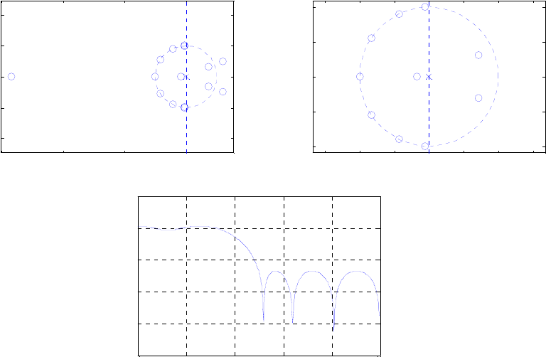
% Design the linear-phase filter G(z)
lenerr= res.error(length(res.error));
c = [b1 (b(K+1) + lenerr)) fliplr(b1)]/(1+Ds);
zplane(c);title('Zeros of G(z)');pause
c1 = c(K+1:N+1);
[y, ssp, iter] = minphase(c1);
zplane(y);title(‘Zeros of the minimum-phase filter’);
pause
[hh,w] = freqz(y,1, 512);
% Plot the gain response of the minimum-phase filter
plot(w/pi, 20*log10(abs(hh)));grid
xlabel('\omega/\pi');ylabel('Gain, dB');
-6 -4 -2 0
-2
-1
0
1
2
220
Real Part
Imaginary Part
Zeros of G(z)
-1.5 -1 -0.5 00.5 11.5
-1
-0.5
0
0.5
1
10
Real Part
I
mag
i
nary
P
ar
t
Zeros of the minimum-phase filter
00.2 0.4 0.6 0.8 1
-80
-60
-40
-20
0
20
ω
/
π
Gain, dB
M10.29 % Program #M10.29
c = [2.4 6.76 26.15 68.43 186.83 326.51 565.53 678.95 805.24
678.95 565.53 326.51 186.83 68.43 26.15 6.76 2.4];
h = firminphase(c)
The coefficients of the minimum phase spectral factor are:
h = 7.6730 8.5329 18.0722 12.5696 12.6822 4.8388 2.0784 0.5332 0.3128
M10.30 % Program #M10.30
[h,g]=ifir(6,'low',[.1 .15],[.001 .001]);
[hh,w]=freqz(h,1,1024); hg=freqz(g,1,1024);
h = hh.*hg; % Compounded response
Fg = 20*log10(abs(hh)); Ig = 20*log10(abs(hg));
plot(w/pi,Fg,'-r',w/pi,Ig,'--b'); grid;
axis([0 1 -90 5]);
Not for sale 383
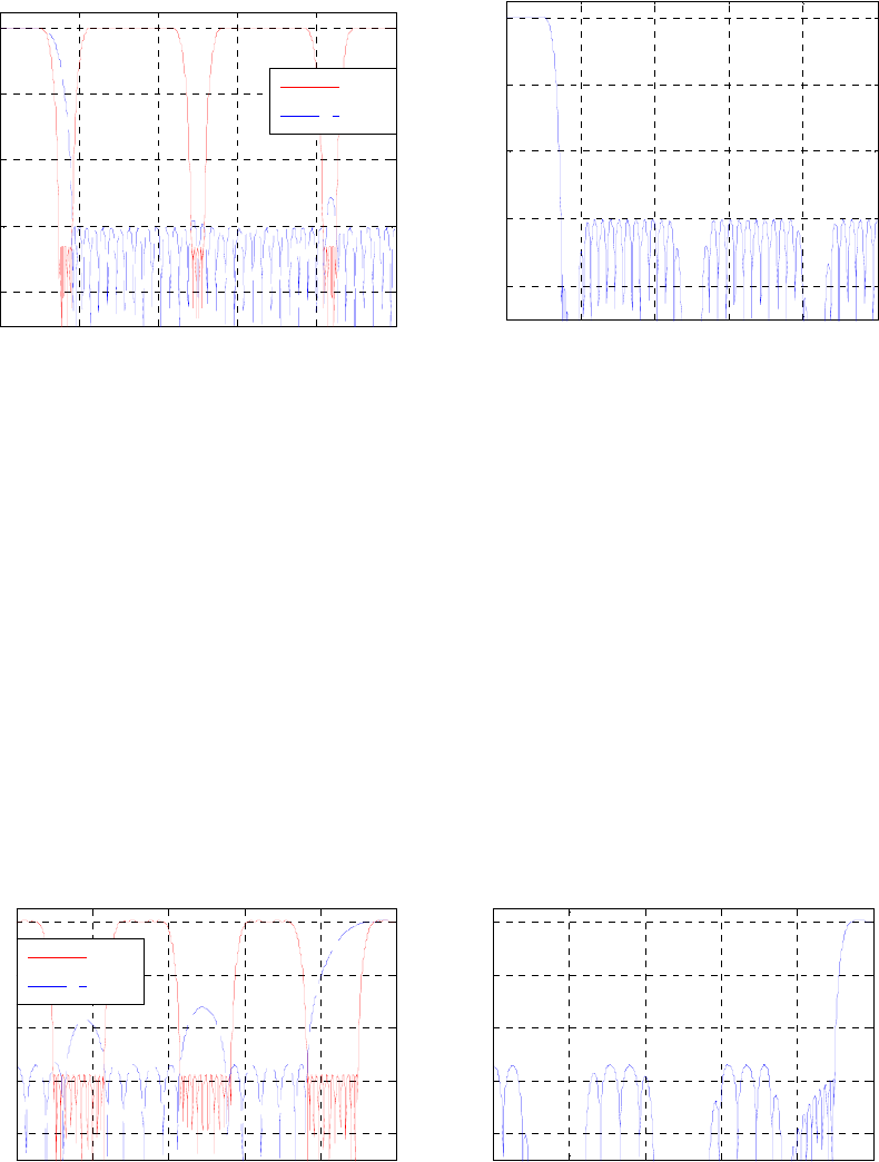
legend('F(z^6)','I(z)');
xlabel('\omega/\pi');title('Gain responses, in dB');
pause;
plot(w/pi,20*log10(abs(h))); grid;
axis([0 1 -90 5]);
xlabel('\omega/\pi');title('Gain response, in dB');
gtext('H_{IFIR}(z)');
00.2 0.4 0.6 0.8 1
-80
-60
-40
-20
0
ω
/
π
Gain responses, in dB
F(z
6
)
I(z)
00.2 0.4 0.6 0.8 1
-80
-60
-40
-20
0
ω/π
Gain response, in dB
HIFIR(z)
M10.31 % Program #M10.31
[h,g]=ifir(6,'high',[.9 .95],[.002 .004]);
[hh,w]=freqz(h,1,1024); hg=freqz(g,1,1024);
h = hh.*hg; % Compounded response
Fg = 20*log10(abs(hh)); Ig = 20*log10(abs(hg));
plot(w/pi,Fg,'-r',w/pi,Ig,'--b'); grid;
axis([0 1 -90 5]);
legend('F(z^6)','I(z)');
xlabel('\omega/\pi');title('Gain responses, in dB');
pause;
plot(w/pi,20*log10(abs(h))); grid;
axis([0 1 -90 5]);
xlabel('\omega/\pi');title('Gain response, in dB');
gtext('H_{IFIR}(z)');
00.2 0.4 0.6 0.8 1
-80
-60
-40
-20
0
ω
/
π
Gain responses, in dB
F(z
6
)
I(z)
00.2 0.4 0.6 0.8 1
-80
-60
-40
-20
0
ω
/
π
Gain response, in dB
H
IFIR
(z)
Not for sale 384
M10.32 % Problem #M10.32
InpN = ceil(2*pi/(0.15*pi));
% Plotting function
% plots the result of using an equalizer of length InpN
%function [N] = plotfunc(InpN);
% Creating filters
Wfilt = ones(1, InpN);
Efilt = remezfunc(InpN, Wfilt);
% Plot running sum filter response
figure(1);
Wfilt = Wfilt/sum(Wfilt);
[hh, w] = freqz(Wfilt, 1, 512);
plot(w/pi, 20*log10(abs(hh)));
axis([0 1 -50 5]);grid;
xlabel('\omega/\pi');ylabel('Gain, dB');
title('Prefilter H(z)');
% Plot equalizer filter response
figure(2);
[hw, w] = freqz(Efilt, 1, 512);
plot(w/pi, 20*log10(abs(hw)));
axis([0 1 -50 5]);grid;
xlabel('\omega/\pi');ylabel('Gain, dB');
title('Equalizer F(z)');
% Plot cascade filter response
figure(3);
Cfilt = conv(Wfilt, Efilt);
[hc, w] = freqz(Cfilt, 1, 512);
plot(w/pi, 20*log10(abs(hc)));
axis([0 1 -80 5]);grid;
xlabel('\omega/\pi');ylabel('Gain, dB');
title('Cascade filter H(z)F(z)');
% Remez function using 1/P(z) as desired amplitude
% and P(z) as weighting
function [N] = remezfunc(Nin, Wfilt);
% Nin : number of tuples in the remez equalizer filter
% Wfilt : the prefilter
a = [0:0.001:0.999]; % The accuracy of the computation
w = a.*pi;wp = 0.05*pi;ws = 0.15*pi;
i = 1;n = 1;
for t = 1:(length(a)/2),
Not for sale 385
if w(2*t) < wp
pas(i) = w(2*t - 1);
pas(i+1) = w(2*t);
i = i+2;
end
if w(2*t-1) > ws
sto(n) = w(2*t - 1);
sto(n+1) = w(2*t);
n = n+2;
end
end
w = cat(2, pas, sto);
bi = length(w)/2;
for t1 = 1:bi,
bw(t1) = (w(2*t1) + w(2*t1-1))/2;
W(t1) = Weight(bw(t1), Wfilt, ws);
end
W = W/max(W);
for t2 = 1:length(w),
G(t2) = Hdr(w(t2), Wfilt, wp);
end
G = G/max(G);
N = remez(Nin, w/pi, G, W);
% Weighting function
function[Wout] = Weight(w, Wfilt, ws);
K = 22.8;
L = length(Wfilt);
Wtemp = 0;
Wsum = 0;
for k = 1:L,
Wtemp = Wfilt(k)*exp((k-1)*i*w);
Wsum = Wsum + Wtemp;
end
Wout = abs(Wsum);
if w > ws,
Wout = K*max(Wout);
end
% Desired function
function [Wout] = Hdr(w, Wfilt, ws);
if w <= ws,
L = length(Wfilt);
Wtemp = 0;
Wsum = 0;
for k = 1:L,
Wtemp = Wfilt(k)*exp(i*(k-1)*w);
Wsum = Wsum + Wtemp;
end
Wsum = abs(Wsum);
Wout = 1/Wsum;
Not for sale 386
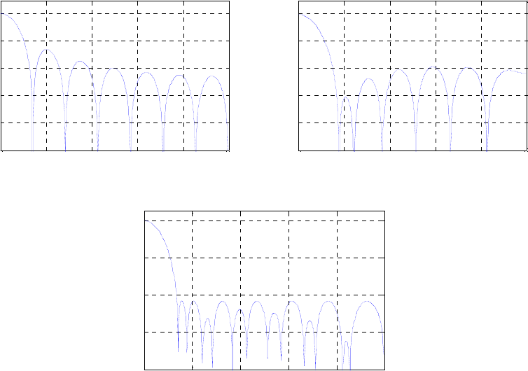
else
Wout = 0;
end
00.2 0.4 0.6 0.8 1
-50
-40
-30
-20
-10
0
ω
/
π
Gain, dB
Prefilter H(z)
00.2 0.4 0.6 0.8 1
-50
-40
-30
-20
-10
0
ω
/
π
Gain, dB
Equalizer F(z)
00.2 0.4 0.6 0.8 1
-80
-60
-40
-20
0
ω
/
π
Gain, dB
Cascade filter H(z)F(z)
Not for sale 387
Chapter 11
11.1 Analysis yields
{}
],[][][,]1[]1[][ 3122211 nwnwnwnwnxnw
+
=
−+−= αβ
{}
],[][][,]1[]1[][ 534422213 nwnwnwnwnwnw
+
=
−
+−= ααβ
{}
].[][][,]1[]1[][ 01534235 nxnwnynwnwnw αααβ
+
=
−
+−=
In matrix form the above equations can be written as
1111
22
3 3 22 22
44
552333
[] 000000 [] 0 0 0 0 0
[] 1 0 1 0 0 0 [] 0 0 0 0 0 0
[] 000000 [] 0 0 0 0
[] 001010 [] 0 0 0 0 0 0
[] 000000 [] 0 0 0 0
[] 100000 [] 0 0 0 0 0
wn wn
wn wn
wn wn
wn wn
wn wn
yn yn
αβ
αβ αβ
αβ αβ
⎡⎤⎡ ⎤⎡⎤
⎢⎥⎢ ⎥⎢⎥
⎢⎥⎢ ⎥⎢⎥
⎢⎥⎢ ⎥⎢⎥
=+
⎢⎥⎢ ⎥⎢⎥
⎢⎥⎢ ⎥⎢⎥
⎢⎥⎢ ⎥⎢⎥
⎢⎥⎢ ⎥⎢⎥
⎣⎦⎣ ⎦⎣⎦
1
1
2
3
4
5
0
[1]
[1]
0
[1]
0
[1]
0
[1]
0
[1]
[]
0[1]
xn
wn
wn
wn
wn
wn
xn
yn
β
α
−
−
⎡
⎤
⎡⎤⎡⎤
⎢
⎥
⎢⎥⎢⎥
−
⎢
⎥
⎢⎥⎢⎥
⎢
⎥
⎢⎥⎢⎥
−+
⎢
⎥
⎢⎥⎢⎥
−
⎢
⎥
⎢⎥⎢⎥
⎢
⎥
⎢⎥⎢⎥
−
⎢
⎥
⎢⎥⎢⎥
−
⎢
⎥
⎣⎦⎣⎦
⎣
⎦
Here the F matrix is given by: .
000001
000000
010100
000000
000101
000000
⎥
⎥
⎥
⎥
⎥
⎦
⎤
⎢
⎢
⎢
⎢
⎢
⎣
⎡
=
F
Since the F matrix contains nonzero entries above the main diagonal, the above set of
equations are not computable.
11.2 A computable set of equations are given by:
{}
,]1[]1[][ 2111 −+−= nwnxnw αβ
{
}
,]1[]1[][ 422213
−
+
−
=
nwnwnw ααβ
{}
,]1[]1[][ 534235
−
+−= nwnwnw ααβ ],[][][ 312 nwnwnw
+
=
][][][ 01 nxnwny α+
=
,
][][][ 534 nwnwnw += .
In matrix form the above equations can be written as
11
11
33
22 22
55
23 33
22
44
[] []
000000 0 0 0 0 0
[] []
000000 0 0 0 0
[] []
000000 0 0 0 0
[] []
101000 0000 00
[] []
100000 0000 00
[] []
001010 0
wn wn
wn wn
wn wn
wn wn
yn yn
wn wn
αβ
αβ αβ
αβ αβ
⎡⎤ ⎡⎤
⎡⎤
⎢⎥ ⎢⎥
⎢⎥
⎢⎥ ⎢⎥
⎢⎥
⎢⎥ ⎢⎥
⎢⎥
=+
⎢⎥ ⎢⎥
⎢⎥
⎢⎥ ⎢⎥
⎢⎥
⎢⎥ ⎢⎥
⎢⎥
⎢⎥ ⎢⎥
⎢⎥
⎢⎥ ⎢⎥
⎣⎦
⎣⎦ ⎣⎦
11
3
5
2
0
4
[1] [1]
[1] 0
[1] 0
[1] 0
[1] []
[1]
000 00 0
wn xn
wn
wn
wn
yn xn
wn
β
α
−
−
⎡⎤
⎡
⎤⎡
⎢⎥ ⎤
⎢
⎥⎢
−
⎢⎥ ⎥
⎢
⎥⎢
⎢⎥ ⎥
⎢
⎥⎢
−+
⎢⎥ ⎥
⎢
⎥⎢
−
⎢⎥ ⎥
⎢
⎥⎢
⎢⎥ ⎥
⎢
⎥⎢
−
⎢⎥ ⎥
⎢
⎥⎢
−
⎢⎥ ⎥
⎣
⎦⎣
⎣⎦ ⎦
Here the F matrix is given by: .
010100
000001
000101
000000
000000
000000
⎥
⎥
⎥
⎥
⎥
⎦
⎤
⎢
⎢
⎢
⎢
⎢
⎣
⎡
=
F
Not for sale 388
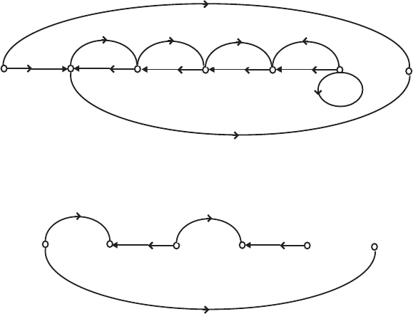
Since the F matrix has no nonzero entries above the main diagonal, the new set of equations
are computable.
11.3 Analysis yields
{}
],[][][,]1[]1[]1[][ 1263422111 nxnwnwnwnwnwnw
+
=
−
+
−
+
−
=αααβ
{}
],[][][,]1[]1[][ 324634223 nwnwnwnwnwnw
+
=
−
+−= ααβ
{}
,]1[][ 63
3
5
−
=nwnw αβ
],[][][ 546 nwnwnw += ].[][][][][ 0634221 nxnwnwnwny αααα
+
+
+
=
In matrix form the above set of equations are given by
111112
22
33
44
55
66
123
0000000
[] [] 0 0 0
1000000
[] []
0000000
[] []
0110000
[] []
0000000
[] []
0001100
[] []
0000
[] []
wn wn
wn wn
wn wn
wn wn
wn wn
wn wn
aaa
yn yn
βα βα β
⎡⎤
⎡⎤ ⎡⎤
⎢⎥
⎢⎥ ⎢⎥
⎢⎥
⎢⎥ ⎢⎥
⎢⎥
⎢⎥ ⎢⎥
⎢⎥
⎢⎥ ⎢⎥
=+
⎢⎥
⎢⎥ ⎢⎥
⎢⎥
⎢⎥ ⎢⎥
⎢⎥
⎢⎥ ⎢⎥
⎢⎥
⎢⎥ ⎢⎥
⎢⎥
⎢⎥ ⎢⎥
⎣⎦ ⎣⎦
⎣⎦
13 1
2
22 23 3
4
33 5
6
0
0
0[1]
[]
0000 000 [1]
0
000 0 0 [1]
0
0000 000 [1]
0
0000 0 0 [1]
0
0000 000 [1]
[]
0000 000 [1]
wn
x
n
wn
wn
wn
wn
wn
x
n
yn
α
βα βα
βα
α
−⎡⎤
⎡⎤⎡
⎢⎥
⎢⎥⎢
−⎢⎥
⎢⎥⎢
⎢⎥
⎢⎥⎢
−⎢⎥
⎢⎥⎢
+
−⎢⎥
⎢⎥⎢
⎢⎥
⎢⎥⎢
−⎢⎥
⎢⎥⎢
−⎢⎥
⎢⎥⎢
⎢⎥
⎢⎥⎢
−
⎣⎦⎣
⎣⎦
⎤
⎥
⎥
⎥
⎥
⎥
⎥
⎥
⎥
⎥
⎦
Here the F matrix is given by:
.
0000
0011000
0000000
0000110
0000000
0000001
0000000
321 ⎥
⎥
⎥
⎥
⎥
⎥
⎦
⎤
⎢
⎢
⎢
⎢
⎢
⎢
⎣
⎡
=
ααα
F
Since the diagonal of the F matrix has all zeros, and no nonzero entries above the main
diagonal, the new set of equations are computable.
11.4
x
[n]y[n]
w [n]
1
w [n]
2
w [n]
3
w [n]
4
w [n]
5
α
0
1
β
_1
z
1
α
1
1
β
_1
z
1
11
α
1
2
β
_1
z
α
2
2
β
_1
z
α
2
3
β
_1
z
α
3
3
β
_1
z
1
Reduced signal flow graph obtained by removing the branches going out of the input node
and the delay branches is:
y[n]
w [n]
1w [n]
2w [n]
3w [n]
4
w [n]
5
11
11
1
Not for sale 389
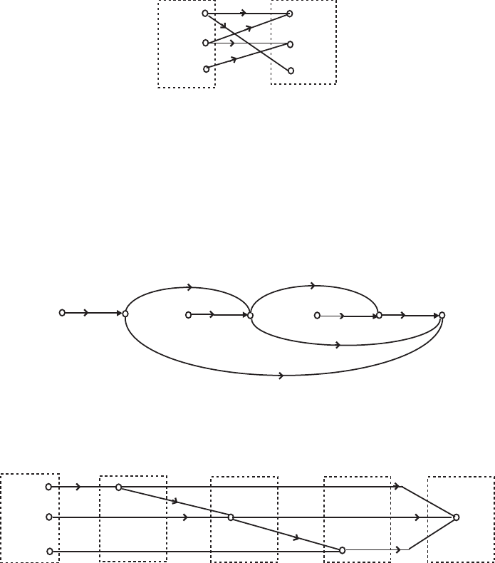
The node sets of the precedence graph are as follows:
{}{ }
{
}
{
}
.][],[],[,][],[],[ 4225311 nwynwnwnwnwnw
=
=NN
w [n]
1
w [n]
3
w [n]
5
y[n]
w [n]
2
w [n]
4
N
1
N
2
In the above precedence graph, contains only outgoing nodes and contains only incoming
branches. The structure has no delay free loops. A valid computational algorithm is:
1
N2
N
{}
,]1[]1[][ 2111 −+−= nwnxnw αβ
{
}
,]1[]1[][ 422213
−
+
−
=
nwnwnw ααβ
{}
,]1[]1[][ 534235
−
+−= nwnwnw ααβ ],[][][ 312 nwnwnw
+
=
][][][ 01 nxnwny α+
=
,
][][][ 534 nwnwnw += .
11.5 Reduced signal flow graph is:
y[n]
w [n]
1
w [n]
2
w [n]
3
w [n]
4
111
11
1
w [n]
5
w [n]
6
1
α
2
α
3
α
The node sets of the precedence graph are as follows:
{
}
{
}
,][],[],[ 5311 nwnwnw
=
N
{} {}
{
}
{
}
]}.[{]},[{]},[{]},[{ 5644322 nynwnwnw
=
=
== NNNN
w [n]
1
w [n]
3
w [n]
5
w [n]
2
w [n]
4
w [n]
6
y[n]
N
1
N
2
N
3
N
4
N
5
A valid computational algorithm is:
{}
,]1[]1[]1[][ 63422111
−
+
−
+−= nwnwnwnw αααβ
{}
,]1[]1[][ 634223
−
+−= nwnwnw ααβ
{
}
,]1[][ 63
3
5
−
=
nwnw αβ
],[][][ 12 nxnwnw += ],[][][ 324 nwnwnw
+
=],[][][ 546 nwnwnw
+
=
].[][][][][ 0634221 nxnwnwnwny αααα
+
++=
11.6 (a) Analysis yields ],1[][][],1[][][ 22321121 −
−
=
−
−
=nsknwnwnwknwnw
],1[][][ 333 −−= nsknxnw ],1[][][],1[][][ 22231112 −+
=
−
+
=
nsnwknsnwnwkns
].1[][][ 333 −+= nsnwkny In matrix form we have
Not for sale 390
.
⎥
⎥
⎥
⎥
⎥
⎥
⎦
⎤
⎢
⎢
⎢
⎢
⎢
⎢
⎣
⎡
⎥
⎥
⎥
⎥
⎥
⎦
⎤
⎢
⎢
⎢
⎢
⎢
⎣
⎡
+
⎥
⎥
⎥
⎥
⎥
⎦
⎤
⎢
⎢
⎢
⎢
⎢
⎣
⎡
=
⎥
⎥
⎥
⎥
⎥
⎥
⎦
⎤
⎢
⎢
⎢
⎢
⎢
⎢
⎣
⎡
][
][
][
][
][
][
00000
00000
00000
000000
000100
000010
0
0
0
][
0
0
][
]
[
][
][
][
][
3
2
3
2
1
3
2
1
3
2
3
2
1
ny
ns
ns
nw
nw
nw
k
k
k
nx
ny
ns
ns
nw
nw
nw
44443444421
F
⎥
⎥
⎥
⎥
⎥
⎥
⎦
⎤
⎢
⎢
⎢
⎢
⎢
⎢
⎣
⎡
−
−
−
−
−
−
⎥
⎥
⎥
⎥
⎥
⎦
⎤
⎢
⎢
⎢
⎢
⎢
⎣
⎡
−
−
−
+
]1[
]1[
]1[
]1[
]1[
]1[
010000
001000
000001
00000
00000
00000
3
2
3
2
1
3
2
1
ny
ns
ns
nw
nw
nw
k
k
k
4444434444421
G
As the diagonal elements of F-matrix are all zeros, there are no delay-free loops. However,
the above set of equations are not computable as there are non-zero elements above the
diagonal of F.
(b) The reduced signal flow-graph representation of Figure P11.3 is shown below:
From the above flow-graph we observe that the set composed of nodes with only outgoing
branches is The set of nodes with incoming branches from and
outgoing branches is The set of nodes with incoming branches from
and and outgoing branches is
]}.[{ 31 nw=N1
N
]}.[{ 22 nw=N1
N
2
N]}.[{ 13 nw
=
N Finally, the set of nodes with only
incoming branches from , and , and no outgoing branches
Therefore, one possible ordered set of equations that is
computable is given by
1
N2
N3
N
]}.[],[],[{ 324 nynsns=N
⎥
⎥
⎥
⎥
⎥
⎥
⎦
⎤
⎢
⎢
⎢
⎢
⎢
⎢
⎣
⎡
⎥
⎥
⎥
⎥
⎥
⎦
⎤
⎢
⎢
⎢
⎢
⎢
⎣
⎡
=
⎥
⎥
⎥
⎥
⎥
⎥
⎦
⎤
⎢
⎢
⎢
⎢
⎢
⎢
⎣
⎡
][
][
][
][
][
][
00000
00000
00000
000010
000001
000000
][
][
][
][
][
][
1
2
1
2
3
3
2
1
1
2
1
2
3
ny
ns
ns
nw
nw
nw
k
k
k
ny
ns
ns
nw
nw
nw
44443444421
F
.
⎥
⎥
⎥
⎥
⎥
⎥
⎦
⎤
⎢
⎢
⎢
⎢
⎢
⎢
⎣
⎡
−
−
−
−
−
−
⎥
⎥
⎥
⎥
⎥
⎥
⎦
⎤
⎢
⎢
⎢
⎢
⎢
⎢
⎣
⎡
−
−
−
+
]1[
]1[
]1[
]1[
]1[
]1[
010000
001000
000100
00000
00000
00000
1
2
1
2
3
3
2
3
ny
ns
ns
nw
nw
nw
k
k
k
4444434444421
G
Note: All elements on the diagonal and above diagonal of F are zeros.
Not for sale 391

11.7 .
5.131
)( 21
2
2
1
10
−−
−−
+−
++
=
zz
zpzpp
zH From Eq. (11.18) we get,
Hence,
.
0.5
0.4
2.3
5.1
3
1
2.36.50.7
02.36.5
002.3
2
1
0
⎥
⎥
⎥
⎦
⎤
⎢
⎢
⎢
⎣
⎡
−
−=
⎥
⎥
⎥
⎦
⎤
⎢
⎢
⎢
⎣
⎡
−
⎥
⎥
⎥
⎦
⎤
⎢
⎢
⎢
⎣
⎡
=
⎥
⎥
⎥
⎦
⎤
⎢
⎢
⎢
⎣
⎡
p
p
p
.
5.131
542.3
)( 21
21
−−
−−
+−
−−
=
zz
zz
zH
11.8 From Eqn (11.15),
0
1
1
2
2
200
1
220
422
0842
01284
p
p
d
p
d
⎡⎤⎡ ⎤
⎢⎥⎢ ⎥
−
⎡
⎤
⎢⎥⎢ ⎥
⎢
⎥
⎢⎥⎢ ⎥
=−
⎢
⎥
⎢⎥⎢ ⎥
⎢
⎥
−
⎣
⎦
⎢⎥⎢ ⎥
⎢⎥⎢ ⎥
−
⎣⎦⎣ ⎦
and from Eqn (11.20),
. Finally, from Eqn (11.21),
Hence,
.
5.3
25.0
12
8
48
24 1
2
1⎥
⎦
⎤
⎢
⎣
⎡−
=
⎥
⎦
⎤
⎢
⎣
⎡
−
⎥
⎦
⎤
⎢
⎣
⎡−
−=
⎥
⎦
⎤
⎢
⎣
⎡−
d
d
.
5.11
5.2
2
5.3
25.0
1
224
022
002
2
1
0
⎥
⎥
⎥
⎦
⎤
⎢
⎢
⎢
⎣
⎡
−=
⎥
⎥
⎥
⎦
⎤
⎢
⎢
⎢
⎣
⎡
−
⎥
⎥
⎥
⎦
⎤
⎢
⎢
⎢
⎣
⎡
−
−=
⎥
⎥
⎥
⎦
⎤
⎢
⎢
⎢
⎣
⎡
p
p
p
.
5.325.01
5.115.22
)( 21
21
−−
−−
+−
+−
=
zz
zz
zH
11.9 From Eqn. (11.15)
0
1
2
1
3
2
3
2000
42 0 0
1
8420
88 42
012884
0161288
0 8 16 12 8
p
p
p
d
p
d
d
⎡⎤⎡ ⎤
⎢⎥⎢ ⎥
−
⎡
⎤
⎢⎥⎢ ⎥
⎢
⎥
⎢⎥⎢ ⎥
−
⎢
⎥
⎢⎥⎢ ⎥
⎢
⎥
=−−
⎢⎥⎢ ⎥
⎢
⎥
⎢⎥⎢ ⎥
−−
⎢
⎥
⎢⎥⎢ ⎥
⎢
⎥
−
⎢⎥⎢ ⎥
⎣
⎦
⎢⎥⎢ ⎥
−−
⎣⎦⎣ ⎦
. Next, from Eqn. (11.20),
Finally, from Eqn. (11.21),
Hence,
.
4.7
8.4
4.0
8
16
12
81216
8812
488 1
3
2
1
⎥
⎥
⎥
⎦
⎤
⎢
⎢
⎢
⎣
⎡
−
−=
⎥
⎥
⎥
⎦
⎤
⎢
⎢
⎢
⎣
⎡
−
⎥
⎥
⎥
⎦
⎤
⎢
⎢
⎢
⎣
⎡
−
−
−−
=
⎥
⎥
⎥
⎦
⎤
⎢
⎢
⎢
⎣
⎡−
d
d
d
.
4.0
2.3
2.3
0.2
4.7
8.4
4.0
1
2488
0248
0024
0002
3
2
1
0
⎥
⎥
⎥
⎥
⎦
⎤
⎢
⎢
⎢
⎢
⎣
⎡
−
−
−
=
⎥
⎥
⎥
⎥
⎦
⎤
⎢
⎢
⎢
⎢
⎣
⎡
−
−
⎥
⎥
⎥
⎥
⎦
⎤
⎢
⎢
⎢
⎢
⎣
⎡
−−
−
−
=
⎥
⎥
⎥
⎥
⎦
⎤
⎢
⎢
⎢
⎢
⎣
⎡
p
p
p
p
.
4.78.44.01
4.02.32.32
)( 321
321
−−−
−−−
−−+
−−−
=
zzz
zzz
zH
Not for sale 392

11.10 . Hence,
0
1
2
3
2000 1 2
42 00 0.6 5.2
44200.2 6.8
66421.8 5.6
p
p
p
p
⎡⎤⎡⎤⎡⎤
⎢⎥⎢⎥⎢⎥
−−
⎢⎥⎢⎥⎢⎥
==
⎢⎥⎢⎥⎢⎥
−
⎢⎥⎢⎥⎢⎥
−−− −
⎣⎦⎣⎦
⎣⎦
⎡⎤
⎢⎥
−
⎢⎥
⎢⎥
⎢⎥
⎣⎦
(
)
12
2 5.2 6.8 5.6Pz z z z
−−
=− + − 3−
.
11.11
0
22
33
1
23
2
23
3
51
33
4
200001 2
22 0 00
422000 2
64 2202 4
86 4 22 3
p
p
p
p
p
⎡⎤⎡⎤⎡⎤⎡⎤
⎢⎥
⎢⎥
⎢⎥
⎢⎥
⎢⎥
⎢⎥
⎣⎦
⎢⎥⎢⎥⎢⎥
−−
⎢⎥⎢⎥⎢⎥
⎢⎥⎢⎥⎢⎥
==
−
⎢⎥⎢⎥⎢⎥
−−
⎢⎥⎢⎥⎢⎥
⎢⎥⎢⎥⎢⎥
−− −
⎣⎦⎣⎦
⎣⎦
.
{
}
{
}
222 1
333 3
2, ,2 ,4 , 3
i
p=− −
11.12 The –th sample of an –point DFT is given by Thus, the
computation of requires
kN.][][ 1
0
∑−
=
=N
n
nk
N
WnxkX
][kX
N
complex multiplications and 1
−
N complex additions.
Now, each complex multiplication, in turn, requires 4 real multiplications and 2 real
additions. Likewise, each complex addition requires 2 real additions. As a result, the
complex multiplications needed to compute require a total of real multiplications
and a total of real additions. Therefore, each sample of the –point DFT involves
real multiplications and
N
][kX N4
22 −NN
N4 24
−
N real additions. Hence, the computation of all DFT
samples thus requires real multiplications and
2
4NNN )24(
−
real additions.
11.13 Let the two complex numbers be bja
+
=
α and .djc
+
=
β Thus, ))(( djcbja
+
+=αβ
which requires 4 real multiplications and 2 real additions. Consider
the product and which require 3 real multiplications and 2 real
additions. The imaginary part of can be formed from
),()( bcadjbdac ++−=
,),)(( acdcba ++ ,bd
αβ bdacdcba −−
+
+
))(( ,bcad
+
=
which now requires 2 real additions. Likewise, the real part of can be formed from
requiring an additional real additions. Hence, the complex multiplication can be
computed using 3 real multiplications and 5 real additions.
αβ
bdac −
11.14 Recall, ,
/2 sjceW Nj
N+==
−
π where )/2cos( Nc π
=
and )./2sin( Ns π
−
=
Thus,
Now,
.1
22 =+ sc
(
)
}Im{}Re{)( rrrNr jsjcW
Ψ
+
Ψ
+
=
Ψ
⋅
=Ψ +1
()(
.}Re{}Im{}Im{}Re{ rrrr scjsc ΨΨΨΨ
)
⋅
+
⋅+⋅−⋅=
Thus, }Im{}Re{}Re{ 1rrr sc ΨΨΨ
⋅
−⋅=
+ and }.Re{}Im{}Im{ 1rrr sc ΨΨΨ ⋅+
⋅
=
+
Figure P11.4 with internal node label is shown below. Its analysis yields
c 1
s
____
_c 1
s
____
_
s
Re{ψ }
r
Im{ψ }
r
Re{ψ }
r+1
Im{ψ }
r+1
U
Not for sale 393
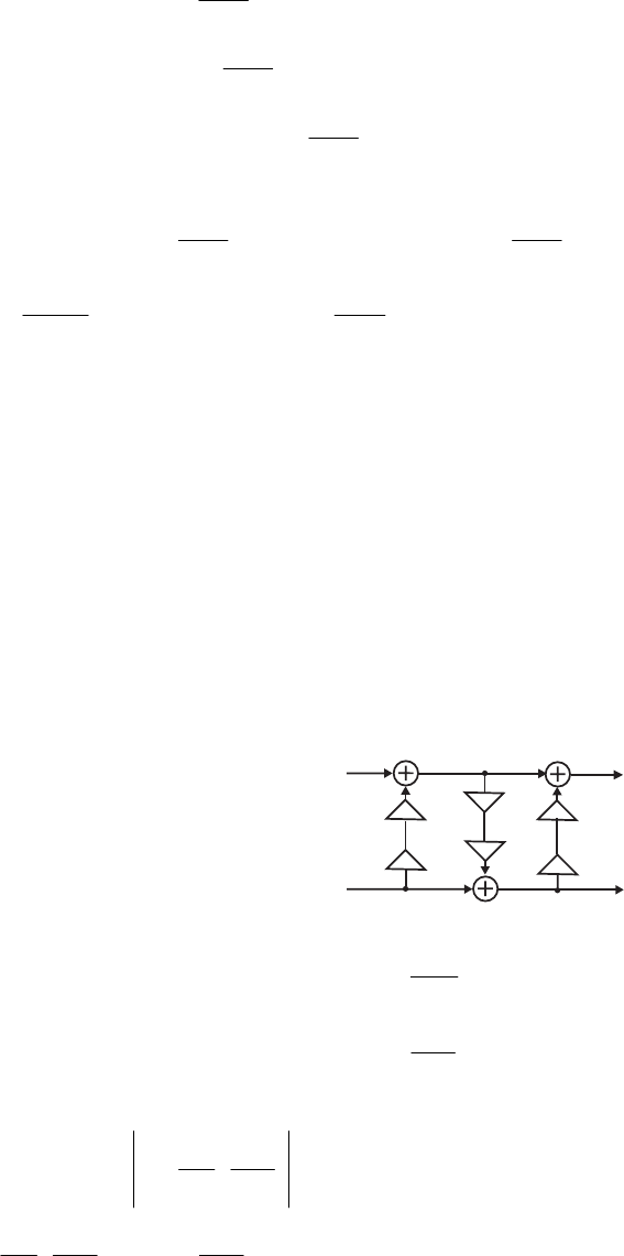
(1): },Im{
1
}Re{ rr s
c
UΨΨ −
+= (2): ,}Im{}Im{ 1sU
rr
+
=
+
ΨΨ and
(3): }.Im{
1
}Re{ 11 ++ −
+= rr s
c
UΨΨ Substituting Eqs. (1) in Eq. (2) we get
(4): }.Re{}Im{}Re{}Im{
1
}Im{}Im{ 1rrrrrr sc
s
c
sΨΨΨΨΨΨ ⋅+⋅=
⎟
⎠
⎞
⎜
⎝
⎛+
−
+=
+ Next,
substituting Eqs. (1) and (4) in Eq. (3) we get (5):
(5):
()
}Re{}Im{
1
}Re{}Im{
1
}Re{ 1rrrrr s
c
sc
s
cΨΨΨΨΨ +
−
+⋅+⋅
−
=
+
}.Re{Im}Re{}Re{}Im{}Re{}Im{
122
rrrrrr cscc
s
s
c
s
cΨΨΨΨΨΨ ⋅⋅−⋅=⋅+⋅
−
=⋅+
−
=
It thus follows that the structure of Figure P11.4 implements the multiplication of a complex
signal with the twiddle factor using only 3 real multiplications.
.
In the case of multiplication by complex twiddle factor we have
,jscWN−=
−1
()
}Im{}Re{)( rrrNr jsjcW Ψ+Ψ−=Ψ⋅=Ψ −
+1
1
()
(
)
.}Re{}Im{}Im{}Re{
r
r
r
r
scjsc
Ψ
⋅
−
Ψ
⋅
+Ψ⋅+Ψ⋅= Thus, here
}Im{}Re{}Re{
r
r
r
sc
Ψ
⋅+Ψ⋅=Ψ +1 and }.Re{}Im{}Im{
r
r
r
sc Ψ⋅
−
Ψ
⋅
=
Ψ
+
1 It follows
then that the real and imaginary parts are simply obtained by reversing the sign of of the
real and imaginary parts derived in the case of multiplication by As a result, the
corresponding structure is obtained by cascading an inverter to the real multipliers in Figure
P11.4 as indicated below:
s
.
N
W
c 1
s
____
_
c 1
s
____
_
s
Re{ψ }
r
Im{ψ }
r
Re{ψ }
r+1
Im{ψ }
r+1
U
_1_1
_1
11.15 The center frequency bin ,)(: N
kF
kfk T
c= where #
=
N of bins, and
T
F is the sampling
frequency. Inverting we have .)( ⎥
⎦
⎥
⎢
⎣
⎢
=
T
F
Nf
fk Therefore, the absolute difference from one of
the given four tones (150 Hz, 375 Hz, 620 Hz, and 850 Hz) to the center of its bin is given by
.),( ⎥
⎦
⎥
⎢
⎣
⎢
−=
T
T
F
Nf
N
F
ffNdist It follows from this equation that the distance goes to zero if
f
F
Nf
N
F
T
T=
⎥
⎦
⎥
⎢
⎣
⎢ or
T
F
Nf is an integer.
Not for sale 394

The total distance is reduced to zero if
T
i
F
Nf is an integer for .4,,1 K
=
i The minimum value
of for which this true is 500.
N
However, the total distance can be small, but nonzero, for significantly smaller values of
.N
11.16 .
1
1
)( 1−−
−
=
zW
zH k
N
k Hence, ),()(
1
1
1
)(
)( 2/
1
2/
1zVzzV
zW
z
zW
zX
zY N
k
N
N
k
N
−
−−
−
−− +=
−
+
=
−
=
where .
1
1
)( 1−−
−
=
zW
zV k
N
Or, in other words, ].[][][ 2
N
nvnvny −+=
Consider Then
:1=k.
1
1
)( 11 −−
−
=
zW
zV
N
This implies,
⎪
⎭
⎪
⎬
⎫
⎪
⎩
⎪
⎨
⎧
== +−
−−−− LL ,,,,,,1][][
)1
2
(
2/21
N
N
N
NNN
n
NWWWWnWnv µ
{
}
,,,1,,,,1 121 LL
−
−− −−= NNN WWW since ,,1 1
)1
2
(
2/ −
+−
−−=−= N
N
N
N
NWWW and
son on. Thus,
{}
.,,,1,,0,0,0][ 21
2LL −−
=− NN
NWWnv Hence,
.,0,0,0,,,,,1][][][
)1
2
(
21
2⎪
⎭
⎪
⎬
⎫
⎪
⎩
⎪
⎨
⎧
=−+= −−
−− LL
N
NNN
NWWWnvnvny
Now, consider :
2
N
k= .
1
1
)( 12/ −−
−
=
zW
zV N
N
This implies,
.,,,,,,1][][ 2
)1
2
(
222
)2/(
⎪
⎭
⎪
⎬
⎫
⎪
⎩
⎪
⎨
⎧
== ⋅+−⋅−
−
−
−LL
NN
N
NN
N
N
N
N
N
nN
NWWWWnWnv µ
Thus,
{
}
.,,,1,0,,0,0,0][ 2/
2LL N
N
N
N
NWWnv −−
=−
Now, ),1()1(,1,1,)1( 2/
2
)1
2
(
2
2/
22 −−==−=−= +−
−
−⋅− N
NN
N
N
N
N
N
N
NN
NWWWW etc. Hence,
.,,)1(1,)1(1,,1,1,1,1][
1
1
2/
2/
2
2
⎪
⎭
⎪
⎬
⎫
⎪
⎩
⎪
⎨
⎧
−+−+−−=
+=
+
=
LLL
N
N
n
Nn
N
ny Therefore, if
is even,
2/N
,,2,2,2,,1,1,1,1][
1
2/
2
⎪
⎭
⎪
⎬
⎫
⎪
⎩
⎪
⎨
⎧
−−−=
+=
=LL
N
n
Nn
ny and if is odd,
2/N
Not for sale 395
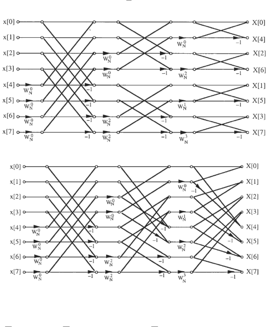
,,0,0,0,,1,1,1,1][
1
2/
2
⎪
⎭
⎪
⎬
⎫
⎪
⎩
⎪
⎨
⎧
−−=
+=
=LL
N
n
Nn
ny
11.17
11.18
11.19
∑
−
=
=
1
0
][][
N
n
nk
N
WnxkX
∑∑∑
−
=
−+
−
=
+
−
=
−+++++=
1
0
)1(
11
1
0
1
1
0
1
1
11
1
1
1
1]1[]1[][
r
N
n
krnkr
N
r
N
n
knkr
N
r
N
n
nkr
NWrnrxWnrxWnrx K
Not for sale 396

∑∑
−
=−
−
=⎟
⎟
⎟
⎟
⎟
⎠
⎞
⎜
⎜
⎜
⎜
⎜
⎝
⎛
+=
1
0
1
0
1
1
1
1
1
r
i
ki
N
rN
r
N
n
nkr
NWWinrx
DFTpoint)/(
][ .
Thus, if the -point DFT has been calculated, we need at the first stage an additional
multiplications to compute one sample of the –point DFT and, as a result,
additional multiplications are required to compute all
)/( 1
rN
)1( 1−rN][kX
Nr )1( 1−
N
samples of the
N
–point
DFT. Decomposing it further, it follows that additional Nr )1( 2
−
multiplications are needed
at the second stage, and so on. Therefore, the total number of multiply (add) operations
.)1()1()1( 1
21 NrNrNrNr ii⎟
⎠
⎞
⎜
⎝
⎛−=−++−+−= ∑=ν
ν
ν
K
11.20 An examination of the flow-graph of the 8-point DIT FFT algorithm shown in Figure 11.24
reveals that in the first stage all twiddle factors are and in the second stage the
twiddle factors are either or Hence, there are no twiddle factors with
nonunity magnitudes in the first two stages. In all succeeding stages, one of the twiddle
factors is and another one is The number of twiddle factors with
nonzero magnitudes in the -th stage, is Hence, the total number of twiddle
factors with nonzero magnitudes in an N-point radix-2 FFT algorithm is
where
1
0=
N
W
1
0=
N
W.
/jW N
N=
4
1
0=
N
W.
/jW N
N=
4
i,3≥i.22 1−
−i
,),()( 3222R
3
1≥ν−ν−
⎟
⎟
⎟
⎠
⎞
⎜
⎜
⎜
⎝
⎛
=ν ∑
ν
=
−
i
i.2ν
=N
11.21 Direct computation of
M
samples of an
N
-point DFT requires multiplications,
whereas, the Radix-2 FFT algorithm requires
2
M
N
N
2
2log multiplications. In order for a N-
point radix-2 FFT algorithm to be computationally more efficient than a direct computation
of
M
samples of an
N
-point DFT, the following inequality must hold: .log2
2⎥
⎦
⎥
⎢
⎣
⎢
>NM N
a) N = 512, M = 49, b) N = 1024, M = 72, c) N = 2048, M = 107
11.22 ).()()()( 3
2
23
1
13
0zXzzXzzXzX
−
−++= Thus, the –point DFT can be expressed as
Hence, the structural
interpretation of the first stage of the radix-3 DFT is as indicated below:
N
].[][][][ 3/2
2
3/13/0 N
k
N
N
k
N
NkXWkXWkXkX 〉〈+〉〈+〉〈=
Not for sale 397
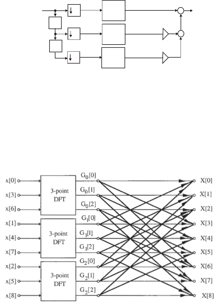
3
3
3
z
z
N
_
3
-point
DFT
N
_
3
-point
DFT
N
_
3
-point
DFT
+
X [< k > ]
1N/3
+
x
[n]
x [n]
0
x [n]
1
x [n]
2
2k
N
W
k
N
W
X [< k > ]
2N/3
X [< k > ]
0N/3
X[k]
11.23
()
kkk
n
nk WxWxWxWnxkX 6
9
3
9
0
9
8
0
9]6[]3[]0[][][ ++== ⋅
=
∑
(
)
(
)
kkkkkk WxWxWxWxWxWx 8
9
5
9
2
9
7
9
4
99 ]8[]5[]2[]7[]4[]1[ ++++++
(
)
(
)
kkkkkkk WWxWxWxWxWxWx 9
6
9
3
9
0
9
6
9
3
9
0
9]7[]4[]1[]6[]3[]0[ +++++=
⋅
⋅
(
)
kkkk WWxWxWx 2
9
6
9
3
9
0
9]8[]5[]2[ +++ ⋅,][][][ 2
9
32
9
3130 kk WkGWkGkG 〉〈+〉〈+〉〈= where
,]6[]3[]0[][ 2
33
0
3
30 kkk WxWxWxkG ++=〉〈 ⋅,]7[]4[]1[][ 2
33
0
3
31 kkk WxWxWxkG ++=〉〈
⋅
are 3-point DFTs. A flow-graph representation
of this radix-3 DIT FFT computation scheme is shown below,
,]8[]5[]2[][ 2
33
0
3
32 kkk WxWxWxkG ++=〉〈 ⋅
where the twiddle factors for computing the DFT samples are indicated below for a typical
DFT sample:
Not for sale 398
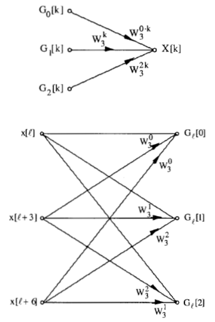
In the above diagram, the 3-point DFT computation is carried out as indicated below:
11.24
()
kkkkk
n
nk WxWxWxWxWxWnxkX 12
15
9
15
6
15
3
15
0
15
14
0
15 ]12[]9[]6[]3[]0[][][ ++++== ⋅
=
∑
(
)
kkkkk WxWxWxWxWx 13
15
10
15
7
15
4
1515 ]13[]10[]7[]4[]1[ +++++
(
)
kkkkk WxWxWxWxWx 14
15
11
15
8
15
5
15
2
15 ]14[]11[]8[]5[]2[ +++++
where ,][][][ 2
15
52
15
5150 kk WkGWkGkG 〉〈+〉〈+〉〈=
,]12[]9[]6[]3[]0[][ 4
5
3
5
2
55
0
5
50 kkkkk WxWxWxWxWxkG ++++=〉〈 ⋅
,]13[]10[]7[]4[]1[][ 4
5
3
5
2
55
0
5
51 kkkkk WxWxWxWxWxkG ++++=〉〈 ⋅ and
.]14[]11[]8[]5[]2[][ 4
5
3
5
2
55
0
5
52 kkkkk WxWxWxWxWxkG ++++=〉〈 ⋅
A flow-graph representation of this mixed-radix DIT FFT computation scheme is shown
below:
Not for sale 399
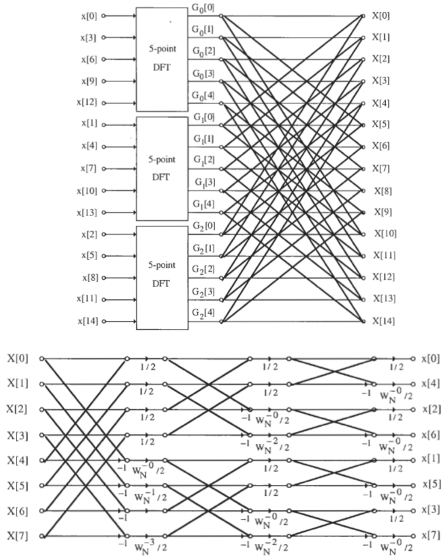
11.25
11.26 Now, by definition, ]}.[Re{]}[Im{][ nXjnXnq
+
= Its -point DFT is given by
N
Thus, .][][
1
0
∑
−
=
=
N
n
nk
N
WnqkQ
Not for sale 400

(1): ∑
−
=⎥
⎦
⎤
⎢
⎣
⎡⎟
⎠
⎞
⎜
⎝
⎛
+
⎟
⎠
⎞
⎜
⎝
⎛
=
1
0
2
sin][Re{
2
cos][Im{]}[Re{
N
mN
mk
nX
N
mk
nXkQ ππ ,
(2): ∑
−
=⎥
⎦
⎤
⎢
⎣
⎡⎟
⎠
⎞
⎜
⎝
⎛
+
⎟
⎠
⎞
⎜
⎝
⎛
−=
1
0
2
cos][Re{
2
sin][Im{]}[Im{
N
mN
mk
nX
N
mk
nXkQ ππ .
From the definition of the inverse DFT we observe .][
1
][
1
0
∑
−
=
−
=
N
m
mk
N
WmX
N
kx Hence,
(3): ,
2
sin]}[Im{
2
cos]}[Re{
1
]}[Re{
1
0
∑
−
=⎥
⎦
⎤
⎢
⎣
⎡⎟
⎠
⎞
⎜
⎝
⎛
−
⎟
⎠
⎞
⎜
⎝
⎛
=
N
mN
mk
mX
N
mk
mX
N
kx ππ
(4): .
2
sin]}[Re{
2
cos]}[Im{
1
]}[Im{
1
0
∑
−
=⎥
⎦
⎤
⎢
⎣
⎡⎟
⎠
⎞
⎜
⎝
⎛
+
⎟
⎠
⎞
⎜
⎝
⎛
=
N
mN
mk
mX
N
mk
mX
N
kx ππ
Comparing Eqs. (2) and (3) we get ,]}[Im{
1
]}[Re{ nk
kQ
N
nx =
⋅= and comparing Eqs. (1)
and (4) we get .]}[Re{
1
]}[Im{ nk
kQ
N
nx =
⋅=
11.27 Therefore,
Thus,
⎩
⎨
⎧≠−
=
=〉〈−= .0if],[
,0if],0[
][][ nnNX
nX
nXnr N
∑∑∑ −
=
−
=
−
=
−+=+==
1
1
1
1
1
0
][]0[][]0[][][
N
n
nk
N
N
n
nk
N
N
n
nk
NWnNXXWnrrWnrkR
].[][][]0[][]0[
1
0
1
1
1
1
)( kxNWnXWnXXWnXX
N
n
nk
N
N
n
nk
N
N
n
knN
N⋅==+=+= ∑∑∑ −
=
−
−
=
−
−
=
−
.][][ 1
nk
NkRnx =
⋅=
11.28 Let denote the result of convolving a length-L sequence x[n] with a length-N sequence
h[n]. The length of y[n] is then L + N – 1. Here L = 16 and N = 9, hence length of y[n] is 24.
][ny
Method #1: Direct linear convolution - For a length-L sequence x[n] and a length-N sequence
h[n],
# of real mult. = . 135)1916(92)1(2
9
11
=−−+=−−+ ∑∑ == n
N
n
nNLNn
Method # 2: Linear convolution via circular convolution - Since y[n] is of length 24, to get
the correct result we need to pad both sequences with zeros to increase their lengths to 24
before carrying out the circular convolution.
# of real mult. = 24 ×24 = 576.
Not for sale 401

Method #3: Linear convolution via radix-2 FFT - The process involves computing the 16-
point FFT G of the length-16 complex sequence ][k],[][][ nhjnxng e
+
=
where is
obtained by zero-padding h[n] to length 16. Then, the 16-point DFTs, and of
][nhe
][kX ],[kHe
][n
x
and , respectively, are recovered from . Finally, the IDFT of the product
yields y[n].
][nhe][kG
][][][ kHkXkY e
⋅=
Now, the first stage of the 16-point radix-2 FFT requires 0 complex multiplications, the
second stage requires 0 complex multiplications, the third stage requires 4 complex
multiplications, and the last stage requires 6 complex multiplications, resulting in a total of
10 complex multiplications.
# of complex mult. to implement = 10 ][kG
# of complex mult. to recover and from = 0 ][kX ][kHe][kG
# of complex mult. to form = 16 ][kY
# of complex mult. to form the IDFT of = 10 ][kY
Hence, the total number of complex mult. = 36
A direct implementation of a complex multiplication requires 4 real multiplications resulting
in a total of 4× 36 = 144 real multiplications for Method #3. However, if a complex multiply
can be implemented using 3 real multiplies (see Problem 11.13), in which case Method #3
requires a total of 3× 36 = 108 real multiplications.
11.29 Let y[n] denote the result of convolving a length-L sequence x[n] with a length-N sequence
h[n]. The length of y[n] is then L + N – 1. Here, L = 16 and N = 10, hence length of y[n] is
25.
Method #1: Direct linear convolution - For a length-L sequence x[n] and a length-N sequence
h[n],
# of real mult. = . 160)11016(102)1(2
10
11
=−−+=−−+ ∑∑ == n
N
n
nNLNn
Method # 2: Linear convolution via circular convolution - Since y[n] is of length 24, to get
the correct result we need to pad both sequences with zeros to increase their lengths to 24
before carrying out the circular convolution.
# of real mult. = 25 ×25 = 625.
Method #3: Linear convolution via radix-2 FFT - The process involves computing the 16-
point FFT G of the length-16 complex sequence ][k],[][][ nhjnxng e
+
=
where is
obtained by zero-padding h[n] to length 16. . Then, the 16-point DFTs, and of
][nhe
][kX ],[kHe
][n
x
and , respectively, are recovered from . Finally, the IDFT of the product
yields y[n].
][nhe][kG
][][][ kHkXkY e
⋅=
Now, the first stage of the 16-point radix-2 FFT requires 0 complex multiplications, the
second stage requires 0 complex multiplications, the third stage requires 4 complex
Not for sale 402

multiplications, and the last stage requires 6 complex multiplications resulting in a total of 10
complex multiplications.
# of complex mult. to implement = 10 ][kG
# of complex mult. to recover and from = 0 ][kX ][kHe][kG
# of complex mult. to form = 16 ][kY
# of complex mult. to form the IDFT of = 10 ][kY
Hence, the total number of complex mult. = 36
A direct implementation of a complex multiplication requires 4 real multiplications resulting
in a total of 4× 36 = 144 real multiplications for Method #3. However, if a complex multiply
can be implemented using 3 real multiplies (see Problem 11.13), in which case Method #3
requires a total of 3× 36 = 108 real multiplications.
11.30 (a) Since the impulse response of the filter is of length 72, the transform length N should be
greater than 72. If L denotes the number of input samples used for convolution, then L = N –
71. So for every L samples of the input sequence, an N -point DFT is computed and
multiplied with an N -point DFT of the impulse response sequence h[n] (which needs to be
computed only once), and finally an N -point inverse of the product sequence is evaluated.
Hence, the total number
M
R of complex multiplications required (assuming N is a power-
of-2) is given by .log)log( 2
2
2
71
2048 NNNN N
N
M++
⎥
⎥
⎤
⎢
⎢
⎡
=−
R
It should be noted that in developing the above expression, multiplications due to twiddle
factors of values ±1 and ± j have not been excluded. The values of
M
R for different values
of N are as follows:
1) For N = 128,
M
R = 37312, 2) For N = 256,
M
R = 28672, 3) For N = 512,
M
R =
27904, 4) For N = 1024,
M
R = 38912.
Hence, N = 512 is the appropriate choice for the transform length requiring 27904 complex
multiplications or equivalently, 27904 × 3 = 83712 real multiplications.
Since the first stage of the FFT calculation process requires only multiplications by ±1, the
total number of complex multiplications for N = 128 is actually
,27648log)log( 2
2
2
2
71
2048 =−++
⎥
⎥
⎤
⎢
⎢
⎡
=−
NN
N
MNNNNR or equivalently, 27648× 3 = 82944
real multiplications.
(b) For direct convolution, # of real multiplications =
147456)1722048(722)1(2
72
11
=−−+=−−+ ∑∑ == n
N
n
nNLNn .
11.31 (a)
Not for sale 403
,
0001000
0000100
0000010
0000001
0001000
0000100
0000010
0000001
7
8
6
8
5
8
4
8
3
8
2
8
1
8
0
8
8
⎥
⎥
⎥
⎥
⎥
⎥
⎥
⎥
⎥
⎥
⎥
⎦
⎤
⎢
⎢
⎢
⎢
⎢
⎢
⎢
⎢
⎢
⎢
⎢
⎣
⎡
=
W
W
W
W
W
W
W
W
V
,
0100000
0010000
0100000
0010000
0000010
0000001
0000010
0000001
2
8
0
8
2
8
0
8
2
8
0
8
2
8
0
8
4
⎥
⎥
⎥
⎥
⎥
⎥
⎥
⎥
⎥
⎥
⎥
⎦
⎤
⎢
⎢
⎢
⎢
⎢
⎢
⎢
⎢
⎢
⎢
⎢
⎣
⎡
=
W
W
W
W
W
W
W
W
V
,
1000000
1000000
0010000
0010000
0000100
0000100
0000001
0000001
4
8
0
8
4
8
0
8
4
8
0
8
4
8
0
8
2
⎥
⎥
⎥
⎥
⎥
⎥
⎥
⎥
⎥
⎥
⎥
⎦
⎤
⎢
⎢
⎢
⎢
⎢
⎢
⎢
⎢
⎢
⎢
⎢
⎣
⎡
=
W
W
W
W
W
W
W
W
V.
10000000
00001000
00100000
00000010
01000000
00000100
00010000
00000001
⎥
⎥
⎥
⎥
⎥
⎥
⎥
⎦
⎤
⎢
⎢
⎢
⎢
⎢
⎢
⎢
⎣
⎡
=
E
As can be seen from the above, multiplication by each matrix ,3,2,1,
=
k
k
V requires at most
8 complex multiplications.
(b) The transpose of the matrices given in Part (a) are as follows:
,
000000
000000
000000
000000
10001000
01000100
00100010
00010001
3
8
3
8
2
8
2
8
1
8
1
8
0
8
0
8
8
⎥
⎥
⎥
⎥
⎥
⎥
⎥
⎥
⎥
⎦
⎤
⎢
⎢
⎢
⎢
⎢
⎢
⎢
⎢
⎢
⎣
⎡
=
WW
WW
WW
WW
t
V
,
000000
000000
10100000
01010000
000000
000000
00001010
00000101
2
8
2
8
0
8
0
8
2
8
2
8
0
8
0
8
4
⎥
⎥
⎥
⎥
⎥
⎥
⎥
⎥
⎥
⎦
⎤
⎢
⎢
⎢
⎢
⎢
⎢
⎢
⎢
⎢
⎣
⎡
=
WW
WW
WW
WW
t
V
,
000000
11000000
000000
00110000
000000
00001100
000000
00000011
4
8
0
8
4
8
0
8
4
8
0
8
4
8
0
8
2
⎥
⎥
⎥
⎥
⎥
⎥
⎥
⎥
⎥
⎦
⎤
⎢
⎢
⎢
⎢
⎢
⎢
⎢
⎢
⎢
⎣
⎡
=
WW
WW
WW
WW
t
V .
10000000
00001000
00100000
00000010
01000000
00000100
00010000
00000001
⎥
⎥
⎥
⎥
⎥
⎥
⎥
⎦
⎤
⎢
⎢
⎢
⎢
⎢
⎢
⎢
⎣
⎡
== EEt
It is easy to show that the flow-graph representation of is precisely the 8-
point DIF FFT algorithm of Figure 11.28.
tttt 842
8VVVED =
Not for sale 404

11.32 .10,][][][]2[ 2
1
2/
2
1
2
0
2
1
0
2−≤≤+== ∑∑∑ −
=
−
=
−
=
N
N
Nn
n
N
N
n
n
N
N
n
n
NWnxWnxWnxX ll lll Replacing n by
2
N
n+ in the right-most sum we get
,][][][][]2[
1
2
0
2/
2
1
2
0
2
2
1
2
0
2∑∑∑
−
=
−
=
−
=
⎟
⎠
⎞
⎜
⎝
⎛++=++=
N
n
n
N
N
N
n
n
N
N
N
n
n
NWnxnxWnxWnxX lll
l.10 2−≤≤ N
l
Likewise,
,][][][][]14[
1
4
3
)14(
1
4
3
2
)14(
1
2
4
)14(
1
4
0
)14( ∑∑∑∑ −
=
+
−
=
+
−
=
+
−
=
++++=+
N
N
n
n
N
N
N
n
n
N
N
N
n
n
N
N
n
n
NWnxWnxWnxWnxX llll
l
where .10 4−≤≤ N
l Replacing by
n4
N
n+ in the second sum, by
n2
N
n+ in the third
sum, and by
n4
3N
n+ in the fourth sum, we get
4/
1
4
0
4
1
4
0
4]
4
[][]14[ N
N
N
N
N
n
n
N
n
N
N
n
n
N
n
NWWWW
N
nxWWnxX lll
l∑∑
−
=
−
=
++=+
.][][ 4/33
1
4
0
4
4
3
2/2
1
4
0
4
2
N
N
N
N
N
n
n
N
n
N
N
N
N
N
N
N
n
n
N
n
N
NWWWWnxWWWWnx llll ∑∑
−
=
−
=
++++
Now, and Therefore, ,,1 4/32 jWWWW N
N
N
N
N
N
N
N−==== lll ,1
2/ −=
N
N
W.
4/3 jW N
N+=
.10,][][][][]14[ 4
4/
1
4
04
3
42 −≤≤
⎭
⎬
⎫
⎩
⎨
⎧⎟
⎠
⎞
⎜
⎝
⎛+−+−
⎟
⎠
⎞
⎜
⎝
⎛+−=+ ∑
−
=
N
n
N
n
N
N
n
NNN WWnxnxjnxnxX ll l
Similarly, 4/)34(
1
4
0
)34(
4
1
4
0
)34( ][][]34[ N
N
N
n
n
N
N
N
n
n
NWWnxWnxX +
−
=
+
−
=
+∑∑ ++=+ lll
l
4/3)34(
1
4
0
)34(
4
3
2/)34(
1
4
0
)34(
2][][ N
N
N
n
n
N
N
N
N
N
n
n
N
NWWnxWWnx +
−
=
++
−
=
+∑∑ ++++ llll
4/3
1
4
0
34
4
1
4
0
34 ][][ N
N
N
N
N
n
n
N
n
N
N
N
n
n
N
n
NWWWWnxWWnx lll ∑∑
−
=
−
=
++=
Not for sale 405
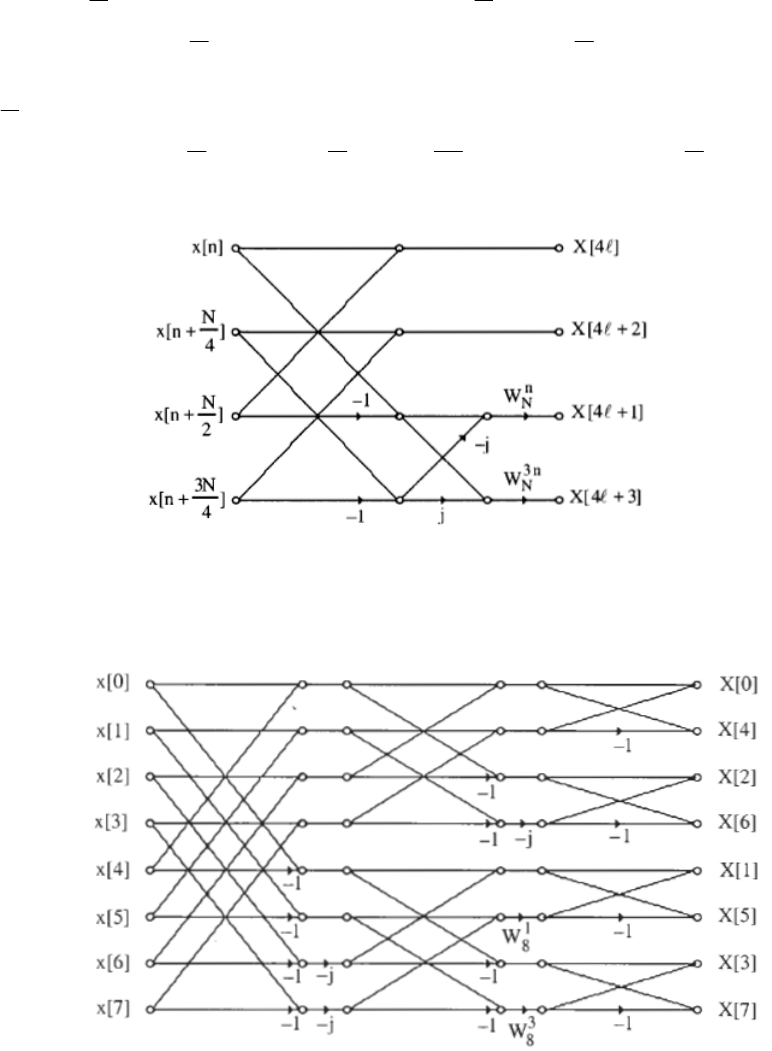
4/93
1
4
0
34
4
4/62
1
4
0
34
2][][ N
N
N
N
N
n
n
N
n
N
N
N
N
N
N
N
n
n
N
n
N
NWWWWnxWWWWnx llll ∑∑
−
=
−
=
++++
.10,][][][][ 4
4/
3
1
4
04
3
42 −≤≤
⎭
⎬
⎫
⎩
⎨
⎧⎟
⎠
⎞
⎜
⎝
⎛+−++
⎟
⎠
⎞
⎜
⎝
⎛+−= ∑
−
=
N
n
N
n
N
N
n
NNN WWnxnxjnxnx l
l
The butterfly here is as shown below which is seen to require two complex multiplications.
11.33 From the flow-graph of the 8-point split-radix FFT algorithm given below it can be seen
that the total number of complex multiplications required is 2. On the other hand, the total
number of complex multiplications required for a standard DIF FFT algorithm is also 2.
11.34 If multiplications by are ignored, the flow-graph shown below requires 8 complex
multiplications = 24 real multiplications. A radix-2 DIF 16-point FFT algorithm, on the
other hand requires 10 complex multiplications = 30 real multiplications.
1, ±± j
Not for sale 406
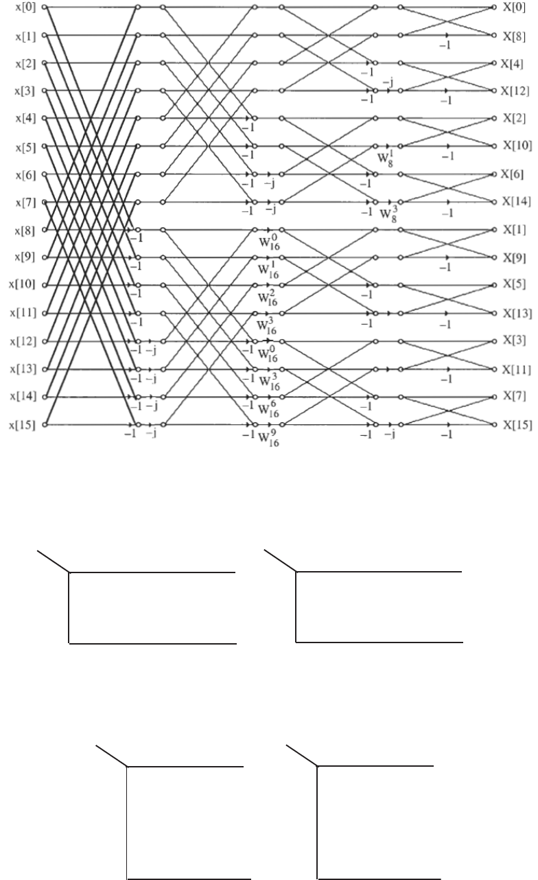
11.35 (a) N = 12. Choose and
4
1=N.3
2
=
N Thus, and
The corresponding index mappings are indicated below:
⎩
⎨
⎧≤≤
≤≤
+= ,
,
,20
30
4
2
1
21 n
n
nnn
⎩
⎨
⎧≤≤
≤≤
+= .
,
,20
30
3
2
1
21 k
k
kkk
0123
n
1
n
2
x[0] x[1] x[2] x[3]
x[4] x[5] x[6] x[7]
x[8] x[9] x[10] x[11]
0
1
2
0123
k
1
k
2
X[0] X[3] X[6]
X[1] X[4] X[7] X[10]
X[2] X[5] X[8] X[11]
0
1
2
X[9]
(b) N = 15. Choose and
3
1=N.5
2
=
N Thus, and
The corresponding index mappings are indicated below:
⎩
⎨
⎧≤≤
≤≤
+= ,
,
,40
20
3
2
1
21 n
n
nnn
⎩
⎨
⎧≤≤
≤≤
+= .
,
,40
20
5
2
1
21 k
k
kkk
012
n
1
n
2
x[0] x[1] x[2]
x[3] x[4]
x[6]
x[5]
x[7] x[8]
x[9] x[10] x[11]
0
1
2
3
4x[12] x[13] x[14]
012
k
1
k
2
X[0] X[5] X[10]
X[1] X[6]
X[2]
X[11]
X[7] X[12]
X[3] X[8] X[13]
0
1
2
3
4X[4] X[9] X[14]
Not for sale 407

(c) N = 21. Choose and
7
1=N.3
2
=
N Thus, and
The corresponding index mappings are indicated below:
⎩
⎨
⎧≤≤
≤≤
+= ,
,
,20
60
7
2
1
21 n
n
nnn
⎩
⎨
⎧≤≤
≤≤
+= .
,
,20
60
3
2
1
21 k
k
kkk
0123
n
1
n
2
x[0] x[1] x[2] x[3] x[4] x[5] x[6]
x[7] x[8] x[9] x[10] x[11]
0
1
2
45 6
x[12] x[13]
x[14] x[15] x[16] x[17] x[18] x[19] x[20]
0123
k
1
k
2
X[0] X[3] X[6] X[9] X[12] X[15] X[18]
X[1] X[4] X[7] X[10] X[13]
0
1
2
45 6
X[16] X[19]
X[2] X[5] X[8] X[11] X[14] X[17] X[20]
(d) N = 35. Choose and
7
1=N.5
2
=
N Thus, and
The corresponding index mappings are indicated below:
⎩
⎨
⎧≤≤
≤≤
+= ,
,
,40
60
7
2
1
21 n
n
nnn
⎩
⎨
⎧≤≤
≤≤
+= .
,
,40
60
5
2
1
21 k
k
kkk
0123
n1
n2
x[0] x[1] x[2] x[3] x[4] x[5] x[6]
x[7] x[8] x[9] x[10] x[11]
0
1
2
45 6
x[12] x[13]
x[14] x[15] x[16] x[17] x[18] x[19] x[20]
3x[21] x[22] x[23] x[24] x[25] x[26] x[27]
4x[28] x[29] x[30] x[31] x[32] x[33] x[34]
0123
k1
k2
X[0] X[5] X[10] X[15] X[20] X[25] X[30]
X[1] X[6] X[11] X[16] X[21]
0
1
2
45 6
X[26] X[31]
X[2] X[7] X[12] X[17] X[22] X[27] X[32]
3X[3] X[8] X[13] X[18] X[23] X[28] X[33]
4X[4] X[9] X[14] X[19] X[24] X[29] X[34]
11.36 (a) N = 12. Choose and
4
1=N.3
2
=
N
Thus,
,,, 93343 4
1=〉〈=== −
CBA
.444 3
1=〉〈= −
D⎩
⎨
⎧≤≤
≤≤
〉+〈= ,
,
,20
30
43
2
1
1221 n
n
nnn ⎩
⎨
⎧≤≤
≤≤
〉+〈= .
,
,20
30
49
2
1
1221 k
k
kkk
The corresponding index mappings are indicated below:
0123
n
1
n
2
x[0] x[3] x[6] x[9]
x[4] x[7] x[10] x[1]
x[8] x[11] x[2] x[5]
0
1
2
0123
k
1
k
2
X[0] X[9] X[6]
X[4] X[1] X[10] X[7]
X[8] X[5] X[2] X[11]
0
1
2
X[3]
(b) N = 15. Choose and
3
1=N.5
2
=
N
,,, 105535 3
1=〉〈=== −
CBA .633 5
1=〉〈= −
D
Not for sale 408

Thus,
⎩
⎨
⎧≤≤
≤≤
〉+〈= ,
,
,40
20
35
2
1
1521 n
n
nnn ⎩
⎨
⎧≤≤
≤≤
〉+〈= .
,
,40
20
610
2
1
1521 k
k
kkk
The corresponding index mappings are indicated below:
012
n
1
n
2
x[0] x[5] x[10]
x[3] x[8]
x[6]
x[13]
x[11] x[1]
x[9] x[14] x[4]
0
1
2
3
4x[12] x[2] x[7]
012
k
1
k
2
X[0] X[10] X[5]
X[6] X[1]
X[12]
X[11]
X[7] X[2]
X[3] X[13] X[8]
0
1
2
3
4X[9] X[4] X[14]
(c) N = 21. Choose and
7
1=N.3
2
=
N
Thus,
The corresponding index mappings are indicated
below:
,,, 15533373 4
1=×=〉〈=== −
CBA
.71777 3
1=×=〉〈= −
D⎩
⎨
⎧≤≤
≤≤
〉+〈= ,
,
,20
60
73
2
1
2121 n
n
nnn
⎩
⎨
⎧≤≤
≤≤
〉+〈= .
,
,20
60
715
2
1
2121 k
k
kkk
0123
n
1
n
2
x[0] x[3] x[6] x[9] x[12] x[15] x[18]
x[7] x[10] x[13] x[16] x[19]
0
1
2
45 6
x[1] x[4]
x[14] x[17] x[20] x[2] x[5] x[8] x[11]
0123
k
1
k
2
X[0] X[15] X[9] X[3] X[18] X[12] X[6]
X[7] X[1] X[16] X[10] X[4]
0
1
2
45 6
X[19] X[13]
X[14] X[8] X[2] X[17] X[11] X[5] X[20]
(d) N = 35. Choose and
7
1=N.5
2
=
N
Thus,
The corresponding index mappings are indicated
below:
,,, 15355575 7
1=×=〉〈=== −
CBA
.213777 5
1=×=〉〈= −
D⎩
⎨
⎧≤≤
≤≤
〉+〈= ,
,
,40
60
75
2
1
3521 n
n
nnn
⎩
⎨
⎧≤≤
≤≤
〉+〈= .
,
,40
60
2115
2
1
3521 k
k
kkk
0123
n1
n2
x[0] x[5] x[10] x[15] x[20] x[25] x[30]
x[7] x[12] x[17] x[22] x[27]
0
1
2
45 6
x[32] x[2]
x[14] x[19] x[24] x[29] x[34] x[4] x[9]
3x[21] x[26] x[31] x[1] x[6] x[11] x[16]
4x[28] x[33] x[3] x[8] x[13] x[18] x[23]
0123
k1
k2
X[0] X[15] X[30] X[10] X[25] X[5] X[20]
X[21] X[1] X[16] X[31] X[11]
0
1
2
45 6
X[26] X[6]
X[7] X[22] X[2] X[17] X[32] X[12] X[27]
3X[28] X[8] X[23] X[3] X[18] X[33] X[13]
4X[14] X[29] X[9] X[24] X[4] X[19] X[34]
Not for sale 409
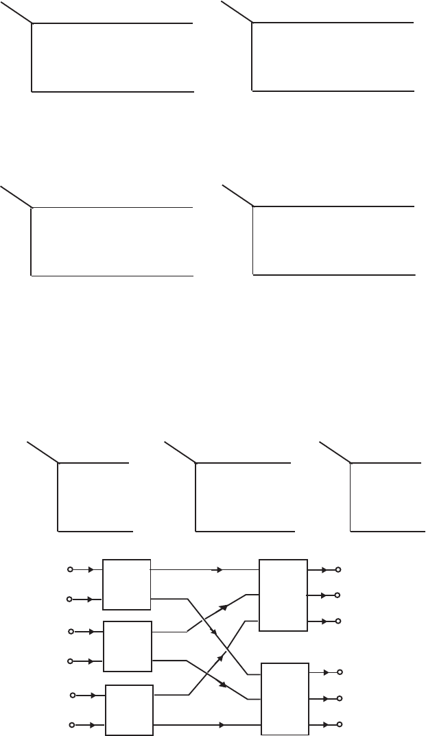
11.37 N = 12. Choose and
4
1=N.3
2
=
N
Thus,
,,, 93343 4
1=〉〈=== −
CBA .444 3
1=〉〈= −
D
⎩
⎨
⎧≤≤
≤≤
〉+〈= ,
,
,20
30
43
2
1
1221 n
n
nnn ⎩
⎨
⎧≤≤
≤≤
〉+〈= .
,
,20
30
49
2
1
1221 k
k
kkk
The corresponding index mappings are indicated below:
0123
n
1
n
2
x[0] x[3] x[6] x[9]
x[4] x[7] x[10] x[1]
x[8] x[11] x[2] x[5]
0
1
2
0123
k
1
k
2
X[0] X[9] X[6]
X[4] X[1] X[10] X[7]
X[8] X[5] X[2] X[11]
0
1
2
X[3]
Alternately,
⎩
⎨
⎧≤≤
≤≤
〉+〈= ,
,
,20
30
49
2
1
1221 n
n
nnk ⎩
⎨
⎧≤≤
≤≤
〉+〈= .
,
,20
30
43
2
1
1221 k
k
kkk
The corresponding index mappings are indicated below:
0123
k
1
k
2
X[0] X[3] X[6] X[9]
X[4] X[7] X[10] X[1]
X[8] X[11] X[2] X[5]
0
1
2
0123
n
1
n
2
x[0] x[9] x[6]
x[4] x[1] x[10] x[7]
x[8] x[5] x[2] x[11]
0
1
2
x[3]
Hence, and
],[][ kYkX 22 =.,,,],)([][ 51012612 12 K
=
〉
+
+
〈
=
+
kkYkX
11.38 (a) N = 6. Choose and
2
1=N.3
2
=
N
Thus,
,,, 33323 2
1=〉〈=== −
CBA .422 3
1=〉〈= −
D
⎩
⎨
⎧≤≤
≤≤
〉+〈= ,
,
,20
10
23
2
1
621 n
n
nnn ⎩
⎨
⎧≤≤
≤≤
〉+〈= .
,
,20
10
43
2
1
621 k
k
kkk
The corresponding index mappings are indicated below:
01
n
1
n
2
x[0] x[3]
x[2] x[5]
x[4] x[1]
0
1
2
01
n
1
k
2
G[0,0] G[1,0]
G[0,1] G[1,1]
G[0,2] G[1,2]
0
1
2
01
k
1
k
2
X[0] X[3]
X[4] X[1]
X[2] X[5]
0
1
2
3-pt
DFT
3-pt
DFT
2-pt
DFT
2-pt
DFT
2-pt
DFT
G[0,0]
G[1,0]
G[0,1]
G[1,1]
G[0,2]
G[1,2]
x
[0]
x[1]
x[2]
x[3]
x[4]
x[5]
X[0]
X[1]
X[2]
X[3]
X[4]
X[5]
Not for sale 410
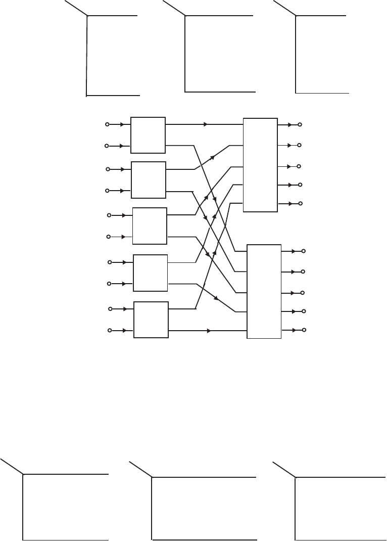
(b) N = 10. Choose and
2
1=N.5
2
=
N
Thus,
,,, 55525 2
1=〉〈=== −
CBA .622 5
1=〉〈= −
D
⎩
⎨
⎧≤≤
≤≤
〉+〈= ,
,
,20
40
25
2
1
1021 n
n
nnn ⎩
⎨
⎧≤≤
≤≤
〉+〈= .
,
,20
40
65
2
1
1021 k
k
kkk
The corresponding index mappings are indicated below:
01
n1
n2
x[0] x[5]
x[2] x[7]
0
1
x[4] x[9]
2
01
n1
k2
G[0,0] G[1,0]
G[0,1] G[1,1]
G[0,2] G[1,2]
0
1
2
01
k1
k2
X[0] X[5]
X[6] X[1]
X[2] X[7]
0
1
2
x[6] x[1]
3
x[8] x[3]
4
G[0,3] G[1,3]
3
G[0,4] G[1,4]
4
X[8] X[3]
3
X[4] X[9]
4
2-pt
DFT
2-pt
DFT
2-pt
DFT
G[0,0]
G[1,0]
x
[0]
x[1]
x[2]
x[3]
x[4]
x[5]
X[0]
X[1]
X[2]
X[3]
X[4]
X[5]
2-pt
DFT
2-pt
DFT
5-pt
DFT
5-pt
DFT
x[7]
x[9]
x[6]
x[8]
X[6]
X[8]
X[7]
X[9]
G[0,1]
G[1,1]
G[0,2]
G[1,2]
G[1,3]
G[1,4]
G[0,3]
G[0,4]
(c) N = 12. Choose and
3
1=N.4
2
=
N
Thus,
,,, 44434 3
1=〉〈=== −
CBA .333 4
1=〉〈= −
D
⎩
⎨
⎧≤≤
≤≤
〉+〈= ,
,
,30
20
34
2
1
1221 n
n
nnn ⎩
⎨
⎧≤≤
≤≤
〉+〈= .
,
,30
20
34
2
1
1221 k
k
kkk
The corresponding index mappings are indicated below:
012
k1
n2
G[0,0] G[1,0] G[2,0]
G[0,1] G[1,1] G[2,1]
G[0,2] G[1,2] G[2,2]
0
1
2
012
n1
n2
x[0] x[4] x[8]
x[3] x[7] x[11]
x[6] x[10] x[2]
0
1
2
x[9] x[1] x[5]
3G[0,3] G[1,3] G[2,3]
3
012
k1
k2
X[0] X[4] X[8]
X[3] X[7] X[11]
X[6] X[10] X[2]
0
1
2
X[9] X[1] X[5]
3
Not for sale 411
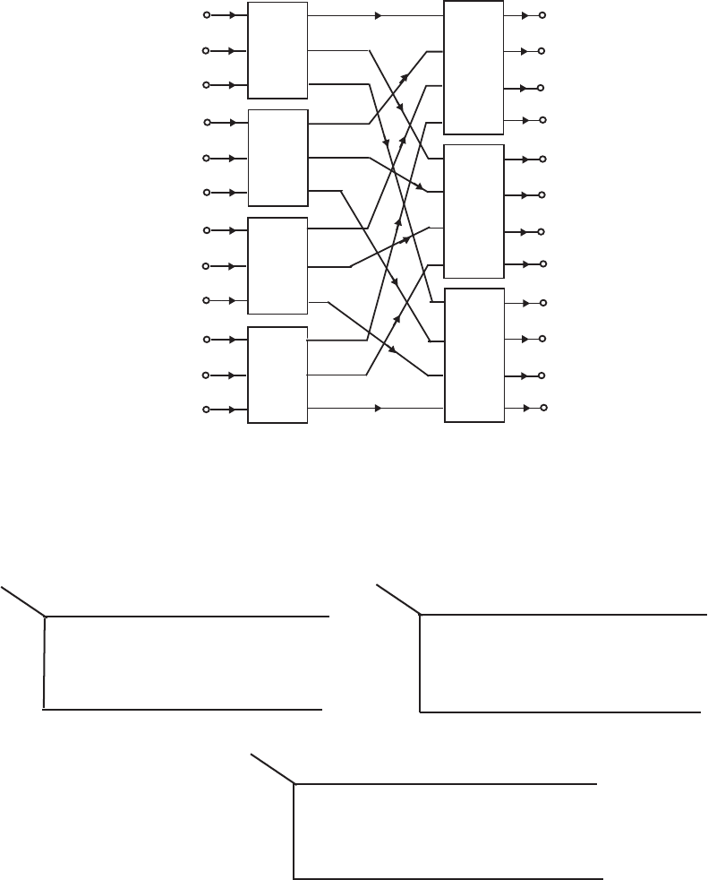
G[0,0]
G[1,0]
x[0]
x[1]
x[2]
x[3]
x[4]
x[5]
X[0]
X[1]
X[2]
X[3]
X[4]
X[5]
4-pt
DFT
x[7]
x[9]
x[6]
x[8] X[6]
X[8]
X[7]
X[9]
3-pt
DFT
3-pt
DFT
3-pt
DFT
4-pt
DFT
4-pt
DFT
x[10]
x
[11]
X[10]
X[11]
3-pt
DFT
G[0,1]
G[1,1]
G[0,2]
G[1,2]
G[1,3]
G[2,1]
G[0,3]
G[2,0]
G[2,2]
G[2,3]
(d) N = 15. Choose and
5
1=N.3
2
=
N
Thus,
,,, 103353 5
1=〉〈=== −
CBA
.655 3
1=〉〈= −
D⎩
⎨
⎧≤≤
≤≤
〉+〈= ,
,
,20
40
35
2
1
1021 n
n
nnn ⎩
⎨
⎧≤≤
≤≤
〉+〈= .
,
,20
40
610
2
1
1021 k
k
kkk
The corresponding index mappings are indicated below:
01
n1
n2
x[0]
x[5] x[2]
x[7]
0
1
x[4]
x[9]
2
01
n1
k2
G[0,0] G[1,0]
G[0,1] G[1,1]
G[0,2] G[1,2]
0
1
2
01
k1
k2
X[0]
X[5]
X[6]
X[1]
X[2]
X[7]
0
1
2
x[6]
x[1]
3
x[8]
x[3]
G[3,1]
G[2,1]
3
G[2,2] G[3,2]
4
X[8]
X[3]
3
X[4]
X[9]
2
x[12]
x[11] x[14]
x[10] x[13]
2
G[2,0] G[3,0]
24
X[10]
X[12]
X[11] X[14]
X[13]
Not for sale 412
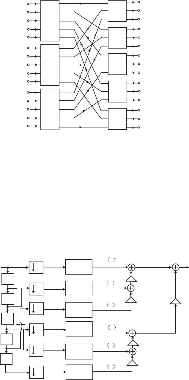
G[0,0]
G[1,0]
x[0]
x[1]
x[2]
x[3]
x[4]
x[5]
X[0]
X[1]
X[2]
X[3]
X[4]
X[5]
x[7]
x[9]
x[6]
x[8]
X[6]
X[8]
X[7]
X[9]
G[0,1]
G[1,1]
G[0,2]
G[1,2]
G[1,3]
G[1,4]
G[0,3]
G[0,4]
5-pt
DFT
5-pt
DFT
5-pt
DFT
3-pt
DFT
3-pt
DFT
3-pt
DFT
3-pt
DFT
3-pt
DFT
x[10]
x[13]
x[11]
x
[14]
x[12]
X[14]
X[11]
X[12]
X[13]
X[10]
G[2,4]
G[2,3]
G[2,2]
G[2,1]
G[2,0]
11.39 Note that 1536 = 256 × 6. Now an -point DFT , with divisible by 6, can be computed
as follows:
where
N N
][][][][][ 6/2
2
6/1
1
0
6/0 N
k
N
N
k
N
N
n
N
nk
NkXWkXWkXWnxkX 〉〈+〉〈+〉〈== ∑
−
=
],[][][ 6/5
5
6/4
4
6/3
3N
k
N
N
k
N
N
k
NkXWkXWkXW 〉〈+〉〈+〉〈+
.50,]6[][
1
6
0
6/
6/ ≤≤+=〉〈 ∑
−
=
ll
l
N
r
rk
N
NWrxkX For ,1536
=
N we thus get
where
][][][][][ 2563
3
1536
2562
2
1536
2561
1536
2560 〉〈+〉〈+〉〈+〉〈= kXWkXWkXWkXkX kkk
],[][ 2565
5
1536
2564
4
1536 〉〈+〉〈+ kXWkXW kk .50,]6[][
5111
0
256
256 ≤≤+=〉〈 ∑
=
ll
l
r
rk
WrxkX
X[k]
768
k
W
6
z
x
[n]
DFT
256-point
z
z
z
6
6
6
6
6
z
DFT
256-point
DFT
256-point
DFT
256-point
DFT
256-point
DFT
256-point
x [n]
000
x [n]
001
x [n]
010
x [n]
011
x [n]
100
x [n]
101
768
k
W
768
k
W
768
k
W
1536
k
W
k ]
X [
256
000
k ]
X [
256
001
k ]
X [
256
010
k ]
X [
256
100
k ]
X [
256
101
k ]
X [
256
011
Not for sale 413

Now an N-point FFT algorithm requires N
N
2
2log complex multiplications and
complex additions. Hence, an
NN 2
log
6
N-point FFT algorithm requires )6/(log2
12 N
N complex
multiplications and )6/(log2
6N
Ncomplex additions. In addition, we need complex
multiplications and complex additions to compute the N-point DFT X[k]. Hence, for N =
1536, the evaluation of using six 256-point FFT modules requires
N5
N5
][kX NN
N5)6/(log2
12 +
complex multiplications and
870415365)256(log128 2=×+×= NN
N5)6/(log2
6+
972815365)256(log256 2=×+×= complex additions. It should be noted that a direct
computation of the 3072-point DFT would require 6431296 complex multiplications and
2357760 complex additions.
11.40 (a) # of zero-valued samples to be added is 512 – 498 = 14.
(b) Direct computation of a 512-point DFT of a length-498 sequence requires (498)2 =
248004 complex multiplications and 497 ×498 = 247506 complex additions.
(c) A 512-point Cooley-Tukey type FFT algorithm requires 2304)512(log256 2=
×
complex
multiplications and 46308)512(log512 2
=
× complex additions.
11.41 Hence, Since
.
l
lα=z.
l
l
lα=
φ−θ
−oo jj
oo eeVA
α
is real, we have ,/,
α
=
=11 oo VA
., 00 =φ=θ oo
11.42 (a) or
)()()( zXzHzY =).]1[]0[)(]1[]0[(]2[]1[]0[ 1121
−
−
−
−
++=++ zxxzhhzyzyy Now,
]),1[]0[])(1[]0[()1()1(]2[]1[]0[)1()( 0xxhhXHyyyYzY
−
−
=
−
−
=
+−=−=
],0[]0[)()(]0[)()( 1xhXHyYzY
=
∞∞==∞=
}).1{]0[])(1[]0[{)1()1(]2[]1[]0[)1()( 2xxhhXHyyyYzY
+
+
=
=
++==
From Eqs. (6.114) and (6.115), we arrive at
),(
)(
)(
)(
)(
)(
)(
)(
)(
)( 2
22
2
1
11
1
0
00
0zY
zI
zI
zY
zI
zI
zY
zI
zI
zY ++= where ),1)(1()( 1
2
1
10
−
−−−= zzzzzI
),1)(1()( 1
2
1
01 −− −−= zzzzzI ).1)(1()( 1
1
1
02
−
−
−−= zzzzzI Therefore,
),1(
)1)(1(
)1)(1(
)(
)( 11
2
1
1
0
2
1
0
1
1
2
1
1
00
0−−
−−
−
−
−−=
−−
−−
=zz
zzzz
zzzz
zI
zI
),1(
)1)(1(
)1)(1(
)(
)( 2
1
1
2
1
1
0
1
2
1
0
11
1−
−−
−− −=
−−
−−
=z
zzzz
zzzz
zI
zI and
).1(
)1)(1(
)1)(1(
)(
)( 11
2
1
1
2
1
1
2
0
1
1
1
0
02
2−−
−−
−− +=
−−
−−
=zz
zzzz
zzzz
zI
zI Hence,
Not for sale 414

)()1()()1()()1()( 2
11
2
1
1
2
0
11
2
1zYzzzYzzYzzzY −−−−− ++−+−−=
2
2
2
1
10
2
1
1
2
2
1
0
2
1
1)()()()()()( −− ⎟
⎠
⎞
⎜
⎝
⎛+−+
⎟
⎠
⎞
⎜
⎝
⎛+−+= zzYzYzYzzYzYzY
1
2
1
2
1])1[]0[])(1[]0[(])1[]0[])(1[]0[(]0[]0[ −
⎟
⎠
⎞
⎜
⎝
⎛+++−−−+= zxxhhxxhhxh
2
2
1
2
1])1[]0[])(1[]0[(]0[]0[])1[]0[])(1[]0[( −
⎟
⎠
⎞
⎜
⎝
⎛+++−−−+ zxxhhxhxxhh
.]1[]1[])0[]1[]1[]0[(]0[]0[ 21
−
−
+++= zxhzxhxhxh
Ignoring the multiplications by
,
2
1 computation of the coefficients of require the values
of and , which can be evaluated using only 3 multiplications.
)(zY
)( 2
zY
),(),( 10 zYzY
(b) or
)()()( zXzHzY =
(
)
(
)
.]2[]1[]0[]2[]1[]0[]4[]3[]2[]1[]0[ 21214321
−
−
−
−
−
−
−− ++++=++++ zxzxxzhzhhzyzyzyzyy
Now,
]),2[4]1[2]0[])(2[4]1[2]0[()()( 2
1
0xxxhhhYzY +−+−=−=
]),2[]1[]0[])(2[]1[]0[()1()( 1xxxhhhYzY
+
−
+−=−= ],0[]0[)()( 2xhYzY =
∞
=
]),2[]1[]0[])(2[]1[]0[()1()( 3xxxhhhYzY
+
+
++==
]).2[4]1[2]0[])(2[4]1[2]0[()()( 2
1
4xxxhhhYzY ++++==
From Eqs. (6.114) and (6.115), we arrive at
),(
)(
)(
)(
)(
)(
)(
)(
)(
)(
)(
)(
)(
)(
)(
)( 4
44
4
3
33
3
2
22
2
1
11
1
0
00
0zY
zI
zI
zY
zI
zI
zY
zI
zI
zY
zI
zI
zY
zI
zI
zY ++++= where
),1)(1)(1)(1()( 1
4
1
3
1
2
1
10
−
−
−− −−−−= zzzzzzzzzI
),1)(1)(1)(1()( 1
4
1
3
1
2
1
01
−
−
−− −−−−= zzzzzzzzzI
),1)(1)(1)(1()( 1
4
1
3
1
1
1
02
−
−
−− −−−−= zzzzzzzzzI
),1)(1)(1)(1()( 1
4
1
2
1
1
1
03
−
−
−− −−−−= zzzzzzzzzI
).1)(1)(1)(1()( 1
3
1
2
1
1
1
04
−
−
−− −−−−= zzzzzzzzzI Therefore,
),1)(1(
)1)(1)(1)(1(
)1)(1)(1)(1(
)(
)( 21
2
1
1
12
1
1
0
4
1
0
3
1
0
2
1
0
1
1
4
1
3
1
2
1
1
00
0−−−
−−−−
−−−− −−=
−−−−
−−−−
=zzz
zzzzzzzz
zzzzzzzz
zI
zI
),1)(1(
)1)(1)(1)(1(
)1)(1)(1)(1(
)(
)( 2
4
1
11
3
2
1
1
4
1
1
3
1
1
2
1
1
0
1
4
1
3
1
2
1
0
11
1−−−
−−−−
−−−− −−−=
−−−−
−−−−
=zzz
zzzzzzzz
zzzzzzzz
zI
zI
),1)(1(
)1)(1)(1)(1(
)1)(1)(1)(1(
)(
)( 2
4
1
2
1
2
4
1
2
3
1
2
1
1
2
0
1
4
1
3
1
1
1
0
22
2−−
−−−−
−−−− −−=
−−−−
−−−−
=zz
zzzzzzzz
zzzzzzzz
zI
zI
),1)(1(
)1)(1)(1)(1(
)1)(1)(1)(1(
)(
)( 2
4
1
11
3
2
1
3
4
1
3
2
1
3
1
1
3
0
1
4
1
2
1
1
1
0
33
3−−−
−−−−
−−−− −+=
−−−−
−−−−
=zzz
zzzzzzzz
zzzzzzzz
zI
zI
Not for sale 415

).1)(1(
)1)(1)(1)(1(
)1)(1)(1)(1(
)(
)( 21
2
1
1
12
1
1
4
3
1
4
2
1
4
1
1
4
0
1
3
1
2
1
1
1
0
44
4−−−
−−−−
−−−− −+−=
−−−−
−−−−
=zzz
zzzzzzzz
zzzzzzzz
zI
zI Hence,
)())())( 1
4
4
1
3
4
1
21
(
3
2
0
4
4
1
32
2
1
1
(
12
1zYzzzzzYzzzzzY −−−−−−−− +−−−+−−=
)())()1( 3
4
4
1
3
4
1
21
(
3
2
2
4
4
1
2
4
5zYzzzzzYzz −−−−−− −−+++−+
)() 4
4
2
1
31
2
1
1
(
12
1zYzzzz −−−− −−+−
1
4
12
1
3
3
2
1
3
2
0
12
1
2)()()()()( −
⎟
⎠
⎞
⎜
⎝
⎛−+−+= zzYzYzYzYzY
2
4
24
1
3
3
2
2
4
5
1
3
2
0
24
1)()()()()( −
−⎟
⎠
⎞
⎜
⎝
⎛−+−++ zzYzYzYzYzY
3
4
12
1
3
6
1
1
6
1
0
12
1)()()()( −
−⎟
⎠
⎞
⎜
⎝
⎛+−++ zzYzYzYzY
.)()()()()( 4
4
24
1
3
6
1
2
4
1
1
6
1
0
24
1−
⎟
⎠
⎞
⎜
⎝
⎛+−+−+ zzYzYzYzYzY
Substituting the expressions for and in the above
equation, we then arrive at the expressions for the coefficients in terms of the
coefficients and Thus,
),(),(),(),( 3210 zYzYzYzY ),( 4
zY
]}[{ ny
]}[{ nh ]}.[{ nx ],0[]0[)(]0[ 2xhzYy
=
=
],0[]1[]1[]0[)()()()(]1[ 4
12
1
3
3
2
1
3
2
0
12
1xhxhzYzYzYzYy +=−+−=
],0[]2[]1[]1[]2[]0[)()()()()(]2[ 4
24
1
3
3
2
2
4
5
1
3
2
0
24
1xhxhxhzYzYzYzYzYy ++=−+−+= −
],1[]2[]2[]1[)()()()(]3[ 4
12
1
3
6
1
1
6
1
0
12
1xhxhzYzYzYzYy +=+−+= −
].2[]2[)()()()()(]4[ 4
24
1
3
6
1
2
4
1
1
6
1
0
24
1xhzYzYzYzYzYy =+−+−=
Hence, ignoring the multiplications by ,,,,, 6
1
4
1
4
5
3
2
12
1 and ,
24
1 computation of the
coefficients of require the values of and which can
be evaluated using only 5 multiplications.
)(zY ),(),(),(),( 3210 zYzYzYzY ),( 4
zY
11.43 or
)()()( zXzHzY =
(
)
(
)
1121 ]1[]0[]1[]0[]2[]1[]0[ −
−
−
−
++=++ zxxzhhzyzyy
.]2[[]2[])0[]1[]1[]0[(]0[]0[ 21
−
−
+++= zxhzxhxhxh Hence, ],0[]0[]0[ xhy
=
].1[]1[]2[],0[]1[]1[]0[]1[ xhyxhxhy
=
+= Now,
].1[]0[]1[]1[]0[]1[]1[]0[]0[])1[]0[])(1[]0[( yxhxhxhxhxxhh
=
+
=
−
−
+
+ As a result,
evaluation of requires the computation of 3 products, , and
. In addition, it requires 4 additions,
)()( zXzH ]1[]1[],0[]0[ xhxh
])1[]0[])(1[]0[( xxhh ++ ],1[]0[],1[]0[ xxhh +
+
and
]1[]1[]0[]0[])1[]0[])(1[]0[( xhxhxxhh
−
−++ .
11.43 Let the two length- sequences be denoted by and Denote the sequence
]}[{ nh ]}.[{ nx
N
Not for sale 416

generated by the linear convolution of and ][nh ][n
x
as Let and ].[ny ∑−
=−
=1
0][)( N
n
n
znhzH
.][)( 1
0
∑−
=−
=N
n
n
znxzX Rewrite and in the form and
where
)(zH )(zX ),()()( 1
2/
0zHzzHzH N−
+=
),()()( 1
2/
0zXzzXzX N−
+= ,][)( 1)2/(
0
0∑−
=−
=N
n
n
znhzH
,][)( 1)2/(
02
1∑−
=−
+= N
n
n
NznhzH ,][)( 1)2/(
0
0∑−
=−
=N
n
n
znxzX
.][)( 1)2/(
02
1∑−
=−
+= N
n
n
NznxzX Therefore, we can write
(
)
(
)
)()()()()( 1
2/
01
2/
0zXzzXzHzzHzY NN
−
−++=
()
)()()()()()()()( 110110
2/
00 zXzHzzXzHzXzHzzXzH NN
−
−+++=
where
),()()( 21
2/
0zYzzYzzY NN −− ++= ),()()( 000 zXzHzY
=
and ),()()()()( 01101 zXzHzXzHzY += ).()()( 112 zXzHzY
=
Note that and are
products of two polynomials of degree
)(
0zY )(
1zY
2
N each, and hence, require
2
2⎟
⎠
⎞
⎜
⎝
⎛N multiplications each.
Now, we can write
()
(
)
).()()()()()()( 1010101 zYzYzXzXzHzHzY
−
−
+
+
= Since,
is a product of two polynomials of degree
()(
)()()()( 1010 zXzXzHzH ++
)
2
N each, it can be
computed using
2
2⎟
⎠
⎞
⎜
⎝
⎛N multiplications. As a result, )()()( zXzHzY
=
can be computed using
2
2
3⎟
⎠
⎞
⎜
⎝
⎛N multiplications instead of multiplications. If is a power-of-2,
2
NN2
N is even, and
the same procedure can be applied to compute and reducing further the
number of multiplications. This process can be continued until the sequences being
convolved are of length 1 each.
),(),( 10 zYzY ),(
2zY
Let )(N
R
denote the total number of multiplications required to compute the linear
convolution of two –length sequences. Then, in the method outlined above, we have
N
)2/(3)( NN
R
R
⋅= with .1)1(
=
R
A solution of this equation is given by
.3)( 2
log N
N=R
11.45 The dynamic range of a signed –bit integer is given by Bη)12()12( )1()1( −<≤−−
−
−BB η
which for is given by
32=B).12()12( 3131 −<≤−− η
(a) For and the value of a 32-bit floating-point number is given by
Hence, the value of the largest number is and the value of the
smallest number is The dynamic range is therefore
6=E,25=M
).(2)1( 31 M
Es −
−=η,232
≈
.232
−≈ .22 32
×≈
(b) For 7=
E
and the value of a 32-bit floating-point number is given by ,24=M
).(2)1( 63 M
Es −
−=η Hence, the value of the largest number is and the value of the ,264
≈
Not for sale 417

smallest number is The dynamic range is therefore
.264
−≈ .22 64
×≈
(c) For and the value of a 32-bit floating-point number is given by
Hence, the value of the largest number is and the value of the
smallest number is The dynamic range is therefore
8=E,23=M
).(2)1( 127 M
Es −
−=η,2128
≈
.2128
−≈ .22 128
×≈
Hence, the dynamic range in a floating-point representation is much larger than that in a fixed-
point representation with the same wordlength.
11.46 A 32-bit floating-point number in the IEEE Format has E = 8 and M = 23. Also, the
exponent E is coded in a biased form as 127
−
E with certain conventions for special cases
such as E = 0, 255, and M = 0 (See page 637 of text).
Now, a positive 32-bit floating-point number represented in the “normalized” form have an
exponent in the range 0 < E < 255, and is of the form ).1(2)1( 127 M
Es ∆
−
−=η Hence, the
smallest positive number that can be represented will have E = 1, and
and has therefore a value given by
,0000
22
4434421K
bits
M=
.1018.12 38126
−
−
×≅ For the largest positive number, E
= 254, and Thus, here
.1111
22
4434421K
bits
M=22)11111(2)1( 127
22
1270 ×≈−= 4434421K
bits
∆
η
.104.3 38
×≅
Note: For representing numbers less than ,2 126
−
IEEE format uses the “de-normalized”
form where E = 0, and ).0(2)1( 126 M
s∆
−
−=η In this case, the smallest positive number
that can be represented is given by
149
22
1260 2)10000(2)1( −
≈−= 4434421K
bits
∆
η
.104013.1 45−
×≅
11.47 For a two’s-complement binary fraction the decimal equivalent for
is simply For
,
21 b
aaas −−− K
∆
0=s.2
1
i
b
ii
a−
=−
∑,1
=
s the decimal equivalent is given by
⎟
⎟
⎠
⎞
⎜
⎜
⎝
⎛+−− −
=
−
−
∑b
b
i
i
i
a22)1(
1
+−−=−+−= −−
=
−
−
=
−∑∑ )21(222
11
bb
b
i
i
i
b
i
iabi
b
i
i
a−−
=
−−
∑22
1
Hence, the decimal equivalent of is given by
.21
1
i
b
i
i
a−
=
−
∑
+−= b
aaas −−− K
21∆
.2
1
i
b
i
i
as −
=
−
∑
+−
11.48 For a ones’-complement binary fraction the decimal equivalent for ,
21 b
aaas −−− K
∆
Not for sale 418

0=s is simply For .2
1
i
b
ii
a−
=−
∑,1
=
s the decimal equivalent is given by
⎟
⎟
⎠
⎞
⎜
⎜
⎝
⎛−− ∑
=
−
−
b
i
i
i
a
1
2)1( +−−=+−= −
=
−
−
=
−∑∑ )21(22
11
b
b
i
i
i
b
i
iai
b
i
i
a−
=
−
∑2
1
Hence, the decimal equivalent of is given by
.21
1
i
b
i
i
a−
=
−
∑
+−= b
aaas −−− K
21∆
.2)21(
1
i
b
i
i
bas −
=
−
−∑
+−−
11.49 .01111153125.0,10110068750.0,11001078125.0 103102101 ∆∆∆ =
=
=
=
== ηηη
.011111101100110010
21 ∆∆∆
=
+=+ ηη
Dropping thee overflow bit and adding )( 21 ηη
+
to :
3
η
,9375.0111100011111011110)( 10321
=
=
+=++ ∆∆∆
nηη
where we have dropped the carry bit in the MSB location. Note that the final sum is correct
inspite of the overflow.
11.49 The transformation ωβαω ˆ
coscos
+
= is equivalent to ,
22
ˆˆ
⎟
⎟
⎠
⎞
⎜
⎜
⎝
⎛+
+=
+−− ωωωω
βα
jjjj eeee
which by analytic continuation can be expressed as .
2
ˆˆ
2
11
⎟
⎟
⎠
⎞
⎜
⎜
⎝
⎛+
+=
+−− zzzz βα Now, let
be a Type 1 linear-phase FIR transfer function of degree As indicated in Eq. (8.128),
can be expressed as
)(zH
.2M
)(zH ∑=
−
−⎟
⎟
⎠
⎞
⎜
⎜
⎝
⎛+
=M
n
n
Mzz
nazzH 0
1
2
][)( with a frequency response
given by with ,)](cos[)( 0
∑=
−
=M
n
njMj naeeH ω
ωω ∑=
=M
n
n
naH 0)](cos[)( ωω
(
denoting
the amplitude function or the zero-phase frequency response. The amplitude function or the
zero-phase frequency response of the transformed filter obtained by applying the mapping
is therefore given by
ωβαω ˆ
coscos += .)
ˆ
cos]([)
ˆ
(0
∑=+= M
n
n
naH ωβαω
(
Or, equivalently,
the transfer function of the transformed filter is given by
∑=
−
−⎟
⎟
⎠
⎞
⎜
⎜
⎝
⎛+
+= M
n
n
Mzz
nazzH 0
1
2
ˆˆ
][)
ˆ
(βα A convenient way to realize is to consider the
realization of the parent transfer function in the form of a Taylor structure as outlined in
Problem 8.17 which is obtained by expressing in the form
)
ˆ
(zH
)(zH
)(zH
.
2
1
][)( 0
2
∑=
−
+− ⎟
⎟
⎠
⎞
⎜
⎜
⎝
⎛+
=M
n
n
nM z
znazH Similarly, the transformed filter can be realized by
Not for sale 419
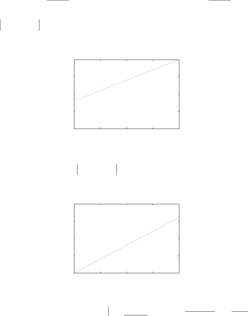
replacing each block 2
12−
+z in the Taylor structure by the block .
2
ˆ
1
ˆ
2
1−
−+
+z
zβα
Now, for a lowpass-to-lowpass transformation we can impose the condition
.)()
ˆ
(00
ˆ== =ωω ωω HH
(
(
This condition is met if 1
=
+
βα and .10 <
≤
α In this case, the
transformation reduces to .
ˆ
cos)1(cos ωααω
−
+
=
From the plot of the mapping given below, it
follows that as is varied between 0 and 1,
α.
ˆcc ωω
<
-1 -0.5 00.5 1
-1
-0.5
0
0.5
1
cos
ω
cos
ω
^
On the other hand if is desired along with a lowpass-to-lowpass transformation, we
can impose the condition
.
ˆcc ωω >
.)()
ˆ
(ˆπωπω ωω == =HH
(
(
This condition is met if and
The corresponding transformation is now given by From
the plot of the mapping given below, it follows that as is varied between 0 and 1,
αβ += 1
.11 ≤<− α.
ˆ
cos)1(cos ωααω ++=
α.
ˆcc ωω >
-1 -0.5 00.5 1
-1
-0.5
0
0.5
1
cos
ω
cos
ω
^
11.51 (a)
.][)( ∑
−
=
−
=1
0
N
n
n
znxzX ,
)(
)(
][)()( zD
zP
z
z
nxzXzX
N
n
n
z
z
z(
(
(
(
(
(
(=
⎟
⎟
⎠
⎞
⎜
⎜
⎝
⎛
α−
+α−
== ∑
−
=−
−
α−
+α−
=−
−
−
1
01
1
11
1
1
1
where ,)()]([][)( nnN
N
n
N
n
nzznxznpzP 11
1
0
1
1
0
1−−−
−
=
−
−
=
−+α−α−== ∑∑ (((( and
.)(][)( 11
1
0
1−−−
−
=
α−== ∑Nn
N
n
zzndzD (((
Not for sale 420

(b) ,
][
][
)(
)(
)(][
/
/kD
kP
zD
zP
zXkX
Nkj
Nkj
ez
ez (
(
(
(
(
(
(
(=== π
π
=
=2
2 where Nkj
ez
zPkP /
)(][ π
=
=2
(
(
(
is
the –point DFT of the sequence and
N][np Nkj
ez
zDkD /
)(][ π
=
=2
(
(
(
is the –point DFT
of the sequence
N
].[nd
(c) Let and
[]
t
Nppp ][][][ 110 −= LP
[
]
.][][][ t
Nxxx 110 −= LX Without any
loss of generality, assume in which case
4=N
()
][][][][][)( 3210 32
3
0
xxxxznpzP
n
nα−α+α−== ∑
=
−
((
(
)
1222 332212103 −
α+α+α−α++α−+ zxxxx
(
][][)(][)(][
(
)
2222 33211203 −
α−α+−α+α−α+ zxxxx
(
][][)(][)(][
(
)
.][][][][ 323 3210 −
α+α−α+α−+ zxxxx
(
Equating like powers of 1−
z
(
we can write
or It can be shown
that the elements
XQP ⋅= .
][
][
][
][
)(
][
][
][
][
⎢
⎢
⎢
⎢
⎣
⎡
αα−
α+α−α
α+α−
α−
=
⎥
⎥
⎥
⎦
⎤
⎢
⎢
⎢
⎣
⎡
23
213
1
3
2
1
0
23
22
2
p
p
p
p
)(
⎥
⎥
⎥
⎦
⎤
⎢
⎢
⎢
⎣
⎡
⎥
⎥
⎥
⎥
⎦
⎤
α−
α−α+
αα+α−
α−α
3
2
1
0
1
321
32
2
22
32
x
x
x
x
,,,
,30
≤
≤srq sr of the 4
×
4 matrix Q can be determined as follows:
(i) The first row is given by
,)(
,s
s
qα−=
0
(ii) The first column is given by ,)(
)!(!
!
)(
,rr
rr rr
Cq α−
−
=α−= 3
3
3
0 and
(iii) The remaining elements can be obtained using the recurrence relation
.
,,,, srsrsrsr qqqq 1111 −−−−
α
+α−=
In the general case, we only change the computation of the elements of the first column
using the relation .)(
)!(!
)!(
)(
,rr
r
N
rrNr
N
Cq α−
−−
−
=α−= −
1
1
1
0
11.52 The highpass transfer function can be expressed as
[]
,)()()( 10
2
1zAzAzH here −= w
1
1
03038.01
3038.0
)( −
−
+
+
=
z
z
zA and 21
21
1639.04012.01
4012.0639.0
)( −−
−−
++
++
=
zz
zz
zA . The tunable highpass
transfer function is obtained by applying the lowpass-to-lowpass transformation of Eq.
(11.115) where the tuning parameter is given by .
]2/)
ˆ
6.0sin[(
]2/)
ˆ
6.0sin[(
p
p
ωπ
ωπ
α+
−
= The tunable
highpass transfer function is then given by
[
]
,)(
ˆ
)(
ˆ
),( 10
2
1zAzAzH −=α where from Eqn.
Not for sale 421
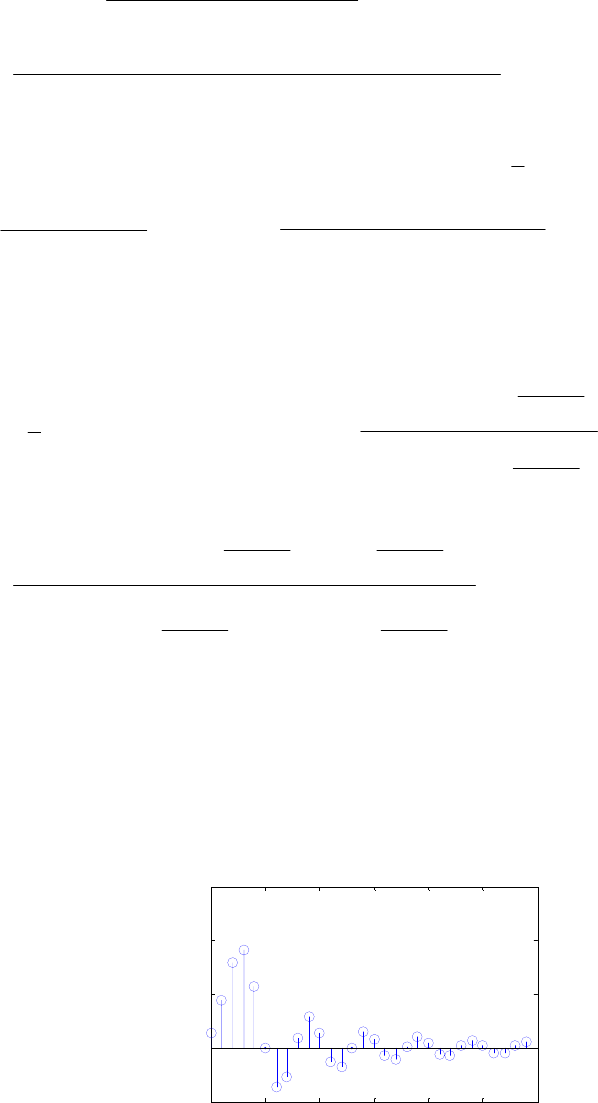
(11.119) 1
1
0]9077.03038.0[1
]9077.03038.0[
)(
ˆ−
−
−+
+−
=
z
z
zA
α
α and from Eqn. (11.123)
.
]1448.0639.0[]439.34012.0[1
]439.34012.0[]1448.0639.0[
)(
ˆ
21
21
1−−
−−
−++++
+++−
=
zz
zz
zA
αα
αα
11.53 The lowpass transfer function can be expressed as
[]
,)()()( 10
2
1zAzAzH += where
1
1
01584.01
1584.0
)( −
−
−
+−
=
z
z
zA and .
3554.04191.01
4191.03554.0
)( 21
21
1−−
−−
+−
+−
=
zz
zz
zA The tunable bandpass
transfer function is obtained by applying the lowpass-to-bandpass transformation of Eq.
(11.124) where the tuning parameter is given by o
ωβ cos
=
with denoting the center
frequency of the bandpass filter. The tunable bandpass transfer function is then given by
o
ω
[]
,)(
ˆ
)(
ˆ
),( 10
2
1zAzAzH +=α where
⎟
⎟
⎠
⎞
⎜
⎜
⎝
⎛
+
⎟
⎟
⎠
⎞
⎜
⎜
⎝
⎛
−−
=
−
−
−
−
+
+
−
+
+
−
1
1
1
1
1
1
1
1
0
1584.01
1584.0
)(
ˆ
z
z
z
z
z
z
zA
β
β
β
β
and
.
3554.04191.01
4191.03554.0
)(
ˆ
2
1
2
1
1
2
1
2
1
1
1
1
1
1
1
1
1
1
1
⎟
⎟
⎠
⎞
⎜
⎜
⎝
⎛
+
⎟
⎟
⎠
⎞
⎜
⎜
⎝
⎛
+
⎟
⎟
⎠
⎞
⎜
⎜
⎝
⎛
+
⎟
⎟
⎠
⎞
⎜
⎜
⎝
⎛
+
=
−
−
−
−
−
−
−
−
+
+
−
+
+
−
+
+
−
+
+
−
z
z
z
z
z
z
z
z
zz
zz
zA
β
β
β
β
β
β
β
β
M11.1 (a) Numerator coefficients =
[0.0528 0.0797 0.1295 0.1295 0.0797 0.0528]
Denominator coefficients =
[1.0000 -1.8107 2.4947 -1.8801 0.9537 -0.2336]
0 5 10 15 20 25 30
-0.2
0
0.2
0.4
0.6
Time index n
A
mp
lit
u
d
e
Impulse response samples
(b) Numerator coefficients =
[0.0084 -0.0335 0.0502 -0.0335 0.0084]
Denominator coefficients =
Not for sale 422
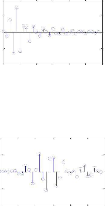
[1.0000 2.3741 2.7057 1.5917 0.4103]
0 5 10 15 20 25 30
-0.4
-0.2
0
0.2
0.4
Time index n
A
mp
lit
u
d
e
Impulse response samples
(c) Numerator coefficients = [0.0003 0 -0.0019 0 0.0057 0
-0.0095 0 0.0095 0 -0.0057 0 0.0019 0 -0.0003]
Denominator coefficients = [1.0000 1.7451 4.9282 6.1195
9.8134 9.2245 10.4323 7.5154 6.4091 3.4595
2.2601 0.8470 0.4167 0.0856 0.0299]
0 5 10 15 20 25 30
-0.4
-0.2
0
0.2
0.4
Time index n
A
mp
lit
u
d
e
Impulse response samples
M11.2 The modified MATLAB program is given below:
n = 0:60;
w = input('Normalized angular frequency vector = ');
num = input('Numerator coefficients = ');
den = input('Denominator coefficients = ');
x1 = cos(w(1)*pi*n); x2 = cos(w(2)*pi*n);
x = x1+x2;
% Generate the output sequence by filtering the input
y = filter(num,den,x);
% Plot the input and the output sequences
figure(1)
stem(n,x);
xlabel('Time index n'); ylabel('Amplitude');
title('Input sequence');
figure(2)
stem(n,y);
xlabel('Time index n'); ylabel('Amplitude');
Not for sale 423
title('Output sequence');
The plots generated by the above program for the filter of Example 9.14 for an input
composed of a sum of two sinusoidal sequences of angular frequencies, 0.3π and 0.6π, are
given below:
010 20 30 40 50 60
-2
-1
0
1
2
Time index n
Amplitude
Input sequence
010 20 30 40 50 60
-1
-0.5
0
0.5
1
Time index n
A
mp
lit
u
d
e
Output sequence
The blocking of the high-frequency signal by the lowpass filter can be demonstrated by
replacing the statement stem(n,x); with stem(n,x2); and the statement
y=filter(num,den,x); with y=filter(num,den,x2);. The plots of the high-
frequency input signal and the corresponding output are shown below:
010 20 30 40 50 60
-1
-0.5
0
0.5
1
Time index n
A
mp
lit
u
d
e
Input sequence
010 20 30 40 50 60
-0.2
-0.1
0
0.1
0.2
0.3
Time index n
A
mp
lit
u
d
e
Output sequence
M11.3 The plots generated by the program of Exercise M11.2 for the filter of Example 9.15
for an input composed of a sum of two sinusoidal sequences of angular frequencies, 0.3π and
0.6π, are given below:
010 20 30 40 50 60
-2
-1
0
1
2
Time index n
Amplitude
Input sequence
010 20 30 40 50 60
-0.6
-0.4
-0.2
0
0.2
0.4
Time index n
A
mp
lit
u
d
e
Output sequence
Not for sale 424
The blocking of the low-frequency signal by the highpass filter can be demonstrated by
replacing the statement stem(n,x); with stem(n,x1); and the statement
y=filter(num,den,x); with y=filter(num,den,x1);. The plots of the low-
frequency input signal and the corresponding output are shown below:
010 20 30 40 50 60
-1
-0.5
0
0.5
1
Time index n
A
mp
lit
u
d
e
Input sequence
010 20 30 40 50 60
-0.2
-0.1
0
0.1
0.2
Time index n
A
mp
lit
u
d
e
Output sequence
M11.4 % The factors for the transfer function of
% the lowpass filter of Example 9.14 are
% num1 = [0.0528 0.0528 0];
% den1 = [1.0000 -0.4909 0];
% num2 = [1.0000 0.6040 1.0000];
% den2 = [1.0000 -0.7624 0.5390];
% num3 = [1.0000 -0.0949 1.0000];
% den3 = [1.0000 -0.5574 0.8828];
N = input(‘Total number of sections = ‘);
for k = 1:N;
num(k,:) = input('Numerator factor = ');
den(k,:) = input('Denominator factor = ');
end
n = 0:60;
w = input('Normalized angular frequency vector = ');
x1 = cos*w(1)*pi*n); x2 = cos*w(2)*pi*n);
x = x1 + x2;
% Plot the input sequence
figure(1)
stem(n,x);
xlabel('Time index n'); ylabel('Amplitude');
title('Input sequence');
si = [0 0];
for k = 1:N;
y(k,:) = filter(num(k,:),den(k,:),x,si);
x = y(k,:);
end
% Plot the output sequence
figure(2)
stem(n,y(N,:));
xlabel('Time index n'); ylabel('Amplitude');
title('Output sequence');
Not for sale 425
The plots generated by the above program for the filter of Example 9.14 for an input
composed of a sum of two sinusoidal sequences of angular frequencies, 0.3π and 0.6π, are
given below:
010 20 30 40 50 60
-2
-1
0
1
2
Time index n
Amplitude
Input sequence
010 20 30 40 50 60
-1
-0.5
0
0.5
1
Time index n
A
mp
lit
u
d
e
Output sequence
M11.5 % The factors for the transfer function of
% the highpass filter of Example 9.15 are
% num1 = [0.0084 -0.0167 0.0084];
% den1 = [1.0000 1.3101 0.5151];
% num2 = [1.0000 -2.0000 1.0000];
% den2 = [1.0000 1.0640 0.7966];
The plots generated by the program of Exercise M11.4 for the filter of Example 9.15 for an
input composed of a sum of two sinusoidal sequences of angular frequencies, 0.3π and 0.6π,
are given below:
010 20 30 40 50 60
-2
-1
0
1
2
Time index n
Amplitude
Input sequence
010 20 30 40 50 60
-0.6
-0.4
-0.2
0
0.2
0.4
Time index n
A
mp
lit
u
d
e
Output sequence
M11.6 To apply the function direct2 to filter a sum of two sinusoidal sequences, we replace
the statement y = filter(num,den,x,si); in the MATLAB program given in the
solution of Exercise M11.2 with the statement y = direct2(num,den,x,si);. The
plots generated by running the modified program for the data given in this problem are given
below:
Not for sale 426
010 20 30 40 50 60
-2
-1
0
1
2
Time index n
Amplitude
Input sequence
010 20 30 40 50 60
-1
-0.5
0
0.5
1
Time index n
A
mp
lit
u
d
e
Output sequence
M11.7 The MATLAB program that can be used to compute all DFT samples using the function
goertzel and the function fft is as follows:
clear
N = input('Desired DFT length = ');
x = input('Input sequence = ');
for j = 1:N
Y(j)=goertzel(x,j);
end
disp('DFT samples computed using goertzel are ') ;
disp(Y)
disp('DFT samples computed using fft are ') ;
X = fft(x); disp(X);
Results obtained for two input sequences of lengths 8 and 12, respectively, are given below:
Desired DFT length = 8
Input sequence = [1 2 3 4 4 3 2 1]
DFT samples computed using goertzel are
Columns 1 through 4
20.0000 -5.8284-2.4142i -0.0000-0.0000i -0.1716-0.4142i
Columns 5 through 8
0-0.0000i -0.1716+0.4142i 0.0000-0.0000i -5.8284+2.4142i
DFT samples computed using fft are
Columns 1 through 4
20.0000 -5.8284-2.4142i 0 -0.1716-0.4142i
Columns 5 through 8
0 -0.1716+0.4142i 0 -5.828 +2.4142i
Desired DFT length = 12
Input sequence = [1 2 4 8 10 12 7 3 -4 5 0 6]
DFT samples computed using goertzel are
Columns 1 through 4
54.0000 -13.0622-21.0885i 1.5000+19.9186i -4.0000-2.0000i
Columns 5 through 8
Not for sale 427
4.5000+2.5981i -0.9378+10.0885i -18.0000+0.0000i
-0.9378-10.0885i
Columns 9 through 12
4.5000-2.5981i -4.0000+2.0000i 1.5000-19.9186i -
13.0622 +21.0885i
DFT samples computed using fft are
54.0000 -13.0622-21.0885i 1.5000+19.9186i -4.0000-2.0000i
Columns 5 through 8
4.5000+2.5981i -0.9378+10.0885i -18.0000+0.0000i
-0.9378-10.0885i
Columns 9 through 12
4.5000-2.5981i -4.0000+2.0000i 1.5000-19.9186i -
13.0622 +21.0885i
M11.8 The MATLAB program that can be used to verify the plots of Figure 11.43 is given below:
%Program_11_8.m
[z,p,k] = ellip(5,0.5,40,0.4);
a = conv([1 -p(1)],[1 -p(2)]);b =[1 -p(5)];
c = conv([1 -p(3)],[1 -p(4)]);
w = 0:pi/255:pi;
alpha = 0;
an1 = a(2) + (a(2)*a(2) - 2*(1 + a(3)))*alpha;
an2 = a(3) + (a(3) -1)*a(2)*alpha;
g = b(2) - (1 - b(2)*b(2))*alpha;
cn1 = c(2) + (c(2)*c(2) - 2*(1 + c(3)))*alpha;
cn2 = c(3) + (c(3) -1)*c(2)*alpha;
a = [1 an1 an2];b = [1 g]; c = [1 cn1 cn2];
h1 = freqz(fliplr(a),a,w); h2 = freqz(fliplr(b),b,w);
h3 = freqz(fliplr(c),c,w);
ha = 0.5*(h1.*h2 + h3);ma = 20*log10(abs(ha));
alpha = 0.1;
an1 = a(2) + (a(2)*a(2) - 2*(1 + a(3)))*alpha;
an2 = a(3) + (a(3) -1)*a(2)*alpha;
g = b(2) - (1 - b(2)*b(2))*alpha;
cn1 = c(2) + (c(2)*c(2) - 2*(1 + c(3)))*alpha;
cn2 = c(3) + (c(3) -1)*c(2)*alpha;
a = [1 an1 an2];b = [1 g]; c = [1 cn1 cn2];
h1 = freqz(fliplr(a),a,w); h2 = freqz(fliplr(b),b,w);
h3 = freqz(fliplr(c),c,w);
hb = 0.5*(h1.*h2 + h3);mb = 20*log10(abs(hb));
alpha = -0.25;
an1 = a(2) + (a(2)*a(2) - 2*(1 + a(3)))*alpha;
an2 = a(3) + (a(3) -1)*a(2)*alpha;
g = b(2) - (1 - b(2)*b(2))*alpha;
cn1 = c(2) + (c(2)*c(2) - 2*(1 + c(3)))*alpha;
cn2 = c(3) + (c(3) -1)*c(2)*alpha;
Not for sale 428
a = [1 an1 an2];b = [1 g]; c = [1 cn1 cn2];
h1 = freqz(fliplr(a),a,w); h2 = freqz(fliplr(b),b,w);
h3 = freqz(fliplr(c),c,w);
hc = 0.5*(h1.*h2 + h3);mc = 20*log10(abs(hc));
plot(w/pi,ma,'r-',w/pi,mb,'b--',w/pi,mc,'g-.');axis([0 1 -80 5]);
xlabel('Normalized frequency');ylabel('Gain, dB');
legend('b--','\alpha = 0.1 ','r-','\alpha = 0 ','g-.','\alpha = -0.25
');
M11.9 The MATLAB program that can be used to verify the plots of Figure 11.44 is given below:
%Program_11_9.m
w = 0:pi/255:pi;
wc2 = 0.31*pi;
f = [0 0.36 0.46 1];m = [1 1 0 0];
b1 = remez(50, f, m);
h1 = freqz(b1,1,w);
m1 = 20*log10(abs(h1));
n = -25:-1;
c = b1(1:25)./sin(0.41*pi*n);
d = c.*sin(wc2*n);q = (b1(26)*wc2)/(0.4*pi);
b2 = [d q fliplr(d)];
h2 = freqz(b2,1,w);
m2 = 20*log10(abs(h2));
wc3 = 0.51*pi;
d = c.*sin(wc3*n);q = (b1(26)*wc3)/(0.4*pi);
b3 = [d q fliplr(d)];
h3 = freqz(b3,1,w);
m3 = 20*log10(abs(h3));
plot(w/pi,m1,'r-',w/pi,m2,'b--',w/pi,m3,'g-.');
axis([0 1 -80 5]);
xlabel('Normalized frequency');ylabel('Gain, dB');
legend('b--','\omega_c = 0.3\pi','r-','\omega_c = 0.41\pi','g-
.','\omega_c = 0.51\pi')
M11.10 The MATLAB program to evaluate Eqs. (11.155) is given below:
%Program_11_10.m
x = 0:0.001:0.5;
y = 3.140625*x + 0.0202636*x.^2 - 5.325196*x.^3 +
0.5446778*x.^4 + 1.800293*x.^5;
x1 = pi*x;
z = sin(x1);
plot(x,y);
xlabel('Normalized angle, radians');ylabel('Amplitude');
title('Approximate sine values');grid;axis([0 0.5 0 1]);
pause
plot(x,y-z);
xlabel('Normalized angle, radians');ylabel('Amplitude');
title('Error of approximation');grid;
The plots generated by the above program are as indicated below:
Not for sale 429
00.1 0.2 0.3 0.4 0.5
0
0.2
0.4
0.6
0.8
1
Normalized an
g
le, radians
Amplitude
Approximate sine values
00.1 0.2 0.3 0.4 0.5
-2
-1
0
1
2
3
4x 10
-5
Normalized an
g
le, radians
Amplitude
Error of approximation
M11.11 The MATLAB program to evaluate Eqs. (11.156) and (11.135) is given below:
%Program_11_11.m
k = 1;
for x = 0:.01:1
op1 = 0.318253*x+0.00331*x^2-0.130908*x^3+0.068524*x^4-
0.009159*x^5;
op2 = 0.999866*x-0.3302995*x^3+0.180141*x^5-
0.085133*x^7+0.0208351*x^9;
arctan1(k) = op1*180/pi;
arctan2(k) = 180*op2/pi;
actual(k) = atan(x)*180/pi;
k = k+1;
end
subplot(211)
x = 0:.01:1;
plot(x,arctan2);
ylabel('Angle, degrees');xlabel('Tangent Values');
subplot(212)
plot(x,actual-arctan2,'--');
ylabel('Tangent Values');xlabel('error, radians');
The plots generated by the above program are as indicated below:
00.2 0.4 0.6 0.8 1
0
10
20
30
40
50
Angle, degrees
Tan
g
ent Values
00.2 0.4 0.6 0.8 1
-1
-0.5
0
0.5
1x 10
-3
T
angen
t
V
a
l
ues
error, radians
Not for sale 430

Chapter 12
12.1 Two’s Complement Truncation - Assume The relative error e
.0>xt is given by
.
222
)()( 111
M
a
M
aa
M
MMQ
x
xxQ bi
i
i
b
ii
i
i
i
i
t
∑∑∑ += −
−
==
−
−
−
−−
=
−
=
−
=
−
=
ββ
e Now will
be a minimum if all ‘s are 1 and will be a maximum if all ‘s are 0 for
i
a−i
a−.1 β
≤
≤
+ib
Thus, .
0
MM t≤≤− e
δ Since, 15.0
<
≤
M, hence .02
≤
≤
−
t
eδ
Next, consider .0
<
x Here, the relative error et is given by
.
2121
)()( 11
M
aa
M
MMQ
x
xxQ
b
ii
i
i
i
i
t
∑∑
==
−
−
−
−−++−
=
−
=
−
=
β
e As before,
.
0
MM t≤≤− e
δ In this case, ,5.01
−
≤
≤
−M and hence, .20 δ
≤
≤
t
e
Ones’ Complement Truncation - Assume The relative error e
.0>xt is given by
.
222
)()( 111
M
a
M
aa
M
MMQ
x
xxQ bi
i
i
b
ii
i
i
i
i
t
∑∑∑ += −
−
==
−
−
−
−−
=
−
=
−
=
−
=
ββ
e
.
222
)()( 111
M
a
M
aa
M
MMQ
x
xxQ bi
i
i
b
ii
i
i
i
i
t
∑∑∑ += −
−
==
−
−
−
−−
=
−
=
−
=
−
=
ββ
e Now will
be a minimum if all ‘s are 1 and will be a maximum if all ‘s are 0 for
i
a−i
a−.1 β
≤
≤
+ib
Thus, .
0
MM t≤≤− e
δ Since, 15.0
≤
≤
M, hence .02
≤
≤
−
t
eδ
Next, consider .0
<
x Here, the relative error et is given by
M
aa
M
MMQ
x
xxQ
b
ii
i
i
i
i
b
t
∑∑
==
−
−
−−
−
−−−++−−
=
−
=
−
=11
2)21(2)21(
)()(
β
β
e
.
2)22( 1
M
a
bi
i
i
b∑+= −
−
−− +−
=
β
β
Now will be a minimum if all ‘s are 1 and will be a
maximum if all ‘s are 0 for
i
a−
i
a−.1 β
≤
≤
+
ib In this case, .
0
MM t
δ
≤≤ e Since,
, hence,
15.0 −<≤− M.02
≤
≤− t
eδ
Sign-Magnitude Truncation - Assume The relative error e
.0>xt is given by
.
222
)( 111
M
a
M
aa
M
MMQ bi
i
i
b
ii
i
i
i
i
t
∑∑∑ += −
−
==
−
−
−
−=
+−
=
−
=
ββ
e Since,
, hence
15.0 −<≤− M.02
<
≤− t
eδ
Not for sale 431

Rounding - Hence,
.)( MMQ −=ε.
22 MM
δ
ε
δ≤≤− Since, ,5.01 −≤
<
−
M hence,
.δδ ≤≤− t
e
12.2 The denominator is given by .)( α
−
=
zzD Here, the pole is at where ,α
θ== j
rez α
=
r
and The components of the pole sensitivities are therefore given by
.0=θ1=
∂
∂
α
r and
.0=
∂
∂
α
θ
12.3 The denominator is given by
Comparing we get
))(()1()( 2θθ
ααβ jj erzerzzzzD −
−−=++−=
.cos2 22 rzrz +−= θ)1(cos2 αβθ
+
=
r and Taking the partials
of both sides of the last two equations we get
.
2α=r
⎥
⎦
⎤
⎢
⎣
⎡
⎥
⎥
⎦
⎤
⎢
⎢
⎣
⎡
+
=
⎥
⎦
⎤
⎢
⎣
⎡
⎥
⎦
⎤
⎢
⎣
⎡+
=
⎥
⎦
⎤
⎢
⎣
⎡
⎥
⎦
⎤
⎢
⎣
⎡−+β
α
β
α
αβθθθ θ∆
∆
∆
∆
∆
∆2
1
cos2 1
01
1
01
sin2cos2
02
2r
r
r
r
r
r, or
.
sin2
1
0
1
01
sin2cos2
02 2
sin)1(2
cos)1(
2
1
2
1
cos2
1
22
2
2⎥
⎦
⎤
⎢
⎣
⎡
⎥
⎥
⎥
⎦
⎤
⎢
⎢
⎢
⎣
⎡
+
−
=
⎥
⎦
⎤
⎢
⎣
⎡
⎥
⎥
⎦
⎤
⎢
⎢
⎣
⎡
+
⎥
⎦
⎤
⎢
⎣
⎡−
=
⎥
⎦
⎤
⎢
⎣
⎡
+
−
+
−
β
α
θ
β
α
θθθ
θ
θ
θ∆
∆
∆
∆
∆
∆
r
r
r
r
rr
rr
r
r
r
r
Hence, the components of the pole sensitivities are given by
,
sin)1(2
cos)1(
,0,
2
1
22
2
θ
θ
α
θ
βα rr
rr
r
r
+
−
=
∂
∂
=
∂
∂
=
∂
∂ and .
sin2
12
θβ
θ
r
r+
−=
∂
∂
12.4 The digital filter structure of Figure P12.1 with internal variables labeled is shown below.
Analysis yields
_1
z
cc
dd
_
1
_1
z
X
(z)Y(z)
W(z)U(z)V(z)
,
)()()(
)()()()(),()()( 11
1
11 −−
−
−
−
=
−
=⇒+=−=
zdc
zYzX
zdc
zW
zUzUzdczWzUzYzXzW and
.
)(
)()()(
1
c
zYz
zVzYzVzc =⇒=
− Also, ).()()( 1zYdzUzczV +=
−
Thus,
).(})1(1){( 2222111 zXzczczdczdczdczY
−
−
−
−− =+−−−− Hence,
.
)1(2
)(
)(
)( 222
2
dczdcz
c
zX
zY
zH ++−
==
Not for sale 432
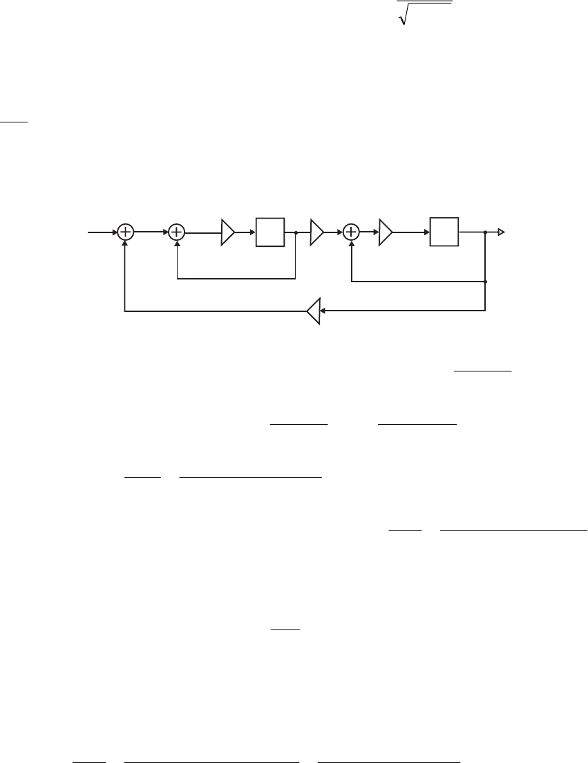
Let and Solving we get
222 )1( rdc =+ .cos θrdc =.
1
cos 2
d
d
+
=θ Thus,
θcot=d and Hence, and
.sin θrc =)(
2θθ ∆∆ cosec−=d).(cos)(sin θθθθ ∆∆∆ rc +
=
Or,
⎥
⎦
⎤
⎢
⎣
⎡
⎥
⎦
⎤
⎢
⎣
⎡−−
−=
⎥
⎦
⎤
⎢
⎣
⎡
⇒
⎥
⎦
⎤
⎢
⎣
⎡
⎥
⎦
⎤
⎢
⎣
⎡−
=
⎥
⎦
⎤
⎢
⎣
⎡
d
c
r
rr
r
d
c
∆
∆
∆
∆
∆
∆
∆
∆
θ
θθ
θ
θθ
θ
θθ
sin0
cos
sin
0
cossin 2
2cosec
cosec
.
sin0
coscos
2
sin
1
⎥
⎦
⎤
⎢
⎣
⎡
⎥
⎥
⎦
⎤
⎢
⎢
⎣
⎡
−
⋅−
=d
c
r
∆
∆
θ
θθ
θ
The digital filter structure of Figure 12.54 with internal variables labeled is shown below.
_1
z
_1
z
cc
d
d
_
X
(z)Y(z)
U(z)V(z)W(z)
Analysis yields ,
1
)(
)()()()(),()()( 1
1−
−
−
=⇒+=−=
zc
zU
zVzVzczUzVzdYzXzU and
or
),()()( 11 zWzczVzdczW −− += ).(
)1(
)(
1
)( 21
1
1
1
zU
zc
zdc
zV
zc
zdc
zW −
−
−
−
−
=
−
= As a result,
or,
)()( 1zWzczY −
=
(
)
.
)1(
)()()(
21
1
1−
−
−−
−
=
zc
zdYzXzdc
zc
zY Thus,
).(})1){(( 222221 zXzdczdczczY
−
−− =+− Hence, .
)1(2
)(
)(
)( 222
2
dczcz
dc
zX
zY
zH ++−
==
We let and . Therefore, Taking
partials we then get
,cosθrc =222 )1( rdc =+ .tansec1 22 θθ =⇒=+ dd
)(sin)(cos θθθ ∆∆∆ rrc
−
= and Thus,
).(sec2θθ ∆∆ =d
.
cos0
cossin
sec0
sincos
2
cos
1
2⎥
⎦
⎤
⎢
⎣
⎡
⎥
⎥
⎦
⎤
⎢
⎢
⎣
⎡⋅
=
⎥
⎦
⎤
⎢
⎣
⎡
⇒
⎥
⎦
⎤
⎢
⎣
⎡
⎥
⎦
⎤
⎢
⎣
⎡−
=
⎥
⎦
⎤
⎢
⎣
⎡
d
c
r
rr
r
d
c
∆
∆
∆
∆
∆
∆
∆
∆
θ
θ
θθ
θ
θθ θ
12.5 The digital filter structure of Figure P12.2 with internal variables labeled is shown on the next
page. Analysis yields )()()()()(2)( 11 zSzcYzYzSbzzSzzX =−−−+
−
−
and ).()( 2zSzzY
−
=
Thus, .
)1()2(
1
)1()2(1
)(
)(
)( 221
2
czbzzczb
z
zX
zY
zH ++−+
=
++−+
== −−
−
Let and Taking partials, we get
2
1rc =+ .cos22 θrb =−
and
)(2 rrc ∆∆ =).(sin2)(cos2 θθθ ∆∆∆ rrb
−
=− Therefore, we have
Not for sale 433
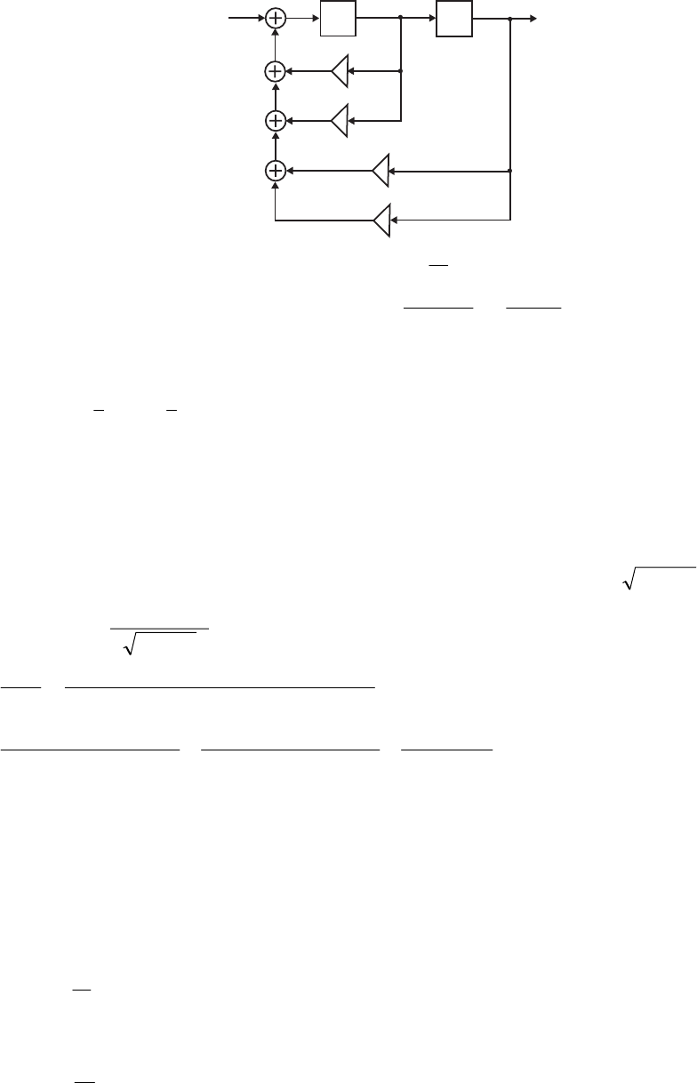
_1
z
_
1
2
b
_
c
_
_1
z
X
(z)Y(z)
S(z)
or,
⎥
⎦
⎤
⎢
⎣
⎡
⎥
⎦
⎤
⎢
⎣
⎡−
=
⎥
⎦
⎤
⎢
⎣
⎡
θθθ ∆
∆
∆
∆r
r
r
b
c
sin2cos2
02 .
0
sin2
1
tan
2
2
1
2
1
⎥
⎦
⎤
⎢
⎣
⎡
⎥
⎥
⎥
⎦
⎤
⎢
⎢
⎢
⎣
⎡
=
⎥
⎦
⎤
⎢
⎣
⎡
−b
cr
r
r
r
∆
∆
∆
∆
θ
θ
θ
From Eq. (12.19) the pole sensitivities for Figure 12.11 are given by
.
cossin
sincos
11 ⎥
⎦
⎤
⎢
⎣
⎡
⎥
⎥
⎦
⎤
⎢
⎢
⎣
⎡
−
=
⎥
⎦
⎤
⎢
⎣
⎡
β
α
θθ
θθ
θ∆
∆
∆
∆
rr
r
12.6 (a) For direct form implementation ),)()(()( 321 zzzzzzzB
−
−
−
=
where
and Thus,
,, 21 2211 θθ jj erzerz == .
3
33 θj
erz =))(cos2()( 3
2
1
11
2rzrzrzzB −+−= θ
This implies,
and
).0606.0)(7386.05625.0( 2−++= zzz
,0606.0,7386.0,5625.0cos2 3
2
1
11 ==−= rrr θ.
3πθ
=
Thus, 8594.07386.0
1==r
and .3273.0
2
5625.0
cos 1−=
−
= 0.7386
θ Now,
=
−++
=
)0606.0)(7386.05625.0(
1
)(
1
2zzz
zB
.
0606.0
2811.1
8121.02813.0
2711.06440.0
8121.02813.0
2711.06440.0
+
+
−+
−
−
+
++
+−
zjz
j
jz
j
[
]
[
]
,2417.08594.03273.0coscos 1
2
1
111 −−== θθ rrP
[
]
[]
,6440.0,6979.009449.0sin0sin 11
2
1
11 −=−== Rr θθQ and
Likewise,
.2711.0
1=X
[
]
[
]
,0037.00606.01coscos 3
2
3
333 −−== θθ rrP
[
]
[
]
,2881.1,000sin0sin 33
2
3
33 === Rr θθQ and .0
3
=
X
Thus,
=
⋅+−= BQP ∆∆ )( 11111 XRr ,0335.05535.04669.0 210 bbb ∆∆∆
+
+
−
,4467.02711.08113.0)(
1
2101111
1
1bbbRX
r
∆∆∆∆∆ −−=⋅+−= BQPθ
,0048.00781.02881.1)( 21033333 bbbXRr ∆∆∆∆∆
+
−
=⋅+−= BQP and
.0)(
1
3333
3
3=⋅+−= BQP ∆∆ RX
r
θ
Not for sale 434

(b) Cascade form: where
and Comparing we get
),()())(()( 21001
2zBzBdzczczzB =+++=
2
1
1
2
11
2
01
2
1cos2))((7386.05625.0)( 11 rzrzerzerzzzczczzB jj +−=−−=++=++= −θ
θθ
.0606.0)( 3
302 θj
erzzdzzB −=−=+=
,7386.0,5625.0cos2 2
1
11 == rr θ.,0606.0 33 πθ
=
=
r Solving the first two equations we get
8594.07386.0
1==r and .3273.0
2
5625.0
cos 1−=
−
= 0.7386
θ
Now, 8121.02813.0
6157.0
8121.02813.0
6157.0
)(
1
1jz
j
jz
j
zB ++
+
−+
−
=. Hence, and
0
1=R
.6157.0
1−=X].09449.0[]0sin[],8594.03273.0[]cos[ 11111 −=
−
=
−
=
=θθ QP r
Next, .
0606.0
1
)(
1
2+
=zzB Hence, 1
3
=
R and .0
3
=
X Here, ,1cos 33 −=
=
θP and
Thus,
.0sin 33 =−= θQ
,5818.0][][)( 010111011111 c
t
ccX
t
ccXRr ∆∆∆∆∆∆ =⋅=⋅+−= QQP
,6157.023458.0][
1
][)(
1
101011
1
101111
1
1cc
t
ccX
r
t
ccRX
r
∆∆∆∆∆∆∆ +−=⋅⋅−=⋅+−= PQPθ
0
1
)(
1
,)( 033
3
03333
3
30033333 =⋅−=⋅+−=−=⋅+−= dR
r
dRX
r
ddXRr ∆∆∆∆∆∆ QQPQP θ
.
12.7 In terms of the transfer parameters, the input-output relation of the two-pair of Figure P12.3 is
given by and
)()()( 2121111 zXtzXtzY += ).()()( 2221212 zXtzXtzY
+
=
The constraining
equation of the two-pair is given by ).()( 22 zYzX α
=
From Eq. (7.135b) we get
.
1)(
)(
)(
22
2112
11
1
1
t
tt
t
zX
zY
zH α
α
−
+== Hence, .
)1()1(
)1(
)(
2
22
2112
2
22
211222222112
t
tt
t
tttttt
zH
αα
αα
α−
=
−
+−
=
∂
∂
Substituting in
)()( 22 zYzX α=),()()( 2221212 zXtzXtzY
+
=
we get the expression for the
scaling transfer function .
1)(
)(
)(
22
21
1
2
t
t
zX
zY
zF α
α−
==
Next, from the structure given below we observe that the noise transfer function is given by
.
)(
)(
)(
0)(
1
1=
=
zX
zU
zY
zGα From the structure we also observe that
Substituting this in the transfer relations we arrive at, with
).()()( 22 zUzYzX += α
,0)(
1
=
zX
()
)()()()( 2122121 zUzXtzXtzY
+
== α and
(
)
.)()()()( 2222222 zUzYtzXtzY +
=
=
α From
these two equations we obtain, after some algebra,
).(
1
)()(
1
)(
22
12
12
22
2212
1zU
t
t
zUtzU
t
tt
zY αα
α
−
=+
−
= Hence, the noise transfer function is given by
.
1)(
)(
)(
22
12
0)(
1
1t
t
zU
zY
zG
zX α
α−
==
=
Therefore, ).()(
11
)(
22
12
22
21 zGzF
t
t
t
t
zH
αα
ααα =
−
⋅
−
=
∂
∂
Not for sale 435

12.8 (a) .)(cos41
12
1
)sin(
])1sin[(
12
1
)(
2/1
2/
1
2
2/1
⎥
⎥
⎦
⎤
⎢
⎢
⎣
⎡
⎟
⎟
⎠
⎞
⎜
⎜
⎝
⎛+
+
=
⎥
⎦
⎤
⎢
⎣
⎡⎟
⎟
⎠
⎞
⎜
⎜
⎝
⎛+
+
+
=∑
=
N
n
Nn
N
N
N
N
Wω
ω
ω
ω Since the
maximum value of is 1 and the minimum value is 0, hence,
)(cos2nω
1
2
4
1
12
1
)}(max{
2/1
=
⎥
⎦
⎤
⎢
⎣
⎡⎟
⎠
⎞
⎜
⎝
⎛+
+
=N
N
WNω and .0
12
1
)}(min{
2/1
>
⎥
⎦
⎤
⎢
⎣
⎡
+
=N
WNω Therefore,
.1)(0 ≤< ω
N
W
(b) .1141
12
1
)0(
2/1
2/
1
=
⎥
⎥
⎦
⎤
⎢
⎢
⎣
⎡
⎟
⎟
⎠
⎞
⎜
⎜
⎝
⎛+
+
=∑
=
N
m
NN
W .1141
12
1
)(
2/1
2/
1
=
⎥
⎥
⎦
⎤
⎢
⎢
⎣
⎡
⎟
⎟
⎠
⎞
⎜
⎜
⎝
⎛+
+
=∑
=
N
m
NN
Wπ
(c) .
)sin(
))1sin((
12
1
lim
12
lim)(lim
2/1
⎥
⎦
⎤
⎢
⎣
⎡+
⋅
+
+
+
=∞→∞→∞→ ω
ω
πN
NN
N
W
NN
N
N Since
,1))1sin(( ≤+ ωN .0
)sin(
))1sin((
12
1
lim =
+
⋅
+
∞→ ω
ωN
N
N
Hence, 2
1
)(lim =
∞→ π
N
N
W.
12.9 From Eq. (12.75), )(log2081.160206.6 10/ Kb
DA
−
+
=
SNR dB. For a constant value of K,
an increase in b by 1 bit, increases the by 6.0206 dB and an increase in b by 2 bits,
increases the by 12.0412 dB.
DA /
SNR
DA /
SNR
If
K = 4 and b = 7, then 9122.46)4(log2081.1670206.6 10/ =
−
+
×
=
DA
SNR dB. Therefore,
for K = 4 and b = 9, 95.5804.1291.46
/
=
+
=
DA
SNR dB; for K = 4 and b = 11,
dB; for K = 4 and b = 13, 99.7004.1295.58
/=+=
DA
SNR 04.1299.70
/
+
=
DA
SNR =
83.03 dB; for K = 4 and b = 15, 08.9504.1203.83
/
=
+
=
DA
SNR dB.
If
K = 6 and b = 7, then 3902.43)6(log2081.1670206.6 10/ =
−
+
×
=
DA
SNR dB. Therefore,
for K = 6 and b = 9, 43.5504.1239.43
/
=
+
=
DA
SNR dB; for K = 6 and b = 11,
dB; for K = 6 and b = 13, 47.6704.1243.55
/=+=
DA
SNR 04.1247.67
/
+
=
DA
SNR =
79.51 dB; for K = 6 and b = 15, 56.9104.1251.79
/
=
+
=
DA
SNR dB.
If
K = 8 and b = 7, then 8922.40)8(log2081.1670206.6 10/ =
−
+
×
=
DA
SNR dB. Therefore,
for K = 8 and b = 9, 93.5204.1289.40
/
=
+
=
DA
SNR dB; for K = 8 and b = 11,
dB; for K = 8 and b = 13, 97.6404.1293.52
/=+=
DA
SNR 04.1297.64
/
+
=
DA
SNR =
77.01 dB; for K = 8 and b = 15, 05.89104.1201.77
/
=
+
=
DA
SNR dB.
Not for sale 436

12.10 (a) ,)(
1
)(
1111
BzFCaC
az
za
C
az
A
zH k
N
k
k
N
k
kk
N
kk
k
k
N
kk
k+=−
+
+
=
+
=∑∑∑∑ ====
where ,
12
k
k
ka
A
C−
=
,
1
)(
k
k
kaz
za
zF +
+
= and .
1
∑
=
−=
N
k
kk aCB
(b) dzzBzFCBzFC
j
dzzzHzH
j
N
k
kk
C
N
k
kk
C
o1
1
1
1
112 )()(
2
1
)()(
2
1−
=
−
=
−−
⎥
⎥
⎦
⎤
⎢
⎢
⎣
⎡+
⎥
⎥
⎦
⎤
⎢
⎢
⎣
⎡+== ∑
∫∑
∫ππ
σ
dzzzFCBdzzzFCBdzzB
jC
N
C
k
N
k
k
C
∫
∑
∫
∑
∫−−
=
−
=
−++= 11
1
1
1
12 )()(
2
1[l
l
l
π
]
1
11
)()( dzzzFzFCC
C
k
N
k
N
k−
== ∫
∑∑
+ll
l
.
Now, ,
2
1212 BdzzB
jC
=
∫−
π ,)(
2
1
,)(
2
1111 ll adzzzF
j
adzzzF
jC
k
C
k== ∫∫ −−−
ππ and
.
1
1
)()(
2
122
1
l
l
l
laa
aaaa
dzzzFzF
jk
k
k
C
k−
+−−
=
∫−
π Therefore,
.
1
1
2
11
22
1
22 ∑∑∑===−
+−−
++=
N
k
N
k
k
k
k
N
k
ko aa
aaaa
aCBB
ll
l
l
σ Since, we have ,
1
BaC k
N
k
k−=
∑
=
∑∑
== −
+−−
+−=
N
k
N
k
k
k
k
oCC
aa
aaaa
B
11
22
22
1
1
l
l
l
l
l
σ
∑∑∑∑ ==== −
+−−
+−=
N
k
N
k
k
k
k
N
k
N
kk aa
aaaa
CCaaCC
11
22
11 1
1
ll
l
l
l
l
ll
∑∑
== ⎥
⎥
⎦
⎤
⎢
⎢
⎣
⎡−
−
+−−
=
N
k
N
k
k
k
k
kaa
aa
aaaa
CC
11
22
1
1
ll
l
l
l ∑∑
== ⎥
⎥
⎦
⎤
⎢
⎢
⎣
⎡−
−
+−−
−
⋅
−
=
N
k
N
k
k
k
k
k
kaa
aa
aaaa
a
A
a
A
11
22
22 1
1
11
ll
l
l
l
l
.
11
)1)(1(
11 1111
22
22 ∑∑∑∑ ==== −
=
⎥
⎥
⎦
⎤
⎢
⎢
⎣
⎡
−
−−
−
⋅
−
=
N
k
N
k
k
N
k
N
k
k
k
k
aa
AA
aa
aa
a
A
a
A
ll
l
ll
l
l
l (A)
Further, ∑∑∑∑∑−
=+=
−
=+== −
+
−
+
−
=
1
11
1
1112
2
2
11
1
NN
kk
k
N
k
N
kk
k
N
kk
k
oaa
AA
aa
AA
a
A
ll l
l
ll
l
σ
.
1
2
1
1
1112
2∑∑∑−
=+== −
+
−
=
N
k
N
kk
k
N
kk
k
aa
AA
a
A
ll
l
(c) See Eq. (A).
Not for sale 437

12.11 (a) .
2.0
9.18
6.0
1.16
1
)6.0)(2.0(
)4)(2(
)(
1−
+
−
−
+=
−−
+
−
=zzzz
zz
zH Making use of Eq. (12.87) and Table
12.4, we get )2.0()6.0(1
)9.18()1.16(2
)2.0(1
)9.18(
)6.0(1
)1.16(
12
2
2
2
2
,1 ×−
×−×
+
−
+
−
−
+=
n
σ
5411.865682.6910937.3720156.4051
=
−++= .
Output of Program 12_4.m is 86.5412.
(b) .
5.08.0
2174.217826.18
5.0
2174.0
5.0
25
)5.08.0)(5.0)(12(
)142)(13(2
)( 22
2
2++
−−
+
−
−
+
+
=
+++−
+−−
=
zz
z
zz
zzzz
zzz
zH
Making use of Eq. (12.87) and Table 12.4, we get 2
2
2
2
2,2 )5.0(1
)2174.0(
)5.0(1
)25(
−
+
−
=
n
σ
2
)5.0(5.0)5.0(8.01
)]5.0()2174.21(7826.18[252
25.01
)2174.0(252
−×+−×+
−
×
−
+
−
××
+
+
−××
+
2
)5.0(5.05.08.01
]5.0)2174.21(7826.18[)2174.0(2
×+×+
×
−
+−×−×
+
22222
222
)8.0(])5.0(1[)8.0()5.0(2])5.0(1[
8.0)5.01()2174.21()7826.18(2)5.01(])2174.21()7826.18[(
×+−××+−
×−×−×−×−−×−+−
+
........ 4841973121170437998717256369608063003333833
=
+
+
−
−+=
22
2
2, 22 2
2
22
(25) (0.2174) 2(25)( 0.2174) 2(25)( 18.7826 ( 21.2174)*( 0.5))
1 (0.5) 1 (0.5) 1 0.25 1 0.8( 0.5) 0.5( 0.5)
2( 0.2174)( 18.7826 ( 21.2174)*(0.5))
1 0.8(0.5) 0.5(0.5)
[( 18.7826) ( 21.2174) ](1
n
σ
−−+−
=+ + +
−− + +−+−
−−+−
+++
−+−
+
−
2
22 2 2 2
0.5) 2( 18.7826)( 21.2174)(1 0.5)(0.8)
(1 0.5 ) 2(0.5)(0.8) (1 0.5 )(0.8)
833.3333 0.0630 8.6960 563.7172 8.3799 704.1211 973.4841
−−− − −
−+ −+
= +−− −− =
Output of Program 12_4.m is 973.4831.
(c) .
4.06.0
6.04.1
1
4.06.0
)1(
)( 22
2
3++
+
+=
++
+
=
zz
z
zz
z
zH Making use of Eq. (12.87) and Table 12.4,
we get 2222
222
2,3 )6.0]()4.0(1[)6.0(4.02])42.0(1[
)4.01(6.06.04.12])4.0(1][)6.0()4.1[(
1+−××+−
−×××−−+
+=
n
σ
.3333.33333.21 =+=
Output of Program 12_4.m is 3.3333.
(d) .
4.0
4917.4
5.0
1667.4
8.0
825.0
1
)5.0)(8.0_)(4.0(
)1)(25.1)(5.2(
)(
4−
−
+
+
+
+
−
+=
+−
+
+−
=zzzzzz
zzz
zH
Not for sale 438
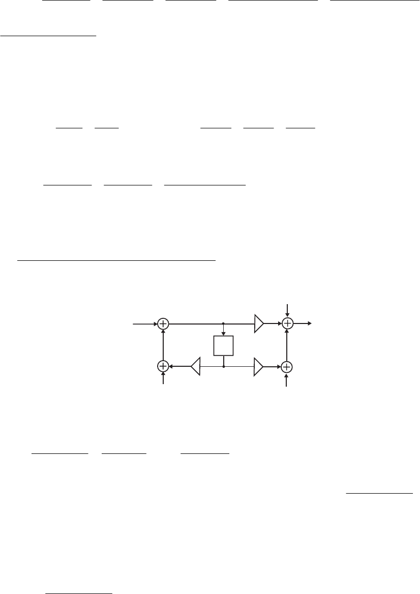
Making use of Eq. (12.87) and Table 12.4, we get
32.01
4917.4825.02
4.01
1667.4825.02
)4.0(1
)4917.4(
)5.0(1
)1667.4(
)8.0(1
)825.0(
12
2
2
2
2
2
2,4 +
××
+
−
××
+
−
+
−
+
−
+=
n
σ
1926.316146.54584.110183.241485.238906.11
25.01
1667.44917.42 −+−+++=
+
××
+
.021.13=
Output of Program 12_4.m is 13.0208.
12.12 .)( γβ +
+
+
+= z
C
z
B
AzH .
βγ−
+
γ−
+
β−
+=σ 1
2
11 2
2
2
2
22 BCCB
A
n For ,8.0,6.0
−
=
=γβ
,2,4,3 =−== CBA we get
..
).().(
)(
).().(
300334
80601
242
801
2
601
4
32
2
2
2
22 =
×−−
×−×
+
−
+
−
+=σn
Output of Program 12_4.m is 34.3003.
12.13 (a) Quantization of products before addition
Direct Form II - The noise model is shown below.
z 1
_
x
[n]
e [n]
1
e [n]
2
e [n]
3
y[n]
d
_1p1
p0
The noise transfer function from the noise source to the filter output is
][
1ne
.
1
)(
1
101
0
1
10
1
1
1
10
1dz
dpp
p
dz
pzp
zd
zpp
zG +
−
+=
+
+
=
+
+
=−
−
The corresponding normalized noise variance at the output is .
1
)(
2
1
2
101
2
0
2
1d
dpp
p−
−
+=σ
The noise transfer function from the noise sources and to the filter output is
][
2ne ][
3ne
.1)()( 32 == zGzG The corresponding normalized noise variance at the output is
.1
2
3
2
2== σσ Hence the total noise variance at the output is
2
3
2
2
2
1
2σσσσ ++=
o
2
1
2
101
2
01
)(
2
d
dpp
p−
−
++= .
Not for sale 439

Direct Form IIt - The noise model is shown below.
z 1
_
x
[n]
e [n]
1
e [n]
2
e [n]
3
y[n]
d
_1
p1
p0
Analyzing the structure, we have that .
1
)()()(
)( 1
1
1
32
1
1
−
−−
+
++
=
zd
zzEzEzzE
zY
The noise transfer function from to the filter output is
][
1ne
.
1
1
)(
)(
)(
1
1
1
1
0)()(
1
1
32 dz
zd
z
zE
zY
zG
zEzE +
=
+
== −
−
==
The corresponding normalized noise
variance at the output is .
1
1
2
1
2
1d−
=σ
The noise transfer function from to the filter output is
][
2ne
.1
1
1
)(
)(
)(
1
1
1
1
1
0)()(
1
2
31 dz
d
dz
z
zd
zE
zY
zG
zEzE +
−=
+
=
+
== −
==
The corresponding
normalized noise variance at the output is .
1
1
1
12
1
2
1
2
1
2
2dd
d
−
=
−
+=
σ
The noise transfer function from to the filter output is ][
3ne
.
1
1
)(
)(
)(
1
1
1
1
0)()(
3
3
21 dz
zd
z
zE
zY
zG
zEzE +
=
+
== −
−
==
The corresponding normalized noise
variance at the output is .
1
1
2
1
2
3d−
=σ
Hence the total noise variance at the output is .
1
3
2
1
2
3
2
2
2
1
2
d
o−
=++= σσσσ
(b) Quantization of products after addition
Direct Form II -
2
3
2
2
2
1
2σσσσ ++=
o2
1
2
101
2
01
)(
2
d
dpp
p−
−
++= .
Direct Form IIt - .
1
3
2
1
2
3
2
2
2
1
2
d
o−
=++= σσσσ
12.14 (a) Quantization of products before addition
Not for sale 440
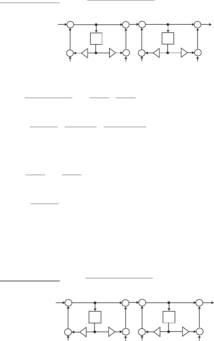
Cascade Structure #1: .
)6.01)(2.01(
)3.01)(4.01(
)( 11
11
−−
−−
−+
−+
=
zz
zz
zG The noise model of this structure is as
below
_0.2
z1
_
+
+
+
+
z1
_
+
+
+
+
0.4 0.6 _0.3
e [n]
1e [n]
2e [n]
3e [n]
4
x
[n]y[n]
The noise transfer function from the noise source to the filter output is
][
1ne
.
2.0
125.0
6.0
375.0
1
)6.0)(2.0(
)3.0)(4.0(
)(
1+
+
−
+=
−+
−+
=zzzz
zz
zG
The corresponding normalized noise variance at the output is
.3197.1
)2.0(6.01
125.0375.20
)2.0(1
)125.0(
)6.0(1
)375.0(
12
2
2
2
2
,1 =
−×−
×
+
−−
+
−
+=
n
σ
Output of Program 12_4.m is 1.3197.
The noise transfer function from the noise sources and to the filter output is
][
2ne ][
3ne
.
6.0
3.0
1
6.0
3.0
)(
2−
+=
−
−
=zz
z
zG
The normalized noise variance at the output due to each of these noise sources is
.1406.1
)6.0(1
)3.0(
12
2
2,2 =
−
+=
n
σ
Output of Program 12_4.m is 1.1406.
The noise transfer function from the noise source to the filter output is
][
4ne .1)(
4
=
zG
The corresponding normalized noise variance at the output is
.1
2,4 =
n
σ
Hence the total normalized noise variance at the output is
.6009.42 2,4
2,2
2
,1
2=++= nnn
nσσσσ
Cascade Structure #2: .
)6.01)(2.01(
)4.01)(3.01(
)( 11
11
−−
−−
−+
+−
=
zz
zz
zG The noise model of this structure is as
below:
_
0.2
z
1
_
+
+
+
+
z
1
_
+
+
+
+
0.4
0.6
_
0.3
e [n]
1
e [n]
2
e [n]
3
e [n]
4
x
[n]y[n]
Not for sale 441
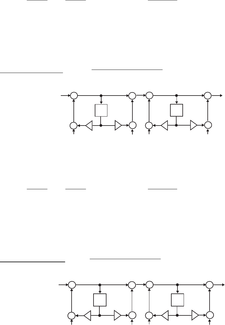
3197.1
2
,1 =
n
σas in Structure#1.
The noise transfer function from the noise sources and to the filter output is
][
2ne ][
3ne
.
6.0
1
1
6.0
4.0
)(
2−
+=
−
+
=zz
z
zG Hence, .5625.2
)6.0(1
)1(
12
2
2,2 =
−
+=
n
σ
Output of Program 12_4.m is 2.5625.
The noise transfer function from the noise source to the filter output is
][
4ne .1)(
4
=
zG
The corresponding normalized noise variance at the output is
.1
2,4 =
n
σ
Hence the total normalized noise variance at the output is .4447.72 2,4
2,2
2
,1
2=++= nnn
nσσσσ
Cascade Structure #3: .
)2.01)(6.01(
)4.01)(3.01(
)( 11
11
−−
−−
+−
+−
=
zz
zz
zG The noise model of this structure is as
below:
_0.2
z1
_
+
+
+
+
z1
_
+
+
+
+0.4
0.6 _0.3
e [n]
1e [n]
2e [n]
3e [n]
4
x
[n]y[n]
3197.1
2
,1 =
n
σas in Structure#1.
The noise transfer function from the noise sources and to the filter output is
][
2ne ][
3ne
.
2.0
2.0
1
2.0
4.0
)(
2+
+=
+
+
=zz
z
zG Hence, .0417.1
)2.0(1
)2.0(
12
2
2,2 =
−
+=
n
σ
Output of Program 12_4.m is 1.0417.
The noise transfer function from the noise source to the filter output is
][
4ne .1)(
4
=
zG
The corresponding normalized noise variance at the output is
.1
2,4 =
n
σ
Hence the total normalized noise variance at the output is
.4031.42 2,4
2,2
2
,1
2=++= nnn
nσσσσ
.
)2.01)(6.01(
)3.01)(4.01(
)( 11
11
−−
−−
+−
−+
=
zz
zz
z
Cascade Structure #4: G The noise model of this structure is as
below:
_0.2
z1
_
+
+
+
+
z1
_
+
+
+
+
0.4
0.6 _0.3
e [n]
1e [n]
2e [n]
3e [n]
4
x
[n]y[n]
3197.1
2
,1 =
n
σas in Structure#1.
The noise transfer function from the noise sources and to the filter output is
][
2ne ][
3ne
Not for sale 442
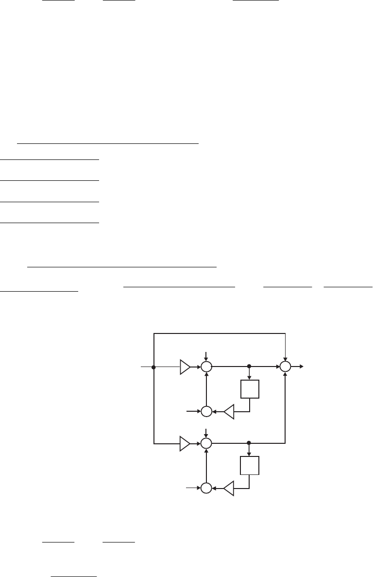
.
2.0
5.0
1
2.0
3.0
)(
2+
−
+=
+
−
=zz
z
zG Hence, .2604.1
)2.0(1
)5.0(
12
2
2,2 =
−
−
+=
n
σ
Output of Program 12_4.m is 1.2604.
The noise transfer function from the noise source to the filter output is
][
4ne .1)(
4
=
zG
The corresponding normalized noise variance at the output is
.1
2,4 =
n
σ
Hence the total normalized noise variance at the output is
.8405.42 2,4
2,2
2
,1
2=++= nnn
nσσσσ
Hence, the Cascade Structure #3 has the smallest round off noise variance.
(b) Quantization of products after addition. From the results of Part (a)
Cascade Structure #1: σ
.4603.3
2,4
2,2
2
,1
2=++= nnn
nσσσ
Cascade Structure #2:
.8822.4
2,4
2,2
2
,1
2=++= nnn
nσσσσ
Cascade Structure #3:
.614.3
2,4
2,2
2
,1
2=++= nnn
nσσσσ
Cascade Structure #4:
.5801.3
2,4
2,2
2
,1
2=++= nnn
nσσσσ
Hence, the Cascade Structure #1 has the smallest round off noise variance.
12.15 (a) Quantization of products before addition.
.
2.01
625.0
6.01
625.0
1
)6.01)(2.01(
)3.01)(4.01(
)( 1111
11
−−−−
−−
+
−
+
−
+=
−+
−+
=
zzzz
zz
zG Parallel Form #1:
The noise model of this structure is shown below:
z1
_
++
0.2
_
+
z1
_
+
+
x
[n]y[n]
e [n]
1
e [n]
2
e [n]
3
e [n]
4
0.625
0.6
0.6
The noise transfer function from the noise sources and to the filter output is
][ne1][ne2
.
6.0
6.0
1
6.0
)(
2−
+=
−
=zz
z
zG The corresponding normalized noise variance at the output is
.5625.1
)6.0(1
)6.0(
12
2
2,2 =
−
+=
n
σ
Not for sale 443
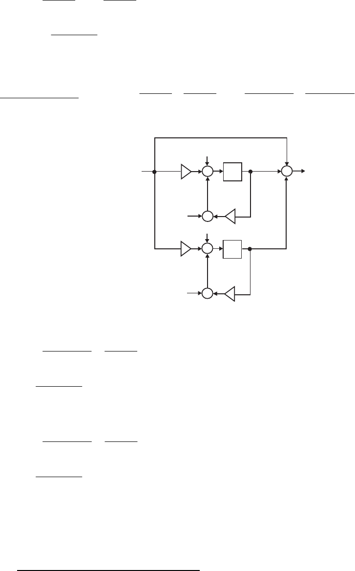
The noise transfer function from the noise sources and to the filter output is
][ne3][ne4
.
2.0
2.0
1
2.0
)(
4+
−
+=
+
=zz
z
zG The corresponding normalized noise variance at the output is
.0417.1
)2.0(1
)2.0(
12
2
2,2 =
−
−
+=
n
σ
Hence the total noise variance at the output is .2804.522 2,4
2,2
2=+= nn
nσσσ
Parallel Form #2: .
2.01
125.0
6.01
375.0
1
2.0
125.0
6.0
375.0
1)( 1
1
1
1
−
−
−
−
+
+
−
+=
+
+
−
+=
z
z
z
z
zz
zG
The noise model of this structure is shown below:
++
0.2
_
+
+
+
x
[n]y[n]
e [n]
1
e [n]
2
e [n]
3
e [n]
4
0.375
0.125
0.6
z1
_
z1
_
The noise transfer function from the noise sources and to the filter output is
][ne1][
2ne
.
6.0
1
6.01
)( 1
1
2−
=
−
=−
−
z
z
z
zG The corresponding normalized noise variance at the output is
.5625.1
)6.0(1
)1(
2
2
2,2 =
−
=
n
σ
The noise transfer function from the noise sources and to the filter output is
][ne3][ne4
.
2.0
1
2.01
)( 1
1
4+
=
+
=−
−
z
z
z
zG The corresponding normalized noise variance at the output is
.0417.1
)2.0(1
)1(
2
2
2,2 =
−
=
n
σ
Hence the total noise variance at the output is
.2804.522 2,4
2,2
2=+= nn
nσσσ
Therefore, both parallel forms have identical round off noise variances.
(b) Quantization of products after addition. From the results of Part (a)
Not for sale 444

Parallel Form #1:
.6402.2
2,4
2,2
2=+= nn
nσσσ
Parallel Form #2:
.6402.2
2,4
2,2
2=+= nn
nσσσ
Hence, both parallel forms have the same round off noise variances.
21
21
15.02.01
6.04.02
)( −−
−−
−+
−−
=
zz
zz
zH
12.16 (a) Direct Form II realization is shown below along with the
noise model.
z
1
_
z
1
_
+
++
+
_
0.2
0.6
_
+
+
+
+
+
0.4
_
2
x
[n]y[n]
1
e [n]
2
e [n]
3
e [n]
4
e [n]
5
e [n]
0.15
The noise transfer function from and to filter output is
][
1ne ][
2ne
.
3.0
675.0
5.0
125.0
2
15.02.01
6.04.02
)()( 21
21
1−
−
+
+
−
+=
−+
−−
== −−
−−
zz
zz
zz
zHzG The corresponding normalized
noise variance at the output is
..
).(.
).().(
).(
).(
).(
).(
)(
,66834
50301
675012502
301
6750
501
1250
22
2
2
2
22
1=
−×−
−×−×
+
−
−
+
−−
−
+=σ n
Output of Program 12_4.m is 4.6683.
The noise transfer function from the noise sources , to the filter output is
][
3ne ][
4ne
.1)(
3=zG
The corresponding normalized noise variance at the output is
.1
2,3 =
n
σ
Hence the total noise variance at the output is .1898.1232 2,3
2
,1
2=+= nn
nσσσ
(b) Cascade Form: .
)5.01)(3.01(
)4568.01)(6568.01(2
)( 11
11
−−
−−
+−
+−
=
zz
zz
zH There are more than 2 possible
cascade realizations. We consider here only two structures.
Cascade Form #1 - .
5.01
4568.01
3.01
6568.01
2)( 1
1
1
1
⎟
⎟
⎠
⎞
⎜
⎜
⎝
⎛
+
+
⎟
⎟
⎠
⎞
⎜
⎜
⎝
⎛
−
−
=−
−
−
−
z
z
z
z
zH The noise model of this
structure is on the next page.
Not for sale 445
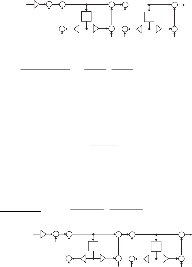
_
0.6568 0.5
_
z
1
_
+
+
+
+
z
1
_
+
+
+
+
0.3 0.4568
2
x
[n]
+
y[n]
e [n]
1
e [n]
2
e [n]
3
e [n]
4
e [n]
5
The noise transfer function from and to filter output is
][
1ne ][
2ne
.
3.0
3375.0
5.0
0625.0
1
15.02.01
3.02.01
)( 21
21
1−
−
+
+
−
+=
−+
−−
=−−
−−
zz
zz
zz
zG The corresponding normalized noise
variance at the output is
.1671.1
)5.0(3.01
)3375.0()0625.0(
)3.0(1
)3375.0(
)5.0(1
)0625.0(
)1( 2
2
2
2
22
,1 =
−×−
−×−
+
−
−
+
−−
−
+=
n
σ
Output of Program 12_4.m is 1.1671.
The noise transfer function from and to filter output is ][
3ne ][
4ne
.
5.0
0432.0
1
5.0
4568.0
5.01
4568.01
)( 1
1
3+
−
+=
+
+
=
+
+
=−
−
zz
z
z
z
zG The corresponding normalized noise
variance at the output is .0025.1
)5.0(1
)0432.0(
)1( 2
2
22,3 =
−
−
+=
n
σ
Output of Program 12_4.m is 1.0025.
The noise transfer function from the noise source to the filter output is ][
5ne .1)(
5
=
zG
The corresponding normalized noise variance at the output is
.1
2,3 =
n
σ
Hence the total noise variance at the output is
3392.522 2,5
2
,3
2
,1
2=++= n
nn
nσσσσ
Cascade Form #2 - .
5.01
6568.01
3.01
4568.01
2)( 1
1
1
1
⎟
⎟
⎠
⎞
⎜
⎜
⎝
⎛
+
−
⎟
⎟
⎠
⎞
⎜
⎜
⎝
⎛
−
+
=−
−
−
−
z
z
z
z
zH The noise model of this
structure is shown below:
_0.6568
0.5
_
z1
_
+
+
+
+
z1
_
+
+
+
+
0.3 0.4568
2
x
[n]+y[n]
e [n]
1
e [n]
2e [n]
3e [n]
4e [n]
5
The noise transfer function from and to filter output is same as for the Cascade
Structure #1. Hence, the corresponding normalized noise variance at the output is
][
1ne ][
2ne
.1671.1
2
,1 =
n
σ
Not for sale 446
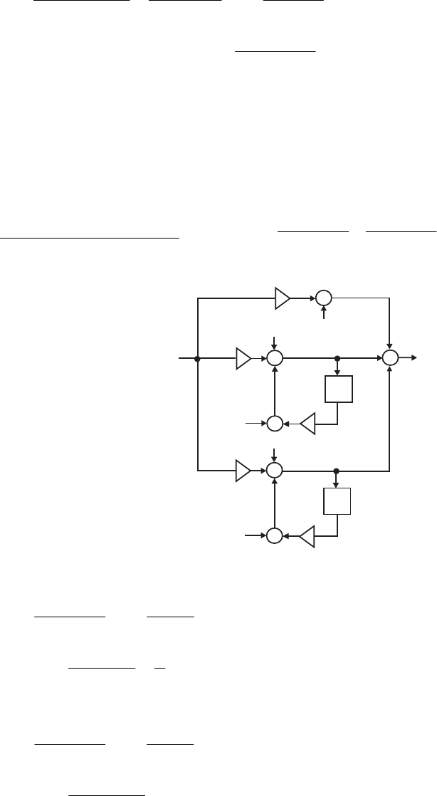
The noise transfer function from and to filter output is ][
3ne ][
4ne
.
5.0
1568.1
1
5.0
6568.0
5.01
6568.01
)( 1
1
3+
−
+=
+
+
=
+
−
=−
−
zz
z
z
z
zG The corresponding normalized noise
variance at the output is .7842.2
)5.0(1
)1568.1(
)1( 2
2
22,3 =
−
−
+=
n
σ
Output of Program 12_4.m is 2.7842.
The noise transfer function from the noise source to the filter output is ][
5ne .1)(
5
=
zG
The corresponding normalized noise variance at the output is
.1
2,5 =
n
σ
Hence the total noise variance at the output is
.1184.622 2,5
2
,3
2
,1
2=++= n
nn
nσσσσ
(c) Parallel Form I realization - .
3.01
25.2
5.01
25.0
4)( 11 −− −
−
+
+
+=
zz
zH The noise model of this
structure is shown below:
++
0.5
_
+
+
+
x
[n]y[n]
e [n]
1
e [n]
2
e [n]
3
e [n]
4
z1
_
z1
_
+
e [n]
5
2.25
_
0.3
4
0.25
The noise transfer function from and to filter output is
][
2ne ][
3ne
.
5.0
5.0
1
5.01
1
)( 1
2+
−
+=
+
=−z
z
zG The corresponding normalized noise variance at the output is
.
3
4
)5.0(1
)5.0(
)1( 2
2
22,2 =
−
−
+=
n
σ
The noise transfer function from and to filter output is
][
4ne ][
5ne
.
3.0
3.0
1
3.01
1
)( 1
4−
+=
−
=−z
z
zG The corresponding normalized noise variance at the output is
.0989.1
)3.0(1
)3.0(
)1( 2
2
22,4 =
−−
+=
n
σ
The noise transfer function from the noise source to the filter output is
][
1ne .1)(
1
=
zG
Not for sale 447
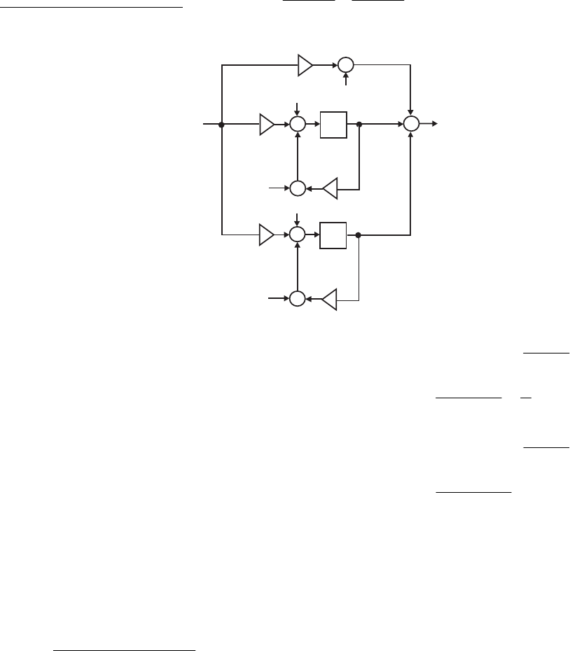
The corresponding normalized noise variance at the output is
.1
2
,1 =
n
σ
Hence the total noise variance at the output is
.8645.52 2,4
2,2
2
,1
2=++= nnn
nσσσσ
Parallel Form II realization. - .
3.0
675.0
5.0
125.0
2)( −
−
+
+
−
+= zz
zH The noise model of this structure
is shown below:
++
0.5
_
+
+
+
x
[n]y[n]
e [n]
1
e [n]
2
e [n]
3
e [n]
4
z1
_
z1
_
+
e [n]
5
0.125
_
0.675
_
0.3
2
The noise transfer function from and to filter output is
][
2ne ][
3ne .
5.0
1
)(
2+
=z
zG The
corresponding normalized noise variance at the output is .
3
4
)5.0(1
1
2
2,2 =
−
=
n
σ
The noise transfer function from and to filter output is
][
4ne ][
5ne .
3.0
1
)(
4−
=z
zG The
corresponding normalized noise variance at the output is .0989.1
)3.0(1
1
2
2,4 =
−−
=
n
σ
The noise transfer function from the noise source to the filter output is
][
1ne .1)(
1
=
zG
The corresponding normalized noise variance at the output is .1
2
,1 =
n
σ
Hence the total noise variance at the output is
.8645.52 2,4
2,2
2
,1
2=++= nnn
nσσσσ
12.17 21
21
15.02.01
6.04.02
)( −−
−−
−+
−−
=
zz
zz
zH . Using Program 8_5.m, the Gray-Markel realization of H(z) is
found to be as shown on top of the next page where
,28.0,6.0,15.0,2353.0 21
'
12 −=−=−== ααdd .9759.1
3
=
α
(a) For quantization of products before addition, the noise model is shown on the next page:
Not for sale 448

α
1
α
2
α
3
z
1
_
z
1
_
d
2
_
d
2
d
1
'
d
1
'
_
x
[n]
y[n]
e [n]
1
e [n]
2
e [n]
3
e [n]
4
e [n]
5
Analyzing the above structure, we obtain the noise transfer function for each noise source,
:71],[ ≤≤ inei,
15.02.01
6.04.02
)()( 21
21
1−−
−−
−+
−−
==
zz
zz
zHzG
21
22
2
1
1
2
'
1
2
2
13
'
12
215.02.01
)1(])1([)(
)( −−
−−
−+
−++−++
=
zz
zdzddd
zG ααααα
,
15.02.01
5668.01950.00179.2
21
21
−−
−−
−+
−−
=
zz
zz
21
2
2
'
1
2
2
1
1
232
'
12
2
2
12
315.02.01
)1(])1([
)( −−
−−
−+
−+−−−+
=
zz
zdddzdddd
zG ααααα
,
15.02.01
02.00416.128.0
21
21
−−
−−
−+
+−−
=
zz
zz
.1)()()(,6.0)( 76514
=
=
=−== zGzGzGzG α
Using Program 12_4.m, we get
Hence, the total normalized output noise variances = 4.6683 + 4.459 + 1.1199 + 0.36 + 3(1) =
13.6072.
,6683.4
2
,1 =
n
σ,4549.4
2,2 =
n
σ,1199.1
2,3 =
n
σ.36.0
2,4 =
n
σ
(b) The realization along with the noise model for the quantization of products after addition is the
same as in Part (a).
The noise transfer functions from the noise sources and are
and respectively and are given in Part (a). Their corresponding noise variances
were also derived in Part (a) and are given by
],[],[ 32 nene ],[
4ne ),(
2zG
),(
3zG ),(
4zG
,4549.4
2,2 =
n
σ,1199.1
2,3 =
n
σ.36.0
2,4 =
n
σ
Hence, the total normalized output noise variances = 4.459 + 1.1199 + 0.365 + 1 = 6.9389
12.18 The noise model is shown on the next page. The noise transfer function from to the
output is
][
1ne
.
)1(
1
1
1
1
)(
211
2
211
211
2
2
2
21
1
1
2
1ddzdz
ddzd
ddzdz
z
zddzd
z
zG ++
++
−=
++
−
=
++
−
=−−
−
Its
corresponding output noise variance is given by
Not for sale 449
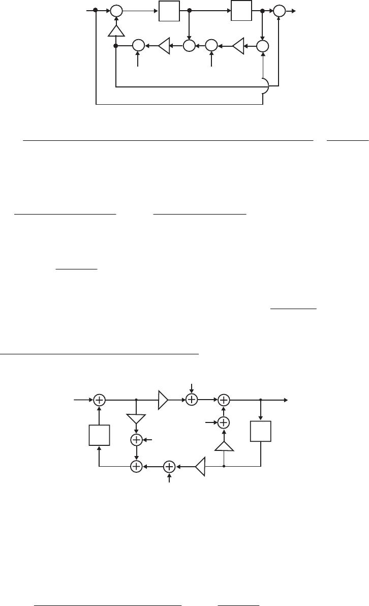
z
1
_
+
z
1
_
+
+
+
2
d
_
1
+
d
1
+
1
x
[n]y[n]
e [n]
2
e [n]
.
1
2
)1(2)1(
])1)(1([2)1]()1([
1
21
2
1
2
2
2
1
2
3
1
22
2
2
1
121211
2
2
2
1
2
21
2
1
2
,1 dd
ddddddd
ddddddddddd
n−
=
+−+−
−+−−++
+=
σ
The noise transfer function from to the output is
][
2ne
.
)1(
1
)1(
)(
211
2
121
2
1
1
2
21
1
1
2
1
1ddzdz
dddzd
d
zddzd
zd
zG ++
++
−=
++
−
=−−
−
Its corresponding
normalized output noise variance is given by
.
1
2
21
2
1
2
,1
2
1
2,2 dd
d
dnn −
== σσ
Total output noise variance is therefore .
1
)1(2
21
2
1
2,2
2
,1
2,dd
d
nn
no −
+
=+= σσσ
12.19 (a) Quantization of products before addition
The noise model of the second-order coupled form structure is shown below;
z_1z_1
α
β
δ
γ
V(z)
U(z)
Y(z)
1
E (z)
2
E (z)
3
E (z)
4
E (z)
We observe from discussion on Page 675 that θγβθδα sin,cos =
−
=
=
=
r and hence,
.,cos2 2
rr =−=+ γβδαθδα
Analysis yields ),()(),()()()( 1
3
1zUzzVzEzVzYzzU
−
−=++= αβ and
Eliminating the variables U(z) and V(z) from these equations
we arrive at
).()()()( 1
1zEzYzzVzY ++= −
δγ
).()(
1
)(
1
)()(1
13
1
1
1
21
zEzE
z
z
zY
z
zz +
−
=
−
−++−
−
−
−
−−
α
γ
α
γβδαδα Hence, the noise
transfer function from the noise sources and to the output is given by
][
1ne ][
2ne
Not for sale 450

)()()()(1
1
)(
)(
)( 2
2
21
1
0)()(
1
1
43 γβδαδα
α
γβδαδα
α
−++−
−
=
−++−
−
== −−
−
== zz
zz
zz
z
zE
zY
zG
zEzE
,
)cos(2
)cos(
1
)()(
)(
122
2
2rzrz
rzr
zz
z
+−
−
+=
−++−
−−
+= θ
θ
γβδαδα
γβδαδ and the noise transfer function from
the noise sources and to the output is given by ][
3ne ][
4ne
)()()()(1
)(
)(
)( 221
1
0)()(
3
3
21 γβδαδα
γ
γβδαδα
γ
−++−
=
−++−
== −−
−
== zz
z
zz
z
zE
zY
zG
zEzE
.
)cos(2
)sin(
22 rzrz
zr
+−
−
=θ
θ
The output roundoff noise variance due each of the noise sources and is
][
1ne ][
2ne
)cos4)(1()cos4(2)1(
)cos2)(coscos(2)1)(cos(
122422224
233442
2
,1 θθ
θθθθ
σ
rrrrr
rrrrrrr
n+−+−
−⋅+−−−+
+=
,
]cos4)1)[(1(
cos4)cos)(1(
122222
242222
θ
θθ
rrr
rrrr
−+−
−++
+= and the output roundoff noise variance due each of
the noise sources and is ][
3ne ][
4ne .
]cos4)1)[(1(
sin)1(
22222
222
2
,3 θ
θ
σ
rrr
rr
n−+−
+
= Hence, the total
roundoff noise variance at the output is
)(2 2,2
2
,1
2nn
nσσσ +=
.
]cos4)1)[(1(
sin)1(
]cos4)1)[(1(
cos4)cos)(1(
12 22222
222
22222
242222
⎟
⎟
⎠
⎞
⎜
⎜
⎝
⎛
−+−
+
+
−+−
−++
+= θ
θ
θ
θθ
rrr
rr
rrr
rrrr
Quantization of products after addition
Here, the total roundoff noise variance at the output is
2,2
2
,1
2nn
nσσσ +=
.
]cos4)1)[(1(
sin)1(
]cos4)1)[(1(
cos4)cos)(1(
122222
222
22222
242222
θ
θ
θ
θθ
rrr
rr
rrr
rrrr
−+−
+
+
−+−
−++
+=
(b) From the solution of Problem 12.4 we observe that the transfer function of the modified
coupled-form structure is ,
)1(2
)( 222
2
dczcz
dc
zH ++−
= where θsinrc
=
and .cot θ
=
d
The noise model is shown on top of the next page. Analysis yields
.
)1(21
)()()()()()(
)( 2221
3
22
1
22
4
1
3
1
2
1
4
−−
−−−−−
++−
−+−++
=
zdccdz
zEdzczEzczEcdzzEczzEczzE
zY
The noise transfer function from to the output is
][
1ne
Not for sale 451

_1
z
cc
dd
_1
_1
z
Y(z)
1
E (z)
2
E (z)
3
E (z)
4
E (z)
.
cos2
sin
)1(21
)(
)(
)( 22
22
2221
22
0)()()(
1
1
432 rzrz
r
zdccdz
zc
zE
zY
zG
zEzEzE +⋅−
=
++−
== −−
−
=== θ
θ
The normalized output roundoff noise variance due to is thus
][
1ne
.
)cos41(cos8)1(
)1)(sin(
4222424
444
2
,1 rrrr
rr
nθθ
θ
σ+−+−
−
=
The noise transfer function from to the output is
][
2ne
.
cos2
)sin(
)1(21
)(
)(
)( 222221
1
0)()()(
2
2
431 rzrz
zr
zdccdz
cz
zE
zY
zG
zEzEzE +⋅−
=
++−
== −−
−
=== θ
θ
The normalized output roundoff noise variance due to is thus
][
2ne
.
)cos41(cos8)1(
)1)(sin(
4222424
422
2,2 rrrr
rr
nθθ
θ
σ+−+−
−
=
The noise transfer function from to the output is ][
3ne
.
cos2
cotsin)sin(
)1(21
)(
)(
)( 22
22
2221
221
0)()()(
3
3
421 rzrz
rzr
zdccdz
dzccz
zE
zY
zG
zEzEzE +⋅−
⋅−
=
++−
−
== −−
−−
=== θ
θθθ
The corresponding normalized output roundoff noise variance is thus
.
)cos41(cos8)1(
cos)1)(cotsin(4)1)(cotsinsin(
4222424
233424422
2,3 rrrr
rrrrrr
nθθ
θθθθθθ
σ+−+−
−−−−
=
The noise transfer function from to the output is
][
4ne
22
2
2221
1
0)()()(
4
4cos2
)cos(
)1(21
1
)(
)(
)(
321 rzrz
zrz
zdccdz
cdz
zE
zY
zG
zEzEzE +⋅−
−
=
++−
−
== −−
−
=== θ
θ
.
cos2
)cos(
122
2
rzrz
rzr
+⋅−
−
+= θ
θ The corresponding normalized output roundoff noise variance is
thus .
)cos41(cos8)1(
cos)1)(cos(4)1)(cos(
14222424
234422
2,4 rrrr
rrrrrr
nθθ
θθθ
σ+−+−
−+−−
+=
Not for sale 452

12.20 The noise model of the Kingsbury structure is shown below:
k
1
k
2
–
z
1
–
z
1
k
1
_
Y(z)
1
E (z)
2
E (z)
3
E (z)
V(z)
U(z)
Analysis yields ),()()( 11 zEzYkzU
+
= ),()()(
1
1
)( 22
1zEzYkzU
z
zV ++
−
=− and
).(
1
)(
11
)]()([)( 3
1
1
1
1
1
1
1
31 zE
z
z
zV
z
zk
z
z
zEzVkzY −
−
−
−
−
−
−
+
−
−=
−
+−= Eliminating and
from these equations we arrive at
)(zU )(zV
).(
1
)(
1
)(
)1(
)(
)1(
)1()](2[1
3
1
1
2
1
1
1
1
21
1
1
21
2
21
1
211 zE
z
z
zE
z
zk
zE
z
zk
zY
z
zkkzkkk
−
−
−
−
−
−
−
−
−
−
+
−
−
−
−=
−
−++−−
Hence, the noise transfer function from to the output is
][
1ne
.
)cos2()1()](2[1
)(
)(
)( 22
1
2
21
1
211
1
1
0)()(
1
1
32 rzrz
zk
zkkzkkk
zk
zE
zY
zG
zEzE +−
−
=
−++−−
−
== −−
−
== θ
The corresponding normalized output roundoff noise variance is thus given by
22222222
222
1
242224
42
1
2
,1 )1(cos4)1()1(
)1)(1(
)cos2)(1()cos2(2)1(
)1(
rrrr
rrk
rrrrr
rk
n−−+−
+−
=
−+−−+−
−
=θθθ
σ
.
]cos4)1)[(1(
)1(
22222
22
1
θrrr
rk
−+−
+
=
The noise transfer function from to the output is
][
2ne
.
)cos2()1()](2[1
)1(
)(
)(
)( 22
11
2
21
1
211
11
1
0)()(
2
2
31 rzrz
kzk
zkkzkkk
zzk
zE
zY
zG
zEzE +−
+−
=
−++−−
−−
== −−
−
−
== θ
Its corresponding normalized output roundoff noise variance is thus given by
.
]cos4)1)[(1(
)1(2
22222
22
1
2,2 θ
σ
rrr
rk
n−+−
+
=
Finally, the noise transfer function from to the output is ][
3ne
.
)cos2(
1
)1()](2[1
)1(
)(
)(
)( 222
21
1
211
11
0)()(
3
3
21 rzrz
z
zkkzkkk
zz
zE
zY
zG
zEzE +−
−
=
−++−−
−
== −−
−−
== θ
Its corresponding normalized output roundoff noise variance is thus given by
.
]cos4)1)[(1(
)1(2
22222
2
2,2 θ
σ
rrr
r
n−+−
+
= Hence, the total normalized noise variance due to
Not for sale 453
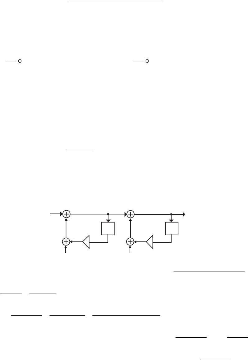
product roundoff before (after) summation is given by
.
]cos4)1)[(1(
)1)(23(
22222
22
1
2,3
2,2
2
,1
2,θ
σσσσ
rrr
rk
nnn
no −+−
++
=++=
12.21 Let be a noise source due to product roundoff inside with an associated noise
transfer function to the output of . Then the normalized noise power at the output
of the cascade structure due to is given by
][ne )(zG
)(zGe)(zG
][ne
dzzzGzG
j
dzzzAzGzAzG
je
C
ee
C
ene 1111
2
1
2
2
,)()(
2
1
)()()()(
2
1−−−−− ∫∫ == ππ
σ since
Assuming is realized with the lowest product roundoff noise power
the normalized noise power at the output of the cascade due to product roundoff in
is still From the solution of Problem 12.14, we note that the lowest roundoff noise power
(assuming quantization before addition) is for cascade structure #3. Next, from
the solution of Problem 12.18, we note that the normalized output noise power due to noise
sources in is
.1)()( 1
22 =
−
zAzA )(zG
,
2,ng
σ)(zG
.
2,ng
σ
4031.4
2,=
ng
σ
)(
2zA .
1
2
21
2
1
2,2 dd
d
n−
=
σ Substituting 2.0
1
=
d and we get
Hence, the total output noise variance of the cascade is given by
,5.0
21 −=dd
.0533.0
2,2 =
n
σ2,2
2,n
ng σσ +
.4564.40533.04031.4 =+=
12.21 The noise model for the structure is as shown below:
z
z1
y[n]
x[n]
__1
0.3
_0.4
e [n]
1e [n]
2
The noise transfer function from to the output is
][
1ne
)4.01)(3.01(
1
)( 11
1−− −+
=
zz
zG
.
3.0
1286.0
4.0
2286.0
1+
−
+
−
+= zz Thus, the normalized noise power at the output due to is
][
1ne
)4.0)(3.0(1
)1286.0(2286.02
)3.0(1
)1286.0(
)4.0(1
)2286.0(
12
2
2
2
2
1−−
−××
+
−−
−
+
−
+=
σ=1.0279.
The noise transfer function from to the output is
][
2ne 1
24.01
1
)( −
−
=
z
zG .
4.0
4.0
1−
+= z
Thus, the normalized noise power at the output due to is
][
2ne .1905.1
)4.0(1
)4.0(
12
2
2
2=
−
+=σ
Therefore, the total normalized noise power at the output .2184.21905.10279.1 =
+
=
Not for sale 454
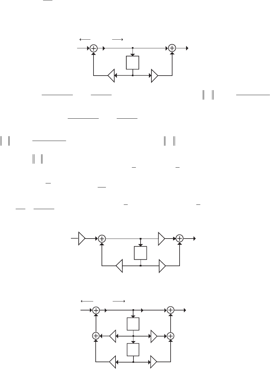
For a 9-bit signed two’s-complement number representation, the quantization level is
Hence, the total output noise power due to product roundoff is
.0039062.02 8== −
δ
== 12
)2184.2(
2
2δ
σo .108208.2 6
−
×
12.22 The unscaled structure is shown below:
y[n]
x
[n]
z
1
_
_0.4 0.5
1
F (z)
Now, .
4.0
4.0
1
4.01
1
)( 1
1+
−
+=
+
=−z
z
zF Using Table 12.4 we obtain =
−−
−
+= 2
2
2
2
1)4.0(1
)4.0(
1F
Next,
.1905.1 .
4.0
9.0
1
4.01
5.01
)( 1
1
−
+=
−
+
=−
−
z
z
z
zH Using Table 12.4 we obtain
.9643.1
)4.0(1
)9.0(
12
2
2
2=
−−
+=H From Eq. (12.128a), ,0911.1
1
2
1== αF and from Eq.
(12.128b), .0415.1
2
2== αH
The scaled structure is shown below, where 101 β=b and .5.0 111 β=b From Eq. (12.129)
and (12.132a), 9165.0
1
1
00 ==== α
ββ KK and from Eq. (12.132b),
.7785.0
0415.1
0911.1
2
1
1=== α
α
β Therefore, 7785.0
101 == βb and .3893.05.0 111 == βb
y[n]
x
[n]
z
1
_
_0.4
K
_b
_
01
b
_
11
12.24 The unscaled structure is shown below:
y[n]
x[n]
z–1
z–1
0.7
0.8
0.4
_
0.6
_
F (z)
1
Not for sale 455
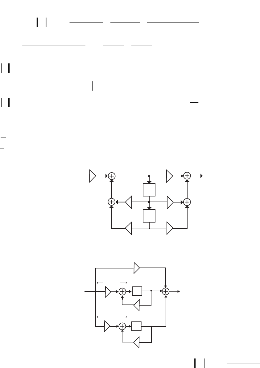
Now, .
2.0
05.0
6.0
45.0
1
12.04.012.04.01
1
)( 2
2
21
1−
+
+
−
+=
−+
=
−+
=−− zz
zz
z
zz
zF Using Table
12.4 we get .2788.1
2.0)6.0(1
05.0)45.0(2
)2.0(1
)05.0(
)6.0(1
)45.0(
12
2
2
2
2
2
1=
×−−
×−×
+
−
+
−−
−
+=
F Next,
.
2.0
5.0
6.0
9.0
1
12.04.01
6.08.01
)( 21
21
−
−
+
+
+=
−+
−+
=−−
−−
zz
zz
zz
zH Using Table 12.4 we get
.7225.1
2.0)6.0(1
)5.0(9.02
)2.0(1
)5.0(
)6.0(1
)9.0(
12
2
2
2
2
2=
×−−
−××
+
−
−
+
−−
+=H
From Eq. (12.128a) we get 1308.1
1
2
1== αF and from Eq. (12.28b) we get
.3124.1
2
2== αH Hence, from Eq. (12.132a) we have 8843.0
1
1
0== α
β and from Eq.
(12.132b) we have .8616.0
2
1
1== α
α
β The scaled structure is as shown below, where
,8843.0
00 === ββ KK ,8616.01 101 =×= βb ,6893.08.0 111 =×= βb and
..).( 5170060 121 −=β×−=b
y[n]
x[n]
z
–1
z
–1
0.7
0.4
_
b
_
01
b
_
11
b
_
21
K
_
12.25 .
8.01
2
6.01
4
3)( 1
1
1
1
−
−
−
−
−
+
+
−
+=
z
z
z
z
zH The unscaled structure is shown below:
z 1
_
z 1
_
A = 3
C = 2
0.8
0.6
_
B = 4
_
x
[n]y[n]
F (z)
1
F (z)
2
Here, .
6.0
6.4
1
6.01
4
)( 1
1
1+
−
+=
+
−
=−
−
z
z
z
zF Using Table 12.4 we get 2
2
2
2
1)6.0(1
)6.4(
1−−
−
+=F
Not for sale 456
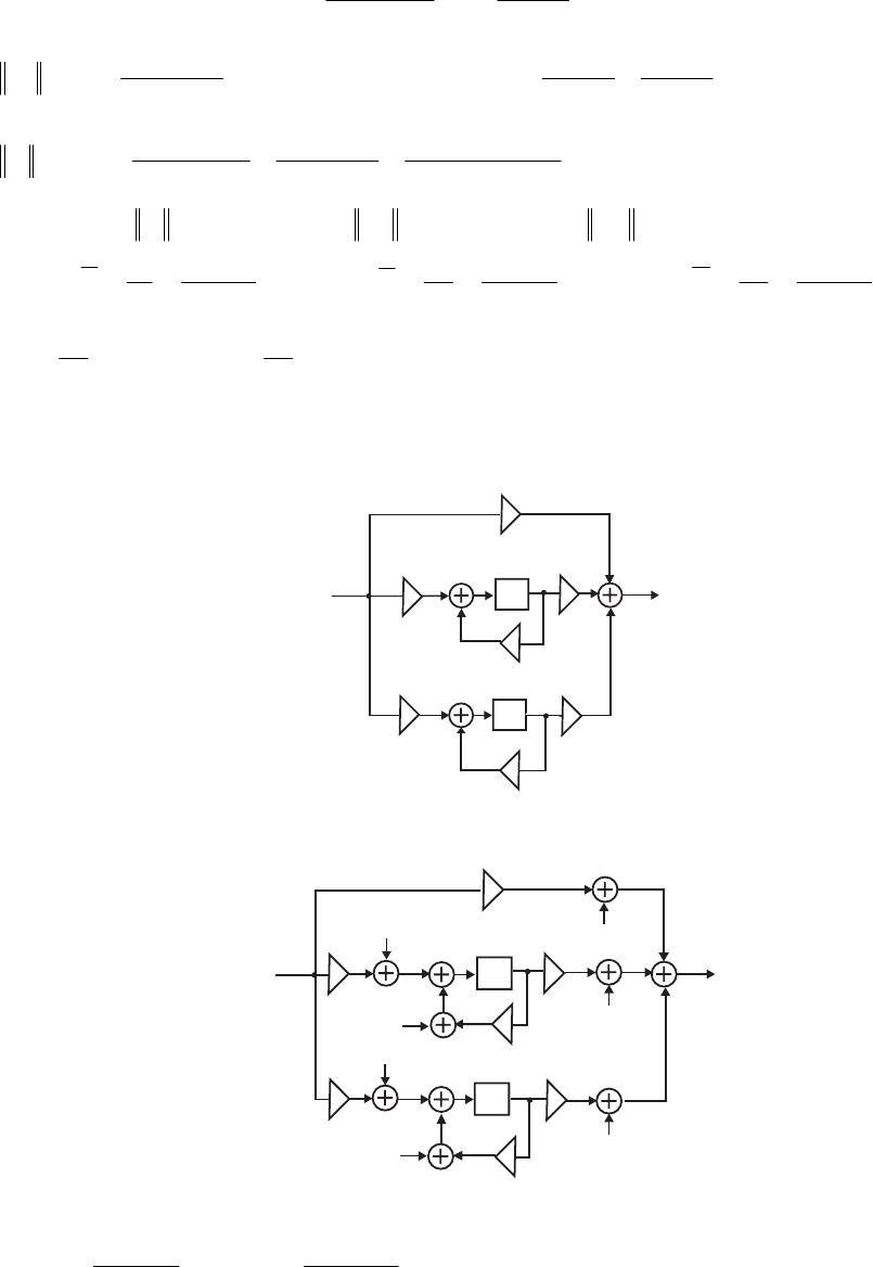
Likewise,
.0625.34=.
8.0
8.2
1
8.01
2
)( 1
1
2−
+=
−
=−
−
z
z
z
zF Using Table 12.4 we get
.7778.22
)8.0(1
)8.2(
12
2
2
2
2=
−
+=F Also, .
8.0
2
6.0
4
3)( −
+
+
−
+= zz
zH Using Table 12.4 we get
.3003.34
8.0)6.0(1
2)4(2
)8.0(1
2
)6.0(1
)4(
32
2
2
2
2
2
2=
×−−
×−×
+
−
+
−−
−
+=H
Denote ,8566.5
2
0== Hγ ,8363.5
2
11 == Fγ .7726.4
2
22 == Fγ
Hence, ,5140.0
8363.5
3
1
=== γ
A
A ,8381.0
7726.4
4
2
−=
−
== γ
B
B ,3415.0
8566.5
2
0
=== γ
C
C
.8149.0,9965.0
0
2
2
0
1
1==== γ
γ
γ
γKK
The scaled structure is shown below:
z 1
_
z 1
_
A
0.8
0.6
_
x
[n]y[n]
_
C
_
B
_K
1
K
2
The noise model is
z
1
_
z
1
_
A
0.8
0.6
_
x
[n]y[n]
_
C
_
B
_K
1
K
2
A
e [n]
B
e [n]
C
e [n]
e [n]
β
e [n]
γ
e [n]
K1
e [n]
K2
The noise transfer function from the noise sources and is given by:
][neB][neβ
.
6.0
5979.0
9965.0
6.0
9965.0
)(
1+
−
+=
+
=zz
z
zG Using Table 12.4, we obtain
Not for sale 457
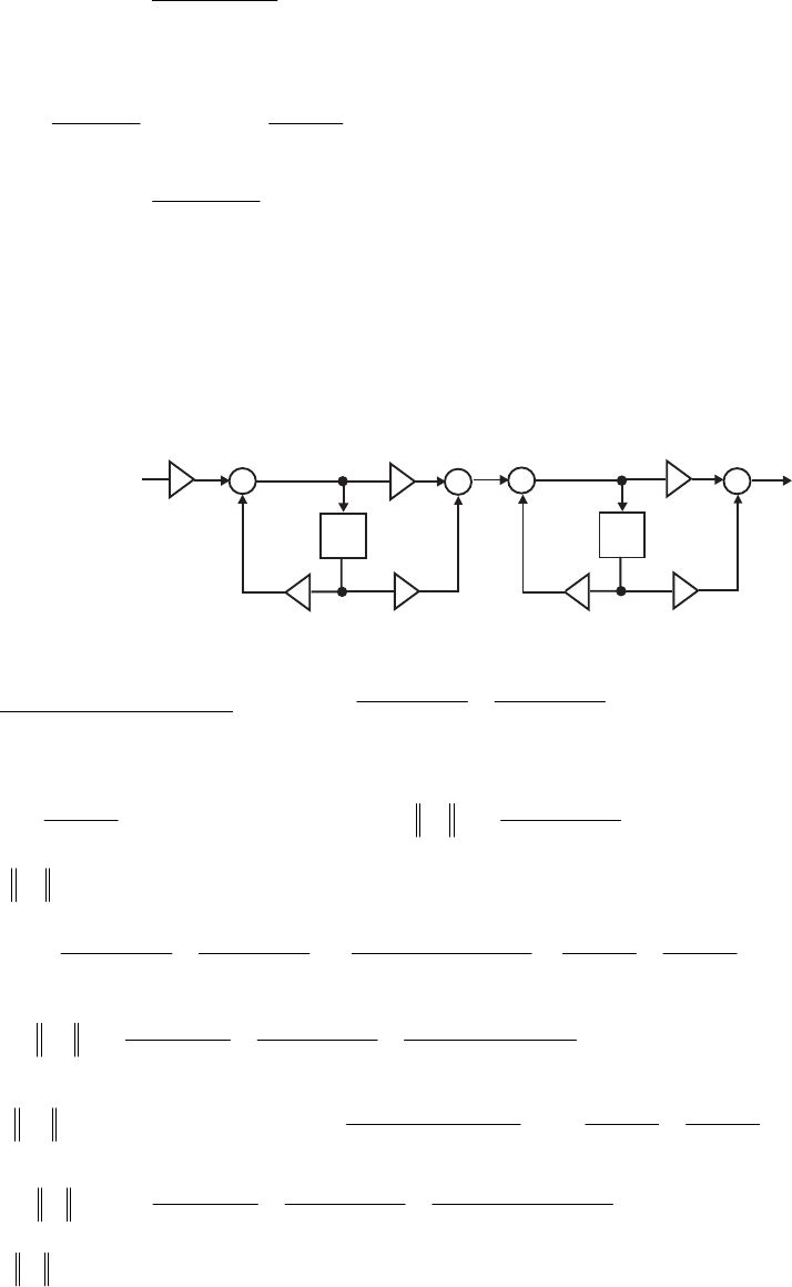
.5516.1
)6.0(1
)5979.0(
)9965.0( 2
2
22
1=
−−
−
+=σ
Likewise, the noise transfer function from the noise sources and is given by:
][neC][neγ
.
8.0
6519.1
8149.0
8.0
8149.0
)(
2−
+=
−
=zz
z
zG Using Table 12.4, we obtain
.8446.1
)8.0(1
)6519.1(
)8149.0( 2
2
22
2=
−
+=σ
The noise transfer function from the remaining three noise sources is Hence, the .1)(
3=zG
normalized output noise variance due to these three noise sources is given by
Therefore, the total normalized output noise variance is
.3
2
3=σ
=σ+σ+σ=σ 2
3
2
2
2
1
2
022 ..79249
12.26 The scaled structure is shown below.
z1
_
+
+
z1
_
+
+
2
k
1
a2
a
3
k
1
k
3
b k
2
2
b k
1
(a) Cascade Structure # 1 – .
6.01
3.01
2.01
4.01
)( 1
1
1
1
⎟
⎟
⎠
⎞
⎜
⎜
⎝
⎛
−
−
⎟
⎟
⎠
⎞
⎜
⎜
⎝
⎛
+
+
=−
−
−
−
z
z
z
z
zH Here, ,4.0,2.0 11
=
−= ba
The values of the scaling constants are determined below.
.3.0,6.0 22 −== ba
.
2.0
1
)(
1+
=z
zF Using Table 12.4 we get .0417.1
)2.0(1
1
2
2
2
1=
−−
=F Hence,
.0206.1
2
11 == Fγ Likewise,
)6.0)(2.0(
4.0
6.012.01
4.01
)( 1
1
1
1
2−+
+
=
⎟
⎟
⎠
⎞
⎜
⎜
⎝
⎛
−
⎟
⎟
⎠
⎞
⎜
⎜
⎝
⎛
+
+
=−
−
−
−
zz
z
z
z
z
z
zF .
2.0
25.0
6.0
25.1
+
−
+
−
=zz Using Table 12.4
we get .9485.1
)2.0(6.01
)2.0(25.12
)2.0(1
)25.0(
)6.0(1
)25.1(
2
2
2
2
2
2
2=
−×−
−××
+
−−
−
+
−
=F Hence,
.3959.1
2
22 == Fγ Next, .
2.0
125.0
6.0
375.0
1
12.04.0
12.01.0
)( 2
2
+
+
−
+=
−−
−+
=zz
zz
zz
zH Using Table 12.4
we get .3197.1
)2.0(6.01
125.0375.02
)2.0(1
)125.0(
)6.0(1
)375.0(
12
2
2
2
2
2=
−×−
××
+
−−
+
−
+=H Hence,
.1488.1
2
0== Hγ
Not for sale 458

The scaling multipliers are therefore given by ,7311.0,9798.0
1
2
1
2
1
1==== γ
γ
γkk and
.2151.1
0
2
3== γ
γ
k Therefore, 2925.0
21
=
kb and .3645.0
32
−
=
kb
The noise at the output due to the input multiplier and multiplier have a variance
The noise at the output due to and have variance which is
calculated below. The noise transfer function for these noise sources is
1
k1
a
.0417.1
2
1
2
1== γσ ,, 21 ka 21kb 2
2
σ
.
6.0
3646.0
2151.1
6.0
3645.02151.1
6.01
3645.02151.1
)( 1
1
2−
+=
−
−
=
−
−
=−
−
zz
z
z
z
zG Using Table 12.4 we get
.6841.1
)6.0(1
)3646.0(
)2151.1( 2
2
22
2=
−
+=σ
Hence the total noise power (variance) at the output .1357.926841.130417.12 =+×
+
×
=
In
case the quantization is carried out after addition, then the total noise power at the output =
1.0417 + 1.6841 + 1 = 3.7258.
(b) Cascade Structure # 2 - .
6.01
4.01
2.01
3.01
)( 1
1
1
1
⎟
⎟
⎠
⎞
⎜
⎜
⎝
⎛
−
+
⎟
⎟
⎠
⎞
⎜
⎜
⎝
⎛
+
−
=−
−
−
−
z
z
z
z
zH Here, ,3.0,2.0 11
−
=
−= ba
The values of the scaling constants are determined below.
.4.0,6.0 22 == ba
.
2.0
1
)(
1+
=z
zF From Part (a) we have 0417.1
2
2
1=F and .0206.1
2
11 == Fγ Likewise,
)6.0)(2.0(
3.0
6.012.01
3.01
)( 1
1
1
1
2−+
−
=
⎟
⎟
⎠
⎞
⎜
⎜
⎝
⎛
−
⎟
⎟
⎠
⎞
⎜
⎜
⎝
⎛
+
−
=−
−
−
−
zz
z
z
z
z
z
zF .
2.0
625.0
6.0
375.0
+
+
−
=zz Using Table 12.4
we get .0452.1
)2.0(6.01
625.0375.02
)2.0(1
)625.0(
)6.0(1
)375.0(
2
2
2
2
2
2
2=
−×−
××
+
−−
+
−
=F Hence,
.0224.1
2
22 == Fγ Next, 12.04.0
12.01.0
)( 2
2
−−
−+
=
zz
zz
zH and from Part (a) we have
.3197.1
2
2=H Hence, .1488.1
2
0== Hγ
The scaling multipliers are therefore given by ,9982.0,9798.0
1
2
1
2
1
1==== γ
γ
γkk and
.89.0
0
2
3== γ
γ
k Therefore, 2995.0
21
−
=
kb and .356.0
32
=
kb
The noise at the output due to the input multiplier and multiplier have a variance
The noise at the output due to and have variance which is
calculated below. The noise transfer function for these noise sources is
1
k1
a
.0417.1
2
1
2
1== γσ ,, 21 ka 21kb 2
2
σ
Not for sale 459

.
6.0
89.0
89.0
6.0
356.089.0
6.01
356.089.0
)( 1
1
2−
+=
−
+
=
−
+
=−
−
zz
z
z
z
zG Using Table 12.4 we get
.0298.2
)6.0(1
)89.0(
)89.0( 2
2
22
2=
−
+=σ
Hence the total noise power (variance) at the output .1728.1020298.230417.12
=
+×
+
×
=
In
case the quantization is carried out after addition, then the total noise power at the output =
1.0417 + 2.0298 + 1 = 4.0715.
(c) Cascade Structure # 3 – .
2.01
4.01
6.01
3.01
)( 1
1
1
1
⎟
⎟
⎠
⎞
⎜
⎜
⎝
⎛
+
+
⎟
⎟
⎠
⎞
⎜
⎜
⎝
⎛
−
−
=−
−
−
−
z
z
z
z
zH Here, ,3.0,6.0 11
−
=
=ba
The values of the scaling constants are determined below.
.4.0,2.0 22 =−= ba
.
6.0
1
)(
1−
=z
zF Using Table 12.4 we get .5625.1
)6.0(1
1
2
2
2
1=
−
=F Hence,
.25.1
2
11 == Fγ Likewise, )2.0)(6.0(
3.0
2.016.01
3.01
)( 1
1
1
1
2+−
−
=
⎟
⎟
⎠
⎞
⎜
⎜
⎝
⎛
+
⎟
⎟
⎠
⎞
⎜
⎜
⎝
⎛
−
−
=−
−
−
−
zz
z
z
z
z
z
zF . From
Part (b) we have 0452.1
2
2
2=F and 0224.1
2
22 == Fγ. Next, 12.04.0
12.01.0
)( 2
2
−−
−+
=
zz
zz
zH
and from Part (a) we have .3197.1
2
2=H Hence, .1488.1
2
0== Hγ
The scaling multipliers are therefore given by ,2226.1,8.0
1
2
1
2
1
1==== γ
γ
γkk and
.89.0
0
2
3== γ
γ
k Therefore, 3668.0
21
−
=
kb and .356.0
32
=
kb
The noise at the output due to the input multiplier and multiplier have a variance
The noise at the output due to and have variance which is
calculated below. The noise transfer function for these noise sources is
1
k1
a
.5625.1
2
1
2
1== γσ ,, 21 ka 21kb 2
2
σ
.
2.0
178.0
89.0
2.0
356.089.0
2.01
356.089.0
)( 1
1
2+
+=
+
+
=
+
+
=−
−
zz
z
z
z
zG Using Table 12.4 we get
.8251.0
)2.0(1
)178.0(
)89.0( 2
2
22
2=
−+
+=σ
Hence the total noise power (variance) at the output .6003.728251.035625.12 =+×
+
×
=
In
case the quantization is carried out after addition, then the total noise power at the output =
1.5625 + 0.8251 + 1 = 3.3876.
(d) Cascade Structure # 4 – .
2.01
3.01
6.01
4.01
)( 1
1
1
1
⎟
⎟
⎠
⎞
⎜
⎜
⎝
⎛
+
−
⎟
⎟
⎠
⎞
⎜
⎜
⎝
⎛
−
+
=−
−
−
−
z
z
z
z
zH Here, ,4.0,6.0 11
=
=ba
The values of the scaling constants are determined below.
.3.0,2.0 22 −=−= ba
Not for sale 460

.
6.0
1
)(
1−
=z
zF From Part (c) we have 5625.1
2
2
1=F and .25.1
2
11 == Fγ Likewise,
)2.0)(6.0(
4.0
2.016.01
4.01
)( 1
1
1
1
2+−
+
=
⎟
⎟
⎠
⎞
⎜
⎜
⎝
⎛
+
⎟
⎟
⎠
⎞
⎜
⎜
⎝
⎛
−
+
=−
−
−
−
zz
z
z
z
z
z
zF . From Part (a) we have 9485.1
2
2
2=F
and .3959.1
2
22 == Fγ Next, 12.04.0
12.01.0
)( 2
2
−−
−+
=
zz
zz
zH and from Part (a) we have
3197.1
2
2=H and .1488.1
2
0== Hγ
The scaling multipliers are therefore given by ,8955.0,8.0
1
2
1
2
1
1==== γ
γ
γkk and
.2151.1
0
2
3== γ
γ
k Therefore, 3582.0
21
=
kb and .3645.0
32
−
=
kb
The noise at the output due to the input multiplier and multiplier have a variance
The noise at the output due to and have variance which is
calculated below. The noise transfer function for these noise sources is
1
k1
a
.5625.1
2
1
2
1== γσ ,, 21 ka 21kb 2
2
σ
.
2.0
6075.0
2151.1
2.0
3645.02151.1
2.01
3645.02151.1
)( 1
1
2+
−
+=
+
−
=
+
−
=−
−
zz
z
z
z
zG Using Table 12.4 we
get .8609.1
)2.0(1
)6075.0(
)89.0( 2
2
22
2=
−+
−
+=σ
Hence the total noise power (variance) at the output .7077.1028609.135625.12 =+×
+
×
=
In
case the quantization is carried out after addition, then the total noise power at the output =
1.5625 + 1.8609 + 1 = 5.4234.
12.27 (a) Parallel Form #1 - .
2.01
6.0
6.01
625.0
1
)6.0)(2.0(
)3.0)(4.0(
)( 11 −− +
+
−
+=
−+
−
+
=
zz
zz
zz
zH The unscaled
structure is shown below:
z1
_
z1
_
+
++
0.625
0.6
x
[n]y[n]
F (z)
1
F (z)
2
0.6
_0.2
Here the scaling transfer function for the middle branch is given by
)(
1zF 6.0
625.0
)(
1−
=z
z
zF
Not for sale 461
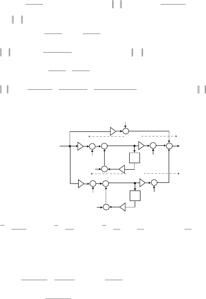
.
6.0
375.0
625.0 −
+= z From Table 12.4 we get .6104.0
)6.0(1
)375.0(
)625.0( 2
2
2
2
2
1=
−
+=F Hence,
.7813.0
2
11 == Fγ Similarly the scaling transfer function for the bottom branch is
given by
)(
2zF
.
2.0
12.0
6.0
2.0
6.0
)(
2+
−
+=
+
=zz
z
zF From Table 12.4 we get
2
2
2
2
2
2)2.0(1
)12.0(
)6.0( −−
−
+=
F Hence,
.375.0=.6124.0
2
22 == Fγ
Finally, .
2.0
125.0
6.0
375.0
1)( +
+
−
+= zz
zH From Table 12.4 we get
.3197.1
)2.0(6.01
125.0375.02
)2.0(1
)125.0(
)6.0(1
)375.0(
12
2
2
2
2
2=
−×−
××
+
−−
+
−
+=H Hence, .1488.1
2
0== Hγ
The scaled structure with noise sources is shown below where
z1
_
z1
_
+
++
x
[n]y[n]
0.6
_0.2
+
+
+
+
+
+
+
A
-
B
-
C
-
k1
k2
e [n]
A
e [n]
B
e [n]
C
e [n]
k
1
e [n]
k
2
e [n]
a
1
e [n]
a
2
1
G (z)
2
G (z)
.5331.0,6801.0,
1
,9798.0
6.0
,7999.0
625.0
0
2
2
0
1
1
021
========= γ
γ
γ
γ
γγγ kkCBA
The noise transfer function from each of the noise sources and is
The corresponding output noise variance is
],[],[ 1nene kC ][
2nek
.1)(
3=zG .1
2
3=σ
The noise transfer function from each of the noise sources and is
][neA][
1nea
.
6.0
4081.0
6801.0
6.0
6801.0
6.01
)( 1
1
1−
+=
−
=
−
=−zz
z
z
k
zG From Table 12.4 we get
.7227.0
)6.0(1
)4081.0(
)6081.0( 2
2
22
1=
−
+=σ
Likewise, the noise transfer function from each of the noise sources ][ne
B
and is
][
2nea
Not for sale 462
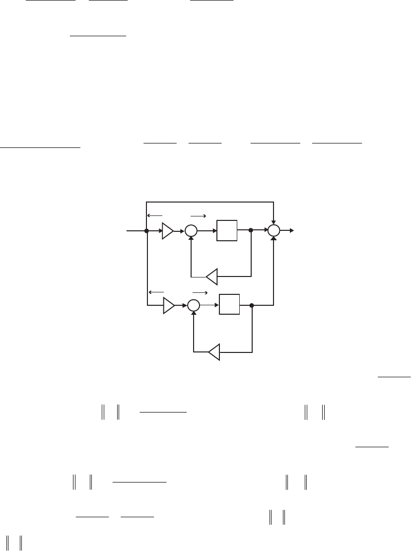
.
2.0
1066.0
53301.0
2.0
5331.0
2.01
)( 1
2
2+
−
+=
+
=
+
=−zz
z
z
k
zG From Table 12.4 we get
.296.0
)2.0(1
)1066.0(
)5331.0( 2
2
22
2=
−−
−
+=σ
Hence the total noise power (variance) at the output, . In case
the quantization is carried out after addition, then the total noise power at the output,
0374.5322 2
3
2
2
2
1
2=++= σσσσo
.0187.2
2
3
2
2
2
1
2=++= σσσσo
(b) Parallel Form #2 - .
2.01
125.0
6.01
375.0
1
2.0
125.0
6.0
375.0
1)( 1
1
1
1
−
−
−
−
+
+
−
+=
+
+
−
+=
z
z
z
z
zz
zH
The unscaled structure is shown below:
z
1
_
z
1
_
+
++
x
[n]y[n]
0.6
_
0.2
0.375
0.1
F (z)
1
F (z)
2
Here the scaling transfer function for the middle branch is given by
)(
1zF .
6.0
375.0
)(
1−
=z
zF
From Table 12.4 we get .2197.0
)6.0(1
)375.0(
2
2
2
2
1=
−
=F Hence, .4687.0
2
11 == Fγ Similarly
the scaling transfer function for the bottom branch is given by
)(
2zF .
2.0
125.0
)(
2+
=z
zF From
Table 12.4 we get .0163.0
)2.0(1
)125.0(
2
2
2
2
2=
−−
=F Hence, .1277.0
2
22 == Fγ
Finally, .
2.0
125.0
6.0
375.0
1)( +
+
−
+= zz
zH From Part (a) we get 3197.1
2
2=H and
.1488.1
2
0== Hγ
The scaled structure with noise sources is shown on the next page where
Not for sale 463
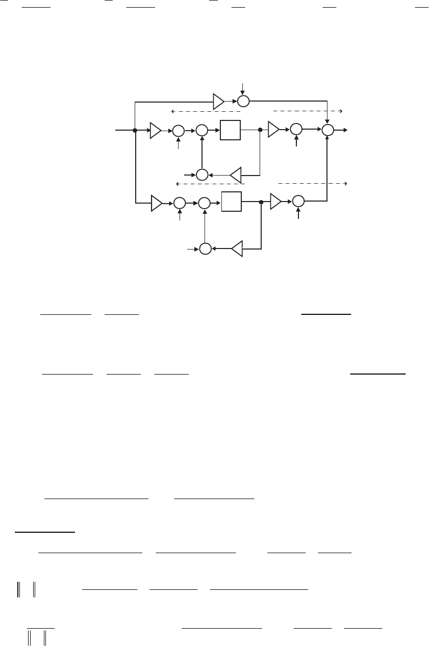
.1111.0,4081.0,8705.0
1
,9796.0
125.0
,7999.0
375.0
0
2
2
0
1
1
021
========== γ
γ
γ
γ
γγγ kkCBA
The noise transfer function from each of the noise sources and is
The corresponding output noise variance is
],[],[ 1nene kC ][
2nek
.1)(
3=zG .1
2
3=σ
z1
_
z1
_
+
++
x
[n]y[n]
0.6
_0.2
+
+
+
+
+
+
+
A
-
B
-
C
-
k1
k2
e [n]
A
e [n]
B
e [n]
C
e [n]
k
1
e [n]
k
2
e [n]
a
1
e [n]
a
2
1
G (z)
2
G (z)
The noise transfer function from each of the noise sources and is
][neA][
1nea
.
6.0
4081.0
6.01
)( 1
1
1
1−
=
−
=−
−
z
z
zk
zG From Table 12.4 we get .2602.0
)6.0(1
)4081.0(
2
2
2
1=
−
=σ
Likewise, the noise transfer function from each of the noise sources ][ne
B
and is
][
2nea
.
2.0
1111.0
2.0
1111.0
2.01
)( 1
1
2
2+
=
+
=
+
=−
−
zz
z
zk
zG From Table 12.4 we get .0129.0
)2.0(1
)1111.0(
2
2
2
2=
−−
=σ
Hence the total noise power (variance) at the output, In case
the quantization is carried out after addition, then the total noise power at the output,
.5462.3322 2
3
2
2
2
1
2=++= σσσσo
.2731.1
2
3
2
2
2
1
2=++= σσσσo
In either case, Parallel form II structure (after scaling) has the lowest roundoff noise variance.
12.28 .
15.02.0
3.02.0
2
15.02.01
6.04.02
)( 2
2
21
21
⎟
⎟
⎠
⎞
⎜
⎜
⎝
⎛
−+
−−
=
−+
−−
=−−
−−
zz
zz
zz
zz
zH
(a) Direct Form: The unscaled structure is shown on top of next page.
.
3.0
225.0
5.0
625.0
2
15.02.0
2
15.02.01
2
)( 2
2
21
1−
+
+
−
+=
−+
=
−+
=−− zz
zz
z
zz
zF From Table 12.4 we
get .3319.4
3.0)5.0(1
225.0)625.0(2
)3.0(1
)225.0(
)5.0(1
)625.0(
22
2
2
2
2
2
2
1=
×−−
×−×
+
−
+
−−
−
+=F Hence,
.4805.0
1
2
1
0== F
β Next, .
3.0
675.0
5.0
125.0
2
15.02.0
6.04.02
)( 2
2
−
−
+
+
−
+=
−+
−−
=zz
zz
zz
zH From Table
Not for sale 464
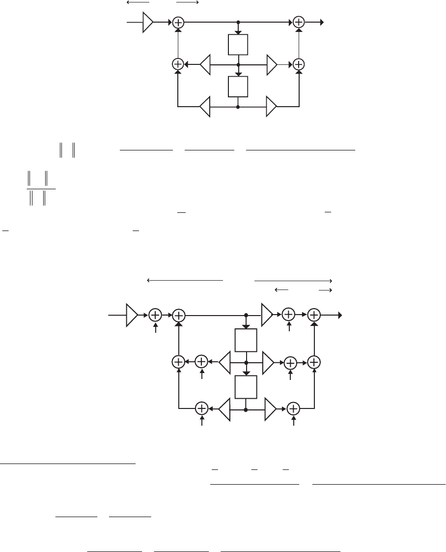
y[n]
z–1
z–1
0.15
0.2
_
0.3
_
0.2
_
2
x
[n]
F (z)
1
12.4 we get .6683.4
3.0)5.0(1
)675.0()125.0(2
)3.0(1
)675.0(
)5.0(1
)125.0(
22
2
2
2
2
2
2=
×−−
−×−×
+
−
−
+
−−
−
+=H Hence,
.9632.0
2
2
1
1== H
F
β
The scaling multipliers are therefore ,9632.0,961.024805.0 1010 ===×== ββ bKK
.289.03.0,1926.02.0 121111 −=×−=−=×−= ββ bb
The scaled structure with the noise sources is shown below:
y[n]
z–1
z–1
2
x
[n]
0.1926
_
_0.289
_0.2
0.15
G (z)
4
G (z)
1
0.9632
e [n]
1
e [n]
2
e [n]
3
e [n]
4
e [n]
5
e [n]
6
Quantization before addition: The noise transfer function associated with the noise sources
and is given by
],[],[ 21 nene ][
3ne
15.02.0
289.01926.09632.0
15.02.0
)( 2
2
2
2111
2
01
1−+
−−
=
−+
++
=
zz
zz
zz
bzbzb
zG
.
3.0
3251.0
5.0
0601.0
9632.0 −
−
+
+
−
+= zz From Table 12.4 we get
.0827.1
3.0)5.0(1
)3251.0()0601.0(2
)3.0(1
)3251.0(
)5.0(1
)0601.0(
)9632.0( 2
2
2
2
22
1=
×−−
−×−×
+
−
−
+
−−
−
+=σ The noise
transfer function associated with the noise sources and is given by
Hence, Hence, total normalized output noise power is
],[],[ 54 nene ][
6ne
.1)(
4=zG .1
2
4=σ
.2481.630827.1333 2
4
2
1
2=+×=+= σσσo
Not for sale 465
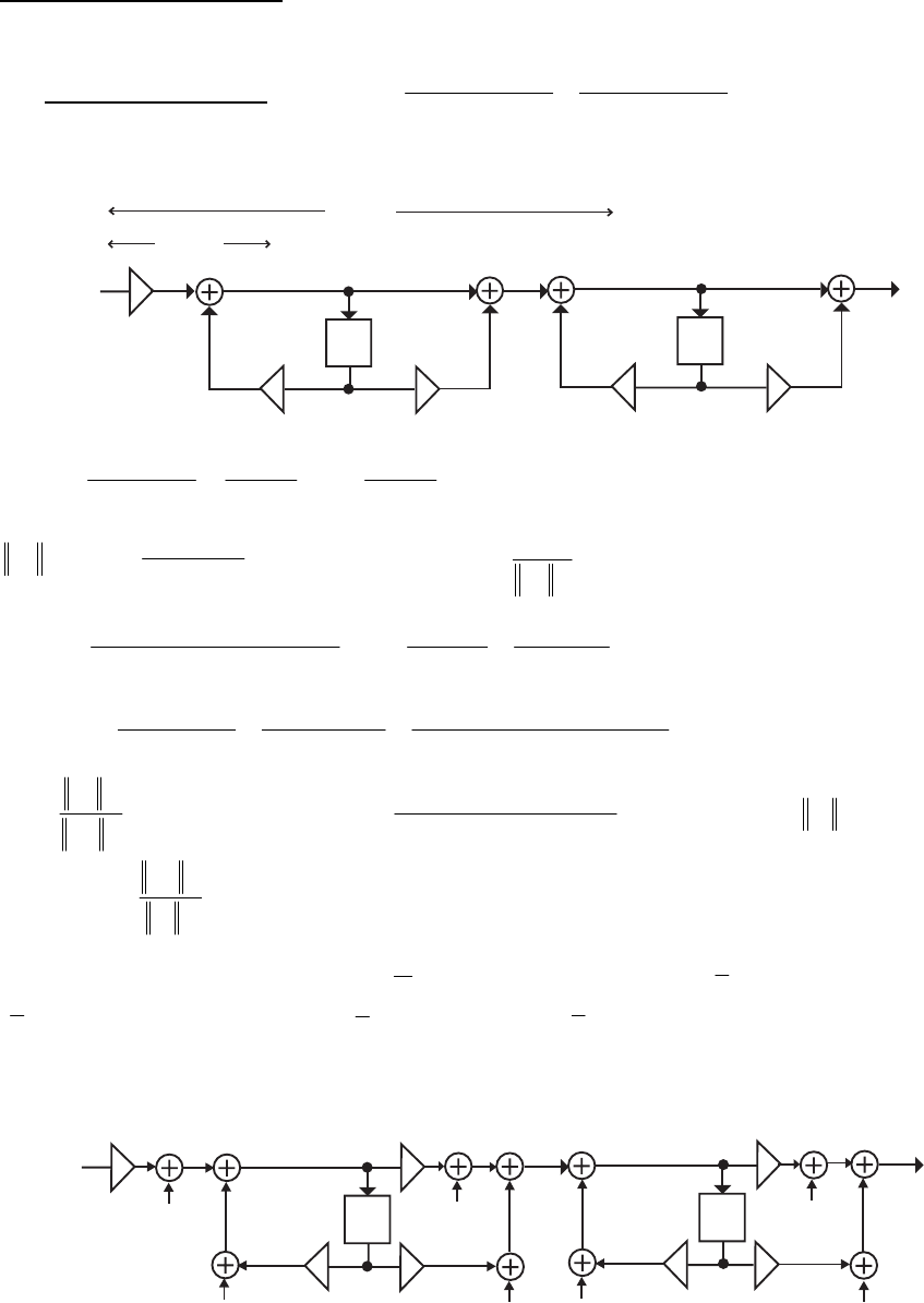
Quantization after addition: Here, total normalized output noise power is
.0827.210827.1
2
4
2
1
2=+=+= σσσo
(b) Cascade Structure #1 - .
5.01
4568.01
3.01
6568.01
2)( 1
1
1
1
⎟
⎟
⎠
⎞
⎜
⎜
⎝
⎛
+
+
⎟
⎟
⎠
⎞
⎜
⎜
⎝
⎛
−
−
=−
−
−
−
z
z
z
z
zH
The unscaled structure is shown below.
y[n]
x
[n]
z1
_z1
_
_0.5 0.4568
0.3
2
F (z)
1
F (z)
2
0.6568
_
.
3.0
6.0
2
3.0
2
3.01
2
)( 1
1−
+=
−
=
−
=−zz
z
z
zF From Table 12.4 we get
2
2
2
2
2
1)3.0(1
)6.0(
2−
+=
F.3956.4= Hence, .477.0
1
2
1
0== F
β
.
3.0
2676.0
5.0
446.1
2
)5.01)(3.01(
)6568.01(2
)( 11
1
2−
−
+
+
−
+=
+−
−
=−−
−
zz
zz
z
zF From Table 12.4 we get
.5395.7
3.0)5.0(1
)2676.0()446.1(2
)3.0(1
)2676.0(
)5.0(1
)446.1(
22
2
2
2
22
2=
×−−
−×−×
+
−
−
+
−−
−
+=σ Hence,
.1737.0
22
21
1== F
F
β Next, .
15.02.01
6.04.02
)( 21
21
−−
−−
−+
−−
=
zz
zz
zH From Part (a), .6683.4
2
2=H
Hence, .2708.1
2
22
1== H
F
β
The scaling multipliers are therefore ,1737.0,954.02477.0 1010 ===×== ββ bKK
,1141.06568.0 111 −=×−= βb ,2708.1
202 == βb .5805.04568.0 212 =×= βb
The scaled structure with the noise sources is shown below:
z1
_z1
_
_0.5 0.5805
0.3 0.1141
_
0.1737 1.2708
0.954
e [n]
1
e [n]
2
e [n]
3
e [n]
4e [n]
5
e [n]
6
e [n]
7
Not for sale 466
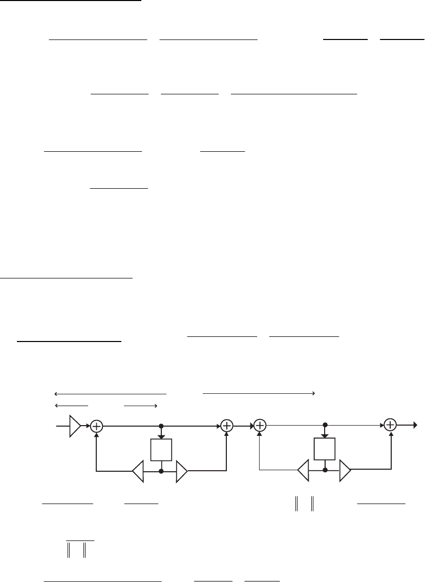
Quantization before addition - The noise transfer function associated with the noise sources
][
1ne and is
][
2ne
=
⎟
⎟
⎠
⎞
⎜
⎜
⎝
⎛
+
+
⎟
⎟
⎠
⎞
⎜
⎜
⎝
⎛
−
−
=−
−
−
−
1
1
1
1
15.01
5805.02708.1
3.01
1141.01737.0
)(
z
z
z
z
zG .
3.0
0745.0
5.0
0138.0
2207.0 −
−
+
+
−
+zz From
Table 12.4 we get
.0569.0
3.0)5.0(1
)0745.0()0138.0(2
)3.0(1
)0745.0(
)5.0(1
)0138.0(
)2207.0( 2
2
2
2
22
1=
×−−
−×−×
+
−
−
+
−−
−
+=σ
The noise transfer function associated with the noise sources and is ],[],[ 43 nene ][
5ne
.
5.0
0549.0
2708.1
5.01
5805.02708.1
)( 1
1
3+
−
+=
+
+
=−
−
z
z
z
zG From Table 12.4 we get
.619.1
)5.0(1
)0549.0(
)2708.1( 2
2
22
3=
−−
−
+=σ The noise transfer function associated with the noise
sources and is given by ][
6ne ][
7ne .1)(
6
=
zG Hence, Hence, total normalized
output noise power is
.1
2
6=σ
.9708.62619.130569.02232 2
6
2
3
2
1
2=+×+×=++= σσσσo
Quantization after addition
Here, total normalized output noise power is .6759.21619.10569.0
2
6
2
3
2
1
2=++=++= σσσσo
(c) Cascade Structure #2 - .
.
.
.
.
)( ⎟
⎟
⎠
⎞
⎜
⎜
⎝
⎛
+
−
⎟
⎟
⎠
⎞
⎜
⎜
⎝
⎛
−
+
=−
−
−
−
1
1
1
1
501
656801
301
456801
2
z
z
z
z
zH
The unscaled structure is shown below:
z1
_z1
_
_0.5
0.3 0.6568
_
2
0.4568
F (z)
1
F (z)
2
.
.
.
.
)( 30
60
2
301
2
1
1−
+=
−
=−z
z
zF Using Table 12.4 we get ..
).(
).( 39564
301
60
22
2
22
21 =
−
+=F
Hence, ..4770
1
2
1
0==β F Likewise,
=
+−
+
=−−
−
).)(.(
).(
)( 11
1
2501301
4568012
zz
z
zF .
.
.
.
.
30
56760
50
0540
2
−
+
+
−
+zz Using Table 12.4 we get
Not for sale 467
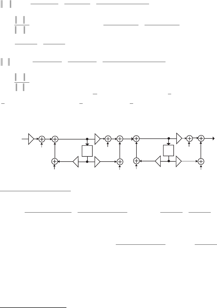
..
.).(
.).(
).(
).(
).(
).( 30464
30501
5676005402
301
56760
501
0540
22
2
2
2
2
2=
×−−
×−×
+
−
+
−−
−
+=F Hence,
..4820
2
2
2
1
2==β F
F Finally, ⎟
⎟
⎠
⎞
⎜
⎜
⎝
⎛
+
−
⎟
⎟
⎠
⎞
⎜
⎜
⎝
⎛
−
+
=−
−
−
−
1
1
1
1
501
656801
301
456801
2
z
z
z
z
zH
.
.
.
.
)(
.
.
.
.
.
30
67510
50
12490
2−
−
+
+
−
+= zz Using Table 12.4 we get
..
.).(
).().(
).(
).(
).(
).( 66834
30501
67510124902
301
67510
501
12490
22
2
2
2
2
2=
×−−
−×−×
+
−
−
+
−−
−
+=H Hence,
..96030
2
2
2
2==β H
F
The scaling multipliers are therefore ,.,.. 4820954024770 1010 =β==×=β= bKK
,.. 3166065680 111 −=β×−=b ,.96030
202 =β=b ... 4387045680 212 =β×=b
The scaled structure with the noise sources is shown below:
z1
_z1
_
_0.5 0.4387
0.3 0.3166
_
0.482 0.9603
0.954
e [n]
1
e [n]
2
e [n]
3
e [n]
4e [n]
5
e [n]
6
e [n]
7
Quantization before addition – The noise transfer function from the noise sources and
is given by
][ne1
][ne2
=
⎟
⎟
⎠
⎞
⎜
⎜
⎝
⎛
+
+
⎟
⎟
⎠
⎞
⎜
⎜
⎝
⎛
−
−
=−
−
−
−
1
1
1
1
1501
4387096030
301
316604820
z
z
z
z
zG
.
..
.
..
)( .
.
.
.
.
.30
15630
50
02890
46290 −
−
+
+
−
+zz Using
Table 12.4 we get Likewise, the noise transfer function from the noise sources
and is given by
..250
2
1=σ
],[],[ nene 43 ][ne550
04150
96030
501
4387096030
1
1
3.
.
.
.
..
)( +
−
+=
+
+
=−
−
z
z
z
zG .
Using Table 12.4 we get Finally, the noise transfer function from the noise
sources and is given by
..92450
2
2=σ
][ne6][ne7.)( 1
6
=
zG Hence, .1
2
6=σ
Therefore, the total normalized output noise power is
.... 2735529245032502232 2
6
2
3
2
1
2=+×+×=σ+σ+σ=σo
Quantization after addition -
Here, total normalized output noise power is
.... 17452192450250
2
6
2
3
2
1
2=++=σ+σ+σ=σo
Not for sale 468

(d) Parallel Form I Realization - .
.
.
.
.
)( 11 301
252
501
250
2−− −
−
+
+
+=
zz
zH
The unscaled structure is shown below:
z
1
_
+
++
x
[n]y[n]
_
2.25
_
0.5
0.3
z
1
_
0.25
2
F (z)
1
F (z)
2
.
.
.
.
.
.
)( 50
1250
250
501
250
1
1+
−
+=
+
=−z
z
zF Using Table 12.4 we get
..
).(
).(
).( 08330
501
1250
250 2
2
2
2
2
1=
−−
−
+=
F Hence, ..46413
1
2
1
1==β F
.
.
.
.
.
.
)( 30
6750
252
301
252
1
2−
−
+−=
−
−
=−z
z
zF Using Table 12.4 we get
..
).(
).(
).( 56325
301
6750
252 2
2
2
2
2
1=
−
−
+−=
F Hence, ..4240
1
2
2
2==β F
.
.
.
.
.
)( 30
6750
50
1250
2−
−
+
+
−
+= zz
zH Using Table 12.4 we get
..
.).(
).().(
).(
).(
).(
).( 66834
30501
675012502
301
6750
501
1250
22
2
2
2
2
2
2=
×−−
−×−×
+
−
−
+
−−
−
+=
H Hence,
..46280
1
2
0==β H
The scaled structure with the noise sources is shown on top of the next page. The noise transfer
function associated with the noise sources and is given by
][ne1][ne2
50
31190
62380
501
1
1
10
1.
.
.
.
/
)( +
−
+=
+
ββ
=−z
z
zG . Using Table 12.4 we obtain,
..
).(
).(
).( 51880
501
31190
62380 2
2
22
1=
−−
−
+=σ Likewise, the noise transfer function associated with
the noise sources and is given by
][ne3][ne4
Not for sale 469
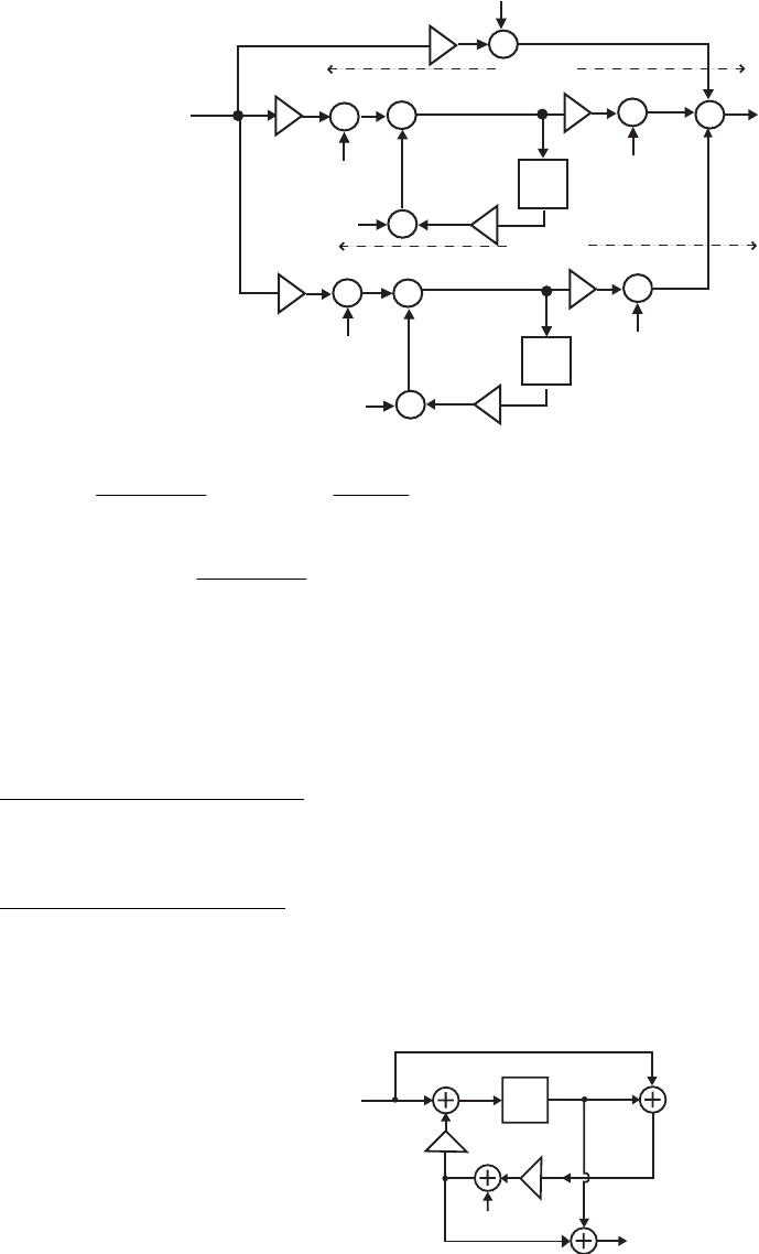
z
1
_
z
1
_
+
++
x
[n]y[n]
0.3
_
0.5
+
+
+
+
+
+
+
e [n]
1
1
G (z)
2
G (z)
e [n]
2
e [n]
3
e [n]
4
e [n]
5
e [n]
6
e [n]
7
_
0.125β
_
0.675β
1
2
2β
0
1/β β
10
1/β β
20
30
27490
91620
301
1
1
20
3.
.
.
.
/
)( −
+=
−
ββ
=−z
z
zG . Using Table 12.4 we obtain,
..
).(
).(
).( 2240
301
27490
91620 2
2
22
3=
−
+=σ
The noise transfer function associated with the remaining three noise sources is .)( 1
5
=
zG
Hence,
.1
2
5=σ
Quantization before addition
Hence, total normalized output noise power is
..88245322 2
5
2
3
2
1
2=σ+σ+σ=σo
Quantization after addition
Here, total normalized output noise power is
..44122
2
5
2
3
2
1
2=σ+σ+σ=σo
12.28 (a) The noise model for the allpass structure of Figure P12.9(a) is shown below:
z
_1
_1di
X
(z)
Y(z)
E(z)
W(z)
R(z)
V(z)
Analysis yields and
To determine the noise transfer function we set
),()()(),()()(),()()( 1zRzzXzVzWzXzRzVdzEzW i−
+=−=+=
).()()( 1zRzzWzY −
+= )(zG 0)(
=
zX in the
Not for sale 470

above equations. This leads to ),()()(),()( 11 zWzzRzzVzWzR
−
−
−==−= and hence,
or,
)()()( 1zWzdzEzW i−
−= ).()1()( 1zWzdzE i
−
+= As a result, )()()( 1zWzzWzY
−
−=
Consequently, the noise transfer function is given by
).()1( 1zWz −
−=
.
)1(
1
1
1
1
)(
)(
)( 1
1
i
i
i
idz
d
dz
z
zd
z
zX
zY
zG +
+−
+=
+
−
=
+
−
== −
−
Using Table 12.4 we get
.
1
2
1
)1(
12
2
2
i
i
i
ed
d
d
−
=
−
+
+=
σ
(b) Let be the noise transfer function for )(zGi.31,
≤
≤
idi Then,
,
1
)(),(
1
)(
2
22
1
1dz
z
zGzA
dz
z
zG +
−
=⋅
+
−
= and .
1
)(
3
3dz
z
zG +
−
= From the results of Part (a), it
follows that the noise variances due to , and are given by
21,dd 3
d
k
kd−
=1
2
2
σ for .3,2,1
=
k
Hence the total noise power at the output of the digital filter structure of Figure P12.9 is given
by .
1
2
1
2
1
2
321
2
ddd
o−
+
−
+
−
=
σ
12.30 Let the total noise power at the output of due to product round-off be given by
Assuming a total of L multipliers in the realization of we get
)(zG .
2
G
σ
)(zG
,)(
2
12
0
2
1
2⎟
⎟
⎠
⎞
⎜
⎜
⎝
⎛
=∫
∑
=
π
ωω
π
σdeGk j
L
Gl
l
l where denotes the noise transfer function due the
–th noise source in Now if each delay is replaced by two delays, then each of the noise
transfer function becomes Thus, the total noise power at the output due to noise
sources in is given by
)(zGl
l).(zG
).( 2
zGl
)( 2
zG .)(
2
1
ˆ
2
0
2
2
1
2⎟
⎟
⎠
⎞
⎜
⎜
⎝
⎛
=∫
∑
=
π
ωω
π
σdeGk j
L
Gl
l
l Replacing ω by in
the integral we get
2/
ˆ
ω
.
ˆ
)2
(
2
1
2
1
ˆ
2
1
)(
2
12
4
0
ˆ
1
4
0
2
ˆ
1
G
j
L
j
L
deGkdeGk σω
π
ω
π
π
ω
π
ω=
⎟
⎟
⎠
⎞
⎜
⎜
⎝
⎛
=
⎟
⎟
⎠
⎞
⎜
⎜
⎝
⎛
⎟
⎠
⎞
⎜
⎝
⎛∫
∑
∫
∑==
l
l
ll
l
l
Since, ,)(
2
1
)()(
2
12
0
2
2
2
0
22
2∫∫ =
π
ω
π
ωω ω
π
ω
πdeGdeAeG jjj the total noise power at the output
of the cascade is still equal to
;
2
o
σ
12.31 For the first factor in the numerator, there are R possible choices of factors. Once this factor
has been chosen, there are 1−
R
choices for the next factor and continuing further we get that
the total number of possible ways in which the factors in the numerator can be generated equal
to . Similarly, the total number of ways in which the factors in the
!12)2)(1( RRRR =×−− L
Not for sale 471
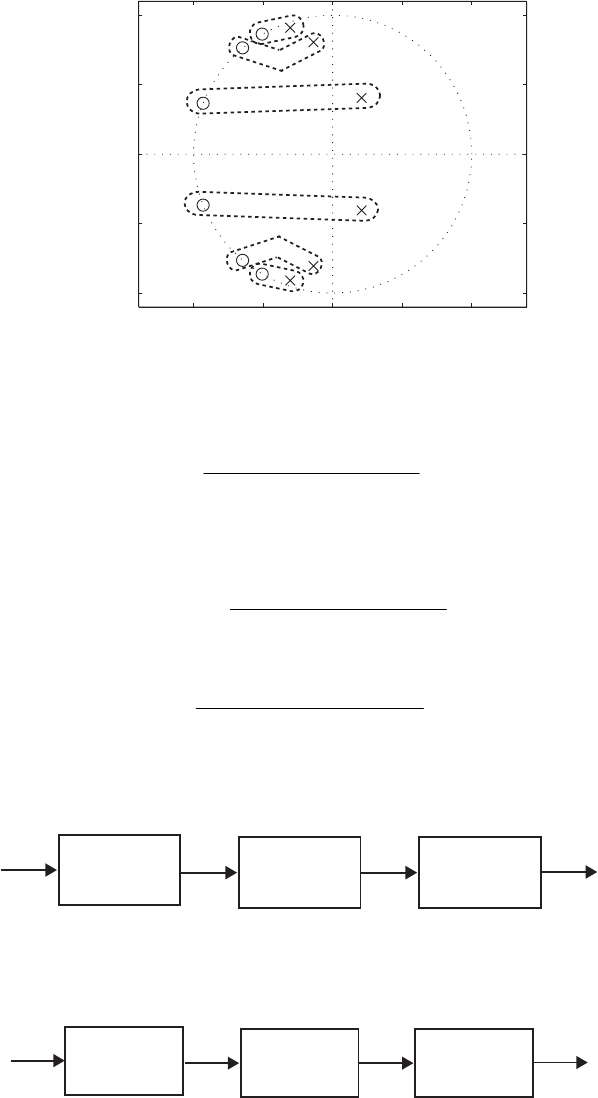
denominator can be generated is equal to . Since the numerator and the denominator are
factored independent of each other, hence the total number of possible realizations are
!R
.)!()!)(!( 2
RRRN ==
12.32 (i) A pole-zero plot of is shown below:
)(
1zH
1 0. 5 0 0.5 1
1
0. 5
0
0.5
1
Real Part
Imaginary Part
1
1
3
3
2
2
First we pair the poles closest to the unit circle with their nearest zeros resulting in the second-
order section
.
9208.06081.0
10094.1
)( 2
2
++
++
=
zz
zz
zHa
Next, the poles that are closest to the poles of are matched with their nearest zeros
resulting in the second-order section
)(zHa
.
6673.02749.0
12914.1
)( 2
2
++
++
=
zz
zz
zHb
Finally, the remaining poles and zeros are matched yielding the second-order section
.
2066.041591.0
18606.1
)( 2
2
+−
++
=
zz
zz
zHc
For ordering the sections to yield the smallest peak output noise due to product round-off under
an -scaling rule, the sections should be placed from most peaked to least peaked as shown
below.
2
L
H (z)
aH (z)
bH (z)
c
For ordering the sections to yield the smallest peak output noise power due to product round-off
under an -scaling rule, the sections should be placed from least peaked to most peaked as
∞
L
shown below.
H (z)
b
H (z)
cH (z)
a
Not for sale 472
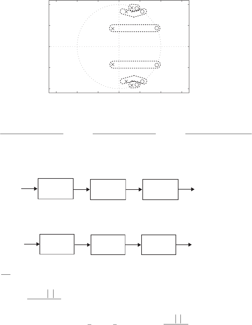
(ii) A pole-zero plot of is shown below:
)(
2zH
(iii)
1. 5 1 0. 5 0 0.5 11.5
1
0. 5
0
0.5
1
Real Part
Imaginary Part
1
1
2
2
3
3
Following the same procedure as in Part (i), we get
.
20358.02993.0
17988.1
)(,
7127.03474.0
11141.1
)(,
9208.06120.0
18508.0
)( 2
2
2
2
2
2
+−
+−
=
+−
+−
=
+−
+−
=
zz
zz
zH
zz
zz
zH
zz
zz
zH aba
For ordering the sections to yield the smallest peak output noise due to product round-off under
an -scaling rule, the sections should be placed from most peaked to least peaked as shown
2
L
below.
H (z)
aH (z)
bH (z)
c
For ordering the sections to yield the smallest peak output noise power due to product round-off
under an -scaling rule, the sections should be placed from least peaked to most peaked as
∞
L
shown below.
H (z)
b
H (z)
cH (z)
a
12.33 2
2
o
x
σ
σ
=SNR . After scaling, changes to where
x
σx
Kσ
K
is as given by Eq. (12.151).
Therefore, .
)(
2
22 1
SNR
o
x
σ
α−σ
=
(i) For uniform density function .
3
1
2
1
1
2
1
2== ∫
−
dxx
x
σ Thus, .
3
)1(
2
2
o
σ
α
−
=
SNR With
Not for sale 473

9
12
2
210967.4,12
24 −
×=== −
o
bσ and .95.0=α Hence,
24.52
3
)1(
log10 2
2
10 =
⎟
⎟
⎠
⎞
⎜
⎜
⎝
⎛−
=
o
dB σ
α
SNR dB.
(ii) For Gaussian input with ,
9
1
2=
x
σ .
9
)1(
2
2
o
σ
α
−
=
SNR Again with
,12=b
97.47
9
)1(
log10 2
2
10 =
⎟
⎟
⎠
⎞
⎜
⎜
⎝
⎛−
=
o
dB σ
α
SNR dB.
(iii) For a sinusoidal input of known frequency, i.e., ).sin(][ nnx o
ω
=
In this case, the average
power = .
2
1
2=
x
σ Hence, .
2
)1()1(
2
2
2
22
oo
x
σ
α
σ
σα −
=
−
=
SNR Therefore,
91.69
2
)1(
log10 2
2
10 =
⎟
⎟
⎠
⎞
⎜
⎜
⎝
⎛−
=
o
dB σ
α
SNR dB.
12.34 (a) )],(1[)( 1
2
1zAzH LP += where .
1
)( 1
1
1−
−
−
+−
=
z
z
zA
α
α Hence,
.
cos21
)cos1(2
2
1
)( 2
2
2
αωα
ωα
ω
+−
+
⎟
⎠
⎞
⎜
⎝
⎛−
=
j
LP eH Proving 0
)(
0
=
∂
∂
=ω
ω
α
j
LP eH
is equivalent to
proving .0
)(
0
2
=
∂
∂
=ω
ω
α
j
LP eH
Now,
.
cos21
)cos2)(cos1(2
2
1
cos21
)cos1(2
2
1
)(
2
2
2
2
αωα
ωαωα
αωα
ωα
α
ω
+−
−+
⋅
⎟
⎠
⎞
⎜
⎝
⎛−
−
+−
+
⋅
−
−=
∂
∂j
LP eH
Thus, .0
1
2
1
2
)(
0
2
=
−
+
−
−
=
∂
∂
=
ααα
ω
ωj
LP eH
(b) )],(1[)( 1
2
1zAzH HP −= where .
1
)( 1
1
1−
−
−
+−
=
z
z
zA
α
α Hence,
.
cos21
)cos1(2
2
1
)( 2
2
2
αωα
ωα
ω
+−
−
⎟
⎠
⎞
⎜
⎝
⎛+
=
j
HP eH Now,
.
cos21
)cos2)(cos1(2
2
1
cos21
)cos1(2
2
1
)(
2
2
2
2
αωα
ωαωα
αωα
ωα
α
ω
+−
−−
⋅
⎟
⎠
⎞
⎜
⎝
⎛+
−
+−
−
⋅
+
−=
∂
∂j
HP eH
Not for sale 474

Thus, .0
1
2
1
2
)(
0
2
=
+
+
+
−
=
∂
∂
=
ααα
ω
ωj
HP eH
12.35 (a) )],(1[)( 2
2
1zAzHBP −= where ,
)1(1
)1(
)( 21
21
2−−
−−
++−
++−+
=
zz
zz
zA
ααβ
αβα with α and being
real. Hence,
β
.
cos)1(
β
2)2cos(2)1(1
)cos1(2
2
1
)( 2222
2
2
⎟
⎟
⎠
⎞
⎜
⎜
⎝
⎛
+−++++
−
⎟
⎠
⎞
⎜
⎝
⎛−
=ωαωαααβ
ωα
ωj
BP eH
Now, ⎟
⎟
⎠
⎞
⎜
⎜
⎝
⎛
+−++++
−
⎟
⎠
⎞
⎜
⎝
⎛−
⎟
⎠
⎞
⎜
⎝
⎛
−
−
=
∂
∂
ωαβωαααβ
ωα
αα
ω
cos)1(2)2cos(2)1(1
)cos1(2
2
1
1
2
)(
2222
2
2
j
BP eH
×
⎟
⎟
⎠
⎞
⎜
⎜
⎝
⎛
+−++++
−
⎟
⎠
⎞
⎜
⎝
⎛−
+ωαβωαααβ
ωα
cos)1(2)2cos(2)1(1
)cos1(2
2
1
2222
2
.
cos)1(2)2cos(2)1(1
cos)1(4)2cos(22)1(2
2222
2
⎟
⎟
⎠
⎞
⎜
⎜
⎝
⎛
+−++++
+−+++
ωαβωαααβ
ωαβωααβ
Using the fact we get ),cos( o
ωβ =
.0
1
2
1
2
221
)2222(
1
2
)(
22222
22
2
=
−
+
−
−
=
−−+−+
−−+
−
−
−
=
∂
∂
=
αα
βαβαβαα
αβαβ
αα
ωω
ω
o
j
BP eH
Similarly, ×
⎟
⎟
⎠
⎞
⎜
⎜
⎝
⎛
+−++++
−
⎟
⎠
⎞
⎜
⎝
⎛−
=
∂
∂
ωαβωαααβ
ωα
β
ω
cos)1(2)2cos(2)1(1
)cos1(2
2
1
)(
2222
2
2
j
BP eH
.
cos)1(2)2cos(2)1(1
cos)1(2)1(2
2222
2
⎟
⎟
⎠
⎞
⎜
⎜
⎝
⎛
+−++++
+−+
−ωαβωαααβ
ωααβ
Again, using the fact it can be seen that ),cos( o
ωβ =.0
)( 2
=
∂
∂
=o
j
BP eH
ωω
ω
β
(b) Here, )],(1[)( 2
2
1zAzH BS += where is as given in Part (a). Hence,
)(
2zA
.
cos)1(2)2cos(2)1(1
cos8)2cos(224
2
1
)( 2222
2
2
2
⎟
⎟
⎠
⎞
⎜
⎜
⎝
⎛
+−++++
−++
⎟
⎠
⎞
⎜
⎝
⎛+
=ωαβωαααβ
ωβωβα
ωj
BS eH Thus,
⎟
⎟
⎠
⎞
⎜
⎜
⎝
⎛
+−++++
−++
⎟
⎠
⎞
⎜
⎝
⎛+
=
∂
∂
ωαβωαααβ
ωβωβα
α
ω
cos)1(2)2cos(2)1(1
cos8)2cos(224
2
1
)(
2222
2
2
j
BS eH
Not for sale 475

×
⎟
⎟
⎠
⎞
⎜
⎜
⎝
⎛
+−++++
−++
⎟
⎠
⎞
⎜
⎝
⎛+
−ωαβωαααβ
ωβωβα
cos)1(2)2cos(2)1(1
cos8)2cos(224
2
1
2222
2
2
.
cos)1(2)2cos(2)1(1
cos)1(4)2cos(22)1(2
2222
2
⎟
⎟
⎠
⎞
⎜
⎜
⎝
⎛
+−++++
+−+++
ωαβωαααβ
ωαβωαβα
Substituting it can be seen that ),cos( o
ωβ =
.0
)1()1(
)1)(1(2
2
1
1
2
)(
22
2
2
0
2
=
⎟
⎟
⎠
⎞
⎜
⎜
⎝
⎛
++
++
⎟
⎠
⎞
⎜
⎝
⎛+
−
−
=
∂
∂
=
βα
βαα
αα
ω
ωj
BS eH
Similarly, .0
)1()1(
)1)(1(2
2
1
1
2
)(
22
2
2
2
=
⎟
⎟
⎠
⎞
⎜
⎜
⎝
⎛
++
++
⎟
⎠
⎞
⎜
⎝
⎛+
−
−
=
∂
∂
=
βα
βαα
αα
πω
ωj
BS eH
Now, ⎟
⎟
⎠
⎞
⎜
⎜
⎝
⎛
+−++++
−
⎟
⎠
⎞
⎜
⎝
⎛+
=
∂
∂
ωαβωαααβ
ωββα
β
ω
cos)1(2)2cos(2)1(1
cos88
2
1
)(
2222
2
2
j
BS eH
×
⎟
⎟
⎠
⎞
⎜
⎜
⎝
⎛
+−++++
−++
⎟
⎠
⎞
⎜
⎝
⎛+
−ωαβωαααβ
ωβωβα
cos)1(2)2cos(2)1(1
cos8)2cos(224
2
1
2222
2
2
.
cos)1(2)2cos(2)1(1
)cos(2)1(
2222
2
⎟
⎟
⎠
⎞
⎜
⎜
⎝
⎛
+−++++
−+
ωαβωαααβ
ωβα
Again, substituting it can be seen that ),cos( o
ωβ =0
)(
0
2
=
∂
∂
=ω
ω
β
j
BS eH
and
.0
)( 2
=
∂
∂
=πω
ω
β
j
BS eH
12.36 For a BR transfer function realized in a parallel allpass form, its power-complementary
transfer function is also BR satisfying the condition
)(zG
)(zH .)(1)( 22 ωω jj eHeG −= Let
be a frequency where
o
ωω =)( ωj
eG is a maximum, i.e., .1)( =
o
j
eG ω Then, it follows that
.0)( =
o
j
eH ω From the power- complementary condition it follows that
.
)(
)(2
)(
)(2 ωω
ω
ω
ω
ω
∂
∂
⋅−=
∂
∂
⋅
j
j
j
jeH
eH
eG
eG Therefore, at o
ωω
=
,
Not for sale 476
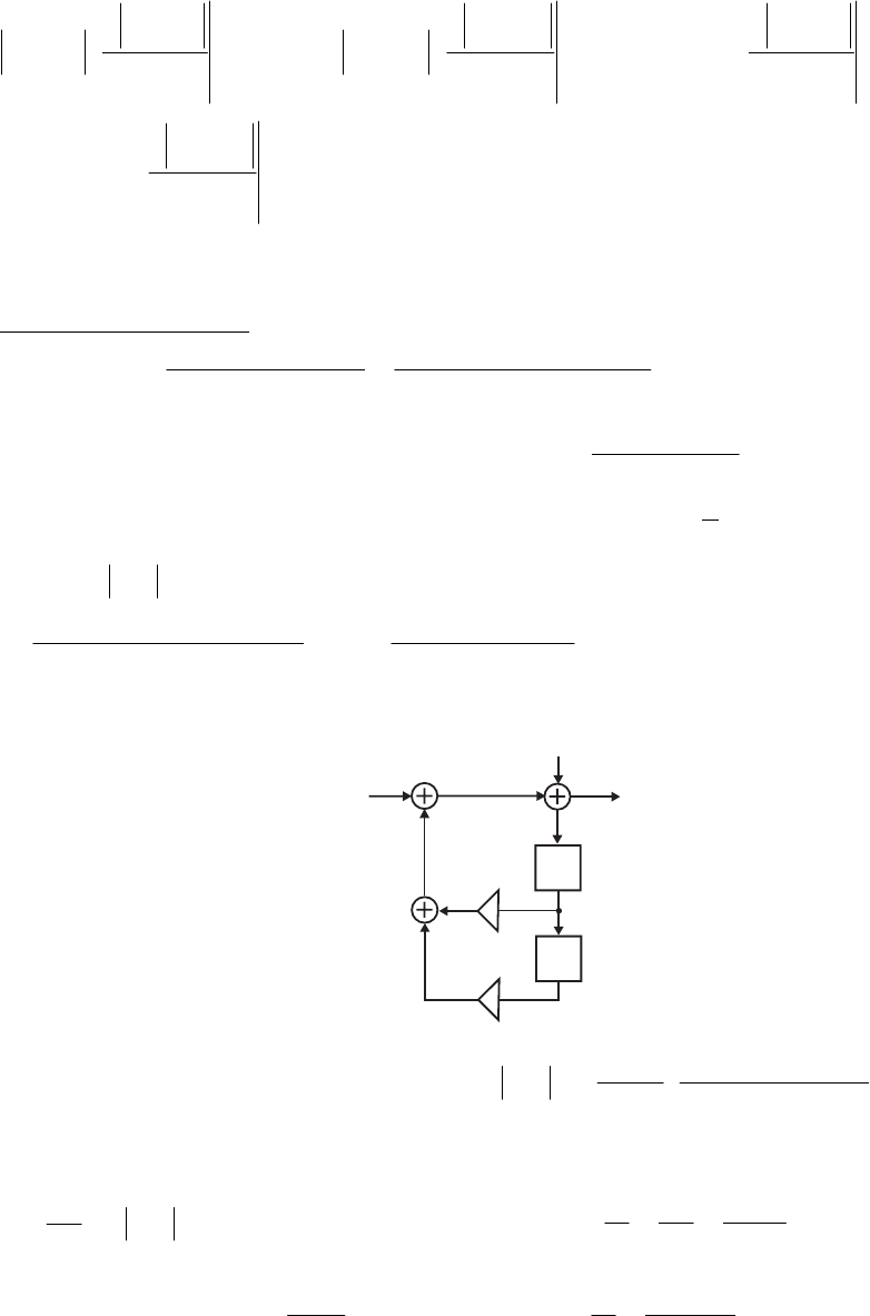
,
)(
)(2
)(
)(2
oo
j
j
j
jeH
eH
eG
eG
ωω
ω
ω
ωω
ω
ω
ωω == ∂
∂
⋅−=
∂
∂
⋅ and thus, 0
)( =
∂
∂
=o
j
eG
ωω
ω
ω
whether or not .0
)( =
∂
∂
=o
j
eH
ωω
ω
ω Hence, low passband sensitivity of does not
necessarily imply low passband sensitivity of .
)(zG
)(zH
12.37 Without error feedback – The transfer function of the structure without error feedback is
given by ,
cos21
1
1
1
)( 2212
2
1
1−−−− +−
=
++
=
zrzrzz
zH
θαα where The
corresponding impulse response is given by
.1 ε−=r
][nh ].[
sin
)1sin(
][ n
nr
nh
n
µ
θ
θ+
= To keep the
output from overflowing we must insert a multiplier of value ][ny
L
1 at the input where
.][
0
∑∞
=
=nnhL From Eq. (12.164) we get
.
sin)1(
16
)cos21()1(
1
:)1( 222
2
22 θπθ r
L
rrr −
≤≤
+−−
The quantization noise model for is as shown below:
)(zH
_
z_1
z_1
1
α
_
2
α
y[n]
e[n]
x
[n]
The output noise power is given by .
1cos2
1
1
1
][ 2
242
2
0
2
22 e
n
en rrr
r
nh σ
θ
σσ ⋅
+−
⋅
−
+
== ∑
∞
=
The output signal power, assuming an input signal of variance is given by
2
x
σ
.][
0
2
2
2
2∑
∞
=
=
n
y
ynh
L
σ
σ Hence, the SNR is given by .
22
2
2
2
e
x
n
y
Lσ
σ
σ
σ=== N
S
SNR For a )1(
+
b-bit
signed representation, .
12
22
2b
e
−
=σ Hence, here .
222
2
b
x
L
−
== σ
N
S
SNR Therefore, from the
Not for sale 477

inequality of Eq. (1) given above, we get
.
sin)1(12
216
)cos21()1(12
2
2222
2
222
2
θπσθσ r
S
N
rrr x
b
x
b
−
×
≤≤
+−−
−−
(a) For an WSS uniformly distributed input between .],1,1[ 3
1
2=− x
σ Hence,
.
sin)1(
24
)cos21()1(4
2
22
2
222
2
θπθ r
S
N
rrr
bb
−
⋅≤≤
+−−
−−
If and then and In
this case we have
,0→ε,0→θ,21sin21)2cos(,)1( 2222 θθθε −≅−=→− r.sin 22 θθ ≅
.
2
)4(4
2
222
2
222
2
θεπθεε
bb
S
N−− ≤≤
+
(b) For an input with a Gaussian distribution between .],1,1[ 3
1
=− x
σ In this case, we have
.
23
)4(4
2
322
2
2222
2
θεπθεε
bb
S
N−− ⋅≤≤
+
⋅
(c) For a sinusoidal input between ]1,1[
−
of known frequency .
2
1
,2=
xo σω The output noise
variance here is therefore .
1cos2
1
1
1
12
2
][ 242
22
0
2
22
+−
⋅
−
+
⋅== −
∞
=
∑θ
σσ
rrr
r
nh
b
n
en Thus,
()
.
24
2
)(24
2
1)2cos(26
1
1
1
2
2
22
2
242
2
εθθεεθ
bb
rrr
r
S
N−− ≅
+
=
+−
⋅
−
+
=
With error feedback
.
1cos2
1)1cos(2
1
1cos2
12
cos21
21
)( 2
2
2
2
221
21
+−
−+−
+=
+−
+−
=
+−
+−
=−−
−−
zrz
rzr
zrz
zz
zrzr
zz
zG
θ
θ
θθ
Thus,
(
)
.
cos)1(4)cos4(2)1(
)1cos()1(cos8)1()1()cos1(4
122422222
224222
2
θθ
θθθ
rrrrr
rrrrrr
G+−+−
−−⋅+−−+−
+=
For with and we get after some manipulation
ε−= 1r,0→ε,0→θ
,
)(4
122
4
2
θεε
θ
+
+=G and .
2
22 G
en σσ =
Now, remains the same as before since it depends only upon the denominator. Also, the overall
transfer function of the structure remains the same as before. The output noise power with
Not for sale 478
error feedback is thus ,
ˆ2
2GN e
σ= whereas, the output noise power without error feedback is
.
2
2HN e
σ= Hence, .
ˆ
2
2
H
G
N
N=
Now, .
)(4
122
4
2
θεε
θ
+
+=G Since .
4
4
,
2
2
4
2
ε
θ
εθ
θ
εθ =≅>> G
Also, 1)21()1(2)1(
1
)1(1
)1(1
1cos2
1
1
1
2242
2
2242
2
2
+−−−−
⋅
−−
−+
=
+−
⋅
−
+
=θεεε
ε
θrrr
r
H
.
4
1
)(4
1
222 εθεθε ≈
+
≈
Thus, .
ˆ4
θ≅
N
N As a result, with error feedback, the S
N ratio gets multiplied by
.
4
θ
(a) input with uniform density: .
2
ˆ
16
2
2
2
2
2
2
22
επ
θ
ε
θbb
S
N−− ⋅≤≤
(b) wide-sense stationary, Gaussian density, white: .
23
ˆ
16
32
2
2
2
2
2
22
επ
θ
ε
θbb
S
N−− ⋅≤≤
(c) sinusoid with known frequency: ε
θ
24
2
ˆ22b
S
N−
=.
12.38 The coupled form with error feedback is shown below:
y[n]
z
_1
z
_1
α
β
δ
γ
Q
Q
z
_1
z
_1
λ1
λ2
e [n]
1
e [n]
2
+
+_
_
v [n]
1
v [n]
2
u[n]
Analysis yields ),()()()( 11
1
1
11 zUzzYzzEzzV
−
−
−++= γδλ ),()()( 11 zVzYzE −
=
),()()()( 11
2
1
22 zUzzYzzEzzV
−
−− ++= αβλ and ).()()( 22 zVzYzE
−
=
Eliminating
and from these equations we arrive at the noise transfer functions
),(),(),( 211 zUzVzU )(
2zV
21
1
1
1
0)(
1
1)()(1
)1)(1(
)(
)(
)(
2
−−
−
−
=−++−
+−
==
zz
zz
zE
zY
zG
zE γβδαδα
λα and
Not for sale 479
.
)()(1
)1(
)(
)(
)( 21
1
2
1
0)(
2
2
2
−−
−
−
=−++−
+
==
zz
zz
zE
zY
zG
zE γβδαδα
λγ The total output noise power is thus
given by .
22
2
2
2
2
1
2
2
1
2ee
oGG σσσ += Hence, the total output noise power, for a lowpass filter
design, can be reduced by placing the zeros of the noise transfer functions in the passband. For
each of the noise transfer functions given above, we can place only a zero at by choosing
1=z
.2,1,1 =−= i
i
λ
Using the notations and
)( δα +−=b,γβδα
−
=
d we rewrite the noise transfer functions as
dbzz
dzb
dbzz
zz
zG ++
−+++−
+=
++
++−
=22
2
1
)()1(
1
)1(
)( αααα and .)( 2
2dbzz
z
zG ++
−
=γγ Using Table
12.4 we obtain 22222
222
2
2
1)1(2)1(
)1)()(1(2)1]()()1[(
1
bddbd
ddbddb
G+−+−
−−+++−−+++
+= αααα and
.
)1(2)1(
)1(2
22222
22
2
2
2bddbd
d
G+−+−
−
=γ
12.39 The Kingsbury structure with error feedback is shown below.
x
[n]y[n]
k
1
k
2
k
1
_
QQ
Q
–
z
1
–
z
1
v [n]
1v [n]
2v [n]
3
–
z
1
–
z
1
–
z
1
+
u [n]
1u [n]
2u [n]
3
++
___
1
λ2
λ3
λ
Analysis yields: ),()()()( 1
1
11
1
11 zEzzUzzYkzV
−
−
++= λ ),()()( 111 zVzUzE −
=
),()()()( 2
1
2122 zEzzUzYkzV −
++= λ),()()( 222 zVzUzE
−
=
),()()()( 3
1
3113 zEzzUkzYzV −
+−= λ),()()( 333 zVzUzE
−
=
and
Eliminating and from these equations we get
).()( 1
1zUzzY −
=
),(),(),(),(),( 32211 zUzVzUzVzU )(
3zV
,
)1()](2[1
)1(
)(
)(
)( 2
21
1
211
1
1
1
1
0)()(
1
1
32
−−
−
−
== −++−−
+−
==
zkkzkkk
zzk
zE
zY
zG
zEzE
λ
,
)1()](2[1
)1)(1(
)(
)(
)( 2
21
1
211
1
2
11
1
0)()(
2
2
31
−−
−
−
−
== −++−−
+−−
==
zkkzkkk
zzzk
zE
zY
zG
zEzE
λ
.
)1()](2[1
)1)(1(
)(
)(
)( 2
21
1
211
1
3
11
0)()(
3
3
21
−−
−−−
== −++−−
+−
==
zkkzkkk
zzz
zE
zY
zG
zEzE
λ
Not for sale 480
The total output noise power is thus given by .
23
2
2
3
22
2
2
2
21
2
2
1
2eee
oGGG σσσσ ++= Hence, the
output noise power for a lowpass filter design can be reduced by placing zeros of the noise
transfer functions in the passband. For each of the noise transfer functions given above, we can
only place one zero at by choosing
1=z,3,2,1,1
=
−
=
i
i
λ in which case, using the notations
and
)](2[ 211 kkkb +−−= ,1 21kkd
−
= the noise transfer functions reduce to
,
1
)1(
)( 2
11
21
11
1
1dzbz
kzk
zdzb
zzk
zG ++
+−
=
++
−−
=−−
−−
,
)(
)1(
1
)1(
)( 2
1
2
2
1
21
211
1
2dzbz
DCz
z
Ak
dzbzz
zzk
zdzb
zzk
zG ++
+
+
−
=
++
++−
=
++
−−
=−−
−−
,
)(
1
1
)1(
)( 22
2
21
211
3dzbz
DCz
z
A
dzbzz
zz
zdzb
zz
zG ++
+
+=
++
++
=
++
−
=−−
−−
where ,
1
d
A= ,
1
1d
C−=
and .2 ⎟
⎠
⎞
⎜
⎝
⎛+−= d
b
D Using Table 12.4 we then obtain
,
)1(2)1(
)1(2)1(2
22222
2
2
1
2
2
1bddbd
bdd
kG +−+−
−−−
⋅=
,
)1(2)1(
)1(2)1)((
222222
222
2
2
2
3bddbd
bdCDdDC
BCAG +−+−
−−−+
++= and .
2
2
3
2
1
2
2
2GkG =
12.40 The coupled-form structure with state-variables labeled is shown below:
x
[n]y[n]
z
_1
z
_1
α
β
δ
γ
s [n+1]
1
s [n+1]
2
Its transfer function is given by Eq. (12.19) where θδα cosr
=
=
and
Analysis of the above structure yields
.sin θγβ r=−=
(
)
][][][]1[ 211 nsnsnxns βα
+
+
=
+
and
Rewriting these two equations in matrix form we get
Thus, Therefore,
Likewise,
Since for stability
()
].[][][]1[ 212 nsnsnxns δγ ++=+
].[
][
][
]1[
]1[
2
1
2
1nx
ns
ns
ns
ns ⎥
⎦
⎤
⎢
⎣
⎡
+
⎥
⎦
⎤
⎢
⎣
⎡
⎥
⎦
⎤
⎢
⎣
⎡
=
⎥
⎦
⎤
⎢
⎣
⎡+
+
γ
α
δγ
βα .
⎥
⎦
⎤
⎢
⎣
⎡
=δγ
βα
A
.
0
0
2
2
22
22
⎥
⎦
⎤
⎢
⎣
⎡
=
⎥
⎦
⎤
⎢
⎣
⎡
++
++
=
⎥
⎦
⎤
⎢
⎣
⎡
⎥
⎦
⎤
⎢
⎣
⎡
=r
r
t
δβγδαβ
γδαβγα
δγ
βα
δβ
γα
AA
.
0
0
2
2
22
22
⎥
⎦
⎤
⎢
⎣
⎡
=
⎥
⎦
⎤
⎢
⎣
⎡
++
++
=
⎥
⎦
⎤
⎢
⎣
⎡
⎥
⎦
⎤
⎢
⎣
⎡
=r
r
t
δγβδαγ
βδαγβα
δβ
γα
δγ
βα
AA ,1
<
r A is a
normal form matrix, and hence the coupled-form structure does not support limit cycles.
Not for sale 481

12.41 The modified coupled-form structure with state-variables labeled is shown on top of the next
page. Its transfer function determined in the solution of Problem 12.4 is given by
.
)1(2
)( 222
2
dccdzz
c
zH ++−
= Now, a second-order transfer function with poles at
x
[n]y[n]
cc
d
_1
z
d
_
1
_1
z
1
s [n+1]
2
s [n+1]
has a denominator given by Comparing this denominator with
that of H(z), we get and
θj
erz ±
=.cos2 22 rzrz +⋅− θ
θsinrc =.cotθ
=
d
Analyzing the modified coupled-form structure we arrive at the following equations:
and
][][][]1[ 211 nxnscnsdcns +−=+ ][][]1[ 212 nsdcnscns
+
=
+
. Rewriting these two
equations in matrix form we get Thus,
Therefore,
Likewise,
Since for stability A is a
normal form matrix, and hence the modified coupled-form structure does not support limit
cycles.
].[
0
1
][
][
]1[
]1[
2
1
2
1nx
ns
ns
cdc
ccd
ns
ns ⎥
⎦
⎤
⎢
⎣
⎡
+
⎥
⎦
⎤
⎢
⎣
⎡
⎥
⎦
⎤
⎢
⎣
⎡−
=
⎥
⎦
⎤
⎢
⎣
⎡+
+
.
cossin
sincos ⎥
⎦
⎤
⎢
⎣
⎡−
=
⎥
⎦
⎤
⎢
⎣
⎡−
=θθ
θθ
rr
rr
cdc
ccd
A
.
0
0
cossin
sincos
cossin
sincos
2
2
⎥
⎦
⎤
⎢
⎣
⎡
=
⎥
⎦
⎤
⎢
⎣
⎡−
⎥
⎦
⎤
⎢
⎣
⎡−
=r
r
rr
rr
rr
rr
t
θθ
θθ
θθ
θθ
AA
.
0
0
cossin
sincos
cossin
sincos
2
2
⎥
⎦
⎤
⎢
⎣
⎡
=
⎥
⎦
⎤
⎢
⎣
⎡−
⎥
⎦
⎤
⎢
⎣
⎡−
=r
r
rr
rr
rr
rr
t
θθ
θθ
θθ
θθ
AA ,1<r
12.42 .1
1+=⇒
−
=Γ
Γδδ z
z
.
1
)(
21
2
21
2
0
2
2
1
1
2
2
1
10
αα
βββ
αα
βββ
++
++
=
++
++
=−−
−−
zz
zz
zz
zz
zH Therefore,
21
2
21
2
0
1
21
2
21
2
0
1)1()1(
)1()1(
)()( αδαδ
βδβδβ
αα
βββ
δ
δ
δ++++
++++
=
++
++
==
+=
+= ΓΓ
ΓΓ
Γ
Γ
z
zzz
zz
zHH
)1()2(
)()2()(
)1()12(
)1()12(
211
22
21010
22
0
21
22
21
22
0
ααδαδ
βββδββδβ
αδαδδ
βδβδδβ
+++++
+++++
=
+++++
+++++
=
ΓΓΓ
ΓΓΓ
ΓΓΓ
ΓΓΓ
.
)1()2(
)()2()(
2
21
1
1
2
2
210
1
10
2
0
−−
−−
+++++
+++++
=δααδα
δβββδβββ
ΓΓΓ
ΓΓΓ
Not for sale 482

12.43 From Section 11.3.1 we know that computation of each DFT sample requires 42
+
N real
multiplications. Assuming that the quantization noise generated from each multiplier is
independent of the noise generated from other multipliers, we get
.
6
)2(2
)42(
2
22 +
=+= −N
N
b
or σσ
12.44 .
2
2
2
N
b
=SNR Hence, an SNR of 30 dB implies ,10
23
2
2=
N
b
or
()
.9829.1251210log 23
2
2
1=×=b We choose 141
=
+
b bits per sample to get an SNR of 30
dB.
12.45 Let Consider the -th stage. The output sees
.2ν
=Nm)2(4 m
−
ν noise sources from the -th
stage. Each noise source has a variance reduction by a factor of
m
m−
⎟
⎠
⎞
⎜
⎝
⎛ν
4
1 due to multiplication
by 2
1 at each stage till the output. Hence the total noise variance at the output due to the noises
injected in the m-th stage is
(
)
(
)
.224 2)(2 o
mm σ
νν
−
−
−
Therefore, the total noise variance at the
output
()( )
∑∑
=
ν
m=
−−−− ===
ν
ννν σσσ
1
2
1
2)(22 224224
m
m
oo
mm
bb
b22
2
2
3
2
)21(2
3
2
12
)12(2
2
12
2
4−−−−
−≈−=
⎟
⎟
⎠
⎞
⎜
⎜
⎝
⎛
−
−
⎟
⎟
⎠
⎞
⎜
⎜
⎝
⎛
=ν
ν
ν for large .
N
12.46 .
2
22
N
b
=SNR Hence,
(
)
.4829.9256210log 3
2
2
1=××=b We choose bits per
sample to get an SNR of 30 dB.
111 =+b
2
2
2
b
SNR N
=. Hence
()
(
)
2.5
2
1log 10 5 256 10.1439
2
b=××=
. We choose b+1 = 12 bits per
sample to get an SNR of 30dB. CHECK
M12.1 %POLE_PLOT
% POLE_PLOT(B) obtains the pole distribution
% plot of a second order transfer function with a denominator
% of the form Z*Z - KZ + L. For stability 0 < L < 1 and
% abs(K) < 1+L so the range of K is (-2,2).
%
% for a B-bit wordlength, 1 bit is reserved for the sign
% as the coefficients are sorted in the sign magnitude form.
% Both L and the K are quantizd to B-1 bits.
%
function[]=pole_plot(bits);
point = 'o';
%
Not for sale 483
% This part prints the unit circle for reference
% One bit is kept for the sign so effectively for the
% quantization. The remaining number of bits is bits-1
%
bits = bits-1;
%
% sets up the axis
zplane(2,2); % plotting queue of roots using zplane.m with a
% dummy zero and pole
axis([-1 1 -1 1]); % adjusting axis to "hide" dummy zero/pole,
% calling zplane without a zero is not legal in MATLAB release
% 12 and 13
title(['Second order Pole distribution for ',num2str(bits+1),'
bits']);
hold on;
%
% The quantization step.
%
step = power(2,-bits);
for index_1 = 0:1:(power(2,bits)-1) % 0 < index1 < 2^bits-1
L = index_1*step; % 0 < L < 1
for index_2 = -(power(2,bits)-1):1:(power(2,bits)-1)
% -2^bits-1 < index2 < 2^bits-1
K = 2*index_2*step; % -2 < K < 2
p = roots([1 -K L]); % finding roots
if abs(p(1)) < 1 % testing root 1
if (imag(p(1)) == 0) % real root
plot(p(1),0,point); % plotting
else % complex root
plot(p(1),point); % plotting
end
end
if abs(p(2)) < 1 % testing root 2
if (imag(p(1)) == 0) % real root
plot(p(2),0,point); % plotting
else % complex root
plot(p(2),point); % plotting
end
end
% title(['L = ',num2str(L),' K = ',num2str(K)]);
% above 3 lines for debugging/demo purposes
% place break here and step thru to see poles for each L and K
end
end
title(['Second order Pole distribution for ',num2str(bits+1),'
bits']);
hold off;
Not for sale 484
M12.2 The pole-distribution plot of the second-order direct form structure is obtained by running the
MATLAB program given in Exercise M12.1. Running this program using the statement
pole_plot(4) yields the following plot:
-1 -0.5 00.5 1
-1
-0.5
0
0.5
1
Real Part
Imaginary Part
Second order Pole distribution for 4 bits
For plotting the pole distribution of the coupled form structure, we use the following MATLAB
program:
% POLE_PLOT_COUPLED(B) obtains the pole distribution
% plot of a second order transfer function in coupled form
% with the transfor function rZ^2 / Z^2 - (a + d)Z + (ad - br)
% For stability -1 < a,b,d,r < 1
%
% for a B-bit wordlength, 1 bit is reserved for the sign
% as the coefficients are sorted in the sign magnitude form.
% Both L and the K are quantizd to B-1 bits.
%
function[]=pole_plot_coupled(bits);
bits = 4;
point = '.';
%
% This part prints the unit circle for referenc
%
% One bit is kept for the sign so effectively for the
% quantization, the remaining number of bits is bits-1
%
bits = bits-1;
%
% sets up the axis
zplane(2,2); % plotting queue of roots using zplane.m with a
% dummy zero and pole
axis([-1 1 -1 1]); % adjusting axis to "hide" dummy zero/pole,
% calling zplane without a zero is not legal in MATLAB release
% 12 and 13
title(['Second-order coupled form pole distribution for ',
num2str(bits+1),' bits']);
hold on;
%
Not for sale 485
% The quantization step.
%
step = power(2,-bits);
for index_1 = -(power(2,bits)-1):1:(power(2,bits)-1)
a = index_1*step;
for index_2 = -(power(2,bits)-1):1:(power(2,bits)-1)
% -2^bits-1 < index2 < 2^bits-1
b = index_2*step;
for index_3 = -(power(2,bits)-1):1:(power(2,bits)-1)
d = index_3*step;
for index_4 = -(power(2,bits)-1):1:(power(2,bits)-1)
r = index_4*step;
p = roots([1 -(a+d) (a*d-b*r)]);
% finding roots
if abs(p(1)) < 1 % testing root 1
if (imag(p(1)) == 0)
% real root
plot(p(1),0,point); % plotting
else % complex root
plot(p(1),point); % plotting
end
end % testing root 2
if (imag(p(1)) == 0) % real root
plot(p(2),0,point); % plotting
else % complex root
plot(p(2),point); % plotting
end
end
end
end
% title(['a = ',num2str(a),' b = ',num2str(b),'d =
',num2str(d),' r = ',num2str(r)]);
end
end
title(['Second-order coupled form pole distribution for
',num2str(bits+1),' bits']);
hold off;
M12.3 % Modified Program 12_1
% Coefficient Quantization Effects on the frequency
% response of a direct form IIR filter
clf;
[b,a] = ellip(7,0.02,55,0.7,'high');
[h,w] = freqz(b,a,512);
g = 20*log10(abs(h));
% Truncate the filter coefficients to 5 bits
bq = a2dT(b,6); aq = a2dT(a,6);
[hq,w] = freqz(bq,aq,512);
gq = 20*log10(abs(hq));
Not for sale 486
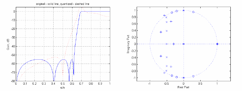
plot(w/pi,g,'b',w/pi,gq,'r:'); grid; axis([0 1 -80 5]);
xlabel('\omega/\pi'); ylabel('Gain, dB');
title('original - solid line, quantized - dashed line');
pause
% The call to the ZPLANE function below sets the axes
% properties to those corresponding to a pole-zero plot
zplane(b,a);
% The HOLD ON command retains the axes properties as
% they are and does not create new axes for the next plot
hold on;
plotzp(bq,aq)
M12.4 MATLAB code fragments are as follows:
num = [0.06891875 0.13808186 0.18636107 0.13808186 0.06891875];
den = [1 -1.30613249 1.48301305 -0.77709026 0.2361457];
nvar = filternorm(num,den)^2;
disp('Normalized Output Noise Variance = ');disp(nvar)
The computed noise variance is
Normalized Output Noise Variance =
0.4026
which is seen to be the same as that determined in Example 12.5..
M 12.5 MATLAB code is shown below:
N = 7; wn = 0.45; Rp = 0.2; Rs = 50;
[B,A] = ellip(N,Rp,Rs,wn);
zplane(B,A);
z = cplxpair(roots(B)); p = cplxpair(roots(A));
const = B(1)/A(1);
disp('Numerator Factors');
factor = factorize(B);disp(factor)
disp('Denominator Factors');
factor = factorize(A);disp(factor)
disp('Scale factor = ');disp(const)
sos = zp2sos(z,p,const)
The above program yields
Not for sale 487
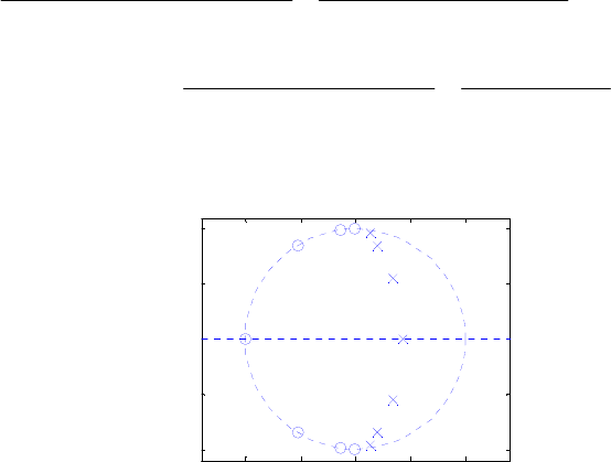
Numerator Factors
1.0000 1.0000 0
1.0000 1.0500 1.0000
1.0000 0.2577 1.0000
1.0000 0.0072 1.0000
Denominator Factors
1.0000 -0.2756 0.9379
1.0000 -0.3951 0.7545
1.0000 -0.6694 0.4245
1.0000 -0.4353 0
Scale factor =
0.03485569511749
×
⎟
⎟
⎠
⎞
⎜
⎜
⎝
⎛
+−
++
⎟
⎟
⎠
⎞
⎜
⎜
⎝
⎛
+−
++
=−
−−
−−
−−
2
21
21
21
7545.03951.01
2577.01
9379.02756.01
05.11
0349.0)(
z
zz
zz
zz
zH
⎟
⎟
⎠
⎞
⎜
⎜
⎝
⎛
−
+
⎟
⎟
⎠
⎞
⎜
⎜
⎝
⎛
+−
++
−
−
−
−−
1
1
2
21
4353.01
1
4245.06694.01
0072.01
z
z
z
zz .
Note that the ordering has no effect if
∞
L− scaling is used.
-1 -0.5 00.5 1
-1
-0.5
0
0.5
1
Real Part
Imaginary Part
sos =
0.0349 0.0349 0 1.0000 -0.4353 0
1.0000 1.0500 1.0000 1.0000 -0.6694 0.4245
1.0000 0.2577 1.0000 1.0000 -0.3951 0.7545
1.0000 0.0072 1.0000 1.0000 -0.2756 0.9379
M 12.6 %Program_M12_6.m
[B,A] = ellip(7,0.2,50,0.45);
[d0,d1]=tf2ca(B,A);
num1 = 0.5*(conv(fliplr(d1),d0)+conv(d1,fliplr(d0)));
den = conv(d0,d1);
num2 = 0.5*(-conv(fliplr(d1),d0)+conv(d1,fliplr(d0)));
[h1,w]=freqz(num1,den,512);
[h2,w]=freqz(num2,den,512);
plot(w/pi,20*log10(abs(h1)),'-r',w/pi,20*log10(abs(h2)),'--b');
Not for sale 488
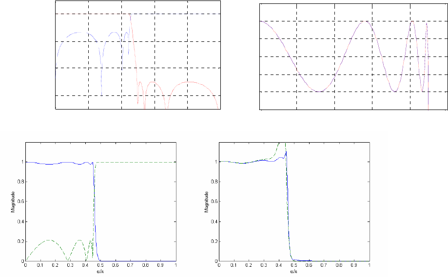
xlabel('\omega/\pi');ylabel('Gain, dB');grid
00.2 0.4 0.6 0.8 1
-60
-40
-20
0
ω
/
π
Gain, dB
HLP(z) HHP(z)
00.1 0.2 0.3 0.4 0.5
-0.25
-0.2
-0.15
-0.1
-0.05
0
0.05
ω
/
π
G
a
i
n,
dB
Passband Details
M12.7
num1 = input('Numerator first factor = ');
num2 = input('Numerator second factor = ');
den1 = input('Denominator first factor = ');
den2 = input('Denominator second factor = ');
% The scaling functions are
f1num = 1;
f1den = [den1];
f2num = num1;
f2den = conv(den1,den2);
f3num = conv(num1,num2);
f3den = conv(den1,den2);
x = [1 zeros([1,511])];
% Impulse Responses
% Sufficient length for impulse response to have
% decayed to nearly zero
f1 = filter(f1num,f1den,x);
f2 = filter(f2num,f2den,x);
f3 = filter(f3num,f3den,x);
figure(1),stem(f1(1:50));
ylabel('Amplitude'); xlabel('Samples');
title('Impulse Response of F_1(z)')
figure(2),stem(f2(1:50));
Not for sale 489
ylabel('Amplitude'); xlabel('Samples');
title('Impulse Response of F_2(z)')
figure(3),stem(f3(1:50));
ylabel('Amplitude'); xlabel('Samples');
title('Impulse Response of H(z)')
k1 = sum(f1.*f1);
k2 = sum(f2.*f2);
k3 = sum(f3.*f3);
disp(['L_2 norm of F_1(z) = ' num2str(k1)]);
disp(['L_2 norm of F_2(z) = ' num2str(k2)]);
disp(['L_2 norm of H(z) = ' num2str(k3)]);
b_0 = 1/sqrt(k1);
b_1 = sqrt(k1)/sqrt(k2);
b_2 = sqrt(k2)/sqrt(k3);
disp(['First scaling factor, b_0 = ' num2str(b_0)]);
disp(['Second scaling factor, b_1 = ' num2str(b_1)]);
disp(['Third scaling factor, b_2 = ' num2str(b_2)]);
% The scaled transfer functions
disp(['Scaled gain = ' num2str(k1)]);
disp('The scaled second order sections are ')
disp([k2*num1 k3*num2 ; den1 den2])
% The noise transfer functions
g1num = conv(num1,num2)*(k2*k3);
g1den = conv(den1,den2)*k3;
g2num = num2;
g2den = den2;
g1 = filter(g1num,g1den,x);
g2 = filter(g2num,g2den,x);
var = sum(f1.*f1)*3+sum(g2.*g2)*5+3;
disp('The normalized noise variance'); disp(var);
For the first cascade realization we have
L_2 norm of F_1(z) = 4.9808
L_2 norm of F_2(z) = 88.2071
L_2 norm of H(z) = 64.2444
First scaling factor, b_0 = 0.44807
Second scaling factor, b_1 = 0.23763
Third scaling factor, b_2 = 1.1717
Scaled gain = 4.9808
The scaled second order sections are
88.2071 -66.9403 88.2071 64.2444 42.1700 64.2444
1.0000 1.0462 0.8385 1.0000 1.0657 0.4046
The normalized noise variance
35.5077
Not for sale 490
For the second cascade realization we have
L_2 norm of F_1(z) = 2.8179
L_2 norm of F_2(z) = 11.375
L_2 norm of H(z) = 64.2444
First scaling factor, b_0 = 0.59572
Second scaling factor, b_1 = 0.49772
Third scaling factor, b_2 = 0.42078
Scaled gain = 2.8179
The scaled second order sections are
11.3750 7.4666 11.3750 64.2444 -48.7551 64.2444
1.0000 1.0657 0.4046 1.0000 1.0462 0.8385
The normalized noise variance
106.5131
The L_2 norm of F_1(z) = 4.9808
The L_2 norm of F_2(z) = 11.375
The L_2 norm of H(z) = 64.2444
The first scaling factor, b_0 = 0.44807
The second scaling factor, b_1 = 0.66172
The third scaling factor, b_2 = 0.42078
The scaled gain = 4.9808
The scaled second order sections are
11.3750 7.4666 11.3750 64.2444 -48.7551 64.2444
1.0000 1.0462 0.8385 1.0000 1.0657 0.4046
The normalized noise variance = 98.0695
M12.8 The parallel form I and II structures used for the simulation are shown on top of the next
page:
Not for sale 491
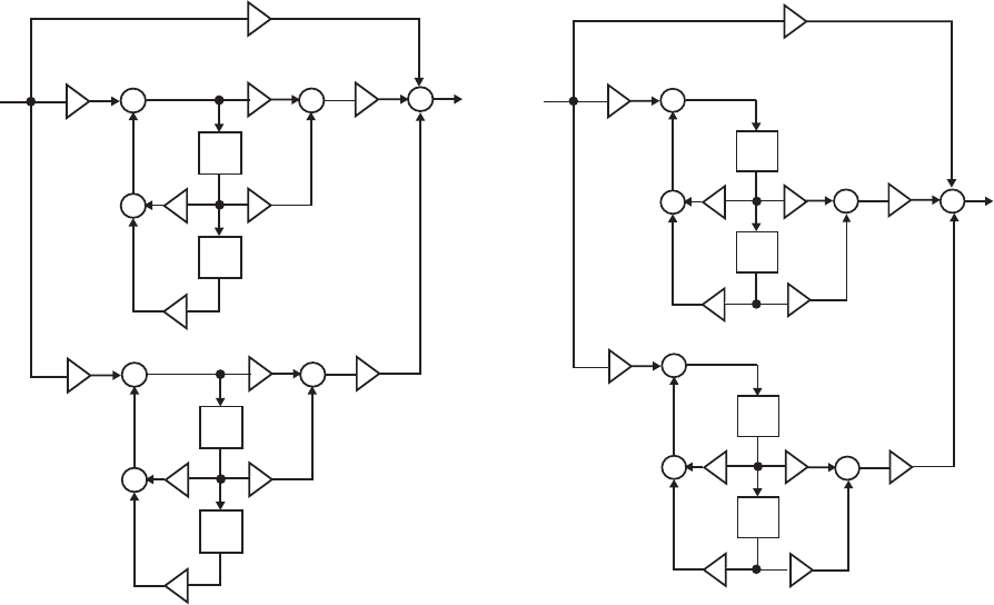
5.2081k
_
+
0.5079k
_
1.4379k
_
z
1
_
z
1
_
+
++
z
1
_
z
1
_
+
++
k
4
k
0
k
2
k
5
k
6
0.9462k
1.0462
0.8385
1.0657
0.4046
1
1
3
3
+
z1
_
z1
_
+
+
+
z1
_
z1
_
+
+
+
k4
k0
k2
k5
k6
1.0462
0.8385
1.0657
0.4046
1.2072k1
4.6669k
_
3
0.2055k
_3
2.4525k1
The MATLAB program below can be used to simulate a 4-th order IIR transfer function in both
parallel forms.
num1 = input('Numerator first factor =');
num2 = input('Numerator Second factor =');
den1 = input('Denominator first factor =');
den2 = input('Denominator second factor =');
% Parallel Form I
num = conv(num1,num2);
den = conv(den1,den2);
[r1,p1,k11] = residuez(num,den);
R1 = [r1(1) r1(2)];
P1 = [p1(1) p1(2)];
R2 =[r1(3) r1(4)];
P2 = [p1(3) p1(4)];
[num11,den11] = residuez(R1,P1,0);
[num12,den12] = residuez(R2,P2,0);
disp('Parallel Form I');
disp('The numerators are');
disp(k11); disp(real(num11)); disp(real(num12));
disp('The denominators are');
disp(real(den11)); disp(real(den12));
imp = [1 zeros([1,2000])];
Not for sale 492
f0 = filter([1 0 0],den11,imp);
f1 = filter(num11,den11,imp);
f2 = filter([1 0 0],den12,imp);
f3 = filter(num12,den12,imp);
figure(1),stem(real(f0(1:50)));
ylabel('Amplitude'); xlabel('Samples');
title('Impulse Response of F_0(z)')
saveas(gcf,'M12_8_P1_0.tif')
figure(2),stem(real(f1(1:50)));
ylabel('Amplitude'); xlabel('Samples');
title('Impulse Response of F_1(z)')
saveas(gcf,'M12_8_P1_1.tif')
figure(3),stem(real(f2(1:50)));
ylabel('Amplitude'); xlabel('Samples');
title('Impulse Response of F_2(z)')
saveas(gcf,'M12_8_P1_2.tif')
figure(4),stem(real(f3(1:50)));
ylabel('Amplitude'); xlabel('Samples');
title('Impulse Response of F_3(z)')
saveas(gcf,'M12_8_P1_3.tif')
g0 = sum(f0.*conj(f0));
g1 = sum(f1.*conj(f1));
g2 = sum(f2.*conj(f2));
g3 = sum(f3.*conj(f3));
disp(['L_2 norm of F_0(z) = ' num2str(g0)]);
disp(['L_2 norm of F_1(z) = ' num2str(g1)]);
disp(['L_2 norm of F_2(z) = ' num2str(g2)]);
disp(['L_2 norm of F_3(z) = ' num2str(g3)]);
k0 = sqrt(1/g0);
k1 = sqrt(g0/g1);
k2 = sqrt(1/g2);
k3 = sqrt(g2/g3);
f = filter(num,den,imp);
g = sum(f.*conj(f));
k4 = sqrt(1/g);
k5 = k4/(k0*k1);
k6 = k4/(k2*k3);
disp('The scaling constants are');
disp(['k0 = ' num2str(k0)]); disp(['k1 = ' num2str(k1)]);
disp(['k2 = ' num2str(k2)]); disp(['k3 = ' num2str(k3)]);
disp(['k4 = ' num2str(k4)]); disp(['k5 = ' num2str(k5)]);
disp(['k6 = ' num2str(k6)]);
noise = 3*(k5/k0)^2+3*(k6/k2)^2+2*k5^2+2*k6^2+3;
disp(['Product roundoff noise variance = ' num2str(noise)]);
% Parallel From II
Not for sale 493
num = conv(num1,num2);
den = conv(den1,den2);
[r1,p1,k11] = residue(num,den);
R1 = [r1(1) r1(2)];
P1 = [p1(1) p1(2)];
R2 =[r1(3) r1(4)];
P2 = [p1(3) p1(4)];
[num11,den11] = residue(R1,P1,0);
[num12,den12] = residue(R2,P2,0);
disp('Parallel Form II');
disp('The numerators are');
disp(k11); disp(real(num11)); disp(real(num12));
disp('The denominators are');
disp(real(den11)); disp(real(den12));
imp = [1 zeros([1,2000])];
f0 = filter([1 0 0],den11,imp);
f1 = filter(num11,den11,imp);
f2 = filter([1 0 0],den12,imp);
f3 = filter(num12,den12,imp);
figure(1),stem(real(f0(1:50)));
ylabel('Amplitude'); xlabel('Samples');
title('Impulse Response of F_0(z)')
saveas(gcf,'M12_8_P2_0.tif')
figure(2),stem(real(f1(1:50)));
ylabel('Amplitude'); xlabel('Samples');
title('Impulse Response of F_1(z)')
saveas(gcf,'M12_8_P2_1.tif')
figure(3),stem(real(f2(1:50)));
ylabel('Amplitude'); xlabel('Samples');
title('Impulse Response of F_2(z)')
saveas(gcf,'M12_8_P2_2.tif')
figure(4),stem(real(f3(1:50)));
ylabel('Amplitude'); xlabel('Samples');
title('Impulse Response of F_3(z)')
saveas(gcf,'M12_8_P2_3.tif')
g0 = sum(f0.*conj(f0));
g1 = sum(f1.*conj(f1));
g2 = sum(f2.*conj(f2));
g3 = sum(f3.*conj(f3));
disp(['L_2 norm of F_0(z) = ' num2str(g0)]);
disp(['L_2 norm of F_1(z) = ' num2str(g1)]);
disp(['L_2 norm of F_2(z) = ' num2str(g2)]);
disp(['L_2 norm of F_3(z) = ' num2str(g3)]);
k0 = sqrt(1/g0);
k1 = sqrt(g0/g1);
k2 = sqrt(1/g2);
Not for sale 494
k3 = sqrt(g2/g3);
f = filter(num,den,imp);
g = sum(f.*conj(f));
k4 = sqrt(1/g);
k5 = k4/(k0*k1);
k6 = k4/(k2*k3);
disp('The scaling constants are');
disp(['k0 = ' num2str(k0)]); disp(['k1 = ' num2str(k1)]);
disp(['k2 = ' num2str(k2)]); disp(['k3 = ' num2str(k3)]);
disp(['k4 = ' num2str(k4)]); disp(['k5 = ' num2str(k5)]);
disp(['k6 = ' num2str(k6)]);
noise = 3*(k5/k0)^2+3*(k6/k2)^2+2*k5^2+2*k6^2+3;
disp(['Product roundoff noise variance = ' num2str(noise)]);
Parallel Form I
The numerators are
2.9476
-1.4397 0.9462 0
-0.5079 -5.2081 0
The denominators are
1.0000 1.0462 0.8385
1.0000 1.0657 0.4046
L_2 norm of F_0(z) = 4.9808
L_2 norm of F_1(z) = 22.5061
L_2 norm of F_2(z) = 2.8179
L_2 norm of F_3(z) = 65.8497
The scaling constants are
k0 = 0.44807
k1 = 0.47044
k2 = 0.59572
k3 = 0.20686
k4 = 0.12476
k5 = 0.59188
k6 = 1.0124
Product roundoff noise variance = 19.6501
Parallel Form II
The numerators are
1
2.4525 1.2072
-4.6669 0.2055
The denominators are
1.0000 1.0462 0.8385
1.0000 1.0657 0.4046
L_2 norm of F_0(z) = 4.9808
L_2 norm of F_1(z) = 20.4333
Not for sale 495
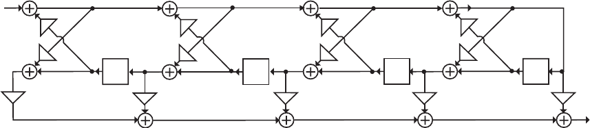
L_2 norm of F_2(z) = 2.8179
L_2 norm of F_3(z) = 65.5918
The scaling constants are
k0 = 0.44807
k1 = 0.49372
k2 = 0.59572
k3 = 0.20727
k4 = 0.12476
k5 = 0.56396
k6 = 1.0104
Product roundoff noise variance = 19.0615
Parallel Form II has the lowest output round off noise.
M 12.9 The scaled Gray-Markel cascaded lattice structure used for simulation is shown below:
W
4
W
1
z
1
_
W
2
z
1
_
z
1
_
W
3
z
1
_
1
4
α C
____
k
2
4
α C
____
3
k k
3
4
α C
____
32
k k k
1
4
4
α C
3
2
k k k k
_______
5
α C
1
4
3
2
k k k k
_______
_
d
4
d
4
_
d
3
'
d
3
'
_
d''
2
d''
2
_
d'''
1
d'''
1
The MATLAB program that can be used to simulate the Gray-Markel realization of a 4-th order
IIR transfer function is as follows:
num1 = input('Numerator first factor = ');
num2 = input('Numerator second factor = ');
den1 = input('Denominator first factor = ');
den2 = input('Denominator second factor = ');
num = conv(num1,num2); den = conv(den1,den2);
num = num/den(1); den = den/den(1);
% Gray-Markel realization
[d,alpha] = tf2latc(num,den);
disp('Lattice parameters are'); disp(['d1 = ' num2str(d(1))]);
disp(['d2 = ' num2str(d(2))]); disp(['d3 = ' num2str(d(3))]);
disp(['d4 = ' num2str(d(4))]);
disp('Feed-forward multipliers are');
disp(['alpha1 = ' num2str(alpha(1))]);
disp(['alpha2 = ' num2str(alpha(2))]);
disp(['alpha3 = ' num2str(alpha(3))]);
disp(['alpha4 = ' num2str(alpha(4))]);
imp = [1 zeros([1,499])];
qold1 = 0;
for k = 1:500
w1 = imp(k)-d(1)*qold1;
Not for sale 496
y1(k) = w1;
qnew1 = w1;
qold1 = qnew1;
end
k1 = sqrt(1/(sum(y1.*conj(y1))));
figure(1),stem(real(y1(1:50)));
ylabel('Amplitude'); xlabel('Samples');
title('Impulse Response of W1')
saveas(gcf,'M12_9_1.tif')
imp = [1 zeros([1,499])];
qold1 = 0;qold2 = 0;
for k = 1:500
w2 = imp(k)-d(2)*qold2*1/k1;
w1 = k1*w2-d(1)*qold1;
y2(k)=w2;
qnew1 = w1;
qnew2 = w1*d(1)+qold1;
qold1 = qnew1;qold2 = qnew2;
end
k2 = sqrt(1/(sum(y2.*conj(y2))));
figure(2),stem(real(y2(1:50)));
ylabel('Amplitude'); xlabel('Samples');
title('Impulse Response of W2')
saveas(gcf,'M12_9_2.tif')
qold1 = 0;qold2 = 0;qold3 = 0;
for k = 1:500
w3 = imp(k)-d(3)*qold3*1/k2;
w2 = k2*w3-d(2)*qold2*1/k1;
w1 = k1*w2-d(1)*qold1;
y3(k) = w3;
qnew1 = w1;
qnew2 = w1*d(1)+qold1;
qnew3 = w2*d(2)+qold2*1/k1;
qold1 = qnew1;qold2 = qnew2;qold3 = qnew3;
end
k3 = sqrt(1/sum(y3.*conj(y3)));
figure(3),stem(real(y3(1:50))); ylabel('Amplitude');
xlabel('Samples'); title('Impulse Response of W3')
saveas(gcf,'M12_9_3.tif')
qold1 = 0;qold2 = 0;qold3 = 0;qold4 = 0;
for k = 1:500
w4 = imp(k)-d(4)*qold4/k3;
w3 = k3*w4-d(3)*qold3/k2;
w2 = k2*w3-d(2)*qold2/k1;
w1 = k1*w2-d(1)*qold1;
y4(k) = w4;
qnew1 = w1;
qnew2 = w1*d(1)+qold1;
qnew3 = w2*d(2)+qold2*1/k1;
qnew4 = w3*d(3)+qold3*1/k2;
qold1 = qnew1;qold2 = qnew2;qold3 = qnew3;qold4 = qnew4;
end
Not for sale 497
k4 = sqrt(1/sum(y4.*conj(y4)));
figure(4),stem(real(y3(1:50))); ylabel('Amplitude');
xlabel('Samples'); title('Impulse Response of W4')
saveas(gcf,'M12_9_4.tif')
disp('The scaling parameters are');
disp(['k1 = ' num2str(k1)]); disp(['k2 = ' num2str(k2)]);
disp(['k3 = ' num2str(k3)]); disp(['k4 = ' num2str(k4)]);
alpha(5) = alpha(5)/(k1*k2*k3*k4);
alpha(4) = alpha(4)/(k1*k2*k3*k4);
alpha(3) = alpha(3)/(k2*k3*k4);
alpha(2) = alpha(2)/(k3*k4);
alpha(1) = alpha(1)/k4;
%%%% Computation of noise variance %%%%%%
imp = [1 zeros([1,499])];
for k = 1:500
w4 = imp(k)-d(4)*qold4/k3;
w3 = k3*w4-d(3)*qold3/k2;
w2 = k2*w3-d(2)*qold2/k1;
w1 = k1*w2-d(1)*qold1;
qnew1 = w1;
qnew2 = w1*d(1)+qold1;
qnew3 = w2*d(2)+qold2*1/k1;
qnew4 = w3*d(3)+qold3*1/k2;
y11 = w4*d(4)+qold4/k3;
y0(k) = alpha(1)*y11+alpha(2)*qnew4+alpha(3)*qnew3 +
alpha(4)*qnew2+alpha(5)*qnew1;
qold1 = qnew1;qold2 = qnew2;qold3 = qnew3;qold4 = qnew4;
end
nv = sum(y0.*conj(y0));
disp(['Product roundoff noise variance = ' num2str(nv)]);
The output data generated by this program are as follows:
Lattice parameters are
d1 = 0.19149
d2 = 0.75953
d3 = 0.44349
d4 = 0.27506
Feed-forward multipliers are
alpha1 = -0.9001
alpha2 = -1.7069
alpha3 = 4.6151
alpha4 = -3.5028
alpha5 = 1.8177
The scaling parameters are
k1 = 0.98149
k2 = 0.65047
k3 = 0.89628
k4 = 0.96143
Not for sale 498
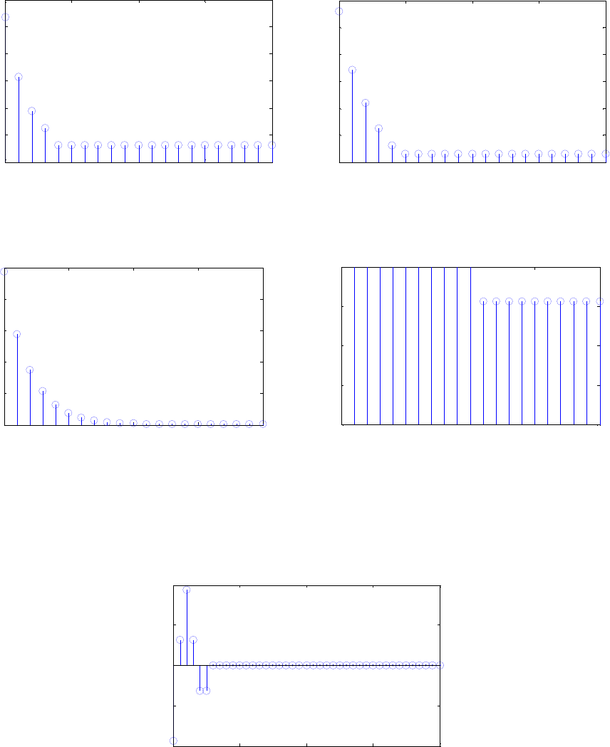
The product roundoff noise variance = 81.1431
M12 .10 (a) (b)
08.0]0[,3.0]1[ ==− xy 03.0]0[,9.0]1[ =
=
−
xy
0 5 10 15 20
0
0.05
0.1
0.15
0.2
0.25
A
mp
lit
u
d
e
Time index n
α
= 0.6
0 5 10 15 20
0
0.1
0.2
0.3
0.4
0.5
Amplitude
Time index n
α
= 0.6
(c)
5]0[,8]1[ ==− xy
0 5 10 15 2
0
0
2
4
6
8
10
Amplitude
Time index n
α
= 0.6
0 5 10 15 2
0
0
0.01
0.02
0.03
0.04
A
mp
lit
u
d
e
Time index n
α
= 0.6
In all three cases, the condition of Eq. (12.187) is satisfied and hence, the structure exhibits
zero input granular limit cycles.
M 12.11 Plot of the output samples generated by the modified program is shown below:
010 20 30 40
-0.4
-0.2
0
0.2
0.4
Time index n
Amplitude
α
1
= -0.875
α
2
= 0.875
Not for sale 499
As can be seen from the above plot, output goes to zero values and hence the structure of
Figure 12.49 does not support overflow limit cycles if sign-magnitude truncation is used to
truncate the sum of products of Eq. (12.195).
Not for sale 500

Chapter 13
13.1 Up-sampler – Let and be the inputs to a factor-of-L up-sampler with
corresponding outputs given by and , respectively:
and
][
1nx ][
2nx
][
1ny ][
2ny
⎩
⎨
⎧±±=
=otherwise,,0
,,2,,0],/[
][ 1
1
KLLnLnx
ny ⎩
⎨
⎧±±=
=otherwise.,0
,,2,,0],/[
][ 2
2
KLLnLnx
ny
Let be the input to the up-sampler. Then, the corresponding
output is given by
Hence, the up-sampler is a linear system.
][][][ 213 nxnxnx βα +=
][
3ny ⎩
⎨
⎧±±=
=otherwise,,0
,,2,,0],/[
][ 3
3
KLLnLnx
ny
⎩
⎨
⎧±±=+
=otherwise,,0
,,2,,0],/[]/[ 21 KLLnLnxLnx βα
⎩
⎨
⎧±±=
=otherwise,,0
,,2,,0],/[
1KLLnLnxα
⎩
⎨
⎧±±=
+otherwise,,0
,,2,,0],/[
2KLLnLnxβ
].[][ 21 nyny βα +=
Down-sampler - Let and be the inputs to a factor-of-M down-sampler with
corresponding outputs given by and , respectively:
][
1nx ][
2nx
][
1ny ][
2ny
and
][][ 11 Mnxny =].[][ 22 Mnxny
=
Let ][][][ 213 nxnxnx βα
+
=
be the input to the
up-sampler. Then, the corresponding output is given by
][
3ny ][][ 33 Mnxny =
][][ 21 MnxMnx βα += ].[][ 21 nyny βα
+
= Hence, the down-sampler is a linear system.
13.2 Up-Sampler – For inputs and the outputs of the factor-of-L up-sampler
are, respectively given by
][
1nx ],[
2nx
and .
⎩
⎨
⎧±±=
=otherwise,,0
,,2,,0],/[
][ 1
1
KLLnLnx
nxu⎩
⎨
⎧±±=
=otherwise,,0
,2,,0],/[
][ 2
2
KLLnLnx
nxu
Let where is an integer. Then, Hence,
But,
],[][ 12 o
nnxnx −= o
n].)/[(]/[ 12 o
nLnxLnx −=
⎩
⎨
⎧±±=−
=otherwise.,0
,,2,,0],/)[(
][ 1
2
KLLnLnnx
nx o
u
⎩
⎨
⎧±±=−−
=otherwise.,0
,,2,,0],/)[(
][ 1
1
KLLnnLnnx
nx oo
u
Since the up-sampler is a time-varying system.
],[][ 12 ouu nnxnx −≠
Down-Sampler – For inputs and the outputs of the factor-of-M down-
sampler are, respectively given by
][
1nx ],[
2nx
][][ 11 Mnxny
=
and ].[][ 22 Mnxny
=
Let
where is an integer. Then, ],[][ 12 o
nnxnx −= o
n].[][][ 122 o
nMnxMnxny −=
=
However, ].[)]([][ 111 ooo MnMnxnnMxnny
−
=
−
=−
Since the down-sampler is a time-varying system. ],[][ 12 o
nnyny −≠
Not for sale 499
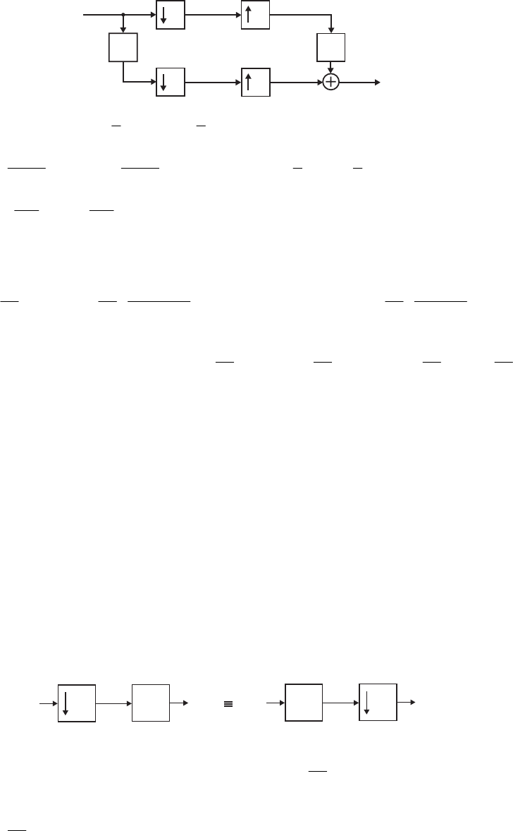
13.3
z
_1
22
22
z
_1
X
(z)
Y(z)
V(z)
W(z)
V (z)
u
W (z)
u
Analysis yields ),()()( 2/1
2
1
2/1
2
1zXzXzV −+=
),()()(),()()( 2
1
2
1
2/1
2
2/1
2
2/12/1
zXzXzVzXzXzW u
zz −+=−−= −−
).()()( 22
11
zXzXzW zz
u−−= −−
Hence, ),()()()( 11 zXzzWzVzzY uu −
−
=+= or in other
words
].1[][ −= nxny
13.4 .
1
1
11
][
1
0⎟
⎟
⎠
⎞
⎜
⎜
⎝
⎛
−
−
== ∑
−
=n
M
nM
M
M
k
kn
MW
W
M
W
M
nc Hence, if .0
1
111
][, =
⎟
⎟
⎠
⎞
⎜
⎜
⎝
⎛
−
−
=≠ n
M
W
M
ncrMn On
the other hand, if ,r
M
n= then .11
111
][
1
0
1
0
1
0
===== ∑∑∑ −
=
−
=
−
=M
M
M
W
M
W
M
nc
M
k
M
k
krM
M
M
k
kn
M
13.5 (a) For and
6=M,5=L
},,,,,{}{}{ 5
6
4
6
3
6
2
6
1
6
0
66
−
−
−
−
−
−− == WWWWWWWW kk
M, and
},,,,,{}{}{ 25
6
20
6
15
6
10
6
5
6
0
6
5
6−
−
−
−
−
−− == WWWWWWWW kLk
M
}.{},,,,,{ 6
1
6
2
6
3
6
4
6
5
6
0
6k
WWWWWWW
−
−
−
−
−− ==
(b) For to have same set of values for
}{ k
M
W−,10
−
≤
≤
Mk as , each should
have unique values for each k. Therefore
}{ kL
M
W−
nL
M
kL
MWW
−
−
≠ for all or
for any positive integer r, which implies that L and M should be
relatively prime.
],1,0[, −∈ Mnk
rMLnk ≠− )(
13.6
MM
H(z)H(z )
M
X
(z)X(z)
V (z)
1Y (z)
1
V (z)
2Y (z)
2
For the figure on the left-hand side we have ),(
1
)(
1
0
/1
1∑
−
=
=
M
k
k
M
MWzX
M
zV and
).()(
1
)(
1
0
/1
1∑
−
=
=
M
k
k
M
MWzXzH
M
zY For the figure on the right-hand side we have
Not for sale 500
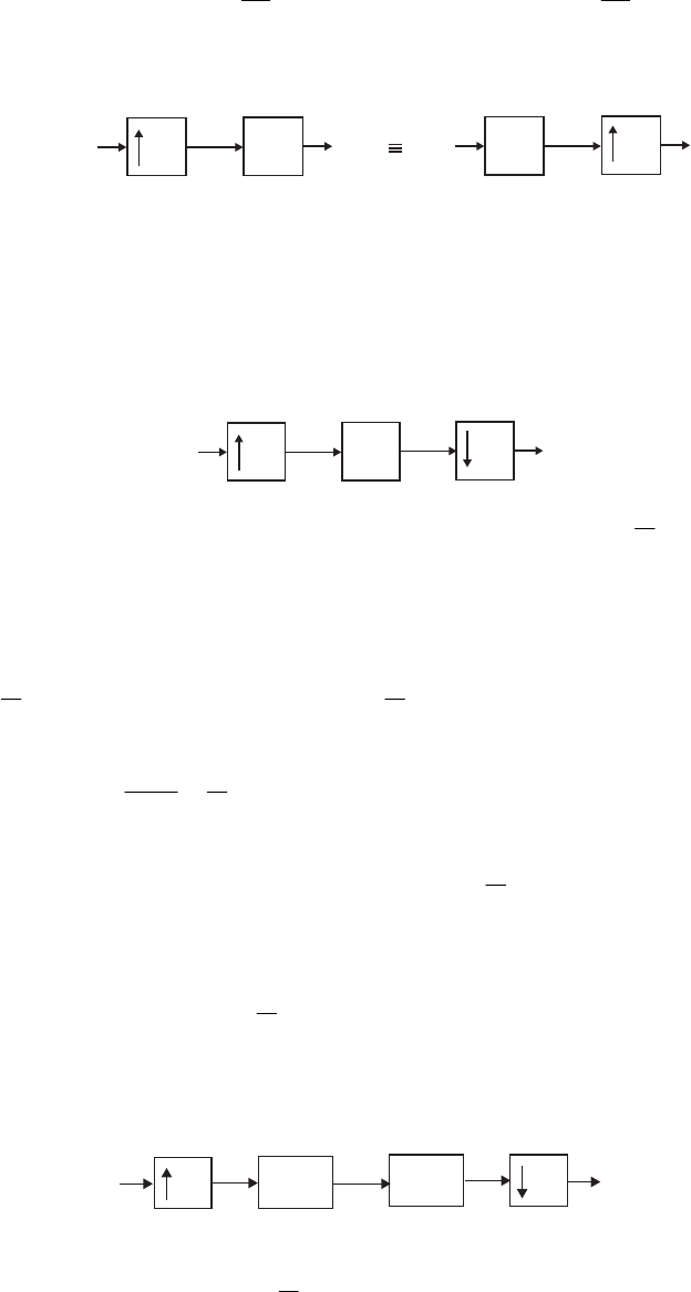
)()(
1
)(),()()( /1
1
0
22 k
M
M
M
k
kM
M
MWzXzWH
M
zYzXzHzV ∑
−
=
== ).()(
1/1
1
0
k
M
M
M
k
WzXzH
M∑
−
=
=
Hence,
).()( 21 zYzY =
LL
H(z)
H(z )
L
X
(z)X(z)
V (z)
1Y (z)
1
V (z)
2Y (z)
2
For the figure on the left-hand side we have For the
).()()(),()( 11 LLL zXzHzYzXzV ==
figure on the right-hand side we have Hence,
).()()(),()()( 22 LL zXzHzYzXzHzV ==
).()( 21 zYzY =
13.7 (a) The system of Figure P13.1 with internal variables labeled is shown below:
LL
G(z)
X
(z)V(z)Y(z)
U(z)
Analysis yields ),()()(),()( zVzGzUzXzV
L
=
= and ).(
1
)(
1
0
/1
∑
−
=
−
=
L
k
k
L
LWzU
L
zY
Substituting the first equation in the second equation we get
Substituting this equation in the expression for in the above we get
).()()( L
zXzGzU =
)(zY
),()(
1
)()(
1
)(
1
0
/1
1
0
/1 zXWzG
L
WzXWzG
L
zY
L
k
k
L
LkL
L
L
k
k
L
L∑∑ −
=
−−
−
=
−⋅=⋅⋅= since .1=
−
kL
L
W
Therefore, ).(
1
)(
)(
)(
1
0
/1
∑
−
=
−
==
L
k
k
L
LWzG
LzX
zY
zH Hence, Figure P13.1 is a LTI system.
(b) It follows from the last equation given above, if ,1)(
11
0
/1 =
∑
−
=
−
L
k
k
L
LWzG
L then
i.e., or
,1)( =zH ),()( zXzY =].[][ n
x
ny
=
Or, in other words, the system of Figure
P13.1 is an identity system for .1)(
11
0
/1 =
∑
−
=
−
L
k
k
L
LWzG
L
13.8 Consider the multirate structure shown below. Analysis yields
L
LG(z)
u[n]
x
[n]H(z)y[n]
and
),()()( L
zXzHzU =).()()( // k
L
L
L
k
k
L
LWzUWzG
L
zY 1
1
0
1
1∑
−
=
= Substituting the first
Not for sale 501
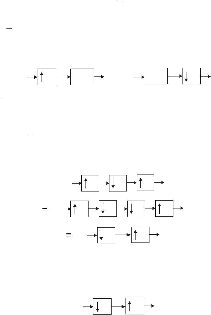
equation into the second we get ).()()()( // zXWzHWzG
L
zY k
L
L
L
k
k
L
L
⎥
⎥
⎦
⎤
⎢
⎢
⎣
⎡
=∑
−
=
1
1
0
1
1 Hence,
if ,)()( // 1
11
1
0
1=
∑
−
=
k
L
L
L
k
k
L
LWzHWzG
L we have ),()( zXzY
=
or in other words, the
above multirate structure is an identity system. We break the system as shown below
into two parts with the transfer functions and satisfying the relation
L
LG(z)
u[n]
x
[n]H(z)x[n]
u[n]
.)()( // 1
11
1
0
1=
∑
−
=
k
L
L
L
k
k
L
LWzHWzG
L If we now place the second system in front of the
first we arrive at the system shown in Figure P13.2 which is an identity system
provided .)()( // 1
11
1
0
1=
∑
−
=
k
L
L
L
k
k
L
LWzHWzG
L
13.9 Making use of the multirate identities we simplify the structure of Figure P13.3 as
indicated below:
5
3
x
[n]y[n]
15
5
3
x[n]y[n]
5
3
5
x[n]y[n]
5
v[n]
Analysis of the last structure yields, ],5[][ nxnv
=
and
or,
⎩
⎨
⎧±±=
=otherwise,
,0
,,10,5,0],5/[
][ Knnv
ny ⎩
⎨
⎧±±=
=otherwise.
,0
,,10,5,0],[
][ Knnx
ny
13.10
L
L
x
[n]y[n]
v[n]
Analysis yields ],[][ Ln
x
nv = and or,
⎩
⎨
⎧±±=
=otherwise,
,0
,,2,,0],/[
][ KLLnLnv
ny
⎩
⎨
⎧±±=
=otherwise.
,0
,,2,,0],[
][ KLLnnx
ny
Not for sale 502
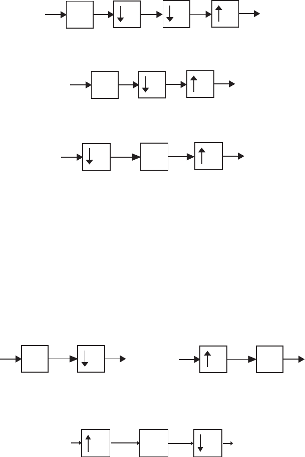
13.11 Since 3 and 4 are relatively prime, we can interchange the positions of the factor-of-3
down-sampler and the factor-of-4 up-sampler as indicated below:
x
[n]y[n]
z
_6
34
2
which simplifies to the structure shown below:
x
[n]y[n]
z_64
6
Using the Noble identity of Figure 13.14(a) we redraw the above structure as indicated
below:
x
[n]y[n]
4
6z
_1
u[n]v[n]
Analysis yields ],16[]1[][],6[][
−
=
−
=
=nxnunvnxnu and
⎩
⎨
⎧±±=−
=
⎩
⎨
⎧±±=
=otherwise.otherwise, ,0
,,8,4,0],1)2/3[(
,0
,,8,4,0],4/[
][ KK nnxnnv
ny
13.12 As outlined in Section 8.2, the transpose of a digital filter structure is obtained by
reversing all paths, replacing the pick-off node with an adder and vice-versa, and
interchanging the input and the output nodes. Moreover, in a multirate structure, the
transpose of a factor-of-M down-sampler is a factor-of-M up-sampler and vice-versa.
Applying these operations to the factor-of-M decimator shown below on the left-hand
side, we arrive at a factor-of-M up-sampler shown below on the right-hand side.
x
[n]y[n]
H(z)M
x[n]y[n]
H(z)M
13.13 (a) To prove Eq. (13.20), consider the fractional-rate sampling rate converter of
Figure 13.16(b) with internal variables labeled as shown below:
LM
x
[n]y[n]
H(z)v[n]
x [n]
u
Analysis yields K,2,1,0],[][
±
±
=
=nnxLnxuand ].[][][ ll
l∑
∞
−∞=
−= u
xnhnv
Substituting the first equation in the second we get Finally,
].[][][ mxLmnhnv
m
∑
∞
−∞=
−=
∑
∞
−∞=
−==
m
mxLmMnhMnvny ].[][][][
Not for sale 503
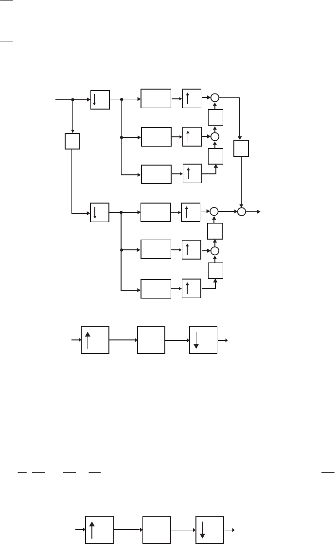
(b) Next, to prove Eq. (13.21), we make use of the z-domain relations of the down-
sampler and the up-sampler. From Eq. (13.17) we have
).()(
1
)( /1
1
0
/1 k
M
M
u
k
M
M
k
MWzXWzH
M
zY −−
−
=
∑
= But Hence,
).()( L
uzXzX =
).()(
1
)( /
1
0
/1 Lk
M
MLk
M
M
k
MWzXWzH
M
zY −−
−
=
∑
=
13.14
2
2
3
E (z)
00
E (z)
01
E (z)
02
E (z)
10
E (z)
11
E (z)
12
z
_1
z
_1
3
3
3
3
3
+
z
_1
+
z
_1
+
z
_1
+
z
_1
+
x
[n]
y[n]
13.15
x[n]y[n]
H(z)
400 Hz
815
3200 Hz 3200 Hz 213.3333 Hz
v[n]
x
u
n
[ ]
(a) 400=
T
F Hz, L = 8, M = 15. Now, the sampling rate of and is
kHz. Hence, the sampling rate of is
Hz.
][nxu][nv
2.38400400 =×=L][ny 15/3200/3200 =M
33.213=
(b) The normalized stopband edge angular frequency of (for no aliasing)
)(zH
.
15
,min ππππ
ω==
⎟
⎠
⎞
⎜
⎝
⎛
=MML
s Hence, the stopband edge frequency is 30
1
=
s
F Hz.
13.16
x
[n]y[n]
H(z)
815
v[n]
xun
[ ]
650 Hz 3.25 kHz 3.25 kHz 361.1 Hz
Not for sale 504
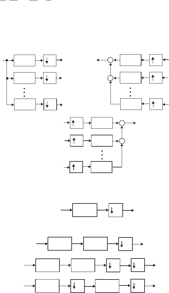
(a) 650=
T
F Hz, L = 5, M = 9. Now, the sampling rate of and is ][nxu][nv
kHz. Hence, the sampling rate of is
Hz.
25.35650650 =×=L][ny 9/3250/3250 =M
1.361=
(b) The normalized stopband edge angular frequency of (for no aliasing)
)(zH
.
9
,min ππππ
ω==
⎟
⎠
⎞
⎜
⎝
⎛
=MML
s Hence, the stopband edge frequency is Hz.
13.17 Applying the transpose operation to the M-channel analysis filter bank shown below
on the left-hand side, we arrive at the M-channel synthesis filter bank shown below on
the right-hand side.
x
[n]v [n]
0
v [n]
1
v [n]
M 1
_
M
M
M
H (z)
0
H (z)
1
H (z)
M 1
_
y[n]v [n]
0
v [n]
1
v [n]
M 1
_
M
M
M
H (z)
0
H (z)
1
H (z)
M 1
_
+
+
y[n]v [n]
0
v [n]
1
v [n]
M 1
_
MH (z)
0
H (z)
1
H (z)
M 1
_
+
+
M
M
13.18 Specifications for H(z) are: 180
=
p
F Hz, 200
=
s
F Hz, .001.0,002.0 =
=
sp δδ
H(z)
30
12 kHz 12 kHz 400 H
z
)()()( 5
zFzIzH =
30
I(z)F(z )
5
I(z)F(z )
556
I(z)56
F(z)
12 kHz 12 kHz 2.4 kHz 2.4 kHz 400 H
z
Specifications for F(z) are: 900
=
p
F Hz, 1000
=
s
F Hz, .001.0,001.0 =
=
sp δδ
Not for sale 505
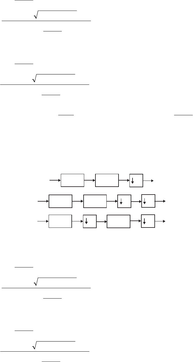
Here .
12000
100
=f∆ Using Eq. (10.3) we arrive at the order of F(z) given by
3873.386
12000
100
6.14
13001.0001.0log20 10 =⇒=
⎟
⎠
⎞
⎜
⎝
⎛
−×−
=FF NN
Specifications for I(z) are: 180
=
p
F Hz, 2200
=
s
F Hz, .001.0,001.0 =
=
sp δδ
Here .
12000
2020
=f∆ Using Eq. (10.3) we arrive at the order of I(z) given by
20712.19
12000
2020
6.14
13001.0001.0log20 10 =⇒=
⎟
⎠
⎞
⎜
⎝
⎛
−×−
=FI NN
Hence, 200,155
6
2400
)1387(
,=+=
FM
R mps, 400,50
5
12000
)120(
,=+=
IM
R mps.
The above realization requires a total of 205,600 mps. As a result, the computational
complexity is slightly higher than in Example 13.10.
13.19 Specifications for H(z) are: 180
=
p
F Hz, 200
=
s
F Hz, .001.0,002.0 =
=
sp δδ
)()()( 3
zFzIzH =
30
I(z)F(z )
3
I(z)F(z )
3310
I(z)310
F(z)
12 kHz 12 kHz 4 kHz 4 kHz 400 H
z
Specifications for F(z) are: 540
=
p
F Hz, 600
=
s
F Hz, .001.0,001.0 =
=
sp δδ
Here .
12000
60
=f∆ Using Eq. (10.3) we arrive at the order of F(z) given by
6448.643
12000
60
6.14
13001.0001.0log20 10 =⇒=
⎟
⎠
⎞
⎜
⎝
⎛
−×−
=FF NN
Specifications for I(z) are: 180
=
p
F Hz, 3800
=
s
F Hz, .001.0,001.0 =
=
sp δδ
Here .
12000
3260
=f∆ Using Eq. (10.3) we arrive at the order of I(z) given by
1285.11
12000
3260
6.14
13001.0001.0log20 10 =⇒=
⎟
⎠
⎞
⎜
⎝
⎛
−×−
=FI NN
Not for sale 506

Hence, 000,262
10
4000
)1644(
,=+=
FM
R mps, 000,52
3
12000
)112(
,=+=
IM
R mps.
The above realization requires a total of 314,000 mps. As a result, the computational
complexity is higher than in Example 13.10 and that in Problem 13.18.
13.20 (a) The desired down-sampling factor is .20
000,2
40000 ==M The general structure of
the desired decimator is thus as shown below:
20
H(z)
40 kHz 40 kHz 2 kHz
Now, the normalized stopband edge angular frequency of a factor-of-20 decimator is
.
20
π
ω=
s Hence, the desired stopband edge frequency in this case is
1000
20
20000 ==
s
F Hz. The specifications of the decimation filter H(z) is thus as
follows: Hz,
800=
p
F1000
=
s
F Hz, .002.0,002.0
=
=
sp δδ Here .
40000
200
=f∆
Using Eq. (10.3) we arrive at the order of H(z) given by
.5624.561
40000
200
6.14
13002.0002.0log20 10 ⇒=
⎟
⎠
⎞
⎜
⎝
⎛
−×−
=
H
N Therefore, the computational
complexity is given by 000,1126
20
40000
)1562(
,=+=
HM
R mps.
(b) For a two-stage realization of the decimator, there are 4 possible realizations of the
decimation filter:
Realization #1 – )()()( zIzFzH 2
=
2
I(z)F(z )
2
10
40 kHz 40 kHz 40 kHz 10 kHz 2 kHz
2
I(z)10
40 kHz 20 kHz 2 kHz
F(z)
20 kHz
40 kHz
Specifications for and are as follows:
)(zF )(zI
1600:)( =
p
FzF Hz, Hz, 2000=
s
F,002.0,001.0
=
=
sp δδ and thus, .
40000
400
=f∆
800:)( =
p
FzI Hz, Hz, 000,19=
s
F,002.0,001.0
=
=
sp δδ and thus, .
40000
18200
=f∆
Orders of and are given by
)(zF )(zI
Not for sale 507

30229.301
40000
400
6.14
13002.0001.0log20 10 ⇒=
⎟
⎠
⎞
⎜
⎝
⎛
−×−
=
F
N
762.6
40000
18200
6.14
13002.0001.0log20 10 ⇒=
⎟
⎠
⎞
⎜
⎝
⎛
−×−
=
I
N
Computational complexities of the two sections are:
000,606
10
20000
)1302(
,=+=
FM
R mps and 000,160
2
40000
)17(
,=+=
IM
R mps.
Hence, the total computational complexity of the two-stage realization is
mps.
000,766
,, =+= IMFMM RRR
Realization #2 – )()()( zIzFzH 4
=
4
I(z)F(z )
4
5
40 kHz 40 kHz 40 kHz 10 kHz 2 kHz
4
I(z)5
40 kHz 10 kHz 2 kHz
F(z)
10 kHz
40 kHz
Specifications for and are as follows:
)(zF )(zI
3200:)( =
p
FzF Hz, 4000
=
s
F Hz, ,002.0,001.0
=
=
sp δδ and thus, .
40000
800
=f∆
800:)( =
p
FzI Hz, Hz, 000,9=
s
F,002.0,001.0
=
=
sp δδ and thus, .
40000
8200
=f∆
Orders of and are given by
)(zF )(zI
15165.150
40000
8000
6.14
13002.0001.0log20 10 ⇒=
⎟
⎠
⎞
⎜
⎝
⎛
−×−
=
F
N
1569.14
40000
8200
6.14
13002.0001.0log20 10 ⇒=
⎟
⎠
⎞
⎜
⎝
⎛
−×−
=
I
N
Computational complexities of the two sections are:
000,304
5
10000
)1151(
,=+=
FM
R mps and 000,160
4
40000
)115(
,=+=
IM
R mps.
Hence, the total computational complexity of the two-stage realization is
mps.
000,464
,, =+= IMFMM RRR
Realization #3 – )()()( zIzFzH 5
=
Not for sale 508
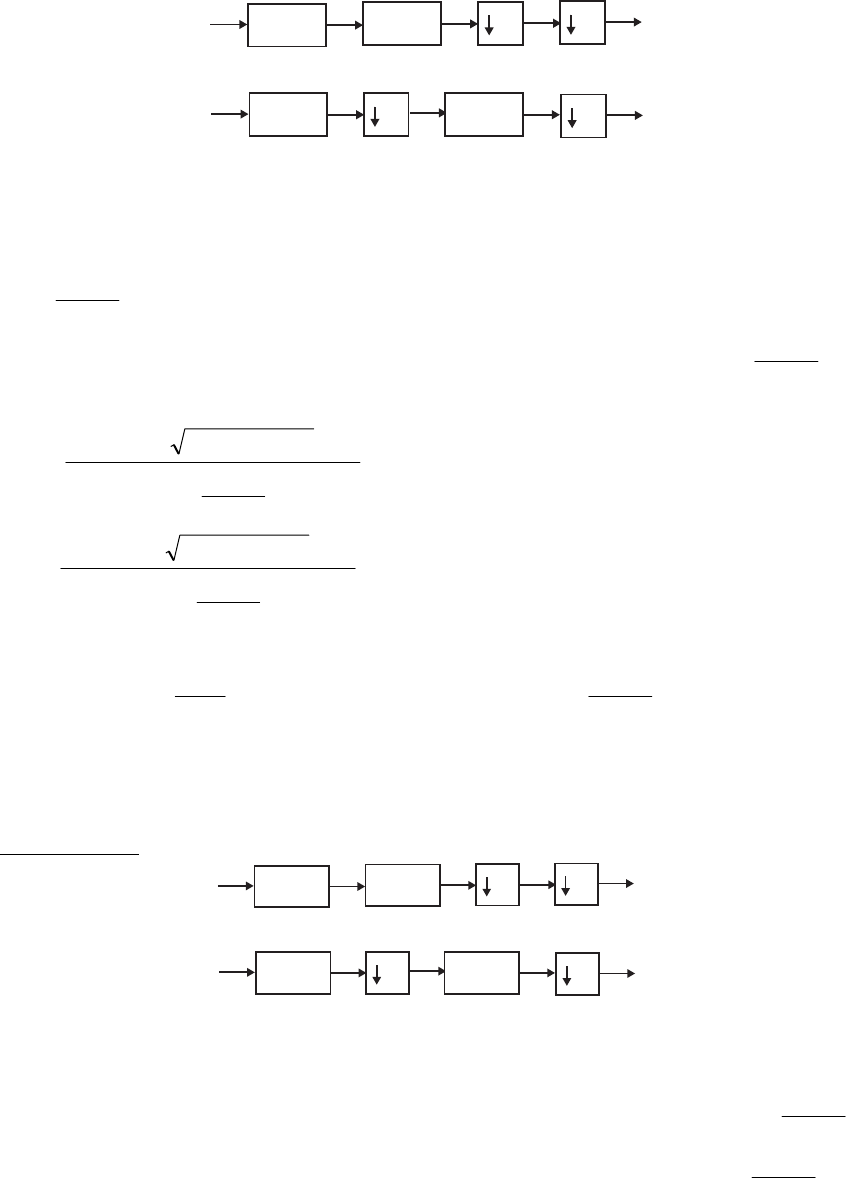
5
I(z)F(z )
5
4
40 kHz 40 kHz 40 kHz 4 kHz 2 kHz
5
I(z)4
40 kHz 8 kHz 2 kHz
F(z)
8 kHz
40 kHz
Specifications for and are as follows:
)(zF )(zI
4000:)( =
p
FzF Hz, 5000
=
s
F Hz, ,002.0,001.0
=
=
sp δδ and thus,
.
40000
1000
=f∆
800:)( =
p
FzI Hz, Hz, 000,7=
s
F,002.0,001.0
=
=
sp δδ and thus, .
40000
6200
=f∆
Orders of and are given by
)(zF )(zI
12152.120
40000
1000
6.14
13002.0001.0log20 10 ⇒=
⎟
⎠
⎞
⎜
⎝
⎛
−×−
=
F
N
2044.19
40000
6200
6.14
13002.0001.0log20 10 ⇒=
⎟
⎠
⎞
⎜
⎝
⎛
−×−
=
I
N
Computational complexities of the two sections are:
000,244
4
8000
)1121(
,=+=
FM
R mps and 000,168
5
40000
)120(
,=+=
IM
R mps.
Hence, the total computational complexity of the two-stage realization is
mps.
000,412
,, =+= IMFMM RRR
Realization #4 – )()()( zIzFzH 10
=
10
I(z)F(z )
10
2
40 kHz 40 kHz 40 kHz 4 kHz 2 kHz
10
I(z)2
40 kHz 4 kHz 2 kHz
F(z)
4 kHz
40 kHz
Specifications for and are as follows:
)(zF )(zI
8000:)( =
p
FzF Hz, Hz, 000,10=
s
F,002.0,001.0
=
=
sp δδ and thus, .
40000
2000
=f∆
800:)( =
p
FzI Hz, Hz, 000,3=
s
F,002.0,001.0
=
=
sp δδ and thus, .
40000
2200
=f∆
Orders of and are given by
)(zF )(zI
Not for sale 509
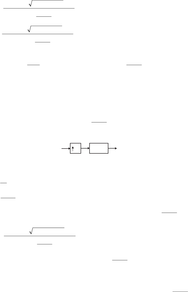
6126.60
40000
2000
6.14
13002.0001.0log20 10 ⇒=
⎟
⎠
⎞
⎜
⎝
⎛
−×−
=
F
N
5578.54
40000
2200
6.14
13002.0001.0log20 10 ⇒=
⎟
⎠
⎞
⎜
⎝
⎛
−×−
=
I
N
Computational complexities of the two sections are:
000,124
2
4000
)161(
,=+=
FM
R mps and 000,224
10
40000
)155(
,=+=
IM
R mps.
Hence, the total computational complexity of the two-stage realization is
mps.
000,348
,, =+= IMFMM RRR
Hence, the optimum two-stage design with the lowest computational complexity is the
Realization #4.
13.21 (a) The desired up-sampling factor is .50
480
24000 ==L The general structure of the
desired interpolator is thus as shown below:
H(z)
50
480 Hz 24 kHz 24 kHz
Now, the normalized stopband edge angular frequency of a factor-of-50 interpolator is
.
50
π
ω=
s Hence, the desired stopband edge frequency in this case is
240
50
12000 ==
s
F Hz. The specifications of the decimation filter H(z) is thus as
follows: Hz,
190=
p
F240
=
s
F Hz, .002.0,002.0
=
=
sp δδ Here .
24000
50
=f∆
Using Eq. (10.3) we arrive at the order of H(z) given by
.134827.1347
24000
50
6.14
13002.0002.0log20 10 ⇒=
⎟
⎠
⎞
⎜
⎝
⎛
−×−
=
H
N
Computational complexity is thus 520,647
50
24000
)11348(
,=+=
HM
R mps.
(b)
).()()( 10 zIzFzH =
Specifications for and are as follows:
)(zF )(zI
1900:)( =
p
FzF Hz, Hz, 2400=
s
F,002.0,001.0
=
=
sp δδ and thus, .
24000
500
=f∆
Not for sale 510
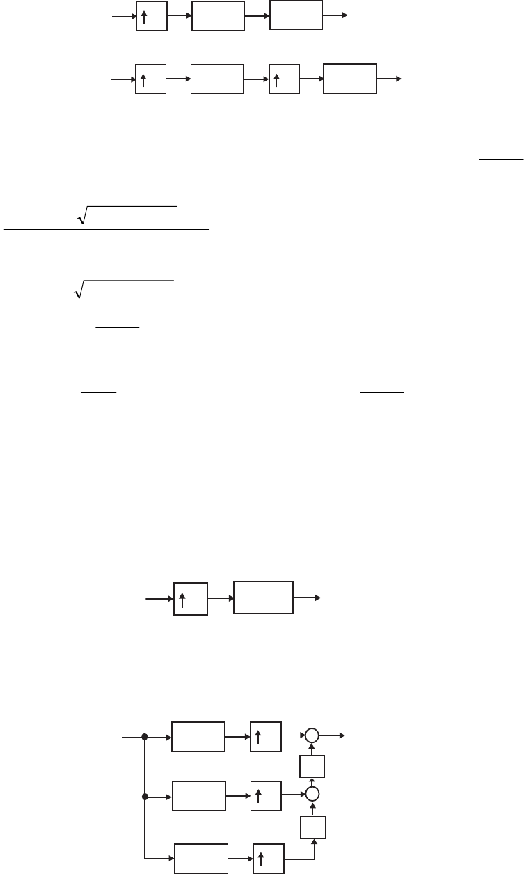
10
I(z)
50 F(z )
10
I(z)
5F(z)
480 Hz 24 kHz 24 kHz 24 kHz
480 Hz 2400 Hz 2400 Hz 24 kHz 24 kHz
190:)( =
p
FzI Hz, Hz, 2160=
s
F,002.0,001.0
=
=
sp δδ and thus, .
24000
1970
=f∆
Orders of and are given by
)(zF )(zI
14562.144
24000
500
6.14
13002.0001.0log20 10 ⇒=
⎟
⎠
⎞
⎜
⎝
⎛
−×−
=
F
N
3771.36
24000
1970
6.14
13002.0001.0log20 10 ⇒=
⎟
⎠
⎞
⎜
⎝
⎛
−×−
=
I
N
Computational complexities of the two sections are:
080,70
5
2400
)1145(
,=+=
FM
R mps and 200,91
10
24000
)137(
,=+=
IM
R mps.
Hence, the total computational complexity of the two-stage realization is
mps.
280,161
,, =+= IMFMM RRR
Therefore, the complexity in a two-stage design with is
approximately 25% of that of the single-stage design.
).()()( 10 zIzFzH =
13.22 A computationally efficient realization of a factor-of-3 interpolator as shown below
3H(z)
is obtained from the 3-band polyphase decomposition of H(z) given by
).()()()( 3
2
23
1
13
0zEzzEzzEzH
−
−++= The general form of the polyphase
representation of the interpolator is as shown below:
E (z)3
0
E (z)3
1
E (z)3
2
1
_
z
+
+
1
_
z
Not for sale 511
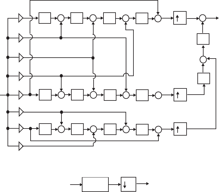
Since H(z) is a length-15 linear-phase transfer function,
1
]1[]0[)( −
+= zhhzH
98765432 ]5[]6[]7[]6[]5[]4[]3[]2[
−
−
−
−
−
−
−− ++++++++ zhzhzhzhzhzhzhzh
,]0[]1[]2[]3[]4[ 1413121110
−
−
−
−− +++++ zhzhzhzhzh the transfer functions of the
sub-filters are as follows:
,]2[]5[]6[]3[]0[)( 4321
0
−
−
−
−++++= zhzhzhzhhzE
,]1[]4[]7[]4[]1[)( 4321
1
−
−
−
−++++= zhzhzhzhhzE
.]0[]3[]6[]5[]2[)( 4321
2
−
−
−
−++++= zhzhzhzhhzE
A computationally efficient realization of the factor-of-3 interpolator is obtained by
sharing common multipliers as shown below:
1
_
z
+
+
1
_
z
3
1
_
z+
1
_
z+
1
_
z+
1
_
z+
3
1
_
z+
1
_
z+
1
_
z+
1
_
z+
3
1
_
z+
1
_
z+
1
_
z+
1
_
z+
h[0]
h[3]
h[6]
h[5]
h[2]
h[4]
h[1]
h[7]
x
[n]
y[n]
13.23 A computationally efficient realization of a factor-of-4 decimator as shown below
4
H(z)
is obtained from the 4-band polyphase decomposition of H(z) given by
).()()()()( 3
3
33
2
23
1
13
0zEzzEzzEzzEzH
−
−
−+++= The general form of the
polyphase representation of the interpolator is as shown below:
Not for sale 512
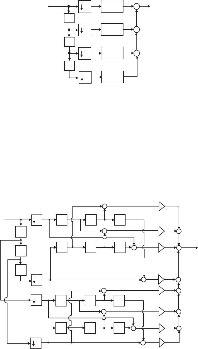
4E (z)
0+
4E (z)
1+
z
_1
4E (z)
2+
z
_1
4E (z)
3
z
_1
Since H(z) is a length-16 linear-phase transfer function,
1
]1[]0[)( −
+= zhhzH
98765432 ]6[]7[]7[]6[]5[]4[]3[]2[
−
−
−
−
−
−
−− ++++++++ zhzhzhzhzhzhzhzh
,]0[]1[]2[]3[]4[]5[ 151413121110
−
−
−
−
−− ++++++ zhzhzhzhzhzh the transfer
functions of the sub-filters are as follows:
,]3[]7[]4[]0[)( 321
0
−
−
−+++= zhzhzhhzE
,]2[]6[]5[]1[)( 321
1
−
−
−+++= zhzhzhhzE
.]1[]5[]6[]2[)( 321
2
−
−
−+++= zhzhzhhzE
.]0[]4[]7[]3[)( 321
3
−
−
−+++= zhzhzhhzE
A computationally efficient realization of the factor-of-4 decimator is obtained by
sharing common multipliers as shown below
z
_1
4
4
+
+
+
+
4
z
_1
z
_1
z
_1
z
_1
z
_1
z
_1
z
_1
+
+
+
z
_1
z
_1
z
_1
z
_1
z
_1
z
_1
z
_1
4+
+
+
+
h[0]
h[1]
h[2]
h[3]
h[4]
h[5]
+
+
+
h[7]
h[6]
13.24
)()()1()( )1()2(321
1
0
−−−−−−−
−
=
−++++++== ∑NN
N
i
izzzzzzzH L
Not for sale 513
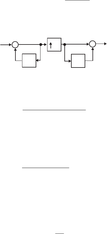
),()1()1)(1( 21)2(221 zGzzzzz N
−
−
−
−−− +=+++++= L where
Using a similar technique we can show that Therefore we
can write where
Continuing this decomposition process further we arrive at
where
.)(
1)2/(
0
∑−
=
−
=
N
i
i
zzG
.)1()(
1)4/(
0
21 ⎟
⎟
⎠
⎞
⎜
⎜
⎝
⎛
+= ∑−
=
−− N
i
i
zzzG
),()1)(1()1)(1()( 421
1)4/(
0
421 zFzzzzzzH
N
i
i−−
−
=
−−− ++=
⎟
⎟
⎠
⎞
⎜
⎜
⎝
⎛
++= ∑
.)(
1)4/(
0
∑−
=
−
=
N
i
i
zzF
),1()1)(1()( 1
221 −
−−− +++= K
zzzzH L.2K
N=
The transfer function of a box-car decimation filter of length-16 can be expressed as:
.
1
1
)( 1
16
15
0−
−
=
−
−
−
== ∑z
z
zzH
i
i
As a result, a computationally efficient realization of a factor-of-16 decimator using a
length-16 boxcar decimation filter is as shown below:
z1
_
+
+
z1
_
16
13.25 Let denote the output of the factor-of-L interpolator. Then
][nu
,
][
])1[][(
2
2
∑
∑
∞
−∞=
∞
−∞=
−−
=
n
n
nu
nunu
E (13-1)
and
.
][
]1[][
2nu
nunu
C
n
n
∑
∑
∞
−∞=
∞
−∞=
−
= (13-2)
Substituting Eq. (13-2) in Eq. (13-1) we get ).1(2 C
−
=
E
Hence, as i.e., as the
signal becomes highly correlated,
,1→C
][nu .0→E
Now, by Parsevals’relation, ,)(*)(
2
1
][][ ω
π
ω
π
π
ωdeVeUnvnu jj
n∫
∑
−
∞
−∞=
= where
)( ωj
eU
Not for sale 514
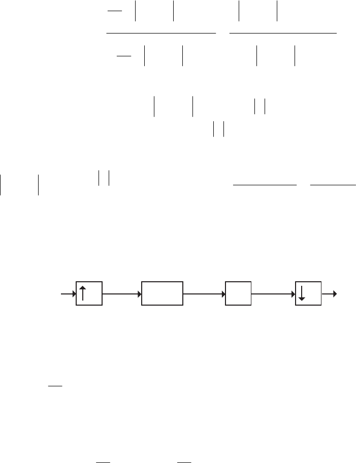
and are the DTFTs of and , respectively. If we let
)( ωj
eV ][nu ][nv ]1[][
−
=nunv in
the numerator of Eq. (13-1), and ][][ nunv
=
in the denominator of Eq. (13-1), then we
can write
,
)(
)cos()(
)(
2
1
)(
2
1
0
2
0
2
2
2
∫
∫
∫
∫
==
−
−
π
ω
π
ω
π
π
ω
π
π
ωω
ω
ωω
ω
π
ω
π
deU
deU
deU
deeU
E
j
j
j
jj
assuming to be a real sequence. If
][nu ][n
x
is assumed to be a broadband signal with
a flat magnitude spectrum, i.e., 1)( =
ωj
eX for ,0 πω ≤≤ then the magnitude
spectrum of is bandlimited to the range ,/0 Lπω ≤≤ i.e.,
⎩
⎨
⎧<≤
=otherwise.,0
,/0,1
)( L
eU jπω
ω Therefore, .
)/(
)/sin(
)cos(
/
0
/
0
L
L
d
d
CL
L
π
π
ω
ωω
π
π
==
∫
∫
Hence, as
.1, →∞→ CL
13.26
z L
H(z)
MM
–
X
(e )
jωW(e )
jωR(e )
jω
Y(e )
jω
S(e )
jω
Analysis of the above structure yields
),()( Mjj eXeW ωω =
),()()( Mjjj eXeHeR ωωω =),()()()( MjjLjjLjj eXeHeeReeS ωωω−ωω−ω ==
.)()( //
∑
−
=
ωω−ω =
1
0
1M
k
MjMkjj eeS
M
eY If the filter is assumed to be close to
an ideal lowpass filter with a cutoff at
)(ωj
eH
,/ M
ω
we can assume that all images of
are suppressed leaving only the term in the expression for Hence, we
can write
)( ωj
eX ).(ωj
eY
).()()()( /// ωω−ωωω == jMLjMjMjj eXeeH
M
eS
M
eY 11 Since is a
Type 1 FIR filter with exact linear phase and a delay of
)(zH
KMN =
−
21 /)( samples and a
magnitude response equal to M in the passband, we have
Thus, the structure of Figure P13.7 Is
approximately an allpass filter with a fixed delay of K samples and a variable
noninteger delay of L/M samples.
).()( /ωω−ω−ω =jMLjKjj eXeeeY
13.27 An ideal M-th band lowpass filter is characterized by a frequency response
)(zH
Not for sale 515
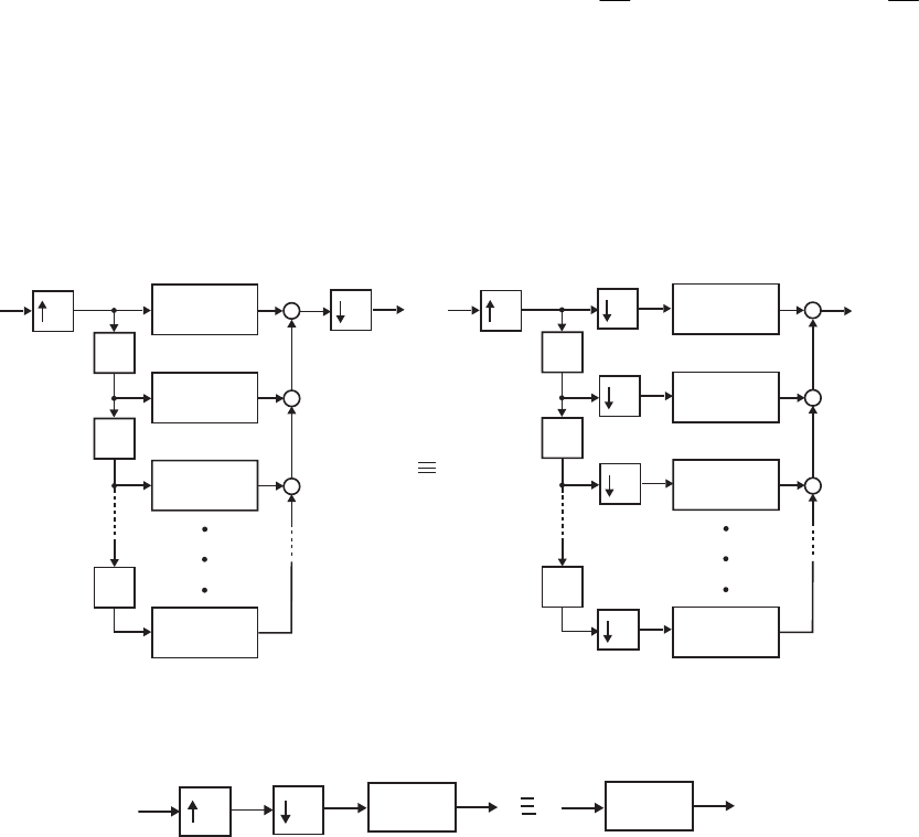
⎩
⎨
⎧π≤ω≤π−
=
ω
otherwise.,
,//,
)( 0
1MM
eH j The transfer function can be expressed in
an M-branch polyphase form as From the above we observe
Therefore,
)(zH
).()( M
k
M
k
kzHzzH ∑
−
=
−
=
1
0
).()( M
M
r
r
MzHMzWH 0
1
0
=
∑
−
=
.)()( /(
M
eH
M
eH
M
r
MrjMj 11 1
0
2
0== ∑
−
=
π−ωω
Or in other words, is an allpass function.
)( M
zH 0
13.28 An equivalent realization of the structure of Figure P13.38 obtained by realizing the
filter in a Type 1 polyphase form is shown below on the left. By moving the down-
sampler through the system and invoking the cascade equivalence #1 of Figure 13.14 we
arrive at the structure shown below on the right.
z
_1
+
+
+
z
_1
z
_1
0
E (z )
L
1
E (z )
L
2
E (z )
L
L 1
_
E (z )
L
L
L
z
_1
+
+
+
z
_1
z
_1
0
E (z)
1
E (z)
2
E (z)
L 1
_
E (z)
LL
L
L
L
The structure on the right hand side reduces to the one shown below on the left from
which we arrive at the simplified equivalent structure shown below on the right.
L
LE (z)
0
E (z)
0
13.29 (a) Let and
Then
(b)
.][)(
1
0
∑
−
=
−
=
N
n
n
znhzH ∑−
=
−
++=
1)2/(
0
2
0])12[]2[()(
N
i
i
zihihzH
.])12[]2[()(
1)2/(
0
2
1∑−
=
−
+−=
N
i
i
zihihzH
).(1]12[]2[)()1()()1(
1)2/(
0
2
1)2/(
0
22
1
12
0
1zHzihzihzHzzHz
N
i
i
N
i
i=+++=−++ ∑∑ −
=
−
−
=
−−−
)()1()()1()( 2
1
12
0
1zHzzHzzH
−
−−++=
Not for sale 516

(
)
(
)
).()()()()()( 2
1
12
0
2
1
2
0
12
1
2
0zEzzEzHzHzzHzH
−
−+=−++= Therefore,
and )()()( 100 zHzHzE += ).()()( 101 zHzHzE
−
=
(c) Now,
[]
[
]
⎥
⎦
⎤
⎢
⎣
⎡
−
+
=
⎥
⎦
⎤
⎢
⎣
⎡
⎥
⎦
⎤
⎢
⎣
⎡−
=−−
)()(
)()(
1
)(
)(
11
11
1)( 2
1
2
0
2
1
2
0
1
2
1
2
0
1
zHzH
zHzH
z
zH
zH
zzH
(
)
(
)
).()1()()1()()()()( 2
1
12
0
12
1
2
0
12
1
2
0zHzzHzzHzHzzHzH −
−
−−++=−++=
(d) If i.e., then we can express
,2=L,22
=N
)()1()()1()( 4
01
24
00
22
0zHzzHzzH
−
−−++= and
).()1()()1()( 4
11
24
10
22
1zHzzHzzH
−
−−++= Substituting these expressions in
)()1()()1()( 2
1
12
0
1zHzzHzzH
−
−−++= we get
[
]
)()1()()1()1()( 4
01
24
00
21 zHzzHzzzH
−
−− −+++=
[
]
)()1()()1()1( 4
11
24
10
21 zHzzHzz
−
−
−
−++−+
)()1)(1()()1)(1( 4
01
214
00
21 zHzzzHzz
−
−
−− −++++=
)()1)(1()()1)(1( 4
11
214
10
21 zHzzzHzz −
−
−
−
−−++−+
[] []
.
)(
ˆ
)(
ˆ
)(
ˆ
)(
ˆ
1
)(
)(
)(
)(
1111
1111
1111
1111
1
4
3
4
2
4
1
4
0
4
321
4
11
4
10
4
01
4
00
321
⎥
⎥
⎥
⎥
⎦
⎤
⎢
⎢
⎢
⎢
⎣
⎡
=
⎥
⎥
⎥
⎥
⎦
⎤
⎢
⎢
⎢
⎢
⎣
⎡
⎥
⎥
⎥
⎦
⎤
⎢
⎢
⎢
⎣
⎡
−− −− −−
=−−−−−−
zH
zH
zH
zH
zzz
zH
zH
zH
zH
zzz R
Continuing this process it is easy to establish that for we have
[]
⎥
⎥
⎥
⎥
⎦
⎤
⎢
⎢
⎢
⎢
⎣
⎡
=
−
−−−
)(
ˆ
)(
ˆ
)(
ˆ
1)(
1
1
0
)1(1
L
L
L
L
L
L
zH
zH
zH
zzzH M
LR.
13.30 Now
Therefore,
[][]
.
)(
)(
)(
)(
1
)(
ˆ
)(
ˆ
)(
ˆ
)(
ˆ
1)(
4
3
4
2
4
1
4
0
321
4
3
4
2
4
1
4
0
4
321
⎥
⎥
⎥
⎥
⎦
⎤
⎢
⎢
⎢
⎢
⎣
⎡
=
⎥
⎥
⎥
⎥
⎦
⎤
⎢
⎢
⎢
⎢
⎣
⎡
=−−−−−−
zE
zE
zE
zE
zzz
zH
zH
zH
zH
zzzzH R
.
)(
)(
)(
)(
1111
1111
1111
1111
4
1
)(
)(
)(
)(
4
1
)(
)(
)(
)(
)(
ˆ
)(
ˆ
)(
ˆ
)(
ˆ
3
2
1
0
3
2
1
0
4
3
2
1
0
1
4
3
2
1
0
⎥
⎥
⎥
⎦
⎤
⎢
⎢
⎢
⎣
⎡
⎥
⎥
⎥
⎦
⎤
⎢
⎢
⎢
⎣
⎡
−− −− −−
=
⎥
⎥
⎥
⎦
⎤
⎢
⎢
⎢
⎣
⎡
=
⎥
⎥
⎥
⎦
⎤
⎢
⎢
⎢
⎣
⎡
=
⎥
⎥
⎥
⎥
⎦
⎤
⎢
⎢
⎢
⎢
⎣
⎡
−
zE
zE
zE
zE
zE
zE
zE
zE
zE
zE
zE
zE
zH
zH
zH
zH
RR
A length-16 Type 1 linear-phase FIR transfer function is of the form
9
6
8
7
7
7
6
6
5
5
4
4
3
3
2
2
1
10
)(
−
−−
−
−
−
−
−− +++++++++= zhzhzhzhzhzhzhzhzhhzH
Not for sale 517
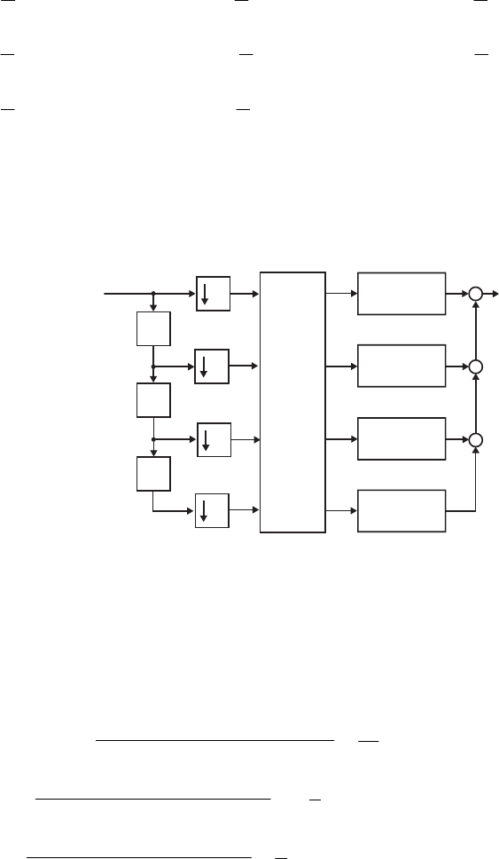
.
15
0
14
1
13
2
12
3
11
4
10
5−
−
−
−
−
−++++++ zhzhzhzhzhzh
Hence, ,)(,)( 3
2
2
6
1
511
3
3
2
7
1
400
−
−
−
−
−
−+++=+++= zhzhzhhzEzhzhzhhzE
.)(,)( 3
0
2
4
1
733
3
1
2
5
1
622 −
−
−
−
−− +++=+++= zhzhzhhzEzhzhzhhzE Thus,
,)(
ˆ
,)(
ˆ3
2
2
3
1
321
3
0
2
1
1
100 −
−
−
−
−− −−+=+++= zgzgzggzHzgzgzggzH
,)(
ˆ
,)(
ˆ3
6
2
7
1
763
3
4
2
5
1
542 −
−
−
−
−− +++=−−+= zgzgzggzHzgzgzggzH where
),(
4
1
),(
4
1
),(
4
1
321027654132100 hhhhghhhhghhhhg −+−=+++=+++=
),(
4
1
),(
4
1
),(
4
1
765453210476543 hhhhghhhhghhhhg −−+=−−+=−+−=
).(
4
1
),(
4
1
7654732106 hhhhghhhhg +−−=+−−= Note that and
are Type 1 linear-phase FIR transfer functions, whereas, and are Type 2
linear-phase FIR transfer functions. A computationally efficient realization of a factor-
of-4 decimator using a four-band structural subband decomposition of the decimation
filter is shown below:
)(
ˆ0zH )(
ˆ3zH
)(
ˆ1zH )(
ˆ2zH
)(zH
z
_1
z
_1
z
_1
+
+
+
M
M
M
M
R
4
0
H (z)
^
1
H (z)
^
2
H (z)
^
H (z)
3
^
Because of the symmetry or anti-symmetry in the impulse responses of the subband
filters, each subband filter can be realized using only 2 multipliers. Hence, the final
realization uses only 8 multipliers. Note also that by delay-sharing, the total number of
delays in implementing the four subband filters can be reduced to 3.
13.31 ]2[)(]1[)(][)(]1[)(]2[)(][ 21012
+
+
+
+
+
−
+−= −− nxPnxPnxPnxPnxPny ααααα
where ),22(
)22)(12)(2)(12(
)2)(1()1(
)( 234
24
1
2αααα
αααα
α+−−=
−−−−−+−
−
−
+
=
−
P
),44(
)21)(11)(1)(21(
)2)(1()2(
)( 234
6
1
1αααα
αααα
α+−−−=
−−−−−+−
−
−+
=
−
P
),45(
)20)(10)(10)(20(
)2)(1)(1)(2(
)( 24
4
1
0+−=
−−++
−
−++
=αα
αααα
αP
Not for sale 518

),44(
)21)(01)(11)(21(
)2()1)(2(
)( 234
6
1
1αααα
αααα
α−−+−=
−−++
−
++
=P
).22(
)12)(02)(12)(22(
)1()1)(2(
)( 234
24
1
2αααα
αααα
α−−+=
−−++
−
++
=P
We consider the computation of ]3[],2[],1[],[
+
+
+
nynynyny using 5 input samples:
through ]2[ −nx ].2[ +nx
For ,0)(,1)(,0)(,0)(,0 010001020
=
=
=
== −− ααααα PPPP and For .0)( 02 =αP
,3428.0)(,127.0)(,022.0)(,4/5 1011121
−
=
=
−== −− αααα PPP
and
,1426.1)( 11 =αP
.0952.0)( 12 =αP
For ,9531.2)(,4062.1)(,2734.0)(,4/10 2021222
=
−
=
== −− αααα PPP
and
,2812.3)( 21 −=αP.4609.2)( 22
=
αP
For ,86.32)(,2949.17)(,5718.3)(,4/15 3031323
=
−
=
== −− αααα PPP
and ,873.29)( 31 −=αP.7358.11)( 32
=
αP
The block filter implementation is thus given by
Another
implementation is given by
.
]2[
]1[
][
]1[
]2[
7358.11873.2986.322949.175718.3
4609.22812.39531.24062.12734.0
0952.01426.13428.0127.0022.0
00100
]3[
]2[
]1[
][
⎥
⎥
⎥
⎥
⎦
⎤
⎢
⎢
⎢
⎢
⎣
⎡
+
+
−
−
⎥
⎥
⎥
⎦
⎤
⎢
⎢
⎢
⎣
⎡
−
−−− −−
=
⎥
⎥
⎥
⎦
⎤
⎢
⎢
⎢
⎣
⎡
+
+
+
nx
nx
nx
nx
nx
ny
ny
ny
ny
⎟
⎠
⎞
⎜
⎝
⎛+++−+−−−= ]2[]1[][]1[]2[][ 24
1
6
1
4
1
6
1
24
1
4nxnxnxnxnxny α
⎟
⎠
⎞
⎜
⎝
⎛+++−−+−+ −]2[]1[]1[]2[ 12
1
6
1
6
1
12
1
3nxnxnxnxα
⎟
⎠
⎞
⎜
⎝
⎛+−++−−+−+ −]2[]1[][]1[]2[ 24
1
6
4
4
5
6
4
24
1
2nxnxnxnxnxα
].[]2[]1[]1[]2[ 12
1
6
4
6
4
12
1nxnxnxnxnx +
⎟
⎠
⎞
⎜
⎝
⎛+−++−−−+ α
The Farrow structure implementation of the interpolator is shown below:
y[n]
x
[n]
H
3
(z)
H
1
(z)H2(z)
ααα
H
0
(z)
α
where ,)(,)( 2
24
1
6
1
1
6
1
2
12
1
1
2
24
1
6
1
4
1
1
6
1
2
24
1
0zzzzzHzzzzzH −++−=+−+−= −−−−
Not for sale 519

,)( 2
24
1
6
4
4
5
1
6
4
2
24
1
2zzzzzH −−+−= +
−− and .)( 2
12
1
6
4
1
6
4
2
12
1
3zzzzzH −+−= −−
13.32 From Eq. (13.75), we have .
1111
1111
3
3
3
2
3
1
3
0
2
3
2
2
2
1
2
0
3210
3
3
3
2
3
1
3
4
2
3
2
2
2
1
2
4
3214
40
tttt
tttt
tttt
tttt
tttt
tttt
aa −= Both the numerator and the
denominator are determinants of Vandermonde matrices and have a nonzero value if
From the solution of Problem 6.28, we get
., jitt ji ≠≠
))()()()()((
))()()()()((
231312030201
231312434241
40 tttttttttttt
tttttttttttt
aa −−−−−−
−
−
−
−−−
= ,
))()((
))()((
030201
434241
4tttttt
tttttt
a−−−
−−
−
= or
.
))()((
))()((
302010
342414
40 tttttt
tttttt
aa −−−
−
−−
−=
13.33 From Eq. (13.74) we get ))()()()()((
))()()()()((
231312030201
234342030204
41 tttttttttttt
tttttttttttt
aa −−−−−−
−−
−
−
−
−
−=
.
))()((
))()((
131201
434204
4tttttt
tttttt
a−−−
−−−
−= Substituting the value of given by Eq. (13.77) in
the above we arrive at
4
a
.
))()()(( 41312101
1
1
tttttttt
a−−−−
= Likewise, from Eq. (13.74)
we get ))()()()()((
))()()()()((
231312030201
431314030401
42 tttttttttttt
tttttttttttt
aa −−−−−−
−
−
−
−
−−
=
.
))()((
))()((
231202
431404
4tttttt
tttttt
a−−−
−−−
= Substituting the value of given by Eq. (13.77) in the
above we arrive at
4
a
.
))()()(( 42321202
0
1
tttttttt
a−−−−
= Finally, from Eq. (13.74) we
get ))()()()()((
))()()()()((
231312030201
241412040201
43 tttttttttttt
tttttttttttt
aa −−−−−−
−
−
−
−
−−
−=
.
))()((
))()((
231303
241404
4tttttt
tttttt
a−−−
−−−
−= Substituting the value of given by Eq. (13.77) in the
above we arrive at
4
a
.
))()()(( 43231303
3
1
tttttttt
a−−−−
=
13.34 ., 4+
≤
≤= mimiti
Not for sale 520

,
))()()(( 24
1
4321
1=
−−−−−−−−
=mmmmmmmm
am
,
))()()(( 6
1
4131211
1
1−=
−−+−−+−−+−+
=
+mmmmmmmm
am
,
))()()(( 4
1
4232122
1
2=
−−+−−+−−+−+
=
+mmmmmmmm
am
,
))()()(( 6
1
4323133
1
3−=
−−+−−+−−+−+
=
+mmmmmmmm
am
.
))()()(( 24
1
3424144
1
4=
−−+−−+−−+−+
=
+mmmmmmmm
am
From Eq. (13.69), we have the expressions for given by
)(
)( tBm
3
⎪
⎪
⎪
⎪
⎩
⎪
⎪
⎪
⎪
⎨
⎧
+≥
+<≤+−−−−−+−−−−
+<≤+−−+−−−−
+<≤+−−−−
+<≤−
<
=
.,
,,)()()()(
,,)()()(
,,)()(
,,)(
,,
)(
)(
40
43321
3221
211
1
0
3
6
1
3
4
1
3
6
1
3
24
1
3
4
1
3
6
1
3
24
1
3
6
1
3
24
1
3
24
1
3
mt
mtmmtmtmtmt
mtmmtmtmt
mtmmtmt
mtmmt
mt
tBm
The normalized 3rd order B-spline is then given by
)()()( )()( tBmmt mm 33 4−+=β
⎪
⎪
⎪
⎪
⎩
⎪
⎪
⎪
⎪
⎨
⎧
+≥
+<≤+−−−−−+−−−−
+<≤+−−+−−−−
+<≤+−−−−
+<≤−
<
==
.,
,,)()()()(
,,)()()(
,,)()(
,,)(
,,
)(
)(
40
43321
3221
211
1
0
4
3
3
2
33
3
2
3
6
1
33
3
2
3
6
1
3
3
2
3
6
1
3
6
1
3
mt
mtmmtmtmtmt
mtmmtmtmt
mtmmtmt
mtmmt
mt
tBm
Substituting and evaluating for
α+= 1t)(
)( t
m
3
β,,, 2101
−
=
m we have
,)(
)(
6
1
226
23
3
1+
α
−
α
+
α
−=αβ− ,)(
)(
3
2
2
2
3
3
0+α+
α
=αβ
,)(
)(
6
1
222
23
3
1+
α
+
α
+
α
−=αβ .)(
)(
6
3
3
2
α
=αβ
Substituting back in Eq. (13.91), we have
][)(][ )( knxny
k
k+αβ= ∑
−=
2
1
3
Not for sale 521
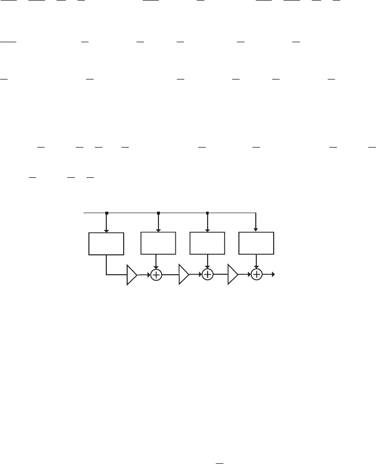
][][][ 1
6
1
2223
2
2
1
6
1
226
23
2
323 +
⎟
⎟
⎠
⎞
⎜
⎜
⎝
⎛+
α
+
α
+
α
−+
⎟
⎟
⎠
⎞
⎜
⎜
⎝
⎛+α+
α
+−
⎟
⎟
⎠
⎞
⎜
⎜
⎝
⎛+
α
−
α
+
α
−= nxnxnx
][ 2
6
3+
⎟
⎟
⎠
⎞
⎜
⎜
⎝
⎛α
+nx α
⎟
⎠
⎞
⎜
⎝
⎛++−−+
⎟
⎠
⎞
⎜
⎝
⎛++−= ][][][][][ 1
2
1
1
2
1
6
1
3
2
1
6
1nxnxnxnxnx
.][][][][][][][ 32 2
6
1
1
2
1
2
1
1
6
1
1
2
1
1
2
1α
⎟
⎠
⎞
⎜
⎝
⎛+++−+−−+α
⎟
⎠
⎞
⎜
⎝
⎛++−−+ nxnxnxnxnxnxnx
In the z-domain, the input-output relation is thus given by
where
,)()()()()( 3
0
2
123 α+α+α+= zHzHzHzHzY
,)( 21
06
1
2
1
2
1
6
1zzzzH +−+−= − ,)( zzzH 2
1
1
2
11
1+−= − ,)( zzzH 2
1
2
11
2+−= −
.)( zzzH 6
1
3
2
6
11
3++= − The corresponding Farrow structure is shown on top of the
next page:
y[n]
x
[n]
H
3
(z)
H
1
(z)H2(z)
αα
H
0
(z)
α
13.35 For the factor-of-4/3 interpolator design, if we use cubic B-spline with uniformly
spaced knots at the problem reduces exactly to the design given in the solution of
Problem 13.34.
13.36 From Eq. (13.94) with 0
=
k we have Substituting the
expression for on the left-hand side Eq. (13.97) we get INCOMPLETE
).()(
1
1
L
L
i
i
izEzzH ∑
−
=
−
+= α
13.37 For a half-band zero-phase lowpass filter, the transfer function is of the form
where
,]2[]0[)(
0
21 ∑
∞
≠
−∞=
−−
+=
n
n
n
znhzhzH .
2
1
]0[ =h If the half-band filter has a zero at
then or
,1−=
z,0]2[]0[)1(
0
=−=− ∑
∞
≠
−∞=
n
n
nhhH .]2[]0[
0
∑
∞
≠
−∞=
=
n
n
nhh
13.38 From Eq. (13.99), a zero-phase half-band filter satisfies the condition
a constant.
)(zH
=−+ )()( zHzH
Not for sale 522
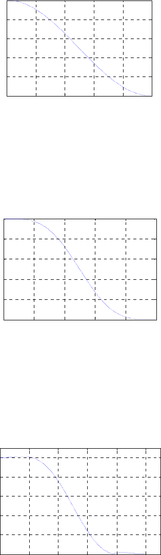
(a) The zero-phase equivalent here is given by .2)( 1
1
−
++= zzzH Hence,
.422)()( 11
11 =−+−++=−+
−
−
zzzzzHzH A plot of the scaled magnitude
response of is given below:
)(
1zH
00.2 0.4 0.6 0.8 1
0
0.2
0.4
0.6
0.8
1
ω
/
π
Magnitude
H
1
(z)
(b) The zero-phase equivalent here is given by .9169)( 313
2
−
−−+++−= zzzzzH
Hence,
.3291699169)()( 313313
22 =+−+−+−+++−=−+ −−
−
−
zzzzzzzzzHzH
A plot of the scaled magnitude response of is given below:
)(
2zH
00.2 0.4 0.6 0.8 1
0
0.2
0.4
0.6
0.8
1
ω
/
π
Magnitude
H
2
(z)
(c) The zero-phase equivalent here is given by
.319326193)( 313
3
−
−
−+++−= zzzzzH Hence,
.643193219331932193)()( 313313
33 =+−+−+−+++−=−+
−
−
−
−
zzzzzzzzzHzH
A plot of the scaled magnitude response of is given below: )(
3zH
00.2 0.4 0.6 0.8 1
0
0.2
0.4
0.6
0.8
1
ω
/
π
Magnitude
H
3
(z)
Not for sale 523

(d) The zero-phase equivalent here is given by
.325150256150253)( 53135
4
−
−
−
+−+++−= zzzzzzzH Hence, )()( 44 zHzH
−
+
13553135 150256150253325150256150253
−
−
−
−
−+−+−+−+++−= zzzzzzzzzz
.512325 53 =−+ −− zz A plot of the scaled magnitude response of is given
below:
)(
4zH
00.2 0.4 0.6 0.8 1
0
0.2
0.4
0.6
0.8
1
ω
/
π
Magnitude
H
4
(z)
13.39 (a) A function of has p-th order zero at a frequency
)(ωFi
ω
=
ω
if
.
)( 0=
ω
ω
ω=ω i
p
p
d
Fd The function has p zeros at )(ωj
eH 1
=
ω
cos , i.e., at
π
=
ω.
Hence, .
)( 0=
ωπ=ω
ω
p
jp
d
eHd Moreover, the order of the highest power of
is As a result,
21 /)cos( ω− .1−p.
)( 0
0
1
1=
ω=ω
−
ω−
p
jp
d
eHd
(b) Now,
2
2
1
2
1
⎟
⎟
⎠
⎞
⎜
⎜
⎝
⎛+
=
ω+ ω−
ωj
je
e
cos and .
cos 2
2
1
2
1
⎟
⎟
⎠
⎞
⎜
⎜
⎝
⎛−
−=
ω− ω−
ωj
je
e
Substituting these expressions in Eq. (13.120) we arrive at
.)()(
l
l
l
l
l
⎟
⎟
⎠
⎞
⎜
⎜
⎝
⎛−
−
⎟
⎠
⎞
⎜
⎝
⎛+−
⎟
⎟
⎠
⎞
⎜
⎜
⎝
⎛+
=ω−
−
=
ω−
ω−
ωω ∑2
1
1
2
11
0
j
p
j
p
j
jpj e
e
p
e
eeH Replacing with
in z the above we get the expression for the zero-phase transfer function as
ωj
e
.)()(
l
l
l
l
l
l
⎟
⎟
⎠
⎞
⎜
⎜
⎝
⎛−
−
⎟
⎠
⎞
⎜
⎝
⎛+−
⎟
⎟
⎠
⎞
⎜
⎜
⎝
⎛+
=−
−
−∑2
1
1
2
11
1
1z
z
p
z
zzH
p
p
13.40 (a)
Not for sale 524

+
2
2
2
2
2
2
_1
z
_1
z
1 z
__1
_1
1 + z
0
H (z)
1
H (z)
1
H (z)
0
H (z)+
z z
_
_2_1
X
(z)Y(z)
V (z)
1
V (z)
0
V (z)
2
W (z)
0
W (z)
1
W (z)
2
U (z)
0
U (z)
1
U (z)
2
R (z)
0
R (z)
1
R (z)
2
Analysis of the above structure yields
),(
1
1
)(
)(
)(
)( 1
1
2
1
0
zXz
z
zV
zV
zV
z
⎥
⎥
⎥
⎦
⎤
⎢
⎢
⎢
⎣
⎡
+=
⎥
⎥
⎦
⎤
⎢
⎢
⎣
⎡
=−
−
V
),(
1
1)(
1
1
)(
)(
)(
)( 2/12/1
2/1
2/12/1
2/1
2
1
0−−
−
−
−
⎥
⎥
⎥
⎦
⎤
⎢
⎢
⎢
⎣
⎡
−
−
+
⎥
⎥
⎥
⎦
⎤
⎢
⎢
⎢
⎣
⎡
+=
⎥
⎥
⎦
⎤
⎢
⎢
⎣
⎡
=zXz
z
zXz
z
zW
zW
zW
zW
() ()
),(
)(
)()()1(
)(
)(
)(
)()()1(
)(
)(
)(
)(
)( 2/1
1
10
2/1
0
2/1
2/1
1
10
2/1
0
2/1
2
1
0
zX
zH
zHzHz
zHz
zX
zH
zHzHz
zHz
zU
zU
zU
z−
⎥
⎥
⎥
⎦
⎤
⎢
⎢
⎢
⎣
⎡
+−
−
+
⎥
⎥
⎥
⎦
⎤
⎢
⎢
⎢
⎣
⎡
++=
⎥
⎥
⎦
⎤
⎢
⎢
⎣
⎡
=−
−
−
−
U
() ()
).(
)(
)()()1(
)(
)(
)(
)()()1(
)(
)(
)(
)(
)(
2
1
2
1
2
0
1
0
1
2
1
2
1
2
0
1
2
0
1
2
1
0
zX
zH
zHzHz
zHz
zX
zH
zHzHz
zHz
zR
zR
zR
z−
⎥
⎥
⎥
⎦
⎤
⎢
⎢
⎢
⎣
⎡
+−
−
+
⎥
⎥
⎥
⎦
⎤
⎢
⎢
⎢
⎣
⎡
++=
⎥
⎥
⎦
⎤
⎢
⎢
⎣
⎡
=−
−
−
−
R
)()()()()1()( 2
12
1
1
0
1zRzzzRzzRzzY
−
−
−
−−++−=
(
)
[
]
)()()()()()1()()1( 2
1
122
1
2
0
112
0
11 zXzHzzzHzHzzzHzz −
−
−
−
−− −++++−=
(
)
[
]
)()()()()()1()()1( 2
1
122
1
2
0
112
0
11 zXzHzzzHzHzzzHzz −−++−+−−+ −
−
−
−
−−
[
]
).()()(2)()(2)(2 ][ 2
1
12
0
12
1
22
0
1zXzHzzHzzXzHzzHz
−
−
−− +=+= Hence,
].[ )()(2)( 2
1
12
0
1zHzzHzzT −− +=
(b) ).(2)(
2
1
)(
2
1
)(
2
1
)(
2
1
2)( 11 zHzzHzHzHzHzzT −− =
⎥
⎦
⎤
⎢
⎣
⎡−−+−+=
(c) Length of and length of KzH =)(
0.)(
1KzH
=
(d) The total computational complexity of the above structure is 2
3T
F
K
multiplications per second, where is the sampling frequency in Hz. On the other hand,
a direct implementation of requires
)(zH
T
KF2 multiplications per second.
13.41
Not for sale 525
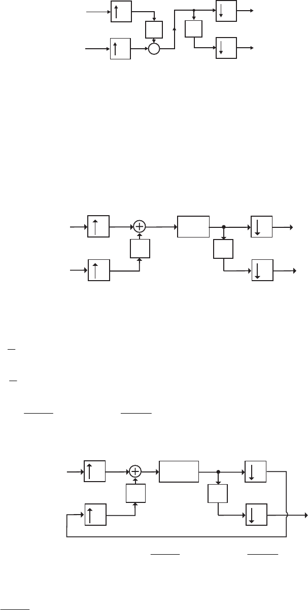
+
2
2
2
2
_1
z
_1
z
R(z)
X (z)
1
X
(z)
2
Y (z)
1
Y (z)
2
Analysis yields
),()()( 2
2
2
1
1zXzXzzR += −)()()( 2/12/1
1zRzRzY −+=
),(2)]()([)]()([ 221
2/1
21
2/1 zXzXzXzzXzXz =+−++=
−
−
)()()( 2/12/12/12/1
2zRzzRzzY −−= −−
).(2)]()([)]()([ 1
1
2
2/1
1
1
2
2/1
1
1zXzzXzzXzzXzzXz
−
−
−
−− =−++= Thus, the output
is a scaled replica of the input while the output is a scaled replica of
the delayed input
][
1ny ][
2nx ][
2ny
].1[
1−nx
13.42
2
2H(z2)
2
2
z 1
–
z 1
–
X (z)
1
X
(z)
2Y (z)
2
Y (z)
1
W(z)V(z)
Analysis yields ),()()( 2
2
12
1zXzzXzW
−
+=
),()()()()( 2
2
212
1
2zXzHzzXzHzV −
+=
()
),()()()(
2
1
)( 1
2/12/1
1zXzHzVzVzY =−+=
()
).()()()(
2
1
)( 2
12/12/12/12/1
2zXzHzzVzzVzzY −−− =−−=
Therefore, ),(
)(
)(
1
1zH
zX
zY = and ).(
)(
)( 1
2
2zHz
zX
zY −
= Hence, the system is time-invariant.
13.43
2
2H(z2)
2
2
z 1
–z 1
–
1
X (z)
2
X
(z)2
Y (z)
1
Y (z)
From the solution of Problem 13.42, ),(
)(
)(
1
1zH
zX
zY = and ).(
)(
)( 1
2
2zHz
zX
zY −
= Here now,
and hence,
),()( 12 zYzX =).()()()()()()( 1
21
1
1
2
1
2zXzHzzYzHzzXzHzzY −
−
−
===
Thus, ).(
)(
)( 21
1
2zHz
zX
zY −
= Hence, the system is time-invariant.
13.44
Not for sale 526
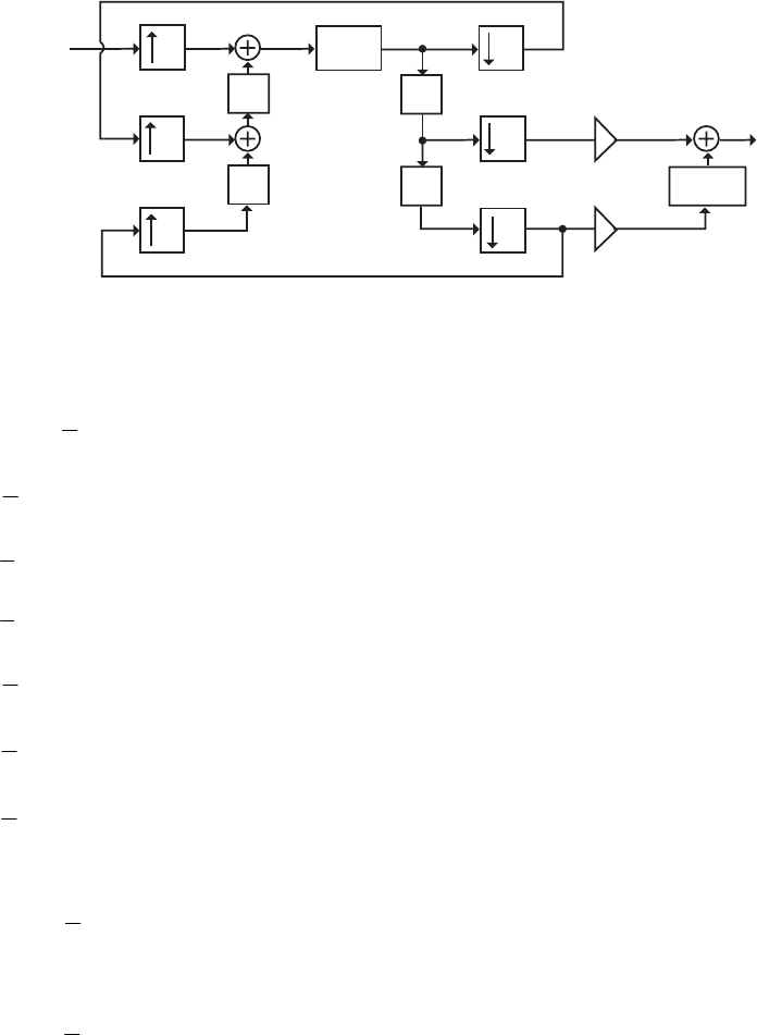
3
3H(z3)
3
3
3
3
–2
3
z 1
–
z 1
–z 1
–
z 1
–z (C 1)
–+
1
X
(z)
2
X (z)
3
X (z)
W(z)V(z)
Y(z)
Y (z)
1
2
Y (z)
Y (z)
3
Analysis yields ),()()()( 3
3
23
1
13
1zXzzYzzXzW
−
−
++=
),()()()()()()()()( 3
3
323
2
313
1
33 zXzHzzXzHzzXzHzWzHzV
−
−
++==
[]
)()()(
3
1
)( 3/43/13/23/13/1
1ππ jj ezVezVzVzY −− ++=
[]
)()()()()()(
3
14
1
42
1
2
1ππππ jjjj ezXezHezXezHzXzH −−−− ++=
[ ]
)()()()()()(
3
14
2
43/43/12
2
23/23/1
2
3/1 ππππππ jjjjjj ezXezHezezXezHezzXzHz −−−−−−−−− +++
[ ]
)()()()()()(
3
18
3
83/83/24
3
43/43/2
3
3/2 ππππππ jjjjjj ezXezHezezXezHezzXzHz −−−−−−−−− +++
[]
)()()()()()(
3
1
111 zXzHzXzHzXzH ++=
[]
)()()()()()(
3
1
2
3/43/1
2
3/23/1
2
3/1 zXzHezzXzHezzXzHz jj ππ −−−−− +++
[]
)()()()()()(
3
1
3
3/83/2
3
3/43/2
3
3/2 zXzHezzXzHezzXzHz jj ππ −−−−− +++
),()( 1zXzH=
[]
)()()(
3
1
)( 3/43/13/43/13/23/13/23/13/13/1
2ππππ jjjj ezVezezVezzVzzY −−−−− ++=
),()( 3
1zXzHz−
=
[]
)()()(
3
1
)( 3/43/13/83/13/23/13/43/13/13/1
3ππππ jjjj ezVezezVezzVzzY −−−−− ++=
).()( 2
2zXzHz −
=
Now, and
)()( 33 zYzX =).()( 12 zYzX
=
Hence,
)()()()()( 3
1
3
1
2zYzHzzXzHzzY −− == )()()()()( 1
22
2
11 ][ zYzHzzXzHzzHz −
−
−
==
Therefore,
).()( 1
32 zXzHz−
=)(3)(2)( 3
)1(
2zYzzYzY C
+
−
+−=
)()(2)(3)()(3)()(2 1
322
1
21)1(
1
32 ][ zXzHzHzzXzHzzzXzHz C−=+−=
−
−
+
−− for
Thus, the transfer function of the system of Figure P13.12 is
.0=C
.)(2)(3)( ][ 322 zHzHzzG −= −
M13.1 (a) (i)
Not for sale 527
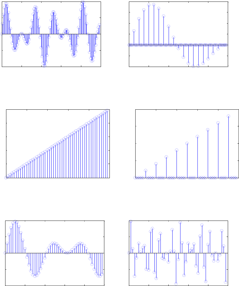
020 40 60 80 100
-2
-1
0
1
2
Input Sequence
Time index n
Amplitude
020 40 60 80 100
-1
-0.5
0
0.5
1
1.5
2
Output sequence up-sampled by5
Time index n
A
mp
lit
u
d
e
(ii)
010 20 30 40 50
0
0.2
0.4
0.6
0.8
1
Input Sequence
Time index n
Amplitude
010 20 30 40 50
0
0.05
0.1
0.15
0.2
Output sequence up-sampled by5
Time index n
Amplitude
M13.2 (a) (i)
010 20 30 40 50
-2
-1
0
1
2
Input Sequence
Time index n
Amplitude
010 20 30 40 50
-2
-1
0
1
2
Output sequence down-sampled by 5
Time index n
Amplitude
(ii)
Not for sale 528
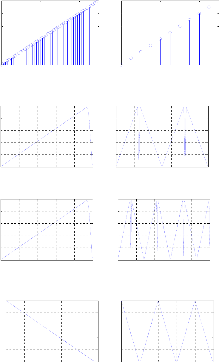
010 20 30 40 50
0
0.2
0.4
0.6
0.8
1
Input Sequence
Time index n
Amplitude
0 2 4 6 8 10
0
0.2
0.4
0.6
0.8
1
Output sequence down-sampled by 5
Time index n
Amplitude
M13.3 (a)
00.2 0.4 0.6 0.8 1
0
0.2
0.4
0.6
0.8
1
ω
/
π
Magnitude
Input spectrum
00.2 0.4 0.6 0.8 1
0
0.2
0.4
0.6
0.8
1
ω
/
π
Magnitude
Output spectrum
(b)
00.2 0.4 0.6 0.8 1
0
0.2
0.4
0.6
0.8
1
ω
/
π
Magnitude
Input spectrum
00.2 0.4 0.6 0.8 1
0
0.2
0.4
0.6
0.8
1
ω
/
π
Magnitude
Output spectrum
M13.4 (a)
00.2 0.4 0.6 0.8 1
0
0.2
0.4
0.6
0.8
1
ω
/
π
Magnitude
Input spectrum
00.2 0.4 0.6 0.8 1
0
0.2
0.4
0.6
0.8
1
ω
/
π
Magnitude
Output spectrum
Not for sale 529
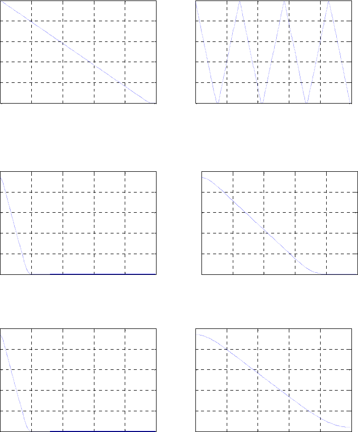
(b)
00.2 0.4 0.6 0.8 1
0
0.2
0.4
0.6
0.8
1
ω
/
π
Magnitude
Input spectrum
00.2 0.4 0.6 0.8 1
0
0.2
0.4
0.6
0.8
1
ω
/
π
Magnitude
Output spectrum
M13.5 (a)
00.2 0.4 0.6 0.8 1
0
0.2
0.4
0.6
0.8
1
ω
/
π
Magnitude
Input spectrum
00.2 0.4 0.6 0.8 1
0
0.05
0.1
0.15
0.2
0.25
ω
/
π
Magnitude
Output spectrum
(b)
00.2 0.4 0.6 0.8 1
0
0.2
0.4
0.6
0.8
1
ω
/
π
Magnitude
Input spectrum
00.2 0.4 0.6 0.8 1
0.04
0.06
0.08
0.1
0.12
0.14
ω
/
π
Magnitude
Output spectrum
M13.6 (a)
Not for sale 530
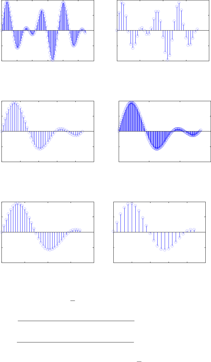
020 40 60 80 100 120
-2
-1
0
1
2
Input sequence
Time index n
Amplitude
010 20 30 40
-2
-1
0
1
2
Output sequence
Time index n
Amplitude
M13.7 (a)
010 20 30 40 50
-2
-1
0
1
2
Input sequence
Time index n
Amplitude
050 100 150
-2
-1
0
1
2
Output sequence
Time index n
Amplitude
M13.8 (a)
010 20 30 40
-2
-1
0
1
2
Input sequence
Time index n
Amplitude
0 5 10 15 20 25
-2
-1
0
1
2
Output sequence
Time index n
Amplitude
M13.9 Using Program 13_9.m we arrive at the transfer function of the desired elliptic half-
band lowpass filter:
[
]
,)()(
2
1
)( 2
1
12
00 zzzzH AA −
+= where
642
642
2
00192.03903.02456.11
2456.13903.00192.0
)( −−−
−−−
+++
+++
=
zzz
zzz
z
A and
.
1206.08884.07442.11
7442.18884.01206.0
)( 642
642
2
1−−−
−−−
+++
+++
=
zzz
zzz
z
A The power-complentary half-
band highpass transfer function is given by
[
]
.)()(
2
1
)( 2
1
12
00 zzzzH AA −
−= A plot
Not for sale 531
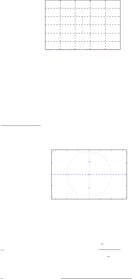
of the magnitude responses of the above half-band lowpass and highpass filters is
shown below:
00.2 0.4 0.6 0.8 1
0
0.2
0.4
0.6
0.8
1
ω
/
π
Magnitude
H
0
(z) H
1
(z)
M13.10 (a) A digital lowpass half-band filter can be designed by applying a bilinear
transformation to an analog lowpass Butterworth transfer function with a 3-dB cutoff
frequency at 1 rad/sec. The 3-dB cutoff frequency of the digital lowpass Butterworth
half-band filter is therefore at .5.0/)1(tan2 1==
−
πωc
To design a 3rd-order digital lowpass Butterworth half-band filter we use the MATLAB
statement [num,den] = butter(3,0.5); which yields
.
3333.01
)1(1667.0
)( 2
31
−
−
+
+
=
z
z
zH As can be seen from the pole-zero plot of given below all
poles are on the imaginary axis:
-1.5 -1 -0.5 00.5 11.5
-1
-0.5
0
0.5
1
3
Real Part
I
mag
i
nary
P
ar
t
Using the MATLAB statement
[d1,d2] = tf2ca([1 3 3 1]/6, [1 0 1/3 0]);
we arrive at the parallel allpass decomposition of as
)(zH
)],()([)( 2
1
12
0
2
1zAzzAzH −
+= where 2
3
1
2
3
1
2
0
1
)( −
−
+
+
=
z
z
zA and Hence,
the power-complementary highpass transfer function is given by
.1)( 2
1=zA
.
3333.01
)331(1667.0
)]()([)( 2
321
2
1
12
0
2
1
−
−−−
−
+
−+−
=−=
z
zzz
zAzzAzG
Not for sale 532
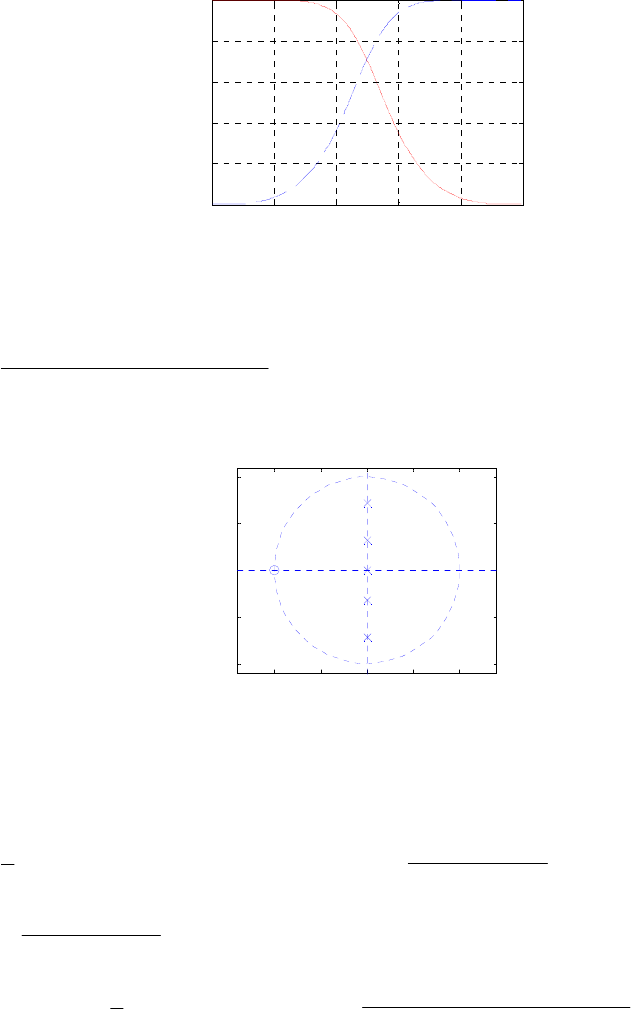
00.2 0.4 0.6 0.8 1
0
0.2
0.4
0.6
0.8
1
ω
/
π
Magnitude
H(z)G(z)
(b) To design a 5th-order digital lowpass Butterworth half-band filter we use the
MATLAB statement [num,den] = butter(5,0.5); which yields
.
0557.06334.01
)1(0528.0
)( 42
51
−−
−
++
+
=
zz
z
zH As can be seen from the pole-zero plot of given
below all poles are on the imaginary axis:
-1 -0.5 00.5 1
-1
-0.5
0
0.5
1
Real Part
Imaginary Part
Using the MATLAB statement
[d1,d2] =
tf2ca(0.0528*[1 5 10 10 5 1], [1 0 0.6334 0 0.0557]);
we arrive at the parallel allpass decomposition of as
)(zH
)],()([)( 2
1
12
0
2
1zAzzAzH −
+= where 2
2
2
01056.01
1056.0
)( −
−
+
+
=
z
z
zA and
.
5279.01
5279.0
)( 2
2
2
1−
−
+
+
=
z
z
zA Hence, the power-complementary highpass transfer function
is given by .
0557.06334.01
)1(0528.0
)]()([)( 42
51
2
1
12
0
2
1
−−
−
−
++
−
=−=
zz
z
zAzzAzG
Not for sale 533
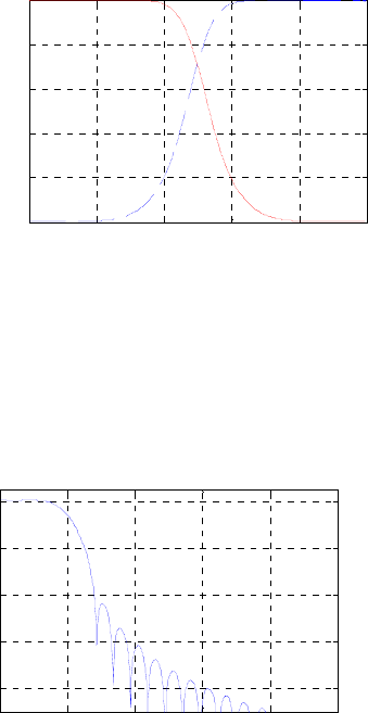
00.2 0.4 0.6 0.8 1
0
0.2
0.4
0.6
0.8
1
ω
/
π
Magnitude
H
(
z)G
(
z)
M13.11
M13.12
00.2 0.4 0.6 0.8 1
-80
-60
-40
-20
0
ω
/
π
Gain, dB
L-th band Nyquist Filter, L = 5
Not for sale 534

Chapter 14
14.1 (a) 2-band polyphase decomposition – Using ,1)( 1
−
−= zczP we express
1
1
1
)( −
−
+
+
=
cz
bza
zH as
22
21
11
11
1
)(
)1)(1(
)1)((
)( −
−−
−−
−−
−
−−+
=
−+
−+
=
zc
bczzacba
czcz
czbza
zH
.
11 22
1
22
2
⎟
⎟
⎠
⎞
⎜
⎜
⎝
⎛
−
−
+
⎟
⎟
⎠
⎞
⎜
⎜
⎝
⎛
−
−
=−
−
−
−
zc
acb
z
zc
bcza Hence, 22
2
2
01
)( −
−
−
−
=
zc
bcza
zE and
.
1
)( 22
2
1−
−
−
=
zc
acb
zE
(b) 3-band polyphase decomposition – Using ,1)( 221 −
−
+−= zcczzP we rewrite
as
)(zH
33
3221
2211
2211
1
)()(
)1)(1(
)1)((
)( −
−−−
−−−
−−−
−
+−+−+
=
+−+
+−+
=
zc
zbczbacczacba
zcczcz
zcczbza
zH
.
1
)(
11 33
2
33
1
33
32
⎟
⎟
⎠
⎞
⎜
⎜
⎝
⎛
−
−
+
⎟
⎟
⎠
⎞
⎜
⎜
⎝
⎛
−
−
+
⎟
⎟
⎠
⎞
⎜
⎜
⎝
⎛
−
+
=−
−
−
−
−
−
zc
bacc
z
zc
acb
z
zc
zbca Hence, ,
1
)( 33
32
3
0−
−
−
+
=
zc
zbca
zE
.
1
)(
)(,
1
)( 33
3
2
33
3
1−− −
−
=
−
−
=
zc
bacc
zE
zc
acb
zE
14.2 (a) .
1
)()(.
1
)( 1
1
1
2
1
1
−
−
−
−
−
−
=−=
+
+
=
cz
bza
zHzWH
cz
bza
zH aaa Thus,
22
2
1
1
1
1
2
0111
2
1
)]()([
2
1
)( −
−
−
−
−
−
−
−
=
⎟
⎟
⎠
⎞
⎜
⎜
⎝
⎛
−
−
+
+
+
=−+=
zc
bcza
cz
bza
cz
bza
zHzHzE aa and
.
1
)(
11
2
1
)]()([
2
1
)( 22
1
1
1
1
1
2
1
1−
−
−
−
−
−
−
−
−
=
⎟
⎟
⎠
⎞
⎜
⎜
⎝
⎛
−
−
−
+
+
=−−=
zc
zacb
cz
bza
cz
bza
zHzHzEz aa
Hence, a 2-band polyphase decomposition of is given by )(zHa
.
11
)( 22
1
22
2
⎟
⎟
⎠
⎞
⎜
⎜
⎝
⎛
−
−
+
⎟
⎟
⎠
⎞
⎜
⎜
⎝
⎛
−
−
=−
−
−
−
zc
acb
z
zc
bcza
zHa
(b) .
7.08.01
1.243
)()(.
7.08.01
1.243
)( 21
21
1
2
21
21
−−
−−
−−
−−
++
++
=−=
+−
+−
=
zz
zz
zHzWH
zz
zz
zH bbb
Thus,
⎟
⎟
⎠
⎞
⎜
⎜
⎝
⎛
++
++
+
+−
+−
=−+= −−
−−
−−
−−
21
21
21
21
2
07.08.01
1.243
7.08.01
1.243
2
1
)]()([
2
1
)(
zz
zz
zz
zz
zHzHzE bb
Not for sale 535

.
49.076.01
47.13
42
42
−−
−−
++
++
=
zz
zz
⎟
⎟
⎠
⎞
⎜
⎜
⎝
⎛
++
++
−
+−
+−
=−−= −−
−−
−−
−−
−
21
21
21
21
2
1
1
7.08.01
1.243
7.08.01
1.243
2
1
)]()([
2
1
)(
zz
zz
zz
zz
zHzHzEz bb
.
49.076.01
12.16.1
42
31
−−
−−
++
−−
=
zz
zz Hence, .
49.076.01
12.16.1
)( 42
2
2
1−−
−
++
−−
=
zz
z
zE
Hence, a 2-band polyphase decomposition of is given by
)(zHb
.
49.076.01
12.16.1
49.076.01
47.13
)( 42
2
1
42
42
⎟
⎟
⎠
⎞
⎜
⎜
⎝
⎛
++
−−
+
⎟
⎟
⎠
⎞
⎜
⎜
⎝
⎛
++
++
=−−
−
−
−−
−−
zz
z
z
zz
zz
zHb
(c) .
18.078.04.01
25.35.24
)(.
18.078.04.01
25.35.24
)( 321
321
321
321
−−−
−−−
−−−
−−−
−++
−−−
=−
++−
+−+
=
zzz
zzz
zH
zzz
zzz
zH cc
)]()([
2
1
)( 2
0zHzHzE cc −+=
⎟
⎟
⎠
⎞
⎜
⎜
⎝
⎛
−++
−−−
+
++−
+−+
=−−−
−−−
−−−
−−−
321
321
321
321
18.078.04.01
25.35.24
18.078.04.01
25.35.24
2
1
zzz
zzz
zzz
zzz
.
0324.07524.04.11
36.038.262.04
642
642
−−−
−−−
−++
−−+
=
zzz
zzz
=−−=
−)]()([
2
1
)( 2
1
1zHzHzEz cc
⎟
⎟
⎠
⎞
⎜
⎜
⎝
⎛
−++
−−−
−
++−
+−+
=−−−
−−−
−−−
−−−
321
321
321
321
18.078.04.01
25.35.24
18.078.04.01
25.35.24
2
1
zzz
zzz
zzz
zzz
.
0324.07524.04.11
19.283.11.4
642
531
−−−
−−−
−++
++
=
zzz
zzz Thus,
.
0324.07524.04.11
19.283.11.4
)( 642
42
2
1−−−
−−
−++
++
=
zzz
zz
zE
Hence, a 2-band polyphase decomposition of is given by
)(zHc
.
0324.07524.04.11
19.283.11.4
0324.07524.04.11
36.038.262.04
)( 642
42
1
642
642
⎟
⎟
⎠
⎞
⎜
⎜
⎝
⎛
−++
++
+
⎟
⎟
⎠
⎞
⎜
⎜
⎝
⎛
−++
−−+
=−−−
−−
−
−−−
−−−
zzz
zz
z
zzz
zzz
zHc
14.3 (a) ).(
5.01
43
)( 3
2
0
1
1
1zEz
z
z
zH k
k
k
∑
=
−
−
−=
−
−
= We can write,
Not for sale 536

Thus,
.
)(
)(
)(
1
1
111
)(
)(
)(
3
2
2
3
1
1
3
0
1
3
2
3
2
3
1
3
2
3
1
1
3
1
1
⎥
⎥
⎥
⎦
⎤
⎢
⎢
⎢
⎣
⎡
⎥
⎥
⎥
⎦
⎤
⎢
⎢
⎢
⎣
⎡
=
⎥
⎥
⎥
⎦
⎤
⎢
⎢
⎢
⎣
⎡
−
−
−−
−−
zEz
zEz
zE
WW
WW
zWH
zWH
zH
.
)(
)(
)(
1
1
111
3
1
)(
)(
)(
1
1
111
)(
)(
)(
2
3
1
1
3
1
1
1
3
2
3
2
3
1
3
2
3
1
1
3
1
1
1
1
3
2
3
2
3
1
3
3
2
2
3
1
1
3
0
⎥
⎥
⎥
⎦
⎤
⎢
⎢
⎢
⎣
⎡
⎥
⎥
⎥
⎦
⎤
⎢
⎢
⎢
⎣
⎡
=
⎥
⎥
⎥
⎦
⎤
⎢
⎢
⎢
⎣
⎡
⎥
⎥
⎥
⎦
⎤
⎢
⎢
⎢
⎣
⎡
=
⎥
⎥
⎥
⎦
⎤
⎢
⎢
⎢
⎣
⎡−
−−
−−
−
−
zWH
zWH
zH
WW
WW
zWH
zWH
zH
WW
WW
zEz
zEz
zE
Therefore,
)]()()([)( 2
3
1
1
3
11
3
1
3
0zWHzWHzHzE ++=
,
)5.0(1
3
5.01
43
5.01
43
5.01
43
3
1
33
3
13/4
13/4
13/2
13/2
1
1
−
−
−
−
−
−
−
−
−
−
=
⎟
⎟
⎠
⎞
⎜
⎜
⎝
⎛
−
−
+
−
−
+
−
−
=
z
z
ze
ze
ze
ze
z
z
j
j
j
j
π
π
π
π
)]()()([)( 2
3
1
2
3
1
3
1
1
3
1
3
1
3
1
1zWHWzWHWzHzEz ++=
−
⎟
⎟
⎠
⎞
⎜
⎜
⎝
⎛
−
−
+
−
−
+
−
−
=−
−
−
−
−
−
13/4
13/4
3/4
13/2
13/2
3/2
1
1
5.01
43
5.01
43
5.01
43
3
1
ze
ze
e
ze
ze
e
z
z
j
j
j
j
j
j
π
π
π
π
π
π
,
)5.0(1
5.2
33
1⎟
⎟
⎠
⎞
⎜
⎜
⎝
⎛
−
−
=−
−
z
z
)]()()([)( 2
3
1
1
3
1
3
1
2
3
1
3
1
3
2
2zWHWzWHWzHzEz ++=
−
⎟
⎟
⎠
⎞
⎜
⎜
⎝
⎛
−
−
+
−
−
+
−
−
=−
−
−
−
−
−
13/4
13/4
3/2
13/2
13/2
3/4
1
1
5.01
43
5.01
43
5.01
43
3
1
ze
ze
e
ze
ze
e
z
z
j
j
j
j
j
j
π
π
π
π
π
π
.
)5.0(1
25.1
33
2⎟
⎟
⎠
⎞
⎜
⎜
⎝
⎛
−
−
=−
−
z
z
Hence, ,
125.01
3
)( 1
1
0−
−
−
−
=
z
z
zE ,
125.01
5.2
)( 1
1−
−
−
=
z
zE .
125.01
25.1
)( 1
2−
−
−
=
z
zE
(b) ).(
6.08.01
4.31.24
)( 3
2
0
21
21
2zEz
zz
zz
zH k
k
k
∑
=
−
−−
−− =
+−
−+
= We can write,
.
)(
)(
)(
1
1
111
)(
)(
)(
3
2
2
3
1
1
3
0
1
3
2
3
2
3
1
3
2
3
2
1
3
2
2
⎥
⎥
⎥
⎦
⎤
⎢
⎢
⎢
⎣
⎡
⎥
⎥
⎥
⎦
⎤
⎢
⎢
⎢
⎣
⎡
=
⎥
⎥
⎥
⎦
⎤
⎢
⎢
⎢
⎣
⎡
−
−
−−
−−
zEz
zEz
zE
WW
WW
zWH
zWH
zH
Thus,
.
)(
)(
)(
1
1
111
3
1
)(
)(
)(
1
1
111
)(
)(
)(
2
3
2
1
3
2
2
1
3
2
3
2
3
1
3
2
3
2
1
3
2
2
1
1
3
2
3
2
3
1
3
3
2
2
3
1
1
3
0
⎥
⎥
⎥
⎦
⎤
⎢
⎢
⎢
⎣
⎡
⎥
⎥
⎥
⎦
⎤
⎢
⎢
⎢
⎣
⎡
=
⎥
⎥
⎥
⎦
⎤
⎢
⎢
⎢
⎣
⎡
⎥
⎥
⎥
⎦
⎤
⎢
⎢
⎢
⎣
⎡
=
⎥
⎥
⎥
⎦
⎤
⎢
⎢
⎢
⎣
⎡−
−−
−−
−
−
zWH
zWH
zH
WW
WW
zWH
zWH
zH
WW
WW
zEz
zEz
zE
Therefore, )]()()([)( 2
3
1
1
3
11
3
1
3
0zWHzWHzHzE ++=
Not for sale 537

⎟
⎟
⎠
⎞
⎜
⎜
⎝
⎛
+−
−+
+
+−
−+
+
+−
−+
=−−
−−
−−
−−
−−
−−
23/213/4
23/213/4
23/413/2
23/413/2
21
21
6.08.01
4.31.24
6.08.01
4.31.24
6.08.01
4.31.24
3
1
zeze
zeze
zeze
zeze
zz
zz
jj
jj
jj
jj
ππ
ππ
ππ
ππ
,
..
..
63
63
216092801
224171604
−−
−−
++
−−
=zz
zz
)]()()([)( 2
3
2
2
3
1
3
2
1
3
2
3
1
3
1
1zWHWzWHWzHzEz ++=
− 21
21
3
1
6.08.01
4.31.24
(−−
−−
+−
−+
=
zz
zz
)
23/213/4
23/213/4
3/4
23/413/2
23/413/2
3/2
6.08.01
4.31.24
6.08.01
4.31.24
−−
−−
−−
−−
+−
−+
+
+−
−+
+
zeze
zeze
e
zeze
zeze
ejj
jj
j
jj
jj
j
ππ
ππ
π
ππ
ππ
π
,
..
..
63
63
216092801
8760561
−−
−−
++
−−
=zz
zz
)]()()([)( 2
3
2
1
3
1
3
2
2
3
2
3
1
3
2
1zWHWzWHWzHzEz ++=
−
21
21
3
1
6.08.01
4.31.24
(−−
−−
+−
−+
=
zz
zz
)
//
//
/
//
//
/
..
..
..
..
232134
232134
32
234132
234132
34
60801
43124
60801
43124
−−
−−
−−
−−
+−
−+
+
+−
−+
+zeze
zeze
e
zeze
zeze
ejj
jj
j
jj
jj
j
ππ
ππ
π
ππ
ππ
π
.
..
..
63
63
216092801
312235
−−
−−
++
+
=zz
zz
Hence, ,
..
..
)( 21
21
0216092801
224171604
−−
−−
++
−−
=zz
zz
zE ,
..
..
)( 21
21
1216092801
8760561
−−
−−
++
−−
=zz
zz
zE
.
..
..
)( 21
21
2216092801
312235
−−
−−
++
+
=zz
zz
zE
14.4 ,]5[]4[]3[]2[]1[]0[)( 54321
0
−
−
−
−
−+++++= zhzhzhzhzhhzH and
.]5[]4[]3[]2[]1[]0[)()( 54321
01 −
−
−
−
−
−+−+−=−= zhzhzhzhzhhzHzH A
realization of and in the form of Figure P14.1 using 5 delays and 6
multipliers is shown below:
)(
0zH )(
1zH
y[n]
h[4]
z–1 z–1 z–1 z–1
h[3] h[2] h[1]
h[5]
z–1
h[0]
1
_
1
_
1
_
x
[n]
0
x [n]
1
14.5 ,]5[]4[]3[]2[]1[]0[)( 54321
0
−
−
−
−
−+++++= zhzhzhzhzhhzH and
.]0[]1[]2[]3[]4[]5[)()( 543211
0
5
1−−
−
−
−
−− +++++== zhzhzhzhzhhzHzzH
Not for sale 538
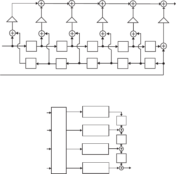
.]5[]4[]3[]2[]1[]0[)()( 54321
01 −
−
−
−
−
−+−+−=−= zhzhzhzhzhhzHzH A
realization of and in the form of Figure P14.1 using 6 multipliers is
shown below:
)(
0zH )(
1zH
y[n]
h[4]
z–1 z–1 z–1 z–1
h[3]
h[2]h[1] h[5]
z–1
h[0]
x [n]
0
x
[n]
1
z–1 z–1 z–1 z–1 z–1
14.6 (a) The structure of Figure P14.2(a) with internal variables labeled is shown below:
z
_1
z
_1
z
_1
D
3
R (z )
4
2
R (z )
4
R (z )
4
0
R (z )
4
1
Y(z)
X (z)
0
X (z)
1
X
(z)
2
X (z)
3
V (z)
0
V (z)
1
V (z)
2
V (z)
3
Analyzing the above structure we arrive at
and
,
)(
)(
)(
)(
)(
)(
)(
)(
⎥
⎥
⎥
⎦
⎤
⎢
⎢
⎢
⎣
⎡
⎥
⎥
⎥
⎦
⎤
⎢
⎢
⎢
⎣
⎡
−− −− −−
=
⎥
⎥
⎥
⎦
⎤
⎢
⎢
⎢
⎣
⎡
zX
zX
zX
zX
jj
jj
zV
zV
zV
zV
3
2
1
0
3
2
1
0
11
1111
11
1111
).()()()()()()()()( zVzRzzVzRzzVzRzzVzRzY 0
4
0
3
1
4
1
2
2
4
2
1
3
4
3−
−
−
+++=
The first equation leads to
),()()()()( zXzXzXzXzV 32100
+
++= ),()()()()( zjXzXzjXzXzV 32101 +−
−
=
),()()()()( zXzXzXzXzV 32102
−
+−= ).()()()()( zjXzXzjXzXzV 32104 −−
+
=
Substituting these 4 equations in the equation for and solving for the transfer
functions
)(zY
,),(/)()( 30
≤
≤
=izXzYzG ii we arrive at
),()()()()( 4
0
34
1
24
2
14
30 zRzzRzzRzzRzG
−
−
−+++=
),()()()()( 4
0
34
1
24
2
14
31 zRzzRjzzRzzjRzG
−
−
−+−−=
),()()()()( 4
0
34
1
24
2
14
32 zRzzRzzRzzRzG
−
−
−+−+−=
).()()()()( 4
0
34
1
24
2
14
33 zRzzRjzzRzzjRzG
−
−
−++−−=
Not for sale 539
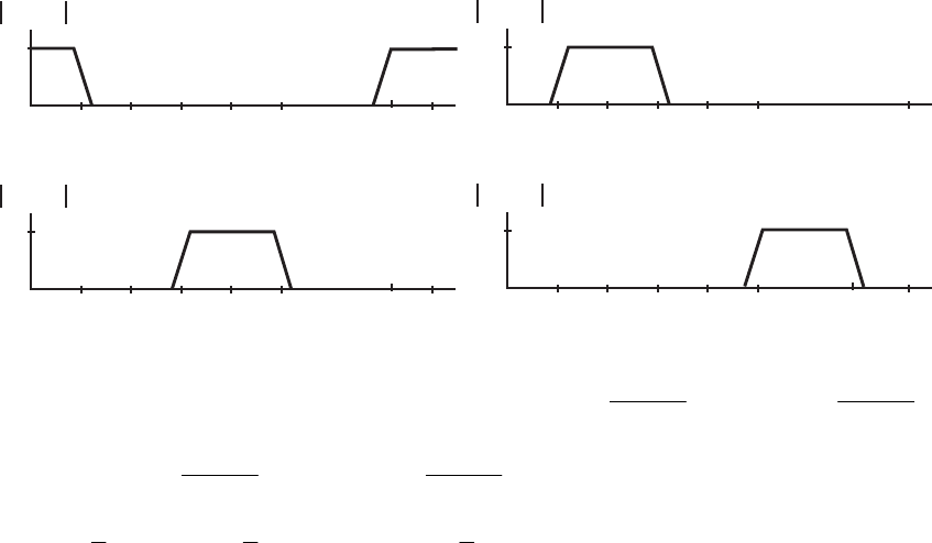
Substituting the expressions for ,),( 30
≤
≤
izRi we finally arrive at
987654321
080137390305142
−
−
−
−
−
−
−
−− −++−+−+++= zzzzzzzzzzG ......)(
,.. 1110 7132 −− ++ zz
87654321
142 1373903051
−
−
−
−
−
−
−+++−−+ zjzzjzzjzz .....
−−−= jzjzG )(
,... 11109 713280
−
−− +−+ zzjz
87654321
2137390305142 −−
−
−
−
−
−− −+++++−+−= zzzzzzzzzG .....)(
,... 11109 713280 −−− +−− zzz
87654321
342 1373903051
−
−
−
−
−
−
−− ++−−= zzjzjzG )(
.... 11109 713280
−+−−+ zjzzjzzj .....
−
−− +++ zzjz
(b) The magnitude responses of all 4 analysis filters are shown below:
G
0
(ejω)
0
1
ω
2π
π
π
4
_
3π
4
__
G
1
(ejω)
0
1
ω
2π
π
π
4
_
3π
4
__
7π
4
_
G
2
(ejω)
0
1
ω
2π
π
π
4
_
3π
4
__
G
3
(ejω)
0
1
ω
2π
π
π
4
_
3π
4
__
7π
4
_
7π
4
_
5π
4
_
14.7 Now, ).()()()()()( ][ zXzGzHzGzHzY 1100 += 2
1
)(
1
0
−
+
=z
zH and .
2
1
)(
1
1
−
−
=z
zH
Choose 2
1
)(
1
0
−
+
=z
zG and .
2
1
)(
1
1
−
−
−= z
zG Then,
)()2121()()1()1()( 2121
4
1
21
4
1
21
4
1zXzzzzzXzzzY −−−−−− −+−++=
⎟
⎠
⎞
⎜
⎝
⎛−−+=
).(
1zXz −
= Or in other words, ]1[][
−
=
nxny indicating that the structure of Figure
P14.3 is a perfect reconstruction system with the above choices of filters.
14.8 (a) Since and are power-complementary, )(
0zH )(
1zH
.1)()()()( 1
11
1
00 =+
−
−zHzHzHzH Now,
()
)()()()()()( 1100 zXzGzHzGzHzY +=
(
)
).()()()()()( 1
11
1
00 zXzzXzHzHzHzHz NN
−
−
−− =+= Or in other words,
][][
N
n
x
ny −= indicating that the structure of Figure P14.3 is a perfect reconstruction
system with the above choices of filters.
Not for sale 540

(b) If and are causal FIR transfer functions of order N each,
and are polynomials in
)(
0zH )(
1zH )(
0zH
)(
1zH .
1
−
z As a result, )( 1
0
−
zH and are
polynomials in z with the highest power being Hence,
)( 1
1−
zH
.
N
z)( 1
0−
−
zHz N and
are polynomials in
)( 1
1−− zHz N,
1
−
z making the synthesis filters and
causal FIR transfer functions of order N each.
)(
0zG )(
1zG
(c) From Figure P14.3, for perfect reconstruction we require
.)()()()( 1100 N
zzGzHzGzH
−
=+ From Part (a) we note that the perfect
reconstruction condition is satisfied with )()( 1
00
−
−
=zHzzG N and
if
),()( 1
11 −−
=zHzzG N,1)()()()( 1
11
1
00 =+
−
−
zHzHzHzH i.e., if and
are power-complementary. The last condition is satisfied if and only
if
)(
0zH
)(
1zH
)(
2
)(
2/
0oo nn
N
zz
z
zH += −
−
and ).(
2
)(
2/
1oo nn
N
zz
z
zH −= −
−
As a result,
and are also of the form
)(
0zG )(
1zG )(
2
)(
2/
0oo nn
N
zz
z
zG += −
−
and
).(
2
)(
2/
1oo nn
N
zz
z
zG −= −
−
14.9 (a) )..)(.(
)(.
)( 211
31
35540418901158401
109850
−−−
−
+−−
+
=
zzz
z
zG
.
.
.
..
.. ][ 1
1
21
21
158401
15840
35540418901
4189035540
2
1
−
−
−−
−−
−
+−
+
+−
+−
=
z
z
zz
zz Hence,
21
21
035540418901
4189035540
−−
−−
+−
+−
=
zz
zz
z
..
..
)(A and .
.
.
)( 1
1
1158401
15840
−
−
−
+−
=
z
z
zA
(b) can be realized with only 3 multipliers as a parallel connection of two
allpass filters in the form of Figure 8.43, where the allpass filter is realized
using any one of the Type 2 or Type 3 second-order allpass structures requiring 2
multipliers and the allpass filter is realized using any one of the Type 1
first-order allpass structures requiring 1 multiplier.
)(zG
)(z
0
A
)(z
1
A
(c) .
)..)(.(
)(.
)()()( ][ 211
31
10
2
1
35540418901158401
125640
−−−
−
+−−
−
=−=
zzz
z
zzzH AA
(d) A plot of the magnitude responses of and is shown on top of the
next page:
)(zG )(zH
Not for sale 541
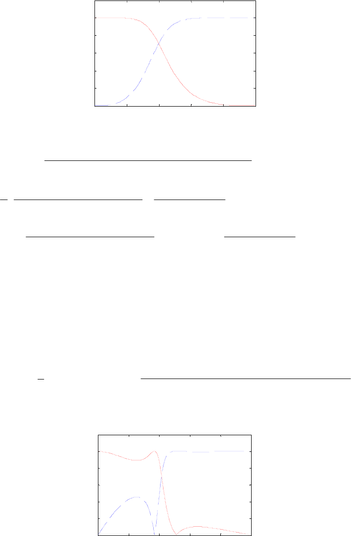
00.2 0.4 0.6 0.8 1
0
0.2
0.4
0.6
0.8
1
ω
/
π
Magnitude
|G(e
jω
)| |H(e
jω
)|
14.10 (a) )..)(.(
)..(.
)( 211
321
73630511101362801
0902109021118680
−−−
−−−
+−−
+++
=
zzz
zzz
zG
.
.
.
..
.. ][ 1
1
21
21
362801
36280
73630511101
5111073630
2
1
−
−
−−
−−
−
+−
+
+−
+−
=
z
z
zz
zz Hence,
21
21
073630511101
5111073630
−−
−−
+−
+−
=
zz
zz
z
..
..
)(A and .
.
.
)( 1
1
1362801
36280
−
−
−
+−
=
z
z
zA
(b) can be realized with only 3 multipliers as a parallel connection of two
allpass filters in the form of Figure 8.43, where the allpass filter is realized
using any one of the Type 2 or Type 3 second-order allpass structures requiring 2
multipliers and the allpass filter is realized using any one of the Type 1
first-order allpass structures requiring 1 multiplier.
)(zG
)(z
0
A
)(z
1
A
(c) .
)..)(.(
)..(.
)()()( ][ 211
321
10
2
1
73630511101362801
7866178661154950
−−−
−−−
+−−
+−−
=−=
zzz
zzz
zzzH AA
(d) A plot of the magnitude responses of and is shown below:
)(zG )(zH
00.2 0.4 0.6 0.8 1
0
0.2
0.4
0.6
0.8
1
ω
/
π
Magnitude
|G(e
jω
)| |H(e
jω
)|
14.11 An N-th order, with N odd, elliptic lowpass transfer function satisfies the
condition
)(zH
Not for sale 542

,
)()(
)()( 12
1
1
1
−
−
ε+
=
zRzR
zHzH
NN
(A)
where is a rational function of the form )(zRN
.
))((
))((
)( ∏
−
=ξ−
−
ξ
−
φ−
−
φ
−
−
−
−−
−−
⎟
⎟
⎠
⎞
⎜
⎜
⎝
⎛
−
−
=
2
1
0
11
11
1
1
11
11
1
1
N
jj
jj
Nezez
ezez
z
z
zR
l
ll
ll
(B)
In the above equation, the frequencies l
ξ
are the transmission zeros at which
is equal to 0, i.e., and the frequencies )( ωj
eH ,)( 0=
ξl
j
eH l
φ
are the reflection
zeros at which )( ωj
eH is equal to the maximum value of 1, i.e., .)( 1=
φl
j
eH
From Eq. (B) it follows that
(C)
).()( 1−
−= zRzR NN
Now, as satisfies the power-symmetric condition, we have
i.e.,
)(zH
,)()()()( 1
11 =−−+ −− zHzHzHzH
(D)
).()()()( 11 1−− −−−= zHzHzHzH
From the above equation it follows that the transmission zeros of are at
frequencies and its reflection zeros are at
)( zH −
l
φ−π .
l
ξ
−
π
As a result, .
π
=
ξ+φ ll
Hence, it follows that ),(/)( zRzR NN 1
=
−
or equivalently,
.)()( 1
=
−
zRzR NN (E)
From Eq. (A) we have ,
)()(
)()( 12
1
1
1
−
−
−−ε+
=−−
zRzR
zHzH
NN
which when
substituted in Eq. (D) yields
.
)()(
)()(
)()(
12
12
1
1
1
1
1
1
1
−
−
−
−−ε
+
=
−−ε+
−=
zRzR
zRzR
zHzH
NN
NN
In view of
Eq. (E), the above equation reduces to
.
)()(
)()(
1
2
1
1
1
1
−
−
ε
+
=
zRzR
zHzH
NN
(F)
Comparing Eqs. (A) and (F) we thus conclude that and hence,
,1
2=ε
.
)()(
)()( 1
1
1
1
−
−
+
=
zRzR
zHzH
NN
Now at a pole
λ
=
z of
From this relation, and Eqs. (C) and (E), it follows then that
),(zH
.)()( 1
1−=λλ −
NN RR
.
)(
)( 1=
λ−
λ
N
N
R
R Also, for a lowpass power-symmetric transfer function, 2/π>ξl
Not for sale 543

and Consequently, the poles of the rational function
must lie on the left half of the z-plane.
./2π<φl)(/)( zRzR NN −
Since, the magnitude of the rational function )(/)( zRzR NN
−
on the imaginary
axis is 1, using maximum-modulus theorem it can be shown that
1<− )(/)( zRzR NN for In a similar manner by replacing with it
can be shown that
.Re 0>zz,z−
1<− )(/)( zRzR NN for or, equivalently,
,Re 0>z
1>− )(/)( zRzR NN for .Re 0
<
z Thus,
⎪
⎩
⎪
⎨
⎧
<>
==
><
−,Re,
,Re,
,Re,
)(
)(
01
01
01
z
z
z
zR
zR
N
N
or, in other words, all poles of lie on the imaginary axis of the z-plane.
)(zH
14.12 Now the magnitude-square function of an N-th order analog lowpass Butterworth
function is given by
)(sGa,
)/(
)( N
c
ajG 2
2
1
1
ΩΩ
Ω+
= where is the 3-dB
cutoff angular frequency. For
c
Ω
,1
=
c
Ωthen .)( N
ajG 2
2
1
1
Ω
Ω
+
= The
corresponding transfer function of of an N-th order analog highpass Butterworth
function is simply whose the magnitude-square function is given by
),/( sGa1
.
N
N
aj
G2
2
2
1
1
Ω
Ω
Ω+
=
⎟
⎟
⎠
⎞
⎜
⎜
⎝
⎛ As a result,
.)( 1
11
1
2
2
2
2
1
2=
+
+
+
=
⎟
⎠
⎞
⎜
⎝
⎛
+N
N
N
j
aa GjG
Ω
Ω
Ω
Ω
Ω Now the bilinear transformation
maps the analog angular frequency Ω to the digital angular frequency ω through the
relation .
1
1
Ω
Ω
j
j
ej
+
−
=
ω As ,
)/1(1
)/1(1
Ω
Ω
j
j
ej
+
−
=− ω the analog angular frequency 1/Ω is
mapped to the digital angular frequency .ω
π
+
Hence, the relation
,)( 1
2
1
2=
⎟
⎠
⎞
⎜
⎝
⎛
+Ω
Ω
j
aa GjG becomes =+ +2
)(
0
2
0)()( ωπω jj eHeH
,1)()()()( 2
1
2
0
2
0
2
0=+=−+ ωωωω jjjj eHeHeHeH where is the
frequency response of the digital lowpass filter obtained by applying the bilinear
transformation to and is the frequency response of the digital highpass
filter obtained by applying the bilinear transformation to Note that a
digital transfer function satisfying the condition
)(
0ωj
eH
)(
0zH
)(sGa)(
1ωj
eH
)(
0zH )./( sGa1
,1)()( 2
1
2
0=+ ωω jj eHeH is called
power-symmetric.
Not for sale 544

Moreover, from the relation it follows that the analog 3-dB cutoff angular frequency
is mapped into the digital 3-dB cutoff angular frequency Hence,
is a digital half-band lowpass filter.
1=
c
Ω.2/πω =
c
)(
0zH
Let ,
)(
)(
)(
0
0
0zD
zP
zH = where and are polynomials in Hence, )(
0zP )(
0zD .
1−
z
)(
)(
)(
0
0
0ω
ω
ω
j
j
j
eD
eP
eH = and .
)(
)(
)(
0
0
0ω
ω
ω
j
j
j
eD
eP
eH −
−
=− Now,
)()(
)()(
1)(1
)()(
)()(
)( *
00
*
00
2
0
*
00
*
00
2
0ωω
ωω
ω
ωω
ωω
ω
jj
jj
j
jj
jj
j
eDeD
ePeP
eH
eDeD
ePeP
eH −=−=
−−
−−
=−
.
)()(
)()()()(
*
00
*
00
*
00
ωω
ωωωω
jj
jjjj
eDeD
ePePeDeD −
= Note that there are no common factors between
and , and between and As a result, there are no
common factors between and This implies
then Consequently, or
Hence, Since
)(
0ωj
eP )(
0ωj
eD )(
*
0ωj
eP ).(
*
0ωj
eD
)()( *
00 ωω jj ePeP −− ).()( *
00 ωω jj eDeD −−
).()()()( *
00
*
00 ωωωω jjjj eDeDeDeD −−= ),()( 00 ωω jj eDeD −=
).()( 2
00 ωω jj edeD =).()( 2
00 zdzD =,
)(
)(
)(
)(
)( 2
0
0
0
0
0zd
zP
zD
zP
zH == it
follows then .
)(
)(
)( 2
0
0
1zd
zP
zH −
= We have shown earlier that and are power-
complementary. Also, is a symmetric polynomial of odd order and is an
anti-symmetric polynomial of odd order. As a result, we can express
)(
0zH )(
1zH
)(
0zP )(
1zP
][ )()()( 10
2
1
0zAzAzH += and ,)()()( ][ 10
2
1
1zAzAzH −= where and are
stable allpass functions for stable and But, Hence,
)(
0zA )(
1zA
)(
0zH ).(
1zH ).()( 01 zHzH −=
.)()()( ][ 10
2
1
0zAzAzH −−−= It therefore follows that and
Thus,
),()()( 2
000 zzAzA A=−=
).()()( 2
1
1
11 zzzAzA A
−
=−−= .)()()( ][ 2
1
12
0
2
1
0zzzzH AA −
+=
14.13 From Eq. (14.18), ).()()()()( zXzAzXzTzY
−
+
= Let ],[)}({
1ntzT =
−
Z and
Then, an inverse z-transform of Eq. (14.18) yields
Define and
].[)}({
1nazA =
−
Z
].[][)1(][][)1(][][][][ )( lllllll
l
ll
ll
−−+=−−+−= ∑∑∑ ∞
−∞=
−−
∞
−∞=
∞
−∞=
nxatnxanxtny nn
][)1(][][
0nantnf n−
−+= ].[)1(][][
1nantnf n
−
−−= Then we can write
Not for sale 545

⎪
⎩
⎪
⎨
⎧
−
−
=∑
∑∞
−∞=
∞
−∞=
.oddfor],[][
,evenfor],[][
][
nnxf
nnxf
ny
l
l
ll
ll
1
0 The corresponding equivalent
realization of the 2-channel QMF bank is therefore as indicated below:
x
[n]y[n]
f [n]
0
f [n]
1
n even
n odd
As can be seen from the above representation, the QMF bank is, in general, a time-
varying system with a period 2. Note that ,)( 0
=
zA if then it becomes a linear,
time-invariant system.
14.14 .
))((
)( 11
1
2+++
=sss
sGa The digital transfer function obtained by a
bilinear transformation is given by
)(zH0
])()())[((
)(
)()( 222
3
1
1
011111
1
++−+−++−
+
==
+
−
=zzzzz
z
sGzH
z
z
s
a )(
)(
132
1
2
3
+
+
=zz
z
,)()(
)( ][ 2
1
12
0
1
2
2
2
321
2
31
2
1
3
31
2
1
26
331
26
1zzzz
z
z
z
zzz
z
zAA −−
−
−
−
−−−
−
−+=
⎟
⎟
⎠
⎞
⎜
⎜
⎝
⎛+
+
+
=
+
+++
=
+
+
=
where 1
1
03
31
−
−
+
+
=z
z
z)(A and .)( 1
1
=
zA
The corresponding power-complementary transfer function is given by
.
)(
)()()( ][ 2
31
1
2
2
2
1
12
01 26
1
3
31
2
1
2
1
−
−
−
−
−
−
+
−
=
⎟
⎟
⎠
⎞
⎜
⎜
⎝
⎛−
+
+
=−= z
z
z
z
z
zzzzH AA
A realization of the analysis part of the QMF bank is as shown in Figure 14.11
where the first-order allpass transfer function is realized using any one of
the single-multiplier structure of Figure 8.24 and the zero-th order allpass transfer
function is replaced with a direct connection between the input and the
output.
)(z
0
A
)(z
1
A
14.15 .
....
)( 123613236152361523613
1
2345 +++++
=sssss
sGa The digital
transfer function obtained by a bilinear transformation is given by
)(zH0
42
51
42
51
005570633401
105280
0557112944318
1
−−
−
−−
−
++
+
=
++
+
=zz
z
zz
z
zH ..
)(.
..
)(
)(
Not for sale 546

42
531
42
42
05570633401
052805279026390
05570633401
263905279005280
−−
−−−
−−
−−
++
++++
+
++
++
=zz
zzz
zz
zz
..
...
..
...
2
2
1
2
2
527801
89481126390
105601
47049105280
−
−
−
−
−
+
+
+
+
+
=z
z
z
z
z
.
).(.
.
).(.
],[ )()( 2
1
12
0
2
1zzz AA −
+= where 1
1
0105601
10560
−
−
+
+
=z
z
z.
.
)(
A and
.
.
.
)( 1
1
1527801
52780
−
−
+
+
=z
z
zA
Its power-complementary transfer function is given by
][ )()()( 2
1
12
0
2
1
1zzzzH AA −
−= ].[ .
.
.
.
2
2
1
2
2
527801
52780
105601
10560
2
1
−
−
−
−
−
+
+
−
+
+
=z
z
z
z
z
In the realization of a magnitude-preserving QMF bank as shown in Figure 14.11,
the realization of the allpass filters and require 1 multiplier each,
and hence, the realization of the analysis (and the synthesis) filter bank requires a
total of 2 multipliers.
)(z
0
A)(z
1
A
14.16 (a) Total number of multipliers required is ).( 124
−
N Hence, the total number of
multiplications per second is equal to ,/)()( TNFN
T
124124
−
=
−
where
TF
T
/1= is the sampling frequency in Hz.
(b) In Figure 14.11, ][ )()()( 2
1
12
0
2
1
0zzzzH AA −
+= and
].[ )()()( 2
1
12
0
2
1
1zzzzH AA −
−= If the order of is K and the order of
is L, then the order of is
)(z
0
A
)(z
1
A)(zH0.NLK
=
+
+
122 Hence,
The total number of multipliers needed to implement is K,
while the total number of multipliers needed to implement is L. Hence, the total
number of multipliers required to implement the QMF bank of Figure 14.11 is
However, the multipliers here are operating t half of the
sampling rate of the input As a result, the total number of multiplications per
second in this case is .
./)( 21−=+ NLK
.)( 12 −=+ NLK
].[nx
/)(/)( TNFN
T
2121
−
=
−
14.17 The 4 filters of the 2-channel QMF bank are: ,)(,4)( 1
1
2
0−
−
== zzHzzH
.)(,25.0)( 1
1
1
0
−
−== zzGzzG Substituting these transfer functions in Eq. (14.21)
we get 2112
1100 25.04)()()()(
−
−
−
−
×−×=−+− zzzzzGzHzGzH
implying aliasing cancellation condition holds. Next, substituting
the transfer functions in Eq. (14.27) we get
,0
33 =−= −− zz
Not for sale 547
.225.04)()()()( 32112
1100
−
−
−
−
−
=×+×=+ zzzzzzGzHzGzH Hence, it is a
perfect reconstruction QMF bank.
14.18 The aliasing cancellation condition is satisfied if the synthesis filters satisfy Eq.
(14.37). Hence, we choose ,)()( 4321
01 −−
−
−
+−+−=−= zhzgzfzedzGzH
and .)()()( 2121
01
−
−
−
−
−−−=+−−=−−= czbzaczbzazHzG
14.19 The 4 filters satisfy the aliasing cancellation condition of Eq. (14.21) and the
perfect reconstruction condition of Eq. (14.27). Interchanging and
and interchanging and in Eq. (14.21) we arrive at the new aliasing
term
)(
0zH ),(
0zG
)(
1zH )(
1zG
).()()()()( 1100 zHzGzHzGzA
−
+−= Hence,
,0)()()()()( 1100
=
−
+−=− zHzGzHzGzA implying that the aliasing condition is
still satisfied after interchanging the analysis and synthesis filters. It also follows
from Eq. (14.27), an interchange of the analysis and synthesis filters does not
change the expression for the distortion transfer function and as a result the perfect
reconstruction condition is still satisfied.
14.20 From Eq, (14.73), it can be seen that the normalized product filter is of odd
length Let the degrees of and be and
)(zP
.12 +L)(zH0)(zG0N,
K
respectively.
Hence, it follows from Eq. (14.76), .LKN 2
=
+
Therefore, either and
N
K
are
both even or both odd. As a result, and cannot be of even and odd
lengths, respectively.
)(zH0)(zG0
Moreover, is a symmetric polynomial. If is a symmetric polynomial
and is an antisymmetric polynomial, their product cannot be a symmetric
polynomial.
)(zP )(zH0
)(zG0
14.21 )()1()1()( 212331
−
−
−++++++= azbzcbzazzzzP
45 )6( zbaaz ++=
)203012()152616()61620()615( 23 cbazcbazcbazcba ++++++++++++
321 )615()61620()152616(
−
−
−+++++++++ zcbazcbazcba .)6( 54
−
−
+++ azzba
Since the even powers of must be zeros and the coefficient of be equal to
1, we must have
)(zP 0
z
,061620,06
=
+
+
=+ cbaba and .1203012 =
+
+
cba Solving
these 3 equations we arrive at .1484375.0,0703125.0,01171875.0 =
−
=
=
cba
Hence,
1484375.00703125.01171875.0()1()1()( 2331 +−++= −zzzzzP
)4438.94255.51()1(1171875.0)1171875.00703125.0 2161521
−
−
−
−+−+=+− zzzzzz
)1059.05745.01( 21
−
−+−× zz .
One possible factorization of is given by
)(zP
Not for sale 548
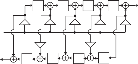
),1059.05745.01)(4438.94255.51)(1(01171875.0)( 21211
0
−
−
−
−
−+−+−+= zzzzzzH
and Thus, the highpass analysis filter is given by
.)1()( 51
0−
+= zzG
.)1()()( 51
01 −
−=−= zzGzH
14.22 Without any loss of generality, let N = 4. Let
Then,
A realization of the analysis filter
bank using multipliers and
.][][][][][)( 4321
043210 −−−− ++++= zhzhzhzhhzH
)( ][][][][][)()( 43241
0
4
143210 zhzhzhzhhzzHzzH +−+−=−= −−−
.][][][][][ 4321 01234 −−−− +−+−= zhzhzhzhh
51 =+N82
=
N two-input adders is shown on top of
the next page:
x[n]
h[4]
z–1 z–1 z–1
h[3] h[2] h[1]
z–1
h[0]
1
_
y [n]
0
y
[n]
1
z–1 z–1 z–1
z–1
1
_
14.23 For an orthogonal filter bank, the two analysis filters
∑
=
−
=N
n
n
znhzH 000 ][)(
and are causal FIR filters satisfy the power
complementary property, i.e., where
We assume and
∑=
−
=N
n
n
znhzH 011 ][)(
,)()()()( γ=+ −− 1
11
1
00 zHzHzHzH .0>γ
00
0≠][h.][ 00
1
≠
h It follows from Section 7.3 that a linear-
phase FIR filter has either a symmetric or an anti-symmetric impulse response. As
a result, if and are linear-phase transfer functions, then they are of
)(zH 0)(zH1
the form and
)()( 1
00 0−−
β−
=zHzezH N
j).()( 1
11 0−−
β−
=zHzezH N
j
Substituting the expressions for and in the power-
complementary condition we arrive at which
can be rewritten as
. Both
quantities inside the square brackets are causal FIR transfer functions. Hence, we
have
)( 1
0−
zH )(1
1−
zH
,)()( γ=+ β
βzHzezHze N
j
N
j2
1
2
01
0
/
/
/
/][][ )()()()( N
j
j
j
jzzHjezHezHjezHe −
β
β
β
βγ=−+ 1
2
0
2
1
2
0
21
0
1
0
(G)
,)()( /
/0
1
001
2
0
2N
j
jzzHjezHe −
β
βα=+
and
(H)
,)()( /
/11
011
2
0
2Nj
jzzHjezHe −β
βα=−
Not for sale 549
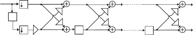
where
γ
=αα 10 and .NNN
=
+10 Adding Eq. (H) from Eq. (G) we get
and
Hence, as the analysis filters have
transfer functions that are weighted sum of two delays, they can not be used to
design filters with any practical frequency response specifications.
)()( /1
00 10
2
0N
Nj zzezH −
−β− α+α=
).()( /1
0
110
2
1N
N
jzzjezH −
−
β− α−α−=
14.24 From Eq. (14.90) we have )()()( 3231
1
3
0dzczbzazzHzzH −+−−=−−=
−
−
−
Next, from Eq. (14.92) we get
.
321 −−− −+−= azbzczd
3213231
0
3
0)()()( −−
−
−−− +−+−=−+−== dzczbzaazbzczdzzHzzG and
.)()()( 3213231
1
3
1−
−
−
−−− +++=+++== azbzczddzczbzazzHzzG
14.25 Substituting the transfer functions in Eq. (14.21) we get
)25.1)(21()5.0)(43()()()()( 1111
1100 −
−
−
−
−−++−−=−+− zzzzzGzHzGzH
0)455.1()455.1( 2121 =+−+−+−=
−
−
−− zzzz implying that the aliasing
cancellation condition is satisfied. Next, substituting the transfer functions in Eq.
(14.27) we get
)25.1)(21()5.0)(43()()()()( 1
1100 111 −
−
−
−
−++ zz+−+=+ zzzGzHzGzH
12121 2)45.1()45.1(
−
−
−
−− =−++++−= zzzzz implying that the perfect
reconstruction condition is satisfied.
14.26 From Eq. (14.90) we get
From Eq. (14.92), we arrive at
and
.)( 54321
0−−−−− +++++= fzezdzczbzazH
)()()( 543251
0
5
1fzezdzczbzazzHzzH −+−+−=−= −−−
.
54321 −−−−− +−+−+−= azbzczdzezf
543211
0
5
0−−−−−−− +++++== azbzczdzezfzHzzG )()(
.)()( 543211
1
5
1−−−−−−− −+−+−== fzezdzczbzazHzzG
14.27 To develop the realization of the synthesis filter bank we redraw Figure P14.4 as
shown below:
_
z1
_
z1
_
__
3
kN
k
N
k
k1
k13
k
2
_1
2z1
_
The i-th stage of the above analysis filter bank is of the form shown below:
Not for sale 550
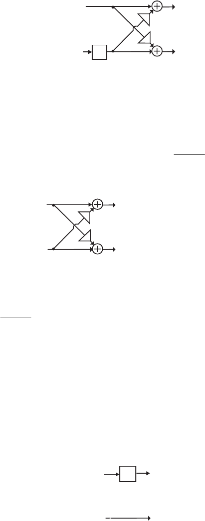
z
1
_
_
k
i
k
i
Y (z)
(i)
0
Y (z)
(i)
1
V (z)
(i)
0
V (z)
(i)
1
X (z)
(i)
0
X
(z)
(i)
1
The input-output relation of the lattice part of the above figure is given by
which can be solved for the input variables
leading to
⎥
⎥
⎦
⎤
⎢
⎢
⎣
⎡
⎥
⎦
⎤
⎢
⎣
⎡−
=
⎥
⎥
⎦
⎤
⎢
⎢
⎣
⎡
)(
)(
)(
)(
)(
)(
)(
)(
zV
zV
k
k
zY
zY
i
i
i
i
i
i
1
0
1
0
1
1
,
)(
)(
)(
)(
)(
)(
)(
)(
)(
)(
)(
)(
⎥
⎥
⎦
⎤
⎢
⎢
⎣
⎡
⎥
⎦
⎤
⎢
⎣
⎡−
+
=
⎥
⎥
⎦
⎤
⎢
⎢
⎣
⎡
⎥
⎦
⎤
⎢
⎣
⎡−
=
⎥
⎥
⎦
⎤
⎢
⎢
⎣
⎡−
zY
zY
k
k
k
zY
zY
k
k
zU
zU
i
i
i
i
i
i
i
i
i
i
i
1
0
2
1
0
1
1
0
1
1
1
1
1
1 a
realization of which is indicated below:
Y (z)
(i)
0
Y (z)
(i)
1
U (z)
(i)
0
U (z)
(i)
1
ii
k /(1+k )
2
i
s =
s
i
_
s
i
where A cascade of the above two lattice structures thus has an
input-output relation given by
)./( 2
1iii kks +=
.
)(
)(
)(
)(
)(
)(
)(
)(
)(
)(
)(
)(
⎥
⎥
⎦
⎤
⎢
⎢
⎣
⎡
⎥
⎦
⎤
⎢
⎣
⎡
=
⎥
⎥
⎦
⎤
⎢
⎢
⎣
⎡
⎥
⎦
⎤
⎢
⎣
⎡−
⎥
⎦
⎤
⎢
⎣
⎡−
+
=
⎥
⎥
⎦
⎤
⎢
⎢
⎣
⎡
zV
zV
zV
zV
k
k
k
k
k
zU
zU
i
i
i
i
i
i
i
i
i
i
i
1
0
1
0
2
1
010
01
1
1
1
1
1
1
Likewise, the input-output relation of the delay part of the i-th stage of the analysis
filter bank is given by which can be solved for the
input variables leading to a realization of which is
indicated below:
⎥
⎥
⎦
⎤
⎢
⎢
⎣
⎡
⎥
⎦
⎤
⎢
⎣
⎡
=
⎥
⎥
⎦
⎤
⎢
⎢
⎣
⎡
−)(
)(
)(
)(
)(
)(
)(
)(
zX
zX
z
zV
zV
i
i
i
i
1
0
1
1
0
0
01
,
)(
)(
)(
)(
)(
)(
)(
)(
⎥
⎥
⎦
⎤
⎢
⎢
⎣
⎡
⎥
⎦
⎤
⎢
⎣
⎡
=
⎥
⎥
⎦
⎤
⎢
⎢
⎣
⎡−
zV
zV
z
zW
zW
i
i
i
i
1
0
1
1
0
10
0
W (z)
(i)
0
W (z)
(i)
1
V (z)
(i)
0
V (z)
(i)
1
z
_1
Hence, the cascaded-lattice realization of the synthesis filter bank of the two-
channel orthogonal filter bank is as shown below where : )./( 2
1iii kks +=
Not for sale 551
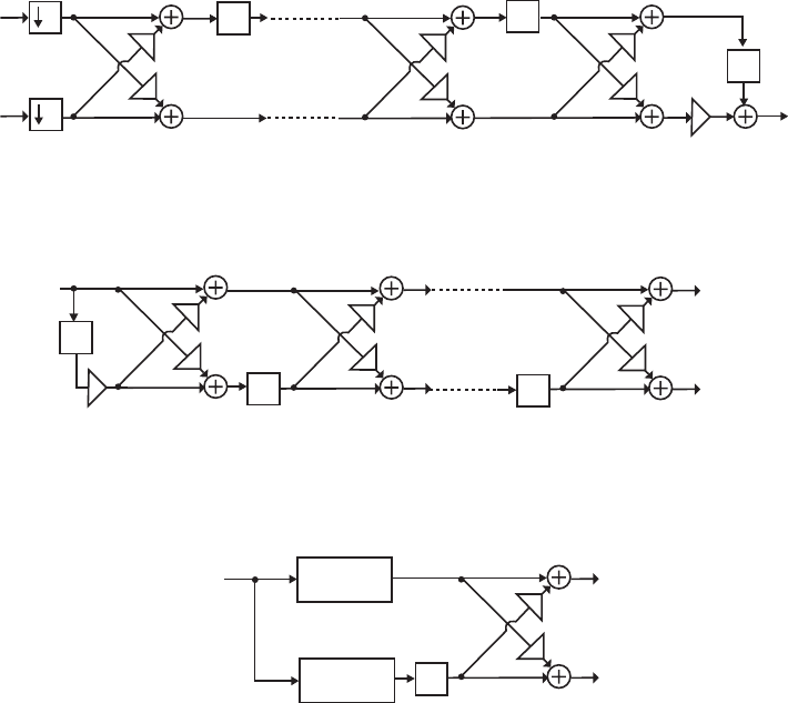
z
1
_
N
s
_
N
s
2
2
z
2
_
_
1
z
2
_
3
s
1
s
3
s
__1
s
14.28 Figure P14.4 with the down-samplers removed and internal variables labeled is
shown below:
_
z
2
_
z
1
_
z
2
_
__
3
k
N
k
N
k
k
1
k
13
k
_
1
X
(z)Y (z)
0
(N)
Y (z)
1
(N)
Y (z)
0
(N 2)
_
Y (z)
1
(N 2)
_
Denoting the transfer functions and
we arrive at an equivalent representation of the above analysis filter bank as indicated
below:
)(/)()( )()( zXzYzH rr
00 =),(/)()( )()( zXzYzH rr
11 =
z2
_
_
N
k
N
k
X
(z)H (z)
0
(N)
H (z)
1
(N)
H (z)
0
(N 2)
_
H (z)
1
(N 2)
_
Analysis yields and
Solving these two equations, we get
and
Choose such that the highest power of
in is eliminated. By construction, the next highest power of
also is removed reducing the order of to
)()()( )()()( zHzkzHzH N
N
NN 2
1
2
2
00
−
−
−+=
).()()( )()()( zHzzHkzH NN
N
N2
1
2
2
01
−
−
−+−=
)()()()( )()()( zHkzHzHk N
N
NN
N10
2
0
2
1−=+ −
).()()()( )()()( zHzHkzHzk NN
N
N
N10
2
1
22
1+=+ −
−N
k
1−
z)()( )()( zHkzH N
N
N
10 −1−
z
)(
)( zH N2
0
−.2
−
N Moreover, the coefficients of
and in are also zero for the above choice of , resulting in a
causal of order
0
z
1−
z)()( )()( zHzHk NN
N10 +N
k
)(
)( zH N2
1
−.2
−
N Continuing this process, we arrive at a cascaded lattice
realization of the analysis filter bank of an orthogonal QMF bank.
From Eq. (14.87) we have and
from Eq. (14.89a) we have
We now form
321
3
009150158505915034150 −−− −++= zzzzH ....)(
)(
321
3
134150591501585009150 −−− −+−−= zzzzH ....)(
)(
)()()()( )()()( zHkzHzHk 3
1
3
3
0
1
0
2
3
1−=+ )..( 3
0915034150 k+
=
1
3
1585059150 −
++ zk )..( 2
3
5915015850 −
−+ zk )..(.)..( 3
3
3415009150 −
+−+ zk
Not for sale 552
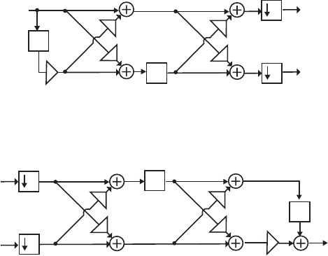
Choose .../. 267903415009150
3
=
=k Then
implying,
We next form or,
, implying,
Hence, A cascaded
lattice realization of the analysis filter bank is as shown below:
)()()(. )()()( zHkzHzH 3
1
3
3
0
1
0
07181 −=
,.. 1
63403660 −
+= z)..(...)(
)( 11
1
0732111341505915034150 −− +=+= zzzH
][ )()()()( )()()( zHzHkzHzk 3
1
3
0
3
1
1
22
3
1+=+ −
1
3
1
3
0
1
1
2366063402679007181 −− −=+= zzHzHzHz ..)()(.)(. ][ )()()(
)..(...)(
)( 11
1
173211341503415059150 −− −=−= zzzH ..73211
1=k
z
2
_
z
1
_
_
1
2
2
1.7321
_
1.7321
0.2679
_
0.2679
From the solution of Problem 14.27 we arrive at the structure of the synthesis filter
bank shown on the next page to ensure the realization of the orthogonal perfect
reconstruction QMF bank.
z
1
_
2
2
z
2
_
1
_
_
0.433
0.433
_
0.25
0.25
14.29 (a) Hence,
.)( 54321
0412221431 −−−−− +−+++= zzzzzzH
.)()( 543211
0
5
131422124 −−−−−−− −+−++=−−= zzzzzzHzzH
(b) To develop the cascade lattice realization of the analysis filter bank, we rewrite
the analysis transfer functions as and Next,
we determine using the relation
and choose so that the coefficient of is eliminated. Now,
We choose
)()(
)( zHzH 0
5
0=).()(
)( zHzH 1
5
1=
)(
)( zH 3
0)()()()( )()()( zHkzHzHk 5
1
5
5
0
3
0
2
5
1−=+
5
k5−
z
3
5
2
5
1
55
3
0
2
514222214123411 −−− ++−+−+−=+ zkzkzkkzHk )()()()()()( )(
.)()( 5
5
4
54312 −− ++−−+ zkzk .4
5
−
=
k Then
Note that as expected the above
choice of also cancels the coefficient of . We thus have,
Next we determine using the relation
which leads to
It should be noted that here,
=+ )()( )( zHk 3
0
2
5
1
.)(
)( 1
3
0102511717 −++== zzzH 32 34 −− −z
5
k4−
z
.)(
)( 321
3
02631 −−− −++= zzzzH )(
)( zH 3
1
)()()()( )()()( zHzHkzHzk 5
1
5
0
5
3
1
22
5
1+=+ −
.)(
)( 5432
3
1
217511023417 −−−−− −+−−= zzzzzHz
Not for sale 553
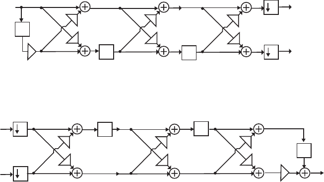
as expected, the choice of has resulted in zero-valued coefficients of and
Hence, It can be verified that the same
expression for is obtained from
5
k0
z
.
1−
z.)(
)( 321
3
1362 −−− −+−−= zzzzH
)(
)( zH 3
1).()( )()( 1
3
0
3
3
1
−− −−= zHzzH
Next, we determine using the relation
and choose
)(
)( zH 1
0
)()()()( )()()( zHkzHzHk 3
1
3
3
0
1
0
2
3
1−=+ 2
3
=
k so that the coefficient
of is eliminated. This results in and
Analysis of the structure of Figure P14.4 yields and
Hence,
3−
z1
1
031 −
+= zzH )(
)( .)(
)( 1
1
13−
−= zzH
1
1
1
01−
+= zkzH )(
)(
.)(
)( 1
1
1
1
−
−= zkzH .3
1
=
k The final realization of the analysis filter bank
is shown below:
_
z
2
_
z
1
_
z
2
_
_
_
_
1
3
3
2
24
4
2
2
From the solution of Problem 14.27 we arrive at the structure of the synthesis filter
bank shown below to ensure the realization of a paraunitary perfect reconstruction
QMF bank.
z1
_
2
2
z2
_z2
_
_
_
_3/10
3/10
2/5
2/5
4/17
4/17
1
_
14.30 (a) Hence,
.....)( 54321
052551351050 −−−−−
−−−−+= zzzzzzH
.....)()( 543211
0
5
150510513552 −−−−−
+
−− −−−−−=−−= zzzzzzHzzH
(b) To develop the cascade lattice realization of the analysis filter bank, we rewrite
the analysis transfer functions as and Next,
we determine using the relation
and choose so that the coefficient of is eliminated. Now,
We choose
)()(
)( zHzH 0
5
0=).()(
)( zHzH 1
5
1=
)(
)( zH 3
0)()()()( )()()( zHkzHzHk 5
1
5
5
0
3
0
2
5
1−=+
5
k5−
z
3
5
2
5
1
55
3
0
2
55105135135105152501 −−− +−+++−−++=+ zkzkzkkzHk )..()..()()..()()( )(
.)..()( 5
5
4
550525 −− +−++−+ zkzk .5
5
=
k Then
Note that as expected the above
choice of also cancels the coefficient of . We thus have,
=+ )()( )( zHk 3
0
2
5
1
.)(
)( 21
3
078261326 −− ++−== zzzH 3
39 −
z
5
k4−
z
Not for sale 554
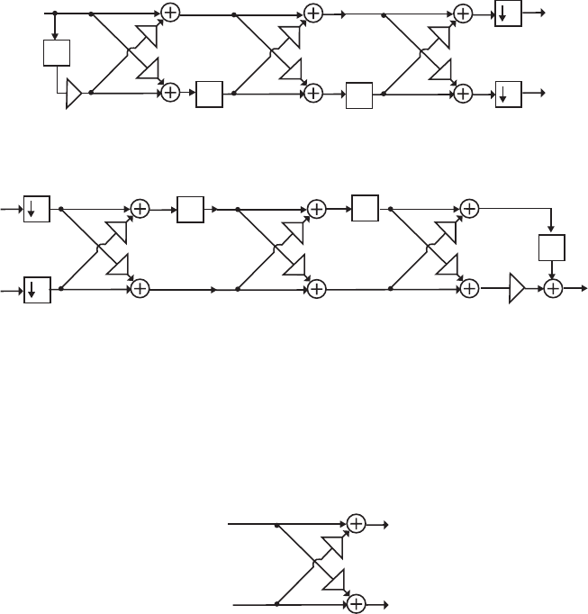
...)(
)( 321
3
051350 −−− ++−= zzzzH Next we determine using the
relation which leads to
It should be noted that here, as
expected, the choice of has resulted in zero-valued coefficients of and
Hence, It can be verified that the same
expression for is obtained from Next, we
determine using the relation and
choose so that the coefficient of is eliminated. This results in
and
Analysis of the structure of Figure P14.4 yields and
Hence,
)(
)( zH 3
1
)()()()( )()()( zHzHkzHzk 5
1
5
0
5
3
1
22
5
1+=+ −
.)(
)( 5432
3
1
21326783926 −−−−− −−−= zzzzzHz
5
k0
z.
1−
z
...)(
)( 321
3
150351 −−− −−−= zzzzH
)(
)( zH 3
1).()( )()( 1
3
0
3
3
1
−− −−= zHzzH
)(
)( zH 1
0)()()()( )()()( zHkzHzHk 3
1
3
3
0
1
0
2
3
1−=+
3
3−=k3−
z
)(..)(
)( 11
1
0215050 −− −=−= zzzH ).(..)(
)( 11
1
1250501 −− −−=−−= zzzH
1
1
1
01−
+= zkzH )(
)(
.)(
)( 1
1
1
1
−
−= zkzH .2
1
−
=
k The final realization of the analysis filter
bank is shown on top of next page:
z
2
_
z
1
_
z
2
_
_
_
1
_
3
3
_
2
2
5
5
2
2
From the solution of Problem 14.27 we arrive at the structure of the synthesis filter
bank shown below to ensure the realization of a paraunitary perfect reconstruction
QMF bank.
z1
_
2
2
z2
_z2
_
1
_
_3/10
3/10
_2/5
2/5
_5/26
5/26
14.31 (a) The input-output relation of the l–th two-pair is given by
from which we obtain
and
,
)(
)(
)(
)( ⎥
⎦
⎤
⎢
⎣
⎡
⎥
⎦
⎤
⎢
⎣
⎡
=
⎥
⎦
⎤
⎢
⎣
⎡
−
−−
zSz
zR
k
k
zS
zR
1
2
1
1
1
l
l
l
l
l
l
)]([)()( zSzkzRzR 1
2
1−
−
−+= llll )].([)()( zSzzRkzS 1
2
1−
−
−+= llll The
realization of the two-pair is thus as shown below:
l
R (z)
l
S (z)
R (z)
l
_1
l
k
l
k
S (z)
l
_1
_2
z
(b) The portion of Figure P14.5 upto the m-th stage is then as shown below:
Not for sale 555

P (z)
m
Q (z)
m
k
m
k
m
P (z)
m 1
_
Q (z)
m 1
_
z
_2
Analysis of the above structure yields and
)()()( zQzkzPzP mmmm 1
2
1−
−
−+=
).()()( zQzzPkzQ mmmm 1
2
1−
−
−+=
(c) Analysis of the structure of Figure P14.5 yields )()()( zQzPzH MM +
=
0
).()( )( 112
−
+−
+= zPzzP M
M
M Hence, ).()()( )( zPzzPzH M
M
M1211
0+
−
−
+=
Therefore, ).()()()( )()( zHzPzPzzHz MM
MM 0
1121
0
12 =+=
−
+
−
−+− Since the
order of is ) is a Type 2 linear-phase FIR transfer function.
)(zH0,12 +M(zH0
Similarly, analysis of the structure of Figure P14.5 yields )()()( zQzPzH
M
M
−
=
1
Hence,
).()( )( 112 −+−
−= zPzzP M
M
M).()()( )( zPzzPzH M
M
M1211
1+
−
−
−=
Therefore, ).()()()( )()( zHzPzPzzHz MM
MM 1
1121
1
12 −=−=
−
+
−
−+− Since the
order of is is a Type 4 linear-phase FIR transfer function.
)(zH1,12 +M)(zH1
(c) It follows from Figure P14.5 that
Γ
⎥
⎦
⎤
⎢
⎣
⎡
⎥
⎦
⎤
⎢
⎣
⎡
⎥
⎦
⎤
⎢
⎣
⎡
⎥
⎦
⎤
⎢
⎣
⎡
⎥
⎦
⎤
⎢
⎣
⎡
⎥
⎦
⎤
⎢
⎣
⎡−
=−− 1
1
0
01
1
1
0
01
1
1
11
11
0
0
1
1
1
1k
k
z
k
k
z
k
k
z
M
ML)(E
2
D=1
TT K
M
(z) Γ where and ΓWe
determine the synthesis bank for perfect reconstruction by choosing
,
0
T(z) ⎥
⎦
⎤
⎢
⎣
⎡−
=11
11
2
D.)( ⎥
⎦
⎤
⎢
⎣
⎡
=−1
0
01
z
z
== −− )()( zzz M1
ER α1
2
−
−D
M
zαΓ1
1
11
−
−
−
TT K
M
z)( Γ.)( 1
0
1
−
−
Tz The final
realization of the synthesis filter bank is shown below which satisfies the perfect
reconstruction condition within a scale factor.
z1
_
2
2
z2
_z2
_
_1
k
_
M
k
_
M
k
_1
k
_1
k
_0
k
_0
14.32 From Figure P14.5 we observe that )()()( zQzPzH MM
+
=
0 and
).()()( zQzPzH
M
M
−=
1 Solving these equations we get
)]()([)( zHzHzPM10
2
1+= and )].()([)( zHzHzQM10
2
1−= Next, from the
Not for sale 556
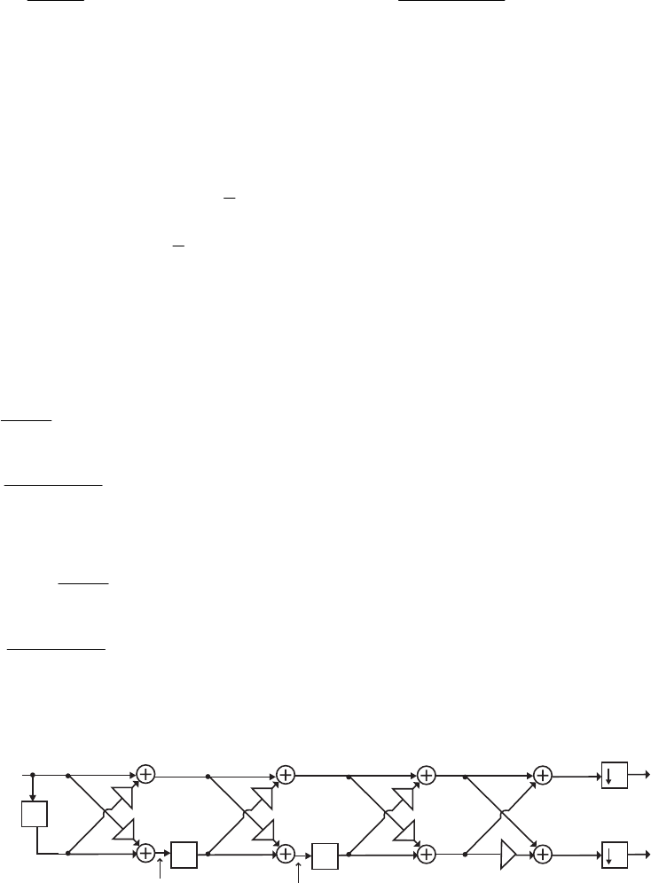
solution of Problem 14.31, Part (b), we have
and Solving these two equations we get
)()()( zQzkzPzP mmmm 1
2
1−
−
−+=
).()()( zQzzPkzQ mmmm 1
2
1−
−
−+=
)]()([)( zQkzP
k
zP mmm
m
m−
−
=
−2
11
1 and )].()([
)(
)( zPkzQ
zk
zQ mmm
m
m−
−
=−
−22
11
1
To synthesize the analysis filter bank, choose so that the coefficient of the highest
power of in is equal to 0. It can be shown that this choice of also guarantees
that the coefficient of the second highest power of is also 0. Hence, the order of is
2 less that of
m
k
)(zP
m1−1−
z
)(zP
m1−
).(zPm
(a) Here Hence,
.2=M)]()([)( zHzHzP 10
2
1
2+=
321 151221 −−− +++= zzz
54
4−− ++ zz and )]()([)( zHzHzQ 10
2
1
2−= .
54321 2121542
−
−
−
−
−
+++++= zzzzz
We form
3
2
2
2
1
22222 121515124221 −
−
−
−+−+−+−=− zkzkzkkzQkzP )()()()()()(
.)()( 5
2
4
2224
−
−−+−+ zkzk Choose .2
2
=
k Then
.)()( 1
222 63 32 918
−
−
−
−zz−−−=− zzQkzP Thus,
)]()([)( zQkzP
k
zP 222
2
2
11
1−
−
=.
321 3621
−
−
−
+++= zzz Likewise,
.)]()([
)(
)( 321
222
22
2
1263
1
1−−−
−+++=−
−
=zzzzPkzQ
zk
zQ Next, we form
.)()()()()()( 3
1
2
1
1
11111 3266231 −
−
−
−+−+−+−=− zkzkzkkzQkzP Choose .3
1
=
k
Then, .)]()([)( 1
111
2
1
021
1
1−
+=−
−
=zzQkzP
k
zP Likewise,
.)]()([
)(
)( 1
111
22
1
02
1
1−
−+=−
−
=zzPkzQ
zk
zQ From Figure P14.5 we have
and
1
00 1−
+= zkzP )( .)( 1
00
−
+= zkzQ Hence, it follows that As a result, the
analysis filter bank is as shown below:
.2
0=k
z
2
_
z
1
_
z
2
_
X
(z)
_
1
2
2
H (z)
0
H (z)
1
Q (z)
P (z)
2
2
P (z)
1
P (z)
0
Q (z)
1
Q (z)
0
2
2
3
3
2
2
The corresponding synthesis filter bank for a perfect reconstruction filter bank is as shown
below:
Not for sale 557
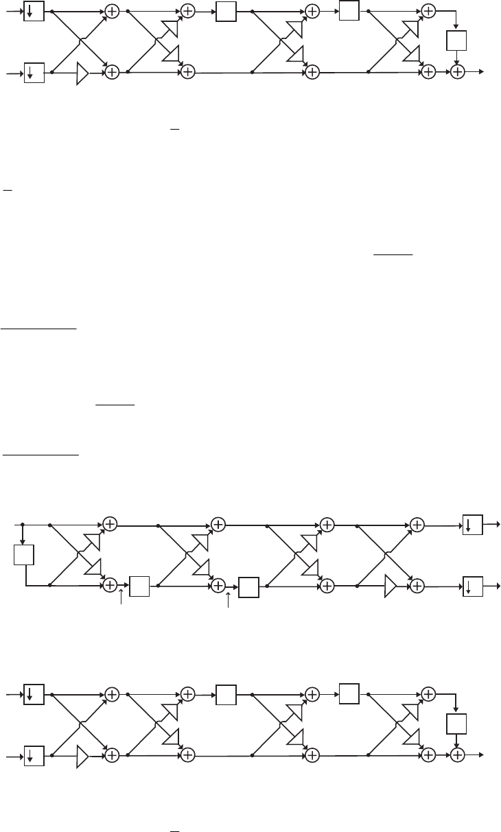
z
1
_
2
2
z
2
_
z
2
_
_
1
_
2
_
2
_
2
_
2
_
3
_
3
(b) Here Hence,
.2=M)]()([)( zHzHzP 10
2
1
2+= 321 18513521
−
−
−
+−−= zzz ..
54 25 −− −+ zz and
)]()([)( zHzHzQ 10
2
1
2−= ... 54321 525131852 −−
−
−
−
+−−++−= zzzzz We form
3
2
2
2
1
22222 513181851355221
−
−
−
+++−+−+=− zkzkzkkzQkzP ).().().()()()(
.)().( 5
2
4
22525
−
−+−++ zkzk Choose .2
2
−
=
k Then )]()([)( zQkzP
k
zP 222
2
2
11
1−
−
=
Likewise,
... 321 357521 −−− +−−= zzz
...)]()([
)(
)( 321
222
22
2
152573
1
1−−−
−+−−=−
−
=zzzzPkzQ
zk
zQ Next, we form
.)()..()..()()()( 3
1
2
1
1
11111 35257575231 −
−
−
−+−−−−−=− zkzkzkkzQkzP Choose
Then,
.3
1=k..)]()([)( 1
111
2
1
0521
1
1−
−=−
−
=zzQkzP
k
zP Likewise,
..)]()([
)(
)( 1
111
22
1
052
1
1−
−+−=−
−
=zzPkzQ
zk
zQ Hence, ..52
0−
=
k As a result, the
analysis filter bank is as shown below:
z2
_
z1
_
z2
_
X
(z)
_1
2
2
H (z)
0
H (z)
1
Q (z)
P (z)
2
2
P (z)
1
P (z)
0
Q (z)
1
Q (z)
0
2.5
_
2.5
_
2
_
2
_
3
3
The corresponding synthesis filter bank for a perfect reconstruction filter bank is as shown
below:
z
1
_
2
2
z
2
_
z
2
_
_
1
2
_
3
_
3
2
2.5
2.5
(c) Here Hence,
.2=M)]()([)( zHzHzP 10
2
1
2+= 321 6750521
−
−
−
++−= zzz ..
Not for sale 558
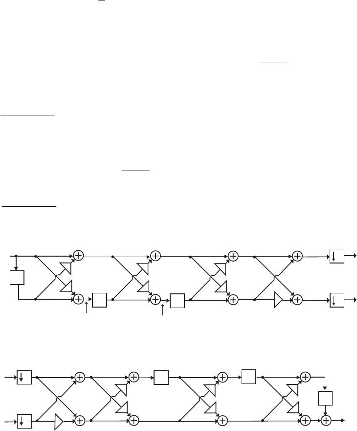
54 25 −− +− zz and )]()([)( zHzHzQ 10
2
1
2−=
... 54321 52750652
−
−
−−− +−++−= zzzzz We form
3
2
2
2
1
22222 7506675055221
−
−
−
−+−−−−−=− zkzkzkkzQkzP ).().().()()()(
.)().( 5
2
4
22525
−
−−+−− zkzk Choose .2
2
=
k Then )]()([)( zQkzP
k
zP 222
2
2
11
1−
−
=
.... 321 51753521
−
−− −+−= zzz Likewise,
....)]()([
)(
)( 321
222
22
2
15275351
1
1−−−
−+−+−=−
−
=zzzzPkzQ
zk
zQ Next, we form
.).()..()..().()()( 3
1
2
1
1
11111 515275375352511
−
−
−
+−++−−+=− zkzkzkkzQkzP
Choose Then,
..51
1−=k..)]()([)( 1
111
2
1
0521
1
1−
−=−
−
=zzQkzP
k
zP Likewise,
..)]()([
)(
)( 1
111
22
1
052
1
1−
−+−=−
−
=zzPkzQ
zk
zQ Hence, ..52
0−
=
k As a result, the
analysis filter bank is as shown below:
z
2
_
z
1
_
z
2
_
X
(z)
_
1
2
2
H (z)
0
H (z)
1
Q (z)
P (z)
2
2
P (z)
1
P (z)
0
Q (z)
1
Q (z)
0
2
2
1.5
_
2.5
_
2.5
_
1.5
_
The corresponding synthesis filter bank for a perfect reconstruction filter bank is as shown
below:
z
1
_
2
2
z
2
_
z
2
_
_
1
2.5
2.5
_
2
_
2
1.5
1.5
14.33 To show the system of Figure 14.18 is, in general, periodic with a period L, we need to
show that if is the output for an input and is the output for an input
then if i.e.,
)(
ˆzX1),(zX1)(
ˆzX2
),(zX2),()( zXzzX L12 −
=],[][ Lnxnx
−
=
12 then the corresponding output
satisfies i.e.,
),(
ˆ
)(
ˆzXzzX L12 −
=].[
ˆ
][
ˆLnxnx
−
=
12 Now,
,
)(
)(
)(
)()()(
ˆ)(
⎥
⎥
⎥
⎦
⎤
⎢
⎢
⎢
⎣
⎡
=
−1L
mT
zWX
zWX
zX
zzzX M
Hg where is the vector composed of the synthesis
bank filters given by Eq. (14.98) and is the analysis filter bank modulation
)(zg
)(
)( z
m
H
Not for sale 559
matrix given Eq. (14.102). Now,
As a
result, the structure of Figure 14.18 is, in general, a time-varying system with a period of L.
⎥
⎥
⎥
⎦
⎤
⎢
⎢
⎢
⎣
⎡
=
−)(
)(
)(
)()()(
ˆ)(
1
2
2
2
2
L
mT
zWX
zWX
zX
zzzX M
Hg
).(
ˆ
)(
)(
)(
)()(
)(
)(
)(
)()( )()( zXz
zWX
zWX
zX
zzz
zWXz
zWXz
zXz
zz L
L
mTL
LL
L
L
mT 1
1
1
1
1
1
1
1
1
−
−
−
−−
−
−
=
⎥
⎥
⎥
⎦
⎤
⎢
⎢
⎢
⎣
⎡
=
⎥
⎥
⎥
⎥
⎦
⎤
⎢
⎢
⎢
⎢
⎣
⎡
=M
MHgHg
14.34 ).()()(),()()( 2
11
12
101
2
01
12
000 zEzzEzHzEzzEzH
−
−+=+= Thus,
.
)()(
)()(
)( ⎥
⎦
⎤
⎢
⎣
⎡
=zEzE
zEzE
z
1110
0100
E
(a) Hence,
Thus,
).()()( 2
1
12
00 zEzzEzH −
+= ).()()()( 2
1
12
001 zEzzEzHzH −
−=−=
),()(),()(),()( zEzEzEzEzEzE 010101000
=
=
= and
Therefore,
).()( zEzE 111 −=
.
)()(
)()(
)( ⎥
⎦
⎤
⎢
⎣
⎡−
=zEzE
zEzE
z
10
10
E
(b) Two cases need to be considered – N odd and N even. Consider first the N odd
case. For simplicity let .)( 3
3
2
2
1
100
−
−
−
+++= zazazaazH Then,
.)()()( 3
0
2
1
1
23
3
3
2
210
31
0
3
1
−
−−−−− +++=+++== zazazaazazazaazzHzzH
Thus, ,)()(,)()( 1
31101
1
20000
−
−
+==+== zaazEzEzaazEzE and
)()()(,)( 1
1
1
10
1
0211
1
1310
−
−
−
−=⇒+=+= zEzzEzaazEzaazE and
).()( 1
0
1
11 −−
=zEzzE
Next, consider the N even case. Assume .)( 4
4
3
3
2
2
1
100
−
−−
−
++++= zazazazaazH
Then,
)()()( 4
4
3
3
2
210
41
0
4
1zazazazaazzHzzH ++++== −−−
.
4
0
3
1
2
2
1
34
−
−
−− ++++= zazazazaa Thus,
,)()(,)()( 2
4
1
20000 1
31101 −
−
−
+== zaazEz++== EzazaazEzE and
)()()(,)( 1
0
2
10
1
1311
2
0
1
2410 −−
−
−
−=⇒+=++= zEzzEzaazEzazaazE and
).()( 1
1
1
11 −−
=zEzzE
In the general case, for N odd with ,12
+
=
KN )()( 1
011 −
−
=zEzzE K and
⇒= −− )()( 1
110 zEzzE K.
)()(
)()(
)( /)(/)( ⎥
⎦
⎤
⎢
⎣
⎡
=−−−−−− 1
0
211
1
21
10
zEzzEz
zEzE
zNN
E
Not for sale 560

Likewise, for N even with ,KN 2
=
)()( 1
010
−
−
=zEzzE K and
⇒= −−− )()( )( 1
1
1
11 zEzzE K.
)()(
)()(
)( /)(/ ⎥
⎦
⎤
⎢
⎣
⎡
=−−−−− 1
1
221
0
2
10
zEzzEz
zEzE
zNN
E
14.35 (a) ][ )()()( 2
1
12
0
4
1
0zzzzH AA −
+= and ].[ )()()( 2
1
12
0
4
1
1zzzzH AA −
−=
Hence, and
)(zE,
)()(
)()( ⎥
⎦
⎤
⎢
⎣
⎡−
=zz
zz
10
10
AA
AA )(zR.
)()(
)()( ⎥
⎦
⎤
⎢
⎣
⎡−
=zz
zz
00
11
AA
AA
(b) To prove is lossless, we need to show E
)(zE†IE 2
cee jj =)()( ωω for some
constant c: E†=)()( ωω jj ee E
⎥
⎦
⎤
⎢
⎣
⎡
−
⎥
⎥
⎦
⎤
⎢
⎢
⎣
⎡
−)()(
)()(
)()(
)(*)(*
ωω
ωω
ωω
ωω
jj
jj
jj
jj
ee
ee
ee
ee
10
10
1
00
1AA
AA
AA
AA
⎥
⎥
⎥
⎦
⎤
⎢
⎢
⎢
⎣
⎡
+
+
=2
1
2
1
2
0
2
0
0
0
)()(
)()(
ωω
ωω
jj
jj
ee
ee
AA
AA
.I2
=
Hence, E(z) is
lossless.
(c) .
)()(
)()(
)()(
)()( IER 2
20
02 01
01
01
4
1zz
zz
zz
zz AA
AA
AA =
⎥
⎦
⎤
⎢
⎣
⎡
= Therefore,
).(
)()(
)( z
zz
z1
01
2
−
=ER AA
(d) As in part (c), .
)()(
)()( IER 2
01 zz
zz AA
=
14.36 Hence, .
)()(
)()(
)( ⎥
⎦
⎤
⎢
⎣
⎡
+−
−−+−
=
⎥
⎦
⎤
⎢
⎣
⎡
=−
−−−
123
2682
1
112
1110
0100
z
zzz
zEzE
zEzE
z
E
43212
01
12
000 2826
−
−
−
−
−−−++−=+= zzzzzEzzEzH )()()( and
.)()()( 212
11
12
101 23
−
−
−++−=+= zzzEzzEzH
Now, det(E(z)) = .))(()( 11112 232682
−
−
−
−
−=+−−−−+− zzzzz From Eq.
(14.133) we have
⎥
⎦
⎤
⎢
⎣
⎡
−
+−−+−
==
⎥
⎦
⎤
⎢
⎣
⎡
=−
−−−
−
−
−−
123
2682
1
112
1
1
1110
0100
z
zzz
z
cz
zcz
zRzR
zRzR
z
K
K)(
)()(
)()(
)( ER
for
⎥
⎦
⎤
⎢
⎣
⎡
−
+−−+−
=−
−−−
123
2682
1
112
z
zzz 1
=
K and .1
=
c Therefore,
43212
01
12
000 2826
−
−
−
−
−−++−−=+= zzzzzRzzRzG )()()( and
.)()()( 212
11
12
101 23
−
−
−−+=+= zzzRzzRzG
Not for sale 561
14.37 From Eqs. (14.121) and (14.122a) to (14.122c), we thus get
resulting in the analysis filters
.
⎥
⎥
⎦
⎤
⎢
⎢
⎣
⎡−
−
=
242
213
122
P
,
)(
)(
)(
⎥
⎥
⎦
⎤
⎢
⎢
⎣
⎡
⎥
⎥
⎦
⎤
⎢
⎢
⎣
⎡−
−
=
⎥
⎥
⎦
⎤
⎢
⎢
⎣
⎡
−
−
2
1
2
1
01
242
213
122
z
z
zH
zH
zH
.)(,)(,)( 21
2
21
1
21
02422322 −−
−
−
−− ++=−+=+−= zzzHzzzHzzzH
Now, Using Eqs. (14.124) and (14.125a) to (14.125c),
we arrive at
[]
, leading to
the synthesis filters
.
...
...
...
⎥
⎥
⎦
⎤
⎢
⎢
⎣
⎡
−
−=
−
64096080
56016080
24064080
41
P
[]
⎥
⎥
⎦
⎤
⎢
⎢
⎣
⎡
−
−= −−
64096080
56016080
24064080
1
12
210 ...
...
...
)()()( zzzGzGzG
,...)(,...)( 21
1
21
0640160960808080
−
−
−
−
++−=+−= zzzGzzzG
....)( 21
2240560640
−
−++= zzzG
14.38 For .)(
⎥
⎥
⎥
⎦
⎤
⎢
⎢
⎢
⎣
⎡
−
−
−−
=
2111
1130
0112
1321
z
R][][ 34
−
=
nxny to hold, we require
Hence,
.)()( IER 4=zz
1
1
2111
1130
0112
1321
44
−
−
⎥
⎥
⎥
⎦
⎤
⎢
⎢
⎢
⎣
⎡
−
−
−−
== )]([)( zz RE
.
....
....
....
....
⎥
⎥
⎥
⎦
⎤
⎢
⎢
⎢
⎣
⎡
−
−−
−−
=
35292176511176288241
23530117624118158822
70590647112353023530
23530882415882241181
14.39 Therefore,
[]
[]
.)()()( ⎥
⎥
⎦
⎤
⎢
⎢
⎣
⎡−= −−
212
133
221
1
12
210 zzzHzHzH
.)(,)(,)( 21
2
21
1
21
02223132 −−
−
−
−− ++=+−=++= zzzHzzzHzzzH The
corresponding Type 1 polyphase component matrix is thus given by
For perfect reconstruction we require the Type 2 polyphase component matrix to be given
by Hence, the synthesis filters are obtained from
.)( ⎥
⎥
⎦
⎤
⎢
⎢
⎣
⎡−=
212
231
132
zE
.
//
//
//
)]([)( ⎥
⎥
⎦
⎤
⎢
⎢
⎣
⎡
−−− −
== −
33438
13232
33538
1
zz ER
Not for sale 562

[]
[]
⎥
⎥
⎦
⎤
⎢
⎢
⎣
⎡
−−− −
=−−
33438
13232
33538
1
12
210 //
//
//
)()()( zzzGzGzG resulting in
,)(,)( 2
3
5
1
3
2
3
4
1
2
3
8
1
3
2
3
8
0−−−− +−=+−−= zzzGzzzG and .)( 21
233
−
−++= zzzG
14.40 For perfect reconstruction we require .)(
⎥
⎥
⎥
⎦
⎤
⎢
⎢
⎢
⎣
⎡
−
−−
=
2131
1213
2113
2112
z
E
.
....
....
..
..
)()(
⎥
⎥
⎥
⎦
⎤
⎢
⎢
⎢
⎣
⎡
−−−
−−−−
== −
1506015021
0502195040
25102501
500501
3
1
1zz ER Thus,
[]
[]
.
....
....
..
..
)()()()(
⎥
⎥
⎥
⎦
⎤
⎢
⎢
⎢
⎣
⎡
−−−
−−−−
=−−−
1506015021
0502195040
25102501
500501
1
123
3
1
3210 zzzzGzGzGzG
Hence,
),....()(),..()( 321
3
1
1
321
3
1
0502509501504021 −−−−−− ++−−=+−−= zzzzGzzzzG
).....()(),..()( 321
3
1
3
1
3
1
2502510501502160 −−−− −++−=+−= zzzzGzzG
14.41 .)(,)(,)( 21
0
21
0
21
0223232 −−
−
−
−− +−=−+=++−= zzzGzzzGzzzG
Rewriting these equations in an matrix form we get
This implies,
For perfect reconstruction we require
Hence,
implying
[]
[]
.)()()( ⎥
⎥
⎦
⎤
⎢
⎢
⎣
⎡
−−
−
=−−
132
113
222
1
12
210 zzzGzGzG
.)( ⎥
⎥
⎦
⎤
⎢
⎢
⎣
⎡
−−
−
=
132
113
222
zR
.
...
...
..
)()( ⎥
⎥
⎦
⎤
⎢
⎢
⎣
⎡
−
−== −
2500625034380
2501875003130
02501250
1zz RE
⎥
⎥
⎦
⎤
⎢
⎢
⎣
⎡
⎥
⎥
⎦
⎤
⎢
⎢
⎣
⎡
−
−=
⎥
⎥
⎦
⎤
⎢
⎢
⎣
⎡
−
−
2
1
2
1
01
2500625034380
2501875003130
02501250
z
z
zH
zH
zH
...
...
..
)(
)(
)(
,...)(,..)( 21
1
1
025018750031302501250
−
−
−++−=+= zzzHzzH
....)( 21
12500625034380
−
−+−= zzzH
14.42 If the filter bank is alias-free, then
Not for sale 563
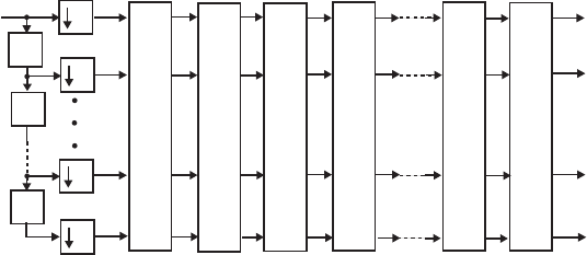
The above
L equations are
⎥
⎥
⎥
⎦
⎤
⎢
⎢
⎢
⎣
⎡
=
⎥
⎥
⎥
⎦
⎤
⎢
⎢
⎢
⎣
⎡
⎥
⎥
⎥
⎦
⎤
⎢
⎢
⎢
⎣
⎡
−
−
−
−−
−
−
0
0
1
1
0
1
1
1
1
1
0
110
110
M
M
L
MOMM
L
L)(
)(
)(
)(
)()()(
)()()(
)()()( zT
zG
zG
zG
zWHzWHzWH
zWHzWHzWH
zHzHzH
L
L
L
LL
L
L
(1): ),()()()()()()( zTzGzHzGzHzGzH LL
=
+
+
+−− 111100 K
(2):
.,)()()()()()( 110
111100 −≤≤=+++ −− LrzGzWHzGzWHzGzWH L
r
L
rr K
Replacing
z by in the above equation we get
rL
zW −
,)()()()()()( 0
111100 =+++
−
−−
−
−rL
L
L
L
rLLrLL zWGzWHzWGzWHzWGzWH K
or equivalently,
(3): ,)()()()()()( 0
111100 =+++ −
−−
−
−rL
LL
rLrL zWGzHzWGzHzWGzH K
Rewriting Eqs. (1) and (3) in matrix form we get
.10 −≤≤ Lr
.
)(
)(
)(
)(
)()()(
)()()(
)()()(
⎥
⎥
⎥
⎦
⎤
⎢
⎢
⎢
⎣
⎡
=
⎥
⎥
⎥
⎦
⎤
⎢
⎢
⎢
⎣
⎡
⎥
⎥
⎥
⎦
⎤
⎢
⎢
⎢
⎣
⎡
−
−
−
−−
−
−
0
0
1
1
0
1
1
1
1
1
0
110
110
M
M
L
MOMM
L
LzT
zH
zH
zH
zWGzWGzWG
zWGzWGzWG
zGzGzG
L
L
L
LL
L
L
Thus, if an L-channel filter bank is alias-free with a given set of analysis and synthesis
filters, then the filter bank is still alias-free if the analysis and synthesis filters are
interchanged.
14.43 An equivalent representation of the structure of Figure P14.6 is shown below
where Γ.
⎥
⎥
⎥
⎦
⎤
⎢
⎢
⎢
⎣
⎡
=
−1
00
010
001
z
m
L
MOMM
L
L
z
_1
S
0
z
_1
z
_1
L
L
L
L
S
1
S
K
X
(z)
Γ
1
Γ
2
Γ
K
The corresponding synthesis bank for designing an L-channel perfect
reconstruction bank is thus as shown below where and
ΛΓ
1−
=mm ST
2−
=z
m.
⎥
⎥
⎥
⎦
⎤
⎢
⎢
⎢
⎣
⎡
=−
−
−
100
00
00
1
1
1
L
MOMM
L
L
z
z
m
Not for sale 564
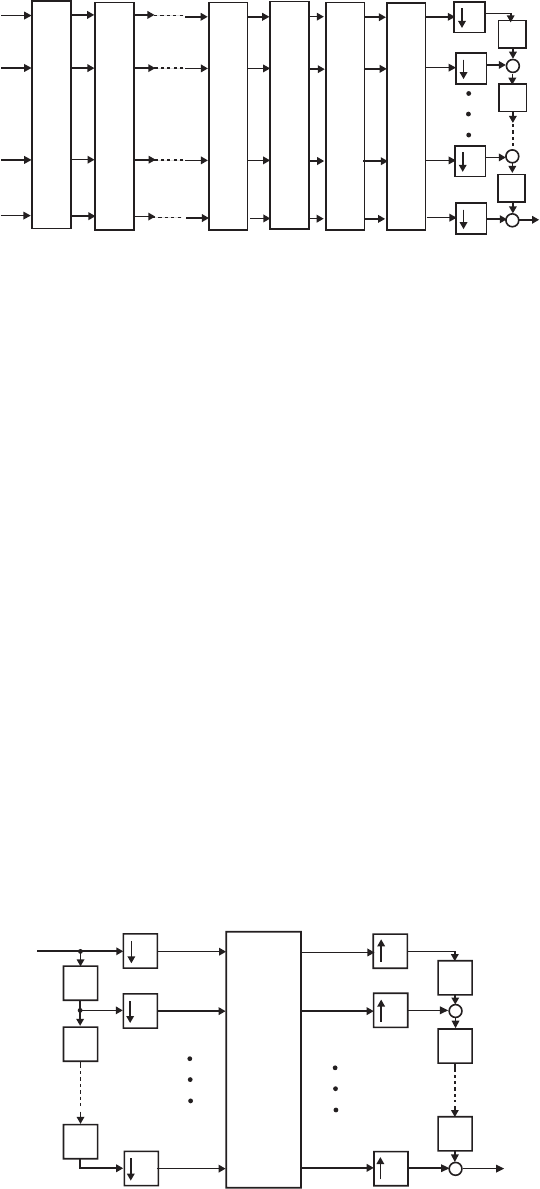
T
0
L
L
L
L
T
1
T
K
Λ
1
Λ
2
Λ
K
+
+
+
_
1
z
_
1
z
_
1
z
14.44
Hence,
⎥
⎥
⎦
⎤
⎢
⎢
⎣
⎡
⎥
⎥
⎦
⎤
⎢
⎢
⎣
⎡
−−− −
⎥
⎥
⎦
⎤
⎢
⎢
⎣
⎡
⎥
⎥
⎦
⎤
⎢
⎢
⎣
⎡−
−
=
⎥
⎥
⎦
⎤
⎢
⎢
⎣
⎡
−
−
−2
1
1
2
1
01
110
231
353
00
010
001
100
210
321
z
z
z
zH
zH
zH
)(
)(
)(
.
⎥
⎥
⎦
⎤
⎢
⎢
⎣
⎡
⎥
⎥
⎥
⎦
⎤
⎢
⎢
⎢
⎣
⎡
−
−−+−
+−−
=−
−
−−
−−
−−
2
1
11
11
11 1
0
22231
373115
z
z
zz
zz
zz
,)( 321
034115 −−− ++−= zzzzH
.)(,)( 32
2
31
1231 −−−− +−=−+−= zzzHzzzH
Hence,
[]
[]
1
1
1
1
12
210 110
231
353
100
00
00
100
210
321
1
−
−
−
−
−−
⎥
⎥
⎦
⎤
⎢
⎢
⎣
⎡
−−− −
⎥
⎥
⎥
⎦
⎤
⎢
⎢
⎢
⎣
⎡
⎥
⎥
⎦
⎤
⎢
⎢
⎣
⎡−
−
=z
z
zzzGzGzG )()()(
[]
.
⎥
⎥
⎥
⎦
⎤
⎢
⎢
⎢
⎣
⎡
+++
+++
=−−−
−−−
−−
431
83632
473813
1111
111
12 zzz
zzz
zz
,)( 321
03221 −−− +++= zzzzG ,)( 321
18663 −−− +++= zzzzG
.)( 321
27784 −−− +++= zzzzG
14.45 Figure 14.20 with internal variables labeled is shown below:
z
_1
+
+
z
_1
z
_1
z
_1
z
_1
z
_1
P(z)
L
L
L
L
L
L
x
[n]
y[n]
c [n]
0
c [n]
1
c [n]
L 1
_
b [n]
L 1
_
b [n]
0
b [n]
1
Not for sale 565

From the above figure it follows that we can express the z-transforms of as ]}[{ ncl
,),(()()( // 10
11
1
0
1−≤≤= −
−
=
∑LWzXWz
L
zC kLk
L
Ll
l
l
l where
Likewise, the z-transforms of can be expressed as
.
/Lj
eW π2−
=
]}[{ nbs
where denotes the z-transforms the
–th element of Finally, the z-transform of the output is given by
,),()()( ,10
1
0
−≤≤= ∑
−
=
LszCzPzB
L
s
ss ll )(
,zPsl
),( ls).(zP][ny
∑∑∑ −
=
−
=
−−−
−
=
−−− ==
1
0
1
0
1
1
0
1
L
LL
s
L
s
sLL
s
L
s
sL zCzPzzBzzY
l
ll )()()()( ,
)()(
∑∑∑−
=
−
=
−
−
=
−−−
=
1
0
1
0
1
0
1
1L
k
L
k
kL
s
L
s
sL zWXzWzPz
Ll
l
l)()()(
,
)(
).()( ,
)( L
s
LL
s
sLk
L
k
kzPzzWzWX
Ll
l
ll
∑∑∑−
=
−
=
−−−−−
−
=
=
1
0
1
0
1
1
0
1
In the above expression, terms of the form represent the
contribution coming from aliasing. Hence, the expression for is free from
these aliasing terms for any arbitrary input if and only if
,),( 0≠kzWX k
)(zY
][nx
.,)(
,
)( 00
1
0
1
0
1≠=
∑∑
−
=
−
=
−−−−− kzPzzW L
s
LL
s
sLk l
l
ll
The above expression can be written in a matrix form as D†,
)(
)(
)(
)(
⎥
⎥
⎥
⎦
⎤
⎢
⎢
⎢
⎣
⎡
=
⎥
⎥
⎥
⎦
⎤
⎢
⎢
⎢
⎣
⎡
−0
0
1
1
0
M
M
zT
zV
zV
zV
L
where D is the DFT matrix, is transfer function of the alias-free system, and
Since †
)(zT
).()( ,
)( L
s
sL
L
s
zPzzzV l
l
l−−−
−
=
−
∑
=1
1
0
DD ,IL
=
the above matrix equation can
be alternately written as This implies that
as the first column of D has all elements equal to 1. As
a result, the L-channel QMF bank is alias-free if and only if is the same for
all
.
)(
)(
)(
)(
⎥
⎥
⎥
⎦
⎤
⎢
⎢
⎢
⎣
⎡
=
⎥
⎥
⎥
⎦
⎤
⎢
⎢
⎢
⎣
⎡
−0
0
1
1
0
M
M
zT
zV
zV
zV
L
D
,),()( 10 −≤≤= LzVzV l
l
)(zVl
.l
The two figures below show the polyphase realizations of and :
)(zV0)(zV1
Not for sale 566
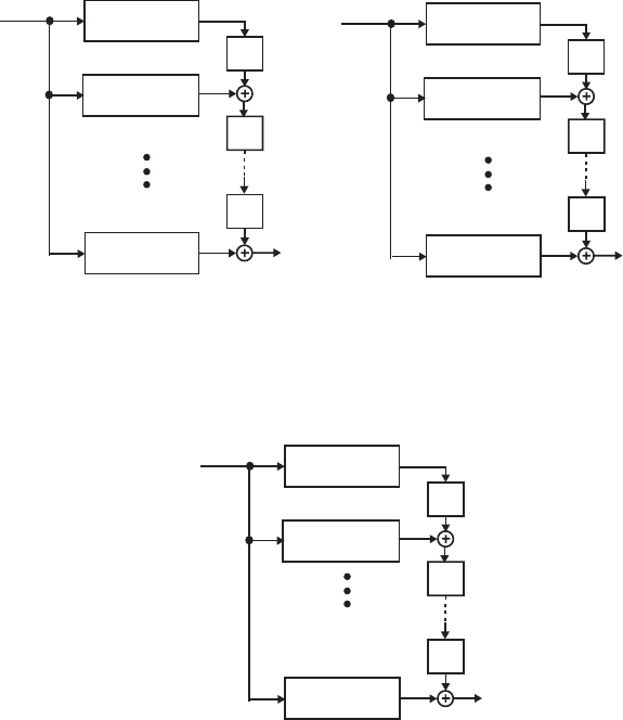
z
_1
z
_1
y[n]
P (z )
L
0,1
1,1
P (z )
L
z
_1
P (z )
L
L 1,1
_
z
_1
z
_1
y[n]
P (z )
L
0,0
1,0
P (z )
L
z
_1
P (z )
L
L 1,0
_
(a) (b) )(zV0)(zV1
The realization of can be redrawn as indicated below:
)(zV1
z
_1
z
_1
y[n]
P (z )
L
2,1
1,1
P (z )
L
P (z )
L
0,1
_L
z
z
_1
(c)
)(zV1
Because of the constraint ),()( zVzV 10
=
the polyphase components in Figures (a)
and (c) should be the same. From these two figures it follows that the first column
of is an upwards-shifted version of the second column, with the topmost
element appearing with a
)(zP
1
−
z attached. This type of relation holds for the k-th
column and the –th column of . As a result, is a pseudo-circulant
matrix of the form of Eq. (14.155).
)( 1+k)(zP)(zP
14.46 Hence,
Likewise,
Hence,
Therefore,
).()()(),()()( 2
1
12
01
2
1
12
00 zEzzEzHzEzzEzH −− −=+=
.
)()(
)()(
)( ⎥
⎦
⎤
⎢
⎣
⎡−
=zEzE
zEzE
z
10
10
E
),()()()()( 2
10
2
00
12
1
12
00 zRzRzzEzzEzG +=+= −−
).()()()()( 2
11
2
01
12
1
12
01 zRzRzzEzzEzG +=+−= −−
.
)()(
)()(
)()(
)()(
)( ⎥
⎦
⎤
⎢
⎣
⎡−
=
⎥
⎦
⎤
⎢
⎣
⎡
=zEzE
zEzE
zRzR
zRzR
z
00
11
1110
0100
R
Not for sale 567

.
)()(
)()(
)()(
)()(
)()(
)()(
)()()( ⎥
⎦
⎤
⎢
⎣
⎡
=
⎥
⎦
⎤
⎢
⎣
⎡−
⎥
⎦
⎤
⎢
⎣
⎡−
== zEzE
zEzE
zEzE
zEzE
zEzE
zEzE
zzz
10
10
10
10
00
11
20
02
ERP
Here, and )()()( zEzEzP 100 2=.)( 0
1
=
zP As a result, P(z) is pseudo-circuluant.
14.47 (a)
Therefore,
Thus,
Hence, is a power-symmetric function.
The highpass analysis filter is given by
The two synthesis
filters are time-reversed versions of the analysis filters as per Eq. (14.92):
and
,..)( 54321
05065421 −−−−− ++++−= zzzzzzH
...)( 1254650 23451
0+−+++=
−zzzzzzH
........)()( 531351
00 5025652256252225650 −−−− ++++++= zzzzzzzHzH
.)()()()( 125
1
00
1
00 =−−+ −− zHzHzHzH )(zH0
...)()( 543211
0
5
1254650 −−−−−−− +++−+−=−= zzzzzzHzzH
543211
0
5
024912212 −−−−−−− +−+++== zzzzzzHzzG )()(
.)()( 543211
1
5
12129422 −−−−−−− −+−++== zzzzzzHzzG
(b) .)(,)( 1221 2
1
2
4
15
451
0
542
4
15
1
2
1
0+++−=+−++= −−−−− zzzzzHzzzzzH
Therefore,
Thus,
Hence, is a power-symmetric
function. The highpass analysis filter is given by
......)()( 531351
00 275103753312520375375102 −−−− ++−+−+= zzzzzzzHzH
..)()()()( 62540
1
00
1
00 =−−+ −− zHzHzHzH )(zH0
.)()( 54
2
1
3
4
15
11
0
5
12−−−−−− +−+−−=−= zzzzzHzzH The two synthesis filters are
time-reversed versions of the analysis filters as per Eq. (14.92):
543
2
15
11
0
5
02242 −−−−−− +++−== zzzzzHzzG )()( and
.)()( 54211
1
5
142
2
15
22 −−−−−− −−+−== zzzzzHzzG
14.48 and
21
01−− ++= zazzH )( .)( 4321
11−
−
−
−
++++= zazbzazzH The corresponding
synthesis filters are given by ,)()( 4321
10 1−−
−
−
+−+−=−= zazbzazzHzG and
.)()( 21
01 1
−
−
−+−=−−= zazzHzG
To show that the filter bank is alias-free and satisfies the perfect reconstruction property we
need to show that where Now,
,
)(
)(
)()(
)()( ⎥
⎦
⎤
⎢
⎣
⎡
=
⎥
⎦
⎤
⎢
⎣
⎡
⎥
⎦
⎤
⎢
⎣
⎡−−
−−
0
1
0
10
00 K
cz
zG
zG
zHzH
zHzH .0≠c
))(()()()()( 432121
1100 11 −−
−
−
−
−
+−+−++=+ zazzazzazzGzHzGzH
,)())(( 3432121 2211
−
−
−
−
−−− −=++++−+−+ zbazazzazzaz and
.)()()()()()()()( 10101100 =0
−
−
−
−
−
=
−+− zHzHzHzHzGzHzGzH Thus, if 0
≠
a and
Not for sale 568

,2≠bthe above filter bank is alias-free and also satisfies the perfect reconstruction
property.
14.49 If is required to have 2 zeros at )(zH0,1
−
=
z then it is of the form
where is a first-order polynomial. Now,
),()()( zCzzH 21
01−
+= )(zC
),()()()()()( zRzzzHzHzP 2211
00 11 ++==
−
− where is a zero-phase
polynomial of the form
)(zR
.)( 1
−
++= azbazzR For perfect reconstruction we
require, i.e.,
,)()( 2=−+ zPzP
.)()()()()()( 21111 12211221 =−+−−−+++++ −
−
−
−azbazzzazbazzz Since
the above equation must hold for all ,
z
we observe that at ,1
=
z we get
.
8
1
2=+ ba Likewise, at ,j
z
=
we get .
4
1
=b Hence, .
16
1
−=a Therefore,
).()()()( 1
16
1
4
1
16
1
221 11 −− −+−++= zzzzzP The analysis filter is
obtained by a spectral factorization of P(z). Three choices of spectral factorization
resulting in linear-phase analysis filters are given in Section 14.3.3.
)(zH0
14.50
14.51 (a) An orthogonal perfect reconstruction filter bank is obtained by choosing the
minimum-phase spectral factor of P(z) as the lowpass analysis filter and then
determining the lowpass synthesis filter using the relation
The minimum-phase spectral factor of P(z) is given by
)(zH0
)(zG0
).()( 1
0
5
0−−
=zHzzG
)...()(.)( 2131
0105905745011332670
−
−
−+−+= zzzzH Hence,
)...()(.)()( 21311
0
5
057450105901332670 −
−
−
−− +−+== zzzzHzzG
(b) A perfect reconstruction filter bank with symmetric lowpass analysis and
synthesis filters of even length is given by
))(()( 43211
01
−
−
−
−− +++++= azbzczbzazzH and
Another possible design of a perfect reconstruction filter bank with symmetric
lowpass analysis and synthesis filters of even length is given by
.)()( 51
01−
+= zzG
)()()( 432131
01
−
−
−
−− +++++= azbzczbzazzH and
.)()( 31
01−
+= zzG
(c) A perfect reconstruction filter bank with symmetric lowpass analysis and
synthesis filters of odd length is given by
)()( 4321
0
−
−
−− ++++= azbzczbzazH and .)()( 61
01
−
+= zzG Another
possible design of a perfect reconstruction filter bank with symmetric lowpass
analysis and synthesis filters of odd length is given by
)()()( 432121
01
−
−
−
−− +++++= azbzczbzazzH and
.)()( 41
01−
+= zzG
Not for sale 569
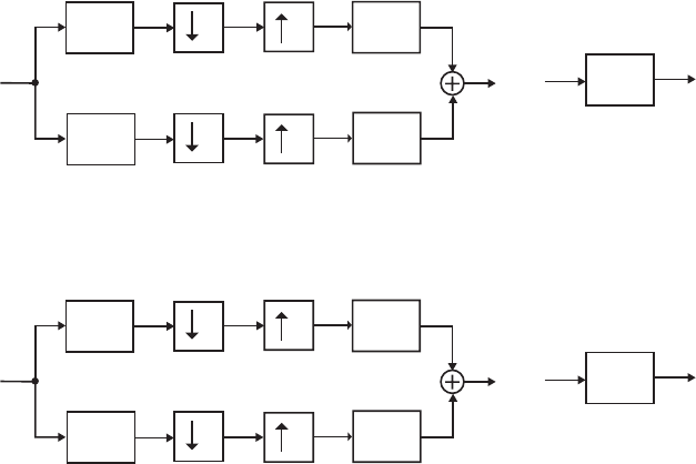
14.52
14.53
14.54 The polyphase matrices for the structure of Figure P14.7(a) are given by
and Therefore,
Hence, the structure of Figure
P14.7(a) is a perfect reconstruction QMF bank.
⎥
⎦
⎤
⎢
⎣
⎡
=1
01
)(
)( zP
z
E.
)(
)( ⎥
⎦
⎤
⎢
⎣
⎡−
=1
01
zP
z
R
.
)()(
)()( ⎥
⎦
⎤
⎢
⎣
⎡
=
⎥
⎦
⎤
⎢
⎣
⎡
⎥
⎦
⎤
⎢
⎣
⎡−
=10
01
1
01
1
01
zPzP
zz ER
14.55 The polyphase matrices for the structure of Figure P14.7(b) are given by
and Therefore,
Hence, the structure of Figure P14.7(b) is a perfect reconstruction QMF
bank.
⎥
⎦
⎤
⎢
⎣
⎡
⎥
⎦
⎤
⎢
⎣
⎡
=1
01
10
1
)(
)(
)( zP
zQ
zE.
)(
)(
)( ⎥
⎦
⎤
⎢
⎣
⎡−
⎥
⎦
⎤
⎢
⎣
⎡−
=10
1
1
01 zQ
zP
zR
⎥
⎦
⎤
⎢
⎣
⎡
⎥
⎦
⎤
⎢
⎣
⎡
⎥
⎦
⎤
⎢
⎣
⎡−
=
⎥
⎦
⎤
⎢
⎣
⎡
⎥
⎦
⎤
⎢
⎣
⎡
⎥
⎦
⎤
⎢
⎣
⎡−
⎥
⎦
⎤
⎢
⎣
⎡−
=1
01
10
01
1
01
1
01
10
1
10
1
1
01
)()()(
)()(
)(
)()( zPzPzP
zQzQ
zP
zz ER
⎥
⎦
⎤
⎢
⎣
⎡
=10
01
14.56 If the 2-channel QMF banks in the middle of the structure of Figure 14.24 are of
perfect reconstruction type, then each of these two filter banks have a distortion
transfer function of the form ,
M
z
−
α where M is a positive integer.
2
2
2
2
10
H (z)
11
H (z)
10
G (z)
11
G (z)
αz_M
_
_
_
Likewise, the 2-channel analysis filter bank on the left with the 2-channel synthesis
filter bank on the right form a perfect reconstruction QMF bank with a distortion
transfer function where L is a positive integer: ,
L
z−
β
2
2
2
2
L
H (z)
βz_L
_
_
_
H
H (z)H
G (z)
L
G (z)
Hence, an equivalent representation of Figure 14.24 is as indicated below:
Not for sale 570
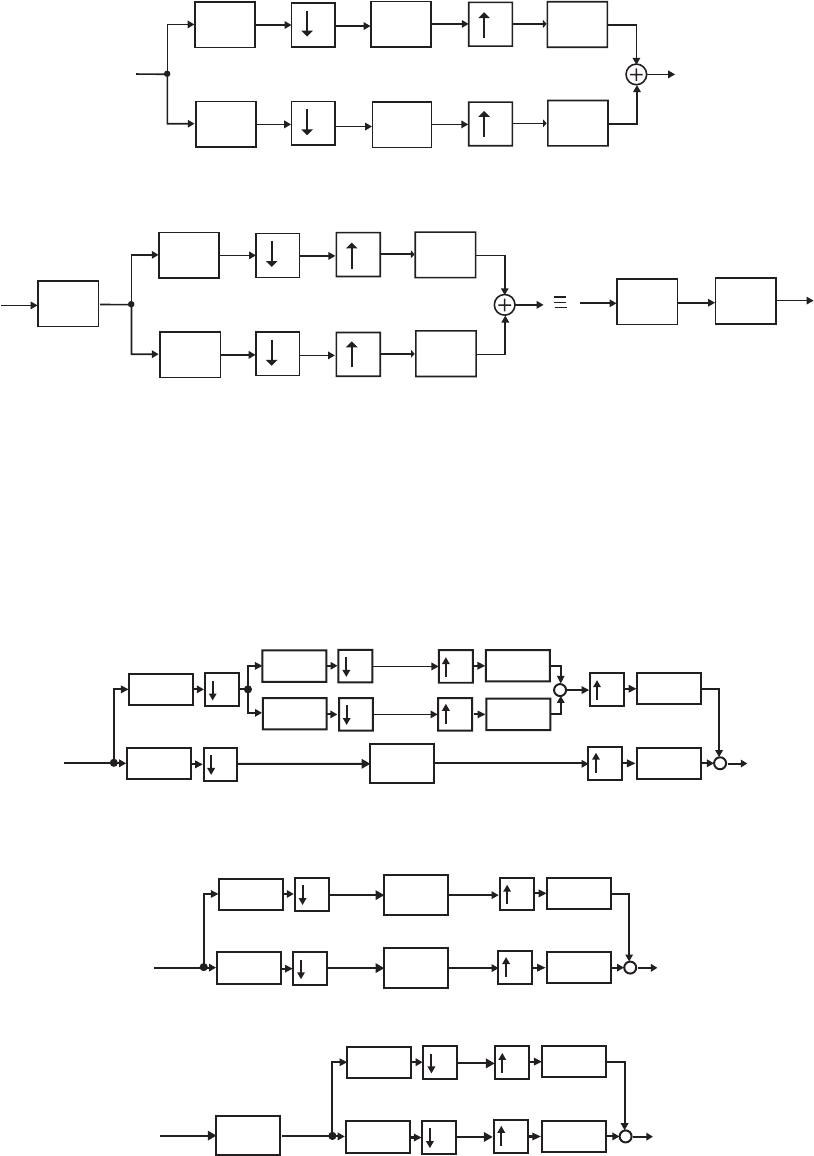
2
2
2
2
L
H (z)αz_M
H
H (z)H
G (z)
L
G (z)
αz
_M
which reduces to
2
2
2
2
L
H (z)
αz_2M
H
H (z)H
G (z)
L
G (z)
βz_L
αz_2M
Thus, the overall structure is also of perfect reconstruction type with have a
distortion transfer function given by .
)( LM
z
+
−
2
αβ
14.57 We analyze the 3-channel filter bank of Figure 14.27(b). If the 2-channel QMF
bank of Figure 14.27(a) is of perfect reconstruction type with a distortion transfer
function the structure of Figure 14.27(b) should be implemented as indicated
below to ensure perfect reconstruction:
,
L
z−
β
+
2
2
2
2
*
x
[n]y[n]
+
22
2
H (z)
12
H (z)
1
G (z)
0
G (z)
1
G (z)
1
G (z)
0
H (z)
0
H (z)
0
βz
_L
An equivalent representation of the above structure is as shown below:
x
[n]y[n]
+
22
2
H (z)
12
G (z)
0
G (z)
1
H (z)
0
βz
_L
βz
_L
which reduces to
x
[n]y[n]
+
22
2
H (z)
12
G (z)
0
G (z)
1
H (z)
0
βz
_2L
verifying the perfect reconstruction property.
In a similar manner, the perfect reconstruction property of Figure 14.27(c) can be
proved.
Not for sale 571
M14.1 The specifications of the corresponding zero-phase half-band filter are as follows:
stopband edge and a minimum stopband attenuation of
dB. The desired stopband ripple is therefore
The passband edge of the half-band filter is at
Using the function remezord we then estimate the order
of F(z) and using the function remez we next design Q(z). To this end the code
fragments used are
πω 650.=
s
0266026302 .. =+×=
s
α
..
.
/000501010 3013
20 === −
−s
sα
δ
... πππω 4060 =−=
p
[N,fpts,mag,wt]=remezord([0.4 0.6],[1 0],[0.0005 0.005]);
The order of F(z) is found to be 30 which is of the form NK
=
+
24 for K = 4. The
order of is therefore 15. The filter Q(z) is designed using the statement
[q,err]=remez(N,fpts,mag,wt);
)(zH0
To determine the coefficients of the filter F(z) we add err to the central
coefficient q[16]. Next using the statement h0 = firminphase(f); we
determine the minimum-phase spectral factor of F(z) which are the coefficients of
the lowpass analysis filter :
]}[{ nf
)(zH 0
Columns 1 through 7
0.2818 0.5076 0.3582 -0.0386 -0.1749
0.0083 0.1047
Columns 8 through 14
-0.0089 -0.0663 0.0122 0.0418 -0.0134 -
0.0319 0.0335
Columns 15 through 16
-0.0121 0.0008
The highpass analysis filter is obtained using the code fragments
)(zH1
k = 0:15;
h1 = ((-1).^k).*h0;
The synthesis filters and can be found from the analysis filters using
the code fragments
)(zG0)(zG1
G0 = fliplr(h0);
G1 = fliplr(h1);
Plots of the roots of and the gain responses of the two analysis filters are shown
below:
Not for sale 572
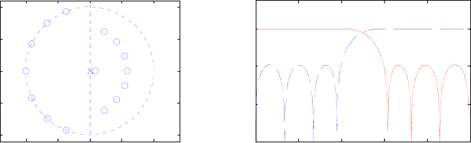
-1 -0.5 00.5 1
-1
-0.5
0
0.5
1
15
Real Part
Imaginary Part
00.2 0.4 0.6 0.8 1
-60
-40
-20
0
ω
/
π
Gain, dB
H
0
(z) H
1
(z)
M14.2 The following MATLAB programs can be used to design the analysis filters
corresponding to a two-channel QMF paraunitary lattice filter bank. (The program uses
the function fminu from the MATLAB Optimization Toolbox, which in turn uses the
functions cubici2, cubici3, optint, searchq, and updhess.)
% Program for the design of a two-channel QMF
% lattice filter bank.
Len = input('The length of the filter = ');
if (mod(Len,2) ~= 0)
sprintf('Length has to be an even number')
Len = Len+1;
end
ord = Len/2-1;
ws = 0.55*pi;
kinit = [1;zeros([ord,1])];
% set the parameters for the optimization routine
options = optimset('MaxIter', 2500, 'Display', 'off');
kfin = fminunc('filtopt',kinit,options,Len,ws);
e00old = 1;
e01old = kfin(1);
e10old = -kfin(1);
e11old = 1;
for k = 2:length(kfin)
e00new = [e00old 0]-kfin(k)*[0 e01old];
e01new = kfin(k)*[e00old 0]+[0 e01old];
e10new = [e10old 0]-kfin(k)*[0 e11old];
e11new = kfin(k)*[e10old 0]+[0 e11old];
e00old = e00new;
e01old = e01new;
e10old = e10new;
e11old = e11new;
end
E1 = [e00old;e01old];
h0 = E1(:);
scale_factor = abs(sum(h0));
h0 = h0/scale_factor;
E2 = [e10old;e11old];
h1 = E2(:);
Not for sale 573
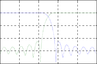
h1 = h1/scale_factor;
[H0,W] = freqz(h0,1,1024);
[H1,W] = freqz(h1,1,1024);
plot(W/pi,20*log10(abs(H0)), W/pi, 20*log10(abs(H1)));
grid on
title('Gain response of the analysis filters');
xlabel('\omega/\pi'); ylabel('Gain, dB');
function val = filtopt(kval,Len,ws)
e00old = 1;
e01old = kval(1);
e10old = -kval(1);
e11old = 1;
for k = 2:length(kval)
e00new = [e00old 0]-kval(k)*[0 e01old];
e01new = kval(k)*[e00old 0]+[0 e01old];
e10new = [e10old 0]-kval(k)*[0 e11old];
e11new = kval(k)*[e10old 0]+[0 e11old];
e00old = e00new;
e01old = e01new;
e10old = e10new;
e11old = e11new;
end
E1 = [e00old;e01old];
h0 = E1(:);
[H0,W] = freqz(h0,1,1024);
val = 0;
for k = 1:length(W)
if (W(k) > ws)
val = val+abs(H0(k))^2;
end
end
Due to the non-linear nature of the function to be optimized, different values of kinit
should be used to optimize the analysis filter's gain response. The gain responses of the
two analysis filters is as shown below. From the gain responses, the minimum
stopband attenuation of the analysis filters is observed to be about 23 dB.
00.2 0.4 0.6 0.8 1
-40
-30
-20
-10
0
10
Gain response of the analysis filters
ω
/
π
Gain, dB
H0(z) H1(z)
Not for sale 574
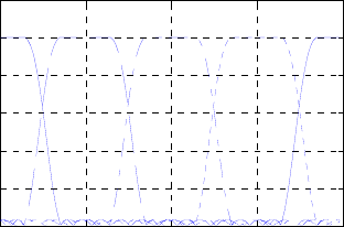
M14.3 The MATLAB program used to generate the prototype lowpass filter and the analysis
filters of the 4-channel uniform DFT filter bank is given below:
L = 19; f = [0 0.15 0.35 1]; m = [1 1 0 0]; w = [10 1];
N = 4; WN = exp(-2*pi*j/N);
plottag = ['- ';'--';'-.';': '];
h = zeros(N,L);
n = 0:L-1;
h(1,:) = remez(L-1, f, m, w);
for i = 1:N-1
h(i+1,:) = h(1,:).*(WN.^(-i*n));
end;
clf;
for i = 1:N
[H,w] = freqz(h(i,:), 1, 256, 'whole');
plot(w/pi, abs(H), plottag(i,:));
hold on;
end;
grid on;
hold off;
xlabel('\omega/\pi');ylabel('Magnitude');
title('Magnitude responses of the analysis filter bank');
The plots generated by the above program is given below:
00.5 11.5 2
0
0.2
0.4
0.6
0.8
1
ω
/
π
Magnitude
Magnitude responses of the analysis filter bank
H0(z) H0(z)H1(z) H2(z) H3(z)
M14.4 The first 8 impulse response coefficients of Johnston's 16A lowpass filter )(zH
L
are
given by
0.001050167, –0.005054526, –0.002589756, 0.0276414, –0.009666376, –0.09039223,
0.09779817, 0.4810284
The remaining 8 coefficients are given by flipping the coefficients left to right, From Eq.
(14.98), the highpass filter in the tree-structured 3-channel filter bank is given by
).()()(
2== zHzzHzH L115 −−
H
The two remaining filters are given by
and
)()()(
0zHzHzH LL
=22).()()(
1zHzHzH
H
L
= The MATLAB program used to
generate the gain plots of the 3 analysis filters is given by:
Not for sale 575
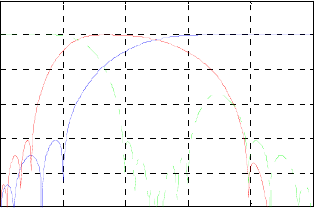
G1 = [0.10501670e-2 -0.50545260e-2 -0.25897560e-2
0.27641400e-1 -0.96663760e-2 -0.90392230e-1 0.97798170e-1
0.48102840];
G = [G1 fliplr(G1)];
n = 0:15;
H0 = (-1).^n.*G;
Hsqar = zeros(1,31); Gsqar = zeros(1,31);
Hsqar(1:2:31) = H0; Gsqar(1:2:31) = G;
H1 = conv(Hsqar,G); H2 = conv(Gsqar,G);
[h0,w0] = freqz(H0,[1]); [h1,w1] = freqz(H1,[1]); [h2,w2] =
freqz(H2,[1]);
g0 = 20*log10(abs(h0));g1 = 20*log10(abs(h1));
g2 = 20*log10(abs(h2));
plot(w0/pi,g0,'b-',w1/pi,g1,'r-',w2/pi,g2,'g-.');
axis([0 1 -120 20]);
grid on;
xlabel('\omega/\pi');ylabel('Gain, dB');
The plots generated are given below:
00.2 0.4 0.6 0.8 1
-80
-60
-40
-20
0
20
ω
/
π
Gain, dB
H
0
(z) H
1
(z) H
2
(z)
M14.5
Not for sale 576
