3D Forest User Guide 041

User Manual:

Open the PDF directly: View PDF .
Page Count: 38

3D Forest

User Guide

Release 0.41

A tool for processing of pointclouds acquired by terrestrial

laser scanning in forests

The Silva Tarouca Research Institute, Pub. Res. Inst.

Department of Forest Ecology.

Authors: Martin Krůček, Jan Trochta and Kamil Král

Table of content

Table of content ............................................................................................................. 3

About application .......................................................................................................... 5

Detectable attributes .................................................................................................... 6

Tree attributes ........................................................................................................... 6

Crown attributes ....................................................................................................... 7

Installation ...................................................................................................................... 8

Brief insight .................................................................................................................... 9

Application window description .............................................................................. 9

Cloud type description ........................................................................................... 10

Basic control ............................................................................................................ 11

Getting started ............................................................................................................. 12

Creating new project............................................................................................... 12

Creating new transformation matrix ................................................................ 12

Opening project ...................................................................................................... 13

Importing project .................................................................................................... 13

Importing data ......................................................................................................... 14

Terrain .......................................................................................................................... 15

Terrain from octree................................................................................................. 15

Terrain from voxels ................................................................................................. 15

Statistical outlier removal ....................................................................................... 16

Radius outlier removal ........................................................................................... 16

Manual adjustment ................................................................................................. 16

IDW interpolation .................................................................................................... 17

Vegetation .................................................................................................................... 18

Automatic segmentation ........................................................................................ 18

Manual segmentation ............................................................................................. 19

Trees ............................................................................................................................. 20

Tree cloud edit ......................................................................................................... 20

DBH cloud edit ........................................................................................................ 20

Tree position ............................................................................................................ 20

Position by lowest points ................................................................................... 21

Position RHT ........................................................................................................ 21

Diameter at breast height (DBH) ........................................................................... 21

DBH by randomized Hough transformation .................................................... 22

DBH by Least squares regression ..................................................................... 23

Tree height ............................................................................................................... 24

Tree length ............................................................................................................... 24

Tree planar projection ............................................................................................ 25

Convex planar projection ................................................................................... 25

Concave planar projection ................................................................................. 25

Stem curve ............................................................................................................... 27

Crowns .......................................................................................................................... 29

Set manual ............................................................................................................... 29

Set automatic........................................................................................................... 29

Volume by voxels .................................................................................................... 29

Volume and surface by cross sections .................................................................. 30

Volume and surface by 3D convex hull................................................................. 31

Crown intersections ................................................................................................ 31

Other Features ............................................................................................................. 33

Cloud merge ............................................................................................................ 33

Cloud subtraction .................................................................................................... 33

Voxelize cloud .......................................................................................................... 33

Create convex or concave 2D hull ......................................................................... 33

Remove duplicate points ........................................................................................ 34

Save into tiff ............................................................................................................. 34

Change background color ...................................................................................... 34

Exporting data ............................................................................................................. 35

Exporting clouds...................................................................................................... 35

Exporting tree or crown parameters .................................................................... 35

Exporting tree planar projection ........................................................................... 35

Export Stem Curve .................................................................................................. 36

Export intersections parameters ........................................................................... 36

References ................................................................................................................... 38

About application

The application 3D Forest was created to produce detailed information about

forest stands and trees using terrestrial laser scanning technology and its result –

clouds of points.

The application is released under the terms of the GNU General Public License v3

as published by the Free Software Foundation. For more information about

License you can view LIECNSE.txt file in program folder or visit web page

http://www.gnu.org/licenses/

Applications is programmed in C++ with dependencies on those libraries: VTK,

PCL, Eigen, Boost, Flann, LibLAS and Qt. For successful compiling user have to

build those libraries before 3D Forest.

For now on web site is provided source code for downloading and compiling on

any machine. User can also use compiled installer for Windows users together

with test data. All versions and datasets are available on site: www.3dforest.eu.

Detectable attributes

In current version of 3D Forest (0.4) one can calculate following tree and tree

crown parameters:

Tree attributes

Position:

Coordinates of tree base position (X, Y, Z) in Cartesian coordinates system.

DBH:

Diameter at breast height, tree stem diameter calculated from a sub-set of

points located in height from 1.25 to 1.35 m above the tree position. See

also: least squares regression and randomized Hough transformation.

Height:

Vertical distance (i.e. difference in Z coordinates) in meters between the

tree base position and the highest point of the tree.

Cloud length:

Largest distance between two points in Tree cloud (suitable for calculation

of length of highly inclined or lying trees).

Stem Curve:

The stem centers and diameters calculated by fitted circles in various

heights above the tree position (0.65m,1.3m, 2m, 3m, etc.).

Convex planar projection of the tree:

Polygon with the shortest possible boundary containing all points in tree

cloud orthogonally projected at the horizontal plain.

Concave planar projection of the tree:

Polygon with the smallest possible area containing all points in tree cloud

orthogonally projected at the horizontal plain.

Number of points

Number of points representing a single tree.

Crown attributes

Crown position:

Coordinates of tree crown position (X, Y, Z) in Cartesian coordinates

system computed from crown external points, more in section Crowns and

Volume and surface by cross sections.

Crown position deviation:

Deviation of crown position from the tree position, defined by distance (m)

and direction (°).

Crown bottom height:

Vertical distance (i.e. difference in Z coordinates) in meters between tree

position and height where first living branch is connected with stem.

Crown height:

Vertical distance (i.e. difference in Z coordinates) in meters between the

crown bottom height and the highest point of the tree crown.

Crown total height:

Vertical distance (i.e. difference in Z coordinates) in meters between the

lowest and the highest point of the tree crown.

Crown volume by voxels:

Crown volume computed from voxels with given size.

Crown volume and surface area using cross sections:

Crown volume and surface area computed from cross sections with given

height and concave hull threshold distance.

Crown volume and surface area by 3D convex hull:

Crown volume and surface area computed for object created by 3D

convex hull.

Crown intersections:

Volume and surface area for intersecting space between two crowns.

Installation

From the web site you can download installation wizard for windows that install

3D Forest into your computer. Wizard will guide you through the installation and

at the end you can launch 3D forest application.

Or you can choose to download the source code and compile it on your own. For

this you will need also some additional libraries like VKT, PCL, Qt, Eigen, Flann or

libLAS and compiler. We use mingw64 as cross-compiler for all dependencies

and for 3D Forest. Right now we are using modified version of PCL for point and

area picking in selection mode so contact the development team if you want to

obtain the libraries.

At the same address mentioned above you can also download sample data to

test and play with 3D Forest.

For uninstalling run the uninstall.exe file, located in the folder where software was

installed e. g.: C:\Program Files\3D Forest.

FIG. 1 INSTALLING WIZARD OF THE 3D FOREST APPLICATION

Brief insight

Application window description

FIG. 2 MAIN WINDOW DESCRIPTION

For user interaction we toolbars or menus in on top of the application window.

Toolbars are divided into logical sections – project bar with opening, creating

new, importing of project etc. Next toolbar affects the view of the clouds in

visualization area. Six icon represents six defined views of all displayed clouds.

Those are followed by two icons representing the change of the view –

ortoghonal and perspective projection. Tree and crown toolbars serve for

displaying of computed parameters.

On the left side is list of all clouds imported in project. The biggest part of

application window is vizualizetion area where selected clouds and parameters

are visualized. For information about selected cloud we use Statusbar where

information about selected methods or clouds area displayed. In the right

bottow corner is displayed progressbar when some action take place.

Cloud type description

All data imported into 3D Forest are stored in PCD (binary compressed

PointCloudData) file format. File contains coordinates of all points with intensity

value. For now only those 4 parameters of point representation are accepted.

Other information such as color and path to the file of transformation matrix are

in the MyProject.3df file.

While processing data in 3D Forest, one can meet different types of point clouds:

Base cloud:

Represents raw data imported in 3D Forest. The data should be

preprocessed in some other software (usually provided with the scanner),

where cloud fitting and registration are made. Base cloud embodies

points of all objects such as terrain, vegetation, buildings etc., which are

not differentiated.

Terrain cloud:

Using segmentation the base cloud can be divided into vegetation and

terrain – two main parts of forest ecosystem. The terrain cloud

represents ground surface and can be used for better calculation of tree

position or exported into GIS software for detailed (micro-) topography

analysis.

Vegetation cloud:

The part of the base cloud which is not terrain is labeled as vegetation.

From this pointcloud one can manually select trees and thus create

another cloud type – tree cloud.

Tree cloud:

This cloud represents single tree after manual segmentation. Only for tree

clouds it‘s possible to compute tree parameters like DBH, height, position,

etc.

Other:

Cloud representing unclassifiable points or points which do not belong to

any other cloud type. These clouds can be displayed or used as vegetation

for tree selection.

Basic control

Mouse button configuration in visualization area:

Left click Draw to rotate the view

Middle click Draw to zoom the view

Middle rotate Zoom the view

Right click Draw to move the view

Shift + left click Information about trees around selected point

Ctrl + left click Clockwise or counter-clockwise rotation

Context menu on cloud list (right button click on cloud name):

Delete Delete cloud from project and if needed from the disk

Color Change color of cloud

Color by field Set color of points in cloud by selected field (axis x, y, z and

intensity)

Point size Change size of points in cloud

All Clouds ON All clouds in project are visible

All clouds OFF All clouds in project are invisible

Keyboard:

p, P : switch to a point-based representation

w, W : switch to a wireframe-based representation (where available)

s, S : switch to a surface-based representation (where available)

+ / - : increment/decrement overall point size

g, G : display scale grid (on/off)

u, U : display lookup table (on/off)

r, R : reset camera

f, F : focus on point

x, X : selection (in selection mode)

o, O : perspective (on/off)

Alt + : show and allow quick access keys in menu (underlined character)

Tips:

– Switching to wireframe or point based representation affects only the displayed characters,

polygons and lines, not point clouds.

– Scale grid show correct values only when perspective is off.

– Display lookup table show values extent and color range if Color by field is used.

Getting started

After installing and launching the application few steps need to be done for

proper use. The following tasks are necessary: to set up working project, import

data and segment data to terrain, vegetation and trees to be able to compute

tree and crown parameters.

Creating new project

For creating new project go to Project → New Project.

Or click on the New Project icon in Project toolbar -> .

In Project manager window set a name of your project (without spaces) and

folder, where you want to save your project. In this folder a new folder with the

project name will be created and all files of the project will be stored there, i.e.

project base file (MyProject.3df) and all imported clouds.

Next step is to set transformation matrix. Transformation matrix serve for

reducing number of digits in coordinates values for faster data management

(saving RAM). It is possible to select from existing matrices or create a new

matrix. For creating new matrix set name of matrix and values for transform

imported data. If you are not sure about your data extend, you can use

NO_MATRIX form the list.

Data are transformed in to new coordinate system automatically while importing

(only when importing .pcd files you can choose if you want to use transformation

or not), exported data from 3D Forest are transformed back into original

coordinate system. It is possible to use only one transformation matrix in each

project.

Creating new transformation matrix

For creating new transformation matrices it’s necessary to know exact extent of

your data coordinates. The goal is to set into transformation matrix as big

number as possible while the data extent remains constant. See the table 1 with

example below.

TAB. 1 TRANSFORMATION MATRIX APPLICATION ON SPATIAL DATA

Original

data extent

Transformation

matrix

Data extent after

transformation

max. x

18857748,76

-18857100

648,755

min. x

18857104,96

4,96

max. y

987657123,6

987656800

-323,55

min. y

987656816,6

-16,55

max. z

425,33

min. z

358,13

In this case (Tab. 1) it isn´t necessary to set the transformation value for Z axis,

because the number is quite short. But in case, when the values are really long

(e.g. X, Y axis) numbers without transformation may be rounded if they exceed

the limit of the data type (float, 32 bit). Visualized data then would have regular

structure (points would be in rows and columns) and computational operations

would lose precision.

Opening project

To open a project go to Project→ Open Project.

Or click on the Open Project icon in Project toolbar -> . In new dialog select

your project file (file with extension .3df).

Importing project

Since projects save its path, just copy of it in another location (disc or directory)

can broke the project. If such change of directory is needed, you can import old

project into new location.

Go to Project → Import Project.

Or click on the Import Project icon in panel-> .

In the dialog window choose the path to the old project, set a name of the new

project and location where the new project will be created. In this folder the new

folder with the project name will be created and all data files will be moved

there. It is also possible to select the option for removing old project from disk

after the import.

Importing data

For importing data into your project go to Project → Import and choose which

type of data you want to import.

It is possible to import data in following formats: .txt, .xyz, .las, .pts, .ptx. If you

already have data in 3D Forest native format (PCD) choose appropriate cloud

type for your data (see Cloud type description) and set if you want to use project

transformation matrix. After importing data will be visible in visualizer area and

in list of project clouds.

Terrain

For terrain adjustment one can use following two automatic methods.

Frequently, results produced by each method are not perfect, for that reason

you can combine them, filter the noise points and there is also a possibility of

manual adjustment.

Terrain from octree

Go to Terrain → Terrain from octree.

In the dialog window select the base cloud from which you want to extract the

terrain, enter a name of the new terrain cloud, a name of the cloud where the

rest of data (usually vegetation) will be stored, and set the resolution (edge

length of cubes in cm).

Input cloud is divided into cubes. Cubes which contain points and have the

lowest z-value are considered as the “ground cubes”. Terrain is then defined by

the points in the ground cubes.

This means that all the points in ground cubes are considered as terrain and

contrary to voxelization there is no reduction of points and no generalization.

This method is more laborious for manual post processing, but the results are

more detailed and created by original points.

Terrain from voxels

Go to Terrain → Terrain from voxels.

In the dialog window select the base cloud from which you want to extract the

terrain, enter a name of the new terrain cloud, a name of the cloud where the

rest of data will be stored and set the resolution of voxelization (length of voxel

edge in cm).

Input point cloud will be reduced into voxels and centroids of voxels (i.e. points

with average coordinates from all original points within individual voxels) with

the lowest z-values will define the terrain.

With increasing voxel size increases also overestimation of terrain height (z-value

of centroids is affected by more points which lie above the terrain). But the

manual post-processing is usually a bit faster than after Terrain from octree

method because resulting cloud contains fewer points. With appropriate

resolution (50 cm and less), the method produces applicable results.

Statistical outlier removal

For filtering terrain cloud from voxels or octree using statistical outlier removal

go to Terrain → Statistical outlier removal. In the dialogue window select terrain

cloud, set the name for cloud with removed points and set number of neighbors

for computing mean distance and standard deviation. Points with mean distance

longer than standard deviation are removed. For more details see the PCL

documentation.

Radius outlier removal

For applying radius outlier removal filter to terrain cloud go to Terrain → Radius

outlier removal. In the dialogue window select terrain cloud, set the name for

cloud with removed points, set the radius and the number of neighbors. Points

with less neighbors in given radius than was adjusted are removed. For more

details see the PCL documentation.

Tips:

– If too much or too few points was removed by filters use Cloud merge feature and repeat the

procedure.

– For best result combination of both filters is recommended.

– Note that different voxel size and various initial cloud density (when Terrain from octree is used)

need different filters settings.

– Both filters are better to use with cloud created by Terrain from voxels due its regularity.

Manual adjustment

Results of automated methods of terrain extraction described above can be

adjusted by manual editing. Go to Terrain → Manual adjustment, select terrain

cloud for editing and set a name for a new cloud where points removed from

terrain cloud will be saved.

After pressing “x” you can draw the selection box by the left mouse button. The

selected points will be removed from the terrain file and stored in the separate

file defined above.

For step back press undo icon -> in top panel. Or you can use split

function that creates user-defined width strips of terrain or easier point

selection. With arrows user can switch the strips. For ending the strip selection

click again of the icon of split function.

After finishing all edits press Stop EDIT icon -> in the top panel and all

changes will be saved in the original (input) terrain cloud.

IDW interpolation

Areas with missing terrain points (typically obscured by thick trees or located

right under the scanner during scanning) may be filled in by Inverse Distance

Weighted interpolation from the surrounding terrain points.

Go to Terrain → IDW, select input terrain cloud for interpolation, set a resolution

of interpolation in cm, a number of the closest points (n) to be included in

interpolation and a name for the new interpolated terrain cloud, which will be

free of empty areas.

The interpolation uses n closest points of the original terrain to estimate Z value

of the new terrain point according to this formula:





n

Z = new computed Z coordinate; Zi = Z coordinate of know point; Wi = distance

from the i-th point to the new point; n = number of surrounding points.

Vegetation

After terrain extraction in project are present two types of cloud – terrain and

vegetation cloud. This needs to be segmented into single trees to finally get the

desired tree parameters. Right now two methods are implemented in 3D Forest –

automatic and manual segmentation.

Automatic segmentation

Automated segmentation can be found in Vegetation → Automatic tree

segmentation. In 3D Forest we present automatic approach based on distance

between points and minimal number of points forming clusters and an angle

between centroids of the clusters.

In the dialog window you have to select the vegetation cloud that you want to

segment into trees, terrain cloud, minimal distance of points in cluster (S),

minimal count of points in cluster (N), prefix of the segmented trees and name of

the non-segmented points.

In the first step of segmentation the whole vegetation is divided into horizontal

slices with user-defined input size [cm]. Within these slices the clusters with user

defined minimal number of points N and maximal distance S between two

nearest points are constructed. Next step is to reconstruct bases of the trees. For

each cluster with centroid height lower than 1.3 m above terrain the 10

neighboring (nearest) clusters up to distance 2S are found. We suppose those

clusters come from the same tree base. All such clusters are merged into

segments and tested if they are formed by at least 5 clusters and if the maximal

dimension of segment is at least 1 m to be identified as the tree.

When all segments are tested and evaluated, we use different approach to add

more clusters to the tree. A cluster is added to the tree if its centroid lies within

the distance 4S to the nearest centroid of the tree and the angle between the

vector of these two centroids and the Eigen vector of the 5 closest centroids of

the stem is less than 10 degrees. For resting clusters we test distance between

cluster points and tree points and if the cluster fit condition of S are joined to the

tree. At the final step all resting points are tested if they can be joined to any tree

according to rising distance (maximaly to 3S). Automatically segmented trees can

be visually checked and in case of need adjusted by manual segmentation.

Manual segmentation

For manual tree segmentation (or segmentation of other vegetation) go to

Vegetation → Manual tree selection.

In the dialog window select a source cloud with vegetation to be segmented and

set a name of the cloud where the rest of un-segmented points will be saved. A

name of the cloud with segmented tree (i.e. the tree cloud) will be set later.

Press “x” and draw the selection box by the left mouse button. Selected points

will be removed from the view. You can use undo icon if needed. The goal is to

remove all points not belonging to the target tree. After finishing the edits (i.e.

only the target tree is in the view) press Stop EDIT icon -> and set a name of

the new tree cloud file (e.g. Tree1). After that you can continue by segmentation

of the next tree (all the removed but un-segmented points will re-appear) or

terminate the segmentation.

After segmenting all the trees, some vegetation points belonging to trees (e.g.

isolated branches) may remain in the un-segmented vegetation file. These points

may be attributed to any of the segmented trees. For this use the function Cloud

merge.

Tips:

– Larger areas are recommended to split in smaller tiles for better visibility and easier handling.

This may be made in various software (e.g. LAStools by Rapidlasso).

– The segmented trees are removed from the edited vegetation cloud, which leads to its gradual

simplification. Thus, the simple and/or stand-alone trees are suggested to be segmented first

and the most complex tree neighborhoods at the end.

– If only tree position and DBH is required it is not necessary to segment the whole trees. For

these tree parameters it’s enough to separate only bottom part of the stem (about 2 meters

above the terrain).

– During the segmentation, if you are not sure whether the points belong to the target tree or to its

neighbors, you can display the neighboring tree clouds and/or the vegetation cloud by checking

the box in the tree widget.

Trees

This menu serves for computing of tree parameters or editing of tree cloud. Each

menu is described in following sections.

Tree cloud edit

I f you need to remove some point from an existing tree cloud go to Trees → Tree

cloud edit.

In the dialog window select which tree you want to edit and set a name for a new

cloud where the removed points will be saved. For removing points use the same

procedure used for manual segmentation.

DBH cloud edit

If the results given by functions for DBH computation (Diameter at breast height

(DBH)) are inappropriate, you can display and edit the point cloud used for the

calculation.

Go to Trees → DBH cloud edit and select tree of which DBH cloud you want to edit.

Then you can remove outlying points by pressing “x” and drawing the selection

box by left mouse button. The selected points won’t be removed from the tree

cloud, but will be temporarily (during one 3D Forest session) excluded from the

DBH computation. As you close the project, DBH edits are canceled.

Tree position

Tree base position is a key parameter providing a baseline for computation of

other tree parameters such as DBH, tree height and stem curve and affects also

the visualization of convex/concave tree projection. Therefore, none of these

functions are available until the tree position is calculated. Actual tree position

may slightly vary according to the computation method used (Fig. 3). Changing

the method of position calculation thus affects also other calculated tree

parameters and these are always automatically modified according to the

actual tree position. Therefore, be always aware which method of tree position

calculation are you actually using for particular trees.

In addition, both methods may be calculated with / without the use of the terrain

cloud for adjustment of the Z coordinate of the tree base. We strongly

recommend always using terrain adjustment if the terrain cloud is available. The

tree base position is then less affected by the lowest outliers of the tree cloud

(Fig. 3), which is particularly important on steeper slopes. Yet, the possibility to

calculate tree positon without terrain is preserved for cases when the terrain

cloud is missing for some reason. To show/hide currently computed positions

use icon ->

Position by lowest points

For calculating the tree position go to Trees → Position lowest points and in the

dialog window select for which tree(s) you want to calculate the position of the

tree base and set the vertical distance [cm] from the lowest point of the tree(s)

for the selection of tree points included in the calculation. Also select terrain

cloud, if available, for adjustment of the Z coordinate to terrain level and set the

number of the closest terrain points (N) used for that adjustment. Position is

displayed as a sphere with the center at the position and with the radius of 5 cm.

The XY position is computed as a median coordinates of tree points lying

vertically up to the user defined distance from the lowest point of the tree cloud.

The Z coordinate is defined as the median Z value of N closest points of terrain at

that XY position. If no terrain cloud is available, the Z value is defined by the

lowest tree point.

Position RHT

For obtaining tree position computed by randomized Hough transformation go

to Trees → Position RHT and in the dialog window select for which tree(s) you want

to calculate the tree base position and set the number of RHT iterations (min 200

recommended). Also select terrain cloud, if available, for adjustment of the Z

coordinate to terrain level and set the number of the closest terrain points (N)

used for that adjustment. This function compute tree position using centers of

two circles fitted by RHT to the stem at 1.3 and 0.65 m above the position

mentioned above if previously computed. If no initial positon is present, it uses

the lowest point of the tree cloud. The RHT position is then defined by the point,

where vector heading from upper center (1.3) thru lower center (0.65) intersects

the horizontal plain defined by median Z value of the N closest points of the

terrain cloud.

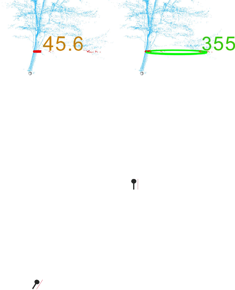
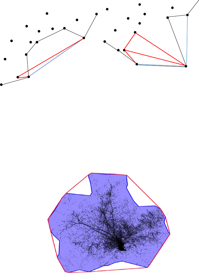
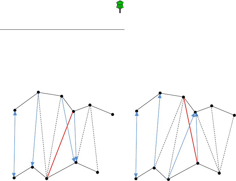
Diameter at breast height (DBH)

The diameter at breast height (DBH) is computed from the subset of points of

the tree cloud, which lie between 1.25 and 1.35 m above the tree base position

(so called DBH cloud). It is highly recommended to build on the tree position

adjusted to terrain level as mentioned above (section 7.3), otherwise DBH might

be significantly biased (Fig. 3).

There are two methods of DBH estimation implemented in 3D Forest: i)

randomized Hough transformation (RHT) and ii) least square regression (LSR).

Both use the same DBH cloud, but there may be considerable differences

between the results. RHT usually gives better results, because the LSR function

frequently overestimates the diameter value in the presence of outlying points.

The usual reason of the big difference between both methods is that the subset

of points from which DBH is calculated includes overhanging branches or points

which do not belong to tree point cloud (i.e. the tree was not segmented

appropriately). This may be fixed by the Tree cloud edit function (7.1) or by the

DBH cloud edit function (7.2), where only the tree points in the subset 1.25 –1.35

m above the ground are adjusted.

FIG. 3 DIFFERENCES BETWEEN DBH COMPUTED ACCORDING TO THE TREE POSITION NOT ADJUSTED TO TERRAIN

LEVEL (LEFT) AND DBH RECOMPUTED WITH TERRAIN CLOUD (RIGHT).

DBH by randomized Hough transformation

For computing DBH using randomized Hough transformation go to Trees -> DBH

RHT and in the dialog window select for which tree(s) you want to calculate it and

set the number of iterations. The number of iterations is a trade-off between

computation time and accuracy. We recommend at least 200 iterations for fast

computation. The use of 2000 iterations is much slower, but provides fairly

consistent results. Resulting DBH will be displayed as a 10cm high cylinder with

the diameter of the best fitted circle. To show/hide the computed DBH RHT use

icon ->

Description:

The method consists in founding parametric description of objects and transformation of Cartesian

coordinates system to polar coordinate system. First, the DBH subset of the tree cloud (i.e. from 1.25 to

1.35 m) is projected to a horizontal plain (Z coordinates are transformed to 1.3m). Then, for each point

the method searches every possible center of the circle. The most frequent circle center is then selected

as a resulting center (Xu and Oja, 1993).

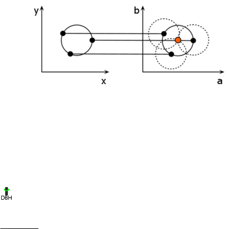
Circle is parametrically described as:

r2 = (x - a)2 + (y - b)2

which can be written as two equations:

x = a - r * cos (δ)

y = b - r * cos (δ)

Where: r = radius

(a,b) = coordinates of the center

(x,y) = coordinates of a point on the circle

δ = angle, where the center could be

FIG. 4 SEARCHING CENTER FOR CIRCLE WITH KNOW PARAMETER. (MCDONALD J. 2014).

DBH by Least squares regression

For computing DBH using Least squares regression go to Trees → DBH LSR and in

the dialog window select for which tree(s) you want to calculate it. Resulting DBH

will be displayed as 10cm high cylinder with center and diameter of the best

fitted circle. The LSR method is very sensitive to points not representing the tree

stem (Fig.5). Therefore it is more suitable to apply this tool to the tree clouds

where only stems are segmented. To show/hide computed DBH LSR use icon ->

Description

First, the DBH subset of points lying between 1.25 and 1.35 m is projected to a horizontal plain (Z

coordinates are transformed to 1.3m). Then the circle is fitted to these points by the Least squares

regression. The method is based on minimizing mean square distance between fitted circle and data

points, for circle fitting Gauss-Newton method is used (Chernov and Lesort, 2003).

FIG. 5 DIFFERENCES BETWEEN RHT (LEFT) AND LSR (RIGHT); WRONG VALUE GIVEN BY LSR IS CAUSED BY AN

OVERHANGING BRANCH, WHICH WAS INCLUDED IN AUTOMATICALLY DEFINED DBH SUBSET (RED DOTS) OF THE

TREE CLOUD.

Tree height

For obtaining tree height go to Trees → Height.

In the dialog window select for which tree(s) you want to calculate the height. The

result is displayed in meters at the top of the tree. The tool also displays a

vertical line from the tree position to the height of the highest point. To

show/hide the calculated heights use icon ->

Tree length

For calculation of tree cloud length go to Tree → Length.

In the dialog window select for which tree cloud(s) you want to calculate the

length. The tool calculates Euclidean distance between two the most distant

points in the tree cloud and displays their connecting line. The cloud length value

(in meters) is displayed at the bottom of the tree. The tool is suitable for

calculation of the real length of inclined or lying trees. To show/hide the lengths

use icon-> .

Tree planar projection

Convex planar projection

For computing tree convex planar projection go to Trees → Convex planar

projection.

In the dialog window select for which tree cloud(s) you want to calculate the

projection. The tool calculates and displays the area of convex hull of the tree

cloud orthogonally projected to the horizontal plane in the tree base height.

Then it is possible to use the show/hide icon -> .

The result can be exported/imported to the ArcGIS polygon shapefile (see

Exporting tree planar projection). The calculation is based on the Gift wrapping

algorithm (Rosén et al., 2014).

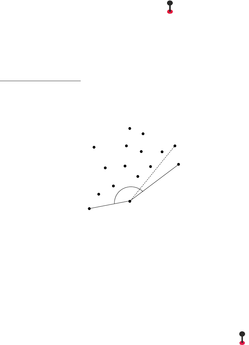
Algorithm description:

In the first step point with the lowest y value is found. This point (A) is the first and the last point in the

polygon. For each point (X) in the point cloud the angle between vector (-1,-1) and a vector given by

points A and X is then calculated. The point with largest angle(α) is selected as the second point in the

polygon. Other points of the polygon are added similarly, only the vector (-1,-1) is replaced by a vector

given by last two points in polygon. This continues until the added point is equal to the first point.

FIG. 6 NEXT POINT TO CONVEX HULL

Concave planar projection

For computing tree concave planar projection go to Trees → Concave planar

projection.

In the dialog window select for which tree cloud you want to calculate the

projection and set the maximum edge length in cm. The tool calculates and

displays the area of orthogonal concave tree projection to the horizontal plane in

the tree base height. Then it is possible to use the show/hide icon-> .

The result can be exported/imported to the ArcGIS polygon shapefile (see 9.2). The calculation is based

on the Gift wrapping algorithm and modified Divide and conquer algorithm (Rosén et al., 2014)

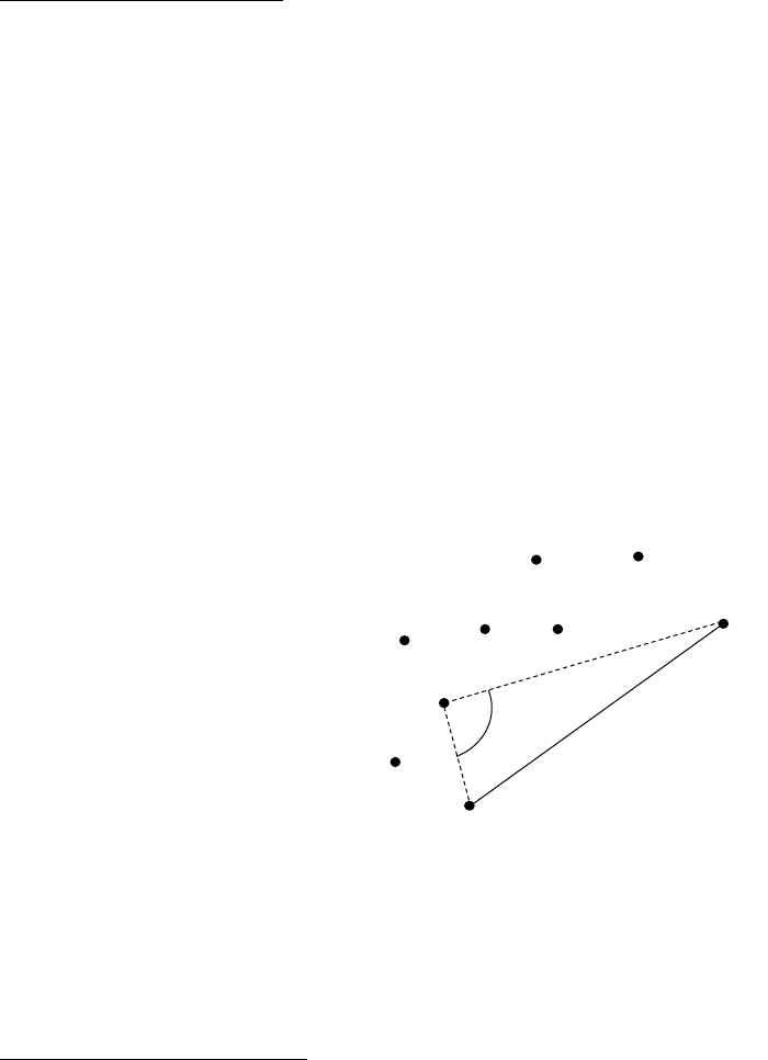
Algorithm description:

In the first step, the convex hull is computed as mentioned in previous section. Then edges longer than

initial threshold/searching distance (TD, set by user) are found. Those edges are split in the next step

and the algorithm looking for points inside the polygon is as follows:

A, B are adjacent points of the convex hull and X is a point tested to be added in between them.

Step 1: If the distance between A and X (AX) is shorter then TD and BX < AB, or BX < TD and AX < AB.

Then X is considered a possible candidate. If more than one point complies with these rules, the one

with biggest α (see below) is selected.

Step 2: In case that the point was selected the algorithm continues with edge AX or BX if one of them is

longer than TD, etc..

Step 3: In some cases it may happen that some edges are not splitted, because no points satisfy the

conditions in step 1. In this case the algorithm increases TD by 10 cm and repeats the splitting

procedure. This continues until all edges are shorter than TD.

FIG. 7 SEARCH OF A POINT TO CONVEX HULLL

Theoretical background:

Conditions described in step 1 avoid too sharp angles in new polygon. Also new edges, created by

splitting, must be shorter than the older one, because sometimes outliers occur in the point cloud, which

may cause that there are no other points to split the edge.

FIG. 8 BLUE LINE WAS SPLITTED, RED LINE CONNECTS POINTS WITH TOO SHARP ANGLE (LEFT), RESULTING

POLYGON IS BLACK; POSSIBLE ISSUE WHEN B IS AN OUTLIER AND ADDING A NEW EDGE LONGER THAN THE

ORIGINAL ONE IS ALLOWED. AB WAS DIVIDED FIRST, THEN BC, BLUE LINES ARE ORIGINAL EDGES OF THE CONVEX

HULL, BLACK IS A NEW CONCAVE HULL, RED LINES CONNECT POINTS WHICH WERE INCORRECTLY SELECTED

(RIGHT), IN THIS CASE EDGE AB IS RETAINED BECAUSE ALL POSSIBLE NEW EDGES ARE LONGER THAN THE ORIGINAL

ONE, RESULTING POLYGON IS IN BLACK.

FIG. 9 PLANAR PROJECTION OF THE SAME TREE, CONVEX (RED), CONCAVE (BLUE).

Stem curve

For obtaining stem diameters in 1 m intervals go to Trees → Stem Curvature. The

stem diameters are computed as circles by Randomized Hough transformation

(see DBH by randomized Hough transformation) from 7 cm high slices of the tree

cloud. They are displayed as 7 cm high cylinders defined by the RHT fitted circles;

the number of RHT iterations may be set by the user. The algorithm starts with

computing first the stem diameter at 0.65 m above the ground, then at 1.3m and

2m above the ground and then continues computing diameters with 1 m spacing

until the new diameter is two times wider than both previous two diameters.

Because numerous circles are fitted to each tree, the higher number of RHT

iterations significantly increases the computational time. Though, for higher

accuracy more iterations are recommended. The fitted circles can be

shown/hidden using -> icon. See also chapter Export Stem Curve.

Crowns

To begin work with crowns at least tree position and height has to be computed.

Crown heights, position and position deviation is computed automatically, all

three parameters are recomputed automatically when tree position is changed.

Position is computed as average coordinate from external points. External points

are 2D concave hulls of cross sections with threshold distance (see Concave

planar projection) 1 m, section height is 1 m. To show/hide external points use -

> icon. For resetting external points with different section parameters (height,

threshold distance) see chapter Volume and surface by cross sections.

Set manual

For adjusting crown cloud manually go to Crowns → Set manual and select tree

for which you want adjust the crown, than remove stem points by routines

commonly used in 3D Forest.

Set automatic

For adjusting crown cloud automatically go to Crowns → Set automatic, in the

dialog window select for which tree cloud you want to adjust crown.

Algorithm description:

In the first step, cross sections along the z axis with height 0.5 m are created and width of each section

is computed as the average from section x and y axis extensions. Than sections widths are compared

one by one from the lowest to the highest. If three consecutive sections are wider more than 25 % the

last section before is marked as starting place for detailed search.

The detailed search begin by computing two superimposed stem diameters (by LSR) from subset of

points with height 10 cm. From these diameters the center of following diameter is predicted. For

diameter computation only points closer than previous diameters times two are used. This should avoid

influence of overhanging branches. Predicting the new diameter center and diameter computation

continuous while difference between last two diameters is smaller than 25 %.

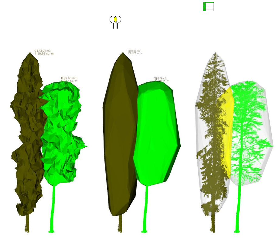
Volume by voxels

For computing crown volume by voxels go to Crowns → Volume by voxels, in the

dialogue window select the three and set voxel size in cm. Resulting volume is

shown in project attribute table . Voxels are not visualized due its

visualization ambitiousness.

Volume and surface by cross sections

For computing crown volume and surface area by cross sections go to Crowns →

Volume and surface by sections, in the dialogue window select tree, set section

height and threshold distance for section concave hull. In case that other than

implicit values are set the crown position and position deviation is recomputed

with external points extracted by this new parameters. Crown volume is

computed as total amount of sections volume, each section volume is than

computed by its planar projection area (created by concave hull) times section

height. Surface area is computed by strip triangulation, however the algorithm

(description below) works fine, in some cases intersecting triangles may occur. To

show/hide resulting objects use -> icon.

Triangulation algorithm description:

For triangulation, polygons created by concave hull for each section are used (z coordinates of polygon

vertices are not aligned as in planar projection). Top and bottom of the crown is triangulated by creating

triangles between highest/lowest point of the crown and highest/lowest polygon edges. The rest is

triangulated by strip triangulation of two superimposed polygons. This may cause intersecting tringles,

not within triangulated strip but between two superimposed strips.

First step of strip triangulation is computing connecting edges between sections polygons as nearest

neighbors point from the other polygon for each point. Edge intersecting is not allowed (Fig. 10a,b)

Fig. 10a,b Possible options for creating connecting edges between sections. In both cases,

edge 1A,1B is given as first, blue lines are created shortest edges, dashed line are possible

options to choose, red is not allowed line, a) leading polygon is A, possible connections for

point 3B are constrained to points 2A,3A, next step is selecting point for point 5A, b)

leading polygon is B, possible connections for point 3A are constrained to points 2B,3B,

next step is selecting point for point 5B.

Total length of edges might be various depending on a) which edge is used as leading for nearest

neighbor searching (for points from this polygon are nearest neighbors searched from the other polygon,

Fig. 10a,b), b) which two points are selected as the first edge. For creating first edge two approaches

are used. Implicitly, first point in each polygon is the point with lowest y coordinate, so the first edge

connecting first points in polygons, or the shortest possible edge between polygons is found and used

as first edge. This create four options to select set of edges with shortest total length. After that, we

have set of edges where each point in both polygons is connected with at least one point from the other

edge. Next step is to create triangles using polygon edges and connecting edges. Each triangle is

created by one polygon edge and two connecting edges. If new connecting edges has to be added, the

shortest one is used (Fig. 11).

Fig. 11 Black lines are polygons, blue are original set of connecting edges, green are new

edges.

Volume and surface by 3D convex hull

For computing crown volume and surface area by 3D convex hull go to Crowns →

Compute 3D ConvexHull, in the dialogue window select tree and check the check

box for computation using all crown points is needed. For computation of 3D

Delaunay triangulation and mesh parameters (volume and surface area) VTK

libraries is used. Only external points and points belonging to lowest and highest

section are used implicitly. This provide significant decreasing of computational

time costs and mostly produce the same results as if computation using all

crown points is used. To show/hide resulting shapes use -> icon.

Crown intersections

For computing crown intersections go to Crowns → Intersections. All existing

crowns are tested for intersections. Existing intersection between two crowns is

computed using VTK as Boolean AND in 3D space. Computing intersections is

only possible using convex shapes, thus volume and surface by 3D convex hull

has to be computed first to create a 3D objects.

For intersecting crowns following parameters are computing: horizontal angle

(azimuth), vertical angle (from horizontal plane) and distance from crown

position to intersection center of gravity, intersection volume and surface area.

Those parameters are shown in Intersections table by -> icon. Intersecting

parts can by shown/hide by -> icon, line connecting crowns positions with

intersection center of gravity and angles are also visible.

Fig. 12 a) shapes defining crown volume and surface by sections, b) crown 3D convex hull,

c) crowns intersection (yellow).

)

Other Features

This menu serve for various function that can be applied to all clouds.

Cloud merge

For joining two point clouds into a new cloud go to Other features → Cloud merge.

In the dialog window select the clouds to be merged, set a name of the new

cloud, select its type (e.g. Tree, Base etc.) and check the box if you want to delete

the input clouds.

Cloud subtraction

For cloud subtraction go to Other features → Cloud subtraction.

In the dialog window select the point clouds to be subtracted and set a name of

the resulting cloud.

The tool subtracts a smaller cloud from a bigger cloud. Identical points in both

clouds are removed from the bigger cloud and the result is saved as a new cloud.

Voxelize cloud

For reduction of the point cloud density go to Other features → Voxelize cloud.

In the dialog window select the cloud you want to voxelize, set a name of the

voxelized point cloud and the size of the voxels in cm. The tool generates a

voxelized point cloud from the input point cloud. The voxelized point cloud is

formed by centroids of voxels that included at least one point of the original

point cloud.

Create convex or concave 2D hull

For creating convex/concave hull of any cloud go to Other features → Create

convex hull or Other features → Create concave hull.

These functions calculate convex/concave hull of orthogonal projection of the

cloud into the horizontal plane in the height of the lowest point and save it as a

new cloud (type Others). For computing the same algorithms as described in

chapters Convex planar projection and Concave planar projection are used.

Anticipated usage is for creating a layer with the same extent and boundaries as

the area in 3D Forest. May be used to transfer different areas of interest from 3D

Forest to any GIS.

Tip:

– For importing this data into ArcMap and creating polyline or polygon, export the hull cloud as .txt

(Data export is described in chapter Exporting data ).

– Open it in ArcMap and use function POINTS TO LINE in DATA MANAGEMENT TOOLS → FEATURES

and then FEATURE TO POLYGON at the same place.

Remove duplicate points

To removing redundant points go to Other features →Remove duplicate points and

select the cloud for filtering.

As 3D Forest can process large point clouds, the filtered point cloud is

divided into smaller point clouds using octree search (octree resolution is 20 cm)

and each cloud is separately voxelized with 1 mm voxel size, after that the clouds

are merged together. This allow also better computation power utilization.

Save into tiff

For saving current view from visualization area go to Other features → Save into

tiff and set name for the .tiff file and the destination folder.

Change background color

For changing background color in the viewer go to Other features → Change

background color and select new color.

Exporting data

All data exported form the 3D Forest are re-transformed to the original

coordinates system.

Exporting clouds

For data export go to Project → Export and choose the format in which you want

to save your data (.txt, .ply or .pcd file format), then select the cloud for export

and set a name and location for the new file.

Exporting tree or crown parameters

For exporting all calculated tree parameters in a tabular output go to Trees →

Export tree parameters, or Crown → Export crown parameters and then set a name,

location and separator of the exported .txt file. Only the actually calculated tree

parameters will be exported; the rest will be exported as -1 value.

Exporting tree planar projection

For exporting planar projections of trees go to Trees → Export convex planar

projection or Trees → Export concave planar projection, then set a name and

location of the new file. Planar projection for all trees will be exported in one file.

Those projections that weren´t computed previously during current 3D forest

session are are not exported.

Both functions create .txt file with coordinates of vertices of the polygon in

following format:

Tree ID;Xstart;Ystart;Xend;Yend;Z

Tip:

For importing this data in ArcGIS and creating polygon or polyline shapefiles:

– Add exported file into your project.

– Use function XY TO LINE in ARCTOOLBOX → DATA MANAGEMENT TOOLS → FEATURES. Which

creates a new layer containing geodetic line features constructed based on input files.

– To create a closed polyline from this layer use function UNSPLIT LINE in ARCTOOLBOX → DATA

MANAGEMENT TOOLS → FEATURES.

– Now it is possible to use function FEATURE TO POLYGON in ARCTOOLBOX → DATA MANAGEMENT

TOOLS → FEATURES, if polygons are not overlapping.

– In order to create overlapping polygons, one of the possible solutions is to use Tools for

Graphics and Shapes, available at http://www.jennessent.com/ for free. And use CONVERT

POLYLINES TO POLYGONS function.

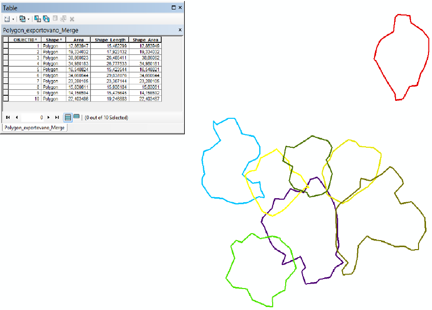
FIG. 13 POLYGONS OF CONCAVE TREE PLANAR PROJECTION IMPORTED IN ARCMAP.

Export Stem Curve

For exporting stem curve go to Trees → Export Stem Curve, select for which tree

you want to export the stem curve, specify file name and destination folder.

Exported file is in .txt format with following structure:

Tree name diameter: 70.6 67.6 64.6 ….. -1 -1 -1

Tree name x: 182.474 182.5 182.455 ….. -1 -1 -1

Tree name y: -1594.55 -1594.56 -1594.57 ….. -1 -1 -1

Tree name z: 1017.6 1018.25 1018.95 ….. -1 -1 -1

Diameters and center coordinates of fitted circles are in ascending order from

0.65 to 1.3, 2 etc. The values -1 at the end of line indicate irrelevant data

(diameters which were impossible to calculate due to the crowns)

Export intersections parameters

For exporting intersections parameters go to Crowns → Export intersections

parameters, in dialogue window set name of new file and destination folder.

Parameters are exported in txt file with following structure: tree name, name of

intersecting tree, intersection volume (m3), surface area of the intersection (m2),

horizontal angle (°) vertical angle (°), distance (m). As separator is used

semicolon.

Example:

name;intersecting with;volume;surface;horizontal angle;vertical angle;distance

tree_3.pcd;tree_4.pcd;314.142;381.171;240.260;38.120;3.380

tree_4.pcd;tree_3.pcd;314.142;381.171;86.770;1.270;4.840

References

Chernov, N. and C. Lesort (2003). Least squares fitting of circles and lines. arXiv

preprint cs/0301001.

McDonald, J. (2014). The Hough Transform-Explained and Extended. [online]

cited 17.7.2014. Available at:

www.cis.rit.edu/class/simg782.old/talkHough/HoughLecCircles.html.

Rosén, E., E Jansson and M. Brundin (2014). Implementation of a fast and

efficient concave hull algorithm. Available at:

http://www.it.uu.se/edu/course/homepage/projektTDB/ht13/project10/ Project-

10-report.pdf. Project Report. Uppsala University.

Rusu, R. B., S. Cousins and Ieee (2011). 3D is here: Point Cloud Library (PCL). 2011

Ieee International Conference on Robotics and Automation (Icra).

Xu, L. and E. Oja (1993). Randomized Hough transform (RHT): basic mechanisms,

algorithms, and computational complexities. CVGIP: Image understanding 57(2):

131-154.

3D Forest User Guide 041

Navigation menu

Versions of this User Manual:

Views

Navigation