UCLA Physics 4AL Lab Manual V37

User Manual:

Open the PDF directly: View PDF .
Page Count: 126 [warning: Documents this large are best viewed by clicking the View PDF Link!]

Introduction to the Data Acquisition (DAQ) system
Determining and Reporting Measurement Uncertainties
- Statement of measured values in this course
- Propagation of uncertainties
  - Specific formulas
Experiment 0: Sensor Calibration and Linear Regression
Experiment 1: Uniform Acceleration
Experiment 2: Measurement of g
Experiment 3: Conservation of Mechanical Energy
Experiment 4: Momentum and Impulse
Experiment 5: Harmonic Oscillator Part I. Spring Oscillator.
Experiment 6: Harmonic Oscillator Part II. Physical Pendulum.
Experiment 7: Waves on a Vibrating String
Appendix A
Appendix B
- Guide for Making and Inserting Plots
  - Obtaining Graph data from Excel
  - Formatting the Graph
Appendix C

Physics 4AL: Mechanics Lab Manual1

UCLA Department of Physics & Astronomy

May 12, 2017

1This manual is an adaptation of the work of William Slater by W. C. Campbell, Priscilla Yitong

Zhao, Julio S. Rodriguez, Jr., Chandler Schlupf, and Anthony Ransford

Abstract

Physics 4AL is designed to give students an introduction to laboratory experiments on me-

chanics. This course is intended to be taken after completion of Physics 1A or 1AH and

concurrently to the student taking Physics 1B or 1BH. We will be experimentally investigat-

ing some of the most foundational concepts in physics, including gravity, energy, momentum,

harmonic oscillation and resonance. These concepts are the basis for the classical motion of

everything from electrons to galaxies. There are a lot of “science skeptics” in the world; I

invite you to come to class with a critical eye and to experimentally test whether we, your

instructors, have been lying to you all these years!

i. Introduction to the Data

Acquisition (DAQ) system

A crucial part of modern experimental physics is the use of computers to aide in data

acquisition and experimental control. Computers can allow us to take data faster, more

accurately, and with far less tedium than was possible before their integration into the

laboratory. It is therefore crucial that an introductory physics laboratory course include the

use of computer-aided data acquisition (DAQ), and we will be using the DAQ throughout

the course to allow us to focus on the physics. This chapter will introduce the system we

will use and can be regarded as a user manual and general reference for later experiments.

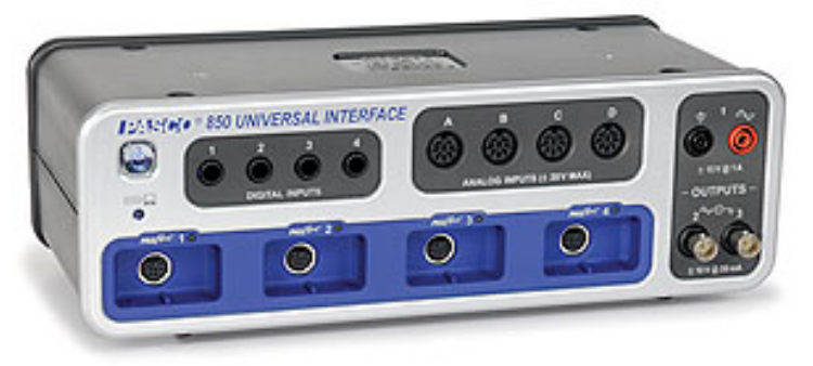
i.1 PASCO DAQ System: Capstone and the 850 Uni-

versal Interface

Figure i.1: The PASCO 850 Universal Interface

The data acquisition (DAQ) system we will use in this course is produced by PASCO

Scientiﬁc for instructional lab courses. The software is called Capstone, and provides the

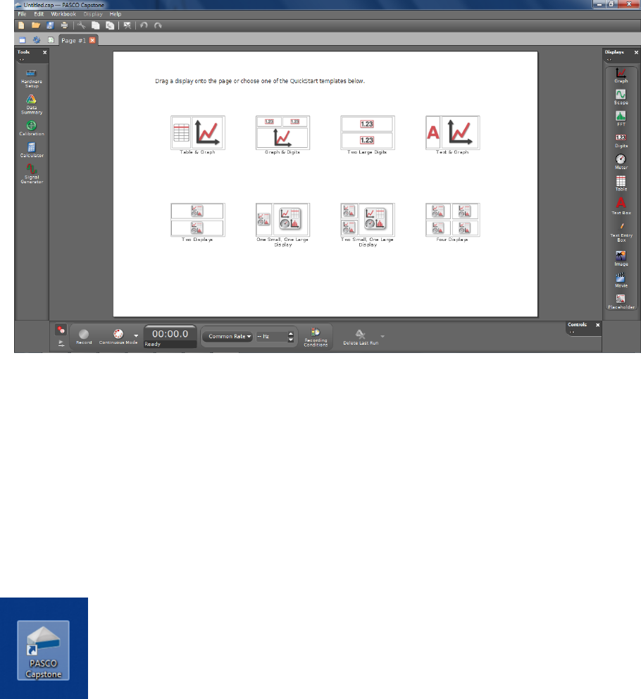
Figure i.2: The default startup screen for PASCO Capstone version 1.0.1. You may be using

a slightly newer version that looks a little diﬀerent, but the basics should be the same.

communication with the hardware interface. This guide is based on PASCO Capstone 1.0.1

and the PASCO 850 Universal Interface, which is the piece of hardware that connects the

computer to your instruments, shown in Figure i.1.

i.2 Startup

To begin, ensure that the 850 is connected to the computer (via USB) and

power it on by pressing the power button on the front if the 850 is not already

on. If the unit is powered up and connected to the computer, the power button

will be backlit in blue and the connection indicator light just below the power

button will be illuminated in green. If you encounter problems with either of

these, check that cables have not come loose or ask for help from your TA.

Next, start the Capstone program, which has a logo that looks like, well, a capstone. Once

running, the program should look something like Figure i.2.

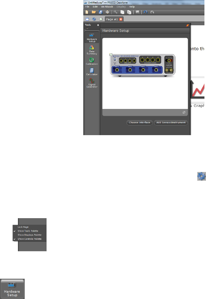
Figure i.3: Clickable Hardware Setup screen shot

If the Tools palette on the left is missing, click the gear icon in the upper left (“Change

properties of current page and Tools Palette”) and check Show Tools Palette under Page

Options. You can also right-click on the gray Capstone desktop and check Show Tools

Palette. The same thing goes for the Controls and Displays palettes.

If your palettes are not shown on the screen, right-click the

gray desktop and select the appropriate palette.

i.3 Conﬁguring Hardware

To set up the hardware for a speciﬁc experiment, click on the Hardware Setup

icon in the Tools palette. If the 850 interface is turned on and is communicating

with the computer, this will bring up a clickable picture of the front panel of the

850 interface, as shown in Fig. i.3.

The yellow circles are clickable and will enable you to tell the computer what hardware

is attached to each connector on the 850 interface. Clicking on the yellow circle will bring

up a drop-down menu showing the possible types of hardware connected to each port. Once

you select the appropriate type of hardware from the list, icons will appear indicating how

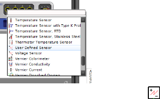
the software thinks the hardware is connected. For example, to conﬁgure Capstone for the

vibrating string lab, you could choose Light Sensor from the drop down menu of the analog

input channel used for the photodiode and Output Voltage Current Sensor for output

channel 1.

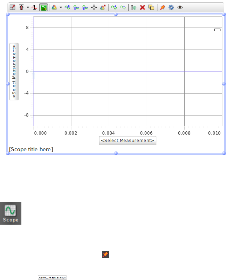
Figure i.4: Clickable Scope screen shot

i.4 Scope Display

The Scope feature is useful for running diagnostics of your apparatus and setting

things up with real-time readout of the results. When all else fails, you can try

using the scope to see if your DAQ is receiving input from its transducers. To

start a full-screen Scope session, double click the Scope icon from the Displays

palette (typically upper right, as shown in Fig. i.2). This will produce a large set of axes on

the screen to display the measurement, such as shown in Fig. i.4. If you have the Hardware

Setup or Signal Generator screens open and the left side of the plot is not visible, either

close those screens or click the push pin at the upper right side of those windows to force

the scope plot to shrink to ﬁt the available space.

To conﬁgure what is being plotted on each axis, click the axis label, which is the but-

ton that says to bring up the drop down menu. This menu will have the

names of devices that can be used for plotting, but the only selectable items are the ac-

tual measurements listed below each device name. Selecting the proper measurement for

each axis will display the name of that measurement as the axis label. There is a menu

bar for the scope trace that will appear when it is clicked or moused over in the display.

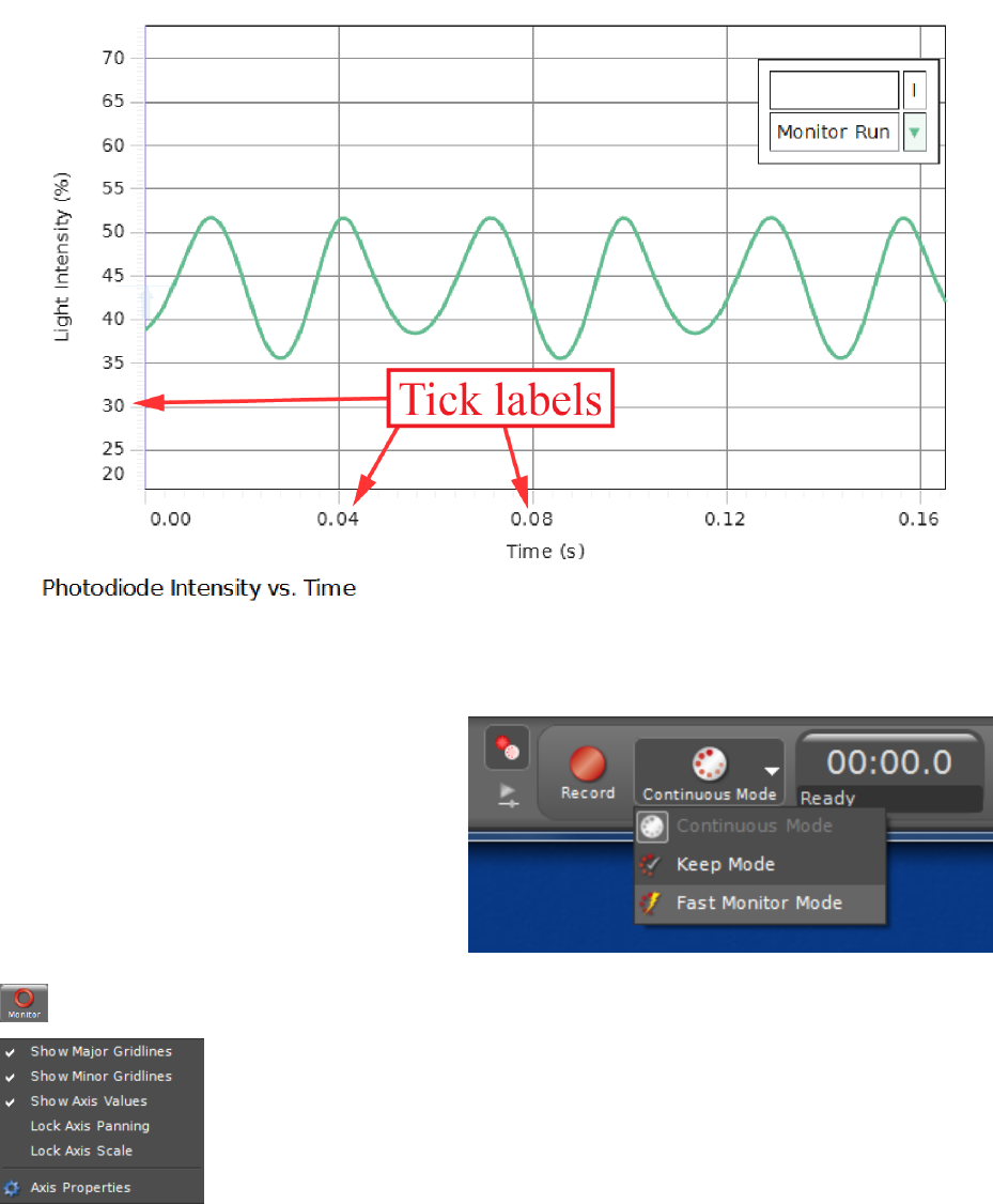
Figure i.5: The scope tool in action, with tick labels pointed out in red.

The x-axis will almost always be time

for our purposes, so to begin plotting

whatever is on the y-axis vs. time in

real-time, you may need to change from

Keep Mode or Continuous Mode to

Fast Monitor Mode, which can be se-

lected in the Controls palette, usually

found at the bottom of the screen. This

will allow you to start seeing real-time traces on the scope by clicking the Monitor button:

Changing the scale and oﬀset of the axes is a little tricky. To change

the oﬀset (i.e. to move the location of the origin), you can grab the plot

region itself and drag it around. If this doesn’t work, make sure that

axis panning is not locked by right-clicking on a tick label and making

sure that Lock Axis Panning is not checked. To change the scale of

an axis, either mouse over the tick labels and use the scroll wheel, or

grab an axis tick label and drag it toward or away from the origin to change the scale.

If nothing appears on the scope trace, make sure the expected signal would be shown in

the range that is being plotted. If there is still no trace shown, mouse over the plot area to

bring up the pop-up menu at the top and check to make sure that the trigger button

is not depressed. If it is, click it to unselect “normal trigger” mode.1

To plot multiple traces on the same set of axes, click the Add new y-axis to scope

display button on the pop-up menu for the scope trace. (If you don’t see the pop-up

menu at the top of the scope trace such as is shown in Fig. i.4, mouse over the plot region.)

The new y-axis will appear on the right side. To change the color of the plot, click on the

sensor data summary, right click the run, and the option “color picker” will come up.

1If you understand how to use a trigger on an oscilloscope, feel free to use it; it can be quite handy. The

trigger level is indicated by a very faint vertical arrow on the y-axis (at x= 0, shown in Fig. i.5 at t= 0.00 s,

y= 44%)) that can be dragged around to change the trigger level. The arrow starts at (0,0) on the plot, so

if you click the trigger button and can’t ﬁnd the arrow, make sure you have x= 0 and y= 0 visible in your

plot region.

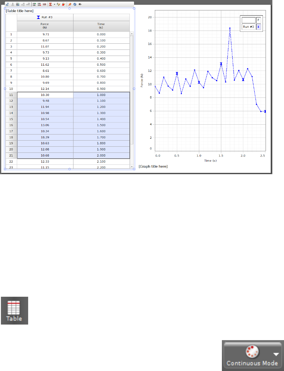
Figure i.6: A Table and Graph showing the same data. If you only want to save the data

between, say, t= 1 s and t= 2 s, you can highlight just the relevant portion in the Table

on the left and copy-and-paste it into Excel.

i.5 Exporting your Data

PASCO has not yet provided a way to save your data in a format that is useful. Ideally,

you should be able to import your data into an analysis program, such as Matlab, Excel,

Mathematica, Open Oﬃce Calc, IGOR Pro, Google Spreadsheets, or whatever else is your

preferred program. The way we will get around this software limitation is by displaying the

data in a table, from which you can later copy and paste the data directly into Excel on the

lab computer. Then you can save your Excel ﬁle in whatever format you prefer (.xls, .csv,

etc.) and, for instance, email it to yourself for analysis at home.

To display the acquired data in a table, ﬁrst start a new table by click-

ing the Table icon in the Displays palette. This will open a new, blank,

two-column table on the workspace. The heading of each column will be a

clickable drop-down menu just like the Scope axes, and you can choose the

data you want to save for each column.

For example, Figure i.6 shows the results of a short measurement of

force vs. time. Both the Table column headings and the Graph axis

labels have been conﬁgured to display force (in Newtons) and time (in

seconds). The data were then recorded using, for instance, Continuous

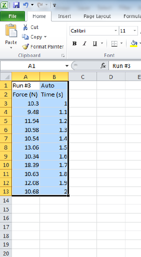
Figure i.7: The same data highlighted in Fig. i.6 right after being pasted into a new workbook

in Excel. Note that the column headers from the table in PASCO were automatically pasted

with the data. This spreadsheet can now be used for plotting, analysis, and saving for further

analysis and inclusion in a lab report.

Mode from the Controls palette, though it may also be acquired using Fast Monitor

Mode and Keep Mode if those are better suited to the particular experiment.

If we only want to save the section of data with the large peak in it for analysis and

plotting in a lab report, we can do this by highlighting the relevant portion of the Table

and copying it to Excel using copy (ctrl-c) and paste (ctrl-v). Figure i.7 shows the data

that was highlighted in Fig. i.6 as it appears in Excel directly after pasting it into a new

workbook. The data are now available for saving, plotting, curve ﬁtting, and inclusion in a

lab report.

ii. Determining and Reporting

Measurement Uncertainties

Throughout this course, we will be making and reporting quantitative measurements of

experimental parameters. In order to interpret the results of a measurement or experiment,

it is crucial to specify the uncertainty (often called the “error” or “error bars”) with which

the measurement claims to be a report of the “true value” of the quantity being measured.

This chapter is designed to be a quick reference for the assignment and propagation of errors

for your lab reports. For a more detailed treatment, I recommend the excellent books by

Taylor [9] or Bevington and Robinson [1].

ii.1 Statement of measured values in this course

Every measurement is subject to constraints that limit the precision and accuracy with which

the measured “best value” corresponds to the “true value” of the quantity being measured.

It is fairly standard in physics to use the following notation to specify both the measured

best value and the uncertainty with which this value is known:

q=qbest ±δq. (ii.1)

Here, qis the quantity for which we are reporting a measurement, qbest is the measured

best value (often an average, but not infrequently generated in other ways) and δq is the

uncertainty in the best value, which is deﬁned to be positive and always has the same units

as qbest. For our purposes in this course, the uncertainty will always be symmetric about the

measured best value, so the notation of Eq. ii.1 will be used throughout.

For example, the most accurately measured quantity in the world is currently the ratio

of the energy splittings between pairs of special states in two atomic ions [7], which is given

by νAl+

νHg+

= 1.052 871 833 148 990 44 ±0.000 000 000 000 000 06.(ii.2)

Here, the measured best value is 1.052 871 833 148 990 44 and the uncertainty is 6 ×10−17.

This level of precision and accuracy is far beyond anything we will be measuring in this

course, but the notation in nonetheless understandable because it is given in the form of

Eq. ii.1.

In this course, you will almost exclusively be measuring quantities with units. Measured

values for quantities that have units must be stated with their units. Failing to do so results

in complete nonsense, the loss of $300 million space probes [6], dogs and cats living together,

mass hysteria [5], not to mention the loss of points on your lab report grade. It is ﬁne for the

units to appear as abbreviations, words, in column headers, after the numerical values, or in

some combination of these just so long as it is clear what the units are. A good example of

how to report a measured value is given by the 2010 CODATA recommended value for the

proton mass:

mp= (1.672 621 78 ±0.000 000 07) ×10−27 kg.(ii.3)

Note that the parentheses are used around the measured best value and the uncertainty

because they have the same units (which is always true) and are written with the same

exponential factor (which can help to make it easy to read).

There are two last points to make here about reporting measured values. First, in these

two examples, the uncertainties are written with the same precision (in scientiﬁc notation,

the number of digits where we include any leading zeros) as the measured best value. This

should always be the case, and when you report a measured value with an uncertainty, you

must make sure the uncertainty is reported with the same precision as the measured best

value.

Second, if we disregard all of the leading zeros, the uncertainty is presented with one

nonzero digit. There are times when it is appropriate to use up to two digits for this

(particularly when the ﬁrst digit of the uncertainty is small, say, a 1 or 2), but uncertainties

should never have three signiﬁcant digits. This is because the size of the uncertainty itself sets

the scale of where the measurement can no longer claim to be providing useful information.

ii.1.1 Other notation you will encounter

A quick glance at Eq. ii.2 and ii.3 reveals that it is diﬃcult to read oﬀ the absolute value of

the uncertainty, since one has to count a lot of zeros. For this course, you will be expected to

report your measurements in the form of Eq. ii.1, but you should be aware of other methods

that are used so that you can interpret their meaning.

Concise notation is useful when the fractional uncertainty becomes very small (as in the

examples above). In concise notation, only the signiﬁcant digit or digits of the uncertainty are

written, and they are written in parentheses directly after the best value, which is written to

the same precision. For example, the following shows two ways to express the same measured

value for the frequency of a laser

ν= (3.842 30 ±0.000 02) ×1014 Hz (ii.4)

ν= 3.842 30(2) ×1014 Hz.(ii.5)

The second line uses concise notation, where since the number in parentheses has one digit,

we are being told that this is the uncertainty in the last digit of the best value. This gets

more complicated when uncertainties are quoted with two digits, which seems to be getting

more common in the literature. As a concrete example, the mass of the electron reported

by CODATA is actually reported in the following form:

me= 9.109 382 91(40) ×10−31 kg (ii.6)

Here, we are being told that the last two digits have an uncertainty given by the two digits

in parentheses. This notation can seem somewhat confusing for a number of reasons, but if

we always think of writing the digits in parentheses below the best value so that they end

at the same place, it is easier to keep from getting confused, as in

me= 9.109 382 91 ×10−31 kg

±0.000 000 40 ×10−31 kg (ii.7)

Asymmetric uncertainties are also sometimes encountered in the scientiﬁc literature,

where the upper uncertainty may have a diﬀerent size than the lower one. In this case, the

following three examples show how one may see this written, using an example of a measured

radiative decay lifetime:

τ= (37.0 +2.0/−0.8) ms (ii.8)

τ= (37.0+2.0

−0.8) ms (ii.9)

τ= 3.70(+20

−08)×10−2s (ii.10)

ii.1.2 “Sig Figs”

There is a system for implicitly including the order of magnitude of the uncertainty of a

measured quantity by simply stating the value with a certain number of digits, which is

often called the “sig ﬁgs” method for reporting uncertainty. Since our uncertainties will be

determined with higher precision than their order of magnitude, we will not be using this

shorthand method in this course, and you will be expected to explicitly write the uncertainty

of your measured quantities, either in the form of Eq. ii.1 or as a separate column entry in

a table. However, you should be aware of this shorthand since it does get used, though

typically outside of formal scientiﬁc literature.

Aside from its lack of speciﬁcity, an additional drawback of the sig ﬁgs method for report-

ing uncertainties is that all too often it leads to laziness and people reporting numbers with

implicit uncertainties far better than are actually merited. Your author starts to become

suspicious that this might be happening when measurements of continuous quantities are

reported to 4 or more digits, particularly by non-scientists. At or after the 4th digit, one

has to think seriously about things such as the calibration and resolution of measurement

equipment, thermal expansion of tape measures and rulers, ﬁnite response time and jitter of

timing systems, the linearly and stability of spring constants, surface roughness and cleanli-

ness, not to mention whether it makes sense at all to deﬁne the quantity you’re measuring

to that scale.

Example ii.1 Your author just looked at espn.com and noticed that they report the

speeds of NASCAR racers to 6 digits. They claim that, for instance, Kyle Busch just

completed a lap with an average speed of 126.648 mph. Can you think of reasons

to suspect that some (perhaps half) of these digits should not be believed? Hint:

was the length of the track even known to 6 digits at that particular time on that

particular day [10]?

ii.1.3 Accuracy and Precision

In physics and other sciences, the words accuracy and precision mean diﬀerent things, and

it is important to distinguish between them. The accuracy of a measurement is how close

the measured value is to the true value of the quantity being measured. If the true value is

within the uncertainty that is reported, we ﬁnd that the measurement was accurate.

Estimating the accuracy of a measurement is notoriously diﬃcult without knowing the

true value. The standards that must be met to produce quantitative accuracy estimates vary

from ﬁeld to ﬁeld, but they generally consist of trying to estimate the size of the impact of

every possible source of error.

One cheap way to make a measurement that won’t be inaccurate is to construct the

measurement poorly on purpose so that the uncertainty is gigantic and is thereby highly

likely to overlap with the true value. However, this illustrates the point that accuracy is not

very useful without another key ingredient of a good measurement: precision.

The precision of a measurement is how small the range is that a statistical spread of

repeated measurements will fall into. The precision tells us nothing about the accuracy of

a measurement, and is determined entirely without knowing the true value of the quantity

being measured. Measurement precision is often determined by the statistical spread of

repeated measurements, and it will be fairly standard in this course to use the standard

deviation of a collection of repeated measurements to set the precision of the reported mea-

sured value (see §ii.1.6 for a more sophisticated treatment). However, the resolution of the

measurement tool itself could be larger than this spread, in which case the quoted precision

will be dominated by the instrument resolution.

Exercise ii.1 A researcher needs to determine the diameter of a 10 cm long quartz

rod to make sure it will ﬁt the mirror mounts for an optical cavity. The calipers

used have a digital display whose most-precise digit is in the 0.01 mm place. 10

measurements along the length of the rod all yield the same reading on the display,

5.98 mm. It is clear that the measured best value is dbest = 5.98 mm, but how can

the uncertainty δd of the measurement be determined?

ii.1.4 Computer use and too many digits

A common mistake that students make in reporting measured values is to have too many

(way too many) digits on their numbers. After all, the computer will report a measured value

often to 16-bit precision, which gives a relative precision of 10−5. However, just because a

computer gives you a number with 5 digits of precision does not mean that the measurement

is accurate at that level. If you have a computer multiply a raw measured value of something

by π, for instance, the computer will happily tell you the answer to 50 digits. This may look

impressive at ﬁrst, but if the original number is only measured to 2 digits, all of that extra

stuﬀ is nonsense.

For example, if you see that repeated measurements of the same quantity ﬂuctuate at

about the 3rd decimal place, there is not going to be much useful information in the 8th

decimal place and it should probably not ﬁnd its way into your report in any form. In this

case, it would make sense to hang on to maybe 4 or 5 digits during the calculations and for

making tables of your raw data. However, the uncertainty is likely to be in the 3rd digit in

the end, in which case you will be throwing out everything after the 3rd digit in your ﬁnal

reported number and there is no reason to keep hauling those 8th digits around, cluttering

up your spreadsheets and implying an unrealistic uncertainty in your numbers. If you keep

things simple, you will ﬁnd that the physics is easier to see!

ii.1.5 Sources of uncertainty

There are many factors that can contribute to uncertainty in measured quantities. These

sources are often separated into two types, systematic uncertainty and statistical uncertainty.

This is a slight oversimpliﬁcation, but for our purposes in this course, sources of statistical

uncertainty tend to produce a random distribution of data points about the mean upon

repeated measurements of the same quantity. As such, statistical uncertainty aﬀects the

precision of measured values, but not the accuracy.

Systematic uncertainty, on the other hand, aﬀects all of the measured data points in the

same way and therefore does not contribute to the statistical spread. Systematic uncertainty

limits the accuracy of a measurement, but not the precision of the measured value. If you

need to compare your measured value to a known true value (for instance, perhaps in a

measurement of g), you will need to consider systematic eﬀects, particularly if you ﬁnd that

your measurement was inaccurate (the true value does not fall within your uncertainty of

your measured best value).

However, we will primarily be concerned with quantitative assessments of statistical un-

certainty in this course. To reiterate an earlier point, you are likely to encounter two main

types of statistical uncertainty in this course, those due to ﬁnite instrument resolution and

those due to “noise” sources that cause repeated measurements of the same quantity to ﬂuc-

tuate. The quantitative method for combining multiple sources of uncorrelated uncertainties

is covered in section ii.2.

ii.1.6 Estimation of Statistical Uncertainty in a Mean

One way to estimate the statistical uncertainty in a measurement is to repeat the mea-

surement many times and to look at the spread in measured points. This method is only

applicable in cases where the precision is limited by statistics (instead of, for instance, in-

strument resolution), but will be commonly encountered and so we provide a summary of

the procedure here.

Let us assume we have a set of Ndata points xithat all measure some quantity x. If

we do not have a good estimate for the uncertainty in each xi, we can still combine them to

come up with a best value and uncertainty in xby looking at their statistics.

For our purposes in this course, we may assume xbest = ¯x, which is to say that the best

value for our measurement of xis the mean of our measured points

¯x=1

i=1

xi.(ii.11)

One commonly used method for estimating the uncertainty in our knowledge of xis to

use the standard deviation (σx) of the collection of points xi. The standard deviation is a

measure of the spread of points around a mean value. In our case, we should use the so-called

sample standard deviation1, given by

σx≡v

N−1

i=1

(xi−¯x)2.(ii.12)

The reason we divide by N−1 instead of Nis that ¯xwas determined from the data

points themselves and not independently. In Microsoft Excel, the functions STDEV() and

STDEV.S() both calculate the sample standard deviation using the formula above and you

may use either one if you don’t want to enter that formula manually.

While it is probably okay in most cases in this course to use the sample standard deviation

as an estimate of the statistical uncertainty in the mean, there is something about this that

is missing. Speciﬁcally, the problem with using δx =σxis that it does not really get smaller

as you collect more data. However, if we take 100 times as many data points as we had and

they have the same spread as our original data set, we should be able to use this to come

up with a signiﬁcantly better measurement of xsince we get to average over 100 times as

many individual data points. Speciﬁcally, we should get a statistical uncertainty that is 10

times smaller if we take 100 times as many data points, which fact is evident when we use

the following formula to calculate our statistical uncertainty:

δx =σx

√N=1

√Nv

N−1

i=1

(xi−¯x)2.(ii.13)

You may apply Eq. ii.13 anytime you are trying to estimate the statistical uncertainty in the

mean of a collection of data points based only on the distribution of those points.

ii.1.7 Summary

When writing your lab report, you may at times choose to include raw data in your report.

This will likely take the form of a table or plot of some kind. Raw data does not need to have

1There is also something called a population standard deviation, which diﬀers from Eq. ii.12 in that the

factor of 1/(N−1) is replaced by 1/N. The population standard deviation is appropriate in cases where the

mean of the parent distribution is determined independently from the data.

explicit uncertainties for each entry unless you are speciﬁcally asked to provide it. However,

even your raw data must have units labeled. This can be done in column headers or plot

axis labels, but there should not be any room for ambiguity on this point.

•Every single number in your report that describes a quantity that has units must have

its units clearly labeled in your report.

When reporting the results of measurements in your report (as opposed to just showing

examples of raw data), you will be expected to report the measured best value and the

uncertainty. When you quote the ﬁnal measured value of a quantity in your report, be sure

that

•You report the measured best value and the uncertainty: q=qbest ±δq

•You include proper units

•The measured best value and the uncertainty are written with the same absolute

precision

•The uncertainty has no more than two signiﬁcant digits

ii.2 Propagation of uncertainties

Fairly often in the laboratory we will be measuring many diﬀerent quantities and combining

those measurements together in some mathematical way to come up with a measured value

for a composite quantity. For instance, let’s say we wanted to measure the average velocity

of a glider on an air track (Fig. 1.1) by using a stopwatch to measure the time tit takes

the glider to travel some distance x. Using the guidelines above, we will have assigned an

uncertainty to each of these quantities, so we want to know how to turn our measured values

for the parameters xbest ±δx and tbest ±δt into a measured value for the composite quantity,

the average velocity v=vbest ±δv.

The way we do this is by using the functional form of how the composite quantity

depends upon the input parameters to mathematically determine the resulting uncertainty

in the composite quantity. It is important to use the following methods only in the cases

where the uncertainties are uncorrelated, so be sure that the uncertainties are generated by

physically independent mechanisms (statistical uncertainties typically fall ﬁrmly into this

category).

We will write the expression relating the uncertainty δf of some composite quantity fto

the uncertainties (δx, ···, δz) of the parameters used to compute f=f(x, ···, z) without

proof or derivation (see, e.g., [1]):

δf =v

t ∂f

∂x δx!2

+··· + ∂f

∂z δz!2xbest,···,zbest

(ii.14)

where the vertical line on the right side instructs us to evaluate the resulting expression at

x=xbest,···, z =zbest.2

If you are not familiar with the notation of those derivatives (∂f/∂x), they are called

partial derivatives and simply instruct you to treat everything except the variable of diﬀer-

entiation as a constant when taking the derivative. If we come back to our example of the

measurement of the average velocity of a glider, we ﬁrst identify f=v=x/t. We need

to determine δv in terms of xbest,δx,tbest, and δt. We can begin by taking the partial

derivatives: ∂v

∂x =∂

∂x x

t=1

t(ii.15)

and ∂v

∂t =∂

∂t x

t=−x

t2.(ii.16)

This gives us

δv =s1

tδx2

+−x

t2δt2xbest ,tbest

√t2s(δx)2+x2

t2(δt)2xbest ,tbest

=sx2

t2v

t δx

x!2

+ δt

t!2xbest ,tbest

.(ii.17)

Normally, we would say that qx2/t2=±x/t to reﬂect the two solutions of that equation.

However, we have deﬁned all uncertainties (δq in Eq. ii.1) to be positive, so here we take the

absolute value: sx2

t2

=

t.(ii.18)

We can now evaluate our expression at x=xbest and t=tbest to give us

δv =

xbest

tbest v

t δx

xbest !2

+ δt

tbest !2

.(ii.19)

We have identiﬁed vbest =xbest/tbest, so dividing both sides by the absolute value of this

quantity and noting that we can add an absolute value sign to both terms under the radical

since they are squared anyway gives us the following symmetric-looking form:

δv

|vbest|=v

t δx

|xbest|!2

+ δt

|tbest|!2

.(ii.20)

2The assumption we are going to invoke here is that fbest =f(xbest,···, zbest). This is sometimes not

strictly correct, but will serve for the purposes of this course.

The quantity δq/|qbest|is called the fractional uncertainty or relative uncertainty of some

measurement of q, so we can restate Eq. ii.20 in words by saying that the fractional uncer-

tainty in a ratio of two quantities is given by the quadrature sum of the fractional uncer-

tainties of the two quantities.

ii.2.1 Speciﬁc formulas

While form given in Eq. ii.14 is suﬃciently general to allow it to be applied directly for every

case encountered in this course, we can summarize some of the most common results that

can be derived from it as follows.

•Measured quantity times an exact number: f=Ax

δf =|A|δx (ii.21)

•Sums and diﬀerences (they follow the same rule): f=x+y−z+···

δf =q(δx)2+ (δy)2+ (δz)2+··· (ii.22)

•Products and ratios (they follow the same rule): f=x×···×z

u×···×w

δf

|fbest|=v

t δx

|xbest|!2

+··· + δz

|zbest|!2

+ δu

|ubest|!2

+··· + δw

|wbest|!2

(ii.23)

•Measured quantity raised to an exact number power: f=Axn

δf

|fbest|=|n|δx

|x|(ii.24)

•Exponential with measured quantity in the exponent f=Aeax

δf

|fbest|=|a|δx (ii.25)

You may recognize that Eq. ii.20 is a special case of Eq. ii.23, as is Eq. ii.21. And, of

course, all of these are special cases of Eq. ii.14. These cases are not the only possibilities

for functional forms of the relationships between measured values, but they are the most

common for us in this course. You should be sure to keep in mind that these formulas are

valid only for uncertainties that are uncorrelated.

Experiment 0: Sensor Calibration and

Linear Regression

Your ﬁrst experiment is intended to familiarize you with some of the basics of the DAQ

system. There will not be a formal report due next week. Instead, there is a short set of

homework problems (“Homework 0”) at the end of this chapter that you will complete and

turn in online. Be sure to read through the homework problems to make sure you have saved

all of the data you will need to complete Homework 0.

For many experiments in this course, you will be using a force sensor similar to the one

shown in Fig. 0.1. This device is designed to output a voltage that is proportional to the

force applied between the hook and the body of the sensor. The DIN cable allows your

computer to read this voltage via the 850 interface. If Force Sensor is selected as the type

of input, the 850 will assume it knows how to convert voltage to force and will simply read

in units of force (N). However, to illustrate how the interface really works, we will not trust

this conversion implicitly and will instead be looking at the raw voltage from the sensor.

The process of determining how voltage corresponds to force is an example of a process

called calibration, and Experiment 0 walks you through a manual calibration procedure for

this force sensor. This procedure is not the same as the Calibration feature in Capstone,

and the manual calibration described here will be far more accurate than that supplied

by the manufacturer. Plastic deformations of the sensor components, changes in ambient

conditions, and electrical oﬀset sources may all change between experiments, so to increase

the accuracy of your force measurements, you may consider checking the sensor calibration

each week that it is used. Your TA may or may not ask you to do this explicitly.

0.1 Hardware setup

To set up the force sensor to read its raw voltage, start your DAQ

system using the instructions in §i.2 and connect the DIN cable to one

of the Analog Inputs of the 850. Set up the 850 to read voltage from

the appropriate analog input (see §i.3) by choosing User Deﬁned Sensor

from the drop-down menu of the appropriate input (Do not choose

Force Sensor), at which point your Hardware Setup pane will show a

little electricity-looking icon with a line to the channel you chose.

To test that you have set up the connection correctly and that there are no software or

hardware errors happening to keep you from reading the sensor correctly, use the Scope

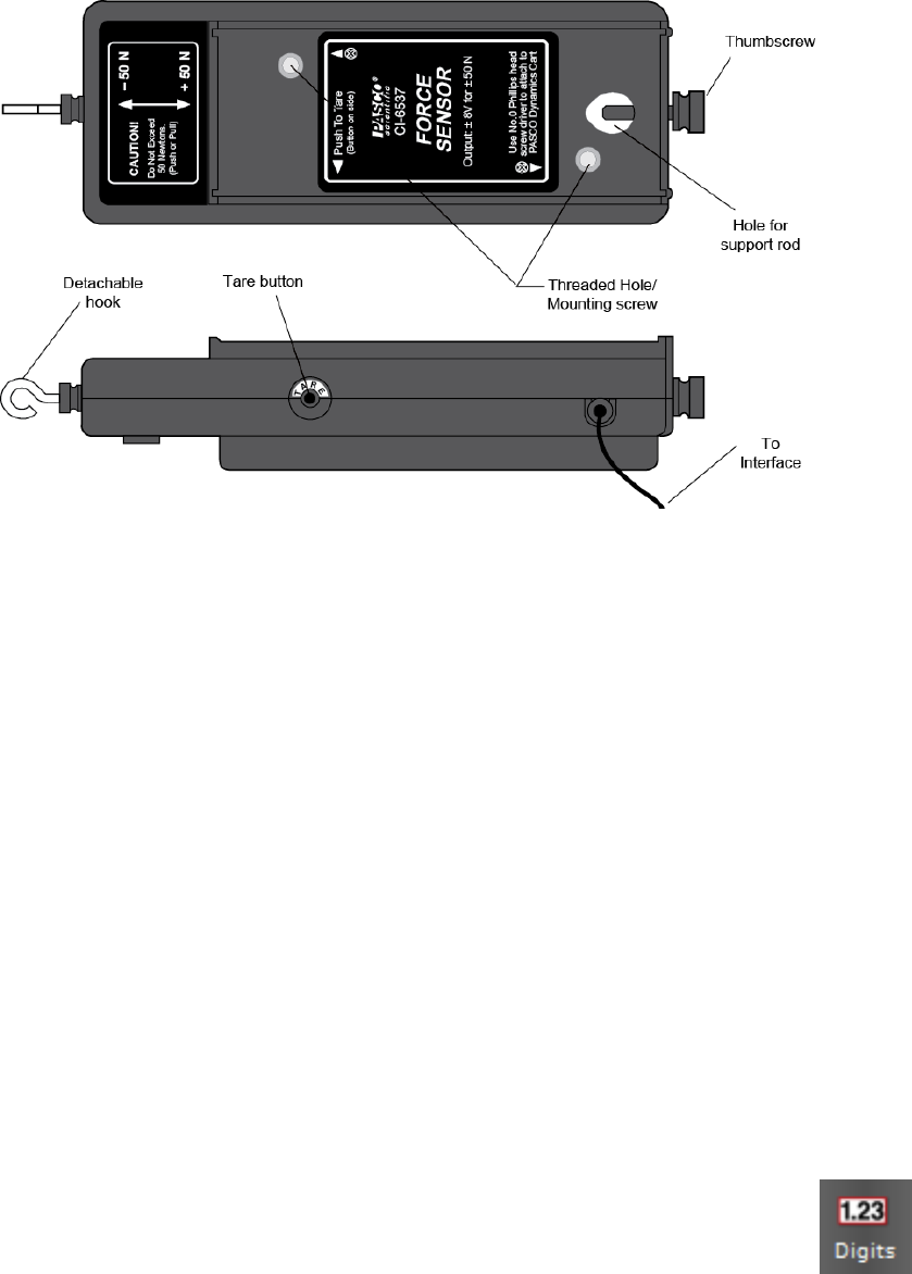
Figure 0.1: PASCO CI-6537 force sensor. This transducer can sense both tension and

compression applied between the hook and the body of the unit, up to 50 N in either mode.

feature in Fast Monitor Mode to see that the voltage changes when you push or pull a

little on the hook. An overview of how to use the Scope feature can be found in section

i.4. If you cannot see any signal from your sensor on the screen, go back through these steps

carefully to see if you missed something; if not, ask your TA for help.

0.2 Manual calibration procedure

Once your DAQ is able to read voltage from the force sensor you are ready to begin the

calibration. The procedure will be to attempt to zero, or tare the sensor, and then to hang

known weights from the hook while monitoring the voltage. You will record several readings,

then use Excel or whatever other program you like to ﬁt a line to the data. The slope and

oﬀset of this line is the calibration curve for your sensor. The oﬀset will almost certainly not

be zero, which will tell you something about how well the tare procedure worked.

0.2.1 Measurement Apparatus

First, attach the force sensor to a horizontal post so that the hook hangs vertically

downward, appropriate for hanging weights from it. The best software tool for

measuring the voltage is probably the Digits feature in the Displays palette. If

the Displays palette is missing, see section i.2 for instructions on how to get it

back onto the screen. You can conﬁgure your Digits display to show the voltage produced

by the sensor by choosing User Deﬁned (V) from the drop-down menu of the

button.

Your calibration of the force sensor will be capable of accounting for an

oﬀset in the reading caused by a nonzero voltage reading with no applied force.

However, it is useful to know how to tare the sensor in hardware for calibration

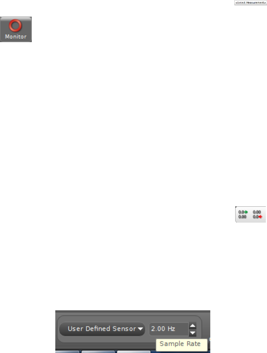
and making diﬀerential measurements. Using Fast Monitor Mode with your

Digits display, you should be able to read the oﬀset voltage in real-time by clicking Monitor

in the controls palette.

The voltage you see displayed will ﬂuctuate around some value that is not necessarily

zero. You can deﬁne this oﬀset to be 0 V by pressing the tare button on the side of the sensor,

shown in Fig. 0.1. The voltage reading will now be centered near zero. Your calibration will

tell you how well this procedure worked when we produce a ﬁt line.

0.2.2 Changing the Display Precision

You may notice that your sensor reading ﬂuctuates around as a function of time, even

after taring the sensor. This gives you some idea of the precision of the sensor, which

determines the minimum size of the steps between distinct values. You will need to observe

and record the magnitude of ﬂuctuations like this in various sensor readings throughout the

course, because they are an important part of your uncertainty determination for measured

quantities.

Aside from the precision of the sensor, it is possible that Capstone is only displaying a

subset of the digits it actually gets from the sensor. This is called the display precision of

your DAQ. It will be crucial in later labs to be able to change the display precision to avoid

becoming limited by this (which is known as quantization error ).

To change the display precision, mouse-over the Digits display to pop up

the menu bar at the top. On the far left side of the menu bar, there will be two

buttons to control the display precision, one to increase it and one to reduce

it. Click each one a few times while watching your sensor reading to get a feel for how the

system works. Determine the maximum number of digits that Capstone is willing to display

by increasing the precision until the button no longer changes the display. Typically, the

ideal display precision is just at the point where the reading ﬂuctuations show up in the last

digit.

Next, we will record the voltage reading for a series of known weights hung from the

hook. To get a steady reading, it will be helpful to turn down the sample rate to something

on the order of a couple of times per second. This can be done in the Controls palette at

the bottom of the screen.

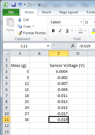
Figure 0.2: Some fake data entered into Excel in two columns with an empty column next

to the mass column. Note the unit labels on the column header.

0.2.3 Entering and Plotting Data in Excel

Next, we will be collecting our data in a table, so start a new workbook in Excel and record

the voltage reading and mass of a series of weights hung from the force sensor hook. Now is

probably a good time to get in the habit of labeling the columns of tables with descriptive

labels and appropriate units, as shown in Fig. 0.2. Since you will be converting mass to force

using F=mg, it is a good idea to leave a blank column next to the column where masses

are recorded so that we can make Excel do the work of ﬁlling in the force column.

To have excel ﬁll in the force column with the calculated force in N, highlight the top

cell of the new column (right next to the cell with your ﬁrst mass value entered) and enter

the formula you want Excel to execute. Formulas in Excel begin with an =sign, followed

by the mathematical expression you want, where variables can be entered either manually,

or through reference to the cell address in which the variable value has been entered.

For instance, for the data shown in Fig. 0.2, to make cell B3 display the gravitational

force (in N) acting on the mass entered in cell A3, one could type in “=A3*0.001*9.80” and

hit enter. In this case, the factor of 0.001 comes from converting g into kg and the factor of

9.80 is for g= 9.80 m/s2. The formula can now be copied down the column by highlighting

the cell with the formula, grabbing the bottom right corner of the cell, and dragging it down

the column. Excel will recognize that “A3” should be changed to “A4” in the formula for

cell B4 and so forth.

Once you have two columns recording the applied force and the output voltage, you can

plot your data. Excel calls this a “chart” (because Excel is made for businesspeople) and

you can create one by highlighting the two columns with your data and choosing Scatter

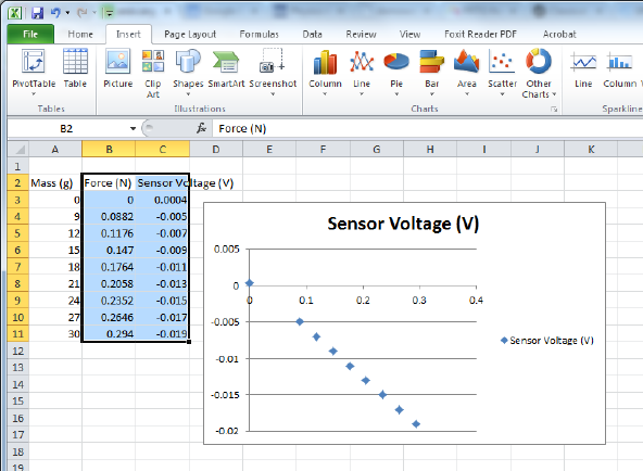
Figure 0.3: Excel has created a terrible-looking plot. In the opinion of your author, what

Excel lacks in the appearance of its plots it makes up for in ease-of-use for students, which

is why it is recommended here. If you have other programs you prefer to do your own data

analysis, feel free to use them.

from the Insert →Charts menu or something similar in whatever version of Excel you are

using.

If you had Excel make a scatter chart for you in this way, your workbook probably looks

similar to that in Fig. 0.3 This plot has no axis labels, so it takes a little looking to even ﬁgure

out which column was used for the y-axis and which for the x-axis. I would recommend that

the ﬁrst thing you do when creating a plot in Excel is to label the axes and units for those

axes. How this is done will depend upon your version of Excel, but you’re probably looking

for something like Chart Tools →Layout. Using the features you have at your disposal

and a bit of web searching, you can hopefully ﬁgure out how to make a reasonably clear plot

of your data, such as that shown in Fig. 0.4. All plots that end up in your report must have

axis labels and appropriate units, as well as a ﬁgure caption with a title, description of what

is displayed, and possibly a ﬁt line equation. Instructions for how to incorporate plots into

your reports can be found in Appendix B.

0.2.4 Linear Fit to Numerical Data

Next, we would like to have Excel calculate the equation of the best ﬁt line to our data. To

do this, you will have Excel “add a trendline” to your data. Since we expect the voltage to

be linear in the applied force, we are looking for an expression in the form

V=aF +b(0.1)

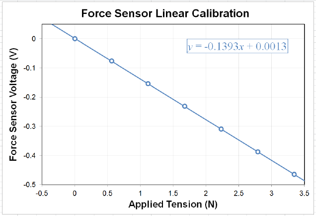
Figure 0.4: A fairly clear plot of some data shown with a linear ﬁt line. Note the title, axis

labels, units, and ﬁt line equation are all clearly visible, and none of the tick labels or text

is overlapped with anything that makes it diﬃcult to read.

to relate the measured voltage Vto the applied tension Fin terms of the slope aand oﬀset

bof our sensor. Note that aand bwill have units, that they constitute the results of a

measurement, and that they need to have a quantitative uncertainty associated with them.

We will use Excel to calculate aand bfor us by having it add a linear trendline (a.k.a. a

linear best ﬁt) to the data and display its equation on the chart, as shown in Fig. 0.4. The

procedure for adding a trendline will vary from version to version of Excel, but right-clicking

on one of the data points or going to Chart Tools →Layout are likely places for this

option to be hiding. In the trendline options, remember that we want a linear trendline,

we do not want the oﬀset set to a particular value (so it will remain a ﬁtting parameter;

your sensor may still have an oﬀset despite the tare procedure), and we want the equation

displayed on the chart.

A guide to making ﬁgures and captioning them using Word and Excel by Julio S. Ro-

driguez, Jr. and Anthony Ransford can be found in Appendix B.

0.2.5 Calculating Uncertainties in a Linear Fit with Excel

For the example data of Fig. 0.4, we ﬁnd that the linear ﬁt line is described by the equa-

tion y=−0.1393x+ 0.0013. Comparing this to Eq. 0.1, we are tempted to identify

a=−0.1393 V/N and b= 0.0013 V and declare victory. However, we still need the un-

certainty in the measured values (δa and δb) used to generate this ﬁt before we can report

the results of a measurement. As is always the case, we cannot claim we measured something

(in this case, the sensor calibration) without also describing the uncertainty associated with

this measurement.

One question that we can ask ourselves is “why is there an uncertainty at all? After

all, there is a single, unique ﬁt line that is the very best ﬁt to these data. Why would that

have an uncertainty?” This is a very good question. The answer is that the scatter in the

data will eﬀectively permit a series of diﬀerent lines that all essentially model the data to

the same degree. For data with a lot of scatter, the “goodness of ﬁt” of the best ﬁt line is

only a very tiny amount “more good” than a whole collection of lines with similar slopes

and oﬀsets, so the uncertainty will be large. For data with very little scatter, a small change

in the slope or oﬀset will substantially degrade the “goodness of ﬁt,” and the uncertainty is

correspondingly small. Excel provides you with the quantitative tools to evaluate statements

like this in a scientiﬁc manner, and we will use this throughout the term.

The trendline feature in Excel was a quick and easy way to get the best-ﬁt slope and

intercept from a least-squares ﬁt, but it gives us no quantitative way to determine the

uncertainty in the slope and intercept that it found. There are two ways your author knows

of to get the uncertainties in linear ﬁts in Excel. The ﬁrst is to use an Excel function called

LINEST that returns an array and is powerful, but not incredibly user-friendly. The other

way is to use the Regression tool.

The regression analysis tool will take as its input your two columns of data and give you

lots of information about how well your data can be described by a linear relationship. For

instance, it will calculate the same equation for the best ﬁt line that we got from the Add

Trendline feature, but it will provide more digits, and (most importantly) it will provide

the uncertainties in the ﬁt parameters. These uncertainties are based entirely on the scatter

in your data points around the ﬁt line and therefore do not contain any information about

systematic uncertainties. If your data span a range much larger than the resolution of your

measurement tool (probably true in this case), the scatter in your data points already reﬂects

this resolution limit implicitly.1

To perform a linear regression analysis in Excel, look for the regression tool somewhere

like Data →Data Analysis or Tools →Data Analysis. One of the data analysis tools

should be Regression. You will enter the location of your xand ydata, and I would

recommend having the output option set to new worksheet, such as shown in Fig. 0.5.

Figure 0.6 shows the results of the linear regression analysis, along with some high-

lighting of the parameters we were interested in calculating. The regression tool gives the

uncertainties in the slope and intercept in the column called Standard Error .

At this point, it would again be tempting to think we are done and write a= (−0.139320505±

0.0000776577) V/N and b= (0.001334872±0.000181541) V and call it a day. After all, we’ve

got the uncertainties and the units, right? The problem with this is that the precision of

these reported numbers is much, much better than the uncertainty indicates it should be.

The statistical uncertainty given by, for instance, δb = 0.000181541 V tells us immediately

that the last four or ﬁve digits of this number are meaningless. The data itself ﬂuctuates at

1If your data do not span a range larger than your instrument resolution, all of your data points are

probably identical, and the instrument resolution is likely the largest source of statistical uncertainty in this

case.

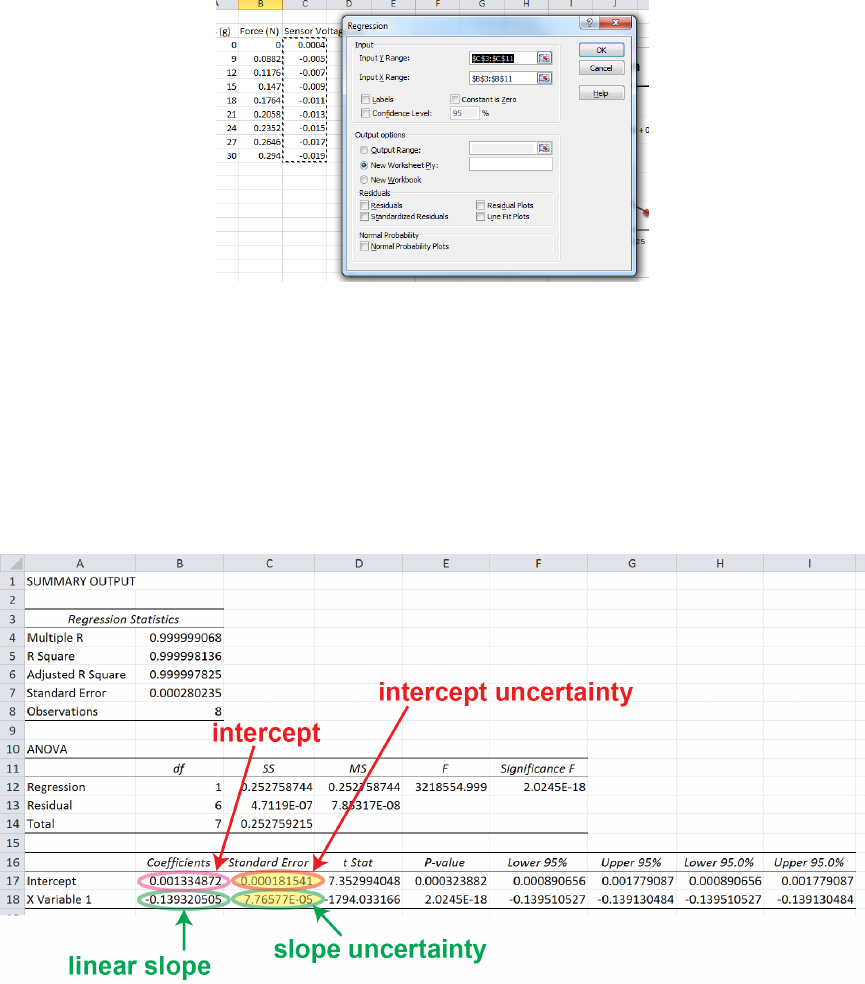
Figure 0.5: The linear regression tool in some version of Excel. Your version may look a

little diﬀerent, but the basics will be the same.

Figure 0.6: The results of using the linear regression tool in Excel. The best-ﬁt line slope

and intercept are highlighted, along with their uncertainties.

a level that is way too large for us to say anything about bon the 10−9V scale. You can

always keep just one nonzero digit on an uncertainty and not get yourself into any trouble

in this course, so that would give us δb = 0.0002 V and δa = 0.00008 V/N. The best values

should then be written with the same absolute precision, and we have our ﬁnal result for the

measured calibration of this force sensor:

V=aF +b(0.2)

a= (−139.32 ±0.08) mV/N

b= (1.3±0.2) mV (0.3)

As a quick sanity check on these measured results, we note that the last digit of abest is in

the 0.01 mV/N place, which is the same position as the last digit in δa, as it should be. The

same is true for b: the last digit we quote for bis in the 0.1 mV place, as is the last digit of

δb.

0.3 Homework 0

Read through these problems before you leave the lab to ensure that you have

saved all of the data you will need. This short exercise is designed to prepare

you for your ﬁrst real experiment, Experiment 1. Your completed homework

must be a short document that is typed and formatted using a computer.

During your lab section for Experiment 0, your TA will give you a due date

and instructions for how to turn in your completed homework. You may ﬁnd

that the information in Appendix B is useful for completing your homework,

so be sure to take a look at Appendix B.

1. You will need a cover page for your reports in this course, so now is a good time to

make a template for yourself you can reuse later. Make a cover sheet that includes the

following information:

•Experiment number and title. This week, this will be something like “Experiment

0: Sensor Calibration and Linear Regression”

•your name and UID

•the date the lab was performed

•your lab section (for instance, “Wednesday 9am.”)

•your TA’s name

•your lab partners’ names

2. A student is trying to measure the constant acceleration of some object in the lab by

measuring the change in velocity of the object over some ﬁxed time interval. Repetition

of the experiment many times and careful error analysis has resulted in a measurement

of the velocity change (∆v= ∆vbest ±δ∆v) and the time duration (∆t= ∆tbest ±δ∆t)

with uncertainties. Knowing that the measured acceleration is given by a= ∆v/∆t,

what is the proper expression for the uncertainty in the measured acceleration, δa?

3. What is the maximum number of digits Capstone will display (recall §0.2.2)? If the

sensor precision is exactly 4 digits and you take data with 10 displayed digits, describe

what your actual measurement precision is and what you would expect to see in digits

5 through 10. If the display precision is turned down far enough, it may be possible

to completely eliminate sensor ﬂuctuations. Describe why doing this might not be the

best idea for taking good data.

4. Present your ﬁnal plotted results of the calibration procedure as a ﬁgure (include the

data, the ﬁt line, and the ﬁt line equation on the plot). You should take the time to

make the plot look clear and have all of the axes labeled. Present a brief line or two

of text that could be used as a ﬁgure caption for this plot.

5. State the results of your calibration (with uncertainty from your ﬁt). This may require

a sentence or two of explanation to clearly deﬁne your parameters, but you do not need

to describe the whole procedure of the experiment. Your ﬁt should have included a

possible nonzero y-intercept. What does your value for this intercept tell you about

the eﬀectiveness of the taring procedure (§0.2.1)?

6. Equations 0.1 and 0.3 tell us how to convert a known tension Finto a predicted output

voltage of the sensor V(including the uncertainty in this conversion), but to use this

as a “force sensor,” we really want to know how to convert Vinto F, right? Use the

measured values of abest ±δa and bbest ±δb that you presented in your response to the

previous question to rewrite your calibration curve in the form F=cV +d, including

the appropriate uncertainties in cand d. Hint: look at Eq. ii.23.

7. You have been provided with information on how to access the syllabus for this course.

Read the syllabus, paying special attention to the text in red. Consider a case where two

students, Frankie Fiveﬁngers and Avril Armstrong are in diﬀerent sections of Physics

4AL this quarter. At the end of the quarter, they both have an average numerical score

of 84, but Frankie gets a B+ in the course while Avril gets a C+. How is this possible?

What can you conclude about the mean numerical scores of the other students in their

sections?

Experiment 1: Uniform Acceleration

Experiment 1 is the ﬁrst experiment for which you will be expected to submit a full-credit

report. Your report is due about a week from now, and your TA or instructor will give you

speciﬁc instructions on how to submit your report as well as when the due date is.

In Experiment 1, you will be measuring the acceleration of a composite system composed

of some masses connected by a string passing over a pulley. The position of the accelerating

masses and string will be monitored as a function of time by the DAQ system, and these

data will be recorded for a series of 5 diﬀerent masses. A bit of data analysis is required to

produce a plot that can be ﬁt to a straight line to obtain a measurement of the acceleration.

You should already have experience working with the DAQ (chapter i), producing linear

ﬁts with uncertainties (§0.2.4 & §0.2.5) and doing a proper uncertainty analysis of your

complete measurement (chapter ii), so you may ﬁnd those sections to be helpful references

for Experiment 1.

In order to measure constant acceleration, the friction between the accelerating object

and everything that is stationary must be kept to a minimum. While there will still be some

residual friction (as well as drag forces), the air track setup depicted in Fig. 1.1 does a good

job of minimizing its eﬀect. A “glider” placed on this track will ﬂoat along on a cushion

of air when the pump is pressurizing the track, exhibiting nearly-ideal linear motion. The

glider and air track setup will be used for many experiments in this course.

Fig. 1.2 shows the air track set up for Experiment 1. A glider with total mass Mis

supported on a cushion of air on a level air track and is attached to a hanging weight (mass

m) by a string that passes over a pulley.

The equation of motion for this system is given by:

a=gm

m+M(1.1)

where ais the acceleration of the glider-string-weight system and gis the earth’s gravitational

acceleration for a free-falling body.

In this lab, you will be measuring the acceleration for 5 diﬀerent values of m(do not

exceed m= 50 g). Feel free to vary Mas well for any of these runs. The acceleration

measurement will require that you convert position vs. time data into a measured value for

acceleration (with uncertainty, of course!). These position vs. time data will be recorded by

the DAQ using a “smart pulley.”

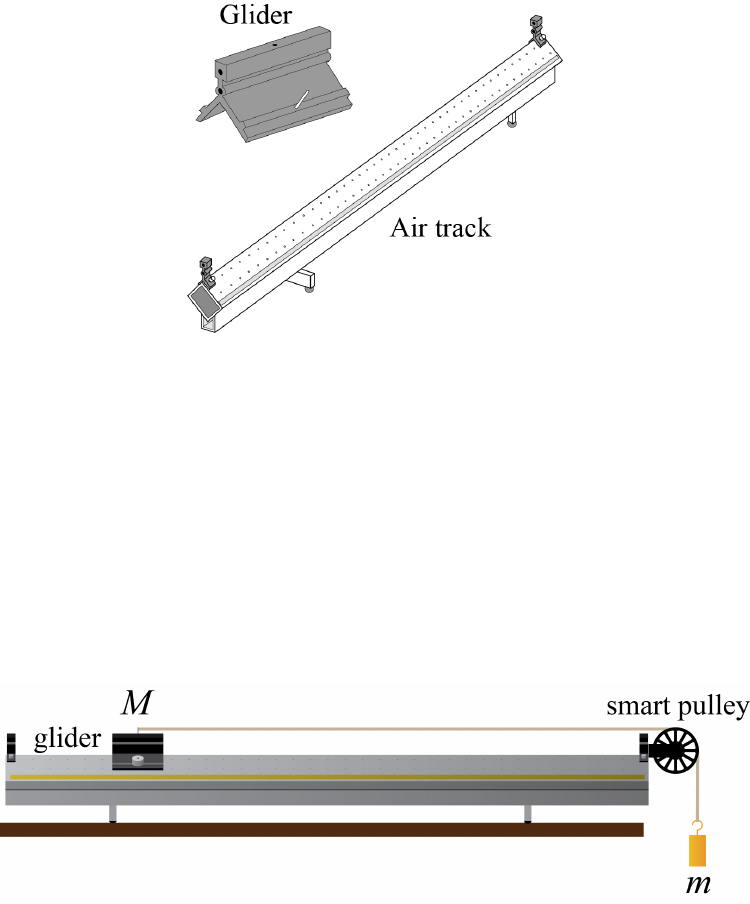
Figure 1.1: Apparatus for linear motion with very low friction. The air track is pressurized

by a continuously-ﬂowing pump, causing air to ﬂow out through the array of holes on the

surface. When a glider is placed on this track, it moves freely in 1D with very little friction,

just like an air-hockey puck.

Figure 1.2: Experiment 1 setup. The glider mass can be changed by putting diﬀerent

amounts of weight on its sides, and the hanging mass can be changed by adding more

weights with hooks. The smart pulley is attached to the DAQ and records the timing as the

spokes pass by a sensor.

1.1 Procedure

In order for Eq. 1.1 to be valid, we have assumed that the air track is level. This is generally

not the case, and there will be multiple experiments in this course that use the air track.

Your ﬁrst task is to level the air track. You can accomplish this by placing a glider on the

track and turning on the blower. The track itself is not completely ﬂat, so there is really no

such thing as “perfectly level” over the whole length of the track, so do the best you can.

You will ﬁnd that the two feet under the cross-bar of the air track (one is visible sticking

out from the bottom of Fig. 1.1) can be turned to change their height. Your goal is to get

to the point where a free glider won’t move either direction with the blower on.

You will also need to set up your DAQ to work with the smart pulley, so plug the smart

pulley cord into a digital channel on the 850, turn it on, and start Capstone. Conﬁgure the

appropriate channel for Photogate with Pulley.

The smart pulley really only has the ability to measure whether or not a wheel spoke is

blocking a little infrared LED from shining into a photodiode. The LED and photodiode

are set up with a gap between them, which is called a photogate. Every time the photogate

goes from being unblocked by a spoke to being blocked by it, the 850 tells Capstone the time

stamp for that event, so the raw data in this case is really the time stamp for each time when

the photodiode detects a “falling edge.” Therefore, no data is collected if the pulley isn’t

moving, or during the time when the spoke is moving but hasn’t yet blocked the photogate.

Furthermore, the photogate has no idea which direction the pulley is moving, so you should

be careful when interpreting results. You may assume that the linear distance the perimeter

of the pulley moves between successive times when the photogate goes from being unblocked

to blocked is given by

κSP = (1.50 ±0.05) cm/block.(1.2)

You may notice that Equation 1.2 is given in the from κSP =κSP,best ±δκSP, but you are not

told whether the uncertainty δκSP should be treated as systematic or statistical in nature.

You may take this uncertainty to be statistical for the purposes of your analysis, in which

case it will already be taken into account when you do your regression analysis, because this

eﬀect will show up as scatter of your data points.

Capstone has the ability to perform some computational tasks on the data and to use its

own algorithms and calibration of the hardware to display position, velocity, acceleration,

etc. This will be useful for future tasks, but for Experiment 1, you should save the raw

data (Block Count () vs. Time (s)) and use your own data analysis to convert this into 5

acceleration measurements (with uncertainties, of course!). This is designed to help you

understand how to turn raw experimental data into a measured value with uncertainties,

where you have full knowledge and control over the algorithms being applied to the raw

data.

Fig. 1.3 shows an example with some fake data. It is always helpful to have a visual

representation of the data you are collecting in real-time, because this can give you a quick

feel for whether something is not set up properly. For this, it might be a good idea to open

aScope or Graph display to show, for instance, Linear Speed (m/s) vs. Time (s).Since

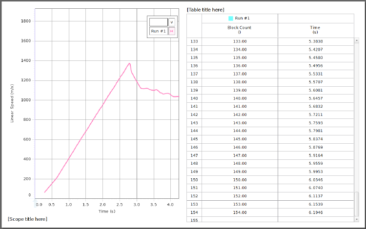
Figure 1.3: Example data from Capstone showing the simultaneous generation of a Scope

plot qualitatively showing the portion of the data that will be useful and the Table that can

be used to cut-and-paste your data into Excel for saving and analysis. Note that the Scope

plot shown here is showing a glider moving at about Mach 4, so don’t trust it! It is only a

qualitative tool to help you view your data in real-time.

you do not know how Capstone calculates linear speed, you will not use this. The only data

you should use will be Block Count () vs. Time (s). The display of speed is only to give you

a visual cue of your data. Since you will also be saving your data to analyze it , you will

also need to open (simultaneously) a Table for collecting your data. Remember, the two

columns you will need to generate are Block Count () and Time (s). Do not save a column for

Position,Linear Speed,Linear Acceleration, or any other pre-processed quantity. Continuous

Mode in the Controls palette should work for gathering your data. The sample rate seems

to have no eﬀect for this hardware.

With your lab partner, you will be saving 5 data sets (each with a diﬀerent set of masses).

Keep in mind that you will need to measure the mass of the glider, so don’t forget! Once the

DAQ is set up, you should be able to generate a plot something like that shown in Fig. 1.3.

The Scope plot in that ﬁgure shows the point where the velocity stops increasing linearly,

which is when the weight hits the ﬂoor or the glider hits the pulley, whichever comes ﬁrst.

You may use this plot to decide which data to save (you are only interested in the linear

portion). Be sure to increase the number of displayed digits in the table until you are no

longer precision limited before exporting your data (look at the Time (s) column in Fig. 1.3).

Highlight the data you want to save in the Table and copy and paste it into Excel. You

should then save it somewhere safe. Each person should get 5 data sets with diﬀerent masses

for mand/or Mthat are unique. You may use the same masses as your lab partners, but

the raw data should be unique for each person.

1.2 Analysis

The data you saved is in the form of something called “Block Number” vs. time. Using

Eq. 1.2, you can create a new column for position by simply multiplying block number by

κSP,best. Remember, you have been instructed to ignore δκSP for this analysis since your

regression analysis will automatically take this eﬀect into account, so you will really only be

using κSP,best. Next, you will need to numerically diﬀerentiate the position data. To do this,

you may calculate a single average velocity for every two position vs. time points using

¯vi=∆x

∆t=xi+1 −xi

ti+1 −ti

.(1.3)

Note that since each velocity measurement requires two position data points, you will have

one fewer data points for velocity than position. The column of velocities you generate now

needs a column of times associated with them. Since the formula in Eq. 1.3 gives you the

average velocity in the time interval between tiand ti+1, the best time to associate with

velocity ¯viis the average of tiand ti+1,

ti=ti+ti+1

2.(1.4)

Armed with your two new columns, velocity and time, you can now generate a scatter

plot of your data. Be sure to truncate your data to only show the linear portion of your plot.

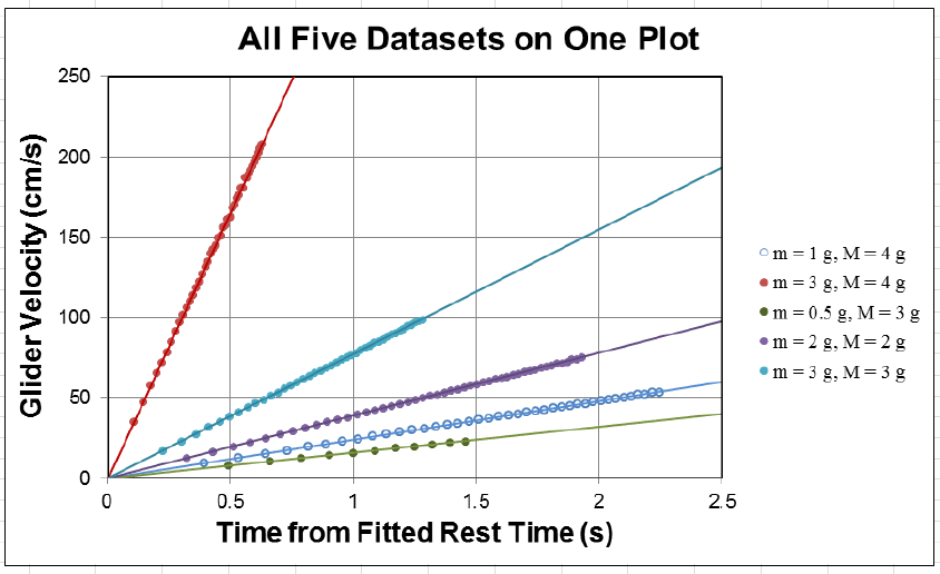
Figure 1.4: An example of ﬁve diﬀerent data sets on one Excel scatter chart. Making the ﬁt

lines the same color as the data points lends clarity to what would otherwise be an incredibly

cluttered plot. This is fake data with fake units, so please do not try to make your plot look

just like this one! The important thing is to make your results as clear as possible.

Using the techniques that were discussed in chapter 0, ﬁt a line to the velocity vs. time for

each of your 5 data sets to produce 5 measurements of the acceleration (with uncertainties

obtained from the ﬁts). Keep in mind that the reason we are obtaining uncertainties from the

ﬁts here is that we expect the uncertainty to be dominated by the scatter of the individual

data points, not the systematic uncertainty of each data points. The ﬁt line uncertainty

captures this eﬀect beautifully. Note that since you are only interested in the slope, it is

probably best to leave the intercept as a free ﬁtting parameter and then to ignore it since

the initial velocity may not have been zero when the spoke crossed the photogate. Compare

these measured accelerations to your predicted values.

1.3 Report guidelines

For experiments 1 through 5, your reports will be a single document but will have two sec-

tions. The ﬁrst section will be called the worksheet, the second will be called the presentation

mini-report. The worksheet will contain your main results presented as numbered items. The

worksheet section is intended to be a basic report of what you did in the lab and how you

analyzed your data to draw conclusions, but does not need to be a self-contained, full lab

report (you will be writing full lab reports for experiments 5, 6, and 7 in later weeks). Most

of your grade for the worksheet section of your report will be based on your data taking,

analysis, and conclusions.

Each week until experiment 5 we will focus on one aspect of a formal written lab report

(such as the abstract, or ﬁgures, or citations), and you will be asked to produce some example

of this aspect for the presentation mini-report section of your assignment. The details of this

section will change from week to week and may or may not involve your data. Most of your

grade for this section will be based on the degree to which your presentation mini-report is

on par with high-quality published scientiﬁc presentations in physics journal articles.

This week, the worksheet will be worth 40% of your grade and the presentation mini-

report will be worth 60%.

1.3.1 Worksheet guidelines

Your worksheet should contain the following sections

1. Cover Sheet

•experiment number and title

•your name and UID

•the date the lab was performed

•your lab section (for instance, “Monday 3pm”)

•your TA’s name

•your lab partners’ names

2. Plots

Include plots of all ﬁve of your data runs showing velocity vs. time and the ﬁt lines.

This could be a single plot with ﬁve data sets on it or ﬁve plots with one data set on

each. Report the slope of the ﬁt line for each (with its uncertainty, units, etc.) in a

ﬁgure caption.

3. Data Table

Report the main results from your experiment in a table such as the one below, where

your entires will be from your measurements and analysis. Your table does not need

to be exactly like this one, but should contain essentially the same information.

Hanging mass Glider mass Fit acceleration Predicted acceleration

Trial mbest (g) Mbest (g) aﬁt (m/s2)apredict (m/s2)

1 5.0 15.0 0.23 ±0.01 0.25 ±0.08

2 4.0 20.0 0.19 ±0.01 0.20 ±0.07

3 3.0 25.0 0.100 ±0.005 0.08 ±0.07

4 2.0 35.0 0.300 ±0.006 0.29 ±0.05

5 1.0 45.0 0.200 ±0.002 0.30 ±0.06

4. Derivations

Derive equation 1.1 in this manual as well as your propagation of uncertainties used in

the table above.

5. Conclusions

Write a brief discussion of your results. Compare the accelerations you measure from

ﬁtting your velocity vs. time data sets to what you would predict from Eq. 1.1 with

your measurements for the masses. Do they agree? If not, try to convince your reader

that the reason for the disagreement is understood and suggest a way to improve the

agreement in a future experiment.

6. Extra Credit (always optional)

Instead of obtaining a measurement of the acceleration by ﬁtting a slope to the cal-

culated velocity vs. time, which only works in the case of constant acceleration, we

could have diﬀerentiated the data once more to obtain a direct measure of acceleration

vs. time. Try this with just one of your data runs and present a plot of your results.

Discuss your results and explain why the noise looks the way it does. Obtain a mea-

surement of the acceleration by using the mean of your calculated accelerations and

an uncertainty based on the procedure outlined in §ii.1.6. Compare the results of the

two methods and use this to draw a conclusion of which measure you believe is better.

1.3.2 Presentation Mini-Report Guidelines

Credit where credit is due

Formal scientiﬁc writing contains proper citation of the works whose ideas and results

are used. In a highly interconnected world, students (and professors alike, I might add) have

a vast wealth of material available to them that can occasionally ﬁnd its way into their work

without appropriate citation of the person who deserves credit. Any time you use material

that has been generated by somebody else, you will be expected to either give appropriate

credit to that person’s work or to be able to successfully argue that it is common knowledge

that does not require citation.

For instance, if a student were to take a ﬁgure from the lab manual and to use it in their

report without giving credit to the author(s), a person reading the report will see the ﬁgure

and assume the student made this themselves. The student would be implicitly claiming

credit for something somebody else did and passing it oﬀ as their own. Claiming credit for

another person’s work is probably the second biggest “no-no” in science (behind fabricating

results). Furthermore, whether on North campus or South, a student’s turning in another

person’s work as their own is a clear violation of the UCLA standard for academic honesty,

and can carry with it fairly severe consequences. We will therefore be particularly diligent

about giving credit where credit is due in Physics 4AL, which is the main focus of this week’s

presentation mini-report.

A word of caution

It is easy to ﬁnd many lab reports for Physics 4AL written by former and current students.

As discussed in the syllabus, your lab report must represent your own work. This includes

the logical presentation of the report, which is often the most diﬃcult part of writing. If a

student uses another person’s work as source material for their own (even if they re-word

everything), they are using another person’s presentation and passing it oﬀ as their own,

which is a violation of academic and scientiﬁc ethics.

The same thing is true of ﬁgures (and their captions). You must generate all of the ﬁgures

in your reports on your own (the only exception to this is pictures from the lab manual that

depict the apparatus, as discussed below in §1.3.5). It is not okay to have, for instance, the

same ﬁgures as your lab partners, even if you cite them in an eﬀort to give them credit; the

entirety of your reports must be generated by you.

verbatim text

It will almost certainly not be appropriate for you to include verbatim text from any

source in your work for this course (please see the syllabus if you are confused as to why

this is). It is important to understand that one cannot pull verbatim text from a source and

just drop a reference number and the end of the sentence or paragraph with a bibliography

citation – the reader deserves to know where the quotation started, as well as whether or not

you are taking someone else’s words. If you need to use verbatim text in a scientiﬁc paper, it

should probably have quotation marks around it and the full author’s name (in addition to a

reference designator and bibliography entry), or maybe even be its own paragraph, probably

with diﬀerent indentation and font (italics are standard) than the rest of the paper. The

point is that the reader needs to be able to clearly identify when another person’s words are

being used.

Presentation mini-report on a current topic in physics research

For this week’s presentation mini-report you are tasked with writing a short review (no

more than 700 words) about a topic of your choice in contemporary physics research. This

will be a review-style paper where you can discuss the basics of some result in physics in the

past decade or so and what the likely next steps may be in the ﬁeld. Your target readers are

scientiﬁcally-literate non-specialists; your goal is to inform them of the main points driving

the ﬁeld and the likely directions it will go in the future. This should be written as if it were

to be published in a scientiﬁc journal, which means you will need to properly cite research

and review articles in scientiﬁc and engineering journals, with full citations in a bibliography

(the bibliography does not count toward the word count). Please do not cite any source that

is not either a journal article or a book. Websites, patents, overpass graﬃti, and the like are

not appropriate as they typically raise questions about source permanence and whether the

name of the author is the one who really deserves credit (highly questionable for patents).

You are not expected to be responsible for understanding the technical details of the

physics topic you choose, which is beyond the scope of this course. Your grade will primarily

be based on how well you are able to produce a short review that covers the main topics

and cites relevant and important sources properly. Your writing will be graded, and should

be concise, objective, scientiﬁc prose. Please state the word count of your review paragraph

below the last sentence.

1.3.3 How to write a bibliography

Scientiﬁc bibliographies and citation styles diﬀer from journal to journal. In physics 4AL,

for your reports you will use the format from the journal Nature. The full format guide for

Nature citations can be found at http://www.nature.com, but since we only care about a

subset of those instructions, the important points are as follows.

•References are each numbered in the order in which they are ﬁrst cited in the text,

tables, and ﬁgure legends of the document that references them.

•When cited in the text, reference numbers are superscript with no space between

the superscript numeral and the word, not in brackets unless they are likely to be

confused with a superscript number. Multiple citations are separated by commas in

the superscript, unless they are part of three or more consecutive bibliography items,

in which case the range of citation numbers may be indicated by a dash between the

ﬁrst and last citation numbers.

•The bibliography will follow the text of your review and is a list of the articles cited

in order of the citation numbers.

•Each entry starts with its number on a new line, followed by the authors’ names, the

article title, journal name, volume, starting page (or full page range) of the article, and

then the year of publication.

•All authors should be included in reference lists unless there are more than ﬁve, in

which case only the ﬁrst author should be given, followed by “et al.”. Authors should

be listed surname (typically their last name) ﬁrst, followed by a comma and initials

of given names (typically their ﬁrst name or ﬁrst and middle names), in the order in

which the names appeared on the paper.

•Titles of articles should be in upright (not italic) text. The ﬁrst word of the title is

capitalized, followed by the rest of the title written exactly as it appears in the work

cited (aside from capitalization), ending with a full stop. If there are words or symbols

in the title whose capitalization is necessary to properly convey their meaning, they

may be capitalized as needed.

•Journal titles are italic and either abbreviated according to common usage or written

in full. Volume numbers are bold, upright font, followed by a bold comma and then the

page numbers (or at least the number of the ﬁrst page) in regular (not bold), upright

font. This is followed by a space and then the year of publication in parentheses in

regular, upright font. The entire entry is terminated by a full stop.

•Citations of whole books begin with the authors’ or editors’ names (subject to the

same formatting as journal article authors). The book title follows in italic font with

all main words capitalized. Next, the publisher, city of publication, and publication

year appear parentheses and upright font. The entire entry is terminated by a full

stop.

1.3.4 Resources

Nature Format Guidelines

http://www.nature.com/nature/authors/gta/#a5.4

Scientiﬁc typesetting guidelines from NIST

http://physics.nist.gov/cuu/pdf/typefaces.pdf

http://physics.nist.gov/cuu/pdf/sp811.pdf

Appendix C shows an example bibliography (a very long one!) from a Nature paper [2].

You are expected to use the formatting found in this bibliography. This bibliography is a

good example of how to format entries, but is also a good example because of its makeup.

Almost all (>99%) of the entires are published journal articles or published books, which is

what is expected in scientiﬁc writing. Citation of another student’s lab report, for instance,

would be entirely inappropriate. Cited material needs to be static, available to the readers

of your paper, have clear authorship, and should ideally be peer-reviewed (such as is true

for scientiﬁc journals, and is generally close to being true for published books). Sources that

are published only online are in almost no cases appropriate. This is because online content

changes with time and often has unknown authorship, which explains why citing Wikipedia

is not appropriate. An author of a scientiﬁc paper needs to make sure that somebody reading

their writing 70 years from now will be able to read the exact source they are citing in their

writing.

1.3.5 Exception: Citing this lab manual for reproduced ﬁgures

Students in 4AL are welcome to use the images from this lab manual that depict the Physics

4AL equipment in their reports if they properly cite the lab manual as the source of these

ﬁgures. This is an exception to the rules for citations given above (the lab manual is not

actually appropriate, strictly speaking, but I have decided to allow students to use the ﬁgures

of the apparatus unless they are speciﬁcally requested not to). The rest of the content of the

lab report should probably not appear in your lab reports and therefore should probably not

be cited. Copying text from this lab manual (which includes ﬁgure captions, even for ﬁgures

that are borrowed and properly cited) is not appropriate for a report in physics 4AL, since

the syllabus clearly indicates that each student should be writing their reports in their own

words.

If you use an image of a piece of scientiﬁc apparatus from this lab manual in your report,

that is considered a suﬃciently direct re-use of material as to warrant a mention of the

authors’ names in the ﬁgure caption, followed by a citation number and of course a bibli-

ography item. For instance, if Figure 1.1 is reproduced in a student’s lab report (whether

they modify it or not), the ﬁgure caption should say something like “Figure reproduced

(with permission) from Fig. 1.1 by Campbell, W. C. et al.4” and then there would be a

bibliography item following the format below:

4. Campbell, W. C. et al. Physics 4AL: Mechanics Lab Manual (ver. May 12, 2017).

(Univ. California Los Angeles, Los Angeles, California).

1.4 Epilogue

Experiment 2 will be a measurement of the free-fall acceleration due to earth’s gravity, g.

However, it should be possible for you to use your results from Experiment 1 (along with

a little bit of theory) to produce a measurement of g. A measurement of this type would

be considered somewhat more “indirect” than what you will do in Experiment 2 to measure

the acceleration due to gravity, but it is worthwhile thinking about this and considering the

advantages of each method as you perform Experiment 2 next week.

Experiment 2: Measurement of g

In the previous experiment, you measured the uniform acceleration of a mechanical system

subjected to a constant force. Since the force in Experiment 1 was produced by gravity

acting on a measured mass m, you should be able to turn your results into a measurement

of the gravitational acceleration g. However, the actual acceleration (a) that was measured

in Experiment 1 was much less than gbecause the system was not in free-fall. This week,

you will be directly measuring a free-falling body to determine (a) if the acceleration due to

gravity is a constant during free fall and, (b) what is the value of the acceleration g.

Experiment 2 will involve making a few choices about how you set up the experiment.

Consider, for instance, a single photogate, similar to that used on the smart pulley in Exper-

iment 1. If the gap between the LED and the photodiode is large enough to permit a falling

object to occult the LED, this device can be used with the 850 to record the arrival time of

the object at the photogate. One way to look at this is that a single photogate can be used

to determine the position of the object at that arrival time, which we can write as (x1, t1).

This does not even give us enough information to measure the average velocity, much less

the acceleration of the ball. Just like your data analysis from Experiment 1, we need at least

two points, (x1, t1) and (x2, t2) to measure a velocity, and at least two velocities to measure

an acceleration, etc.

We therefore imagine that we now have two such photogates, vertically separated by some

distance d. If we drop, say, a plastic ball from above so that it goes through one and then the

other photogate as it accelerates in free-fall, the diﬀerence between the arrival times at each

photogate (recorded by the DAQ) should permit us to measure the average velocity between

the gates, essentially given by Eq. 1.3. But we still only have a single velocity measurement,

which is not enough information for us to measure the acceleration.

One could imagine measuring a series of velocities as a function of the height above the

top photogate from which the ball is dropped, but this would not necessarily allow you to

determine if the acceleration is independent of the height from which the ball is dropped.

Another approach would be to take many measurements from a given height while changing

the spacing between the photogates, then repeating this process for a series of diﬀerent

heights to see if the acceleration is dependent upon the initial height.

We would, however, prefer a method that can provide a measured acceleration in a single

trial, and that does not require us to drop a ball from a well-calibrated height and particular

initial velocity, which would be diﬃcult to perform. In this experiment, you will be using

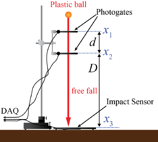
Figure 2.1: Apparatus for measuring acceleration of a ball in free-fall. A plastic ball passes

through two photogates before striking an impact sensor mat. The DAQ should be able to

measure the arrival time of the ball at all three transducers. Measured values for x2−x1

and x3−x2can then be used to determine the acceleration. By changing the height of the

pair of photogates above the impact sensor, one can test if the acceleration depends upon

initial height.

two diﬀerent arrangements to measure g: multiple sensors that record the arrival of a simple

object (a ball), and a single senor that records the arrival of various diﬀerent parts of a

complex object (a photogate comb).

First, you will be using a set of three transducers to measure the acceleration of a falling

ball (as shown in Fig. 2.1). The ﬁrst two transducers are photogates, with the last transducer

being an impact sensor mat. You will show through derivation in your report that if the

gravitational acceleration is constant (independent of initial height or velocity), your mea-

surement method does not require knowledge of the initial height or velocity, which makes

it robust against these diﬃcult to control systematics. You will also vary the height of the

pair of photogates above the impact sensor to test this claim.

Second, you will be using a single photogate to record the arrival time of each slot edge

in a slotted bar called a photogate comb (Fig. 2.3). By measuring the distance between

successive slot edges, the arrival time of each at the photogate can be used to track the

overall position of the comb vs. time. A polynomial ﬁt to the data will have a quadratic

term that is proportional to g.

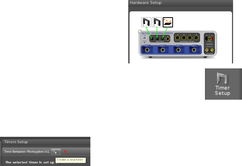
2.1 Procedure

2.1.1 Multi-sensor Method

An example apparatus conﬁguration for the ﬁrst method of determining gis shown in Fig. 2.1.

Each photogate is ﬁtted with a slotted mask that the light must pass through to hit the

photodiode. When the bottom of the ball blocks this slit, the DAQ will record the time of

this event, so the relevant height that corresponds to, say, x1in Fig. 2.1 is the height of this

slit. You will need to measure the distances x2−x1≡dand x3−x2≡Dand record your

measurements, along with your best estimate of the systematic error in these measurements

(note that the slit has some width).

To setup the DAQ, we will actually be

recording the time between photogate trig-

gers (T1) and the time between the second

photogate trigger and the impact sensor trig-

ger (T2). Plug the three transducers into

three digital channels on the 850. Choose

Photogate and Time Of Flight Accessory for

the appropriate channels in Capstone Hard-

ware Setup.

The two measurements we want will be prepared in Timer Setup, which

can be found in the Tools palette. Your ﬁrst measurement to set up is to have

the DAQ record the time between when the ball blocks the ﬁrst photogate to

when it blocks the second photogate. Set up a <New Timer>, choose Build

your own timer in step 1, and select your two photogates in step 2. By clicking

on the little drop-down menu next to each photogate in step 3, you can select Blocked for

each photogate (as shown in Fig. 2.2a.). You can then give your timer a descriptive name

(this will appear as a column header) and click Finish. Capstone will automatically identify

the units it uses for this display (seconds, normally).

To conﬁgure your second timing measurement (the

time between when the ball reaches the second pho-

togate and when it hits the impact sensor), click the

Create a new timer button at the top of the Timer

Setup area. Your second timer will measure the time between when the second photogate is

blocked to when the ball hits the impact sensor (which Capstone calls Blocked for the Time

Of Flight Accessory), as shown in Fig. 2.2b.

Once your timers are prepared, you can start a Table from the Displays palette with

your two timer measurements in the table. You may now record data in Continuous Mode.

Capstone will put the two measured times in the table every time the ball is dropped through

the sensor setup. You should set the number of displayed digits on the text in the columns

to one or two more digits than you think you need so that you do not limit your precision.

One thing to keep in mind is that the impact sensors tend to work best and have the

fastest response when the ball lands right above the position of the sensor on the bottom of

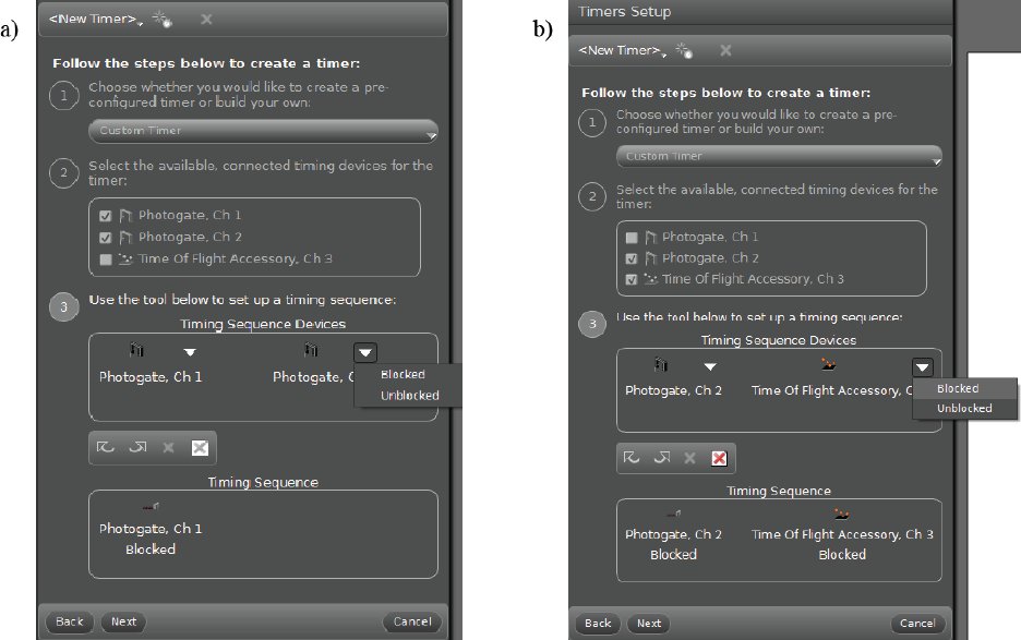
Figure 2.2: Setting up the two timers for Experiment 2. a) Example parameters to have the

DAQ measure the time between when the ball reaches the upper and lower photogates. b)

Same idea, but for the DAQ to measure the time between when the ball reaches the second

photogate and hits the impact sensor. Note that the software refers to this as producing a

Blocked state for the impact sensor.

Figure 2.3: A photogate comb with uniformly-spaced through-slots. By dropping this verti-

cally through a photogate, the position of the comb can be tracked as it accelerates in free

fall by monitoring the slots passing through the photogate as a function of time. The spacing

between successive leading (or trailing) slot edges is shown as λ.

the pad. The pads tend to be marked with a little circle on the top where this is, but you

may want to aim for that spot to reduce your systematic uncertainty associated with the

transit time of the acoustic wave between where the ball hits and the sensor location.

Each person should record at least 10 drops for each of 5 diﬀerent heights of the pair

of photogates above the impact sensor Dfor a total of at least 50 data points. Do not

share data points, but feel free to use the same values of Das your lab partners. Try to

spread these heights out over a wide range to really provide a stringent test of whether the

acceleration is independent of height. Be sure to record your measured values for Dwith

uncertainties.

2.1.2 Photogate Comb Method

Now we will attempt the same measurement with a diﬀerent apparatus. Remove the impact

sensor and one of the photogates from the ring stand and the 850 so that you have just one

photogate. You will be dropping a fairly long photogate comb through the gap, so be sure

to set the height of the remaining photogate high enough that the comb can fall all the way

through it before hitting the table. Please feel free to move the whole setup to the ﬂoor if

you like since it takes a good bit of vertical space to measure gwith this method.

An example photogate comb is shown in Fig. 2.3. First, measure the spacing between

successive edges of the slots in your comb (shown as λin Fig. 2.3). You may assume that

the placement of the slot edges is uniform across the whole length of the comb to 0.1 mm,

so the best way to determine λis probably not by measuring λ, but rather by measuring

nλ (for some integer n) and dividing by n. If you do this, the uncertainty in your measured

value for nλ will clearly be a systematic uncertainty, since it will apply to all of your data

points. You should take this into account when you think about assigning an uncertainty to

your measurement.

Next, set up the DAQ to record the arrival time of each slot edge. In Timer Setup,

make a new Pre-Conﬁgured Timer. For timer type, select Picket Fence. You will record Block

Event Times in a table. This means you may need to throw out your ﬁrst data point (since

the bottom edge of the comb is not a slot), so it is worth thinking about this a little bit. The

ﬂag spacing ﬁeld does not matter for your data since you will be recording times. You will

use your measurement of λwhen you perform your analysis, which will allow you to account

for your uncertainty in that measurement.

One person can hold the photogate comb above the photogate and the other can use a

Table to record the Block Event Times by clicking Fast Monitor Mode a little before

their partner lets go of the photogate comb. Each person should use unique data set for

their report (do not share these data with your partners). Take at least 5 data sets each.

You can experiment with the starting height above the photogate to maximize your chances

that you get at least one data set with as small an uncertainty as possible.

2.2 Analysis

2.2.1 Multi-sensor Method

For the ball drop experiments, you will have sets of data for 5 diﬀerent values of D. The

data the DAQ has recorded for each trial is T1and T2, the time between the photogates and

the time between the second photogate and the impact sensor. These data points can be

combined with your measured values for the distances Dand dto measure the acceleration

g=2

T1+T2 D

T2−d

T1!.(2.1)

You will need to derive this expression in your worksheet, but you will ﬁnd that it corresponds

to the diﬀerence between the average velocities in both regions divided by the travel time

between the middle of the upper region to the middle of the lower one.

You will have two contributions (statistical and systematic) to the uncertainty in your

measurement of gfor each distance D, which you may add together to get your total un-

certainty. Since we have to this point not spent a lot of time dealing with systematic

uncertainties, we will start by discussing this rather dicey topic.

Unlike statistical uncertainties, for which there are provably reliable methods for estima-

tion and combination, there are no generally-applicable rules for systematic uncertainties.

Recall from §ii.1.5 that systematic uncertainties can generally not be quantiﬁed by repeating

measurements, and are therefore typically estimated by using logical arguments about the

inﬂuence of various eﬀects on the measurement. If there is more than one source of system-

atic uncertainty in a measurement, you, the scientist, must decide how to combine them. An

aggressive method that is applicable in the case that the uncertainties are uncorrelated and

normally distributed, is to add the uncertainties in quadrature, which produces a relatively

small uncertainty in the measured value and a danger that the true value does not fall within

this uncertainty about a third of the time. A more conservative method that is often used is

to add the uncertainties directly, which produces a larger uncertainty in the ﬁnal measure-

ment, but a stronger guarantee that the true value falls within this uncertainty. We will use

a very conservative method in this case by estimating the total inﬂuence of the systematic

uncertainties and stating a large uncertainty that is almost guaranteed to contain the true

value.

You may estimate the systematic uncertainty in your measured value of gfor a particular

value of Ddue to uncertainty in Dand dby using their upper and lower limits (for instance,

using d=dbest +δd and d=dbest −δd) in your calculation of g. Plugging the upper and lower

limits for dand Dinto Excel with your best values for T1and T2for each height is a good

way to see how these aﬀect your measured value for g. You can then take (gmax −gmin)/2 as

your systematic contribution to δg for each D.

There is also a statistical contribution to δg for each Ddue to the spread in your 10

measured values. Use the method of §ii.1.6 to calculate your statistical contribution to

δg. Compare the size of these two contributions. If they are of comparable size, add them

together to make your ﬁnal estimate of δg. If either the statistical or systematic contribution

to δg is more than 10 times smaller than the other, you may ignore it, in which case your

value for δg is just equal to the larger one. If you think about this, there is no diﬀerence

between these two methods since you will almost certainly be stating your uncertainty with

only one signiﬁcant digit. You will be asked to discuss the process by which you determined

δg in your worksheet.

After determining a measured value for g(with uncertainty) for each value of D, plot

your measured best values gbest vs. D. Is there a trend? One way to determine if there

is a trend in a collection of data is to try to ﬁt your data to a line and see if the slope is

consistent with zero. For our purposes in this course, “consistent with zero” would mean

that the uncertainty in the slope overlaps with zero.

2.2.2 Photogate Comb Method

For each data set, you will now have a table of time stamps for when the photogate was

blocked by the edge of a slot. Using your measured value of λ, construct a table of position

vs. time. It is not necessarily clear what object’s position is being tracked (it’s probably the

top edge of the ﬁrst slot, though this depends upon your deﬁnition of x= 0), but that’s not

important for your measurement; what you care about is the quadratic part of the curve,

not the oﬀset in x(or t).

For each of your data sets, make a plot of position vs. time. Does this look like (part

of) a parabola? If not, you may have something amiss with your data. Remember to think

about the ﬁrst data point and whether or not to include it.

Excel provides an easy way to ﬁt your data to a quadratic through the Add Trendline

option. You can choose Polynomial and make it of order 2, and even display the resulting

equation on the chart to get gbest. The problem with this is that it doesn’t provide you with

an uncertainty in g! In order to do that, we will need to do a full regression analysis for a

2nd order polynomial, which is not as easy to implement as the Add Trendline option.

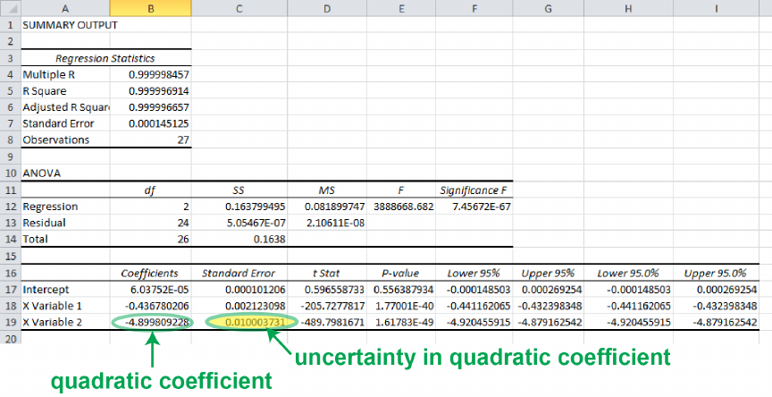
Figure 2.4: The results of a quadratic regression in Excel. The third row of results shows

the best value and uncertainty of the quadratic term. See Fig. 0.6 for a description of the

constant and linear terms.

2.2.3 Quadratic Regression Analysis

When we introduced the linear regression analysis in Excel in §0.2.5, the LINEST function

was mentioned as an alternative way to calculate linear ﬁt parameters, and the same is true

for a quadratic ﬁt. However, in the interest of ease-of-use, we will again choose to describe

how to do this using the Regression tool, but feel free to research how to do this with

LINEST if you like.

The trick to making a quadratic regression is to make a third column of data that has

the square of the original horizontal-axis data in it. In our case, if our time data is in cells

A1:A100, we can make another column right next to this one whose ﬁrst entry is =A1ˆ2

and copy that down the rest of the column by, e.g dragging its corner down to row 100.

Assuming that A1:A100 has our measured Block Times,B1:B100 has the squares of these

block times, and C1:C100 has the distance data, we start a quadratic regression analysis the

same way as was explained for a linear ﬁt in §0.2.5, but enter the range $A$1:$B$100 for the

Input X Range. This can be easily accomplished by highlighting both columns.

An example quadratic regression result is shown in Fig. 2.4. Comparing this to Fig. 0.6,

we can immediately see the constant and linear terms and their uncertainties in the same

places, but there is a third row beneath them now. This row contains the information about

the quadratic term, with the best value and uncertainty shown in Fig. 2.4.

Using quadratic regression on your data, extract a measured value for gfrom your data.

Remember, the uncertainty given by the regression is only the statistical uncertainty. If you

have a systematic uncertainty in, for instance, the distance column due to uncertainty in

λ, you may want to perform separate regressions for diﬀerent values of nλ at the top and

bottom of your range of uncertainty in nλ and compare the resulting range in measurements

of gbest to the statistical uncertainty in ggiven by the regression.

2.3 Report Guidelines

Last week, we covered citations. From this point forward in 4AL, if you need to reference

prior work by somebody, you will be expected to do so using the rules from last week

(even in your worksheet). If you cite somebody’s work, you will of course need to include a

bibliography at the end of your report in Nature format, and this bibliography will never be

counted toward a word count if there is a limit for that section of that week’s report.

This week’s worksheet will be worth 30% of your grade and the presentation mini-report

will be worth 70%.

2.3.1 Worksheet Guidelines

Your worksheet should contain the following sections

1. Cover Sheet

•experiment number and title

•your name and UID

•the date the lab was performed

•your lab section (for instance, “Wednesday 12pm.”)

•your TA’s name

•your lab partners’ names

2. Derivation Derive Eq. 2.1. Please include just enough detail to demonstrate how this

equation describes what you care about, no more than that.

3. Plots The focus of this week’s presentation mini-report is plots, but the plots you are

asked to include in your worksheet this week do not have to meet the same standard

as the one you will make for your presentation mini-report.

Include a plot of gvs. Dfor the ball drop method. Do you expect that gshould

depend upon D? Brieﬂy discuss this and what your data tell you. Can you ﬁnd a way

to quantitatively conﬁrm or rule out a linear dependence on D?

You will include a plot of your best dataset of photogate comb results in your presen-

tation mini-report, so decide which set is your best and then include your four other

data sets as a plot (or plots) in your worksheet. Include the ﬁt curves on your plots.

4. Data Tables

Include a table of your ball drop results from diﬀerent heights. An example is shown

below. If an entire column shares the same systematic uncertainty, this should be

stated in the table caption. If the uncertainty diﬀers row-by-row, it is best to state the

uncertainty explicitly in each entry.

Photogate spacing Gap to impact sensor Measured acceleration

Trial d(cm) D(cm) g(m/s2)

1 1.1 3.0 9.6±0.7

2 1.1 5.0 9.8±0.3

3 1.1 15.1 10.1±1.3

4 1.1 20.3 8.6±1.8

5 1.1 30.7 9.843 ±0.004

Include a table of your ﬁve photogate-method measured values of g. Brieﬂy describe

your uncertainty analysis and whether the uncertainty is dominated by statistical or

systematic uncertainties.

5. Conclusion

Write a brief discussion of your uncertainty analysis and results. Compare the ac-

celerations you measured with the expected value of g. Which method (ball drop or

photogate comb) do you this is the most accurate? Which do you think is the most

precise? Did you choose to use a combination of systematic and statistical error or did

you just use one? Explain why.

6. Extra Credit (optional)

One of the main challenges associated with getting an accurate measurement of gwith

the photogate comb method is keeping the comb vertical as it drops. You will ﬁnd

some string and other things around the lab that you can use to experiment with ways

to make sure the comb doesn’t swing or tip once it has been released. For instance,

some students have experimented with using paper strips, tape, string, and other tools

they have constructed to try to get the best measurement.

Design and perform your own experimental test comparing a couple of methods, and

analyze the data to draw conclusions about whether there are methods that perform

better than others.

2.3.2 Presentation Mini-Report Guidelines

Many people reading a journal article will immediately jump to the ﬁgures before deciding

to read the article. The ﬁgures will often give a quick visual representation of the content of

the paper. It is important for an author to use this knowledge to guide the reader through

what they are presenting by laying out the ﬁgures in a logical and possibly chronological

way.

Make a ﬁgure showing your best photogate comb measurement (the distance vs. time)

to the standards of a scientiﬁc journal (see below) and write a paragraph with fewer than

400 words of body text introducing the ﬁgure and discussing what it shows. This does not

need to be a completely self-explanatory paragraph, but should instead resemble a paragraph

taken verbatim from a (non-existent) longer paper that you would have written about this

experiment. Your ﬁgure should be referenced in your paragraph and will need a caption.

The quadratic ﬁt should be shown, and its results should be described. The caption does

not count toward the word count, and should probably not exceed 200 words or so. Please

write the number of words used in your ﬁgure caption and the number used in your body

text on a separate line at the end of your presentation mini-report.

2.3.3 Plots in scientiﬁc papers

All ﬁgures in well-written scientiﬁc journal articles are both clear and necessary. Along with

the guidelines below, an important part of clarity is that the text in the ﬁgure must be as

large or larger than the font of the body text. This usually means that the ﬁgure itself is

formatted with very large font sizes for its labels since the ﬁgure is typically reduced in size

when inserted into the text. A guide for how to insert Microsoft Excel ﬁgures into Microsoft

word documents with captions and ﬁgure labels can be found in Appendix B.

In Physics 4AL, it should be possible for students to complete their assignments with only

two diﬀerent types of ﬁgures: linear-axis scatter or line plots and apparatus diagrams. We

will focus on the former, though many of the points discussed below regarding the caption

will apply to diagrams as well.

1. Plots should include the following items unless there is a good reason to omit any of

them:

•axes and a bounding box with tick marks pointing inward

•axis labels (see below)

•tick labels (these are the numbers)

•data points and possibly lines joining subsequent points (when needed for clarity)

•a ﬁt or theory curve may be included

•If multiple related data sets can be plotted on the same axes without creating

confusion, they should share the same axes. If multiple plots or ﬁgures are closely

related, they should be combined into one ﬁgure if doing so does not come at the

expense of clarity.

2. Every ﬁgure (and table) needs a caption directly below the item it describes, and plot

captions should include the following items:

•“Figure XX.” or some other appropriate designator with a unique number that is

referenced in the body text, followed by

•a descriptive title, followed by

•a description of all lines and symbols on the plot and what they mean

•a brief discussion of what the data (and curves) show

Typically, about ﬁve labeled tick marks will be suﬃcient for fully-specifying an axis.

Tick labels should have an appropriate number of digits for the range they describe.

Though you are unlikely to encounter this in physics 4AL, if the plot range covers a

small fraction of some large absolute scale, you can subtract an overall oﬀset from the

tick labels and explain what this is in the axis label. For instance, if frequency is being

plotted from fmin = 12.642 808 GHz to fmax = 12.642 816 GHz, the tick labels should

probably be every 2 kHz, so the tick labels would be the numbers 8, 10, 12, 14, and

16 and then the axis label would say something like “Oscillator frequency, f(kHz)

−12 642 800 kHz.”

3. Common mistakes to avoid:

•Do not include any lines or curves that are not well-deﬁned (such as splines that

are not fully described, etc.). All lines and curves must be completely speciﬁed.

•Do not put a title at the top, as the title is the ﬁrst part of the caption. Note

that this is one of many diﬀerences between a ﬁgure in a scientiﬁc journal and the

ﬁgures in this lab manual, which is not a scientiﬁc journal article.

•If possible, avoid the use of yellow or light green (or any color that will be hard

to see).

4. Plot Axis

The format for an axis label in physics 4AL will be “Quantity name, Symbolic Des-

ignation (Unit).” The quantity name should be plain English words (e.g. “Distance

to stop,” “Delay between pulses,” “Glider speed,” “Number of events,” etc.). The

symbolic designation is optional, and if used is the mathematical symbol you be use to

represent this quantity in the body text and its equations (D,t,v,N, etc.). Last (and

not optional), the units symbol for the tick mark labels should be written in parenthe-

ses. Though you are unlikely to encounter this in Physics 4AL, if the units of an axis

(almost always the vertical axis) are suppressed because they are truly irrelevant and

would be distracting, it is conventional to write “(arb.)” for the units.

Axis limits should be chosen to highlight the important points of the plotted material

as well as possible. This may involve cutting oﬀ some of your data (typically on the far

left or far right), so you will have to think about whether you can omit parts of your

data set without changing what the data show. Omitting data to change conclusions

is not okay – data may only be omitted if doing so improves clarity of presentation

without altering the interpretation of what the data support.

5. Adding the caption

A good ﬁgure caption tells the reader not only what is on the plot, but why it is

important and what conclusions can be drawn from the results. The ﬁrst thing after

the designation (e.g. “Figure 1.”) should be a short, descriptive title. The title should

not simply be “(y-axis label) vs. (x-axis label)” – your reader will already know that

from looking at your ﬁgure. Your goal is to give the reader a good idea of what it

is you are presenting and why you are presenting it. For instance, for a ﬁgure from

Experiment 0, instead of “Voltage vs. Weight,” a much more descriptive ﬁgure title

would be “Calibration of the force sensor.”

Next, describe what is on the plot. The reader should be able to tell what every data

point and curve on the plot is. If there is a ﬁt curve on the plot, it needs to be discussed

in the ﬁgure caption. In contrast to many of the ﬁgures you see in this lab manual

(which is not a scientiﬁc paper), please do not put your ﬁt line equation on the body

of the plot; the ﬁt line equation and the ﬁt parameters need to either appear in the

caption or the caption should clearly indicate to the reader where they can be found.

One good way to add a ﬁtted curve’s equation to the caption is to write the equation

using symbols, then to present the values for these symbols (and their associated

units and uncertainties). For instance, “The solid red curve is a ﬁt of the data to

an exponential decay, J(t) = Ae−t/τ with ﬁt parameters A= (43 ±4) km and τ=

(22.60 ±0.06) fs.” Alternatively, this can be accomplished by of referencing speciﬁc

equations in the body text instead (see, e.g. Eqs. 0.2 and 0.3 of this manual).

6. Final notes

A guide to graphing in Excel and adding captions in Word by Julio S. Rodriquez, Jr.

and Anthony Ransford can be found in Appendix B of this lab manual.

2.4 Epilogue

2.4.1 Specialized deﬁned units for gravitational acceleration

The “law of falling bodies” is usually attributed to Galileo, by which we mean that he

is often described as the ﬁrst to discover that gravitational acceleration is constant and

independent of mass. In recognition for this achievement, he has been given the highest

honor in physics (even higher than the Nobel prize!): a unit named after him. Naturally, it

is a unit of acceleration, the “Galileo.” 1 Gal ≡1 cm/s2. Gravimetric maps often display

their gravity anomaly data in units of mGal, or “milli-Galileos.” There is also a deﬁned unit

called Standard Gravity [8] that is given by go≡9.806 65 m/s2.

2.4.2 gin Knudsen 1-2381

1This analysis and section were contributed by Chandler Schlupf (2015).

Standard Gravity (go) is some sort of average of the apparent gravitational acceleration over

the surface of the earth, but the gravitational acceleration at any given point can change

by up to about a percent depending where the point is due to several factors. The ﬁrst is

that the Earth is not perfectly round, but rather an oblate spheroid (shaped like an onion),

so its radius is not constant and the surface is not equidistant from the geometric center.

Second, since the Earth is spinning, a centrifugal pseudo-potential that varies with latitude

is produced, decreasing the apparent gravitational acceleration near the equator compared

to the poles.

Furthermore, local variations in the makeup of the Earth’s crust can inﬂuence the value

of gby changing the average density of the ground below, as well as the distance from

the center of the earth. For example, a pocket of low-density material such as a liquid or

gas underneath the Earth’s surface can cause a tiny decrease in the measured gravitational

acceleration right above it. Gravimetric measurements are therefore sometimes used to locate

petroleum deposits.

All of this means that the value of gin a given location is not, in general, equal to

Standard Gravity go. In fact, these eﬀects (and others) essentially guarantee that gois

actually the gravitational acceleration almost nowhere on the surface of the earth (look how

many digits there are on go)! Luckily, the only important thing for Experiment 2 is knowing

the value in our lab room.

Measured data of variations in the Earth’s gravitational ﬁeld are collected on gravimetric

maps. One such map for our location created by the Southern California Areal Mapping

Project can be found at http://pubs.usgs.gov/of/2003/0269/. Unfortunately, there is

not a data point on UCLA’s campus (to obtain accurate measurements, they only take

data points on solid bedrock). However, we can use surrounding points to get a good

estimate. Averaging the three closest points to UCLA and taking their standard deviation

as an estimate of the systematic uncertainty gives us a value for gravity in Knudsen 1-238

of g= (9.7955 ±0.0003) m/s2.

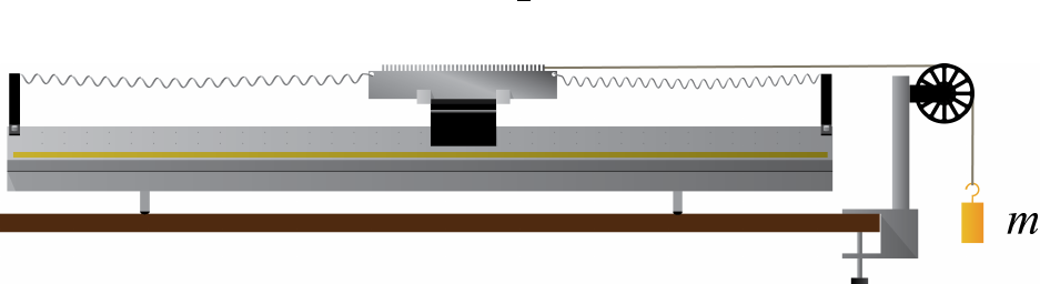
Experiment 3: Conservation of

Mechanical Energy

Conservation of energy is a powerful conceptual and computational tool that is useful in

essentially every ﬁeld of science and engineering. Dissipation of energy into random thermal

motion still obeys conservation of energy, but it is sometimes diﬃcult to keep track of the

dissipated energy, so we will be focusing here on the conservation of mechanical energy. In

this experiment, you will measure the kinetic and potential energy of a harmonic oscillator

during half of an oscillation cycle, where you will try to determine to what degree the

initial potential energy is converted entirely into kinetic energy and then back into potential

energy. The experiment has been designed in a way to try to minimize dissipation, but you

will be able to analyze your data to quantify how much energy is being dissipated from the

mechanical energies.

A glider is provided that has a comb of photogate ﬂags mounted to the top. You will be

using a photogate to measure the passing of each ﬂag, which will enable you to determine

the position and velocity of the glider. Two springs are also provided to produce a restoring

force on the glider to some point on the air track. By measuring the spring constant of this

restoring system, you will be able calculate potential energy as a function of position

U=1

2kx2.(3.1)

Figure 3.1: Apparatus for measuring the eﬀective spring constant providing the restoring

force for your glider. Once the spring constant has been determined, the hanging mass,

string, and pulley should be removed.

You will also measure the mass of the glider (with photogate comb attached!), which will

enable you to determine the kinetic energy as a function of velocity:

K=1

2Mv2.(3.2)

The tricky part of Experiment 3 will be the data analysis, where you will need to ﬁgure

out how to interpret your raw data (a series of time stamps for when the photogate goes from

being unblocked to blocked) to calculate these quantities. You will need to determine how

to ﬁnd the kinetic energy as a function of position so that for every data point where you

calculate the potential energy, you can also calculate the kinetic energy. By plotting these

together, you can also plot their sum, which should be constant in the absence of dissipation.

You will ﬁnd that despite the fact that the amount of energy of each type changes drastically

over the course of half an oscillation, their sum is remarkably ﬂat. The slight decrease in total

energy over your measurement will enable you (through ﬁtting) to determine the coeﬃcient

of friction of your nearly-lossless air track setup.

3.1 Procedure

The ﬁrst experimental task to complete is to determine the mass of the glider with its

photogate comb and record this for your analysis. You will then need to determine the

spring constant associated with the restoring force of your spring setup, as shown in Fig.

3.1. The spring constant measurement does not utilize the DAQ at all, and will require you

to write down a series of measurements for your analysis and report.

Figures 3.1 and 3.3 show the basic idea. By measuring the position of the glider for a series

of diﬀerent masses m, a plot of applied force (mg) vs. displacement can be ﬁt to determine

the slope of this trend, which has units of force per displacement and is the eﬀective spring

constant of your system. Be sure to get data for at least 5 diﬀerent masses. Once you have

gathered enough data for your spring constant measurement, you may disconnect the pulley

system and hanging mass from the glider and move it out of the way. You may share data

for the spring constant measurement with your lab partners, but will be expected to use

your own data sets for the rest of Experiment 3.

To measure the position and velocity of the glider for your analysis and report, we will

be using a photogate to tell us when each tooth ﬁrst blocks the photogate. This is a tricky

business, and you will want to be very careful that you describe your procedure in your own

notes so that you can use them to interpret your data later.

The teeth on the photogate comb are 2 mm wide, as are the spaces between teeth, both

to an uncertainty of 30 µm. You will only be using half of a single oscillation of the glider

for Experiment 3, so you may pick a direction for the glider to be moving when it passes the

photogate. Remember, the photogate cannot tell the diﬀerence between the glider moving

left or right, so this will simplify your analysis by conﬁning the movement to one direction

only. You will pull the glider back just beyond the photogate, start the DAQ recording, then

release the glider. You may stop recording as soon as the glider stops to reverse its direction.

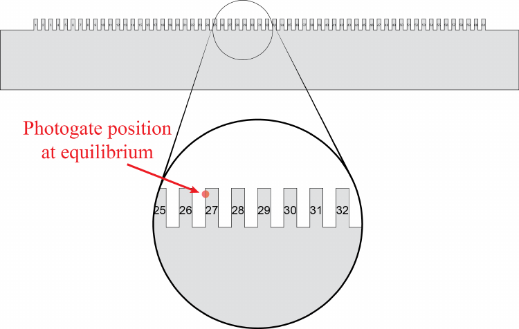
Figure 3.2: An example photogate comb shown with an example for a position of the pho-

togate when the glider is in its equilibrium position. In this case, it is probably easiest to

analyze the data if one chooses to pull the glider back to the right instead of the left.

First, it is important to set and record the equilibrium position of the glider relative to

the photogate beam. A good choice is to put the photogate so that a tooth near the center

of the comb is just on the verge of blocking it (the light on the top of the photogate turns on

when it is blocked). You will thank yourself later if you are very careful about recording (a)

which tooth that is and (b) which direction the glider needs to move to block the beam when

it is at equilibrium. Beware that the teeth may have marks on them that are meaningless;

be sure to do your own counting to determine which tooth number you are using.

Figure 3.2 shows an example conﬁguration where the photogate is set up to trigger on

the 27th tooth if the glider is displaced to the left a tiny amount from equilibrium. In this

example, pulling the glider all the way to the right so that tooth number 1 is just past

the photogate position and then letting go and having the DAQ record the time stamps

every time the photogate goes from being unblocked to blocked means that the 27th time

stamp happens at exactly the equilibrium position, which one could deﬁne as being x≡0.

This would mean that the ﬁrst time stamp happened at a displacement from equilibrium

of x=−104 mm. Likewise, if for the same conﬁguration the glider had been pulled oﬀ to

the left and then let go for recording data, the equilibrium position would be reached about

halfway between time stamp 35 and 36, because the photogate triggers when it goes from

being unblocked to being blocked. In this case, the ﬁrst time stamp indicates the glider is

at a position of x=−138 mm from equilibrium.

To set up the DAQ for recording these time stamps, connect your photogate to a digital

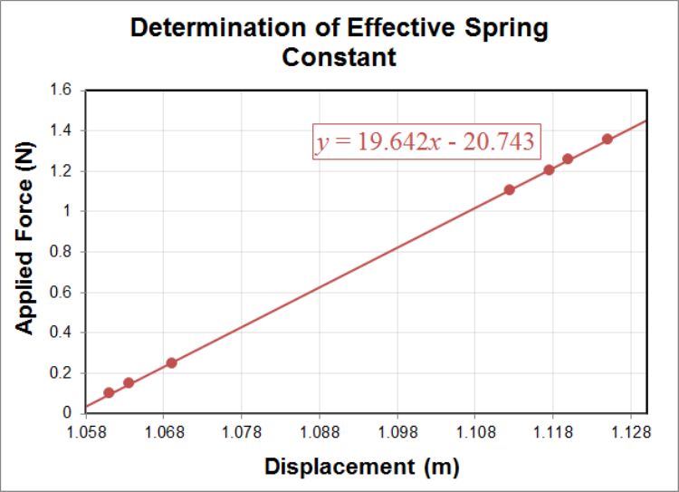
Figure 3.3: Determination of a spring constant by ﬁtting a line to measured values of force vs.

displacement. In this case, the spring constant was determined to be k= (19.64±0.04) N/m.

channel and select Photogate in Hardware Setup. In Timer Setup, you should make a

new Pre-Conﬁgured Timer based on your photogate channel that is of the Picket Fence type.

You will record Block Event Times in a table. The ﬂag spacing ﬁeld does not matter for

your data since you will be recording time stamps. Once this timer has been created, you

may create a Table and use Fast Monitor Mode. One person can pull the glider back in

the chosen direction past the photogate, then their lab partner can click fast monitor mode.

The glider can then be released. Once the glider reverses its direction, stop the DAQ and

you may copy and paste your data into Excel to save for your analysis. Each person needs

their own data set, but all three may be recorded in a row using the same apparatus setup.

3.2 Analysis

For your measurement of the spring constant of the restoring force, plot your force vs.

displacement data. You will need to make sure your plot has the appropriate data as xand

y, because it is easy to get these mixed up, especially in Excel. Figure 3.3 shows an example

with some fake data. The y-intercept is of no interest here as we are only concerned with

determining the slope of the ﬁt line. Remember, the SI units for spring constant are N/m, so

be sure to convert your masses into applied force correctly (remember the diﬀerence between

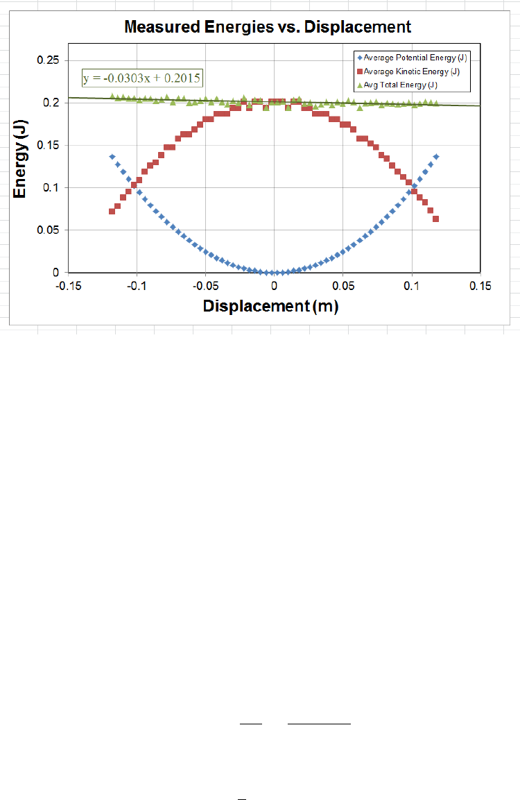
Figure 3.4: Mechanical energy of a glider vs. position. The potential energy shows the

harmonic well for this oscillator. The kinetic energy is based on diﬀerentiating the same

data that was used to calculate the potential energy, so it is more noisy, as expected when

diﬀerentiating data.

grams and kilograms), and you hopefully found in Experiment 2 that g= 9.8 m/s2(you may

of course use this value even if you got a diﬀerent answer in Expt. 2).

Your data for the moving glider should consist of a column of time stamps. Using

your knowledge of where the photogate was relative to the comb when the glider was at

equilibrium, you should be able to convert these time stamps into positions, where you

should deﬁne the equilibrium position to be x= 0. This is important because you will be

calculating the potential energy using Eq. 3.1, so x= 0 should correspond to U= 0.

It is certainly true that we could calculate the potential energy as a function of distance

based on these data (since you now have a value for the spring constant k). However, we

will be calculating velocity by numerically diﬀerentiating your data, which is the same as

saying we will be using the following expression (as in previous experiments)

v(¯x(i)) = ∆x

∆t=xi+1 −xi

ti+1 −ti

(3.3)

where ¯x(i) is the average position in this interval,

¯x(i)≡1

2(xi+1 +xi).(3.4)

So we will have a value of Uat every xi, but a value for Konly halfway between every xi

and xi+1 (which we call ¯x(i)). Since we want to calculate the potential, kinetic, and total

energy at the same place, we can, for instance, determine the potential energy for each value

of ¯x(i). To do this, create a new column for the average positions ¯x(i) that is the average of

each successive pair of points in the xicolumn. You can then create a column that calculates

the potential energy U(¯x(i)) = 1

2k¯x(i)2at each value of ¯x(i) using Eq. 3.1. Create another

column and ﬁll it with calculated values of the kinetic energy

K(¯x(i)) = 1

2M xi+1 −xi

ti+1 −ti!2

(3.5)

using your measured value for the mass of the glider with its comb on top. Last, create a

third column that calculates the total mechanical energy for each position ¯x(i).

Create a plot that shows kinetic energy, potential energy, and the total energy as a

function of displacement ¯x(i). An example is shown in Fig. 3.4. Your potential energy

should look like a parabola, characteristic of a harmonic oscillator. The kinetic energy will

be more noisy than the potential energy since it is based on numerical diﬀerentiation of data,

which magniﬁes noise in the data. The total energy should be very linear. If your calculated

total energy does not look linear, it is likely that you have set your zero point in the wrong

place when trying to convert between time stamps and displacement from equilibrium. Fit

a line to the total energy vs. distance and determine its slope (with uncertainty). The slope

of this line has units of J/m = N, and represents a constant force that dissipates energy

from your oscillator, probably due to friction. Using your known value for the glider mass,

calculate the coeﬃcient of friction needed to produce this slope.

3.3 Report Guidelines

For both the worksheet and the presentation mini-report for Experiment 3, you will be

expected to apply what you learned in the previous experiments about citations and plots.

For instance, your worksheet for Experiment 3 will contain two plots, and those plots should

conform to all of the guidelines from §2.3.3 (aside from the body text, which will often not

be necessary on a worksheet).

This experiment’s worksheet will be worth 30% of your grade, with the presentation

mini-report worth 70%.

3.3.1 Worksheet Guidelines

Your worksheet should contain the following sections

1. Cover Sheet

•experiment number and title

•your name and UID

•the date the lab was performed

•your lab section (for instance, “Monday 9am.”)

•your TA’s name

•your lab partners’ names

2. Discussion

•Include a description of which direction your glider moved and where the photo-

gate was compared to which tooth.

•Describe how you calculated the potential energy and kinetic energy at the same

positions in space.

3. Plots and Tables

•State your measured value for the mass of the glider with its photogate comb.

•Make a table of your data used to calculate the spring constant.

•Include your plot showing the ﬁt line for determining the spring constant. State

your measured value for the spring constant (as always, with its uncertainty and

units).

•Include your plot of the three energies vs. position, along with a linear ﬁt to the

total energy vs. position.

•Present your calculated value for the coeﬃcient of friction of the glider on the air

track (with its uncertainty, of course!).

4. Extra Credit

Since the photogate does not distinguish between movement of the glider in the +x

and −xdirections, we conﬁned our analysis to half of an oscillation. However, by

appropriately converting the measured times stamps into displacement (warning: this

step is very tricky!), it is possible to generate a plot with multiple oscillations. Save

data for at least two full oscillations of your glider and use this to plot the two types

of energy vs. time (as opposed to plotting them vs. distance). Estimate how long it

would take your glider to decrease its oscillation amplitude by a factor of e(one digit

of precision is okay for this). Fig. 3.5 shows the results of doing something like this,

where the decay of the energy in the mechanical degrees of freedom is clearly visible.

3.3.2 Presentation Mini-Report Guidelines

The ﬁrst page of a scientiﬁc paper will almost always contain the title, author list, and an

abstract for the paper. The title and abstract are where you will tell your story to the largest

audience. The title and abstract must stand alone and the main points should be able to be

understood without the bulk of the report. An emphasis on clear, speciﬁc, and minimalist

writing will be important not only to communicate what you have done and why it is im-

portant but also to convince the reader that the rest of your paper is worth their time. In

Physics 4AL, we will follow the guideline that no abstract is to contain more than 200 words.

Please always write the number of words contained in your abstracts on a separate line below

the last sentence. For this week’s presentation mini-report, please write a title, author list,

and abstract for your work on experiment 3. Please put this mini-report on a single, new

page, with the title at the top, followed by the author list (centered), followed by the abstract.

Abstract

An abstract is a recap of all the information of a scientiﬁc article, conference, presentation

or research update. The abstract should be a standalone document where the reader could

broadly understand all major points (including the conclusions) of the research without

reading further. You are tasked with writing an abstract for Experiment 3 (the one you have

just performed) with fewer than 200 words. In this abstract you will describe what was done

and why. Were you testing some model or another for the behavior of some physical system?

Were you testing a fundamental principle of physics, or measuring a property of something?

Were you investigating the degree to which a system exhibits some desired eﬀect?

In this course, we will depart somewhat from the Nature style in that your abstracts

should not include citations or background. An abstract should be succinct with no un-

needed words. Scrutinize every word and use the minimum number of words required to

express your ideas. Remove words that are ambiguous or imprecise. Even though an ab-

stract is short, it is worth your while as a scientist to make sure you put the time in to make

something you are proud of, as many times it is the only published evidence of conference

talks, presentations or research updates.

Title

Above your abstract you will include a title. The title is sometimes the single most

important thing in a paper. By the pigeonhole principle it is at least the most read part

of a paper. The title should be explicit and understood by the most general of your target

audiences. You need to tie yourself to the similar research out there while distinguishing

what you have done as something diﬀerent. Like the abstract it is of utmost importance to

scrutinize every word with a focus on clarity. The title should not be an English sentence.

Author List

We will follow the standard U.S. author list convention of initials followed by surname.

You will be the only author on your Physics 4AL papers. At the end of your name include a

superscript that indicates a footnote with your aﬃliation. For example “F. D. Roosevelt1”.

On the bottom of your abstract you would note the aﬃliation, for example “1Department of

Physics Port Chester University”. Your lab partners’ names will be on your cover sheet, so

there is no need to worry about giving them credit for helping you to take data. Since all of

the analysis, ﬁgures, text, and so forth for your report have to be entirely generated by you,

we will let the cover page suﬃce for crediting lab partners.

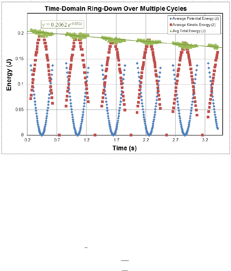
Figure 3.5: The total mechanical energy of a glider slowly decreases due to dissipation (see

Extra Credit). In Experiments 5 & 6, you will be measuring properties of harmonic oscillators

that have similarities to this one.

3.4 Epilogue

A plot of the potential energy vs. position (such as shown in Fig. 3.4) gives a visual repre-

sentation of the “potential well” in which the glider oscillates. The frequency of a mass m

oscillating in a parabolic well (U=1

2kx2) is given by

ω=sk

m.(3.6)

Using the measured value for kassociated with the data in Fig. 3.3 and the measured mass

gives a prediction for the oscillation frequency that matches the frequency shown in Fig. 3.5

at the 10−2level, demonstrating that this system is well-modeled as a simple harmonic

oscillator.

Experiment 4: Momentum and

Impulse

In the previous experiment, you investigated conservation of energy by monitoring the trade-

oﬀ between kinetic and potential energy in a harmonic oscillator. However, as you were able

to quantitatively verify in Experiment 3, mechanical energy can be dissipated into heat in

a number of ways. It is often fairly diﬃcult to keep track of these dissipation mechanisms,

and so the conservation of energy balance sheet can end up with a kind of catch-all entry for

“dissipation” that limits its usefulness as a predictive tool in all but the most well-controlled

environments.

Compared to conservation of energy, conservation of momentum is often said to be more

“fundamental.” There are a few reasons why you may hear this claim, but for our purposes

it should suﬃce that it’s often easier to keep track of and predict the ﬂow of momentum

in real-world situations than energy. For instance, both elastic and inelastic collisions are

required to conserve linear momentum with respect to the movement of the colliding objects,

while conservation of energy allows kinetic energy to be converted into, for example, heat

during the collision.

In Experiment 4, you will be investigating the relationship between two diﬀerent ways of

measuring an impulse, which is a momentum change (and therefore has units of momentum).

You will measure the initial and ﬁnal velocities of a glider on an air track that impacts a

rigidly-mounted force sensor, which will give you a ﬁrst method for measuring impulse:

∆P=Pf−Pi.(4.1)

You will also record the reading on the force sensor during the collision as a function of time,

allowing you to integrate the force to provide you with your second method for measuring

the impulse:

∆P=Zdt F (t).(4.2)

It is interesting to note that we expect the two measurements, Eq. 4.1 and Eq. 4.2 to be

equal to each other no matter how inelastic the collision with the force sensor is. It should

not matter if this collision conserves the kinetic energy of the glider, increases it, or decreases

it; we should always expect to be able to use Eq. 4.2 to predict Pfbased on Pi, regardless of

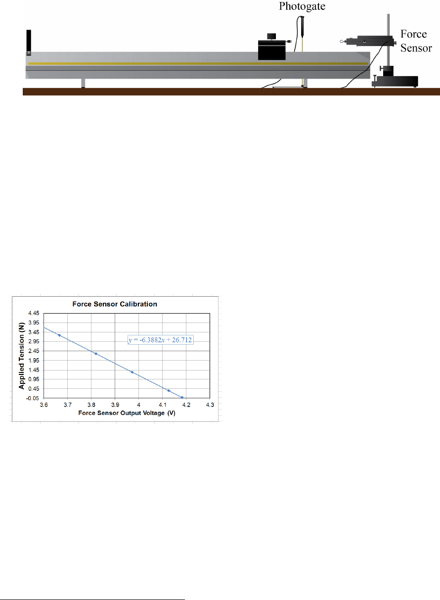
Figure 4.1: Apparatus for measuring the impulse of a glider colliding with a force sensor.

The ﬂag on the glider passes through the photogate both before and after the collision,

providing a means to measure the initial and ﬁnal momentum. The force sensor allows you

to record F(t), which can be integrated numerically to obtain an independent measure of

the impulse.

whether there is a piece of bubble gum or a diamond on the end of the glider that hits the

force sensor1.

4.1 Procedure

Your ﬁrst step will be to calibrate your

force sensor, whose internal calibration is

not trustworthy on the level needed for this

experiment. You will essentially follow the

same procedure as that used in Chapter 0.

You will set up your force sensor as a User

Deﬁned Sensor whose output will be in volts.

You should record the voltage reading for at

least 5 diﬀerent weights hanging from the

force sensor hook spanning the range from

0 to not more than 1 kg. You may assume that the calibration slope found by measuring

tension is also appropriate for compression. You should be suﬃciently familiar with the

hardware at this point to be able to do this step without detailed instructions, but you may

want to take a look back at Chapter 0 if you have questions. You may share your sensor

calibration data with your lab partners, but you should perform the analysis and ﬁtting on

your own.

Figure 4.1 shows the experimental setup for producing your two, independent measure-

ments of the impulse of the collision between the glider and the hook of the force sensor.

The photogate ﬂag on top of the glider allows you to use the photogate to measure the speed

of the glider both before and after the collision. For this, you will need to know the mass of

the glider (with all of its attached ﬂags and bumpers) and the length of the photogate ﬂag.

1Please do not put gum on the lab equipment. However, please do feel free to leave diamonds all over it.

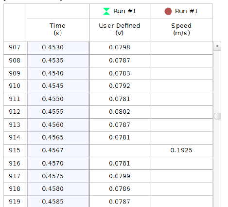
Figure 4.2: The DAQ will rapidly ﬁll in the ﬁrst two columns of your table once you tell it to

record. By scrolling through the table while watching the speed column, you should be able

to ﬁnd your measured initial and ﬁnal speeds, which will be the two entries in this column.

You will use the Speed function of the photogate timer, so you will need to enter the length

of the ﬂag into Capstone during setup.

To conﬁgure the photogate, select Photogate for the appropriate channel and then move

on to Timer Setup. Choose a Pre-Conﬁgured Timer for one photogate with a single ﬂag.

In Step 4, you will choose Speed as the measurement that will be visible, at which point

you will need to type in the length of the ﬂag (in meters) to complete your timer setup.

The Speed measurement that Capstone uses is simply the entered ﬂag length divided by

Time in Gate, so feel free to use either, keeping in mind that the important thing is that

the fractional uncertainty in ﬂag length will be the same as the fractional uncertainty in the

speed measurement (assuming the timing has a much smaller fractional uncertainty).

For the force sensor, you should keep the same settings you had for the calibration, which

is to call it a User Deﬁned Sensor on an analog channel.

Your data will consist of three columns in a Table, which will be ﬁlled in Continuous

Mode once you hit Record. You will want a column for Time (s),User Deﬁned (V), and

Speed (m/s). The ﬁrst two columns will start getting ﬁlled in as soon as you hit Record,

where the Speed column will only get two entries, which will show up only at the time

the glider has passed through the photogate. In the Controls palette, be sure the sample

rate for the User Deﬁned Sensor is set fast enough to generate enough samples to give you

good results without creating an excess of data. Capstone has been known to have sporadic

problems on this experiment for high sample rates (≥10 kHz), so you may want to stick to

sample rates of a few kHz and fairly gentle collisions to get good data for this experiment.

To take your data, start the glider moving toward to photogate and start recording just

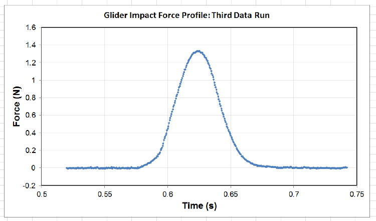
Figure 4.3: Force sensor reading before, during, and after the collision. The ﬁrst 100 ms

or so of data was averaged to provide a measurement of the force sensor baseline, which

was subtracted from the data before creating this plot. The area under this curve is a

measurement of the impulse of the collision.

before it reaches it. As soon as the glider has passed through the photogate on its way back

the second time, you may stop recording. You will now have three columns of data, two

of which are very full with the third one almost completely empty. Be sure to increase the

number of displayed digits on your table to high enough precision so that you are not limited

by this. Figure 4.2 shows an example of what part of your data might look like. You should

be able to ﬁnd two entries in the Speed (m/s) column. Write these down somewhere for your

analysis, and be sure to think about whether or not to enter a minus sign on one of them

(remember, the photogate does not know which direction your glider is moving).

Your two remaining columns of data may be quite long. If there are more than about

5000 rows, you should probably try re-taking your data with a faster trigger-ﬁnger on the

record button so that you only get the part of the data you really need. You may ﬁnd that

you need to move the photogate closer to the force sensor to minimize the dead time, but

be sure your photogate measures the glider speed when it is freely moving, not while it is

impacting the sensor. By scrolling through your data, you should be able to ﬁnd a section

that shows lots of changes in the User Deﬁned (V) section. That section is what you will

need for your report, so copy and paste it (both columns) into Excel for saving. Be sure to

get enough data before and after the collision to give you a good feel for your baseline (see

Fig. 4.3). Each person will need two data sets of their own for their analysis. Try

to get two diﬀerent speeds to compare them to one another.

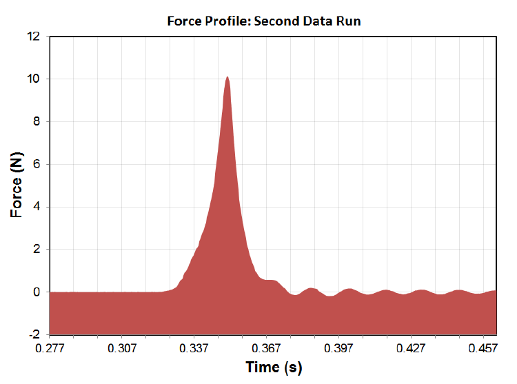
Figure 4.4: Force sensor reading before, during, and after a fast collision. The reading shows

oscillations, or “ringing” after the collision that can be ignored for your integration.

4.2 Analysis

For your determination of the calibration of the force sensor, plot your data and run a

regression ﬁt to determine the slope (with uncertainty). You will probably want your slope to

have units of N/V so that you can just multiply it by your column of recorded voltages to get

force. Remember to ﬂip the sign appropriately to convert between tension and compression.

Your ﬁrst measurement of the impulse comes from your two speed measurements given

by the photogate. Multiply your measured velocities by the mass of the glider to create a

measured value of the initial and ﬁnal momentum, then use Eq. 4.1 to convert this into a

measurement of the impulse.

Using your calibration of the force sensor, you can create a new column in Excel that

converts your measured voltages into force. Create a scatter plot of your measured force

vs. time. Even if you tared the force sensor before taking your data, you will want to choose

a big group of data points at the beginning to average to deﬁne your baseline, so use your

scatter plot to choose an appropriate range to average for this and create a new column of

forces that have the background subtracted. You can now create a new scatter plot of your

results, as shown in Fig. 4.3.

You may notice that your plot shows some “ringing” in the reading after the collision,

such as is shown in Fig. 4.4. For your numerical integration of your data, this can be safely

ignored as long as the amplitude of the oscillations is much smaller than your impact (such

as is shown in Fig. 4.4), and your integration really only needs to include the big peak from

when it starts to rise to about the point where it crosses zero again.

To complete your analysis, you will want to integrate your data to ﬁnd the area under

the big peak of your force vs. time plot (Eq. 4.2). To do this integral numerically, simply

ﬁnd the sum of all of the force measurements during the big peak and multiply this by the

duration of the small time step ∆tbetween successive points. This method of numerical

integration is called a Riemann sum, and we have assumed that the force measurements are

all equally spaced in time by ∆t. Mathematically, we are using

∆P=Ztn

dt F (t)≈∆t

i=1

F(ti) (4.3)

where ∆t≡ti+1 −ti. You should compare your impulse measured with both methods. If they

are oﬀ by a large factor, make sure you got all your units correct and that you subtracted

the background force reading appropriately.

4.3 Report Guidelines

As usual, you will be expected to use what you learned from the presentation mini-reports

of Experiments 1 and 2 to format your report (citations and plot guidelines). However, you

will not be called upon to produce an abstract, etc. (covered in Experiment 3’s presentation

mini-report) again until you begin writing full lab reports in Experiment 5.

This week’s worksheet will be worth 40% of your grade, with the presentation mini-report

representing the remaining 60%.

4.3.1 Worksheet Guidelines

Your worksheet should contain the following sections

1. Cover Sheet

•experiment number and title

•your name and UID

•the date the lab was performed

•your lab section (for instance, “Wednesday 9am”)

•your TA’s name

•your lab partners’ names

2. Discussion

•Present your measured values for the mass of the glider (with all its accessories

on it) and the width of the photogate ﬂag, with uncertainties.

•Present a plot of your calibration of the force sensor. You do not need to make a

table, but be sure to include the ﬁt line on your plot.

•Be sure to state your calibration constant for converting the force sensor voltage

into newtons with the uncertainty you found for this constant. This can either

be in the plot caption or can be written as body text and referenced in the plot

caption.

•Present your two calculated impulses that were based on the photogate speed

measurements, one for each data run.

•Include a plot of each of your two measured force vs. time curves with the back-

ground subtracted from the force sensor.

•Describe how you used the force vs. time data to determine the impulse, i.e. how

you performed the numerical integration.

•Present your two measured values for the impulses based on numerical integration

of the force proﬁles. To assign an uncertainty, you may estimate this by assuming

the fractional uncertainty of your integral is the same as the fractional uncertainty

of your force sensor calibration coeﬃcient.

•State the results of the two diﬀerent methods for both runs in a table (with

uncertainties).

3. Extra Credit (optional, as always)

The inelasticity of a collision can be quantiﬁed through a unitless number called the

coeﬃcient of restitution,CR. When two objects collide, CRis deﬁned as the ratio of

the ﬁnal relative speed of the colliding objects to the initial relative speed. As such,

it tells you something about how elastic the collision was, where CR= 1 for perfectly

elastic collisions and CR= 0 for completely inelastic collisions. Team up with another

table and use two gliders and two photogates on the same setup to measure CRfor

two gliders colliding with diﬀerent bumpers (including one collision with no bumpers).

Compare the degree to which energy and momentum have been conserved for each

collision.

4.3.2 Presentation Mini-Report Guidelines

For this week’s presentation mini-report, please write an introduction and a methods section

for your work on Experiment 4. Please write the word count for your introduction on a new

line below its last sentence.

Introduction

The introduction section explains, in your own words, the purpose of your experiment

and how you will demonstrate this purpose. Try to be as brief as possible while getting

your point across. The main idea is to leave the reader with a good idea of what you were

trying to measure and how you went about it without going into painfully extreme detail.

According to Nature letters this should be less than 300 words so we will stick to that.

The introduction should give historical background, explain what problem you are trying to

solve, motivate how this work solves that problem and brieﬂy explain what you did.

Methods

The methods section should outline in full technical detail how you set up the experiment,

what equipment you used and how you avoided systematic errors. How you analyze your

data is normally included in the analysis section that is not required this week. This means

you may reference analysis techniques in your methods section even if though the analysis

section does not exist! The methods section should have enough detail that a student with

the same equipment should be able to reproduce your results, after all science demands

reproducibility. Be sure that any images of equipment, charts or graphs are properly cited

unless explicitly created by you.

4.4 Epilogue

Smart phones these days are amazing. Your author could go on about this for days, but one

of the neat features available is the vector accelerometer. By attaching a smart phone to the

glider and performing the same experiment you did this week, your author was able to take

data at the same time with the smart phone and the PASCO force sensor. By multiplying

the measured acceleration by the mass of the smart phone and glider system, very good

agreement between these two methods was achieved (see Fig. 4.5).

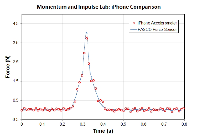
Figure 4.5: Comparison between the PASCO force sensor reading and the accelerometer from

an iPhone 4 that was riding along with the glider. The only free parameter for simultaneously

plotting the two data sets was the time oﬀset.

Experiment 5: Harmonic Oscillator

Part I. Spring Oscillator.

The career of a young theoretical physicist consists of treating the harmonic

oscillator in ever-increasing levels of abstraction. -Sidney Coleman

You have already brieﬂy encountered a harmonic oscillator in Experiment 3, where a

glider was held between two springs on an air track. The next three experiments in this

course are spent going into greater detail in the study of oscillating systems. You will study

the eﬀects of damping, resonance, driving, superposition, normal modes, and phase shifts

in these systems. Here, in Experiment 5, you will be measuring the resonant frequency of

an undamped and damped harmonic oscillator. You will measure the damping term and

compare your results to predicted values based on a simple model. You will want to keep

your calculations from this experiment handy because you will need to apply some of these

techniques in your analysis of Experiment 6.

The oscillator for Experiment 5 is a mass hanging from a spring, shown in Fig. 5.1. You

will measure the mass and the spring constant, which will allow you to make a prediction for

the resonant frequency (fo, the cyclic frequency in Hz) of this undamped harmonic oscillator:

fo=1

2πsk

m.(5.1)

The spring will hang from a force sensor, providing you with a means to monitor the

oscillations of the hanging mass as a function of time using the DAQ. In your analysis, you

will be able to produce a measurement of foand compare it to your predicted value based

on Eq. 5.1.

We will then add a damping force F=−bv that is proportional to the velocity vof the

oscillating mass. We can model this system by an equation of motion of the form

m¨x=−kx −b˙x(5.2)

where kis the spring constant and xis the position of the mass in the vertical direction1.

The damping term, b, has units of mass/time, and tells you something about how much

1If you are not familiar with the dotted notation, each dot is a shorthand for a derivative with respect to

time. So ˙x≡dx/dtand ¨x≡d2x/dt2, etc.

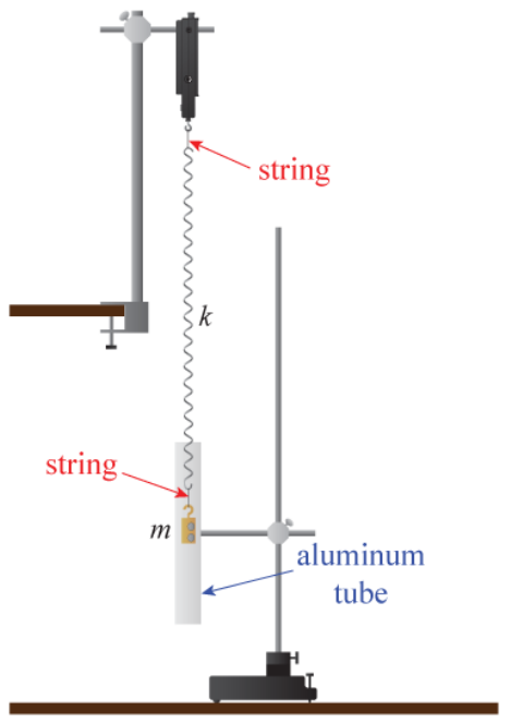
Figure 5.1: A weight hanging from a spring can exhibit oscillatory motion that is well-

described as being a simple harmonic oscillator. The force sensor from which the weight

hangs provides readout of the oscillatory motion. The weight has strong magnets attached

so that when the motion occurs inside a hollow aluminum tube, eddy-current heating provides

a dissipative force that is proportional to velocity. It is important to decouple the rotation

of the spring from the mass by using thin strings to attach the spring at both ends.

time it takes to damp out oscillations of some given mass. We will typically be concerned

not with bitself, but with combinations of b,m,fo, and kthat are more straightforward to

interpret.

Experimentally, it is a little bit challenging to come up with a method for producing

a pure damping term of this form without, for instance, adding a friction term (which

would not depend upon velocity). Your hanging mass for this experiment has some strong

magnets embedded in it, which we will use to produce the necessary damping force. The

hanging, oscillating mass will be surrounded by a vertical conducting tube that is made from

aluminum, a “nonmagnetic” material.

The eﬀect of this tube on a magnet that is not moving will be very small and we will

neglect it here. However, when the magnetic ﬁeld is changing in time due to the motion

of your oscillating mass, it causes eddy currents in the aluminum to be created due to the

tube’s inductance. The induced current is proportional to the velocity of the hanging mass.

Since aluminum has some ﬁnite resistivity, these currents are dissipated into heat. You will

not be required to derive these eﬀects, but it is useful for you to have some idea why a

non-magnetic material might have a profound eﬀect on the motion of a magnet.

By monitoring the amplitude of oscillations as a function of time, you will be able to test

whether the damping really is well-described by Eq. 5.2, and to provide a measured value

for 2m/b, which is the characteristic “damping time” of your damped oscillator. This will

also permit you to measure the Q-factor (or, simply the Q) of your resonance, which allows

you to complete your simple model of this system.

5.1 Theoretical Background

Your TA will probably cover this in more detail before you begin your experiment, but this

section is a brief discussion of how to derive the relationships needed for your analysis. Given

Equation 5.2:

m¨x=−kx −b˙x,

we want to ﬁnd the form of the solutions for x(t). As is often the case when dealing with

diﬀerential equations, we can resort to a method of guess-and-check to ﬁnd solutions. We

will use complex notation for our oscillator to make the algebra easier, choosing to try the

following form for our solution

x(t) = Aeiωt.(5.3)

We are in this case only interested in ﬁnding the (possibly complex) frequency ω, which

characterizes the time-dependence of the oscillator’s behavior. To ﬁnd ω, we can simply

plug this into 5.2 to get

−ω2mAeiωt =−kAeiωt −iωbAeiωt

mω2=k+iωb. (5.4)

We can solve this quadratic equation for ωusing the quadratic formula to get

ω=ib

2m±sk

m−b2

4m2.(5.5)

Exercise 5.1 Sanity check: what does Eq. 5.5 give us if we remove the damping?

This should make some sense given what you know about oscillating spring-and-mass

systems. Also, how should we interpret the ±in Eq. 5.5? As a hint, consider the fact

that we chose a solution of the form x(t) = Aeiωt instead of x(t) = Aeiωt +Be−iωt.

We will take the plus sign of the ±for concreteness, but all of this analysis works just as well

if we chose the minus sign. Since this frequency has a nonzero imaginary part, we would like

to interpret what this means. Consider what happens if we plug Eq. 5.5 back into Eq. 5.3:

x(t) = Ae

iib

2m+qk

m−b2

4m2t

=Aeiqk

m−b2

4m2t×e−bt/2m.(5.6)

The second term in Eq. 5.6 is a pure exponential decay and does not contain any oscillating

terms. This comes from the imaginary part of Eq. 5.5, and demonstrates that imaginary

frequencies are usually used to express dissipative terms. We can therefore introduce the

damping time τ, deﬁned as

τ≡2m

b.(5.7)

The damping time is the amount of time it takes this undriven, damped oscillator to have

its amplitude decrease by a factor of 1/e.

The ﬁrst term in Eq. 5.6 is oscillatory and suggests that we adopt the following deﬁnition:

fdamped =ωdamped

2π≡1

2πsk

m−b2

4m2=fos1−b2

4km (5.8)

where fois given by Eq. 5.1. It is helpful to look back at Eq. 5.6 with these new deﬁnitions,

giving us

x(t) = Aeiωdamped t×e−t/τ .(5.9)

The real part of this expression is clearly a sinusoidal oscillation at frequency ωdamped that

has an exponentially-decaying amplitude with time constant τ.

Last, we will deﬁne something called the Q-factor (also known as the “quality factor”

or simply as “the Q”) of this resonance, which is 2πtimes the ratio of the total mechanical

energy to the amount of energy that is dissipated in a single cycle. Without proof, we will

deﬁne Qto satisfy

fdamped ≡fos1−1

4Q2,(5.10)

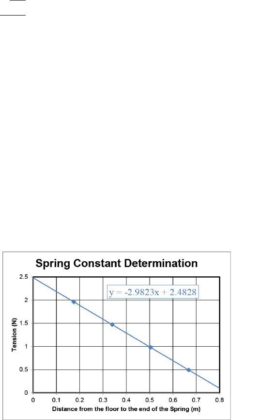
which gives us

Q=√km

b.(5.11)

In the limit of Q1, the Qof a resonance is also the ratio of the resonant frequency

(fdamped) to ∆f, the full-width-at-half-maximum (FWHM) of the (power) resonance curve.

The power resonance curve would be a plot of, for instance, energy dissipated per cycle

vs. frequency. You will explore this in more detail in Experiment 6.

5.2 Procedure

Since you will be measuring the frequency of a weight hanging from a spring, you will need

to measure the mass of the weight and the spring constant to provide something against

which to compare your direct time-domain measurement. While it may not be important

for your measurement of the spring constant, make sure that the spring is attached to the

hook of the force sensor via a string instead of being attached directly (and likewise for the

weight on the bottom of the spring), as shown in Fig. 5.1. Using a string to decouple the

rotation of the spring as it stretches from the mass and hook is important for making sure

your system is well-modeled by the simple equations above.

Measure the spring constant by hanging

at least 5 diﬀerent masses from the spring

and recording its length. You may ﬁnd it is

easiest to record the distance from the end

of the spring to the ﬂoor, because this re-

moves the need to hold the meter stick up

in the air. Since this distance is linearly re-

lated to the length of the spring, the spring

constant is still the slope, but there will be

an overall minus sign (the spring constant

is positive for these springs). You will per-

form the usual ﬁtting in your analysis to turn

these measurements into a measurement of

the spring constant.

Next, you will set up the DAQ to measure the tension applied to the hook on the force

sensor as a function of time. For Experiment 5, you do not need to know the value of the

force, so feel free to set up the force sensor to display voltage or (uncalibrated) force units

as you see ﬁt. For this discussion, we will assume the output is being recorded in volts.

In order to measure the frequency of oscillations, you will start the mass oscillating freely

and record the force sensor reading vs. time, as shown in Fig. 5.2. Be sure to keep the

oscillation amplitude small enough that the spring stays linear, which means the coils should

not touch one another and the spring should not be anywhere close to being plastically

deformed, etc. For this measurement, it is good to have both a Table and a Scope display

running simultaneously. You will want a sample rate that is high enough to really capture

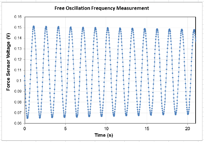
Figure 5.2: Free oscillation of a mass hanging from a spring. The oscillation frequency can be

obtained by, for instance, zooming in on the ﬁrst and 14th oscillation minima and dividing 13

by the diﬀerence between these two times. Note the subtle decay of the oscillation amplitude

due to dissipation; this oscillator has a Qof more than 500.

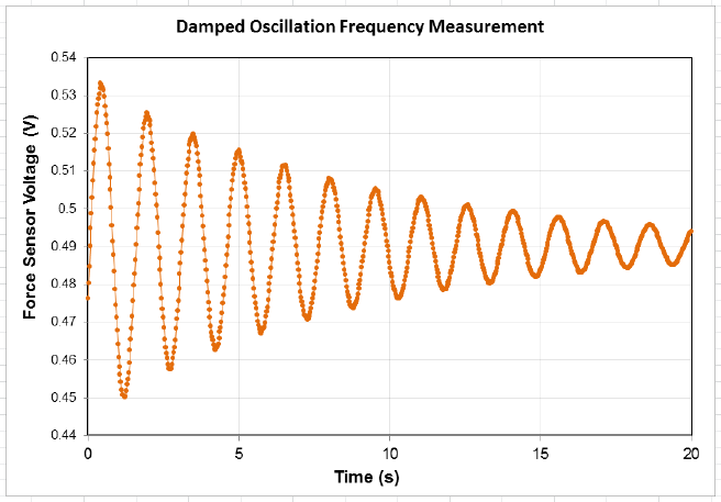
Figure 5.3: Damped harmonic motion. The characteristic damping time in this case is about

9.5 seconds, which corresponds to a Qof about 20.

the force maxima and minima (the “extrema”), so be sure your sample rate is at least 20

Hz in the Controls palette. If you exceed 50 Hz sample rate, it is likely that the amount

of data you generate will be large enough to be a headache for you and you will not get

a better measurement, so try something in the middle. Record oscillations for at least 20

seconds and up to 1 minute and then copy your voltage vs. time data into Excel for your

records. Sometimes the force sensors show a signiﬁcant drift in their mean value over the

course of 20 seconds, so you may want to write down an estimate for this drift or to “warm

up” the sensor by letting your weight oscillate on the force sensor for a few minutes. This

eﬀect is more important for the damped motion, so be sure to keep an eye on it and to either

quantify the drift or ﬁnd a way to remove it for the next part.

Next, you will record the same time-domain data with the damping term added. Arrange

the aluminum tube to surround the oscillating weight without touching it. The magnets in

the weight will produce a damping force when the tube surrounds the moving weight. Record

the force sensor reading vs. time again and save your data. You will notice a signiﬁcant decay

in the oscillation amplitude as a function of time, as shown in Fig. 5.3.

5.3 Analysis

Plot your displacement vs. weight data and ﬁt a line to determine the spring constant. Use

a regression analysis to get an uncertainty on the slope, as usual. Combine this with your

measured mass of the weight with embedded magnets to come up with a prediction for the

free oscillation frequency fousing Eq. 5.1.

Next, you will measure the frequency of free oscillations directly from your time-domain

voltage vs. time data. Plot your data and use the positions of the extrema to determine the

oscillation frequency. You can do this by, for instance, zooming in on the ﬁrst maximum

to determine the time when this occurred, doing the same for the nth maximum, then

dividing n−1 by the time diﬀerence, which will yield fo. You should estimate uncertainty

by using some reasonable method, such as repeated measurements with diﬀerent extrema or

estimating your uncertainty in identifying exactly when each extremum occurred.

Do the same for your damped motion data. You will ﬁnd that it is more diﬃcult to

determine the damped motion frequency (fdamped) than the free oscillation frequency since

the signal-to-noise ratio gets worse as the signal amplitude decays, so your uncertainty is

likely to be quite a bit larger for the damped motion than the free oscillations. Nonetheless, it

should be possible to obtain a pretty good measurement of the damped oscillation frequency.

Next, you will see if the damping is well described by a velocity-dependent force and

estimate the damping time τ(see Eq. 5.7). τis the 1/e decay time of the amplitude of

the oscillations, and the amplitude will only decay exponentially in time if the damping is

indeed caused by a velocity-dependent damping force (as opposed to, say, a friction force).

To do this, your ﬁrst step will be to ﬁnd the voltage that corresponds to the midpoint in the

oscillations, as there is almost certainly a signiﬁcant oﬀset in your measurement. You need

to subtract this oﬀset from the peak voltages to measure the amplitude.

For instance, consider the data shown in Fig. 5.3. These oscillations are clearly not

centered around 0 volts, and it looks like there is an oﬀset of about 0.49 V. Try to ﬁnd the

proper oﬀset voltage to subtract from your data to give you oscillations that are centered

around zero. You may ﬁnd that the force sensor reading drifted during your data run, in

which case you may need to choose a sort of mean value or try subtracting a linear drift

from the data. If your data includes points after essentially all of the oscillations died out,

that may provide you will a good measure of the oﬀset voltage. Subtract your oﬀset from

your data to produce oscillations that are centered around zero.

One of the things about an exponential decay is that the ratio of the heights of all pairs

of successive maxima should be the same since the maxima are separated by the same time

interval (T= 1/f). Record the heights of at least 6 successive maxima (more if you have

good data). Calculate the ratio of the height of peak 1 to peak 2, then peak 2 to peak 3,

and so forth for your data set. If the damping is indeed proportional to the velocity, these

ratios should all give the same result.

Plot your ratios as a function of which extrema were being used as shown in Fig. 5.4.

If the damping force is proportional to velocity, there should not be a discernible nonzero

slope to the data in the plot and the scatter will be centered around some mean value. If

you do detect a systematic trend upward or downward, be sure that you subtracted your

oﬀset voltage correctly, as doing this improperly will also result in a drift of the peak hight

ratios with extremum number.

If you recorded amplitudes once per oscillation period T, the ratio of successive amplitude

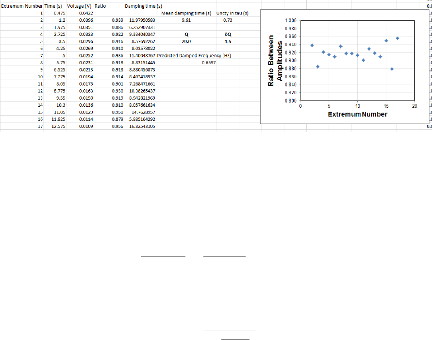
Figure 5.4: Analysis of the damped motion shown in Fig. 5.3. The peak height ratios are all

centered around 0.92. Notice that the scatter seems to increase with extremum number, as

expected since the peak height uncertainty increases.

measurements in an exponentially-decaying oscillation will be given by

V(t+T)

V(t)=e−(t+T)/τ

e−t/τ =e−T/τ .(5.12)

Since you already have a measurement of T= 1/fdamped, you can convert each ratio mea-

surement into a measurement of τby solving for the amplitude damping time

τ=−T

ln hV(t+T)

V(t)i.(5.13)

If your individual data points for the amplitude ratio did not show a trend (such as shown

in Fig. 5.4), you can use your ﬁrst and last measured amplitude to determine the damping

time. Alternatively, you may combine all of your data points into a measurement of the

damping time with uncertainty, τ=τbest ±δτ. For this, you may use the procedure outlined

in §ii.1.6 to help you come up with an uncertainty in your mean value of τ.

Next, determine Qfrom your measurements. There are a couple of ways to do this, so

ﬁnd a method that makes sense to you. Last, using your measured Q, predict the frequency

of damped oscillations based on your measured frequency of free oscillations fo. Is your

measurement of fdamped consistent with this? Is the diﬀerence between your best value for

foand fdamped statistically signiﬁcant, or is the diﬀerence smaller than their uncertainties?

5.4 Report guidelines

This week, you will turn in your ﬁrst full lab report. There will not be a

worksheet this week. If you do the extra credit, include it in your lab report

as if it were a normal part of your experiment. Your lab report should contain

the following items.

1. Cover Sheet

•experiment number and title

•your name and UID

•the date the lab was performed

•your lab section (for instance, “Tuesday 3pm”)

•your TA’s name

•your lab partners’ names

•the word counts for your abstract and for the body text of your whole report

2. Full Lab Report

This week you will write a full lab report including abstract, introduction, methods,

analysis and conclusions sections. Your completed lab report should look like an ar-

ticle submitted to a scientiﬁc journal. All guidelines from all of the previous weeks’

presentation mini-reports apply to this report, with the exception of reporting word

counts, which are to be reported in the cover page as described above. Since you will

be adding the analysis and conclusions sections, we will discuss some of the important

points of these parts of a journal article.

Analysis

This section should contain an explanation of how the data were analyzed to test

the experimental results against theoretical models. The methods section should have

explained how the data were obtained, but the analysis section presents the data itself

to communicate what the data show about the relevant physics. This section will

also typically include the discussion of uncertainty analysis, including any relevant

derivations of error propagation equations that were used.

The analysis section is typically where you would put your “main plot” for the paper.

The methods section can have plots, but the point of those is to describe how the data

were taken, whereas the goal of a plot in the analysis section is to show how the data

illustrate some point about physics.

Conclusions

Brieﬂy restate the goals of the experiment and describe how your results demonstrate

(or fail to demonstrate) these objectives. Brieﬂy describe at least one possible source

of systematic uncertainty that could aﬀect your measurement (and which direction

the eﬀect would tend to systematically shift your observations) and suggest a future

measurement to eliminate it.

Suggested content

Your report should be a fully self-contained description of your work this week. If

you performed a derivation or a measurement as part of this, it should probably ﬁnd

its way into your report. While this is probably all the instructions you need at this

point to write a high-quality report, the following is a list of some of the speciﬁc things

from this experiment that you should probably include in your report in one form or

another. That said, anything that is needed to communicate to the reader what was

done and what it showed should be included.

•A derivation of two or three equations that show how the quantities fo,Q,τ, and

bare related to one another. You may take Eq. 5.10 to be a deﬁnition of Q.

•A description of how you determined the frequency of oscillations and how you

measured the decay time in the damped case.

•Your measured mass of the hanging weight.

•A plot of the spring constant measurement and a statement of the result, with

uncertainty.

•Your predicted value for the free oscillation frequency.

•A plot of the free oscillatory motion vs. time. You do not need to worry about

calibrating the y-axis and may simply plot it as being the force sensor reading in

volts.

•How did you determine the free oscillation frequency from the data in this plot?

What was your result?

•Compare your predicted free oscillation period and your measured value. Do they

agree? If not, try to explain what is the cause of the mismatch.

•A plot of the damped oscillatory motion in the same manner as your previous

plot. Use these data to measure the damped oscillation frequency.

•A plot of the measured ratios of successive extrema in your damped oscillation

measurement. Is there a trend? If so, what does this mean? If not, what does

this tell you?

•Present your measured value for the damping time with uncertainty.

•State your measured value for Q(with uncertainty) and use this to make a pre-

diction of the damped oscillation frequency.

•Compare your measured damped oscillation frequency to this prediction. Do they

agree? Are the two oscillation frequencies distinguishable given their uncertain-

ties?

3. Extra Credit

It is possible to determine the frequency response of this system to any periodic driving

force using the data you obtained. One way that this frequency response may be

obtained is by taking the Fourier transform of the time-domain signal, which is called

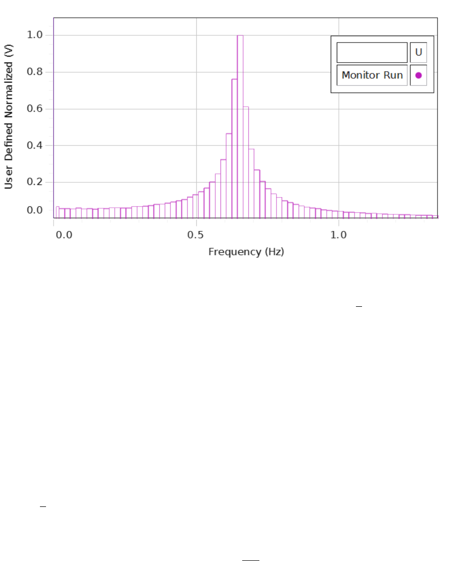
Figure 5.5: Fast Fourier Transform (FFT) of the data from Fig. 5.3. Based on the analysis,

we would predict this amplitude spectrum to have a full width at 1/√2 of its maximum of

about fo/Q ≈33 Hz, which would be about two frequency bins wide on this plot, consistent

with the spectrum shown.

the step response of your system. In Experiment 6, you will be looking at the amplitude

response of another oscillator in the frequency domain, but it may be instructive to

see what this would look like for the oscillator in Experiment 5. Capstone provides

an algorithm for showing the frequency content in a time-domain signal called a Fast

Fourier Transform (or FFT). Figure 5.5 shows the results of using this tool, which

shows a very nice resonance curve.

Use the Capstone FFT tool in the Displays palette to see if you can generate a

frequency-domain representation of your data such as that shown in Fig. 5.5. Estimate

the width of the resonance (∆f), deﬁned as the full width of this peak at a height of

1/√2 of its maximum value. If Qis large, one way to calculate Qis as the ratio of the

resonance frequency to the resonance width:

Q=fo

∆f.(5.14)

Use this to calculate Qand compare your answer to that obtained from your time-

domain analysis.

5.5 Epilogue

Q-factors for resonators span a large range of values. The highest Qof which your author

is aware for a man-made oscillator is an optical cavity that is made out of a single crystal

of silicon [3]. This oscillator has a center frequency of fo= 200 THz and a frequency width

of ∆f < 40 mHz, which gives us Q > 5×1015. It is by using cavities such as these that

researchers are able to obtain the passive stability required to make measurements such as

those reported in [7] (Eq. ii.2).

Experiment 6: Harmonic Oscillator

Part II. Physical Pendulum.1

The harmonic motion you have studied in previous experiments in this course was typically

analyzed in the time domain, meaning you acquired and studied data as a function of time.

It is also possible to analyze the properties of a harmonic oscillator in the frequency domain,

which you will begin to explore in Experiment 6. You will also study the eﬀects of damping in

more detail, allowing you to demonstrate underdamped, overdamped, and critically-damped

motion by experimentally controlling the damping coeﬃcient. These concepts are important

in control systems for physics and engineering applications, where we are often concerned

with trying to ﬁnd the fastest way to bring a system to a desired state.

The spring-and-mass oscillator you used in Experiment 5 was very well modeled by

Eq. 5.2. However, you were not able to adjust the damping coeﬃcient in a well-controlled

manner using the aluminum tube, so we will use a more ﬂexible setup in Experiment 6, shown

in Fig. 6.1. An aluminum pendulum shaped like an anchor will serve as your oscillator. The

oscillation frequency of this pendulum will be approximately independent of amplitude so

long as the amplitude is small, where we will say that “small” means the angular motion does

not move the bottom further than the width of the curved bottom portion of the pendulum.

A “wave driver” will be coupled to the pendulum through a vee-shaped torsion spring.

This will allow us to not only drive the oscillator with a periodic signal, but also to read

out the instantaneous position of the oscillator via the rotation sensor. Even though the

wave driver will not be used for your study of damping regimes, the spring that couples the

wave driver to the pendulum will be a factor in determining the resonant frequency of the

pendulum. Since you will apply your results from the damping study to your study of driven

oscillations and resonance, you should leave the wave driver attached to the pulley for your

damping study even though it is not in use.

The wave driver can be connected to the DAQ via the banana jacks on the upper right

of the 850 interface (see Fig. i.1). The rotation sensor plugs into one of the four “Passport”

sockets on the bottom row of the 850 interface. Capstone will automatically detect and

conﬁgure the rotation sensor, but you should conﬁgure output channel 1 to be an Output

Voltage Current Sensor, which will allow you to monitor the phase of the drive signal.

1This chapter was contributed by Priscilla Yitong Zhao (2013).

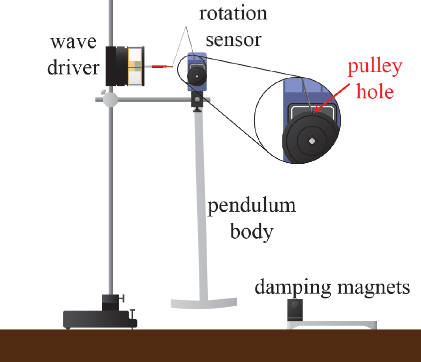
Figure 6.1: A physical pendulum for studying damping regimes and resonance. For small

oscillations, the pendulum is a harmonic oscillator, and its angular position can be measured

in real-time using a rotation sensor. A wave driver coupled to the pendulum by a torsion

spring (shaped like a Λ, shown above) can be used to study damped, driven oscillations. The

damping magnets can be moved into place and their spacing changed to provide a tunable

velocity-dependent damping force.

Damping will once again be provided by eddy-current heating due to the motion of the

oscillator. Unlike Experiment 5, however, this time it is the conductor that will be moving,

and the magnets will be stationary. By moving the magnet stand so that the pendulum

bottom passes midway between the two damping magnets, the amount of damping can be

tuned by adjusting the spacing between the magnet poles and the bottom of the pendulum

body.

You will acquire time traces for underdamped, overdamped, and critically-damped mo-

tion.

6.1 Theoretical Background

6.1.1 Undriven oscillations of a damped physical pendulum

A pendulum that is made of a rigid object (as opposed to a point-mass on an ideal ﬂexible

string) is known as a physical pendulum. It is no more or less physical than a ball on a rope,

but this terminology is used nonetheless. The physical pendulum in this experiment is a sort

of anchor-shaped piece of aluminum alloy cut from sheet metal, and will be characterized by

a moment of inertia Iabout the rotation axis.

If we call the angular deviation of the pendulum from its equilibrium conﬁguration θ, any

nonzero value of θwill lift the center of mass of the pendulum above its equilibrium height. If

the pendulum has a total mass Mand the location of its center of mass is a distance lbelow

the rotation axis, the restoring torque due to gravity will be given by τgrav =−Mgl sin(θ).

The spring attached at the top also exerts a torque on the pendulum about its rotation

axis. For an angular displacement θ, the spring’s length is changed by an amount propor-

tional to sin(θ). The torque this exerts on the pendulum is proportional to this force times

cos(θ), resulting in a restoring torque that we may write as τspring =−Bsin(θ) cos(θ).

Last, the magnet assembly at the bottom of the pendulum will exert a damping torque

on the pendulum, turning the angular kinetic energy into heat via eddy-currents in the

pendulum blade. This damping force is proportional to the tangential velocity of the blade,

so the damping torque will be proportional to the angular velocity, which we will write as

τdamping =−b˙

θ. Putting these three terms together gives us an equation of motion for the

pendulum that is rather complicated:

I¨

θ=X

τi

=−Mgl sin(θ)−Bsin(θ) cos(θ)−b˙

θ(6.1)

For small angular displacements (θ1 rad), we may expand the trig functions and keep

the ﬁrst terms only, thereby invoking a small angle approximation (sin(θ)≈θ, cos(θ)≈1):

I¨

θ≈ −(Mgl +B)θ−b˙

=−kθ −b˙

θ(6.2)

where we have deﬁned a constant k≡Mgl +B.

If we compare Eq. 6.2 to Eq. 5.2, we see that this is exactly the same equation of motion as

we had in Experiment 5 with the replacement x→θ,m→Iand diﬀerent physical deﬁnitions

of kand b(with diﬀerent dimensions). We may therefore write down the solutions directly

by making these simple substitutions in Eq. 5.6

θ(t) = Aeiqk

I−b2

4I2t×e−bt/2I(6.3)

=Aeiωdamped t×e−t/τ .(6.4)

with the analogous deﬁnitions of the oscillatory frequency2and damping time:

ωdamped ≡sk

I−b2

4I2=sω2

o−1

τ2(6.5)

and

τ≡2I

b(6.6)

with the undamped resonance frequency ωo≡qk/I > 0.

The motion (described by the real part of θ) is again a sinusoidal oscillation at frequency

ωdamped that has an amplitude that exponentially decays with time constant τ. We identify

three regimes of damping in this system:

•Underdamped motion occurs when there is still oscillation of the pendulum for zero

initial velocity, meaning θchanges sign at least once. This occurs when the oscillation

frequency is faster than the damping rate: ωo>1

τ, which guarantees that ωdamped is

purely real. A good example of underdamped motion can be seen in Fig. 5.3.

•Overdamped motion occurs when ωo<1

τ. Looking at Eq. 6.5 shows us that in this

case, ωdamped will be purely imaginary, which means the angular displacement of the

pendulum for zero initial velocity (Eq. 6.4) will be described by a pure exponential

decay with no oscillations.

•Critically-damped motion is the crossover regime between these two cases, given by

ωo=1

τ. For critical damping, the system will return to its equilibrium state faster

than either overdamped or underdamped motion. Automobile suspension systems, the

dash pots on the doors to the lab, and earthquake suppression systems are all examples

of engineering tasks where one would want this feature of critical damping.

6.1.2 Driven oscillations

If the wave driver is driven by the analog output of the 850 interface, there will be a new

term in the equation of motion for this physical pendulum that oscillates with the driving

2Here, as elsewhere in this manual, we use ωas a symbol for angular frequency (units of rad/s or just

s−1) and fas a symbol for cyclic frequency (units of Hz).

current, which we will assume is proportional to cos(ωdt) for drive frequency ωd. In the

small-angle approximation, we have

I¨

θ=−kθ −b˙

θ+Ccos(ωdt).(6.7)

The solution to Eq. 6.7 consists of the sum of two terms, known as the complimentary

and particular solutions:

θ(t) = Acθc(t) + Apθp(t) (6.8)

where the complimentary solution is the one we have from undriven oscillations

θc(t)≡eiωdamped t×e−t/τ (6.9)

and the particular solution is given by [4]

θp(t)≡1

r(ω2

o−ω2

d)2+2ωd

τ2cos (ωdt−φ(ωd)) (6.10)

where

φ(ωd)≡arctan 2ωd

τ(ω2

o−ω2

d)!.(6.11)

The complimentary solution describes all of the transient behavior of the system, which

depends upon things such as initial conditions but does not depend upon the driving term

in any way. This behavior is called transient because as t→ ∞,θc→0. The timescale over

which the transient behavior dies out is τfor critical and underdamping. For this experiment,

this means that when you make a change to the system by, for instance, changing the drive

frequency, you must wait at least τbefore interpreting the behavior of the system as being

dominated by the particular solution. You should consider this when trying to decide how

to set the damping rate for the second half of this experiment.

6.1.3 Resonance

The particular solution, on the other hand, describes the steady-state behavior of the system

under a constant-amplitude, sinusoidal driving torque. The pendulum will oscillate at exactly

the drive frequency ωd, but with an amplitude and phase that depend upon the relationship

between ωdand ωdamped. Fig. 6.2 shows the calculated amplitude of the steady-state behavior

for a series of oscillators with the same undamped resonance frequency but diﬀerent levels

of damping.

The drive frequency at which the amplitude is maximized is called the resonant frequency

of the damped, driven system, ωR. To ﬁnd ωR, we can diﬀerentiate the amplitude of the

response in Eq. 6.10 with respect to ωdand solve for ωdsuch that this is zero, which gives

us the resonant frequency of a damped and driven harmonic oscillator:

ωR=sω2

o−21

τ2.(6.12)

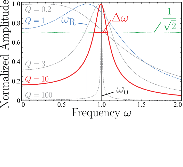
Figure 6.2: Amplitude response of damped resonators. The amplitudes are normalized to

set the peak amplitude equal to 1, and the undamped resonance frequency for all curves

is ωo= 1. Low-Qoscillators show resonant frequencies ωRthat are signiﬁcantly diﬀerent

from ωo. As the quality factor increases, the resonance position converges to ωR=ωo. The

resonance width ∆ωis shown for a Q= 10 resonance, where ∆ωis the full width when the

amplitude is 1/√2 times its maximum value.

Comparing this to Eq. 6.5, we see that the resonant frequency can be close to ωdamped, and

in many situations they are used interchangeably. In the limit τ1/ωo, both of these

resonant frequencies converge to ωo, and you will ﬁnd that they are often assumed to be

equal (especially for Q≥10 or so, see below).

We can deﬁne the quality factor Qof this system to be

Q≡1

2τωR(6.13)

to rewrite our particular solution as

θp(t)≡1

r(ω2

o−ω2

d)2+ωRωd

Q2cos (ωdt−φ(ωd)) (6.14)

For an oscillator with a high Q-factor (Q1), the damping time τis many oscilla-

tion periods long. As discussed above, in this case we see that ωRand ωdamped are both

approximately equal to ωo. In fact, we can rewrite Eq. 6.12 in terms of Qas

ωR

ωo

q1 + 1

2Q2

.(6.15)

This factor goes to 1 very quickly as Qis increased. For instance, an oscillator with a modest

quality factor of Q= 3 has a resonance frequency that is only about 3% slower than the

undamped case.

For these cases where the damping is very slight and the Qis therefore substantially

greater than 1, it can be shown that the Q-factor is the ratio of the resonant frequency to

the width of the resonance curve

Q≈ωo

∆ω(6.16)

where ∆ωis the full width of the resonance, deﬁned to be the frequency range over which

the amplitude response (the amplitude in Eq. 6.14) is greater than or equal to 1/√2 of its

maximum value. (This will be familiar to you if you did the Extra Credit from Experiment

5.)

Last, the phase term described in Eq. 6.11 is shown in Fig. 6.3 for the same oscillators as

the amplitudes in Fig. 6.2. This plot has been constrained to positive values of φto show that

the phase changes smoothly through resonance, a general property of damped oscillators.

Far below undamped resonance, the phase of the response is almost exactly the same as the

drive, but begins to increase as undamped resonance is approached. Right on undamped

resonance (ωd=ωo), the phase lag is exactly φ=π

2, regardless of the quality factor. Past

this point, the phase lag continues to increase, asymptotically approaching φ=πat inﬁnite

frequency.

From a practical perspective, if we are tasked with trying to locate the (un-

damped) resonant frequency ωo(a common situation in physics and engineering),

looking at the phase response is going to be far more sensitive than using the

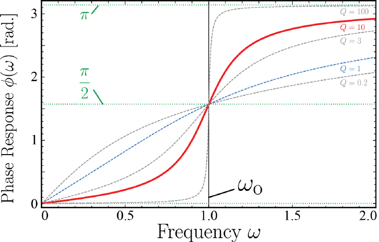
Figure 6.3: Phase response of damped resonators. The phase response is the diﬀerence

between the phase of the driving force and that of the displacement. Curves are shown for

the same parameters as Fig. 6.2. For driving frequencies below undamped resonance, the

response is said to be “in phase with the drive,” with the lag increasing as the drive frequency

increases. At the undamped resonant frequency, the response is out of phase from the drive

by π/2, regardless of Q. Past this point, the response is said to be “out of phase with the

drive” and the phase lag continues to increase with frequency, saturating at φ=π.

amplitude response. The reason is that in the immediate neighborhood of resonance,

the amplitude response levels out and does not depend sensitively on frequency, whereas

the phase response has a maximum slope at this point. The amplitude response therefore

becomes insensitive to frequency right where you need it the most, while the sensitivity of

the phase to frequency is maximized here.

6.2 Procedure

To set up the apparatus, start by connecting the spring on the wave driver to the wheel on

the pendulum rotation sensor as shown in Fig. 6.1. You will leave this connected for the

entire experiment. To make sure the pendulum swings freely for all parts of the experiment,

set the heights of the posts and clamps so that the pendulum blade can swing freely a couple

of inches above the table so that the blade is well-centered at the height of the magnets. In

order to center the angular readings about the equilibrium position, uncheck Zero Sensor

Measurements at Start in the options for the rotary motion sensor and click Zero Sensor

Now when the pendulum is in its equilibrium position.

6.2.1 Harmonic motion with damping

To investigate the various regimes of damping, you will be pulling back the pendulum to

some starting position and letting it go, recording the angular displacement vs. time using

the rotation sensor via the DAQ. Remember, the small-angle approximation we used in the

theory section is only valid for angles right around θ= 0, so be sure to set your starting

position no more than one blade length from the equilibrium position.

You may ﬁnd it useful to have a photogate attached to the 850 to record the starting

condition when you let go of the pendulum. To do this, position the photogate such that

the pendulum blade just unblocks it when motion begins.

The amplitude sampling rate should be set so that you get enough data points to clearly

see which damping regime you are in without recording lots of points for the same value

of the angle. You should play around with this in Scope mode to choose an appropriate

sampling rate. You will be recording angle vs. time for diﬀerent values of the spacing between

the magnets.

Record traces of the pendulum angle vs. time for the case where the magnets are removed

entirely, as well as 4 or ﬁve gaps between 50 mm and 10 mm. You will want to get a clear

set of data for underdamped motion and a clear set for overdamped motion for your report.

Next, determine the magnet spacing to achieve critical damping. Remember, you are

looking for the minimum damping such that the angular velocity of the pendulum does not

change sign. Take steps at least as small as 1 mm for this, and save a good set of data

showing critical damping for your report. Fig. 6.4 shows some example data for all three

regimes. Note that you may need to record where θ= 0 is for each data set to plot them on

the same axes.

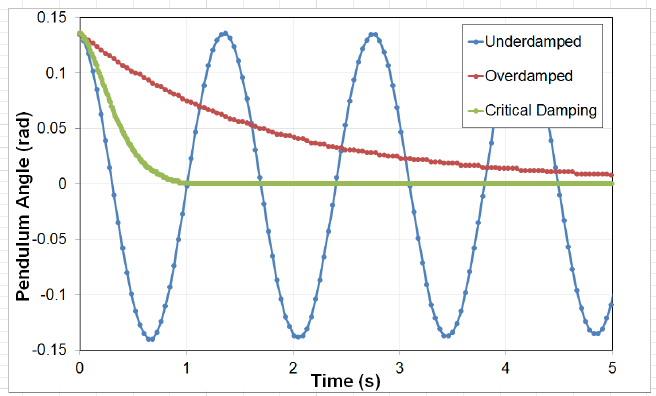
Figure 6.4: Illustration of damped motion in all three regimes of damping. All three plots

were obtained with the same initial displacement and no initial velocity. The critically-

damped trace clearly converges to θ= 0 the fastest.

6.2.2 Harmonic motion with driving

For the second part of the experiment, you will be examining the amplitude and phase

response of the driven, damped harmonic oscillator. For this whole section you will want to

set the magnet gap to something with fairly low damping. Remember, you are looking to

add just enough damping so that you don’t have to wait too long for the system to reach

steady state, but not so much that the oscillation amplitude is diﬃcult to detect. You will

beneﬁt from trying to use your data from the previous section to set the magnet so that

the free undriven oscillations damped out in about 5 to 10 seconds. Record a good trace of

displacement vs. time for this setting of the magnet in undriven conditions just like you did

for the previous part of the experiment.

You will be using the wave driver to produce a sinusoidal driving torque on the pendulum

using the Signal Generator function. This is physically accomplished by attaching the

banana plugs from the wave driver into Output 1 of the 850. The drive function will be a

Sine function, and you should probably keep the drive voltage below 5 V or so. The frequency

range you will be exploring will be very near the frequency of the undriven, undamped

oscillator, so take a look at your data from the ﬁrst part with no damping magnets to

estimate the undamped frequency.

First, you will locate the driven, damped oscillator resonance ωR, which you may assume

is equal to ωosince you are working with low damping. As discussed, the easiest way to do

this is by looking at the phase response. To accomplish this, you will be making parametric

plots known as Lissajous ﬁgures. What I mean by “parametric plot” is that you will be

plotting two separate quantities that are related by a parameter, which in our case will be

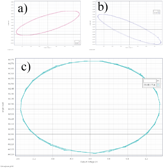
Figure 6.5: Parametric plots of the driving and response of a damped harmonic oscillator

showing Lissajous ﬁgures. These screen shots from Capstone show the measured pendulum

angle on the vertical axes and the drive voltage on the horizontal axes for drive frequencies

(a) below, (b) above, and (c) right on resonance.

time. You will be plotting Angle on the y-axis and Output Voltage on the x-axis of a

Graph display. You will also need to record data for several oscillations after the system

reaches steady-state for your analysis, so now is a good time to set up a Table for doing

that.

Your parametric plot will show both the drive voltage and the system response (the

angle) on one set of axes. For steady-state behavior, this plot will look like a closed curve.

You will need to play around with scaling the axes to try to make the extent of the shape on

the x-axis be about the same distance as the extent on the y-axis so that you can clearly see

the diﬀerence between a perfect circle and a slight ellipse. Fig. 6.5 shows an example screen

shot of the parametric plot.

To ﬁnd ωR, you are looking for the drive frequency such that the steady-state behavior

looks like a symmetric circle on the parametric plot, such as shown in Fig. 6.5(c). You will

ﬁnd that this technique is incredibly sensitive to the proximity to resonance, and even a

small deviation from resonance will be visible as a slightly-tilted ellipse. The direction of the

tilt tells you which direction you need to go to ﬁnd resonance, as shown in Fig. 6.5(a) and

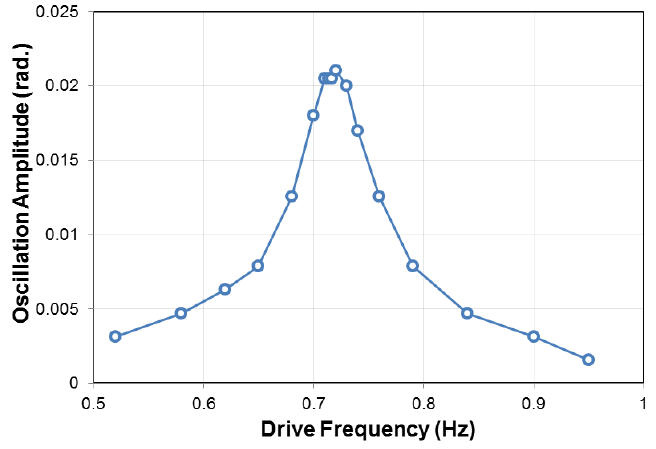
Figure 6.6: Measured oscillation amplitude spectrum of a damped, driven oscillator. The

points are connected by straight lines, showing the Lorentzian shape of the resonance as

predicted in Fig. 6.2.

(b). Estimate an uncertainty in your measurement of ωRbased on how small a deviation

you think you can make without being able to tell a diﬀerence in the ﬁgure. You will need to

save data for plotting Lissajous ﬁgures in your report for driving the system below, above,

and right on resonance.

Last, you will examine the amplitude response of the oscillator as a function of frequency.

It is by design that this lab manual is not going to provide you with detailed instructions

for how to go about this; you are expected to come up with an appropriate experiment on

your own (or with your lab partner) that you think makes sense. Record the amplitude of

the pendulum oscillations in steady-state for at least 10 diﬀerent drive frequencies. You are

trying to make a ﬁgure that allows you to see the shape of the resonance curve, which will

allow you to ﬁnd its height and estimate its width. An example is shown in Fig. 6.6 with the

data points connected by straight lines, which shows a Lorentzian shape similar to Fig. 6.2.

6.3 Analysis

For undriven damped motion, you recorded time traces of the angular displacement. From

your trace that was taken with no magnets present, you should be able to determine the

undamped oscillation frequency ωo. Make a plot clearly showing three time traces, one in

each regime of damping. You can assign an uncertainty to the critical damping gap between

the magnets based on how well you can measure the gap and how much change it would

take for you to say deﬁnitively that the damping has changed regimes.

For the driven, damped oscillator, plot your time trace of the undriven oscillator at the

magnet gap you used for the rest of the lab. Using the same technique you employed in

Experiment 5, ﬁnd the damping time τby analyzing how much the amplitude decreases as

a function of time for undriven oscillations. Assign an uncertainty to your measurement of

τbased on how well you think you were able to measure the change in amplitude.

You recorded a measurement of the driven resonant frequency ωRthat was obtained

by looking at the Lissajous plots. Combine this with your measurement of τto report a

measured value for Qvia Eq. 6.13. Plot three Lissajous ﬁgures for your report showing the

shape below, on, and above resonance.

You have one more way to determine Q, which you will compare to this method. This

second method to measure Qis to examine the amplitude response to apply Eq. 6.16. To do

this, plot your amplitude spectrum and determine the peak height (which should occur at

ωR). It is sometimes helpful to connect the data points with straight lines for this analysis.

Using your plot, come up with some way to estimate the full width of the resonance where

the amplitude is 1/√2 times its maximum (∆ω), such as depicted in Fig. 6.2. You are

unlikely to have two data points at exactly the right place, so you will need to make an

educated guess about this width based on the plot and assign an uncertainty to it. You

have been assigning uncertainties in this course for many labs now, and you should be able

to come up with a way to do this that eﬀectively reﬂects how well you really measured this

quantity. Use your measurement of ∆ωto calculate Q, and think about how much you trust

this measurement compared to your other method for determining Q.

6.4 Report guidelines

This week you will NOT turn in a lab report, nor will there be a worksheet

this week. Your presentation of this week’s experiment will be part of a double

credit lab report on resonance that will cover both Experiments 6 and 7. If you

do the extra credit, please save it for your lab report next week and include it

as if it were a normal part of your experiment. Even though there is no report

due next week, students are encouraged to make sure they can be prepared to

include everything they did this week.

1. Some items to consider including in your next report: It will be up to you to

form a coherent story in the lab report due next week. You must decide what graphs,

tables and other information should be included. Some general concepts for this lab

are

•Regimes of damping

•Resonance

•Q-factor and line widths

2. Extra Credit In the driven resonance part of this experiment, you estimated ∆ωby

using a plot that probably did not have two data points right at 1/√2 of the maximum

amplitude. Find these two frequencies experimentally by moving the drive frequency

around until the amplitude is at 1/√2 of its maximum value. The diﬀerence between

these two frequencies should be ∆ω. Plot Lissajous ﬁgures at both frequencies and

describe what they have in common. Use your new measured value for ∆ωto determine

Q. Further, since the frequency of the peak of your amplitude spectrum is ωR(even

when ωRand ωoare not approximately equal), this gives you yet a third method

for determining Q. The damped, driven resonance frequency ωRmust be halfway

between the two frequencies you found for achieving 1/√2 of the maximum amplitude.

Combine this with Eq. 6.15 to get a third measurement of Qand compare all of your

measurements and methods. Which do you believe is the most accurate, and why?

6.5 Epilogue

It is remarkable how much physics can be understood by modeling systems as harmonic oscil-

lators. The Lorentzian line shape shows up in everything from nuclear scattering to molecular

spectroscopy and plays an important role in almost every ﬁeld of physics. Understanding

the fundamentals, such as the phase change across resonance and how the shape changes

with damping will be helpful for many advanced courses and research work in engineering

and physics.

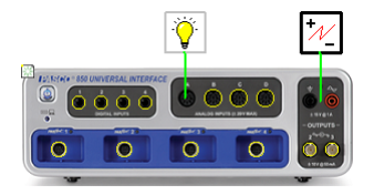
Experiment 7: Waves on a Vibrating

String

In Experiments 3, 5, and 6 you studied systems that exhibited simple harmonic oscillations,

where the part of the system that was oscillating was often modeled as being a single point-

mass. Non-rigid, spatially-extensive systems can also exhibit simple harmonic motion, where

each point in space has some property that oscillates periodically in time and is somehow

related to the oscillations of its neighboring points. Phenomena such as these exhibit wave

behavior, and wave phenomena show up in everything from light to sound to the quantum

mechanical nature of probability amplitudes. In Experiment 7, you will be examining waves

on a stretched, massive string with clamped boundary conditions. You will measure the

group velocity of traveling waves on this string and predict and observe the behavior of

many modes of standing-wave oscillation. Last, you will investigate one of the curious

features of interference, where the addition of an intermediate boundary condition can be

used to suppress certain modes while leaving others eﬀectively unchanged. Information about

laser safety can be found in Appendix A and should be read if you do not know how to safely

use a low-power visible laser.

7.1 Procedure

To conﬁgure the DAQ for this experiment, you will

need to be able to read the signal from a light sensor

(analog channel) and to send a signal to the wave

driver via output channel 1 (the red and black banana

plugs). The polarity of the plugs does not matter.

In order to excite and monitor wave behavior, we

will be using transverse motion of a thick, elastic

string about a meter long. The tension in the string is an important parameter for us

to control in a known way, so while one end of the string will be held in a clamp (shown in

Fig. 7.1a and b), the other will pass over a pulley wheel (Fig. 7.1a and c) and weights can

be hung from this end. The tension will be set by T= (m1+m2)g, where m1and m2are

the mass of the hanging weight and the portion of the string that is hanging from the pulley

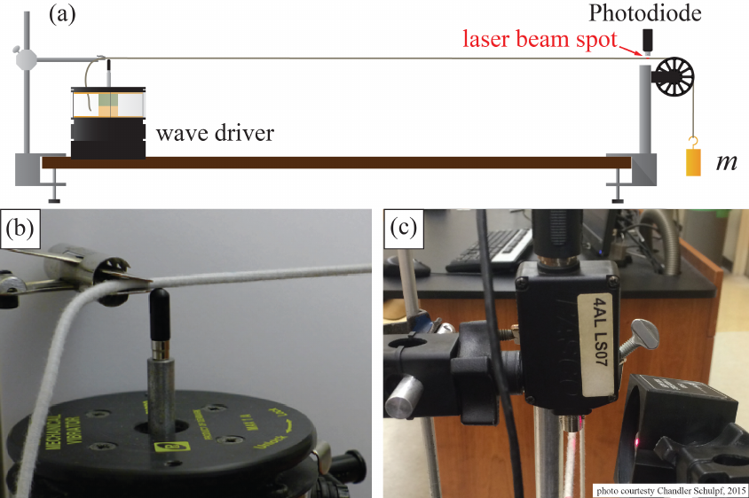
Figure 7.1: Apparatus for observing the vibrational motion of a massive string. (a,b) A

wave driver excites vibrations near the clamp, which can be detected when (c) a laser beam

scatters light into a photodetector at the other end. The tension in the string is controlled

by hanging known masses from a pulley that deﬁnes the other boundary.

100

(which has a non-negligible mass!).

The wave driver will excite vibrations in the string by moving the actuator in the vertical

direction. The actuator tip should just barely touch the string when the actuator is not

running, and should be positioned 1-2 mm from the clamp, as shown in Fig. 7.1b. You may

need to move the wave driver on the table until the driven waves are in the vertical plane

and do not have a signiﬁcant horizontal component. It is recommended that you do not

put the string into the notch on the tip of the actuator, but rather just use the tip to push

against the string.

You will be measuring the displacement of the string in the vertical direction by scattering

laser light into a photodiode (also called a photodetector, light sensor, or simply “detector”).

The laser spot should be positioned so that it illuminates the top third or so of the string

when the string is not moving. The photodetector should be positioned directly above the

laser spot very close to the string to minimize the eﬀect of ambient light getting into the

detector. In this way, if that section of the string moves downward, it scatters less of the

laser light into the detector and the signal decreases, with the converse being true if this

string moves upward. A photodiode gain setting of 10 seems to work well for this, but feel

free to experiment.

The laser beam should illuminate the string fairly close to the pulley (see Fig. 7.1c). For

Part 1 of this experiment (measuring the wave speed), it is recommended that you set the

beam (and photodetector) 6-8 cm from the pulley apex. For Part 2 and Part 3 (standing

waves), you will likely obtain the best results if the beam and photodiode detector are about

1 cm away from the pulley apex.

Setting the laser spot and detector positions correctly can be tricky, and it is worth your

time to make sure you do this well to get high-quality data. It is recommended that you

use Scope mode to monitor the Light Sensor while using Signal Generator to run the

wave driver in a sinusoid at 4-10 Hz with 1-2 V of output. For measuring the wave speed

(Part 1), adjust the laser beam and detector until the resulting signal is clearly visible above

the background noise. For the standing waves sections of this experiment (Parts 2 and 3),

you will also want to make sure that when you drive a standing wave on resonance with a

sinusoidal drive, the output signal also looks like a nice, symmetric sinusoid, which indicates

that the response is linear. Figure i.5 in Chapter i shows an example of non-sinusoidal

response, where an asymmetry is clearly visible. By moving the laser spot, detector, and

adjusting the drive amplitude, you should be able to get a signal that looks more like a

sinusoid.

7.1.1 Part 1: wave speed

In the ﬁrst part of this experiment, you will measure the wave speed for several values of the

tension by hanging diﬀerent weights from the string, but be sure to read below regarding

length measurements before changing weights. The wave velocity is predicted by a simple

model to be given by

v=sT

µ(7.1)

101

where Tis the tension and µis the linear mass density of the stretched string. Since

the string stretches under tension, its linear mass density will change depending

upon the amount of weight that is hung from the pulley.

As a ﬁrst step to tackle this mass density issue, measure the mass Mof the string, and

be sure to subtract oﬀ the amount that will be hanging limply from the back of the clamp

since this portion will not stretch when the weights are applied and plays no role in the

experiment.

Example 7.1 A student has a string with total unstretched length of 2 m and total

mass M. After setting up the experiment, the student measures that there is 40 cm

of excess string hanging oﬀ the backside of the clamp. The mass of the string involved

in the experiment (this includes the portion hanging down to the weights since this

section stretches as well) is therefore given by

M=M1.6 m

2 m ,(7.2)

which is M= 0.8× M.

When tension is applied to the string, it will stretch, and the height of the knot holding

the end of the string to the hanging masses will change. The linear mass density is therefore

the mass Mdivided by total stretched length of the string from the clamp, over the pulley,

all the way to the knot at the top of the weights. This length will change when the tension

is changed, so be sure to keep track of it to note the changing linear mass density of the

string. You should also try to estimate the mass of the portion of the string that hangs from

the pulley to see if it needs to be included in your calculation of the tension, or if it is small

enough to be neglected.

You will be measuring the wave speed for 3 diﬀerent values of the tension T, so it is

probably a good idea to go ahead and measure the stretched linear mass densities for 3

diﬀerent values of the weight. For the second part of the experiment, you will want a good

bit of tension on the string, so choose at least one of your 3 weights to have a mass of 350 g

or more and then use this for Parts 2 and 3.

Conceptually, the wave speed measurement will proceed when you create a sharp rising

edge with the Signal Generator driving the wave driver and measure the time it takes the

resulting excitation to bounce back and forth between the pulley and the clamp. There

will be a signal on the photodiode (some sort of wiggle) every time the pulse arrives at the

photodiode. If the pulse travels down to the clamp and back in some time ∆t, the speed will

be the distance the wave traveled (call it 2L) divided by ∆t.

To take your wave speed measurement, select Continuous mode in the Controls palette.

Figure 7.2 shows Signal Generator settings appropriate for measuring the wave speed. Set

the signal generator to Auto, which will initiate the signal generator only when you start

recording data. You can create a fast rising edge by changing the Waveform from Sine to

Square. You will want the frequency to be quite low to give you lots of time to see the wave

reﬂecting back and forth on the string, so it is recommended that you set the Frequency to

102

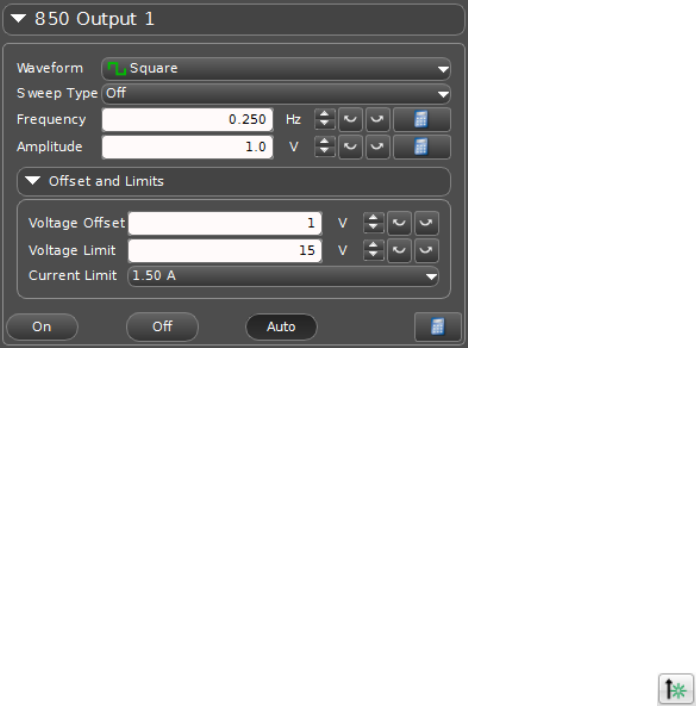
Figure 7.2: Capstone settings for creating a fast rising edge to measure the wave speed.

0.2 Hz or so (the exact frequency does not matter). The recommended Amplitude is about 1

V. Last, set the Voltage Oﬀset to be the same voltage as you used for the Amplitude so that

you don’t excite a pulse before you can record a rising edge.

You can visualize your results by opening a Graph session from the Displays palette.

You will be plotting two signals simultaneously (the wave driver voltage and the photodiode

signal) to see when the pulse is launched. To set this up, select Light Intensity (%) for the

y-axis and plot Time (s) on the x-axis. To add another y-axis, mouse over the plot area

to wake up the menu bar and click on the “Add new y-axis to active plot area” button .

The new axis will appear on the right side of the plot, and you can set it to plot Output

Voltage, Ch01 (V), as shown in Fig. 7.3. When you click Record on the Controls palette, the

photodiode signal will be fairly ﬂat and the voltage should be zero until the rising edge, at

which point the voltage will jump to twice the amplitude setting and there will be a series of

peaks on the photodiode signal for each time the wave gets near the laser beam spot. Click

Stop once the voltage goes back to zero. Figure 7.3 shows a screen shot from Capstone with

an example signal.

The size and shape of the wiggles you get will probably look very diﬀerent from everyone

else’s, but the only thing that matters is that you see some sort of signal that repeats itself a

few times. You can open a Table and save your data in Excel for your analysis and plotting.

This may involve quite a bit of data, but hopefully not too much to take home with you.

As always, be sure the table is displaying enough digits for you to get your data without

introducing nasty rounding errors. Save data for all 3 values of the tension so that you can

determine the wave speed during your analysis. Remember to measure the length between

the pulley and the clamp so that you know how far the pulse travels between successive

arrivals at the laser spot.

103

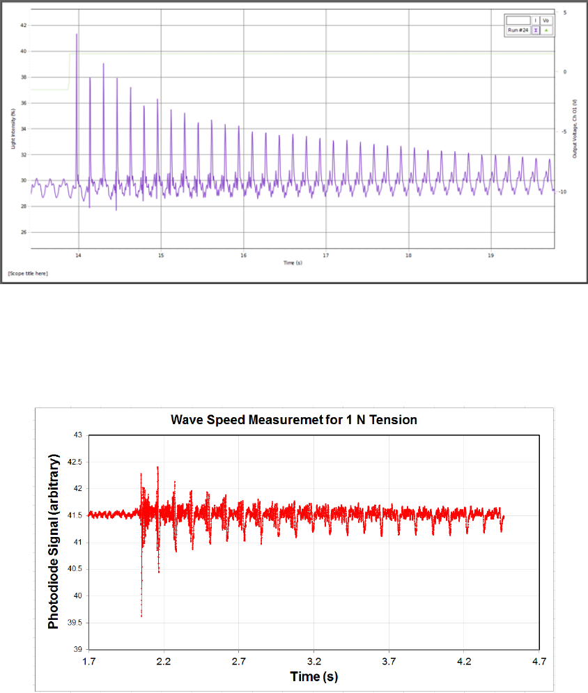
Figure 7.3: Capstone screen shot showing the launch of a pulse that makes many round-trips

along the string.

Figure 7.4: Close-up of the signal from a pulse reﬂecting back and forth from the clamp

and pulley. The wave speed can me measured by identifying some feature that repeats and

measuring the time duration between repetitions. In this case, the sharp downward spike

would probably be a good candidate. The uncertainty in this measurement can be estimated

from the width of the spike.

104

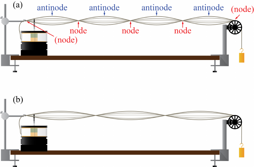
Figure 7.5: Transverse standing waves on a string. The positions where the displacement

amplitude is zero are called nodes, while the maxima are called antinodes. In contrast, a

normal mode of oscillation in this system is an entire standing wave. The n= 4 mode is

shown in (a), while an entirely diﬀerent mode (with a correspondingly diﬀerent frequency)

is shown in (b). The mode in (b) corresponds to n= 3.

7.1.2 Part 2: standing waves

For the second part of this experiment, you will be observing standing waves in the vibrating

string, as shown in Fig. 7.5. You will probably get the best results if you use your heaviest

weight from the ﬁrst part of the experiment, and be sure to re-position the laser spot and

photodiode and optimize the linearity of the signal as mentioned above (driving the wave

driver with a sine wave should give you a nice sine wave on the photodiode signal).

Since both ends of the string have ﬁxed boundary conditions, the string will support a

series of harmonics of the fundamental standing wave mode. Note: this resonance frequency

will probably be less than 20 Hz, so please do not try to turn on the wave driver at 1

kHz, which will primarily produce a painful noise. When driving the fundamental mode

on resonance, the string will oscillate with large amplitude (probably clearly visible by eye)

and will not have any nodes between end points. We can assign an integer n= 1 to this

mode. There will be an entire series of harmonics associated with this motion for other

integer values of n. Find the resonant frequency for this fundamental mode by monitoring

the amplitude of the photodiode signal and ﬁnding the frequency for which this amplitude

105

is maximized. Be sure to make a measurement that is as precise as possible in order to

accurately predict the frequency at which higher values of nwill also be normal modes of

the string. By using the DAQ, it should be possible for you to nail this down to at least

3 digits of precision (10s of mHz) using this “maximum amplitude” method. Record this

frequency for your records.

Before moving on to ﬁnd the frequencies of higher-order modes, recall that you learned

last week how to ﬁnd the undamped resonant frequency ωoof an oscillator using the phase

information of the signal. You created parametric plots of Lissajous ﬁgures such as Fig. 6.5,

and the resonant frequency was the frequency when the ﬁgure was most symmetric. Using

what you recall from last week about how to plot the system response (for this week, this

is the photodiode signal) vs. the drive signal (in this case, the wave driver output), set up

a parametric plot of your system that will allow you to identify resonant frequencies by

observing the symmetry of the waveform. You may assume ωR≈ωosince the damping time

in this system is many oscillation periods. Do this for the fundamental (n= 1) mode, and

see if you measure the same resonant frequency as you did with the “maximum amplitude”

method above. Be sure to record not just the resonant frequency, but also an uncertainty in

your measurement of this frequency. How far can you move the frequency before you notice

that the Lissajous ﬁgure is no longer symmetric?

Using your parametric plot, record the resonant frequencies for a series of harmonics of

this fundamental frequency (each harmonic is called a normal mode of oscillation). The nth

normal mode will have a resonant frequency that is ntimes the fundamental frequency, so

you should use your measured fundamental frequency to predict where to ﬁnd each harmonic.

The nth mode will have nanti-nodes in it (nodes are positions with minimum amplitude, anti-

nodes are positions with maximum amplitude). Split up the measurement of the frequencies

of the harmonics with your parter up to n= 9. For instance, if there are two of you, one can

measure the frequencies of modes n= 1,3,5,7,9 and the other can measure n= 1,2,4,6,8.

If there are 3 of you sharing an apparatus, each should choose 5 harmonics at random from

n= 2 ···9.

For the higher frequency modes, you may ﬁnd that it is helpful to turn up the signal

generator amplitude. If you have trouble ﬁnding those signals, you may have the laser and

photodiode too far from the pulley, so moving them closer may help. Try to ﬁnd the 30th

harmonic (you should be able to predict where you think it will occur) and record what you

observe.

7.1.3 Part 3: boundary eﬀects

The last part of the experiment is an investigation of intermediate boundary conditions and

interference. Using your measured resonant frequencies for n=2, 4, and 5, drive these modes

at some ﬁxed drive amplitude and record the amplitude of the photodiode oscillations for

each one (Scope mode is good for this). The “amplitude” you record can simply be the

peak-to-peak size of the photodiode signal (because this number will be proportional to the

actual wave amplitude for transverse displacement of the string).

For all of the normal modes, the pulley apex and the clamp are always nodes, but for n= 2

106

and higher, there are also nodes between these endpoints. Drive the fundamental (n= 2)

mode with the same drive amplitude you just used when you measured its amplitude. Using

a ring stand and a post, constrain the motion of the string at the node that is in the middle

of the string for n= 2. You should be able to do this without substantially altering this

mode (the signal level should be the same). Record the new signal amplitude you measure

for this mode once you have optimized the position of the post to maximize it. Without

moving the post, drive the n= 4 mode with the same drive amplitude you used before, and

compare your new measured signal amplitude to the old one. Do the same (without moving

the post!) for n= 5 and record what you ﬁnd.

7.2 Analysis

7.2.1 Part 1 analysis

To measure the wave speed from your data, for each tension, plot the photodiode signal

vs. time, as shown in Fig. 7.4. The excitation itself is likely to be a somewhat complicated

set of wiggles on the signal, but the important thing is not the shape of the signal so much

as it is identifying some feature that repeats itself. Each time the feature repeats, it will be

slightly smaller than the previous time, so you will have to make a decision about how far

out in time you want to look. Since you know the distance the excitation travels between

repetitions, measure the wave speed by dividing this distance by the time delay. Estimate an

uncertainty in your measurement based on how well you feel you can localize the excitation

feature in time and how well you know the distance traveled.

7.2.2 Part 2 analysis

The frequency of the nth normal mode is predicted to be given by

f(n) = nv

2L(7.3)

where vis the wave speed (predicted and measured for this tension in Part 1) and Lis

the distance between the clamp and pulley apex. Using your measured value for the wave

speed from Part 1, calculate a predicted value for the frequency of the fundamental mode.

Using Eq. 7.3, calculate predicted values for the higher-order modes whose frequencies you

measured. Compare your results.

7.3 Report guidelines

Write a full, formal lab report that covers Experiments 6 and 7.

1. Cover Sheet

•experiment number and title

107

•your name

•the date the lab was performed

•your lab section (for instance, “Monday 3pm”)

•your TA’s name

•your lab partners’ names

•the word count of your abstract

2. Guidelines

By this point in Physics 4AL, your experience in writing lab reports should enable you

to write a lab report without detailed guidelines. You will be responsible for developing

a coherent narrative to connect each of the results you obtained and deciding which

ﬁgures, plots, tables and analysis will be appropriate to accomplish this. You should

look back over your old returned reports and guidelines from earlier in this manual to

guide you through this process. If you did the extra credit from this week and/or last,

please ﬁnd a way to include it in your lab report as if it were just another part of your

experiment.

3. Extra Credit In experiments 6 and 7, you used Lissajous ﬁgures to ﬁnd the resonance

frequency of a couple of harmonic oscillators. Using this method for your standing

waves, try to ﬁnd out what the highest mode you can ﬁnd is. Can you see the n= 60

mode? Report your determination of each mode starting from n= 1 and going as high

in nas you can. State the distance you have between your laser spot on the string

and the point where the string touches the pulley. Calculate the frequency of the ﬁrst

mode that will have a node at this location, and describe why this may make your

data taking for modes near this one diﬃcult.

7.4 Epilogue

Throughout this course, you have investigated a series of diﬀerent mechanical phenomena

in a laboratory setting. Many of the eﬀect observed in this setting, however, manifest

themselves in many diﬀerent contexts, including electricity and magnetism, atomic physics,

nuclear physics, astrophysics, communications, particle physics, et cetera. The material in

this course is therefore far more general than mechanics, and it is hoped that working with

your hands to investigate these phenomena will help to prepare you to have a more intuitive

understanding of these concepts as you move forward.

108

Appendix A

Laser safety.

109

Laser Safety

Lab Hazard Awareness Information

501 Westwood Plaza, 4th Floor • Los Angeles, CA 90095

Phone: 310-825-5689 • Fax: 310-825-7076 • www.ehs.ucla.edu

Provides information to lab workers/visitors who are NOT authorized laser users about hazards existing at this

location.

Location Knudsen 1238, 2115, 2122, 2136

LASERS

• Lasers may only be operated in these labs by personnel who have received permission to use them from a suitably

qualified class trainer.

• In order to maintain and protect equipment, personnel, and research, no worker, except for trained personnel, can

touch move or interfere with any laser equipment, materials or processes.

• Personnel should never use class-supplied laser pointers as presentation pointers in the classroom.

• Personnel should never introduce a shiny or mirrored surface in front of laser beam that might cause uncontrolled

specular reflection.

• Classroom laser personnel should not move or adjust laser equipment set up by any other class laser operator

unless specifically instructed to do so. This includes not detaching the lasers from any stands or moving the stands in

any way that could create a hazard for other classroom occupants.

• Laser equipment should be turned on only when necessary for presenting the demonstration.

• Laser equipment, whether powered by an external power supply or batteries, should be turned off following

completion of a given classroom demonstration so as to prevent inadvertent exposure during class dismissal.

EYE HAZARDS

• This lab uses and operates lasers that create light radiation which, if of sufficient power, can cause biological damage

to the eyes. Eye damage caused from lasers includes retinal burns, glaucoma, cataracts and total loss of vision.

• Personnel should never stare into a laser or look directly into a beam and never stand or sit at the same level as the

beam path.

• Laser operators must make sure that any laser beam points away from other members of the class.

• The person primarily responsible for the class training can order all personnel to leave the room if necessary for any

reason

Laser Safety

LASER LITE; A Quick Overview of Laser Safety 06/09

501 Westwood Plaza, 4th Floor • Los Angeles, CA 90095

Phone: 310-825-5689 • Fax: 310-825-7076 • www.ehs.ucla.edu

THE PRIMARY PURPOSE

OF THE UCLA LASER

SAFETY PROGRAM IS TO

AVOID GETTING A

LASER BEAM IN

YOUR EYE

NEVER STARE DIRECTLY

AT A LASER BEAM,

EVEN WITH PROTECTIVE

EYEWEAR

LASER LIGHT

• Maintains strength over long distances

• Produces significant eye hazards at relatively low levels

• Concentrates to a very high intensity when focused by a lens

• Occurs in the Visible and Non-visible spectrum

BIOLOGICAL HAZARDS

• Can be laser beam and non-beam related

• Can occur at all wavelengths

• Occur mainly in the eyes and skin

MOST INJURIES

• Affect the eyes

• Occur during alignment

• Result from operator error

PROTECTION

• Eyewear must be worn for Class 3B and Class 4 laser use

• Eyewear must meet ANSI standards and be marked with

Optical Density and Wavelength

• Appropriate skin protection is required for Class 4 lasers

LASER CLASSIFICATION TABLE

Class 1 / 1M

Maximum power output is a few microwatts. Visible spectrum output

Considered incapable of producing hazardous eye/skin exposure unless viewed with collecting

optics (1M). Does not apply to open Class 1 enclosures containing higher-class lasers

Class 2 / 2M

Maximum power output is < 1 mW. Visible spectrum output

Considered incapable of producing hazardous eye/skin exposure within the time period of human

eye aversion response (0.25 s).unless viewed with collecting optics (2M)

Class 3R

Maximum power output is 1 mW - < 5 mW. Visible and non-visible spectrum

Potentially hazardous under some direct and specular reflection viewing condition if the eye is

appropriately focused and stable or if viewed with collecting optics.

Class 3B

Maximum power output is 5 mW - < 500 mW Visible and non-visible spectrum

Presents a potential eye hazard for intrabeam (direct) or specular (mirror-like) conditions.

Presents a significant skin hazard by long-term diffuse (scatter) exposure if higher powered and

operating in 200 – 280 nm UVC ranges

Class 4

Maximum power output is > 500 mW. Visible and non-visible spectrum

Presents potential acute hazards to the eye and skin for all intrabeam and diffused conditions

Potential hazard for fire (ignition), explosion and emissions from target or process materials.

EYE DAMAGE - WAVELENGTHS

WAVELENGTH

AREA OF DAMAGE

PATHOLOGICAL EFFECT

180 - 315 nm

(Ultraviolet UV-B, UVC)

CORNEA; Deep-ultraviolet light causes

accumulating damage, even at very low power

Photokeratitis; Inflammation of the

cornea, similar to sunburn

315 - 400 nm

(Ultraviolet UV-A)

CORNEA and LENS

Photochemical cataract; Clouding

of the lens

400 - 780 nm

(Visible)

RETINA; Visible light is focused on the retina

Photochemical damage; Damage

to retina and retinal burns

780 - 1400 nm

(Near Infrared)

RETINA; Near IR light is not absorbed by iris

and is focused on the retina

Thermal damage to cataract and

retinal burns

1400 - 3000 nm

(Infrared)

CORNEA and LENS; IR light is absorbed by

transparent parts of eye before reaching the

retina

Aqueous flare; Protein in aqueous

humor, cataract, corneal burn

3000 – 10000 nm

(Far Infrared)

CORNEA

Corneal burn

Laser Safety

LASER LITE; A Quick Overview of Laser Safety 06/09

501 Westwood Plaza, 4th Floor • Los Angeles, CA 90095

Phone: 310-825-5689 • Fax: 310-825-7076 • www.ehs.ucla.edu

LASER OPERATION GUIDELINES

OPERATORS MUST;

• Review Standard Operating Procedures, operating and safety instructions and

laboratory-specific laser instructions

• Be trained in laser safety and specific laser procedures

• Observe all written procedures, safety rules and properly use appropriate

PPE

• Be authorized by the Principal Investigator

• Be directly supervised by a person knowledgeable in laser safety

• Wear appropriate PPE, follow safety procedures and SOP’s

• Never circumvent Administrative or Engineering safety controls

• Know the location and use of the power kill switch and fire extinguisher

• Use the buddy system when working with high voltage equipment

• Not wear reflective metal jewelry when working with laser beams

• Never stare directly into a beam even with eye protection; use indirect viewing

• Give sufficient attention to non-beam hazards to prevent possible injury and

illness

• Be aware of plasma and collateral radiation

• Notify supervisor immediately of potentially hazardous conditions, personal

injury, or property damage

IN EACH LAB, PERSONNEL MUST BE ABLE TO OBTAIN:

• Training on equipment, procedures and emergency procedures

• Safety Equipment that is sufficient in numbers for lab staff, appropriate for the

equipment in use and in good operating condition

• Standard Operational Procedures for the safe use of all equipment

• Information from the PI or Lab Manager about potential equipment hazards

EMERGENCY INSTRUCTIONS

1. Shut the laser off immediately and remove the interlock key. If not possible,

alert everyone to exit the laboratory and be the last to leave the laboratory

2. If there is a fire, get everyone out of the laboratory immediately. At the same

time shout “FIRE” loudly and frequently. Turn on a fire alarm. Do not try to

“fight” the fire from inside the laboratory; do it from the doorway to maintain an

escape route

3. In the event of MAJOR injury, Summon Medical Assistance. Call 911 from a

campus phone or 310-825-1491 from a cell phone

4. Call Security and/or Fire Department (911) as necessary

5. Call EHS Hotline (59797) to report the incident

Note; ALL incidents must be reported to the Laser Safety Officer

6. Contact the PI and/or Lab Manager and describe the emergency

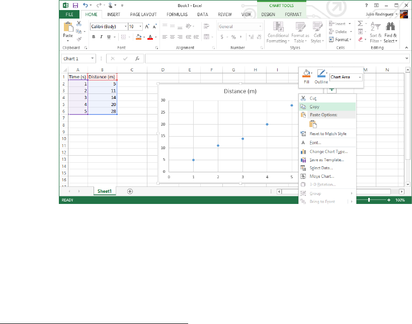
Appendix B

B.1 Guide for Making and Inserting Plots1

B.1.1 Obtaining Graph data from Excel

In MS Excel simply click on the white space in your graph, this will select the entire graph.

You can then use the ctrl+c keyboard shortcut to copy the graph. Alternatively you can

right click on the graphs white space and click “copy” from the menu. Simply paste this in

Word in the normal way (ctrl+p) or right click and selecting “paste.”

B.1.2 Formatting the Graph

Now that the graph is in MS Word, you need to format the graph according to the rules

agreed upon by the grading staﬀ. Every graph needs these three things: Axis labels, units,

and a title. Additionally, graphs with multiple datasets require some way of determining

1This section was contributed by Julio S. Rodriguez, Jr. (2014) and revised by Anthony Ransford (2016).

113

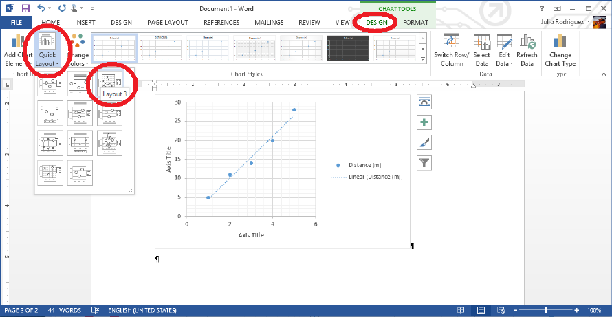
what the data represents (either an explanation or a legend), and some graphs require a

trendline with an equation. Many of these things can be set up in Excel beforehand and will

be copied over. You may also generate them directly in Word. The lab manual has a pretty

good explanation of how to do all of this in Excel and the procedure is largely the same in

word. The labels, units, and trendline should appear on the graph while title and possibly

the trendline equation (with error) should appear in the caption. If you use a legend you do

not need an explanation of what the data points represent, if you do not have a legend, you

should include such an explanation in the caption.

Axis Labels

There is an easy way to add axis labels. Click on the whitespace in your graph and on

the ribbon, a few new tabs will open up under the group heading “Chart Tools.” On the

“Design” tab there are some preset layouts. In general, you should pick the preset with

axis labels (see Figure B.1). You can click on the axis labels to edit their content. I will

be working with the assumption that the legend is not necessary since we will have a very

descriptive caption. Simply click on the legend and press the “delete” key on the keyboard.

Figure B.1: There are templates in Excel that have axis labels by default, which is a good

way to make sure axes don’t end up in a report without labels.

Adding the caption

This is probably the trickiest part of the whole process. The caption function in Word is

great in that it auto-numbers things for you, and lets you use diﬀerent numberings for ﬁgure

114

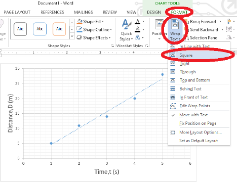
and tables. The cross-reference tool adds to its functionality, because changing the caption

numbering order will not mess up the numbering in the text of your paper. Before we add a

caption, we need to change the nature of the graph. Right now Word is treating our graph

like an object that takes up its own line, but we want Word to treat the graph as an object

embedded in the text (like the image on the right). Click on your graph and this time on

the ribbon click on the Format tab under the Chart Tools heading. Here click the Wrap

Text button and on the Square option (on older versions of Word, the image for this button

looks like a dog instead of an arched curve). Move your graph where you want it to appear

in your paper and then add the caption. Right click on the whitespace of your graph and

click the insertcaption option. All kinds of options come up, but the default settings are

okay for graphs. This will insert the caption as a text box, but we need the caption to be

associated with the graph. To do this: If the border and sizing handles on the textbox are

not already showing, click on the textbox (anywhere inside). While holding down ctrl, click

on the graph. This should select both objects. Release ctrl and right click on either object,

then select “Group >Group.”

These two objects will now be treated as a unit; moving one of them will move the other

one. Reformat the text in the text box to match rest of your document. You may choose

to format the title of the graph in bold font for clarity, but this is not strictly required.

To add equations, you can either type things out and use the “symbol” function to include

any non-standard symbols, or you can use the equation editor (alt = or insert >equation).

A common convention is to italicize variables and leave units un-italicized in equations,

remember to leave a space between the units and variables if the two are being multiplied.

When referencing you graphs or images in your paper, you should refer to them by their

designation. To make this as painless as possible, you may want to use the cross-reference

tool in Word. If you change the order of your graphs, insert another graph before one you

have already referenced, or anything else along those lines, this tool will keep all of your

numbers in order. On the ribbon under the references tab, click “Cross-reference.” Under

“Reference Type,” select “Figure,” and under, “Insert Reference To,” select “Only Label and

115

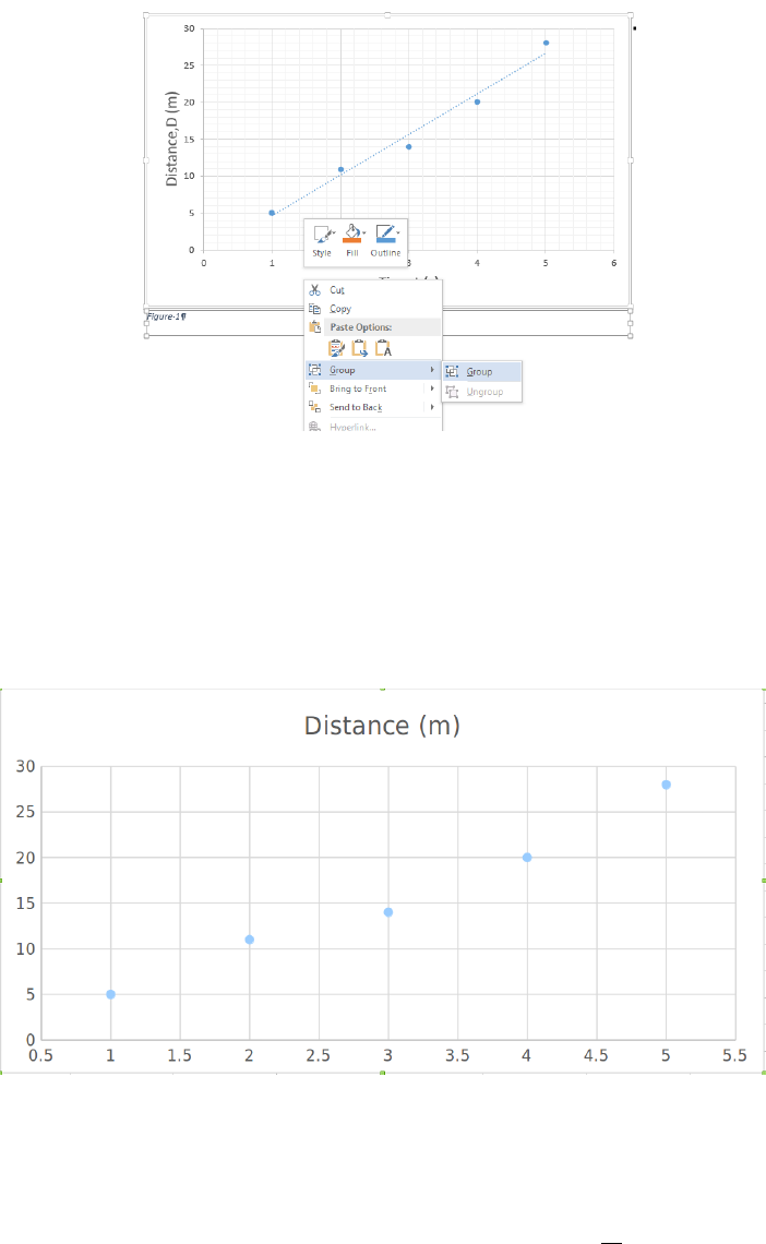
Number.” You can leave on the “hyperlink” function if you wish. Select which ﬁgure you

wish to make reference to in the box labeled “For which caption.” This inserts a reference

to your chart. For example, Fig. B.2 shows what a proper graph should look like. If you

insert any addition graphs or change the order, select your entire document and right click

any of the selected text and click “Update Field.”

Figure B.2: The blue dots on this graph represent data points taken from the Fakemeter 5000

while on a bicycle ride though Imaginary Park. Distance as a function of time was calculated

using the regression tool in Microsoft Excel 365 in order to ﬁnd the average velocity of the

cyclist. The line of best ﬁt is represented by D=t×(5.5±0.5) m

s−(1 ±2) m.

116

Appendix C

To help you ﬁgure out how to write bibliography entries in the style of Nature formatting,

a long example of bibliography formatting from Nature is reproduced here. This example

shows entries for published journal articles, journal articles in press, and published books.

These are page images taken from the paper reporting sequencing of the human genome

[2].

117

because of the availability of tissues from all developmental time

points. A challenge will be to de®ne the gene-speci®c patterns of

alternative splicing, which may affect half of human genes. Existing

collections of ESTs and cDNAs may allow identi®cation of the most

abundant of these isoforms, but systematic exploration of this

problem may require exhaustive analysis of cDNA libraries from

multiple tissues or perhaps high-throughput reverse transcription±

PCR studies. Deep understanding of gene function will probably

require knowledge of the structure, tissue distribution and abun-

dance of these alternative forms.

Large-scale identi®cation of regulatory regions

The one-dimensional script of the human genome, shared by

essentially all cells in all tissues, contains suf®cient information to

provide for differentiation of hundreds of different cell types, and

the ability to respond to a vast array of internal and external

in¯uences. Much of this plasticity results from the carefully orche-

strated symphony of transcriptional regulation. Although much has

been learned about the cis-acting regulatory motifs of some speci®c

genes, the regulatory signals for most genes remain uncharacterized.

Comparative genomics of multiple vertebrates offers the best hope

for large-scale identi®cation of such regulatory sites440. Previous

studies of sequence alignment of regulatory domains of ortho-

logous genes in multiple species has shown a remarkable

correlation between sequence conservation, dubbed `phylogenetic

footprints'441, and the presence of binding motifs for transcription

factors. This approach could be particularly powerful if combined

with expression array technologies that identify cohorts of genes

that are coordinately regulated, implicating a common set of cis-

acting regulatory sequences442±445. It will also be of considerable

interest to study epigenetic modi®cations such as cytosine methyla-

tion on a genome-wide scale, and to determine their biological

consequences446,447. Towards this end, a pilot Human Epigenome

Project has been launched448,449.

Sequencing of additional large genomes

More generally, comparative genomics allows biologists to peruse

evolution's laboratory notebookÐto identify conserved functional

features and recognize new innovations in speci®c lineages. Deter-

mination of the genome sequence of many organisms is very

desirable. Already, projects are underway to sequence the genomes

of the mouse, rat, zebra®sh and the puffer®shes T. nigroviridis and

Takifugu rubripes. Plans are also under consideration for sequencing

additional primates and other organisms that will help de®ne key

developments along the vertebrate and nonvertebrate lineages.

To realize the full promise of comparative genomics, however, it

needs to become simple and inexpensive to sequence the genome of

any organism. Sequencing costs have dropped 100-fold over the last

10 years, corresponding to a roughly twofold decrease every 18

months. This rate is similar to `Moore's law' concerning improve-

ments in semiconductor manufacture. In both sequencing and

semiconductors, such improvement does not happen automatically,

but requires aggressive technological innovation fuelled by major

investment. Improvements are needed to move current dideoxy

sequencing to smaller volumes and more rapid sequencing

times, based upon advances such as microchannel technology.

More revolutionary methods, such as mass spectrometry, single-

molecule sequencing and nanopore approaches76, have not yet

been fully developed, but hold great promise and deserve strong

encouragement.

Completing the catalogue of human variation

The human draft genome sequence has already allowed the identi-

®cation of more than 1.4 million SNPs, comprising a substantial

proportion of all common human variation. This program should

be extended to obtain a nearly complete catalogue of common

variants and to identify the common ancestral haplotypes present in

the population. In principle, these genetic tools should make it

possible to perform association studies and linkage disequilibrium

studies376 to identify the genes that confer even relatively modest risk

for common diseases. Launching such an intense era of human

molecular epidemiology will also require major advances in the cost

ef®ciency of genotyping technology, in the collection of carefully

phenotyped patient cohorts and in statistical methods for relating

large-scale SNP data to disease phenotype.

From sequence to function

The scienti®c program outlined above focuses on how the genome

sequence can be mined for biological information. In addition, the

sequence will serve as a foundation for a broad range of functional

genomic tools to help biologists to probe function in a more

systematic manner. These will need to include improved techniques

and databases for the global analysis of: RNA and protein expres-

sion, protein localization, protein±protein interactions and chemi-

cal inhibition of pathways. New computational techniques will be

needed to use such information to model cellular circuitry. A full

discussion of these important directions is beyond the scope of this

paper.

Concluding thoughts

The Human Genome Project is but the latest increment in a

remarkable scienti®c program whose origins stretch back a hundred

years to the rediscovery of Mendel's laws and whose end is nowhere

in sight. In a sense, it provides a capstone for efforts in the past

century to discover genetic information and a foundation for efforts

in the coming century to understand it.

We ®nd it humbling to gaze upon the human sequence now

coming into focus. In principle, the string of genetic bits holds long-

sought secrets of human development, physiology and medicine. In

practice, our ability to transform such information into under-

standing remains woefully inadequate. This paper simply records

some initial observations and attempts to frame issues for future

study. Ful®lling the true promise of the Human Genome Project will

be the work of tens of thousands of scientists around the world, in

both academia and industry. It is for this reason that our highest

priority has been to ensure that genome data are available rapidly,

freely and without restriction.

The scienti®c work will have profound long-term consequences

for medicine, leading to the elucidation of the underlying molecular

mechanisms of disease and thereby facilitating the design in many

cases of rational diagnostics and therapeutics targeted at those

mechanisms. But the science is only part of the challenge. We

must also involve society at large in the work ahead. We must set

realistic expectations that the most important bene®ts will not be

reaped overnight. Moreover, understanding and wisdom will be

required to ensure that these bene®ts are implemented broadly and

equitably. To that end, serious attention must be paid to the many

ethical, legal and social implications (ELSI) raised by the accelerated

pace of genetic discovery. This paper has focused on the scienti®c

achievements of the human genome sequencing efforts. This is not

the place to engage in a lengthy discussion of the ELSI issues, which

have also been a major research focus of the Human Genome

Project, but these issues are of comparable importance and could

appropriately ®ll a paper of equal length.

Finally, it is has not escaped our notice that the more we learn

about the human genome, the more there is to explore.

``We shall not cease from exploration. And the end of all our

exploring will be to arrive where we started, and know the place for

the ®rst time.''ÐT. S. Eliot450 M

Received 7 December 2000; accepted 9 January 2001.

1. Correns, C. Untersuchungen u

Èber die Xenien bei Zea mays. Berichte der Deutsche Botanische

Gesellschaft 17, 410±418 (1899).

2. De Vries, H. Sur la loie de disjonction des hybrides. Comptes Rendue Hebdemodaires, Acad. Sci. Paris

130, 845±847 (1900).

3. von Tschermack, E. Uber Ku

Ènstliche Kreuzung bei Pisum sativum. Berichte der Deutsche Botanische

Gesellschaft 18, 232±239. (1900).

4. Sanger, F. et al. Nucleotide sequence of bacteriophage FX174 DNA. Nature 265, 687±695 (1977).

5. Sanger, F. et al. The nucleotide sequence of bacteriophage FX174. J Mol Biol 125, 225±246 (1978).

articles

914 NATURE

VOL 409

15 FEBRUARY 2001

www.nature.com

6. Sanger, F., Coulson, A. R., Hong, G. F., Hill, D. F. & Petersen, G. B. Nucleotide-sequence of

bacteriophage Lambda DNA. J. Mol. Biol. 162, 729±773 (1982).

7. Fiers, W. et al. Complete nucleotide sequence of SV40 DNA. Nature 273, 113±120 (1978).

8. Anderson, S. et al. Sequence and organization of the human mitochondrial genome. Nature 290,

457±465 (1981).

9. Botstein, D., White, R. L., Skolnick, M. & Davis, R. W. Construction of a genetic linkage map in man

using restriction fragment length polymorphisms. Am. J. Hum. Genet. 32, 314±331 (1980).

10. Olson, M. V. et al. Random-clone strategy for genomic restriction mapping in yeast. Proc. Natl Acad.

Sci. USA 83, 7826±7830 (1986).

11. Coulson, A., Sulston, J., Brenner, S. & Karn, J. Toward a physical map of the genome of the nematode

Caenorhabditis elegans.Proc. Natl Acad. Sci. USA 83, 7821±7825 (1986).

12. Putney, S. D., Herlihy, W. C. & Schimmel, P. A new troponin T and cDNA clones for 13 different

muscle proteins, found by shotgun sequencing. Nature 302, 718±721 (1983).

13. Milner, R. J. & Sutcliffe, J. G. Gene expression in rat brain. Nucleic Acids Res. 11, 5497±5520 (1983).

14. Adams, M. D. et al. Complementary DNA sequencing: expressed sequence tags and human genome

project. Science 252, 1651±1656 (1991).

15. Adams, M. D. et al. Initial assessment of human gene diversity and expression patterns based upon

83 million nucleotides of cDNA sequence. Nature 377, 3±174 (1995).

16. Okubo, K. et al. Large scale cDNA sequencing for analysis of quantitative and qualitative aspects of

gene expression. Nature Genet. 2, 173±179 (1992).

17. Hillier, L. D. et al. Generation and analysis of 280,000 human expressed sequence tags. Genome Res.

6, 807±828 (1996).

18. Strausberg, R. L., Feingold, E. A., Klausner, R. D. & Collins, F. S. The mammalian gene collection.

Science 286, 455±457 (1999).

19. Berry, R. et al. Gene-based sequence-tagged-sites (STSs) as the basis for a human gene map. Nature

Genet. 10, 415±423 (1995).

20. Houlgatte, R. et al. The Genexpress Index: a resource for gene discovery and the genic map of the

human genome. Genome Res. 5, 272±304 (1995).

21. Sinsheimer, R. L. The Santa Cruz WorkshopÐMay 1985. Genomics 5, 954±956 (1989).

22. Palca, J. Human genomeÐDepartment of Energy on the map. Nature 321, 371 (1986).

23. National Research Council Mapping and Sequencing the Human Genome (National Academy Press,

Washington DC, 1988).

24. Bishop, J. E. & Waldholz, M. Genome (Simon and Schuster, New York, 1990).

25. Kevles, D. J. & Hood, L. (eds) The Code of Codes: Scienti®c and Social Issues in the Human Genome

Project (Harvard Univ. Press, Cambridge, Massachusetts, 1992).

26. Cook-Deegan, R. The Gene Wars: Science, Politics, and the Human Genome (W. W. Norton & Co.,

New York, London, 1994).

27. Donis-Keller, H. et al. A genetic linkage map of the human genome. Cell 51, 319±337 (1987).

28. Gyapay, G. et al. The 1993±94 Genethon human genetic linkage map. Nature Genet. 7, 246±339

(1994).

29. Hudson, T. J. et al. An STS-based map of the human genome. Science 270, 1945±1954 (1995).

30. Dietrich, W. F. et al. A comprehensive genetic map of the mouse genome. Nature 380, 149±152

(1996).

31. Nusbaum, C. et al. A YAC-based physical map of the mouse genome. Nature Genet. 22, 388±393

(1999).

32. Oliver, S. G. et al. The complete DNA sequence of yeast chromosome III. Nature 357, 38±46 (1992).

33. Wilson, R. et al. 2.2 Mb of contiguous nucleotide sequence from chromosome III of C. elegans.

Nature 368, 32±38 (1994).

34. Chen, E. Y. et al. The human growth hormone locus: nucleotide sequence, biology, and evolution.

Genomics 4, 479±497 (1989).

35. McCombie, W. R. et al. Expressed genes, Alu repeats and polymorphisms in cosmids sequenced

from chromosome 4p16.3. Nature Genet. 1, 348±353 (1992).

36. Martin-Gallardo, A. et al. Automated DNA sequencing and analysis of 106 kilobases from human

chromosome 19q13.3. Nature Genet. 1, 34±39 (1992).

37. Edwards, A. et al. Automated DNA sequencing of the human HPRT locus. Genomics 6, 593±608

(1990).

38. Marshall, E. A strategy for sequencing the genome 5 years early. Science 267, 783±784 (1995).

39. Project to sequence human genome moves on to the starting blocks. Nature 375, 93±94 (1995).

40. Shizuya, H. et al. Cloning and stable maintenance of 300-kilobase-pair fragments of human DNA in

Escherichia coli using an F-factor-based vector. Proc. Natl Acad. Sci. USA 89, 8794±8797 (1992).

41. Burke, D. T., Carle, G. F. & Olson, M. V. Cloning of large segments of exogenous DNA into yeast by

means of arti®cial chromosome vectors. Science 236, 806±812 (1987).

42. Marshall, E. A second private genome project. Science 281, 1121 (1998).

43. Marshall, E. NIH to produce a `working draft' of the genome by 2001. Science 281, 1774±1775

(1998).

44. Pennisi, E. Academic sequencers challenge Celera in a sprint to the ®nish. Science 283, 1822±1823

(1999).

45. Bouck, J., Miller, W., Gorrell, J. H., Muzny, D. & Gibbs, R. A. Analysis of the quality and utility of

random shotgun sequencing at low redundancies. Genome Res. 8, 1074±1084 (1998).

46. Collins, F. S. et al. New goals for the U. S. Human Genome Project: 1998±2003. Science 282, 682±689

(1998).

47. Sanger, F. & Coulson, A. R. A rapid method for determining sequences in DNA by primed synthesis

with DNA polymerase. J. Mol. Biol. 94, 441±448 (1975).

48. Maxam, A. M. & Gilbert, W. A new method for sequencing DNA. Proc. Natl Acad. Sci. USA 74, 560±

564 (1977).

49. Anderson, S. Shotgun DNA sequencing using cloned DNase I-generated fragments. Nucleic Acids

Res. 9, 3015±3027 (1981).

50. Gardner, R. C. et al. The complete nucleotide sequence of an infectious clone of cauli¯ower mosaic

virus by M13mp7 shotgun sequencing. Nucleic Acids Res. 9, 2871±2888 (1981).

51. Deininger, P. L. Random subcloning of sonicated DNA: application to shotgun DNA sequence

analysis. Anal. Biochem. 129, 216±223 (1983).

52. Chissoe, S. L. et al. Sequence and analysis of the human ABL gene, the BCR gene, and regions

involved in the Philadelphia chromosomal translocation. Genomics 27, 67±82 (1995).

53. Rowen, L., Koop, B. F. & Hood, L. The complete 685-kilobase DNA sequence of the human beta T

cell receptor locus. Science 272, 1755±1762 (1996).

54. Koop, B. F. et al. Organization, structure, and function of 95 kb of DNA spanning the murine T-cell

receptor C alpha/C delta region. Genomics 13, 1209±1230 (1992).

55. Wooster, R. et al. Identi®cation of the breast cancer susceptibility gene BRCA2. Nature 378, 789±792

(1995).

56. Fleischmann, R. D. et al. Whole-genome random sequencing and assembly of Haemophilus

in¯uenzae Rd. Science 269, 496±512 (1995).

57. Lander, E. S. & Waterman, M. S. Genomic mapping by ®ngerprinting random clones: a

mathematical analysis. Genomics 2, 231±239 (1988).

58. Weber, J. L. & Myers, E. W. Human whole-genome shotgun sequencing. Genome Res. 7, 401±409

(1997).

59. Green, P. Against a whole-genome shotgun. Genome Res. 7, 410±417 (1997).

60. Venter, J. C. et al. Shotgun sequencing of the human genome. Science 280, 1540±1542 (1998).

61. Venter, J. C. et al. The sequence of the human genome. Science 291, 1304±1351 (2001).

62. Smith, L. M. et al. Fluorescence detection in automated DNA sequence analysis. Nature 321, 674±

679 (1986).

63. Ju, J. Y., Ruan, C. C., Fuller, C. W., Glazer, A. N. & Mathies, R. A. Fluorescence energy-transfer dye-

labeled primers for DNA sequencing and analysis. Proc. Natl Acad. Sci. USA 92, 4347±4351 (1995).

64. Lee, L. G. et al. New energy transfer dyes for DNA sequencing. Nucleic Acids Res. 25, 2816±2822 (1997).

65. Rosenblum, B. B. et al. New dye-labeled terminators for improved DNA sequencing patterns.

Nucleic Acids Res. 25, 4500±4504 (1997).

66. Metzker, M. L., Lu, J. & Gibbs, R. A. Electrophoretically uniform ¯uorescent dyes for automated

DNA sequencing. Science 271, 1420±1422 (1996).

67. Prober, J. M. et al. A system for rapid DNA sequencing with ¯uorescent chain-terminating

dideoxynucleotides. Science 238, 336±341 (1987).

68. Reeve, M. A. & Fuller, C. W. A novel thermostable polymerase for DNA sequencing. Nature 376,

796±797 (1995).

69. Tabor, S. & Richardson, C. C. Selective inactivation of the exonuclease activity of bacteriophage T7

DNA polymerase by in vitro mutagenesis. J. Biol. Chem. 264, 6447±6458 (1989).

70. Tabor, S. & Richardson, C. C. DNA sequence analysis with a modi®ed bacteriophage T7 DNA

polymeraseÐeffect of pyrophosphorolysis and metal ions. J. Biol. Chem. 265, 8322±8328 (1990).

71. Murray, V. Improved double-stranded DNA sequencing using the linear polymerase chain reaction.

Nucleic Acids Res. 17, 8889 (1989).

72. Guttman, A., Cohen, A. S., Heiger, D. N. & Karger, B. L. Analytical and micropreparative ultrahigh

resolution of oligonucleotides by polyacrylamide-gel high-performance capillary electrophoresis.

Anal. Chem. 62, 137±141 (1990).

73. Luckey, J. A. et al. High-speed DNA sequencing by capillary electrophoresis. Nucleic Acids Res. 18,

4417±4421 (1990).

74. Swerdlow, H., Wu, S., Harke, H. & Dovichi, N. J. Capillary gel-electrophoresis for DNA sequencingÐ

laser-induced ¯uorescence detection with the sheath ¯ow cuvette. J. Chromatogr. 516, 61±67 (1990).

75. Meldrum, D. Automation for genomics, part one: preparation for sequencing. Genome Res. 10,

1081±1092 (2000).

76. Meldrum, D. Automation for genomics, part two: sequencers, microarrays, and future trends.

Genome Res. 10, 1288±1303 (2000).

77. Ewing, B. & Green, P. Base-calling of automated sequencer traces using phred. II. Error probabilities.

Genome Res. 8, 186±194 (1998).

78. Ewing, B., Hillier, L., Wendl, M. C. & Green, P. Base-calling of automated sequencer traces using

phred. I. Accuracy assessment. Genome Res. 8, 175±185 (1998).

79. Bentley, D. R. Genomic sequence information should be released immediately and freely in the

public domain. Science 274, 533±534 (1996).

80. Guyer, M. Statement on the rapid release of genomic DNA sequence. Genome Res. 8, 413 (1998).

81. Dietrich, W. et al. A genetic map of the mouse suitable for typing intraspeci®c crosses. Genetics 131,

423±447 (1992).

82. Kim, U. J. et al. Construction and characterization of a human bacterial arti®cial chromosome

library. Genomics 34, 213±218 (1996).

83. Osoegawa, K. et al. Bacterial arti®cial chromosome libraries for mouse sequencing and functional

analysis. Genome Res. 10, 116±128 (2000).

84. Marra, M. A. et al. High throughput ®ngerprint analysis of large-insert clones. Genome Res. 7, 1072±

1084 (1997).

85. Marra, M. et al. A map for sequence analysis of the Arabidopsis thaliana genome. Nature Genet. 22,

265±270 (1999).

86. The International Human Genome Mapping Consortium. A physical map of the human genome.

Nature 409, 934±941 (2001).

87. Zhao, S. et al. Human BAC ends quality assessment and sequence analyses. Genomics 63, 321±332

(2000).

88. Mahairas, G. G. et al. Sequence-tagged connectors: A sequence approach to mapping and scanning

the human genome. Proc. Natl Acad. Sci. USA 96, 9739±9744 (1999).

89. Tilford, C. A. et al. A physical map of the human Y chromosome. Nature 409, 943±945 (2001).

90. Bentley, D. R. et al. The physical maps for sequencing human chromosomes 1, 6, 9, 10, 13, 20 and X.

Nature 409, 942±943 (2001).

91. Montgomery, K. T. et al. A high-resolution map of human chromosome 12. Nature 409, 945±946

(2001).

92. Bru

Èls, T. et al. A physical map of human chromosome 14. Nature 409, 947±948 (2001).

93. Hattori, M. et al. The DNA sequence of human chromosome 21. Nature 405, 311±319 (2000).

94. Dunham, I. et al. The DNA sequence of human chromosome 22. Nature 402, 489±495 (1999).

95. Cox, D. et al. Radiation hybrid map of the human genome. Science (in the press).

96. Osoegawa, K. et al. An improved approach for construction of bacterial arti®cial chromosome

libraries. Genomics 52, 1±8 (1998).

97. The International SNP Map Working Group. A map of human genome sequence variation

containing 1.42 million single nucleotide polymorphisms. Nature 409, 928±933 (2001).

98. Collins, F. S., Brooks, L. D. & Chakravarti, A. A DNA polymorphism discovery resource for research

on human genetic variation. Genome Res. 8, 1229±1231 (1998).

99. Stewart, E. A. et al. An STS-based radiation hybrid map of the human genome. Genome Res. 7, 422±

433 (1997).

100. Deloukas, P. et al. A physical map of 30,000 human genes. Science 282, 744±746 (1998).

101. Dib, C. et al. A comprehensive genetic map of the human genome based on 5,264 microsatellites.

articles

NATURE

VOL 409

15 FEBRUARY 2001

www.nature.com 915

Nature 380, 152±154 (1996).

102. Broman, K. W., Murray, J. C., Shef®eld, V. C., White, R. L. & Weber, J. L. Comprehensive human

genetic maps: individual and sex-speci®c variation in recombination. Am. J. Hum. Genet. 63, 861±

869 (1998).

103. The BAC Resource Consortium. Integration of cytogenetic landmarks into the draft sequence of the

human genome. Nature 409, 953±958 (2001).

104. Kent, W. J. & Haussler, D. GigAssembler: an algorithm for the initial assembly of the human working

draft . Technical Report UCSC-CRL-00-17 (Univ. California at Santa Cruz, Santa Cruz, California,

2001).

105. Morton, N. E. Parameters of the human genome. Proc. Natl Acad. Sci. USA 88, 7474±7476 (1991).

106. Podugolnikova, O. A. & Blumina, M. G. Heterochromatic regions on chromosomes 1, 9, 16, and Yin

children with some disturbances occurring during embryo development. Hum. Genet. 63, 183±188

(1983).

107. Lundgren, R., Berger, R. & Kristoffersson, U. Constitutive heterochromatin C-band polymorphism

in prostatic cancer. Cancer Genet. Cytogenet. 51, 57±62 (1991).

108. Lee, C., Wevrick, R., Fisher, R. B., Ferguson-Smith, M. A. & Lin, C. C. Human centromeric DNAs.

Hum. Genet. 100, 291±304 (1997).

109. Riethman, H. C. et al. Integration of telomere sequences with the draft human genome sequence.

Nature 409, 953±958 (2001).

110. Pruit, K. D. & Maglott, D. R. RefSeq and LocusLink: NCBI gene-centered resources. Nucleic Acids

Res. 29, 137±140 (2001).

111. Wolfsberg, T. G., McEntyre, J. & Schuler, G. D. Guide to the draft human genome. Nature 409, 824±

826 (2001).

112. Hurst, L. D. & Eyre-Walker, A. Evolutionary genomics: reading the bands. Bioessays 22, 105±107

(2000).

113. Saccone, S. et al. Correlations between isochores and chromosomal bands in the human genome.

Proc. Natl Acad. Sci. USA 90, 11929±11933 (1993).

114. Zoubak, S., Clay, O. & Bernardi, G. The gene distribution of the human genome. Gene 174, 95±102

(1996).

115. Gardiner, K. Base composition and gene distribution: critical patterns in mammalian genome

organization. Trends Genet. 12, 519±524 (1996).

116. Duret, L., Mouchiroud, D. & Gautier, C. Statistical analysis of vertebrate sequences reveals that long

genes are scarce in GC-rich isochores. J. Mol. Evol. 40, 308±317 (1995).

117. Saccone, S., De Sario, A., Della Valle, G. & Bernardi, G. The highest gene concentrations in the

human genome are in telomeric bands of metaphase chromosomes. Proc. Natl Acad. Sci. USA 89,

4913±4917 (1992).

118. Bernardi, G. et al. The mosaic genome of warm-blooded vertebrates. Science 228, 953±958

(1985).

119. Bernardi, G. Isochores and the evolutionary genomics of vertebrates. Gene 241, 3±17 (2000).

120. Fickett, J. W., Torney, D. C. & Wolf, D. R. Base compositional structure of genomes. Genomics 13,

1056±1064 (1992).

121. Churchill, G. A. Stochastic models for heterogeneous DNA sequences. Bull. Math. Biol. 51, 79±94

(1989).

122. Bird, A., Taggart, M., Frommer, M., Miller, O. J. & Macleod, D. A fraction of the mouse genome that

is derived from islands of nonmethylated, CpG-rich DNA. Cell 40, 91±99 (1985).

123. Bird, A. P. CpG islands as gene markers in the vertebrate nucleus. Trends Genet. 3, 342±347 (1987).

124. Chan, M. F., Liang, G. & Jones, P. A. Relationship between transcription and DNA methylation. Curr.

Top. Microbiol. Immunol. 249, 75±86 (2000).

125. Holliday, R. & Pugh, J. E. DNA modi®cation mechanisms and gene activity during development.

Science 187, 226±232 (1975).

126. Larsen, F., Gundersen, G., Lopez, R. & Prydz, H. CpG islands as gene markers in the human genome.

Genomics 13, 1095±1107 (1992).

127. Tazi, J. & Bird, A. Alternative chromatin structure at CpG islands. Cell 60, 909±920 (1990).

128. Gardiner-Garden, M. & Frommer, M. CpG islands in vertebrate genomes. J. Mol. Biol. 196, 261±282

(1987).

129. Antequera, F. & Bird, A. Number of CpG islands and genes in human and mouse. Proc. Natl Acad.

Sci. USA 90, 11995±11999 (1993).

130. Ewing, B. & Green, P. Analysis of expressed sequence tags indicates 35,000 human genes. Nature

Genet. 25, 232±234 (2000).

131. Yu, A. Comparison of human genetic and sequence-based physical maps. Nature 409, 951±953 (2001).

132. Kaback, D. B., Guacci, V., Barber, D. & Mahon, J. W. Chromosome size-dependent control of meiotic

recombination. Science 256, 228±232 (1992).

133. Riles, L. et al. Physical maps of the 6 smallest chromosomes of Saccharomyces cerevisiae at a

resolution of 2.6-kilobase pairs. Genetics 134, 81±150 (1993).

134. Lynn, A. et al. Patterns of meiotic recombination on the long arm of human chromosome 21.

Genome Res. 10, 1319±1332 (2000).

135. Laurie, D. A. & Hulten, M. A. Further studies on bivalent chiasma frequency in human males with

normal karyotypes. Ann. Hum. Genet. 49, 189±201 (1985).

136. Roeder, G. S. Meiotic chromosomes: it takes two to tango. Genes Dev. 11, 2600±2621 (1997).

137. Wu, T.-C. & Lichten, M. Meiosis-induced double-strand break sites determined by yeast chromatin

structure. Science 263, 515±518 (1994).

138. Gerton, J. L. et al. Global mapping of meiotic recombination hotspots and coldspots in the yeast

Saccharomyces cerevisiae.Proc. Natl Acad. Sci. USA 97, 11383±11390 (2000).

139. Li, W. -H. Molecular Evolution (Sinauer, Sunderland, Massachusetts, 1997).

140. Gregory, T. R. & Hebert, P. D. The modulation of DNA content: proximate causes and ultimate

consequences. Genome Res. 9, 317±324 (1999).

141. Hartl, D. L. Molecular melodies in high and low C. Nature Rev. Genet. 1, 145±149 (2000).

142. Smit, A. F. Interspersed repeats and other mementos of transposable elements in mammalian

genomes. Curr. Opin. Genet. Dev. 9, 657±663 (1999).

143. Prak, E. L. & Haig, H. K. Jr Mobile elements and the human genome. Nature Rev. Genet. 1, 134±144

(2000).

144. Okada, N., Hamada, M., Ogiwara, I. & Ohshima, K. SINEs and LINEs share common 39sequences: a

review. Gene 205, 229±243 (1997).

145. Esnault, C., Maestre, J. & Heidmann, T. Human LINE retrotransposons generate processed

pseudogenes. Nature Genet. 24, 363±367 (2000).

146. Wei, W. et al. Human L1 retrotransposition: cis-preference vs. trans-complementation. Mol. Cell.

Biol. 21, 1429±1439 (2001)

147. Malik, H. S., Henikoff, S. & Eickbush, T. H. Poised for contagion: evolutionary origins of the

infectious abilities of invertebrate retroviruses. Genome Res. 10, 1307±1318 (2000).

148. Smit, A. F. The origin of interspersed repeats in the human genome. Curr. Opin. Genet. Dev. 6, 743±

748 (1996).

149. Clark, J. B. & Tidwell, M. G. A phylogenetic perspective on P transposable element evolution in

Drosophila. Proc. Natl Acad. Sci. USA 94, 11428±11433 (1997).

150. Haring, E., Hagemann, S. & Pinsker, W. Ancient and recent horizontal invasions of Drosophilids by

P elements. J. Mol. Evol. 51, 577±586 (2000).

151. Koga, A. et al. Evidence for recent invasion of the medaka ®sh genome by the Tol2 transposable

element. Genetics 155, 273±281 (2000).

152. Robertson, H. M. & Lampe, D. J. Recent horizontal transfer of a mariner transposable element

among and between Diptera and Neuroptera. Mol. Biol. Evol. 12, 850±862 (1995).

153. Simmons, G. M. Horizontal transfer of hobo transposable elements within the Drosophila

melanogaster species complex: evidence from DNA sequencing. Mol. Biol. Evol. 9, 1050±1060

(1992).

154. Malik, H. S., Burke, W. D. & Eickbush, T. H. The age and evolution of non-LTR retrotransposable

elements. Mol. Biol. Evol. 16, 793±805 (1999).

155. Kordis, D. & Gubensek, F. Bov-B long interspersed repeated DNA (LINE) sequences are present in

Vipera ammodytes phospholipase A2 genes and in genomes of Viperidae snakes. Eur. J. Biochem. 246,

772±779 (1997).

156. Jurka, J. Repbase update: a database and an electronic journal of repetitive elements. Trends Genet.

16, 418±420 (2000).

157. Sarich, V. M. & Wilson, A. C. Generation time and genome evolution in primates. Science 179,

1144±1147 (1973).

158. Smit, A. F., Toth, G., Riggs, A. D., & Jurka, J. Ancestral, mammalian-wide subfamilies of LINE-1

repetitive sequences. J. Mol. Biol. 246, 401±417 (1995).

159. Lim, J. K. & Simmons, M. J. Gross chromosome rearrangements mediated by transposable elements

in Drosophila melanogaster.Bioessays 16, 269±275 (1994).

160. Caceres, M., Ranz, J. M., Barbadilla, A., Long, M. & Ruiz, A. Generation of a widespread Drosophila

inversion by a transposable element. Science 285, 415±418 (1999).

161. Gray, Y. H. It takes two transposons to tango: transposable-element-mediated chromosomal

rearrangements. Trends Genet. 16, 461±468 (2000).

162. Zhang, J. & Peterson, T. Genome rearrangements by nonlinear transposons in maize. Genetics 153,

1403±1410 (1999).

163. Smit, A. F. Identi®cation of a new, abundant superfamily of mammalian LTR-transposons. Nucleic

Acids Res. 21, 1863±1872 (1993).

164. Cordonnier, A., Casella, J. F. & Heidmann, T. Isolation of novel human endogenous retrovirus-like

elements with foamy virus-related pol sequence. J. Virol. 69, 5890±5897 (1995).

165. Medstrand, P. & Mager, D. L. Human-speci®c integrations of the HERV-K endogenous retrovirus

family. J. Virol. 72, 9782±9787 (1998).

166. Myers, E. W. et al. A whole-genome assembly of Drosophila. Science 287, 2196±2204 (2000).

167. Petrov, D. A., Lozovskaya, E. R. & Hartl, D. L. High intrinsic rate of DNA loss in Drosophila.Nature

384, 346±349 (1996).

168. Li, W. H., Ellsworth, D. L., Krushkal, J., Chang, B. H. & Hewett-Emmett, D. Rates of nucleotide

substitution in primates and rodents and the generation-time effect hypothesis. Mol. Phylogenet.

Evol. 5, 182±187 (1996).

169. Goodman, M. et al. Toward a phylogenetic classi®cation of primates based on DNA evidence

complemented by fossil evidence. Mol. Phylogenet. Evol. 9, 585±598 (1998).

170. Kazazian, H. H. Jr & Moran, J. V. The impact of L1 retrotransposons on the human genome. Nature

Genet. 19, 19±24 (1998).

171. Malik, H. S. & Eickbush, T. H. NeSL-1, an ancient lineage of site-speci®c non-LTR retrotransposons

from Caenorhabditis elegans.Genetics 154, 193±203 (2000).

172. Casavant, N. C. et al. The end of the LINE?: lack of recent L1 activity in a group of South American

rodents. Genetics 154, 1809±1817 (2000).

173. Meunier-Rotival, M., Soriano, P., Cuny, G., Strauss, F. & Bernardi, G. Sequence organization and

genomic distribution of the major family of interspersed repeats of mouse DNA. Proc. Natl Acad. Sci.

USA 79, 355±359 (1982).

174. Soriano, P., Meunier-Rotival, M. & Bernardi, G. The distribution of interspersed repeats is

nonuniform and conserved in the mouse and human genomes. Proc. Natl Acad. Sci. USA 80, 1816±

1820 (1983).

175. Goldman, M. A., Holmquist, G. P., Gray, M. C., Caston, L. A. & Nag, A. Replication timing of genes

and middle repetitive sequences. Science 224, 686±692 (1984).

176. Manuelidis, L. & Ward, D. C. Chromosomal and nuclear distribution of the HindIII 1.9-kb human

DNA repeat segment. Chromosoma 91, 28±38 (1984).

177. Feng, Q., Moran, J. V., Kazazian, H. H. Jr & Boeke, J. D. Human L1 retrotransposon encodes a

conserved endonuclease required for retrotransposition. Cell 87, 905±916 (1996).

178. Jurka, J. Sequence patterns indicate an enzymatic involvement in integration of mammalian

retroposons. Proc. Natl Acad. Sci. USA 94, 1872±1877 (1997).

179. Arcot, S. S. et al. High-resolution cartography of recently integrated human chromosome 19-speci®c

Alu fossils. J. Mol. Biol. 281, 843±856 (1998).

180. Schmid, C. W. Does SINE evolution preclude Alu function? Nucleic Acids Res. 26, 4541±4550 (1998).

181. Chu, W. M., Ballard, R., Carpick, B. W., Williams, B. R. & Schmid, C. W. Potential Alu function:

regulation of the activity of double-stranded RNA-activated kinase PKR. Mol. Cell. Biol. 18, 58±68

(1998).

182. Li, T., Spearow, J., Rubin, C. M. & Schmid, C. W. Physiological stresses increase mouse short

interspersed element (SINE) RNA expression in vivo. Gene 239, 367±372 (1999).

183. Liu, W. M., Chu, W. M., Choudary, P. V. & Schmid, C. W. Cell stress and translational inhibitors

transiently increase the abundance of mammalian SINE transcripts. Nucleic Acids Res. 23, 1758±

1765 (1995).

184. Filipski, J. Correlation between molecular clock ticking, codon usage ®delity of DNA repair,

chromosome banding and chromatin compactness in germline cells. FEBS Lett. 217, 184±186

(1987).

185. Sueoka, N. Directional mutation pressure and neutral molecular evolution. Proc. Natl Acad. Sci.

articles

916 NATURE

VOL 409

15 FEBRUARY 2001

www.nature.com

USA 85, 2653±2657 (1988).

186. Wolfe, K. H., Sharp, P. M. & Li, W. H. Mutation rates differ among regions of the mammalian

genome. Nature 337, 283±285 (1989).

187. Bains, W. Local sequence dependence of rate of base replacement in mammals. Mutat. Res. 267, 43±

54 (1992).

188. Mathews, C. K. & Ji, J. DNA precursor asymmetries, replication ®delity, and variable genome

evolution. Bioessays 14, 295±301 (1992).

189. Holmquist, G. P. & Filipski, J. Organization of mutations along the genome: a prime determinant of

genome evolution. Trends Ecol. Evol. 9, 65±68 (1994).

190. Eyre-Walker, A. Evidence of selection on silent site base composition in mammals: potential

implications for the evolution of isochores and junk DNA. Genetics 152, 675±683 (1999).

191. The International SNP Map Working Group. An SNP map of the human genome generated by

reduced representation shotgun sequencing. Nature 407, 513±516 (2000).

192. Bohossian, H. B., Skaletsky, H. & Page, D. C. Unexpectedly similar rates of nucleotide substitution

found in male and female hominids. Nature 406, 622±625 (2000).

193. Skowronski, J., Fanning, T. G. & Singer, M. F. Unit-length LINE-1 transcripts in human

teratocarcinoma cells. Mol. Cell. Biol. 8, 1385±1397 (1988).

194. Boissinot, S., Chevret, P. & Furano, A. V. L1 (LINE-1) retrotransposon evolution and ampli®cation

in recent human history. Mol. Biol. Evol. 17, 915±928 (2000).

195. Moran, J. V. Human L1 retrotransposition: insights and peculiarities learned from a cultured cell

retrotransposition assay. Genetica 107, 39±51 (1999).

196. Kazazian, H. H. Jr et al. Haemophilia A resulting from de novo insertion of L1 sequences represents a

novel mechanism for mutation in man. Nature 332, 164±166 (1988).

197. Sheen, F.-m. et al. Reading between the LINEs: Human genomic variation introduced by LINE-1

retrotransposition. Genome Res. 10, 1496±1508 (2000).

198. Dombroski, B. A., Mathias, S. L., Nanthakumar, E., Scott, A. F. & Kazazian, H. H. Jr Isolation of an

active human transposable element. Science 254, 1805±1808 (1991).

199. Holmes, S. E., Dombroski, B. A., Krebs, C. M., Boehm, C. D. & Kazazian, H. H. Jr A new

retrotransposable human L1 element from the LRE2 locus on chromosome 1q produces a chimaeric

insertion. Nature Genet. 7, 143±148 (1994).

200. Sassaman, D. M. et al. Many human L1 elements are capable of retrotransposition. Nature Genet. 16,

37±43 (1997).

201. Dombroski, B. A., Scott, A. F. & Kazazian, H. H. Jr Two additional potential retrotransposons

isolated from a human L1 subfamily that contains an active retrotransposable element. Proc. Natl

Acad. Sci. USA 90, 6513±6517 (1993).

202. Kimberland, M. L. et al. Full-length human L1 insertions retain the capacity for high frequency

retrotransposition in cultured cells. Hum. Mol. Genet. 8, 1557±1560 (1999).

203. Moran, J. V. et al. High frequency retrotransposition in cultured mammalian cells. Cell 87, 917±927

(1996).

204. Moran, J. V., DeBerardinis, R. J. & Kazazian, H. H. Jr Exon shuf¯ing by L1 retrotransposition. Science

283, 1530±1534 (1999).

205. Pickeral, O. K., Makalowski, W., Boguski, M. S. & Boeke, J. D. Frequent human genomic DNA

transduction driven by LINE-1 retrotransposition. Genome Res. 10, 411±415 (2000).

206. Miki, Y. et al. Disruption of the APC gene by a retrotransposal insertion of L1 sequence in a colon

cancer. Cancer Res. 52, 643±645 (1992).

207. Branciforte, D. & Martin, S. L. Developmental and cell type speci®city of LINE-1 expression in

mouse testis: implications for transposition. Mol. Cell. Biol. 14, 2584±2592 (1994).

208. Trelogan, S. A. & Martin, S. L. Tightly regulated, developmentally speci®c expression of the ®rst

open reading frame from LINE-1 during mouse embryogenesis. Proc. Natl Acad. Sci. USA 92, 1520±

1524 (1995).

209. Jurka, J. & Kapitonov, V. V. Sectorial mutagenesis by transposable elements. Genetica 107, 239±248

(1999).

210. Fraser, M. J., Ciszczon, T., Elick, T. & Bauser, C. Precise excision of TTAA-speci®c lepidopteran

transposons piggyBac (IFP2) and tagalong (TFP3) from the baculovirus genome in cell lines from

two species of Lepidoptera. Insect Mol. Biol. 5, 141±151 (1996).

211. Brosius, J. Genomes were forged by massive bombardments with retroelements and retrosequences.

Genetica 107, 209±238 (1999).

212. Kruglyak, S., Durrett, R. T., Schug, M. D. & Aquadro, C. F. Equilibrium distribution of microsatellite

repeat length resulting from a balance between slippage events and point mutations. Proc. Natl Acad.

Sci. USA 95, 10774±10778 (1998).

213. Toth, G., Gaspari, Z. & Jurka, J. Microsatellites in different eukaryotic genomes: survey and analysis.

Genome Res. 10, 967±981 (2000).

214. Ellegren, H. Heterogeneous mutation processes in human microsatellite DNA sequences. Nature

Genet. 24, 400±402 (2000).

215. Ji, Y., Eichler, E. E., Schwartz, S. & Nicholls, R. D. Structure of chromosomal duplicons and their role

in mediating human genomic disorders. Genome Res. 10, 597±610 (2000).

216. Eichler, E. E. Masquerading repeats: paralogous pitfalls of the human genome. Genome Res. 8, 758±

762 (1998).

217. Mazzarella, R. & D. Schlessinger, D. Pathological consequences of sequence duplications in the

human genome. Genome Res. 8, 1007±1021 (1998).

218. Eichler, E. E. et al. Interchromosomal duplications of the adrenoleukodystrophy locus: a

phenomenon of pericentromeric plasticity. Hum. Mol. Genet. 6, 991±1002 (1997).

219. Horvath, J. E., Schwartz, S. & Eichler, E. E. The mosaic structure of human pericentromeric DNA: a

strategy for characterizing complex regions of the human genome. Genome Res. 10, 839±852 (2000).

220. Brand-Arpon, V. et al. A genomic region encompassing a cluster of olfactory receptor genes and a

myosin light chain kinase (MYLK) gene is duplicated on human chromosome regions 3q13-q21 and

3p13. Genomics 56, 98±110 (1999).

221. Arnold, N., Wienberg, J., Ermert, K. & Zachau, H. G. Comparative mapping of DNA probes derived

from the V kappa immunoglobulin gene regions on human and great ape chromosomes by

¯uorescence in situ hybridization. Genomics 26, 147±150 (1995).

222. Eichler, E. E. et al. Duplication of a gene-rich cluster between 16p11.1 and Xq28: a novel

pericentromeric-directed mechanism for paralogous genome evolution. Hum. Mol. Genet. 5, 899±

912 (1996).

223. Potier, M. et al. Two sequence-ready contigs spanning the two copies of a 200-kb duplication on

human 21q: partial sequence and polymorphisms. Genomics 51, 417±426 (1998).

224. Regnier, V. et al. Emergence and scattering of multiple neuro®bromatosis (NF1)-related sequences

during hominoid evolution suggest a process of pericentromeric interchromosomal transposition.

Hum. Mol. Genet. 6, 9±16 (1997).

225. Ritchie, R. J., Mattei, M. G. & Lalande, M. A large polymorphic repeat in the pericentromeric region

of human chromosome 15q contains three partial gene duplications. Hum. Mol. Genet. 7, 1253±

1260 (1998).

226. Trask, B. J. et al. Members of the olfactory receptor gene family are contained in large blocks of DNA

duplicated polymorphically near the ends of human chromosomes. Hum. Mol. Genet. 7, 13±26

(1998).

227. Trask, B. J. et al. Large multi-chromosomal duplications encompass many members of the olfactory

receptor gene family in the human genome. Hum. Mol. Genet. 7, 2007±2020 (1998).

228. van Deutekom, J. C. et al. Identi®cation of the ®rst gene (FRG1) from the FSHD region on human

chromosome 4q35. Hum. Mol. Genet. 5, 581±590 (1996).

229. Zachau, H. G. The immunoglobulin kappa locusÐorÐwhat has been learned from looking closely

at one-tenth of a percent of the human genome. Gene 135, 167±173 (1993).

230. Zimonjic, D. B., Kelley, M. J., Rubin, J. S., Aaronson, S. A. & Popescu, N. C. Fluorescence in situ

hybridization analysis of keratinocyte growth factor gene ampli®cation and dispersion in evolution

of great apes and humans. Proc. Natl Acad. Sci. USA 94, 11461±11465 (1997).

231. van Geel, M. et al. The FSHD region on human chromosome 4q35 contains potential coding regions

among pseudogenes and a high density of repeat elements. Genomics 61, 55±65 (1999).

232. Horvath, J. E. et al. Molecular structure and evolution of an alpha satellite/non-alpha satellite

junction at 16p11. Hum. Mol. Genet. 9, 113±123 (2000).

233. Guy, J. et al. Genomic sequence and transcriptional pro®le of the boundary between pericentromeric

satellites and genes on human chromosome arm 10q. Hum. Mol. Genet. 9, 2029±2042 (2000).

234. Reiter, L. T., Murakami, T., Koeuth, T., Gibbs, R. A. & Lupski, J. R. The human COX10 gene is

disrupted during homologous recombination between the 24 kb proximal and distal CMT1A-REPs.

Hum. Mol. Genet. 6, 1595±1603 (1997).

235. Amos-Landgraf, J. M. et al. Chromosome breakage in the Prader-Willi and Angelman syndromes

involves recombination between large, transcribed repeats at proximal and distal breakpoints. Am. J.

Hum. Genet. 65, 370±386 (1999).

236. Christian, S. L., Fantes, J. A., Mewborn, S. K., Huang, B. & Ledbetter, D. H. Large genomic duplicons

map to sites of instability in the Prader-Willi/Angelman syndrome chromosome region (15q11-

q13). Hum. Mol. Genet. 8, 1025±1037 (1999).

237. Edelmann, L., Pandita, R. K. & Morrow, B. E. Low-copy repeats mediate the common 3-Mb deletion

in patients with velo-cardio-facial syndrome. Am. J. Hum. Genet. 64, 1076±1086 (1999).

238. Shaikh, T. H. et al. Chromosome 22-speci®c low copy repeats and the 22q11.2 deletion syndrome:

genomic organization and deletion endpoint analysis. Hum. Mol. Genet. 9, 489±501 (2000).

239. Francke, U. Williams-Beuren syndrome: genes and mechanisms. Hum. Mol. Genet. 8, 1947±1954

(1999).

240. Peoples, R. et al. A physical map, including a BAC/PAC clone contig, of the Williams-Beuren

syndrome-deletion region at 7q11.23. Am. J. Hum. Genet. 66, 47±68 (2000).

241. Eichler, E. E., Archidiacono, N. & Rocchi, M. CAGGG repeats and the pericentromeric duplication

of the hominoid genome. Genome Res. 9, 1048±1058 (1999).

242. O'Keefe, C. & Eichler, E. in Comparative Genomics: Empirical and Analytical Approaches to Gene

Order Dynamics, Map Alignment and the Evolution of Gene Families (eds Sankoff, D. & Nadeau, J.)

29±46 (Kluwer Academic, Dordrecht, 2000).

243. Lander, E. S. The new genomics: Global views of biology. Science 274, 536±539 (1996).

244. Eddy, S. R. Noncoding RNA genes. Curr. Op. Genet. Dev. 9, 695±699 (1999).

245. Ban, N., Nissen, P., Hansen, J., Moore, P. B. & Steitz, T. A. The complete atomic structure of the large

ribosomal subunit at 2.4 angstrom resolution. Science 289, 905±920 (2000).

246. Nissen, P., Hansen, J., Ban, N., Moore, P. B. & Steitz, T. A. The structural basis of ribosome activity in

peptide bond synthesis. Science 289, 920±930 (2000).

247. Weinstein, L. B. & Steitz, J. A. Guided tours: from precursor snoRNA to functional snoRNP. Curr.

Opin. Cell Biol. 11, 378±384 (1999).

248. Bachellerie, J.-P. & Cavaille, J. in Modi®cation and Editing of RNA (ed. Benne, H. G. a. R.) 255±272

(ASM, Washington DC, 1998).

249. Burge, C. & Sharp, P. A. Classi®cation of introns: U2-type or U12-type. Cell 91, 875±879 (1997).

250. Brown, C. J. et al. The Human Xist geneÐanalysis of a 17 kb inactive X-speci®c RNA that contains

conserved repeats and is highly localized within the nucleus. Cell 71, 527±542 (1992).

251. Kickhoefer, V. A., Vasu, S. K. & Rome, L. H. Vaults are the answer, what is the question? Trends Cell

Biol. 6, 174±178 (1996).

252. Hatlen, L. & Attardi, G. Proportion of the HeLa cell genome complementary to the transfer RNA and

5S RNA. J. Mol. Biol. 56, 535±553 (1971).

253. Sprinzl, M., Horn, C., Brown, M., Ioudovitch, A. & Steinberg, S. Compilation of tRNA sequences

and sequences of tRNA genes. Nucleic Acids Res. 26, 148±153 (1998).

254. Long, E. O. & Dawid, I. B. Repeated genes in eukaryotes. Annu. Rev. Biochem. 49, 727±764 (1980).

255. Crick, F. H. Codon±anticodon pairing: the wobble hypothesis. J. Mol. Biol. 19, 548±555 (1966).

256. Guthrie, C. & Abelson, J. in The Molecular Biology of the Yeast Saccharomyces: Metabolism and Gene

Expression (eds Strathern, J. & Broach J.) 487±528 (Cold Spring Harbor Laboratory Press,

Cold Spring Harbor, New York, 1982).

257. Soll, D. & RajBhandary, U. (eds) tRNA: Structure, Biosynthesis, and Function (ASM, Washington DC,

1995).

258. Ikemura, T. Codon usage and tRNA content in unicellular and multicellular organisms. Mol. Biol.

Evol. 2, 13±34 (1985).

259. Bulmer, M. Coevolution of codon usage and transfer-RNA abundance. Nature 325, 728±730 (1987).

260. Duret, L. tRNA gene number and codon usage in the C. elegans genome are co-adapted for optimal

translation of highly expressed genes. Trends Genet. 16, 287±289 (2000).

261. Sharp, P. M. & Matassi, G. Codon usage and genome evolution. Curr. Opin. Genet. Dev. 4, 851±860

(1994).

262. Buckland, R. A. A primate transfer-RNA gene cluster and the evolution of human chromosome 1.

Cytogenet. Cell Genet. 61, 1±4 (1992).

263. Gonos, E. S. & Goddard, J. P. Human tRNA-Glu genes: their copy number and organization. FEBS

Lett. 276, 138±142 (1990).

264. Sylvester, J. E. et al. The human ribosomal RNA genes: structure and organization of the complete

repeating unit. Hum. Genet. 73, 193±198 (1986).

articles

NATURE

VOL 409

15 FEBRUARY 2001

www.nature.com 917

265. Sorensen, P. D. & Frederiksen, S. Characterization of human 5S ribosomal RNA genes. Nucleic Acids

Res. 19, 4147±4151 (1991).

266. Timofeeva, M. et al. [Organization of a 5S ribosomal RNA gene cluster in the human genome].

Mol. Biol. (Mosk.) 27, 861±868 (1993).

267. Little, R. D. & Braaten, D. C. Genomic organization of human 5S rDNA and sequence of one tandem

repeat. Genomics 4, 376±383 (1989).

268. Maden, B. E. H. The numerous modi®ed nucleotides in eukaryotic ribosomal RNA. Prog. Nucleic

Acid Res. Mol. Biol. 39, 241±303 (1990).

269. Tycowski, K. T., You, Z. H., Graham, P. J. & Steitz, J. A. Modi®cation of U6 spliceosomal RNA is

guided by other small RNAs. Mol. Cell 2, 629±638 (1998).

270. Pavelitz, T., Liao, D. Q. & Weiner, A. M. Concerted evolution of the tandem array encoding primate

U2 snRNA (the RNU2 locus) is accompanied by dramatic remodeling of the junctions with ¯anking

chromosomal sequences. EMBO J. 18, 3783±3792 (1999).

271. Lindgren, V., Ares, A., Weiner, A. M. & Francke, U. Human genes for U2 small nuclear RNA map to a

major adenovirus 12 modi®cation site on chromosome 17. Nature 314, 115±116 (1985).

272. Van Arsdell, S. W. & Weiner, A. M. Human genes for U2 small nuclear RNA are tandemly repeated.

Mol. Cell. Biol. 4, 492±499 (1984).

273. Gao, L. I., Frey, M. R. & Matera, A. G. Human genes encoding U3 snRNA associate with coiled

bodies in interphase cells and are clustered on chromosome 17p11. 2 in a complex inverted repeat

structure. Nucleic Acids Res. 25, 4740±4747 (1997).

274. Hawkins, J. D. A survey on intron and exon lengths. Nucleic Acids Res. 16, 9893±9908 (1988).

275. Burge, C. & Karlin, S. Prediction of complete gene structures in human genomic DNA. J. Mol. Biol.

268, 78±94 (1997).

276. Labeit, S. & Kolmerer, B. Titins: giant proteins in charge of muscle ultrastructure and elasticity.

Science 270, 293±296 (1995).

277. Sterner, D. A., Carlo, T. & Berget, S. M. Architectural limits on split genes. Proc. Natl Acad. Sci. USA

93, 15081±15085 (1996).

278. Sun, Q., Mayeda, A., Hampson, R. K., Krainer, A. R. & Rottman, F. M. General splicing factor SF2/

ASF promotes alternative splicing by binding to an exonic splicing enhancer. Genes Dev. 7, 2598±

2608 (1993).

279. Tanaka, K., Watakabe, A. & Shimura, Y. Polypurine sequences within a downstream exon function as

a splicing enhancer. Mol. Cell. Biol. 14, 1347±1354 (1994).

280. Carlo, T., Sterner, D. A. & Berget, S. M. An intron splicing enhancer containing a G-rich repeat

facilitates inclusion of a vertebrate micro-exon. RNA 2, 342±353 (1996).

281. Burset, M., Seledtsov, I. A. & Solovyev, V. V. Analysis of canonical and non-canonical splice sites in

mammalian genomes. Nucleic Acids Res. 28, 4364±4375 (2000).

282. Burge, C. B., Padgett, R. A. & Sharp, P. A. Evolutionary fates and origins of U12-type introns.

Mol. Cell 2, 773±785 (1998).

283. Mironov, A. A., Fickett, J. W. & Gelfand, M. S. Frequent alternative splicing of human genes. Genome

Res. 9, 1288±1293 (1999).

284. Hanke, J. et al. Alternative splicing of human genes: more the rule than the exception? Trends Genet.

15, 389±390 (1999).

285. Brett, D. et al. EST comparison indicates 38% of human mRNAs contain possible alternative splice

forms. FEBS Lett. 474, 83±86 (2000).

286. Dunham, I. The gene guessing game. Yeast 17, 218±224 (2000).

287. Lewin, B. Gene Expression (Wiley, New York, 1980).

288. Lewin, B. Genes IV 466±481 (Oxford Univ. Press, Oxford, 1990).

289. Smaglik, P. Researchers take a gamble on the human genome. Nature 405, 264 (2000).

290. Fields, C., Adams, M. D., White, O. & Venter, J. C. How many genes in the human genome? Nature

Genet. 7, 345±346 (1994).

291. Liang, F. et al. Gene index analysis of the human genome estimates approximately 120,000 genes.

Nature Genet. 25, 239±240 (2000).

292. Roest Crollius, H. et al. Estimate of human gene number provided by genome-wide analysis using

Tetraodon nigroviridis DNA sequence. Nature Genet. 25, 235±238 (2000).

293. The C. elegans Sequencing Consortium. Genome sequence of the nematode C. elegans: A platform

for investigating biology. Science 282, 2012±2018 (1998).

294. Rubin, G. M. et al. Comparative genomics of the eukaryotes. Science 287, 2204±2215 (2000).

295. Green, P. et al. Ancient conserved regions in new gene sequences and the protein databases. Science

259, 1711±1716 (1993).

296. Fraser, A. G. et al. Functional genomic analysis of C. elegans chromosome I by systematic RNA

interference. Nature 408, 325±330 (2000).

297. Mott, R. EST_GENOME: a program to align spliced DNA sequences to unspliced genomic DNA.

Comput. Appl. Biosci. 13, 477±478 (1997).

298. Florea, L., Hartzell, G., Zhang, Z., Rubin, G. M. & Miller, W. A computer program for aligning a

cDNA sequence with a genomic DNA sequence. Genome Res. 8, 967±974 (1998).

299. Bailey, L. C. Jr, Searls, D. B. & Overton, G. C. Analysis of EST-driven gene annotation in human

genomic sequence. Genome Res. 8, 362±376 (1998).

300. Birney, E., Thompson, J. D. & Gibson, T. J. PairWise and SearchWise: ®nding the optimal alignment

in a simultaneous comparison of a protein pro®le against all DNA translation frames. Nucleic Acids

Res. 24, 2730±2739 (1996).

301. Gelfand, M. S., Mironov, A. A. & Pevzner, P. A. Gene recognition via spliced sequence alignment.

Proc. Natl Acad. Sci. USA 93, 9061±9066 (1996).

302. Kulp, D., Haussler, D., Reese, M. G. & Eeckman, F. H. A generalized hidden Markov model for the

recognition of human genes in DNA. ISMB 4, 134±142 (1996).

303. Reese, M. G., Kulp, D., Tammana, H. & Haussler, D. GenieÐgene ®nding in Drosophila

melanogaster.Genome Res. 10, 529±538 (2000).

304. Solovyev, V. & Salamov, A. The Gene-Finder computer tools for analysis of human and model

organisms genome sequences. ISMB 5, 294±302 (1997).

305. Guigo, R., Agarwal, P., Abril, J. F., Burset, M. & Fickett, J. W. An assessment of gene prediction

accuracy in large DNA sequences. Genome Res. 10, 1631±1642 (2000).

306. Hubbard, T. & Birney, E. Open annotation offers a democratic solution to genome sequencing.

Nature 403, 825 (2000).

307. Bateman, A. et al. The Pfam protein families database. Nucleic Acids Res. 28, 263±266 (2000).

308. Birney, E. & Durbin, R. Using GeneWise in the Drosophila annotation experiment. Genome Res. 10,

547±548 (2000).

309. The RIKEN Genome Exploration Research Group Phase II Team and the FANTOM Consortium.

Functional annotation of a full-length mouse cDNA collection. Nature 409, 685±690 (2001).

310. Basrai, M. A., Hieter, P. & Boeke, J. D. Small open reading frames: beautiful needles in the haystack.

Genome Res. 7, 768±771 (1997).

311. Janin, J. & Chothia, C. Domains in proteins: de®nitions, location, and structural principles. Methods

Enzymol. 115, 420±430 (1985).

312. Ponting, C. P., Schultz, J., Copley, R. R., Andrade, M. A. & Bork, P. Evolution of domain families.

Adv. Protein Chem. 54, 185±244 (2000).

313. Doolittle, R. F. The multiplicity of domains in proteins. Annu. Rev. Biochem. 64, 287±314 (1995).

314. Bateman, A. & Birney, E. Searching databases to ®nd protein domain organization. Adv. Protein

Chem. 54, 137±157 (2000).

315. Futreal, P. A. et al. Cancer and genomics. Nature 409, 850±852 (2001).

316. Nestler, E. J. & Landsman, D. Learning about addiction from the human draft genome. Nature 409,

834±835 (2001).

317. Tupler, R., Perini, G. & Green, M. R. Expressing the human genome. Nature 409, 832±835 (2001).

318. Fahrer, A. M., Bazan, J. F., Papathanasiou, P., Nelms, K. A. & Goodnow, C. C. A genomic view of

immunology. Nature 409, 836±838 (2001).

319. Li, W. -H., Gu, Z., Wang, H. & Nekrutenko, A. Evolutionary analyses of the human genome. Nature

409, 847±849 (2001).

320. Bock, J. B., Matern, H. T., Peden, A. A. & Scheller, R. H. A genomic perspective on membrane

compartment organization. Nature 409, 839±841 (2001).

321. Pollard, T. D. Genomics, the cytoskeleton and motility. Nature 409, 842±843 (2001).

322. Murray, A. W. & Marks, D. Can sequencing shed light on cell cycling? Nature 409, 844±846 (2001).

323. Clayton, J. D., Kyriacou, C. P. & Reppert, S. M. Keeping time with the human genome. Nature 409,

829±831 (2001).

324. Chervitz, S. A. et al. Comparison of the complete protein sets of worm and yeast: orthology and

divergence. Science 282, 2022±2028 (1998).

325. Aravind, L. & Subramanian, G. Origin of multicellular eukaryotesÐinsights from proteome

comparisons. Curr. Opin. Genet. Dev. 9, 688±694 (1999).

326. Attwood, T. K. et al. PRINTS-S: the database formerly known as PRINTS. Nucleic Acids Res. 28, 225±

227 (2000).

327. Hofmann, K., Bucher, P., Falquet, L. & Bairoch, A. The PROSITE database, its status in 1999. Nucleic

Acids Res. 27, 215±219 (1999).

328. Altschul, S. F. et al. Gapped BLAST and PSI-BLAST: a new generation of protein database search

programs. Nucleic Acids Res. 25, 3389±3402 (1997).

329. Wolf, Y. I., Kondrashov, F. A. & Koonin, E. V. No footprints of primordial introns in a eukaryotic

genome. Trends Genet. 16, 333±334 (2000).

330. Brunner, H. G., Nelen, M., Breake®eld, X. O., Ropers, H. H. & van Oost, B. B. A. Abnormal behavior

associated with a point mutation in the structural gene for monoamine oxidase A. Science 262, 578±

580 (1993).

331. Cases, O. et al. Aggressive behavior and altered amounts of brain serotonin and norepinephrine in

mice lacking MAOA. Science 268, 1763±1766 (1995).

332. Brunner, H. G. et al. X-linked borderline mental retardation with prominent behavioral disturbance:

phenotype, genetic localization, and evidence for disturbed monoamine metabolism. Am. J. Hum.

Genet. 52, 1032±1039 (1993).

333. Deckert, J. et al. Excess of high activity monoamine oxidase A gene promoter alleles in female

patients with panic disorder. Hum. Mol. Genet. 8, 621±624 (1999).

334. Smith, T. F. & Waterman, M. S. Identi®cation of common molecular subsequences. J. Mol. Biol. 147,

195±197 (1981).

335. Tatusov, R. L., Koonin, E. V. & Lipman, D. J. A genomic perspective on protein families. Science 278,

631±637 (1997).

336. Ponting, C. P., Aravind, L., Schultz, J., Bork, P. & Koonin, E. V. Eukaryotic signalling domain

homologues in archaea and bacteria. Ancient ancestry and horizontal gene transfer. J. Mol. Biol. 289,

729±745 (1999).

337. Zhang, J., Dyer, K. D. & Rosenberg, H. F. Evolution of the rodent eosinophil-associated Rnase gene

family by rapid gene sorting and positive selection. Proc. Natl Acad. Sci. USA 97, 4701±4706 (2000).

338. Shashoua, V. E. Ependymin, a brain extracellular glycoprotein, and CNS plasticity. Ann. NY Acad.

Sci. 627, 94±114 (1991).

339. Schultz, J., Copley, R. R., Doerks, T., Ponting, C. P. & Bork, P. SMART: a web-based tool for the study

of genetically mobile domains. Nucleic Acids Res. 28, 231±234 (2000).

340. Koonin, E. V., Aravind, L. & Kondrashov, A. S. The impact of comparative genomics on our

understanding of evolution. Cell 101, 573±576 (2000).

341. Bateman, A., Eddy, S. R. & Chothia, C. Members of the immunoglobulin superfamily in bacteria.

Protein Sci. 5, 1939±1941 (1996).

342. Sutherland, D., Samakovlis, C. & Krasnow, M. A. Branchless encodes a Drosophila FGF homolog

that controls tracheal cell migration and the pattern of branching. Cell 87, 1091±1101 (1996).

343. Warburton, D. et al. The molecular basis of lung morphogenesis. Mech. Dev. 92, 55±81 (2000).

344. Fuchs, T., Glusman, G., Horn-Saban, S., Lancet, D. & Pilpel, Y. The human olfactory subgenome:

from sequence to structure to evolution. Hum. Genet. 108, 1±13 (2001).

345. Glusman, G. et al. The olfactory receptor gene family: data mining, classi®cation and nomenclature.

Mamm. Genome 11, 1016±1023 (2000).

346. Rouquier, S. et al. Distribution of olfactory receptor genes in the human genome. Nature Genet. 18,

243±250 (1998).

347. Sharon, D. et al. Primate evolution of an olfactory receptor cluster: Diversi®cation by gene

conversion and recent emergence of a pseudogene. Genomics 61, 24±36 (1999).

348. Gilad, Y. et al. Dichotomy of single-nucleotide polymorphism haplotypes in olfactory receptor genes

and pseudogenes. Nature Genet. 26, 221±224 (2000).

349. Gearhart, J. & Kirschner, M. Cells, Embryos, and Evolution (Blackwell Science, Malden, Massachu-

setts, 1997).

350. Barbazuk, W. B. et al. The syntenic relationship of the zebra®sh and human genomes. Genome Res.

10, 1351±1358 (2000).

351. McLysaght, A., Enright, A. J., Skrabanek, L. & Wolfe, K. H. Estimation of synteny conservation and

genome compaction between puffer®sh (Fugu) and human. Yeast 17, 22±36 (2000).

352. Trachtulec, Z. et al. Linkage of TATA-binding protein and proteasome subunit C5 genes in mice and

humans reveals synteny conserved between mammals and invertebrates. Genomics 44, 1±7 (1997).

articles

918 NATURE

VOL 409

15 FEBRUARY 2001

www.nature.com

353. Nadeau, J. H. Maps of linkage and synteny homologies between mouse and man. Trends Genet. 5,

82±86 (1989).

354. Nadeau, J. H. & Taylor, B. A. Lengths of chromosomal segments conserved since divergence of man

and mouse. Proc. Natl Acad. Sci. USA 81, 814±818 (1984).

355. Copeland, N. G. et al. A genetic linkage map of the mouse: current applications and future prospects.

Science 262, 57±66 (1993).

356. DeBry, R. W. & Seldin, M. F. Human/mouse homology relationships. Genomics 33, 337±351 (1996).

357. Nadeau, J. H. & Sankoff, D. The lengths of undiscovered conserved segments in comparative maps.

Mamm. Genome 9, 491±495 (1998).

358. Thomas, J. W. et al. Comparative genome mapping in the sequence-based era: early experience with

human chromosome 7. Genome Res. 10, 624±633 (2000).

359. Pletcher, M. T. et al. Chromosome evolution: The junction of mammalian chromosomes in the

formation of mouse chromosome 10. Genome Res. 10, 1463±1467 (2000).

360. Novacek, M. J. Mammalian phylogeny: shaking the tree. Nature 356, 121±125 (1992).

361. O'Brien, S. J. et al. Genome maps 10. Comparative genomics. Mammalian radiations. Wall chart.

Science 286, 463±478 (1999).

362. Romer, A. S. Vertebrate Paleontology (Univ. Chicago Press, Chicago and New York, 1966).

363. Paterson, A. H. et al. Toward a uni®ed genetic map of higher plants, transcending the monocot-dicot

divergence. Nature Genet. 14, 380±382 (1996).

364. Jenczewski, E., Prosperi, J. M. & Ronfort, J. Differentiation between natural and cultivated

populations of Medicago sativa (Leguminosae) from Spain: analysis with random ampli®ed

polymorphic DNA (RAPD) markers and comparison to allozymes. Mol. Ecol. 8, 1317±1330 (1999).

365. Ohno, S. Evolution by Gene Duplication (George Allen and Unwin, London, 1970).

366. Wolfe, K. H. & Shields, D. C. Molecular evidence for an ancient duplication of the entire yeast

genome. Nature 387, 708±713 (1997).

367. Blanc, G., Barakat, A., Guyot, R., Cooke, R. & Delseny, M. Extensive duplication and reshuf¯ing in

the arabidopsis genome. Plant Cell 12, 1093±1102 (2000).

368. Paterson, A. H. et al. Comparative genomics of plant chromosomes. Plant Cell 12, 1523±1540 (2000).

369. Vision, T., Brown, D. & Tanksley, S. The origins of genome duplications in Arabidopsis.Science 290,

2114±2117 (2000).

370. Sidow, A. & Bowman, B. H. Molecular phylogeny. Curr. Opin. Genet. Dev. 1, 451±456 (1991).

371. Sidow, A. & Thomas, W. K. A molecular evolutionary framework for eukaryotic model organisms.

Curr. Biol. 4, 596±603 (1994).

372. Sidow, A. Gen(om)e duplications in the evolution of early vertebrates. Curr. Opin. Genet. Dev. 6,

715±722 (1996).

373. Spring, J. Vertebrate evolution by interspeci®c hybridisationÐare we polyploid? FEBS Lett. 400, 2±8

(1997).

374. Skrabanek, L. & Wolfe, K. H. Eukaryote genome duplicationÐwhere's the evidence? Curr. Opin.

Genet. Dev. 8, 694±700 (1998).

375. Hughes, A. L. Phylogenies of developmentally important proteins do not support the hypothesis of

two rounds of genome duplication early in vertebrate history. J. Mol. Evol. 48, 565±576 (1999).

376. Lander, E. S. & Schork, N. J. Genetic dissection of complex traits. Science 265, 2037±2048 (1994).

377. Horikawa, Y. et al. Genetic variability in the gene encoding calpain-10 is associated with type 2

diabetes mellitus. Nature Genet. 26, 163±175 (2000).

378. Hastbacka, J. et al. The diastrophic dysplasia gene encodes a novel sulfate transporter: positional

cloning by ®ne-structure linkage disequilibrium mapping. Cell 78, 1073±1087 (1994).

379. Tischkoff, S. A. et al. Global patterns of linkage disequilibrium at the CD4 locus and modern human

origins. Science 271, 1380±1387 (1996).

380. Kidd, J. R. et al. Haplotypes and linkage disequilibrium at the phenylalanine hydroxylase locus PAH,

in a global representation of populations. Am. J. Hum. Genet. 63, 1882±1899 (2000).

381. Mateu, E. et al. Worldwide genetic analysis of the CFTR region. Am. J. Hum. Genet. 68, 103±117

(2001).

382. Abecasis, G. R. et al. Extent and distribution of linkage disequilibrium in three genomic regions.

Am. J. Hum. Genet. 68, 191±197 (2001).

383. Taillon-Miller, P. et al. Juxtaposed regions of extensive and minimal linkage disequilibrium in Xq25

and Xq28. Nature Genet. 25, 324±328 (2000).

384. Martin, E. R. et al. SNPing away at complex diseases: analysis of single-nucleotide polymorphisms

around APOE in Alzheimer disease. Am. J. Hum. Genet. 67, 383±394 (2000).

385. Collins, A., Lonjou, C. & Morton, N. E. Genetic epidemiology of single-nucleotide polymorphisms.

Proc. Natl Acad. Sci. USA 96, 15173±15177 (1999).

386. Dunning, A. M. et al. The extent of linkage disequilibrium in four populations with distinct

demographic histories. Am. J. Hum. Genet. 67, 1544±1554 (2000).

387. Rieder, M. J., Taylor, S. L., Clark, A. G. & Nickerson, D. A. Sequence variation in the human

angiotensin converting enzyme. Nature Genet. 22, 59±62 (1999).

388. Collins, F. S. Positional cloning moves from perditional to traditional. Nature Genet. 9, 347±350

(1995).

389. Nagamine, K. et al. Positional cloning of the APECED gene. Nature Genet. 17, 393±398 (1997).

390. Reuber, B. E. et al. Mutations in PEX1 are the most common cause of peroxisome biogenesis

disorders. Nature Genet. 17, 445±448 (1997).

391. Portsteffen, H. et al. Human PEX1 is mutated in complementation group 1 of the peroxisome

biogenesis disorders. Nature Genet. 17, 449±452 (1997).

392. Everett, L. A. et al. Pendred syndrome is caused by mutations in a putative sulphate transporter gene

(PDS). Nature Genet. 17, 411±422 (1997).

393. Coffey, A. J. et al. Host response to EBV infection in X-linked lymphoproliferative disease results

from mutations in an SH2-domain encoding gene. Nature Genet. 20, 129±135 (1998).

394. Van Laer, L. et al. Nonsyndromic hearing impairment is associated with a mutation in DFNA5.

Nature Genet. 20, 194±197 (1998).

395. Sakuntabhai, A. et al. Mutations in ATP2A2, encoding a Ca2+ pump, cause Darier disease. Nature

Genet. 21, 271±277 (1999).

396. Gedeon, A. K. et al. Identi®cation of the gene (SEDL) causing X-linked spondyloepiphyseal

dysplasia tarda. Nature Genet. 22, 400±404 (1999).

397. Hurvitz, J. R. et al. Mutations in the CCN gene family member WISP3 cause progressive

pseudorheumatoid dysplasia. Nature Genet. 23, 94±98 (1999).

398. Laberge-le Couteulx, S. et al. Truncating mutations in CCM1, encoding KRIT1, cause hereditary

cavernous angiomas. Nature Genet. 23, 189±193 (1999).

399. Sahoo, T. et al. Mutations in the gene encoding KRIT1, a Krev-1/rap1a binding protein, cause

cerebral cavernous malformations (CCM1). Hum. Mol. Genet. 8, 2325±2333 (1999).

400. McGuirt, W. T. et al. Mutations in COL11A2 cause non-syndromic hearing loss (DFNA13). Nature

Genet. 23, 413±419 (1999).

401. Moreira, E. S. et al. Limb-girdle muscular dystrophy type 2G is caused by mutations in the gene

encoding the sarcomeric protein telethonin. Nature Genet. 24, 163±166 (2000).

402. Ruiz-Perez, V. L. et al. Mutations in a new gene in Ellis-van Creveld syndrome and Weyers acrodental

dysostosis. Nature Genet. 24, 283±286 (2000).

403. Kaplan, J. M. et al. Mutations in ACTN4, encoding alpha-actinin-4, cause familial focal segmental

glomerulosclerosis. Nature Genet. 24, 251±256 (2000).

404. Escayg, A. et al. Mutations of SCN1A, encoding a neuronal sodium channel, in two families with

GEFS+2. Nature Genet. 24, 343±345 (2000).

405. Sacksteder, K. A. et al. Identi®cation of the alpha-aminoadipic semialdehyde synthase gene, which is

defective in familial hyperlysinemia. Am. J. Hum. Genet. 66, 1736±1743 (2000).

406. Kalaydjieva, L. et al. N-myc downstream-regulated gene 1 is mutated in hereditary motor and

sensory neuropathy-Lom. Am. J. Hum. Genet. 67, 47±58 (2000).

407. Sundin, O. H. et al. Genetic basis of total colourblindness among the Pingelapese islanders. Nature

Genet. 25, 289±293 (2000).

408. Kohl, S. et al. Mutations in the CNGB3 gene encoding the beta-subunit of the cone photoreceptor

cGMP-gated channel are responsible for achromatopsia (ACHM3) linked to chromosome 8q21.

Hum. Mol. Genet. 9, 2107±2116 (2000).

409. Avela, K. et al. Gene encoding a new RING-B-box-coiled-coil protein is mutated in mulibrey

nanism. Nature Genet. 25, 298±301 (2000).

410. Verpy, E. et al. A defect in harmonin, a PDZ domain-containing protein expressed in the inner ear

sensory hair cells, underlies usher syndrome type 1C. Nature Genet. 26, 51±55 (2000).

411. Bitner-Glindzicz, M. et al. A recessive contiguous gene deletion causing infantile hyperinsulinism,

enteropathy and deafness identi®es the usher type 1C gene. Nature Genet. 26, 56±60 (2000).

412. The May-Hegglin/Fetchner Syndrome Consortium. Mutations in MYH9 result in the May-Hegglin

anomaly, and Fechtner and Sebastian syndromes. Nature Genet. 26, 103±105 (2000).

413. Kelley, M. J., Jawien, W., Ortel, T. L. & Korczak, J. F. Mutation of MYH9, encoding non-muscle

myosin heavy chain A, in May-Hegglin anomaly. Nature Genet. 26, 106±108 (2000).

414. Kirschner, L. S. et al. Mutations of the gene encoding the protein kinase A type I-aregulatory

subunit in patients with the Carney complex. Nature Genet. 26, 89±92 (2000).

415. Lalwani, A. K. et al. Human nonsyndromic hereditary deafness DFNA17 is due to a mutation in

non-muscle myosin MYH9. Am. J. Hum. Genet. 67, 1121±1128 (2000).

416. Matsuura, T. et al. Large expansion of the ATTCT pentanucleotide repeat in spinocerebellar ataxia

type 10. Nature Genet. 26, 191±194 (2000).

417. Delettre, C. et al. Nuclear gene OPA1, encoding a mitochondrial dynamin-related protein, is

mutated in dominant optic atrophy. Nature Genet. 26, 207±210 (2000).

418. Pusch, C. M. et al. The complete form of X-linked congenital stationary night blindness is caused by

mutations in a gene encoding a leucine-rich repeat protein. Nature Genet. 26, 324±327 (2000).

419. The ADHR Consortium. Autosomal dominant hypophosphataemic rickets is associated with

mutations in FGF23. Nature Genet. 26, 345±348 (2000).

420. Bomont, P. et al. The gene encoding gigaxonin, a new member of the cytoskeletal BTB/kelch repeat

family, is mutated in giant axonal neuropathy. Nature Genet. 26, 370±374 (2000).

421. Tullio-Pelet, A. et al. Mutant WD-repeat protein in triple-A syndrome. Nature Genet. 26, 332±335

(2000).

422. Nicole, S. et al. Perlecan, the major proteoglycan of basement membranes, is altered in patients with

Schwartz-Jampel syndrome (chondrodystrophic myotonia). Nature Genet. 26, 480±483 (2000).

423. Rogaev, E. I. et al. Familial Alzheimer's disease in kindreds with missense mutations in a gene on

chromosome 1 related to the Alzheimer's disease type 3 gene. Nature 376, 775±778 (1995).

424. Sherrington, R. et al. Cloning of a gene bearing missense mutations in early-onset familial

Alzheimer's disease. Nature 375, 754±760 (1995).

425. Olivieri, N. F. & Weatherall, D. J. The therapeutic reactivation of fetal haemoglobin. Hum. Mol.

Genet. 7, 1655±1658 (1998).

426. Drews, J. Research & development. Basic science and pharmaceutical innovation. Nature Biotechnol.

17, 406 (1999).

427. Drews, J. Drug discovery: a historical perspective. Science 287, 1960±1964 (2000).

428. Davies, P. A. et al. The 5-HT3B subunit is a major determinant of serotonin-receptor function.

Nature 397, 359±363 (1999).

429. Heise, C. E. et al. Characterization of the human cysteinyl leukotriene 2 receptor. J. Biol. Chem. 275,

30531±30536 (2000).

430. Fan, W. et al. BACE maps to chromosome 11 and a BACE homolog, BACE2, reside in the obligate

Down Syndrome region of chromosome 21. Science 286, 1255a (1999).

431. Saunders, A. J., Kim, T. -W. & Tanzi, R. E. BACE maps to chromosome 11 and a BACE homolog,

BACE2, reside in the obligate Down Syndrome region of chromosome 21. Science 286, 1255a (1999).

432. Firestein, S. The good taste of genomics. Nature 404, 552±553 (2000).

433. Matsunami, H., Montmayeur, J. P. & Buck, L. B. A family of candidate taste receptors in human and

mouse. Nature 404, 601±604 (2000).

434. Adler, E. et al. A novel family of mammalian taste receptors. Cell 100, 693±702 (2000).

435. Chandrashekar, J. et al. T2Rs function as bitter taste receptors. Cell 100, 703±711 (2000).

436. Hardison, R. C. Conserved non-coding sequences are reliable guides to regulatory elements. Trends

Genet. 16, 369±372 (2000).

437. Onyango, P. et al. Sequence and comparative analysis of the mouse 1-megabase region orthologous

to the human 11p15 imprinted domain. Genome Res. 10, 1697±1710 (2000).

438. Bouck, J. B., Metzker, M. L. & Gibbs, R. A. Shotgun sample sequence comparisons between mouse

and human genomes. Nature Genet. 25, 31±33 (2000).

439. Marshall, E. Public-private project to deliver mouse genome in 6 months. Science 290, 242±243 (2000).

440. Wasserman, W. W., Palumbo, M., Thompson, W., Fickett, J. W. & Lawrence, C. E. Human-mouse

genome comparisons to locate regulatory sites. Nature Genet. 26, 225±228 (2000).

441. Tagle, D. A. et al. Embryonic epsilon and gamma globin genes of a prosimian primate (Galago

crassicaudatus). Nucleotide and amino acid sequences, developmental regulation and phylogenetic

footprints. J. Mol. Biol. 203, 439±455 (1988).

442. McGuire, A. M., Hughes, J. D. & Church, G. M. Conservation of DNA regulatory motifs and

discovery of new motifs in microbial genomes. Genome Res. 10, 744±757 (2000).

articles

NATURE

VOL 409

15 FEBRUARY 2001

www.nature.com 919

Bibliography

[1] Philip R. Bevington and D. Kieth Robinson. Data Reduction and Error Analysis for

the Physical Sciences. McGraw-Hill, Inc., 2nd edition, 1992.

[2] International Human Genome Sequencing Consortium. Initial sequencing and analysis

of the human genome. Nature, 409:860, 2001.

[3] T. Kessler, C. Hagemann, C. Grebing, T. Legero, U. Sterr, F. Riehle, M. J. Martin,

L. Chen, and J. Ye. A sub-40-mHz-linewidth laser based on a silicon single-crystal

optical cavity. Nature Photonics, 6:687, 2012.

[4] Jerry B. Marion and Stephen T. Thornton. Classical Dynamics of Particles and Systems.

Saunders College Publishing, 4th edition, 1995.

[5] William J. Murray, 1984.

[6] Tony Reichhardt. NASA reworks its sums after Mars ﬁasco. Nature, 401:517, 1999.

[7] T. Rosenband, D. B. Hume, P. O. Schmidt, C. W. Chou, A. Brusch, L. Lorini, W. H.

Oskay, R. E. Drullinger, T. M. Fortier, J. E. Stalnaker, S. A. Diddams, W. C. Swann,

N. R. Newbury, W. M. Itano, D. J. Wineland, and J. C. Bergquist. Frequency ratio of

Al+and Hg+single-ion optical clocks; metrology at the 17th decimal place. Science,

319:1808, 2008.

[8] Barry N. Taylor and Ambler Thompson. NIST special publication 330: The Inter-

national System of Units (SI). Technical report, National Institute of Standards and

Technology, 2008. Available online at http://physics.nist.gov/Pubs/SP330/sp330.pdf.

[9] John R. Taylor. An Introduction to Error Analysis. University Science Books, Sausalito,

California, 2nd edition, 1997.

[10] Menglan Zeng and Donald H. Shields. Nonlinear thermal expansion and contraction of

asphalt concrete. Can. J. Civ. Eng., 26:26, 1999.

124

UCLA Physics 4AL Lab Manual V37

Navigation menu

Versions of this User Manual:

Views

Navigation