Qualcomm Hexagon DSP User Guide 80 VB419 108
User Manual:
Open the PDF directly: View PDF ![]() .
.
Page Count: 47
- 1 Introduction
- 2 Architecture overview
- 3 Run tasks on the DSP threads
- 4 Optimize tasks for the DSP
- 5 Debugging
- 6 Profiling

All Qualcomm products mentioned herein are products of Qualcomm Technologies, Inc. and/or its subsidiaries.
Qualcomm, Hexagon, Snapdragon, and DragonBoard are trademarks of Qualcomm Incorporated, registered in the United States
and other countries. Other product and brand names may be trademarks or registered trademarks of their respective owners.
This technical data may be subject to U.S. and international export, re-export, or transfer (“export”) laws. Diversion contrary to U.S.
and international law is strictly prohibited.
Qualcomm Technologies, Inc.
5775 Morehouse Drive
San Diego, CA 92121
U.S.A.
© 2017-2019 Qualcomm Technologies, Inc. and/or its subsidiaries. All rights reserved.
Qualcomm® Hexagon™ DSP
User Guide
80-VB419-108 Rev. D
January 4, 2019

80-VB419-108 Rev. D 2
Contents
1 Introduction ...................................................................................................... 5
1.1 Purpose ........................................................................................................ 5
1.2 Conventions .................................................................................................. 5
1.3 Technical assistance ..................................................................................... 5
2 Architecture overview ..................................................................................... 6
2.1 Qualcomm® Snapdragon™ processors ........................................................ 6
2.2 cDSP ............................................................................................................ 8
2.2.1 Hexagon scalar unit ...........................................................................10
2.2.2 Hexagon HVX unit .............................................................................10
2.3 Memory subsystem ......................................................................................11
2.4 Development boards ....................................................................................12
3 Run tasks on the DSP threads ..................................................................... 13
3.1 When to offload tasks onto the DSP .............................................................13
3.2 Offload tasks from the CPU onto a DSP thread ............................................14
3.2.1 FastRPC fundamentals ......................................................................14
3.2.2 Multi-domain support .........................................................................15
3.2.3 Run the main function on Hexagon DSP ............................................16
3.3 Offload tasks from one DSP thread to another .............................................17
3.4 Optimize multi-threaded DSP code ..............................................................18
3.4.1 Compile-time multithreading ..............................................................18
3.4.2 Run-time multithreading .....................................................................18
3.5 Verify an application running on the DSP .....................................................19
3.6 Overhead for a FastRPC call .......................................................................21
3.7 Overhead for launching DSP threads from the DSP .....................................22
4 Optimize tasks for the DSP ........................................................................... 23
4.1 Programming languages and extensions .....................................................23
4.1.1 C/C++ support ...................................................................................23
4.1.2 Halide language .................................................................................24
4.1.3 Compiler intrinsics..............................................................................24
4.1.4 Assembly language ............................................................................25
4.2 Guidelines for assembly and intrinsic optimization .......................................26
4.2.1 Maximize instructions per packet .......................................................27
4.2.2 Understand and reduce stalls ............................................................30
4.2.3 Software pipelining.............................................................................34
4.3 HVX-specific optimizations ...........................................................................34
4.3.1 When to use HVX ..............................................................................34

Qualcomm Hexagon DSP User Guide Contents
80-VB419-108 Rev. D 3
4.3.2 64-byte mode deprecation .................................................................35
4.3.3 Rearrange elements within HVX vectors ............................................35
4.3.4 VTCM/lookup .....................................................................................39
4.3.5 Emulate floating-point ........................................................................39
4.3.6 Convert float to fix ..............................................................................39
5 Debugging ...................................................................................................... 40
5.1 Common issues ...........................................................................................40
5.2 Debugging with the tools ..............................................................................42
5.2.1 qprintf.................................................................................................42
5.2.2 Build targets .......................................................................................43
5.2.3 Disassemble code..............................................................................43
5.2.4 Use the debugger ..............................................................................44
6 Profiling .......................................................................................................... 45
6.1 Read timers .................................................................................................45
6.1.1 Measure time .....................................................................................45
6.1.2 Measure processor cycles .................................................................45
6.2 Profile on the simulator ................................................................................46
6.2.1 High-level profiling .............................................................................46
6.2.2 Low-level profiling ..............................................................................46
6.3 Profile on target with the Hexagon Trace Analyzer .......................................47
6.4 Profile on target with the Android Hexagon profiler ......................................47

Qualcomm Hexagon DSP User Guide Contents
80-VB419-108 Rev. D 4
Figures
Figure 2-1 SM8150 block diagram ........................................................................................................ 7
Figure 2-2 cDSP V66 block diagram .................................................................................................... 9
Figure 2-3 DSP memory subsystem ................................................................................................... 11
Figure 4-1 Instruction classes and combinations ............................................................................... 28
Figure 4-2 Summary of the most common HVX element manipulations ........................................... 36
Figure 6-1 Flamegraph output from the Hexagon Trace Analyzer ..................................................... 47
Tables
Table 2-1 Key chip features and usage for DSP variants .................................................................... 8
Table 2-2 Development boards available for recent Snapdragon devices ........................................ 12
Table 3-1 Recommended approach for multi-domain support ........................................................... 15
Table 4-1 HVX slot/resource/latency summary .................................................................................. 29

80-VB419-108 Rev. D 5
1 Introduction
1.1 Purpose
This document is intended for software developers whose main task is to run code
efficiently on the Qualcomm® Hexagon™ DSP. Each chapter provides a brief overview
of some of the most important concepts and tools with which a developer should be
familiar when optimizing code for the Hexagon DSP.
1.2 Conventions
Function declarations, function names, type declarations, attributes, and code samples
appear in a different font, for example, #include.
Code variables appear in angle brackets, for example, <number>.
1.3 Technical assistance
For assistance or clarification on information in this document, submit a case to
Qualcomm Technologies, Inc. (QTI) at https://createpoint.qti.qualcomm.com/.
If you do not have access to the CDMATech Support website, register for access or
send email to support.cdmatech@qti.qualcomm.com.

80-VB419-108 Rev. D 6
2 Architecture overview
Following is an architecture overview of Hexagon processors used for embedded
advanced computing applications.
2.1 Qualcomm® Snapdragon™ processors
Qualcomm Technologies, Inc. (QTI) offers a large and increasing number of variants of
the Snapdragon chipset solution. This section provides a brief overview of the different
Snapdragon chipset families and the relative differences in the DSP processing power of
these devices.
The Snapdragon processors are organized in different performance tiers. The
Snapdragon mobile product family is organized into five product tiers. The highest tier
includes the SM8xxx and SDM8xx series. Lower tiers include the SDM7xx, SDM6xx,
SDM4xx, and SDM2xx series.
These product tiers are differentiated by scalable computing resources for the CPU,
GPU, and DSP processor. When moving from low to premium tiers, these processor
resource changes are characterized by an increasing number of processors, increasing
processor complexity, and increasing clock speeds (for details, visit
https://www.qualcomm.com/products/mobile-processors).
For DSP processors, the lowest tiers might contain only a single Hexagon DSP, whereas
the premium tier contains up to four Hexagon DSP processors (often partitioned around
the chip to be dedicated for specific functions or use cases). For example, the following
sections discuss the configuration of the Hexagon DSP supporting our highest tier, the
SM8xxxx/SDM8xx Snapdragon products.
Figure 2-1 provides an overview of the SM8150 chipset. The processing units include a
Kryo CPU, an Adreno 640, and four separate DSPs, each devoted to a specific
application space: sensor (sDSP), modem (mDSP), audio (aDSP), and compute (cDSP).
Qualcomm Hexagon DSP User Guide Architecture overview
80-VB419-108 Rev. D 7
Figure 2-1 SM8150 block diagram
Major architectural blocks:
1. Kryo subsystem
2. Always-on subsystem (AOSS)
3. Multimedia subsystem (MMSS)
4. Low-power audio subsystem (LPASS)
5. Peripheral subsystem (PSS)
6. Modem system
7. Qualcomm All-Ways Aware hub
8. Memory support and the bus system
that supports all major blocks
9. Compute subsystem
10. Qualcomm Secure Processing Unit
11. WLAN subsystem
12. Qualcomm Neural Processing Unit
Kryo
subsystem
Peripheral subsystem
Four high-
performance
Kryo Gold
Multimedia subsystem
Bus interconnect
DDR controller
LPDDR4X
Memory
support
Adreno 640 3D
graphics
Qualcomm
Spectra 380
DPU 895VPU 554 video
4-lane DSI
13
5
8
PCIe_0
PCIe_1
QUP (20)
UART
I2C
SPI
SDC (2)
USB3.1
Type C
TSIF (2)
GPIO_168
Low-power DSP
Qualcomm All-Ways
Aware hub
GPIO_155
7
LPDDR4X
Four low-power
Kryo Silver
PoP
Core circuits
GRFCs
UIM dV (2)
QLink
RFFE (6)
Modem system
Modem DSP
6
Audio DSP
LPASS SB
Spkr I2S
MI2S (4)
PCM/TDM (4)
Low-power audio
subsystem
4
4-lane DSI
4-lane CSI
4 CCI I2C
Core circuits
Core circuits
Core circuits
Compute DSP +
HVX +
Hexagon
coprocessor (HCP)
Compute
subsystem
9
Core circuits
Core circuits
WLAN subsystem
11
System
cache 3 MB
USB 3.1
UFS 2-ln
QSPI
IMEM
256 KB
4-lane CSI
DP USB-C
I3C
Always-on subsystem
Always-on
processor
SPMI
JTAG
Debug
Core circuits
RPMh
2
L3 2 MB
CoXM
WLAN0
WLAN1
Qualcomm Secure
Processing Unit
Anti-replay
island
Crypto management unit
QFPROM
CPU Core
circuits
10
4-lane CSI
4-lane CSI
BTFM SB
Qualcomm Neural
Processing Unit
Control
plane
data Plane
12
MGPI
Qualcomm Hexagon DSP User Guide Architecture overview
80-VB419-108 Rev. D 8
2.2 cDSP
This section provides a closer look at the cDSP, which is intended for compute-intensive
tasks such as image processing, computer vision, and camera streaming.
Compared to the host CPU, the DSP typically runs at a lower clock speed but provides
more parallelism opportunities at the instruction level. This makes the DSP a better
alternative to the CPU for power consumption. As a result, it is preferable to offload as
many large compute-intensive tasks as possible onto the DSP to reduce the overall
power consumption of the device. Section 3.1 discusses this process in more detail.
Hexagon DSPs have evolved over the years, both in terms of their speeds and
instruction sets. Table 2-1 provides a quick summary, comparing key implementation
details associated to some of the chips using each of these variants. Included are the
instruction set versions that the aDSP, cDSP, and SLPI (Sensor Low Power Island)
support when present on the chip.
Table 2-1 Key chip features and usage for DSP variants
Chip examples SM8150 SDM845 SDM710 SDM835
MSM8998 SDM660 SDM820
MSM8996
Turbo DSP speed (MHz) 1400* 1190 1190 900 787 825
Nominal DSP speed (MHz) 1172* 940 940 765 650 650
aDSP version V66 V65 V65 V62
(HVX)
V62 V60
(HVX)
cDSP version V66
(HVX)
V65
(HVX)
V65
(HVX)
- V60
(HVX)
-
SLPI version V66 V65 V65 V62 - -
16-bit MMAC/MHz/DSP
w/ scalar threads
w/ HVX threads
8
64
8-bit MMAC/MHz/DSP
w/ scalar threads
w/ HVX threads
32
1024
16
512
16
256
16-bit HVX MMOPS/MHz 512 256
MFLOP/MHz 8 4
Scatter-gather Yes N.A.
* Subject to change.
The cDSP is made of a scalar unit and a Qualcomm Hexagon™ Vector eXtensions
(HVX) unit for extended vectorized support. Not all Hexagon DSP variants include an
HVX extension.
Qualcomm Hexagon DSP User Guide Architecture overview
80-VB419-108 Rev. D 9
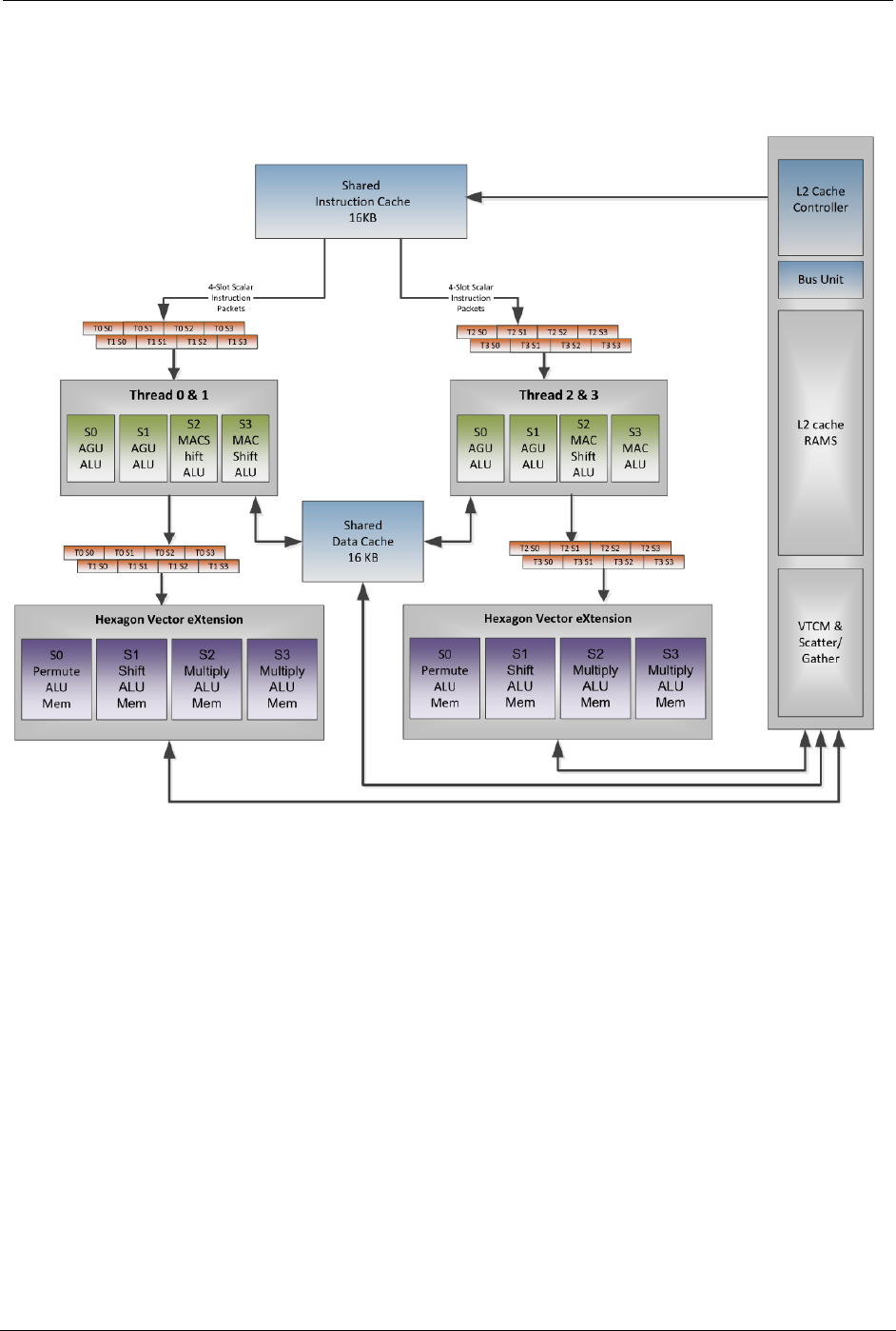
Following is an overview of the processing units within the DSP and how they connect to
cache.
Figure 2-2 cDSP V66 block diagram

Qualcomm Hexagon DSP User Guide Architecture overview
80-VB419-108 Rev. D 10
2.2.1 Hexagon scalar unit
The Hexagon scalar unit is made of a number of DSP hardware threads—four on most
current cDSPs. Each DSP hardware thread has access to the Hexagon scalar units,
which performs fixed-point and floating operations on single or pairs of 32-bit registers.
Each Data Unit is capable of performing a load or store up to 64-bit wide, or 32-bit scalar
ALU operation.
Each Execution Unit is capable of 16/32/64-bit vectorized multiply, ALU, bit
manipulation, shift or floating-point operations.
Prior to V66, the scalar floating-point and multiplier resources were shared by all
execution units. This meant that all combined hardware threads performed a maximum
of one of each operation every processor cycle. Starting with V66, each cluster has its
own floating-point and multiplier resources.
A cluster refers to a pair of threads (Thread 0&1 and Thread 2&3). Within a cluster, the
two threads typically commit instruction packets on alternating clock cycles because
most instructions require at least two clock cycles to complete. In this case, each cluster
completes one instruction packet on every DSP clock cycle, yielding a total throughput of
(2 * DSP Clock) instruction packets per second as long as stalls are avoided. (See
Section 4.2.2 for guidelines on avoiding latencies.) On V65 and earlier, this throughput
might get lower when there are contentions to the shared resources, as explained in
Section 4.2.2.2.
2.2.2 Hexagon HVX unit
HVX is an optional coprocessor that adds 128-byte vector processing capabilities to the
scalar DSP unit. Scalar hardware threads use the HVX coprocessor by accessing an
HVX register file, also referred as HVX context.
Two 128-byte HVX contexts are available on all HVX-enabled aDSPs and cDSPs up
through SM8150. From a programmer’s stand point, Section 4.3.2 discusses which and
how HVX contexts should be used.
NOTE: A legacy 64-byte mode allows HVX registers to be 64 bytes wide. Starting with V66, this
mode is no longer supported. Therefore, we recommend not using the 64-byte mode on
any device.
Qualcomm Hexagon DSP User Guide Architecture overview
80-VB419-108 Rev. D 11
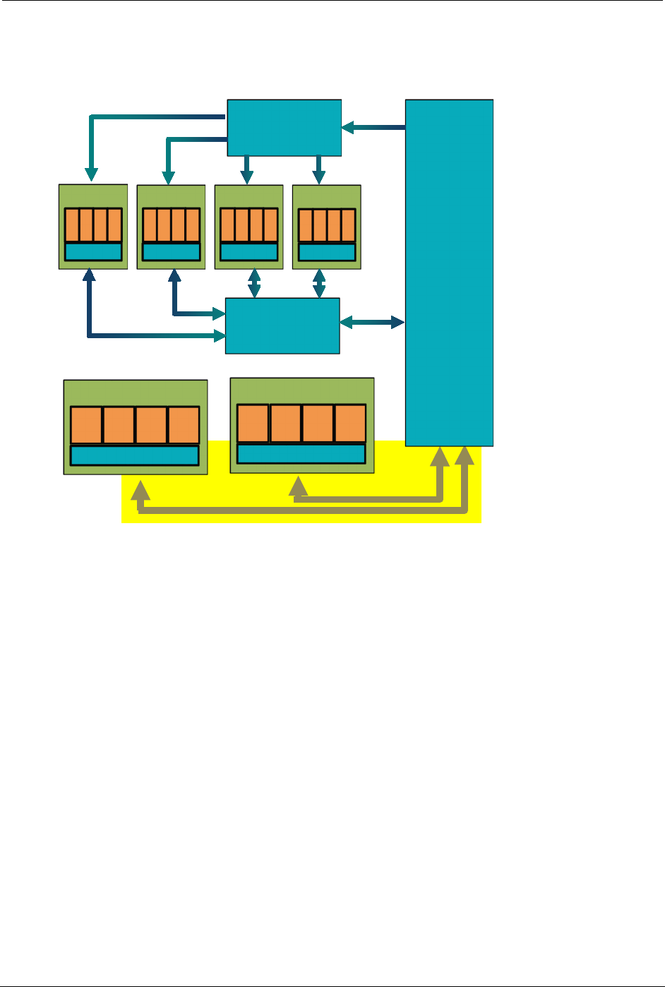
2.3 Memory subsystem
Figure 2-3 DSP memory subsystem
The cDSP has a two-level cache memory subsystem. L1 is only accessible to the scalar
unit, making L2 the second level memory for the scalar unit and the first level memory
for the HVX coprocessor.
L1 is write-through only. This allows the caches to be hardware coherent. To maintain
coherency, if an HVX store hits in L1, the L1 line is invalidated.
The vector units support a variety of load/store instructions, including support for
unaligned vectors and per-byte conditional stores.
A pipelined vector FIFO is in place for the HVX hardware to read L2 contents and hide
L2 read latencies from the programmer. Section 4.2.2.3 discusses this mechanism in
more details and its implications to a developer with respect to memory latencies.
On the SM8150, the L2 memory size is extended to 1 MB.
Scalar
Scalar
S
0
S
1
S
2
S
3
Scalar
Scalar
S
0
S
1
S
2
S
3
Scalar
Scalar
S
0
S
1
S
2
S
3
Scalar
Scalar
S
0
S
1
S
2
S
3
1024b Vectors
Vector RF
V0
V1
V2
V3
1024b Vectors
Vector RF
V0
V1
V2
V3
L1 Instruction Cache
L1 Data Cache
Shared L2
Cache

Qualcomm Hexagon DSP User Guide Architecture overview
80-VB419-108 Rev. D 12
2.4 Development boards
This section provides a high-level overview of board options that are available to
developers working with the Hexagon compute DSP. For more details, see the websites
of each provider.
Table 2-2 Development boards available for recent Snapdragon devices
Name Provider Description
Open-Q
For example: SDM660
Intrinsyc HDK made of two components:
SOM powered by Snapdragon processor and
including a 64-bit multicore CPU, Qualcomm Adreno
GPU, Hexagon DSP along with Android OS.
Carrier board to provide additional connectivity and
display capabilities
NOTE: Intrinsyc continually adds new boards. See
https://www.intrinsyc.com/development-kits/.
DragonBoard™
development kit
For example: SDM410c
Arrow Electronics Single small development board.
MTP
For example: MSM8998,
SDM710
Qualcomm Earliest reference platforms to become available after
new processors come out. Limited supply. Only
provided through direct engagements.
IP Camera
For example: SDM650
Thundercomm IP Camera Reference Design
NOTE: DragonBoard products used to be manufactured by Intrinsyc. They have been renamed
as Open-Q boards.
NOTE: Earlier Open-Q boards are manufactured by Intrinsyc. Starting with 835, the boards are
designed and manufactured by Qualcomm.

80-VB419-108 Rev. D 13
3 Run tasks on the DSP threads
3.1 When to offload tasks onto the DSP
Using the DSP offers several benefits:
For fixed-point computation, the Hexagon DSP is generally much lower in power
consumption, and free from thermal concerns, compared to the CPU.
In many cases that vectorize well on HVX, the DSP performs the same computations
in less time (while at a lower clock) than multiple CPU cores.
Moving large blocks of computational software to the DSP keeps the CPU
unburdened for other tasks that might work well only on the CPU.
Communication between the CPU and DSP is done through shared memory with
interrupts. Because the CPU and DSP do not share a cache, maintenance operations
are required upon all buffers transacted between them. These can take a minimum of a
few hundred microseconds. Depending on system clock settings and CPU sleep modes
enabled, the overhead for each invocation to the DSP could extend to several
milliseconds (this is explained in greater details in Section 3.6). Hence it is preferable to
offload large tasks onto the DSP instead of invoking it for small trivial tasks.
Separately, as discussed in Chapter 4 , the DSP does well with signal processing tasks
in general, and excels in particular at fixed-point operations that are parallelized.
Running such tasks on the DSP uses the DSP to the best of its ability and result in
significant gains with respect to power consumption.
In summary, the software designer should prioritize moving large signal-processing
tasks onto the DSP and leave to the CPU the role of running control-oriented code and
short individual processing functions.

Qualcomm Hexagon DSP User Guide Run tasks on the DSP threads
80-VB419-108 Rev. D 14
3.2 Offload tasks from the CPU onto a DSP thread
3.2.1 FastRPC fundamentals
The primary mechanism in place to offload tasks onto the DSP is called FastRPC.
FastRPC facilitates remote procedure calls between the CPU and the DSP by
transparently marshalling and unmarshalling parameters exchanged between the two
processors.
The SDK online documentation discusses in details the FastRPC mechanism on the
docs/Technologies_FastRPC.html online documentation page.
In summary, you are responsible for declaring the procedure API in an IDL file. The IDL
syntax allows to define the name of the function call and the type of each parameter
being exchanged between the application and DSP processors.
For example, the following example shows how you define in an IDL file a function sum
as part of the calculator library:
interface calculator {
long sum(in sequence<long> vec, rout long long res);
...
}
In this example, calculator is the name of the library being created and sum identifies
one of the functions allowing the CPU to interface the DSP. The name of the FastRPC
function that the CPU invokes and the DSP that is responsible for providing an
implementation is created by concatenating the library and function identifier:
calculator_sum.
In its C/C++ implementation, calculator_sum is expected to contain two parameters. in
designates an input parameter, i.e. a parameter passed in from the CPU and consumed
by the DSP during the FastRPC implementation, and rout designates the opposite, a
parameter generated by the DSP during the FastRPC implementation for consumption
by the CPU thereafter.
In the corresponding C/C++ definition of the FastRPC function, input parameters are
defined as constant; output parameters map are expressed as pointers.
Finally, sequence<x> designates a parameter that is exchanged in the form of an array.
2D MxN arrays such as images are also expressed as sequences of MxN elements.
In the corresponding C/C++ definition of the function, arrays are expanded into two
parameters, the first one being an array pointer, and the second one being an integer
defining the number of elements in the array.
As a result, the IDL definition above results in declaring in C/C++ the following function
for cross-communication between the CPU and DSP:
int calculator_sum(const int* vec, int vecLength, int64* res)
NOTE: When a FastRPC call is made, data buffers declared in ION memory are not copied
between the CPU and DSP. The APIs are simply declaring which buffers are to be made
available to the CPU or DSP for reading or writing purpose. We discuss this data sharing
mechanism in more details in Section 3.6.

Qualcomm Hexagon DSP User Guide Run tasks on the DSP threads
80-VB419-108 Rev. D 15
3.2.2 Multi-domain support
Recent Snapdragon products include multiple Hexagon DSP’s (for example: cDSP,
aDSP, mDSP, or SLPI). On many targets, more than one of these is available to
FastRPC applications. A new multi-domain framework has been added to FastRPC
starting in MSM8998 and SDM660, to enable FastRPC applications defining a single
interface (via IDL) to perform a run-time choice of destination DSP. This framework is
not present in MSM8996.
This multi-domain framework provides the following benefits over the previous
framework:
An application can query the target, and attempt to open a session for an interface
derived from the multi-domain base interface on the DSP features (for example, the
one with HVX).
An application can open multiple concurrent sessions on different DSPs.
The multi-domain session is handle-based, allowing for user application to restart a
crashed DSP session by closing the handle and re-opening a new handle. Upon
closing the handle, the framework calls the user-written deinit function, which allows
you to clean up any resource being used. (This process is referred to as “session
restart”.)
The handle for a session is passed to each interface API and can easily be
associated to user-defined context stored in the DSP memory. This allows an
application to access data persistent across FastRPC calls.
More information about FastRPC domains is found in the Hexagon SDK online
documentation under Technologies/FastRPC/FastRPC Domains.
A basic example is given at Examples->Compute offload->Calculator domain. This
example does not support domain using the remote_handle64 interface.
If a FastRPC application is intended to support multiple Snapdragon products and
offload to whichever DSP contains HVX on a given device, some logic is needed in the
application to find and engage with that DSP. The SDK example benchmark application
examples\common\benchmark_v65 illustrates the logic for supporting both MSM8998
(where HVX is in the aDSP) and SDM660/SM8150 (and beyond, where HVX is present
in the cDSP).
The following table summarizes the best practices available for applications required to
support various combinations of Snapdragon products.
Table 3-1 Recommended approach for multi-domain support
MSM8996 MSM8998 SDM660
and later Approach Comments
Use a multi-domain interface. Link application to
libadsprpc.so. At run-time, attempt to open a
handle with cDSP specified in the URI string.
Recommended
approach.
Provides handle and
session restart support
Same as above but if opening a handle with
cDSP fails, attempt again with aDSP.

Qualcomm Hexagon DSP User Guide Run tasks on the DSP threads
80-VB419-108 Rev. D 16
MSM8996 MSM8998 SDM660
and later Approach Comments
Same as above but also define a second legacy
interface without domain support. If attempts at
opening a handle with both aDSP and cDSP fail,
use the second interface.
on all targets except
MSM8996.
Same as above but without the need to attempt
to opening a handle with the cDSP.
Use legacy non-domain interface definition. Link
to libadsprpc.so.
Allows legacy code to
run unchanged on any
target.
Not recommended
moving forward.
Same as above but link to libcdsprpc.so instead
of libadsprpc.so for SDM660/SM8150? target.
3.2.3 Run the main function on Hexagon DSP
Starting with V65 and the Hexagon SDK 3.4, you can request that the tools execute the
program main function on the DSP directly.
With this approach, the tools automatically create the FastRPC interface required for the
CPU to invoke the DSP and run the specified code. This approach guarantees that all
the code written by the user will be compiled into a dynamic library that will be loaded
and run on the DSP.
This approach is supported to run both on the simulator and on target devices. For more
information, see {HEXAGON_SDK_ROOT}/tools/HEXAGON_Tools/<version
number>/examples/compute/benchmark_v65.

Qualcomm Hexagon DSP User Guide Run tasks on the DSP threads
80-VB419-108 Rev. D 17
3.3 Offload tasks from one DSP thread to another
To take full advantage of the DSP resources, compute-intensive applications should use
as evenly as possible all DSP threads available. The application spreads its work over
multiple concurrent software threads, and the DSP RTOS schedules those threads
across the hardware threads. Applications can perform this split either by making
multiple FastRPC calls from parallel concurrent CPU threads (each of which is
processed by a mirrored thread on the DSP), or by splitting work across software
threads within the DSP implementation.
To run multiple DSP threads, different CPU threads can make multiple FastRPC calls in
parallel. Alternatively, the dspCV dynamic library included in the SDK provides a set of
APIs that allow a DSP thread to use its thread worker pool to invoke multiple callbacks in
parallel. This approach enables one FastRPC call to turn into a multi-threaded DSP
implementation without spawning new threads.
Specifically, dspCV provides APIs with the following functionality:
Define a job—referred as a dspCV_worker_job_t—to be executed by a DSP thread
Submit that job to a queue with the dspCV_worker_pool_submit API
Synchronize the parent thread with the completion of submitted jobs, for example:
dspCV_worker_pool_synctoken_wait, to wait until a given number of threads have
completed their tasks,
dspCV_worker_pool_synctoken_jobdone, for a thread to indicate the completion
of a task,
dspCV_atomic_inc_return and dspCV_atomic_dec_return, to increment or
decrement atomically a variable.
To understand how the dependency on a dynamic library like dspCV should be
expressed in a project and how to make it available to the application when running on
target, see Section 3.5.

Qualcomm Hexagon DSP User Guide Run tasks on the DSP threads
80-VB419-108 Rev. D 18
3.4 Optimize multi-threaded DSP code
Optimizing an application expected to run as fast as possible on the DSP requires that
you balance the workload between available DSP threads.Various techniques are
available to meet this goal.
3.4.1 Compile-time multithreading
One approach for balancing at compile time the workload between threads consists of
using data parallelism: in the code, you explicitly assign different threads to different data
regions. For example, this can mean that one thread is assigned to processing the upper
half on an image while another thread is assigned the lower half.
This approach is often the simplest conceptually, and it might be appropriate if
processing time is not data dependent and the number of threads available is known in
advance.
Alternatively, you can decide when writing an implementation to allocate different tasks
to different threads. For example, in a pyramid decomposition, you might decide to
explicitly assign one thread to running a filter and downsampling at the highest
resolution, a second thread to running additional filters at all smaller subsequent
resolutions, and a third thread to searching through the pyramid for some specific
patterns. The synchronization tokens discussed in Section 3.3 can be used to indicate
when one thread has produced enough lines for the next thread to begin its work.
The drawback of that approach is that as the implementation changes—for example, a
processing block is modified, or added, or better optimized—or the target device
changes and presents different characteristics, the workload of each thread might no
longer be balanced. Re-optimizing such an implementation might require significant
rework of the code. Another concern is that you might not have any long-term
guarantees on what other applications are running on the device and be competing for
resources.
3.4.2 Run-time multithreading
Parallelism is usually best applied dynamically. In this scenario, a number of threads
begin processing a new job as soon as they completed their previous one. Because of
the limitations listed above, that approach is usually the most efficient and robust way of
multithreading an implementation.
In its simplest and most common form, run-time multithreading is used for data-
parallelism: multiple threads are allocated to processing one image linearly, small
chunks such as lines at a time. In this scenario, all threads can share the same data set
and one variable pointing to the next line to be processed. All threads modify that
variable atomically when beginning a new task as explained in Section 3.3 to ensure that
no two threads ever process the same line. This approach is illustrated in the project
gaussian7x7 provided as part of the SDK examples.

Qualcomm Hexagon DSP User Guide Run tasks on the DSP threads
80-VB419-108 Rev. D 19
More refined multi-threaded implementations can extend that approach to declaring jobs
that do not include necessarily the same functionality. For example, the parent thread
might create a pool of tasks that progressively apply different transforms to an image
one line at a time and one transform at a time. Such an approach needs some care in
order to ensure that tasks are blocked when their input buffers are not available yet, that
threads are running the majority of the time instead of being stalled while starved for
data, and that the implementation does not run into a deadlock.
Finally, note that the number of software threads to use depends on the type of threads
being used. In general, it is recommended to split scalar workload according to how
many hardware threads there are, and HVX workload according to how many HVX
contexts there are. The dspCV library has global variables for each of these numbers so
that the code can remain optimal on various architectures.
3.5 Verify an application running on the DSP
When working with the simulator, it is possible to directly compile code for the DSP and
simulate that code. This allows to test a function without the use of a FastRPC call.
However, to run on a hardware device, you must typically implement a CPU application
that makes a FastRPC call to the DSP to invoke a workload. It is therefore typical to
implement a simple test driver that is built as an Android command line application for
device testing, or a Hexagon executable for simulator testing. When built as a Hexagon
executable, the FastRPC calls in the test driver is directly linked to the skeleton
implementations in the DSP application.
After installing the SDK and setting up a new device, familiarize yourself with the
process of building and testing sample applications with the simulator or with a device.
The rest of this section highlights the main steps that are involved during that process.
For more details, see some of the project examples included and documented in the
online SDK, such as calculator, downscaleBy2, or benchmark.
Verifying an implementation using FastRPC calls on the simulator is simple: this is
accomplished with the following example command line:
make tree V=hexagon_ReleaseG_toolv81_v62
This results in compiling and then running both the test driver and DSP code with the
Hexagon DSP compiler and simulator.
In the example above, v81 means that the code is compiled with version 8.1 of the
Hexagon tools, and V62 means that the code is compiled to target the DSP variant V62.
Verifying that same implementation on target involves multiple steps:
Compile for the CPU the main executable, which is responsible for making FastRPC
calls. For example, this is accomplished with:
make tree V=android_ReleaseG
Compile for the DSP the code implementing the FastRPC functions. For example:
make tree V=hexagon_ReleaseG_dynamic_toolv81_v60
NOTE: The dynamic keyword indicates we are building a dynamic library with a .so
extension.

Qualcomm Hexagon DSP User Guide Run tasks on the DSP threads
80-VB419-108 Rev. D 20
Push the DSP dynamic library (and any other dynamic libraries the project depends
on) to one of the locations the executable is looking for dynamic libraries. The
locations being searched successively are:
/vendor/dsp (or /dsp prior to Android-P)
/system/lib/rfsa/adsp
/vendor/lib/rfsa/adsp (aka /system/vendor/lib/rfsa/adsp)
For example:
adb push hexagon_ReleaseG_dynamic\ship\libName.so
/system/lib/rfsa/adsp
NOTE: libName.so refers to the name of the DSP dynamic library that was built
accordingly to rules defined in the file hexagon.min.
Push the CPU executable in the target directory from which the code is executed,
change the file permission to make the file executable, and execute it. For example:
adb push android_ReleaseG\ship\exeName /vendor/bin
adb shell chmod 755 /vendor/bin/exeName; /vendor/bin/exeName
NOTE: exeName refers to the name of the CPU executable that was built accordingly
to rules defined in the file android.min.
The first time a device is used since it has been flashed, the device needs to be signed.
The SDK tools provide python scripts that fully automate the signing process and the
signing process is documented in full details under docs/Tools_Signing.html of the online
SDK documentation.
Sometimes, a project also depends on a library, such as dspCV, which is provided as a
static library for simulation purpose and as a dynamic library for the purpose of running
on the device. This means that in the hexagon.min, the dependency of the project on
that library is specified as follows to build the dynamic library to be pushed on the
device:
lib<libname>_skel_DLLS+=libdspCV_skel
The user is responsible for pushing the libdspCV_skel.so onto the device as explained in
Section 3.5.
A separate line is needed in hexagon.min to specify a dependency on the static version
of the same library to build the Hexagon executable to be fed to the Hexagon simulator:
lib<libname>_q_LIBS+=libdspCV_skel

Qualcomm Hexagon DSP User Guide Run tasks on the DSP threads
80-VB419-108 Rev. D 21
3.6 Overhead for a FastRPC call
The latency of a given FastRPC invocation depends on a several factors:
CPU build configuration (Android build needs to be a Performance build to get best
results)
CPU and memory clock rates (both are subject to DCVS—Dynamic Clock Voltage
Scaling—under normal operation)
CPU scheduling latencies (having impact on interrupt servicing latency when DSP
responds to the invocation). These can vary depending on what might be running on
various CPU threads.
Time to complete DSP invocation (the more time consumed by the DSP invocation,
the more likely the CPU goes to a lower clock or to a low-power state that requires
extra wake-up steps when the DSP responds).
Proper usage of ION memory for shared buffers (required for zero-copy FastRPC)
Cacheability of buffers shared between CPU and DSP.
If buffers are configured as uncached from the CPU side (for example, they originate
from the camera hardware without being changed by CPU), then CPU-side cache
maintenance is avoided and overhead reduced.
IO Coherence (available only on SDM660, MSM8998, and later targets).
IO Coherence is enabled by default for CPU-cached buffers shared with the DSP,
but is disabled on a per-buffer basis. IO-coherent buffers require no CPU-side cache
maintenance, hence facilitate reduced FastRPC overhead with little dependence on
the total size of buffers being shared. However, IO-coherent buffers might suffer
some performance loss when being accessed by the DSP, due to the CPU cache
snooping operations that performed in HW to ensure coherent behavior. Non-IO-
coherent buffers have a larger FastRPC round-trip overhead, proportional to the total
size of non-IO-coherent buffers being shared.
Under idealized conditions, the FastRPC round-trip overhead is on the order of 200 to
300 microseconds. This performance is achievable when the CPU and memory clocks
are set to their maxima, and low-power states disabled. Unfortunately these settings are
usually not tolerable from a power consumption perspective in a production environment.
In more realistic conditions, the CPU and memory clocks are driven by DCVS, and when
necessary, limited by thermal conditions. During DSP-based workloads, the CPU tends
to decrease its clock speed or go into a low-power (sleep) state to save energy while
awaiting DSP responses to FastRPC calls. Under these conditions, the unmitigated
round-trip FastRPC overhead varies based on instantaneous conditions, but it might be
up to several milliseconds.

Qualcomm Hexagon DSP User Guide Run tasks on the DSP threads
80-VB419-108 Rev. D 22
FastRPC offers APIs to help manage performance in typical conditions by disabling
certain sleep states when there is sufficient FastRPC traffic or voting for floor clock rates.
In particular, the Hexagon SDK 3.4.0 introduces a new API,
remote_handle64_control, that controls the CPU sleep mode and significantly
reduces the FastRPC latencies at the expense of a small increase in power
consumption. When the DSPRPC_CONTROL_LATENCY mode is selected, the
FastRPC driver monitors the RPC activity. When no activity is detected over a period of
time, the driver enables low-power modes, which result in the CPU switching to sleep
mode. As long as RPC calls keep occurring, CPU power collapse will be disabled, which
will ensure that the FastRPC latency remains small.
We recommend that you experiment with various configurations to determine which
settings are best suited for your needs. For more information, see FastRPC and
FastRPC QoS in the Hexagon SDK documentation.
3.7 Overhead for launching DSP threads from the DSP
The use of the dspCV_worker_pool_submit described in Section 3.3 allows a job to be
submitted to a pool and picked up by a hardware thread when one becomes available.
The overhead for submitting a job is around 5,000 processor cycles. In other words, the
parent thread is slightly faster than the other threads it launches to complete a task. As a
result, it is a good practice after kicking N-1 worker threads to let the parent thread
execute the same call job to get best performance.
Concretely, it can improve performance to switch from this code:
for (i = 0; i < numJobs; i++) {
(void) dspCV_worker_pool_submit(job);
}
to this code:
for (i = 0; i < numJobs-1; i++) {
(void) dspCV_worker_pool_submit(job);
}
job.fptr(job.dptr); // executed on parent thread, likely to start first

80-VB419-108 Rev. D 23
4 Optimize tasks for the DSP
This chapter provides an overview of how to port and run compute tasks efficiently on
the DSP. It discusses various aspects of the programming environment, DSP
instructions, and architecture details that are key to consider when writing optimized
DSP code.
4.1 Programming languages and extensions
4.1.1 C/C++ support
Reference code to be ported to the DSP is usually written in C or C++. Such code does
not require any change to run on the DSP: Qualcomm’s compiler relies on LLVM and
currently supports the following version of the C and C++ standards:
C language: K&R C, ANSI C89, ISO C90, ISO C94 (C89+AMD1), ISO C99 (+TC1,
TC2, TC3)
C++ language: C++98, C++11, C++14
NOTE: C++11 and 14 are supported only on SDM835, SDM660, and later chipsets.
The Hexagon LLVM compilers support all versions of the Hexagon processors currently
released: V4, V5, V55, V56, V60, V61, V62, V65, and V66.
NOTE: In the remainder of this document, when covering DSP scalar variants, only V66 is
discussed. Unless noted otherwise, comments regarding V65 are also applicable to
older variants.
For additional information on the LLVM compiler, see the Hexagon LLVM C/C++
Compiler User Guide included as part of the Hexagon document bundle.
Once you validate that the reference C/C++ code runs properly on the DSP, additional
languages and extensions are available to optimize the code further, as described in the
following sections.

Qualcomm Hexagon DSP User Guide Optimize tasks for the DSP
80-VB419-108 Rev. D 24
4.1.2 Halide language
Halide is a programming language for vision processing. Halide is designed as a dialect
of C++. It allows programmers who are familiar with C++ to start authoring Halide
programs.
The Halide toolset is available as part of the Hexagon SDK and the Hexagon LLVM
toolset. The toolset contains a Halide compiler that targets the HVX architecture. The
Halide for HVX compiler allows you to exploit the powerful features of the HVX
processor without knowledge of the underlying HVX architecture. This, in turn, enables a
higher level of abstraction that allows you to focus on the image algorithm and achieve
high levels of performance from HVX.
The Halide runtime also makes the task of offloading kernels to HVX easy. Simply add
a .hexagon() directive in the Halide program, and the Halide runtime ensures that the
kernel is transparently dispatched to the HVX processor.
For more information on the Halide programming language, see the Halide for HVX User
Guide (80-PD002-1) and visit the resources available at http://halide-lang.org/. You can
also direct questions on Halide HVX to the halide@quicinc.com email address.
4.1.3 Compiler intrinsics
Compiler intrinsics are treated by the compiler as machine instructions. The vast majority
of assembly instructions have a one-to-one map with compiler intrinsics, thus allowing
you to express a function as a sequence of assembly instructions, leaving it up to the
compiler to perform register assignment, instruction grouping into packets, and
instruction scheduling.
Programming with intrinsics gives the flexibility of remaining in C/C++, interleaving
compiler intrinsics in places where they are most needed. This approach provides an
environment where the code is easy to debug and test since you can still print variable
contents to the logs or to a file, or run test routines written in C.
The C/C++ compiler is not HVX-aware. As a result, use intrinsics for sections of code
where data parallelism provides a speed improvement. For example, many instructions
from the V65 scalar instruction set and all HVX instructions are SIMD instructions and
process multiple 32-bit, 16-bit or 8-bit neighboring elements in parallel. Using intrinsic
SIMD instructions guarantees that the compiler generates assembly instructions able to
process these elements in parallel.
The Hexagon V66 Programmer’s Reference Manual (80-N2040-42) and Hexagon V66
HVX Programmer’s Reference Manual (80-N2040-44) detail the syntax and functionality
of all intrinsic assembly instructions available for the scalar core and HVX, respectively.
All compiler intrinsics are accessible in a C/C++ program by including the library header
file hexagon_protos.h.

Qualcomm Hexagon DSP User Guide Optimize tasks for the DSP
80-VB419-108 Rev. D 25
For example, if x and y are declared as 64-bit numbers (declared as long long int),
the following code assigns y to the saturated absolute value of each of the four halfword
of x:
y = Q6_P_vabsh_P_sat(x)
Or if x, y, z are defined as 128-byte numbers (declared as HVX_Vector), the following
code assigns z to the byte-wise addition of x and y followed by saturation:
z = Q6_Vh_vadd_VhVh_sat(x,y)
In addition to performing transforms on variables, it is often necessary to access or
combine variables together. These operations do not necessarily map into assembly
instructions, and as such, they are not covered in the Programmer’s Reference Manuals.
They are covered in Sections 11.3 and 11.4 of the Hexagon LLVM C/C++ Compiler User
Guide (80-VB419-89).
For example, the following syntax creates a copy of the vector pair vp where the lower
half is replaced with vector x. The Q6_W_vcombine_VV instruction below is an intrinsic in
the PRM that translates into the assembly instruction vcombine, while Q6_V_hi_W is a
macro described in the compiler guide.
HVX_VectorPair vp;
HVX_Vector x;
HVX_Vector v = Q6_V_hi_W(vp); // set v to the high vector of vp
HVX_VectorPair new_vp = Q6_W_vcombine_VV(v, x); // create a new pair
NOTE: The compiler automatically optimizes such a syntax: if the rest of the code allows for it,
new_vp and vp can reuse the same registers for their internal representation and no
assembly instruction vcombine might even be needed.
4.1.4 Assembly language
The tools also provide the ability to write any section of code in assembly language.
Writing assembly provides the utmost control to the software developer, who is
responsible for choosing, scheduling, and grouping instructions, as well as assigning
registers to variables.
The processor pipeline is fully interlocked: if an instruction consumes a register whose
contents is expected to be computed by an earlier instruction but not yet available, the
hardware automatically stalls and guarantees that the register value is correct by the
time it is consumed. This approach allows you to not to be concerned with instruction
timing to write functional code: as long as instructions are written in the order in which
they are expected to be executed, the output is correct independently of how many times
the thread might have to stall.
The most common and recommended usage for writing in assembly is to write an entire
function in assembly. For example, if only one section of a large block of C code needs
to be optimized, this section is expressed as one function call and then be written in
assembly.
If you are writing assembly code, you must abide by the compiler calling conventions. In
particular, callee-saved registers, scalar registers R16 to R31 (except R28), must be
properly saved if they are altered.

Qualcomm Hexagon DSP User Guide Optimize tasks for the DSP
80-VB419-108 Rev. D 26
NOTE: All HVX registers are caller-saved registers and thus can all be used directly without the
need to save them on the stack when writing a leaf assembly function.
For more information, see the Register usage across calls chapter in the Hexagon
Application Binary Interface Specification (80-N2040-23).
NOTE: It is also possible to write assembly using inline assembly. This approach allows to tap
into assembly directly from a C/C++ source file. However, this usage is strongly
discouraged as the inline assembly syntax is cumbersome to use and error prone.
An assembly file can contain the implementation of one or more function, which you only
need to declare in the C/C++ source files as extern in order to call directly from your
C/C++ code.
For example, if an assembly file contains an implementation of foo that takes a 32-bit
element array pointer as input, does not return any value, and has an assembly
implementation that begins as follows:
.globl foo // makes function have global scope
.type foo, @function
foo: // begin implementation here
Then this function is called from C/C++ with the following declaration:
extern "C" void foo(int ptr);
NOTE: "C" should follow the extern pragma if the function is called within a C++ file to prevent
any mangling of the function name. It can be omitted if the function is called within a C
file.
4.2 Guidelines for assembly and intrinsic optimization
There are a few basic concepts to keep in mind in order to write efficient assembly code.
These concepts are also quite relevant for developers writing with intrinsics because
such a developer should know approximately how the compiler should be able to group
and schedule intrinsics in order to achieve maximum performance.
This section briefly describes some of these fundamental concepts.
Tip: When writing code with intrinsics or assembly instructions, it is best to start by
writing functional code using the right instructions, and then only optimizing code
further by following the optimization guidelines discussed in the following sections.
Attempting to do too much at once tend to be more time consuming as low-level
optimizations usually obscure the clarity of the code.

Qualcomm Hexagon DSP User Guide Optimize tasks for the DSP
80-VB419-108 Rev. D 27
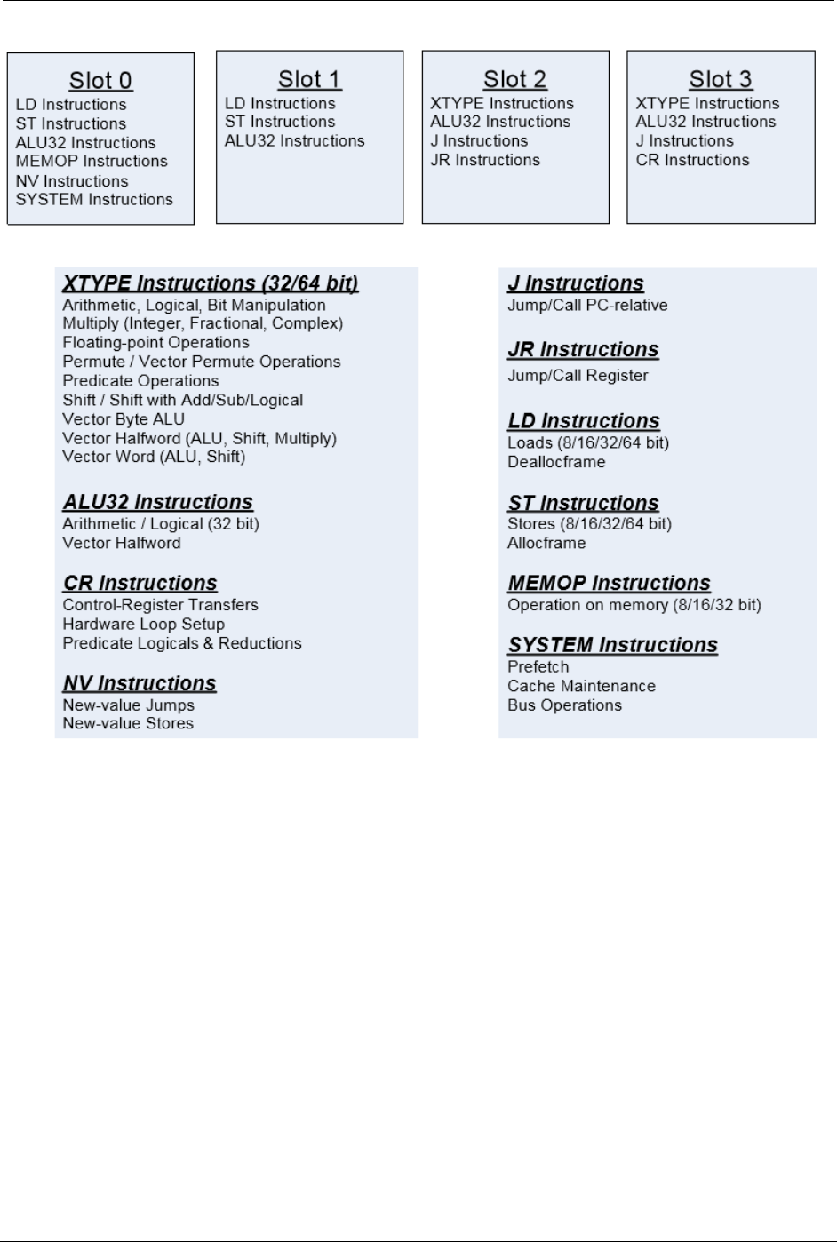
4.2.1 Maximize instructions per packet
Each hardware thread is capable of executing a packet of up to four instructions in a
given thread cycle. Instructions occurring in a packet executes in parallel, making it
possible within one packet to consume a register and update its content at the same
time. For example, the following packet consumes the contents of R0 that was produced
in the packets that preceded and then update its content with R4.
{
R2 = vaddh(R0,R1)
R0 = R4
}
The exception to this rule is when the specifier .new is used within an
instruction. For example, the following packet first computes R2 and
then store its content to memory.
{
R2 = memh(R4+#8)
memw(R5) = R2.new
}
To maximize the number of instructions per packet, it is important to understand how
instructions can or cannot be combined in each packet. The restrictions are different for
scalar and HVX instructions.
4.2.1.1 Scalar instruction packing rules
Rules on how to form packets are explained in the Instruction packets section of the
Hexagon V66 Programmer’s Reference Manual (80-N2040-42).
Focus on mastering the most important restriction to packing instructions together:
resource constraints.
The simplest way to understand the impact of resource constraints on grouping with V66
is to think simply in terms of slots. Because of the resources they use, each type of
instruction can only execute on one specific slot, out of four available. For example,
logical and multiply operations consume either slot 2 or 3, whereas a load instruction
consumes either slot 0 or 1. This means that at most two logical operations, or one
logical and one multiply operation, or two multiply operations can execute in a single
packet.
The description of which type of instruction is acceptable for each slot is provided in
Figure 3-1 of the Hexagon V66 Programmer’s Reference Manual (80-N2040-42) as well
as in the detailed description of each instruction. For convenience, this figure is
reproduced in Figure 4-1.
Qualcomm Hexagon DSP User Guide Optimize tasks for the DSP
80-VB419-108 Rev. D 28
Figure 4-1 Instruction classes and combinations
Other restrictions outlined in the Instruction packets section of the same manual
occasionally causes a packet following the resource constraints to still generate an error
message at compile time. However, these other rules tend to come into play much less
frequently and you can choose to simply learn about them over time.
4.2.1.2 HVX packing rules
Rules on how to form packets in HVX are explained in the VLIW packing rules section of
the Hexagon V66 HVX Programmer’s Reference Manual (80-N2040-44).
HVX instructions share the same slots as V6x and there are restrictions on which slot
each HVX instruction uses. However, unlike with V6x, resources and slots are not
correlated one-to-one. It is best, as a software developer, to focus on understanding
which resources each HVX instruction share, and understand how this impact the ability
to group instructions in a packet since slot restrictions rarely come into consideration
when writing HVX code.
Qualcomm Hexagon DSP User Guide Optimize tasks for the DSP
80-VB419-108 Rev. D 29
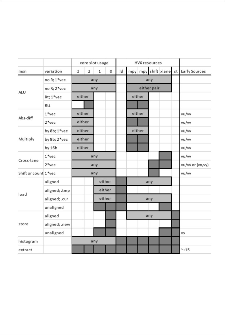
Resource restrictions are summarized in the Hexagon V66 HVX Programmer’s
Reference Manual (80-N2040-44) and reproduced in Table 4-1 for convenience. The
detailed description of each HVX instruction also indicate which HVX resources it
consumes.
Table 4-1 HVX slot/resource/latency summary
Be aware that some instructions such as vrmpy come in different flavors, some of which
consume two HVX resources, and some of which only consume one.
For example, halfword multiplies use both mpy resources, which means that no other
HVX multiply instruction is present in the same packet. When trying to optimize the inner
loop of a function multiply-bound, plan early on how to maximize mpy resource utilization
in as many packets as possible.
NOTE: Unlike scalar stores, you cannot group two HVX stores in a single packet.

Qualcomm Hexagon DSP User Guide Optimize tasks for the DSP
80-VB419-108 Rev. D 30
4.2.2 Understand and reduce stalls
In addition to executing as many instructions as possible in any given packet to
maximize parallelization, it is important to be aware of latencies that might cause the
processor to stall. This section discusses the most common causes of stalls that
deteriorate performance.
4.2.2.1 Instruction latencies
4.2.2.1.1 Thread vs. processor cycles
Hexagon cores dynamically schedule packets from threads into the core pipeline. The
number of cycles to execute a packet varies depending on the behavior of other threads.
The optimal schedule for a single-thread running in isolation could be different than the
optimal schedule for a thread running with other threads.
For example, in all recent generations, when multiple threads execute in parallel, one
thread executes every other processor cycle. This means that if the processor is clocked
at 800 MHz and four threads execute in parallel, each thread runs effectively at 400
MHz.
However, when a thread is idle, another thread might be able to “steal” some of its
cycles, allowing it to run faster than it runs if all HW threads were busy. In practice, on
Hexagon versions up through SM8150, a single-threaded workload might run up to 20-
30% faster if it is the only running thread, compared to when it is concurrent with other
running SW threads consuming all the HW threads.
In the remaining of this section, we provide some general rules on latency scheduling
assuming at least 2 threads are running. This provides a simplified programming model.
Using this model, we introduce the concept of a packet delay. This delay is the number
of packets that are to be scheduled between two dependent packets to prevent the
thread to stall.

Qualcomm Hexagon DSP User Guide Optimize tasks for the DSP
80-VB419-108 Rev. D 31
4.2.2.1.2 Scalar latencies
Starting with V65, instructions have no packet delays with the following exceptions:
Instructions that are paired with the .new predicate, allowing two sequential
instructions to execute within the same packet
Mispredicted jumps, which typically incur around five packet stalls and waste energy.
For more information on speculative branches, see the Compare jumps section in
the Hexagon V66 Programmer’s Reference Manual (80-N2040-42).
NOTE: Whenever possible, try using hardware loops: these does not generate stalls,
even when exiting the loop.
Long-latency instructions that consume the result of another long-latency instruction.
These instructions experience a one packet delay with the exception of back to back
multiplies simply sharing the same accumulator, which do not experience any delay.
Long latency instructions are all the load, multiply, and float instructions.
For example, the following instruction sequences stall:
{ R2=mpy(R0.L,R0.L) }
// one-cycle stall
{ R3=mpy(R2.L,R2.L) }
…
{ R2 = memw(R1) }
// one-cycle stall
{ R3=mpy(R2.L,R2.L) }
But this instruction sequence does not stall:
{ R2=mpy(R0.L,R0.L) }
{ R2+=mpy(R1.L,R1.L) } // no stall
4.2.2.1.3 HVX latencies
The Instruction latency section of the Hexagon V66 HVX Programmer’s Reference
Manual (80-N2040-44) discusses latencies. In this section, we discuss the most
common HVX arithmetic instruction sequences responsible for stalls that you should
know about.
The most common causes of stalls to keep in mind are one-packet delays present when
the following instructions consuming a result that was produced in the previous packet:
Multiplies
However, back-to-back multiplies only sharing the same accumulator do not stall
Shift and permute operations
The Instruction latency section provides some examples of these rules:
{ V8 = VADD(V0,V0) }
{ V0 = VADD(V8,V9) } // NO STALL
{ V1 = VMPY(V0,R0) } // STALL due to V0
{ V2 = VSUB(V2,V1) } // NO STALL on V1
{ V5:4 = VUNPACK(V2) } // STALL due to V2
{ V2 = VADD(V0,V4) } // NO STALL on V4

Qualcomm Hexagon DSP User Guide Optimize tasks for the DSP
80-VB419-108 Rev. D 32
4.2.2.2 Resource contention on the shared scalar resources
Another source of stalls on V6x comes from multiple threads using the following
resources shared across all hardware threads:
The floating-point unit (V65 and earlier versions only)
The multiplier unit (V65 and earlier versions only)
The L1 cache
As discussed in Section 2.2.1, prior to V66, the floating-point and multiplier units are
shared across all threads. This means that on versions earlier than V66, in any
processor cycle, only two floating-point operations execute. In other words, if four
threads were to execute a sequence of packets, each containing two floating-point
operations, each thread stalls every other thread cycle.
In addition, the L1 cache is also a shared resource. Therefore, it is important to load data
as unfrequently as possible and take advantage of registers to store values locally
before reusing them.
4.2.2.3 Understand and optimize memory accesses
As discussed in Section 2.3, scalar data memory accesses go through a two-level cache
hierarchy while HVX memory accesses only transit through the L2 memory.
Cache sizes vary depending on the exact chip variant:
L1 cache sizes are 16 to 32 KB
L2 cache sizes are 128 to 1024 KB on aDSP variants, and 512 to 2048 KB on cDSP
variants
HVX data memory accesses bypass L1.
To avoid cache misses when writing optimized applications, it is critical to reduce the
data memory throughput and maximize data locality. Common data optimization
techniques exploiting data locality include such techniques as:
Register data reuse
The application stores values into registers for later use. For example, applying a
filter on multiple lines at the same time allows to hold coefficients into registers, thus
reducing the overall data bandwidth.
Tiling
A tile defines a small region of an image. The application processes an image one
tile at a time or a few tiles at a time. This approach might be appropriate when using
scalar instructions rather than HVX instructions because it allows preservation of
data within L1 and thus maximize scalar processing throughput. Larger buffers, such
as groups of image lines, are typically too large for L1. Using a tiling approach
usually comes at the cost of greater programming complexity and more non-linear
data addressing.

Qualcomm Hexagon DSP User Guide Optimize tasks for the DSP
80-VB419-108 Rev. D 33
Line processing
The application processes an image a few lines at a time. This is the most common
approach for HVX implementations as it allows to load entire HVX vectors and
leverage the large L2 memory cache size.
Another type of cache optimization consists of explicitly managing cache contents by
way of prefetching data into cache and, more rarely, invalidating cache line contents.
This optimization should be left for the end once you have already ensured a maximum
of data locality in their code.
The Hexagon V66 Programmer’s Reference Manual (80-N2040-42) details the L2 cache
prefetching mechanism. A good illustration of the various forms of L1 and L2 cache
management techniques is provided in the downscaleBy2 project example included in
the SDK under the example/common directory and discussed in the SDK online
documentation.
NOTE: It is common to optimize an application on a single-thread first and then multi-thread the
code later. When following that approach, extrapolating multi-threaded performance
from single-thread performance can occasionally be misleading: memory bandwidth
might not be a bottleneck when only one thread is running but become one of the
limiting resources as more threads run in parallel. As a result, it is a good practice to
write applications as conservatively as possible with respect to memory bandwidth
usage regardless of the performance of the single-threaded code.
Though data memory latencies depend on many parameters and architecture variants, it
is useful to know to a first order the cost of memory accesses when planning the
optimization of an application. The following numbers are rough estimates on what to
expect in making memory accesses:
DDR memory access: ~250 ns
L2 read latency: 6 thread cycles
On HVX, a mechanism is implemented to push HVX instructions into a queue
called V FIFO. As long as no mispredicted branches occur, this queue remains full
and the L2 reads triggered by VMEM instructions occur enough in advance that the
result from a VMEM load is available in the next cycle without stalling. In other
words, on HVX, L2 reads have a 1-cycle latency and the following instruction
sequence does not stall as long as no mispredicted branch has occurred recently:
{ V0 = VMEM(R0++) }
{ V1 = VADD(V0,V1) } // No stall if no recent mispredicted branch
Maximum sustainable read-write L2 bandwidth with no bank conflicts: 128 bytes per
processor cycle

Qualcomm Hexagon DSP User Guide Optimize tasks for the DSP
80-VB419-108 Rev. D 34
4.2.3 Software pipelining
The Hexagon instruction set allows multiple unrelated instructions within one packet.
This flexibility provides great opportunities for parallelizing the code, which are often best
exploited by doing software pipelining. Software pipelining consists of processing a few
consecutive instances of a loop in parallel to reduce data dependencies and provide
more opportunities for operations to be executed in parallel.
This approach comes at the expense of having separate code for prologue and epilogue
code. For example, if a loop processes loads data for iteration n+2, performs some
computations for iteration n and n+1, and store results of iteration n, the prologue and
epilogue code can potentially have to handle the first and last 2 or 3 loop iterations
separately and handle cases where the number of loop iteration is small.
The Hexagon instruction set allows to decrease the complexity of the prologue and
epilogue code by supporting pipelined hardware loops. Pipelined hardware loops set
predicate registers after a loop has been iterated a specific number of times thus
allowing some operations—typically stores—to only execute after a few loop iterations.
For more information on this approach, see the Pipelined hardware loops section in the
Hexagon V66 Programmer’s Reference Manual (80-N2040-42).
NOTE: The Hexagon compiler automatically conducts software pipelining of appropriate loops.
4.3 HVX-specific optimizations
HVX adds a powerful set of instructions allowing to process large vectors very efficiently.
The Hexagon V66 HVX Programmer’s Reference Manual (80-N2040-44) is the
authoritative source for HVX instruction syntax and behavior for any given revision.
Within the following section, we highlight some instructions contained therein.
4.3.1 When to use HVX
HVX vectors are 128-byte wide. As a result, HVX lends itself well to sequences of
identical operations on contiguous 32-bit, 16-bit, or 8-bit elements.
In addition, HVX only supports operations on integers natively.
These two characteristics make HVX ideally suited for some application spaces such as
image processing where many integer operations are to be applied independently to
continuous pixels. However, it does not mean that HVX is restricted to only perform
integer operations on contiguous elements in memory as explained below.
Even though HVX memory loads and stores access contiguous elements in memory,
HVX provides a number of powerful instructions for shuffling and interleaving elements
between and within HVX vectors. These instructions allow HVX to process efficiently
non-continuous elements that follow some predictable patterns, such as odd and even
elements, or vertical lines. Section 4.3.3 discusses these instructions in more detail.

Qualcomm Hexagon DSP User Guide Optimize tasks for the DSP
80-VB419-108 Rev. D 35
HVX does not have native support for floating-point. However, using HVX on floating-
point code is still worth considering if some portions of the code are either converted to
using fixed-point arithmetic, or if strict compliance to the IEEE floating-point format is not
required. Sections 4.3.5 and 4.3.6 discuss techniques for porting floating-point code onto
HVX in more detail.
For portions of code that only operate sequentially, one element at a time, and where no
parallelism opportunity is found, using V6x instructions instead and leaving other threads
use the HVX resources is often the best approach.
4.3.2 64-byte mode deprecation
On most architecture variants, the tools still support an earlier mode that allowed
developers to set HVX register lengths to 64 bytes instead of 128 bytes. However, do
not use this mode because it is not supported on V66 devices and beyond.
Files compiled with -mhvx assume the 64-byte mode should be used. Therefore, it is
important to compile code with -mhvx-double to assume the 128-byte mode. Add the
following line to your hexagon.min to ensure that the compiler targets the 128-byte
mode:
CC_FLAGS += $(MHVX_DOUBLE_FLAG)
4.3.3 Rearrange elements within HVX vectors
Depending on the nature of the algorithm being ported on HVX, it might be necessary to
rearrange elements from an HVX vector or pair of HVX vectors in various ways. A
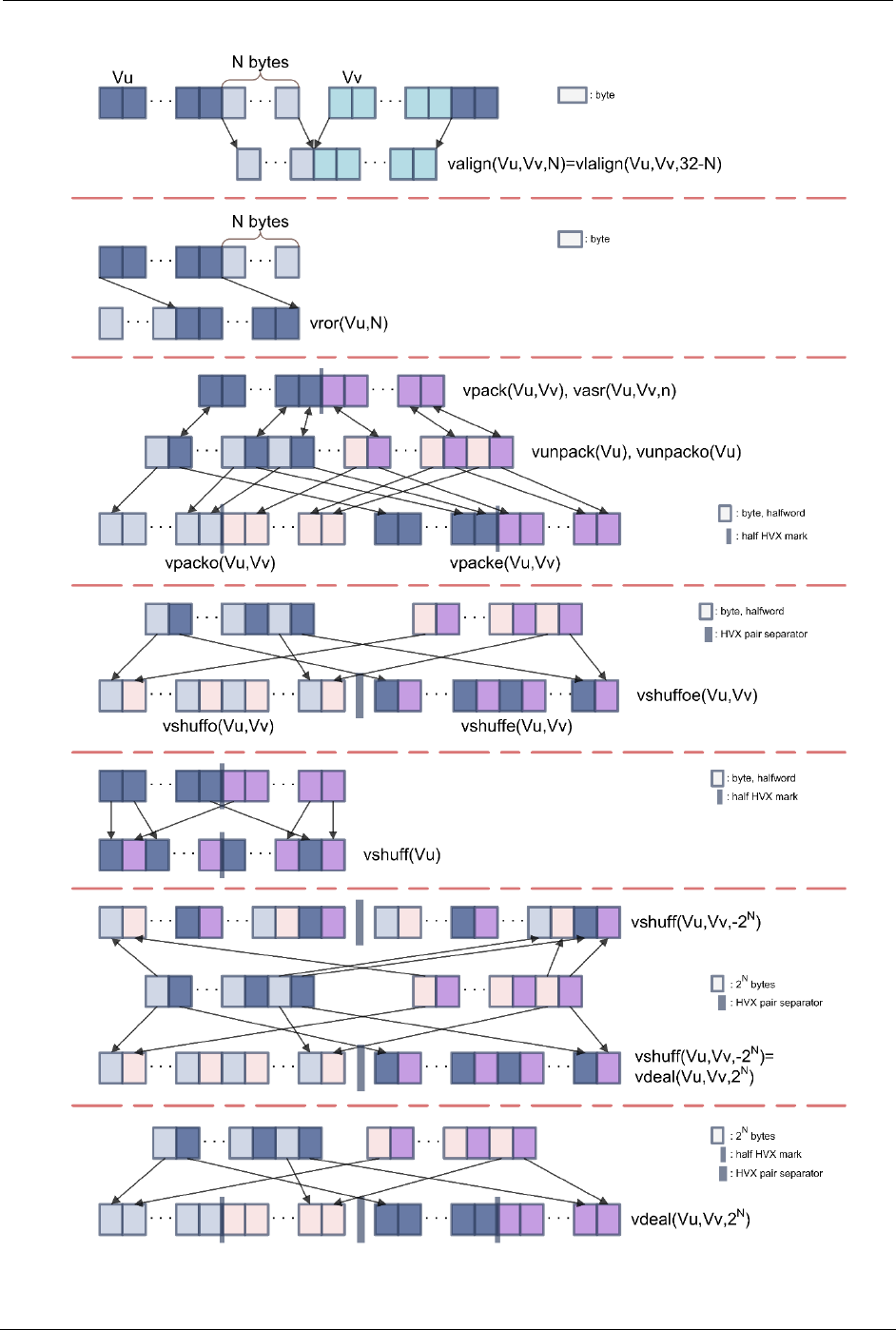
number of HVX instructions allow to address that challenge. Figure 4-2 describes these
instructions and provides a visual summary of these instructions.
Qualcomm Hexagon DSP User Guide Optimize tasks for the DSP
80-VB419-108 Rev. D 36
Figure 4-2 Summary of the most common HVX element manipulations

Qualcomm Hexagon DSP User Guide Optimize tasks for the DSP
80-VB419-108 Rev. D 37
valign, vlalign, vror
These three instructions are straightforward:
valign and vlalign create an HVX vector made out of the lowest bytes of one
vector and the upper bytes of another.
vror performs a circular rotation of an HVX vector by an arbitrary number of
bytes.
vpacke, vpacko, vpack, vunpack, vunpacko, vdeal
vpacke and vpacko pack the even or odd 32-bit or 16-bit elements of two HVX
vectors into one.
vpack performs an element size reduction, shrinking the contents of two HVX vectors
into one after saturation.
vunpack and vunpacko are the opposite forms from vpack, respectively unpacking
the even and the odd 8-bit or 16-bit elements into elements twice as large.
vdeal (the flavor that consumes one input register) operates in the same way as
vpacke and vpacko combined together but on half the number of elements: it packs
the even elements from the input register into the lower half of the output register
and packs the odd elements into the upper half.
vshuffe, vshuffo, vshuffoe, vshuff
vshuffe and vshuffo are similar to their counterparts, vpacke and vpacko, in that
they move the even or odd elements of two HVX into one HVX vector. The difference
with their vpack counterparts is that elements from both input HVX vectors are
interleaved (the contents of both input register is being shuffled into one register).
The vshuff and vpack variants come handy in different use cases. For example, if
an HVX register contains pairs of (x,y) coordinates, vpacke and vpacko are useful to
separate the x and y elements in different vectors. On the other hand, vshuffo or
vshuffe might be best suited following HVX instructions that produce HVX vectors
with double precision and store the results of consecutive operations in the upper
and lower registers of a pair.
vshuffoe executes both vshuffe and vshuffo at the same time and generates a
register pair where the two registers in the pair are the output from the vshuffo and
vshuffe instructions.
vshuff (the flavor that consumes one input register) interleaves the elements from
the upper and lower parts of a register into another register.
vasr
A narrowing shift: it takes two input HVX vectors and returns one output HVX vector.
The narrowing shift is applied alternatively on each element of the two input HVX
registers, and thus produces output with the same order as a vshuffe or vshuffo
instruction.

Qualcomm Hexagon DSP User Guide Optimize tasks for the DSP
80-VB419-108 Rev. D 38
Crosslane vshuff, vdeal
These instructions are very powerful but not trivial to understand. They perform a
multi-level transpose operation between groups of registers. The most common
configurations used with vshuff and vdeal are for positive and negative powers of 2.
vshuff with an element size of Rt = 2N bytes place in the low register of the output
pair the 2N-byte even elements from both input vectors, and the 2N-byte odd
elements in the high register. This operation is essentially a generalization of
vshuffoe to larger element sizes.
vshuff with an element size of Rt = -2N bytes interleave the 2N-byte elements from
both input vectors into the output register. This operation is essentially a
generalization of the non-crosslane variant of vshuff to larger element sizes.
vdeal with an element size of Rt = 2N bytes is identical to vshuff.
vdeal with an element size of Rt = -2N bytes pack the 2N-byte even elements from
both input vectors into the low output register pair and the odd elements in the high
pair. For N=0, this instruction is therefore being the same as executing packo and
packe at the same time.
vdelta, vrdelta
vdelta and vrdelta use a network of switchboxes to permute or copy bytes within
an HVX vector. Consider using these instructions when you need some transforms
with some irregular patterns not covered in the various operations listed above.
vdelta and vrdelta are configured with an HVX vector. The simplest and safest way
of determining the configuration values for this register is to use a configuration tools
provided with the SDK tools under
{HEXAGON_SDK_ROOT}/tools/HEXAGON_Tools/<version
number>/Examples/libcore/Vdelta_Helper/General_permute_network.htm.
At the bottom of this page, you can specify a pattern in which the bytes of the input
vector should be reordered. For example, if bytes 1 and 5 needed to be dropped
from the input vector, specify in the TPERM[N] control box a sequence of bytes that
begins with
0, 2, 3, 4, 6, … .
Once the output pattern is fully specified, click Submit for Benes or Submit for
Delta to retrieve the configuration, if one exists, to achieve the pattern transformation
using either a sequence of a vrdelta and vdelta instruction (Benes approach), or
one vrdelta instruction.

Qualcomm Hexagon DSP User Guide Optimize tasks for the DSP
80-VB419-108 Rev. D 39
4.3.4 VTCM/lookup
Starting with V65, support is added for scatter/gather. With this added support, you can
now perform vectorized random-access memory lookups that are not limited to 256
entries as is the case with the vlut instruction available on all DSP variants.
For more details on this instruction, see the Hexagon V66 HVX Programmer’s Reference
Manual (80-N2040-44).
NOTE: The scatter/gather operations are very memory intensive, so they are prone to stalling
when memory conflicts occur. For information on how to avoid scatter/gather stalls, see
the Avoid scatter/gather stalls section of the Hexagon V66 HVX Programmer’s
Reference Manual (80-N2040-44).
4.3.5 Emulate floating-point
HVX does not have native floating-point support. However, the qmath library provided
with the SDK introduces a pseudo floating-format that supports a similar precision and
dynamic range to IEEE floating-point. In this format and using the libraries provided in
qmath, it is possible to perform all basic arithmetic operations (add, sub, mult, mac,
divide, sqrt). In addition, the qmath library provides a set of functions allowing to convert
an array of IEEE floating-point values into this pseudo float format and vice-versa.
Using the qmath float library is the simplest way to speed up floating-point code with
HVX, as long as data processing is parallelized. For more details on this library, see the
library package and its documentation (Qualcomm Math (qmath) Library, 80-VB419-105)
in {HEXAGON_SDK_ROOT}/libs/common/qmath. For examples on how to use the library,
see the code example in {HEXAGON_SDK_ROOT}/examples/compute/qmath_sample.
4.3.6 Convert float to fix
Another approach for porting floating-point code to an HVX implementation consists of
converting the arithmetic to fixed-point. Qualcomm provides a library that helps with that
process. The library helps you characterize the behavior of all floating-point variables,
provide hints on how to represent floating-point variables in fixed-point to maximize
accuracy and guarantee no overflow, and provide bit-exact simulations of various fixed-
point implementations to help you strike the right balance between accuracy and
compute efficiency without having to write any actual HVX code first. Only when you are
satisfied with the behavior of the fixed-point model do you need to write the
corresponding HVX implementation, thus saving considerable development effort.
For more details on this library, see the library package and its documentation
(Qualcomm Fixed Point (qfxp) Library, 80-VB419-69) in
{HEXAGON_SDK_ROOT}/libs/common/qfxp. For examples on how to use the library, see
the code example in {HEXAGON_SDK_ROOT}/examples/compute/qfxp_sample.

80-VB419-108 Rev. D 40
5 Debugging
Why is it not working?
All software developers find themselves in this situation at one time or another. And
there are many ways of approaching such a situation, with or without the use of tools.
Tools might occasionally point you to the source of a bug. More often than not however,
this process is not quick. As a result, it is preferable to begin with ensuring you are not
making one of the most common mistakes before resolving to spending time actually
debugging the code. Section 5.1 discusses common mistakes that lead to the program
crashing or behaving unexpectedly. Section 5.2 discusses various tools that you might
want to use to assist with debugging code.
5.1 Common issues
Using incorrect array size with FastRPC
When passing an array to the DSP using FastRPC, the array size must be specified
as the number of elements in the array, not its size in bytes.
Missing the 128-byte compilation flag
If you compile a function to be run with the 128-byte HVX mode, you must explicitly
set the -mhvx-double when compiling the code.
Using incorrect memory alignment for scalar accesses
When making memory accesses from assembly, you must ensure that the address is
aligned to the size you are accessing. Common ways of ensuring correct pointer
alignment include using:
Static allocation with a type large enough to guarantee alignment. For example,
HVX_Vector ptr[3];
Static allocation with the aligned attribute. For example,
int16 ptr[N] __attribute__((aligned(128)));
Dynamic memory allocation with memalign. For example,
int16* ptr = (int16 *)memalign(128,N);
Dynamic memory allocation of more memory than needed, zeroing out the lowest
bits and adding a 128 byte offset to the address. For example,
int16* tmpPtr = (int16 *)malloc(128,N+127);
int16* ptr = (int16*) (((int8*)tmpPtr+127) &~127);
// ensure to free(tmpPtr) and not free(ptr) when done!

Qualcomm Hexagon DSP User Guide Debugging
80-VB419-108 Rev. D 41
NOTE: HVX load and stores are unaligned: the memory access instructions simply ignores the
lower bits, yielding an aligned address, and allowing the code to run without crashing.
Calling input/output libraries such as printf from the DSP
With the SDK 3.2 or below, printf is only supported when running on the CPU.
When running code on the DSP, use FARF instead or use SDK 3.3 and beyond.
Compiling for the wrong target
Ensure your compilation flag is compatible with the architecture you are targeting.
For example, do not run code compiled for V62 on an MSM8996 device.
Making out of bound memory accesses
This is obviously a common mistake to make on any target architecture and can
result in various behaviors. However, this behavior also applies to L2 prefetching: L2
prefetching throws an exception if the start address is invalid. However, if a prefetch
crosses into an invalid page, the remainder is simply dropped without failure.
Missing a function implementation
A missing function implementation does not result in a compilation error if the
function is declared as extern but it results in a runtime error. Inspect the DSP logs
for the presence of an undefined PLT symbol <function name> in <your
library>.so message. Also, remember that C++ mangles function names, so to
access a function written in C or assembly from a C++ file, the function must be
defined as extern “C”.
Using an incorrect function declaration
If you modify the parameters of an implementation, remember to modify the
parameters of its declaration. Otherwise, your code might still compile but you end
up passing incorrect parameters to a function and get an unexpected behavior.
Modifying callee-saved registers
The calling conventions specify which registers are the responsibility of the calling
function to save, and which registers are the responsibility of the callee function to
save. When writing assembly code, it is important to save all callee-saved registers if
you modify them in your implementation. These registers are R16-R27 and R29-R31.
The following example shows how you do so with registers R16-R19, for example:
{
ALLOCFRAME(#2*8) // enough space for 4 32-bit registers
// Note: needs to be a multiple of 8
} {
memd(r29 + #0) = r17:16
memd(r29 + #8) = r19:18
} {
<your code here>
} {
r17:16 = memd(r29 + #0)
r19:18 = memd(r29 + #8)
} {
DEALLOC_RETURN
}

Qualcomm Hexagon DSP User Guide Debugging
80-VB419-108 Rev. D 42
Not locking HVX context before executing HVX code.
Prior to V65, you must explicitly lock an HVX context before running any HVX code.
Failing to make assembly code position-independent
Code can compiled properly when testing for the simulator, which builds a static
library, but fail to compile when building a dynamic library. This might be caused by
setting a register to an immediate address:
test_array:
.byte 0,1,2,3
...
r1 = #test_array
instead of using a PC relative approach:
r1 = ADD(PC,##test_array@PCREL)
Running out of memory on the stack
Thread stacks are 16 KB currently. Do not use excessive local variables, and be especially careful with
HVX intrinsics, which might spill onto the stack and add up quickly.
5.2 Debugging with the tools
5.2.1 qprintf
The SDK comes with the qprintf library. This library provides different APIs to display
scalar and vector registers in various formats from C/C++ or assembly.
For example, after including qprintf_asm.h to your assembly code, insert the following
lines to display the contents of V0 as a succession of 32-bit integers in the logs:
qprintf("v0 = %d",v0);
qprintf_example_asm.S[174]: v0 =
-1,-1,-1,-1,-1,-1,-1,-1
-1,-1,-1,-1,-1,-1,-1,-1
-1,-1,-1,-1,-1,-1,-1,-1
-1,-1,-1,-1,-1,-1,-1,-1
The library also supports more advanced options for controlling the format of the output,
the elements to hide or display, or the number of columns for displaying the elements of
a vector register. For example:
qprintf("Displaying scalar registers in various
formats: %u, %x. %23d. %+.6d or %5.2f. Etc.",r20,r20,r20,r20,r21);
qprintf_example_asm.S[162]: Displaying scalar registers in various
formats: 20, 14, 20, +000020, 4.00. Etc.

Qualcomm Hexagon DSP User Guide Debugging
80-VB419-108 Rev. D 43
Another example:
qprintf("Masked vector register contents as 16-bit unsigned integers in
rows of 5 elements: %m(5)uu",v0);
qprintf_example_asm.S[183]: Masked vector register contents as 16-bit
unsigned integers in rows of 5 elements:
[7e]= 65535,[7c]= 65535,[76]= 65535,[74]= 65535,[6e]= 65535
[6c]= 65535,[66]= 65535,[64]= 65535,[5e]= 65535,[5c]= 65535
[56]= 65535,[54]= 65535,[4e]= 65535,[4c]= 65535,[46]= 65535
[44]= 65535,[3a]= 65535,[38]= 65535,[32]= 65535,[30]= 65535
[2a]= 65535,[28]= 65535,[22]= 65535,[20]= 65535,[1a]= 65535
[18]= 65535,[12]= 65535,[10]= 65535,[0a]= 65535,[08]= 65535
[02]= 65535,[00]= 65535,
For more details on this library, see the library package and its documentation
(Qualcomm qprintf Library, 80-VB419-109) in
{HEXAGON_SDK_ROOT}/libs/common/qprintf.
For examples on how to use the library, see the code example in
{HEXAGON_SDK_ROOT}/examples/compute/qprintf_example.
5.2.2 Build targets
Until the application has been fully debugged, it is preferable to build the Debug flavor of
the DSP library. This flavor uses fewer compilation optimizations and enables diagnostic
messages making it easier to follow disassembled code.
5.2.3 Disassemble code
When an application does not behave as expected, it might be necessary to understand
what exact instructions are being executed on the DSP. Inspecting the assembly code
produced by the compiler can sometimes help you to understand the source of a bug, a
mismatch between what you intended the C code to do and what it actually got
interpreted.
If foo.c was compiled with the hexagon_ReleaseG_dynamic_toolv81_v60 target, the
following command interleaves the C/C++ source with the corresponding assembly for
any given object file and it writes the output to temp.txt:
hexagon-llvm-objdump -disassemble -source -demangle
hexagon_ReleaseG_dynamic_toolv81_v60\foo.o > temp.txt
NOTE: hexagon-llvm-objdump.exe is found in the tools\bin directory of the Hexagon tools
provided as part of the SDK and the -source flag is only available starting with 8.1.x
Hexagon tools, which are used in the SDK 3.3 and beyond.
In some cases, compiler optimizations make it difficult to follow exactly how each C
expression is being translated into assembly and it can be useful to recompile the code
with all optimizations disabled to facilitate the debugging process.

Qualcomm Hexagon DSP User Guide Debugging
80-VB419-108 Rev. D 44
Disabling all compiler optimizations is accomplished by building the Debug flavor or
adding the following line in hexagon.min:
_OPT = -O0
When the simulator reports a crash, it returns the following information:
An error code (SSR) indicating the type of exception that occurred
the PC value for the instruction executed when the exception occurred (ELR)
When applicable, a virtual address indicating the data accessed when the exception
occurred (BADVA)
If the code was disassembled with the -r option (for relocation), you can use the ELR
value returned in the crash report to find the corresponding location in the disassembled
code where the exception occurred. In addition, table 7-15 in the Hexagon V66
Programmer’s Reference Manual (80-N2040-42) explains the meaning of the various
SSR codes.
5.2.4 Use the debugger
As of SDK release 3.3, it is possible to use the LLDB debugger with the MSM8998 and
beyond, on target or in simulator mode. There is, however, no on-target debugger
support for earlier processor variants.
The simplest way to access the debugger is to use it from Eclipse. The Debugging >
Remote Debugger section of the SDK online documentation describes the process for
creating an Eclipse project from a make-based Hexagon project and setting up the target
for debugging support.
Once these steps are followed, you can perform common debugging operations such as
single-stepping through the code, using breakpoints, and inspecting register and
memory contents.

80-VB419-108 Rev. D 45
6 Profiling
The SDK provides debugging and profiling tools, depending on what you are interested
in.
6.1 Read timers
You can use timer APIs to time a specific section of code directly. The most useful APIs
are the following:
6.1.1 Measure time
The most accurate way of measuring time consists of accessing the
UTIMERHI:UTIMERLO registers. This pair of 32-bit register is a direct measure of the
elapsed time reported in ticks. One tick is 1/19.2 MHz seconds.
These registers can be accessed from C with the HAP_perf_get_qtimer_count API.
Alternatively, you can invoke HAP_perf_get_time_us accessible from C by including
HAP_perf.h. This API returns directly the elapsed time in microseconds by deriving the
time from the number of ticks and performing a division, which consumes some extra
cycles.
6.1.2 Measure processor cycles
For measuring elapsed processor cycles, access the UPCYCLEHI: UPCYCLELO registers
using the HAP_perf_get_pcycles API available from C by including HAP_perf.h.
However, this measuring technique is not as precise because the register values are
accessed using traps, which might include occasional delays.

Qualcomm Hexagon DSP User Guide Profiling
80-VB419-108 Rev. D 46
6.2 Profile on the simulator
The Hexagon simulator enables various kinds of profiling data to be collected. Two types
of profiling are available and intended to work together.
6.2.1 High-level profiling
The simulator generates a number of profiling data that help you get a sense of where
the bottlenecks are in an application. This information is useful to work on high-level
software optimizations.
When profiling an application on the simulator, ensure that the simulator runs in its cycle-
accurate mode. That mode is enabled by using the --timing option. This option results
in the simulator counting cycles accurately but results in increasing significantly the
simulation time.
The --profile or -p options direct the simulator to generate gmon data files that are
then postprocessed with hexagon-gprof.
The main purpose of hexagon-gprof is to report the number of cycles executed in each
function. This allows you to have a high-level understanding of where most cycles are
spent in a given implementation. For more information about the hexagon-gprof profiler,
see the Hexagon gprof Profiler User Guide (80-N2040-29).
In addition, you can use the --statsfile and --pmu_statsfile options to direct the
simulator to gather statistics on instruction and cache utilization. The statistics are not
required to be postprocessed with hexagon-gprof. For more information about these
options, For more information about these options, see the Simulator statistics files and
PMU statistics files sections in the Hexagon Simulator User Guide (80-N2040-17).
6.2.2 Low-level profiling
If more performance is needed in an application, check the implementation of a specific
function and understand how the cycles are spent. In order to do so, you must run the
simulator with additional options such as --packet_analyze or --uarchtrace.
The SDK includes tools that assist you by postprocessing some of these files. For
example, the Hexagon profiler processes the output from the simulator packet analysis
and generates a user-friendly html file displaying the following information:
Total number of cycles executed
Total number of stall cycles
Highest cycle or stall counts (by function or instruction packet)
Commit and stall statistics (by function or instruction packet)
PMU event counts (by event type or instruction packet)
Annotated disassembly of instruction packets
Assembly instruction counts
For more information about the Hexagon profiler, see the Hexagon Profiler User Guide
(80-N2040-10).
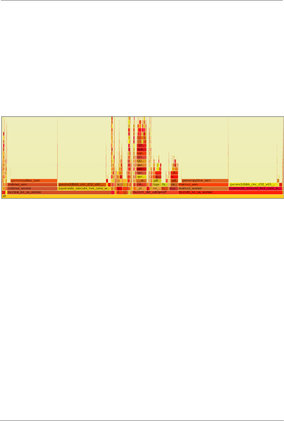
Qualcomm Hexagon DSP User Guide Profiling
80-VB419-108 Rev. D 47
6.3 Profile on target with the Hexagon Trace Analyzer
Starting with SM8150, 7150 and 6150 devices, Qualcomm provides the ability to collect
Starting with the SM8150, SM7150, and SM6150 devices, Qualcomm provides the
ability to collect trace files (only on the Compute DSP) and post process them with a
trace analysis tool, the Hexagon Trace Analyzer. This tool outputs detailed per function,
per instruction, and per section statistics.
One type of output from the trace analyzer is Flamegraph files, which can be viewed in a
browser. These views allow you to zoom in and out, and for each thread, understand
which functions take the most cycles to execute. Figure 6-1 provides an example of such
a view.
Figure 6-1 Flamegraph output from the Hexagon Trace Analyzer
The trace analyzer also provides a view that shows thread activity over time, and an
Excel spreadsheet with detailed per function and per packet statistics.
For more information about the trace analyzer, see
${HEXAGON_SDK_ROOT}/tools/debug/hexagon-trace-analyzer/readme.txt.
6.4 Profile on target with the Android Hexagon profiler
Qualcomm provides an Android application called the Sysmon DSP profiler. This
application allows to collect high-level statistics on an application running on target. This
application is useful to monitor load distribution and bus activity over time.
For more information about this tool, see Tools > Sysmon DSP Profiler included in the
SDK online documentation.
