Learning TensorFlow: A Guide To Building Deep Systems 90.002 Tensor Flow Tom Hope
User Manual:
Open the PDF directly: View PDF ![]() .
.
Page Count: 321 [warning: Documents this large are best viewed by clicking the View PDF Link!]
- Preface
- 1. Introduction
- 2. Go with the Flow: Up and Running with TensorFlow
- 3. Understanding TensorFlow Basics
- 4. Convolutional Neural Networks
- 5. Text I: Working with Text and Sequences, and TensorBoard Visualization
- 6. Text II: Word Vectors, Advanced RNN, and Embedding Visualization
- 7. TensorFlow Abstractions and Simplifications
- 8. Queues, Threads, and Reading Data
- 9. Distributed TensorFlow
- 10. Exporting and Serving Models with TensorFlow
- A. Tips on Model Construction and Using TensorFlow Serving
- Index

Learning TensorFlow
A Guide to Building Deep Learning Systems
Tom Hope, Yehezkel S. Resheff, and Itay Lieder

Learning TensorFlow
by Tom Hope, Yehezkel S. Resheff, and Itay Lieder
Copyright © 2017 Tom Hope, Itay Lieder, and Yehezkel S. Resheff. All rights reserved.
Printed in the United States of America.
Published by O’Reilly Media, Inc., 1005 Gravenstein Highway North, Sebastopol, CA 95472.
O’Reilly books may be purchased for educational, business, or sales promotional use. Online
editions are also available for most titles (http://oreilly.com/safari). For more information,
contact our corporate/institutional sales department: 800-998-9938 or corporate@oreilly.com.
Editor: Nicole Tache
Production Editor: Shiny Kalapurakkel
Copyeditor: Rachel Head
Proofreader: Sharon Wilkey
Indexer: Judith McConville
Interior Designer: David Futato
Cover Designer: Karen Montgomery
Illustrator: Rebecca Demarest
August 2017: First Edition

Revision History for the First Edition
2017-08-04: First Release
The O’Reilly logo is a registered trademark of O’Reilly Media, Inc. Learning TensorFlow, the
cover image, and related trade dress are trademarks of O’Reilly Media, Inc.
While the publisher and the authors have used good faith efforts to ensure that the information
and instructions contained in this work are accurate, the publisher and the authors disclaim all
responsibility for errors or omissions, including without limitation responsibility for damages
resulting from the use of or reliance on this work. Use of the information and instructions
contained in this work is at your own risk. If any code samples or other technology this work
contains or describes is subject to open source licenses or the intellectual property rights of
others, it is your responsibility to ensure that your use thereof complies with such licenses and/or
rights.
978-1-491-97851-1
[M]

Preface
Deep learning has emerged in the last few years as a premier technology for building intelligent
systems that learn from data. Deep neural networks, originally roughly inspired by how the
human brain learns, are trained with large amounts of data to solve complex tasks with
unprecedented accuracy. With open source frameworks making this technology widely available,
it is becoming a must-know for anybody involved with big data and machine learning.
TensorFlow is currently the leading open source software for deep learning, used by a rapidly
growing number of practitioners working on computer vision, natural language processing
(NLP), speech recognition, and general predictive analytics.
This book is an end-to-end guide to TensorFlow designed for data scientists, engineers, students,
and researchers. The book adopts a hands-on approach suitable for a broad technical audience,
allowing beginners a gentle start while diving deep into advanced topics and showing how to
build production-ready systems.
In this book you will learn how to:
1. Get up and running with TensorFlow, rapidly and painlessly.
2. Use TensorFlow to build models from the ground up.
3. Train and understand popular deep learning models for computer vision and NLP.
4. Use extensive abstraction libraries to make development easier and faster.
5. Scale up TensorFlow with queuing and multithreading, training on clusters, and serving
output in production.
6. And much more!
This book is written by data scientists with extensive R&D experience in both industry and
academic research. The authors take a hands-on approach, combining practical and intuitive
examples, illustrations, and insights suitable for practitioners seeking to build production-ready
systems, as well as readers looking to learn to understand and build flexible and powerful
models.
Prerequisites
This book assumes some basic Python programming know-how, including basic familiarity with
the scientific library NumPy.
Machine learning concepts are touched upon and intuitively explained throughout the book. For
readers who want to gain a deeper understanding, a reasonable level of knowledge in machine
learning, linear algebra, calculus, probability, and statistics is recommended.
Conventions Used in This Book
The following typographical conventions are used in this book:
Italic
Indicates new terms, URLs, email addresses, filenames, and file extensions.
Constant width
Used for program listings, as well as within paragraphs to refer to program elements such as
variable or function names, databases, data types, environment variables, statements, and
keywords.
Constant width bold
Shows commands or other text that should be typed literally by the user.
Constant width italic
Shows text that should be replaced with user-supplied values or by values determined by
context.
Using Code Examples
Supplemental material (code examples, exercises, etc.) is available for download at
https://github.com/Hezi-Resheff/Oreilly-Learning-TensorFlow.
This book is here to help you get your job done. In general, if example code is offered with this
book, you may use it in your programs and documentation. You do not need to contact us for
permission unless you’re reproducing a significant portion of the code. For example, writing a
program that uses several chunks of code from this book does not require permission. Selling or
distributing a CD-ROM of examples from O’Reilly books does require permission. Answering a
question by citing this book and quoting example code does not require permission.
Incorporating a significant amount of example code from this book into your product’s
documentation does require permission.
We appreciate, but do not require, attribution. An attribution usually includes the title, author,
publisher, and ISBN. For example: “Learning TensorFlow by Tom Hope, Yehezkel S. Resheff,
and Itay Lieder (O’Reilly). Copyright 2017 Tom Hope, Itay Lieder, and Yehezkel S. Resheff,
978-1-491-97851-1.”
If you feel your use of code examples falls outside fair use or the permission given above, feel
free to contact us at permissions@oreilly.com.
O’Reilly Safari
NOTE
Safari (formerly Safari Books Online) is a membership-based training and reference platform for
enterprise, government, educators, and individuals.
Members have access to thousands of books, training videos, Learning Paths, interactive
tutorials, and curated playlists from over 250 publishers, including O’Reilly Media, Harvard
Business Review, Prentice Hall Professional, Addison-Wesley Professional, Microsoft Press,
Sams, Que, Peachpit Press, Adobe, Focal Press, Cisco Press, John Wiley & Sons, Syngress,
Morgan Kaufmann, IBM Redbooks, Packt, Adobe Press, FT Press, Apress, Manning, New
Riders, McGraw-Hill, Jones & Bartlett, and Course Technology, among others.
For more information, please visit http://oreilly.com/safari.

How to Contact Us
Please address comments and questions concerning this book to the publisher:
O’Reilly Media, Inc.
1005 Gravenstein Highway North
Sebastopol, CA 95472
800-998-9938 (in the United States or Canada)
707-829-0515 (international or local)
707-829-0104 (fax)
We have a web page for this book, where we list errata, examples, and any additional
information. You can access this page at http://bit.ly/learning-tensorflow.
To comment or ask technical questions about this book, send email to
bookquestions@oreilly.com.
For more information about our books, courses, conferences, and news, see our website at
http://www.oreilly.com.
Find us on Facebook: http://facebook.com/oreilly
Follow us on Twitter: http://twitter.com/oreillymedia
Watch us on YouTube: http://www.youtube.com/oreillymedia
Acknowledgments
The authors would like to thank the reviewers who offered feedback on this book: Chris Fregly,
Marvin Bertin, Oren Sar Shalom, and Yoni Lavi. We would also like to thank Nicole Tache and
the O’Reilly team for making it a pleasure to write the book.
Of course, thanks to all the people at Google without whom TensorFlow would not exist.

Chapter 1. Introduction
This chapter provides a high-level overview of TensorFlow and its primary use: implementing
and deploying deep learning systems. We begin with a very brief introductory look at deep
learning. We then present TensorFlow, showcasing some of its exciting uses for building
machine intelligence, and then lay out its key features and properties.
Going Deep
From large corporations to budding startups, engineers and data scientists are collecting huge
amounts of data and using machine learning algorithms to answer complex questions and build
intelligent systems. Wherever one looks in this landscape, the class of algorithms associated with
deep learning have recently seen great success, often leaving traditional methods in the dust.
Deep learning is used today to understand the content of images, natural language, and speech, in
systems ranging from mobile apps to autonomous vehicles. Developments in this field are taking
place at breakneck speed, with deep learning being extended to other domains and types of data,
like complex chemical and genetic structures for drug discovery and high-dimensional medical
records in public healthcare.
Deep learning methods — which also go by the name of deep neural networks — were originally
roughly inspired by the human brain’s vast network of interconnected neurons. In deep learning,
we feed millions of data instances into a network of neurons, teaching them to recognize patterns
from raw inputs. The deep neural networks take raw inputs (such as pixel values in an image)
and transform them into useful representations, extracting higher-level features (such as shapes
and edges in images) that capture complex concepts by combining smaller and smaller pieces of
information to solve challenging tasks such as image classification (Figure 1-1). The networks
automatically learn to build abstract representations by adapting and correcting themselves,
fitting patterns observed in the data. The ability to automatically construct data representations is
a key advantage of deep neural nets over conventional machine learning, which typically
requires domain expertise and manual feature engineering before any “learning” can occur.
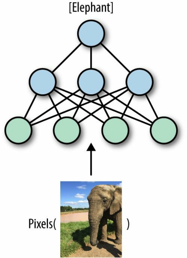
Figure 1-1. An illustration of image classification with deep neural networks. The network takes raw inputs (pixel
values in an image) and learns to transform them into useful representations, in order to obtain an accurate
image classification.
This book is about Google’s framework for deep learning, TensorFlow. Deep learning
algorithms have been used for several years across many products and areas at Google, such as
search, translation, advertising, computer vision, and speech recognition. TensorFlow is, in fact,
a second-generation system for implementing and deploying deep neural networks at Google,
succeeding the DistBelief project that started in 2011.
TensorFlow was released to the public as an open source framework with an Apache 2.0 license
in November 2015 and has already taken the industry by storm, with adoption going far beyond
internal Google projects. Its scalability and flexibility, combined with the formidable force of
Google engineers who continue to maintain and develop it, have made TensorFlow the leading
system for doing deep learning.
Using TensorFlow for AI Systems
Before going into more depth about what TensorFlow is and its key features, we will briefly give
some exciting examples of how TensorFlow is used in some cutting-edge real-world
applications, at Google and beyond.
Pre-trained models: state-of-the-art computer vision for all
One primary area where deep learning is truly shining is computer vision. A fundamental task in
computer vision is image classification — building algorithms and systems that receive images
as input, and return a set of categories that best describe them. Researchers, data scientists, and
engineers have designed advanced deep neural networks that obtain highly accurate results in
understanding visual content. These deep networks are typically trained on large amounts of
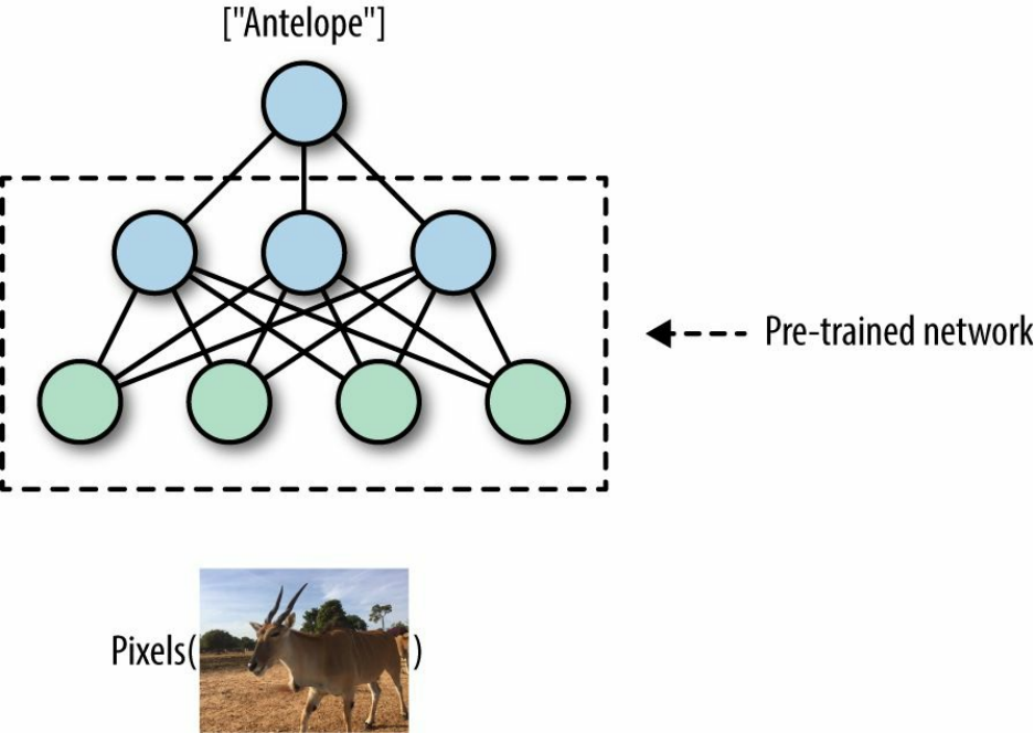
image data, taking much time, resources, and effort. However, in a growing trend, researchers
are publicly releasing pre-trained models — deep neural nets that are already trained and that
users can download and apply to their data (Figure 1-2).
Figure 1-2. Advanced computer vision with pre-trained TensorFlow models.
TensorFlow comes with useful utilities allowing users to obtain and apply cutting-edge
pretrained models. We will see several practical examples and dive into the details throughout
this book.
Generating rich natural language descriptions for images
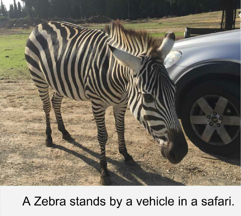
One exciting area of deep learning research for building machine intelligence systems is focused
on generating natural language descriptions for visual content (Figure 1-3). A key task in this
area is image captioning — teaching the model to output succinct and accurate captions for
images. Here too, advanced pre-trained TensorFlow models that combine natural language
understanding with computer vision are available.
Figure 1-3. Going from images to text with image captioning (illustrative example).
Text summarization
Natural language understanding (NLU) is a key capability for building AI systems. Tremendous
amounts of text are generated every day: web content, social media, news, emails, internal
corporate correspondences, and many more. One of the most sought-after abilities is to
summarize text, taking long documents and generating succinct and coherent sentences that
extract the key information from the original texts (Figure 1-4). As we will see later in this book,
TensorFlow comes with powerful features for training deep NLU networks, which can also be
used for automatic text summarization.
Figure 1-4. An illustration of smart text summarization.
TensorFlow: What’s in a Name?
Deep neural networks, as the term and the illustrations we’ve shown imply, are all about
networks of neurons, with each neuron learning to do its own operation as part of a larger
picture. Data such as images enters this network as input, and flows through the network as it
adapts itself at training time or predicts outputs in a deployed system.
Tensors are the standard way of representing data in deep learning. Simply put, tensors are just
multidimensional arrays, an extension of two-dimensional tables (matrices) to data with higher
dimensionality. Just as a black-and-white (grayscale) images are represented as “tables” of pixel
values, RGB images are represented as tensors (three-dimensional arrays), with each pixel
having three values corresponding to red, green, and blue components.
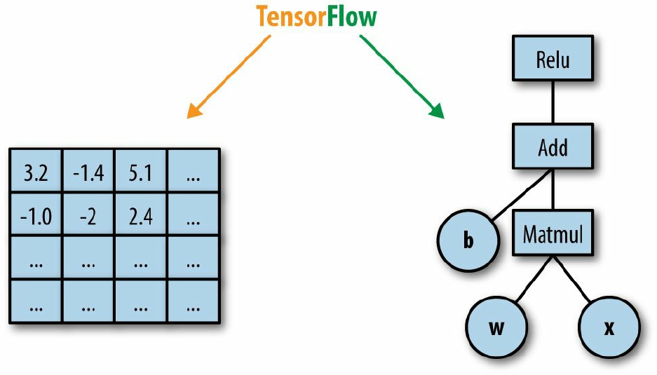
In TensorFlow, computation is approached as a dataflow graph (Figure 1-5). Broadly speaking,
in this graph, nodes represent operations (such as addition or multiplication), and edges represent
data (tensors) flowing around the system. In the next chapters, we will dive deeper into these
concepts and learn to understand them with many examples.
Figure 1-5. A dataflow computation graph. Data in the form of tensors flows through a graph of computational
operations that make up our deep neural networks.
A High-Level Overview
TensorFlow, in the most general terms, is a software framework for numerical computations
based on dataflow graphs. It is designed primarily, however, as an interface for expressing and
implementing machine learning algorithms, chief among them deep neural networks.
TensorFlow was designed with portability in mind, enabling these computation graphs to be
executed across a wide variety of environments and hardware platforms. With essentially
identical code, the same TensorFlow neural net could, for instance, be trained in the cloud,
distributed over a cluster of many machines or on a single laptop. It can be deployed for serving
predictions on a dedicated server or on mobile device platforms such as Android or iOS, or
Raspberry Pi single-board computers. TensorFlow is also compatible, of course, with Linux,
macOS, and Windows operating systems.
The core of TensorFlow is in C++, and it has two primary high-level frontend languages and
interfaces for expressing and executing the computation graphs. The most developed frontend is
in Python, used by most researchers and data scientists. The C++ frontend provides quite a low-
level API, useful for efficient execution in embedded systems and other scenarios.
Aside from its portability, another key aspect of TensorFlow is its flexibility, allowing
researchers and data scientists to express models with relative ease. It is sometimes revealing to
think of modern deep learning research and practice as playing with “LEGO-like” bricks,
replacing blocks of the network with others and seeing what happens, and at times designing new
blocks. As we shall see throughout this book, TensorFlow provides helpful tools to use these
modular blocks, combined with a flexible API that enables the writing of new ones. In deep
learning, networks are trained with a feedback process called backpropagation based on gradient
descent optimization. TensorFlow flexibly supports many optimization algorithms, all with
automatic differentiation — the user does not need to specify any gradients in advance, since
TensorFlow derives them automatically based on the computation graph and loss function
provided by the user. To monitor, debug, and visualize the training process, and to streamline
experiments, TensorFlow comes with TensorBoard (Figure 1-6), a simple visualization tool that
runs in the browser, which we will use throughout this book.
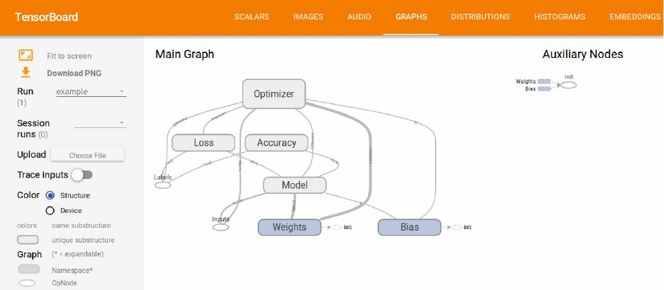
Figure 1-6. TensorFlow’s visualization tool, TensorBoard, for monitoring, debugging, and analyzing the training
process and experiments.
Key enablers of TensorFlow’s flexibility for data scientists and researchers are high-level
abstraction libraries. In state-of-the-art deep neural nets for computer vision or NLU, writing
TensorFlow code can take a toll — it can become a complex, lengthy, and cumbersome
endeavor. Abstraction libraries such as Keras and TF-Slim offer simplified high-level access to
the “LEGO bricks” in the lower-level library, helping to streamline the construction of the
dataflow graphs, training them, and running inference. Another key enabler for data scientists
and engineers is the pretrained models that come with TF-Slim and TensorFlow. These models
were trained on massive amounts of data with great computational resources, which are often
hard to come by and in any case require much effort to acquire and set up. Using Keras or TF-
Slim, for example, with just a few lines of code it is possible to use these advanced models for
inference on incoming data, and also to fine-tune the models to adapt to new data.
The flexibility and portability of TensorFlow help make the flow from research to production
smooth, cutting the time and effort it takes for data scientists to push their models to deployment
in products and for engineers to translate algorithmic ideas into robust code.

TENSORFLOW ABSTRACTIONS
TensorFlow comes with abstraction libraries such as Keras and TF-Slim, offering simplified high-level
access to TensorFlow. These abstractions, which we will see later in this book, help streamline the
construction of the dataflow graphs and enable us to train them and run inference with many fewer
lines of code.
But beyond flexibility and portability, TensorFlow has a suite of properties and tools that make it
attractive for engineers who build real-world AI systems. It has natural support for distributed
training — indeed, it is used at Google and other large industry players to train massive networks
on huge amounts of data, over clusters of many machines. In local implementations, training on
multiple hardware devices requires few changes to code used for single devices. Code also
remains relatively unchanged when going from local to distributed, which makes using
TensorFlow in the cloud, on Amazon Web Services (AWS) or Google Cloud, particularly
attractive. Additionally, as we will see further along in this book, TensorFlow comes with many
more features aimed at boosting scalability. These include support for asynchronous computation
with threading and queues, efficient I/O and data formats, and much more.
Deep learning continues to rapidly evolve, and so does TensorFlow, with frequent new and
exciting additions, bringing better usability, performance, and value.
Summary
With the set of tools and features described in this chapter, it becomes clear why TensorFlow has
attracted so much attention in little more than a year. This book aims at first rapidly getting you
acquainted with the basics and ready to work, and then we will dive deeper into the world of
TensorFlow with exciting and practical examples.

Chapter 2. Go with the Flow: Up and
Running with TensorFlow
In this chapter we start our journey with two working TensorFlow examples. The first (the
traditional “hello world” program), while short and simple, includes many of the important
elements we discuss in depth in later chapters. With the second, a first end-to-end machine
learning model, you will embark on your journey toward state-of-the-art machine learning with
TensorFlow.
Before getting started, we briefly walk through the installation of TensorFlow. In order to
facilitate a quick and painless start, we install the CPU version only, and defer the GPU
installation to later.1 (If you don’t know what this means, that’s OK for the time being!) If you
already have TensorFlow installed, skip to the second section.
Installing TensorFlow
If you are using a clean Python installation (probably set up for the purpose of learning
TensorFlow), you can get started with the simple pip installation:
$ pip install tensorflow
This approach does, however, have the drawback that TensorFlow will override existing
packages and install specific versions to satisfy dependencies. If you are using this Python
installation for other purposes as well, this will not do. One common way around this is to install
TensorFlow in a virtual environment, managed by a utility called virtualenv.
Depending on your setup, you may or may not need to install virtualenv on your machine. To
install virtualenv, type:
$ pip install virtualenv
See http://virtualenv.pypa.io for further instructions.
In order to install TensorFlow in a virtual environment, you must first create the virtual
environment — in this book we choose to place these in the ~/envs folder, but feel free to put
them anywhere you prefer:
$ cd ~
$ mkdir envs
$ virtualenv ~/envs/tensorflow
This will create a virtual environment named tensorflow in ~/envs (which will manifest as the
folder ~/envs/tensorflow). To activate the environment, use:
$ source ~/envs/tensorflow/bin/activate
The prompt should now change to indicate the activated environment:
(tensorflow)$
At this point the pip install command:
(tensorflow)$ pip install tensorflow
will install TensorFlow into the virtual environment, without impacting other packages installed
on your machine.
Finally, in order to exit the virtual environment, you type:
(tensorflow)$ deactivate

at which point you should get back the regular prompt:
$
TENSORFLOW FOR WINDOWS USERS
Up until recently TensorFlow had been notoriously difficult to use with Windows machines. As of
TensorFlow 0.12, however, Windows integration is here! It is as simple as:
pip install tensorflow
for the CPU version, or:
pip install tensorflow-gpu
for the GPU-enabled version (assuming you already have CUDA 8).

ADDING AN ALIAS TO ~/.BASHRC
The process described for entering and exiting your virtual environment might be too cumbersome if
you intend to use it often. In this case, you can simply append the following command to your
~/.bashrc file:
alias tensorflow="source ~/envs/tensorflow/bin/activate"
and use the command tensorflow to activate the virtual environment. To quit the environment, you
will still use deactivate.
Now that we have a basic installation of TensorFlow, we can proceed to our first working
examples. We will follow the well-established tradition and start with a “hello world” program.

Hello World
Our first example is a simple program that combines the words “Hello” and “ World!” and
displays the output — the phrase “Hello World!” While simple and straightforward, this example
introduces many of the core elements of TensorFlow and the ways in which it is different from a
regular Python program.
We suggest you run this example on your machine, play around with it a bit, and see what works.
Next, we will go over the lines of code and discuss each element separately.
First, we run a simple install and version check (if you used the virtualenv installation option,
make sure to activate it before running TensorFlow code):
import tensorflow as tf
print(tf.__version__)
If correct, the output will be the version of TensorFlow you have installed on your system.
Version mismatches are the most probable cause of issues down the line.
Example 2-1 shows the complete “hello world” example.
Example 2-1. “Hello world” with TensorFlow
import tensorflow as tf
h = tf.constant("Hello")
w = tf.constant(" World!")
hw = h + w
with tf.Session() as sess:
ans = sess.run(hw)
print ans
We assume you are familiar with Python and imports, in which case the first line:
import tensorflow as tf
requires no explanation.

IDE CONFIGURATION
If you are running TensorFlow code from an IDE, then make sure to redirect to the virtualenv where
the package is installed. Otherwise, you will get the following import error:
ImportError: No module named tensorflow
In the PyCharm IDE this is done by selecting Run→Edit Configurations, then changing Python
Interpreter to point to ~/envs/tensorflow/bin/python, assuming you used ~/envs/tensorflow as the
virtualenv directory.
Next, we define the constants "Hello" and " World!", and combine them:
import tensorflow as tf
h = tf.constant("Hello")
w = tf.constant(" World!")
hw = h + w
At this point, you might wonder how (if at all) this is different from the simple Python code for
doing this:
ph = "Hello"
pw = " World!"
phw = h + w
The key point here is what the variable hw contains in each case. We can check this using the
print command. In the pure Python case we get this:
>print phw
Hello World!
In the TensorFlow case, however, the output is completely different:
>print hw
Tensor("add:0", shape=(), dtype=string)
Probably not what you expected!
In the next chapter we explain the computation graph model of TensorFlow in detail, at which
point this output will become completely clear. The key idea behind computation graphs in
TensorFlow is that we first define what computations should take place, and then trigger the
computation in an external mechanism. Thus, the TensorFlow line of code:
hw = h + w
does not compute the sum of h and w, but rather adds the summation operation to a graph of
computations to be done later.
Next, the Session object acts as an interface to the external TensorFlow computation
mechanism, and allows us to run parts of the computation graph we have already defined. The
line:
ans = sess.run(hw)
actually computes hw (as the sum of h and w, the way it was defined previously), following which
the printing of ans displays the expected “Hello World!” message.
This completes the first TensorFlow example. Next, we dive right in with a simple machine
learning example, which already shows a great deal of the promise of the TensorFlow
framework.
MNIST
The MNIST (Mixed National Institute of Standards and Technology) handwritten digits dataset is
one of the most researched datasets in image processing and machine learning, and has played an
important role in the development of artificial neural networks (now generally referred to as deep
learning).
As such, it is fitting that our first machine learning example should be dedicated to the
classification of handwritten digits (Figure 2-1 shows a random sample from the dataset). At this
point, in the interest of keeping it simple, we will apply a very simple classifier. This simple
model will suffice to classify approximately 92% of the test set correctly — the best models
currently available reach over 99.75% correct classification, but we have a few more chapters to
go until we get there! Later in the book, we will revisit this data and use more sophisticated
methods.
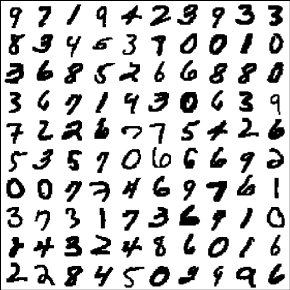
Figure 2-1. 100 random MNIST images
Softmax Regression
In this example we will use a simple classifier called softmax regression. We will not go into the
mathematical formulation of the model in too much detail (there are plenty of good resources
where you can find this information, and we strongly suggest that you do so, if you have never
seen this before). Rather, we will try to provide some intuition into the way the model is able to
solve the digit recognition problem.
Put simply, the softmax regression model will figure out, for each pixel in the image, which
digits tend to have high (or low) values in that location. For instance, the center of the image will
tend to be white for zeros, but black for sixes. Thus, a black pixel in the center of an image will
be evidence against the image containing a zero, and in favor of it containing a six.
Learning in this model consists of finding weights that tell us how to accumulate evidence for the
existence of each of the digits. With softmax regression, we will not use the spatial information
in the pixel layout in the image. Later on, when we discuss convolutional neural networks, we
will see that utilizing spatial information is one of the key elements in making great image-
processing and object-recognition models.
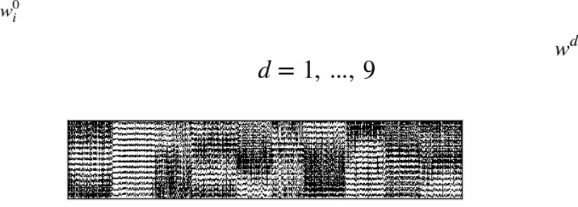
Since we are not going to use the spatial information at this point, we will unroll our image
pixels as a single long vector denoted x (Figure 2-2). Then
xw0 = ∑xi
will be the evidence for the image containing the digit 0 (and in the same way we will have
weight vectors for each one of the other digits, ).
Figure 2-2. MNIST image pixels unrolled to vectors and stacked as columns (sorted by digit from left to right).
While the loss of spatial information doesn’t allow us to recognize the digits, the block structure evident in this
figure is what allows the softmax model to classify images. Essentially, all zeros (leftmost block) share a similar
pixel structure, as do all ones (second block from the left), etc.
All this means is that we sum up the pixel values, each multiplied by a weight, which we think of
as the importance of this pixel in the overall evidence for the digit zero being in the image.2
For instance, w038 will be a large positive number if the 38th pixel having a high intensity points
strongly to the digit being a zero, a strong negative number if high-intensity values in this
position occur mostly in other digits, and zero if the intensity value of the 38th pixel tells us
nothing about whether or not this digit is a zero.3
Performing this calculation at once for all digits (computing the evidence for each of the digits

appearing in the image) can be represented by a single matrix operation. If we place the weights
for each of the digits in the columns of a matrix W, then the length-10 vector with the evidence
for each of the digits is
[xw0···xw9] = xW
The purpose of learning a classifier is almost always to evaluate new examples. In this case, this
means that we would like to be able to tell what digit is written in a new image we have not seen
in our training data. In order to do this, we start by summing up the evidence for each of the 10
possible digits (i.e., computing xW). The final assignment will be the digit that “wins” by
accumulating the most evidence:
digit = argmax(xW)
We start by presenting the code for this example in its entirety (Example 2-2), then walk through
it line by line and go over the details. You may find that there are many novel elements or that
some pieces of the puzzle are missing at this stage, but our advice is that you go with it for now.
Everything will become clear in due course.
Example 2-2. Classifying MNIST handwritten digits with softmax regression
import tensorflow as tf
from tensorflow.examples.tutorials.mnist import input_data
DATA_DIR = '/tmp/data'
NUM_STEPS = 1000
MINIBATCH_SIZE = 100
data = input_data.read_data_sets(DATA_DIR, one_hot=True)
x = tf.placeholder(tf.float32, [None, 784])
W = tf.Variable(tf.zeros([784, 10]))
y_true = tf.placeholder(tf.float32, [None, 10])
y_pred = tf.matmul(x, W)
cross_entropy = tf.reduce_mean(tf.nn.softmax_cross_entropy_with_logits(
logits=y_pred, labels=y_true))
gd_step = tf.train.GradientDescentOptimizer(0.5).minimize(cross_entropy)
correct_mask = tf.equal(tf.argmax(y_pred, 1), tf.argmax(y_true, 1))
accuracy = tf.reduce_mean(tf.cast(correct_mask, tf.float32))
with tf.Session() as sess:
# Train
sess.run(tf.global_variables_initializer())
for _ in range(NUM_STEPS):
batch_xs, batch_ys = data.train.next_batch(MINIBATCH_SIZE)
sess.run(gd_step, feed_dict={x: batch_xs, y_true: batch_ys})
# Test
ans = sess.run(accuracy, feed_dict={x: data.test.images,
y_true: data.test.labels})
print "Accuracy: {:.4}%".format(ans*100)
If you run the code on your machine, you should get output like this:
Extracting /tmp/data/train-images-idx3-ubyte.gz
Extracting /tmp/data/train-labels-idx1-ubyte.gz
Extracting /tmp/data/t10k-images-idx3-ubyte.gz
Extracting /tmp/data/t10k-labels-idx1-ubyte.gz
Accuracy: 91.83%
That’s all it takes! If you have put similar models together before using other platforms, you
might appreciate the simplicity and readability. However, these are just side bonuses, with the
efficiency and flexibility gained from the computation graph model of TensorFlow being what
we are really interested in.
The exact accuracy value you get will be just under 92%. If you run the program once more, you
will get another value. This sort of stochasticity is very common in machine learning code, and
you have probably seen similar results before. In this case, the source is the changing order in
which the handwritten digits are presented to the model during learning. As a result, the learned
parameters following training are slightly different from run to run.
Running the same program five times might therefore produce this result:
Accuracy: 91.86%
Accuracy: 91.51%
Accuracy: 91.62%
Accuracy: 91.93%
Accuracy: 91.88%
We will now briefly go over the code for this example and see what is new from the previous
“hello world” example. We’ll break it down line by line:
import tensorflow as tf
from tensorflow.examples.tutorials.mnist import input_data
The first new element in this example is that we use external data! Rather than downloading the
MNIST dataset (freely available at http://yann.lecun.com/exdb/mnist/) and loading it into our
program, we use a built-in utility for retrieving the dataset on the fly. Such utilities exist for most
popular datasets, and when dealing with small ones (in this case only a few MB), it makes a lot
of sense to do it this way. The second import loads the utility we will later use both to
automatically download the data for us, and to manage and partition it as needed:
DATA_DIR = '/tmp/data'
NUM_STEPS = 1000
MINIBATCH_SIZE = 100
Here we define some constants that we use in our program — these will each be explained in the
context in which they are first used:
data = input_data.read_data_sets(DATA_DIR, one_hot=True)
The read_data_sets() method of the MNIST reading utility downloads the dataset and saves it
locally, setting the stage for further use later in the program. The first argument, DATA_DIR, is the
location we wish the data to be saved to locally. We set this to '/tmp/data', but any other
location would be just as good. The second argument tells the utility how we want the data to be
labeled; we will not go into this right now.4
Note that this is what prints the first four lines of the output, indicating the data was obtained
correctly. Now we are finally ready to set up our model:
x = tf.placeholder(tf.float32, [None, 784])
W = tf.Variable(tf.zeros([784, 10]))
In the previous example we saw the TensorFlow constant element — this is now complemented
by the placeholder and Variable elements. For now, it is enough to know that a variable is an
element manipulated by the computation, while a placeholder has to be supplied when triggering
it. The image itself (x) is a placeholder, because it will be supplied by us when running the
computation graph. The size [None, 784] means that each image is of size 784 (28×28 pixels
unrolled into a single vector), and None is an indicator that we are not currently specifying how
many of these images we will use at once:
y_true = tf.placeholder(tf.float32, [None, 10])
y_pred = tf.matmul(x, W)
In the next chapter these concepts will be dealt with in much more depth.
A key concept in a large class of machine learning tasks is that we would like to learn a function
from data examples (in our case, digit images) to their known labels (the identity of the digit in
the image). This setting is called supervised learning. In most supervised learning models, we
attempt to learn a model such that the true labels and the predicted labels are close in some sense.
Here, y_true and y_pred are the elements representing the true and predicted labels,
respectively:
cross_entropy = tf.reduce_mean(tf.nn.softmax_cross_entropy_with_logits(
logits=y_pred, labels=y_true))
The measure of similarity we choose for this model is what is known as cross entropy — a
natural choice when the model outputs class probabilities. This element is often referred to as the
loss function:5
gd_step = tf.train.GradientDescentOptimizer(0.5).minimize(cross_entropy)
The final piece of the model is how we are going to train it (i.e., how we are going to minimize
the loss function). A very common approach is to use gradient descent optimization. Here, 0.5 is
the learning rate, controlling how fast our gradient descent optimizer shifts model weights to
reduce overall loss.
We will discuss optimizers and how they fit into the computation graph later on in the book.
Once we have defined our model, we want to define the evaluation procedure we will use in
order to test the accuracy of the model. In this case, we are interested in the fraction of test
examples that are correctly classified:6
correct_mask = tf.equal(tf.argmax(y_pred, 1), tf.argmax(y_true, 1))
accuracy = tf.reduce_mean(tf.cast(correct_mask, tf.float32))
As with the “hello world” example, in order to make use of the computation graph we defined,
we must create a session. The rest happens within the session:
with tf.Session() as sess:
First, we must initialize all variables:
sess.run(tf.global_variables_initializer())
This carries some specific implications in the realm of machine learning and optimization, which
we will discuss further when we use models for which initialization is an important issue
SUPERVISED LEARNING AND THE TRAIN/TEST SCHEME
Supervised learning generally refers to the task of learning a function from data objects to labels associated
with them, based on a set of examples where the correct labels are already known. This is usually subdivided
into the case where labels are continuous (regression) or discrete (classification).
The purpose of training supervised learning models is almost always to apply them later to new examples
with unknown labels, in order to obtain predicted labels for them. In the MNIST case discussed in this
section, the purpose of training the model would probably be to apply it on new handwritten digit images and
automatically find out what digits they represent.
As a result, we are interested in the extent to which our model will label new examples correctly. This is
reflected in the way we evaluate the accuracy of the model. We first partition the labeled dataset into train
and test partitions. During model training we use only the train partition, and during evaluation we test the
accuracy only on the test partition. This scheme is generally known as a train/test validation.
for _ in range(NUM_STEPS):
batch_xs, batch_ys = data.train.next_batch(MINIBATCH_SIZE)
sess.run(gd_step, feed_dict={x: batch_xs, y_true: batch_ys})
The actual training of the model, in the gradient descent approach, consists of taking many steps
in “the right direction.” The number of steps we will make, NUM_STEPS, was set to 1,000 in this
case. There are more sophisticated ways of deciding when to stop, but more about that later! In
each step we ask our data manager for a bunch of examples with their labels and present them to
the learner. The MINIBATCH_SIZE constant controls the number of examples to use for each step.
Finally, we use the feed_dict argument of sess.run for the first time. Recall that we defined
placeholder elements when constructing the model. Now, each time we want to run a
computation that will include these elements, we must supply a value for them.
ans = sess.run(accuracy, feed_dict={x: data.test.images,
y_true: data.test.labels})
In order to evaluate the model we have just finished learning, we run the accuracy computing
operation defined earlier (recall the accuracy was defined as the fraction of images that are
correctly labeled). In this procedure, we feed a separate group of test images, which were never
seen by the model during training:
print "Accuracy: {:.4}%".format(ans*100)
Lastly, we print out the results as percent values.
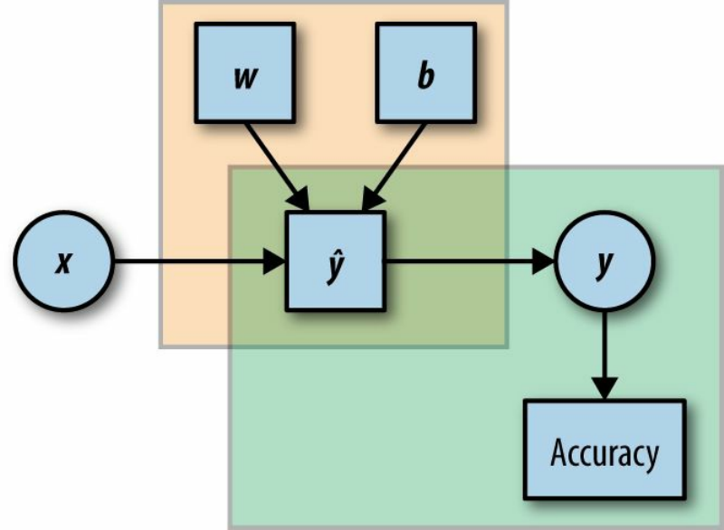
Figure 2-3 shows a graph representation of our model.
Figure 2-3. A graph representation of the model. Rectangular elements are Variables, and circles are
placeholders. The top-left frame represents the label prediction part, and the bottom-right frame the evaluation.

MODEL EVALUATION AND MEMORY ERRORS
When using TensorFlow, like any other system, it is important to be aware of the resources being used,
and make sure not to exceed the capacity of the system. One possible pitfall is in the evaluation of
models — testing their performance on a test set. In this example we evaluate the accuracy of the
models by feeding all the test examples in one go:
feed_dict={x: data.test.images, y_true: data.test.labels}
ans = sess.run(accuracy, feed_dict)
If all the test examples (here, data.test.images) are not able to fit into the memory in the system you
are using, you will get a memory error at this point. This is likely to be the case, for instance, if you are
running this example on a typical low-end GPU.
The easy way around this (getting a machine with more memory is a temporary fix, since there will
always be larger datasets) is to split the test procedure into batches, much as we did during training.

Summary
Congratulations! By now you have installed TensorFlow and taken it for a spin with two basic
examples. You have seen some of the fundamental building blocks that will be used throughout
the book, and have hopefully begun to get a feel for TensorFlow.
Next, we take a look under the hood and explore the computation graph model used by
TensorFlow.
We refer the reader to the official TensorFlow install guide for further details, and especially the ever-
changing details of GPU installations.
It is common to add a “bias term,” which is equivalent to stating which digits we believe an image to be before
seeing the pixel values. If you have seen this before, then try adding it to the model and check how it affects
the results.
If you are familiar with softmax regression, you probably realize this is a simplification of the way it works,
especially when pixel values are as correlated as with digit images.
Here and throughout, before running the example code, make sure DATA_DIR fits the operating system you are
using. On Windows, for instance, you would probably use something like c:\tmp\data instead.
As of TensorFlow 1.0 this is also contained in tf.losses.softmax_cross_entropy.
As of TensorFlow 1.0 this is also contained in tf.metrics.accuracy.
1
2
3
4
5
6

Chapter 3. Understanding TensorFlow Basics
This chapter demonstrates the key concepts of how TensorFlow is built and how it works with
simple and intuitive examples. You will get acquainted with the basics of TensorFlow as a
numerical computation library using dataflow graphs. More specifically, you will learn how to
manage and create a graph, and be introduced to TensorFlow’s “building blocks,” such as
constants, placeholders, and Variables.
Computation Graphs
TensorFlow allows us to implement machine learning algorithms by creating and computing
operations that interact with one another. These interactions form what we call a “computation
graph,” with which we can intuitively represent complicated functional architectures.
What Is a Computation Graph?
We assume a lot of readers have already come across the mathematical concept of a graph. For
those to whom this concept is new, a graph refers to a set of interconnected entities, commonly
called nodes or vertices. These nodes are connected to each other via edges. In a dataflow graph,
the edges allow data to “flow” from one node to another in a directed manner.
In TensorFlow, each of the graph’s nodes represents an operation, possibly applied to some
input, and can generate an output that is passed on to other nodes. By analogy, we can think of
the graph computation as an assembly line where each machine (node) either gets or creates its
raw material (input), processes it, and then passes the output to other machines in an orderly
fashion, producing subcomponents and eventually a final product when the assembly process
comes to an end.
Operations in the graph include all kinds of functions, from simple arithmetic ones such as
subtraction and multiplication to more complex ones, as we will see later on. They also include
more general operations like the creation of summaries, generating constant values, and more.
The Benefits of Graph Computations
TensorFlow optimizes its computations based on the graph’s connectivity. Each graph has its
own set of node dependencies. When the input of node y is affected by the output of node x, we
say that node y is dependent on node x. We call it a direct dependency when the two are
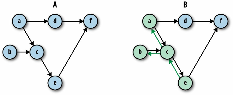
connected via an edge, and an indirect dependency otherwise. For example, in Figure 3-1 (A),
node e is directly dependent on node c, indirectly dependent on node a, and independent of node
d.
Figure 3-1. (A) Illustration of graph dependencies. (B) Computing node e results in the minimal amount of
computations according to the graph’s dependencies — in this case computing only nodes c, b, and a.
We can always identify the full set of dependencies for each node in the graph. This is a
fundamental characteristic of the graph-based computation format. Being able to locate
dependencies between units of our model allows us to both distribute computations across
available resources and avoid performing redundant computations of irrelevant subsets, resulting
in a faster and more efficient way of computing things.
Graphs, Sessions, and Fetches
Roughly speaking, working with TensorFlow involves two main phases: (1) constructing a graph
and (2) executing it. Let’s jump into our first example and create something very basic.
Creating a Graph
Right after we import TensorFlow (with import tensorflow as tf), a specific empty default
graph is formed. All the nodes we create are automatically associated with that default graph.
Using the tf.<operator> methods, we will create six nodes assigned to arbitrarily named
variables. The contents of these variables should be regarded as the output of the operations, and
not the operations themselves. For now we refer to both the operations and their outputs with the
names of their corresponding variables.
The first three nodes are each told to output a constant value. The values 5, 2, and 3 are assigned
to a, b, and c, respectively:
a = tf.constant(5)
b = tf.constant(2)
c = tf.constant(3)
Each of the next three nodes gets two existing variables as inputs, and performs simple
arithmetic operations on them:
d = tf.multiply(a,b)
e = tf.add(c,b)
f = tf.subtract(d,e)
Node d multiplies the outputs of nodes a and b. Node e adds the outputs of nodes b and c. Node
f subtracts the output of node e from that of node d.
And voilà! We have our first TensorFlow graph! Figure 3-2 shows an illustration of the graph
we’ve just created.
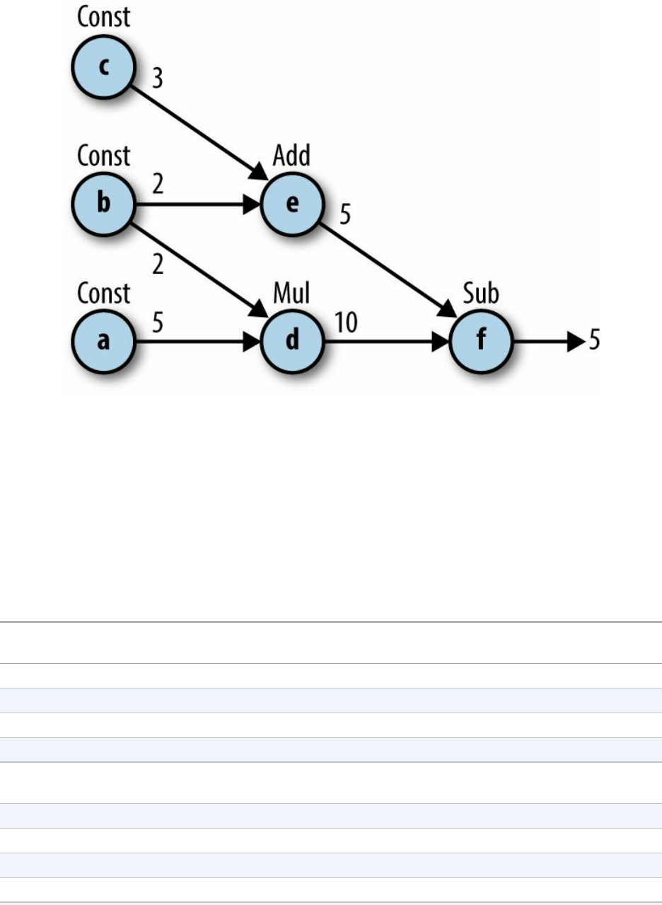
Figure 3-2. An illustration of our first constructed graph. Each node, denoted by a lowercase letter, performs the
operation indicated above it: Const for creating constants and Add, Mul, and Sub for addition, multiplication, and
subtraction, respectively. The integer next to each edge is the output of the corresponding node’s operation.
Note that for some arithmetic and logical operations it is possible to use operation shortcuts
instead of having to apply tf.<operator>. For example, in this graph we could have used */+/-
instead of tf.multiply()/tf.add()/tf.subtract() (like we did in the “hello world” example in
Chapter 2, where we used + instead of tf.add()). Table 3-1 lists the available shortcuts.
Table 3-1. Common TensorFlow operations and their respective shortcuts
TensorFlow
operator
Shortcut Description
tf.add() a + b Adds a and b, element-wise.
tf.multiply() a * b Multiplies a and b, element-wise.
tf.subtract() a - b Subtracts a from b, element-wise.
tf.divide() a / b Computes Python-style division of a by b.
tf.pow() a ** b Returns the result of raising each element in a to its corresponding element b,
element-wise.
tf.mod() a % b Returns the element-wise modulo.
tf.logical_and() a & b Returns the truth table of a & b, element-wise. dtype must be tf.bool.
tf.greater() a > b Returns the truth table of a > b, element-wise.
tf.greater_equal() a >= b Returns the truth table of a >= b, element-wise.

tf.less_equal() a <= b Returns the truth table of a <= b, element-wise.
tf.less() a < b Returns the truth table of a < b, element-wise.
tf.negative() -a Returns the negative value of each element in a.
tf.logical_not() ~a Returns the logical NOT of each element in a. Only compatible with Tensor
objects with dtype of tf.bool.
tf.abs() abs(a) Returns the absolute value of each element in a.
tf.logical_or() a | b Returns the truth table of a | b, element-wise. dtype must be tf.bool.

Creating a Session and Running It
Once we are done describing the computation graph, we are ready to run the computations that it
represents. For this to happen, we need to create and run a session. We do this by adding the
following code:
sess = tf.Session()
outs = sess.run(f)
sess.close()
print("outs = {}".format(outs))
Out:
outs = 5
First, we launch the graph in a tf.Session. A Session object is the part of the TensorFlow API
that communicates between Python objects and data on our end, and the actual computational
system where memory is allocated for the objects we define, intermediate variables are stored,
and finally results are fetched for us.
sess = tf.Session()
The execution itself is then done with the .run() method of the Session object. When called,
this method completes one set of computations in our graph in the following manner: it starts at
the requested output(s) and then works backward, computing nodes that must be executed
according to the set of dependencies. Therefore, the part of the graph that will be computed
depends on our output query.
In our example, we requested that node f be computed and got its value, 5, as output:
outs = sess.run(f)
When our computation task is completed, it is good practice to close the session using the
sess.close() command, making sure the resources used by our session are freed up. This is an
important practice to maintain even though we are not obligated to do so for things to work:
sess.close()
Example 3-1. Try it yourself! Figure 3-3 shows another two graph examples. See if you can
produce these graphs yourself.
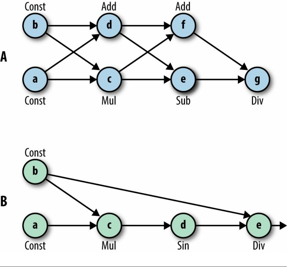
Figure 3-3. Can you create graphs A and B? (To produce the sine function, use tf.sin(x)).
Constructing and Managing Our Graph
As mentioned, as soon as we import TensorFlow, a default graph is automatically created for us.
We can create additional graphs and control their association with some given operations.
tf.Graph() creates a new graph, represented as a TensorFlow object. In this example we create
another graph and assign it to the variable g:
import tensorflow as tf
print(tf.get_default_graph())
g = tf.Graph()
print(g)
Out:
<tensorflow.python.framework.ops.Graph object at 0x7fd88c3c07d0>
<tensorflow.python.framework.ops.Graph object at 0x7fd88c3c03d0>
At this point we have two graphs: the default graph and the empty graph in g. Both are revealed
as TensorFlow objects when printed. Since g hasn’t been assigned as the default graph, any
operation we create will not be associated with it, but rather with the default one.
We can check which graph is currently set as the default by using tf.get_default_graph().
Also, for a given node, we can view the graph it’s associated with by using the
<node>.graph attribute:
g = tf.Graph()
a = tf.constant(5)
print(a.graph is g)
print(a.graph is tf.get_default_graph())
Out:
False
True
In this code example we see that the operation we’ve created is associated with the default graph
and not with the graph in g.
To make sure our constructed nodes are associated with the right graph we can construct them
using a very useful Python construct: the with statement.

THE WITH STATEMENT
The with statement is used to wrap the execution of a block with methods defined by a context
manager — an object that has the special method functions .__enter__() to set up a block of code and
.__exit__() to exit the block.
In layman’s terms, it’s very convenient in many cases to execute some code that requires “setting up”
of some kind (like opening a file, SQL table, etc.) and then always “tearing it down” at the end,
regardless of whether the code ran well or raised any kind of exception. In our case we use with to set
up a graph and make sure every piece of code will be performed in the context of that graph.
We use the with statement together with the as_default() command, which returns a context
manager that makes this graph the default one. This comes in handy when working with multiple
graphs:
g1 = tf.get_default_graph()
g2 = tf.Graph()
print(g1 is tf.get_default_graph())
with g2.as_default():
print(g1 is tf.get_default_graph())
print(g1 is tf.get_default_graph())
Out:
True
False
True
The with statement can also be used to start a session without having to explicitly close it. This
convenient trick will be used in the following examples.
Fetches
In our initial graph example, we request one specific node (node f) by passing the variable it was
assigned to as an argument to the sess.run() method. This argument is called fetches,
corresponding to the elements of the graph we wish to compute. We can also ask sess.run() for
multiple nodes’ outputs simply by inputting a list of requested nodes:
with tf.Session() as sess:
fetches = [a,b,c,d,e,f]
outs = sess.run(fetches)
print("outs = {}".format(outs))
print(type(outs[0]))
Out:
outs = [5, 2, 3, 10, 5, 5]
<type 'numpy.int32'>
We get back a list containing the outputs of the nodes according to how they were ordered in the
input list. The data in each item of the list is of type NumPy.

NUMPY
NumPy is a popular and useful Python package for numerical computing that offers many
functionalities related to working with arrays. We assume some basic familiarity with this package,
and it will not be covered in this book. TensorFlow and NumPy are tightly coupled — for example, the
output returned by sess.run() is a NumPy array. In addition, many of TensorFlow’s operations share
the same syntax as functions in NumPy. To learn more about NumPy, we refer the reader to Eli
Bressert’s book SciPy and NumPy (O’Reilly).
We mentioned that TensorFlow computes only the essential nodes according to the set of
dependencies. This is also manifested in our example: when we ask for the output of node d, only
the outputs of nodes a and b are computed. Another example is shown in Figure 3-1(B). This is a
great advantage of TensorFlow — it doesn’t matter how big and complicated our graph is as a
whole, since we can run just a small portion of it as needed.

AUTOMATICALLY CLOSING THE SESSION
Opening a session using the with clause will ensure the session is automatically closed once all
computations are done.
Flowing Tensors
In this section we will get a better understanding of how nodes and edges are actually
represented in TensorFlow, and how we can control their characteristics. To demonstrate how
they work, we will focus on source operations, which are used to initialize values.
Nodes Are Operations, Edges Are Tensor Objects
When we construct a node in the graph, like we did with tf.add(), we are actually creating an
operation instance. These operations do not produce actual values until the graph is executed, but
rather reference their to-be-computed result as a handle that can be passed on — flow — to
another node. These handles, which we can think of as the edges in our graph, are referred to as
Tensor objects, and this is where the name TensorFlow originates from.
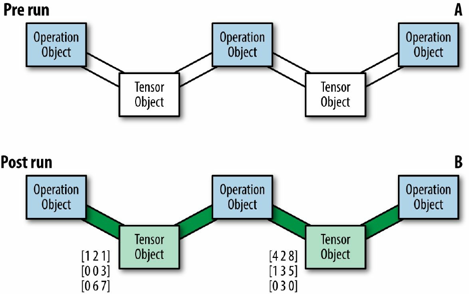
TensorFlow is designed such that first a skeleton graph is created with all of its components. At
this point no actual data flows in it and no computations take place. It is only upon execution,
when we run the session, that data enters the graph and computations occur (as illustrated in
Figure 3-4). This way, computations can be much more efficient, taking the entire graph
structure into consideration.
Figure 3-4. Illustrations of before (A) and after (B) running a session. When the session is run, actual data
“flows” through the graph.
In the previous section’s example, tf.constant() created a node with the corresponding passed
value. Printing the output of the constructor, we see that it’s actually a Tensor object instance.
These objects have methods and attributes that control their behavior and that can be defined
upon creation.
In this example, the variable c stores a Tensor object with the name Const_52:0, designated to
contain a 32-bit floating-point scalar:
c = tf.constant(4.0)
print(c)
Out:
Tensor("Const_52:0", shape=(), dtype=float32)

A NOTE ON CONSTRUCTORS
The tf.<operator> function could be thought of as a constructor, but to be more precise, this is
actually not a constructor at all, but rather a factory method that sometimes does quite a bit more than
just creating the operator objects.
Setting attributes with source operations
Each Tensor object in TensorFlow has attributes such as name, shape, and dtype that help
identify and set the characteristics of that object. These attributes are optional when creating a
node, and are set automatically by TensorFlow when missing. In the next section we will take a
look at these attributes. We will do so by looking at Tensor objects created by ops known as
source operations. Source operations are operations that create data, usually without using any
previously processed inputs. With these operations we can create scalars, as we already
encountered with the tf.constant() method, as well as arrays and other types of data.

Data Types
The basic units of data that pass through a graph are numerical, Boolean, or string
elements. When we print out the Tensor object c from our last code example, we see that its
data type is a floating-point number. Since we didn’t specify the type of data, TensorFlow
inferred it automatically. For example 5 is regarded as an integer, while anything with a decimal
point, like 5.1, is regarded as a floating-point number.
We can explicitly choose what data type we want to work with by specifying it when we create
the Tensor object. We can see what type of data was set for a given Tensor object by using the
attribute dtype:
c = tf.constant(4.0, dtype=tf.float64)
print(c)
print(c.dtype)
Out:
Tensor("Const_10:0", shape=(), dtype=float64)
<dtype: 'float64'>
Explicitly asking for (appropriately sized) integers is on the one hand more memory conserving,
but on the other may result in reduced accuracy as a consequence of not tracking digits after the
decimal point.
Casting
It is important to make sure our data types match throughout the graph — performing an
operation with two nonmatching data types will result in an exception. To change the data type
setting of a Tensor object, we can use the tf.cast() operation, passing the relevant Tensor and
the new data type of interest as the first and second arguments, respectively:
x = tf.constant([1,2,3],name='x',dtype=tf.float32)
print(x.dtype)
x = tf.cast(x,tf.int64)
print(x.dtype)
Out:
<dtype: 'float32'>
<dtype: 'int64'>
TensorFlow supports many data types. These are listed in Table 3-2.
Table 3-2. Supported Tensor data types
Data type Python type Description
DT_FLOAT tf.float32 32-bit floating point.
DT_DOUBLE tf.float64 64-bit floating point.
DT_INT8 tf.int8 8-bit signed integer.
DT_INT16 tf.int16 16-bit signed integer.

DT_INT32 tf.int32 32-bit signed integer.
DT_INT64 tf.int64 64-bit signed integer.
DT_UINT8 tf.uint8 8-bit unsigned integer.
DT_UINT16 tf.uint16 16-bit unsigned integer.
DT_STRING tf.string Variable-length byte array. Each element of a Tensor is a byte array.
DT_BOOL tf.bool Boolean.
DT_COMPLEX64 tf.complex64 Complex number made of two 32-bit floating points: real and imaginary parts.
DT_COMPLEX128 tf.complex128 Complex number made of two 64-bit floating points: real and imaginary parts.
DT_QINT8 tf.qint8 8-bit signed integer used in quantized ops.
DT_QINT32 tf.qint32 32-bit signed integer used in quantized ops.
DT_QUINT8 tf.quint8 8-bit unsigned integer used in quantized ops.
Tensor Arrays and Shapes
A source of potential confusion is that two different things are referred to by the name, Tensor.
As used in the previous sections, Tensor is the name of an object used in the Python API as a
handle for the result of an operation in the graph. However, tensor is also a mathematical term
for n-dimensional arrays. For example, a 1×1 tensor is a scalar, a 1×n tensor is a vector, an n×n
tensor is a matrix, and an n×n×n tensor is just a three-dimensional array. This, of course,
generalizes to any dimension. TensorFlow regards all the data units that flow in the graph as
tensors, whether they are multidimensional arrays, vectors, matrices, or scalars. The TensorFlow
objects called Tensors are named after these mathematical tensors.
To clarify the distinction between the two, from now on we will refer to the former as Tensors
with a capital T and the latter as tensors with a lowercase t.
As with dtype, unless stated explicitly, TensorFlow automatically infers the shape of the data.
When we printed out the Tensor object at the beginning of this section, it showed that its shape
was (), corresponding to the shape of a scalar.
Using scalars is good for demonstration purposes, but most of the time it’s much more practical
to work with multidimensional arrays. To initialize high-dimensional arrays, we can use Python
lists or NumPy arrays as inputs. In the following example, we use as inputs a 2×3 matrix using a
Python list and then a 3D NumPy array of size 2×2×3 (two matrices of size 2×3):
import numpy as np
c = tf.constant([[1,2,3],
[4,5,6]])
print("Python List input: {}".format(c.get_shape()))
c = tf.constant(np.array([
[[1,2,3],
[4,5,6]],
[[1,1,1],
[2,2,2]]
]))
print("3d NumPy array input: {}".format(c.get_shape()))
Out:
Python list input: (2, 3)
3d NumPy array input: (2, 2, 3)
The get_shape() method returns the shape of the tensor as a tuple of integers. The number of
integers corresponds to the number of dimensions of the tensor, and each integer is the number
of array entries along that dimension. For example, a shape of (2,3) indicates a matrix, since it
has two integers, and the size of the matrix is 2×3.
Other types of source operation constructors are very useful for initializing constants in
TensorFlow, like filling a constant value, generating random numbers, and creating sequences.
Random-number generators have special importance as they are used in many cases to create the
initial values for TensorFlow Variables, which will be introduced shortly. For example, we can
generate random numbers from a normal distribution using tf.random.normal(), passing the
shape, mean, and standard deviation as the first, second, and third arguments,
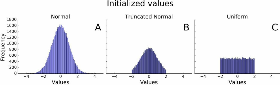
respectively. Another two examples for useful random initializers are the truncated normal that,
as its name implies, cuts off all values below and above two standard deviations from the mean,
and the uniform initializer that samples values uniformly within some interval [a,b).
Examples of sampled values for each of these methods are shown in Figure 3-5.
Figure 3-5. 50,000 random samples generated from (A) standard normal distribution, (B) truncated normal, and
(C) uniform [–2,2).
Those who are familiar with NumPy will recognize some of the initializers, as they share the
same syntax. One example is the sequence generator tf.linspace(a, b, n) that creates n
evenly spaced values from a to b.
A feature that is convenient to use when we want to explore the data content of an object is
tf.InteractiveSession(). Using it and the .eval() method, we can get a full look at the
values without the need to constantly refer to the session object:
sess = tf.InteractiveSession()
c = tf.linspace(0.0, 4.0, 5)
print("The content of 'c':\n {}\n".format(c.eval()))
sess.close()
Out:
The content of 'c':
[ 0. 1. 2. 3. 4.]
INTERACTIVE SESSIONS
tf.InteractiveSession() allows you to replace the usual tf.Session(), so that you don’t need a
variable holding the session for running ops. This can be useful in interactive Python environments,
like when writing IPython notebooks, for instance.
We’ve mentioned only a few of the available source operations. Table 3-2 provides short
descriptions of more useful initializers.
TensorFlow operation Description
tf.constant(value)Creates a tensor populated with the value or values specified by the argument value
tf.fill(shape, value)Creates a tensor of shape shape and fills it with value
tf.zeros(shape)Returns a tensor of shape shape with all elements set to 0
tf.zeros_like(tensor)Returns a tensor of the same type and shape as tensor with all elements set to 0
tf.ones(shape)Returns a tensor of shape shape with all elements set to 1
tf.ones_like(tensor)Returns a tensor of the same type and shape as tensor with all elements set to 1
tf.random_normal(shape,
mean, stddev)
Outputs random values from a normal distribution
tf.truncated_normal(shape,
mean, stddev)
Outputs random values from a truncated normal distribution (values whose
magnitude is more than two standard deviations from the mean are dropped and re-
picked)
tf.random_uniform(shape,
minval, maxval)
Generates values from a uniform distribution in the range [minval, maxval)
tf.random_shuffle(tensor)Randomly shuffles a tensor along its first dimension
Matrix multiplication
This very useful arithmetic operation is performed in TensorFlow via the tf.matmul(A,B)
function for two Tensor objects A and B.
Say we have a Tensor storing a matrix A and another storing a vector x, and we wish to compute
the matrix product of the two:
Ax = b
Before using matmul(), we need to make sure both have the same number of dimensions and that
they are aligned correctly with respect to the intended multiplication.
In the following example, a matrix A and a vector x are created:
A = tf.constant([ [1,2,3],
[4,5,6] ])
print(a.get_shape())
x = tf.constant([1,0,1])
print(x.get_shape())
Out:
(2, 3)
(3,)
In order to multiply them, we need to add a dimension to x, transforming it from a 1D vector to a
2D single-column matrix.
We can add another dimension by passing the Tensor to tf.expand_dims(), together with the
position of the added dimension as the second argument. By adding another dimension in the
second position (index 1), we get the desired outcome:
x = tf.expand_dims(x,1)
print(x.get_shape())
b = tf.matmul(A,x)
sess = tf.InteractiveSession()
print('matmul result:\n {}'.format(b.eval()))
sess.close()
Out:
(3, 1)
matmul result:
[[ 4]
[10]]
If we want to flip an array, for example turning a column vector into a row vector or vice versa,
we can use the tf.transpose() function.
Names
Each Tensor object also has an identifying name. This name is an intrinsic string name, not to be
confused with the name of the variable. As with dtype, we can use the .name attribute to see the
name of the object:
with tf.Graph().as_default():
c1 = tf.constant(4,dtype=tf.float64,name='c')
c2 = tf.constant(4,dtype=tf.int32,name='c')
print(c1.name)
print(c2.name)
Out:
c:0
c_1:0
The name of the Tensor object is simply the name of its corresponding operation (“c”;
concatenated with a colon), followed by the index of that tensor in the outputs of the operation
that produced it — it is possible to have more than one.

DUPLICATE NAMES
Objects residing within the same graph cannot have the same name — TensorFlow forbids it. As a
consequence, it will automatically add an underscore and a number to distinguish the two. Of course,
both objects can have the same name when they are associated with different graphs.
Name scopes
Sometimes when dealing with a large, complicated graph, we would like to create some node
grouping to make it easier to follow and manage. For that we can hierarchically group nodes
together by name. We do so by using tf.name_scope("prefix") together with the useful with
clause again:
with tf.Graph().as_default():
c1 = tf.constant(4,dtype=tf.float64,name='c')
with tf.name_scope("prefix_name"):
c2 = tf.constant(4,dtype=tf.int32,name='c')
c3 = tf.constant(4,dtype=tf.float64,name='c')
print(c1.name)
print(c2.name)
print(c3.name)
Out:
c:0
prefix_name/c:0
prefix_name/c_1:0
In this example we’ve grouped objects contained in variables c2 and c3 under the scope
prefix_name, which shows up as a prefix in their names.
Prefixes are especially useful when we would like to divide a graph into subgraphs with some
semantic meaning. These parts can later be used, for instance, for visualization of the graph
structure.
Variables, Placeholders, and Simple Optimization
In this section we will cover two important types of Tensor objects: Variables and placeholders.
We then move forward to the main event: optimization. We will briefly talk about all the basic
components for optimizing a model, and then do some simple demonstration that puts everything
together.
Variables
The optimization process serves to tune the parameters of some given model. For that
purpose, TensorFlow uses special objects called Variables. Unlike other Tensor objects that are
“refilled” with data each time we run the session, Variables can maintain a fixed state in the
graph. This is important because their current state might influence how they change in the
following iteration. Like other Tensors, Variables can be used as input for other operations in the
graph.
Using Variables is done in two stages. First we call the tf.Variable() function in order to
create a Variable and define what value it will be initialized with. We then have to explicitly
perform an initialization operation by running the session with the
tf.global_variables_initializer() method, which allocates the memory for the Variable
and sets its initial values.
Like other Tensor objects, Variables are computed only when the model runs, as we can see in
the following example:
init_val = tf.random_normal((1,5),0,1)
var = tf.Variable(init_val, name='var')
print("pre run: \n{}".format(var))
init = tf.global_variables_initializer()
with tf.Session() as sess:
sess.run(init)
post_var = sess.run(var)
print("\npost run: \n{}".format(post_var))
Out:
pre run:
Tensor("var/read:0", shape=(1, 5), dtype=float32)
post run:
[[ 0.85962135 0.64885855 0.25370994 -0.37380791 0.63552463]]
Note that if we run the code again, we see that a new variable is created each time, as indicated
by the automatic concatenation of _1 to its name:
pre run:
Tensor("var_1/read:0", shape=(1, 5), dtype=float32)
This could be very inefficient when we want to reuse the model (complex models could have
many variables!); for example, when we wish to feed it with several different inputs. To reuse
the same variable, we can use the tf.get_variables() function instead of tf.Variable().
More on this can be found in “Model Structuring” of the appendix.
Placeholders
So far we’ve used source operations to create our input data. TensorFlow, however, has
designated built-in structures for feeding input values. These structures are called placeholders.
Placeholders can be thought of as empty Variables that will be filled with data later on. We use
them by first constructing our graph and only when it is executed feeding them with the input
data.
Placeholders have an optional shape argument. If a shape is not fed or is passed as None, then the
placeholder can be fed with data of any size. It is common to use None for the dimension of a
matrix that corresponds to the number of samples (usually rows), while having the length of the
features (usually columns) fixed:
ph = tf.placeholder(tf.float32,shape=(None,10))
Whenever we define a placeholder, we must feed it with some input values or else an exception
will be thrown. The input data is passed to the session.run() method as a dictionary, where
each key corresponds to a placeholder variable name, and the matching values are the data values
given in the form of a list or a NumPy array:
sess.run(s,feed_dict={x: X_data,w: w_data})
Let’s see how it looks with another graph example, this time with placeholders for two inputs: a
matrix x and a vector w. These inputs are matrix-multiplied to create a five-unit vector xw and
added with a constant vector b filled with the value -1. Finally, the variable s takes the maximum
value of that vector by using the tf.reduce_max() operation. The word reduce is used because
we are reducing a five-unit vector to a single scalar:
x_data = np.random.randn(5,10)
w_data = np.random.randn(10,1)
with tf.Graph().as_default():
x = tf.placeholder(tf.float32,shape=(5,10))
w = tf.placeholder(tf.float32,shape=(10,1))
b = tf.fill((5,1),-1.)
xw = tf.matmul(x,w)
xwb = xw + b
s = tf.reduce_max(xwb)
with tf.Session() as sess:
outs = sess.run(s,feed_dict={x: x_data,w: w_data})
print("outs = {}".format(outs))
Out:
outs = 3.06512

Optimization
Now we turn to optimization. We first describe the basics of training a model, giving a short
description of each component in the process, and show how it is performed in TensorFlow. We
then demonstrate a full working example of an optimization process of a simple regression
model.
Training to predict
We have some target variable , which we want to explain using some feature vector . To do
so, we first choose a model that relates the two. Our training data points will be used for “tuning”
the model so that it best captures the desired relation. In the following chapters we focus on deep
neural network models, but for now we will settle for a simple regression problem.
Let’s start by describing our regression model:
f(xi) = wTxi + b
yi = f(xi) + εi
f(xi) is assumed to be a linear combination of some input data xi, with a set of weights w and an
intercept b. Our target output yi is a noisy version of f(xi) after being summed with Gaussian
noise εi (where i denotes a given sample).
As in the previous example, we will need to create the appropriate placeholders for our input and
output data and Variables for our weights and intercept:
x = tf.placeholder(tf.float32,shape=[None,3])
y_true = tf.placeholder(tf.float32,shape=None)
w = tf.Variable([[0,0,0]],dtype=tf.float32,name='weights')
b = tf.Variable(0,dtype=tf.float32,name='bias')
Once the placeholders and Variables are defined, we can write down our model. In this example,
it’s simply a multivariate linear regression — our predicted output y_pred is the result of a
matrix multiplication of our input container x and our weights w plus a bias term b:
y_pred = tf.matmul(w,tf.transpose(x)) + b
Defining a loss function
Next, we need a good measure with which we can evaluate the model’s performance. To capture
the discrepancy between our model’s predictions and the observed targets, we need a measure
reflecting “distance.” This distance is often referred to as an objective or a loss function, and we
optimize the model by finding the set of parameters (weights and bias in this case) that minimize
it.
There is no ideal loss function, and choosing the most suitable one is often a blend of art and
science. The choice may depend on several factors, like the assumptions of our model, how easy
it is to minimize, and what types of mistakes we prefer to avoid.
MSE and cross entropy
Perhaps the most commonly used loss is the MSE (mean squared error), where for all samples
we average the squared distances between the real target and what our model predicts across
samples:
This loss has intuitive interpretation — it minimizes the mean square difference between an
observed value and the model’s fitted value (these differences are referred to as residuals).
In our linear regression example, we take the difference between the vector y_true (y), the true
targets, and y_pred (ŷ), the model’s predictions, and use tf.square() to compute the square of
the difference vector. This operation is applied element-wise. We then average the squared
differences using the tf.reduce_mean() function:
loss = tf.reduce_mean(tf.square(y_true-y_pred))
Another very common loss, especially for categorical data, is the cross entropy, which we used
in the softmax classifier in the previous chapter. The cross entropy is given by
H(p,q)=-Σxp(x) log q(x)
and for classification with a single correct label (as is the case in an overwhelming majority of
the cases) reduces to the negative log of the probability placed by the classifier on the correct
label.
In TensorFlow:
loss = tf.nn.sigmoid_cross_entropy_with_logits(labels=y_true,logits=y_pred)
loss = tf.reduce_mean(loss)
Cross entropy is a measure of similarity between two distributions. Since the classification
models used in deep learning typically output probabilities for each class, we can compare the
true class (distribution p) with the probabilities of each class given by the model (distribution q).
The more similar the two distributions, the smaller our cross entropy will be.
The gradient descent optimizer
The next thing we need to figure out is how to minimize the loss function. While in some cases it
is possible to find the global minimum analytically (when it exists), in the great majority of cases
we will have to use an optimization algorithm. Optimizers update the set of weights iteratively in
a way that decreases the loss over time.
The most commonly used approach is gradient descent, where we use the loss’s gradient with
respect to the set of weights. In slightly more technical terms, if our loss is some multivariate
function F(w̄), then in the neighborhood of some point w̄0, the “steepest” direction of decrease of
F(w̄) is obtained by moving from w̄0 in the direction of the negative gradient of F at w̄0.
So if w̄1 = w̄0-γ∇F(w̄0) where ∇F(w̄0) is the gradient of F evaluated at w̄0, then for a small
enough γ:
F(w̄0) ⩾ F(w̄1)
The gradient descent algorithms work well on highly complicated network architectures and
therefore are suitable for a wide variety of problems. More specifically, recent advances make it
possible to compute these gradients by utilizing massively parallel systems, so the approach
scales well with dimensionality (though it can still be painfully time-consuming for large real-
world problems). While convergence to the global minimum is guaranteed for convex functions,
for nonconvex problems (which are essentially all problems in the world of deep learning) they
can get stuck in local minima. In practice, this is often good enough, as is evidenced by the huge
success of the field of deep learning.
Sampling methods
The gradient of the objective is computed with respect to the model parameters and evaluated
using a given set of input samples, xs. How many of the samples should we take for this
calculation? Intuitively, it makes sense to calculate the gradient for the entire set of samples in
order to benefit from the maximum amount of available information. This method, however, has
some shortcomings. For example, it can be very slow and is intractable when the dataset requires
more memory than is available.
A more popular technique is the stochastic gradient descent (SGD), where instead of feeding the
entire dataset to the algorithm for the computation of each step, a subset of the data is sampled
sequentially. The number of samples ranges from one sample at a time to a few hundred, but the
most common sizes are between around 50 to around 500 (usually referred to as mini-batches).
Using smaller batches usually works faster, and the smaller the size of the batch, the faster are
the calculations. However, there is a trade-off in that small samples lead to lower hardware
utilization and tend to have high variance, causing large fluctuations to the objective function.
Nevertheless, it turns out that some fluctuations are beneficial since they enable the set of
parameters to jump to new and potentially better local minima. Using a relatively smaller batch
size is therefore effective in that regard, and is currently overall the preferred approach.
Gradient descent in TensorFlow
TensorFlow makes it very easy and intuitive to use gradient descent algorithms. Optimizers in
TensorFlow compute the gradients simply by adding new operations to the graph, and the
gradients are calculated using automatic differentiation. This means, in general terms, that
TensorFlow automatically computes the gradients on its own, “deriving” them from the
operations and structure of the computation graph.
An important parameter to set is the algorithm’s learning rate, determining how aggressive each
update iteration will be (or in other words, how large the step will be in the direction of the
negative gradient). We want the decrease in the loss to be fast enough on the one hand, but on
the other hand not large enough so that we over-shoot the target and end up at a point with a
higher value of the loss function.
We first create an optimizer by using the GradientDescentOptimizer() function with the
desired learning rate. We then create a train operation that updates our variables by calling the
optimizer.minimize() function and passing in the loss as an argument:
optimizer = tf.train.GradientDescentOptimizer(learning_rate)
train = optimizer.minimize(loss)
The train operation is then executed when it is fed to the sess.run() method.
Wrapping it up with examples
We’re all set to go! Let’s combine all the components we’ve discussed in this section and
optimize the parameters of two models: linear and logistic regression. In these examples we will
create synthetic data with known properties, and see how the model is able to recover these
properties with the process of optimization.
Example 1: linear regression
In this problem we are interested in retrieving a set of weights w and a bias term b, assuming our
target value is a linear combination of some input vector x, with an additional Gaussian
noise εi added to each sample.
For this exercise we will generate synthetic data using NumPy. We create 2,000 samples of x, a
vector with three features, take the inner product of each x sample with a set of weights w ([0.3,
0.5, 0.1]), and add a bias term b (–0.2) and Gaussian noise to the result:
import numpy as np
# === Create data and simulate results =====
x_data = np.random.randn(2000,3)
w_real = [0.3,0.5,0.1]
b_real = -0.2
noise = np.random.randn(1,2000)*0.1
y_data = np.matmul(w_real,x_data.T) + b_real + noise
The noisy samples are shown in Figure 3-6.
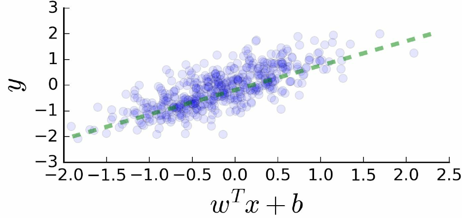
Figure 3-6. Generated data to use for linear regression: each filled circle represents a sample, and the dashed
line shows the expected values without the noise component (the diagonal).
Next, we estimate our set of weights w and bias b by optimizing the model (i.e., finding the best
parameters) so that its predictions match the real targets as closely as possible. Each iteration
computes one update to the current parameters. In this example we run 10 iterations, printing our
estimated parameters every 5 iterations using the sess.run() method.
Don’t forget to initialize the variables! In this example we initialize both the weights and the bias
with zeros; however, there are “smarter” initialization techniques to choose, as we will see in the
next chapters. We use name scopes to group together parts that are related to inferring the output,
defining the loss, and setting and creating the train object:
NUM_STEPS = 10
g = tf.Graph()
wb_ = []
with g.as_default():
x = tf.placeholder(tf.float32,shape=[None,3])
y_true = tf.placeholder(tf.float32,shape=None)
with tf.name_scope('inference') as scope:
w = tf.Variable([[0,0,0]],dtype=tf.float32,name='weights')
b = tf.Variable(0,dtype=tf.float32,name='bias')
y_pred = tf.matmul(w,tf.transpose(x)) + b
with tf.name_scope('loss') as scope:
loss = tf.reduce_mean(tf.square(y_true-y_pred))
with tf.name_scope('train') as scope:
learning_rate = 0.5
optimizer = tf.train.GradientDescentOptimizer(learning_rate)
train = optimizer.minimize(loss)
# Before starting, initialize the variables. We will 'run' this first.
init = tf.global_variables_initializer()
with tf.Session() as sess:
sess.run(init)
for step in range(NUM_STEPS):
sess.run(train,{x: x_data, y_true: y_data})
if (step % 5 == 0):
print(step, sess.run([w,b]))
wb_.append(sess.run([w,b]))
print(10, sess.run([w,b]))
And we get the results:
(0, [array([[ 0.30149955, 0.49303722, 0.11409992]],
dtype=float32), -0.18563795])
(5, [array([[ 0.30094019, 0.49846715, 0.09822173]],
dtype=float32), -0.19780949])
(10, [array([[ 0.30094025, 0.49846718, 0.09822182]],
dtype=float32), -0.19780946])
After only 10 iterations, the estimated weights and bias are = [0.301, 0.498, 0.098] and = –
0.198. The original parameter values were w = [0.3,0.5,0.1] and b = –0.2.
Almost a perfect match!
Example 2: logistic regression
Again we wish to retrieve the weights and bias components in a simulated data setting, this time
in a logistic regression framework. Here the linear component wTx + b is the input of a nonlinear
function called the logistic function. What it effectively does is squash the values of the linear
part into the interval [0, 1]:
Pr(yi = 1|xi) =
We then regard these values as probabilities from which binary yes/1 or no/0 outcomes are
generated. This is the nondeterministic (noisy) part of the model.
The logistic function is more general, and can be used with a different set of parameters for the
steepness of the curve and its maximum value. This special case of a logistic function we are
using is also referred to as a sigmoid function.
We generate our samples by using the same set of weights and biases as in the previous example:
N = 20000
def sigmoid(x):
return 1 / (1 + np.exp(-x))
# === Create data and simulate results =====
x_data = np.random.randn(N,3)
w_real = [0.3,0.5,0.1]
b_real = -0.2
wxb = np.matmul(w_real,x_data.T) + b_real
y_data_pre_noise = sigmoid(wxb)
y_data = np.random.binomial(1,y_data_pre_noise)
The outcome samples before and after the binarization of the output are shown in Figure 3-7.
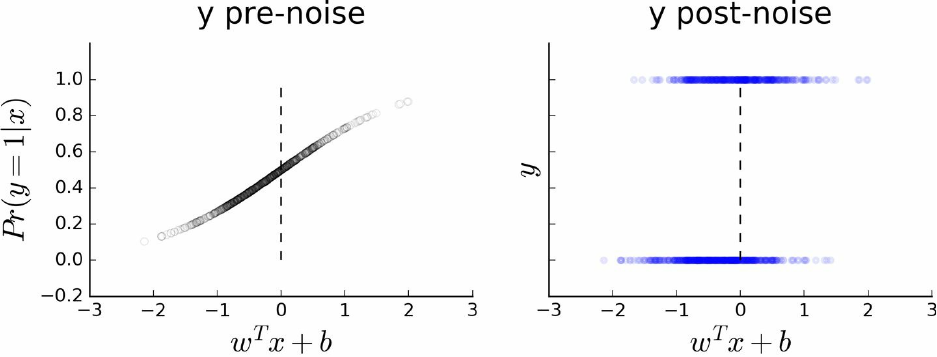
Figure 3-7. Generated data to use for logistic regression: each circle represents a sample. In the left plot we see
the probabilities generated by inputting the linear combination of the input data to the logistic function. The right
plot shows the binary target output, randomly sampled from the probabilities in the left image.
The only thing we need to change in the code is the loss function we use.
The loss we want to use here is the binary version of the cross entropy, which is also the
likelihood of the logistic regression model:
y_pred = tf.sigmoid(y_pred)
loss = y_true*tf.log(y_pred) - (1-y_true)*tf.log(1-y_pred)
loss = tf.reduce_mean(loss)
Luckily, TensorFlow already has a designated function we can use instead:
tf.nn.sigmoid_cross_entropy_with_logits(labels=,logits=)
To which we simply need to pass the true outputs and the model’s linear predictions:
NUM_STEPS = 50
with tf.name_scope('loss') as scope:
loss = tf.nn.sigmoid_cross_entropy_with_logits(labels=y_true,logits=y_pred)
loss = tf.reduce_mean(loss)
# Before starting, initialize the variables. We will 'run' this first.
init = tf.global_variables_initializer()
with tf.Session() as sess:
sess.run(init)
for step in range(NUM_STEPS):
sess.run(train,{x: x_data, y_true: y_data})
if (step % 5 == 0):
print(step, sess.run([w,b]))
wb_.append(sess.run([w,b]))
print(50, sess.run([w,b]))
Let’s see what we get:
(0, [array([[ 0.03212515, 0.05890014, 0.01086476]],
dtype=float32), -0.021875083])
(5, [array([[ 0.14185661, 0.25990966, 0.04818931]],
dtype=float32), -0.097346731])
(10, [array([[ 0.20022796, 0.36665651, 0.06824245]],
dtype=float32), -0.13804035])
(15, [array([[ 0.23269908, 0.42593899, 0.07949805]],
dtype=float32), -0.1608445])
(20, [array([[ 0.2512995 , 0.45984453, 0.08599731]],
dtype=float32), -0.17395383])
(25, [array([[ 0.26214141, 0.47957924, 0.08981277]],
dtype=float32), -0.1816061])
(30, [array([[ 0.26852587, 0.49118528, 0.09207394]],
dtype=float32), -0.18611355])
(35, [array([[ 0.27230808, 0.49805275, 0.09342111]],
dtype=float32), -0.18878292])
(40, [array([[ 0.27455658, 0.50213116, 0.09422609]],
dtype=float32), -0.19036882])
(45, [array([[ 0.27589601, 0.5045585 , 0.09470785]],
dtype=float32), -0.19131286])
(50, [array([[ 0.27656636, 0.50577223, 0.09494986]],
dtype=float32), -0.19178495])
It takes a few more iterations to converge, and more samples are required than in the previous
linear regression example, but eventually we get results that are quite similar to the original
chosen weights.
Summary
In this chapter we learned about computation graphs and what we can use them for. We saw how
to create a graph and how to compute its outputs. We introduced the main building blocks of
TensorFlow — the Tensor object, representing the graph’s operations, placeholders for our input
data, and Variables we tune as part of the model training process. We learned about tensor arrays
and covered the data type, shape, and name attributes. Finally, we discussed the model
optimization process and saw how to implement it in TensorFlow. In the next chapter we will go
into more advanced deep neural networks used in computer vision.

Chapter 4. Convolutional Neural Networks
In this chapter we introduce convolutional neural networks (CNNs) and the building blocks and
methods associated with them. We start with a simple model for classification of the MNIST
dataset, then we introduce the CIFAR10 object-recognition dataset and apply several CNN
models to it. While small and fast, the CNNs presented in this chapter are highly representative
of the type of models used in practice to obtain state-of-the-art results in object-recognition tasks.
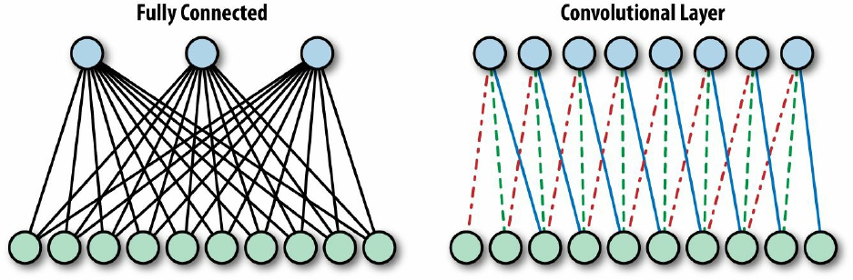
Introduction to CNNs
Convolutional neural networks have gained a special status over the last few years as an
especially promising form of deep learning. Rooted in image processing, convolutional layers
have found their way into virtually all subfields of deep learning, and are very successful for the
most part.
The fundamental difference between fully connected and convolutional neural networks is the
pattern of connections between consecutive layers. In the fully connected case, as the name
might suggest, each unit is connected to all of the units in the previous layer. We saw an example
of this in Chapter 2, where the 10 output units were connected to all of the input image pixels.
In a convolutional layer of a neural network, on the other hand, each unit is connected to a
(typically small) number of nearby units in the previous layer. Furthermore, all units are
connected to the previous layer in the same way, with the exact same weights and structure. This
leads to an operation known as convolution, giving the architecture its name (see Figure 4-1 for
an illustration of this idea). In the next section, we go into the convolution operation in some
more detail, but in a nutshell all it means for us is applying a small “window” of weights (also
known as filters) across an image, as illustrated in Figure 4-2 later.
Figure 4-1. In a fully connected layer (left), each unit is connected to all units of the previous layers. In a
convolutional layer (right), each unit is connected to a constant number of units in a local region of the previous
layer. Furthermore, in a convolutional layer, the units all share the weights for these connections, as indicated by
the shared linetypes.
There are motivations commonly cited as leading to the CNN approach, coming from different
schools of thought. The first angle is the so-called neuroscientific inspiration behind the model.
The second deals with insight into the nature of images, and the third relates to learning theory.
We will go over each of these shortly before diving into the actual mechanics.
It has been popular to describe neural networks in general, and specifically convolutional neural
networks, as biologically inspired models of computation. At times, claims go as far as to state
that these mimic the way the brain performs computations. While misleading when taken at face

value, the biological analogy is of some interest.
The Nobel Prize–winning neurophysiologists Hubel and Wiesel discovered as early as the 1960s
that the first stages of visual processing in the brain consist of application of the same local filter
(e.g., edge detectors) to all parts of the visual field. The current understanding in the
neuroscientific community is that as visual processing proceeds, information is integrated from
increasingly wider parts of the input, and this is done hierarchically.
Convolutional neural networks follow the same pattern. Each convolutional layer looks at an
increasingly larger part of the image as we go deeper into the network. Most commonly, this will
be followed by fully connected layers that in the biologically inspired analogy act as the higher
levels of visual processing dealing with global information.
The second angle, more hard fact engineering–oriented, stems from the nature of images and
their contents. When looking for an object in an image, say the face of a cat, we would typically
want to be able to detect it regardless of its position in the image. This reflects the property of
natural images that the same content may be found in different locations of an image. This is
property is known as an invariance — invariances of this sort can also be expected with respect
to (small) rotations, changing lighting conditions, etc.
Correspondingly, when building an object-recognition system, it should be invariant to
translation (and, depending on the scenario, probably also rotation and deformations of many
sorts, but that is another matter). Put simply, it therefore makes sense to perform the same exact
computation on different parts of the image. In this view, a convolutional neural network layer
computes the same features of an image, across all spatial areas.
Finally, the convolutional structure can be seen as a regularization mechanism. In this view,
convolutional layers are like fully connected layers, but instead of searching for weights in the
full space of matrices (of certain size), we limit the search to matrices describing fixed-size
convolutions, reducing the number of degrees of freedom to the size of the convolution, which is
typically very small.
Regularization
The term regularization is used throughout this book. In machine learning and statistics, regularization
is mostly used to refer to the restriction of an optimization problem by imposing a penalty on the
complexity of the solution, in the attempt to prevent overfitting to the given examples.
Overfitting occurs when a rule (for instance, a classifier) is computed in a way that explains the
training set, but with poor generalization to unseen data.
Regularization is most often applied by adding implicit information regarding the desired results (this
could take the form of saying we would rather have a smoother function, when searching a function
space). In the convolutional neural network case, we explicitly state that we are looking for weights in
a relatively low-dimensional subspace corresponding to fixed-size convolutions.
In this chapter we cover the types of layers and operations associated with convolutional neural
networks. We start by revisiting the MNIST dataset, this time applying a model with
approximately 99% accuracy. Next, we move on to the more interesting object recognition
CIFAR10 dataset.
MNIST: Take II
In this section we take a second look at the MNIST dataset, this time applying a small
convolutional neural network as our classifier. Before doing so, there are several elements and
operations that we must get acquainted with.
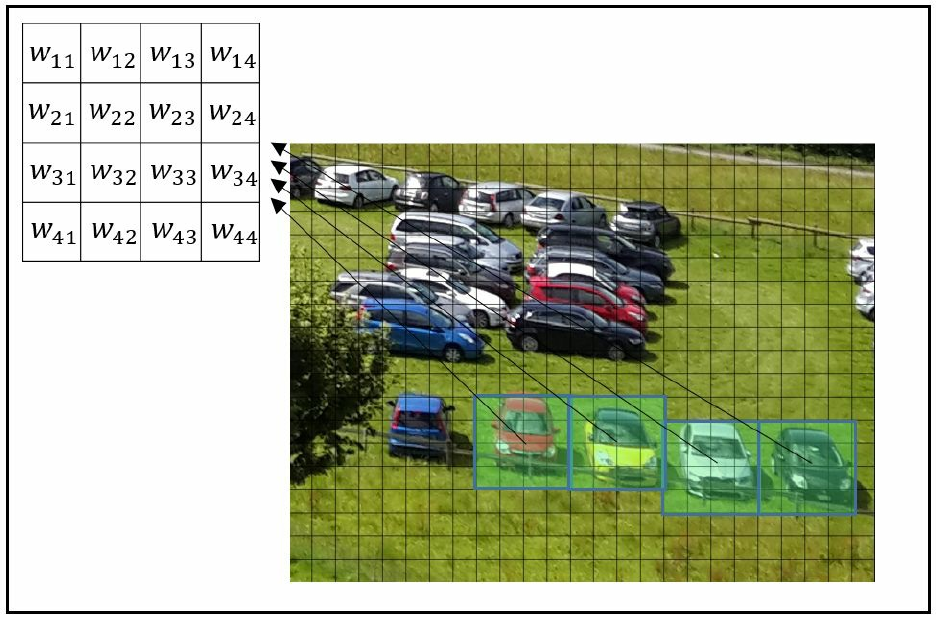
Convolution
The convolution operation, as you probably expect from the name of the architecture, is the
fundamental means by which layers are connected in convolutional neural networks. We use the
built-in TensorFlow conv2d():
tf.nn.conv2d(x, W, strides=[1, 1, 1, 1], padding='SAME')
Here, x is the data — the input image, or a downstream feature map obtained further along in the
network, after applying previous convolution layers. As discussed previously, in typical CNN
models we stack convolutional layers hierarchically, and feature map is simply a commonly used
term referring to the output of each such layer. Another way to view the output of these layers is
as processed images, the result of applying a filter and perhaps some other operations. Here, this
filter is parameterized by W, the learned weights of our network representing the convolution
filter. This is just the set of weights in the small “sliding window” we see in Figure 4-2.
Figure 4-2. The same convolutional filter — a “sliding window” — applied across an image.
The output of this operation will depend on the shape of x and W, and in our case is four-
dimensional. The image data x will be of shape:
[None, 28, 28, 1]
meaning that we have an unknown number of images, each 28×28 pixels and with one color
channel (since these are grayscale images). The weights W we use will be of shape:
[5, 5, 1, 32]
where the initial 5×5×1 represents the size of the small “window” in the image to be convolved,
in our case a 5×5 region. In images that have multiple color channels (RGB, as briefly discussed
in Chapter 1), we regard each image as a three-dimensional tensor of RGB values, but in this
one-channel data they are just two-dimensional, and convolutional filters are applied to two-
dimensional regions. Later, when we tackle the CIFAR10 data, we’ll see examples of multiple-
channel images and how to set the size of weights W accordingly.
The final 32 is the number of feature maps. In other words, we have multiple sets of weights for
the convolutional layer — in this case, 32 of them. Recall that the idea of a convolutional layer is
to compute the same feature along the image; we would simply like to compute many such
features and thus use multiple sets of convolutional filters.
The strides argument controls the spatial movement of the filter W across the image (or feature
map) x.
The value [1, 1, 1, 1] means that the filter is applied to the input in one-pixel intervals in each
dimension, corresponding to a “full” convolution. Other settings of this argument allow us to
introduce skips in the application of the filter — a common practice that we apply later — thus
making the resulting feature map smaller.
Finally, setting padding to 'SAME' means that the borders of x are padded such that the size of
the result of the operation is the same as the size of x.
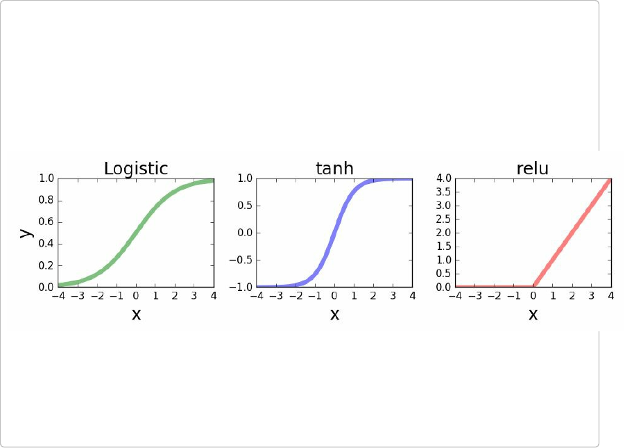
ACTIVATION FUNCTIONS
Following linear layers, whether convolutional or fully connected, it is common practice to apply
nonlinear activation functions (see Figure 4-3 for some examples). One practical aspect of activation
functions is that consecutive linear operations can be replaced by a single one, and thus depth doesn’t
contribute to the expressiveness of the model unless we use nonlinear activations between the linear
layers.
FIGURE 4-3. COMMON ACTIVATION FUNCTIONS: LOGISTIC (LEFT),
HYPERBOLIC TANGENT (CENTER), AND RECTIFYING LINEAR UNIT
(RIGHT)
Pooling
It is common to follow convolutional layers with pooling of outputs. Technically, pooling means
reducing the size of the data with some local aggregation function, typically within each feature
map.
The reasoning behind this is both technical and more theoretical. The technical aspect is that
pooling reduces the size of the data to be processed downstream. This can drastically reduce the
number of overall parameters in the model, especially if we use fully connected layers after the
convolutional ones.
The more theoretical reason for applying pooling is that we would like our computed features not
to care about small changes in position in an image. For instance, a feature looking for eyes in
the top-right part of an image should not change too much if we move the camera a bit to the
right when taking the picture, moving the eyes slightly to the center of the image. Aggregating
the “eye-detector feature” spatially allows the model to overcome such spatial variability
between images, capturing some form of invariance as discussed at the beginning of this chapter.
In our example we apply the max pooling operation on 2×2 blocks of each feature map:
tf.nn.max_pool(x, ksize=[1, 2, 2, 1], strides=[1, 2, 2, 1], padding='SAME')
Max pooling outputs the maximum of the input in each region of a predefined size (here 2×2).
The ksize argument controls the size of the pooling (2×2), and the strides argument controls
by how much we “slide” the pooling grids across x, just as in the case of the convolution layer.
Setting this to a 2×2 grid means that the output of the pooling will be exactly one-half of the
height and width of the original, and in total one-quarter of the size.
Dropout
The final element we will need for our model is dropout. This is a regularization trick used in
order to force the network to distribute the learned representation across all the neurons. Dropout
“turns off” a random preset fraction of the units in a layer, by setting their values to zero during
training. These dropped-out neurons are random — different for each computation — forcing the
network to learn a representation that will work even after the dropout. This process is often
thought of as training an “ensemble” of multiple networks, thereby increasing generalization.
When using the network as a classifier at test time (“inference”), there is no dropout and the full
network is used as is.
The only argument in our example other than the layer we would like to apply dropout to is
keep_prob, the fraction of the neurons to keep working at each step:
tf.nn.dropout(layer, keep_prob=keep_prob)
In order to be able to change this value (which we must do, since for testing we would like this to
be 1.0, meaning no dropout at all), we will use a tf.Variable and pass one value for train (.5)
and another for test (1.0).
The Model
First, we define helper functions that will be used extensively throughout this chapter to create
our layers. Doing this allows the actual model to be short and readable (later in the book we will
see that there exist several frameworks for greater abstraction of deep learning building blocks,
which allow us to concentrate on rapidly designing our networks rather than the somewhat
tedious work of defining all the necessary elements). Our helper functions are:
def weight_variable(shape):
initial = tf.truncated_normal(shape, stddev=0.1)
return tf.Variable(initial)
def bias_variable(shape):
initial = tf.constant(0.1, shape=shape)
return tf.Variable(initial)
def conv2d(x, W):
return tf.nn.conv2d(x, W, strides=[1, 1, 1, 1], padding='SAME')
def max_pool_2x2(x):
return tf.nn.max_pool(x, ksize=[1, 2, 2, 1],
strides=[1, 2, 2, 1], padding='SAME')
def conv_layer(input, shape):
W = weight_variable(shape)
b = bias_variable([shape[3]])
return tf.nn.relu(conv2d(input, W) + b)
def full_layer(input, size):
in_size = int(input.get_shape()[1])
W = weight_variable([in_size, size])
b = bias_variable([size])
return tf.matmul(input, W) + b
Let’s take a closer look at these:
weight_variable()
This specifies the weights for either fully connected or convolutional layers of the network.
They are initialized randomly using a truncated normal distribution with a standard
deviation of .1. This sort of initialization with a random normal distribution that is truncated
at the tails is pretty common and generally produces good results (see the upcoming note on
random initialization).
bias_variable()
This defines the bias elements in either a fully connected or a convolutional layer. These are
all initialized with the constant value of .1.
conv2d()
This specifies the convolution we will typically use. A full convolution (no skips) with an
output the same size as the input.
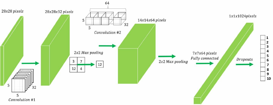
max_pool_2×2
This sets the max pool to half the size across the height/width dimensions, and in total a
quarter the size of the feature map.
conv_layer()
This is the actual layer we will use. Linear convolution as defined in conv2d, with a bias,
followed by the ReLU nonlinearity.
full_layer()
A standard full layer with a bias. Notice that here we didn’t add the ReLU. This allows us to
use the same layer for the final output, where we don’t need the nonlinear part.
With these layers defined, we are ready to set up our model (see the visualization in Figure 4-4):
x = tf.placeholder(tf.float32, shape=[None, 784])
y_ = tf.placeholder(tf.float32, shape=[None, 10])
x_image = tf.reshape(x, [-1, 28, 28, 1])
conv1 = conv_layer(x_image, shape=[5, 5, 1, 32])
conv1_pool = max_pool_2x2(conv1)
conv2 = conv_layer(conv1_pool, shape=[5, 5, 32, 64])
conv2_pool = max_pool_2x2(conv2)
conv2_flat = tf.reshape(conv2_pool, [-1, 7*7*64])
full_1 = tf.nn.relu(full_layer(conv2_flat, 1024))
keep_prob = tf.placeholder(tf.float32)
full1_drop = tf.nn.dropout(full_1, keep_prob=keep_prob)
y_conv = full_layer(full1_drop, 10)
Figure 4-4. A visualization of the CNN architecture used.

RANDOM INITIALIZATION
In the previous chapter we discussed initializers of several types, including the random initializer used
here for our convolutional layer’s weights:
initial = tf.truncated_normal(shape, stddev=0.1)
Much has been said about the importance of initialization in the training of deep learning models. Put
simply, a bad initialization can make the training process “get stuck,” or fail completely due to
numerical issues. Using random rather than constant initializations helps break the symmetry between
learned features, allowing the model to learn a diverse and rich representation. Using bound values
helps, among other things, to control the magnitude of the gradients, allowing the network to converge
more efficiently.
We start by defining the placeholders for the images and correct labels, x and y_, respectively.
Next, we reshape the image data into the 2D image format with size 28×28×1. Recall we did not
need this spatial aspect of the data for our previous MNIST model, since all pixels were treated
independently, but a major source of power in the convolutional neural network framework is the
utilization of this spatial meaning when considering images.
Next we have two consecutive layers of convolution and pooling, each with 5×5 convolutions
and 64 feature maps, followed by a single fully connected layer with 1,024 units. Before
applying the fully connected layer we flatten the image back to a single vector form, since the
fully connected layer no longer needs the spatial aspect.
Notice that the size of the image following the two convolution and pooling layers is 7×7×64.
The original 28×28 pixel image is reduced first to 14×14, and then to 7×7 in the two pooling
operations. The 64 is the number of feature maps we created in the second convolutional layer.
When considering the total number of learned parameters in the model, a large proportion will be
in the fully connected layer (going from 7×7×64 to 1,024 gives us 3.2 million parameters). This
number would have been 16 times as large (i.e., 28×28×64×1,024, which is roughly 51 million)
if we hadn’t used max-pooling.
Finally, the output is a fully connected layer with 10 units, corresponding to the number of labels
in the dataset (recall that MNIST is a handwritten digit dataset, so the number of possible labels
is 10).
The rest is the same as in the first MNIST model in Chapter 2, with a few minor changes:
train_accuracy
We print the accuracy of the model on the batch used for training every 100 steps. This is
done before the training step, and therefore is a good estimate of the current performance of
the model on the training set.
test_accuracy
We split the test procedure into 10 blocks of 1,000 images each. Doing this is important
mostly for much larger datasets.
Here’s the complete code:
mnist = input_data.read_data_sets(DATA_DIR, one_hot=True)
cross_entropy = tf.reduce_mean(tf.nn.softmax_cross_entropy_with_logits(y_conv,
y_))
train_step = tf.train.AdamOptimizer(1e-4).minimize(cross_entropy)
correct_prediction = tf.equal(tf.argmax(y_conv, 1), tf.argmax(y_, 1))
accuracy = tf.reduce_mean(tf.cast(correct_prediction, tf.float32))
with tf.Session() as sess:
sess.run(tf.global_variables_initializer())
for i in range(STEPS):
batch = mnist.train.next_batch(50)
if i % 100 == 0:
train_accuracy = sess.run(accuracy, feed_dict={x: batch[0],
y_: batch[1],
keep_prob: 1.0})
print "step {}, training accuracy {}".format(i, train_accuracy)
sess.run(train_step, feed_dict={x: batch[0], y_: batch[1],
keep_prob: 0.5})
X = mnist.test.images.reshape(10, 1000, 784)
Y = mnist.test.labels.reshape(10, 1000, 10)
test_accuracy = np.mean([sess.run(accuracy,
feed_dict={x:X[i], y_:Y[i],keep_prob:1.0})
for i in range(10)])
print "test accuracy: {}".format(test_accuracy)
The performance of this model is already relatively good, with just over 99% correct after as
little as 5 epocs,1 which are 5,000 steps with mini-batches of size 50.
For a list of models that have been used over the years with this dataset, and some ideas on how
to further improve this result, take a look at http://yann.lecun.com/exdb/mnist/.
CIFAR10
CIFAR10 is another dataset with a long history in computer vision and machine learning. Like
MNIST, it is a common benchmark that various methods are tested against. CIFAR10 is a set of
60,000 color images of size 32×32 pixels, each belonging to one of ten categories: airplane,
automobile, bird, cat, deer, dog, frog, horse, ship, and truck.
State-of-the-art deep learning methods for this dataset are as good as humans at classifying these
images. In this section we start off with much simpler methods that will run relatively quickly.
Then, we discuss briefly what the gap is between these and the state of the art.

Loading the CIFAR10 Dataset
In this section we build a data manager for CIFAR10, similarly to the built-in
input_data.read_data_sets() we used for MNIST.2
First, download the Python version of the dataset and extract the files into a local directory. You
should now have the following files:
data_batch_1, data_batch_2, data_batch_3, data_batch_4, data_batch_5
test_batch
batches_meta
readme.html
The data_batch_X files are serialized data files containing the training data, and test_batch is a
similar serialized file containing the test data. The batches_meta file contains the mapping from
numeric to semantic labels. The .html file is a copy of the CIFAR-10 dataset’s web page.
Since this is a relatively small dataset, we load it all into memory:
class CifarLoader(object):
def __init__(self, source_files):
self._source = source_files
self._i = 0
self.images = None
self.labels = None
def load(self):
data = [unpickle(f) for f in self._source]
images = np.vstack([d["data"] for d in data])
n = len(images)
self.images = images.reshape(n, 3, 32, 32).transpose(0, 2, 3, 1)\
.astype(float) / 255
self.labels = one_hot(np.hstack([d["labels"] for d in data]), 10)
return self
def next_batch(self, batch_size):
x, y = self.images[self._i:self._i+batch_size],
self.labels[self._i:self._i+batch_size]
self._i = (self._i + batch_size) % len(self.images)
return x, y
where we use the following utility functions:
DATA_PATH = "/path/to/CIFAR10"
def unpickle(file):
with open(os.path.join(DATA_PATH, file), 'rb') as fo:
dict = cPickle.load(fo)
return dict
def one_hot(vec, vals=10):
n = len(vec)
out = np.zeros((n, vals))
out[range(n), vec] = 1
return out
The unpickle() function returns a dict with fields data and labels, containing the image data
and the labels, respectively. one_hot() recodes the labels from integers (in the range 0 to 9) to
vectors of length 10, containing all 0s except for a 1 at the position of the label.
Finally, we create a data manager that includes both the training and test data:
class CifarDataManager(object):
def __init__(self):
self.train = CifarLoader(["data_batch_{}".format(i)
for i in range(1, 6)])
.load()
self.test = CifarLoader(["test_batch"]).load()
Using Matplotlib, we can now use the data manager in order to display some of the CIFAR10
images and get a better idea of what is in this dataset:
def display_cifar(images, size):
n = len(images)
plt.figure()
plt.gca().set_axis_off()
im = np.vstack([np.hstack([images[np.random.choice(n)] for i in range(size)])
for i in range(size)])
plt.imshow(im)
plt.show()
d = CifarDataManager()
print "Number of train images: {}".format(len(d.train.images))
print "Number of train labels: {}".format(len(d.train.labels))
print "Number of test images: {}".format(len(d.test.images))
print "Number of test images: {}".format(len(d.test.labels))
images = d.train.images
display_cifar(images, 10)
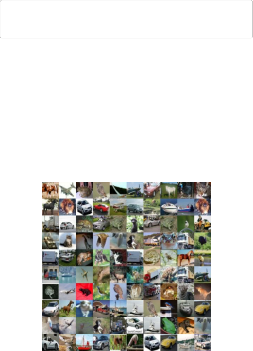
MATPLOTLIB
Matplotlib is a useful Python library for plotting, designed to look and behave like MATLAB plots. It
is often the easiest way to quickly plot and visualize a dataset.
The display_cifar()function takes as arguments images (an iterable containing images), and
size (the number of images we would like to display), and constructs and displays a size×size
grid of images. This is done by concatenating the actual images vertically and horizontally to
form a large image.
Before displaying the image grid, we start by printing the sizes of the train/test sets. CIFAR10
contains 50K training images and 10K test images:
Number of train images: 50000
Number of train labels: 50000
Number of test images: 10000
Number of test images: 10000
The image produced and shown in Figure 4-5 is meant to give some idea of what CIFAR10
images actually look like. Notably, these small, 32×32 pixel images each contain a full single
object that is both centered and more or less recognizable even at this resolution.
Figure 4-5. 100 random CIFAR10 images.
Simple CIFAR10 Models
We will start by using the model that we have previously used successfully for the MNIST
dataset. Recall that the MNIST dataset is composed of 28×28-pixel grayscale images, while the
CIFAR10 images are color images with 32×32 pixels. This will necessitate minor adaptations to
the setup of the computation graph:
cifar = CifarDataManager()
x = tf.placeholder(tf.float32, shape=[None, 32, 32, 3])
y_ = tf.placeholder(tf.float32, shape=[None, 10])
keep_prob = tf.placeholder(tf.float32)
conv1 = conv_layer(x, shape=[5, 5, 3, 32])
conv1_pool = max_pool_2x2(conv1)
conv2 = conv_layer(conv1_pool, shape=[5, 5, 32, 64])
conv2_pool = max_pool_2x2(conv2)
conv2_flat = tf.reshape(conv2_pool, [-1, 8 * 8 * 64])
full_1 = tf.nn.relu(full_layer(conv2_flat, 1024))
full1_drop = tf.nn.dropout(full_1, keep_prob=keep_prob)
y_conv = full_layer(full1_drop, 10)
cross_entropy = tf.reduce_mean(tf.nn.softmax_cross_entropy_with_logits(y_conv,
y_))
train_step = tf.train.AdamOptimizer(1e-3).minimize(cross_entropy)
correct_prediction = tf.equal(tf.argmax(y_conv, 1), tf.argmax(y_, 1))
accuracy = tf.reduce_mean(tf.cast(correct_prediction, tf.float32))
def test(sess):
X = cifar.test.images.reshape(10, 1000, 32, 32, 3)
Y = cifar.test.labels.reshape(10, 1000, 10)
acc = np.mean([sess.run(accuracy, feed_dict={x: X[i], y_: Y[i],
keep_prob: 1.0})
for i in range(10)])
print "Accuracy: {:.4}%".format(acc * 100)
with tf.Session() as sess:
sess.run(tf.global_variables_initializer())
for i in range(STEPS):
batch = cifar.train.next_batch(BATCH_SIZE)
sess.run(train_step, feed_dict={x: batch[0], y_: batch[1],
keep_prob: 0.5})
test(sess)
This first attempt will achieve approximately 70% accuracy within a few minutes (using a batch
size of 100, and depending naturally on hardware and configurations). Is this good? As of now,
state-of-the-art deep learning methods achieve over 95% accuracy on this dataset,3 but using
much larger models and usually many, many hours of training.
There are a few differences between this and the similar MNIST model presented earlier. First,
the input consists of images of size 32×32×3, the third dimension being the three color channels:
x = tf.placeholder(tf.float32, shape=[None, 32, 32, 3])
Similarly, after the two pooling operations, we are left this time with 64 feature maps of size
8×8:
conv2_flat = tf.reshape(conv2_pool, [-1, 8 * 8 * 64])
Finally, as a matter of convenience, we group the test procedure into a separate function called
test(), and we do not print training accuracy values (which can be added back in using the same
code as in the MNIST model).
Once we have a model with some acceptable baseline accuracy (whether derived from a simple
MNIST model or from a state-of-the-art model for some other dataset), a common practice is to
try to improve it by means of a sequence of adaptations and changes, until reaching what is
necessary for our purposes.
In this case, leaving all the rest the same, we will add a third convolution layer with 128 feature
maps and dropout. We will also reduce the number of units in the fully connected layer from
1,024 to 512:
x = tf.placeholder(tf.float32, shape=[None, 32, 32, 3])
y_ = tf.placeholder(tf.float32, shape=[None, 10])
keep_prob = tf.placeholder(tf.float32)
conv1 = conv_layer(x, shape=[5, 5, 3, 32])
conv1_pool = max_pool_2x2(conv1)
conv2 = conv_layer(conv1_pool, shape=[5, 5, 32, 64])
conv2_pool = max_pool_2x2(conv2)
conv3 = conv_layer(conv2_pool, shape=[5, 5, 64, 128])
conv3_pool = max_pool_2x2(conv3)
conv3_flat = tf.reshape(conv3_pool, [-1, 4 * 4 * 128])
conv3_drop = tf.nn.dropout(conv3_flat, keep_prob=keep_prob)
full_1 = tf.nn.relu(full_layer(conv3_drop, 512))
full1_drop = tf.nn.dropout(full_1, keep_prob=keep_prob)
y_conv = full_layer(full1_drop, 10)
This model will take slightly longer to run (but still way under an hour, even without
sophisticated hardware) and achieve an accuracy of approximately 75%.
There is still a rather large gap between this and the best known methods. There are several
independently applicable elements that can help close this gap:
Model size
Most successful methods for this and similar datasets use much deeper networks with many
more adjustable parameters.
Additional types of layers and methods
Additional types of popular layers are often used together with the layers presented here,
such as local response normalization.
Optimization tricks
More about this later!
Domain knowledge
Pre-processing utilizing domain knowledge often goes a long way. In this case that would
be good old-fashioned image processing.
Data augmentation
Adding training data based on the existing set can help. For instance, if an image of a dog is
flipped horizontally, then it is clearly still an image of a dog (but what about a vertical
flip?). Small shifts and rotations are also commonly used.
Reusing successful methods and architectures
As in most engineering fields, starting from a time-proven method and adapting it to your
needs is often the way to go. In the field of deep learning this is often done by fine-tuning
pretrained models.
The final model we will present in this chapter is a smaller version of the type of model that
actually produces great results for this dataset. This model is still compact and fast, and achieves
approximately 83% accuracy after ~150 epocs:
C1, C2, C3 = 30, 50, 80
F1 = 500
conv1_1 = conv_layer(x, shape=[3, 3, 3, C1])
conv1_2 = conv_layer(conv1_1, shape=[3, 3, C1, C1])
conv1_3 = conv_layer(conv1_2, shape=[3, 3, C1, C1])
conv1_pool = max_pool_2x2(conv1_3)
conv1_drop = tf.nn.dropout(conv1_pool, keep_prob=keep_prob)
conv2_1 = conv_layer(conv1_drop, shape=[3, 3, C1, C2])
conv2_2 = conv_layer(conv2_1, shape=[3, 3, C2, C2])
conv2_3 = conv_layer(conv2_2, shape=[3, 3, C2, C2])
conv2_pool = max_pool_2x2(conv2_3)
conv2_drop = tf.nn.dropout(conv2_pool, keep_prob=keep_prob)
conv3_1 = conv_layer(conv2_drop, shape=[3, 3, C2, C3])
conv3_2 = conv_layer(conv3_1, shape=[3, 3, C3, C3])
conv3_3 = conv_layer(conv3_2, shape=[3, 3, C3, C3])
conv3_pool = tf.nn.max_pool(conv3_3, ksize=[1, 8, 8, 1], strides=[1, 8, 8, 1],
padding='SAME')
conv3_flat = tf.reshape(conv3_pool, [-1, C3])
conv3_drop = tf.nn.dropout(conv3_flat, keep_prob=keep_prob)
full1 = tf.nn.relu(full_layer(conv3_flat, F1))
full1_drop = tf.nn.dropout(full1, keep_prob=keep_prob)
y_conv = full_layer(full1_drop, 10)
This model consists of three blocks of convolutional layers, followed by the fully connected and
output layers we have already seen a few times before. Each block of convolutional layers
contains three consecutive convolutional layers, followed by a single pooling and dropout.
The constants C1, C2, and C3 control the number of feature maps in each layer of each of the
convolutional blocks, and the constant F1 controls the number of units in the fully connected
layer.
After the third block of convolutional layers, we use an 8×8 max pool layer:
conv3_pool = tf.nn.max_pool(conv3_3, ksize=[1, 8, 8, 1], strides=[1, 8, 8, 1],
padding='SAME')
Since at this point the feature maps are of size 8×8 (following the first two poolings that each
reduced the 32×32 pictures by half on each axis), this globally pools each of the feature maps
and keeps only the maximal value. The number of feature maps at the third block was set to 80,
so at this point (following the max pooling) the representation is reduced to only 80 numbers.
This keeps the overall size of the model small, as the number of parameters in the transition to
the fully connected layer is kept down to 80×500.

Summary
In this chapter we introduced convolutional neural networks and the various building blocks they
are typically made of. Once you are able to get small models working properly, try running
larger and deeper ones, following the same principles. While you can always have a peek in the
latest literature and see what works, a lot can be learned from trial and error and figuring some of
it out for yourself. In the next chapters, we will see how to work with text and sequence data and
how to use TensorFlow abstractions to build CNN models with ease.
In machine learning and especially in deep learning, an epoc refers to a single pass over all the training data;
i.e., when the learning model has seen each training example exactly one time.
This is done mostly for the purpose of illustration. There are existing open source libraries containing this sort
of data wrapper built in, for many popular datasets. See, for example, the datasets module in Keras
(keras.datasets), and specifically keras.datasets.cifar10.
See Who Is the Best in CIFAR-10? for a list of methods and associated papers.
1
2
3

Chapter 5. Text I: Working with Text and
Sequences, and TensorBoard Visualization
In this chapter we show how to work with sequences in TensorFlow, and in particular text. We
begin by introducing recurrent neural networks (RNNs), a powerful class of deep learning
algorithms particularly useful and popular in natural language processing (NLP). We show how
to implement RNN models from scratch, introduce some important TensorFlow capabilities, and
visualize the model with the interactive TensorBoard. We then explore how to use an RNN in a
supervised text classification problem with word-embedding training. Finally, we show how to
build a more advanced RNN model with long short-term memory (LSTM) networks and how to
handle sequences of variable length.
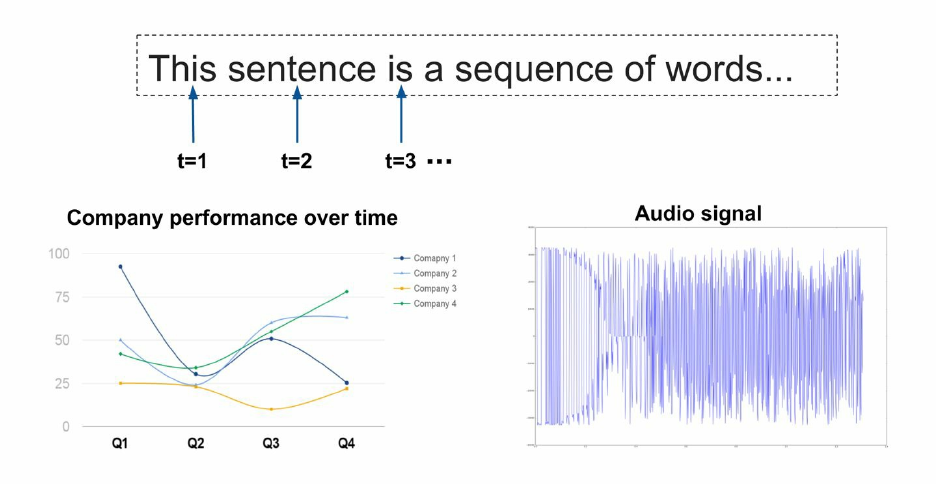
The Importance of Sequence Data
We saw in the previous chapter that using the spatial structure of images can lead to advanced
models with excellent results. As discussed in that chapter, exploiting structure is the key to
success. As we will see shortly, an immensely important and useful type of structure is the
sequential structure. Thinking in terms of data science, this fundamental structure appears in
many datasets, across all domains. In computer vision, video is a sequence of visual content
evolving over time. In speech we have audio signals, in genomics gene sequences; we have
longitudinal medical records in healthcare, financial data in the stock market, and so on (see
Figure 5-1).
Figure 5-1. The ubiquity of sequence data.
A particularly important type of data with strong sequential structure is natural language — text
data. Deep learning methods that exploit the sequential structure inherent in texts — characters,
words, sentences, paragraphs, documents — are at the forefront of natural language
understanding (NLU) systems, often leaving more traditional methods in the dust. There are a
great many types of NLU tasks that are of interest to solve, ranging from document classification
to building powerful language models, from answering questions automatically to generating
human-level conversation agents. These tasks are fiendishly difficult, garnering the efforts and
attention of the entire AI community in both academia and industry.
In this chapter, we focus on the basic building blocks and tasks, and show how to work with
sequences — primarily of text — in TensorFlow. We take a detailed deep dive into the core
elements of sequence models in TensorFlow, implementing some of them from scratch, to gain a
thorough understanding. In the next chapter we show more advanced text modeling techniques
Introduction to Recurrent Neural Networks
Recurrent neural networks are a powerful and widely used class of neural network architectures
for modeling sequence data. The basic idea behind RNN models is that each new element in the
sequence contributes some new information, which updates the current state of the model.
In the previous chapter, which explored computer vision with CNN models, we discussed how
those architectures are inspired by the current scientific perceptions of the way the human brain
processes visual information. These scientific perceptions are often rather close to our
commonplace intuition from our day-to-day lives about how we process sequential information.
When we receive new information, clearly our “history” and “memory” are not wiped out, but
instead “updated.” When we read a sentence in some text, with each new word, our current state
of information is updated, and it is dependent not only on the new observed word but on the
words that preceded it.
A fundamental mathematical construct in statistics and probability, which is often used as a
building block for modeling sequential patterns via machine learning is the Markov chain model.
Figuratively speaking, we can view our data sequences as “chains,” with each node in the chain
dependent in some way on the previous node, so that “history” is not erased but carried on.
RNN models are also based on this notion of chain structure, and vary in how exactly they
maintain and update information. As their name implies, recurrent neural nets apply some form
of “loop.” As seen in Figure 5-2, at some point in time t, the network observes an input xt (a
word in a sentence) and updates its “state vector” to ht from the previous vector ht-1. When we
process new input (the next word), it will be done in some manner that is dependent on ht and
thus on the history of the sequence (the previous words we’ve seen affect our understanding of
the current word). As seen in the illustration, this recurrent structure can simply be viewed as one
long unrolled chain, with each node in the chain performing the same kind of processing “step”
based on the “message” it obtains from the output of the previous node. This, of course, is very
related to the Markov chain models discussed previously and their hidden Markov model
(HMM) extensions, which are not discussed in this book.
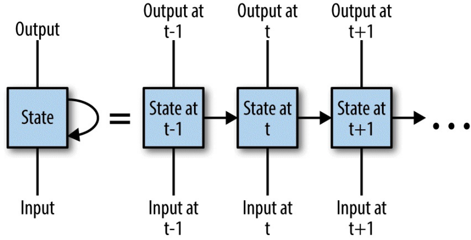
Figure 5-2. Recurrent neural networks updating with new information received over time.
Vanilla RNN Implementation
In this section we implement a basic RNN from scratch, explore its inner workings, and gain
insight into how TensorFlow can work with sequences. We introduce some powerful, fairly low-
level tools that TensorFlow provides for working with sequence data, which you can use to
implement your own systems.
In the next sections, we will show how to use higher-level TensorFlow RNN modules.
We begin with defining our basic model mathematically. This mainly consists of defining the
recurrence structure — the RNN update step.
The update step for our simple vanilla RNN is
ht = tanh(Wxxt + Whht-1 + b)
where Wh, Wx, and b are weight and bias variables we learn, tanh(·) is the hyperbolic tangent
function that has its range in [–1,1] and is strongly connected to the sigmoid function used in
previous chapters, and xt and ht are the input and state vectors as defined previously. Finally, the
hidden state vector is multiplied by another set of weights, yielding the outputs that appear in
Figure 5-2.
MNIST images as sequences
To get a first taste of the power and general applicability of sequence models, in this section we
implement our first RNN to solve the MNIST image classification task that you are by now
familiar with. Later in this chapter we will focus on sequences of text, and see how neural
sequence models can powerfully manipulate them and extract information to solve NLU tasks.
But, you may ask, what have images got to do with sequences?
As we saw in the previous chapter, the architecture of convolutional neural networks makes use
of the spatial structure of images. While the structure of natural images is well suited for CNN
models, it is revealing to look at the structure of images from different angles. In a trend in
cutting-edge deep learning research, advanced models attempt to exploit various kinds of
sequential structures in images, trying to capture in some sense the “generative process” that
created each image. Intuitively, this all comes down to the notion that nearby areas in images are
somehow related, and trying to model this structure.
Here, to introduce basic RNNs and how to work with sequences, we take a simple sequential
view of images: we look at each image in our data as a sequence of rows (or columns). In our
MNIST data, this just means that each 28×28-pixel image can be viewed as a sequence of length
28, each element in the sequence a vector of 28 pixels (see Figure 5-3). Then, the temporal
dependencies in the RNN can be imaged as a scanner head, scanning the image from top to
bottom (rows) or left to right (columns).
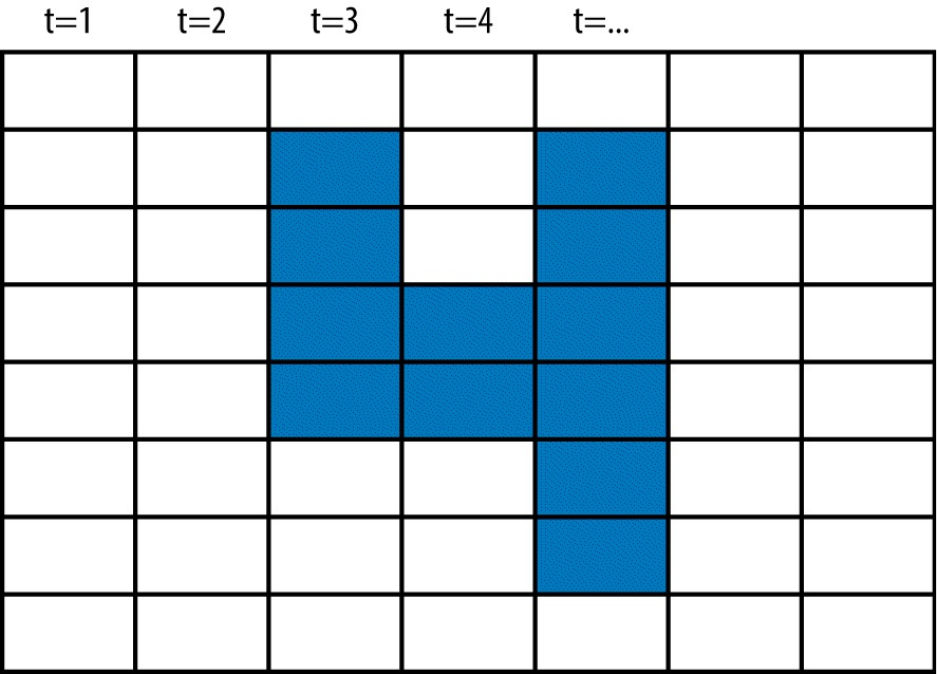
Figure 5-3. An image as a sequence of pixel columns.
We start by loading data, defining some parameters, and creating placeholders for our data:
import tensorflow as tf
# Import MNIST data
from tensorflow.examples.tutorials.mnist import input_data
mnist = input_data.read_data_sets("/tmp/data/", one_hot=True)
# Define some parameters
element_size = 28
time_steps = 28
num_classes = 10
batch_size = 128
hidden_layer_size = 128
# Where to save TensorBoard model summaries
LOG_DIR = "logs/RNN_with_summaries"
# Create placeholders for inputs, labels
_inputs = tf.placeholder(tf.float32,shape=[None, time_steps,
element_size],
name='inputs')
y = tf.placeholder(tf.float32, shape=[None, num_classes],
name='labels')
element_size is the dimension of each vector in our sequence — in our case, a row/column of
28 pixels. time_steps is the number of such elements in a sequence.
As we saw in previous chapters, when we load data with the built-in MNIST data loader, it
comes in unrolled form — a vector of 784 pixels. When we load batches of data during training
(we’ll get to that later in this section), we simply reshape each unrolled vector to [batch_size,
time_steps, element_size]:
batch_x, batch_y = mnist.train.next_batch(batch_size)
# Reshape data to get 28 sequences of 28 pixels
batch_x = batch_x.reshape((batch_size, time_steps, element_size))
We set hidden_layer_size (arbitrarily to 128, controlling the size of the hidden RNN state
vector discussed earlier.
LOG_DIR is the directory to which we save model summaries for TensorBoard visualization. You
will learn what this means as we go.

TENSORBOARD VISUALIZATIONS
In this chapter, we will also briefly introduce TensorBoard visualizations. TensorBoard allows you to
monitor and explore the model structure, weights, and training process, and requires some very simple
additions to the code. More details are provided throughout this chapter and further along in the book.
Finally, our input and label placeholders are created with the suitable dimensions.
The RNN step
Let’s implement the mathematical model for the RNN step.
We first create a function used for logging summaries, which we will use later in TensorBoard to
visualize our model and training process (it is not important to understand its technicalities at this
stage):
# This helper function, taken from the official TensorFlow documentation,
# simply adds some ops that take care of logging summaries
def variable_summaries(var):
with tf.name_scope('summaries'):
mean = tf.reduce_mean(var)
tf.summary.scalar('mean', mean)
with tf.name_scope('stddev'):
stddev = tf.sqrt(tf.reduce_mean(tf.square(var - mean)))
tf.summary.scalar('stddev', stddev)
tf.summary.scalar('max', tf.reduce_max(var))
tf.summary.scalar('min', tf.reduce_min(var))
tf.summary.histogram('histogram', var)
Next, we create the weight and bias variables used in the RNN step:
# Weights and bias for input and hidden layer
with tf.name_scope('rnn_weights'):
with tf.name_scope("W_x"):
Wx = tf.Variable(tf.zeros([element_size, hidden_layer_size]))
variable_summaries(Wx)
with tf.name_scope("W_h"):
Wh = tf.Variable(tf.zeros([hidden_layer_size, hidden_layer_size]))
variable_summaries(Wh)
with tf.name_scope("Bias"):
b_rnn = tf.Variable(tf.zeros([hidden_layer_size]))
variable_summaries(b_rnn)
Applying the RNN step with tf.scan()
We now create a function that implements the vanilla RNN step we saw in the previous section
using the variables we created. It should by now be straightforward to understand the
TensorFlow code used here:
def rnn_step(previous_hidden_state,x):
current_hidden_state = tf.tanh(
tf.matmul(previous_hidden_state, Wh) +
tf.matmul(x, Wx) + b_rnn)
return current_hidden_state
Next, we apply this function across all 28 time steps:
# Processing inputs to work with scan function
# Current input shape: (batch_size, time_steps, element_size)
processed_input = tf.transpose(_inputs, perm=[1, 0, 2])
# Current input shape now: (time_steps, batch_size, element_size)
initial_hidden = tf.zeros([batch_size,hidden_layer_size])
# Getting all state vectors across time
all_hidden_states = tf.scan(rnn_step,
processed_input,
initializer=initial_hidden,
name='states')
In this small code block, there are some important elements to understand. First, we reshape the
inputs from [batch_size, time_steps, element_size] to [time_steps, batch_size,
element_size]. The perm argument to tf.transpose() tells TensorFlow which axes we want to
switch around. Now that the first axis in our input Tensor represents the time axis, we can iterate
across all time steps by using the built-in tf.scan() function, which repeatedly applies a callable
(function) to a sequence of elements in order, as explained in the following note.

TF.SCAN()
This important function was added to TensorFlow to allow us to introduce loops into the computation
graph, instead of just “unrolling” the loops explicitly by adding more and more replications of the
same operations. More technically, it is a higher-order function very similar to the reduce operator, but
it returns all intermediate accumulator values over time. There are several advantages to this approach,
chief among them the ability to have a dynamic number of iterations rather than fixed, computational
speedups and optimizations for graph construction.
To demonstrate the use of this function, consider the following simple example (which is
separate from the overall RNN code in this section):
import numpy as np
import tensorflow as tf
elems = np.array(["T","e","n","s","o","r", " ", "F","l","o","w"])
scan_sum = tf.scan(lambda a, x: a + x, elems)
sess=tf.InteractiveSession()
sess.run(scan_sum)
Let’s see what we get:
array([b'T', b'Te', b'Ten', b'Tens', b'Tenso', b'Tensor', b'Tensor ',
b'Tensor F', b'Tensor Fl', b'Tensor Flo', b'Tensor Flow'],
dtype=object)
In this case, we use tf.scan() to sequentially concatenate characters to a string, in a manner
analogous to the arithmetic cumulative sum.
Sequential outputs
As we saw earlier, in an RNN we get a state vector for each time step, multiply it by some
weights, and get an output vector — our new representation of the data. Let’s implement this:
# Weights for output layers
with tf.name_scope('linear_layer_weights') as scope:
with tf.name_scope("W_linear"):
Wl = tf.Variable(tf.truncated_normal([hidden_layer_size,
num_classes],
mean=0,stddev=.01))
variable_summaries(Wl)
with tf.name_scope("Bias_linear"):
bl = tf.Variable(tf.truncated_normal([num_classes],
mean=0,stddev=.01))
variable_summaries(bl)
# Apply linear layer to state vector
def get_linear_layer(hidden_state):
return tf.matmul(hidden_state, Wl) + bl
with tf.name_scope('linear_layer_weights') as scope:
# Iterate across time, apply linear layer to all RNN outputs
all_outputs = tf.map_fn(get_linear_layer, all_hidden_states)
# Get last output
output = all_outputs[-1]
tf.summary.histogram('outputs', output)
Our input to the RNN is sequential, and so is our output. In this sequence classification example,
we take the last state vector and pass it through a fully connected linear layer to extract an output
vector (which will later be passed through a softmax activation function to generate predictions).
This is common practice in basic sequence classification, where we assume that the last state
vector has “accumulated” information representing the entire sequence.
To implement this, we first define the linear layer’s weights and bias term variables, and create a
factory function for this layer. Then we apply this layer to all outputs with tf.map_fn(), which
is pretty much the same as the typical map function that applies functions to sequences/iterables
in an element-wise manner, in this case on each element in our sequence.
Finally, we extract the last output for each instance in the batch, with negative indexing
(similarly to ordinary Python). We will see some more ways to do this later and investigate
outputs and states in some more depth.
RNN classification
We’re now ready to train a classifier, much in the same way we did in the previous chapters. We
define the ops for loss function computation, optimization, and prediction, add some more
summaries for TensorBoard, and merge all these summaries into one operation:
with tf.name_scope('cross_entropy'):
cross_entropy = tf.reduce_mean(
tf.nn.softmax_cross_entropy_with_logits(logits=output, labels=y))
tf.summary.scalar('cross_entropy', cross_entropy)
with tf.name_scope('train'):
# Using RMSPropOptimizer
train_step = tf.train.RMSPropOptimizer(0.001, 0.9)\
.minimize(cross_entropy)
with tf.name_scope('accuracy'):
correct_prediction = tf.equal(
tf.argmax(y,1), tf.argmax(output,1))
accuracy = (tf.reduce_mean(
tf.cast(correct_prediction, tf.float32)))*100
tf.summary.scalar('accuracy', accuracy)
# Merge all the summaries
merged = tf.summary.merge_all()
By now you should be familiar with most of the components used for defining the loss function
and optimization. Here, we used the RMSPropOptimizer, implementing a well-known and strong
gradient descent algorithm, with some standard hyperparameters. Of course, we could have used
any other optimizer (and do so throughout this book!).
We create a small test set with unseen MNIST images, and add some more technical ops and
commands for logging summaries that we will use in TensorBoard.
Let’s run the model and check out the results:
# Get a small test set
test_data = mnist.test.images[:batch_size].reshape((-1, time_steps,
element_size))
test_label = mnist.test.labels[:batch_size]
with tf.Session() as sess:
# Write summaries to LOG_DIR -- used by TensorBoard
train_writer = tf.summary.FileWriter(LOG_DIR + '/train',
graph=tf.get_default_graph())
test_writer = tf.summary.FileWriter(LOG_DIR + '/test',
graph=tf.get_default_graph())
sess.run(tf.global_variables_initializer())
for i in range(10000):
batch_x, batch_y = mnist.train.next_batch(batch_size)
# Reshape data to get 28 sequences of 28 pixels
batch_x = batch_x.reshape((batch_size, time_steps,
element_size))
summary,_ = sess.run([merged,train_step],
feed_dict={_inputs:batch_x, y:batch_y})
# Add to summaries
train_writer.add_summary(summary, i)
if i % 1000 == 0:
acc,loss, = sess.run([accuracy,cross_entropy],
feed_dict={_inputs: batch_x,
y: batch_y})
print ("Iter " + str(i) + ", Minibatch Loss= " + \
"{:.6f}".format(loss) + ", Training Accuracy= " + \
"{:.5f}".format(acc))
if i % 10:
# Calculate accuracy for 128 MNIST test images and
# add to summaries
summary, acc = sess.run([merged, accuracy],
feed_dict={_inputs: test_data,
y: test_label})
test_writer.add_summary(summary, i)
test_acc = sess.run(accuracy, feed_dict={_inputs: test_data,
y: test_label})
print ("Test Accuracy:", test_acc)
Finally, we print some training and testing accuracy results:
Iter 0, Minibatch Loss= 2.303386, Training Accuracy= 7.03125
Iter 1000, Minibatch Loss= 1.238117, Training Accuracy= 52.34375
Iter 2000, Minibatch Loss= 0.614925, Training Accuracy= 85.15625
Iter 3000, Minibatch Loss= 0.439684, Training Accuracy= 82.81250
Iter 4000, Minibatch Loss= 0.077756, Training Accuracy= 98.43750
Iter 5000, Minibatch Loss= 0.220726, Training Accuracy= 89.84375
Iter 6000, Minibatch Loss= 0.015013, Training Accuracy= 100.00000
Iter 7000, Minibatch Loss= 0.017689, Training Accuracy= 100.00000
Iter 8000, Minibatch Loss= 0.065443, Training Accuracy= 99.21875
Iter 9000, Minibatch Loss= 0.071438, Training Accuracy= 98.43750
Testing Accuracy: 97.6563
To summarize this section, we started off with the raw MNIST pixels and regarded them as
sequential data — each column (or row) of 28 pixels as a time step. We then applied the vanilla
RNN to extract outputs corresponding to each time-step and used the last output to perform
classification of the entire sequence (image).
Visualizing the model with TensorBoard
TensorBoard is an interactive browser-based tool that allows us to visualize the learning process,
as well as explore our trained model.
To run TensorBoard, go to the command terminal and tell TensorBoard where the relevant
summaries you logged are:
tensorboard --logdir=LOG_DIR
Here, LOG_DIR should be replaced with your log directory. If you are on Windows and this is not
working, make sure you are running the terminal from the same drive where the log data is, and
add a name to the log directory as follows in order to bypass a bug in the way TensorBoard
parses the path:
tensorboard --logdir=rnn_demo:LOG_DIR
TensorBoard allows us to assign names to individual log directories by putting a colon between
the name and the path, which may be useful when working with multiple log directories. In such
a case, we pass a comma-separated list of log directories as follows:
tensorboard --logdir=rnn_demo1:LOG_DIR1, rnn_demo2:LOG_DIR2
In our example (with one log directory), once you have run the tensorboard command, you
should get something like the following, telling you where to navigate in your browser:
Starting TensorBoard b'39' on port 6006
(You can navigate to http://10.100.102.4:6006)
If the address does not work, go to localhost:6006, which should always work.
TensorBoard recursively walks the directory tree rooted at LOG_DIR looking for subdirectories
that contain tfevents log data. If you run this example multiple times, make sure to either delete
the LOG_DIR folder you created after each run, or write the logs to separate subdirectories within
LOG_DIR, such as LOG_DIR/run1/train, LOG_DIR/run2/train, and so forth, to avoid issues with
overwriting log files, which may lead to some “funky” plots.
Let’s take a look at some of the visualizations we can get. In the next section, we will explore
interactive visualization of high-dimensional data with TensorBoard — for now, we focus on
plotting training process summaries and trained weights.
First, in your browser, go to the Scalars tab. Here TensorBoard shows us summaries of all
scalars, including not only training and testing accuracy, which are usually most interesting, but
also some summary statistics we logged about variables (see Figure 5-4). Hovering over the
plots, we can see some numerical figures.
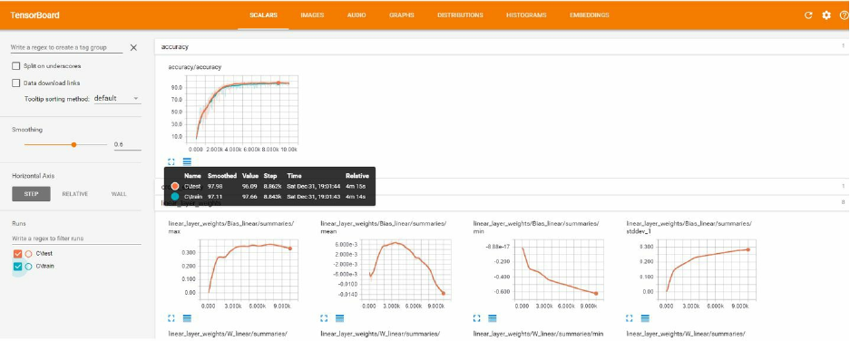
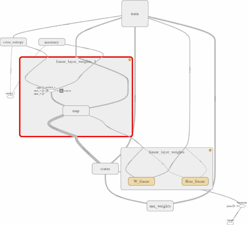
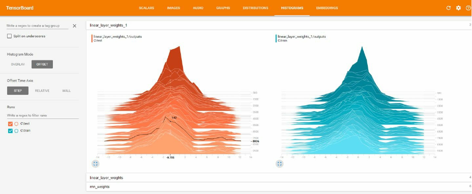
Figure 5-6. Histograms of weights throughout the learning process.
TensorFlow Built-in RNN Functions
The preceding example taught us some of the fundamental and powerful ways we can work with
sequences, by implementing our graph pretty much from scratch. In practice, it is of course a
good idea to use built-in higher-level modules and functions. This not only makes the code
shorter and easier to write, but exploits many low-level optimizations afforded by TensorFlow
implementations.
In this section we first present a new, shorter version of the code in its entirety. Since most of the
overall details have not changed, we focus on the main new elements,
tf.contrib.rnn.BasicRNNCell and tf.nn.dynamic_rnn():
import tensorflow as tf
from tensorflow.examples.tutorials.mnist import input_data
mnist = input_data.read_data_sets("/tmp/data/", one_hot=True)
element_size = 28;time_steps = 28;num_classes = 10
batch_size = 128;hidden_layer_size = 128
_inputs = tf.placeholder(tf.float32,shape=[None, time_steps,
element_size],
name='inputs')
y = tf.placeholder(tf.float32, shape=[None, num_classes],name='inputs')
# TensorFlow built-in functions
rnn_cell = tf.contrib.rnn.BasicRNNCell(hidden_layer_size)
outputs, _ = tf.nn.dynamic_rnn(rnn_cell, _inputs, dtype=tf.float32)
Wl = tf.Variable(tf.truncated_normal([hidden_layer_size, num_classes],
mean=0,stddev=.01))
bl = tf.Variable(tf.truncated_normal([num_classes],mean=0,stddev=.01))
def get_linear_layer(vector):
return tf.matmul(vector, Wl) + bl
last_rnn_output = outputs[:,-1,:]
final_output = get_linear_layer(last_rnn_output)
softmax = tf.nn.softmax_cross_entropy_with_logits(logits=final_output,
labels=y)
cross_entropy = tf.reduce_mean(softmax)
train_step = tf.train.RMSPropOptimizer(0.001, 0.9).minimize(cross_entropy)
correct_prediction = tf.equal(tf.argmax(y,1), tf.argmax(final_output,1))
accuracy = (tf.reduce_mean(tf.cast(correct_prediction, tf.float32)))*100
sess=tf.InteractiveSession()
sess.run(tf.global_variables_initializer())
test_data = mnist.test.images[:batch_size].reshape((-1,
time_steps, element_size))
test_label = mnist.test.labels[:batch_size]
for i in range(3001):
batch_x, batch_y = mnist.train.next_batch(batch_size)
batch_x = batch_x.reshape((batch_size, time_steps, element_size))
sess.run(train_step,feed_dict={_inputs:batch_x,
y:batch_y})
if i % 1000 == 0:
acc = sess.run(accuracy, feed_dict={_inputs: batch_x,
y: batch_y})
loss = sess.run(cross_entropy,feed_dict={_inputs:batch_x,
y:batch_y})
print ("Iter " + str(i) + ", Minibatch Loss= " + \
"{:.6f}".format(loss) + ", Training Accuracy= " + \
"{:.5f}".format(acc))
print ("Testing Accuracy:",
sess.run(accuracy, feed_dict={_inputs: test_data, y: test_label}))
tf.contrib.rnn.BasicRNNCell and tf.nn.dynamic_rnn()
TensorFlow’s RNN cells are abstractions that represent the basic operations each recurrent “cell”
carries out (see Figure 5-2 at the start of this chapter for an illustration), and its associated state.
They are, in general terms, a “replacement” of the rnn_step() function and the associated
variables it required. Of course, there are many variants and types of cells, each with many
methods and properties. We will see some more advanced cells toward the end of this chapter
and later in the book.
Once we have created the rnn_cell, we feed it into tf.nn.dynamic_rnn(). This function
replaces tf.scan() in our vanilla implementation and creates an RNN specified by rnn_cell.
As of this writing, in early 2017, TensorFlow includes a static and a dynamic function for
creating an RNN. What does this mean? The static version creates an unrolled graph (as in
Figure 5-2) of fixed length. The dynamic version uses a tf.While loop to dynamically construct
the graph at execution time, leading to faster graph creation, which can be significant. This
dynamic construction can also be very useful in other ways, some of which we will touch on
when we discuss variable-length sequences toward the end of this chapter.
Note that contrib refers to the fact that code in this library is contributed and still requires testing.
We discuss the contrib library in much more detail in Chapter 7. BasicRNNCell was moved to
contrib in TensorFlow 1.0 as part of ongoing development. In version 1.2, many of the RNN
functions and classes were moved back to the core namespace with aliases kept in contrib for
backward compatibiliy, meaning that the preceding code works for all versions 1.X as of this
writing.
RNN for Text Sequences
We began this chapter by learning how to implement RNN models in TensorFlow. For ease of
exposition, we showed how to implement and use an RNN for a sequence made of pixels in
MNIST images. We next show how to use these sequence models on text sequences.
Text data has some properties distinctly different from image data, which we will discuss here
and later in this book. These properties can make it somewhat difficult to handle text data at first,
and text data always requires at least some basic pre-processing steps for us to be able to work
with it. To introduce working with text in TensorFlow, we will thus focus on the core
components and create a minimal, contrived text dataset that will let us get straight to the action.
In Chapter 7, we will apply RNN models to movie review sentiment classification.
Let’s get started, presenting our example data and discussing some key properties of text datasets
as we go.
Text Sequences
In the MNIST RNN example we saw earlier, each sequence was of fixed size — the width (or
height) of an image. Each element in the sequence was a dense vector of 28 pixels. In NLP tasks
and datasets, we have a different kind of “picture.”
Our sequences could be of words forming a sentence, of sentences forming a paragraph, or even
of characters forming words or paragraphs forming whole documents.
Consider the following sentence: “Our company provides smart agriculture solutions for farms,
with advanced AI, deep-learning.” Say we obtain this sentence from an online news blog, and
wish to process it as part of our machine learning system.
Each of the words in this sentence would be represented with an ID — an integer, commonly
referred to as a token ID in NLP. So, the word “agriculture” could, for instance, be mapped to the
integer 3452, the word “farm” to 12, “AI” to 150, and “deep-learning” to 0. This representation
in terms of integer identifiers is very different from the vector of pixels in image data, in multiple
ways. We will elaborate on this important point shortly when we discuss word embeddings, and
in Chapter 6.
To make things more concrete, let’s start by creating our simplified text data.
Our simulated data consists of two classes of very short “sentences,” one composed of odd digits
and the other of even digits (with numbers written in English). We generate sentences built of
words representing even and odd numbers. Our goal is to learn to classify each sentence as either
odd or even in a supervised text-classification task.
Of course, we do not really need any machine learning for this simple task — we use this
contrived example only for illustrative purposes.
First, we define some constants, which will be explained as we go:
import numpy as np
import tensorflow as tf
batch_size = 128;embedding_dimension = 64;num_classes = 2
hidden_layer_size = 32;times_steps = 6;element_size = 1
Next, we create sentences. We sample random digits and map them to the corresponding
“words” (e.g., 1 is mapped to “One,” 7 to “Seven,” etc.).
Text sequences typically have variable lengths, which is of course the case for all real natural
language data (such as in the sentences appearing on this page).
To make our simulated sentences have different lengths, we sample for each sentence a random
length between 3 and 6 with np.random.choice(range(3, 7)) — the lower bound is inclusive,
and the upper bound is exclusive.
Now, to put all our input sentences in one tensor (per batch of data instances), we need them to
somehow be of the same size — so we pad sentences with a length shorter than 6 with zeros (or
PAD symbols) to make all sentences equally sized (artificially). This pre-processing step is
known as zero-padding. The following code accomplishes all of this:
digit_to_word_map = {1:"One",2:"Two", 3:"Three", 4:"Four", 5:"Five",
6:"Six",7:"Seven",8:"Eight",9:"Nine"}
digit_to_word_map[0]="PAD"
even_sentences = []
odd_sentences = []
seqlens = []
for i in range(10000):
rand_seq_len = np.random.choice(range(3,7))
seqlens.append(rand_seq_len)
rand_odd_ints = np.random.choice(range(1,10,2),
rand_seq_len)
rand_even_ints = np.random.choice(range(2,10,2),
rand_seq_len)
# Padding
if rand_seq_len<6:
rand_odd_ints = np.append(rand_odd_ints,
[0]*(6-rand_seq_len))
rand_even_ints = np.append(rand_even_ints,
[0]*(6-rand_seq_len))
even_sentences.append(" ".join([digit_to_word_map[r] for
r in rand_odd_ints]))
odd_sentences.append(" ".join([digit_to_word_map[r] for
r in rand_even_ints]))
data = even_sentences+odd_sentences
# Same seq lengths for even, odd sentences
seqlens*=2
Let’s take a look at our sentences, each padded to length 6:
even_sentences[0:6]
Out:
['Four Four Two Four Two PAD',
'Eight Six Four PAD PAD PAD',
'Eight Two Six Two PAD PAD',
'Eight Four Four Eight PAD PAD',
'Eight Eight Four PAD PAD PAD',
'Two Two Eight Six Eight Four']
odd_sentences[0:6]
Out:
['One Seven Nine Three One PAD',
'Three Nine One PAD PAD PAD',
'Seven Five Three Three PAD PAD',
'Five Five Three One PAD PAD',
'Three Three Five PAD PAD PAD',
'Nine Three Nine Five Five Three']
Notice that we add the PAD word (token) to our data and digit_to_word_map dictionary, and
separately store even and odd sentences and their original lengths (before padding).
Let’s take a look at the original sequence lengths for the sentences we printed:
seqlens[0:6]
Out:
[5, 3, 4, 4, 3, 6]
Why keep the original sentence lengths? By zero-padding, we solved one technical problem but
created another: if we naively pass these padded sentences through our RNN model as they are,
it will process useless PAD symbols. This would both harm model correctness by processing
“noise” and increase computation time. We resolve this issue by first storing the original lengths
in the seqlens array and then telling TensorFlow’s tf.nn.dynamic_rnn() where each sentence
ends.
In this chapter, our data is simulated — generated by us. In real applications, we would start off
by getting a collection of documents (e.g., one-sentence tweets) and then mapping each word to
an integer ID.
So, we now map words to indices — word identifiers — by simply creating a dictionary with
words as keys and indices as values. We also create the inverse map. Note that there is no
correspondence between the word IDs and the digits each word represents — the IDs carry no
semantic meaning, just as in any NLP application with real data:
# Map from words to indices
word2index_map ={}
index=0
for sent in data:
for word in sent.lower().split():
if word not in word2index_map:
word2index_map[word] = index
index+=1
# Inverse map
index2word_map = {index: word for word, index in word2index_map.items()}
vocabulary_size = len(index2word_map)
This is a supervised classification task — we need an array of labels in the one-hot format, train
and test sets, a function to generate batches of instances, and placeholders, as usual.
First, we create the labels and split the data into train and test sets:
labels = [1]*10000 + [0]*10000
for i in range(len(labels)):
label = labels[i]
one_hot_encoding = [0]*2
one_hot_encoding[label] = 1
labels[i] = one_hot_encoding
data_indices = list(range(len(data)))
np.random.shuffle(data_indices)
data = np.array(data)[data_indices]
labels = np.array(labels)[data_indices]
seqlens = np.array(seqlens)[data_indices]
train_x = data[:10000]
train_y = labels[:10000]
train_seqlens = seqlens[:10000]
test_x = data[10000:]
test_y = labels[10000:]
test_seqlens = seqlens[10000:]
Next, we create a function that generates batches of sentences. Each sentence in a batch is simply
a list of integer IDs corresponding to words:
def get_sentence_batch(batch_size,data_x,
data_y,data_seqlens):
instance_indices = list(range(len(data_x)))
np.random.shuffle(instance_indices)
batch = instance_indices[:batch_size]
x = [[word2index_map[word] for word in data_x[i].lower().split()]
for i in batch]
y = [data_y[i] for i in batch]
seqlens = [data_seqlens[i] for i in batch]
return x,y,seqlens
Finally, we create placeholders for data:
_inputs = tf.placeholder(tf.int32, shape=[batch_size,times_steps])
_labels = tf.placeholder(tf.float32, shape=[batch_size, num_classes])
# seqlens for dynamic calculation
_seqlens = tf.placeholder(tf.int32, shape=[batch_size])
Note that we have created a placeholder for the original sequence lengths. We will see how to
make use of these in our RNN shortly.
Supervised Word Embeddings
Our text data is now encoded as lists of word IDs — each sentence is a sequence of integers
corresponding to words. This type of atomic representation, where each word is represented with
an ID, is not scalable for training deep learning models with large vocabularies that occur in real
problems. We could end up with millions of such word IDs, each encoded in one-hot (binary)
categorical form, leading to great data sparsity and computational issues. We will discuss this in
more depth in Chapter 6.
A powerful approach to work around this issue is to use word embeddings. The embedding is, in
a nutshell, simply a mapping from high-dimensional one-hot vectors encoding words to lower-
dimensional dense vectors. So, for example, if our vocabulary has size 100,000, each word in
one-hot representation would be of the same size. The corresponding word vector — or word
embedding — would be of size 300, say. The high-dimensional one-hot vectors are thus
“embedded” into a continuous vector space with a much lower dimensionality.
In Chapter 6 we dive deeper into word embeddings, exploring a popular method to train them in
an “unsupervised” manner known as word2vec.
Here, our end goal is to solve a text classification problem, and we will train word vectors in a
supervised framework, tuning the embedded word vectors to solve the downstream classification
task.
It is helpful to think of word embeddings as basic hash tables or lookup tables, mapping words to
their dense vector values. These vectors are optimized as part of the training process. Previously,
we gave each word an integer index, and sentences are then represented as sequences of these
indices. Now, to obtain a word’s vector, we use the built-in tf.nn.embedding_lookup()
function, which efficiently retrieves the vectors for each word in a given sequence of word
indices:
with tf.name_scope("embeddings"):
embeddings = tf.Variable(
tf.random_uniform([vocabulary_size,
embedding_dimension],
-1.0, 1.0),name='embedding')
embed = tf.nn.embedding_lookup(embeddings, _inputs)
We will see examples of and visualizations of our vector representations of words shortly.
LSTM and Using Sequence Length
In the introductory RNN example with which we began, we implemented and used the basic
vanilla RNN model. In practice, we often use slightly more advanced RNN models, which differ
mainly by how they update their hidden state and propagate information through time. A very
popular recurrent network is the long short-term memory (LSTM) network. It differs from
vanilla RNN by having some special memory mechanisms that enable the recurrent cells to better
store information for long periods of time, thus allowing them to capture long-term dependencies
better than plain RNN.
There is nothing mysterious about these memory mechanisms; they simply consist of some more
parameters added to each recurrent cell, enabling the RNN to overcome optimization issues and
propagate information. These trainable parameters act as filters that select what information is
worth “remembering” and passing on, and what is worth “forgetting.” They are trained in exactly
the same way as any other parameter in a network, with gradient-descent algorithms and
backpropagation. We don’t go into the more technical mathematical formulations here, but there
are plenty of great resources out there delving into the details.
We create an LSTM cell with tf.contrib.rnn.BasicLSTMCell() and feed it to
tf.nn.dynamic_rnn(), just as we did at the start of this chapter. We also give dynamic_rnn()
the length of each sequence in a batch of examples, using the _seqlens placeholder we created
earlier. TensorFlow uses this to stop all RNN steps beyond the last real sequence element. It also
returns all output vectors over time (in the outputs tensor), which are all zero-padded beyond the
true end of the sequence. So, for example, if the length of our original sequence is 5 and we zero-
pad it to a sequence of length 15, the output for all time steps beyond 5 will be zero:
with tf.variable_scope("lstm"):
lstm_cell = tf.contrib.rnn.BasicLSTMCell(hidden_layer_size,
forget_bias=1.0)
outputs, states = tf.nn.dynamic_rnn(lstm_cell, embed,
sequence_length = _seqlens,
dtype=tf.float32)
weights = {
'linear_layer': tf.Variable(tf.truncated_normal([hidden_layer_size,
num_classes],
mean=0,stddev=.01))
}
biases = {
'linear_layer':tf.Variable(tf.truncated_normal([num_classes],
mean=0,stddev=.01))
}
# Extract the last relevant output and use in a linear layer
final_output = tf.matmul(states[1],
weights["linear_layer"]) + biases["linear_layer"]
softmax = tf.nn.softmax_cross_entropy_with_logits(logits = final_output,
labels = _labels)
cross_entropy = tf.reduce_mean(softmax)
We take the last valid output vector — in this case conveniently available for us in the states
tensor returned by dynamic_rnn() — and pass it through a linear layer (and the softmax
function), using it as our final prediction. We will explore the concepts of last relevant output
and zero-padding further in the next section, when we look at some outputs generated by
dynamic_rnn() for our example sentences.
Training Embeddings and the LSTM Classifier
We have all the pieces in the puzzle. Let’s put them together, and complete an end-to-end
training of both word vectors and a classification model:
train_step = tf.train.RMSPropOptimizer(0.001, 0.9).minimize(cross_entropy)
correct_prediction = tf.equal(tf.argmax(_labels,1),
tf.argmax(final_output,1))
accuracy = (tf.reduce_mean(tf.cast(correct_prediction,
tf.float32)))*100
with tf.Session() as sess:
sess.run(tf.global_variables_initializer())
for step in range(1000):
x_batch, y_batch,seqlen_batch = get_sentence_batch(batch_size,
train_x,train_y,
train_seqlens)
sess.run(train_step,feed_dict={_inputs:x_batch, _labels:y_batch,
_seqlens:seqlen_batch})
if step % 100 == 0:
acc = sess.run(accuracy,feed_dict={_inputs:x_batch,
_labels:y_batch,
_seqlens:seqlen_batch})
print("Accuracy at %d: %.5f" % (step, acc))
for test_batch in range(5):
x_test, y_test,seqlen_test = get_sentence_batch(batch_size,
test_x,test_y,
test_seqlens)
batch_pred,batch_acc = sess.run([tf.argmax(final_output,1),
accuracy],
feed_dict={_inputs:x_test,
_labels:y_test,
_seqlens:seqlen_test})
print("Test batch accuracy %d: %.5f" % (test_batch, batch_acc))
output_example = sess.run([outputs],feed_dict={_inputs:x_test,
_labels:y_test,
_seqlens:seqlen_test})
states_example = sess.run([states[1]],feed_dict={_inputs:x_test,
_labels:y_test,
_seqlens:seqlen_test})
As we can see, this is a pretty simple toy text classification problem:
Accuracy at 0: 32.81250
Accuracy at 100: 100.00000
Accuracy at 200: 100.00000
Accuracy at 300: 100.00000
Accuracy at 400: 100.00000
Accuracy at 500: 100.00000
Accuracy at 600: 100.00000
Accuracy at 700: 100.00000
Accuracy at 800: 100.00000
Accuracy at 900: 100.00000
Test batch accuracy 0: 100.00000
Test batch accuracy 1: 100.00000
Test batch accuracy 2: 100.00000
Test batch accuracy 3: 100.00000
Test batch accuracy 4: 100.00000
We’ve also computed an example batch of outputs generated by dynamic_rnn(), to further
illustrate the concepts of zero-padding and last relevant outputs discussed in the previous section.
Let’s take a look at one example of these outputs, for a sentence that was zero-padded (in your
random batch of data you may see different output, of course — look for a sentence whose
seqlen was lower than the maximal 6):
seqlen_test[1]
Out:
4
output_example[0][1].shape
Out:
(6, 32)
This output has, as expected, six time steps, each a vector of size 32. Let’s take a glimpse at its
values (printing only the first few dimensions to avoid clutter):
output_example[0][1][:6,0:3]
Out:
array([[-0.44493711, -0.51363373, -0.49310589],
[-0.72036862, -0.68590945, -0.73340571],
[-0.83176643, -0.78206956, -0.87831545],
[-0.87982416, -0.82784462, -0.91132098],
[ 0. , 0. , 0. ],
[ 0. , 0. , 0. ]], dtype=float32)
We see that for this sentence, whose original length was 4, the last two time steps have zero
vectors due to padding.
Finally, we look at the states vector returned by dynamic_rnn():
states_example[0][1][0:3]
Out:
array([-0.87982416, -0.82784462, -0.91132098], dtype=float32)
We can see that it conveniently stores for us the last relevant output vector — its values match
the last relevant output vector before zero-padding.
At this point, you may be wondering how to access and manipulate the word vectors and explore
the trained representation. We show how to do so, including interactive embedding visualization,
in the next chapter.
Stacking multiple LSTMs
Earlier, we focused on a one-layer LSTM network for ease of exposition. Adding more layers is
straightforward, using the MultiRNNCell() wrapper that combines multiple RNN cells into one
multilayer cell.
Say, for example, we wanted to stack two LSTM layers in the preceding example. We can do
this as follows:
num_LSTM_layers = 2
with tf.variable_scope("lstm"):
lstm_cell = tf.contrib.rnn.BasicLSTMCell(hidden_layer_size,
forget_bias=1.0)
cell = tf.contrib.rnn.MultiRNNCell(cells=[lstm_cell]*num_LSTM_layers,
state_is_tuple=True)
outputs, states = tf.nn.dynamic_rnn(cell, embed,
sequence_length = _seqlens,
dtype=tf.float32)
We first define an LSTM cell as before, and then feed it into the
tf.contrib.rnn.MultiRNNCell() wrapper.
Now our network has two layers of LSTM, causing some shape issues when trying to extract the
final state vectors. To get the final state of the second layer, we simply adapt our indexing a bit:
# Extract the final state and use in a linear layer
final_output = tf.matmul(states[num_LSTM_layers-1][1],
weights["linear_layer"]) + biases["linear_layer"]
Summary
In this chapter we introduced sequence models in TensorFlow. We saw how to implement a
basic RNN model from scratch by using tf.scan() and built-in modules, as well as more
advanced LSTM networks, for both text and image data. Finally, we trained an end-to-end text
classification RNN with word embeddings, and showed how to handle sequences of variable
length. In the next chapter, we dive deeper into word embeddings and word2vec. In Chapter 7,
we will see some cool abstraction layers over TensorFlow, and how they can be used to train
advanced text classification RNN models with considerably less effort.

Chapter 6. Text II: Word Vectors, Advanced
RNN, and Embedding Visualization
In this chapter, we go deeper into important topics discussed in Chapter 5 regarding working
with text sequences. We first show how to train word vectors by using an unsupervised method
known as word2vec, and how to visualize embeddings interactively with TensorBoard. We then
use pretrained word vectors, trained on massive amounts of public data, in a supervised text-
classification task, and also introduce more-advanced RNN components that are frequently used
in state-of-the-art systems.
Introduction to Word Embeddings
In Chapter 5 we introduced RNN models and working with text sequences in TensorFlow. As
part of the supervised model training, we also trained word vectors — mapping from word IDs to
lower-dimensional continuous vectors. The reasoning for this was to enable a scalable
representation that can be fed into an RNN layer. But there are deeper reasons for the use of
word vectors, which we discuss next.
Consider the sentence appearing in Figure 6-1: “Our company provides smart agriculture
solutions for farms, with advanced AI, deep-learning.” This sentence may be taken from, say, a
tweet promoting a company. As data scientists or engineers, we now may wish to process it as
part of an advanced machine intelligence system, that sifts through tweets and automatically
detects informative content (e.g., public sentiment).
In one of the major traditional natural language processing (NLP) approaches to text processing,
each of the words in this sentence would be represented with N ID — say, an integer. So, as we
posited in the previous chapter, the word “agriculture” might be mapped to the integer 3452, the
word “farm” to 12, “AI” to 150, and “deep-learning” to 0.
While this representation has led to excellent results in practice in some basic NLP tasks and is
still often used in many cases (such as in bag-of-words text classification), it has some major
inherent problems. First, by using this type of atomic representation, we lose all meaning
encoded within the word, and crucially, we thus lose information on the semantic proximity
between words. In our example, we of course know that “agriculture” and “farm” are strongly
related, and so are “AI” and “deep-learning,” while deep learning and farms don’t usually have
much to do with one another. This is not reflected by their arbitrary integer IDs.
Another important issue with this way of looking at data stems from the size of typical
vocabularies, which can easily reach huge numbers. This means that naively, we could need to
keep millions of such word identifiers, leading to great data sparsity and in turn, making learning
harder and more expensive.
With images, such as in the MNIST data we used in the first section of Chapter 5, this is not
quite the case. While images can be high-dimensional, their natural representation in terms of
pixel values already encodes some semantic meaning, and this representation is dense. In
practice, RNN models like the one we saw in Chapter 5 require dense vector representations to
work well.
We would like, therefore, to use dense vector representations of words, which carry semantic
meaning. But how do we obtain them?
In Chapter 5 we trained supervised word vectors to solve a specific task, using labeled data. But
it is often expensive for individuals and organizations to obtain labeled data, in terms of the
resources, time, and effort involved in manually tagging texts or somehow acquiring enough
labeled instances. Obtaining huge amounts of unlabeled data, however, is often a much less
daunting endeavor. We thus would like a way to use this data to train word representations, in an
unsupervised fashion.
There are actually many ways to do unsupervised training of word embeddings, including both
more traditional approaches to NLP that can still work very well and newer methods, many of
which use neural networks. Whether old or new, these all rely at their core on the distributional
hypothesis, which is most easily explained by a well-known quote by linguist John Firth: “You
shall know a word by the company it keeps.” In other words, words that tend to appear in
similar contexts tend to have similar semantic meanings.
In this book, we focus on powerful word embedding methods based on neural networks. In
Chapter 5 we saw how to train them as part of a downstream text-classification task. We now
show how to train word vectors in an unsupervised manner, and then how to use pretrained
vectors that were trained using huge amounts of text from the web.
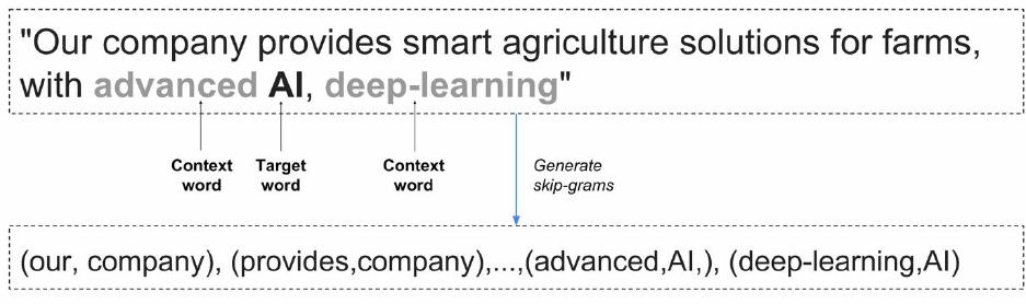
Word2vec
Word2vec is a very well-known unsupervised word embedding approach. It is actually more like
a family of algorithms, all based in some way on exploiting the context in which words appear to
learn their representation (in the spirit of the distributional hypothesis). We focus on the most
popular word2vec implementation, which trains a model that, given an input word, predicts the
word’s context by using something known as skip-grams. This is actually rather simple, as the
following example will demonstrate.
Consider, again, our example sentence: “Our company provides smart agriculture solutions for
farms, with advanced AI, deep-learning.” We define (for simplicity) the context of a word as its
immediate neighbors (“the company it keeps”) — i.e., the word to its left and the word to its
right. So, the context of “company” is [our, provides], the context of “AI” is [advanced, deep-
learning], and so on (see Figure 6-1).
Figure 6-1. Generating skip-grams from text.
In the skip-gram word2vec model, we train a model to predict context based on an input word.
All that means in this case is that we generate training instance and label pairs such as (our,
company), (provides, company), (advanced, AI), (deep-learning, AI), etc.
In addition to these pairs we extract from the data, we also sample “fake” pairs — that is, for a
given input word (such as “AI”), we also sample random noise words as context (such as
“monkeys”), in a process known as negative sampling. We use the true pairs combined with
noise pairs to build our training instances and labels, which we use to train a binary classifier that
learns to distinguish between them. The trainable parameters in this classifier are the vector
representations — word embeddings. We tune these vectors to yield a classifier able to tell the
difference between true contexts of a word and randomly sampled ones, in a binary classification
setting.
TensorFlow enables many ways to implement the word2vec model, with increasing levels of
sophistication and optimization, using multithreading and higher-level abstractions for optimized
and shorter code. We present here a fundamental approach, which will introduce you to the core
ideas and operations.
Let’s dive straight into implementing the core ideas in TensorFlow code.
Skip-Grams
We begin by preparing our data and extracting skip-grams. As in Chapter 5, our data comprises
two classes of very short “sentences,” one composed of odd digits and the other of even digits
(with numbers written in English). We make sentences equally sized here, for simplicity, but this
doesn’t really matter for word2vec training. Let’s start by setting some parameters and creating
sentences:
import os
import math
import numpy as np
import tensorflow as tf
from tensorflow.contrib.tensorboard.plugins import projector
batch_size=64
embedding_dimension = 5
negative_samples =8
LOG_DIR = "logs/word2vec_intro"
digit_to_word_map = {1:"One",2:"Two", 3:"Three", 4:"Four", 5:"Five",
6:"Six",7:"Seven",8:"Eight",9:"Nine"}
sentences = []
# Create two kinds of sentences - sequences of odd and even digits
for i in range(10000):
rand_odd_ints = np.random.choice(range(1,10,2),3)
sentences.append(" ".join([digit_to_word_map[r] for r in rand_odd_ints]))
rand_even_ints = np.random.choice(range(2,10,2),3)
sentences.append(" ".join([digit_to_word_map[r] for r in rand_even_ints]))
Let’s take a look at our sentences:
sentences[0:10]
Out:
['Seven One Five',
'Four Four Four',
'Five One Nine',
'Eight Two Eight',
'One Nine Three',
'Two Six Eight',
'Nine Seven Seven',
'Six Eight Six',
'One Five Five',
'Four Six Two']
Next, as in Chapter 5, we map words to indices by creating a dictionary with words as keys and
indices as values, and create the inverse map:
# Map words to indices
word2index_map ={}
index=0
for sent in sentences:
for word in sent.lower().split():
if word not in word2index_map:
word2index_map[word] = index
index+=1
index2word_map = {index: word for word, index in word2index_map.items()}
vocabulary_size = len(index2word_map)
To prepare the data for word2vec, let’s create skip-grams:
# Generate skip-gram pairs
skip_gram_pairs = []
for sent in sentences:
tokenized_sent = sent.lower().split()
for i in range(1, len(tokenized_sent)-1) :
word_context_pair = [[word2index_map[tokenized_sent[i-1]],
word2index_map[tokenized_sent[i+1]]],
word2index_map[tokenized_sent[i]]]
skip_gram_pairs.append([word_context_pair[1],
word_context_pair[0][0]])
skip_gram_pairs.append([word_context_pair[1],
word_context_pair[0][1]])
def get_skipgram_batch(batch_size):
instance_indices = list(range(len(skip_gram_pairs)))
np.random.shuffle(instance_indices)
batch = instance_indices[:batch_size]
x = [skip_gram_pairs[i][0] for i in batch]
y = [[skip_gram_pairs[i][1]] for i in batch]
return x,y
Each skip-gram pair is composed of target and context word indices (given by the
word2index_map dictionary, and not in correspondence to the actual digit each word represents).
Let’s take a look:
skip_gram_pairs[0:10]
Out:
[[1, 0],
[1, 2],
[3, 3],
[3, 3],
[1, 2],
[1, 4],
[6, 5],
[6, 5],
[4, 1],
[4, 7]]
We can generate batches of sequences of word indices, and check out the original sentences with
the inverse dictionary we created earlier:
# Batch example
x_batch,y_batch = get_skipgram_batch(8)
x_batch
y_batch
[index2word_map[word] for word in x_batch]
[index2word_map[word[0]] for word in y_batch]
x_batch
Out:
[6, 2, 1, 1, 3, 0, 7, 2]
y_batch
Out:
[[5], [0], [4], [0], [5], [4], [1], [7]]
[index2word_map[word] for word in x_batch]
Out:
['two', 'five', 'one', 'one', 'four', 'seven', 'three', 'five']
[index2word_map[word[0]] for word in y_batch]
Out:
['eight', 'seven', 'nine', 'seven', 'eight',
'nine', 'one', 'three']
Finally, we create our input and label placeholders:
# Input data, labels
train_inputs = tf.placeholder(tf.int32, shape=[batch_size])
train_labels = tf.placeholder(tf.int32, shape=[batch_size, 1])
Embeddings in TensorFlow
In Chapter 5, we used the built-in tf.nn.embedding_lookup() function as part of our supervised
RNN. The same functionality is used here. Here too, word embeddings can be viewed as lookup
tables that map words to vector values, which are optimized as part of the training process to
minimize a loss function. As we shall see in the next section, unlike in Chapter 5, here we use a
loss function accounting for the unsupervised nature of the task, but the embedding lookup,
which efficiently retrieves the vectors for each word in a given sequence of word indices,
remains the same:
with tf.name_scope("embeddings"):
embeddings = tf.Variable(
tf.random_uniform([vocabulary_size, embedding_dimension],
-1.0, 1.0),name='embedding')
# This is essentially a lookup table
embed = tf.nn.embedding_lookup(embeddings, train_inputs)
The Noise-Contrastive Estimation (NCE) Loss Function
In our introduction to skip-grams, we mentioned we create two types of context–target pairs of
words: real ones that appear in the text, and “fake” noisy pairs that are generated by inserting
random context words. Our goal is to learn to distinguish between the two, helping us learn a
good word representation. We could draw random noisy context pairs ourselves, but luckily
TensorFlow comes with a useful loss function designed especially for our task.
tf.nn.nce_loss() automatically draws negative (“noise”) samples when we evaluate the loss
(run it in a session):
# Create variables for the NCE loss
nce_weights = tf.Variable(
tf.truncated_normal([vocabulary_size, embedding_dimension],
stddev=1.0 / math.sqrt(embedding_dimension)))
nce_biases = tf.Variable(tf.zeros([vocabulary_size]))
loss = tf.reduce_mean(
tf.nn.nce_loss(weights = nce_weights, biases = nce_biases, inputs = embed,
labels = train_labels, num_sampled = negative_samples, num_classes =
vocabulary_size))
We don’t go into the mathematical details of this loss function, but it is sufficient to think of it as
a sort of efficient approximation to the ordinary softmax function used in classification tasks, as
introduced in previous chapters. We tune our embedding vectors to optimize this loss function.
For more details about it, see the official TensorFlow documentation and references within.
We’re now ready to train. In addition to obtaining our word embeddings in TensorFlow, we next
introduce two useful capabilities: adjustment of the optimization learning rate, and interactive
visualization of embeddings.
Learning Rate Decay
As discussed in previous chapters, gradient-descent optimization adjusts weights by making
small steps in the direction that minimizes our loss function. The learning_rate hyperparameter
controls just how aggressive these steps are. During gradient-descent training of a model, it is
common practice to gradually make these steps smaller and smaller, so that we allow our
optimization process to “settle down” as it approaches good points in the parameter space. This
small addition to our training process can actually often lead to significant boosts in
performance, and is a good practice to keep in mind in general.
tf.train.exponential_decay() applies exponential decay to the learning rate, with the exact
form of decay controlled by a few hyperparameters, as seen in the following code (for exact
details, see the official TensorFlow documentation at http://bit.ly/2tluxP1). Here, just as an
example, we decay every 1,000 steps, and the decayed learning rate follows a staircase function
— a piecewise constant function that resembles a staircase, as its name implies:
# Learning rate decay
global_step = tf.Variable(0, trainable=False)
learningRate = tf.train.exponential_decay(learning_rate=0.1,
global_step= global_step,
decay_steps=1000,
decay_rate= 0.95,
staircase=True)
train_step = tf.train.GradientDescentOptimizer(learningRate).minimize(loss)
Training and Visualizing with TensorBoard
We train our graph within a session as usual, adding some lines of code enabling cool interactive
visualization in TensorBoard, a new tool for visualizing embeddings of high-dimensional data —
typically images or word vectors — introduced for TensorFlow in late 2016.
First, we create a TSV (tab-separated values) metadata file. This file connects embedding vectors
with associated labels or images we may have for them. In our case, each embedding vector has
a label that is just the word it stands for.
We then point TensorBoard to our embedding variables (in this case, only one), and link them to
the metadata file.
Finally, after completing optimization but before closing the session, we normalize the word
embedding vectors to unit length, a standard post-processing step:
# Merge all summary ops
merged = tf.summary.merge_all()
with tf.Session() as sess:
train_writer = tf.summary.FileWriter(LOG_DIR,
graph=tf.get_default_graph())
saver = tf.train.Saver()
with open(os.path.join(LOG_DIR,'metadata.tsv'), "w") as metadata:
metadata.write('Name\tClass\n')
for k,v in index2word_map.items():
metadata.write('%s\t%d\n' % (v, k))
config = projector.ProjectorConfig()
embedding = config.embeddings.add()
embedding.tensor_name = embeddings.name
# Link embedding to its metadata file
embedding.metadata_path = os.path.join(LOG_DIR,'metadata.tsv')
projector.visualize_embeddings(train_writer, config)
tf.global_variables_initializer().run()
for step in range(1000):
x_batch, y_batch = get_skipgram_batch(batch_size)
summary,_ = sess.run([merged,train_step],
feed_dict={train_inputs:x_batch,
train_labels:y_batch})
train_writer.add_summary(summary, step)
if step % 100 == 0:
saver.save(sess, os.path.join(LOG_DIR, "w2v_model.ckpt"), step)
loss_value = sess.run(loss,
feed_dict={train_inputs:x_batch,
train_labels:y_batch})
print("Loss at %d: %.5f" % (step, loss_value))
# Normalize embeddings before using
norm = tf.sqrt(tf.reduce_sum(tf.square(embeddings), 1, keep_dims=True))
normalized_embeddings = embeddings / norm
normalized_embeddings_matrix = sess.run(normalized_embeddings)
Checking Out Our Embeddings
Let’s take a quick look at the word vectors we got. We select one word (one) and sort all the
other word vectors by how close they are to it, in descending order:
ref_word = normalized_embeddings_matrix[word2index_map["one"]]
cosine_dists = np.dot(normalized_embeddings_matrix,ref_word)
ff = np.argsort(cosine_dists)[::-1][1:10]
for f in ff:
print(index2word_map[f])
print(cosine_dists[f])
Now let’s take a look at the word distances from the one vector:
Out:
seven
0.946973
three
0.938362
nine
0.755187
five
0.701269
eight
-0.0702622
two
-0.101749
six
-0.120306
four
-0.159601
We see that the word vectors representing odd numbers are similar (in terms of the dot product)
to one, while those representing even numbers are not similar to it (and have a negative dot
product with the one vector). We learned embedded vectors that allow us to distinguish between
even and odd numbers — their respective vectors are far apart, and thus capture the context in
which each word (odd or even digit) appeared.
Now, in TensorBoard, go to the Embeddings tab. This is a three-dimensional interactive
visualization panel, where we can move around the space of our embedded vectors and explore
different “angles,” zoom in, and more (see Figures 6-2 and 6-3). This enables us to understand
our data and interpret the model in a visually comfortable manner. We can see, for instance, that
the odd and even numbers occupy different areas in feature space.
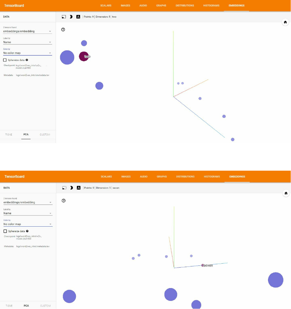
Figure 6-2. Interactive visualization of word embeddings.
Figure 6-3. We can explore our word vectors from different angles (especially useful in high-dimensional
problems with large vocabularies).
Of course, this type of visualization really shines when we have a great number of embedded
vectors, such as in real text classification tasks with larger vocabularies, as we will see in
Chapter 7, for example, or in the Embedding Projector TensorFlow demo. Here, we just give you
a taste of how to interactively explore your data and deep learning models.
Pretrained Embeddings, Advanced RNN
As we discussed earlier, word embeddings are a powerful component in deep learning models
for text. A popular approach seen in many applications is to first train word vectors with methods
such as word2vec on massive amounts of (unlabeled) text, and then use these vectors in a
downstream task such as supervised document classification.
In the previous section, we trained unsupervised word vectors from scratch. This approach
typically requires very large corpora, such as Wikipedia entries or web pages. In practice, we
often use pretrained word embeddings, trained on such huge corpora and available online, in
much the same manner as the pretrained models presented in previous chapters.
In this section, we show how to use pretrained word embeddings in TensorFlow in a simplified
text-classification task. To make things more interesting, we also take this opportunity to
introduce some more useful and powerful components that are frequently used in modern deep
learning applications for natural language understanding: the bidirectional RNN layers and the
gated recurrent unit (GRU) cell.
We will expand and adapt our text-classification example from Chapter 5, focusing only on the
parts that have changed.
Pretrained Word Embeddings
Here, we show how to take word vectors trained based on web data and incorporate them into a
(contrived) text-classification task. The embedding method is known as GloVe, and while we
don’t go into the details here, the overall idea is similar to that of word2vec — learning
representations of words by the context in which they appear. Information on the method and its
authors, and the pretrained vectors, is available on the project’s website.
We download the Common Crawl vectors (840B tokens), and proceed to our example.
We first set the path to the downloaded word vectors and some other parameters, as in Chapter 5:
import zipfile
import numpy as np
import tensorflow as tf
path_to_glove = "path/to/glove/file"
PRE_TRAINED = True
GLOVE_SIZE = 300
batch_size = 128
embedding_dimension = 64
num_classes = 2
hidden_layer_size = 32
times_steps = 6
We then create the contrived, simple simulated data, also as in Chapter 5 (see details there):
digit_to_word_map = {1:"One",2:"Two", 3:"Three", 4:"Four", 5:"Five",
6:"Six",7:"Seven",8:"Eight",9:"Nine"}
digit_to_word_map[0]="PAD_TOKEN"
even_sentences = []
odd_sentences = []
seqlens = []
for i in range(10000):
rand_seq_len = np.random.choice(range(3,7))
seqlens.append(rand_seq_len)
rand_odd_ints = np.random.choice(range(1,10,2),
rand_seq_len)
rand_even_ints = np.random.choice(range(2,10,2),
rand_seq_len)
if rand_seq_len<6:
rand_odd_ints = np.append(rand_odd_ints,
[0]*(6-rand_seq_len))
rand_even_ints = np.append(rand_even_ints,
[0]*(6-rand_seq_len))
even_sentences.append(" ".join([digit_to_word_map[r] for
r in rand_odd_ints]))
odd_sentences.append(" ".join([digit_to_word_map[r] for
r in rand_even_ints]))
data = even_sentences+odd_sentences
# Same seq lengths for even, odd sentences
seqlens*=2
labels = [1]*10000 + [0]*10000
for i in range(len(labels)):
label = labels[i]
one_hot_encoding = [0]*2
one_hot_encoding[label] = 1
labels[i] = one_hot_encoding
Next, we create the word index map:
word2index_map ={}
index=0
for sent in data:
for word in sent.split():
if word not in word2index_map:
word2index_map[word] = index
index+=1
index2word_map = {index: word for word, index in word2index_map.items()}
vocabulary_size = len(index2word_map)
Let’s refresh our memory of its content — just a map from word to an (arbitrary) index:
word2index_map
Out:
{'Eight': 7,
'Five': 1,
'Four': 6,
'Nine': 3,
'One': 5,
'PAD_TOKEN': 2,
'Seven': 4,
'Six': 9,
'Three': 0,
'Two': 8}
Now, we are ready to get word vectors. There are 2.2 million words in the vocabulary of the
pretrained GloVe embeddings we downloaded, and in our toy example we have only 9. So, we
take the GloVe vectors only for words that appear in our own tiny vocabulary:
def get_glove(path_to_glove,word2index_map):
embedding_weights = {}
count_all_words = 0
with zipfile.ZipFile(path_to_glove) as z:
with z.open("glove.840B.300d.txt") as f:
for line in f:
vals = line.split()
word = str(vals[0].decode("utf-8"))
if word in word2index_map:
print(word)
count_all_words+=1
coefs = np.asarray(vals[1:], dtype='float32')
coefs/=np.linalg.norm(coefs)
embedding_weights[word] = coefs
if count_all_words==vocabulary_size -1:
break
return embedding_weights
word2embedding_dict = get_glove(path_to_glove,word2index_map)
We go over the GloVe file line by line, take the word vectors we need, and normalize them.
Once we have extracted the nine words we need, we stop the process and exit the loop. The
output of our function is a dictionary, mapping from each word to its vector.
The next step is to place these vectors in a matrix, which is the required format for TensorFlow.
In this matrix, each row index should correspond to the word index:
embedding_matrix = np.zeros((vocabulary_size ,GLOVE_SIZE))
for word,index in word2index_map.items():
if not word == "PAD_TOKEN":
word_embedding = word2embedding_dict[word]
embedding_matrix[index,:] = word_embedding
Note that for the PAD_TOKEN word, we set the corresponding vector to 0. As we saw in Chapter 5,
we ignore padded tokens in our call to dynamic_rnn() by telling it the original sequence length.
We now create our training and test data:
data_indices = list(range(len(data)))
np.random.shuffle(data_indices)
data = np.array(data)[data_indices]
labels = np.array(labels)[data_indices]
seqlens = np.array(seqlens)[data_indices]
train_x = data[:10000]
train_y = labels[:10000]
train_seqlens = seqlens[:10000]
test_x = data[10000:]
test_y = labels[10000:]
test_seqlens = seqlens[10000:]
def get_sentence_batch(batch_size,data_x,
data_y,data_seqlens):
instance_indices = list(range(len(data_x)))
np.random.shuffle(instance_indices)
batch = instance_indices[:batch_size]
x = [[word2index_map[word] for word in data_x[i].split()]
for i in batch]
y = [data_y[i] for i in batch]
seqlens = [data_seqlens[i] for i in batch]
return x,y,seqlens
And we create our input placeholders:
_inputs = tf.placeholder(tf.int32, shape=[batch_size,times_steps])
embedding_placeholder = tf.placeholder(tf.float32, [vocabulary_size,
GLOVE_SIZE])
_labels = tf.placeholder(tf.float32, shape=[batch_size, num_classes])
_seqlens = tf.placeholder(tf.int32, shape=[batch_size])
Note that we created an embedding_placeholder, to which we feed the word vectors:
if PRE_TRAINED:
embeddings = tf.Variable(tf.constant(0.0, shape=[vocabulary_size,
GLOVE_SIZE]),
trainable=True)
# If using pretrained embeddings, assign them to the embeddings variable
embedding_init = embeddings.assign(embedding_placeholder)
embed = tf.nn.embedding_lookup(embeddings, _inputs)
else:
embeddings = tf.Variable(
tf.random_uniform([vocabulary_size,
embedding_dimension],
-1.0, 1.0))
embed = tf.nn.embedding_lookup(embeddings, _inputs)
Our embeddings are initialized with the content of embedding_placeholder, using the assign()
function to assign initial values to the embeddings variable. We set trainable=True to tell
TensorFlow we want to update the values of the word vectors, by optimizing them for the task at
hand. However, it is often useful to set trainable=False and not update these values; for
example, when we do not have much labeled data or have reason to believe the word vectors are
already “good” at capturing the patterns we are after.
There is one more step missing to fully incorporate the word vectors into the training — feeding
embedding_placeholder with embedding_matrix. We will get to that soon, but for now we
continue the graph building and introduce bidirectional RNN layers and GRU cells.

Bidirectional RNN and GRU Cells
Bidirectional RNN layers are a simple extension of the RNN layers we saw in Chapter 5. All
they consist of, in their basic form, is two ordinary RNN layers: one layer that reads the sequence
from left to right, and another that reads from right to left. Each yields a hidden representation,
the left-to-right vector , and the right-to-left vector . These are then concatenated into one
vector. The major advantage of this representation is its ability to capture the context of words
from both directions, which enables richer understanding of natural language and the underlying
semantics in text. In practice, in complex tasks, it often leads to improved accuracy. For
example, in part-of-speech (POS) tagging, we want to output a predicted tag for each word in a
sentence (such as “noun,” “adjective,” etc.). In order to predict a POS tag for a given word, it is
useful to have information on its surrounding words, from both directions.
Gated recurrent unit (GRU) cells are a simplification of sorts of LSTM cells. They also have a
memory mechanism, but with considerably fewer parameters than LSTM. They are often used
when there is less available data, and are faster to compute. We do not go into the mathematical
details here, as they are not important for our purposes; there are many good online resources
explaining GRU and how it is different from LSTM.
TensorFlow comes equipped with tf.nn.bidirectional_dynamic_rnn(), which is an extension
of dynamic_rnn() for bidirectional layers. It takes cell_fw and cell_bw RNN cells, which are
the left-to-right and right-to-left vectors, respectively. Here we use GRUCell() for our forward
and backward representations and add dropout for regularization, using the built-in
DropoutWrapper():
with tf.name_scope("biGRU"):
with tf.variable_scope('forward'):
gru_fw_cell = tf.contrib.rnn.GRUCell(hidden_layer_size)
gru_fw_cell = tf.contrib.rnn.DropoutWrapper(gru_fw_cell)
with tf.variable_scope('backward'):
gru_bw_cell = tf.contrib.rnn.GRUCell(hidden_layer_size)
gru_bw_cell = tf.contrib.rnn.DropoutWrapper(gru_bw_cell)
outputs, states = tf.nn.bidirectional_dynamic_rnn(cell_fw=gru_fw_cell,
cell_bw=gru_bw_cell,
inputs=embed,
sequence_length=
_seqlens,
dtype=tf.float32,
scope="BiGRU")
states = tf.concat(values=states, axis=1)
We concatenate the forward and backward state vectors by using tf.concat() along the suitable
axis, and then add a linear layer followed by softmax as in Chapter 5:
weights = {
'linear_layer': tf.Variable(tf.truncated_normal([2*hidden_layer_size,
num_classes],
mean=0,stddev=.01))
}
biases = {
'linear_layer':tf.Variable(tf.truncated_normal([num_classes],
mean=0,stddev=.01))
}
# extract the final state and use in a linear layer
final_output = tf.matmul(states,
weights["linear_layer"]) + biases["linear_layer"]
softmax = tf.nn.softmax_cross_entropy_with_logits(logits=final_output,
labels=_labels)
cross_entropy = tf.reduce_mean(softmax)
train_step = tf.train.RMSPropOptimizer(0.001, 0.9).minimize(cross_entropy)
correct_prediction = tf.equal(tf.argmax(_labels,1),
tf.argmax(final_output,1))
accuracy = (tf.reduce_mean(tf.cast(correct_prediction,
tf.float32)))*100
We are now ready to train. We initialize the embedding_placeholder by feeding it our
embedding_matrix. It’s important to note that we do so after calling
tf.global_variables_initializer() — doing this in the reverse order would overrun the pre-
trained vectors with a default initializer:
with tf.Session() as sess:
sess.run(tf.global_variables_initializer())
sess.run(embedding_init, feed_dict=
{embedding_placeholder: embedding_matrix})
for step in range(1000):
x_batch, y_batch,seqlen_batch = get_sentence_batch(batch_size,
train_x,train_y,
train_seqlens)
sess.run(train_step,feed_dict={_inputs:x_batch, _labels:y_batch,
_seqlens:seqlen_batch})
if step % 100 == 0:
acc = sess.run(accuracy,feed_dict={_inputs:x_batch,
_labels:y_batch,
_seqlens:seqlen_batch})
print("Accuracy at %d: %.5f" % (step, acc))
for test_batch in range(5):
x_test, y_test,seqlen_test = get_sentence_batch(batch_size,
test_x,test_y,
test_seqlens)
batch_pred,batch_acc = sess.run([tf.argmax(final_output,1),
accuracy],
feed_dict={_inputs:x_test,
_labels:y_test,
_seqlens:seqlen_test})
print("Test batch accuracy %d: %.5f" % (test_batch, batch_acc))
print("Test batch accuracy %d: %.5f" % (test_batch, batch_acc))
Summary
In this chapter, we extended our knowledge regarding working with text sequences, adding some
important tools to our TensorFlow toolbox. We saw a basic implementation of word2vec,
learning the core concepts and ideas, and used TensorBoard for 3D interactive visualization of
embeddings. We then incorporated publicly available GloVe word vectors, and RNN
components that allow for richer and more efficient models. In the next chapter, we will see how
to use abstraction libraries, including for classification tasks on real text data with LSTM
networks.

Chapter 7. TensorFlow Abstractions and
Simplifications
The aim of this chapter is to get you familiarized with important practical extensions to
TensorFlow. We start by describing what abstractions are and why they are useful to us,
followed by a brief review of some of the popular TensorFlow abstraction libraries. We then go
into two of these libraries in more depth, demonstrating some of their core functionalities along
with some examples.
Chapter Overview
As most readers probably know, the term abstraction in the context of programming refers to a
layer of code “on top” of existing code that performs purpose-driven generalizations of the
original code. Abstractions are formed by grouping and wrapping pieces of code that are related
to some higher-order functionality in a way that conveniently reframes them together. The result
is simplified code that is easier to write, read, and debug, and generally easier and faster to work
with. In many cases TensorFlow abstractions not only make the code cleaner, but can also
drastically reduce code length and as a result significantly cut development time.
To get us going, let’s illustrate this basic notion in the context of TensorFlow, and take another
look at some code for building a CNN like we did in Chapter 4:
def weight_variable(shape):
initial = tf.truncated_normal(shape, stddev=0.1)
return tf.Variable(initial)
def bias_variable(shape):
initial = tf.constant(0.1, shape=shape)
return tf.Variable(initial)
def conv2d(x, W):
return tf.nn.conv2d(x, W, strides=[1, 1, 1, 1],
padding='SAME')
def conv_layer(input, shape):
W = weight_variable(shape)
b = bias_variable([shape[3]])
h = tf.nn.relu(conv2d(input, W) + b)
hp = max_pool_2x2(h)
return hp
def max_pool_2x2(x):
return tf.nn.max_pool(x, ksize=[1, 2, 2, 1],
strides=[1, 2, 2, 1], padding='SAME')
x = tf.placeholder(tf.float32, shape=[None, 784])
x_image = tf.reshape(x, [-1, 28, 28, 1])
h1 = conv_layer(x_image, shape=[5, 5, 1, 32])
h2 = conv_layer(h1, shape=[5, 5, 32, 64])
h3 = conv_layer(h2, shape=[5, 5, 64, 32])
In native TensorFlow, in order to create a convolutional layer, we have to define and initialize its
weights and biases according to the shapes of the input and the desired output, apply the
convolution operation with defined strides and padding, and finally add the activation function
operation. It’s easy to either accidentally forget one of these fundamental components or get it
wrong. Also, repeating this process multiple times can be somewhat laborious and feels as if it
could be done more efficiently.
In the preceding code example we created our own little abstraction by using functions that
eliminate some of the redundancies in this process. Let’s compare the readability of that code
with another version of it that does exactly the same, but without using any of the functions:
x = tf.placeholder(tf.float32, shape=[None, 784])
x_image = tf.reshape(x, [-1, 28, 28, 1])
W1 = tf.truncated_normal([5, 5, 1, 32], stddev=0.1)
b1 = tf.constant(0.1, shape=[32])
h1 = tf.nn.relu(tf.nn.conv2d(x_image, W1,
strides=[1, 1, 1, 1], padding='SAME') + b1)
hp1 = tf.nn.max_pool(h1, ksize=[1, 2, 2, 1],
strides=[1, 2, 2, 1], padding='SAME')
W2 = tf.truncated_normal([5, 5, 32, 64], stddev=0.1)
b2 = tf.constant(0.1, shape=[64])
h2 = tf.nn.relu(tf.nn.conv2d(hp1, W2,
strides=[1, 1, 1, 1], padding='SAME') + b2)
hp2 = tf.nn.max_pool(h2, ksize=[1, 2, 2, 1],
strides=[1, 2, 2, 1], padding='SAME')
W3 = tf.truncated_normal([5, 5, 64, 32], stddev=0.1)
b3 = tf.constant(0.1, shape=[32])
h3 = h1 = tf.nn.relu(tf.nn.conv2d(hp2, W3,
strides=[1, 1, 1, 1], padding='SAME') + b3)
hp3 = tf.nn.max_pool(h3, ksize=[1, 2, 2, 1],
strides=[1, 2, 2, 1], padding='SAME')
Even with just three layers, the resulting code looks pretty messy and confusing. Clearly, as we
progress to larger and more advanced networks, code such as this would be hard to manage and
pass around.
Beyond the more typical medium-sized batching of code, long and complex code is
often “wrapped up” for us in abstraction libraries. This is particularly effective in relatively
simple models where very little customization is ever required. As a preview to what will follow
in the next section, you can already see how in contrib.learn, one of the abstractions available
for TensorFlow, the core of defining and training a linear regression model similar to the one at
the end of Chapter 3 could be done in just two lines:
regressor = learn.LinearRegressor(feature_columns=feature_columns,
optimizer=optimizer)
regressor.fit(X, Y, steps=200, batch_size=506)

High-Level Survey
More than a few great TensorFlow open source extensions are available at the time of writing
this book. Among the popular ones are:
tf.contrib.learn
TFLearn
TF-Slim
Keras
While TFLearn needs to be installed, contrib.learn and TF-Slim (now tf.contrib.slim) are
merged with TensorFlow and therefore require no installation. In 2017 Keras gained official
Google support, and it has also been moved into tf.contrib as of version 1.1
(tf.contrib.keras). The name contrib refers to the fact that code in this library is “contributed”
and still requires testing to see if it receives broad acceptance. Therefore, it could still
change, and is yet to be part of the core TensorFlow.
contrib.learn started as an independent simplified interface for TensorFlow and was initially
called Scikit Flow, with the intention of making the creation of complex networks with
TensorFlow more accessible for those who are transitioning from the scikit-learn world of
“one-liner” machine learning. As is often the case, it was later merged to TensorFlow and is now
regarded as its Learn module, with extensive documentation and examples that are available on
the official TensorFlow website.
Like other libraries, the main goal of contrib.learn is to make it easy to configure, train, and
evaluate our learning models. For very simple models, you can use out-of-the-box
implementations to train with just a few lines of code. Another great advantage of
contrib.learn, as we will see shortly, is functionality with which data features can be handled
very conveniently.
While contrib.learn is more transparent and low-level, the other three extensions are a bit
cleaner and more abstract, and each has its own specialties and little advantages that might come
in handy depending on the needs of the user.
TFLearn and Keras are full of functionality and have many of the elements needed for various
types of state-of-the-art modeling. Unlike all the other libraries, which were created to
communicate solely with TensorFlow, Keras supports both TensorFlow and Theano (a popular
library for deep learning).
TF-Slim was created mainly for designing complex convolutional nets with ease and has a wide
variety of pretrained models available, relieving us from the expensive process of having to train
them ourselves.
These libraries are very dynamic and are constantly changing, with the developers adding new
models and functionalities, and occasionally modifying their syntax.

THEANO
Theano is a Python library that allows you to manipulate symbolic mathematical expressions that
involve tensor arrays in an efficient way, and as such it can serve as a deep learning framework,
competing with TensorFlow. Theano has been around longer, and therefore is a bit more mature than
TensorFlow, which is still changing and evolving but is rapidly becoming the leader of the pack (it is
widely considered by many to already be the leading library, with many advantages over other
frameworks).
In the following sections we demonstrate how to use these extensions, alongside some examples.
We begin by focusing on contrib.learn, demonstrating how easily it lets us train and run
simple regression and classification models. Next we introduce TFLearn and revisit the more
advanced models introduced in the previous chapters — CNN and RNN. We then give a short
introduction to autoencoders and demonstrate how to create one with Keras. Finally, we close
this chapter with brief coverage of TF-Slim and show how to classify images using a loaded
pretrained state-of-the-art CNN model.
contrib.learn
Using contrib.learn doesn’t require any installation since it’s been merged with TensorFlow:
import tensorflow as tf
from tensorflow.contrib import learn
We start with contrib.learn’s out-of-the-box estimators (a fancy name for models), which we
can train in a quick and efficient manner. These predefined estimators include simple linear and
logistic regression models, a simple linear classifier, and a basic deep neural network. Table 7-1
lists some of the popular estimators we can use.
Table 7-1. Popular built-in contrib.learn estimators
Estimator Description
LinearRegressor() Linear regression model to predict label value given observation of feature values.
LogisticRegressor() Logistic regression estimator for binary classification.
LinearClassifier() Linear model to classify instances into one of multiple possible classes. When the number
of possible classes is 2, this is binary classification.
DNNRegressor() A regressor for TensorFlow deep neural network (DNN) models.
DNNClassifier() A classifier for TensorFlow DNN models.
Of course, we would also like to use more-advanced and customized models, and for that
contrib.learn lets us conveniently wrap our own homemade estimators, a feature that will be
covered as we go along. Once we have an estimator ready for deployment, whether it was made
for us or we made it ourselves, the steps are pretty much the same:
1. We instantiate the estimator class to create our model:
model = learn.<some_Estimator>()
2. Then we fit it using our training data:
model.fit()
3. We evaluate the model to see how well it does on some given dataset:
model.evaluate()
4. Finally, we use our fitted model to predict outcomes, usually for new data:
model.predict()
These four fundamental stages are also found in other extensions.
contrib offers many other functionalities and features; in particular, contrib.learn has a very
neat way to treat our input data, which will be the focus of the next subsection, where we discuss
linear models.
Linear Regression
We start our contrib.learn engagement with one of its strongest features: linear models. We
say that a model is linear whenever it is defined by a function of a weighted sum of the features,
or more formally f(w1x1 + w2x2 +...+ wnxn), where f could be any sort of function, like the
identity function (as in linear regression) or a logistic function (as in logistic regression).
Although limited in their expressive power, linear models have lots of advantages, such as clear
interpretability, optimization speed, and simplicity.
In Chapter 3 we created our own linear regression model using native TensorFlow by first
creating a graph with placeholders for the input and target data, Variables for the set of
parameters, a loss function, and an optimizer. After the model was defined, we ran the session
and obtained results.
In the following section we first repeat this full process, and then show how drastically easier it
is to do with contrib.learn. For this example we use the Boston Housing dataset, available to
download using the sklearn library. The Boston Housing dataset is a relatively small dataset
(506 samples), containing information concerning housing in the area of Boston, Massachusetts.
There are 13 predictors in this dataset:
1. CRIM: per capita crime rate by town
2. ZN: proportion of residential land zoned for lots over 25,000 sq.ft.
3. INDUS: proportion of nonretail business acres per town
4. CHAS: Charles River dummy variable (= 1 if tract bounds river; 0 otherwise)
5. NOX: nitric oxide concentration (parts per 10 million)
6. RM: average number of rooms per dwelling
7. AGE: proportion of owner-occupied units built prior to 1940
8. DIS: weighted distances to five Boston employment centers
9. RAD: index of accessibility to radial highways
10. TAX: full-value property tax rate per $10,000
11. PTRATIO: pupil–teacher ratio by town
12. B: 1000(Bk – 0.63)^2, where Bk is the proportion of blacks by town
13. LSTAT: % lower status of the population
The target variable is the median value of owner-occupied homes in thousands of dollars. In this
example we try to predict the target variable by using some linear combination of these 13
features.
First, we import the data:
from sklearn import datasets, metrics, preprocessing
boston = datasets.load_boston()
x_data = preprocessing.StandardScaler().fit_transform(boston.data)
y_data = boston.target
Next, we use the same linear regression model as in Chapter 3. This time we track the “loss” so
we can measure the mean squared error (MSE), which is the average of the squared differences
between the real target value and our predicted value. We use this measure as an indicator of
how well our model performs:
x = tf.placeholder(tf.float64,shape=(None,13))
y_true = tf.placeholder(tf.float64,shape=(None))
with tf.name_scope('inference') as scope:
w = tf.Variable(tf.zeros([1,13],dtype=tf.float64,name='weights'))
b = tf.Variable(0,dtype=tf.float64,name='bias')
y_pred = tf.matmul(w,tf.transpose(x)) + b
with tf.name_scope('loss') as scope:
loss = tf.reduce_mean(tf.square(y_true-y_pred))
with tf.name_scope('train') as scope:
learning_rate = 0.1
optimizer = tf.train.GradientDescentOptimizer(learning_rate)
train = optimizer.minimize(loss)
init = tf.global_variables_initializer()
with tf.Session() as sess:
sess.run(init)
for step in range(200):
sess.run(train,{x: x_data, y_true: y_data})
MSE = sess.run(loss,{x: x_data, y_true: y_data})
print(MSE)
Out:
MSE = 21.9036388397
After 200 iterations, we print out the MSE calculated for the training set. Now we perform the
exact same process, but using contrib.learn’s estimator for linear regression. The whole
process of defining, fitting, and evaluating the model comes down to just a few lines:
1. The linear regression model is instantiated using learn.LinearRegressor() and fed
with knowledge about the data representation and the type of optimizer:
reg = learn.LinearRegressor(
feature_columns=feature_columns,
optimizer=tf.train.GradientDescentOptimizer(
learning_rate=0.1)
)
2. The regressor object is trained using .fit(). We pass the covariates and the target
variable, and set the number of steps and batch size:
reg.fit(x_data, boston.target, steps=NUM_STEPS,
batch_size=MINIBATCH_SIZE)
3. The MSE loss is returned by .evaluate():
MSE = regressor.evaluate(x_data, boston.target, steps=1)
Here’s the code in its entirety:
NUM_STEPS = 200
MINIBATCH_SIZE = 506
feature_columns = learn.infer_real_valued_columns_from_input(x_data)
reg = learn.LinearRegressor(
feature_columns=feature_columns,
optimizer=tf.train.GradientDescentOptimizer(
learning_rate=0.1)
)
reg.fit(x_data, boston.target, steps=NUM_STEPS,
batch_size=MINIBATCH_SIZE)
MSE = reg.evaluate(x_data, boston.target, steps=1)
print(MSE)
Out:
{'loss': 21.902138, 'global_step': 200}
Some representation of the input data is passed in the regressor instantiation as a processed
variable called feature_columns. We will return to this shortly.
DNN Classifier
As with regression, we can use contrib.learn to apply an out-of-the-box classifier. In Chapter 2
we created a simple softmax classifier for the MNIST data. The DNNClassifier estimator allows
us to perform a similar task with a considerably reduced amount of code. Also, it lets us add
hidden layers (the “deep” part of the DNN).
As in Chapter 2, we first import the MNIST data:
import sys
import numpy as np
from tensorflow.examples.tutorials.mnist import input_data
DATA_DIR = '/tmp/data' if not 'win32' in sys.platform else "c:\\tmp\\data"
data = input_data.read_data_sets(DATA_DIR, one_hot=False)
x_data, y_data = data.train.images,data.train.labels.astype(np.int32)
x_test, y_test = data.test.images,data.test.labels.astype(np.int32)
Note that in this case, due to the requirement of the estimator, we pass the target in its class label
form:
one_hot=False
returning a single integer per sample, corresponding to the correct digit class (i.e., values from 0
to [number of classes] – 1), instead of the one-hot form where each label is a vector with 1 in the
index that corresponds to the correct class.
The next steps are similar to the ones we took in the previous example, except that when we
define the model, we add the number of classes (10 digits) and pass a list where each element
corresponds to a hidden layer with the specified number of units. In this example we use one
hidden layer with 200 units:
NUM_STEPS = 2000
MINIBATCH_SIZE = 128
feature_columns = learn.infer_real_valued_columns_from_input(x_data)
dnn = learn.DNNClassifier(
feature_columns=feature_columns,
hidden_units=[200],
n_classes=10,
optimizer=tf.train.ProximalAdagradOptimizer(
learning_rate=0.2)
)
dnn.fit(x=x_data,y=y_data, steps=NUM_STEPS,
batch_size=MINIBATCH_SIZE)
test_acc = dnn.evaluate(x=x_test,y=y_test, steps=1)["accuracy"]
print('test accuracy: {}'.format(test_acc))
Out:
test accuracy: 0.977
Though not as good as our CNN model in Chapter 4 (above 99%), the test accuracy here (around
98%) is significantly better than it was in the simple softmax example (around 92%) as a result
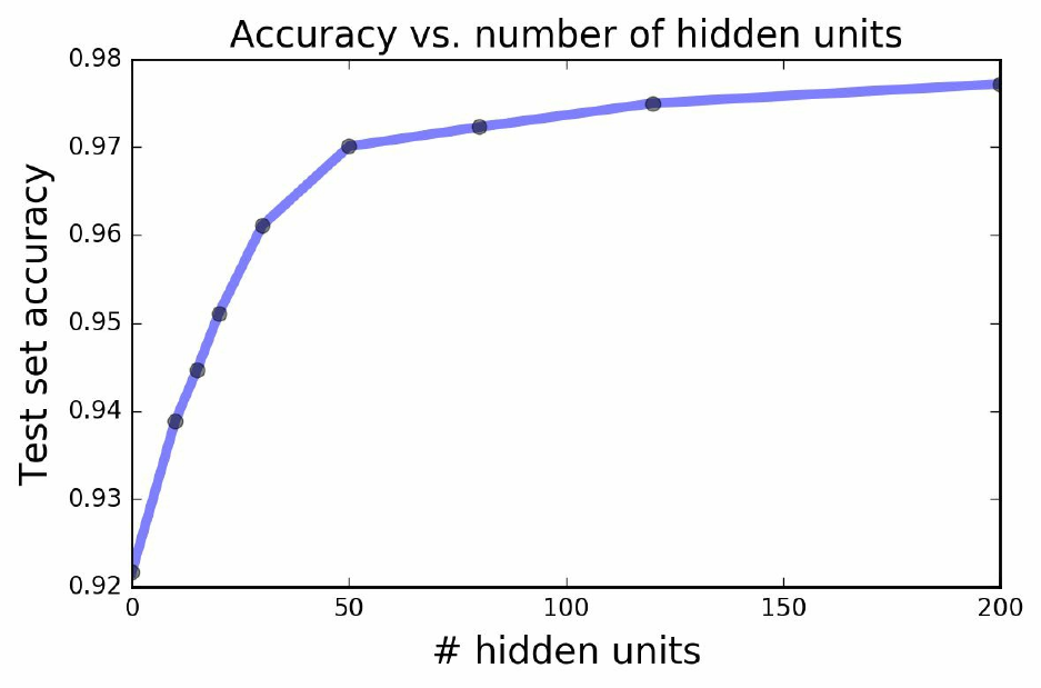
of adding just a single layer. In Figure 7-1 we see how the accuracy of the model increases with
the number of units in that hidden layer.
Figure 7-1. MNIST classification test accuracy as a function of units added in a single hidden layer.
Using the <Estimator>.predict() method, we can predict the classes of new samples. Here we
will use the predictions to demonstrate how we can analyze our model’s performance — what
classes were best identified and what types of typical errors were made. Plotting a confusion
matrix can help us understand these behaviors. We import the code to create the confusion
matrix from the scikit-learn library:
from sklearn.metrics import confusion_matrix
y_pred = dnn.predict(x=x_test,as_iterable=False)
class_names = ['0','1','2','3','4','5','6','7','8','9']
cnf_matrix = confusion_matrix(y_test, y_pred)
The confusion matrix is shown in Figure 7-2. Its rows correspond to the true digits, its columns
to the predicted digits. We see, for example, that the model sometimes misclassified 5 as 3 and 9
as 4 and 7.
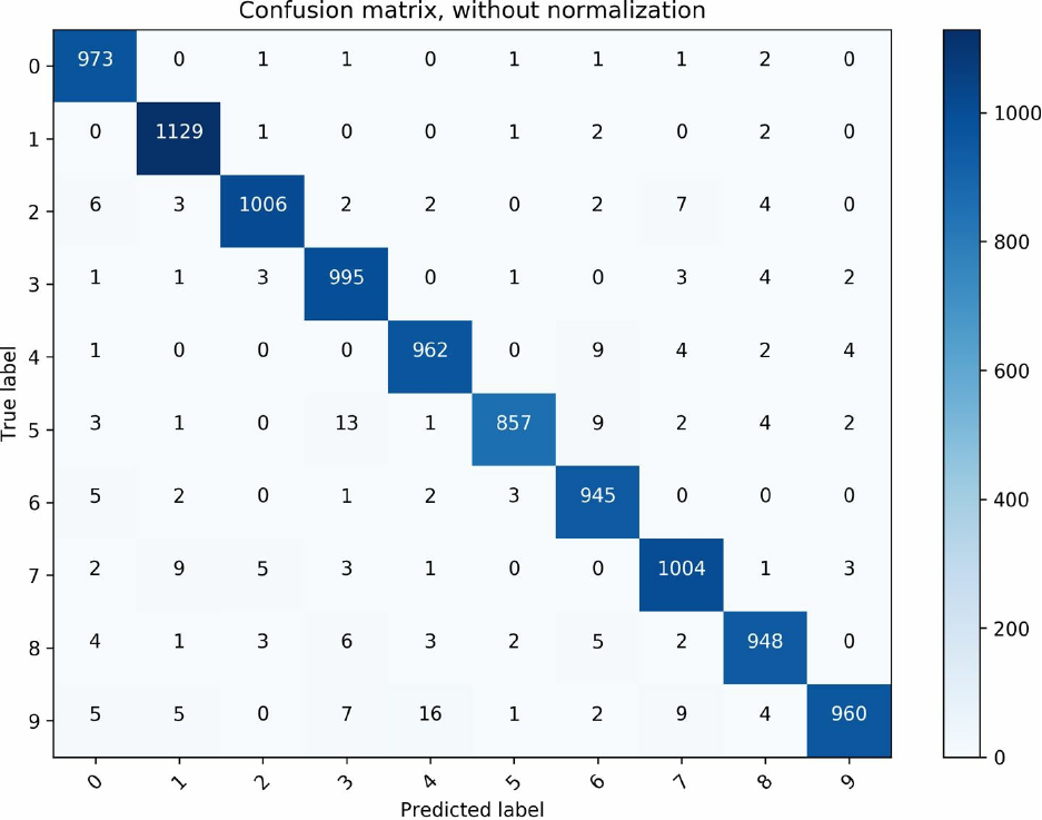
Figure 7-2. A confusion matrix showing the number of predicted digits (columns) for each true label (rows).
FeatureColumn
One of contrib.learn’s nicest offerings is handling features of different types, which can
sometimes be a little tricky. To make things easier, contrib.learn offers us the FeatureColumn
abstraction.
With a FeatureColumn we can maintain a representation of a single feature in our data, while
performing a range of transformations defined over it. A FeatureColumn can be either one of the
original columns or any new columns that may be added depending on our transformations.
These may include creating a suitable and effective representation for categorical data by
encoding it as a sparse vector (often referred to as dummy encoding), creating feature crosses to
look for feature interactions, and bucketization (discretization of the data). All this can be done
while manipulating the feature as a single semantic unit (encompassing, for example, all dummy
vectors).
We use the FeatureColumn abstraction to specify the form and structure of each feature of our
input data. For instance, let’s say that our target variable is height, and we try to predict it using
two features, weight and species. We make our own synthetic data where heights are generated
by dividing each weight by a factor of 100 and adding a constant that varies according to the
species: 1 is added for Humans, 0.9 for Goblins, and 1.1 for ManBears. We then add normally
distributed noise to each instance:
import pandas as pd
N = 10000
weight = np.random.randn(N)*5+70
spec_id = np.random.randint(0,3,N)
bias = [0.9,1,1.1]
height = np.array([weight[i]/100 + bias[b] for i,b in enumerate(spec_id)])
spec_name = ['Goblin','Human','ManBears']
spec = [spec_name[s] for s in spec_id]
Figure 7-3 shows visualizations of the data samples.
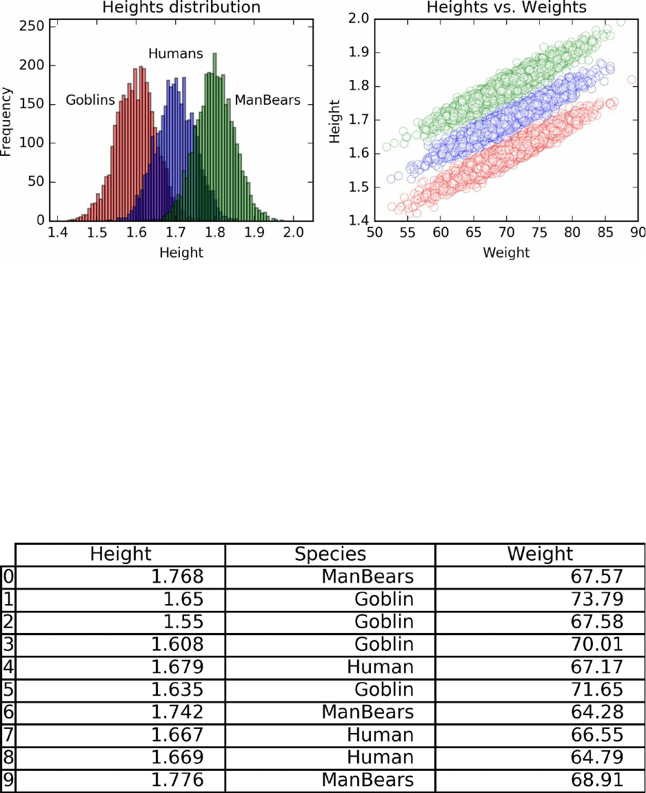
Figure 7-3. Left: A histogram of heights for the three types of species: Goblins, Humans, and ManBears
(distributions centered at 1.6, 1.7, and 1.8, respectively). Right: A scatter plot of heights vs. weights.
Our target variable is a numeric NumPy array of heights height, and our covariates are the
numeric NumPy array of weights weight and a list of strings denoting the name of each species
spec.
We use the Pandas library to have the data represented as a data frame (table), so that we can
conveniently access each of its columns:
df = pd.DataFrame({'Species':spec,'Weight':weight,'Height':height})
Figure 7-4 shows what our data frame looks like.
Figure 7-4. Ten rows of the Height–Species–Weight data frame. Heights and Weights are numeric; Species is
categorical with three categories.

PANDAS
Pandas is a very popular and useful library in Python for working with relational or labeled data like
tabular data, multidimensional time series, etc. For more information on how to use Pandas, we refer
the reader to Wes McKinney’s book Python for Data Analysis (O’Reilly).
We start by specifying the nature of each feature. For Weight we use the following
FeatureColumn command, indicating that it’s a continuous variable:
from tensorflow.contrib import layers
Weight = layers.real_valued_column("Weight")

LAYERS
contrib.layers is not a part of contrib.learn, but another independent subsection of the TensorFlow
Python API that offers high-level operations and tools for building neural network layers.
The name that was passed to the function (in this case Weight) is crucially important since it will
be used to associate the FeatureColumn representation with the actual data.
Species is a categorical variable, meaning its values have no natural ordering, and therefore
cannot be represented as a single variable in the model. Instead, it has to be extended and
encoded as several variables, depending on the number of categories. FeatureColumn does this
for us, so we just have to use the following command to specify that it is a categorical feature
and indicate the name of each category:
Species = layers.sparse_column_with_keys(
column_name="Species", keys=['Goblin','Human','ManBears'])
Next, we instantiate an estimator class and input a list of our FeatureColumns:
reg = learn.LinearRegressor(feature_columns=[Weight,Species])
Up to now we’ve defined how the data will be represented in the model; in the following stage of
fitting the model we need to provide the actual training data. In the Boston Housing example, the
features were all numeric, and as a result we could just input them as x_data and target data.
Here, contrib.learn requires that we use an additional encapsulating input function. The
function gets both predictors and target data in their native form (Pandas data frame, NumPy
array, list, etc.) as input, and returns a dictionary of tensors. In these dictionaries, each key is a
name of a FeatureColumn (the names Weight and Species that were given as input
previously), and its value needs to be a Tensor that contains the corresponding data. This means
that we also have to transform the values into a TensorFlow Tensor inside the function.
In our current example, the function receives our data frame, creates a dictionary feature_cols,
and then stores the values of each column in the data frame as a Tensor for the corresponding
key. It then returns that dictionary and the target variable as a Tensor. The keys have to match
the names we used to define our FeatureColumns:
def input_fn(df):
feature_cols = {}
feature_cols['Weight'] = tf.constant(df['Weight'].values)
feature_cols['Species'] = tf.SparseTensor(
indices=[[i, 0] for i in range(df['Species'].size)],
values=df['Species'].values,
dense_shape=[df['Species'].size, 1])
labels = tf.constant(df['Height'].values)
return feature_cols, labels
The values of Species are required by their FeatureColumn specification to be encoded in a
sparse format. For that we use tf.SparseTensor(), where each i index corresponds to a nonzero
value (in this case, all the rows in a one-column matrix).
For example, the following:
SparseTensor(indices=[[0, 0], [2, 1], [2, 2]], values=[2, 5, 7],
dense_shape=[3, 3])
represents the dense tensor:
[[2, 0, 0]
[0, 0, 0]
[0, 5, 7]]
We pass it to the .fit() method in the following way:
reg.fit(input_fn=lambda:input_fn(df), steps=50000)
Here, input_fn() is the function we just created, df is the data frame containing the data, and
we also specify the number of iterations.
Note that we pass the function in a form of a lambda function rather than the function’s outputs,
because the .fit() method requires a function object. Using lambda allows us to pass our input
arguments and keep it in an object form. There are other workarounds we could use to achieve
the same outcome, but lambda does the trick.
The fitting process may take a while. If you don’t want to do it all at once, you can split it into
segments (see the following note).
SPLITTING THE TRAINING PROCESS
It’s possible to perform the fit iteratively since the state of the model is preserved in the classifier. For
example, instead of performing all 50,000 iterations consecutively like we did, we could split it into
five segments:
reg.fit(input_fn=lambda:input_fn(df), steps=10000)
reg.fit(input_fn=lambda:input_fn(df), steps=10000)
reg.fit(input_fn=lambda:input_fn(df), steps=10000)
reg.fit(input_fn=lambda:input_fn(df), steps=10000)
reg.fit(input_fn=lambda:input_fn(df), steps=10000)
and achieve the same outcome. This could be useful if we want to have some tracking of the model
while training it; however, there are better ways to do that, as we will see later on.
Now let’s see how well the model does by looking at the estimated weights. We can use the the
.get_variable_value() method to get the variables’ values:
w_w = reg.get_variable_value('linear/Weight/weight')
print('Estimation for Weight: {}'.format(w_w))
s_w = reg.get_variable_value('linear/Species/weights')
b = reg.get_variable_value('linear/bias_weight')
print('Estimation for Species: {}'.format(s_w + b))
Out:
Estimation for Weight: [[0.00992305]]
Estimation for Species: [[0.90493023]
[1.00566959]
[1.10534406]]
We request the values of the weights for both Weight and Species. Species is a categorical
variable, so its three weights serve as different bias terms. We see that the model did quite well
in estimating the true weights (0.01 for Weight and 0.9, 1, 1.1 for Goblins, Humans, and
ManBears, respectively, for Species). We can get the names of the variables by using the
.get_variable_names() method.
The same process can be used in more complicated scenarios where we want to handle many
types of features and their interactions. Table 7-2 lists some useful operations you can do with
contrib.learn.
Table 7-2. Useful feature transformation operations
Operation Description
layers.sparse_column_with_keys() Handles the conversion of categorical values
layers.sparse_column_with_hash_bucket() Handles the conversion of categorical features for which you don’t
know all possible values
layers.crossed_column() Sets up feature crosses (interactions)

layers.bucketized_column() Turns a continuous column into a categorical column
Homemade CNN with contrib.learn
We next move on to creating our own estimator by using contrib.learn. To do so, we first need
to construct a model function where our homemade network will reside and an object containing
our training settings.
In the following example we create a custom CNN estimator that is identical to the one used at
the beginning of Chapter 4, and use it again to classify the MNIST data. We begin by creating a
function for our estimator with inputs that include our data, the mode of operation (training or
test), and the parameters of the model.
In the MNIST data the pixels are concatenated in the form of a vector and therefore require that
we reshape them:
x_image = tf.reshape(x_data, [-1, 28, 28, 1])
We build the network by using the contrib.layers functionality, making the process of layer
construction simpler.
Using layers.convolution2d() we can set everything in a one-liner command: we pass the
input (the output of the previous layer), and then indicate the number of feature maps (32), the
size of the filter (5×5), and the activation function (relu), and initialize the weights and biases.
The dimensionality of the input is automatically identified and does not need to be specified.
Also, unlike when working in lower-level TensorFlow, we don’t need to separately define the
shapes of the variables and biases:
conv1 = layers.convolution2d(x_image, 32, [5,5],
activation_fn=tf.nn.relu,
biases_initializer=tf.constant_initializer(0.1),
weights_initializer=tf.truncated_normal_initializer(stddev=0.1))
The padding is set to 'SAME' by default (unchanged number of pixels), resulting in an output of
shape 28×28×32.
We also add the standard 2×2 pooling layer:
pool1 = layers.max_pool2d(conv1, [2,2])
We then repeat these steps, this time for 64 target feature maps:
conv2 = layers.convolution2d(pool1, 64, [5,5],
activation_fn=tf.nn.relu,
biases_initializer=tf.constant_initializer(0.1),
weights_initializer=tf.truncated_normal_initializer(stddev=0.1))
pool2 = layers.max_pool2d(conv2, [2,2])
Next, we flatten the 7×7×64 tensor and add a fully connected layer, reducing it to 1,024 entries.
We use fully_connected() similarly to convolution2d(), except we specify the number of
output units instead of the size of the filter (there’s just one of those):
pool2_flat = tf.reshape(pool2, [-1, 7*7*64])
fc1 = layers.fully_connected(pool2_flat, 1024,
activation_fn=tf.nn.relu,
biases_initializer=tf.constant_initializer(0.1),
weights_initializer=tf.truncated_normal_initializer(stddev=0.1))
We then add dropout with keep_prob as set in the parameters given to the function (train/test
mode), and the final fully connected layer with 10 output entries, corresponding to the 10
classes:
fc1_drop = layers.dropout(fc1, keep_prob=params["dropout"],
is_training=(mode == 'train'))
y_conv = layers.fully_connected(fc1_drop, 10, activation_fn=None)
We complete our model function by defining a training object with the loss and the learning rate
of the optimizer.
We now have one function that encapsulates the entire model:
def model_fn(x, target, mode, params):
y_ = tf.cast(target, tf.float32)
x_image = tf.reshape(x, [-1, 28, 28, 1])
# Conv layer 1
conv1 = layers.convolution2d(x_image, 32, [5,5],
activation_fn=tf.nn.relu,
biases_initializer=tf.constant_initializer(0.1),
weights_initializer=tf.truncated_normal_initializer(stddev=0.1))
pool1 = layers.max_pool2d(conv1, [2,2])
# Conv layer 2
conv2 = layers.convolution2d(pool1, 64, [5,5],
activation_fn=tf.nn.relu,
biases_initializer=tf.constant_initializer(0.1),
weights_initializer=tf.truncated_normal_initializer(stddev=0.1))
pool2 = layers.max_pool2d(conv2, [2,2])
# FC layer
pool2_flat = tf.reshape(pool2, [-1, 7*7*64])
fc1 = layers.fully_connected(pool2_flat, 1024,
activation_fn=tf.nn.relu,
biases_initializer=tf.constant_initializer(0.1),
weights_initializer=tf.truncated_normal_initializer(stddev=0.1))
fc1_drop = layers.dropout(fc1, keep_prob=params["dropout"],
is_training=(mode == 'train'))
# Readout layer
y_conv = layers.fully_connected(fc1_drop, 10, activation_fn=None)
cross_entropy = tf.reduce_mean(
tf.nn.softmax_cross_entropy_with_logits(logits=y_conv, labels=y_))
train_op = tf.contrib.layers.optimize_loss(
loss=cross_entropy,
global_step=tf.contrib.framework.get_global_step(),
learning_rate=params["learning_rate"],
optimizer="Adam")
predictions = tf.argmax(y_conv, 1)
return predictions, cross_entropy, train_op
We instantiate the estimator by using contrib.learn.Estimator(), and we’re good to go. Once
defined, we can use it with the same functionalities as before:
from tensorflow.contrib import layers
data = input_data.read_data_sets(DATA_DIR, one_hot=True)
x_data, y_data = data.train.images,np.int32(data.train.labels)
tf.cast(x_data,tf.float32)
tf.cast(y_data,tf.float32)
model_params = {"learning_rate": 1e-4, "dropout": 0.5}
CNN = tf.contrib.learn.Estimator(
model_fn=model_fn, params=model_params)
print("Starting training for %s steps max" % 5000)
CNN.fit(x=data.train.images,
y=data.train.labels, batch_size=50,
max_steps=5000)
test_acc = 0
for ii in range(5):
batch = data.test.next_batch(2000)
predictions = list(CNN.predict(batch[0], as_iterable=True))
test_acc = test_acc + (np.argmax(batch[1],1) == predictions).mean()
print(test_acc/5)
Out:
0.9872
Using contrib.learn and contrib.layers, the number of lines of code was cut down
considerably in comparison to lower-level TensorFlow. More important, the code is much more
organized and easier to follow, debug, and write.
With this example we conclude the contrib.learn portion of this chapter. We’ll now move on
to cover some of the functionalities of the TFLearn library.
TFLearn
TFLearn is another library that allows us to create complex custom models in a very clean and
compressed way, while still having a reasonable amount of flexibility, as we will see shortly.
Installation
Unlike the previous library, TFLearn first needs to be installed. The installation is
straightforward using pip:
pip install tflearn
If that doesn’t work, it can be downloaded from GitHub and installed manually.
After the library has been successfully installed, you should be able to import it:
import tflearn
CNN
Many of the functionalities of TFLearn resemble those covered in the previous section on
contrib.learn; however, creating a custom model is a bit simpler and cleaner in comparison. In
the following code we use the same CNN used earlier for the MNIST data.
Model construction is wrapped and finalized using regression(), where we set the loss and
optimization configuration as we did previously for the training object in contrib.learn (here
we simply specify 'categorical_crossentreopy' for the loss, rather than explicitly defining it):
from tflearn.layers.core import input_data, dropout, fully_connected
from tflearn.layers.conv import conv_2d, max_pool_2d
from tflearn.layers.normalization import local_response_normalization
from tflearn.layers.estimator import regression
# Data loading and basic transformations
import tflearn.datasets.mnist as mnist
X, Y, X_test, Y_test = mnist.load_data(one_hot=True)
X = X.reshape([-1, 28, 28, 1])
X_test = X_test.reshape([-1, 28, 28, 1])
# Building the network
CNN = input_data(shape=[None, 28, 28, 1], name='input')
CNN = conv_2d(CNN, 32, 5, activation='relu', regularizer="L2")
CNN = max_pool_2d(CNN, 2)
CNN = local_response_normalization(CNN)
CNN = conv_2d(CNN, 64, 5, activation='relu', regularizer="L2")
CNN = max_pool_2d(CNN, 2)
CNN = local_response_normalization(CNN)
CNN = fully_connected(CNN, 1024, activation=None)
CNN = dropout(CNN, 0.5)
CNN = fully_connected(CNN, 10, activation='softmax')
CNN = regression(CNN, optimizer='adam', learning_rate=0.0001,
loss='categorical_crossentropy', name='target')
# Training the network
model = tflearn.DNN(CNN,tensorboard_verbose=0,
tensorboard_dir = 'MNIST_tflearn_board/',
checkpoint_path = 'MNIST_tflearn_checkpoints/checkpoint')
model.fit({'input': X}, {'target': Y}, n_epoch=3,
validation_set=({'input': X_test}, {'target': Y_test}),
snapshot_step=1000,show_metric=True, run_id='convnet_mnist')
Another layer that’s been added here, and that we briefly mentioned in Chapter 4, is the local
response normalization layer. See the upcoming note for more details about this layer.
The tflearn.DNN() function is somewhat equivalent to contrib.learn.Estimator() — it’s the
DNN model wrapper with which we instantiate the model and to which we pass our constructed
network.
Here we can also set the TensorBoard and checkpoints directories, the level of verbosity of
TensorBoard’s logs (0–3, from basic loss and accuracy reports to other measures like gradients
and weights), and other settings.
Once we have a model instance ready, we can then perform standard operations with it. Table 7-
3 summarizes the model’s functionalities in TFLearn.
Table 7-3. Standard TFLearn operations
Table 7-3. Standard TFLearn operations
Function Description
evaluate(X, Y, batch_size=128)Perform evaluations of the model on given samples.
fit(X, Y, n_epoch=10)Train the model with input features X and target Y to the network.
get_weights(weight_tensor)Get a variable’s weights.
load(model_file)Restore model weights.
predict(X)Get model predictions for the given input data.
save(model_file)Save model weights.
set_weights(tensor, weights)Assign a tensor variable a given value.
Similarly with contrib.learn, the fitting operation is performed by using the .fit() method, to
which we feed the data and control training settings: the number of epochs, training and
validation batch sizes, displayed measures, saved summaries frequency, and more. During
fitting, TFLearn displays a nice dashboard, enabling us to track the training process online.

LOCAL RESPONSE NORMALIZATION
The local response normalization (LRN) layer performs a kind of lateral inhibition by normalizing
over local input regions. This is done by dividing the input values by the weighted, squared sum of all
inputs within some depth radius, which we can manually choose. The resulting effect is that the
activation contrast between the excited neurons and their local surroundings increases, producing more
salient local maxima. This method encourages inhibition since it will diminish activations that are
large, but uniform. Also, normalization is useful to prevent neurons from saturating when inputs may
have varying scale (ReLU neurons have unbounded activation). There are more modern alternatives
for regularization, such as batch normalization and dropout, but it is good to know about LRN too.
After fitting the model, we evaluate performance on the test data:
evaluation = model.evaluate({'input': X_test},{'target': Y_test})
print(evaluation):
Out:
0.9862
and form new predictions (using them here again as a “sanity check” to the previous evaluation):
pred = model.predict({'input': X_test})
print((np.argmax(testY,1)==np.argmax(pred,1)).mean())
Out:
0.9862
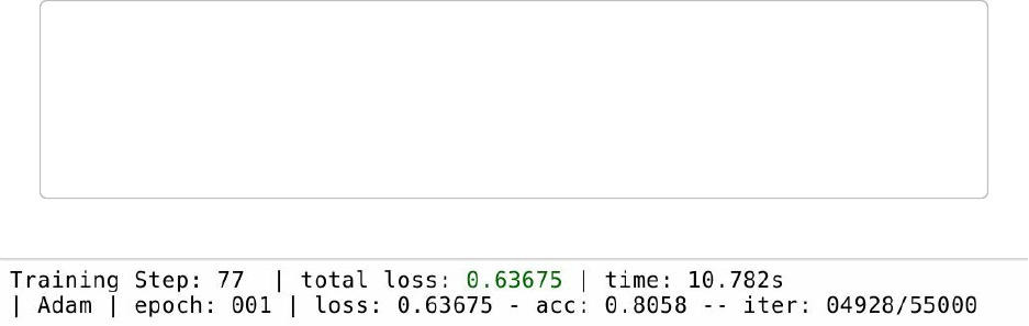
ITERATIONS TRAINING STEPS AND EPOCHS IN TFLEARN
In TFLearn, each iteration is a full pass (forward and backward) over one example. The training step
is the number of full passes to perform, determined by the batch size you set (the default is 64), and an
epoch is a full pass over all the training examples (50,000 in the case of MNIST). Figure 7-5 shows an
example of the interactive display in TFLearn.
Figure 7-5. Interactive display in TFLearn.
RNN
We wrap up our introduction to TFLearn by constructing a fully functioning text classification
RNN model that considerably simplifies the code we saw in Chapters 5 and 6.
The task we perform is a sentiment analysis for movie reviews with binary classification (good
or bad). We will use a well-known dataset of IMDb reviews, containing 25,000 training samples
and 25,000 test samples:
from tflearn.data_utils import to_categorical, pad_sequences
from tflearn.datasets import imdb
# IMDb dataset loading
train, test, _ = imdb.load_data(path='imdb.pkl', n_words=10000,
valid_portion=0.1)
X_train, Y_train = train
X_test, Y_test = test
We first prepare the data, which has different sequence lengths, by equalizing the sequences with
zero-padding by using tflearn.data_utils.pad_sequences() and setting 100 as the maximum
sequence length:
X_train = pad_sequences(X_train, maxlen=100, value=0.)
X_test = pad_sequences(X_test, maxlen=100, value=0.)
Now we can represent data in one tensor, with samples in its rows and word IDs in its columns.
As was explained in Chapter 5, IDs here are integers that are used to encode the actual words
arbitrarily. In our case, we have 10,000 unique IDs.
Next, we embed each word into a continuous vector space by using tflearn.embedding(),
transforming our two-dimensional tensor [samples, IDs] into a three-dimensional tensor,
[samples, IDs, embedding-size], where each word ID now corresponds to a vector of size of
128. Before that we use input_data() to input/feed data to the network (a TensorFlow
placeholder is created with the given shape):
RNN = tflearn.input_data([None, 100])
RNN = tflearn.embedding(RNN, input_dim=10000, output_dim=128)
Finally, we add an LSTM layer and a fully connected layer to output the binary outcome:
RNN = tflearn.lstm(RNN, 128, dropout=0.8)
RNN = tflearn.fully_connected(RNN, 2, activation='softmax'
Here’s the full code:
from tflearn.data_utils import to_categorical, pad_sequences
from tflearn.datasets import imdb
# Load data
train, test, _ = imdb.load_data(path='imdb.pkl', n_words=10000,
valid_portion=0.1)
X_train, Y_train = train
X_test, Y_test = test
# Sequence padding and converting labels to binary vectors
X_train = pad_sequences(X_train, maxlen=100, value=0.)
X_test = pad_sequences(X_test, maxlen=100, value=0.)
Y_train = to_categorical(Y_train, nb_classes=2)
Y_test = to_categorical(Y_test, nb_classes=2)
# Building an LSTM network
RNN = tflearn.input_data([None, 100])
RNN = tflearn.embedding(RNN, input_dim=10000, output_dim=128)
RNN = tflearn.lstm(RNN, 128, dropout=0.8)
RNN = tflearn.fully_connected(RNN, 2, activation='softmax')
RNN = tflearn.regression(RNN, optimizer='adam', learning_rate=0.001,
loss='categorical_crossentropy')
# Training the network
model = tflearn.DNN(RNN, tensorboard_verbose=0)
model.fit(X_train, Y_train, validation_set=(X_test, Y_test),
show_metric=True, batch_size=32)
In this section, we had just a quick taste of TFLearn. The library has nice documentation and
many examples that are well worth looking at.
Keras
Keras is one of the most popular and powerful TensorFlow extension libraries. Among the
extensions we survey in this chapter, Keras is the only one that supports both Theano — upon
which it was originally built — and TensorFlow. This is possible because of Keras’s complete
abstraction of its backend; Keras has its own graph data structure for handling computational
graphs and communicating with TensorFlow.
In fact, because of that it could even be possible to define a Keras model with either TensorFlow
or Theano and then switch to the other.
Keras has two main types of models to work with: sequential and functional. The sequential type
is designed for simple architectures, where we just want to stack layers in a linear fashion. The
functional API can support more-general models with a diverse layer structure, such as
multioutput models.
We will take a quick look at the syntax used for each type of model.
Installation
In TensorFlow 1.1+ Keras can be imported from the contrib library; however, for older versions
it needs to be installed externally. Note that Keras requires the numpy, scipy, and yaml
dependencies. Similarly to TFLearn, Keras can either be installed using pip:
pip install keras
or downloaded from GitHub and installed using:
python setup.py install
By default, Keras will use TensorFlow as its tensor manipulation library. If it is set to use
Theano, it can be switched by changing the settings in the file called $HOME/.keras/keras.json
(for Linux users — modify the path according to your OS), where the attribute backend appears
in addition to other technical settings not important in this chapter:
{
"image_data_format": "channels_last",
"epsilon": 1e-07,
"floatx": "float32",
"backend": "tensorflow"
}
If we want to access the backend, we can easily do so by first importing it:
from keras import backend as K
We can then use it for most tensor operations as we would in TensorFlow (also for Theano). For
example, this:
input = K.placeholder(shape=(10,32))
is equivalent to:
tf.placeholder(shape=(10,32))
Sequential model
Using the sequential type is very straightforward — we define it and can simply start adding
layers:
from keras.models import Sequential
from keras.layers import Dense, Activation
model = Sequential()
model.add(Dense(units=64, input_dim=784))
model.add(Activation('softmax'))
Or equivalently:
model = Sequential([
Dense(64, input_shape=(784,),activation='softmax')
])
A dense layer is a fully connected layer. The first argument denotes the number of output units,
and the input shape is the shape of the input (in this example the weight matrix would be of size
784×64). Dense() also has an optional argument where we can specify and add an activation
function, as in the second example.
After the model is defined, and just before training it, we set its learning configurations by using
the .compile() method. It has three input arguments — the loss function, the optimizer, and
another metric function that is used to judge the performance of your model (not used as the
actual loss when training the model):
model.compile(loss='categorical_crossentropy',
optimizer='sgd',
metrics=['accuracy'])
We can set the optimizer at a finer resolution (learning rate, method, etc.) using .optimizers.
For example:
optimizer=keras.optimizers.SGD(lr=0.02, momentum=0.8, nesterov=True))
Finally, we feed .fit() the data and set the number of epochs and batch size. As with the
previous libraries, we can now easily evaluate how it does and perform predictions with new test
data:
from keras.callbacks import TensorBoard, EarlyStopping, ReduceLROnPlateau
early_stop = EarlyStopping(monitor='val_loss', min_delta=0,
patience=10, verbose=0, mode='auto')
model.fit(x_train, y_train, epochs=10, batch_size=64,
callbacks=[TensorBoard(log_dir='/models/autoencoder',)
early_stop])
loss_and_metrics = model.evaluate(x_test, y_test, batch_size=64)
classes = model.predict(x_test, batch_size=64)
Note that a callbacks argument was added to the fit() method. Callbacks are functions that are
applied during the training procedure, and we can use them to get a view on statistics and make
dynamic training decisions by passing a list of them to the .fit() method.
In this example we plug in two callbacks: TensorBoard, specifying its output folder, and early
stopping.

EARLY STOPPING
Early stopping is used to protect against overfitting by preventing the learner from further improving
its fit to the training data at the expense of increasing the generalization error. In that sense, it can be
thought of as a form of regularization. In Keras we can specify the minimum change to be monitored
(min_delta), the number of no-improvement epochs to stop after (patience), and the direction of
wanted change (mode).
Functional model
The main practical difference between the functional model and the sequential model is that here
we first define our input and output, and only then instantiate the model.
We first create an input Tensor according to its shape:
inputs = Input(shape=(784,))
Then we define our model:
x = Dense(64, activation='relu')(inputs)
x = Dense(32, activation='relu')(x)
outputs = Dense(10, activation='softmax')(x)
As we can see, the layers act as functions, giving the functional model its name.
And now we instantiate the model, passing both inputs and outputs to Model:
model = Model(inputs=inputs, outputs=outputs)
The other steps follow as before:
model.compile(optimizer='rmsprop',
loss='categorical_crossentropy',
metrics=['accuracy'])
model.fit(x_train, y_train, epochs=10, batch_size=64)
loss_and_metrics = model.evaluate(x_test, y_test, batch_size=64)
classes = model.predict(x_test, batch_size=64)
We will end this section by introducing the concept of autoencoders and then showing how to
implement one using Keras.
Autoencoders
Autoencoders are neural networks that try to output a reconstruction of the input. In most cases
the input is reconstructed after having its dimensionality reduced. Dimensionality reduction will
be our main focus; however, autoencoders can also be used to achieve “overcomplete”
representations (for more stable decomposition), which actually increases dimensions.
In dimensionality reduction we wish to translate each vector of data with size n to a vector with
size m, where m < n, while trying to keep as much important information as possible. One very
common way to do that is using principal component analysis (PCA), where we can represent
each original data column xj (all data points corresponding to an original feature) with some
linear combination of the new reduced features, called the principal components, such that xj =
Σi=1mwibi.
PCA, however, is limited to only linear transformation of the data vectors.
Autoencoders are more general compressors, allowing complicated nonlinear transformations
and finding nontrivial relations between visible and hidden units (in fact, PCA is like a one-layer
“linear autoencoder”). The weights of the models are learned automatically by reducing a given
loss function with an optimizer (SGD, for example).
Autoencoders that reduce input dimensionality create a bottleneck layer called a hidden layer
that has a smaller number of units than the input layer, forcing the data to be represented in a
lower dimension (Figure 7-6) before it is reconstructed. For the reconstruction
(decoding), autoencoders extract representative features that capture some hidden abstractions,
like the shape of an eye, wheel of a car, type of sport, etc., with which we can reconstruct the
original input.
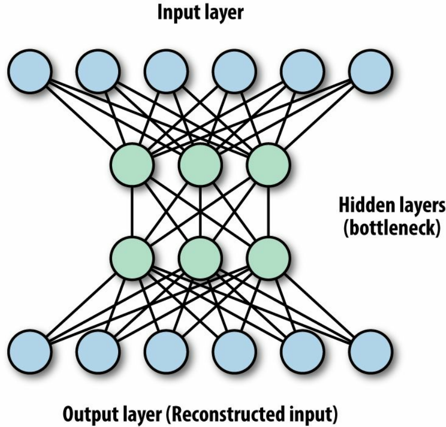
Figure 7-6. Illustration of an autoencoder — a typical autoencoder will have input and output layers consisting of
the same number of units, and bottleneck hidden layers, where the dimensionality of the data is reduced
(compressed).
Like some of the models we’ve seen so far, autoencoder networks can have layers stacked on top
of each other, and they can include convolutions as in CNNs.
Autoencoders are currently not very suitable for real-world data compression problems due to
their data specificity — they are best used on data that is similar to what they were trained on.
Their current practical applications are mostly for extracting lower-dimensional representations,
denoising data, and data visualization with reduced dimensionality. Denoising works because the
network learns the important abstractions of the image, while losing unimportant image-specific
signals like noise.
Now let’s build a toy CNN autoencoder with Keras. In this example we will train the
autoencoder on one category of a noisy version of the CIFAR10 data images, and then use it to
denoise a test set of the same category. In this example we will use the functional model API.
First we load the images by using Keras, and then we choose only the images that correspond to
the label 1 (the automobile class):
from keras.layers import Input, Conv2D, MaxPooling2D, UpSampling2D
from keras.models import Model
from keras.callbacks import TensorBoard, ModelCheckpoint
from keras.datasets import cifar10
import numpy as np
(x_train, y_train), (x_test, y_test) = cifar10.load_data()
x_train = x_train[np.where(y_train==1)[0],:,:,:]
x_test = x_test[np.where(y_test==1)[0],:,:,:]
Next we do a little pre-processing, by first converting our data to float32 and then normalizing
it to a range between [0,1]. This normalization will allow us to perform an element-wise
comparison at the pixel level, as we will see shortly. First, the type conversion:
x_train = x_train.astype('float32') / 255.
x_test = x_test.astype('float32') / 255.
We then add some Gaussian noise to create the noisy dataset, and clip values that are either
smaller than 0 or larger than 1:
x_train_n = x_train + 0.5 *\
np.random.normal(loc=0.0, scale=0.4, size=x_train.shape)
x_test_n = x_test + 0.5 *\
np.random.normal(loc=0.0, scale=0.4, size=x_test.shape)
x_train_n = np.clip(x_train_n, 0., 1.)
x_test_n = np.clip(x_test_n, 0., 1.)
Now we declare the input layer (every image in the CIFAR10 dataset is 32×32 pixels with RGB
channels):
inp_img = Input(shape=(32, 32, 3))
Next, we start adding our usual “LEGO brick" layers. Our first layer is a 2D convolution layer,
where the first argument is the number of filters (and thus the number of output images), and the
second is the size of each filter. Like the other libraries, Keras automatically identifies the shape
of the input.
We use a 2×2 pooling layer, which reduces the total number of pixels per channel by 4, creating
the desired bottleneck. After another convolutional layer, we regain the same number of units for
each channel by applying an up-sampling layer. This is done by quadrupling each pixel in a
pixel’s near vicinity (repeating the rows and columns of the data) to get back the same number of
pixels in each image.
Finally, we add a convolutional output layer where we go back to three channels:
img = Conv2D(32, (3, 3), activation='relu', padding='same')(inp_img)
img = MaxPooling2D((2, 2), padding='same')(img)
img = Conv2D(32, (3, 3), activation='relu', padding='same')(img)
img = UpSampling2D((2, 2))(img)
decoded = Conv2D(3, (3, 3), activation='sigmoid', padding='same')(img)
We declare the functional model format, passing both inputs and outputs:
autoencoder = Model(inp_img, decoded)
Next we compile the model, defining the loss function and the optimizer — in this case we use
the Adagrad optimizer (just to show another example!). For denoising of the images, we want
our loss to capture the discrepancy between the decoded images and the original, pre-noise
images. For that we use a binary cross-entropy loss, comparing each decoded pixel to its
corresponding original one (it’s now between [0,1]):
autoencoder.compile(optimizer='adadelta', loss='binary_crossentropy')
After the model is defined, we fit it with 10 training epochs:
tensorboard = TensorBoard(log_dir='<some_path>',
histogram_freq=0, write_graph=True, write_images=True)
model_saver = ModelCheckpoint(
filepath='<some_path>',
verbose=0, period=2)
autoencoder.fit(x_train_n, x_train,
epochs=10,
batch_size=64,
shuffle=True,
validation_data=(x_test_n, x_test),
callbacks=[tensorboard, model_saver])
Hopefully the model will capture some internal structure, which it can later generalize to other
noisy images, and denoise them as a result.
We use our test set as validation data for loss evaluation at the end of each epoch (the model will
not be trained on this data), and also for visualization in TensorBoard. In addition to the
TensorBoard callback, we add a model saver callback and set it to save our weights every two
epochs.
Later, when we wish to load our weights, we need to reconstruct the network and then use the
Model.load_weights() method, passing our model as the first argument and our saved weights
file path as the second (more on saving models in Chapter 10):
inp_img = Input(shape=(32, 32, 3))
img = Conv2D(32, (3, 3), activation='relu', padding='same')(inp_img)
img = MaxPooling2D((2, 2), padding='same')(img)
img = Conv2D(32, (3, 3), activation='relu', padding='same')(img)
img = UpSampling2D((2, 2))(img)
decoded = Conv2D(3, (3, 3), activation='sigmoid', padding='same')(img)
autoencoder = Model(inp_img, decoded)
Model.load_weights(autoencoder,'some_path')
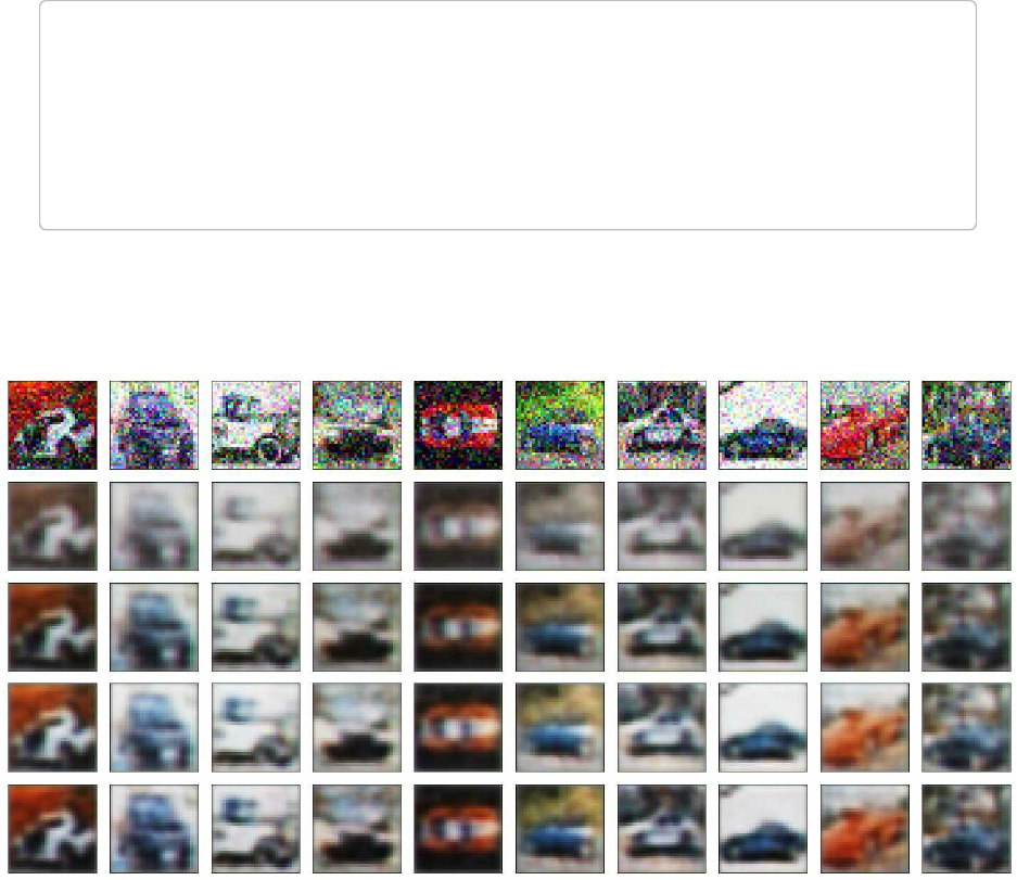
H5PY REQUIREMENT
For model saving, it is required that the h5py package is installed. This package is primarily used for
storing large amounts of data and manipulating it from NumPy. You can install it using pip:
pip install h5py
Figure 7-7 shows the denoised test images of our chosen category for different numbers of
training epochs.
Figure 7-7. Noisy CIFAR10 images before autoencoding (upper row) and after autoencoding (lower rows). The 4
bottom rows show results after increasing number of training epochs.
Keras also has a bunch of pretrained models to download, like inception, vgg, and resnet. In the
next and final section of this chapter, we will discuss these models and show an example of how
to download and use a pretrained VGG model for classification using the TF-Slim extension.
Pretrained models with TF-Slim
In this section of the chapter we will introduce the last abstraction to be covered here, TF-Slim.
TF-Slim stands out by offering simplified syntax for defining convolutional neural networks in
TensorFlow — its abstractions make it easy to build complex networks in a clean, streamlined
manner. Like Keras, it also offers a nice variety of pretrained CNN models to download and use.
We start this section by learning about some of the general features and benefits of TF-Slim, and
why it’s a great tool to use for building CNNs. In the second part of this section we will
demonstrate how to download and deploy a pretrained model (VGG) for image classification.
TF-Slim
TF-Slim is a relatively new lightweight extension of TensorFlow that, like other abstractions,
allows us to define and train complex models quickly and intuitively. TF-Slim doesn’t require
any installation since it’s been merged with TensorFlow.
This extension is all about convolutional neural networks. CNNs are notorious for having a lot of
messy boilerplate code. TF-Slim was designed with the goal of optimizing the creation of very
complex CNN models so that they could be elegantly written and easy to interpret and debug by
using high-level layers, variable abstractions, and argument scoping, which we will touch upon
shortly.
In addition to enabling us to create and train our own models, TF-Slim has available pretrained
networks that can be easily downloaded, read, and used: VGG, AlexNet, Inception, and more.
We start this section by briefly describing some of TF-Slim’s abstraction features. Then we shift
our focus to how to download and use a pretrained model, demonstrating it for the VGG image
classification model.
Creating CNN models with TF-Slim
With TF-Slim we can create a variable easily by defining its initialization, regularization, and
device with one wrapper. For example, here we define weights initialized from a truncated
normal distribution using L2 regularization and placed on the CPU (we will talk about
distributing model parts across devices in Chapter 9):
import tensorflow as tf
from tensorflow.contrib import slim
W = slim.variable('w',shape=[7, 7, 3 , 3],
initializer=tf.truncated_normal_initializer(stddev=0.1),
regularizer=slim.l2_regularizer(0.07),
device='/CPU:0')
Like the other abstractions we’ve seen in this chapter, TF-Slim can reduce a lot of boilerplate
code and redundant duplication. As with Keras or TFLearn, we can define a layer operation at an
abstract level to include the convolution operation, weights initialization, regularization,
activation function, and more in a single command:
net = slim.conv2d(inputs, 64, [11, 11], 4, padding='SAME',
weights_initializer=tf.truncated_normal_initializer(stddev=0.01),
weights_regularizer=slim.l2_regularizer(0.0007), scope='conv1')
TF-Slim extends its elegance even beyond that, providing a clean way to replicate layers
compactly by using the repeat, stack, and arg_scope commands.
repeat saves us the need to copy and paste the same line over and over so that, for example,
instead of having this redundant duplication:
net = slim.conv2d(net, 128, [3, 3], scope='con1_1')
net = slim.conv2d(net, 128, [3, 3], scope='con1_2')
net = slim.conv2d(net, 128, [3, 3], scope='con1_3')
net = slim.conv2d(net, 128, [3, 3], scope='con1_4')
net = slim.conv2d(net, 128, [3, 3], scope='con1_5')
we could just enter this:
net = slim.repeat(net, 5, slim.conv2d, 128, [3, 3], scope='con1')
But this is viable only in cases where we have layers of the same size. When this does not hold,
we can use the stack command, allowing us to concatenate layers of different shapes. So,
instead of this:
net = slim.conv2d(net, 64, [3, 3], scope='con1_1')
net = slim.conv2d(net, 64, [1, 1], scope='con1_2')
net = slim.conv2d(net, 128, [3, 3], scope='con1_3')
net = slim.conv2d(net, 128, [1, 1], scope='con1_4')
net = slim.conv2d(net, 256, [3, 3], scope='con1_5')
we can write this:
slim.stack(net, slim.conv2d, [(64, [3, 3]), (64, [1, 1]),
(128, [3, 3]), (128, [1, 1]),
(256, [3, 3])], scope='con')
Finally, we also have a scoping mechanism referred to as arg_scope, allowing users to pass a set
of shared arguments to each operation defined in the same scope. Say, for example, that we have
four layers having the same activation function, initialization, regularization, and padding. We
can then simply use the slim.arg_scope command, where we specify the shared arguments as in
the following code:
with slim.arg_scope([slim.conv2d],
padding='VALID',
activation_fn=tf.nn.relu,
weights_initializer=tf.truncated_normal_initializer(stddev=0.02)
weights_regularizer=slim.l2_regularizer(0.0007)):
net = slim.conv2d(inputs, 64, [11, 11], scope='con1')
net = slim.conv2d(net, 128, [11, 11], padding='VALID', scope='con2')
net = slim.conv2d(net, 256, [11, 11], scope='con3')
net = slim.conv2d(net, 256, [11, 11], scope='con4')
The individual arguments inside the arg_scope command can still be overwritten, and we can
also nest one arg_scope inside another.
In these examples we used conv2d(): however, TF-Slim has many of the other standard methods
for building neural networks. Table 7-4 lists some of the available options. For the full list,
consult the documentation.
Table 7-4. Available layer types in TF-Slim
Layer TF-Slim
BiasAdd slim.bias_add()
BatchNorm slim.batch_norm()
Conv2d slim.conv2d()
Conv2dInPlane slim.conv2d_in_plane()
Conv2dTranspose (Deconv) slim.conv2d_transpose()
FullyConnected slim.fully_connected()
AvgPool2D slim.avg_pool2d()
Dropout slim.dropout()
Flatten slim.flatten()
MaxPool2D slim.max_pool2d()
OneHotEncoding slim.one_hot_encoding()
SeparableConv2 slim.separable_conv2d()
UnitNorm slim.unit_norm
To illustrate how convenient TF-Slim is for creating complex CNNs, we will build the VGG
model by Karen Simonyan and Andrew Zisserman that was introduced in 2014 (see the
upcoming note for more information). VGG serves as a good illustration of how a model with
many layers can be created compactly using TF-Slim. Here we construct the 16-layer version: 13
convolution layers plus 3 fully connected layers.
Creating it, we take advantage of two of the features we’ve just mentioned:
1. We use the arg_scope feature since all of the convolution layers have the same
activation function and the same regularization and initialization.
2. Many of the layers are exact duplicates of others, and therefore we also take advantage
of the repeat command.
The result very compelling — the entire model is defined with just 16 lines of code:
with slim.arg_scope([slim.conv2d, slim.fully_connected],
activation_fn=tf.nn.relu,
weights_initializer=tf.truncated_normal_initializer(0.0, 0.01),
weights_regularizer=slim.l2_regularizer(0.0005)):
net = slim.repeat(inputs, 2, slim.conv2d, 64, [3, 3], scope='con1')
net = slim.max_pool2d(net, [2, 2], scope='pool1')
net = slim.repeat(net, 2, slim.conv2d, 128, [3, 3], scope='con2')
net = slim.max_pool2d(net, [2, 2], scope='pool2')
net = slim.repeat(net, 3, slim.conv2d, 256, [3, 3], scope='con3')
net = slim.max_pool2d(net, [2, 2], scope='pool3')
net = slim.repeat(net, 3, slim.conv2d, 512, [3, 3], scope='con4')
net = slim.max_pool2d(net, [2, 2], scope='pool4')
net = slim.repeat(net, 3, slim.conv2d, 512, [3, 3], scope='con5')
net = slim.max_pool2d(net, [2, 2], scope='pool5')
net = slim.fully_connected(net, 4096, scope='fc6')
net = slim.dropout(net, 0.5, scope='dropout6')
net = slim.fully_connected(net, 4096, scope='fc7')
net = slim.dropout(net, 0.5, scope='dropout7')
net = slim.fully_connected(net, 1000, activation_fn=None, scope='fc8')

VGG AND THE IMAGENET CHALLENGE
The ImageNet project is a large database of images collected for the purpose of researching visual
object recognition. As of 2016 it contained over 10 million hand-annotated images.
Each year (since 2010) a competition takes place called the ImageNet Large Scale Visual Recognition
Challenge (ILSVRC), where research teams try to automatically classify, detect, and localize objects
and scenes in a subset of the ImageNet collection. In the 2012 challenge, dramatic progress occurred
when a deep convolutional neural net called AlexNet, created by Alex Krizhevsky, managed to get a
top 5 (top 5 chosen categories) classification error of only 15.4%, winning the competition by a large
margin.
Over the next couple of years the error rate kept falling, from ZFNet with 14.8% in 2013, to
GoogLeNet (introducing the Inception module) with 6.7% in 2014, to ResNet with 3.6% in 2015. The
Visual Geometry Group (VGG) was another CNN competitor in the 2014 competition that also
achieved an impressive low error rate (7.3%). A lot of people prefer VGG over GoogLeNet because it
has a nicer, simpler architecture.
In VGG the only spatial dimensions used are very small 3×3 filters with a stride of 1 and a 2×2 max
pooling, again with a stride of 1. Its superiority is achieved by the number of layers it uses, which is
between 16 and 19.
Downloading and using a pretrained model
Next we will demonstrate how to download and deploy a pretrained VGG model.
First we need to clone the repository where the actual models will reside by running:
git clone https://github.com/tensorflow/models
Now we have the scripts we need for modeling on our computer, and we can use them by setting
the path:
import sys
sys.path.append("<some_path> + models/slim")
Next we will download the pretrained VGG-16 (16 layers) model — it is available on GitHub, as
are other models, such as Inception, ResNet, and more:
from datasets import dataset_utils
import tensorflow as tf
target_dir = '<some_path> + vgg/vgg_checkpoints'
The downloaded checkpoint file contains information about both the model and the variables.
Now we want to load it and use it for classification of new images.
However, before that we first have to prepare our input image, turning it into a readable
TensorFlow format and performing a little pre-processing to make sure that it is resized to match
the size of the images the model was trained on.
We can load the image into TensorFlow either as a URL link or as a desktop image. For a URL
link, we can load the image as a string with urllib2 (this needs to be imported), and then decode
it into a Tensor by using tf.image_decode_jpeg():
import urllib2
url = ("https://somewebpage/somepicture.jpg")
im_as_string = urllib2.urlopen(url).read()
im = tf.image.decode_jpeg(im_as_string, channels=3)
Or, for PNG:
im = tf.image.decode_png(im_as_string, channels=3)
To load an image from our computer, we can create a queue of our filenames in the target
directory, and then read the entire image file by using tf.WholeFileReader():
filename_queue = tf.train.string_input_producer(
tf.train.match_filenames_once("./images/*.jpg"))
image_reader = tf.WholeFileReader()
_, image_file = image_reader.read(filename_queue)
image = tf.image.decode_jpeg(image_file)
Don’t worry about the details for this step; we will discuss queues and reading data in much
more depth in Chapter 8.
Next we want to resize the image so that it matches the size of the images VGG was trained on.
For that, we first extract the desired size from the VGG script (in this case, it is 224):
from nets import vgg
image_size = vgg.vgg_16.default_image_size
Then we feed the raw image and the image size to the VGG pre-processing unit, where the image
will be resized with a preserved aspect ratio (the width-to-height ratio of the image) and then
cropped:
from preprocessing import vgg_preprocessing
processed_im = vgg_preprocessing.preprocess_image(image,
image_size,
image_size,
is_training=False)
Next we use tf.expand_dims() to insert a dimension of 1 into a tensor’s shape. This is done to
add a batch dimension to a single element (changing [height, width, channels] to [1,
height, width, channels]):
processed_images = tf.expand_dims(processed_im, 0)
Now we create the model from the script we cloned earlier. We pass the model function the
images and number of classes. The model has shared arguments; therefore, we call it using
arg_scope, as we saw earlier, and use the vgg_arg_scope() function in the script to define the
shared arguments. The function is shown in the following code snippet.
vgg_16() returns the logits (numeric values acting as evidence for each class), which we can
then turn into probabilities by using tf.nn.softmax(). We use the argument is_training to
indicate that we are interested in forming predictions rather than training:
with slim.arg_scope(vgg.vgg_arg_scope()):
logits, _ = vgg.vgg_16(processed_images,
num_classes=1000,
is_training=False)
probabilities = tf.nn.softmax(logits)
def vgg_arg_scope(weight_decay=0.0005):
with slim.arg_scope([slim.conv2d, slim.fully_connected],
activation_fn=tf.nn.relu,
weights_regularizer=slim.l2_regularizer(weight_decay),
biases_initializer=tf.zeros_initializer):
with slim.arg_scope([slim.conv2d], padding='SAME') as arg_sc:
return arg_sc
Now, just before starting the session, we need to load the variables we downloaded using
slim.assign_from_checkpoint_fn(), to which we pass the containing directory:
import os
load_vars = slim.assign_from_checkpoint_fn(
os.path.join(target_dir, 'vgg_16.ckpt'),
slim.get_model_variables('vgg_16'))
Finally, the main event — we run the session, load the variables, and feed in the images and the
desired probabilities.
We can get the class names by using the following lines:
from datasets import imagenet
imagenet.create_readable_names_for_imagenet_labels()
We extract the five classes with the highest probabilities for our given image, and the
probabilities as well:
names = []
with tf.Session() as sess:
load_vars(sess)
network_input, probabilities = sess.run([processed_images,
probabilities])
probabilities = probabilities[0, 0:]
names_ = imagenet.create_readable_names_for_imagenet_labels()
idxs = np.argsort(-probabilities)[:5]
probs = probabilities[idxs]
classes = np.array(names_.values())[idxs+1]
for c,p in zip(classes,probs):
print('Class: '+ c + ' |Prob: ' + str(p))
In this example we passed the image shown in Figure 7-8 as input to the pretrained VGG model.

Figure 7-8. A lakeside in Switzerland.
Here are the output results for the top-five chosen classes and their probabilities:
Output:
Class: lakeside, lakeshore |Prob: 0.365693
Class: pelican |Prob: 0.163627
Class: dock, dockage, docking facility |Prob: 0.0608374
Class: breakwater, groin, groyne, mole, bulwark, seawall, jetty |Prob: 0.0393285
Class: speedboat |Prob: 0.0391587
As you can see, the classifier does quite well at capturing different elements in this image.
Summary
We started this chapter by discussing the importance of abstractions, followed by high-level
coverage and then focusing in on some of the popular TensorFlow extensions: contrib.learn,
TFLearn, Keras, and TF-Slim. We revisited models from previous chapters, using out-of-the-box
contrib.learn linear regression and linear classification models. We then saw how to use the
FeatureColumn abstraction for feature handling and pre-processing, incorporate TensorBoard,
and create our own custom estimator. We introduced TFLearn and exemplified how easily CNN
and RNN models can be constructed with it. Using Keras, we demonstrated how to implement an
autoencoder. Finally, we created complex CNN models with TF-Slim and deployed a pretrained
model.
In the next chapters we cover scaling up, with queuing and threading, distributed computing, and
model serving.

Chapter 8. Queues, Threads, and Reading
Data
In this chapter we introduce the use of queues and threads in TensorFlow, with the main
motivation of streamlining the process of reading input data. We show how to write and read
TFRecords, the efficient TensorFlow file format. We then demonstrate queues, threads, and
related functionalities, and connect all the dots in a full working example of a multithreaded
input pipeline for image data that includes pre-processing, batching, and training.
The Input Pipeline
When dealing with small datasets that can be stored in memory, such as MNIST images, it is
reasonable to simply load all data into memory, then use feeding to push data into a TensorFlow
graph. For larger datasets, however, this can become unwieldy. A natural paradigm for handling
such cases is to keep the data on disk and load chunks of it as needed (such as mini-batches for
training), such that the only limit is the size of your hard drive.
In addition, in many cases in practice, a typical data pipeline often includes steps such as reading
input files with different formats, changing the shape or structure of input, normalizing or doing
other forms of pre-processing, and shuffling the input, all before training has even started.
Much of this process can trivially be decoupled and broken into modular components. Pre-
processing, for example, does not involve training, and thus naively inputs can be preprocessed
all at once and then fed to training. Since our training works on batches of examples in any case,
we could in principle handle batches of inputs on the fly, reading them from disk, applying pre-
processing, and then feeding them into the computational graph for training.
This approach, however, can be wasteful. Because pre-processing is independent of training,
waiting for each batch to be pre-processed would lead to severe I/O latency, forcing each training
step to (impatiently) wait for mini-batches of data to be loaded and processed. A more scalable
practice would be to prefetch the data and use independent threads for loading and processing
and for training. But this practice, in turn, could become messy when working with many files
kept on disk that need to be repeatedly read and shuffled, and require a fair amount of
bookkeeping and technicalities to run seamlessly.
It’s important to note that even without taking pre-processing into consideration, using the
standard feeding mechanism (with a feed_dict) we saw in previous chapters is wasteful in itself.
feed_dict does a single-threaded copy of data from the Python runtime to the TensorFlow
runtime, causing further latency and slowdowns. We would like to avoid this by somehow
reading data directly into native TensorFlow.
To make our lives easier (and faster), TensorFlow comes with a set of tools to streamline this
input-pipeline process. The main building blocks are a standard TensorFlow file format, utilities
for encoding and decoding this format, queues of data, and multithreading.
We will go over these key components one by one, exploring how they work and building
toward an end-to-end multithreaded input pipeline. We begin by introducing TFRecords, the
recommended file format for TensorFlow, which will come in useful later on.
TFRecords
Datasets, of course, can come in many formats, sometimes even mixed (such as images and
audio files). It can often be convenient — and useful — to convert input files into one unifying
format, regardless of their original formats. TensorFlow’s default, standard data format is the
TFRecord. A TFRecord file is simply a binary file, containing serialized input data. Serialization
is based on protocol buffers (protobufs), which in plain words convert data for storage by using a
schema describing the data structure, independently of what platform or language is being used
(much like XML).
In our setting, using TFRecords (and protobufs/binary files in general) has many advantages over
just working with raw data files. This unified format allows for a tidy way to organize input data,
with all relevant attributes for an input instance kept together, avoiding the need for many
directories and subdirectories. TFRecord files enable very fast processing. All data is kept in one
block of memory, as opposed to storing each input file separately, cutting the time needed to read
data from memory. It’s also important to note that TensorFlow comes with many
implementations and utilities optimized for TFRecords, making it well suited for use as part of a
multithreaded input pipeline.
Writing with TFRecordWriter
We begin by writing our input files to TFRecord format, to allow us to work with them (in other
cases, we may already have the data stored in this format). In this example we will convert
MNIST images to this format, but the same ideas carry on to other types of data.
First, we download the MNIST data to save_dir, using a utility function from
tensorflow.contrib.learn:
from __future__ import print_function
import os
import tensorflow as tf
from tensorflow.contrib.learn.python.learn.datasets import mnist
save_dir = "path/to/mnist"
# Download data to save_dir
data_sets = mnist.read_data_sets(save_dir,
dtype=tf.uint8,
reshape=False,
validation_size=1000)
Our downloaded data includes train, test, and validation images, each in a separate split. We go
over each split, putting examples in a suitable format and using TFRecordWriter() to write to
disk:
data_splits = ["train","test","validation"]
for d in range(len(data_splits)):
print("saving " + data_splits[d])
data_set = data_sets[d]
filename = os.path.join(save_dir, data_splits[d] + '.tfrecords')
writer = tf.python_io.TFRecordWriter(filename)
for index in range(data_set.images.shape[0]):
image = data_set.images[index].tostring()
example = tf.train.Example(features=tf.train.Features(feature={
'height': tf.train.Feature(int64_list=
tf.train.Int64List(value=
[data_set.images.shape[1]])),
'width': tf.train.Feature(int64_list=
tf.train.Int64List(value =
[data_set.images.shape[2]])),
'depth': tf.train.Feature(int64_list=
tf.train.Int64List(value =
[data_set.images.shape[3]])),
'label': tf.train.Feature(int64_list=
tf.train.Int64List(value =
[int(data_set.labels[index])])),
'image_raw': tf.train.Feature(bytes_list=
tf.train.BytesList(value =
[image]))}))
writer.write(example.SerializeToString())
writer.close()
Let’s break this code down to understand the different components.
We first instantiate a TFRecordWriter object, giving it the path corresponding to the data split:
filename = os.path.join(save_dir, data_splits[d] + '.tfrecords')
writer = tf.python_io.TFRecordWriter(filename)
We then go over each image, converting it from a NumPy array to a byte string:
image = data_set.images[index].tostring()
Next, we convert images to their protobuf format. tf.train.Example is a structure for storing
our data. An Example object contains a Features object, which in turn contains a map from
attribute name to a Feature. A Feature can contain an Int64List, a BytesList, or a FloatList
(not used here). For example, here we encode the label of the image:
tf.train.Feature(int64_list=tf.train.Int64List(value =
[int(data_set.labels[index])]))
And here is the encoding for the actual raw image:
tf.train.Feature(bytes_list=tf.train.BytesList(value =[image]))
Let’s take a look at what our saved data looks like. We do this with
tf.python_io.tf_record_iterator, an iterator that reads records from a TFRecords file:
filename = os.path.join(save_dir, 'train.tfrecords')
record_iterator = tf.python_io.tf_record_iterator(filename)
seralized_img_example= next(record_iterator)
serialized_img is a byte string. To recover the structure we used when saving the image to a
TFRecord, we parse this byte string, allowing us to access all the attributes we stored earlier:
example = tf.train.Example()
example.ParseFromString(seralized_img_example)
image = example.features.feature['image_raw'].bytes_list.value
label = example.features.feature['label'].int64_list.value[0]
width = example.features.feature['width'].int64_list.value[0]
height = example.features.feature['height'].int64_list.value[0]
Our image was saved as a byte string too, so we convert it back to a NumPy array and reshape it
back to a tensor with shape (28,28,1):
img_flat = np.fromstring(image[0], dtype=np.uint8)
img_reshaped = img_flat.reshape((height, width, -1))
This basic example should have given you a feel for TFRecords and how to write and read them.
In practice, we will typically want to read TFRecords into a queue of prefetched data as part of a
multithreaded process. In the next section, we first introduce TensorFlow queues before showing
how to use them with TFRecords.
Queues
A TensorFlow queue is similar to an ordinary queue, allowing us to enqueue new items, dequeue
existing items, etc. The important difference from ordinary queues is that, just like anything else
in TensorFlow, the queue is part of a computational graph. Its operations are symbolic as usual,
and other nodes in the graph can alter its state (much like with Variables). This can be slightly
confusing at first, so let’s walk through some examples to get acquainted with basic queue
functionalities.
Enqueuing and Dequeuing
Here we create a first-in, first-out (FIFO) queue of strings, with a maximal number of 10
elements that can be stored in the queue. Since queues are part of a computational graph, they are
run within a session. In this example, we use a tf.InteractiveSession():
import tensorflow as tf
sess= tf.InteractiveSession()
queue1 = tf.FIFOQueue(capacity=10,dtypes=[tf.string])
Behind the scenes, TensorFlow creates a memory buffer for storing the 10 items.
Just like any other operation in TensorFlow, to add items to the queue, we create an op:
enque_op = queue1.enqueue(["F"])
Since you are by now familiar with the concept of a computational graph in TensorFlow, it
should be no surprise that defining the enque_op does not add anything to the queue — we need
to run the op. So, if we look at the size of queue1 before running the op, we get this:
sess.run(queue1.size())
Out:
0
After running the op, our queue now has one item populating it:
enque_op.run()
sess.run(queue1.size())
Out:
1
Let’s add some more items to queue1, and look at its size again:
enque_op = queue1.enqueue(["I"])
enque_op.run()
enque_op = queue1.enqueue(["F"])
enque_op.run()
enque_op = queue1.enqueue(["O"])
enque_op.run()
sess.run(queue1.size())
Out:
4
Next, we dequeue items. Dequeuing too is an op, whose output evaluates to a tensor
corresponding to the dequeued item:
x = queue1.dequeue()
x.eval()
Out: b'F'
x.eval()
Out: b'I'
x.eval()
Out: b'F'
x.eval()
Out: b'O'
Note that if we were to run xs.eval() one more time, on an empty queue, our main thread
would hang forever. As we will see later in this chapter, in practice we use code that knows when
to stop dequeuing and avoid hanging.
Another way to dequeue is by retrieving multiple items at once, with the dequeue_many()
operation. This op requires that we specify the shape of items in advance:
queue1 = tf.FIFOQueue(capacity=10,dtypes=[tf.string],shapes=[()])
Here we fill the queue exactly as before, and then dequeue four items at once:
inputs = queue1.dequeue_many(4)
inputs.eval()
Out:
array([b'F', b'I', b'F', b'O'], dtype=object)
Multithreading
A TensorFlow session is multithreaded — multiple threads can use the same session and run ops
in parallel. Individual ops have parallel implementations that are used by default with multiple
CPU cores or GPU threads. However, if a single call to sess.run() does not make full use of the
available resources, one can increase throughput by making multiple parallel calls. For example,
in a typical scenario, we may have multiple threads apply pre-processing to images and push
them into a queue, while another thread pulls pre-processed images from the queue for training
(in the next chapter, we will discuss distributed training, which is conceptually related, with
important differences).
Let’s walk our way through a few simple examples introducing threading in TensorFlow and the
natural interplay with queues, before connecting all the dots later on in a full example with
MNIST images.
We start by creating a FIFO queue with capacity of 100 items, where each item is a random float
generated with tf.random_normal():
from __future__ import print_function
import threading
import time
gen_random_normal = tf.random_normal(shape=())
queue = tf.FIFOQueue(capacity=100,dtypes=[tf.float32],shapes=())
enque = queue.enqueue(gen_random_normal)
def add():
for i in range(10):
sess.run(enque)
Note, again, that the enque op does not actually add the random numbers to the queue (and they
are not yet generated) prior to graph execution. Items will be enqueued using the function add()
we create that adds 10 items to the queue by calling sess.run() multiple times.
Next, we create 10 threads, each running add() in parallel, thus each pushing 10 items to the
queue, asynchronously. We could think (for now) of these random numbers as training data
being added into a queue:
threads = [threading.Thread(target=add, args=()) for i in range(10)]
threads
Out:
[<Thread(Thread-77, initial)>,
<Thread(Thread-78, initial)>,
<Thread(Thread-79, initial)>,
<Thread(Thread-80, initial)>,
<Thread(Thread-81, initial)>,
<Thread(Thread-82, initial)>,
<Thread(Thread-83, initial)>,
<Thread(Thread-84, initial)>,
<Thread(Thread-85, initial)>,
<Thread(Thread-86, initial)>]
We have created a list of threads, and now we execute them, printing the size of the queue at
short intervals as it grows from 0 to 100:
for t in threads:
t.start()
print(sess.run(queue.size()))
time.sleep(0.01)
print(sess.run(queue.size()))
time.sleep(0.01)
print(sess.run(queue.size()))
Out:
10
84
100
Finally, we dequeue 10 items at once with dequeue_many(), and examine the results:
x = queue.dequeue_many(10)
print(x.eval())
sess.run(queue.size())
Out:
[ 0.05863889 0.61680967 1.05087686 -0.29185265 -0.44238046 0.53796548
-0.24784896 0.40672767 -0.88107938 0.24592835]
90
Coordinator and QueueRunner
In realistic scenarios (as we shall see later in this chapter), it can be more complicated to run
multiple threads effectively. Threads should be able to stop properly (to avoid “zombie” threads,
for example, or to close all threads together when one fails), queues need to be closed after
stopping, and there are other technical but important issues that need to be addressed.
TensorFlow comes equipped with tools to help us in this process. Key among them are
tf.train.Coordinator, for coordinating the termination of a set of threads, and
tf.train.QueueRunner, which streamlines the process of getting multiple threads to enqueue
data with seamless cooperation.
tf.train.Coordinator
We first demonstrate how to use tf.train.Coordinator with a simple, toy example. In the next
section, we’ll see how to use it as part of a real input pipeline.
We use the code similar to that in the previous section, altering the add() function and adding a
coordinator:
gen_random_normal = tf.random_normal(shape=())
queue = tf.FIFOQueue(capacity=100,dtypes=[tf.float32],shapes=())
enque = queue.enqueue(gen_random_normal)
def add(coord,i):
while not coord.should_stop():
sess.run(enque)
if i == 11:
coord.request_stop()
coord = tf.train.Coordinator()
threads = [threading.Thread(target=add, args=(coord,i)) for i in range(10)]
coord.join(threads)
for t in threads:
t.start()
print(sess.run(queue.size()))
time.sleep(0.01)
print(sess.run(queue.size()))
time.sleep(0.01)
print(sess.run(queue.size()))
10
100
100
Any thread can call coord.request_stop() to get all other threads to stop. Threads typically run
loops that check whether to stop, using coord.should_stop(). Here, we pass the thread index i
to add(), and use a condition that is never satisfied (i==11) to request a stop. Thus, our threads
complete their job, adding the full 100 items to the queue. However, if we were to alter add() as
follows:
def add(coord,i):
while not coord.should_stop():
sess.run(enque)
if i == 1:
coord.request_stop()
then thread i=1 would use the coordinator to request all threads to stop, stopping all enqueueing
early:
print(sess.run(queue.size()))
time.sleep(0.01)
print(sess.run(queue.size()))
time.sleep(0.01)
print(sess.run(queue.size()))
Out:
10
17
17
tf.train.QueueRunner and tf.RandomShuffleQueue
While we can create a number of threads that repeatedly run an enqueue op, it is better practice
to use the built-in tf.train.QueueRunner, which does exactly that, while closing the queue upon
an exception.
Here we create a queue runner that will run four threads in parallel to enqueue items:
gen_random_normal = tf.random_normal(shape=())
queue = tf.RandomShuffleQueue(capacity=100,dtypes=[tf.float32],
min_after_dequeue=1)
enqueue_op = queue.enqueue(gen_random_normal)
qr = tf.train.QueueRunner(queue, [enqueue_op] * 4)
coord = tf.train.Coordinator()
enqueue_threads = qr.create_threads(sess, coord=coord, start=True)
coord.request_stop()
coord.join(enqueue_threads)
Note that qr.create_threads() takes our session as an argument, along with our coordinator.
In this example, we used a tf.RandomShuffleQueue rather than the FIFO queue. A
RandomShuffleQueue is simply a queue with a dequeue op that pops items in random order. This
is useful when training deep neural networks with stochastic gradient-descent optimization,
which requires shuffling the data. The min_after_dequeue argument specifies the minimum
number of items that will remain in the queue after calling a dequeue op — a bigger number
entails better mixing (random sampling), but more memory.
A Full Multithreaded Input Pipeline
We now put all the pieces together in a working example with MNIST images, from writing data
to TensorFlow’s efficient file format, through data loading and pre-processing, to training a
model. We do so by building on the queuing and multithreading functionality demonstrated
earlier, and along the way introduce some more useful components for reading and processing
data in TensorFlow.
First, we write the MNIST data to TFRecords, with the same code we used at the start of this
chapter:
from __future__ import print_function
import os
import tensorflow as tf
from tensorflow.contrib.learn.python.learn.datasets import mnist
import numpy as np
save_dir = "path/to/mnist"
# Download data to save_dir
data_sets = mnist.read_data_sets(save_dir,
dtype=tf.uint8,
reshape=False,
validation_size=1000)
data_splits = ["train","test","validation"]
for d in range(len(data_splits)):
print("saving " + data_splits[d])
data_set = data_sets[d]
filename = os.path.join(save_dir, data_splits[d] + '.tfrecords')
writer = tf.python_io.TFRecordWriter(filename)
for index in range(data_set.images.shape[0]):
image = data_set.images[index].tostring()
example = tf.train.Example(features=tf.train.Features(feature={
'height': tf.train.Feature(int64_list=
tf.train.Int64List(value=
[data_set.images.shape[1]])),
'width': tf.train.Feature(int64_list=
tf.train.Int64List(value =
[data_set.images.shape[2]])),
'depth': tf.train.Feature(int64_list=
tf.train.Int64List(value =
[data_set.images.shape[3]])),
'label': tf.train.Feature(int64_list=
tf.train.Int64List(value =
[int(data_set.labels[index])])),
'image_raw': tf.train.Feature(bytes_list=
tf.train.BytesList(value =
[image]))}))
writer.write(example.SerializeToString())
writer.close()
tf.train.string_input_producer() and tf.TFRecordReader()
tf.train.string_input_producer() simply creates a QueueRunner behind the scenes,
outputting filename strings to a queue for our input pipeline. This filename queue will be shared
among multiple threads:
filename = os.path.join(save_dir ,"train.tfrecords")
filename_queue = tf.train.string_input_producer(
[filename], num_epochs=10)
The num_epochs argument tells string_input_producer() to produce each filename string
num_epochs times.
Next, we read files from this queue using TFRecordReader(), which takes a queue of filenames
and dequeues filename by filename off the filename_queue. Internally, TFRecordReader() uses
the state of the graph to keep track of the location of the TFRecord being read, as it loads “chunk
after chunk” of input data from the disk:
reader = tf.TFRecordReader()
_, serialized_example = reader.read(filename_queue)
features = tf.parse_single_example(
serialized_example,
features={
'image_raw': tf.FixedLenFeature([], tf.string),
'label': tf.FixedLenFeature([], tf.int64),
})
tf.train.shuffle_batch()
We decode the raw byte string data, do (very) basic pre-processing to convert pixel values to
floats, and then shuffle the image instances and collect them into batch_size batches with
tf.train.shuffle_batch(), which internally uses a RandomShuffleQueue and accumulates
examples until it contains batch_size + min_after_dequeue elements:
image = tf.decode_raw(features['image_raw'], tf.uint8)
image.set_shape([784])
image = tf.cast(image, tf.float32) * (1. / 255) - 0.5
label = tf.cast(features['label'], tf.int32)
# Randomly collect instances into batches
images_batch, labels_batch = tf.train.shuffle_batch(
[image, label], batch_size=128,
capacity=2000,
min_after_dequeue=1000)
The capacity and min_after_dequeue parameters are used in the same manner as discussed
previously. The mini-batches that are returned by shuffle_batch() are the result of a
dequeue_many() call on the RandomShuffleQueue that is created internally.
tf.train.start_queue_runners() and Wrapping Up
We define our simple softmax classification model as follows:
W = tf.get_variable("W", [28*28, 10])
y_pred = tf.matmul(images_batch, W)
loss = tf.nn.sparse_softmax_cross_entropy_with_logits(logits=y_pred,
labels=labels_batch)
loss_mean = tf.reduce_mean(loss)
train_op = tf.train.AdamOptimizer().minimize(loss)
sess = tf.Session()
init = tf.global_variables_initializer()
sess.run(init)
init = tf.local_variables_initializer()
sess.run(init)
Finally, we create threads that enqueue data to queues by calling
tf.train.start_queue_runners(). Unlike other calls, this one is not symbolic and actually
creates the threads (and thus needs to be done after initialization):
from __future__ import print_function
# Coordinator
coord = tf.train.Coordinator()
threads = tf.train.start_queue_runners(sess=sess,coord=coord)
Let’s take a look at the list of created threads:
threads
Out:
[<Thread(Thread-483, stopped daemon 13696)>,
<Thread(Thread-484, started daemon 16376)>,
<Thread(Thread-485, started daemon 4320)>,
<Thread(Thread-486, started daemon 13052)>,
<Thread(Thread-487, started daemon 7216)>,
<Thread(Thread-488, started daemon 4332)>,
<Thread(Thread-489, started daemon 16820)>]
Having everything in place, we are now ready to run the multithreaded process, from reading and
pre-processing batches into a queue to training a model. It’s important to note that we do not use
the familiar feed_dict argument anymore — this avoids data copies and offers speedups, as
discussed earlier in this chapter:
try:
step = 0
while not coord.should_stop():
step += 1
sess.run([train_op])
if step%500==0:
loss_mean_val = sess.run([loss_mean])
print(step)
print(loss_mean_val)
except tf.errors.OutOfRangeError:
print('Done training for %d epochs, %d steps.' % (NUM_EPOCHS, step))
finally:
# When done, ask the threads to stop
coord.request_stop()
# Wait for threads to finish
coord.join(threads)
sess.close()
We train until a tf.errors.OutOfRangeError error is thrown, indicating that queues are empty
and we are done:
Out:
Done training for 10 epochs, 2299500 steps.

FUTURE INPUT PIPELINE
In mid-2017, the TensorFlow development team announced the Dataset API, a new preliminary input
pipeline abstraction offering some simplifications and speedups. The concepts presented in this
chapter, such as TFRecords and queues, are fundamental and remain at the core of TensorFlow and its
input pipeline process. TensorFlow is still very much a work in progress, and exciting and important
changes naturally occur from time to time. See the issue tracker for an ongoing discussion.
Summary
In this chapter, we saw how to use queues and threads in TensorFlow, and how to create a
multithreaded input pipeline. This process can help increase throughput and utilization of
resources. In the next chapter, we take this a step forward and show how to work in a distributed
setting with TensorFlow, across multiple devices and machines.

Chapter 9. Distributed TensorFlow
In this chapter we discuss the use of TensorFlow for distributed computing. We start by briefly
surveying the different approaches to distributing model training in machine learning in general,
and specifically for deep learning. We then introduce the elements of TensorFlow designed to
support distributed computing, and finally put everything together with an end-to-end example.
Distributed Computing
Distributed computing, in the most general terms, entails the utilization of more than one
component in order to perform the desired computation or achieve a goal. In our case, this means
using multiple machines in order to speed up the training of a deep learning model.
The basic idea behind this is that by using more computing power, we should be able to train the
same model faster. This is indeed often the case, although just how much faster depends on many
factors (i.e., if you expect to use 10× resources and get a 10× speedup, you are most likely going
to be disappointed!).
There are many ways to distribute computations in a machine learning setting. You may want to
utilize multiple devices, either on the same machine or across a cluster. When training a single
model, you may want to compute gradients across a cluster to speed up training, either
synchronously or asynchronously. A cluster may also be used to train multiple models at the
same time, or in order to search for the optimal parameters for a single model.
In the following subsections we map out these many aspects of parallelism.
Where Does the Parallelization Take Place?
The first split in the classification of types of parallelization is the location. Are we using
multiple computing devices on a single machine or across a cluster?
It is becoming increasingly common to have powerful hardware with multiple devices on a
single machine. Cloud providers (such as Amazon Web Services) now offer this sort of platform
set up and ready to go.
Whether in the cloud or on premises, a cluster configuration affords more flexibility in design
and evolution, and the setup can grow way beyond what is currently feasible with multiple
devices on the same board (essentially, you can use a cluster of arbitrary size).
On the other hand, while several devices on the same board can use shared memory, the cluster
approach introduces the time cost of communication between nodes. This can become a limiting
factor, when the amount of information that has to be shared is large and communication is
relatively slow.
What Is the Goal of Parallelization?
The second split is the actual goal. Do we want to use more hardware to make the same process
faster, or in order to parallelize the training of multiple models?
The need to train multiple models often arises in development stages where a choice needs to be
made regarding either the models or the hyperparameters to use. In this case it is common to run
several options and choose the best-performing one. It is natural to do so in parallel.
Alternatively, when training a single (often large) model, a cluster may be used in order to speed
up training. In the most common approach, known as data parallelism, the same model structure
exists on each computation device separately, and the data running through each copy is what is
parallelized.
For example, when training a deep learning model with gradient descent, the process is
composed of the following steps:
1. Compute the gradients for a batch of training examples.
2. Sum the gradients.
3. Apply an update to the model parameters accordingly.
Clearly, step 1 of this schema lends itself to parallelization. Simply use multiple devices to
compute the gradients (with respect to different training examples), and then aggregate the
results and sum them up in step 2, just as in the regular case.

SYNCHRONOUS VERSUS ASYNCHRONOUS DATA PARALLELISM
In the process just described, gradients from different training examples are aggregated together, in
order to make a single update to the model parameters. This is what is known as synchronous training,
since the summation step defines a point where the flow has to wait for all of the nodes to complete the
gradient computation.
One case where it might be better to avoid this is when there are heterogeneous computing resources
being used together, since the synchronous option entails waiting for the slowest of the nodes.
The alternative, asynchronous option is to apply the update step independently after each node finishes
computing the gradients for the training examples it was assigned.
TensorFlow Elements
In this section we go over the TensorFlow elements and concepts that are used in parallel
computations. This is not a complete overview, and primarily serves as an introduction to the
parallel example that concludes this chapter.

tf.app.flags
We start with a mechanism that is completely unrelated to parallel computing, but is essential for
our example at the end of the chapter. Indeed, the flags mechanism is heavily used in
TensorFlow examples and deserves to be discussed.
Essentially, tf.app.flags is a wrapper for the Python argparse module, which is commonly
used to process command-line arguments, with some extra and specific functionality.
Consider, for instance, a Python command-line program with typical command-line arguments:
'python distribute.py --job_name="ps" --task_index=0'
The program distribute.py is passed the following:
job_name="ps"
task_index=0
This information is then extracted within the Python script, by using:
tf.app.flags.DEFINE_string("job_name", "", "name of job")
tf.app.flags.DEFINE_integer("task_index", 0, "Index of task")
The arguments (both string and integer) are defined by the name in the command line, a default
value, and a description of the argument.
The flags mechanism allows the following types of arguments:
tf.app.flags.DEFINE_string defines a string value.
tf.app.flags.DEFINE_boolean defines a Boolean value.
tf.app.flags.DEFINE_float defines a floating-point value.
tf.app.flags.DEFINE_integer defines an integer value.
Finally, tf.app.flags.FLAGS is a structure containing the values of all the arguments parsed
from the command-line input. The arguments are accessed as FLAGS.arg, or via the dictionary
FLAGS.__flags if necessary (it is, however, highly recommended to use the first option — the
way it was designed to be used).
Clusters and Servers
A TensorFlow cluster is simply a set of nodes (a.k.a. tasks) that participate in parallel processing
of a computation graph. Each task is defined by the network address at which it may be accessed.
For example:
parameter_servers = ["localhost:2222"]
workers = ["localhost:2223",
"localhost:2224",
"localhost:2225"]
cluster = tf.train.ClusterSpec({"parameter_server": parameter_servers,
"worker": workers})
Here we defined four local tasks (note that localhost:XXXX points to port XXXX on the current
machine, and in a multiple-computer setting the localhost would be replaced by an IP address).
The tasks are divided into a single parameter server and three workers. The parameter
server/worker assignments are referred to as jobs. We further describe what each of these does
during training later on in the chapter.
Each of the tasks must run a TensorFlow server, in order to both use local resources for the
actual computations and communicate with other tasks in the cluster to facilitate parallelization.
Building on the cluster definition, a server on the first worker node (i.e., localhost:2223) would
be started by:
server = tf.train.Server(cluster,
job_name="worker",
task_index=0)
The arguments received by Server() let it know its identity, as well as the identities and
addresses of the other members in the cluster.
Once we have the clusters and servers in place, we build the computation graph that will allow us
to go forward with the parallel computation.
Replicating a Computational Graph Across Devices
As mentioned previously, there is more than one way to perform parallel training. In “Device
Placement”, we briefly discuss how to directly place operations on a specific task in a cluster. In
the rest of this section we go over what is necessary for between-graph replication.
Between-graph replication refers to the common parallelization mode where a separate but
identical computation graph is built on each of the worker tasks. During training, gradients are
computed by each of the workers and combined by the parameter server, which also keeps track
of the current versions of the parameters, and possibly other global elements of training (such as
a global step counter, etc.).
We use tf.train.replica_device_setter() in order to replicate the model (computation
graph) on each of the tasks. The worker_device argument should point to the current task within
the cluster. For instance, on the first worker we run this:
with tf.device(tf.train.replica_device_setter(
worker_device="/job:worker/task:%d" % 0,
cluster=cluster)):
# Build model...
The exception is the parameter server, on which we don’t build a computation graph. In order for
the process not to terminate, we use:
server.join()
which will keep the parameter server alive for the duration of the parallel computation.
Managed Sessions
In this section we cover the mechanism that we will later use for parallel training of our model.
First, we define a Supervisor:
sv = tf.train.Supervisor(is_chief=...,
logdir=...,
global_step=...,
init_op=...)
As the name suggests, the Supervisor is used to supervise training, providing some utilities
necessary for the parallel setting.
There are four arguments passed:
is_chief (Boolean)
There must be a single chief, which is the task responsible for initialization, etc.
logdir (string)
Where to store logs.
global_step
A TensorFlow Variable that will hold the current global step during training.
init_op
A TensorFlow op for initializing the model, such as
tf.global_variables_initializer().
The actual session is then launched:
with sv.managed_session(server.target) as sess:
# Train ...
At this point the chief will initialize variables, while all other tasks wait for this to be completed.
Device Placement
The final TensorFlow mechanism we discuss in this section is device placement. While the full
extent of this topic is outside the scope of this chapter, the overview would not be complete
without a mention of this ability, which is mostly useful when engineering advanced systems.
When operating in an environment with multiple computational devices (CPUs, GPUs, or any
combination of these), it may be useful to control where each operation in the computational
graph is going to take place. This may be done to better utilize parallelism, exploit the different
capabilities of different devices, and overcome limitations such as memory limits on some
devices.
Even when you do not explicitly choose device placement, TensorFlow will output the
placement used if required to. This is enabled while constructing the session:
tf.Session(config=tf.ConfigProto(log_device_placement=True))
In order to explicitly choose a device, we use:
with tf.device('/gpu:0'):
op = ...
The '/gpu:0' points TensorFlow to the first GPU on the system; likewise, we could have used
'/cpu:0' to place the op on the CPUs, or '/gpu:X' on a system with multiple GPU devices,
where X is the index of the GPU we would like to use.
Finally, placement across a cluster is done by pointing to the specific task. For instance:
with tf.device("/job:worker/task:2"):
op = ...
This will assign to the second worker task, as defined in the cluster specification.

PLACEMENT ACROSS CPUS
By default, TensorFlow uses all the CPUs available on the system and handles the threading internally.
For this reason, the device placement '/cpu:0' is the full CPU power, and '/cpu:1' doesn’t exist by
default, even in a multiple-CPU environment.
In order to manually assign to specific CPUs (which you would need a very good reason to do —
otherwise, let TensorFlow handle it), a session has to be defined with the directive to separate the
CPUs:
config = tf.ConfigProto(device_count={"CPU": 8},
inter_op_parallelism_threads=8,
intra_op_parallelism_threads=1)
sess = tf.Session(config=config)
Here, we define two parameters:
inter_op_parallelism_threads=8, meaning we allow eight threads for different ops
intra_op_parallelism_threads=1, indicating that each op gets a single thread
These settings would make sense for an 8-CPU system.
Distributed Example
In this section we put it all together with an end-to-end example of distributed training of the
MNIST CNN model we saw in Chapter 4. We will use one parameter server and three worker
tasks. In order to make it easily reproducible, we will assume all the tasks are running locally on
a single machine (this is easily adapted to a multiple-machine setting by replacing localhost
with the IP address, as described earlier). As usual, we first present the full code, and then break
it down into elements and explain it:
import tensorflow as tf
from tensorflow.contrib import slim
from tensorflow.examples.tutorials.mnist import input_data
BATCH_SIZE = 50
TRAINING_STEPS = 5000
PRINT_EVERY = 100
LOG_DIR = "/tmp/log"
parameter_servers = ["localhost:2222"]
workers = ["localhost:2223",
"localhost:2224",
"localhost:2225"]
cluster = tf.train.ClusterSpec({"ps": parameter_servers, "worker": workers})
tf.app.flags.DEFINE_string("job_name", "", "'ps' / 'worker'")
tf.app.flags.DEFINE_integer("task_index", 0, "Index of task")
FLAGS = tf.app.flags.FLAGS
server = tf.train.Server(cluster,
job_name=FLAGS.job_name,
task_index=FLAGS.task_index)
mnist = input_data.read_data_sets('MNIST_data', one_hot=True)
def net(x):
x_image = tf.reshape(x, [-1, 28, 28, 1])
net = slim.layers.conv2d(x_image, 32, [5, 5], scope='conv1')
net = slim.layers.max_pool2d(net, [2, 2], scope='pool1')
net = slim.layers.conv2d(net, 64, [5, 5], scope='conv2')
net = slim.layers.max_pool2d(net, [2, 2], scope='pool2')
net = slim.layers.flatten(net, scope='flatten')
net = slim.layers.fully_connected(net, 500, scope='fully_connected')
net = slim.layers.fully_connected(net, 10, activation_fn=None,
scope='pred')
return net
if FLAGS.job_name == "ps":
server.join()
elif FLAGS.job_name == "worker":
with tf.device(tf.train.replica_device_setter(
worker_device="/job:worker/task:%d" % FLAGS.task_index,
cluster=cluster)):
global_step = tf.get_variable('global_step', [],
initializer=tf.constant_initializer(0),
trainable=False)
x = tf.placeholder(tf.float32, shape=[None, 784], name="x-input")
y_ = tf.placeholder(tf.float32, shape=[None, 10], name="y-input")
y = net(x)
cross_entropy = tf.reduce_mean(
tf.nn.softmax_cross_entropy_with_logits(y, y_))
train_step = tf.train.AdamOptimizer(1e-4)\
.minimize(cross_entropy, global_step=global_step)
correct_prediction = tf.equal(tf.argmax(y, 1), tf.argmax(y_, 1))
accuracy = tf.reduce_mean(tf.cast(correct_prediction, tf.float32))
init_op = tf.global_variables_initializer()
sv = tf.train.Supervisor(is_chief=(FLAGS.task_index == 0),
logdir=LOG_DIR,
global_step=global_step,
init_op=init_op)
with sv.managed_session(server.target) as sess:
step = 0
while not sv.should_stop() and step <= TRAINING_STEPS:
batch_x, batch_y = mnist.train.next_batch(BATCH_SIZE)
_, acc, step = sess.run([train_step, accuracy, global_step],
feed_dict={x: batch_x, y_: batch_y})
if step % PRINT_EVERY == 0:
print "Worker : {}, Step: {}, Accuracy (batch): {}".\
format(FLAGS.task_index, step, acc)
test_acc = sess.run(accuracy, feed_dict={x: mnist.test.images,
y_: mnist.test.labels})
print "Test-Accuracy: {}".format(test_acc)
sv.stop()
In order to run this distributed example, from four different terminals we execute the four
commands for dispatching each of the tasks (we will shortly explain how exactly this happens):
python distribute.py --job_name="ps" --task_index=0
python distribute.py --job_name="worker" --task_index=0
python distribute.py --job_name="worker" --task_index=1
python distribute.py --job_name="worker" --task_index=2
Alternatively, the following will dispatch the four tasks automatically (depending on the system
you are using, the output may all go to a single terminal or to four separate ones):
import subprocess
subprocess.Popen('python distribute.py --job_name="ps" --task_index=0',
shell=True)
subprocess.Popen('python distribute.py --job_name="worker" --task_index=0',
shell=True)
subprocess.Popen('python distribute.py --job_name="worker" --task_index=1',
shell=True)
subprocess.Popen('python distribute.py --job_name="worker" --task_index=2',
shell=True)
Next, we go over the code in the preceding example and highlight where this is different from
the examples we have seen thus far in the book.
The first block deals with imports and constants:
import tensorflow as tf
from tensorflow.contrib import slim
from tensorflow.examples.tutorials.mnist import input_data
BATCH_SIZE = 50
TRAINING_STEPS = 5000
PRINT_EVERY = 100
LOG_DIR = "/tmp/log"
Here we define:
BATCH_SIZE
The number of examples to use during training in each mini-batch.
TRAINING_STEPS
The total number of mini-batches we will use during training.
PRINT_EVERY
How often to print diagnostic information. Since in the distributed training we use there is a
single counter of the current step for all of the tasks, the print at a certain step will happen
only from a single task.
LOG_DIR
The training supervisor will save logs and temporary information to this location. Should be
emptied between runs of the program, since old info could cause the next session to crash.
Next, we define the cluster, as discussed earlier in this chapter:
parameter_servers = ["localhost:2222"]
workers = ["localhost:2223",
"localhost:2224",
"localhost:2225"]
cluster = tf.train.ClusterSpec({"ps": parameter_servers, "worker": workers})
We run all tasks locally. In order to use multiple computers, replace localhost with the correct
IP address. The ports 2222–2225 are also arbitrary, of course (but naturally have to be distinct
when using a single machine): you might as well use the same port on all machines in a
distributed setting.
In the following, we use the tf.app.flags mechanism to define two parameters that we will
provide through the command line when we call the program on each task:
tf.app.flags.DEFINE_string("job_name", "", "'ps' / 'worker'")
tf.app.flags.DEFINE_integer("task_index", 0, "Index of task")
FLAGS = tf.app.flags.FLAGS
The parameters are as follows:
job_name
This will be either 'ps' for the single-parameter server, or 'worker' for each of the worker
tasks.
task_index
The index of the task in each of the types of jobs. The parameter server will therefore use
task_index = 0, and for the workers we will have 0, 1, and 2.
Now we are ready to use the identity of the current task in the cluster we defined in order to
define the server for this current task. Note that this happens on each of the four tasks that we
run. Each one of the four tasks knows its identity (job_name, task_index), as well as that of
everybody else in the cluster (which is provided by the first argument):
server = tf.train.Server(cluster,
job_name=FLAGS.job_name,
task_index=FLAGS.task_index)
Before we start the actual training, we define our network and load the data to be used. This is
similar to what we have done in previous examples, so we will not go into the details again here.
We use TF-Slim for the sake of brevity:
mnist = input_data.read_data_sets('MNIST_data', one_hot=True)
def net(x):
x_image = tf.reshape(x, [-1, 28, 28, 1])
net = slim.layers.conv2d(x_image, 32, [5, 5], scope='conv1')
net = slim.layers.max_pool2d(net, [2, 2], scope='pool1')
net = slim.layers.conv2d(net, 64, [5, 5], scope='conv2')
net = slim.layers.max_pool2d(net, [2, 2], scope='pool2')
net = slim.layers.flatten(net, scope='flatten')
net = slim.layers.fully_connected(net, 500, scope='fully_connected')
net = slim.layers.fully_connected(net, 10, activation_fn=None, scope='pred')
return net
The actual processing to do during training depends of the type of task. For the parameter server,
we want the mechanism to, well, serve parameters, for the most part. This entails waiting for
requests and processing them. This is all it takes to achieve this:
if FLAGS.job_name == "ps":
server.join()
The .join() method of the server will not terminate even when all other tasks do, so this process
will have to be killed externally once it is no longer needed.
In each of the worker tasks, we define the same computation graph:
with tf.device(tf.train.replica_device_setter(
worker_device="/job:worker/task:%d" % FLAGS.task_index,
cluster=cluster)):
global_step = tf.get_variable('global_step', [],
initializer=tf.constant_initializer(0),
trainable=False)
x = tf.placeholder(tf.float32, shape=[None, 784], name="x-input")
y_ = tf.placeholder(tf.float32, shape=[None, 10], name="y-input")
y = net(x)
cross_entropy = tf.reduce_mean(
tf.nn.softmax_cross_entropy_with_logits(y, y_))
train_step = tf.train.AdamOptimizer(1e-4)\
.minimize(cross_entropy, global_step=global_step)
correct_prediction = tf.equal(tf.argmax(y, 1), tf.argmax(y_, 1))
accuracy = tf.reduce_mean(tf.cast(correct_prediction, tf.float32))
init_op = tf.global_variables_initializer()
We use tf.train.replica_device_setter() in order to specify this, meaning that the
TensorFlow Variables will be synchronized through the parameter server (which is the
mechanism that allows us to do the distributed computations).
The global_step Variable will hold the total number of steps during training across the tasks
(each step index will occur only on a single task). This creates a timeline so that we can always
know where we are in the grand scheme, from each of the tasks separately.
The rest of the code is the standard setup we have seen before in numerous examples throughout
the book.
Next, we set up a Supervisor and a managed_session:
sv = tf.train.Supervisor(is_chief=(FLAGS.task_index == 0),
logdir=LOG_DIR,
global_step=global_step,
init_op=init_op)
with sv.managed_session(server.target) as sess:
This is similar to the regular session we use throughout, except it is able to handle some aspects
of the distribution. The initialization of the Variables will be done only in a single task (the chief
designated via the is_chief argument; in our case, this will be the first worker task). All other
tasks will wait for this to happen, then continue.
With the session live, we run training:
while not sv.should_stop() and step <= TRAINING_STEPS:
batch_x, batch_y = mnist.train.next_batch(BATCH_SIZE)
_, acc, step = sess.run([train_step, accuracy, global_step],
feed_dict={x: batch_x, y_: batch_y})
if step % PRINT_EVERY == 0:
print "Worker : {}, Step: {}, Accuracy (batch): {}".\
format(FLAGS.task_index, step, acc)
Every PRINT_EVERY steps, we print the current accuracy on the current mini-batch. This will go
to 100% pretty fast. For instance, the first two rows might be:
Worker : 1, Step: 0.0, Accuracy (batch): 0.140000000596
Worker : 0, Step: 100.0, Accuracy (batch): 0.860000014305
Finally, we run the test accuracy:
test_acc = sess.run(accuracy,
feed_dict={x: mnist.test.images, y_: mnist.test.labels})
print "Test-Accuracy: {}".format(test_acc)
Note that this will execute on each of the worker tasks, and thus the same exact output will
appear three times. In order to save on computation, we could have run this in only a single task
(for instance, in the first worker only).
Summary
In this chapter we covered the main concepts pertaining to parallelization in deep learning and
machine learning in general, and concluded with an end-to-end example of distributed training
on a cluster with data parallelization.
Distributed training is a very important tool that is utilized both in order to speed up training, and
to train models that would otherwise be infeasible. In the next chapter we introduce the serving
capabilities of TensorFlow, allowing trained models to be utilized in production environments.

Chapter 10. Exporting and Serving Models
with TensorFlow
In this chapter we will learn how to save and export models by using both simple and advanced
production-ready methods. For the latter we introduce TensorFlow Serving, one of TensorFlow’s
most practical tools for creating production environments. We start this chapter with a quick
overview of two simple ways to save models and variables: first by manually saving the weights
and reassigning them, and then by using the Saver class that creates training checkpoints for our
variables and also exports our model. Finally, we shift to more advanced applications where we
can deploy our model on a server by using TensorFlow Serving.
Saving and Exporting Our Model
So far we’ve dealt with how to create, train, and track models with TensorFlow. Now we will see
how to save a trained model. Saving the current state of our weights is crucial for obvious
practical reasons — we don’t want to have to retrain our model from scratch every time, and we
also want a convenient way to share the state of our model with others (as in the pretrained
models we saw in Chapter 7).
In this section we go over the basics of saving and exporting. We start with a simple way of
saving and loading our weights to and from files. Then we will see how to use TensorFlow’s
Saver object to keep serialized model checkpoints that include information about both the state
of our weights and our constructed graph.
Assigning Loaded Weights
A naive but practical way to reuse our weights after training is saving them to a file, which we
can later load to have them reassigned to the model.
Let’s look at some examples. Say we wish to save the weights of the basic softmax model used
for the MNIST data in Chapter 2. After fetching them from the session, we have the weights
represented as a NumPy array, and we save them in some format of our choice:
import numpy as np
weights = sess.run(W)
np.savez(os.path.join(path, 'weight_storage'), weights)
Given that we have the exact same graph constructed, we can then load the file and assign the
loaded weight values to the corresponding variables by using the .assign() method within a
session:
loaded_w = np.load(path + 'weight_storage.npz')
loaded_w = loaded_w.items()[0][1]
x = tf.placeholder(tf.float32, [None, 784])
W = tf.Variable(tf.zeros([784, 10]))
y_true = tf.placeholder(tf.float32, [None, 10])
y_pred = tf.matmul(x, W)
cross_entropy = tf.reduce_mean(
tf.nn.softmax_cross_entropy_with_logits(logits=y_pred,
labels=y_true))
gd_step = tf.train.GradientDescentOptimizer(0.5)\
.minimize(cross_entropy)
correct_mask = tf.equal(tf.argmax(y_pred, 1), tf.argmax(y_true, 1))
accuracy = tf.reduce_mean(tf.cast(correct_mask, tf.float32))
with tf.Session() as sess:
# Assigning loaded weights
sess.run(W.assign(loaded_w))
acc = sess.run(accuracy, feed_dict={x: data.test.images,
y_true: data.test.labels})
print("Accuracy: {}".format(acc))
Out:
Accuracy: 0.9199
Next, we will perform the same procedure, but this time for the CNN model used for the MNIST
data in Chapter 4. Here we have eight different sets of weights: two filter weights and their
corresponding biases for the convolution layers 1 and 2, and two sets of weights and biases for
the fully connected layer. We encapsulate the model inside a class so we can conveniently keep
an updated list of these eight parameters.
We also add optional arguments for weights to load:
if weights is not None and sess is not None:
self.load_weights(weights, sess)
and a function to assign their values when weights are passed:
def load_weights(self, weights, sess):
for i,w in enumerate(weights):
print("Weight index: {}".format(i),
"Weight shape: {}".format(w.shape))
sess.run(self.parameters[i].assign(w))
In its entirety:
class simple_cnn:
def __init__(self, x_image,keep_prob, weights=None, sess=None):
self.parameters = []
self.x_image = x_image
conv1 = self.conv_layer(x_image, shape=[5, 5, 1, 32])
conv1_pool = self.max_pool_2x2(conv1)
conv2 = self.conv_layer(conv1_pool, shape=[5, 5, 32, 64])
conv2_pool = self.max_pool_2x2(conv2)
conv2_flat = tf.reshape(conv2_pool, [-1, 7*7*64])
full_1 = tf.nn.relu(self.full_layer(conv2_flat, 1024))
full1_drop = tf.nn.dropout(full_1, keep_prob=keep_prob)
self.y_conv = self.full_layer(full1_drop, 10)
if weights is not None and sess is not None:
self.load_weights(weights, sess)
def weight_variable(self,shape):
initial = tf.truncated_normal(shape, stddev=0.1)
return tf.Variable(initial,name='weights')
def bias_variable(self,shape):
initial = tf.constant(0.1, shape=shape)
return tf.Variable(initial,name='biases')
def conv2d(self,x, W):
return tf.nn.conv2d(x, W, strides=[1, 1, 1, 1],
padding='SAME')
def max_pool_2x2(self,x):
return tf.nn.max_pool(x, ksize=[1, 2, 2, 1],
strides=[1, 2, 2, 1], padding='SAME')
def conv_layer(self,input, shape):
W = self.weight_variable(shape)
b = self.bias_variable([shape[3]])
self.parameters += [W, b]
return tf.nn.relu(self.conv2d(input, W) + b)
def full_layer(self,input, size):
in_size = int(input.get_shape()[1])
W = self.weight_variable([in_size, size])
b = self.bias_variable([size])
self.parameters += [W, b]
return tf.matmul(input, W) + b
def load_weights(self, weights, sess):
for i,w in enumerate(weights):
print("Weight index: {}".format(i),
"Weight shape: {}".format(w.shape))
sess.run(self.parameters[i].assign(w))
In this example the model was already trained and the weights were saved as cnn_weights. We
load the weights and pass them to our CNN object. When we run the model on the test data, it
will be using the pretrained weights:
x = tf.placeholder(tf.float32, shape=[None, 784])
x_image = tf.reshape(x, [-1, 28, 28, 1])
y_ = tf.placeholder(tf.float32, shape=[None, 10])
keep_prob = tf.placeholder(tf.float32)
sess = tf.Session()
weights = np.load(path + 'cnn_weight_storage.npz')
weights = weights.items()[0][1]
cnn = simple_cnn(x_image, keep_prob, weights, sess)
cross_entropy = tf.reduce_mean(
tf.nn.softmax_cross_entropy_with_logits(
logits=cnn.y_conv,
labels=y_))
train_step = tf.train.AdamOptimizer(1e-4).minimize(cross_entropy)
correct_prediction = tf.equal(tf.argmax(cnn.y_conv, 1),
tf.argmax(y_, 1))
accuracy = tf.reduce_mean(tf.cast(correct_prediction, tf.float32))
X = data.test.images.reshape(10, 1000, 784)
Y = data.test.labels.reshape(10, 1000, 10)
test_accuracy = np.mean([sess.run(accuracy,
feed_dict={x:X[i], y_:Y[i],keep_prob:1.0})
for i in range(10)])
sess.close()
print("test accuracy: {}".format(test_accuracy))
Out:
Weight index: 0 Weight shape: (5, 5, 1, 32)
Weight index: 1 Weight shape: (32,)
Weight index: 2 Weight shape: (5, 5, 32, 64)
Weight index: 3 Weight shape: (64,)
Weight index: 4 Weight shape: (3136, 1024)
Weight index: 5 Weight shape: (1024,)
Weight index: 6 Weight shape: (1024, 10)
Weight index: 7 Weight shape: (10,)
test accuracy: 0.990100026131
And we obtain high accuracy without the need to retrain.
The Saver Class
TensorFlow also has a built-in class we can use for the same purpose as in the previous
examples, offering additional useful features as we will see shortly. This class is referred to as
the Saver class (already briefly presented in Chapter 5).
Saver adds operations that allow us to save and restore the model’s parameters by using binary
files called checkpoint files, mapping the tensor values to the names of the variables. Unlike the
method used in the previous section, here we don’t have to keep track of our parameters —
Saver does it automatically for us.
Using Saver is straightforward. We first create a saver instance by using tf.train.Saver(),
indicating how many recent variable checkpoints we would like to keep and optionally the time
interval at which to keep them.
For example, in the following code we ask that only the seven most recent checkpoints will be
kept, and in addition we specify that one checkpoint be kept each half hour (this can be useful for
performance and progression evaluation analysis):
saver = tf.train.Saver(max_to_keep=7,
keep_checkpoint_every_n_hours=0.5)
If no inputs are given, the default is to keep the last five checkpoints, and the every_n_hours
feature is effectively disabled (it’s set to 10000 by default).
Next we save the checkpoint files by using the .save() method of the saver instance, passing
the session argument, the path where the files are to be saved, and also the step number
(global_step), which is automatically concatenated to the name of each checkpoint file as an
indication of its iteration count. This creates multiple checkpoints at different steps while training
a model.
In this code example, every 50 training iterations a file will be saved in the designated directory:
DIR = "path/to/model"
with tf.Session() as sess:
for step in range(1,NUM_STEPS+1):
batch_xs, batch_ys = data.train.next_batch(MINIBATCH_SIZE)
sess.run(gd_step, feed_dict={x: batch_xs, y_true: batch_ys})
if step % 50 == 0:
saver.save(sess, os.path.join(DIR, "model"),
global_step=step)
An additional saved file carrying the name checkpoint contains the list of saved checkpoints, and
also the path to the most recent checkpoint:
model_checkpoint_path: "model_ckpt-1000"
all_model_checkpoint_paths: "model_ckpt-700"
all_model_checkpoint_paths: "model_ckpt-750"
all_model_checkpoint_paths: "model_ckpt-800"
all_model_checkpoint_paths: "model_ckpt-850"
all_model_checkpoint_paths: "model_ckpt-900"
all_model_checkpoint_paths: "model_ckpt-950"
all_model_checkpoint_paths: "model_ckpt-1000"
In the following code we use Saver to save the state of the weights:
from tensorflow.examples.tutorials.mnist import input_data
DATA_DIR = '/tmp/data'
data = input_data.read_data_sets(DATA_DIR, one_hot=True)
NUM_STEPS = 1000
MINIBATCH_SIZE = 100
DIR = "path/to/model"
x = tf.placeholder(tf.float32, [None, 784],name='x')
W = tf.Variable(tf.zeros([784, 10]),name='W')
y_true = tf.placeholder(tf.float32, [None, 10])
y_pred = tf.matmul(x, W)
cross_entropy = tf.reduce_mean(
tf.nn.softmax_cross_entropy_with_logits(logits=y_pred,
labels=y_true))
gd_step = tf.train.GradientDescentOptimizer(0.5)\
.minimize(cross_entropy)
correct_mask = tf.equal(tf.argmax(y_pred, 1), tf.argmax(y_true, 1))
accuracy = tf.reduce_mean(tf.cast(correct_mask, tf.float32))
saver = tf.train.Saver(max_to_keep=7,
keep_checkpoint_every_n_hours=1)
with tf.Session() as sess:
sess.run(tf.global_variables_initializer())
for step in range(1,NUM_STEPS+1):
batch_xs, batch_ys = data.train.next_batch(MINIBATCH_SIZE)
sess.run(gd_step, feed_dict={x: batch_xs, y_true: batch_ys})
if step % 50 == 0:
saver.save(sess, os.path.join(DIR, "model_ckpt"),
global_step=step)
ans = sess.run(accuracy, feed_dict={x: data.test.images,
y_true: data.test.labels})
print("Accuracy: {:.4}%".format(ans*100))
Out:
Accuracy: 90.87%
And now we simply restore the checkpoint we want for the same graph model by using
saver.restore(), and the weights are automatically assigned to the model:
tf.reset_default_graph()
x = tf.placeholder(tf.float32, [None, 784],name='x')
W = tf.Variable(tf.zeros([784, 10]),name='W')
y_true = tf.placeholder(tf.float32, [None, 10])
y_pred = tf.matmul(x, W)
cross_entropy = tf.reduce_mean(
tf.nn.softmax_cross_entropy_with_logits(logits=y_pred,
labels=y_true))
gd_step = tf.train.GradientDescentOptimizer(0.5)\
.minimize(cross_entropy)
correct_mask = tf.equal(tf.argmax(y_pred, 1), tf.argmax(y_true, 1))
accuracy = tf.reduce_mean(tf.cast(correct_mask, tf.float32))
saver = tf.train.Saver()
with tf.Session() as sess:
saver.restore(sess, os.path.join(DIR,"model_ckpt-1000"))
ans = sess.run(accuracy, feed_dict={x: data.test.images,
y_true: data.test.labels})
print("Accuracy: {:.4}%".format(ans*100))
Out:
Accuracy: 90.87%

RESETTING THE GRAPH BEFORE RESTORING
The loaded variables need to be paired with the ones in the current graph, and thus should have
matching names. If for some reason the names don’t match, then an error similar to this might follow:
NotFoundError: Key W_1 not found in checkpoint
[[Node: save/RestoreV2_2 = RestoreV2[
dtypes=[DT_FLOAT], _device="/job:localhost/replica:0
/task:0/cpu:0"](_recv_save/Const_1_0, save/RestoreV2_2
/tensor_names, save/RestoreV2_2/shape_and_slices)]]
This can happen if the names were used by some old, irrelevant graph. By using the
tf.reset_default_graph() command to reset the graph, you can solve this issue.
So far, in both methods we needed to re-create the graph for the restored parameters to be
reassigned. Saver, however, also allows us to restore the graph without having to reconstruct it
by generating .meta checkpoint files containing all the required information about it.
The information about the graph and how to incorporate the saved weights in it
(metainformation) is referred to as the MetaGraphDef. This information is serialized —
transformed to a string — using protocol buffers (see “Serialization and Protocol Buffers”), and
it includes several parts. The information about the architecture of the network is kept in
graph_def.
Here is a little sample of textual serialization of the graph information (more about serialization
follows):
meta_info_def {
stripped_op_list {
op {
name: "ApplyGradientDescent"
input_arg {
name: "var"
type_attr: "T"
is_ref: true
}
input_arg {
name: "alpha"
type_attr: "T"
}...
graph_def {
node {
name: "Placeholder"
op: "Placeholder"
attr {
key: "_output_shapes"
value {
list {
shape {
dim {
size: -1
}
dim {
size: 784
}
}
}
}
}...
In order to load the saved graph, we use tf.train.import_meta_graph(), passing the name of
the checkpoint file we want (with the .meta extension). TensorFlow already knows what to do
with the restored weights, since this information is also kept:
tf.reset_default_graph()
DIR = "path/to/model"
with tf.Session() as sess:
saver = tf.train.import_meta_graph(os.path.join(
DIR,"model_ckpt-1000.meta"))
saver.restore(sess, os.path.join(DIR,"model_ckpt-1000"))
ans = sess.run(accuracy, feed_dict={x: data.test.images,
y_true: data.test.labels})
print("Accuracy: {:.4}%".format(ans*100))
Simply importing the graph and restoring the weights, however, is not enough and will result in
an error. The reason is that importing the model and restoring the weights doesn’t give us
additional access to the variables used as arguments when running the session (fetches and keys
of feed_dict) — the model doesn’t know what the inputs and outputs are, what measures we
wish to calculate, etc.
One way to solve this problem is by saving them in a collection. A collection is a TensorFlow
object similar to a dictionary, in which we can keep our graph components in an orderly,
accessible fashion.
In this example we want to have access to the measure accuracy (which we wish to fetch) and
the feed keys x and y_true. We add them to a collection before saving the model under the name
of train_var:
train_var = [x,y_true,accuracy]
tf.add_to_collection('train_var', train_var[0])
tf.add_to_collection('train_var', train_var[1])
tf.add_to_collection('train_var', train_var[2])
As shown, the saver.save() method automatically saves the graph architecture together with
the weights’ checkpoints. We can also save the graph explicitly using
saver.export_meta.graph(), and then add a collection (passed as the second argument):
train_var = [x,y_true,accuracy]
tf.add_to_collection('train_var', train_var[0])
tf.add_to_collection('train_var', train_var[1])
tf.add_to_collection('train_var', train_var[2])
saver = tf.train.Saver(max_to_keep=7,
keep_checkpoint_every_n_hours=1)
saver.export_meta_graph(os.path.join(DIR,"model_ckpt.meta")
,collection_list=['train_var'])

Now we retrieve the graph together with the collection, from which we can extract the required
variables:
tf.reset_default_graph()
DIR = "path/to/model"
with tf.Session() as sess:
sess.run(tf.global_variables_initializer())
saver = tf.train.import_meta_graph(os.path.join(
DIR,"model_ckpt.meta")
saver.restore(sess, os.path.join(DIR,"model_ckpt-1000"))
x = tf.get_collection('train_var')[0]
y_true = tf.get_collection('train_var')[1]
accuracy = tf.get_collection('train_var')[2]
ans = sess.run(accuracy, feed_dict={x: data.test.images,
y_true: data.test.labels})
print("Accuracy: {:.4}%".format(ans*100))
Out:
Accuracy: 91.4%
When defining the graph, think about which variables/operations you would like to retrieve once
the graph has been saved and restored, such as the accuracy operation in the preceding
example. In the next section, when we talk about Serving, we’ll see that it has built-in
functionality for guiding the exported model without the need to save the variables as we do
here.
SERIALIZATION AND PROTOCOL BUFFERS
When we run a program, the state of our code-produced data structure is stored in memory. Whenever we
want to either make a copy of this data structure, save it to a file, or transfer it somewhere, we need to
translate it to some representation that can be efficiently saved or sent through a connection in a sequential
manner. We do that by what is referred to as the process of serialization, where we use some function that
flattens our data as a string. This string can then later be deserialized to a code format by applying the same
serializing function in a reversed order.
While in simple data structure instances this may be trivial to do (e.g., representing an array as a simple
concatenation of its values), in complex data structures that have nested arrays, dictionaries, and objects, the
approach to take is not as straightforward.
There are several popular representations for serialization — perhaps the most famous ones you may have
heard of or even worked with are JSON and XML. Both have nested elements that belong within a set of
delimiters. In JSON all elements are comma-separated; arrays are denoted with square brackets and objects
by curly braces. XML, which at its core is a markup language, uses tags for the same purpose.
The serialized string can be encoded either in a readable, human-friendly text format, making it easier to
check and debug it with any text editor, or in a machine-friendly binary format, which can sometimes be
more compact.
Protocol buffers, or protobufs for short, is the format TensorFlow uses to transfer data, developed internally
by Google. Protobufs (mentioned in Chapter 8, when reading data was discussed) can be used either as an
uncompressed text format for debugging and editing or a more compact binary format.
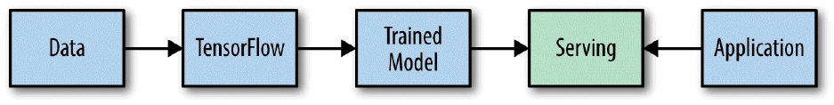
Introduction to TensorFlow Serving
TensorFlow Serving, written in C++, is a high-performance serving framework with which we
can deploy our model in a production setting. It makes our model usable for production by
enabling client software to access it and pass inputs through Serving’s API (Figure 10-1). Of
course, TensorFlow Serving is designed to have seamless integration with TensorFlow models.
Serving features many optimizations to reduce latency and increase throughput of predictions,
useful for real-time, large-scale applications. It’s not only about accessibility and efficient
serving of predictions, but also about flexibility — it’s quite common to want to keep a model
updated for various reasons, like having additional training data for improving the model,
making changes to the network architecture, and more.
Figure 10-1. Serving links our trained model to external applications, allowing client software easy access.
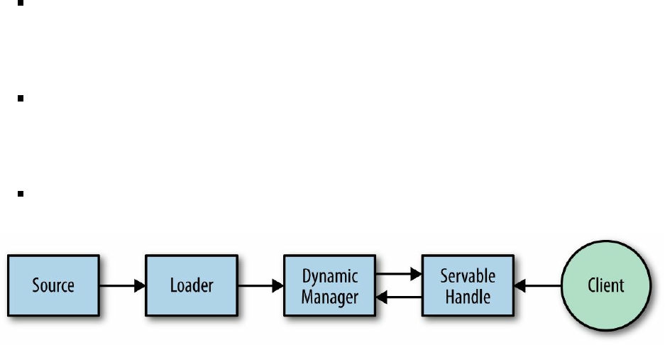
Overview
Say that we run a speech-recognition service and we want to deploy our models with
TensorFlow Serving. In addition to optimized serving, it is important for us to update our models
periodically as we obtain more data or experiment with new network architectures. In slightly
more technical terms, we’d like to have the ability to load new models and serve their outputs,
and unload old ones, all while streamlining model life-cycle management and version policies.
In general terms, we can accomplish this with Serving as follows. In Python, we define the
model and prepare it to be serialized in a way that can be parsed by the different modules
responsible for loading, serving, and managing versions, for example. The core Serving “engine”
resides in a C++ module that we will need to access only if we wish to control specific tuning
and customization of Serving behaviors.
In a nutshell, this is how Serving’s architecture works (Figure 10-2):
A module called Source identifies new models to be loaded by monitoring plugged-in
filesystems, which contain our models and their associated information that we exported
upon creation. Source includes submodules that periodically inspect the filesystem and
determine the latest relevant model versions.
When it identifies a new model version, source creates a loader. The loader passes its
servables (objects that clients use to perform computations such as predictions) to
a manager. The manager handles the full life cycle of servables (loading, unloading, and
serving) according to a version policy (gradual rollout, reverting versions, etc.).
Finally, the manager provides an interface for client access to servables.
Figure 10-2. An outline of the Serving architecture.
What’s especially nice about how Serving is built is that it’s designed to be flexible and
extendable. It supports building various plug-ins to customize system behavior, while using the
generic builds of other core components.
In the next section we will build and deploy a TensorFlow model with Serving, demonstrating
some of its key functionalities and inner workings. In advanced applications it is likely that we
may have to control for different types of optimizations and customization; for example,
controlling version policies and more. In this chapter we show you how to get up and running
with Serving and understand its fundamentals, laying the foundations for production-ready
deployment.
Installation
Serving requires several installations, including some third-party components. The installation
can be done from source or using Docker, which we use here to get you started quickly. A
Docker container bundles together a software application with everything needed to run it (for
example, code, files, etc.). We also use Bazel, Google’s own build tool for building client and
server software. In this chapter we only briefly touch on the technicalities behind tools such as
Bazel and Docker. More comprehensive descriptions appear in the appendix, at the end of the
book.
Installing Serving
Docker installation instructions can be found in on the Docker website.
Here, we demonstrate the Docker setup using Ubuntu.
Docker containers are created from a local Docker image, which is built from a dockerfile, and
encapsulates everything we need (dependency installations, project code, etc.). Once we have
Docker installed, we need to download the TensorFlow Serving dockerfile.
This dockerfile contains all of the dependencies needed to build TensorFlow Serving.
First, we produce the image from which we can run containers (this may take some time):
docker build --pull -t $USER/tensorflow-serving-devel -f
Dockerfile.devel .
Now that we’ve got the image created locally on our machine, we can create and run a container
by using:
docker run -v $HOME/docker_files:/host_files
-p 80:80 -it $USER/tensorflow-serving-devel
The docker run -it $USER/tensorflow-serving-devel command would suffice to create and
run a container, but we make two additions to this command.
First, we add -v $HOME/home_dir:/docker_dir, where -v (volume) indicates a request for a
shared filesystem so we have a convenient way to transfer files between the Docker container
and the host. Here we created the shared folders docker_files on our host and host_files on our
Docker container. Another way to transfer files is simply by using the command docker cp
foo.txt mycontainer:/foo.txt. The second addition is -p <host port>:<container port>,
which makes the service in the container accessible from anywhere by having the indicated port
exposed.
Once we enter our run command, a container will be created and started, and a terminal will be
opened. We can have a look at our container’s status by using the command docker ps -a
(outside the Docker terminal). Note that each time we use the docker run command, we create
another container; to enter the terminal of an existing container, we need to use docker exec -
it <container id> bash.
Finally, within the opened terminal we clone and configure TensorFlow Serving:
git clone --recurse-submodules https://github.com/tensorflow/serving
cd serving/tensorflow
./configure
And that’s it; we’re ready to go!
Building and Exporting
Now that Serving is cloned and operational, we can start exploring its features and how to use it.
The cloned TensorFlow Serving libraries are organized in a Bazel architecture. The source code
Bazel builds upon is organized in a workspace directory, inside nested hierarchies of packages
that group related source files together. Each package has a BUILD file, specifying the output to
be built from the files inside that package.
The workspace in our cloned library is located in the /serving folder, containing the
WORKSPACE text file and the /tensorflow_serving package, which we will return to later.
We now turn to look at the Python script that handles the training and exportation of the model,
and see how to export our model in a manner ready for serving.
Exporting our model
As when we used the Saver class, our trained model will be serialized and exported to two
files: one that contains information about our variables, and another that holds information about
our graph and other metadata. As we shall see shortly, Serving requires a specific serialization
format and metadata, so we cannot simply use the Saver class, as we saw at the beginning of this
chapter.
The steps we are going to take are as follows:
1. Define our model as in previous chapters.
2. Create a model builder instance.
3. Have our metadata (model, method, inputs and outputs, etc.) defined in the builder in a
serialized format (this is referred to as SignatureDef).
4. Save our model by using the builder.
We start by creating a builder instance using Serving’s SavedModelBuilder module, passing the
location to which we want our files to be exported (the directory will be created if it does not
exist). SavedModelBuilder exports serialized files representing our model in the required format:
builder = saved_model_builder.SavedModelBuilder(export_path)
The serialized model files we need will be contained in a directory whose name will specify the
model and its version:
export_path_base = sys.argv[-1]
export_path = os.path.join(
compat.as_bytes(export_path_base),
compat.as_bytes(str(FLAGS.model_version)))
This way, each version will be exported to a distinct subdirectory with its corresponding path.
Note that the export_path_base is obtained as input from the command line with sys.argv, and
the version is kept as a flag (presented in the previous chapter). Flag parsing is handled by
tf.app.run(), as we will see shortly.
Next, we want to define the input (shape of the input tensor of the graph) and output (tensor of
the prediction) signatures. In the first part of this chapter we used TensorFlow collection objects
to specify the relation between input and output data and their corresponding placeholders, and
also operations for computing predictions and accuracy. Here, signatures serve a somewhat
analogous purpose.
We use the builder instance we created to add both the variables and meta graph information,
using the SavedModelBuilder.add_meta_graph_and_variables() method:
builder.add_meta_graph_and_variables(
sess, [tag_constants.SERVING],
signature_def_map={
'predict_images':
prediction_signature,
signature_constants.DEFAULT_SERVING_SIGNATURE_DEF_KEY:
classification_signature,
},
legacy_init_op=legacy_init_op)
We need to pass four arguments: the session, tags (to “serve” or “train”), the signature map, and
some initializations.
We pass a dictionary with the prediction and classification signatures. We start with the
prediction signature, which again can be thought of as analogical to specifying and saving a
prediction op in a TensorFlow collection as we saw earlier:
prediction_signature = signature_def_utils.build_signature_def(
inputs={'images': tensor_info_x},
outputs={'scores': tensor_info_y},
method_name=signature_constants.PREDICT_METHOD_NAME)
images and scores here are arbitrary names that we will use to refer to our x and y Tensors later.
The images and scores are encoded into the required format by using the following commands:
tensor_info_x = utils.build_tensor_info(x)
tensor_info_y = utils.build_tensor_info(y_conv)
Similar to the prediction signature, we have the classification signature, where we input the
information about the scores (the probability values of the top k classes) and the corresponding
classes:
# Build the signature_def_map
classification_inputs = utils.build_tensor_info(
serialized_tf_example)
classification_outputs_classes = utils.build_tensor_info(
prediction_classes)
classification_outputs_scores = utils.build_tensor_info(values)
classification_signature = signature_def_utils.build_signature_def(
inputs={signature_constants.CLASSIFY_INPUTS:
classification_inputs},
outputs={
signature_constants.CLASSIFY_OUTPUT_CLASSES:
classification_outputs_classes,
signature_constants.CLASSIFY_OUTPUT_SCORES:
classification_outputs_scores
},
method_name=signature_constants.CLASSIFY_METHOD_NAME)
Finally, we save our model by using the save() command:
builder.save()
This, in a nutshell, wraps all the parts together in a format ready to be serialized and exported
upon execution of the script, as we shall see immediately.
Here is the final code for our main Python model script, including our model (the CNN model
from Chapter 4):
import os
import sys
import tensorflow as tf
from tensorflow.python.saved_model import builder
as saved_model_builder
from tensorflow.python.saved_model import signature_constants
from tensorflow.python.saved_model import signature_def_utils
from tensorflow.python.saved_model import tag_constants
from tensorflow.python.saved_model import utils
from tensorflow.python.util import compat
from tensorflow_serving.example import mnist_input_data
tf.app.flags.DEFINE_integer('training_iteration', 10,
'number of training iterations.')
tf.app.flags.DEFINE_integer(
'model_version', 1, 'version number of the model.')
tf.app.flags.DEFINE_string('work_dir', '/tmp', 'Working directory.')
FLAGS = tf.app.flags.FLAGS
def weight_variable(shape):
initial = tf.truncated_normal(shape, stddev=0.1)
return tf.Variable(initial,dtype='float')
def bias_variable(shape):
initial = tf.constant(0.1, shape=shape)
return tf.Variable(initial,dtype='float')
def conv2d(x, W):
return tf.nn.conv2d(x, W, strides=[1, 1, 1, 1], padding='SAME')
def max_pool_2x2(x):
return tf.nn.max_pool(x, ksize=[1, 2, 2, 1],
strides=[1, 2, 2, 1], padding='SAME')
def main(_):
if len(sys.argv) < 2 or sys.argv[-1].startswith('-'):
print('Usage: mnist_export.py [--training_iteration=x] '
'[--model_version=y] export_dir')
sys.exit(-1)
if FLAGS.training_iteration <= 0:
print('Please specify a positive
value for training iteration.')
sys.exit(-1)
if FLAGS.model_version <= 0:
print ('Please specify a positive
value for version number.')
sys.exit(-1)
print('Training...')
mnist = mnist_input_data.read_data_sets(
FLAGS.work_dir, one_hot=True)
sess = tf.InteractiveSession()
serialized_tf_example = tf.placeholder(
tf.string, name='tf_example')
feature_configs = {'x': tf.FixedLenFeature(shape=[784],
dtype=tf.float32),}
tf_example = tf.parse_example(serialized_tf_example,
feature_configs)
x = tf.identity(tf_example['x'], name='x')
y_ = tf.placeholder('float', shape=[None, 10])
W_conv1 = weight_variable([5, 5, 1, 32])
b_conv1 = bias_variable([32])
x_image = tf.reshape(x, [-1,28,28,1])
h_conv1 = tf.nn.relu(conv2d(x_image, W_conv1) + b_conv1)
h_pool1 = max_pool_2x2(h_conv1)
W_conv2 = weight_variable([5, 5, 32, 64])
b_conv2 = bias_variable([64])
h_conv2 = tf.nn.relu(conv2d(h_pool1, W_conv2) + b_conv2)
h_pool2 = max_pool_2x2(h_conv2)
W_fc1 = weight_variable([7 * 7 * 64, 1024])
b_fc1 = bias_variable([1024])
h_pool2_flat = tf.reshape(h_pool2, [-1, 7*7*64])
h_fc1 = tf.nn.relu(tf.matmul(h_pool2_flat, W_fc1) + b_fc1)
keep_prob = tf.placeholder(tf.float32)
h_fc1_drop = tf.nn.dropout(h_fc1, keep_prob)
W_fc2 = weight_variable([1024, 10])
b_fc2 = bias_variable([10])
y_conv = tf.matmul(h_fc1_drop, W_fc2) + b_fc2
y = tf.nn.softmax(y_conv, name='y')
cross_entropy = -tf.reduce_sum(y_ * tf.log(y_conv))
train_step = tf.train.AdamOptimizer(1e-4)\
.minimize(cross_entropy)
values, indices = tf.nn.top_k(y_conv, 10)
prediction_classes = tf.contrib.lookup.index_to_string(
tf.to_int64(indices),
mapping=tf.constant([str(i) for i in xrange(10)]))
sess.run(tf.global_variables_initializer())
for _ in range(FLAGS.training_iteration):
batch = mnist.train.next_batch(50)
train_step.run(feed_dict={x: batch[0],
y_: batch[1], keep_prob: 0.5})
print(_)
correct_prediction = tf.equal(tf.argmax(y_conv,1),
tf.argmax(y_,1))
accuracy = tf.reduce_mean(tf.cast(correct_prediction, 'float'))
y_: mnist.test.labels})
print('training accuracy %g' % accuracy.eval(feed_dict={
x: mnist.test.images,
y_: mnist.test.labels, keep_prob: 1.0}))
print('training is finished!')
export_path_base = sys.argv[-1]
export_path = os.path.join(
compat.as_bytes(export_path_base),
compat.as_bytes(str(FLAGS.model_version)))
print 'Exporting trained model to', export_path
builder = saved_model_builder.SavedModelBuilder(export_path)
classification_inputs = utils.build_tensor_info(
serialized_tf_example)
classification_outputs_classes = utils.build_tensor_info(
prediction_classes)
classification_outputs_scores = utils.build_tensor_info(values)
classification_signature = signature_def_utils.build_signature_def(
inputs={signature_constants.CLASSIFY_INPUTS:
classification_inputs},
outputs={
signature_constants.CLASSIFY_OUTPUT_CLASSES:
classification_outputs_classes,
signature_constants.CLASSIFY_OUTPUT_SCORES:
classification_outputs_scores
},
method_name=signature_constants.CLASSIFY_METHOD_NAME)
tensor_info_x = utils.build_tensor_info(x)
tensor_info_y = utils.build_tensor_info(y_conv)
prediction_signature = signature_def_utils.build_signature_def(
inputs={'images': tensor_info_x},
outputs={'scores': tensor_info_y},
method_name=signature_constants.PREDICT_METHOD_NAME)
legacy_init_op = tf.group(tf.initialize_all_tables(),
name='legacy_init_op')
builder.add_meta_graph_and_variables(
sess, [tag_constants.SERVING],
signature_def_map={
'predict_images':
prediction_signature,
signature_constants.DEFAULT_SERVING_SIGNATURE_DEF_KEY:
classification_signature,
},
legacy_init_op=legacy_init_op)
builder.save()
print('new model exported!')
if __name__ == '__main__':
tf.app.run()
The tf.app.run() command gives us a nice wrapper that handles parsing command-line
arguments.
In the final part of our introduction to Serving, we use Bazel for the actual exporting and
deployment of our model.
Most Bazel BUILD files consist only of declarations of build rules specifying the relationship
between inputs and outputs, and the steps to build the outputs.
For instance, in this BUILD file we have a Python rule py_binary to build executable programs.
Here we have three attributes, name for the name of the rule, srcs for the list of files that are
processed to create the target (our Python script), and deps for the list of other libraries to be
linked into the binary target:
py_binary(
name = "serving_model_ch4",
srcs = [
"serving_model_ch4.py",
],
deps = [
":mnist_input_data",
"@org_tensorflow//tensorflow:tensorflow_py",
"@org_tensorflow//tensorflow/python/saved_model:builder",
"@org_tensorflow//tensorflow/python/saved_model:constants",
"@org_tensorflow//tensorflow/python/saved_model:loader",
"@org_tensorflow//tensorflow/python/saved_model:
signature_constants",
"@org_tensorflow//tensorflow/python/saved_model:
signature_def_utils",
"@org_tensorflow//tensorflow/python/saved_model:
tag_constants",
"@org_tensorflow//tensorflow/python/saved_model:utils",
],
)
Next we run and export the model by using Bazel, training with 1,000 iterations and exporting
the first version of the model:
bazel build //tensorflow_serving/example:serving_model_ch4
bazel-bin/tensorflow_serving/example/serving_model_ch4
--training_iteration=1000 --model_version=1 /tmp/mnist_model
To train the second version of the model, we just use:
--model_version=2
In the designated subdirectory we will find two files, saved_model.pb and variables, that contain
the serialized information about our graph (including metadata) and its variables, respectively. In
the next lines we load the exported model with the standard TensorFlow model server:
bazel build //tensorflow_serving/model_servers:
tensorflow_model_server
bazel-bin/tensorflow_serving/model_servers/tensorflow_model_server
--port=8000 --model_name=mnist
--model_base_path=/tmp/mnist_model/ --logtostderr
Finally, our model is now served and ready for action at localhost:8000. We can test the server
with a simple client utility, mnist_client:
bazel build //tensorflow_serving/example:mnist_client
bazel-bin/tensorflow_serving/example/mnist_client
--num_tests=1000 --server=localhost:8000
Summary
This chapter dealt with how to save, export, and serve models, from simply saving and
reassigning of weights using the built-in Saver utility to an advanced model-deployment
mechanism for production. The last part of this chapter touched on TensorFlow Serving, a great
tool for making our models commercial-ready with dynamic version control. Serving is a rich
utility with many functionalities, and we strongly recommend that readers who are interested in
mastering it seek out more in-depth technical material online.

Appendix A. Tips on Model Construction
and Using TensorFlow Serving
Model Structuring and Customization
In this short section we will focus on two topics that continue from and extend the previous
chapters — how to construct a proper model, and how to customize the model’s entities. We start
by describing how we can effectively reframe our code by using encapsulations and allow its
variables to be shared and reused. In the second part of this section we will talk about how to
customize our own loss functions and operations and use them for optimization.
Model Structuring
Ultimately, we would like to design our TensorFlow code efficiently, so that it can be reused for
multiple tasks and is easy to follow and pass around. One way to make things cleaner is to use
one of the available TensorFlow extension libraries, which were discussed in Chapter 7.
However, while they are great to use for typical networks, models with new components that we
wish to implement may sometimes require the full flexibility of lower-level TensorFlow.
Let’s take another look at the optimization code from the previous chapter:
import tensorflow as tf
NUM_STEPS = 10
g = tf.Graph()
wb_ = []
with g.as_default():
x = tf.placeholder(tf.float32,shape=[None,3])
y_true = tf.placeholder(tf.float32,shape=None)
with tf.name_scope('inference') as scope:
w = tf.Variable([[0,0,0]],dtype=tf.float32,name='weights')
b = tf.Variable(0,dtype=tf.float32,name='bias')
y_pred = tf.matmul(w,tf.transpose(x)) + b
with tf.name_scope('loss') as scope:
loss = tf.reduce_mean(tf.square(y_true-y_pred))
with tf.name_scope('train') as scope:
learning_rate = 0.5
optimizer = tf.train.GradientDescentOptimizer(learning_rate)
train = optimizer.minimize(loss)
.
init = tf.global_variables_initializer()
with tf.Session() as sess:
sess.run(init)
for step in range(NUM_STEPS):
sess.run(train,{x: x_data, y_true: y_data})
if (step % 5 == 0):
print(step, sess.run([w,b]))
wb_.append(sess.run([w,b]))
print(10, sess.run([w,b]))
We get:
(0, [array([[ 0.30149955, 0.49303722, 0.11409992]],
dtype=float32), -0.18563795])
(5, [array([[ 0.30094019, 0.49846715, 0.09822173]],
dtype=float32), -0.19780949])
(10, [array([[ 0.30094025, 0.49846718, 0.09822182]],
dtype=float32), -0.19780946])
The entire code here is simply stacked line by line. This is OK for simple and focused examples.
However, this way of coding has its limits — it’s neither reusable nor very readable when the
code gets more complex.
Let’s zoom out and think about what characteristics our infrastructure should have. First, we
would like to encapsulate the model so it can be used for various tasks like training, evaluation,
and forming predictions. Furthermore, it can also be more efficient to construct the model in a
modular fashion, giving us specific control over its subcomponents and increasing readability.
This will be the focus of the next few sections.
Modular design
A good start is to split the code into functions that capture different elements in the learning
model. We can do this as follows:
def predict(x,y_true,w,b):
y_pred = tf.matmul(w,tf.transpose(x)) + b
return y_pred
def get_loss(y_pred,y_true):
loss = tf.reduce_mean(tf.square(y_true-y_pred))
return loss
def get_optimizer(y_pred,y_true):
loss = get_loss(y_pred,y_true)
optimizer = tf.train.GradientDescentOptimizer(0.5)
train = optimizer.minimize(loss)
return train
def run_model(x_data,y_data):
wb_ = []
# Define placeholders and variables
x = tf.placeholder(tf.float32,shape=[None,3])
y_true = tf.placeholder(tf.float32,shape=None)
w = tf.Variable([[0,0,0]],dtype=tf.float32)
b = tf.Variable(0,dtype=tf.float32)
print(b.name)
# Form predictions
y_pred = predict(x,y_true,w,b)
# Create optimizer
train = get_optimizer(y_pred,y_data)
# Run session
init = tf.global_variables_initializer()
with tf.Session() as sess:
sess.run(init)
for step in range(10):
sess.run(train,{x: x_data, y_true: y_data})
if (step % 5 == 0):
print(step, sess.run([w,b]))
wb_.append(sess.run([w,b]))
run_model(x_data,y_data)
run_model(x_data,y_data)
And here is the result:
Variable_9:0 Variable_8:0
0 [array([[ 0.27383861, 0.48421991, 0.09082422]],
dtype=float32), -0.20805186]
4 [array([[ 0.29868397, 0.49840903, 0.10026278]],
dtype=float32), -0.20003076]
9 [array([[ 0.29868546, 0.49840906, 0.10026464]],
dtype=float32), -0.20003042]
Variable_11:0 Variable_10:0
0 [array([[ 0.27383861, 0.48421991, 0.09082422]],
dtype=float32), -0.20805186]
4 [array([[ 0.29868397, 0.49840903, 0.10026278]],
dtype=float32), -0.20003076]
9 [array([[ 0.29868546, 0.49840906, 0.10026464]],
dtype=float32), -0.20003042]
Now we can reuse the code with different inputs, and this division makes it easier to read,
especially when it gets more complex.
In this example we called the main function twice with the same inputs and printed the variables
that were created. Note that each call created a different set of variables, resulting in the creation
of four variables. Let’s assume, for example, a scenario where we wish to build a model with
multiple inputs, such as two different images. Say we wish to apply the same convolutional
filters to both input images. New variables will be created. To avoid this, we “share” the filter
variables, using the same variables on both images.
Variable sharing
It’s possible to reuse the same variables by creating them with tf.get_variable() instead of
tf.Variable(). We use this very similarly to tf.Variable(), except that we need to pass an
initializer as an argument:
w = tf.get_variable('w',[1,3],initializer=tf.zeros_initializer())
b = tf.get_variable('b',[1,1],initializer=tf.zeros_initializer())
Here we used tf.zeros_initializer(). This initializer is very similar to tf.zeros(), except
that it doesn’t get the shape as an argument, but rather arranges the values according to the shape
specified by tf.get_variable().
In this example the variable w will be initialized as [0,0,0], as specified by the given shape,
[1,3].
With get_variable() we can reuse variables that have the same name (including the scope
prefix, which can be set by tf.variable_scope()). But first we need to indicate this intention
by either using tf.variable_scope.reuse_variable() or setting the reuse flag
(tf.variable.scope(reuse=True)). An example of how to share variables is shown in the code
that follows.

HEADS-UP FOR FLAG MISUSE
Whenever a variable has the exact same name as another, an exception will be thrown when the reuse
flag is not set. The same goes for the opposite scenario — variables with mismatching names that are
expected to be reused (when reuse = True) will cause an exception as well.
Using these methods, and setting the scope prefix to Regression, by printing their names we can
see that the same variables are reused:
def run_model(x_data,y_data):
wb_ = []
# Define placeholders and variables
x = tf.placeholder(tf.float32,shape=[None,3])
y_true = tf.placeholder(tf.float32,shape=None)
w = tf.get_variable('w',[1,3],initializer=tf.zeros_initializer())
b = tf.get_variable('b',[1,1],initializer=tf.zeros_initializer())
print(b.name,w.name)
# Form predictions
y_pred = predict(x,y_true,w,b)
# Create optimizer
train = get_optimizer(y_pred,y_data)
# Run session
init = tf.global_variables_initializer()
sess.run(init)
for step in range(10):
sess.run(train,{x: x_data, y_true: y_data})
if (step % 5 == 4) or (step == 0):
print(step, sess.run([w,b]))
wb_.append(sess.run([w,b]))
sess = tf.Session()
with tf.variable_scope("Regression") as scope:
run_model(x_data,y_data)
scope.reuse_variables()
run_model(x_data,y_data)
sess.close()
The output is shown here:
Regression/b:0 Regression/w:0
0 [array([[ 0.27383861, 0.48421991, 0.09082422]],
dtype=float32), array([[-0.20805186]], dtype=float32)]
4 [array([[ 0.29868397, 0.49840903, 0.10026278]],
dtype=float32), array([[-0.20003076]], dtype=float32)]
9 [array([[ 0.29868546, 0.49840906, 0.10026464]],
dtype=float32), array([[-0.20003042]], dtype=float32)]
tf.get_variables() is a neat, lightweight way to share variables. Another approach is to
encapsulate our model as a class and manage the variables there. This approach has many other
benefits, as described in the following section
Class encapsulation
As with any other program, when things get more complex and the number of code lines grows,
it becomes very convenient to have our TensorFlow code reside within a class, giving us quick
access to methods and attributes that belong to the same model. Class encapsulation allows us to
maintain the state of our variables and then perform various post-training tasks like forming
predictions, model evaluation, further training, saving and restoring our weights, and whatever
else is related to the specific problem our model solves.
In the next batch of code we see an example of a simple class wrapper. The model is created
when the instance is instantiated, and the training process is performed by calling the fit()
method.

@PROPERTY AND PYTHON DECORATORS
This code uses a @property decorator. A decorator is simply a function that takes another function as
input, does something with it (like adding some functionality), and returns it. In Python, a decorator is
defined with the @ symbol.
@property is a decorator used to handle access to class attributes.
Our class wrapper is as follows:
class Model:
def __init__(self):
# Model
self.x = tf.placeholder(tf.float32,shape=[None,3])
self.y_true = tf.placeholder(tf.float32,shape=None)
self.w = tf.Variable([[0,0,0]],dtype=tf.float32)
self.b = tf.Variable(0,dtype=tf.float32)
init = tf.global_variables_initializer()
self.sess = tf.Session()
self.sess.run(init)
self._output = None
self._optimizer = None
self._loss = None
def fit(self,x_data,y_data):
print(self.b.name)
for step in range(10):
self.sess.run(self.optimizer,{self.x: x_data, self.y_true: y_data})
if (step % 5 == 4) or (step == 0):
print(step, self.sess.run([self.w,self.b]))
@property
def output(self):
if not self._output:
y_pred = tf.matmul(self.w,tf.transpose(self.x)) + self.b
self._output = y_pred
return self._output
@property
def loss(self):
if not self._loss:
error = tf.reduce_mean(tf.square(self.y_true-self.output))
self._loss= error
return self._loss
@property
def optimizer(self):
if not self._optimizer:
opt = tf.train.GradientDescentOptimizer(0.5)
opt = opt.minimize(self.loss)
self._optimizer = opt
return self._optimizer
lin_reg = Model()
lin_reg.fit(x_data,y_data)
lin_reg.fit(x_data,y_data)
And we get this:
Variable_89:0
0 [array([[ 0.32110521, 0.4908163 , 0.09833425]],
dtype=float32), -0.18784374]
4 [array([[ 0.30250472, 0.49442694, 0.10041162]],
dtype=float32), -0.1999902]
9 [array([[ 0.30250433, 0.49442688, 0.10041161]],
dtype=float32), -0.19999036]
Variable_89:0
0 [array([[ 0.30250433, 0.49442688, 0.10041161]],
dtype=float32), -0.19999038]
4 [array([[ 0.30250433, 0.49442688, 0.10041161]],
dtype=float32), -0.19999038]
9 [array([[ 0.30250433, 0.49442688, 0.10041161]],
dtype=float32), -0.19999036]
Splitting the code into functions is somewhat redundant in the sense that the same lines of code
are recomputed with every call. One simple solution is to add a condition at the beginning of
each function. In the next code iteration we will see an even nicer workaround.
In this setting there is no need to use variable sharing since the variables are kept as attributes of
the model object. Also, after calling the training method model.fit() twice, we see that the
variables have maintained their current state.
In our last batch of code for this section we add another enhancement, creating a custom
decorator that automatically checks whether the function was already called.
Another improvement we can make is having all of our variables kept in a dictionary. This will
allow us to keep track of our variables after each operation, as we saw in Chapter 10 when we
looked at saving weights and models.
Finally, additional functions for getting the values of the loss function and our weights are added:
class Model:
def __init__(self):
# Model
self.x = tf.placeholder(tf.float32,shape=[None,3])
self.y_true = tf.placeholder(tf.float32,shape=None)
self.params = self._initialize_weights()
init = tf.global_variables_initializer()
self.sess = tf.Session()
self.sess.run(init)
self.output
self.optimizer
self.loss
def _initialize_weights(self):
params = dict()
params['w'] = tf.Variable([[0,0,0]],dtype=tf.float32)
params['b'] = tf.Variable(0,dtype=tf.float32)
return params
def fit(self,x_data,y_data):
print(self.params['b'].name)
for step in range(10):
self.sess.run(self.optimizer,{self.x: x_data, self.y_true: y_data})
if (step % 5 == 4) or (step == 0):
print(step,
self.sess.run([self.params['w'],self.params['b']]))
def evaluate(self,x_data,y_data):
print(self.params['b'].name)
MSE = self.sess.run(self.loss,{self.x: x_data, self.y_true: y_data})
return MSE
def getWeights(self):
return self.sess.run([self.params['b']])
@property_with_check
def output(self):
y_pred = tf.matmul(self.params['w'],tf.transpose(self.x)) + \
self.params['b']
return y_pred
@property_with_check
def loss(self):
error = tf.reduce_mean(tf.square(self.y_true-self.output))
return error
@property_with_check
def optimizer(self):
opt = tf.train.GradientDescentOptimizer(0.5)
opt = opt.minimize(self.loss)
return opt
lin_reg = Model()
lin_reg.fit(x_data,y_data)
MSE = lin_reg.evaluate(x_data,y_data)
print(MSE)
print(lin_reg.getWeights())
Here is the output:
Variable_87:0
0 [array([[ 0.32110521, 0.4908163 , 0.09833425]],
dtype=float32), -0.18784374]
4 [array([[ 0.30250472, 0.49442694, 0.10041162]],
dtype=float32), -0.1999902]
9 [array([[ 0.30250433, 0.49442688, 0.10041161]],
dtype=float32), -0.19999036]
Variable_87:0
0 [array([[ 0.30250433, 0.49442688, 0.10041161]],
dtype=float32), -0.19999038]
4 [array([[ 0.30250433, 0.49442688, 0.10041161]],
dtype=float32), -0.19999038]
9 [array([[ 0.30250433, 0.49442688, 0.10041161]],
dtype=float32), -0.19999036]
Variable_87:0
0.0102189
[-0.19999036]
The custom decorator checks whether an attribute exists, and if not, it sets it according to the
input function. Otherwise, it returns the attribute. functools.wrap() is used so we can reference
the name of the function:
import functools
def property_with_check(input_fn):
attribute = '_cache_' + input_fn.__name__
@property
@functools.wraps(input_fn)
def check_attr(self):
if not hasattr(self, attribute):
setattr(self, attribute, input_fn(self))
return getattr(self, attribute)
return check_attr
This was a fairly basic example of how we can improve the overall code for our model. This
kind of optimization might be overkill for our simple linear regression example, but it will
definitely be worth the effort for complicated models with plenty of layers, variables, and
features.
Customization
So far we’ve used two loss functions. In the classification example in Chapter 2 we used the
cross-entropy loss, defined as follows:
cross_entropy = tf.reduce_mean(
tf.nn.softmax_cross_entropy_with_logits(logits=y_pred, labels=y_true))
In contrast, in the regression example in the previous section we used the square error loss,
defined as follows:
loss = tf.reduce_mean(tf.square(y_true-y_pred))
These are the most commonly used loss functions in machine learning and deep learning right
now. The purpose of this section is twofold. First, we want to point out the more general
capabilities of TensorFlow in utilizing custom loss functions. Second, we will discuss
regularization as a form of extension of any loss function in order to achieve a specific goal,
irrespective of the basic loss function used.
Homemade loss functions
This book (and presumably our readers) takes a specific view of TensorFlow with the aspect of
deep learning in mind. However, TensorFlow is more general in scope, and most machine
learning problems can be formulated in a way that TensorFlow can be used to solve.
Furthermore, any computation that can be formulated in the computation graph framework is a
good candidate to benefit from TensorFlow.
The predominant special case is the class of unconstrained optimization problems. These are
extremely common throughout scientific (and algorithmic) computing, and for these,
TensorFlow is especially helpful. The reason these problems stand out is that TensorFlow
provides an automatic mechanism for computing gradients, which affords a tremendous speedup
in development time for such problems.
In general, optimization with respect to an arbitrary loss function will be in the form
def my_loss_function(key-variables...):
loss = ...
return loss
my_loss = my_loss_function(key-variables...)
gd_step = tf.train.GradientDescentOptimizer().minimize(my_loss)
where any optimizer could be used in place of the GradientDescentOptimizer.
Regularization
Regularization is the restriction of an optimization problem by imposing a penalty on the
complexity of the solution (see the note in Chapter 4 for more details). In this section we take a
look at specific instances where the penalty is directly added to the basic loss function in an
additive form.
For example, building on the softmax example from Chapter 2, we have this:
x = tf.placeholder(tf.float32, [None, 784])
W = tf.Variable(tf.zeros([784, 10]))
y_true = tf.placeholder(tf.float32, [None, 10])
y_pred = tf.matmul(x, W)
cross_entropy = tf.reduce_mean(
tf.nn.softmax_cross_entropy_with_logits(logits=y_pred, labels=y_true))
total_loss = cross_entropy + LAMBDA * tf.nn.l2_loss(W)
gd_step = tf.train.GradientDescentOptimizer(0.5).minimize(total_loss)
The difference between this and the original in Chapter 2 is that we added LAMBDA *
tf.nn.l2_loss(W) to the loss we are optimizing with respect to. In this case, using a small value
of the trade-off parameter LAMBDA will have very little effect on the resulting accuracy (a large
value will be detrimental). In large networks, where overfitting is a serious issue, this sort of
regularization can often be a lifesaver.
Regularization of this sort can be done with respect to the weights of the model, as shown in the
previous example (also called weight decay, since it will cause the weights to have smaller
values), as well as to the activations of a specific layer, or indeed all layers.
Another factor is what function we use — we could have used l1 instead of the l2
regularization, or a combination of the two. All combinations of these regularizers are valid and
used in various contexts.
Many of the abstraction layers make the application of regularization as easy as specifying the
number of filters, or the activation function. In Keras (a very popular extension reviewed in
Chapter 7), for instance, we are provided with the regularizers listed in Table A-1, applicable to
all the standard layers.
Table A-1. Regularization with Keras
Regularizer What it does Example
l1 l1 regularization of weights Dense(100, W_regularizer=l1(0.01))
l2 l2 regularization of weights Dense(100, W_regularizer=l2(0.01))
l1l2 Combined l1 + l2 regularization of weights Dense(100, W_regularizer=l1l2(0.01))
activity_l1 l1 regularization of activations Dense(100, activity_regularizer=activity_l1(0.01))
activity_l2 l2 regularization of activations Dense(100, activity_regularizer=activity_l2(0.01))
activity_l1l2 Combined l1 + l2 regularization of activations Dense(100, activity_regularizer=activity_l1l2(0.01))
Using these shortcuts makes it easy to test different regularization schemes when a model is
overfitting.
Writing your very own op
TensorFlow comes ready packed with a large number of native ops, ranging from standard
arithmetic and logical operations to matrix operations, deep learning–specific functions, and
more. When these are not enough, it is possible to extend the system by creating a new op. This
is done in one of two ways:
Writing a “from scratch” C++ version of the operation
Writing Python code that combines existing ops and Python code to create the new one
We will spend the remainder of this section discussing the second option.
The main reason to construct a Python op is to utilize NumPy functionality in the context of a
TensorFlow computational graph. For the sake of illustration, we will construct the
regularization example from the previous section by using the NumPy multiplication function
rather than the TensorFlow op:
import numpy as np
LAMBDA = 1e-5
def mul_lambda(val):
return np.multiply(val, LAMBDA).astype(np.float32)
Note that this is done for the sake of illustration, and there is no special reason why anybody
would want to use this instead of the native TensorFlow op. We use this oversimplified example
in order to shift the focus to the details of the mechanism rather than the computation.
In order to use our new creation from within TensorFlow, we use the py_func() functionality:
tf.py_func(my_python_function, [input], [output_types])
In our case, this means we compute the total loss as follows:
total_loss = cross_entropy + \
tf.py_func(mul_lambda, [tf.nn.l2_loss(W)], [tf.float32])[0]
Doing this, however, will not be enough. Recall that TensorFlow keeps track of the gradients of
each of the ops in order to perform gradient-based training of our overall model. In order for this
to work with the new Python-based op, we have to specify the gradient manually. This is done in
two steps.
First, we create and register the gradient:
@tf.RegisterGradient("PyMulLambda")
def grad_mul_lambda(op, grad):
return LAMBDA*grad
Next, when using the function, we point to this function as the gradient of the op. This is done
using the string registered in the previous step:
with tf.get_default_graph().gradient_override_map({"PyFunc": "PyMulLambda"}):
total_loss = cross_entropy + \
tf.py_func(mul_lambda, [tf.nn.l2_loss(W)], [tf.float32])[0]
Putting it all together, the code for the softmax model with regularization through our new
Python-based op is now:
import numpy as np
import tensorflow as tf
LAMBDA = 1e-5
def mul_lambda(val):
return np.multiply(val, LAMBDA).astype(np.float32)
@tf.RegisterGradient("PyMulLambda")
def grad_mul_lambda(op, grad):
return LAMBDA*grad
x = tf.placeholder(tf.float32, [None, 784])
W = tf.Variable(tf.zeros([784, 10]))
y_true = tf.placeholder(tf.float32, [None, 10])
y_pred = tf.matmul(x, W)
cross_entropy =
tf.reduce_mean(tf.nn.softmax_cross_entropy_with_logits\
(logits=y_pred, labels=y_true))
with tf.get_default_graph().gradient_override_map({"PyFunc": "PyMulLambda"}):
total_loss = cross_entropy + \
tf.py_func(mul_lambda, [tf.nn.l2_loss(W)], [tf.float32])[0]
gd_step = tf.train.GradientDescentOptimizer(0.5).minimize(total_loss)
correct_mask = tf.equal(tf.argmax(y_pred, 1), tf.argmax(y_true, 1))
accuracy = tf.reduce_mean(tf.cast(correct_mask, tf.float32))
This can now be trained using the same code as in Chapter 2, when this model was first
introduced.

USING THE INPUTS IN THE COMPUTATION OF GRADIENTS
In the simple example we just showed, the gradient depends only on the gradient with respect to the
input, and not on the input itself. In the general case, we will need access to the input as well. This is
done easily, using the op.inputs field:
x = op.inputs[0]
Other inputs (if they exist) are accessed in the same way.
Required and Recommended Components for TensorFlow Serving
In this section, we add details on some of the material covered in Chapter 10 and review in more
depth some of the technical components used behind the scenes in TensorFlow Serving.
In Chapter 10, we used Docker to run TensorFlow Serving. Those who prefer to avoid using a
Docker container need to have the following installed:
Bazel
Bazel is Google’s own build tool, which recently became publicly available. When we use
the term build, we are referring to using a bunch of rules to create output software from
source code in a very efficient and reliable manner. The build process can also be used to
reference external dependencies that are required to build the outputs. Among other
languages, Bazel can be used to build C++ applications, and we exploit this to build the
C++-written TensorFlow Serving’s programs. The source code Bazel builds upon is
organized in a workspace directory inside nested hierarchies of packages, where each
package groups related source files together. Every package consists of three types of files:
human-written source files called targets, generated files created from the source files, and
rules specifying the steps for deriving the outputs from the inputs.
Each package has a BUILD file, specifying the output to be built from the files inside that
package. We use basic Bazel commands like bazel build to build generated files from
targets, and bazel run to execute a build rule. We use the -bin flag when we want to
specify the directories to contain the build outputs.
Downloads and installation instructions can be found on the Bazel website.
gRPC
Remote procedure call (RPC) is a form of client (caller)–server (executer) interaction; a
program can request a procedure (for example, a method) that is executed on another
computer (commonly in a shared network). gRPC is an open source framework developed
by Google. Like any other RPC framework, gRPC lets you directly call methods on other
machines, making it easier to distribute the computations of an application. The greatness of
gRPC lies in how it handles the serialization, using the fast and efficient protocol buffers
instead of XML or other methods.
Downloads and installation instructions can be found on GitHub.
Next, you need to make sure that the necessary dependencies for Serving are installed with the
following command:
sudo apt-get update && sudo apt-get install -y \
build-essential \
curl \
libcurl3-dev \
git \
libfreetype6-dev \
libpng12-dev \
libzmq3-dev \
pkg-config \
python-dev \
python-numpy \
What Is a Docker Container and Why Do We Use It?
Docker is essentially solving the same problem as Vagrant with VirtualBox, and that is making
sure our code will run smoothly on other machines. Different machines might have different
operating systems as well as different tool sets (installed software, configurations, permissions,
etc.). By replicating the same environment — maybe for production purposes, maybe just to
share with others — we guarantee that our code will run exactly the same way elsewhere as on
our original development machine.
What’s unique about Docker is that, unlike other similarly purposed tools, it doesn’t create a
fully operational virtual machine on which the environment will be built, but rather creates a
container on top of an existing system (Ubuntu, for example), acting as a virtual machine in a
sense and using our existing OS resources. These containers are created from a local Docker
image, which is built from a dockerfile and encapsulates everything we need (dependency
installations, project code, etc.). From that image we can create as many containers as we want
(until we run out of memory, of course). This makes Docker a very cool tool with which we can
easily create complete multiple environment replicas that contain our code and run them
anywhere (very useful for cluster computing).
Some Basic Docker Commands
To get you a bit more comfortable with using Docker, here’s a quick look at some useful
commands, written in their most simplified form. Given that we have a dockerfile ready, we can
build an image by using docker build <dockerfile>. From that image we can then create a
new container by using the docker run <image> command. This command will also
automatically run the container and open a terminal (type exit to close the terminal). To run,
stop, and delete existing containers, we use the docker start <container id>, docker stop
<container id>, and docker rm <container id> commands, respectively. To see the list of all
of our instances, both running and idle, we write docker ps -a.
When we run an instance, we can add the -p flag followed by a port for Docker to expose, and
the -v flag followed by a home directory to be mounted, which will enable us to work locally
(the home directory is addressed via the /mnt/home path in the container).

Index
Symbols
.assign(), Pretrained Word Embeddings, Assigning Loaded Weights
.compile(), Sequential model
.eval(), Tensor Arrays and Shapes
.evaluate(), Linear Regression
.fit(), Linear Regression, FeatureColumn, CNN, Sequential model
.get_variable_value(), FeatureColumn
.meta checkpoint files, The Saver Class
.name attribute, Names
.optimizers, Sequential model
.run() method, Creating a Session and Running It
.save(), The Saver Class
.__enter__(), Constructing and Managing Our Graph
.__exit__(), Constructing and Managing Our Graph
<Estimator>.predict(), DNN Classifier
@property decorator, Class encapsulation
A
abstraction libraries
abstraction illustration, Chapter Overview
benefits of, A High-Level Overview, Chapter Overview
contrib.learn, contrib.learn-Homemade CNN with contrib.learn
popular libraries, High-Level Survey
regularization and, Regularization
TFLearn, TFLearn-Downloading and using a pretrained model
acknowledgments, Acknowledgments
activation functions, Convolution
aliases, Installing TensorFlow
argparse module, tf.app.flags
arguments
callbacks, Sequential model
feed_dict argument, Softmax Regression, The Input Pipeline
fetches argument, Fetches
ksize argument, Pooling
num-epochs argument, tf.train.string_input_producer() and tf.TFRecordReader()
perm argument, Applying the RNN step with tf.scan()
shape argument, Placeholders
strides argument, Convolution
arrays, Tensor Arrays and Shapes-Name scopes
.assign(), Pretrained Word Embeddings, Assigning Loaded Weights
asynchronous training, What Is the Goal of Parallelization?
as_default() command, Constructing and Managing Our Graph
attributes
.name, Names
<node>.graph attribute, Constructing and Managing Our Graph
dtype, Data Types
purpose of, Nodes Are Operations, Edges Are Tensor Objects
setting with source operations, Setting attributes with source operations
attributions, Using Code Examples
autoencoders, Autoencoders-Autoencoders
B
backpropagation, A High-Level Overview
bag-of-words text classification, Introduction to Word Embeddings
BasicRNNCell, tf.contrib.rnn.BasicRNNCell and tf.nn.dynamic_rnn()
batch_size, MNIST images as sequences
Bazel build tool, Building and Exporting, Exporting our model, Required and
Recommended Components for TensorFlow Serving
between-graph replication, Replicating a Computational Graph Across Devices
bias_variable(), The Model
binary classification, RNN
biologically inspired models, Introduction to CNNs
C
callbacks argument, Sequential model
casting, Casting
chains, Introduction to Recurrent Neural Networks
CIFAR10 dataset, CIFAR10-Simple CIFAR10 Models
class encapsulation, Class encapsulation
clusters, Clusters and Servers
code examples, obtaining and using, Using Code Examples
command-line arguments, tf.app.flags
comments and questions, How to Contact Us
Common Crawl vectors, Pretrained Word Embeddings
.compile(), Sequential model
computation graphs (see dataflow computation graphs)
computer vision
pretrained models for, Pre-trained models: state-of-the-art computer vision for all
sequence data and, The Importance of Sequence Data
confusion matrices, DNN Classifier
constructors, Nodes Are Operations, Edges Are Tensor Objects
contact information, How to Contact Us
context managers, Constructing and Managing Our Graph
continuous (regression) learning, Softmax Regression, Training to predict, contrib.learn
contrib library, tf.contrib.rnn.BasicRNNCell and tf.nn.dynamic_rnn(), Installation
contrib.layers, FeatureColumn, Homemade CNN with contrib.learn
contrib.learn
built-in estimators, contrib.learn
custom CNN estimators, Homemade CNN with contrib.learn-Homemade CNN with
contrib.learn
deploying custom models, contrib.learn
DNN classifier, DNN Classifier-DNN Classifier
feature transformation operations, FeatureColumn
FeatureColumn, FeatureColumn-FeatureColumn
importing, contrib.learn
linear regression, Linear Regression
overview of, High-Level Survey
contrib.learn.Estimator(), Homemade CNN with contrib.learn, CNN
conv2d(), Convolution, The Model
convolutional neural networks (CNNs)
architecture visualization, The Model
CIFAR10 dataset classification, CIFAR10-Simple CIFAR10 Models
convolution operation, Convolution, The Model
creating models with TF-Slim, Creating CNN models with TF-Slim-Downloading and
using a pretrained model
custom estimators using contrib.learn, Homemade CNN with contrib.learn-Homemade
CNN with contrib.learn
MNIST dataset classification, MNIST: Take II-The Model
model creation using TFLearn, CNN-CNN
overview of, Introduction to CNNs-Introduction to CNNs
conv_layer(), The Model
coord.request_stop(), tf.train.Coordinator
coord.should_stop(), tf.train.Coordinator
cross entropy, Softmax Regression, MSE and cross entropy, Customization
customization
loss functions, Customization
regularization, Regularization
TensorFlow Ops, Writing your very own op
D
data augmentation, Simple CIFAR10 Models
data frames (tables), FeatureColumn
data parallelism, Where Does the Parallelization Take Place?
data types
changing, Casting
choosing explicitly, Data Types
default data format, TFRecords
labeled vs. unlabeled data, Introduction to Word Embeddings
sequence data, The Importance of Sequence Data
supported types, Casting
type inference, Tensor Arrays and Shapes
dataflow computation graphs
benefits of, The Benefits of Graph Computations
constructing and managing, Constructing and Managing Our Graph-Constructing and
Managing Our Graph
creating, Creating a Graph
fetches argument, Fetches
overview of, TensorFlow: What’s in a Name?, Computation Graphs
replicating across devices, Replicating a Computational Graph Across Devices
resetting prior to restoring, The Saver Class
session closing, Creating a Session and Running It
session creation, Creating a Session and Running It
deactivate command, Installing TensorFlow
decorators, Class encapsulation
deep learning
advances in, Going Deep
computer vision, Pre-trained models: state-of-the-art computer vision for all, The
Importance of Sequence Data
data processing in, TensorFlow: What’s in a Name?
image captioning, Generating rich natural language descriptions for images
overview of, Going Deep
sequence data and, The Importance of Sequence Data
supervised learning, Softmax Regression, Softmax Regression
unsupervised learning, Word2vec
deep learning models (see models)
deep neural networks (see deep learning)
dense vector representations, Introduction to Word Embeddings
Dense(), Sequential model
dequeing and enqueuing, Enqueuing and Dequeuing
design tips
class encapsulation, Class encapsulation
model structure, Model Structuring
modular design, Modular design
variable sharing, Variable sharing
device placement, Device Placement
digit_to_word_map dictionary, Text Sequences
dimensionality reduction, Autoencoders
discrete (classification) learning, Softmax Regression
display_cifar(), Loading the CIFAR10 Dataset
DistBelief , Going Deep
distributed computing
distributed example, Distributed Example-Distributed Example
overview of, Distributed Computing
parallelization and, Where Does the Parallelization Take Place?
TensorFlow elements, TensorFlow Elements-Device Placement
distributional hypothesis, Word2vec
DNN classifier, DNN Classifier-DNN Classifier
Docker
alternatives to, Required and Recommended Components for TensorFlow Serving
basic commands, Some Basic Docker Commands
benefits of, Installation, What Is a Docker Container and Why Do We Use It?
container creation, Installing Serving
overview of, What Is a Docker Container and Why Do We Use It?
setup, Installing Serving
dropout, Dropout, Bidirectional RNN and GRU Cells
DropoutWrapper(), Bidirectional RNN and GRU Cells
dtype attribute, Data Types
dynamic_rnn(), LSTM and Using Sequence Length, Training Embeddings and the LSTM
Classifier, Pretrained Word Embeddings, Bidirectional RNN and GRU Cells
E
early stopping, Sequential model
edge detectors, Introduction to CNNs
edges, Nodes Are Operations, Edges Are Tensor Objects
elements (see TensorFlow elements)
element_size, MNIST images as sequences
embedding_matrix, Pretrained Word Embeddings, Bidirectional RNN and GRU Cells
embedding_placeholder, Pretrained Word Embeddings, Bidirectional RNN and GRU Cells
enqueuing and dequeuing, Enqueuing and Dequeuing
.__enter__(), Constructing and Managing Our Graph
estimators, contrib.learn
.eval(), Tensor Arrays and Shapes
.evaluate(), Linear Regression
.__exit__(), Constructing and Managing Our Graph
external data, Softmax Regression
F
feature maps, Convolution
feature_columns, Linear Regression, FeatureColumn-FeatureColumn
feed_dict argument, Softmax Regression, The Input Pipeline
fetches argument, Fetches
filters
in CNNs, Introduction to CNNs, Convolution
in human visual processing, Introduction to CNNs
.fit(), Linear Regression, FeatureColumn, CNN, Sequential model
flags mechanism, tf.app.flags
fully connected neural networks, Introduction to CNNs
full_layer(), The Model
functools.wrap(), Class encapsulation
G
gated recurrent unit (GRU) cells, Bidirectional RNN and GRU Cells
get_shape(), Tensor Arrays and Shapes
.get_variable_value(), FeatureColumn
global_step, Distributed Example
GloVe embedding method, Pretrained Word Embeddings
gradient descent optimization, A High-Level Overview, Softmax Regression, The gradient
descent optimizer-Gradient descent in TensorFlow, RNN classification, Learning Rate
Decay
GradientDescentOptimizer(), Gradient descent in TensorFlow
graphs (see dataflow computation graphs)
gRPC framework, Required and Recommended Components for TensorFlow Serving
GRUCell(), Bidirectional RNN and GRU Cells
H
h5py package, Autoencoders
“hello world” program, Hello World-Hello World
helper functions, The Model
hidden layers, Autoencoders
hidden Markov model (HMM), Introduction to Recurrent Neural Networks
hidden_layer_size, MNIST images as sequences
I
IDE configuration, Hello World
image captioning, Generating rich natural language descriptions for images
image classification
CIFAR10, CIFAR10-Simple CIFAR10 Models
illustration of, Going Deep
images as sequences, MNIST images as sequences
invariance property, Introduction to CNNs
MNIST, MNIST, MNIST: Take II-The Model
pretrained models for, Pre-trained models: state-of-the-art computer vision for all
softmax regression, Softmax Regression-Softmax Regression, The Noise-Contrastive
Estimation (NCE) Loss Function, tf.train.start_queue_runners() and Wrapping Up
ImageNet project, Creating CNN models with TF-Slim
IMDb reviews dataset, RNN
initializers, Tensor Arrays and Shapes, The Model, Bidirectional RNN and GRU Cells,
Variable sharing
input pipeline
full multithreaded, A Full Multithreaded Input Pipeline-tf.train.start_queue_runners()
and Wrapping Up
overview of, The Input Pipeline
queues, Queues-Enqueuing and Dequeuing
redesign of, tf.train.start_queue_runners() and Wrapping Up
TFRecords, TFRecords-Writing with TFRecordWriter
input_data.read_data_sets(), Loading the CIFAR10 Dataset
input_fn(), FeatureColumn
integer IDs, Introduction to Word Embeddings
invariance, Introduction to CNNs
J
JSON, The Saver Class
K
keep_prob, Homemade CNN with contrib.learn
Keras
autoencoders, Autoencoders-Autoencoders
benefits of, Keras
functional model, Functional model
installing, Installation
overview of, High-Level Survey
pre-trained models, Autoencoders
regularization with, Regularization
sequential model, Sequential model
ksize argument, Pooling
L
labeled data, Introduction to Word Embeddings
lambda functions, FeatureColumn
language models, The Importance of Sequence Data
layers.convolution2d(), Homemade CNN with contrib.learn
learn.LinearRegressor(), Linear Regression
learning rates, Softmax Regression, Gradient descent in TensorFlow, Learning Rate Decay
learning_rate hyperparameter, Learning Rate Decay
lifecycle management, Overview
linear regression, Example 1: linear regression-Example 1: linear regression, contrib.learn
loaded weights, assigning, Assigning Loaded Weights
local response normalization (LRN), CNN
logistic regression, Example 2: logistic regression-Example 2: logistic regression,
contrib.learn
LOG_DIR, MNIST images as sequences, Visualizing the model with TensorBoard
long short-term memory (LSTM), LSTM and Using Sequence Length-Stacking multiple
LSTMs, Bidirectional RNN and GRU Cells
loss functions
choosing, Defining a loss function
cross entropy, Softmax Regression, MSE and cross entropy, Customization
customizing, Homemade loss functions
Noise-Contrastive Estimation (NCE), The Noise-Contrastive Estimation (NCE) Loss
Function
square error loss, Customization
M
Markov chain model, Introduction to Recurrent Neural Networks
Matplotlib, Loading the CIFAR10 Dataset
matrices, Tensor Arrays and Shapes, DNN Classifier
matrix multiplication, Matrix multiplication
max_pool_2×2, The Model
mean squared error (MSE), MSE and cross entropy, Linear Regression
memory errors, Softmax Regression
.meta checkpoint files, The Saver Class
metadata files, Training and Visualizing with TensorBoard
metainformation, The Saver Class
mini-batches, Sampling methods
MINIBATCH_SIZE, Softmax Regression
MNIST (Mixed National Institute of Standards and Technology) , MNIST, MNIST: Take
II-The Model, MNIST images as sequences-MNIST images as sequences
model.fit(), Class encapsulation
Model.load_weights(), Autoencoders
models
biologically inspired, Introduction to CNNs
CNN classification of CIFAR10 dataset, Simple CIFAR10 Models-Simple CIFAR10
Models
CNN classification of MNIST dataset, The Model-The Model
customizing loss functions, Customization-Writing your very own op
evaluating, Softmax Regression
language models, The Importance of Sequence Data
measures of similarity in, Softmax Regression, MSE and cross entropy
optimizing, Optimization-Example 2: logistic regression
pretrained, Pre-trained models: state-of-the-art computer vision for all
regression, Training to predict, contrib.learn
saving, Autoencoders
saving and exporting, Saving and Exporting Our Model-The Saver Class
sequential model, Sequential model
serving, Introduction to TensorFlow Serving-Exporting our model
softmax regression, Softmax Regression-Softmax Regression, The Noise-Contrastive
Estimation (NCE) Loss Function, tf.train.start_queue_runners() and Wrapping Up
structuring, Model Structuring and Customization-Class encapsulation
training, Softmax Regression, Training to predict, The Model, FeatureColumn, CNN,
Distributed Computing
VGG model, Creating CNN models with TF-Slim
MSE (mean squared error), MSE and cross entropy, Linear Regression, Customization
multiple computational devices , Device Placement
MultiRNNCell(), Stacking multiple LSTMs
multithreading
device placement and, Device Placement
full input pipeline example, A Full Multithreaded Input Pipeline-
tf.train.start_queue_runners() and Wrapping Up
queues and, Multithreading
N
names and naming
duplicate names, Names
.name attribute, Names
name scopes, Name scopes
natural language processing (NLP), Introduction to Word Embeddings
natural language understanding (NLU), Text summarization, The Importance of Sequence
Data
neuroscientific inspiration, Introduction to CNNs
nodes, Nodes Are Operations, Edges Are Tensor Objects
Noise-Contrastive Estimation (NCE), The Noise-Contrastive Estimation (NCE) Loss
Function
normal distribution, Tensor Arrays and Shapes
normalization, CNN, CNN
np.random.choice(range()), Text Sequences
NumPy, Fetches, Tensor Arrays and Shapes, Writing your very own op
num_epochs argument, tf.train.string_input_producer() and tf.TFRecordReader()
O
objectives, Defining a loss function
(see also loss function)
operation instances, Nodes Are Operations, Edges Are Tensor Objects
operators and shortcuts, Creating a Graph
ops, Writing your very own op
optimization
cross entropy loss, Softmax Regression, MSE and cross entropy, Customization
gradient descent, Softmax Regression, The gradient descent optimizer-Gradient descent
in TensorFlow
linear regression example, Example 1: linear regression-Example 1: linear regression,
contrib.learn
logistic regression example, Example 2: logistic regression-Example 2: logistic
regression, contrib.learn
loss function, Defining a loss function
MSE (mean squared error), Linear Regression, Customization
MSE loss, MSE and cross entropy
training to predict, Training to predict
optimizer.minimize(), Gradient descent in TensorFlow
.optimizers, Sequential model
overfitting, Introduction to CNNs
P
padding, Convolution, Text Sequences
PAD_TOKEN, Pretrained Word Embeddings
Pandas library, FeatureColumn
parallelization, Where Does the Parallelization Take Place?, Replicating a Computational
Graph Across Devices
parameter servers, Clusters and Servers
part-of-speech (POS) tagging, Bidirectional RNN and GRU Cells
perm argument, Applying the RNN step with tf.scan()
placeholders
in CNNs, The Model
example of, Placeholders
purpose of, Placeholders
shape argument, Placeholders
pooling, Pooling, The Model
pre-processing, The Input Pipeline
pre-trained models, Pre-trained models: state-of-the-art computer vision for all, Pretrained
models with TF-Slim-Downloading and using a pretrained model
principal component analysis (PCA), Autoencoders
processed images, Convolution
@property decorator, Class encapsulation
protocol buffers (protobufs), TFRecords, The Saver Class
PyCharm IDE, Hello World
Python
argparse module, tf.app.flags
CIFAR10 dataset version, Loading the CIFAR10 Dataset
data types supported in TensorFlow, Casting
decorators, Class encapsulation
ops, Writing your very own op
vs. TensorFlow programs, Hello World
Theano library, High-Level Survey
with statements, Constructing and Managing Our Graph
Q
qr.create_threads(), tf.train.QueueRunner and tf.RandomShuffleQueue
questions and comments, How to Contact Us
queues
enqueuing and dequeuing, Enqueuing and Dequeuing
multithreading, Multithreading
vs. ordinary queues, Queues
tf.train.Coordinator, tf.train.Coordinator
tf.train.QueueRunner, tf.train.QueueRunner and tf.RandomShuffleQueue
R
random initializers, Tensor Arrays and Shapes, The Model
read_data_sets() method, Softmax Regression
recurrent neural networks (RNNs)
basic implementation of, Vanilla RNN Implementation-Visualizing the model with
TensorBoard
bidirectional RNNs, Bidirectional RNN and GRU Cells
functions built into TensorFlow, TensorFlow Built-in RNN Functions-
tf.contrib.rnn.BasicRNNCell and tf.nn.dynamic_rnn()
model creation using TFLearn, RNN
overview of, Introduction to Recurrent Neural Networks
sequence data and, The Importance of Sequence Data, Introduction to Recurrent Neural
Networks
static vs. dynamic creation, tf.contrib.rnn.BasicRNNCell and tf.nn.dynamic_rnn()
for text sequences, RNN for Text Sequences-Summary
regression problems
linear, Example 1: linear regression-Example 1: linear regression, contrib.learn
logistic, Example 2: logistic regression-Example 2: logistic regression, contrib.learn
simple, Training to predict
regression(), CNN
regularization
definition of term, Introduction to CNNs, Regularization
dropout, Dropout, Bidirectional RNN and GRU Cells
with Keras, Regularization
loss functions and, Regularization
ReLU neurons, CNN
remote procedure call (RPC), Required and Recommended Components for TensorFlow
Serving
RGB images, TensorFlow: What’s in a Name?
RMSPropOptimizer, RNN classification
rnn_cell, tf.contrib.rnn.BasicRNNCell and tf.nn.dynamic_rnn()
rnn_step(), tf.contrib.rnn.BasicRNNCell and tf.nn.dynamic_rnn()
.run() method, Creating a Session and Running It
S
sampling methods, Sampling methods
.save(), The Saver Class
saver.save(), The Saver Class
save_dir, Writing with TFRecordWriter
saving and exporting, Saving and Exporting Our Model-The Saver Class
assigning loaded weights, Assigning Loaded Weights
required and recommended components for, Required and Recommended Components
for TensorFlow Serving
resetting graphs prior to restore, The Saver Class
Saver class, The Saver Class
saving as a collection, The Saver Class
serialization and protocol buffers, The Saver Class
scalars, Setting attributes with source operations, Tensor Arrays and Shapes, Visualizing
the model with TensorBoard
Scikit Flow, High-Level Survey
scikit-learn, High-Level Survey
sentiment analysis, RNN
sequence data, The Importance of Sequence Data, MNIST images as sequences
(see also text sequences)
sequential model, Sequential model
serialization, The Saver Class
servers, Clusters and Servers
serving output in production, Introduction to TensorFlow Serving-Exporting our model,
Required and Recommended Components for TensorFlow Serving-Some Basic Docker
Commands
sess.run() method, Fetches, Example 1: linear regression
session.run(), Placeholders
sessions
closing, Creating a Session and Running It
creating and running, Creating a Session and Running It
interactive, Tensor Arrays and Shapes
managed, Managed Sessions
pre- and post-run, Nodes Are Operations, Edges Are Tensor Objects
shape argument, Placeholders
skip-grams, Word2vec-Skip-Grams
slim.assign_from_checkpoint_fn(), Downloading and using a pretrained model
softmax regression, Softmax Regression-Softmax Regression, The Noise-Contrastive
Estimation (NCE) Loss Function, tf.train.start_queue_runners() and Wrapping Up
source operations
descriptions of, Tensor Arrays and Shapes
purpose of, Flowing Tensors, Setting attributes with source operations
special method functions, Constructing and Managing Our Graph
square error loss, MSE and cross entropy, Linear Regression, Customization
stochastic gradient descent (SGD), Sampling methods
strides argument, Convolution
supervised learning, Softmax Regression, Softmax Regression, Text Sequences
Supervisor, Managed Sessions
synchronous training, What Is the Goal of Parallelization?
T
tanh(·), Vanilla RNN Implementation
tensor (mathematical term), Tensor Arrays and Shapes
TensorBoard
Embeddings tab, Checking Out Our Embeddings
functions of, MNIST images as sequences
Graphs tab, Visualizing the model with TensorBoard
Histograms tab, Visualizing the model with TensorBoard
illustration of, A High-Level Overview
log verbosity, CNN
logging summaries, The RNN step
LOG_DIR (directory), MNIST images as sequences
model visualization using, Visualizing the model with TensorBoard
Scalars tab, Visualizing the model with TensorBoard
tensorboard command, Visualizing the model with TensorBoard
Word2vec training and visualization, Training and Visualizing with TensorBoard
TensorFlow
applications of by Google, Using TensorFlow for AI Systems-Text summarization
data types supported, Casting
documentation, The Noise-Contrastive Estimation (NCE) Loss Function
history of, Going Deep
IDE configuration, Hello World
installing, Installing TensorFlow-Installing TensorFlow
key features, A High-Level Overview-A High-Level Overview
main phases of operation, Graphs, Sessions, and Fetches
naming of, Nodes Are Operations, Edges Are Tensor Objects
operators and shortcuts, Creating a Graph, Tensor Arrays and Shapes
prerequisites to learning, Prerequisites
tensorflow command, Installing TensorFlow
TensorFlow elements, TensorFlow Elements
clusters and servers, Clusters and Servers
device placement, Device Placement
managed sessions, Managed Sessions
replicating computational graphs, Replicating a Computational Graph Across Devices
tf.app.flags, tf.app.flags
TensorFlow ops, Writing your very own op
TensorFlow Serving
benefits of, Introduction to TensorFlow Serving
exporting models, Exporting our model-Exporting our model
installing, Installation
overview of, Overview
required and recommended components for, Required and Recommended Components
for TensorFlow Serving-Some Basic Docker Commands
workspace directory and packages, Building and Exporting
tensorflow.contrib.learn, Writing with TFRecordWriter
Tensors
attributes, Setting attributes with source operations
basics of, Nodes Are Operations, Edges Are Tensor Objects
data types, Data Types
flowing data through, Nodes Are Operations, Edges Are Tensor Objects-Name scopes
data types, Data Types
names and naming, Names
nodes and edges, Nodes Are Operations, Edges Are Tensor Objects
tensor arrays and shapes, Tensor Arrays and Shapes
names, Names
optimization, Optimization-Example 2: logistic regression
placeholders, Placeholders
purpose of, TensorFlow: What’s in a Name?
Variables, Variables
test(), Simple CIFAR10 Models
test_accuracy, The Model
text sequences
natural language understanding and, The Importance of Sequence Data
RNN for, RNN for Text Sequences-Summary
word embeddings and, Introduction to Word Embeddings, Pretrained Embeddings,
Advanced RNN
Word2vec and, Word2vec-Checking Out Our Embeddings
text summarization, Text summarization
TF-Slim
available layer types, Creating CNN models with TF-Slim
benefits of, TF-Slim
creating CNN models with, Creating CNN models with TF-Slim
overview of, High-Level Survey
pre-trained models, Downloading and using a pretrained model
tf.<operator> methods, Creating a Graph, Nodes Are Operations, Edges Are Tensor
Objects, Tensor Arrays and Shapes
tf.add(), Nodes Are Operations, Edges Are Tensor Objects
tf.app.flags, tf.app.flags
tf.app.flags.FLAGS, tf.app.flags
tf.cast(), Casting
tf.concat(), Bidirectional RNN and GRU Cells
tf.constant(), Nodes Are Operations, Edges Are Tensor Objects, Setting attributes with
source operations
tf.contrib.rnn.BasicLSTMCell(), LSTM and Using Sequence Length
tf.contrib.rnn.BasicRNNCell, TensorFlow Built-in RNN Functions
tf.contrib.rnn.MultiRNNCell(), Stacking multiple LSTMs
tf.expand_dims(), Matrix multiplication, Downloading and using a pretrained model
tf.get_variables(), Variables, Variable sharing
tf.global_variables_initializer(), Variables, Bidirectional RNN and GRU Cells
tf.Graph(), Constructing and Managing Our Graph
tf.InteractiveSession(), Tensor Arrays and Shapes
tf.linspace(a, b, n), Tensor Arrays and Shapes
tf.map_fn(), Sequential outputs
tf.matmul(A,B), Matrix multiplication
tf.nn.bidirectional_dynamic_rnn(), Bidirectional RNN and GRU Cells
tf.nn.dynamic_rnn(), TensorFlow Built-in RNN Functions, Text Sequences, LSTM and
Using Sequence Length
tf.nn.embedding_lookup(), Supervised Word Embeddings, Embeddings in TensorFlow
tf.nn.nce_loss(), The Noise-Contrastive Estimation (NCE) Loss Function
tf.random.normal(), Tensor Arrays and Shapes
tf.RandomShuffleQueue, tf.train.QueueRunner and tf.RandomShuffleQueue
tf.reduce_mean(), MSE and cross entropy
tf.reset_default_graph(), The Saver Class
tf.scan(), Applying the RNN step with tf.scan(), tf.contrib.rnn.BasicRNNCell and
tf.nn.dynamic_rnn()
tf.Session, Creating a Session and Running It
tf.SparseTensor(), FeatureColumn
tf.square(), MSE and cross entropy
tf.summary.histogram(), Visualizing the model with TensorBoard
tf.TFRecordReader(), tf.train.string_input_producer() and tf.TFRecordReader()
tf.train.Coordinator, Coordinator and QueueRunner
tf.train.exponential_decay(), Learning Rate Decay
tf.train.import_meta_graph(), The Saver Class
tf.train.QueueRunner, Coordinator and QueueRunner
tf.train.replica_device_setter(), Replicating a Computational Graph Across Devices,
Distributed Example
tf.train.Saver(), The Saver Class
tf.train.shuffle_batch(), tf.train.shuffle_batch()
tf.train.start_queue_runners(), tf.train.start_queue_runners() and Wrapping Up
tf.train.string_input_producer(), tf.train.string_input_producer() and tf.TFRecordReader()
tf.transpose(), Matrix multiplication
tf.Variable(), Variables, Variable sharing
tf.variable_scope.reuse_variable(), Variable sharing
tf.While, tf.contrib.rnn.BasicRNNCell and tf.nn.dynamic_rnn()
tf.zeros_initializer(), Variable sharing
TFLearn
benefits of, TFLearn
custom CNN model creation, CNN-CNN
epochs and iteration in, CNN
installing, Installation
Keras extension for, Keras-Autoencoders
local response normalization (LRN), CNN
overview of, High-Level Survey
pre-trained models with TF-Slim, Pretrained models with TF-Slim-Downloading and
using a pretrained model
RNN text classification using, RNN
standard operations, CNN
tflearn.data_utils.pad_sequences(), RNN
tflearn.DNN(), CNN
tflearn.embedding(), RNN
TFRecords, TFRecords
TFRecordWriter, Writing with TFRecordWriter
Theano, High-Level Survey, Keras
three-dimensional arrays, Tensor Arrays and Shapes
time_steps, MNIST images as sequences
train/test validation, Softmax Regression
train_accuracy, The Model
transformations, FeatureColumn
truncated normal initializers, Tensor Arrays and Shapes
TSV (tab-separated values), Training and Visualizing with TensorBoard
tuning (see optimization)
type inference, Data Types, Tensor Arrays and Shapes
typographical conventions, Conventions Used in This Book
U
unconstrained optimization problems, Homemade loss functions
uniform initializers, Tensor Arrays and Shapes
unpickle(), Loading the CIFAR10 Dataset
unsupervised learning, Word2vec
V
Vagrant, What Is a Docker Container and Why Do We Use It?
Variables
initializing, Example 1: linear regression
purpose of, Variables
random number generators and, Tensor Arrays and Shapes
reusing, Variables, Variable sharing
storing in dictionaries, Class encapsulation
using, Variables
vectors, Tensor Arrays and Shapes
versioning, Overview
VGG model, Creating CNN models with TF-Slim
virtual environments, Installing TensorFlow, What Is a Docker Container and Why Do We
Use It?
VirtualBox, What Is a Docker Container and Why Do We Use It?
visualizations, using TensorBoard, A High-Level Overview, MNIST images as sequences,
Training and Visualizing with TensorBoard
W
weights, Introduction to CNNs, Assigning Loaded Weights
weight_variable(), The Model
Windows, Installing TensorFlow
with statements, Constructing and Managing Our Graph
word embeddings
bidirectional RNNs, Bidirectional RNN and GRU Cells
LSTM classifier, Training Embeddings and the LSTM Classifier
overview of, Introduction to Word Embeddings
pretrained, Pretrained Embeddings, Advanced RNN-Pretrained Word Embeddings
RNN example, Supervised Word Embeddings
using Word2vec, Word2vec-Checking Out Our Embeddings
word vectors (see word embeddings)
Word2vec
embeddings in TensorFlow, Embeddings in TensorFlow
examining word vectors, Checking Out Our Embeddings
learning rate decay, Learning Rate Decay
skip-grams, Skip-Grams-Skip-Grams
training and visualizing with TensorBoard, Training and Visualizing with TensorBoard
workers, Clusters and Servers
X
XML, The Saver Class
Z
zero-padding, Text Sequences
About the Authors
Tom Hope is an applied machine learning researcher and data scientist with extensive
backgrounds in academia and industry. He has experience as a senior data scientist in large
international corporate settings, leading data science and deep learning R&D teams across
multiple domains including web mining, text analytics, computer vision, sales and marketing,
IoT, financial forecasting, and large-scale manufacturing. Previously, he was at a successful
ecommerce startup in its early days, leading data science R&D. He has also served as a data
science consultant for major international companies and startups. His research in computer
science, data mining, and statistics revolves around machine learning, deep learning, NLP, weak
supervision, and time series.
Yehezkel S. Resheff is an applied researcher in the fields of machine learning and data mining.
His graduate work at Hebrew University was centered around developing machine learning and
deep learning methods for the analysis of data from wearable devices and the IoT. He has led
research initiatives both in large companies and small startups, resulting in several patents and
research papers. Currently, Yehezkel is involved in the development of next generation deep
learning technologies, and is a consultant for companies pushing the boundaries of machine
learning.
Itay Lieder is an applied researcher in machine learning and computational neuroscience.
During his graduate work at Hebrew University, he developed computational methods for
modeling low-level perception and applied them as a profiling tool for individuals with learning
deficits. He has worked for large international corporations, leading innovative deep learning
R&D in text analytics, web mining, financial records, and various other domains.
Colophon
The animal on the cover of Learning TensorFlow is a Blue tilapia (Oreochromis aureus). This
freshwater fish is also known as Israeli tilapia because of its origins in the Middle East and parts
of Africa. It is part of the cichlidae family and has spread to many parts of the US.
Blue tilapia youths are a more muted gray in color than adults, and have a black spot on the rear
of their dorsal fins. Adults are more colorful with hues of blue (hence their name), red, white,
and silver/gray. Light blue to white appears on their bellies, while shades of red and pink appear
near and on the borders of their spiny dorsal and caudal fins. Average lengths for adults is
between five and eight inches, and weights are around five to six pounds.
Blue tilapia are mouthbrooders, with mothers carrying between 160 and 1,600 eggs in her mouth
after fertilization. They will hatch in her mouth, which will remain their home for about three
weeks, going out only to feed. The mother will not eat the usual herbivorous diet or zooplankton
for the days her brood are incubating.
Many of the animals on O’Reilly covers are endangered; all of them are important to the world.
To learn more about how you can help, go to animals.oreilly.com.
The cover image is from Lydekker’s Royal Natural History. The cover fonts are URW
Typewriter and Guardian Sans. The text font is Adobe Minion Pro; the heading font is Adobe
Myriad Condensed; and the code font is Dalton Maag’s Ubuntu Mono.
Preface
1. Introduction
Going Deep
Using TensorFlow for AI Systems
TensorFlow: What’s in a Name?
A High-Level Overview
Summary
2. Go with the Flow: Up and Running with TensorFlow
Installing TensorFlow
Hello World
MNIST
Softmax Regression
Summary
3. Understanding TensorFlow Basics
Computation Graphs
What Is a Computation Graph?
The Benefits of Graph Computations
Graphs, Sessions, and Fetches
Creating a Graph
Creating a Session and Running It
Constructing and Managing Our Graph
Fetches
Flowing Tensors
Nodes Are Operations, Edges Are Tensor Objects
Data Types
Tensor Arrays and Shapes
Names
Variables, Placeholders, and Simple Optimization
Variables
Placeholders
Optimization
Summary
4. Convolutional Neural Networks
Introduction to CNNs
MNIST: Take II
Convolution
Pooling
Dropout
The Model
CIFAR10
Loading the CIFAR10 Dataset
Simple CIFAR10 Models
Summary
5. Text I: Working with Text and Sequences, and TensorBoard Visualization
The Importance of Sequence Data
Introduction to Recurrent Neural Networks
Vanilla RNN Implementation
TensorFlow Built-in RNN Functions
RNN for Text Sequences
Text Sequences
Supervised Word Embeddings
LSTM and Using Sequence Length
Training Embeddings and the LSTM Classifier
Summary
6. Text II: Word Vectors, Advanced RNN, and Embedding Visualization
Introduction to Word Embeddings
Word2vec
Skip-Grams
Embeddings in TensorFlow
The Noise-Contrastive Estimation (NCE) Loss Function
Learning Rate Decay
Training and Visualizing with TensorBoard
Checking Out Our Embeddings
Pretrained Embeddings, Advanced RNN
Pretrained Word Embeddings
Bidirectional RNN and GRU Cells
Summary
7. TensorFlow Abstractions and Simplifications
Chapter Overview
High-Level Survey
contrib.learn
Linear Regression
DNN Classifier
FeatureColumn
Homemade CNN with contrib.learn
TFLearn
Installation
CNN
RNN
Keras
Pretrained models with TF-Slim
Summary
8. Queues, Threads, and Reading Data
The Input Pipeline
TFRecords
Writing with TFRecordWriter
Queues
Enqueuing and Dequeuing
Multithreading
Coordinator and QueueRunner
A Full Multithreaded Input Pipeline
tf.train.string_input_producer() and tf.TFRecordReader()
tf.train.shuffle_batch()
tf.train.start_queue_runners() and Wrapping Up
Summary
9. Distributed TensorFlow
Distributed Computing
Where Does the Parallelization Take Place?
What Is the Goal of Parallelization?
TensorFlow Elements
tf.app.flags
Clusters and Servers
Replicating a Computational Graph Across Devices
Managed Sessions
Device Placement
Distributed Example
Summary
10. Exporting and Serving Models with TensorFlow
Saving and Exporting Our Model
Assigning Loaded Weights
The Saver Class
Introduction to TensorFlow Serving
Overview
Installation
Building and Exporting
Summary
A. Tips on Model Construction and Using TensorFlow Serving
Model Structuring and Customization
Model Structuring
Customization
Required and Recommended Components for TensorFlow Serving
What Is a Docker Container and Why Do We Use It?
Some Basic Docker Commands
Index
This book was downloaded from AvaxHome!
Visit my blog for more new books:
www.avxhm.se/blogs/AlenMiler
