A1 Instructions
A1_instructions
User Manual:
Open the PDF directly: View PDF ![]() .
.
Page Count: 5

ECE 3620
Programming Assignment # 1
Numerical Solution of Differential Equations: The Zero-Input
Solution
Due: Oct 10, 2014
Objective and Background
This assignment has two basic objectives:
1. To remind you that you know how to program (or that you should know!)
2. To give you a little practice solving differential equations numerically
In this assignment you will write a program in C or C++ to solve first-order differential equations of the
form
(D−a)y0(t)=0,(1)
subject to some initial condition on y0(t). One way (not the best, but probably the easiest) is to make the
following approximation:
Dy0(t)≈y0(t+ ∆t)−y0(t)
∆t.(2)
Observe that in the limit as ∆t→0, this approximation becomes exact. Substituting (2) into (1) we obtain
y0(t+ ∆t)−y0(t)
∆t−ay0(t)=0
Solving for y0(t+ ∆t),
y0(t+ ∆t) = (1 + a∆t)y0(t) (3)
If we know y0(t) at time t= 0, say y0(0) = y0and we choose some ∆t, then we can find the (approximate)
value at later times by iterating (3):
y0(∆t) = (1 + a∆t)y0(0)
y0(2∆t) = (1 + a∆t)y0(∆t)
y0(3∆t) = (1 + a∆t)y0(2∆t)
y0(4∆t) = (1 + a∆t)y0(3∆t)
and so forth. This immediately suggests a for loop in a programming language:
y = y0;
for(i = 0; i < N; i++) {
y = (1+a*deltat)*y;
}
(You must, of course, set all the variables correctly).
What works for one first-order differential equation works for systems of first-order equations (i.e., dif-
ferential equations in state-variable form). Suppose we have a 3rd-order system given by
(D3+a2D2+a1D+a0)y0(t) = 0.
We will assign the derivitives of y(t) in the following way:
x1(t) = y0(t)
x2(t) = ˙y0(t)
x3(t) = ¨y0(t).
1
With this definition, it should be obvious that
x2(t) = ˙x1(t) (4)
x3(t) = ˙x2(t) (5)
and the entire differential equation can be written as:
˙x3(t) + a2x3(t) + a1x2(t) + a0x1(t) = 0.(6)
Let
x(t) =
x1(t)
x2(t)
x3(t)
and let
A=
a11 a12 a13
a21 a22 a23
a31 a32 a33
.
Then a system of first-order differential equations
˙
x(t) = Ax(t) (7)
may be written as
(D−A)x(t) = 0
where the vector derivative is defined as
Dx(t) =
˙x1(t)
˙x2(t)
˙x3(t)
.
Then following the same steps as before, it is possible to approximate the next step of the solution:
x(t+ ∆t)=(I+A∆t)x(t).(8)
where Iis the identity matrix,
I=
100
010
001
.
How do we form the matrix A? Substituting (4), (5), and (6) into (7), we find that Ais given by
A=
010
001
−a0−a1−a2
.
This structure can be extended to any order differential equation.
Assignment
1. For the differential equation
(D+ 2.5)y0(t) = 0
with initial condition y0(0) = 3:
(a) Find and plot the analytical (exact) solution to the differential equation for 0 ≤t≤10.
(b) Write a program in C(++) to plot a numerical solution using (3). You may have to try several
values of ∆tto get a good enough approximation.
2
(c) Compare the exact solution with the approximate solution.
2. For the third-order differential equation
(D3+ 0.6D2+ 25.1125D+ 2.5063)y0(t)=0
with initial conditions y0(0) = 1.5, ˙y0(0) = 2, ¨y(0) = −1:
(a) Find and plot the analytical solution to the differential equation for 0 ≤t≤10. Identify the roots
of the characteristic equation and plot them in the complex plane.
(b) Put the third-order differential equation into state-space form.
(c) Write a program in C(++) to plot an approximate solution using (8). You may have to try several
values of ∆tto get a reasonable approximation.
(d) Compare the exact solution with the approximate solution.
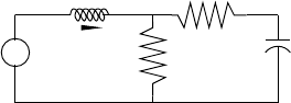
3. For the circuit shown here:
−
+
f(t)R1
R2
Cy(t)
+
−
i1(t)
L
where R1= 1 kΩ, R2= 22 kΩ, C= 10 µF , and L= 5 H.
(a) Determine a differential equation relating the input f(t) to the output y(t).
(b) Determine the initial conditions on y(t) if i1(0) = 0.2 A and y(0) = 5 V.
(c) Determine the analytical solution for the zero-input response of the system with these initial
conditions.
(d) Represent the differential equation for the circuit in state variable form.
(e) Using your program, determine a numerical solution to the differential equation for the zero-input
response.
(f) Plot and compare the analytical and the numerical solution. Comment on your results.
(g) Suppose that the circuit had nonlinear element in it, such as dependent sources. Describe how
the analytical solution and numerical solution would change.
Turn in your programs, your plots, and your observations.
Hints and helps
Making plots To make plots, I recommend you write out an ascii file with the tand yvalues that you
want. Then use Matlab to make the plots.
To write the files using C++, at the top of your program you need to open a file to write into:
#include <fstream> /* appears near the beginning of your program */
.
.
.
main()
{
.
3
.
.
ofstream outfile("junk"); /* open a filed called ’junk’ for writing */
.
.
.
Then any time you want to write, you simply use the ofstream operators:
outfile << t << " " << y << endl;
At the end of the program you should close the file:
outfile.close();
The steps above will save the computed data into a file named “junk”. Then you can use the plot
facilities of Matlab to make the plot. This is done by reading the data into Matlab, then plotting the
data. The following commands are to be done inside Matlab.
load junk % load the file ’junk’ into a variable called ’junk’
plot(junk(:,1),junk(:,2)) % plot the first column vs. the second
% column
Matrix/vector operations The following are some simple, fixed size matrix and vector routines that
might be helpful.
void mattimes(double t, double a[][3],double m[][3])
{
int i,j;
for(i = 0; i < 3; i++)
for(j = 0; j < 3; j++)
m[i][j] = t*a[i][j];
}
void matsub(double a[][3],double b[][3],double c[][3])
{
int i,j;
for(i = 0; i < 3; i++)
for(j = 0; j < 3; j++)
c[i][j] = a[i][j]-b[i][j];
}
void matvecmult(double m[][3], double *v, double *prod)
{
double sum;
int i,j;
for(i = 0; i < 3; i++) {
sum = 0;
for(j = 0; j < 3; j++) {
sum += m[i][j]*v[j];
}
prod[i] = sum;
}
}
4
And here is a suggested way to use some of these (but check the signs carefully!):
double a[3][3] = {{0,-1,0},{0,0,-1},{20.002,100.05,0.4}};
double m[3][3];
double I[3][3] = {{1,0,0},{0,1,0},{0,0,1}};
...
mattimes(deltat,a,m);
matsub(I,a,m);
Miscellaneous hints Remember that the starting index for arrays in C/C++ is 0.
An example loop for the time variable:
for(t = 0; t <= 4; t += deltat) {
5
