A Common Sense Guide To Data Structures And Algorithms: Level Up Your Core Programming Skills Algorithms Jay Wengrow
User Manual:
Open the PDF directly: View PDF ![]() .
.
Page Count: 299 [warning: Documents this large are best viewed by clicking the View PDF Link!]
- Preface
- 1. Why Data Structures Matter
- 2. Why Algorithms Matter
- 3. Oh Yes! Big O Notation
- 4. Speeding Up Your Code with Big O
- 5. Optimizing Code with and Without Big O
- 6. Optimizing for Optimistic Scenarios
- 7. Blazing Fast Lookup with Hash Tables
- 8. Crafting Elegant Code with Stacks and Queues
- 9. Recursively Recurse with Recursion
- 10. Recursive Algorithms for Speed
- 11. Node-Based Data Structures
- 12. Speeding Up All the Things with Binary Trees
- 13. Connecting Everything with Graphs
- 14. Dealing with Space Constraints

ACommon-SenseGuideto
DataStructuresand
Algorithms
LevelUpYourCoreProgrammingSkills
byJayWengrow
Version:P1.0(August2017)
Copyright©2017ThePragmaticProgrammers,LLC.Thisbookislicensedtothe
individualwhopurchasedit.Wedon'tcopy-protectitbecausethatwouldlimityour
abilitytouseitforyourownpurposes.Pleasedon'tbreakthistrust—youcanusethis
acrossallofyourdevicesbutpleasedonotsharethiscopywithothermembersof
yourteam,withfriends,orviafilesharingservices.Thanks.
Manyofthedesignationsusedbymanufacturersandsellerstodistinguishtheir
productsareclaimedastrademarks.Wherethosedesignationsappearinthisbook,
andThePragmaticProgrammers,LLCwasawareofatrademarkclaim,the
designationshavebeenprintedininitialcapitallettersorinallcapitals.ThePragmatic
StarterKit,ThePragmaticProgrammer,PragmaticProgramming,Pragmatic
BookshelfandthelinkinggdevicearetrademarksofThePragmaticProgrammers,
LLC.
Everyprecautionwastakeninthepreparationofthisbook.However,thepublisher
assumesnoresponsibilityforerrorsoromissions,orfordamagesthatmayresultfrom
theuseofinformation(includingprogramlistings)containedherein.
AboutthePragmaticBookshelf
ThePragmaticBookshelfisanagilepublishingcompany.We’reherebecausewe
wanttoimprovethelivesofdevelopers.Wedothisbycreatingtimely,practicaltitles,
writtenbyprogrammersforprogrammers.
OurPragmaticcourses,workshops,andotherproductscanhelpyouandyourteam
createbettersoftwareandhavemorefun.Formoreinformation,aswellasthelatest
Pragmatictitles,pleasevisitusathttp://pragprog.com.
OurebooksdonotcontainanyDigitalRestrictionsManagement,andhavealways
beenDRM-free.Wepioneeredthebetabookconcept,whereyoucanpurchaseand
readabookwhileit’sstillbeingwritten,andprovidefeedbacktotheauthortohelp
makeabetterbookforeveryone.Freeresourcesforallpurchasersincludesourcecode
downloads(ifapplicable),errataanddiscussionforums,allavailableonthebook's
homepageatpragprog.com.We’reheretomakeyourlifeeasier.
NewBookAnnouncements
Wanttokeepuponourlatesttitlesandannouncements,andoccasionalspecialoffers?
Justcreateanaccountonpragprog.com(anemailaddressandapasswordisallit
takes)andselectthecheckboxtoreceivenewsletters.Youcanalsofollowuson
twitteras@pragprog.
AboutEbookFormats
Ifyoubuydirectlyfrompragprog.com,yougetebooksinallavailableformatsforone
price.Youcansynchyourebooksamongstallyourdevices(includingiPhone/iPad,
Android,laptops,etc.)viaDropbox.Yougetfreeupdatesforthelifeoftheedition.
And,ofcourse,youcanalwayscomebackandre-downloadyourbookswhenneeded.
EbooksboughtfromtheAmazonKindlestorearesubjecttoAmazon'spolices.
LimitationsinAmazon'sfileformatmaycauseebookstodisplaydifferentlyon
differentdevices.Formoreinformation,pleaseseeourFAQat
pragprog.com/frequently-asked-questions/ebooks.Tolearnmoreaboutthisbookand
accessthefreeresources,gotohttps://pragprog.com/book/jwdsal,thebook's
homepage.
Thanksforyourcontinuedsupport,
AndyHunt
ThePragmaticProgrammers
Theteamthatproducedthisbookincludes:AndyHunt(Publisher),
JanetFurlow(VPofOperations), SusannahDavidsonPfalzer(ExecutiveEditor),
BrianMacDonald(DevelopmentEditor), PotomacIndexing,LLC(Indexing),
NicoleAbramowtiz(CopyEditor), GilsonGraphics(Layout)
Forcustomersupport,pleasecontactsupport@pragprog.com.

TableofContents
Preface
WhoIsThisBookFor?
What’sinThisBook?
HowtoReadThisBook
OnlineResources
Acknowledgments
1. WhyDataStructuresMatter
TheArray:TheFoundationalDataStructure
Reading
Searching
Insertion
Deletion
Sets:HowaSingleRuleCanAffectEfficiency
WrappingUp
2. WhyAlgorithmsMatter
OrderedArrays
SearchinganOrderedArray
BinarySearch
BinarySearchvs.LinearSearch
WrappingUp
3. OhYes!BigONotation
BigO:CounttheSteps
ConstantTimevs.LinearTime
SameAlgorithm,DifferentScenarios
AnAlgorithmoftheThirdKind
Logarithms
O(logN)Explained
PracticalExamples
WrappingUp
4. SpeedingUpYourCodewithBigO
BubbleSort
BubbleSortinAction
BubbleSortImplemented
TheEfficiencyofBubbleSort
AQuadraticProblem
ALinearSolution
WrappingUp
5. OptimizingCodewithandWithoutBigO
SelectionSort
SelectionSortinAction
SelectionSortImplemented
TheEfficiencyofSelectionSort
IgnoringConstants
TheRoleofBigO
APracticalExample
WrappingUp
6. OptimizingforOptimisticScenarios
InsertionSort
InsertionSortinAction
InsertionSortImplemented
TheEfficiencyofInsertionSort
TheAverageCase
APracticalExample
WrappingUp
7. BlazingFastLookupwithHashTables
EntertheHashTable
HashingwithHashFunctions
BuildingaThesaurusforFunandProfit,butMainlyProfit
DealingwithCollisions
TheGreatBalancingAct
PracticalExamples
WrappingUp
8. CraftingElegantCodewithStacksandQueues
Stacks
StacksinAction
Queues
QueuesinAction
WrappingUp
9. RecursivelyRecursewithRecursion
RecurseInsteadofLoop
TheBaseCase
ReadingRecursiveCode
RecursionintheEyesoftheComputer
RecursioninAction
WrappingUp
10. RecursiveAlgorithmsforSpeed
Partitioning
Quicksort
TheEfficiencyofQuicksort
Worst-CaseScenario
Quickselect
WrappingUp
11. Node-BasedDataStructures
LinkedLists
ImplementingaLinkedList
Reading
Searching
Insertion
Deletion
LinkedListsinAction
DoublyLinkedLists
WrappingUp
12. SpeedingUpAlltheThingswithBinaryTrees
BinaryTrees
Searching
Insertion
Deletion
BinaryTreesinAction
WrappingUp
13. ConnectingEverythingwithGraphs
Graphs
EarlyPraiseforACommon-Sense
GuidetoDataStructuresand
Algorithms
ACommon-SenseGuidetoDataStructuresandAlgorithmsisamuch-needed
distillationoftopicsthateludemanysoftwareprofessionals.Thecasualtoneand
presentationmakeiteasytounderstandconceptsthatareoftenhiddenbehind
mathematicalformulasandtheory.Thisisagreatbookfordeveloperslookingto
strengthentheirprogrammingskills.
→ JasonPike
Seniorsoftwareengineer,AtlasRFIDSolutions
Atuniversity,the“DataStructuresandAlgorithms”coursewasoneofthedriest
inthecurriculum;itwasonlylaterthatIrealizedwhatakeytopicitis.Asa
softwaredeveloper,youmustknowthisstuff.Thisbookisareadable
introductiontothetopicthatomitstheobtusemathematicalnotationcommonin
manycoursetexts.
→ NigelLowry
Companydirector&principalconsultant,Lemmata
Whetheryouarenewtosoftwaredevelopmentoragrizzledveteran,youwill
reallyenjoyandbenefitfrom(re-)learningthefoundations.JayWengrow
presentsaveryreadableandengagingtourthroughbasicdatastructuresand
algorithmsthatwillbenefiteverysoftwaredeveloper.
→ KevinBeam
Softwareengineer,NationalSnowandIceDataCenter(NSIDC),
UniversityofColoradoBoulder

Preface
Datastructuresandalgorithmsaremuchmorethanabstractconcepts.Mastering
themenablesyoutowritemoreefficientcodethatrunsfaster,whichis
particularlyimportantfortoday’swebandmobileapps.Ifyoulastsawan
algorithminauniversitycourseoratajobinterview,you’remissingoutonthe
rawpoweralgorithmscanprovide.
Theproblemwithmostresourcesonthesesubjectsisthatthey’re...well...obtuse.
Mosttextsgoheavyonthemathjargon,andifyou’renotamathematician,it’s
reallydifficulttograspwhatonEarthisgoingon.Evenbooksthatclaimto
makealgorithms“easy”assumethatthereaderhasanadvancedmathdegree.
Becauseofthis,toomanypeopleshyawayfromtheseconcepts,feelingthat
they’resimplynot“smart”enoughtounderstandthem.
Thetruth,however,isthateverythingaboutdatastructuresandalgorithmsboils
downtocommonsense.Mathematicalnotationitselfissimplyaparticular
language,andeverythinginmathcanalsobeexplainedwithcommon-sense
terminology.Inthisbook,Idon’tuseanymathbeyondaddition,subtraction,
multiplication,division,andexponents.Instead,everyconceptisbrokendownin
plainEnglish,andIuseaheavydoseofimagestomakeeverythingapleasureto
understand.
Onceyouunderstandtheseconcepts,youwillbeequippedtowritecodethatis
efficient,fast,andelegant.Youwillbeabletoweightheprosandconsof
variouscodealternatives,andbeabletomakeeducateddecisionsastowhich
codeisbestforthegivensituation.
Someofyoumaybereadingthisbookbecauseyou’restudyingthesetopicsat
school,oryoumaybepreparingfortechinterviews.Whilethisbookwill
demystifythesecomputersciencefundamentalsandgoalongwayinhelping
youatthesegoals,Iencourageyoutoappreciatethepowerthattheseconcepts
provideinyourday-to-dayprogramming.Ispecificallygooutofmywayto
maketheseconceptsrealandpracticalwithideasthatyoucouldmakeuseof
today.

WhoIsThisBookFor?
Thisbookisidealforseveralaudiences:
Youareabeginningdeveloperwhoknowsbasicprogramming,butwantsto
learnthefundamentalsofcomputersciencetowritebettercodeand
increaseyourprogrammingknowledgeandskills.
Youareaself-taughtdeveloperwhohasneverstudiedformalcomputer
science(oradeveloperwhodidbutforgoteverything!)andwantsto
leveragethepowerofdatastructuresandalgorithmstowritemorescalable
andelegantcode.
Youareacomputersciencestudentwhowantsatextthatexplainsdata
structuresandalgorithmsinplainEnglish.Thisbookcanserveasan
excellentsupplementtowhatever“classic”textbookyouhappentobe
using.
Youareadeveloperwhoneedstobrushupontheseconceptssinceyou
mayhavenotutilizedthemmuchinyourcareerbutexpecttobequizzedon
theminyournexttechnicalinterview.
Tokeepthebooksomewhatlanguage-agnostic,ourexamplesdrawfromseveral
programminglanguages,includingRuby,Python,andJavaScript,sohavinga
basicunderstandingoftheselanguageswouldbehelpful.Thatbeingsaid,I’ve
triedtowritetheexamplesinsuchawaythatevenifyou’refamiliarwitha
differentlanguage,youshouldbeabletofollowalong.Tothatend,Idon’t
alwaysfollowthepopularidiomsforeachlanguagewhereIfeelthatanidiom
mayconfusesomeonenewtothatparticularlanguage.
What’sinThisBook?
Asyoumayhaveguessed,thisbooktalksquiteabitaboutdatastructuresand
algorithms.Butmorespecifically,thebookislaidoutasfollows:
InChapter1,WhyDataStructuresMatterandChapter2,WhyAlgorithms
Matter,weexplainwhatdatastructuresandalgorithmsare,andexplorethe
conceptoftimecomplexity—whichisusedtodeterminehowefficientan
algorithmis.Intheprocess,wealsotalkagreatdealaboutarrays,sets,and
binarysearch.
InChapter3,OhYes!BigONotation,weunveilBigONotationandexplainit
intermsthatmygrandmothercouldunderstand.We’llusethisnotation
throughoutthebook,sothischapterisprettyimportant.
InChapter4,SpeedingUpYourCodewithBigO,Chapter5,OptimizingCode
withandWithoutBigO,andChapter6,OptimizingforOptimisticScenarios,
we’lldelvefurtherintoBigONotationanduseitpracticallytomakeourday-to-
daycodefaster.Alongtheway,we’llcovervarioussortingalgorithms,including
BubbleSort,SelectionSort,andInsertionSort.
Chapter7,BlazingFastLookupwithHashTablesandChapter8,Crafting
ElegantCodewithStacksandQueuesdiscussafewadditionaldatastructures,
includinghashtables,stacks,andqueues.We’llshowhowtheseimpactthe
speedandeleganceofourcode,andusethemtosolvereal-worldproblems.
Chapter9,RecursivelyRecursewithRecursionintroducesrecursion,ananchor
conceptintheworldofcomputerscience.We’llbreakitdownandseehowit
canbeagreattoolforcertainsituations.Chapter10,RecursiveAlgorithmsfor
Speedwilluserecursionasthefoundationforturbo-fastalgorithmslike
QuicksortandQuickselect,andtakeouralgorithmdevelopmentskillsupafew
notches.
Thefollowingchapters,Chapter11,Node-BasedDataStructures,Chapter12,
SpeedingUpAlltheThingswithBinaryTrees,andChapter13,Connecting

EverythingwithGraphs,explorenode-baseddatastructuresincludingthelinked
list,thebinarytree,andthegraph,andshowhoweachisidealforvarious
applications.
Thefinalchapter,Chapter14,DealingwithSpaceConstraints,exploresspace
complexity,whichisimportantwhenprogrammingfordeviceswithrelatively
smallamountsofdiskspace,orwhendealingwithbigdata.
HowtoReadThisBook
You’vegottoreadthisbookinorder.Therearebooksouttherewhereyoucan
readeachchapterindependentlyandskiparoundabit,butthisisnotoneof
them.Eachchapterassumesthatyou’vereadthepreviousones,andthebookis
carefullyconstructedsothatyoucanrampupyourunderstandingasyou
proceed.
Anotherimportantnote:tomakethisbookeasytounderstand,Idon’talways
revealeverythingaboutaparticularconceptwhenIintroduceit.Sometimes,the
bestwaytobreakdownacomplexconceptistorevealasmallpieceofit,and
onlyrevealthenextpiecewhenthefirstpiecehassunkenin.IfIdefinea
particulartermassuch-and-such,don’ttakethatasthetextbookdefinitionuntil
you’vecompletedtheentiresectiononthattopic.
It’satrade-off:tomakethebookeasytounderstand,I’vechosentooversimplify
certainconceptsatfirstandclarifythemovertime,ratherthanensurethatevery
sentenceiscompletely,academically,accurate.Butdon’tworrytoomuch,
becausebytheend,you’llseetheentireaccuratepicture.

OnlineResources
Thisbookhasitsownwebpage[1]inwhichyoucanfindmoreinformationabout
thebookandinteractinthefollowingways:
Participateinadiscussionforumwithotherreadersandmyself
Helpimprovethebookbyreportingerrata,includingcontentsuggestions
andtypos
Youcanfindpracticeexercisesforthecontentineachchapterat
http://commonsensecomputerscience.com/,andinthecodedownloadpackage
forthisbook.
Acknowledgments
Whilethetaskofwritingabookmayseemlikeasolitaryone,thisbooksimply
couldnothavehappenedwithoutthemanypeoplewhohavesupportedmeinmy
journeywritingit.I’dliketopersonallythankallofyou.
Tomywonderfulwife,Rena—thankyouforthetimeandemotionalsupport
you’vegiventome.YoutookcareofeverythingwhileIhunkereddownlikea
recluseandwrote.Tomyadorablekids—Tuvi,Leah,andShaya—thankyoufor
yourpatienceasIwrotemybookon“algorizms.”Andyes—it’sfinallyfinished.
Tomyparents,Mr.andMrs.HowardandDebbieWengrow—thankyoufor
initiallysparkingmyinterestincomputerprogrammingandhelpingmepursue
it.Littledidyouknowthatgettingmeacomputertutorformyninthbirthday
wouldsetthefoundationformycareer—andnowthisbook.
WhenIfirstsubmittedmymanuscripttothePragmaticBookshelf,Ithoughtit
wasgood.However,throughtheexpertise,suggestions,anddemandsofallthe
wonderfulpeoplewhoworkthere,thebookhasbecomesomethingmuch,much
betterthanIcouldhavewrittenonmyown.Tomyeditor,BrianMacDonald—
you’veshownmehowabookshouldbewritten,andyourinsightshave
sharpenedeachchapter;thisbookhasyourimprintalloverit.Tomymanaging
editor,SusannahPfalzer—you’vegivenmethevisionforwhatthisbookcould
be,takingmytheory-basedmanuscriptandtransformingitintoabookthatcan
beappliedtotheeverydayprogrammer.TothepublishersAndyHuntandDave
Thomas—thankyouforbelievinginthisbookandmakingthePragmatic
Bookshelfthemostwonderfulpublishingcompanytowritefor.
TotheextremelytalentedsoftwaredeveloperandartistColleenMcGuckin—
thankyoufortakingmychickenscratchandtransformingitintobeautifuldigital
imagery.Thisbookwouldbenothingwithoutthespectacularvisualsthatyou’ve
createdwithsuchskillandattentiontodetail.
I’vebeenfortunatethatsomanyexpertshavereviewedthisbook.Yourfeedback
[1]
hasbeenextremelyhelpfulandhasmadesurethatthisbookcanbeasaccurate
aspossible.I’dliketothankallofyouforyourcontributions:AaronKalair,
AlbertoBoschetti,AlessandroBahgat,ArunS.Kumar,BrianSchau,Daivid
Morgan,DerekGraham,FrankRuiz,IvoBalbaert,JasdeepNarang,JasonPike,
JavierCollado,JeffHolland,JessicaJaniuk,JoyMcCaffrey,KennethParekh,
MatteoVaccari,MohamedFouad,NeilHainer,NigelLowry,PeterHampton,
PeterWood,RodHilton,SamRose,SeanLindsay,StephanKämper,Stephen
Orr,StephenWolff,andTiborSimic.
I’dalsoliketothankallthestaff,students,andalumniatActualizeforyour
support.ThisbookwasoriginallyanActualizeproject,andyou’veall
contributedinvariousways.I’dliketoparticularlythankLukeEvansforgiving
metheideatowritethisbook.
Thankyouallformakingthisbookareality.
JayWengrow
mailto:jay@actualize.co
August,2017
Footnotes
https://pragprog.com/book/jwdsal
Copyright©2017,ThePragmaticBookshelf.

Chapter1
WhyDataStructuresMatter
Anyonewhohaswrittenevenafewlinesofcomputercodecomestorealizethat
programminglargelyrevolvesarounddata.Computerprogramsareallabout
receiving,manipulating,andreturningdata.Whetherit’sasimpleprogramthat
calculatesthesumoftwonumbers,orenterprisesoftwarethatrunsentire
companies,softwarerunsondata.
Dataisabroadtermthatreferstoalltypesofinformation,downtothemost
basicnumbersandstrings.Inthesimplebutclassic“HelloWorld!”program,the
string"HelloWorld!"isapieceofdata.Infact,eventhemostcomplexpiecesof
datausuallybreakdownintoabunchofnumbersandstrings.
Datastructuresrefertohowdataisorganized.Let’slookatthefollowingcode:
x="Hello!"
y="Howareyou"
z="today?"
printx+y+z
Thisverysimpleprogramdealswiththreepiecesofdata,outputtingthreestrings
tomakeonecoherentmessage.Ifweweretodescribehowthedataisorganized
inthisprogram,we’dsaythatwehavethreeindependentstrings,eachpointedto
byasinglevariable.
You’regoingtolearninthisbookthattheorganizationofdatadoesn’tjust
matterfororganization’ssake,butcansignificantlyimpacthowfastyourcode
runs.Dependingonhowyouchoosetoorganizeyourdata,yourprogrammay
runfasterorslowerbyordersofmagnitude.Andifyou’rebuildingaprogram
thatneedstodealwithlotsofdata,orawebappusedbythousandsofpeople
simultaneously,thedatastructuresyouselectmayaffectwhetherornotyour
softwarerunsatall,orsimplyconksoutbecauseitcan’thandletheload.
Whenyouhaveasolidgrasponthevariousdatastructuresandeachone’s
performanceimplicationsontheprogramthatyou’rewriting,youwillhavethe
keystowritefastandelegantcodethatwillensurethatyoursoftwarewillrun
quicklyandsmoothly,andyourexpertiseasasoftwareengineerwillbegreatly
enhanced.
Inthischapter,we’regoingtobeginouranalysisoftwodatastructures:arrays
andsets.Whilethetwodatastructuresseemalmostidentical,you’regoingto
learnthetoolstoanalyzetheperformanceimplicationsofeachchoice.
TheArray:TheFoundationalDataStructure
Thearrayisoneofthemostbasicdatastructuresincomputerscience.We
assumethatyouhaveworkedwitharraysbefore,soyouareawarethatanarray
issimplyalistofdataelements.Thearrayisversatile,andcanserveasauseful
toolinmanydifferentsituations,butlet’sjustgiveonequickexample.
Ifyouarelookingatthesourcecodeforanapplicationthatallowsusersto
createanduseshoppinglistsforthegrocerystore,youmightfindcodelikethis:
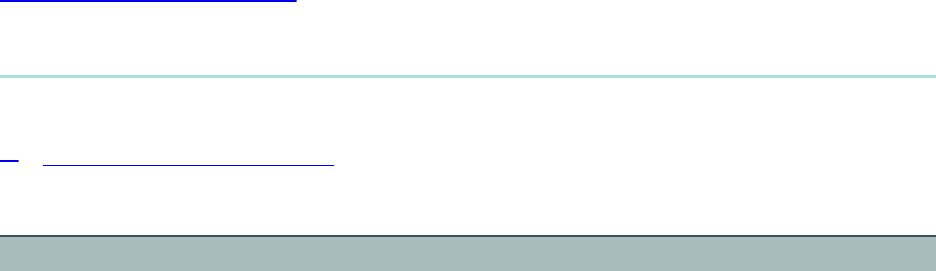
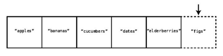
array=["apples","bananas","cucumbers","dates","elderberries"]
Thisarrayhappenstocontainfivestrings,eachrepresentingsomethingthatI
mightbuyatthesupermarket.(You’vegottotryelderberries.)
Theindexofanarrayisthenumberthatidentifieswhereapieceofdatalives
insidethearray.
Inmostprogramminglanguages,webegincountingtheindexat0.Soforour
examplearray,"apples"isatindex0,and"elderberries"isatindex4,likethis:
Tounderstandtheperformanceofadatastructure—suchasthearray—weneed
toanalyzethecommonwaysthatourcodemightinteractwiththatdata
structure.
Mostdatastructuresareusedinfourbasicways,whichwerefertoas
operations.Theyare:
Read:Readingreferstolookingsomethingupfromaparticularspotwithin
thedatastructure.Withanarray,thiswouldmeanlookingupavalueata

particularindex.Forexample,lookingupwhichgroceryitemislocatedat
index2wouldbereadingfromthearray.
Search:Searchingreferstolookingforaparticularvaluewithinadata
structure.Withanarray,thiswouldmeanlookingtoseeifaparticularvalue
existswithinthearray,andifso,whichindexit’sat.Forexample,looking
toseeif"dates"isinourgrocerylist,andwhichindexit’slocatedatwould
besearchingthearray.
Insert:Insertionreferstoaddinganothervaluetoourdatastructure.With
anarray,thiswouldmeanaddinganewvaluetoanadditionalslotwithin
thearray.Ifweweretoadd"figs"toourshoppinglist,we’dbeinsertinga
newvalueintothearray.
Delete:Deletionreferstoremovingavaluefromourdatastructure.Withan
array,thiswouldmeanremovingoneofthevaluesfromthearray.For
example,ifweremoved"bananas"fromourgrocerylist,thatwouldbe
deletingfromthearray.
Inthischapter,we’llanalyzehowfasteachoftheseoperationsarewhenapplied
toanarray.
AndthisbringsustothefirstEarth-shatteringconceptofthisbook:whenwe
measurehow“fast”anoperationtakes,wedonotrefertohowfastthe
operationtakesintermsofpuretime,butinsteadinhowmanystepsittakes.
Whyisthis?
Wecanneversaywithdefinitivenessthatanyoperationtakes,say,fiveseconds.
Whilethesameoperationmaytakefivesecondsonaparticularcomputer,itmay
takelongeronanolderpieceofhardware,ormuchfasteronthesupercomputers
oftomorrow.Measuringthespeedofanoperationintermsoftimeisflaky,since
itwillalwayschangedependingonthehardwarethatitisrunon.
However,wecanmeasurethespeedofanoperationintermsofhowmanysteps
ittakes.IfOperationAtakesfivesteps,andOperationBtakes500steps,wecan
assumethatOperationAwillalwaysbefasterthanOperationBonallpiecesof
hardware.Measuringthenumberofstepsisthereforethekeytoanalyzingthe
speedofanoperation.
Measuringthespeedofanoperationisalsoknownasmeasuringitstime
complexity.Throughoutthisbook,we’llusethetermsspeed,timecomplexity,
efficiency,andperformanceinterchangeably.Theyallrefertothenumberof
stepsthatagivenoperationtakes.
Let’sjumpintothefouroperationsofanarrayanddeterminehowmanysteps
eachonetakes.
Reading
Thefirstoperationwe’lllookatisreading,whichislookingupwhatvalueis
containedataparticularindexinsidethearray.
Readingfromanarrayactuallytakesjustonestep.Thisisbecausethecomputer
hastheabilitytojumptoanyparticularindexinthearrayandpeerinside.Inour
exampleof["apples","bananas","cucumbers","dates","elderberries"],ifwelookedup
index2,thecomputerwouldjumprighttoindex2andreportthatitcontainsthe
value"cucumbers".
Howisthecomputerabletolookupanarray’sindexinjustonestep?Let’ssee
how:
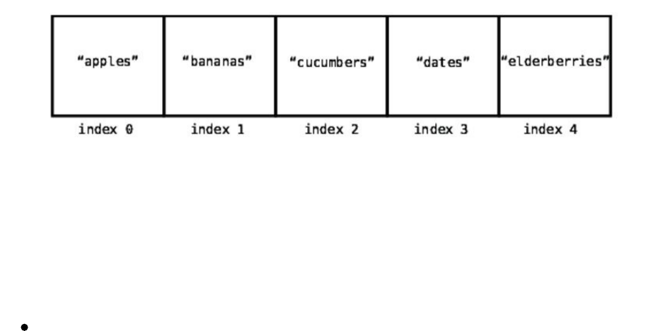
Acomputer’smemorycanbeviewedasagiantcollectionofcells.Inthe
followingdiagram,youcanseeagridofcells,inwhichsomeareempty,and
somecontainbitsofdata:
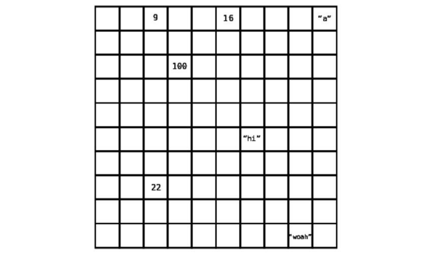
Whenaprogramdeclaresanarray,itallocatesacontiguoussetofemptycellsfor
useintheprogram.So,ifyouwerecreatinganarraymeanttoholdfive
elements,yourcomputerwouldfindanygroupoffiveemptycellsinarowand
designateittoserveasyourarray:
Now,everycellinacomputer’smemoryhasaspecificaddress.It’ssortoflikea
streetaddress(forexample,123MainSt.),exceptthatit’srepresentedwitha
simplenumber.Eachcell’smemoryaddressisonenumbergreaterthanthe
previouscell.Seethefollowingdiagram:
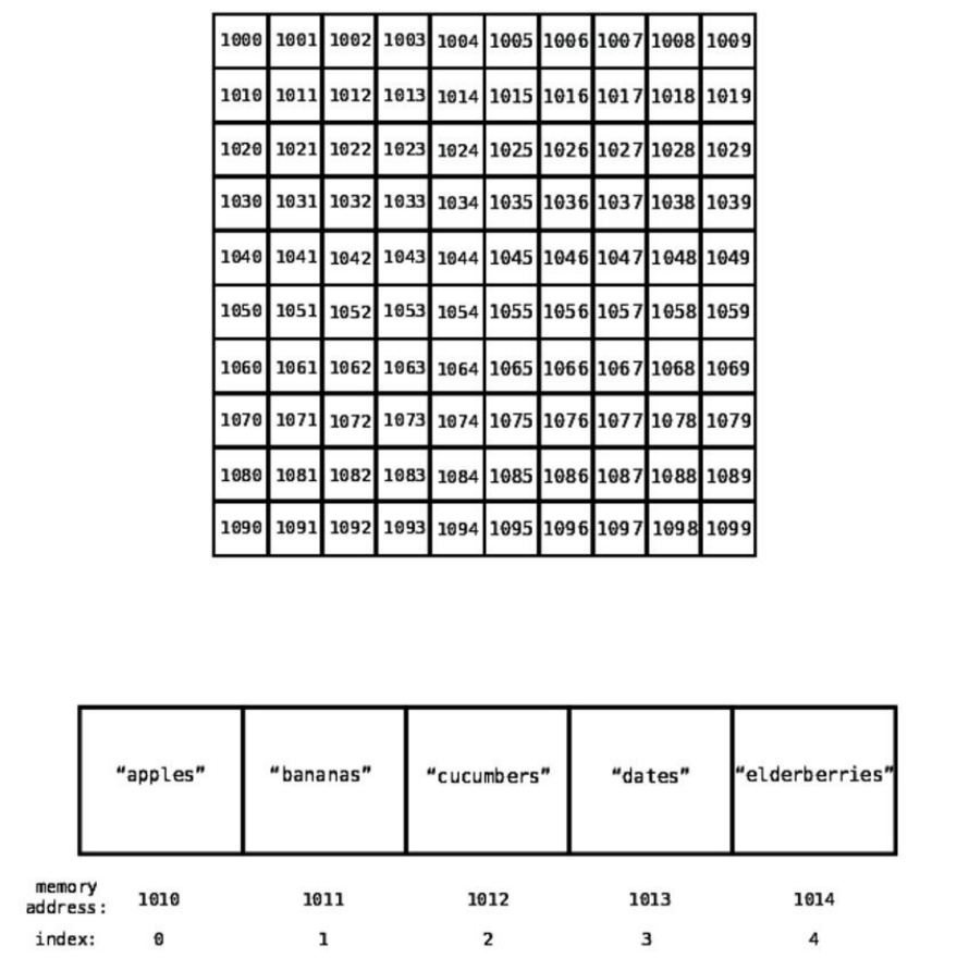
Inthenextdiagram,wecanseeourshoppinglistarraywithitsindexesand
memoryaddresses:
Whenthecomputerreadsavalueataparticularindexofanarray,itcanjump
straighttothatindexinonestepbecauseofthecombinationofthefollowing
facts:
1. Acomputercanjumptoanymemoryaddressinonestep.(Thinkofthisas
drivingto123MainStreet—youcandrivethereinonetripsinceyouknow
exactlywhereitis.)
2. Recordedineacharrayisthememoryaddresswhichitbeginsat.Sothe
computerhasthisstartingaddressreadily.
3. Everyarraybeginsatindex0.
Inourexample,ifwetellthecomputertoreadthevalueatindex3,thecomputer
goesthroughthefollowingthoughtprocess:
1. Ourarraybeginswithindex0atmemoryaddress1010.
2. Index3willbeexactlythreeslotspastindex0.
3. Sotofindindex3,we’dgotomemoryaddress1013,since1010+3is
1013.
Oncethecomputerjumpstothememoryaddress1013,itreturnsthevalue,
whichis"dates".
Readingfromanarrayis,therefore,averyefficientoperation,sinceittakesjust
onestep.Anoperationwithjustonestepisnaturallythefastesttypeof
operation.Oneofthereasonsthatthearrayissuchapowerfuldatastructureis
thatwecanlookupthevalueatanyindexwithsuchspeed.
Now,whatifinsteadofaskingthecomputerwhatvalueiscontainedatindex3,
weaskedwhether"dates"iscontainedwithinourarray?Thatisthesearch
operation,andwewillexplorethatnext.
Searching
Aswestatedpreviously,searchinganarrayislookingtoseewhetheraparticular
valueexistswithinanarrayandifso,whichindexit’slocatedat.Let’sseehow
manystepsthesearchoperationtakesforanarrayifweweretosearchfor
"dates".
WhenyouandIlookattheshoppinglist,oureyesimmediatelyspotthe"dates",
andwecanquicklycountinourheadsthatit’satindex3.However,acomputer
doesn’thaveeyes,andneedstomakeitswaythroughthearraystepbystep.
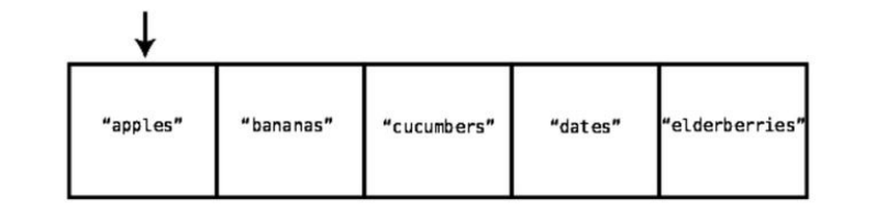
Tosearchforavaluewithinanarray,thecomputerstartsatindex0,checksthe
value,andifitdoesn’tfindwhatit’slookingfor,movesontothenextindex.It
doesthisuntilitfindsthevalueit’sseeking.
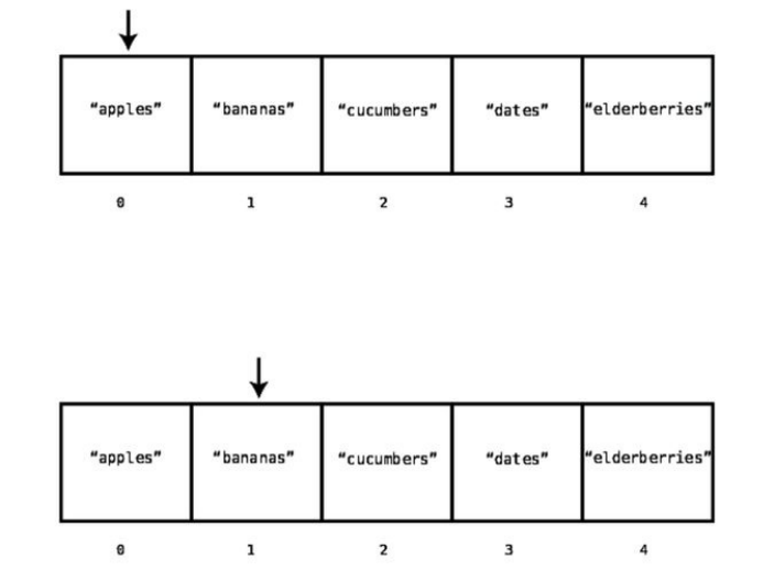
Thefollowingdiagramsdemonstratethisprocesswhenthecomputersearches
for"dates"insideourgrocerylistarray:
First,thecomputerchecksindex0:
Sincethevalueatindex0is"apples",andnotthe"dates"thatwe’relookingfor,
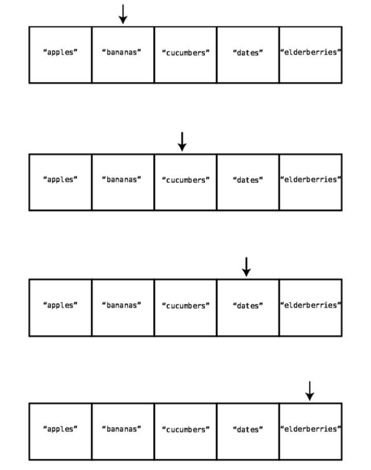
thecomputermovesontothenextindex:
Sinceindex1doesn’tcontainthe"dates"we’relookingforeither,thecomputer
movesontoindex2:
Onceagain,we’reoutofluck,sothecomputermovestothenextcell:
Aha!We’vefoundtheelusive"dates".Wenowknowthatthe"dates"areatindex
3.Atthispoint,thecomputerdoesnotneedtomoveontothenextcellofthe
array,sincewe’vealreadyfoundwhatwe’relookingfor.
Inthisexample,sincewehadtocheckfourdifferentcellsuntilwefoundthe
valueweweresearchingfor,we’dsaythatthisparticularoperationtookatotal
offoursteps.
InChapter2,WhyAlgorithmsMatter,we’lllearnaboutanotherwaytosearch,
butthisbasicsearchoperation—inwhichthecomputercheckseachcelloneata
time—isknownaslinearsearch.
Now,whatisthemaximumnumberofstepsacomputerwouldneedtoconducta
linearsearchonanarray?
Ifthevaluewe’reseekinghappenstobeinthefinalcellinthearray(like
"elderberries"),thenthecomputerwouldendupsearchingthrougheverycellof
thearrayuntilitfinallyfindsthevalueit’slookingfor.Also,ifthevaluewe’re
lookingfordoesn’toccurinthearrayatall,thecomputerwouldlikewisehaveto
searcheverycellsoitcanbesurethatthevaluedoesn’texistwithinthearray.
Soitturnsoutthatforanarrayoffivecells,themaximumnumberofstepsthat
linearsearchwouldtakeisfive.Foranarrayof500cells,themaximumnumber
ofstepsthatlinearsearchwouldtakeis500.
AnotherwayofsayingthisisthatforNcellsinanarray,linearsearchwilltakea
maximumofNsteps.Inthiscontext,Nisjustavariablethatcanbereplacedby
anynumber.
Inanycase,it’sclearthatsearchingislessefficientthanreading,sincesearching
cantakemanysteps,whilereadingalwaystakesjustonestepnomatterhow
largethearray.
Next,we’llanalyzetheoperationofinsertion—or,insertinganewvalueintoan
array.
Insertion
Theefficiencyofinsertinganewpieceofdatainsideanarraydependsonwhere
insidethearrayyou’dliketoinsertit.
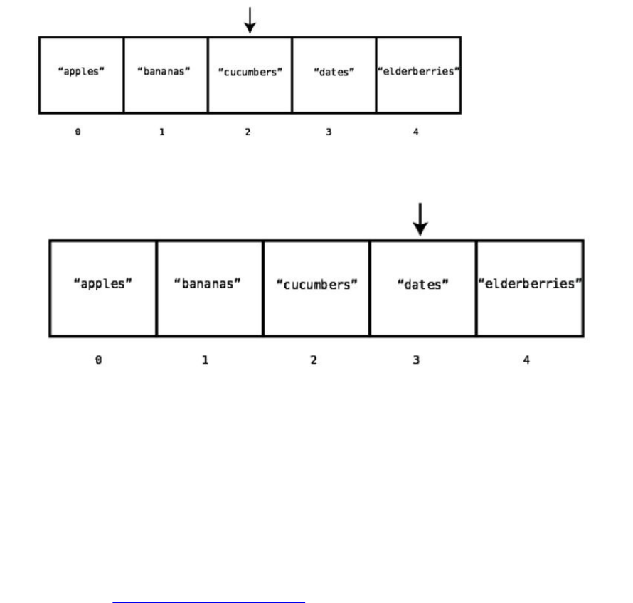
Let’ssaywewantedtoadd"figs"totheveryendofourshoppinglist.Suchan
insertiontakesjustonestep.Aswe’veseenearlier,thecomputerknowswhich
memoryaddressthearraybeginsat.Now,thecomputeralsoknowshowmany
elementsthearraycurrentlycontains,soitcancalculatewhichmemoryaddress
itneedstoaddthenewelementto,andcandosoinonestep.Seethefollowing
diagram:
Insertinganewpieceofdataatthebeginningorthemiddleofanarray,however,
isadifferentstory.Inthesecases,weneedtoshiftmanypiecesofdatatomake
roomforwhatwe’reinserting,leadingtoadditionalsteps.
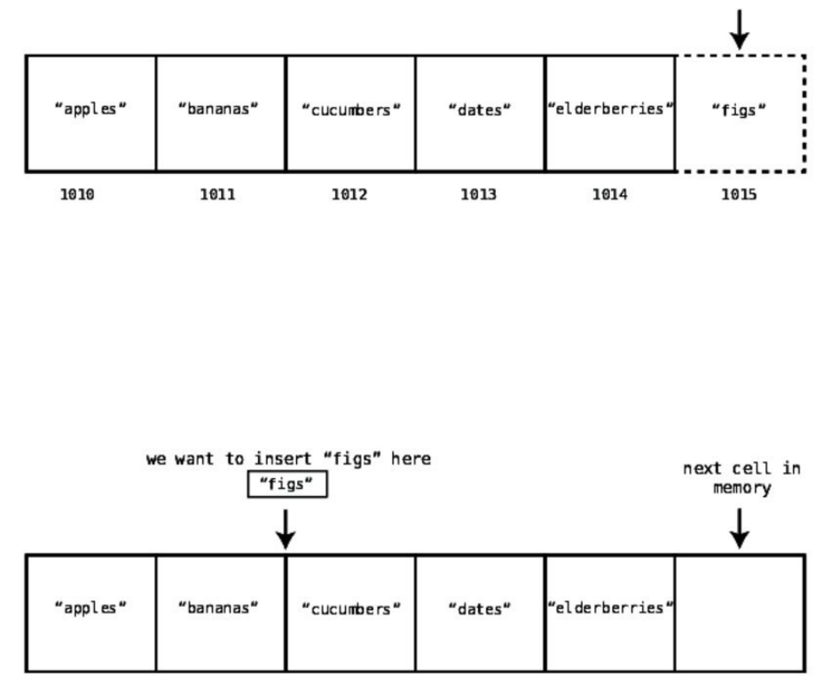
Forexample,let’ssaywewantedtoadd"figs"toindex2withinthearray.Seethe
followingdiagram:
Todothis,weneedtomove"cucumbers","dates",and"elderberries"totherightto
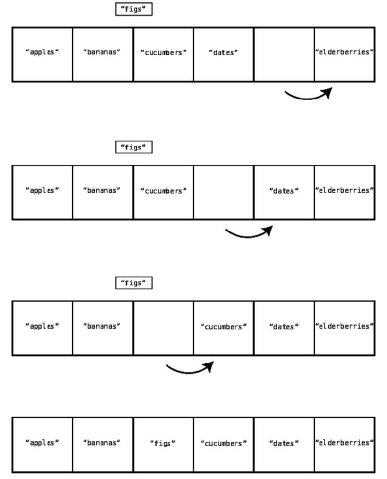
makeroomforthe"figs".Buteventhistakesmultiplesteps,sinceweneedto
firstmove"elderberries"onecelltotherighttomakeroomtomove"dates".We
thenneedtomove"dates"tomakeroomforthe"cucumbers".Let’swalkthrough
thisprocess.
Step#1:Wemove"elderberries"totheright:
Step#2:Wemove"dates"totheright:
Step#3:Wemove"cucumbers"totheright:
Step#4:Finally,wecaninsert"figs"intoindex2:
Wecanseethatintheprecedingexample,therewerefoursteps.Threeofthe
stepswereshiftingdatatotheright,whileonestepwastheactualinsertionof
thenewvalue.
Theworst-casescenarioforinsertionintoanarray—thatis,thescenarioin
whichinsertiontakesthemoststeps—iswhereweinsertdataatthebeginningof
thearray.Thisisbecausewheninsertingintothebeginningofthearray,wehave
tomovealltheothervaluesonecelltotheright.
Sowecansaythatinsertioninaworst-casescenariocantakeuptoN+1steps
foranarraycontainingNelements.Thisisbecausetheworst-casescenariois
insertingavalueintothebeginningofthearrayinwhichthereareNshifts
(everydataelementofthearray)andoneinsertion.
Thefinaloperationwe’llexplore—deletion—islikeinsertion,butinreverse.
Deletion
Deletionfromanarrayistheprocessofeliminatingthevalueataparticular
index.
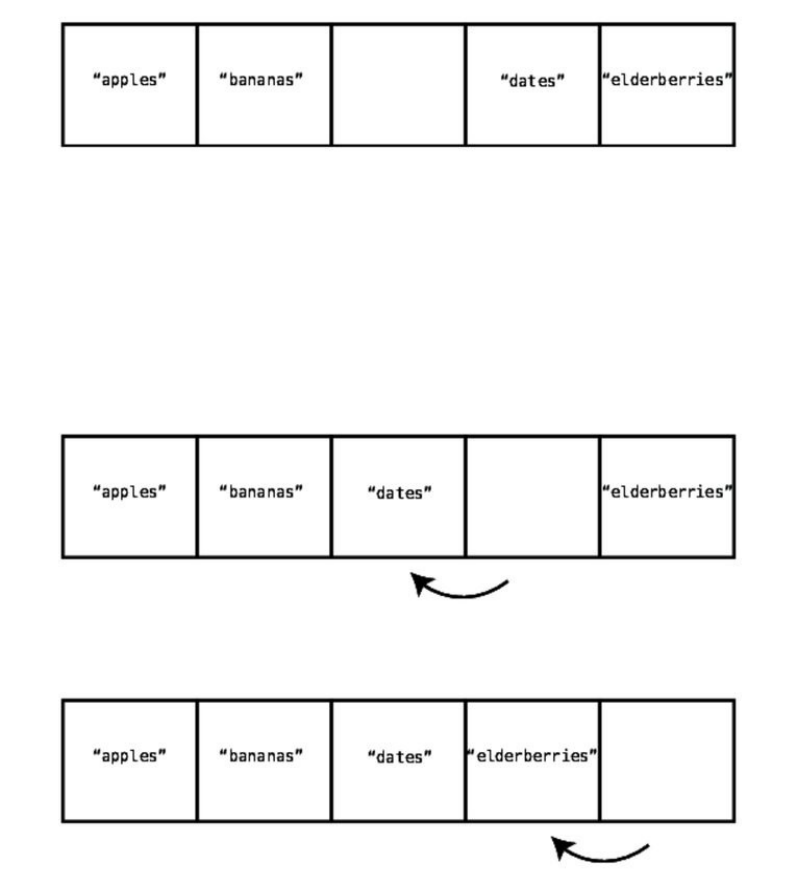
Let’sreturntoouroriginalexamplearray,anddeletethevalueatindex2.Inour
example,thiswouldbethe"cucumbers".
Step#1:Wedelete"cucumbers"fromthearray:
Whiletheactualdeletionof"cucumbers"technicallytookjustonestep,wenow
haveaproblem:wehaveanemptycellsittingsmackinthemiddleofourarray.
Anarrayisnotallowedtohavegapsinthemiddleofit,sotoresolvethisissue,
weneedtoshift"dates"and"elderberries"totheleft.
Step#2:Weshift"dates"totheleft:
Step#3:Weshift"elderberries"totheleft:
Soitturnsoutthatforthisdeletion,theentireoperationtookthreesteps.The
firststepwastheactualdeletion,andtheothertwostepsweredatashiftstoclose
thegap.
Sowe’vejustseenthatwhenitcomestodeletion,theactualdeletionitselfis
reallyjustonestep,butweneedtofollowupwithadditionalstepsofshifting
datatothelefttoclosethegapcausedbythedeletion.
Likeinsertion,theworst-casescenarioofdeletinganelementisdeletingthevery
firstelementofthearray.Thisisbecauseindex0wouldbeempty,whichisnot
allowedforarrays,andwe’dhavetoshiftalltheremainingelementstotheleft
tofillthegap.
Foranarrayoffiveelements,we’dspendonestepdeletingthefirstelement,and
fourstepsshiftingthefourremainingelements.Foranarrayof500elements,
we’dspendonestepdeletingthefirstelement,and499stepsshiftingthe
remainingdata.Wecanconclude,then,thatforanarraycontainingNelements,
themaximumnumberofstepsthatdeletionwouldtakeisNsteps.
Nowthatwe’velearnedhowtoanalyzethetimecomplexityofadatastructure,
wecandiscoverhowdifferentdatastructureshavedifferentefficiencies.Thisis
extremelyimportant,sincechoosingthecorrectdatastructureforyourprogram
canhaveseriousramificationsastohowperformantyourcodewillbe.
Thenextdatastructure—theset—issosimilartothearraythatatfirstglance,it
seemsthatthey’rebasicallythesamething.However,we’llseethatthe
operationsperformedonarraysandsetshavedifferentefficiencies.
Sets:HowaSingleRuleCanAffectEfficiency
Let’sexploreanotherdatastructure:theset.Asetisadatastructurethatdoesnot
allowduplicatevaluestobecontainedwithinit.
Thereareactuallydifferenttypesofsets,butforthisdiscussion,we’lltalkabout
anarray-basedset.Thissetisjustlikeanarray—itisasimplelistofvalues.The
onlydifferencebetweenthissetandaclassicarrayisthatthesetneverallows
duplicatevaluestobeinsertedintoit.
Forexample,ifyouhadtheset["a","b","c"]andtriedtoaddanother"b",the
computerjustwouldn’tallowit,sincea"b"alreadyexistswithintheset.
Setsareusefulwhenyouneedtoensurethatyoudon’thaveduplicatedata.
Forinstance,ifyou’recreatinganonlinephonebook,youdon’twantthesame
phonenumberappearingtwice.Infact,I’mcurrentlysufferingfromthiswith
mylocalphonebook:myhomephonenumberisnotjustlistedformyself,butit
isalsoerroneouslylistedasthephonenumberforsomefamilynamedZirkind.
(Yes,thisisatruestory.)Letmetellyou—it’squiteannoyingtoreceivephone
callsandvoicemailsfrompeoplelookingfortheZirkinds.Forthatmatter,I’m
suretheZirkindsarealsowonderingwhynooneevercallsthem.AndwhenI
calltheZirkindstoletthemknowabouttheerror,mywifepicksupthephone
becauseI’vecalledmyownnumber.(Okay,thatlastpartneverhappened.)If
onlytheprogramthatproducedthephonebookhadusedaset…
Inanycase,asetisanarraywithonesimpleconstraintofnotallowing
duplicates.Yet,thisconstraintactuallycausesthesettohaveadifferent
efficiencyforoneofthefourprimaryoperations.
Let’sanalyzethereading,searching,insertion,anddeletionoperationsincontext
ofanarray-basedset.
Readingfromasetisexactlythesameasreadingfromanarray—ittakesjust
onestepforthecomputertolookupwhatiscontainedwithinaparticularindex.
Aswedescribedearlier,thisisbecausethecomputercanjumptoanyindex
withinthesetsinceitknowsthememoryaddressthatthesetbeginsat.
Searchingasetalsoturnsouttobenodifferentthansearchinganarray—ittakes
uptoNstepstosearchtoseeifavalueexistswithinaset.Anddeletionisalso
identicalbetweenasetandanarray—ittakesuptoNstepstodeleteavalueand
movedatatothelefttoclosethegap.
Insertion,however,iswherearraysandsetsdiverge.Let’sfirstexploreinserting
avalueattheendofaset,whichwasabest-casescenarioforanarray.Withan
array,thecomputercaninsertavalueatitsendinasinglestep.
Withaset,however,thecomputerfirstneedstodeterminethatthisvaluedoesn’t
alreadyexistinthisset—becausethat’swhatsetsdo:theypreventduplicate
data.Soeveryinsertfirstrequiresasearch.
Let’ssaythatourgrocerylistwasaset—andthatwouldbeadecentchoicesince
wedon’twanttobuythesamethingtwice,afterall.Ifourcurrentsetis["apples",
"bananas","cucumbers","dates","elderberries"],andwewantedtoinsert"figs",we’d
havetoconductasearchandgothroughthefollowingsteps:
Step#1:Searchindex0for"figs":
It’snotthere,butitmightbesomewhereelseintheset.Weneedtomakesure
that"figs"doesnotexistanywherebeforewecaninsertit.
Step#2:Searchindex1:
Step#3:Searchindex2:
Step#4:Searchindex3:
Step#5:Searchindex4:
Onlynowthatwe’vesearchedtheentiresetdoweknowthatit’ssafetoinsert
"figs".Andthatbringsustoourfinalstep.
Step#6:Insert"figs"attheendoftheset:
Insertingavalueattheendofasetisstillthebest-casescenario,butwestillhad
toperformsixstepsforasetoriginallycontainingfiveelements.Thatis,wehad
tosearchallfiveelementsbeforeperformingthefinalinsertionstep.
Saidanotherway:insertionintoasetinabest-casescenariowilltakeN+1
stepsforNelements.ThisisbecausethereareNstepsofsearchtoensurethat
thevaluedoesn’talreadyexistwithintheset,andthenonestepfortheactual
insertion.
Inaworst-casescenario,wherewe’reinsertingavalueatthebeginningofaset,
thecomputerneedstosearchNcellstoensurethatthesetdoesn’talready
containthatvalue,andthenanotherNstepstoshiftallthedatatotheright,and
anotherfinalsteptoinsertthenewvalue.That’satotalof2N+1steps.
Now,doesthismeanthatyoushouldavoidsetsjustbecauseinsertionisslower
forsetsthanregulararrays?Absolutelynot.Setsareimportantwhenyouneedto
ensurethatthereisnoduplicatedata.(Hopefully,onedaymyphonebookwill
befixed.)Butwhenyoudon’thavesuchaneed,anarraymaybepreferable,
sinceinsertionsforarraysaremoreefficientthaninsertionsforsets.Youmust
analyzetheneedsofyourownapplicationanddecidewhichdatastructureisa
betterfit.

WrappingUp
Analyzingthenumberofstepsthatanoperationtakesistheheartof
understandingtheperformanceofdatastructures.Choosingtherightdata
structureforyourprogramcanspellthedifferencebetweenbearingaheavyload
vs.collapsingunderit.Inthischapterinparticular,you’velearnedtousethis
analysistoweighwhetheranarrayorasetmightbetheappropriatechoicefora
givenapplication.
Nowthatwe’vebeguntolearnhowtothinkaboutthetimecomplexityofdata
structures,wecanalsousethesameanalysistocomparecompetingalgorithms
(evenwithinthesamedatastructure)toensuretheultimatespeedand
performanceofourcode.Andthat’sexactlywhatthenextchapterisabout.
Copyright©2017,ThePragmaticBookshelf.

Chapter2
WhyAlgorithmsMatter
Inthepreviouschapter,wetookalookatourfirstdatastructuresandsawhow
choosingtherightdatastructurecansignificantlyaffecttheperformanceofour
code.Eventwodatastructuresthatseemsosimilar,suchasthearrayandtheset,
canmakeorbreakaprogramiftheyencounteraheavyload.
Inthischapter,we’regoingtodiscoverthatevenifwedecideonaparticular
datastructure,thereisanothermajorfactorthatcanaffecttheefficiencyofour
code:theproperselectionofwhichalgorithmtouse.
Althoughthewordalgorithmsoundslikesomethingcomplex,itreallyisn’t.An
algorithmissimplyaparticularprocessforsolvingaproblem.Forexample,the
processforpreparingabowlofcerealcanbecalledanalgorithm.Thecereal-
preparationalgorithmfollowsthesefoursteps(forme,atleast):
1. Grababowl.
2. Pourcerealinthebowl.
3. Pourmilkinthebowl.
4. Dipaspooninthebowl.
Whenappliedtocomputing,analgorithmreferstoaprocessforgoingabouta
particularoperation.Inthepreviouschapter,weanalyzedfourmajoroperations,
includingreading,searching,insertion,anddeletion.Inthischapter,we’llsee
thatattimes,it’spossibletogoaboutanoperationinmorethanoneway.Thatis
tosay,therearemultiplealgorithmsthatcanachieveaparticularoperation.
We’reabouttoseehowtheselectionofaparticularalgorithmcanmakeourcode
eitherfastorslow—eventothepointwhereitstopsworkingunderalotof
pressure.Butfirst,let’stakealookatanewdatastructure:theorderedarray.
We’llseehowthereismorethanonealgorithmforsearchinganorderedarray,
andwe’lllearnhowtochoosetherightone.
OrderedArrays
Theorderedarrayisalmostidenticaltothearraywediscussedintheprevious
chapter.Theonlydifferenceisthatorderedarraysrequirethatthevaluesare
alwayskept—youguessedit—inorder.Thatis,everytimeavalueisadded,it
getsplacedinthepropercellsothatthevaluesofthearrayremainsorted.Ina
standardarray,ontheotherhand,valuescanbeaddedtotheendofthearray
withouttakingtheorderofthevaluesintoconsideration.
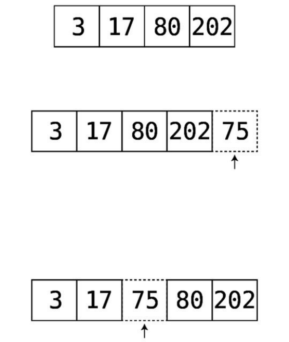
Forexample,let’stakethearray[3,17,80,202]:
Assumethatwewantedtoinsertthevalue75.Ifthisarraywerearegulararray,
wecouldinsertthe75attheend,asfollows:
Aswenotedinthepreviouschapter,thecomputercanaccomplishthisina
singlestep.
Ontheotherhand,ifthiswereanorderedarray,we’dhavenochoicebutto
insertthe75intheproperspotsothatthevaluesremainedinascendingorder:
Now,thisiseasiersaidthandone.Thecomputercannotsimplydropthe75into
therightslotinasinglestep,becausefirstithastofindtherightplaceinwhich
the75needstobeinserted,andthenshiftothervaluestomakeroomforit.Let’s
breakdownthisprocessstepbystep.
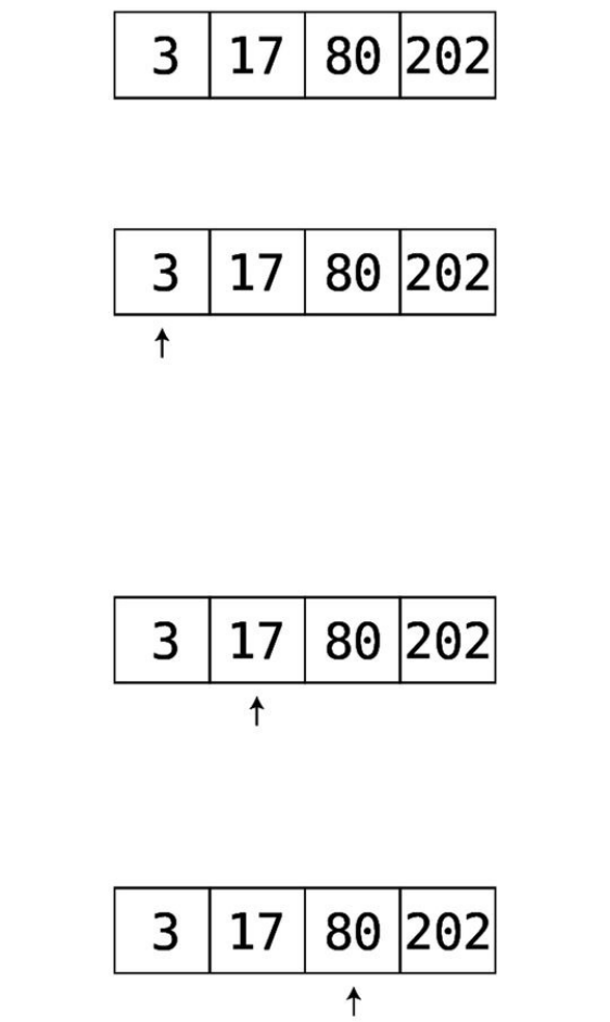
Let’sstartagainwithouroriginalorderedarray:
Step#1:Wecheckthevalueatindex0todeterminewhetherthevaluewewant
toinsert—the75—shouldgotoitsleftortoitsright:
Since75isgreaterthan3,weknowthatthe75willbeinsertedsomewheretoits
right.However,wedon’tknowyetexactlywhichcellitshouldbeinsertedinto,
soweneedtocheckthenextcell.
Step#2:Weinspectthevalueatthenextcell:
75isgreaterthan17,soweneedtomoveon.
Step#3:Wecheckthevalueatthenextcell:
We’veencounteredthevalue80,whichisgreaterthanthe75thatwewishto
insert.Sincewe’vereachedthefirstvaluewhichisgreaterthan75,wecan
concludethatthe75mustbeplacedimmediatelytotheleftofthis80tomaintain
theorderofthisorderedarray.Todothat,weneedtoshiftdatatomakeroomfor
the75.
Step#4:Movethefinalvaluetotheright:
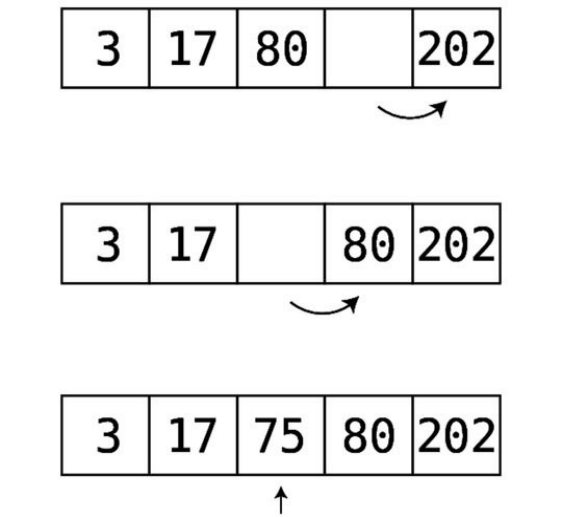
Step#5:Movethenext-to-lastvaluetotheright:
Step#6:Wecanfinallyinsertthe75intoitscorrectspot:
Itemergesthatwheninsertingintoanorderedarray,weneedtoalwaysconduct
asearchbeforetheactualinsertiontodeterminethecorrectspotfortheinsertion.
Thatisonekeydifference(intermsofefficiency)betweenastandardarrayand
anorderedarray.
Whileinsertionislessefficientbyanorderedarraythaninaregulararray,the
orderedarrayhasasecretsuperpowerwhenitcomestothesearchoperation.
SearchinganOrderedArray
Inthepreviouschapter,wedescribedtheprocessforsearchingforaparticular
valuewithinaregulararray:wecheckeachcelloneatatime—fromlefttoright
—untilwefindthevaluewe’relookingfor.Wenotedthatthisprocessisreferred
toaslinearsearch.
Let’sseehowlinearsearchdiffersbetweenaregularandorderedarray.
Saythatwehavearegulararrayof[17,3,75,202,80].Ifweweretosearchforthe
value22—whichhappenstobenonexistentinourexample—wewouldneedto
searcheachandeveryelementbecausethe22couldpotentiallybeanywherein
thearray.Theonlytimewecouldstopoursearchbeforewereachthearray’s
endisifwehappentofindthevaluewe’relookingforbeforewereachtheend.
Withanorderedarray,however,wecanstopasearchearlyevenifthevalueisn’t
containedwithinthearray.Let’ssaywe’researchingfora22withinanordered
arrayof[3,17,75,80,202].Wecanstopthesearchassoonaswereachthe75,
sinceit’simpossiblethatthe22isanywheretotherightofit.
Here’saRubyimplementationoflinearsearchonanorderedarray:
deflinear_search(array,value)
#Weiteratethrougheveryelementinthearray:
array.eachdo|element|
#Ifwefindthevaluewe'relookingfor,wereturnit:
ifelement==value
returnvalue
#Ifwereachanelementthatisgreaterthanthevalue
#we'relookingfor,wecanexittheloopearly:
elsifelement>value
break
end
end
#Wereturnnilifwedonotfindthevaluewithinthearray:
returnnil
end
Inthislight,linearsearchwilltakefewerstepsinanorderedarrayvs.astandard
arrayinmostsituations.Thatbeingsaid,ifwe’researchingforavaluethat
happenstobethefinalvalueorgreaterthanthefinalvalue,wewillstillendup
searchingeachandeverycell.
Atfirstglance,then,standardarraysandorderedarraysdon’thavetremendous
differencesinefficiency.
Butthatisbecausewehavenotyetunlockedthepowerofalgorithms.Andthat
isabouttochange.
We’vebeenassuminguntilnowthattheonlywaytosearchforavaluewithinan
orderedarrayislinearsearch.Thetruth,however,isthatlinearsearchisonly
onepossiblealgorithm—thatis,itisoneparticularprocessforgoingabout
searchingforavalue.Itistheprocessofsearchingeachandeverycelluntilwe
findthedesiredvalue.Butitisnottheonlyalgorithmwecanusetosearchfora
value.
Thebigadvantageofanorderedarrayoveraregulararrayisthatanordered
arrayallowsforanalternativesearchingalgorithm.Thisalgorithmisknownas
binarysearch,anditisamuch,muchfasteralgorithmthanlinearsearch.
BinarySearch
You’veprobablyplayedthisguessinggamewhenyouwereachild(ormaybe
youplayitwithyourchildrennow):I’mthinkingofanumberbetween1and
100.KeeponguessingwhichnumberI’mthinkingof,andI’llletyouknow
whetheryouneedtoguesshigherorlower.
Youknowintuitivelyhowtoplaythisgame.Youwouldn’tstarttheguessingby
choosingthenumber1.You’dstartwith50whichissmackinthemiddle.Why?
Becausebyselecting50,nomatterwhetherItellyoutoguesshigherorlower,
you’veautomaticallyeliminatedhalfthepossiblenumbers!
Ifyouguess50andItellyoutoguesshigher,you’dthenpick75,toeliminate
halfoftheremainingnumbers.Ifafterguessing75,Itoldyoutoguesslower,
you’dpick62or63.You’dkeeponchoosingthehalfwaymarkinordertokeep
eliminatinghalfoftheremainingnumbers.
Let’svisualizethisprocesswithasimilargame,exceptthatwe’retoldtoguessa
numberbetween1and10:
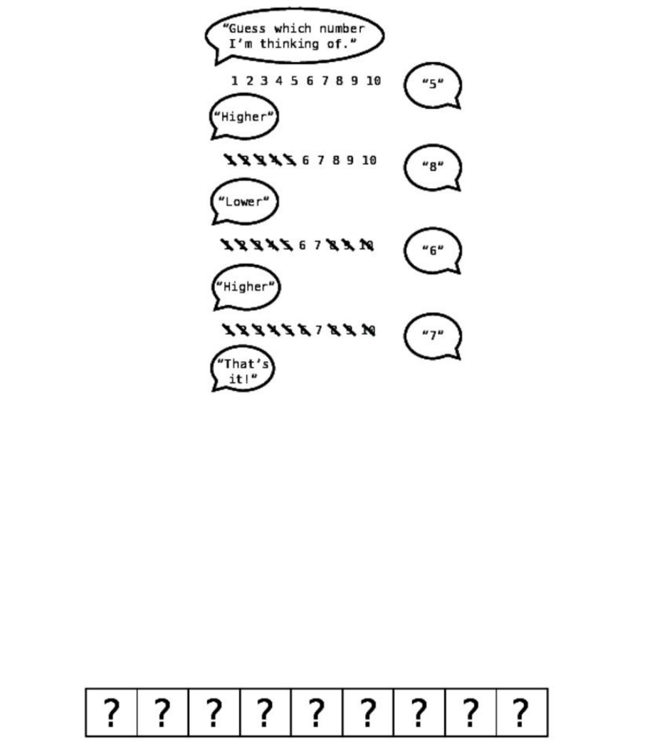
This,inanutshell,isbinarysearch.
Themajoradvantageofanorderedarrayoverastandardarrayisthatwehave
theoptionofperformingabinarysearchratherthanalinearsearch.Binary
searchisimpossiblewithastandardarraybecausethevaluescanbeinany
order.
Toseethisinaction,let’ssaywehadanorderedarraycontainingnineelements.
Tothecomputer,itdoesn’tknowwhatvalueeachcellcontains,sowewill
portraythearraylikethis:
Saythatwe’dliketosearchforthevalue7insidethisorderedarray.Wecando
sousingbinarysearch:
Step#1:Webeginoursearchfromthecentralcell.Wecaneasilyjumptothis
cellsinceweknowthelengthofthearray,andcanjustdividethatnumberby
twoandjumptotheappropriatememoryaddress.Wecheckthevalueatthat
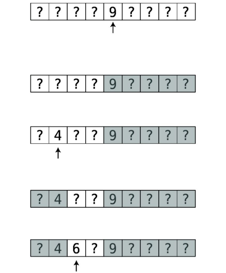
cell:
Sincethevalueuncoveredisa9,wecanconcludethatthe7issomewheretoits
left.We’vejustsuccessfullyeliminatedhalfofthearray’scells—thatis,allthe
cellstotherightofthe9(andthe9itself):
Step#2:Amongthecellstotheleftofthe9,weinspectthemiddlemostvalue.
Therearetwomiddlemostvalues,sowearbitrarilychoosetheleftone:
It’sa4,sothe7mustbesomewheretoitsright.Wecaneliminatethe4andthe
celltoitsleft:
Step#3:Therearetwomorecellswherethe7canbe.Wearbitrarilychoosethe
leftone:
Step#4:Weinspectthefinalremainingcell.(Ifit’snotthere,thatmeansthat
thereisno7withinthisorderedarray.)
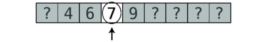
We’vefoundthe7successfullyinfoursteps.Whilethisisthesamenumberof
stepslinearsearchwouldhavetakeninthisexample,we’lldemonstratethe
powerofbinarysearchshortly.
Here’sanimplementationofbinarysearchinRuby:
defbinary_search(array,value)
#First,weestablishthelowerandupperboundsofwherethevalue
#we'researchingforcanbe.Tostart,thelowerboundisthefirst
#valueinthearray,whiletheupperboundisthelastvalue:
lower_bound=0
upper_bound=array.length-1
#Webeginaloopinwhichwekeepinspectingthemiddlemostvalue
#betweentheupperandlowerbounds:
whilelower_bound<=upper_bounddo
#Wefindthemidpointbetweentheupperandlowerbounds:
#(Wedon'thavetoworryabouttheresultbeinganon-integer
#sinceinRuby,theresultofdivisionofintegerswillalways
#beroundeddowntothenearestinteger.)
midpoint=(upper_bound+lower_bound)/2
#Weinspectthevalueatthemidpoint:
value_at_midpoint=array[midpoint]
#Ifthevalueatthemidpointistheonewe'relookingfor,we'redone.
#Ifnot,wechangethelowerorupperboundbasedonwhetherweneed
#toguesshigherorlower:
ifvalue<value_at_midpoint
upper_bound=midpoint-1
elsifvalue>value_at_midpoint
lower_bound=midpoint+1
elsifvalue==value_at_midpoint
returnmidpoint
end
end
#Ifwe'venarrowedtheboundsuntilthey'vereachedeachother,that
#meansthatthevaluewe'researchingforisnotcontainedwithin
#thisarray:
returnnil
end

BinarySearchvs.LinearSearch
Withorderedarraysofasmallsize,thealgorithmofbinarysearchdoesn’thave
muchofanadvantageoverthealgorithmoflinearsearch.Butlet’sseewhat
happenswithlargerarrays.
Withanarraycontainingonehundredvalues,herearethemaximumnumbersof
stepsitwouldtakeforeachtypeofsearch:
Linearsearch:onehundredsteps
Binarysearch:sevensteps
Withlinearsearch,ifthevaluewe’researchingforisinthefinalcelloris
greaterthanthevalueinthefinalcell,wehavetoinspecteachandevery
element.Foranarraythesizeof100,thiswouldtakeonehundredsteps.
Whenweusebinarysearch,however,eachguesswemakeeliminateshalfofthe
possiblecellswe’dhavetosearch.Inourveryfirstguess,wegettoeliminatea
whoppingfiftycells.
Let’slookatthisanotherway,andwe’llseeapatternemerge:
Withanarrayofsize3,themaximumnumberofstepsitwouldtaketofind
somethingusingbinarysearchistwo.
Ifwedoublethenumberofcellsinthearray(andaddonemoretokeepthe
numberoddforsimplicity’ssake),therearesevencells.Forsuchanarray,the
maximumnumberofstepstofindsomethingusingbinarysearchisthree.
Ifwedoubleitagain(andaddone)sothattheorderedarraycontainsfifteen
elements,themaximumnumberofstepstofindsomethingusingbinarysearchis
four.
Thepatternthatemergesisthatforeverytimewedoublethenumberofitemsin
theorderedarray,thenumberofstepsneededforbinarysearchincreasesbyjust
one.
Thispatternisunusuallyefficient:foreverytimewedoublethedata,thebinary
searchalgorithmaddsamaximumofjustonemorestep.
Contrastthiswithlinearsearch.Ifyouhadthreeitems,you’dneeduptothree
steps.Forsevenelements,you’dneedamaximumofsevensteps.Forone
hundred,you’dneeduptoonehundredsteps.Withlinearsearch,thereareas
manystepsasthereareitems.Forlinearsearch,everytimewedoublethe
numberofelementsinthearray,wedoublethenumberofstepsweneedtofind
something.Forbinarysearch,everytimewedoublethenumberofelementsin
thearray,weonlyneedtoaddonemorestep.
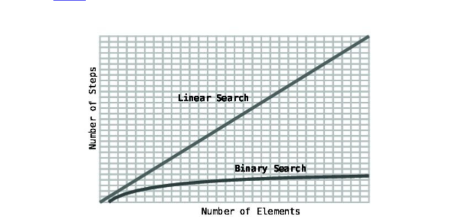
Wecanvisualizethedifferenceinperformancebetweenlinearandbinarysearch
withthisgraph.
Let’sseehowthisplaysoutforevenlargerarrays.Withanarrayof10,000
elements,alinearsearchcantakeupto10,000steps,whilebinarysearchtakes
uptoamaximumofjustthirteensteps.Foranarraythesizeofonemillion,
linearsearchwouldtakeuptoonemillionsteps,whilebinarysearchwouldtake
uptojusttwentysteps.
Again,keepinmindthatorderedarraysaren’tfasterineveryrespect.Asyou’ve
seen,insertioninorderedarraysisslowerthaninstandardarrays.Buthere’sthe
trade-off:byusinganorderedarray,youhavesomewhatslowerinsertion,but
muchfastersearch.Again,youmustalwaysanalyzeyourapplicationtoseewhat
isabetterfit.

WrappingUp
Andthisiswhatalgorithmsareallabout.Often,thereismorethanonewayto
achieveaparticularcomputinggoal,andthealgorithmyouchoosecanseriously
affectthespeedofyourcode.
It’salsoimportanttorealizethatthereusuallyisn’tasingledatastructureor
algorithmthatisperfectforeverysituation.Forexample,justbecauseordered
arraysallowforbinarysearchdoesn’tmeanyoushouldalwaysuseordered
arrays.Insituationswhereyoudon’tanticipatesearchingthedatamuch,but
onlyaddingdata,standardarraysmaybeabetterchoicebecausetheirinsertion
isfaster.
Aswe’veseen,thewaytoanalyzecompetingalgorithmsistocountthenumber
ofstepseachonetakes.
Inthenextchapter,we’regoingtolearnaboutaformalizedwayofexpressing
thetimecomplexityofcompetingdatastructuresandalgorithms.Havingthis
commonlanguagewillgiveusclearerinformationthatwillallowustomake
betterdecisionsaboutwhichalgorithmswechoose.
Copyright©2017,ThePragmaticBookshelf.

Chapter3
OhYes!BigONotation
We’veseenintheprecedingchaptersthatthenumberofstepsthatanalgorithm
takesistheprimaryfactorindeterminingitsefficiency.
However,wecan’tsimplylabelonealgorithma“22-stepalgorithm”andanother
a“400-stepalgorithm.”Thisisbecausethenumberofstepsthatanalgorithm
takescannotbepinneddowntoasinglenumber.Let’stakelinearsearch,for
example.Thenumberofstepsthatlinearsearchtakesvaries,asittakesasmany
stepsastherearecellsinthearray.Ifthearraycontainstwenty-twoelements,
linearsearchtakestwenty-twosteps.Ifthearrayhas400elements,however,
linearsearchtakes400steps.
Themoreaccuratewaytoquantifyefficiencyoflinearsearchistosaythatlinear
searchtakesNstepsforNelementsinthearray.Ofcourse,that’saprettywordy
wayofexpressingthisconcept.
Inordertohelpeasecommunicationregardingtimecomplexity,computer
scientistshaveborrowedaconceptfromtheworldofmathematicstodescribea
conciseandconsistentlanguagearoundtheefficiencyofdatastructuresand
algorithms.KnownasBigONotation,thisformalizedexpressionaroundthese
conceptsallowsustoeasilycategorizetheefficiencyofagivenalgorithmand
conveyittoothers.
OnceyouunderstandBigONotation,you’llhavethetoolstoanalyzeevery
algorithmgoingforwardinaconsistentandconciseway—andit’sthewaythat
theprosuse.
WhileBigONotationcomesfromthemathworld,we’regoingtoleaveoutall
themathematicaljargonandexplainitasitrelatestocomputerscience.
Additionally,we’regoingtobeginbyexplainingBigONotationinverysimple
terms,andcontinuetorefineitasweproceedthroughthisandthenextthree
chapters.It’snotadifficultconcept,butwe’llmakeiteveneasierbyexplaining
itinchunksovermultiplechapters.

BigO:CounttheSteps
Insteadoffocusingonunitsoftime,BigOachievesconsistencybyfocusing
onlyonthenumberofstepsthatanalgorithmtakes.
InChapter1,WhyDataStructuresMatter,wediscoveredthatreadingfroman
arraytakesjustonestep,nomatterhowlargethearrayis.Thewaytoexpress
thisinBigONotationis:
O(1)
Manypronouncethisverballyas“BigOhof1.”Otherscallit“Orderof1.”My
personalpreferenceis“Ohof1.”Whilethereisnostandardizedwayto
pronounceBigONotation,thereisonlyonewaytowriteit.
O(1)simplymeansthatthealgorithmtakesthesamenumberofstepsnomatter
howmuchdatathereis.Inthiscase,readingfromanarrayalwaystakesjustone
stepnomatterhowmuchdatathearraycontains.Onanoldcomputer,thatstep
mayhavetakentwentyminutes,andontoday’shardwareitmaytakejusta
nanosecond.Butinbothcases,thealgorithmtakesjustasinglestep.
OtheroperationsthatfallunderthecategoryofO(1)aretheinsertionand
deletionofavalueattheendofanarray.Aswe’veseen,eachofthese
operationstakesjustonestepforarraysofanysize,sowe’ddescribetheir
efficiencyasO(1).
Let’sexaminehowBigONotationwoulddescribetheefficiencyoflinear
search.Recallthatlinearsearchistheprocessofsearchinganarrayfora
particularvaluebycheckingeachcell,oneatatime.Inaworst-casescenario,
linearsearchwilltakeasmanystepsasthereareelementsinthearray.Aswe’ve
previouslyphrasedit:forNelementsinthearray,linearsearchcantakeuptoa
maximumofNsteps.
TheappropriatewaytoexpressthisinBigONotationis:
O(N)
Ipronouncethisas“OhofN.”
O(N)isthe“BigO”wayofsayingthatforNelementsinsideanarray,the
algorithmwouldtakeNstepstocomplete.It’sthatsimple.
SoWhere'stheMath?
AsImentioned,inthisbook,I’mtakinganeasy-to-understandapproachtothe
topicofBigO.That’snottheonlywaytodoit;ifyouweretotakeatraditional
collegecourseonalgorithms,you’dprobablybeintroducedtoBigOfroma
mathematicalperspective.BigOisoriginallyaconceptfrommathematics,and
thereforeit’softendescribedinmathematicalterms.Forexample,onewayof
describingBigOisthatitdescribestheupperboundofthegrowthrateofa
function,orthatifafunctiong(x)growsnofasterthanafunctionf(x),thengis
saidtobeamemberofO(f).Dependingonyourmathematicsbackground,that
eithermakessense,ordoesn’thelpverymuch.I’vewrittenthisbooksothatyou
don’tneedasmuchmathtounderstandtheconcept.
IfyouwanttodigfurtherintothemathbehindBigO,checkoutIntroductionto
AlgorithmsbyThomasH.Cormen,CharlesE.Leiserson,RonaldL.Rivest,and
CliffordStein(MITPress,2009)forafullmathematicalexplanation.Justin
Abrahmsprovidesaprettygooddefinitioninhisarticle:
https://justin.abrah.ms/computer-science/understanding-big-o-formal-
definition.html.Also,theWikipediaarticleonBigO
(https://en.wikipedia.org/wiki/Big_O_notation)takesafairlyheavymathematical
approach.
ConstantTimevs.LinearTime
Nowthatwe’veencounteredO(N),wecanbegintoseethatBigONotationdoes
morethansimplydescribethenumberofstepsthatanalgorithmtakes,suchasa
hardnumbersuchas22or400.Rather,itdescribeshowmanystepsanalgorithm
takesbasedonthenumberofdataelementsthatthealgorithmisactingupon.
AnotherwayofsayingthisisthatBigOanswersthefollowingquestion:how
doesthenumberofstepschangeasthedataincreases?
AnalgorithmthatisO(N)willtakeasmanystepsasthereareelementsofdata.
Sowhenanarrayincreasesinsizebyoneelement,anO(N)algorithmwill
increasebyonestep.AnalgorithmthatisO(1)willtakethesamenumberof
stepsnomatterhowlargethearraygets.
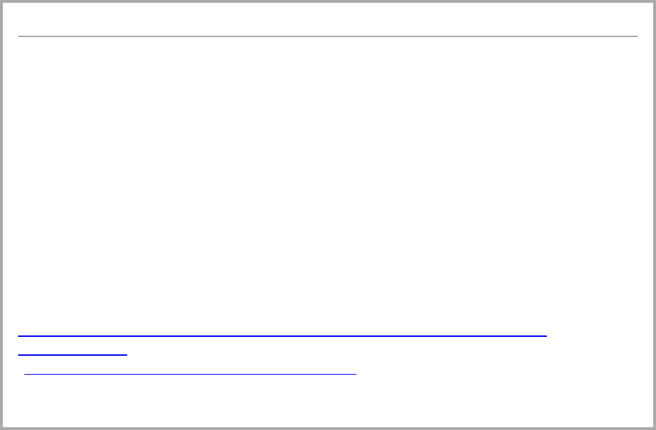
Lookathowthesetwotypesofalgorithmsareplottedonagraph.
You’llseethatO(N)makesaperfectdiagonalline.Thisisbecauseforevery
additionalpieceofdata,thealgorithmtakesoneadditionalstep.Accordingly,the
moredata,themorestepsthealgorithmwilltake.Fortherecord,O(N)isalso
knownaslineartime.
ContrastthiswithO(1),whichisaperfecthorizontalline,sincethenumberof
stepsinthealgorithmremainsconstantnomatterhowmuchdatathereis.
Becauseofthis,O(1)isalsoreferredtoasconstanttime.
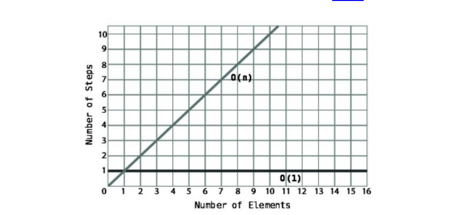
AsBigOisprimarilyconcernedabouthowanalgorithmperformsacross
varyingamountsofdata,animportantpointemerges:analgorithmcanbe
describedasO(1)evenifittakesmorethanonestep.Let’ssaythataparticular
algorithmalwaystakesthreesteps,ratherthanone—butitalwaystakesthese
threestepsnomatterhowmuchdatathereis.Onagraph,suchanalgorithm
wouldlooklikethis:
Becausethenumberofstepsremainsconstantnomatterhowmuchdatathereis,
thiswouldalsobeconsideredconstanttimeandbedescribedbyBigONotation
asO(1).Eventhoughthealgorithmtechnicallytakesthreestepsratherthanone
step,BigONotationconsidersthattrivial.O(1)isthewaytodescribeany
algorithmthatdoesn’tchangeitsnumberofstepsevenwhenthedataincreases.
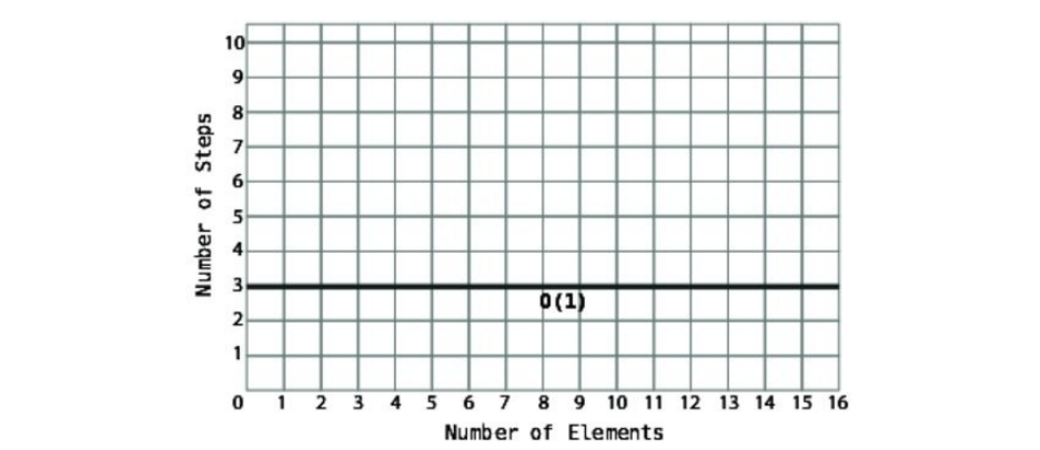
Ifathree-stepalgorithmisconsideredO(1)aslongasitremainsconstant,it
followsthatevenaconstant100-stepalgorithmwouldbeexpressedasO(1)as
well.Whilea100-stepalgorithmislessefficientthanaone-stepalgorithm,the
factthatitisO(1)stillmakesitmoreefficientthananyO(N)algorithm.
Whyisthis?
Seethefollowinggraph:
Asthegraphdepicts,foranarrayoffewerthanonehundredelements,O(N)
algorithmtakesfewerstepsthantheO(1)100-stepalgorithm.Atexactlyone
hundredelements,thetwoalgorithmstakethesamenumberofsteps(100).But
here’sthekeypoint:forallarraysgreaterthanonehundred,theO(N)algorithm
takesmoresteps.
Becausetherewillalwaysbesomeamountofdatainwhichthetidesturn,and
O(N)takesmorestepsfromthatpointuntilinfinity,O(N)isconsideredtobe,on
thewhole,lessefficientthanO(1).
ThesameistrueforanO(1)algorithmthatalwaystakesonemillionsteps.As
thedataincreases,therewillinevitablyreachapointwhereO(N)becomesless
efficientthantheO(1)algorithm,andwillremainsoupuntilaninfiniteamount
ofdata.
SameAlgorithm,DifferentScenarios
Aswelearnedinthepreviouschapters,linearsearchisn’talwaysO(N).It’strue
thatiftheitemwe’relookingforisinthefinalcellofthearray,itwilltakeN
stepstofindit.Butwheretheitemwe’researchingforisfoundinthefirstcellof
thearray,linearsearchwillfindtheiteminjustonestep.Technically,thiswould
bedescribedasO(1).Ifweweretodescribetheefficiencyoflinearsearchinits
totality,we’dsaythatlinearsearchisO(1)inabest-casescenario,andO(N)ina
worst-casescenario.
WhileBigOeffectivelydescribesboththebest-andworst-casescenariosofa
givenalgorithm,BigONotationgenerallyreferstoworst-casescenariounless
specifiedotherwise.Thisiswhymostreferenceswilldescribelinearsearchas
beingO(N)eventhoughitcanbeO(1)inabest-casescenario.
Thereasonforthisisthatthis“pessimistic”approachcanbeausefultool:
knowingexactlyhowinefficientanalgorithmcangetinaworst-casescenario
preparesusfortheworstandmayhaveastrongimpactonourchoices.

AnAlgorithmoftheThirdKind
Inthepreviouschapter,welearnedthatbinarysearchonanorderedarrayis
muchfasterthanlinearsearchonthesamearray.Let’slearnhowtodescribe
binarysearchintermsofBigONotation.
Wecan’tdescribebinarysearchasbeingO(1),becausethenumberofsteps
increasesasthedataincreases.Italsodoesn’tfitintothecategoryofO(N),since
thenumberofstepsismuchfewerthanthenumberofelementsthatitsearches.
Aswe’veseen,binarysearchtakesonlysevenstepsforanarraycontainingone
hundredelements.
BinarysearchseemstofallsomewhereinbetweenO(1)andO(N).
InBigO,wedescribebinarysearchashavingatimecomplexityof:
O(logN)
Ipronouncethisas“OhoflogN.”Thistypeofalgorithmisalsoknownas
havingatimecomplexityoflogtime.
Simplyput,O(logN)istheBigOwayofdescribinganalgorithmthatincreases
onestepeachtimethedataisdoubled.Aswelearnedinthepreviouschapter,
binarysearchdoesjustthat.We’llseemomentarilywhythisisexpressedas
O(logN),butlet’sfirstsummarizewhatwe’velearnedsofar.
Ofthethreetypesofalgorithmswe’velearnedaboutsofar,theycanbesorted
frommostefficienttoleastefficientasfollows:
O(1)
O(logN)
O(N)
Let’slookatagraphthatcomparesthethreetypes.
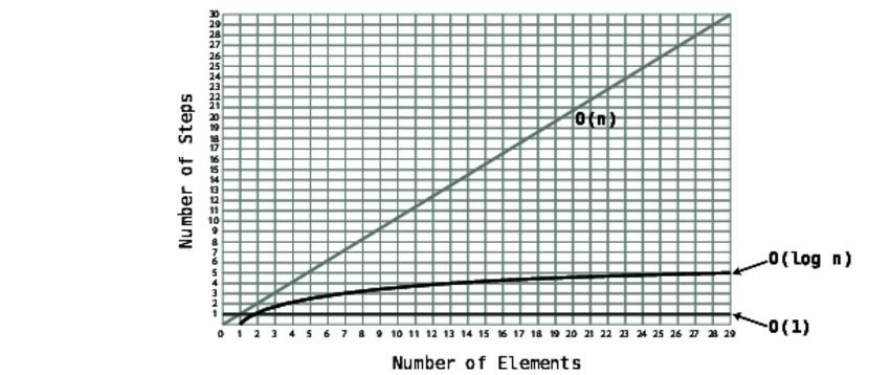
NotehowO(logN)curvesever-so-slightlyupwards,makingitlessefficientthan
O(1),butmuchmoreefficientthanO(N).
Tounderstandwhythisalgorithmiscalled“O(logN),”weneedtofirst
understandwhatlogarithmsare.Ifyou’realreadyfamiliarwiththis
mathematicalconcept,youcanskipthenextsection.
Logarithms
Let’sexaminewhyalgorithmssuchasbinarysearcharedescribedasO(logN).
Whatisalog,anyway?
Logisshorthandforlogarithm.Thefirstthingtonoteisthatlogarithmshave
nothingtodowithalgorithms,eventhoughthetwowordslookandsoundso
similar.
Logarithmsaretheinverseofexponents.Here’saquickrefresheronwhat
exponentsare:
23istheequivalentof:
2*2*2
whichjusthappenstobe8.
Now,log28istheconverseoftheabove.Itmeans:howmanytimesdoyouhave
tomultiply2byitselftogetaresultof8?
Sinceyouhavetomultiply2byitself3timestoget8,log28=3.
Here’sanotherexample:
26translatesto:
2*2*2*2*2*2=64
Since,wehadtomultiply2byitself6timestoget64,
log264=6.
Whiletheprecedingexplanationistheofficial“textbook”definitionof
logarithms,Iliketouseanalternativewayofdescribingthesameconcept
becausemanypeoplefindthattheycanwraptheirheadsarounditmoreeasily,
especiallywhenitcomestoBigONotation.
Anotherwayofexplaininglog28is:ifwekeptdividing8by2untilweendedup
with1,howmany2swouldwehaveinourequation?
8/2/2/2=1
Inotherwords,howmanytimesdoweneedtodivide8by2untilweendup
with1?Inthisexample,ittakesus3times.Therefore,
log28=3.
Similarly,wecouldexplainlog264as:howmanytimesdoweneedtohalve64
untilweendupwith1?
64/2/2/2/2/2/2=1
Sincethereare62s,log264=6.
Nowthatyouunderstandwhatlogarithmsare,themeaningbehindO(logN)will
becomeclear.
O(logN)Explained
Let’sbringthisallbacktoBigONotation.WheneverwesayO(logN),it’s
actuallyshorthandforsayingO(log2N).We’rejustomittingthatsmall2for
convenience.
RecallthatO(N)meansthatforNdataelements,thealgorithmwouldtakeN
steps.Ifthereareeightelements,thealgorithmwouldtakeeightsteps.
O(logN)meansthatforNdataelements,thealgorithmwouldtakelog2Nsteps.
Ifthereareeightelements,thealgorithmwouldtakethreesteps,sincelog28=3.
Saidanotherway,ifwekeepdividingtheeightelementsinhalf,itwouldtakeus
threestepsuntilweendupwithoneelement.
Thisisexactlywhathappenswithbinarysearch.Aswesearchforaparticular
item,wekeepdividingthearray’scellsinhalfuntilwenarrowitdowntothe
correctnumber.
Saidsimply:O(logN)meansthatthealgorithmtakesasmanystepsasittakes
tokeephalvingthedataelementsuntilweremainwithone.
Thefollowingtabledemonstratesastrikingdifferencebetweentheefficiencies
ofO(N)andO(logN):
NElements O(N) O(logN)
8 8 3
16 16 4
32 32 5
64 64 6
128 128 7
256 256 8
512 512 9
1024 1024 10
WhiletheO(N)algorithmtakesasmanystepsastherearedataelements,the
O(logN)algorithmtakesjustoneadditionalstepeverytimethedataelements
aredoubled.
Infuturechapters,wewillencounteralgorithmsthatfallundercategoriesofBig
ONotationotherthanthethreewe’velearnedaboutsofar.Butinthemeantime,
let’sapplytheseconceptstosomeexamplesofeverydaycode.
PracticalExamples
Here’ssometypicalPythoncodethatprintsoutalltheitemsfromalist:
things=['apples','baboons','cribs','dulcimers']
forthinginthings:
print"Here'sathing:%s"%thing
HowwouldwedescribetheefficiencyofthisalgorithminBigONotation?
Thefirstthingtorealizeisthatthisisanexampleofanalgorithm.Whileitmay
notbefancy,anycodethatdoesanythingatallistechnicallyanalgorithm—it’s
aparticularprocessforsolvingaproblem.Inthiscase,theproblemisthatwe
wanttoprintoutalltheitemsfromalist.Thealgorithmweusetosolvethis
problemisaforloopcontainingaprintstatement.
Tobreakthisdown,weneedtoanalyzehowmanystepsthisalgorithmtakes.In
thiscase,themainpartofthealgorithm—theforloop—takesfoursteps.Inthis
example,therearefourthingsinthelist,andweprinteachoneoutonetime.
However,thisprocessisn’tconstant.Ifthelistwouldcontaintenelements,the
forloopwouldtaketensteps.Sincethisforlooptakesasmanystepsasthereare
elements,we’dsaythatthisalgorithmhasanefficiencyofO(N).
Let’stakeanotherexample.Hereisoneofthemostbasiccodesnippetsknown
tomankind:
print'Helloworld!'
Thetimecomplexityoftheprecedingalgorithm(printing“Helloworld!”)is
O(1),becauseitalwaystakesonestep.
ThenextexampleisasimplePython-basedalgorithmfordeterminingwhethera
numberisprime:
defis_prime(number):
foriinrange(2,number):
ifnumber%i==0:
returnFalse
returnTrue
Theprecedingcodeacceptsanumberasanargumentandbeginsaforloopin
whichwedivideeverynumberfrom2uptothatnumberandseeifthere’sa
remainder.Ifthere’snoremainder,weknowthatthenumberisnotprimeandwe
immediatelyreturnFalse.Ifwemakeitallthewayuptothenumberandalways
findaremainder,thenweknowthatthenumberisprimeandwereturnTrue.
TheefficiencyofthisalgorithmisO(N).Inthisexample,thedatadoesnottake
theformofanarray,buttheactualnumberpassedinasanargument.Ifwepass
thenumber7intois_prime,theforlooprunsforaboutsevensteps.(Itreallyruns
forfivesteps,sinceitstartsattwoandendsrightbeforetheactualnumber.)For
thenumber101,thelooprunsforabout101steps.Sincethenumberofsteps
increasesinlockstepwiththenumberpassedintothefunction,thisisaclassic
exampleofO(N).

WrappingUp
NowthatweunderstandBigONotation,wehaveaconsistentsystemthat
allowsustocompareanytwoalgorithms.Withit,wewillbeabletoexamine
real-lifescenariosandchoosebetweencompetingdatastructuresandalgorithms
tomakeourcodefasterandabletohandleheavierloads.
Inthenextchapter,we’llencounterareal-lifeexampleinwhichweuseBigO
Notationtospeedupourcodesignificantly.
Copyright©2017,ThePragmaticBookshelf.

Chapter4
SpeedingUpYourCodewithBigO
BigONotationisagreattoolforcomparingcompetingalgorithms,asitgivesan
objectivewaytomeasurethem.We’vealreadybeenabletouseittoquantifythe
differencebetweenbinarysearchvs.linearsearch,asbinarysearchisO(logN)
—amuchfasteralgorithmthanlinearsearch,whichisO(N).
However,theremaynotalwaysbetwoclearalternativeswhenwritingeveryday
code.Likemostprogrammers,youprobablyusewhateverapproachpopsinto
yourheadfirst.WithBigO,youhavetheopportunitytocompareyouralgorithm
togeneralalgorithmsoutthereintheworld,andyoucansaytoyourself,“Isthis
afastorslowalgorithmasfarasalgorithmsgenerallygo?”
IfyoufindthatBigOlabelsyouralgorithmasa“slow”one,youcannowtakea
stepbackandtrytofigureoutifthere’sawaytooptimizeitbytryingtogetitto
fallunderafastercategoryofBigO.Thismaynotalwaysbepossible,ofcourse,
butit’scertainlyworththinkingaboutbeforeconcludingthatit’snot.
Inthischapter,we’llwritesomecodetosolveapracticalproblem,andthen
measureouralgorithmusingBigO.We’llthenseeifwemightbeabletomodify
thealgorithminordertogiveitaniceefficiencybump.(Spoiler:wewill.)
BubbleSort
Beforejumpingintoourpracticalproblem,though,weneedtofirstlearnabouta
newcategoryofalgorithmicefficiencyintheworldofBigO.Todemonstrateit,
we’llgettouseoneoftheclassicalgorithmsofcomputersciencelore.
Sortingalgorithmshavebeenthesubjectofextensiveresearchincomputer
science,andtensofsuchalgorithmshavebeendevelopedovertheyears.They
allsolvethefollowingproblem:
Givenanarrayofunsortednumbers,howcanwesortthemsothattheyendup
inascendingorder?
Inthisandthefollowingchapters,we’regoingtoencounteranumberofthese
sortingalgorithms.Someofthefirstoneswe’llbelearningaboutareknownas
“simplesorts,”inthattheyareeasiertounderstand,butarenotasefficientas
someofthefastersortingalgorithmsoutthere.
BubbleSortisaverybasicsortingalgorithm,andfollowsthesesteps:
1. Pointtotwoconsecutiveitemsinthearray.(Initially,westartatthevery
beginningofthearrayandpointtoitsfirsttwoitems.)Comparethefirst
itemwiththesecondone:
2. Ifthetwoitemsareoutoforder(inotherwords,theleftvalueisgreater
thantherightvalue),swapthem:
(Iftheyalreadyhappentobeinthecorrectorder,donothingforthisstep.)

3. Movethe“pointers”onecelltotheright:
Repeatsteps1and2untilwereachtheendofthearrayoranyitemsthat
havealreadybeensorted.
4. Repeatsteps1through3untilwehavearoundinwhichwedidn’thaveto
makeanyswaps.Thismeansthatthearrayisinorder.
Eachtimewerepeatsteps1through3isknownasapassthrough.Thatis,
we“passedthrough”theprimarystepsofthealgorithm,andwillrepeatthe
sameprocessuntilthearrayisfullysorted.
BubbleSortinAction
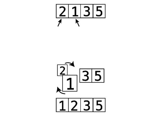
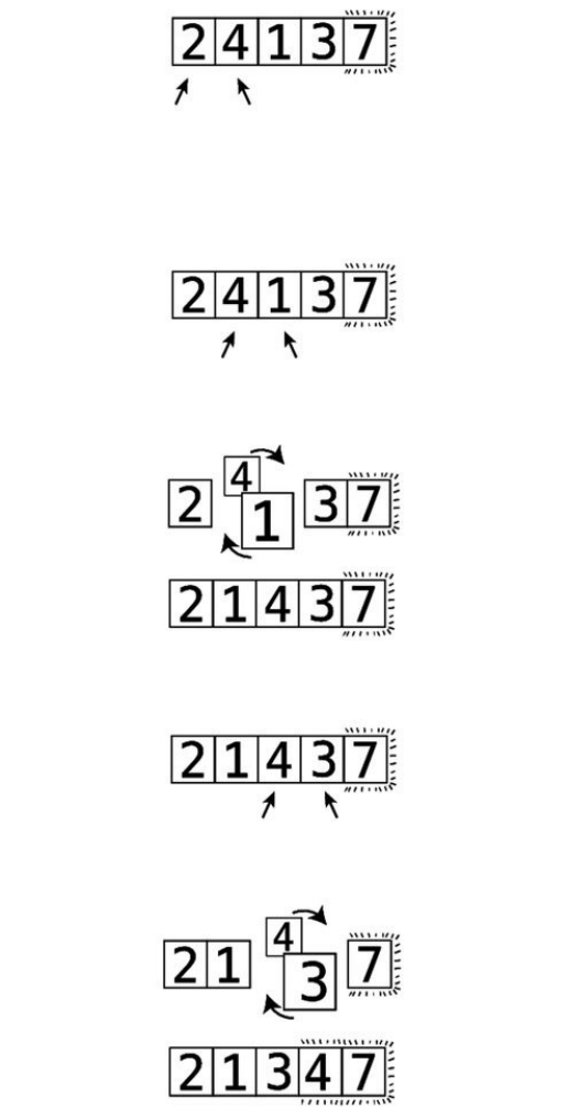
Let’swalkthroughacompleteexample.Assumethatwewantedtosortthearray
[4,2,7,1,3].It’scurrentlyoutoforder,andwewanttoproduceanarray
containingthesamevaluesinthecorrect,ascendingorder.
Let’sbeginPassthrough#1:
Thisisourstartingarray:
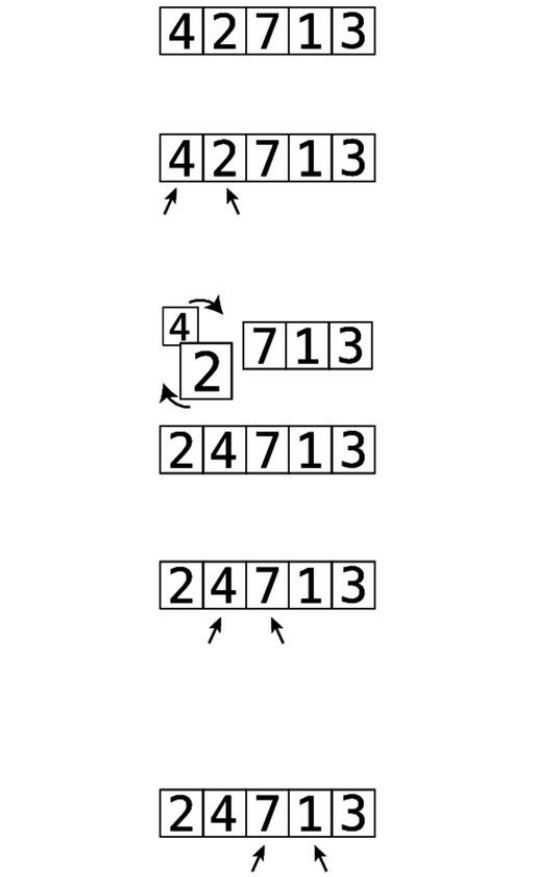
Step#1:First,wecomparethe4andthe2.They’reoutoforder:
Step#2:Soweswapthem:
Step#3:Next,wecomparethe4andthe7:
They’reinthecorrectorder,sowedon’tneedtoperformanyswaps.
Step#4:Wenowcomparethe7andthe1:
Step#5:They’reoutoforder,soweswapthem:
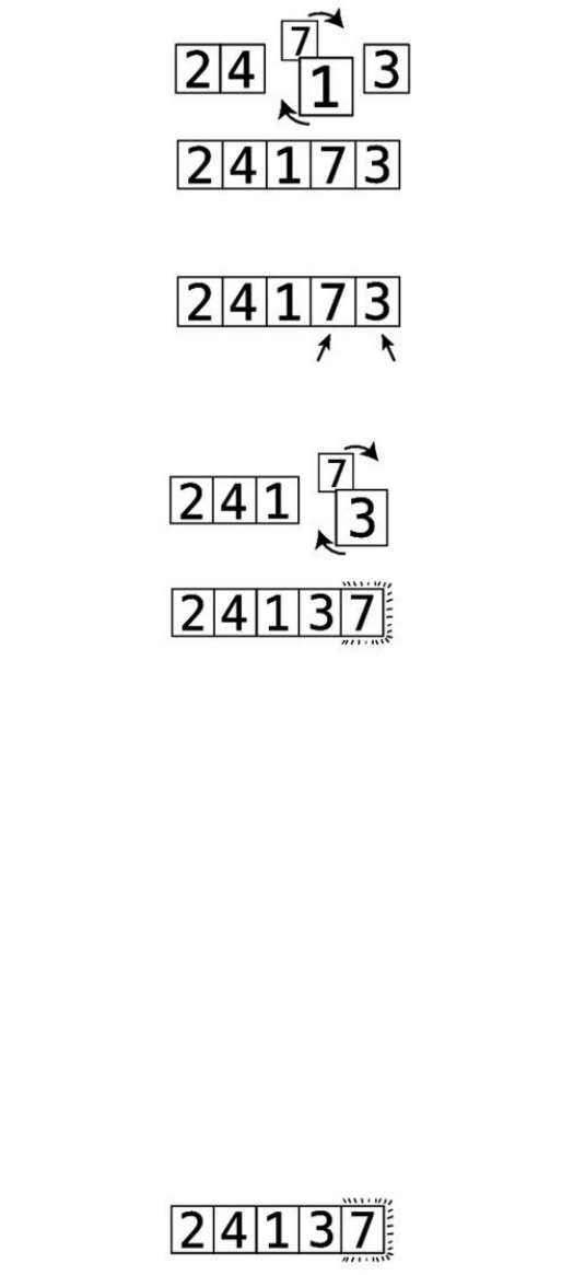
Step#6:Wecomparethe7andthe3:
Step#7:They’reoutoforder,soweswapthem:
Wenowknowforafactthatthe7isinitscorrectpositionwithinthearray,
becausewekeptmovingitalongtotherightuntilitreacheditsproperplace.
We’veputlittlelinessurroundingittoindicatethisfact.
ThisisactuallythereasonthatthisalgorithmiscalledBubbleSort:ineach
passthrough,thehighestunsortedvalue“bubbles”uptoitscorrectposition.
Sincewemadeatleastoneswapduringthispassthrough,weneedtoconduct
anotherone.
WebeginPassthrough#2:
The7isalreadyinthecorrectposition:
Step#8:Webeingbycomparingthe2andthe4:
They’reinthecorrectorder,sowecanmoveon.
Step#9:Wecomparethe4andthe1:
Step#10:They’reoutoforder,soweswapthem:
Step#11:Wecomparethe4andthe3:
Step#12:They’reoutoforder,soweswapthem:
Wedon’thavetocomparethe4andthe7becauseweknowthatthe7isalready
initscorrectpositionfromthepreviouspassthrough.Andnowwealsoknow
thatthe4isbubbleduptoitscorrectpositionaswell.Thisconcludesoursecond
passthrough.Sincewemadeatleastoneswapduringthispassthrough,weneed
toconductanotherone.
WenowbeginPassthrough#3:
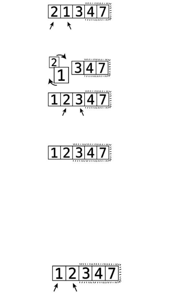
Step#13:Wecomparethe2andthe1:
Step#14:They’reoutoforder,soweswapthem:
Step#15:Wecomparethe2andthe3:
They’reinthecorrectorder,sowedon’tneedtoswapthem.
Wenowknowthatthe3hasbubbleduptoitscorrectspot.Sincewemadeat
leastoneswapduringthispassthrough,weneedtoperformanotherone.
AndsobeginsPassthrough#4:
Step#16:Wecomparethe1andthe2:
Sincethey’reinorder,wedon’tneedtoswap.Wecanendthispassthrough,
sincealltheremainingvaluesarealreadycorrectlysorted.
Nowthatwe’vemadeapassthroughthatdidn’trequireanyswaps,weknowthat
ourarrayiscompletelysorted:

BubbleSortImplemented
Here’sanimplementationofBubbleSortinPython:
defbubble_sort(list):
unsorted_until_index=len(list)-1
sorted=False
whilenotsorted:
sorted=True
foriinrange(unsorted_until_index):
iflist[i]>list[i+1]:
sorted=False
list[i],list[i+1]=list[i+1],list[i]
unsorted_until_index=unsorted_until_index-1
list=[65,55,45,35,25,15,10]
bubble_sort(list)
printlist
Let’sbreakthisdownlinebyline.We’llfirstpresentthelineofcode,followed
byitsexplanation.
unsorted_until_index=len(list)-1
Wekeeptrackofuptowhichindexisstillunsortedwiththeunsorted_until_index
variable.Atthebeginning,thearrayistotallyunsorted,soweinitializethis
variabletobethefinalindexinthearray.
sorted=False
Wealsocreateasortedvariablethatwillallowustokeeptrackwhetherthearray
isfullysorted.Ofcourse,whenourcodefirstruns,itisn’t.
whilenotsorted:
sorted=True
Webeginawhileloopthatwilllastaslongasthearrayisnotsorted.Next,we
preliminarilyestablishsortedtobeTrue.We’llchangethisbacktoFalseassoonas
wehavetomakeanyswaps.Ifwegetthroughanentirepassthroughwithout
havingtomakeanyswaps,we’llknowthatthearrayiscompletelysorted.
foriinrange(unsorted_until_index):
iflist[i]>list[i+1]:
sorted=False
list[i],list[i+1]=list[i+1],list[i]
Withinthewhileloop,webeginaforloopthatstartsfromthebeginningofthe
arrayandgoesuntiltheindexthathasnotyetbeensorted.Withinthisloop,we
compareeverypairofadjacentvalues,andswapthemifthey’reoutoforder.We
alsochangesortedtoFalseifwehavetomakeaswap.
unsorted_until_index=unsorted_until_index-1
Bythislineofcode,we’vecompletedanotherpassthrough,andcansafely
assumethatthevaluewe’vebubbleduptotherightisnowinitscorrectposition.
Becauseofthis,wedecrementtheunsorted_until_indexby1,sincetheindexitwas
alreadypointingtoisnowsorted.
Eachroundofthewhilelooprepresentsanotherpassthrough,andwerunituntil
weknowthatourarrayisfullysorted.

TheEfficiencyofBubbleSort
TheBubbleSortalgorithmcontainstwokindsofsteps:
Comparisons:twonumbersarecomparedwithoneanothertodetermine
whichisgreater.
Swaps:twonumbersareswappedwithoneanotherinordertosortthem.
Let’sstartbydetermininghowmanycomparisonstakeplaceinBubbleSort.
Ourexamplearrayhasfiveelements.Lookingback,youcanseethatinourfirst
passthrough,wehadtomakefourcomparisonsbetweensetsoftwonumbers.
Inoursecondpassthrough,wehadtomakeonlythreecomparisons.Thisis
becausewedidn’thavetocomparethefinaltwonumbers,sinceweknewthat
thefinalnumberwasinthecorrectspotduetothefirstpassthrough.
Inourthirdpassthrough,wemadetwocomparisons,andinourfourth
passthrough,wemadejustonecomparison.
So,that’s:
4+3+2+1=10comparisons.
Toputitmoregenerally,we’dsaythatforNelements,wemake
(N-1)+(N-2)+(N-3)…+1comparisons.
Nowthatwe’veanalyzedthenumberofcomparisonsthattakeplaceinBubble
Sort,let’sanalyzetheswaps.
Inaworst-casescenario,wherethearrayisnotjustrandomlyshuffled,but
sortedindescendingorder(theexactoppositeofwhatwewant),we’dactually
needaswapforeachcomparison.Sowe’dhavetencomparisonsandtenswaps
insuchascenarioforagrandtotaloftwentysteps.
Solet’slookatthecompletepicture.Withanarraycontainingtenelementsin
reverseorder,we’dhave:
9+8+7+6+5+4+3+2+1=45comparisons,andanotherforty-five
swaps.That’satotalofninetysteps.
Withanarraycontainingtwentyelements,we’dhave:
19+18+17+16+15+14+13+12+11+10+9+8+7+6+5+4+3+2
+1=190comparisons,andapproximately190swaps,foratotalof380steps.
Noticetheinefficiencyhere.Asthenumberofelementsincrease,thenumberof
stepsgrowsexponentially.Wecanseethisclearlywiththefollowingtable:
Ndataelements Max#ofsteps
5 20
10 90
20 380
40 1560
80 6320
IfyoulookpreciselyatthegrowthofstepsasNincreases,you’llseethatit’s
growingbyapproximatelyN2.
Ndataelements #ofBubbleSortsteps N2
5 20 25
10 90 100
20 380 400
40 1560 1600
80 6320 6400
Therefore,inBigONotation,wewouldsaythatBubbleSorthasanefficiency
ofO(N2).
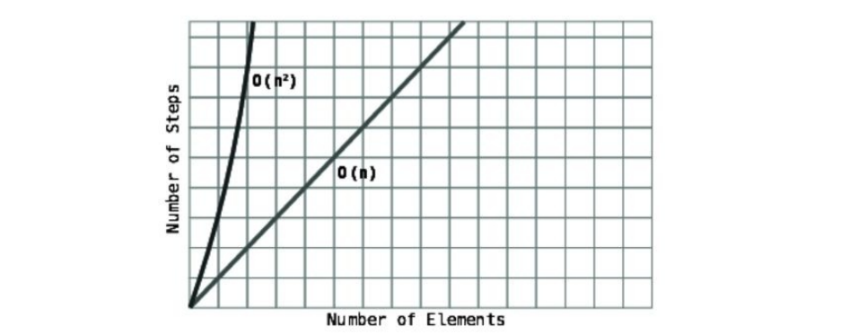
Saidmoreofficially:inanO(N2)algorithm,forNdataelements,thereare
roughlyN2steps.
O(N2)isconsideredtobearelativelyinefficientalgorithm,sinceasthedata
increases,thestepsincreasedramatically.Lookatthisgraph:
NotehowO(N2)curvessharplyupwardsintermsofnumberofstepsasthedata
grows.ComparethiswithO(N),whichplotsalongasimple,diagonalline.
Onelastnote:O(N2)isalsoreferredtoasquadratictime.
AQuadraticProblem
Let’ssayyou’rewritingaJavaScriptapplicationthatrequiresyoutocheck
whetheranarraycontainsanyduplicatevalues.
Oneofthefirstapproachesthatmaycometomindistheuseofnestedforloops,
asfollows:
functionhasDuplicateValue(array){
for(vari=0;i<array.length;i++){
for(varj=0;j<array.length;j++){
if(i!==j&&array[i]==array[j]){
returntrue;
}
}
}
returnfalse;
}
Inthisfunction,weiteratethrougheachelementofthearrayusingvari.Aswe
focusoneachelementini,wethenrunasecondforloopthatchecksthroughall
oftheelementsinthearray—usingvarj—andchecksiftheelementsatpositions
iandjarethesame.Iftheyare,thatmeanswe’veencounteredduplicates.Ifwe
getthroughalloftheloopingandwehaven’tencounteredanyduplicates,wecan
returnfalse,indicatingthattherearenoduplicatesinthegivenarray.
Whilethiscertainlyworks,isitefficient?NowthatweknowabitaboutBigO
Notation,let’stakeastepbackandseewhatBigOwouldsayaboutthis
function.
RememberthatBigOisameasureofhowmanystepsouralgorithmwouldtake
relativetohowmuchdatathereis.Toapplythattooursituation,we’dask
ourselves:forNelementsinthearrayprovidedtoourhasDuplicateValuefunction,
howmanystepswouldouralgorithmtakeinaworst-casescenario?
Toanswertheprecedingquestion,wefirstneedtodeterminewhatqualifiesasa
stepaswellaswhattheworst-casescenariowouldbe.
Theprecedingfunctionhasonetypeofstep,namelycomparisons.Itrepeatedly
comparesiandjtoseeiftheyareequalandthereforerepresentaduplicate.Ina
worst-casescenario,thearraycontainsnoduplicates,whichwouldforceour
codetocompletealloftheloopsandexhausteverypossiblecomparisonbefore
returningfalse.
Basedonthis,wecanconcludethatforNelementsinthearray,ourfunction
wouldperformN2comparisons.Thisisbecauseweperformanouterloopthat
mustiterateNtimestogetthroughtheentirearray,andforeachiteration,we
mustiterateanotherNtimeswithourinnerloop.That’sNsteps*Nsteps,which
isotherwiseknownasN2steps,leavinguswithanalgorithmofO(N2).
Wecanactuallyprovethisbyaddingsomecodetoourfunctionthattracksthe
numberofsteps:
functionhasDuplicateValue(array){
varsteps=0;
for(vari=0;i<array.length;i++){
for(varj=0;j<array.length;j++){
steps++;
if(i!==j&&array[i]==array[j]){
returntrue;
}
}
}
console.log(steps);
returnfalse;
}
IfwerunhasDuplicateValue([1,2,3]),we’llseeanoutputof9intheJavaScript
console,indicatingthattherewereninecomparisons.Sincethereareninesteps
foranarrayofthreeelements,thisisaclassicexampleofO(N2).
Unsurprisingly,O(N2)istheefficiencyofalgorithmsinwhichnestedloopsare
used.Whenyouseeanestedloop,O(N2)alarmbellsshouldstartgoingoffin
yourhead.
WhileourimplementationofthehasDuplicateValuefunctionistheonlyalgorithm
we’vedevelopedsofar,thefactthatit’sO(N2)shouldgiveuspause.Thisis
becauseO(N2)isconsideredarelativelyslowalgorithm.Wheneverencountering
aslowalgorithm,it’sworthspendingsometimetothinkaboutwhetherthere
maybeanyfasteralternatives.Thisisespeciallytrueifyouanticipatethatyour
functionmayneedtohandlelargeamountsofdata,andyourapplicationmay
cometoascreechinghaltifnotoptimizedproperly.Theremaynotbeanybetter
alternatives,butlet’sfirstmakesure.
ALinearSolution
BelowisanotherimplementationofthehasDuplicateValuefunctionthatdoesn’t
relyuponnestedloops.Let’sanalyzeitandseeifit’sanymoreefficientthanour
firstimplementation.
functionhasDuplicateValue(array){
varexistingNumbers=[];
for(vari=0;i<array.length;i++){
if(existingNumbers[array[i]]===undefined){
existingNumbers[array[i]]=1;
}else{
returntrue;
}
}
returnfalse;
}
Thisimplementationusesasingleloop,andkeepstrackofwhichnumbersithas
alreadyencounteredusinganarraycalledexistingNumbers.Itusesthisarrayinan
interestingway:everytimethecodeencountersanewnumber,itstoresthevalue
1insidetheindexoftheexistingNumberscorrespondingtothatnumber.
Forexample,ifthegivenarrayis[3,5,8],bythetimetheloopisfinished,the
existingNumbersarraywilllooklikethis:
[undefined,undefined,undefined,1,undefined,1,undefined,undefined,1]
The1sarelocatedinindexes3,5,and8toindicatethatthosenumbersarefound
inthegivenarray.
However,beforethecodestores1intheappropriateindex,itfirstcheckstosee
whetherthatindexalreadyhas1asitsvalue.Ifitdoes,thatmeanswealready
encounteredthatnumberbefore,meaningthatwe’vefoundaduplicate.
TodeterminetheefficiencyofthisnewalgorithmintermsofBigO,weonce
againneedtodeterminethenumberofstepsthealgorithmtakesinaworst-case
scenario.Likeourfirstimplementation,thesignificanttypeofstepthatour
algorithmhasiscomparisons.Thatis,itlooksupaparticularindexofthe
existingNumbersarrayandcomparesittoundefined,asexpressedinthiscode:
if(existingNumbers[array[i]]===undefined)
(Inadditiontothecomparisons,wedoalsomakeinsertionsintothe
existingNumbersarray,butwe’reconsideringthattrivialinthisanalysis.Moreon
thisinthenextchapter.)
Onceagain,theworst-casescenarioiswhenthearraycontainsnoduplicates,in
whichcaseourfunctionmustcompletetheentireloop.
ThisnewalgorithmappearstomakeNcomparisonsforNdataelements.Thisis
becausethere’sonlyoneloop,anditsimplyiteratesforasmanyelementsas
thereareinthearray.Wecantestoutthistheorybytrackingthestepsinthe
JavaScriptconsole:
functionhasDuplicateValue(array){
varsteps=0;
varexistingNumbers=[];
for(vari=0;i<array.length;i++){
steps++;
if(existingNumbers[array[i]]===undefined){
existingNumbers[array[i]]=1;
}else{
returntrue;
}
}
console.log(steps);
returnfalse;
}
WhenrunninghasDuplicateValue([1,2,3]),weseethattheoutputintheJavaScript
consoleis3,whichisthesamenumberofelementsinourarray.
UsingBigONotation,we’dconcludethatthisnewimplementationisO(N).
WeknowthatO(N)ismuchfasterthanO(N2),sobyusingthissecondapproach,
we’veoptimizedourhasDuplicateValuesignificantly.Ifourprogramwillhandle
lotsofdata,thiswillmakeabigdifference.(Thereisactuallyonedisadvantage
withthisnewimplementation,butwewon’tdiscussituntilthefinalchapter.)

WrappingUp
It’sclearthathavingasolidunderstandingofBigONotationcanallowusto
identifyslowcodeandselectthefasteroftwocompetingalgorithms.However,
therearesituationsinwhichBigONotationwillhaveusbelievethattwo
algorithmshavethesamespeed,whileoneisactuallyfaster.Inthenextchapter,
we’regoingtolearnhowtoevaluatetheefficienciesofvariousalgorithmseven
whenBigOisn’tnuancedenoughtodoso.
Copyright©2017,ThePragmaticBookshelf.

Chapter5
OptimizingCodewithandWithout
BigO
We’veseenthatBigOisagreattoolforcontrastingalgorithmsanddetermining
whichalgorithmshouldbeusedforagivensituation.However,it’scertainlynot
theonlytool.Infact,therearetimeswheretwocompetingalgorithmsmaybe
describedinexactlythesamewayusingBigONotation,yetonealgorithmis
significantlyfasterthantheother.
Inthischapter,we’regoingtolearnhowtodiscernbetweentwoalgorithmsthat
seemtohavethesameefficiency,andselectthefasterofthetwo.
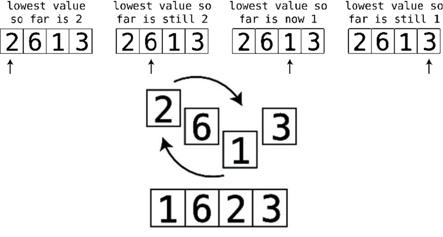
SelectionSort
Inthepreviouschapter,weexploredanalgorithmforsortingdataknownas
BubbleSort,whichhadanefficiencyofO(N2).We’renowgoingtodiginto
anothersortingalgorithmcalledSelectionSort,andseehowitmeasuresupto
BubbleSort.
ThestepsofSelectionSortareasfollows:
1. Wecheckeachcellofthearrayfromlefttorighttodeterminewhichvalue
isleast.Aswemovefromcelltocell,wekeepinavariablethelowest
valuewe’veencounteredsofar.(Really,wekeeptrackofitsindex,butfor
thepurposesofthefollowingdiagrams,we’lljustfocusontheactual
value.)Ifweencounteracellthatcontainsavaluethatisevenlessthanthe
oneinourvariable,wereplaceitsothatthevariablenowpointstothenew
index.Seethefollowingdiagram:
2. Oncewe’vedeterminedwhichindexcontainsthelowestvalue,weswap
thatindexwiththevaluewebeganthepassthroughwith.Thiswouldbe
index0inthefirstpassthrough,index1inthesecondpassthrough,andso
onandsoforth.Inthenextdiagram,wemaketheswapofthefirst
passthrough:
3. Repeatsteps1and2untilallthedataissorted.

SelectionSortinAction
Usingtheexamplearray[4,2,7,1,3],ourstepswouldbeasfollows:
Webeginourfirstpassthrough:
Wesetthingsupbyinspectingthevalueatindex0.Bydefinition,it’sthelowest
valueinthearraythatwe’veencounteredsofar(asit’stheonlyvaluewe’ve
encounteredsofar),sowekeeptrackofitsindexinavariable:
Step#1:Wecomparethe2withthelowestvaluesofar(whichhappenstobe4):
The2isevenlessthanthe4,soitbecomesthelowestvaluesofar:
Step#2:Wecomparethenextvalue—the7—withthelowestvaluesofar.The7
isgreaterthanthe2,so2remainsourlowestvalue:
Step#3:Wecomparethe1withthelowestvaluesofar:
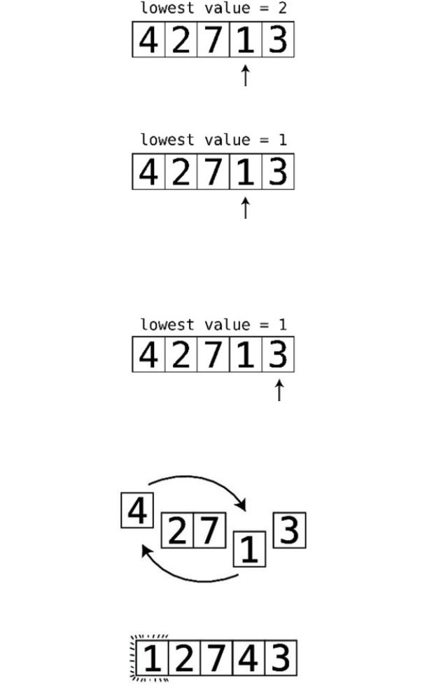
Sincethe1isevenlessthanthe2,the1becomesournewlowestvalue:
Step#4:Wecomparethe3tothelowestvaluesofar,whichisthe1.We’ve
reachedtheendofthearray,andwe’vedeterminedthat1isthelowestvalueout
oftheentirearray:
Step#5:Since1isthelowestvalue,weswapitwithwhatevervalueisatindex0
—theindexwebeganthispassthroughwith:
Wehavenowdeterminedthatthe1isinitscorrectplacewithinthearray:
Wearenowreadytobeginoursecondpassthrough:
Setup:thefirstcell—index0—isalreadysorted,sothispassthroughbeginsat
thenextcell,whichisindex1.Thevalueatindex1isthenumber2,anditisthe
lowestvaluewe’veencounteredinthispassthroughsofar:
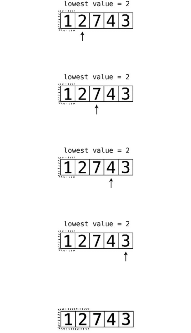
Step#6:Wecomparethe7withthelowestvaluesofar.The2islessthanthe7,
sothe2remainsourlowestvalue:
Step#7:Wecomparethe4withthelowestvaluesofar.The2islessthanthe4,
sothe2remainsourlowestvalue:
Step#8:Wecomparethe3withthelowestvaluesofar.The2islessthanthe3,
sothe2remainsourlowestvalue:
We’vereachedtheendofthearray.Wedon’tneedtoperformanyswapsinthis
passthrough,andwecanthereforeconcludethatthe2isinitscorrectspot.This
endsoursecondpassthrough,leavinguswith:
WenowbeginPassthrough#3:
Setup:webeginatindex2,whichcontainsthevalue7.The7isthelowestvalue
we’veencounteredsofarinthispassthrough:
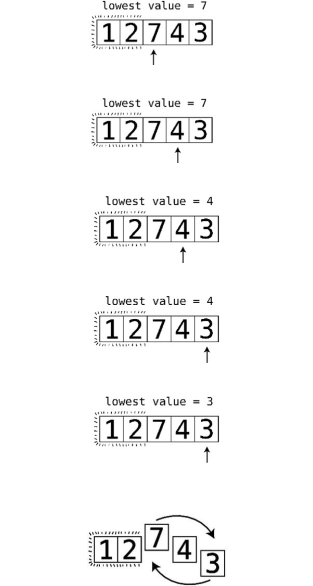
Step#9:Wecomparethe4withthe7:
Wenotethat4isournewlowestvalue:
Step#10:Weencounterthe3,whichisevenlowerthanthe4:
3isnowournewlowestvalue:
Step#11:We’vereachedtheendofthearray,soweswapthe3withthevalue
thatwestartedourpassthroughat,whichisthe7:
Wenowknowthatthe3isinthecorrectplacewithinthearray:
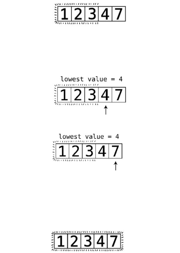
WhileyouandIcanbothseethattheentirearrayiscorrectlysortedatthispoint,
thecomputerdoesnotknowthisyet,soitmustbeginafourthpassthrough:
Setup:webeginthepassthroughwithindex3.The4isthelowestvaluesofar:
Step#12:Wecomparethe7withthe4:
The4remainsthelowestvaluewe’veencounteredinthispassthroughsofar,so
wedon’tneedanyswapsandweknowit’sinthecorrectplace.
Sinceallthecellsbesidesthelastonearecorrectlysorted,thatmustmeanthat
thelastcellisalsointhecorrectorder,andourentirearrayisproperlysorted:
SelectionSortImplemented
Here’saJavaScriptimplementationofSelectionSort:
functionselectionSort(array){
for(vari=0;i<array.length;i++){
varlowestNumberIndex=i;
for(varj=i+1;j<array.length;j++){
if(array[j]<array[lowestNumberIndex]){
lowestNumberIndex=j;
}
}
if(lowestNumberIndex!=i){
vartemp=array[i];
array[i]=array[lowestNumberIndex];
array[lowestNumberIndex]=temp;
}
}
returnarray;
}
Let’sbreakthisdown.We’llfirstpresentthelineofcode,followedbyits
explanation.
for(vari=0;i<array.length;i++){
Here,wehaveanouterloopthatrepresentseachpassthroughofSelectionSort.
Wethenbeginkeepingtrackoftheindexcontainingthelowestvaluewe
encountersofarwith:
varlowestNumberIndex=i;
whichsetslowestNumberIndextobewhateverindexirepresents.Notethatwe’re
actuallytrackingtheindexofthelowestnumberinsteadoftheactualnumber
itself.Thisindexwillbe0atthebeginningofthefirstpassthrough,1atthe
beginningofthesecond,andsoon.
for(varj=i+1;j<array.length;j++){
kicksoffaninnerforloopthatstartsati+1.
if(array[j]<array[lowestNumberIndex]){
lowestNumberIndex=j;
}
checkseachelementofthearraythathasnotyetbeensortedandlooksforthe
lowestnumber.Itdoesthisbykeepingtrackoftheindexofthelowestnumberit
foundsofarinthelowestNumberIndexvariable.
Bytheendoftheinnerloop,we’vedeterminedtheindexofthelowestnumber
notyetsorted.
if(lowestNumberIndex!=i){
vartemp=array[i];
array[i]=array[lowestNumberIndex];
array[lowestNumberIndex]=temp;
}
Wethenchecktoseeifthislowestnumberisalreadyinitscorrectplace(i).If
not,weswapthelowestnumberwiththenumberthat’sinthepositionthatthe
lowestnumbershouldbeat.
TheEfficiencyofSelectionSort
SelectionSortcontainstwotypesofsteps:comparisonsandswaps.Thatis,we
compareeachelementwiththelowestnumberwe’veencounteredineach
passthrough,andweswapthelowestnumberintoitscorrectposition.
Lookingbackatourexampleofanarraycontainingfiveelements,wehadto
makeatotaloftencomparisons.Let’sbreakitdown.
Passthrough# #ofcomparisons
1 4comparisons
2 3comparisons
3 2comparisons
4 1comparison
Sothat’sagrandtotalof4+3+2+1=10comparisons.
Toputitmoregenerally,we’dsaythatforNelements,wemake
(N-1)+(N-2)+(N-3)…+1comparisons.
Asforswaps,however,weonlyneedtomakeamaximumofoneswapper
passthrough.Thisisbecauseineachpassthrough,wemakeeitheroneorzero
swaps,dependingonwhetherthelowestnumberofthatpassthroughisalready
inthecorrectposition.ContrastthiswithBubbleSort,whereinaworst-case
scenario—anarrayindescendingorder—wehavetomakeaswapforeachand
everycomparison.
Here’stheside-by-sidecomparisonbetweenBubbleSortandSelectionSort:
N
elements
Max#ofstepsinBubble
Sort
Max#ofstepsinSelectionSort
5 20 14(10comparisons+4swaps)
10 90 54(45comparisons+9swaps)
20 380 199(180comparisons+19
swaps)
40 1560 819(780comparisons+39
swaps)
80 6320 3239(3160comparisons+79
swaps)
Fromthiscomparison,it’sclearthatSelectionSortcontainsabouthalfthe
numberofstepsthatBubbleSortdoes,indicatingthatSelectionSortistwiceas
fast.
IgnoringConstants
Buthere’sthefunnything:intheworldofBigONotation,SelectionSortand
BubbleSortaredescribedinexactlythesameway.
Again,BigONotationdescribeshowmanystepsarerequiredrelativetothe
numberofdataelements.Soitwouldseematfirstglancethatthenumberof
stepsinSelectionSortareroughlyhalfofwhateverN2is.Itwouldtherefore
seemreasonablethatwe’ddescribetheefficiencyofSelectionSortasbeing
O(N2/2).Thatis,forNdataelements,thereareN2/2steps.Thefollowing
tablebearsthisout:
Nelements N2/2 Max#ofstepsinSelectionSort
552/2=12.5 14
10 102/2=50 54
20 202/2=200 199
40 402/2=800 819
80 802/2=3200 3239
Inreality,however,SelectionSortisdescribedinBigOasO(N2),justlike
BubbleSort.ThisisbecauseofamajorruleofBigOthatwe’renowintroducing
forthefirsttime:
BigONotationignoresconstants.
ThisissimplyamathematicalwayofsayingthatBigONotationneverincludes
regularnumbersthataren’tanexponent.
Inourcase,whatshouldtechnicallybeO(N2/2)becomessimplyO(N2).
Similarly,O(2N)wouldbecomeO(N),andO(N/2)wouldalsobecomeO(N).
EvenO(100N),whichis100timesslowerthanO(N),wouldalsobereferredto
asO(N).
Offhand,itwouldseemthatthisrulewouldrenderBigONotationentirely
useless,asyoucanhavetwoalgorithmsthataredescribedinthesameexactway
withBigO,andyetonecanbe100timesfasterthantheother.Andthat’sexactly
whatwe’reseeingherewithSelectionSortandBubbleSort.Botharedescribed
inBigOasO(N2),butSelectionSortisactuallytwiceasfastasBubbleSort.
Andindeed,ifgiventhechoicebetweenthesetwooptions,SelectionSortisthe
betterchoice.
So,whatgives?
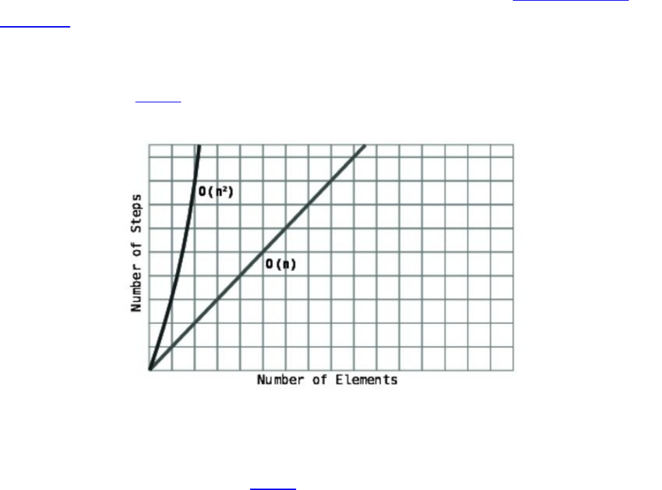
TheRoleofBigO
DespitethefactthatBigOdoesn’tdistinguishbetweenBubbleSortand
SelectionSort,itisstillveryimportant,becauseitservesasagreatwayto
classifythelong-termgrowthrateofalgorithms.Thatis,forsomeamountof
data,O(N)willbealwaysbefasterthanO(N2).Andthisistruenomatter
whethertheO(N)isreallyO(2N)orevenO(100N)underthehood.Itisafact
thatthereissomeamountofdataatwhichevenO(100N)willbecomefasterthan
O(N2).(We’veseenessentiallythesameconceptinChapter3,OhYes!BigO
Notationwhencomparinga100-stepalgorithmwithO(N),butwe’llreiterateit
hereinourcurrentcontext.)
Lookatthefirstgraph,inwhichwecompareO(N)withO(N2).
We’veseenthisgraphinthepreviouschapter.ItdepictshowO(N)isfasterthan
O(N2)forallamountsofdata.
Nowtakealookatthesecondgraph,wherewecompareO(100N)withO(N2).
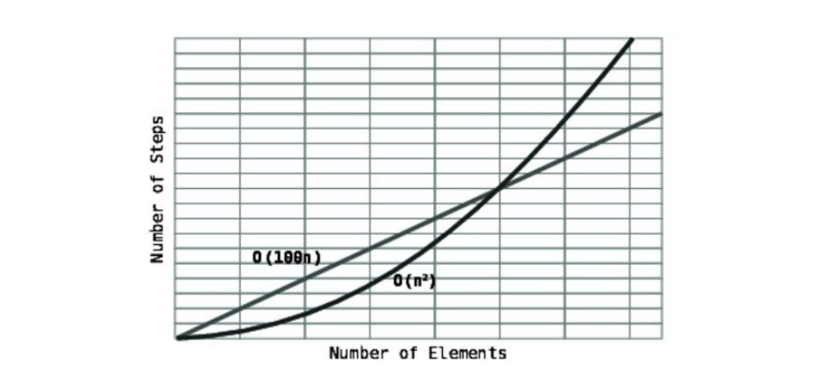
Inthissecondgraph,weseethatO(N2)isfasterthanO(100N)forcertain
amountsofdata,butafterapoint,evenO(100N)becomesfasterandremains
fasterforallincreasingamountsofdatafromthatpointonward.
ItisforthisveryreasonthatBigOignoresconstants.ThepurposeofBigOis
thatfordifferentclassifications,therewillbeapointatwhichoneclassification
supersedestheotherinspeed,andwillremainfasterforever.Whenthatpoint
occursexactly,however,isnottheconcernofBigO.
Becauseofthis,therereallyisnosuchthingasO(100N)—itissimplywrittenas
O(N).
Similarly,withlargeamountsofdata,O(logN)willalwaysbefasterthanO(N),
evenifthegivenO(logN)algorithmisactuallyO(2*logN)underthehood.
SoBigOisanextremelyusefultool,becauseiftwoalgorithmsfallunder
differentclassificationsofBigO,you’llgenerallyknowwhichalgorithmtouse
sincewithlargeamountsofdata,onealgorithmisguaranteedtobefasterthan
theotheratacertainpoint.
However,themaintakeawayofthischapteristhatwhentwoalgorithmsfall
underthesameclassificationofBigO,itdoesn’tnecessarilymeanthatboth
algorithmsprocessatthesamespeed.Afterall,BubbleSortistwiceasslowas
SelectionSorteventhoughbothareO(N2).SowhileBigOisperfectfor
contrastingalgorithmsthatfallunderdifferentclassificationsofBigO,when
twoalgorithmsfallunderthesameclassification,furtheranalysisisrequiredto
determinewhichalgorithmisfaster.
APracticalExample
Let’ssayyou’retaskedwithwritingaRubyapplicationthattakesanarrayand
createsanewarrayoutofeveryotherelementfromtheoriginalarray.Itmight
betemptingtousetheeach_with_indexmethodavailabletoarraystoloopthrough
theoriginalarrayasfollows:
defevery_other(array)
new_array=[]
array.each_with_indexdo|element,index|
new_array<<elementifindex.even?
end
returnnew_array
end
Inthisimplementation,weiteratethrougheachelementoftheoriginalarrayand
onlyaddtheelementtothenewarrayiftheindexofthatelementisaneven
number.
Whenanalyzingthestepstakingplacehere,wecanseethattherearereallytwo
typesofsteps.Wehaveonetypeofstepinwhichwelookupeachelementofthe
array,andanothertypeofstepinwhichweaddelementstothenewarray.
WeperformNarraylookups,sinceweloopthrougheachandeveryelementof
thearray.WeonlyperformN/2insertions,though,sinceweonlyinsertevery
otherelementintothenewarray.SincewehaveNlookups,andwehaveN/2
insertions,wewouldsaythatouralgorithmtechnicallyhasanefficiencyofO(N
+(N/2)),whichwecanalsorephraseasO(1.5N).ButsinceBigONotation
throwsouttheconstants,wewouldsaythatouralgorithmissimplyO(N).
Whilethisalgorithmdoeswork,wealwayswanttotakeastepbackandseeif
there’sroomforanyoptimization.Andinfact,wecan.
Insteadofiteratingthrougheachelementofthearrayandcheckingwhetherthe
indexisanevennumber,wecaninsteadsimplylookupeveryotherelementof
thearrayinthefirstplace:
defevery_other(array)
new_array=[]
index=0
whileindex<array.length
new_array<<array[index]
index+=2
end
returnnew_array
end
Inthissecondimplementation,weuseawhilelooptoskipovereachelement,
ratherthancheckeachone.ItturnsoutthatforNelements,thereareN/2
lookupsandN/2insertionsintothenewarray.Likethefirstimplementation,
we’dsaythatthealgorithmisO(N).
However,ourfirstimplementationtrulytakes1.5Nsteps,whileoursecond
implementationonlytakesNsteps,makingoursecondimplementation
significantlyfaster.Whilethefirstimplementationismoreidiomaticintheway
Rubyprogrammerswritetheircode,ifwe’redealingwithlargeamountsofdata,
it’sworthconsideringusingthesecondimplementationtogetasignificant
performanceboost.

WrappingUp
Wenowhavesomeverypowerfulanalysistoolsatourdisposal.WecanuseBig
Otodeterminebroadlyhowefficientanalgorithmis,andwecanalsocompare
twoalgorithmsthatfallwithinoneclassificationofBigO.
However,thereisanotherimportantfactortotakeintoaccountwhencomparing
theefficienciesoftwoalgorithms.Untilnow,we’vefocusedonhowslowan
algorithmisinaworst-casescenario.Now,worst-casescenarios,bydefinition,
don’thappenallthetime.Onaverage,thescenariosthatoccurare—well—
average-casescenarios.Inthenextchapter,we’lllearnhowtotakeallscenarios
intoaccount.
Copyright©2017,ThePragmaticBookshelf.

Chapter6
OptimizingforOptimisticScenarios
Whenevaluatingtheefficiencyofanalgorithm,we’vefocusedprimarilyonhow
manystepsthealgorithmwouldtakeinaworst-casescenario.Therationale
behindthisissimple:ifyou’repreparedfortheworst,thingswillturnoutokay.
However,we’lldiscoverinthischapterthattheworst-casescenarioisn’tthe
onlysituationworthconsidering.Beingabletoconsiderallscenariosisan
importantskillthatcanhelpyouchoosetheappropriatealgorithmforevery
situation.
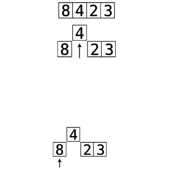
InsertionSort
We’vepreviouslyencounteredtwodifferentsortingalgorithms:BubbleSortand
SelectionSort.BothhaveefficienciesofO(N2),butSelectionSortisactually
twiceasfast.Nowwe’lllearnaboutathirdsortingalgorithmcalledInsertion
Sortthatwillrevealthepowerofanalyzingscenariosbeyondtheworstcase.
InsertionSortconsistsofthefollowingsteps:
1. Inthefirstpassthrough,wetemporarilyremovethevalueatindex1(the
secondcell)andstoreitinatemporaryvariable.Thiswillleaveagapat
thatindex,sinceitcontainsnovalue:
Insubsequentpassthroughs,weremovethevaluesatthesubsequent
indexes.
2. Wethenbeginashiftingphase,wherewetakeeachvaluetotheleftofthe
gap,andcompareittothevalueinthetemporaryvariable:
Ifthevaluetotheleftofthegapisgreaterthanthetemporaryvariable,we
shiftthatvaluetotheright:
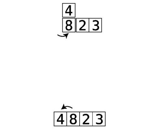
Asweshiftvaluestotheright,inherently,thegapmovesleftwards.Assoon
asweencounteravaluethatislowerthanthetemporarilyremovedvalue,
orwereachtheleftendofthearray,thisshiftingphaseisover.
3. Wetheninsertthetemporarilyremovedvalueintothecurrentgap:
4. Werepeatsteps1through3untilthearrayisfullysorted.
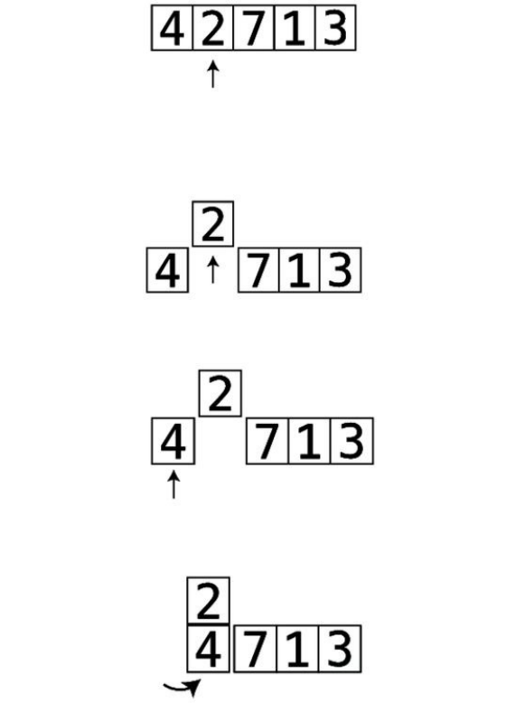
InsertionSortinAction
Let’sapplyInsertionSorttothearray:[4,2,7,1,3].
Webeginthefirstpassthroughbyinspectingthevalueatindex1.Thishappens
tocontainthevalue2:
Setup:wetemporarilyremovethe2,andkeepitinsideavariablecalled
temp_value.Werepresentthisvaluebyshiftingitabovetherestofthearray:
Step#1:Wecomparethe4tothetemp_value,whichis2:
Step#2:Since4isgreaterthan2,weshiftthe4totheright:
There’snothinglefttoshift,asthegapisnowattheleftendofthearray.
Step#3:Weinsertthetemp_valuebackintothearray,completingourfirst
passthrough:
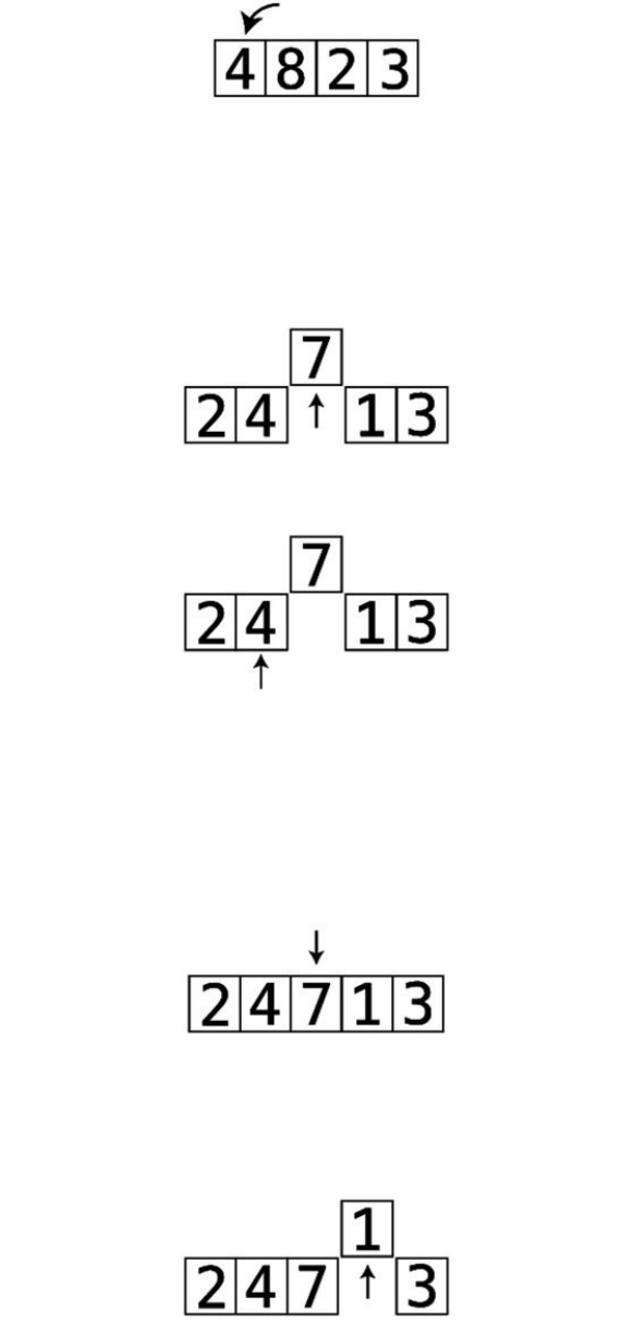
WebeginPassthrough#2:
Setup:inoursecondpassthrough,wetemporarilyremovethevalueatindex2.
We’llstorethisintemp_value.Inthiscase,thetemp_valueis7:
Step#4:Wecomparethe4tothetemp_value:
4islower,sowewon’tshiftit.Sincewereachedavaluethatislessthanthe
temp_value,thisshiftingphaseisover.
Step#5:Weinsertthetemp_valuebackintothegap,endingthesecond
passthrough:
Passthrough#3:
Setup:wetemporarilyremovethe1,andstoreitintemp_value:
Step#6:Wecomparethe7tothetemp_value:
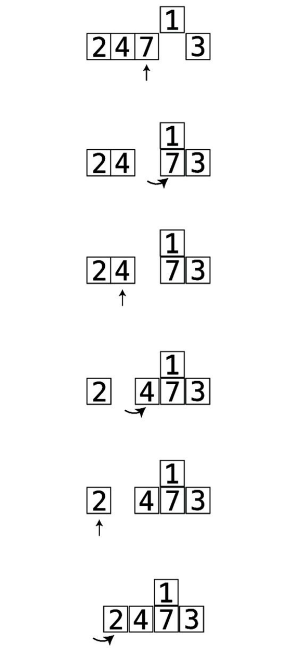
Step#7:7isgreaterthan1,soweshiftthe7totheright:
Step#8:Wecomparethe4tothetemp_value:
Step#9:4isgreaterthan1,soweshiftitaswell:
Step#10:Wecomparethe2tothetemp_value:
Step#11:The2isgreater,soweshiftit:
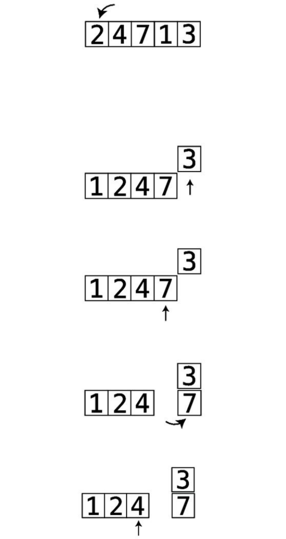
Step#12:Thegaphasreachedtheleftendofthearray,soweinsertthe
temp_valueintothegap,concludingthispassthrough:
Passthrough#4:
Setup:wetemporarilyremovethevaluefromindex4,makingitourtemp_value.
Thisisthevalue3:
Step#13:Wecomparethe7tothetemp_value:
Step#14:The7isgreater,soweshiftthe7totheright:
Step#15:Wecomparethe4tothetemp_value:
Step#16:The4isgreaterthanthe3,soweshiftthe4:
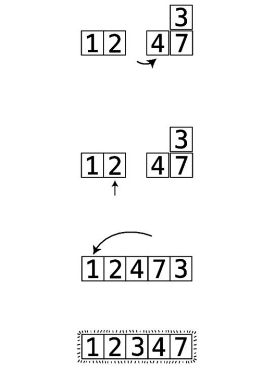
Step#17:Wecomparethe2tothetemp_value.2islessthan3,soourshifting
phaseiscomplete:
Step#18:Weinsertthetemp_valuebackintothegap:
Ourarrayisnowfullysorted:
InsertionSortImplemented
HereisaPythonimplementationofInsertionSort:
definsertion_sort(array):
forindexinrange(1,len(array)):
position=index
temp_value=array[index]
whileposition>0andarray[position-1]>temp_value:
array[position]=array[position-1]
position=position-1
array[position]=temp_value
Let’swalkthroughthisstepbystep.We’llfirstpresentthelineofcode,followed
byitsexplanation.
forindexinrange(1,len(array)):
First,westartaloopbeginningatindex1thatrunsthroughtheentirearray.The
currentindexiskeptinthevariableindex.
position=index
temp_value=array[index]
Next,wemarkapositionatwhateverindexcurrentlyis.Wealsoassignthevalue
atthatindextothevariabletemp_value.
whileposition>0andarray[position-1]>temp_value:
array[position]=array[position-1]
position=position-1
Wethenbeginaninnerwhileloop.Wecheckwhetherthevaluetotheleftof
positionisgreaterthanthetemp_value.Ifitis,wethenusearray[position]=
array[position-1]toshiftthatleftvalueonecelltotheright,andthendecrement
positionbyone.Wethencheckwhetherthevaluetotheleftofthenewpositionis
greaterthantemp_value,andkeeprepeatingthisprocessuntilwefindavaluethat
islessthanthetemp_value.
array[position]=temp_value
Finally,wedropthetemp_valueintothegapwithinthearray.
TheEfficiencyofInsertionSort
TherearefourtypesofstepsthatoccurinInsertionSort:removals,comparisons,
shifts,andinsertions.ToanalyzetheefficiencyofInsertionSort,weneedtotally
upeachofthesesteps.
First,let’sdigintocomparisons.Acomparisontakesplaceeachtimewe
compareavaluetotheleftofthegapwiththetemp_value.
Inaworst-casescenario,wherethearrayissortedinreverseorder,wehaveto
compareeverynumbertotheleftoftemp_valuewithtemp_valueineach
passthrough.Thisisbecauseeachvaluetotheleftoftemp_valuewillalwaysbe
greaterthantemp_value,sothepassthroughwillonlyendwhenthegapreaches
theleftendofthearray.
Duringthefirstpassthrough,inwhichtemp_valueisthevalueatindex1,a
maximumofonecomparisonismade,sincethereisonlyonevaluetotheleftof
thetemp_value.Onthesecondpassthrough,amaximumoftwocomparisonsare
made,andsoonandsoforth.Onthefinalpassthrough,weneedtocomparethe
temp_valuewitheverysinglevalueinthearraybesidestemp_valueitself.Inother
words,ifthereareNelementsinthearray,amaximumofN-1comparisonsare
madeinthefinalpassthrough.
Wecan,therefore,formulatethetotalnumberofcomparisonsas:
1+2+3+…+N-1comparisons.
Inourexampleofanarraycontainingfiveelements,that’samaximumof:
1+2+3+4=10comparisons.
Foranarraycontainingtenelements,therewouldbe:
1+2+3+4+5+6+7+8+9=45comparisons.
(Foranarraycontainingtwentyelements,therewouldbeatotalof190
comparisons,andsoon.)
Whenexaminingthispattern,itemergesthatforanarraycontainingNelements,
thereareapproximatelyN2/2comparisons.(102/2is50,and202/2is200.)
Let’scontinueanalyzingtheothertypesofsteps.
Shiftsoccureachtimewemoveavalueonecelltotheright.Whenanarrayis
sortedinreverseorder,therewillbeasmanyshiftsastherearecomparisons,
sinceeverycomparisonwillforceustoshiftavaluetotheright.
Let’saddupcomparisonsandshiftsforaworst-casescenario:
N2/2comparisons
+N2/2shifts
_____________________________
N2steps
Removingandinsertingthetemp_valuefromthearrayhappenonceper
passthrough.SincetherearealwaysN-1passthroughs,wecanconcludethat
thereareN-1removalsandN-1insertions.
Sonowwe’vegot:
N2comparisons&shiftscombined
N-1removals
+N-1insertions
_____________________________
N2+2N-2steps
We’vealreadylearnedonemajorruleofBigO—thatBigOignoresconstants.
Withthisruleinmind,we’d—atfirstglance—simplifythistoO(N2+N).
However,thereisanothermajorruleofBigOthatwe’llrevealnow:
BigONotationonlytakesintoaccountthehighestorderofN.
Thatis,ifwehavesomealgorithmthattakesN4+N3+N2+Nsteps,weonly
considerN4tobesignificant—andjustcallitO(N4).Whyisthis?
Lookatthefollowingtable:
NN2N3N4
2 4 8 16
5 25 125 625
10 100 1,000 10,000
100 10,000 1,000,000 100,000,000
1,000 1,000,000 1,000,000,000 1,000,000,000,000
AsNincreases,N4becomessomuchmoresignificantthananyotherorderofN.
WhenNis1,000,N4is1,000timesgreaterthanN3.Becauseofthis,weonly
considerthegreatestorderofN.
Inourexample,then,O(N2+N)simplybecomesO(N2).
Itemergesthatinaworst-casescenario,InsertionSorthasthesametime
complexityasBubbleSortandSelectionSort.They’reallO(N2).
WenotedinthepreviouschapterthatalthoughBubbleSortandSelectionSort
arebothO(N2),SelectionSortisfastersinceSelectionSorthasN2/2steps
comparedwithBubbleSort’sN2steps.Atfirstglance,then,we’dsaythat
InsertionSortisasslowasBubbleSort,sinceittoohasN2steps.(It’sreallyN2
+2N-2steps.)
Ifwe’dstopthebookhere,you’dwalkawaythinkingthatSelectionSortisthe
bestchoiceoutofthethree,sinceit’stwiceasfastaseitherBubbleSortor
InsertionSort.Butit’sactuallynotthatsimple.
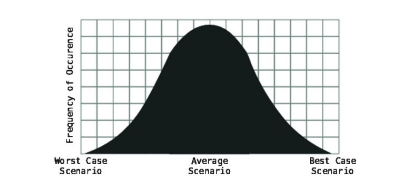
TheAverageCase
Indeed,inaworst-casescenario,SelectionSortisfasterthanInsertionSort.
However,itiscriticalthatwealsotakeintoaccounttheaverage-casescenario.
Why?
Bydefinition,thecasesthatoccurmostfrequentlyareaveragescenarios.The
worst-andbest-casescenarioshappenonlyrarely.Let’slookatthissimplebell
curve:
Best-andworst-casescenarioshappenrelativelyinfrequently.Intherealworld,
however,averagescenariosarewhatoccurmostofthetime.
Andthismakesalotofsense.Thinkofarandomlysortedarray.Whatarethe
oddsthatthevalueswilloccurinperfectascendingordescendingorder?It’s
muchmorelikelythatthevalueswillbeallovertheplace.
Let’sexamineInsertionSortincontextofallscenarios.
We’velookedathowInsertionSortperformsinaworst-casescenario—where
thearraysortedindescendingorder.Intheworstcase,wepointedoutthatin
eachpassthrough,wecompareandshifteveryvaluethatweencounter.(We
calculatedthistobeatotalofN2comparisonsandshifts.)
Inthebest-casescenario,wherethedataisalreadysortedinascendingorder,we
endupmakingjustonecomparisonperpassthrough,andnotasingleshift,since
eachvalueisalreadyinitscorrectplace.
Wheredataisrandomlysorted,however,we’llhavepassthroughsinwhichwe
compareandshiftallofthedata,someofthedata,orpossiblynoneofdata.If
you’lllookatourprecedingwalkthroughexample,you’llnoticethatin
Passthroughs#1and#3,wecompareandshiftallthedataweencounter.In
Passthrough#4,wecompareandshiftsomeofit,andinPassthrough#2,we
makejustonecomparisonandshiftnodataatall.
Whileintheworst-casescenario,wecompareandshiftallthedata,andinthe
best-casescenario,weshiftnoneofthedata(andjustmakeonecomparisonper
passthrough),fortheaveragescenario,wecansaythatintheaggregate,we
probablycompareandshiftabouthalfofthedata.
SoifInsertionSorttakesN2stepsfortheworst-casescenario,we’dsaythatit
takesaboutN2/2stepsfortheaveragescenario.(IntermsofBigO,however,
bothscenariosareO(N2).)
Let’sdiveintosomespecificexamples.
Thearray[1,2,3,4]isalreadypresorted,whichisthebestcase.Theworstcase
forthesamedatawouldbe[4,3,2,1],andanexampleofanaveragecasemight
be[1,3,4,2].
Intheworstcase,therearesixcomparisonsandsixshifts,foratotaloftwelve
steps.Intheaveragecase,therearefourcomparisonsandtwoshifts,foratotal
ofsixsteps.Inthebestcase,therearethreecomparisonsandzeroshifts.
WecannowseethattheperformanceofInsertionSortvariesgreatlybasedon
thescenario.Intheworst-casescenario,InsertionSorttakesN2steps.Inan
averagescenario,ittakesN2/2steps.Andinthebest-casescenario,ittakes
aboutNsteps.
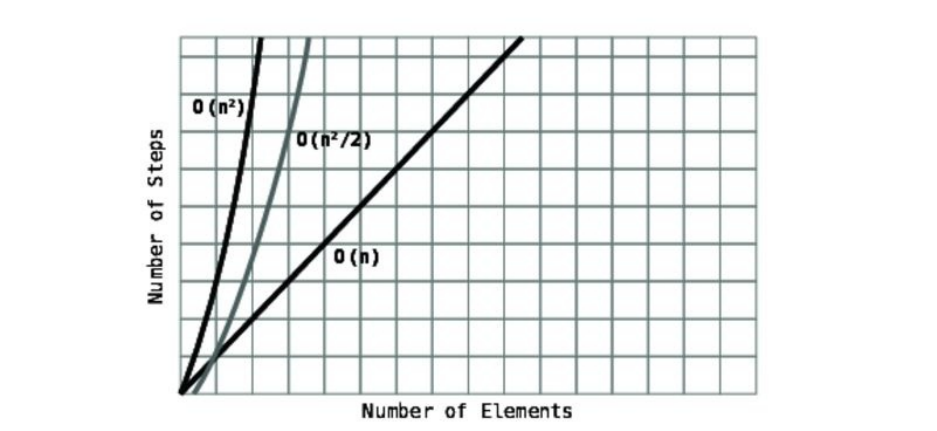
Thisvarianceisbecausesomepassthroughscompareallthedatatotheleftof
thetemp_value,whileotherpassthroughsendearly,duetoencounteringavalue
thatislessthanthetemp_value.
Youcanseethesethreetypesofperformanceinthisgraph:
ComparethiswithSelectionSort.SelectionSorttakesN2/2stepsinallcases,
fromworsttoaveragetobest-casescenarios.ThisisbecauseSelectionSort
doesn’thaveanymechanismforendingapassthroughearlyatanypoint.Each
passthroughcompareseveryvaluetotherightofthechosenindexnomatter
what.
Sowhichisbetter:SelectionSortorInsertionSort?Theansweris:well,it
depends.Inanaveragecase—whereanarrayisrandomlysorted—theyperform
similarly.Ifyouhavereasontoassumethatyou’llbedealingwithdatathatis
mostlysorted,InsertionSortwillbeabetterchoice.Ifyouhavereasontoassume
thatyou’llbedealingwithdatathatismostlysortedinreverseorder,Selection
Sortwillbefaster.Ifyouhavenoideawhatthedatawillbelike,that’s
essentiallyanaveragecase,andbothwillbeequal.
APracticalExample
Let’ssaythatyouarewritingaJavaScriptapplication,andsomewhereinyour
codeyoufindthatyouneedtogettheintersectionbetweentwoarrays.The
intersectionisalistofallthevaluesthatoccurinbothofthearrays.For
example,ifyouhavethearrays[3,1,4,2]and[4,5,3,6],theintersectionwouldbe
athirdarray,[3,4],sincebothofthosevaluesarecommontothetwoarrays.
JavaScriptdoesnotcomewithsuchafunctionbuiltin,sowe’llhavetocreate
ourown.Here’sonepossibleimplementation:
functionintersection(first_array,second_array){
varresult=[];
for(vari=0;i<first_array.length;i++){
for(varj=0;j<second_array.length;j++){
if(first_array[i]==second_array[j]){
result.push(first_array[i]);
}
}
}
returnresult;
}
Here,wearerunningasimplenestedloop.Intheouterloop,weiterateover
eachvalueinthefirstarray.Aswepointtoeachvalueinthefirstarray,wethen
runaninnerloopthatcheckseachvalueofthesecondarraytoseeifitcanfinda
matchwiththevaluebeingpointedtointhefirstarray.
Therearetwotypesofstepstakingplaceinthisalgorithm:comparisonsand
insertions.Wecompareeveryvalueofthetwoarraysagainsteachother,andwe
insertmatchingvaluesintothearrayresult.Theinsertionsarenegligiblebeside
thecomparisons,sinceeveninascenariowherethetwoarraysareidentical,
we’llonlyinsertasmanyvaluesasthereareinoneofthearrays.Theprimary
stepstoanalyze,then,arethecomparisons.
Ifthetwoarraysareofequalsize,thenumberofcomparisonsperformedareN2.
Thisisbecauseforeachelementofthefirstarray,wemakeacomparisonofthat
elementtoeachelementofthesecondarray.Thus,ifwe’dhavetwoarrayseach
containingfiveelements,we’dendupmakingtwenty-fivecomparisons.Sothis
intersectionalgorithmhasanefficiencyofO(N2).
(Ifthearraysaredifferentsizes—sayNandM—we’dsaythattheefficiencyof
thisfunctionisO(N*M).Tosimplifythisexample,however,let’sassumethat
botharraysareofequalsize.)
Isthereanywaywecanimprovethisalgorithm?
Thisiswhereit’simportanttoconsiderscenariosbeyondtheworstcase.Inthe
currentimplementationoftheintersectionfunction,wemakeN2comparisonsin
everytypeofcase,fromwherewehavetwoarraysthatdonotcontainasingle
commonvalue,toacaseoftwoarraysthatarecompletelyidentical.
Thetruthisthatinacasewherethetwoarrayshavenocommonvalue,wereally
havenochoicebuttocheckeachandeveryvalueofbotharraystodetermine
thattherearenointersectingvalues.
Butwherethetwoarrayssharecommonelements,wereallyshouldn’thaveto
checkeveryelementofthefirstarrayagainsteveryelementofthesecondarray.
Let’sseewhy.
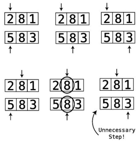
Inthisexample,assoonaswefindacommonvalue(the8),there’sreallyno
reasontocompletethesecondloop.Whatarewecheckingforatthispoint?
We’vealreadydeterminedthatthesecondarraycontainsthesameelementasthe
valuewe’repointingtointhefirstarray.We’reperforminganunnecessarystep.
Tofixthis,wecanaddasinglewordtoourimplementation:
functionintersection(first_array,second_array){
varresult=[];
for(vari=0;i<first_array.length;i++){
for(varj=0;j<second_array.length;j++){
if(first_array[i]==second_array[j]){
result.push(first_array[i]);
break;
}
}
}
returnresult;
}
Withtheadditionofthebreak,wecancuttheinnerloopshort,andsavesteps
(andthereforetime).
Now,inaworst-casescenario,wherethetwoelementsdonotcontainasingle
sharedvalue,wehavenochoicebuttoperformN2comparisons.Inthebest-case
scenario,wherethetwoarraysareidentical,weonlyhavetoperformN
comparisons.Inanaveragecase,wherethetwoarraysaredifferentbutshare
somevalues,theperformancewillbesomewhereinbetweenNandN2.
Thisisasignificantoptimizationtoourintersectionfunction,sinceourfirst
implementationwouldmakeN2comparisonsinallcases.

WrappingUp
Havingtheabilitytodiscernbetweenbest-,average-,andworst-casescenariosis
akeyskillinchoosingthebestalgorithmforyourneeds,aswellastaking
existingalgorithmsandoptimizingthemfurthertomakethemsignificantly
faster.Remember,whileit’sgoodtobepreparedfortheworstcase,average
casesarewhathappenmostofthetime.
Inthenextchapter,we’regoingtolearnaboutanewdatastructurethatissimilar
tothearray,buthasnuancesthatcanallowittobemoreperformantincertain
circumstances.Justasyounowhavetheabilitytochoosebetweentwo
competingalgorithmsforagivenusecase,you’llalsoneedtheabilitytochoose
betweentwocompetingdatastructures,asonemayhavebetterperformance
thantheother.
Copyright©2017,ThePragmaticBookshelf.

Chapter7
BlazingFastLookupwithHash
Tables
Imaginethatyou’rewritingaprogramthatallowscustomerstoorderfoodtogo
fromafast-foodrestaurant,andyou’reimplementingamenuoffoodswiththeir
respectiveprices.Youcould,ofcourse,useanarray:
menu=[["frenchfries",0.75],["hamburger",2.5],
["hotdog",1.5],["soda",0.6]]
Thisarraycontainsseveralsubarrays,andeachsubarraycontainstwoelements.
Thefirstelementisastringrepresentingthefoodonthemenu,andthesecond
elementrepresentsthepriceofthatfood.
AswelearnedinChapter2,WhyAlgorithmsMatter,ifthisarraywere
unordered,searchingforthepriceofagivenfoodwouldtakeO(N)stepssince
thecomputerwouldhavetoperformalinearsearch.Ifit’sanorderedarray,the
computercoulddoabinarysearch,whichwouldtakeO(logN).
WhileO(logN)isn’tbad,wecandobetter.Infact,wecandomuchbetter.By
theendofthischapter,you’lllearnhowtouseaspecialdatastructurecalleda
hashtable,whichcanbeusedtolookupdatainjustO(1).Byknowinghow
hashtablesworkunderthehoodandtherightplacestousethem,youcan
leveragetheirtremendouslookupspeedsinmanysituations.
EntertheHashTable
Mostprogramminglanguagesincludeadatastructurecalledahashtable,andit
hasanamazingsuperpower:fastreading.Notethathashtablesarecalledby
differentnamesinvariousprogramminglanguages.Othernamesincludehashes,
maps,hashmaps,dictionaries,andassociativearrays.
Here’sanexampleofthemenuasimplementedwithahashtableusingRuby:
menu={"frenchfries"=>0.75,"hamburger"=>2.5,
"hotdog"=>1.5,"soda"=>0.6}
Ahashtableisalistofpairedvalues.Thefirstitemisknownasthekey,andthe
seconditemisknownasthevalue.Inahashtable,thekeyandvaluehavesome
significantassociationwithoneanother.Inthisexample,thestring"frenchfries"
isthekey,and0.75isthevalue.Theyarepairedtogethertoindicatethatfrench
friescost75cents.
InRuby,youcanlookupakey’svalueusingthissyntax:
menu["frenchfries"]
Thiswouldreturnthevalueof0.75.
LookingupavalueinahashtablehasanefficiencyofO(1)onaverage,asit
takesjustonestep.Let’sseewhy.
HashingwithHashFunctions
Doyourememberthosesecretcodesyouusedasakidtocreateanddecipher
messages?
Forexample,here’sasimplewaytomapletterstonumbers:
A=1
B=2
C=3
D=4
E=5
andsoon.
Accordingtothiscode,
ACEconvertsto135,
CABconvertsto312,
DABconvertsto412,
and
BADconvertsto214.
Thisprocessoftakingcharactersandconvertingthemtonumbersisknownas
hashing.Andthecodethatisusedtoconvertthoselettersintoparticular
numbersiscalledahashfunction.
Therearemanyotherhashfunctionsbesidesthisone.Anotherexampleofahash
functionistotakeeachletter’scorrespondingnumberandreturnthesumofall
thenumbers.Ifwedidthat,BADwouldbecomethenumber7followingatwo-
stepprocess:
Step#1:First,BADconvertsto214.
Step#2:Wethentakeeachofthesedigitsandgettheirsum:
2+1+4=7
Anotherexampleofahashfunctionistoreturntheproductofalltheletters’
correspondingnumbers.ThiswouldconvertthewordBADintothenumber8:
Step#1:First,BADconvertsto214.
Step#2:Wethentaketheproductofthesedigits:
2*1*4=8
Inourexamplesfortheremainderofthischapter,we’regoingtostickwiththis
lastversionofthehashfunction.Real-worldhashfunctionsaremorecomplex
thanthis,butthis“multiplication”hashfunctionwillkeepourexamplesclear
andsimple.
Thetruthisthatahashfunctionneedstomeetonlyonecriteriontobevalid:a
hashfunctionmustconvertthesamestringtothesamenumbereverysingletime
it’sapplied.Ifthehashfunctioncanreturninconsistentresultsforagivenstring,
it’snotvalid.
Examplesofinvalidhashfunctionsincludefunctionsthatuserandomnumbers
orthecurrenttimeaspartoftheircalculation.Withthesefunctions,BADmight
convertto12onetime,and106anothertime.
Withour“multiplication”hashfunction,however,BADwillalwaysconvertto
8.That’sbecauseBisalways2,Aisalways1,andDisalways4.And2*1*4
isalways8.There’snowayaroundthis.
Notethatwiththishashfunction,DABwillalsoconvertinto8justasBADwill.
Thiswillactuallycausesomeissuesthatwe’lladdresslater.
Armedwiththeconceptofhashfunctions,wecannowunderstandhowahash
tableactuallyworks.
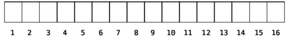
BuildingaThesaurusforFunandProfit,butMainly
Profit
Onnightsandweekends,you’resingle-handedlyworkingonastealthstartup
thatwilltakeovertheworld.It’s…athesaurusapp.Butthisisn’tanyold
thesaurusapp—thisisQuickasaurus.Andyouknowthatitwilltotallydisrupt
thebillion-dollarthesaurusmarket.Whenauserlooksupawordin
Quickasaurus,itreturnstheword’smostpopularsynonym,insteadofevery
possiblesynonymasold-fashionedthesaurusappsdo.
Sinceeverywordhasanassociatedsynonym,thisisagreatusecaseforahash
table.Afterall,ahashtableisalistofpaireditems.Solet’sgetstarted.
Wecanrepresentourthesaurususingahashtable:
thesaurus={}
Underthehood,ahashtablestoresitsdatainabunchofcellsinarow,similarto
anarray.Eachcellhasacorrespondingnumber.Forexample:
Let’saddourfirstentryintothehash:
thesaurus["bad"]="evil"
Incode,ourhashtablenowlookslikethis:
{"bad"=>"evil"}
Let’sexplorehowthehashtablestoresthisdata.
First,thecomputerappliesthehashfunctiontothekey.Again,we’llbeusingthe
“multiplication”hashfunctiondescribedpreviouslyfordemonstrationpurposes.
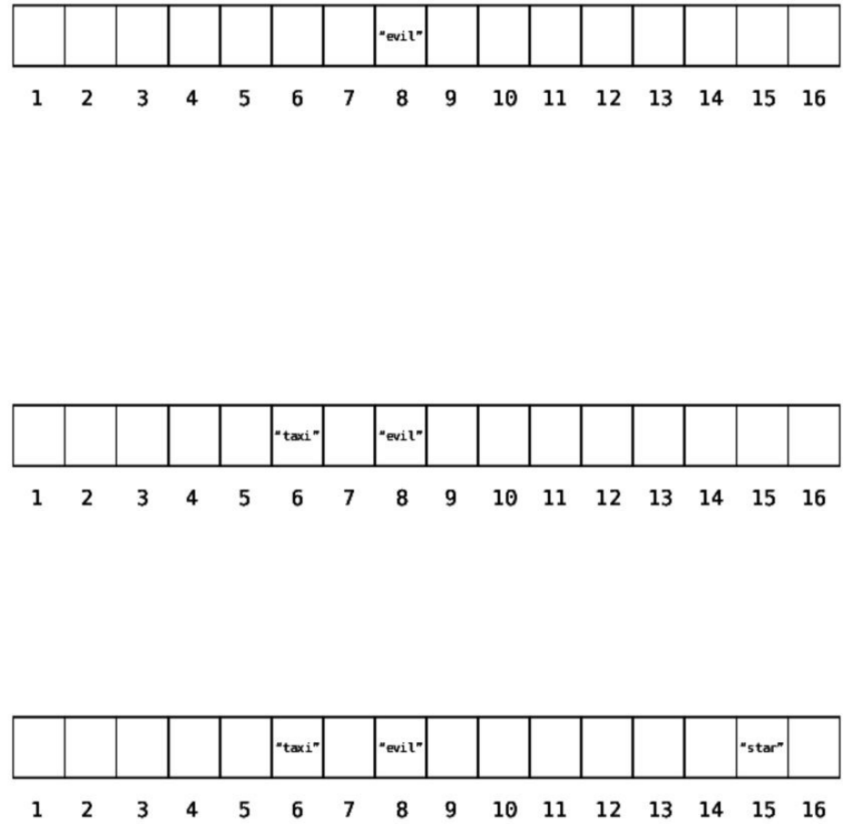
BAD=2*1*4=8
Sinceourkey("bad")hashesinto8,thecomputerplacesthevalue("evil")into
cell8:
Now,let’saddanotherkey/valuepair:
thesaurus["cab"]="taxi"
Again,thecomputerhashesthekey:
CAB=3*1*2=6
Sincetheresultingvalueis6,thecomputerstoresthevalue("taxi")insidecell6.
Let’saddonemorekey/valuepair:
thesaurus["ace"]="star"
ACEhashesinto15,sinceACE=1*3*5=15,so"star"getsplacedintocell
15:
Incode,ourhashtablecurrentlylookslikethis:
{"bad"=>"evil","cab"=>"taxi","ace"=>"star"}
Nowthatwe’vesetupourhashtable,let’sseewhathappenswhenwelookup
valuesfromit.Let’ssaywewanttolookupthevalueassociatedwiththekeyof
"bad".Inourcode,we’dsay:
thesaurus["bad"]
Thecomputerthenexecutestwosimplesteps:
1. Thecomputerhashesthekeywe’relookingup:BAD=2*1*4=8.
2. Sincetheresultis8,thecomputerlooksinsidecell8andreturnsthevalue
thatisstoredthere.Inthiscase,thatwouldbethestring"evil".
ItnowbecomesclearwhylookingupavalueinahashtableistypicallyO(1):
it’saprocessthattakesaconstantamountoftime.Thecomputerhashesthekey
we’relookingup,getsthecorrespondingvalue,andjumpstothecellwiththat
value.
Wecannowunderstandwhyahashtablewouldyieldfasterlookupsforour
restaurantmenuthananarray.Withanarray,werewetolookupthepriceofa
menuitem,wewouldhavetosearchthrougheachcelluntilwefoundit.Foran
unorderedarray,thiswouldtakeuptoO(N),andforanorderedarray,thiswould
takeuptoO(logN).Usingahashtable,however,wecannowusetheactual
menuitemsaskeys,allowingustodoahashtablelookupofO(1).Andthat’s
thebeautyofahashtable.
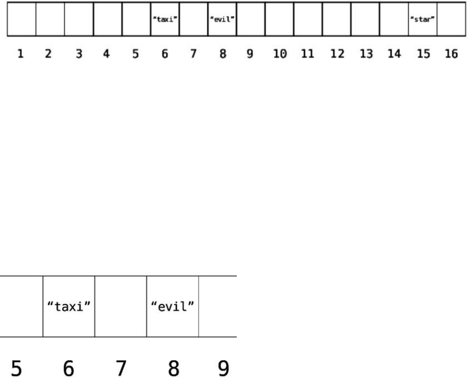
DealingwithCollisions
Ofcourse,hashtablesarenotwithouttheircomplications.
Continuingourthesaurusexample:whathappensifwewanttoaddthe
followingentryintoourthesaurus?
thesaurus["dab"]="pat"
First,thecomputerwouldhashthekey:
DAB=4*1*2=8
Andthenitwouldtrytoadd"pat"toourhashtable’scell8:
Uhoh.Cell8isalreadyfilledwith"evil"—literally!
Tryingtoadddatatoacellthatisalreadyfilledisknownasacollision.
Fortunately,therearewaysaroundit.
Oneclassicapproachforhandlingcollisionsisknownasseparatechaining.
Whenacollisionoccurs,insteadofplacingasinglevalueinthecell,itplacesin
itareferencetoanarray.
Let’slookmorecarefullyatasubsectionofourhashtable’sunderlyingdata
storage:
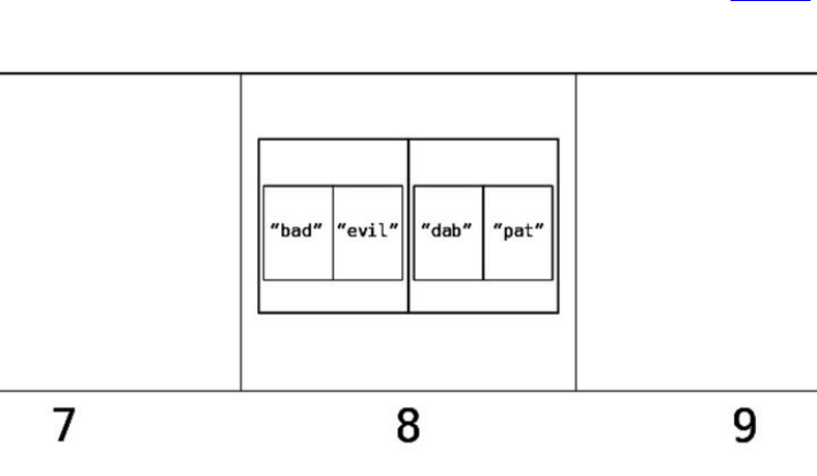
Inourexample,thecomputerwantstoadd"pat"tocell8,butitalreadycontains
"evil".Soitreplacesthecontentsofcell8withanarrayasshown.
Thisarraycontainssubarrayswherethefirstvalueistheword,andthesecond
wordisitssynonym.
Let’swalkthroughhowahashtablelookupworksinthiscase.Ifwelookup:
thesaurus["dab"]
thecomputertakesthefollowingsteps:
1. Ithashesthekey.DAB=4*1*2=8.
2. Itlooksupcell8.Thecomputertakesnotethatcell8containsanarrayof
arraysratherthanasinglevalue.
3. Itsearchesthroughthearraylinearly,lookingatindex0ofeachsubarray
untilitfindsthewordwe’relookingup("dab").Itthenreturnsthevalueat
index1ofthecorrectsubarray.
Let’swalkthroughthesestepsvisually.
WehashDABinto8,sothecomputerinspectsthatcell:
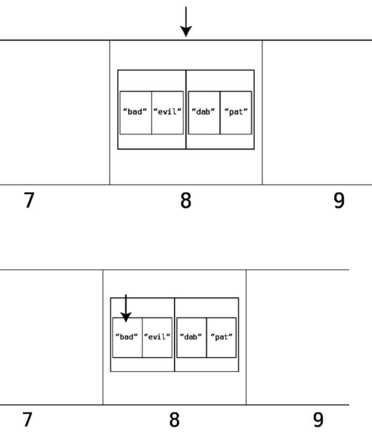
Sincecell8containsanarray,webeginalinearsearchthrougheachcell,starting
atthefirstone.Itcontainsanotherarray,andweinspectindex0:
Itdoesnotcontainthekeywearelookingfor("dab"),sowemoveontothenext
cell:
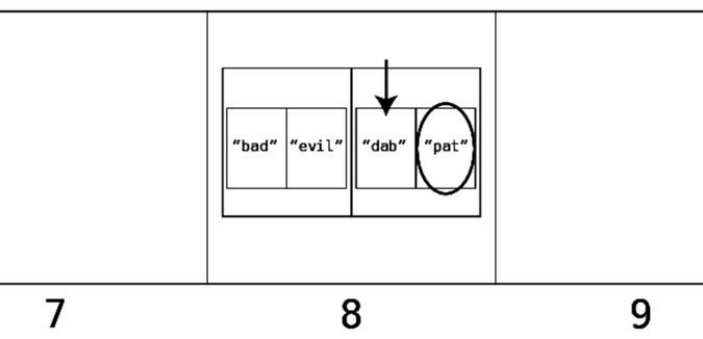
Wefound"dab",whichwouldindicatethatthevalueatindex1ofthatsubarray
("pat")isthevaluewe’relookingfor.
Inascenariowherethecomputerhitsuponacellthatreferencesanarray,its
searchcantakesomeextrasteps,asitneedstoconductalinearsearchwithinan
arrayofmultiplevalues.Ifsomehowallofourdataendedupwithinasinglecell
ofourhashtable,ourhashtablewouldbenobetterthananarray.Soitactually
turnsoutthattheworst-caseperformanceforahashtablelookupisO(N).
Becauseofthis,itiscriticalthatahashtablebedesignedinawaythatitwill
havefewcollisions,andthereforetypicallyperformlookupsinO(1)timerather
thanO(N)time.
Let’sseehowhashtablesareimplementedintherealworldtoavoidfrequent
collisions.

TheGreatBalancingAct
Ultimately,ahashtable’sefficiencydependsonthreefactors:
Howmuchdatawe’restoringinthehashtable
Howmanycellsareavailableinthehashtable
Whichhashfunctionwe’reusing
Itmakessensewhythefirsttwofactorsareimportant.Ifyouhavealotofdata
tostoreinonlyafewcells,therewillbemanycollisionsandthehashtablewill
loseitsefficiency.Let’sexplore,however,whythehashfunctionitselfis
importantforefficiency.
Let’ssaythatwe’reusingahashfunctionthatalwaysproducesavaluethatfalls
intherangebetween1and9inclusive.Anexampleofthisisahashfunction
thatconvertslettersintotheircorrespondingnumbers,andkeepsaddingthe
resultingdigitstogetheruntilitendsupwithasingledigit.
Forexample:
PUT=16+21+20=57
Since57containsmorethanonedigit,thehashfunctionbreaksupthe57into5
+7:
5+7=12
12alsocontainsmorethanonedigit,soitbreaksupthe12into1+2:
1+2=3
Intheend,PUThashesinto3.Thishashfunctionbyitsverynaturewillalways
returnanumber1through9.
Let’sreturntoourexamplehashtable:
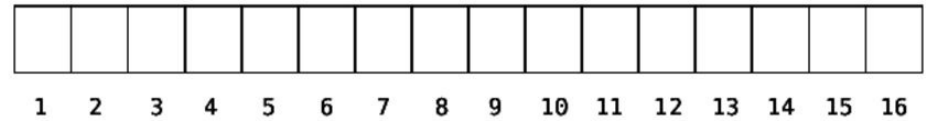
Withthishashfunction,thecomputerwouldneverevenusecells10through16
eventhoughtheyexist.Alldatawouldbestuffedintocells1through9.
Agoodhashfunction,therefore,isonethatdistributesitsdataacrossall
availablecells.
Ifweneedahashtabletostorejustfivevalues,howbigshouldourhashtable
be,andwhattypeofhashfunctionshouldweuse?
Ifahashtablehadonlyfivecells,we’dneedahashfunctionthatconvertskeys
intonumbers1through5.Evenifweonlyplannedonstoringfivepiecesofdata,
there’sagoodchancethattherewillbeacollisionortwo,sincetwokeysmaybe
easilyhashedtothesamevalue.
However,ifourhashtableweretohaveonehundredcells,andourhashfunction
convertsstringsintonumbers1through100,whenstoringjustfivevaluesit
wouldbemuchlesslikelytohaveanycollisionssincethereareonehundred
possiblecellsthateachofthosestringsmightendupin.
Althoughahashtablewithonehundredcellsisgreatforavoidingcollisions,
we’dbeusinguponehundredcellstostorejustfivepiecesofdata,andthat’sa
pooruseofmemory.
Thisisthebalancingactthatahashtablemustperform.Agoodhashtable
strikesabalanceofavoidingcollisionswhilenotconsuminglotsofmemory.
Toaccomplishthis,computerscientistshavedevelopedthefollowingruleof
thumb:foreverysevendataelementsstoredinahashtable,itshouldhaveten
cells.
So,ifyou’replanningonstoringfourteenelements,you’dwanttohavetwenty
availablecells,andsoonandsoforth.
Thisratioofdatatocellsiscalledtheloadfactor.Usingthisterminology,we’d
saythattheidealloadfactoris0.7(7elements/10cells).
Ifyouinitiallystoredsevenpiecesofdatainahash,thecomputermightallocate
ahashwithtencells.Whenyoubegintoaddmoredata,though,thecomputer
willexpandthehashbyaddingmorecellsandchangingthehashfunctionsothat
thenewdatawillbedistributedevenlyacrossthenewcells.
Luckily,mostoftheinternalsofahashtablearemanagedbythecomputer
languageyou’reusing.Itdecideshowbigthehashtableneedstobe,whathash
functiontouse,andwhenit’stimetoexpandthehashtable.Butnowthatyou
understandhowhasheswork,youcanusethemtoreplacearraysinmanycases
tooptimizeyourcode’sperformanceandtakeadvantageofsuperiorlookupsthat
haveanefficiencyofO(1).

PracticalExamples
Hashtableshavemanypracticalusecases,butherewe’regoingtofocuson
usingthemtoincreasealgorithmspeed.
InChapter1,WhyDataStructuresMatter,welearnedaboutarray-basedsets—
arraysthatensurethatnoduplicatevaluesexist.Therewefoundthateverytime
anewvalueisinsertedintotheset,weneedtorunalinearsearch(ifthesetis
unordered)tomakesurethatthevaluewe’reinsertingisn’talreadyintheset.
Ifwe’redealingwithalargesetinwhichwe’remakinglotsofinsertions,this
cangetunwieldyveryquickly,sinceeveryinsertionrunsatO(N),whichisn’t
veryfast.
Inmanycases,wecanuseahashtabletoserveasaset.
Whenweuseanarrayasaset,wesimplyplaceeachpieceofdatainacell
withinthearray.Whenweuseahashtableasaset,however,eachpieceofdata
isakeywithinthehashtable,andthevaluecanbeanything,suchasa1ora
Booleanvalueoftrue.
Let’ssaywesetupourhashtablesetinJavaScriptasfollows:
varset={};
Let’saddafewvaluestotheset:
set["apple"]=1;
set["banana"]=1;
set["cucumber"]=1;
Everytimewewanttoinsertanewvalue,insteadofaO(N)linearsearch,we
cansimplyadditinO(1)time.Thisistrueevenifweaddakeythatalready
exists:
set["banana"]=1;

Whenweattempttoaddanother"banana"totheset,wedon’tneedtocheck
whether"banana"alreadyexists,sinceevenifitdoes,we’resimplyoverwriting
thevalueforthatkeywiththenumber1.
Thetruthisthathashtablesareperfectforanysituationwherewewanttokeep
trackofwhichvaluesexistwithinadataset.InChapter4,SpeedingUpYour
CodewithBigO,wediscussedwritingaJavaScriptfunctionthatwouldtellus
whetheranyduplicatenumbersoccurwithinanarray.Thefirstsolutionwe
providedwas:
functionhasDuplicateValue(array){
for(vari=0;i<array.length;i++){
for(varj=0;j<array.length;j++){
if(i!==j&&array[i]==array[j]){
returntrue;
}
}
}
returnfalse;
}
Wenotedtherethatthiscode,whichcontainsnestedloops,runsatO(N2).
ThesecondsolutionwesuggestedthererunsatO(N),butonlyworksifthearray
exclusivelycontainspositiveintegers.Whatifthearraycontainssomethingelse,
likestrings?
Withahashtable(whichiscalledanobjectinJavaScript),wecanachievea
similarsolutionthatwouldeffectivelyhandlestrings:
functionhasDuplicateValue(array){
varexistingValues={};
for(vari=0;i<array.length;i++){
if(existingValues[array[i]]===undefined){
existingValues[array[i]]=1;
}else{
returntrue;
}
}
returnfalse;
}
ThisapproachalsorunsatO(N).HereexistingValuesisahashtableratherthanan
array,soitskeyscanincludestringsaswellasintegers.
Let’ssaywearebuildinganelectronicvotingmachine,inwhichvoterscan
choosefromalistofcandidatesorwriteinanothercandidate.Iftheonlytime
wecountedthefinaltallyofvoteswasattheendoftheelection,wecouldstore
thevotesasasimplearray,andinserteachvoteattheendasitcomesin:
varvotes=[];
functionaddVote(candidate){
votes.push(candidate);
}
We’dendupwithaverylongarraythatwouldlooksomethinglike
["ThomasJefferson","JohnAdams","JohnAdams","ThomasJefferson",
"JohnAdams",...]
Withthisapproach,eachinsertionwouldonlytakeO(1).
Butwhataboutthefinaltally?Well,wecouldcountthevotesbyrunningaloop
andkeepingtrackoftheresultsinahashtable:
functioncountVotes(votes){
vartally={};
for(vari=0;i<votes.length;i++){
if(tally[votes[i]]){
tally[votes[i]]++;
}else{
tally[votes[i]]=1;
}
}
returntally;
}
However,sincewe’dhavetocounteachvoteattheendoftheday,thecountVotes
functionwouldtakeO(N).Thismighttaketoolong!
Instead,wemayconsiderusingthehashtabletostorethedatainthefirstplace:
varvotes={};
functionaddVote(candidate){
if(votes[candidate]){
votes[candidate]++;
}else{
votes[candidate]=1;
}
}
functioncountVotes(){
returnvotes;
}
Withthistechnique,notonlyareinsertionsO(1),butourtallyisaswell,since
it’salreadykeptasthevotingtakesplace.

WrappingUp
Hashtablesareindispensablewhenitcomestobuildingefficientsoftware.With
theirO(1)readsandinsertions,it’sadifficultdatastructuretobeat.
Untilnow,ouranalysisofvariousdatastructuresrevolvedaroundtheir
efficiencyandspeed.Butdidyouknowthatsomedatastructuresprovide
advantagesotherthanspeed?Inthenextlesson,we’regoingtoexploretwodata
structuresthatcanhelpimprovecodeeleganceandmaintainability.
Copyright©2017,ThePragmaticBookshelf.

Chapter8
CraftingElegantCodewithStacks
andQueues
Untilnow,ourdiscussionarounddatastructureshasfocusedprimarilyonhow
theyaffecttheperformanceofvariousoperations.However,havingavarietyof
datastructuresinyourprogrammingarsenalallowsyoutocreatecodethatis
simplerandeasiertoread.
Inthischapter,you’regoingtodiscovertwonewdatastructures:stacksand
queues.Thetruthisthatthesetwostructuresarenotentirelynew.They’re
simplyarrayswithrestrictions.Yet,theserestrictionsareexactlywhatmake
themsoelegant.
Morespecifically,stacksandqueuesareeleganttoolsforhandlingtemporary
data.Fromoperatingsystemarchitecturetoprintingjobstotraversingdata,
stacksandqueuesserveastemporarycontainersthatcanbeusedtoform
beautifulalgorithms.
Thinkoftemporarydatalikethefoodordersinadiner.Whateachcustomer
ordersisimportantuntilthemealismadeanddelivered;thenyouthrowthe
orderslipaway.Youdon’tneedtokeepthatinformationaround.Temporarydata
isinformationthatdoesn’thaveanymeaningafterit’sprocessed,soyoudon’t
needtokeepitaround.However,theorderinwhichyouprocessthedatacanbe
important—inthediner,youshouldideallymakeeachmealintheorderin
whichitwasrequested.Stacksandqueuesallowyoutohandledatainorder,and
thengetridofitonceyoudon’tneeditanymore.
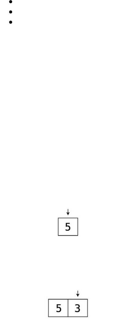
Stacks
Astackstoresdatainthesamewaythatarraysdo—it’ssimplyalistofelements.
Theonecatchisthatstackshavethefollowingthreeconstraints:
Datacanonlybeinsertedattheendofastack.
Datacanonlybereadfromtheendofastack.
Datacanonlyberemovedfromtheendofastack.
Youcanthinkofastackasanactualstackofdishes:youcan’tlookatthefaceof
anydishotherthantheoneatthetop.Similarly,youcan’taddanydishexceptto
thetopofthestack,norcanyouremoveanydishbesidestheoneatthetop.(At
least,youshouldn’t.)Infact,mostcomputerscienceliteraturereferstotheend
ofthestackasitstop,andthebeginningofthestackasitsbottom.
Whiletheserestrictionsseem—well—restrictive,we’llseeshortlyhowtheyare
toourbenefit.
Toseeastackinaction,let’sstartwithanemptystack.
Insertinganewvalueintoastackisalsocalledpushingontothestack.Thinkof
itasaddingadishontothetopofthedishstack.
Let’spusha5ontothestack:
Again,there’snothingfancygoingonhere.We’rejustinsertingdataintotheend
ofanarray.
Now,let’spusha3ontothestack:
Next,let’spusha0ontothestack:
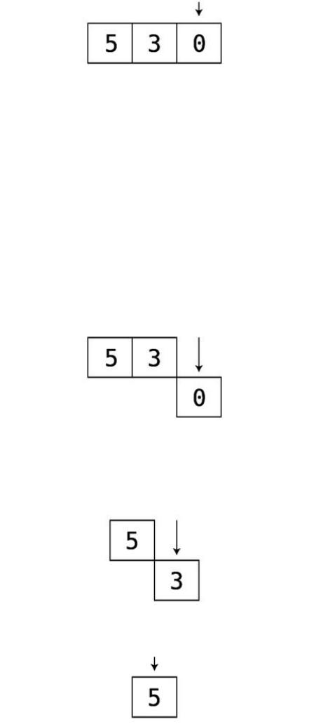
Notethatwe’realwaysaddingdatatothetop(thatis,theend)ofthestack.Ifwe
wantedtoinsertthe0intothebottomormiddleofthestack,wecouldn’t,
becausethatisthenatureofastack:datacanonlybeaddedtothetop.
Removingelementsfromthetopofthestackiscalledpoppingfromthestack.
Becauseofastack’srestrictions,wecanonlypopdatafromthetop.
Let’spopsomeelementsfromourexamplestack:
Firstwepopthe0:
Ourstacknowcontainsonlytwoelements,the5andthe3.
Next,wepopthe3:
Ourstacknowonlycontainsthe5:
AhandyacronymusedtodescribestackoperationsisLIFO,whichstandsfor
“LastIn,FirstOut.”Allthismeansisthatthelastitempushedontoastackis
alwaysthefirstitempoppedfromit.It’ssortoflikestudentswhoslackoff—
they’realwaysthelasttoarrivetoclass,butthefirsttoleave.
StacksinAction
Althoughastackisnottypicallyusedtostoredataonalong-termbasis,itcanbe
agreattooltohandletemporarydataaspartofvariousalgorithms.Here’san
example:
Let’screatethebeginningsofaJavaScriptlinter—thatis,aprogramthat
inspectsaprogrammer’sJavaScriptcodeandensuresthateachlineis
syntacticallycorrect.Itcanbeverycomplicatedtocreatealinter,asthereare
manydifferentaspectsofsyntaxtoinspect.We’llfocusonjustonespecific
aspectofthelinter—openingandclosingbraces.Thisincludesparentheses,
squarebrackets,andcurlybraces—allcommoncausesoffrustratingsyntax
errors.
Tosolvethisproblem,let’sfirstanalyzewhattypeofsyntaxisincorrectwhenit
comestobraces.Ifwebreakitdown,we’llfindthattherearethreesituationsof
erroneoussyntax:
Thefirstiswhenthereisanopeningbracethatdoesn’thaveacorresponding
closingbrace,suchasthis:
(varx=2;
We’llcallthisSyntaxErrorType#1.
Thesecondiswhenthereisaclosingbracethatwasneverprecededbya
correspondingopeningbrace:
varx=2;)
We’llcallthatSyntaxErrorType#2.
Thethird,whichwe’llrefertoasSyntaxErrorType#3,iswhenaclosingbrace
isnotthesametypeofbraceastheimmediatelyprecedingopeningbrace,such
as:
(varx=[1,2,3)];

Intheprecedingexample,thereisamatchingsetofparentheses,andamatching
pairofsquarebrackets,buttheclosingparenthesisisinthewrongplace,asit
doesn’tmatchtheimmediatelyprecedingopeningbrace,whichisasquare
bracket.
Howcanweimplementanalgorithmthatinspectsalineofcodeandensuresthat
therearenosyntaxerrorsinthisregard?Thisiswhereastackallowsusto
implementabeautifullintingalgorithm,whichworksasfollows:
Weprepareanemptystack,andthenwereadeachcharacterfromlefttoright,
followingtheserules:
1. Ifwefindanycharacterthatisn’tatypeofbrace(parenthesis,square
bracket,orcurlybrace),weignoreitandmoveon.
2. Ifwefindanopeningbrace,wepushitontothestack.Havingitonthe
stackmeanswe’rewaitingtoclosethatparticularbrace.
3. Ifwefindaclosingbrace,weinspectthetopelementinthestack.Wethen
analyze:
Iftherearenoelementsinthestack,thatmeanswe’vefoundaclosing
bracewithoutacorrespondingopeningbracebeforehand.Thisis
SyntaxErrorType#2.
Ifthereisdatainthestack,buttheclosingbraceisnotacorresponding
matchforthetopelementofthestack,thatmeanswe’veencountered
SyntaxErrorType#3.
Iftheclosingcharacterisacorrespondingmatchfortheelementatthe
topofthestack,thatmeanswe’vesuccessfullyclosedthatopening
brace.Wepopthetopelementfromthestack,sincewenolongerneed
tokeeptrackofit.
4. Ifwemakeittotheendofthelineandthere’sstillsomethingleftonthe
stack,thatmeansthere’sanopeningbracewithoutacorrespondingclosing
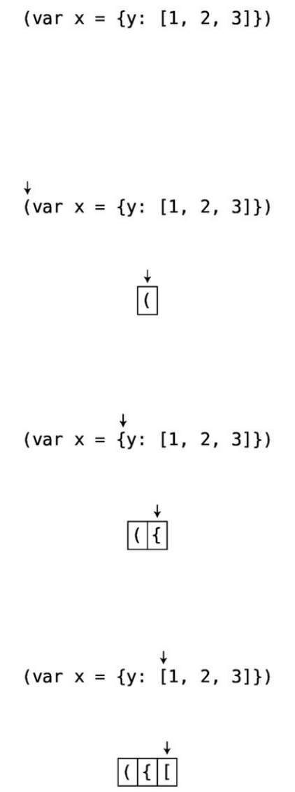
brace,whichisSyntaxErrorType#1.
Let’sseethisinactionusingthefollowingexample:
Afterweprepareanemptystack,webeginreadingeachcharacterfromleftto
right:
Step#1:Webeginwiththefirstcharacter,whichhappenstobeanopening
parenthesis:
Step#2:Sinceit’satypeofopeningbrace,wepushitontothestack:
Wethenignoreallthecharactersvarx=,sincetheyaren’tbracecharacters.
Step#3:Weencounterournextopeningbrace:
Step#4:Wepushitontothestack:
Wethenignorethey:
Step#5:Weencountertheopeningsquarebracket:
Step#6:Weaddthattothestackaswell:
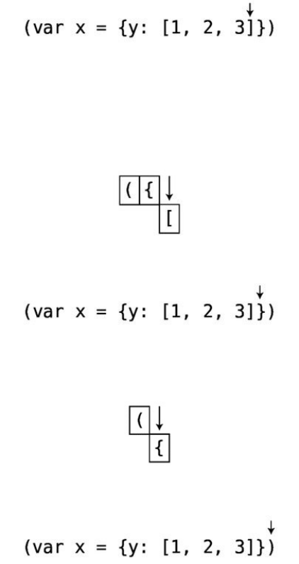
Wethenignorethe1,2,3.
Step#7:Weencounterourfirstclosingbrace—aclosingsquarebracket:
Step#8:Weinspecttheelementatthetopofthestack,whichhappenstobean
openingsquarebracket.Sinceourclosingsquarebracketisacorresponding
matchtothisfinalelementofthestack,wepoptheopeningsquarebracketfrom
thestack:
Step#9:Wemoveon,encounteringaclosingcurlybrace:
Step#10:Wereadthelastelementinthestack.It’sanopeningcurlybrace,so
we’vefoundamatch.Wepoptheopeningcurlybracefromourstack:
Step#11:Weencounteraclosingparenthesis:
Step#12:Wereadthelastelementinthestack.It’sacorrespondingmatch,so
wepopitfromthestack,leavinguswithanemptystack.
Sincewe’vemadeitthroughtheentirelineofcode,andourstackisempty,our
lintercanconcludethattherearenosyntacticalerrorsonthisline(thatrelateto
openingandclosingbraces).
Here’saRubyimplementationoftheprecedingalgorithm.NotethatRubyhas
pushandpopmethodsbuiltintoarrays,andtheyareessentiallyshortcutsfor
addinganelementtotheendofthearrayandremovinganelementfromtheend
ofanarray,respectively.Byonlyusingthosetwomethodstoaddandremove
datafromthearray,weeffectivelyusethearrayasastack.
classLinter
attr_reader:error
definitialize
#Weuseasimplearraytoserveasourstack:
@stack=[]
end
deflint(text)
#Westartaloopwhichreadseachcharacterinourtext:
text.each_char.with_indexdo|char,index|
ifopening_brace?(char)
#Ifthecharacterisanopeningbrace,wepushitontothestack:
@stack.push(char)
elsifclosing_brace?(char)
ifcloses_most_recent_opening_brace?(char)
#Ifthecharacterclosesthemostrecentopeningbrace,
#wepoptheopeningbracefromourstack:
@stack.pop
else#ifthecharacterdoesNOTclosethemostrecentopeningbrace
@error="Incorrectclosingbrace:#{char}atindex#{index}"
return
end
end
end
if@stack.any?
#Ifwegettotheendofline,andthestackisn'tempty,thatmeans
#wehaveanopeningbracewithoutacorrespondingclosingbrace:
@error="#{@stack.last}doesnothaveaclosingbrace"
end
end
private
defopening_brace?(char)
["(","[","{"].include?(char)
end
defclosing_brace?(char)
[")","]","}"].include?(char)
end
defopening_brace_of(char)
{")"=>"(","]"=>"[","}"=>"{"}[char]
end
defmost_recent_opening_brace
@stack.last
end
defcloses_most_recent_opening_brace?(char)
opening_brace_of(char)==most_recent_opening_brace
end
end
Ifweusethisclassasfollows:
linter=Linter.new
linter.lint("(varx={y:[1,2,3]})")
putslinter.error
WewillnotreceiveanyerrorssincethislineofJavaScriptiscorrect.However,if
weaccidentallyswapthelasttwocharacters:
linter=Linter.new
linter.lint("(varx={y:[1,2,3])}")
putslinter.error
Wewillthengetthemessage:
Incorrectclosingbrace:)atindex25
Ifweleaveoffthelastclosingparenthesisaltogether:
linter=Linter.new
linter.lint("(varx={y:[1,2,3]}")
putslinter.error
We’llgetthiserrormessage:
(doesnothaveaclosingbrace
Inthisexample,weuseastacktoelegantlykeeptrackofopeningbracesthat
havenotyetbeenclosed.Inthenextchapter,we’lluseastacktosimilarlykeep
trackoffunctionsofcodethatneedtobeinvoked,whichisthekeytoacritical
conceptknownasrecursion.
Stacksareidealforprocessinganydatathatshouldbehandledinreverseorder
tohowitwasreceived(LIFO).The“undo”functioninawordprocessor,or
functioncallsinanetworkedapplication,areexamplesofwhenyou’dwantto
useastack.
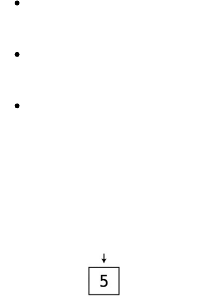
Queues
Aqueuealsodealswithtemporarydataelegantly,andislikeastackinthatitis
anarraywithrestrictions.Thedifferenceliesinwhatorderwewanttoprocess
ourdata,andthisdependsontheparticularapplicationweareworkingon.
Youcanthinkofaqueueasalineofpeopleatthemovietheater.Thefirstoneon
thelineisthefirstonetoleavethelineandenterthetheater.Withqueues,the
firstitemaddedtothequeueisthefirstitemtoberemoved.That’swhy
computerscientistsusetheacronym“FIFO”whenitcomestoqueues:FirstIn,
FirstOut.
Likestacks,queuesarearrayswiththreerestrictions(it’sjustadifferentsetof
restrictions):
Datacanonlybeinsertedattheendofaqueue.(Thisisidenticalbehavior
asthestack.)
Datacanonlybereadfromthefrontofaqueue.(Thisistheoppositeof
behaviorofthestack.)
Datacanonlyberemovedfromthefrontofaqueue.(This,too,isthe
oppositebehaviorofthestack.)
Let’sseeaqueueinaction,beginningwithanemptyqueue.
First,weinserta5:(Whileinsertingintoastackiscalledpushing,insertinginto
aqueuedoesn’thaveastandardizedname.Variousreferencescallitputting,
adding,orenqueuing.)
Next,weinserta9:
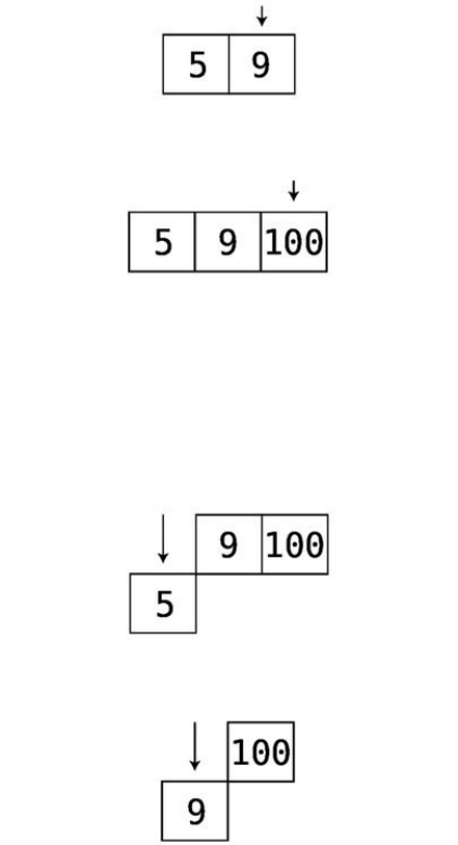
Next,weinserta100:
Asofnow,thequeuehasfunctionedjustlikeastack.However,removingdata
happensinthereverse,asweremovedatafromthefrontofthequeue.
Ifwewanttoremovedata,wemuststartwiththe5,sinceit’satthefrontofthe
queue:
Next,weremovethe9:
Ourqueuenowonlycontainsoneelement,the100.
QueuesinAction
Queuesarecommoninmanyapplications,rangingfromprintingjobsto
backgroundworkersinwebapplications.
Let’ssayyouwereprogrammingasimpleRubyinterfaceforaprinterthatcan
acceptprintingjobsfromvariouscomputersacrossanetwork.Byutilizingthe
Rubyarray’spushmethod,whichaddsdatatotheendofthearray,andtheshift
method,whichremovesdatafromthebeginningofthearray,youmaycreatea
classlikethis:
classPrintManager
definitialize
@queue=[]
end
defqueue_print_job(document)
@queue.push(document)
end
defrun
while@queue.any?
#theRubyshiftmethodremovesandreturnsthe
#firstelementofanarray:
print(@queue.shift)
end
end
private
defprint(document)
#Codetoruntheactualprintergoeshere.
#Fordemopurposes,we'llprinttotheterminal:
putsdocument
end
end
Wecanthenutilizethisclassasfollows:
print_manager=PrintManager.new
print_manager.queue_print_job("FirstDocument")
print_manager.queue_print_job("SecondDocument")
print_manager.queue_print_job("ThirdDocument")
print_manager.run
Theprinterwillthenprintthethreedocumentsinthesameorderinwhichthey
werereceived:
FirstDocument
SecondDocument
ThirdDocument
Whilethisexampleissimplifiedandabstractsawaysomeofthenitty-gritty
detailsthatarealliveprintingsystemmayhavetodealwith,thefundamental
useofaqueueforsuchanapplicationisveryrealandservesasthefoundation
forbuildingsuchasystem.
Queuesarealsotheperfecttoolforhandlingasynchronousrequests—they
ensurethattherequestsareprocessedintheorderinwhichtheywerereceived.
Theyarealsocommonlyusedtomodelreal-worldscenarioswhereeventsneed
tooccurinacertainorder,suchasairplaneswaitingfortakeoffandpatients
waitingfortheirdoctor.

WrappingUp
Asyou’veseen,stacksandqueuesareprogrammers’toolsforelegantlyhandling
allsortsofpracticalalgorithms.
Nowthatwe’velearnedaboutstacksandqueues,we’veunlockedanew
achievement:wecanlearnaboutrecursion,whichdependsuponastack.
Recursionalsoservesasthefoundationformanyofthemoreadvancedand
superefficientalgorithmsthatwewillcoverintherestofthisbook.
Copyright©2017,ThePragmaticBookshelf.

Chapter9
RecursivelyRecursewithRecursion
You’llneedtounderstandthekeyconceptofrecursioninordertounderstand
mostoftheremainingalgorithmsinthisbook.Recursionallowsforsolving
trickyproblemsinsurprisinglysimpleways,oftenallowingustowriteafraction
ofthecodethatwemightotherwisewrite.
Butfirst,apopquiz!
Whathappenswhentheblah()functiondefinedbelowisinvoked?
functionblah(){
blah();
}
Asyouprobablyguessed,itwillcallitselfinfinitely,sinceblah()callsitself,
whichinturncallsitself,andsoon.
Recursionistheofficialnameforwhenafunctioncallsitself.Whileinfinite
functioncallsaregenerallyuseless—andevendangerous—recursionisa
powerfultoolthatcanbeharnessed.Andwhenweharnessthepowerof
recursion,wecansolveparticularlytrickyproblems,asyou’llnowsee.
RecurseInsteadofLoop
Let’ssayyouworkatNASAandneedtoprogramacountdownfunctionfor
launchingspacecraft.Theparticularfunctionthatyou’reaskedtowriteshould
acceptanumber—suchas10—anddisplaythenumbersfrom10downto0.
Takeamomentandimplementthisfunctioninthelanguageofyourchoice.
Whenyou’redone,readon.
Oddsarethatyouwroteasimpleloop,alongthelinesofthisJavaScript
implementation:
functioncountdown(number){
for(vari=number;i>=0;i--){
console.log(i);
}
}
countdown(10);
There’snothingwrongwiththisimplementation,butitmayhaveneveroccurred
toyouthatyoudon’thavetousealoop.
How?
Let’stryrecursioninstead.Here’safirstattemptatusingrecursiontoimplement
ourcountdownfunction:
functioncountdown(number){
console.log(number);
countdown(number-1);
}
countdown(10);
Let’swalkthroughthiscodestepbystep.
Step#1:Wecallcountdown(10),sotheargumentnumberholdsa10.
Step#2:Weprintnumber(whichcontainsthevalue10)totheconsole.
Step#3:Beforethecountdownfunctioniscomplete,itcallscountdown(9)(since
number-1is9).
Step#4:countdown(9)beginsrunning.Init,weprintnumber(whichiscurrently9)
totheconsole.
Step#5:Beforecountdown(9)iscomplete,itcallscountdown(8).
Step#6:countdown(8)beginsrunning.Weprint8totheconsole.
Beforewecontinuesteppingthroughthecode,notehowwe’reusingrecursion
toachieveourgoal.We’renotusinganyloopconstructs,butbysimplyhaving
thecountdownfunctioncallitself,weareabletocountdownfrom10andprint
eachnumbertotheconsole.
Inalmostanycaseinwhichyoucanusealoop,youcanalsouserecursion.
Now,justbecauseyoucanuserecursiondoesn’tmeanthatyoushoulduse
recursion.Recursionisatoolthatallowsforwritingelegantcode.Inthe
precedingexample,therecursiveapproachisnotnecessarilyanymorebeautiful
orefficientthanusingaclassicforloop.However,wewillsoonencounter
examplesinwhichrecursionshines.Inthemeantime,let’scontinueexploring
howrecursionworks.
TheBaseCase
Let’scontinueourwalkthroughofthecountdownfunction.We’llskipafewsteps
forbrevity…
Step#21:Wecallcountdown(0).
Step#22:Weprintnumber(i.e.,0)totheconsole.
Step#23:Wecallcountdown(-1).
Step#24:Weprintnumber(i.e.,-1)totheconsole.
Uhoh.Asyoucansee,oursolutionisnotperfect,aswe’llendupstuckwith
infinitelyprintingnegativenumbers.
Toperfectoursolution,weneedawaytoendourcountdownat0andprevent
therecursionfromcontinuingonforever.
Wecansolvethisproblembyaddingaconditionalstatementthatensuresthatif
numberiscurrently0,wedon’tcallcountdown()again:
functioncountdown(number){
console.log(number);
if(number===0){
return;
}else{
countdown(number-1);
}
}
countdown(10);
Now,whennumberis0,ourcodewillnotcallthecountdown()functionagain,but
insteadjustreturn,therebypreventinganothercallofcountdown().
InRecursionLand(arealplace),thiscaseinwhichthemethodwillnotrecurse
isknownasthebasecase.Soinourcountdown()function,0isthebasecase.
ReadingRecursiveCode
Ittakestimeandpracticetogetusedtorecursion,andyouwillultimatelylearn
twosetsofskills:readingrecursivecode,andwritingrecursivecode.Reading
recursivecodeissomewhateasier,solet’sfirstgetsomepracticewiththat.
Let’slookatanotherexample:calculatingfactorials.
Afactorialisbestillustratedwithanexample:
Thefactorialof3is:
3*2*1=6
Thefactorialof5is:
5*4*3*2*1=120
Andsoonandsoforth.Here’sarecursiveimplementationthatreturnsa
number’sfactorialusingRuby:
deffactorial(number)
ifnumber==1
return1
else
returnnumber*factorial(number-1)
end
end
Thiscodecanlooksomewhatconfusingatfirstglance,buthere’stheprocess
youneedtoknowforreadingrecursivecode:
1. Identifywhatthebasecaseis.
2. Walkthroughthefunctionassumingit’sdealingwiththebasecase.
3. Then,walkthroughthefunctionassumingit’sdealingwiththecase
immediatelybeforethebasecase.
4. Progressthroughyouranalysisbymovingupthecasesoneatatime.

Let’sapplythisprocesstotheprecedingcode.Ifweanalyzethecode,we’ll
quicklynoticethattherearetwopaths:
ifnumber==1
return1
else
returnnumber*factorial(number-1)
end
Wecanseethattherecursionhappenshere,asfactorialcallsitself:
else
returnnumber*factorial(number-1)
end
Soitmustbethatthefollowingcodereferstothebasecase,sincethisisthecase
inwhichthefunctiondoesnotcallitself:
ifnumber==1
return1
Wecanconclude,then,thatnumberbeing1isthebasecase.
Next,let’swalkthroughthefactorialmethodassumingit’sdealingwiththebase
case,whichwouldbefactorial(1).Therelevantcodefromourmethodis:
ifnumber==1
return1
Well,that’sprettysimple—it’sthebasecase,sonorecursionactuallyhappens.If
wecallfactorial(1),themethodsimplyreturns1.Okay,sograbanapkinandwrite
thisfactdown:
Next,let’smoveuptothenextcase,whichwouldbefactorial(2).Therelevant
lineofcodefromourmethodis:
else
returnnumber*factorial(number-1)
end
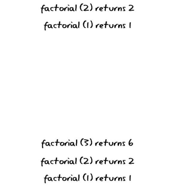
So,callingfactorial(2)willreturn2*factorial(1).Tocalculate2*factorial(1),weneed
toknowwhatfactorial(1)returns.Ifyoucheckyournapkin,you’llseethatit
returns1.So2*factorial(1)willreturn2*1,whichjusthappenstobe2.
Addthisfacttoyournapkin:
Now,whathappensifwecallfactorial(3)?Again,therelevantlineofcodeis:
else
returnnumber*factorial(number-1)
end
Sothatwouldtranslateintoreturn3*factorial(2).Whatdoesfactorial(2)return?You
don’thavetofigurethatoutalloveragain,sinceit’sonyournapkin!Itreturns2.
Sofactorial(3)willreturn6(3*2=6).Goaheadandaddthiswonderfulfactoid
toyournapkin:
Takeamomentandfigureoutforyourselfwhatfactorial(4)willreturn.
Asyoucansee,startingtheanalysisfromthebasecaseandbuildingupisa
greatwaytoreasonaboutrecursivecode.
Infact,followingthisprocessisnotjustagoodwayforhumanstoconceptualize
recursion.Yourcomputerusesasimilarapproach.Let’sseehow.
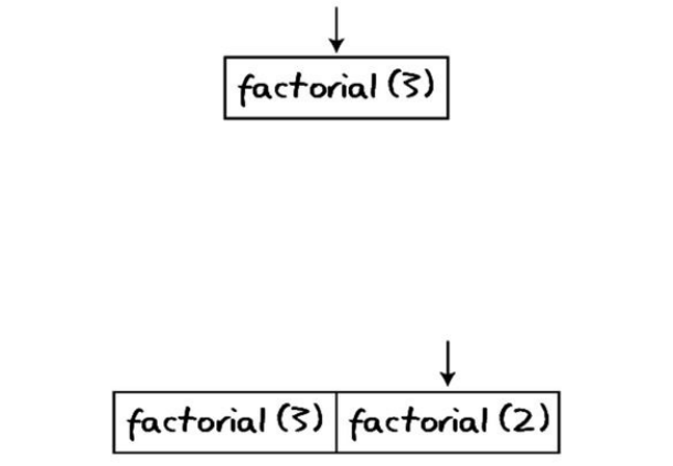
RecursionintheEyesoftheComputer
Ifyouthinkaboutourfactorialmethod,you’llrealizewhenwecallfactorial(3),the
followinghappens:
Thecomputercallsfactorial(3),andbeforethemethodiscomplete,itcalls
factorial(2),andbeforefactorial(2)iscomplete,itcallsfactorial(1).Technically,
whilethecomputerrunsfactorial(1),it’sstillinthemiddleoffactorial(2),whichin
turnisrunningwithinfactorial(3).
Thecomputerusesastacktokeeptrackofwhichfunctionsit’sinthemiddleof
calling.Thisstackisknown,appropriatelyenough,asthecallstack.
Let’swatchthecallstackinactionusingthefactorialexample.
Thecomputerbeginsbycallingfactorial(3).Beforethemethodcompletes
executing,however,factorial(2)getscalled.Inordertotrackthatthecomputeris
stillinthemiddleoffactorial(3),thecomputerpushesthatinfoontoacallstack:
Thecomputerthenproceedstoexecutefactorial(2).Now,factorial(2),inturn,calls
factorial(1).Beforethecomputerdivesintofactorial(1),though,thecomputerneeds
torememberthatit’sstillinthemiddleoffactorial(2),soitpushesthatontothe
callstackaswell:
Thecomputerthenexecutesfactorial(1).Since1isthebasecase,factorial(1)
completeswithoutthefactorialmethodagain.
Evenafterthecomputercompletesfactorial(1),itknowsthatit’snotfinishedwith
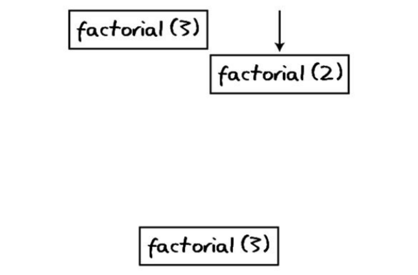
everythingitneedstodosincethere’sdatainthecallstack,whichindicatesthat
itisstillinthemiddleofrunningothermethodsthatitneedstocomplete.As
youwillrecall,stacksarerestrictedinthatwecanonlyinspectthetop(inother
words,thefinal)element.Sothenextthingthecomputerdoesispeekatthetop
elementofthecallstack,whichcurrentlyisfactorial(2).
Sincefactorial(2)isthelastiteminthecallstack,thatmeansthatfactorial(2)isthe
mostrecentlycalledmethodandthereforetheimmediatemethodthatneedsto
becompleted.
Thecomputerthenpopsfactorial(2)fromthecallstack
andcompletesrunningfactorial(2).
Thenthecomputerlooksatthecallstacktoseewhichmethoditneedsto
completenext,andsincethecallstackiscurrently
itpopsfactorial(3)fromthestackandcompletesit.
Atthispoint,thestackisempty,sothecomputerknowsit’sdoneexecutingall
ofthemethods,andtherecursioniscomplete.
Lookingbackatthisexamplefromabird’s-eyeview,you’llseethattheorderin
whichthecomputercalculatesthefactorialof3isasfollows:
1. factorial(3)iscalledfirst.
2. factorial(2)iscalledsecond.
3. factorial(1)iscalledthird.
4. factorial(1)iscompletedfirst.
5. factorial(2)iscompletedbasedontheresultoffactorial(1).
6. Finally,factorial(3)iscompletedbasedontheresultoffactorial(2).
Interestingly,inthecaseofinfiniterecursion(suchastheveryfirstexamplein
ourchapter),theprogramkeepsonpushingthesamemethodoverandover
againontothecallstack,untilthere’snomoreroominthecomputer’smemory
—andthiscausesanerrorknownasstackoverflow.
RecursioninAction
WhilepreviousexamplesoftheNASAcountdownandcalculatingfactorialscan
besolvedwithrecursion,theycanalsobeeasilysolvedwithclassicalloops.
Whilerecursionisinteresting,itdoesn’treallyprovideanadvantagewhen
solvingtheseproblems.
However,recursionisanaturalfitinanysituationwhereyoufindyourself
havingtorepeatanalgorithmwithinthesamealgorithm.Inthesecases,
recursioncanmakeformorereadablecode,asyou’reabouttosee.
Taketheexampleoftraversingthroughafilesystem.Let’ssaythatyouhavea
scriptthatdoessomethingwitheveryfileinsideofadirectory.However,you
don’twantthescripttoonlydealwiththefilesinsidetheonedirectory—you
wantittoactonallthefileswithinthesubdirectoriesofthedirectory,andthe
subdirectoriesofthesubdirectories,andsoon.
Let’screateasimpleRubyscriptthatprintsoutthenamesofallsubdirectories
withinagivendirectory.
deffind_directories(directory)
Dir.foreach(directory)do|filename|
ifFile.directory?("#{directory}/#{filename}")&&
filename!="."&&filename!=".."
puts"#{directory}/#{filename}"
end
end
end
#Callthefind_directoriesmethodonthecurrentdirectory:
find_directories(".")
Inthisscript,welookthrougheachfilewithinthegivendirectory.Ifthefileis
itselfasubdirectory(andisn’tasingleordoubleperiod,whichrepresentthe
currentandpreviousdirectories,respectively),weprintthesubdirectoryname.
Whilethisworkswell,itonlyprintsthenamesofthesubdirectoriesimmediately
withinthecurrentdirectory.Itdoesnotprintthenamesofthesubdirectories
withinthosesubdirectories.
Let’supdateourscriptsothatitcansearchoneleveldeeper:
deffind_directories(directory)
#Loopthroughouterdirectory:
Dir.foreach(directory)do|filename|
ifFile.directory?("#{directory}/#{filename}")&&
filename!="."&&filename!=".."
puts"#{directory}/#{filename}"
#Loopthroughinnersubdirectory:
Dir.foreach("#{directory}/#{filename}")do|inner_filename|
ifFile.directory?("#{directory}/#{filename}/#{inner_filename}")&&
inner_filename!="."&&inner_filename!=".."
puts"#{directory}/#{filename}/#{inner_filename}"
end
end
end
end
end
#Callthefind_directoriesmethodonthecurrentdirectory:
find_directories(".")
Now,everytimeourscriptdiscoversadirectory,itthenconductsanidentical
loopthroughthesubdirectoriesofthatdirectoryandprintsoutthenamesofthe
subdirectories.Butthisscriptalsohasitslimitations,becauseit’sonlysearching
twolevelsdeep.Whatifwewantedtosearchthree,four,orfivelevelsdeep?
Whatifwewantedtosearchasdeepasoursubdirectoriesgo?Thatwouldseem
tobeimpossible.
Andthisisthebeautyofrecursion.Withrecursion,wecanwriteascriptthat
goesarbitrarilydeep—andisalsosimple!
deffind_directories(directory)
Dir.foreach(directory)do|filename|
ifFile.directory?("#{directory}/#{filename}")&&
filename!="."&&filename!=".."
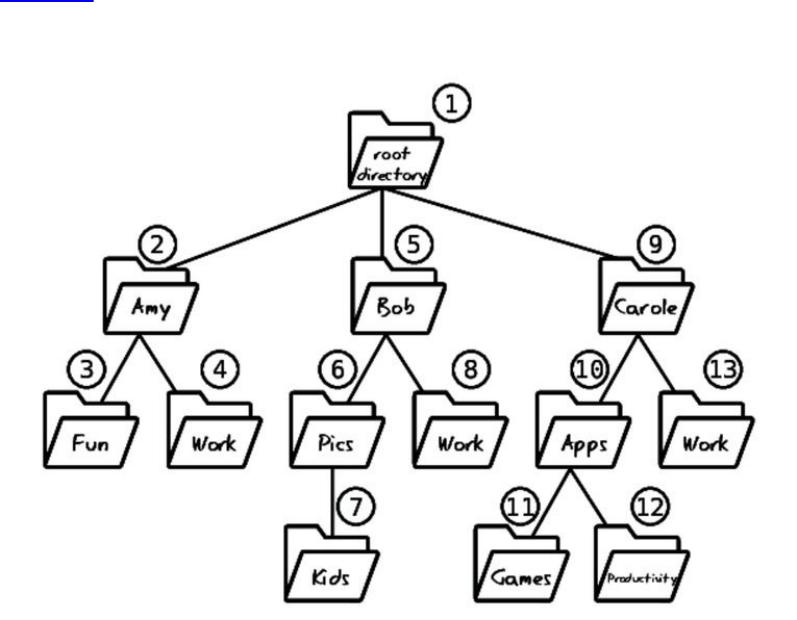
puts"#{directory}/#{filename}"
find_directories("#{directory}/#{filename}")
end
end
end
#Callthefind_directoriesmethodonthecurrentdirectory:
find_directories(".")
Asthisscriptencountersfilesthatarethemselvessubdirectories,itcallsthe
find_directoriesmethoduponthatverysubdirectory.Thescriptcanthereforedig
asdeepasitneedsto,leavingnosubdirectoryunturned.
Tovisuallyseehowthisalgorithmappliestoanexamplefilesystem,examinethe
diagram,whichspecifiestheorderinwhichthescripttraversesthe
subdirectories.
Notethatrecursioninavacuumdoesnotnecessarilyspeedupanalgorithm’s
efficiencyintermsofBigO.However,wewillseeinthefollowingchapterthat
recursioncanbeacorecomponentofalgorithmsthatdoesaffecttheirspeed.

WrappingUp
Asyou’veseeninthefilesystemexample,recursionisoftenagreatchoicefor
analgorithminwhichthealgorithmitselfdoesn’tknowontheoutsethowmany
levelsdeepintosomethingitneedstodig.
Nowthatyouunderstandrecursion,you’vealsounlockedasuperpower.You’re
abouttoencountersomereallyefficient—yetadvanced—algorithms,andmany
ofthemrelyontheprinciplesofrecursion.
Copyright©2017,ThePragmaticBookshelf.

Chapter10
RecursiveAlgorithmsforSpeed
We’veseenthatunderstandingrecursionunlocksallsortsofnewalgorithms,
suchassearchingthroughafilesystem.Inthischapter,we’regoingtolearnthat
recursionisalsothekeytoalgorithmsthatcanmakeourcoderunmuch,much
faster.
Inpreviouschapters,we’veencounteredanumberofsortingalgorithms,
includingBubbleSort,SelectionSort,andInsertionSort.Inreallife,however,
noneofthesemethodsareactuallyusedtosortarrays.Mostcomputerlanguages
havebuilt-insortingfunctionsforarraysthatsaveusthetimeandeffortfrom
implementingourown.Andinmanyoftheselanguages,thesortingalgorithm
thatisemployedunderthehoodisQuicksort.
Thereasonwe’regoingtodigintoQuicksorteventhoughit’sbuiltintomany
computerlanguagesisbecausebystudyinghowitworks,wecanlearnhowto
userecursiontogreatlyspeedupanalgorithm,andwecandothesameforother
practicalalgorithmsoftherealworld.
Quicksortisanextremelyfastsortingalgorithmthatisparticularlyefficientfor
averagescenarios.Whileinworst-casescenarios(thatis,inverselysorted
arrays),itperformssimilarlytoInsertionSortandSelectionSort,itismuch
fasterforaveragescenarios—whicharewhatoccurmostofthetime.
Quicksortreliesonaconceptcalledpartitioning,sowe’lljumpintothatfirst.
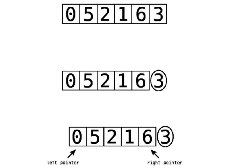
Partitioning
Topartitionanarrayistotakearandomvaluefromthearray—whichisthen
calledthepivot—andmakesurethateverynumberthatislessthanthepivot
endsuptotheleftofthepivot,andthateverynumberthatisgreaterthanthe
pivotendsuptotherightofthepivot.Weaccomplishpartitioningthrougha
simplealgorithmthatwillbedescribedinthefollowingexample.
Let’ssaywehavethefollowingarray:
Forconsistency’ssake,we’llalwaysselecttheright-mostvaluetobeourpivot
(althoughwecantechnicallychooseothervalues).Inthiscase,thenumber3is
ourpivot.Weindicatethisbycirclingit:
Wethenassign“pointers”—onetotheleft-mostvalueofthearray,andoneto
theright-mostvalueofthearray,excludingthepivotitself:
We’renowreadytobegintheactualpartition,whichfollowsthesesteps:
1. Theleftpointercontinuouslymovesonecelltotherightuntilitreachesa
valuethatisgreaterthanorequaltothepivot,andthenstops.
2. Then,therightpointercontinuouslymovesonecelltotheleftuntilit
reachesavaluethatislessthanorequaltothepivot,andthenstops.
3. Weswapthevaluesthattheleftandrightpointersarepointingto.
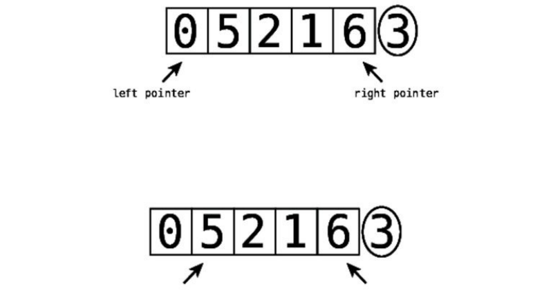
4. Wecontinuethisprocessuntilthepointersarepointingtotheverysame
valueortheleftpointerhasmovedtotherightoftherightpointer.
5. Finally,weswapthepivotwiththevaluethattheleftpointeriscurrently
pointingto.
Whenwe’redonewithapartition,wearenowassuredthatallvaluestotheleft
ofthepivotarelessthanthepivot,andallvaluestotherightofthepivotare
greaterthanit.Andthatmeansthatthepivotitselfisnowinitscorrectplace
withinthearray,althoughtheothervaluesarenotyetnecessarilycompletely
sorted.
Let’sapplythistoourexample:
Step#1:Comparetheleftpointer(nowpointingto0)toourpivot(thevalue3):
Since0islessthanthepivot,theleftpointermovesoninthenextstep.
Step#2:Theleftpointermoveson:
Wecomparetheleftpointer(the5)toourpivot.Isthe5lowerthanthepivot?
It’snot,sotheleftpointerstops,andwebegintoactivatetherightpointerinour
nextstep.
Step#3:Comparetherightpointer(6)toourpivot.Isthevaluegreaterthanthe
pivot?Itis,soourpointerwillmoveoninthenextstep.
Step#4:Therightpointermoveson:
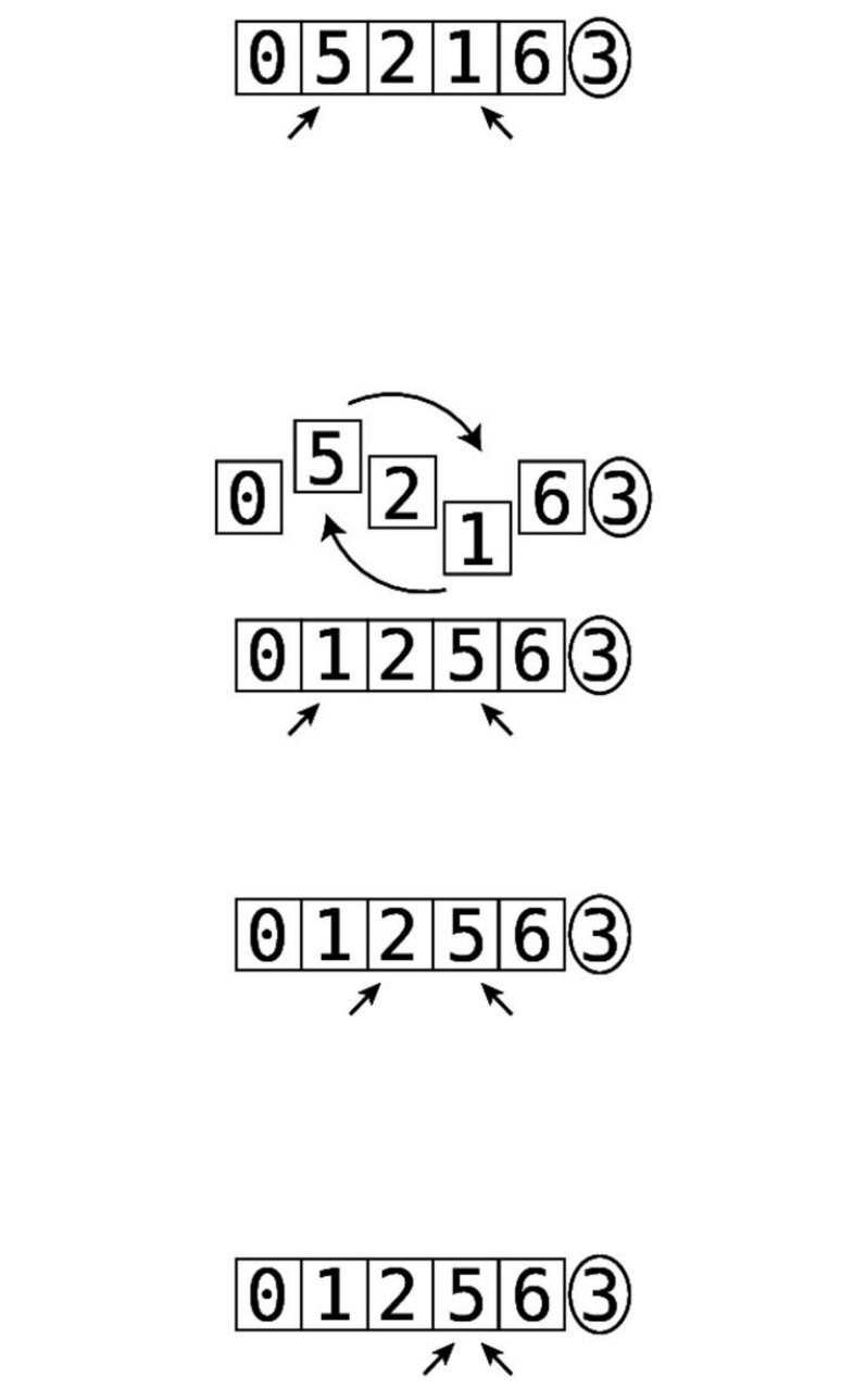
Wecomparetherightpointer(1)toourpivot.Isthevaluegreaterthanthepivot?
It’snot,soourrightpointerstops.
Step#5:Sincebothpointershavestopped,weswapthevaluesofthetwo
pointers:
Wethenactivateourleftpointeragaininthenextstep.
Step#6:Theleftpointermoveson:
Wecomparetheleftpointer(2)toourpivot.Isthevaluelessthanthepivot?It
is,sotheleftpointermoveson.
Step#7:Theleftpointermovesontothenextcell.Notethatatthispoint,both
theleftandrightpointersarepointingtothesamevalue:

Wecomparetheleftpointertoourpivot.Sinceourleftpointerispointingtoa
valuethatisgreaterthanourpivot,itstops.Atthispoint,sinceourleftpointer
hasreachedourrightpointer,wearedonewithmovingpointers.
Step#8:Forourfinalstepofthepartition,weswapthevaluethattheleftpointer
ispointingtowiththepivot:
Althoughourarrayisn’tcompletelysorted,wehavesuccessfullycompleteda
partition.Thatis,sinceourpivotwasthenumber3,allnumbersthatareless
than3aretoitsleft,whileallnumbersgreaterthan3aretoitsright.Thisalso
meansthatthe3isnowinitscorrectplacewithinthearray:
Below,we’veimplementedaSortableArrayclassinRubythatincludesapartition!
methodthatpartitionsthearrayaswe’vedescribed.
classSortableArray
attr_reader:array
definitialize(array)
@array=array
end
defpartition!(left_pointer,right_pointer)
#Wealwayschoosetheright-mostelementasthepivot
pivot_position=right_pointer
pivot=@array[pivot_position]
#Westarttherightpointerimmediatelytotheleftofthepivot
right_pointer-=1
whiletruedo
while@array[left_pointer]<pivotdo
left_pointer+=1
end
while@array[right_pointer]>pivotdo
right_pointer-=1
end
ifleft_pointer>=right_pointer
break
else
swap(left_pointer,right_pointer)
end
end
#Asafinalstep,weswaptheleftpointerwiththepivotitself
swap(left_pointer,pivot_position)
#Wereturntheleft_pointerforthesakeofthequicksortmethod
#whichwillappearlaterinthischapter
returnleft_pointer
end
defswap(pointer_1,pointer_2)
temp_value=@array[pointer_1]
@array[pointer_1]=@array[pointer_2]
@array[pointer_2]=temp_value
end
end
Notethatthepartition!methodacceptsthestartingpointsoftheleftandright
pointersasparameters,andreturnstheendpositionoftheleftpointeronceit’s
complete.ThisisallnecessarytoimplementQuicksort,aswe’llseenext.
Quicksort
TheQuicksortalgorithmreliesheavilyonpartitions.Itworksasfollows:
1. Partitionthearray.Thepivotisnowinitsproperplace.
2. Treatthesubarraystotheleftandrightofthepivotastheirownarrays,and
recursivelyrepeatsteps#1and#2.Thatmeansthatwe’llpartitioneach
subarray,andendupwithevensmallersubarraystotheleftandrightof
eachsubarray’spivot.Wethenpartitionthosesubarrays,andsoonandso
forth.
3. Whenwehaveasubarraythathaszerooroneelements,thatisourbase
caseandwedonothing.
Belowisaquicksort!methodthatwecanaddtotheprecedingSortableArrayclass
thatwouldsuccessfullycompleteQuicksort:
defquicksort!(left_index,right_index)
#basecase:thesubarrayhas0or1elements
ifright_index-left_index<=0
return
end
#Partitionthearrayandgrabthepositionofthepivot
pivot_position=partition!(left_index,right_index)
#Recursivelycallthisquicksortmethodonwhateveristotheleftofthe
pivot:
quicksort!(left_index,pivot_position-1)
#Recursivelycallthisquicksortmethodonwhateveristotherightofthe
pivot:
quicksort!(pivot_position+1,right_index)
end
Toseethisinaction,we’drunthefollowingcode:
array=[0,5,2,1,6,3]
sortable_array=SortableArray.new(array)
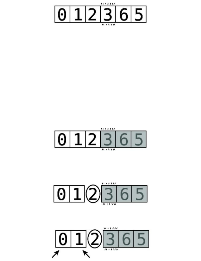
sortable_array.quicksort!(0,array.length-1)
psortable_array.array
Let’sreturntoourexample.Webeganwiththearrayof[0,5,2,1,6,3]andrana
singlepartitionontheentirearray.SinceQuicksortbeginswithsuchapartition,
thatmeansthatwe’realreadypartlythroughtheQuicksortprocess.Weleftoff
with:
Asyoucansee,thevalue3wasthepivot.Nowthatthepivotisinthecorrect
place,weneedtosortwhateveristotheleftandrightofthepivot.Notethatin
ourexample,itjustsohappensthatthenumberstotheleftofthepivotare
alreadysorted,butthecomputerdoesn’tknowthatyet.
Thenextstepafterthepartitionistotreateverythingtotheleftofthepivotasits
ownarrayandpartitionit.
We’llobscuretherestofthearrayfornow,aswe’renotfocusingonitatthe
moment:
Now,ofthis[0,1,2]subarray,we’llmaketheright-mostelementthepivot.So
thatwouldbethenumber2:
We’llestablishourleftandrightpointers:
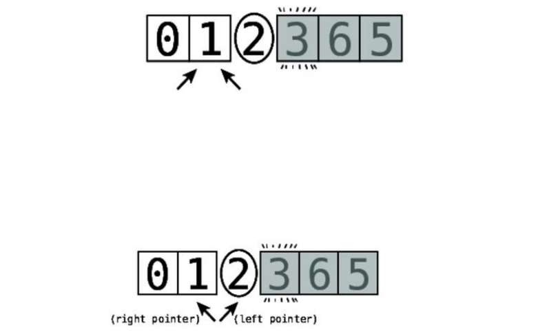
Andnowwe’rereadytopartitionthissubarray.Let’scontinuefromafterStep
#8,whereweleftoffpreviously.
Step#9:Wecomparetheleftpointer(0)tothepivot(2).Sincethe0islessthan
thepivot,wecontinuemovingtheleftpointer.
Step#10:Wemovetheleftpointeronecelltotheright,anditnowhappenstobe
pointingtothesamevaluethattherightpointerispointingto:
Wecomparetheleftpointertothepivot.Sincethevalue1islessthanthepivot,
wemoveon.
Step#11:Wemovetheleftpointeronecelltotheright,whichjusthappenstobe
thepivot:
Atthispoint,theleftpointerispointingtoavaluethatisequaltothepivot
(sinceitisthepivot!),andsotheleftpointerstops.
Step#12:Now,weactivatetherightpointer.However,sincetherightpointer’s
value(1)islessthanthepivot,itstaysstill.
Sinceourleftpointerhaspassedourrightpointer,we’redonemovingpointers
altogetherinthispartition.
Step#13:Asafinalstep,weswapthepivotwiththeleftpointer’svalue.Now,it
justsohappensthattheleftpointerispointingtothepivotitself,soweswapthe
pivotwithitself,whichresultsinnochangeatall.Atthispoint,thepartitionis
completeandthepivot(2)isnowinitscorrectspot:
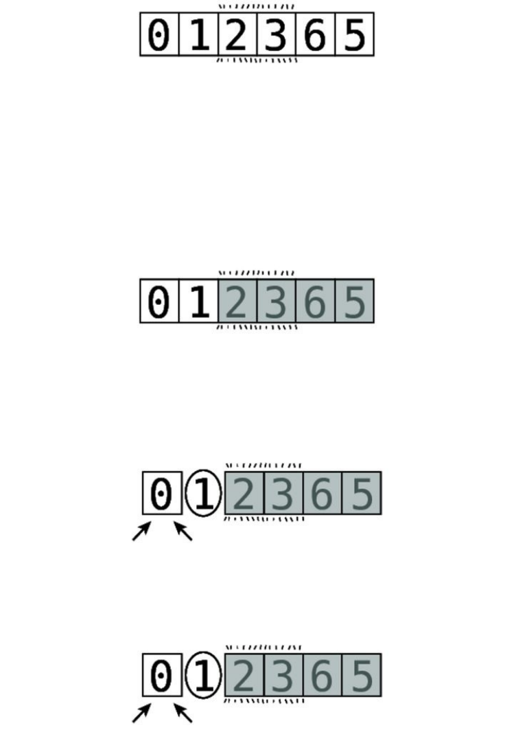
Wenowhaveasubarrayof[0,1]totheleftofthepivot(the2)andnosubarrayto
itsright.Thenextstepistorecursivelypartitionthesubarraytothepivot’sleft,
whichagainis[0,1].Wedon’thavetodealwithanysubarraytotherightofthe
pivotsincenosuchsubarrayexists.
Sinceallwe’llfocusoninthenextstepisthesubarray[0,1],we’llblockoutthe
restofthearraysoitlookslikethis:
Topartitionthesubarray[0,1],we’llmaketheright-mostelement(the1)the
pivot.Wherewillweputtheleftandrightpointers?Well,theleftpointerwill
pointtothe0,buttherightpointerwillalsopointtothe0,sincewealwaysstart
therightpointeroutatonecelltotheleftofthepivot.Thisgivesusthis:
We’renowreadytobeginthepartition.
Step#14:Wecomparetheleftpointer(0)withthepivot(1):
It’slessthanthepivot,sowemoveon.
Step#15:Weshifttheleftpointeronecelltotheright.Itnowpointstothepivot:
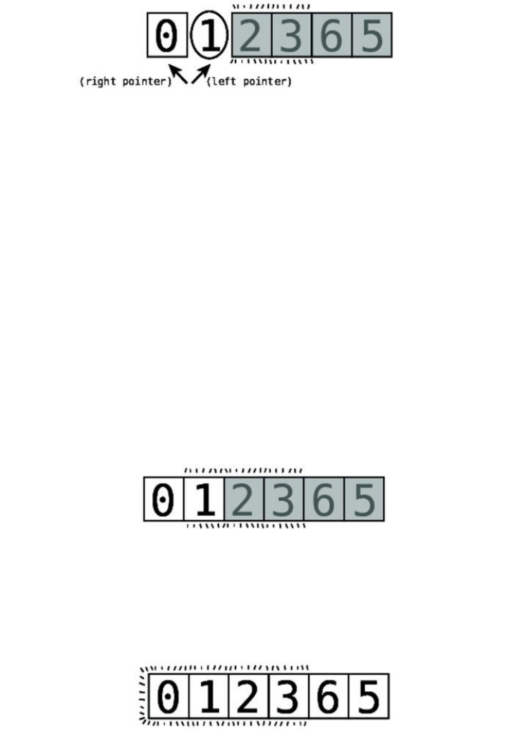
Sincetheleftpointer’svalue(1)isnotlowerthanthepivot(sinceitisthepivot),
theleftpointerstopsmoving.
Step#16:Wecomparetherightpointerwiththepivot.Sinceit’spointingtoa
valuethatislessthanthepivot,wedon’tmoveitanymore.Sincetheleftpointer
haspassedtherightpointer,we’redonemovingpointersforthispartition.We’re
readyforthefinalstep.
Step#17:Wenowswaptheleftpointerwiththepivot.Again,inthiscase,the
leftpointerisactuallypointingtothepivotitself,sotheswapdoesn’tactually
changeanything.Thepivotisnowinitsproperplace,andwe’redonewiththis
partition.
Thatleavesuswiththis:
Nextup,weneedtopartitionthesubarraytotheleftofthemostrecentpivot.In
thiscase,thatsubarrayis[0]—anarrayofjustoneelement.Anarrayofzeroor
oneelementsisourbasecase,sowedon’tdoanything.Theelementisjust
consideredtobeinitsproperplaceautomatically.Sonowwe’vegot:
Westartedoutbytreating3asourpivot,andpartitioningthesubarraytoitsleft
([0,1,2]).Aspromised,wenowneedtocomebacktopartitioningthesubarrayto
therightofthe3,whichis[6,5].
We’llobscurethe[0,1,2,3],sincewe’vealreadysortedthose,andnowwe’re
onlyfocusingonthe[6,5]:
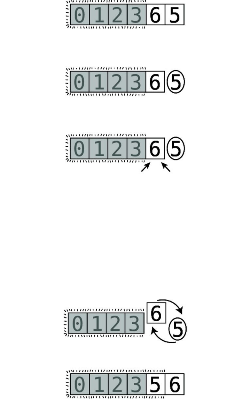
Inthenextpartition,we’lltreattheright-mostelement(the5)asthepivot.That
givesus:
Whensettingupournextpartition,ourleftandrightpointersbothendup
pointingtothe6:
Step#18:Wecomparetheleftpointer(6)withthepivot(5).Since6isgreater
thanthepivot,theleftpointerdoesn’tmovefurther.
Step#19:Therightpointerispointingtothe6aswell,sowouldtheoretically
moveontothenextcelltotheleft.However,therearenomorecellstotheleft
ofthe6,sotherightpointerstopsmoving.Sincetheleftpointerhasreachedthe
rightpointer,we’redonemovingpointersaltogetherforthispartition.That
meanswe’rereadyforthefinalstep.
Step#20:Weswapthepivotwiththevalueoftheleftpointer:
Ourpivot(5)isnowinitscorrectspot,leavinguswith:

Nextup,wetechnicallyneedtorecursivelypartitionthesubarraytotheleftand
rightofthe[5,6]subarray.Sincethereisnosubarraytoitsleft,thatmeansthat
weonlyneedtopartitionthesubarraytotheright.Sincethesubarraytotheright
ofthe5isasingleelementof[6],that’sourbasecaseandwedonothing—the6
isautomaticallyconsideredtobeinitsproperplace:
Andwe’redone!
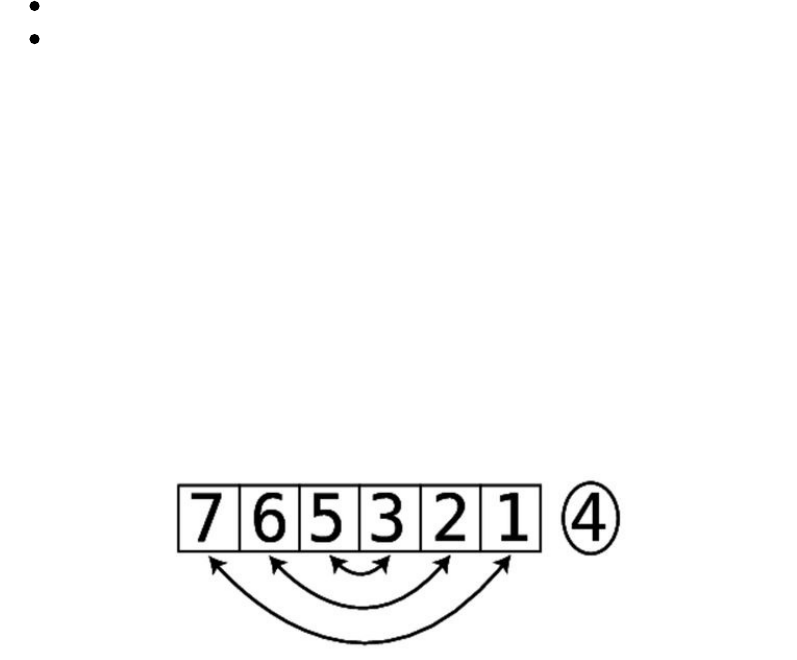
TheEfficiencyofQuicksort
TofigureouttheefficiencyofQuicksort,let’sfirstdeterminetheefficiencyofa
partition.Whenbreakingdownthestepsofapartition,we’llnotethatapartition
consistsoftwotypesofsteps:
Comparisons:Wecompareeachvaluetothepivot.
Swaps:Whenappropriate,weswapthevaluesbeingpointedtobytheleft
andrightpointers.
EachpartitionhasatleastNcomparisons—thatis,wecompareeachelementof
thearraywiththepivot.Thisistruebecauseapartitionalwayshastheleftand
rightpointersmovethrougheachcelluntiltheleftandrightpointersreacheach
other.
Thenumberofswapsdependsonhowthedataissorted.Eachpartitionhasat
leastoneswap,andthemostswapsthatapartitioncanhavewouldbeN/2,
sinceevenifwe’dswapeverypossiblevalue,we’dstillbeswappingtheones
fromthelefthalfwiththeonesfromtherighthalf.Seethisdiagram:
Now,forrandomlysorteddata,therewouldberoughlyhalfofN/2swaps,orN
/4swaps.SowithNcomparisonsandN/4,we’dsaythereareabout1.25N
steps.InBigONotation,weignoreconstants,sowe’dsaythatapartitionrunsin
O(N)time.
Sothat’stheefficiencyofasinglepartition.ButQuicksortinvolvesmany
partitionsonarraysandsubarraysofdifferentsizes,soweneedtodoafurther
analysistodeterminetheefficiencyofQuicksort.
Tovisualizethismoreeasily,hereisadiagramdepictingatypicalQuicksorton
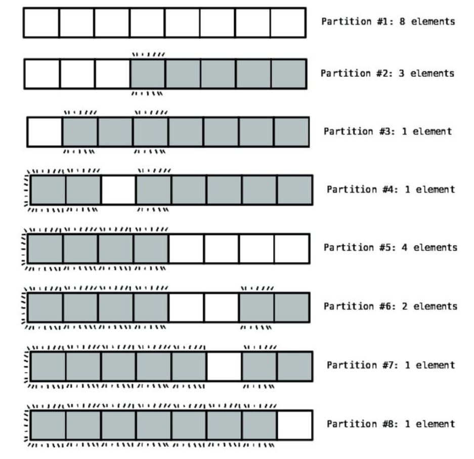
anarrayofeightelementsfromabird’s-eyeview.Inparticular,thediagram
showshowmanyelementseachpartitionactsupon.We’veleftouttheactual
numbersfromthearraysincetheexactnumbersdon’tmatter.Notethatinthe
diagram,theactivesubarrayisthegroupofcellsthatarenotgrayedout.
Wecanseethatwehaveeightpartitions,buteachpartitiontakesplaceon
subarraysofvarioussizes.Now,whereasubarrayisjustoneelement,that’sour
basecase,andwedon’tperformanyswapsorcomparisons,sothesignificant
partitionsaretheonesthattakeplaceonsubarraysoftwoelementsormore.
Sincethisexamplerepresentsanaveragecase,let’sassumethateachpartition
takesapproximately1.25Nsteps.Sothatgivesus:
8elements*1.25steps=10steps
3elements*1.25steps=3.75steps
4elements*1.25steps=5steps
+2elements*1.25steps=2.5steps
__________
Total=Around21steps
Ifwedothisanalysisforarraysofvarioussizes,we’llseethatforNelements,
thereareaboutN*logNsteps.TogetafeelforN*logN,seethefollowing
table:
N logN N*logN
4 2 8
8 3 24
16 4 64
Intheprecedingexample,foranarrayofsize8,Quicksorttookabout21steps,
whichisaboutwhat8*log8is(24).Thisisthefirsttimewe’reencountering
suchanalgorithm,andinBigO,it’sexpressedasO(NlogN).
Now,it’snotacoincidencethatthenumberofstepsinQuicksortjusthappensto
alignwithN*logN.IfwethinkaboutQuicksortmorebroadly,wecanseewhy
itisthisway:
WhenwebeginQuicksort,wepartitiontheentirearray.Assumingthatthepivot
endsupsomewhereinthemiddleofthearray—whichiswhathappensinthe
averagecase—wethenbreakupthetwohalvesofthearrayandpartitioneach
half.Wethentakeeachofthosehalves,breakthemupintoquarters,andthen
partitioneachquarter.Andsoonandsoforth.
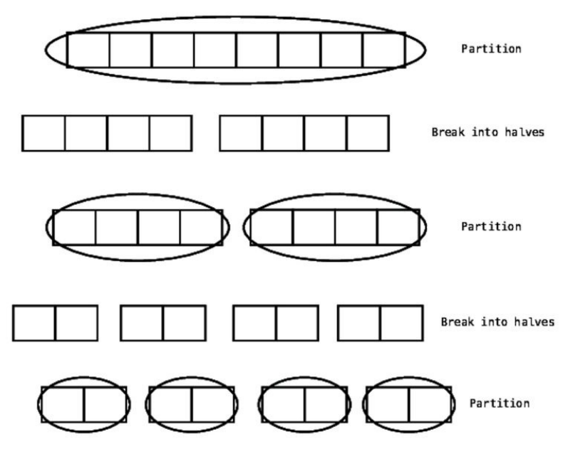
Inessence,wekeeponbreakingdowneachsubarrayintohalvesuntilwereach
subarrayswithelementsof1.Howmanytimescanwebreakupanarrayinthis
way?ForanarrayofN,wecanbreakitdownlogNtimes.Thatis,anarrayof8
canbebrokeninhalfthreetimesuntilwereachelementsof1.You’realready
familiarwiththisconceptfrombinarysearch.
Now,foreachroundinwhichwebreakdowneachsubarrayintotwohalves,we
thenpartitionalltheelementsfromtheoriginalarrayoveragain.Seethis
diagram:
SincewecanbreakuptheoriginalarrayintoequalsubarrayslogNtimes,and
foreachtimewebreakthemup,wemustrunpartitionsonallNcellsfromthe
originalarray,weendupwithaboutN*logNsteps.
Formanyotheralgorithmswe’veencountered,thebestcasewasonewherethe
arraywasalreadysorted.WhenitcomestoQuicksort,however,thebest-case
scenarioisoneinwhichthepivotalwaysendsupsmackinthemiddleofthe
subarrayafterthepartition.
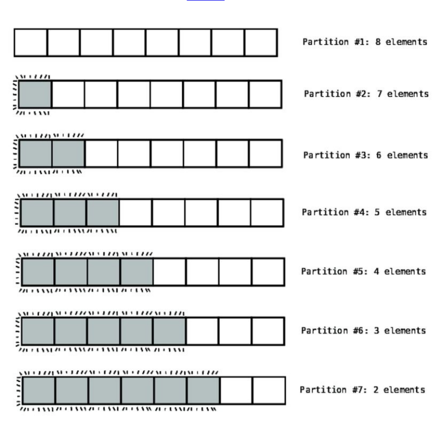
Worst-CaseScenario
Theworst-casescenarioforQuicksortisoneinwhichthepivotalwaysendsup
ononesideofthesubarrayinsteadofthemiddle.Thiscanhappeninseveral
cases,includingwherethearrayisinperfectascendingordescendingorder.The
visualizationforthisprocessisshown.
While,inthiscase,eachpartitiononlyinvolvesoneswap,weloseoutbecause
ofthemanycomparisons.Inthefirstexample,whenthepivotalwaysendedup
towardsthemiddle,eachpartitionafterthefirstonewasconductedonrelatively
smallsubarrays(thelargestsubarrayhadasizeof4).Inthisexample,however,
thefirstfivepartitionstakeplaceonsubarraysofsize4orgreater.Andeachof
thesepartitionshaveasmanycomparisonsasthereareelementsinthesubarray.
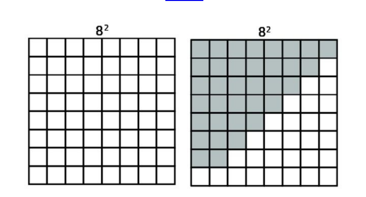
Sointhisworst-casescenario,wehavepartitionsof8+7+6+5+4+3+2
elements,whichwouldyieldatotalof35comparisons.
Toputthisalittlemoreformulaically,we’dsaythatforNelements,thereareN
+(N-1)+(N-2)+(N-3)…+2steps.ThisalwayscomesouttobeaboutN2/
2steps,asyoucanseeinthefigures.
SinceBigOignoresconstants,we’dsaythatinaworst-casescenario,Quicksort
hasanefficiencyofO(N2).
Nowthatwe’vegotQuicksortdown,let’scompareitwithInsertionSort:
Bestcase Averagecase Worstcase
InsertionSort O(N) O(N2) O(N2)
Quicksort O(NlogN) O(NlogN) O(N2)
Wecanseethattheyhaveidenticalworst-casescenarios,andthatInsertionSort
isactuallyfasterthanQuicksortforabest-casescenario.However,thereason
whyQuicksortissomuchmoresuperiorthanInsertionSortisbecauseofthe
averagescenario—which,again,iswhathappensmostofthetime.Foraverage
cases,InsertionSorttakesawhoppingO(N2),whileQuicksortismuchfasterat
O(NlogN).
Thefollowinggraphdepictsvariousefficienciessidebyside:
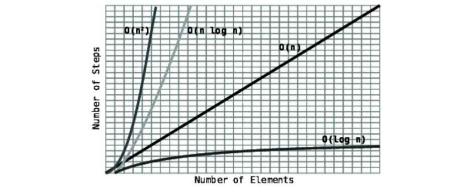
BecauseofQuicksort’ssuperiorityinaveragecircumstances,manylanguages
implementtheirownsortingfunctionsbyusingQuicksortunderthehood.
Becauseofthis,it’sunlikelythatyou’llbeimplementingQuicksortyourself.
However,thereisaverysimilaralgorithmthatcancomeinhandyforpractical
cases—andit’scalledQuickselect.
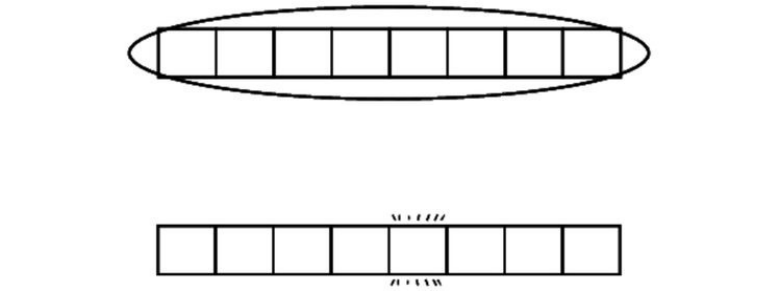
Quickselect
Let’ssaythatyouhaveanarrayinrandomorder,andyoudonotneedtosortit,
butyoudowanttoknowthetenth-lowestvalueinthearray,orthefifth-highest.
Thiscanbeusefulifwehadalotoftestgradesandwantedtoknowwhatthe
25thpercentilewas,orifwewantedtofindthemediangrade.
Theobviouswaytosolvethiswouldbetosorttheentirearrayandthenjumpto
theappropriatecell.
EvenwerewetouseafastsortingalgorithmlikeQuicksort,thisalgorithm
wouldtakeatleastO(NlogN)foraveragecases,andwhilethatisn’tbad,we
candoevenbetterwithabrilliantlittlealgorithmknownasQuickselect.
QuickselectreliesonpartitioningjustlikeQuicksort,andcanbethoughtofasa
hybridofQuicksortandbinarysearch.
Aswe’veseenearlierinthischapter,afterapartition,thepivotvalueendsupin
theappropriatespotinthearray.Quickselecttakesadvantageofthisinthe
followingway:
Let’ssaythatwehaveanarrayofeightvalues,andwewanttofindthesecond-
to-lowestvaluewithinthearray.
First,wepartitiontheentirearray:
Afterthepartition,thepivotwillhopefullyendupsomewheretowardsthe
middleofthearray:
Thispivotisnowinitscorrectspot,andsinceit’sinthefifthcell,wenowknow
whichvalueisthefifth-lowestvaluewithinthearray.Now,we’relookingforthe
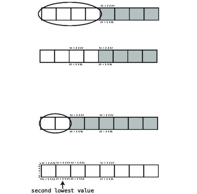
second-lowestvalue.Butwealsonowknowthatthesecond-lowestvalueis
somewheretotheleftofthepivot.Wecannowignoreeverythingtotherightof
thepivot,andfocusontheleftsubarray.ItisinthisrespectthatQuickselectis
similartobinarysearch:wekeepdividingthearrayinhalf,andfocusonthehalf
inwhichweknowthevaluewe’reseekingforwillbefound.
Next,wepartitionthesubarraytotheleftofthepivot:
Let’ssaythatthenewpivotofthissubarrayendsupthethirdcell:
Wenowknowthatthevalueinthethirdcellisinitscorrectspot,meaningthat
it’sthethird-to-lowestvalueinthearray.Bydefinition,then,thesecond-to-
lowestvaluewillbesomewheretoitsleft.Wecannowpartitionthesubarrayto
theleftofthethirdcell:
Afterthisnextpartition,thelowestandsecond-lowestvalueswillendupintheir
correctspotswithinthearray:
Wecanthengrabthevaluefromthesecondcellandknowwithconfidencethat
it’sthesecond-lowestvalueintheentirearray.Oneofthebeautifulthingsabout
Quickselectisthatwecanfindthecorrectvaluewithouthavingtosorttheentire
array.
WithQuicksort,foreverytimewecutthearrayinhalf,weneedtore-partition
everysinglecellfromtheoriginalarray,givingusO(NlogN).With
Quickselect,ontheotherhand,foreverytimewecutthearrayinhalf,weonly
needtopartitiontheonehalfthatwecareabout—thehalfinwhichweknowour
valueistobefound.
WhenanalyzingtheefficiencyofQuickselect,we’llseethatit’sO(N)for
averagescenarios.RecallthateachpartitiontakesaboutNstepsforthesubarray
it’srunupon.Thus,forQuickselectonanarrayofeightelements,werun
partitionsthreetimes:onanarrayofeightelements,onasubarrayoffour
elements,andonasubarrayoftwoelements.Thisisatotalof8+4+2=14
steps.Soanarrayof8elementsyieldsroughly14steps.
Foranarrayof64elements,werun64+32+16+8+4+2=126steps.For
128elements,wewouldhave254steps.Andfor256elements,wewouldhave
510steps.
Ifweweretoformulatethis,wewouldsaythatforNelements,wewouldhave
N+(N/2)+(N/4)+(N/8)+…2steps.Thisalwaysturnsouttoberoughly2N
steps.SinceBigOignoresconstants,wewouldsaythatQuickselecthasan
efficiencyofO(N).
Below,we’veimplementedaquickselect!methodthatcanbedroppedintothe
SortableArrayclassdescribedpreviously.You’llnotethatit’sverysimilartothe
quicksort!method:
defquickselect!(kth_lowest_value,left_index,right_index)
#Ifwereachabasecase-thatis,thatthesubarrayhasonecell,
#weknowwe'vefoundthevaluewe'relookingfor
ifright_index-left_index<=0
return@array[left_index]
end
#Partitionthearrayandgrabthepositionofthepivot
pivot_position=partition!(left_index,right_index)
ifkth_lowest_value<pivot_position
quickselect!(kth_lowest_value,left_index,pivot_position-1)
elsifkth_lowest_value>pivot_position
quickselect!(kth_lowest_value,pivot_position+1,right_index)
else#kth_lowest_value==pivot_position
#ifafterthepartition,thepivotpositionisinthesamespot
#asthekthlowestvalue,we'vefoundthevaluewe'relookingfor
return@array[pivot_position]
end
end
Ifyouwantedtofindthesecond-to-lowestvalueofanunsortedarray,you’drun
thefollowingcode:
array=[0,50,20,10,60,30]
sortable_array=SortableArray.new(array)
psortable_array.quickselect!(1,0,array.length-1)
Thefirstargumentofthequickselect!methodacceptsthepositionthatyou’re
lookingfor,startingatindex0.We’veputina1torepresentthesecond-to-
lowestvalue.

WrappingUp
TheQuicksortandQuickselectalgorithmsarerecursivealgorithmsthatpresent
beautifulandefficientsolutionstothornyproblems.They’regreatexamplesof
howanon-obviousbutwell-thought-outalgorithmcanboostperformance.
Algorithmsaren’ttheonlythingsthatarerecursive.Datastructurescanbe
recursiveaswell.Thedatastructuresthatwewillencounterinthenextfew
chapters—linkedlist,binarytree,andgraph—usetheirrecursivenaturesto
allowforspeedydataaccessintheirowningeniousways.
Copyright©2017,ThePragmaticBookshelf.

Chapter11
Node-BasedDataStructures
Forthenextseveralchapters,we’regoingtoexploreavarietyofdatastructures
thatallbuilduponasingleconcept—thenode.Node-baseddatastructuresoffer
newwaystoorganizeandaccessdatathatprovideanumberofmajor
performanceadvantages.
Inthischapter,we’regoingtoexplorethelinkedlist,whichisthesimplestnode-
baseddatastructureandthefoundationforthefuturechapters.You’realsogoing
todiscoverthatlinkedlistsseemalmostidenticaltoarrays,butcomewiththeir
ownsetoftrade-offsinefficiencythatcangiveusaperformanceboostfor
certainsituations.
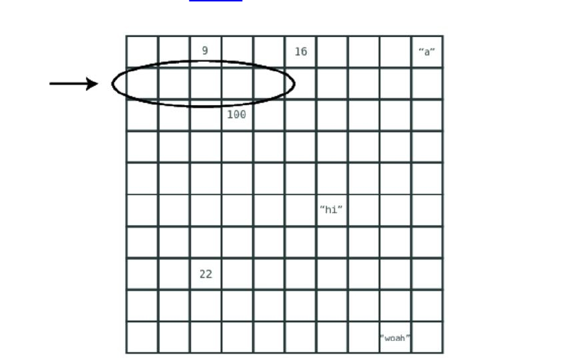
LinkedLists
Alinkedlistisadatastructurethatrepresentsalistofitems,justlikeanarray.In
fact,inanyapplicationinwhichyou’reusinganarray,youcouldprobablyusea
linkedlistinstead.Underthehood,however,linkedlistsareimplemented
differentlyandcanhavedifferentperformanceinvaryingsituations.
Asmentionedinourfirstchapter,memoryinsideacomputerexistsasagiantset
ofcellsinwhichbitsofdataarestored.Whencreatinganarray,yourcodefinds
acontiguousgroupofemptycellsinmemoryanddesignatesthemtostoredata
foryourapplicationasshown.
Wealsoexplainedtherethatthecomputerhastheabilitytojumpstraighttoany
indexwithinthearray.Ifyouwrotecodethatsaid,“Lookupthevalueatindex
4,”yourcomputercouldlocatethatcellinasinglestep.Again,thisisbecause
yourprogramknowswhichmemoryaddressthearraystartsat—say,memory
address1000—andthereforeknowsthatifitwantstolookupindex4,itshould
simplyjumptomemoryaddress1004.
Linkedlists,ontheotherhand,donotconsistofabunchofmemorycellsina
row.Instead,theyconsistofabunchofmemorycellsthatarenotnexttoeach
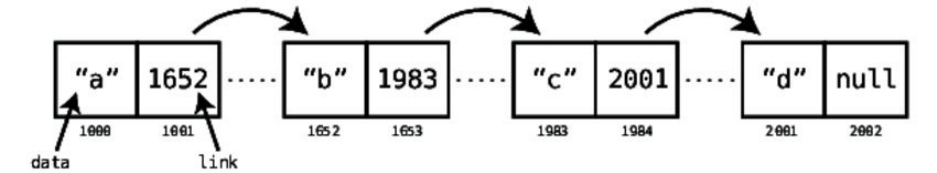
other,butcanbespreadacrossmanydifferentcellsacrossthecomputer’s
memory.Thesecellsthatarenotadjacenttoeachotherareknownasnodes.
Thebigquestionis:ifthesenodesarenotnexttoeachother,howdoesthe
computerknowwhichnodesarepartofthesamelinkedlist?
Thisisthekeytothelinkedlist:inadditiontothedatastoredwithinthenode,
eachnodealsostoresthememoryaddressofthenextnodeinthelinkedlist.
Thisextrapieceofdata—thispointertothenextnode’smemoryaddress—is
knownasalink.Hereisavisualdepictionofalinkedlist:
Inthisexample,wehavealinkedlistthatcontainsfourpiecesofdata:"a","b",
"c",and"d".However,ituseseightcellsofmemorytostorethisdata,because
eachnodeconsistsoftwomemorycells.Thefirstcellholdstheactualdata,
whilethesecondcellservesasalinkthatindicateswhereinmemorythenext
nodebegins.Thefinalnode’slinkcontainsnullsincethelinkedlistendsthere.
Forourcodetoworkwithalinkedlist,allitreallyneedstoknowiswherein
memorythefirstnodebegins.Sinceeachnodecontainsalinktothenextnode,
iftheapplicationisgiventhefirstnodeofthelinkedlist,itcanpiecetogether
therestofthelistbyfollowingthelinkofthefirstnodetothesecondnode,and
thelinkfromthesecondnodetothethirdnode,andsoon.
Oneadvantageofalinkedlistoveranarrayisthattheprogramdoesn’tneedto
findabunchofemptymemorycellsinarowtostoreitsdata.Instead,the
programcanstorethedataacrossmanycellsthatarenotnecessarilyadjacentto
eachother.
ImplementingaLinkedList
Let’simplementalinkedlistusingRuby.We’llusetwoclassestoimplement
this:NodeandLinkedList.Let’screatetheNodeclassfirst:
classNode
attr_accessor:data,:next_node
definitialize(data)
@data=data
end
end
TheNodeclasshastwoattributes:datacontainsthevaluethatthenodeismeant
tohold,whilenext_nodecontainsthelinktothenextnodeinthelist.Wecanuse
thisclassasfollows:
node_1=Node.new("once")
node_2=Node.new("upon")
node_1.next_node=node_2
node_3=Node.new("a")
node_2.next_node=node_3
node_4=Node.new("time")
node_3.next_node=node_4
Withthiscode,we’vecreatedalistoffournodesthatserveasalistcontaining
thestrings"once","upon","a",and"time".
Whilewe’vebeenabletocreatethislinkedlistwiththeNodeclassalone,we
needaneasywaytotellourprogramwherethelinkedlistbegins.Todothis,
we’llcreateaLinkedListclassaswell.Here’stheLinkedListclassinitsbasicform:
classLinkedList
attr_accessor:first_node
definitialize(first_node)
@first_node=first_node
end
end
Withthisclass,wecantellourprogramaboutthelinkedlistwecreated
previouslyusingthefollowingcode:
list=LinkedList.new(node_1)
ThisLinkedListactsasahandleonthelinkedlistbypointingtoitsfirstnode.
Nowthatweknowwhatalinkedlistis,let’smeasureitsperformanceagainsta
typicalarray.We’lldothisbyanalyzingthefourclassicoperations:reading,
searching,insertion,anddeletion.
Reading
Wenotedpreviouslythatwhenreadingavaluefromanarray,thecomputercan
jumptotheappropriatecellinasinglestep,whichisO(1).Thisisnotthecase,
however,withalinkedlist.
Ifyourprogramwantedtoreadthevalueatindex2ofalinkedlist,thecomputer
couldnotlookitupinonestep,becauseitwouldn’timmediatelyknowwhereto
finditinthecomputer’smemory.Afterall,eachnodeofalinkedlistcouldbe
anywhereinmemory!Instead,alltheprogramknowsisthememoryaddressof
thefirstnodeofthelinkedlist.Tofindindex2(whichisthethirdnode),the
programmustbeginlookingupindex0ofthelinkedlist,andthenfollowthe
linkatindex0toindex1.Itmustthenagainfollowthelinkatindex1toindex
2,andfinallyinspectthevalueatindex2.
Let’simplementthisoperationinsideourLinkedListclass:
classLinkedList
attr_accessor:first_node
definitialize(first_node)
@first_node=first_node
end
defread(index)
#Webeginatthefirstnodeofthelist:
current_node=first_node
current_index=0
whilecurrent_index<indexdo
#Wekeepfollowingthelinksofeachnodeuntilwegettothe
#indexwe'relookingfor:
current_node=current_node.next_node
current_index+=1
#Ifwe'repasttheendofthelist,thatmeansthe
#valuecannotbefoundinthelist,soreturnnil:
returnnilunlesscurrent_node
end
returncurrent_node.data
end
end
Wecanthenlookupaparticularindexwithinthelistwith:
list.read(3)
Ifweaskacomputertolookupthevalueataparticularindex,theworst-case
scenariowouldbeifwe’relookingupthelastindexinourlist.Insuchacase,
thecomputerwilltakeNstepstolookupthisindex,sinceitneedstostartatthe
firstnodeofthelistandfolloweachlinkuntilitreachesthefinalnode.Since
BigONotationexpressestheworst-casescenariounlessexplicitlystated
otherwise,wewouldsaythatreadingalinkedlisthasanefficiencyofO(N).
Thisisasignificantdisadvantageincomparisonwitharraysinwhichreadsare
O(1).
Searching
Arraysandlinkedlistshavethesameefficiencyforsearch.Remember,
searchingislookingforaparticularpieceofdatawithinthelistandgettingits
index.Withbotharraysandlinkedlists,theprogramneedstostartatthefirst
cellandlookthrougheachandeverycelluntilitfindsthevalueit’ssearching
for.Inaworst-casescenario—wherethevaluewe’researchingforisinthefinal
cellornotinthelistaltogether—itwouldtakeO(N)steps.
Here’showwe’dimplementthesearchoperation:
classLinkedList
attr_accessor:first_node
#restofcodeomittedhere...
defindex_of(value)
#Webeginatthefirstnodeofthelist:
current_node=first_node
current_index=0
begin
#Ifwefindthedatawe'relookingfor,wereturnit:
ifcurrent_node.data==value
returncurrent_index
end
#Otherwise,wemoveonthenextnode:
current_node=current_node.next_node
current_index+=1
endwhilecurrent_node
#Ifwegetthroughtheentirelist,withoutfindingthe
#data,wereturnnil:
returnnil
end
end
Wecanthensearchforanyvaluewithinthelistusing:
list.index_of("time")
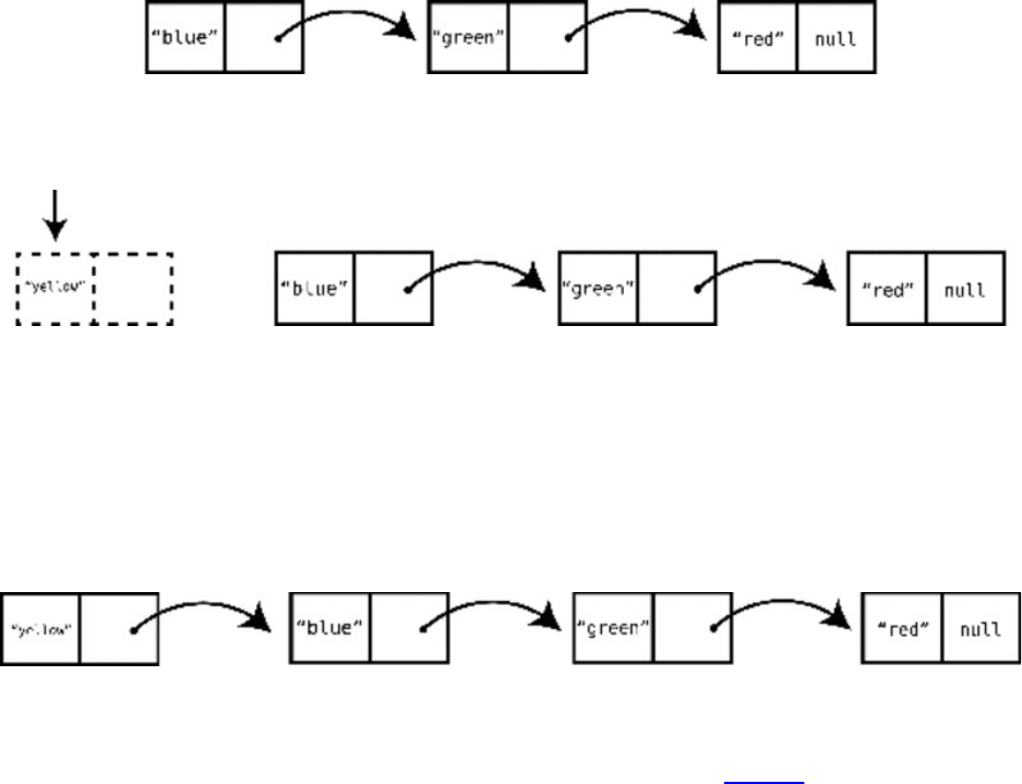
Insertion
Insertionisoneoperationinwhichlinkedlistscanhaveadistinctadvantage
overarraysincertainsituations.Recallthattheworst-casescenarioforinsertion
intoanarrayiswhentheprograminsertsdataintoindex0,becauseitthenhasto
shifttherestofthedataonecelltotheright,whichendsupyieldingan
efficiencyofO(N).Withlinkedlists,however,insertionatthebeginningofthe
listtakesjustonestep—whichisO(1).Let’sseewhy.
Saythatwehadthefollowinglinkedlist:
Ifwewantedtoadd"yellow"tothebeginningofthelist,allwewouldhavetodo
iscreateanewnodeandhaveitlinktothenodecontaining"blue":
Incontrastwiththearray,therefore,alinkedlistprovidestheflexibilityof
insertingdatatothefrontofthelistwithoutrequiringtheshiftingofanyother
data.
Thetruthisthat,theoretically,insertingdataanywherewithinalinkedlisttakes
justonestep,butthere’sonegotcha.Let’ssaythatwenowhavethislinkedlist:
Andsaythatwewanttoinsert"purple"atindex2(whichwouldbebetween
"blue"and"green").Theactualinsertiontakesonestep,sincewecreateanew
nodeandmodifythelinksoftheblueandgreennodesasshown.
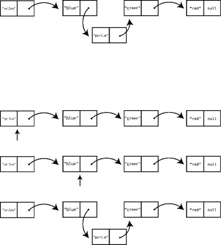
However,forthecomputertodothis,itfirstneedstofindthenodeatindex1
("blue")soitcanmodifyitslinktopointtothenewlycreatednode.Aswe’ve
seen,though,readingfromalinkedlistalreadytakesO(N).Let’sseethisin
action.
Weknowthatwewanttoaddanewnodeafterindex1.Sothecomputerneeds
tofindindex1ofthelist.Todothis,wemuststartatthebeginningofthelist:
Wethenaccessthenextnodebyfollowingthefirstlink:
Nowthatwe’vefoundindex1,wecanfinallyaddthenewnode:
Inthiscase,adding"purple"tookthreesteps.Ifweweretoaddittotheendof
ourlist,itwouldtakefivesteps:fourstepstofindindex3,andonesteptoinsert
thenewnode.
Therefore,insertingintothemiddleofalinkedlisttakesO(N),justasitdoesfor
anarray.
Interestingly,ouranalysisshowsthatthebest-andworst-casescenariosfor
arraysandlinkedlistsaretheoppositeofoneanother.Thatis,insertingatthe
beginningisgreatforlinkedlists,butterribleforarrays.Andinsertingattheend
isanarray’sbest-casescenario,buttheworstcasewhenitcomestoalinkedlist.
Thefollowingtablebreaksthisalldown:
Scenario Array Linkedlist
Insertatbeginning Worstcase Bestcase
Insertatmiddle Averagecase Averagecase
Insertatend Bestcase Worstcase
Here’showwecanimplementtheinsertoperationinourLinkedListclass:
classLinkedList
attr_accessor:first_node
#restofcodeomittedhere...
definsert_at_index(index,value)
current_node=first_node
current_index=0
#First,wefindtheindeximmediatelybeforewherethe
#newnodewillgo:
whilecurrent_index<indexdo
current_node=current_node.next_node
current_index+=1
end
#Wecreatethenewnode:
new_node=Node.new(value)
new_node.next_node=current_node.next_node
#Wemodifythelinkofthepreviousnodetopointto
#ournewnode:
current_node.next_node=new_node
end
end
Deletion
Deletionisverysimilartoinsertionintermsofefficiency.Todeleteanodefrom
thebeginningofalinkedlist,allweneedtodoisperformonestep:wechange
thefirst_nodeofthelinkedlisttonowpointtothesecondnode.
Let’sreturntoourexampleofthelinkedlistcontainingthevalues"once","upon",
"a",and"time".Ifwewantedtodeletethevalue"once",wewouldsimplychange
thelinkedlisttobeginat"upon":
list.first_node=node_2
Contrastthiswithanarrayinwhichdeletingthefirstelementmeansshiftingall
remainingdataonecelltotheleft,anefficiencyofO(N).
Whenitcomestodeletingthefinalnodeofalinkedlist,theactualdeletiontakes
onestep—wejusttakethesecond-to-lastnodeandmakeitslinknull.However,it
takesNstepstofirstgettothesecond-to-lastnode,sinceweneedtostartatthe
beginningofthelistandfollowthelinksuntilwereachit.
Thefollowingtablecontraststhevariousscenariosofdeletionforbotharrays
andlinkedlists.Notehowit’sidenticaltoinsertion:
Situation Array Linkedlist
Deleteatbeginning Worstcase Bestcase
Deleteatmiddle Averagecase Averagecase
Deleteatend Bestcase Worstcase
Todeletefromthemiddleofthelist,thecomputermustmodifythelinkofthe
precedingnode.Thefollowingexamplewillmakethisclear.
Let’ssaythatwewanttodeletethevalueatindex2("purple")fromtheprevious
linkedlist.Thecomputerfindsindex1andswitchesitslinktopointtothe
"green"node:
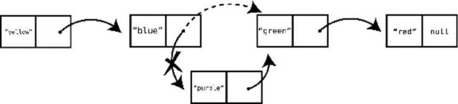
Here’swhatthedeleteoperationwouldlooklikeinourclass:
classLinkedList
attr_accessor:first_node
#restofcodeomittedhere...
defdelete_at_index(index)
current_node=first_node
current_index=0
#First,wefindthenodeimmediatelybeforetheonewe
#wanttodeleteandcallitcurrent_node:
whilecurrent_index<index-1do
current_node=current_node.next_node
current_index+=1
end
#Wefindthenodethatcomesaftertheonewe'redeleting:
node_after_deleted_node=current_node.next_node.next_node
#Wechangethelinkofthecurrent_nodetopointtothe
#node_after_deleted_node,leavingthenodewewant
#todeleteoutofthelist:
current_node.next_node=node_after_deleted_node
end
end
Afterouranalysis,itemergesthatthecomparisonoflinkedlistsandarrays
breaksdownasfollows:
Operation Array Linkedlist
Reading O(1) O(N)
Search O(N) O(N)
Insertion O(N)(O(1)atend) O(N)(O(1)atbeginning)
Deletion O(N)(O(1)atend) O(N)(O(1)atbeginning)
Search,insertion,anddeletionseemtobeawash,andreadingfromanarrayis
muchfasterthanreadingfromalinkedlist.Ifso,whywouldoneeverwantto
usealinkedlist?
LinkedListsinAction
Onecasewherelinkedlistsshineiswhenweexamineasinglelistanddelete
manyelementsfromit.Let’ssay,forexample,thatwe’rebuildinganapplication
thatcombsthroughlistsofemailaddressesandremovesanyemailaddressthat
hasaninvalidformat.Ouralgorithminspectseachandeveryemailaddressone
atatime,andusesaregularexpression(aspecificpatternforidentifyingcertain
typesofdata)todeterminewhethertheemailaddressisinvalid.Ifit’sinvalid,it
removesitfromthelist.
Nomatterwhetherthelistisanarrayoralinkedlist,weneedtocombthrough
theentirelistoneelementatatimetoinspecteachvalue,whichwouldtakeN
steps.However,let’sexaminewhathappenswhenweactuallydeleteemail
addresses.
Withanarray,eachtimewedeleteanemailaddress,weneedanotherO(N)steps
toshifttheremainingdatatothelefttoclosethegap.Allthisshiftingwill
happenbeforewecaneveninspectthenextemailaddress.
SobesidestheNstepsofreadingeachemailaddress,weneedanotherNsteps
multipliedbyinvalidemailaddressestoaccountfordeletionofinvalidemail
addresses.
Let’sassumethatoneintenemailaddressesareinvalid.Ifwehadalistof1,000
emailaddresses,therewouldbeapproximately100invalidones,andour
algorithmwouldtake1,000stepsforreadingplusabout100,000stepsfor
deletion(100invalidemailaddresses*N).
Withalinkedlist,however,aswecombthroughthelist,eachdeletiontakesjust
onestep,aswecansimplychangeanode’slinktopointtotheappropriatenode
andmoveon.Forour1,000emails,then,ouralgorithmwouldtakejust1,100
steps,asthereare1,000readingsteps,and100deletionsteps.

DoublyLinkedLists
Anotherinterestingapplicationofalinkedlististhatitcanbeusedasthe
underlyingdatastructurebehindaqueue.WecoveredqueuesinChapter8,
CraftingElegantCodewithStacksandQueues,andyou’llrecallthattheyare
listsofitemsinwhichdatacanonlybeinsertedattheendandremovedfromthe
beginning.Backthen,weusedanarrayasthebasisforthequeue,explaining
thatthequeueissimplyanarraywithspecialconstraints.However,wecanalso
usealinkedlistasthebasisforaqueue,assumingthatweenforcethesame
constraintsofonlyinsertingdataattheendandremovingdatafromthe
beginning.Doesusingalinkedlistinsteadofanarrayhaveanyadvantages?
Let’sanalyzethis.
Again,thequeueinsertsdataattheendofthelist.Aswediscussedearlierinthis
chapter,arraysaresuperiorwhenitcomestoinsertingdata,sincewe’reableto
dosoatanefficiencyofO(1).Linkedlists,ontheotherhand,insertdataat
O(N).Sowhenitcomestoinsertion,thearraymakesforabetterchoicethana
linkedlist.
Whenitcomestodeletingdatafromaqueue,though,linkedlistsarefaster,
sincetheyareO(1)comparedtoarrays,whichdeletedatafromthebeginningat
O(N).
Basedonthisanalysis,itwouldseemthatitdoesn’tmatterwhetherweusean
arrayoralinkedlist,aswe’dendupwithonemajoroperationthatisO(1)and
anotherthatisO(N).Forarrays,insertionisO(1)anddeletionisO(N),andfor
linkedlists,insertionisO(N)anddeletionisO(1).
However,ifweuseaspecialvariantofalinkedlistcalledthedoublylinkedlist,
we’dbeabletoinsertanddeletedatafromaqueueatO(1).
Adoublylinkedlistislikealinkedlist,exceptthateachnodehastwolinks—
onethatpointstothenextnode,andonethatpointstotheprecedingnode.In
addition,thedoublylinkedlistkeepstrackofboththefirstandlastnodes.
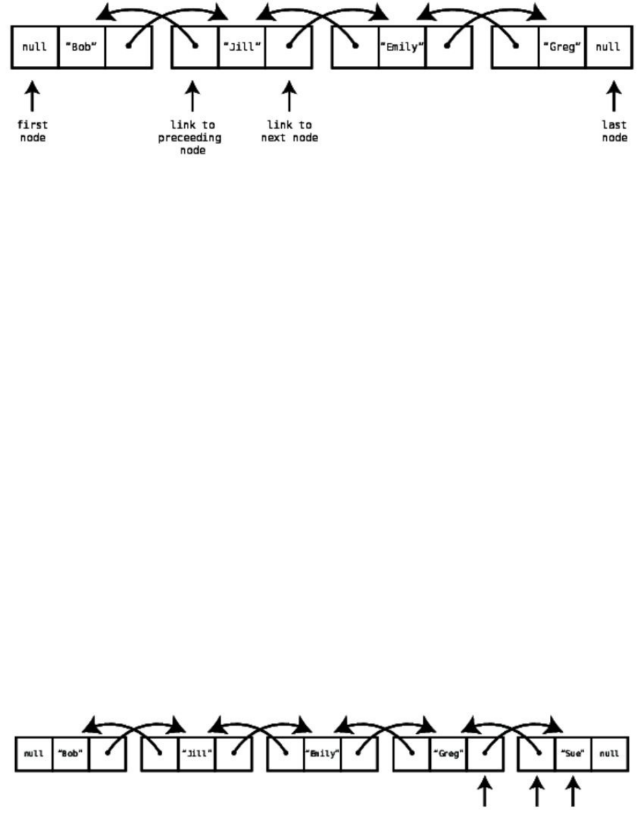
Here’swhatadoublylinkedlistlookslike:
Incode,thecoreofadoublylinkedlistwouldlooklikethis:
classNode
attr_accessor:data,:next_node,:previous_node
definitialize(data)
@data=data
end
end
classDoublyLinkedList
attr_accessor:first_node,:last_node
definitialize(first_node=nil,last_node=nil)
@first_node=first_node
@last_node=last_node
end
end
Sinceadoublylinkedlistalwaysknowswherebothitsfirstandlastnodesare,
wecanaccesseachoftheminasinglestep,orO(1).Similarly,wecaninsert
dataattheendofadoublylinkedlistinonestepbydoingthefollowing:
Wecreateanewnode("Sue")andhaveitsprevious_nodepointtothelast_nodeof
thelinkedlist("Greg").Then,wechangethenext_nodeofthelast_node("Greg")to
pointtothisnewnode("Sue").Finally,wedeclarethenewnode("Sue")tobethe
last_nodeofthelinkedlist.
Here’stheimplementationofanewinsert_at_endmethodavailabletodoubly
linkedlists:
classDoublyLinkedList
attr_accessor:first_node,:last_node
definitialize(first_node=nil,last_node=nil)
@first_node=first_node
@last_node=last_node
end
definsert_at_end(value)
new_node=Node.new(value)
#Iftherearenoelementsyetinthelinkedlist:
if!first_node
@first_node=new_node
@last_node=new_node
else
new_node.previous_node=@last_node
@last_node.next_node=new_node
@last_node=new_node
end
end
end
Becausedoublylinkedlistshaveimmediateaccesstoboththefrontandendof
thelist,theycaninsertdataoneithersideatO(1)aswellasdeletedataoneither
sideatO(1).SincedoublylinkedlistscaninsertdataattheendinO(1)timeand
deletedatafromthefrontinO(1)time,theymaketheperfectunderlyingdata
structureforaqueue.
Here’sacompleteexampleofaqueuethatisbuiltuponadoublylinkedlist:
classNode
attr_accessor:data,:next_node,:previous_node
definitialize(data)
@data=data
end
end
classDoublyLinkedList
attr_accessor:first_node,:last_node
definitialize(first_node=nil,last_node=nil)
@first_node=first_node
@last_node=last_node
end
definsert_at_end(value)
new_node=Node.new(value)
#Iftherearenoelementsyetinthelinkedlist:
if!first_node
@first_node=new_node
@last_node=new_node
else
new_node.previous_node=@last_node
@last_node.next_node=new_node
@last_node=new_node
end
end
defremove_from_front
removed_node=@first_node
@first_node=@first_node.next_node
returnremoved_node
end
end
classQueue
attr_accessor:queue
definitialize
@queue=DoublyLinkedList.new
end
defenque(value)
@queue.insert_at_end(value)
end
defdeque
removed_node=@queue.remove_from_front
returnremoved_node.data
end
deftail
return@queue.last_node.data
end
end

WrappingUp
Yourcurrentapplicationmaynotrequireaqueue,andyourqueuemayworkjust
fineevenifit’sbuiltuponanarrayratherthanadoublylinkedlist.However,you
arelearningthatyouhavechoices—andyouarelearninghowtomaketheright
choiceattherighttime.
You’velearnedhowlinkedlistscanbeusefulforboostingperformancein
certainsituations.Inthenextchapters,we’regoingtolearnaboutmorecomplex
node-baseddatastructuresthataremorecommonandusedinmanyeveryday
circumstancestomakeapplicationsrunatgreaterefficiency.
Copyright©2017,ThePragmaticBookshelf.

Chapter12
SpeedingUpAlltheThingswith
BinaryTrees
InChapter2,WhyAlgorithmsMatter,wecoveredtheconceptofbinarysearch,
anddemonstratedthatifwehaveanorderedarray,wecanusebinarysearchto
locateanyvalueinO(logN)time.Thus,orderedarraysareawesome.
However,thereisaproblemwithorderedarrays.
Whenitcomestoinsertionsanddeletions,orderedarraysareslow.Whenevera
valueisinsertedintoanorderedarray,wefirstshiftallitemsgreaterthanthat
valueonecelltotheright.Andwhenavalueisdeletedfromanorderedarray,
weshiftallgreatervaluesonecelltotheleft.ThistakesNstepsinaworst-case
scenario(insertingintoordeletingfromthefirstvalueofthearray),andN/2
stepsonaverage.Eitherway,it’sO(N),andO(N)isrelativelyslow.
Now,welearnedinChapter7,BlazingFastLookupwithHashTablesthathash
tablesareO(1)forsearch,insertion,anddeletion,buttheyhaveonesignificant
disadvantage:theydonotmaintainorder.
Butwhatdowedoifwewantadatastructurethatmaintainsorder,andalsohas
fastsearch,insertion,anddeletion?Neitheranorderedarraynorahashtableis
ideal.
Enterthebinarytree.
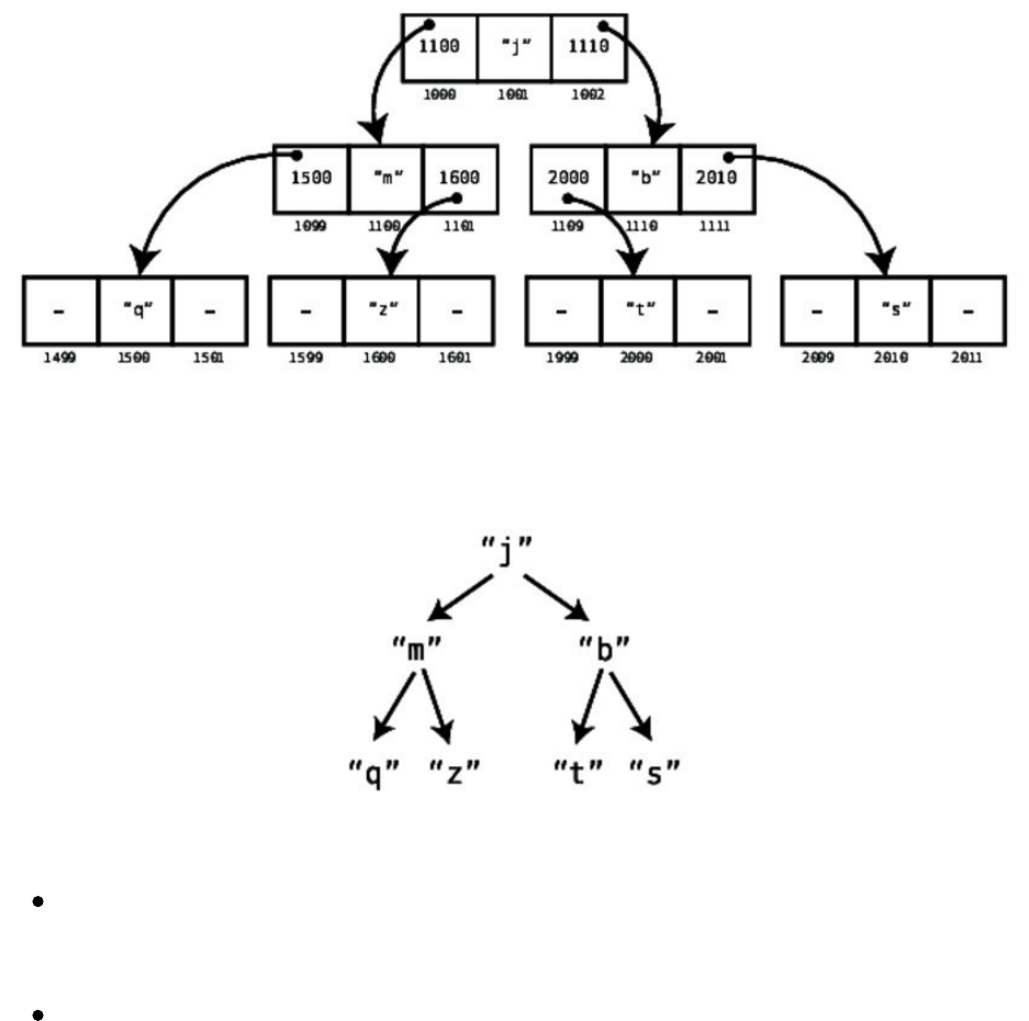
BinaryTrees
Wewereintroducedtonode-baseddatastructuresinthepreviouschapterusing
linkedlists.Inasimplelinkedlist,eachnodecontainsalinkthatconnectsthis
nodetoasingleothernode.Atreeisalsoanode-baseddatastructure,butwithin
atree,eachnodecanhavelinkstomultiplenodes.
Hereisavisualizationofasimpletree:
Inthisexample,eachnodehaslinksthatleadtotwoothernodes.Forthesakeof
simplicity,wecanrepresentthistreevisuallywithoutshowingalltheactual
links:
Treescomewiththeirownuniquenomenclature:
Theuppermostnode(inourexample,the“j”)iscalledtheroot.Yes,inour
picturetherootisatthetopofthetree;dealwithit.
Inourexample,we’dsaythatthe“j”isaparentto“m”and“b”,whichare
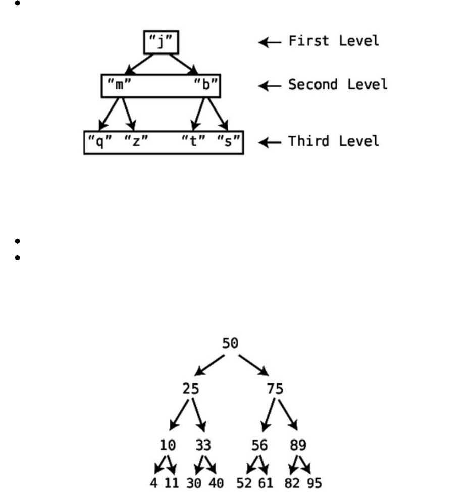
inturnchildrenof“j”.The“m”isaparentof“q”and“z”,whichareinturn
childrenof“m”.
Treesaresaidtohavelevels.Theprecedingtreehasthreelevels:
Therearemanydifferentkindsoftree-baseddatastructures,butinthischapter,
we’llbefocusingonaparticulartreeknownasabinarytree.Abinarytreeisa
treethatabidesbythefollowingrules:
Eachnodehaseitherzero,one,ortwochildren.
Ifanodehastwochildren,itmusthaveonechildthathasalesservalue
thantheparent,andonechildthathasagreatervaluethantheparent.
Here’sanexampleofabinarytree,inwhichthevaluesarenumbers:
Notethateachnodehasonechildwithalesservaluethanitself,whichis
depictedusingaleftarrow,andonechildwithagreatervaluethanitself,which
isdepictedusingarightarrow.
Whilethefollowingexampleisatree,itisnotabinarytree:

Itisnotavalidbinarytreebecausebothchildrenoftheparentnodehavevalues
lessthantheparentitself.
TheimplementationofatreenodeinPythonmightlooksomethinglikethis:
classTreeNode:
def__init__(self,val,left=None,right=None):
self.value=val
self.leftChild=left
self.rightChild=right
Wecanthenbuildasimpletreelikethis:
node=TreeNode(1)
node2=TreeNode(10)
root=TreeNode(5,node,node2)
Becauseoftheuniquestructureofabinarytree,wecansearchforanyvalue
withinitvery,veryquickly,aswe’llnowsee.
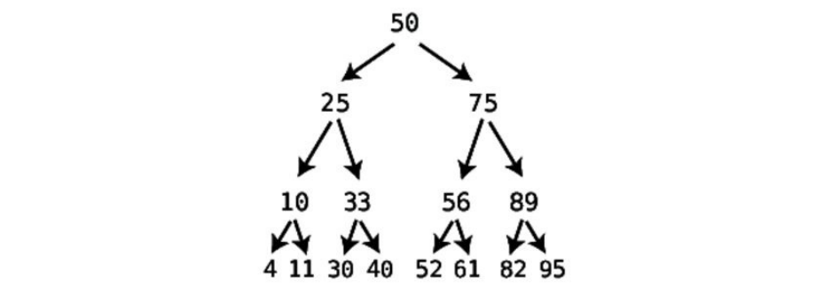
Searching
Hereagainisabinarytree:
Thealgorithmforsearchingwithinabinarytreebeginsattherootnode:
1. Inspectthevalueatthenode.
2. Ifwe’vefoundthevaluewe’relookingfor,great!
3. Ifthevaluewe’relookingforislessthanthecurrentnode,searchforitin
itsleftsubtree.
4. Ifthevaluewe’relookingforisgreaterthanthecurrentnode,searchforit
initsrightsubtree.
Here’sasimple,recursiveimplementationforthissearchinPython:
defsearch(value,node):
#Basecase:Ifthenodeisnonexistent
#orwe'vefoundthevaluewe'relookingfor:
ifnodeisNoneornode.value==value:
returnnode
#Ifthevalueislessthanthecurrentnode,perform
#searchontheleftchild:
elifvalue<node.value:
returnsearch(value,node.leftChild)
#Ifthevalueislessthanthecurrentnode,perform
#searchontherightchild:
else:#value>node.value
returnsearch(value,node.rightChild)
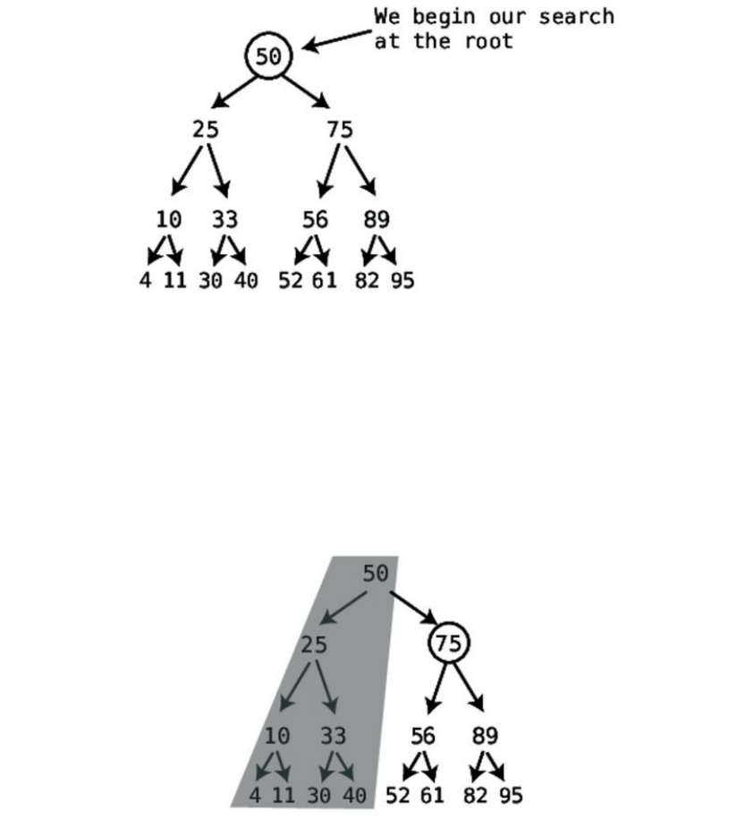
Saywewantedtosearchforthe61.Let’sseehowmanystepsitwouldtakeby
walkingthroughthisvisually.
Whensearchingatree,wemustalwaysbeginattheroot:
Next,thecomputerasksitself:isthenumberwe’researchingfor(61)greateror
lessthanthevalueofthisnode?Ifthenumberwe’relookingforislessthanthe
currentnode,lookforitintheleftchild.Ifit’sgreaterthanthecurrentnode,
lookforitintherightchild.
Inthisexample,since61isgreaterthan50,weknowitmustbesomewhereto
theright,sowesearchtherightchild:
“Areyoumymother?”asksthealgorithm.Sincethe75isnotthe61we’re
lookingfor,weneedtomovedowntothenextlevel.Andsince61islessthan
75,we’llchecktheleftchild,sincethe61couldonlybethere:
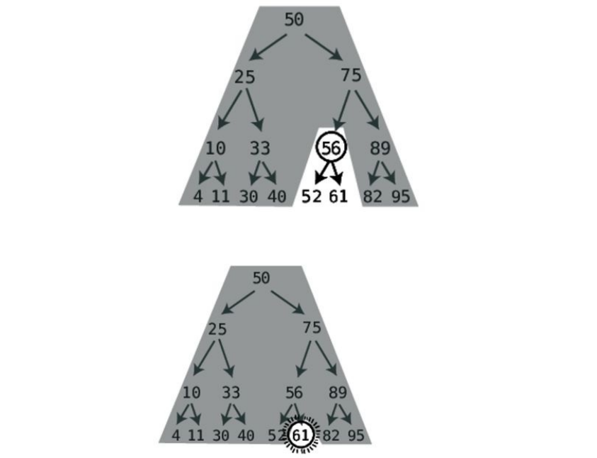
Since61isgreaterthan56,wesearchforitintherightchildofthe56:
Inthisexample,ittookusfourstepstofindourdesiredvalue.
Moregenerally,we’dsaythatsearchinginabinarytreeisO(logN).Thisis
becauseeachstepwetakeeliminateshalfoftheremainingpossiblevaluesin
whichourvaluecanbestored.(We’llseesoon,though,thatthisisonlyfora
perfectlybalancedbinarytree,whichisabest-casescenario.)
Comparethiswithbinarysearch,anotherO(logN)algorithm,inwhicheach
numberwetryalsoeliminateshalfoftheremainingpossiblevalues.Inthis
regard,then,searchingabinarytreehasthesameefficiencyasbinarysearch
withinanorderedarray.
Wherebinarytreesreallyshineoverorderedarrays,though,iswithinsertion.
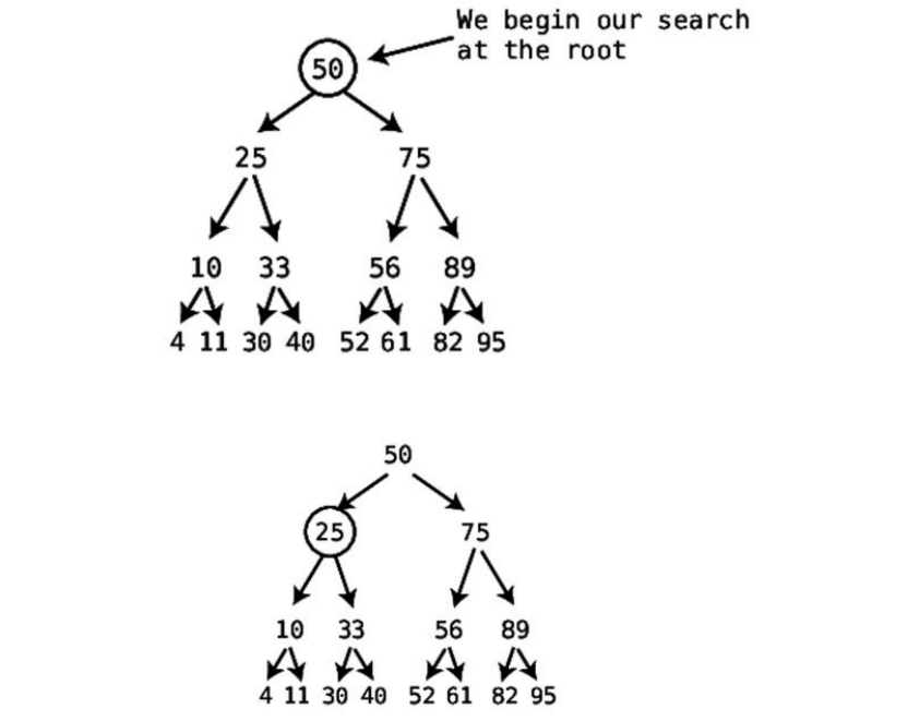
Insertion
Todiscoverthealgorithmforinsertinganewvalueintoabinarytree,let’swork
withanexample.Saythatwewanttoinsertthenumber45intotheprevioustree.
Thefirstthingwe’dhavetodoisfindthecorrectnodetoattachthe45to.To
beginoursearch,westartattheroot:
Since45islessthan50,wedrilldowntotheleftchild:
Since45isgreaterthan25,wemustinspecttherightchild:
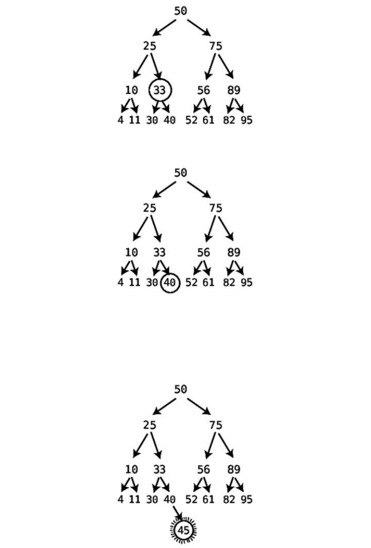
45isgreaterthan33,sowecheckthe33’srightchild:
Atthispoint,we’vereachedanodethathasnochildren,sowehavenowhereto
go.Thismeanswe’rereadytoperformourinsertion.
Since45isgreaterthan40,weinsertitasarightchildnodeofthe40:
Inthisexample,insertiontookfivesteps,consistingoffoursearchsteps,andone
insertionstep.Insertionalwaystakesjustoneextrastepbeyondasearch,which
meansthatinsertiontakeslogN+1steps,whichisO(logN)asBigOignores
constants.
Inanorderedarray,bycontrast,insertiontakesO(N),becauseinadditionto
search,wemustshiftalotofdatatotherighttomakeroomforthevaluethat
we’reinserting.
Thisiswhatmakesbinarytreessoefficient.WhileorderedarrayshaveO(logN)
searchandO(N)insertion,binarytreeshaveO(logN)andO(logN)insertion.
Thisbecomescriticalinanapplicationwhereyouanticipatealotofchangesto
yourdata.
Here’saPythonimplementationofinsertingavalueintoabinarytree.Likethe
searchfunction,itisrecursive:
definsert(value,node):
ifvalue<node.value:
#Iftheleftchilddoesnotexist,wewanttoinsert
#thevalueastheleftchild:
ifnode.leftChildisNone:
node.leftChild=TreeNode(value)
else:
insert(value,node.leftChild)
elifvalue>node.value:
#Iftherightchilddoesnotexist,wewanttoinsert
#thevalueastherightchild:
ifnode.rightChildisNone:
node.rightChild=TreeNode(value)
else:
insert(value,node.rightChild)
Itisimportanttonotethatonlywhencreatingatreeoutofrandomlysorteddata
dotreesusuallywindupwell-balanced.However,ifweinsertsorteddataintoa
tree,itcanbecomeimbalancedandlessefficient.Forexample,ifwewereto
insertthefollowingdatainthisorder—1,2,3,4,5—we’dendupwithatreethat
lookslikethis:
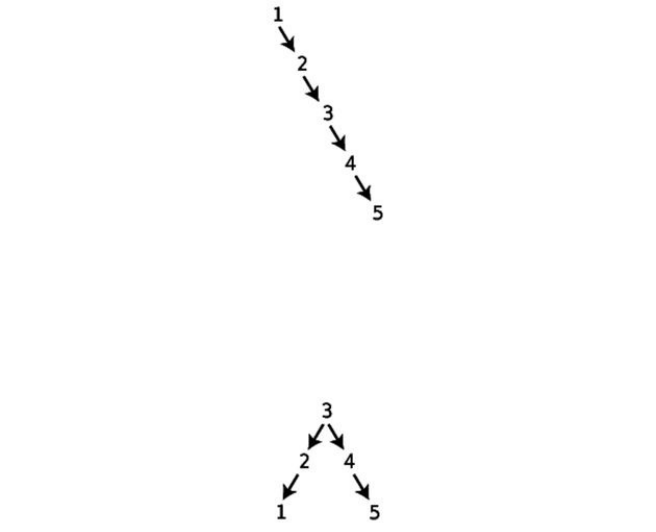
Searchingforthe5withinthistreewouldtakeO(N).
However,ifweinsertedthesamedatainthefollowingorder—3,2,4,1,5—the
treewouldbeevenlybalanced:
Becauseofthis,ifyoueverwantedtoconvertanorderedarrayintoabinarytree,
you’dbetterfirstrandomizetheorderofthedata.
Itemergesthatinaworst-casescenario,whereatreeiscompletelyimbalanced,
searchisO(N).Inabest-casescenario,whereitisperfectlybalanced,searchis
O(logN).Inthetypicalscenario,inwhichdataisinsertedinrandomorder,a
treewillbeprettywellbalancedandsearchwilltakeaboutO(logN).
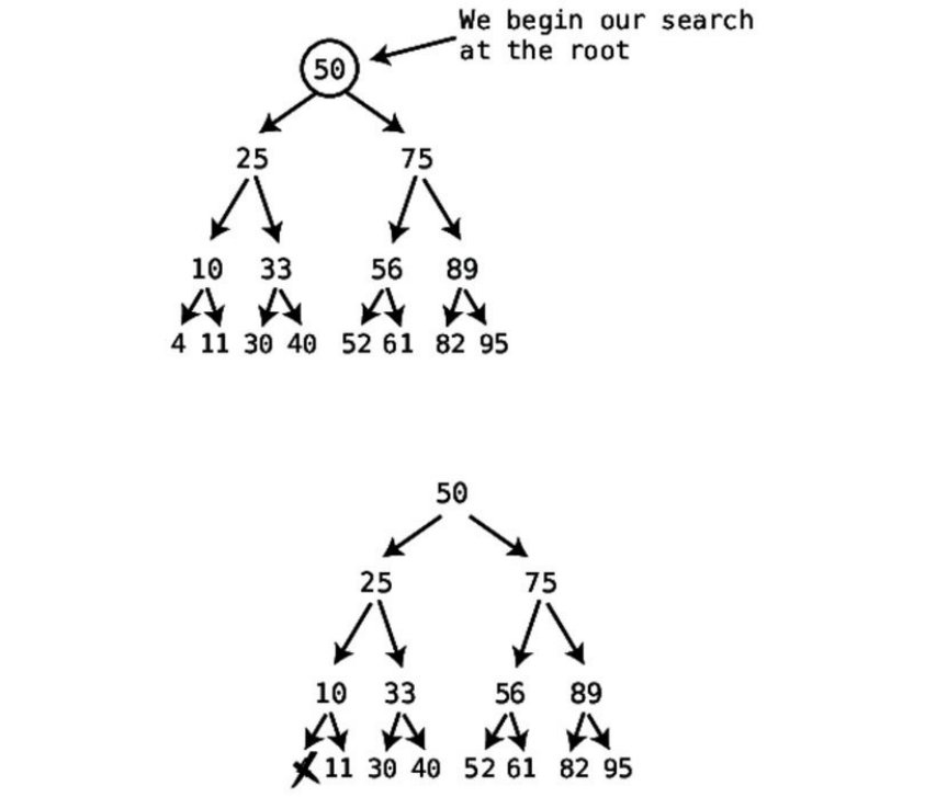
Deletion
Deletionistheleaststraightforwardoperationwithinabinarytree,andrequires
somecarefulmaneuvering.Let’ssaythatwewanttodeletethe4fromthis
binarytree:
First,weperformasearchtofirstfindthe4,andthenwecanjustdeleteitone
step:
Whilethatwassimple,let’ssaywenowwanttodeletethe10aswell.Ifwe
deletethe10
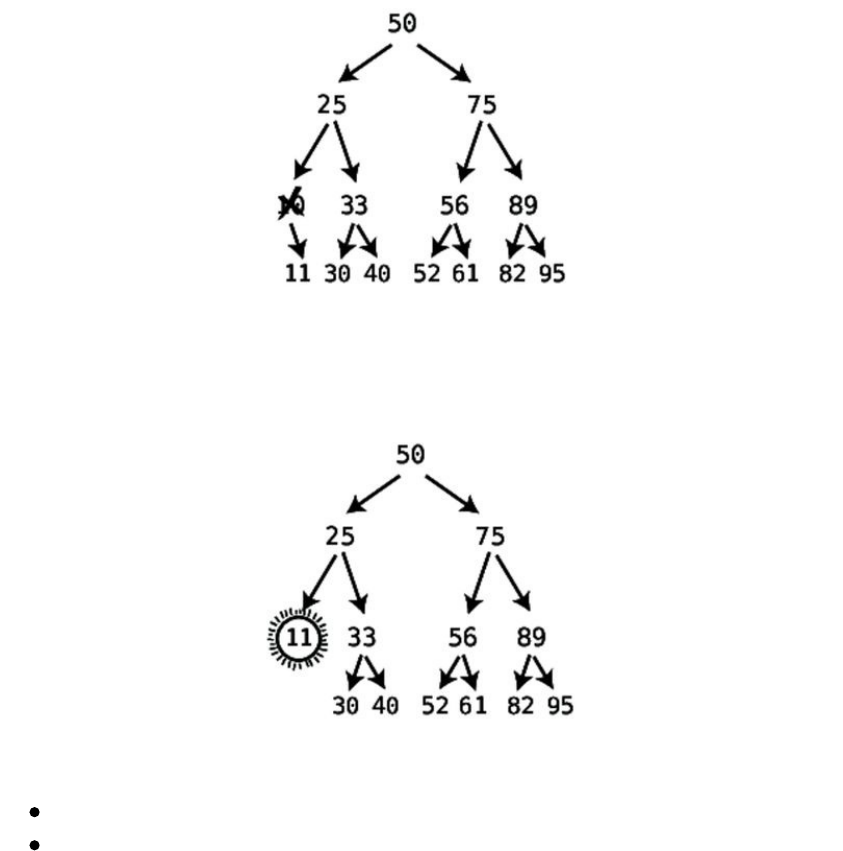
weendupwithan11thatisn’tconnectedtothetreeanymore.Andwecan’t
havethat,becausewe’dlosethe11forever.However,there’sasolutiontothis
problem:we’llplugthe11intowherethe10usedtobe:
Sofar,ourdeletionalgorithmfollowstheserules:
Ifthenodebeingdeletedhasnochildren,simplydeleteit.
Ifthenodebeingdeletedhasonechild,deleteitandplugthechildintothe
spotwherethedeletednodewas.
Deletinganodethathastwochildrenisthemostcomplexscenario.Let’ssay
thatwewantedtodeletethe56:
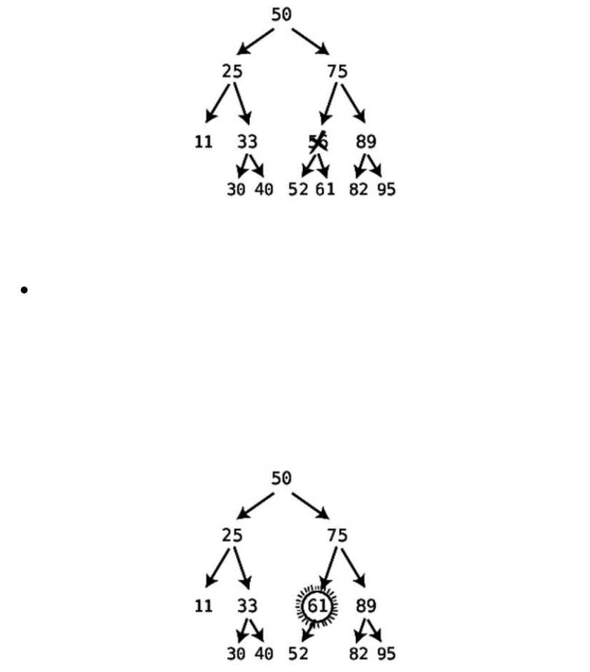
Whatarewegoingtodowiththe52and61?Wecannotputbothofthemwhere
the56was.Thatiswherethenextruleofthedeletionalgorithmcomesintoplay:
Whendeletinganodewithtwochildren,replacethedeletednodewiththe
successornode.Thesuccessornodeisthechildnodewhosevalueisthe
leastofallvaluesthataregreaterthanthedeletednode.
Thatwasatrickysentence.Inotherwords,thesuccessornodeisthenext
numberupfromthedeletedvalue.Inthiscase,thenextnumberupamongthe
descendantsof56is61.Sowereplacethe56withthe61:
Howdoesthecomputerfindthesuccessorvalue?Thereisanalgorithmforthat:
Visittherightchildofthedeletedvalue,andthenkeeponvisitingtheleftchild
ofeachsubsequentchilduntiltherearenomoreleftchildren.Thebottomvalue
isthesuccessornode.
Let’sseethisagaininactioninamorecomplexexample.Let’sdeletetheroot
node:
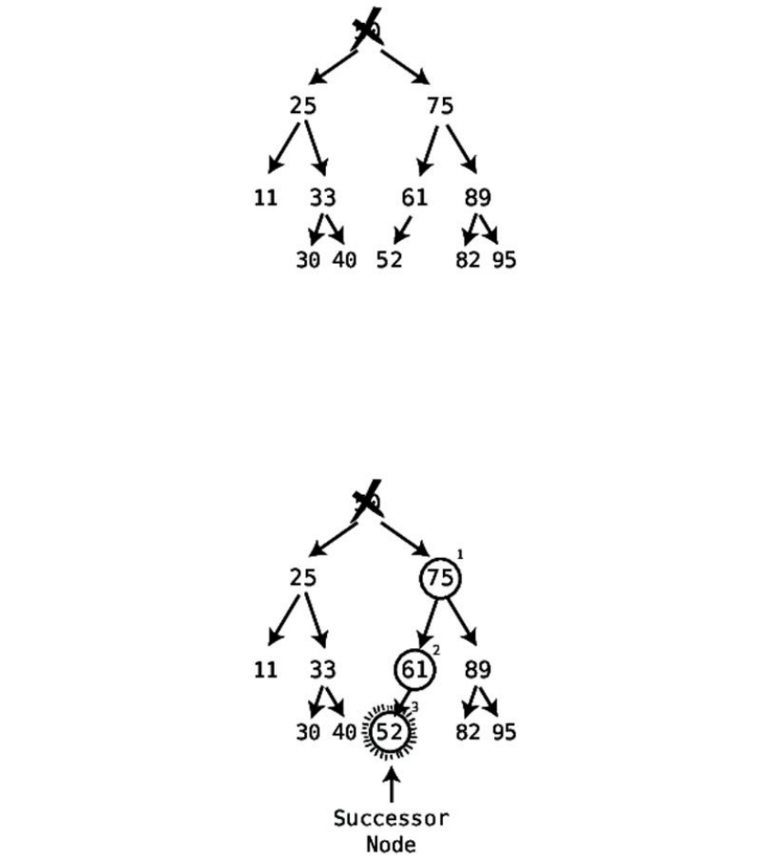
Wenowneedtoplugthesuccessorvalueintotherootnode.Let’sfindthe
successorvalue.
Todothis,wefirstvisittherightchild,andthenkeepdescendingleftwarduntil
wereachanodethatdoesn’thavealeftchild:
Nowthatwe’vefoundthesuccessornode—the52—weplugitintothenodethat
wedeleted:
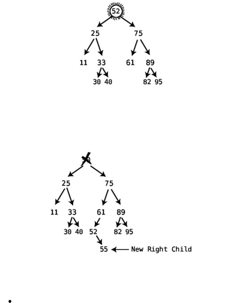
Andwe’redone!
However,thereisonecasethatwehaven’taccountedforyet,andthat’swhere
thesuccessornodehasarightchildofitsown.Let’srecreatetheprecedingtree,
butaddarightchildtothe52:
Inthiscase,wecan’tsimplyplugthesuccessornode—the52—intotheroot,
sincewe’dleaveitschildof55hanging.Becauseofthis,there’sonemorerule
toourdeletionalgorithm:
Ifthesuccessornodehasarightchild,afterpluggingthesuccessorintothe
spotofthedeletednode,taketherightchildofthesuccessornodeandturn
itintotheleftchildoftheparentofthesuccessornode.
Let’swalkthroughthesteps.
First,weplugthesuccessornodeintotheroot:

Atthispoint,the55isleftdangling.Next,weturnthe55intotheleftchildof
whatwastheparentofthesuccessornode.Inthiscase,61wastheparentofthe
successornode,sowemakethe55theleftchildofthe61:
Andnowwe’rereallydone.
Pullingallthestepstogether,thealgorithmfordeletionfromabinarytreeis:
Ifthenodebeingdeletedhasnochildren,simplydeleteit.
Ifthenodebeingdeletedhasonechild,deleteitandplugthechildintothe
spotwherethedeletednodewas.
Whendeletinganodewithtwochildren,replacethedeletednodewiththe
successornode.Thesuccessornodeisthechildnodewhosevalueisthe
leastofallvaluesthataregreaterthanthedeletednode.

Ifthesuccessornodehasarightchild,afterpluggingthesuccessor
nodeintothespotofthedeletednode,taketherightchildofthe
successornodeandturnitintotheleftchildoftheparentofthe
successornode.
Here’sarecursivePythonimplementationofdeletionfromabinarytree.It’sa
littletrickyatfirst,sowe’vesprinkledcommentsliberally:
defdelete(valueToDelete,node):
#Thebasecaseiswhenwe'vehitthebottomofthetree,
#andtheparentnodehasnochildren:
ifnodeisNone:
returnNone
#Ifthevaluewe'redeletingislessorgreaterthanthecurrentnode,
#wesettheleftorrightchildrespectivelytobe
#thereturnvalueofarecursivecallofthisverymethodonthecurrent
#node'sleftorrightsubtree.
elifvalueToDelete<node.value:
node.leftChild=delete(valueToDelete,node.leftChild)
#Wereturnthecurrentnode(anditssubtreeifexistent)to
#beusedasthenewvalueofitsparent'sleftorrightchild:
returnnode
elifvalueToDelete>node.value:
node.rightChild=delete(valueToDelete,node.rightChild)
returnnode
#Ifthecurrentnodeistheonewewanttodelete:
elifvalueToDelete==node.value:
#Ifthecurrentnodehasnoleftchild,wedeleteitby
#returningitsrightchild(anditssubtreeifexistent)
#tobeitsparent'snewsubtree:
ifnode.leftChildisNone:
returnnode.rightChild
#(IfthecurrentnodehasnoleftORrightchild,thisendsup
#beingNoneasperthefirstlineofcodeinthisfunction.)
elifnode.rightChildisNone:
returnnode.leftChild
#Ifthecurrentnodehastwochildren,wedeletethecurrentnode
#bycallingtheliftfunction(below),whichchangesthecurrentnode's
#valuetothevalueofitssuccessornode:
else:
node.rightChild=lift(node.rightChild,node)
returnnode
deflift(node,nodeToDelete):
#Ifthecurrentnodeofthisfunctionhasaleftchild,
#werecursivelycallthisfunctiontocontinuedown
#theleftsubtreetofindthesuccessornode.
ifnode.leftChild:
node.leftChild=lift(node.leftChild,nodeToDelete)
returnnode
#Ifthecurrentnodehasnoleftchild,thatmeansthecurrentnode
#ofthisfunctionisthesuccessornode,andwetakeitsvalue
#andmakeitthenewvalueofthenodethatwe'redeleting:
else:
nodeToDelete.value=node.value
#Wereturnthesuccessornode'srightchildtobenowused
#asitsparent'sleftchild:
returnnode.rightChild
Likesearchandinsertion,deletingfromtreesisalsotypicallyO(logN).Thisis
becausedeletionrequiresasearchplusafewextrastepstodealwithany
hangingchildren.Contrastthiswithdeletingavaluefromanorderedarray,
whichtakesO(N)duetoshiftingelementstothelefttoclosethegapofthe
deletedvalue.
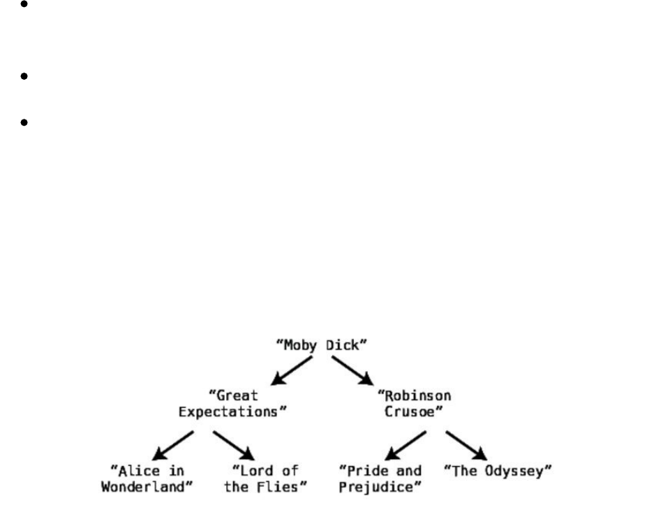
BinaryTreesinAction
We’veseenthatbinarytreesboastefficienciesofO(logN)forsearch,insertion,
anddeletion,makingitanefficientchoiceforscenariosinwhichweneedto
storeandmanipulateordereddata.Thisisparticularlytrueifwewillbe
modifyingthedataoften,becausewhileorderedarraysarejustasfastasbinary
treeswhensearchingdata,binarytreesaresignificantlyfasterwhenitcomesto
insertinganddeletingdata.
Forexample,let’ssaythatwe’recreatinganapplicationthatmaintainsalistof
booktitles.We’dwantourapplicationtohavethefollowingfunctionality:
Ourprogramshouldbeabletoprintoutthelistofbooktitlesinalphabetical
order.
Ourprogramshouldallowforconstantchangestothelist.
Ourprogramshouldallowtheusertosearchforatitlewithinthelist.
Ifwedidn’tanticipatethatourbooklistwouldbechangingthatoften,anordered
arraywouldbeasuitabledatastructuretocontainourdata.However,we’re
buildinganappthatshouldbeabletohandlemanychangesinrealtime.Ifour
listhadmillionsoftitles,we’dbetteruseabinarytree.
Suchatreemightlooksomethinglikethis:
Now,we’vealreadycoveredhowtosearch,insert,anddeletedatafromabinary
tree.Wementioned,though,thatwealsowanttobeabletoprinttheentirelistof
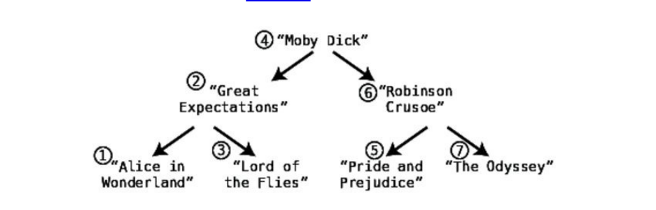
booktitlesinalphabeticalorder.Howcanwedothat?
Firstly,weneedtheabilitytovisiteverysinglenodeinthetree.Theprocessof
visitingeverynodeinadatastructureisknownastraversingthedatastructure.
Secondly,weneedtomakesurethatwetraversethetreeinalphabetically
ascendingordersothatwecanprintoutthelistinthatorder.Therearemultiple
waystotraverseatree,butforthisapplication,wewillperformwhatisknown
asinordertraversal,sothatwecanprintouteachtitleinalphabeticalorder.
Recursionisagreattoolforperforminginordertraversal.We’llcreatea
recursivefunctioncalledtraversethatcanbecalledonaparticularnode.The
functionthenperformsthefollowingsteps:
1. Callitself(traverse)onthenode’sleftchildifithasone.
2. Visitthenode.(Forourbooktitleapp,weprintthevalueofthenodeatthis
step.)
3. Callitself(traverse)onthenode’srightchildifithasone.
Forthisrecursivealgorithm,thebasecaseiswhenanodehasnochildren,in
whichcasewesimplyprintthenode’stitlebutdonotcalltraverseagain.
Ifwecalledtraverseonthe“MobyDick”node,we’dvisitallthenodesofthe
treeintheordershownonthediagram.
Andthat’sexactlyhowwecanprintoutourlistofbooktitlesinalphabetical
order.NotethattreetraversalisO(N),sincebydefinition,traversalvisitsevery
nodeofthetree.
Here’saPythontraverse_and_printfunctionthatworksforourlistofbooktitles:
deftraverse_and_print(node):
ifnodeisNone:
return
traverse_and_print(node.leftChild)
print(node.value)
traverse_and_print(node.rightChild)

WrappingUp
Binarytreesareapowerfulnode-baseddatastructurethatprovidesorder
maintenance,whilealsoofferingfastsearch,insertion,anddeletion.They’re
morecomplexthantheirlinkedlistcousins,butoffertremendousvalue.
Itisworthmentioningthatinadditiontobinarytrees,therearemanyothertypes
oftree-baseddatastructuresaswell.Heaps,B-trees,red-blacktrees,and2-3-4
trees,aswellasmanyothertreeseachhavetheirownuseforspecialized
scenarios.
Inthenextchapter,we’llencounteryetanothernode-baseddatastructurethat
servesastheheartofcomplexapplicationssuchassocialnetworksandmapping
software.It’spowerfulyetnimble,andit’scalledagraph.
Copyright©2017,ThePragmaticBookshelf.

Chapter13
ConnectingEverythingwithGraphs
Let’ssaythatwe’rebuildingasocialnetworksuchasFacebook.Insuchan
application,manypeoplecanbe“friends”withoneanother.Thesefriendships
aremutual,soifAliceisfriendswithBob,thenBobisalsofriendswithAlice.
Howcanwebestorganizethisdata?
Oneverysimpleapproachmightbetouseatwo-dimensionalarraythatstores
thelistoffriendships:
relationships=[
["Alice","Bob"],
["Bob","Cynthia"],
["Alice","Diana"],
["Bob","Diana"],
["Elise","Fred"],
["Diana","Fred"],
["Fred","Alice"]
]
Unfortunately,withthisapproach,there’snoquickwaytoseewhoAlice’s
friendsare.We’dhavetoinspecteachrelationshipwithinthearray,andcheckto
seewhetherAliceiscontainedwithintherelationship.Bythetimeweget
throughtheentirearray,we’dcreatealistofallofAlice’sfriends(whohappen
tobeBob,Diana,andFred).We’dalsoperformthesameprocessifwewanted
tosimplycheckwhetherElisewasAlice’sfriend.
Basedonthewaywe’vestructuredourdata,searchingforAlice’sfriendswould
haveanefficiencyofO(N),sinceweneedtoinspecteveryrelationshipinour
database.
Butwecandomuch,muchbetter.Withadatastructureknownasagraph,we
canfindeachofAlice’sfriendsinjustO(1)time.
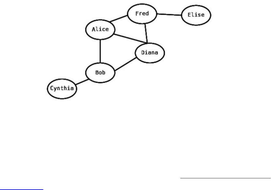
Graphs
Agraphisadatastructurethatspecializesinrelationships,asiteasilyconveys
howdataisconnected.
HereisavisualizationofourFacebooknetwork:
Eachpersonisrepresentedbyanode,andeachlineindicatesafriendshipwith
anotherperson.Ingraphjargon,eachnodeiscalledavertex,andeachlineis
calledanedge.Verticesthatareconnectedbyanedgearesaidtobeadjacentto
eachother.
Thereareanumberofwaysthatagraphcanbeimplemented,butoneofthe
simplestwaysisusingahashtable(seeChapter7,BlazingFastLookupwith
HashTables).Here’sabare-bonesRubyimplementationofoursocialnetwork:
friends={
"Alice"=>["Bob","Diana","Fred"],
"Bob"=>["Alice","Cynthia","Diana"],
"Cynthia"=>["Bob"],
"Diana"=>["Alice","Bob","Fred"],
"Elise"=>["Fred"],
"Fred"=>["Alice","Diana","Elise"]
}
Withagraph,wecanlookupAlice’sfriendsinO(1),becausewecanlookupthe
valueofanykeyinahashtableinonestep:

friends["Alice"]
WithTwitter,incontrasttoFacebook,relationshipsarenotmutual.Thatis,Alice
canfollowBob,butBobdoesn’tnecessarilyfollowAlice.Let’sconstructanew
graph(shownatright)thatdemonstrateswhofollowswhom.
Inthisexample,thearrowsindicatethedirectionoftherelationship.Alice
followsbothBobandCynthia,butnoonefollowsAlice.BobandCynthia
followeachother.
Usingourhashtableapproach,we’dusethefollowingcode:
followees={
"Alice"=>["Bob","Cynthia"],
"Bob"=>["Cynthia"],
"Cynthia"=>["Bob"]
}
WhiletheFacebookandTwitterexamplesaresimilar,thenatureofthe
relationshipsineachexamplearedifferent.BecauserelationshipsinTwitterare
one-directional,weusearrowsinourvisualimplementation,andsuchagraphis
knownasadirectedgraph.InFacebook,wheretherelationshipsaremutualand
weusesimplelines,thegraphiscalledanon-directedgraph.
Whileasimplehashtablecanbeusedtorepresentagraph,amorerobustobject-
orientedimplementationcanbeusedaswell.
Here’samorerobustimplementationofagraph,usingRuby:
classPerson
attr_accessor:name,:friends
definitialize(name)
@name=name
@friends=[]
end
defadd_friend(friend)
@friends<<friend
end
end
WiththisRubyclass,wecancreatepeopleandestablishfriendships:
mary=Person.new("Mary")
peter=Person.new("Peter")
mary.add_friend(peter)
peter.add_friend(mary)
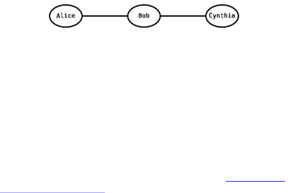
Breadth-FirstSearch
LinkedInisanotherpopularsocialnetworkthatspecializesinbusiness
relationships.Oneofitswell-knownfeaturesisthatyoucandetermineyour
second-andthird-degreeconnectionsinadditiontoyourdirectnetwork.
Inthediagramontheright,AliceisconnecteddirectlytoBob,andBobis
connecteddirectlytoCynthia.However,Aliceisnotconnecteddirectlyto
Cynthia.SinceCynthiaisconnectedtoAlicebywayofBob,Cynthiaissaidto
beAlice’ssecond-degreeconnection.
IfwewantedtofindAlice’sentirenetwork,includingherindirectconnections,
howwouldwegoaboutthat?
Therearetwoclassicwaystotraverseagraph:breadth-firstsearchanddepth-
firstsearch.We’llexplorebreadth-firstsearchhere,andyoucanlookupdepth-
firstsearchonyourown.Botharesimilarandworkequallywellformostcases,
though.
Thebreadth-firstsearchalgorithmusesaqueue(seeChapter8,CraftingElegant
CodewithStacksandQueues),whichkeepstrackofwhichverticestoprocess
next.Attheverybeginning,thequeueonlycontainsthestartingvertex(Alice,in
ourcase).So,whenouralgorithmbegins,ourqueuelooklikethis:
[Alice]
WethenprocesstheAlicevertexbyremovingitfromthequeue,markingitas
havingbeen“visited,”anddesignatingitasthecurrentvertex.(Thiswillall
becomeclearerwhenwewalkthroughtheexampleshortly.)
Wethenfollowthreesteps:
1. Visiteachvertexadjacenttothecurrentvertex.Ifithasnotyetbeenvisited,
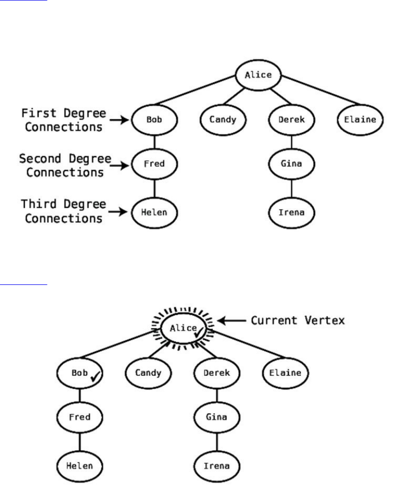
markitasvisited,andaddittoaqueue.(Wedonotyetmakeitthecurrent
vertex,though.)
2. Ifthecurrentvertexhasnounvisitedverticesadjacenttoit,removethenext
vertexfromthequeueandmakeitthecurrentvertex.
3. Iftherearenomoreunvisitedverticesadjacenttothecurrentvertex,and
therearenomoreverticesinthequeue,thealgorithmiscomplete.
Let’sseethisinaction.HereisAlice’sLinkedInnetworkasshowninthetop
diagram.WestartbymakingAlicethecurrentvertex.Toindicateinourdiagram
thatsheisthecurrentvertex,wesurroundherwithlines.Wealsoputacheck
markbyhertoindicatethatshehasbeenvisited.
Wethencontinuethealgorithmbyvisitinganunvisitedadjacentvertex—inthis
case,Bob.Weaddacheckmarkbyhisnametooasshowninthesecond
diagram.
WealsoaddBobtoourqueue,soourqueueisnow:[Bob].Thisindicatesthatwe
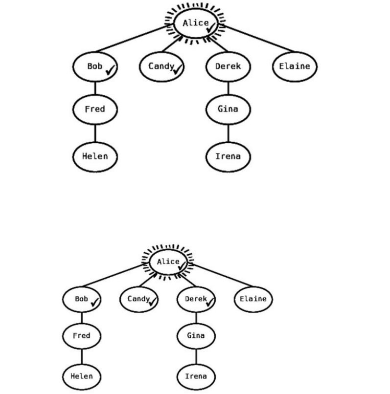
stillhaveyettomakeBobthecurrentvertex.NotethatwhileAliceisthecurrent
vertex,we’vestillbeenabletovisitBob.
Next,wecheckwhetherAlice—thecurrentvertex—hasanyotherunvisited
adjacentvertices.WefindCandy,sowemarkthatasvisited:
Ourqueuenowcontains[Bob,Candy].
AlicestillhasDerekasanunvisitedadjacentvertex,sowevisitit:
Thequeueisnow[Bob,Candy,Derek].
Alicehasonemoreunvisitedadjacentconnection,sowevisitElaine:
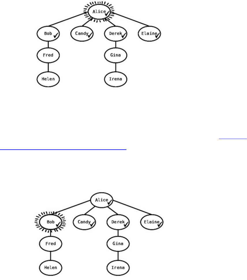
Ourqueueisnow[Bob,Candy,Derek,Elaine].
Alice—ourcurrentvertex—hasnomoreunvisitedadjacentvertices,sowemove
ontothesecondruleofouralgorithm,whichsaysthatweremoveavertexfrom
thequeue,andmakeitourcurrentvertex.RecallfromChapter8,Crafting
ElegantCodewithStacksandQueuesthatwecanonlyremovedatafromthe
beginningofaqueue,sothatwouldbeBob.
Ourqueueisnow[Candy,Derek,Elaine],andBobisourcurrentvertex:
Wenowreturntothefirstrule,whichasksustofindanyunvisitedadjacent
verticesofthecurrentvertex.Bobhasonesuchvertex—Fred—sowemarkitas
visitedandaddittoourqueue:
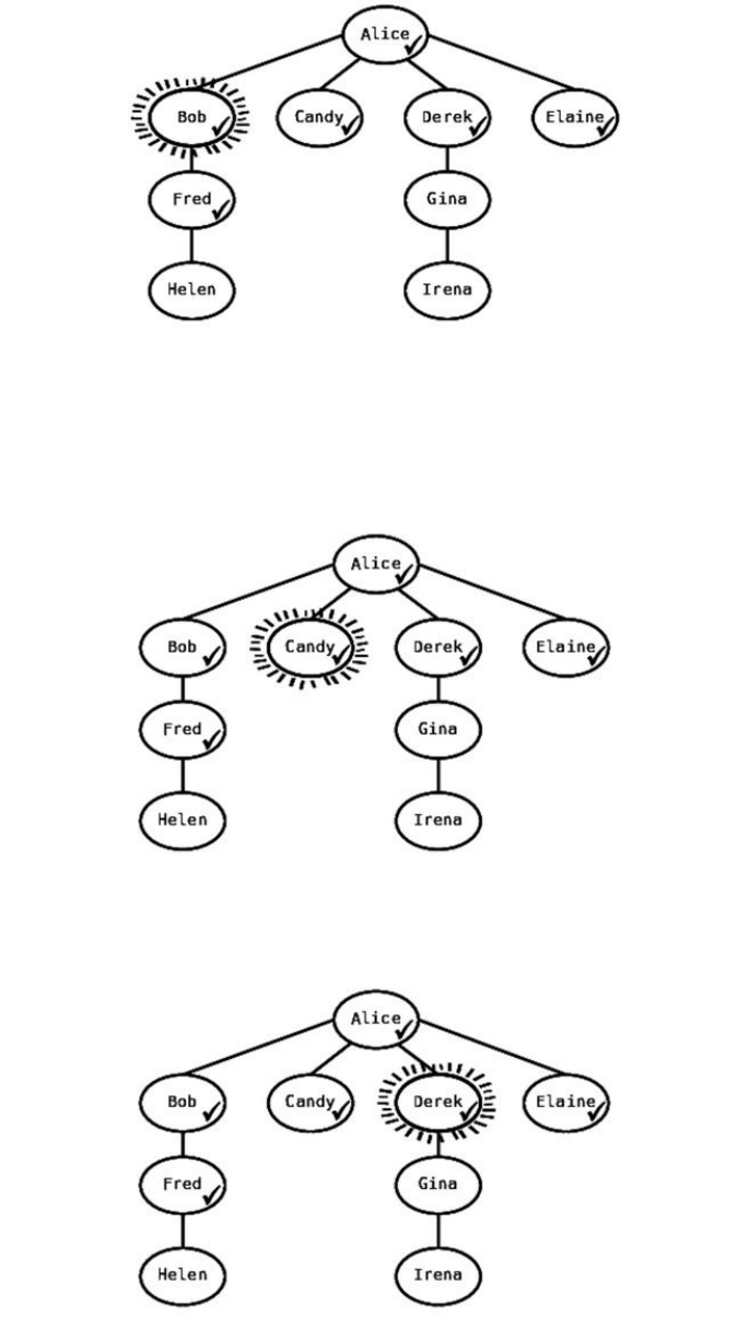
Ourqueuenowcontains[Candy,Derek,Elaine,Fred].
SinceBobhasnomoreunvisitedadjacentvertices,weremovethenextvertex
fromthequeue—Candy—andmakeitthecurrentvertex:
However,Candyhasnounvisitedadjacentvertices.Sowegrabthenextitemoff
thequeue—Derek—leavingourqueueas[Elaine,Fred]:
DerekhasGinaasanunvisitedadjacentconnection,sowemarkGinaasvisited:
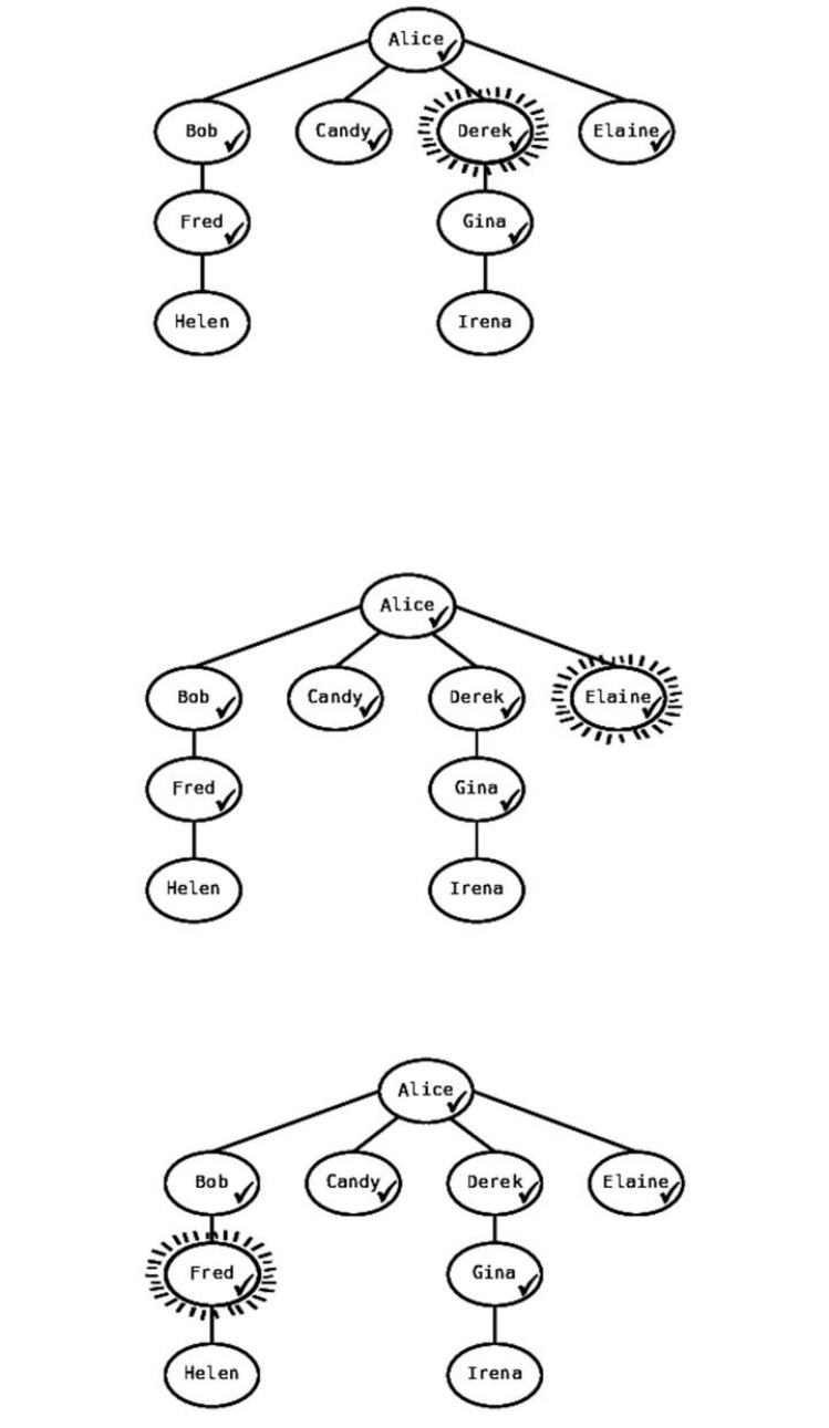
Thequeueisnow[Elaine,Fred,Gina].
Derekhasnomoreadjacentverticestovisit,sowetakeElaineoffthequeueand
makeherthecurrentvertex:
Elainehasnoadjacentverticesthathavenotbeenvisited,sowetakeFredoffthe
queue:
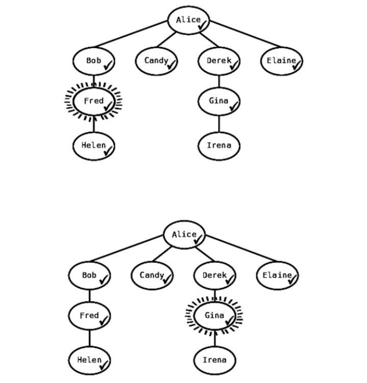
Atthispoint,ourqueueis[Gina].
Now,Fredhasonepersontovisit—Helen—sowemarkherasvisitedandadd
hertothequeue,makingit[Gina,Helen]:
SinceFredhasnomoreunvisitedconnections,wetakeGinaoffthequeue,
makingherthecurrentvertex:
OurqueuenowonlycontainsHelen:[Helen].
Ginahasonevertextovisit—Irena:
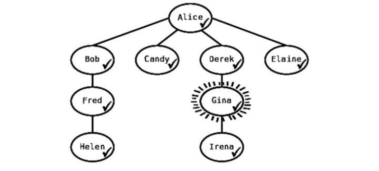
Ourqueuecurrentlycontains[Helen,Irena].
Ginahasnomoreconnectionstovisit,sowetakeHelenfromthequeue,making
herthecurrentvertex,andleavingourqueuewith[Irena].Helenhasnobodyto
visit,sowetakeIrenafromthequeueandmakeherthecurrentvertex.Now,
Irenaalsohasnoverticestovisit,sosincethequeueisempty—we’redone!
Let’saddadisplay_networkmethodtoourPersonclassthatusesbreadth-first
searchtodisplaythenamesofaperson’sentirenetwork:
classPerson
attr_accessor:name,:friends,:visited
definitialize(name)
@name=name
@friends=[]
@visited=false
end
defadd_friend(friend)
@friends<<friend
end
defdisplay_network
#Wekeeptrackofeverynodeweevervisit,sowecanresettheir
#'visited'attributebacktofalseafterouralgorithmiscomplete:
to_reset=[self]
#Createthequeue.Itstartsoutcontainingtherootvertex:
queue=[self]

self.visited=true
whilequeue.any?
#Thecurrentvertexiswhateverisremovedfromthequeue
current_vertex=queue.shift
putscurrent_vertex.name
#Weaddalladjacentverticesofthecurrentvertextothequeue:
current_vertex.friends.eachdo|friend|
if!friend.visited
to_reset<<friend
queue<<friend
friend.visited=true
end
end
end
#Afterthealgorithmiscomplete,wereseteachnode's'visited'
#attributetofalse:
to_reset.eachdo|node|
node.visited=false
end
end
end
Tomakethiswork,we’vealsoaddedthevisitedattributetothePersonclassthat
keepstrackofwhetherthepersonwasvisitedinthesearch.
Theefficiencyofbreadth-firstsearchinourgraphcanbecalculatedbybreaking
downthealgorithm’sstepsintotwotypes:
Weremoveavertexfromthequeuetodesignateitasthecurrentvertex.
Foreachcurrentvertex,wevisiteachofitsadjacentvertices.
Now,eachvertexendsupbeingremovedfromthequeueonce.InBigO
Notation,thisiscalledO(V).Thatis,forVverticesinthegraph,thereareV
removalsfromthequeue.
Whydon’twesimplycallthisO(N),withNbeingthenumberofvertices?The
answerisbecauseinthis(andmanygraphalgorithms),wealsohaveadditional
stepsthatprocessnotjusttheverticesthemselves,butalsotheedges,aswe’ll
nowexplain.
Let’sexaminethenumberoftimeswevisiteachoftheadjacentverticesofa
currentvertex.
Let’szeroinonthestepwhereBobisthecurrentvertex.
Atthisstep,thiscoderuns:
current_vertex.friends.eachdo|friend|
if!friend.visited
queue<<friend
friend.visited=true
end
end
Thatis,wevisiteveryvertexadjacenttoBob.Thisdoesn’tjustincludeFred,but
italsoincludesAlice!Whilewedon’tqueueAliceatthisstepbecausehervertex
wasalreadyvisited,shestilltakesupanotherstepinoureachloop.
Ifyouwalkthroughthestepsofbreadth-firstsearchagaincarefully,you’llsee
thatthenumberoftimeswevisitadjacentverticesistwicethenumberofedges
inthegraph.Thisisbecauseeachedgeconnectstwovertices,andforevery
vertex,wecheckallofitsadjacentvertices.Soeachedgegetsusedtwice.
So,forEedges,wecheckadjacentvertices2Etimes.Thatis,forEedgesinthe
graph,wechecktwicethatnumberofadjacentvertices.However,sinceBigO
ignoresconstants,wejustwriteitasO(E).
SincethereareO(V)removalsfromthequeue,andO(E)visits,wesaythat
breadth-firstsearchhasanefficiencyofO(V+E).
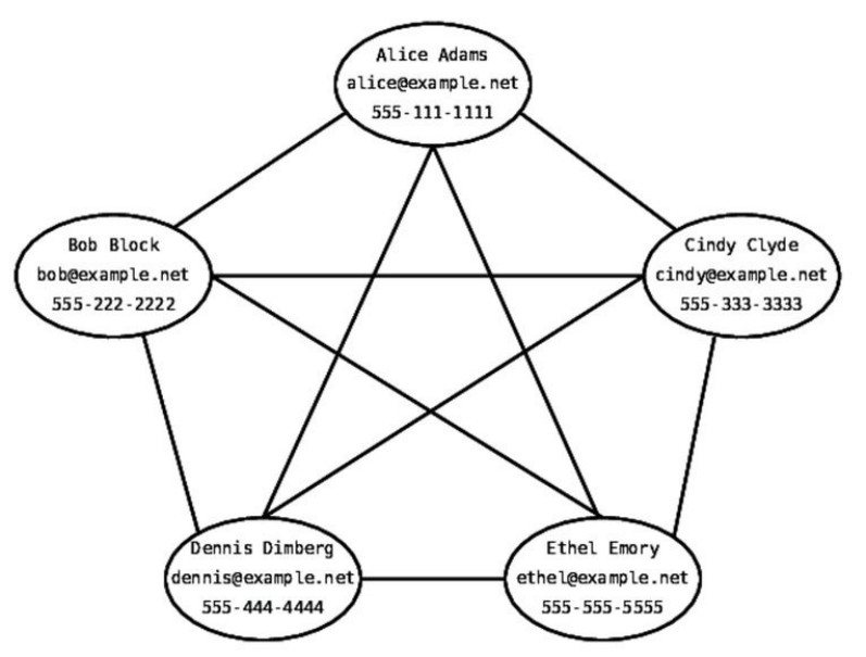
GraphDatabases
Becausegraphsaresoversatileathandlingrelationships,thereareactually
databasesthatstoredataintheformofagraph.Traditionalrelationaldatabases
(databasesthatstoredataascolumnsandrows)canalsostoresuchdata,butlet’s
comparetheirperformanceagainstgraphdatabasesfordealingwithsomething
likeasocialnetwork.
Let’ssaythatwehaveasocialnetworkinwhichtherearefivefriendswhoare
allconnectedtoeachother.ThesefriendsareAlice,Bob,Cindy,Dennis,and
Ethel.Agraphdatabasethatwillstoretheirpersonalinformationmaylook
somethinglikethis:
Wecanusearelationaldatabasetostorethisinformationaswell.Thiswould
likelyusetwotables—oneforstoringthepersonalinfoofeachuser,andonefor
storingtherelationshipsbetweenthefriends.HereistheUserstable:
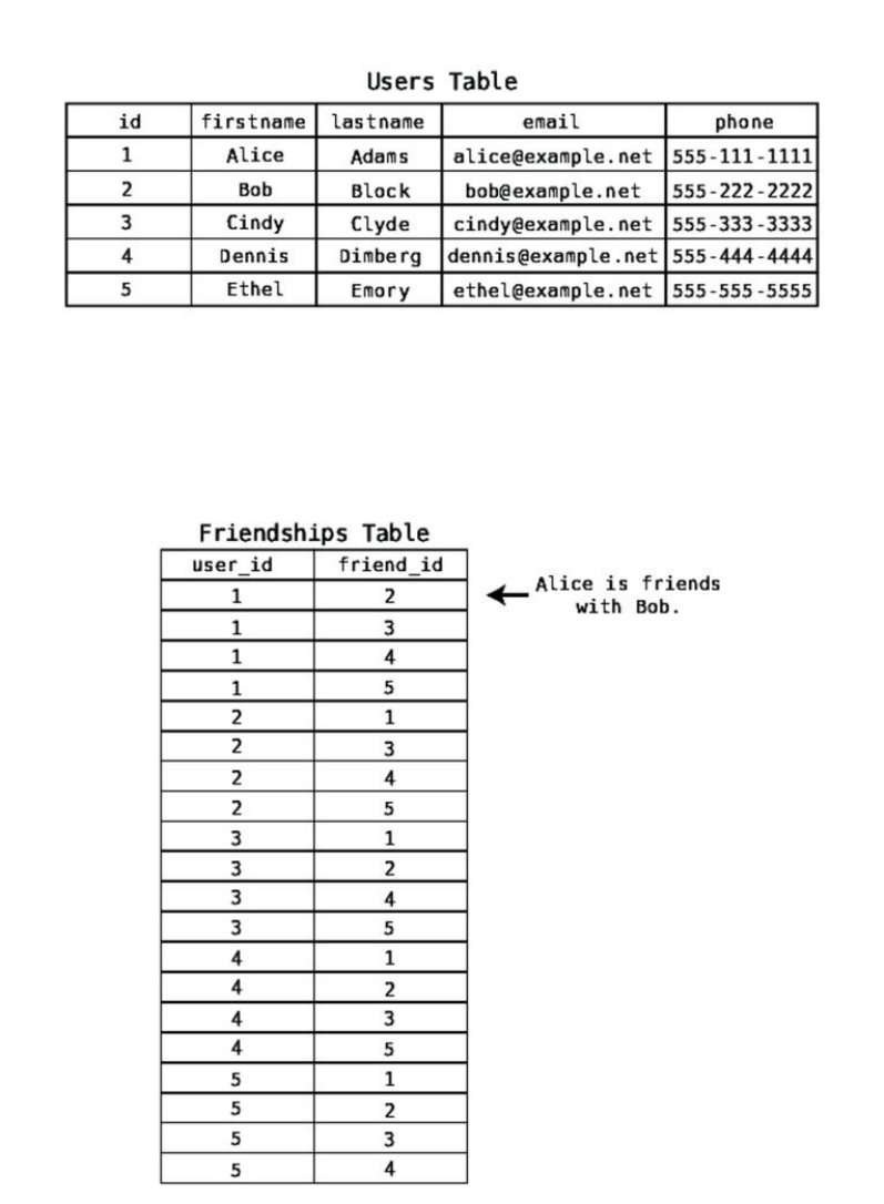
WewoulduseaseparateFriendshipstabletokeeptrackofwhoisfriendswith
whom:
We’llavoidgettingtoodeepintodatabasetheory,butnotehowthisFriendships
tableusestheidsofeachusertorepresenteachuser.
Assumethatoursocialnetworkhasafeaturethatallowseachusertoseeallthe
personalinformationabouttheirfriends.IfCindywererequestingthisinfo,that
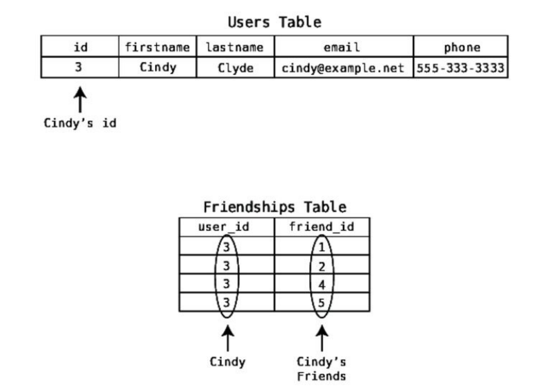
wouldmeanshe’dliketoseeeverythingaboutAlice,Bob,Dennis,andEthel,
includingtheiremailaddressesandphonenumbers.
Let’sseehowCindy’srequestwouldbeexecutedifourapplicationwasbacked
byarelationaldatabase.First,wewouldhavetolookupCindy’sidintheUsers
table:
Then,we’dlookforalltherowsintheFriendshipstablewheretheuseridis3:
WenowhavealistoftheidsofallofCindy’sfriends:[1,2,4,5].
Withthisidlist,weneedtoreturntotheUserstabletofindeachrowwiththe
appropriateid.ThespeedatwhichthecomputercanfindeachrowintheUsers
tablewillbeapproximatelyO(logN).Thisisbecausethedatabasemaintainsthe
rowsinorderoftheirids,andthedatabasecanthenusebinarysearchtofind
eachrow.(Thisexplanationappliestocertainrelationaldatabases;other
processesmayapplytootherrelationaldatabases.)
SinceCindyhasfourfriends,thecomputerneedstoperformO(logN)fourtimes
topullallthefriends’personaldata.Tosaythismoregenerally,forMfriends,
theefficiencyofpullingtheirinformationisO(MlogN).Thatis,foreachfriend,
werunasearchthattakeslogNsteps.
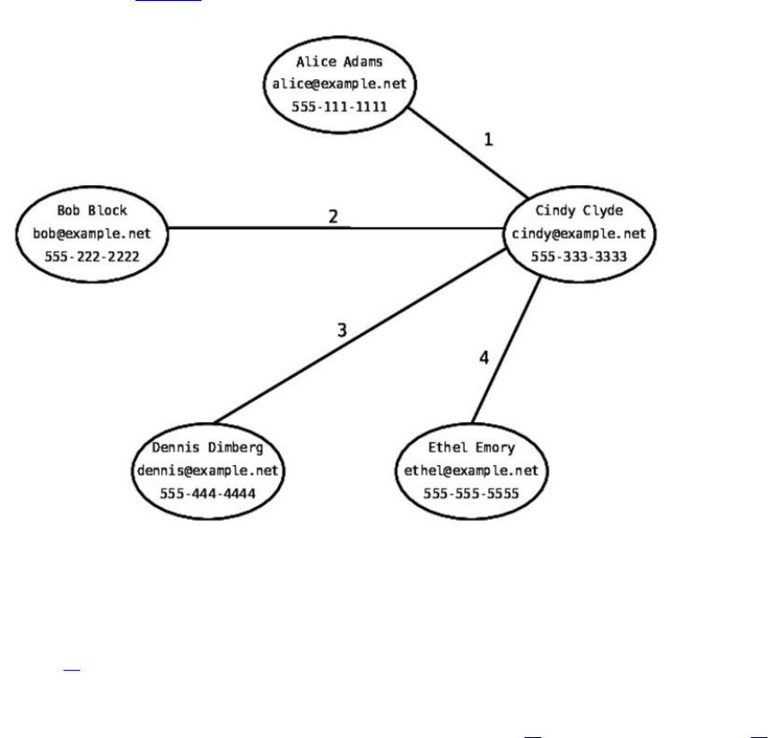
ContrastthiswithgettingthescooponCindy’sfriendsifourapplicationwas
backedbyagraphdatabase.Inthiscase,oncewe’velocatedCindyinour
database,ittakesjustonesteptofindonefriend’sinfo.Thisisbecauseeach
vertexinthedatabasecontainsalltheinformationofitsuser,sowesimply
traversetheedgesfromCindytoeachofherfriends.Thistakesagrandtotalof
fourstepsasshown.
Withagraphdatabase,forNfriends,pullingtheirdatatakesO(N)steps.Thisis
asignificantimprovementovertheefficiencyofO(MlogN)thatarelational
databasewouldprovide.
Neo4j[2]isanexampleofapopularopensourcegraphdatabase.Iencourageyou
tovisittheirwebsiteforfurtherresourcesaboutgraphdatabases.Otherexamples
ofopensourcegraphdatabasesincludeArangoDB[3]andApacheGiraph[4].
Notethatgraphdatabasesaren’talwaysthebestsolutionforagivenapplication.
You’llneedtocarefullyassesseachapplicationanditsneeds.
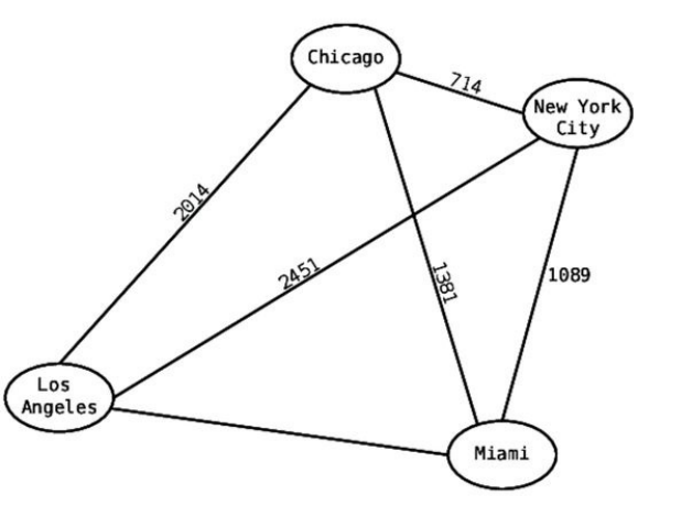
WeightedGraphs
Anothertypeofgraphisoneknownasaweightedgraph.Aweightedgraphis
likearegulargraphbutcontainsadditionalinformationabouttheedgesinthe
graph.
Here’saweightedgraphthatrepresentsabasicmapofafewmajorcitiesinthe
UnitedStates:
Inthisgraph,eachedgeisaccompaniedbyanumberthatrepresentsthedistance
inmilesbetweenthecitiesthattheedgeconnects.Forexample,thereare714
milesbetweenChicagoandNewYorkCity.
It’salsopossibletohavedirectionalweightedgraphs.Inthefollowingexample,
wecanseethatalthoughaflightfromDallastoTorontois$138,aflightfrom
TorontotoDallasis$216:

Toaddweightstoourgraph,weneedtomakeaslightmodificationtoourRuby
implementation.Specifically,we’llbeusingahashtableratherthananarrayto
representtheadjacentnodes.Inthiscase,eachvertexwillberepresentedbya
Cityclass:
classCity
attr_accessor:name,:routes
definitialize(name)
@name=name
#Fortheadjacentvertices,wearenowusingahashtable
#insteadofanarray:
@routes={}
end
defadd_route(city,price)
@routes[city]=price
end
end
Now,wecancreatecitiesandrouteswithprices:
dallas=City.new("Dallas")
toronto=City.new("Toronto")
dallas.add_route(toronto,138)
toronto.add_route(dallas,216)
Let’susethepoweroftheweightedgraphtosolvesomethingknownasthe
shortestpathproblem.
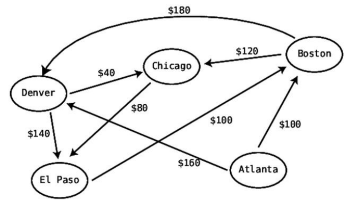
Here’sagraphthatdemonstratesthecostsofavailableflightsbetweenfive
differentcities.(Don’taskmehowairlinesdeterminethepricesofthesethings!)
Now,saythatI’minAtlantaandwanttoflytoElPaso.Unfortunately,there’sno
directrouteatthistime.However,IcangetthereifI’mwillingtoflythrough
othercities.Forexample,IcanflyfromAtlantatoDenver,andfromDenverto
ElPaso.Thatroutewouldsetmeback$300.However,ifyoulookclosely,
you’llnoticethatthere’sacheaperrouteifIgofromAtlantatoDenverto
ChicagotoElPaso.AlthoughIhavetotakeanextraflight,Ionlyendup
shellingout$280.
Inthiscontext,theshortestpathproblemisthis:howcanIgetfromAtlantatoEl
Pasowiththeleastamountofmoney?
Dijkstra’sAlgorithm
Therearenumerousalgorithmsforsolvingtheshortestpathproblem,andone
reallyinterestingonewasdiscoveredbyEdsgerDijkstra(pronounced“dike’
struh”)in1959.Unsurprisingly,thisalgorithmisknownasDijkstra’salgorithm.
HerearetherulesofDijkstra’salgorithm(don’tworry—they’llbecomeclearer
whenwewalkthroughourexample):
1. Wemakethestartingvertexourcurrentvertex.
2. Wecheckalltheverticesadjacenttothecurrentvertexandcalculateand
recordtheweightsfromthestartingvertextoallknownlocations.
3. Todeterminethenextcurrentvertex,wefindthecheapestunvisitedknown
vertexthatcanbereachedfromourstartingvertex.
4. Repeatthefirstthreestepsuntilwehavevisitedeveryvertexinthegraph.
Let’swalkthroughthisalgorithmstepbystep.
TorecordthecheapestpriceoftheroutesfromAtlantatoothercities,wewill
useatableasfollows:
FromAtlantato: Boston Chicago Denver ElPaso
? ? ? ?
First,wemakethestartingvertex(Atlanta)thecurrentvertex.Allouralgorithm
hasaccesstoatthispointisthecurrentvertexanditsconnectionstoitsadjacent
vertices.Toindicatethatit’sthecurrentvertex,we’llsurrounditwithlines.And
toindicatethatthisvertexwasoncethecurrentvertex,we’llputacheckmark
throughit:
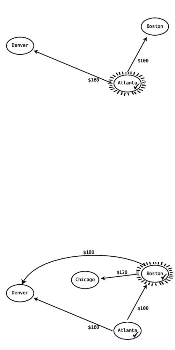
Wenextcheckalladjacentverticesandrecordtheweightsfromthestarting
vertex(Atlanta)toallknownlocations.Sincewecanseethatwecangetfrom
AtlantatoBostonfor$100,andfromAtlantatoDenverfor$160,we’llrecord
thatinourtable:
FromAtlantato: Boston Chicago Denver ElPaso
$100 ?$160 ?
Next,wefindthecheapestvertexthatcanbereachedfromAtlantathathasnot
yetbeenvisited.WeonlyknowhowtogettoBostonandDenverfromAtlantaat
thispoint,andit’scheapertogettoBoston($100)thanitistoDenver($160).So
wemakeBostonourcurrentvertex:
WenowcheckbothoftheroutesfromBoston,andrecordallnewdataaboutthe
costoftheroutesfromAtlanta—thestartingvertex—toallknownlocations.We
canseethatBostontoChicagois$120.Now,wecanalsoconcludethatsince
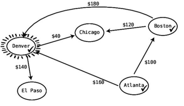
AtlantatoBostonis$100,andBostontoChicagois$120,thecheapest(and
only)knownroutefromAtlantatoChicagois$220.We’llrecordthisinour
table:
FromAtlantato: Boston Chicago Denver ElPaso
$100 $220 $160 ?
WealsolookatBoston’sotherroute—whichistoDenver—andthatturnsoutto
be$180.NowwehaveanewroutefromAtlantatoDenver:AtlantatoBostonto
Denver.However,sincethiscosts$280whilethedirectflightfromAtlantato
Denveris$160,wedonotupdatethetable,sinceweonlykeepthecheapest
knownroutesinthetable.
Nowthatwe’veexploredalltheoutgoingroutesfromthecurrentvertex
(Boston),wenextlookfortheunvisitedvertexthatisthecheapesttoreachfrom
Atlanta,whichwasourstartingpoint.Accordingtoourtable,Bostonisstillthe
cheapestknowncitytoreachfromAtlanta,butwe’vealreadycheckeditoff.So
thatwouldmakeDenverthecheapestunvisitedcity,sinceit’sonly$160from
Atlanta,comparedwithChicago,whichis$220fromAtlanta.SoDenver
becomesourcurrentvertex:
WenowinspecttheroutesthatleaveDenver.Onerouteisa$40flightfrom
DenvertoChicago.Wecanupdateourtablesincewenowhaveacheaperpath
fromAtlantatoChicagothanbefore.Ourtablecurrentlysaysthatthecheapest
routefromAtlantatoChicagois$220,butifwetakeAtlantatoChicagobyway
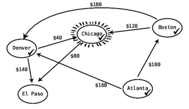
ofDenver,itwillcostusjust$200.Weupdateourtableaccordingly:
FromAtlantato: Boston Chicago Denver ElPaso
$100 $200 $160 ?
There’sanotherflightoutofDenveraswell,andthatistothenewlyrevealed
cityofElPaso.WenowhavetofigureoutthecheapestknownpathfromAtlanta
toElPaso,andthatwouldbethe$300pathfromAtlantatoDenvertoElPaso.
Wecannowaddthistoourtableaswell:
FromAtlantato: Boston Chicago Denver ElPaso
$100 $200 $160 $300
Wenowhavetwounvisitedvertices:ChicagoandElPaso.Sincethecheapest
knownpathtoChicagofromAtlanta($200)ischeaperthanthecheapestknown
pathtoElPasofromAtlanta($300),wewillnextmakeChicagothecurrent
vertex:
Chicagohasjustoneoutboundflight,andthatisan$80triptoElPaso.Wenow
haveacheaperpathfromAtlantatoElPaso:AtlantatoDenvertoChicagotoEl
Paso,whichcostsatotalof$280.Weupdateourtablewiththisnewfounddata:
FromAtlantato: Boston Chicago Denver ElPaso
$100 $200 $160 $280
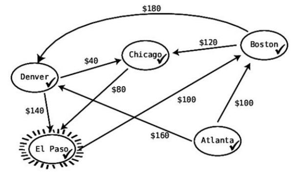
There’soneknowncitylefttomakethecurrentvertex,andthatisElPaso:
ElPasohasonlyoneoutboundroute,andthatisa$100flighttoBoston.This
datadoesn’trevealanycheaperpathsfromAtlantatoanywhere,sowedon’t
needtomodifyourtable.
Sincewehavevisitedeveryvertexandcheckeditoff,wenowknoweverypath
fromAtlantatoeveryothercity.Thealgorithmisnowcomplete,andour
resultingtablerevealsthecheapestpriceofAtlantatoeveryothercityonthe
map:
FromAtlantato: Boston Chicago Denver ElPaso
$100 $200 $160 $280
HereisaRubyimplementationofDijkstra’salgorithm:
We’llbeginbycreatingaRubyclassrepresentingacity.Eachcityisanodeina
graph,whichkeepstrackofitsownname,androutestoadjacentcities:
classCity
attr_accessor:name,:routes
definitialize(name)
@name=name
#Fortheadjacentnodes,wearenowusingahashtable
#insteadofanarray:
@routes={}
#Asanexample,ifthiswereAtlanta,itsrouteswouldbe:
#{boston=>100,denver=>160}
end
defadd_route(city,price_info)
@routes[city]=price_info
end
end
We’llusetheadd_routemethodtosetupthecitiesfromourexample:
atlanta=City.new("Atlanta")
boston=City.new("Boston")
chicago=City.new("Chicago")
denver=City.new("Denver")
el_paso=City.new("ElPaso")
atlanta.add_route(boston,100)
atlanta.add_route(denver,160)
boston.add_route(chicago,120)
boston.add_route(denver,180)
chicago.add_route(el_paso,80)
denver.add_route(chicago,40)
denver.add_route(el_paso,140)
ThecodeforDijkstra’sAlgorithmissomewhatinvolved,soI’vesprinkled
commentsliberally:
defdijkstra(starting_city,other_cities)
#Theroutes_from_cityhashtablebelowholdsthedataofallprice_infos
#fromthegivencitytoallotherdestinations,andthecitywhichit
#tooktogetthere:
routes_from_city={}
#Theformatofthisdatais:
#{city=>[price,othercitywhichimmediatelyprecedesthiscity
#alongthepathfromtheoriginalcity]}
#Inourexamplethiswillendupbeing:
#{atlanta=>[0,nil],boston=>[100,atlanta],chicago=>[200,denver],
#denver=>[160,atlanta],el_paso=>[280,chicago]}
#Sinceitcostsnothingtogettothestartingcityfromthestartingcity:
routes_from_city[starting_city]=[0,starting_city]
#Wheninitializingourdata,wesetupallothercitieshavingan
#infinitecost-sincethecostandthepathtogettoeachothercity
#iscurrentlyunknown:
other_cities.eachdo|city|
routes_from_city[city]=[Float::INFINITY,nil]
end
#Inourexample,ourdatastartsoutas:
#{atlanta=>[0,nil],boston=>[Float::INFINITY,nil],
#chicago=>[Float::INFINITY,nil],
#denver=>[Float::INFINITY,nil],el_paso=>[Float::INFINITY,nil]}
#Wekeeptrackofwhichcitieswevisitedinthisarray:
visited_cities=[]
#Webeginvisitingthestartingcitybymakingitthecurrent_city:
current_city=starting_city
#Welaunchtheheartofthealgorithm,whichisaloopthatvisits
#eachcity:
whilecurrent_city
#Weofficiallyvisitthecurrentcity:
visited_cities<<current_city
#Wecheckeachroutefromthecurrentcity:
current_city.routes.eachdo|city,price_info|
#Iftheroutefromthestartingcitytotheothercity
#ischeaperthancurrentlyrecordedinroutes_from_city,weupdateit:
ifroutes_from_city[city][0]>price_info+
routes_from_city[current_city][0]
routes_from_city[city]=
[price_info+routes_from_city[current_city][0],current_city]
end
end
#Wedeterminewhichcitytovisitnext:
current_city=nil
cheapest_route_from_current_city=Float::INFINITY
#Wecheckallavailableroutes:
routes_from_city.eachdo|city,price_info|
#ifthisrouteisthecheapestfromthiscity,andithasnotyetbeen
#visited,itshouldbemarkedasthecitywe'llvisitnext:
ifprice_info[0]<cheapest_route_from_current_city&&
!visited_cities.include?(city)
cheapest_route_from_current_city=price_info[0]
current_city=city
end
end
end
returnroutes_from_city
end
Wecanrunthismethodasfollows:
routes=dijkstra(atlanta,[boston,chicago,denver,el_paso])
routes.eachdo|city,price_info|
p"#{city.name}:#{price_info[0]}"
end
Althoughourexampleherefocusedonfindingthecheapestflight,thesame
exactapproachcanbeusedformappingandGPStechnology.Iftheweightson
eachedgerepresentedhowfastitwouldtaketodrivefromeachcitytotheother
ratherthantheprice,we’djustaseasilyuseDijkstra’salgorithmtodetermine
whichrouteyoushouldtaketodrivefromoneplacetoanother.
[2]
[3]
[4]
WrappingUp
We’realmostattheendofourjourney,asthischapterrepresentsthelast
significantdatastructurethatwe’llencounterinthisbook.We’veseenthat
graphsareextremelypowerfultoolsfordealingwithdatainvolving
relationships,andinadditiontomakingourcodefast,theycanalsohelpsolve
trickyproblems.
Alongourtravels,ourprimaryfocushasbeenonhowfastourcodewillrun.
Thatis,we’vebeenmeasuringhowefficientourcodeperformsintermsoftime,
andwe’vebeenmeasuringthatintermsofcountingthenumberofstepsthatour
algorithmstake.
However,efficiencycanbemeasuredinotherways.Incertainsituations,there
aregreaterconcernsthanspeed,andwemightcaremoreabouthowmuch
memoryadatastructureoralgorithmmightconsume.Inthenextchapter,we’ll
learnhowtoanalyzetheefficiencyofourcodeintermsofspace.
Footnotes
http://neo4j.com
https://www.arangodb.com/
http://giraph.apache.org/
Copyright©2017,ThePragmaticBookshelf.

Chapter14
DealingwithSpaceConstraints
Throughoutthisbook,whenanalyzingtheefficiencyofvariousalgorithms,
we’vefocusedexclusivelyontheirtimecomplexity—thatis,howfasttheyrun.
Therearesituations,however,whereweneedtomeasurealgorithmefficiency
byanothermeasureknownasspacecomplexity,whichishowmuchmemoryan
algorithmconsumes.
Spacecomplexitybecomesanimportantfactorwhenmemoryislimited.This
canhappenwhenprogrammingforsmallhardwaredevicesthatonlycontaina
relativelysmallamountofmemoryorwhendealingwithverylargeamountsof
data,whichcanquicklyfillevenlargememorycontainers.
Inaperfectworld,we’dalwaysusealgorithmsthatarebothquickandconsume
asmallamountofmemory.However,therearetimeswherewe’refacedwith
choosingbetweenthespeedyalgorithmorthememory-efficientalgorithm—and
weneedtolookcarefullyatthesituationtomaketherightchoice.
BigONotationasAppliedtoSpaceComplexity
Interestingly,computerscientistsuseBigONotationtodescribespace
complexityjustastheydotodescribetimecomplexity.
Untilnow,we’veusedBigONotationtodescribeanalgorithm’sspeedas
follows:forNelementsofdata,analgorithmtakesarelativenumberof
operationalsteps.Forexample,O(N)meansthatforNdataelements,the
algorithmtakesNsteps.AndO(N2)meansthatforNdataelements,the
algorithmtakesN2steps.
BigOcansimilarlybeusedtodescribehowmuchspaceanalgorithmtakesup:
forNelementsofdata,analgorithmconsumesarelativenumberofadditional
dataelementsinmemory.Let’stakeasimpleexample.
Let’ssaythatwe’rewritingaJavaScriptfunctionthatacceptsanarrayofstrings,
andreturnsanarrayofthosestringsinALLCAPS.Forexample,thefunction
wouldacceptanarraylike["amy","bob","cindy","derek"]andreturn["AMY","BOB",
"CINDY","DEREK"].Here’sonewaywecanwritethisfunction:
functionmakeUpperCase(array){
varnewArray=[];
for(vari=0;i<array.length;i++){
newArray[i]=array[i].toUpperCase();
}
returnnewArray;
}
InthismakeUpperCase()function,weacceptanarraycalledarray.Wethencreatea
brand-newarraycallednewArray,andfillitwithuppercaseversionsofeach
stringfromtheoriginalarray.
Bythetimethisfunctioniscomplete,wehavetwoarraysfloatingaroundinour
computer’smemory.Wehavearray,whichcontains["amy","bob","cindy","derek"],
andwehavenewArray,whichcontains["AMY","BOB","CINDY","DEREK"].
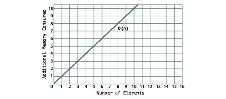
Whenweanalyzethisfunctionintermsofspacecomplexity,wecanseethatit
acceptsanarraywithNelements,andcreatesabrand-newarraythatalso
containsNelements.Becauseofthis,we’dsaythatthemakeUpperCase()function
hasaspaceefficiencyofO(N).
Thewaythisappearsonthefollowinggraphshouldlookquitefamiliar:
Notethatthisgraphisidenticaltothewaywe’vedepictedO(N)inthegraphs
frompreviouschapters,withtheexceptionthattheverticalaxisnowrepresents
memoryratherthanspeed.
Now,let’spresentanalternativemakeUpperCase()functionthatismorememory
efficient:
functionmakeUpperCase(array){
for(vari=0;i<array.length;i++){
array[i]=array[i].toUpperCase();
}
returnarray;
}
Inthissecondversion,wedonotcreateanynewvariablesornewarrays.Infact,
wehavenotconsumedanynewmemoryatall.Instead,wemodifyeachstring
withintheoriginalarrayinplace,makingthemuppercaseoneatatime.Wethen
returnthemodifiedarray.
Sincethisfunctiondoesnotconsumeanymemoryinadditiontotheoriginal
array,we’ddescribethespacecomplexityofthisfunctionasbeingO(1).
Rememberthatbytimecomplexity,O(1)representsthatthespeedofan
algorithmisconstantnomatterhowlargethedata.Similarly,byspace
complexity,O(1)meansthatthememoryconsumedbyanalgorithmisconstant
nomatterhowlargethedata.
Inourcase,thealgorithmconsumesthesameamountofadditionalspace(zero!)
nomatterwhethertheoriginalarraycontainsfourelementsoronehundred.
Becauseofthis,ournewversionofmakeUpperCase()issaidtohaveaspace
efficiencyofO(1).
It’simportanttoreiteratethatinthisbook,wejudgethespacecomplexitybased
onadditionalmemoryconsumed—knownasauxiliaryspace—meaningthatwe
don’tcounttheoriginaldata.Eveninthissecondversion,wedohaveaninputof
array,whichcontainsNelementsofmemory.However,sincethisfunctiondoes
notconsumeanymemoryinadditiontotheoriginalarray,itisO(1).
(Therearesomereferencesthatincludetheoriginalinputwhencalculatingthe
spacecomplexity,andthat’sfine.We’renotincludingit,andwheneveryousee
spacecomplexitydescribed,youneedtodeterminewhetherit’sincludingthe
originalinput.)
Let’snowcomparethetwoversionsofmakeUpperCase()inbothtimeandspace
complexity:
Version Timecomplexity Spacecomplexity
Version#1 O(N) O(N)
Version#2 O(N) O(1)
BothversionsareO(N)intimecomplexity,sincetheytakeNstepsforNdata
elements.However,thesecondversionismorememoryefficient,beingO(1)in
spacecomplexitycomparedtothefirstversion’sO(N).
Thisisaprettystrongcasethatversion#2ispreferabletoversion#1.

Trade-OffsBetweenTimeandSpace
InChapter4,SpeedingUpYourCodewithBigO,wewroteaJavaScript
functionthatcheckedwhetheranarraycontainedanyduplicatevalues.Ourfirst
versionlookedlikethis:
functionhasDuplicateValue(array){
for(vari=0;i<array.length;i++){
for(varj=0;j<array.length;j++){
if(i!==j&&array[i]==array[j]){
returntrue;
}
}
}
returnfalse;
}
Itusesnestedforloops,andwepointedoutthatithasatimecomplexityof
O(N2).
Wethencreatedamoreefficientversion,whichlookedlikethis:
functionhasDuplicateValue(array){
varexistingNumbers=[];
for(vari=0;i<array.length;i++){
if(existingNumbers[array[i]]===undefined){
existingNumbers[array[i]]=1;
}else{
returntrue;
}
}
returnfalse;
}
ThissecondversioncreatesanarraycalledexistingNumbers,andforeachnumber
weencounterinarray,wefindthecorrespondingindexinexistingNumbersandfill
itwitha1.Ifweencounteranumberandalreadyfinda1inthecorresponding
indexwithinexistingNumbers,weknowthatthisnumberalreadyexistsandthat
we’vethereforefoundaduplicatevalue.
Wedeclaredvictorywiththissecondversion,pointingtoitstimecomplexityof
O(N)comparedwiththefirstversion’sO(N2).Indeed,fromtheperspectiveof
timealone,thesecondversionismuchfaster.
However,whenwetakespaceintoaccount,wefindthatthissecondversionhas
adisadvantagecomparedwiththefirstversion.Thefirstversiondoesnot
consumeanyadditionalmemorybeyondtheoriginalarray,andthereforehasa
spacecomplexityofO(1).Ontheotherhand,thissecondversioncreatesa
brand-newarraythatisthesamesizeastheoriginalarray,andthereforehasa
spacecomplexityofO(N).
Let’slookatthecompletecontrastbetweenthetwoversionsof
hasDuplicateValue():
Version Timecomplexity Spacecomplexity
Version#1 O(N2)O(1)
Version#2 O(N) O(N)
Wecanseethatversion#1takesuplessmemorybutisslower,whileversion#2
isfasterbuttakesupmorememory.Howdowedecidewhichtochoose?
Theanswer,ofcourse,isthatitdependsonthesituation.Ifweneedour
applicationtobeblazingfast,andwehaveenoughmemorytohandleit,then
version#2mightbepreferable.If,ontheotherhand,speedisn’tcritical,but
we’redealingwithahardware/datacombinationwhereweneedtoconsume
memorysparingly,thenversion#1mightbetherightchoice.Likealltechnology
decisions,whentherearetrade-offs,weneedtolookatthebigpicture.

PartingThoughts
You’velearnedalotinthisjourney.Mostimportantly,you’velearnedthatthe
analysisofdatastructuresandalgorithmscandramaticallyaffectyourcode—in
speed,memory,andevenelegance.
Whatyoucantakeawayfromthisbookisaframeworkformakingeducated
technologydecisions.Now,computingcontainsmanydetails,andwhile
somethinglikeBigONotationmaysuggestthatoneapproachisbetterthan
another,otherfactorscanalsocomeintoplay.Thewaymemoryisorganized
withinyourhardwareandthewaythatyourcomputerlanguageofchoice
implementsthingsunderthehoodcanalsoaffecthowefficientyourcodemay
be.Sometimeswhatyouthinkisthemostefficientchoicemaynotbedueto
variousexternalreasons.
Becauseofthis,itisalwaysbesttotestyouroptimizationswithbenchmarking
tools.Therearemanyexcellentsoftwareapplicationsouttherethatcanmeasure
thespeedandmemoryconsumptionofyourcode.Theknowledgeinthisbook
willpointyouintherightdirection,andthebenchmarkingtoolswillconfirm
whetheryou’vemadetherightchoices.
Ihopethatyoualsotakeawayfromthisbookthattopicslikethese—whichseem
socomplexandesoteric—arejustacombinationofsimpler,easierconceptsthat
arewithinyourgrasp.Don’tbeintimidatedbyresourcesthatmakeaconcept
seemdifficultsimplybecausetheydon’texplainitwell—youcanalwaysfinda
resourcethatexplainsitbetter.
Thetopicofdatastructuresandalgorithmsisbroadanddeep,andwe’veonly
justscratchedthesurface.Thereissomuchmoretolearn—butwiththe
foundationthatyounowhave,you’llbeabletodoso.Goodluck!
Copyright©2017,ThePragmaticBookshelf.
ProgrammingElixir1.3
Explorefunctionalprogrammingwithouttheacademic
overtones(tellmeaboutmonadsjustonemoretime).
Createconcurrentapplications,butgetthemright
withoutallthelockingandconsistencyheadaches.Meet
Elixir,amodern,functional,concurrentlanguagebuilt
ontherock-solidErlangVM.Elixir’spragmaticsyntax
andbuilt-insupportformetaprogrammingwillmake
youproductiveandkeepyouinterestedforthelonghaul.Maybethetimeis
rightfortheNextBigThing.Maybeit’sElixir.Thisbookistheintroduction
toElixirforexperiencedprogrammers,completelyupdatedforElixir1.3.
DaveThomas
(362pages)ISBN:9781680502008$38
MetaprogrammingElixir
WritecodethatwritescodewithElixirmacros.Macros
makemetaprogrammingpossibleanddefinethe
languageitself.Inthisbook,you’lllearnhowtouse
macrostoextendthelanguagewithfast,maintainable
codeandsharefunctionalityinwaysyouneverthought
possible.You’lldiscoverhowtoextendElixirwithyour
ownfirst-classfeatures,optimizeperformance,and
createdomain-specificlanguages.
ChrisMcCord
YouMayBeInterestedIn…
Selectacoverformoreinformation

(128pages)ISBN:9781680500417$17
DomainModelingMadeFunctional
Youwantincreasedcustomersatisfaction,faster
developmentcycles,andlesswastedwork.Domain-
drivendesign(DDD)combinedwithfunctional
programmingistheinnovativecombothatwillgetyou
there.Inthispragmatic,down-to-earthguide,you’llsee
howapplyingthecoreprinciplesoffunctional
programmingcanresultinsoftwaredesignsthatmodel
real-worldrequirementsbothelegantlyandconcisely—oftenmoresothanan
object-orientedapproach.Practicalexamplesintheopen-sourceF#functional
language,andexamplesfromfamiliarbusinessdomains,showyouhowto
applythesetechniquestobuildsoftwarethatisbusiness-focused,flexible,and
highquality.
ScottWlaschin
(260pages)ISBN:9781680502541$47.95
ProgrammingClojure,ThirdEdition
Drowninginunnecessarycomplexity,unmanagedstate,
andtanglesofspaghetticode?Inthebesttraditionof
Lisp,Clojuregetsoutofyourwaysoyoucanfocuson
expressingsimplesolutionstohardproblems.Clojure
cutsthroughcomplexitybyprovidingasetof
composabletools—immutabledata,functions,macros,
andtheinteractiveREPL.Writtenbymembersofthe
Clojurecoreteam,thisbookistheessential,definitiveguidetoClojure.This
neweditionincludesinformationonallthenewestfeaturesofClojure,suchas
transducersandspecs.

AlexMillerwithStuartHallowayandAaronBedra
(300pages)ISBN:9781680502466$49.95
SwiftStyle
Discoverthedo’sanddon’tsinvolvedincrafting
readableSwiftcodeasyouexplorecommonSwift
codingchallengesandthebestpracticesthataddress
them.Fromspacing,bracing,andsemicolonstoproper
APIstyle,discoverthewhysbehindeach
recommendation,andaddtoorestablishyourownhouse
styleguidelines.Thispractical,powerful,and
opinionatedguideoffersthebestpracticesyouneedtoknowtowork
successfullyinthisequallyopinionatedprogramminglanguage.
EricaSadun
(224pages)ISBN:9781680502350$29.95
ExercisesforProgrammers
Whenyouwritesoftware,youneedtobeatthetopofyour
game.Greatprogrammerspracticetokeeptheirskillssharp.
Getsharpandstaysharpwithmorethanfiftypractice
exercisesrootedinreal-worldscenarios.Ifyou’reanew
programmer,thesechallengeswillhelpyoulearnwhatyou
needtobreakintothefield,andifyou’reaseasonedpro,
youcanusetheseexercisestolearnthathotnewlanguage
foryournextgig.
BrianP.Hogan
(118pages)ISBN:9781680501223$24

SevenLanguagesinSevenWeeks
Youshouldlearnaprogramminglanguageeveryyear,as
recommendedbyThePragmaticProgrammer.Butifone
peryearisgood,howaboutSevenLanguagesinSeven
Weeks?Inthisbookyou’llgetahands-ontourof
Clojure,Haskell,Io,Prolog,Scala,Erlang,andRuby.
Whetherornotyourfavoritelanguageisonthatlist,
you’llbroadenyourperspectiveofprogrammingby
examiningtheselanguagesside-by-side.You’lllearnsomethingnewfrom
each,andbestofall,you’lllearnhowtolearnalanguagequickly.
BruceA.Tate
(330pages)ISBN:9781934356593$34.95
SevenMoreLanguagesinSevenWeeks
Greatprogrammersaren’tborn—they’remade.The
industryismovingfromobject-orientedlanguagesto
functionallanguages,andyouneedtocommittoradical
improvement.Newprogramminglanguagesarmyou
withthetoolsandidiomsyouneedtorefineyourcraft.
Whileotherlanguageprimerstakeyouthroughbasic
installationand“Hello,World,”weaimhigher.Each
languageinSevenMoreLanguagesinSevenWeekswilltakeyouonastep-
by-stepjourneythroughthemostimportantparadigmsofourtime.You’ll
learnsevenexcitinglanguages:Lua,Factor,Elixir,Elm,Julia,MiniKanren,
andIdris.
BruceTate,FredDaoud,JackMoffitt,IanDees

(318pages)ISBN:9781941222157$38
tmux2
Yourmouseisslowingyoudown.Thetimeyouspend
contextswitchingbetweenyoureditorandyourconsoles
eatsawayatyourproductivity.Takecontrolofyour
environmentwithtmux,aterminalmultiplexerthatyou
cantailortoyourworkflow.Withthisupdatedsecond
editionfortmux2.3,you’llcustomize,script,and
leveragetmux’suniqueabilitiestocraftaproductive
terminalenvironmentthatletsyoukeepyourfingersonyourkeyboard’shome
row.
BrianP.Hogan
(102pages)ISBN:9781680502213$21.95
PracticalVim,SecondEdition
Vimisafastandefficienttexteditorthatwillmakeyou
afasterandmoreefficientdeveloper.It’savailableon
almosteveryOS,andifyoumasterthetechniquesinthis
book,you’llneverneedanothertexteditor.Inmorethan
120Vimtips,you’llquicklylearntheeditor’score
functionalityandtackleyourtrickiesteditingandwriting
tasks.Thisbelovedbestsellerhasbeenrevisedand
updatedtoVim8andincludesthreebrand-newtipsandfivefullyrevisedtips.
DrewNeil
(354pages)ISBN:9781680501278$29
