A Guide To Convolutional Neural Networks For Computer Vision
User Manual:
Open the PDF directly: View PDF ![]() .
.
Page Count: 209 [warning: Documents this large are best viewed by clicking the View PDF Link!]
- Preface
- Acknowledgments
- Introduction
- Features and Classifiers
- Neural Networks Basics
- Convolutional Neural Network
- CNN Learning
- Examples of CNN Architectures
- Applications of CNNs in Computer Vision
- Deep Learning Tools and Libraries
- Conclusion
- Bibliography
- Authors' Biographies
- Blank Page

A Guide to
Convolutional Neural
Networks for
Computer Vision
Salman Khan
Hossein Rahmani
Syed Afaq Ali Shah
Mohammed Bennamoun
Series Editors: Gérard Medioni, University of Southern California
Sven Dickinson, University of Toronto
A Guide to Convolutional Neural Networks for Computer Vision
Salman Khan, Data61-CSIRO and Australian National University
Hossein Rahmani, e University of Western Australia
Syed Afaq Ali Shah, e University of Western Australia
Mohammed Bennamoun, e University of Western Australia
Computer vision has become increasingly important and eective in recent years due to its wide-ranging
applications in areas as diverse as smart surveillance and monitoring, health and medicine, sports and recreation,
robotics, drones, and self-driving cars. Visual recognition tasks, such as image classication, localization, and
detection, are the core building blocks of many of these applications, and recent developments in Convolutional
Neural Networks (CNNs) have led to outstanding performance in these state-of-the-art visual recognition tasks
and systems. As a result, CNNs now form the crux of deep learning algorithms in computer vision.
is self-contained guide will benet those who seek to both understand the theory behind CNNs
and to gain hands-on experience on the application of CNNs in computer vision. It provides a comprehensive
introduction to CNNs starting with the essential concepts behind neural networks: training, regularization, and
optimization of CNNs. e book also discusses a wide range of loss functions, network layers, and popular CNN
architectures, reviews the dierent techniques for the evaluation of CNNs, and presents some popular CNN tools
and libraries that are commonly used in computer vision. Further, this text describes and discusses case studies that
are related to the application of CNN in computer vision, including image classication, object detection, semantic
segmentation, scene understanding, and image generation.
is book is ideal for undergraduate and graduate students, as no prior background knowledge in the
eld is required to follow the material, as well as new researchers, developers, engineers, and practitioners who are
interested in gaining a quick understanding of CNN models.
store.morganclaypool.com
About SYNTHESIS
This volume is a printed version of a work that appears in the Synthesis
Digital Library of Engineering and Computer Science. Synthesis
books provide concise, original presentations of important research and
development topics, published quickly, in digital and print formats.
KHAN • ET AL A GUIDE TO CONVOLUTIONAL NEURAL NETWORKS FOR COMPUTER VISION MORGAN & CLAYPOOL
Series ISSN: 2153-1056

A Guide to
Convolutional Neural Networks
for Computer Vision

Synthesis Lectures on
Computer Vision
Editors
Gérard Medioni, University of Southern California
Sven Dickinson, University of Toronto
Synthesis Lectures on Computer Vision is edited by Gérard Medioni of the University of Southern
California and Sven Dickinson of the University of Toronto. e series publishes 50–150 page
publications on topics pertaining to computer vision and pattern recognition. e scope will largely
follow the purview of premier computer science conferences, such as ICCV, CVPR, and ECCV.
Potential topics include, but not are limited to:
• Applications and Case Studies for Computer Vision
• Color, Illumination, and Texture
• Computational Photography and Video
• Early and Biologically-inspired Vision
• Face and Gesture Analysis
• Illumination and Reflectance Modeling
• Image-Based Modeling
• Image and Video Retrieval
• Medical Image Analysis
• Motion and Tracking
• Object Detection, Recognition, and Categorization
• Segmentation and Grouping
• Sensors
• Shape-from-X
• Stereo and Structure from Motion
• Shape Representation and Matching

iv
• Statistical Methods and Learning
• Performance Evaluation
• Video Analysis and Event Recognition
A Guide to Convolutional Neural Networks for Computer Vision
Salman Khan, Hossein Rahmani, Syed Afaq Ali Shah, and Mohammed Bennamoun
2018
Covariances in Computer Vision and Machine Learning
Hà Quang Minh and Vittorio Murino
2017
Elastic Shape Analysis of ree-Dimensional Objects
Ian H. Jermyn, Sebastian Kurtek, Hamid Laga, and Anuj Srivastava
2017
e Maximum Consensus Problem: Recent Algorithmic Advances
Tat-Jun Chin and David Suter
2017
Extreme Value eory-Based Methods for Visual Recognition
Walter J. Scheirer
2017
Data Association for Multi-Object Visual Tracking
Margrit Betke and Zheng Wu
2016
Ellipse Fitting for Computer Vision: Implementation and Applications
Kenichi Kanatani, Yasuyuki Sugaya, and Yasushi Kanazawa
2016
Computational Methods for Integrating Vision and Language
Kobus Barnard
2016
Background Subtraction: eory and Practice
Ahmed Elgammal
2014
Vision-Based Interaction
Matthew Turk and Gang Hua
2013

v
Camera Networks: e Acquisition and Analysis of Videos over Wide Areas
Amit K. Roy-Chowdhury and Bi Song
2012
Deformable Surface 3D Reconstruction from Monocular Images
Mathieu Salzmann and Pascal Fua
2010
Boosting-Based Face Detection and Adaptation
Cha Zhang and Zhengyou Zhang
2010
Image-Based Modeling of Plants and Trees
Sing Bing Kang and Long Quan
2009

Copyright © 2018 by Morgan & Claypool
All rights reserved. No part of this publication may be reproduced, stored in a retrieval system, or transmitted in
any form or by any means—electronic, mechanical, photocopy, recording, or any other except for brief quotations
in printed reviews, without the prior permission of the publisher.
A Guide to Convolutional Neural Networks for Computer Vision
Salman Khan, Hossein Rahmani, Syed Afaq Ali Shah, and Mohammed Bennamoun
www.morganclaypool.com
ISBN: 9781681730219 paperback
ISBN: 9781681730226 ebook
ISBN: 9781681732787 hardcover
DOI 10.2200/S00822ED1V01Y201712COV015
A Publication in the Morgan & Claypool Publishers series
SYNTHESIS LECTURES ON COMPUTER VISION
Lecture #15
Series Editors: Gérard Medioni, University of Southern California
Sven Dickinson, University of Toronto
Series ISSN
Print 2153-1056 Electronic 2153-1064

A Guide to
Convolutional Neural Networks
for Computer Vision
Salman Khan
Data61-CSIRO and Australian National University
Hossein Rahmani
e University of Western Australia, Crawley, WA
Syed Afaq Ali Shah
e University of Western Australia, Crawley, WA
Mohammed Bennamoun
e University of Western Australia, Crawley, WA
SYNTHESIS LECTURES ON COMPUTER VISION #15
C
M
&cLaypoolMorgan publishers
&

ABSTRACT
Computer vision has become increasingly important and effective in recent years due to its
wide-ranging applications in areas as diverse as smart surveillance and monitoring, health and
medicine, sports and recreation, robotics, drones, and self-driving cars. Visual recognition tasks,
such as image classification, localization, and detection, are the core building blocks of many of
these applications, and recent developments in Convolutional Neural Networks (CNNs) have
led to outstanding performance in these state-of-the-art visual recognition tasks and systems.
As a result, CNNs now form the crux of deep learning algorithms in computer vision.
is self-contained guide will benefit those who seek to both understand the theory be-
hind CNNs and to gain hands-on experience on the application of CNNs in computer vision.
It provides a comprehensive introduction to CNNs starting with the essential concepts behind
neural networks: training, regularization, and optimization of CNNs. e book also discusses a
wide range of loss functions, network layers, and popular CNN architectures, reviews the differ-
ent techniques for the evaluation of CNNs, and presents some popular CNN tools and libraries
that are commonly used in computer vision. Further, this text describes and discusses case stud-
ies that are related to the application of CNN in computer vision, including image classification,
object detection, semantic segmentation, scene understanding, and image generation.
is book is ideal for undergraduate and graduate students, as no prior background knowl-
edge in the field is required to follow the material, as well as new researchers, developers, engi-
neers, and practitioners who are interested in gaining a quick understanding of CNN models.
KEYWORDS
deep learning, computer vision, convolution neural networks, perception, back-
propagation, feed-forward networks, image classification, action recognition, object
detection, object tracking, video processing, semantic segmentation, scene under-
standing, 3D processing

ix
SK: To my parents and my wife Nusrat
HR: To my father Shirzad, my mother Rahimeh, and my wife
Shahla
AS: To my parents, my wife Maleeha, and our children Abiya,
Maryam, and Muhammad. anks for always being there
for me.
MB: To my parents: Mostefa and Rabia Bennamoun and to my
nuclear family: Leila, Miriam, Basheer, and Rayaane Ben-
namoun

xi
Contents
Preface ..........................................................xvii
Acknowledgments ................................................ xix
1Introduction .......................................................1
1.1 WhatisComputerVision? ......................................... 1
1.1.1 Applications................................................ 1
1.1.2 Image Processing vs. Computer Vision . . . . . . . . . . . . . . . . . . . . . . . . . . 3
1.2 WhatisMachineLearning? ........................................ 4
1.2.1 WhyDeepLearning? ........................................ 6
1.3 BookOverview................................................... 6
2Features and Classifiers .............................................11
2.1 Importance of Features and Classifiers . . . . . . . . . . . . . . . . . . . . . . . . . . . . . . . 11
2.1.1 Features .................................................. 11
2.1.2 Classifiers................................................. 13
2.2 Traditional Feature Descriptors . . . . . . . . . . . . . . . . . . . . . . . . . . . . . . . . . . . . . 13
2.2.1 Histogram of Oriented Gradients (HOG) . . . . . . . . . . . . . . . . . . . . . . 14
2.2.2 Scale-invariant Feature Transform (SIFT) . . . . . . . . . . . . . . . . . . . . . . 16
2.2.3 Speeded-up Robust Features (SURF) . . . . . . . . . . . . . . . . . . . . . . . . . . 19
2.2.4 Limitations of Traditional Hand-engineered Features . . . . . . . . . . . . . 21
2.3 Machine Learning Classifiers . . . . . . . . . . . . . . . . . . . . . . . . . . . . . . . . . . . . . . 21
2.3.1 Support Vector Machine (SVM) . . . . . . . . . . . . . . . . . . . . . . . . . . . . . . 22
2.3.2 Random Decision Forest. . . . . . . . . . . . . . . . . . . . . . . . . . . . . . . . . . . . . 26
2.4 Conclusion ..................................................... 29
3Neural Networks Basics .............................................31
3.1 Introduction .................................................... 31
3.2 Multi-layerPerceptron............................................ 32
3.2.1 ArchitectureBasics ......................................... 32
3.2.2 ParameterLearning......................................... 32
3.3 Recurrent Neural Networks . . . . . . . . . . . . . . . . . . . . . . . . . . . . . . . . . . . . . . . . 36

xii
3.3.1 ArchitectureBasics ......................................... 37
3.3.2 ParameterLearning......................................... 38
3.4 Link with Biological Vision . . . . . . . . . . . . . . . . . . . . . . . . . . . . . . . . . . . . . . . . 39
3.4.1 BiologicalNeuron.......................................... 39
3.4.2 Computational Model of a Neuron . . . . . . . . . . . . . . . . . . . . . . . . . . . . 40
3.4.3 Artificial vs. Biological Neuron. . . . . . . . . . . . . . . . . . . . . . . . . . . . . . . . 41
4Convolutional Neural Network .......................................43
4.1 Introduction .................................................... 43
4.2 NetworkLayers ................................................. 44
4.2.1 Pre-processing............................................. 44
4.2.2 Convolutional Layers . . . . . . . . . . . . . . . . . . . . . . . . . . . . . . . . . . . . . . . 45
4.2.3 PoolingLayers............................................. 53
4.2.4 Nonlinearity............................................... 54
4.2.5 Fully Connected Layers . . . . . . . . . . . . . . . . . . . . . . . . . . . . . . . . . . . . . 56
4.2.6 Transposed Convolution Layer . . . . . . . . . . . . . . . . . . . . . . . . . . . . . . . . 57
4.2.7 Region of Interest Pooling . . . . . . . . . . . . . . . . . . . . . . . . . . . . . . . . . . . 60
4.2.8 Spatial Pyramid Pooling Layer . . . . . . . . . . . . . . . . . . . . . . . . . . . . . . . . 61
4.2.9 Vector of Locally Aggregated Descriptors Layer . . . . . . . . . . . . . . . . . . 63
4.2.10 Spatial Transformer Layer . . . . . . . . . . . . . . . . . . . . . . . . . . . . . . . . . . . 63
4.3 CNNLossFunctions............................................. 65
4.3.1 Cross-entropyLoss......................................... 66
4.3.2 SVMHingeLoss .......................................... 66
4.3.3 SquaredHingeLoss ........................................ 67
4.3.4 EuclideanLoss ............................................ 67
4.3.5 e `1Error............................................... 67
4.3.6 ContrastiveLoss ........................................... 67
4.3.7 ExpectationLoss........................................... 68
4.3.8 Structural Similarity Measure . . . . . . . . . . . . . . . . . . . . . . . . . . . . . . . . . 68
5CNN Learning ....................................................69
5.1 WeightInitialization ............................................. 69
5.1.1 Gaussian Random Initialization . . . . . . . . . . . . . . . . . . . . . . . . . . . . . . . 69
5.1.2 Uniform Random Initialization . . . . . . . . . . . . . . . . . . . . . . . . . . . . . . . 70
5.1.3 Orthogonal Random Initialization . . . . . . . . . . . . . . . . . . . . . . . . . . . . . 70
5.1.4 Unsupervised Pre-training . . . . . . . . . . . . . . . . . . . . . . . . . . . . . . . . . . . 70
5.1.5 Xavier Initialization . . . . . . . . . . . . . . . . . . . . . . . . . . . . . . . . . . . . . . . . . 70

xiii
5.1.6 ReLU Aware Scaled Initialization . . . . . . . . . . . . . . . . . . . . . . . . . . . . . 71
5.1.7 Layer-sequential Unit Variance . . . . . . . . . . . . . . . . . . . . . . . . . . . . . . . 71
5.1.8 Supervised Pre-training . . . . . . . . . . . . . . . . . . . . . . . . . . . . . . . . . . . . . 71
5.2 RegularizationofCNN ........................................... 73
5.2.1 DataAugmentation ........................................ 73
5.2.2 Dropout.................................................. 75
5.2.3 Drop-connect ............................................. 75
5.2.4 BatchNormalization........................................ 76
5.2.5 Ensemble Model Averaging . . . . . . . . . . . . . . . . . . . . . . . . . . . . . . . . . . 77
5.2.6 e `2Regularization ....................................... 77
5.2.7 e `1Regularization ....................................... 78
5.2.8 Elastic Net Regularization . . . . . . . . . . . . . . . . . . . . . . . . . . . . . . . . . . . 78
5.2.9 Max-norm Constraints . . . . . . . . . . . . . . . . . . . . . . . . . . . . . . . . . . . . . . 79
5.2.10EarlyStopping ............................................ 79
5.3 Gradient-based CNN Learning . . . . . . . . . . . . . . . . . . . . . . . . . . . . . . . . . . . . 80
5.3.1 Batch Gradient Descent . . . . . . . . . . . . . . . . . . . . . . . . . . . . . . . . . . . . . 80
5.3.2 Stochastic Gradient Descent . . . . . . . . . . . . . . . . . . . . . . . . . . . . . . . . . 81
5.3.3 Mini-batch Gradient Descent . . . . . . . . . . . . . . . . . . . . . . . . . . . . . . . . 81
5.4 Neural Network Optimizers . . . . . . . . . . . . . . . . . . . . . . . . . . . . . . . . . . . . . . . 81
5.4.1 Momentum............................................... 81
5.4.2 NesterovMomentum ....................................... 82
5.4.3 AdaptiveGradient.......................................... 83
5.4.4 AdaptiveDelta ............................................ 84
5.4.5 RMSprop................................................. 85
5.4.6 Adaptive Moment Estimation . . . . . . . . . . . . . . . . . . . . . . . . . . . . . . . . 85
5.5 Gradient Computation in CNNs . . . . . . . . . . . . . . . . . . . . . . . . . . . . . . . . . . . 87
5.5.1 Analytical Differentiation . . . . . . . . . . . . . . . . . . . . . . . . . . . . . . . . . . . . 87
5.5.2 Numerical Differentiation . . . . . . . . . . . . . . . . . . . . . . . . . . . . . . . . . . . . 87
5.5.3 Symbolic Differentiation . . . . . . . . . . . . . . . . . . . . . . . . . . . . . . . . . . . . . 88
5.5.4 Automatic Differentiation. . . . . . . . . . . . . . . . . . . . . . . . . . . . . . . . . . . . 89
5.6 Understanding CNN through Visualization . . . . . . . . . . . . . . . . . . . . . . . . . . . 92
5.6.1 Visualizing Learned Weights . . . . . . . . . . . . . . . . . . . . . . . . . . . . . . . . . 92
5.6.2 Visualizing Activations . . . . . . . . . . . . . . . . . . . . . . . . . . . . . . . . . . . . . . 93
5.6.3 Visualizations based on Gradients . . . . . . . . . . . . . . . . . . . . . . . . . . . . . 95

xiv
6Examples of CNN Architectures .....................................101
6.1 LeNet ........................................................ 101
6.2 AlexNet....................................................... 102
6.3 NetworkinNetwork ............................................ 103
6.4 VGGnet ...................................................... 104
6.5 GoogleNet .................................................... 104
6.6 ResNet ....................................................... 106
6.7 ResNeXt...................................................... 108
6.8 FractalNet..................................................... 112
6.9 DenseNet ..................................................... 114
7Applications of CNNs in Computer Vision ............................117
7.1 ImageClassification............................................. 117
7.1.1 PointNet ................................................ 117
7.2 Object Detection and Localization . . . . . . . . . . . . . . . . . . . . . . . . . . . . . . . . . 120
7.2.1 Region-basedCNN ....................................... 120
7.2.2 FastR-CNN ............................................. 122
7.2.3 Regional Proposal Network (RPN) . . . . . . . . . . . . . . . . . . . . . . . . . . . 123
7.3 SemanticSegmentation.......................................... 127
7.3.1 Fully Convolutional Network (FCN) . . . . . . . . . . . . . . . . . . . . . . . . . . 127
7.3.2 Deep Deconvolution Network (DDN) . . . . . . . . . . . . . . . . . . . . . . . . 130
7.3.3 DeepLab ................................................ 133
7.4 SceneUnderstanding............................................ 135
7.4.1 DeepContext............................................. 135
7.4.2 Learning Rich Features from RGB-D Images . . . . . . . . . . . . . . . . . . 139
7.4.3 PointNet for Scene Understanding . . . . . . . . . . . . . . . . . . . . . . . . . . . . 141
7.5 ImageGeneration............................................... 141
7.5.1 Generative Adversarial Networks (GANs) . . . . . . . . . . . . . . . . . . . . . 142
7.5.2 Deep Convolutional Generative Adversarial Networks (DCGANs) . 145
7.5.3 Super Resolution Generative Adversarial Network (SRGAN) . . . . . . 147
7.6 Video-based Action Recognition. . . . . . . . . . . . . . . . . . . . . . . . . . . . . . . . . . . 150
7.6.1 Action Recognition From Still Video Frames . . . . . . . . . . . . . . . . . . . 150
7.6.2 Two-streamCNNs ........................................ 153
7.6.3 Long-term Recurrent Convolutional Network (LRCN) . . . . . . . . . . . 155

xv
8Deep Learning Tools and Libraries ..................................159
8.1 Caffe......................................................... 159
8.2 TensorFlow.................................................... 160
8.3 MatConvNet .................................................. 160
8.4 Torch7........................................................ 161
8.5 eano ....................................................... 161
8.6 Keras......................................................... 162
8.7 Lasagne....................................................... 162
8.8 Marvin ....................................................... 164
8.9 Chainer....................................................... 164
8.10 PyTorch ...................................................... 165
9Conclusion ......................................................169
Bibliography .....................................................173
Authors’ Biographies ..............................................185

xvii
Preface
e primary goal of this book is to provide a comprehensive treatment to the subject of convo-
lutional neural networks (CNNs) from the perspective of computer vision. In this regard, this
book covers basic, intermediate and well as advanced topics relating to both the theoretical and
practical aspects.
is book is organized into nine chapters. e first chapter introduces the computer vi-
sion and machine learning disciplines and presents their highly relevant application domains.
is sets up the platform for the main subject of this book, “Deep Learning”, which is first de-
fined towards the later part of first chapter. e second chapter serves as a background material,
which presents popular hand-crafted features and classifiers which have remained popular in
computer vision during the last two decades. ese include feature descriptors such as Scale-
Invariant Feature Transform (SIFT), Histogram of Oriented Gradients (HOG), Speeded-Up
Robust Features (SURF), and classifiers such as Support Vector Machines (SVM), and Random
Decision Forests (RDF).
Chapter 3describes neural networks and covers preliminary concepts related to their ar-
chitecture, basic building blocks, and learning algorithms. Chapter 4builds on this and serves
as a thorough introduction to CNN architecture. It covers its layers, including the basic ones
(e.g., sub-sampling, convolution) as well as more advanced ones (e.g., pyramid pooling, spa-
tial transform). Chapter 5comprehensively presents techniques to learn and regularize CNN
parameters. It also provides tools to visualize and understand the learned parameters.
Chapter 6and onward are more focused on the practical aspects of CNNs. Specifically,
Chapter 6presents state-of-the-art CNN architectures that have demonstrated excellent per-
formances on a number of vision tasks. It also provides a comparative analysis and discusses
their relative pros and cons. Chapter 7goes in further depth regarding applications of CNNs to
core vision problems. For each task, it discusses a set of representative works using CNNs and
reports their key ingredients for success. Chapter 8covers popular software libraries for deep
learning such as eano, Tensorflow, Caffe, and Torch. Finally, in Chapter 9, open problems
and challenges for deep learning are presented along with a succinct summary of the book.
e purpose of the book is not to provide a literature survey for the applications of CNNs
in computer vision. Rather, it succinctly covers key concepts and provides a bird’s eye view of
recent state-of-the-art models designed for practical problems in computer vision.
Salman Khan, Hossein Rahmani, Syed Afaq Ali Shah, and Mohammed Bennamoun
January 2018

xix
Acknowledgments
We would like to thank Gerard Medioni and Sven Dickinson, the editors of this Synthesis Lec-
tures on Computer Vision series, for giving us an opportunity to contribute to this series. We
greatly appreciate the help and support of Diane Cerra, Executive Editor at Morgan & Clay-
pool, who managed the complete book preparation process. We are indebted to our colleagues,
students, collaborators, and co-authors we worked with during our careers, who contributed to
the development of our interest in this subject. We are also deeply thankful to the wider research
community, whose work has led to major advancements in computer vision and machines learn-
ing, a part of which is covered in this book. More importantly, we want to express our gratitude
toward the people who allowed us to use their figures or tables in some portions of this book. is
book has greatly benefited from the constructive comments and appreciation by the reviewers,
which helped us improve the presented content. Finally, this effort would not have been possible
without the help and support from our families.
We would like to acknowledge support from Australian Research Council (ARC), whose
funding and support was crucial to some of the contents of this book.
Salman Khan, Hossein Rahmani, Syed Afaq Ali Shah, and Mohammed Bennamoun
January 2018

1
C H A P T E R 1
Introduction
Computer Vision and Machine Learning have played together decisive roles in the development
of a variety of image-based applications within the last decade (e.g., various services provided
by Google, Facebook, Microsoft, Snapchat). During this time, the vision-based technology has
transformed from just a sensing modality to intelligent computing systems which can under-
stand the real world. us, acquiring computer vision and machine learning (e.g., deep learning)
knowledge is an important skill that is required in many modern innovative businesses and is
likely to become even more important in the near future.
1.1 WHAT IS COMPUTER VISION?
Humans use their eyes and their brains to see and understand the 3D world around them. For
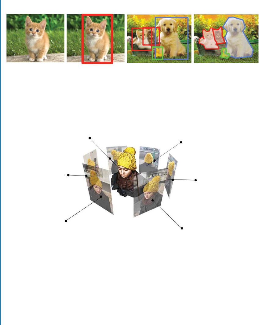
example, given an image as shown in Fig. 1.1a, humans can easily see a “cat” in the image and
thus, categorize the image (classification task); localize the cat in the image (classification plus
localization task as shown in Fig. 1.1b); localize and label all objects that are present in the image
(object detection task as shown in Fig. 1.1c); and segment the individual objects that are present
in the image (instance segmentation task as shown in Fig. 1.1d). Computer vision is the science
that aims to give a similar, if not better, capability to computers. More precisely, computer vision
seeks to develop methods which are able to replicate one of the most amazing capabilities of the
human visual system, i.e., inferring characteristics of the 3D real world purely using the light
reflected to the eyes from various objects.
However, recovering and understanding the 3D structure of the world from two-
dimensional images captured by cameras is a challenging task. Researchers in computer vision
have been developing mathematical techniques to recover the three-dimensional shape and ap-
pearance of objects/scene from images. For example, given a large enough set of images of an
object captured from a variety of views (Fig. 1.2), computer vision algorithms can reconstruct
an accurate dense 3D surface model of the object using dense correspondences across multiple
views. However, despite all of these advances, understanding images at the same level as humans
still remains challenging.
1.1.1 APPLICATIONS
Due to the significant progress in the field of computer vision and visual sensor technology,
computer vision techniques are being used today in a wide variety of real-world applications,
such as intelligent human-computer interaction, robotics, and multimedia. It is also expected
2 1. INTRODUCTION
Classification
CAT CAT CAT, DOG, DUCK CAT, DOG, DUCK
Object Detection Instance Segmentation
Classification
+ Localization
Figure 1.1: What do we want computers to do with the image data? To look at the image and
perform classification, classification plus localization (i.e., to find a bounding box around the
main object (CAT) in the image and label it), to localize all objects that are present in the image
(CAT, DOG, DUCK) and to label them, or perform semantic instance segmentation, i.e., the
segmentation of the individual objects within a scene, even if they are of the same type.
View#1
View#2
View#3
View#4
View#5
View#6
Figure 1.2: Given a set of images of an object (e.g., upper human body) captured from six dif-
ferent viewpoints, a dense 3D model of the object can be reconstructed using computer vision
algorithms.
that the next generation of computers could even understand human actions and languages at
the same level as humans, carry out some missions on behalf of humans, and respond to human
commands in a smart way.

1.1. WHAT IS COMPUTER VISION? 3
Human-computer Interaction
Nowadays, video cameras are widely used for human-computer interaction and in the entertain-
ment industry. For instance, hand gestures are used in sign language to communicate, transfer
messages in noisy environments, and interact with computer games. Video cameras provide a
natural and intuitive way of human communication with a device. erefore, one of the most
important aspects for these cameras is the recognition of gestures and short actions from videos.
Robotics
Integrating computer vision technologies with high-performance sensors and cleverly designed
hardware has given rise to a new generation of robots which can work alongside humans and
perform many different tasks in unpredictable environments. For example, an advanced hu-
manoid robot can jump, talk, run, or walk up stairs in a very similar way a human does. It can
also recognize and interact with people. In general, an advanced humanoid robot can perform
various activities that are mere reflexes for humans and do not require a high intellectual effort.
Multimedia
Computer vision technology plays a key role in multimedia applications. ese have led to a
massive research effort in the development of computer vision algorithms for processing, ana-
lyzing, and interpreting multimedia data. For example, given a video, one can ask “What does
this video mean?”, which involves a quite challenging task of image/video understanding and
summarization. As another example, given a clip of video, computers could search the Internet
and get millions of similar videos. More interestingly, when one gets tired of watching a long
movie, computers would automatically summarize the movie for them.
1.1.2 IMAGE PROCESSING VS. COMPUTER VISION
Image processing can be considered as a preprocessing step for computer vision. More precisely,
the goal of image processing is to extract fundamental image primitives, including edges and
corners, filtering, morphology operations, etc. ese image primitives are usually represented as
images. For example, in order to perform semantic image segmentation (Fig. 1.1), which is a
computer vision task, one might need to apply some filtering on the image (an image processing
task) during that process.
Unlike image processing, which is mainly focused on processing raw images without giv-
ing any knowledge feedback on them, computer vision produces semantic descriptions of images.
Based on the abstraction level of the output information, computer vision tasks can be divided
into three different categories, namely low-level, mid-level, and high-level vision.
Low-level Vision
Based on the extracted image primitives, low-level vision tasks could be preformed on im-
ages/videos. Image matching is an example of low-level vision tasks. It is defined as the automatic

4 1. INTRODUCTION
identification of corresponding image points on a given pair of the same scene from different
view points, or a moving scene captured by a fixed camera. Identifying image correspondences
is an important problem in computer vision for geometry and motion recovery.
Another fundamental low-level vision task is optical flow computation and motion anal-
ysis. Optical flow is the pattern of the apparent motion of objects, surfaces, and edges in a visual
scene caused by the movement of an object or camera. Optical flow is a 2D vector field where
each vector corresponds to a displacement vector showing the movement of points from one
frame to the next. Most existing methods which estimate camera motion or object motion use
optical flow information.
Mid-level Vision
Mid-level vision provides a higher level of abstraction than low-level vision. For instance, infer-
ring the geometry of objects is one of the major aspects of mid-level vision. Geometric vision
includes multi-view geometry, stereo, and structure from motion (SfM), which infer the 3D
scene information from 2D images such that 3D reconstruction could be made possible. An-
other task of mid-level vision is visual motion capturing and tracking, which estimate 2D and
3D motions, including deformable and articulated motions. In order to answer the question
“How does the object move?,” image segmentation is required to find areas in the images which
belong to the object.
High-level Vision
Based on an adequate segmented representation of the 2D and/or 3D structure of the image,
extracted using lower level vision (e.g., low-level image processing, low-level and mid-level vi-
sion), high-level vision completes the task of delivering a coherent interpretation of the image.
High-level vision determines what objects are present in the scene and interprets their interre-
lations. For example, object recognition and scene understanding are two high-level vision tasks
which infer the semantics of objects and scenes, respectively. How to achieve robust recognition,
e.g., recognizing object from different viewpoint is still a challenging problem.
Another example of higher level vision is image understanding and video understanding.
Based on information provided by object recognition, image and video understanding try to
answer questions such as “Is there a tiger in the image?” or “Is this video a drama or an action?,” or
“Is there any suspicious activity in a surveillance video?” Developing such high-level vision tasks
helps to fulfill different higher level tasks in intelligent human-computer interaction, intelligent
robots, smart environment, and content-based multimedia.
1.2 WHAT IS MACHINE LEARNING?
Computer vision algorithms have seen a rapid progress in recent years. In particular, combining
computer vision with machine learning contributes to the development of flexible and robust
computer vision algorithms and, thus, improving the performance of practical vision systems.

1.2. WHAT IS MACHINE LEARNING? 5
For instance, Facebook has combined computer vision, machine learning, and their large corpus
of photos, to achieve a robust and highly accurate facial recognition system. at is how Face-
book can suggest who to tag in your photo. In the following, we first define machine learning
and then describe the importance of machine learning for computer vision tasks.
Machine learning is a type of artificial intelligence (AI) which allows computers to learn
from data without being explicitly programmed. In other words, the goal of machine learn-
ing is to design methods that automatically perform learning using observations of the real
world (called the “training data”), without explicit definition of rules or logic by the humans
(“trainer”/“supervisor”). In that sense, machine learning can be considered as programming by
data samples. In summary, machine learning is about learning to do better in the future based
on what was experienced in the past.
A diverse set of machine learning algorithms has been proposed to cover the wide vari-
ety of data and problem types. ese learning methods can be mainly divided into three main
approaches, namely supervised,semi-supervised, and unsupervised. However, the majority of prac-
tical machine learning methods are currently supervised learning methods, because of their supe-
rior performance compared to other counter-parts. In supervised learning methods, the training
data takes the form of a collection of .data:x; label:y/ pairs and the goal is to produce a prediction
yin response to a query sample x. e input xcan be a features vector, or more complex data
such as images, documents, or graphs. Similarly, different types of output yhave been stud-
ied. e output ycan be a binary label which is used in a simple binary classification problem
(e.g., “yes” or “no”). However, there has also been numerous research works on problems such
as multi-class classification where yis labeled by one of klabels, multi-label classification where
ytakes on simultaneously the Klabels, and general structured prediction problems where yis
a high-dimensional output, which is constructed from a sequence of predictions (e.g., semantic
segmentation).
Supervised learning methods approximate a mapping function f .x/ which can predict
the output variables yfor a given input sample x. Different forms of mapping function f .:/ exist
(some are briefly covered in Chapter 2), including decision trees, Random Decision Forests
(RDF), logistic regression (LR), Support Vector Machines (SVM), Neural Networks (NN),
kernel machines, and Bayesian classifiers. A wide range of learning algorithms has also been
proposed to estimate these different types of mappings.
On the other hand, unsupervised learning is where one would only have input data X
and no corresponding output variables. It is called unsupervised learning because (unlike super-
vised learning) there are no ground-truth outputs and there is no teacher. e goal of unsuper-
vised learning is to model the underlying structure/distribution of data in order to discover an
interesting structure in the data. e most common unsupervised learning method is the clus-
tering approach such as hierarchical clustering, k-means clustering, Gaussian Mixture Models
(GMMs), Self-Organizing Maps (SOMs), and Hidden Markov Models (HMMs).

6 1. INTRODUCTION
Semi-supervised learning methods sit in-between supervised and unsupervised learning.
ese learning methods are used when a large amount of input data is available and only some
of the data is labeled. A good example is a photo archive where only some of the images are
labeled (e.g., dog, cat, person), and the majority are unlabeled.
1.2.1 WHY DEEP LEARNING?
While these machine learning algorithms have been around for a long time, the ability to auto-
matically apply complex mathematical computations to large-scale data is a recent development.
is is because the increased power of today’s computers, in terms of speed and memory, has
helped machine learning techniques evolve to learn from a large corpus of training data. For ex-
ample, with more computing power and a large enough memory, one can create neural networks
of many layers, which are called deep neural networks. ere are three key advantages which are
offered by deep learning.
•Simplicity: Instead of problem specific tweaks and tailored feature detectors, deep net-
works offer basic architectural blocks, network layers, which are repeated several times to
generate large networks.
•Scalability: Deep learning models are easily scalable to huge datasets. Other competing
methods, e.g., kernel machines, encounter serious computational problems if the datasets
are huge.
•Domain transfer: A model learned on one task is applicable to other related tasks and the
learned features are general enough to work on a variety of tasks which may have scarce
data available.
Due to the tremendous success in learning these deep neural networks, deep learning tech-
niques are currently state-of-the-art for the detection, segmentation, classification and recogni-
tion (i.e., identification and verification) of objects in images. Researchers are now working to
apply these successes in pattern recognition to more complex tasks such as medical diagnoses
and automatic language translation. Convolutional Neural Networks (ConvNets or CNNs) are
a category of deep neural networks which have proven to be very effective in areas such as image
recognition and classification (see Chapter 7for more details). Due to the impressive results of
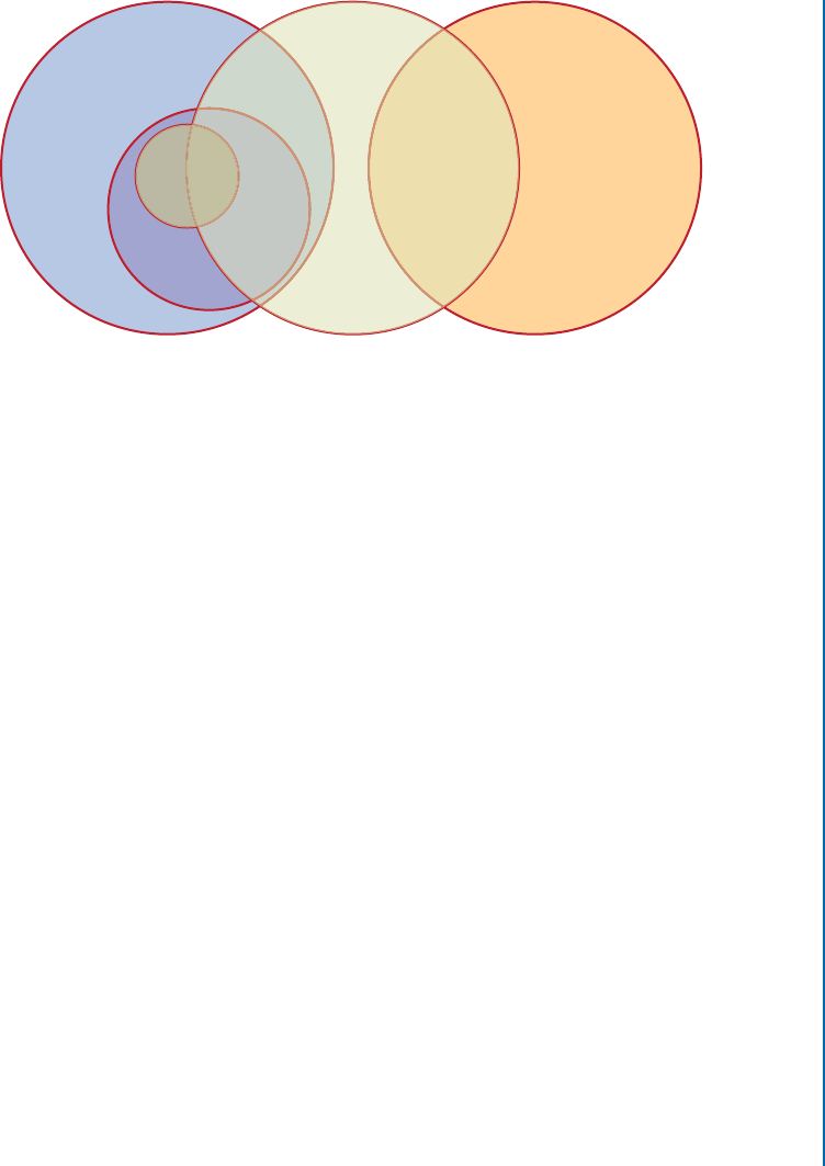
CNNs in these areas, this book is mainly focused on CNNs for computer vision tasks. Figure 1.3
illustrates the relation between computer vision, machine learning, human vision, deep learning,
and CNNs.
1.3 BOOK OVERVIEW
CHAPTER 2
e book begins in Chapter 2with a review of the traditional feature representation and classi-
fication methods. Computer vision tasks, such as image classification and object detection, have
1.3. BOOK OVERVIEW 7
Machine
Learning
Human
Vision
Deep
Learning
CNN Computer
Vision
Figure 1.3: e relation between human vision, computer vision, machine learning, deep learn-
ing, and CNNs.
traditionally been approached using hand-engineered features which are divided into two differ-
ent main categories: global features and local features. Due to the popularity of the low-level rep-
resentation, this chapter first reviews three widely used low-level hand-engineered descriptors,
namely Histogram of Oriented Gradients (HOG) [Triggs and Dalal,2005], Scale-Invariant
Feature Transform (SIFT) [Lowe,2004], and Speed-Up Robust Features (SURF) [Bay et al.,
2008]. A typical computer vision system feeds these hand-engineered features to machine learn-
ing algorithms to classify images/videos. Two widely used machine learning algorithms, namely
SVM [Cortes,1995] and RDF [Breiman,2001,Quinlan,1986], are also introduced in details.
CHAPTER 3
e performance of a computer vision system is highly dependent on the features used. ere-
fore, current progress in computer vision has been based on the design of feature learners which
minimizes the gap between high-level representations (interpreted by humans) and low-level
features (detected by HOG [Triggs and Dalal,2005] and SIFT [Lowe,2004] algorithms).
Deep neural networks are one of the well-known and popular feature learners which allow the
removal of complicated and problematic hand-engineered features. Unlike the standard feature
extraction algorithms (e.g., SIFT and HOG), deep neural networks use several hidden layers
to hierarchically learn the high level representation of an image. For instance, the first layer
might detect edges and curves in the image, the second layer might detect object body-parts
(e.g., hands or paws or ears), the third layer might detect the whole object, etc. In this chapter,
we provide an introduction to deep neural networks, their computational mechanism and their
historical background. Two generic categories of deep neural networks, namely feed-forward
and feed-back networks, with their corresponding learning algorithms are explained in detail.

8 1. INTRODUCTION
CHAPTER 4
CNNs are a prime example of deep learning methods and have been most extensively studied.
Due to the lack of training data and computing power in the early days, it was hard to train a
large high-capacity CNN without overfitting. After the rapid growth in the amount of annotated
data and the recent improvements in the strengths of Graphics Processor Units (GPUs), research
on CNNs has emerged rapidly and achieved state-of-the-art results on various computer vision
tasks. In this chapter, we provide a broad survey of the recent advances in CNNs, including state-
of-the-art layers (e.g., convolution, pooling, nonlinearity, fully connected, transposed convolu-
tion, ROI pooling, spatial pyramid pooling, VLAD, spatial transformer layers), weight initial-
ization approaches (e.g., Gaussian, uniform and orthogonal random initialization, unsupervised
pre-training, Xavier, and Rectifier Linear Unit (ReLU) aware scaled initialization, supervised
pre-training), regularization approaches (e.g., data augmentation, dropout, drop-connect, batch
normalization, ensemble averaging, the `1and `2regularization, elastic net, max-norm con-
straint, early stopping), and several loss functions (e.g., soft-max, SVM hinge, squared hinge,
Euclidean, contrastive, and expectation loss).
CHAPTER 5
e CNN training process involves the optimization of its parameters such that the loss function
is minimized. is chapter reviews well-known and popular gradient-based training algorithms
(e.g., batch gradient descent, stochastic gradient descent, mini-batch gradient descent) followed
by state-of-the-art optimizers (e.g., Momentum, Nesterov momentum, AdaGrad, AdaDelta,
RMSprop, Adam) which address the limitations of the gradient descent learning algorithms.
In order to make this book a self-contained guide, this chapter also discusses the different ap-
proaches that are used to compute differentials of the most popular CNN layers which are em-
ployed to train CNNs using the error back-propagation algorithm.
CHAPTER 6
is chapter introduces the most popular CNN architectures which are formed using the basic
building blocks studied in Chapter 4and Chapter 7. Both early CNN architectures which are
easier to understand (e.g., LeNet, NiN, AlexNet, VGGnet) and the recent CNN ones (e.g.,
GoogleNet, ResNet, ResNeXt, FractalNet, DenseNet), which are relatively complex, are pre-
sented in details.
CHAPTER 7
is chapter reviews various applications of CNNs in computer vision, including image classifi-
cation, object detection, semantic segmentation, scene labeling, and image generation. For each
application, the popular CNN-based models are explained in detail.

1.3. BOOK OVERVIEW 9
CHAPTER 8
Deep learning methods have resulted in significant performance improvements in computer vi-
sion applications and, thus, several software frameworks have been developed to facilitate these
implementations. is chapter presents a comparative study of nine widely used deep learning
frameworks, namely Caffe, TensorFlow, MatConvNet, Torch7, eano, Keras, Lasagne, Mar-
vin, and Chainer, on different aspects. is chapter helps the readers to understand the main
features of these frameworks (e.g., the provided interface and platforms for each framework)
and, thus, the readers can choose the one which suits their needs best.

11
C H A P T E R 2
Features and Classifiers
Feature extraction and classification are two key stages of a typical computer vision system. In
this chapter, we provide an introduction to these two steps: their importance and their design
challenges for computer vision tasks.
Feature extraction methods can be divided into two different categories, namely hand-
engineering-based methods and feature learning-based methods. Before going into the details
of the feature learning algorithms in the subsequent chapters (i.e., Chapter 3, Chapter 4, Chap-
ter 5, and Chapter 6), we introduce in this chapter some of the most popular traditional hand-
engineered features (e.g., HOG [Triggs and Dalal,2005], SIFT [Lowe,2004], SURF [Bay
et al.,2008]), and their limitations in details.
Classifiers can be divided into two groups, namely shallow and deep models. is
chapter also introduces some well-known traditional classifiers (e.g., SVM [Cortes,1995],
RDF [Breiman,2001,Quinlan,1986]), which have a single learned layer and are therefore
shallow models. e subsequent chapters (i.e., Chapter 3, Chapter 4, Chapter 5, and Chap-
ter 6) cover the deep models, including CNNs, which have multiple hidden layers and, thus,
can learn features at various levels of abstraction.
2.1 IMPORTANCE OF FEATURES AND CLASSIFIERS
e accuracy, robustness, and efficiency of a vision system are largely dependent on the quality
of the image features and the classifiers. An ideal feature extractor would produce an image rep-
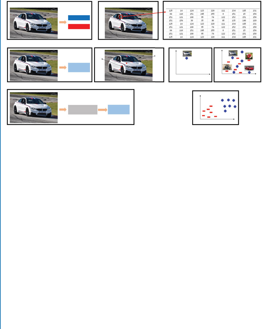
resentation that makes the job of the classifier trivial (see Fig. 2.1). Conversely, unsophisticated
features extractors require a “perfect” classifier to adequately perform the pattern recognition
task. However, ideal features extraction and a perfect classification performance are often im-
possible. us, the goal is to extract informative and reliable features from the input images, in
order to enable the development of a largely domain-independent theory of classification.
2.1.1 FEATURES
A feature is any distinctive aspect or characteristic which is used to solve a computational task
related to a certain application. For example, given a face image, there is a variety of approaches
to extract features, e.g., mean, variance, gradients, edges, geometric features, color features, etc.
e combination of nfeatures can be represented as a n-dimensional vector, called a fea-
ture vector. e quality of a feature vector is dependent on its ability to discriminate image
samples from different classes. Image samples from the same class should have similar feature
12 2. FEATURES AND CLASSIFIERS
(a) (b) (c)
(d) (e) (g)(f )
(h) (i)
“Car”
“non-Car”
Learning
Algorithm
Learning
Algorithm
Feature
Representation
Raw
Pixel
Pixel
2
Pixel 2
Pixel 1
Pixel 2
Pixel 1
Doors
Wheels
Pixel
1
Humans see this: But, the computer sees this:
E.g., Wheels? Doors? etc.
Figure 2.1: (a) e aim is to design an algorithm which classifies input images into two different
categories: “Car” or “non-Car.” (b) Humans can easily see the car and categorize this image
as “Car.” However, computers see pixel intensity values as shown in (c) for a small patch in the
image. Computer vision methods process all pixel intensity values and classify the image. (d) e
straightforward way is to feed the intensity values to the classifiers and the learned classifier will
then perform the classification job. For better visualization, let us pick only two pixels, as shown
in (e). Because pixel 1 is relatively bright and pixel 2 is relatively dark, that image has a position
shown in blue plus sign in the plot shown in (f). By adding few positive and negative samples,
the plot in (g) shows that the positive and negative samples are extremely jumbled together. So
if this data is fed to a linear classifier, the subdivision of the feature space into two classes is
not possible. (h) It turns out that a proper feature representation can overcome this problem.
For example, using more informative features such as the number of wheels in the images, the
number of doors in the images, the data looks like (i) and the images become much easier to
classify.
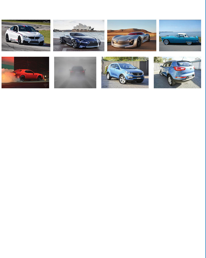
values and images from different classes should have different feature values. For the example
shown in Fig. 2.1, all cars shown in Fig. 2.2 should have similar feature vectors, irrespective of
their models, sizes, positions in the images, etc. us, a good feature should be informative,
invariant to noise and a set of transformations (e.g., rotation and translation), and fast to com-
pute. For instance, features such as the number of wheels in the images, the number of doors
in the images could help to classify the images into two different categories, namely “car” and
2.2. TRADITIONAL FEATURE DESCRIPTORS 13
“non-car.” However, extracting such features is a challenging problem in computer vision and
machine learning.
Figure 2.2: Images of different classes of cars captured from different scenes and viewpoints.
2.1.2 CLASSIFIERS
Classification is at the heart of modern computer vision and pattern recognition. e task of the
classifier is to use the feature vector to assign an image or region of interest (RoI) to a category.
e degree of difficulty of the classification task depends on the variability in the feature values of
images from the same category, relative to the difference between feature values of images from
different categories. However, a perfect classification performance is often impossible. is is
mainly due to the presence of noise (in the form of shadows, occlusions, perspective distortions,
etc.), outliers (e.g., images from the category “buildings” might contain people, animal, building,
or car category), ambiguity (e.g., the same rectangular shape could correspond to a table or a
building window), the lack of labels, the availability of only small training samples, and the
imbalance of positive/negative coverage in the training data samples. us, designing a classifier
to make the best decision is a challenging task.
2.2 TRADITIONAL FEATURE DESCRIPTORS
Traditional (hand-engineered) feature extraction methods can be divided into two broad cat-
egories: global and local. e global feature extraction methods define a set of global features
which effectively describe the entire image. us, the shape details are ignored. e global fea-
tures are also not suitable for the recognition of partially occluded objects. On the other hand,
the local feature extraction methods extract a local region around keypoints and, thus, can han-
dle occlusion better [Bayramoglu and Alatan,2010,Rahmani et al.,2014]. On that basis, the
focus of this chapter is on local features/descriptors.

14 2. FEATURES AND CLASSIFIERS
Various methods have been developed for detecting keypoints and constructing descrip-
tors around them. For instance, local descriptors, such as HOG [Triggs and Dalal,2005], SIFT
[Lowe,2004], SURF [Bay et al.,2008], FREAK [Alahi et al.,2012], ORB [Rublee et al.,2011],
BRISK [Leutenegger et al.,2011], BRIEF [Calonder et al.,2010], and LIOP [Wang et al.,
2011b] have been used in most computer vision applications. e considerable recent progress
that has been achieved in the area of recognition is largely due to these features, e.g., optical flow
estimation methods use orientation histograms to deal with large motions; image retrieval and
structure from motion are based on SIFT descriptors. It is important to note that CNNs, which
will be discussed in Chapter 4, are not that much different than the traditional hand-engineered
features. e first layer in the CNNs learn to utilize gradients in a way that is similar to hand-
engineered features such as HOG, SIFT and SURF. In order to have a better understanding of
CNNs, we describe next, three important and widely used feature detectors and/or descriptors,
namely HOG [Triggs and Dalal,2005], SIFT [Lowe,2004], and SURF [Bay et al.,2008] in
some details. As you will see in Chapter 4, CNNs are also able to extract similar hand-engineered
features (e.g., gradients) in their lower layers but through an automatic feature learning process.
2.2.1 HISTOGRAM OF ORIENTED GRADIENTS (HOG)
HOG [Triggs and Dalal,2005] is a feature descriptor that is used to automatically detect ob-
jects from images. e HOG descriptor encodes the distribution of directions of gradients in
localized portions of an image.
HOG features have been introduced by Triggs and Dalal [2005] who have studied the
influence of several variants of HOG descriptors (R-HOG and C-HOG), with different gra-
dient computation and normalization methods. e idea behind the HOG descriptors is that
the object appearance and the shape within an image can be described by the histogram of edge
directions. e implementation of these descriptors consists of the following four steps.
Gradient Computation
e first step is the computation of the gradient values. A 1D centered point discrete derivative
mask is applied on an image in both the horizontal and vertical directions. Specifically, this
method requires the filtering of the gray-scale image with the following filter kernels:
fxDŒ1 0 C1 and fyDŒ1 0 C1T:(2.1)
us, given an image I, the following convolution operations (denoted by ) result in the
derivatives of the image Iin the xand ydirections:
IxDIfxand IyDIfy:(2.2)
us, the orientation and the magnitude jgjof the gradient are calculated as follows:
Darctan Iy
Ix
and jgj D 2
qI2
xCI2
y:(2.3)

2.2. TRADITIONAL FEATURE DESCRIPTORS 15
As you will see in Chapter 4, just like the HOG descriptor, CNNs also use convolution
operations in their layers. However, the main difference is that instead of using hand-engineered
filters, e.g., fx; fyin Eq. (2.1), CNNs use trainable filters which make them highly adaptive.
at is why they can achieve high accuracy levels in most applications such as image recognition.
Cell Orientation Histogram
e second step is the calculation of the cell histograms. First, the image is divided into small
(usually 88pixels) cells. Each cell has a fixed number of gradient orientation bins, which are
evenly spread over 0–180ıor 0–360ı, depending on whether the gradient is unsigned or signed.
Each pixel within the cell casts a weighted vote for a gradient orientation bin based on the
gradient magnitude at that pixel. For the vote weight, the pixel contribution can be the gradient
magnitude, or the square root of the gradient magnitude or the square of the gradient magnitude.
Block Descriptor
To deal with changes in illumination and contrast, the gradient strengths are locally normal-
ized by grouping the cells together into larger, spatially connected blocks. e HOG descriptor
is then the vector of the components of the normalized cell histograms from all of the block
regions.
Block Normalization
e final step is the normalization of the block descriptors. Let vbe the non-normalized vector
containing all histograms in a given block, jjvjjkbe its k-norm for kD1; 2, and be a small
constant. en the normalization factor can be one of the following:
L2-norm: vDv
qjjvjj2
2Ce2
;(2.4)
or
L1-norm: vDv
jjvjj1C;(2.5)
or
L1-sqrt: vDrv
jjvjj1C:(2.6)
ere is another normalization factor, L2-Hys, which is obtained by clipping the L2-norm
of v(i.e., limiting the maximum values of vto 0:2) and then re-normalizing.
e final image/RoI descriptor is formed by concatenating all normalized block descrip-
tors. e experimental results in Triggs and Dalal [2005] show that all four block normalization
methods achieve a very significant improvement over the non-normalized one. Moreover, the
L2-norm, L2-Hys, and L1-sqrt normalization approaches provide a similar performance, while
the L1-norm provides a slightly less reliable performance.
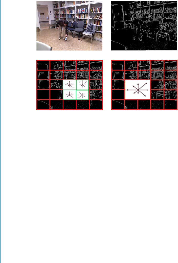
16 2. FEATURES AND CLASSIFIERS
Original Image Gradient
Cell Orientation Histogram Block Descriptor
Figure 2.3: HOG descriptor. Note that for better visualization, we only show the cell orientation
histogram for four cells and a block descriptor corresponding to those four cells.
2.2.2 SCALE-INVARIANT FEATURE TRANSFORM (SIFT)
SIFT [Lowe,2004] provides a set of features of an object that are are robust against object
scaling and rotations. e SIFT algorithm consists of four main steps, which are discussed in
the following subsections.
Scale-space Extrema Detection
e first step aims to identify potential keypoints that are invariant to scale and orientation.
While several techniques can be used to detect keypoint locations in the scale-space, SIFT uses
the Difference of Gaussians (DoG), which is obtained as the difference of Gaussian blurring of
an image with two different scales, , one with scale ktimes the scale of the other, i.e., k.
is process is performed for different octaves of the image in the Gaussian Pyramid, as shown
in Fig. 2.4a.
en, the DoG images are searched for local extrema over all scales and image locations.
For instance, a pixel in an image is compared with its eight neighbors in the current image as
well as nine neighbors in the scale above and below, as shown in Fig. 2.4b. If it is the minimum
or maximum of all these neighbors, then it is a potential keypoint. It means that a keypoint is
best represented in that scale.
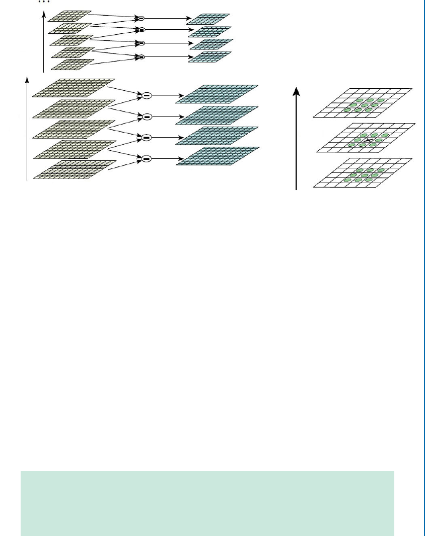
2.2. TRADITIONAL FEATURE DESCRIPTORS 17
Scale
(next
octave)
Gaussian
Difference of
Gaussian (DOG)
Scale
(first
octave) Scale
(a) (b)
Figure 2.4: Scale-space feature detection using a sub-octave DoG pyramid. (a) Adjacent levels
of a sub-octave Gaussian pyramid are subtracted to produce the DoG; and (b) extrema in the
resulting 3D volume are detected by comparing a pixel to its 26 neighbors. (Figure from Lowe
[2004], used with permission.)
Accurate Keypoint Localization
is step removes unstable points from the list of potential keypoints by finding those that have
low contrast or are poorly localized on an edge. In order to reject low contrast keypoints, a Taylor
series expansion of the scale space is computed to get more accurate locations of extrema, and if
the intensity at each extrema is less than a threshold value, the keypoint is rejected.
Moreover, the DoG function has a strong response along the edges, which results in a large
principal curvature across the edge but a small curvature in the perpendicular direction in the
DoG function. In order to remove the keypoints located on an edge, the principal curvature at
the keypoint is computed from a 22Hessian matrix at the location and scale of the keypoint.
If the ratio between the first and the second eigenvalues is greater than a threshold, the keypoint
is rejected.
Remark: In mathematics, the Hessian matrix or Hessian is a square matrix
of second-order partial derivatives of a scalar-valued function. Specifically,
suppose f .x1; x2; ; xn/is a function outputting a scalar, i.e., fWRn!R;
if all the second partial derivatives of fexist and are continuous over the

18 2. FEATURES AND CLASSIFIERS
domain of the function, then the Hessian Hof fis a square nnmatrix,
defined as follows:
HD
2
6
6
6
6
6
6
4
@2f
@x2
1
@2f
@x1@x2 @2f
@x1@xn
@2f
@x2@x1
@2f
@x2
2 @2f
@x2@xn
:
:
::
:
:::::
:
:
@2f
@xn@x1
@2f
@xn@x2 @2f
@x2
n
3
7
7
7
7
7
7
5
:(2.7)
Orientation Assignment
In order to achieve invariance to image rotation, a consistent orientation is assigned to each
keypoint based on its local image properties. e keypoint descriptor can then be represented
relative to this orientation. e algorithm used to find an orientation consists of the following
steps.
1. e scale of the keypoint is used to select the Gaussian blurred image with the closest
scale.
2. e gradient magnitude and orientation are computed for each image pixel at this scale.
3. As shown in Fig. 2.5, an orientation histogram, which consists of 36 bins covering the
360ırange of orientations, is built from the gradient orientations of pixels within a local
region around the keypoint.
4. e highest peak in the local orientation histogram corresponds to the dominant direction
of the local gradients. Moreover, any other local peak that is within 80%of the highest
peak is also considered as a keypoint with that orientation.
Keypoint Descriptor
e dominant direction (the highest peak in the histogram) of the local gradients is also used to
create keypoint descriptors. e gradient orientations are rotated relative to the orientation of
the keypoint and then weighted by a Gaussian with a variance of 1:5 keypoi ntscale. en, a
16 16 neighborhood around the keypoint is divided into 16 sub-blocks of size 44. For each
sub-block, an 8bin orientation histogram is created. is results in a feature vector, called SIFT
descriptor, containing 128 elements. Figure 2.6 illustrates the SIFT descriptors for keypoints
extracted from an example image.
Complexity of SIFT Descriptor
In summary, SIFT tries to standardize all images (if the image is blown up, SIFT shrinks it;
if the image is shrunk, SIFT enlarges it). is corresponds to the idea that if a keypoint can
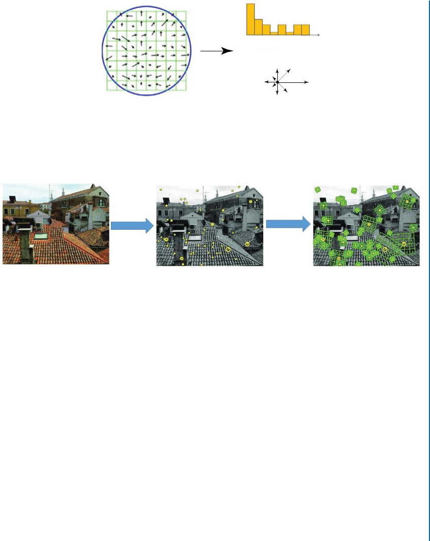
2.2. TRADITIONAL FEATURE DESCRIPTORS 19
Image Gradients
Angle Histogram
0 2π
Figure 2.5: A dominant orientation estimate is computed by creating a histogram of all the
gradient orientations weighted by their magnitudes and then finding the significant peaks in
this distribution.
Original Image SIFT Keypoints
SIFT
Detector
SIFT
Descriptor
SIFT Descriptors
Figure 2.6: An example of the SIFT detector and descriptor: (left) an input image, (middle)
some of the detected keypoints with their corresponding scales and orientations, and (right)
SIFT descriptors–a 16 16 neighborhood around each keypoint is divided into 16 sub-blocks
of 44size.
be detected in an image at scale , then we would need a larger dimension k to capture the
same keypoint, if the image was up-scaled. However, the mathematical ideas of SIFT and many
other hand-engineered features are quite complex and require many years of research. For ex-
ample, Lowe [2004] spent almost 10 years on the design and tuning of the SIFT parameters.
As we will show in Chapters 4,5, and 6, CNNs also perform a series of transformations on the
image by incorporating several convolutional layers. However, unlike SIFT, CNNs learn these
transformation (e.g., scale, rotation, translation) from image data, without the need of complex
mathematical ideas.
2.2.3 SPEEDED-UP ROBUST FEATURES (SURF)
SURF [Bay et al.,2008] is a speeded up version of SIFT. In SIFT, the Laplacian of Gaussian is
approximated with the DoG to construct a scale-space. SURF speeds up this process by approx-

20 2. FEATURES AND CLASSIFIERS
imating the LoG with a box filter. us, a convolution with a box filter can easily be computed
with the help of integral images and can be performed in parallel for different scales.
Keypoint Localization
In the first step, a blob detector based on the Hessian matrix is used to localize keypoints. e
determinant of the Hessian matrix is used to select both the location and scale of the potential
keypoints. More precisely, for an image Iwith a given point pD.x; y/, the Hessian matrix
H.p; / at point pand scale , is defined as follows:
H.p; / DLxx.p; / Lxy .p; /
Lxy .p; / Lyy .p; /;(2.8)
where Lxx.p; / is the convolution of the second-order derivative of the Gaussian, @2
@x2g. /, with
the image Iat point p. However, instead of using Gaussian filters, SURF uses approximated
Gaussian second-order derivatives, which can be evaluated using integral images at a very low
computational cost. us, unlike SIFT, SURF does not require to iteratively apply the same
filter to the output of a previously filtered layer, and scale-space analysis is done by keeping the
same image and varying the filter size, i.e., 99,25 15,21 21, and 27 27.
en, a non-maximum suppression in a 333neighborhood of each point in the image
is applied to localize the keypoints in the image. e maxima of the determinant of the Hessian
matrix are then interpolated in the scale and image space, using the method proposed by Brown
and Lowe [2002].
Orientation Assignment
In order to achieve rotational invariance, the Haar wavelet responses in both the horizontal
xand vertical ydirections within a circular neighborhood of radius 6s around the keypoint
are computed, where sis the scale at which the keypoint is detected. en, the Haar wavelet
responses in both the horizontal dx and vertical dy directions are weighted with a Gaussian
centered at a keypoint, and represented as points in a 2D space. e dominant orientation of
the keypoint is estimated by computing the sum of all the responses within a sliding orientation
window of angle 60ı. e horizontal and vertical responses within the window are then summed.
e two summed responses is considered as a local vector. e longest orientation vector over all
the windows determines the orientation of the keypoint. In order to achieve a balance between
robustness and angular resolution, the size of the sliding window need to be chosen carefully.
Keypoint Descriptor
To describe the region around each keypoint p, a 20s 20s square region around pis extracted
and then oriented along the orientation of p. e normalized orientation region around pis
split into smaller 44square sub-regions. e Haar wavelet responses in both the horizontal
dx and vertical dy directions are extracted at 55regularly spaced sample points for each sub-

2.3. MACHINE LEARNING CLASSIFIERS 21
region. In order to achieve more robustness to deformations, noise and translation, e Haar
wavelet responses are weighted with a Gaussian. en, dx and dy are summed up over each sub-
region and the results form the first set of entries in the feature vector. e sum of the absolute
values of the responses, jdxjand jdyj, are also computed and then added to the feature vector to
encode information about the intensity changes. Since each sub-region has a 4D feature vector,
concatenating all 44sub-regions results in a 64D descriptor.
2.2.4 LIMITATIONS OF TRADITIONAL HAND-ENGINEERED
FEATURES
Until recently, progress in computer vision was based on hand-engineering features. However,
feature engineering is difficult, time-consuming, and requires expert knowledge on the problem
domain. e other issue with hand-engineered features such as HOG, SIFT, SURF, or other
algorithms like them, is that they are too sparse in terms of information that they are able to
capture from an image. is is because the first-order image derivatives are not sufficient features
for the purpose of most computer vision tasks such as image classification and object detection.
Moreover, the choice of features often depends on the application. More precisely, these fea-
tures do not facilitate learning from previous learnings/representations (transfer learning). In
addition, the design of hand-engineered features is limited by the complexity that humans can
put in it. All these issues are resolved using automatic feature learning algorithms such as deep
neural networks, which will be addressed in the subsequent chapters (i.e., Chapters 3,4,5, and
6).
2.3 MACHINE LEARNING CLASSIFIERS
Machine learning is usually divided into three main areas, namely supervised,unsupervised, and
semi-supervised. In the case of the supervised learning approach, the goal is to learn a mapping
from inputs to outputs, given a labeled set of input-output pairs. e second type of machine
learning is the unsupervised learning approach, where we are only given inputs, and the goal is to
automatically find interesting patterns in the data. is problem is not a well-defined problem,
because we are not told what kind of patterns to look for. Moreover, unlike supervised learning,
where we can compare our label prediction for a given sample to the observed value, there is
no obvious error metric to use. e third type of machine learning is semi-supervised learning,
which typically combines a small amount of labeled data with a large amount of unlabeled data
to generate an appropriate function or classifier. e cost of the labeling process of a large corpus
of data is infeasible, whereas the acquisition of unlabeled data is relatively inexpensive. In such
cases, the semi-supervised learning approach can be of great practical value.
Another important class of machine learning algorithms is “reinforcement learning,”
where the algorithm allows agents to automatically determine the ideal behavior given an ob-
servation of the world. Every agent has some impact on the environment, and the environment
provides reward feedback to guide the learning algorithm. However, in this book our focus is

22 2. FEATURES AND CLASSIFIERS
mainly on the supervised learning approach, which is the most widely used machine learning
approach in practice.
A wide range of supervised classification techniques has been proposed in the literature.
ese methods can be divided into three different categories, namely linear (e.g., SVM [Cortes,
1995]; logistic regression; Linear Discriminant Analysis (LDA) [Fisher,1936]), nonlinear (e.g.,
Multi Layer Perceptron (MLP), kernel SVM), and ensemble-based (e.g., RDF [Breiman,2001,
Quinlan,1986]; AdaBoost [Freund and Schapire,1997]) classifiers. e goal of ensemble meth-
ods is to combine the predictions of several base classifiers to improve generalization over a
single classifier. e ensemble methods can be divided into two categories, namely averaging
(e.g., Bagging methods; Random Decision Forests [Breiman,2001,Quinlan,1986]) and boost-
ing (e.g., AdaBoost [Freund and Schapire,1997]; Gradient Tree Boosting [Friedman,2000]).
In the case of the averaging methods, the aim is to build several classifiers independently and
then to average their predictions. For the boosting methods, base “weak” classifiers are built se-
quentially and one tries to reduce the bias of the combined overall classifier. e motivation is
to combine several weak models to produce a powerful ensemble.
Our definition of a machine learning classifier that is capable of improving computer
vision tasks via experience is somewhat abstract. To make this more concrete, in the following
we describe three widely used linear (SVM), nonlinear (kernel SVM) and ensemble (RDF)
classifiers in some detail.
2.3.1 SUPPORT VECTOR MACHINE (SVM)
SVM [Cortes,1995] is a supervised machine learning algorithm used for classification or regres-
sion problems. SVM works by finding a linear hyperplane which separates the training dataset
into two classes. As there are many such linear hyperplanes, the SVM algorithm tries to find
the optimal separating hyperplane (as shown in Fig. 2.7) which is intuitively achieved when the
distance (also known as the margin) to the nearest training data samples is as large as possible.
It is because, in general, the larger the margin the lower the generalization error of the model.
Mathematically, SVM is a maximum margin linear model. Given a training dataset of n
samples of the form f.x1; y1/; ; .xn; yn/g, where xiis an m-dimensional feature vector and
yiD f1; 1gis the class to which the sample xibelongs to. e goal of SVM is to find the
maximum-margin hyperplane which divides the group of samples for which yiD1from the
group of samples for which yiD 1. As shown in Fig. 2.7b (the bold blue line), this hyperplane
can be written as the set of sample points satisfying the following equation:
wTxiCbD0; (2.9)
where wis the normal vector to the hyperplane. More precisely, any samples above the hyper-
plane should have label 1, i.e., xis.t. wTxiCb > 0 will have corresponding yiD1. Similarly,
any samples below the hyperplane should have label 1, i.e., xis.t. wTxiCb < 0 will have
corresponding yiD 1.

2.3. MACHINE LEARNING CLASSIFIERS 23
Notice that there is some space between the hyperplane (or decision boundary, which is
the bold blue line in Fig. 2.7b) and the nearest data samples of either class. us, the sample
data is rescaled such that anything on or above the hyperplane wTxiCbD1is of one class with
label 1, and anything on or below the hyperplane wTxiCbD 1is of the other class with label
1. Since these two new hyperplanes are parallel, the distance between them is 2
pwTw, as shown
in Fig. 2.7c.
Recall that SVM tries to maximize the distance between these two new hyperplanes de-
marcating two classes, which is equivalent to minimizing wTw
2. us, SVM is learned by solving
the following primal optimization problem:
min
w;b
wTw
2(2.10)
subject to:
yi.wTxiCb/ 1 .8samples xi/: (2.11)
Soft-margin Extension
In the case where the training samples are not perfectly linearly separable, SVM can allow some
samples of one class to appear on the other side of the hyperplane (boundary) by introducing
slack variables, an ifor each sample xias follows:
min
w;b;
wTw
2CCX
i
i;(2.12)
subject to:
yi.wTxiCb/ 1iand i0 .8samples xi/: (2.13)
Unlike deep neural networks, which will be introduced in Chapter 3, linear SVMs can
only solve problems that are linearly separable, i.e., where the data samples belonging to class
1 can be separated from the samples belonging to class 2 by a hyperplane as shown in Fig. 2.7.
However, in many cases, the data samples are not linearly separable.
Nonlinear Decision Boundary
SVM can be extended to nonlinear classification by projecting the original input space (Rd) into
a high-dimensional space (RD), where a separating hyperplane can hopefully be found. us,
the formulation of the quadratic programming problem is as above (Eq. (2.12) and Eq. (2.13)),
but with all xireplaced with .xi/, where provides a higher-dimensional mapping.
min
w;b;
wTw
2CCX
i
i;(2.14)
subject to:
yi.wT.xi/Cb/ 1iand i0 .8samples xi/: (2.15)
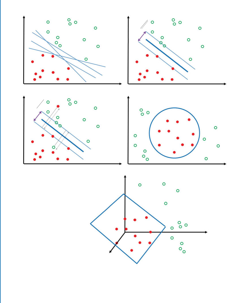
24 2. FEATURES AND CLASSIFIERS
(a) (b)
(c) (d)
(e)
W TX + b = 1
W TX + b = 0
W TX + b = -1
W TX + b = 1
W TX + b = 0
W TX + b = -1
Nonlinear Decision
Boundary
Linear Decision Boundary
ε1
Margin = 2
W TW
Decision Boundary
Decision Boundary
Margin = 2
√W TW
ε2
Figure 2.7: (Continues.)

2.3. MACHINE LEARNING CLASSIFIERS 25
Figure 2.7: (Continued.) For two classes, separable training datasets, such as the one shown
in (a), there are lots of possible linear separators as shown with the blue lines in (a). Intuitively, a
separating hyperplane (also called decision boundary) drawn in the middle of the void between
the data samples of the two classes (the bold blue line in (b)) seems better than the ones shown
in (a). SVM defines the criterion for a decision boundary that is maximally far away from any
data point. is distance from the decision surface to the closest data point determines the
margin of the classifier as shown in (b). In the hard-margin SVM, (b), a single outlier can
determine the decision boundary, which makes the classifier overly sensitive to the noise in the
data. However, a soft margin SVM classifier, shown in (c), allows some samples of each class
to appear on the other side of the decision boundary by introducing slack variables ifor each
sample. (d) Shows an example where classes are not separable by a linear decision boundary.
us, as shown in (e), the original input space R2is projected onto R3, where a linear decision
boundary can be found, i.e., using the kernel trick.
Dual Form of SVM
In the case that Dd, there are many more parameters to learn for w. In order to avoid that,
the dual form of SVM is used for optimization problem.
max
˛X
i
˛i1
2X
i;j
˛i˛jyiyj.xi/T.xj/; (2.16)
subject to:
X
i
˛iyiD0and 0˛iC; (2.17)
where Cis a hyper-parameter which controls the degree of misclassification of the model, in
case classes are not linearly separable.
Kernel Trick
Since .xi/is in a high-dimensional space (even infinite-dimensional space), calculating .xi/T
.xj/may be intractable. However, there are special kernel functions, such as linear, polynomial,
Gaussian, and Radial Basis Function (RBF), which operate on the lower dimension vectors xi
and xjto produce a value equivalent to the dot-product of the higher-dimensional vectors. For
example, consider the function WR3! R10, where
.x/D.1; p2x.1/;p2x.2/;p2x.3/; Œx.1/2; Œx.2/2; Œx.3/2;p2x.1/x.2/;p2x.1/x.3/;p2x.2/x.3//:
(2.18)
It is interesting to note that for the given function in Eq. (2.18),
K.xi;xj/D.1 CxiTxj/2D.xi/T.xj/: (2.19)

26 2. FEATURES AND CLASSIFIERS
us, instead of calculating .xi/T.xj/, the polynomial kernel function K.xi;xj/D
.1 CxiTxj/2is calculated to produce a value equivalent to the dot-product of the higher-
dimensional vectors, .xi/T.xj/.
Note that the dual optimization problem is exactly the same, except that the dot product
.xi/T.xj/is replaced by a kernel K.xi;xj/, which corresponds to the dot product of .xi/
and .xj/in the new space.
max
˛X
i
˛i1
2X
i;j
˛i˛jyiyjK.xi;xj/; (2.20)
subject to:
X
i
˛iyiD0and 0˛iC: (2.21)
In summary, linear SVMs can be thought of as a single layer classifier and kernel SVMs
can be thought of as a 2 layer neural network. However, unlike SVMs, Chapter 3shows that
deep neural networks are typically built by concatenating several nonlinear hidden layers, and
thus, can extract more complex pattern from data samples.
2.3.2 RANDOM DECISION FOREST
A random decision forest [Breiman,2001,Quinlan,1986] is an ensemble of decision trees.
As shown in Fig. 2.8a, each tree consists of split and leaf nodes. A split node performs binary
classification based on the value of a particular feature of the features vector. If the value of the
particular feature is less than a threshold, then the sample is assigned to the left partition, else to
the right partition. Figure 2.8b shows an illustrative decision tree used to figure out whether a
photo represents and indoor or an outdoor scene. If the classes are linearly separable, after log2.c/
decisions each sample class will get separated from the remaining c1classes and reach a leaf
node. For a given feature vector f, each tree predicts independently its label and a majority voting
scheme is used to predict the final label of the feature vector. It has been shown that random
decision forests are fast and effective multi-class classifiers [Shotton et al.,2011].
Training
Each tree is trained on a randomly selected samples of the training data (usually 2
3samples of the
training data). e remaining samples of the training data are used for validation. A subset of
features is randomly selected for each split node. en, we search for the best feature fŒi and an
associated threshold ithat maximize the information gain of the training data after partitioning.
Let H.Q/ be the original entropy of the training data and H.QjffŒi; ig/the entropy of Qafter
partitioning it into “left” and “right” partitions, Qland Qr. e information gain,G, is given by
G.QjffŒi; ig/DH.Q/ H.QjffŒi; ig/; (2.22)
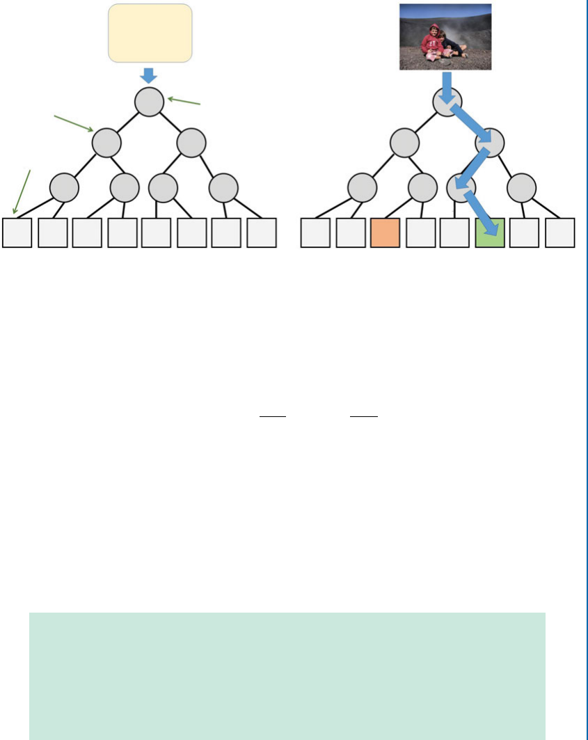
2.3. MACHINE LEARNING CLASSIFIERS 27
Input
Split Node Root Node False
False
False
(b)(a)
False
True
True True
True
Leaf Node
Is top part blue?
Is bottom
part blue?
Is bottom
part green?
Indoor Outdoor
Figure 2.8: (a) A decision tree is a set of nodes and edges organized in a hierarchical fashion. e
split (or internal) nodes are denoted with circles and the leaf (or terminal) nodes with squares.
(b) A decision tree is a tree where each split node stores a test function which is applied to the
input data. Each leaf stores the final label (here whether “indoor” or “outdoor”).
where
H.QjffŒi; ig/DjQlj
jQjH.Ql/CjQrj
jQjH.Qr/; (2.23)
and jQljand jQrjdenote the number of data samples in the left and right partitions. e entropy
of Qlis given by
H.Ql/D X
i2Ql
pilog2pi;(2.24)
where piis the number of samples of class iin Qldivided by jQlj. e feature and the associated
threshold which maximize the gain are selected as the splitting test for that node
ffgŒi; igDarg max
ffgŒi;igG.QjffgŒi; ig/: (2.25)
Entropy and Information Gain: e entropy and information gain are two
important concepts in the RDF training process. ese concepts are usually
discussed in information theory or probability courses and are briefly dis-
cussed below.
Information entropy is defined as a measure of the randomness in
the information being processed. More precisely, the higher the entropy,

28 2. FEATURES AND CLASSIFIERS
the lower the information content. Mathematically, given a discrete random
variable Xwith possible values fx1; ; xngand a probability mass function
P .X /, the entropy H(also called Shannon entropy) can be written as follows:
H.X / D
n
X
iD1
P .xi/log2P .xi/: (2.26)
For example, an action such as flipping a coin that has no affinity for
“head” or “tail,” provides information that is random (Xwith possible values
of f“head,” “tail”g). erefore, Eq. (2.26) can be written as follows:
H.X / D P .“head”/log2P .“head”/P .“tail”/log2P .“tail”/: (2.27)
As shown in Fig. 2.9, this binary entropy function (Eq. (2.27)) reaches
its maximum value (uncertainty is at a maximum) when the probability is
1
2, meaning that P .X D“head”/D1
2or similarly P .X D“tail”/D1
2. e
entropy function reaches its minimum value (i.e., zero) when probability is
1or 0with complete certainty P .X D“head” D1/ or P .X D“head” D0/
respectively.
Information gain is defined as the change in information entropy H
from a prior state to a state that takes some information (t) and can be written
as follows:
G.Qjt/ DH.Q/ H.Qjt/: (2.28)
If a partition consists of only a single class, it is considered as a leaf node. Partitions
consisting of multiple classes are further partitioned until either they contain single classes or
the tree reaches its maximum height. If the maximum height of the tree is reached and some
of its leaf nodes contain labels from multiple classes, the empirical distribution over the classes
associated with the subset of the training samples v, which have reached that leaf, is used as
its label. us, the probabilistic leaf predictor model for the t-th tree is pt.cjv/, where c2 fckg
denotes the class.
Classification
Once a set of decision trees have been trained, given a previously unseen sample xj, each decision
tree hierarchically applies a number of predefined tests. Starting at the root, each split node
applies its associated split function to xj. Depending on the result of the binary test the data is
sent to the right or the left child. is process is repeated until the data point reaches a leaf node.
Usually the leaf nodes contain a predictor (e.g., a classifier) which associates an output (e.g., a
class label) to the input xj. In the case of forests, many tree predictors are combined together to
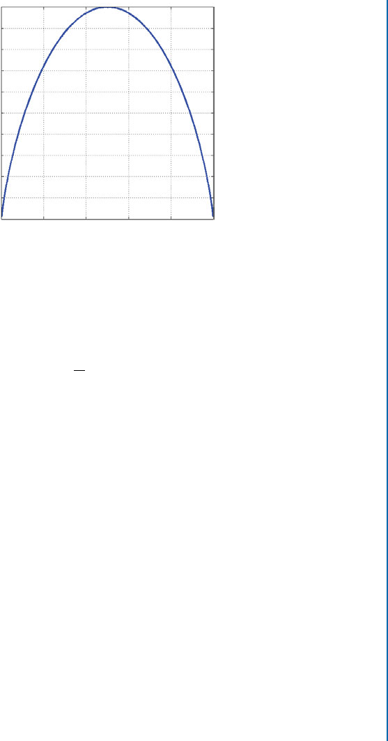
2.4. CONCLUSION 29
1
0.9
0.8
0.7
0.6
0.5
0.4
0.3
0.2
0.1
00 10.2 0.4 0.6 0.8
Probability
Entropy
Figure 2.9: Entropy vs. probability for a two class variable.
form a single forest prediction:
p.cjxj/D1
T
T
X
tD1
pt.cjxj/; (2.29)
where Tdenotes the number of decision trees in the forest.
2.4 CONCLUSION
Traditional computer vision systems consist of two steps: feature design and learning algorithm
design, both of which are largely independent. us, computer vision problems have tradition-
ally been approached by designing hand-engineered features such as HOG [Triggs and Dalal,
2005], SIFT [Lowe,2004], and SURF [Bay et al.,2008] that lack in generalizing well to other
domains, are time consuming, expensive, and require expert knowledge on the problem do-
main. ese feature engineering processes are usually followed by learning algorithms such as
SVM [Cortes,1995] and RDF [Breiman,2001,Quinlan,1986]. However, progress in deep
learning algorithms resolves all these issues, by training a deep neural network for feature ex-
traction and classification in an end-to-end learning framework. More precisely, unlike tradi-
tional approaches, deep neural networks learn to simultaneously extract features and classify data
samples. Chapter 3will discuss deep neural networks in detail.
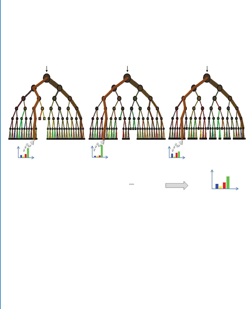
30 2. FEATURES AND CLASSIFIERS
= 1
= 1
3
= 2 = 3
1(|)
2(|)
3(|)
(|)
RDF output probability is: (|) = 1 (|)
3
Figure 2.10: RDF classification for a test sample xj. During testing the same test sample is
passed through each decision tree. At each internal node a test is applied and the test sample
is sent to the appropriate child. is process is repeated until a leaf is reached. At the leaf the
stored posterior pt.cjxj/is read. e forest class posterior p.cjxj/is the average of all decision
tree posteriors.

31
C H A P T E R 3
Neural Networks Basics
3.1 INTRODUCTION
Before going into the details of the CNNs, we provide in this chapter an introduction to artifi-
cial neural networks, their computational mechanism, and their historical background. Neural
networks are inspired by the working of cerebral cortex in mammals. It is important to note,
however, that these models do not closely resemble the working, scale and complexity of the
human brain. Artificial neural network models can be understood as a set of basic processing
units, which are tightly interconnected and operate on the given inputs to process the informa-
tion and generate desired outputs. Neural networks can be grouped into two generic categories
based on the way the information is propagated in the network.
•Feed-forward networks
e information flow in a feed-forward network happens only in one direction. If the
network is considered as a graph with neurons as its nodes, the connections between the
nodes are such that there are no loops or cycles in the graph. ese network architectures
can be referred as Directed Acyclic Graphs (DAG). Examples include MLP and CNNs,
which we will discuss in details in the upcoming sections.
•Feed-back networks
As the name implies, feed-back networks have connections which form directed cycles (or
loops). is architecture allows them to operate on and generate sequences of arbitrary
sizes. Feed-back networks exhibit memorization ability and can store information and
sequence relationships in their internal memory. Examples of such architectures include
Recurrent Neural Network (RNN) and Long-Short Term Memory (LSTM).
We provide an example architecture for both feed-forward and feed-back networks in
Sections 3.2 and 3.3, respectively. For feed-forward networks, we first study MLP, which is a
simple case of such architectures. In Chapter 4, we will cover the CNNs in detail, which also
work in a feed-forward manner. For feed-back networks, we study RNNs. Since our main focus
here is on CNNs, an in-depth treatment of RNNs is out of the scope of this book. We refer
interested readers to Graves et al. [2012] for RNN details.
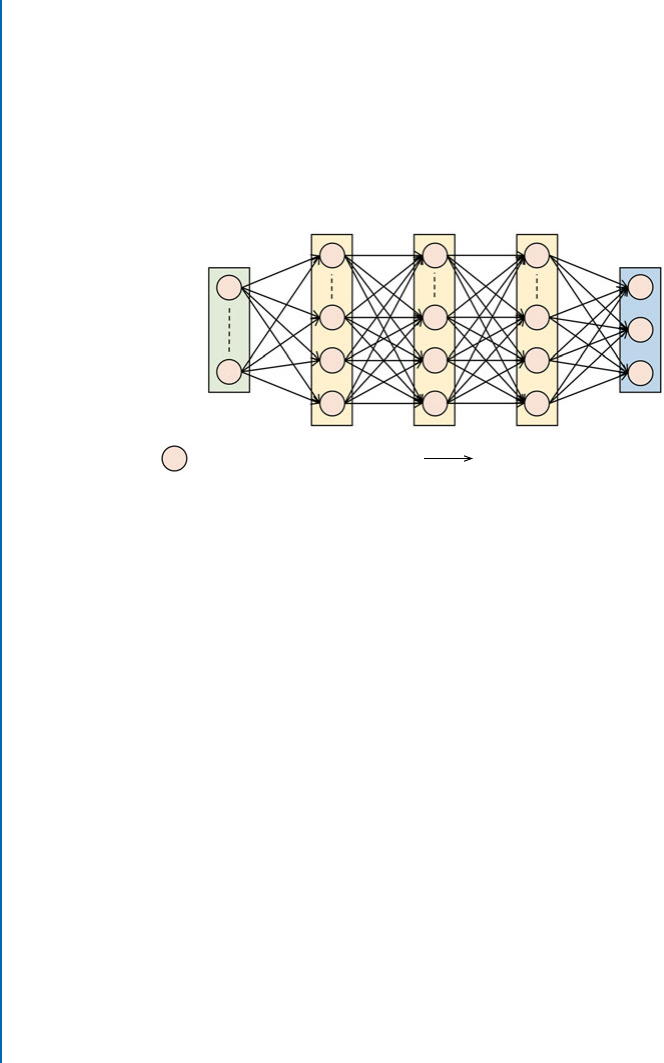
32 3. NEURAL NETWORKS BASICS
3.2 MULTI-LAYER PERCEPTRON
3.2.1 ARCHITECTURE BASICS
Figure 3.1 shows an example of a MLP network architecture which consists of three hidden
layers, sandwiched between an input and an output layer. In simplest terms, the network can
be treated as a black box, which operates on a set of inputs and generates some outputs. We
highlight some of the interesting aspects of this architecture in more details below.
Input
Layer
Output
Layer
Hidden Layers
Artificial Neurons or Units Connections between Units
Figure 3.1: A simple feed-forward neural network with dense connections.
Layered Architecture: Neural networks comprise a hierarchy of processing levels. Each
level is called a “network layer” and consists of a number of processing “nodes” ( also called “neu-
rons” or “units”). Typically, the input is fed through an input layer and the final layer is the output
layer which makes predictions. e intermediate layers perform the processing and are referred
to as the hidden layers. Due to this layered architecture, this neural network is called an MLP.
Nodes: e individual processing units in each layer are called the nodes in a neural net-
work architecture. e nodes basically implement an “activation function” which given an input,
decides whether the node will fire or not.
Dense Connections: e nodes in a neural network are interconnected and can com-
municate with each other. Each connection has a weight which specifies the strength of the
connection between two nodes. For the simple case of feed-forward neural networks, the infor-
mation is transferred sequentially in one direction from the input to the output layers. erefore,
each node in a layer is directly connected to all nodes in the immediate previous layer.
3.2.2 PARAMETER LEARNING
As we described in Section 3.2.1, the weights of a neural network define the connections between
neurons. ese weights need to be set appropriately so that a desired output can be obtained from
the neural network. e weights encode the “model” generated from the training data that is used
to allow the network to perform a designated task (e.g., object detection, recognition, and/or

3.2. MULTI-LAYER PERCEPTRON 33
classification). In practical settings, the number of weights is huge which requires an automatic
procedure to update their values appropriately for a given task. e process of automatically
tuning the network parameters is called “learning” which is accomplished during the training
stage (in contrast to the test stage where inference/prediction is made on “unseen data,” i.e., data
that the network has not “seen” during training). is process involves showing examples of the
desired task to the network so that it can learn to identify the right set of relationships between
the inputs and the required outputs. For example, in the paradigm of supervised learning, the
inputs can be media (speech, images) and the outputs are the desired set of “labels” (e.g., identity
of a person) which are used to tune the neural network parameters.
We now describe a basic form of learning algorithm, which is called the Delta Rule.
Delta Rule
e basic idea behind the delta rule is to learn from the mistakes of the neural network during
the training phase. e delta rule was proposed by Widrow et al. [1960], which updates the
network parameters (i.e., weights denoted by , considering 0biases) based on the difference
between the target output and the predicted output. is difference is calculated in terms of the
Least Mean Square (LMS) error, which is why the delta learning rule is also referred to as the
LMS rule. e output units are a “linear function” of the inputs denoted by x, i.e.,
piDX
j
ij xj:
If pnand yndenote the predicted and target outputs, respectively, the error can be calculated as:
ED1
2X
n
.ynpn/2;(3.1)
where nis the number of categories in the dataset (or the number of neurons in the output
layer). e delta rule calculates the gradient of this error function (Eq. (3.1)) with respect to
the parameters of the network: @E=@ij . Given the gradient, the weights are updated iteratively
according to the following learning rule:
tC1
ij Dt
ij C@E
@ij
(3.2)
tC1
ij Dt
ij C.yipi/xj;(3.3)
where tdenotes the previous iteration of the learning process. e hyper-parameter denotes
the step size of the parameter update in the direction of the calculated gradient. One can visualize
that no learning happens when the gradient or the step size is zero. In other cases, the parameters
are updated such that the predicted outputs get closer to the target outputs. After a number of
iterations, the network training process is said to converge when the parameters do not change
any longer as a result of the update.

34 3. NEURAL NETWORKS BASICS
If the step size is unnecessarily too small, the network will take longer to converge and
the learning process will be very slow. On the other hand, taking very large steps can result in an
unstable erratic behavior during the training process as a result of which the network may not
converge at all. erefore, setting the step-size to a right value is really important for network
training. We will discuss different approaches to set the step size in Section 5.3 for CNN training
which are equally applicable to MLP.
Generalized Delta Rule
e generalized delta rule is an extension of the delta rule. It was proposed by Rumelhart et al.
[1985]. e delta rule only computes linear combinations between the input and the output
pairs. is limits us to only a single-layered network because a stack of many linear layers is not
better than a single linear transformation. To overcome this limitation, the generalized delta rule
makes use of nonlinear activation functions at each processing unit to model nonlinear relation-
ships between the input and output domains. It also allows us to make use of multiple hidden
layers in the neural network architecture, a concept which forms the heart of deep learning.
e parameters of a multi-layered neural network are updated in the same manner as the
delta rule, i.e.,
tC1
ij Dt
ij C@E
@ij
:(3.4)
But different to the delta rule, the errors are recursively sent backward through the multi-layered
network. For this reason, the generalized delta rule is also called the “back-propagation” algo-
rithm. Since for the case of the generalized delta rule, a neural network not only has an output
layer but also intermediate hidden layers, we can separately calculate the error term (differential
with respect to the desired output) for the output and hidden layers. Since the case of the output
layer is simple, we first discuss the error computation for this layer.
Given the error function in Eq. (3.1), its gradient with respect to the parameters in the
output layer Lfor each node ican be computed as follows:
@E
@L
ij DıL
ixj;(3.5)
ıL
iD.yipi/f 0
i.ai/; (3.6)
where, aiDPji;j xjCbiis the activation which is the input to the neuron (prior to the acti-
vation function), xj’s are the outputs from the previous layer, piDf .ai/is the output from the
neuron (prediction for the case of output layer) and f ./denotes a nonlinear activation function
while f0./represents its derivative. e activation function decides whether the neuron will fire
or not, in response to a given input activation. Note that the nonlinear activation functions are
differentiable so that the parameters of the network can be tuned using error back-propagation.

3.2. MULTI-LAYER PERCEPTRON 35
One popular activation function is the sigmoid function, given as follows:
piDf .ai/D1
1Cexp.ai/:(3.7)
We will discuss other activation functions in detail in Section 4.2.4. e derivative of the sigmoid
activation function is ideally suitable because it can be written in terms of the sigmoid function
itself (i.e., pi) and is given by:
f0
i.ai/Dpi.1 pi/: (3.8)
erefore, we can write the gradient equation for the output layer neurons as follows:
@E
@L
ij D.yipi/.1 pi/xjpi:(3.9)
Similarly, we can calculate the error signal for the intermediate hidden layers in a multi-layered
neural network architecture by back propagation of errors as follows:
ıl
iDf0.al
i/X
j
lC1
ij ılC1
j;(3.10)
where l2 f1 : : : L 1gand Ldenotes the total number of layers in the network. e above
equation applies the chain rule to progressively calculate the gradients of the internal parameters
using the gradients of all subsequent layers. e overall update equation for the MLP parameters
ij can be written as:
tC1
ij Dt
ij Cıl
ixl1
j;(3.11)
where xl1
jis the output from the previous layer and tdenotes the number of previous training
iteration. e complete learning process usually involves a number of iterations and the param-
eters are continually updated until the network is optimized (i.e., after a set number of iterations
or when tC1
ij does not change).
Gradient Instability Problem: e generalized delta rule successfully works
for the case of shallow networks (ones with one or two hidden layers). How-
ever, when the networks are deep (i.e., Lis large), the learning process can
suffer from the vanishing or exploding gradient problems depending on the
choice of the activation function (e.g., sigmoid in above example). is in-
stability relates particularly to the initial layers in a deep network. As a result,
the weights of the initial layers cannot be properly tuned. We explain this
with an example below.
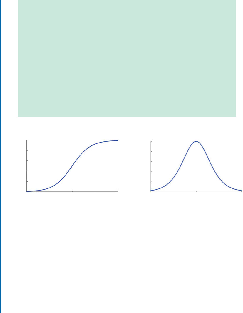
36 3. NEURAL NETWORKS BASICS
Consider a deep network with many layers. e outputs of each weight
layer are squashed within a small range using an activation function (e.g.,
[0,1] for the case of the sigmoid). e gradient of the sigmoid function
leads to even smaller values (see Fig. 3.2). To update the initial layer pa-
rameters, the derivatives are successively multiplied according to the chain
rule (as in Eq. (3.10)). ese multiplications exponentially decay the back-
propagated signal. If we consider a network depth of 5, and the maximum
possible gradient value for the sigmoid (i.e., 0:25), the decaying factor would
be .0:25/5D0:0009. is is called the “vanishing gradient” problem. It is easy
to follow that in cases where the gradient of the activation function is large,
successive multiplications can lead to the “exploding gradient” problem.
We will introduce the ReLU activation function in Chapter 4, whose
gradient is equal to 1(when a unit is “on”). Since 1LD1, this avoids both
the vanishing and the exploding gradient problems.
Sigmoid Activation Function Derivative of Sigmoid
InputInput
Output
Output
1
0.8
0.6
0.4
0.2
0
0.25
0.2
0.15
0.1
0.05
0
-5 0 5 -5 0 5
Figure 3.2: e sigmoid activation function and its derivative. Note that the range of values for
the derivative is relatively small which leads to the vanishing gradient problem.
3.3 RECURRENT NEURAL NETWORKS
e feed-back networks contain loops in their network architecture, which allows them to pro-
cess sequential data. In many applications, such as caption generation for an image, we want to
make a prediction such that it is consistent with the previously generated outputs (e.g., already
generated words in the caption). To accomplish this, the network processes each element in an
input sequence in a similar fashion (while considering the previous computational state). For
this reason it is also called an RNN.
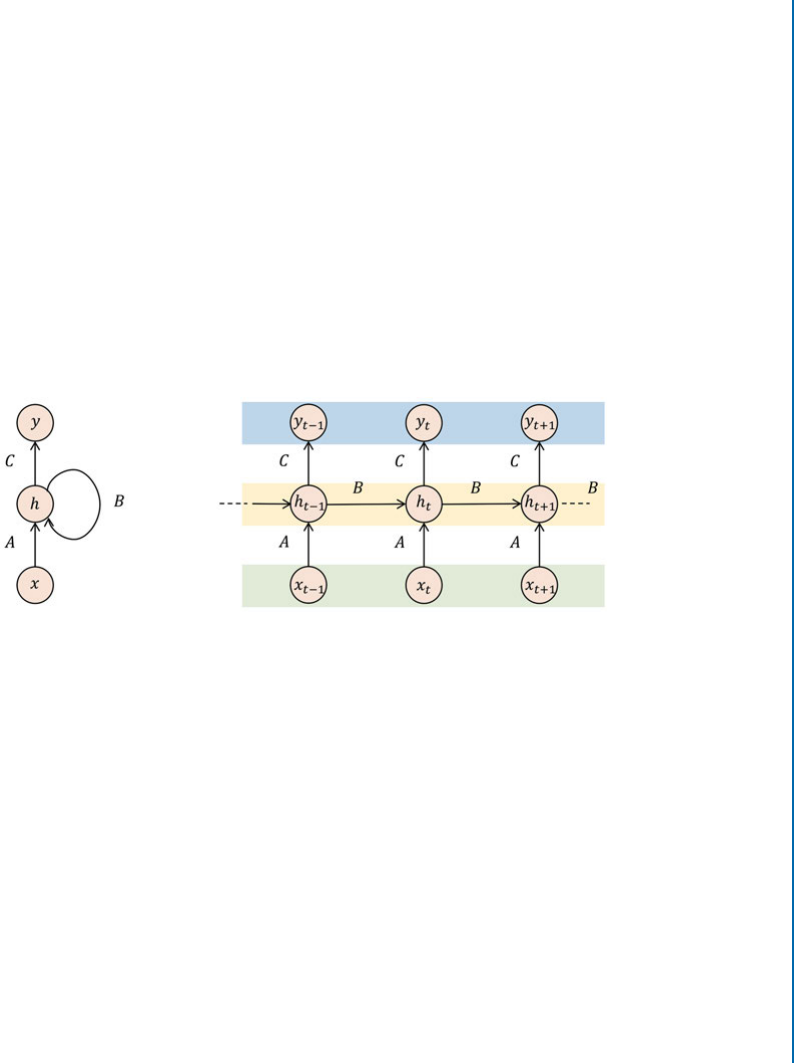
3.3. RECURRENT NEURAL NETWORKS 37
Since, RNNs process information in a manner that is dependent on the previous computa-
tional states, they provide a mechanism to “remember” previous states. e memory mechanism
is usually effective to remember only the short term information that is previously processed by
the network. Below, we outline the architectural details of an RNN.
3.3.1 ARCHITECTURE BASICS
A simple RNN architecture is shown in Fig. 3.3. As described above, it contains a feed-back
loop whose working can be visualized by unfolding the recurrent network over time (shown on
the right). e unfolded version of the RNN is very similar to a feed-forward neural network
described in Section 3.2. We can, therefore, understand RNN as a simple multi-layered neural
network, where the information flow happens over time and different layers represent the com-
putational output at different time instances. e RNN operates on sequences and therefore the
input and consequently the output at each time instance also varies.
Output Layer
Hidden Layer
Input Layer
(a) (b)
Figure 3.3: e RNN Architecture. Left: A simple recurrent network with a feed-back loop.
Right: An unfolded recurrent architecture at different time-steps.
We highlight the key features of an RNN architecture below.
Variable Length Input: RNN can operate on inputs of variable length, e.g., videos with
variable frame length, sentences with different number of words, 3D point clouds with variable
number of points. e length of the unfolded RNN structure depends on the length of the
input sequence, e.g., for a sentence consisting of 12 words, there will be a total of 12 layers in
the unfolded RNN architecture. In Fig. 3.3, the input to the network at each time instance tis
represented by the variable xt.
Hidden State: e RNN holds internally the memory of the previous computation in a
hidden state represented by ht. is state can be understood as an input from the previous layer
in the unfolded RNN structure. At the beginning of the sequence processing, it is initialized with
a zero or a random vector. At each time step, this state is updated by considering its previous

38 3. NEURAL NETWORKS BASICS
value and the current input to the network:
htDf .AxtCBht1/; (3.12)
where f ./is the nonlinear activation function. e weight matrix Bis called the transition
matrix since it influences how the hidden state changes over time.
Variable Length Output: e output of RNN at each time step is denoted by yt. e
RNNs are capable of generating variable length outputs, e.g., translating a sentence in one lan-
guage to another language where the output sequence lengths can be different from the input
sequence length. is is possible because RNNs consider the hidden state while making predic-
tions. e hidden state models the joint probability of the previously processed sequence which
can be used to predict new outputs. As an example, given a few starting words in a sentence,
the RNN can predict the next possible word in the sentence, where a special end of a sentence
symbol is used to denote the end of each sentence. In this case all possible words (including the
end of sentence symbol) are included in the dictionary over which the prediction is made:
ytDf .C ht/; (3.13)
where f ./is an activation function such as a softmax (Section 4.2.4).
Shared Parameters: e parameters in the unfolded RNN linking the input, the hidden
state and the output (denoted by A; B, and C, respectively) are shared between all layers. is
is the reason why the complete architecture can be represented by using a loop to represent its
recurrent architecture. Since the parameters in a RNN are shared, the total number of tunable
parameters are considerably less than an MLP, where a separate set of parameters are learned for
each layer in the network. is enables efficient training and testing of the feed-back networks.
Based on the above description of RNN architecture, it can be noted that indeed the hid-
den state of the network provides a memory mechanism, but it is not effective when we want
to remember long-term relationships in the sequences. erefore, RNN only provide short-
term memory and find difficulties in “remembering” (a few time-steps away) old information
processed through it. To overcome this limitation, improved versions of recurrent networks
have been introduced in the literature which include the LSTM [Hochreiter and Schmidhu-
ber,1997], Gated Recurrent Unit (GRU) [Cho et al.,2014], Bi-directional RNN (B-RNN)
[Graves and Schmidhuber,2005] and Neural Turing Machines (NTM) [Graves et al.,2014].
However, the details of all these network architectures and their functioning is out of the scope
of this book which is focused on feed-forward architectures (particularly CNNs).
3.3.2 PARAMETER LEARNING
e parameters in a feed-back network can be learned using the generalized delta rule (back-
propagation algorithm), similar to feed-forward networks. However, instead of error back-
propagation through network layers as in feed-forward networks, back-propagation is performed

3.4. LINK WITH BIOLOGICAL VISION 39
through time in the feed-back networks. At each time instance, the output of the RNN is com-
puted as a function of its previous and current inputs. e Back Propagation rough Time
(BPTT) algorithm cannot allow the learning of long-term relationships in sequences, because
of difficulties in error computations over long sequences. Specifically, when the number of it-
erations increases, the BPTT algorithm suffers from the vanishing or the exploding gradient
problem. One way around this problem is to compute the error signal over a truncated unfolded
RNN. is reduces the cost of the parameter update process for long sequences, but limits the
dependence of the output at each time instance to only few previous hidden states.
3.4 LINK WITH BIOLOGICAL VISION
We think it is important to briefly discuss biological neural networks (BNNs) and their oper-
ational mechanisms in order to study their similarities and dissimilarities with artificial neural
networks. As a matter of fact, artificial neural networks do not resemble their biological coun-
terparts in terms of functioning and scale, however they are indeed motivated by the BNNs and
several of the terms used to describe artificial neural networks are borrowed from the neuro-
science literature. erefore, we introduce neural networks in the brain, draw parallels between
artificial and biological neurons, and provide a model of the artificial neuron based on biological
vision.
3.4.1 BIOLOGICAL NEURON
e human brain contains approximately 100 billion neurons. To interpret this number, let us
assume we have 100 billion one dollar bills, where each bill is only 0.11 mm thick. If we stack
all these one dollar bills on top of each other, the resulting stack will be 10922.0 km high. is
illustrates the scale and magnitude of the human brain.
A biological neuron is a nerve cell which processes information [Jain et al.,1996]. Each
neuron is surrounded by a membrane and has a nucleus which contains genes. It has specialized
projections which manage the input and output to the nerve cell. ese projections are termed
dendrites and axons. We describe these and other key aspects of the biological neuron below.
Dendrites: Dendrites are fibers which act as receptive lines and bring information (acti-
vations) to the cell body from other neurons. ey are the inputs of the neuron.
Axons: Axons are fibers which act as transmission lines and take information away from
the cell body to other neurons. ey act as outputs of the neuron.
Cell body: e cell body (also called the soma) receives the incoming information through
dendrites, processes it and sends it, to other neurons via axons.
Synapses: e specialized connections between axons and dendrites which allow the com-
munication of signals are called synapses. e communication takes place by an electro-chemical
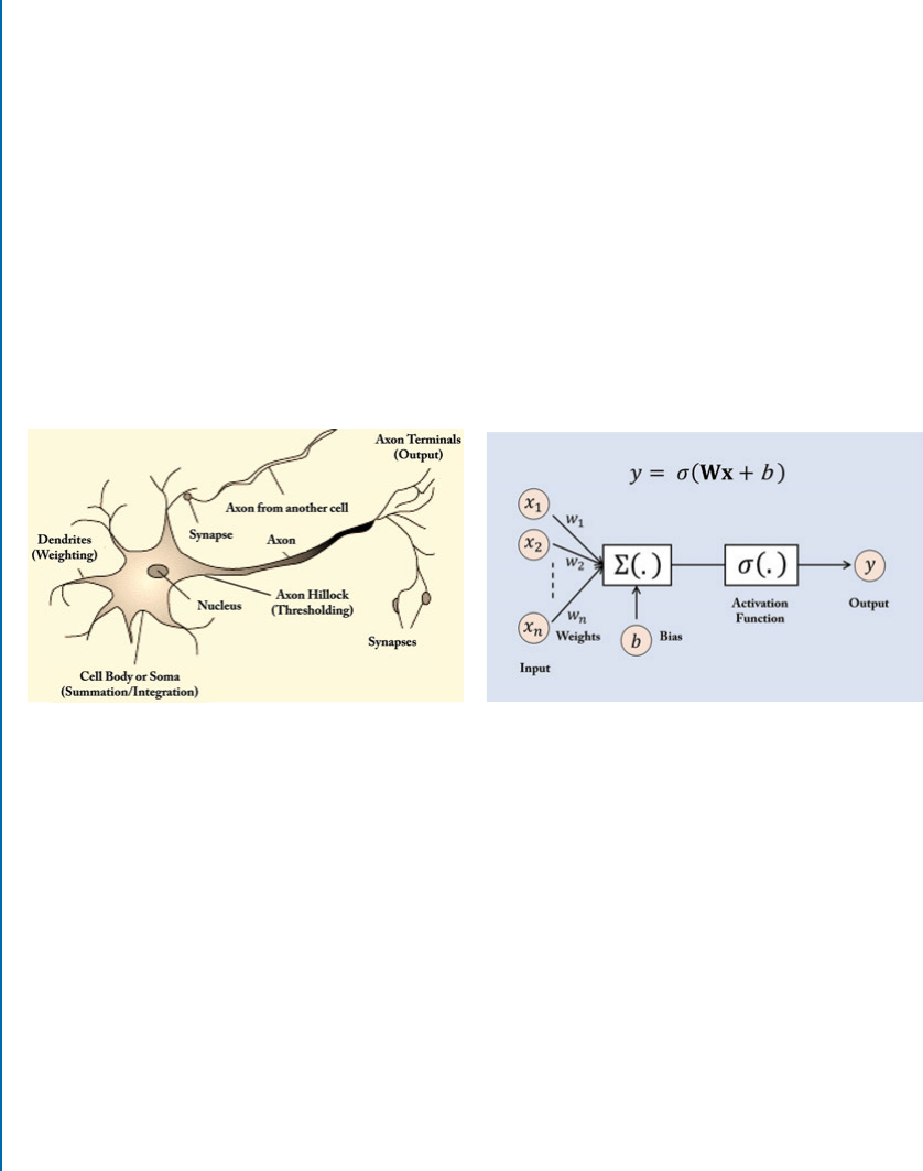
40 3. NEURAL NETWORKS BASICS
process where the neurotransmitters (chemicals) are released at the synapse and are diffused
across the synaptic gap to transmit information. ere is a total of approximately 1 quadrillion
(1015) synapses in the human brain [Changeux and Ricoeur,2002].
Connections: Neurons are densely inter-connected with each other. On average, each
neuron receives inputs from approximately 105synapses.
Neuron Firing: A neuron receives signals from connected neurons via dendrites. e cell
body sums up the received signals and the neuron fires if the combined input signal exceeds a
threshold. By neuron firing, we mean that it generates an output which is sent out through axons.
If the combined input is below the threshold, no response signal is generated by the neuron (i.e.,
the neuron does not fire). e thresholding function which decides whether a neuron fires or
not is called activation function.
Next, we describe a simple computational model which mimics the working of a biological
neuron.
Figure 3.4: A biological neuron (left) and a computational model (right) which is used to develop
artificial neural networks.
3.4.2 COMPUTATIONAL MODEL OF A NEURON
A simple mathematical model of the biological neuron known as the reshold Logic Unit (TLU)
was proposed by McCulloch and Pitts [1943]. It consists of a set of incoming connections which
feed the unit with activations coming from other neurons. ese inputs are weighted using a set
of weights denoted by fwg. e processing unit then sums all the inputs and applies a nonlinear
threshold function (also known as the activation function) to calculate the output. e resulting
output is then transmitted to other connected neural units. We can denote the operation of a
McCulloch-Pitts neuron as follows:
yDf n
X
iD1
wixiCb!;(3.14)

3.4. LINK WITH BIOLOGICAL VISION 41
where bis a threshold, widenote the synapse weight, xiis the input to the neuron, and f ./
represents a nonlinear activation function. For the simplest case, fis a step function which
gives 0(i.e., neuron does not fire) when the input is below 0(i.e., Pn
iD1wixiCbless than the
firing threshold) and 1when it is greater than 0. For other cases, the activation function can be
a sigmoid, tanh, or an ReLU for a smooth thresholding operation (see Chapter 4).
e McCulloch-Pitts neuron is a very simple computational model. However, they have
been shown to approximate complex functions quite well. McCulloch and Pitts showed that a
network comprising of such neurons can perform universal computations. e universal com-
putational ability of neural networks ensures their ability to model a very rich set of continuous
functions using only a finite number of neurons. is fact is formally known as the “Univer-
sal Approximation eorem” for neural networks. Different to McCulloch-Pitts model, state
of the art neuron models also incorporate additional features such as stochastic behaviors and
non-binary input and output.
3.4.3 ARTIFICIAL VS. BIOLOGICAL NEURON
Having outlined the basics of artificial and biological neuron operation, we can now draw par-
allels between their functioning and identify the key differences between the two.
An artificial neuron (also called a unit or a node) takes several input connections (dendrites
in biological neuron) which are assigned certain weights (analogous to synapses). e unit then
computes the sum of the weighted inputs and applies an activation function (analogous to the cell
body in biological neuron). e result of the unit is then passed on using the output connection
(axon function).
Note that the above-mentioned analogy between a biological and an artificial neuron is
only valid in the loose sense. In reality, there exists a number of crucial differences in the func-
tioning of biological neurons. As an example, biological neurons do not sum the weighted in-
puts, rather dendrites interact in a much complex way to combine the incoming information.
Furthermore, biological neurons communicate asynchronously, different from their computa-
tional counterparts which operate synchronously. e training mechanisms in both types of
neural networks are also different, while the training mechanisms in biological networks are
not precisely known. e topology in biological networks are very complicated compared to the
artificial networks which currently have either a feed-forward or feed-back architecture.

43
C H A P T E R 4
Convolutional Neural Network
4.1 INTRODUCTION
We discussed neural networks in Chapter 3. CNNs are one of the most popular categories of
neural networks, especially for high-dimensional data (e.g., images and videos). CNNs operate
in a way that is very similar to standard neural networks. A key difference, however, is that each
unit in a CNN layer is a two- (or high-) dimensional filter which is convolved with the input
of that layer. is is essential for cases where we want to learn patterns from high-dimensional
input media, e.g., images or videos. CNN filters incorporate spatial context by having a similar
(but smaller) spatial shape as the input media, and use parameter sharing to significantly reduce
the number of learn-able variables. We will describe these concepts in detail in Chapters 4,5,
and 6. However, we find it important to first give a brief historical background of CNNs.
An earliest form of CNN was the Neocognitron model proposed by Kunihiko Fukushima
[Fukushima and Miyake,1982]. It consisted of multiple layers which automatically learned a
hierarchy of feature abstractions for pattern recognition. e Neocognitron was motivated by the
seminal work by Hubel and Wiesel [1959] on the primary visual cortex which demonstrated that
the neurons in the brain are organized in the form of layers. ese layers learn to recognize visual
patterns by first extracting local features and subsequently combining them to obtain higher-
level representations. e network training was performed using a reinforcement learning rule.
A major improvement over the Neocognitron was the LeNet model proposed by LeCun et al.
[1989], where the model parameters were learned using error back-propagation. is CNN
model was successfully applied to recognize handwritten digits.
CNNs are a useful class of models for both supervised and unsupervised learning
paradigms. e supervised learning mechanism is the one where the input to the system and
the desired outputs (true labels) are known and the model learns a mapping between the two. In
the unsupervised learning mechanism, the true labels for a given set of inputs are not known
and the model aims to estimate the underlying distribution of the inputs data samples. An ex-
ample of a supervised learning task (image classification) is shown in Fig. 4.1. e CNN learns
to map a given image to its corresponding category by detecting a number of abstract feature
representations, ranging from simple to more complex ones. ese discriminative features are
then used within the network to predict the correct category of an input image. e neural net-
work classifier is identical to the MLP we studied in Chapter 3. Recall that we reviewed popular
hand-crafted feature representations and machine learning classifiers in Chapter 2. e function
of a CNN is similar to this pipeline, with the key difference being the automatic learning of a
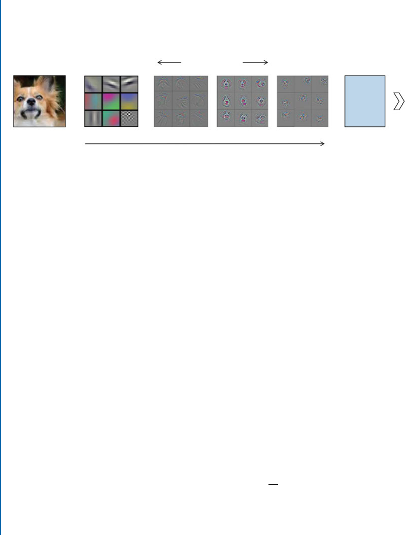
44 4. CONVOLUTIONAL NEURAL NETWORK
hierarchy of useful feature representations and its integration of the classification and feature
extraction stages in a single pipeline which is trainable in an end-to-end manner. is reduces
the need for manual design and expert human intervention.
Input
Image
Initial
Layers
Final
Layers
Neural
Network
Classifier
Intermediate
Layers
Complexity of Learned Feature Representations
High
Dog
Low
Figure 4.1: A CNN learns low-level features in the initial layers, followed by more complex
intermediate and high-level feature representations which are used for a classification task. e
feature visualizations are adopted from Zeiler and Fergus [2014].
4.2 NETWORK LAYERS
A CNN is composed of several basic building blocks, called the CNN layers. In this section,
we study these building blocks and their function in the CNN architecture. Note that some of
these layers implement basic functionalities such as normalization, pooling, convolution, and
fully connected layers. ese basic layers are covered first in this section to develop a basic un-
derstanding of the CNN layers. Along with such basic but fundamental building blocks, we
also introduce several more complex layers later in this section which are composed of multiple
building blocks (e.g., Spatial Transformer Layer and VLAD pooling layer).
4.2.1 PRE-PROCESSING
Before passing input data to the networks, the data needs to be pre-processed. e general pre-
processing steps that are used consist of the following.
•Mean-subtraction: e input patches (belonging to both train and test sets) are zero-
centered by subtracting the mean computed on the entire training set. Given Ntraining
images, each denoted by x2Rhwc, we can denote the mean-subtraction step as follows:
x0DxO
x;where O
xD1
N
N
X
iD1
xi:(4.1)
•Normalization: e input data (belonging to both train and test sets) is divided with the
standard deviation of each input dimension (pixels in the case of an image) calculated on

4.2. NETWORK LAYERS 45
the training set to normalize the standard deviation to a unit value. It can be represented
as follows:
x00 Dx0
qPN
iD1.xiO
x/2
N1
:(4.2)
•PCA Whitening: e aim of PCA whitening is to reduce the correlations between dif-
ferent data dimensions by independently normalizing them. is approach starts with the
zero-centered data and calculates the covariance matrix which encodes the correlation be-
tween data dimensions. is covariance matrix is then decomposed via the Singular Value
Decomposition (SVD) algorithm and the data is decorrelated by projecting it onto the
eigenvectors found via SVD. Afterward, each dimension is divided by its corresponding
eigenvalue to normalize all the respective dimensions in the data space.
•Local Contrast Normalization: is normalization scheme gets its motivation from neu-
roscience. As the name depicts, this approach normalizes the local contrast of the feature
maps to obtain more prominent features. It first generates a local neighborhood for each
pixel, e.g., for a unit radius eight neighboring pixels are selected. Afterward, the pixel is
zero-centered with the mean calculated using its own and neighboring pixel values. Sim-
ilarly, the pixel is also normalized with a standard deviation of its own and neighboring
pixel values (only if the standard deviation is greater than one). e resulting pixel value is
used for further computations.
Another similar approach is the local response normalization [Krizhevsky et al.,2012]
which normalizes the contrast of features obtained from adjacent filters in a convolution
layer.
Note that PCA whitening can amplify the noise in the data and therefore recent
CNN models just use a simple mean-subtraction (and optionally normalization step) for pre-
processing. e scaling and shifting achieved through mean-subtraction and normalization is
helpful for gradient-based learning. is is because equivalent updates are made to the network
weights for all input dimensions, which enables a stable learning process. Furthermore, the local
contrast normalization (LCN) and the local response normalization (LRN) are not common in
the recent architectures since other approaches (e.g., batch normalization, which we will describe
in Section 5.2.4) have proven to be more effective.
4.2.2 CONVOLUTIONAL LAYERS
A convolutional layer is the most important component of a CNN. It comprises a set of filters
(also called convolutional kernels) which are convolved with a given input to generate an output
feature map.

46 4. CONVOLUTIONAL NEURAL NETWORK
What is a Filter? Each filter in a convolutional layer is a grid of discrete numbers. As an
example, consider a 22filter shown in Fig. 4.2. e weights of each filter (the numbers in
the grid) are learned during the training of CNN. is learning procedure involves a random
initialization of the filter weights at the start of the training (different approaches for weight
initialization will be discussed in Section 5.1). Afterward, given input-output pairs, the filter
weights are tuned in a number of different iterations during the learning procedure. We will
cover network training in more detail in Chapter 5.
2 0
-1 3
Figure 4.2: An example of a 2D image filter.
What is a Convolution Operation? We mentioned earlier that the convolution layer per-
forms convolution between the filters and the input to the layer. Let’s consider a 2D convolution
in Fig. 4.3 to develop an insight into the layer’s operation. Given a 2D input feature map and a
convolution filter of matrix sizes 44and 22, respectively, a convolution layer multiplies the
22filter with a highlighted patch (also 22) of the input feature map and sums up all values
to generate one value in the output feature map. Note that the filter slides along the width and
height of the input feature map and this process continues until the filter can no longer slide
further.
Remark: In the signal processing literature, there is a distinction between
the terms “convolution” and “cross correlation.” e operation we described
above is the “correlation operation.” During convolution, the only difference
is that the filter is flipped along its height and width before multiplication
and sum-pooling (see Fig. 4.4).
In machine learning, both operations are equivalent and there is rarely
a distinction made between the two. Both terms are used interchangeably
and most of the deep learning libraries implement the correlation operation
in the convolution layers. e reason is that the network optimization will
converge on the right filter weights for either of the two operations. If the
weights of a convolutional network are replaced with the ones learned using
a correlation network, the network performance will remain the same, be-
cause only the order of the operation is changed in the two networks, and
their discriminative ability stays the same. In this book, we follow the ma-
chine learning convention and do not make a distinction between the two
operations, i.e., a convolution layer performs the correlation operation in our
case.

4.2. NETWORK LAYERS 47
Figure 4.3: e operation of a convolution layer is illustrated in the figure above. (a)–(i) show
the computations performed at each step, as the filter is slided onto the input feature map to
compute the corresponding value in the output feature map. e 22filter (shown in green) is
multiplied with the same sized region (shown in orange) within a 44input feature map and
the resulting values are summed up to obtain a corresponding entry (shown in blue) in the output
feature map at each convolution step.
Correlation
Convolution
Filter Image Filter Image
Figure 4.4: e distinction between the correlation and convolution operations in the signal
processing literature. In machine learning, this distinction is usually not important and the deep
learning literature normally refers to the layers implementing the correlation operation as the
convolution operation. In this book, we also follow the same naming convention that is adopted
in the machine learning literature.
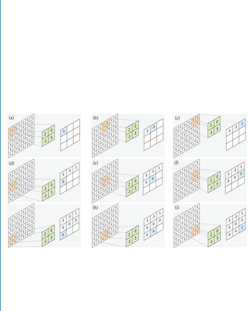
48 4. CONVOLUTIONAL NEURAL NETWORK
In the above example, in order to calculate each value of the output feature map, the filter
takes a step of 1along the horizontal or vertical position (i.e., along the column or the row of the
input). is step is termed as the stride of the convolution filter, which can be set to a different
(than 1) value if required. For example, the convolution operation with a stride of 2is shown in
Fig. 4.5. Compared to the stride of 1in the previous example, the stride of 2results in a smaller
output feature map. is reduction in dimensions is referred to as the sub-sampling operation.
Such a reduction in dimensions provides moderate invariance to scale and pose of the objects,
which is a useful property in applications such as object recognition. We will discuss other sub-
sampling mechanisms in the section where we discuss the pooling layers (Section 4.2.3).
We saw in Fig. 4.3 that the spatial size of the output feature map is reduced compared
to the input feature map. Precisely, for a filter with size ff, an input feature map with size
(g)
Figure 4.5: e operation of a convolution layer with a zero padding of 1 and a stride of 2 is
illustrated in the figure above. (a)–(i) show the computations that are performed at each step, as
the filter is slided onto the input feature map to compute the corresponding value of the output
feature map. e 22filter (shown in green) is multiplied with the same sized region (shown in
orange) within a 66input feature map (including zero-padding) and the resulting values are
summed up to obtain a corresponding entry (shown in blue) in the output feature map at each
convolution step.

4.2. NETWORK LAYERS 49
hwand a stride length s, the output feature dimensions are given by:
h0DhfCs
s; w0DwfCs
s;(4.3)
where, bcdenotes the floor operation. However, in some applications, such as image de-noising,
super-resolution, or segmentation, we want to keep the spatial sizes constant (or even larger) af-
ter convolution. is is important because these applications require more dense predictions at
the pixel level. Moreover, it allows us to design deeper networks (i.e., with more weight layers) by
avoiding a quick collapse of the output feature dimensions. is helps in achieving better perfor-
mances and higher resolution output labelings. is can be achieved by applying zero-padding
around the input feature map. As shown in Fig. 4.5, zero padding the horizontal and vertical
dimensions allows us to increase the output dimensions and therefore gives more flexibility in
the architecture design. e basic idea is to increase the size of the input feature map such that
an output feature map, with desired dimensions, is obtained. If pdenotes the increase in the in-
put feature map along each dimension (by padding zeros), we can represent the modified output
feature map dimensions as follows:
h0DhfCsCp
s; w0DwfCsCp
s:(4.4)
In Fig. 4.5,pD2and therefore the output dimensions have been increased from 66to 33.
If the convolutional layers were to not zero-pad the inputs and apply only valid convolutions,
then the spatial size of the output features will be reduced by a small factor after each convolution
layer and the information at the borders will be “washed away” too quickly.
e padding convolutions are usually categorized into three types based on the involve-
ment of zero-padding.
•Valid Convolution is the simplest case where no zero-padding is involved. e filter al-
ways stays within “valid” positions (i.e., no zero-padded values) in the input feature map
and the output size is reduced by f1along the height and the width.
•Same Convolution ensures that the output and input feature maps have equal (the “same”)
sizes. To achieve this, inputs are zero-padded appropriately. For example, for a stride of 1,
the padding is given by pDjf
2k. is is why it is also called “half ” convolution.
•Full Convolution applies the maximum possible padding to the input feature maps before
convolution. e maximum possible padding is the one where at least one valid input value
is involved in all convolution cases. erefore, it is equivalent to padding f1zeros for
a filter size fso that at the extreme corners at least one valid value will be included in the
convolutions.

50 4. CONVOLUTIONAL NEURAL NETWORK
Receptive Field: You would have noticed above that we used a relatively small sized kernel
with respect to the input. In computer vision, the inputs are of very high dimensions (e.g.,
images and videos) and are required to be efficiently processed through large-scale CNN models.
erefore, instead of defining convolutional filters that are equal to the spatial size of the inputs,
we define them to be of a significantly smaller size compared to the input images (e.g., in practice
33,55, and 77filters are used to process images with sizes such as 110 110,224 224,
and even larger). is design provides two key benefits: (a) the number of learn-able parameters
are greatly reduced when smaller sized kernels are used; and (b) small-sized filters ensure that
distinctive patterns are learned from the local regions corresponding to, e.g., different object
parts in an image. e size (height and width) of the filter which defines the spatial extent of
a region, which a filter can modify at each convolution step, is called the “receptive field” of
the filter. Note that the receptive field specifically relates to the spatial dimensions of the input
image/features. When we stack many convolution layers on top of each other, the “effective
receptive field” of each layer (relative to the input of the network) becomes a function of the
receptive fields of all the previous convolution layers. e effective receptive field for a stack of
Nconvolution layers, each with a kernel size of f, is given as:
RFn
eff DfCn.f 1/; n 2Œ1; N : (4.5)
As an example, if we stack two convolution layers each of kernel size 55and 33, respectively,
the receptive field of the second layer would be 33but its effective receptive field with respect
to the input image would be 77. When the stride and filter sizes of stacked convolution layers
are different, the effective receptive field of each layer can be represented in a more general form
as follows:
RFn
eff DRFn1
eff C.fn1/
n1
Y
iD1
si;(4.6)
where fndenotes the filter size in the nth layer, sirepresents the stride length for each previous
layer and RFn1
eff represents the effective receptive field of the previous layer.
Extending the Receptive Field: In order to enable very deep models with a relatively re-
duced number of parameters, a successful strategy is to stack many convolution layers with small
receptive fields (e.g., 33in the VGGnet [Simonyan and Zisserman,2014b] in Chapter 6).
However, this limits the spatial context of the learned convolutional filters which only scales
linearly with the number of layers. In applications such as segmentation and labeling, which
require pixel-wise dense predictions, a desirable characteristic is to aggregate broader contex-
tual information using bigger receptive fields in the convolution layer. Dilated convolution (or
atrous convolutions [Chen et al.,2014]) is an approach which extends the receptive field size,
without increasing the number of parameters [Yu and Koltun,2015]. e central idea is that
a new dilation parameter (d) is introduced, which decides on the spacing between the filter
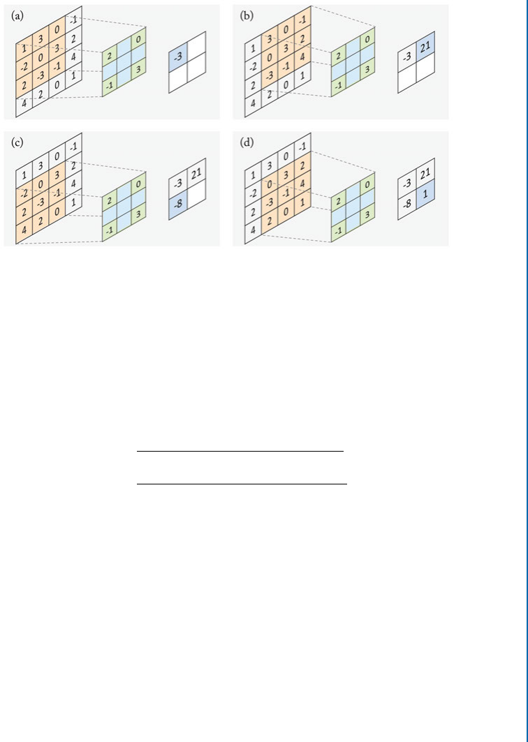
4.2. NETWORK LAYERS 51
Figure 4.6: Convolution with a dilated filter where the dilation factor is dD2.
weights while performing convolution. As shown in Fig. 4.6, a dilation by a factor of dmeans
that the original filter is expanded by d1spaces between each element and the intermediate
empty locations are filled in with zeros. As a result, a filter of size ffis enlarged to a size of:
fC.d 1/.f 1/. e output dimensions corresponding to a convolution operation with a
pre-defined filter size (f), zero padding (p), stride (s), dilation factor (d), an input with height
(h), and width (w) is given as:
h0Dhf.d 1/.f 1/ CsC2p
s(4.7)
w0Dwf.d 1/.f 1/ CsC2p
s:(4.8)
e effective receptive field of an nth layer can be expressed as:
RFn
eff DRFn1
eff Cd.f 1/; s:t:; RF1
eff Df: (4.9)
e effect of the dilation operation can easily be understood by looking at the dilated filter for
different values of parameter d. In Fig. 4.7, a stack of three convolution layers, each with different
dilation parameters is shown. In the first layer, dD1and the dilated convolution is equivalent
to a standard convolution. e receptive field size in this case is equal to the filter size, i.e., 3. In
the second convolution layer where dD2, the elements of the kernel are spread out such that
there is one space between each element. is inflation of the convolution filter exponentially
increases the receptive field size to 77. Similarly in the third layer, dD3which increases the
receptive field size to 13 13 according to the relationship of Eq. (4.9). is effectively allows
us to incorporate a wider context while performing convolutions. Combining multiple levels
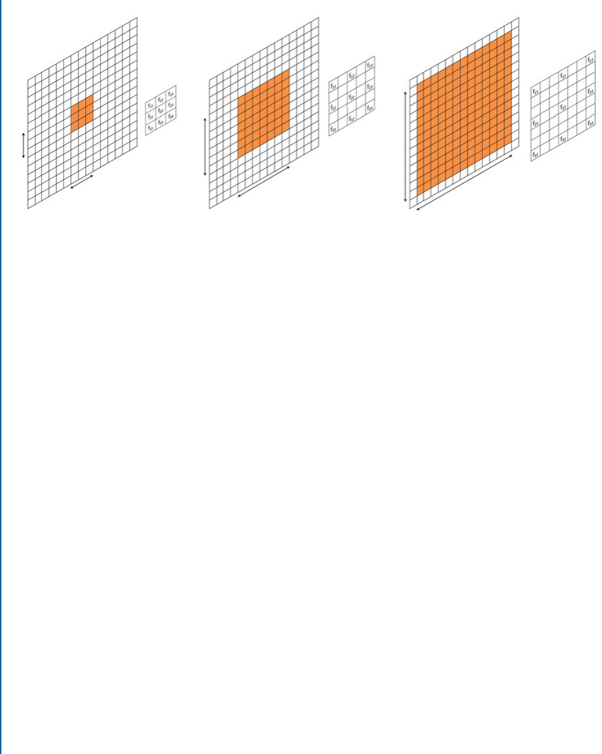
52 4. CONVOLUTIONAL NEURAL NETWORK
Effective Receptive Field = 3×3
First Convolution Layer Second Convolution Layer Third Convolution Layer
Effective Receptive Field = 7×7 Effective Receptive Field = 13×13
3
3
13
13
7
7
d = 1 d = 2
d = 3
Figure 4.7: is figure shows three convolution layers with a filter of size 33. e first, second,
and third layers have dilation factors of one, two, and three, respectively (from left to right). e
effective receptive field with respect to the input image is shown in orange at each convolution
layer. Note that an effective receptive field corresponds to the size of the region in the input
image which affects each output activation in a convolution layer. At the first layer, each output
activation is affected by a 33region in the input image because the filter size is 33. In
the subsequent layers, the receptive field increases due to the increasing network depth and the
increasing dilation factor, both of which contribute to the incorporation of a wider context in
the output feature responses.
of image context has been shown to improve the performance of classification, detection, and
segmentation using deep CNNs (Chapter 7).
Hyper-parameters: e parameters of the convolution layer which need to be set by the
user (based on cross-validation or experience) prior to the filter learning (such as the stride and
padding) are called hyper-parameters. ese hyper-parameters can be interpreted as the design
choices of our network architecture based on a given application.
High Dimensional Cases: e 2D case is the simplest one, where the filter has only a
single channel (represented as a matrix) which is convolved with the input feature channels to
produce an output response. For higher dimensional cases, e.g., when the input to the CNN
layers are tensors (e.g., 3D volumes in the case of volumetric representations), the filters are also
3D cubes which are convolved along the height, width, and depth of the input feature maps to
generate a corresponding 3D output feature map. However, all the concepts that we discussed
above for the 2D case still remain applicable to the processing of 3D and higher dimensional
inputs (such as 3D spatio-temporal representation learning). e only difference is that the
convolution operation is extended to an extra dimension, e.g., for the case of 3D, in addition to
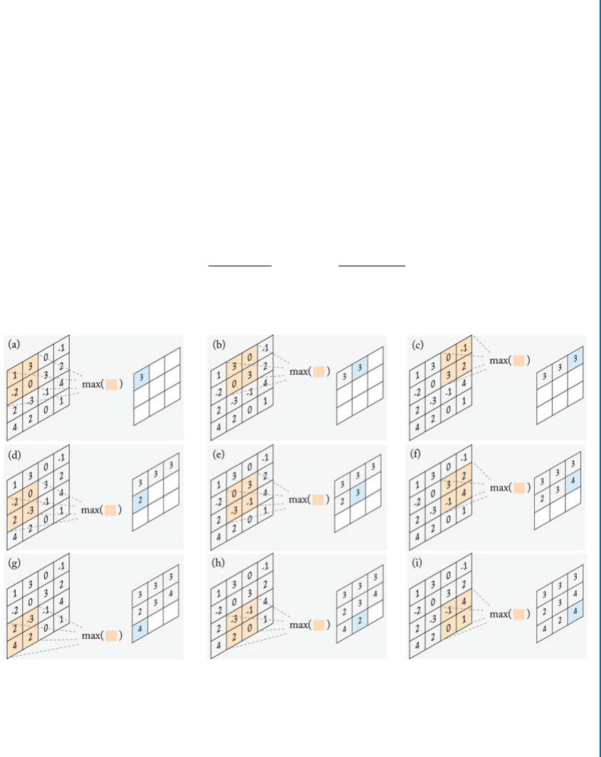
4.2. NETWORK LAYERS 53
a convolution along height and width in 2D case, convolutions are performed along the depth
as well. Similarly, zero-padding and striding can be performed along the depth for the 3D case.
4.2.3 POOLING LAYERS
A pooling layer operates on blocks of the input feature map and combines the feature activations.
is combination operation is defined by a pooling function such as the average or the max
function. Similar to the convolution layer, we need to specify the size of the pooled region and
the stride. Figure 4.8 shows the max pooling operation, where the maximum activation is chosen
from the selected block of values. is window is slided across the input feature maps with a
step size defined by the stride (1in the case of Fig. 4.8). If the size of the pooled region is given
by ff, with a stride s, the size of the output feature map is given by:
h0DhfCs
s; w0DwfCs
s:(4.10)
Figure 4.8: e operation of max-pooling layer when the size of the pooling region is 22and
the stride is 1.(a)–(i) shows the computations performed at each step as the pooled region in the
input feature map (shown in orange) is slided at each step to compute the corresponding value
in the output feature map (shown in blue).
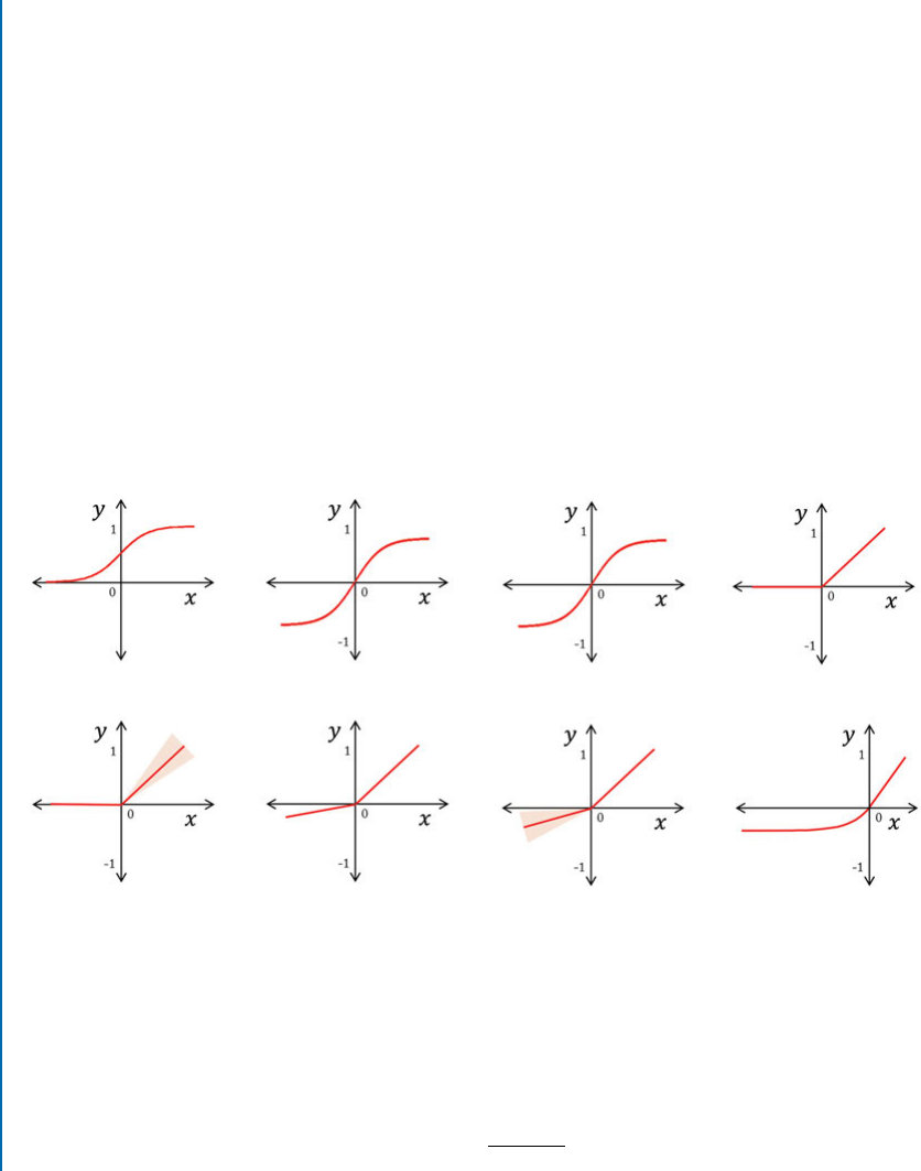
54 4. CONVOLUTIONAL NEURAL NETWORK
e pooling operation effectively down-samples the input feature map. Such a down-
sampling process is useful for obtaining a compact feature representation which is invariant to
moderate changes in object scale, pose, and translation in an image [Goodfellow et al.,2016].
4.2.4 NONLINEARITY
e weight layers in a CNN (e.g., convolutional and fully connected layers) are often followed
by a nonlinear activation (or a piece-wise linear) function. e activation function takes a real-
valued input and squashes it within a small range such as [0; 1] and [1; 1]. e application of
a nonlinear function after the weight layers is highly important, since it allows a neural network
to learn nonlinear mappings. In the absence of nonlinearities, a stacked network of weight layers
is equivalent to a linear mapping from the input domain to the output domain.
A nonlinear function can also be understood as a switching or a selection mechanism,
which decides whether a neuron will fire or not given all of its inputs. e activation functions
that are commonly used in deep networks are differentiable to enable error back propagation
(Chapter 6). Below is a list of the most common activation functions that are used in deep
neural networks.
(a) Sigmoid (b) Tanh (c) Algebraic Sigmoid (d) ReLU
(e) Noisy ReLU (f ) Leaky ReLU/PReLU (g) Randomized
Leaky ReLU
(h) Exponential
Linear Unit
Figure 4.9: Some of the common activation functions that are used in deep neural networks.
Sigmoid (Fig. 4.9a): e sigmoid activation function takes in a real number as its input, and
outputs a number in the range of [0,1]. It is defined as:
fsigm.x/ D1
1Cex:(4.11)

4.2. NETWORK LAYERS 55
Tanh (Fig. 4.9b): e tanh activation function implements the hyperbolic tangent function to
squash the input values within the range of [1; 1]. It is represented as follows:
ftanh.x/ Dexex
exCex:(4.12)
Algebraic Sigmoid Function (Fig. 4.9c): e algebraic sigmoid function also maps the input
within the range [1; 1]. It is given by:
fasig .x/ Dx
p1Cx2:(4.13)
Rectifier Linear Unit (Fig. 4.9d): e ReLU is a simple activation function which is of a special
practical importance because of its quick computation. A ReLU function maps the input to a 0
if it is negative and keeps its value unchanged if it is positive. is can be represented as follows:
frelu.x/ Dmax.0; x/: (4.14)
e ReLU activation is motivated by the processing in the human visual cortex [Hahnloser et al.,
2000]. e popularity and effectiveness of ReLU has lead to a number of its variants, which
we introduce next. ese variants address some of the shortcomings of the ReLU activation
function, e.g., leaky ReLU does not completely reduce the negative inputs to zero.
Noisy ReLU (Fig. 4.9e): e noisy version of ReLU adds a sample drawn from a Gaussian
distribution with mean zero and a variance which depends on the input value (.x/) in the
positive input. It can be represented as follows:
fnrel.x/ Dmax.0; x C/; N.0; .x//: (4.15)
Leaky ReLU (Fig. 4.9f ): e rectifier function (Fig. 4.9d) completely switches off the output if
the input is negative. A leaky ReLU function does not reduce the output to a zero value, rather
it outputs a down-scaled version of the negative input. is function is represented as:
flrel.x/ Dx if x > 0
cx if x 0; (4.16)
where cis the leak factor which is a constant and typically set to a small value (e.g., 0:01).
Parametric Linear Units (Fig. 4.9f ): e parametric ReLU function behaves in a similar manner
as the leaky ReLU, with the only difference that the tunable leak parameter is learned during
the network training. It can be expressed as follows:
fprel.x/ Dx if x > 0
ax if x 0; (4.17)

56 4. CONVOLUTIONAL NEURAL NETWORK
where ais the leak factor which is automatically learned during the training.
Randomized Leaky Rectifier Linear Unit (Fig. 4.9g): e randomized leaky ReLU (RReLU)
randomly selects the leak factor in the leaky ReLU function from a uniform distribution. ere-
fore,
frrel.x/ Dx if x > 0
ax if x 0:(4.18)
e factor ais randomly chosen during training and set to a mean value during the test phase
to get the contribution of all samples. us,
aU.l; u/ during training (4.19)
aDlCu
2during testing:(4.20)
e upper and lower limits of the uniform distribution are usually set to 8 and 3, respectively.
Exponential Linear Units (Fig. 4.9h): e exponential linear units have both positive and nega-
tive values and they therefore try to push the mean activations toward zero (similar to the batch
normalization). It helps in speeding up the training process while achieving a better perfor-
mance.
felu.x/ Dx if x > 0
a.ex1/ if x 0: (4.21)
Here, ais a non-negative hyper parameter which decides on the saturation level of the ELU in
response to negative inputs.
4.2.5 FULLY CONNECTED LAYERS
Fully connected layers correspond essentially to convolution layers with filters of size 11. Each
unit in a fully connected layer is densely connected to all the units of the previous layer. In a typ-
ical CNN, full-connected layers are usually placed toward the end of the architecture. However,
some successful architectures are reported in the literature which use this type of layer at an
intermediate location within a CNN (e.g., NiN [Lin et al.,2013] which will be discussed in
Section 6.3). Its operation can be represented as a simple matrix multiplication followed by
adding a vector of bias terms and applying an element-wise nonlinear function f ./:
yDf .WTxCb/; (4.22)
where xand yare the vector of input and output activations, respectively, Wdenotes the matrix
containing the weights of the connections between the layer units, and brepresents the bias term
vector. Note that a fully connected layer is identical to a weight layer that we studied in the case
of the Multi-layer Perceptron in Section 3.4.2.

4.2. NETWORK LAYERS 57
4.2.6 TRANSPOSED CONVOLUTION LAYER
e normal convolution layer maps a spatially large-sized input to a relatively smaller sized out-
put. In several cases, e.g., image super-resolution, we want to go from a spatially low-resolution
feature map to a larger output feature with a higher resolution. is requirement is achieved by
a transposed convolution layer, which is also called a “fractionally strided convolution layer” or
the “up-sampling layer” and sometimes (incorrectly) as the deconvolution layer.1
One can interpret the operation of a transposed convolution layer as the equivalent of a
convolution layer, but by passing through it in the opposite direction, as in a backward pass dur-
ing back propagation. If the forward pass through the convolution layer gives a low-dimensional
convolved output, the backward pass of the convolved output through the convolution layer
should give the original high spatial dimensional input. is backward transformation layer is
called the “transposed convolution layer.” It can easily be understood in terms of standard convo-
lution by revisiting the example of Fig. 4.3. In that example, a 22filter was applied to a 44
input feature map with a stride of one and no zero padding to generate a 33output feature
map. Note that this convolution operation can be represented as a matrix multiplication, which
offers a highly efficient implementation in practice. For this purpose, we can represent the 22
kernel as an unrolled Toeplitz matrix as follows:
KD
2
6
6
6
6
6
6
6
6
6
6
6
6
6
4
k1;1 k1;2 0 0 k2;1 k2;2 0000000000
0 k1;1 k1;2 0 0 k2;1 k2;2 000000000
0 0 k1;1 k1;2 0 0 k2;1 k2;2 00000000
0 0 0 0 k1;1 k1;2 0 0 k2;1 k2;2 000000
0 0 0 0 0 k1;1 k1;2 0 0 k2;1 k2;2 00000
0 0 0 0 0 0 k1;1 k1;2 0 0 k2;1 k2;2 0 0 0 0
0 0 0 0 0 0 0 0 k1;1 k1;2 0 0 k2;1 k2;2 0 0
0 0 0 0 0 0 0 0 0 k1;1 k1;2 0 0 k2;1 k2;2 0
0 0 0 0 0 0 0 0 0 0 k1;1 k1;2 0 0 k2;1 k2;2
3
7
7
7
7
7
7
7
7
7
7
7
7
7
5
:
Here, ki;j represents the filter element in the ith row and jth column. For an input feature map
X, the convolution operation can be expressed in terms of the matrix multiplication between K
and the vectorized form of input, i.e., xDvec.X /:
yDKx;(4.23)
where yis the corresponding vectorized output. In the transposed convolution, we will input a
33feature map to generate an output feature map of 44as follows:
yDKTx:(4.24)
Note that the xand yin the above two equations have different dimensions.
1Note that deconvolution in signal processing literature refers to undoing the effect of the convolution operation with a filter
Fby applying its inverse filter F1. is deconvolution operation is usually performed in the Fourier domain. is is clearly
different from the operation of a convolution transpose layer which does not use an inverse filter.
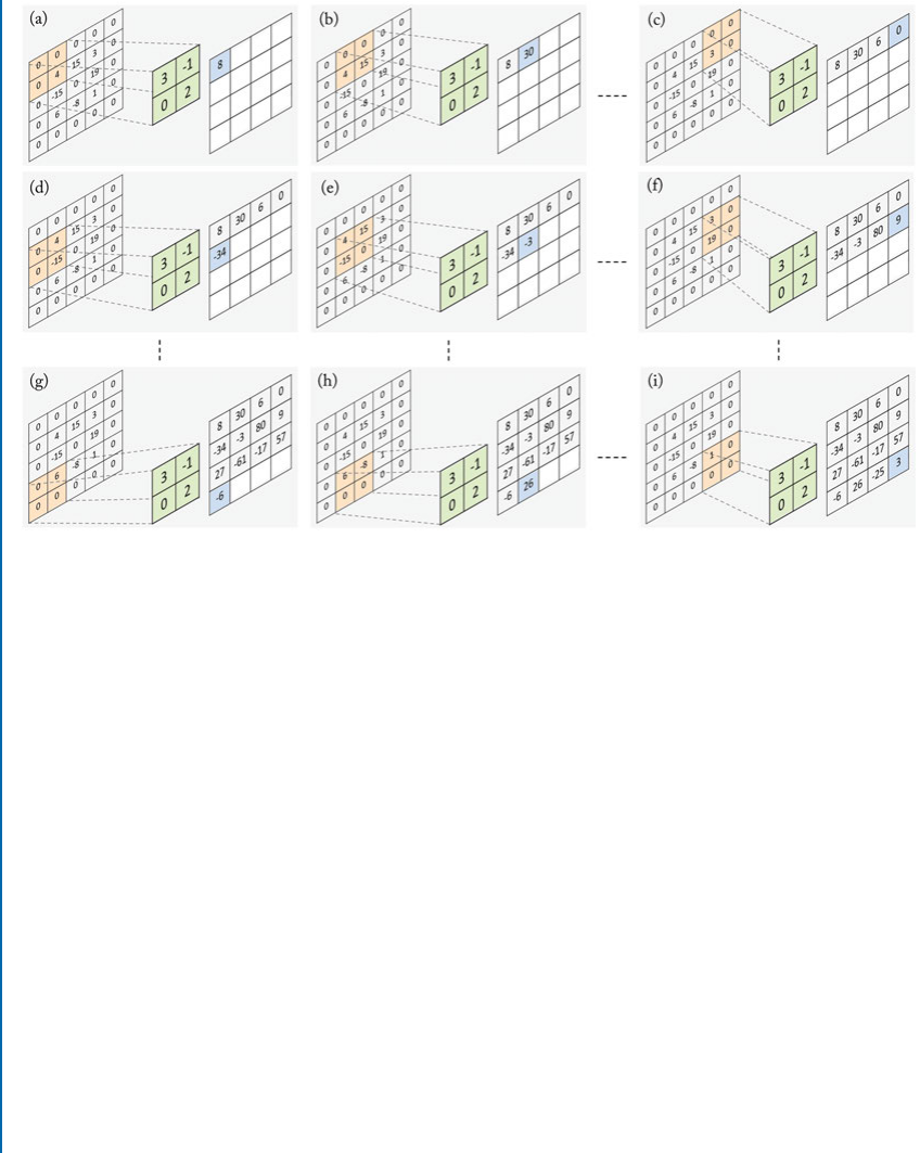
58 4. CONVOLUTIONAL NEURAL NETWORK
Figure 4.10: Convolution transpose operation corresponding to a forward convolution operation
with a unit stride and no zero padding shown in Fig. 4.3. e input in this example has been
zero-padded to obtain a 44output. (a)–(i) show the computations performed at each step as
the filter is slided onto the input feature map to compute the corresponding value in the output
feature map. e 22filter (shown in green) is multiplied with the same sized region (shown in
orange) within a 55input feature map (including zero-padding) and the resulting values are
summed up to obtain a corresponding entry (shown in blue) in the output feature map at each
convolution transpose step. Note that the convolution transpose operation does not invert the
convolution operation (the input in Fig. 4.3 and the output here are different). However, it can
be used to recover the loss in the spatial dimensions of the feature map (input size in Fig. 4.3
and output size here are the same). Furthermore, note that the filter values have been reversed
for the convolution transpose operation compared to the filter used in Fig. 4.3.
e transposed convolution layers effectively up-samples the input feature maps. is can
also be understood as a convolution with an input feature map which has additional rows and
columns consisting of null values inserted around the actual values. e convolution with this up-
sampled input will then generate the desired result. is process is shown in Figs. 4.10 and 4.11
for the outputs we obtained in the examples of Figs. 4.3 and 4.5. It is important to note that the
filter entries are reversed for the convolution transpose operation. Furthermore, note that the
output from the convolution transpose is equal to the size of input of the convolution operation.
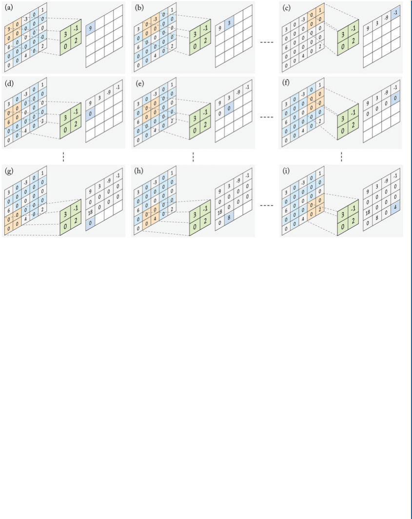
4.2. NETWORK LAYERS 59
Figure 4.11: Convolution transpose operation corresponding to a forward convolution operation
with a stride of 2 and unit zero padding shown in Fig. 4.5. e input in this example has been
zero-padded in between the feature map values to obtain a 44output (shown in light blue).
(a)–(i) show the computations performed at each step as the filter is slided onto the input feature
map to compute the corresponding value in the output feature map. e 22filter (shown in
green) is multiplied with the same sized region (shown in orange) within a 55input feature
map (including zero-padding) and the resulting values are summed up to obtain a corresponding
entry (shown in blue) in the output feature map at each convolution transpose step. Note that the
convolution transpose operation does not invert the convolution operation (input in Fig. 4.5 and
output here are different). However, it can be used to recover the loss in the spatial dimensions
of the feature map (input size in Fig. 4.5 and output size here are the same). Furthermore, note
that the filter values have been reversed for the convolution transpose operation compared to the
filter used in Fig. 4.5.
However the individual entries are different because the convolution transpose does not invert
the forward convolution. We can calculate the size of the output given a kernel of size ff,
stride s, padding p:
h0Ds. O
h1/ Cf2p C.h fC2p/ mod s; (4.25)
w0Ds. Ow1/ Cf2p C.w fC2p/ mod s; (4.26)
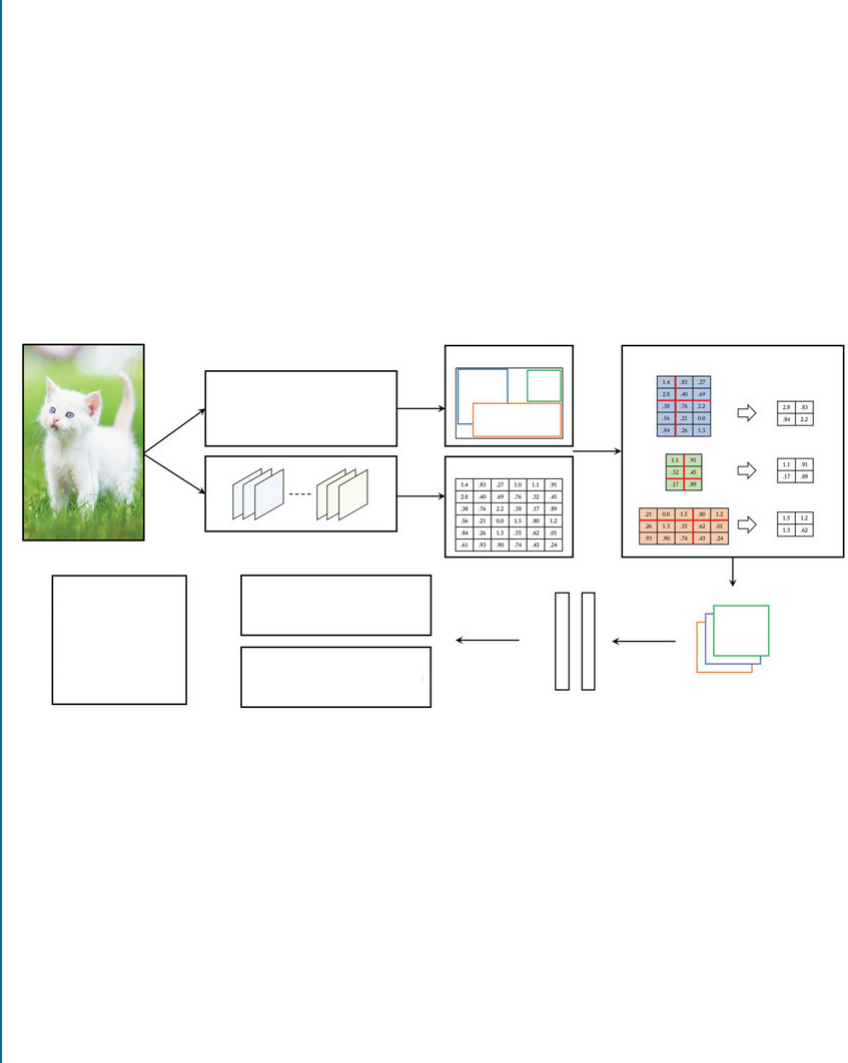
60 4. CONVOLUTIONAL NEURAL NETWORK
where mod denotes the modulus operation, O
hand Owdenote the input dimensions without any
zero-padding, and hand wdenote the spatial dimensions of the input in the equivalent forward
convolution (as shown in Figs. 4.3 and 4.5).
In the example shown in Fig. 4.10,pD0,sD1,fD2, and O
hD OwD3. erefore, the
spatial dimensions of the output feature map are h0Dw0D4. In Fig. 4.11,s1zero values
are added between each pair of input elements to extend the input to produce a spatially large
output. e parameter values are pD1,sD2,fD2, and O
hD OwD3and the resulting output
dimensions are again h0Dw0D4.
Finally, it is important to note that, from an implementation point of view, the transposed
convolution operation is much faster when implemented as a matrix multiplication operation
compared to the zero padding of the input feature map at intermediate locations followed by
normal convolutions [Dumoulin and Visin,2016].
Fully Connected
Layers
During Testing
During Training
Convolutional Neural NetworkInput Image
Object Proposal Generation
(off-the-shelf detector or a
deep network-based detector)
Bounding Box Regression
Loss
Class Probabilities
for all object
bounding boxes
Bounding Box Classification
Loss 2×2 Feature
Maps
ROI Pooling Layer (2×2)Object ROIs
CNN Feature map
Figure 4.12: e function of a ROI pooling layer with in an object detection framework is
illustrated in this figure. Note that a single feature channel, few RoI proposals (just three), and
a relatively smaller output size (22) from the ROI pooling layer has been demonstrated here
for the sake of clarity.
4.2.7 REGION OF INTEREST POOLING
e Region of Interest (RoI) Pooling layer is an important component of convolutional neu-
ral networks which is mostly used for object detection [Girshick,2015] (and slightly modified
versions for related tasks, e.g., instance segmentation [He et al.,2017]). In the object detection
problem, the goal is to precisely locate each object in an image using a bounding box and tag

4.2. NETWORK LAYERS 61
it with the relevant object category. ese objects can be located at any region in an image and
generally vary greatly in their size, shape, appearance, and texture properties. e usual course
of action with such problems is to first generate a large set of candidate object proposals with the
aim to include all possible object bounding boxes that may be discovered in an image. For these
initial proposals, usually off-the-shelf detectors are used such as the selective search [Uijlings
et al.,2013] or the EdgeBox [Zitnick and Dollár,2014]. Recent works have also proposed ap-
proaches to integrate the proposal generation step into a CNN (e.g., Region Proposal Network
[Ren et al.,2015]). Since the valid detections are very few compared to the generated proposals
(usually < 1%), the resources used to process all the negative detections are wasted.
e ROI pooling layer provides a solution to this problem by shifting the processing spe-
cific to individual bounding-boxes later in the network architecture. An input image is processed
through the deep network and intermediate CNN feature maps (with reduced spatial dimen-
sions compared to the input image) are obtained. e ROI pooling layer takes the input feature
map of the complete image and the coordinates of each ROI as its input. e ROI co-ordinates
can be used to roughly locate the features corresponding to a specific object. However, the fea-
tures thus obtained have different spatial sizes because each ROI can be of a different dimension.
Since CNN layers can only operate on fixed dimensional inputs, a ROI pooling layer converts
these variable sized feature maps (corresponding to different object proposals) to a fixed sized
output feature map for each object proposal, e.g., a 55or a 77map. e fixed size output
dimensions is a hyper-parameter which is fixed during the training process. Specifically, this
same-sized output is achieved by dividing each ROI into a set of cells with equal dimensions.
e number of these cells is the same as the required output dimensions. Afterward, the maxi-
mum value in each cell is calculated (max-pooling) and it is assigned to the corresponding output
feature map location.
By using a single set of input feature maps to generate a feature representation for each
region proposal, the ROI pooling layer greatly improves the efficiency of a deep network. us, a
CNN only needs a single pass to compute features corresponding to all the ROIs. It also makes
it possible to train the network in an end-to-end manner, as a unified system. Note that the
ROI pooling layer is usually plugged in the latter portion of a deep architecture to save a lot of
computations which can result if the region-based processing is performed in the early layers of
the network (due to the large number of proposals). An example use case of ROI pooling layer
in a CNN is described in Section 7.2.1.
4.2.8 SPATIAL PYRAMID POOLING LAYER
e spatial pyramid pooling (SPP) layer [He et al.,2015b] in CNNs is inspired by the pyramid-
based approaches proposed for the Bag of Visual Words (BoW) style feature encoding methods
[Lazebnik et al.,2006]. e main intuition behind the SPP layer is that the interesting discrim-
inative features can appear at a variety of scales in the convolutional feature maps. erefore, it
is useful to incorporate this information for classification purposes.
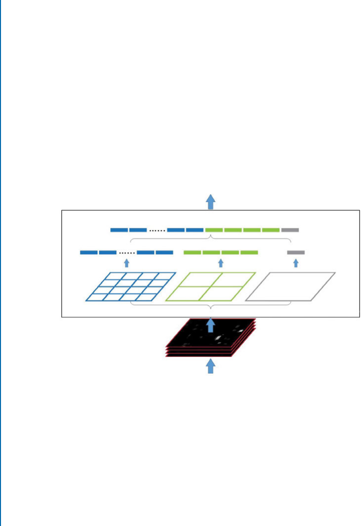
62 4. CONVOLUTIONAL NEURAL NETWORK
To efficiently encode this information in a single descriptor, the SPP layer divides the
feature maps into three levels of spatial blocks. At the global level, the features corresponding
to all the spatial locations are pooled together to obtain just a single vector (with a dimension
equal to the number of channels of the previous layer, say n). At the middle level, the feature
maps are divided into four (22) disjoint spatial blocks of equal dimensions and features within
each block are pooled together to obtain a single feature vector in each of the four blocks. is n
dimensional representation is concatenated for each block, resulting in a 4n dimensional feature
vector for the middle level. Finally, at the local level, the feature maps are divided into 16
blocks (44). Features within each spatial block are pooled together to give an ndimensional
feature vector. All the 16 features are concatenated to form a single 16n dimensional feature
representation. Finally, the local, mid-level, and global feature representations are concatenated
together to generate a 16n C4n Cndimensional feature representation, which is forwarded to
the classifier layers (or fully connected layers) for classification (see Fig. 4.13).
Fully Connected Layers (fc6, fc7)
Fixed-length Representation
Spatial Pyramid Pooling Layer
Feature maps of conv5 wih
a depth of 256 (arbitrary size)
Convolutional Layers
Input Image
16×256-d 4×256-d 256-d
Figure 4.13: e Spatial Pyramid Pooling Layer [He et al.,2014] incorporates discriminative
information at three scales which is useful for accurate classification. (Figure used with permis-
sion.)
erefore, an SPP layer makes use of the localized pooling and the concatenation opera-
tions to generate a high-dimensional feature vector as its output. e combination of informa-
tion at multiple scales helps in achieving robustness against variations in object pose, scale, and
shape (deformations). Since the SPP layer output is not dependent on the length and width of
the feature maps, it allows the CNN to handle input images of any size. Furthermore, it can
perform a similar operation on individual object regions for the detection task. is saves a rea-

4.2. NETWORK LAYERS 63
sonable amount of time compared to the case where we input individual object proposals and
obtain a feature representation for each of them.
4.2.9 VECTOR OF LOCALLY AGGREGATED DESCRIPTORS LAYER
As we saw for the case of SPP layer, the Vector of Locally Aggregated Descriptors (VLAD)
layer in CNNs [Arandjelovic et al.,2016] also gets its inspiration from the VLAD pooling
approach used in the BoW style models to aggregate local features [Jégou et al.,2010]. e
main idea behind the VLAD layer can be explained as follows. Given a set of local descrip-
tors fxi2RDgN
iD1, we aim to represent these local features in terms of a set of visual words
fci2RDgK
iD1(also called “key-points” or “cluster centers”). is is achieved by finding the as-
sociation of each local descriptor with all the cluster centers. e (soft) association is measured
as a weighted difference between each descriptor and all the Kcluster centers. is results in a
KDdimensional feature matrix Fgiven by:
F .j; k/ D
N
X
iD1
ak.xi/.xi.j / ck.j //: (4.27)
Here, the association term akmeasures the connection between the ith local feature (xi) and
the kth cluster center (ck), e.g., it will be 0 if xiis furthest away from ckand 1 if xiis closest to
ck. e association term is defined as follows:
ak.xi/Dexp.wT
kxiCbk/
Prexp.wT
rxiCbr/;(4.28)
where, w; b are the weights and biases of a fully connected layer. From an implementation point
of view, the computation of the association term can be understood as passing the descriptors
through a fully connected CNN layer, followed by a soft-max operation. e parameters w; b,
and care learned during the training process. Note that since all the operations are differen-
tiable, an end-to-end training is feasible. For classification purposes, the feature matrix Fis
first normalized column-wise using the `2norm of each column, then converted to a vector and
again `2normalized. Figure 4.14 summarizes the operation of a VLAD layer.
4.2.10 SPATIAL TRANSFORMER LAYER
As you would have noticed for the case of the VLAD layer, the introduced layer does not involve
a single operation. Instead, it involves a set of inter-connected sub-modules, each of which
is implemented as an individual layer. e spatial transformer layer [Jaderberg et al.,2015] is
another such example which comprises three main modules, namely (a) localization network,
(b) grid generator, and (c) sampler. Figure 4.15 illustrates the three individual blocks and their
function.
In a nutshell, the spatial transformer layer learns to focus on the interesting part of its
input. is layer applies geometric transformations on the interesting parts of the input to focus

64 4. CONVOLUTIONAL NEURAL NETWORK
Input Image Convolutional Neural Network
VLAD Feature Vector (K×D dimensions)
Local Features
from Previous Layer
∈
Soft Assignment
Soft-max
Operation
VLAD Core ()Channel-wise 2
Normalization
2 Normalization
Vectorization
Fully Connected Layer
( ∈ ,
b ∈ )
Figure 4.14: e figure shows the working of VLAD Layer [Arandjelovic et al.,2016]. It takes
multiple local features from the CNN layers and aggregate them to generate a high-dimensional
output feature representation.
attention and perform rectification. It can be plugged in after the input layer or any of the earlier
convolutional layers which generate a relatively large-sized (heightwidth) output feature map.
e first module, called the localization network, takes the input feature maps (or the
original input image) and predicts the parameters of transformation which needs to be applied.
is net can be implemented as any combination of convolutional and/or fully connected layers.
However, the final layer is a regression layer which generates the parameter vector . e di-
mensions of the output parameters depends on the kind of transformation, e.g., for an affine
transformation, it is has six parameters defined as follows:
D123
456:(4.29)
e grid generator generates a grid of coordinates in the input image corresponding to each pixel
from the output image. is mapping is useful for the next step, where a sampling function is
used to transform the input image. e sampler generates the output image using the grid given
by the grid generator. is is achieved by using a sampling kernel which is applied at each pixel
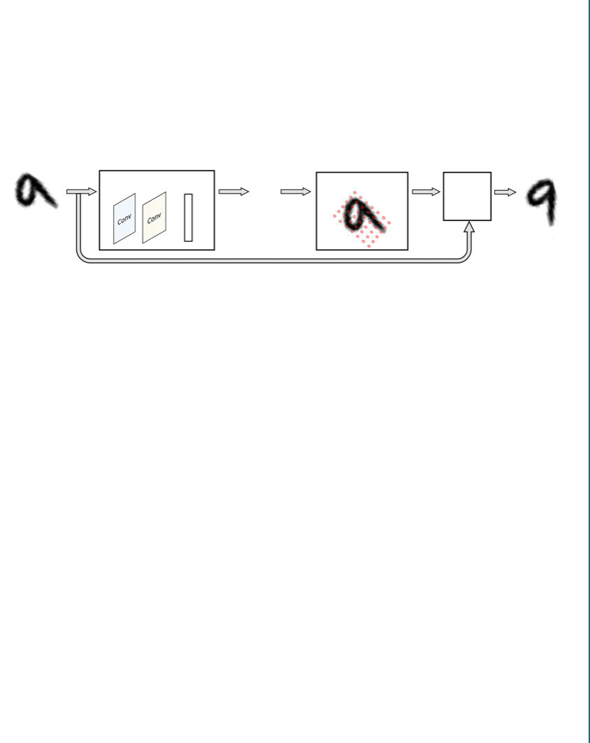
4.3. CNN LOSS FUNCTIONS 65
of the input image (or at each value in the input feature map). To enable end-to-end training, the
sampling kernel should be differentiable with respect to the input and the grid co-ordinates (x
and ycoordinates). Examples of kernels include the nearest neighbor copying from the source
(input) to the target (output) and the bilinear sampling kernels.
Since all the modules are fully differentiable, the spatial transformation can be learned
end-to-end using a standard back-propagation algorithm. is provides a big advantage since it
allows the network to automatically shift focus toward the more discriminative portions of the
input image or the feature maps.
Localization Network
Input Image (or
Feature Maps)
Output Image (or
Feature Maps)
Transformation
Parameters
Grid Generator
Sampler
Figure 4.15: e spatial transformer layer with its three modules. e localization network pre-
dicts the transformation parameters. e grid generator identifies the points in the input domain
on which a sampling kernel is applied using the sampler.
4.3 CNN LOSS FUNCTIONS
Having studied a wide variety of simple and relatively more complex CNN layers, we discuss
the final layer in a CNN which is used only during the training process. is layer uses a “loss
function,” also called the “objective function,” to estimate the quality of predictions made by the
network on the training data, for which the actual labels are known. ese loss functions are
optimized during the learning process of a CNN, whose details will be covered in Chapter 5.
A loss function quantifies the difference between the estimated output of the model (the
prediction) and the correct output (the ground truth).
e type of loss function used in our CNN model depends on our end problem. e
generic set problems for which neural networks are usually used (and the associated loss func-
tions) can be categorized into the following categories.
1. Binary Classification (SVM hinge loss, Squared hinge loss).
2. Identity Verification (Contrastive loss).
3. Multi-class Classification (Softmax loss, Expectation loss).
4. Regression (SSIM, `1error, Euclidean loss).
Note that the loss functions which are suitable for multi-class classification tasks are also
applicable to binary classification tasks. However, the case reverse is generally not true unless a

66 4. CONVOLUTIONAL NEURAL NETWORK
multi-class problem is divided into multiple one-vs.-rest binary classification problems where a
separate classifier is trained for each case using a binary classification loss. Below, we discuss the
above mentioned loss functions in more detail.
4.3.1 CROSS-ENTROPY LOSS
e cross-entropy loss (also termed “log loss” and “soft-max loss”) is defined as follows:
L.p;y/D X
n
ynlog.pn/; n 2Œ1; N ; (4.30)
where ydenotes the desired output and pis the probability for each output category. ere is
a total of Nneurons in the output layer, therefore p;y2RN. e probability of each class can
be calculated using a soft-max function: pnDexp.Opn/
Pkexp.Opk/, where Opnis the unnormalized output
score from the previous layer in the network. Due to the form of the normalizing function in
the loss, this loss is also called the soft-max loss.
It is interesting to note that optimizing the network parameters using the cross-entropy
loss is equivalent to minimizing the KL-divergence between the predicted output (generated
distribution, p) and the desired output (true distribution y). e KL-divergence between pand
ycan be expressed as the difference between cross-entropy (denoted by L./) and the entropy
(denoted by H./) as follows:
KL.pky/DL.p;y/H.p/: (4.31)
Since entropy is just a constant value, minimizing cross entropy is equivalent to minimizing the
KL-divergence between the two distributions.
4.3.2 SVM HINGE LOSS
e SVM hinge loss is motivated by the error function which is normally used during the train-
ing of SVM classifier. Hinge loss maximizes the margin between the true and the negative class
samples. is loss is defined as follows:
L.p;y/DX
n
max.0; m .2yn1/pn/; (4.32)
where “m” is the margin which is usually set equal to a constant value of 1 and p;ydenote the
predicted and desired outputs, respectively. An alternative formulation of the hinge loss is the
Crammer and Singer’s [Crammer and Singer,2001] loss function given below:
L.p;y/Dmax.0; m Cmax
i¤cpipc/; c Dargmax
j
yj;(4.33)

4.3. CNN LOSS FUNCTIONS 67
where, pcdenotes the prediction at the correct class index c. Another similar formulation of the
hinge loss was proposed by Weston and Watkins [Weston et al.,1999]:
L.p;y/DX
i¤c
max.0; m Cpipc/; c Dargmax
j
yj:(4.34)
4.3.3 SQUARED HINGE LOSS
e squared hinge loss function has been shown to perform slightly better than the vanilla hinge
loss function in some applications [Tang,2013]. is loss function simply includes the square
of the max function in Eqs. (4.32)–(4.34). e squared hinge loss is more sensitive to margin
violations compared to the vanilla hinge loss.
4.3.4 EUCLIDEAN LOSS
e Euclidean loss (also termed the “quadratic loss,” “mean square error” or “`2error”) is defined
in terms of the squared error between the predictions (p2RN) and the ground truth labels
(y2RN):
L.p;y/D1
2N X
n
.pnyn/2; n 2Œ1; N : (4.35)
4.3.5 THE `1ERROR
e `1loss can be used for regression problems and has been shown to outperform the Euclidean
loss in some cases [Zhao et al.,2015]. It is defined as follows:
L.p;y/D1
NX
njpnynj; n 2Œ1; N : (4.36)
4.3.6 CONTRASTIVE LOSS
e contrastive loss is used to map similar inputs to nearby points in the feature/output space
and to map the dissimilar inputs to distant points. is loss function works on the pairs of
either similar or dissimilar inputs (e.g., in siamese networks [Chopra et al.,2005]). It can be
represented as follows:
L.p; y/ D1
2N X
n
yd 2C.1 y/ max.0; m d /2; n 2Œ1; N ; (4.37)
where mis the margin and y2Œ0; 1 shows whether the input pairs are dissimilar or similar
respectively. Here, “d” can be any valid distance measure such as the Euclidean distance:
dDk fafbk2;(4.38)

68 4. CONVOLUTIONAL NEURAL NETWORK
where faand fbare the learned representations of the two inputs in the feature space and k k2
represents the `2(or Euclidean) norm.
ere are other variants of verification losses which extend to triplets (e.g., the triplet loss
is used for triplet networks [Schroff et al.,2015] as opposed to a Siamese network).
4.3.7 EXPECTATION LOSS
e expectation loss is defined as follows:
L.p;y/DX
njynexp.pn/
Pkexp.pk/j; n 2Œ1; N : (4.39)
It minimizes the expected misclassification probability, which is why it is called the expecta-
tion loss. Note that the cross entropy loss also uses the soft-max function which is similar to
the expectation loss. However, it directly maximizes the probability of fully correct predictions
[Janocha and Czarnecki,2017].
e expectation loss provides more robustness against outliers because the objective max-
imizes the expectation of true predictions. However, this loss function is seldom used in deep
neural networks because it is not a convex or concave function with respect to the weights of
the preceding layer. is leads to optimization issues (such as instability and slow convergence)
during the learning process.
4.3.8 STRUCTURAL SIMILARITY MEASURE
For image processing problems, perceptually grounded loss functions have been used in combi-
nation with CNNs [Zhao et al.,2015]. One example of such losses is the Structural Similarity
(SSIM) measure. It is defined as follows:
L.p;y/D1SSIM.n/; (4.40)
where nis the center pixel of the image, p;ydenote the predicted output and the desired output,
respectively, and the structural similarity for that pixel is given by:
SSIM.n/ D2pnynCC1
2
pnC2
ynCC12pnynCC2
2
pnC2
ynCC2
:(4.41)
Here, the mean and standard deviation and covariance are represented by ; and pnyn, respec-
tively. At each pixel location n, the mean and standard deviation are calculated using a Gaussian
filter centered at the pixel with a standard deviation G.C1; C2denote the image dependent
constants which provide stabilization against small denominators. Note that the calculation of
SSIM at one pixel requires the neighboring pixel values in the support of the Gaussian filter.
Also note that we do not calculate the SSIM measure at each pixel because it cannot be calcu-
lated straightforwardly for the pixels that are close to image boundaries.
In the following chapter, we will introduce different techniques for weight initialization
and gradient-based parameter learning algorithms for deep networks.

69
C H A P T E R 5
CNN Learning
In Chapter 4, we discussed different architecture blocks of the CNN and their operational de-
tails. Most of these CNN layers involve parameters which are required to be tuned appropriately
for a given computer vision task (e.g., image classification and object detection). In this chapter,
we will discuss various mechanisms and techniques that are used to set the weights in deep neural
networks. We will first cover concepts such as weight initialization and network regularization
in Sections 5.1 and 5.2, respectively, which helps in a successful optimization of the CNNs. Af-
terward, we will introduce gradient-based parameter learning for CNNs in Section 5.3, which
is quite similar to the MLP parameter learning process discussed in Chapter 3. e details of
neural network optimization algorithms (also called “solvers”) will come in Section 5.4. Finally
in Section 5.5, we will explain various types of approaches which are used for the calculation of
the gradient during the error back-propagation process.
5.1 WEIGHT INITIALIZATION
A correct weight initialization is the key to stably train very deep networks. An ill-suited initial-
ization can lead to the vanishing or exploding gradient problem during error back-propagation.
In this section, we introduce several approaches to perform weight initialization and provide
comparisons between them to illustrate their benefits and problems. Note that the discussion
below pertains to the initialization of neuron weights within a network and the biases are usually
set to zero at the start of the network training. If all the weights are also set to zero at the start
of training, the weight updates will be identical (due to symmetric outputs) and the network
will not learn anything useful. To break this symmetry between neural units, the weights are
initialized randomly at the start of the training. In the following, we describe several popular
approaches to network initialization.
5.1.1 GAUSSIAN RANDOM INITIALIZATION
A common approach to weight initialization in CNNs is the Gaussian random initialization
technique. is approach initializes the convolutional and the fully connected layers using ran-
dom matrices whose elements are sampled from a Gaussian distribution with zero mean and a
small standard deviation (e.g., 0.1 and 0.01).

70 5. CNN LEARNING
5.1.2 UNIFORM RANDOM INITIALIZATION
e uniform random initialization approach initializes the convolutional and the fully connected
layers using random matrices whose elements are sampled from a uniform distribution (instead
of a normal distribution as in the earlier case) with a zero mean and a small standard deviation
(e.g., 0.1 and 0.01). e uniform and normal random initializations generally perform identi-
cally. However, the training of very deep networks becomes a problem with a random initializa-
tion of weights from a uniform or normal distribution [Simonyan and Zisserman,2014b]. e
reason is that the forward and backward propagated activations can either diminish or explode
when the network is very deep (see Section 3.2.2).
5.1.3 ORTHOGONAL RANDOM INITIALIZATION
Orthogonal random initialization has also been shown to perform well in deep neural networks
[Saxe et al.,2013]. Note that the Gaussian random initialization is only approximately orthog-
onal. For the orthogonal random initialization, a random weight matrix is decomposed by ap-
plying e.g., an SVD. e orthogonal matrix (U) is then used for the weight initialization of the
CNN layers.
5.1.4 UNSUPERVISED PRE-TRAINING
One approach to avoid the gradient diminishing or exploding problem is to use layer-wise pre-
training in an unsupervised fashion. However, this type of pre-training has found more success
in the training of deep generative networks, e.g., Deep Belief Networks [Hinton et al.,2006]
and Auto-encoders [Bengio et al.,2007]. e unsupervised pre-training can be followed by
a supervised fine-tuning stage to make use of any available annotations. However, due to the
new hyper-parameters, the considerable amount of effort involved in such an approach and
the availability of better initialization techniques, layer-wise pre-training is seldom used now to
enable the training of CNN-based very deep networks. We describe some of the more successful
approaches to initialize deep CNNs next.
5.1.5 XAVIER INITIALIZATION
A random initialization of a neuron makes the variance of its output directly proportional to
the number of its incoming connections (a neuron’s fan-in measure). To alleviate this problem,
Glorot and Bengio [2010] proposed to randomly initialize the weights with a variance measure
that is dependent on the number of incoming and outgoing connections (n
fin and n
fout
respectively) from a neuron,
Var.w/ D2
n
fin Cn
fout
;(5.1)
where ware network weights. Note that the fan-out measure is used in the variance above to
balance the back-propagated signal as well. Xavier initialization works quite well in practice and

5.1. WEIGHT INITIALIZATION 71
leads to better convergence rates. But a number of simplistic assumptions are involved in the
above initialization, among which the most prominent is that a linear relationship between the
input and output of a neuron is assumed. In practice all the neurons contain a nonlinearity term
which makes Xavier initialization statistically less accurate.
5.1.6 RELU AWARE SCALED INITIALIZATION
He et al. [2015a] suggested an improved version of the scaled (or Xavier) initialization noting
that the neurons with a ReLU nonlinearity do not follow the assumptions made for the Xavier
initialization. Precisely, since the ReLU activation reduces nearly half of the inputs to zero,
therefore the variance of the distribution from which the initial weights are randomly sampled
should be
Var.w/ D2
n
fi n
:(5.2)
e ReLU aware scaled initialization works better compared to Xavier initialization for recent
architectures which are based on the ReLU nonlinearity.
5.1.7 LAYER-SEQUENTIAL UNIT VARIANCE
e layer-sequential unit variance (LSUV) initialization is a simple extension of the orthonormal
weight initialization in deep network layers [Mishkin and Matas,2015]. It combines the benefits
of batch-normalization and the orthonormal weight initialization to achieve an efficient training
for very deep networks. It proceeds in two steps, described below.
•Orthogonal initialization—In the first step, all the weight layers (convolutional and fully
connected) are initialized with orthogonal matrices.
•Variance normalization—In the second step, the method starts from the initial toward
the final layers in a sequential manner and the variance of each layer output is normalized
to one (unit variance). is is similar to the batch normalization layer, which normalizes
the output activations for each batch to be zero centered with a unit variance. However,
different from batch normalization which is applied during the training of the network,
LSUV is applied while initializing the network and therefore saves the overhead of nor-
malization for each batch during the training iterations.
5.1.8 SUPERVISED PRE-TRAINING
In practical scenarios, it is desirable to train very deep networks, but we do not have a large
amount of annotated data available for many problem settings. A very successful practice in
such cases is to first train the neural network on a related but different problem, where a large
amount of training data is already available. Afterward, the learned model can be “adapted” to
the new task by initializing with weights pre-trained on the larger dataset. is process is called

72 5. CNN LEARNING
“fine-tuning” and is a simple, yet effective, way to transfer learning from one task to another
(sometimes interchangeably referred to as domain transfer or domain adaptation). As an exam-
ple, in order to perform scene classification on a relatively small dataset, MIT-67, the network
can be initialized with the weights learned for object classification on a much larger dataset such
as ImageNet [Khan et al.,2016b].
Transfer Learning is an approach to adapt and apply the knowledge ac-
quired on another related task to the task at hand. Depending on our CNN
architecture, this approach can take two forms.
•Using a Pre-trained Model: If one wants to use an off-the-shelf CNN
architecture (e.g., AlexNet, GoogleNet, ResNet, DenseNet) for a given
task, an ideal choice is to adopt the available pre-trained models that are
learned on huge datasets such as ImageNet (with 1.2 million images)a
and Places205 (with 2.5 million images).b
e pre-trained model can be tailored for a given task, e.g., by chang-
ing the dimensions of output neurons (to cater for a different num-
ber of classes), modifying the loss function and learning the final few
layers from scratch (normally learning the final 2-3 layers suffices for
most cases). If the dataset available for the end-task is sufficiently large,
the complete model can also be fine-tuned on the new dataset. For
this purpose, small learning rates are used for the initial pre-trained
CNN layers, so that the learning previously acquired on the large-scale
dataset (e.g., ImageNet) is not completely lost. is is essential, since
it has been shown that the features learned over large-scale datasets
are generic in nature and can be used for new tasks in computer vision
[Azizpour et al.,2016,Sharif Razavian et al.,2014].
•Using a Custom Architecture: If one opts for a customized CNN archi-
tecture, transfer learning can still be helpful if the target dataset is con-
strained in terms of size and diversity. To this end, one can first train
the custom architecture on a large scale annotated dataset and then use
the resulting model in the same manner as described in the bullet point
above.
Alongside the simple fine-tuning approach, more involved transfer
learning approaches have also been proposed in the recent literature, e.g., An-
derson et al. [2016] learns the way pre-trained model parameters are shifted
on new datasets. e learned transformation is then applied to the network
parameters and the resulting activations beside the pre-trained (non-tunable)
network activations are used in the final model.

5.2. REGULARIZATION OF CNN 73
aPopular deep learning libraries host a wide variety of pre-trained CNN models, e.g.,
Tensorflow (https://github.com/tensorflow/models),
Torch (https://github.com/torch/torch7/wiki/ModelZoo),
Keras (https://github.com/albertomontesg/keras-model-zoo,
Caffe (https://github.com/BVLC/caffe/wiki/Model-Zoo),
MatConvNet (http://www.vlfeat.org/matconvnet/pretrained/).
bhttp://places.csail.mit.edu/downloadCNN.html
5.2 REGULARIZATION OF CNN
Since deep neural networks have a large number of parameters, they tend to over-fit on the
training data during the learning process. By over-fitting, we mean that the model performs
really well on the training data but it fails to generalize well to unseen data. It, therefore, results
in an inferior performance on new data (usually the test set). Regularization approaches aim
to avoid this problem using several intuitive ideas which we discuss below. We can categorize
common regularization approaches into the following classes, based on their central idea:
• approaches which regularize the network using data level techniques
(e.g., data augmentation);
• approaches which introduce stochastic behavior in the neural activations
(e.g., dropout and drop connect);
• approaches which normalize batch statistics in the feature activations
(e.g., batch normalization);
• approaches which use decision level fusion to avoid over-fitting
(e.g., ensemble model averaging);
• approaches which introduce constraints on the network weights
(e.g., `1norm, `2norm, max-norm, and elastic net constraints); and
• approaches which use guidance from a validation set to halt the learning process
(e.g., early stopping).
Next, we discuss the above-mentioned approaches in detail.
5.2.1 DATA AUGMENTATION
Data augmentation is the easiest, and often a very effective way of enhancing the generalization
power of CNN models. Especially for cases where the number of training examples is relatively
low, data augmentation can enlarge the dataset (by factors of 16x, 32x, 64x, or even more) to
allow a more robust training of large-scale models.
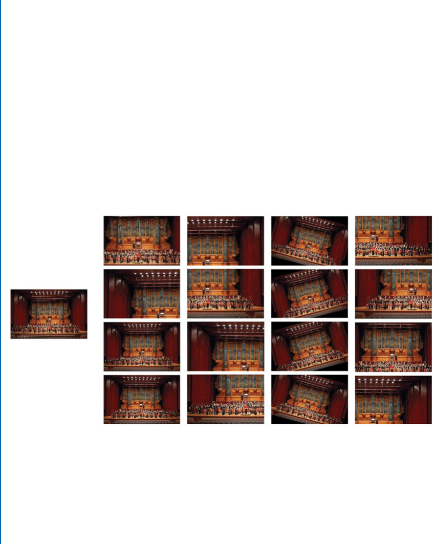
74 5. CNN LEARNING
Data augmentation is performed by making several copies from a single image using
straightforward operations such as rotations, cropping, flipping, scaling, translations, and shear-
ing (see Fig. 5.1). ese operations can be performed separately or combined together to form
copies, which are both flipped and cropped.
Color jittering is another common way of performing data augmentation. A simple form
of this operation is to perform random contrast jittering in an image. One could also find the
principal color directions in the R, G, and B channels (using PCA) and then apply a random
offset along these directions to change the color values of the whole image. is effectively
introduces color and illumination invariance in the learned model [Krizhevsky et al.,2012].
Another approach for data augmentation is to utilize synthetic data, alongside the real
data, to improve the generalization ability of the network [Rahmani and Mian,2016,Rahmani
et al.,2017,Shrivastava et al.,2016]. Since synthetic data is usually available in large quantities
from rendering engines, it effectively extends the training data, which helps avoid over-fitting.
Image Crops
Theater in Taiwan
Rotations Flips
Figure 5.1: e figure shows an example of data augmentation using crops (column 1and 2),
rotations (column 3) and flips (column 4). Since the input image is quite complex (has several
objects), data augmentation allows the network to figure out some possible variations of the
same image, which still denote the same scene category, i.e., a theater.

5.2. REGULARIZATION OF CNN 75
5.2.2 DROPOUT
One of the most popular approaches for neural network regularization is the dropout technique
[Srivastava et al.,2014]. During network training, each neuron is activated with a fixed proba-
bility (usually 0.5 or set using a validation set). is random sampling of a sub-network within
the full-scale network introduces an ensemble effect during the testing phase, where the full
network is used to perform prediction. Activation dropout works really well for regularization
purposes and gives a significant boost in performance on unseen data in the test phase.
Let us consider a CNN that is composed of Lweight layers, indexed by l2 f1 : : : Lg.
Since dropout has predominantly been applied to Fully Connected (FC) layers in the literature,
we consider the simpler case of FC layers here. Given output activations al1from the previous
layer, a FC layer performs an affine transformation followed by a element-wise nonlinearity, as
follows:
alDf .Wal1Cbl/: (5.3)
Here, al12Rnand b2Rmdenote the activations and biases respectively. e input and output
dimensions of the FC layer are denoted by nand mrespectively. W2Rmnis the weight matrix
and f ./is the ReLU activation function.
e random dropout layer generates a mask m2Bm, where each element miis indepen-
dently sampled from a Bernoulli distribution with a probability “p” of being “on,” i.e., a neuron
fires:
miBernoulli.p/; mi2m:(5.4)
is mask is used to modify the output activations al:
alDmıf .Wal1Cbl/; (5.5)
where, “ı” denotes the Hadamard product. e Hadamard product denotes a simple element
wise matrix multiplication between the mask and the CNN activations.
5.2.3 DROP-CONNECT
Another similar approach to dropout is the drop-connect [Wan et al.,2013], which randomly
deactivates the network weights (or connections between neurons) instead of randomly reducing
the neuron activations to zero.
Similar to dropout, drop-connect performs a masking out operation on the weight matrix
instead of the output activations, therefore:
alDf ..MıW/al1Cbl/; (5.6)
Mi;j Bernoulli.p/; Mi;j 2M;(5.7)
where “ı” denotes the Hadamard product as in the case of dropout.

76 5. CNN LEARNING
5.2.4 BATCH NORMALIZATION
Batch normalization [Ioffe and Szegedy,2015] normalizes the mean and variance of the output
activations from a CNN layer to follow a unit Gaussian distribution. It proves to be very useful
for the efficient training of a deep network because it reduces the “internal covariance shift” of the
layer activations. Internal covariance shift refers to the change in the distribution of activations
of each layer as the parameters are updated during training. If the distribution, which a hidden
layer of a CNN is trying to model, keeps on changing (i.e., the internal covariance shift is
high), the training process will slow down and the network will take a long time to converge
(simply because it is hard to reach a static target than to reach a continuously shifting target).
e normalization of this distribution leads us to a consistent activation distribution during the
training process, which enhances the convergence and avoids network instability issues such as
the vanishing/exploding gradients and activation saturation.
Reflecting on what we have already studied in Chapter 4, this normalization step is similar
to the whitening transform (applied as an input pre-processing step) which enforces the inputs
to follow a unit Gaussian distribution with zero mean and unit variance. However, different to
the whitening transform, batch normalization is applied to the intermediate CNN activations
and can be integrated in an end-to-end network because of its differentiable computations.
e batch normalization operation can be implemented as a layer in a CNN. Given a
set of activations fxiWi2Œ1; mg(where xiD fxi
jWj2Œ1; nghas ndimensions) from a CNN
layer corresponding to a specific input batch with mimages, we can compute the first and second
order statistics (mean and variance respectively) of the batch for each dimension of activations
as follows:
xjD1
m
m
X
iD1
xi
j(5.8)
2
xjD1
m
m
X
iD1
.xi
jxj/2;(5.9)
where xjand 2
xjrepresent the mean and variance for the jth activation dimension computed
over a batch, respectively. e normalized activation operation is represented as:
Oxi
jDxi
jxj
q2
xjC
:(5.10)
Just the normalization of the activations is not sufficient, because it can alter the activations and
disrupt the useful patterns that are learned by the network. erefore, the normalized activations
are rescaled and shifted to allow them to learn useful discriminative representations:
yi
jDjOxi
jCˇj;(5.11)

5.2. REGULARIZATION OF CNN 77
where jand ˇjare the learnable parameters which are tuned during error back-propagation.
Note that batch normalization is usually applied after the CNN weight layers, before
applying the nonlinear activation function. Batch normalization is an important tool that is
used in state of the art CNN architectures (examples in Chapter 6). We briefly summarize the
benefits of using batch normalization below.
• In practice, the network training becomes less sensitive to hyper-parameter choices (e.g.,
learning rate) when batch normalization is used [Ioffe and Szegedy,2015].
• It stabilizes the training of very deep networks and provides robustness against bad weight
initializations. It also avoids the vanishing gradient problem and the saturation of activa-
tion functions (e.g., tanh and sigmoid).
• Batch normalization greatly improves the network convergence rate. is is very impor-
tant because very deep network architectures can take several days (even with reasonable
hardware resources) to train on large-scale datasets.
• It integrates the normalization in the network by allowing back-propagation of errors
through the normalization layer, and therefore allows end-to-end training of deep net-
works.
• It makes the model less dependent on regularization techniques such as dropout. ere-
fore, recent architectures do not use dropout when batch normalization is extensively used
as a regularization mechanism [He et al.,2016a].
5.2.5 ENSEMBLE MODEL AVERAGING
e ensemble averaging approach is another simple, but effective, technique where a number of
models are learned instead of just a single model. Each model has different parameters due to
different random initializations, different hyper-parameter choices (e.g., architecture, learning
rate) and/or different sets of training inputs. e output from these multiple models is then
combined to generate a final prediction score. e prediction combination approach can be a
simple output averaging, a majority voting scheme or a weighted combination of all predictions.
e final prediction is more accurate and less prone to over-fitting compared to each individual
model in the ensemble. e committee of experts (ensemble) acts as an effective regularization
mechanism which enhances the generalization power of the overall system.
5.2.6 THE `2REGULARIZATION
e `2regularization penalizes large values of the parameters wduring the network training.
is is achieved by adding a term with `2norm of the parameter values weighted by a hyper-
parameter , which decides on the strength of penalization (in practice half of the squared mag-
nitude times is added to the error function to ensure a simpler derivative term). Effectively,

78 5. CNN LEARNING
this regularization encourages small and spread-out weight distributions over large values con-
centrated over only few neurons. Consider a simple network with only a single hidden layer with
parameters wand output pn; n 2Œ1; N when the output layer has Nneurons. If the desired
output is denoted by yn, we can use an euclidean objective function with `2regularization to
update the parameters as follows:
wDargmin
w
M
X
mD1
N
X
nD1
.pnyn/2Ckwk2;(5.12)
where Mdenote the number of training examples. Note that, as we will discuss later, `2regu-
larization performs the same operation as the weight decay technique. is approach is called
“weight decay” because applying `2regularization means that the weights are updated linearly
(since the derivative of the regularizer term is w for each neuron).
5.2.7 THE `1REGULARIZATION
e `1regularization technique is very similar to the `2regularization, with the only difference
being that the regularizer term uses the `1norm of weights instead of an `2norm. A hyper-
parameter is used to define the strength of regularization. For a single layered network with
parameters w, we can denote the parameter optimization process using `1norm as follows:
wDargmin
w
M
X
mD1
N
X
nD1
.pnyn/2Ckwk1;(5.13)
where Nand Mdenote the number of output neurons and the number of training examples
respectively. is effectively leads to sparse weight vectors for each neuron with most of the
incoming connections having very small weights.
5.2.8 ELASTIC NET REGULARIZATION
Elastic net regularization linearly combines both `1and `2regularization techniques by adding
a term 1jwj C 2w2for each weight value. is results in sparse weights and often performs
better than the individual `1and `2regularizations, each of which is a special case of elastic net
regularization. For a single-layered network with parameters w, we can denote the parameter
optimization process as follows:
wDargmin
w
M
X
mD1
N
X
nD1
.pnyn/2C1kwk1C2kwk2;(5.14)
where Nand Mdenote the number of output neurons and the number of training examples,
respectively.
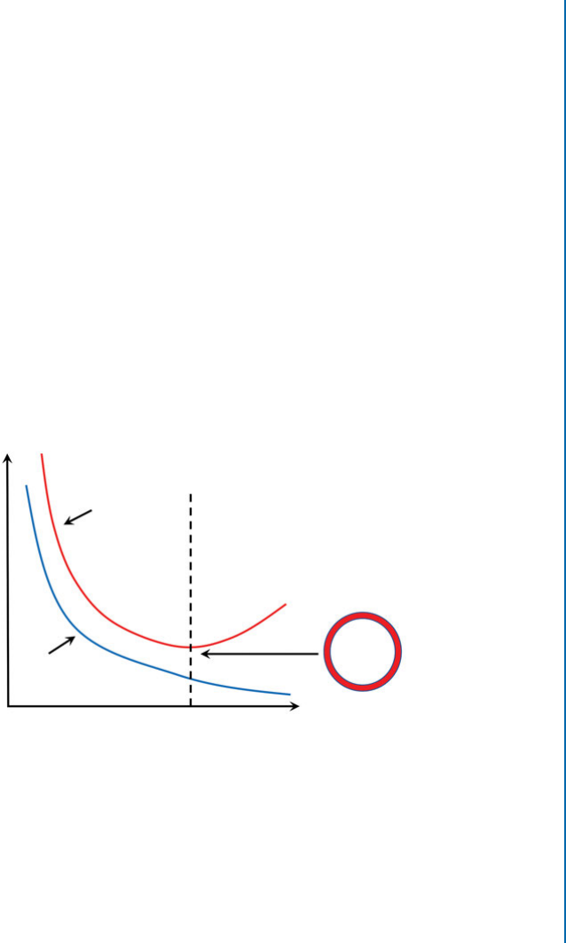
5.2. REGULARIZATION OF CNN 79
5.2.9 MAX-NORM CONSTRAINTS
e max-norm constraint is a form of regularization which puts an upper bound on the norm
of the incoming weights of each neuron in a neural network layer. As a result, the weight vector
wmust follow the constraint kwk2< h, where his a hyper-parameter, whose value is usually
set based on the performance of the network on a validation set. e benefit of using such a
regularization is that the network parameters are guaranteed to remain in a reasonable numerical
range even when high values of learning rates are used during network training. In practice, this
leads to a better stability and performance [Srivastava et al.,2014].
5.2.10 EARLY STOPPING
e over-fitting problem occurs when a model performs very well on the training set but behaves
poorly on unseen data. Early stopping is applied to avoid overfitting in the iterative gradient-
based algorithms. is is achieved by evaluating the performance on a held-out validation set at
different iterations during the training process. e training algorithm can continue to improve
on the training set until the performance on the validation set also improves. Once there is a
drop in the generalization ability of the learned model, the learning process can be stopped or
slowed down (Fig. 5.2).
Validation Error
Training Error
Training Iterations
Error
t
Stop
at ‘t’
Figure 5.2: An illustration of the early stopping approach during network training.
Having discussed the concepts which enable successful training of deep neural networks
(e.g., correct weight initialization and regularization techniques), we dive into the details of the
network learning process. Gradient-based algorithms are the most important tool to optimally
train such networks on large-scale datasets. In the following, we discuss different variants of
optimizers for CNNs.

80 5. CNN LEARNING
5.3 GRADIENT-BASED CNN LEARNING
e CNN learning process tunes the parameters of the network such that the input space is
correctly mapped to the output space. As discussed before, at each training step, the current
estimate of the output variables is matched with the desired output (often termed the “ground-
truth” or the “label space”). is matching function serves as an objective function during the
CNN training and it is usually called the loss function or the error function. In other words,
we can say that the CNN training process involves the optimization of its parameters such that
the loss function is minimized. e CNN parameters are the free/tunable weights in each of
its layers (e.g., filter weights and biases of the convolution layers) (Chapter 4).
An intuitive, but simple, way to approach this optimization problem is by repeatedly up-
dating the parameters such that the loss function progressively reduces to a minimum value.
It is important to note here that the optimization of nonlinear models (such as CNNs) is a
hard task, exacerbated by the fact that these models are mostly composed of a large number of
tunable parameters. erefore, instead of solving for a globally optimal solution, we iteratively
search for the locally optimal solution at each step. Here, the gradient-based methods come as
a natural choice, since we need to update the parameters in the direction of the steepest de-
scent. e amount of parameter update, or the size of the update step is called the “learning
rate.” Each iteration which updates the parameters using the complete training set is called a
“training epoch.” We can write each training iteration at time tusing the following parameter
update equation:
tDt1 ıt(5.15)
s:t:; ıtD rF.t/; (5.16)
where F./denotes the function represented by the neural network with parameters ,rrep-
resents the gradient, and denotes the learning rate.
5.3.1 BATCH GRADIENT DESCENT
As we discussed in the previous section, gradient descent algorithms work by computing the
gradient of the objective function with respect to the neural network parameters, followed by
a parameter update in the direction of the steepest descent. e basic version of the gradient
descent, termed “batch gradient descent,” computes this gradient on the entire training set. It
is guaranteed to converge to the global minimum for the case of convex problems. For non-
convex problems, it can still attain a local minimum. However, the training sets can be very
large in computer vision problems, and therefore learning via the batch gradient descent can
be prohibitively slow because for each parameter update, it needs to compute the gradient on
the complete training set. is leads us to the stochastic gradient descent, which effectively
circumvents this problem.

5.4. NEURAL NETWORK OPTIMIZERS 81
5.3.2 STOCHASTIC GRADIENT DESCENT
Stochastic Gradient Descent (SGD) performs a parameter update for each set of input and
output that are present in the training set. As a result, it converges much faster compared to
the batch gradient descent. Furthermore, it is able to learn in an “online manner,” where the
parameters can be tuned in the presence of new training examples. e only problem is that its
convergence behavior is usually unstable, especially for relatively larger learning rates and when
the training datasets contain diverse examples. When the learning rate is appropriately set, the
SGD generally achieves a similar convergence behavior, compared to the batch gradient descent,
for both the convex and non-convex problems.
5.3.3 MINI-BATCH GRADIENT DESCENT
Finally, the mini-batch gradient descent method is an improved form of the stochastic gradient
descent approach, which provides a decent trade-off between convergence efficiency and con-
vergence stability by dividing the training set into a number of mini-batches, each consisting of
a relatively small number of training examples. e parameter update is then performed after
computing the gradients on each mini-batch. Note that the training examples are usually ran-
domly shuffled to improve homogeneity of the training set. is ensures a better convergence
rate compared to the Batch Gradient Descent and a better stability compared to the Stochastic
Gradient Descent [Ruder,2016].
5.4 NEURAL NETWORK OPTIMIZERS
After a general overview of the gradient descent algorithms in Section 5.3, we can note that
there are certain caveats which must be avoided during the network learning process. As an ex-
ample, setting the learning rate can be a tricky endeavor in many practical problems. e training
process is often highly affected by the parameter initialization. Furthermore, the vanishing and
exploding gradients problems can occur especially for the case of deep networks. e training
process is also susceptible to get trapped into a local minima, saddle points or a high error plateau
where the gradient is approximately zero in every direction [Pascanu et al.,2014]. Note that the
saddle points (also called the “minmax points”) are those stationary points on the surface of the
function, where the partial derivative with respect to its dimensions becomes zero (Fig. 5.3). In
the following discussion we outline different methods to address these limitations of the gradi-
ent descent algorithms. Since our goal is to optimize over high-dimensional parameter spaces,
we will restrict our discussion to the more feasible first-order methods and will not deal with
the high-order methods (Newton’s method) which are ill-suited for large datasets.
5.4.1 MOMENTUM
Momentum-based optimization provides an improved version of SGD with better convergence
properties. For example, the SGD can oscillate close to a local minima, resulting in an un-
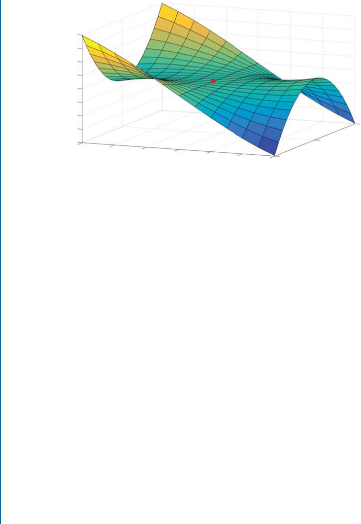
82 5. CNN LEARNING
200
150
100
50
0
-50
-100
-150
-200
-3 -2 -1 0
0
5
2
13-5
Figure 5.3: A saddle point shown as a red dot on a 3D surface. Note that the gradient is effectively
zero, but it corresponds to neither a “minima” nor a “maxima” of the function.
necessarily delayed convergence. e momentum adds the gradient calculated at the previous
time-step (at1) weighted by a parameter to the weight update equation as follows:
tDt1at(5.17)
atDrF.t/Cat1;(5.18)
where F./denotes the function represented by the neural network with parameters ,rrep-
resents the gradient and denotes the learning rate.
e momentum term has physical meanings. e dimensions whose gradients point in the
same direction are magnified quickly, while those dimensions whose gradients keep on changing
directions are suppressed. Essentially, the convergence speed is increased because unnecessary
oscillations are avoided. is can be understood as adding more momentum to the ball so that it
moves along the direction of the maximum slope. Typically, the momentum is set to 0:9 during
the SGD-based learning.
5.4.2 NESTEROV MOMENTUM
e momentum term introduced in the previous section would carry the ball beyond the min-
imum point. Ideally, we would like the ball to slow down when the ball reaches the minimum
point and the slope starts ascending. is is achieved by the Nesterov momentum [Nesterov,
1983] which computes the gradient at the next approximate point during the parameter update
process, instead of the current point. is gives the algorithm the ability to “look ahead” at each
iteration and plan a jump such that the learning process avoids uphill steps. e update process
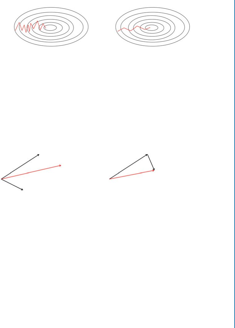
5.4. NEURAL NETWORK OPTIMIZERS 83
Vanilla SGD SGD with Momentum
Figure 5.4: Comparison of the convergence behavior of the SGD with (right) and without (left)
momentum.
can be represented as:
tDt1at(5.19)
atDrF.tat1/Cat1;(5.20)
where F./denotes the function represented by the neural network with parameters ,rrep-
resents the gradient operation, denotes the learning rate and is the momentum.
Momentum Term Momentum Term “Look ahead” Gradient Term
Gradient Term
Momentum Step Nesterov Step
-1 -1
Figure 5.5: Comparison of the convergence behavior of the SGD with momentum (left) and the
Nesterov update (right). While momentum update can carry the solver quickly toward a local
optima, it can overshoot and miss the optimum point. A solver with Nesterov update corrects
its update by looking ahead and correcting for the next gradient value.
5.4.3 ADAPTIVE GRADIENT
e momentum in the SGD refines the update direction along the slope of the error function.
However, all parameters are updated at the same rate. In several cases, it is more useful to update
each parameter differently, depending on its frequency in the training set or its significance for
our end problem.
Adaptive Gradient (AdaGrad) algorithm [Duchi et al.,2011] provides a solution to this
problem by using an adaptive learning rate for each individual parameter i. is is done at each
time step tby dividing the learning rate of each parameter with the accumulation of the square

84 5. CNN LEARNING
of all the historical gradients for each parameter i. is can be shown as follows:
i
tDi
t1
st
P
D1
ıi
2C
ıi
t;(5.21)
where ıi
tis the gradient at time-step twith respect to the parameter iand is a very small
term in the denominator to avoid division by zero. e adaptation of the learning rate for each
parameter removes the need to manually set the value of the learning rate. Typically, is kept
fixed to a single value (e.g., 102or 103) during the training phase. Note that AdaGrad works
very well for sparse gradients, for which a reliable estimate of the past gradients is obtained by
accumulating all of the previous time steps.
5.4.4 ADAPTIVE DELTA
Although AdaGrad eliminates the need to manually set the value of the learning rate at different
epochs, it suffers from the vanishing learning rate problem. Specifically, as the number of iter-
ations grows (tis large), the sum of the squared gradients becomes large, making the effective
learning rate very small. As a result, the parameters do not change in the subsequent training
iterations. Lastly, it also needs an initial learning rate to be set during the training phase.
e Adaptive Delta (AdaDelta) algorithm [Zeiler,2012] solves both these problems by
accumulating only the last kgradients in the denominator term of Eq. (5.21). erefore, the
new update step can be represented as follows:
i
tDi
t1
st
P
DtkC1
ıi
2C
ıi
t:(5.22)
is requires the storage of the last kgradients at each iteration. In practice, it is much easier to
work with a running average EŒı2t, which can be defined as:
EŒı2tDEŒı2t1C.1 /ıt2:(5.23)
Here, has a similar function to the momentum parameter. Note that the above function im-
plements an exponentially decaying average of the squared gradients for each parameter. e
new update step is:
i
tDi
t1
pEŒı2tCıi
t;(5.24)
D
pEŒı2tCıi
t:(5.25)
Note that we still did not get rid of the initial learning rate .Zeiler [2012] noted that this
can be avoided by making the units of the update step consistent by introducing a Hessian

5.4. NEURAL NETWORK OPTIMIZERS 85
approximation in the update rule. is boils down to the following:
i
tDi
t1pEŒ./2t1C
pEŒı2tCıi
t:(5.26)
Note that we have considered here the local curvature of the function Fto be approximately flat
and replaced EŒ./2t(not known) with EŒ./2t1(known).
5.4.5 RMSPROP
RMSprop [Tieleman and Hinton,2012] is closely related to the AdaDelta approach, aiming to
resolve the vanishing learning rate problem of AdaGrad. Similar to AdaDelta, it also calculates
the running average as follows:
EŒı2tDEŒı2t1C.1 /ıt2:(5.27)
Here, a typical value of is 0.9. e update rule of the tunable parameters takes the following
form:
i
tDi
t1
pEŒı2tCıi
t:(5.28)
5.4.6 ADAPTIVE MOMENT ESTIMATION
We stated that the AdaGrad solver suffers from the vanishing learning rate problem, but Ada-
Grad is very useful for cases where gradients are sparse. On the other hand, RMSprop does
not reduce the learning rate to a very small value at higher time steps. However on the negative
side, it does not provide an optimal solution for the case of sparse gradients. e ADAptive
Moment Estimation (ADAM) [Kingma and Ba,2014] approach estimates a separate learning
rate for each parameter and combines the positives of both AdaGrad and RMSprop. e main
difference between Adam and its two predecessors (RMSprop and AdaDelta) is that the up-
dates are estimated by using both the first moment and the second moment of the gradient (as
in Eqs. (5.26) and (5.28)). erefore, a running average of gradients (mean) is maintained along
with a running average of the squared gradients (variance) as follows:
EŒıtD1EŒıt1C.1 1/ıt;(5.29)
EŒı2tD2EŒı2t1C.1 2/ıt2;(5.30)
where 1and 2are the parameters for running averages of the mean and the variance respec-
tively. Since the initial moment estimates are set to zero, they can remain very small even af-
ter many iterations, especially when 1;2 ¤1. To overcome this issue, the initialization bias-
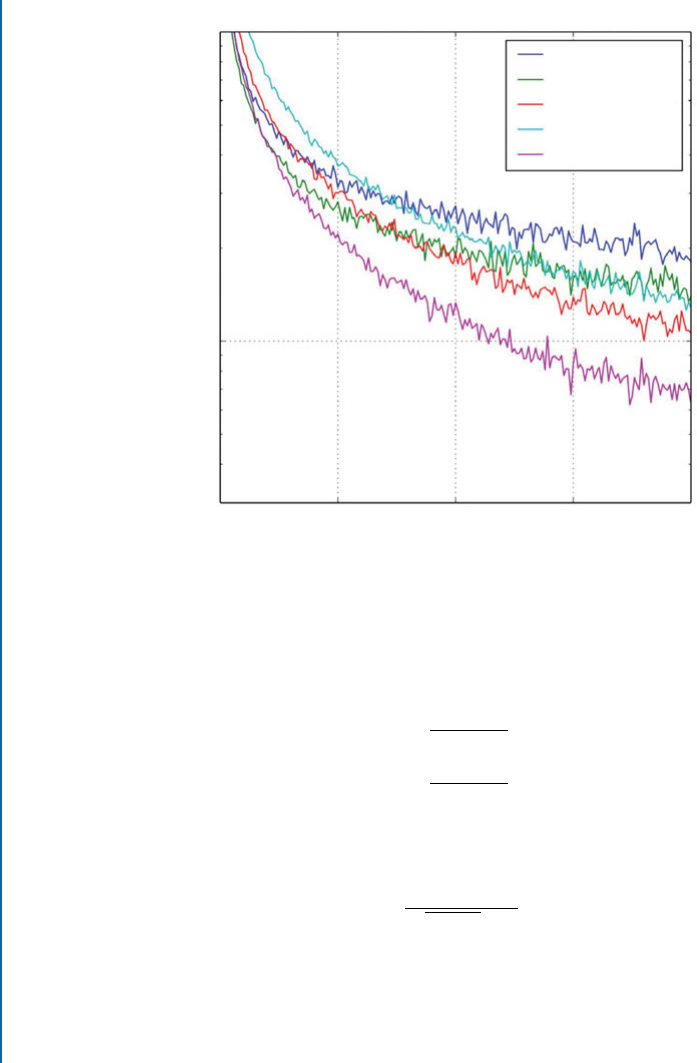
86 5. CNN LEARNING
MNIST Multilayer Neural Network + Dropout
Iterations over Entire Dataset
Training Cost
10-1
10-2
0 50 200100 150
AdaGrad
RMSProp
SGDNesterov
AdaDelta
Adam
Figure 5.6: Convergence performance on the MNIST dataset using different neural network
optimizers [Kingma and Ba,2014]. (Figure used with permission.)
corrected estimates of EŒıtand EŒı2tare obtained as follows:
O
EŒıtDEŒıt
1.1/t(5.31)
O
EŒı2tDEŒı2t
1.2/t:(5.32)
Very similar to what we studied in the case of AdaGrad, AdaDelta and RMSprop, the update
rule for Adam is given by:
i
tDi
t1
qO
EŒı2tCO
EŒıt:(5.33)
e authors found 1D0:9; 2D0:999; D0:001 to be good default values of the decay ()
and learning () rates during the training process.
Figure 5.6 [Kingma and Ba,2014] illustrates the convergence performance of the dis-
cussed solvers on the MNIST dataset for handwritten digit classification. Note that the SGD

5.5. GRADIENT COMPUTATION IN CNNS 87
with Nesterov shows a good convergence behavior, however it requires a manual tuning of the
learning rate hyper-parameter. Among the solvers with an adaptive learning rate, Adam per-
forms the best in this example (also beating the manually tuned SGD-Nesterov solver). In
practice, Adam usually scales very well to large-scale problems and exhibits nice convergence
properties. at is why Adam is often a default choice for many computer vision applications
based on deep learning.
5.5 GRADIENT COMPUTATION IN CNNS
We have discussed a number of layers and architectures for CNNs. In Section 3.2.2, we also
described the back-propagation algorithm used to train CNNs. In essence, back-propagation
lies at the heart of CNN training. Error back-propagation can only happen if the CNN layers
implement a differentiable operation. erefore, it is interesting to study how the gradient can
be computed for the different CNN layers. In this section, we will discuss in detail the different
approaches which are used to compute the differentials of popular CNN layers.
We describe in the following the four different approaches which can be used to compute
gradients.
5.5.1 ANALYTICAL DIFFERENTIATION
It involves the manual derivation of the derivatives of a function performed by a CNN layer.
ese derivatives are then implemented in a computer program to calculate the gradients. e
gradient formulas are then used by an optimization algorithm (e.g., Stochastic Gradient De-
scent) to learn the optimal CNN weights.
Example: Assume for a simple function, yDf .x/ Dx2, we want to cal-
culate the derivative analytically. By applying the differentiation formula for
polynomial functions, we can find the derivative as follows:
dy
dx D2x; (5.34)
which can give us the slope at any point x.
Analytically deriving the derivatives of complex expressions is time-consuming and labo-
rious. Furthermore, it is necessary to model the layer operation as a closed-form mathematical
expression. However, it provides an accurate value for the derivative at each point.
5.5.2 NUMERICAL DIFFERENTIATION
Numerical differentiation techniques use the values of a function to estimate the numerical value
of the derivative of the function at a specific point.

88 5. CNN LEARNING
Example: For a given function f .x/, we can estimate the first-order numer-
ical derivative at a point xby using the function values at two nearby points,
i.e., f .x/ and f .x Ch/, where his a small change in x:
f .x Ch/ f .x/
h:(5.35)
e above equation estimates the first-order derivative as the slope of a line
joining the two points f .x/ and f .x Ch/. e above expression is called the
“Newton’s Difference Formula.”
Numerical differentiation is useful in cases where we know little about the underline real
function or when the actual function is too complex. Also, in several cases we only have access
to discrete sampled data (e.g., at different time instances) and a natural choice is to estimate
the derivatives without necessarily modeling the function and calculating the exact derivatives.
Numerical differentiation is fairly easy to implement, compared to other approaches. However,
numerical differentiation provides only an estimate of the derivative and works poorly, particu-
larly for the calculation of higher-order derivatives.
5.5.3 SYMBOLIC DIFFERENTIATION
Symbolic differentiation uses standard differential calculus formulas to manipulate mathemat-
ical expressions using computer algorithms. Popular softwares which perform symbolic differ-
entiation include Mathematica, Maple, and Matlab.
Example: Suppose we are given a function f .x/ Dexp.sin.x//, we need to
calculate its 10th derivative with respect to x. An analytical solution would
be cumbersome, while a numerical solution will be less accurate. In such
cases, we can effectively use symbolic differentiation to get a reliable answer.
e following code in Matlab (using the Symbolic Math Toolbox) gives the
desired result.
>> syms x
>> f(x) = exp(sin(x))
>> diff(f,x,10)
256exp(sin(x))cos(x)2- exp(sin(x))sin(x) -
5440exp(sin(x))cos(x)4+ 2352exp(sin(x))cos(x)6- …
Symbolic differentiation, in a sense, is similar to analytical differentiation, but leveraging
the power of computers to perform laborious derivations. is approach reduces the need to
manually derive differentials and avoids the inaccuracies of numerical methods. However, sym-
bolic differentiation often leads to complex and long expressions which results in slow software
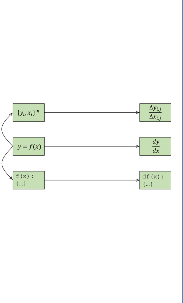
5.5. GRADIENT COMPUTATION IN CNNS 89
programs. Also, it does not scale well to higher-order derivatives (similar to numerical differenti-
ation) due to the high complexity of the required computations. Furthermore, in neural network
optimization, we need to calculate partial derivatives with respect to a large number of inputs to
a layer. In such cases, symbolic differentiation is inefficient and does not scale well to large-scale
networks.
5.5.4 AUTOMATIC DIFFERENTIATION
Automatic differentiation is a powerful technique which uses both numerical and symbolic tech-
niques to estimate the differential calculation in the software domain, i.e., given a coded com-
puter program which implements a function, automatic differentiation can be used to design
another program which implements the derivative of that function. We illustrate the automatic
differentiation and its relationship with the numerical and symbolic differentiation in Fig. 5.7.
Samples from Function
Actual Function
Programmed Function
Numerical Differentiation
Analytical/Symbolic Differentiation
Automatic Differentiation
Figure 5.7: Relationships between different differentiation methods.
Every computer program is implemented using a programming language, which only
supports a set of basic functions (e.g., addition, multiplication, exponentiation, logarithm and
trigonometric functions). Automatic differentiation uses this modular nature of computer pro-
grams to break them into simpler elementary functions. e derivatives of these simple functions
are computed symbolically and the chain rule is then applied repeatedly to compute any order
of derivatives of complex programs.
Automatic differentiation provides an accurate and efficient solution to the differentiation
of complex expressions. Precisely, automatic differentiation gives results which are accurate to
the machine precision. e computational complexity of calculating derivatives of a function
is almost the same as evaluating the original function itself. Unlike symbolic differentiation,
it neither needs a closed form expression of the function nor does it suffer from expression
swell which renders symbolic differentiation inefficient and difficult to code. Current state of

90 5. CNN LEARNING
Algorithm 5.1 Forward mode of Automatic Differentiation
Input : x,C
Output : yn
1: y0 x% initialization
2: for all i2Œ1; n do
3: yi fe
i.yPa.f e
i//% each function operates on its parents output in the graph
4: end for
Algorithm 5.2 Backward mode of Automatic Differentiation
Input : x,C
Output : dyn
dx
1: Perform forward mode propagation
2: for all i2Œn 1; 0 do
3: % chain rule to compute derivatives using child nodes in the graph
4: dyn
dyi P
j2Ch.f e
i/
dyn
dyj
df e
j
dyi
5: end for
6: dyn
dx dyn
dy0
the art CNN libraries such as eano and Tensorflow use automatic differentiation to compute
derivatives (see Chapter 8).
Automatic differentiation is very closely related to the back-propagation algorithm we
studied before in Section 3.2.2. It operates in two modes, the forward mode and the backward
mode. Given a complex function, we first decompose it into a computational graph consisting
of simple elementary functions which are joined with each other to compute the complex func-
tion. In the forward mode, given an input x, the computational graph Cwith nintermediate
states (corresponding to ffegnelementary functions) can be evaluated sequentially as shown in
Algorithm 5.1.
After the forward computations shown in Algorithm 5.1, the backward mode starts com-
puting the derivatives toward the end and successively applies the chain rule to calculate the
differential with respect to each intermediate output variable yi, as shown in Algorithm 5.2.
A basic assumption in the automatic differentiation approach is that the expression is
differentiable. If this is not the case, automatic differentiation will fail. We provide a simple ex-
ample of forward and backward modes of automatic differentiation below and refer the reader to
Baydin et al. [2015] for a detailed treatment of this subject in relation to machine/deep learning
techniques.

5.5. GRADIENT COMPUTATION IN CNNS 91
Example: Consider a slightly more complex function than the previous ex-
ample for symbolic differentiation,
yDf .x/ Dexp.sin.x/ Csin.x/2/Csin.exp.x/ Cexp.x/2/: (5.36)
We can represent its analytically or symbolically calculated differential as fol-
lows:
df
dx Dcos.exp.2x/ Cexp.x//.2 exp.2x/ Cexp.x//
Cexp.sin.x/2Csin.x//.cos.x/ C2cos.x/ sin.x//: (5.37)
But, if we are interested in calculating its derivative using automatic differ-
entiation, the first step would be to represent the complete function in terms
of basic operations (addition, exp and sin) defined as:
aDsin.x/ b Da2cDaCb
dDexp.c/ e Dexp.x/ f De2
gDeCf h Dsin.g/ y DdCh: (5.38)
e flow of computations in terms of these basic operations is illustrated
in the computational graph in Fig. 5.8. Given this computational graph we
can easily calculate the differential of the output with respect to each of the
variables in the graph as follows:
dy
dd D1dy
dh D1dy
dc Ddy
dd
dd
dc
dy
dg Ddy
dh
dh
dg
dy
db Ddy
dc
dc
db
dy
da Ddy
dc
dc
da Cdy
db
db
da
dy
df Ddy
dg
dg
df
dy
de Ddy
dg
dg
de Cdy
df
df
de
dy
dx Ddy
da
da
dx Cdy
de
de
dx :(5.39)
All of the above differentials can easily be computed because it is simple to
compute the derivative of each basic function, e.g.,
dd
dc Dexp.c/ dh
dg Dcos.g/ dc
db Ddc
da D1df
de D2e: (5.40)
Note that we started toward the end of the computational graph, and com-
puted all of the intermediate differentials moving backward, until we got
the differential with respect to input. e original differential expression we
calculated in Eq. (5.37) was quite complex. However, once we decomposed
the original expression in to simpler functions in Eq. (5.38), we note that
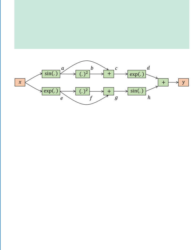
92 5. CNN LEARNING
the complexity of the operations that are required to calculate the deriva-
tive (back-ward pass) is almost the same as the calculation of the original
expression (forward pass) according to the computational graph. Automatic
differentiation uses the forward and backward operation modes to efficiently
and precisely calculate the differentials of complex functions. As we discussed
above, the operations for the calculation of differentials in this manner have
a close resemblance to the back-propagation algorithm.
Figure 5.8: Computational graph showing the calculation of our desired function.
5.6 UNDERSTANDING CNN THROUGH VISUALIZATION
Convolutional networks are large-scale models with a huge number of parameters that are
learned in a data driven fashion. Plotting an error curve and objective function on the train-
ing and validation sets against the training iterations is one way to track the overall training
progress. However, this approach does not give an insight into the actual parameters and activa-
tions of the CNN layers. It is often useful to visualize what CNNs have learned during or after
the completion of the training process. We outline some basic approaches to visualize CNN
features and activations below. ese approaches can be categorized into three types depend-
ing on the network signal that is used to obtain the visualization, i.e., weights, activations, and
gradients. We summarize some of these three types of visualization methods below.
5.6.1 VISUALIZING LEARNED WEIGHTS
One of the simplest approaches to visualize what a CNN has learned is to look at the con-
volution filters. For example, 99and 55sized convolution kernels that are learned on a
labeled shadow dataset are illustrated in Fig. 5.9. ese filters correspond to the first and second
convolutional layers in a LeNet style CNN (see Chapter 6for details on CNN architectures).
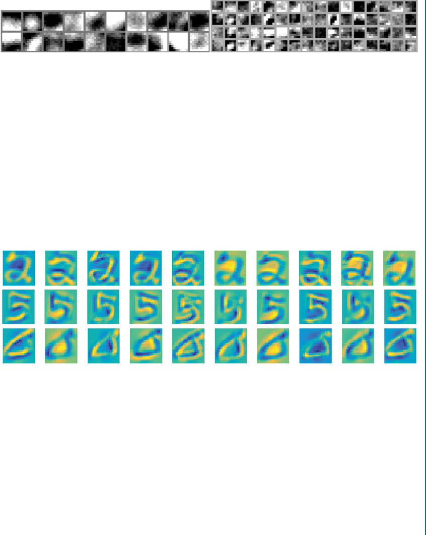
5.6. UNDERSTANDING CNN THROUGH VISUALIZATION 93
Figure 5.9: Examples of 99(left) and 55(right) sized convolution kernels learned for the
shadow detection task. e filters illustrate the type of patterns that a particular CNN layer is
looking for in the input data. (Figure adapted from Khan et al. [2014].)
5.6.2 VISUALIZING ACTIVATIONS
e feature activations from the intermediate CNN layers can also provide useful clues about
the quality of learned representations.
A trivial way to visualize learned features is to plot the output feature activations cor-
responding to an input image. As an example, we show the output convolutional activations
(or features) corresponding to sample digits 2, 5, and 0 belonging to the MNIST dataset in
Fig. 5.10. Specifically, these features are the output of the first convolution layer in the LeNet
architecture (see Chapter 6for details on this architecture type).
Figure 5.10: Intermediate feature representations from a CNN corresponding to example input
images of handwritten digits from the MNIST dataset. Such a visualization of output activations
can provide an insight about the patterns in input images that are extracted as useful features for
classification.
Another approach is to obtain the feature representation from the penultimate layer of a
trained CNN and visualize all the training images in a dataset as a 2D plot (e.g., using tSNE low
dimensional embedding). e tSNE embedding approximately preserves the original distances
in the high dimensional space between features. An example of such a visualization is shown in
Fig. 5.11. is visualization can provide a holistic view and suggest the quality of learned feature
representations for different classes. For instance, classes that are clustered tightly together in
the feature space will be classified more accurately compared to the ones that have a widespread
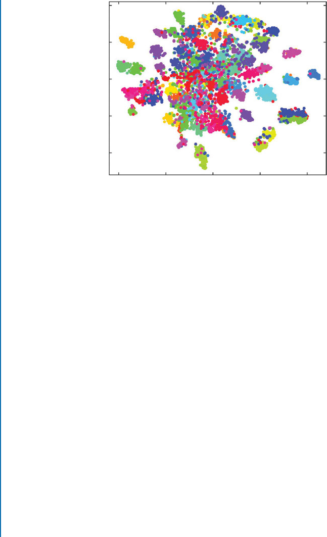
94 5. CNN LEARNING
Figure 5.11: tSNE visualization of the final fully connected layer features corresponding to im-
ages from the MIT-67 indoor scene dataset. Each color represents a different class in the dataset.
Note that the features belonging to the same class are clustered together. (Figure adapted from
Khan et al. [2017b].)
overlapping with other classes, making it difficult to accurately model the classification bound-
aries. Alongside visualizing 2D embedding of the high-dimensional feature vectors, we can also
visualize the input images associated with each feature vector (see Fig. 5.13). In this manner,
we can observe how visually similar images are clustered together in the tSNE embedding of
high-dimensional features. As an example, cellar images are clustered together on the top left
in the illustration shown in Fig. 5.13.
An attention map can also provide an insight into the regions which were given more
importance while making a classification decision. In other words, we can visualize the regions
in an image which contributed most to the correct prediction of a category. One way to achieve
this is to obtain prediction scores for individual overlapping patches with in an image and plot
the final prediction score for the correct class. Examples of such a visualization is shown in
Fig. 5.12. We can note that distinctive portions of the scenes played a crucial role in the correct
prediction of the category for each image, e.g., a screen in an auditorium, train in a train station
and bed in a bedroom.
Other interesting approaches have also been used in the literature to visualize the image
parts which contribute most to the correct prediction. Zeiler and Fergus [2014] systematically
occluded a square patch within an input image and plotted a heat map indicating the change in
the prediction probability of the correct class. e resulting heat map indicates which regions in
an input image are most important for a correct output response from the network (see Fig. 5.14a
for examples). Bolei et al. [2015] first segments an input image into regions, these segments
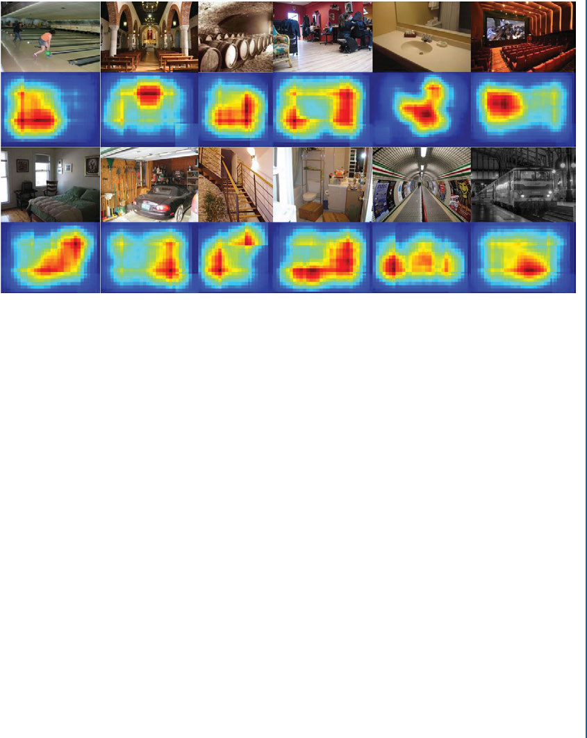
5.6. UNDERSTANDING CNN THROUGH VISUALIZATION 95
Figure 5.12: e contributions of distinctive patches with in an image toward the prediction of
correct scene class are shown in the form of a heat map (“red” color denotes higher contribution).
(Figure adapted from Khan et al. [2016b].)
are then iteratively dropped such that the correct class prediction is least affected. is process
continues until an image with minimal scene details is left. ese details are sufficient for the
correct classification of the input image (see Fig. 5.14b for examples).
5.6.3 VISUALIZATIONS BASED ON GRADIENTS
Balduzzi et al. [2017] presented the idea that visualizing distributions of gradients can provide
useful insight into the convergence behavior of deep neural networks. eir analysis showed that
naively increasing the depth of a neural network results in the gradient shattering problem (i.e.,
the gradients show similar distribution as white noise). ey demonstrated that the gradient
distribution resembled brown noise when batch normalization and skip connections were used
in a very deep network (see Fig. 5.15).
Back-propagated gradients within a CNN have been used to identify specific patterns in
the input image that maximally activate a particular neuron in a CNN layer. In other words,
gradients can be adjusted to generate visualizations that illustrate the patterns that a neuron has
learned to look for in the input data. Zeiler and Fergus [2014] pioneered this idea and introduced
a deconvolution-based approach to invert the feature representations to identify associated pat-
terns in the input images. Yosinski et al. [2015] generated synthetic images by first selecting
an ith neuron in a CNN layer. Afterward, an input image with random color values is passed
96 5. CNN LEARNING
Figure 5.13: Visualization of images based on the tSNE embedding of the convolutional features
from a deep network. e images belong to the MIT-67 dataset. Note that the images belonging
to the same class are clustered together, e.g., all cellar images can be found in the top-left corner.
(Figure adapted from Hayat et al. [2016].)
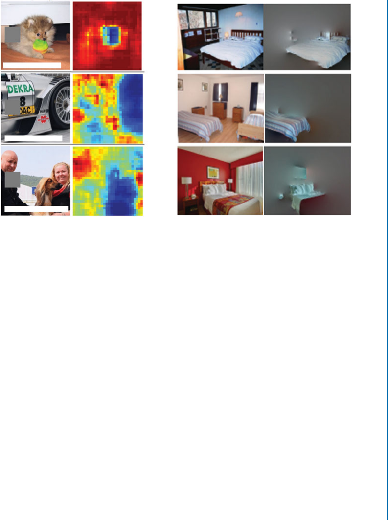
5.6. UNDERSTANDING CNN THROUGH VISUALIZATION 97
(a) (b)
True Label: Pomeranian
True Label: Afghan Hound
True Label: Car Wheel
Figure 5.14: Visualization of regions which are important for the correct prediction from a
deep network. (a) e grey regions in input images is sequentially occluded and the output
probability of correct class is plotted as a heat map (blue regions indicate high importance for
correct classification). (b) Segmented regions in an image are occluded until the minimal image
details that are required for correct scene class prediction are left. As we expect, a bed is found
to be the most important aspect of a bed-room scene. (Figures adapted from Bolei et al. [2015]
and Zeiler and Fergus [2014], used with permission.)
through the network and the corresponding activation value for ith neuron is calculated. e
gradient of this activation with respect to the input image is calculated via error back propaga-
tion. is gradient basically denotes how the pixels can be changed such that the neuron gets
maximally activated. e input gets iteratively modified using this information so that we obtain
an image which results in a high activation for neuron i. Normally it is useful to impose a “style
constraint” while modifying the input image which acts as a regularizer and enforces the input
image to remain similar to the training data. Some example images thus obtained are shown in
Fig. 5.16.
Mahendran and Vedaldi [2015] propose an approach to recover input images that corre-
spond to identical high-dimensional feature representations in the second to last layer of CNN.
Given an image x, a learned CNN Fand a high dimensional representation f, the following loss
is minimized through gradient descent optimization to find images in the input domain that
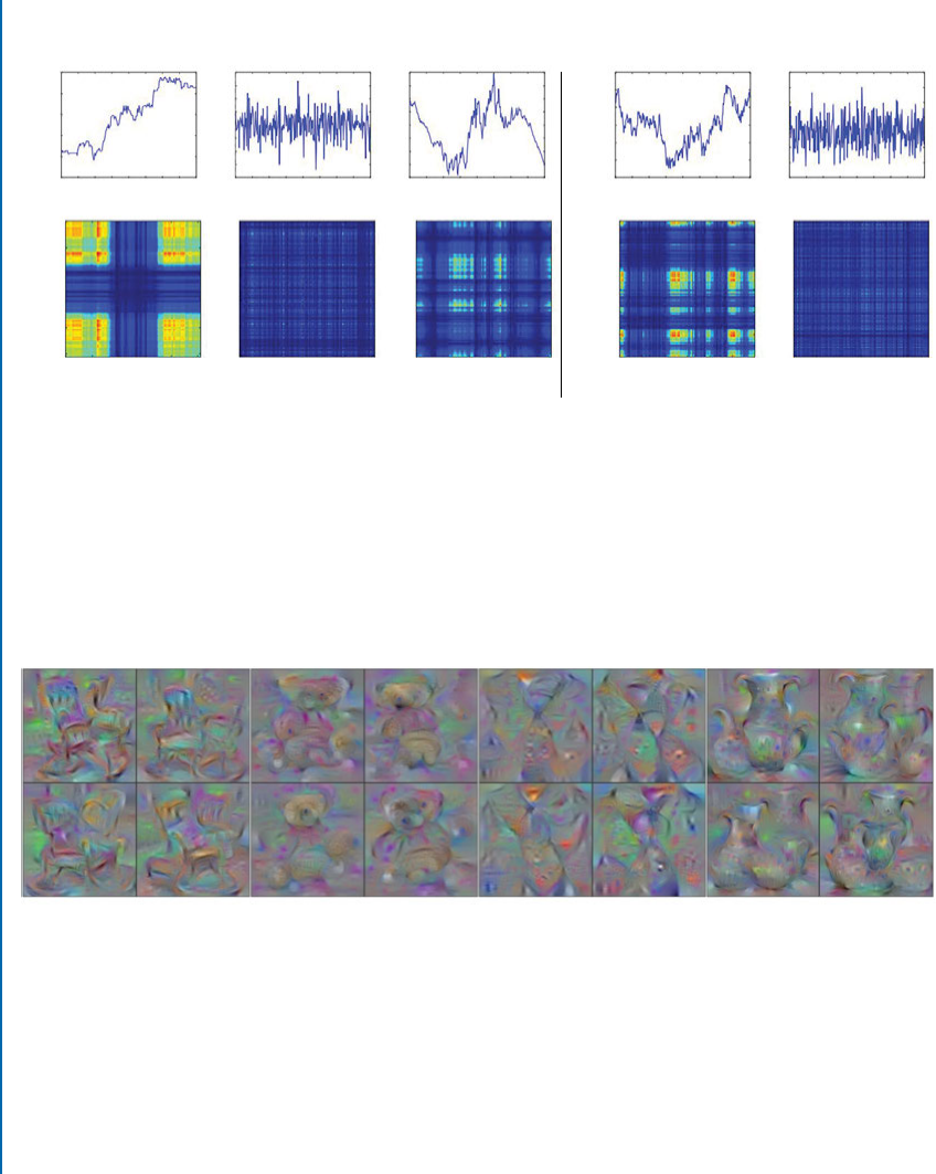
98 5. CNN LEARNING
(a) 1-Layer
Feedforward
(b) 24-Layer
Feedforward
(c) 50-Layer
ResNet
(d) Brown Noise (d) White Noise
Covariance Matrices Gradients
Noise
2.0
1.5
1.0
0.5
0.0
-0.5
0
50
100
150
200
250
0.4
0.2
0.0
-0.2
-0.4
-0.6
-0.8
4
3
2
1
0
-1
-2
-3
0.20
0.15
0.10
0.05
0.00
-0.05
-0.10
-0.15
-0.20
4.5
4.0
3.5
3.0
2.5
2.0
1.5
1.0
0.5
-2.0 -1.5 -1.0 -0.5 0.0 0.5 1.0 1.5 -2.0
Input -2.0 -1.5 -1.0 -0.5 0.0 0.5 1.0 1.5 -2.0
Input -2.0 -1.5 -1.0 -0.5 0.0 0.5 1.0 1.5 -2.0 -2.0
0 50 100 150 200 250 0
50
100
150
200
250
0 50 100 150 200 250 0
50
100
150
200
250
0 50 100 150 200 250 0
50
100
150
200
250
0 50 100 150 200 250 0
50
100
150
200
250
0 50 100 150 200 250
-1.5 -1.0 -0.5 0.0 0.5 1.0 1.5 -2.0 -2.0 -1.5-1.0 -0.5 0.0 0.5 1.0 1.5 -2.0
Input
Figure 5.15: e top row shows the gradient distributions for a range of uniformly sampled
inputs. e bottom row shows the covariance matrices. e gradient for the case of a 24 layered
network resemble white noise, while the gradients of high-performing ResNet resemble brown
noise. Note that the ResNet used skip connections and batch normalization which results in
better converegence even with much deeper network architectures. e ResNet architecture will
be discussed in detail in Chapter 6. (Figure from Balduzzi et al. [2017], used with permission.)
Rocking Chair Teddy Bear Windsor Tie Pitcher
Figure 5.16: e figure illustrates synthetic input images that maximally activate the output
neurons corresponding to different classes. As evident, the network looks for objects with similar
low-level and high-level cues, e.g., edge information and holistic shape information, respectively,
in order to maximally activate the relevant neuron. (Figure from Yosinski et al. [2015], used with
permission.)

5.6. UNDERSTANDING CNN THROUGH VISUALIZATION 99
correspond to the same feature representation f:
x arg mi n
xkF.x/fk2CR.x/:
Here, Rdenotes a regularizer which enforces the generated images to look natural and avoid
noisy and spiky patterns that are not helpful in perceptual visualization. Figure 5.17 illustrates
examples of reconstructed images obtained from the CNN features at different layers of the
network. It is interesting to note that the objects vary in position, scale and deformations but the
holistic characteristics remain the same. is denotes that the network has learned meaningful
characteristics of the input image data.
pool5 relu6 relu7 fc8
Figure 5.17: Multiple inverted images obtained from the high dimensional feature representa-
tions of a CNN. Note that the features from lower layers retain local information better than
the higher ones. (Figure from Mahendran and Vedaldi [2015], used with permission.)
Up to this point, we have completed the discussion about the CNN architecture, its train-
ing process and the visualization approaches to understand the working of CNNs. Next, we will
describe a number of successful CNN examples from the literature which will help us develop
an insight into the state-of-the-art network topologies and their mutual pros and cons.

101
C H A P T E R 6
Examples of CNN
Architectures
We have covered the basic modules in the previous chapters which can be joined together to de-
velop CNN-based deep learning models. Among these modules, we covered convolution, sub-
sampling and several other layers which form large-scale CNN architectures. We noticed that
the loss functions are used during training to measure the difference between the predicted and
desired outputs from the model. We discussed modules which are used to regularize the networks
and optimize their performance and convergence speeds. We also covered several gradient-based
learning algorithms for successful CNN training, along with different tricks to achieve stable
training of CNNs, such as weight initialization strategies. In this chapter, we introduce several
successful CNN designs which are constructed using the basic building blocks that we studied
in the previous chapters. Among these, we present both early architectures (which have been
traditionally popular in computer vision and are rather easier to understand) and the most re-
cent CNN models (which are relatively complex and built on top of the conventional designs).
We note that there is a natural order in these architectures according to which their designs have
evolved through the recent years. erefore, we elaborate on each of these designs, while empha-
sizing their connections and the trend in which the designs have progressed. In the following,
we begin with a simple CNN architecture, known as the LeNet.
6.1 LENET
e LeNet [LeCun et al.,1998] architecture is one of the earliest and basic forms of CNNs
which was applied to handwritten digit identification. A successful variant of this architecture
style is called the LeNet-5 model, because it comprises 5 weight layers in total. Specifically,
it consists of two convolution layers each followed by a sub-sampling (max-pooling) layer to
extract features. Afterward, a single convolution layer, followed by a set of two fully connected
layers toward the end of the model to act as a classifier on the extracted features. Note that
the activations after the weight layers are also squashed using a tanh nonlinearity. e model
architecture used to train on the MNIST digit dataset is shown in Fig. 6.1.
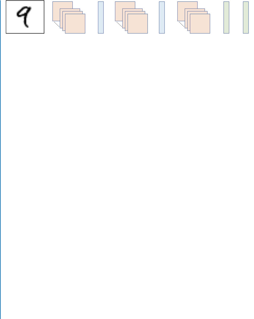
102 6. EXAMPLES OF CNN ARCHITECTURES
Input Image
32×32
Max-pooling
(2×2)
FC
Layer
(64)
FC
Layer
(10)
Max-pooling
(2×2)
Convolution
Layer
5×5 (6 filters)
Convolution
Layer
5×5 (16 filters)
Convolution
Layer
4×4 (120 filters)
Figure 6.1: e LeNet-5 Architecture.
6.2 ALEXNET
AlexNet [Krizhevsky et al.,2012] was the first large-scale CNN model which led to the resur-
gence of deep neural networks in computer vision (other CNN architectures before AlexNet,
e.g., [Cireşan et al.,2011,LeCun et al.,1998] were relatively smaller and were not tested on
large-scale datasets such as the ImageNet dataset). is architecture won the ImageNet Large-
Scale Visual Recognition Challenge (ILSVRC) in 2012 by a large margin.
e main difference between the AlexNet architecture and its predecessors is the increased
network depth, which leads to a significantly larger number of tunable parameters, and the used
regularization tricks (such as the activation dropout [Srivastava et al.,2014] and data augmen-
tation). It consists of a total of eight parameter layers among which the five initial layers are
convolutional layers, while the later three layers are fully connected layers. e final fully con-
nected layer (i.e., the output layer) classifies an input image into one of the thousand classes of
the ImageNet dataset, and therefore contains 1,000 units. e filter sizes and the location of
the max-pooling layers are shown in Fig. 6.2. Note that dropout is applied after the first two
fully connected layers in the AlexNet architecture, which leads to a reduced over-fitting and a
better generalization to unseen examples. Another distinguishing aspect of AlexNet is the usage
of ReLU nonlinearity after every convolutional and fully connected layer, which substantially
improves the training efficiency compared to the traditionally used tanh function.
Although AlexNet is relatively much smaller (in terms of the number of layers) compared
to the recent state-of-the-art CNN architectures, it is interesting to note that Krizhevsky et al.
[2012] had to split the training between two GPUs at the time of its first implementation.
is was necessary because a single NVIDIA GTX 580 (with 3 Gb memory) could not hold
the complete network which consists of around 62 million parameters. It took around six days
to train the network on the complete ImageNet dataset. Note that the ImageNet training set
contains 1:2 million images belonging to a thousand of different object classes.
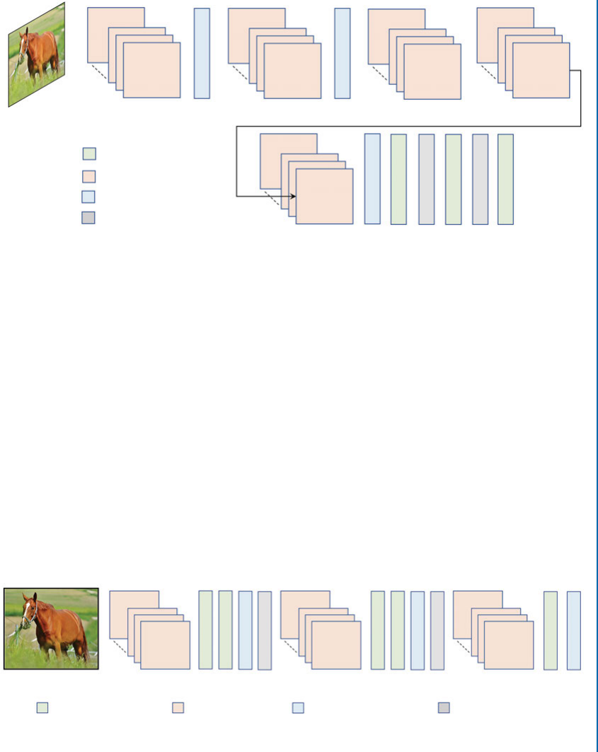
6.3. NETWORK IN NETWORK 103
Input Image
(224×224×3)
11×11 (96)
Stride 4
5×5 (256) 3×3 (384)
3×3 (256) 4096 4096 1000
3×3 (384)
Fully Connected Layers
Convolution Layers
Max-pooling Layers
Dropout Layers
Figure 6.2: e AlexNet Architecture.
6.3 NETWORK IN NETWORK
e Network in Network (NiN) [Lin et al.,2013] architecture is a simple and lightweight CNN
model which generally performs really well on small-scale datasets. It introduces two new ideas
in the CNN design. First, it shows that incorporating fully connected layers in-between the
convolutional layers results is helpful in network training. erefore, the example architecture
consists of three convolutional layers at the first, fourth, and and seventh locations (among the
weight layers) with filters of size 55,55, and 33, respectively. Each of these convolutional
layers is followed by a pair of fully connected layers (or convolutional layers with 11filter sizes)
and a max-pooling layer. Second, this architecture utilizes a global average pooling at the end of
the model as a regularizer. is pooling scheme just combines all activations within each feature
map (by averaging) to obtain a single classification score which is forwarded to a soft-max loss
layer. Note that a drop-out regularization block after the first two max-pooling layers also help
in achieving a lower test error on a given dataset.
Input Image 5×5 5×5 3×3
Fully Connected Layers Convolution Layers Pooling Layers (max or avg) Dropout Layers
Figure 6.3: e NiN Architecture.
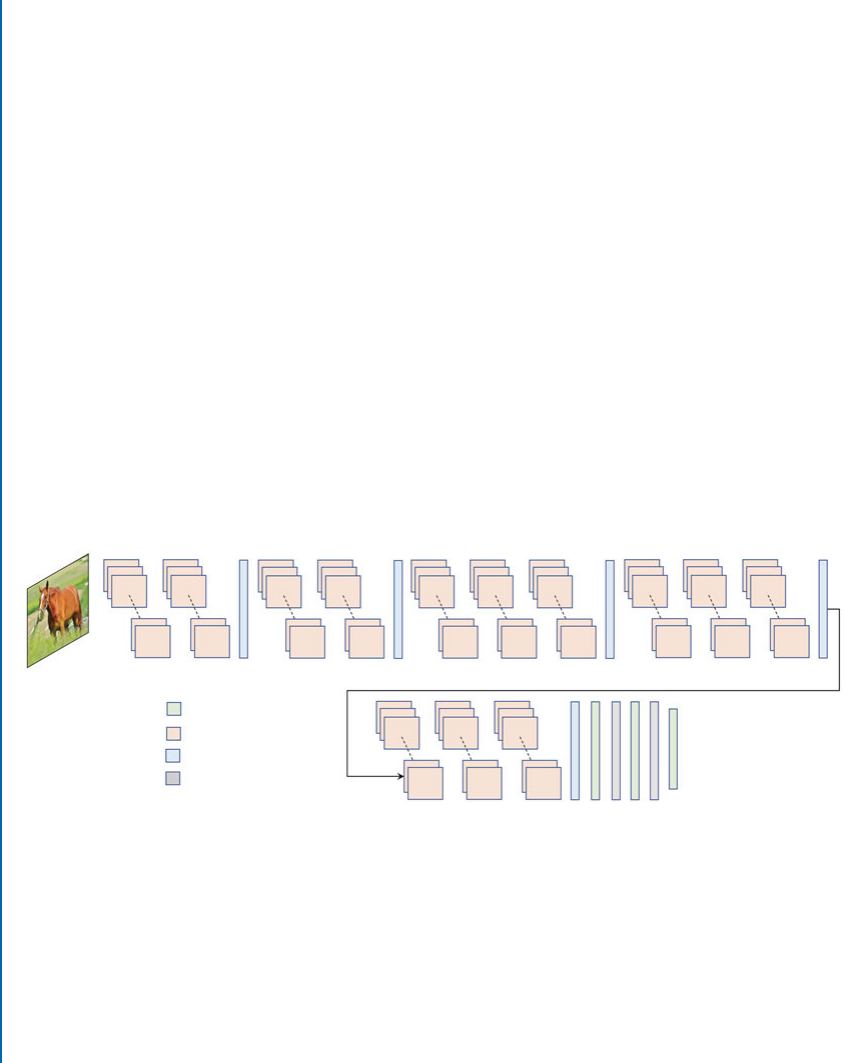
104 6. EXAMPLES OF CNN ARCHITECTURES
6.4 VGGNET
e VGGnet architecture [Simonyan and Zisserman,2014b] is one of the most popular CNN
models since its introduction in 2014, even though it was not the winner of ILSVRC’14. e
reason for its popularity is in its model simplicity and the use of small-sized convolutional kernels
which leads to very deep networks. e authors introduced a set of network configurations,
among which the configuration D and E (commonly referred as VGGnet-16 and VGGnet-19
in the literature) are the most successful ones.
e VGGnet architecture strictly uses 33convolution kernels with intermediate max-
pooling layers for feature extraction and a set of three fully connected layers toward the end for
classification. Each convolution layer is followed by a ReLU layer in the VGGnet architecture.
e design choice of using smaller kernels leads to a relatively reduced number of parameters, and
therefore an efficient training and testing. Moreover, by stacking a series of 33sized kernels,
the effective receptive field can be increased to larger values (e.g., 55with two layers, 77with
three layers, and so on). Most importantly, with smaller filters, one can stack more layers resulting
in deeper networks, which leads to a better performance on vision tasks. is essentially conveys
the central idea of this architecture, which supports the usage of deeper networks for an improved
feature learning. Figure 6.4 shows the best performing model VGGnet-16 (confiugration D)
which has 138 million parameters. Similar to AlexNet, it also uses activation dropouts in the
first two fully connected layers to avoid over-fitting.
Input Image
(224×224×3)
3×3
(256) 3×3
(256) 3×3
(256) 3×3
(512)
3×3
(512) 3×3
(512) 3×3
(512)
3×3
(512) 3×3
(512)
3×3
(64) 3×3
(64) 3×3
(128) 3×3
(128)
4096 4096 1000
Fully Connected Layers
Convolution Layers
Max-pooling Layers
Dropout Layers
Figure 6.4: e VGGnet-16 Architecture (configuration-D).
6.5 GOOGLENET
All the previously discussed, networks consists of a sequential architecture with only a single
path. Along this path, different types of layers such as the convolution, pooling, ReLU, dropout,
and fully connected layers are stacked on top of each others to create an architecture of desired
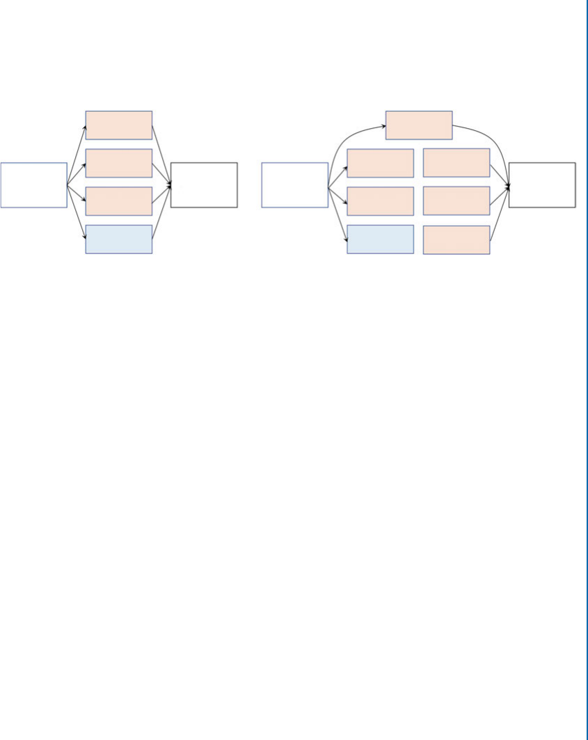
6.5. GOOGLENET 105
depth. e GoogleNet [Szegedy et al.,2015] architecture is the first popular model which uses
a more complex architecture with several network branches. is model won the ILSVRC’14
competition with the best top-5 error rate of 6.7% on the classification task. Afterward, sev-
eral improved and extended versions of GoogleNet have also been proposed. However, we will
restrict this discussion to the ILSVRC’14 submission of the GoogleNet.
Convolution
Layer (1×1)
Convolution
Layer (1×1)
Output from
Previous Layer
Output from
Previous Layer
Feature
Concatenation
(along depth)
Feature
Concatenation
(along depth)
Convolution
Layer (3×3)
Convolution
Layer (1×1)
Convolution
Layer (3×3)
Convolution
Layer (5×5)
Convolution
Layer (1×1)
Convolution
Layer (1×1)
Convolution
Layer (5×5)
Max-pooling
(3×3)
Max-pooling
(3×3)
(a) Basic Inception Module Concept (b) Inception Module with Dimension Reductions
Figure 6.5: e Inception Module.
GoogleNet consists of a total of 22 weight layers. e basic building block of the network
is the “Inception Module,” due to which the architecture is also commonly called the “Inception
Network.” e processing of this module happens in parallel, which is in contrast to the sequen-
tial processing of previously discussed architectures. A simple (naive) version of this module
in shown in Fig. 6.5a. e central idea here is to place all the basic processing blocks (which
occur in a regular sequential convolutional network) in parallel and combine their output fea-
ture representations. e good thing with this design is that multiple inception modules can be
stacked together to create a giant network and without the need to worry about the design of
each individual layer at different stages of the network. However, as you might have noticed,
the problem is that if we concatenate all the individual feature representations from each indi-
vidual block along the depth dimension, it will result in a very high-dimensional feature output.
To overcome this problem, the full inception module performs dimensionality reduction before
passing the input feature volume (say with dimensions hwd) through the 33and 55
convolution filters. is dimensionality reduction is performed by using a fully connected layer
which is equivalent to a 11dimensional convolution operation. As an example, if the 11
convolution layer has d0filters, such that d0< d , the output from this layer will have a smaller
dimension of hwd0. We saw a similar fully connected layer before the convolution layer in
the NiN architecture discussed earlier in Section 6.3. In both cases, such a layer leads to a better
performance. You may be wondering why a fully connected layer is useful when used before the
convolutional layers. e answer is that while the convolution filters operate in the spatial do-
main (i.e., along the height and width of the input feature channels), a fully connected layer can
combine information from multiple feature channels (i.e., along the depth dimension). Such a

106 6. EXAMPLES OF CNN ARCHITECTURES
flexible combination of information leads to not only reduced feature dimensions, but also to an
enhanced performance of the inception module.
If you closely look at the inception module (Fig. 6.5), you can understand the intuition
behind the combination of a set of different operations into a single block. e advantage is
that the features are extracted using a range of filter sizes (e.g., 11; 3 3; 5 5) which cor-
responds to different receptive fields and an encoding of features at multiple levels from the
input. Similarly, there is a max-pooling layer which down-samples the input to obtain a feature
representation. Since all the convolution layers in the GoogleNet architecture are followed by a
ReLU nonlinearity, this further enhances the capability of the network to model nonlinear re-
lationships. In the end, these different complementary features are combined together to obtain
a more useful feature representation.
In the GoogleNet architecture shown in Fig. 6.6, 9 inception modules are stacked together,
which results in a 22 layer deep network (the total number of layers in the network is > 100).
Similar to NiN, GoogleNet uses a global average pooling followed by a fully connected layer
toward the end of the network for classification. e global average pooling layer provides faster
computations with a better classification accuracy and a much reduced number of parameters.
Another intuitive characteristic of the GoogleNet design is the availability of several output
branches in the intermediate layers (e.g., after 4a and 4d), where classifiers are trained on the
end task. is design feature avoids the vanishing gradients problem by passing strong feedback
signals to the initial layers due to the classification branches extended from the initial layers.
GoogleNet also uses dropout before the final fully connected layers in each output branch for
regularization.
Although the GoogleNet architecture looks much more complex than its predecessors,
e.g., AlexNet and VGGnet, it involves a significantly reduced number of parameters (6 million
compared to 62 million in AlexNet and 138 million parameters in VGGnet). With a much
smaller memory footprint, a better efficiency and a high accuracy, GoogleNet is one of the most
intuitive CNN architectures which clearly demonstrates the importance of good design choices.
6.6 RESNET
e Residual Network [He et al.,2016a] from Microsoft won the ILSVRC 2015 challenge
with a big leap in performance, reducing the top-5 error rate to 3.6% from the previous year’s
winning performance of 6.7% by GoogleNet [Szegedy et al.,2015]. It is worth mentioning here
that the ILSVRC 2016 winners obtained an error rate of 3.0% using an ensemble of previous
popular models such as the GoogleNet Inception and the Residual Network, along with their
variants (e.g., Wide Residual Networks and the Inception-ResNets) [ILS].
e remarkable feature of the residual network architecture is the identity skip connections
in the residual blocks, which allows to easily train very deep CNN architectures. To understand
these connections, consider the residual block in Fig. 6.7. Given an input x, the CNN weight
layers implement a transformation function on this input, depicted by F .x/. In a residual block,
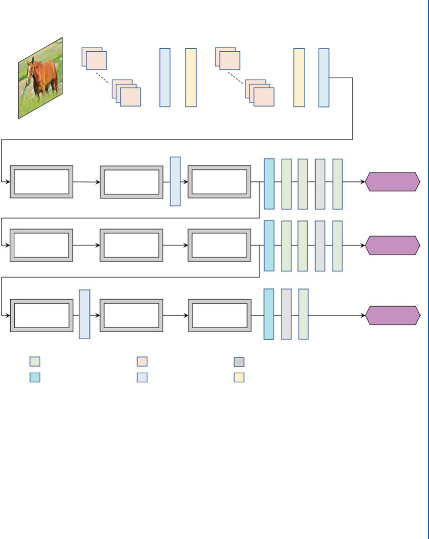
6.6. RESNET 107
Input Image
(224×224×3)
Inception 3a Inception 3b Inception 4a
Inception 4b Inception 4c Inception 4d
Inception 4e Inception 5a Inception 5b Softmax 3
Softmax 2
Softmax 1
7×7 (64)
Stride 2, Padding 3 3×3 (192)
Padding 1
3×3
Stride 2 3×3
Stride 2
5×5
(Stride 3) 128 1024 1000
.7
.7
.7
5×5
(Stride 3)
3×3 (Stride 2)
3×3 (Stride 2)
128 1024 1000
7×7 1000
Fully Connected Layers Convolution Layers Dropout Layers
Average Pooling Max-pooling Layers Local Response Normalization
Figure 6.6: e GoogleNet Architecture. All the inception modules have the same basic archi-
tecture as described in Fig. 6.5b, however, the number of filters in each layer are different for
each module. As an example, Inception 3a has 64 filters in the top-most branch (see Fig. 6.5b),
96 and 128 filters in the second branch from top, 16 and 32 filters in the third branch from top
and 32 filters in the bottom branch. In contrast, Inception 4a has 192 filters in the top-most
branch (in Fig. 6.5b), 96 and 208 filters in the second branch from top, 16 and 48 filters in the
third branch from top and 64 filters in the bottom branch. Interested readers are referred to
Table 1 in Szegedy et al. [2015] for the exact dimensions of all layers in each inception block.

108 6. EXAMPLES OF CNN ARCHITECTURES
the original input is added to this transformation using a direct connection from the input,
which bypasses the transformation layers. is connection is called the “skip identity connection.”
In this way, the transformation function in a residual block is split into an identity term (which
represents the input) and a residual term, which helps in focusing on the transformation of the
residue feature maps (Fig. 6.7). In practice, such an architecture achieves a stable learning of
very deep models. e reason is that the residual feature mapping is often much simpler than
the unreferenced mapping learned in the conventional architectures.
Just like the inception module in GoogleNet, the Residual Network comprises multiple
residual blocks stacked on top of each others. e winning model of ILSVRC consisted of 152
weights layers (about 8deeper than the VGGnet-19), which is shown along with a 34 layer
model in Table 6.1. Figure 6.8 shows the 34 layer Residual Network as a stack of multiple residual
blocks. Note that in contrast to ResNet, a very deep plain network without any residual connec-
tions achieves much higher train and test error rates. is shows that the residual connections
are key to a better classification accuracy of such deep networks.
e weight layers in the residual block in Fig. 6.7 are followed by a batch normalization
and a ReLU activation layer. In this design, the identity mapping has to pass through the ReLU
activation after addition with the output of the weight layers. A follow-up work from the authors
of Residual Networks demonstrated that this “post-activation” mechanism can be replaced by a
“pre-activation” mechanism, where the batch normalization and ReLU layers are placed before
the weight layers [He et al.,2016b]. is leads to a direct “unhindered” identity connection
from the input to the output which further enhances the feature learning capability of very deep
networks. is idea is illustrated in Fig. 6.9. With this modified design of the residual blocks,
networks of a depth of 200 layers were shown to perform well without any over-fitting on the
training data (in contrast to the previous design of Residual Networks which started over-fitting
for the same number of layers).
Another similar network architecture is the Highway network [Srivastava et al.,2015],
which adds learnable parameters to the shortcut and the main branches. is acts as a switching
mechanism to control the signal flow through both the main and the shortcut branches and
allows the network to decide which branch is more useful for the end-task.
6.7 RESNEXT
e ResNeXt architecture combines the strengths of GoogleNet and ResNet designs. Specifi-
cally, it utilizes skip connections which were proposed for residual networks and combines them
with the multi-branch architecture in the inception module. is applies a set of transformations
to the input feature maps and merges the resulting outputs together before feed-forwarding the
output activations to the next module.
e ResNext block is different to the inception module in three key aspects. First, it con-
tains a considerably large number of branches compared to the inception module. Second, in
contrast to different sizes of filters in different branches of the inception architecture, the se-
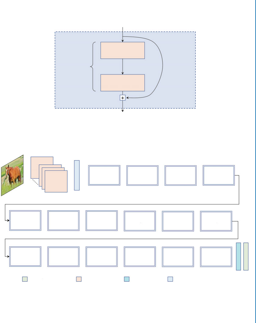
6.7. RESNEXT 109
Residual
Block (f,n) Convolution Layer
(‘f×f ’ size, ‘n’ filters)
Relu Non-linearityF (x)
x + F (x)
x
Identity
Connection
Relu Non-linearity
Convolution Layer
(‘f×f ’ size, ‘n’ filters)
Figure 6.7: e Residual Block.
Input Image
Residual Block
(3×3, 64)
Residual Block
(3×3, 64)
Residual Block
(3×3, 64)
Residual Block
(3×3, 128)
Residual Block
(3×3, 256)
Residual Block
(3×3, 256)
Residual Block
(3×3, 256)
Residual Block
(3×3, 128)
Residual Block
(3×3, 128)
Residual Block
(3×3, 128)
Residual Block
(3×3, 256)
Residual Block
(3×3, 256)
Residual Block
(3×3, 256)
Residual Block
(3×3, 512)
Residual Block
(3×3, 512)
Residual Block
(3×3, 512)
Softmax 2
Softmax 1
7×7 (64)
Stride 2 3×3
Stride 2
10007×7
Fully Connected Layers Convolution Layers Average Pooling Max-pooling Layers
Figure 6.8: e Residual Network architecture.

110 6. EXAMPLES OF CNN ARCHITECTURES
Table 6.1: e ResNet Architecture for a 34-layer (left) and a 152-layer network (right). Each
residual block is encompassed using a right brace (g) and the number of similar residual blocks is
denoted beside each brace (e.g., 3denotes three consecutive residual blocks). e residual block
in the 34-layer network consists of two convolution layers each with 33filters. In contrast,
each residual block in the 152-layer network consists of three convolution layers with 11,
33and 11filter sizes, respectively. is design of a residual block is called the “bottleneck
architecture” because the first convolution layer is used to reduce the number of feature channels
coming from the previous layer (e.g., the first convolution layer in the second group of residual
blocks in the 152-layer network reduce the number of feature channels to 128). Note that the
depth of the architecture can be increased by simply replicating the basic residual block which
contains identity connections (Fig. 6.7). For clarity, the 34-layer network architecture has also
been illustrated in Fig. 6.8.
ResNet (34 Layers) ResNet (152 Layers)
cnv–7×7 (64), stride 2
maxpool–3×3, stride 2
cnv–3×3 (64)
cnv–3×3 (64)
cnv–3×3 (128)
cnv–3×3 (128)
cnv–3×3 (256)
cnv–3×3 (256)
cnv–3×3 (512)
cnv–3×3 (512)
avgpool
cnv–1×1 (1000)
softmax loss
cnv–7×7 (64), stride 2
maxpool–3×3, stride 2
cnv–1×1 (64)
cnv–3×3 (64)
cnv–1×1 (256)
cnv–1×1 (128)
cnv–3×3 (128)
cnv–1×1 (512)
cnv–1×1 (256)
cnv–3×3 (256)
cnv–1×1 (1024)
cnv–1×1 (512)
cnv–3×3 (512)
cnv–1×1 (2048)
avgpool
cnv–1×1 (1000)
softmax loss
×3 ×3
×3
×8
×36
×3
×4
×6
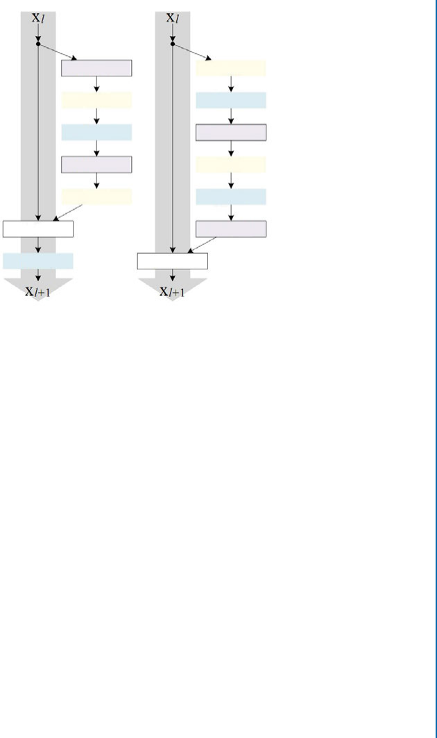
6.7. RESNEXT 111
Weight
ReLU
ReLU
Addition
Addition
BN
BN
Weight
ReLU
ReLU
BN
BN
Weight
Weight
(a) Original (b) Proposed
Figure 6.9: e residual block with pre-activation mechanism [He et al.,2016b]. (Figure used
with permission.)
quence of transformations in each branch are identical to other branches in the ResNext module.
is simplifies the hyper-parameter choices of the ResNext architecture, compared to the incep-
tion module. Finally, the ResNext block contains skip connections which have been found to
be critical in the training of very deep networks. A comparison between a ResNet and ResNext
block is shown in Fig. 6.10. Note that the multi-branch architecture, followed by the aggregation
of responses, leads to an improved performance compared to ResNet. Specifically, a 101-layer
ResNeXt architecture was able to achieve a better accuracy than ResNet with almost a double
size (200 layers).
e overall ResNext architecture is identical to the ResNet design shown in Table 6.1.
e only difference is that the residual blocks are replaced with the ResNext blocks described
above. For efficiency purposes, the group of transformations in each ResNext block are imple-
mented as grouped convolutions, where all the Ntransformation paths are joined in a single layer
with a number of output channels equal to NC, when Cis the number of output channels in
each individual transformation layer. As an example, the first layer in a ResNext block, shown in
Fig. 6.10, is implemented as a single layer with 32 4output channels. e grouped convolu-
tions only allow convolutions within each of the 32 groups, effectively resembling the multi-path
architecture shown in the ResNext block.
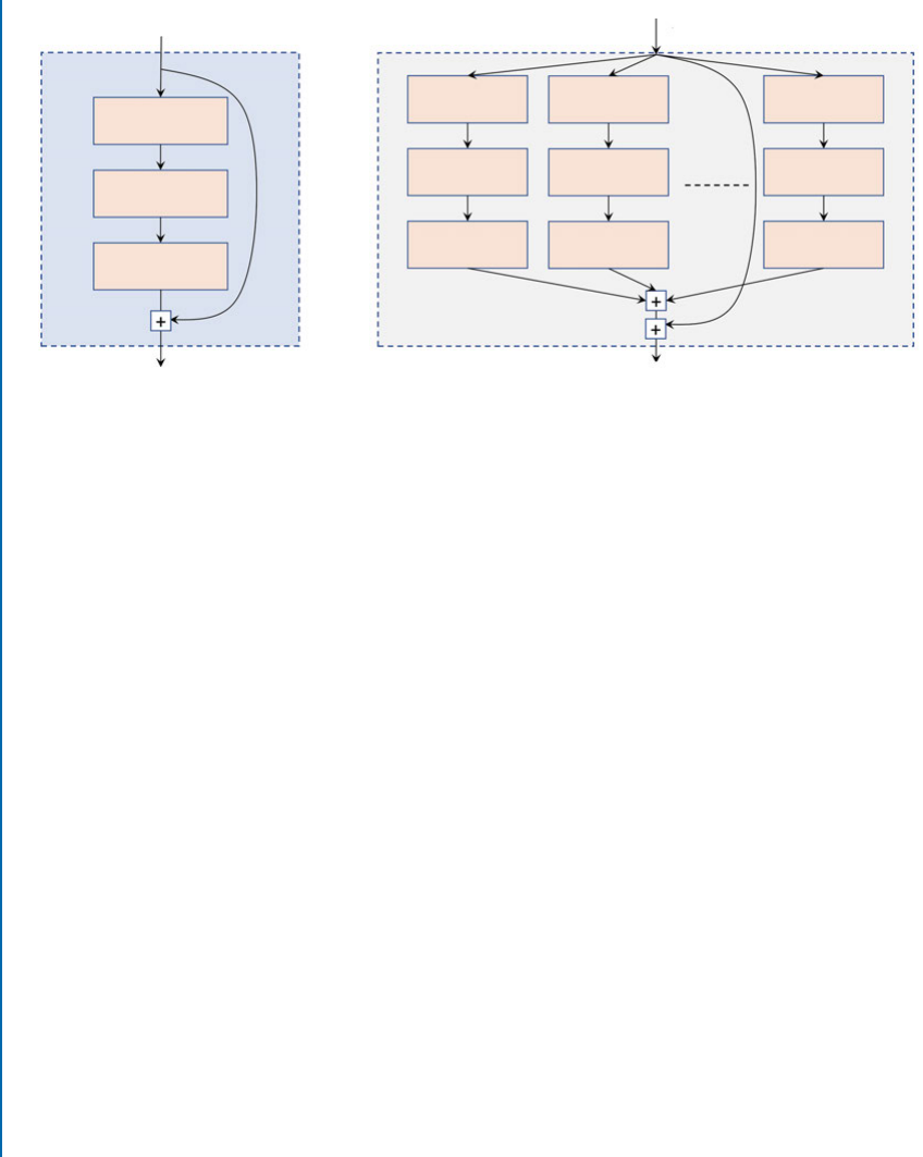
112 6. EXAMPLES OF CNN ARCHITECTURES
256 Dimensional Input 256 Dimensional Input
256 Dimensional Output
(a) A ResNet Block with
Bottleneck Architecture
(b) A ResNext Block with Bottleneck Architecture
256 Dimensional Output
Conv (1×1, 64)
Conv (3×3, 64)
Conv (1×1, 256)
Conv (1×1, 4)
Conv (3×3, 4)
Conv (1×1, 256)
Conv (1×1, 4)
Conv (3×3, 4)
Conv (1×1, 256)
Conv (1×1, 4)
Total 32
Branches Conv (3×3, 4)
Conv (1×1, 256)
Figure 6.10: A ResNet (a) and a ResNext (b) block with roughly the same number of parame-
ters. While the ResNet block comprises a single main branch alongside a skip connection, the
ResNext block consists of a number of branches (formally termed the “block cardinality”), each
of which implements a transformation. e proposed ResNext block has 32 branches, where
each transformation is shown as the number of input channels filter dimensions number of
output channels.
6.8 FRACTALNET
e FractalNet design is based on the observation that the residual-based learning is not the only
key enabler for a successful training of very deep convolutional networks. Rather, the existence of
multiple shortcut paths for (both forward and backward) information flow in a network enable a
form of deep supervision, which helps during the network training. e fractal design achieves
a better performance than its residual counterparts on MNIST, CIFAR-10, CIFAR-100, and
SVHN datasets when no data augmentation is used during model training [Larsson et al.,2016].
e fractal design is explained in Fig. 6.11. Instead of a single main branch (as in VGG)
or a two branch network where on of them is an identity connection which learns residual func-
tions, the fractal design consists of multiple branches each of which has a different number of
convolution layers. e number of convolution layers depends on the column number of the
branch in the fractal block. If crepresents the column number, the number of layers in the cth
branch is 2c1. For example, the first column from the left has only one weight layer, the second
column has two weight layers, the third has four and the fourth has eight weight layers. If C
denotes the maximum number of columns in a FractalNet block, the total depth of the block
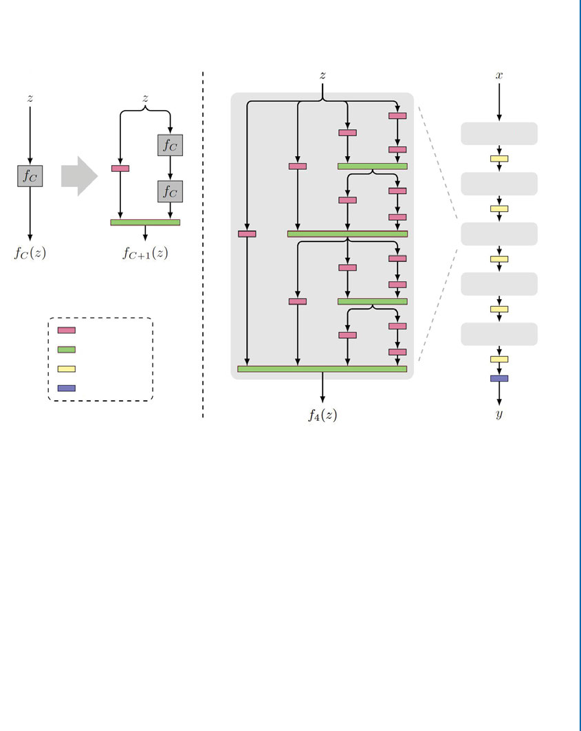
6.8. FRACTALNET 113
will be 2C1. Note that the outputs from multiple branches are averaged together to produce a
joint output.
Fractal Expansion Rule
Block 1
Block 2
Block 3
Block 4
Block 5
Layer Key
Convolution
Join
Pool
Prediction
Figure 6.11: Left: e basic fractal design expansion rule is shown. It contains two branches
for information flow. Each branch transforms the input using a single (left branch) or multi-
ple transformations (right branch). Right: A FractalNet [Larsson et al.,2016] with five fractal
blocks. Each block consists of Ccolumns and Hhierarchies of fractals. In the example block
shown, CD4and HD3. (Figure used with permission.)
In order to avoid redundant features representations and co-adaptations between the
branches, FractalNet utilizes “path-dropout” for the regularization of the network. e path-
dropout randomly ignores one of the incoming paths during the joining operation. Although
this approach (called the “local drop-path”) acts as a regularizer, multiple paths may still be avail-
able from input to output. erefore, a second version of path-dropout (called the “global drop-
path”) was also introduced where only a single column was randomly picked in a FractalNet.
Both these regularizations were alternatively applied during the network training to avoid model
over-fitting.
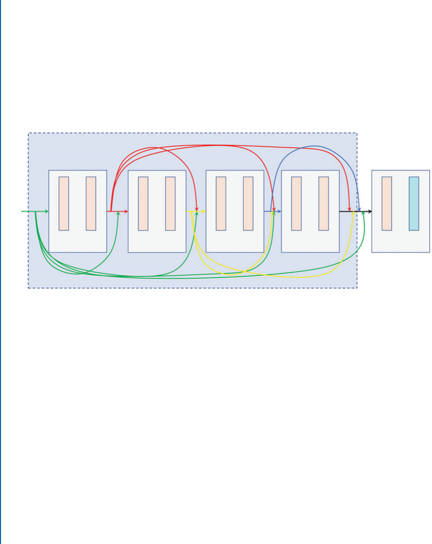
114 6. EXAMPLES OF CNN ARCHITECTURES
6.9 DENSENET
e use of skip (and shortcut) connections in the previously discussed architectures, such as
ResNet, FractalNet, ResNext, and Highway networks avoid the vanishing gradient problem
and enable the training of very deep networks. DenseNet extends this idea by propagating the
output of each layer to all subsequent layers, effectively easing the information propagation in
the forward and backward directions during network training [Huang et al.,2016a]. is allows
all layers in the network to “talk” to each other, and to automatically figure out the best way to
combine multi-stage features in a deep network.
DenseNet Block
Input Feature Maps
Transition Layer
Conv
(1×1, 4k)
Conv
(3×3, k)
Conv
(1×1, 4k)
Conv
(3×3, k)
Conv
(1×1, 4k)
Conv
(3×3, k)
Conv
(1×1, 4k)
Conv
(3×3, k)
Conv
(1×1)
Avg Pool
(2×2, k)
Figure 6.12: A densely connected CNN block with five layers. Note that every layer receives
features from all preceding layers. A transition layer is used toward the end of each dense block
to reduce the feature set dimensionality.
An example DenseNet is shown in Fig. 6.12. Since the information flow is in the forward
direction, every initial layer is directly connected to all the following layers. ese connections
are realized by concatenating the feature maps of a layer with the feature maps from all the
preceding layers. is is in contrast to ResNet, where skip connections are used to add the
output from an initial layer before processing it through the next ResNet block (see Fig. 6.10).
ere are three main consequences of such direct connections in a DenseNet. First, the features
from the initial layers are directly passed on to the later layers without any loss of information.
Second, the number of input channels in the subsequent layers of a DenseNet increases rapidly
because of the concatenation of the preceding feature maps from all preceding layers. To keep
the network computations feasible, the number of output channels (also termed the “growth rate”
in DenseNets) for each convolutional layer are relatively quite small (e.g., 6 or 12). ird, the
concatenation of feature maps can only be performed when their spatial sizes match with each
other. erefore, a densely connected CNN consists of multiple blocks, each of which has dense
connections within the layers and the pooling or strided convolution operations are performed
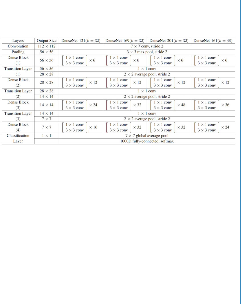
6.9. DENSENET 115
in-between these blocks to collapse the input to a compact representation (see Fig. 6.13). e
layers which reduce the size of feature representations between each pair of DenseNet blocks
are called the “transition layers.” e transition layers are implemented as a combination of batch
normalization, an 1×1 convolutional layer and by a 2×2 average pooling layer.
Figure 6.13: Variants of DenseNet Architectures [Huang et al.,2016a]. In each variant, the
number of dense blocks remain the same (i.e., 4), however the growth rate and the number
of convolution layers are increased to design larger architectures. Each transition layer is im-
plemented as a combination of dimensionality reduction layer (with 11convolutional filters)
and an average pooling layer for sub-sampling. (Table used with permission from Huang et al.
[2016a].)
e concatenated feature maps from the preceding layers in a DenseNet block are not
tunable. erefore, each layer learns its own representation and concatenates it with the global
information which comes from the previous network stages. is information is then provided
to the next layer which can add additional information, but cannot directly alter the global
information that was learned by the previous layers. is design greatly reduces the number of
tunable parameters and explicitly differentiates between the global state of the network and the
local contribution additions, that are made by each layer to the global state.
DenseNet borrows several design choices from the previous best approaches. For example,
a pre-activation mechanism where each convolution layer is preceded by a Batch Normalization
and a ReLU layer. Similarly, bottleneck layers with 11filters are used to first reduce the
number of input feature maps before processing them through the 33filter layers. DenseNet
achieves state of the art performance on a number of datasets such as MNIST, CIFAR10, and
CIFAR100 with a relatively less number of parameters compared to ResNet.

117
C H A P T E R 7
Applications of CNNs in
Computer Vision
Computer vision is a very broad research area which covers a wide variety of approaches not only
to process images but also to understand their contents. It is an active research field for convolu-
tional neural network applications. e most popular of these applications include, classification,
segmentation, detection, and scene understanding. Most CNN architectures have been used for
computer vision problems including, supervised or unsupervised face/object classification (e.g.,
to identify an object or a person in a given image or to output the class label of that object), de-
tection (e.g., annotate an image with bounding boxes around each object), segmentation (e.g.,
labeling pixels of an input image), and image generation (e.g., converting low-resolution images
to high resolution ones). In this chapter, we describe various applications of convolutional neural
networks in computer vision. Note that this chapter is not a literature review, it rather provides
a description of representative works in different areas of computer vision.
7.1 IMAGE CLASSIFICATION
CNNs have been shown to be an effective tool for the task of image classification [Deng,2014].
For instance, in the 2012 ImageNet LSVRC contest, the first large-scale CNN model, which
was called AlexNet [Krizhevsky et al.,2012] (Section 6.2), achieved considerably lower error
rates compared to the previous methods. ImageNet LSVRC is a challenging contest as the
training set consists of about 1.2 million images belonging to 1,000 different classes, while the
test set has around 150,000 images. After that, several CNN models (e.g., VGGnet, GoogleNet,
ResNet, DenseNet) have been proposed to further decrease the error rate. While Chapter 6has
already introduced these state-of-the art CNN models for image classification task, we will
discuss below a more recent and advanced architecture, which was proposed for 3D point cloud
classification (input to the model is a raw 3D point cloud) and achieved a high classification
performance.
7.1.1 POINTNET
PointNet [Qi et al.,2016] is a type of neural network which takes orderless 3D point clouds as
input and well respects the permutation invariance of the input points. More precisely, PointNet
approximates a set function gdefined on an orderless 3D point cloud, fx1; x2; ; xng, to map
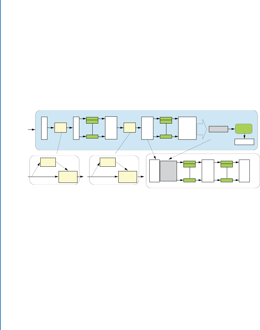
118 7. APPLICATIONS OF CNNS IN COMPUTER VISION
the point cloud to a vector:
g.fx1; x2; ; xng/D. max
iD1nfh.xi/g/; (7.1)
where and hare multi-layer perceptron (mlp) networks. us, the set function gis invariant to
the permutation of the input points and can approximate any continuous set function [Qi et al.,
2016].
PointNet, shown in Fig. 7.1, can be used for classification, segmentation, and scene se-
mantic parsing from point clouds. It directly takes an entire point cloud as input and outputs
a class label to accomplish 3D object classification. For segmentation, the network returns per-
point labels for all points within the input point cloud. PointNet has three main modules, which
we briefly discuss below.
3D Points
Input
Transform
Input Transform T-Net
3×3
Transform
64×64
Transform
Feature
Transform
n×3
n×3
n×64
n×64
n×1024
Shared Shared
Shared Shared
mlp(64, 64) mlp(64, 128, 1024) mlp
(512, 256, k)
mlp (512, 256, 128) mlp (128, m)
Max
Pool f
1024
Global
Feature
Point Features
Output
Scores
Output
Scores
g
n
T-Net
Matrix
Multiply Matrix
Multiply
T-Net
× 1088
Module A
Submodule A-1
Feature TransformT-Net
Submodule A-2
Segmentation Network
Module B
Classification Network
n×128
n×m
Figure 7.1: PointNet architecture: e input to classification network (Module A) are 3D point
clouds. e network applies a sequence of non-linear transformations, including input and fea-
ture transformations (Submodule A-1), and then uses max-pooling to aggregate point features.
e output is a classification score for Cnumber of classes. e classification network can be
extended to form the segmentation network (Module B). “mlp” stands for multi-layered per-
ceptron and numbers in bracket are layer sizes.
Classification Network (Module A):
e first key module of PointNet is the classification network (module A), shown in Fig. 7.1.
is module consists of input (Submodule A-1) and feature (Submodule A-2) transformation
networks, multi-layer perceptrons (mlp) networks, and a max-pooling layer. Each point within
the orderless input point cloud (fx1; x2; ; xng) is first passed through two shared mlp networks
(function h./in Eq. (7.1)) to transfer 3D points to a high dimensional, e.g., 1024-dimensional,
feature space. Next, the max-pooling layer (function max./in Eq. (7.1)) is used as a symmetric

7.1. IMAGE CLASSIFICATION 119
function to aggregate information from all the points, and to make a model invariant to input
permutations. e output of the max-pooling layer ( max
iD1nfh.xi/gin Eq. (7.1)) is a vector, which
represents a global shape feature of the input point cloud. is global feature is then passed
through an mlp network followed by a soft-max classifier (function ./in Eq. (7.1)) to assign
a class label to the input point cloud.
Transformation/Alignment Network (Submodule A-1 and Submodule A-2):
e second module of PointNet is the transformation network (mini-network or T-net in
Fig. 7.1), which consists of a a shared mlp network, that is applied on each point, followed by a
max-pooling layer which is applied across all points and two fully connected layers. is network
predicts an affine transformation to ensure that the semantic labeling of a point cloud is invari-
ant to geometric transformations. As shown in Fig. 7.1, there are two different transformation
networks, including the input (Submodule A-1) and the feature transformation (Submodule
A-2) networks. e input 3D points are first passed through the input transformation network
to predict a 33affine transformation matrix. en, new per-point features are computed by
applying the affine transformation matrix to the input point cloud (“Matrix multiply” box in
Submodule A-1).
e feature transform network is a replica of the input transform network, shown in
Fig. 7.1 (Submodule A-2), and is used to predict the feature transformation matrix. How-
ever, unlike the input transformation network, the feature transformation network takes 64-
dimensional points. us, its predicted transformation matrix has a dimension of 64 64, which
is higher than the input transformation matrix (i.e., 3 3 in Submodule A-1). is contributes
to the difficulty of achieving optimization. To address this problem, a regularization term is
added to the soft-max loss to constrain the 64 64 feature transformation matrix to be close to
an orthogonal matrix:
Lreg D
IAAT
2
F;(7.2)
where Ais the feature transformation matrix.
Segmentation Network (Module B):
PointNet can be extended to predict per point quantities, which rely on both the local geometry
and the global semantics. e global feature computed by the classification network (Module
A) is fed to the segmentation network (Module B). e segmentation network combines the
global and per-point point features, and then passed them through an mlp network to extract
new per-point features. ese new features contain both the global and local information, which
has shown to be essential for segmentation [Qi et al.,2016]. Finally, the point features are passed
through a shared mlp layer to assign a label to each point.
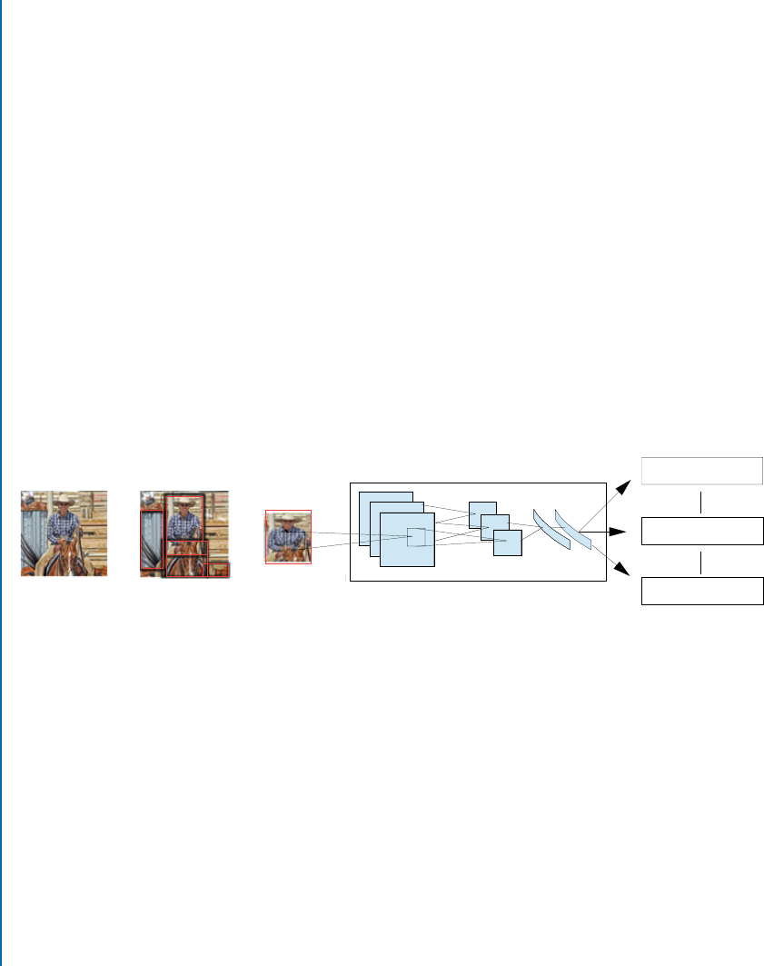
120 7. APPLICATIONS OF CNNS IN COMPUTER VISION
7.2 OBJECT DETECTION AND LOCALIZATION
Recognizing objects and localizing them in images is one of the challenging problems in com-
puter vision. Recently, several attempts have been made to tackle this problem using CNNs. In
this section, we will discuss three recent CNN-based techniques, which were used for detection
and localization.
7.2.1 REGION-BASED CNN
In Girshick et al. [2016], Region-based CNN (R-CNN) has been proposed for object detection.
It will be good to give here the broad idea behind R-CNN, i.e., region wise feature extraction
using deep CNNs and the learning of independent linear classifiers for each object class. e
R-CNN object detection system consists of the following three modules.
Regional Proposals (Module A in Fig. 7.2) and Feature Extraction (Module B)
Given an image, the first module (Module A in Fig. 7.2) uses selective search [Uijlings et al.,
2013] to generate category-independent region proposals, which represent the set of candidate
detections available to the object detector.
Input
Image
Extract Region
Proposals
Warped
Region
Module A Module B Module C
Compute
CNN Features
Classify Regions
Aeroplane? No.
TV monitor? No.
Person? Yes.
Figure 7.2: RCNN object detection system. Input to R-CNN is an RGB image. It then extracts
region proposals (Module A), computes features for each proposal using a deep CNN, e.g.,
AlexNet (Module B), and then classifies each region using class-specific linear SVMs (Module
C).
e second module (Module B in Fig. 7.2) is a deep CNN (e.g., AlexNet or VGGnet),
which is used to extract a fixed-length feature vector from each region. In both cases (AlexNet or
VGGnet), the feature vectors are 4096-dimensional. In order to extract features from a region
of a given image, the region is first converted to make it compatible with the network input.
More precisely, irrespective of the candidate region’s aspect ratio or size, all pixels are converted
to the required size by warping them in a tight bounding box. Next, features are computed by
forward propagating a mean-subtracted RGB image through the network and reading off the
output values by the last fully connected layer just before the soft-max classifier.

7.2. OBJECT DETECTION AND LOCALIZATION 121
Training Class Specific SVMs (Module C)
After feature extraction, one linear SVM per class is learned, which is the third module of this
detection system. In order to assign labels to training data, all region proposals with an overlap
greater than or equal to 0.5 IoU with a ground-truth box are considered as positives for the class
of that box, while the rest are considered as negatives. Since the training data is very large for
the available memory, the standard hard negative mining method [Felzenszwalb et al.,2010] is
used to achieve quick convergence.
Pre-training and Domain Specific Training of Feature Extractor
For the pre-training of the CNN feature extractor, a large ILSVRC2012 classification dataset
with image-level annotations is used. Next, SGD training with the warped region proposals is
performed for adaptation of the network to the new domain and the new task of image detection.
e network architecture is kept unchanged except for a 1000-way classification layer, which is
set to 20C1 for PASCAL VOC and to 200C1 for ILSVRC2013 datasets (equal to the number
of classes in these datasets + background).
R-CNN Testing
At test time, a selective search is run to select 2,000 region proposals from the test image. To
extract features from these regions, each one of them is warped and then forward propagated
through the learned CNN feature extractor. SVM trained for each class is then used to score the
feature vectors of each class. Once all these regions have been scored, a greedy non-maximum
suppression is used to reject a proposal, which has an IoU overlap with a higher scoring selected
region greater than a pre-specified threshold. R-CNN has been shown to improve the mean
average precision (mAP) by a significant margin.
R-CNN Drawbacks
e R-CNN discussed above achieves an excellent object detection accuracy. However, it still
has few drawbacks. e training of R-CNN is multi-staged. In the case of R-CNN, soft-max
loss is employed to fine tune the CNN feature extractor (e.g., AlexNet, VGGnet) on object
proposals. SVM are next fitted to the network’s features. e role of SVMs is to perform object
detection and replace the soft-max classifier. In terms of complexity in time and space, the
training of this model is computationally expensive. is is because, every region proposal is
required to pass through the network. For example, training VGGnet-16 on 5,000 images of the
PASCAL VOC07 dataset using a GPU takes 2.5 days. In addition, the extracted features need
a huge storage, i.e., hundreds of gigabytes. R-CNN is also slow in performing object detection
at test time. For example, using VGGnet-16 (on a GPU) as the feature extractor in Module B,
detection of an object takes around 47 seconds per image. To overcome these problems, an
extension of R-CNN called the Fast R-CNN was proposed.
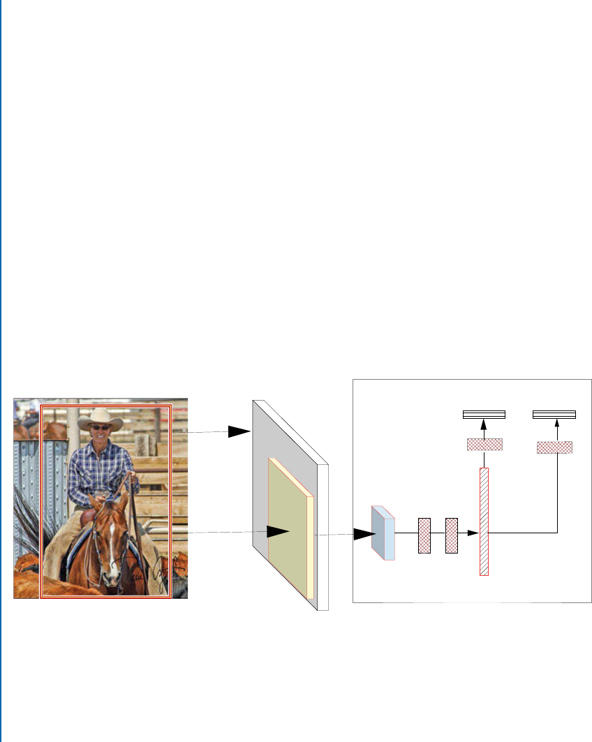
122 7. APPLICATIONS OF CNNS IN COMPUTER VISION
7.2.2 FAST R-CNN
Figure 7.3 shows the Fast R-CNN model. e input to Fast R-CNN is an entire image along
with object proposals, which are extracted using the selective search algorithm [Uijlings et al.,
2013]. In the first stage, convolutional feature maps (usually feature maps of the last convolu-
tional layer) are extracted by passing the entire image through a CNN, such as AlexNet and
VGGnet (Module A in Fig. 7.3). For each object proposal, a feature vector of fixed size is then
extracted from the feature maps by a Region of Interest (RoI) pooling layer (Module B), which
has been explained in Section 4.2.7. e role of the RoI pooling layer is to convert the features,
in a valid RoI, into small feature maps of fixed size (XY, e.g., 7 7), using max-pooling. X
and Yare the layer hyper-parameters. A RoI itself is a rectangular window which is character-
ized by a 4-tuple that defines its top-left corner (a,b) and its height and width (x,y). e RoI
layer divides the RoI rectangular area of size xyinto an XYgrid of sub-windows, which
has a size of x=X y=Y . e values in each sub-window are then max-pooled into the cor-
responding output grid. Note that the max-pooling operator is applied independently to each
convolutional feature map. Each feature vector is then given as input to fully connected layers,
which branch into two sibling output layers. One of these sibling layers (Module C in Fig. 7.3)
gives estimates of the soft-max probability over object classes and a background class. e other
layer (Module D in Fig. 7.3) produces four values, which redefine bounding box positions, for
each of the object classes.
Deep
ConvNet
RoI
Projection
RoI
Pooling
Layer
RoI Feature
Vector For each RoI
FC
FCs
Outputs:
Softmax
Bbox
Regressor
A
B
Conv
Feature Map
C D
Figure 7.3: Fast R-CNN Architecture. e input to a fully convolutional network (e.g., AlexNet)
is an image and RoIs (Module A). Each RoI is pooled into a fixed-size feature map (Module B)
and then passed through the two fully-connected layers to form a RoI feature vector. Finally, the
RoI feature vector is passed through two sibling layers, which output the soft-max probability
over different classes (Module C) and bounding box positions (Module D).

7.2. OBJECT DETECTION AND LOCALIZATION 123
Fast R-CNN Initialization and Training
Fast R-CNN is initialized from three pre-trained ImageNet models including:
AlexNet [Krizhevsky et al.,2012], VGG-CNN-M-1024 [Chatfield et al.,2014], and
VGGnet-16 [Simonyan and Zisserman,2014b] models. During initialization, a Fast R-CNN
model undergoes three transformations. First, a RoI pooling layer (Module B) replaces the last
max-pooling layer to make it compatible with the network’s first fully connected layer (e.g., for
VGGnet-16 X=Y= 7). Second, the two sibling layers ((Module C and Module D), discussed
above, replace the last fully connected layer and soft-max of the network. ird, the network
model is tweaked to accept two data inputs, i.e., a list of images and their RoIs. en SGD
simultaneously optimizes the soft-max classifier (Module C) and the bounding-box regressor
(Module D) in an end-to-end fashion by using a multi-task loss on each labeled RoI.
Detection Using Fast R-CNN
For detection, the Fast R-CNN takes as an input, an image along with a list of Robject propos-
als to score. During testing, Ris kept at around 2,000. For each test RoI (r), the class probability
score for each of the Kclasses (module C in Fig. 7.3) and a set of refined bounding boxes are
computed (module D in Fig. 7.3). Note that each of the Kclasses has its own refined bounding
box. Next, the algorithm and the configurations from R-CNN are used to independently per-
form non-maximum suppression for each class. Fast R-CNN has been shown to achieve a higher
detection performance (with a mAP of 66% compared to 62% for R-CNN) and computational
efficiency on PASCAL VOC 2012 dataset. e training of Fast R-CNN, using VGGnet-16,
was 9faster than R-CNN and this network was found 213 faster at test-time.
While Fast R-CNN has increased the training and testing speed of R-CNN by sharing a
single CNN computation across all region proposals, its computational efficiency is bounded by
the speed of the region proposal methods, which are run on CPUs. e straightforward approach
to address this issue is to implement region proposal algorithms on GPUs. Another elegant way
is to rely on algorithmic changes. In the following section, we discuss an architecture, known
as Regional Proposal Network [Ren et al.,2015], which relies on an algorithmic change by
computing nearly cost-free region proposals with CNN in an end-to-end learning fashion.
7.2.3 REGIONAL PROPOSAL NETWORK (RPN)
e Regional Proposal Network [Ren et al.,2015] (Fig. 7.4) simultaneously predicts object
bounding boxes and objectness scores at each position. RPN is a fully convolutional network,
which is trained in an end-to-end fashion, to produce high quality region proposals for object
detection using Fast R-CNN (described in Section 7.2.2). Combining RPN with Fast R-CNN
object detector results in a new model, which is called Faster R-CNN (shown in Fig. 7.5).
Notably, in Faster R-CNN, the RPN shares its computation with Fast R-CNN by sharing the
same convolutional layers, allowing for joint training. e former has five, while the later has
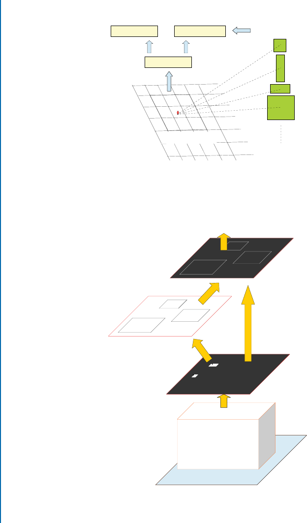
124 7. APPLICATIONS OF CNNS IN COMPUTER VISION
sliding window
Conv Feature Map
Module A
Module B Module D
Module C
For ZF: 256-d
For VGG Net: 512-d
cls Layer
2r Scores
256-d
4r Coordinates
reg Layer
r Anchor Boxes
Figure 7.4: Regional proposal network (RPN) architecture, which is illustrated at a single posi-
tion.
Classifier
Proposals
Region Proposal Network
Feature Maps
Conv Layers
Image
RoI Pooling
Figure 7.5: Faster R-CNN. Combining RPN with fast R-CNN object detector.

7.2. OBJECT DETECTION AND LOCALIZATION 125
13 shareable convolutional layers. In the following, we first discuss the RPN and then Faster
R-CNN, which merges RPN and Fast R-CNN into a single network.
e input to the RPN is an image (re-scaled in such a way that its smaller side is equal to
600 pixels) and the output is a set of object bounding boxes and associated objectness scores (as
shown in Fig. 7.4). To generate region proposals with RPN, the image is first passed through
the shareable convolutional layers. A small spatial window (e.g., 33) is then slid over the out-
put feature maps of the last shared convolutional layer, e.g., conv5 for VGGnet-16 (Module A
in Fig. 7.4). is sliding window at each position is then transformed to a lower-dimensional
vector of size 256-dand 512-dfor ZF and VGGnet-16 models (Module B in Fig. 7.4), respec-
tively. Next, this vector is given as an input to two sibling fully connected layers, including the
bounding box regression layer (reg) and the bounding box classification layer (cls) (Module C
in Fig. 7.4). In summary, the above-mentioned steps (Module A, Module B, and Module C)
can be implemented with a 33convolutional layer followed by two sibling 11convolutional
layers.
Multi-scale Region Proposal Detection
Unlike image/feature pyramid-based methods, such as the spatial pyramid pooling (SPP)
layer [He et al.,2015b] (discussed in Section 4.2.8), which uses time-consuming feature pyra-
mids in convolutional feature maps, RPN uses a nearly cost-free algorithm for addressing mul-
tiple scales and aspect ratios. For this purpose, rregion proposals are simultaneously predicted
at the location of each sliding window. e reg layer (Module C in Fig. 7.4) therefore encodes
the coordinates of rboxes by producing 4routputs. To predict the probability of “an object” or
“no object” in each proposal, the cls layer outputs 2rscores (the sum of outputs is 1 for each
proposal). e rproposals are parameterized relative to anchors (i.e., rreference boxes which
are centered at the sliding window as shown in Module D). ese anchors are associated with
three different aspect ratios and three different scales, resulting in a total of nine anchors at each
sliding window.
RPN Anchors Implementation
For the anchors, 3 scales with box areas of 1282,2562, and 5122pixels, and 3 aspect ratios of
2:1, 1:1, and 1:2 are used. When predicting large proposals, the proposed algorithm allows for
the use of anchors that are larger than the receptive field. is design helps in achieving high
computational efficiency, since multi-scale features are not needed.
During the training phase, all cross-boundary anchors are avoided to reduce their contri-
bution to the loss (otherwise, the training does not converge). ere are roughly 20kanchors,
i.e., 60 40 9, used for a 1,000 600 image.1By ignoring the cross-boundary anchors only
around 6kanchors per image are left for training. During testing, the entire image is given as
1Since the total stride for both ZF and VGG nets on the last convolutional layer is 16 pixels.

126 7. APPLICATIONS OF CNNS IN COMPUTER VISION
an input to the RPN. As a result, cross boundary boxes are produced which are then clipped to
the image boundary.
RPN Training
During the training of RPN, each anchor takes a binary label to indicate the presence of “an
object” or “no object” in the input image. Two types of anchors take a positive label: either an
anchor which has the highest IoU overlap or the IoU overlap is higher than 0.7 with ground-
truth bounding box. An anchor that has an IoU ratio lower than 0.3 is assigned a negative label.
In addition, the contribution of anchors which do not have a positive or negative label is not
considered toward the training objective. e RPN multi-task loss function for an image is given
by:
L.fpig;ftig/D1
Ncls X
i
Lcls.pi; p
i/C1
Nreg X
i
p
iLreg.ti; t
i/; (7.3)
where idenotes the index of an anchor, pirepresents the probability that an anchor iis an
object. p
istands for the ground-truth label, which is 1 for a positive anchor, and zero otherwise.
Vectors tiand t
icontain the four coordinates of the predicted bounding box and the ground-
truth box, respectively. Lcls is the soft-max loss over two classes. e term p
iLreg (where Lreg
is the regression loss) indicates the activation of the regression loss only for positive anchors,
otherwise it is disabled. Ncls,Nreg, and a balancing weight are next used to normalize cls and
reg layers.
Faster R-CNN Training: Sharing Convolutional Features for Region Proposal and Object
Detection
In the previous sections, we discussed the training of the RPN network for the generation of
region proposals. We did not, however, consider Fast R-CNN for region-based object detec-
tion using these proposals. In the following, we explain the training of the Faster R-CNN net-
work, that is composed of RPN and Fast R-CNN with shared convolutional layers, as shown in
Fig. 7.5.
Instead of learning the two networks (i.e., RPN and Fast R-CNN) separately, a four-
step alternating optimization approach is used to share convolutional layers between these two
models. Step 1: e RPN is trained using the previously stated strategy. Step 2: e proposals
produced by step 1 are used to train a separate Fast R-CNN detection network. e two networks
do not share convolutional layers at this stage. Step 3: e Fast R-CNN network initializes
the training of RPN and the layers specific to RPN are fine-tuned, while keeping the shared
convolutional layers fixed. At this point, the two networks share convolutional layers. Step 4:
e fc layers of the Fast R-CNN are fine-tuned by keeping the shared convolutional layers fixed.
As such, a unified network, which is called Faster R-CNN, is formed by using both of these
models, which share the same convolutional layers. e Faster R-CNN model has been shown
to achieve competitive detection results, with mAP of 59.9%, on PASCAL VOC 2007 dataset.
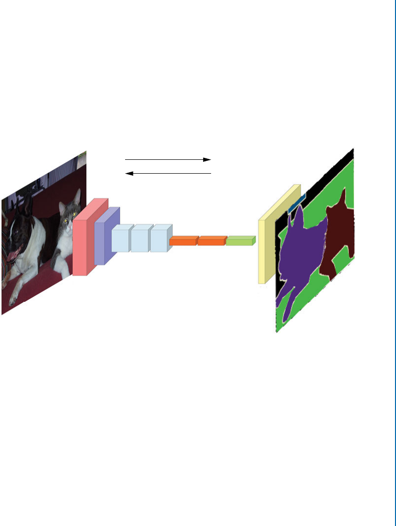
7.3. SEMANTIC SEGMENTATION 127
7.3 SEMANTIC SEGMENTATION
CNNs can also be adapted to perform dense predictions for per-pixel tasks such as semantic
segmentation. In this section, we discuss three representative semantic segmentation algorithms
which use CNN architectures.
7.3.1 FULLY CONVOLUTIONAL NETWORK (FCN)
In this section, we will briefly describe the Fully Convolutional Network (FCN) [Long et al.,
2015], shown in Fig. 7.6, for semantic segmentation.
96 256
384 384 256 4096 4096 21
21
Forward/Inference
Backward/Learning
Pixelwise Prediction
Segmentation g.t
Figure 7.6: FCN architecture. e first seven layers are adopted from AlexNet. Convolutional
layers, shown in orange, have been changed from fully connected (fc6and fc7in AlexNet) to
convolutional layers (conv6and conv7in FCN). e next convolutional layer (shown in green)
is added on top of conv7to produce 21 coarse output feature maps (21 denotes the number of
classes + background in the PASCAL VOC dataset). e last layer (yellow) is the transposed
convolutional layer, that up-samples the coarse output feature maps produced by conv8layer.
Typical classification networks (discussed in Chapter 6) take fixed-size images as input
and produce non-spatial output maps, that are fed to a soft-max layer to perform classification.
e spatial information is lost, because these networks use fixed dimension fully connected layers
in their architecture. However, these fully connected layers can also be viewed as convolution
layers with large kernels, which cover their entire input space. For example, a fully-connected
layer with 4,096 units that takes a volume of size 13 13 256 as input, can be equivalently
expressed as a convolutional layer with 4,096 kernels of size 13 13. Hence, the dimension of

128 7. APPLICATIONS OF CNNS IN COMPUTER VISION
the output will be 114,096, which results in an identical output as the initial fully-connected
layer. Based on this reinterpretation, the convolutionalized networks can take (1) input images
of any size and produce (2) spatial output maps. ese two aspects make the fully convolutional
models a natural choice for semantic segmentation.
FCN for semantic segmentation [Long et al.,2015] is built by first converting typical clas-
sification networks, (e.g., AlexNet, VGGnet-16) into fully convolutional networks and, then,
appending a transposed convolution layer (discussed in Section 4.2.6) to the end of the convo-
lutionalized networks. e transposed convolution layer is used for up-sampling the coarse out-
put feature maps produced by the last layer of the convolutionalized networks. More precisely,
given a classification network, e.g., AlexNet, the last three fully-connected layers (4,096-D fc6,
4,096-D fc7, and 1,000-D fc8) are converted to three convolutional layers (conv6: consisting
of 4,096 filters with size 13 13,conv7: consisting of 4,096 filters with size 11, and conv8:
consisting of 212filters with size 11) for semantic segmentation on PASCAL VOC dataset.
However, forward passing an HW3input image through this modified network produces
output feature maps with a spatial size of H
32 W
32 which is 32smaller than the spatial size
of the original input image. us, these coarse output feature maps are fed to the transposed
convolution layer3to produce a dense prediction of the input image.
However, a large pixel stride, (e.g., 32 for the AlexNet) at the transposed convolution
layer limits the level of details in the up-sampled output. To address this issue, FCN is extended
to new fully convolutional networks, i.e., FCN-16s and FCN-8s by combining coarse features
with fine ones that are extracted from the shallower layers. e architecture of these two FCNs
are shown in the second and third rows of Fig. 7.7, respectively. e FCN-32s in this figure is
identical to the FCN discussed above (and shown in Fig. 7.6), except that their architectures are
different.4
FCN-16s
As shown in the second row of Fig. 7.7, FCN-16s combines predictions from the final convo-
lutional layer and the pool4layer, at stride 16. us, the network predicts finer details compared
to FCN-32s, while retaining high-level semantic information. More precisely, the class scores
computed on top of conv7layer are passed through a transposed convolutional layer (i.e., 2
up-sampling layer) to produce class scores for each of the PASCAL VOC classes (including
background). Next, a 11convolutional layer with a channel dimension of 21 is added on top
of pool4layer to predict new scores for each of the PASCAL classes. Finally, these 2 stride
16 predicted scores are summed up and fed to another transposed convolutional layer (i.e., 16
up-sampling layer) to produce prediction maps with the same size as the input image. FCN-16s
2Equal to the number of classes in the PASCAL VOC dataset plus the background class.
3e 32 pixel stride is used to output a dense prediction at the same scale as the input image.
4e original FCN shown in Fig. 7.6 initialized with AlexNet model and the extended FCN shown in Fig. 7.7 initialized
with VGGnet-16 model.
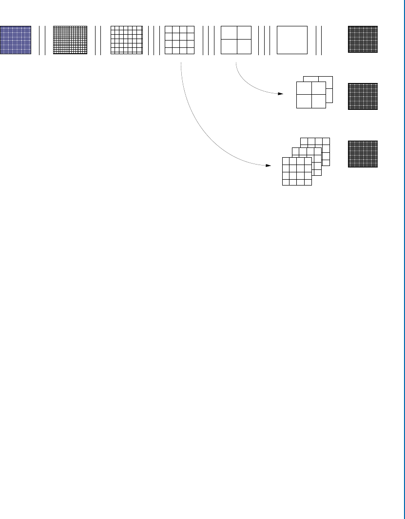
7.3. SEMANTIC SEGMENTATION 129
Image Conv1 Pool1 Conv2 Pool2 Conv3 Pool3 Conv4 Pool4
Pool4
Pool3
2× conv7
Conv5 Conv6-7
32× Unsampled
Prediction
(FCN-32s)
16× Unsampled
Prediction
(FCN-16s)
2× Pool4
4× conv7
8× Unsampled
Prediction
(FCN-8s)
Pool5
Figure 7.7: FCN learns to combine shallow layer (fine) and deep layer (coarse) information.
e first row shows FCN-32s, which up-samples predictions back to pixels in a single step. e
second row illustrates FCN-16s, which combines predictions from both the final and the pool4
layer. e third row shows FCN-8s, which provides further precision by considering additional
predictions from pool3layer.
improved the performance of FCN-32s on the PASCAL VOC 2011 dataset by 3mean IoU
and achieved 62:4 mean IoU.
FCN-8s
In order to obtain more accurate prediction maps, FCN-8s combines predictions from the final
convolutional layer and shallower layers, i.e., pool3and pool4layers. e third row of Fig. 7.7
shows the architecture of the FCN-8s network. First, a 11convolutional layer with channel
dimension of 21 is added on top of pool3layer to predict new scores at stride 8 for each of the
PASCAL VOC classes. en, the summed predicted scores at stride 16 (second row in Fig. 7.7)
is passed through a transposed convolutional layer (i.e., 2up-sampling layer) to produce new
prediction scores at stride 8. ese two predicted scores at stride 8 are summed up and then
fed to another transposed convolutional layer (i.e., 8up-sampling layer) to produce prediction
maps with the same size as the input image. FCN-8s improved the performance of FCN-18s
by a small mean IoU and achieved 62:7 mean IoU on the PASCAL VOC 2011.
FCN Fine-tuning
Since training from scratch is not feasible due to the large number of training parameters and
the small number of training samples, fine-tuning using back-propagation through the entire

130 7. APPLICATIONS OF CNNS IN COMPUTER VISION
network is done to train FCN for segmentation. It is important to note that FCN uses whole
image training instead of patch-wise training, where the network is learned from batches of
random patches (i.e., small image regions surrounding the objects of interest). Fine-tuning of
the coarse FCN-32s version, takes three GPU days, and about one day on GPU each for the
FCN-16s and FCN-8s [Long et al.,2015]. FCN has been tested on PASCAL VOC, NYUDv2,
and SIFT Flow datasets for the task of segmentation. It has been shown to achieve superior
performance compared to other reported methods.
FCN Drawbacks
FCN discussed above has few limitations. e first issue is related to a single transposed convo-
lutional layer of FCN, which cannot accurately capture the detailed structures of objects. While
FCN-16s and FCN-8s attempt to avoid this issue by combining coarse (deep layer) informa-
tion with fine (shallower layers) information, the detailed structure of objects are still lost or
smoothed in many cases. e second issue is related to the scale, i.e., fixed-size receptive field of
FCN. is causes the objects that are larger or smaller than the receptive field to be mislabeled.
To overcome these challenges, Deep Deconvolution Network (DDN) has been proposed, which
is discussed in the following section.
7.3.2 DEEP DECONVOLUTION NETWORK (DDN)
DDN [Noh et al.,2015] consists of convolution (Module A shown in Fig. 7.8) and deconvolu-
tion networks (Module B). e convolution network acts as a feature extractor and converts the
input image to a multi-dimensional feature representation. On the other hand, the deconvolu-
tion network is a shape generator, that uses these extracted feature maps and produces class score
prediction maps at the output with a spatial size of the input image. ese class score prediction
maps represent the probability that each pixel belongs to different classes.
Input
Image
Max
Pooling
Max
Pooling
Max
Pooling
Max
Pooling
Max
Pooling Unpooling
Unpooling Unpooling
UnpoolingUnpooling
Segmented
Image
224×224 224×224
112×112 112×112
56×56 56×56
28×28 28×28
14×14 14×14
7×7 7×7
1×1 1×1
Module A: Convolutional Network Module B: Deonvolutional Network
Figure 7.8: Overall architecture of deep deconvolution network. A multilayer deconvolution
network is put on top of the convolution network to accurately perform image segmentation.
Given a feature representation from the convolution network (Module A), dense class score
prediction maps are constructed through multiple un-pooling and transposed convolution layers
(Module B).

7.3. SEMANTIC SEGMENTATION 131
DDN uses convolutionalized VGGnet-16 network for the convolutional part. More pre-
cisely, the last fully connected layer of VGGnet-16 is removed and the last two fully connected
layers are converted to convolutional layers (similar to FCN). e deconvolution part is the
reciprocal of the convolution network. Unlike FCN-32s, which uses a single transposed convo-
lutional layer, the deconvolution network of DDN uses a sequence of un-pooling and transposed
convolution layers to generate class prediction maps with the same spatial size as the input im-
age. In contrast to the convolution part of the model, which decreases the spatial size of the
output feature maps through feed-forwarding, its counterpart increases the size by combining
the transposed convolution and un-pooling layers.
Un-pooling Layer
e un-pooling layers of the deconvolution network of DDN perform the reverse operation of
the max-pooling layers of the convolution network. To be able to perform reverse max-pooling,
the max-pooling layers save the locations of the maximum activations in their “switch variables,”
i.e., essentially the argmax of the max-pooling operation. e un-pooling layers then employ
these switch variables to place the activations back to their original pooled locations.
DDN Training
To train this very deep network with relatively small training examples, the following strate-
gies are adopted. First, every convolutional and transposed convolutional layer is followed by
a batch normalization layer (discussed in Section 5.2.4), which has been found to be critical
for DDN optimization. Second, unlike FCN which performs image-level segmentation, DDN
uses instance-wise segmentation, in order to handle objects in various scales and decrease the
training complexity. For this purpose, a two-stage training approach is used.
In the first phase, DDN is trained with easy samples. To generate the training samples
for this phase, ground-truth bounding box annotations of objects are used to crop each object so
that the object is centered at the cropped bounding box. In the subsequent phase, the learned
model from the first phase is fine-tuned with more challenging samples. us, each object pro-
posal contributes to the training samples. Specifically, the candidate object proposals, which
sufficiently overlap with the ground-truth segmented regions (0.5 in IoU) are selected for
training. To include context, post-processing is also adopted in this phase.
DDN Inference
Since DDN uses instance-wise segmentation, an algorithm is required to aggregate the output
score prediction maps of individual object proposals within an image. DDN uses the pixel-wise
maximum of the output prediction maps for this purpose. More precisely, the output prediction
maps of each object proposal (gi2RWHC, where Cis the number of classes and i,Wand H
denote the index, height and width of the object proposal, respectively) are first superimposed
on the image space with zero padding outside gi. en, the pixel-wise prediction map of the

132 7. APPLICATIONS OF CNNS IN COMPUTER VISION
entire image is computed as follows:
P .x; y; c/ Dmax
iGi.x; y; c/; 8i; (7.4)
where Giis the prediction map corresponding to giin the image space with zero padding out-
side gi. Next, a soft-max loss is applied to the aggregated prediction maps, Pin Eq. (7.4), to
obtain class probability maps (O) in the entire image space. e final pixel-wise labeled image is
computed by applying the fully connected CRF [Krähenbühl and Koltun,2011] to the output
class probability maps O.
Conditional Random Field (CRF): CRF is a class of statistical model-
ing technique, which are categorized as the sequential version of logistic re-
gression. In contrast to logistic regression, which is a log linear classification
model, CRFs are log linear models for sequential labeling.
e CRF is defined as the conditional probabilities of Xand Y, represented
as P .Y jX/, where Xdenotes a multi-dimensional input, i.e., features, and
Ydenotes a multi-dimensional output, i.e., labels. e probabilities can be
modeled in two different ways, i.e., unary potential and pairwise potential.
Unary potential is used to model the probabilities that a given pixel or a
patch belongs to each particular category, while pairwise potential is defined
to model the relation between two different pixels and patches of an image.
In fully connected CRF, e.g., Krähenbühl and Koltun [2011], the latter ap-
proach is explored to establish pairwise potential on all pixel pairs in a given
image, thus resulting into refined segmentation and labeling. For more de-
tails on CRF, the readers are referred to Krähenbühl and Koltun [2011].
DDN Testing
For each testing image, approximately 2,000 object proposals are generated using edge-box al-
gorithm [Zitnick and Dollár,2014]. Next, the best 50 proposals with the highest objectness
scores are selected. ese object proposals are then used to compute instance-wise segmenta-
tions, which are then aggregated, using the algorithm discussed above, to obtain the semantic
segmentation for the whole image. DDN has been shown to achieve an outstanding perfor-
mance of 72.5% on PASCAL VOC 2012 dataset compared to other reported methods.
DDN Drawbacks
DDN discussed above has a couple of limitations. First, DDN uses multiple transposed convo-
lutional layers in its architecture, which requires additional memory and time. Second, training
DDN is tricky and requires a large corpus of training data to learn the transposed convolutional
layers. ird, DDN deals with objects at multiple scales by performing instant-wise segmen-
tation. erefore, it requires feed-forwarding all object proposals through the DDN, which is

7.3. SEMANTIC SEGMENTATION 133
a time-consuming process. To overcome these challenges, DeepLab model has been proposed,
which is discussed in the following section.
7.3.3 DEEPLAB
In DeepLab [Chen et al.,2014], the task of semantic segmentation has been addressed by em-
ploying convolutional layers with up-sampled filters, which are called atrous convolution (or
dilated convolution as discussed in Chapter4).
Recall that forward passing an input image through the typical convolution classification
networks reduces the spatial scale of the output feature maps, typically by a factor of 32. However,
for dense predictions tasks, e.g., semantic segmentation, a stride of 32 pixels limits the level of
details in the up-sampled output maps. One partial solution is to append multiple transposed
convolutional layers as in FCN-8s and DDN, to the top of the convolutionalized classification
networks to produce output maps with the same size of the input image. However, this approach
is too costly.5Another critical limitation of these convolutionalized classification networks is
that they have a predefined fixed-size receptive field. For example, FCN and all its variants (i.e.,
FCN-16s and FCN-8s) use VGNNnet-16 with fixed-size 33filters. erefore, an object with
a substantially smaller or larger spatial size than the receptive field is problematic.6
DeepLab uses atrous convolution in its architecture to simultaneously address these two
issues. As discussed in Chapter 4, atrous convolution allows to explicitly control the spatial size
of the output feature maps that are computed within convolution networks. It also extends the
receptive field, without increasing the number of parameters. us, it can effectively incorporate
a wider image context while performing convolutions. For example, to increase the spatial size
of the output feature maps in the convolutionalized VGGnet-16 network7by a factor of 2, one
could set the stride of the last max-pooling layer (pool5) to 1, and then substitute the subse-
quent convolutional layer (conv6, which is the convolutionalized version of fc6) with the atrous
convolutional layers with a sampling factor dD2. is modification also extends the filter size
of 33to 55, and therefore enlarges the receptive field of the filters.
DeepLab-LargeFOV Architecture
DeepLab-LargeFOV is a CNN with an atrous convolutional layer which has a large receptive
field. Specifically, DeepLab-LargeFOV is built by converting the first two fully-connected lay-
ers of VGGnet-16 (i.e., fc6and fc7) to convolutional layers (i.e., conv6and conv7) and then
appending a 11convolution layer (i.e., conv8) with 21 channels at the end of the convolution-
alized networks for semantic segmentation on PASCAL VOC dataset. e stride of the last
two max-pooling layers (i.e., pool4and pool5) is changed to 1,8and the convolutional filter of
5Training these networks requires relatively more training data, time, and memory.
6Label prediction for large objects are obtained from only local information. us, the pixels which belong to the same large
object may have inconsistent labels. Moreover, the pixels which belong to small objects may be classified as background.
7A convolutionalized VGGnet-16 is obtained by converting all the fully-connected layers to convolution layers.
8e stride of pool4 and pool5 layers in the original VGGnet-16 is 2.
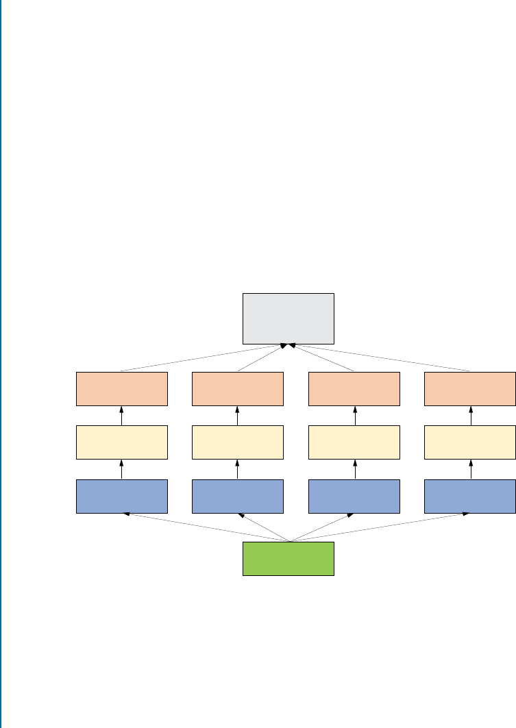
134 7. APPLICATIONS OF CNNS IN COMPUTER VISION
conv6layer is replaced with an atrous convolution of kernel size 33and an atrous sampling
factor dD12. erefore, the spatial size of the output class score prediction maps is increased
by a factor of 4. Finally, a fast bilinear interpolation layer9(i.e., 8up-sampling) is employed to
recover the output prediction maps at the original image size.
Atrous Spatial Pyramid Pooling (ASPP)
In order to capture objects and context at multiple scales, DeepLab employs multiple parallel
atrous convolutional layers (discussed in Section 4.2.2) with different sampling factors d, which
is inspired by the success of the Spatial Pyramid Pooling (SPP) layer discussed in Section 4.2.8.
Specifically, DeepLab with atrous Spatial Pyramid Pooling layer (called DeepLab-ASPP) is
built by employing 4 parallel conv6conv7conv8branches with 33filters and different
atrous factors (dD f6; 12; 18; 24g) in the conv6layers, as shown in Fig. 7.9. e output predic-
tion maps from all four parallel branches are aggregated to generate the final class score maps.
Next, a fast bilinear interpolation layer is employed to recover the output prediction maps with
the original image size.
4
= 1
!
!1!2!3!4
Conv8
(1×1)
Conv7
(1×1)
Conv6
(3×3, d = 6)
Conv8
(1×1)
Conv7
(1×1)
Conv6
(3×3, d = 12)
Conv8
(1×1)
Conv7
(1×1)
Pool5
Conv6
(3×3, d = 18)
Conv8
(1×1)
Conv7
(1×1)
Conv6
(3×3, d = 24)
Figure 7.9: Architecture of DeepLab-ASPP (DeepLab with Atrous Spatial Pyramid Pooling
layer). pool5denotes the output of the last pooling layer of VGGnet-16.
9Instead of using transposed convolutional layers as in FCN and DDN, DeepLab uses a fast bilinear interpolation layer
without training its parameters. is is because, unlike FCN and DDN, the output class score prediction maps of DeepLab
(i.e., the output maps of conv8layer) are quite smooth and thus a single up-sampling step can efficiently recover the output
prediction maps with the same size as the input image

7.4. SCENE UNDERSTANDING 135
DeepLab Inference and Training
e output prediction maps of the bilinear interpolation layer can only predict the presence
and rough position of objects, but the boundaries of objects cannot be recovered. DeepLab
handles this issue by combining the fully connected CRF [Krähenbühl and Koltun,2011] with
the output class prediction maps of the bilinear interpolation layer. e same approach is also
used in DDN. During training, the Deep Convolutional Neural Network (DCNN) and the
CRF training stages are decoupled. Specifically, a cross validation of the fully connected CRF
is performed after the fine-tuning of the convolutionalized VGGnet-16 network.
DeepLab Testing
DeepLab has been tested on the PASCAL VOC 2012 validation set and has been shown to
achieve state-of-the-art performance of 71.6% mean IoU compared to other reported meth-
ods including fully convolutional networks. Moreover, DeepLab with atrous Spatial Pyramid
Pooling layer (DeepLab-ASPP) achieved about 2% higher accuracy than DeepLab-LargeFOV.
Experimental results show that DeepLab based on ResNet-101 delivers better segmentation
results compared to Deep Lab employing VGGnet-16.
7.4 SCENE UNDERSTANDING
In computer vision, the recognition of single or isolated objects in a scene has achieved significant
success. However, developing a higher level of visual scene understanding requires more complex
reasoning about individual objects, their 3D layout and mutual relationships [Khan,2016,Li
et al.,2009]. In this section, we will discuss how CNNs have been used in the area of scene
understanding.
7.4.1 DEEPCONTEXT
DeepContext [Zhang et al.,2016] presents an approach to embed 3D context into the topology
of a neural network, trained to perform holistic scene understanding. Given an input RGB-
D image, the network can simultaneously make global predictions (e.g., scene category and
3D scene layout) as well as local decisions (e.g., the position and category of each constituent
object in the 3D space). is method works by first learning a set of scene templates from
the training data, which encodes the possible locations of single or multiple instances of objects
belonging to a specific category. Four different scene templates, including sleeping area, lounging
area, office area, and a table and chair sets are used. Given this contextual scene representation,
DeepContext matches an input volumetric representation of an RGBD image with one of the
scene templates using a CNN (Module B, Fig. 7.10). Afterward, the input scene is aligned
with the scene template using a transformation network (Module C, Fig. 7.10). e aligned
volumetric input is fed to a deep CNN with two main branches; one works on the complete
3D input and obtains a global feature representation while the second works on the local object
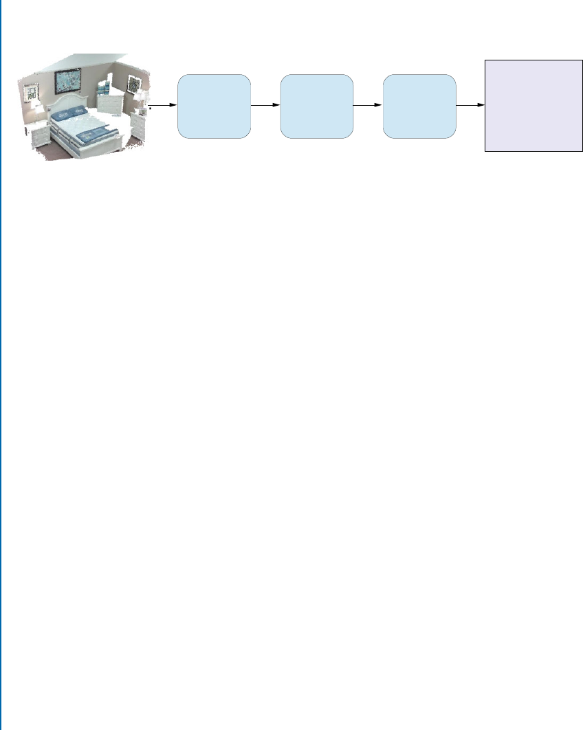
136 7. APPLICATIONS OF CNNS IN COMPUTER VISION
level and predicts the location and existence of each potential object in the aligned template
(Module D, Fig. 7.10).
Scene
Classification
Transformation
Network
3D Context
Network
Output:
3D
Understanding
Module A Module B Module C Module D Module E
Figure 7.10: e block diagram for DeepContext processing pipeline. Given a 3D volumetric input (mod-
ule A), the transformation network (module C) aligns the input data with its corresponding scene template
(estimated by module B). Using this roughly aligned scene, the 3D context network (module D) estimates the
existence of an object and adjusts the object location based on local object features and holistic scene features,
to understand a 3D scene.
e DeepContext algorithm follows a hierarchical process for scene understanding which
is discussed below.
Learning Scene Templates
e layouts of the scene templates (e.g., office, sleeping area) are learned from the SUN RGB-
D dataset [Song et al.,2015], which comes with 3D object bounding box annotations. Each
template represents a scene context by summarizing the bounding box locations and the category
information of the objects that are present in the training set. As an initial step, all the clean
examples of each scene template (i.e., sleeping area, lounging area, office area and a table and
chair sets) are identified. Next, a major object is manually identified in each scene template (e.g.,
a bed in the sleeping area) and its position is used to align all the scenes belonging to a specific
category. is rough alignment is used to find the most frequent locations for each object (also
called “anchor positions”) by performing k-means clustering and choosing the top kcenters for
each object. Note that the object set includes not only the regular objects (e.g., bed, desk) but
also the scene elements which define the room layout (e.g., walls, floor and ceiling).
e clean dataset of the scene categories used to learn the scene templates, is also used
in subsequent processing stages, such as scene classification, scene alignment, and 3D object
detection. We will discuss these stages below.
Scene Classification (Module B, Fig. 7.10)
A global CNN is trained to classify an input image to one of the scene templates. Its architecture
is exactly same as the global scene pathway in Fig. 7.11. Note that the input to the network
is a 3D volumetric representation of the input RGB-D images, which is obtained using the
Truncated Signed Distance Function (TSDF) [Song and Xiao,2016]. is first representation is
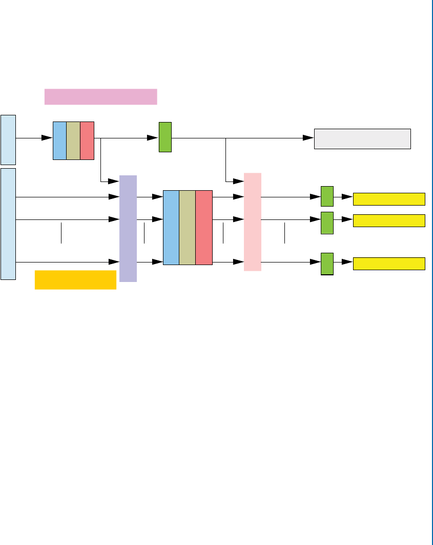
7.4. SCENE UNDERSTANDING 137
processed using three processing blocks, each consisting of a 3D convolution layer, a 3D pooling
layer, and a ReLU nonlinearity. e output is an intermediate “spatial feature” representation
corresponding to a grid of 3D spatial locations in the input. It is further processed by two fully
connected layers to obtain a “global feature” which is used to predict the scene category. Note
that both the local spatial feature and the global scene-level feature is later used in the 3D context
network.
Global Scene Pathway
Object Pathway
Spatial Feature
Anchor Position 1
Anchor Position 2
Anchor Position k
Object Feature 1
Object Feature 2
Object Feature k
Object Exist/Reg
Object Exist/Reg
Object Exist/Reg
Global FeatureVector Scene Classification
3D InputAligned Template
3D RoI Pooling
3D Conv
3D Pooling
ReLU
3D Conv
3D Pooling
ReLU
Concatenation
FC FC ×2
FC ×2
×3
×2
FC
Figure 7.11: Deep 3D Context network (Module D, Fig. 7.10) architecture. e network con-
sists of two channels for global scene-level recognition and local object-level detection. e scene
pathway is supervised with the scene classification task during pre-training only (Module B). e
object pathway performs object detection, i.e., predicts the existence/non-existence of an object
and regresses its location. Note that the object pathway brings in both local and global features
from the scene pathway.
3D Transformation Network (Module C, Fig. 7.10)
Once the corresponding scene template category has been identified, a 3D transformation net-
work estimates a global transformation which aligns the input scene to the corresponding scene-
template. e transformation is calculated in two steps: a rotation followed by a translation. Both
these transformation steps are implemented individually as classification problems, for which
CNNs are well suited.
For the rotation, only the rotation about the vertical-axis (yaw) is predicted since the
gravity direction is known for each scene in the SUN RGB-D dataset. Since an exact estima-
tion of the rotation along the vertical axis is not required, the 360ıangular range is divided into
36 regions, each encompassing 10ı. A 3D CNN is trained to predict the angle of rotation along

138 7. APPLICATIONS OF CNNS IN COMPUTER VISION
the vertical axis. e CNN has the same architecture as the one used in Module B (scene clas-
sification), however, its output layer has 36 units which predicts one of the 36 regions denoting
the y-axis rotation.
Once the rotation has been applied, another 3D CNN is used to estimate the translation
that is required to align the major object (e.g., bed, desk) in the input scene and the identified
scene template. Again, the CNN has essentially the same architecture as Module B, however,
the last layer is replaced by a soft-max layer with 726 units. Each value of the output units de-
notes a translation in a discretized space of 11 11 6values. Similar to rotation, the estimated
translation is also a rough match due to the discretized set of values. Note that for such problems
(i.e., parameter estimation), regression is a natural choice since it avoids errors due to discretiza-
tion. However, the authors could not successfully train a CNN with a regression loss for this
problem. Since the context network regresses the locations of each detected object in the scenes
in the next stage, a rough alignment suffices at this stage. We explain the context network below.
3D Context Network (Fig. 7.11)
e context neural network performs 3D object detection and layout estimation. A separate net-
work is trained for each scene template category. is network has two main branches, as shown
in Fig. 7.11: a global scene level branch and a local object level branch. Both network pathways
encode different levels of details about the 3D scene input, which are complementary in nature.
e local object-level branch is dependent on the features from the initial and final layers of the
global scene-level branch. To avoid any optimization problems, the global scene-level branch
is initialized with the weights of the converged scene classification network (Module B) (since
both have the same architecture). Each category-specific context network is then trained sepa-
rately using only the data from that specific scene template. During this training procedure, the
scene-level branch is fine-tuned while the object-level branch is trained from scratch.
e object-level branch operates on the spatial feature from the global scene-level branch.
e spatial feature is the output activation map after the initial set of three processing layers, each
consisting of a 3D convolution, pooling, and ReLU layers. is feature map is used to calcu-
late object-level features (corresponding to anchor positions) at a 666resolution using the
3D Region of Interest (RoI) pooling. e 3D RoI pooling is identical to its 2D counterpart
described in Section 4.2.7, with only an extra depth dimension. e pooled feature is then pro-
cessed through 3D convolution and fully connected layers to predict the object existence and
its location (3D bounding box). e object location is regressed using the R-CNN localiza-
tion loss to minimize the offset between the ground-truth and the predicted bounding boxes
(Section 7.2.1).
Hybrid Data for Pre-training
Due to the lack of huge amount of RGB-D training data for scene understanding, this approach
uses an augmented dataset for training. In contrast to the simple data augmentation approaches

7.4. SCENE UNDERSTANDING 139
we discussed in Section 5.2.1, the proposed approach is more involved. Specifically, a hybrid
training set is generated by replacing the annotated objects from the SUN RGB-D dataset with
the same category CAD models. e resulting hybrid set is 1,000 times bigger than the original
RGBD training set. For the training of 3D context network (scene pathway), the models are
trained on this large hybrid dataset first, followed by a fine-tuning on the real RGB-D depth
maps to ensure that the training converges. For the alignment network, the pre-trained scene
pathway from the 3D context network is used for the initialization. erefore, the alignment
network also benefits from the hybrid data.
e DeepContext model has been evaluated on the SUN RGB-D dataset and has been
shown to model scene contexts adequately.
7.4.2 LEARNING RICH FEATURES FROM RGB-D IMAGES
e object and scene level reasoning system presented in the previous section was trained end-to-
end on 3D images. Here, we present an RGB-D- (2.5D instead of 3D) based approach [Gupta
et al.,2014] which performs object detection, object instance segmentation, and semantic seg-
mentation, as shown in Fig. 7.12. is approach is not end-to-end trainable, it rather extends
the pre-trained CNN on color images to depth images by introducing a new depth encoding
method. is framework is interesting, since it demonstrates how pre-trained networks can be
effectively used to transfer learning from domains where large quantities of data is available to
the ones where labeled data is scarce, and even for new data modalities (e.g., depth in this case).
In the following sections, we briefly discuss the processing pipeline (summarized in Fig. 7.12).
Encoding Depth Images for Feature Learning
Instead of directly training a CNN on the depth images, Gupta et al. [2014] propose to encode
the depth information using three geometric features calculated at each pixel location. ese
include: the horizontal disparity, the height above the ground, and the angle between the surface
normals at a given pixel and the estimated gravity direction. is encoding is termed as the HHA
encoding (first letter of each geometric feature). For the training dataset, all these channels are
mapped to a constant range of 0–255.
e HHA encoding and color images are then fed to the deep network to learn more
discriminative feature representations on top of the geometric features based on raw depth in-
formation. Since the NYU-Depth dataset used in this work, consisted of only 400 images, an
explicit encoding of the geometric properties of the data made a big difference to the network,
which usually requires much larger amounts of data to automatically learn the best feature repre-
sentations. Furthermore, the training dataset was extended by rendering synthetic CAD models
in the NYU-Depth dataset scenes. is is consistent with the data augmentation approach that
we discussed for the case of DeepContext [Zhang et al.,2016].
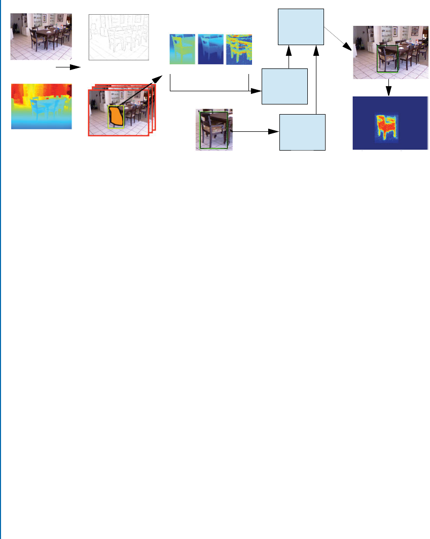
140 7. APPLICATIONS OF CNNS IN COMPUTER VISION
Input Ouput
RGB
RGB Instance Segmentation
Disparity Height Angle
Contour Detection
Regional Proposal
Generation
Depth Image
Geometric Encoding
of Depth
SVM
Classifier
Depth CNN
Features
Extraction
RGB CNN
Features
Extraction
Object Detection
Figure 7.12: e input to this framework is a RGB and a depth image. First, object proposals
are generated using the contour information. e color and the encoded depth image are passed
through separately trained CNNs to obtain features which are then classified into object cate-
gories using the SVM classifiers. After detection, a Random Forest classifier is used to identify
foreground object segmentation within each valid detection.
CNN Fine-tuning for Feature Learning
Since the main goal of this work is object detection, it is useful to work on the object propos-
als. e region proposals are obtained using an improved version of Multiscale Combinatorial
Grouping (MCG) [Arbeláez et al.,2014] approach which incorporated additional geometric
features based on the depth information. e regions proposals which have a high overlap with
the ground-truth object bounding box are first used to train a deep CNN model for classifica-
tion. Similar to R-CNN, the pre-trained AlexNet [Krizhevsky et al.,2012] is fine-tuned for
this object classification task. Once the network is fine-tuned, object specific linear classifiers
(SVMs) are trained using the intermediate CNN features for the object detection task.
Instance Segmentation
Once the object detections are available, the pixels belonging to each object instance are labeled.
is problem is tackled by predicting the foreground or background label for each pixel within
a valid detection. For this purpose, a random forest classifier is used to provide the pixel level
labelings. is classifier is trained on the local hand-crafted features whose details are available
in Gupta et al. [2013]. Since these predictions are calculated roughly for individual pixels, they
can be noisy. To smooth the initial predictions of the random forest classifier, these predictions
are averaged on each super-pixel. Note that subsequent works on instance segmentation (e.g.,
He et al. [2017]) have incorporated a similar pipeline (i.e., first detecting object bounding boxes
and then predicting the foreground mask to label the individual object instance). However, in

7.5. IMAGE GENERATION 141
contrast to Gupta et al. [2014], He et al. [2017] use an end to end trainable CNN model which
avoids manual parameter selection and a series of isolated processing steps toward the final goal.
As a result, He et al. [2017] achieve highly accurate segmentations compared to the non-end-
to-end trainable approaches.
Another limitation of this approach is the separate processing of both color and depth
images. As we discussed in Chapter 6, AlexNet has a huge number of parameters, and learning
two separate set of parameters for both modalities doubles the parameter space. Moreover, since
both images belong to the same scene, we expect to learn better cross-modality relationships if
both modalities are considered jointly. One approach to learn a shared set of parameters in such
cases is to stack the two modalities in the form of a multichannel input (e.g., six channels) and
perform a joint training over both modalities [Khan et al.,2017c,Zagoruyko and Komodakis,
2015].
7.4.3 POINTNET FOR SCENE UNDERSTANDING
PointNet (discussed in Section 7.1.1) has also been used for scene understanding by assigning
a semantically meaningful category label to each pixel in an image (Module B in Figure 7.1).
While we have discussed the details of PointNet before, it is interesting to note its similarity
with the Context Network in DeepContext (Section 7.4.1 and Figure 7.11). Both these networks
learn an initial representation, shared among the global (scene classification) and the local (se-
mantic segmentation or object detection) tasks. Afterward, the global and local branches split
up, and the scene context is added in the local branch by copying the high-level features from
the global branch to the local one. One can notice that the incorporation of both the global
and local contexts are essential for a successful semantic labeling scheme. Other recent works in
scene segmentation are also built on similar ideas, i.e., better integration of scene context using
for example a pyramid-based feature description [Zhao et al.,2017], dilated convolutions [Yu
and Koltun,2015], or a CRF model [Khan et al.,2016a,Zheng et al.,2015].
7.5 IMAGE GENERATION
Recent advances in image modeling with neural networks, such as Generative Adversarial Net-
works (GANs) [Goodfellow et al.,2014], have made it feasible to generate photo-realistic im-
ages, which can capture the high-level structure of the natural training data [van den Oord et al.,
2016]. GANs are one type of generative networks, which can learn to produce realistic-looking
images in an unsupervised manner. In recent years, a number of GAN-based image generation
methods have emerged which work quite well. One such promising approach is Deep Convo-
lutional Generative Adversarial Networks (DCGANs) [Radford et al.,2015], which generates
photo-realistic images by passing random noise through a deep convolutional network. Another
interesting approach is Super-Resolution Generative Adversarial Networks (SRGAN) [Ledig
et al.,2016], which generates high-resolution images from low-resolution counterparts. In this
142 7. APPLICATIONS OF CNNS IN COMPUTER VISION
section, we shall first briefly discuss GANs and then extend our discussion to DCGANs and
SRGAN.
7.5.1 GENERATIVE ADVERSARIAL NETWORKS (GANS)
GANs were first introduced by Goodfellow et al. [2014]. e main idea behind a GAN is to have
two competing neural network models (shown in Fig. 7.13). e first model is called generator,
which takes noise as input and generates samples. e other neural network, called discriminator,
receives samples from both the generator (i.e., fake data) and the training data (i.e., real data),
and discriminates between the two sources. ese two networks undergo a continuous learning
process, where the generator learns to produce more realistic samples, and the discriminator
learns to get better at distinguishing generated data from real data. ese two networks are
trained simultaneously with the aim that this training will drive the generated samples to be
indistinguishable from real data. One of the advantages of GANs is that they can back-propagate
the gradient information from the discriminator back to the generator network. e generator,
therefore, knows how to adapt its parameters in order to produce output data that can fool the
discriminator.
Noise Generator
Generator
Sample
Data Sample Discriminator
Yes/No
Data Sample?
Figure 7.13: Generative Adversarial Networks Overview. Generator takes the noise as an input
and generates samples. e discriminator distinguishes between the generator samples and the
training data.
GANs Taining
e training of GANs involves the computation of two loss functions, one for the generator and
one for the discriminator. e loss function for the generator ensures that it produces better data
samples, while the loss function for the discriminator ensures that it distinguishes between the
generated and real samples. We now briefly discuss these loss functions. For more details, the
readers are referred to Goodfellow [2016].

7.5. IMAGE GENERATION 143
Discriminator Loss Function
e discriminator’s loss function J.D/ is represented by:
J.D/..D/; .G//D 1
2Expdat a Œlog D.x/ 1
2Ezp.z/ Œlog.1 D.G.z///; (7.5)
which is the cross entropy loss function. In this equation, .D/ and .G/ are the parameters of
the discriminator and the generator networks, respectively. pdata denotes the distribution of
real data, xis a sample from pdat a,p.z/ is the distribution of the generator, zis a sample from
p.z/,G.z/ is the generator network and Dis the discriminator network. One can note from
Eq. (7.5) that the discriminator is trained as a binary classifier (with sigmoid output) on two
mini-batches of data. One of the them is from the data set containing real data samples with
label 1assigned to all examples, and the other from the generator (i.e., fake data) with label 0
for all the examples.
Cross-entropy: e cross-entropy loss function for the binary classification
task is defined as follows:
H..x1; y1/; D/ D y1log D.x1/.1 y1/log.1 D.x1//; (7.6)
where x1and y12Œ1 1 denote a sample from a probability distribution
function Dand its desired output, respectively. After summing over mdata
samples, Eq. (7.5) can be written as follows:
H..xi; yi/m
iD1; D/ D
m
X
iD1
yilog D.xi/
m
X
iD1
.1 yi/log.1 D.xi//:
(7.7)
In the case of GANs, data samples come from two sources, the dis-
criminator’s distribution xipdata or the generator’s distribution xiDG.z/,
where zp.z/. Let’s assume that the number of samples from both dis-
tributions is equal. By writing Eq. (7.7) probabilistically, i.e., replacing the
sums with expectations, the label yiwith 1
2(because the number of sam-
ples from both generator and discriminator distributions is equal), and the
log.1 D.xi// with log.1 D.G.z///, we get the same loss function as
Eq. (7.5), for the discriminator.
Generator Loss Function
e discriminator, discussed above, distinguishes between the two classes, i.e., the real and the
fake data, and therefore needs the cross entropy function, which is the best option for such tasks.
However, in the case of the generator, the following three types of loss functions can be used.

144 7. APPLICATIONS OF CNNS IN COMPUTER VISION
•e minimax Loss function: e minimax loss10 is the simplest version of the loss func-
tion, which is represented as follows:
J.G/ D J.D/ D1
2Expdata Œlog D.x/ C1
2Ezp.z/ Œlog.1 D.G.z///: (7.8)
e minimax version has been found to be less useful due to the gradient saturation prob-
lem. e latter occurs due to the poor design of the generator’s loss function. Specifically,
as shown in Fig. 7.14, when the generator samples are successfully rejected by the dis-
criminator with high confidence11 (i.e., D.G.z// is close to zero), the generator’s gradient
vanishes and thus, the generator’s network cannot learn anything.
•Heuristic, non-saturation loss function: e heuristic version is represented as follows:
J.G/ D 1
2EzŒlog D.G.z//: (7.9)
is version of the loss function is based on the concept that the gradient of the generator
is only dependent on the second term in Eq. (7.5). erefore, as opposed to the minimax
function, where the signs of J.D/ are changed, in this case the target is changed, i.e.,
log D.G.z// is used instead of log.1 D.G.z///. e advantage of this strategy is that
the generator gets a strong gradient signal at the start of the training process (as shown
in Fig. 7.14), which helps it in attaining a fast improvement to generate better data, e.g.,
images.
•Maximum Likelihood loss function: As the name indicates, this version of the loss func-
tion is motivated by the concept of maximum likelihood (a well-known approach in ma-
chine learning) and can be written as follows:
J.G/ D 1
2EzŒexp .1.D.G.z////; (7.10)
where is the logistic sigmoid function. Like the minimax loss function, the maximum
likelihood loss also suffers from the gradient vanishing problem when D.G.z// is close to
zero, as shown in Fig. 7.14. Moreover, unlike the minimax and the heuristic loss functions,
the maximum likelihood loss, as a function of D.G.z//, has a very high variance, which is
problematic. is is because most of the gradient comes from a very small number of the
generator’s samples that are most likely to be real rather than fake.
10In the minimax game, there are two players (e.g., generator and discriminator) and in all states the reward of player 1 is the
negative of reward of player 2. Specifically, the discriminator minimizes a cross-entropy, but the generator maximizes the
same cross-entropy.
11At the start of the training, the generator likely produces random samples, which are quite different from the real samples,
so the discriminator can easily classify the real and fake samples.
7.5. IMAGE GENERATION 145
Minimax
Non-saturating Heuristic
Maximum Likelihood Cost
5
0
-5
-10
-15
-20
0.0 0.2 0.4 0.6 0.8 1.0
D(G(𝒛))
J(G)
Figure 7.14: e loss response curves as functions of D.G.z// for three different variants of the
GAN generator’s loss functions.
To summarize, one can note that all three generator loss functions do not depend on the
real data (xin Eq. (7.5)). is is advantageous, because the generator cannot copy input data
x, which helps in avoiding the over-fitting problem in the generator. With this brief overview
of generative adversarial models and their loss functions, we will now summarize the different
steps that are involved in GANs training.
1. sampling a mini-batch of msamples from the real dataset pdata;
2. sampling a mini-batch of msamples from the generator p.z/ (i.e., fake samples);
3. learning the discriminator by minimizing its loss function in Eq. (7.5);
4. sampling a mini-batch of msamples from the generator p.z/ (i.e., fake sample); and
5. learning the generator by minimizing its loss function in Eq. (7.9).
ese steps are repeated until convergence occurs or until the iteration is terminated. With
this brief overview of generative adversarial networks, we will now discuss two representative
applications of GANs, known as DCGANs [Radford et al.,2015] and SRGAN [Ledig et al.,
2016].
7.5.2 DEEP CONVOLUTIONAL GENERATIVE ADVERSARIAL
NETWORKS (DCGANS)
DCGANs [Radford et al.,2015] are the first GAN models, which can generate realistic images
from random input samples. In the following, we shall discuss the architecture and the training
of DCGANs.
146 7. APPLICATIONS OF CNNS IN COMPUTER VISION
Architecture of DCGANs
DCGANs provide a family of CNN architectures, which can be used in the generator and the
discriminator parts of GANs. e overall architecture is the same as the baseline GAN archi-
tecture, which is shown in Fig. 7.13. However, the architecture of both the generator (shown
in Fig. 7.15) and the discriminator (shown in Fig. 7.16) is borrowed from the all-convolutional
network [Springenberg,2015], meaning that these models do not contain any pooling or un-
pooling layers. In addition, the generator uses transposed convolution to increase the repre-
sentation’s spatial size, as illustrated in Fig. 7.15. Unlike the generator, the discriminator uses
convolution to squeeze the representation’s spatial size for the classification task (Fig. 7.16). For
both networks, a stride greater than 1(usually 2) is used in the convolutional and transposed
convolutional layers. Batch normalization is used in all layers of both the discriminator and the
generator models of DCGANs with the exception of the first layer of the discriminator and
the last layer of the generator. is is done to ensure that DGCAN learns the correct scale of
the data distribution and its mean. DCGANs use the ReLU activation in all transposed con-
volutional layers except the output layer, which uses tanh activation function. It is because a
bounded activation function such as tanh, allows the generator to speed-up the learning process
and cover the color space of the samples from the training distribution. For the discriminator
model, leaky ReLU (discussed in Section 4.2.4) was found to be better than ReLU. DCGANs
use the Adam optimizer (discussed in Section 5.4.6) rather than SGD with momentum.
100-D
Project
and
Reshape
1024
512
256
128 3
48
4 8 16 32
64
32 64
16
Stride 2
tconv1 tconv2 tconv3 tconv4
Stride 2 Stride 2 Stride 2
Z
Input
Figure 7.15: Example DCGAN generator’s architecture for Large-scale Scene Understanding
(LSUN) dataset [Song and Xiao,2015]. A 100-dimensional uniform distribution zis projected
and then reshaped to a 441,024 tensor, where 1,024 is the number of feature maps. Next, the
tensor is passed through a sequence of transposed convolutional layers (i.e., tconv1tconv2
tconv3tconv4) to generate a 64 64 3realistic image.
7.5. IMAGE GENERATION 147
512
256
128
64
3
4
8
4
8
1632
64
32
64
16
conv1 conv2 conv3 conv4
Input
Stride 2 Stride 2 Stride 2 Stride 2
Reshape to Vector
FC(2)
Loss Function
Figure 7.16: Example DCGAN discriminator’s architecture for LSUN dataset [Song and Xiao,
2015]. An 64 64 RGB input image is passed through a sequence of convolutional layers (i.e.,
conv1conv2conv3conv4) followed by a fully-connected layer with 2 outputs.
DCGANs as a Feature Extractor
DCGANs uses ImageNet as a dataset of natural images for unsupervised training to evaluate
the quality of the features learned by DCGAN. For this purpose, DCGANs is first trained on
ImageNet dataset. Note that the image labels are not required during training (unsupervised
learning). Also, it is important to note that all the training and test images are scaled to the
range of [-1, 1], i.e., the range of tanh activation function. No other pre-processing is done.
en, for each training image in a supervised dataset (e.g., CIFAR-10 dataset), the output fea-
ture maps from all the convolutional layers of the discriminator are max-pooled to produce a
44spatial grid for each layer. ese spatial grids are then flattened and concatenated to form
a high dimensional feature representation of the image. Finally, an `2regularized linear SVM is
trained on the high dimensional feature representation of all the training images in the super-
vised dataset. It is interesting to note that although DCGAN is not trained on the supervised
dataset, it outperforms all K-means-based methods. DCGANs can also be used for image gen-
eration. For example, experiments show that the output of the last layer in the generator network
of DCGAN trained on LSUN dataset [Song and Xiao,2015] produces really cool bedroom im-
ages.
7.5.3 SUPER RESOLUTION GENERATIVE ADVERSARIAL NETWORK
(SRGAN)
In Ledig et al. [2016], a generative adversarial network for single SRGAN is presented, where
the input to the network is a low-resolution (LR) image and the output is its high-resolution
(HR) counterpart. Unlike existing optimization-based super resolution techniques, which rely
on the minimization of the Mean Squared Error (MSE) as loss function, this technique proposes
the perceptual loss function for the generator. e latter is comprised of two losses which are

148 7. APPLICATIONS OF CNNS IN COMPUTER VISION
called “content loss” and “adversarial loss.” In the following, we will briefly discuss these loss
functions, followed by the architecture of SRGAN.
Content Loss
e MSE loss function smooths images by suppressing the high-frequency contents, which
results in perceptually unsatisfied solutions [Ledig et al.,2016]. To overcome this problem, a
content loss function that is motivated by perceptual similarity is used in SRGAN:
lSR
Con D1
W H
W
X
xD1
H
X
yD1
..I HR/x;y .GG.I LR//x;y /2;(7.11)
where ILR and IHR are the LR and HR images, ./is the output feature map produced by
a convolutional layer of VGGnet-19, Wand Hare the width and the height of the feature
map, respectively. In summary, Eq. (7.11) computes the Euclidean distance between the output
feature maps (i.e., the output of a convolutional layer of the pre-trained VGGnet-19) of the
generated image (GG.I LR/) and the real high resolution image IHR. Note that the pre-trained
VGGnet-19 is only used as a feature extractor (i.e., its weight parameters are not changed during
the training of SRGAN).
Adversarial Loss
e adversarial loss is the same as the heuristic loss function in the baseline GAN (Eq. (7.9)),
and is defined as follows:
lSR
Adv D log DD.GG.I LR//; (7.12)
where DD.GG.I LR// is the probability that the image produced by the generator, GG.I LR/,
is a HR image (i.e., real image).
Perceptual Loss Function as the Generator Loss
e perceptual loss function, which is used as the generator loss in SRGAN, is calculated as the
weighted sum of the content loss and the adversarial loss, discussed above and is given by:
lSR DlSR
Con=i;j C103lSR
Adv;(7.13)
where lSR
Con=i;j represents the content loss, while lSR
Gen is the adversarial loss.
Discriminator Loss
e discriminator loss is the cross-entropy loss function (Eq. (7.5)), which is trained as a binary
classifier (HR or LR class) with a sigmoid output.
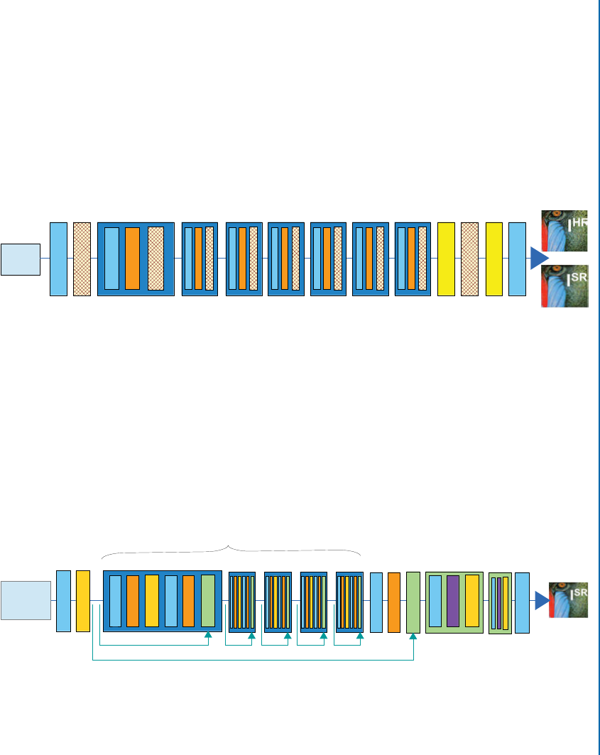
7.5. IMAGE GENERATION 149
SRGAN Architecture
Similar to the baseline GAN [Goodfellow et al.,2014], SRGAN has two key components:
the discriminator and the generator. We will now briefly discuss the architecture of these two
SRGAN components.
Discriminator Network of SRGAN
e discriminator network of SRGAN, shown in Fig. 7.17, is inspired by the architecture of
DCGAN (discussed in Section 7.5.2). e network consists of eight convolutional layers with
33convolution kernels followed by two fully connected layers, and a sigmoid function to
perform binary classification.
Input
k3n64s1 k3n64s2 k3n128s1 k3n128s2 k3n256s1 k3n256s2 k3n512s1 k3n512s2
Conv
Conv
BN
Leaky ReLU
Leaky ReLU
Dense (1024)
Dense (1)
Sigmoid
Leaky ReLU
?
Figure 7.17: Architecture of the discriminator network of SRGAN. k,n, and srepresent the
kernel size, number of feature maps, and stride for each convolutional layer.
Generator Network of SRGAN
e generator component of the SRGAN, shown in Fig. 7.18, is inspired by the deep residual
network (discussed in Section 6.6) and the architecture of DCGAN (discussed in Section 7.5.2).
As suggested by DCGAN [Radford et al.,2015], a leaky ReLU activation function is used in all
layers. Moreover, batch normalization is used after all convolutional layers with the exception of
the first convolutional layer.
Conv
PReLU
PReLU
PReLU
Elementwise Sum
Elementwise Sum
Conv
BN
BN
BN
Conv
Conv
Conv
Input
Low Res
Image
B Residual Blocks
Skip Connection
k9n64s1 k9n3s1k3n64s1 k3n64s2 k3n64s1 k3n256s1
Figure 7.18: Architecture of the generator network of SRGAN. Similar to the discriminator
network, k,n, and srepresent the kernel size, number of feature maps, and stride for each
convolutional layer.

150 7. APPLICATIONS OF CNNS IN COMPUTER VISION
In summary, SRGAN is able to estimate high resolution images with photo-realistic tex-
tures from heavily down-sampled images. It achieved a very good performance on three publicly
available datasets including Set5, Set14, and BSD100.
7.6 VIDEO-BASED ACTION RECOGNITION
Human action recognition in videos is a challenging research problem, which has received a sig-
nificant amount of attention in the computer vision community [Donahue et al.,2015,Karpathy
et al.,2014,Rahmani and Bennamoun,2017,Rahmani and Mian,2016,Rahmani et al.,2017,
Simonyan and Zisserman,2014a]. Action recognition aims to enable computers to automatically
recognize human actions from real world videos. Compared to the single-image classification,
the temporal extent of action videos provides an additional information for action recognition.
Inspired by this, several approaches have been proposed to extend state-of-the-art image classifi-
cation CNNs (e.g., VGGnet, ResNet) for action recognition from video data. In this section, we
shall briefly discuss three representative CNN-based architectures used for video-based human
action recognition task.
7.6.1 ACTION RECOGNITION FROM STILL VIDEO FRAMES
CNNs have so far achieved promising image recognition results. Inspired by this, an extensive
evaluation of CNNs for extending the connectivity of a CNN to the temporal domain for the
task of large-scale action recognition is provided in Karpathy et al. [2014]. We shall now discuss
different architectures for encoding temporal variations of action videos.
Single Frame Architecture
We discuss a single-frame baseline architecture, shown in Fig. 7.19a, to analyze the
contribution of the static appearance to the classification accuracy. e single frame
model is similar to the AlexNet [Krizhevsky et al.,2012], which won the Ima-
geNet challenge. However, instead of accepting the original input of size 224 224
3, the network takes 170 170 3 sized image. is network has the fol-
lowing configuration: Covn.96; 11; 3/ NPConv.256; 5; 1/ NPConv.384; 3; 1/
Conv.384; 3; 1/ Conv.256; 3; 1/ PFC.4096/ FC.4096/, where Conv.f; s; t/ represents a
convolutional layer, which has filters fof spatial size ssand an input stride t. A fully con-
nected layer, with nnodes, is represented by FC.n/. For the pooling layers Pand all the nor-
malization layers Nthe architectural details described in Krizhevsky et al. [2012] are used along
with the following parameters: k= 2; n= 5; ˛=104;ˇ= 0.5, where the constants k,n,˛, and ˇ
are hyper-parameters. A softmax layer is connected to the last fully connected layer with dense
connections.
Given an entire action video, the video-level prediction is produced by forward propagat-
ing each frame individually through the network and then averaging individual frame predic-
tions over the durations of the video.

7.6. VIDEO-BASED ACTION RECOGNITION 151
Single Frame
(a) (b) (c) (d)
Early Fusion Late Fusion Slow Fusion
Figure 7.19: Approaches for fusing information over the temporal dimension through the net-
work. (a) Single Frame, (b) Early Fusion, (c) Late Fusion, and (d) Slow Fusion. In the Slow
Fusion Model (d), the depicted columns share parameters. e pink, green, and blue boxes de-
note convolutional, normalization and pooling layers, respectively.
Early Fusion Architecture
We now discuss the Early Fusion model (Fig. 7.19b). is model captures an entire time window
information and combines it across at a pixel level. To achieve this, the filters on the first Conv
layer in the single frame network (described above) are modified. e new filters have a size of
11 11 3Tpixels, where Tdefines the temporal extent and is set to 10. is direct and early
connectivity to the pixel data helps this model to accurately detect the speed and the direction
of the local motion.
For a given entire video, 20 randomly selected sample clips are individually passed through
the network and their class predictions are then averaged to produce video-level action class
prediction.
Late Fusion Architecture
e late fusion model (Fig. 7.19c) consists of two separate single frame networks (described
above) with shared parameters up to the last Conv layer, Conv.256; 3; 1/. e outputs of the
last Conv layer of these two separate single frame networks are then merged in the first fully
connected layer. Global motion characteristics are computed by the first fully connected layer by
comparing the output of both single-frame networks. ese two separate single frame networks
are placed at a distance of 15 frames apart. More precisely, the input to the first and the second
single frame networks is the i-th frame and iC15-th frame, respectively.

152 7. APPLICATIONS OF CNNS IN COMPUTER VISION
Slow Fusion Architecture
is model (Fig. 7.19d) slowly fuses the temporal information throughout the network in such
way that the higher layers have access to more global information in both the temporal and
the spatial domains. is is achieved by performing a temporal convolution along with a spatial
convolution to calculate the weights and by extending the connectivity of all convolutional layers
in time. More precisely, as shown in Fig. 7.19d, every filter in the first convolutional layer is
applied on an input clip, with a size of 10 frames. e temporal extent of each filter is TD4
and the stride is equal to 2. us, 4 responses are produced for each video clip. is process is
iterated by the second and third layers with filters of temporal extent TD2and a stride equal
to 2. erefore, the information across all the input frames (a total of 10) can be accessed by the
third convolutional layer.
Given an entire human action video, video-level classification is performed by passing 20
randomly selected sample clips through the network and then averaging individual clip predic-
tions over the durations of the video.
Multi-resolution Architecture
In order to speed-up the above mentioned models while retaining their accuracy, the multi-
resolution architecture has been proposed in Karpathy et al. [2014]. e multi-resolution model
consists of two separate networks (i.e., fovea and context networks) over two spatial resolutions,
as shown in Fig 7.20. e architecture of the fovea and context networks is similar to the single-
frame architecture discussed above. However, instead of accepting the original input of size 170
170 3, these networks take 89 89 3 sized images. More precisely, the input to the fovea
model is the center region of size 89 89 at the original spatial resolution, while for the context
stream the down-sampled frames at half the original resolution are used. e total dimension-
ality of the inputs is therefore halved. Moreover, the last pooling layer is removed from both the
fovea and context networks and the activation outputs of both networks are concatenated and
fed into the first fully connected layer.
Model Comparison
All models were trained on the Sport-1M dataset [Simonyan and Zisserman,2014a], which
consists of 200,000 test videos. e results showed that the variation among different CNN ar-
chitectures (e.g., Single Frame, Multi-resolution, Early, Late, and Slow Fusion) is surprisingly
insignificant. Moreover, the results were significantly worse than the state-of-the-art hand-
crafted shallow models. One reason is that these models cannot capture the motion information
in many cases. For example, the Slow Fusion model is expected to implicitly learn the spatio-
temporal features in its first layers, which is a difficult task [Simonyan and Zisserman,2014a]. To
resolve this issue, two-stream CNNs [Simonyan and Zisserman,2014a] model was proposed
to explicitly take into account both spatial and temporal information in a single end-to-end
learning framework.
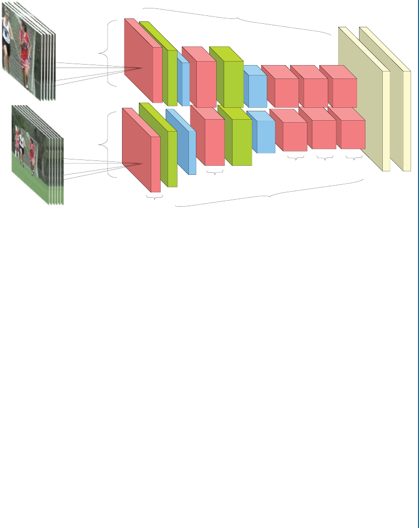
7.6. VIDEO-BASED ACTION RECOGNITION 153
Fovea Stream
Context Stream
27
27
96
256
384 384 256
Figure 7.20: Multi-resolution architecture. Input frames are passed through two separate
streams: a context stream which models the low-resolution image and a fovea stream which
processes the high-resolution center crop image. e pink, green, and blue boxes denote con-
volutional, normalization, and pooling layers, respectively. Both streams converge to two fully
connected layers (yellow boxes).
7.6.2 TWO-STREAM CNNS
e two-stream CNNs model [Simonyan and Zisserman,2014a] (shown in Fig. 7.21) uses
two separate spatial and temporal CNNs, which are then combined by late fusion. e spatial
network performs action recognition from single video frames, while the temporal network is
learned to recognize action from motion, i.e., dense optical flow. e idea behind this two-stream
model is related to the fact that the human visual cortex contains two pathways for object and
motion recognition, i.e., the ventral stream performs object recognition and the dorsal stream
recognizes motion.
Spatial Stream CNN
e spatial stream CNN model is similar to the single frame model in Section 7.6.1. Given
an action video, each video frame is individually passed through the spatial model shown in
Fig. 7.21 and an action label is assigned to each frame. Note that the label of all frames belonging
to a given action video is the same as the label of the action video.
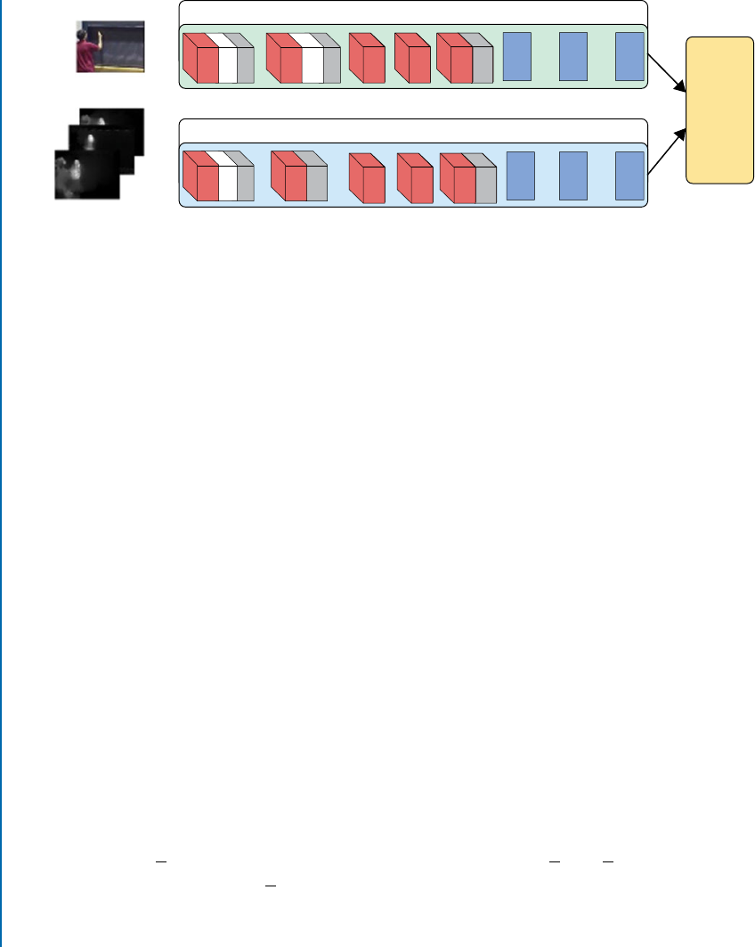
154 7. APPLICATIONS OF CNNS IN COMPUTER VISION
Single Frame
Multiple Frame Optical Flow
Spatial Stream CNN
Class
Scores
Fusion
Temporal Stream CNN
C1 N1 P1 C2 C3 C4 C5 P5 FC6 FC7 FC8
FC6 FC7 FC8
N2 P2
C1 N1 P1 C2 C3 C4 C5 P5P2
Figure 7.21: e architecture of the two-stream CNNs for action classification.
Temporal Stream CNN
Unlike the motion-aware CNN models introduced in Section 7.6.1 (e.g., Slow Fusion), which
use stacked single video frames as input, temporal stream CNN takes stacked optical flow dis-
placement fields between several consecutive frames as input to explicitly learn the temporal
feature. In the following, three variations of the optical flow-based input are explained.
•Optical flow stacking: e input of the temporal stream CNN is formed by stacking the
dense optical flow of Lconsecutive frames (shown in Fig. 7.22). e optical flow at point
.u; v/ in frame tis a 2D displacement vector (i.e., horizontal and vertical displacement),
which moves the point to the corresponding point in the next frame tC1. Note that the
horizontal and vertical components of the dense optical flow of a frame can be seen as
image channels. us, the stacked dense optical flow of Lconsecutive frames forms an
input image of 2L channels, which are fed to the temporal stream CNN as input.
•Trajectory stacking: Unlike the optical flow stacking method which samples the displace-
ment vectors at the same location in Lconsecutive frames, the trajectory stacking method
represents motion in an input image of 2L channels by sampling L2D points along the
motion trajectories [Wang et al.,2011a], as shown in Fig. 7.22.
•Bi-directional optical flow stacking: Both optical flow and trajectory stacking methods
operate on the forward optical flow. e bi-directional optical flow stacking method ex-
tends these methods by computing both forward and backward displacement optical flow
fields. More precisely, motion information is encoded in an input image of 2L channels
by stacking L
2forward optical flows between frames tand tCL
2and L
2backward optical
flows between frames tL
2and t.
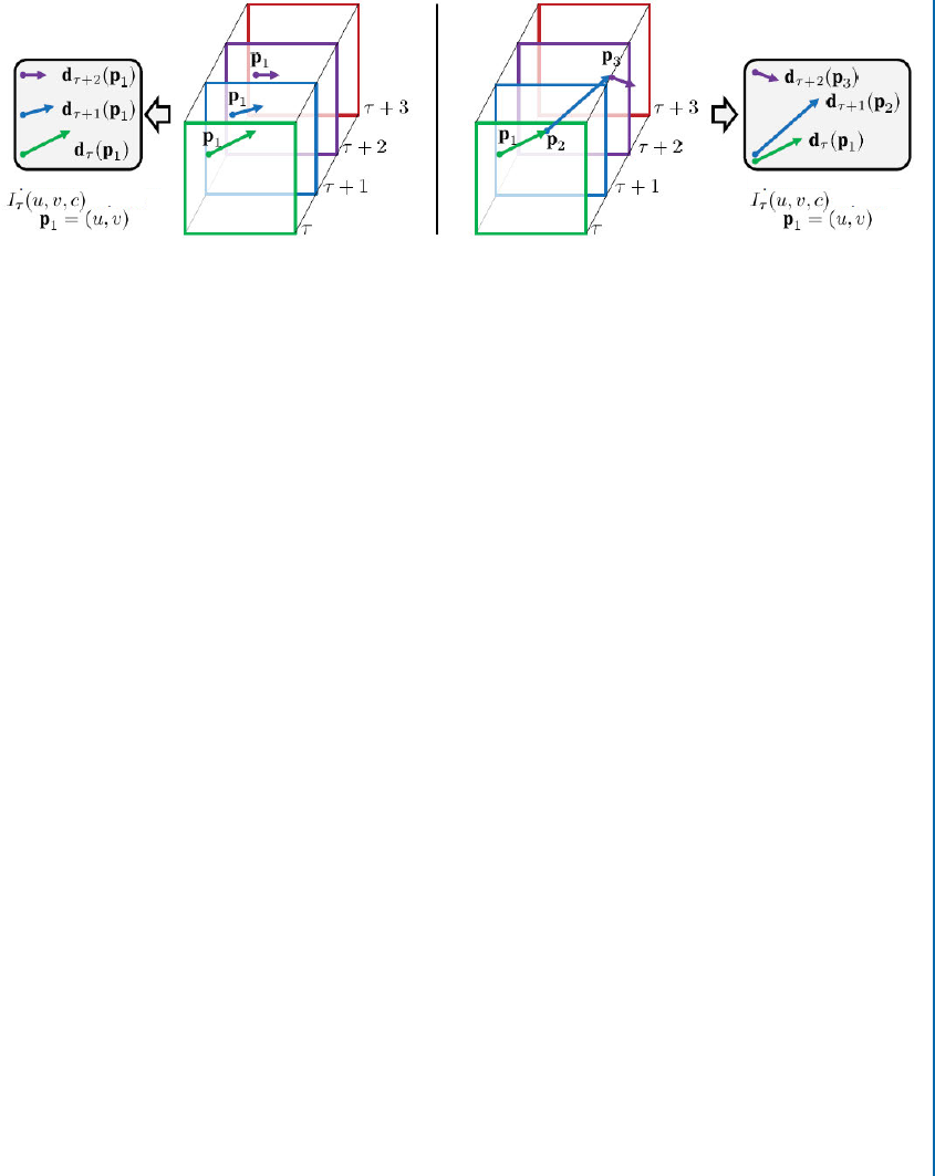
7.6. VIDEO-BASED ACTION RECOGNITION 155
Input volume channels
at point
Input volume channels
at point
Figure 7.22: Left: optical flow stacking method; right: trajectory stacking method.
Architecture
e architecture of the two-stream CNNs model is shown in Fig. 7.21. e architecture of
the spatial and temporal CNN models is similar, except that the second normalization layer is
removed from the temporal CNN to reduce memory consumption. As shown in this figure,
a class score fusion is added to the end of the model to combine the softmax scores of both
the spatial and temporal models by late fusion. Different approaches can be used for class score
fusion. However, experimental results showed that training a linear SVM classifier on stacked
`2-normalized softmax scores outperforms simple averaging.
7.6.3 LONG-TERM RECURRENT CONVOLUTIONAL NETWORK (LRCN)
Unlike the methods in Section 7.6.1 and Section 7.6.2 which learn CNN filters based on
a stack of a fixed number of input frames, Long-term Recurrent Convolutional Network
(LRCN) [Donahue et al.,2015] is not constrained to fixed length input frames and, thus, could
learn to recognize more complex action video. As shown in Fig. 7.23, in LRCN, individual
video frames are first passed through CNN models with shared parameters and then connected
to a single-layer LSTM network (described in Chapter 3). More precisely, the LRCN model
combines a deep hierarchical visual feature extractor, which is a CNN feature extractor, with an
LSTM that can learn to recognize the temporal variations in an end-to-end fashion.
In this chapter, we discussed representative works, which use CNNs in computer vision.
In Table 7.1, we provide an overview of some of the other important CNN applications and
the most representative recent works, which have not been covered in detail in this book. In the
following chapter, we will discuss some prominent tools and libraries of CNN.

156 7. APPLICATIONS OF CNNS IN COMPUTER VISION
Table 7.1: Few recent/most representative applications of CNN, not discussed in this book (Con-
tinues.)
Applications Paper Title
Image
captioning
• Deep Visual-Semantic Alignments for Generating Image Descriptions [Karp-
athy and Fei-Fei, 2015]
• DenseCap: Fully Convolutional Localization Networks for Dense Captioning
[Johnson et al., 2016]
3D recon-
struction
from a 2D
image
• Large Pose 3D Face Reconstruction from a Single Image via Direct Volumet-
ric CNN Regression [Jackson et al., 2017]
• Semantic Scene Completion from a Single Depth Image [Song et al. 2017]
Contour/
edge detec-
tion
• DeepContour: A Deep Convolutional Feature Learned by Positive Sharing
Loss for Contour Detection [Shen et al., 2015b]
• Edge Detection Using Convolutional Neural Network [Wang, 2016]
Text detec-
tion and rec-
ognition
• Reading Text in the Wild with Convolutional Neural Networks [ Jaderberg et
al., 2016]
• End-to-End Text Recognition with Convolutional Neural Networks [Wang
et al., 2012]
Octree rep-
resentation
for shape
analysis
• O-CNN: Octree-based Convolutional Neural Networks for 3D Shape Analy-
sis [Wang et al., 2017]
• OctNet: Learning Deep 3D Representations at High Resolutions [Riegler et
al., 2016]
Face recogni-
tion
• DeepFace: Closing the Gap to Human-Level Performance in Face Verifi ca-
tion [Taigman et al., 2014]
• FaceNet: A Unifi ed Embedding for Face Recognition and Clustering [Schroff
et al., 2015]
Depth esti-
mation
• Learning Depth from Single Monocular Images Using Deep Convolutional
Neural Fields [Liu et al., 2016]
• Deep Convolutional Neural Fields for Depth Estimation from a Single Image
[Liu et al., 2015]
Pose estima-
tion
• PoseNet: A Convolutional Network for Real-Time 6-DOF Camera Relocal-
ization [Kendall et al., 2015]
• DeepPose: Human Pose Estimation via Deep Neural Networks [Toshev and
Szegedy, 2014]

7.6. VIDEO-BASED ACTION RECOGNITION 157
Table 7.1: (Continued.) Few recent/most representative applications of CNN, not discussed in
this book
Tracking • Hedged Deep Tracking [Qi et al., 2016b]
• Hierarchical Convolutional Features for Visual Tracking [Ma et al., 2015]
Shadow de-
tection
• Automatic Shadow Detection and Removal from a Single Image [Khan et al.,
2016a]
• Shadow Optimization from Structured Deep Edge Detection [Shen et al.,
2015a]
Video sum-
marization
• Highlight Detection with Pairwise Deep Ranking for First-Person Video
Summarization [Yao et al., 2016]
• Large-Scale Video Summarization Using Web-Image Priors [Khosla et al.,
2013]
Visual ques-
tion answer-
ing
• Multi-level Attention Networks for Visual Question Answering [Yu et al.,
2017]
• Image Captioning and Visual Question Answering Based on Attributes and
External Knowledge [Wu et al., 2017]
Event detec-
tion
• DevNet: A Deep Event Network for multimedia event detection and evidence
recounting [Gan et al., 2015]
• A Discriminative CNN Video Representation for Event Detection [Xu et al.,
2015]
Image re-
trieval
• Collaborative Index Embedding for Image Retrieval [Zhou et al., 2017]
• Deep Semantic Ranking Based Hashing for Multi-Label Image Retrieval
[Zhao et al., 2015a]
Person
re-identifi ca-
tion
• Recurrent Convolutional Network for Video-Based Person Reidentifi cation
[McLaughlin et al., 2016]
• An Improved Deep Learning Architecture for Person Re-Identifi cation
[Ahmed et al., 2015]
Change de-
tection
• Forest Change Detection in Incomplete Satellite Images with Deep Neural
Networks [Khan et al., 2017c]
• Detecting Change for Multi-View, Long-Term Surface Inspection [Stent et
al., 2015]
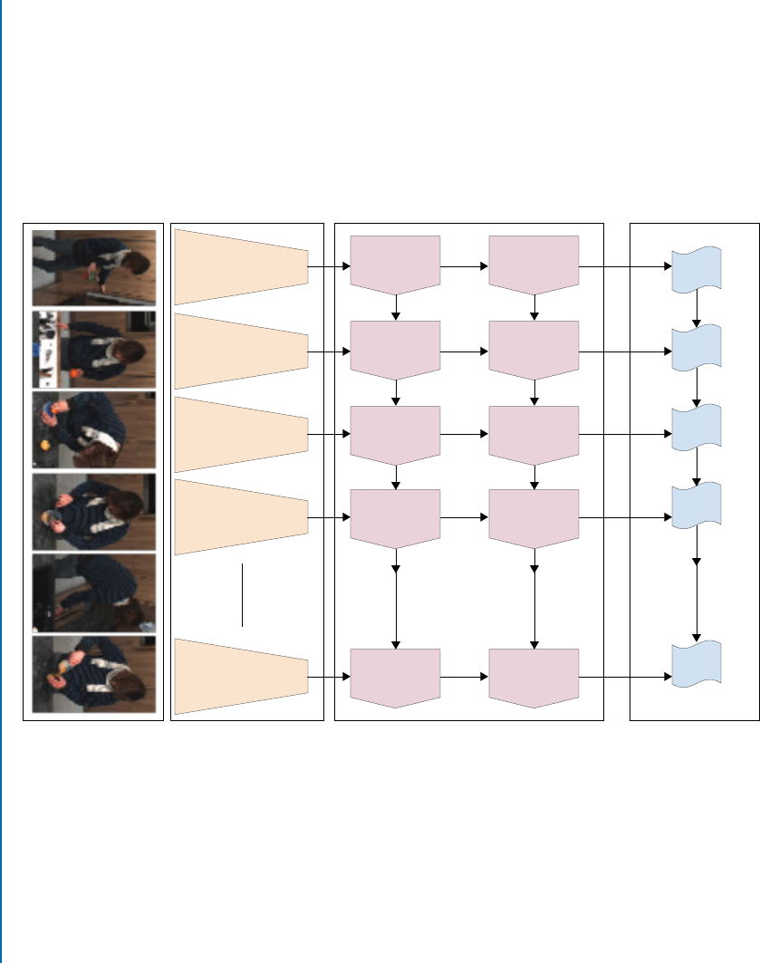
158 7. APPLICATIONS OF CNNS IN COMPUTER VISION
Visual Input Visual Features Sequence Learning Predictions
CNN LSTM LSTM W1
CNN LSTM LSTM
CNN LSTM LSTM
CNN LSTM LSTM
W2
W3
W4
CNN LSTM LSTM WT
Figure 7.23: e architecture of the LRCN.

159
C H A P T E R 8
Deep Learning Tools and
Libraries
ere have been a lot of interest from academics (e.g., e University of California Berkeley,
New York University, e University of Toronto, e University of Montreal) and industry
groups (e.g., Google, Facebook, Microsoft) to develop deep learning frameworks. It is mainly
due to their popularity in many applications domains over the last few years. e key motivation
for developing these libraries is to provide an efficient and friendly development environment
for researchers to design and implement deep neural networks. Some of the widely used deep
learning frameworks are: Caffe, TensorFlow, MatConvNet, Torch7, eano, Keras, Lasange,
Marvin, Chainer, DeepLearning4J, and MXNet.1Many of these libraries are well supported,
with dozens of active contributors and large user bases. Because of strong CUDA backends,
many of these frameworks are very fast in training deep networks with billions of parameters.
Based on the number of users in the Google groups and the number of contributors for each of
the frameworks in their corresponding GitHub repositories, we selected ten widely developed
and supported deep learning frameworks including Caffe, TensorFlow, MatConvNet, Torch7,
eano, Keras, Lasagne, Marvin, Chainer, and PyTorch for further discussions.
8.1 CAFFE
Caffe is a fully open-source deep learning framework and perhaps the first industry-grade deep
learning framework, due to its excellent CNN implementation at the time. It was developed
by the Berkeley Vision and Learning Center (BVLC), as well as community contributors. It
is highly popular within the computer vision community. e code is written in C++, with
CUDA used for GPU computation, and has Python, MATLAB, and commandline interfaces
for training and deployment purposes. Caffe stores and communicates data using blobs, which
are 4-dimensional arrays. It provides a complete set of layer types including: convolution, pool-
ing, inner products, nonlinearities like rectified linear and logistic, local response normalization,
element-wise operations, and different types of losses, such as soft-max and hinge. e learned
1For a more complete list of Deep Learning frameworks, see http://deeplearning.net/software_links/.

160 8. DEEP LEARNING TOOLS AND LIBRARIES
models can be saved to disk as Google Protocol Buffers,2which have many advantages such
as minimal-size binary strings when serialized, efficient serialization, easier to use program-
matically, and a human-readable text format compatible with the binary version, over XML for
serializing structured data. Large-scale data is stored in LevelDB2 databases. ere are also pre-
trained models for the state-of-the-art networks which allows reproducible research. We refer
the readers to the official website3to learn more about the Caffe framework.
However, its support for recurrent networks and language modeling is poor in general.
Moreover, it can only be used for image-based application, while not for other deep learning
applications such as text or speech. Another draw back is that the user needs to manually define
gradient formula for back propagation. As we will discuss further, more recent libraries offer
automatic gradient computations which makes it easy to define new layers and modules.
Following the footsteps of Caffe, Facebook also developed Caffe2, a new lightweight,
modular deep learning framework which is built on the original Caffe and make improvements
on Caffe, particularly a modern computation graph design, supporting large-scale distributed
training, flexibility to port to multiple platforms with ease, and minimalist modularity.
8.2 TENSORFLOW
TensorFlow was originally developed by the Google Brain team. TensorFlow is written with a
Python API over a C/C++ engine for numerical computation using data flow graphs. Multiple
APIs have been provided. e complete programming control is provided with the lowest level
APIs, called TensorFlow Core. Machine learning researchers and others who need fine levels
of control over their models are recommended to use the TensorFlow Core. e higher level
APIs are built on top of TensorFlow Core and they are easier to learn and use, compared to the
TensorFlow Core.
TensorFlow offers automatic differentiation capabilities, which simplify the process of
defining new operations in the network. It uses data flow graphs to perform numerical com-
putations. e graph nodes represent mathematical operations and the edges represent tensors.
TensorFlow supports multiple backends, CPU or GPU on desktop, server or mobile platforms.
It has well-supported bindings to Python and C++. TensorFlow also has tools to support rein-
forcement learning. For more details, we suggest the readers to visit the TensorFlow website.4
8.3 MATCONVNET
is is a MATLAB toolbox for the implementation of convolutional neural networks. It was
developed by the Oxford Visual Geometry Group, as an educational and research platform. Un-
2Google Protocol Buffers are a way of efficiently encoding structured data. It is smaller, faster and simpler than XML. It is
useful in developing programs to communicate with each others over a wire or for storing data. First, a user-defined data
structure is built, and then, a special generated source code is used to easily write and read the structured data to and from
a variety of data streams and using a variety of languages.
3http://caffe.berkeleyvision.org/
4https://www.tensorflow.org/

8.4. TORCH7 161
like most existing deep network frameworks which hide the neural network layers behind a wall
of a compiled code, MatConvNet layers can be implemented directly in MATLAB, which is
one of the most popular development environments in computer vision research and in many
other areas. us, layers can easily be modified, extended, or integrated with new ones. How-
ever, many of its CNN building blocks, such as convolution, normalization, and pooling, use
optimized CPU and GPU implementations written in C++ and CUDA. e implementation
of the CNN computations in this library are inspired by the Caffe framework.
Unlike most existing deep learning frameworks, MatConvNet is simple to compile and
install. e implementation is fully self-contained, requiring only MATLAB and a compatible
C++ compiler. However, MatConvNet does not support recurrent networks. It has a few number
of state-of-the-art pre-trained models. In order to learn more about this framework, we refer
the readers to the official website.5
8.4 TORCH7
Torch7 is a scientific computing framework which provides a wide support for machine learning
algorithms, especially deep neural networks. It provides a MATLAB-like environment and has
strong CUDA and CPU backends. Torch7 is built using Lua that runs on Lua ( JIT) compiler.
e Lua scripting language was chosen to provide three main advantages: (1) Lua is easy for the
development of numerical algorithms, (2) Lua can easily be embedded in a C application, and
provides a great C API, and (3) Lua is the fastest interpreted language (also the fastest Just In
Time ( JIT) compiler). Lua is implemented as a library, written in C.
Torch7 relies on its Tensor class to provide an efficient multi-dimensional array type.
Torch7 has C, C++, and Lua interfaces for model learning and deployment purposes. It also
has an easy to use multi-GPU support which makes it powerful for the learning of deep models.
Torch7 has a large community of developers and is being actively used within large organizations
such as, New York University, Facebook AI lab, Google DeepMind, and Twitter. Unlike most
existing frameworks, Torch7 offers a rich set of RNNs. However, unlike TensorFlow, Torch7 has
the GPU and automatic differentiation support in two separate libraries, cutorch and autograd,
that makes Torch7 a little less slick and a little harder to learn. e tutorials and demos provided
in the Torch7 official website6help the readers to better understand this framework. Torch7 is
probably the fastest deep learning platform available.
8.5 THEANO
eano is a Python library and an optimizing compiler which efficiently defines, optimizes, and
evaluates mathematical expressions involving multi-dimensional arrays. eano was primarily
developed by a machine learning group at the University of Montreal. It combines computer
5http://www.vlfeat.org/matconvnet/
6http://torch.ch/docs/getting-started.html

162 8. DEEP LEARNING TOOLS AND LIBRARIES
algebra system with an optimizing compiler that is useful for tasks in which complicated math-
ematical expressions are evaluated repeatedly, and evaluation speed is critical. eano provides
different implementations for the convolution operation, such as an FFT-based implementa-
tion [Mathieu et al.,2014], and an implementation based on the open-source code of image
classification network in Krizhevsky et al. [2012]. Several libraries, such as Pylearn2, Keras,
and Lasagne, have been developed on top of eano providing building blocks for fast experi-
mentation of well-known models. eano uses symbolic graph for programming a network. Its
symbolic API supports looping control, which makes the implementation of RNNs easy and
efficient.
eano has implementations for most state-of-the-art networks, either in the form of a
higher-level framework, such as Blocksa and Keras, or in pure eano. However, eano is
somewhat low-level and large models have long compilation times. For more information, we
refer the authors to the official website.7However, eano will no longer be developed (imple-
menting new features) after 2018.
8.6 KERAS
Keras is an open-source high-level neural networks API, written in Python, and capable of
running on top of TensorFlow and eano. us, Keras benefits from the advantages of both
and provides a higher-level and more intuitive set of abstractions, which make it easy to configure
neural networks, regardless of the back-end scientific computing library. e primary motivation
behind Keras is to enable fast experimentation with deep neural networks and to go from idea
to results as quickly as possible. e library consists of numerous implementations of neural
network building blocks and tools to make working with image and text data easier. For instance,
Fig. 8.1 shows a Keras code, compared with the code needed to program in Tensorflow, to
achieve the same purpose. As shown in this figure, a neural network can be built in just few lines
of code. For more examples, please visit the Keras official website.8
Keras offers two types of deep neural networks including sequence-based networks (where
the inputs flow linearly through the network) and graph-based networks (where the inputs
can skip certain layers). us, implementing more complex network architectures such as
GoogLeNet and SqueezeNet is easy. However, Keras does not provide most state-of-the-art
pre-trained models.
8.7 LASAGNE
Lasagne9is a lightweight python library to construct and train networks in eano. Unlike
Keras, Lasange was developed to be a light wrapper around eano. Lasange supports a wide
7http://deeplearning.net/software/theano/
8https://keras.io/
9https://github.com/Lasagne/Lasagne
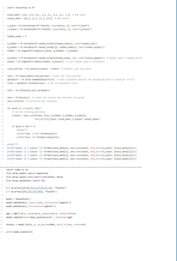
8.7. LASAGNE 163
(b) Keras
(a) TensorFlow
Figure 8.1: is figure illustrates the difference in the size of the code for (a) TensorFlow and
(b) Keras to achieve the same purpose.

164 8. DEEP LEARNING TOOLS AND LIBRARIES
range of deep models including feed-forward networks, such as Convolutional Neural Net-
works (CNNs), recurrent networks, such as LSTM, and any combination of feed-forward and
recurrent networks. It allows architectures of multiple inputs and multiple outputs, including
auxiliary classifiers. Defining cost functions is easy and there is no need to derive gradients due
to eano’s symbolic differentiation.
8.8 MARVIN
Marvin10 was developed by researchers from Princeton University’s Vision Group. It is a GPU-
only neural network framework, written in C++, and made with simplicity, hackability, speed,
memory consumption, and high-dimensional data in mind. Marvin implementation consists of
two files, namely marvin.hpp and marvin.cu. It supports multi-GPU, receptive field calculations
and filter visualization. Marvin can easily be installed on different operating systems including
Windows, Linux, Mac, and all other platforms that CUDNN supports.
Marvin does not provide most state-of-the-art pre-trained models. It, however, provides
a script to convert Caffe models into a format that works in Marvin. Moreover, Marvin does
not provide a good documentation, which makes the building of new models difficult.
8.9 CHAINER
Chainer is an open-source neural network framework with a Python API. It was developed at
Preferred Networks, a machine-learning startup based in Tokyo. Unlike existing deep learning
frameworks, which use the define-and-run approach, Chainer was designed on the principle of
define-by-run.
In the define-and-run-based frameworks, as shown in Fig. 8.2, models are built in two
phases, namely define and run. In the Define phase, a computational graph is constructed. More
precisely, the Define phase is the instantiation of a neural network object based on a model defi-
nition, which specifies the inter-layer connections, initial weights, and activation functions, such
as Protobuf for Caffe. In the Run phase, given a set of training examples, the model is trained
by minimizing the loss function using optimization algorithms, such as SGD. However, the
define-and-run-based frameworks have three major problems, namely (1) inefficient memory
usage, especially for RNN models; (2) limited extensibility; and (3) the inner workings of the
neural network are not accessible to the user, e.g., for the debugging of the models.
Chainer overcomes these drawbacks by providing an easier and more straightforward way
to implement the more complex deep learning architectures. Unlike other frameworks, Chainer
does not fix a model’s computational graph before the model is trained. Instead, the computa-
tional graph is implicitly memorized when the forward computation for the training data set
takes place as shown in Fig. 8.2. us, Chainer allows to modify networks during runtime, and
10http://marvin.is/
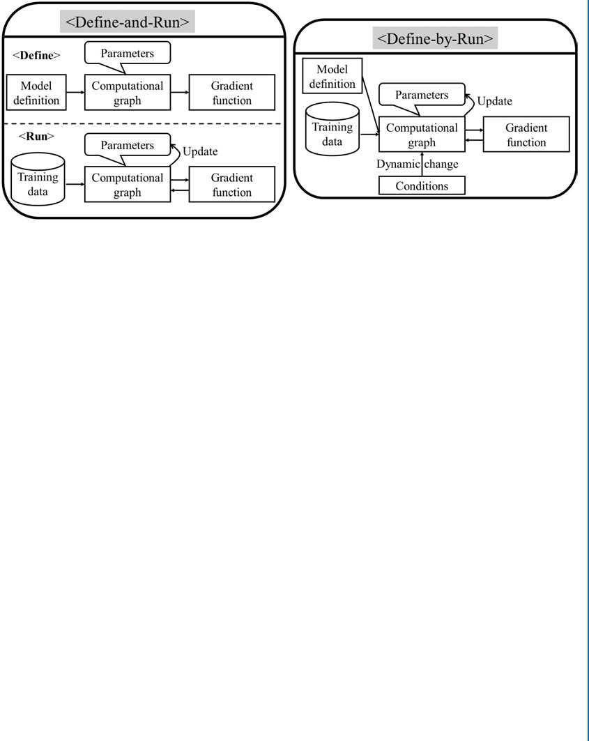
8.10. PYTORCH 165
Figure 8.2: Unlike define-and-run-based frameworks, Chainer is a define-by-run framework,
which does not fix a model’s computational graph before the model is trained.
use arbitrary control flow statements. e Chainer official website11 provides several examples
and more details about Chainer core Concept.
8.10 PYTORCH
PyTorch is an open source machine learning library for Python. It was developed by Facebook’s
artificial intelligence research group. Unlike Torch which is written in Lua (a relatively unpopular
programming language), PyTorch leverages the rising popularity of Python. Since its introduc-
tion, PyTorch has quickly become the favorite among machine-learning researchers because it
allows certain complex architectures to be built easily.
PyTorch is mainly influenced by Chainer. Particularly, PyTorch allows to modify networks
during runtime, i.e., define-by-run framework. e tutorials and demos provided in the PyTorch
official website12 help the readers to better understand this framework.
11https://github.com/chainer/chainer
12http://pytorch.org/tutorials/

166 8. DEEP LEARNING TOOLS AND LIBRARIES
Table 8.1: Comparison of deep learning framework in terms of creator, platform, language, and
provided interface
Software Creator Platform Core Language Interface
Caff e Berkeley Vision
and
Learning Center
(BVLC)
Linux,
Mac OS X,
Windows
C++ Python,
MATLAB
TensorFlow Google Brain team Linux,
Mac OS X
Windows
C++, Python Python, C/
C++, Java, Go
MatConvNet Oxford Visual
Geometry Group
(VGG)
Linux,
Mac OS X,
Windows
MATLAB, C++ MATLAB
Torch7 Ronan Collobert,
Koray Kavukcuoglu,
Clement Farabet,
Soumith Chintala
Linux,
Mac OS X,
Windows,
Android, iOS
C, Lua Lua, LuaJIT,
C, utility
library for
C++
eano Monteral University Cross-platform Python Python
Keras Francois Chollet Linux,
Mac OS X,
Windows
Python Python
Lasagne Saunder Dieleman and
others
Linux,
Mac OS X,
Windows
Python Python
Marvin Jianxiong Xiao,
Shuran Song,
Daniel Suo,
Fisher Yu
Linux,
Mac OS X,
Windows
C++ C++
Chainer Seiya Tokui,
Kenta Oono,
Shohei Hido,
Justin Clayton
Linux,
Mac OS X,
Python Python
PyTorch Adam Paszke,
Sam Gross,
Soumith Chintala,
Gregory Chanan
Linux,
Mac OS X,
Windows
Python, C,
CUDA
Python

8.10. PYTORCH 167
Table 8.2: Comparison of deep learning framework in terms of OpenMP, OpenCL, and Cuda
support, number of available pre-trained models, RNNs, CNNs, and RBM/DBNs
Software OpenMP
Support
OpenCL
Support
CUDA
Support
Pretrained
Models RNNs CNNs RBM/
DBNs
Caff e No Yes Yes Yes Yes Yes Yes
TensorFlow No On roadmap Yes Yes Yes Yes Yes
MatConvNet Yes No Yes A few No Yes No
Torch7 Yes ird party im-
plementations
Yes Yes Yes Yes Yes
eano Yes If using eano
as backend
Under
develop-
ment
Yes Yes Yes Yes
Keras Yes Under
development
for the eano
backend, on
roadmap for the
TensorFlo
backend
Yes A few Yes Yes Yes
Lasagne No Yes Yes Yes Yes Yes Yes
Marvin Yes Yes Yes A few Yes Yes No
Chainer Yes No Yes A few Yes Yes No
PyTorch Yes No Yes Yes Yes Yes Yes

169
C H A P T E R 9
Conclusion
BOOK SUMMARY
e application of deep learning algorithms, especially CNNs, to computer vision problems
have seen a rapid progress. is has led to highly robust, efficient, and flexible vision systems.
is book aimed to introduce different aspects of CNNs in computer vision problems. e first
part of this book (Chapter 1and Chapter 2) introduced computer vision and machine learn-
ing subjects, and reviewed the traditional feature representation and classification methods. We
then briefly covered two generic categories of deep neural networks, namely the feed-forward
and the feed-back networks, their respective computational mechanisms and historical back-
ground in Chapter 3. Chapter 4provided a broad survey of the recent advances in CNNs, in-
cluding state-of-the-art layers, weight initialization techniques, regularization approaches, and
several loss functions. Chapter 5reviewed popular gradient-based learning algorithms followed
by gradient-based optimization methodologies. Chapter 6introduced the most popular CNN
architectures which were mainly developed for object detection and classification tasks. A wide
range of CNN applications in computer vision tasks, including image classification, object de-
tection, object tracking, pose estimation, action recognition, and scene labeling have been dis-
cussed in Chapter 7. Finally, several widely used deep learning libraries have been presented in
Chapter 8to help the readers to understand the main features of these frameworks.
FUTURE RESEARCH DIRECTIONS
While Convolutional Neural Networks (CNNs) have achieved great performances in experi-
mental evaluations, there are still several challenges which we believe deserve further investiga-
tion.
First, deep neural networks require massive amounts of data and computing power to be
trained. However, the manual collection of large-scale labeled datasets is a daunting task. e
requirement of large amounts of labeled data can be relaxed by extracting hierarchical features
through unsupervised learning techniques. Meanwhile, to speed up the learning process, the de-
velopment of effective and scalable parallel learning algorithms warrants further investigation. In
several application domains, there exists a long tail distribution of object classes, where enough
training examples are not available for the less frequent ones. In such scenarios, deep networks
need to be adapted appropriately to overcome the class-imbalance problem [Khan et al.,2017a].

170 9. CONCLUSION
Second, the memory required to store the huge amounts of parameters is another chal-
lenge in deep neural networks, including CNNs. At testing time, these deep models have a high
memory footprint, which makes them unsuitable for mobile and other hand-held devices that
have limited resources. us, it is important to investigate how to decrease the complexity of
deep neural networks without the loss of accuracy.
ird, selecting suitable model hyper-parameters (e.g., learning rate, number of layers,
kernel size, number of feature maps, stride, pooling size, and pooling regions) requires consid-
erable skill and experience. ese hyper-parameters have a significant impact on the accuracy
of deep models. Without an automated hyper-parameter tuning method, one needs to make
manual adjustments to the hyper-parameters using many training runs to achieve the optimal
values. Some recent works [He et al.,2016a,Huang et al.,2016b] have tried optimization tech-
niques for hyper-parameter selection and have shown that there is room to improve current
optimization techniques for learning deep CNN architectures.
Fourth, although deep CNNs have demonstrated an impressive performance on a vari-
ety of applications, they still lack solid mathematical and theoretical foundations. ere is little
insight into the behavior of these complex neural networks, or how they achieve such good
performance. As a result, it might be difficult to improve their performance, and thus, the de-
velopment of better models is restricted to trial-and-error. erefore, attempting to see what
features have been learned, and to understand what computations are performed at each layer
in deep CNNs is an increasingly popular direction of research [Mahendran and Vedaldi,2015,
2016,Zeiler and Fergus,2014].
Fifth, several machine learning algorithms, including state-of-the-art CNNs are vulner-
able to adversarial examples. Adversarial examples have intentionally been designed to cause
the learned model to make a mistake. For example, by adding a small perturbation to an image
of a “panda” in a way that is undetectable to the human eye, the resultant image is recognized
as a “gibbon” with high confidence (Fig. 9.1). us, sophisticated attackers could trick neu-
ral networks. For example, one could target autonomous vehicles by using stickers to design an
adversarial stop sign that the vehicle would interpret as a yield sign [Papernot et al.,2017]. ere-
fore, coming up with sophisticated defense strategies is a vital part of many machine learning
algorithms, including CNNs.
Finally, a major shortcoming of convolutional networks is the inability to work on arbi-
trary shaped inputs, e.g., cyclic and acyclic graphs. Furthermore, there does not exist a principled
way to incorporate structured losses in the deep network formulation. Such losses are essential
for structured prediction tasks such as the body pose estimation and semantic segmentation.
ere have recently been some efforts toward the extension of CNNs to arbitrarily shaped graph
structures [Defferrard et al.,2016,Kipf and Welling,2016]. However, this area has numerous
promising applications and needs further technical breakthroughs to enable fast and scalable
architectures that are suitable for graphs.
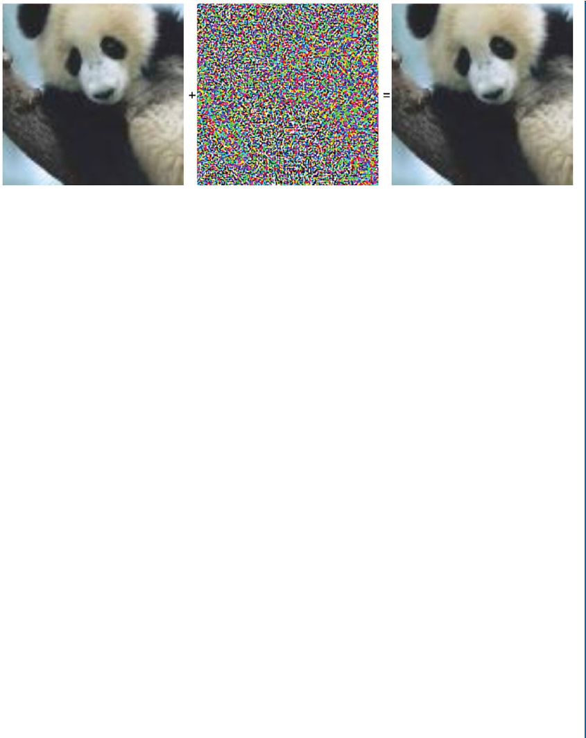
171
Original image classified as a
panda with 60% confidence.
Modified image classified as a
gibbon with 99% confidence.
Small adversarial
perturbation.
Figure 9.1: Adversarial example: by mathematically manipulating a “panda” image in a way that
is undetectable to the human eye (e.g., adding a small perturbation), the learned neural networks
can be tricked into misclassifying objects by sophisticated attackers.
In conclusion, we hope that this book not only provides a better understanding of CNNs
for computer vision tasks, but also facilitates future research activities and application develop-
ments in the field of computer vision and CNNs.

173
Bibliography
ILSVRC 2016 Results. http://image-net.org/challenges/LSVRC/2016/results 106
A. Alahi, R. Ortiz, and P. Vandergheynst. Freak: Fast retina keypoint. In IEEE
Conference on Computer Vision and Pattern Recognition, pages 510–517, 2012. DOI:
10.1109/cvpr.2012.6247715.14
Ark Anderson, Kyle Shaffer, Artem Yankov, Court D. Corley, and Nathan O. Hodas. Beyond
fine tuning: A modular approach to learning on small data. arXiv preprint arXiv:1611.01714,
2016. 72
Relja Arandjelovic, Petr Gronat, Akihiko Torii, Tomas Pajdla, and Josef Sivic. Netvlad: CNN
architecture for weakly supervised place recognition. In Proc. of the IEEE Conference on Com-
puter Vision and Pattern Recognition, pages 5297–5307, 2016. DOI: 10.1109/cvpr.2016.572.
63,64
Pablo Arbeláez, Jordi Pont-Tuset, Jonathan T. Barron, Ferran Marques, and Jitendra Malik.
Multiscale combinatorial grouping. In Proc. of the IEEE Conference on Computer Vision and
Pattern Recognition, pages 328–335, 2014. DOI: 10.1109/cvpr.2014.49.140
Hossein Azizpour, Ali Sharif Razavian, Josephine Sullivan, Atsuto Maki, and Stefan
Carlsson. Factors of transferability for a generic convnet representation. IEEE
Transactions on Pattern Analysis and Machine Intelligence, 38(9):1790–1802, 2016. DOI:
10.1109/tpami.2015.2500224.72
David Balduzzi, Marcus Frean, Lennox Leary, J. P. Lewis, Kurt Wan-Duo Ma, and Brian
McWilliams. e shattered gradients problem: If resnets are the answer, then what is the
question? arXiv preprint arXiv:1702.08591, 2017. 95,98
Herbert Bay, Andreas Ess, Tinne Tuytelaars, and Luc Van Gool. Speeded-up robust fea-
tures (surf ). Computer Vision and Image Understanding, 110(3):346–359, 2008. DOI:
10.1016/j.cviu.2007.09.014.7,11,14,19,29
Atilim Gunes Baydin, Barak A. Pearlmutter, Alexey Andreyevich Radul, and Jeffrey Mark
Siskind. Automatic differentiation in machine learning: A survey. arXiv preprint
arXiv:1502.05767, 2015. 90

174 BIBLIOGRAPHY
N. Bayramoglu and A. Alatan. Shape index sift: Range image recognition using local fea-
tures. In 20th International Conference on Pattern Recognition, pages 352–355, 2010. DOI:
10.1109/icpr.2010.95.13
Yoshua Bengio, Pascal Lamblin, Dan Popovici, Hugo Larochelle, et al. Greedy layer-wise train-
ing of deep networks. Advances in Neural Information Processing Systems, 19:153, 2007. 70
Zhou Bolei, Aditya Khosla, Agata Lapedriza, Aude Oliva, and Antonio Torralba. Object de-
tectors emerge in deep scene CNNs. In International Conference on Learning Representations,
2015. 94,97
Leo Breiman. Random forests. Machine Learning, 45(1):5–32, 2001. DOI:
10.1023/A:1010933404324.7,11,22,26,29
M. Brown and D. Lowe. Invariant features from interest point groups. In Proc. of the British
Machine Vision Conference, pages 23.1–23.10, 2002. DOI: 10.5244/c.16.23.20
M. Calonder, V. Lepetit, C. Strecha, and P. Fua. BRIEF: Binary robust independent elemen-
tary features. In 11th European Conference on Computer Vision, pages 778–792, 2010. DOI:
10.1007/978-3-642-15561-1_56.14
Jean-Pierre Changeux and Paul Ricoeur. What Makes Us ink?: A Neuroscientist and a Philoso-
pher Argue About Ethics, Human Nature, and the Brain. Princeton University Press, 2002. 40
Ken Chatfield, Karen Simonyan, Andrea Vedaldi, and Andrew Zisserman. Return of the devil
in the details: Delving deep into convolutional nets. arXiv preprint arXiv:1405.3531, 2014.
DOI: 10.5244/c.28.6.123
Liang-Chieh Chen, George Papandreou, Iasonas Kokkinos, Kevin Murphy, and Alan L. Yuille.
Semantic image segmentation with deep convolutional nets and fully connected CRFs. arXiv
preprint arXiv:1412.7062, 2014. 50,133
Kyunghyun Cho, Bart Van Merriënboer, Dzmitry Bahdanau, and Yoshua Bengio. On the
properties of neural machine translation: Encoder-decoder approaches. arXiv preprint
arXiv:1409.1259, 2014. DOI: 10.3115/v1/w14-4012.38
Sumit Chopra, Raia Hadsell, and Yann LeCun. Learning a similarity metric discrimi-
natively, with application to face verification. In Computer Vision and Pattern Recogni-
tion, (CVPR). IEEE Computer Society Conference on, volume 1, pages 539–546, 2005. DOI:
10.1109/cvpr.2005.202.67
Dan C. Cireşan, Ueli Meier, Jonathan Masci, Luca M. Gambardella, and Jürgen Schmid-
huber. High-performance neural networks for visual object classification. arXiv preprint
arXiv:1102.0183, 2011. 102

BIBLIOGRAPHY 175
Corinna Cortes. Support-vector networks. Machine Learning, 20(3):273–297, 1995. DOI:
10.1007/bf00994018.7,11,22,29
Koby Crammer and Yoram Singer. On the algorithmic implementation of multiclass kernel-
based vector machines. Journal of Machine Learning Research, 2:265–292, 2001. 66
Michaël Defferrard, Xavier Bresson, and Pierre Vandergheynst. Convolutional neural networks
on graphs with fast localized spectral filtering. In Advances in Neural Information Processing
Systems, pages 3844–3852, 2016. 170
Li Deng. A tutorial survey of architectures, algorithms, and applications for deep learning.
APSIPA Transactions on Signal and Information Processing, 3:e2, 2014. DOI: 10.1017/at-
sip.2014.4.117
Jeff Donahue, Lisa Anne Hendricks, Sergio Guadarrama, Marcus Rohrbach, Subhashini Venu-
gopalan, Kate Saenko, and Trevor Darrell. Long-term recurrent convolutional networks for
visual recognition and description. IEEE Conference on Computer Vision and Pattern Recogni-
tion (CVPR), pages 2625–2634, 2015. DOI: 10.1109/cvpr.2015.7298878.150,155
John Duchi, Elad Hazan, and Yoram Singer. Adaptive subgradient methods for online learning
and stochastic optimization. Journal of Machine Learning Research, 12:2121–2159, 2011. 83
Vincent Dumoulin and Francesco Visin. A guide to convolution arithmetic for deep learning.
arXiv preprint arXiv:1603.07285, 2016. 60
Pedro F. Felzenszwalb, Ross B. Girshick, David McAllester, and Deva Ramanan. Object detec-
tion with discriminatively trained part-based models. IEEE Transactions on Pattern Analysis
and Machine Intelligence, 32(9):1627–1645, 2010. DOI: 10.1109/tpami.2009.167.121
R. A. Fisher. e use of multiple measurements in taxonomic problems. Annals of Eugenics,
7(7):179–188, 1936. DOI: 10.1111/j.1469-1809.1936.tb02137.x.22
Yoav Freund and Robert E. Schapire. A decision-theoretic generalization of online learning
and an application to boosting. Journal of Computer and System Sciences, 55(1):119–139, 1997.
DOI: 10.1006/jcss.1997.1504.22
Jerome H. Friedman. Greedy function approximation: A gradient boosting machine. Annals of
Statistics, 29:1189–1232, 2000. 22
Kunihiko Fukushima and Sei Miyake. Neocognitron: A self-organizing neural network model
for a mechanism of visual pattern recognition. In Competition and Cooperation in Neural Nets,
pages 267–285. Springer, 1982. DOI: 10.1007/978-3-642-46466-9_18.43
Ross Girshick. Fast R-CNN. In Proc. of the IEEE International Conference on Computer Vision,
pages 1440–1448, 2015. DOI: 10.1109/iccv.2015.169.60

176 BIBLIOGRAPHY
Ross Girshick, Jeff Donahue, Trevor Darrell, and Jitendra Malik. Region-based convolutional
networks for accurate object detection and segmentation. IEEE Transactions on Pattern Anal-
ysis and Machine Intelligence, 38(1):142–158, 2016. DOI: 10.1109/tpami.2015.2437384.120
Xavier Glorot and Yoshua Bengio. Understanding the difficulty of training deep feedforward
neural networks. In Aistats, 9:249–256, 2010. 70
Ian Goodfellow. Nips 2016 tutorial: Generative adversarial networks. arXiv preprint
arXiv:1701.00160, 2016. 142
Ian Goodfellow, Jean Pouget-Abadie, Mehdi Mirza, Bing Xu, David Warde-Farley, Sherjil
Ozair, Aaron Courville, and Yoshua Bengio. Generative adversarial nets. In Advances in
Neural Information Processing Systems, pages 2672–2680, 2014. 141,142,149
Ian Goodfellow, Yoshua Bengio, and Aaron Courville. Deep Learning. MIT Press, 2016. http:
//www.deeplearningbook.org 54
Alex Graves and Jürgen Schmidhuber. Framewise phoneme classification with bidirectional
LSTM and other neural network architectures. Neural Networks, 18(5):602–610, 2005. DOI:
10.1016/j.neunet.2005.06.042.38
Alex Graves, Greg Wayne, and Ivo Danihelka. Neural turing machines. arXiv preprint
arXiv:1410.5401, 2014. 38
Alex Graves et al. Supervised Sequence Labelling with Recurrent Neural Networks, volume 385.
Springer, 2012. DOI: 10.1007/978-3-642-24797-2.31
Saurabh Gupta, Pablo Arbelaez, and Jitendra Malik. Perceptual organization and recognition
of indoor scenes from RGB-D images. In Proc. of the IEEE Conference on Computer Vision
and Pattern Recognition, pages 564–571, 2013. DOI: 10.1109/cvpr.2013.79.140
Saurabh Gupta, Ross Girshick, Pablo Arbeláez, and Jitendra Malik. Learning rich features from
RGB-D images for object detection and segmentation. In European Conference on Computer
Vision, pages 345–360. Springer, 2014. DOI: 10.1007/978-3-319-10584-0_23.139,141
Richard H. R. Hahnloser, Rahul Sarpeshkar, Misha A. Mahowald, Rodney J. Douglas, and
H. Sebastian Seung. Digital selection and analogue amplification coexist in a cortex-inspired
silicon circuit. Nature, 405(6789):947, 2000. DOI: 10.1038/35016072.55
Munawar Hayat, Salman H. Khan, Mohammed Bennamoun, and Senjian An. A spatial layout
and scale invariant feature representation for indoor scene classification. IEEE Transactions
on Image Processing, 25(10):4829–4841, 2016. DOI: 10.1109/tip.2016.2599292.96
Kaiming He, Xiangyu Zhang, Shaoqing Ren, and Jian Sun. Spatial pyramid pooling in deep
convolutional networks for visual recognition. In European Conference on Computer Vision,
pages 346–361. Springer, 2014. DOI: 10.1007/978-3-319-10578-9_23.62

BIBLIOGRAPHY 177
Kaiming He, Xiangyu Zhang, Shaoqing Ren, and Jian Sun. Delving deep into rectifiers: Sur-
passing human-level performance on imagenet classification. In Proc. of the IEEE Interna-
tional Conference on Computer Vision, pages 1026–1034, 2015a. DOI: 10.1109/iccv.2015.123.
71
Kaiming He, Xiangyu Zhang, Shaoqing Ren, and Jian Sun. Spatial pyramid pooling in deep
convolutional networks for visual recognition. IEEE Transactions on Pattern Analysis and Ma-
chine Intelligence, 37(9):1904–1916, 2015b. DOI: 10.1109/tpami.2015.2389824.61,125
Kaiming He, Xiangyu Zhang, Shaoqing Ren, and Jian Sun. Deep residual learning for im-
age recognition. In Proc. of the IEEE Conference on Computer Vision and Pattern Recognition,
pages 770–778, 2016a. DOI: 10.1109/cvpr.2016.90.77,106,170
Kaiming He, Xiangyu Zhang, Shaoqing Ren, and Jian Sun. Identity mappings in deep residual
networks. In European Conference on Computer Vision, pages 630–645. Springer, 2016b. DOI:
10.1007/978-3-319-46493-0_38.108,111
Kaiming He, Georgia Gkioxari, Piotr Dollár, and Ross Girshick. Mask R-CNN. arXiv preprint
arXiv:1703.06870, 2017. DOI: 10.1109/iccv.2017.322.60,140,141
Geoffrey E. Hinton, Simon Osindero, and Yee-Whye Teh. A fast learning al-
gorithm for deep belief nets. Neural Computation, 18(7):1527–1554, 2006. DOI:
10.1162/neco.2006.18.7.1527.70
Sepp Hochreiter and Jürgen Schmidhuber. Long short-term memory. Neural Computation,
9(8):1735–1780, 1997. DOI: 10.1162/neco.1997.9.8.1735.38
Gao Huang, Zhuang Liu, Kilian Q. Weinberger, and Laurens van der Maaten. Densely
connected convolutional networks. arXiv preprint arXiv:1608.06993, 2016a. DOI:
10.1109/cvpr.2017.243.114,115
Gao Huang, Yu Sun, Zhuang Liu, Daniel Sedra, and Kilian Q. Weinberger. Deep networks
with stochastic depth. In European Conference on Computer Vision, pages 646–661, 2016b.
DOI: 10.1007/978-3-319-46493-0_39.170
David H. Hubel and Torsten N. Wiesel. Receptive fields of single neurones in the cat’s
striate cortex. e Journal of Physiology, 148(3):574–591, 1959. DOI: 10.1113/jphys-
iol.1959.sp006308.43
Sergey Ioffe and Christian Szegedy. Batch normalization: Accelerating deep network training
by reducing internal covariate shift. arXiv preprint arXiv:1502.03167, 2015. 76,77
Max Jaderberg, Karen Simonyan, Andrew Zisserman, et al. Spatial transformer networks. In
Advances in Neural Information Processing Systems, pages 2017–2025, 2015. 63

178 BIBLIOGRAPHY
Anil K. Jain, Jianchang Mao, and K. Moidin Mohiuddin. Artificial neural networks: A tutorial.
Computer, 29(3):31–44, 1996. DOI: 10.1109/2.485891.39
Katarzyna Janocha and Wojciech Marian Czarnecki. On loss functions for deep
neural networks in classification. arXiv preprint arXiv:1702.05659, 2017. DOI:
10.4467/20838476si.16.004.6185.68
Hervé Jégou, Matthijs Douze, Cordelia Schmid, and Patrick Pérez. Aggregating local descrip-
tors into a compact image representation. In Computer Vision and Pattern Recognition (CVPR),
IEEE Conference on, pages 3304–3311, 2010. DOI: 10.1109/cvpr.2010.5540039.63
Andrej Karpathy, George Toderici, Sanketh Shetty, omas Leung, Rahul Sukthankar, and
Li Fei-Fei. Large-scale video classification with convolutional neural networks. In Proc. of the
IEEE Conference on Computer Vision and Pattern Recognition, pages 1725–1732, 2014. DOI:
10.1109/cvpr.2014.223.150,152
Salman H. Khan. Feature learning and structured prediction for scene understanding. Ph.D.
esis, University of Western Australia, 2016. 135
Salman H. Khan, Mohammed Bennamoun, Ferdous Sohel, and Roberto Togneri. Automatic
shadow detection and removal from a single image. IEEE Transactions on Pattern Analysis
and Machine Intelligence, 38(3):431–446, 2016a. DOI: 10.1109/tpami.2015.2462355.141
Salman H. Khan, Munawar Hayat, Mohammed Bennamoun, Roberto Togneri, and Fer-
dous A. Sohel. A discriminative representation of convolutional features for indoor
scene recognition. IEEE Transactions on Image Processing, 25(7):3372–3383, 2016b. DOI:
10.1109/tip.2016.2567076.72,95
Salman H. Khan, Munawar Hayat, Mohammed Bennamoun, Ferdous A. Sohel, and
Roberto Togneri. Cost-sensitive learning of deep feature representations from imbal-
anced data. IEEE Transactions on Neural Networks and Learning Systems, 2017a. DOI:
10.1109/tnnls.2017.2732482.169
Salman H. Khan, Munawar Hayat, and Fatih Porikli. Scene categorization with spectral fea-
tures. In Proc. of the IEEE Conference on Computer Vision and Pattern Recognition, pages 5638–
5648, 2017b. DOI: 10.1109/iccv.2017.601.94
Salman H. Khan, Xuming He, Fatih Porikli, Mohammed Bennamoun, Ferdous Sohel, and
Roberto Togneri. Learning deep structured network for weakly supervised change detection.
In Proc. of the International Joint Conference on Artificial Intelligence (IJCAI), pages 1–7, 2017c.
DOI: 10.24963/ijcai.2017/279.141
Salman Hameed Khan, Mohammed Bennamoun, Ferdous Sohel, and Roberto Togneri. Auto-
matic feature learning for robust shadow detection. In Computer Vision and Pattern Recognition
(CVPR), IEEE Conference on, pages 1939–1946, 2014. DOI: 10.1109/cvpr.2014.249.93

BIBLIOGRAPHY 179
Diederik Kingma and Jimmy Ba. Adam: A method for stochastic optimization. arXiv preprint
arXiv:1412.6980, 2014. 85,86
omas N. Kipf and Max Welling. Semi-supervised classification with graph convolutional
networks. arXiv preprint arXiv:1609.02907, 2016. 170
Philipp Krähenbühl and Vladlen Koltun. Efficient inference in fully connected CRFS with
Gaussian edge potentials. In Advances in Neural Information Processing Systems 24, pages 109–
117, 2011. 132,135
Alex Krizhevsky, Ilya Sutskever, and Geoffrey E. Hinton. Imagenet classification with
deep convolutional neural networks. In Advances in Neural Information Processing Systems,
pages 1097–1105, 2012. DOI: 10.1145/3065386.45,74,102,117,123,140,150,162
Gustav Larsson, Michael Maire, and Gregory Shakhnarovich. Fractalnet: Ultra-deep neural
networks without residuals. arXiv preprint arXiv:1605.07648, 2016. 112,113
Svetlana Lazebnik, Cordelia Schmid, and Jean Ponce. Beyond bags of features: Spatial pyramid
matching for recognizing natural scene categories. In Computer Vision and Pattern Recognition,
IEEE Computer Society Conference on, 2:2169–2178, 2006. DOI: 10.1109/cvpr.2006.68.61
Yann LeCun, Bernhard Boser, John S. Denker, Donnie Henderson, Richard E. Howard, Wayne
Hubbard, and Lawrence D. Jackel. Backpropagation applied to handwritten zip code recog-
nition. Neural Computation, 1(4):541–551, 1989. DOI: 10.1162/neco.1989.1.4.541.43
Yann LeCun, Léon Bottou, Yoshua Bengio, and Patrick Haffner. Gradient-based learn-
ing applied to document recognition. Proc. of the IEEE, 86(11):2278–2324, 1998. DOI:
10.1109/5.726791.101,102
Christian Ledig, Lucas eis, Ferenc Huszár, Jose Caballero, Andrew Cunningham, Alejan-
dro Acosta, Andrew Aitken, Alykhan Tejani, Johannes Totz, Zehan Wang, et al. Photo-
realistic single image super-resolution using a generative adversarial network. arXiv preprint
arXiv:1609.04802, 2016. DOI: 10.1109/cvpr.2017.19.141,145,147,148
Stefan Leutenegger, Margarita Chli, and Roland Y. Siegwart. BRISK: Binary robust invariant
scalable keypoints. In Proc. of the International Conference on Computer Vision, pages 2548–
2555, 2011. DOI: 10.1109/iccv.2011.6126542.14
Li-Jia Li, Richard Socher, and Li Fei-Fei. Towards total scene understanding: Classi-
fication, annotation and segmentation in an automatic framework. In Computer Vi-
sion and Pattern Recognition, (CVPR). IEEE Conference on, pages 2036–2043, 2009. DOI:
10.1109/cvpr.2009.5206718.135
Min Lin, Qiang Chen, and Shuicheng Yan. Network in network. arXiv preprint
arXiv:1312.4400, 2013. 56,103

180 BIBLIOGRAPHY
Jonathan Long, Evan Shelhamer, and Trevor Darrell. Fully convolutional networks for semantic
segmentation. In Proc. of the IEEE Conference on Computer Vision and Pattern Recognition,
pages 3431–3440, 2015. DOI: 10.1109/cvpr.2015.7298965.127,128,130
David G. Lowe. Distinctive image features from scale-invariant keypoints. International Journal
on Computer Vision, 60(2):91–110, 2004. DOI: 10.1023/b:visi.0000029664.99615.94.7,11,
14,16,17,19,29
A. Mahendran and A. Vedaldi. Understanding deep image representations by inverting them.
In Computer Vision and Pattern Recognition, (CVPR). IEEE Computer Society Conference on,
pages 5188–5196, 2015. DOI: 10.1109/cvpr.2015.7299155.97,99,170
A. Mahendran and A. Vedaldi. Visualizing deep convolutional neural networks using nat-
ural pre-images. International Journal on Computer Vision, 120(3):233–255, 2016. DOI:
10.1007/s11263-016-0911-8.170
Michael Mathieu, Mikael Henaff, and Yann LeCun. Fast training of convolutional networks
through FFTs. In International Conference on Learning Representations (ICLR2014), 2014.
162
Warren S. McCulloch and Walter Pitts. A logical calculus of the ideas immanent in
nervous activity. e Bulletin of Mathematical Biophysics, 5(4):115–133, 1943. DOI:
10.1007/bf02478259.40
Dmytro Mishkin and Jiri Matas. All you need is a good INIT. arXiv preprint arXiv:1511.06422,
2015. 71
B. Triggs and N. Dalal. Histograms of oriented gradients for human detection. In IEEE
Computer Society Conference on Computer Vision and Pattern Recognition, pages 1063–6919,
2005. DOI: 10.1109/CVPR.2005.177.7,11,14,15,29
Yurii Nesterov. A method for unconstrained convex minimization problem with the rate of
convergence o (1/k2). In Doklady an SSSR, 269:543–547, 1983. 82
Hyeonwoo Noh, Seunghoon Hong, and Bohyung Han. Learning deconvolution network for
semantic segmentation. In Proc. of the IEEE International Conference on Computer Vision,
pages 1520–1528, 2015. DOI: 10.1109/iccv.2015.178.130
Nicolas Papernot, Patrick McDaniel, Ian Goodfellow, Somesh Jha, Z. Berkay Celik, and Anan-
thram Swami. Practical black-box attacks against machine learning. In Proc. of the ACM on
Asia Conference on Computer and Communications Security, (ASIA CCS’17), pages 506–519,
2017. DOI: 10.1145/3052973.3053009.170
Razvan Pascanu, Yann N. Dauphin, Surya Ganguli, and Yoshua Bengio. On the saddle point
problem for non-convex optimization. arXiv preprint arXiv:1405.4604, 2014. 81

BIBLIOGRAPHY 181
Charles R. Qi, Hao Su, Kaichun Mo, and Leonidas J. Guibas. Pointnet: Deep learning on point
sets for 3D classification and segmentation. arXiv preprint arXiv:1612.00593, 2016. DOI:
10.1109/cvpr.2017.16.117,118,119
J. R. Quinlan. Induction of decision trees. Machine Learning, pages 81–106, 1986. DOI:
10.1007/bf00116251.7,11,22,26,29
Alec Radford, Luke Metz, and Soumith Chintala. Unsupervised representation learning with
deep convolutional generative adversarial networks. arXiv preprint arXiv:1511.06434, 2015.
141,145,149
H. Rahmani, A. Mahmood, D. Q. Huynh, and A. Mian. HOPC: Histogram of oriented
principal components of 3D pointclouds for action recognition. In 13th European Conference
on Computer Vision, pages 742–757, 2014. DOI: 10.1007/978-3-319-10605-2_48.13
Hossein Rahmani and Mohammed Bennamoun. Learning action recognition model from
depth and skeleton videos. In e IEEE International Conference on Computer Vision (ICCV),
2017. DOI: 10.1109/iccv.2017.621.150
Hossein Rahmani and Ajmal Mian. 3D action recognition from novel viewpoints. In Computer
Vision and Pattern Recognition, (CVPR). IEEE Computer Society Conference on, pages 1506–
1515, 2016. DOI: 10.1109/cvpr.2016.167.74,150
Hossein Rahmani, Ajmal Mian, and Mubarak Shah. Learning a deep model for human ac-
tion recognition from novel viewpoints. IEEE Transactions on Pattern Analysis and Machine
Intelligence, 2017. DOI: 10.1109/tpami.2017.2691768.74,150
Shaoqing Ren, Kaiming He, Ross Girshick, and Jian Sun. Faster R-CNN: Towards real-time
object detection with region proposal networks. In Advances in Neural Information Processing
Systems, pages 91–99, 2015. DOI: 10.1109/tpami.2016.2577031.61,123
Ethan Rublee, Vincent Rabaud, Kurt Konolige, and Gary Bradski. ORB: An efficient alterna-
tive to SIFT or SURF. In Proc. of the International Conference on Computer Vision, pages 2564–
2571, 2011. DOI: 10.1109/iccv.2011.6126544.14
Sebastian Ruder. An overview of gradient descent optimization algorithms. arXiv preprint
arXiv:1609.04747, 2016. 81
David E. Rumelhart, Geoffrey E. Hinton, and Ronald J. Williams. Learning internal represen-
tations by error propagation. Technical report, DTIC Document, 1985. DOI: 10.1016/b978-
1-4832-1446-7.50035-2.34
Andrew M. Saxe, James L. McClelland, and Surya Ganguli. Exact solutions to the nonlinear
dynamics of learning in deep linear neural networks. arXiv preprint arXiv:1312.6120, 2013.
70

182 BIBLIOGRAPHY
Florian Schroff, Dmitry Kalenichenko, and James Philbin. Facenet: A unified embedding for
face recognition and clustering. In Proc. of the IEEE Conference on Computer Vision and Pattern
Recognition, pages 815–823, 2015. DOI: 10.1109/cvpr.2015.7298682.68
Ali Sharif Razavian, Hossein Azizpour, Josephine Sullivan, and Stefan Carlsson. CNN fea-
tures off-the-shelf: An astounding baseline for recognition. In Proc. of the IEEE Con-
ference on Computer Vision and Pattern Recognition Workshops, pages 806–813, 2014. DOI:
10.1109/cvprw.2014.131.72
J. Shotton, A. Fitzgibbon, M. Cook, T. Sharp, M. Finocchio, R. Moore, A. Kipman, and
A. Blake. Real-time human pose recognition in parts from single depth images. In Computer
Vision and Pattern Recognition, (CVPR). IEEE Computer Society Conference on, pages 1297–
1304, 2011. DOI: 10.1145/2398356.2398381.26
Ashish Shrivastava, Tomas Pfister, Oncel Tuzel, Josh Susskind, Wenda Wang, and Russ Webb.
Learning from simulated and unsupervised images through adversarial training. arXiv
preprint arXiv:1612.07828, 2016. DOI: 10.1109/cvpr.2017.241.74
Karen Simonyan and Andrew Zisserman. Two-stream convolutional networks for action recog-
nition in videos. In Proc. of the 27th International Conference on Neural Information Processing
Systems—Volume 1, (NIPS’14), pages 568–576, 2014a. 150,152,153
Karen Simonyan and Andrew Zisserman. Very deep convolutional networks for large-scale
image recognition. arXiv preprint arXiv:1409.1556, 2014b. 50,70,104,123
Fisher Yu, Yinda Zhang, Shuran Song, Ari Seff, and Jianxiong Xiao. Construction of a
large-scale image dataset using deep learning with humans in the loop. arXiv preprint
arXiv:1506.03365, 2015. 146,147
Shuran Song and Jianxiong Xiao. Deep sliding shapes for a modal 3D object detection in
RGB-D images. In Proc. of the IEEE Conference on Computer Vision and Pattern Recognition,
pages 808–816, 2016. DOI: 10.1109/cvpr.2016.94.136
Shuran Song, Samuel P. Lichtenberg, and Jianxiong Xiao. Sun RGB-D: A RGB-D scene un-
derstanding benchmark suite. In Proc. of the IEEE Conference on Computer Vision and Pattern
Recognition, pages 567–576, 2015. DOI: 10.1109/cvpr.2015.7298655.136
Jost Tobias Springenberg. Unsupervised and semi-supervised learning with categorical genera-
tive adversarial networks. arXiv preprint arXiv:1511.06390, 2015. 146
Nitish Srivastava, Geoffrey E. Hinton, Alex Krizhevsky, Ilya Sutskever, and Ruslan Salakhut-
dinov. Dropout: A simple way to prevent neural networks from overfitting. Journal of Machine
Learning Research, 15(1):1929–1958, 2014. 75,79,102

BIBLIOGRAPHY 183
Rupesh Kumar Srivastava, Klaus Greff, and Jürgen Schmidhuber. Highway networks. arXiv
preprint arXiv:1505.00387, 2015. 108
Christian Szegedy, Wei Liu, Yangqing Jia, Pierre Sermanet, Scott Reed, Dragomir Anguelov,
Dumitru Erhan, Vincent Vanhoucke, and Andrew Rabinovich. Going deeper with convolu-
tions. In Proc. of the IEEE Conference on Computer Vision and Pattern Recognition, pages 1–9,
2015. DOI: 10.1109/cvpr.2015.7298594.105,106,107
Yichuan Tang. Deep learning using linear support vector machines. arXiv preprint
arXiv:1306.0239, 2013. 67
Tijmen Tieleman and Geoffrey Hinton. Lecture 6.5-rmsprop: Divide the gradient by a running
average of its recent magnitude. COURSERA: Neural Networks for Machine Learning, 4(2),
2012. 85
Jasper R. R. Uijlings, Koen E. A. Van De Sande, eo Gevers, and Arnold W. M. Smeulders.
Selective search for object recognition. International Journal of Computer Vision, 104(2):154–
171, 2013. DOI: 10.1007/s11263-013-0620-5.61,120,122
Aaron van den Oord, Nal Kalchbrenner, Lasse Espeholt, Oriol Vinyals, Alex Graves, et al.
Conditional image generation with pixel CNN decoders. In Advances in Neural Information
Processing Systems, pages 4790–4798, 2016. 141
Li Wan, Matthew Zeiler, Sixin Zhang, Yann L. Cun, and Rob Fergus. Regularization of neural
networks using dropconnect. In Proc. of the 30th International Conference on Machine Learning
(ICML’13), pages 1058–1066, 2013. 75
Heng Wang, A. Klaser, C. Schmid, and Cheng-Lin Liu. Action recognition by dense trajecto-
ries. In Proc. of the IEEE Conference on Computer Vision and Pattern Recognition, (CVPR’11),
pages 3169–3176, 2011a. DOI: 10.1109/cvpr.2011.5995407.154
Zhenhua Wang, Bin Fan, and Fuchao Wu. Local intensity order pattern for feature description.
In Proc. of the International Conference on Computer Vision, pages 1550–5499, 2011b. DOI:
10.1109/iccv.2011.6126294.14
Jason Weston, Chris Watkins, et al. Support vector machines for multi-class pattern recognition.
In ESANN, 99:219–224, 1999. 67
Bernard Widrow, Marcian E. Hoff, et al. Adaptive switching circuits. In IRE WESCON Con-
vention Record, 4:96–104, New York, 1960. DOI: 10.21236/ad0241531.33
Jason Yosinski, Jeff Clune, omas Fuchs, and Hod Lipson. Understanding neural networks
through deep visualization. In In ICML Workshop on Deep Learning, Citeseer, 2015. 95,98

184 BIBLIOGRAPHY
Fisher Yu and Vladlen Koltun. Multi-scale context aggregation by dilated convolutions. arXiv
preprint arXiv:1511.07122, 2015. 50,141
Sergey Zagoruyko and Nikos Komodakis. Learning to compare image patches via convolutional
neural networks. In Proc. of the IEEE Conference on Computer Vision and Pattern Recognition,
pages 4353–4361, 2015. DOI: 10.1109/cvpr.2015.7299064.141
Matthew D. Zeiler. Adadelta: An adaptive learning rate method. arXiv preprint
arXiv:1212.5701, 2012. 84
Matthew D. Zeiler and Rob Fergus. Visualizing and understanding convolutional networks. In
European Conference on Computer Vision, pages 818–833, Springer, 2014. DOI: 10.1007/978-
3-319-10590-1_53.44,94,95,97,170
Yinda Zhang, Mingru Bai, Pushmeet Kohli, Shahram Izadi, and Jianxiong Xiao. Deepcon-
text: Context-encoding neural pathways for 3D holistic scene understanding. arXiv preprint
arXiv:1603.04922, 2016. DOI: 10.1109/iccv.2017.135.135,139
Hang Zhao, Orazio Gallo, Iuri Frosio, and Jan Kautz. Loss functions for neural networks for
image processing. arXiv preprint arXiv:1511.08861, 2015. 67,68
Hengshuang Zhao, Jianping Shi, Xiaojuan Qi, Xiaogang Wang, and Jiaya Jia. Pyramid scene
parsing network. In Proc. of the IEEE Conference on Computer Vision and Pattern Recognition,
pages 1–7, 2017. DOI: 10.1109/cvpr.2017.660.141
Shuai Zheng, Sadeep Jayasumana, Bernardino Romera-Paredes, Vibhav Vineet, Zhizhong Su,
Dalong Du, Chang Huang, and Philip H. S. Torr. Conditional random fields as recurrent
neural networks. In Proc. of the IEEE International Conference on Computer Vision, pages 1529–
1537, 2015. DOI: 10.1109/iccv.2015.179.141
C. Lawrence Zitnick and Piotr Dollár. Edge boxes: Locating object proposals from edges. In
European Conference on Computer Vision, pages 391–405, Springer, 2014. DOI: 10.1007/978-
3-319-10602-1_26.61,132

185
Authors’ Biographies
SALMAN KHAN
Salman Khan received a B.E. in Electrical Engineering from the National University of Sci-
ences and Technology (NUST) in 2012 with high distinction, and a Ph.D. from e University
of Western Australia (UWA) in 2016. His Ph.D. thesis received an Honorable Mention on the
Dean’s list Award. In 2015, he was a visiting researcher with National ICT Australia, Canberra
Research Laboratories. He is currently a Research Scientist with Data61, Commonwealth Sci-
entific and Industrial Research Organization (CSIRO), and has been an Adjunct Lecturer with
Australian National University (ANU) since 2016. He was awarded several prestigious schol-
arships such as the International Postgraduate Research Scholarship (IPRS) for Ph.D. and the
Fulbright Scholarship for MS. He has served as a program committee member for several lead-
ing computer vision and robotics conferences such as IEEE CVPR, ICCV, ICRA, WACV,
and ACCV. His research interests include computer vision, pattern recognition, and machine
learning.
HOSSEIN RAHMANI
Hossein Rahmani received his BSc. in Computer Software Engineering in 2004 from Isfahan
University of Technology, Isfahan, Iran and his MSc. degree in Software Engineering in 2010
from Shahid Beheshti University, Tehran, Iran. He completed his Ph.D. from e University
of Western Australia in 2016. He has published several papers in top conferences and journals
such as CVPR, ICCV, ECCV, and TPAMI. He is currently a Research Fellow in the School of
Computer Science and Software Engineering at e University of Western Australia. He has
served as a reviewer for several leading computer vision conferences and journals such as IEEE
TPAMI, and CVPR. His research interests include computer vision, action recognition, 3D
shape analysis, and machine learning.
SYED AFAQ ALI SHAH
Syed Afaq Ali Shah received his B.Sc. and M.Sc. degrees in Electrical Engineering from the
University of Engineering and Technology (UET) Peshawar, in 2003 and 2010, respectively.
He obtained his Ph.D. from the University of Western Australia in the area of computer vi-
sion and machine learning in 2016. He is currently working as a research associate in the school
of computer science and software engineering at the University of Western Australia, Craw-

186 AUTHORS’ BIOGRAPHIES
ley, Australia. He has been awarded the “Start Something Prize for Research Impact through
Enterprise” for 3D facial analysis project funded by the Australian Research Council. He has
served as a program committee member for ACIVS 2017. His research interests include deep
learning, computer vision, and pattern recognition.
MOHAMMED BENNAMOUN
Mohammed Bennamoun received his M.Sc. from Queen’s University, Kingston, Canada in
the area of Control eory, and his Ph.D. from Queen’s QUT in Brisbane, Australia, in the
area of Computer Vision. He lectured Robotics at Queen’s, and then joined QUT in 1993 as an
associate lecturer. He is currently a Winthrop Professor. He served as the Head of the School of
Computer Science and Software Engineering at e University of Western Australia (UWA)
for five years (February 2007–March 2012). He served as the Director of a University Centre at
QUT: e Space Centre for Satellite Navigation from 1998–2002.
He served as a member of the Australian Research Council (ARC) College of Experts
from 2013–2015. He was an Erasmus Mundus Scholar and Visiting Professor in 2006 at the
University of Edinburgh. He was also a visiting professor at CNRS (Centre National de la
Recherche Scientifique) and Telecom Lille1, France in 2009, e Helsinki University of Tech-
nology in 2006, and e University of Bourgogne and Paris 13 in France in 2002–2003. He is
the co-author of the book Object Recognition: Fundamentals and Case Studies (Springer-Verlag,
2001), and the co-author of an edited book Ontology Learning and Knowledge Discovery Using
the Web, published in 2011.
Mohammed has published over 100 journal papers and over 250 conference papers, and
secured highly competitive national grants from the ARC, government, and other funding bod-
ies. Some of these grants were in collaboration with industry partners (through the ARC Link-
age Project scheme) to solve real research problems for industry, including Swimming Aus-
tralia, the West Australian Institute of Sport, a textile company (Beaulieu Pacific), and AAM-
GeoScan. He worked on research problems and collaborated (through joint publications, grants,
and supervision of Ph.D. students) with researchers from different disciplines including ani-
mal biology, speech processing, biomechanics, ophthalmology, dentistry, linguistics, robotics,
photogrammetry, and radiology. He has collaborated with researchers from within Australia
(e.g., CSIRO), as well as internationally (e.g. Germany, France, Finland, U.S.). He won several
awards, including the Best Supervisor of the Year Award at QUT in 1998, an award for teaching
excellence (research supervision), and the Vice-Chancellor’s Award for Research Mentorship in
2016. He also received an award for research supervision at UWA in 2008.
He has served as a guest editor for a couple of special issues in international journals, such
as the International Journal of Pattern Recognition and Artificial Intelligence (IJPRAI). He was se-
lected to give conference tutorials at the European Conference on Computer Vision (ECCV),
the International Conference on Acoustics Speech and Signal Processing (IEEE ICASSP), the
IEEE International Conference on Computer Vision (CVPR 2016), Interspeech (2014), and

AUTHORS’ BIOGRAPHIES 187
a course at the International Summer School on Deep Learning (DeepLearn2017). He has
organized several special sessions for conferences, including a special session for the IEEE In-
ternational Conference in Image Processing (IEEE ICIP). He was on the program committee
of many conferences, e.g., 3D Digital Imaging and Modeling (3DIM) and the International
Conference on Computer Vision. He also contributed in the organization of many local and
international conferences. His areas of interest include control theory, robotics, obstacle avoid-
ance, object recognition, machine/deep learning, signal/image processing, and computer vision
(particularly 3D).