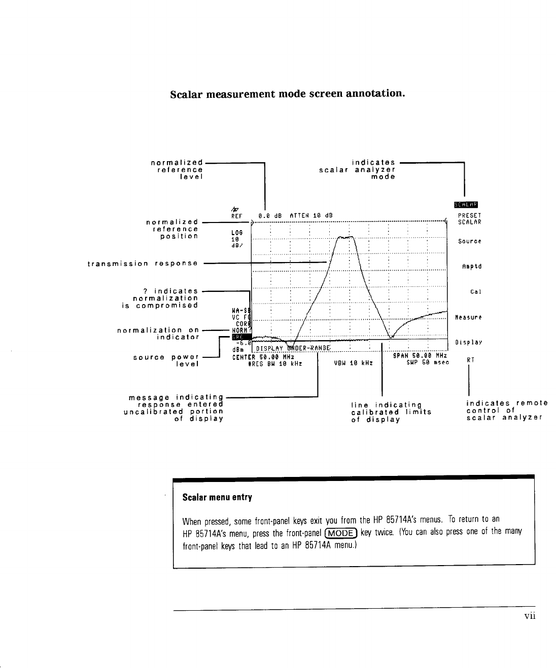
HP 85714A Scalar Measurements Personality User's Guide A_85630A A 85630A
User Manual: A_85630A
Open the PDF directly: View PDF ![]() .
.
Page Count: 340 [warning: Documents this large are best viewed by clicking the View PDF Link!]
- Title Page
- Scalar measurements with the HP 85714A
- 1: Quick Start Guide
- Quick Start Guide
- Before you begin
- Step 1. Connect the optional HP 85630A test set
- Step 2. Load the personality
- Step 3. Calibrate a transmission measurement
- Step 4. Display the response full screen
- Step 5. Measure the filter's passband
- Step 6. Set up standard device testing
- Step 7. Calibrate a transmission measurement
- Step 8. Calibrate a reflection measurement
- Step 9. Measure reflection coefficient and VSWR
- Step 10. View transmission and reflection results
- 2: Preparing for Measurements
- Preparing for Measurements
- Changing scalar analyzer mode
- Viewing the revision number
- Controlling the frequency
- Controlling the amplitude
- Changing the input attenuation
- Controlling the source's frequency and power
- Changing the source's attenuation
- Compensating for external gain or loss
- Power sweeps
- Controlling the HP 85630A test set
- AC/DC coupling
- 3: Calibrating for Measurements
- Calibrating for Measurements
- Using self-guided calibrations
- Calibrating for maximum dynamic range
- Peaking the tracking generator
- Calibrating transmission measurements
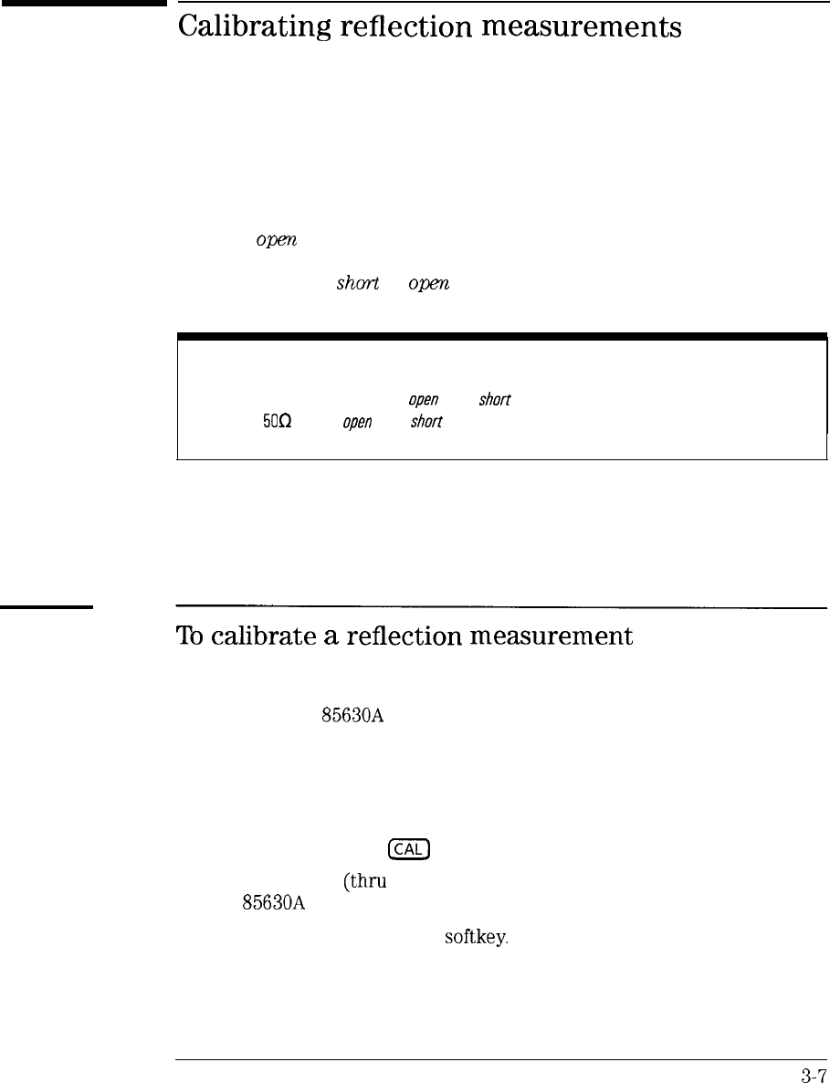
- Calibrating reflection measurements
- Calibrating for a standard device
- Saving and recalling calibrations
- Viewing calibration limits
- Changing the normalized position and reference level
- 4: Measuring Reflection/Transmission Parameters
- Measuring Reflection/Transmission Parameters
- Viewing transmission and reflection
- Viewing 120 dB of measurement range
- Automatically scaling the response
- Measuring VSWR, transmission, and reflection
- Measuring insertion loss and bandwidth parameters
- Measuring filter shape factor
- Performing fast fourier transforms
- Making swept-power measurements
- 5: Using Markers and Limit Lines
- 6: Displaying Results in a Table
- 7: Programming
- 8: Reference
- Reference
- Menu maps
- Definitions of keys
- 120 dB ON OFF
- AMPLITUDE
- Amptd
- ANNOT ON OFF
- ATTEN AUTO MAN
- ATTEN PORT 1
- AUTO SCALE
- AUX CTRL
- AVERAGE ON OFF
- BW
- BW MEAS ON OFF
- CAL
- Cal
- CAL OPN/SHRT
- CAL STD DEV
- CAL THRU
- CANCEL
- CHANGE TITLE
- CHANGE PREFIX
- Compress Function
- CONFIG
- COUPLE DC AC
- DELETE SEGMENT
- DELTA MEAS
- Device BW MEAS
- DISPLAY
- Display
- DISPOSE SCALAR
- DSP LINE ON OFF
- DUAL DSP ON OFF
- EDIT DONE
- EDIT LIMIT
- EDIT LOWER
- EDIT MID/DELT
- EDIT UP/LOW
- EDIT UPPER
- EDIT UPR LWR
- EXIT DELTA
- EXIT FFT
- EXIT PK-PK
- FFT MEAS
- FLAT
- GRAT ON OFF
- LIMITS FIX REL
- Limit Lines
- LIMITEST ON OFF
- LOG SCALE
- LOWER BW TARGET
- LOWER LIMIT
- MAG S11 ON OFF
- MAG S21 ON OFF
- Main Menu
- MAN TRK ADJUST
- Marker Convert
- MARKER DELTA
- MAX RNG ON OFF
- Measure
- MEAS/USER
- MIN RNG ON OFF
- NEGATIVE ON OFF
- NEW LIMIT
- NEXT PEAK
- NEXT PK LEFT
- NEXT PK RIGHT
- NORM REF POSN
- NORMAL ON OFF
- NORMALIZE ON OFF
- NUMBER POINTS
- PEAK EXCURSN
- PK-PK MEAS
- POINT
- POSITIVE ON OFF
- PRINT PAGE ALL
- PRESET SCALAR
- PURGE LIMITS
- PWR SWP ON OFF
- RECAL CAL
- RECALL LIMIT
- REF LEVEL
- REFL
- SAMPLE ON OFF
- SAVE CAL
- SAVE LIMIT
- SCALAR ANALYZER
- SCALAR REVISION
- SELECT AMPLITUD
- SELECT DLT AMPL
- SELECT FREQ
- SELECT LWR AMPL
- SELECT MID AMPL
- SELECT SEGMENT
- SELECT TYPE
- SELECT UPR AMPL
- SF MEAS ON OFF
- SLOPE
- Source
- SPAN
- SRC ATN AUTO MAN
- SRC PWR OFFSET
- SRC PWR ON OFF
- STORE OPEN
- STORE SHORT
- STORE STD DEV
- STORE THRU
- Tabular Display
- TABULAR ON OFF
- TEST SET YES NO
- TRACKING PEAK
- TRANS
- UPPER BW TARGET
- UPPER LIMIT
- VIEW NEXT PG
- VIEW PREV PG
- VSWR ON OFF
- Programming commands
- Preferred commands
- Equivalent commands
- ns_ANNOT
- ns_AT
- ns_AUTOSC
- ns_BMT
- ns_BWM
- ns_CALR
- ns_CALS
- ns_CALT
- ns_CAN
- ns_DDM
- ns_DISPOSE
- ns_EDR
- ns_EXATN
- ns_FFT
- ns_LBW
- ns_LIMITEST
- ns_LRNG
- ns_MCM
- ns_MCT
- ns_MP
- ns_NORM
- ns_NRL
- ns_NRP
- ns_OPEN
- ns_RCI
- ns_REFL
- ns_RL
- ns_SCI
- ns_SDLL
- ns_SDUL
- ns_SFM
- ns_SHRT
- ns_SRCOFF
- ns_SRCPOFS
- ns_SRCPWR
- ns_STD
- ns_TAKESWP
- ns_TCA
- ns_TDD
- ns_TDP
- ns_THRU
- ns_TRANS
- ns_UBW
- ns_URNG
- Characteristics
- 9: Concepts
- 10: If You Have a Problem
- Glossary
- Index

About this Manual
We’ve added this manual to the Agilent website in an effort to help you support
your product. This manual is the best copy we could find; it may be incomplete
or contain dated information. If we find a more recent copy in the future, we will
add it to the Agilent website.
Support for Your Product
Agilent no longer sells or supports this product. Our service centers may be able
to perform calibration if no repair parts are needed, but no other support from
Agilent is available. You will find any other available product information on the
Agilent Test & Measurement website, www.tm.agilent.com.
HP References in this Manual
This manual may contain references to HP or Hewlett-Packard. Please note that
Hewlett-Packard's former test and measurement, semiconductor products and
chemical analysis businesses are now part of Agilent Technologies. We have
made no changes to this manual copy. In other documentation, to reduce
potential confusion, the only change to product numbers and names has been in
the company name prefix: where a product number/name was HP XXXX the
current name/number is now Agilent XXXX. For example, model number
HP8648A is now model number Agilent 8648A.

I
-
I
-
User’s Guide
-HP
85714A
Scalar
Measurements
Personality
I
-
HP Part No. 85714-90008
Printed in USA July 1994
@Copyright Hewlett-Packard Company 1994
All Rights Reserved. Reproduction, adaptation, or translation without prior
written permission is prohibited, except as allowed under the copyright laws.
1400 Fountaingrove Parkway, Santa Rosa, CA 95403-1799, USA
I
-
I
-
Scalar measurements with the HP
85714A
The HP
85714A
scalar measurements personality provides a portable
easy-to-use solution for making scalar measurements. The HP
85714A
installs
in any HP 8590 Series Option 010 spectrum analyzers. (Option 010 spectrum
analyzers have built-in tracking generators.) Depending on your spectrum
analyzer, you can perform transmission measurements in the following
frequency range:
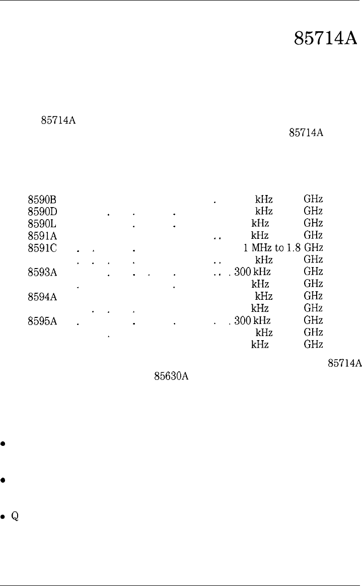
HP
8590B
HP
8590D
HP
8590L
HP
8591A
HP
8591C
HP 85913
HP
8593A
HP 85933
HP
8594A
HP 85943
HP
8595A
HP 85953
HP 85963
.
.
.
.
.
.
.
.
.
.
.
.
.
.
.
.
.
.
.
.
.
.
.
.
.
.
.
.
.
.
.
.
.
. 100
kHz
to 1.8
GHz
. 100
kHz
to 1.8
GHz
100
kHz
to 1.8
GHz
100
kHz
to 1.8
GHz
. .
1MHzto
1.8GHz
. 100
kHz
to 1.8
GHz
.300
kHz
to 2.9
GHz
300
kHz
to 2.9
GHz
. 300
kHz
to 2.9
GHz
300
kHz
to 2.9
GHz
.300
kHz
to 2.9
GHz
. 300
kHz
to 2.9
GHz
300
kHz
to 2.9
GHz
Reflection measurements are possible when the spectrum analyzer/HP
85714A
combination is used with an HP
85630A
transmission/reflection test set.
One-button measurement solutions.
The HP 857148 offers one-button measurement solutions that allow you to
measure parameters such as:
0
transmission coefficient
l
reflection coefficient
l
VSWR
0
insertion loss
l
bandwidth
l
shape factor
.Q
Using limit lines, you can implement pass/fail testing.
111
I
-
I
-
Once installed, the features of the HP
85714A
scalar measurements
personality are accessed via front-panel keys and softkeys.
Required spectrum analyzer:
HP
8590B
HP
8590D
.
HP
85901,
.
HP
8591A
. .
HP
8591C
. .
HP 85913 .
HP
8593A
.
HP 85933
HP 85948
HP 85943
HP
8595A
HP
8595E
HP 85963 . .
.
.
..
..
.
.
.
.
.
.
.
.
.
.
.
.
.
.
.
.
.
.
.
.
.
.
.
.
..
.
.
.
.
OPTIONS 003 AND 010
OPTIONS 003 AND 010
OPTIONS 003 AND 010
............
OPTION 0 10
............
OPTION 010
............
OPTION 010
............
OPTION 010
............
OPTION 010
............
OPTION 010
............
OPTION 010
............
OPTION 010
............
OPTION 010
............
OPTION 010
iv
I
-
\
PVZlA
-OPT
IONAL
HP
8563OA
SCALAR
TRANSMISSION/
REFLECTION TEST SET
V
I
-
To make a measurement.
1. Install the HP
85714A
as shown in Chapter 1.
2. Set the frequency and amplitude parameters as shown in Chapter 2.
3. Perform a calibration as shown in Chapter 3.
4. Measure the response as described in Chapter 4.
External tracking generators
The HP
85714A
scalar measurements personality is designed to use the spectrum analyzer’s internal
tracking generator. Although external tracking generators can be used, the HP
85714A
cannot control
them.
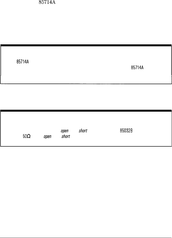
Calibration kit
Reflection calibration requires both
open
and
short
standards. The HP
85032B
Option 001 Calibration
Kit supplies
5OQ
type N
open
and
short
standards for calibration.
vi
I
-
I
-
Redefined front-panel keys.
While in the scalar measurement mode, many of the front-panel keys invoke
new
softkeys
menus. Refer to Chapter 8, “Reference,” for menu maps
showing the changed keys.
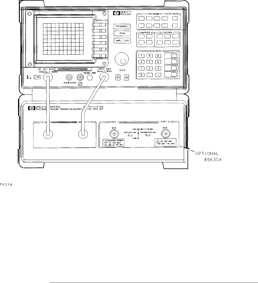
Optional HP 85630A Scalar Transmission/Reflection Test Set.
The optional HP
85630A
scalar transmission/reflection test set greatly reduces
the setup time required for reflection measurements. The test set also allows
you to make
simuItaneous
transmission and reflection measurements without
having to change the equipment setup. The scalar measurements personality
controls the scalar test set via the spectrum analyzer’s rear-panel AUX
INTERFACE connector.
Memory allocation.
The HP
85714A
scalar measurements personality stores calibration and limit
line data in trace memory. Therefore, when saving traces use caution to avoid
overwriting calibrations or limit lines. Before saving traces, use the spectrum
analyzer’s catalog feature to determine which trace registers are available for
data.
Reflection measurements.
The optional HP
85630A
scalar transmission/reflection test set provides the
necessary external bridge needed to perform reflection measurements. If you
don’t have the HP
85630A,
you will need to connect the necessary bridge and
cables to perform the measurement.
In addition to providing a bridge, the test set allows you to perform both
transmission and reflection measurements using the same setup. There’s no
time consuming equipment changes.
Vlll
I-

I
-
I
-
In this book
This book provides all the information needed to install and operate the
HP 857148 scalar measurements personality and the HP
85630A
scalar
transmission/reflection test set.
Softkeys
are indicated by a boxed word written in a shadow typeface.
Chapter
1,
“Quick Start Guide,
11
explains how to install the personality and
guides you through some simple scalar measurements.
Chapters 2 through 7 describes how to perform measurements using the
scalar measurement mode.
Chapter 8, “Reference,” lists reference material in a easy-to-find manner.
Chapter 9, “Concepts,” is a technical discussion on scalar measurement
accuracy.
Chapter 10, “If You Have a Problem” provides solutions for problems you may
encounter.
Spectrum analyzer operation
If you are not familiar with your spectrum analyzer, refer to the spectrum analyzer’s installation and
operation and programming manuals. These manuals describe spectrum analyzer preparation and
verification, and tell you what to do if something goes wrong. Also, they describe spectrum analyzer
features and tell you how to make spectrum analyzer measurements. Consult these manuals whenever
you have a question about standard spectrum analyzer use.
I
1
ix

I
-
I
-
Hewlett-Packard Software Product License
Agreement and Limited Warranty
Important
Please carefully read this License Agreement before opening the media envelope or operating the
equipment. Rights in the software are offered only on the condition that the Customer agrees to
all terms and conditions of the License Agreement. Opening the media envelope or operating the
equipment indicates your acceptance of these terms and conditions. If you do not agree to the License
Agreement, you may return the unopened package for a full refund.
X

I
-
License Agreement
In return for payment of the applicable fee, Hewlett-Packard grants the
Customer a license in the software, until terminated, subject to the following:
Use.
l
Customer may use the software on one spectrum-analyzer instrument.
l
Customer may not reverse assemble or decompile the software.
Copies and Adaptations.
l
Customer may make copies or adaptations of the software:
q
For archival purposes, or
q
When copying or adaptation is an essential step in the use of the
software with a computer so long as the copies and adaptations are used
in no other manner.
l
Customer has no other rights to copy unless they acquire an appropriate
license to reproduce which is available from Hewlett-Packard for some
software.
l
Customer agrees that no warranty, free installation, or free training is
provided by Hewlett-Packard for any copies or adaptations made by
Customer.
l
All copies and adaptations of the software must bear the copyright
notices(s) contained in or on the original.
Ownership.
l Customer agrees that they do not have any title or ownership of the
software, other than ownership of the physical media.
l
Customer acknowledges and agrees that the software is copyrighted and
protected under the copyright laws.
l
Customer acknowledges and agrees that the software may have been
developed by a third party software supplier named in the copyright
notice(s) included with the software, who shall be authorized to hold the
Customer responsible for any copyright infringement or violation of this
License Agreement.
xi

I
-
I
-
Transfer of Rights in Software.
l
Customer may transfer rights in the software to a third party only as part
of the transfer of all their rights and only if Customer obtains the prior
agreement of the third party to be bound by the terms of this License
Agreement.
l
Upon such a transfer, Customer agrees that their rights in the software are
terminated and that they will either destroy their copies and adaptations or
deliver them to the third party.
l
Transfer to a U.S. government department or agency or to a prime or
lower tier contractor in connection with a U.S. government contract shall
be made only upon their prior written agreement to terms required by
Hewlett-Packard.
Sublicensing and Distribution.
l
Customer may not sublicense the software or distribute copies or
adaptations of the software to the public in physical media or by
telecommunication without the prior written consent of Hewlett-Packard.
Termination.
l
Hewlett-Packard may terminate this software license for failure to comply
with any, of these terms provided Hewlett-Packard has requested Customer
to cure the failure and Customer has failed to do so within thirty (30) days
of such notice.
Updates and Upgrades.
l
Customer agrees that the software does not include future updates
and upgrades which may be available for HP under a separate support
agreement.
Export.
l
Customer agrees not to export or re-export the software or any copy or
adaptation in violation of the U.S. Export Administration regulations or
other applicable regulations.
xii

I
-
Limited Warranty
Software.
Hewlett-Packard warrants for a period of 90 days from the date of purchase
that the software product will execute its programming instructions when
properly installed on the spectrum-analyzer instrument indicated on this
package. Hewlett-Packard does not warrant that the operation of the software
will be uninterrupted or error free. In the event that this software product
fails to execute its programming instructions during the warranty period,
customer’s remedy shall be to return the measurement card (“media”) to
Hewlett-Packard for replacement. Should Hewlett-Packard be unable to
replace the media within a reasonable amount of time, Customer’s alternate
remedy shall be a refund of the purchase price upon return of the product
and all copies.
Media.
Hewlett-Packard warrants the media upon which this product is recorded
to be free from defects in materials and workmanship under normal use
for a period of 90 days from the date of purchase. In the event any media
prove to be defective during the warranty period, Customer’s remedy
shall be to return the media to Hewlett-Packard for replacement. Should
Hewlett-Packard be unable to replace the media within a reasonable amount
of time, Customer’s alternate remedy shall be a refund of the purchase price
upon return of the product and all copies.
Notice of Warranty Claims.
Customer must notify Hewlett-Packard in writing of any warranty claim not
later than thirty (30) days after the expiration of the warranty period.
Limitation of Warranty.
Hewlett-Packard makes no other express warranty, whether written or oral,
with respect to this product. Any implied warranty of merchantability or
fitness is limited to the 90 day duration of this written warranty.
This warranty gives specific legal rights, and Customer may also have other
rights which vary from state to state, or province to province.
x111

I
-
Exclusive Remedies.
The remedies provided above are Customer’s sole and exclusive remedies.
In no event shall Hewlett-Packard be liable for any direct, indirect, special,
incidental, or consequential damages (including lost profit) whether based on
warranty, contract, tort, or any other legal theory.
Warranty Service.
Warranty service may be obtained from the nearest Hewlett-Packard sales
office or other location indicated in the owner’s manual or service booklet
xiv
-1

I
-
1
Quick Start Guide
I
-
Quick Start Guide
Use the steps in this chapter to install the HP
85714A
scalar measurements
personality and the optional HP
85630A
scalar transmission/reflection test set.
These steps also introduce you to some basic measurement features.
You can complete this chapter in about 20 minutes. For instructional
purposes, a 50 MHz bandpass filter is used. You can easily substitute your
own hlter or other device by simply adjusting the frequencies used in these
procedures.
l-2
I
-
I
-
Before
you
begin
l
To install the HP
85714A
and skip the tutorial steps, perform only step 2.
l
Perform steps 1 and 7 through 10 only if you have an HP
85630A
test set.
CAUTION
Do not connect or disconnect the HP
85630A
test set’s control cable to the
spectrum analyzer’s rear-panel AUX INTERFACE connector while power is
on. Connecting or disconnecting the cable while power is applied may result
in loss of factory correction constants.
l-3
I
-
I
-
Step
1.
Connect
the
optional
HP
85630A
test
set
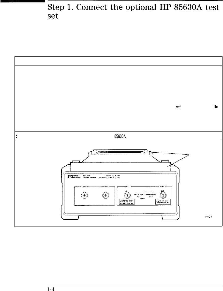
ITurn the spectrum analyzer off, and remove the line-power cord.
CAUTION: loss of factory correction constants may result if the spectrum analyzer is powered while connecting or disconnecting th
rear-panel AUX INTERFACE cable.
You may notice the test set’s front-panel PORT 2 connector has a small amount of movement. This is
nor
a mechanical fault. The
movement is designed to make connecting semirigid cables easier.
!Place the two stacking support shoes on the top of the HP
85630A.
STACK I NG
SUPPORT
SHOES
l-4
I
-
I
-
Quick Start Guide
Step 1. Connect the optional HP 8563OA test set
1
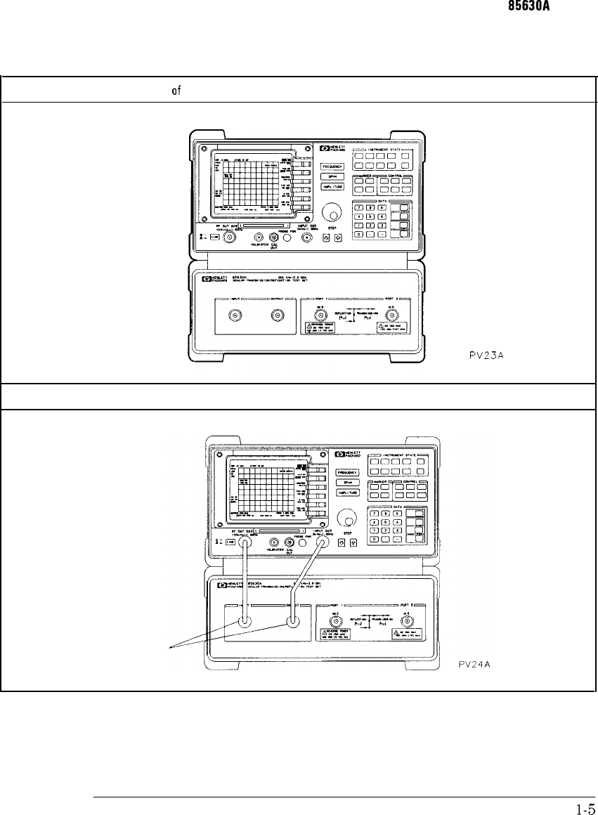
I Connect the front-panel semirigid cables.
3Set the spectrum analyzer on top of the stacking support shoes.
PV23A
CABLES
l-5
I
-
I
-
Buick
Start Guide
Step 1. Connect the optional HP
85630A
test set
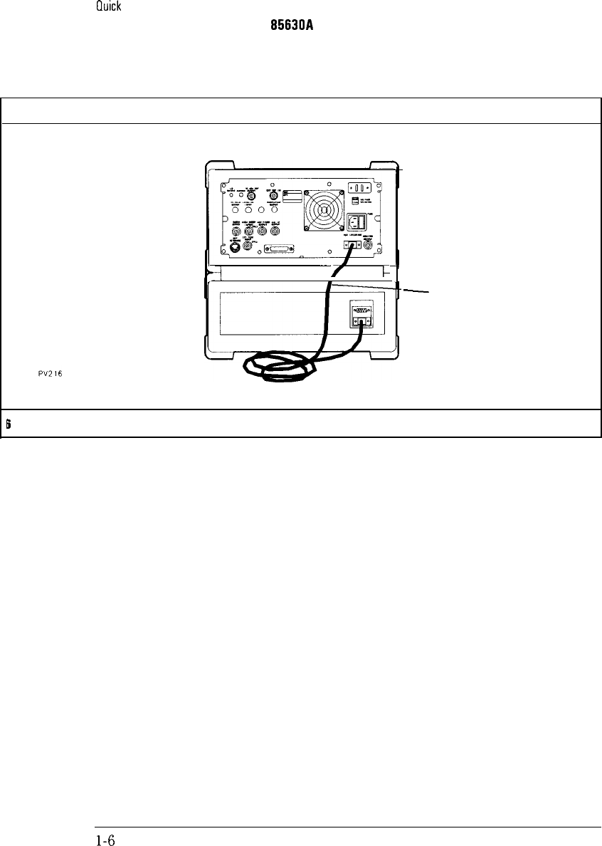
5 Connect the rear-panel auxiliary interface cable.
/
c
-
AUX
INTERFACE
CABLE
l-6
-
6
Connect the line-power cord to the spectrum analyzer, end turn the power on.
I
-
I
-
Step
2.
Load
the
personality
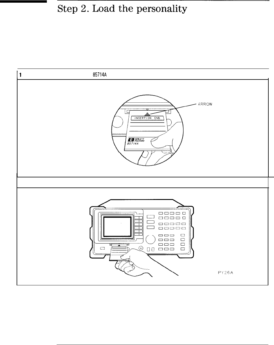
11
locate the arrow printed on the HP
85714A
card’s label.
I
,RROW
2Insert the card into the spectrum analyzer with its arrow matching the raised arrow on the bezel around the card-insertion slot.
1-7
I
-
Chick
Start Guide
Step 2. load the personality
1
3
On the spectrum analyzer, press
Cm).
Press the INTRNL
CRD
softkey so that
CRD
is underlined.
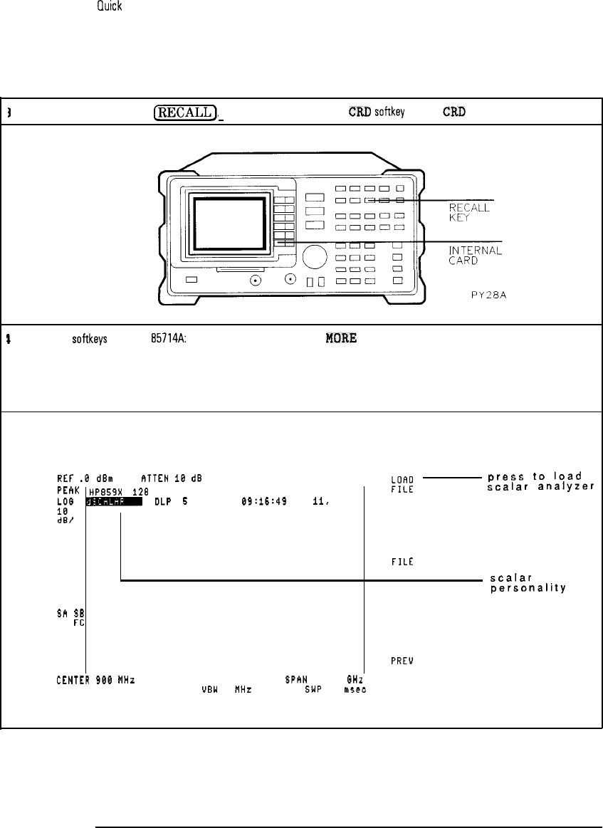
PY28A
1
Press the following
softkeys
to load the HP
85714A:
CATALOG CARD ,
MORE
1 OF 2, CATALOG DLP
, end
LOAD FILE.
This step takes about 1 minute to complete. If INVALID SYMTAB ENTRY:
SYMTAB OVERFLOW
is displayed, refer
to Chapter 10, “If You Have a Problem.”
6
REF
.B
dBm
ATTEN
IE
dB
KY
press
to
load
. . . . . . . . . . . . . . , . . . . . . . . . . . . . . . . . . . . . . . . . . . . . . . . . . . . . . . . . . . . . . . . . . . . . . . . . . . . . . . . . . . . . . . . . . . . . . .
PEAK
HPB59X
128
scalar
analyzer
:i”
-
!lLP
5
105
09:16:49
JAN
ii,
1991
dB/
DELETE
FILE
scalar
analyzer
personality
SA
SG
SC
FC
EXIT
CORR CATALOG
CENTER
900
MHz
RES BW 3 MHz
PREU
MENU
SPhN
1.800
GHz
UBW 1
MHz
SWP 28
M5eC
1-8
Quick
Start Guide
Step 2. load the personality
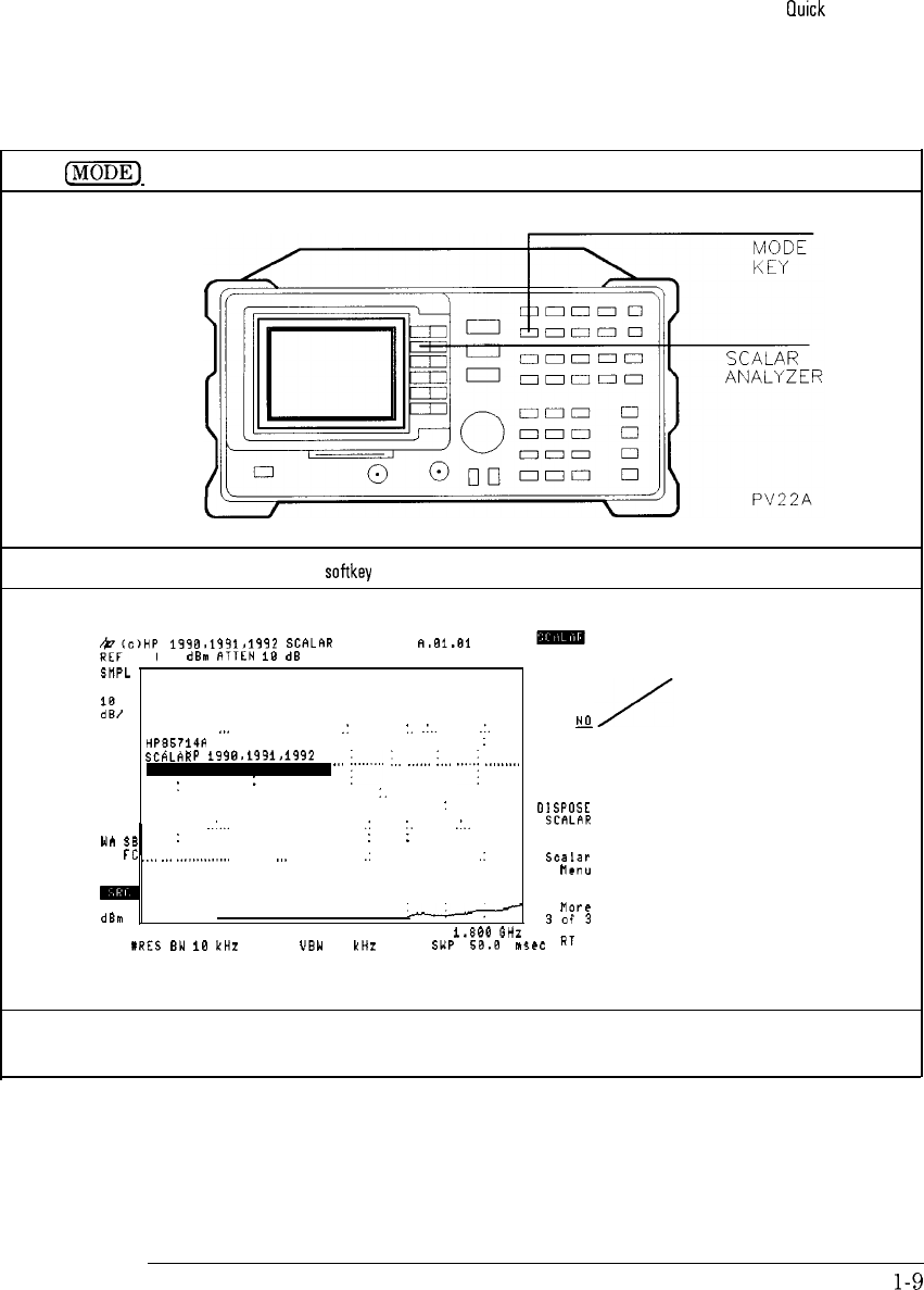
Press
Cm]
and then
SCALAR ANALYZER.
i Press the TEST SET YES NO softkey so that YES is underlined.
$7;,,HP
1998,1991,1992
SCALRR ANALYZER
A.Bl.01
8.8
dBm
ATTEN
18
dS
SMPL
LOO
press to
ii/
TEST SET underline YES
YES
g
,.. .:
:.
.:..
.:.
HP86714f(
SCALAR ANALYZER :
:
(c)HP
i99@.199i>1992
SCRLfiR
REVISION
:
;
.,,
(,,,,,,,,
:,,
,,,,,,
I,,,
,,,.,;
..,.....,
:
:.
:
OISPOS~
.:...
. . . . . .
.:
'.
:..
SCRLAR
Wh
SE
:
: :
SC
FC
,.,,
.,,
,,,,,..,......
,,.
.:
.:
SEalaP
CORR
ncnu
m
-10.0 nore
d0m
-
3af3
CENTER 900 MHz SPAN
i.#00
0Hz
RRES
BY
1E
kHz UBN
10
kHz SWP
50.8
lh5ce
RT
I
The scalar measurements personality is now configured for the test set. Turning the spectrum analyzer off or removing the line
power does not alter this configuration.
l-9
I
-
I
-
Quick Start Guide
Step 2. load the personality
,
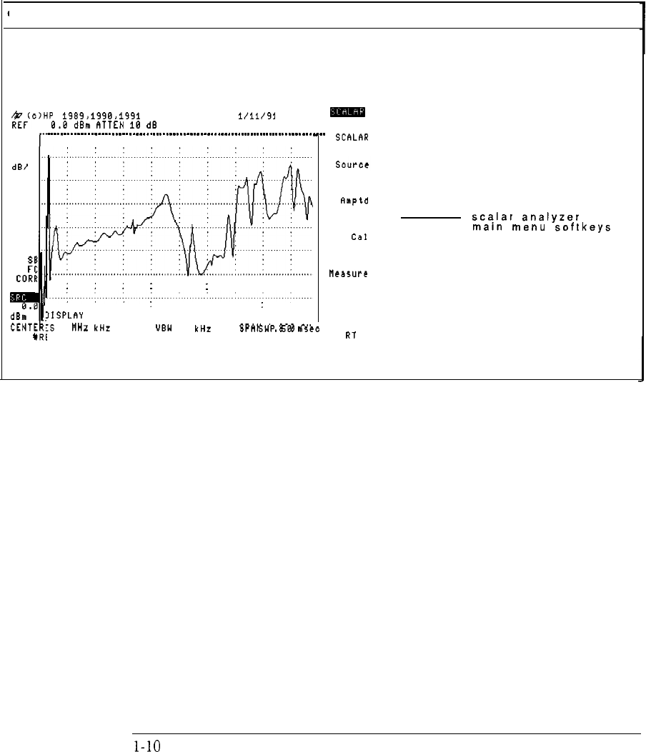
9 Remove the card from the spectrum analyzer.
$&b,HP
1989>199G,1991
SCALAR ANALYZER l/11/91
0.E dBm
ATTEN
10
dB
LOG
10
dB/
WA
SI
SC
FI
CORI
q
dBs'
CENTI
I
.
.
.
.
.
.
.
.
.
.
.
.
.
.
.
.
.
.
.
.
.
.
.
.
.
.
.
.
.
.
.
.
.
.
.
.
.
.
.
.
.
.
.
.
.
.
.
.
.
.
.
.
.
.
.
.
.
.
.
.
.
.
.
.
.
.
.
.
.
.
.
.
.
.
.
.
.
.
.
.
.
.
.
:
:
:::
.
.
PRESET
SCRLAR
Anptd
Cal
scalar
analyzer
main
menu
softkeys
Measure
:
:
Display
IISPLAY
UNDER-RANGE
I
900
MHz SPAN
1.800
GHz
:5
BW 18 kHz UBW
18
kHz SWP
58
15ec
R,
l-10
I
-
Step
3.
Calibrate
a
transmission
measurement
This step calibrates the scalar measurements personality for measuring
transmission through a filter.
1. Connect a short, low-loss cable between the input and output
l
If you are using the HP
85630A,
connect between Port 1 and Port 2.
l
If you are using a spectrum analyzer, connect between RF OUT and
INPUT.
2. Press @?ZGKiWJ, and set the center frequency. Our example is 50 MHz.
3. Press
ISPANJ,
and set the spanwidth. Our example is 50 MHz.
4.
Press the
ICAL)
key and then the CAL
THRU
softkey.
This enters a guided calibration routine. This routine normalizes the
system response thus eliminating system errors from any measurements.
5. Press the STORE
THRU
softkey.
1-11
I
-
I
-
Step
4.
Display
the
response
full
screen
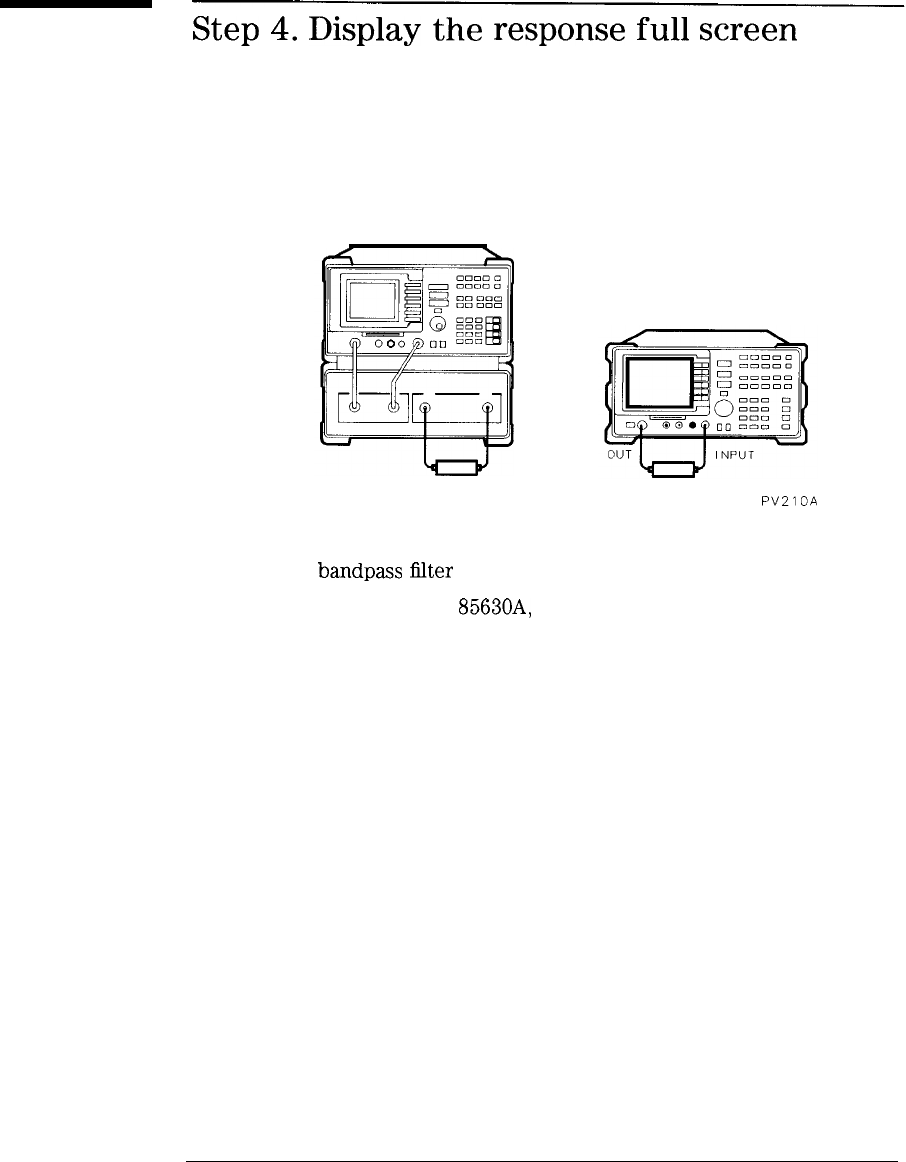
FILTER
SPECTRUM ANALYZER
RF
FILTER
PV210A
1. Connect a bandpass
iilter
between the input and output.
l
If you are using the HP
85630A,
connect between Port 1 and Port 2.
l
If you are using a spectrum analyzer, connect between RF OUT and
INPUT.
1-12
I
-
I
-
Quick Start Guide
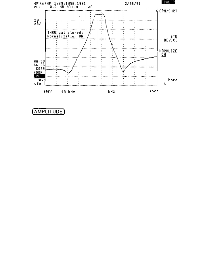
Step 4. Display the response full screen
The response should appear similar to the following figure.
~;c)HP
1989,199t3,1991 SCALAR ANALYZER 2/68/91
8.0
dB
RTTEN
10
dB
SMPL
. . . . . . . . . . . . . . . . . . .
LOG
*%.
18
dB/
0.11
dBm
CENTER 50.00 MHz
#RES
BW
18
kliz
SPAN 50.00 MHz
'JBW
18
kHz SWP 50 msec
2. Press the
@LiKiKK)
key.
CAL
OPN/SHRT
CAL
THRU
CAL ST0
OEVICE
NORMLIZE
E
OFF
TRACKING
PERK
MbI-C
1
of 2
RT
1-13
I
-
I
-
Quick
Start Guide
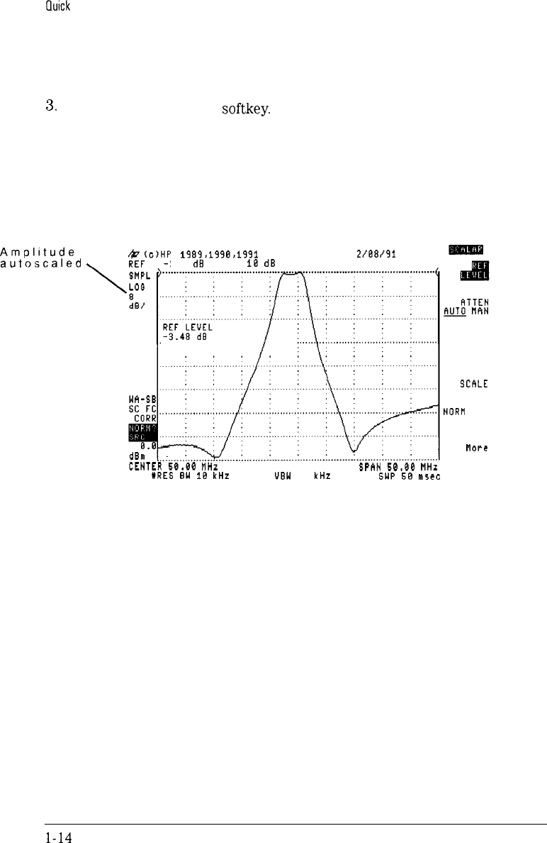
Step 4. Display the response full screen
3.
Press the AUTO SCALE
softkey.
The response peak is automatically placed at the normalized reference
level, and the vertical log scale is adjusted to view the response as large
as possible.
Amplitude
autoscaled
\
$&WHP
1989,1998,1991
SCALAR ANALYZER
2/88/91
-3.5 d8 RTTEN
18
dB
CENTER
50.00
MHz
SPAN
50-00
MHz
#RES
8W 18
kHz U8W
18
kHz GWP 58
lSec
ATTEN
m
MRN
LOG
SCALE
AUTO
SCRLE
NORR
REF
POSN
NbPc
1 of 2
RT
l-14
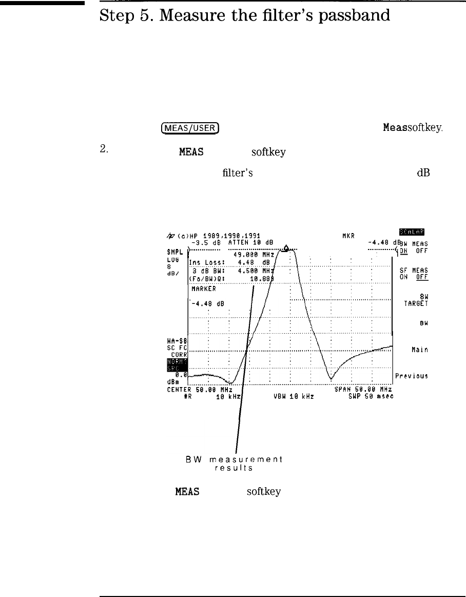
Step
5.
Measure
the
filter’s
passband
1. Press the
fjMEAS/USER]
key followed by the Device BW
Meas
softkey.
2.
Press the BW
MEAS
ON OFF
softkey
so that ON is underlined.
3. The display shows the
titer’s
center frequency, insertion loss, 3
dB
bandwidth, and Q.
/@(c)HP
1989>1998>1991 SCALAR
F1KR
49.88 MHz
REF
SMPL
1
Center:
__
,.:".:5...?
. . . .
il.;.;.F!;F!.;.$.+.
. . . . . . . . . . . . . . . . . . . . . . . . . . . . . . . .
?.!8...~
ElARKER
49.88 MHz
ES BW
1B
kH UBW IO kHz SWP 58
15ec
BW
measurement
results
UPPER 8W
TRRGET
LOWER BW
TARGET
haln
Menu
Previbus
Menu
RT
1-15
I-
4. Press the SF
MEAS
ON OFF
softkey
so that ON is underlined.
I
-
I
-
hick
Start Guide
Step 5. Measure the filter’s
passband
5. The display shows the filter’s shape factor (lower bandwidth divided by
upper bandwidth).
8
dBj
$;c,HP
1989,1998,1991
SCALAR MKR
A
22.88 MHz
I
-3.5 dB RTTEN IB
d8
)
. . . . . . . . . . . . . . . . . . . . . . . . . . . . . . . . . . . . . . . .
.I6
dB 8W
flEAS
SMPL
. . . . . . . . . . . . . . . . . . . . . . . . . . . . . . . . . . . . . . . . . . . . . . . . . . . . . . . . .
LOG Shape Fabtbr
(L/U):
5.88:1
,,-y
:
I
'1-
Upper BW: -3 SF NEA
LbWer BW: -68
gg
OF
MARKER
b
22.88 MHz
LOWER BW
:
TflRGET
Nain
Menu
Previaus
Menu
UBW 18
kHz SWP
58
m5ec
RT
Shape
factor
measurement
results
6. Press the SF
MEAS
ON OFF
softkey
so that OFF is underlined.
7. To turn the markers off,
l If you are using an HP
8590B,
HP
8591A,
HP
5893A,
HP
8594A,
or
HP
8595A,
press the
IrV1KR)
then MARKERS OFF
softkey.
l
If you are using an HP
8590D,
HP 85913, HP 85933, HP 85943,
HP 85953, or HP 85963, press the
(MKR),
then More, 1 of 2 , and
then the MARKERS ALL OFF
softkey.
l-16
-1
I
-
Step
6.
Set
up
standard
device
testing
Standard device testing automatically creates and displays test limits for a
“standard” device. Similar devices can then be compared to the standard
response. This feature is very useful in repetitive production-line testing.
1.
Press the
ICAL)
key followed by the CAL STD
DEUICE
softkey.
2. With the filter still connected to the spectrum analyzer, press the
STORE STD
DEV
softkey.
The spectrum analyzer displays upper and
lower limit traces that are parallel to the standard devices response.
$;c,HP
1989,1998.---e
-3.5 d8 RTTEN IS
.1991
SCALAR ANALYZER
Z/88/91
I
d8 UPPER
LIMIT
:
LOWER
LIMIT
:S
8W
1E
kHz
__...___
!$-$TiH:.58..i&.iil
\Lower
VBW
16
kHz
SUP
58
y15ec
RT
limit
trace
I
-
hick
Start Guide
Step 6. Set up standard device testing
3. Remove the filter and observe the limit traces displayed on the screen.
The UPPER LIMIT and LOWER LIMIT
softkeys
define the placement of
the limit traces.
$+$&HP
1989>1938.1991 SCALAR ANALYZER
2/08/91
-3.5
dB
RTTEN
18
dB
SMPL
LOG
8
dB/
tRES BW
18
kHz UBW
18
kHz SUP 58
nt5ec
UPPER
LIMIT
LOWER
LIMIT
STORE
ST0 OEU
LINITEST
&4
OFF
TRACKING
PERK
CANCEL
RT
4. Press the LIMITEST
ON
OFF
softkey
so that OFF is underlined.
l-18
I
-
I
-
Step
7.
Calibrate
a
transmission
measurement
1. Connect a short, low-loss cable between the input and output.
l
If you are using the HP
85630A,
connect between Port 1 and Port 2.
l
If you are using a spectrum analyzer, connect between RF OUT and
INPUT.
2. Press
[
FREQUENCY
),
and set the center frequency. Our example is 50 MHz.
3. Press
LSPAN),
and set the span width. Our example is 50 MHz.
4.
Press the (CAL) key and then the CAL THRU
softkey.
5.
Press the STORE
THOU
softkey.
l-19
I
-
I
-
Step
8.
Calibrate
a
reflection
measurement
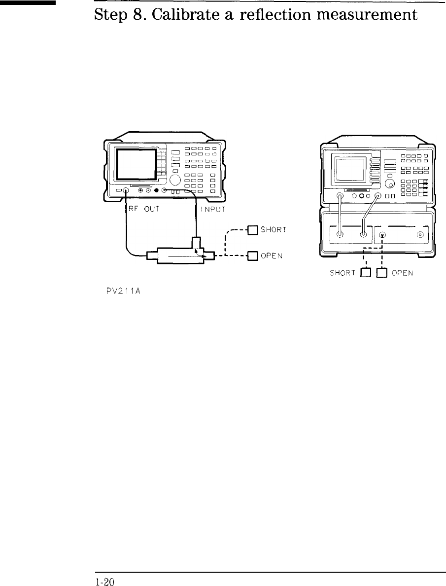
SPECTRUM ANALYZER
I
RF
OUT
I
INPUT
DIRECTIONAL
COUPLER
(OR BRIDGE)
PV21
IA
SHORT
OPEN
SHORT
h
6
OPEN
l-20
I
-
I
-
Buick
Start Guide
Step 8. Calibrate a reflection measurement
Reflection Measurements
In order to measure reflection, a directional signal splitting device, such as a coupler, bridge, or the
HP
85630A
test set is required.
II
1. Press the CAL
OPN/SHRT
softkey.
2.
Connect an
OJWZ
to the measurement port, and then press STORE OPEN
The measurement port may be from the coupler, bridge, or the
HP
85630A
test set.
It is good practice to place the
OJXYZ
at the end of any cable used to
connect PORT 1 to the device being tested. This moves the calibration
to the plane of measurement.
3. Remove the
OJWZ
and replace it with a short.
4.
Press the STORE SHORT
softkey.
5. Remove the short.
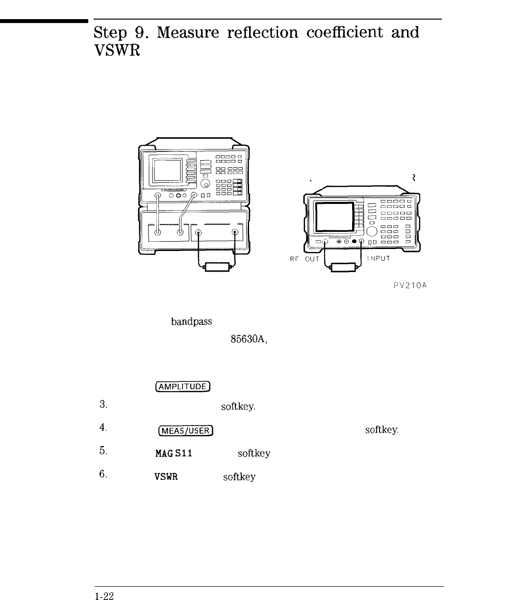
Step
9.
Measure
reflection
coefficient
and
VSWR
FILTER
SPECTRUM ANALYZEF
FILTER
PVZIOA
1. Connect the bandpass filter between the input and output.
l
If you are using the HP
85630A,
connect between Port 1 and Port 2.
l
If you are using a spectrum analyzer, connect between RF OUT and
INPUT.
2. Press the
[AMPLITUDE)
key.
3.
Press the AUTO SCALE
softkey.
4.
Press the
(j-3
key, and then Marker Convert
softkey.
5.
Press the
MAC
Sll
ON OFF
softkey
so that ON is underlined.
6.
Press the
VSWR
ON OFF
softkey
so that ON is underlined.
7. The reflection coefficient and VSWR at the marker is displayed on the
screen.
Use the front-panel knob to move the marker and read the value at
any point.
l-22
I
-
I
-
Chick Start Guide
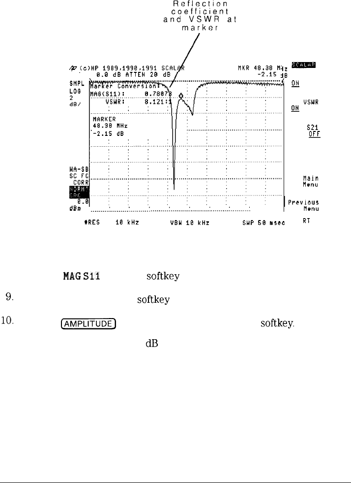
Step 9. Measure reflection coefficient and VSWR
ReflectIon
coefficient
and
VSWR
at
marker
REF 8.8 dB
ATTEN
20 dB
ii
i
NAG Sll
g
OFF
USWR
u
OFF
NAG S21
ON
OFJ
main
nenu
I
_________:
_________:
__.._.___:
_________:
_________:
_________:
_________:
.____....:
. . . . . . . . . . .
CENTER 50.00 MHz SPAN 50.00 MHz
#RES
BW
18
kHz UBW
IB kHz SWP 58
M5eC
RT
8. Press the
MAC
Sll
ON OFF
softkey
so that OFF is underlined.
g.
Press the VSWR ON OFF
softkey
so that OFF is underlined.
lo.
Press the
(j-1
key and then the LOG SCALE
softkey.
11. Set the log scale back to 10
dB
per division.
1-23
Step
10.
View
transmission
and
reflection
results
ReflectIon
Transmission
response
response
@I
OFF
:
120 dB
ON
m
_
CENTER
50.00
HHz
. .
I
of
2
SPAN
50.00
MHz
__
XRES BW
18
kHz UBW 18
kH
1-24
I
-
I
-
Quick Start Guide
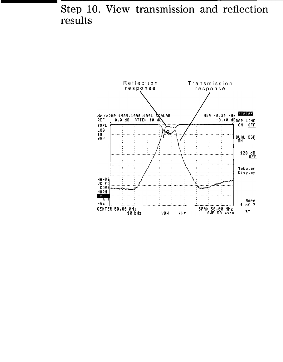
Step 10. View transmission and reflection results
Simultaneous Results
In order to simultaneously view reflection and transmission results, an HP
85630A
is required.
1. Press the
(MEAS/USER)
key, and view the reflection response.
2.
Press the
TRANS
softkey
to view the transmission response.
3.
Press the
@iGiX)
key followed by the DUAL DSP
OM
OFF
softkey
to
view both the reflection and transmission responses at the same time.
If the
Iilter
is adjustable, you can adjust it while observing the resulting
transmission and reflection responses in near real time. The scalar
measurements personality updates the traces on alternating sweeps.
4.
Press the DUAL DSP
ON
OFF
softkey
so that OFF is underlined.
Configuration Error
If the error message
“85630A
TEST SET CONFIGURATION
REOUIRED”
is displayed, the scalar
personality must be configured. Press
CZFiFJ
More 1 of 3 , More 2 of 3 , then
TEST SET YES MO so that YES is underlined.
l-25

I
-
2
Preparing for
Measurements

I
-
I
-
Preparing for Measurements
This chapter teaches the basic controls for the scalar measurements
personality. To use the scalar measurements personality, you must first install
it, refer to Chapter 1, then change to scalar analyzer mode.
2-2
I
-
I
-
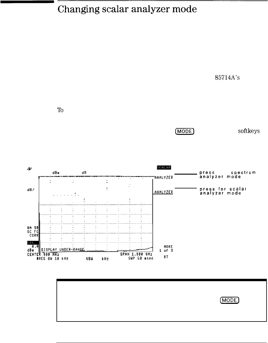
Changing
scalar
analyzer
mode
In this section, you’ll learn how to start, preset, exit, and remove the scalar
measurements personality. Information on finding the HP
85714A’s
revision
number is also included. If you followed the instructions in Chapter 1, the
scalar measurements personality should already be installed and in the active
mode.
‘lb
use the scalar measurements personality, you must first change the
spectrum analyzer to scalar analyzer mode. You can switch your instrument
between signal analyzer and scalar analyzer operation at any time. This
is accomplished by pressing the front-panel
IIVIODE)
key, and using
softkeys
displayed shown below:
t
REF 0.0 dBm RTTEN 10
dB
SPECTRUM
press
for
spectrum
,
.
.
.
.
.
.
.
.
.
.
.
.
.
.
.
.
.
.
.
.
.
.
.
.
.
.
.
.
.
.
.
.
.
.
.
.
.
.
.
.
.
.
.
.
.
.
.
.
.
.
.
.
.
.
.
.
.
.
.
.
. .
.
. . . . .
.
.
.
. . . . . . .
.
.
. . . . . . .
.
. . . .
.
ANIILY*ER
analyzer
mode
LOG
:
: :
10
.'
dB/ :
:
SCALAR
AHRLYZER
press
for
scalar
analyzer
mode
.
.
.
.
.
.
.
.
: :
UBW 10 kHz
Main menu
Enter the scalar measurements personality’s Main menu at any time by pressing
[m)
SCALAR ANALYZER.
2-3
I
-
Preparing for Measurements
Changing scalar analyzer mode
The HP
85714A
scalar measurements personality does
not
need to be
reinstalled after switching between the two modes of operation. However, if
you remove the HP
85714A
scalar measurements personality as shown in this
section, you’ll need to reinstall it using the procedure in Chapter 1.
Presetting the scalar measurements personality returns it to a known start-up
state. PRESET SCALAR in Chapter 8 provides information on the preset
state.
To
enter
scalar
analyzer
mode
1. Press the front-panel
(rvroDEl)
key.
2.
If the SCALAR ANALYZER mode softkey does not appear, press
Ijjj
again.
3.
Press the SCALAR ANALYZER
softkey.
To
return
to
spectrum
analyzer
mode
2-4
1. Press the front-panel
[MODE)
key.
2.
Press the SPECTRUM ANALYZER
softkey.
I-
I
-
I
-
Preparing for Measurements
Changing scalar analyzer mode
To
preset
the
scalar
measurements
personality
1. Press the
(MODE)
key.
2.
Press Scalar Analyzer to enter the main menu.
3.
Press the PRESET SCALAR
softkey.
To
remove
the
HP
85714A
1. Press the front-panel
(CONFIG)
key.
2.
Press the MORE
1
of 3 and then MORE 2 of 3 softkeys.
3.
Press the DISPOSE SCALAR
softkey
twice.
This procedure removes the HP 857148 from the spectrum analyzer’s
memory. You must reinstall the HP
85714A
to use it again.
2-5

I
-
Viewing
the
revision
number
The scalar measurements personality’s revision number is available via
softkeys. It is used by the factory to indicate the vintage of the program. You
may be asked for this number when requesting help from Hewlett-Packard.
2-6
I
-
I
-
Preparing for Measurements
Viewing the revision number
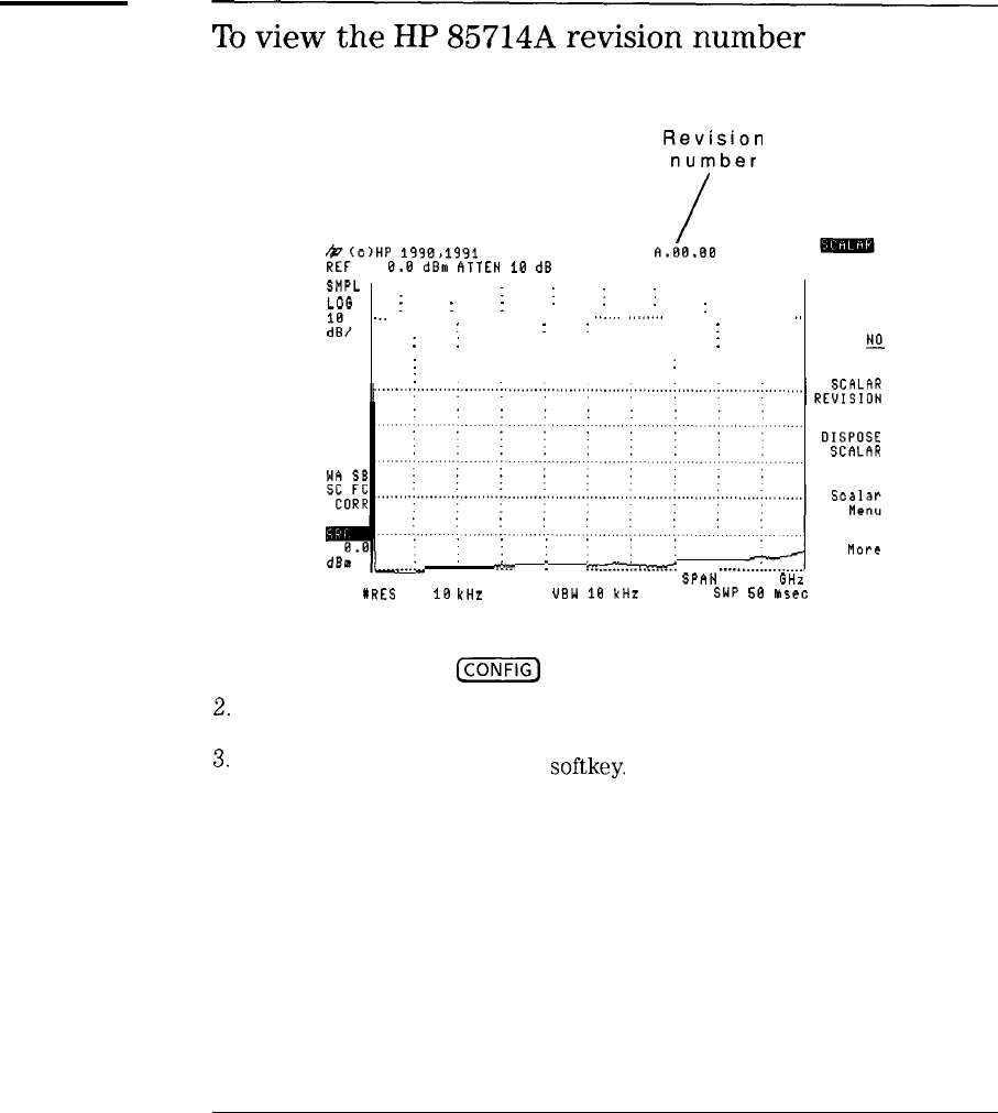
To
view
the
HP
85714A
revision
number
Revision
number
/
$;o)HP
1990>1991
SCALAR ANALYZER
A.EB.BE
8.8 dBm
ATTEN
10
dB
SMPL
. . . . . . . . . . . . . . . . . . . . . . . . . . . . . . . . . . . . . . . . . . . . . . . . . . . . . . . . . . . . . . . . . . . . . . . . . . . . . . . . . . . . . . . . . . . . . . . . . . .
LO0
j
:
j
I
I
:
:
:
dlgB/
.._
. . . . . . . . . . . .
. . . . . .
.._
,,,,....
.,
:
:
::
TEST SET
;
: :
YES
E
:
:
:
:
dB:"li
'
. . . . . .
iv
. . . . . . .
i
. . . . . . . . .
,:;...::..i.;.,
. . . . . . . . . .
____..
2
CENTER 900 MHz
SPhN
1.800 GHz
lRES BW
18
kHz
UBW
18
kHz SWP
58
M5eC
01SP0SE
SChLAR
MOPC
3 of 3
RT
1. Press the front-panel
(jCONFIG)
key.
2.
Press
the
MORE
1
of
3
and
then
MORE
2
of
3
softkeys.
3.
Press the SCALAR REVISION
softkey.
4. The revision number is displayed at the top of the display.
2-7
I
-
I
-
Controlling
the
frequency
The scalar measurements personality uses the spectrum analyzer’s built in
tracking generator as the RF source. The tracking generator’s output tracks
the scalar analyzer’s input frequency.
Set the scalar analyzer’s frequency using the front-panel
[
FREQUENCY
)
and
LSPAN_)
keys. The tracking generator’s output frequency tracks the scalar
analyzer’s frequency. So, by setting the scalar analyzer’s frequency you
control the tracking generator.
2-8
I
-
Preparing for Measurements
Controlling the frequency
To
sweep
the
frequency
1. Press the front-panel
CFREQUENCY)
key.
2. Use the front-panel knob or numeric keypad to set the center frequency.
3. Press the (SPAN] key.
4. Use the front-panel knob or numeric keypad to set the frequency span.
2-9
I
-
I
-
Controlling
the
amplitude
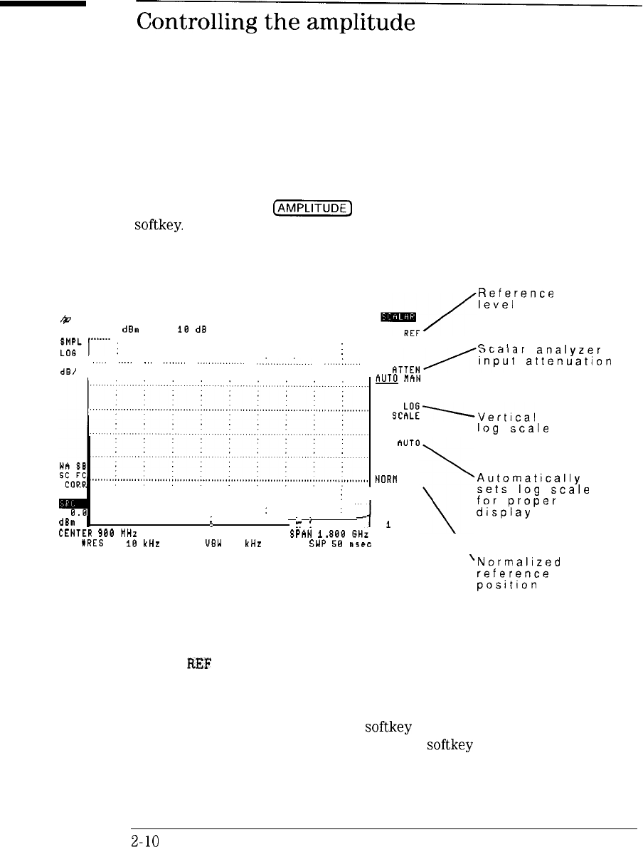
The Amplitude menu allows you to control the scalar analyzer’s vertical scale,
reference level, and normalized trace position. To enter the Amplitude menu,
press the front-panel
@KiKiKK]
key or press the main menu’s Amptd
softkey.
/;o
REF 6.0 dBm RTTEN 10 dB
. . . . . . . . . . . . . . . . . . . . . . . . . . . . . . . . . . . . . . . . . . . . . . . . . . . . . . . . . . . . . . . . . . . . . . . . . . . . . . . . . . . . . . . .
I
I
10
“‘.’
.....
“’
“““”
..““““““.‘.
..-..........:......
-....:......
dB/
I
I
dl
CENTER
#RI
w
i
I
: :
:
:
sm
. . . . . . . . . . . . . .
i
. . . . . . . . . . . . . . .
:r
.
i
. . . . . . . . . .
900
MHz SPAN
1.
:S
BW
10
kHz UBW 10 kHz SWP
Reference
level
LEVEL
Scalar
analyzer
ATTEN/input
attenuation
m
MhN
ScEYVertrcaI
log
scale
hUT0
SCALE
NORN
REF
POSN
Mare
1
of
2
RT \
,Automatically
sets
log
scale
for
proper
display
‘Normalized
reference
Page One of Amplitude Menu
position
Any changes in the reference level should be made before measurement
calibration. To change the reference position after calibration, use
NORM
REF
POSN Refer to Chapter 3 for information on calibrating for
measurements.
For best measurement accuracy, place the peak signal response at the
reference level. The AUTO SCALE
softkey
automatically sets the vertical
scale to show a displayed response. Use this
softkey
after calibration.
2-10

I
-
I
-
Preparing for Measurements
Controlling the amplitude
&h,HP
1990>1991,1992 SCALAR ANALYZER
A.O1.O1
0.0 dBm
ATTEN
10
dB
SMPL
I:
:
:
:
COlJPLE/~~"
iyi\it
0
n
DC
K
HP
8594AIE
,,,,,,,,,,,,,,,,,,:
,,,,,,,,,:,,,,,,,I,,,..,......,........:
. . .
. . . . . .
..I
HP
8595AIE
,........ MaIn
Menu
HP
8598E
.:
:...
mare
2 of 2
CENTER 900 MHz SPAN
i.800
GHz
I)RES
BW 10 kHz UBW 10 kHz SWP 50.0
msec
RT
Page Two of Amplitude Menu
2-11
I
-
I
-
Preparing for Measurements
Controlling the amplitude
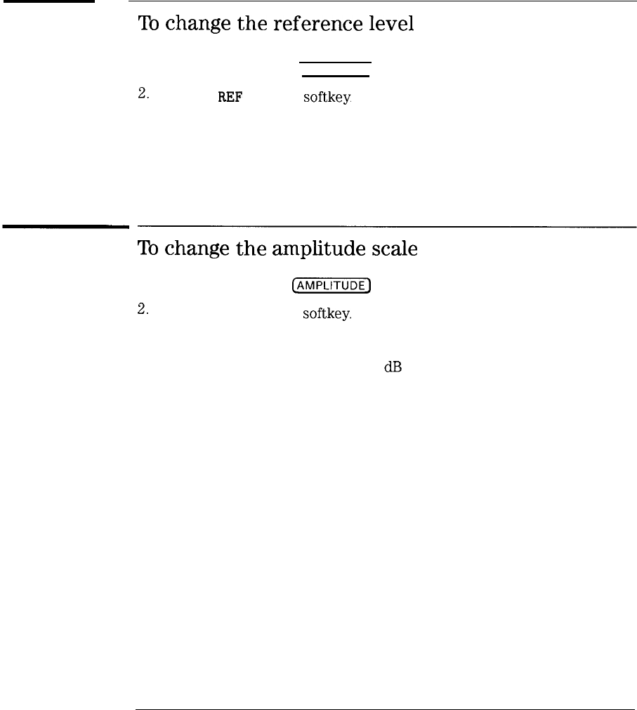
To
change
the
reference
level
1. Press the front-panel
[
AMPLITUDE
)
key.
2.
Press the
REF
LEVEL
softkey.
3. Use the front-panel knob or numeric keypad to set the new reference
level.
To
change
the
amplitude
scale
1. Press the front-panel
@KiKKKK]
key.
2.
Press the LOG SCALE
softkey.
3. Use the front-panel knob or numeric keypad to change the amplitude scale.
The default log scale is set to 10
dB
per division.
2-12
I
-
I
-
Changing
the
input
attenuation
The scalar analyzer’s input attenuator can be set in 10
dB
increments. For
HP
8590B
and HP
8591A
spectrum analyzers, the range is from 0
dB
to 60
dB.
For HP
8593A,
HP
8594A,
and HP
8595A
spectrum analyzers, the range is
from 0
dB
to 70
dB.
To protect the scalar analyzer, 0
dB
attenuation can only
be set using the numeric keypad (not the front-panel knob).
Input attenuation can be controlled automatically by the scalar analyzer
personality or manually from the front-panel. Automatic coupling adjusts the
attenuator to prevent compression of the input signal. Attenuation that is
set manually is uncoupled from the reference level. (The reference level is
limited at the high end by the manual attenuation setting. This limit is equal
to -10
dBm
plus the amount of RF attenuation.)
To
change
the
input
attenuation
1. Press the front-panel
CAMPL’TUDE]
key.
2.
Press the
ATTEN
AUTO MAN
softkey
to activate the input attenuation.
3.
Press the
ATTEN
AUTO MAN
softkey
until MAN is underlined.
4. Use the front-panel knob or numeric keypad to set the input attenuation.
2-13
I
-
I
-
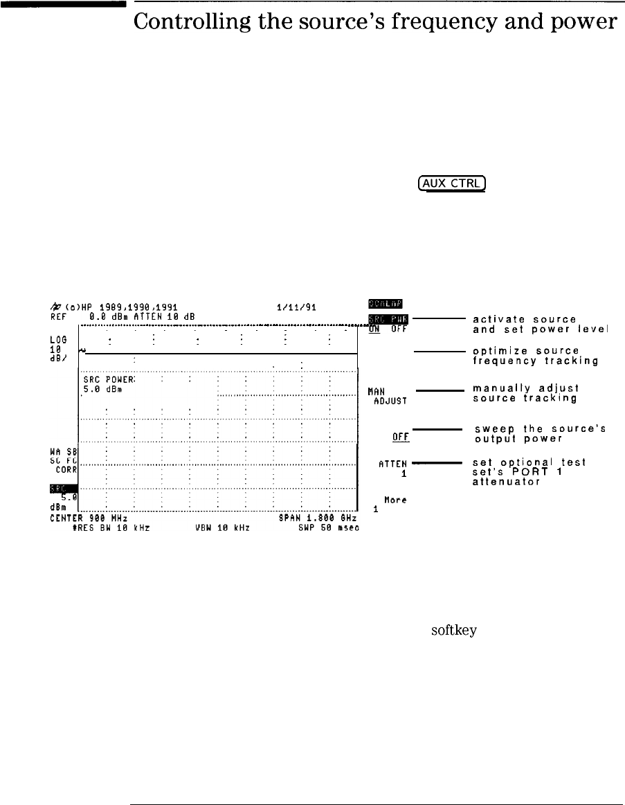
Controlling
the
source’s
frequency
and
power
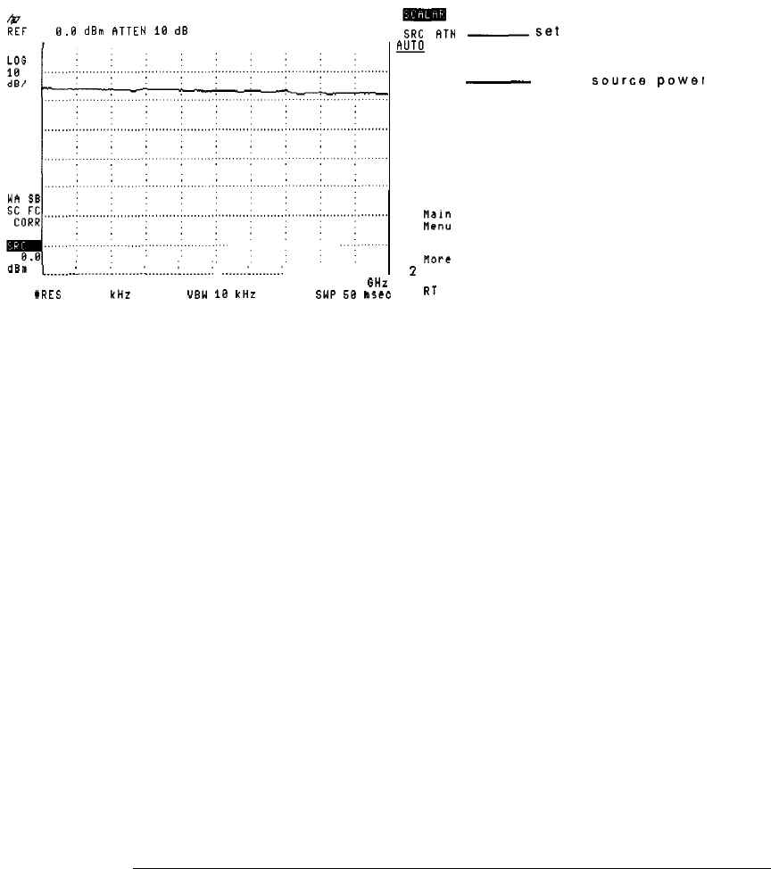
You control the built-in tracking generator through the Source menu. To
enter the source menu, press the front-panel
(AUXCTRL)
key or use the scalar
analyzer’s main menu.
$f7;c,HP
1989,1998>1991 SCALAR ANALYZER
l/11/91
0.8
dBm
fITTEN
lb3
dB
. . .
..*..............
. . .
.
.
. . . . .
.
. .
.
. .
.
. . . . .
.
. .
.
. .
.
. .
.
. . . . . .
.
.
.
.
. . . . . . . . . . . . . .
.
. . . . . . . . . . .
.
. .
.
.
.
.
. .
.
.
LOG
:
j
:
j
j
j
10
u
dBr'
TRACKING
::
PEAK
activate
source
and
set
power
level
optimize
source
frequency
tracking
IRWIN
TRK
manually
adjust
RDJUST
source
tracking
PWR SWP
ON
j3FJ
ATTEN
-
PORT
1
r-lore
1
of 2
RT
sweep
the
source’s
output
power
set
optional
test
set’s
PORT
1
attenuator
Page One of Source Menu
The source frequency tracks the input frequency of the scalar analyzer. To
ensure accurate frequency tracking between the scalar analyzer and its
tracking generator, press the TRACKING PEAK softkey in the CAL menu.
Peaking the source is especially important at these times:
l
Before a calibration.
l
After temperature changes.
l
After any resolution bandwidth changes.
2-14
I
-
8.8 dBm
RTTEN
10
dB
. . . . . . . . . . . . . . . . . . . . . . . . . . . , . . . . . . . . . . . . . . . . . . . . . . . . . . . . . . . . . . . . . . . . . . . . . . . . . . . . . . . . . . . . . . . . .
Preparing for Measurements
Controlling the source’s frequency and power
SRC
,q*~
-set
automatic or manual
m
MAN control of source attenuator
SRC PWR
-
offset
?.ource
power
OFFSET
_....._..
i
.__.._.__:
_._______:
_________~
________.~
. .
.._____.
_________:
. . . . . . . . . . . . . . . . ...! . . . . . . .
NOPC
2
of 2
CENTER 900 MHz SPAN 1.800 GHz
#RES BW 10 kHz UBW 18 kHz SWP 58 15co
RT
Page Two of Source Menu
2-15
I
-
I
-
Preparing for Measurements
Controlling the source’s frequency and power
The amount of control over the source’s output power depends on the
spectrum analyzer used. See the following table for a summary of the
options, power ranges and attenuations.
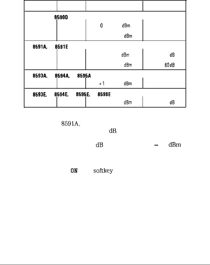
HP 8590 Series Source Power Range and Attenuation
I
Model Number
Option Power Range
Attenuation
HP 85908, HP 8590D
010
0
to -15
dBm
None
011 -6 to -21
dBm
None
HP
8691A.
HP
8591E010 0 to -70
dBm
0
to ‘60
dB
011 -6 to -70
dBm
0
to 60
dB
HP 8593A. HP 8594A. HP 8595A
010
+l
to -10
dBm
None
HP 8593E, HP
8594L
HP 8595E. HP
8698E
010
-1 to -66
dBm
0
to 56
dB
Attenuation on the HP
8591A,
HP 85933, HP 85943, HP 85953, and
HP 85963 can be changed from 0 to 60
dB.
With automatic control, the scalar
analyzer sets the attenuation as necessary to maintain a calibrated display.
The default setting is AUTO with 0
dB
of attenuation and
-
10
dBm
source
power.
The default setting after presetting the scalar analyzer is power on.
Activating the SRC PWR
CM
OFF
softkey
makes the output power the active
function.
2-16
I
-
I
-
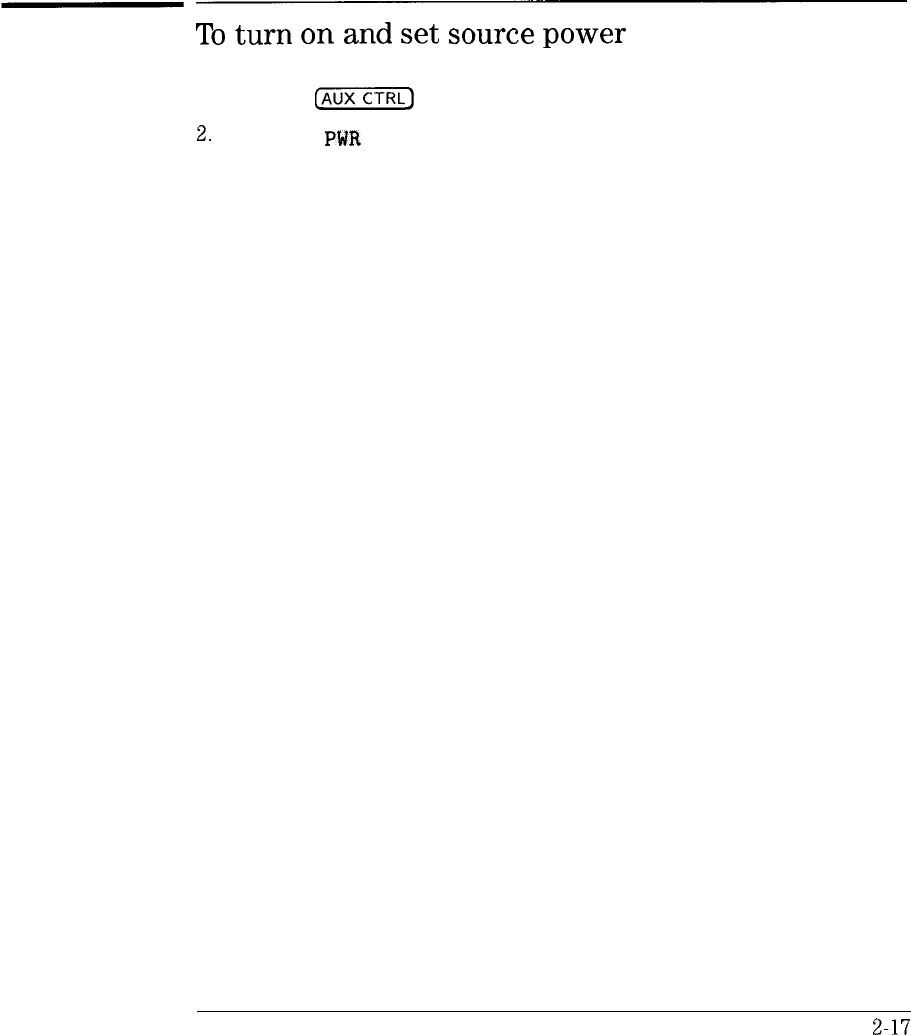
Preparing for Measurements
Controlling the source’s frequency and power
To
turn
on
and
set
source
power
1. Press the
[AUX]
key to enter the scalar analyzer’s Source menu
2.
Press SRC
WA
ON OFF so that ON is underlined.
3. Use the front-panel knob or numeric keypad to set the source output
power.
2-17
I
-
I
-
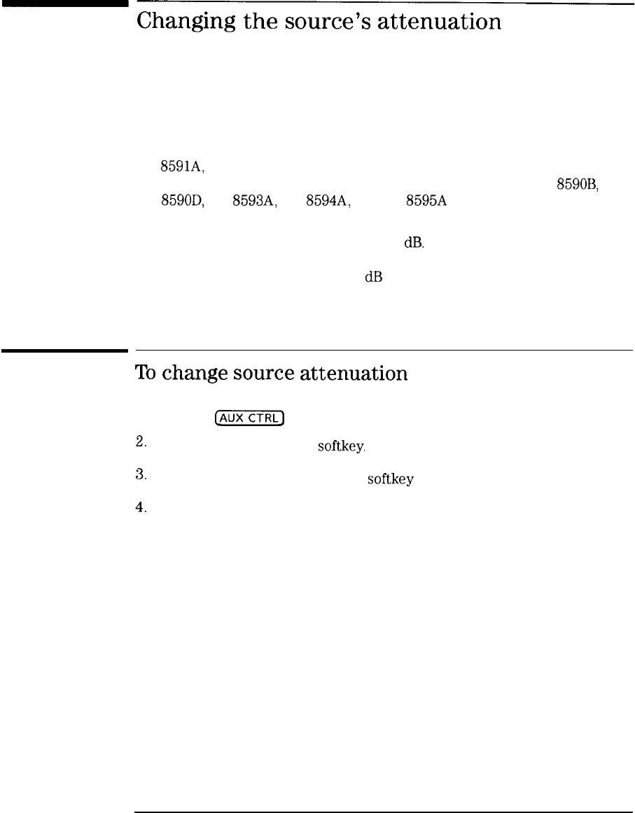
Changing
the
source’s
attenuation
HP
8591A,
HP 85933, HP 85943, HP 85953, and HP 85963 spectrum
analyzers have output attenuators for the tracking generator. HP
8590B,
HP
8590D,
HP
8593A,
HP
8594A,
and HP
8595A
spectrum analyzers do not
have output attenuators.
Attenuation can be changed from 0 to 60
dB.
In automatic mode, the scalar
analyzer sets the attenuation as necessary to maintain a calibrated display.
The default setting is AUTO with 0
dB
of attenuation.
To
change
source
attenuation
1. Press the
@KZKj
key.
2.
Press the More 1 of 2
softkey.
3.
Press the SRC ATM AUTO MAN softkey to activate the function.
4.
Press the SRC ATM AUTO MAN again so that MAN is underlined.
5. Use the front-panel knob or numeric keypad to set the source attenuation.
2-18
I
-
Compensating
for
external
gain
or
loss
Compensating for external gain or loss ensures that display readouts reflect
the true power levels at the input to the device being tested.
For example, if the source power is 0
dBm,
and 3
dB
of loss occurs between
the RF OUT connector and the device being tested, the display readouts show
the power at the RF OUT connector. With the source power offset set to 3
dB,
the displayed source power annotation indicates the power at the device
being tested: -3
dBm.
Because output power is specified over a finite range, certain combinations
of source power and source power offset can produce an uncalibrated or
unleveled source output.
To
compensate
for
external
gain
or
attenuation
1. Press the
(AUXj
key to enter the scalar analyzer’s Source menu.
2.
Press the More 1 of 2
softkey.
3.
Press the
SIX!
PWR OFFSET
softkey.
4. Enter the amount of offset in
dB.
(Press the
[ENTER)
key to complete the
entry.)
2-19
I
-
I
-
Power
sweeps
You can configure the scalar measurements personality for swept-power
measurements. Power sweeps can be used in a zero frequency span or with
frequency sweeps. As an example, use power sweeps to measure the 1
dB
gain compression of a limiter. Or, use a power sweep to remove the slope
from cable related losses. (You can compensate for roll off, but not roll up,
with power sweeps.) Refer to the spectrum analyzer’s operating manual for
more information on power sweeps.
To
sweep
the
power
1. Press the
(AUX]
key to enter the scalar measurements personality’s
Source menu.
2. Use the front-panel knob or numeric keypad to enter the starting power
for the sweep.
3. Press TRACKING PEAK
softkey.
4.
Press the PWR SWP
IIN
OFF
softkey
twice so that ON is underlined.
5. Use the front-panel knob or numeric keypad to enter the amount in
dB
to
sweep the power.
2-20
I
-
I
-
Preparing for Measurements
Power sweeps
To
remove
slope
from
the
test
setup
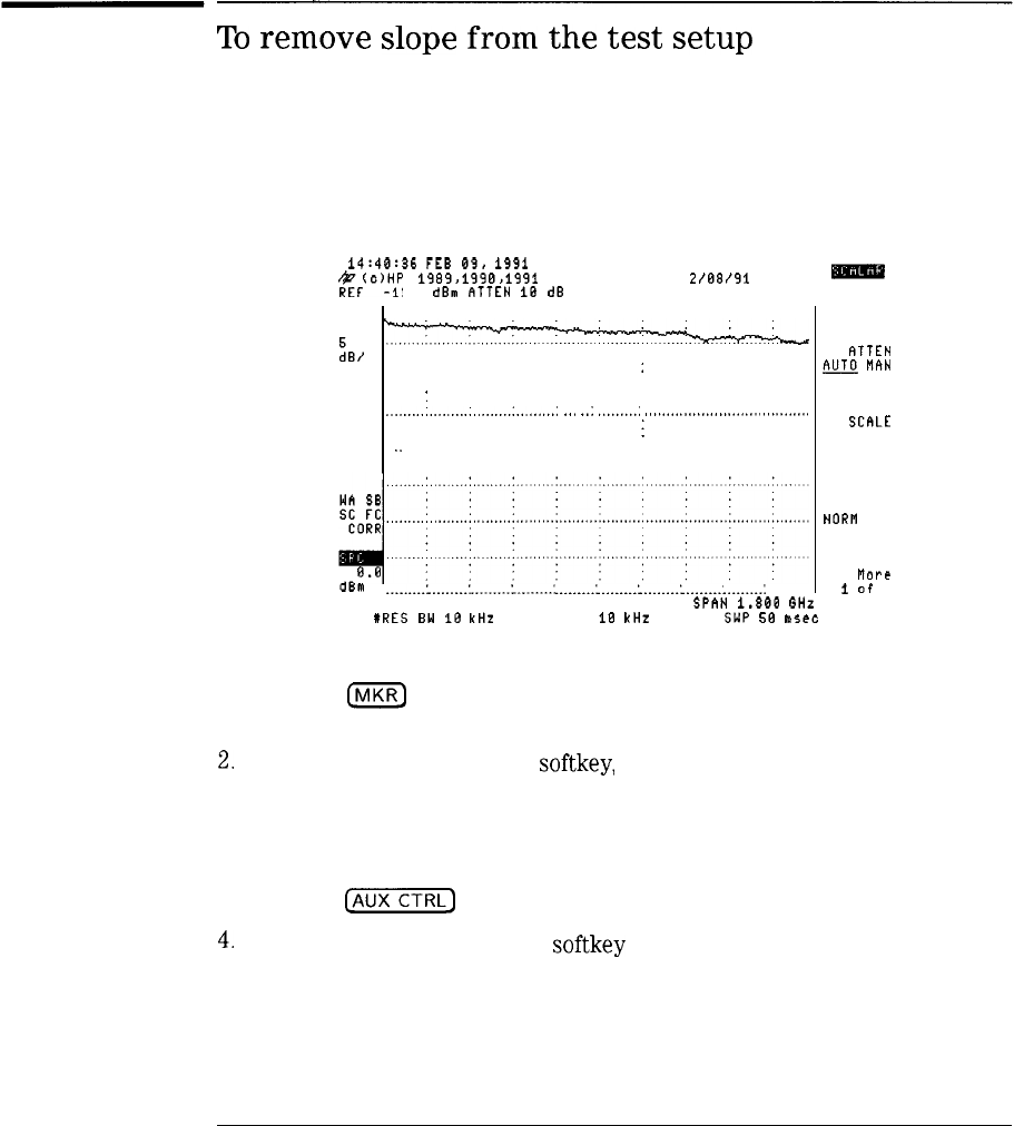
The scalar analyzer’s power sweeps can be used to remove slope from the
test setup. By sweeping the source’s power level we can compensate for the
system loss. The following figure illustrates slope caused by the frequency
response of the system.
14:40:36
FEB
09,
1991
$'Fh,HP
1989,1990>1991
SCALAR ANALYZER
Z/88/91
-13.9 dBm
ATTEN
18
dB
SMPL
. . . . . . . . . . . . . . . . . . . . . . . . . . . . . . . . . . . . . . . . . . . . . . . . . . . . . . . . . . . . . . . . . . . . . . . . . . . . . . . . . . . . . . . . . . . . . .
LOG
:e/ :
:
. . . . . . . . . . . . . . . . . . . .
:
:
.,.......,..........,...........,......:
..I
I,:
II.......:
,,......1................~~~~.........
:
1
,.
. . . .
:
not-e
1
ot
2
I
_________:
_________:
___._____:
.._._____:
_________:
_________:
_________:
_________:
_________:
_________
CENTER 900 MHz
SPAN
1.300 GHz
XRES
BW
18
kHz VBW
18
kHz SWP
58
lasec
RT
1. Press the
a
key, and place the marker at the start of the displayed
response. This is the start power level.
2.
Press the MARKER DELTA
softkey,
and place the delta marker at the other
end of the display.
The delta marker now reads the amount of loss or gain in the response
over the entire viewed frequency range.
3. Press the
[AUX]
key to enter the Source menu.
4.
Press the PWR SWP ON OFF
softkey
so that ON is underlined.
5. Enter the power gain or loss required at the end of the sweep relative to
the start of the sweep.
REF
LEVEL
ATTEN
m
MRN
LOG
SCRLE
AUTO
SCALE
NORII
REF
POSN
2-21
I
-
-
Preparing for Measurements
Power sweeps
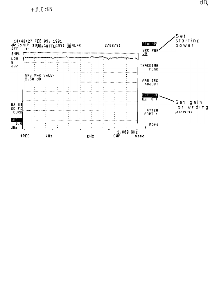
This is equal to the negative of the value determined using the marker
keys in the above steps. For example, if the delta marker reads -2.6
dB,
enter
+2.6
dB
for the power sweep.
14:43:27
FEB
09,
1991
$&MiP
1989>1998a1991
SCRLAR
ANALYZER
2/08/91
-13.9 dBm
ATTEN
10 dB
Set
starting
power
2
OFF
;
:
Mare
.
.
.
.
.
1
of 2
CENTER 900 MHz SPAN
1.800
GHz
XRES
BW 10 kHz VBW 10
kHz
SWP 50
bsec
RT
2-22
I
-
I
-
Controlling
the
HP
85630A
test
set
HP
85630A
scalar transmission/reflection test set with Option 001 includes an
output attenuator at PORT 1. You can change the attenuation from 0 to 70
dB
in 10
dB
steps.
&h,HP
1989,1990,1991
SGALRR
ANALYZER l/11/91
8.0 d8n RTTEN
10
dB
SRC PYR
. . . . . . . . . . . . . . . . . . . . . . . . . . . . . . . . . . . . . . . . . . . . . . . . . . . . . . . . . . . . . . . . . . . . . . . . . . . . . . . . . . . . . . . . . . . . . . . . . . .
oN
OFF
:
. . . . . . . . . . . . .
:...
dB/ ,
_,
:TRACKING
PEbK
RTTEN PORT 1
0
dB
:
:
.,,,,,,,,:
,,,,.,,...,,..,....,.....,...:
MAN TRK
AOJUST
::
:
PWR SUP
psOsftd;u;
attenuation
.
.
.
.
.
I
.
.
..I
:
Piore
._.______:
_____._____________:
__.......:
.
.
.
.
.
.
.
.
.
.
.
.
.
.
.
.
.
.
.
.
.
.
.
.
.
.
.
.
.
.
.
.
.
.
.
.
.
.
.
.
.
.
.
.
.
.
.
.
.
.
.
.
.
.
.
1
of 2
CENTER 900 MHz
SPAN
i-800
GHz
XRES BW 10 kHz VBW 10 kHz SWP 59
I!.CC
RT
You must inform the scalar analyzer if you have the optional HP
85630A
scalar transmission/reflection test set connected. Refer to the following
procedure. The scalar analyzer controls the test set through the auxiliary
interface on the spectrum analyzer’s rear panel.
2-23
I
-
I
-
Preparing for Measurements
Controlling the HP
85830A
test set
To
turn
on
the
test
set
1. Press the front-panel
(m]
key.
2.
Press the MORE 1 of 3 and then MORE 2 of 3 softkeys.
3.
Press the TEST SET YES NO
softkey
so that YES is underlined.
Turning the test set on informs the scalar analyzer that the optional
HP
85630A
test set is attached.
To
change
the
test
set’s
attenuation
1. Press the
(AUXCTRL)
key.
2.
Press the More 1 of 2
softkey.
3.
Press the
ATTEN
PORT 1
softkey.
4. Use the front-panel knob or numeric keypad to set the source attenuation
from 0 to 70
dB.
HP
85630A
scalar transmission/reflection test set must include Option 001.
Standard test sets do not have the PORT 1 attenuator.
2-24
I
-
I
-
AC/DC
coupling
With HP
8594A,
HP 85943, HP
8595A,
HP 85953, and HP 85963
spectrum analyzers, you can select either AC or DC coupling between the
INPUT connector and the internal circuits. Use the Amplitude menu’s
COUPLE AC DC softkey to select AC or DC coupling.
2-25

I
-
I
-
3
Calibrating for
Measurements

I
-
I
-
Calibrating for Measurements
Measurement calibration is required before performing accurate reflection
or transmission measurements. Calibration “normalizes” the test setup by
canceling system frequency response.
3-2
I
-
Using
self-guided
calibrations
The calibration procedures described in this chapter are self guided. They
prompt you to make the necessary equipment connections. Using the
Calibration menu you can:
l
Calibrate reflection measurements.
l
Calibrate transmission measurements.
l
Calibrate standard device measurements.
l
Turn normalization on or off.
l
Save and recall calibrations.
l
Show calibration ranges using display lines.
l
Peak the tracking generator.
To enter the Calibration menu, press the front-panel
ICAL)
key or press the
Main menu’s Cal
softkey.
Calibration data
Until saved, calibration data is stored in volatile memory and can be lost.
3-3
I
-
I
-
Calibrating
for
maximum
dynamic
range
Maximum dynamic range is the amplitude range between the largest and
smallest signal that can be measured simultaneously. Maximum dynamic
range is especially important during transmission measurements.
To
ensure
maximum
dynamic
range
1. Display the uncalibrated response of the device.
2. Reduce the spectrum analyzer’s input attenuation and tracking generator’s
output attenuation to the lowest level possible. Use the maximum tracking
generator power without causing signal compression.
3. Change the reference level so that the response is at the top of the display.
4. Perform the calibration as described in this chapter.
3-4
I
-
I
-
Peaking
the
tracking
generator
Peaking optimizes the source’s frequency tracking. This ensures optimum
frequency tracking between the RF OUT and the scalar analyzer’s input
frequency. Remember to peak the tracking generator before calibration.
To
peak
the
tracking
generator
1. Press the front-panel
m
key.
2.
Press the TRACKING PEAK
softkey.
3-5
I
-
I
-
Calibrating
transmission
measurements
During transmission calibrations, the device being tested is replaced with
a through-line (cable). The resulting calibration cancels out the frequency
response of the system including the cable. Use a low-loss cable with low
VSWR to avoid introducing errors.
To
calibrate
a
transmission
measurement
1. Set the scalar analyzer’s frequency, span, output power, output
attenuation, resolution bandwidth, and reference level for the desired
response.
2. Connect a low-loss, low-VSWR, cable (thru line) between the front-panel
RF OUT and INPUT connectors.
If using the HP
85630A
test set, connect the cable between the test set’s
PORT 1 and PORT 2 connectors.
3. Press the front-panel
ICAL)
key.
4.
Press the TRACKING PEAK
softkey.
The scalar analyzer performs a short routine to optimize the frequency
tracking of the tracking generator.
5. Press the CAL THRU
softkey.
6.
Press the
STORE
THRU
softkey.
Notice the “NORM” annotation in the lower-left corner of the display
indicating the display is normalized.
3-6
I
-
I
-
Calibrating
reflection
measurements
During Reflection calibrations, you terminate the line at the plane of reflection
using an
OJXX
and
short
connection. The plane of reflection is typically
located at the input to the device being tested. Simply remove the device and
replace it with the
short
or
OJXVZ
as directed by the calibration routine.
Calibration kit
Reflection calibration requires both
open
and
shurr
standards. The HP 850328 Option 001 Calibration
Kit supplies
5OQ
type N
open
and
short
standards for calibration.
To
calibrate
a
reflection
measurement
You must use an external bridge (test set) to make reflection measurements.
The optional HP
85630A
scalar transmission/reflection test set is the
recommended test set.
1. Set the scalar analyzer’s frequency, span, output power, output
attenuation, resolution bandwidth, and reference level for the desired
response.
2. Press the front-panel
a
key.
3. Connect a cable (thru line) between PORT 1 and PORT 2 of the
HP
85630A
test set.
4. Press the TRACKING PEAK softkey.
-1
The scalar analyzer performs a short routine to optimize the frequency
tracking of the tracking generator.
3-7
I
-
I
-
Calibrating for Measurements
Calibrating reflection measurements
5. Remove the cable from the path between the PORT 1 and PORT 2
connectors.
6. Press the
CAL
OPN/SHRT
softkey.
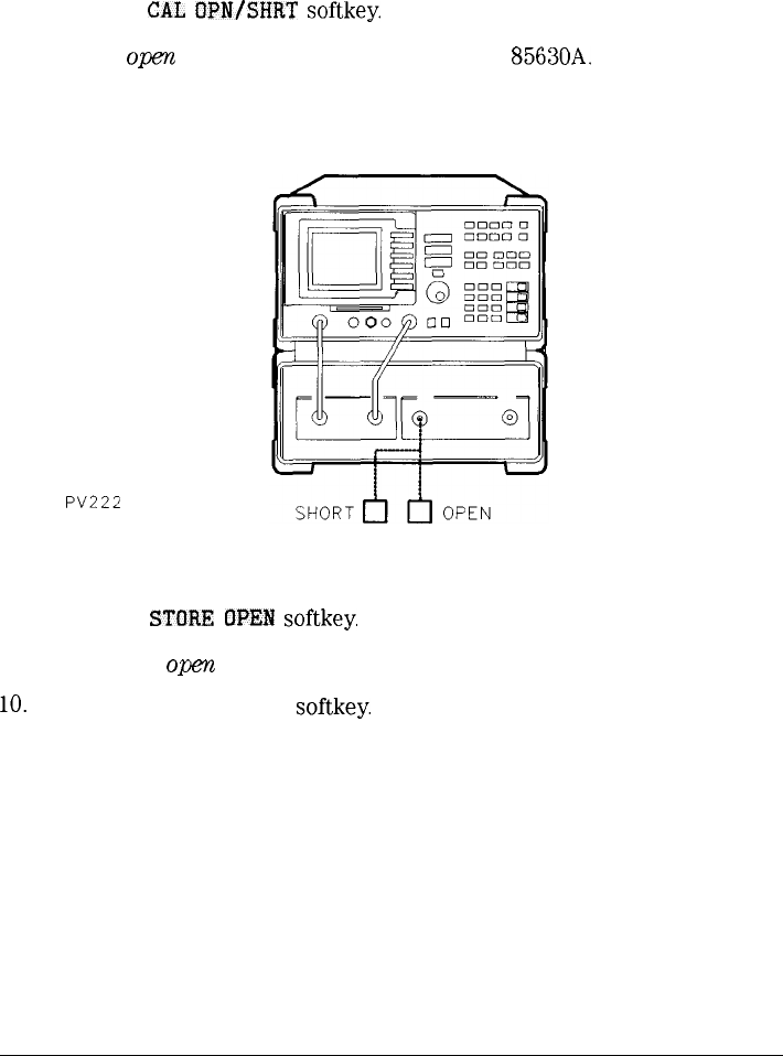
7. Place an
OJXX
connector on PORT 1 of the HP
85630A.
This is the output
of the bridge.
PV222
8. Press the
STORE
OPEN
softkey.
9. Replace the
0~
connector with a
short
connector.
10.
Press the STORE SHORT
softkey.
Notice the NORM annotation in the lower-left corner of the display
indicating the display is normalized.
3-8
I
-
I
-
Calibrating
for
a
standard
device
The scalar measurements personality provides a standard device calibration
routine. Standard device calibration allows you to make repeated pass/fail
testing based on the response of a standard device-under-test. During
calibration, instead of using a through line, your standard device is placed in
the path between the RF output and the RF input connectors. The scalar
analyzer personality then creates special limit-line traces above and below the
response of the standard device.
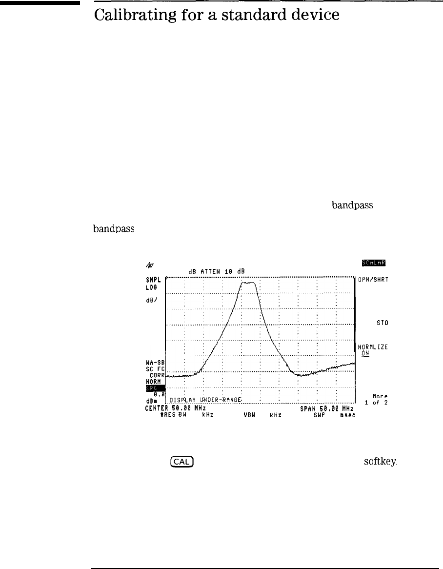
The following figure shows the response of a 50 MHz bandpass filter. You
could save this response as a standard device against which to test similar
bandpass filters.
c
REF
SMPL
LOG
10
dB/
0.0
dB
ATTEN
16
dB
CENTER
56.66
MHz
SPAN
58.66
MHz
tRES
BW 10 kHz UBW 10 kHz SWP 50
ld5ec
CAL
OPN/SHRT
CAL
THRU
CAL ST0
DEVICE
NORMLIZE
E
OFF
TRACKING
PEAK
RT
Limit-line testing is turned on (and upper and lower limit traces displayed)
after pressing the
ICAL)
key and then the CAL STD DEVICE
softkey.
3-9
I
-
Calibrating for Measurements
Calibrating for a standard device
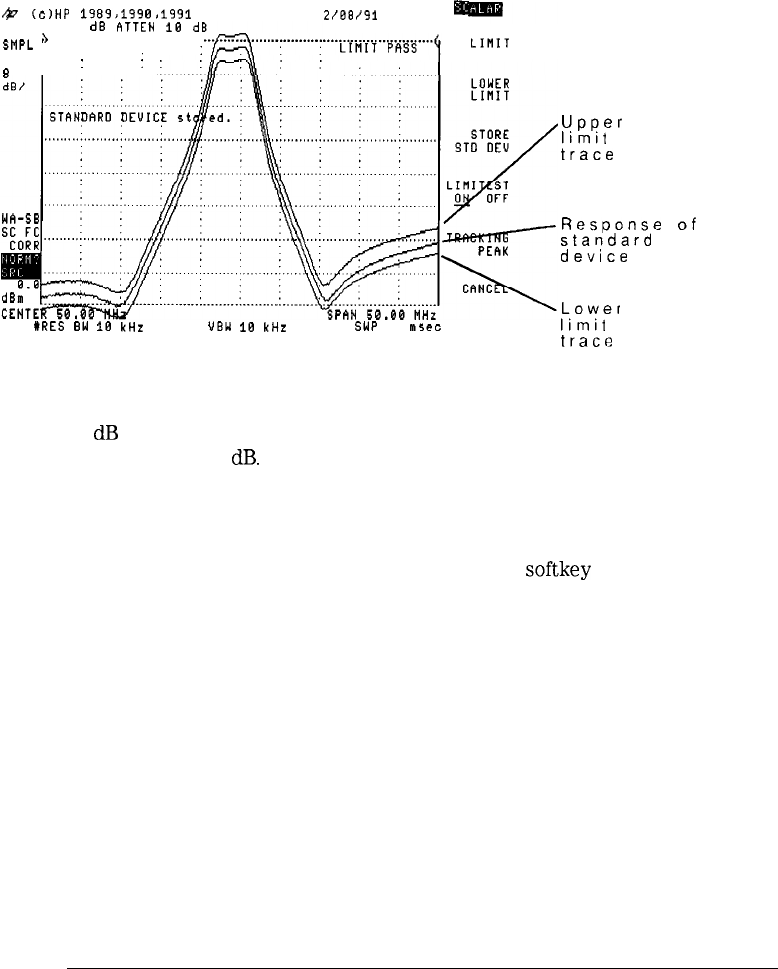
&
(c)HP
1989,199B,1991
SCALAR ANALYZER Z/88/91
EB
REF -3.5 dG
ATTEN
1G
dl
‘,
. . . . . . . . . . . . . . . . . . . . . . . . . . . . . . . . . . . . .
SMPL
LOG
:
j
:
*
I
UPPER
LINIT
#RES
GW
18
kHz UBW
18
kHz SWP 58
15ec
RT
Upper
limit
trace
Response
of
standard
device
Lower
limit
trace
You define the
window
between the upper and lower limit traces using the
UPPER LIMIT and LOWER LIMIT softkeys. Enter the amount of deviation
in
dB
between the response of the standard device and the limit trace. The
default value is 3
dB.
Standard device calibrations can be performed after a normal open/short
or thru calibration. Limit traces created by the standard device calibration
cannot
be edited or stored. To turn off a standard device calibration,
press the Calibration menu’s LIMITEST ON OFF
softkey
so that OFF is
underlined.
3-10
I
-
I
-
Calibrating for Measurements
Calibrating for a standard device
To
calibrate
a
standard
device
1. Connect the device between the front-panel RF OUT and INPUT
connectors.
or
If you are using the HP
85630A
test set, connect the device between the
test set’s PORT 1 and PORT 2 connectors.
2. Set the scalar analyzer’s frequency, span, output power, output
attenuation, resolution bandwidth, and reference level for the desired
response.
3. Press the front-panel
ICAL)
key.
4.
Press the TRACKIWG PEAK softkey.
The scalar analyzer performs a short routine to optimize the frequency
tracking of the tracking generator.
5. Press the CAL STD DEVICE
softkey.
6.
Press the UPPER LIMIT
softkey,
and enter the amount of deviation in
dB
that is acceptable above the displayed response.
7.
Press the LOWER LIMIT
softkey,
and enter the amount of deviation in
dB
that is acceptable below the displayed response.
3.
Press the STORE STD DEV
softkey
9. Replace the standard device with the device to be tested.
3-11
I-
I
-
I
-
Saving
and
recalling
calibrations
Transmission, reflection, and standard device calibrations can be saved and
recalled for later use. (Turning the scalar analyzer off or presetting it will
not effect the calibration data.) However, if a calibration is not saved, the
calibration data can be lost if one of the following occurs:
l
the spectrum analyzer is turned off
l
the front-panel [PRESET) key is pressed
l
another calibration is performed
Saving
calibrations
When saving calibration data, keep in mind that reflection and transmission
calibrations are saved in the same operation as a group of data. Two separate
save and recall operations are not needed.
CAUTION
Calibration data is saved in trace memory registers. Use caution to avoid
deleting any previously saved traces.
Calibrations are saved in CAL groups starting with number 1. Each group
requires two trace memory registers and is saved starting at trace register
51. (Trace register 52 is used by the program and is not available.) Trace
CAL group 1 corresponds to trace memory registers 50 and 51. As more
calibrations are saved, calibration memory grows towards trace memory
register 1. If you need to determine availability and use of trace registers,
catalog trace memory.
3-12
Before being saved, calibration data is temporarily stored in CAL group
0. Unlike the CAL groups used for saving calibrations, this storage area is
temporary. Calibration data in CAL group 0 can be lost if it is not saved as
described in this section.
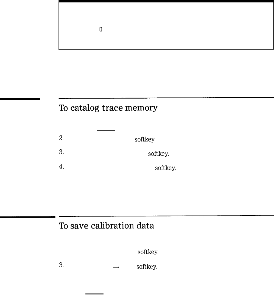
I
-
I
-
Calibrating for Measurements
Saving and recalling calibrations
limit lines
Limit lines, as described in Chapter 5, are also saved in trace memory Limit lines are saved starting at
memory register 0 and increasing towards calibration memory As the number of saved calibrations and
limit lines grows, the possibility of overwriting limit line or calibration data increases.
To
catalog
trace
memory
1. Press the [RECALL) key.
2.
Press the INTRNL CRD
softkey
so that INTRNL is underlined.
3.
Press the CATALOG INTRNL
softkey.
4.
Press the CATALOG REGISTER
softkey.
5. Use the front-panel knob to scroll the display of trace memory.
To
save
calibration
data
1. Perform a calibration.
2. Press the More 1 of 2
softkey.
3.
Press the SAVE
+
CAL
softkey.
4. Enter a register number.
5. Press [ENTER) to store the calibration data.
3-13
I
-
I
-
Calibrating for Measurements
Saving and recalling calibrations
Recalling
calibrations
When recalled, calibration data automatically sets the scalar analyzer’s
frequency, amplitude, and scale parameters appropriate to the calibration.
When recalling calibration data, remember the following:
l
Normalization remains off until you turn it on.
l
Both transmission and reflection calibration data is recalled (if both saved).
l
Measurement type (transmission/reflection) is not selected.
To
recall
calibration
data
1. Press the front-panel
a
key.
3.
Press the More 1 of 2
softkey.
3.
Press the RECALL
--+
CAL
softkey,
4. Enter the register number.
5. Press
@KKK)
to recall the calibration data.
3-14
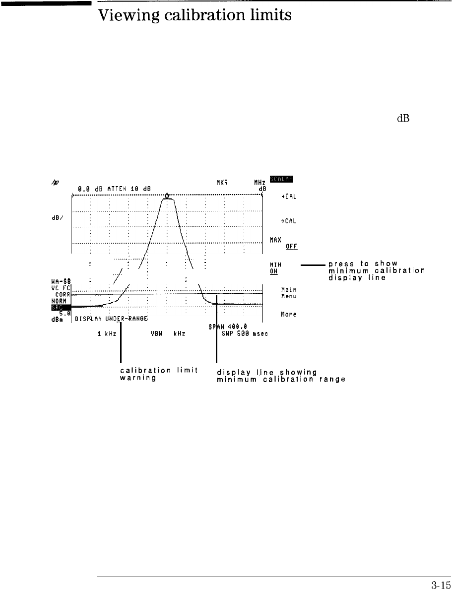
I
-
I
-
Viewing
calibration
limits
Display calibration has a finite amplitude range. This is due to 70
dB
of log
fidelity and because normalization shifts the response.
&
llKR
321.4
NH,?
m
REF
'3.8
dB
ATTEN
16
dB
-2.37
dB
SAVE
+CRL
LOG
10
dB/ RECALL
rCRL
MAX RNG
ON
OFF
. . . . . . . .
,,.....
:.
.,,.,
:
//
.\
:
:: :
Wh-SB
:
/
I
. . . . . . . . . . . . . . . . .
\
:
dBa
0ISP:LAY
UNDER-:RtoNGE:
.
._
. . . .
CENTER 321.4 MHz
SPhN
468.8
MHz
XRES BW
1
kHz UBW 1 kHz SWP 568 M5eC
HIN RNG
fi
OFF
n0re
2 of 2
RT
press
to
show
minimum
calibrati
display
line
on
calibration
limit
warning
display
Line
showing
minimum
calibration
range
To view the limits of calibration, use the MAX RNG ON OFF and
MIN RNG ON OFF softkeys. Horizontal calibration lines are displayed
indicating the limits of display calibration. (The lines may not be visible if
their amplitude is beyond the displayed scale.) Normally, the calibration lines
are turned off.
3-15
I
-
I
-
Calibrating for Measurements
Viewing calibration limits
When a response goes beyond the calibrated limit, the scalar analyzer
displays one of the following two messages:
DISPLAYUNDER-RANGE
DISPLAYOVER-RANGE
Portions of the trace displayed outside the calibration limit lines do not show
an accurate response. The portion of the response that falls between the two
display lines remains calibrated. Portions which cross the displayed line are
uncalibrated. Changing the log scale does not affect calibration.
To
view
the
calibrated
limits
of
the
display
1. Press the front-panel
@ZJ
key.
2.
Press the More 1 of 2
softkey.
3.
To show the maximum level of calibrated display, press MAX RNG ON OFF
so that ON is underlined.
4.
To show the minimum level of calibrated display, press MIN RNG ON OFF
so that ON is underlined.
3-16
I
-
Changing
the
normalized
position
and
reference
level
The default normalized reference position is at the display’s top graticule line.
(It is represented on screen by an angle bracket at each end of a horizontal
graticule line.) NORM
REF
POSN sets the reference position to any of the
eight major horizontal graticule lines. Position eight is the top graticule;
position zero is the bottom graticule.
The reference position is
always
the top graticule line when normalization is
turned off.
The scalar analyzer places the normalized reference level at the normalized
reference position. (The default is at top horizontal line of the graticule.)
To
change
the
normalized
reference
position
1. Press the front-panel
(-J
key.
3.
Press the NORM
RRF
POSN
softkey.
3. Use the front-panel knob or numeric keypad to place the normalized
reference position at any of the eight major horizontal graticules.

I
-
I
-
4
Measuring
Reflection/Transmission
Parameters

I
-
Measuring Reflection/Transmission Param-
eters
The HP
85714A
scalar measurements personality not only displays device
reflection and transmission, but in addition provides automatic measurements
for device characterization. These include VSWR, transmission/reflection
coefficients, bandwidth, and shape factor parameters. This chapter includes
information on swept-power measurements which allow you to characterize
distortion related to input power.
4-2
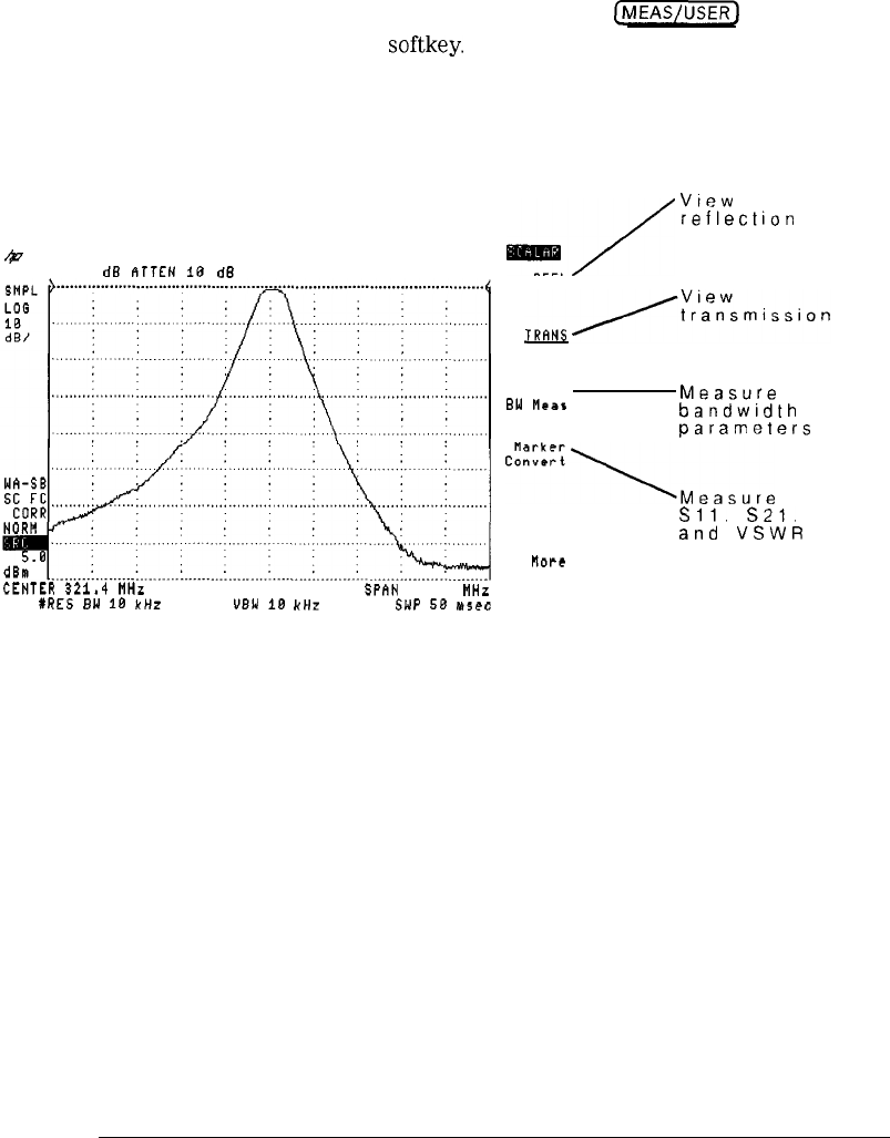
I
-
I
-
Measuring Reflection/Transmission Parameters
Changing the normalized position and reference level
To enter the Measure menu, press the front-panel
[MEAS/USER)
key or press
the Main menu’s Measure
softkey.
t
REF 0.0 dB
flTTEN
.tB
dB
CENTER
321.4
MHz SPAN
500.8
MHz
#RES
BW 18
kHi!
UBW
18
kHz
SWP
58
nt5ec
-/
View
reflection
REFL
Device
BW
Mear
Measure
bandwidth
parameters
C~~::::\Meas”re
Sil.
s21.
and
VSWR
nbPt
1 of 2
RT
Page One of Measure Menu
4-3
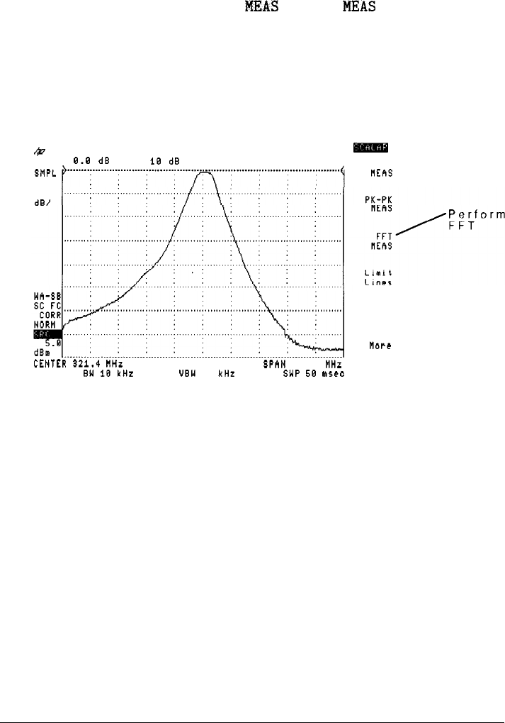
I
-
Measuring Reflection/Transmission Parameters
Changing the normalized position and reference level
For information on using the DELTA
MEAS
, PK-PK
MEAS
, and
Limit Lines softkeys, refer to Chapter 5.
t
REF B.B dB RTTEN IB dB
SMPL
LOG
10
dB/
CENTER
321.4
RHz SPAN
500.0
MHz
XRES BW
18
kHz
'JEW
18
kHz
SW,'
58
M5tb
DELTA
nfhs
Main
Menu
MbPt
2 of 2
RT
Page Two of Measure Menu
4-4
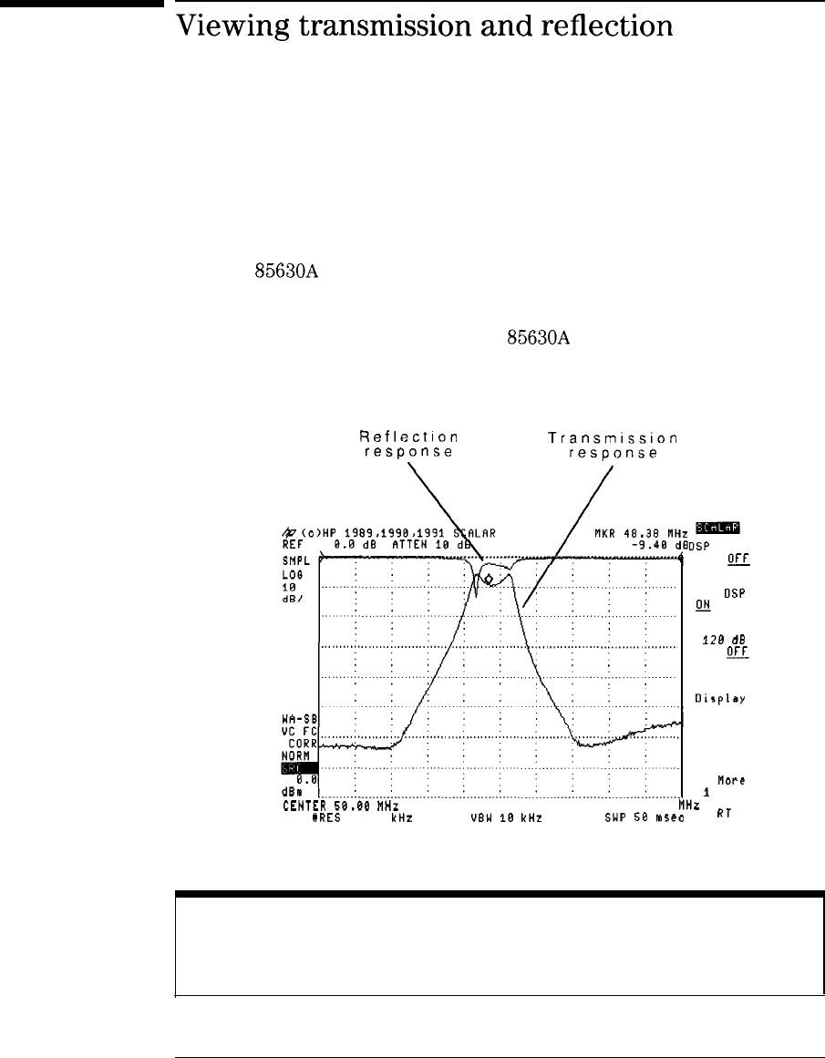
I
-
Viewing
transmission
and
reflection
After normalizing the display, the scalar measurements personality offers
extensive control for viewing the response on the screen.
If an HP
85630A
scalar transmission/reflection test set is used, you can easily
switch between transmission and reflection measurements. The test set also
provides the ability to simultaneously display both responses. The scalar
analyzer automatically controls the HP
85630A
scalar transmission/reflection
test set for the two measurement setups.
Reflection
Transmission
response
response
CENTER
50.00
MHz
#RES
BW 18 kHz UEW 18 kHz SPAN 50.00
MHz
RT
s!dP
58
M5tb
DSP LINE
ON
OFF
DUAL OSP
Qy
OFF
120
dE
ON
@-J
Tabular
Display
NbPt
I
of 2
NOTE
If you don’t have the test set, you must manually use external cabling and couplers to view reflection.
4-5
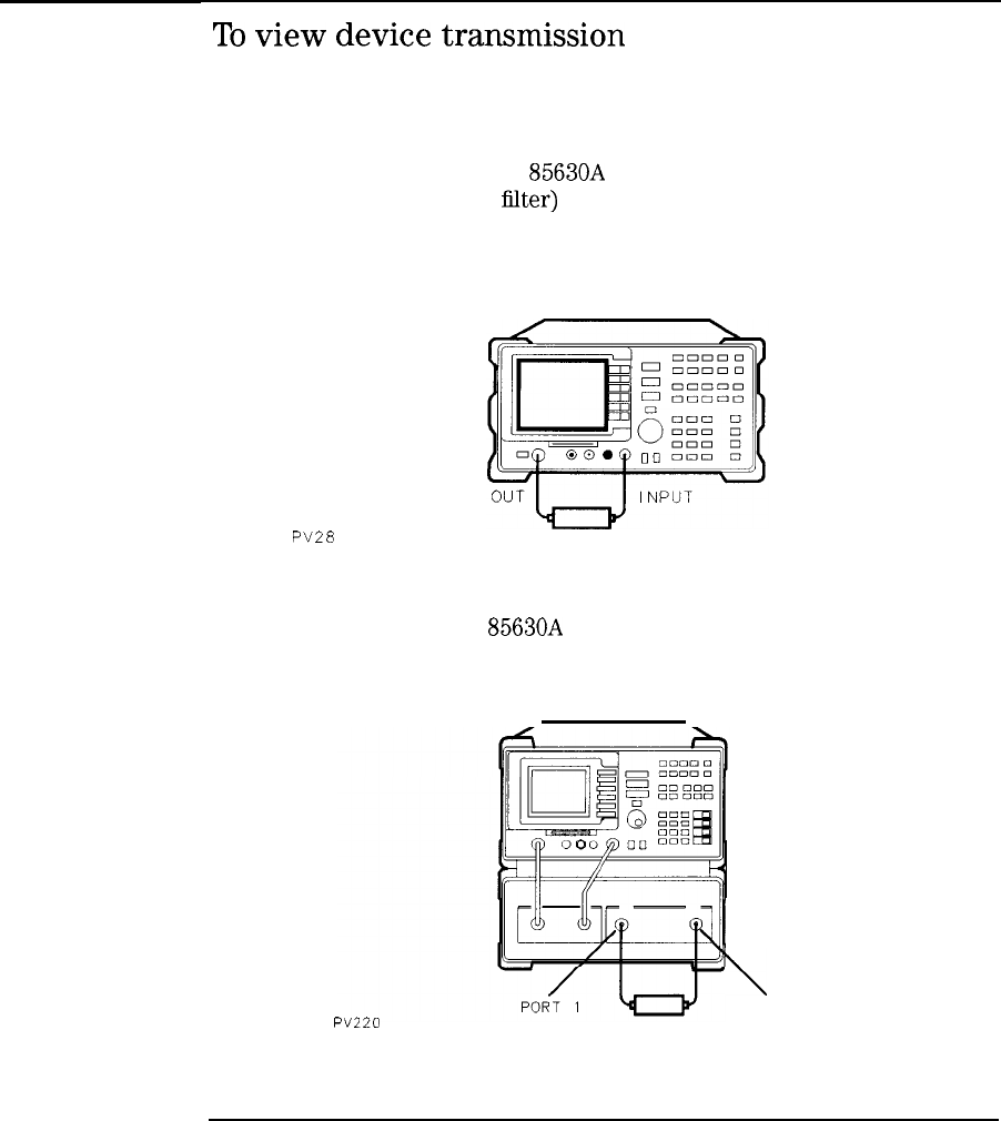
I
-
I
-
Measuring Reflection/Transmission Parameters
Viewing transmission and reflection
To
view
device
transmission
1. Calibrate the measurement as explained in “To Calibrate a Transmission
Measurement” in this chapter.
2. If you are
not
using the HP
85630A
test set, connect the device being
measured (for example
INPUT connectors.
PV28
FILTER
3. If you are
using the HP
85630A
test set, connect the device being
measured
between the PORT 1 and PORT 2 connectors.
RF
a
Iilter)
between the scalar analyzer’s RF OUT and
SPECTRUM ANALYZER
2
PORT 2
cviiv
FILTER
4-6
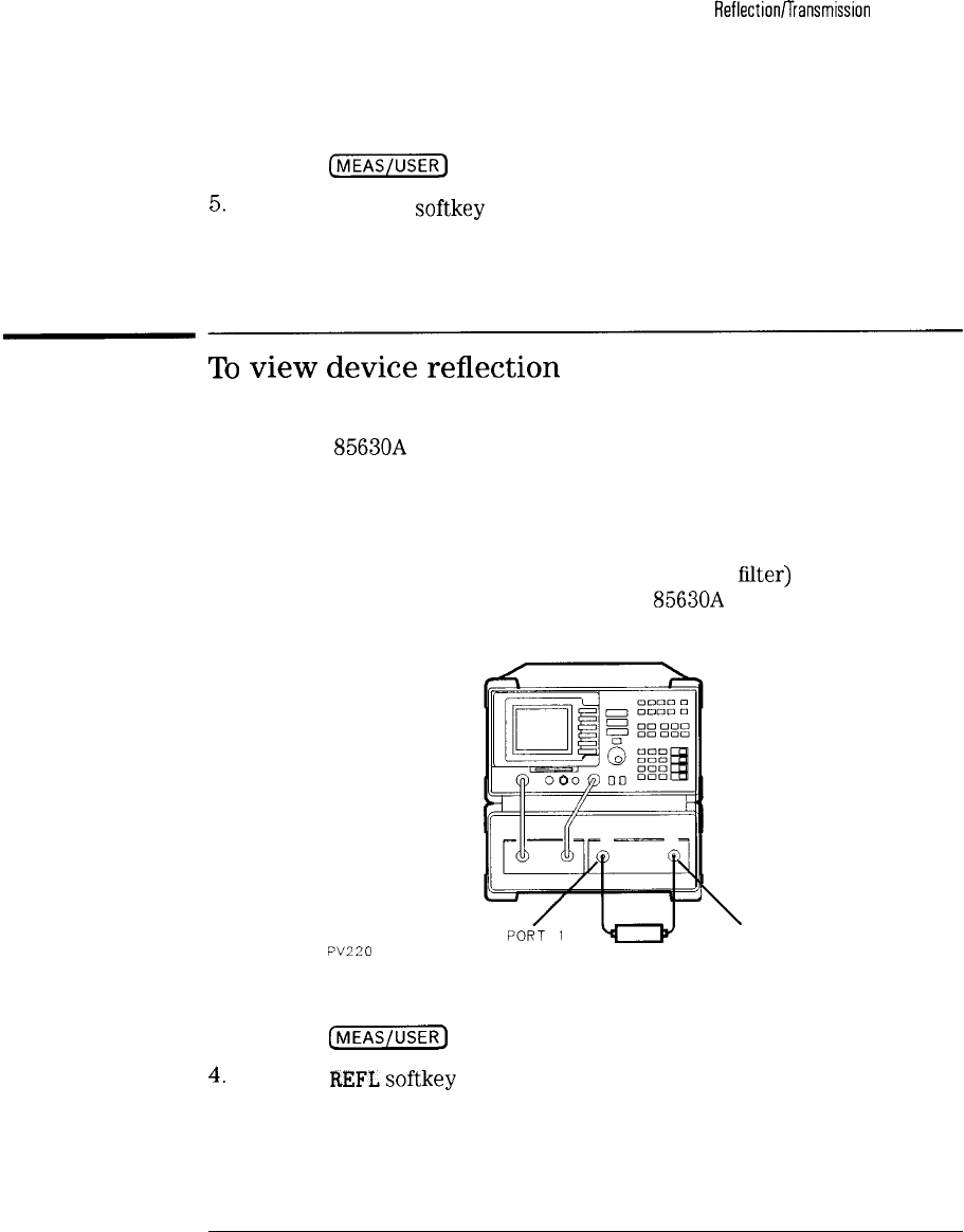
I
-
Measuring
Reflectionflransmission
Parameters
Viewing transmission and reflection
4. Press the
(jMEAS/USER]
key.
5.
Press the TRAWS
softkey
so that it is underlined.
To
view
device
reflection
You must use an external bridge (test set) to view device reflection. The
optional HP
85630A
scalar transmission/reflection test set is the recommended
test set.
1. Calibrate the measurement as explained in “To Calibrate a Reflection
Measurement” in Chapter 3.
2. Connect the device being measured (for example a
filter)
between the
PORT 1 and PORT 2 connectors of the HP
85630A
test set.
PV220
FILTER
3. Press the
(jMEAS/USER)
key.
4.
Press the
REFL
softkey
so that it is underlined.
\
PORT 2
4-7
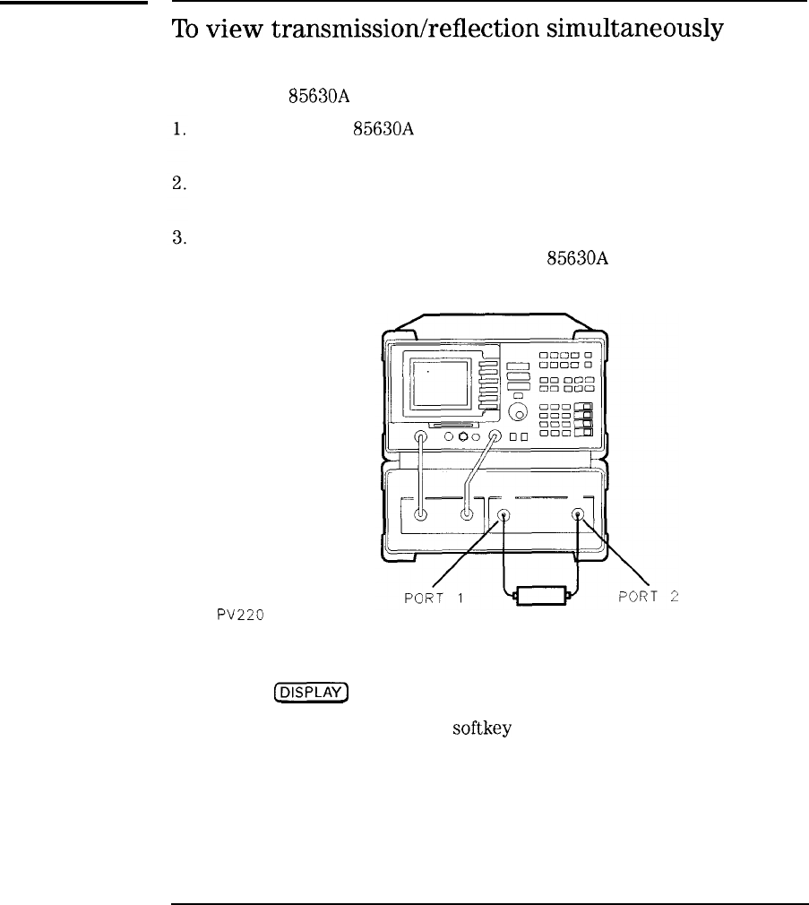
I
-
Measuring Reflection/Transmission Parameters
Viewing transmission and reflection
To
view
transmission/reflection
simultaneously
Viewing both the transmission and reflection response simultaneously
requires an HP
85630A
scalar transmission/reflection test set.
4.
5.
Make sure the HP
85630A
scalar transmission/reflection test set is turned
on as described in Chapter 2.
Calibrate the measurement as explained in “To calibrate a Transmission
measurement” and “To calibrate a reflection measurement” in Chapter 3.
Connect the device being measured (for example a filter) between the
PORT 1 and PORT 2 connectors of the HP
85630A
test set.
PV220
FILTER
Press the
c-1
key.
Press the DUAL DSP ON OFF
softkey
so that ON is underlined.
4-8
I
-
I
-
Measuring Reflection/Transmission Parameters
Viewing transmission and reflection
To
turn
normalization
off
1. Press the front-panel
ICALl
key.
2.
Press the
NORMLIZE
ON OFF
softkey
so that OFF is underlined.
Use this feature to temporarily turn normalization on or off.
4-9
I
-
Viewing
120
dB
of
measurement
range
The scalar analyzer can display a 120
dB
measurement range not available
with the normal 15
dB
per division log scale.
k
REF
8.8
dB
ATTEN
1B dB
CENTER
321.4
MHz
SPAN
500.0
MHz
#RES
BW
18 kHz
UBW
18
kHz
SUP
58
15ec
OSP
LINE
ON
JIFJ
Tabular
Display
L
The 120
dB
calibrated measurement range is achieved by splicing two
separate traces. For each visible sweep, the scalar analyzer first saves the top
50
dB
of trace data. Then, the reference level is set up to 50
dB
below the
current reference level and another reading is taken. Finally, these two traces
are spliced together and displayed on the screen.
To achieve greater than 85
dB
of dynamic range, perform the measurement
without the HP
85630A
Scalar Transmission/Reflection Test Set.
In dual display mode
You cannot view 120
dB
measurement range in the dual display mode.
Klual
display refers to
simultaneously displaying both transmission and reflection responses.)
4-10
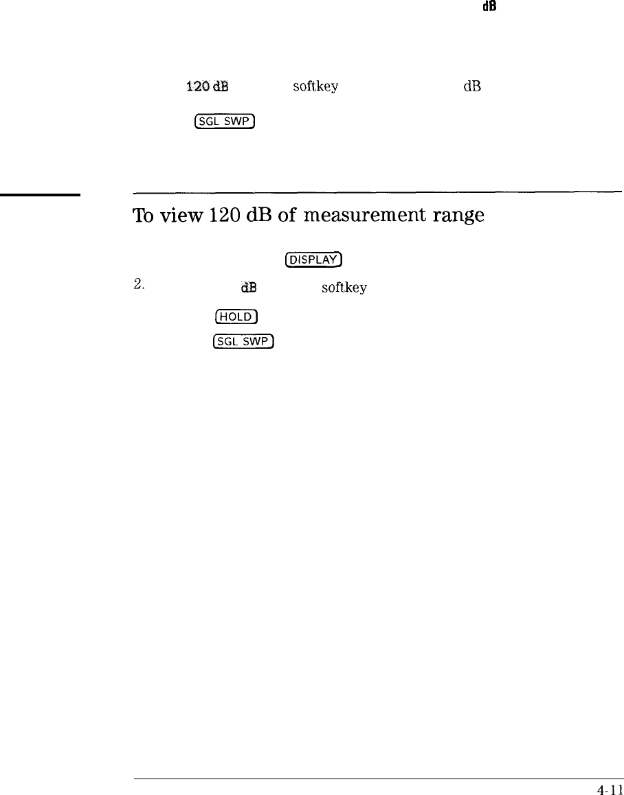
I
-
I
-
Measuring Reflection/Transmission Parameters
Viewing 120
dB
of measurement range
Use the
120
dB
ON OFF
softkey
to turn on the 120
dB
measurement range
feature. This feature places the spectrum analyzer in single sweep mode.
Press the
(j-1
key to remeasure a device.
To
view
120
dB
of
measurement
range
1. Press the front-panel
I-J
key.
2.
Press the 120
dE!
ON OFF
softkey
so that ON is underlined.
3. Press the
[HOLD]
key to remove the displayed measurement message
4. Press the
CsGLSWP)
key each time you need an updated display.
4-11
I
-
I
-
Automatically
scaling
the
response
The scalar analyzer provides one-button scaling. To scale the response for
full screen, simply press the Amplitude menu’s AUTO SCALE
softkey.
Of
course, you can still manually scale the response by changing the normalized
reference level and log scale.
CENTER
321.40
MHz SPAN
75.00
MHz
tRES
BW
18
kHz VBW
18
ktiz
SWP 58
m5ec
~IUTO
SCRLE
NORN REF
POSN
Response before Automatic Scaling
Press
scale
autom
10
atically
Auto scaling is a one-time adjustment. The log scale does not continually
update when the response amplitude changes.
4-12
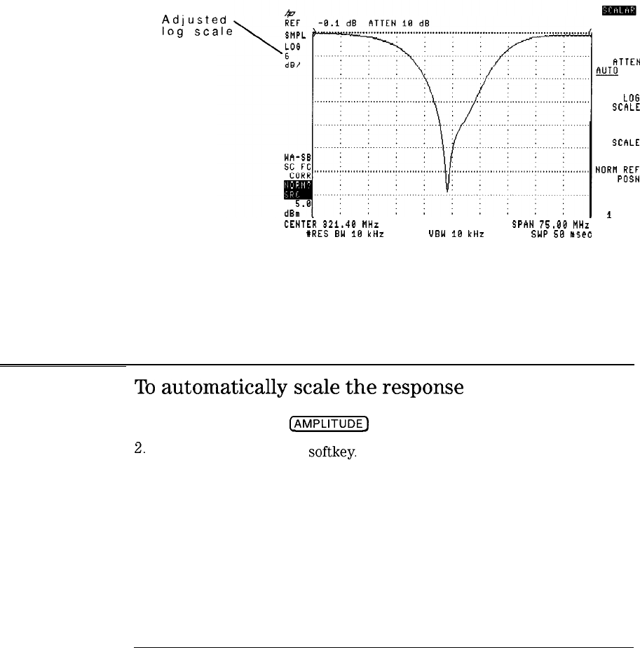
I
-
Adjuste
log
sea
Measuring Reflection/Transmission Parameters
Automatically scaling the response
. . . . .
CENTER
321.40
MHz SPAN
75.00
MHz
tRES
BW
18
kHz
UBW
18
kHz
SWP
58
15ec
Response after Automatic Scaling
REF
LEVEL
ATTEN
&UTJ
MAN
LOG
SCALE
AUTO
SC~ILE
NORN
REF
POSN
Mare
i
of 2
RT
To
automatically
scale
the
response
1. Press the front-panel
(XiKiKKJ
key.
2.
Press the AUTO SCALE
softkey.
4-13
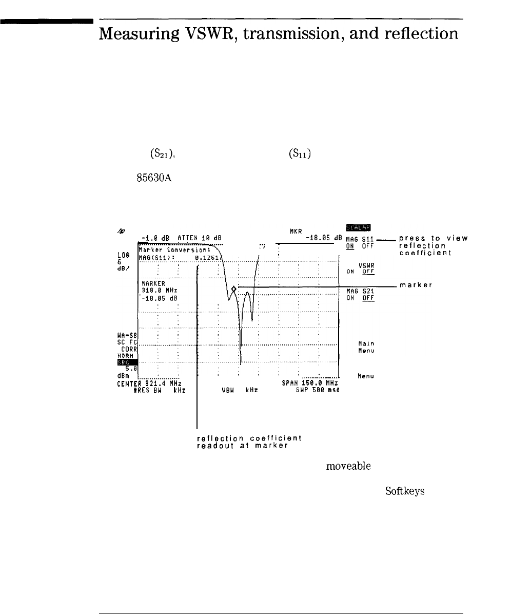
I
-
Measuring
VSWR,
transmission,
and
reflection
The scalar measurements personality can display the VSWR, transmission
coefficient (&r), or reflection coefficient
(&I)
at any point along the displayed
response. (VSWR and reflection coefficient measurements require the use of
the HP
85630A
scalar transmission/reflection test set.)
llKR
318.6 MHz
ATTEN
1B
dB
-18.65
dB
,tAG
SII-
*ET
. . . . . . . . . . . . . . . :..
;
. . . . . . . . . . . . . . . . . . . . . . . . . . . .
,
;
to
view
Elion
icient
c
REF
-1.B
dB
LO0
6
dB/
.
.
.
.
.
.
.
.
.
.
.
.
.
.
.
.
.
.
CENTER
321.4
MHz
SPAN
150.0
MHz
XRES
BW
1 kHz
U8W
I kHr
SWP
588
15.e
Previous
MeFlu
'0
RT
reflection
coefficient
readout
at
marker
The scalar measurements personality displays a
moveable
marker showing
the value at the marker position. The displayed values are continuously
updated. This is true even in single sweep and view modes.
Softkeys
for
these measurements are available from the Measure menu’s Marker Convert
selection.
4-14
I
-
I
-
Measuring Reflection/Transmission Parameters
Measuring VSWR, transmission, and reflection
To
measure
transmission
coefficient
1. Display the desired response on the scalar analyzer’s display.
2.
Press the
fjMEAS/USER)
key and then the Marker Convert
softkey.
3.
Press the NAG
S21
ON OFF
softkey
so that ON is underlined.
4. Move the marker to the desired trace position, and read the displayed
transmission coefficient.
To
measure
reflection
coefficient
1. Display the desired response on the scalar analyzer’s display.
2.
Press the
C-1
key and then the Marker Convert
softkey.
3.
Press the MAG
Sll
ON OFF
softkey
so that ON is underlined.
4. Move the marker to the desired trace position, and read the displayed
reflection coefficient.
4-15
I
-
I
-
Measuring Reflectionilransmission Parameters
Measuring VSWR, transmission, and reflection
To
measure
VSWR
1. Display the desired response on the scalar analyzer’s display.
2.
Press the
(j-1
key and then the Marker Convert
softkey.
3.
Press the VSWR ON OFF
softkey
so that ON is underlined.
4. Move the marker to the desired trace position, and read the displayed
voltage standing wave ratio.
4-16
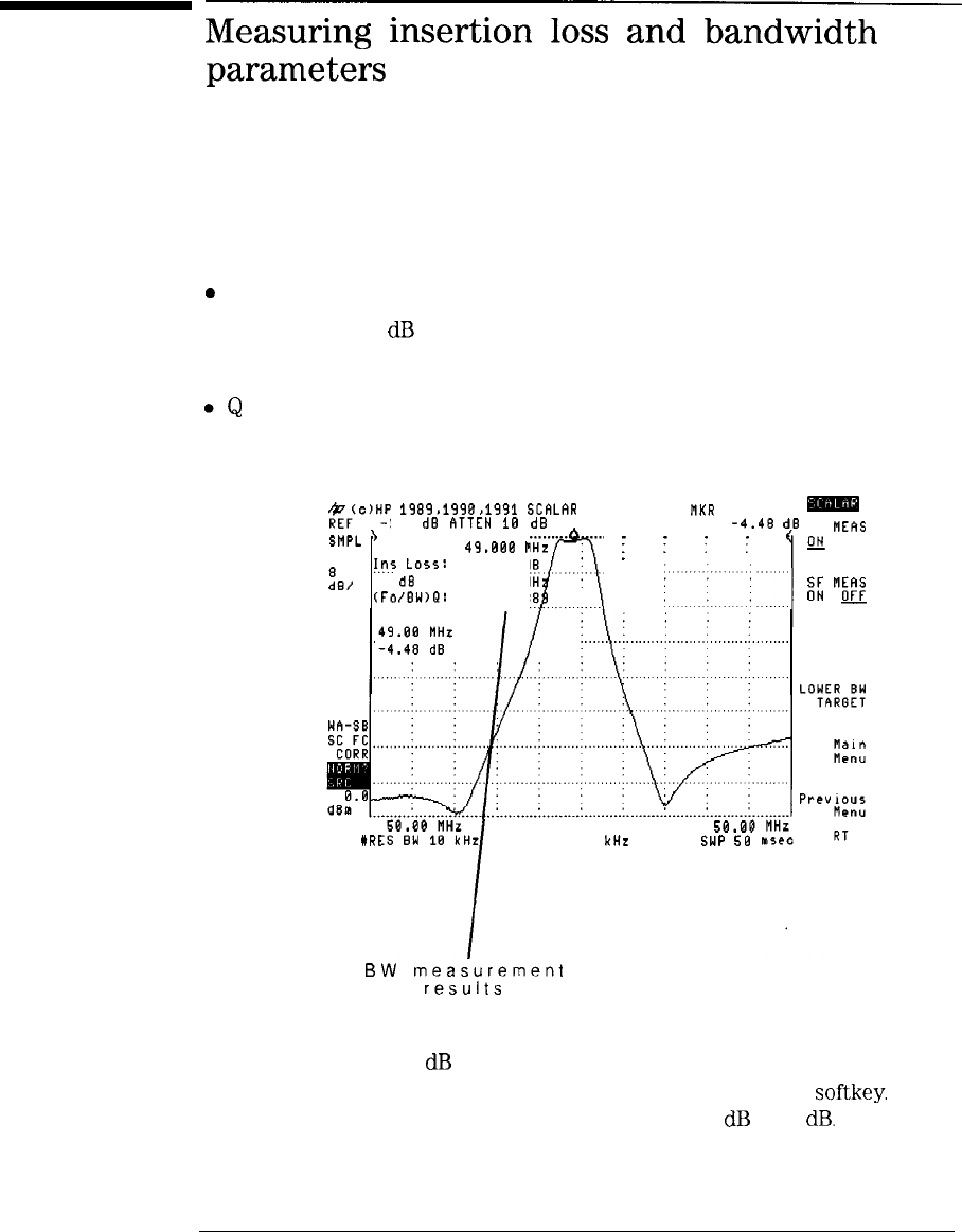
I
-
I
-
Measuring
insertion
loss
and
bandwidth
parameters
The scalar analyzer performs the following bandwidth measurements:
0
center frequency
l
insertion loss in
dB
l
bandwidth
.Q
$V:o,HP
1989~1998>1991
SCALfiR
-3.5 dB
ATTEN
18 dB
I
ilKR
49.68 MHz
m
-4.48
dB BW
MERS
SMPL
>
. . . . . . . . . . . . . . . . . . . . . . . . . . . . . . . . . . . . . . . . . . . . .
Center: 4q
,BBB MHz
:
LOG
!,"r
Loss:
4.48
dB
:
. . . . . . . .
i
. . . . . . . . .
I
. . . . . . . . .
I
. . . . . . . . .
I
. . . . . . . .
3
OFF
8
dB/
3 dB BW: 4.588 NH
(Fa/BW)Q:
.
..n
18.88 ;:
"2;
-
MARKER UPPER BW
TARGET
SPAN
50.0G
'JBW 18
kHr SWP
50
CENTER
#RE
BW
measurement
results
Bandwidth measurements are updated after each sweep. The bandwidth
measurement uses a 3
dB
default bandwidth (upper bandwidth). The default
bandwidth used can be changed using the UPPER BW TARGET
softkey.
For example, you could change the bandwidth from 3
dB
to 6
dB.
Lower
bandwidth is not defined for this measurement.
4-17
I
I
-
I
-
Measuring Reflection/Transmission Parameters
Measuring insertion loss and bandwidth parameters
The Q indicates the frequency selectivity of a response. The narrower
the bandwidth at a given frequency, the higher the
Q.
It is
deEned
by the
following formula:
where:
f,
is the center frequency of the displayed response
BW is the bandwidth of the displayed response.
To
measure
insertion
loss
and
bandwidth
parameters
1. Display the desired response on the scalar analyzer’s display.
2.
Press the
[MEAWJSER)
key and then the Device
3W
Meas
softkey.
3.
Press the
BW
MEAS
ON OFF
softkey
so that ON is underlined.
The measurement continually repeats until the BW
MEAS
ON OFF
softkey
is pressed so that OFF is underlined.
The response’s center frequency, insertion loss, bandwidth, and Q is
displayed on the screen.
4-18
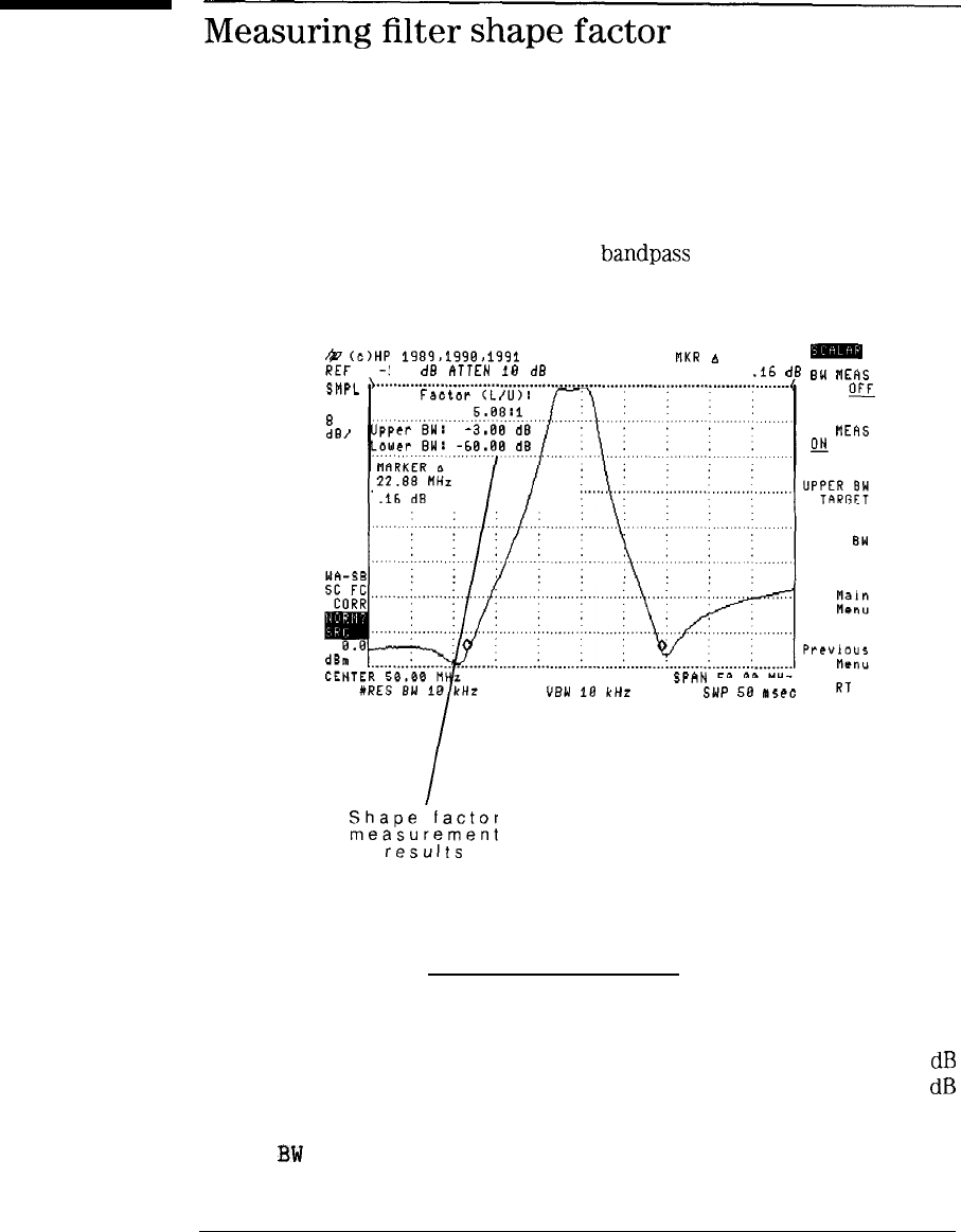
I
-
I
-
Measuring
filter
shape
factor
Shape factor characterizes the slope of a bandpass filter’s skirts.
f&WHP
1989,1996>1991
SCALAR
-3.5 dE
ATTEN
fG dG
FlKR
A
22.88 MHz
m
.f6 dB RW
IF(IS
Sl4PL
LOG
8
dB1
Shape
Factor
<L/U):
_..
..-.,_
ON
OFF
SF
MERS
u
OFF
SPhN
50.00 MHz
UEW
10
kHr SWP
SG
lSCC
LOWER BW
TARGET
Shape
factor
measurement
results
Shape factor is the ratio of upper and lower bandwidths of the response. The
larger the shape factor, the less selective the filter.
shape factor = lower response bandwidth
upper response bandwidth
The default bandwidths used are:
upper bandwidth . . . . . . . . 3
dB
lower bandwidth
. . . . . . . 60
dB
Default bandwidths for shape factor measurements can be changed using the
UPPER
BW
TARGET and LOWER BW TARGET softkeys. For example, using
4-19
I
-
I
-
Measuring Reflection/Transmission Parameters
Measuring filter shape factor
the UPPER BW TARGET
softkey,
you could change the upper bandwidth from
3
dB
to 6
dB.
Shape factor measurements are updated after each sweep.
To
measure
shape
factor
1. Display the desired response on the scalar analyzer’s display.
2. Press the
(j-1
key and then the Device BW
Meas
softkey.
3.
Press the SF
MEAS
ON OFF
softkey
so that ON is underlined.
The measurement continually repeats until the SF
MEAS
ON OFF
softkey
is pressed so that OFF is underlined.
4-20
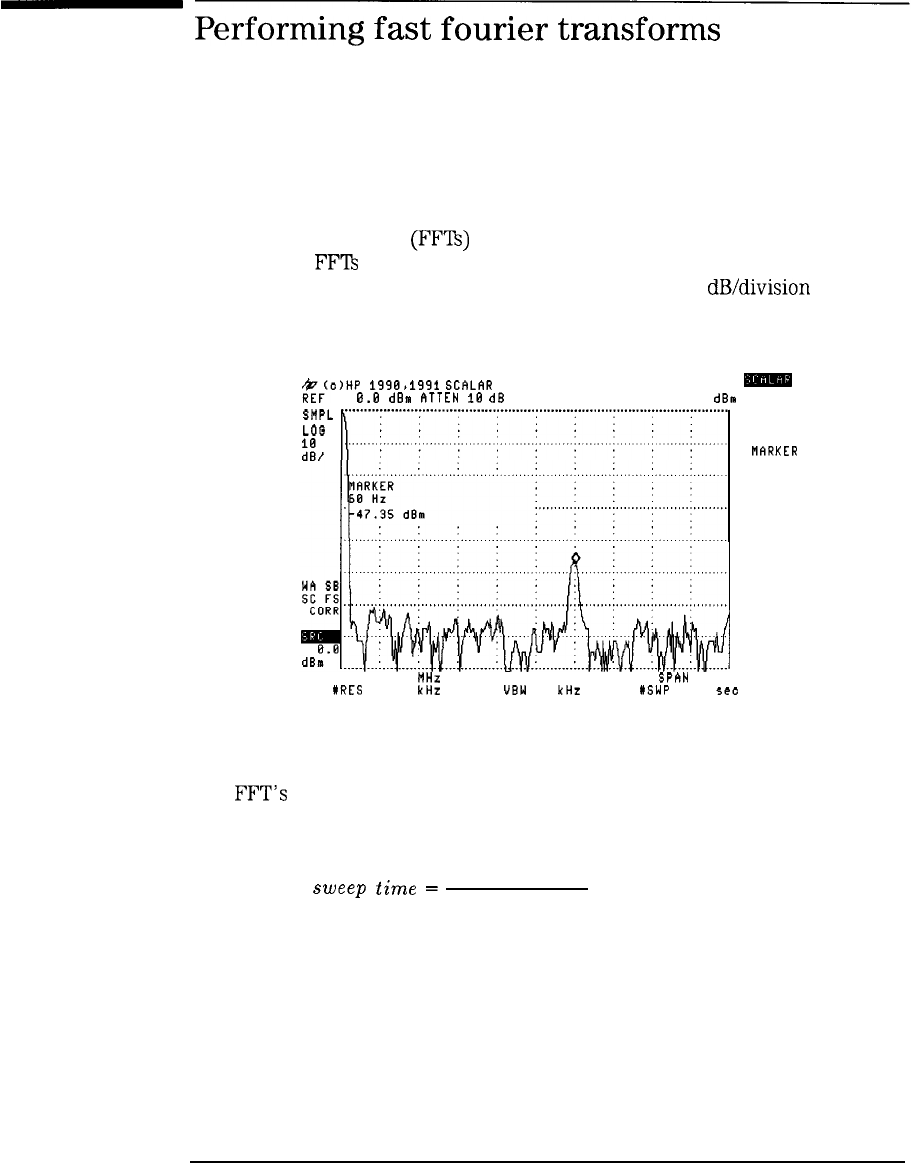
I
-
I
-
Performing
fast
fourier
transforms
Fast fourier transforms
(FFTs)
convert zero-span data into the frequency
domain. Use
FFTs
to observe signal distortion caused by a device. During
an FFT, the scalar analyzer is in single sweep with a 10
dB/division
log
amplitude scale.
&h,HP
1998,199l
SChLAR
ANAL\
8.8 dBn
ATTEN
10
dB
PMPL
LOO
ii/
MKR 60 HZ
m
-47.35 dBn EXIT
FFT
NARKER
DELTA
NEXT
PEAK
NEXT PK
RIGHT
NEXT PK
LEFT
PEAK
EXCURSN
CENTER 49.1094 MHz SPhN 0 Hz
#RES BW 18 kHz UBW 10 kHz lSWP 2.0 5ec
L
Performing an FFT turns on the marker for locating signal peaks on the FFT.
The
FFT’s
frequency span is related to the sweep time. (The slower the
sweep time, the narrower the span.) Set the sweep time according to the
following formula:
200
sweep
time
=
frequency span
4-21
I
-
I
-
Measuring
ReflectionRransmission
Parameters
Performing fast fourier transforms
To
perform
fast
fourier
transforms
1. Press the front-panel [FREQUENCY] key, and enter the frequency at which
to perform the FFT.
2. Press the front-panel (SPAN) key and enter 0 Hz.
3. Press the front-panel
CSWEEP)
key.
4. Enter the sweep time required to achieve the desired FFT frequency span.
200
sweep
time
= frequency span
5.
Press the
(jj)
key and then the More 1 of 2
softkey.
6.
Press the FFT
MEAS
softkey
to display the FFT.
4-22
7.
To exit from the FFT display, press the EXIT FFT
softkey
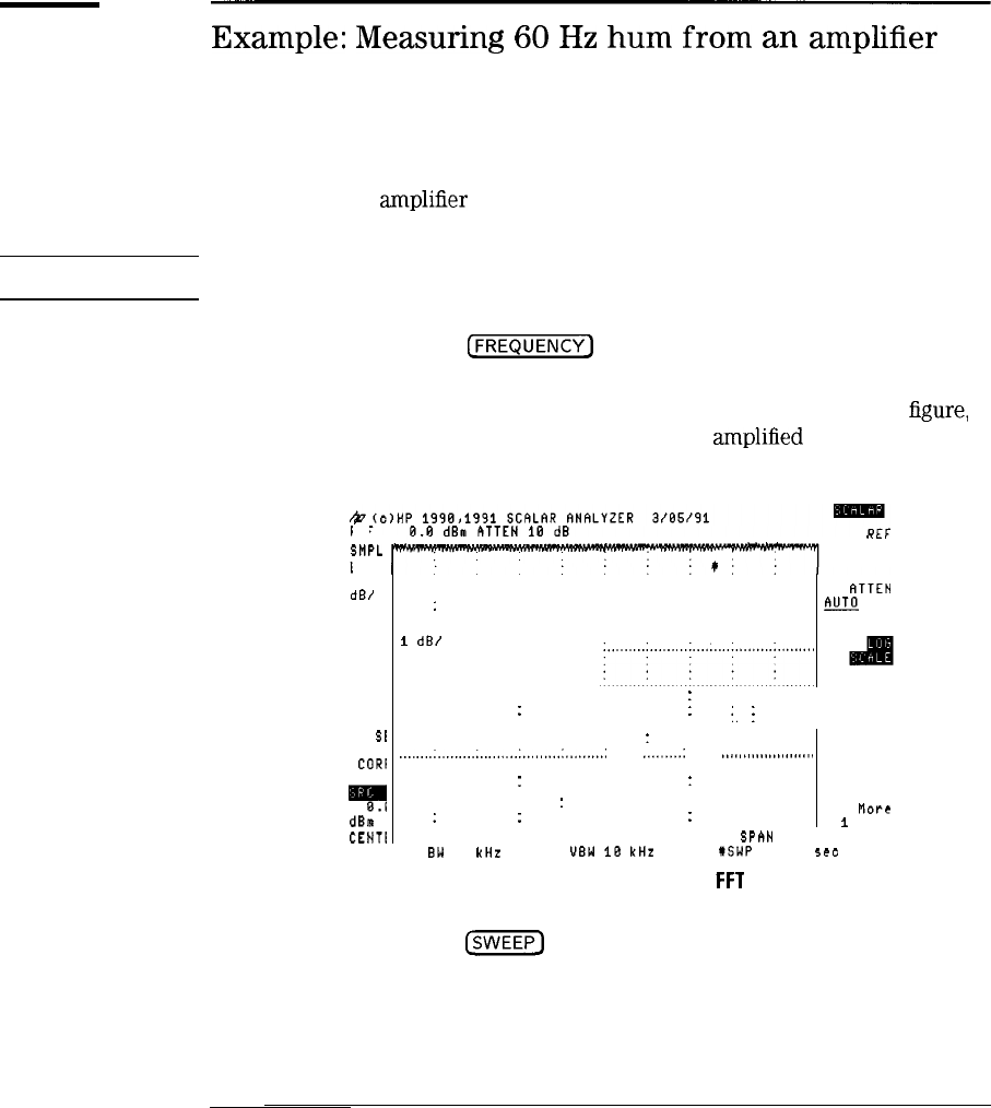
I
-
I
-
Measuring Reflection/Transmission Parameters
Performing fast fourier transforms
Example:
Measuring
60
Hz
hum
from
an
amplifier
One measure of an amplifier’s performance is 60 Hz hum. This measures the
amount of 60 Hz amplitude-modulation distortion placed on the amplified
signal.
1. Connect the
ampliEer
between the scalar analyzer’s front-panel RF OUT
and INPUT connectors.
CAUTION
Make sure the input power level is not above the spectrum analyzer’s
maximum input value.
2. Press the front-panel
CFREQUENCY]
key, and enter the frequency at which
to perform the FFT.
3. Press the front-panel [SPAN) key and enter 0 Hz. In the following
figure,
the amplitude modulation can be seen on the
ampliEed
signal.
REF
SMPL
LOG
1
dB/
.~_I
LEVEL
ATTEN
:
m
MAN
. . . . . . . . . . . . . . . . . . . . . . . . . . . . . . . . ...'
LOG :
1
dB/
WA
$1
SC F!
CORI
T#
dBm'
CENTI
I
:
AUTO
::
i.
I
SCALE
:
,,,,,,,,,,,,,,,,,,,,,,,,,,,,,,,,,,,,,,,,,,.,.,,,;
,...,....:
..I.................~.
NORM REF
POSN
::
. . . . .
:
:
;:
Mb?@
1
of 2
49.1084 MHz SPhN 0 Hz
ES
BW
18 kHz UBW 18 kHz
I~SWP
2.0 set RT
Zero-span response before
FFT
4. Press the front-panel
C-1
key.
5. Enter a sweep time of 2.0 seconds.
A 2.0 second sweep time gives an FFT frequency span of 100 Hz
4-23
I-
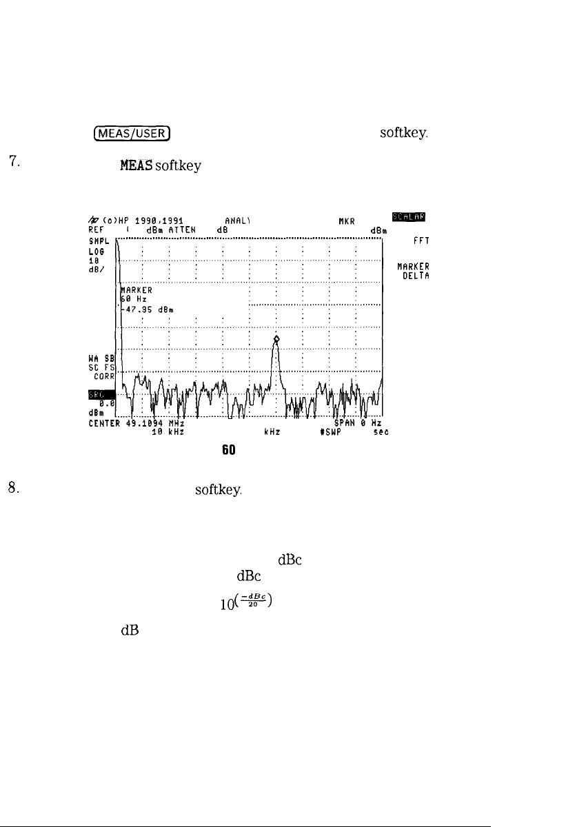
I
-
Measuring Reflection/Transmission Parameters
Performing fast fourier transforms
6. Press the
[MEAS/USER)
key and then the More 1 of 2
softkey.
7.
Press the FFT
MRAS
softkey
to display the FFT.
c$7;o,HP
1990>1991
SCALAR ANAL\
0.0 dBa
ATTEN
10 dB mKR 60 Hz
w
-47.35 dBa EXIT
FFT
mARKER
OELTh
NEXT
PEAK
XRES BW
10
kHi!
VBW 10 kHz #SWP 2.0 5ec
NEXT PK
RIGHT
NEXT PK
LEFT
PEAK
EXCURSN
FFT showing
60
Hz amplitude modulation
8.
Press the MARKER DELTA
softkey.
9. Use the front-panel knob to scroll the marker to the 60 Hz peak.
10. Read the marker value, and determine the percent of amplitude
modulation by substituting the value as
dBc
in the following formula.
(Notice the minus sign indicating
dBc
is a negative value.)
Percent AM = (200)
lo(*)
For example, if 60
dB
separates the 60 Hz modulation from the carrier, the
percent of amplitude modulation is 0.2 %
4-24
I
-
I
-
Measuring Reflection/Transmission Parameters
Making swept-power measurements
To
perform
swept-power
measurements
1. Connect the source’s output to the scalar analyzer’s input.
2. Set the scalar analyzer to the desired center frequency. Set the
spanwidth to 0 Hz.
3. Press the
(AUX)
key, then enter the source’s power.
This is the sweep’s start power.
4. Press the
PWR
SWP
ON
OFF
softkey
twice so that ON is underlined.
5. Enter the amount of power change in
dB
of the power sweep. (Press the
CENTER)
key to complete the entry.)
6. Set the reference level so that when the device to be tested is inserted in
the line, any gain will not cause the response to be off screen.
7.
Press the (CAL) key, CAL
THRU
, and STORE THRU softkeys.
8. Place the device to be tested between the source’s output and the scalar
analyzer’s input.
9. Press the
[W)
key, and then set the normalized reference level so
that the response is displayed.
10.
Press the AUTO SCALE
softkey.
4-26
I-
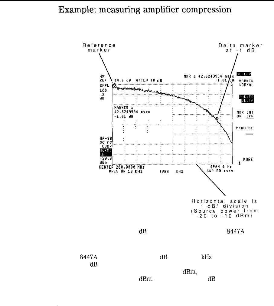
I
-
Measuring Reflection/Transmission Parameters
Making swept-power measurements
Example:
measuring
amplifier
compression
Reference
Delta
marker
marker
at
-1
dB
dB
:
:
:
::
:
CENTER
200.0806
MHz
#RES
BW
18 kHz
lVBW
1 kHz
tlKNOISE
ON OFF
-
MARKERS
OFF
NORE
1
of 2
L
Horizontal
scale
is
1
dB/
dlvlslon
(Source
power
from
-20
to
-10
dBm)
This example measures the 1
dB
compression point of an HP
8447A
Dual
Amplifier. The measurement requires placing the scalar analyzer in a zero
frequency span and sweeping the input power to the amplifier.
The HP
8447A
Dual Amplifier has 20
dB
of gain 100
kHz
to 400 MHz. We’ll
locate its 1
dB
compression point at 200 MHz. Because the amplifier’s output
compression point is typically greater than 6
dBm,
we need to sweep its
output power from 0 to + 10
dBm.
The amplifier’s 20
dB
of gain requires
4-27
-1
Measuring Reflection/Transmission Parameters
Making swept-power measurements
that we sweep its input power from -20 to -10
dBm
to meet our output
requirements.
The example does
not
use the HP
85630A
scalar transmission/reflection test
set. If you use the test set, you’ll need to compensate for the power loss of
the test set.
CAUTION
Be sure that the spectrum analyzer’s input power does not exceed
+30
dBm
or damage will result.
1.
Press the PRESET SCALAR
softkey
in the scalar analyzer’s Main menu.
2. Use a BNC cable to connect the scalar analyzer’s RF OUT and INPUT
connectors.
3. Press the [FREQUENCY) key and enter a center frequency of 200 MHz.
4. Press the
m
key and enter a frequency span of 0 Hz.
The scalar analyzer is now a fixed-tuned receiver at 200 MHz.
5. Press the
[AUX]
key.
6.
Press the TRACKING PEAK
softkey.
7. Enter a source power level of -20
dBm.
This sets the starting power level for the power sweep.
3.
Press the PWR
SUP
ON OFF
softkey
twice so that ON is underlined.
9. Enter 10
dB.
This sets the amount of the power sweep. The scalar analyzer is now
sweeping the source’s output power from -20 to -10
dBm.
10. Press the (AMPLITUDE] key and enter a reference level of 10
dBm.
This step places the stop power level 20
dB
below the displayed
reference level. This is necessary to ensure a calibrated display with
the amplifier’s 20
dB
of gain.
4-28
-1
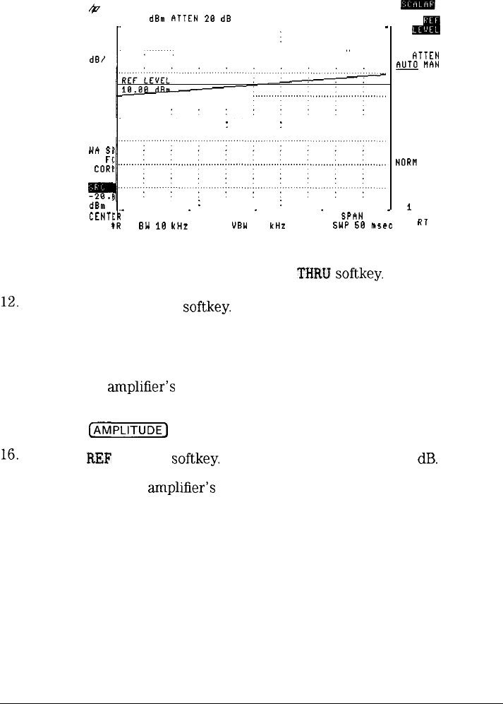
I
-
I
-
&
REF
SMPL
LOG
10
dB/
Nh
Sl
SC
FI
CORI
M
dBn'
CENTI
I
lB.O dBm
ATTEN
28
dB
Measuring Reflection/Transmission Parameters
Making swept-power measurements
:
;
,,
:.,
::
::
.
ATTEN
u
MhN
LOG
SCRLE
AUTO
SCRLE
NORFl
REF
POSN
more
1
of 2
::
.
.
.
.
.
200.0000 MHz
SPhN
0 Hz
ES BW
18
kHz
'JEW
10 kHz SWP
58
h5eC
Rl
11. Press the (CAL) key followed by the CAL
TMRU
softkey.
12.
Press the STORE TWRU
softkey.
The scalar analyzer’s display is now normalized for the power sweep.
13. Connect the scalar analyzer’s RF OUT to the amplifier’s INPUT connector,
14. Connect the
ampliEer’s
OUTPUT connector to the scalar analyzer’s
INPUT connector.
15. Press the
(AMPLITUDE)
key.
l6.
Press the
REF
LEVEL
softkey.
Enter a reference level of 20
dB.
This places the
ampliEer’s
response on the screen. However, changing
the reference level introduces error caused by reference level accuracy.
This is indicated on screen by the
? character displayed after the NORM
annotation.
4-29
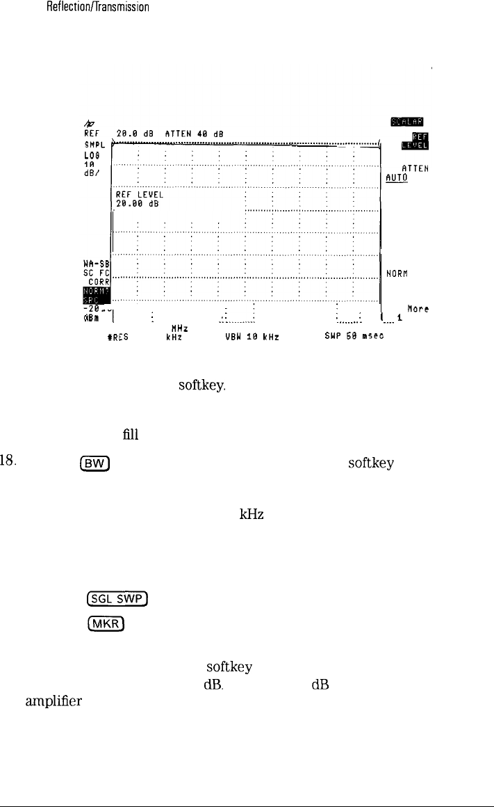
I
-
I
-
Measuring
Reflection~ransmission
Parameters
Making swept-power measurements
ATTEN
m
MAN
LOG
SCALE
AUTO
SCALE
,
CENTER
#RI
‘7
. . . . . . . . .
I
. . . . . . . . . . . . . . . .
.:
i
..__.....: . . . . . . . . . . . . . . . . . . . .
I
..___..
i
. . . . .
.._.
I
200.0000 MHZ SPAN 0
HZ
TS
BW 10 kHz UBW
18
kHz SWP 58
I
se0
NORfl
REF
POSN
flare
1
of 2
RT
17. Press the AUTO SCALE
softkey.
The AUTO SCALE function reduces the scalar analyzer’s log scale as
necessary to
fill
the complete display with the response.
18.
Press the
m
key. Press the VID BW AUTO MAN
softkey
twice so that
MAN is underlined.
19. Reduce the video bandwidth to 1
kHz
Do
not
change the resolution bandwidth or additional measurement
uncertainties will be introduced. Reducing the video bandwidth
reduces the noise displayed on the trace.
20. Press the
(SGLSWP)
key to stop the trace.
21. Press the
INIKR]
key, and use the front-panel knob to place the marker at
the peak of the response.
22. Press the MARKER DELTA
softkey
and move the delta marker on the
response so that it reads -1
dB.
This is the 1
dB
compression point of the
ampliEer at 200 MHz.
4-30
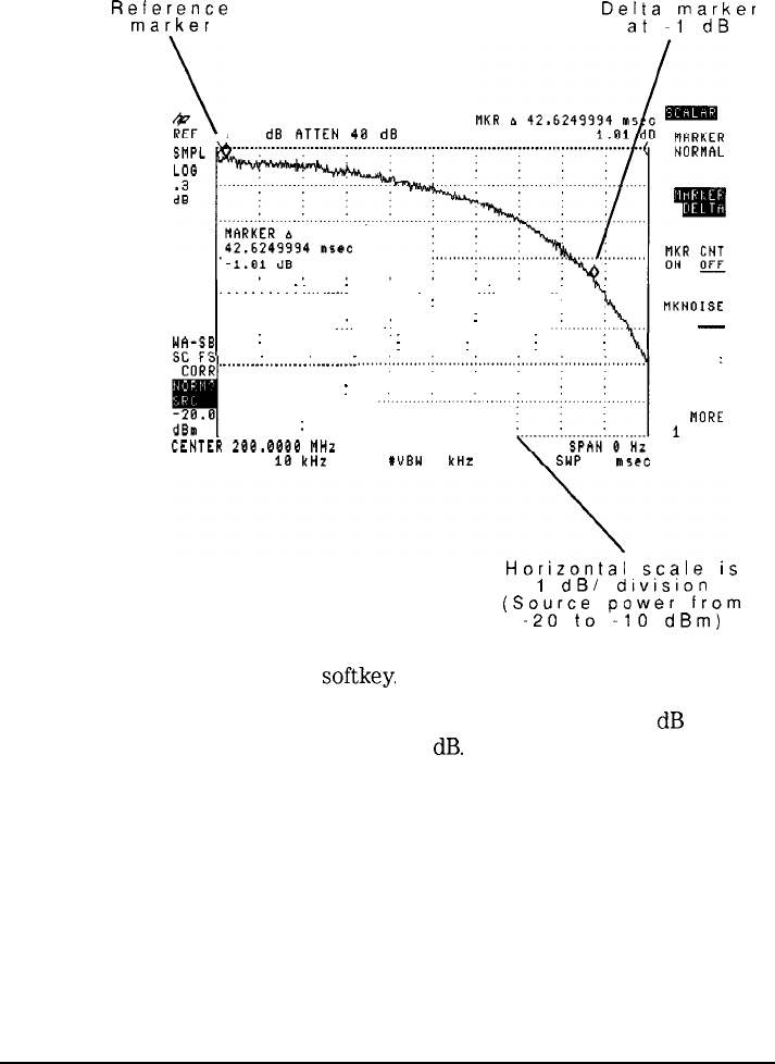
I
-
I
-
Measuring Reflection/Transmission Parameters
Making swept-power measurements
Reference
Delta
marker
marker
at
-1
dB
19.5 dB
ATTEN
48 dB
.
.
.
.
.
.
.
.
.
.
:...
.
.
.
.
.
. .
..I.
:
IKNOISE
..I.
.:
:
ON OFF
-
W*-$B
:
:
;
:
i
j
.
.
.
.
.
.
.
.
.
.
.
.
.
.
.
.
.
.
.
.
.
.
.
.
.
.
.
.
.
.
MARKERS
OFF
:
:
;
i'lORE
. . .
1
of 2
CENTER
20G.0000
MHz
XRES BW 18
kHz #WBW
1 kHz SWP 58
15ec
L
Horizontal
scale
is
1
dB/
dlvislon
(Source
power
from
-20
to -10
dBm)
23. Press the MARKER NORMAL softkey.
The marker readout now indicates the device gain at the 1
dB
compression point. In this case 18.4
dB.
See the Egure at the end of
this procedure.
4-31
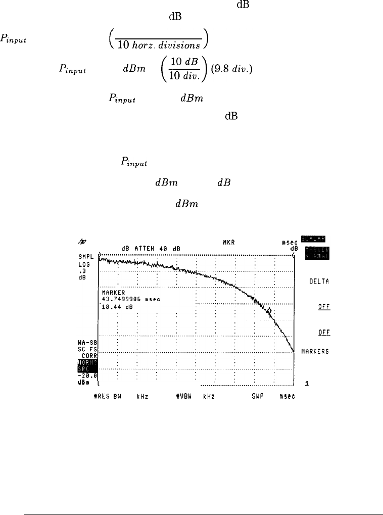
I
-
I
-
Measuring Reflection/Transmission Parameters
Making swept-power measurements
24. Based on the horizontal power scale of 1
dB
per division, calculate the
input power level at the 1
dB
compression point.
Pinput
= start power + power sweep range
1O
horr,
divisions
(number of divisions)
pinput
= -20
dBm
+
Pinput
= -10.2 dBm
25. To calculate the output power at the 1
dB
compression point, add the
input power level determined in the previous step to the gain at the
compression point (marker value).
P
output
=
Pinput
+ compressed gain
P
output
= -10.2
dBm
+ 18.4 dB
P
output
= 8.2 dBm
R
llKR
43.7499986 MS~C
REF 19.5
dB
ATTEN
48
dB
18.44
dB
. . . . . . . . . . . . . . . . . . . . . . . . . . . . . . . . . . . . . . . . . . . . . . . . . . . .
CENTER 200.0000 MHz
#RES
BW
10 kHz #UBW 1 kHz SPAN 0 Hz
SWP 50
15ec
MARKER
DELTA
MKR CNT
ON
m
RKNOISE
ON
@J
MARKER5
OFF
MORE
1
of 2
R
4-32

I
-
5
Using Markers and Limit
Lines

I
-
I
-
Using Markers and Limit Lines
Peak-to-peak markers and delta markers enable you to quickly measure
absolute and relative amplitude and frequencies of a response. Limit lines
enable you to perform repeatable production-line testing.
5-2
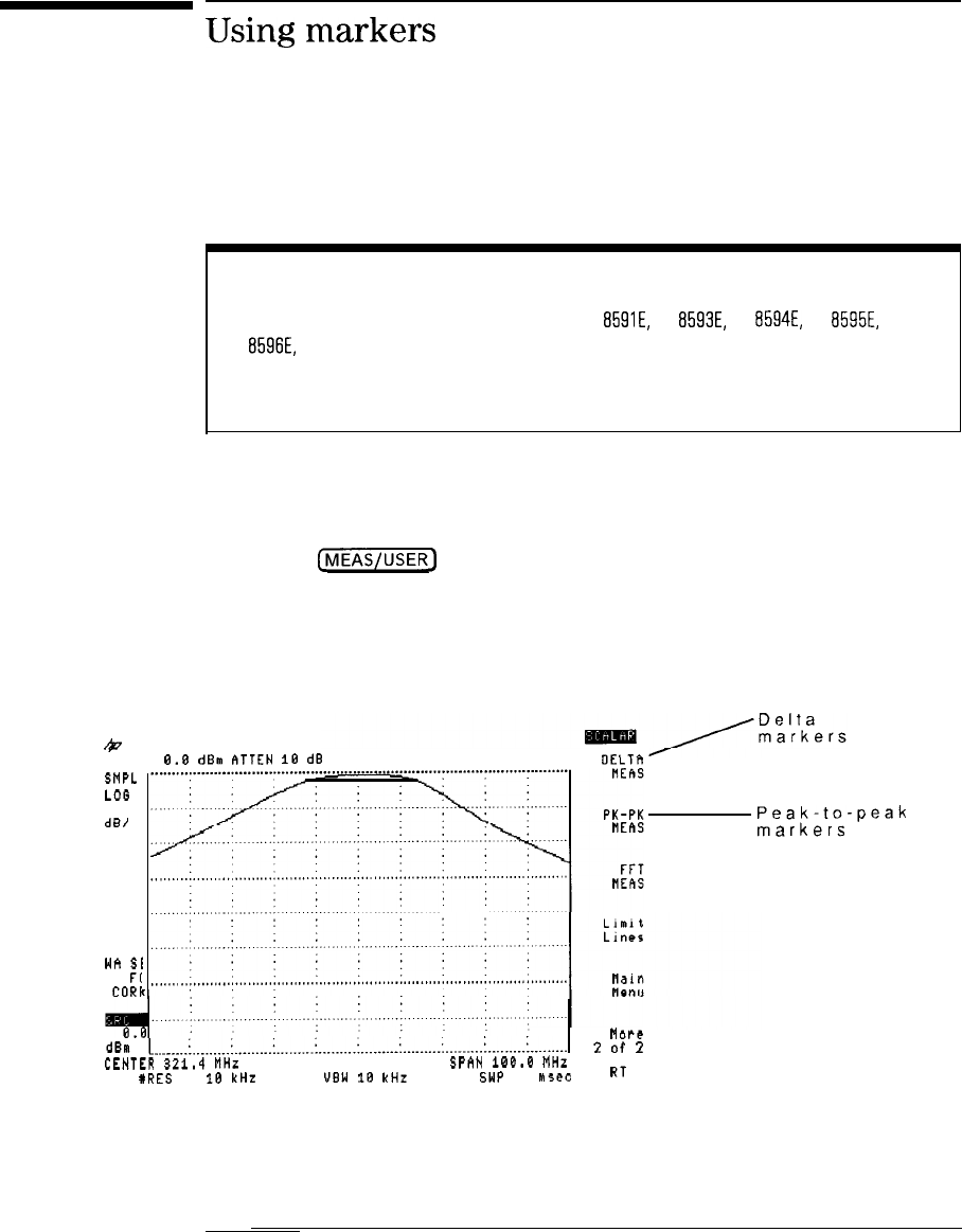
I
-
Using
markers
t
REF
SMPL
LOG
10
dB/
WA
SI
SC
FI
CORl
Multiple Markers and Marker Tables
Multiple markers, which are available with the HP
8591E,
HP
8593E,
HP
8594E,
HP
8595E,
and
HP
8596E,
are not available when in Dual Display Mode.
The MK TABLE function is not available when in the Scalar personality mode.
Enter the second page of the Measure menu to use markers. (Press the
front-panel
c-1
key, or press the Main menu’s Measure softkey.)
B.B
dBm
ATTEN
1B dB
Peak-to-peak
markers
.
.
.
.
.
.
.
..i.........i.........i.........i.....~.........~.........
!bPe
2
of
2
CENTER
32104
MHz
SPAN
10G.G
MHz
#RES
BW
18
kHz UBW
18
kHz
SWP 58
M5eC
RT
Second Page of Measure Menu
5-3
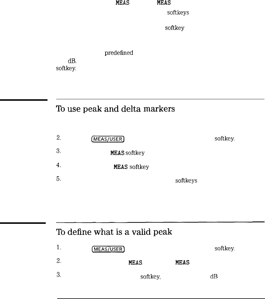
I
-
I
-
Using Markers and Limit Lines
Using markers
After selecting DELTA
MEAS
or PK-PK
MEAS
,
use the NEXT
PEAK ,
NEXT PK RIGHT , and NEXT PK LEFT softkeys to place the displayed
marker on a signal peak. Marker frequency and amplitude are directly read
from the display. The MARKER DELTA softkey displays the relative amplitude
and frequency between two displayed markers.
When searching for a signal peak, the scalar analyzer recognizes signals that
rise and fall by a predehned excursion value. This default excursion value
is 6
dB.
You can change the excursion value by using the PEAK EXCURSN
softkey.
To
use
peak
and
delta
markers
1. Display the desired response on the scalar analyzer’s display.
2.
Press the
CMEAS/USER)
key and then the More 1 of 2
softkey.
3.
Press the PK-PK
MEAS
softkey
to perform peak marker measurements.
4.
Press the DELTA
MEAS
softkey
to perform relative marker measurements.
5.
Press the EXIT PK-PK or EXIT DELTA
softkeys
to turn the markers off
and return to the Measure menu.
To
define
what
is
a
valid
peak
1.
Press the
[MEAS~USER)
key and then the More 1 of 2
softkey.
2.
Press either the PK-PK
MEAS
or DELTA
MEAS
softkeys.
3.
Press the PEAK EXCURSN
softkey,
enter the value in
dB
that represents
the smallest acceptable peak excursion.
5-4
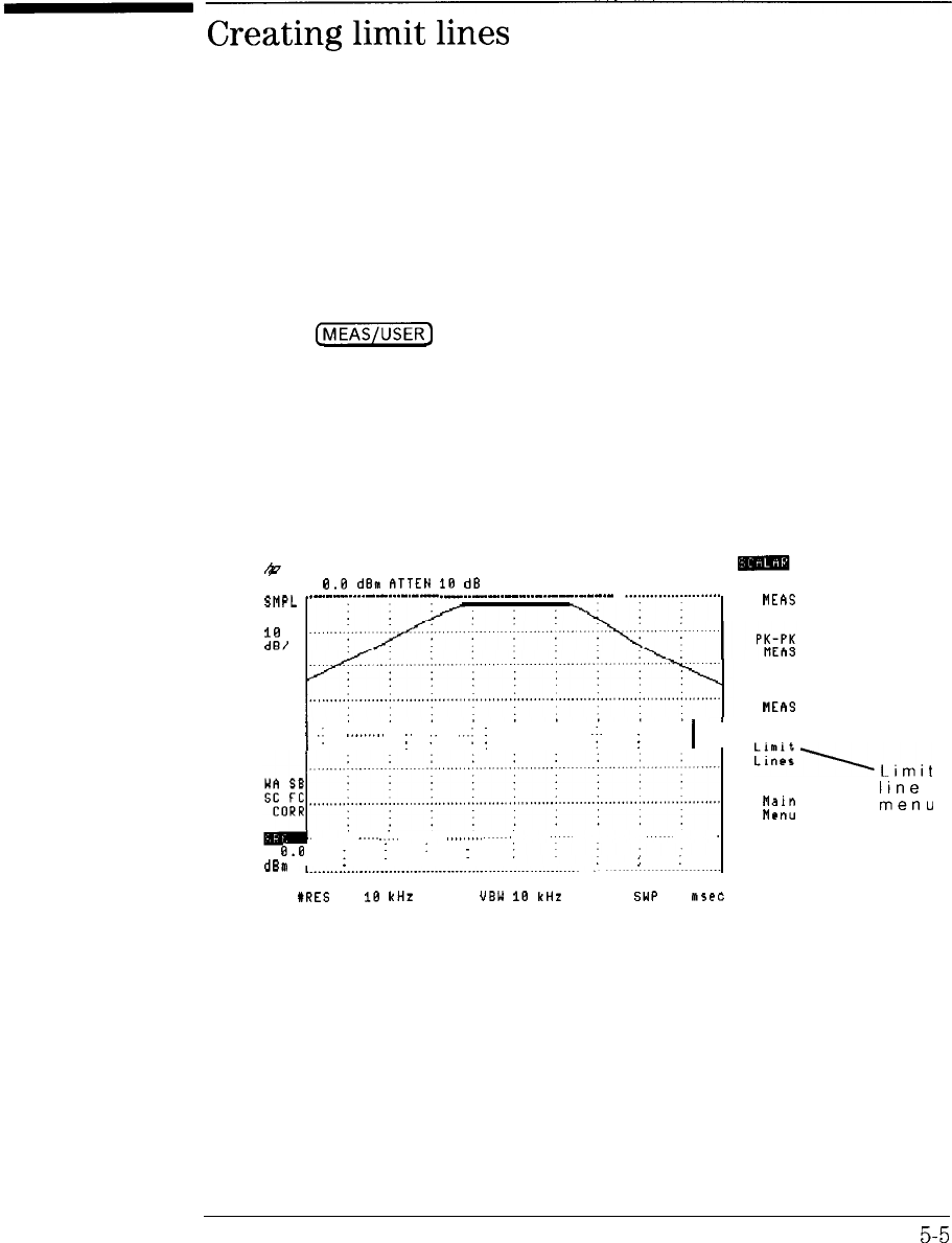
Creating
limit
lines
Limit lines are displayed lines showing acceptable limits for a displayed
response. In production settings, limit lines can be used for pass/fail testing.
Enter the second page of the Measure menu to use limit lines. (Press the
front-panel
C-1
key, or press the Main menu’s Measure softkey.)
You define the shape (including upper and lower limits) of the limit lines. If
the response is outside the limit lines, a failure message is displayed.
k
REF
B.B
dBn
ATTEN
1B dB
SMPL
.
.
.
.
.
.
.
.
.
.
.
.
.
.
.
.
.
.
.
.
.
.
.
.
.
.
.
.
.
.
.
.
.
.
.
.
.
.
.
.
.
.
.
.
.
.
.
.
.
.
.
.
.
.
.
.
.
.
.
.
.
.
.
.
.
.
.
.
.
.
.
.
.
.
.
.
.
LOG
18
dEI
1
.I
.._......
I.
,.
...I
i
. . . . .
.;.
I
1
..I.,
,........
0.B
;
j
:
:
:
dBm
:
CENTER 321.4 MHz SPAN 100.0 MHz
XRES
BW
18
kHz
'JBW
18
kHz
SWP 58
m5ec
Second Page of Measure Menu
DELTA
MERS
FFT
MEAS
:::::\,imit
line
ila1n
menu
Menu
mare
2 of 2
RT
You define the shape (including upper and lower limits) of the limit lines. If
the response is outside the limit lines, a failure message is displayed as shown
in the following figures.
5-5
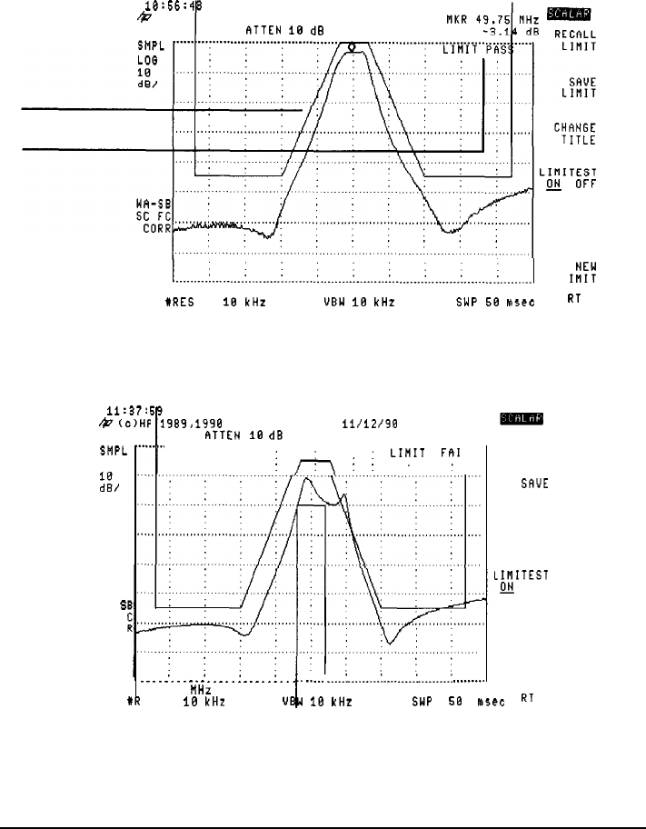
I
-
I
-
Using Markers and Limit Lines
Creating limit lines
limit line
limit pass
message
10:56:4
OEC 25, 1990
/tz
ATTEN
it3
dB
LIMITEST
fi
OFF
EOIT
LIMIT
l.........:.........i.....................~........~........~........~.........:........~.........l
L Ii::
CENTER 50.80 MHz SPAN 50.00 MHz
#RES
BW
18
kHz
UBW 18 kHZ
SWP
58
M5eC
RT
limit line with LIMIT PASS message
ii:37:
&(c)HF
SHPL
LOG
ii,
WA
s
SC F
COR
CENT
ER
XR
OEC 06. 1990
.989,1990 SCALAR ANALYZER
11/12/98
RTTEN
IO dB
I.. . . . . . . . . . . . . . . . . . . . . . . . . . . . . . . . . . . . . . . . . . . . . . . . . . . . . . . . . . . . . . . . . . . . . . . . . . . . . . . . . . . . . . .
i
+,
i
j
LIrIT
F;I
I
NEW
LIMIT
.
.
.
.
.
.
.
.
.
.
.
.
.
.
.
.
.
.
.
.
.
.
.
.
.
.
..
..___
_____:
____..._.:
.
.
.._____.
_________:
________.
50.00 MHz
1
I SPAN 50.00 MHz
ES BW 18 kHz
UB 18
kHz SWP
5B
MS~C
RT
limit line with LIMIT FAIL message
RECALL
LIMIT
SAVE
LIMIT
CHANGE
TITLE
.INITEST
fi
OFF
EOIT
LIMIT
5-6
Using Markers and Limit Lines
Creating limit lines
You can create Iimit lines that:
1. Define the upper limit of a response.
2. Define the lower limit of a response.
3. Define both lower and upper response limits.
4. Display relative to the center frequency and reference level.
5. Display at a fixed center frequency and reference level.
You create limit lines that are either fixed or relative with respect to the
scalar analyzer’s frequency and reference level. After being displayed,
relative limit lines do not change screen position if the frequency or reference
level is changed. However, fixed limit lines do change screen position if the
frequency or reference level is changed.
The two tutorials, located at the end of this, chapter give step-by-step
instructions for creating limit lines. Be prepared to spend about twenty
minutes on the tutorials. Both tutorials draw the same limit lines using two
alternate methods.
limit-line amplitude units
After display normalization, the amplitude units displayed for limit lines and entered using the front
panel are in
dEIm
(decibels relative to 1
mW1.
However, because of display normalization, the units
actually used are decibels
Idt3).
The power levels are relative to the normalized reference level.
limit lines and the normalized reference position
When editing or creating limit lines (the EDIT LIMIT or
NEX
LIMIT
softkey
is pressed),
the scalar measurements personality sets the normalized reference position to eight. This is the default
normalized reference position at the top of the screen. The original position is restored when the
EDIT DONE
softkey
is pressed.
5-7
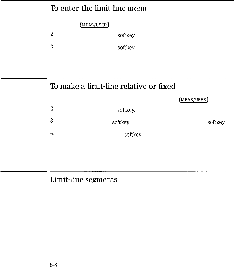
I
-
I
-
Using Markers and Limit Lines
Creating limit lines
To
enter
the
limit
line
menu
1. Press the
fjj]
key.
2.
Press the More 1 of 2
softkey.
3.
Press the Limit; Lines
softkey.
To
make
a
limit-line
relative
or
fixed
1. With a limit line displayed on the screen, press the
CMEAS/USER)
key.
2.
Press the More 1 of 2
softkey.
3.
Press the Limit Lines
softkey
followed by the EDIT LIMIT
softkey.
4.
Press the LIMITS FIX REL
softkey
so that desired selection is
underlined.
Limit-line
segments
Limit lines are made by “drawing” lines between frequency/amplitude points.
Each line is called a segment. Segments begin at a starting frequency and
continue to the next segment.
Segments can be one of three types: SLOPE, FLAT, or POINT. With slope
types, segments with different amplitudes are connected using sloping lines.
With Flat types, segments remain constant in amplitude until the next
segment’s starting frequency is reached. With point types, a segment’s
starting frequency is not connected to the next segment.
5-a
I
-
Using Markers and Limit Lines
Creating limit lines
The following figures illustrate the difference between the three slope types.
The limit lines in each figure are identical except for the segment’s type.
ii:39:5
DEC
06,
1990
b
(c)HP SCALAR ANALYZER
llCl2/90
ATTEN
10
dB
I
SELECT
SEGMENT
SELECT
FRED
SELECT
MID RMPL
SELECT
OLT
AMPL
SELECT
TYPE
MORE
SMPL
LOG
ZL
WA
3
SC
F
COR
B'
,;.
CENT
xii
XR
:
1
of 2
RT
:
50.00 NHz
'ES BW IE kNz
__........._...............................
I
SPAN 50.00 MHz
IHZ
SWP
58
R5eC
SLOPE Segment Types
13:55:54
DEC
06,
1990
~$7
(c)HP 1989,1990 SCALAR ANALYZER 11/12/98
ATTEN
18
dB
RECALL
LIMIT
SAVE
LIMIT
CHANGE
TITLE
LIIIITEST
m
OFF
EDIT
LIMIT
NEW
LIMIT
CENTEl(.5i..~i..iHr
I
XRES
iW
18
kHz
..:
. . . . . . . . . .
i
I
I
SPAN 30.00 MHz
Hz
SWP
58
m5e.c
RI
FLAT Segment Types
5-9
I
-
I
-
Using Markers and Limit Lines
Creating limit lines
i4:0
:33
DEC 06,
II
k
Cc
HP 1989,1990 S
B I
SMPL
. . . . . . . . . . . . . . . . . . . . . . . . . . . . . . . . . . . . . . . . . . . . . . . . . . . . . . . . . . . . . . . . . . . . . . . . . . .
LIMI.
PRSS
LOG
RECALL
LIMIT
SAVE
LIMIT
CHANGE
TITLE
LIllITEST
fi
OFF
EDIT
LIMIT
I
:
:
. NEW
LIMIT
CENTER 50.00 MHz SPAN 30.00 MHz
URES
BW 10 kHz SWP 50
lh5eo
RT
POINT Segment Types
To
enter
or
edit
a
limit-line’s
title
1. If you are creating or editing a limit line, press the EDIT DONE
softkey
after all data has been entered.
2. In the Limit Line menu, press the CHANGE TITLE
softkey.
3. Use the front-panel
softkeys
to select the desired characters.
You can also press the
MORE
1 af 2 then RPG TITLE
softkeys
and
use the front-panel knob to select the desired characters.
4. Press the front-panel
cm)
key to backspace over a character.
5.
To erase a title, press the
YX,#
SPC CLEAR
softkey
and then the CLEAR
softkey.
5-10
-1

I
-
I
-
Using Markers and Limit Lines
Creating limit lines
To
turn
limit
testing
on
In order to turn limit testing on, you must first create a limit line.
1. Create a limit line.
2. Press the limit-line menu’s LIMITEST ON OFF
softkey
so that ON is
underlined.
I
-
Saving
and
recalling
limit
lines
Limit lines can be saved and recalled for later use. (Presetting or turning the
scalar measurements personality off will not effect the limit line data.)
CAUTION
Limit line data is saved in trace memory registers. Use caution to avoid
deleting any previously saved traces.
Each limit line requires one trace memory register and is saved starting at
trace register 0. Limit line 0 corresponds to trace memory registers 0. As
more limit lines are saved, limit line memory grows towards trace memory
register 5 1.
Catalog trace memory if you need to determine availability and use of trace
registers.
Calibration data
Calibrations are also saved in trace memory starting at memory register 51 and growing towards
register 0. As the number of saved calibrations and limit lines grows, the possibility of overwriting
memory increases.
5-12
I
-
I
-
Using Markers and Limit tines
Saving and recalling limit lines
To
catalog
trace
memory
1. Press the
[RECALL)
key.
2.
Press the INTRNL CRD
softkey
so that INTRNL is underlined.
3.
Press the CATALOG INTRNL softkey.
4.
Press the CATALOG REGISTER
softkey.
5. Use the front-panel knob to scroll the display of trace memory.
To
save
a
limit
line
1. Create a limit line.
2. Press the limit-line menu’s SAVE LIMIT
softkey.
3. Press a number representing a memory register.
4. Press the (Z?FK] key.
To
recall
a
limit
line
1. Press the limit-line menu’s RECALL LIMIT
softkey.
2. Press a number representing a memory register between 0 and 51.
3. Press the
CENTER]
key.
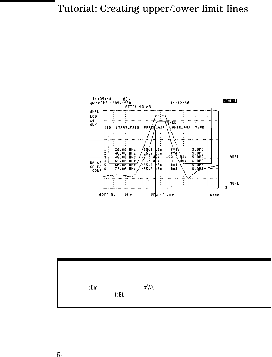
I
-
Tutorial:
Creating
upper/lower
limit
lines
This procedure should take you about 10 minutes to complete. It shows the
basics of creating limit lines.
11:39:1
DEC
06,
1990
b
(c)HP SCALAR ANALYZER
11/12/9B
f?TTEN
18
dB
I
SELECT
SEGMENT
CENTER 50.00 MHz
#RES
8W 10 kHz
.
.
.
SPAN 50.00 MHz
kHz SUP 50
!a5ec
SELECT
FREQ
SELECT
UPR AMPL
SELECT
LWR
~IMPL
SELECT
TYPE
NORE
1
of 2
RT
Upper/lower limit lines
The following procedure guides you through the task of creating a limit
line centered at 50 MHz. The limit line contains both upper and lower
limits. Limit lines are divided into segments, with each segment defining an
amplitude limit for a range of frequencies.
5-
14
limit-line amplitude units
After display normalization, the amplitude units displayed for limit lines and entered using the front
panel are in
dBm
(decibels relative to 1
mW1.
However, because of display normalization, the units
actually used are decibels
IdfN.
The power levels are relative to the normalized reference level.
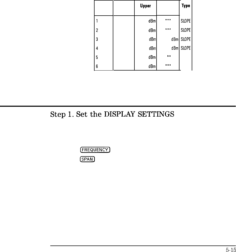
I
-
I
-
Using Markers and Limit tines
Tutorial: Creating upper/lower limit lines
The data entered to create the limit line is shown in the following table.
Upper/Lower limit line Example Data
Segment
Start
Upper
Frequency
Amplitude
28.00 MHz -55.0 dBm
40.00 MHz -55.0 dBm
48.00 MHz -5.0 dBm
52.00 MHz -5.0 dBm
60.00 MHz -55.0
dBm
72.00 MHz -55.0
dBm
lower
Amplitude
*a*
I(“”
-20.0
dBm
-20.0 dBm
l
“”
**(I
Type
SLOPE
SLOPE
SLOPE
SLOPE
SLOPE
SLOPE
Step
1.
Set
the
DISPLAY
SETTINGS
When creating a limit line it is convenient to view the limit lines as you
create them. Set the frequency and span so that the desired frequency range
is viewed.
1. Press the
CFREQUENCY)
key and enter 50 MHz.
2. Press the
m
key and enter 50 MHz.
5-15
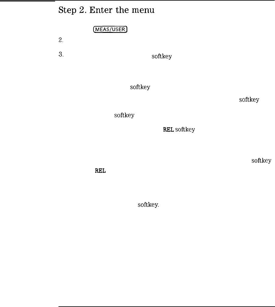
I
-
Using Markers and Limit Lines
Tutorial: Creating upper/lower limit lines
Step
2.
Enter
the
menu
1. Press the
(j-1
key.
2.
Press the More 1 of 2 then Limit Lines softkeys.
3.
Press the LIMITEST ON OFF
softkey
so that ON is underlined.
Turning limitest on allows you to view the limit lines as you create
them.
4. Press the NEW LIMIT
softkey
twice.
Any previously entered limit line data is lost. Pressing the
softkey
twice prevents accidental erasure. Data previously saved using the
SAVE LIMIT
softkey
is not erased.
You’ll notice the LIMITS FIX
REL
softkey
has FIX underlined.
This indicates that the limit lines are fixed with respect to the center
frequency and span. (This means you can change the center frequency
such that the limit lines is no longer displayed.) If you want the limit
line to track the center frequency, press the LIMITS FIX REL
softkey
so that
REL
is underlined.
When NEW LIMIT is pressed, the normalized reference position is
automatically set to 8.
5. Press the EDIT UP/LOW
softkey.
5-16
I
-
Using Markers and Limit Lines
Tutorial: Creating upper/lower limit lines
Step
3.
Enter
the
first
segment
A total of five segments will be used to define the limit line. This step enters
the starting frequency for the first limit-line segment.
1.
Press the SELECT SEGMENT
softkey.
2. Enter 1 to select the first segment.
3. Press SELECT FREQ and enter 30 MHz.
4.
Press SELECT UPR AMPL and enter -55
dBm.
Step
4.
Enter
the
second
segment
1.
Press the SELECT SEGMENT softkey.
2. Enter 2 to select the second segment.
3.
Press SELECT FREQ and enter 40 MHz.
4.
Press SELECT UPR AMPL and enter -50
dBm.
5-17
-
I
-
I
-
Using
Markers and Limit Lines
Tutorial: Creating upper/lower limit lines
Step
5.
Enter
the
third
segment
1.
Press the SELECT SEGMENT
softkey.
2. Enter 3 to select the third segment.
3. Press SELECT FREQ and enter 48 MHz.
4.
Press SELECT
UPR
AMPL and enter -5
dB.
5.
Press SELECT
LWR
AMPL and enter -20
dBm.
Step
6.
Enter
the
fourth
segment
1.
Press the SELECT SEGMENT
softkey.
2. Enter 4 to select the fourth segment.
3. Press SELECT FREQ and enter 52 MHz.
4.
Press SELECT UPR AMPL and enter -5
dBm.
5.
Press SELECT LWR AMPL and enter -20
dB.
Step
7.
Enter
the
fifth
segment
1.
Press the SELECT SEGMENT
softkey.
2. Enter 5 to select the fifth segment.
3. Press SELECT FREQ and enter 60 MHz.
4.
Press SELECT UPR AMPL and enter -50
dBm.
5-18
I
-
I
-
Using Markers and Limit Lines
Tutorial: Creating upper/lower limit lines
Step
8.
Enter
the
sixth
segment
1.
Press the SELECT SEGMENT
softkey.
2. Enter 6 to select the sixth segment.
3.
Press SELECT FREQ and enter 70 MHz.
4.
Press SELECT
UPR
AMPL and enter -50
dBm.
Step
9.
Exjt
and
save
the
limit
lines
1.
Press the More
i
of 2
softkey
2.
Press the EDIT DONE
softkey.
When you leave the limit line editing menu, limit line testing is
automatically turned off and the limit lines are not longer displayed on
the screen. The limit line data is now stored in
volatile
RAMmemmy.
3.
Press the SAVE LIMIT
softkey.
You must save the limit line data in
non-volatile
RAM to protect loss
from an instrument preset, power disruption, or creating another limit
line.
4. Press 1 and the
@?i@
key to select memory register 2.
5. Press the
[ENTER]
key.
5-19
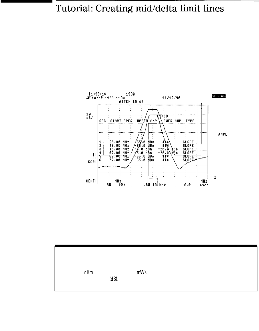
I
-
Tutorial:
Creating
mid/delta
limit
lines
This procedure should take you about 10 minutes to complete. It shows the
basics of creating limit lines.
11:39:1
DEC 06, 1990
&
(c)HP
P1989,199&i
SCALAR ANALYZER
11/12/9!3
I
-
I
ATTEN
1G
dtl
I
SMPL
LOG
18
dB/
WA
SI
SC
FI
CORI
CENTI
. . . . . . . . . . . . . . . . . . . . . . . . . . . . .
50.00 MHz SPAN 50.00 MHz
'ES
BW
10 kHz SWP 50 MSeE
Mid/Delta limit lines
SELECT
SEGMENT
SELECT
FREQ
SELECT
UPR
AtlPL
SELECT
LWR AMPL
SELECT
TYPE
MORE
i
of 2
RT
The following procedure guides you through the task of creating a limit
line centered at 50 MHz. The limit line contains both upper and lower
limits. Limit lines are divided into segments, with each segment defining an
amplitude limit for a range of frequencies.
Limit-line amplitude units
After display normalization, the amplitude units displayed for limit lines and entered using the front
panel are in
dHm
(decibels relative to 1
mW).
However, because of display normalization, the units
actually used are decibels
idHI.
The power levels are relative to the normalized reference level.
5-20
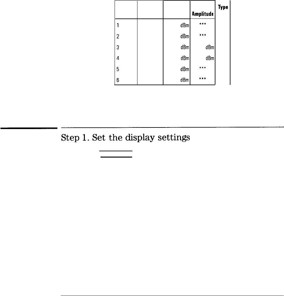
I
-
I
-
Using Markers and Limit Lines
Tutorial: Creating mid/delta limit lines
The data entered to create the limit line is shown in the following table.
Mid/Delta limit line Example Data
Segment
Start
Frequency
28.00 MHz
40.00 MHz
48.00 MHz
52.00 MHz
60.00 MHz
72.00 MHz
Middle
Amplitude
-55.0 dBm
-55.0 dBm
-12.5 dBm
-12.5 dBm
-55.0 dBm
-55.0 dBm
Delta
Rmplitude
“f”
x*x
-7.5 dBm
-7.5 dBm
XXI
XX”
Type
SLOPE
SLOPE
SLOPE
SLOPE
SLOPE
SLOPE
Step
1.
Set
the
display
settings
1. Press the [FREQUENCY) key and enter 50 MHz.
2. Press the (SPAN) key and enter 50 MHz.
When creating a limit line it is convenient to view the limit lines as you
create them. These steps set the frequency and span so that the desired
frequency range is viewed.
5-21
I
-
Using Markers and Limit tines
Tutorial: Creating mid/delta limit lines
Step
2.
Enter
the
menu
1. Press the
(-1
key.
2.
Press the More
1
of 2 then Limit Lines softkeys.
3.
Press the LIMITEST
OM
OFF
softkey
so that ON is underlined.
Turning limitest on allows you to view the limit lines as you create
them.
4. Press the NEW LIMIT
softkey
twice.
Any previously entered limit line data is lost. Pressing the
softkey
twice prevents accidental erasure. Data previously saved using the
SAVE LIMIT
softkey
is not erased.
You’ll notice the LIMITS FIX REL
softkey
has FIX underlined.
This indicates that the limit lines are fixed with respect to the center
frequency and span. (This means you can change the center frequency
such that the limit lines is no longer displayed.) If you want the limit
line to track the center frequency, press the LIMITS FIX REL
softkey
so that REL is underlined.
When NEW LIMIT is pressed, the normalized reference position is
automatically set to 8.
5. Press the EDIT UP/LOW
softkey.
5-22
I
-
I
-
Using Markers and Limit Lines
Tutorial: Creating mid/delta limit lines
Step
3.
Enter
first
segment
A total of five segments will be used to define the limit line. This step enters
the starting frequency for the first limit-line segment.
1. Press the SELECT SEGMENT
softkey.
2. Enter 1 to select the first segment.
3. Press SELECT FREQ and enter 30 MHz.
4.
Press SELECT MID AMPL and enter -50
dBm.
Step
4.
Enter
the
second
segment
1.
Press the SELECT SEGMENT softkey.
2. Enter 2 to select the second segment.
3. Press SELECT FREQ and enter 40 MHz.
4.
Press SELECT MID AMPL and enter -50
dBm.
5-23
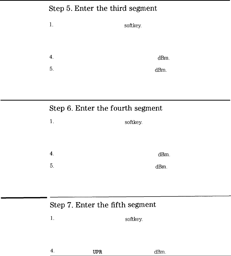
I
-
I
-
Using Markers and Limit tines
Tutorial: Creating mid/delta limit lines
Step
5.
Enter
the
third
segment
1.
Press the SELECT SEGMENT
softkey.
2. Enter 3 to select the third segment.
3. Press SELECT FREQ and enter 48 MHz.
4.
Press SELECT MID AMPL and enter -12.5
dBm.
5.
Press SELECT DLT AMPL and enter -7.5
dBm.
Step
6.
Enter
the
fourth
segment
1.
Press the SELECT SEGMENT
softkey.
2. Enter 4 to select the fourth segment.
3. Press SELECT FREQ and enter 52 MHz.
4.
Press SELECT MID AMPL and enter -12.5
dBm.
5.
Press SELECT DLT AMPL and enter -7.5
dBm.
Step
7.
Enter
the
fifth
segment
1.
Press the SELECT SEGMENT
softkey.
2. Enter 5 to select the fifth segment.
3. Press SELECT FREQ and enter 60 MHz.
4.
Press SELECT
UFR
AMPL and enter -50
dBm.
5-24
I
-
I
-
Using Markers and Limit tines
Tutorial: Creating mid/delta limit lines
Step
8.
Enter
the
sixth
segment
1.
Press the SELECT SEGMENT
softkey.
2. Enter 6 to select the sixth segment.
3. Press SELECT FREQ and enter 70 MHz.
4.
Press SELECT UPR AMPL and enter -50
dBm.
Step
9.
Exit
and
save
the
limit
lines
1.
Press the More 1 of 2
softkey.
2.
Press the EDIT DONE
softkey.
When you leave the limit line editing menu, limit line testing is
automatically turned off and the limit lines are no longer displayed on
the screen. The limit line data is now stored in
volatile RAM
memxxy.
3.
Press the SAVE LIMIT
softkey.
You must save the limit line data in
non-volatile
RAM to protect loss
from an instrument preset, power disruption, or creating another limit
line.
4. Press 2 and the
Cm)
key to select memory register 2.
5. Press the
(ENTER)
key.
5-25

I
-
6
Displaying Results in a
7hble

I
-
I
-
Displaying Results in a
Yhble
The scalar measurement personality’s
Tabular
Display feature displays
transmission and reflection results in a table. The displayed results consist of
the values of each of the 401 trace measurement points. The table can then
be printed on a Hewlett-Packard printer. A compress feature is available for
reducing the number of table entries.
6-2
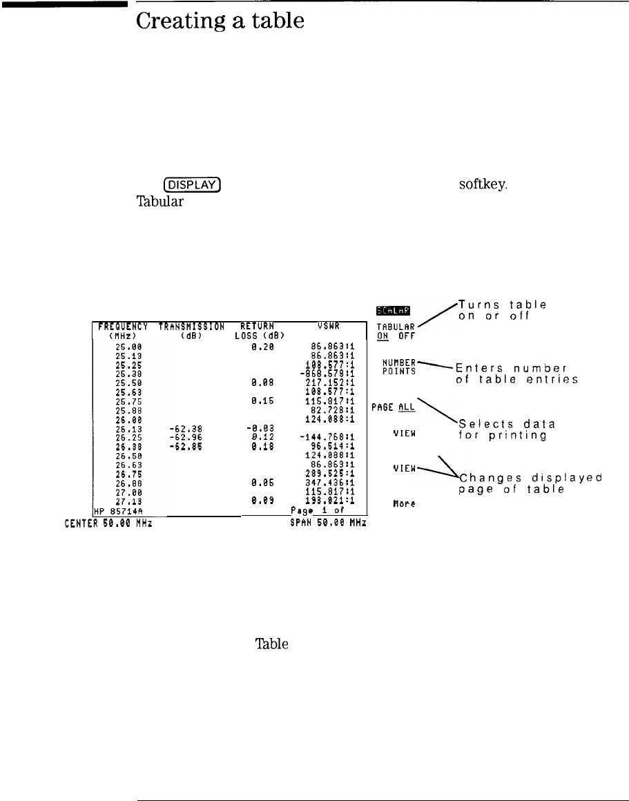
I
-
Creating
a
table
Tabular Display is located in the Display menu, and is reached by pressing
the
@iSFiX]
key and then the Tabular Display
softkey.
When turned on,
Tabular
Display places the scalar measurements personality in single-sweep
mode.
FREQUENCY
TRANSMISSION
RETURN
USWR
(ilHz) (dB)
LOSS
(CIB)
CENTER
50.00
MHz
-62.49
-62.49
-62.64
-62.62
-62.66
-62.63
-63.14
-62.93
-62.64
I;;*;;
-62185
-62.89
-62.96
-63.14
-62.78
-62.54
-62.87
e.2e 86.863:I
0.20
86.863:I
0.16
10s.577:1
-0.02
-868.578:1
0.08
217.152:1
0.16
108.577:1
0.15
115.817:1
0.21
82.728:I
0.14
124.088~1
-K
0:18 -579.086:1
144.768:I
96.514:l
0.14
124.088:1
0.28
86.863:l
0.06
289.525:i
0.85
347.436:1
0.15
115.317:1
8.89
193.021:1
Pa3e
I
of
23
SPhN
50,00
MHz
Turns
table
on
or
off
@j
OFF
TI%
-
Enters
number
of
table
entries
PRINT
PhGE
G
\
Selects
data
VIEW
NEXT PG \
for
printing
VIEW
PREV PG
-4
hanges
display
page
of
table
flare
I of 2
RT
Page one of Tabular Display menu
ed
Results are displayed only for normalized transmission and return loss
(reflection) responses. The scalar measurements personality’s dual display
feature must be turned on in order to fill the table with both transmission and
return loss results.
Table
entries are listed as UNCAL if a calibration has not
been performed.
6-3
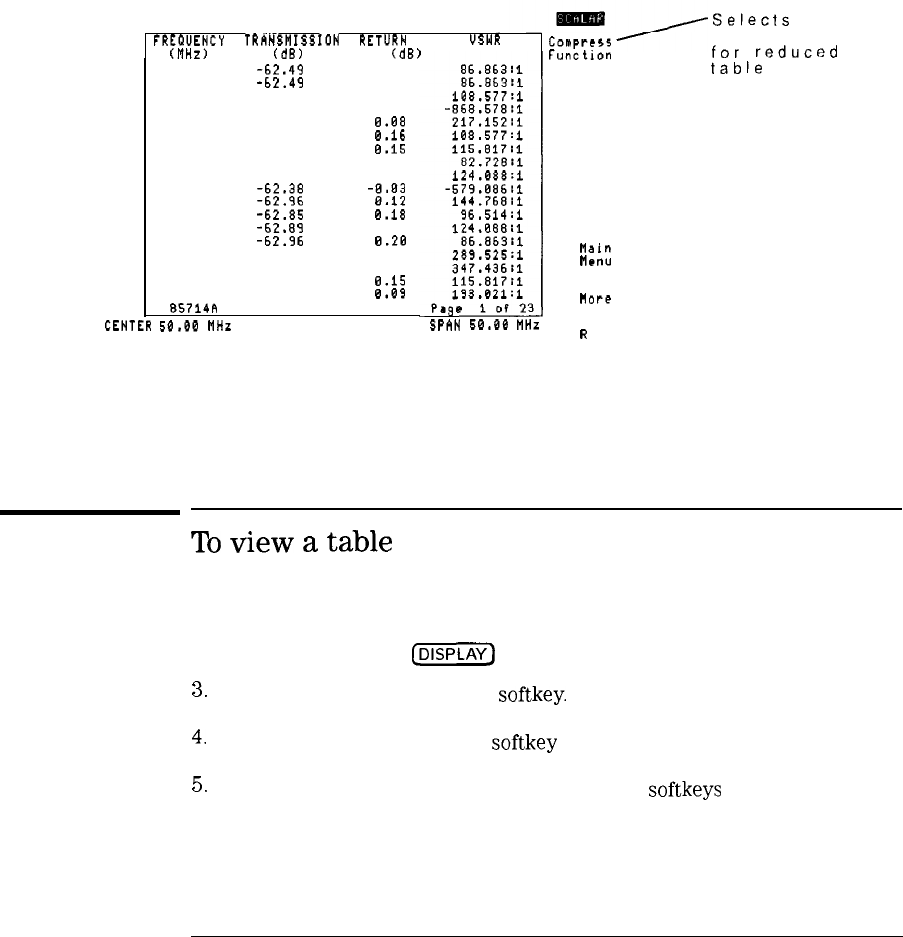
I
-
I
-
Displaying Results in a Table
Creating a table
FREQUENCY
TRANSMISSfON
RETURN
(MHz) (dB) LOSS (dB)
USWR
25.00
-62.49
0.20
25.13
-62.49
0.20
25.25 -62.64 0.16
25.38 -62.62 -0.02
25.50 -62.66
0.08
25.63 -62.63
0.16
25.75 -63.14
0.15
25.88 -62.93 0.21
26.00 -62.64 0.14
26.13
26.25
I;;*;; -:-i:
26.38
-62185 0:18
26.50
-62.89
0.14
26.63
-62.96 8.20
26.75 -63.14 0.06
26.88 -62.78 0.05
27.00 -62.54
0.15
27.13 -62.87
0.09
HP
85714R
CENTER
50.00
MHz SPAN
50.00
MHz
C0mprc55
Function
Main
Menu
uore
2 of 2
R
Selects
compression
for
reduced
table
Page two of Tabular Display menu
To
view
a
table
1. Display a normalized transmission and/or reflection response as described
in the previous chapters.
2. Press the front-panel
cm)
key.
3.
Press the Tabular Display
softkey.
4.
Press the TABULAR ON OFF
softkey
so that ON is underlined.
5.
Use the VIEW NEXT PG and VIEW PREV PG
softkeys
to scroll through
the table.
6-4
I
-
I
-
Printing
a
table
In order to print the table, you must first connect a graphics printer, and
then configure the scalar analyzer for the printer. For detailed information
on configuring the printer and spectrum analyzer, refer to the printer and
spectrum analyzer manuals.
Examples of graphics printers include the following Hewlett Packard printers:
l
ThinkJet
l
QuietJet
l
LaserJet
0
PaintJet
To
configure
the
printer
1. Configure the printer for the interface used. This will vary depending on
RS-232
or HP-IB interfaces.
Refer to the printer manual for any switch settings. Refer to the
spectrum analyzer manual for information on
RS-232
interfacing.
2. Connect the printer.
3. Press the scalar analyzer’s front-panel
[CONFIG)
key.
4.
Press the COPY DEV PRNT PLT
softkey
so that PRNT is underlined.
5.
Press the PRINT
CONFIG
softkey.
6. Press the
softkey
to select the appropriate printer.
7. If an HP-IB interface is used to connect the printer, press
PRINTER ADDRESS , and enter the address of the printer.
6-5
I
-
I
-
Displaying Results in a Table
Printing a table
To
print
the
table
1. View the table on the screen as previously described in this chapter.
2. To indicate that the complete table should be printed, press the
PRINT PAGE ALL
softkey
so that ALL is underlined. To indicate only the
displayed table page should be printed, press the
softkey
so that PAGE is
underlined.
3. Press the front-panel [copy) key.
6-6
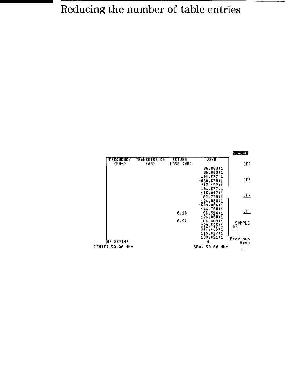
I
-
Reducing
the
number
of
table
entries
Transmission and reflection response traces are displayed using 401
measurement points. This results in 401 table entries. The number of
table entries can be compressed while retaining the relative frequency and
amplitude characteristics of the original response.
The source trace data is divided into intervals equal to the number desired
table entries. The data in each interval is compressed to obtain a table entry.
Tabular display offers five data compression methods: AVERAGE, NORMAL,
NEGATIVE, POSITIVE, and SAMPLE.
25.80 -62.49 0.20
25.13 -62.49 0.20
25.25 -62.64 0.16
25.38 -62.62 . -0.02
25.50 -62.66 0.08
25.63 -62.63 0.16
25.75 -63.14 0.15
25.88 -62.93 0.21
AVERAGE
ON
E
NORMAL
ON
OFF
108.577:1
115.817:1
NEGATIVE
82.728:i
ON
OFF
26.00 -62.64 0.14
26.13 -62.38 -0.03
26.25 -62.96 0.12
26.38 -62.85
0.i8
26.50 -62.89 0.14
26.63 -62.96
e.2e
26.75 -63.14 0.06
26.88 -62.78 3.05
27.00 -62.54 0.15
27.18 -62.87 0.09
124.088:i
-579.086:1
144.768:l
POSITIVE
96.514:i
ON
OFF
124.088:1
86.863:1
289.525:1
SAIIPLE
347.436:l
g4 OFF
115.817:1
IHP
85714A
CENTER
50.00
MHz
193.021:1
Page
1
of 23
PreVi0Us
Menu
SPAN
50.00
MHz
L
6-7
I
-
Displaying Results in a Table
Reducing the number of table entries
With AVERAGE compression, the data in each interval is averaged to obtain
the table entry.
With NORMAL compression, the data in each interval is obtained using a
Rosenfell algorithm. The Rosenfell algorithm is a mathematical operation that
selectively chooses between positive and negative peak values in the interval.
With NEGATIVE compression, the lowest value data in each interval is placed
in the table entry.
With POSITIVE compression, the highest value data in each interval is placed
in the table entry.
With SAMPLE compression, the last value in each interval is placed in the
table entry.
To
reduce
tabular
entries
1. Press
(-1
and then the Tabular Display
softkey
to enter the
Tabular Display menu.
2.
Press the
NUMBER
POINTS
softkey,
and enter the desired number of table
entries.
To
select
the
compression
method
1.
Press
(jj)
and then the Tabular Display
softkey
to enter the
Tabular
Display menu.
2.
Press the More 1 of 2
softkey.
3.
Press the Compress Function
softkey.
4. Press the
softkey
corresponding to the desired compression method.
6-8
I-

I
-
I
-
7
-
Programming

I
-
Programming
This chapter presents programming techniques for sending commands
and receiving data. You can program the HP
85714A
scalar measurements
personality using the programming commands listed in Chapter 8, Reference.
For information on programming the spectrum analyzer, refer to the spectrum
analyzer’s programming manual.
7-2
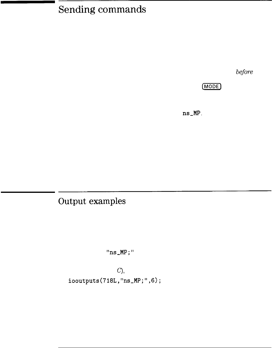
I
-
Sending
commands
Always place the spectrum analyzer in the scalar analyzer mode
befie
sending any scalar measurement commands. To place the spectrum analyzer
in the scalar measurements personality mode, press
c-1
and then
SCALAR ANALYZER.
All scalar analyzer commands begin with the characters ns,. For example,
the command to preset the scalar analyzer is
ns-MP.
Chapter 8 documents all
available scalar measurements personality commands. Chapter 8 also contains
a table grouping all commands according to function.
While the scalar measurements personality is operating, some spectrum
analyzer commands should not be used. For example, instead of the
analyzer’s FFT command, use the ns-FFT command documented in Chapter
8. Refer to Chapter 8 for a list of all replaced spectrum analyzer commands.
Output
examples
Send commands as ASCII strings. The method used depends on the
programming language and environment used. Using an HP 9000 Series 300
technical computer with the HP-BASIC language, send the command to the
spectrum analyzer as follows:
OUTPUT 718; “ns_MP;”
Using an HP Vectra computer with the HP-IB Interface and Command Library
(and programming in
c),
the same command could be sent as follows:
iooutputs(718L,“ns_MP;“,6);
7-3
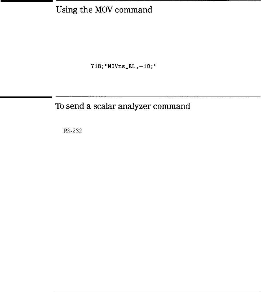
I
-
I
-
Programming
Sending commands
Using
the
MOV
command
It is recommended that the MOV command be used to execute all
programming commands that take number parameters. Using the MOV
command is faster and avoids displaying text on the analyzer screen. For
example, to set the reference level using the BASIC language, send the
following:
OUTPUT
718;“MOV
ns-RL,-10;”
To
send
a
scalar
analyzer
command
1. Connect the spectrum analyzer to the computer using either the HP-IB or
RS-232
interface.
Refer to the spectrum analyzer’s programming manual for information
on connecting the interface.
2. Locate the appropriate command in Chapter 8.
3. Use your programming language’s output statement to send the command
as an ASCII string to the spectrum analyzer.
7-4
I-
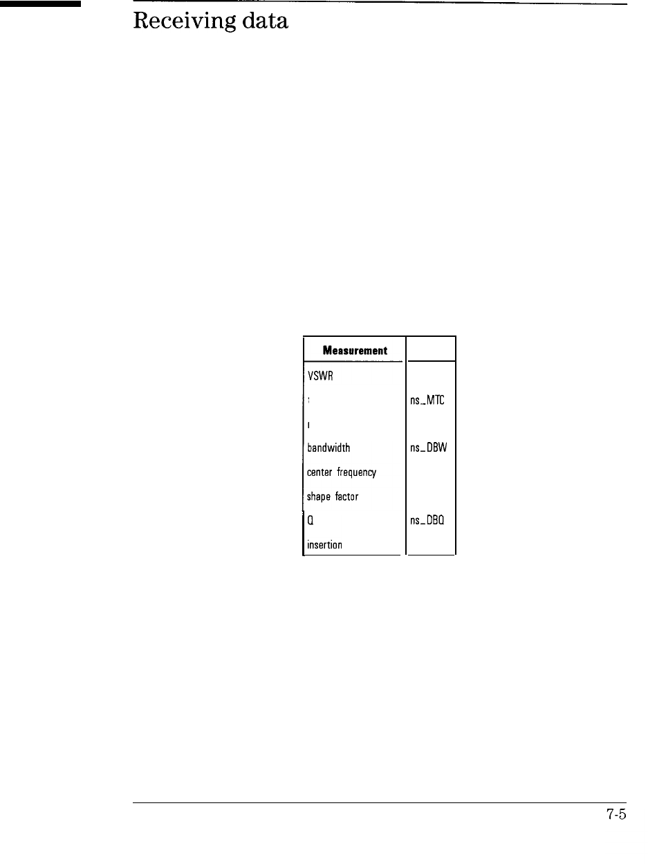
I
-
Receiving
data
Measurement Variables
Variable
ns-VSWF
transmission coefficient
ns_MTC
reflection coefficient ns-MRC
ns-DEW
ns-OCF
ns-DSF
ns-DBQ
ns-OIL
1
Zsertion
loss
Many programming commands can be sent as queries requesting the state
of the scalar measurements personality. For example, ns-NORM? requests
whether normalization is turned on or off. The command reference in
Chapter 8 documents available command queries.
Automatic measurement results are stored in spectrum analyzer variables.
The contents of these variables can be requested by your application program
to obtain measurement results. The measurements and their variables are
listed in the following table.
Queries and variables are normally sent from the spectrum analyzer in the
form of ASCII strings. It is your responsibility to allocate memory for them in
your application.

I
-
Programming
Receiving data
To
return
a
measurement
value
1. Send to the spectrum analyzer an ASCII string consisting of the variable
name with the ? character appended.
For example, to return the shape factor, send
ns_DSF?.
7-6

I
-
8
Reference

I
-
I
-
Reference
This chapter gives you quick access to information on the scalar
measurements personality. The chapter contains four sections: menu maps,
definitions of keys, programming commands, and characteristics. Within each
section, the material is organized alphabetically.
8-2

I
-
Menu
maps
Menu maps illustrate how
softkeys
are located relative to each other; they
help you form a “mental” map of instrument functions. The five menu maps
in this section graphically represent
softkey
paths and include front-panel
keys used to access the menus.
8-3
_I
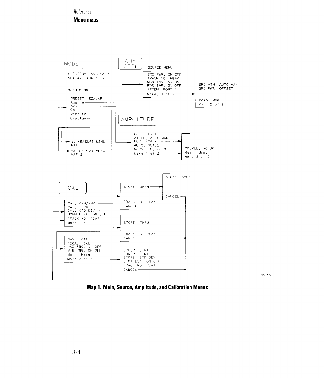
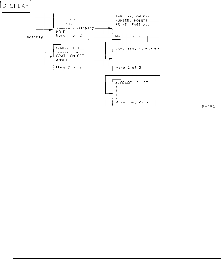
I
-
iD
I
SPLAYj
Reference
Menu maps
DISPLAY MENU
DSP LINE, ON OFF
DUAL
DSP.
ON OFF
120
dB,
ON OFF
From Map l’s Tabular,
D~sploy
MAIN MENU
Display
softkey
1
CHANG, PREFIX
ANNOT.
ON OFF
Main, Menu
VIEW. NEXT PG
VIEW. PRE” PG
Main, Menu
-
AVERAGE,
ON OFF
NORMAL, ON OFF
NEGATIVE, ON OFF
POSITIVE, ON OFF
SAMPLE, ON OFF
PV25A
Map 2. Display and Tabular Display Menus
8-5
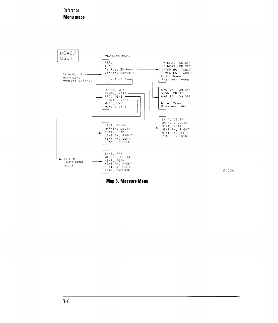
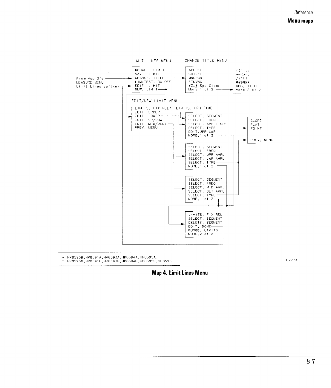
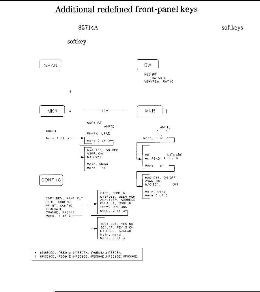
I
-
Reference
Menu maps
Additional
redefined
front-panel
keys
The HP
85714A
scalar measurements personality redefines the
softkeys
associated for several front-panel keys not listed in the scalar analyzer menu.
The
softkey
maps for these redefined keys are shown on this page.
SPAN
SPAN. ZOOM
FULL, SPAN
ZERO. SPAN
PEAK, ZOOM
t
I
I
RES
BW
AUTO MAN
“ID
BW
AUTO MAN
“BW,RSW.
RATIO
“ID AVG. ON OFF
MARKER, NORMAL
MARKER, DELTA
MKNO, SE, ON OFF
MARKERS. OFF
MKPAUSE.
ON OFF
MARKER, AMPTD
r
PK-PK.
MEAS
MARKER. NORMAL
MARKER, DELTA
MARKER.
AMF’TD
SELECT
1
2 3 4
MARKER
1,
ON OFF
i
“SWR,
Oi4
OFF
MAG
S21 ON OFF
L
MK
TRACE,
AVTO
ABC
MK
READ,
F
T
/
P
Mo,n.
Menu
MARKER. ALL OFF
More
2
0,
3
More
3 Of 3
1
“SWR.
ON
OFF
MAG
s21,
ON
OFF
Map 5. Redefined Front-Panel Keys
8-8
I
-
I
-
Definitions
of
keys
This section lists in alphabetical order the definitions of all HP
85714A
scalar
measurements personality keys. Alphabetically listed definitions give you a
quick access to information concerning any key or
softkey.
Some front-panel
keys have been redefined to allow quick access of scalar analyzer functions.
Refer to the spectrum analyzer’s operating manual for information on any key
not affected by the personality.
120
dB
ON
OFF
The 120
d3
ON OFF
softkey
displays 120
dB
of calibrated measurement
range.
This feature provides 120
dB
of measurement range not available with the
normal 15
dB
per division log scale. The 120
dB
calibrated measurement
range is achieved by splicing two separate traces. For each visible sweep, the
scalar analyzer first saves the top 50
dB
of trace data. Then, the reference
level is set up to 50
dB
below the current reference level and another reading
is taken. Finally, these two traces are spliced together and displayed on the
screen.
You cannot use this feature in the dual display mode. (Dual display refers to
simultaneously displaying both transmission and reflection responses.)
The default setting for this measurement is OFF.
Related Programming
Command
ns-EDR
8-9
I-
I
-
I
-
Reference
Definitions of keys
The front panel
(AMPLITUDE)
key presents the scalar analyzer’s Amplitude
menu.
This key is identical to pressing the scalar analyzer’s Amptd
softkey.
Use this
menu to control the log scale, reference level, and input attenuation.
Amptd
The Amptd
softkey
enters a menu used for controlling the log scale, reference
level, and input attenuation. This
softkey
is identical to pressing the scalar
analyzer’s
@LiKiEK]
key.
ANNOT
ON
OFF
The
ANNOT
ON OFF
softkey
turns the displayed annotation text on or off.
Related Programming
Command
ns-ANNOT
8-10
I
-
I
-
Reference
Definitions of keys
ATTEN
AUTO
MAN
The
ATTEN
AUTO MAN softkey selects automatic or manual RF input
attenuation control.
Signal levels above +30
dBm
will damage the spectrum analyzer.
AUTO.
The RF input attenuator is coupled to the reference level. When a continuous
wave signal is displayed with its peak at or below the reference level,
attenuator coupling keeps the signal level at the internal RF mixer at or
below the specified level.
MAN.
The RF input attenuator is not coupled to the reference level. Its value can
be set independently. In certain situations, increasing the input attenuation
may reduce signal compression in the presence of broadband signals.
See Also AUTO SCALE in this chapter.
ATTEN
PORT
1
The
ATTEN
PORT 1
softkey
controls the attenuator in Option 001
HP
85630A
scalar transmission/reflection test sets.
The test set has an input attenuator which reduces the power applied to its
PORT 1 output connector. The default attenuation is 0
dB.
Related Programming
Command
ns-EXATN
8-11
I
-
I
-
Reference
Definitions of keys
AUTO
SCALE
The
AUTO
SCALE
softkey
automatically adjusts the log scale to display a
signal full screen.
This function is a one-time adjustment. The log scale does not continually
update with each new trace acquisition.
Related Programming
Command
ns_AUTOSC
(AUXCTRL)
The
(AUX]
key presents the scalar analyzer’s Source menu.
The Source menu controls the RF output of the spectrum analyzer’s
tracking generator. It can also be used to set the optional attenuator on the
HP
85630A
test set.
8-12
I
-
I
-
Reference
Definitions of keys
AVERAGE
ON
OFF
The
AWERAGE
ON OFF
softkey
selects average compression for the Tabular
Display feature.
l%bular
display lists each transmission and/or reflection measurement point as
an entry in a table. Traces comprise 401 measurement points resulting in 401
table entries. The number of table entries can be compressed while retaining
the relative frequency and amplitude characteristics of the original response.
If the table is compressed, the source trace data is divided into intervals equal
to the number desired table entries. The data in each interval is compressed
to obtain a table entry. With average compression, the data in each interval
is averaged to obtain the table entry.
Related Programming
Command
ns-TCA
0
BW
The
Isw)
key presents a menu for controlling the scalar analyzer’s
bandwidth.
8-13
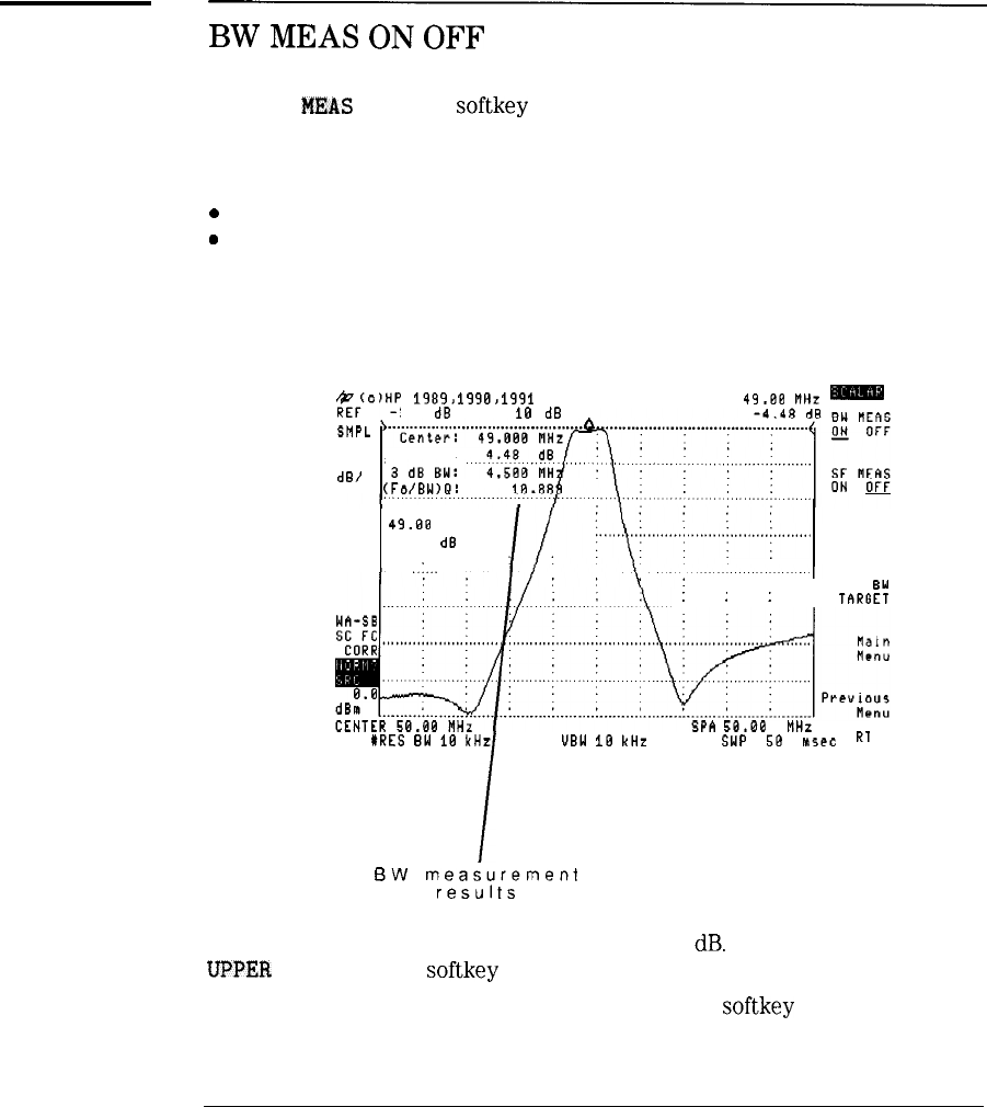
I
-
I
-
Reference
Definitions of keys
BW
MEAS
ON
OFF
The BW
MEAS
ON OFF
softkey
automatically performs bandwidth
measurements on a transmission response.
Parameters measured include the following:
0
center frequency
0
insertion loss
l
bandwidth
l Q
$:c)HP
1989.1990,1991
SCALAR
-3.5 dB RTTEN 16 dB
SnPL
LOG
8
Ins Lass:
dB/
(Fa/BW)Q:
MKR
49.88
Rtlz
m
MARKER
49.08
MHz
'-4.48
dB
.
..I...
UPPER BW
TARGET
LOWER RW
:
:
:
TARC
_
!ET
I
N
58.66
MHz
#RES
BW
18
kHz UBW 18 kHz SWP 5G
nsec
R'
BW
measurement
results
The measurement uses a default bandwidth of 3
dB.
Use the
UPPEB
BW TARGET
softkey
to change the bandwidth used in the
measurement. (The displayed LOWER BW TARGET softkey is not used in this
8-14
I
-
Reference
Definitions of keys
measurement.) For example, using the UPPER BW TARGET
softkey,
you could
change the bandwidth used in the measurement from 3
dB
to 6
dB.
The bandwidth measurement repeats continuously until turned off.
Related Programming
Command
ns-BMT
See Also
SF
MEAS
ON
OFF
in this chapter.
The
a
key presents the scalar analyzer’s calibration menu.
The scalar analyzer provides guided calibration routines for both transmission
and reflection measurements.
Cal
The Cal
softkey
presents the scalar analyzer’s calibration menu.
The scalar analyzer provides guided calibration routines for both transmission
and reflection measurements.
8-15
I-
I
-
I
-
Reference
Definitions of keys
CAL
OPN/SHRT
The CAL
OPN/SHRT
softkey
preforms a guided calibration for reflection
measurements.
Reflection calibration requires both
0~
and
short
standards. The HP
85032B
Option 001 Calibration Kit supplies
5061
type N
0~
and
short
standards for
calibration.
After calibration, normalization is turned on as indicated by the screen
annotation NORM displayed on the lower left side of the screen. Turn
normalization on or off using the NORMALIZE ON OFF
softkey.
Related Programming
Command
ns_CALR
See Also
NORMALIZE
ON
OFF
in this chapter.
CAL
STD
DEV
The CAL STD DEV
softkey
preforms a guided calibration for transmission
measurements using a standard device.
After calibration of the standard device, a limit line is created around the
response of the device. This feature allows repeated response testing in
production-line environments.
Standard device calibration requires a through-line. After calibration,
normalization is turned on as indicated by the screen annotation “NORM”
displayed on the lower left side of the screen. Turn normalization on or off
using the Cal, NORMALIZE ON OFF
softkey.
Related Programming
Command
ns_CALS
8-16
I
-
I
-
Reference
Definitions of keys
CAL
THRU
The CAL
THRU
softkey
preforms a guided calibration for transmission
measurements.
Transmission calibration requires a through-line. After calibration,
normalization is turned on as indicated by the screen annotation “NORM”
displayed on the lower left side of the screen. Turn normalization on or off
using the NORMALIZE UN OFF
softkey.
Related Programming
Command
ns-CALT
See Also NORMALIZE ON OFF in this chapter.
CANCEL
The CANCEL
softkey
cancels the current calibration routine and returns to
the Cal menu.
NS-CAN
CHANGE
TITLE
The CHANCE TITLE
softkey
presents a menu for writing titles on the screen.
8-17
I
-
I
-
Reference
Definitions of keys
CHANGE
PREFIX
The CHANGE PREFIX
softkey
changes the prefix used in saving and recalling
data to and from the memory card. You can also catalog by prefix. The
default preEx is SCALAR.
The prefix can be from one to seven characters long. The longer the prefix,
the shorter the register number must be. The total length of the prefix and
register number cannot exceed eight characters, The prefix can be any
character; however, the underscore should not be the first character of the
prefix.
Pressing CHANGE PREFIX accesses a menu containing the letters of the
alphabet, the underscore symbol (-), the number symbol
(ty),
a space, and the
clear function. To select a character, press the
softkey
that displays the group
of characters that contains the desired character. The
softkey
menu changes
to allow you to select an individual character. If you make a mistake, press
m
to space back over the incorrect character. Additional characters are
available by pressing
YZ,#
SPC CLEAR , MORE
1
OF
2 Numbers may be
selected with the numeric keypad.
A prefix can be cleared with the clear function. Press
CDISPLAYI),
CHANGE PREFIX ,
YZ,%
SPC CLEAR, CLEAR to clear the current prefix.
Compress
Function
The Compress Function
softkey
presents a menu for compressing the data
in a tabular display.
8-18
I
-
Reference
Definitions of keys
CONFIG
The
(-1
key presents the scalar analyzer’s Configuration Menu.
The first two menu pages are identical to the spectrum analyzer
CONFIG
menu. Page three provides the following features specific to the scalar
analyzer:
l
Turn the HP
85630A
test set on or off.
l
Remove the HP
85714A
from the spectrum analyzer.
l
Display the HP
85714A
revision number.
COUPLE
DC
AC
The COUPLE DC AC softkey selects either AC or DC RF input coupling
on HP
8594A,
HP 85943, HP
8595A,
HP 85953, and HP 85963 spectrum
analyzers.
DELETE
SEGMENT
The DELETE SEGMENT softkey deletes the current limit-line segment from
the table.
This function removes unwanted limit lines and their values from the
currently active limit-line table.
8-19
I
-
I
-
Reference
Definitions of keys
DELTA
MEAS
The DELTA
MEAS
softkey
presents a menu for measuring delta amplitude and
frequency values using the delta marker delta marker function.
The marker is placed on the peak of the response.
Device
BW
MEAS
The Device
BW
MEAS
softkey
presents a menu for measuring response
bandwidth and shape factor in transmission measurements.
For bandwidth measurements, the display shows the following measurement
values :
0
center frequency
0
insertion loss
l
bandwidth
.Q
For shape factor measurements, the display shows the following measurement
values :
l
shape factor
l
upper bandwidth
l
lower bandwidth
See Also
BW
MEAS
ON
OFF
and
SF
MEAS
ON
OFF
in this chapter.
8-20
I
-
I
-
Reference
Definitions of keys
The
c-1
front-panel key presents the scalar analyzer’s menu for
controlling the display of information.
The scalar analyzer redefines the
softkeys
for this spectrum analyzer key with
functions unique to the scalar analyzer.
Display
The Display
softkey
presents a menu for controlling the display of
information. From this menu, you can perform the following tasks:
l
View a display line.
The display line is an adjustable horizontal line used as a visual
reference line.
0
View reflection/transmission results simultaneously.
Simultaneous viewing requires the HP
85630A
scalar
transmission/reflection test set.
l
View 120
dB
of measurement range.
l
View a table of measurement results.
l
Add a screen title.
l
Turn on or off the graticule and/or annotation.
DISPOSE
SCALAR
The DISPOSE SCALAR removes the scalar analyzer personality from the
spectrum analyzer.
Related Programming
Command
ns-DISPOSE
8-21
I
-
I
-
Reference
Definitions of keys
DSP
LINE
ON
OFF
The DSP LINE ON OFF
softkey
displays an adjustable horizontal line that
can be used as a visual reference.
The viewed display line is identical to the display line used by the spectrum
analyzer. The line can be used for trace arithmetic and has amplitude values
that correspond to its vertical position when compared to the reference level.
The display line can be adjusted using the step keys, knob, or numeric
keypad.
DUAL
DSP
ON
OFF
The DUAL DSP ON OFF
softkey
allows you to view both reflection and
transmission measurements at the same time.
This feature requires the optional HP
85630A
scalar transmission/reflection
test set. The HP
85714A
controls the test set allowing you to see either
reflection and transmission results in real time.
Related Programming
Command
ns-DDM
See Also
RER.
and TRANS and TEST SET ON OFF in this chapter.
8-22
I
-
I
-
Reference
Definitions of keys
EDIT
DONE
The EDIT DONE
softkey
ends the editing or creating of a limit-line table.
This function returns you to the limit-lines menu and removes limit lines
from the display. However, limit lines are not saved until you save them
with the SAVE LIMIT
softkey.
Limit lines may be viewed by pressing
LIMITEST ON OFF.
See Also
SAVE LIMIT
and
LIMIEST
ON
OFF
in this chapter.
EDIT
LIMIT
The EDIT LIMIT
softkey
allows you to edit limit lines.
This softkey’s selections are identical to the NEW LIMIT
softkey,
with the
exception that NEW LIMIT erases any currently active limit lines from
memory. Be sure to save edited or created limit lines using the SAVE LIMIT
softkey.
See Also
SAVE LIMIT
in this chapter.
8-23
I
-
I
-
Reference
Definitions of keys
EDIT
LOWER
The EDIT LOWER
softkey
presents a menu for editing a limit line table by
specifying lower amplitude segments.
Although this menu is optimized for editing lower limit-line segments, you
can edit all limit-line values. The menu’s EDIT
UPR
LWR
softkey
is selected
for lower (LWR) segment editing. You can easily edit upper (UPR) segments
by pressing this
softkey
so that UPR is underlined.
EDIT
MID/DELT
The EDIT MID/DELT
softkey
presents a menu for editing a limit-line table by
specifying the distance between upper and lower limits lines centered around
a midpoint power level.
EDIT
UP/LOW
The EDIT UPPER
softkey
presents a menu for editing limit-line tables.
Editing is accomplished by specifying upper and lower amplitude segments.
Although this menu is optimized for editing upper limit-line segments, you
can edit all limit-line values. The menu’s EDIT
UPR
LWR
softkey
is selected
for upper (UPR) segment editing. You can easily edit lower (LWR) segments
by pressing this
softkey
so that LWR is underlined.
8-24
I
-
I
-
Reference
Definitions of keys
EDIT
UPPER
The EDIT UPPER
softkey
presents a menu for editing a limit-line table by
specifying a upper segment’s amplitude.
Although this menu is optimized for editing upper limit-line segments, you
can edit all limit-line values. The menu’s EDIT
UPR
LWR
softkey
is selected
for upper (UPR) segment editing. You can easily edit lower (LWR) segments
by pressing this
softkey
so that LWR is underlined.
EDIT
UPR
LWR
The EDIT
UPR
LWR
softkey
selects a segment’s upper or lower limit line for
editing.
The SELECT AMPLITUD softkey changes the amplitude of the limit line
specified by the EDIT
UPR
LWR
softkey.
EXIT
DELTA
The EXIT DELTA softkey removes the DELTA
MEAS
menu and returns the
scalar analyzer to the Measure menu.
8-25
I
-
Reference
Definitions of keys
EXIT
FFT
The EXIT FFT
softkey
removes the FFT
MEAS
menu and returns the scalar
analyzer to the Measure menu.
The FFT performed by the FFT menu is removed when the EXIT FFT is
pressed.
EXIT
PK-PK
The EXIT PK-PK
softkey
removes the PK-PK
MEAS
menu and returns the
scalar analyzer to the Measure menu.
FFT
MEAS
The FFT
MEAS
softkey
enters the FFT menu.
The scalar analyzer transforms zero span data into the frequency domain
using an FFT (Fast Fourier Transform). After using the FFT function the
following conditions are set:
l
the display is in log mode (10 dB/division)
0
triggering is single sweep
l
markers are available as FFT markers
Any markers must be turned off before attempting to use them in the usual
manner.
8-26
Related Programming
Command
ns_FFT
I
-
I
-
Reference
Definitions of keys
FLAT
The FLAT
softkey
deEnes
a limit-line segment type. A zero-slope line
is drawn between the coordinate point of the current segment and the
coordinate point of the next segment. This produces limit-line values equal in
amplitude for all frequencies between the two points.
See Also SELECT TYPE in this chapter.
GRAT
ON
OFF
The GRAT ON OFF
softkey
turns the displayed graticule on or off.
LIMITS
FIX
REL
The LIMITS FIX
REL
softkey
determines the method used to display the
limit line with respect to frequency.
FIX.
The limit lines are displayed at the Exed frequency and reference level
indicated in the limit line table.
REL. The limits lines are displayed relative to the scalar analyzer’s center
frequency and reference level.
8-27
I-
I
-
I
-
Reference
Definitions of keys
Limit
Lines
The Limit Lines
softkey
accesses a menu for creating limit lines.
Limit lines graphically display test limits on the scalar analyzer’s screen.
These limits can be used for pass/fail testing. You can also enter this menu
be pressing the front-panel
(jj)
key followed by the More 1 of 2
softkey.
LIMITEST
ON
OFF
The LIMITEST ON OFF
softkey
turns on or off limit-line testing.
ON.
Any currently active limit lines are displayed with transmission or reflection
pass/fail conditions indicated on the screen.
OFF.
No limit lines are active or displayed.
LOG
SCALE
The
LOG
SCALE
softkey
allows you to manually change the display’s log
scale.
See Also AUTO SCALE in this chapter.
8-28
I
-
I
-
Reference
Definitions of keys
LOWER
BW
TARGET
The LOWER
BW
TARGET
softkey
changes the bandwidth used in
Elter
shape-factor measurements.
The default lower bandwidth value is -60
dB.
shape factor = 60 dB response bandwidth
3 dB response bandwidth
Related Programming
Command
ns-LBW
See Also
SF
MEAS
ON
OFF
in this chapter.
LOWER
LIMIT
The LOWER LIMIT
softkey
is used when calibrating standard devices. It sets
the acceptable deviation in
dB
between the lower limit trace and the response
of the standard device.
Related Programming
Command
ns-SDLL
8-29
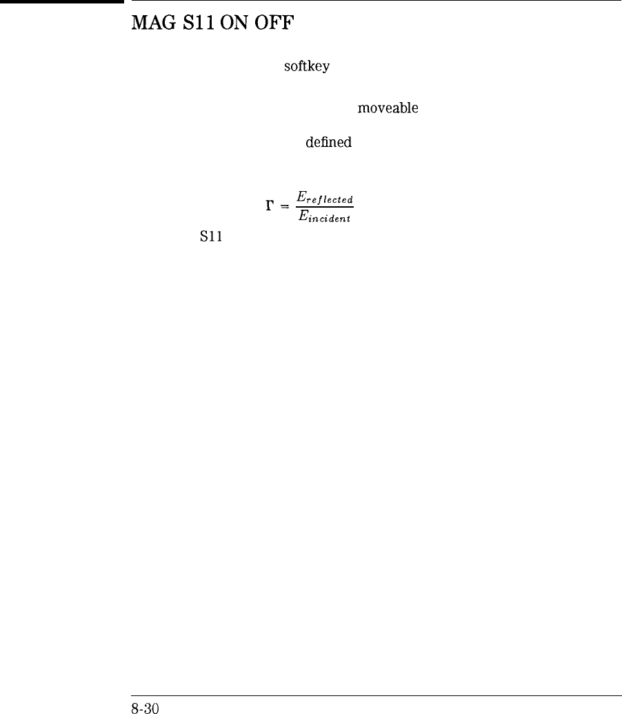
I
-
I
-
Reference
Definitions of keys
MAG
Sll
ON
OFF
The MAG Sll ON OFF
softkey
measures the reflection coefficient during a
reflection measurement.
The display must be normalized. A
moveable
marker is activated for
measuring the reflection coefficient at any point on the displayed response.
The reflection coefficient is
deEned
as the ratio of the reflected signal voltage
from a device being tested to the incident signal voltage. It is shown by the
following formula:
r
=
Ereflected
Eineident
The MAG
Sll
ON OFF function does not give measurement results during
transmission measurements.
Related Programming
ns-MCT
Command
ns-MCM
See Also
VSWR
ON
OFF
in this chapter,
B-30
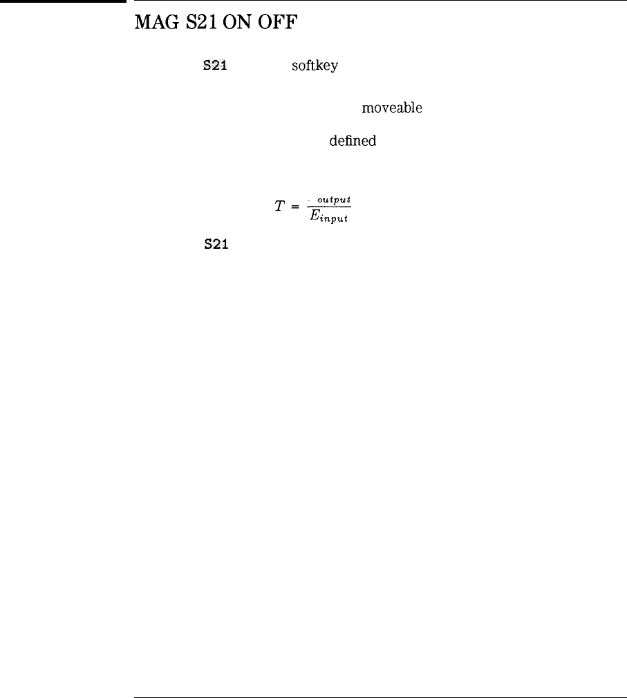
I
-
I
-
Reference
Definitions of keys
MAG
S21
ON
OFF
The MAG
S21
ON OFF
softkey
measures the transmission coefficient during a
transmission measurement.
The display must be normalized. A
moveable
marker is activated for
measuring the transmission coefficient at any point on the displayed response.
The transmission coefficient is
deEned
as the ratio of the voltage at the
output of a device to the voltage at the input of a device. It is shown by the
following formula:
E
output
T=--.----
haput
The MAG
S21
ON OFF function does not give measurement results during
reflection measurements.
Related Programming
ns-MCT
Command
ns-MCM
8-31
I
-
Reference
Definitions of keys
Main
Menu
The Main Menu
softkey
returns the scalar analyzer to the main menu.
MAN
TRK
ADJUST
The MAN TRK ADJUST softkey manually adjusts the source’s tracking.
This function allows you to manually adjust the frequency tracking between
the scalar analyzer and the built-in tracking generator. The frequency
tracking is correctly set when the displayed response is peaked for maximum
amplitude.
See Also TRACKING PEAK in this chapter.
Marker
Convert
The Marker Convert
softkey
presents a menu for measuring VSWR,
SI1
magnitude, and
SX
magnitude.
Menu selections activate a
moveable
marker that display the appropriate
scalar value. For reflection measurements, the marker can indicate
either VSWR or
SI1
magnitude (reflection coefficient). For transmission
measurements, the marker indicates the
SZ1
magnitude (transmission
coefficient).
Related Programming
Command
ns-MCM
See Also MAG
Sll
ON OFF, MAG
S21
ON OFF, and VSWR ON OFF in this chapter.
8-32
I
-
I
-
Reference
Definitions of keys
MARKER
DELTA
The MARKER DELTA softkey places delta markers on the screen.
Two markers are placed on the screen: an anchor marker and a movable
marker. The anchor marker is stationary and is placed on the peak response.
The scalar analyzer places the movable marker on the lowest signal response.
As the front-panel knob moves the movable marker, the display shows the
difference in frequency and amplitude between the two markers.
MAX
RNG
ON
OFF
The MAX RNG ON OFF softkey displays a horizontal line indicating the upper
limit of display calibration.
Because normalization shifts the response, a portion of the displayed response
may be uncalibrated. This function graphically indicates uncalibrated portions
of a response. If the response enters an uncalibrated area, the message
‘DISPLAY OVER-RANGE’ appears on the screen.
Related Programming
Command
ns-URNG
See Also MIN
RNG ON
OFF
in this chapter,
8-33
Reference
Definitions of keys
Measure
The Measure
softkey
presents a menu for performing reflection and
transmission measurements.
Use this menu to switch between transmission and reflection measurements
and to measure response parameters.
(
MEAS~JSERJ
The
(KiZ$EK)
front-panel key presents the scalar analyzer’s Measure
menu.
This key is identical to pressing the scalar analyzer’s Measure
softkey.
Use
this menu to switch between transmission and reflection measurements and
to measure response parameters. The second time the key is pressed, the
user menu appears.
8-34
I
-
I
-
Reference
Definitions of keys
MIN
RNG
ON
OFF
The MIN
RNG
ON OFF
softkey
displays a horizontal line indicating the lower
limit of display calibration.
Because normalization shifts the response, a portion of the displayed response
may be uncalibrated. This function graphically indicates uncalibrated portions
of a response. If the response enters an uncalibrated area, the message
‘DISPLAY UNDER-RANGE’ appears on the screen.
Related Programming
Command
ns_LRNG
See Also
MAX
RLVG
ON
OFF
in this chapter.
8-35
-1
I
-
I
-
Reference
Definitions of keys
NEGATIVE
ON
OFF
The NEGATIVE ON OFF
softkey
selects negative compression for the
‘lobular
Display feature.
Tabular display lists each transmission and/or reflection measurement point as
an entry in a table. Traces comprise 401 measurement points resulting in 401
table entries. The number of table entries can be compressed while retaining
the relative frequency and amplitude characteristics of the original response.
If the table is compressed, the source trace data is divided into intervals equal
to the number desired table entries. The data in each interval is compressed
to obtain a table entry. With negative compression, the lowest value data in
each interval is placed in the table entry.
Related Programming
Command
ns-TCA
NEW
LIMIT
The NEW LIMIT
softkey
allows you to create a limit line table.
The selections with this
softkey
are identical to EDIT LIMIT with the
exception that NEW LIMIT erases any currently active limit-line table.
See Also EDIT LIMIT in this chapter.
8-36
I
-
I
-
Reference
Definitions of keys
NEXTPEAK
The NEXT PEAK
softkey
locates the next highest trace point relative to the
current marker position.
The next peak must meet the current peak excursion criteria in order to be
located.
See Also
PEAK
EXCURSN
in this chapter.
See Also
NEXTPKLEFT
The NEXT PK LEFT
softkey
locates the next signal peak to the left of the
current marker position.
The next peak must meet the current peak excursion criteria in order to be
located.
PEAK EXCURSN in this chapter.
The NEXT PK RIGHT
softkey
locates the next signal peak to the left of the
current marker position.
The next peak must meet the current peak excursion criteria in order to be
located.
See Also
PEAK
EXCURSN
in this chapter.
8-37
I-
I
-
I
-
Reference
Definitions of keys
NORM
REF
POSN
The NORM REF POSN softkey sets the normalized reference position.
This is the position of the normalized reference level after a calibration. It is
indicated by an angle bracket at each end of a horizontal graticule line. The
normalized reference position can be set to any of the eight major horizontal
graticule lines. (Position eight is the top graticule; position 0 is the bottom
graticule.) The default normalized reference position is at the display’s top
graticule line.
Related Programming
Command
ns-NRP
NORMAL
ON
OFF
The NORMAL ON OFF softkey selects normal compression for the
‘Ihbular
Display feature.
Tabular
display lists each transmission and/or reflection measurement point
as an entry in a table. Traces comprise 401 measurement points resulting
in 401 table entries. The number of table entries can be compressed while
retaining the relative frequency and amplitude characteristics of the original
response. If the table is compressed, the source trace data is divided into
intervals equal to the number desired table entries. The data in each interval
is compressed to obtain a table entry. With normal compression, the data in
each interval is obtained using a Rosenfell algorithm. The Rosenfell algorithm
is a mathematical operation that selectively chooses between positive and
negative peak values in the interval.
8-38
I
-
I
-
Reference
Definitions of keys
NORMALIZE
ON
OFF
The NORMALIZE ON OFF softkey turns normalization on or off.
After transmission or reflection calibration, normalization is turned on. Use
this function to disable normalization.
Related Programming
Command
ns-NORM
NUMBER
POINTS
The NUMBER POINTS
softkey
speciEes
the number of measurements in the
tabular display.
The default value is the same as the normal number of points in a trace: 401.
The trace points can be compressed to
Et
a reduced number of table points.
Related Programming
Command
ns-TDP
PEAK
EXCURSN
The PEAK
EXCUESN
softkey
determines the minimum signal excursion
needed to identify a signal peak.
The NEXT PEAK , NEXT PK RIGHT , and
,NEXT
PEAK LEFT functions use
this value to locate signal peaks. The default peak excursion value is 6
dB.
8-39
I-
I
-
Reference
Definitions of keys
PK-PK
MEAS
The PK-PK
MEAS
softkey
presents a menu for measuring peak-to-peak values
using the delta marker function.
POINT
The POINT
softkey
specifies a limit value for a single limit-line segment
frequency.
See Also SELECT TYPE in this chapter
POSITIVE
ON
OFF
The POSITIVE ON OFF
softkey
selects positive compression for the
Tabular
Display feature.
Tabular display lists each transmission and/or reflection measurement point as
an entry in a table. Traces comprise 401 measurement points resulting in 401
table entries. The number of table entries can be compressed while retaining
the relative frequency and amplitude characteristics of the original response.
If the table is compressed, the source trace data is divided into intervals equal
to the number desired table entries. The data in each interval is compressed
to obtain a table entry. With positive compression, the highest value data in
each interval is placed in the table entry.
Related Programming
Command
ns-TCA
B-40
I
-
I
-
Reference
Definitions of keys
PRINT
PAGE
ALL
The PRINT PAGE ALL
softkey
selects how much of the tabular display table
to print when the @ZY] key is pressed. Choices are the current displayed
page or the complete table.
PRESET
SCALAR
The PRESET S&ALAR
softkey
presets the scalar analyzer to its default
settings.
The default settings are identical to those set when the personality was
installed.
Default Settings.
Center frequency
.......
Frequency span
........
Normalization
..........
Unsaved calibration data
Log scale
..............
Dual display
...........
Source power
..........
Source attenuation
......
Power sweep
...........
Test
set on/off
..........
.
.
.
.
.
.
.
.
.
.
.
.
.
.
.
.
.
.
.
.
.
.
.
.
.
.
.
.
.
.
.
set for full span
........
full span
.............
Off
...........
erased
.......
10
dB/div
.............
Off
......
on, 0
dBm
...........
0
dB
.............
Off
......
unchanged
Related Programming
Command
ns-MP
8-41
I
-
I
-
Reference
Definitions of keys
PURGE
LIMITS
The PURGE LIMITS
softkey
erases the current limit-line table from memory.
Tables
previously saved in a register using SAVE LIMIT will
not
be erased.
PWR
SWP
ON
OFF
The PWR SWP ON OFF softkey controls the source’s output power.
The source is the spectrum analyzer’s built-in tracking generator. With the
power on, use the front-panel knob, numeric keys, or step keys to adjust the
power to the desired level. The default power level is 0
dBm.
RECAL
CAL
The RECAL CAL
softkey
recalls previously saved calibration data for
normalization.
See Also
SAVECAL
and CAL
OPN/SHRT
and CAL THRU in this chapter
8-42
I
-
I
-
Reference
Definitions of keys
RECALL
LIMIT
The RECALL LIMIT
softkey
recalls a limit-line table from memory.
The selected limit-line table is recalled, and limit testing is turned on.
Limit-line tables can be recalled from any of 53 registers numbered 0 through
52.
See Also
SAVE LIMIT
in this chapter.
REF
LEVEL
The REF LEVEL
softkey
sets the reference level.
The reference level is the power in
dB
represented at the display’s top
horizontal graticule line. The scalar analyzer’s input attenuator and step gains
are coupled to the reference level and automatically adjusts to avoid signal
compression. Because of this, changing the reference level after calibration
(normalization) introduces measurement uncertainties. However, changing the
reference level can be used to shift the measurement range. Changing the
reference level with normalization on causes a
‘I?”
character to be displayed
after the NORM annotation. This indicates that measurement accuracy may
have been compromised.
Related Programming
ns-RL
Command
ns-NRL
8-43
-1
I
-
I
-
Reference
Definitions of keys
REFL
The REFL
softkey
configures the scalar analyzer for displaying the reflection
response of the device under test.
Related Programming
Command
ns-REFL
See Also
CAL OPN/SHRT
in this chapter.
SAMPLE
ON
OFF
The SAMPLE ON OFF softkey selects sample compression for the Tabular
Display feature.
Tabular display lists each transmission and/or reflection measurement point as
an entry in a table. Traces comprise 401 measurement points resulting in 401
table entries. The number of table entries can be compressed while retaining
the relative frequency and amplitude characteristics of the original response.
If the table is compressed, the source trace data is divided into intervals equal
to the number desired table entries. The data in each interval is compressed
to obtain a table entry. With sample compression, the last value in each
interval is placed in the table entry.
Related Programming
Command
ns-TCA
8-44
I
-
Reference
Definitions of keys
SAVE
CAL
The SAVE GAL
softkey
saves normalization data.
To reduce measurement setup times, recall the saved calibration at a later
date. Recalling the data sets the scalar analyzer’s measurement settings and
turns on the saved normalization.
Related Programming
ns-RCI
Command
ns-SC1
See Also RECAL CAL in this chapter.
SAVE
LIMIT
The SAVE LIMIT
softkey
saves a limit line table in one of 53 available
memory registers.
These 53 registers are non-volatile memory. All data is saved even with line
power is removed.
See Also RECALL LIMIT in this chapter,
SCALAR
ANALYZER
The SCALAR ANALYZER softkey invokes the HP
85714A
personality which
places the spectrum analyzer in scalar analyzer mode.
8-45
I
-
I
-
Reference
Definitions of keys
SCALAR
REVISION
The SCALAR REVISION
softkey
displays the software revision number of the
HP
85714A
scalar measurement personality. It is displayed in the title area.
The revision number is changed by Hewlett Packard whenever
modiEcations
of the HP
85714A
have occurred.
SELECT
AMPLITUD
The SELECT AMPLITUD softkey activates the current limit-line segment’s
amplitude for editing or entry.
Values entered affect the upper or lower limit line depending on the setting of
the EDIT UPR LWR
softkey.
Signals occurring lower than lower limit lines or
greater than upper limit lines cause a fail condition during limit-line testing.
SELECT
DLT
AMPL
The SELECT DLT AMPL softkey deEnes the segment’s delta amplitude.
The delta amplitude is the decibels separating the upper and lower limit-lines
of the selected line segment.
In the EDIT
MID/DELT
menu, the upper and lower limit-line amplitudes are
deEned
by a combination of the midpoint and delta values.
8-46
I
-
Reference
Definitions of keys
SELECT
FREQ
The SELECT
FREQ
softkey
deEnes
the segment’s frequency.
The current limit-line segment’s frequency is activated for editing or entry.
SELECT
LWR
AMPL
The SELECT LWR AMPL softkey defines the segment’s lower amplitude.
The lower limit-line amplitude is relative to the normalized reference level.
SELECT
MID
AMPL
The SELECT MID AMPL
softkey
deEnes
the amplitude midpoint between the
upper and lower limit-line amplitudes.
In
the EDIT
MIDfDELT
menu, the upper and lower limit-line amplitudes are
deEned
by a combination of the midpoint and delta values.
SELECT
SEGMENT
The SELECT SEGMENT softkey selects a limit-line segment for editing.
After selecting a segment, its frequency and amplitude values can be entered
or changed.
8-47
I
-
Reference
Definitions of keys
SELECT
TYPE
The SELECT TYPE
softkey
determines the type of limit-line segments drawn
between segment frequencies.
FLAT selects flat lines, SLOPE selects sloped lines, and POINT selects a point.
FLAT.
Draws a zero-slope line between the coordinate point of the current segment
and the coordinate point of the next segment. This produces limit-line
values equal in amplitude for all frequencies between the two points. If the
amplitude values of the two segments differ, the limit line “steps” to the
frequency value of the second segment.
POINT.
SpeciEes
a limit value for one coordinate point, so that a POINT segment
specihes
a limit value for a single frequency. For an upper limit line, a POINT
segment is indicated by a line drawn vertically from the coordinate point
to a point off the top of screen. For a lower limit line, a POINT segment is
indicated by a line drawn vertically from the coordinate point to a point off
the bottom of screen. The POINT segment type is generally used as the last
segment in the limit-line table. However, if the last segment in the table is
not of the POINT segment type, an implicit point is automatically added at the
right-hand side of the screen. If a visible POINT segment at the right-hand
edge of the display is not desired, add an explicit last-point segment to the
limit-line table that is higher in frequency than the stop frequency.
SLOPE.
Draws a straight line between the coordinate point of the current segment
and the coordinate point of the next segment. This produces limit-line values
for all frequencies between the two points.
8-48
I
-
I
-
Reference
Definitions of keys
SELECT
UPR
AMPL
The SELECT UPR AMPL softkey
deEnes
the segment’s upper amplitude.
The upper limit-line amplitude is relative to the normalized reference level.
SF
MEAS
ON
OFF
The SF
MEAS
ON OFF
softkey
measures the shape factor of a bandpass filter.
The shape factor measurement data updates with each sweep until turned
off. Shape factor is a transmission measurement that characterizes the slope
of a bandpass filter’s skirts. Shape factor is the ratio of upper and lower
bandwidths of the response. The larger the shape factor, the less selective the
filter.
shape factor = lower response bandwidth
upper response bandwidth
The default bandwidths used are:
upper bandwidth . . . . . . . . . . . . . . . . . . . . . . . . . . . . . . . . . . . . . . . . . . . . . . . 3
dB
lower bandwidth
. . . . . . . . . . . . . . . . . . . . 60
dB
8-49
I
-
I
-
Reference
Definitions of keys
REF
SMPL
LO5
8
dB/
t
(c)HP
1989,1990,1991
SCALAR MKR
A
22.88 MHz q
-3.5 dB
PITT
EN 18
dB
\
.
. . . . . . . . . . . . . . . . . . . . . . . . . . . . . . . .
kiwe
Factor
(L/U)!
;
. . . .
m
. . . . . . i . . . . . . . . .
I...
. . . . . . . . . . . . . . . .
-"...y
I
;;
5.88:1
upper Bw: -3.80
dt
Lower
B
NARKER
22.88 I
.16
dB
SF
IEAS
u
OFF
UPPER BW
TARGET
LOWER BW
ThRGET
:
y/
. . . . . . . . . . . . . . . . . . . . . . . . . . . . . . . . . . . . . . . . . . . . . . . . . . . . . . . . . . . . . . . . . . . .
rr’“;;,“:
SPhN
50.00
NHz
UBW 10 kHz
SWP
50
ISCC
RT
Shape
.factor
measurement
results
Changing the Shape
Fktor
Definition.
The bandwidths used to determine the shape factor can be
modiEed
by using
the UPPER BW TARGET and
LOWER
BW
TARGET softkeys. For example,
using the UPPER BW TARGET
softkey,
you could change the upper bandwidth
used in the measurement from 3
dB
to 6
dB.
Using the HP 85630A.
The optional HP
85630A
test set reduces dynamic range, To increase dynamic
range, perform the measurement without the test set.
Related Programming
Command
ns-BMT
See Also
BW
MEAS
ON
OFF
in this chapter.
B-50
I
-
I
-
Reference
Definitions of keys
SLOPE
The SLOPE
softkey
defines a limit-line segment type. A straight line is drawn
between the coordinate point of the current segment and the coordinate point
of the next segment.
See Also SELECT TYPE in this chapter.
Source
The Source
softkey
presents the scalar analyzer’s Source menu.
The Source menu controls the RF output of the spectrum analyzer’s
tracking generator. It can also be used to set the optional attenuator on the
HP
85630A
test set.
See Also AUX
CTRL
in this chapter.
The front-panel (SPAN) key presents the spectrum analyzer’s frequency span
menu.
The scalar analyzer modifies the spectrum analyzer’s Span menu by
eliminating the LAST SPAM
softkey.
8-51
I
-
I
-
Reference
Definitions of keys
SRC
ATN
AUTO
MAN
The SRC ATN AUTO MAN softkey controls the attenuation applied to the
built-in tracking generator’s RF output. It only applies to HP
8591A
spectrum
analyzers.
MAN.
You can manually attenuate the output level of the source from 0 to 60
dB
in
10
dB
steps.
AUTO.
The scalar analyzer automatically adjust the attenuator to yield the source
amplitude level specified by the SRC PWR ON OFF softkey.
SRC
PWR
OFFSET
The SRC PWR OFFSET softkey offsets the source power-level readout.
Use this function to take into account system losses or gains (for example,
cable loss and preamplifier gain.) Offset the loss or gain so that the displayed
power annotation reflects the actual power at the input to the device under
test and not the output power of the source.
8-52
Related Programming
Command
ns-SRCPOFS
I
-
Reference
Definitions of keys
SRC
PWR
ON
OFF
The
SRC
PWR ON OFF
softkey
controls the source (built-in tracking
generator) output power.
The source’s power can be turned on or off. When on, use the front-panel
knob, numeric keypad, or step keys to set the output power.
The screen displays the source power level along its lower left side.
Related Programming
Command
ns_SRCPWR
STORE
OPEN
The STORE OPEN
softkey
stores the open condition during reflection
calibration.
Related Programming
Command
ns-OPEN
STORE
SHORT
The STORE SHORT softkey stores the short condition during reflection
calibration.
Related Programming
Command
ns_SHRT
8-53
I
-
I
-
Reference
Definitions of keys
STORE
STD
DEV
The STORE STD
DEU
softkey
stores standard device transmission
calibrations. When pressed, the scalar analyzer personality calculates and
stores the response limits
specihed
for the standard device.
Related Programming
Command
ns_STD
STORE
THRU
The STORE THRU
softkey
stores the through condition during transmission
calibration.
Related Programming
Command
ns_THRU
Thbular
Display
The Tabular Display
softkey
enters a menu for displaying transmission
and reflection results in a table.
The displayed table consists of the values of each of the 401 trace
measurement points. The table can be printed on a Hewlett-Packard graphics
printer. A compress feature is available for reducing the number of table
entries.
Results are displayed only for normalized transmission and return loss
(reflection) responses. The scalar analyzer’s dual display feature must
be turned on in order to
fill
the table with both transmission and return
loss results.
‘fable
entries are listed as UNCAL if a calibration has not been
performed.
8-54
I
-
I
-
Reference
Definitions of keys
TABULAR
ON
OFF
The TABULAR ON OFF softkey turns on or off the Tabular Display feature.
When turned on, the scalar analyzer is placed in single sweep, with the
measurements displayed in tabular form.
Related Programming
Command
ns_TDD
TEST
SET
YES
NO
The TEST SET YES NO
softkey
turns the optional HP
85630A
scalar
transmission/reflection test set on or off.
This
softkey
informs the HP
85714A
scalar analyzer if an HP
85630A
is
connected.
TRACKING
PEAK
The TRACKING PEAK softkey automatically adjusts the source tracking.
To ensure measurement accuracy, the frequency tracking of the source
(built-in tracking generator) should periodically be adjusted to track the scalar
analyzer. The tracking of the source is correctly set when the displayed
response is peaked for maximum amplitude.
8-55
I
-
Reference
Definitions of keys
TRANS
The TRANS
softkey
configures the scalar analyzer for displaying transmission
response of the device under test.
Related Programming
Command
ns_TRANS
See Also
CAL
TmU
in this chapter.
UPPER
BW
TARGET
The UPPER BW TARGET softkey changes the default bandwidth used in filter
measurements.
The default upper bandwidth value is used in both shape factor and
bandwidth measurements. Entered values affect both measurements.
Related Programming
Command
ns-UBW
See Also
BW
MEAS
ON
OFF
and
SF
MEAS
ON
OFF
in this chapter.
8-56
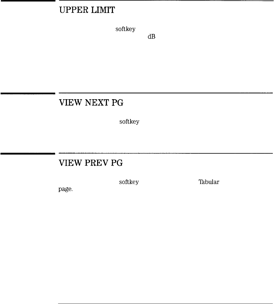
I
-
I
-
Reference
Definitions of keys
UPPER
LIMIT
The UPPER LIMIT
softkey
is used when calibrating standard devices. It
sets the acceptable deviation in
dB
between the upper limit trace and the
response of the standard device.
Related Programming
Command
ns-SDUL
VIEW
NEXT
PG
The VIEW NEXT PG
softkey
displays the next Tabular Display table’s page.
VIEW
PREV
PG
The VIEW PREV PG
softkey
displays the previous
Tabular
Display table’s
page.
8-57

I
-
I
-
Reference
Definitions of keys
VSWR
ON
OFF
The VSWR ON OFF
softkey
measures the voltage standing-wave ratio during
a reflection measurement.
Normalization must be turned on. A
moveable
marker is activated for
measuring the VSWR at any point on the displayed response. The VSWR
is defined as the ratio of the minimum and maximum voltage values on a
transmission line caused by reflections from a mismatch.
1 + reflection coefficient
VSWR
= 1 -reflection coefficient
The VSWR ON OFF function does not give measurement results during
transmission measurements.
Related Programming
Command
ns-MCT
See Also MAG
Sll
ON
OFF
in this chapter.
8-58
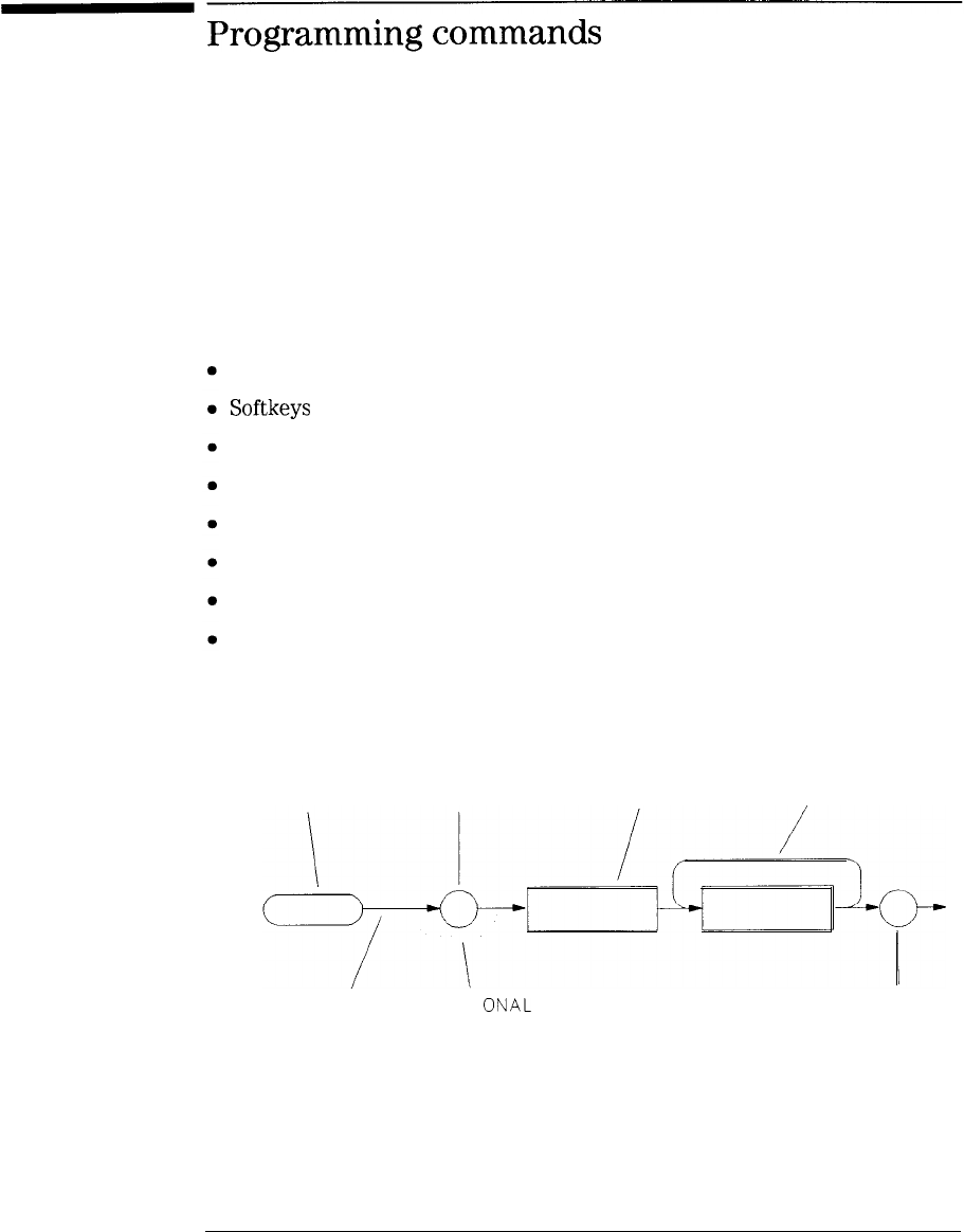
I
-
I
-
Programming
commands
This section documents each of the scalar analyzer’s remote programming
commands in alphabetical order. Included for each command is a syntax
diagram, a description, and an example. The following tables are located in
this introduction:
Preferred Scalar Measurement Commands
Softkeys
versus Programming Commands
Amplitude Commands
Calibration Commands
Display Control Commands
Instrument State Commands
Measurement Mode Commands
Source Control Commands
Each command’s syntax is represented pictorially as shown below.
CHARACTER OR
REPEAT I NG
COMMAND
SECONDARY SYNTAX
SYNTAX
MNEMON I C KEYWORD
ELEMENT ELEMENT
RECOMMENDED
OPT I
ONAL
TERMINATOR
PATH PATH
Syntax diagram shapes have the following meanings:
8-59

I
-
I
-
Reference
Programming commands
l
Narrow ovals enclose command mnemonics. The command mnemonic must
be entered exactly as shown.
l
Circles and wide ovals surround secondary keywords, or special numbers
and characters. The characters in circles and ovals are considered reserved
words and must be entered exactly as shown.
l
Rectangles contain the description of a syntax element
deEned
below the
syntax diagram.
l
A loop above a syntax element indicates that the syntax element can be
repeated.
l
Solid lines represent the recommended path.
l
Dotted lines indicate an optional path for bypassing secondary keywords.
l
Curved intersections indicate command path direction.
l
Semicolons are the recommended command terminators. Using semicolons
makes programs easier to read, prevents command misinterpretation, and
is recommended by IEEE Standard 728.
8-60
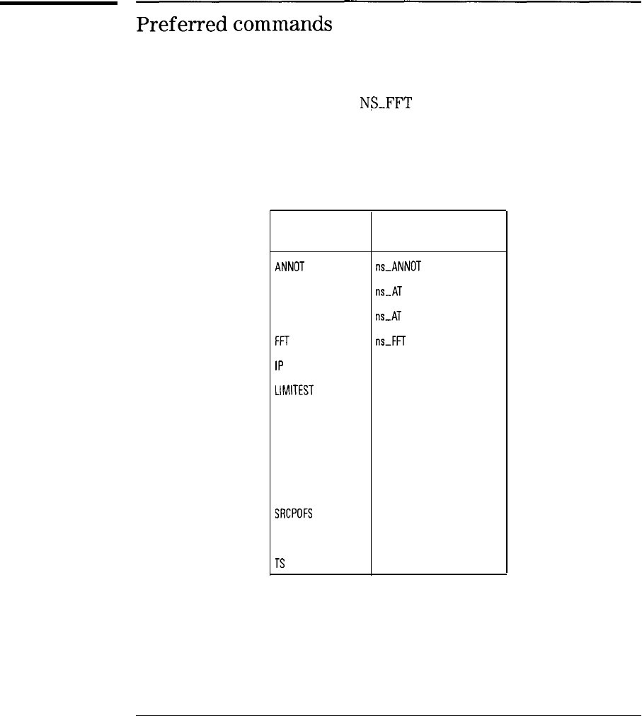
I
-
I
-
Reference
Programming commands
Preferred
commands
While the scalar measurements personality is operating, some spectrum
analyzer commands should not be used. For example, instead of the
analyzer’s FFT command, use the N$.FFT command listed in this chapter.
Using the spectrum analyzer commands may result in measurement errors.
The following table lists the spectrum analyzer commands which are replaced
by commands in this chapter.
Preferred Scalar Measurement Commands
Spectrum Analyzer Preferred Scalar Analyzer
Command Command
ANNOT
ns-ANNOT
AT
m-AT
AT AUTO
ns_AT
AUTO
FFT
ns-FFT
IP
ns-MP
LIMITEST
ns-LIMITEST
NORM ns-NORM
NRL ns-NRL
RL ns-RL
RLPOS ns-NRP
SRCPOFS
ns-SRCPOFS
SRCPWR ns-SRCPWR
TS ns-TAKESWP
8-61
I
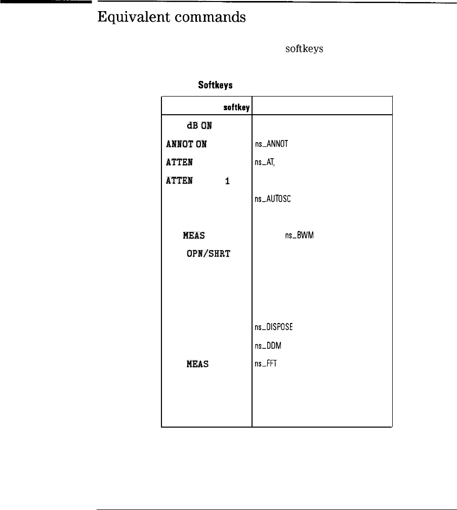
I
-
I
-
Reference
Programming commands
Equivalent
commands
The following table lists scalar analyzer
softkeys
with their equivalent or
similar programming commands.
Softkeys
versus Programming Commands
Scalar Analyzer softkey Corresponding Programming Command
120
dB
c3N
OFF
ns-EOR
ANNOT
ON
OFF
ns_ANNOT
ATTEN
AUTO MAN
ns-AT,
ns-AT AUTO
ATTEN
PORT
i
ns-EXATN
AUTOSCALE
ns-ALITOSC
AVERAGE ON
ns-TCA
BW
MEAS
ON OFF
ns-BMT,
ns_BWM
CAL
OPN/SHRT
ns-CALR
CAL STD DEVICE
ns-CALS
CAL THRU
ns-CALT
CANCEL ns-CAN
DISPOSE SCALAR
ns-OISPOSE
DUAL DSP ON OFF
ns_OOM
FFT
MEAS
ns-FFT
LIMITEST ON OFF ns-LIMITEST
LOWER BW TARGET ns-LBW
LOWER LIMIT
ns-SDLL
8-62
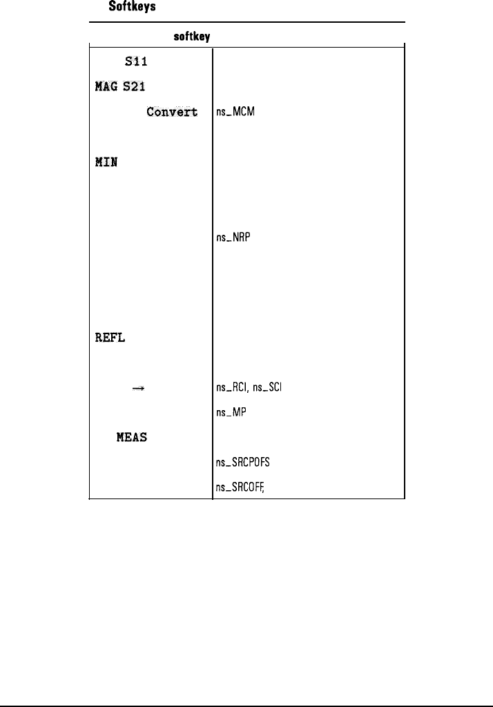
I
-
Reference
Programming commands
Softkeys
versus Programming Commands (continued)
Scalar Analyzer softkey Corresponding Programming Command
I
NAG
St1
ON OFF
MAG
521
ON OFF
Marker
Convext
MAX RNG ON OFF
fffN
RNG ON OFF
NEGATIVE ON
NORM ON OFF
NORM REF POSN
NUMBER POINTS
POSITIVE ON
REF LEVEL
REM,
SAMPLE ON
SAVE
+
CAL
SCALAR PRESET
SF
MEAS
ON OFF
SRC PWR OFFSET
SRC PWR ON OFF
ns-MCM, ns-MCT
ns-MCM, ns-MCT
ns-MCM
ns-URNG
ns-LRNG
ns-TCA
ns-NORM
ns-NRP
ns-TOP
ns-TCA
ns-RL, ns-NRL
ns-REFL
ns-TCA
ns_RCI,
ns_SCI
ns_MP
ns-BMT, ns-SFM
ns_SRCPOFS
ns-SRCOFF,
ns-SRCPWR
8-63
I-
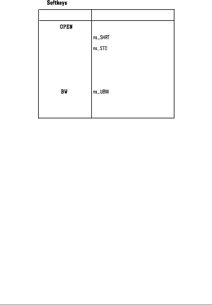
I
-
I
-
Reference
Programming commands
Softkeys versus Programming Commands (continued)
Scalar Analyzer softkry Corresponding Programming Command
STORE
OPEll
ns-OPEN
STORE SHORT
ns-SHRT
STORE STD DEV
ns-ST0
STORE THRU
ns-THRU
TABULAR ON OFF
ns-TOD
TRANS
ns-TRANS
UPPER
BW
TARGET
ns-UBW
UPPER LIMIT
ns-SOUL
VSWR ON OFF
ns-MCT
8-64
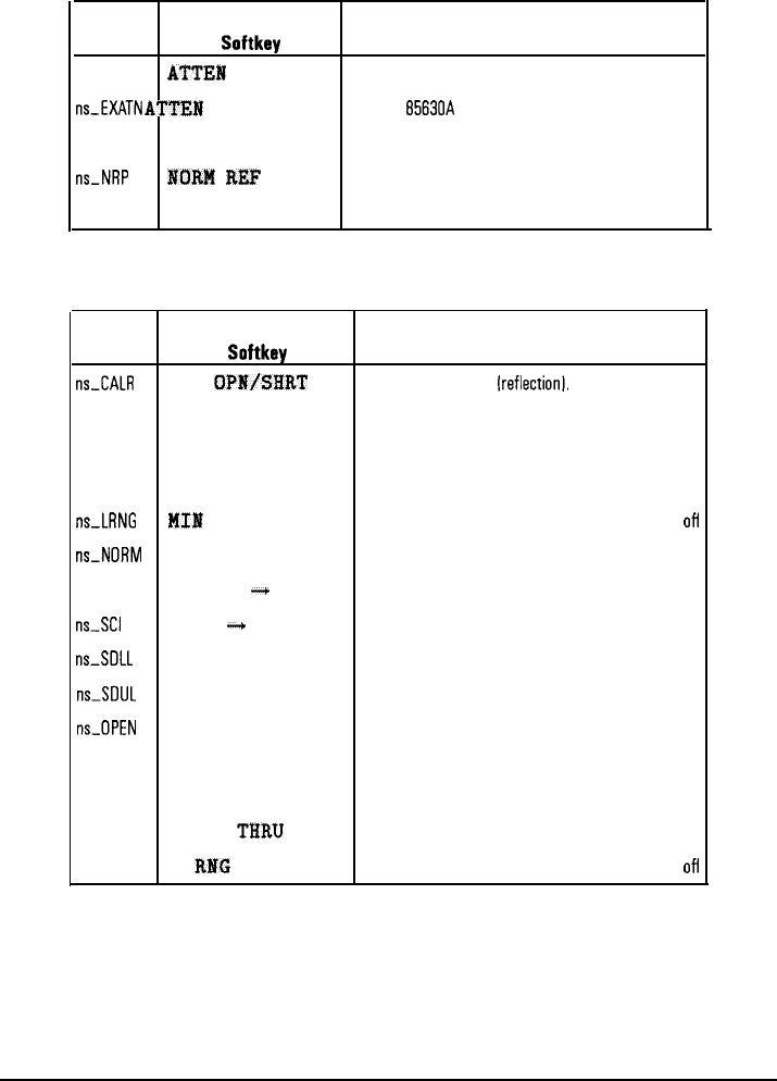
I
-
Reference
Programming commands
Amplitude commands
Command Corresponding
Description
Mnemonic
Softkey
ns-AT
ATTEN
AUTO MAN Sets the spectrum analyzer’s RF input attenuation.
ns_EXATN
ATTEN
PORT 1
Sets HP
85630A
Option 001 test set’s RF attenuator,
ns-NRL
REF LEVEL
Sets normalized reference level.
ns-NRP
NORM
RI%
POSN
Sets normalized reference position.
ns-AL
REF LEVEL
Sets the unnormalized reference level.
Calibration commands
Command Corresponding
Description
Mnemonic
Softkey
ns.CALR
CAL
OPN/SHRT
Calibrate open/short
Ireflectionl.
ns-CALS
CAL STD DEVICE
Calibrate standard device.
ns-CALT
CAL THRU
Calibrate thru (transmission].
ns-CAN
CANCEL
Cancels calibration in progress.
ns_LRNG
III
RNG ON OFF
Turns lower calibrated range limit display on or OR
ns_NORM
NORMLIZE ON OFF
Turns display normalization on or off
ns-RCI
RECALL
+
CAL
Recall calibration set internal.
ns_SCI
SAVE
4
CAL
Save calibration set internal.
ns-SILL
LOWER LIMIT
Set standard device lower limit.
ns-SDUL
UPPER LIMIT
Set standard device upper limit.
ns-OPEN
STORE OPEN
Stores open.
ns-SHRT
STORE SHORT
Stores short.
ns-STD
STORE STD DEV
Store standard device.
ns-THRU
STORE
THRU
Stores thru line measurement.
ns-URNG
MAX
RIG
ON OFF
Turns upper calibrated range limit display on or OR
8-65
I-
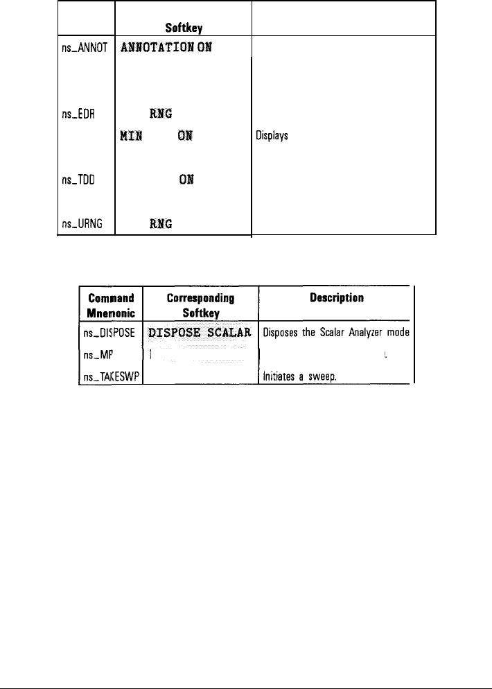
I
-
Reference
Programming commands
Command
Mnemonic
ns-ANNOT
ns-AUTOSC
ns-OOM
ns-EDR
ns-LRNG
ns-TCA
ns_TOO
ns-TOP
nsJJRNG
Display control commands
Corresponding
Softkey Description
~sl~Ol’ATIOH
01s
OFF Turns annotation on or off.
AUTOSCALE
DUAL DSP ON OFF
EXT
RBlG
ON OFF
MIN
RNG
ON
OFF
AVERAGE 0%
TABULAR
OB
OFF
NUMBER POINTS
MAX
RNG
ON OFF
Autoscales contents of trace A.
Turns dual display mode on or off.
Turns extended display range on or off.
Oisplays
lower calibrated range limit lines
Sets tabular data compression algorithm.
Turns tabular data display on or off.
Sets number of tabular data points.
Displays upper calibrated range limit lines
Instrument state commands
r
PRESET SCALAR
Presets Scalar Analyzer mode.
8-66
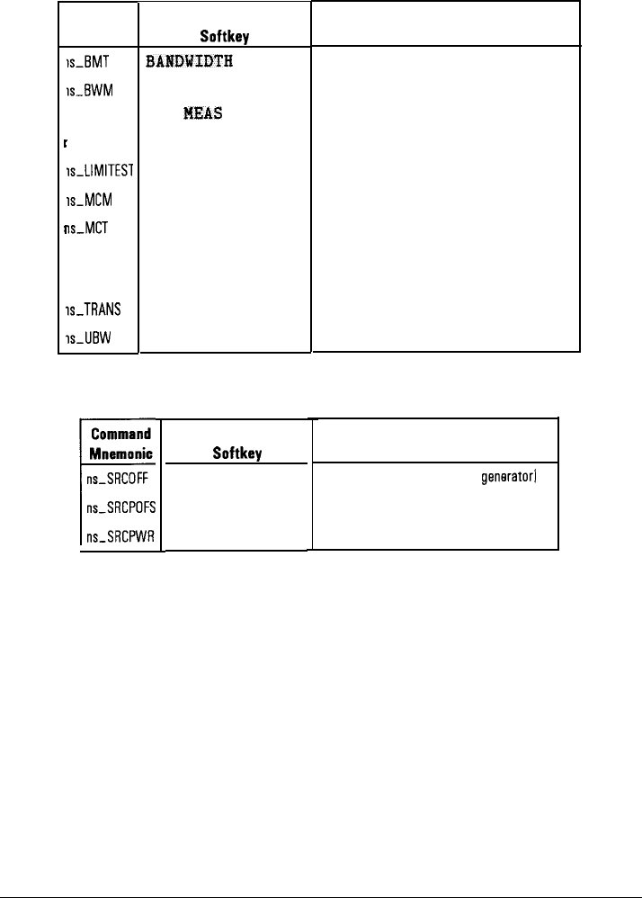
I
-
-
Reference
Programming commands
r
r
r
I
I
I
I
I
II
I
Command
Mnemonic
IS-BMT
IS-BWM
IS-FFT
IS-LBW
IS-LIMITEST
IS-MCM
IS-MCT
IS-REFL
IS-SFM
IS-TRANS
xi-UBW
Measurement mode commands
Corresponding
Softkey
l3ANDWIDTH
ON OFF
FFT
HEAS
LOWER BY TARGET
LIMITEST ON OFF
VSWR
VSWR ON OFF
REFL
TRANS
UPPER BW
Description
Defines bandwidth measurement type.
Performs bandwidth measurement.
Performs fast Fourier transform.
Defines lower bandwidth measurement level.
Turns on or off limit line display and testing.
Performs marker conversion measurements.
Oefines marker conversion measurement type.
Sets reflection measurement mode.
Performs bandwidth shape factor measurement
Sets transmission measurement mode.
Defines upper bandwidth measurement level.
Source control commands
Corresponding
Softkey
SRC PWR ON OFF
SRC PWR OFFSET
SRC PWR ON OFF
Description
Turns source power [tracking generator1 off
Sets source power offset
Turns on and sets source power
8-67
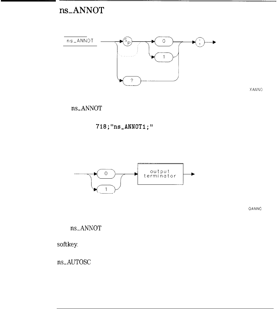
I
-
Reference
Programming commands
ns-ANNOT
ns-ANNOT
XANNO
The
ns_ANNOT
command turns screen annotation on (1) or off (0).
Example
Query Response
See also
OUTPUT
718;“ns-ANNOT
1;”
OANNO
The
ns-ANNOT
command, does not have any effect in the tabular display
mode. This command is functionally equivalent to the ANNOTATION ON OFF
softkey.
ns_AUTOSC
8-68
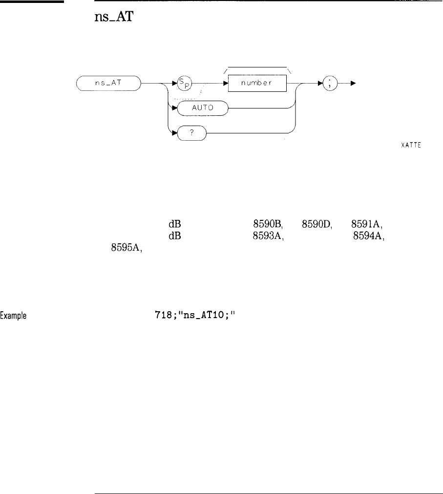
I
-
I
-
Reference
Programming commands
ns-AT
attenuation
number
AUTO
XATTE
The ns-AT command sets the spectrum analyzer’s RF input attenuation.
The parameters are as follows:
0 to 60 db in 10
dB
increments (HP
8590B,
HP
8590D,
HP
8591A,
HP 85913).
0 to 70 db in 10
dB
increments (HP
8593A,
HP 85933, HP
8594A,
HP 85943,
HP
8595A,
HP 85953, HP 85963).
Couples the input attenuator to the reference level or normalized referenced
level.
OUTPUT
718;“ns-AT
10;”
8-69
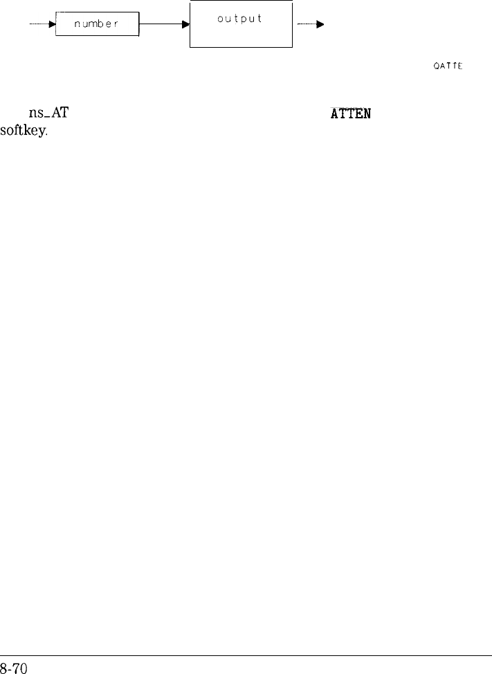
I
-
I
-
Reference
Programming commands
Query Response
See also
output
’
terminator
---+
OATTE
The
ns_AT
command is functionally equivalent to the
ATTEN
AUTO MAN
softkey.
ns-RL, ns-NRL
S-70
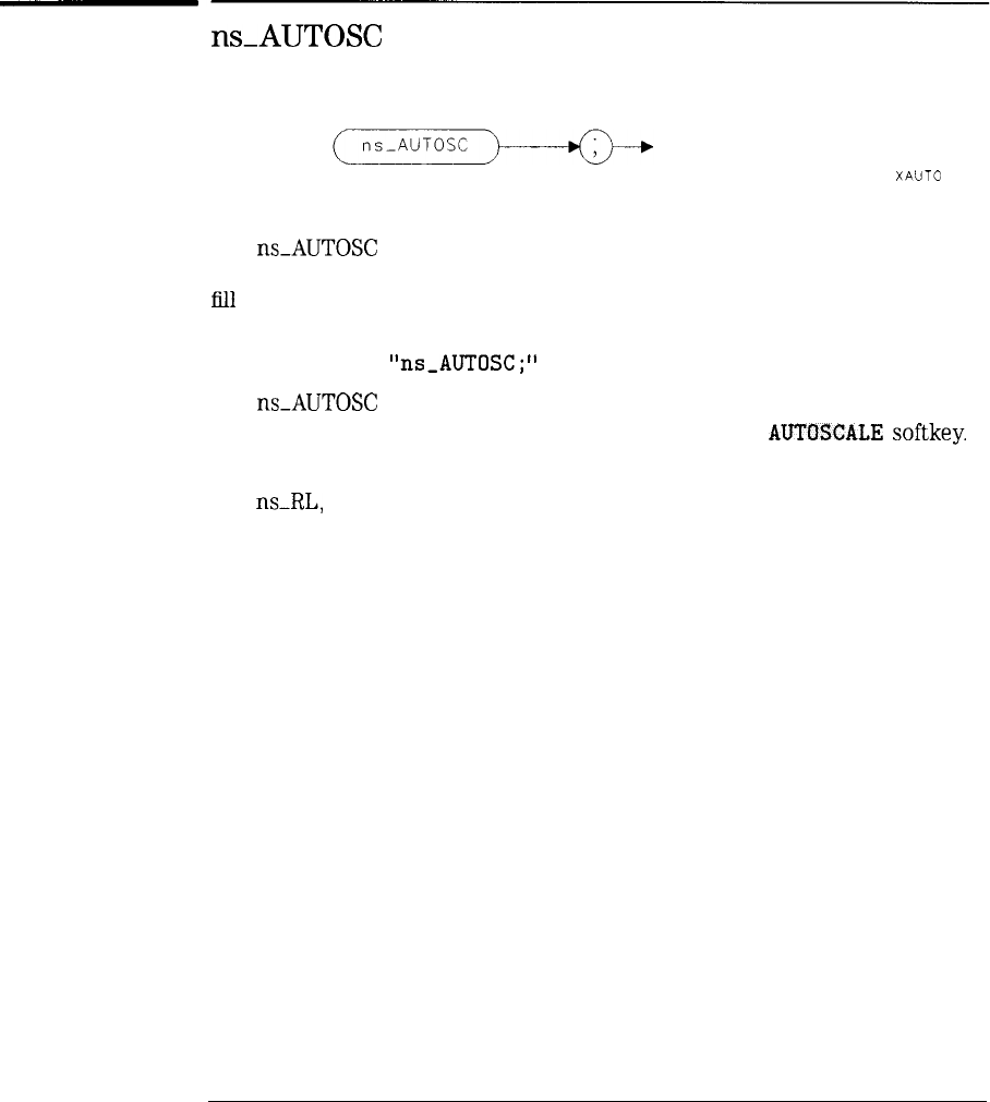
I
-
I
-
Reference
Programming commands
ns_AUTOSC
XAUTO
The
ns_AUTOSC
command performs an immediate autoscale of trace A by
adjusting the peak response to the top graticule, and setting the log scale to
El1
as much of the graticule as possible.
Example
See also
OUTPUT 718;
“ns_AUTOSC;
”
The
ns_AUTOSC
command is ignored if the dual display mode is currently
active. This command is functionally equivalent to the
AUTDSCALE
softkey.
LG,
ns_RL,
ns-NRL, ns-NRP
8-71
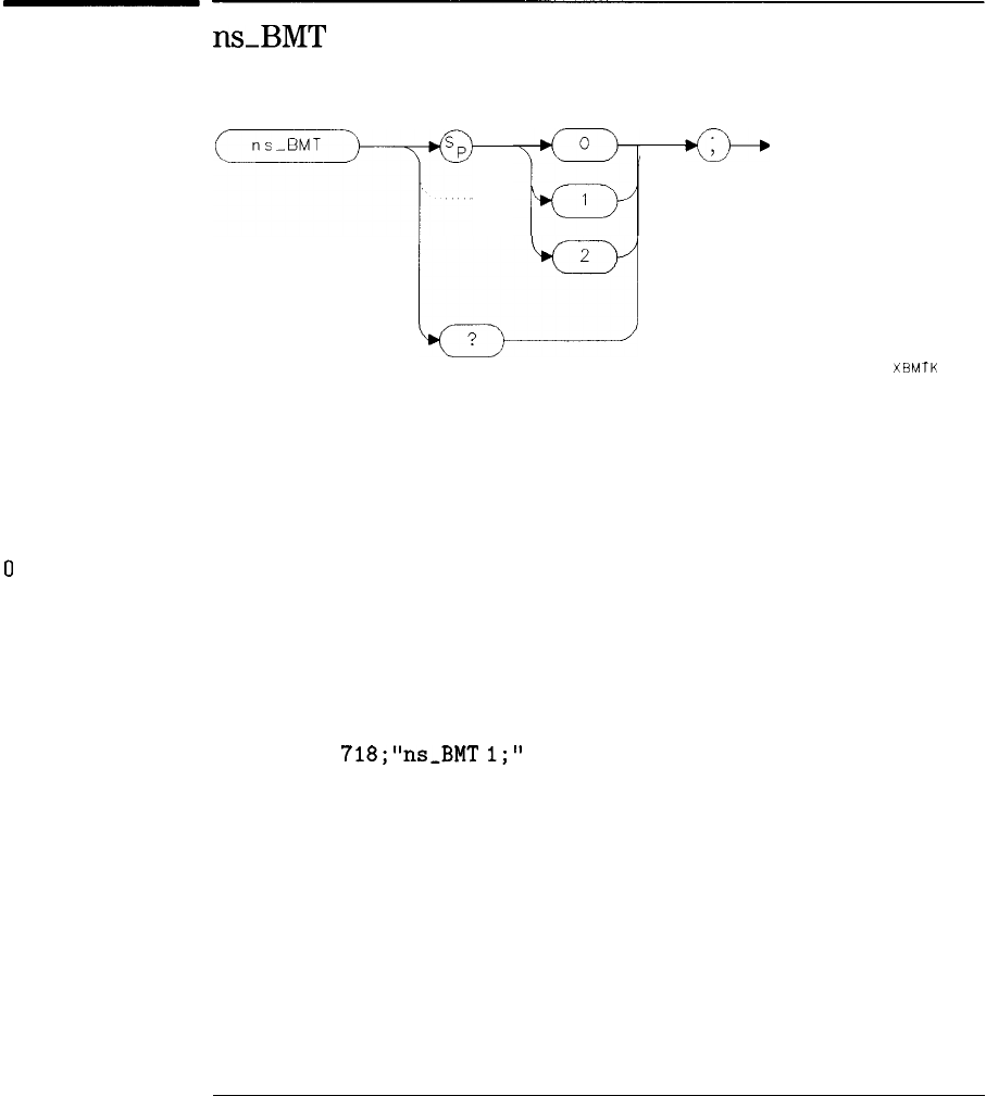
I
-
I
-
Reference
Programming commands
ns-BMT
2
!-
?
XBMTK
The ns-BMT command performs indicated marker measurement and displays
the data.
The parameters are as follows:
0
1
2
Example
No bandwidth measurement.
Measure and display center frequency, bandwidth, loss, and Q.
Measure and display shape factor.
OUTPUT
718;"ns-BMT
1;"
8-72
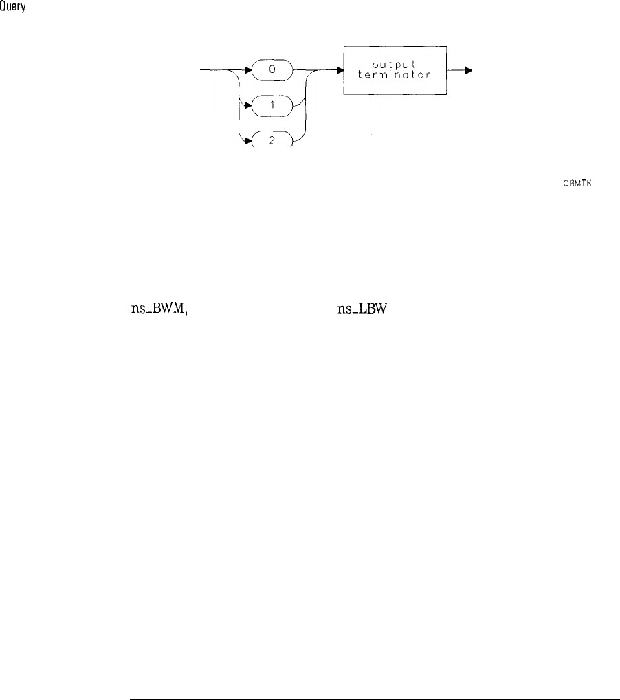
I
-
Reference
Programming commands
lluery
Response
See also
OBMTK
The ns-BMT command continues measurement at the end of every sweep, as
long as a marker remains active. The default value is 0 (zero). This command
is related to the BANDWIDTH ON OFF and SHAPE FACTOR ON OFF softkeys.
ns_BWM,
ns-SFM, ns-UBW, and
ns_LBW
8-73
-
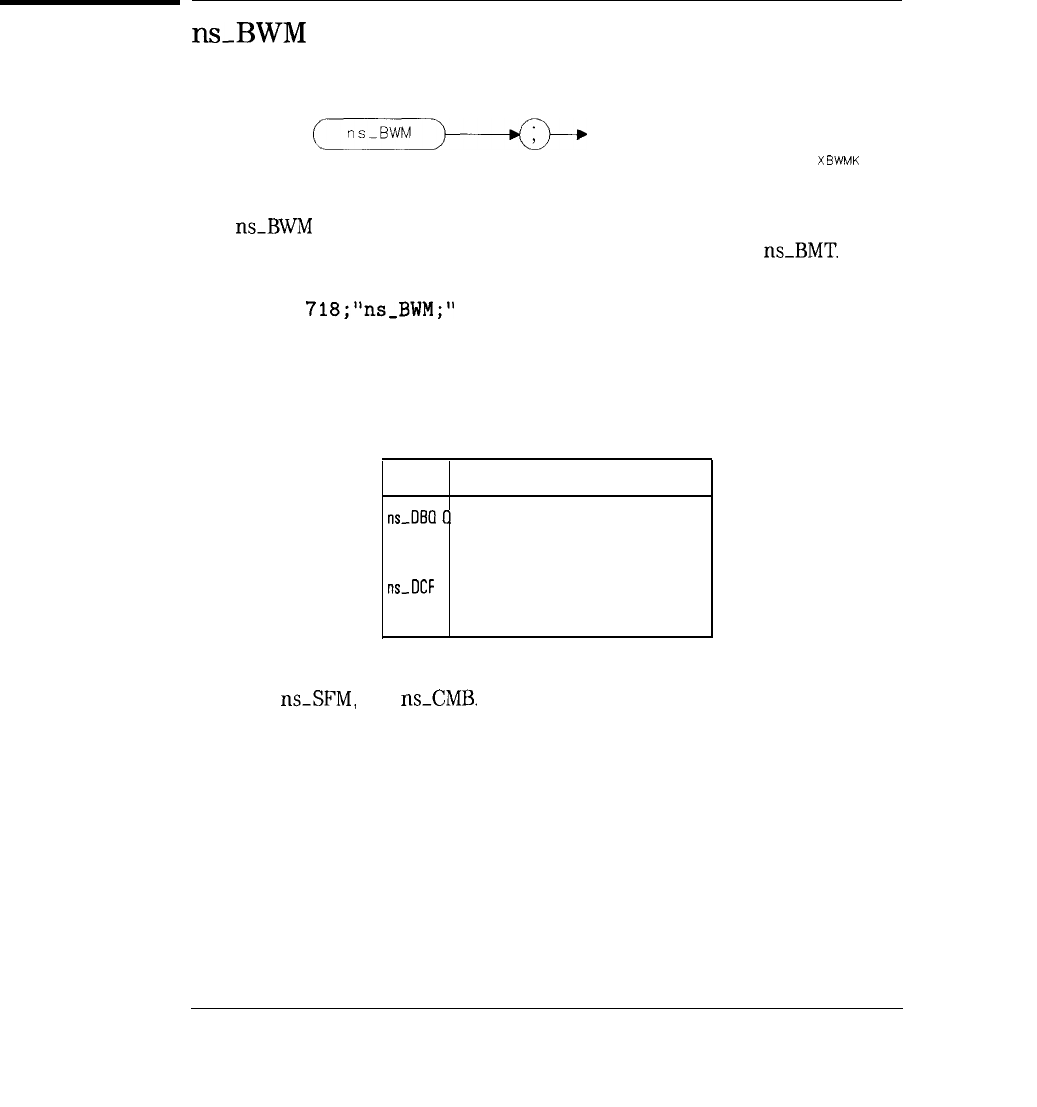
I
-
I
-
Reference
Programming commands
ns-BWM
XBWMK
The
ns_BWM
command performs an immediate center frequency, bandwidth,
insertion loss, and Q measurement regardless of the setting of
ns_BMT.
Example
See also
OUTPUT 718;“ns-BWM;”
The ns-BWM command’s resulting data is both displayed on screen and
available remotely. The insertion loss data is only measured if normalization
is active (Transmission calibration performed and normalization on).
Scalar Measurement Variables
Variable Stored Value
ns-060
11 bandwidth measurement
ns-DBW bandwidth measurement
ns_DCF
center frequency bandwidth measurement
ns-OIL insertion loss bandwidth measurement
ns-UBW,
ns_SFM,
and
nsXMB.
8-74
I
-
I
-
Reference
Programming commands
nsXALR
n
s-CALR
XCALR
The ns-CALR command initializes an open/short (reflection) calibration
Example
See also
OUTPUT 7 18
*
9-m
CALR
*
”
t
-
9
The ns-CALR command causes the display to prompt the user to connect an
open to the appropriate test port. Following the connection, An
ns_OPEN
(store open) should be immediately performed to store the measured data.
This command is functionally equivalent to the CAL
OPN/SHRT
softkey.
ns_OPEN,
ns-SHRT, and ns-CAN.
8-75
I
-
Reference
Programming commands
nsXALS
n
s-CALS
XCALS
The ns-CALS command initializes a standard device calibration
Example
See also
OUTPUT 718
*
“ns
CALS
*
”
,
-
,
The ns-CALS command causes the display to prompt the user to connect
a standard device to the appropriate port(s) for measurement and storage.
Following the connection, an immediate ns-STD should be performed in order
to store the measured data. This command is functionally equivalent to the
CAL STD DEVICE
softkey.
ns-STD.
8-76
I
-
Reference
Programming commands
ns-CALT
XCALT
The ns-CALT command initializes a thru (transmission) calibration.
Example
See also
OUTPUT 718;
“ns_CALT;
”
The
ns_CALT
command causes the display to prompt the user to connect
a thru line to the appropriate ports for measurement. Following the
connection, an immediate
ns_THRU
should be performed in order to save the
measured data. This command is functionally equivalent to the CAL THRU
softkey.
ns-THRU, ns-CAN.
I
-
I
-
Reference
Programming commands
ns-CAN
XCANK
The ns-CAN command cancels an open/short or thru calibration in process.
The
ns_CAN
command activates any valid prior calibration. This command is
functionally equivalent to the CANCEL
softkey.
Example
See also
OUTPUT
718;“ns-CAN;”
ns_CALR,
ns_CALT,
ns_OPEN,
ns-SHRT, and
ns_THRU.
8-78
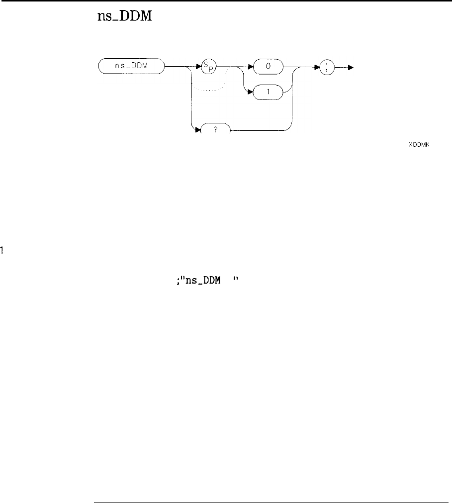
I
-
I
-
Reference
Programming commands
0
1
Example
ns-DDM
1
ti
?
XDDMK
The ns-DDM command immediately turns the dual display mode on or off.
The parameters are as follows:
Dual display mode off
Dual display mode on
OUTPUT 718
;
“ns_DDM
1;
I’
8-79
I-
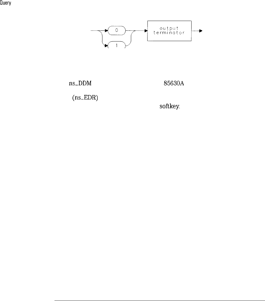
I
-
I
-
Reference
Programming commands
(luery
Response
The
ns_DDM
command requires an HP
85630A
scalar transmission/reflection
test set. This mode is not allowed in conjunction with the extended display
range
(ns_EDR)
mode. The default value is off. This command is functionally
equivalent to the DUAL DSP ON OFF
softkey.
8-80
I-
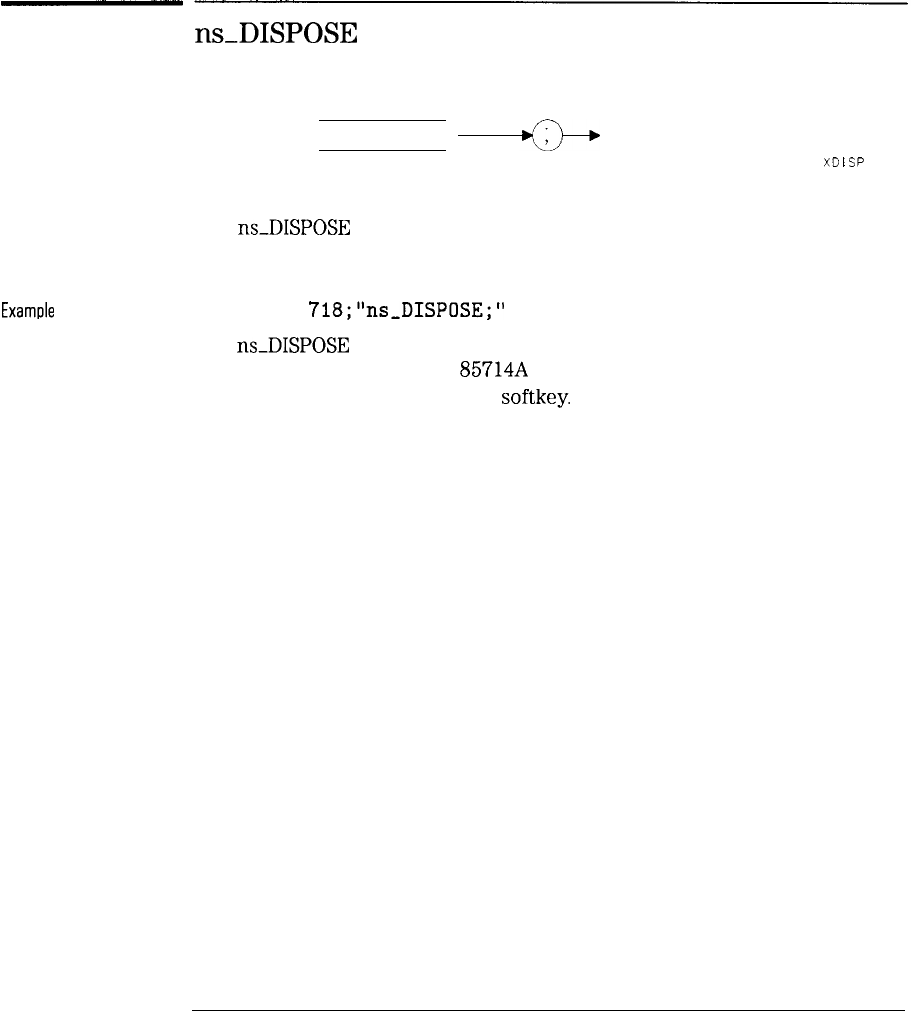
I
-
Reference
Programming commands
ns_DISPOSE
ns-DISPOSE
XD
I
SP
The
ns_DISPOSE
command immediately purges the scalar personality from
the instrument’s memory.
Examule
OUTPUT
718;"ns-DISPOSE;"
The
ns_DISPOSE
command is final. The personality is not recoverable, except
by re-installing from the HP
85714A
personality card. This command is
related to the DISPOSE SCALAR
softkey.
8-81
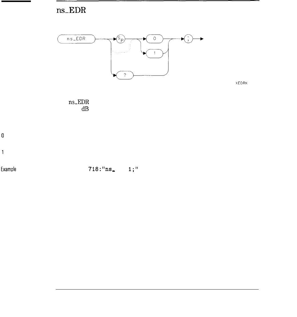
I
-
I
-
Reference
Programming commands
ns-EDR
Examule
XEDRK
The
ns_EDR
command immediately turns on or off the extended display mode
with 120
dB
of measurement range.
The parameters are as follows:
Extended display mode off.
Extended display mode on
OUTPUT
718’5s
,
-
EDR
1;”
8-82
I
-
I
-
Reference
Programming commands
lluery
Response
QEDRK
The ns-EDR command, when activating extended display mode, causes two
complete sweeps to be taken at different reference levels, and a composite
display with up to 120
dB
range is constructed. The analyzer will be left in a
state that allows marker use or hardcopy (printing or plotting). Continuous
sweeps are not allowed, except by repeatedly executing “MOV
ns_EDR,
1))
,
or “ns-TAKESWP”. When deactivated, the analyzer is returned to the state
previous to entering extended display. Extended display is not allowed if the
dual display mode is active. The default value is off.
This command is functionally equivalent to the 120
dB
OH
OFF
softkey.
See also
ns-DDM.
8-83
I
-
I
-
Reference
Programming commands
ns-EXATN
attenuation
XEXAT
The ns-EXATN command sets the input attenuation in the HP 85630 Option
001 test set.
The parameters are as follows:
Example
lluery
Response
See also
0 to 70 db in 10
dB
increments.
OUTPUT
718;"ns,EXATN
10;"
output
’
terminator
+
OEXAT
The ns-EXATN command, if the test set is not present, is ignored. This
command functionally equivalent to the
ATTEN
PORT
1
softkey.
ns-SRCPWR,
ns-SRCPOFS,
and
ns-SRCOFF.
8-84
I
-
I
-
Reference
Programming commands
ns-FFT
0
1
Example
XFFTK
The
ns_FFT
command turns the FFT mode off or on.
The parameters are as follows:
FFT mode off.
FFT mode on.
OUTPUT 718;
“ns_FFT
1;
‘I
Query Response
OFFTK
8-85
I
-
I
-
Reference
Programming commands
The ns-FFT command, when on, performs an FFT on the current trace
and the results displayed on screen. ns-FFT is designed to be used in
transforming zero span information into the frequency domain. Performing
ns-FFT on a frequency sweep will not provide time-domain results. When
turned off, the current measurement mode is restored. The frequency span
of the FFT and the sweep time are related. To determine the sweep time to
achieve a certain span width, use the following formula:
200
sweep
time
=
frequency span
The ns-FFT command is similar to the spectrum analyzer’s FFT command
with the exception the ns-FFT always applies a
FLATTOP
Iilter
window
to the fast Fourier transform. (Refer to the FFT command in the spectrum
analyzer’s programming manual for more information.) The spectrum
analyzer’s TWNDOW command cannot be used to change the window to
UNIFORM or HANNING. The
FLATTOP
filter simulates a
passband
that
represents a give-and-take between amplitude uncertainty, sensitivity, and
frequency resolution.
8-86
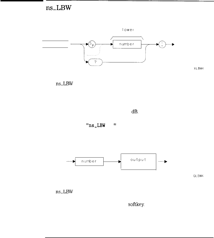
I
-
I
-
Reference
Programming commands
ns-LBW
lowef
ns-LBW
bandwidth
/
i
XLBWK
The
ns_LBW
command defines the lower (wider) target bandwidth for a shape
factor measurement.
The parameters are as follows:
number
Negative integer defining bandwidth in
dB.
Example
OUTPUT 718;
“ns_LBW
-6;
‘I
Query Response
output
’
terminator
----+
QLBWK
The
ns_LBW
command’s default value is -60. The bandwidth shape factor
is defined as the ratio (ns-UBW/ns-LBW). This command is functionally
equivalent to the LOWER BW TARGET
softkey.
See also
ns-BMT, ns-SFM, and ns-UBW.
8-87
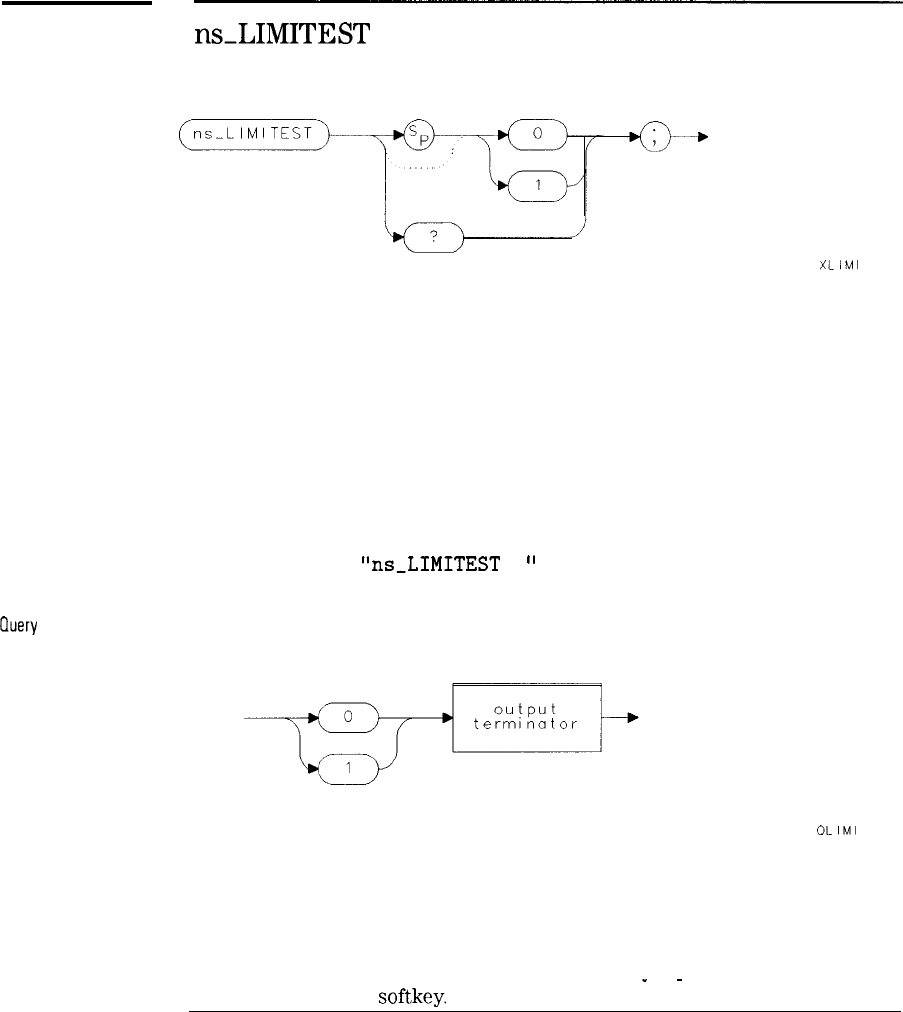
I
-
I
-
Reference
Programming commands
ns-LIMITEST
XLIMI
The ns-LIMITEST command turns the limit-line display and testing on and
Off.
The parameters are as follows:
0
Turns limit-line display and testing off.
1
Turns limit-line display and testing on.
Example
OUTPUT 718 ; “ns_LIMITEST 1;
‘I
Query
Response
OLIMI
The ns-LIMITEST command assumes limit lines are loaded and valid. (To
ensure proper placement of the limit line, be sure to set the normalized
reference position to eight before loading the limit line.) The default for
this command is off. This command is functionally equivalent to the
LIMITEST ON OFF
softkey.
8-88
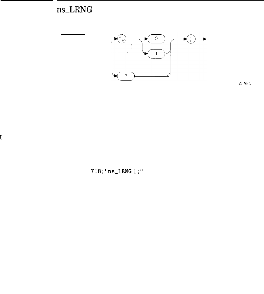
I
-
Reference
Programming commands
ns_LRNG
0
1
Example
ns-LRNG
XLRNG
The ns-LRNG command draws and displays a trace marking the lower
calibrated display limit.
The parameters are as follows:
Calibrated display limits off.
Calibrated display limits on.
OUTPUT
718;"ns-LRNG
1;"
8-89
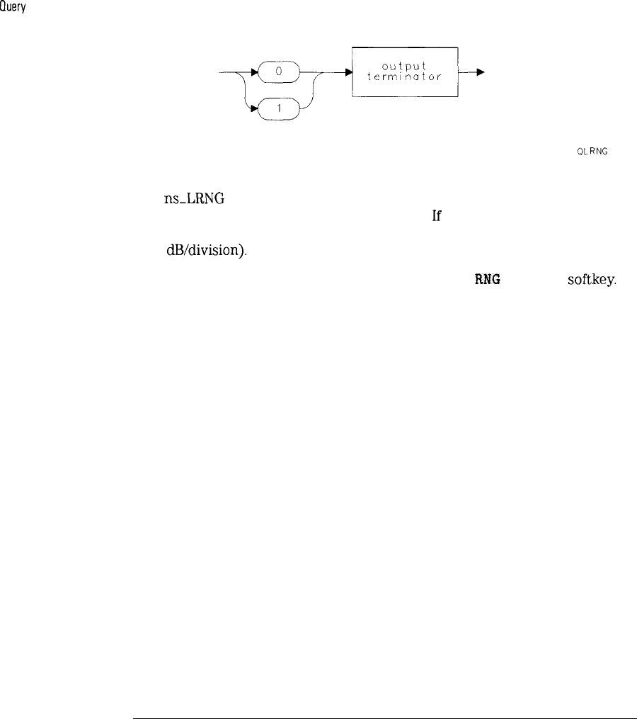
I
-
Reference
Programming commands
Ouery
Response
QLRNG
The
ns_LRNG
command is not available with the dual display or extended
display range mode active. The default is off.
lf
this level is below the
bottom graticule, it may not be visible unless the display is re-scaled
(Log
dB/division).
This command is functionally equivalent to the MIN
RNG
ON OFF
softkey.
See also
ns-URNG.
8-90
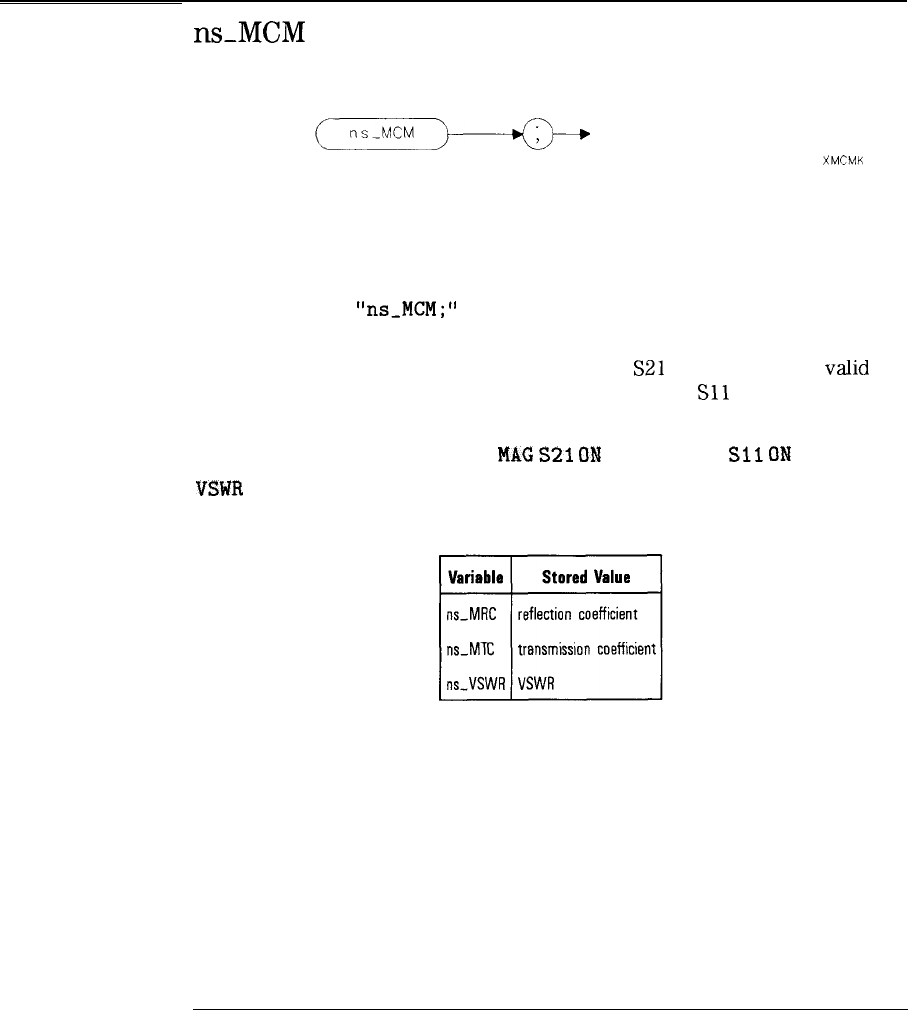
I
-
I
-
Reference
Programming commands
ns_MCM
XMCMK
The ns-MCM command immediately performs all appropriate marker
conversions and displays the results.
Example
See also
OUTPUT 718;
“ns_MCM;
‘I
The ns-MCM command resulting data is available remotely. A valid thru
(transmission) calibration is necessary for MAG
S21
conversion, as a
valid
open/short (reflection) calibration is necessary for MAG
Sll
or VSWR
conversion to be performed.
This command is related to the
WAG
S21
ON
OFF , MAG
Sil
ON
OFF and
VSWR
ON OFF softkeys.
Scalar Measurement Variables
ns-MCT.
8-91
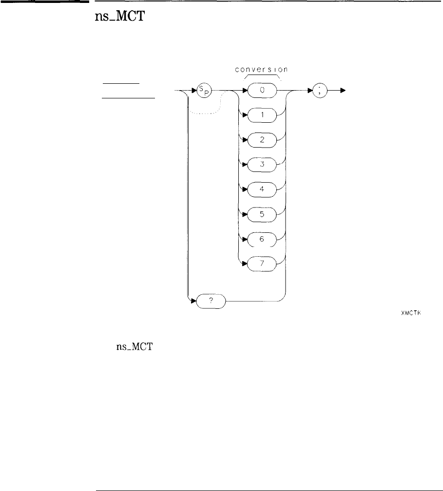
I
-
I
-
Reference
Programming commands
ns_MCT
marker
conversfon
/\
ns-MCT
XMCTK
The
ns_MCT
command defines the type of amplitude marker conversions to
be performed.
8-92
I
-
I
-
II
1
2
3
4
5
6
7
Example
Reference
Programming commands
The parameters are as follows:
All conversions off.
Convert to MAG
Sll
(Magnitude of reflection co-efficient).
Convert to VSWR (Voltage standing- wave ratio).
Convert marker to MAG
Sl
1 and VSWR.
Convert to MAG
S21
(Magnitude of reflection co-efficient).
Convert to MAG
S2
1, MAG
Sl
1 (Dual display only).
Convert to MAG
S21,
VSWR (Dual display only).
Convert to MAG
S2
1,
MAG S 11, VSWR (Dual display only).
OUTPUT
718;“ns-MCT
1;”
8-93
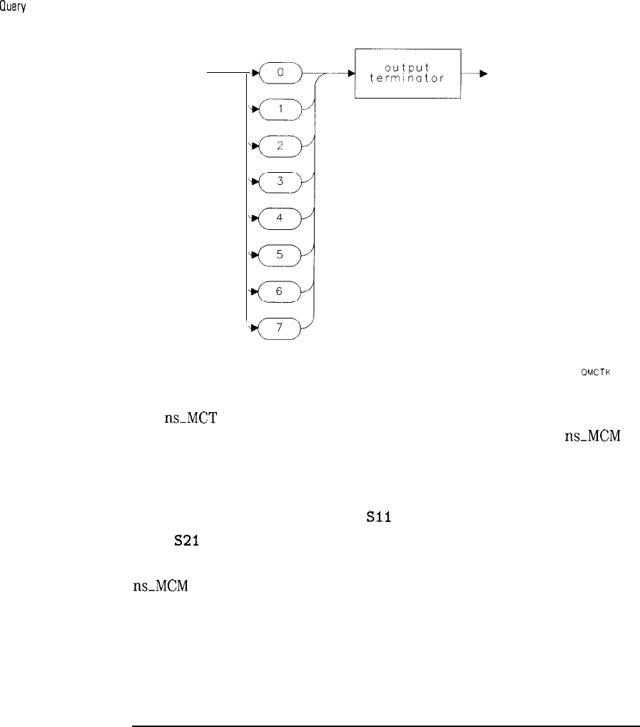
I
-
I
-
Reference
Programming commands
Query
Response
See also
OMCTK
The
ns_MCT
command marker conversions are performed only during
valid measurement conditions and calibrations as outlined for the
ns_MCM
command. The appropriate conversions will be made at the end of each
sweep, provided the marker is turned on (active). The default value is 0
(zero, all conversions off).
This command is related to the MAG
Sll
ON OFF , VSWR ON OFF , and
MAG
S21
ON OFF softkeys.
ns_MCM
8-94
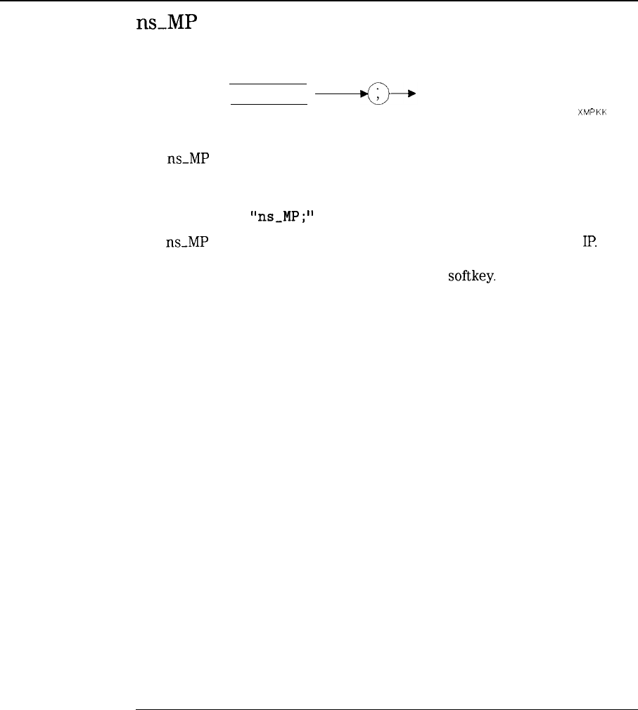
I
-
Reference
Programming commands
ns-MP
ns-MP
XMPKK
The
ns_MP
command presets the spectrum analyzer and scalar measurements
personality to a known state.
Example
OUTPUT 718;
“ns_MP;
”
The
ns_MP
command should be used in place of a spectrum analyzer
IP.
This is because IP exits the scalar measurements mode. This command is
functionally equivalent to the SCALAR PRESET
softkey.
8-95
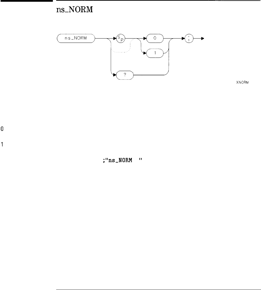
I
-
I
-
Reference
Programming commands
r-s-NORM
0
1
Example
The ns-NORM command turns normalization off or on.
The parameters are as follows:
Normalization off.
Normalization on.
OUTPUT 7 18
;
“ns_NORM
1;
‘I
Turn normalization on.
XNORM
8-96
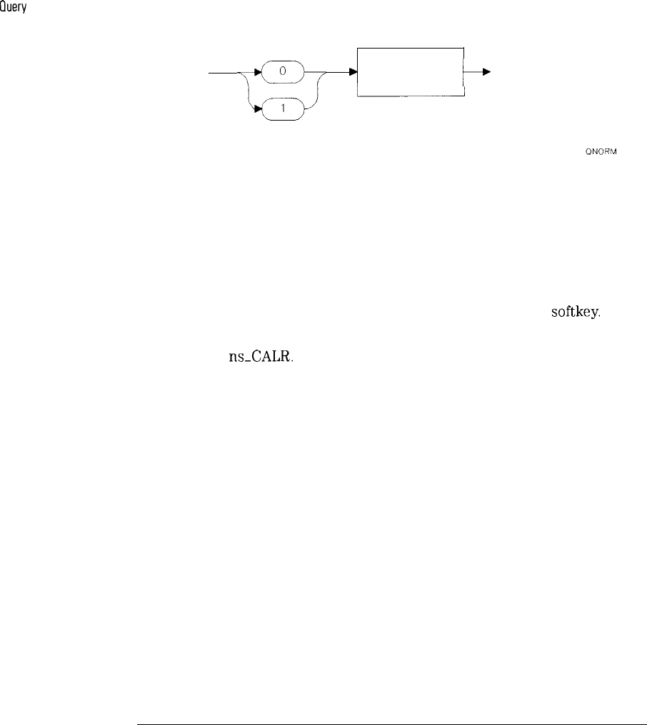
I
-
I
-
Reference
Programming commands
Query
Response
‘?a““
4
0
output
terminator
b
See also
The ns-NORM command cannot be used to turn on normalization if a valid
calibration has not been completed or recalled. Normalization is automatically
turned on at the completion of a calibration (open/short or thru). Note that
normalization is independent between the two main measurement modes
(transmission or reflection), and will be recalled appropriately when shifting
between the modes. The default for normalization is off.
This command is functionally equivalent to the NORM ON OFF
softkey.
ns-CALT and
ns_CALR.
8-97
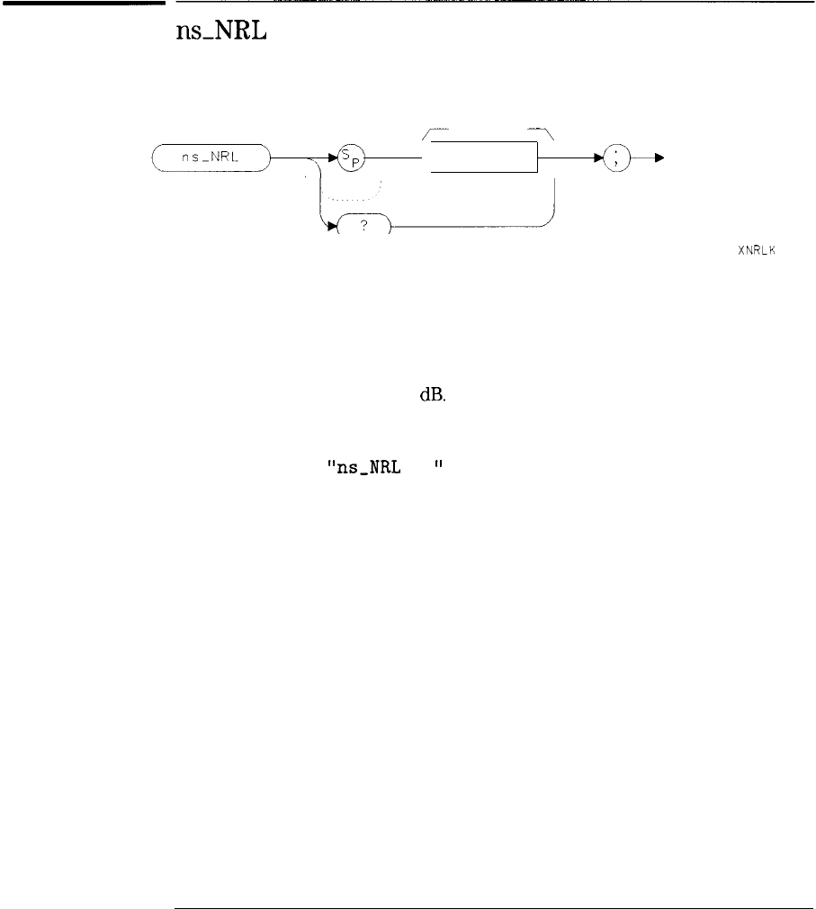
I
-
Reference
Programming commands
ns-NRL
reference
/
level
7
number
number
Example
XNRLK
The ns-NRL command changes the reference level after normalization.
The parameters are as follows:
Valid number is -200 to 200
dB.
Range is dependent on the initial reference
level setting when the calibration is performed.
OUTPUT 718;
“ns,NRL
10;
”
8-98
I
-
I
-
Reference
Programming commands
Ouery
Response
See also
ONRLK
The ns-NRL command’s default parameter is 0
dB.
After a calibration is
complete, the reference level and markers change from an absolute power
(dBm)
to relative power
(dB)
readout. The normalized reference level can be
set or changed remotely if normalization is turned off, however it will not
affect the instrument state until normalization is turned on.
This command is functionally equivalent to the
REF
LEVEL
softkey
when
normalization is on.
ns-NORM and
ns-NRP.
8-99
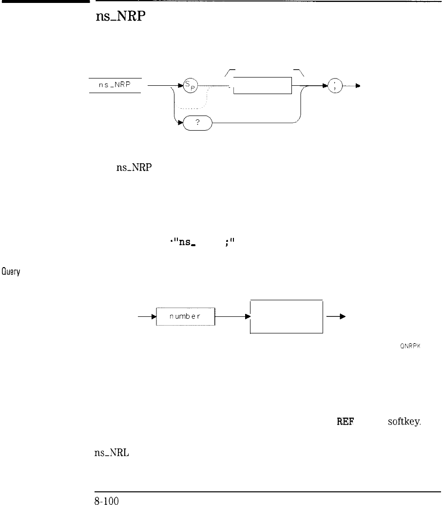
Reference
Programming commands
ns-NRP
ns_NRP
reference
r
position
\
number
number
Integer from 0 and 8.
Example
OUTPUT 7 18
-
“ns
,
-
NRP
4
*
‘I
8
Set position to middle screen.
Ouery
Response
See also
The
ns_NRP
command sets the reference position on screen.
The parameters are as follows:
output
’
terminator
+
ONRPK
The ns-NRP command is only valid if normalization is turned on. The valid
range is from 0 (zero, or bottom of graticule) to 8 (eight, or top of graticule).
The default value is 8, or top of the graticule.
This command is functionally equivalent to the NORM
REF
POSN
softkey.
ns_NRL
and ns-NORM.
S-100
I
-
I
-
Reference
Programming commands
ns-OPEN
ns-OPEN
XOPEN
The
ns_OPEN
command stores the reflection response on an open circuit
Example
See also
OUTPUT 718; “ns,OPEN;
”
The ns-OPEN command causes the display to prompt the operator to connect
a short circuit to the reflection measurement port in order to complete
a reflection calibration. This command is functionally equivalent to the
STORE OPEN
softkey.
ns_CALR,
ns-SHRT,
ns_NORM
S-101
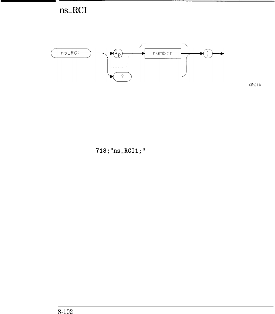
I
-
I
-
Reference
Programming commands
number
Example
ns_RCI
calibration
,,,-
register
>
XRCIK
The ns-RCI command recalls a calibration set from internal memory
The parameters are as follows:
Integer value for valid register.
OUTPUT
718;“ns-RCI
1;”
S-102
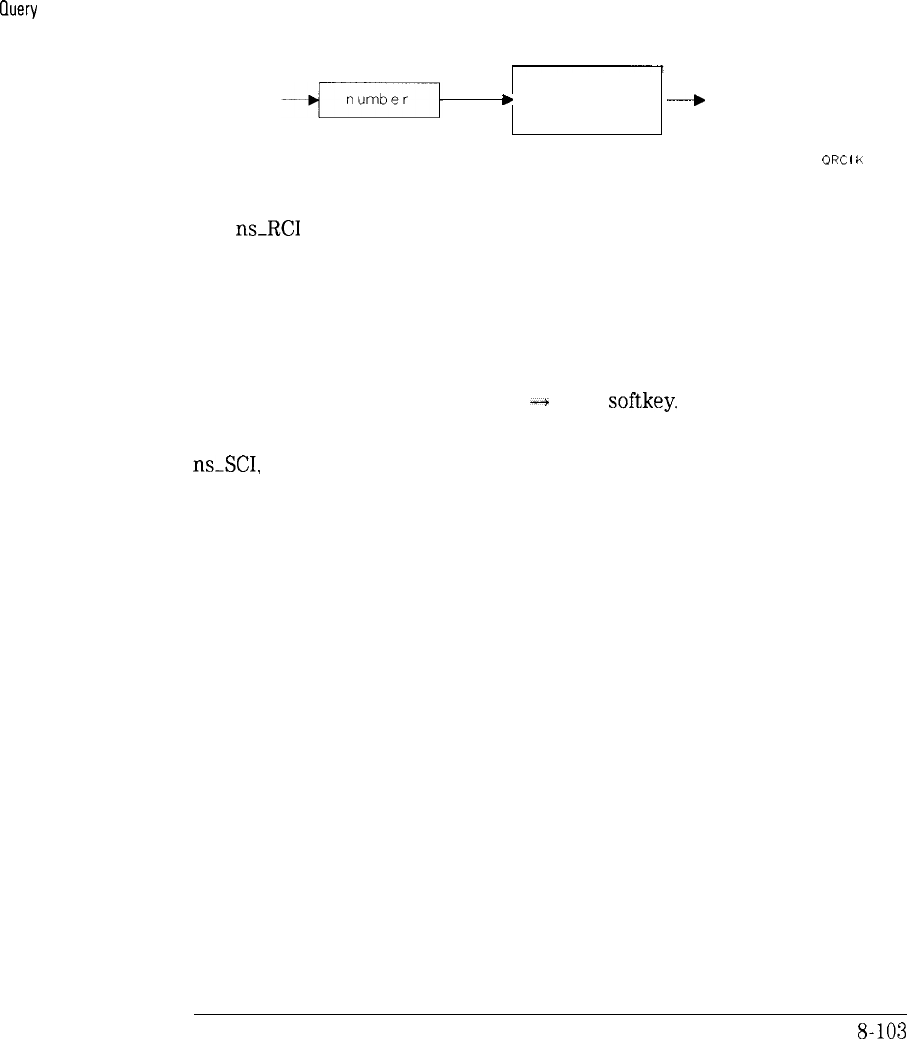
I
-
Reference
Programming commands
Ouery
Response
output
’
terminator
--+
ORC
I
K
The
ns_RCI
command recalls a complete set of transmission and reflection
calibration and instrument states are recalled. Normalization is restored,
if valid when stored. The valid range of register numbers is from 0 (zero)
to a maximum dependent on the total number of trace storage memory
available. Register zero is a special case, which recalls the instrument state
that the current cal is valid at, or the frequency span and reference level
settings which the instrument is currently calibrated for. This command is
functionally equivalent to the SAVE
-+
CAL
softkey.
See also
nsSC1,
TRCMEM
S-103
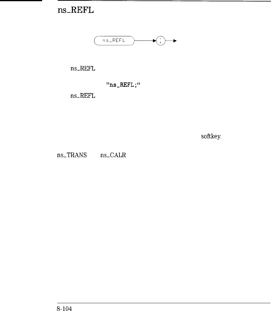
I
-
I
-
Reference
Programming commands
ns_REFL
XREFL
The
ns_REFL
command sets the reflection measurement mode.
Example
See also
OUTPUT 718; “ns_REFL;
‘I
The
ns_REFL
command restores all amplitude and frequency parameters to
the values associated with the reflection measurement, and normalization is
turned on or off appropriately. If the instrument is in the transmission mode
prior to executing this command, all frequency, amplitude and normalization
parameters are stored for future return to that mode.
This command functionally equivalent to the REFL
softkey.
ns_TRANS
and
ns_CALR
S-104
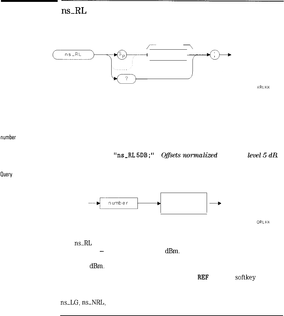
I
-
I
-
Reference
Programming commands
ns-RL
reference
r
level
7
number
Example
Ouery
Response
See also
XRLKK
The ns-RL command sets the reference level before normalization.
The parameters are as follows:
Real number expressed in integer, decimal, or exponential form.
OUTPUT 718;
“ns_RL
5DB;
‘I
Ofsets
normalized reference
level
5
dI3
output
’
terminator
--*
ORLKK
The
ns_RL
command’s range is hard limited dependent on the instrument in
use, typically
-
140 to + 50 or + 60
dBm.
If executed after normalization is
turned on, it will have no affect until normalization is turned off. The default
value is 0
dBm.
This command is functionally equivalent to the
REF
LEVEL
softkey
when
normalization is turned off.
ns-LG,
ns_NRL,
ns-NORM, and ns-NRP
8-105
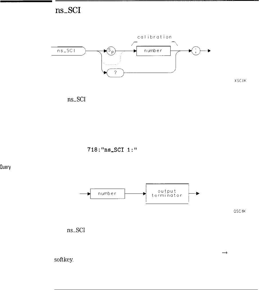
I
-
I
-
Reference
Programming commands
nsSC1
calibration
r
register
7
XSC
I
K
The
ns-SC1
command stores the current calibration set and instrument state
for both transmission and reflection measurements in the register specified.
The parameters are as follows:
number
Integer value for valid register.
Example
OUTPUT
718*"ns
,
-
SC1
1."
,
Ouery
Response
See also
QSC
I
K
The nsSC1 command stores the frequency and amplitude parameters for
each measurement mode independently. The valid range of registers is from
1 (one) to a maximum dependent on the total number of available trace
registers. This command is functionally equivalent to the SAVE
+
CAL
softkey.
ns-RCI and TRCMEM.
8-106
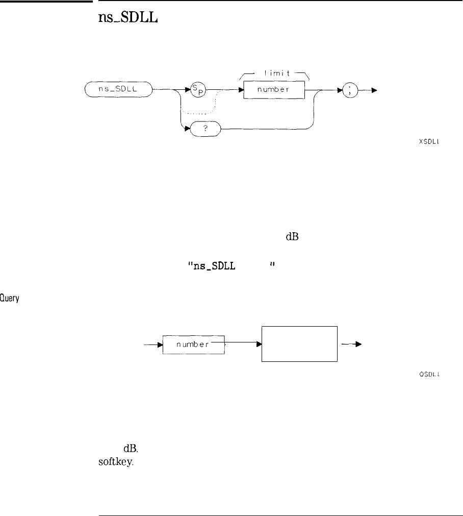
I
-
I
-
Reference
Programming commands
nsSDLL
lower
limit
7
XSDLL
The ns-SDLL command sets the lower limit for a standard device calibration
and limit test.
The parameters are as follows:
number
Negative real number between 0 to 200
dB
inclusive.
Example
OUTPUT 718;
“ns_SDLL
-60.0;
”
(luery
Response
output
’
terminator
+
OSDLL
The ns-SDLL command can set the lower limit before or after performing a
standard device calibration. The lower limit is added to the standard device
response and then transferred to the lower limit line. The default value
is -3
dB.
This command is functionally equivalent to the LOWER LIMIT
softkey.
See also
ns-SDUL and ns-STD
8-107
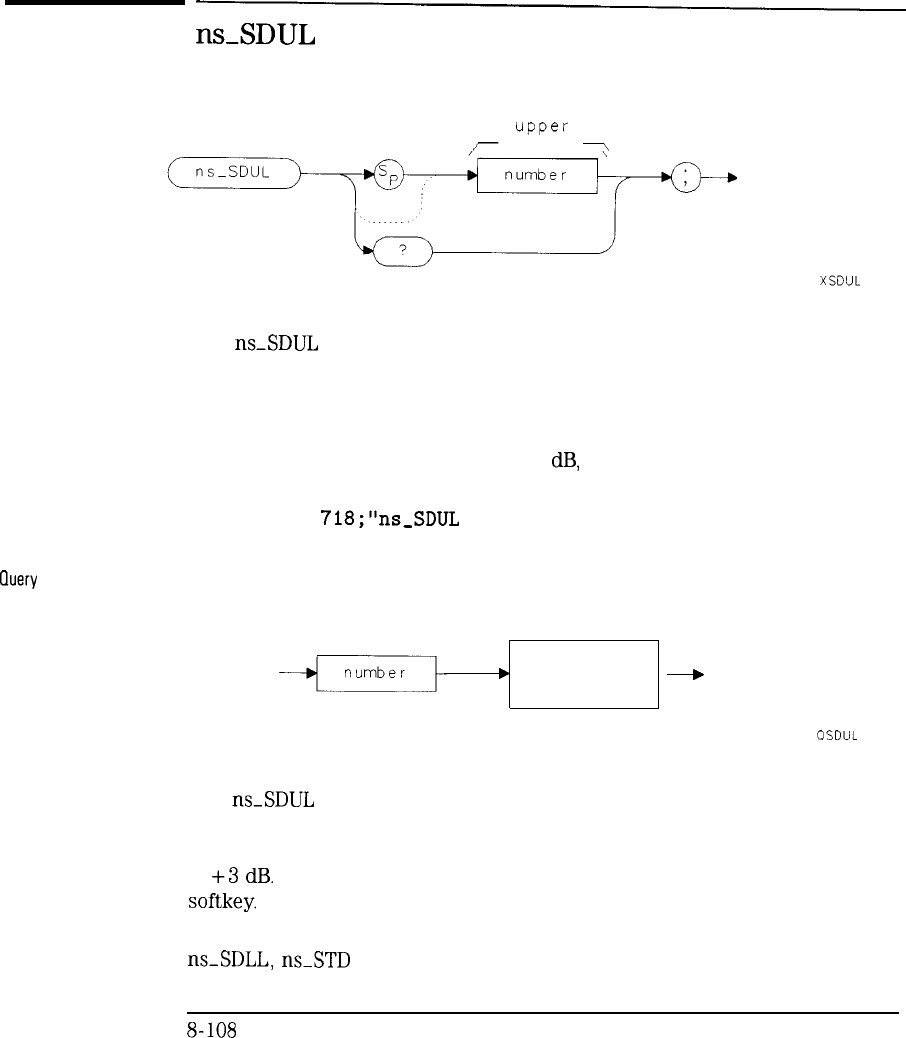
I
-
Reference
Programming commands
ns.SDUL
upper
limit
7
The
ns-SDUL
command sets the upper limit for a standard device calibration
and limit test.
The parameters are as follows:
number
Example
Ouery
Response
See also
Positive real number between 0 to 200
dB,
inclusive.
OUTPUT 718;“ns,SDUL 10.0;”
output
’
terminator
+
OSDUL
The
ns_SDUL
command can set the upper limit before or after performing a
standard device calibration. The upper limit is added to the standard device
response and then transferred to the upper limit line. The default value
is
+3
dB.
This command is functionally equivalent to the UPPER LIMIT
softkey.
ns_SDLL,
nsSTD
B-108
I
-
I
-
Reference
Programming commands
ns-SFM
ns-SFM
XSFMK
The ns-SFM command immediately performs a single bandwidth shape factor
measurement.
Example
See also
OUTPUT 7 18
*
“ns
SFM
*
”
.
-
9
The
ns_SFM
measurement results are displayed on screen as well as being
available remotely. The shape factor is defined as the ratio
ns-LBW/ns-UBW.
Scalar Measurement Variables
ns-UBW, ns-LBW, ns-BMF, and ns-CMB
8-109
I
-
I
-
Reference
Programming commands
ns-SHRT
XSHRT
The ns-SHRT command stores the reflection response of a short circuit.
Example
See also
OUTPUT 718
*
“ns
SHRT
*
I’
t
-
,
The
ns_SHRT
command causes the scalar measurement personality to
perform an average with the previously stored open circuit response, then
stores the results for reflection normalization purposes. Normalization is
turned on.
This command is functionally equivalent to the STORE SHORT
softkey.
ns_CALR,
ns-OPEN, ns-NORM
8-110
I
-
I
-
Reference
Programming commands
ns-SRCOFF
XCOFF
Example
See also
The
ns_SRCOFF
command immediately turns the source RF output power off.
OUTPUT 718 ; “ns,SRCOFF
;
”
ns-SRCPWR
a-111
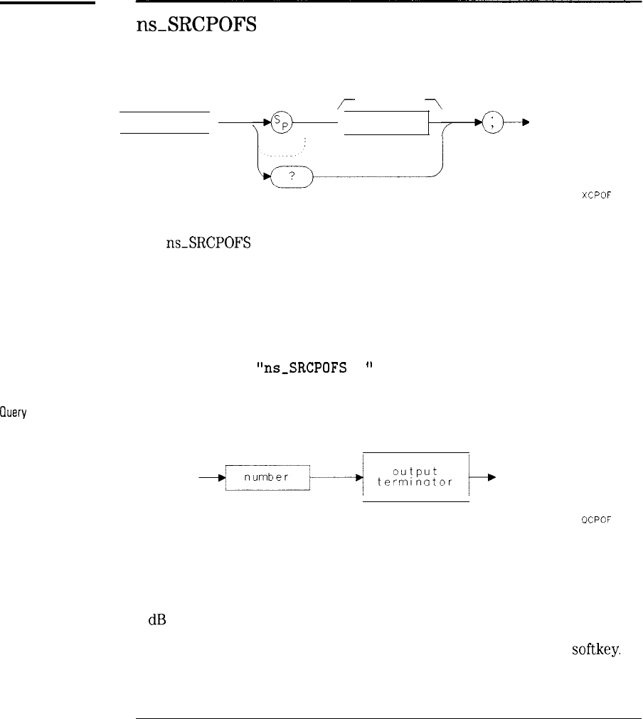
I
-
I
-
Reference
Programming commands
nsSRCPOFS
ns-SRCPOFS
power
r
offset
7
number
XCPOF
number
Real number expressed in integer, decimal, or exponential form.
Example
OUTPUT 718;
“ns_SRCPOFS
5;
”
(luery
Response
The nsSRCPOFS command allows the displayed source output power to be
offset from the actual source output power.
The parameters are as follows:
OCPOF
The ns-SRCPOFS command adds the offset to the current source level and is
displayed. Once set, the offset is subtracted from any incoming source power
level adjustment before setting the actual output power level. The default is
0
dB
(no offset).
This command is functionally equivalent to the SRC PWR OFFSET
softkey.
8-112
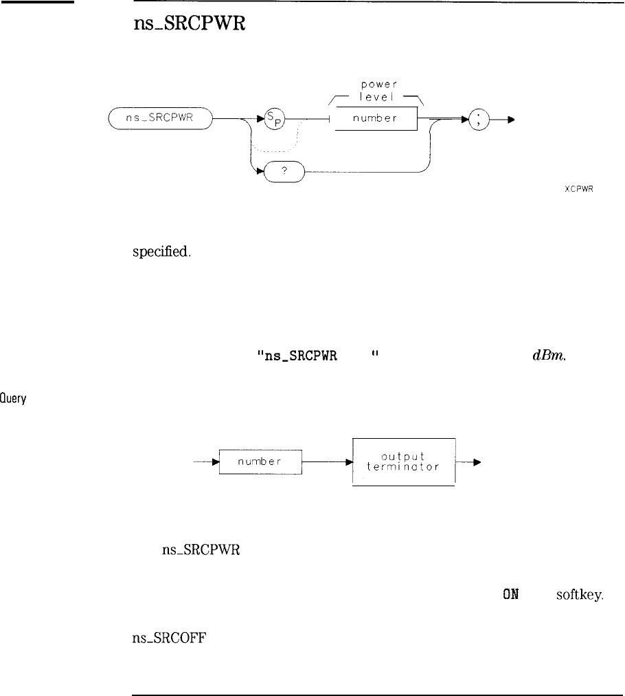
I
-
I
-
Reference
Programming commands
nsSRCPWR
power
r
level
7
number
XCPWR
The ns-SRCPWR command sets the source output power to the level
specihed.
The parameters are as follows:
number
Example
tluery
Response
See also
Real number expressed in integer, decimal, or exponential form.
OUTPUT 718;
“ns_SRCPWR
-5.5;
‘I
Source power to -5.5
dBm.
The
ns_SRCPWR
command turns the source on if the source is turned off.
The range is dependent on the instrument, and is hard limited accordingly,
This command is functionally equivalent to the SRC PWR
ON
OFF
softkey.
nsSRCOFF and ns-SRCPOFS.
8-113
I
-
I
-
Reference
Programming commands
ns-STD
ns-STD
XSTDK
The
nsSTD
command stores the response of a standard device.
Example
See also
OUTPUT
718;“ns-STD;”
The ns-STD command causes the scalar measurement personality to add the
upper and lower test limits, and transfer the results to upper and lower limit
line traces. Limit test is then activated. Note that the stored limit lines are
traces, and therefore cannot be edited as normal limit lines can.
This command is functionally equivalent to the STORE STD DEV
softkey.
ns-CALS,
nsSDLL,
ns-SDUL, and LIMITLINES.
8-114

I
-
I
-
Reference
Programming commands
ns_TAKESWP
ns-TAKESWP
XTAKE
The ns-TAKESWP command replaces the instrument’s TS command.
Example
See also
OUTPUT 718;“ns-TAKESWP;”
The ns-TAKESWP command properly completes sweeps if the extended
display range (ns-EDR) or dual display mode (ns-DDM) are active. If these
modes are not active, a normal TS is generated.
ns-DDM, ns-EDR
8-115
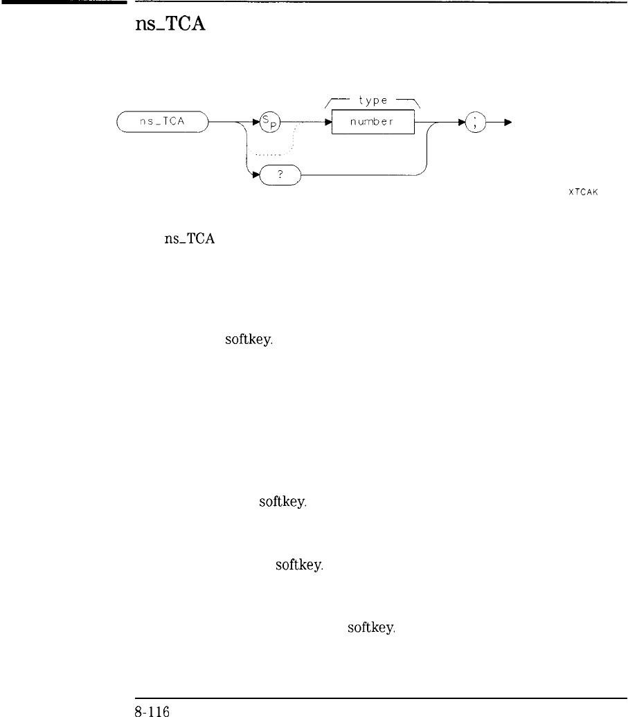
I
-
Reference
Programming commands
ns-TCA
I
-
Average
Normal
Negative
Positive
compression
r
type
7
XTCAK
The
ns_TCA
command sets the compression algorithm to be used when
compressing the tabular data trace.
The parameters are as follows:
The average of the points within an interval are used. Equivalent to the
AVERAGE ON softkey.
The compressed value of the interval is computed using a Rosenfell algorithm.
If the data within the interval is continuously rising, the compressed value
taken is the maximum (last) value within the interval. If the data within the
interval is continuously falling, the compressed value taken is the minimum
(last) value within the interval. If the data within the average is not
continuously rising OR falling, the compressed value will alternate between
the maximum and minimum value detected within the intervals. Equivalent
to the NORMAL ON softkey.
The compressed value taken is the lowest value from the interval. Equivalent
to the NEGATIVE ON
softkey.
The compressed value taken is the highest value from within the interval.
Equivalent to the POSITIVE ON
softkey.
8-116
I
-
I
-
Sample
Example
Query
Response
See also
Reference
Programming commands
The compressed value taken is the last value from the interval. Equivalent to
the SAMPLE ON
softkey.
OUTPUT 718
*
“ns
,
-
TCA
1.
I’
,
output
l terminator
+
QTCAK
The
ns_TCA
command changes the compression type from the default of
sample. As the number of displayed tabular data points can be fewer than
the actual data trace length (401 points), the compression algorithm defines
how the data is compressed.
ns-TDD and ns-TDP.
8-117
-1
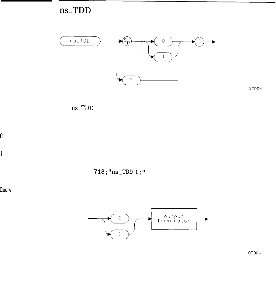
I
-
Reference
Programming commands
ns-TDD
0
1
Example
Cluery
Response
The
ns_TDD
command turns the tabular data display off or on.
The parameters are as follows:
XTDDK
Tabular data display off.
Tabular data display on.
OUTPUT
718;"ns-TDD
1;"
II
OTDDK
8-118

I
-
I
-
See also
Reference
Programming commands
The ns-TDD command is equivalent to the TABULAR ON OFF
softkey.
When
tabular data is activated, a sweep is taken and the resulting data compressed
as per the setting of
ns_TCA.
After compression, the data is displayed on
screen. Continuous sweeps are not allowed except by repeatedly executing
MOV
ns_TDD,
1 or
ns_TAKESWP.
ns_TCA,
ns_TDP
8-119
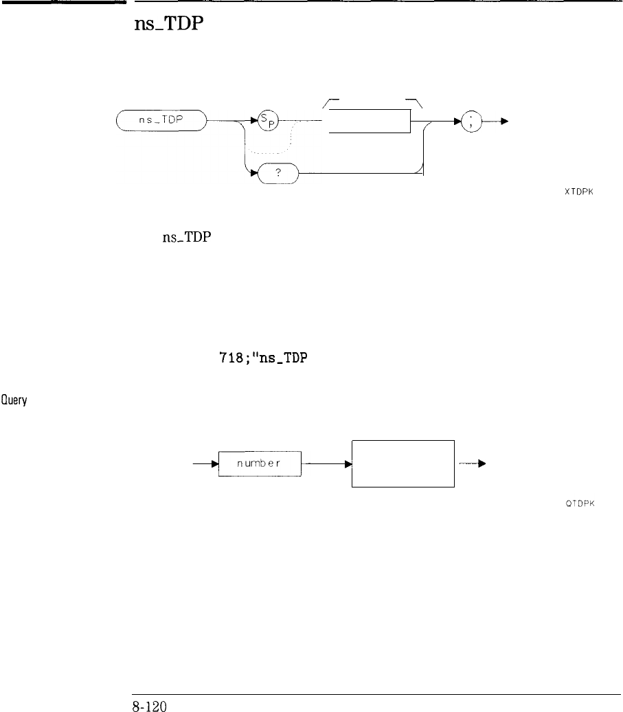
Reference
Programming commands
ns-TDP
data
r
points
7
number
f
XTDPK
The
ns_TDP
command sets the number of points available for a tabular data
display.
The parameters are as follows:
number
Example
lluery
Response
Integer from 3 through 401.
OUTPUT
718;“ns-TDP
256;”
output
c
terminator
----+
B-120

I
-
I
-
See also
Reference
Programming commands
The
ns_TDP
command can be used to change the default of 401 trace
points. The actual data trace (401 points) is compressed, via the algorithm
determined by ns-TCA, into a trace of length ns-TDP. Only 18 points can be
displayed simultaneously on screen, but the whole trace (ns-TDP in length)
is output to a printer if the copy key is pressed and tabular data display is
turned on.
This command is functionally equivalent to the NUMBER POINTS
softkey.
ns-TCA and
ns_TDD.
B-121
-
I
-
I
-
Reference
Programming commands
ns-THRU
XTHRU
The
ns_THRU
command stores the thru transmission measurement for
normalization purposes.
Example
See also
OUTPUT 718;
“ns_THRU;
”
The
ns_THRU
command causes normalization to be turned on. This command
is functionally equivalent to the STORE THRU
softkey.
ns-CALT, ns-NORM
8-122
I-
I
-
I
-
Reference
Programming commands
ns-TRANS
ns_TRANS
XTRAN
The ns-TRANS command sets the transmission measurement mode.
Example
See also
OUTPUT
718;“ns-TRANS;”
The
ns-TRANS
command restores all amplitude and frequency parameters to
the values associated with the transmission measurement, and normalization
is turned on or off appropriately. If the instrument is in the reflection mode
prior to executing this command, all frequency, amplitude and normalization
parameters are stored for future return to that mode.
This command functionally equivalent to the TRANS
softkey.
ns-REFL and
ns_CALT
8-123
-
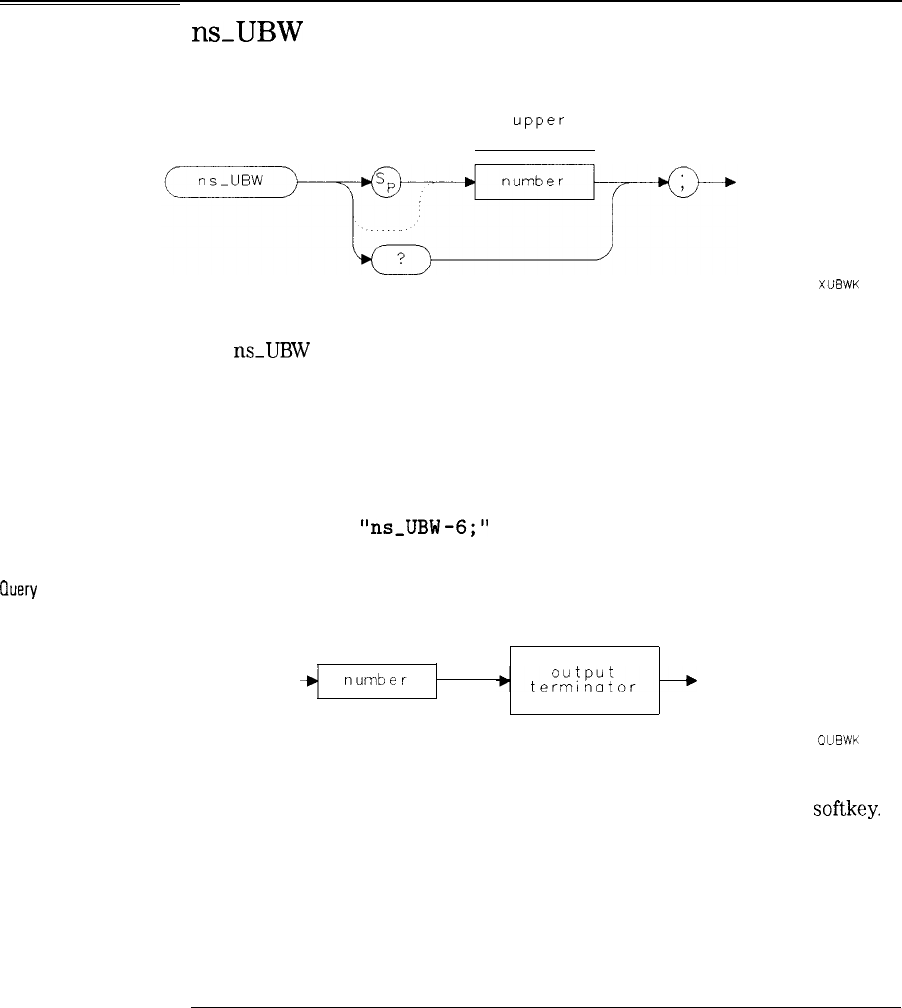
I
-
I
-
Reference
Programming commands
ns-UBW
upper
bandwidth
number
Example
Query
Response
See also
XUBWK
The
ns_UBW
command sets the target bandwidth used for either a bandwidth
measurement or shape factor measurement (upper bandwidth).
The parameters are as follows:
Negative real.
OUTPUT 718;
"ns_UBW
-6;"
OUBWK
The ns-UBW command is functionally equivalent to the UPPER BW
softkey.
The default bandwidth is -3.
ns-BMT, ns-BWM, ns-SFM, and ns-LBW.
8-124
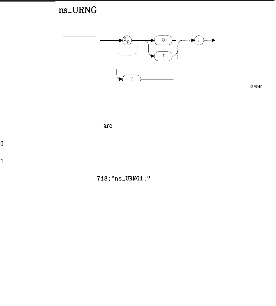
I
-
I
-
Reference
Programming commands
0
1
Example
ns_URNG
ns-URNG
-GYP
i
XURNG
The ns-URNG command draws and displays a trace marking the upper
calibrated display limit.
The parameters are as follows:
Calibrated display limit off.
Calibrated display limit on.
OUTPUT
718;“ns-URNG
1;”
8-125
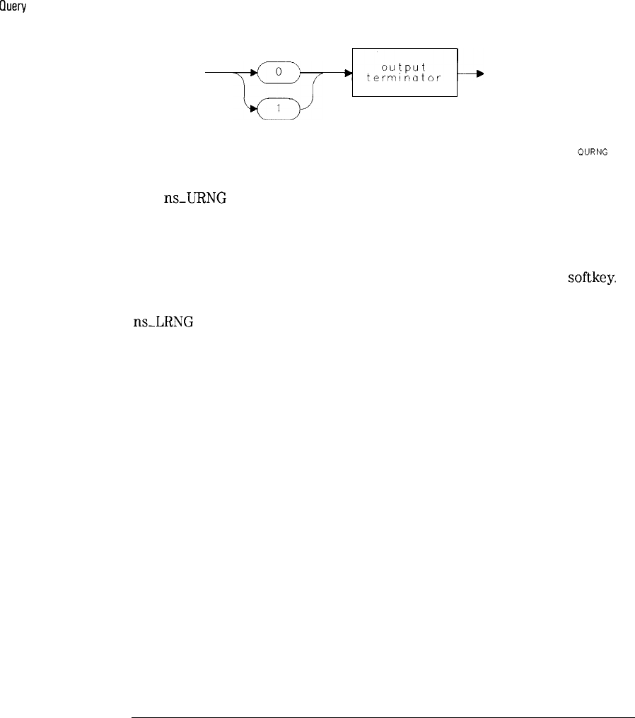
I
-
I
-
Reference
Programming commands
Ouery
Response
See also
The
ns_URNG
command is not available with the dual display or extended
display range mode active. If this level is above the top graticule, it may not
be visible unless the display is re-scaled (Log dB/division) or the reference
level adjusted. The default is off.
This command is functionally equivalent to the MAX RNG ON OFF
softkey.
ns_LRNG
8-126

I
-
I
-
Characteristics
Characteristics provide information about non-warranted instrument
performance in the form of nominal values. These values are bases
on estimated worst-case system performance. Characteristics are
not
specifications. The characteristics in this section are for systems which
include the following:
0
a spectrum analyzer (Option 010)
l
an HP
85630A
scalar transmission/reflection test set
l
an HP
85714A
scalar measurements personality
8-127
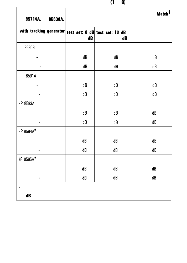
I
-
I
-
Reference
Characteristics
HP 8590 A and B Series
System Characteristics
(1
of
81
Configuration: PORT 1 Source Match
PORT 2 Input Match*
HP g5714A. HP g5630A.
and spectrum analyzer Attenuation (where applicable)
with
tracking
generator
test
set:
0
dB
test
set:
lo
d6
option
source: 0
dB
or source: 10
dB
HP
85908
Opt. 003
0.3 - 1200 MHz 16.3
dB
18.2
dB
15.3
dB
1200
-
1800 MHz 15.7
dB
17.5
d6
12.0
dB
HP
8591A
0.3 - 1200 MHz 16.3
dB
18.2
dB
15.3
dB
1200
-
1800 MHz 15.7
dB
17.5
dB
12.0
dB
iP
8593A
0.3 . 1200 MHz 16.9
dB
19.2
dB
14.6
d6
1200
-
2900 MHz 16.3
dB
18.5
dB
11.8
dB
iP
8594A*
0.3
-
1200 MHz 16.9
dB
19.2
dB
15.3
dB
1200
-
2900 MHz 16.3
dB
18.5
dB
12.0
dB
1P
8595A*
0.3
-
1200 MHz 16.9
dB
19.2
dB
15.3
dB
1200 - 2900 MHz 16.3
dB
18.5
dB
12.0
dB
k
DC coupled signal analyzer input
1
10
dB
signal analyzer
input attenuation
8-128
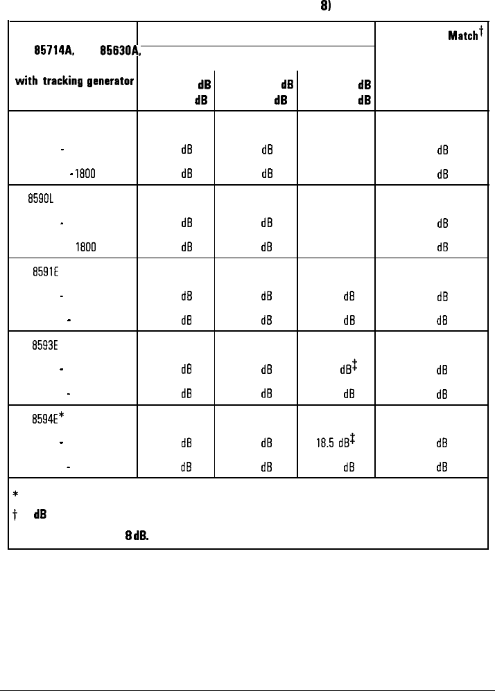
I
-
I
-
Reference
Characteristics
HP 8590 D and E Series
System Characteristics (2 of
8)
Configuration:
PORT 1 Source Match PORT 2 Input Matcht
HP
B5714k
HP
BlNOA,
and spectrum analyzer Attenuation (where applicable)
with
tracking
generator
test set: 0
dB
test set: 10
dB
test set: 0
dB
option
source: 0
dB
source:
0
dB
source: 10
dB
HP 85900 Opt. 003
0.3
-
1200 MHz 16.3
dB
20.9
dB
N/A 15.3
dB
1200
-
1800
MHz 15.7
dB
19.9
dB
N/A 12.0
dB
HP
859OL
Opt. 003
0.3 - 1200 MHz 16.3
dB
20.9
dB
N/A 15.3
dB
1200 .
1800
MHz 15.7
dB
19.9
dB
N/A 12.0
dB
HP
859IE
0.3 - 1200 MHz 16.3
dB
20.9
dB
18.2
dB
15.3
dB
1200 - 1800 MHz 15.7
dB
19.9
dB
17.5
dB
12.0
dB
HP
8593E
0.3 - 1200 MHz 15.3
dB
20.7
dB
18.5
dB$
14.6
dB
1200
-
2900 MHz 14.7
dB
19.8
dB
17.7
dB
11.8
dB
HP
8594E*
0.3 - 1200 MHz 15.3
dB
20.7
dB
18.5
dB$
15.3
dB
1200 - 2900 MHz 14.7
dB
19.8
dB
17.7
dB
12.0
dB
*
DC coupled signal analyzer input
t
10
dB
signal analyzer input attenuation
$ Source attenuation =
8
dB.
8-129
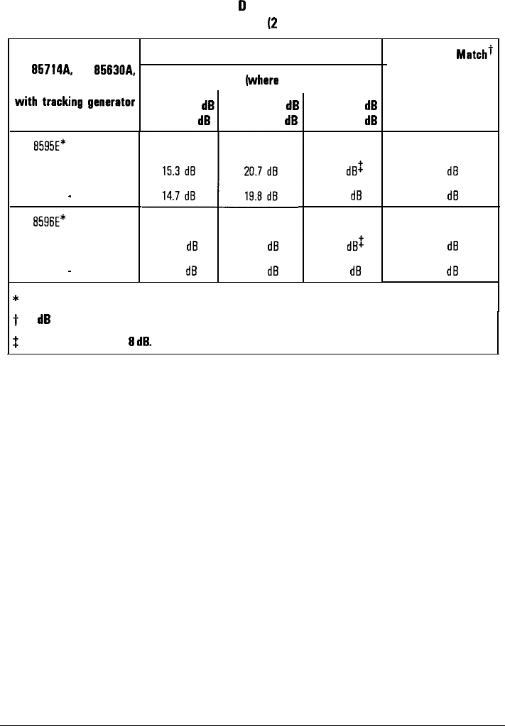
I
-
I
-
Reference
Characteristics
HP 8590
D
and E Series
System Characteristics
(2
of 8 continued)
Configuration:
PORT 1 Source Match PORT 2 Input
Match7
HP 65714A. HP 65630A,
and spectrum analyzer Attenuation (where applicable)
with
tracking
generator
test set: 0
dB
test set: 10
dB
test set: 0
dB
option
source: 0
dB
source: 0
dB
source: 10
dB
HP
6595E*
0.31200 MHz
1200 - 2900 MHz
HP
6596E*
0.31200 MHz
1200
-
2900 MHz
15.3
dB
14.7
dB
20.7
dB
19.8
dB
16.5
dB$
15.3
dB
17.7
dB
12.0
dB
16.5
dB$
17.7
dB
15.3
dB
12.0
dB
*
DC coupled signal analyzer input
t
10
dB
signal analyzer input attenuation
$
Source attenuation =
8
dB.
8-130
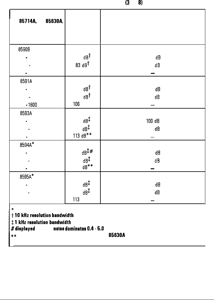
I
-
Reference
Characteristics
HP 9590 A and B Series
System Characteristics
(3
of
91
~ Configuration:
HP 66714A. HP 65630A,
and spectrum analyzer
with tracking generator
option
HP
85908
Opt. 003
0.3 - 1200 MHz
1200 - 1800 MHz
0.1
-
1800 MHz
HP
8591A
0.3 - 1200 MHz
1200 - 1800 MHz
0.1
-
1800
MHz
HP
8593A
0.3 -1200 MHz
1200 - 2900 MHz
0.3
-
2900 MHz
HP
8594A*
0.3 -1200 MHz
1200 - 2900 MHz
0.3
-
2900 MHz
HP
8595A*
0.3 -1200 MHz
1200 - 2900 MHz
0.3 . 2900 MHz
Dynamic Range
Test Set Isolation
86
dBt
100
dB
83
dBt
97
dB
106 dB**
-
86
dBt
83
dBt
IO6
dB**
100
dB
97
dB
-
95
dB$
94
dB$
II3
dB**
100
dB
97
dB
-
91
dBt#
95
dB$
113
dB**
100
dB
97
dB
-
94
dB$
94
dB$
II3
dB**
100
dB
97
dB
-
*
DC coupled signal analyzer input
1:
:o:r~~~~~~~.Dn,l:~~~h.
1
#
dmplayed
average
nome
dommates
0.4.5.0
MHz
**
This range available when bypassing the HP
65630A
and connecting DUT between tracking
generator output and spectrum analyzer input.
8-131
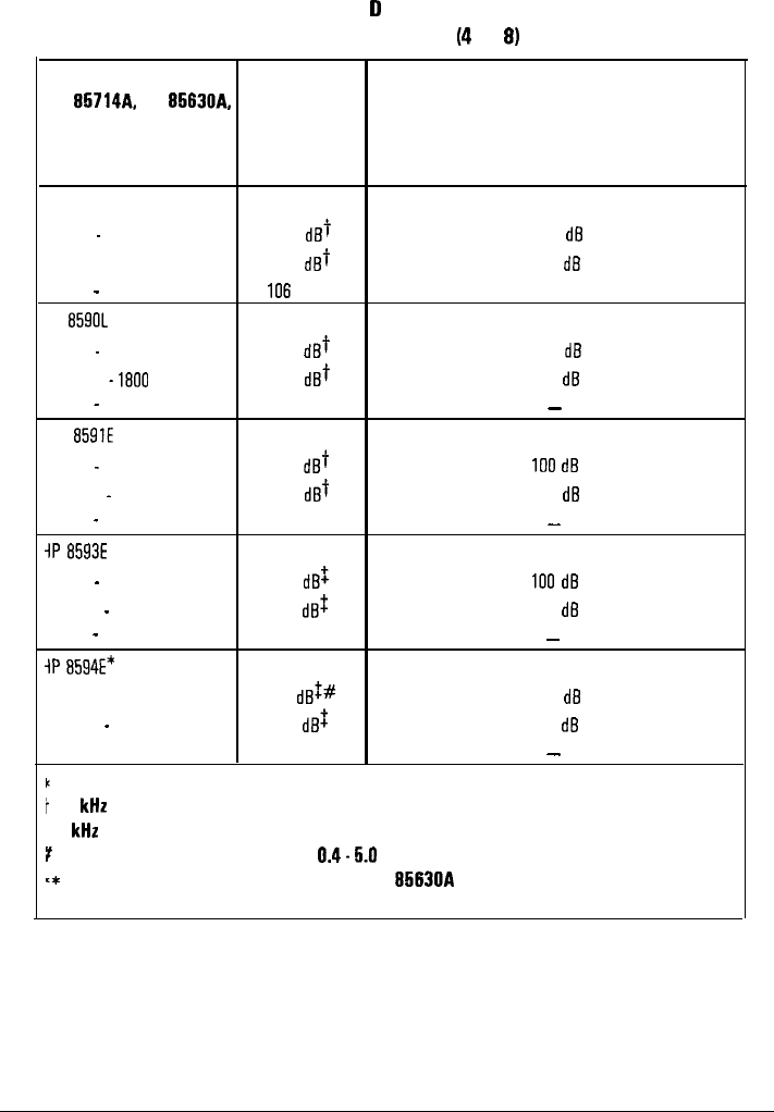
Reference
Characteristics
HP 8590
D
and E Series
System Characteristics
(4
of
81
Configuration: Dynamic Range
Test Set Isolation
HP 66714A, HP
6563OA.
and spectrum analyzer
with tracking generator
option
HP 85900 Opt. 003
0.3
-
1200 MHz 86
dBt
100
dB
1200 . 1800 MHz 83
dBt
97
dB
0.1 - 1800 MHz
IO6
dB**
HP
859OL
Opt. 003
0.3
-
1200 MHz 86
dBt
100
dB
1200 -
Ii300
MHz 83
dBt
97
dB
0.1 - 1800 MHz 106 dB**
-
HP
8591E
0.3 - 1200 MHz 86
dBt
100
dB
1200 - 1800 MHz 83
dBt
97
dB
0.1 - 1800 MHz 106 dB**
-
iP
8593E
0.3
-
1200 MHz 93
dB$
100
dB
1200 - 2900 MHz 92
dB$
97
dB
0.3 - 2900 MHz 111 dB**
-
iP
8594E*
0.3 . 1200 MHz 89
dBt#
100
dB
1200 - 2900 MHz 93
dB$
97
dB
0.3 . 2900 MHz 111 dB**
-
I;
DC coupled signal analyzer input
i
10
kHz
resolution bandwidth
: 1
kHz
resolution bandwidth
r
displayed average noise dominates
0.4.5.0
MHz
I*
This range available when bypassing the HP
65630A
and connecting DUT between tracking
generator output and spectrum analyzer input.
8-132
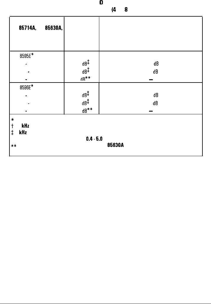
I
-
I
-
Reference
Characteristics
HP 8590
0
and E Series
System Characteristics (4 of
8
continued)
Configuration: Dynamic Range
Test Set Isolation
HP 65714A. HP 65630A.
and spectrum analyzer
with tracking generator
option
HP
6595E*
0.3 -1200 MHz 92
dB$
100
dB
1200 - 2900 MHz 92
dB$
97
dB
0.3 -2900 MHz 111
dR**
-
HP
8596E*
0.3
_
1200 MHz 92
dB$
100
dB
1200 - 2900 MHz 92
dB$
97
dB
0.3 -2900 MHz III
dB**
-
*
DC coupled signal analyzer input
t
10 kHr resolution bandwidth
$
1
kHz
resolution bandwidth
#displayed average noise dominates
0.4.5.0
MHz
*c*
This range available when bypassing the HP 6563OA and connecting DUT between tracking
generator output and spectrum analyzer input.
8-133
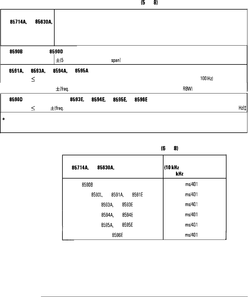
I
-
I
-
Reference
Characteristics
System Characteristics
(5
of
81
Configuration:
HP 66714A, HP 66630A.
and spectrum analyzer
with tracking generator
option
frequency Readout Accuracy
(Start, Stop, Center, Marker)
HP 66908 Opt. 003, HP 6690D Opt. 003
all frequency spans
f15
MHz + 1% of frequency
span1
HP
6591A.
HP
6693A.
HP
6594A.
HP
659fiA
freq. span
5
IO MHz flfreq. readout x freq. reference error*
I
+ 3.0% of span + 20% of RBW +
100
Hz1
freq. span > 10 MHz
I
flfreq.
readout x freq. reference error* + 3.0% of span + 20% of
RBW]
HP
659OD
Opt. 013, HP 65901, HP
6593E,
HP
6694E.
HP 6595E, HP 6596E
freq. span
5
IO MHz
kf(freq.
readout x freq. reference error*
I
+ span accuracy + 1.0% of span + 20% of RBW + 100
Hz11
*
Refer to spectrum analyzer specification.
$ See drift under stability in spectrum analyzer characteristics
System Characteristics
(6
of
81
Configuration: Sweeptime
HP 65714A, HP
6563OA,
and spectrum analyzer
(10
kHz
resolution bandwidth
with tracking generator option 10
kflz
video bandwidth)
HP
85908
Opt. 003, HP 85900 Opt. 003 50
ms1401
points
HP
8590L,
HP
8591A,
HP
8591E
50
ms1401
points
HP
85934
HP
8593E
58
ms1401
points
HP
8594A,
HP
8594E
HP
8595A.
HP
8595E
58
ms1401
points
58
ms1401
points
HP
8596E
58
ms1401
points I
8-134
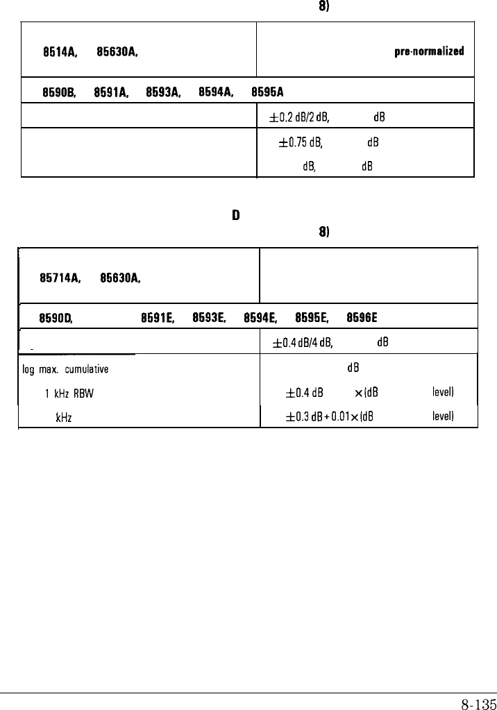
I
-
Reference
Characteristics
HP 8590 A and B Series
System Characteristics (7 of
81
Configuration: Amplitude Accuracy
HP 6514A. HP
6563OA,
and spectrum analyzer (After normalization, with
prenormalized
with tracking generator option reference trace starting at reference level.)
HP 65908. HP 6591A. HP 6593A, HP 6594A. HP 6595A
log incremental
log max. cumulative
f0.2
dB12
dB,
0 to -70
dB
from ref. level
kO.75
dB,
0 to -60
dB
from ref. level
fI.O
dB,
0 to -70
dB
from ref. level
HP 8590
D
and E Series
System Characteristics (8 of
8)
I
Configuration: Amplitude Accuracy
HP 65714A. HP 65630A. and spectrum analyzer
(After normalization, with pre-normalized
with tracking generator option reference trace starting at reference level.)
HP
659013.
HP 65901, HP
g691E,
HP 6593E, HP 6594E, HP
6595E,
HP 6596E
1
log incremental
f0.4
dB14
dB,
0 to -70
dB
from ref. level
0 to -70
dB
from ref. level
f0.4
dB
+O.OI
xldB
from ref. level1
3 kHz to 3 MHz RBW
f0.3
dB
+O.OI
xldB
from ref. level1
8-135

I
-
I
-
9
Concepts

I
-
I
-
Concepts
The concepts discussed in this chapter help you evaluate the measurement
uncertainties inherent in scalar test setups. The information is technical in
nature and is
not
necessary for operating the scalar analyzer. It is provided
for those who wish a more in-depth understanding of scalar measurements.
9-2
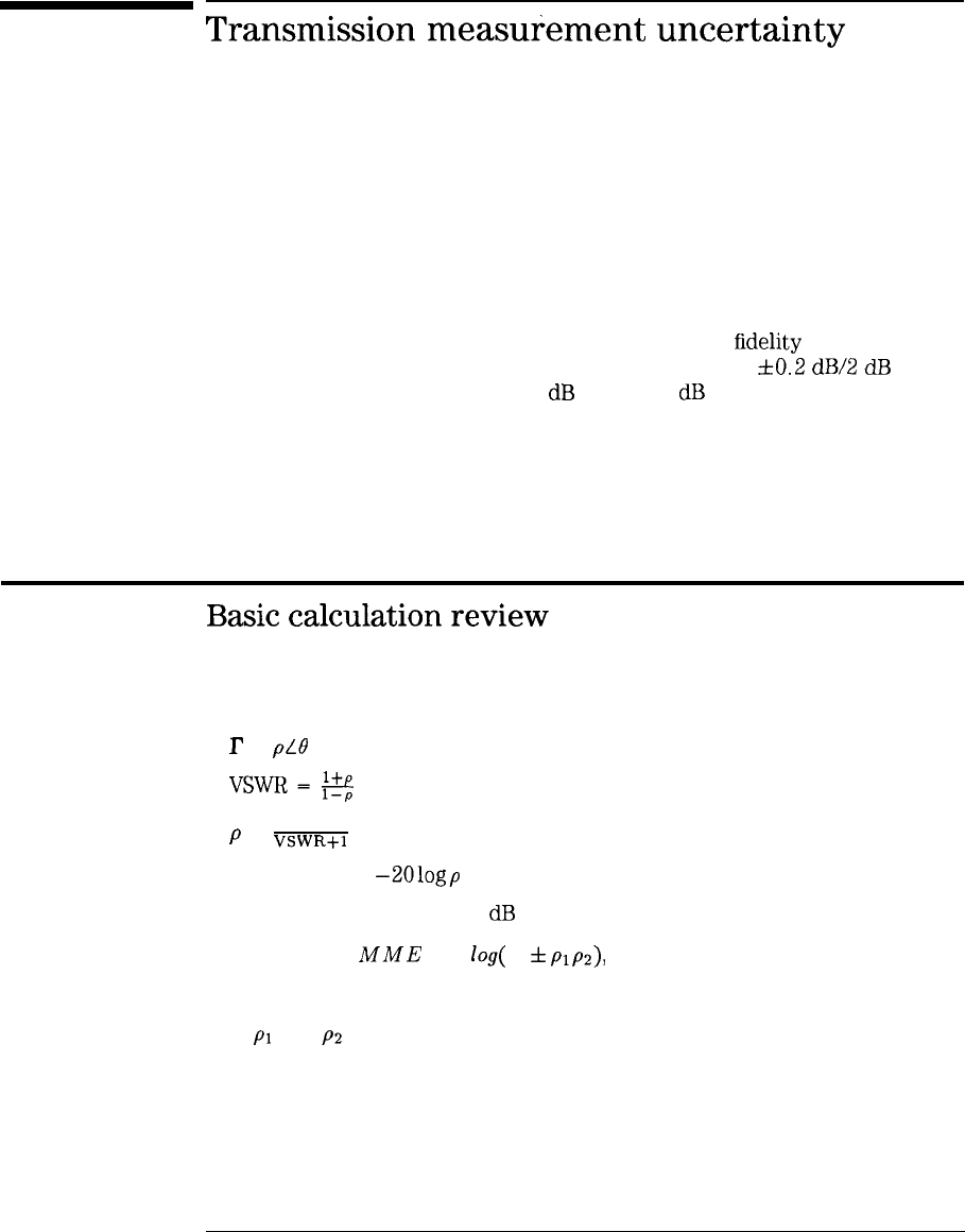
I
-
I
-
Transmission
measurement
uncertainty
Transmission measurement uncertainty is composed primarily of relative
amplitude accuracy (flatness, display fidelity) and the external circuit
mismatch.
Normalization removes flatness uncertainties. Display
fidelity
in the
HP 8590 Series spectrum analyzers is good (greater than
f0.2
dB/2
dB
but
not more than a maximum of fl.O
dB
over a 70
dB
range). The major
causes of transmission measurement uncertainties, then, result from external
mismatch among
source,
receiver, and DUT. These external mismatch
uncertainties arise at calibration and measurement.
Basic
calculation
review
You should be familiar with the relationships among reflection coefficient (I’),
standing wave ratio (VSWR), and return loss:
r
=
pLe
VS~=I+e
l--P
VSWR-I
p =
VSWR+l
Return Loss = -2010gp
Maximum mismatch error in
dB
is expressed by
MME
= 20 log( 1
f
plpz),
where..
p1
and
p2
are the scalar reflection coefficients at the points of connection.
9-3
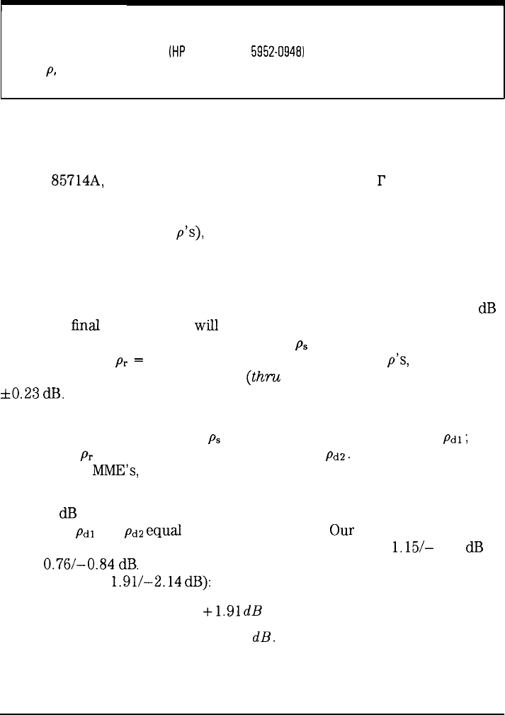
I
-
Concepts
Transmission measurement uncertainty
1
I
Reflectometer calculator
The HP Reflectometer Calculator
IHP
Part Number
5952-0948)
makes it easy to determine equivalents
among
p,
VSWR, and return loss.
Reflection coefficient is a vector (complex) quantity. In a scalar system like
the HP
85714A,
we cannot measure phase of a particular
r
and then account
for it in our error analysis and correct for it in the measurement. We can,
however, ignore phase, determine worst case caused by interaction of two
reflection coefficients (two
p’s),
then know that actual measurement error is
between zero and worst case. Worst case is the same as MME in the above
expression.
In the following example, all results are maximum possible errors. We want
to calculate the maximum mismatch error of a filter measurement at its 3
dB
point. The
Enal
error window
wilI
combine the MME at calibration and the
MME at measurement. Assume a source with
ps
= 0.2 (or 1.5 VSWR) and
a receiver with a
pr
=
0.13 (or 1.3 VSWR). Given these two
p’s,
our MME
equation yields a possible calibration
(thou
measurement) error window of
kO.23
dI3.
Now we must calculate possible errors with the DUT inserted between the
source and receiver. The source
ps
will interact with the DUT input
Pdi;
the receiver
pr
will interact with the DUT output
P&z.
Therefore, we must
calculate two
MME’s,
then add them together to arrive at the measurement
error window.
At the 3
dB
point the filter reflects half of the input power, so reflection
coefficients
pdl
and
Pd2
equal
0.707 (or 5.8 VSWR).
Our
MME equation
yields the input and output mismatch errors, respectively: + 1.15/- 1.3
dB
and +
0.76/-0.84
dB.
We now add these error windows to get the MME at
measurement (+
1.91/-2.14
dB):
1.15 + 0.76 =
+1.91
dB
-1.3 + (-0.84) = -2.14 dB.
9-4
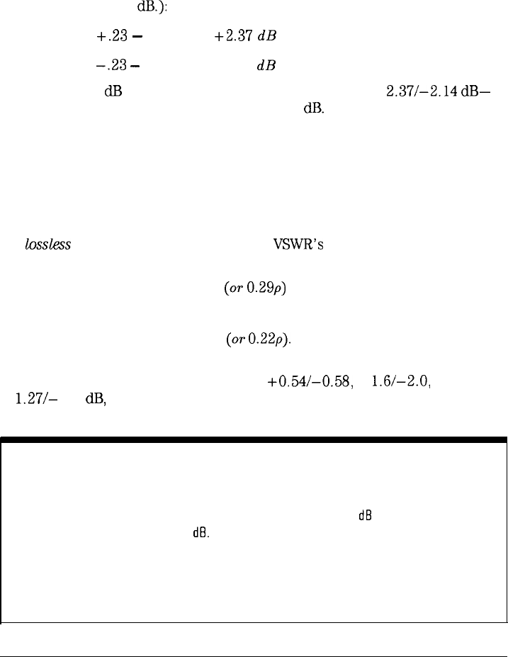
I
-
I
-
Concepts
Transmission measurement uncertainty
To get the total uncertainty of the measurement, we subtract the negative
measurement number from the positive calibration number, and we subtract
the positive measurement number from the negative calibration number (We
subtract because measurement error was the denominator of a linear equation
before converting to
dB.):
+.23
-
(-2.14) =
+2.37
dB
-.23
-
(+ 1.91) = -2.14 dB
Thus, for our 3
dB
point filter measurement, our MME is +
2.37/-2.14
dB-
we might measure anything from 0.86 to 5.37
dB.
The error can be worse if hardware constraints necessitate additional cables
and/or adapters between source and/or receiver and the DUT. The source
is at the end of its cable/adapter; the receiver input is at the end of its
cable/adapter, so we must consider the mismatches at these points rather
than at the panel connectors. Effective mismatch becomes worse.
To determine effective mismatches, multiply the VSWR values. For example, if
the
losskss
cables and adapters each have
VSWR’s
of 1.1, the source VSWR
becomes
1.5 x 1.1 x 1.1 = 1.8
(OT
0.29p)
and the receiver VSWR becomes
1.3 x 1.1 x 1.1 = 1.57
(07‘
0.22p).
With these numbers, the maximum mismatch errors at calibration and at
DUT input/output at measurement are +0.54/-0.58, + 1.6/-2.0, and
+
1.27/-
1.5
dB,
respectively.
low-loss devices
When the OUT is a low-loss device, we must also account for the interaction between source and
receiver when the DUT is connected. We ignore this interaction at the 3
dB
point of our filter,
because it would add only about 0.2
dB.
Also, we assume that the OUT input and output connectors are the same type, opposite sex. If not,
you must insert an adapter at calibration, then remove it when you insert the OUT. A high quality
adapter’s effect on uncertainty is small, thus it is not included here.
9-5
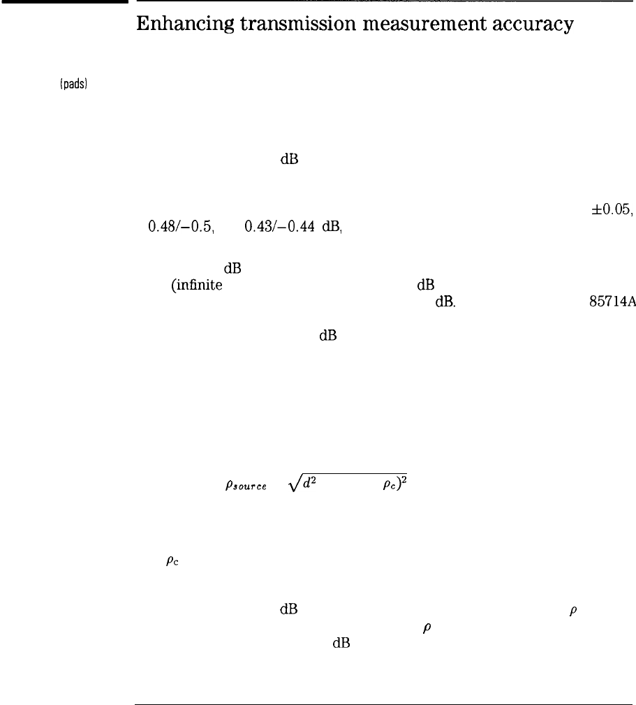
I
-
I
-
Concepts
Transmission measurement uncertainty
Enhancing
transmission
measurement
accuracy
Attenuators
(pads)
The simplest way to improve the situation is to place well-matched Exed
attenuators (with DUT compatible connectors) at the source output and at the
receiver input. Connect the attenuators at the ends of the cables/adapters
discussed above,
not
at the tracking generator and analyzer panel connectors.
For example, given 10
dB
pads with
p’s
of 0.05 (or 1.1 VSWR), the source
and receiver reflection coefficients (assuming the above cables and adapters)
become 0.078 (or 1.17 VSWR) and 0.071 (or 1.16 VSWR) respectively. The
maximum calibration, input, and output mismatch errors then become
f0.05,
+
0.48/-0.5,
+
0.43/-0.44
dB,
respectively-dramatic improvements.
If we need accurate measurement of points farther down the filter skirts, e.g.
the 6, 10, 20
dB
points, the reflection coefficient of the Elter approaches
unity
(inEnite
VSWR). In such cases our 10
dB
pads may not give us enough
isolation, leaving us with errors in excess of 1
dB.
Fortunately, the HP
85714A
has plenty of dynamic range, so we can often afford to use some of it to
enhance accuracy. Using 20
dB
pads totally masks source and receiver
mismatches, for all practical purposes, and leaves just the
p’s
of the pads
themselves.
Directional coupler/detector Another way to improve source match, with essentially no loss of power, is to
use a directional coupler/detector in an external leveling loop. In this case the
output of the coupler becomes the output of the source. The effective source
match in this case becomes
where..
PSOUPce
= ,/d2 + (0.75 x
P,)~
d equals the coupler directivity
pc
equals coupler main line reflection coefficient
0.75 is empirically derived
For a coupler with 30
dB
directivity (equivalent to 0.03
p)
and 0.07
p
(1.15 VSWR), source mismatch becomes 0.06
p
(or 1.13 VSWR), a little better
than we achieved using the 10
dB
pad above.
9-6

I
-
I
-
Concepts
Transmission measurement uncertainty
Two-resistor splitter
Instead of a coupler, we could use a two-resistor splitter in the leveling loop.
Such a splitter has no resistors in the input arm and a series
50-ohm
resistor
in each of the output arms. The leveling detector connects to one of the
resistive arms. The output connector on the other resistive arm becomes the
effective source port at which we measure source mismatch. The leveling
action makes the junction of the input and output arms a virtual RF ground.
As a result, the source mismatch is dependent upon the quality of the resistor
in the output arm. For example, the HP
11667A
has an equivalent source
VSWR of 1.1 from dc to 4
GHz,
1.2 up to 8
GHz,
and 1.33 up to 18
GHz.
Note the wide frequency range of the splitter-a significant advantage over a
coupler. In terms of source power, the splitter does cost 6
dB,
which is more
than a coupler but less than a pad.
9-7
_I
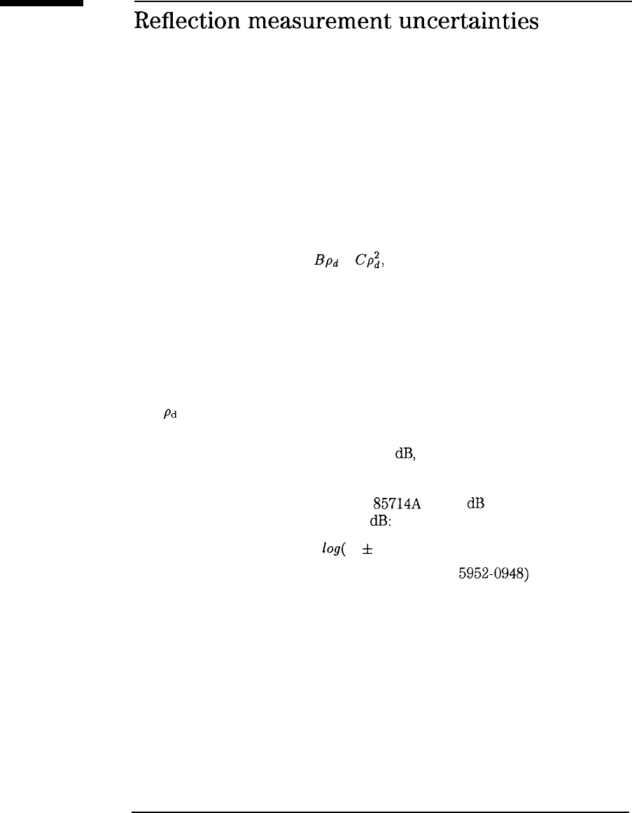
I
-
Reflection
measurement
uncertainties
Instrumentation contributes the same uncertainties to reflection
measurements as indicated above for transmission measurements. In this
section, we shall focus on the uncertainties caused by the external circuit.
However, there is more than just mismatch to consider. The error expression
for reflection is
where..
Ap = A +
Bpd
+
Cp;,
Ap equals the measurement uncertainty
A equals the directivity of the coupler or bridge
B equals the calibration error and frequency response
C equals the source mismatch
pd
is the reflection coefficient of the DUT
The coefficients in the above expression are linear terms, but coupler or
bridge directivity is usually expressed in
dB,
as is frequency response,
and source mismatch is often expressed in VSWR, so all of these must
be converted to linear values. In addition, measurement results from
reflectometer systems such as the HP
85714A
are in
dB
of return loss, and it
is common to express uncertainty in
dB:
Uncertainty = 20
log(
1
f
Ap).
The HP Reflectometer Calculator (HP Part Number
5952-0948)
makes it easy
to determine equivalents among p, VSWR, and return loss.
9-8
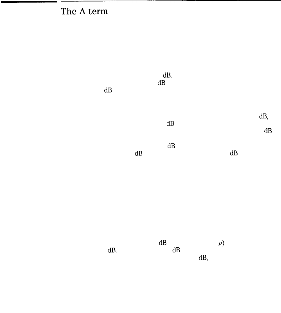
I
-
I
-
Concepts
Reflection measurement uncertainties
The
A
term
Let’s look at the A term in the error expression first. If the measurement
port of a directional coupler or bridge is terminated with a perfect load, there
should be no signal at the detector port because there is no reflection from
the load. (In this case the spectrum analyzer is the detector.) However, since
no coupler or bridge is perfect, there is always some signal at the detector
port. The level of this signal is a measure of the directivity of the coupler or
bridge and is generally expressed in
dB.
For example, if we put a perfect load
on our coupler and measure a 30
dB
return loss, that really means that our
coupler has 30
dB
directivity.
The directivity signal is thus a constant signal at the detector port that adds
vectorially to the desired reflection signal that we wish to measure, producing
an error in the measurement. To produce an error of no more than 1
dB,
the
directivity signal must be at least 20
dB
below the signal to be measured. In
other words, the directivity of the coupler or bridge must be at least 20
dB
better than the return loss of the device to be measured. If we were testing
devices with return losses of about 10
dB
(1.92 VSWR), we would need a
coupler or bridge with 30
dB
directivity for no more than 1
dB
of error just
due to directivity.
The error expression tells us that the B and C terms become small as the
match of the DUT improves. So directivity of the coupler or bridge becomes
the limiting factor when measuring high-return-loss devices. Unless we take
extra-ordinary steps in the measurement process that are beyond the scope
of this discussion, the only thing that we can do to improve measurement
results is to use a better coupler or bridge.
A word of caution-Use a coupler/bridge with a test-port connector that
matches the DUT. Any adapters have their own reflections and degrade the
directivity of the coupler/bridge. For example, a perfect coupler with an
adapter having a 1.065 VSWR (30
dB
return loss, 0.032
p)
has an effective
directivity of 30
dB.
A coupler with 30
dB
directivity would have an effective
directivity ranging anywhere from infinity to 24
dB,
depending upon the
phase of the reflection from the adapter relative to that of the directivity
signal of the coupler itself.
9-9
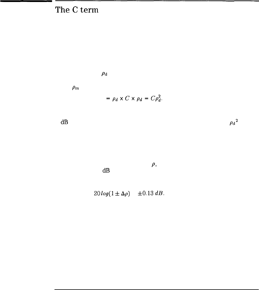
I
-
Concepts
Reflection measurement uncertainties
The
C
term
Next, let’s look at the source match term, C. As far as the DUT is concerned,
the source port is the measurement port of the coupler or bridge, i.e. the port
to which the DUT is attached. Any reflection from the DUT (the signal that
we wish to measure) flows back toward the source, and, unless the match of
the source is perfect, a part of this signal is re-reflected back toward the DUT.
The DUT reflects part of this re-reflected signal just as it did part of the
original signal. If
pd
is the reflection of the DUT and C is the reflection
coefficient of the source, then a first-order approximation of the measured
signal
pm
is
Pm
=pdXCXPd=CP;.
This term becomes important when measuring devices with high reflection
coefficients (low return losses). For example, we might want to measure the
6
dB
return-loss points. In this case reflection coefficient is 0.5, so
pd2
is 0.25.
For a good measurement, then, we need to minimize the mismatch of the
source. When using a coupler for reflection measurements, we usually use a
dual coupler (two couplers in the same physical package) and use one of the
couplers in a leveling loop. We can then calculate effective source match just
as was done in the transmission discussion above. Using the same numbers
as in the transmission example (0.06
p,
1.13 VSWR), the uncertainty in
determining the 6
dB
return loss point due to source mismatch is
Ap = 0.06 x 0.25 = 0.015,
or
201og(l
*Ap) =
f0.13
dB.
Once again, it is best to use a coupler/bridge with a measurement port
that matches the connector type of the DUT because an adapter degrades
source match. We get effective source mismatch by multiplying source VSWR
without the adapter by the VSWR of the adapter. Using the same adapter that
we used above to determine effective directivity, we get a source mismatch of
9-10
I
-
I
-
Concepts
Reflection measurement uncertainties
source mismatch = VSWR, x VSWR,
source mismatch = 1.13 x 1.065
source mismatch = 1.2 VSWR (or 0.09 p)
The effective source match characteristic of the HP
85630A
is 1.46 VSWR
(0.19
p),
and the uncertainty due to source mismatch only is
Ap
= 0.19
x
0.25 = 0.047, or
201og(l
f
Ap) =
+0.38/
-
0.40 dB.
The
B
term
Finally, let’s look at the B term. This term includes calibration uncertainty
and frequency response (as well as instrument uncertainty, which we are
ignoring in this discussion). As was the case in transmission, frequency
response can be removed with trace arithmetic. The calibration uncertainty
also can be removed with trace arithmetic, but we must take a few extra
steps to insure that it is.
In a reflection measurement, we compare the signal reflected from a DUT to
the signal incident upon the DUT. To get a measure of the incident signal, we
connect a device that reflects all of the incident signal to the measurement
port of our coupler or bridge and use this reflected signal as our reference
that represents a reflection coefficient of unity (1.0). The usual calibration
device is a short circuit.
If our system were perfect, we would indeed get an exact measure of the
unity reflection from the short. However, from the above, we know that there
are two other signals that add vectorially to the unity signal: a directivity
signal and a multiple-reflection signal resulting from source mismatch. So
the calibration uncertainty part of the B term is somewhere between zero
and the algebraic sum of A and C, depending upon the phase angles of A
and C relative to the unity (actually
-
1) reflection from the short. Since
the HP
85714A
is a scalar system, it measures the absolute value of the
combination:
9-11
I
-
Concepts
Reflection measurement uncertainties
I--l+A+CI,or
+1-A-C
In most analyzer/tracking-generator systems, we must live with the
calibration uncertainty because there is no provision for removing it.
The HP
85714A
allows us to use a second standard, an open, to eliminate A
and C from the calibration trace. The reflection from an open is also unity,
but in this case it is + 1 because the reflected signal is in phase with the
incident signal rather than 180 degrees out of phase as it is for the short
(hence the -1). As is the case with the short, a calibration trace based on an
open also includes A and C:
I+l+A+CJ
To eliminate A and C we can average the two calibration traces and end up
with just the unity value that we wanted. Thus the two step calibration
process for the HP
85714A:
first calibrate with an open and store that
trace; then replace the open with a short and recalibrate. The HP
85714A
automatically calculates the mean of the short and open calibrations and
stores the result.
The stored open/short average also includes the inherent system frequency
response, so we can eliminate the B term completely, and the error
expression becomes
Ap = A + Cp$.
Still, coupler/bridge directivity (A) is critical for accurate measurement
of well matched devices (high return loss, low VSWR or
p),
while source
match (C) becomes the critical factor for low return-loss (high VSWR or
p)
measurements, for example, the 3
dB
point of our filter.
9-12

10
If You Have a Problem
I
-
I
-
If You Have a Problem
Your spectrum analyzer, with its scalar measurements personality, is built to
provide dependable service. It is unlikely you will experience a problem, but
in the event something goes wrong, refer to the following sections:
l
If you can’t install the HP
85714A
l
If you suspect a problem with the test set
l
If DISPLAY UNDER-RANGE or DISPLAY OVER-RANGE is displayed
l
If you can’t use dual-display mode
l
If you can’t measure MAG
Sll,
VSWR, or MAG
S21
l
If BW
MEAS
measurement shows UNCAL
10-2
I
-
Start
here
Perform the following steps to isolate any problem. If the problem still is not
resolved, call your nearest HP Sales and Service Office.
1. Be sure that the spectrum analyzer’s hrmware date code is 10.26.90 or
later. This is not the revision number of the HP
85714A.
2. Reinstall the HP
85714A
scalar measurements personality using the
instructions in Chapter 1.
3. Refer to the contents of this chapter for common problems and their
solutions.
4. Complete all the basic checks for the spectrum analyzer listed in the
spectrum analyzer’s installation and verihcation manual.
10-3
I-
I
-
I
-
If
you
can’t
install
the
HP
85714A
q
Check that the card is correctly installed.
The arrow on the card must line up with the arrow on the card slot
q
Check the available user memory.
The following message is displayed if available memory is not enough to
hold the HP
85714A:
INVALID SYMTABENTRY: SYMTAB OVERFLOW
10-4
-1
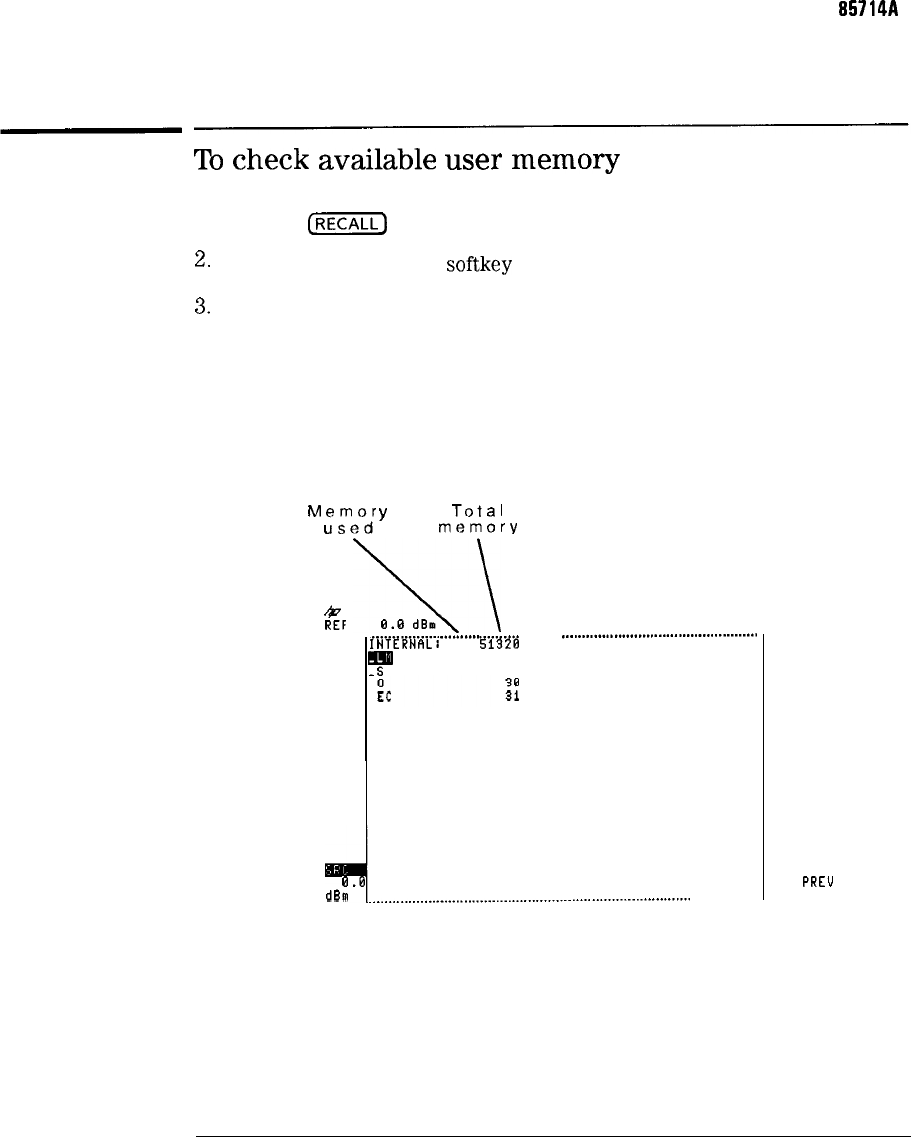
I
-
I
-
If You Have a Problem
If you can’t install the HP
85714A
To
check
available
user
memory
1. Press the
(RECALL]
key.
2.
Press the INTRNL CRD
softkey
so that INTRNL is underlined.
3.
Press the CATALOG INTRNL then CATALOG ALL softkeys.
4. The user memory information is shown at the top of the screen after
the text INTERNAL : .
Available memory is the total memory minus the
memory already used. See the following figure. Available memory must be
at least 47000 bytes.
M
;
peodr
Y
Total
memory
t
REF
\\
G.E
dBm
. . . . . . .
. . . . . . . .
.._..........
. . .
.
. . . . . . . . . . . .
.._._............................................
INTtRNALI
142
<i$fG
!F
31
30
-I
0.0
dBm
.................................................................................
................
DELETE
FILE
SELECT
PREFX
EXIT
CRTRLOG
PREU
MENU
R
10-5
I
-
If You Have a Problem
If you can’t install the HP 857 14A
To
increase
user
memory
To make available all user memory, press the
[WI
key followed by the
MORE
1
of 3 and DISPOSE USER
MEM
softkeys.
If you use this quick method of increasing memory, all user entered data,
downloadable programs, and any other measurement personalities will be
erased.
To make available user memory by erasing selected downloadable programs,
do the following:
1. Press the
(jj)
key.
2.
Press the INTRNL CRD
softkey
so that INTRNL is underlined.
3.
Press the CATALOG INTRNL then MORE 1 of 2 softkeys.
4.
Press the CATALOG DLP
softkey.
5. Use the front-panel knob to select the downloadable program for erasure
then, press the DELETE FILE
softkey.
10-6
I
-
I
-
If
you
suspect
a
problem
with
the
test
set
q
Check that the TEST SET YES NO
softkey
is pressed so that YES is
underlined. Press
(CONFIG),
MORE 1 of 3 , and MORE 2 of 3 to locate
the
softkey.
q
Check the rear-panel AUX INTERFACE and RF cables are correctly
connected. Always remove line power before connecting the AUX
INTERFACE cable.
q
Check that the spectrum analyzer and tracking generator operate
correctly without the HP
85630A
scalar transmission/reflection test set or
HP
85714A
scalar measurements personality.
q
Check the HP
85630A
scalar transmission/reflection test set’s manual for
information on verifying test set operation.
To
check
proper
cable
installation
Refer to Chapter 1, and perform Step 1 “Connect the optional HP
85630A
Test Set”.
To
check
spectrum
analyzer
operation
The following procedure tests the spectrum analyzer and tracking generator
by running the tracking generator’s self-calibration routine. For more
information on the routine, refer to the spectrum analyzer’s operation
manual.
1. Press the front-panel
C-1
key.
2.
Press the SPECTRUM ANALYZER softkey.
10-7
-1
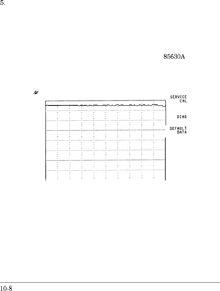
I
-
I
-
If You Have a Problem
If you suspect a problem with the test set
This exits the scalar measurements personality mode.
3. Connect a cable between the front-panel RF OUT and INPUT connectors.
4. Press the (CAL) key.
5.
Press the MORE 1 of 3 , MORE 2 of 3 , and then CAL TRK GEM
softkeys.
Towards the end of the calibration routine, the display should look similar to
the following figure. Notice the level response near the top of the display.
This shows a level tracking generator output at the proper power level for the
test.
If the calibration runs without any errors, refer to the HP
85630A
scalar
transmission/reflection test set’s manual for information on verifying the test
set’s operation and service.
SERVICE
DIAG
OEFAULT
CRL
OATR
CAL
TRK GEN
VERIFY
TIMEBRSE
MORE
3 of 3
RT
10-8
I
-
If
DISPLAY
UNDER-RANGE
or
DISPLAY
OVER-RANGE
is
displayed
Display calibration has a finite amplitude range. When a response goes
beyond the calibrated limit, the scalar analyzer displays these messages.
To
solve
this
problem
l
Change the amplitude scale and recalibrate the measurement.
l
View the Calibration Limits
1. Press the front-panel
ICAL)
key.
3.
Press the More 1 of 2
softkey.
3. To show the maximum level of calibrated display, press
MAX RNG ON OFF so that ON is underlined.
4. To show the minimum level of calibrated display, press
MIN RNG ON OFF so that ON is underlined.
10-9
I
-
If
you
can’t
use
dual-display
mode
q
Check that the HP
85630A
scalar transmission/reflection test set is properly
installed.
Viewing both the transmission and reflection response simultaneously
requires an HP
85630A
scalar transmission/reflection test set.
q
Check that the scalar analyzer is configured for the test set.
The following message is displayed if the scalar analyzer is not
configured for the test set:
85630A
Test Set Configuration Required
To
install
the
test
set
Perform the installation instructions included in step 6 of Chapter 1.
To
configure
the
scalar
analyzer
for
the
test
set
1.
Press the
IhnoDE)
and then the SCALAR ANALYZER
softkey
to enter the
scalar analyzer mode.
2. Press the
C-j
key.
3.
Press the
MORE
1 of 3 and then MORE 2 of 3 softkeys.
4.
Press the TEST SET YES NO
softkey
so that YES is underlined.
10-10
I
-
I
-
If
you
can’t
measure
MAG
Sll,
VSWR,
or
MAG
S21.
q
Check that you’ve calibrated the response.
These measurements require a normalized display.
q
Check (for MAG
Sll
and VSWR measurements) that the HP
85630A
scalar
transmission/reflection test set is properly installed.
Measuring MAG
Sll
and VSWR requires an HP 856308 scalar
transmission/reflection test set.
q
Check (for MAG
Sll
and VSWR measurements) that the scalar analyzer is
configured for the test set.
The following message is displayed if the scalar analyzer is not
configured for the test set:
85630ATestSetConfigurationRequired
To
install
the
test
set
Perform the installation instructions included in step 6 of Chapter 1.
10-11
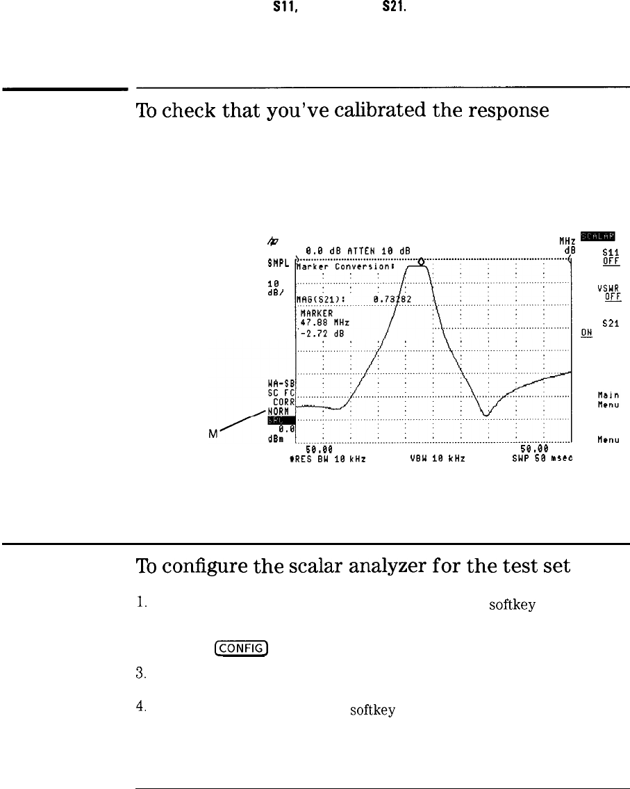
I
-
I
-
If You Have a Problem
If you can’t measure MAG
Sll,
VSWR, or MAG
S21.
To
check
that
you’ve
calibrated
the
response
If the display is normalized, the text NORM appears at the lower-left corner of
the display.
NOR
k
REF
SHPL
LOG
10
dBI
MKR 47.88
FlHz
8.8
d8
ATTEN
18 dB -2.72 d8
CENTER
5G.GG
MHz
tRES
BW
10
kHz
SPAN
58.08
MHz
U8W
10
kHz
SUP 58
hdCC
NAG
$11
ON
OFF
USWR
ON
OFF
RAG S21
fi
OFF
Previous
nenu
RT
To
configure
the
scalar
analyzer
for
the
test
set
1.
Press the (MODE) and then the SCALAR ANALYZER softkey to enter the
scalar analyzer mode.
2. Press the
@XKj
key.
3.
Press the MORE 1 of 3 and then MORE 2 of 3 softkeys.
4.
Press the TEST SET YES NO
softkey
so that YES is underlined.
10-12
-1
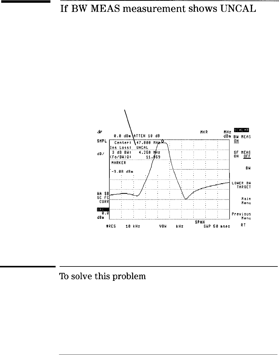
I
-
I
-
If
BW
MEAS
measurement
shows
UNCAL
The insertion loss results of an automatic bandwidth measurement requires
the displayed response to be calibrated.
UNCAL
b
NKR
47.88
MHz
m
REF -3.08
dBm
gW
~~05
SMPL
m
OFF
LOG
10
dB/
E
"E
-
RARKER
47.08 MHz UPPER
8W
TARGET
CENTER 50.00 MHz
SPhN
50.08 MHz
#RES
BW
10
kHz
U8W
18 kHz SUP 58
MSCE
RT
To
solve
this
problem
Calibrate the display as described in Chapter 3.
10-13

I
-
I
-
Glossary

I
-
I
-
Glossary
absolute amplitude accuracy
The degree of correctness or uncertainty (expressed in either volts or
dB
power). It includes relative uncertainties plus calibrator uncertainty. For
improved accuracy, some spectrum analyzers specify frequency response
relative to the calibrator as well as relative to the midpoint between
peak-to-peak extremes.
active function
The active function is the instrument’s feature currently selected for use.
It may be a key selection or remote-programming command.
active function readout
The area of a display screen where the active function and its state are
displayed. The active function is the one that was completed by the last
key selection or remote-programming command.
active marker
The marker on a trace that can be repositioned by front-panel controls or
programming commands.
active trace
The trace (commonly A, B, or C) that is being swept (updated) with
incoming signal information.
amplitude accuracy
The general uncertainty of a spectrum analyzer amplitude measurement,
whether relative or absolute.
ASCII
The acronym for American Standard Code for Information Interchange. It
is an eight-part code (7 bits plus parity check) used for data (information)
interchange. An ASCII value is a specific combination of bits ranging from
0 to 255 that represent characters in machine language that computers
and controllers can understand.
Glossary-2

I
-
I
-
If BW
MEAS
measurement shows
UNCAL
attenuation
A general term used to denote a decrease of signal magnitude in
transmission from one point to another. Attenuation may be expressed as
a scalar ratio of the input to the output magnitude in decibels.
auxiliary interface
A spectrum analyzer rear-panel connector that provides control lines and
power for external equipment.
bandwidth selectivity
This is a measure of the analyzer’s ability to resolve signals unequal in
amplitude. It is the ratio of the 60
dB
bandwidth to the 3
dB
bandwidth
for a given resolution filter (IF). Bandwidth selectivity tells us how steep
the hlter skirts are. Bandwidth selectivity is sometimes called shape
factor.
battery-backed RAM
Random access memory (RAM) data retained by a battery. RAM memory
cards can contain data that is maintained with a battery. Refer also to
nonvolatile memory.
broadband response
A signal whose spectrum is wider than the resolution bandwidth of a
spectrum analyzer, and whose repetition frequency is lower than the
bandwidth of the spectrum analyzer. Notice that it is a combination
of signal and receiver characteristics that determines when a signal is
classified as broadband. For refining incoming signal responses, select
narrower spans and bandwidths. The following checks can help verify
whether or not the response is broadband:
l
Change the resolution bandwidth. The displayed amplitude should
change.
l
Change the sweep time. The spacing of the responses on the display
should change as you change the sweep time.
l
Change the span. The spacing of the responses should not change.
They should be independent of frequency span.
l
Change the video bandwidth. If the video bandwidth is made narrower
than the resolution bandwidth, the displayed amplitude of the
responses should decrease.
Glossary-3

I
-
I
-
If BW
MEAS
measurement shows
UNCAL
card reader
See memory card
character set
The set of elementary symbols. These normally include both alpha and
numeric codes, plus punctuation or any other symbol which may be read,
stored, or written and used for organization, control, or representation of
data.
command
A set of instructions that are translated into instrument actions. The
actions are usually made up of individual steps that together can execute
an operation. Generally, for spectrum analyzers it is a sequence of code
that controls some operation of a spectrum analyzer. These codes can be
keyed in via a controller, or computer. Refer also to function.
continuous sweep mode
The analyzer condition where traces are automatically updated each time
trigger conditions are met.
default
The preset conditions, options, or parameters of an instrument. The
default state may be changed by choosing key selections or writing
programming commands to use other conditions.
delta marker
An analyzer mode in which a fixed reference marker is established, then
a second active marker becomes available so it can be placed anywhere
along the trace. A readout indicates the relative frequency separation and
amplitude difference between the reference and active markers.
display dynamic range
The maximum dynamic range over which both the larger and smaller
signal can be viewed simultaneously on the display. For analyzers with a
maximum logarithmic display of 10
dB/division,
the actual dynamic range
may be greater than the display dynamic range. Refer also to dynamic
range.
Glossary-4
I
-
I
-
If BW
MEAS
measurement shows
UNCAL
display fidelity
The measurement uncertainty of relative differences in amplitude on a
spectrum analyzer. On purely analog analyzers (those analyzers that
display trace information immediately and do not store, then recall the
data to the screen), these differences are displayed on the screen and
the graticule is used to evaluate the measurement. Many analyzers with
digital displays (refer to digital display) have markers that can be used
to measure the signal. As a result, measurement differences are stored
in memory, and the ambiguity of the display is eliminated from the
measurement.
display range
The calibrated range of the display for a particular display mode or scale
factor. Refer also to log display and scale factor.
DLP
The abbreviation for downloadable program. A single programming
command or a sequence of programming commands used to perform
specific operations.
DLPs
can be made up of several functions, variables,
and traces defined by the program creator. The DLP can be downloaded
from one electronic storage medium into another and executed without a
controller.
dynamic range
The power ratio
(dB)
between the smallest and largest signals
simultaneously present at the input of an analyzer that can be measured
with some degree of accuracy. Dynamic range generally refers to
measurement of distortion or inter-modulation products.
error message
A message displayed on the screen indicating missing or failed hardware,
improper user operation, or other conditions that require additional
attention. Generally, the requested action or operation cannot be
completed until the condition is resolved.
FFT
The abbreviation for fast Fourier transform. It is a mathematical operation
performed on a time-domain signal to yield the individual spectral
components that constitute the signal.
Glossary-5

I
-
I
-
If BW
MEAS
measurement shows
UNCAL
firmware
An assembly made up of hardware and instruction code that are
integrated to form a functional set which cannot be altered during normal
operation. The instruction code, permanently installed in the circuitry of
the instrument, is classified as ROM (read-only memory). The firmware
determines the operating characteristics of the instrument or equipment.
Each firmware version is
identihed
by a revision code number, or date
code.
frequency accuracy
The uncertainty with which the frequency of a signal or spectral
component is indicated, either in an absolute sense or relative to some
other signal or spectral component. Absolute and relative frequency
accuracies are specified independently.
frequency range
The range over of frequencies which the spectrum analyzer performance
is specified. The maximum frequency range of many microwave analyzers
can be extended with the application of external mixers.
frequency resolution
The ability of a spectrum analyzer to separate closely spaced spectral
components and display them individually. Resolution of equal amplitude
components is determined by resolution bandwidth. Resolution of
unequal amplitude signals is determined by resolution bandwidth and
bandwidth selectivity.
frequency response
The peak-to-peak variation in the displayed signal amplitude over a
specified center frequency range. Frequency response is typically
specified in terms of
fdB
relative to the value midway between the
extremes. It also may be specified relative to the calibrator signal.
frequency span
The magnitude of the displayed frequency component. Span is
represented by the horizontal axis of the display. Generally, frequency
span is given as the total span across the full display. Some analyzers
represent frequency span (scan width) as a per-division value.
Glossary-6
I
-
I
-
If BW
MEAS
measurement shows
UNCAL
frequency stability
The stability of a frequency component to remain unchanged in frequency
or amplitude over short- and long-term periods of time. Stability refers to
the local oscillator’s ability to remain fixed at a particular frequency over
time. The sweep ramp that tunes the local oscillator influences where a
signal appears on the display. Any long-term variation in local oscillator
frequency (drift) with respect to the sweep ramp causes a signal to shift
its horizontal position on the display slowly. Shorter-term local oscillator
instability can appear as random FM or phase noise on an otherwise
stable signal.
front-panel key
Keys, typically labeled, and located on the front panel of an instrument.
The key labels identify the function the key activities. Numeric keys and
step keys are two examples of front- panel keys.
full span
A mode of operation in which the spectrum analyzer scans the entire
frequency band of an analyzer.
function
The action or purpose which a
specific
item is intended to perform or
serve. The spectrum analyzer contains functions that can be executed
via front-panel key selections, or through programming commands. The
characteristics of these functions are determined by the
firmware
in the
instrument. In some cases, a DLP (downloadable program) execution
of a function allows you to execute the function from front-panel key
selections.
gain compression
The signal level at the input mixer of a spectrum analyzer where the
displayed amplitude of the signal is a
speciEc
number of
dB
too low due
just to mixer saturation. The signal level is generally
speciEed
for 1
dB
or
0.5
dB
compression and is usually between -3
dBm
and -10
dBm.
hard copy
Information or data printed onto paper as opposed to its being stored on
disk or in the instrument’s memory.
Glossary-7

I
-
I
-
If BW
MEAS
measurement shows
UNCAL
HP-IB
The abbreviation for Hewlett-Packard Interface Bus. It is a
Hewlett-
Packard proprietary parallel interface that allows you to “daisy-chain”
more than one device to a port on a computer or instrument.
input attenuator
An attenuator between the input connector and the Erst mixer of a
spectrum analyzer (also called an RF attenuator). The input attenuator is
used to adjust the signal level incident to the Erst mixer, and to prevent
gain compression due to high-level or broadband signals. It is also used to
set the dynamic range by controlling the degree of internally-generated
distortion. For some analyzers, changing the input attenuator settings
changes the vertical position of the signal on the display, which
then changes the reference level accordingly. In Hewlett-Packard
microprocessor-controlled spectrum analyzers, the IF gain is changed to
compensate for changes in input attenuator settings. Because of this, the
signals remain stationary on the display, and the reference level is not
changed.
input impedance
The terminating impedance that the analyzer presents to the signal
source. The nominal impedance for RF and microwave analyzers is
usually
5062.
For some systems, such as cable TV,
75Q
is standard. The
degree of mismatch between the nominal and actual input impedance is
called the VSWR (voltage standing wave ratio).
limit line
A test limit made up of a series of line segments, positioned according to
frequency and amplitude within the spectrum analyzer’s measurement
range. Two
deEned
limit lines may be displayed simultaneously. One sets
an upper test limit, the other sets a lower test limit. Trace data can be
compared with the limit lines as the spectrum analyzer sweeps. If the
trace data exceeds either the upper or lower limits, the spectrum analyzer
displays a message or sounds a warning, indicating that the trace failed
the test limits.
Glossary-8
limit-line file
The user-memory Ele that contains the limit-line table entries. Limit lines
are composed of frequency and amplitude components that make up a
trace array and this data is stored in the Ele. The limit-line Ele feature is
available on spectrum analyzers that are capable of limit-line operation.
Refer also to limit line.
I
-
If BW
MEAS
measurement shows
UNCAL
limit-line table
The line segments of a limit line are stored in the limit-line table. The
table can be recalled to edit the line segments, then restored in the
limit-line
file.
Refer also to limit line.
log display
The display mode in which vertical deflection is a logarithmic function of
the input-signal voltage. Log display is also referred to as logarithmic
mode. The display calibration is set by selecting the value of the top
graticule line (reference level), and scale factor in volts per division. On
Hewlett-Packard analyzers, the bottom graticule line represents zero volts
for scale factors of 10 dB/division or more. The bottom division, therefore,
is not calibrated for those analyzers. Analyzers with microprocessors
allow reference level and marker values to be indicated in
dBm,
dBmV,
dBpV,
volts, and occasionally in watts. Nonmicroprocessor-based
analyzers usually offer only one kind of unit, typically
dBm.
marker
A visual indicator we can place anywhere along the displayed trace. A
marker readout indicates the absolute value of the trace frequency and
amplitude at the marked point. The amplitude value is displayed with the
currently selected units. Refer also to delta marker.
maximum input level
The maximum signal power that may be safely applied to the input of
a spectrum analyzer. Typically 1 W (-30
dBm)
for Hewlett-Packard
spectrum analyzers.
measurement range
The ratio, expressed in
dB,
of the maximum signal level that can be
measured (usually the maximum safe input level) to the lowest achievable
average noise level. This ratio is almost always much greater than can be
realized in a single measurement. Refer also to dynamic range.
memory
A storage medium, device, or recording medium into which data can be
stored and held until some later time, and from which the entire original
data may be retrieved.
Glossary-9
I
-
I
-
If BW
MEAS
measurement shows
UNCAL
memory card
A small, credit-card-shaped memory device that can store data or
programs. The programs are sometimes called personalities and give
additional capabilities to your instrument. Typically, there is only one
personality per memory card. Refer also to personality.
menu
The spectrum analyzer functions that appear on the display and are
selected by pressing front-panel keys. These selections may evoke a series
of other related functions that establish groups called menus.
nonvolatile memory
Memory data that is retained in the absence of an ac power source. This
memory is typically retained with a battery. Refer also to battery-backed
RAM.
normalized reference level
An amplitude level representing 0
dB
deviation from a calibrated system’s
response. It is obtained’by subtracting the system’s response from itself.
normalized reference position
The position on a network analyzer’s display of the normalized reference
level.
parameter units
Standard units of measure, which include the following:
Measured Unit
Parameter Name
frequency hertz
power level decibel relative to milliwatts
power ratio decibel
voltage volt
time second
electrical current ampere
impedance Iresistance) ohm
Unit
Abbreviation
HZ
dBm
dB
v
S
A
n
Glossary- 10
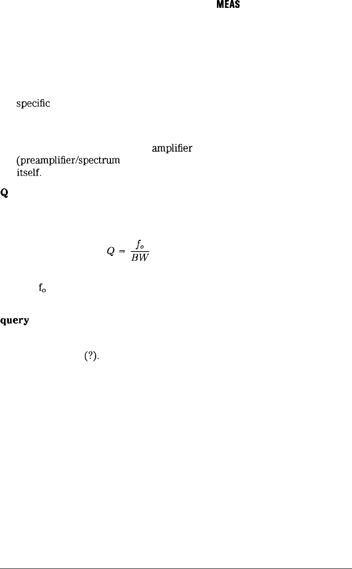
I
-
I
-
If BW
MEAS
measurement shows
UNCAL
personality
Applications available as Hewlett Packard products on a memory card or
other electronic media that extends the capability of an instrument for
speciEc
uses. Examples include digital radio personalities and cable TV
personalities.
preamplifier
An external, low-noise-Egure
ampliEer
that improves system
[~;rnpliEer/spectrum
analyzer) sensitivity over that of the analyzer
Q
Q indicates the frequency selectivity of a response. The narrower the
bandwidth at a given frequency, the higher the Q. It is defined by the
following formula:
where:
f,
is the center frequency of the displayed response.
BW is the bandwidth of the displayed response.
query
Any spectrum analyzer programming command having the distinct
function of returning a response. These commands may end with a
question mark
(?).
Query commands return information either to the
computer or to the analyzer display.
random-access memory
RAM (random-access memory) or read-write memory, is a storage area
allowing access to any of its storage locations. Data can be written to or
retrieved from RAM, but data storage is only temporary. When the power
is removed, the information disappears. User-generated information
appearing on a display is RAM data.
read-only memory
ROM (read-only memory) that is encoded into the analyzer’s Ermware.
The data can be accessed (read) only; it cannot be altered by the user.
-1
Glossary- 11

I
-
I
-
If
BW
MEAS
measurement shows
UNCAL
reference level
The calibrated vertical position on the display used as a reference for
amplitude measurement in which the amplitude of one signal is compared
with the amplitude of another regardless of the absolute amplitude of
either.
reflection coefficient
A scalar measurement defined as the ratio of the reflected signal voltage
to the incident signal voltage on a transmission line not terminated in its
characteristic impedance. The reflected signal is typically reflected from
the input of a device under test. The reflection coefficient is also referred
to as the scattering parameter
&I.
The reflection coefficient is defined by
the following formula:
reflection measurement
Refer to reflection coefficient.
relative-marker mode
The active marker is positioned relative to the position of the reference
marker. Marker readout shows amplitude, frequency, or time differences
between the two markers.
resolution
Refer to frequency resolution.
resolution bandwidth
The ability of a spectrum analyzer to display adjacent responses discretely
(hertz, hertz decibel down). This term is used to identify the width of the
resolution bandwidth filter of a spectrum analyzer at some level below the
minimum insertion-loss point (maximum deflection point on the display).
The 3
dB
resolution bandwidth is specified; for others, it is the 6
dB
resolution bandwidth.
return loss
A scalar measurement on a transmission line with a mismatched load.
Return loss indicates how much less the reflected power is from the
incident power on the line. This is shown in the following formula:
return loss = incident power
-
reflected power
Glossary- 12

I
-
I
-
If BW
MEAS
measurement shows
UNCAL
Sll
Refer to reflection coefficient
s21
Refer to transmission coefficient
scalar-analyzer mode
The operating state that allows a spectrum analyzer to make
network-analysis measurements. Spectrum analyzers with this ability
use tracking generator functions. Measurement results are displayed in a
relative-amplitude scale resulting from a variation, plus or minus, from a
reference (normalized) value stored in a trace.
scale factor
The per-division calibration of the vertical axis of the display.
shape factor
Refer to bandwidth selectivity.
single-sweep mode
The spectrum analyzer sweeps once when trigger conditions are met.
Each sweep is initiated by pressing an appropriate front-panel key, or by
sending a programming command.
softkey
Key labels displayed on a screen or monitor which are activated by
mechanical keys surrounding the display, or located on a keyboard.
Softkey
selections usually evoke menus that are written into the program
software. Front-panel key selections determine which menu (set of
softkeys) appears on the display.
span
Span equals the stop frequency minus the start frequency. The span
setting determines the horizontal-axis scale of the spectrum analyzer
display.
span accuracy
The uncertainty of the indicated frequency separation of any two signals
on the display.
Glossary- 13

I
-
I
-
If BW
MEAS
measurement shows
UNCAL
spectrum analyzer
A device that effectively performs a Fourier transform and displays the
individual spectral components (sine waves) that constitute a time-domain
signal.
stop/start frequency
Terms used in association with the stop and start points of the
frequency measurement range. Together they determine the span of the
measurement range.
sweep time
The time it takes the local oscillator to tune across the selected span.
Sweep time directly affects how long it takes to complete a measurement.
It does not include the dead time between the completion of one sweep
and the start of the next. It is usually a function of frequency span,
resolution bandwidth, and video bandwidth. Resolution affects sweep
time in that the IF filters are band-limited circuits requiring finite times to
charge and discharge. The amount of time the mixing product remains in
the IF hlter passband is directly proportional to the bandwidth; inversely
proportional to the sweep in Hz per unit of time. The rise time of a
Iilter
is inversely proportional to its bandwidth, and if the proportionality
constant “k” is included, then we can make the rise time equal the “k”
divided by resolution bandwidth. Mathematically, this is represented as:
Time in
Passband
= resolution bandwidth
(spansweep time)
(resolution bandwidth x sweep time)
=span
Rise Time =
k
resolution bandwidth
Solving for sweeptime:
Sweep Time = k x span
resolution
bandwidth2
syntax
The grammar rules that specify how commands must be structured for an
operating system, programming language, or applications.
Glossary- 14
I
-
I
-
If BW
MEAS
measurement shows
UNCAL
test set
A device used to measure scattering parameters on two-port or multiport
devices. Test sets include couplers and optionally contain transducers and
RF switches.
trace
A trace is made up of a series of data points containing frequency and
amplitude information. The series of data points is often referred to as an
array. Traces A, B, and C are the typical names of traces that analyzer
displays. The number of traces is specific to the instrument.
transmission coefficient
A scalar measurement of a signal transmitted through a device. It is
de&ted
as the ratio of the output signal voltage over the input signal
voltage of a device. (The transmission line must be terminated in its
characteristic impedance.) The transmission coefficient is also referred to
as the scattering parameter
Szi.
The transmission coefficient is defined
as the ratio of the voltage at the output of a device to the voltage at the
input of a device. It is shown by the following formula:
&apt
transmission measurement
Refer to transmission coefficient
units
Dimensions on the measured quantities. Units usually refer to amplitude
quantities because they can be changed. In spectrum analyzers with
microprocessors, available units are
dBm
(dB
relative to 1
mW
(milliwatt)
dissipated in the nominal input impedance of the analyzer),
dBmV
(dB
relative to 1
mV
(millivolt)),
dB,uV
(dB
relative to 1
pV>,
volts, and in
some analyzers watts.
update
To make existing information current; to bring information up to date.
Glossary 15
I
-
I
-
If BW
MEAS
measurement shows
UNCAL
video
A term describing the output of a spectrum analyzer’s envelope detector.
The frequency range extends from 0 Hz to a frequency that is typically
well beyond the widest resolution bandwidth available in the analyzer.
However, the ultimate bandwidth of the video chain is determined by the
setting of the video
Iilter.
video average
The digital averaging of spectrum analyzer trace information. It is
available only on analyzers with digital displays. Each point on the
display is averaged independently and the average is computed based
on the number of sweeps selected by the user. The averaging algorithm
applies a factor to the amplitude value of a given point on the current
sweep
(l/n,
where
n
is the number of the current sweep); applies another
factor to the previously stored average
[(n
-
l/n)]
;
and combines the
two for a current average. After the designated number of sweeps are
completed, the factors remain constant, and the display becomes a
running average.
video bandwidth
The cut-off frequency (3
dB
point) of an adjustable low-pass filter in the
video circuit. When the video bandwidth is equal to or less than the
resolution bandwidth, the video circuit cannot fully respond to the more
rapid fluctuations of the output of the envelope detector. The result is
a smoothing of the trace, or a reduction in the peak-to-peak excursion,
of broadband signals such as noise and pulsed RF when viewed in
broadband mode. The degree of averaging or smoothing is a function of
the ratio of the video bandwidth to the resolution bandwidth.
video filter
A post-detection, low-pass filter that determines the bandwidth of the
video amplifier. It is used to average or smooth a trace. Refer also to
video bandwidth.
Glossary-16

I
-
I
-
If BW
MEAS
measurement shows
UNCAL
VSWR
The VSWR (voltage standing-wave ratio) is the ratio of the minimum and
maximum voltage values on a transmission line caused by reflections from
a mismatch. VSWR values range from 1 (representing no reflection) to
infinity (representing 100% reflection from the load). Examples of 100%
reflection occurs when the transmission line is terminated with a short or
open.
VSWR is related to return loss
(dB)
as shown in the following formula:
u-l
return loss = -20
log(x)
zero span
The case in which a spectrum analyzer’s local oscillator remains fixed at a
given frequency so that the analyzer becomes a fixed-tuned receiver. In
this state, the bandwidth is equal to the resolution bandwidth. Signal
amplitude variations are displayed as a function of time. To avoid loss of
signal information, the resolution bandwidth must be as wide as the signal
bandwidth.
To
avoid any smoothing, the video bandwidth must be set
wider than the resolution bandwidth.
Glossary 17

I
-
Index
I
-
I
-
Index
Special
i1
8-60
characters
1
120
dB
ON OFF, 4-11, 8-9
A
AC/DC coupling, 2-25
amplitude,
2-10
AMPLITUDE, 8- 10
Amplitude menu, 8-4
Amptd,
2-10,
8-10
annotation, vii, 8-68
ANNOT
ON OFF,
8-
10
ATTEN
AUTO MAN,
8-
11
ATTEN
PORT
1,
8-
11
attenuation
input,
2-
13
output,
2-16
source,
2-
18
attenuator, 8-69, 8-84
AUTO,
8-11
autoscale, 8-71
AUTO SCALE,
2-10,
4-13, 8-12
AUX CTRL, 2-14, 8-12
AUX INFERFACE, 1-3
AVERAGE ON OFF. 8- 13
B
bandwidth,
4-17,
8-124
bandwidth measurement,
8-74
bandwidth type, 8-72
BW, 8-13
BW
MEAS
ON OFF,
4-18,
8-14
Index-2
I-
I
-
C
Cal,
8-15
CAL, 3-3, 8-15
calibrated limit
8-88,
8-89,
range,
8-125
calibrate reflection, 8-75
calibrate standard device, 8-76
calibration, 3-2
limits,
3-
15
memory,
3-12,
5-12
recalling,
3-
14
reflection, 3-7
saving,
3-12
standard device, 3-9
transmission, 3-6
calibration kit, vi, 3-7
Calibration menu, 3-3, 8-4
CAL
OPN/SHRT,
3-7,
8-
16
CAL STD DEV, 8-16
CAL STD DEVICE, 3-9
CAL THRU,
8-17
CANCEL, 8- 17
card, 1-7
center frequency,
4-
17
CHANGE PREFIX, 8- 18
CHANGE TITLE, 5-10, 8-17
Command Mnemonic, 8-59
Command Terminators,
8-60
Compress Function,
8-
18
compression, 4-27
CONFIG,
8-
19
correction constants, 1-3
COUPLE DC AC. 8-19
D
DELETE SEGMENT, 8- 19
deleting, 2-5
DELTA
MEAS,
5-4, 8-20
Device BW
Meas,
4-18,
4-20
Device BW
MEAS,
8-20
Display, 8-21
DISPLAY, 8-21
Display menu, 8-5
DISPLAY OVER-RANGE,
3-15,
10-9
DISPLAY UNDER-RANGE,
l-14,
3-15,
IO-9
DISPOSE SCALAR, 8-21
Dotted Lines,
8-60
DSP LINE ON OFF, 8-22
dual display mode, 8-79
DUAL DSP ON OFF, 4-8, 8-22
dynamic range, 3-4
Index-3
I
-
I
-
E
EDIT DONE, 5-8, 8-23
EDIT LIMIT, 5-8, 8-23
EDIT LOWER, 8-24
EDIT
MID/DELT,
8-24
EDIT UP/LOW, 8-24
EDIT UPPER, 8-25
EDIT UPR LWR, 8-25
EXIT DELTA, 8-25
EXIT FFT, 8-26
EXIT
PK-PK.
8-26
extended display range, 8-82
external gain,
2-19
F
fast fourier transforms,
4-21
FFT
MEAS,
4-22, 8-26
FLAT, 5-9, 8-27
frequency range, iii
frequency tracking,
2-
14
G
GRAT ON OFF, 8-27
H
HP
85630A
test set, 2-23
1
insertion loss,
4-
17
installation, 1-2
INVALID SYMTAB ENTRY, 10-4
K
keys
redefined. 8-8
L
LIMITEST ON OFF, 3-10,
5-11, 8-28
LIMIT FAIL, 5-5
limit lines
amplitude units, 5-7
creating, 5-5
fixed, 5-7
recalling,
5-
12
relative, 5-7
saving,
5-
12
segments, 5-8
title,
5-10
tutorial,
5-14,
5-20
Limit Lines, 5-8, 8-28
Limit Lines menu, 8-7
Index-4
I
-
LIMIT PASS, 5-5
LIMITS FIX REL, 5-8, 8-27
LOG SCALE, 8-28
LOWER BW TARGET,
4-
19, 8-29
LOWER LIMIT, 3-10, 8-29
M
MAG
Sll
ON OFF,
4-15,
8-30
MAG
S21
ON OFF, 4-15, 8-31
Main 8-4menu,
Main Menu, 8-32
MAN TRK ADJUST, 8-32
marker,
4-14
Marker Convert,
4-15,
4-16,
8-32
MARKER DELTA, 8-33
markers, 5-3
Marker Tables, 5-3
maximum dynamic range, 3-4
MAX RNG ON OFF,
3-15,
8-33
Measure, 8-34
measurement, 8-9 1
bandwidth,
4-17
center frequency,
4-
17
FFT, 4-21
FFT example, 4-23
insertion loss,
4-
17
Q,
4-17
range,
4-10
reflection, 4-7,
4-15
simultaneous, 4-8
swept power,
2-20,
4-25
table,
6-2
transmission, 4-6,
4-15
uncertainty, 9-3, 9-8
VSWR,
4-16
measurement type, 8-92
Measure 4-3, 8-6menu,
measuremetn
shape factor,
4-19
MEASAJSER, 4-3, 8-34
memory,
10-4
available,
10-5
increasing,
10-6
MIN RNG ON OFF,
3-
15, 8-35
MODE, vii, 2-3
MOV command, 7-4
Multiple Markers, 5-3
Index-5
I
-
N
NEGATIVE ON OFF, 8-36
NEW LIMIT, 5-8, 8-36
NEXT PEAK, 8-37
NEXT PK LEFT, 8-37
NEXT PK RIGHT, 8-37
NORM, 3-6, 3-8
normalization, 3-2, 4-9
normalized position,
3-17
normalized reference level, 8-98
normalized reference position, 5-7
NORMALIZE ON OFF, 8-39
NORMAL ON OFF, 8-38
NORM REF POSN, 2-10, 3-17, 5-7,
8-38
ns...ANNOT,
8-68
ns-AT, 8-69
ns-AUTOSC, 8-7 1
ns-BMT, 8-72
ns-BWM, 8-74
ns-CALR, 8-75
ns-CALS, 8-76
ns-CALT, 8-77
ns-CAN.8.78
ns-DDM, 8-79
ns-DISPOSE, 8-81
ns_EDR,
8-82
ns-EXATN, 8-84
ns-FFT, 8-85
ns-LBW, 8-87
ns-LIMITEST, 8-88
ns-LRNG, 8-89
ns-MCM,
8-91
ns-MCT,
8-92
ns-MP, 8-95
ns-NORM, 8-96
ns-NRL, 8-98
ns-NRP,
8-
100
ns-OPEN,
8-101
ns-RCI,
8-
102
ns-REFL,
8-
104
ns-RL,
8-
105
ns-SCI,
8-
106
ns-SDLL,
8-107
ns-SDUL, 8-108
ns-SFM,
8-
109
ns-SHRT,
8-l
10
ns_SRCOFF,
8-
111
ns-SRCPOFS, 8-112
ns-SRCPWR,
8-
113
ns-STD.
8-114
Index-6
I
-
I
-
ns_TAKESWP,
8-115
ns-TCA,
8-116
ns-TDD,
8-
118
ns-TDP,
8-120
ns-THRU,
8-122
ns-TRANS,
8-
123
nsSJBW,
8-124
nsJJRNG,
8-
125
NUMBER POINTS, 6.8, 8-39
0
open, vi
p
PEAK EXCURSN, 5-4, 8-39
peaking, 3-5
PK-PK
MEAS,
5-4,
8-40
POINT, 5-9, 8-40
POSITIVE ON OFF, 8-40
power sweep,
2-20
preset condition, 2-5
PRESET SCALAR, 2-4, 8-41
printer configuration, 6-5
printing results, 6-5
PRINT PAGE ALL, 8-41
programming, 7-2
programming commands, 8-59
programming variables, 7-5
PURGE LIMITS, 8-42
PWR SWP ON OFF, 2-20, 4-26, 8-42
Q
Q,
4-17
R
RECAL CAL, 8-42
recall calibration,
8-
102
recalling
calibrations,
3-
14
limit lines,
5-12
RECALL LIMIT, 8-43
Recommended Path,
8-60
reference level,
2-10,
3-17
REFL, 8-44
reflection,
4-7
reflection calibration, 3-7
reflection coefficient,
4-
15
REF LEVEL, 8-43
removing, 2-5
removing slope, 2-21
Index-7
I
-
I
-
Repeating Syntax Element,
8-60
Reserved Words,
8-60
revision number, 2-6
RF input attenuator, 8-69
S
SAMPLE ON OFF, 8-44
SAVE CAL, 8-45
save calibration,
8-106
SAVE LIMIT, 8-45
saving
calibrations,
3-
12
limit lines,
5-12
scalar analyzer, 2-3
calibrate transmission, 8-77
cancel calibration routine, 8-78
dispose DLP, 8-81
fast Fourier transform, 8-85
mode preset, 8-95
normalization, 8-96
normalized reference position,
8-100
reflection measurement and calibration,
8-104
source power offset,
8-l
12
transmission measurement,
8-
123
Scalar Analyzer
reference level,
8-
105
source power,
8-l
13
source power off,
8-
111
store open,
8-101
store short,
8-
110
store thru,
8-122
sweep,
8-115
SCALAR ANALYZER, 8-45
SCALAR REVISION, 8-46
scale,
4-12
Secondary Keywords,
8-60
SELECT AMPLITUD, 8-46
SELECT DLT AMPL, 8-46
SELECT FREQ, 8-47
SELECT LWR AMPL, 8-47
SELECT MID AMPL, 8-47
SELECT SEGMENT, 8-47
SELECT TYPE, 8-48
SELECT UPR AMPL, 8-49
SF
MEAS
ON OFF,
4-20,
8-49
shape factor,
4-19,
8-109
shape factor bandwidth, 8-87
short, vi
slope, 2-21
Index-8
I
-
I
-
SLOPE, 5-9,
8-51
software product license agreement, xi
source
attenuation,
2-
18
frequency,
2-14
frequency tracking,
2-14
power, 2-14,
2-16
Source, 8-51
Source menu,
2-14,
8-4
SPAN, 8-51
Special Numbers and Characters,
8-60
spectrum analyzer, 2-3
SRC ATN AUTO MAN, 8-52
SRC PWR OFFSET, 8-52
SRC PWR ON OFF, 2-16, 8-53
standard device calibration, 3-9
standard device limit,
8.107,
8.108
STORE OPEN, 8-53
STORE SHORT, 8-53
store standard device,
8-
114
STORE STD DEV, 8-54
STORE THRU, 3-6, 8-54
swept power, 4-25
SYMTAB OVERFLOW, 10-4
syntax conventions, 8-59
Syntax Elements,
8-60
T
table, 6-2
reducing, 6-7
tabular data,
8-
118,
8-120
tabular data compression,
8-116
Tabular Display, 6-3, 8-54
Tabular Display menu, 6-3, 8-5
TABULAR ON OFF, 6-4, 8-55
temperature changes,
2-14
test set, viii, 2-23
HP
85630A,
1-4
TEST SET YES NO, 2-24, 8-55
TRACKING PEAK, 2-14, 8-55
TRANS, 8-56
transmission, 4-6
transmission calibration, 3-6
transmission coefficient,
4-
15
Index-9

I
-
U
UNCAL,
6-3, lo-13
UPPER Bw
TARGET, 4-17, 4-19, 8-56
UPPER
LIMIT, 3-10, 8-57
v
VIEW NEXT PG, 8-57
VIEW PREV PG, 8-57
VSWR,
4-16
VSWR
ON OFF,
4- 16,
8-58
W
warranty, xiii
I
-
Index- 10
