Tcon ACTEX P MANUAL NEW 2010 EDITION

User Manual:

Open the PDF directly: View PDF .
Page Count: 506 [warning: Documents this large are best viewed by clicking the View PDF Link!]

iii

TABLE OF CONTENTS

INTRODUCTORY COMMENTS

SECTION 0 - REVIEW OF ALGEBRA AND CALCULUS

Set Theory 1

Graphing an Inequality in Two Dimensions 9

Properties of Functions 10

Limits and Continuity 14

Differentiation 15

Integration 18

Geometric and Arithmetic Progressions 24

and Solutions 25Problem Set 0

SECTION 1 - BASIC PROBABILITY CONCEPTS

Probability Spaces and Events 35

Probability 39

and SolutionsProblem Set 1 49

SECTION 2 - CONDITIONAL PROBABILITY AND INDEPENDENCE

Definition of Conditional Probability 59

Bayes' Rule, Bayes' Theorem and the Law of Total Probability 62

Independent Events 68

and SolutionsProblem Set 2 75

SECTION 3 - COMBINATORIAL PRINCIPLES

Permutations and Combinations 97

and SolutionsProblem Set 3 103

SECTION 4 - RANDOM VARIABLES AND PROBABILITY DISTRIBUTIONS

Discrete Random Variable 111

Continuous Random Variable 113

Mixed Distribution 115

Cumulative Distribution Function 117

Independent Random Variables 119

and SolutionsProblem Set 4 127

SECTION 5 - EXPECTATION AND OTHER DISTRIBUTION PARAMETERS

Expected Value 135

Moments of a Random Variable 137

Variance and Standard Deviation 138

Moment Generating Function 140

Percentiles, Median and Mode 142

and SolutionsProblem Set 5 153

SECTION 6 - FREQUENTLY USED DISCRETE DISTRIBUTIONS

Discrete Uniform Distribution 167

Binomial Distribution 168

Poisson Distribution 171

Geometric Distribution 173

Negative Binomial Distribution 175

Hypergeometric Distribution 177

Multinomial Distribution 178

Summary of Discrete Distributions 179

and SolutionsProblem Set 6 181

SECTION 7 - FREQUENTLY USED CONTINUOUS DISTRIBUTIONS

Continuous Uniform Distribution 197

Normal Distribution 198

Approximating a Distribution Using a Normal Distribution 200

Exponential Distribution 204

Gamma Distribution 207

Summary of Continuous Distributions 209

and SolutionsProblem Set 7 211

SECTION 8 - JOINT, MARGINAL, AND CONDITIONAL DISTRIBUTIONS

Definition of Joint Distribution 221

Expectation of a Function of Jointly Distributed Random Variables 225

Marginal Distributions 226

Independence of Random Variables 229

Conditional Distributions 230

Covariance and Correlation Between Random Variables 234

Moment Generating Function for a Joint Distribution 236

Bivariate Normal Distribution 236

and SolutionsProblem Set 8 243

SECTION 9 - TRANSFORMATIONS OF RANDOM VARIABLES

Distribution of a Transformation of 277\

Distribution of a Transformation of Joint Distribution of and 278\]

Distribution of a Sum of Random Variables 279

Distribution of the Maximum or Minimum of Independent 283Ö\ ß \ ß ÞÞÞß \ ×

"# 8

Order Statistics 284

Mixtures of Distributions 287

and SolutionsProblem Set 9 289

SECTION 10 - RISK MANAGEMENT CONCEPTS

Loss Distributions and Insurance 311

Insurance Policy Deductible 312

Insurance Policy Limit 314

Proportional Insurance 315

and SolutionsProblem Set 10 325

TABLE FOR THE NORMAL DISTRIBUTION

PRACTICE EXAM 1 351

PRACTICE EXAM 2 369

PRACTICE EXAM 3 385

PRACTICE EXAM 4 403

PRACTICE EXAM 5 419

PRACTICE EXAM 6 435

PRACTICE EXAM 7 453

PRACTICE EXAM 8 475

vii

INTRODUCTORY COMMENTS

This study guide is designed to help in the preparation for the Society of Actuaries Exam P-

Casualty Actuarial Society Exam 1. The study manual is divided into two main parts. The first

part consists of a summary of notes and illustrative examples related to the material described in

the exam catalog as well as a series of problem sets and detailed solutions related to each topic.

Many of the examples and problems in the problem sets are taken from actual exams (and from

the sample question list posted on the SOA website).

The second part of the study manual consists of eight practice exams, with detailed solutions,

which are designed to cover the range of material that will be found on the exam. The questions

on these practice exams are not from old Society exams and may be somewhat more challenging,

on average, than questions from previous actual exams. Between the section of notes and the

section with practice exams I have included the normal distribution table provided with the exam.

I have attempted to be thorough in the coverage of the topics upon which the exam is based. I

have been, perhaps, more thorough than necessary on a couple of topics, particularly order

statistics in Section 9 of the notes and some risk management topics in Section 10 of the notes.

Section 0 of the notes provides a brief review of a few important topics in calculus and algebra.

This manual will be most effective, however, for those who have had courses in college calculus

at least to the sophomore level and courses in probability to the sophomore or junior level.

If you are taking the Exam P for the first time, be aware that a most crucial aspect of the exam is

the limited time given to take the exam (3 hours). It is important to be able to work very quickly

and accurately. Continual drill on important concepts and formulas by working through many

problems will be helpful. It is also very important to be disciplined enough while taking the

exam so that an inordinate amount of time is not spent on any one question. If the formulas and

reasoning that will be needed to solve a particular question are not clear within 2 or 3 minutes of

starting the question, it should be abandoned (and returned to later if time permits). Using the

exams in the second part of this study manual and simulating exam conditions will also help give

you a feeling for the actual exam experience.

If you have any comments, criticisms or compliments regarding this study guide, please contact

the publisher, ACTEX, or you may contact me directly at the address below. I apologize in

advance for any errors, typographical or otherwise, that you might find, and it would be greatly

appreciated if you bring them to my attention. Any errors that are found will be posted in an

errata file at the ACTEX website, www.actexmadriver.com .

It is my sincere hope that you find this study guide helpful and useful in your preparation for the

exam. I wish you the best of luck on the exam.

Samuel A. Broverman April, 2010

Department of Statistics

University of Toronto E-mail: sam@utstat.toronto.edu or 2brove@rogers.com

www.sambroverman.com

NOTES, EXAMPLES

AND PROBLEM SETS

SECTION 0 - REVIEW OF ALGEBRA AND CALCULUS 1

SECTION 0 - REVIEW OF ALGEBRA AND CALCULUS

In this introductory section, a few important concepts that are preliminary to probability topics

will be reviewed. The concepts reviewed are set theory, graphing an inequality in two

dimensions, properties of functions, differentiation, integration and geometric series. Students

with a strong background in calculus who are familiar with these concepts can skip this section.

SET THEORY

A is a collection of . The phrase set elements " Bis an element of " EB−Eis denoted by , and

" is not an element of " BEBÂEis denoted by .

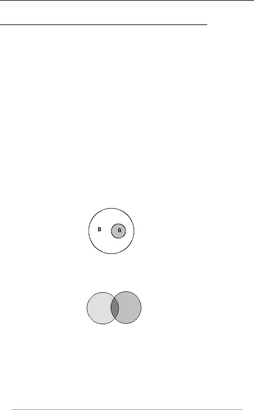
Subset of a set: means that each element of the set is an element of the set .E§F EF

FEEF may contain elements which are not in , but is totally contained within . For instance, if

EF is the set of all odd, positive integers, and is the set of all positive integers, then

EœÖ"ß $ß &ß ÞÞÞ× F œÖ"ß #ß $ß ÞÞÞ× E§F and . For these two sets it is easy to see that ,

since any member of (any odd positive integer) is a member of (is a positive integer).EF

The Venn diagram below illustrates as a subset of .EF

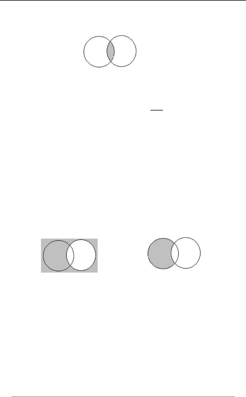
Union of sets: is the set of all elements in either or (or both).E∪F EF

E∪FœÖBlB−E B−F×or

E∪F

If is the set of all positive even integers ( ) and is the set ofE EœÖ#ß %ß 'ß )ß"!ß "#ß ÞÞÞ× F

all positive integers which are multiples of 3 ( ) , thenF œÖ$ß 'ß *ß "#ß ÞÞÞ×

E∪FœÖ#ß$ß%ß'ß)ß*ß"!ß"#ßÞÞÞ× is the set of positive integers which are either

multiples of 2 or are multiples of 3 (or both).

2 SECTION 0 - REVIEW OF ALGEBRA AND CALCULUS

Intersection of sets: is the set of all elements that are in both and .E∩F EF

E∩FœÖBlB−E B−F×and

E∩F

If is the set of all positive even integers and is the set of all positive integers which are aEF

multiple of 3, then is the set of positive integers which are a multipleE∩F œÖ' ß "#ß ÞÞÞ×

of 6. The elements of must satisfy the properties of and . In this example, thatE∩F E Fboth

means an element of must be a multiple of 2 and must also be a multiple of 3, andE∩F

therefore must be a multiple of 6.

The complement of the set : F The complement of consists of all elements , andFnot in F

is denoted or . . When referring to the complement of a set, it isFF µFFœÖBlBÂF×



usually understood that there is some "full set", and the complement of consists of the elementsF

of the full set which are not in . For instance, if is the set of all positive even integers, and ifFF

the "full set" is the set of all positive integers, then consists of all positive odd integers. The setFw

difference of "set minus " is and consists of allEFEFœÖBlB−E+8.BÂF×

elements that are in but not in . Note that . can also beEF EFEFœE∩F

described as the set that results when the intersection is removed from .E∩F E

FœF EFœE∩F



Example 0-1: Verify the following set relationships (DeMorgan's Laws):

(i) (the complement of the union of and is the intersection of theÐE ∪ FÑ œ E ∩ F E F

www

complements of and )EF

(ii) (the complement of the intersection of and is the union of theÐE ∩ FÑ œ E ∪ F E F

www

complements of and )EF

SECTION 0 - REVIEW OF ALGEBRA AND CALCULUS 3

Solution: (i) Since the union of and consists of all points in either , any point notEF EFor

in is in neither nor , and therefore must be in both the complement of theE∪F E F Eand

complement of ; this is the intersection of and . The reverse implication holds in a similarFEF

way; if a point is in the intersection of and then it is not in it is not in so it is notEF E Fß

ww and

in , and therefore it is in . Therefore, and consist of the sameE∪F ÐE∪FÑ ÐE∪FÑ E ∩F

wwww

collection of points, they are the same set.

EFÐE∪FÑœE∩F

wwwww

(ii) The solution is very similar to (i).

ÐE ∩ FÑ œ E ∪ F

www 

Empty set: The is the set that contains no elements, and is denoted . It is alsoempty set g

referred to as the . Sets and are called if .null set disjoint setsEF E∩Fœg

Relationships involving sets:

1. E∪FœF∪Eà E∩FœF∩Eà E∪EœEà E∩EœE

2. E∪ œEàE∩ œ àE œE9999

3. E ∩ ÐF ∪ GÑ œ ÐE ∩ FÑ ∪ ÐE ∩ GÑ

4. E ∪ ÐF ∩ GÑ œ ÐE ∪ FÑ ∩ ÐE ∪ GÑ

5. If , then and (this can be seen E§F E∪FœF E∩FœE

from the Venn diagram in the paragraph above describing subset)

6. For any sets and , and E F E∩F§E§E∪F E∩F§F§E∪F

7. and ÐE∪FÑ œE ∩F ÐE∩FÑ œE ∪F

www www

8. For any set , (the empty set is a subset of any other set ) E§E E9

4 SECTION 0 - REVIEW OF ALGEBRA AND CALCULUS

An important rule (that follows from point 4 above) is the following.

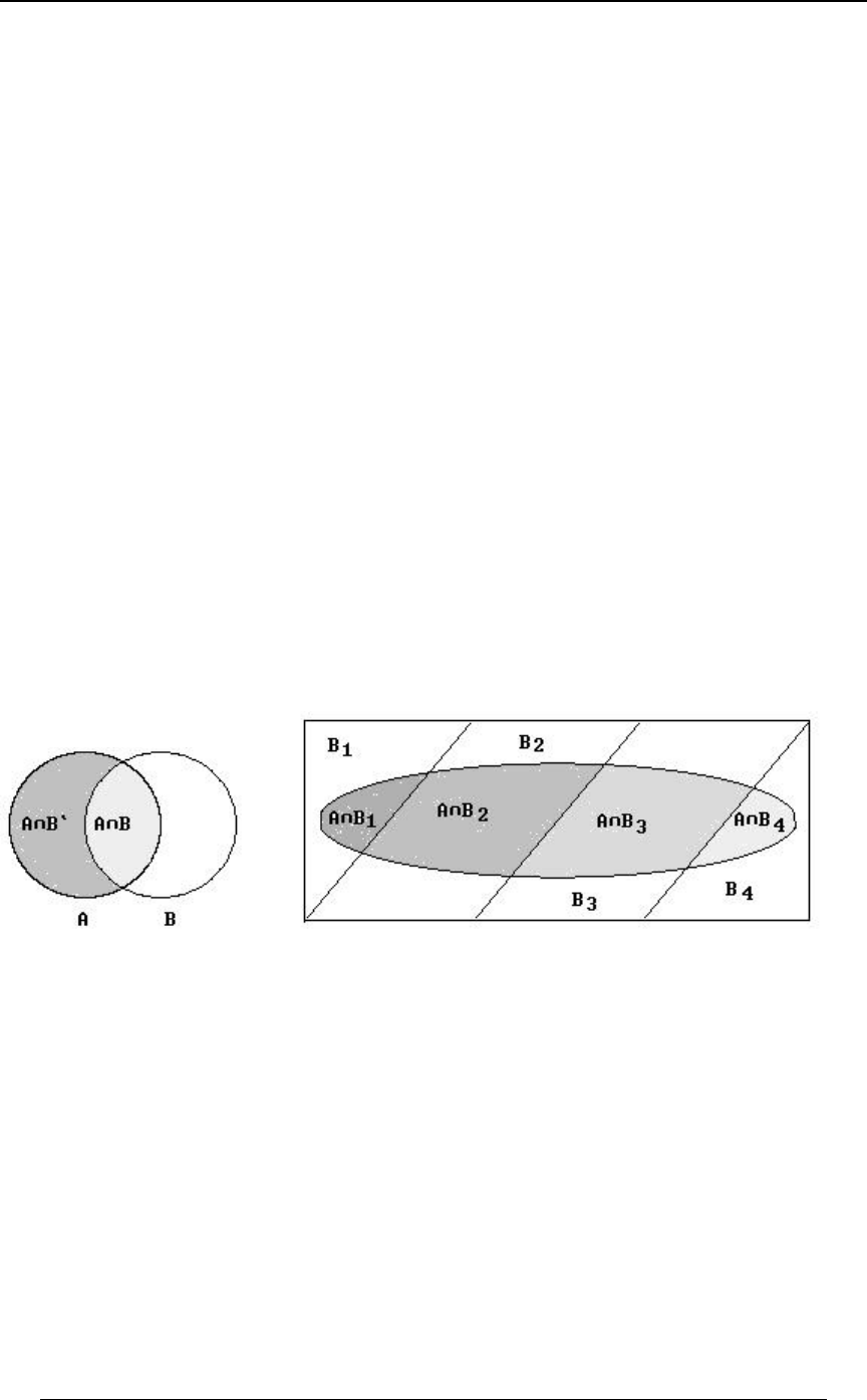
For any two sets and , we have .E F E œ ÐE ∩ FÑ ∪ ÐE ∩ F Ñ

E∩F E∩F E

Related to this is the property that if a finite set is made up of the union of disjoint sets, then

the number of elements in the union is the sum of the numbers in each of the component

sets. For a finite set , we define to be the number of elements in .W8ÐWÑ W

Two useful relationships for counting elements in a set are

8ÐEÑ œ 8ÐE ∩ FÑ  8ÐE ∩ F Ñ E ∩ F E ∩ F

(true since and are disjoint), and

8ÐE ∪ FÑ œ 8ÐEÑ  8ÐFÑ  8ÐE ∩ FÑ E ∩ F (cancels the double counting of ) .

This rule can be extended to three sets,

8ÐE ∪ F ∪ G Ñ œ 8ÐEÑ  8ÐFÑ  8ÐGÑ

8ÐE∩FÑ8ÐE∩GÑ8ÐF∩GÑ

.8ÐE∩F∩GÑ

The main application of set algebra is in a probability context in which we use set algebra to

describe events and combinations of events (this appears in the next section of this study guide).

An understanding of set algebra and Venn diagram representations can be quite helpful in

describing and finding event probabilities.

Example 0-2: Suppose that the "total set" consists of the possible outcomes that can occurW

when tossing a six-faced die. Then . We define the following subsets of :W œ Ö"ß #ß $ß %ß &ß '× W

E œ Ö"ß #ß $× % (a number less than is tossed) ,

F œ Ö#ß %ß '× (an even number is tossed) ,

G œ Ö%× (a 4 is tossed) .

Then ; ;E ∪ F œ Ö"ß #ß $ß %ß '× E ∩ F œ Ö#×

EG E∩GœgG§F and are disjoint since ; ;

E œ Ö%ß &ß '× E à F œ Ö"ß $ß &× E ∪ F œ Ö"ß #ß $ß %ß '×

(complement of ) ; ;

and (this illustrates one of DeMorgan's Laws).ÐE∪FÑ œÖ&×œE ∩F

www

This is illustrated in the following Venn diagrams with sets identified by shaded regions.

SECTION 0 - REVIEW OF ALGEBRA AND CALCULUS 5

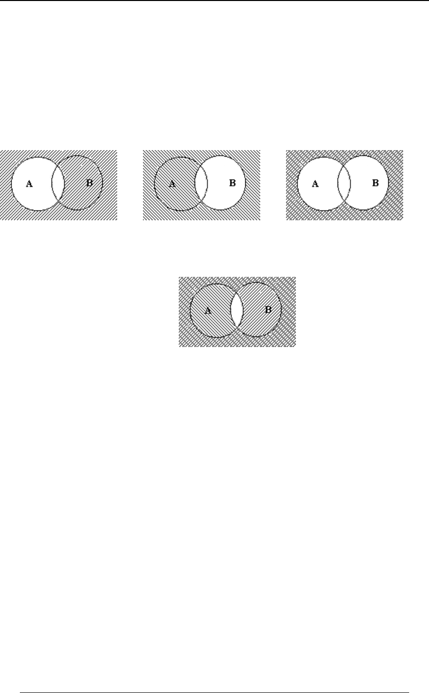
Example 0-2 continued:

EFE∪F

EFÐE∪FÑœE∩F

wwwww



Venn diagrams can sometimes be useful when analyzing the combinations of intersections and

unions of sets and the numbers of elements in various. The following examples illustrates this.

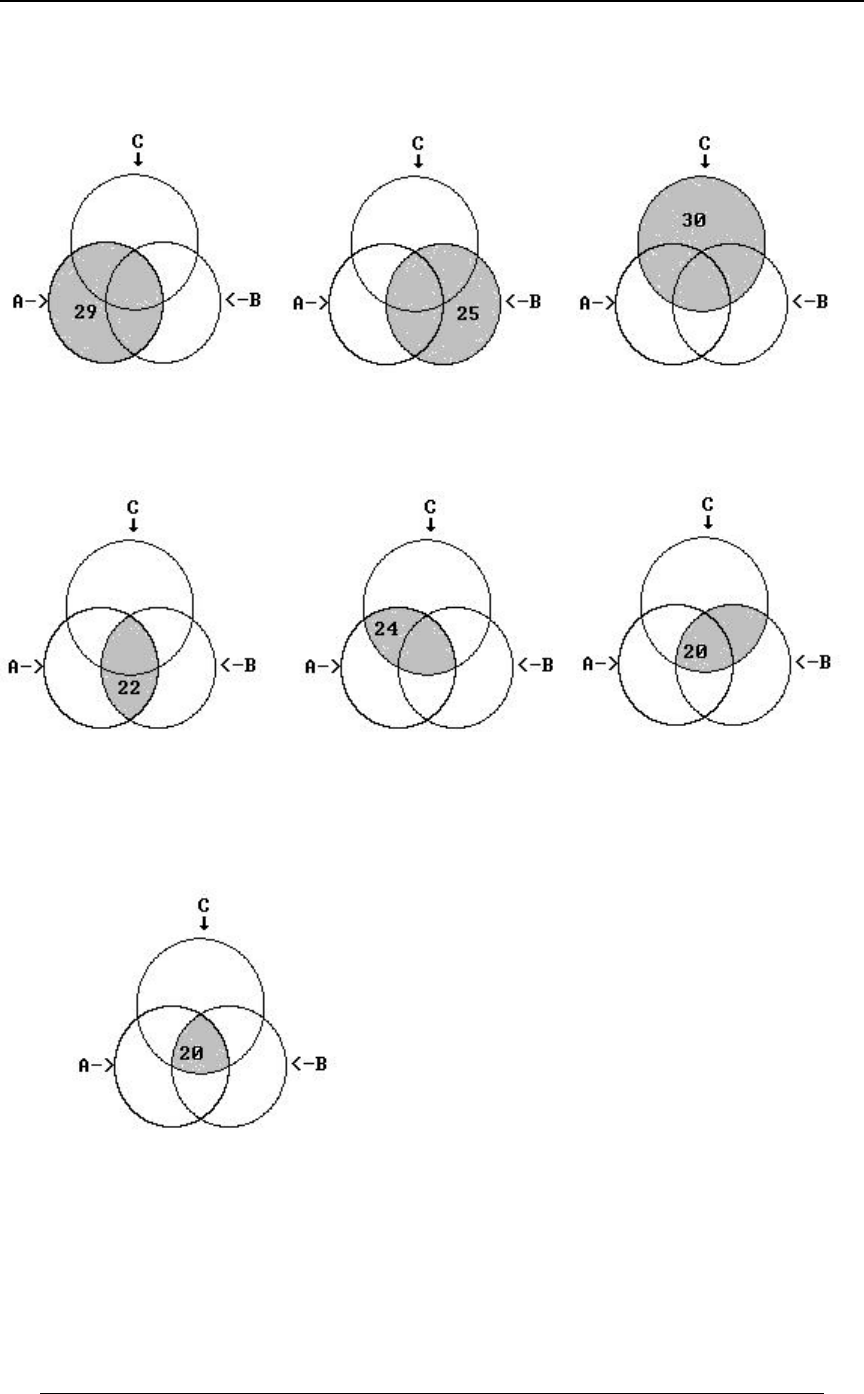
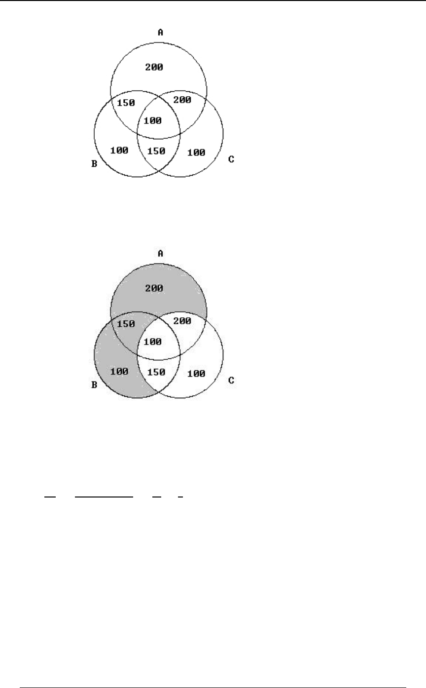
Example 0-3: A heart disease researcher has gathered data on 40,000 people who have suffered

heart attacks. The researcher identifies three variables associated with heart attack victims:

A - smoker , B - heavy drinker , C - sedentary lifestyle .

The following data on the 40,000 victims has been gathered:

29,000 were smokers ; 25,000 were heavy drinkers ; 30,000 had a sedentary lifestyle ;

22,000 were both smokers and heavy drinkers ;

24,000 were both smokers and had a sedentary lifestyle ;

20,000 were both heavy drinkers and had a sedentary lifestyle ; and

20,000 were smokers, and heavy drinkers and had a sedentary lifestyle.

Determine how many victims were:

(i) neither smokers, nor heavy drinkers, nor had a sedentary lifestyle;

(ii) smokers but not heavy drinkers;

(iii) smokers but not heavy drinkers and did not have a sedentary lifestyle?

(iv) either smokers or heavy drinkers (or both) but did not have a sedentary lifestyle?

Solution: It is convenient to represent the data in Venn diagram form. For a subset ,W

8ÐWÑ denotes the number of elements in that set (in thousands). The given information can be

summarized in Venn diagram form as follows:

6 SECTION 0 - REVIEW OF ALGEBRA AND CALCULUS

Example 0-3 continued:

8ÐEÑ œ #* !!! 8ÐFÑ œ #&ß !!! 8ÐGÑ œ $!ß !!!, (smoker) (heavy drinker) (sedentary

lifestyle)

8ÐE ∩ FÑ œ ##ß !!! 8ÐE ∩ GÑ œ #%ß !!! 8ÐF ∩ GÑ œ #!ß !!!

(smoker and heavy drinker) (smoker and sedentary lifestyle) (heavy drinker

and sedentary lifestyle)

(smoker and heavy drinker and sedentary lifestyle)8ÐE ∩ F ∩ GÑ œ #!ß !!!

SECTION 0 - REVIEW OF ALGEBRA AND CALCULUS 7

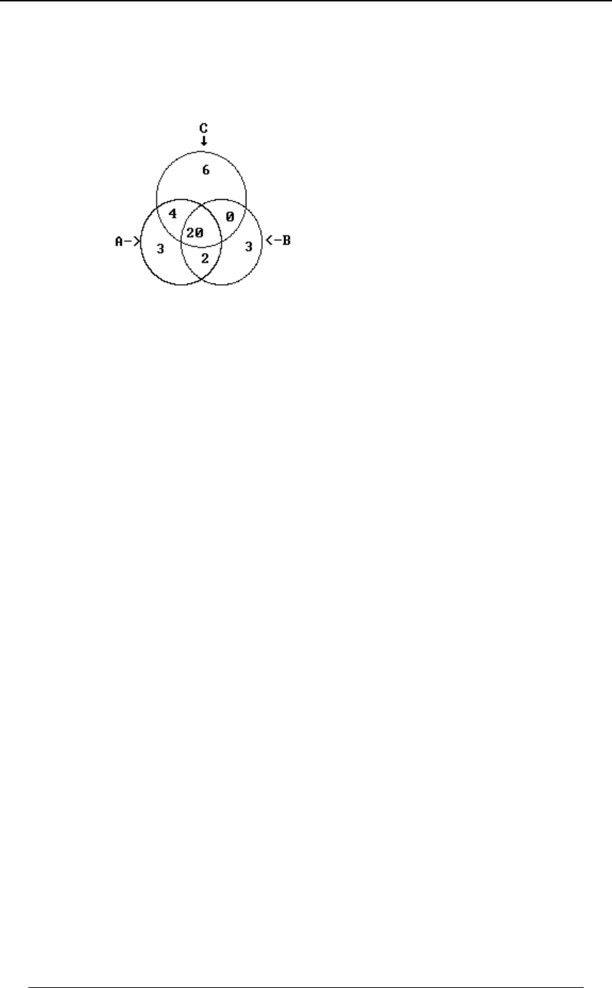
Example 0-3 continued:

Working from the inside outward in the Venn diagrams, we can identify the number within each

minimal subset of all of the intersections:

A typical calculation to fill in this diagram is as follows. We are given 8ÐE ∩ F ∩ GÑ œ #!ß !!!

and ; we use the relationship8ÐE ∩ FÑ œ ##ß !!!

##ß !!! œ 8ÐE ∩ FÑ œ 8ÐE ∩ F ∩ GÑ  8ÐE ∩ F ∩ G Ñ œ #!ß !!!  8ÐE ∩ F ∩ G Ñ

to get (this shows that the 22,000 victims in who are both8ÐE∩F∩G Ñœ#ß!!! E∩F

smokers and heavy drinker can be subdivided into those who also have a sedentary lifestyle

8ÐE ∩ F ∩ GÑ œ #!ß !!! 8ÐE ∩ F ∩ G Ñ, and those who do not have a sedentary lifestyle, , the

other ). Other entries are found in a similar way. From the diagram we can gainœ #ß !!!

additional insight into other combinations of subsets. For instance, 6,000 of the victims have a

sedentary lifestyle, but are neither smokers nor heavy drinkers; this is the entry "6", which in set

notation is . Also, the number of victims who were both heavy8ÐE ∩ F ∩ GÑ œ 'ß !!!

drinkers and had a sedentary lifestyle but were not smokers is 0.

We can now find the requested numbers.

(i) The number of victims who had at least one of the three specified conditions is

8ÐE ∪ F ∪ GÑ , which, from the diagram can be calculated from the disjoint components:

8ÐE ∪ F ∪ GÑ œ #!ß !!!  #ß !!!  %ß !!!  !  $ß !!!  $ß !!!  'ß !!! œ $)ß !!! .

The "total set" in this example is the set of all 40,000 victims. Therefore, there were 2,000 heart

attack victims who had none of the three specified conditions; this is the complement of

8ÐE ∪ F ∪ GÑ. Algebraically, we have used the extension of one of DeMorgan's laws to the case

of three sets, "none of or or " "not " and "not "E F G œÐE∪F∪GÑ œE ∩F ∩G œ E F

wwww

and "not " .G

8 SECTION 0 - REVIEW OF ALGEBRA AND CALCULUS

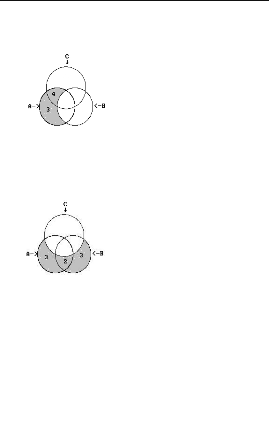
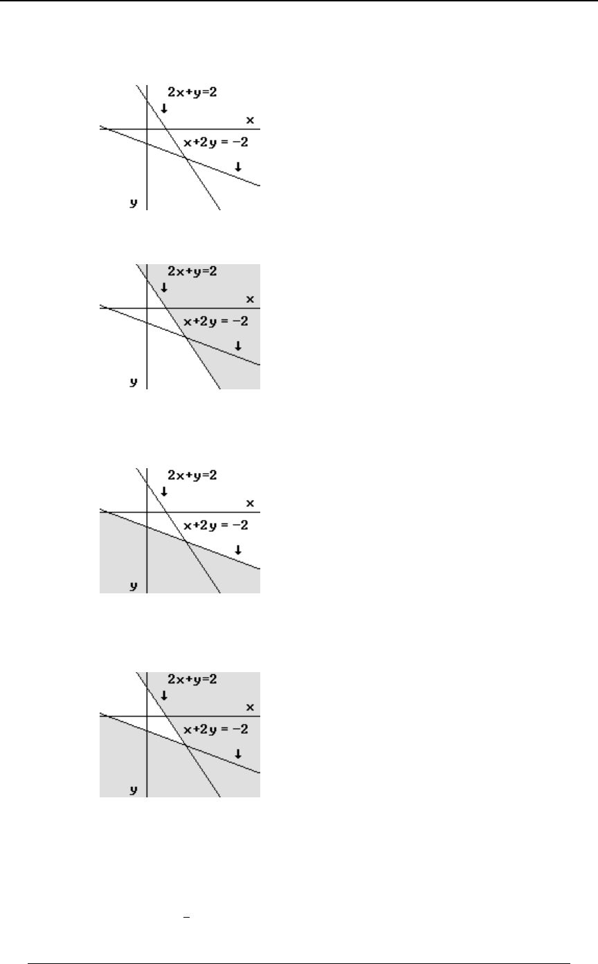
Example 0-3 continued:

(ii) The number of victims who were smokers but not heavy drinkers is

8ÐE ∩ F Ñ œ $ß !!!  %ß !!!

w . This can be seen from the following Venn diagram

(iii) The number of victims who were smokers but not heavy drinkers and did not have a

sedentary lifestyle is (part of the group in (ii)).8ÐE ∩ F ∩ G Ñ œ $ß !!!

(iv) The number of victims who were either smokers or heavy drinkers (or both) but did not have

a sedentary lifestyle is This is illustrated in the following Venn diagram.8ÒÐE ∪ FÑ ∩ G Ó Þ

8ÒÐE ∪ FÑ ∩ G Ó œ $ß !!!  #ß !!!  $ß !!! œ )ß !!!

w . 

SECTION 0 - REVIEW OF ALGEBRA AND CALCULUS 9

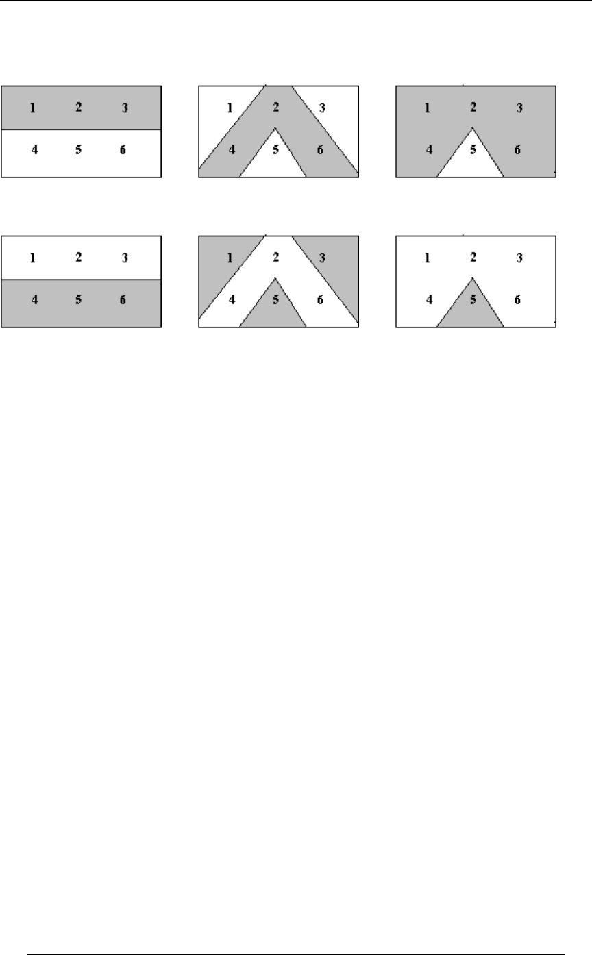
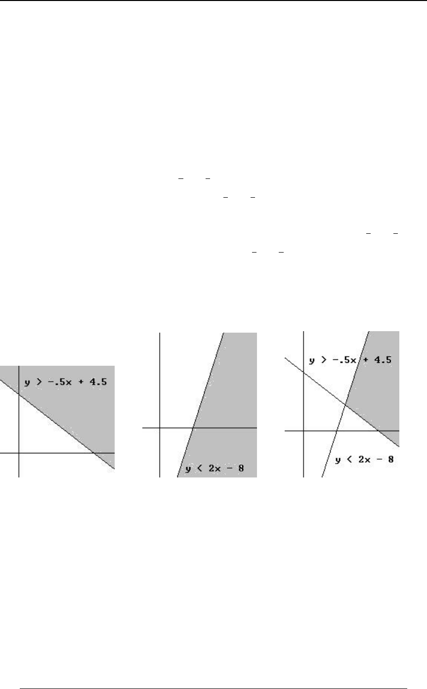
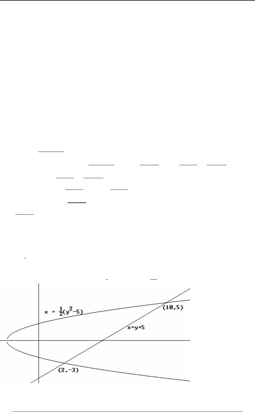
GRAPHING AN INEQUALITY IN TWO DIMENSIONS

The joint distribution of a pair of random variables and is sometimes defined over a two\]

dimensional region which is described in terms of linear inequalities involving and . TheBC

region represented by the inequality is the region above the line (andC+B, Cœ+B,

C+B, is the region below the line).

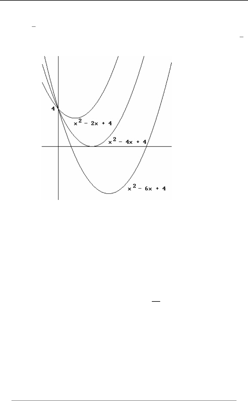
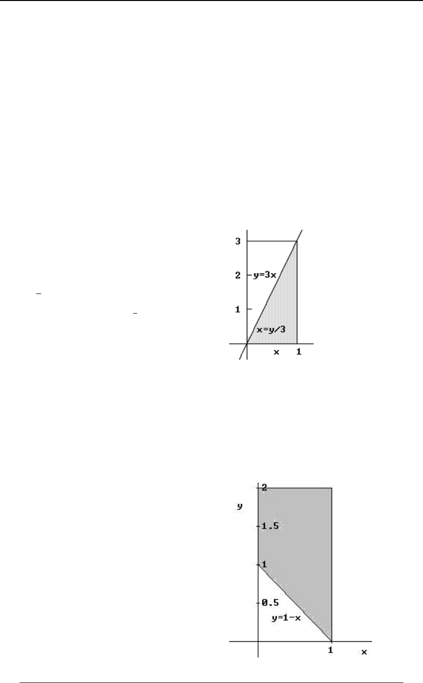
Example 0-4: Using the lines and , find the region in the -Cœ  B Cœ#B) BC

plane that satisfies both of the inequalities and .C  B C#B)

Solution: We graph each of the straight lines, and then determine which side of the line is

represented by the inequality. The first graph below is the graph of the line ,Cœ  B

along with the shaded region, which is the region , consisting of all pointsC  B

"above" that line. The second graph below is the graph of the line , along with theCœ#B)

shaded region, which is the region , consisting of all points "below" that line.C#B)

The third graph is the intersection (first region and second region) of the two regions.



10 SECTION 0 - REVIEW OF ALGEBRA AND CALCULUS

PROPERTIES OF FUNCTIONS

Definition of a function :0 A function is defined on a subset (or the entire set) of real0ÐBÑ

numbers. For each , the function defines a number . he of the function is the setB0ÐBÑ0 T domain

of -values for which the function is defined. The is the set of all values thatB0ÐBÑrange of 0

can occur for 's in the domain. Functions can be defined in a more general way, but we will beB

concerned only with real valued functions of real numbers. Any relationship between two real

variables (say and ) can be represented by its graph in the -plane. If the functionBC ÐBßCÑ

Cœ0ÐBÑ B 0 B is graphed, then for any in the domain of , the vertical line at will intersect the

graph of the function at exactly one point; this can also be described by saying that for each value

of there is (at most) one related value of .BC

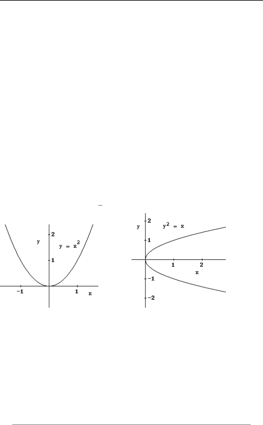
Example 0-5: (i) defines a function since for each there is exactly one value . TheCœB B B

# #

domain of the function is all real numbers (each real number has a square). The range of the

function is all real numbers , since for any real , the square is .! B B !

(ii) does not define a function since if , there are two values of for whichCœB B! C

CœB „ B

#. These two values are . This is illustrated in the graphs below



Functions defined piecewise: A function that is defined in different ways on separate

intervals is called a . The absolute value function is an example of apiecewise defined function

piecewise defined function: .

for

lBl œ B B!

BB!

SECTION 0 - REVIEW OF ALGEBRA AND CALCULUS 11

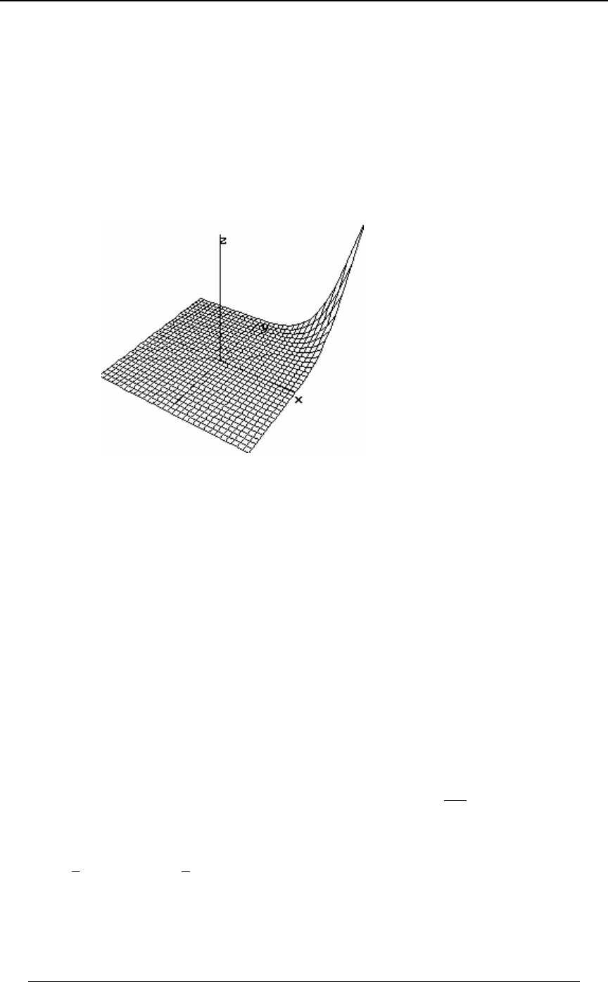
Multivariate function: A function of more than one variable is called a multivariate function.

Example 0-6: is a function of two variables, the domain is the entire 2-Dœ0ÐBßCÑœ/

BC

dimensional plane (the set , are both real numbers ) , and the range is the set of strictlyÖÐBß CÑl B C ×

positive real numbers. The function could be graphed in 3-dimensional - - space. The domainBCD

would be the (horizontal) - plane, and the range would be the (vertical) -dimension.BC D

The 3-dimensional graph is shown below.



The concept of the inverse of a function is important when formulating the distribution of a

transformed random variable. A preliminary concept related to the inverse of a function is that of

a one-to-one function.

One-to-one function: The function is called a one-to-one if the equation has at00ÐBÑœC

most one solution for each (or equivalently, different -values result in different values).BC B 0ÐBÑ

If a graph is drawn of a one-to-one function, any horizontal line crosses the graph in at most one

place.

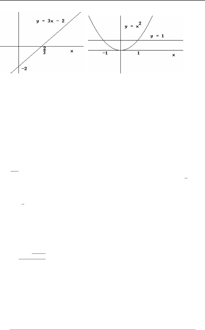
Example 0-7: The function is one-to-one, since for each value of , the0ÐBÑ œ $B  # C

relation has exactly one solution for in terms of ; . The functionCœ$B# B C BœC#

1ÐBÑ œ B# with the whole set of real numbers as its domain is not one-to-one, since for each

C! B C CœB , there are two solutions for in terms of for the relation (those two solutions

are and ; note that if we restrict the domain of to the positiveBœ C Bœ  C 1ÐBÑœB

ÈÈ #

real numbers, it becomes a one-to-one function). The graphs are below.

12 SECTION 0 - REVIEW OF ALGEBRA AND CALCULUS



Inverse of function :0 The inverse of the function is denoted . The inverse exists only if00

"

00ÐCÑœBB0ÐBÑœC is one-to-one, in which case, is the (unique) value of which satisfies

"

(finding the inverse of means that we solve for in terms of , ). ForCœ0ÐBÑ B C Bœ0 ÐCÑ

"

instance, for the function , if then so thatCœ#B œ0ÐBÑ Bœ" Cœ0Ð"Ñœ#Ð" Ñœ#ß

" œ 0 Ð#Ñ œ Ð#Î#Ñ C œ #

" "Î$ . For the example just considered, the inverse function applied to

is the value of for which , or equivalently, , from which we get .B0ÐBÑœ# #Bœ# Bœ"

Example 0-8: (i) The inverse of the function is the functionCœ&B"œ0ÐBÑ

Bœ œ0 ÐCÑ B C

C"

&" (we solve for in terms of ).

(ii) Given the function , solving for in terms of results in , soCœB œ0ÐBÑ B C Bœ „ C

#È

there are two possible values of for each value of ; this function does not have an inverse.BC

However, if the function is defined to be , thenCœB œ0ÐBÑ

#for onlyB!

Bœ  Cœ0 ÐCÑ 0

È" would be the inverse function, since is one-to-one on its domain which

consists of non-negative numbers. 

Quadratic functions and equations: A quadratic function is of the form

:ÐBÑœ+B ,B- +B ,B-œ!

. The roots of the quadratic equation are

<ß< œ

"# ,„ , %+-

È# . The quadratic equation has

(i) distinct real roots if ,,%+-

#!

(ii) distinct complex roots if , and,%+-

#!

(iii) equal real roots if .,%+-

#œ!

SECTION 0 - REVIEW OF ALGEBRA AND CALCULUS 13

Example 0-9: The quadratic equation has two distinct real solutions:B'B%œ!

Bœ$„ & B %B%œ! Bœ#

È. The quadratic equation has both roots equal: .

The quadratic equation has two distinct complex roots: .B#B%œ! Bœ"„3 $

#È



Exponential and logarithmic functions: Exponential functions are of the form ,0ÐBÑ œ ,B

where , and the inverse of this function is denoted .,!ß,Á" 691ÐCÑ

Thus . The log function with base is the ,Cœ, Í691ÐCÑœB /

B,natural logarithm

691 ÐCÑ œ 68 C 691 C

/ (also written ). Some important properties of these functions are:

,œ" 691Ð"Ñœ!

.97+38Ð0Ñ œ œ <+81/Ð0 Ñ<+81/Ð0 Ñ œ Ð!ß  ∞Ñ œ .97+38Ð0 Ñ‘" "

for for all , œC C! 691Ð, ÑœB B

691 ÐCÑ B

,œ/ 691ÐCÑœ

BB†68, ,68 C

68 ,

Ð, Ñ œ , 691 ÐC Ñ œ 5 † 691 ÐCÑ

BC BC 5

, , œ , 691 ÐCDÑ œ 691 ÐCÑ  691 ÐDÑ

BC BC ,,,

, Î, œ , 691 ÐCÎDÑ œ 691 ÐCÑ  691 ÐDÑ

BC BC ,,,

For the function , we have for an , and for the natural log function, we have//œCC!

B68C

68 / œ B B

B for any real number .

14 SECTION 0 - REVIEW OF ALGEBRA AND CALCULUS

LIMITS AND CONTINUITY

Intuitive definition of limit: The expression means that as gets close tolim

BÄ-0ÐBÑ œ P B

(approaches) the number , the value of gets close to .-0ÐBÑP

Example 0-10: , and (forlim lim lim lim

BÄ" BÄ" BÄ"

BÄ∞

B

ÐB$Ñœ% / œ! œ ÐB$Ñœ%

B#B$

B"

this last limit, note that if , but in taking this limit we are

B#B$

B" B"

ÐB$ÑÐB"Ñ

#œœB$BÁ"

only concerned with what happens "near" , that fact that at does notBœ" œ Bœ"

B#B$

B"

mean that the limit does not exist; it means that the function does not exist at the point ).Bœ" 

Continuity: if there is no "break" or "hole"The function is continuous at the point 0Bœ-

in the graph of , or equivalently, if . In Example 0-10 above, theCœ0ÐBÑ lim

BÄ-0ÐBÑ œ 0Ð-Ñ

third function is not continuous at because is not defined. Another reason for aBœ" 0Ð"Ñœ !

discontinuity in occurring at is that the limit of is different from the left than it is0ÐBÑ B œ - 0ÐBÑ

from the right.

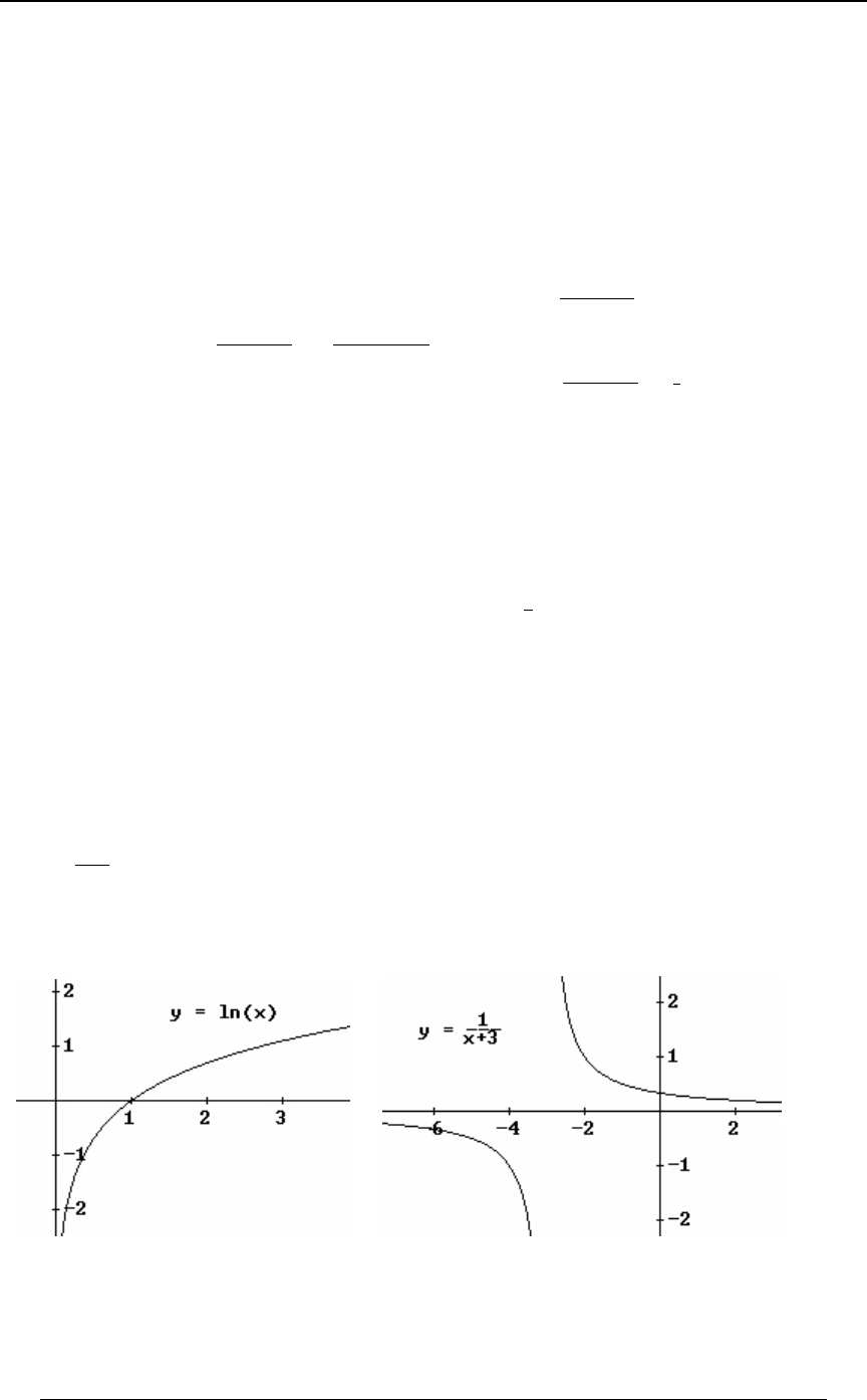
Example 0-11: (i) If and then is discontinuous at since the0ÐBÑœ68B -œ! 0 -œ!

function is not defined at the point (this would also be the case for the function68 B B œ !

0ÐBÑ œ - œ $

B$ and ).

(ii) If , then is discontinuous at since even though is0ÐBÑ œ 0ÐBÑ B œ ! 0Ð!Ñ

š"ÎB BÁ!

!Bœ!

defined, ( doesn't exist). lim lim

BÄ! BÄ!

0ÐBÑ Á 0Ð!Ñ 0ÐBÑ



SECTION 0 - REVIEW OF ALGEBRA AND CALCULUS 15

DIFFERENTATION

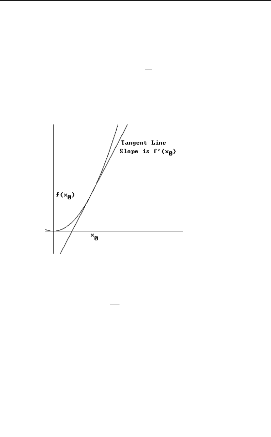
Geometric interpretation of derivative: The derivative of the function at the point0ÐBÑ

BœB Cœ0ÐBÑ ÐBß0ÐBÑÑ

!!!

is the slope of the line tangent to the graph of at the point . The

derivative of at is denoted or 0ÐBÑ B œ B 0 ÐB Ñ Þ

BœB

.B º!

This is also referred to as the derivative of with respect to at the point .0BBœB

The algebraic definition of is0ÐBÑ

0ÐBÑœ œ

w!2Ä! BÄB

lim lim

0ÐB 2Ñ0 ÐB Ñ 0ÐBÑ0 ÐB Ñ

2BB

!! !

The second derivative of at is the derivative of at the point . It is denoted or0B 0ÐBÑ B 0ÐBÑ

!!!

www

0ÐBÑ Þ 8 0 B8

Ð#Ñ !!

BœB

or The -th order derivative of at ( repeated applications of

#º!

differentiation) is denoted . 0ÐBÑœ

Ð8Ñ !

BœB

8º!

The derivative as a rate of change: Perhaps the most important interpretation of the

derivative is as the 0ÐBÑ

w!"instantaneous" rate at which the function is increasing or

decreasing as increases if , the graph of is rising, with the tangent lineBÐ0! Cœ0ÐBÑ

to the graph having positive slope, and if , the graph of is falling0! Cœ0ÐBÑ Ñ

w, and if

0ÐBÑœ!

w! then the tangent line at that point is horizontal (has slope 0). This interpretation is the

one most commonly used when analyzing physical, economic or financial processes.

16 SECTION 0 - REVIEW OF ALGEBRA AND CALCULUS

The following is a summary of some important differentiation rules.

Rules of differentiation: 0 ÐBÑ 0 ÐBÑ

(a constant) -!

Power rule - ( ) -B 8 − -8B

88"

‘

1ÐBÑ  2ÐBÑ 1 ÐBÑ  2 ÐBÑ

Product rule - 1ÐBÑ † 2ÐBÑ 1 ÐBÑ † 2ÐBÑ  1ÐBÑ † 2 ÐBÑ

?ÐBÑ@ÐBÑAÐBÑ ? @A  ?@ A  ?@A

ww w

Quotient rule -

1ÐBÑ 2ÐBÑ1 ÐBÑ1ÐBÑ2 ÐBÑ

2ÐBÑ Ò2ÐBÑÓ

Chain rule - 1Ð2ÐBÑÑ 1 Ð2ÐBÑÑ † 2 ÐBÑ

/1ÐBÑ†/

1ÐBÑ w 1ÐBÑ

68Ð1ÐBÑÑ 1ÐBÑ

1ÐBÑ

+Ð+!Ñ +68+

68 B "

691 B

B68,

=38 B -9= B

-9= B  =38 B

Example 0-12: What is the derivative of ?0ÐBÑ œ %BÐB  "Ñ

Solution: We apply the product rule and chain rule: ,0ÐBÑ œ 1ÐBÑ † 2ÐBÑ

where .1ÐBÑ œ %B ß 2ÐBÑ œ ÐB  "Ñ ß 1 ÐBÑ œ % ß 2 ÐBÑ œ $ÐB  "Ñ † #B

#$w w ##

0 ÐBÑ œ %B † $ÐB  "Ñ † #B  %ÐB  "Ñ œ %ÐB  "Ñ Ð(B  "Ñ

w###$###

Notice that , where and .2ÐBÑ œ ÐB  "Ñ œ ÒAÐBÑÓ œ 2ÐAÐBÑÑ 2ÐAÑ œ A AÐBÑ œ B  "

#$ $ $ #

The chain rule tells us that . 2 ÐBÑ œ 2 ÐAÑ † A ÐBÑ œ $A † Ð#BÑ œ $ÐB  "Ñ † Ð#BÑ

www # ## 

SECTION 0 - REVIEW OF ALGEBRA AND CALCULUS 17

L'Hospital's rules for calculating limits: A limit of the form is said to be inlim

BÄ-

0ÐBÑ

1ÐBÑ

indeterminate form if both the numerator and denominator go to 0, or if both the numerator and

denominator go to . L'Hospital's rules are:„∞

(i) ,

(ii) exists,

(iii) exists and is

IF THEN

and

lim lim

lim

BÄ- BÄ-

wBÄ-

0ÐBÑ œ 1ÐBÑ œ !

0Ð-Ñ

1Ð-Ñ Á!

0ÐBÑ 0 Ð-Ñ

1ÐBÑ 1 Ð-Ñ

(i) ,

(ii) and are differentiable near ,

(iii) exists

IF THEN

and

lim lim

lim

BÄ- BÄ-

BÄ-

0ÐBÑ œ 1ÐBÑ œ !

01 -

0ÐBÑ

1ÐBÑ

BÄ- BÄ-

0ÐBÑ 0 ÐBÑ

1ÐBÑ 1 ÐBÑ

œlim w

In 1 or 2, the conditions and can be replaced by the conditionslim lim

BÄ- BÄ-

0ÐBÑ œ ! 1ÐBÑ œ !

lim lim

BÄ- BÄ-

0ÐBÑ œ „∞ 1ÐBÑ œ „ ∞ - „∞ and , and the point can be replaced by with the

conclusions remaining valid.

Example 0-13: Find .lim

BÄ#

$$

$*

BÎ#

Solution: The limits in both the numerator and denominator are 0, so we apply l'Hospital's rule.

.."$$

.B .B # $ * $ 68 $

$†68$

$œ$68$ $ œ$ † 68$ œ œ

BB BÎ#BÎ#

BÄ# BÄ#

, and , so that . Thislim lim

BÎ#

BÎ# "

limit can also be found by factoring the denominator into , and$  * œ Ð$  $ÑÐ$  $Ñ

B BÎ# BÎ#

then canceling out the factor in the numerator and denominator. $$

BÎ# 

Differentiation of functions of several variables - partial differentiation:

Given the function , a function of two variables, the partial derivative of with respect to0ÐBßCÑ 0

BÐBßCÑ 0 B C at the point is found by differentiating with respect to and regarding the variable

as constant - then substitute in the values and . The partial derivative of withBœB CœC 0

respect to is usually denoted The partial derivative with respect to is defined in a similarBC

`B.

way: "Higher order" partial derivatives can be defined - , ; `0 `0 `0 `0

`B `B `B `C `C `C

œœÐÑ ÐÑ

and "mixed partial" derivatives can be defined (the order of partial differentiation does not

usually matter) - .

` 0 `0 `0 ` 0

`B `C `B `C `C `B `C `B

œœœÐÑ ÐÑ

Example 0-14: If for then find and .0ÐBß CÑ œ B Bß C  !

Ð%ß Ñ Ð%ß Ñ

`0 ` 0

`B `C

¹¹

Solution: , and

`B # %

œ CB œ Ð ÑÐ%Ñ œ

C" "Î#

Ð%ß Ñ

º"

`0 ` 0

`C `C

œB Ð68BÑ œB Ð68BÑ œ% Ð68%Ñ œ#Ð68%Ñ

C C # "Î# # #

Ð%ß Ñ

and .

º

18 SECTION 0 - REVIEW OF ALGEBRA AND CALCULUS

INTEGRATION

Geometric interpretation of the "definite integral" - the area under the curve:

Given a function on the interval , the definite integral of over the interval is0ÐBÑ Ò+ß,Ó 0ÐBÑ

denoted , and is equal to the "signed" area between the graph of the function and the

,0ÐBÑ.B

BBœ+Bœ, 0ÐBÑ!-axis from to . Signed area is positive when and is negative when

0ÐBÑ  ! 0ÐBÑ. What is meant by signed area here is the area from the interval(s) where is

positive minus the area from the intervals where is negative.0ÐBÑ

Integration is related to the antiderivative of a function. Given a function , an antiderivative0ÐBÑ

of is any function which satisfies the relationship . According to the0ÐBÑ J ÐBÑ J ÐBÑ œ 0ÐBÑ

Fundamental Theorem of Calculus, the definite integral for can be found by first finding0ÐBÑ

J ÐBÑ 0ÐBÑ, an antiderivative of . The basic relationships relating integration and differentiation

are:

(i) If for , then . JÐBÑœ0ÐBÑ +ŸBŸ, 0ÐBÑ.BœJÐ,ÑJÐ+Ñ

(ii) If then KÐBÑ œ 1Ð>Ñ .> ß K ÐBÑ œ 1ÐBÑ

Example 0-15: Find the definite integral of the function on the interval .0ÐBÑ œ #  B Ò  "ß $Ó

Solution: The graph of the function is given below. It is clear that for , and0ÐBÑ  ! B  #

0ÐBÑ  ! B  # 0ÐBÑ J ÐBÑ œ #B  Þ for . An antiderivative for is The definite integral will

be Note that the area

'"

$Ð#BÑ.BœJÐ$ÑJÐ"ÑœÐ' ÑÐ# Ñœ%Þ

Ð"Ñ

between the graph and the -axis from to is , and the signed areaB B œ  " B œ # Ð$ÑÐ$Ñ œ

between the graph and the -axis from to is . The total signedB B œ # B œ $  Ð"ÑÐ"Ñ œ 

area is .

œ%



SECTION 0 - REVIEW OF ALGEBRA AND CALCULUS 19

Antiderivatives of some frequently used functions:

0ÐBÑ 0ÐBÑ.B (antiderivative)

1ÐBÑ  2ÐBÑ 1ÐBÑ.B  2ÐBÑ.B  - ''

BÐ8Á"Ñ -

8 B

8"

B 68 B  -

//-

+Ð+!Ñ -

B +

68 +

B/   -

+B .

B/ /

+B +B

=38 B  -9= B  -

-9= B =38 B  -

Integration of on when is not defined at or , or when or is :0Ò+ß,Ó 0 +, +,„∞

Integration over an infinite interval (an "improper integral") is defined by taking limits:

'' '

++ ∞

∞, ,

,Ä∞

0ÐBÑ .B œ 0ÐBÑ .B 0ÐBÑ .Blim , with a similar definition applying to ,

and .

∞ +

∞+

+Ä∞

0ÐBÑ.B œ 0ÐBÑ.Blim

If is not defined at (also called an improper integral), or if is discontinuous at ,0 Bœ+ 0 Bœ+

then .

-Ä+

0ÐBÑ.B œ 0ÐBÑ.Blim



A similar definition applies if is not defined at , or if is discontinuous at .0 Bœ, 0 Bœ,

If has a discontinuity at the point in the interior of , then0ÐBÑ B œ - Ò+ß,Ó

'''

++-

,-,

0ÐBÑ.B œ 0ÐBÑ.B  0ÐBÑ.B

Example 0-16:

(a) ,

'' ’“

ºÈ

-Ä! -Ä! -Ä!

"Î# "Î#

Bœ-

Bœ"

È.B œ B .B œ #B œ Ò#  # -Ó œ #lim lim lim

 

''’“

ºÈ

∞-

-Ä∞ -Ä∞ -Ä∞

"Î# "Î#

Bœ"

Bœ-

È.B œ B .B œ #B œ Ò# -  #Ó œ  ∞ Þlim lim lim

(b) '’“

∞

,Ä∞ ,Ä∞

Bœ"

Bœ,

"" "

BB ,

#.B œ  œ Ò   Ð  "ÑÓ œ "lim lim

'∞

B#.B B œ !

'''

∞ ∞ !

"!"

"""

BBB

###

.B œ .B  .B . The second integral is

+Ä! +Ä!

"" "

BB +

.B œ .B œ Ò  "  Ó œ  ∞lim lim

 , thus, the second improper integral

does not exist (when is infinite or does not exist, the integral is said to "diverge"). lim

Ä'

20 SECTION 0 - REVIEW OF ALGEBRA AND CALCULUS

A few other useful integration rules are:

(i) for integer and real number .8! -! B / .B œ

∞8-B 8x

-8"

(ii) if , then ,KÐBÑ œ 0Ð?Ñ .? K ÐBÑ œ 0Ò2ÐBÑÓ † 2 ÐBÑ

2ÐBÑ ww

(iii) if , then ,KÐBÑ œ 0Ð?Ñ .? K ÐBÑ œ  0ÐBÑ

(iv) if , then ,KÐBÑ œ 0Ð?Ñ .? K ÐBÑ œ  0 Ò1ÐBÑÓ † 1 ÐBÑ

'1ÐBÑ

,ww

(v) if , then .KÐBÑ œ 0Ð?Ñ .? K ÐBÑ œ 0Ò2ÐBÑÓ † 2 ÐBÑ  0Ò1ÐBÑÓ † 1 ÐBÑ

'1ÐBÑ

2ÐBÑ www

Double integral: Given a continuous function of two variables, on the rectangular0ÐBßCÑ

region bounded by and , it is possible to define the definite integralBœ+ßBœ,ßCœ- Cœ.

of over the region. It can be expressed in one of two equivalent ways:0

'' ''

+- - +

,. .,

0ÐBß CÑ .C .B œ 0ÐBß CÑ .B .C

The interpretation of the first expression is [ ] , in which the "inside integral" is

0ÐBß CÑ .C .B

.0ÐBßCÑ.C B , and it is calculated assuming that the value of is constant (it is an integral with

respect to the variable ). When this definite "inside integral" has been calculated, it will be aC

function of alone, which can then be integrated with respect to from to . TheBBBœ+Bœ,

second equivalent expression has a similar interpretation; is calculated assuming

,0ÐBßCÑ.B

that is constant; this results in a function of alone which is then integrated with respect to CC C

from to . Double integration arises in the context of finding probabilities for a jointCœ- Cœ.

distribution of continuous random variables.

Example 0-17: Find .

#.C .B

Solution: First we assume that is constant and find .B.CœBÐ68CÑœBÐ68#Ñ

'º

###

Cœ"

Cœ#

Then we find .

'º

Bœ!

Bœ"

68 #

ÒB Ð68 #ÑÓ .B œ Ð68 #Ñ † œ

We can also write the integral as , and first find

#.B .C

ºº

Cœ"

Cœ#

BB " "" "

C$C $C $C$ $

Bœ!

Bœ"

.B œ œ .C œ Ð68 CÑ œ Ð68 #Ñ. Then, . 

For double integration over the rectangular two-dimensional region , as+ŸBŸ,ß -ŸCŸ.

the expression indicates, it is possible to calculate

'' ''

+- - +

,. .,

0ÐBß CÑ .C .B œ 0ÐBß CÑ .B .C

the double integral by integrating with respect to the variables in either order ( first and secondCB

for the integral on the left, and first and second for the integral on the right of the " " sign).BC œ

SECTION 0 - REVIEW OF ALGEBRA AND CALCULUS 21

Formulations of probabilities and expectations for continuous joint distributions sometimes

involve integrals over a non-rectangular two-dimensional region. It will still be possible to

arrange the integral for integration in either order ( or ), but care must be taken in.C .B .B .C

setting up the limits of integration. If the limits of integration are properly specified, then the

double integral will be the same whichever order of integration is used. Note also that in some

situations, it may be more efficient to formulate the integration in one order than in the other.

Example 0-18: Which of the following integrals is equal to ''

"$B

0ÐBß CÑ .C .B

for every function for which the integral exists?

A) B) C)

'' '' ''

!! !$B !$C

$CÎ$ "$ $"

0ÐBß CÑ .B .C 0ÐBß CÑ .B .C 0ÐBß CÑ .B .C

D) E)

'' ''

!! !CÎ$

"BÎ$ $"

0ÐBß CÑ .B .C 0ÐBß CÑ .B .C

Solution: The graph at the right illustrates

the region of integration. The region is

!ŸBŸ"ß!ŸCŸ$B Cœ$B. Writing

as , we see that the inequalitiesBœ C

translate into , and .!ŸCŸ$ ŸBŸ"

Answer: E 

Example 0-19: The function is to be integrated over the two-dimensional region0ÐBßCÑ

defined by the following constraints: and . Formulate the double!ŸBŸ" "BŸCŸ#

integration in the order and then in the order..C .B .B .C

Solution: The graph at the right illustrates

the region of integration. The region is

!ŸBŸ"ß"BŸCŸ#. The integral can

be formulated in the order as.C .B

!"B

"# 0ÐBÞCÑ .C .B B ; for each , the

integral in the vertical direction starts on the

line and continues to the upperCœ"B

boundary . To use the order,Cœ# .B.C

we must split the integral into two double

integrals; to cover the

!"C

""0ÐBß CÑ .B .C

triangular area below , andCœ"

0ÐBß CÑ .B .C to cover the square area

above . Cœ" 

22 SECTION 0 - REVIEW OF ALGEBRA AND CALCULUS

There are a few integration techniques that are useful to know. The integrations that arise

on Exam P are usually straightforward, but knowing a few additional techniques of

integration are sometimes useful in simplifying an integral in an efficient way.

The Method of Substitution: Substitution is a basic technique of integration that is used to

rewrite the integral in a standard form for which the antiderivative is well known. In general, to

find we may make the substitution for an "appropriate" function .

'0ÐBÑ .B ? œ 1ÐBÑ 1ÐBÑ

We then define the "differential" to be , and we try to rewrite as.? .? œ 1 ÐBÑ .B 0ÐBÑ .B

an integral with respect to the variable .?

For example, to find , we let , so that , or

'ÐB "Ñ B .B ?œB " .?œ$B .B

$ %Î$ # $ #

equivalently, ; then the integral can be written as , which has

$†.?œB .B ? † .?

# %Î$ "

antiderivative .

? †.?œ†?.?œ† œ?Ð-Ñ

%Î$ %Î$ (Î$

"" "?"

$ $ $ (Î$ (

(Î$

We can then write the antiderivative in terms of the original variable -B

'ÐB"ÑB.Bœ? œÐB"Ñ

$ %Î$ # (Î$ $ (Î$

(( .

The main point to note in applying the substitution technique is that the choice of ?œ1ÐBÑ

should result in an antiderivative which is easier to find than was the original antiderivative.

Example 0-20: Find .

'È

B"B.B

Solution: Let Then , so that , and the?œ"B .?œ #B.B  †.?œB.B

antiderivative can be written as . The definite

'? † Ð  Ñ.? œ  ? œ  Ð"  B Ñ

"Î# $Î# # $Î#

"" "

#$ $

integral is then .

'Èº

"## $Î#

Bœ!

Bœ"

B "B .Bœ  Ð"B Ñ œ !Ð Ñœ

"""

$$$

Note that once the appropriate substitution has been made, the definite integral may be

calculated in terms of the variable : and -? ?Ð!Ñ œ " ?Ð"Ñ œ !

Èº

! ?Ð!Ñœ"

" ?Ð"Ñœ!

#"Î# $Î#

?œ

?œ!

B "B .Bœ ? †Ð Ñ.?œ  ? œ !Ð Ñœ

"" ""

#$ $$

1 . 

SECTION 0 - REVIEW OF ALGEBRA AND CALCULUS 23

Integration by parts:

This technique of integration is based upon the product rule

.B Ò0ÐBÑ † 1ÐBÑÓ œ 0 ÐBÑ † 1 ÐBÑ  0 ÐBÑ † 1ÐBÑ

ww . This can be rewritten as

0ÐBÑ † 1 ÐBÑ œ Ò0ÐBÑ † 1ÐBÑÓ  0 ÐBÑ † 1ÐBÑ

.B , which means that the antiderivative of

0ÐBÑ † 1 ÐBÑ 0ÐBÑ † 1 ÐBÑ .B œ 0ÐBÑ † 1ÐBÑ  0 ÐBÑ † 1ÐBÑ .B

www

can be written as .

This technique is useful if has an easier antiderivative to find than .0 ÐBÑ † 1ÐBÑ 0ÐBÑ † 1 ÐBÑ

w w

Given an integral, it may not be immediately apparent how to define and so that the0ÐBÑ 1ÐBÑ

integration by parts technique applies and results in a simplification. It may be necessary to apply

integration by parts more than once to simplify an integral.

Example 0-21: Find , where is a constant.

'B/ .B +

Solution: If we define and , then , and0ÐBÑ œ B 1ÐBÑ œ 1 ÐBÑ œ /

+B w+B

'' '

B/ .B œ 0ÐBÑ1 ÐBÑ .B œ 0 ÐBÑ1ÐBÑ  0 ÐBÑ1ÐBÑ .B

+B w w .

Since , it follows that , and therefore0 ÐBÑ œ " 0 ÐBÑ1ÐBÑ .B œ .B œ

+B +B

'B/ .B œ   -

+B B/ /

+B +B

# .

An alternative to integration by parts is the following approach:

.../+B//

.+ .+ .+ + +

'' '

/.BœB/.B /.Bœ œ

+B +B +B

and +B +B +B

so it follows that 'B/ .B œ œ 

+B +B/ / B/ /

+++

+B +B +B +B

This integral has appeared a number of times on the exam, usually with (it is valid+!

for any ) and it is important to be familiar with it.+Á! 

NOTE: An extension of Example 0-21 shows that

for integer and .8! -! B / .B œ

∞8-B 8x

-8"

This is another useful identity for the exam.

24 SECTION 0 - REVIEW OF ALGEBRA AND CALCULUS

GEOMETRIC AND ARITHMETIC PROGRESSIONS

Geometric progression: sum of the first terms is+ß +<ß +< ß +< ß ÞÞÞß 8

++<+< â+< œ+Ò"<< â< Óœ+† œ+†

# 8" # 8" <" "<

<" "<

if then the series can be summed to , "<" ∞ ++<+< âœ

"<

Arithmetic progression: +ß+.ß +#.ß+$.ßÞÞÞß

sum of the first terms of the series is ,88+.†

8Ð8"Ñ

a special case is the sum of the first integers - 8 "#â8œ 8Ð8"Ñ

Example 0-22: A product sold 10,000 units last week, but sales are forecast to decrease 2% per

week if no advertising campaign is implemented. If an advertising campaign is implemented

immediately, the sales will decrease by 1% of the previous week's sales but there will be 200 new

sales for the week (starting with this week). Under this model, calculate the number of sales for

the 10-th week 100-th week and 1000-th week of the advertising campaign (last week is week 0,ß

this week is week 1 of the campaign).

Solution: Week 1 sales: ÐÞ**ÑÐ"!ß !!!Ñ  #!! ß

Week 2 sales: ÐÞ**ÑÒÐÞ**ÑÐ"!ß !!!Ñ  #!!Ó  #!! œ ÐÞ**Ñ Ð"!ß !!!Ñ  Ð#!!ÑÒ"  Þ**Ó

Week 3 sales: ÐÞ**ÑÒÐÞ**Ñ Ð"!ß !!!Ñ  Ð#!!ÑÒ"  Þ**ÓÓ  #!!

œ ÐÞ**Ñ Ð"!ß !!!Ñ  Ð#!!ÑÒ"  Þ**  Þ** Ó

Week 10 sales: ÐÞ**Ñ Ð"!ß !!!Ñ  Ð#!!ÑÒ"  Þ**  Þ**  â  Þ** Ó

"! # *

.œ ÐÞ**Ñ Ð"!ß !!!Ñ  Ð#!!ÑÒ Ó œ "!ß *&'Þ#

"! "Þ**

"Þ**

Week 100 sales: .ÐÞ**Ñ Ð"!ß !!!Ñ  Ð#!!ÑÒ Ó œ "'ß $$*Þ(

"!! "Þ**

"Þ**

"!!

Week 1000 sales: . ÐÞ**Ñ Ð"!ß !!!Ñ  Ð#!!ÑÒ Ó œ "*ß ***Þ'

"!!! "Þ**

"Þ**

"!!! 

PROBLEM SET 0 25

PROBLEM SET 0

Review of Algebra and Calculus

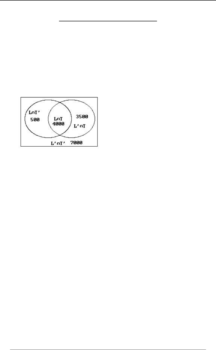
1. The manufacturer of a certain product is conducting a market survey. The manufacturer started

a major marketing campaign at the end of last year and is trying to determine the effect of that

campaign on consumer use of the product. 15,000 individuals are surveyed. The following

information is obtained.

- 4,500 used the product last year,

- 7,500 used the product this year, and

- 4,000 used the product both last year and this year.

Of those surveyed, determine:

(i) the number who used the product either last year or this year, or both years,

(ii) the number that did not use the product either last year or this year,

(iii) the number who used the product last year but not this year, and

(iv) the number who used the product this year but not last year.

2. A group of 5000 undergraduate college students were surveyed regarding the following

characteristics:

- participate in extracurricular activities,

- have a double major, and

- have a part-time job .

The following data was obtained.

2600 participated in extracurricular activities , 1200 had a double major,

2500 had a part time-job ,

400 both participated in extracurricular activities and had a double major ,

1000 both participated in extracurricular activities and had a part-time job ,

300 both had a double major and had a part-time job ,

200 participated in extracurricular activities and had a double major and had a part-time job.

Determine each of the following.

(i) The number who had a double major but did not participate in extra-curricular activities and

did not have a part-time job.

(ii) The number who had a double major and either participated in extra-curricular activities or

had a part-time job , but not both.

(iii) The number who neither participated in extracurricular activities nor had a part-time job.

26 PROBLEM SET 0

3. A group of 1000 patients each diagnosed with a certain disease is being analyzed with regard

to the disease symptoms present. The symptoms are labeled , and , and each patient has atEF G

least one symptom. The following information has also been determined:

- 900 have either symptom or (or both),EF

- 900 have either symptom or (or both),EG

- 800 have either symptom or (or both),FG

- 650 have symptom ,E

- 500 have symptom ,F

- 550 have symptom .G

Determine each of the following.

(i) The number who had both symptoms and .EF

(ii) The number who had either symptom or (or both) but not .EF G

(iii) The number who had all three symptoms.

4. lim

RÄ∞

Rœ

A) B) C) D) E) None of A,B,C,D!&68&∞

5. Which region of the plane represents the solution set to the inequalities

ÖÐBß CÑ À #B  C  #× ∪ ÖÐBß CÑ À B  #C   #× ?

A) B)

C) D)

PROBLEM SET 0 27

6. For what real values of are the roots of not real numbers?55B$B#œ!

A) B) C) D) E)5  5 5  5  5

** *

)) )

7. If then may equal:0ÐBÑ œ 0 ÐBÑ 0ÐBÑ

"

A) B) C) D) E) #"

B"""

BÈ

8. Let . Determine the th derivative of at .0ÐBÑœB / 8 0 Bœ!

A) B) C) D) E) ! " 8Ð8  "ÑÐ8  #Ñ 8Ð8  "ÑÐ8  #ÑÐ8  $Ñ 8x

9. A model for world population assumes a population of 6 billion at reference time 0, with

population increasing to a limiting population of 30 billion. The model assumes that the rate of

population growth at time 0 is billion per year, where is regarded as a> >

ÐÞ!#E/ Ñ

continuous variable. According to this model, at what time will the population reach 10 billion

(nearest .1)?

A) .3 B) .4 C) .5 D) .6 E) .6

10. Calculate the area of the closed region in the -plane bounded by BC C œ B  &

and .Cœ#B&

A) B) C) D) E) )(% *) "## "#)

$$ $ $

11. Let . JÐBÑ œ "> .> J Ð!Ñ œ

'È

B%w

"Î$

A) B) C) D) E) Does not exist!"

12. Let be a continuous function on and let .0Mœ0ÐBßCÑ.C.B‘#!

B

''È

Which of the following expressions is equal to with the order of integration reversed?M

A) D)

'' ' '

# C C

## ##

#

0ÐBß CÑ .B .C 0ÐBß CÑ .B .C

B) E)

'' ''

# C #

## #C

È0ÐBß CÑ .B .C 0ÐBß CÑ .B .C

C) ''

C

È0ÐBß CÑ .B .C

28 PROBLEM SET 0

13. Calculate .

"" "

"C#.C .B

A) B) C) D) E) "68# 68# 68#  68#

"""

####

Question 14 and 15 relate to the following information. Smith begins a new job at a salary of

100,000 . Smith expects to receive a 5% raise every year until he retires.

14. Suppose that Smith works for 35 years. Determine the total salary earned over Smith's career

(nearest million).

A) 5 B) 6 C) 7 D) 8 E) 9

15. At the end of each year, Smith's employer deposits 3% of Smith's salary (for the year just

finished) into a fund earning 4% per year compounded each year. Find the value of the fund just

after the final deposit at the end of Smith's 35th year of employment (nearest 10,000)

A) 450,000 B) 460,000 C) 470,000 D) 480,000 E) 490,000

PROBLEM SET 0 29

PROBLEM SET 0 SOLUTIONS

1. The "total set" is the set of all those who were surveyed and consists of 15,000 individuals.

We define the following sets:

P - those who used the product last year,

X - those who used the product this year.

We are given and .8ÐPÑ œ %ß &!! ß 8ÐX Ñ œ (ß &!! 8ÐP ∩ X Ñ œ %ß !!!

This can be represented in Venn diagram form as follows (not to scale):

(i) The number who used the product either last year or this year, or both years is

8ÐP ∪ X Ñ œ &!!  %!!!  $&!! œ )!!! Þ

(ii) The number that did not use the product either last year or this year is

8ÒÐP ∪ X Ñ Ó œ 8ÐP ∩ X Ñ œ 8Ð Ñ  8ÐP ∪ X Ñ œ "&ß !!!  )ß !!! œ (ß !!!

www

total set .

(iii) The number who used the product last year but not this year is .8ÐP ∩ X Ñ œ &!!

(iv) The number who used the product this year but not last year is .8ÐP ∩ X Ñ œ $&!!

2. Following the same method applied in Example 1-4 of the notes of this study material, we get

the Venn diagram entries below for the numbers in the various combinations.

Iœparticipated in extracurricular activities ,

Hœhad a double major , and

Nœhad a part-time job.

An example illustrating the calculation of one of the entries is the following. Since there are

1000 who both participated in extra-curricular activities and had a part-time job, and since 200

were in all three groups, the number who both participated in extra-curricular activities and had a

part-time job but didn't have a double major is (this would be"!!!  #!! œ )!!

8ÐI ∩ H ∩ N Ñ

w).

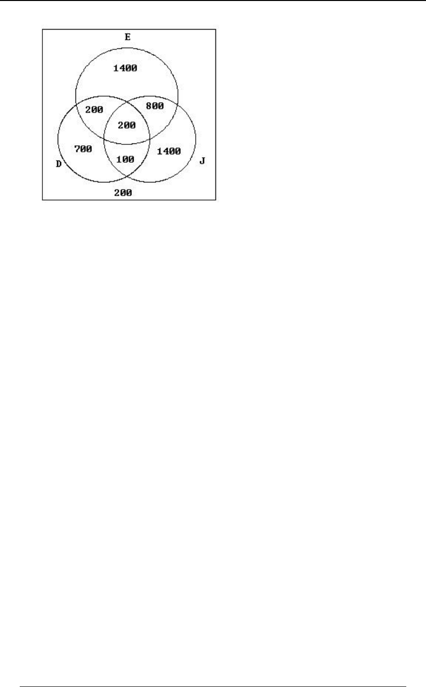
30 PROBLEM SET 0

(i) The number who had a double major but did not participate in extra-curricular activities and

did not have a part-time job is 700 .8ÐH ∩ I ∩ N Ñ œ

(ii) The number who had a double major and either participated in extra-curricular activities or

had a part-time job , but not both is

8ÐH ∩ I ∩ N Ñ  8ÐH ∩ I ∩ N Ñ œ #!!  "!! œ $!!

ww .

(iii) The number who neither participated in extracurricular activities nor had a part-time job is

8ÐI ∩ N Ñ œ 8ÒÐI ∪ N Ñ Ó œ (!!  #!! œ *!! ÐI ∪ N Ñ

ww w w

(those in with double major and those

in without double major).ÐI ∪ N Ñw

3. This is quite similar to the previous problem, but the information is based on different

combinations of sets. We are given

8ÐEÑ œ '&! ß 8ÐFÑ œ &!! ß 8ÐGÑ œ &&! ß 8ÐE ∪ FÑ œ *!! ß 8ÐE ∪ GÑ œ *!! ß

8ÐF ∪ GÑ œ )!! 8ÐE ∪ F ∪ GÑ œ "!!! and .

(i) We are asked for . We can use the relationship8ÐE ∩ FÑ

8ÐE ∪ FÑ œ 8ÐEÑ  8ÐFÑ  8ÐE ∩ FÑ 8ÐE ∩ FÑ œ '&!  &!!  *!! œ #&! Þ to get

In order to solve (ii) and (iii) we can use the given information to fill in the numbers for the

component subsets. We have ,8ÐE ∩ GÑ œ 8ÐEÑ  8ÐGÑ  8ÐE ∪ GÑ œ $!!

8ÐF ∩ GÑ œ #&! Þ We then use

8ÐE ∪ F ∪ GÑ œ 8ÐEÑ  8ÐFÑ  8ÐGÑ  8ÐE ∩ FÑ  8ÐE ∩ GÑ  8ÐF ∩ GÑ  8ÐE ∩ F ∩ GÑ

so that , from which we get"!!! œ '&!  &!!  &&!  #&!  $!!  #&!  8ÐE ∩ F ∩ GÑ

8ÐE ∩ F ∩ GÑ œ "!! . We can express the numbers in the component sets in the following Venn

diagram.

PROBLEM SET 0 31

(ii) The number who had either symptom or (or both) but not isEF G

8ÒÐE ∪ FÑ ∩ G Ó œ #!!  "&!  "!! œ %&!

w. This represented in the following Venn diagram.

(iii) The number who had all three symptoms is , which we have already8ÐE ∩ F ∩ GÑ

identified as 100.

4. . Answer: Alim

RÄ∞

∞

& &†&†&†&†&†&†&††† & &

Rx "†#†$†%†&†'†(††† &x '

œŸ†œ!ÐÑ

32 PROBLEM SET 0

5. The graphs of the lines are illustrated in the following graph.

The inequality is represented by the region "above" the line #B  C  # #B  C œ # À

The inequality is represented by the region "below" the line B#C # B#Cœ #À

The union of the two regions is:

Answer: B

6. The quadratic equation has no real roots if .+B ,B- , %+-!

Thus, . Answer: A*)5!p 5  *

)

PROBLEM SET 0 33

7. . Answer: D"ÎÐ"ÎBÑ œ B

8. 1st derivative - ; 2nd derivative - / ÐB  %B Ñ / ÐB  )B  "#B Ñ

B% $ B% $ #

3rd derivative - / ÐB  "#B  $'B  #%BÑ

B%$#

4th derivative - / ÐB  "'B  (#B  *'B  #%Ñ

B%$#

It might be possible to determine a general expression for the th derivative in terms of then88

substitute . However, note that the 1st, 2nd and 3rd derivatives ) must be ifB œ ! Ð8 œ "ß #ß $ !

Bœ! ! Bœ!, but the 4th derivative is not at . This eliminates answers A, B, C and E.

9. We define to be the population at time . Then ,JÐ>Ñ > JÐ!Ñ œ 'ß JÐ>Ñ œ $!lim

>Ä∞

and . Then (using the substitution ), we haveJ Ð>Ñ œ ? œ Þ!#E  /

w >

ÐÞ!#E/ Ñ

JÐ=ÑJÐ!Ñ œ J Ð>Ñ.> œ .> œ  œ 

'' ¹

>œ!

>œ=

E/ E E E

ÐÞ!#E/ Ñ Þ!#E/ Þ!#E" Þ!#E/

># > =,

so that JÐ=Ñ œ '  Þ

Þ!#E" Þ!#E/=

Then .lim

=Ä∞J Ð=Ñ œ '  œ $! p œ #% p E œ %'Þ"&

Þ!#E" Þ!#E"

Therefore, In order to have , we haveJÐ=Ñ œ $! Þ JÐ>Ñ œ "!

%'Þ"&

Þ*#$/=

$!  œ "! p = œ Þ$#&

%'Þ"&

Þ*#$/= . Answer: A

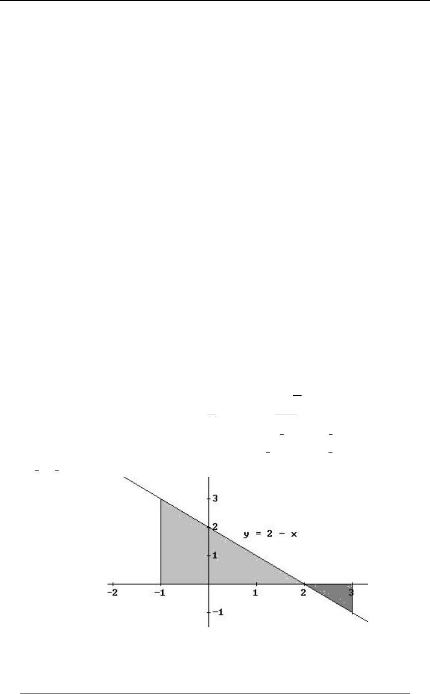
10. The line and the parabola intersect at -values that are the solutions ofC

C&œ ÐC&Ñ Cœ$Bœ# &Bœ"!

# , so that ( ) , ( ) .

The graph below indicates the closed region bounded by the line and the parabola.

The area of the region is '$

&" "#)

ÒÐC  &Ñ  ÐC  &ÑÓ .C œ Þ

Answer: E

34 PROBLEM SET 0

11. , where and . Applying theJ ÐBÑ œ 0Ð1ÐBÑÑ 1ÐBÑ œ B 0ÐDÑ œ "  > .>

"Î$ !

'È

Chain Rule results in .J ÐBÑ œ 0 Ð1ÐBÑÑ † 1 ÐBÑ œ 0 ÐB Ñ † B œ "  ÐB Ñ † B

w w w w "Î$ #Î$ #Î$

"Î$ %

At , this becomes . Answer: EBœ! "

!

12. The region of integration is illustrated in the graph below. For each betweenB

! # BŸCŸB #ŸCŸ# and , we have , or equivalently, for , we

ÈÈ ÈÈ

have . The integral becomes CŸBŸ# 0ÐBßCÑ.B.CÞ

#

È#

Answer: D

13. '' '' ' ¹

!B !! !

"" "C " "

"" "

"C "C "C #

###

.C .B œ .B .C œ .C œ 68Ð"  C Ñ œ 68 #

Note that if we try to solve the integral directly as written, we get

'' ' '

’¹“

!B ! !

"" " "

"C %

#.C .B œ +<->+8ÐCÑ .B œ Ò  +<->+8ÐBÑÓ .B

which is a more difficult integral to determine. Answer: B

14. Total salary œ "!!ß !!!Ò"  Ð"Þ!&Ñ  Ð"Þ!&Ñ  â  Ð"Þ!&Ñ Ó œ "!!ß !!! †

#$%

"Þ!& "

"Þ!&"

. Note that salary in 35th year has grown for 34 years since the first year ofœ *ß !$#ß !$"

employment. Answer: E

15. Value at end of 35 years of deposits is

"!!ß !!!ÐÞ!$ÑÐ"Þ!%Ñ  "!!ß !!!ÐÞ!$ÑÐ"Þ!&ÑÐ"Þ!%Ñ  "!!ß !!!ÐÞ!$ÑÐ"Þ!&Ñ Ð"Þ!%Ñ 

$% $$ # $#

â  "!!ß !!!ÐÞ!$ÑÐ"Þ!&Ñ Ð"Þ!%Ñ  "!!ß !!!ÐÞ!$ÑÐ"Þ!&Ñ

$$ $%

œ "!!ß !!!ÐÞ!$ÑÒÐ"Þ!%Ñ  Ð"Þ!&ÑÐ"Þ!%Ñ  Ð"Þ!&Ñ Ð"Þ!%Ñ

$% $$ # $#

 â  Ð"Þ!&Ñ Ð"Þ!%Ñ  Ð"Þ!&Ñ Ó

$$ $%

(this represents accumulation of 1st yr. deposit, 2nd year deposit, 3rd year deposit,

. . . , 34th year deposit, and 35th year deposit) . If we factor out the sum becomesÐ"Þ!%Ñ$%

"!!ß !!!ÐÞ!$ÑÐ"Þ!%Ñ Ò"   Ð Ñ  â  Ð Ñ  Ð Ñ Ó

$% # $$ $%

"Þ!& "Þ!& "Þ!& "Þ!&

"Þ!% "Þ!% "Þ!% "Þ!%

œ "!!ß !!!ÐÞ!$ÑÐ"Þ!%Ñ Ò Ó œ %(!ß *() Þ

$% ÐÑ"

"

"Þ!&

"Þ!% $&

"Þ!&

"Þ!%

Answer: C

SECTION 1 - BASIC PROBABILITY CONCEPTS 35

SECTION 1 - BASIC PROBABILITY CONCEPTS

PROBABILITY SPACES AND EVENTS

Sample point and sample space: A sample point is the simple outcome of a random

experiment. The probability space (also called sample space) is the collection of all possible

sample points related to a specified experiment. When the experiment is performed, one of the

sample points will be the outcome. The probability space is the "full set" of possible outcomes of

the experiment.

Mutually exclusive outcomes: Outcomes are mutually exclusive if they cannot occur

simultaneously. They are also referred to as outcomes.disjoint

Exhaustive outcomes: Outcomes are exhaustive if they combine to be the entire probability

space, or equivalently, if at least one of the outcomes must occur whenever the experiment is

performed.

Event: Any collection of sample points, or any subset of the probability space is referred to

as an event. We say that "event has occurred" if the experimental outcome was one of theE

sample points in .E

Union of events and :EF denotes the union of events and , and consists ofE∪F E F

all sample points that are in either or .EF

Union of events :E ß E ß ÞÞÞß E

"# 8

denotes the union ofE∪E∪â∪E œ∪ E

3œ"

"# 8 3

the events , and consists of all sample points that are in at least one of the 's.E ß E ß ÞÞÞß E E

"# 8 3

This definition can be extended to the union of infinitely many events.

Intersection of events :E ß E ß ÞÞÞß E

"# 8

denotes theE∩E∩â∩E œ∩ E

3œ"

"# 8 3

intersection of the events , and consists of all sample points that areE ß E ß ÞÞÞß E

"# 8

simultaneously in all of the 's. ( is also denoted or ).EE∩F EFEF

3†

36 SECTION 1 - BASIC PROBABILITY CONCEPTS

Mutually exclusive events :E ß E ß ÞÞÞß E

"# 8

Two events are mutually exclusive if they

have no sample points in common, or equivalently, if they have . Eventsempty intersection

E ß E ß ÞÞÞß E E ∩ E œ g 3 Á 4 g

"# 8 3 4

are mutually exclusive if for all , where denotes the empty

set with no sample points. Mutually exclusive events cannot occur simultaneously.

Exhaustive events :F ß F ß ÞÞÞß F

"# 8

If , the entire probabilityF∪F∪â∪F œW

"# 8

space, then the events are referred to as exhaustive events.F ß F ß ÞÞÞß F

"# 8

Complement of event :E The complement of event consists of all sample points inE

the probability space that are . The complement is denoted or and isnot in EEß µ Eß E E

w-

equal to . When the underlying random experiment is performed, to say that theÖB À B Â E×

complement of has occurred is the same as saying that has not occurred.EE

Subevent (or subset) of event :EF If event contains all the sample points in eventF

EE F E§F E F, then is a subevent of , denoted . The occurrence of event implies that event

has occurred.

Partition of event :E Events form a partition of event if G ß G ß ÞÞÞß G E E œ ∪ G

3œ"

"# 8 3

and the 's are mutually exclusive.G3

DeMorgan's Laws:

(i) , to say that has not occurred is to say that has not occurredÐE∪FÑ œE ∩F E∪F E

www

has not occurred ; this rule generalizes to any number of events;and F

Š‹

∪E œÐ

3œ"

wE ∪E ∪â∪E Ñ œE ∩E ∩â∩E œ ∩ E

3œ"

"# 8

www w w

"# 8 3

(ii) , to say that has not occurred is to say that either has notÐE∩FÑ œE ∪F E∩F E

www

occurred has not occurred (or both have not occurred) ; this rule generalizes to any or F

number of events,

Š‹

∩E œÐ

3œ"

wE ∩E ∩â∩E Ñ œE ∪E ∪â∪E œ ∪ E

3œ"

"# 8

www w w

"# 8 3

Indicator function for event :E The function is the indicator MÐBÑœ

"B−E

!BÂE

š if

function for event , where denotes a sample point. is 1 if event has occurred.EB MÐBÑ E

Basic set theory was reviewed in Section 0 of these notes. The Venn diagrams presented there

apply in the sample space and event context presented here.

SECTION 1 - BASIC PROBABILITY CONCEPTS 37

Example 1-1: Suppose that an "experiment" consists of tossing a six-faced die. The

probability space sample of outcomes consists of the set , each number being a Ö"ß #ß $ß %ß &ß '×

point representing the number of spots that can turn up when the die is tossed. The outcomes "

and (or more formally, and ) are an example of outcomes, since# Ö"× Ö#× mutually exclusive

they cannot occur simultaneously on one toss of the die. The collection of all the outcomes

(sample points) 1 to 6 are for the experiment of tossing a die since one of thoseexhaustive

outcomes must occur. The collection represents the of tossing an even numberÖ#ß %ß '× event

when tossing a die. We define the following events.

"a number less than is tossed" ,E œ Ö"ß #ß $× œ %

"an even number is tossed" ,F œ Ö#ß %ß '× œ

"a 4 is tossed" ,G œ Ö%× œ

"a 2 is tossed" .H œ Ö#× œ

Then (i) ,E ∪ F œ Ö"ß #ß $ß %ß '×

(ii) ,E ∩ F œ Ö#×

(iii) and are mutually exclusive since (when the die is tossed it is notEG E∩Gœg

possible for both and to occur),EG

(iv) ,H§F

(v) (complement of ) ,E œ Ö%ß &ß '× E

(vi) ,F œ Ö"ß $ß &×

(vii) , so that (this illustrates one of E ∪ F œ Ö"ß #ß $ß %ß '× ÐE ∪ FÑ œ Ö&× œ E ∩ F

www

DeMorgan's Laws). 

38 SECTION 1 - BASIC PROBABILITY CONCEPTS

Some rules concerning operations on events:

(i) E∩ÐF ∪F ∪â∪F ÑœÐE∩F Ñ∪ÐE∩F Ñ∪â∪ÐE∩F Ñ

"# 8 " # 8

and

for any eventsE∪ÐF ∩F ∩â∩F ÑœÐE∪F Ñ∩ÐE∪F Ñ∩â∩ÐE∪F Ñ

"# 8 " # 8

Eß F ß F ß ÞÞÞß F

"# 8

(ii) If are exhaustive events ( , the entire probability space),F ß F ß ÞÞÞß F ∪ F œ W

3œ"

"# 8 3

then for any event ,E

.EœE∩ÐF ∪F ∪â∪F ÑœÐE∩F Ñ∪ÐE∩F Ñ∪â∪ÐE∩F Ñ

"# 8 " # 8

If are exhaustive and mutually exclusive events, then they form aF ß F ß ÞÞÞß F

"# 8

. For example, the events , andpartition of the probability space F œ Ö"ß #× F œ Ö$ß %×

form a partition of the probability space for the outcomes of tossing a single die.F œ Ö&ß '×

The general idea of a partition is illustrated in the diagram below. As a special case of a

partition, if is any event, then and form a partition of the probability space. We thenFFF

get the following identity for any two events and :EF

; note also that and form aE œ E ∩ ÐF ∪ F Ñ œ ÐE ∩ FÑ ∪ ÐE ∩ F Ñ

E∩F E∩F

partition of event .E

(iii) For any event , , the entire probability space, and EE∪EœW E∩Eœg

(iv) and is sometimes denoted , and consists ofE∩F œÖBÀB−E BÂF× EF

all sample points that are in event but not in event EF

(v) If then and .E§F E∪FœF E∩FœE

SECTION 1 - BASIC PROBABILITY CONCEPTS 39

PROBABILITY

Probability function for a discrete probability space: A discrete probability space (or

sample space) is a set of a finite or countable infinite number of sample points. or TÒ+ Ó :

denotes the probability that sample point (or outcome occurs. There is some underlyingÑ+

"random experiment" whose outcome will be one of the 's in the probability space. Each time+3

the experiment is performed, one of the 's will occur. The probability function must satisfy+T

the following two conditions:

(i) for each in the sample space, and!ŸTÒ+ÓŸ" +

(ii) (total probability for a probability space is always 1).

all

TÒ+ ÓTÒ+ Óâ œ TÒ+ Ó œ "

"# 3

This definition applies to both finite and infinite probability spaces.

Tossing an ordinary die is an example of an experiment with a finite probability space

Ö"ß #ß $ß %ß &ß '× . An example of an experiment with an infinite probability space is the tossing of

a coin until the first head appears. The toss number of the first head could be any positive

integer, 1, or 2, or 3, .... The probability space for this experiment is the infinite set of positive

integers since the first head could occur on any toss starting with the first toss. TheÖ"ß #ß $ß ÞÞÞ×

notion of discrete random variable covered later is closely related to the notion of discrete

probability space and probability function.

Uniform probability function: If a probability space has a finite number of sample points,

say points, , then the probability function is said to be if each sample5 + ß + ß ÞÞÞß +

"# 5 uniform

point has the same probability of occurring ; for each . Tossing a fairT Ò+ Ó œ 3 œ "ß #ß ÞÞÞß 5

die would be an example of this, with .5œ'

Probability of event :E An event consists of a subset of sample points in the probabilityE

space. In the case of a discrete probability space, the probability of isE

T ÒEÓ œ T Ò+ Ó T Ò+ Ó E , the sum of over all sample points in event .

+−E

Example 1-2: In tossing a "fair" die, it is assumed that each of the six faces has the same

chance of of turning up. If this is true, then the probability function for

" "

' '

TÐ4Ñ œ

4 œ "ß #ß $ß %ß &ß ' Ö"ß #ß $ß %ß &ß '× is a uniform probability function on the sample space .

The event "an even number is tossed" is , and has probabilityE œ Ö#ß %ß '×

TÒEÓœœ

""" "

''' 2 . 

40 SECTION 1 - BASIC PROBABILITY CONCEPTS

Continuous probability space: An experiment can result in an outcome which can be any

real number in some interval. For example, imagine a simple game in which a pointer is spun

randomly and ends up pointing at some spot on a circle. The angle from the vertical (measured

clockwise) is between and . The probability space is the interval , the set of possible!# Ð!ß#Ó11

angles that can occur. We regard this as a continuous probability space. In the case of a

continuous probability space (an interval), we describe probability by assigning probability to

subintervals rather than individual points. If the spin is "fair", so that all points on the circle are

equally likely to occur, then intuition suggests that the probability assigned to an interval would

be the fraction that the interval is of the full circle. For instance, the probability that the pointer

ends up between "3 O'clock" and "9 O'clock" (between or 90 and or 270 from the11Î# $ Î#

°°

vertical) would be .5, since that subinterval is one-half of the full circle. The notion of a

continuous random variable, covered later in this study guide, is related to a continuous

probability space.

Some rules concerning probability:

(when the underlying experiment is(i) if is the entire probability spaceTÒWÓœ" W

performed, some outcome must occur with probability 1; for instance W œ Ö"ß #ß $ß %ß &ß '×

for the die toss example).

(the probability of no face turning up when we toss a die is 0).(ii) TÒgÓœ !

(iii) If events are mutually exclusive (also called disjoint) thenE ß E ß ÞÞÞß E

"# 8

TÒ ∪ E ÓœTÒE ∪E ∪â∪E ÓœTÒE ÓTÒE ÓâTÒE Óœ TÒE Ó

3œ"

3"# 8"# 8 3

3œ"

 .

This extends to infinitely many mutually exclusive events. This rule is similar to the rule

discussed in Section 0 of this study guide, where it was noted that the number of elements in the

union of mutually disjoint sets is the sum of the numbers of elements in each set. When we have

mutually exclusive events and we add the event probabilities, there is no double counting.

For any event , .(iv) E!ŸTÒEÓŸ"

If then .(v) E§F TÒEÓŸTÒFÓ

SECTION 1 - BASIC PROBABILITY CONCEPTS 41

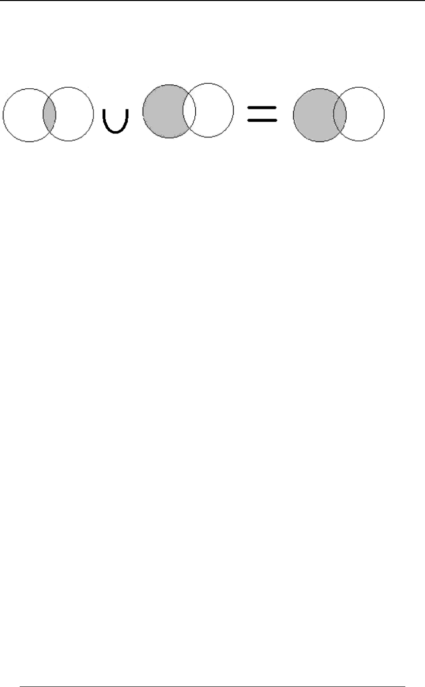
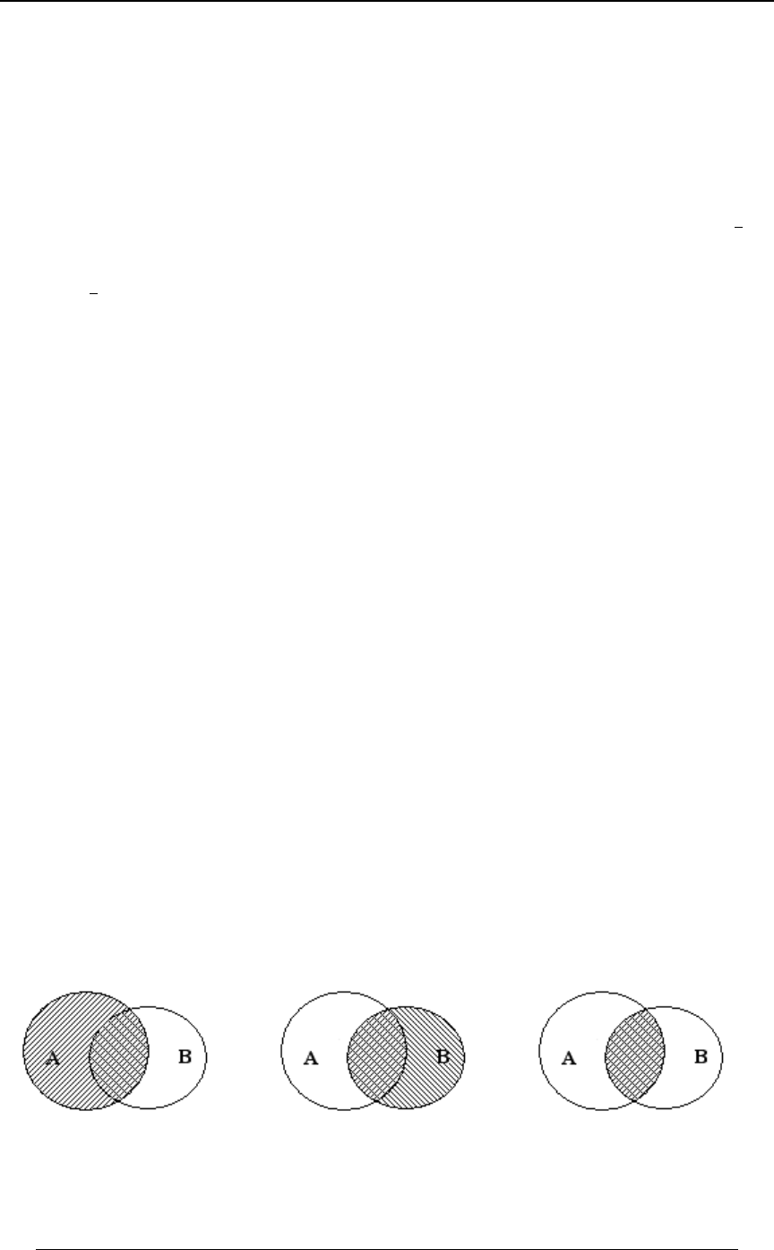
For any events , and , .(vi) EF G TÒE∪FÓœTÒEÓTÒFÓTÒE∩FÓ

This relationship can be explained as follows. We can formulate as the union of threeE∪F

mutually exclusive events as follows: .E ∪ F œ ÐE ∩ F Ñ ∪ ÐE ∩ FÑ ∪ ÐF ∩ E Ñ

This is expressed in the following Venn diagram.

E∩F E∩F F∩E

Since these are mutually exclusive events, it follows that

.TÒE∪FÓ œ TÒE∩F ÓTÒE∩FÓTÒF ∩E Ó

From the Venn diagram we see that , so thatE œ ÐE ∩ F Ñ ∪ ÐE ∩ FÑ

TÒEÓœTÒE∩F ÓTÒE∩FÓ

w , and we also see that .TÒF ∩E Ó œ TÒFÓTÒE∩FÓ

It then follows that

T ÒE ∪ FÓ œ ÐT ÒE ∩ F Ó  T ÒE ∩ FÓÑ  T ÒF ∩ E Ó œ T ÒEÓ  T ÒFÓ  T ÒE ∩ FÓ Þ

We subtract because counts twice. is theT ÒE ∩ FÓ T ÒEÓ  T ÒFÓ T ÒE ∩ FÓ T ÒE ∪ FÓ

probability that at least one of the two events occurs. This was reviewed in Section 0,Eß F

where a similar rule was described for counting the number of elements in .E∪F

For the union of three sets we have

TÒE∪F ∪GÓ œ TÒEÓTÒFÓTÒGÓTÒE∩FÓTÒE∩GÓTÒF ∩GÓTÒE∩F ∩GÓ

For any event , .(vii) ETÒEÓœ "TÒEÓ

For any events and , (viii) EFTÒEÓœTÒE∩FÓTÒE∩F Ó

(this was mentioned in (vi), it is illustrated in the Venn diagram above).

For exhaustive events , .(ix) F ß F ß ÞÞÞß F T Ò ∪ F Ó œ "

3œ"

"# 8 3

If are exhaustive and mutually exclusive, they form a of theF ß F ß ÞÞÞß F

"# 8 partition

entire probability space, and for any event ,E

.TÒEÓœTÒE∩F ÓTÒE∩F ÓâTÒE∩F Óœ TÒE∩F Ó

"# 8 3

3œ"



If is a uniform probability function on a probability space with points, and if event(x) T5

consists of of those points, then .E7 TÒEÓœ

42 SECTION 1 - BASIC PROBABILITY CONCEPTS

.(xi) The words "percentage" and "proportion" are used as alternatives to "probability"

As an example, if we are told that the percentage or proportion of a group of people that are of a

certain type is 20%, this is generally interpreted to mean that a randomly chosen person from

the group has a 20% probability of being of that type. This is the "long-run frequency"

interpretation of probability. As another example, suppose that we are tossing a fair die. In the

long-run frequency interpretation of probability, to say that the probability of tossing a 1 is is

the same as saying that if we repeatedly toss the die, the proportion of tosses that are 1's will

approach .

for any events , , with equality holding if(xii) E ß E ß ÞÞÞß E T Ò ∪ E Ó Ÿ T ÒE Ó

3œ"

"# 8 3 3

3œ"



and only if the events are mutually exclusive

Example 1-3: Suppose that and .TÒE∩FÓ œ Þ#ß TÒEÓ œ Þ'ß TÒFÓ œ Þ&

Find , and .T ÒE ∪ F Ó ß T ÒE ∩ F Ó T ÒE ∩ FÓ T ÒE ∪ FÓ

ww ww w w

Solution: Using probability rules we get the following.

TÒE ∪F Ó œ TÒÐE∩FÑ Ó œ "TÒE∩FÓ œ Þ) Þ

ww w

T ÒE ∪ FÓ œ T ÒEÓ  T ÒFÓ  T ÒE ∩ FÓ œ Þ'  Þ&  Þ# œ Þ*

pTÒE ∩FÓœTÒÐE∪FÑÓœ"TÒE∪FÓœ"Þ*œÞ"Þ

ww w

T ÒFÓ œ T ÒF ∩ EÓ  T ÒF ∩ E Ó p T ÒE ∩ FÓ œ Þ&  Þ# œ Þ$ Þ

.T ÒE ∪ FÓ œ T ÒE Ó  T ÒFÓ  T ÒE ∩ FÓ œ Þ%  Þ&  Þ$ œ Þ'

ww w

The following Venn diagrams illustrate the various combinations of intersections, unions and

complements of the events and .EF

T ÒEÓ œ Þ' T ÒFÓ œ Þ& T ÒE ∩ FÓ œ Þ#

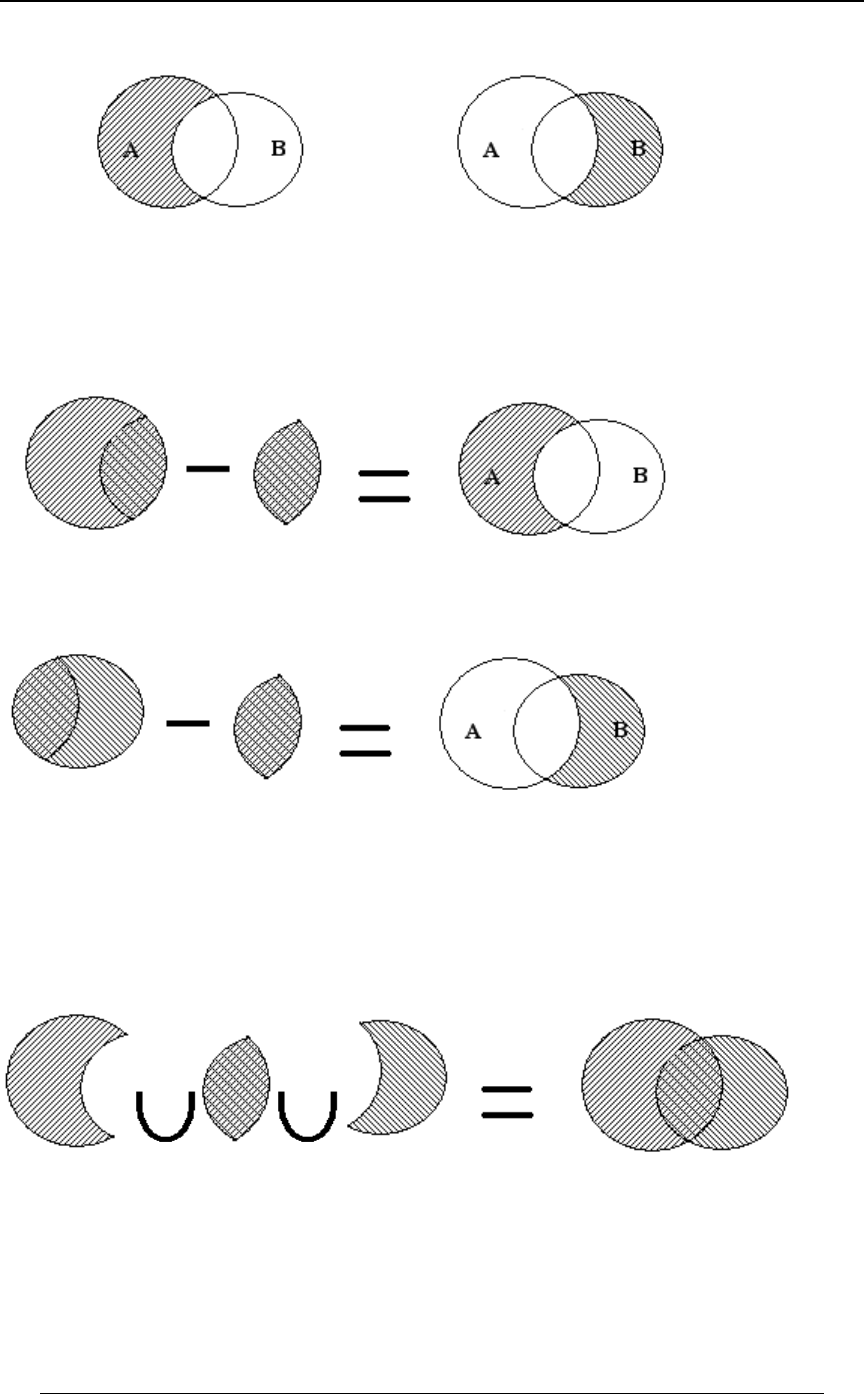
SECTION 1 - BASIC PROBABILITY CONCEPTS 43

T ÒE ∩ F Ó œ Þ% T ÒE ∩ FÓ œ Þ$

From the following Venn diagrams we see that TÒE∩FÓœTÒEÓTÒE∩FÓœÞ'Þ#œÞ%

and TÒE ∩FÓœTÒFÓTÒE∩FÓœÞ&Þ#œÞ$Þ

TÒEÓ  TÒE∩FÓ œ TÒE∩F Ó

Þ'  Þ# œ Þ%

TÒFÓ  TÒE∩FÓ œ TÒE ∩FÓ

Þ&  Þ# œ Þ$

The following Venn diagrams shows how to find .TÒE∪FÓ

TÒE∩F Ó  TÒE∩FÓ  TÒE ∩FÓ œ TÒE∪FÓ

Þ%  Þ#  Þ$ œ Þ* Þ

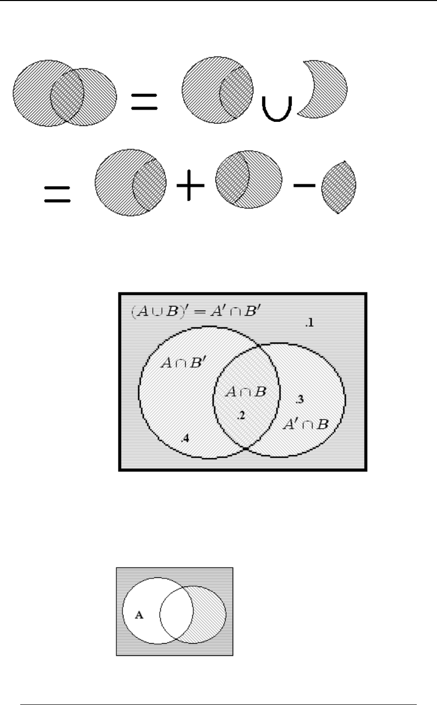
44 SECTION 1 - BASIC PROBABILITY CONCEPTS

The relationship is explained in the following VennTÒE∪FÓ œ TÒEÓTÒFÓTÒE∩FÓ

TÒE∪FÓ œ TÒEÓ  TÒFÓ  TÒE∩FÓ

.œ Þ'  Þ&  Þ# œ Þ*

The components of the events and their probabilities are summarized in the following diagram.

We can represent a variety of events in Venn diagram form and find their probabilities from the

component events described in the previous diagram. For instance, the complement of is theE

combined shaded region in the following Venn diagram, and the probability is

TÒEÓœÞ$Þ"œÞ%Þ TÒEÓœ"TÒEÓœ"Þ'œÞ%Þ

w w

We can get this probability also from

SECTION 1 - BASIC PROBABILITY CONCEPTS 45

Another efficient way of summarizing the probability information for events and is in theEF

form of a table.

(given) TÒEÓ œ Þ' TÒE Ó

T ÒFÓ œ Þ& T ÒE ∩ FÓ œ Þ# T ÒE ∩ FÓ (given) (given)

TÒF Ó TÒE∩F Ó TÒE ∩F Ó

ww ww

Complementary event probabilities can be found from andT ÒE Ó œ "  T ÒEÓ œ Þ%

T ÒF Ó œ "  T ÒFÓ œ Þ&

w . Also, across each row or along each column, the "intersection

probabilities" add up to the single event probability at the end or top:

T ÒFÓ œ T ÒE ∩ FÓ  T ÒE ∩ FÓ p Þ& œ Þ#  T ÒE ∩ FÓ p T ÒE ∩ FÓ œ Þ$

www

T ÒEÓ œ T ÒE ∩ FÓ  T ÒE ∩ F Ó p Þ' œ Þ#  T ÒE ∩ F Ó p T ÒE ∩ F Ó œ Þ%

www

, and

T ÒE Ó œ T ÒE ∩ FÓ  T ÒE ∩ F Ó p Þ% œ Þ$  T ÒE ∩ F Ó p T ÒE ∩ F Ó œ Þ"

w w ww ww ww or

T ÒF Ó œ T ÒE ∩ F Ó  T ÒE ∩ F Ó p Þ& œ Þ%  T ÒE ∩ F Ó p T ÒE ∩ F Ó œ Þ"

w w ww ww ww .

These calculations can be summarized in the next table.

(given) TÒEÓ œ Þ' Ê TÒE Ó œ "TÒEÓ œ Þ%

ËË

T ÒFÓ œ Þ& T ÒE ∩ FÓ œ Þ# T ÒE ∩ FÓ ÉœÞ$



TÒF Ó TÒE∩F Ó TÒE ∩F Ó

ww ww

œÞ& É œÞ%  œÞ" 

Example 1-4: A survey is made to determine the number of households having electric

appliances in a certain city. It is found that 75% have radios ( ), 65% have electric irons ( ),VM

55% have electric toasters ( ), 50% have ( ), 40% have ( ), 30% have ( ), and 20% haveXMVVXMX

all three. Find the probability that a household has at least one of these appliances.

Solution: TÒV ∪M ∪XÓ œ TÒVÓTÒMÓTÒXÓ

TÒV∩MÓTÒV∩XÓTÒM∩XÓTÒV∩M∩XÓ

.œÞ(&Þ'&Þ&&Þ&Þ%Þ$Þ#œÞ*&

The following diagram deconstructs the three events.

46 SECTION 1 - BASIC PROBABILITY CONCEPTS

The entries in this diagram were calculated from the "inside out". For instance, since

TÐV∩MÑœÞ& TÐV∩M∩XÑœÞ# (given) , and since (also given) , it follows that

TÐV ∩M ∩X Ñ œ Þ$

w , since

Þ&œTÐV∩MÑœTÐV∩M∩XÑTÐV∩M∩X ÑœÞ#TÐV∩M∩X Ñ

(this uses the rule , where and ).TÐEÑ œ TÐE∩FÑTÐE∩F Ñ E œ V ∩M F œ X

This is illustrated in the following diagram.

The value ".05" that is inside the diagram for event refers to (the proportionV TÐV∩M ∩X Ñ

who have radios but neither irons nor toasters). This can be found in the following way.

First we find :TÐV ∩M Ñ

Þ(& œ TÐVÑ œ TÐV ∩MÑTÐV ∩M Ñ œ Þ&TÐV ∩M Ñ p TÐV ∩M Ñ œ Þ#&Þ

www

SECTION 1 - BASIC PROBABILITY CONCEPTS 47

TÐV∩M Ñ V

wis the proportion with radios but not irons; this is the ".05" inside combined with the

".2" in the lower triangle inside . Then we find :V∩X TÐV∩M ∩XÑ

Þ%œTÐV∩XÑœTÐV∩M∩XÑTÐV∩M ∩XÑ

œÞ#TÐV∩M ∩XÑ pTÐV∩M ∩XÑœÞ#Þ

Finally we find :TÐV ∩M ∩X Ñ

Þ#&œTÐV∩M ÑœTÐV∩M ∩XÑTÐV∩M ∩X Ñ

ww ww

œÞ#TÐV∩M ∩X Ñ pTÐV∩M ∩X ÑœÞ!&Þ

ww ww

The other probabilities in the diagram can be found in a similar way. Notice that

TÐV∪M ∪XÑ is the sum of the probabilities of all the disjoint pieces inside the three events,

TÐV∪M∪XÑœÞ!&Þ!&Þ!&Þ"Þ#Þ$Þ#œÞ*& .

We can also use the rule

TÐV∪M ∪XÑ œ TÐVÑTÐMÑTÐXÑTÐV∩MÑTÐV∩XÑTÐM ∩XÑTÐV∩M ∩XÑ

œ Þ(&  Þ'&  Þ&&  Þ&  Þ%Þ  $  Þ# œ Þ*& .

Either way, this implies that 5% of the households have none of the three appliances. 

It is possible that information is given in terms of numbers of units in each category rather than

proportion of probability of each category that was given in Example 1-4.

Example 1-5: In a survey of 120 students, the following data was obtained.

60 took English, 56 took Math, 42 took Chemistry, 34 took English and Math, 20 took Math and

Chemistry, 16 took English and Chemistry, 6 took all three subjects.

Find the number of students who took

(i) none of the subjects,

(ii) Math, but not English or Chemistry,

(iii) English and Math but not Chemistry.

Solution:

Since has 34 and has 6 , it follows that has 28 .I∩Q I∩Q∩G I∩Q ∩G

The other entries are calculated in the same way (very much like the previous example).

(i) The total number of students taking any of the three subjects is , and isI∪Q∪G

"'#)'"!)"%"#œ*% #' . The remaining (out of 120) students are not taking

any of the three subjects (this could be described as the set ).I∩Q∩G

www

(ii) has 8 students .Q∩I ∩G

(iii) has 28 students .I∩Q∩G

48 SECTION 1 - BASIC PROBABILITY CONCEPTS

Example 1-5 continued

The following diagram illustrates how the numbers of students can be deconstructed.



PROBLEM SET 1 49

PROBLEM SET 1

Basic Probability Concepts

1. A survey of 1000 people determines that 80% like walking and 60% like biking, and

all like at least one of the two activities. What is the probability that a randomly chosen person in

this survey likes biking but not walking?

A) 0 B) .1 C) .2 D) .3 E) .4

2. A survey of 1000 Canadian sports fans who indicated they were either hockey fans or lacrosse

fans or both, had the following result.

• 800 indicated that they were hockey fans

• 600 indicated that they were lacrosse fans

Based on the sample, find the probability that a Canadian sports fan is not a hockey fan given that

she/he is a lacrosse fan.

A) B) C) D) E) 1

""""

&%$#

3. (SOA) Among a large group of patients recovering from shoulder injuries, it is found that 22%

visit both a physical therapist and a chiropractor, whereas 12% visit neither of these. The

probability that a patient visits a chiropractor exceeds by 0.14 the probability that a patient visits

a physical therapist. Determine the probability that a randomly chosen member of this group

visits a physical therapist.

A) 0.26 B) 0.38 C) 0.40 D) 0.48 E) 0.62

4. (SOA) An urn contains 10 balls: 4 red and 6 blue. A second urn contains 16 red balls and an

unknown number of blue balls. A single ball is drawn from each urn. The probability that both

balls are the same color is 0.44 Calculate the number of blue balls in the second urn.

A) 4 B) 20 C) 24 D) 44 E) 64

50 PROBLEM SET 1

5. (SOA) An insurer offers a health plan to the employees of a large company. As part of this

plan, the individual employees may choose exactly two of the supplementary coverages A, B, and

C, or they may choose no supplementary coverage. The proportions of the company’s employees

that choose coverages A, B, and C are , , and , respectively. Determine the probability that

"" &

%$"#

a randomly chosen employee will choose no supplementary coverage.

A) 0 B) C) D) E)

%( " *( (

"%% # "%% *

6. (SOA) An auto insurance company has 10,000 policyholders.

Each policyholder is classified as

(i) young or old;

(ii) male or female; and

(iii) married or single.

Of these policyholders, 3000 are young, 4600 are male, and 7000 are married. Thepolicyholders

can also be classified as 1320 young males, 3010 married males, and 1400 young married

persons. Finally, 600 of the policyholders are young married males. How many of the company’s

policyholders are young, female, and single?

A) 280 B) 423 C) 486 D) 880 E) 896

7. (SOA) An actuary is studying the prevalence of three health risk factors, denoted by A, B, and

C, within a population of women. For each of the three factors, the probability is 0.1 that a

woman in the population has only this risk factor (and no others). For any two of the three

factors, the probability is 0.12 that she has exactly these two risk factors (but not the other). The

probability that a woman has all three risk factors, given that she has A and B, is . What is the

probability that a woman has none of the three risk factors, given that she does not have risk

factor A?

A) 0.280 B) 0.311 C) 0.467 D) 0.484 E) 0.700

PROBLEM SET 1 51

8. (SOA) The probability that a visit to a primary care physician’s (PCP) office results in neither

lab work nor referral to a specialist is 35% . Of those coming to a PCP’s office, 30%

are referred to specialists and 40% require lab work. Determine the probability that a visit to a

PCP’s office results in both lab work and referral to a specialist.

A) 0.05 B) 0.12 C) 0.18 D) 0.25 E) 0.35

9. (SOA) You are given and . Determine TÒE∪FÓ œ !Þ( TÒE∪F Ó œ !Þ* TÒEÓÞ

A) 0.2 B) 0.3 C) 0.4 D) 0.6 E) 0.8

10. (SOA) A survey of a group’s viewing habits over the last year revealed the following

information:

(i) 28% watched gymnastics

(ii) 29% watched baseball

(iii) 19% watched soccer

(iv) 14% watched gymnastics and baseball

(v) 12% watched baseball and soccer

(vi) 10% watched gymnastics and soccer

(vii) 8% watched all three sports.

Calculate the percentage of the group that watched none of the three sports during the last year.

A) 24 B) 36 C) 41 D) 52 E) 60

52 PROBLEM SET 1

PROBLEM SET 1 SOLUTIONS

1. Let "like walking" and "like biking" . We use the interpretation that "percentage"Eœ Fœ

and "proportion" are taken to mean "probability".

We are given and .TÐEÑ œ Þ)ß TÐFÑ œ Þ' TÐE∪FÑ œ "

From the diagram below we can see that since we haveE∪FœE∪ÐF∩EÑ

TÐE∪FÑ œ TÐEÑTÐE ∩FÑ p TÐE ∩FÑ œ Þ#

is the proportion of people who like biking

but (and) not walking . In a similar way we get .TÐE∩F Ñ œ Þ%

An algebraic approach is the following. Using the rule ,TÐE∪FÑ œ TÐEÑTÐFÑTÐE∩FÑ

we get . Then, using the rule" œ Þ)  Þ'  T ÐE ∩ FÑ p T ÐE ∩ FÑ œ Þ%

TÐFÑ œ TÐF ∩EÑTÐF ∩E Ñ TÐF ∩E Ñ œ Þ'Þ% œ Þ#

, we get . Answer: C

2. From the given information, 400 of those surveyed are both hockey and lacrosse fans,

200 are lacrosse fans and not hockey fans, and 400 are hockey fans an not lacrosse fans.

This is true because there are 1000 fans in the survey, but a combined total of

800 + 600 = 1400 sports preferences, so that 400 must be fans of both. Of the 600 lacrosse fans,

400 are also hockey fans, so 200 are not hockey fans The probability that a Canadian sports fans

is not a hockey fan given that she/he is a lacrosse fan is . Answer: C

#!! "

'!! $

3. - chiropractor visit ; - therapist visit.GX

We are given , , .TÐG ∩XÑ œ Þ## TÐG ∩X Ñ œ Þ"# TÐGÑ œ TÐXÑÞ"%

Þ)) œ "TÐG ∩X Ñ œ TÐG ∪XÑ œ TÐGÑTÐXÑTÐG ∩XÑ

œ T ÐX Ñ  Þ"%  T ÐX Ñ  Þ## p T ÐX Ñ œ Þ%) . Answer: D

PROBLEM SET 1 53

4. Suppose there are blue balls in urn II.F

TÒ Ó œ TÒ ∪ Ó œ TÒ ÓTÒ Óboth balls are same color both blue both red both blue both red

(the last equality is true since the events "both blue" and "both red" are disjoint).

TÒ Ó œ TÒ ∩ Óboth blue blue from urn I blue from urn II

œTÒ Ó†TÒ Óblue from urn I blue from urn II (choices from the two urns are independent)

œÐ ÑÐ Ñ

"! "'F ,

TÒ Ó œ TÒ ∩ Óboth red red from urn I red from urn II

œTÒ Ó†TÒ ÓœÐ ÑÐ Ñred from urn I red from urn II ,

%"'

"! "'F

We are given .Ð ÑÐ ÑÐ ÑÐ ÑœÞ%% p œÞ%%pFœ%

'F %"' 'F'%

"! "'F "! "'F "!Ð"'FÑ

Answer: A

5. Since someone who chooses coverage must choose exactly two supplementary coverages, in

order for someone to choose coverage A, they must choose either A-and-B or A-and-C. Thus, the

proportion of of individuals that choose A is

TÒE∩FÓTÒE∩GÓ œ "

% (where this refers to the probability that someone chosen at random

in the company chooses coverage A). In a similar way we get

TÒF ∩EÓTÒF ∩GÓ œ TÒG ∩EÓTÒG ∩FÓ œ

$"#

and .

Then, ÐT ÒE ∩ FÓ  T ÒE ∩ GÓÑ  ÐT ÒF ∩ EÓ  T ÒF ∩ GÓÑ  ÐT ÒG ∩ EÓ  T ÒG ∩ FÓÑ

œ#Ð   œ"TÒE∩FÓTÒE∩GÓTÒF ∩GÓÑ œ "" &

%$"# .

It follows that TÒE∩FÓTÒE∩GÓTÒF ∩GÓ œ "

# .

This is the probability that a randomly chosen individual chooses some form of coverage, since if

someone who chooses coverage chooses exactly two of A,B, and C. Therefore, the probability

that a randomly chosen individual does not choose any coverage is the probability of the

complementary event, which is also . Answer: C

6. We identify the following subsets of the set of 10,000 policyholders:

]œ ] œyoung, with size 3000 (so that old has size 7000) ,

Qœ Q œmale, with size 4600 (so that female has size 5400), and

Gœ G œmarried, with size 7000 (so that single has size 3000).

We are also given that has size 1320 , has size 3010 ,]∩Q Q∩G

] ∩G ] ∩Q ∩G has size 1400 , and has size 600 .

We wish to find the size of the subset .]∩Q ∩G

We use the following rules of set theory:

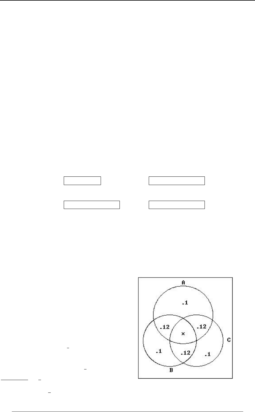
54 PROBLEM SET 1

6. continued

(i) if two finite sets are disjoint (have no elements in common, also referred to as empty

intersection), then the total number of elements in the union of the two sets is the sum of the

numbers of elements in each of the sets;

(ii) for any sets and , , and and are disjoint.E F EœÐE∩FÑ∪ÐE∩FÑ E∩F E∩F



Applying rule (ii), we have . Applying rule (i), it follows that the] œ Ð] ∩ QÑ ∪ Ð] ∩ Q Ñ

size of must be 3000 1320 1680 .]∩Q  œ

We now apply rule (ii) to to get .]∩G ]∩GœÐ]∩G∩QÑ∪Ð]∩G∩QÑ

Applying rule (i), it follows that has size 1400 600 800.]∩G∩Q  œ

Now applying rule (ii) to we get .]∩Q ]∩Q œÐ]∩Q ∩GÑ∪Ð]∩Q ∩GÑ

wwww

Applying rule (i), it follows that has size 1680 800 880 .]∩Q ∩G  œ

Within the "Young" category, which we are told is 3000, we can summarize the calculations in

the following table. This is a more straightforward solution.

Married Single

1400 (given) 1600 3000 1400œ

Male 600 (given) 720 1320 600œ

1320 (given)

Female 800 1400 600 880 1600 720œ œ

1680 œ

3000 1320 Answer: D

7. We are given

TÒE∩F ∩G ÓœTÒE ∩F∩G ÓœTÒE

www

∩F ∩GÓœÞ"

(having exactly one risk factor means not

having either of the other two).

We are also given

TÒE∩F∩G ÓœTÒE∩F ∩GÓœTÒE

www

∩F∩GÓœÞ"#.

And we are given

TÒE∩F∩GlE∩FÓœ "

$ .

We are asked to find .TÒE ∩F ∩G lE Ó

From we getTÒE∩F∩GlE∩FÓœ "

TÒE∩F∩GÓ

TÒE∩FÓ $

œ , and then

TÒE∩F ∩GÓ œ †TÒE∩FÓ

$ .

The following Venn diagram illustrates the

situation:

PROBLEM SET 1 55

7. continued

We see that and , so thatTÒE∩F ∩GÓ œ B TÒE∩FÓ œ BÞ"#

B œ † ÐB  Þ"#Ñ p B œ T ÒE ∩ F ∩ GÓ œ Þ!'

$ .

Alternatively, we can use the rule to getTÒHÓ œ TÒH ∩IÓTÒH∩I Ó

TÒE∩FÓœTÒE∩F∩GÓTÒE∩F∩G ÓœTÒE∩F∩GÓÞ"#

w .

Then, T ÒE ∩ FÓ œ T ÒE ∩ F ∩ GÓ  Þ"# œ † T ÒE ∩ FÓ  Þ"# p T ÒE ∩ FÓ œ Þ")

and .T ÒE ∩ F ∩ GÓ œ † ÐÞ")Ñ œ Þ!'

We can also see from the diagram that .T ÒE ∩ F Ó œ Þ"  Þ"# œ Þ##

Alternatively, we can use the rule above again to get

TÒE∩FÓœTÒE∩F ∩GÓTÒE∩F ∩G ÓœÞ"#Þ"œÞ##Þ

ww w

Then, , and .TÒEÓœTÒE∩FÓTÒE∩FÓœÞ")Þ##œÞ% TÒEÓœ"TÒEÓœÞ'

We are asked to find , so we must findTÒE ∩F ∩G lE Ó œ œ

wwTÒE∩F ∩G Ó TÒE∩F ∩G Ó

TÒEÓ Þ'

TÒE ∩F ∩G Ó

www . From the Venn diagram, we see that

TÒE ∩F ∩G Óœ"ÐÞ"Þ"Þ"Þ"#Þ"#Þ"#Þ!'ÑœÞ#)

www .

Finally, . Answer: CTÒE∩F∩GlEÓœœœœÞ%'(

wwTÒE∩F ∩G Ó TÒE∩F ∩G Ó

TÒEÓ Þ' Þ'

Þ#)

8. We identify events as follows:

PÀ lab work needed

VÀ referral to a specialist needed

We are given . It follows thatT ÒP ∩ V Ó œ Þ$& ß T ÒVÓ œ Þ$ ß T ÒPÓ œ Þ%

T ÒP ∪ VÓ œ "  T ÒP ∩ V Ó œ Þ'&

ww , and then since

T ÒP ∪ VÓ œ T ÒPÓ  T ÒVÓ  T ÒP ∩ VÓ T ÒP ∩ VÓ œ Þ$  Þ%  Þ'& œ Þ!&, we get .

These calculations can be summarized in the following table

P ß Þ% P ß Þ'

given Þ' œ "  Þ%

Vß Þ$ P∩V P∩V w

given Þ!& œ Þ%  Þ$& Þ#& œ Þ$  Þ!&

VÞ( P∩V P∩VÞ$&

wwww

, ,

Þ(œ"Þ$ Þ$&œÞ(Þ$& given Answer: A

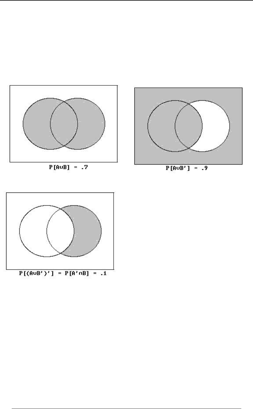
56 PROBLEM SET 1

9. .T ÒE ∪ FÓ œ T ÒEÓ  T ÒFÓ  T ÒE ∩ FÓ ß T ÒE ∪ F Ó œ T ÒEÓ  T ÒF Ó  T ÒE ∩ F Ó

www

We use the relationship . ThenTÒEÓ œ TÒE∩FÓTÒE∩F Ó

TÒE∪FÓTÒE∪F Ó œ TÒEÓTÒFÓTÒE∩FÓ TÒEÓTÒF ÓTÒE∩F Ó

www

œ#TÒEÓ"TÒEÓœTÒEÓ" TÒFÓTÒFÓœ"(since ) .

Therefore, so that . Þ(Þ*œTÒEÓ" TÒEÓœÞ'

An alternative solution is based on the following Venn diagrams.

In the third diagram, the shaded area is the complement of that in the second diagram

(using De Morgan's Law, we have ) . Then it can beÐE∪FÑœE∩F œE∩F

ww w ww w

seen from diagrams 1 and 3 that , so thatE œ ÐE ∪ FÑ  ÐE ∩ FÑ

TÒEÓœTÒE∪FÓTÒE ∩FÓœÞ(Þ"œÞ'

w . Answer: D

PROBLEM SET 1 57

10. We identify the following events:

KFW - watched gymnastics , - watched baseball , - watched soccer .

We wish to find . By DeMorgan's rules we haveTÒK ∩F ∩W Ó

www

TÒK ∩F ∩WÓœ"TÒK∪F∪WÓ

www .

We use the relationship

TÒK∪F ∪WÓ œ TÒKÓTÒFÓTÒWÓ

. T ÒK ∩ FÓ  T ÒK ∩ WÓ  T ÒF ∩ WÓ  T ÒK ∩ F ∩ WÓ

ˆ‰

We are given T ÒKÓ œ Þ#) ß T ÒFÓ œ Þ#* ß T ÒWÓ œ Þ"* ß

T ÒK ∩ FÓ œ Þ"% ß T ÒK ∩ WÓ œ Þ"! ß T ÒF ∩ WÓ œ Þ"# ß T ÒK ∩ F ∩ WÓ œ Þ!) .

Then and . Answer: DTÒK∪F∪WÓœÞ%) TÒK ∩F ∩WÓœ"Þ%)œÞ&#

www

58 PROBLEM SET 1

SECTION 2 - CONDITIONAL PROBABILITY AND INDEPENDENCE 59

SECTION 2 - CONDITIONAL PROBABILITY AND INDEPENDENCE

Conditional probability of event given event :FE

If , then is defined to be the conditional probability that event TÒEÓ  ! FTÒFlEÓœ TÒF∩EÓ

TÒEÓ

occurs given that event has occurred. Events and may be related so that if we know thatEEF

event has occurred, the Econditional probability of event occurring given that event FE

has occurred might not be the same as the unconditional probability of event occurring if weF

had no knowledge about the occurrence of event . For instance, if a fair 6-sided die is tossedE

and if we know that the outcome is even, then the conditional probability is 0 of tossing a 3 given

that the toss is even. If we did not know that the toss was even, if we had no knowledge of the

nature of the toss, then tossing a 3 would have an unconditional probability of , the same as all

other possible tosses that could occur.

When we condition on event , we are assuming that event has occurred so that becomes theEEE

new probability space, and all conditional events must take place within event (the newE

probability space). Dividing by scales all probabilities so that is the entire probabilityTÒEÓ E

space, and . To say that event has occurred given that event has occurred meansT ÒElEÓ œ " F E

that both and ( ) have occurred within the probability space . This explains theFEF∩E E

numerator ( ) in the definition of the conditional probability .TF∩E TÒFlEÓ

Rewriting , the equation that defines conditional probability, results inTÒFlEÓ œ TÒF∩EÓ

TÒEÓ

T ÒF ∩ EÓ œ T ÒFlEÓ † T ÒEÓ , which is referred to as the .multiplication rule

Example 2-1: Suppose that a fair six-sided die is tossed. The probability space is

W œ Ö"ß #ß $ß %ß &ß '×. We define the following events:

E œ œ Ö#ß %ß '× F œ Ÿ $ œ Ö"ß #ß $×"the number tossed is even" , "the number tossed is " ,

G œ " # œ Ö"ß #×"the number tossed is a or a " ,

H œ œ Ö"ß '×"the number tossed doesn't start with the letters 'f' or 't'" .

The conditional probability of given isFE

TÒFlEÓ œ œ œ œ

T ÒÖ"ß#ß$×∩Ö#ß%ß'×Ó T ÒÖ#×Ó "Î'

T ÒÖ#ß%ß'×Ó T ÒÖ#ß%ß'×Ó "Î# $

". The interpretation of this conditional

probability is that if we know that event has occurred, then the toss must be 2, 4 or 6. Since theE

original 6 possible tosses of a die were equally likely, if we are given the additional information

60 SECTION 2 - CONDITIONAL PROBABILITY AND INDEPENDENCE

Example 2-1 continued

that the toss is 2, 4 or 6, it seems reasonable that each of those is equally likely, each with a

probability of . Then within the reduced probability space , the (conditional) probability that

event occurs is the probability, in the reduced space, of tossing a 2; this is .F"

For events and defined above, the conditional probability of given is .FG F GTÒFlGÓœ"

To say that has occurred means that the toss is 1 or 2. It is then guaranteed that event hasGF

occurred ( the toss is a 1, 2 or 3), since .G§F

The conditional probability of given is . EGTÒElGÓœ

#

Example 2-2: If and , and ,T ÒEÓ œ T ÒFÓ œ T ÒElFÓ  T ÒFlEÓ œ

"& (

'"# "!

find .TÒE∩FÓ

Solution: and T ÒFlEÓ œ œ 'T ÒE ∩ FÓ T ÒElFÓ œ œ T ÒE ∩ FÓ

TÒE∩FÓ TÒE∩FÓ

TÒEÓ TÒFÓ &

p Ð' Ñ†TÒE∩FÓ œ p TÒE∩FÓ œ Þ

"# ( "

&"! "2

IMPORTANT NOTE: The following manipulation of event probabilities arises from time to

time: .TÒFÓœTÒFlEÓ†TÐEÑTÒFlEÓ†TÐEÑ

This relationship is a version of the This relationship is valid since forLaw of Total Probability.

any events and , we have . We then use the relationshipsE F TÒFÓ œ TÒF ∩EÓTÒF ∩E Ó

T ÒF ∩ EÓ œ T ÒFlEÓ † T ÐEÑ T ÒF ∩ E Ó œ T ÒFlE Ó † T ÐE Ñ and . If we know the conditional

www

probabilities for event given some other event and if we also know the conditionalFE

probability of given the complement , and if we are given the (unconditional) probability ofFE

event , then we can find the (unconditional) probability of event . EFAn application of this

concept occurs when an experiment has two (or more) steps. The following example illustrates

this idea.

Example 2-3: Urn I contains 2 white and 2 black balls and Urn II contains 3 white and 2 black

balls. An Urn is chosen at random, and a ball is randomly selected from that Urn. Find the

probability that the ball chosen is white.

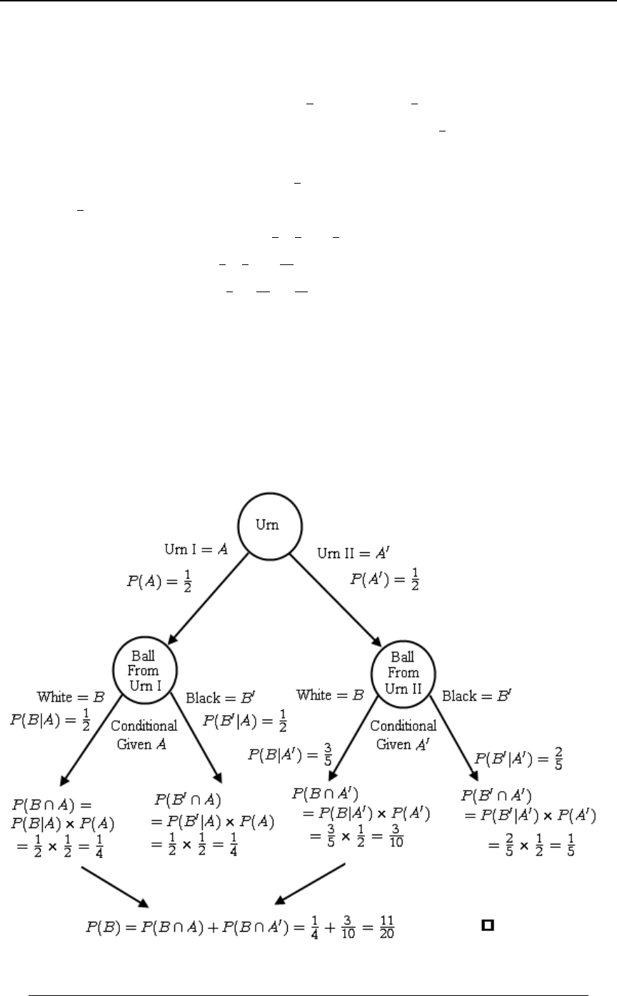
SECTION 2 - CONDITIONAL PROBABILITY AND INDEPENDENCE 61

Solution: Let be the event that Urn I is chosen and is the event that Urn II is chosen. TheEE

implicit assumption is that both Urns are equally likely to be chosen (this is the meaning of "an

Urn is chosen at random"). Therefore, and . Let be the event that theTÒEÓ œ TÒEÓ œ F

ball chosen is white. If we know that Urn I was chosen, then there is probability of choosing a

white ball (2 white out of 4 balls, it is assumed that each ball has the same chance of being

chosen); this can be described as . In a similar way, if Urn II is chosen, thenTÒFlEÓ œ "

TÒFlE Ó œ

& (3 white out of 5 balls). We can now apply the relationship described prior to this

example. , andT ÒF ∩ EÓ œ T ÒFlEÓ † T ÒEÓ œ Ð ÑÐ Ñ œ

"" "

## %

T ÒF ∩ E Ó œ T ÒFlE Ó † T ÒE Ó œ Ð ÑÐ Ñ œ

www

$" $

&# "!

. Finally,

TÒFÓ œ TÒF ∩EÓTÒF ∩EÓ œ  œ

w"$ ""

%"! #!

The order of calculations (1-2-3) can be summarized in the following table

F TÐF∩EÑœTÒFlEÓ†TÒEÓ TÐF∩EÑœTÒFlEÓ†TÒEÓ 1. 2. www

3. TÐFÑ œ TÐF ∩EÑTÐF ∩E Ñ

An event tree diagram, shown below, is another way of illustrating the probability relationships.

62 SECTION 2 - CONDITIONAL PROBABILITY AND INDEPENDENCE

IMPORTANT NOTE: An exam question may state that "an item is to chosen at random"

from a collection of items". Unless there is an indication otherwise, this is interpreted to mean

that each item has the same chance of being chosen. Also, if we are told that a fair coin is tossed

randomly, then we interpret that to mean that the head and tail each have the probability of .5

occurring. Of course, if we are told that the coin is "loaded" so that the probability of tossing a

head is 2/3 and tail is 1/3, then random toss means the head and tail will occur with those stated

probabilities.

Bayes' rule and Bayes' Theorem (basic form):

For any events and with , .EF TÒFÓ!TÒElFÓœ œ

T ÒE∩FÓ T ÒFlEÓ†T ÒEÓ

TÒFÓ TÒFÓ

The usual way that this is applied is in the case that we are given the values of

TÒEÓ TÒFlEÓ TÒFlE Ó TÒEÓ TÒE Ó œ "TÒEÓ , and (from we get ),

and we are asked to find (in other words, we are asked to "turn around" the conditioningTÒElFÓ

of the events and ). We can summarize this process by calculating the quantities in theEF

following table in the order indicated numerically (1-2-3-4) (other entries in the table are not

necessary in this calculation, but might be needed in related calculations).

given givenEß TÐEÑ E ß TÐEÑ

FTÒFlEÓ TÒFlE Ó

T ÒF ∩ EÓ œ T ÒFlEÓ † T ÒEÓ T ÒF ∩ E Ó œ T ÒFlE Ó † T ÒE Ó

given given

1. 2.

www

ÌÌ

3. TÒFÓ œ TÒF ∩EÓTÒF ∩E Ó

Also, we can find

FT ÒF lEÓ œ "  T ÒFlEÓ T ÒF lE Ó œ "  T ÒFlE Ó

T ÒF ∩ EÓ œ T ÒF lEÓ † T ÒEÓ T ÒE ∩ F Ó œ T ÒF lE Ó † T ÒE Ó

wwwww

ww wwwww

and TÒF Ó œ TÒF ∩EÓTÒF ∩EÓ

ww ww

(but we could have found from , once was found).TÒF Ó TÒF Ó œ "TÒFÓ TÒFÓ

Step : .4TÒElFÓ œ TÒE∩FÓ

TÒFÓ

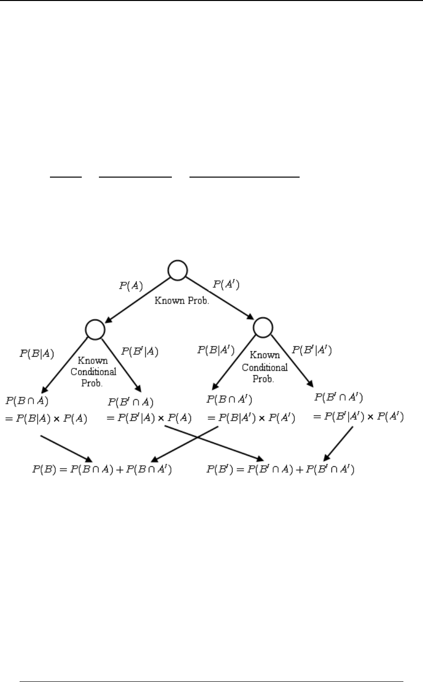
SECTION 2 - CONDITIONAL PROBABILITY AND INDEPENDENCE 63

This can also be summarized in the following sequence of calculations.

, , given , , givenTÒEÓ TÒFlEÓ TÒE Ó œ "TÒEÓ TÒFlE Ó

ÌÌ

TÒF∩EÓ TÒF ∩E Ó

œ T ÒFlEÓ † T ÒEÓ œ T ÒFlE Ó † T ÒE Ó

TÒFÓ œ TÒF ∩EÓTÒF ∩E Ó

Algebraically, we have done the following calculation:

TÒElFÓ œ œ œ

TÒE∩FÓ TÒE∩FÓ TÒFlEÓ†TÒEÓ

T ÒFÓ T ÒF∩EÓT ÒF∩E Ó T ÒFlEÓ†T ÒEÓT ÒFlE Ó†T ÒE Ó

www

where all the factors in the final expression were originally known. Note that the numerator is

one of the components of the denominator. The following event tree is similar to the one in

Example 2-3, illustrating the probability relationships.

Note that at the bottom of the event tree, is also equal to .TÐF Ñ "TÐFÑ

Exam questions that involve conditional probability and make use of Bayes rule

(and its extended form reviewed below) occur frequently. The key starting point is

identifying and labeling unconditional events and conditional events and their probabilities

in an efficient way.

64 SECTION 2 - CONDITIONAL PROBABILITY AND INDEPENDENCE

Example 2-4: Urn I contains 2 white and 2 black balls and Urn II contains 3 white and 2 black

balls. One ball is chosen at random from Urn I and transferred to Urn II, and then a ball is chosen

at random from Urn II. The ball chosen from Urn II is observed to be white. Find the probability

that the ball transferred from Urn I to Urn II was white.

Solution: Let denote the event that the ball transferred from Urn I to Urn II was white and letE

FTÒElFÓ denote the event that the ball chosen from Urn II is white. We are asked to find .

From the simple nature of the situation (and the usual assumption of uniformity in such a

situation, meaning that all balls are equally likely to be chosen from Urn I in the first step), we

have (2 of the 4 balls in Urn I are white), and .TÒEÓ œ TÒE Ó œ

If the ball transferred is white, then Urn II has 4 white and 2 black balls, and the probability of

choosing a white ball out of Urn II is ; this is .

TÒFlEÓ œ

If the ball transferred is black, then Urn II has 3 white and 3 black balls, and the probability of

choosing a white ball out of Urn II is ; this is .

TÒFlE Ó œ

All of the information needed has been identified. From the table described above, we do the

calculations in the following order:

1. T ÒF ∩ EÓ œ T ÒFlEÓ † T ÒEÓ œ Ð ÑÐ Ñ œ

#" "

$# $

2. T ÒF ∩ E Ó œ T ÒFlE Ó † T ÒE Ó œ Ð ÑÐ Ñ œ

www

"" "

## %

3. TÒFÓ œ TÒF ∩EÓTÒF ∩E Ó œ  œ

w"" (

$% "#

4. . TÒElFÓ œ œ œ

T ÒE∩FÓ "Î$

T ÒFÓ (Î"# (

%

Example 2-5: Identical twins come from the same egg and hence are of the same sex. Fraternal

twins have a 50-50 chance of being the same sex. Among twins, the probability of a fraternal set

is and an identical set is . If the next set of twins are of the same sex, what is the:;œ":

probability that they are identical?

Solution: Let be the event "the next set of twins are of the same sex", and let be the eventFE

"the next sets of twins are identical". We are given T ÒFlEÓ œ " ß T ÒFlE Ó œ Þ&

T ÒEÓ œ ; ß T ÒE Ó œ : œ "  ; T ÒElFÓ œ . Then is the probability we are asked to

wTÒF∩EÓ

TÒFÓ

find. But , and .T ÒF ∩ EÓ œ T ÒFlEÓ † T ÒEÓ œ ; T ÒF ∩ E Ó œ T ÒFlE Ó † T ÒE Ó œ Þ&:

www

Thus, , andTÒFÓœTÒF∩EÓTÒF∩EÓœ;Þ&:œ;Þ&Ð";ÑœÞ&Ð";Ñ

TÒElFÓ œ ;

Þ&Ð";Ñ .

SECTION 2 - CONDITIONAL PROBABILITY AND INDEPENDENCE 65

Example 2-5 continued

This can be summarized in the following table

identical, not identical E œ TÒEÓ œ ; E œ TÒE Ó œ ";

F œ TÒFlEÓ œ " TÒFlE Ó œ Þ&

TÒF∩EÓ

œ T ÒFlEÓ † T ÒEÓ œ ;

TÒF∩EÓ

œ T ÒFlE Ó † T ÒE Ó œ Þ&Ð"  ;Ñ

same sex (given) , (given)

.TÒFÓœTÒF∩EÓTÒF∩EÓœ;Þ&Ð";ÑœÞ&Ð";Ñ

Then, . TÒElFÓ œ œ

TÒF∩EÓ

T ÒFÓ Þ&Ð";Ñ

;

The event tree shown on page 63 can be applied to this example. 

Bayes' rule and Bayes' Theorem (extended form):

If form a partition of the entire probability space , thenE ß E ß ÞÞÞß E W

"# 8

for each .T ÒE lFÓ œ œ œ 4 œ "ß #ß ÞÞÞß 8

TÒF∩E Ó TÒF∩E Ó TÒFlE Ó†TÒE Ó

TÒFÓ T ÒF∩E Ó T ÒFlE Ó†T ÒE Ó

44 44

3œ" 3œ"

333



For example, if the 's form a partition of events, we haveE8œ$

TÒE lFÓ œ œ

"T ÒE ∩FÓ T ÒFlE Ó†T ÒE Ó

T ÒFÓ T ÒF∩E ÓT ÒF∩E ÓT ÒF∩E Ó

"""

"#$

œT ÒFlE Ó†T ÒE Ó

T ÒFlE Ó†T ÒE ÓT ÒFlE Ó†T ÒE ÓT ÒFlE Ó†T ÒE Ó

"" ## $$

The relationship in the denominator, is the general Law of TotalT ÒFÓ œ T ÒFlE Ó † T ÒE Ó



3œ"

Probability. The values of are called prior probabilities, and the value of isTÒE Ó TÒE lFÓ

called a posterior probability. The basic form of Bayes' rule is just the case in which the partition

consists of two events, and . The main application of Bayes' rule occurs in the situation inEE

which the probabilities are known and the probabilities are known, and we areTÒE Ó TÒFlE Ó

asked to find for one of the 's. The series of calculations can be summarized in a tableTÒE lFÓ 4

as in the basic form of Bayes' rule. This is illustrated in the following example.

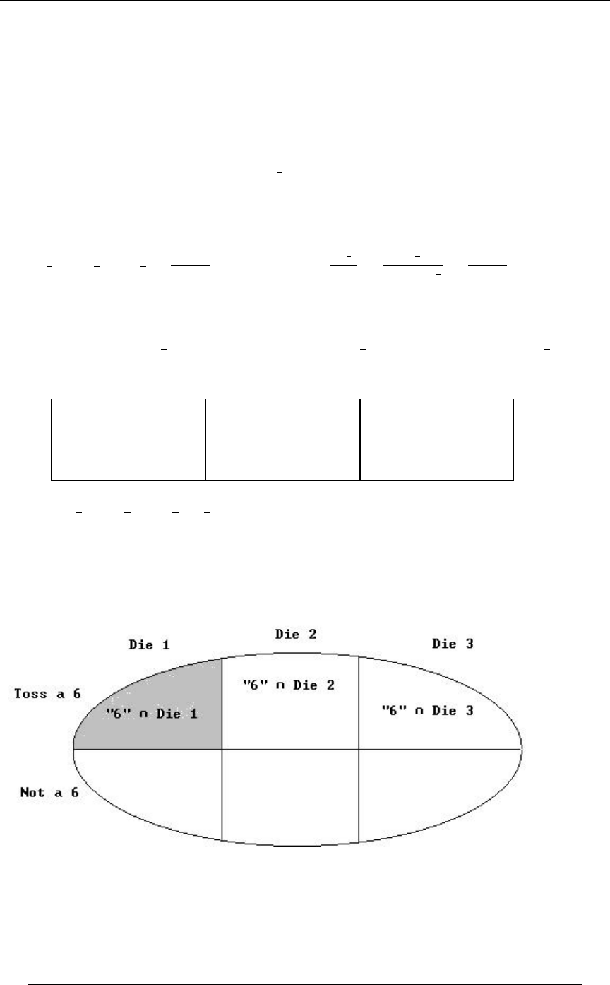
66 SECTION 2 - CONDITIONAL PROBABILITY AND INDEPENDENCE

Example 2-6: Three dice have the following probabilities of throwing a "six": :ß;ß<ß

respectively. One of the dice is chosen at random and thrown (each is equally likely to be

chosen). A "six" appeared. What is the probability that the die chosen was the first one?

Solution: The event " a 6 is thrown" is denoted by and and denote the events thatFEßE E

"# $

die 1, die 2 and die 3 was chosen.

TÒE lFÓ œ œ œ

"T ÒE ∩FÓ T ÒFlE Ó†T ÒE Ó

TÒFÓ TÒFÓ TÒFÓ

:†

"""

$ .

But TÒFÓ œ TÒF ∩E ÓTÒF ∩E ÓTÒF ∩E Ó

"#$

œ TÒFlE Ó†TÒE ÓTÒFlE Ó†TÒE ÓTÒFlE Ó†TÒE Ó

"" ## $$

œ : †  ; †  < † œ Ê T ÒE lFÓ œ œ œ

"""

$$$ "

:;< :

$ T ÒFÓ :;<

:† :†

Ð:;<Ñ†

These calculations can be summarized in the following table.

Die 1 , ) Die 2 , ) Die 3 , )TÐE œ TÐE œ TÐE œ

"#$

"""

$$$

(given) (given) (given)

Toss

"6"

(given) (given) (given)

ßF

TÒFlE Ó œ : TÒFlE Ó œ ; TÒFlE Ó œ <

TÒF∩E Ó TÒF∩E Ó TÒF ∩E Ó

œ T ÒFlE Ó † T ÒE Ó œ T ÒFlE Ó † T ÒE Ó œ T ÒFlE Ó

œ:† œ;†

"#$

"" ## $

†TÒE Ó

œ<†

TÒFÓœ:† ;† <† œ Ð:;<Ñ

""""

$$$$ .

In terms of Venn diagrams, the conditional probability is the ratio of the shaded area probability

in the first diagram to the shaded area probability in the second diagram.

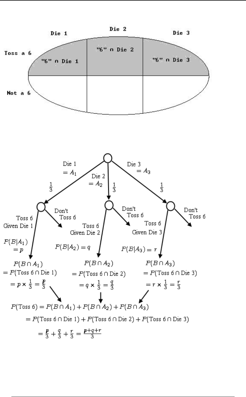
SECTION 2 - CONDITIONAL PROBABILITY AND INDEPENDENCE 67

Example 2-6 continued

The event tree representing the probabilities has three branches at the top node to represent the

three die types that can be chosen in the first step of the process.



68 SECTION 2 - CONDITIONAL PROBABILITY AND INDEPENDENCE

In Example 2-6 there is a certain symmetry to the situation and general reasoning can provide a

shortened solution. In the conditional probability TÒ "l ' Ó œdie " " , we can think

T ÒÐ "Ñ∩Ð ' ÑÓ

TÒ ' Ó

die " "

of the denominator as the combination of the three possible ways a "6" can occur, ,:;<

and we can think of the numerator as the "6" occurring from die 1, with probability . Then the:

conditional probability is the fraction . The symmetry involved here is in the assumption

:;<

that each die was equally likely to be chosen, so there is a chance of any one die being chosen.

This factor of cancels in the numerator and denominator of . If we had not had this

:†

Ð:;<Ñ†

symmetry, we would have to apply different "weights" to the three dice.

Another example of this sort of symmetry is a variation on Example 2-3 above. Suppose that Urn

I has 2 white and 3 black balls and Urn II has 4 white and 1 black balls. An Urn is chosen at

random and a ball is chosen. The reader should verify using the usual conditional probability

rules that the probability of choosing a white is . This can also be seen by noting that if we

consider the 10 balls together, 6 of them are white, so that the chance of picking a white out of

the 10 is . This worked because of two aspects of symmetry, equal chance for picking each

Urn, and same number of balls in each Urn.

Independent events and :EF If events and satisfy the relationshipEF

T ÒE ∩ FÓ œ T ÒEÓ † T ÒFÓ , then the events are said to be independent or stochastically

independent or statistically independent. The independence of (non-empty) events and isEF

equivalent to , and also is equivalent to .T ÒElFÓ œ T ÒEÓ T ÒFlEÓ œ T ÒFÓ

Example 2-1 continued: A fair six-sided die is tossed.

E œ œ Ö#ß %ß '× F œ Ÿ $ œ Ö"ß #ß $×"the number tossed is even" , "the number tossed is " ,

G œ " # œ Ö"ß #×"the number tossed is a or a " ,

H œ œ Ö"ß '×"the number tossed doesn't start with the letters 'f' or 't'" .

We have the following probabilities: TÒEÓ œ ß TÒFÓ œ ß TÒGÓ œ ß TÒHÓ œ Þ

""""

##$$

Events and are not independent since . We alsoE F œ T ÒE ∩ FÓ Á T ÒEÓ † T ÒFÓ œ † œ

""""

'##%

see that and are not independent because E F TÒFlEÓ œ Á œ TÒFÓÞ

Also, and are not independent, since (also sinceF G T ÒF ∩ GÓ œ Á œ T ÒFÓ † T ÒGÓ

"""

$#$

†

TÒFlGÓ œ " Á œ TÒFÓ E G

#). Events and are independent, since

T ÒE ∩ GÓ œ œ œ T ÒEÓ † T ÒGÓ

"""

'#$

†(alternatively,

TÒElGÓ œ œ TÒEÓ E G

# , so that and are independent).

The reader should check that both and are independent of . EF H 

SECTION 2 - CONDITIONAL PROBABILITY AND INDEPENDENCE 69

Mutually independent events: Events are said to be mutuallyE ß E ß ÞÞÞß E

"# 8

independent if the following relationships are satisfied. For any two events, say and , weEE

have . For any three events, Say , we have TÐE ∩EÑœTÐEÑ†TÐEÑ EßEßE Ó

34 3 4 345

TÐE ∩E ∩E Ñ œ TÐE Ñ†TÐE Ñ†TÐE Ñ

345 3 4 5

. This must be true for any four events, any five

events, etc.

Some rules concerning conditional probability and independence are:

for any events and (i) T ÒE ∩ FÓ œ T ÒFlEÓ † T ÒEÓ œ T ÒElFÓ † T ÒFÓ E F

If , then(ii) TÒE∩E∩â∩E Ó!

"# 8"

T ÒE ∩ E ∩ â ∩ E Ó œ T ÒE Ó † T ÒE lE Ó † T ÒE lE ∩ E ÓâT ÒE lE ∩ E ∩ â ∩ E Ó

" # 8 " #" $" # 8" # 8"

(iii) T ÒE lFÓ œ "  T ÒElFÓ

(iv) T ÒE ∪ FlGÓ œ T ÒElGÓ  T ÒFlGÓ  T ÒE ∩ FlGÓ

if then , and ; properties (iv) and (v)(v) E § F T ÒElFÓ œ œ T ÒFlEÓ œ "

TÒE∩FÓ TÒEÓ

TÒFÓ TÒFÓ

are the same properties satisfied by unconditional events

if and are independent events then and are independent events,(vi) EF E F

and are independent events, and and are independent eventsEF E F

www

since for any event , it follows that is(vii) TÒgÓ œ TÒg∩EÓ œ ! œ TÒgÓ†TÒEÓ E g

independent of any event E

Example 2-7: Suppose that events and are independent. Find the probability, in terms ofEF

TÒEÓ TÒFÓ E F and , that exactly one of the events and occurs.

Solution: exactly one of and .T Ò E FÓ œ T ÒÐE ∩ F Ñ ∪ ÐE ∩ FÑÓ

Since and are mutually exclusive, it follows thatE∩F F∩E

TÒ E FÓ œ TÒE∩F ÓTÒE ∩FÓexactly one of and .

Since and are independent, it follows that and are also independent, as are and .EF EF F E

Then TÒÐE∩FÑ∪ÐE ∩FÑÓœTÒEÓ†TÒFÓTÒFÓ†TÒEÓ

ww w w

œ T ÒEÓÐ"  T ÒFÓÑ  T ÒFÓÐ"  T ÒEÓÑ œ T ÒEÓ  T ÒFÓ  #T ÒEÓ † T ÒFÓ 

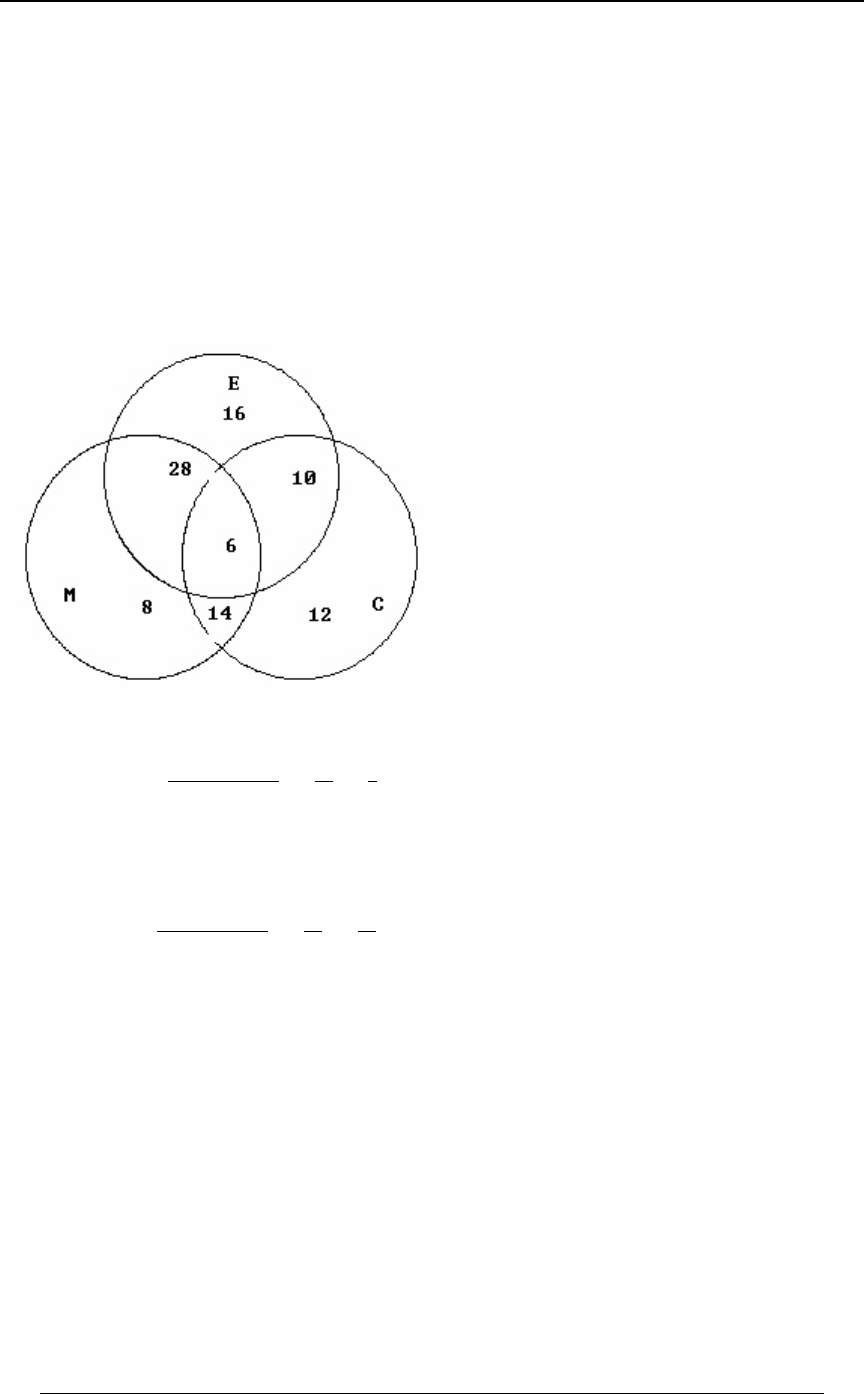
70 SECTION 2 - CONDITIONAL PROBABILITY AND INDEPENDENCE

Example 2-8: In a survey of 94 students, the following data was obtained.

60 took English, 56 took Math, 42 took Chemistry, 34 took English and Math, 20 took Math and

Chemistry, 16 took English and Chemistry, 6 took all three subjects.

Find the following proportions.

(i) Of those who took Math, the proportion who took neither English nor Chemistry,

(ii) Of those who took English or Math, the proportion who also took Chemistry.

Solution: The following diagram illustrates how the numbers of students can be deconstructed.

We calculate proportion of the numbers in the various subsets.

(i) 56 students took Math, and 8 of them took neither English nor Chemistry.

TÐI ∩G lQÑ œ œ œ

ww TÐI ∩G ∩QÑ

T ÐQÑ &' (

ww .

(ii) 82 ( in students took English or Math (or both), andœ)"%'#)"'"! I∪QÑ

30 of them ( in ) also took Chemistry .œ"%'"! ÐI∪QÑ∩G

TÐGlI ∪QÑ œ œ œ Þ

T ÒG∩ÐI∪QÑÓ

T ÐI∪QÑ )# %"

$! "& 

Example 2-9: A survey is made to determine the number of households having electric

appliances in a certain city. It is found that 75% have radios ( ), 65% have irons ( ), 55% haveVM

electric toasters ( ), 50% have ( ), 40% have ( ), 30% have ( ), and 20% have all three.XMVVXMX

Find the following proportions.

(i) Of those households that have a toaster, find the proportion that also have a radio.

(ii) Of those households that have a toaster but no iron, find the proportion that have a radio.

SECTION 2 - CONDITIONAL PROBABILITY AND INDEPENDENCE 71

Solution: This is a continuation of Example 1-3 given earlier in the study guide.

The diagram below deconstructs the three events.

(i) This is . The language "of those households that have a toaster" means, "given thatTÒVlXÓ

the household has a toaster", so we are being asked for a conditional probability.

Then, TÒVlXÓ œ œ œ Þ

TÒV∩XÓ

TÒXÓ Þ&& ""

Þ% )

(ii) This is TÒVlX ∩M Ó œ œ œ Þ

wTÒV∩X∩M Ó

TÒX∩M Ó Þ#& &

Þ# %

w

Example 2-8 presents a "population" of 94 individuals, each with some combination of various

properties (took English, took Math, took Chemistry). We found conditional probabilities

involving the various properties by calculating proportions in the following way

TÐElFÑ œ 8?7,/< 90 38.3@3.?+6= =+>3=0 C381 ,9>2 :<9:/<>3/= E +8. F

8?7,/< 90 38.3@3?.+6= =+>3=0 C381 :<9:/<>C F .

We could approach Example 2-9 in a similar way by creating a "model population" with the

appropriate attributes. Since we are given percentages of households with various properties, we

can imagine a model population of 100 households, in which 75 have radios ( , 75%), 65 haveV

irons ( ), 55 have electric toasters ( ), 50 have ( ), 40 have ( ), 30 have ( ), and 20 haveM X MV VX MX

all three. The diagram in the solution could modified by changing the decimals to numbers out

of 100 - so .2 becomes 10, etc. Then so solve (i), since 55 have toasters and 40 have both a radio

and a toaster, the proportion of those who have toasters that also have a radio is .

Creating a model population is sometimes an efficient way of solving a problem involving

conditional probabilities, particularly when applying Bayes rule. The following example

illustrates this.

72 SECTION 2 - CONDITIONAL PROBABILITY AND INDEPENDENCE

Example 2-10 SOA : A blood test indicates the presence of a particular disease 95% of the

time when the disease is actually present. The same test indicates the presence of the disease

0.5% of the time when the disease is not present. One percent of the population actually has the

disease. Calculate the probability that a person has the disease given that the test indicates the

presence of the disease.

Solution: 13. We identify the following events:

HÀ XT À a person has the disease , a person tests positive for the disease

We are given T ÐHÑ œ Þ!" ß T ÐH Ñ œ Þ** ß T ÐX T lHÑ œ Þ*& ß T ÐX T lHÑ œ Þ!& ß

T ÐX T lH Ñ œ Þ!!& ß T ÐX T lH Ñ œ Þ**&

w .

We wish to find .TÐHlXTÑ

We first solve the problem using rules of conditional probability.

We have .TÐHlXTÑ œ TÐH∩XTÑ

TÐXTÑ

We also have, , andT ÐH ∩ X T Ñ œ T ÐX T lHÑ † T ÐHÑ œ ÐÞ*&ÑÐÞ!"Ñ œ Þ!!*&

TÐXTÑ œ TÐH ∩XTÑ TÐH ∩XTÑ

œ T ÐX T lHÑ † T ÐHÑ  T ÐX T lH Ñ † T ÐH Ñ œ ÐÞ*&ÑÐÞ!"Ñ  ÐÞ!!&ÑÐÞ**Ñ œ Þ!"%%& Þ

Then, . T ÐHlX T Ñ œ œ œ Þ'&(

TÐH∩XTÑ

T ÐX T Ñ Þ!"%%&

Þ!!*&

We can also solve this problem with the model population approach. We imagine a model

population of 100,000 individuals. In this population, the number with disease is #ÐHÑ œ "!!!

(.01 of the population) , the number without disease is # (.99 of the population).ÐH Ñ œ **ß !!!

Since , it follows that 95% of those with the disease will test positive, so theT ÐX T lHÑ œ Þ*&

number who have the disease and test positive is # (this justÐX T ∩ HÑ œ Þ*& ‚ "!!! œ *&!

reflects the fact that , so thatT ÐX T ∩ HÑ œ T ÐX T lHÑ ‚ T ÐHÑ œ Þ*& ‚ Þ!" œ Þ!!*&

Þ!!*& ‚ "!!ß !!! œ *&! in the population have the disease and test positive. In the same way, we

find # is the number who do not have disease but testÐX T ∩ H Ñ œ Þ!!& ‚ **ß !!! œ %*&

positive. Therefore, the total number who test positive is

## #ÐX T Ñ œ ÐX T ∩ HÑ  ÐX T ∩ H Ñ œ *&!  %*& œ "%%& Þ

The probability that a person has the disease given that the test indicates the presence of the

disease is the proportion that have the disease and test positive as a fraction of all those who test

positive, .T ÐHlX T Ñ œ œ œ Þ'&(

ÐX T ∩HÑ

ÐHÑ "%%&

*&!

SECTION 2 - CONDITIONAL PROBABILITY AND INDEPENDENCE 73

Example 2-10 continued

The following table summarizes the calculations in the conditional probability approach.

, given TÐHÑ œ Þ!" TÐH Ñ œ Þ**

œ"Þ!"

XT TÐXTlHÑ œ Þ*& TÐXTlH Ñ œ Þ!!& , given , given

TÐXT ∩HÑ TÐXT ∩H Ñ

œ TÐXTlHÑ†TÐHÑ œ TÐXTlH Ñ†TÐH Ñ

œ ÐÞ*&ÑÐÞ!"Ñ œ Þ!!*& œ ÐÞ!!&ÑÐÞ**Ñ œ Þ!!%*&

XT TÐXT lHÑ œ "TÐXTlHÑ TÐXT lH Ñ œ "TÐXTlH Ñ

ww w

, œ Þ!& œ Þ**& ß

TÐXT ∩HÑ TÐXT ∩H Ñ

œ T ÐX T lHÑ † T ÐHÑ œ T ÐX T lH Ñ † T ÐH Ñ

œ ÐÞ!&ÑÐÞ!"Ñ œ Þ!!!& œ ÐÞ**&ÑÐÞ**Ñ œ Þ*)&!&

T ÐX T Ñ œ T ÐX T ∩ HÑ  T ÐX T ∩ H Ñ œ Þ!!*&  Þ!!%*& œ Þ!"%%& Þ

T ÐHlX T Ñ œ œ œ Þ'&(

TÐH∩XTÑ

T ÐX T Ñ Þ!"%%&

Þ!!*& . Answer: B

74 SECTION 2 - CONDITIONAL PROBABILITY AND INDEPENDENCE

PROBLEM SET 2 75

PROBLEM SET 2

Conditional Probability and Independence

1. Let and be events such that , andEß Fß G H F œ E ß G ∩ H œ g

T ÒEÓ œ T ÒFÓ œ T ÒGlEÓ œ T ÒGlFÓ œ T ÒHlEÓ œ T ÒHlFÓ œ

"$ " $ " "

%% # % % )

, , , , ,

Calculate .TÒG ∪HÓ

A) B) C) D) E)

& " #( $

$#%$#%

2. You are given that and .T ÒEÓ œ Þ& T ÒE ∪ FÓ œ Þ(

Actuary 1 assumes that and are independent and calculates based on that assumption.EF TÒFÓ

Actuary 2 assumes that and mutually exclusive and calculates based on thatEF TÒFÓ

assumption. Find the absolute difference between the two calculations.

A) 0 B) .05 C) .10 D) .15 E) .20

3. (SOA) An actuary studying the insurance preferences of automobile owners makes the

following conclusions:

(i) An automobile owner is twice as likely to purchase collision coverage as disability coverage.

(ii) The event that an automobile owner purchases collision coverage is independent of the event

that he or she purchases disability coverage.

(iii) The probability that an automobile owner purchases both collision and disability coverages

is 0.15 .

What is the probability that an automobile owner purchases neither collision nor disability

coverage?

A) 0.18 B) 0.33 C) 0.48 D) 0.67 E) 0.82

4. Two bowls each contain 5 black and 5 white balls. A ball is chosen at random from bowl 1

and put into bowl 2. A ball is then chosen at random from bowl 2 and put into bowl 1. Find the

probability that bowl 1 still has 5 black and 5 white balls.

A) B) C) D) E)

#$ ' " '

$ & "" # "$

76 PROBLEM SET 2

5. (SOA) An insurance company examines its pool of auto insurance customers and gathers the

following information:

(i) All customers insure at least one car.

(ii) 70% of the customers insure more than one car.

(iii) 20% of the customers insure a sports car.

(iv) Of those customers who insure more than one car, 15% insure a sports car.

Calculate the probability that a randomly selected customer insures exactly one car and that car is

not a sports car.

A) 0.13 B) 0.21 C) 0.24 D) 0.25 E) 0.30

6. (SOA) An insurance company pays hospital claims. The number of claims that include

emergency room or operating room charges is 85% of the total number of claims. The number of

claims that do not include emergency room charges is 25% of the total number of claims. The

occurrence of emergency room charges is independent of the occurrence of operating room

charges on hospital claims. Calculate the probability that a claim submitted to the insurance

company includes operating room charges.

A) 0.10 B) 0.20 C) 0.25 D) 0.40 E) 0.80

7. Let , and be events such that and . Which of theE F G T ÒElGÓ œ Þ!& T ÒFlGÓ œ Þ!&

following statements must be true?

A) B) C) T ÒE ∩ FlGÓ œ ÐÞ!&Ñ T ÒE ∩ F lGÓ  Þ*! T ÒE ∪ FlGÓ Ÿ Þ!&

#ww

D) E) 10TÒE∪FlG Ó  "ÐÞ!&Ñ TÒE∪FlG Ó  Þ

w# w

8. A system has two components placed in series so that the system fails if either of the two

components fails. The second component is twice as likely to fail as the first. If the two

components operate independently, and if the probability that the entire system fails is .28, find

the probability that the first component fails.

A) B) C) D) E)

Þ#) Þ&'

Þ"! Þ#! Þ"%

PROBLEM SET 2 77

9. A ball is drawn at random from a box containing 10 balls numbered sequentially from 1 to 10.

Let be the number of the ball selected, let be the event that is an even number, let be\V\W

the event that , and let be the event that . Which of the pairs \' X \Ÿ% ÐVßWÑßÐVßXÑß

and are independent?ÐWß X Ñ

A) only B) only C) onlyÐVß WÑ ÐVß X Ñ ÐWß X Ñ

D) and only E) and ÐVß WÑ ÐVß X Ñ ÐVß WÑ ß ÐVß X Ñ ÐWß X Ñ

10. (SOA) A health study tracked a group of persons for five years. At the beginning of the

study, 20% were classified as heavy smokers, 30% as light smokers, and 50% as nonsmokers.

Results of the study showed that light smokers were twice as likely as nonsmokers to die during

the five-year study, but only half as likely as heavy smokers. A randomly selected participant

from the study died over the five-year period. Calculate the probability that the participant was a

heavy smoker.

A) 0.20 B) 0.25 C) 0.35 D) 0.42 E) 0.57

11. If and are events such that IßI I TÒIlIÓœTÒIlIÓœTÒIlIÓœ:ß

"#$ "##$$"

TÒI ∩I ÓœTÒI ∩I ÓœTÒI ∩I Óœ<ß TÒI ∩I ∩I Óœ=ß

"# "$ #$ "#$

and

find the probability that at least one of the three events occurs.

A) B) C) D) E)" <= $<= '<= <=

<$< $<

:< : < :

$: $:

12. (SOA) A public health researcher examines the medical records of a group of 937 men who

died in 1999 and discovers that 210 of the men died from causes related to heart disease.

Moreover, 312 of the 937 men had at least one parent who suffered from heart disease, and, of

these 312 men, 102 died from causes related to heart disease. Determine the probability that a

man randomly selected from this group died of causes related to heart disease, given that neither

of his parents suffered from heart disease.

A) 0.115 B) 0.173 C) 0.224 D) 0.327 E) 0.514

78 PROBLEM SET 2

13. In a T-maze, a laboratory rat is given the choice of going to the left and getting food or going

to the right and receiving a mild electric shock. Assume that before any conditioning (in trial

number 1) rats are equally likely to go the left or to the right. After having received food on a

particular trial, the probability of going to the left and right become .6 and .4, respectively on the

following trial. However, after receiving a shock on a particular trial, the probabilities of going to

the left and right on the next trial are .8 and .2, respectively. What is the probability that the

animal will turn left on trial number 2?

A) .1 B) .3 C) .5 D) .7 E) .9

14. In the game show "Let's Make a Deal", a contestant is presented with 3 doors. There is a

prize behind one of the doors, and the host of the show knows which one. When the contestant

makes a choice of door, at least one of the other doors will not have a prize, and the host will

open a door (one not chosen by the contestant) with no prize. The contestant is given the option

to change his choice after the host shows the door without a prize. If the contestant switches

doors, what is the probability that he gets the door with the prize?

A) B) C) D) E)!"""#

'$#$

15. (SOA) A doctor is studying the relationship between blood pressure and heartbeat

abnormalities in her patients. She tests a random sample of her patients and notes their blood

pressures (high, low, or normal) and their heartbeats (regular or irregular). She finds that:

(i) 14% have high blood pressure.

(ii) 22% have low blood pressure.

(iii) 15% have an irregular heartbeat.

(iv) Of those with an irregular heartbeat, one-third have high blood pressure.

(v) Of those with normal blood pressure, one-eighth have an irregular heartbeat.

What portion of the patients selected have a regular heartbeat and low blood pressure?

A) 2% B) 5% C) 8% D) 9% E) 20%

PROBLEM SET 2 79

16. (SOA) An insurance company issues life insurance policies in three separate categories:

standard, preferred, and ultra-preferred. Of the company’s policyholders, 50% are standard, 40%

are preferred, and 10% are ultra-preferred. Each standard policy-holder has probability 0.010 of

dying in the next year, each preferred policyholder has probability 0.005 of dying in the next

year, and each ultra-preferred policyholder has probability 0.001 of dying in the next year. A

policyholder dies in the next year. What is the probability that the deceased policyholder was

ultra-preferred?

A) 0.0001 B) 0.0010 C) 0.0071 D) 0.0141 E) 0.2817

17. (SOA) The probability that a randomly chosen male has a circulation problem is 0.25 . Males

who have a circulation problem are twice as likely to be smokers as those who do not have a

circulation problem. What is the conditional probability that a male has a circulation problem,

given that he is a smoker?

A) B) C) D) E)

""#"#

%$&#$

18. SOA A study of automobile accidents produced the following data:

Probability of

Model Proportion of involvement

year all vehicles in an accident

1997 0.16 0.05

1998 0.18 0.02

1999 0.20 0.03

Other 0.46 0.04

An automobile from one of the model years 1997, 1998, and 1999 was involved

in an accident. Determine the probability that the model year of this automobile is 1997 .

A) 0.22 B) 0.30 C) 0.33 D) 0.45 E) 0.50

80 PROBLEM SET 2

19. (SOA) An auto insurance company insures drivers of all ages. An actuary compiled the

following statistics on the company’s insured drivers:

Age of Probability of Portion of Company's

Driver Accident Insured Drivers

16-20 0.06 0.08

21-30 0.03 0.15

31-65 0.02 0.49

66-99 0.04 0.28

A randomly selected driver that the company insures has an accident.

Calculate the probability that the driver was age 16-20.

A) 0.13 B) 0.16 C) 0.19 D) 0.23 E) 0.40

20. (SOA) Upon arrival at a hospital s emergency room, patients are categorized according to’

their condition as critical, serious, or stable. In the past year:

(i) 10% of the emergency room patients were criticalà

(ii) 30% of the emergency room patients were serious;

(iii) the rest of the emergency room patients were stable;

(iv) 40% of the critical patients died

(v) 10% of the serious patients died; and

(vi) 1% of the stable patients died.

Given that a patient survived, what is the probability that the patient was categorized as serious

upon arrival?

A) 0.06 B) 0.29 C) 0.30 D) 0.39 E) 0.64

21. Let and be mutually independent events such that andEß F G T ÒEÓ œ Þ& ß T ÒFÓ œ Þ'

TÒGÓœÞ" TÒE ∪F ∪GÓ . Calculate .

A) B) C) D) E) Þ'* Þ(" Þ($ Þ*) "Þ!!

22. (SOA) An insurance company estimates that 40% of policyholders who have only an auto

policy will renew next year and 60% of policyholders who have only a homeowners policy will

renew next year. The company estimates that 80% of policyholders who have both an auto and a

homeowners policy will renew at least one of those policies next year. Company records show

that 65% of policyholders have an auto policy, 50% of policyholders have a homeowners policy,

and 15% of policyholders have both an auto and a homeowners policy. Using the company’s

estimates, calculate the percentage of policyholders that will renew at least one policy next year.

A) 20 B) 29 C) 41 D) 53 E) 70

PROBLEM SET 2 81

23. (SOA) An actuary studied the likelihood that different types of drivers would be involved in

at least one collision during any one-year period. The results of the study are presented below.

Type of

driver

Probability

Type of Percentage of of at least one

driver all drivers collision

Teen 8% .15

Young Adult 16% .08

Midlife 45% .04

Senior 31% .05

Total 100%

Given that a driver has been involved in at least one collision in the past year, what is the

probability that the driver is a young adult driver?

A) 0.06 B) 0.16 C) 0.19 D) 0.22 E) 0.25

24. Urn 1 contains 5 red and 5 blue balls. Urn 2 contains 4 red and 6 blue balls, and Urn 3

contains 3 red balls. A ball is chosen at random from Urn 1 and placed in Urn 2. Then a ball is

chosen at random from Urn 2 and placed in Urn 3. Finally, a ball is chosen at random from

Urn 3. Find the probabilities that all three balls chosen are red.

A) B) C) D) E)

&& & & &

"" "# #" ## $$

82 PROBLEM SET 2

PROBLEM SET 2 SOLUTIONS

1. Since and have empty intersection, G H TÒG ∪HÓ œ TÒGÓTÒHÓÞ

Also, since and are "exhaustive" events (since they are complementary events, their union isEF

the entire sample space, with a combined probability of

TÒE∪FÓ œ TÒEÓTÒFÓ œ " ).

We use the rule , and the rule to getTÒGÓ œ TÒG ∩EÓTÒG ∩E Ó TÒGlEÓ œ

wTÒE∩GÓ

TÒEÓ

TÒGÓœTÒGlEÓ†TÒEÓTÒGlEÓ†TÒEÓœ †  † œ

"" $$ ""

#% %% "'

and

TÒHÓœTÒHlEÓ†TÒEÓTÒHlEÓ†TÒEÓœ †  † œ Þ

"" "$ &

%% )% $#

Then, Answer: C.TÒG ∪HÓ œ TÒGÓTÒHÓ œ Þ

2. Actuary 1: Since and are independent, so are and .EF E F

T ÒE ∩ F Ó œ "  T ÒE ∪ FÓ œ Þ$

ww .

But .Þ$ œ T ÒE ∩ F Ó œ T ÒE Ó † T ÒF Ó œ ÐÞ&ÑT ÒF Ó p T ÒF Ó œ Þ' p T ÒFÓ œ Þ%

ww w w w w

Actuary 2: .Þ( œ T ÒE ∪ FÓ œ T ÒEÓ  T ÒFÓ œ Þ&  T ÒFÓ p T ÒFÓ œ Þ#

Absolute difference is . Answer: ElÞ%  Þ#l œ Þ#

3. We identify the following events:

Hœan automobile owner purchases disability coverage, and

Gœan automobile owner purchases collision coverage.

We are given that

(i) , (ii) and are independent, and (iii) .TÒGÓ œ #TÒHÓ G H TÒG ∩HÓ œ Þ"&

From (ii) it follows that , and therefore,T ÒG ∩ HÓ œ T ÒGÓ † T ÒHÓ

Þ"& œ #T ÒHÓ † T ÒHÓ œ #ÐT ÒHÓÑ T ÒHÓ œ Þ!(& œ Þ#($)'

# , from which we get .

Then, , , andT ÒGÓ œ #T ÒHÓ œ Þ&%((# T ÒH Ó œ "  T ÒHÓ œ Þ(#'"%

T ÒG Ó œ "  T ÒGÓ œ Þ%&##)

w .

Since and are independent, so are and , and therefore, the probability that anGH G H

automobile owner purchases neither disability coverage nor collision coverage is

T ÒG ∩ H Ó œ T ÒG Ó † T ÒH Ó œ Þ$#)

. Answer: B

PROBLEM SET 2 83

4. Let be the event that bowl 1 has 5 black balls after the exchange.G

Let be the event that the ball chosen from bowl 1 is black, andF"

let be the event that the ball chosen from bowl 2 is black.F#

Event is the disjoint union of and (black-black orGF∩FF∩F

"# "#

white-white picks), so that .TÒGÓ œ TÒF ∩F ÓTÒF ∩F Ó

"# "#

The black-black combination has probability ,ÐÑÐÑ

"" #

since there is a chance of picking black from bowl 1, and then (with 6 black in bowl 2, which

now has 11 balls) is the probability of picking black from bowl 2. This is

T ÒF ∩ F Ó œ T ÒF lF Ó † T ÒF Ó œ Ð ÑÐ Ñ

"# #" " '"

"" # .

In a similar way, the white-white combination has probability .ÐÑÐÑ

"" #

Then . Answer: CTÒGÓ œÐ ÑÐ ÑÐ ÑÐ Ñ œ

'" '" '

"" # "" # ""

5. We identify the following events:

EE - the policyholder insures exactly one car (so that is the event that the policyholder insures

more than one car), and

W - the policyholder insures a sports car.

We are given (from which it follows that ) , and T ÒE Ó œ Þ( T ÒEÓ œ Þ$ T ÒWÓ œ Þ#

(and ). We are also given the conditional probability ;T ÒW Ó œ Þ) T ÒWlE Ó œ Þ"&

w w

"of those customers who insure more than one car", means that we are looking at a conditional

event given .Ew

We are asked to find .TÒE∩W Ó

We create the following probability table, with the numerals in parentheses indicating the order in

which calculations are performed.

E ß Þ$ E ß Þ(

W ß Þ# T ÒW ∩ EÓ T ÒW ∩ E Ó œ T ÒWlE Ó † T ÒE Ó Ð#Ñ Ð"Ñ www

œ TÒWÓ  T ÒW ∩ E Ó œ ÐÞ"&ÑÐÞ(Ñ œ Þ"!&

œ Þ#  Þ"!& œ Þ!*&

WßÞ) TÒE∩WÓ

Ð$Ñ

œTÒEÓTÒE∩WÓ

œ Þ$  Þ!*& œ Þ#!&

We can solve this problem with a model population of 1000 individuals with auto insurance.

# (since 70% insure more than one car), and # . From we getE œ $!! W œ #!! T ÒWlE Ó œ Þ"&

# # . Then # # # ,W ∩ E œ Þ"& ‚ E œ Þ"& ‚ (!! œ "!& W ∩ E œ W  W ∩ E œ #!!  "!& œ *&

ww w

and # # # is the number that insure exactly one car andW ∩ E œ E  W ∩ E œ $!!  *& œ #!&

the car is not a sports car. Therefore . Answer: BT ÒW ∩ EÓ œ Þ#!&

84 PROBLEM SET 2

6. We define the following events.

I - the claim includes emergency room charges ,

S - the claim includes operating room charges.

We are given , and and are independent.TÒI ∪SÓ œ Þ)& TÒI Ó œ Þ#& I S

We are asked to find .TÒSÓ

We use the probability rule .TÒI ∪SÓ œTÒIÓTÒSÓTÒI ∩SÓ

Since and are independent, we have I S T ÒI ∩ SÓ œ T ÒIÓ † T ÒSÓ œ ÐÞ(&ÑT ÒSÓ

(since ).T ÒIÓ œ "  T ÒI Ó œ "  Þ#& œ Þ(&

Therefore, .Þ)& œ T ÒI ∪ SÓ œ Þ(&  T ÒSÓ  Þ(&T ÒSÓ

Solving for results in . Answer: DTÒSÓ TÒSÓ œ Þ%!

7. ,T ÒE ∩ F lGÓ œ T ÒÐE ∪ FÑ lGÓ œ "  T ÒE ∪ FlGÓ  Þ*

ww w

since . Answer: BT ÒE ∪ FlGÓ Ÿ T ÒElGÓ  T ÒFlGÓ œ Þ"

8. Þ#) œ T ÒG ∪ G Ó œ T ÒG Ó  T ÒG Ó  T ÒG ∩ G Ó œ T ÒG Ó  #T ÒG Ó  #ÐT ÒG ÓÑ

"# "#"# " " "

Solving the quadratic equation results in (or , but we disregard this solution sinceTÒG Ó œ Þ" "Þ%

TÒG Ó Ÿ "

" must be ). Alternatively, each of the five answers can be substituted into the

expression above for to see which one satisfies the equation. Answer: BTÒG Ó

9. .TÒVÓ œ Þ& ß TÒWÓ œ Þ& ß TÒXÓ œ Þ%

T ÒV ∩ WÓ œ T Ò'ß )ß "!Ó œ Þ$ Á ÐÞ&ÑÐÞ&Ñ œ T ÒVÓ † T ÒWÓ p Vß W are not independent

T ÒV ∩ X Ó œ T Ò#ß %Ó œ Þ# œ ÐÞ&ÑÐÞ%Ñ œ T ÒVÓ † T ÒX Ó p Vß X are independent

T ÒW ∩ X Ó œ T ÒgÓ œ ! Á ÐÞ&ÑÐÞ%Ñ œ T ÒWÓ † T ÒX Ó p Wß X are not independent. Answer: B

PROBLEM SET 2 85

10. We identify the following events

RP L - non-smoker , - light smoker , - heavy smoker ,

H - dies during the 5-year study .

We are given T ÒRÓ œ Þ&! ß T ÒPÓ œ Þ$! ß T ÒLÓ œ Þ#! Þ

We are also told that TÒHlPÓ œ #TÒHlRÓ œ TÒHlLÓ

(the probability that a light smoker dies during the 5-year study period is ;TÒHlPÓ

it is the conditional probability of dying during the period given that the individual is a light

smoker). We wish to find the conditional probability .TÒLlHÓ

We will find this probability from the basic definition of conditional probability,

TÒLlHÓ œ TÒL∩HÓ

TÒHÓ . These probabilities can be found from the following probability table.

The numerals indicate the order in which the calculations are made.

We are not given specific values for , , or , so will let ,TÒHlPÓ TÒHlRÓ TÒHlLÓ TÒHlRÓ œ 5

and then and .T ÒHlPÓ œ #5 T ÒHlLÓ œ %5

R ß Þ& P ß Þ$ L ß Þ#

H T ÒH ∩ R Ó T ÒH ∩ PÓ T ÒH ∩ LÓ Ð"Ñ Ð#Ñ Ð$Ñ

œ T ÒHlR Ó † T ÒR Ó œ T ÒHlPÓ † T ÒPÓ œ T ÒHlLÓ † T ÒLÓ

œ Ð5ÑÐÞ&Ñ œ Þ&5 œ Ð#5ÑÐÞ$Ñ œ Þ'5 œ Ð%5ÑÐÞ#Ñ œ Þ)5

Ð%Ñ T ÒHÓ œ T ÒH ∩ R Ó  T ÒH ∩ PÓ  T ÒH ∩ LÓ œ Þ&5  Þ'5  Þ)5 œ "Þ*5 .

Ð&Ñ TÒLlHÓ œ œ œ Þ%#

TÒL∩HÓ

T ÒHÓ "Þ*5

Þ)5 . Answer: D

11. , and similarly .TÒIlIÓœ œ:pTÒIÓœ TÒIÓœTÒIÓœ

"# # $ "

TÒI∩IÓ

TÒI Ó : :

Then, TÒI∪I∪IÓ

"#$

œ T ÒI Ó  T ÒI Ó  T ÒI Ó  ÐT ÒI ∩ I Ó  T ÒI ∩ I Ó  T ÒI ∩ I ÓÑ

"#$ "#"$#$

TÒI ∩I ∩I Óœ$Ð Ñ$<=

"#$ <

: . Answer: C

86 PROBLEM SET 2

12. In this group of 937 man, we regard proportions of people with certain conditions to be

probabilities. We are given the population of 937 men. We identify the following conditions:

HL - died from causes related to heart disease , and

TL - had a parent with heart disease.

We are given # , so if follows that # .T L œ $"# T L œ *$(  $"# œ '#&

We are also given # and # .HL œ #"! HL ∩ T L œ "!#

It follows that # # # .HL ∩ ÐT L Ñ œ HL  HL ∩ T L œ #"!  "!# œ "!)

Then the probability of dying due to heart disease given that neither parent suffered from heart

disease is the proportion .

# #

HL∩ÐT L Ñ

T L '#&

"!)

wœ

The solution in terms of conditional probability rules is as follows. From the given information,

we have

TÒHLÓ œ #"!

*$( (proportion who died from causes related to heart disease)

TÒTLÓ œ $"#

*$( (proportion who have parent with heart disease)

TÒHLlTLÓ œ "!#

$"# (prop. who died from heart disease given that a parent has heart disease).

We are asked to find ( is the complement of event , so that is theTÒHLlTL Ó TL TL TL

ww w

event that neither parent had heart disease). Using event algebra, we have

TÒHLlTLÓ œ Ê TÒHL ∩ TLÓ œ TÒHLlTLÓ † TÒTLÓ œ Ð ÑÐ Ñ œ

TÒHL∩TLÓ

T ÒT LÓ $"# *$( *$(

"!# $"# "!# .

We now use the rule TÒEÓ œ TÒE∩FÓTÒE∩FÓ Þ



Then TÒHLÓ œ TÒHL ∩TLÓTÒHL ∩TL Ó p œ TÒHL ∩TL Ó

#"! "!#

*$( *$(

.ÊTÒHL∩TLÓœ

w"!)

*$(

Finally, T ÒHLlT L Ó œ œ œ œ œ Þ"(#) Þ

wT ÒHL∩T L Ó "!)Î*$( "!)Î*$(

TÒTL Ó "TÒTLÓ '#&

"

"!)

w$"#

*$(

These calculations can be summarized in the following table.

HL ß #"! HL ß (#(

given œ *$(  #"!

T L ß $"# HL ∩ T L œ "!# HL ∩ T L œ #"! w

given given œ $"#  "!#

T L ß '#& HL ∩ T L œ "!) HL ∩ T L œ &"(

wwww

œ *$(  $"# œ #"!  "!# œ (#(  #"! or

œ '#&  "!)

T ÒHLlT L Ó œ œ œ œ Þ"(#) Þ

wTÒHL∩TL Ó ÒHL∩TL Ó

TÒTL Ó ÒTL Ó '#&

"!)

In this example, probability of an event is regarded as the proportion of a group that experiences

that event. Answer: B

PROBLEM SET 2 87

13. turn left on trial 1, turn right on trial 1, turn left on trial 2 .P" œ V" œ P# œ

We are given that .TÒP"Ó œ TÒV"Ó œ Þ&

TÒP#Ó œ TÒP#∩P"ÓTÒP#∩V"Ó P"ßV" since form a partition .

TÒP#lP"Ó œ Þ' (if the rat turns left on trial 1 then it gets food and has a .6 chance of turning left

on trial 2). Then .T ÒP# ∩ P"Ó œ T ÒP#lP"Ó † T ÒP"Ó œ ÐÞ'ÑÐÞ&Ñ œ Þ$

In a similar way, .T ÒP# ∩ V"Ó œ T ÒP#lV"Ó † T ÒV"Ó œ ÐÞ)ÑÐÞ&Ñ œ Þ%

Then, .T ÒP#Ó œ Þ$  Þ% œ Þ(

In a model population of 10 rats, # # , and #P" œ V" œ & P# ∩ P" œ Þ' ‚ & œ $

and # . Then the number turning left on trial 2 will beP# ∩ V" œ Þ) ‚ & œ %

# # # , so the probability of a rat turning left on trial 2 isP# œ P# ∩ P"  P# ∩ V" œ $  % œ (

(Î"! œ Þ( Answer: D

14. We define the events prize door is chosen after contestant switches doors ,Eœ

Fœ TÒFÓœprize door is initial one chosen by contestant . Then , since each door is equally

likely to hold the prize initially. To find we use the Law of Total Probability.TÒEÓ

TÒEÓœTÒElFÓ†TÒFÓTÒElFÓ†TÒFÓœÐ!ÑÐ ÑÐ"ÑÐ Ñœ

ww "##

$$$

If the prize door is initially chosen, then after switching, the door chosen is not the prize door, so

that . If the prize door is not initially chosen, then since the host shows the otherTÒElFÓ œ !

non-prize door, after switching the contestant definitely has the prize door, so that .TÒElF Ó œ "

Answer: E

15. This question can be put into the context of probability event algebra. First we identify

events: high blood pressure , low blood pressure , normal blood pressure ,Lœ Pœ Rœ

Vœ MœV œregular heartbeat , irregular heartbeat

We are told that 14% of patients have high blood pressure, which can be represented as

TÒLÓ œ Þ"% TÒPÓ œ Þ## TÒRÓ œ "TÒLÓTÒPÓ œ Þ'%, and similarly , and therefore .

We are given , so that .TÒMÓ œ Þ"& TÒVÓ œ "TÒMÓ œ Þ)&

We are told that "of those with an irregular heartbeat, one-third have high blood pressure". This

is the conditional probability that given (irregular heartbeat) the probability of (high bloodML

pressure) is . Similarly, we are given .T ÒLlMÓ œ T ÒMlR Ó œ

We are asked to find the portion of patients who have both a regular heartbeat and low blood

pressure; this is . Since every patient is exactly one of or , we haveTÒV∩PÓ Lß P R

T ÒV ∩ PÓ  T ÒV ∩ LÓ  T ÒV ∩ R Ó œ T ÒVÓ œ Þ)& , so that

TÒV ∩PÓ œ Þ)&TÒV ∩LÓTÒV ∩RÓÞ

88 PROBLEM SET 2

15. continued

From the conditional probabilities we have

$œ T ÒLlMÓ œ œ p T ÒL ∩ MÓ œ Þ!&

TÒL∩MÓ TÒL∩MÓ

TÒMÓ Þ"& , and

)œ T ÒMlRÓ œ œ p T ÒM ∩ R Ó œ Þ!)

TÒM∩RÓ TÒM∩RÓ

TÒRÓ Þ'% .

Then, since all patients are exactly one of and , we haveMV

T ÒL ∩ MÓ  T ÒL ∩ VÓ œ T ÒLÓ œ Þ"% p T ÒL ∩ VÓ œ Þ"%  Þ!& œ Þ!* , and

T ÒM ∩ R Ó  T ÒV ∩ R Ó œ T ÒR Ó œ Þ'% p T ÒV ∩ R Ó œ Þ'%  Þ!) œ Þ&' .

Finally, T ÒV ∩ PÓ œ Þ)&  T ÒV ∩ LÓ  T ÒV ∩ RÓ œ Þ)&  Þ!*  Þ&' œ Þ#! Þ

These calculations can be summarized in the following table.

L ß Þ"% R ß Þ'% P ß Þ##

given givenœ"Þ"%Þ##

ÌÌ

M ß Þ"& T ÐLlMÑ œ T ÐMlRÑ œ

given given given

TÐL ∩MÑ TÐR ∩MÑ TÐP∩MÑ

œ T ÐLlMÑ † T ÐMÑ œ T ÐMlRÑ † T ÐR Ñ œ T ÐMÑ  T ÐL ∩ MÑ  T ÐR ∩ MÑ

œ Ð ÑÐÞ"&Ñ œ Þ!& œ Ð ÑÐÞ'%Ñ œ Þ!) Ê œ Þ"&  Þ!&  Þ!) œ Þ!#

Vß Þ)& TÐV∩PÑ

œ"Þ"& œTÐPÑTÐP∩MÑ

œ Þ##  Þ!# œ Þ#

Note that the entries and can also be calculated from this table.TÐV ∩LÑ TÐV∩RÑ

The model population solution is as follows. Suppose that the model population has 2400

individuals. Then we have the following

##### .L œ Þ"% ‚ #%!! œ $$' ß P œ &#) ß R œ "&$' ß M œ $'! ß V œ #!%!

Since one-third of those with an irregular heartbeat have high blood pressure, we get

# , and since one-eighth of those with normal blood pressure have an irregularM ∩ L œ "#!

heartbeat we get # . We wish to find # .R ∩ M œ "*# V ∩ P

From # # # # , we get # ,M œ M ∩ L  M ∩ P  M ∩ R $'! œ "#!  M ∩ P  "*#

so that # . Then from # # # we getM∩Pœ%) Pœ M∩P V∩P

&#) œ %)  V ∩ P V ∩ P œ %)!# , so that # . Finally, the probability of having a regular

heartbeat and low blood pressure is the proportion of the population with those properties, which

is . Answer: E

%)!

#%!! œÞ#

PROBLEM SET 2 89

16. This is a typical exercise involving conditional probability. We first label the events, and

then identify the probabilities.

WT - standard policy - preferred policy

YH- ultra-preferred policy - death occurs in the next year.

We are given T ÒWÓ œ Þ&! ß T ÒT Ó œ Þ%! ß T ÒY Ó œ Þ"! ß

T ÒHlWÓ œ Þ!" ß T ÒHlT Ó œ Þ!!& ß T ÒHlY Ó œ Þ!!" Þ

We are asked to find .TÒYlHÓ

The model population solution is as follows. Suppose there is a model population of 10,000

insured lives. Then # # and # .W œ &!!! ß T œ %!!! Y œ "!!!

From we get # , and we also getT ÒHlWÓ œ Þ!" H ∩ W œ Þ!" ‚ &!!! œ &!

# and # .H ∩ T œ Þ!!& ‚ %!!! œ #! H ∩ Y œ Þ!!" ‚ "!!! œ "

Then # , and is the proportion who are ultra-preferred as aH œ &!  #!  " œ (" T ÒY lHÓ

proportion of all who died. This is .

(" œ Þ!"%"

The conditional probability approach to solving the problem is as follows.

The basic formulation for conditional probability is .TÒYlHÓ œ TÒY∩HÓ

TÒHÓ

We use the following relationships:

T ÒE ∩ FÓ œ T ÒElFÓ † T ÒFÓ , and

T ÒEÓ œ T ÒE ∩ G Ó  T ÒE ∩ G Ó  â  T ÒE ∩ G Ó G ß G ÞÞÞß G

"# 8 "#8

, for a partition .

In this problem, events and form a partition of all policyholders.WßT Y

Using the relationships we get

T ÒY ∩ HÓ œ T ÒHlY Ó † T ÒY Ó œ ÐÞ!!"ÑÐÞ"Ñ œ Þ!!!" , and

TÒHÓ œ TÒH∩WÓTÒH ∩TÓTÒH∩YÓ

œTÒHlWÓ†TÒWÓTÒHlTÓ†TÒTÓTÒHlYÓ†TÒYÓ

œ ÐÞ!"ÑÐÞ&Ñ  ÐÞ!!&ÑÐÞ%Ñ  ÐÞ!!"ÑÐÞ"Ñ œ Þ!!(" .

Then, TÒYlHÓ œ œ

TÒY∩HÓ

TÒHÓ

T ÒHlY Ó†T ÒY Ó

T ÒHlWÓ†T ÒWÓT ÒHlT Ó†T ÒT ÓT ÒHlY Ó†T ÒY Ó

œ œ œ Þ!"%"

ÐÞ!!"ÑÐÞ"Ñ

ÐÞ!"ÑÐÞ&ÑÐÞ!!&ÑÐÞ%ÑÐÞ!!"ÑÐÞ"Ñ Þ!!("

Þ!!!" .

Notice that the numerator is one of the factors of the denominator. This will always be the case

when we are "reversing" conditional probabilities such as has been done here; we are to find

TÒYlHÓ TÒHlYÓ TÒHlWÓ TÒHlTÓ from being given information about , , , etc.

90 PROBLEM SET 2

16. continued

From the calculations already made it is easy to find the probability that the deceased

policyholder was preferred;

TÒTlHÓ œ œ

TÒT∩HÓ TÒHlTÓ†TÒTÓ

T ÒHÓ T ÒHlWÓ†T ÒWÓT ÒHlT Ó†T ÒT ÓT ÒHlY Ó†T ÒY Ó

œ œ œ Þ#)"(

ÐÞ!!&ÑÐÞ%Ñ

ÐÞ!"ÑÐÞ&ÑÐÞ!!&ÑÐÞ%ÑÐÞ!!"ÑÐÞ"Ñ Þ!!("

Þ!!#! .

And is .T ÒWlHÓ œ œ Þ(!%#

ÐÞ!"ÑÐÞ&Ñ

ÐÞ!"ÑÐÞ&ÑÐÞ!!&ÑÐÞ%ÑÐÞ!!"ÑÐÞ"Ñ Þ!!("

Þ!!&!

The calculations can be summarized in the following table.

W ß Þ& T ß Þ% Y ß Þ"

given given given

H T ÐHlWÑ œ Þ!" T ÐHlT Ñ œ Þ!!& T ÐHlY Ñ œ Þ!!"

given given given

TÐH∩WÑ TÐH∩TÑ TÐH∩YÑ

œ TÐHlWÑ†TÐWÑ œ TÐHlTÑ†TÐTÑ œ TÐHlYÑ†TÐYÑ

œ ÐÞ!"ÑÐÞ&Ñ œ Þ!!& œ ÐÞ!!&ÑÐÞ%Ñ œ Þ!!# œ ÐÞ!!"ÑÐÞ"Ñ œ Þ!!!"

T ÐHÑ œ T ÒH ∩ WÓ  T ÒH ∩ T Ó  T ÒH ∩ Y Ó œ Þ!!&  Þ!!#  Þ!!!" œ Þ!!(" Þ

T ÒY lHÓ œ œ œ Þ!"%"

TÒY∩HÓ

T ÒHÓ Þ!!("

Þ!!!" . Answer: D

17. We identify the following events:

G - a randomly chosen male has a circulation problem ,

W - a randomly chosen male is a smoker.

We are given the following probabilities:

T ÒGÓ œ Þ#& ß T ÒWlGÓ œ #T ÒWlG Ó

w .

From the rule , we getT ÒE ∩ FÓ œ T ÒElFÓ † T ÒFÓ

T ÒW ∩ GÓ œ T ÒWlGÓ † T ÒGÓ œ ÐÞ#&ÑT ÒWlGÓ , and

TÒW ∩G Ó œ TÒWlG Ó†TÒG Ó œ TÒWlG Ó†Ð"TÒGÓÑ œ ÐÞ(&ÑÐ ÑTÒWlGÓ

wwww "

# ,

so that .T ÒWÓ œ T ÒW ∩ GÓ  T ÒW ∩ G Ó œ ÐÞ#&ÑT ÒWlGÓ  ÐÞ(&ÑÐ ÑT ÒWlGÓ œ Þ'#&T ÒWlGÓ

We are asked to find . This is .TÒGlWÓ TÒGlWÓ œ œ œ Þ%

TÒG∩WÓ ÐÞ#&ÑTÒWlGÓ

T ÒWÓ Þ'#&T ÒWlGÓ

Note that the way in which information was provided allowed us to formulate various

probabilities in terms of (but we do not have enough to find ). Answer: CTÒWlGÓ TÒWlGÓ

PROBLEM SET 2 91

18. We identify events as follows:

97: the model year is 1997 , 98: the model year is 1998 , 99: the model year is 1999

SS À ßother the model year is not 1997, 1998 or 1999

EÀ the car is involved in an accident

We are given T Ò*(Ó œ Þ"' ß T Ò*)Ó œ Þ") ß T Ò**Ó œ Þ#! ß T Ò!!Ó œ Þ%' ß

T ÒEl*(Ó œ Þ!& ß T ÒEl*)Ó œ Þ!# ß T ÒEl**Ó œ Þ!$ ß T ÒEl Ó œ Þ!%other .

The model population solution is as follows. Suppose there are 10,000 automobiles in the study.

Then #### .*( œ "'!! ß *) œ ")!! ß ** œ #!!! ß SS œ %'!!

From we get # , and in a similar way we getT ÒEl*(Ó œ Þ!& E ∩ *( œ Þ!& ‚ "'!! œ )!

##E ∩ *) œ Þ!# ‚ ")!! œ $' ß E ∩ ** œ Þ!$ ‚ #!!! œ '!

and # .E ∩ SS œ Þ!% ‚ %'!! œ ")%

We are given that an automobile from one of 97, 98 or 99 was involved in an accident, and we

wish to find the probability that it was a 97 model. This is the conditional probability

T Ò*(lE ∩ Ð*( ∪ *) ∪ **ÑÓ . This will be the proportion

###

E∩*(

E∩*( E∩*) E∩** )!$''! "('

)! )!

œ œ œ Þ%&%& .

The conditional probability apporach to solve the problem is as follows.

We use the conditional probability rule , so thatTÒGlHÓ œ TÒG∩HÓ

TÒHÓ

T Ò*(lE ∩ Ð*( ∪ *) ∪ **ÑÓ œ T Ò*(∩ÒE∩Ð*(∪*)∪**ÑÓÓ

T ÒE∩Ð*(∪*)∪**ÑÓ .

From set algebra, we have , and*( ∩ ÒE ∩ Ð*( ∪ *) ∪ **ÑÓ œ *( ∩ E

E ∩ Ð*( ∪ *) ∪ **Ñ œ ÐE ∩ *(Ñ ∪ ÐE ∩ *)Ñ ∪ ÐE ∩ **Ñ .

Since the events 97, 98 and 99 are disjoint, we get

T ÒE ∩ Ð*( ∪ *) ∪ **ÑÓ œ T ÒÐE ∩ *(Ñ ∪ ÐE ∩ *)Ñ ∪ ÐE ∩ **ÑÓ

œ T ÒE ∩ *(Ó  T ÒE ∩ *)Ó  T ÒE ∩ **Ó .

From conditional probability rules we have

T ÒE ∩ *(Ó œ T ÒEl*(Ó † T Ò*(Ó œ ÐÞ!&ÑÐÞ"'Ñ œ Þ!!) , and similarly

T ÒE ∩ *)Ó œ ÐÞ!#ÑÐÞ")Ñ œ Þ!!$' T ÒE ∩ **Ó œ ÐÞ!$ÑÐÞ#!Ñ œ Þ!!' , and .

Then, .T ÒE ∩ Ð*( ∪ *) ∪ **ÑÓ œ Þ!!)  Þ!!$'  Þ!!' œ Þ!"('

Therefore, the probability we are trying to find is

T Ò*(lE ∩ Ð*( ∪ *) ∪ **ÑÓ œ T Ò*(∩ÒE∩Ð*(∪*)∪**ÑÓÓ

T ÒE∩Ð*(∪*)∪**ÑÓ

œ œ œ Þ%&%&

T Ò*(∩EÓ

T ÒE∩Ð*(∪*)∪**ÑÓ

Þ!!)

Þ!"(' .

92 PROBLEM SET 2

18. continued

These calculations can be summarized in the following table.

98 99 Other*( ß Þ"' ß Þ") ß Þ#! ß Þ%'

given given given given

E T ÐEl*(Ñ T ÐEl*)Ñ T ÐEl**Ñ T ÐEl Ñ Other

œÞ!& œÞ!# œÞ!$ œÞ!%

given given given given

OtherT ÐE ∩ *(Ñ T ÐE ∩ *)Ñ T ÐE ∩ **Ñ T ÐE ∩ Ñ

OOT ÒEl*(Ó † T Ò*(ÓT ÒEl*)Ó † T Ò*)ÓT ÒEl**Ó † T Ò**ÓT ÒEl Ó † T Ò Ó

œ ÐÞ!&ÑÐÞ"'Ñ œ ÐÞ!#ÑÐÞ")Ñ œ ÐÞ!$ÑÐÞ#!Ñ œ ÐÞ!%ÑÐÞ%'Ñ

œ Þ!!) œ Þ!!$' œ Þ!!' œ Þ!")%

Then, .T Ò*(lE ∩ Ð*( ∪ *) ∪ **ÑÓ œ œ Þ%&%&

Þ!!)

Þ!!)Þ!!$'Þ!!'

Note that the denominator is the sum of the first three of the intersection probabilities, since the

condition is that the auto was 97, 98 or 99. If the question had asked for the probability that the

model year was 97 given that an accident occurred (without restricting to 97, 98, 99) then the

probability would be ; we would include all model years in the

Þ!!)

Þ!!)Þ!!$'Þ!!'Þ!")%

denominator. If the question had asked for the probability that the model year was 97 given that

an accident occurred and the automobile was from one of the model years 97 or 98, then the

probability would be ; we would include only the 97 and 98 model years.

Þ!!)

Þ!!)Þ!!$'

Answer: D

19. We identify the following events:

E - the driver has an accident ,

X] (teen) - age of driver is 16-20 , (young) - age of driver is 21-30 ,

QW (middle age) - age of driver is 31-65 , (senior) - age of driver is 66-99 .

The final column in the table lists the probabilities of and and the middle columnXß ]ß Q W ß

gives the conditional probability of given driver age. The table can be interpreted asE

Age Probability of Accident Portion of Insured Drivers

16-20 TÒElXÓ œ Þ!' TÒXÓ œ Þ!)

21-30 TÒEl]Ó œ Þ!$ TÒ]Ó œ Þ"&

31-65 TÒElQÓ œ Þ!# TÒQÓ œ Þ%*

66-99 TÒElWÓ œ Þ!% TÒWÓ œ Þ#)

We are asked to find .TÒXlEÓ

PROBLEM SET 2 93

19. continued

We construct the following probability table, with numerals in parentheses indicating the order of

the calculations.

X ß Þ!) ] ß Þ"& Qß Þ%* Wß Þ#)

E T ÒE ∩ X Ó T ÒE ∩ ] Ó T ÒE ∩ Q Ó T ÒE ∩ WÓ Ð"Ñ Ð#Ñ Ð$Ñ Ð%Ñ

œTÒElXÓ†TÒXÓ œTÒEl]Ó†TÒ]Ó œTÒElQÓ†TÒQÓ œTÒElWÓ†TÒWÓ

œ ÐÞ!'ÑÐÞ!)Ñ œ ÐÞ!$ÑÐÞ"&Ñ œ ÐÞ!#ÑÐÞ%*Ñ œ ÐÞ!%ÑÐÞ#)Ñ

œ Þ!!%) œ Þ!!%& œ Þ!!*) œ Þ!""#

Ð&Ñ T ÒEÓ œ T ÒE ∩ X Ó  T ÒE ∩ ] Ó  T ÒE ∩ Q Ó  T ÒE ∩ WÓ œ Þ!$!$

Ð'Ñ T ÒX lEÓ œ œ œ Þ"&)

TÒE∩XÓ

T ÒEÓ Þ!$!$

Þ!!%) . Answer: B

20. We label the following events:

GWXHH



- critical , - serious , -stable , - died , - survived.

The following information is given

TÐGÑ œ Þ"ß TÐWÑ œ Þ$ß TÐXÑ œ Þ' œ "TÐGÑTÐWÑß

TÐHlGÑ œ Þ%ß TÐHlWÑ œ Þ"ß TÐHlXÑ œ Þ!" .

We are asked to find . This can be done by using the following table of probabilities.TÐWlHÑ

The rules being used here is ,TÐE∩FÑ œ TÐElFÑ†TÐFÑ

and if form a partitionTÐEÑœTÐE∩FÑTÐE∩FÑâTÐE∩F Ñ FßFßÞÞÞßF

"# 8"#8

of the probability space. In this case, form a partition since all patients are exactly oneGß Wß X

of these three conditions.

GWX

H T ÐH ∩ GÑ T ÐH ∩ WÑ T ÐH ∩ X Ñ

œTÐHlGÑ†TÐGÑ œTÐHlWÑ†TÐWÑ œTÐHlXÑ†TÐXÑ

œ ÐÞ%ÑÐÞ"Ñ œ Þ!% œ ÐÞ"ÑÐÞ$Ñ œ Þ!$ œ ÐÞ!"ÑÐÞ'Ñ œ Þ!!'

p T ÐHÑ œ T ÐH ∩ GÑ  T ÐH ∩ WÑ  T ÐH ∩ X Ñ œ Þ!%  Þ!$  Þ!!' œ Þ!('

H T ÐH ∩ GÑ T ÐH ∩ WÑ T ÐH ∩ X Ñ

wwww

œTÐHlGÑ†TÐGÑ œTÐHlWÑ†TÐWÑ œTÐHlXÑ†TÐXÑ

www

œ ÐÞ'ÑÐÞ"Ñ œ Þ!' œ ÐÞ*ÑÐÞ$Ñ œ Þ#( œ ÐÞ**ÑÐÞ'Ñ œ Þ&*%

p T ÐH Ñ œ T ÐH ∩ GÑ  T ÐH ∩ WÑ  T ÐH ∩ X Ñ œ Þ!'  Þ#(  Þ&*% œ Þ*#%

ww w w

It was not necessary to do the calculations for , since .H T ÐH Ñ œ "  T ÐHÑ œ "  Þ!(' œ Þ*#%

The probability in question is . Answer: BT ÐWlH Ñ œ œ œ Þ#*#

wTÐW∩H Ñ

TÐHÑ

Þ#(

Þ*#%

94 PROBLEM SET 2

21. TÒE ∪F ∪GÓ

œ T ÒE Ó  T ÒF Ó  T ÒGÓ  ÐT ÒE ∩ F Ó  T ÒE ∩ GÓ  T ÒF ∩ GÓÑ  T ÒE ∩ F ∩ GÓ

ww www w ww

œ Þ&  Þ%  Þ"  ÒÐÞ&ÑÐÞ%Ñ  ÐÞ&ÑÐÞ"Ñ  ÐÞ%ÑÐÞ"ÑÓ  ÐÞ&ÑÐÞ%ÑÐÞ"Ñ œ Þ($ .

If events and are independent, then so are and and , and and .\] \ ]ß\] \ ]

wwww

Alternatively using DeMorgan's Law, we have

TÒE∪F∪GÓœ"TÒÐE∪F∪GÑÓœ"TÒE ∩F ∩GÓœ"TÒE∩F∩GÓ

ww ww w ww w w

. Answer: Cœ "  T ÒEÓ † T ÒFÓ † T ÒG Ó œ "  ÐÞ&ÑÐÞ'ÑÐÞ*Ñ œ Þ($

22. We define the following events

V - renew at least one policy next year

EL - has an auto policy , - has a homeowner policy

A policyholder with an auto policy only can be described by the event , andE∩L

a policyholder with a homeowner policy only can be described by the event .E∩L

We are given and .T ÒVlE ∩ L Ó œ Þ% ß T ÒVlE ∩ LÓ œ Þ' T ÒVlE ∩ LÓ œ Þ)

We are also given and .T ÒEÓ œ Þ'& ß T ÒLÓ œ Þ& T ÒE ∩ LÓ œ Þ"&

We are asked to find .TÒVÓ

We use the rule

TÒVÓœTÒV∩E∩LÓTÒV∩E ∩LÓTÒV∩E∩LÓTÒV∩E ∩LÓ

wwww

Since renewal can only occur if there is at least one policy, it follows that ;TÒV ∩E ∩L Ó œ !

in other words, of there is no auto policy (event ) there is no homeowner policy (event ),EL

and

then there can be no renewal. An alternative way of saying the same thing is that is a subsetV

(subevent) of .E∪L

(Note also that , so this also showT ÒE ∪ LÓ œ T ÒEÓ  T ÒLÓ  T ÒE ∩ LÓ œ Þ'&  Þ&  Þ"& œ "

that must be a subevent of , and it also shows thatVE∪L

TÒE ∩L Óœ"TÒE∪LÓœ""œ! E ∩L œ

ww ww

so that ).9

This can be illustrated in the following diagram.

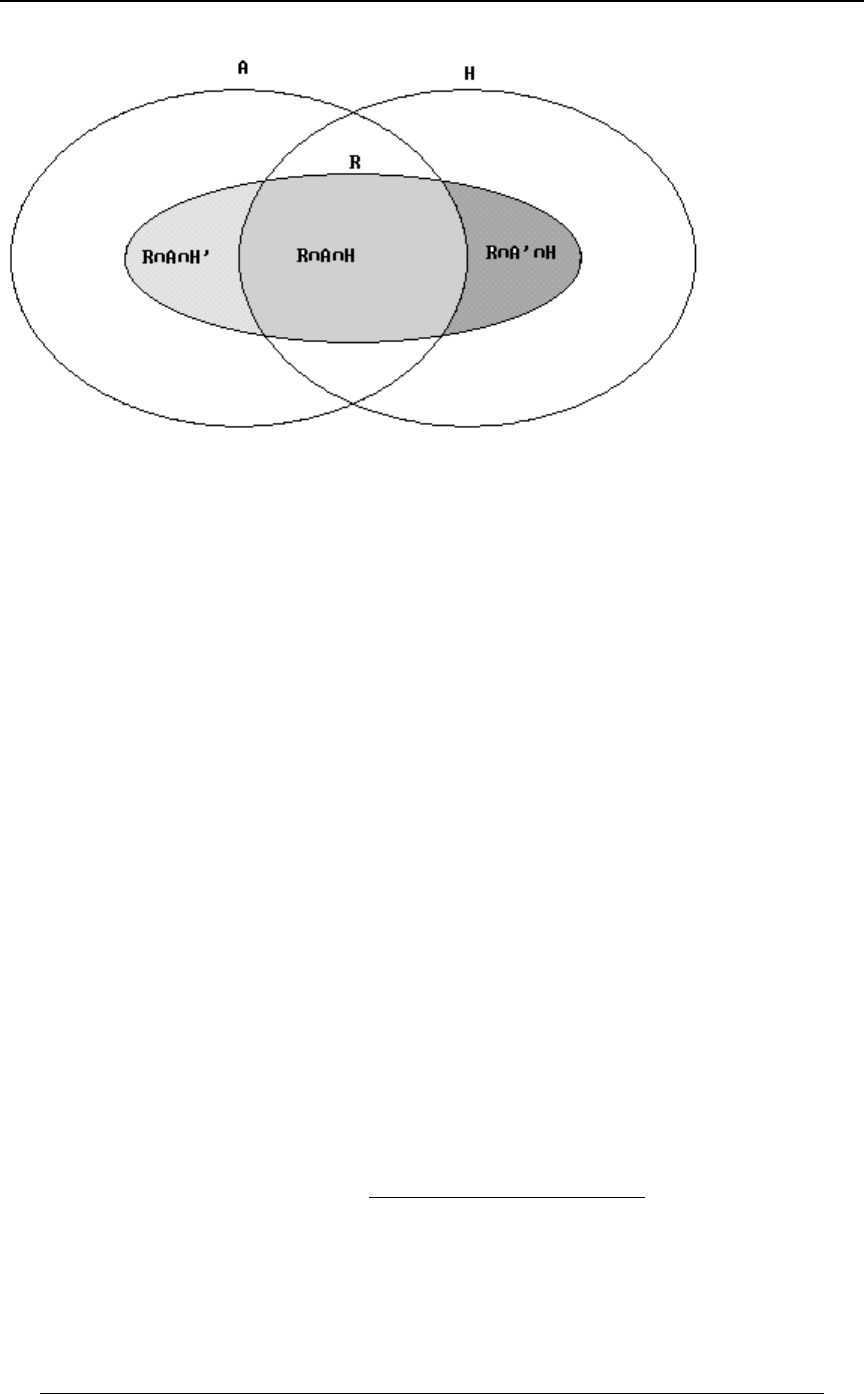
PROBLEM SET 2 95

We find , and by using the ruleTÒV ∩E∩LÓ TÒV ∩E ∩LÓ TÒV ∩E∩L Ó

T ÒG ∩ HÓ œ T ÒGlHÓ † T ÒHÓ :

T ÒV ∩ E ∩ LÓ œ T ÒVlE ∩ LÓ † T ÒE ∩ LÓ œ ÐÞ)ÑÐÞ"&Ñ œ Þ"# ,

T ÒV ∩ E ∩ LÓ œ T ÒVlE ∩ LÓ † T ÒE ∩ LÓ œ ÐÞ'ÑT ÒE ∩ LÓ

www w

T ÒV ∩ E ∩ L Ó œ T ÒVlE ∩ L Ó † T ÒE ∩ L Ó œ ÐÞ%ÑT ÒE ∩ L Ó

www w

In order to complete the calculations we must find and .TÒE ∩LÓ TÒE∩L Ó

From the diagram above, or using the probability rule, we have

TÒEÓ œ TÒE∩LÓTÒE∩L Ó p Þ'& œ Þ"&TÒE∩L Ó p TÒE∩L Ó œ Þ&

www

, and

T ÒLÓ œ T ÒE ∩ LÓ  T ÒE ∩ LÓ p Þ& œ Þ"&  T ÒE ∩ LÓ p T ÒE ∩ LÓ œ Þ$&

www

Then and .TÒV∩E ∩LÓœÐÞ'ÑÐÞ$&ÑœÞ#" TÒV∩E∩LÓœÐÞ%ÑÐÞ&ÑœÞ#

Finally, . 53% of policyholders will renew. Answer: DT ÒVÓ œ Þ"#  Þ#"  Þ# œ Þ&$

23. We are given teen , young adult , midlife andTÐ Ñ œ Þ!) TÐ Ñ œ Þ"' TÐ Ñ œ Þ%&

TÐ Ñ œ Þ$"senior . We are also given the conditional probabilities

TÐ l Ñ œ Þ"& TÐ l Ñ œ Þ!)at least one collision teen , at least one collision young adult ,

TÐ l Ñ œ Þ!% TÐ l Ñ œ Þ!&at least one collision midlife , at least one collision senior .

We wish to find young adult at least one collision .TÐ l Ñ

Using the definition of conditional probability, we have

young adult at least one collision .TÐ l Ñ œ TÐ ∩ Ñ

TÐ Ñ

young adult at least one collision

at least one collision

We use the rule , to getTÐE∩FÑ œ TÐElFÑ†TÐFÑ

TÐ ∩ Ñ œ TÐ ∩ Ñyoung adult at least one collision at least one collision young adult

œ T Ð l Ñ † T Ð Ñ œ ÐÞ!)ÑÐÞ"'Ñ œ Þ!"#)at least one collision young adult young adult .

96 PROBLEM SET 2

24. continued

We also have

TÐ Ñ œ TÐ ∩ Ñat least one collision at least one collision teen

TÐ ∩ ÑTÐ ∩ Ñat least one collision young adult at least one collision midlife

TÐ ∩ Ñat least one collision senior

at least one collision teen young teenœTÐ l Ñ†TÐ Ñ

at least one collision young adult young adultTÐ l Ñ†TÐ Ñ

TÐ l Ñ†TÐ Ñat least one collision midlife midlife

at least one collision senior seniorTÐ l Ñ†TÐ Ñ

œ ÐÞ"&ÑÐÞ!)Ñ  ÐÞ!)ÑÐÞ"'Ñ  ÐÞ!%ÑÐÞ%&Ñ  ÐÞ!&ÑÐÞ$"Ñ œ Þ!&)$ .

Then young adult at least one collision .T Ð l Ñ œ œ Þ#"*'

Þ!"#)

Þ!&)$

These calculations can be summarized in the following table.

X ß Þ!) ] ß Þ"' Q ß Þ%& W ß Þ$"

given given given given

At least one TÐGlXÑ TÐGl]Ñ TÐGlQÑ TÐGlWÑ

collision œÞ"& œÞ!) œÞ!% œÞ!&

given given given given

TÐG ∩XÑ TÐG ∩]Ñ TÐG ∩QÑ TÐG ∩WÑ

œ ÐÞ"&ÑÐÞ!)Ñ œ ÐÞ!)ÑÐÞ"'Ñ œ ÐÞ!%ÑÐÞ%&Ñ œ ÐÞ!&ÑÐÞ$"Ñ

œ Þ!"# œ Þ!"#) œ Þ!") œ Þ!"'&

TÐ Ñ œ TÐGÑ œTÐG ∩XÑTÐG ∩]ÑTÐG ∩QÑTÐG ∩WÑat least one Collision

œ Þ!"#  Þ!"#)  Þ!")  Þ!"'& œ Þ!&*$ Þ

T Ð l Ñ œ T Ð] lGÑ œ œ œ Þ#"*'young adult at least one collision . Answer: D

TÐ]∩GÑ

TÐGÑ

Þ!"#)

Þ!&)$

24. and denote the events that the 1st, 2nd and 3rd ball chosen is red, respectively.VßV V

"# $

TÐV∩V∩VÑœTÐVlV∩VÑ†TÐV∩VÑ

$#" $#" #"

œTÐVlV ∩VÑ†TÐVlVÑ†TÐVÑœ"† † œ

$#"#"" && &

"" "! ## . Answer: D

SECTION 3 - COMBINATORIAL PRINCIPLES, PERMUTATIONS AND COMBINATIONS 97

SECTION 3 - COMBINATORIAL PRINCIPLES,

PERMUTATIONS AND COMBINATIONS

Factorial notation: 8x 8Ð8  "ÑÐ8  #Ñâ# † " denotes the quantity ;

!x " is defined to be equal to .

Permutations:

(a) Given distinct objects, the number of different ways in which the objects may be 8ordered

(or ) is . For example, the set of 3 letters can be ordered in the followingpermuted 8x Ö+ß,ß-×

$x œ ' +,- ß +-, ß ,+- ß ,-+ ß -+, ß -,+ ways: .

We say that we are choosing an ordered subset of size from a collection5without replacement

of objects if after the first object is chosen, the next object is chosen from the remaining ,88"

the next after that from the remaining , etc. The number of ways of doing this is8#

, and is denoted or or .

Ð85Ñx œ8†Ð8"Ñ†âÐ85"Ñ T T TÐ8ß5Ñ

85 8ß5

Using the set again, the number of ways of choosing an ordered subset of size isÖ+ß,ß-× #

- .

$x '

Ð$#Ñx "

œ œ' +,ß+-ß,+ß,-ß-+ß-,

(b) Given objects, of which are of Type 1, are of Type 2, . . . , and are of Type 888 8>

"# >

( is an integer), and , the number of ways of ordering all objects>" 8œ8 8 â8 8

"# >

(where objects of the same Type are indistinguishable) is

, which is sometimes denoted .

8 x†8 xâ8 x 8 8 â 8

"# > "# >

Š‹

For example, the set has 5 objects, 2 are 's (Type 1), 2 are 's (Type 2) and 1 is Ö+ß+ß,ß,ß-× + , -

(Type 3). According to the formula above, there should be distinct ways of

#x†#x†"x œ$!

ordering the 5 objects. These are

++,,-ß ++,-, ß ++-,, ß +,+,- ß +,+-, ß +,,+- ß +,,-+ ß +,-+, ß +,-,+ ß +-+,, ß +-,+, ß +-,,+ ß

,,++-ß ,,+-+ ß ,,-++ ß ,+,+- ß ,+,-+ ß ,++,- ß ,++-, ß ,+-,+ ß ,+-+, ß ,-,++ ß ,-+,+ ß ,-++, ß

-++,, ß -+,+, ß -+,,+ ß -,++, ß -,+,+ ß -,,++

98 SECTION 3 - COMBINATORIAL PRINCIPLES, PERMUTATIONS AND COMBINATIONS

Combinations:

(a) Given distinct objects, the number of ways of choosing a subset of size without85Ÿ8

replacement and without regard to the order in which the objects are chosen is

, which is usually denoted (or , or ) and is read

5x†Ð85Ñx 5

ˆ‰ 85 8ß5

GG GÐ8ß5Ñ

" choose ". is also called a (and can be defined for any real number85

ˆ‰

5binomial coefficient

8585 and non-negative integer ). Note that if is an integer and is a non-negative integer, then

ˆ‰ ˆ‰ ˆ‰

888

55x !8

8Ð8"ÑâÐ85"Ñ

œœœ", and , and

ˆ‰ ˆ ‰ ˆ‰ ˆ ‰

88 88

" 8" 5 85

œœ8 œ , and .

Using the set again, the number of ways of choosing a subset of size withoutÖ+ß,ß-× #

replacement is ; the subsets are , . When considering

Š‹

# #x†Ð$#Ñx

œ œ $ Ö+ß ,× Ö+ß -× ß Ö,ß -×

combinations, the order of the elements in the set is irrelevant, so is considered the sameÖ+ß ,×

combination permutations as . When conisdering is aÖ,ß +× Ö+ß ,×, the order is important, so

different permutation from .Ö,ß +×

The name "binomial coefficient" arises from the fact that these factors appear as coefficients in a

"binomial expansion". For instance,

ÐB  CÑ œ B  %B C  'B C  %BC  C

%% $ ## $%

œ BC B C B C B C B C

ˆ‰ ˆ‰ ˆ‰ ˆ‰ ˆ‰

%%%%%

!"#$%

%! %"" %## %$$ %%%

A general form of this expansion is found in the binomial theorem.

Binomial Theorem: In the power series expansion of , the coefficient of isÐ"  >Ñ >

Š‹ Š‹



55#'

RÐR"Ñ RÐR"ÑÐR#Ñ

, so that Ð">Ñ œ †> œ"R> >  > â

R5 # $

5œ!

∞

If is an integer, then the summation stops at and the series is valid for any real numberR5œR

>R l>l", but if is not an integer, then the series is valid if .

(b) Given objects, of which are of Type 1, are of Type 2, . . . , and are of Type 888 8>

"# >

( is an integer), and , the number of ways of>" 8œ8 8 â8

"# >

choosing a subset of size (without replacement) with objects of Type 1, objects of5Ÿ8 5 5

Type 2,..., and objects of Type , where is5 > 5œ55â5

>"#>

Š‹Š‹Š‹

88 8

55 5

"# >

†â. A general form of the relationship is found in the multinomial theorem

(on the next page).

SECTION 3 - COMBINATORIAL PRINCIPLES, PERMUTATIONS AND COMBINATIONS 99

Multinomial Theorem: In the power series expansion of where is aÐ> > â> Ñ R

"# =

positive integer, the coefficient of (where )> †> â> 5 5 â5 œR

55 =

5"# =

"# =

is . For example, in the expansion of , the coefficient

Š‹

5 5 â 5 5 x†5 xâ5 x

"# = " # =

œÐ"BCÑ

of is the coefficient of , which is .BC " B C œ œ "#

#""#

Š‹

" " # "x†"x†#x

Important Note

In questions involving coin flips or dice tossing, it is understood, unless indicated otherwise

successive flips or tosses are independent of one another. Also, in making a random selection of

an object from a collection of objects, it is understood, unless otherwise indicated, that each8

object has the same chance of being chosen, which is . In questions that arise involving

choosing objects at random from a total of objects, or in constructing a random permutation58

of a collection of objects, it is understood that each of the possible choices or permutations is

equally likely to occur. For instance, if a purse contains one quarter, one dime, one nickel and

one penny, and two coins are chosen, there are possible ways of choosing two coins

Š‹

#œ'

without regard to order of choosing; these are Q-D , Q-N , Q-P , D-N , D-P , N-P (the choice

Q-D is regarded as the same as D-Q, etc.). It would be understood that each of the possible'

ways are equally likely, and each has (uniform) probability of of occurring; the probability

space would consist of the possible pairs of coins, and each sample point would have'

probability . Then, the probability of a particular event occurring would be , where is the

number of sample points in the event. If is the event "one of the coins is either a quarter or aE

dime", then , since event consists of the of the sample pointsTÒEÓ œ E &

Ö×Q-D , Q-N , Q-P , D-N , D-P .

Example 3-1: An ordinary die and a die whose faces have dots are tossed#ß $ß %ß 'ß (ß *ß

independently of one another, and the total number of dots on the two dice is recorded as .R

Find the probability that .R"!

Solution: It is assumed that for each die, each face has a probability of turning up. If the

number of dots turning up on die 1 and die 2 are and , respectively, then the tosses that result..

in are R œ .  .  "! Ð"ß *Ñ ß Ð#ß *Ñ ß Ð$ß (Ñ ß Ð$ß *Ñ ß Ð%ß 'Ñ ß Ð%ß (Ñ ß

Ð%ß *Ñ ß Ð&ß 'Ñ ß Ð&ß (Ñ ß Ð&ß *Ñ ß Ð'ß %Ñ ß Ð'ß 'Ñ ß Ð'ß (Ñ ß Ð'ß *Ñ "% , combinations out of a total of

' ‚ ' œ $' $' Ð. ß . Ñ combinations that can possibly occur. Since each of the "#

combinations is equally likely, the probability is .

$' 

100 SECTION 3 - COMBINATORIAL PRINCIPLES, PERMUTATIONS AND COMBINATIONS

Example 3-2: Three nickels, one dime and two quarters are in a purse. In picking three

coins at one time (without replacement), what is the probability of getting a total of at

least 35 cents?

Solution: In order to get at least 35 cents, at least one quarter must be chosen. The possible

choices are 1Q any 2 of the non-quarters , or 2Q any 1 of the non-quarters.

The total number of ways of choosing three coins from the six coins is .

ˆ‰

$œ#!

If we label the two quarters as Q and Q , then the number of ways of choosing the three coins

so that only Q (and not Q is in the choice is (this is the number of ways of choosing

"# %

Ñœ'

ˆ‰

the other two coins from the three nickels and one dime), and therefore, the number of choices

that contain only Q (and not Q ) is also 6.

The number of ways of choosing the three coins so that both Q and Q are in the choice is (this

"# %

is the number of ways of choosing the other coin from the three nickels and one dime). Thus, the

total number of choices for which at least one of the three coins chosen is a quarter is 16. The

probability in question is .

An alternative approach is to find the number of three coin choices that do not contain any

quarters is (the number of ways of choosing the three coins from the non-quarters), so

ˆ‰

$œ% %

that number of choices that contain at least one quarter is . #!  % œ "' 

Example 3-3: A and B draw coins in turn without replacement from a bag containing 3 dimes

and 4 nickels. A draws first. It is known that A drew the first dime. Find the probability that A

drew it on the first draw.

Solution: draws dime on first draw draws first dimeTÒE lE Ó œ TÒE Ó

TÒE Ó

draws dime on first draw

draws first dime

TÒE Ó œdraws dime on first draw . Since there only 3 dimes, in order for A to draw the first

(

dime, this must happen on A's first, second or third draw. Thus,

TÒE Ó œ TÒE Ódraws first dime draws dime on first draw

TÒE ÓTÒE Ódraws first dime on second draw draws first dime on third draw .

TÒE Ó œ † † œdraws dime on second draw , since A's first draw is one of the four non-

%$$ '

('& $&

dimes, and B's first draw is one of the three remaining non-dimes after A's draw, and A's second

draw is one of the three dimes of the five remaining coins. In a similar way,

TÒE Óœ††††"œdraws first dime on third draw .

%$#" "

('&% $&

Then, draws first dime , andTÒE Ó œ   œ

$' " ##

($&$& $&

TÒE lE Ó œ œdraws dime on first draw draws first dime .

$Î(

##Î$& ##

"& 

SECTION 3 - COMBINATORIAL PRINCIPLES, PERMUTATIONS AND COMBINATIONS 101

Example 3-4: Three people, X, Y and Z, in order, roll an ordinary die. The first one to roll an

even number wins. The game continues until someone rolls an even number. Find the

probability that X will win.

Solution: Since X rolls first, fourth, seventh, etc. until the game ends, the probability that X will

win is the probability that in throwing a die, the first even number will occur on the 1st, or 4th, or

7th, or . . . throw. The probability that the first even number occurs on the -th throw is8

ÐÑ ÐÑœ 8"

"""

###

8" 8. This is true since it requires odd throws followed by an even throw.

Assuming independence of successive throws, with "throw is even", the probability thatEœ 3

the first even throw occurs on throw is8

T ÒE ∩ E ∩ â ∩ E ∩ E Ó œ T ÒE Ó † T ÒE ÓâT ÒE Ó † T ÒE Ó

ww w w w w

"# 8" " # 8"

.œÐ Ñ Ð Ñœ

"""

###

8" 8

Thus, first even throw is on 1st, or 4th, or 7th, or ...TÒ Ó

. œâœÐ"âÑœ

"" " " "" %

##))(

%( #

Example 3-5: Urn I contains 7 red and 3 black balls, and Urn II contains 4 red and 5 black

balls. After a randomly selected ball is transferred fromUrn I to Urn II, 2 balls are randomly

drawn from Urn II without replacement. Find the probability that both balls drawn from Urn II

are red.

Solution: Define the following events:

V": the ball transferred from Urn I to Urn II is red

F": the ball transferred from Urn I to Urn II is black

V#: two red balls are selected from Urn II after the transfer from Urn I to Urn II .

Since and are mutually exclusive,VF

TÒVÓœTÒV ∩ÐV ∪FÑÓœTÒV ∩VÓTÒV ∩FÓ

# # "" #" #"

œTÒV lV Ó†TÒV ÓTÒV lF Ó†TÒF Óœ †  † œ

#" " #" " ˆ‰ ˆ‰

ˆ‰ ˆ‰

"! "!

($%%

"! "! ##& . 

Example 3-6: A calculator has a random number generator button which, when pressed,

displays a random digit . The button is pressed four times. Assuming that the numbers!ß "ß ÞÞÞß *

generated are independent of one another, find the probability of obtaining one "0", one "5", and

two "9"'s in any order.

Solution: There are four-digit orderings that can arise, from 0-0-0-0 to"! œ "!ß !!!

9-9-9-9 . From the notes above on permutations, if we have four digits, with one "0", one "5" and

two "9"'s, the number of orderings is .

"x†"x†#x œ"#

The probability in question is then .

"!ß!!! 

102 SECTION 3 - COMBINATORIAL PRINCIPLES, PERMUTATIONS AND COMBINATIONS

Example 3-7: In Canada's national 6-49 lottery, a ticket has 6 numbers each from 1 to 49, with

no repeats. Find the probability of matching all 6 numbers if the numbers are all randomly

chosen. The ticket cost is $2. If you match exactly 3 of the 6 numbers chosen, you win $10. Find

the probability of winning $10.

Solution: There are possible

Š‹

' 'x†%$x '‚&‚%‚$‚#‚"

%*x %*‚%)‚%(‚%'‚%&‚%%

œ œ œ "$ß *)$ß )"'

combinations of 6 numbers from 1 to 49 (we are choosing 6 numbers from 1 to 49 without

replacement), so the probability of matching all 6 number is "

"$ß*)$ß)"' œ Þ!!!!!!!("&""#

(about 1 in 14 million).

Suppose you have bought a lottery ticket. There are ways of picking 3 numbers from

Š‹

$œ#!

the 6 numbers on your ticket. Suppose we look at one of those subsets of 3 numbers from your

ticket. In order for the winning ticket number to match exactly those 3 of your 6 numbers, the

other 3 winning ticket numbers must come from the 43 numbers between 1 and 49 that are not

numbers on your ticket. There are ways of doing that, and since

Š‹

$ $‚#‚"

%$‚%#‚%"

œ œ "#ß $%"

there are 20 subsets of 3 numbers on your ticket, there are ways in#! ‚ "#ß $%" œ #%'ß )#!

which the winning ticket numbers match exactly 3 of your ticket numbers. Since there are a total

of 13,983,816 ways of picking 6 out of 49 numbers, your chance of matching exactly 3 of the

winning numbers is (about ). So you have about a one in 57 chance of

#%'ß)#!

"$ß*)$ß)"' &(

œ Þ!"('&

turning $2 into $10. 

Example 3-8: In a poker hand of 5 cards from an ordinary deck of 52 cards, a "full house" is a

hand that consist of 3 of one rank and 2 of another rank (such as 3 kings and 2 5's). If 5 cards are

dealt at random from an ordinary deck, find the probability of getting a full house.

Solution: There are possible hands that can be dealt from the 52 cards.

Š‹

&œ #ß &*)ß *'!

There are 13 ranks from deuce (2) to ace, and there are pairs of ranks. For each pair

Š‹

#œ()

of ranks, there are combinations consisting of 3 cards of the first rank and 2

Š‹ Š‹

‚œ#%

cards of the second rank, and there are 24 combinations consisting of 2 cards of the first rank and

3 cards of the second rank, for a total of 48 possible full house hands based on those two ranks.

Since there are 78 pairs of ranks, there are distinct poker hands that are a full() ‚ %) œ $(%%

house. The probability of being dealt a full house is (a little better chance

$(%%

#ß&*)ß*'! œ Þ!!"%%!&)

than 1 in 700). 

PROBLEM SET 3 103

PROBLEM SET 3

Combinatorial Principles

1. A class contains 8 boys and 7 girls. The teacher selects 3 of the children at random and

without replacement. Calculate the probability that number of boys selected exceeds the number

of girls selected.

A) B) C) D) E)

&"# #) ) ")&' $'

$$(& '& "& $$(& '&

2. There are 97 men and 3 women in an organization. A committee of 5 people is chosen at

random, and one these 5 is randomly designated as chairperson. What is the probability that the

committee includes all 3 women and has one of the women as chairperson?

A) B) C) D) E)

$Ð%x *(xÑ $Ð&x *(xÑ

#Ð"!!xÑ #Ð"!!xÑ #Ð"!!xÑ "!!x "!!

&x *(x $x &x *(x $ *( $#

3. A box contains 4 red balls and 6 white balls. A sample of size 3 is drawn without replacement

from the box. What is the probability of obtaining 1 red ball and 2 white balls, given that at least

2 of the balls in the sample are white?

A) B) C) D) E)

"#$ * &%

# $ % "" &&

4. When sent a questionnaire, 50% of the recipients respond immediately. Of those who do not

respond immediately, 40% respond when sent a follow-up letter. If the questionnaire is sent to 4

persons and a follow-up letter is sent to any of the 4 who do not respond immediately, what is the

probability that at least 3 never respond?

A) B) C) ÐÞ$Ñ  %ÐÞ$Ñ ÐÞ(Ñ %ÐÞ$Ñ ÐÞ(Ñ ÐÞ"Ñ  %ÐÞ"Ñ ÐÞ*Ñ

%$ $ %$

D) E) Þ%ÐÞ$ÑÐÞ(Ñ  ÐÞ(Ñ ÐÞ*Ñ  %ÐÞ*Ñ ÐÞ"Ñ

$% % $

5. A box contains 35 gems, of which 10 are real diamonds and 25 are fake diamonds. Gems are

randomly taken out of the box, one at a time without replacement. What is the probability that

exactly 2 fakes are selected before the second real diamond is selected?

A) B) C) D) E)

##& '(& "! #& "! #&

&#$' &#$' # $& $& # $& $&

ˆ‰ˆ‰

ˆ‰

#& "!

%Š‹ Š‹

ÐÑÐÑ ÐÑÐÑ

## ##

104 PROBLEM SET 3

6. (SOA) An insurance company determines that the number of claims received in a week, is aR

random variable with , where The company also determines that theTÒRœ8Ó œ 8  !Þ

#8"

number of claims received in a given week is independent of the number of claims received in

any other week. Determine the probability that exactly seven claims will be received during a

given two-week period.

A) B) C) D) E)

"" (""

#&' "#) &"# '% $#

7. Three boxes are numbered 1, 2 and 3. For , box contains blue marbles and5 œ "ß #ß $ 5 5

&5 red marbles. In a two-step experiment, a box is selected and 2 marbles are drawn from it

without replacement. If the probability of selecting box is proportional to , what is the55

probability that the two marbles drawn have different colors?

A) B) C) D) E)

"( $% " ) "(

'! (& # "& $!

8. In Canada's national 6-49 lottery, a ticket has 6 numbers each from 1 to 49, with no repeats.

Find the probability of matching exactly 4 of the 6 winning numbers if the winning numbers are

all randomly chosen.

A) .00095 B) .00097 C) .00099 D) .00101 E) .00103

9. A number is chosen at random from the series 2,5,8, ... and another number is\]

chosen at random from the series 3,7,11, ... Each series has 100 terms. Find .TÒ\ œ ]Ó

A) B) C) D) E) Þ!!#& Þ!!#$ Þ!!$! Þ!!#" Þ!!$$

PROBLEM SET 3 105

10. In the following diagram, A, B,... refer to successive states through which a traveler

must pass in order to get from A to G, moving from left to right. A path consists of a

sequence of line segments from one state to the next. A path must always move to the

next state until reaching state G. Determine the number of possible paths from A to G.

A) 30 B) 32 C) 34 D) 36 E) 38

11. A store has 80 modems in its inventory, 30 coming from Source A and the remainder from

Source B. Of the modems from Source A, 20% are defective. Of the modems from Source B, 8%

are defective. Calculate the probability that exactly two out of a random sample of five modems

from the store's inventory are defective.

A) 0.010 B) 0.078 C) 0.102 D) 0.105 E) 0.125

106 PROBLEM SET 3

PROBLEM SET 3 SOLUTIONS

1. There are ways of selecting children from a group of

Œ

$œ œ œ %&& $

"&x "&‚"%‚"$

$x†"#x $‚#‚"

"& without replacement. The number of boys selected exceeds the number of girls selected if

either (i) boys and girls are selected, or (ii) boys and girl are selected .$! #"

There are ways in which selection (i) can occur , and

ŒŒ

)(

†œ†œ&'

)x (x

$x‚&x !x‚(x

there are ways in which selection (ii) can occur.

ŒŒ

)(

† œ † œ "*'

)x (x

#x‚'x "x‚'x

The probability of either (i) or (ii) occurring is Answer: E

&'"*' $'

%&& '&

œÞ

2. Let be the event that the committee has a woman as chairperson, and let be the event thatEF

the committee includes all 3 women. Then, .T ÒE ∩ FÓ œ T ÒElFÓ † T ÒFÓ

The conditional probability is equal to since the chairperson is chosen at random fromTÒElFÓ $

the 5 committee members, and, given , 3 of the committee members are women. There areF

Š‹

"!!

& ways of choosing a 5-member committee from the group of 100. Out of all 5-member

committees, there are committees that include all 3 women (i.e., 2 men are chosen from

Š‹

the 97 men). Thus,

TÒFÓœ œÐÑÐÑœ

ˆ‰

"!!

*(x "!!x &x *(x

#x *&x &x *&x #x "!!x

,

and . Answer: ATÒE∩FÓ œ † œ

&x *(x $ $†%x *(x

#x "!!x & #x "!!x

3. at least . Answer: CTÒVß#[l #[Ó œ œ œ

T ÒVß#[ Ó

TÒ #[Ó %



at least ˆ‰ˆ‰

ˆ‰ˆ‰ˆ‰ˆ‰

46 46

12 03

4. The probability that an individual will not respond to either the questionnaire or the

follow-up letter is . The probability that all 4 will not respond to either theÐÞ&ÑÐÞ'Ñ œ Þ$

questionnaire or the follow-up letter is .ÐÞ$Ñ%

TÒ$ Ó œ TÒ" Ó don't respond response on 1st round, no additional responses on 2nd round

TÒ Óno responses on 1st round, 1 response on 2nd round

œ %ÒÐÞ&Ñ ÐÞ'Ñ Ó  %ÒÐÞ&Ñ ÐÞ'Ñ ÐÞ%ÑÓ œ %ÐÞ$Ñ ÐÞ(Ñ

%$ %$ $ . Then,

T Ò Ó œ ÐÞ$Ñ  %ÐÞ$Ñ ÐÞ(Ñat least 3 don't respond . Answer: A

PROBLEM SET 3 107

5. Exactly 2 fakes must be picked in the first 3 picks and the second real diamond must occur on

the 4th pick. The possible ways in which this may occur are ( -fake, -real)JV

JJVV JVJV VJJV (prob. ) , (prob. ) , (prob. ) .

#&‚#%‚"!‚* #&‚"!‚#%‚* "!‚#&‚#%‚*

$&‚$%‚$$‚$# $&‚$%‚$$‚$# $&‚$%‚$$‚$#

The overall probability is . Answer: B$† œ

#&‚#%‚"!‚* '(&

$&‚$%‚$$‚$# &#$'

6. The following combinations result in a total of 7 claims in a 2 week period:

Week 1 , Prob. Week 2 - Prob. Combined Probability

!ß (ß † œ

"""""

#####

))*

"ß 'ß † œ

"""""

###

##*

((

(ß "ß † œ

"""""

#####

))*

The total probability of exactly 7 claims in a two week period is .)† œ

#'%

Answer: D

7. If the probability of selecting box 1 is , then .::#:$:œ"p:œ

Then the probability in question is

TÒ l Ó†TÒ Ó2 different colors box 1 selected box 1 selected

TÒ l Ó†TÒ Ó2 different colors box 2 selected box 2 selected

2 different colors box 3 selected box 3 selectedTÒ l Ó†TÒ Ó

œ†††œ œ

"†% " #†$ # $†# $ $% "(

' ' ' "!‚' $!

ˆ‰ ˆ‰ ˆ‰

&&&

###

. Answer: E

8. Suppose you have bought a lottery ticket. There are ways of picking 4 numbers

ˆ‰

%œ"&

from the 6 numbers on your ticket. Suppose we look at one of those subsets of 4 numbers from

your ticket. In order for the winning ticket number to match exactly those 4 of your 6 numbers,

the other 2 winning ticket numbers must come from the 43 numbers between 1 and 49 that are not

numbers on your ticket. There are ways of doing that, and since there are 15

ˆ‰

##‚"

%$‚%#

œ œ *!$

subsets of 4 numbers on your ticket, there are ways in which the winning"& ‚ *!$ œ "$ß &%&

ticket numbers match exactly 3 of your ticket numbers. Since there are a total of 13,983,816 ways

of picking 6 out of 49 numbers, your chance of matching exactly of the winning numbers is%

13,545

"$ß*)$ß)"' œ Þ!!!*')'# . Answer: B

108 PROBLEM SET 3

9. There are equally likely possible choices of . Of these choices, the"!! œ "!ß !!! Ð\ß ] Ñ

pairs that equal and are -1 -2 -3 -25\ ] Ð""ß""Ñ ß Ð#$ß#$Ñ ß Ð$&ß$&Ñ ß ÞÞÞß Ð#**ß #**Ñ

(they are of the form . The probability is . Answer: AÐ"#5  "ß "#5  "Ñ #&

"!ß!!!

10. This problem can be solved by a "backward induction" on the diagram. At each node

we find the number of paths from that node to state G. We first apply backward

induction to the two nodes in state F. At the upper node there is 1 path to G and at the

lower node there is 1 path to G.

Then we look at the notes in state E and look at the next segments that can be taken. We

see that there are possible paths from the upper node at F to G and 1 possible""œ#

path from the lower node.

We continue in this way at state D. From the top node of state D there are #"œ$

paths to state G, from the middle node of state D there are paths, and from the lower node

there are 3 paths. Continuing in this way back to state A, there will be a total of 38 paths

from state A. The diagram below indicates the number of paths to state G from each

node.

PROBLEM SET 3 109

11. The probability is .

number of ways of choosing 2 defective and 3 non-defective

number of ways of choosing 5 modems

There are a total of defective modems in total.Þ# ‚ $!  Þ!) ‚ &! œ "!

The number of ways of choosing 5 modems at random from the 80 modems is .

ˆ‰

The number of ways of choosing 2 defective and 3 non-defective is ,

ˆ‰ˆ‰

"! (!

‚

since there are 10 defective and 70 non-defective. the probability is .

ˆ‰

ˆ‰ˆ‰

"! (!

‚œ Þ"!#

Answer: C

110 PROBLEM SET 3

SECTION 4 - RANDOM VARIABLES AND PROBABILITY DISTRIBUTIONS 111

SECTION 4 - RANDOM VARIABLES

AND PROBABILITY DISTRIBUTIONS

Random variable :\ The formal definition of a random variable is that it is a function on a

probability space . This function assigns a real number to each sample point . TheW\Ð=Ñ=−W

less formal, but more typical way to describe a random variable is to describe the possible values

that can occur and the probabilities of those values occurring. It is usually implicitly understood

that there is some underlying random experiment whose outcome determines the value of . For\

example, suppose that a gamble based on the outcome of the toss of a die pays $10 if an even

number is tossed, and pays $20 if an odd number is tossed. If the die is a fair die, then there is

probability of of tossing an even number and the same probability of of tossing an odd

number. If the gamble had been described in terms of the flip of a fair coin with a payoff of $10 if

a head is flipped and a payoff of $20 if a tail is flipped, then the probabilities of $10 and $20 are

still each . The crucial components of the description of this random variable are the possible

outcomes ($10 and $20) and their probabilities (both ), and the actual experiment (even-or-odd

die toss, or head-or-tail coin flip) leading to the outcome is not particularly significant, except that

it tells us the probabilities of the possible outcomes. It would be possible to define this random

variable without any reference to die toss or coin flip. We would say that the random variable \

takes on either the value 10 or the value 20 and the probability is for each of these outcomes.

That completely describes the random variable.

Discrete random variable: The random variable is discrete and is said to have a \discrete

distribution if it can take on values only from a finite or countable infinite sequence (usually the

integers or some subset of the integers). As an example, consider the following two random

variables related to successive tosses of a coin:

\œ" \œ! if the first head occurs on an even-numbered toss, if the first head occurs on an

odd-numbered toss;

]œ8 8, where is the number of the toss on which the first head occurs.

Both and are discrete random variables, where can take on only the values or , and \] \ !" ]

can take on any positive integer value. The "probability space" or set of possible outcomes for \

is , and the probability space for is .Ö!ß "× ] Ö"ß #ß $ß %ß Þ Þ Þ×

112 SECTION 4 - RANDOM VARIABLES AND PROBABILITY DISTRIBUTIONS

Probability function of a discrete random variable: The probability function (pf) of a

discrete random variable is usually denoted or , and is equal to the:ÐBÑ ß 0ÐBÑß 0 ÐBÑ :

probability that the value occurs. This probability is sometimes denoted .BTÒ\œBÓ

The probability function must satisfy

(i) for all , and (ii) . ! Ÿ :ÐBÑ Ÿ " :ÐBÑ œ "B

Given a set of real numbers (possible outcomes of ), the probability that is one of theE\\

values in is .E TÒ\ −EÓœ :ÐBÑœTÒEÓ



B−E

Probability plot and histogram: The probability function of a discrete random variable can

be described in a probability plot or in a histogram. Suppose that has the probability function\

:Ð!Ñ œ Þ# ß :Ð"Ñ œ Þ% ß :Ð#Ñ œ Þ$ :Ð$Ñ œ Þ" and (note that the required conditions (i) and (ii)

listed above are satisfied for this random variable ). The graph below on the left is the\

probability plot, and the graph at the right is the histogram for this distribution. For an integer

valued random variable, a histogram is a bar graph. For each integer , the base of the bar is from5

5 5 :Ð5Ñ \œ5

to , and the height of the bar is the probability at the point .

Histograms are also used to graph distributions that are described in interval form.

We can find various probabilities for this random variable . For example\

T Ò\ Ó œ T Ò\ œ "ß $Ó œ T Ò\ œ "Ó  T Ò\ œ $Ó œ Þ%  Þ" œ Þ& is odd and

TÒ\Ÿ#ÓœTÒ\œ!ß"ß#ÓœTÒ\œ!ÓTÒ\œ"ÓTÒ\œ#ÓœÞ* .

We can find conditional probabilities also. For example,

TÒ\"l\Ÿ#Óœ œ œ œ Þ

T ÒÐ\"Ñ∩Ð\Ÿ#ÑÓ T Ò\œ"ß#Ó

T Ò\Ÿ#Ó T Ò\œ!ß"ß#Ó Þ* *

Þ( (

The probability at a point of a discrete random variable is sometimes called a probability

mass. above has a probability mass of .2 at , etc.\\œ!

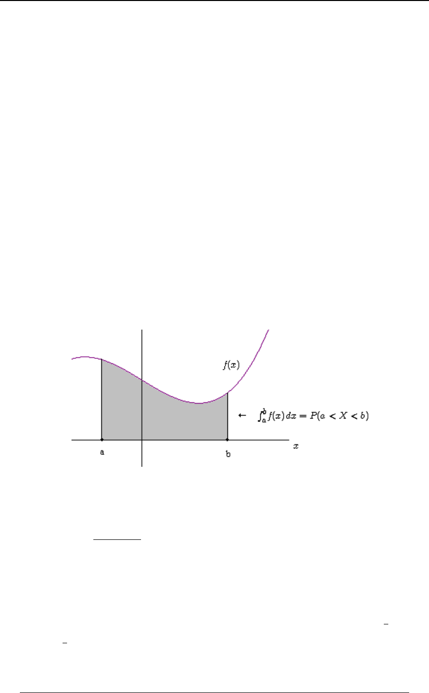
SECTION 4 - RANDOM VARIABLES AND PROBABILITY DISTRIBUTIONS 113

Continuous random variable: A continuous random variable usually can assume numerical

values from an interval of real numbers, or perhaps the whole set of real numbers. The probability

space for the random variable is this interval. As an example, the length of time between

successive streetcar arrivals at a particular (in service) streetcar stop could be regarded as a

continuous random variable (assuming that time measurement can be made perfectly accurate).

Probability density function: A continuous random variable has a \probability density

function pdf ( ) usually denoted or , which is a continuous function except possibly at0ÐBÑ 0 ÐBÑ

a finite number of points. Probabilities related to are found by integrating the density function\

over an interval. The probability that is in the interval is\Ð+ß,Ñ

TÒ\−Ð+ß,ÑÓœTÒ+\,Ó 0ÐBÑ.B , which is defined to be equal to '+

, (probability

on an interval for a continuous random variable is the area under the density curve on that

interval) . Note that for a continuous random variable for any individual point ,TÒ\ œ -Ó œ ! -

since . For a continuous random variable there can only beTÒ\ œ -Ó œ 0ÐBÑ.B œ !

probability over an interval, not at a single point.

Note that for a continuous random variable , the following are all equal:\

, , , .TÐ+  \  ,Ñ TÐ+  \ Ÿ ,Ñ TÐ+ Ÿ \  ,Ñ TÐ+ Ÿ \ Ÿ ,Ñ

This is true since the probability at a single point is 0, so it doesn't matter whether or not we

include the endpoints and or not.+,

For a discrete random variable, probabilities are calculated as the sum of probabilities at

individual points, so is does matter whether not an endpoint of an interval is included. For

instance, for a fair die toss for which denotes the outcome of the toss,, , but\TÐ\Ÿ$Ñœ

TÐ\  $Ñ œ #

' .

The pdf must satisfy (i) for all , and (ii) 0ÐBÑ 0ÐBÑ  ! B 0ÐBÑ.B œ "

'∞

∞.

114 SECTION 4 - RANDOM VARIABLES AND PROBABILITY DISTRIBUTIONS

Condition (ii) can be restated by saying that the integral of over the probability space0ÐBÑ

must be 1. Often, the region of non-zero density (the probability space of ) is a finite interval, \

and outside that interval. If is continuous except at a finite number of points,0ÐBÑ œ ! 0ÐBÑ

then probabilities are defined and calculated as if was continuous everywhere (the0ÐBÑ

discontinuities are ignored).

Example 4-1: Suppose that has density function .\0ÐBÑœ

š#B !B"

for

, elsewhere

(i) Show that satisfies the requirements for being a density function.0

(ii) Find .TÒÞ#\Þ&Ó

(iii) Find .T ÒÞ#  \  Þ&l\  Þ#&Ó

Solution: (i) satisfies the requirements for a density function, since for all and00ÐBÑ!B

∞ !

∞"

0ÐBÑ.B œ #B.B œ ".

(ii) . Note that this is equal to T ÒÞ#  \  Þ&Ó œ #B .B œ B œ Þ#" T ÐÞ# Ÿ \ Ÿ Þ&ÑÞ

'¹

Þ#

Þ& #

Þ#

Þ&

(iii) T ÒÞ#  \  Þ&l\  Þ#&Ó œ T ÒÐÞ#\Þ&Ñ∩Ð\Þ#&ÑÓ

T Ò\Þ#&Ó

. œœœœÞ#

T ÒÞ#&\Þ&Ó

T Ò\Þ#&Ó Þ*$(&

#B .B

Þ")(&

'Þ#&

Þ&

Þ#&

"

Example 4-2: Y has the pdf for .0ÐCÑ œ C  !

#!ß!!!

Ð"!!CÑ$

(i) Show that satisfies the requirements for being a density function.0

(ii) Find if .TÐ]  >Ñ >  !

(iii) Find if .TÐ]>Cl]>Ñ >!

Solution: (i) ,

'¹

∞

Cœ!

Cœ∞

#!ß!!! #!ß!!!

Ð"!!CÑ # #Ð"!! Ñ

#!ß!!!Ð"!!CÑ

#

.C œ œ  !  œ "

and for all .0ÐCÑ  ! C

(ii) TÐ]  >Ñ œ .C œ œ ! œ Ð Ñ

'¹

∞#!ß!!!Ð"!!CÑ

# Cœ>

Cœ∞ #

#!ß!!! #!ß!!!

Ð"!!CÑ #Ð"!!>Ñ "!!>

"!!

#

(iii) . TÐ]>Cl]>Ñœ œ œÐ Ñ

TÐ]>CÑ

T Ð] >Ñ Ð"!!>CÑ Ð"!!>Ñ "!!>C

"!ß!!! "!ß!!! "!!>

‚#

SECTION 4 - RANDOM VARIABLES AND PROBABILITY DISTRIBUTIONS 115

Mixed distribution: A random variable may have some points with non-zero probability mass

combined with a continuous pdf on one or more intervals. Such a random variable is said to have

a . The probability space is a combination of the set of discrete points ofmixed distribution

probability for the discrete part of the random variable along with the intervals of density for the

continuous part. The sum of the probabilities at the discrete points of probability plus the integral

of the density function on the continuous region for is the total probability for , and this must\\

be 1. For example, suppose that has probability of at , and is a continuous random\Þ&\œ!\

variable on the interval with density function for , and has noÐ!ß "Ñ 0ÐBÑ œ B !  B  " \

density or probability elsewhere. This satisfies the requirements for a random variable since the

total probability over the probability space is

TÒ\œ!Ó0ÐBÑ.BœÞ&B.BœÞ&Þ&œ"

"" .

Then, andT Ò!  \  Þ&Ó œ B .B œ Þ"#&ß

Þ&

T Ò! Ÿ \  Þ&Ó œ T Ò\ œ !Ó  T Ò!  \  Þ&Ó œ Þ&  Þ"#& œ Þ'#&

(since is a discrete point of probability, we must include that probability in any interval\œ!

that includes ).\œ!

Cumulative distribution function (and survival function): Given a random variable ,\

the cumulative distribution function of (also called the , or ) is\distribution function cdf

JÐBÑœTÒ\ŸBÓ (also denoted ). is the cumulative probability to the left of (andJ ÐBÑ J ÐBÑ

including) the point . The is the complement of the distribution function,Bsurvival function

WÐBÑ œ "  J ÐBÑ œ T Ò\  BÓ . The event is referred to as a "tail" (or right tail) of\B

the distribution.

For a discrete random variable with probability function , , and:ÐBÑ JÐBÑœ :ÐAÑ



AŸB

in this case is a "step function", it has a jump (or step increase) at each point with non-zeroJÐBÑ

probability, while remaining constant until the next jump.

If has a continuous distribution with density function , then \0ÐBÑ JÐBÑ œ 0Ð>Ñ.>

'∞

and is a continuous, differentiable, non-decreasing function such thatJÐBÑ

.B J ÐBÑ œ J ÐBÑ œ  W ÐBÑ œ 0ÐBÑ

ww . If has a mixed distribution, then is\JÐBÑ

continuous except at the points of non-zero probability mass, where will have a jump.JÐBÑ

For any cdf .TÒ+ \ Ÿ,ÓœJÐ,ÑJÐ+Ñ ßJÐBÑœ"ß JÐBÑœ!lim lim

BÄ∞ BÄ∞

116 SECTION 4 - RANDOM VARIABLES AND PROBABILITY DISTRIBUTIONS

Examples of probability, density and distribution functions:

Example 4-3: Discrete Random Variable on a Finite Number of Points (finite support)

[œ [number turning up when tossing one fair die, so has probability function

:ÐAÑœ: ÐAÑ œTÒ[ œ AÓ œ Aœ"ß#ß$ß%ß&ß'

'for .

J ÐAÑœTÒ[ ŸAÓœ

!A"

"Î' " Ÿ A  #

#Î' # Ÿ A  $

$Î' $ Ÿ A  %

%Î' % Ÿ A  &

&Î' & Ÿ A  '

"A'

[ if

The graph of the cdf (cumulative distribution function) is a step-function that increases at each

point of probability by the amount of probability at that point (all 6 points have probability in

this example). Since the support of is finite (the "support" is the region of non-zero[

probability; for that is the set of integers from 1 to 6), reaches 1 at the largest point[JÐAÑ

[

[œ' A' (and stays at 1 for all ).



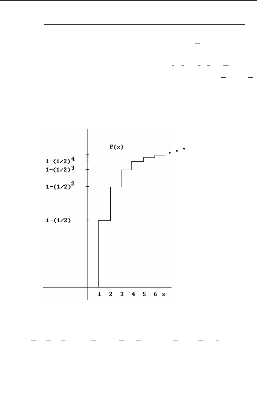
SECTION 4 - RANDOM VARIABLES AND PROBABILITY DISTRIBUTIONS 117

Example 4-4: Discrete Random Variable on an Infinite Number of Points (infinite support)

\œnumber of successive independent tosses of a fair coin until the first head turns up.

\ \:ÐBÑœ can be any integer 1, and the probability function of is , since

TÒ BÓ œ TÒ X ∩ X ∩â∩ B"X ∩ BL Ófirst head on toss (toss 1, ) (toss 2, ) (toss , ) (toss , )

œTÒ XÓ†TÒ XÓâTÒ B"XÓ†TÒ BLÓœÐ ÑÐ ÑâÐ ÑÐ Ñœtoss 1, toss 2, toss , toss , .

"" "" "

## ## #

The cdf is J ÐBÑœTÒ\ŸBÓœTÒ\œ"ÓTÒ\œ#ÓâTÒ\œBÓœ œ"

5œ"

""

for . The graph of this cdf is a step-function that increases at each point ofB œ "ß #ß $ß ÞÞÞ

probability by the amount of probability at that point. Since the support of is infinite (the\

support in this case is the set of integers ) never reaches 1, but approaches 1 as a limit" J ÐBÑ

as . The graph of is below.Bp∞ J ÐBÑ

The probability that the first head occurs on an even numbered toss is

T Ð\ Ñ œ T Ð\ œ #ß %ß 'ß ÞÞÞÑ œ T Ð\ œ #Ñ  T Ð\ œ %Ñ  T Ð\ œ 'Ñ  â is even

.œ   âœ ‚Ò" Ð Ñ âÓœ Ò" Óœ

""" " " " " " "

## ### ##$

#' ### ##

%#‚

The probability that the first head occurs on, or after the -th toss ( ) is5 5 œ"ß#ßÞÞÞ

TÐ\5ÑœTÐ\œ5ÑTÐ\œ5"ÑTÐ\œ5#Ñâ

œâœ‚Ò"âÓœ‚#œ

"" " " """ " "

## # # # #

## #

5 5" 5# 5 5 5"

#$ ,

for 5 œ "ß #ß $ß ÞÞÞ 

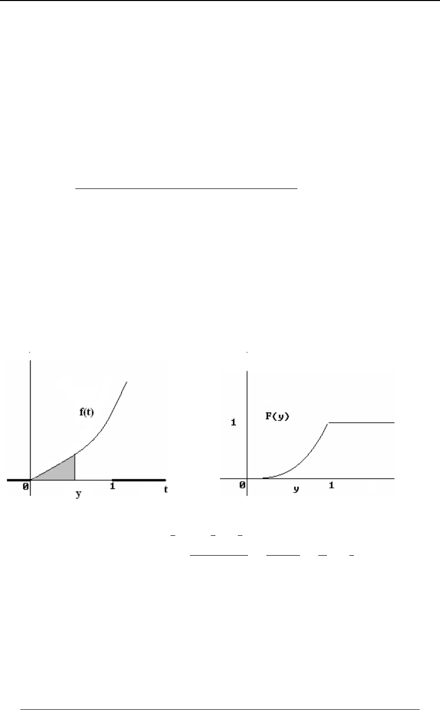
118 SECTION 4 - RANDOM VARIABLES AND PROBABILITY DISTRIBUTIONS

The typical behavior of the cdf is to tend to increase toward 1 as increases. Depending onJÐBÑ B

the nature of the random variable, may actually reach 1 at some point, as in Example 4-3, orJÐBÑ

JÐBÑ JÐBÑ might approach 1 as a limit, as in Example 4-4. For a continuous random variable, has

similar increasing behavior, but will be increasing continuously rather than in the series of steps

we have seen for a discrete random variable. will never decrease, but it may remain "flat"JÐBÑ

for a while, as can be seen in the previous two examples.

Example 4-5: Continuous Random Variable on a Finite Interval

] Ð!ß "Ñ is a continuous random variable on the interval with density function

. The cdf is if .0ÐCÑœ JÐCÑœ 0Ð>Ñ.>œ $>.>œC CŸ"

]]

∞ !

š''

$C !C"

#for

, elsewhere

Then . The graphs of and are as

J ÐCÑ œ 0 Ð>Ñ .> œ 0 ÐCÑ J ÐCÑ

!C!

C !ŸC"

"C"

]] ]]

'œ

follows. The heavy line in the graph of indicates that the density is 0 outside the interval0ÐCÑ

]

Ð!ß "Ñ. Note that the cdf increases continuously, reaching 1 at the right end of the interval for the

probability space.

Some other probabilities are , andTÐ] Ÿ ÑœJÐ Ñœ

"""

##)

for , . !ŸCŸ>Ÿ" TÐ] ŸCl] Ÿ>Ñœ œ œ œÐ Ñ

TÐ]ŸC∩]Ÿ>Ñ TÐ]ŸCÑ

TÐ]Ÿ>Ñ TÐ]Ÿ>Ñ > >

$$

SECTION 4 - RANDOM VARIABLES AND PROBABILITY DISTRIBUTIONS 119

Example 4-6: Continuous Random Variable on an Infinite Interval

YÐ!ß∞Ñ is a continuous random variable on the interval with density function.

.0Ð?Ñœ

Yš?/ ?!

!?Ÿ!

? for

for

The cdf is for J Ð?Ñ œ 0Ð>Ñ .> œ >/ .> œ  >/  / œ "  Ð"  ?Ñ/ ?  !

Y∞ !

> > > ?

>œ!

>œ?

'' ¹

Then . increases, approaching a limit of 1 as .JÐ?Ñœ JÐ?Ñ ?p∞

Yš!?Ÿ!

"Ð"?Ñ/ ?!

for

, for

?



Example 4-7: Mixed Random Variable

^ Ò!ß "Ñ ^ Þ& ^ œ ! ^ has a mixed distribution on the interval . has probability of at , and has

density function for , and has no density or probability elsewhere.0ÐDÑœD !D" ^

The cdf of is .

^JÐDÑœ

!D!

Þ& D œ !

Þ&  D !  D  "

"D"



Note that there is a jump of (probability) .5 at , and then rises continuously on .D œ ! J ÐDÑ Ð!ß "Ñ



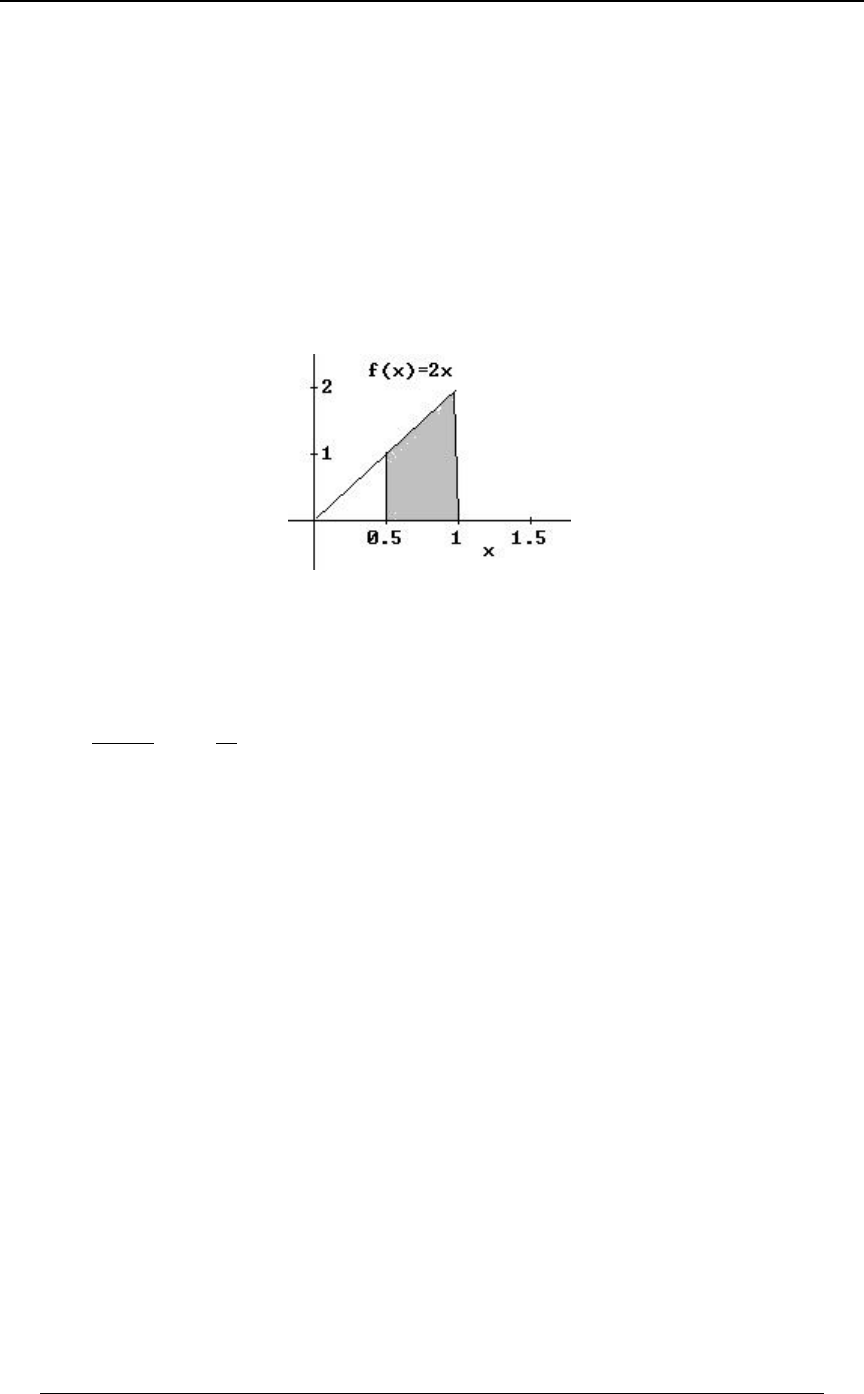
120 SECTION 4 - RANDOM VARIABLES AND PROBABILITY DISTRIBUTIONS

Some results and formulas relating to this section:

(i) For a continuous random variable ,\

TÒ+\,ÓœTÒ+Ÿ\,ÓœTÒ+\Ÿ,ÓœTÒ+Ÿ\Ÿ,Óœ 0 ÐBÑ.B

,\ ,

so that when calculating the probability for a continuous random variable on an interval, it is

irrelevant whether or not the endpoints are included. For the density function

0 ÐBÑœ TÒÞ&\Ÿ"Óœ #B.BœB œ"ÐÞ&Ñ œÞ(&

\Þ&

"##

š¹

#B !B" Bœ"

! BœÞ&

for

, otherwise , we have .

This is illustrated in the shaded area in the graph below.

Also, for a continuous random variable, , the probability at a single point is 0.TÒ\ œ +Ó œ !

Non-zero probabilities only exist over an interval, not at a single point.

(ii) For a continuous random variable, the hazard rate or failure rate is

.2ÐBÑ œ œ  68Ò"  J ÐBÑÓ

0ÐBÑ

"J ÐBÑ .B

(iii) If has a mixed distribution, then will be non-zero for some value(s) of , and\TÒ\œ>Ó >

TÒ+  \  ,Ó TÒ+ Ÿ \ Ÿ ,Ó \will not always be equal to (they will not be equal if has a non-

zero probability mass at either or ).+,

(iv) piecewise may be defined , meaning that is defined by a different algebraic0ÐBÑ 0ÐBÑ

formula on different intervals. Example 4-13 below illustrates this.

(v) Independence of random variables: A more technical definition of independence of

random variables will be given in a later section of these notes. One of the important

consequences of random variables and being independent is that\]

TÒÐ+\Ÿ,Ñ∩Ð-] Ÿ.ÑÓœTÒ+\Ÿ,Ó‚TÒ-] Ÿ.Ó .

In general, what we mean by saying that random variables and are independent is that if is\] E

any event involving only (such as ), and is any event involving only , then \ +\Ÿ, F ] E

and are independent events.F

SECTION 4 - RANDOM VARIABLES AND PROBABILITY DISTRIBUTIONS 121

(vi) Suppose that is the densityConditional distribution of given event :\E 0ÐBÑ

function or probability function of , and suppose that is an event. The conditional pdf or pf of\E

" given " is .

if is an outcome in event

if is not an outcome in event

\E0ÐBlEÑœ BE

!B E

\lE œ0ÐBÑ

TÐEÑ

For example, suppose that ,0ÐBÑœ

\š#B !B"

for

, otherwise

and suppose that is the event that .E\Ÿ

Then , and for , , andTÐEÑœTÐ\Ÿ Ñœ !BŸ 0 ÐBl\Ÿ Ñœ œ)B

"" " " #B

# % # # "Î%

\lE

for (if we are given that , then it is not possible forB ß 0 ÐBl\Ÿ Ñœ! \Ÿ

"" "

## #

\lE

B ß B

so the conditional density is 0 if ).

The conditional density must satisfy the same requirements as any probability density, it must

integrate to 1 over its probability space. This is true for the example just presented, since

"Î# "Î#

\lE

0ÐBl\ŸÑ.Bœ )B.Bœ"

Example 4-8: A die is loaded in such a way that the probability of the face with dots turning4

up is proportional to for . What is the probability, in one roll of the die, that4 4œ"ß#ß$ß%ß&ß'

an even number of dots will turn up?

Solution: Let denote the random variable representing the number of dots that appears when\

the die is rolled once. Then, for , where is theT Ò\ œ 5Ó œ V † 5 5 œ "ß #ß $ß %ß &ß ' V

proportional constant. Since the sum of all of the probabilities of points that can occur must be ,"

it follows that , so that .V†Ò"#$%&'Óœ" Vœ "

Then, even number of dots turns up . TÒ Ó œ TÒ#ÓTÒ%ÓTÒ'Ó œ œ

#%' %

#" ( 

Example 4-9: An ordinary single die is tossed repeatedly and independently until the first even

number turns up. The random variable is defined to be the number of the toss on which the\

first even number turns up. Find the probability that is an even number.\

Solution: is a discrete random variable that can take on an integer value of or more. The\"

probability function for is (this is the probability of \:ÐBÑœTÒ\œBÓœÐÑ B"

successive odd tosses followed by an even toss, we are using the independence of successive

tosses). Then,

TÒ\ ÓœTÒ#ÓTÒ%ÓTÒ'ÓâœÐ Ñ Ð Ñ Ð Ñ âœ œ is even .

""" "

###

ÐÑ

"Ð Ñ

#%' "

##3

122 SECTION 4 - RANDOM VARIABLES AND PROBABILITY DISTRIBUTIONS

Example 4-10: Suppose that the continuous random variable has density function\

0ÐBÑœ$%)B Þ#&ŸBŸÞ#& 0ÐBÑœ! TÒ Ÿ\Ÿ Ó

# for (and elsewhere). Find .

)"'

Solution: , since there is no density for atT ÒÞ"#& Ÿ \ Ÿ Þ$"#&Ó œ T ÒÞ"#& Ÿ \ Ÿ Þ#&Ó \

points greater than . The probability is . Þ#& Ð$  %)B Ñ .B œ

'Þ"#&

Þ#& #&

$# 

Example 4-11: Suppose that the continuous random variable has the cumulative distribution\

function for . Find 's density function.JÐBÑ œ ∞  B  ∞ \

"/B

Solution: The density function for a continuous random variable is the first derivative of the

distribution function. The density function of is . \0ÐBÑœJÐBÑœ

Ð"/ Ñ

B

B # 

Example 4-12: \ TÒ\ŸBÓœ"/ B" is a random variable for which for , and

B

TÒ\ Ÿ BÓ œ ! B  "for . Which of the following statements is true?

A) and TÒ\ œ #Ó œ "/ TÒ\ œ "Ó œ "/

# "

B) and TÒ\ œ #Ó œ "/ TÒ\ Ÿ "Ó œ "/

# "

C) and TÒ\ œ #Ó œ "/ TÒ\  "Ó œ "/

# "

D) and TÒ\  #Ó œ "/ TÒ\  "Ó œ "/

# "

E) and TÒ\  #Ó œ "/ TÒ\ œ "Ó œ "/

# "

Solution: Since for , it follows that .TÒ\ŸBÓœ"/ B" TÒ\Ÿ"Óœ"/

B "

But if , and thus , so that TÒ\ŸBÓœ! B" TÒ\"Óœ! TÒ\œ"Óœ"/

"

(since ). This eliminates answers C and D. SinceTÒ\Ÿ"ÓœTÒ\"ÓTÒ\œ"Ó

the distribution function for is continuous (and differentiable) for , it follows that\B"

TÒ\ œ BÓ œ ! B  "for . This eliminates answers A, B and C. This is an example of a random

variable with a mixed distribution, a point of probability at , with\\œ"

TÐ\œ"Ñœ"/ \" 0ÐBÑœ/ B"

" B

, and a continuous distribution for with pdf for .

Answer: E 

SECTION 4 - RANDOM VARIABLES AND PROBABILITY DISTRIBUTIONS 123

Example 4-13: A continuous random variable has the density function\

0ÐBÑ œ T ÒÞ#&  \ Ÿ "Þ#&Ó

#B !  B 

ŸB#

!ß

elsewhere

. Find .

%#B

Solution: .T ÒÞ#&  \ Ÿ "Þ#&Ó œ 0ÐBÑ .B œ #B .B  .B œ

'''

Þ#& Þ#& Þ&

"Þ#& Þ& "Þ#& %#B

Note that since is a continuous random variable, the probability \ T ÒÞ#& Ÿ \  "Þ#&Ó

would be the same as . This is an example of a density function definedT ÒÞ#&  \ Ÿ "Þ#&Ó

piecewise. The only consequence of this is that in finding a probability for an interval that

contains the point , we must set up two integrals, one integral ending at right hand limit , and

" "

# #

the other integral starting at left hand limit .

Also, note that if the density function was defined to be

1ÐBÑ œ

#B !  B 

! B œ "Î#

BŸ#

œ"

%#B "

( density at ), then all probabilities are unchanged (since the two density functions and! B œ "Î# 0

1 differ at only one point, probability calculations, which are based on integrals of the density

function over an interval, are the same for both and ). 01

Example 4-14: The density function for the continuous random variable isY

0 Ð?Ñ œ T ÒY Ÿ #lY  "Ó

Yš/?!

!?Ÿ!

? for

, for . Find the probability .

Solution: TÒYŸ#lY"Óœ œ

T ÒÐY Ÿ#Ñ∩ÐY "ÑÓ T Ò"Y Ÿ#Ó

TÒY"Ó TÒY"Ó .

TÒ"  Y Ÿ #Ó œ / .? œ / / TÒY  "Ó œ / .? œ /

#∞

? " # ? "

, .

TÒYŸ#lY"Óœ œ"/

//

" #

" " . 

Example 4-15: An ordinary single die is tossed repeatedly until the first even number turns up.

The random variable is defined to be the number of the toss on which the first even number\

turns up. We define the following two events: is even , is a multiple of 3 .Eœ\ Fœ\

Determine whether or not events and are independent.EF

Solution: This is the same distribution as in Example 4-9. is a discrete random variable that\

can take on an integer value of or more. The probability function for is "\

.:ÐBÑœTÒ\œBÓœÐ Ñ

Then, or or . . . ,TÒEÓœTÒ\œ# % ' ÓœÐ Ñ Ð Ñ Ð Ñ âœÐ Ñ †Ò Óœ

""" " " "

### # $

"Ð Ñ

#%' #"

and or or . . . .TÒFÓœTÒ\œ$ ' * ÓœÐ Ñ Ð Ñ Ð Ñ âœÐ Ñ †Ò Óœ

""" " " "

### # (

"Ð Ñ

$'* $"

E∩Fœ\ ' is a multiple of (multiple of 2 and of 3).

124 SECTION 4 - RANDOM VARIABLES AND PROBABILITY DISTRIBUTIONS

Example 4-15 continued

Then or or . . .TÒE∩FÓœTÒ\œ' "# ") Ó

.œÐÑÐÑ ÐÑ âœÐÑ†Ò Óœ

"" " " " "

## # # '$

"Ð Ñ

'"#") '"

We note that , and therefore, and are notTÒE∩FÓ œ Á † œ TÒEÓ†TÒFÓ E F

"""

'$ $ (

independent. 

Example 4-16: A random sample of 4 independent random variables is\ß\ß\ß\

"#$%

obtained. Each of the 's has a density function of the form .\0ÐBÑœ

3š#B !B"

for

, elsewhere

We define the following two random variables:

]œ7+BÖ\ß\ß\ß\× ^œ738Ö\ß\ß\ß\×

"#$% "#$%

and .

Find the density functions of and .]^

Solution: For we first find the distribution function.]

TÒ] ŸCÓœTÒ7+BÖ\ ß\ ß\ ß\ ×ŸCÓ

"#$%

œTÒÐ\ŸCÑ∩Ð\ŸCÑ∩Ð\ŸCÑ∩Ð\ŸCÑÓ

"#$%

œTÒ\ ŸCÓ†TÒ\ ŸCÓ†TÒ\ ŸCÓ†TÒ\ ŸCÓœÐC ÑÐC ÑÐC ÑÐC ÑœC !C"Þ

"#$%

#### )

(We use the cdf of , .)\ TÒ\ŸCÓœ #B.BœC

Thus, .J ÐCÑœTÒ] ŸCÓœC p0 ÐCÑœJ ÐCÑœ)C ß !C"

]]

)w(

]

For we find the survival function (complement of the distribution function).^

TÒ^ DÓœTÒ738Ö\ ß\ ß\ ß\ ×DÓ

"#$%

œTÒÐ\DÑ∩Ð\DÑ∩Ð\DÑ∩Ð\DÑÓ

"#$%

œTÒ\ DÓ†TÒ\ DÓ†TÒ\ DÓ†TÒ\ DÓœÐ"D Ñ ß!D"

"#$% #%

Then , andJ ÐDÑœTÒ^ŸDÓœ"TÒ^DÓœ"Ð"D Ñ ß!D"

^#%

0 ÐDÑ œ J ÐDÑ œ %Ð"  D Ñ Ð#DÑ œ )DÐ"  D Ñ !  D  "

w#$ #$

, .

]^ and are examples of order statistics on a collection of independent random variables. A little

later we will consider order statistics in more detail. 

SECTION 4 - RANDOM VARIABLES AND PROBABILITY DISTRIBUTIONS 125

Example 4-17: Example 4-4 considers the random variable

\œnumber of successive independent tosses of a fair coin until the first head turns up.

\ \:ÐBÑœTÒ\œBÓœ can be any integer 1, and the probability function of is ,

for B œ "ß #ß $ß ÞÞÞ

(a) Find the probability function of the conditional distribution of given that the first head\

occurs on an odd numbered toss. Find the probability that the first head occurs within the first 3

tosses given that the first head occurs on an odd numbered toss.

(b) Find the probability function of the conditional distribution of given that the first head\

occurs within the first 5 tosses. Find the probability that the first head occurs within the first 3

tosses given that the first head occurs within the first 5 tosses.

Solution: (a) is the event that the first head occurs on an odd numbered toss.E

TÐEÑœTÒ\œ"ÓTÒ\œ$Óâœ    â

""""

####

$&(

œ†Ò" ÐÑÐÑâÓœ† œ

"""" ""#

#### # $

"Ð Ñ

## # "

#$ .

Then is odd if is odd,:ÐBl\ Ñœ œ œ† B

\lE

:ÐBÑ

TÐEÑ # #

ÐÑ $"

and is odd if is even. Then:ÐBl\ Ñœ! B

\lE

T Ò\ Ÿ $l\ Ó œ : Ð"l\ Ñ  : Ð#l\ Ñ  : Ð$l\ Ñ is odd is odd is odd is odd

\lE \lE \lE

œ †  !  † œ Þ*$(&

$" $ "

## ##

$ .

Note that we can also find is odd using the definition of conditional probability;TÒ\ Ÿ $l\ Ó

TÒ\ Ÿ $l\ Ó œ œ œ †  † is odd .

T Ò\Ÿ$∩\ Ó T Ò\œ"ÓT Ò\œ$Ó

TÒ\ Ó #Î$ ## ##

$" $ "

is odd

is odd $

(b) is the event that the first head occurs within the first 5 tosses.F

TÐFÑœTÒ\Ÿ&ÓœœÞ

"""""$"

## # # $#

#$ &

: ÐBl\ Ÿ&Ñœ Bœ"ß#ß$ß%ß& : ÐBl\ Ÿ &Ñ œ! B&

\lF \lF

ÐÑ

$# if , and if .

T Ò\ Ÿ $l\ Ÿ &Ó œ : Ð"l\ Ÿ &Ñ  : Ð#l\ Ÿ &Ñ  : Ð$l\ Ÿ &Ñ

\lF \lF \lF

œ†††œÞ*!$

$# " $# " $# "

$" # $" # $" #

Alternatively,

T Ò\ Ÿ $l\ Ÿ &Ó œ œ œ œ Þ*!$

T Ò\Ÿ$∩\Ÿ&Ó T Ò\œ"ÓT Ò\œ#ÓT Ò\œ$Ó

TÒ\Ÿ&Ó TÒ\Ÿ&Ó



"" "

###

. 

126 SECTION 4 - RANDOM VARIABLES AND PROBABILITY DISTRIBUTIONS

Example 4-18: Bob just read a news report that suggested that one-quarter of all cars on the

road are imports, and the rest are domestic. Bob decides to test this suggestion by watching the

cars go by his house. Bob assumes that each successive car that goes by has a chance of being

an import and a chance of being domestic. Bob knows cars, and he can tell the difference

between imports and domestic cars. If Bob's assumption is correct, find the probability that Bob

will see at least 2 imports pass his house before the 3rd domestic car passes his house.

Solution: As soon as the 4th car passes his house, Bob will know whether or not at least

2 imports passed before the third domestic. If 2, 3 or 4 of the first 4 cars are imports, then

the 2nd import passed his house before the 3rd domestic. If 0 or 1 of the first 4 cars are

imports then the 3rd domestic passed his house before the 2nd import.

The probability of 2 of the first 4 cars being imports is the probability of any one of the

following 6 successions of 4 cars occurring:

MMHHß MHMHß MHHM ß HMMH ß HMHM ß HHMM .

Each one of those has a chance of occurring, for a total probability ofÐÑÐÑ

'‚ œ

*#(

#&' "#) .

The probability of 3 of the first 4 cars being imports is the probability of any one of the

following 4 successions of 4 cars occurring: .MMMHß MMHM ß MHMM ß HMMM

Each one of those has a chance of occurring, for a total probability ofÐÑÐÑ

%‚ œ

#&' '% .

The probability that all 4 of the first 4 cars being imports is .ÐÑœ

% #&'

Therefore, the overall total probability of at least 2 imports passing Bob's house before the

3rd domestic car passes his house is .

#( $ " '(

"#) '% #&' #&'

 œ 

PROBLEM SET 4 127

PROBLEM SET 4

Random Variables and Probability Distributions

1. Let be a discrete random variable with probability function\

TÒ\ œBÓœ Bœ"ß#ß$ßÞÞÞ \

$B for What is the probability that is even?

A) B) C) D) E)

"#"#$

%($$%

2. (SOA) In modeling the number of claims filed by an individual under an automobile policy

during a three-year period, an actuary makes the simplifying assumption that for all integers

8! : œ : : 8 , , where represents the probability that the policyholder files claims

8" 8 8

during the period. Under this assumption, what is the probability that a policyholder files more

than one claim during the period?

A) 0.04 B) 0.16 C) 0.20 D) 0.80 E) 0.96

3. Let be a continuous random variable with density function\

0ÐBÑ œ TÒl\  l  Ó

š'BÐ"BÑ !B"

for

otherwise . Calculate .

A) B) C) D) E) Þ!&#" Þ"&'$ Þ$"#& Þ&!!! Þ)!!!

4. Let be a random variable with distribution function\

JÐBÑœ TÒ"Ÿ\Ÿ#Ó

!B!

!ŸB"

"ŸB#

#ŸB$

"B$



for

. Calculate .

)

%"#



A) B) C) D) E)

)

$ ( "$ "*

)"'#%#%

5. (SOA) In a small metropolitan area, annual losses due to storm, fire, and theft are

independently distributed random variables. The pdf's are:

Storm Fire Theft

0ÐBÑ /B #/ &/

$"#

#BÎ$ &BÎ"#

Determine the probability that the maximum of these losses exceeds 3 .

A) 0.002 B) 0.050 C) 0.159 D) 0.287 E) 0.414

128 PROBLEM SET 4

6. Let and be three independent, identically distributed random variables each with\ß\ \

"# $

density function . Let . Find .0ÐBÑœ ] œ7+BÖ\ ß\ ß\ × TÒ]  Ó

š$B !ŸBŸ"

# for

otherwise "#$ "

A) B) C) D) E)

" $( $%$ ( &""

'% '% &"# ) &"#

7. Let the distribution function of for be .\ B! JÐBÑœ"

5œ!

$B/

5B

What is the density function of for ?\B!

A) B) C) D) E)///

B B B

B/ B/ B/ B/

#'' '

#B $B $B $B

8. Let have the density function for , and , otherwise. If\0ÐBÑœ!B0ÐBÑœ!

$B#

))

TÒ\  "Ó œ (

) , find the value of .)

A) B) C) D) E)

"( )

#) (

ÐÑ ÐÑ # #

"Î$ "Î$ "Î$

9. (SOA) A group insurance policy covers the medical claims of the employees of a small

company. The value, , of the claims made in one year is described by where YZ Z œ "!!ß !!!]

is a random variable with density function where is a

for

otherwise,

0ÐCÑ œ 5

5Ð"  CÑ !  C  "

œ%

constant. What is the conditional probability that V exceeds 40,000, given that V exceeds 10,000?

A) 0.08 B) 0.13 C) 0.17 D) 0.20 E) 0.51

10. (SOA) An insurance company insures a large number of homes. The insured value, \

of a randomly selected home is assumed to follow a distribution with density function

0ÐBÑ œ $B B  "

œ% for

otherwise.

Given that a randomly selected home is insured for at least 1.5, what is the probability that it is

insured for less than 2?

A) 0.578 B) 0.684 C) 0.704 D) 0.829 E) 0.875

PROBLEM SET 4 129

11. (SOA) Two life insurance policies, each with a death benefit of 10,000 and a one-time

premium of 500, are sold to a couple, one for each person. The policies will expire at the end of

the tenth year. The probability that only the wife will survive at least ten years is 0.025, the

probability that only the husband will survive at least ten years is 0.01, and the probability that

both of them will survive at least ten years is 0.96 What is the expected excess of premiums overÞ

claims, given that the husband survives at least ten years?

A) 350 B) 385 C) 397 D) 870 E) 897

12. and are two independent random variables, but they have the same density function\\

0ÐBÑ œ š#B !B"

for

, elsewhere . Find the probability that the maximum of and is at least .5.\\

A) .92 B) .94 C) .96 D) .98 E) 1.00

13. For two random variables, the "distance" between two distributions is defined to

be the maximum, over the range for which and are defined,7+B lJ ÐBÑ  J ÐBÑl J J

+66 B "# "#

where is the cumulative distribution function. Find the distance between the following twoJÐBÑ

distributions:

(i) uniform on the interval ,Ò!ß "Ó

(ii) pdf is for .0ÐBÑœ !B∞

ÐB"Ñ#

A) B) C) D) E) 1!""$

%#%

14. A family health insurance policy pays the total of the first three claims in a year. If there is

one claim during the year, the amount claimed is uniformly distributed between 100 and 500. If

there are two claims in the year, the total amount claimed is uniformly distributed between 200

and 1000, and if there are three claims in the year, the total amount claimed is uniformly

distributed between 500 and 2000. The probabilities of 0, 1, 2 and 3 claims in the year are

Þ& ß Þ$ ß Þ" ß Þ" respectively. Find the probability that the insurer pays at least 500 in total claims

for the year.

A) .10 B) .12 C) .14 D) .16 E) .18

130 PROBLEM SET 4

15. (SOA) The loss due to a fire in a commercial building is modeled by a random variable \

with density function

0ÐBÑ œ !Þ!!&Ð#!BÑ !  B  #!

œfor

otherwise.

Given that a fire loss exceeds 8, what is the probability that it exceeds 16?

A) B) C) D) E)

598 37

3""""

16. (SOA) The lifetime of a machine part has a continuous distribution on the interval Ð! ß %!Ñ

with probability density function , where is proportional to .00ÐBÑ Ð"!BÑ

#

Calculate the probability that the lifetime of the machine part is less than 6.

A) 0.04 B) 0.15 C) 0.47 D) 0.53 E) 0.94

17. \0ÐBÑœ-/ßB" is a continuous random variable with density function .

B

Find .TÒ\$l\#Ó

A) B) C) D) E) "/ / "/ / / / /

" " # " # # $

PROBLEM SET 4 131

PROBLEM SET 4 SOLUTIONS

1. is evenTÒ\ ÓœTÒ\œ#ÓTÒ\œ%ÓTÒ\œ'Óâ

. Answer: Aœ†ÒâÓœ† œ

#" " " # " "

$$ $ $ $ %

"

$& # "

2. A requirement for a valid distribution is .



5œ!

∞

:œ"

Since , it follows that:œ : œ † : œ † â:œÐÑ:

88" 8# ! !

"""""""

&&&&&&&

"œ :œ ÐÑ:œ:† :œ



5œ! 5œ!

∞∞

5!! !

"" %

""

(infinite geometric series) so that

and . Then,:œÐÑÐÑ

TÒR "Óœ"TÒRœ! "Óœ": : œ" Ð ÑÐ Ñœ Þ or Answer: A

!" %"% "

&&& #&

3. TÒ \ Ÿ ÓœTÒ Ÿ\ Ÿ ÓœTÒ Ÿ\Ÿ Óœ 'BÐ"BÑ.B

¹¹ '

"" " "" " $

#% % #% % % "Î%

$Î%

. Answer: Cœ Þ')(& p T Ò \   Ó œ "  T Ò \  Ÿ Ó œ Þ$"#&

¹¹ ¹¹

"" ""

#% #%

4. TÒ"Ÿ\Ÿ#ÓœTÒ\Ÿ#ÓTÒ\"ÓœJÐ#Ñ JÐBÑœ  œ Þlim

BÄ"

"" " "*

"# ) #%

Answer: E

5. .TÒ7+BÖWßJßX×  $Ó œ "TÒ7+BÖWßJßXß× Ÿ $Ó

T Ò7+BÖWß J ß X ß × Ÿ $Ó œ T ÒÐW Ÿ $Ñ ∩ ÐJ Ÿ $Ñ ∩ ÐX Ÿ $ÑÓ

œTÒWŸ$Ó†TÒJ Ÿ$Ó†TÒX Ÿ$Ó

œ Ð"  / ÑÐ"  / ÑÐ"  / Ñ œ Þ&)'

$Î" $Î"Þ& $Î#Þ% .

T Ò7+BÖWß J ß X ×  $Ó œ "  Þ&)' œ Þ%"% . Answer: E

6. TÒ]  Ó œ "TÒ] Ÿ Ó œ "TÒÐ\ Ÿ Ñ∩Ð\ Ÿ Ñ∩Ð\ Ÿ ÑÓ

" " """

# # ###

"#$

œ"ÐTÒ\Ÿ ÓÑ œ"Ò $B .BÓ œ"Ð Ñ œ Þ

" " &""

# ) &"#

$#$$

"Î#

' Answer: E

132 PROBLEM SET 4

7. 0ÐBÑ œ J ÐBÑ œ  œ / †

wB

5œ! 5œ!



’“

5B / B / B 5B

5x 5x

5" B 5 B 5 5"

œ/ †Ò"   Óœ Þ

B B" B #B B $B / B

"# ' '

#$#B$

Answer: C

8. Since if , and since , we must conclude that .0ÐBÑ œ ! B  TÒ\  "Ó œ  "))

(

)

Then, , or equivalently, .TÒ\"Óœ 0ÐBÑ.Bœ .Bœ" œ œ#

))

$B " (

)

)) )

Answer: E

9. In order for to be a properly defined density function it must be true that0ÐCÑ

0ÐCÑ.Cœ 5Ð"CÑ .Cœ"p5†Ð Ñœ"p5œ&

& .

We wish to find the conditional probability .T Ò"!!ß !!!]  %!ß !!!l"!!ß !!!]  "!ß !!!Ó

For events and , the definition of the conditional probability EF TÒElFÓ

is . With andT ÒElFÓ œ E œ "!!ß !!!]  %!ß !!!

TÒE∩FÓ

TÒFÓ

F œ "!!ß !!!]  "!ß !!! E ∩ F œ E , we have , and,

T Ò"!!ß !!!]  %!ß !!!l"!!ß !!!]  "!ß !!!Ó œ Þ

T Ò"!!ß!!!] %!ß!!!Ó

T Ò"!!ß!!!] "!ß!!!Ó

From the density function for we have]

T Ò"!!ß !!!]  %!ß !!!Ó œ T Ò]  Þ%Ó œ 0ÐCÑ .C œ &Ð"  CÑ .C œ ÐÞ'Ñ

Þ% Þ%

, and

T Ò"!!ß !!!]  "!ß !!!Ó œ T Ò]  Þ"Ó œ 0ÐCÑ .C œ &Ð"  CÑ .C œ ÐÞ*Ñ

Þ" Þ"

The conditional probability in question is . Answer: B

ÐÞ'Ñ

ÐÞ*Ñ

&œ Þ"$#

10. We are asked to find a conditional probability .T Ò\  #l\  "Þ&Ó

The definition of conditional probability is TÒElFÓ œ Þ

TÒE∩FÓ

TÒFÓ

Then, T Ò\  #l\  "Þ&Ó œ Þ

T Ò"Þ&Ÿ\#Ó

T Ò\"Þ&Ó

From the given density function of we get\

T Ò\  "Þ&Ó œ $B .B œ œ Þ#*'$!

'"Þ&

∞% "

Ð"Þ&Ñ$ and

T Ò"Þ& Ÿ \  #Ó œ $B .B œ  œ Þ"("$!

'"Þ&

#% ""

Ð"Þ&Ñ Ð#Ñ

$$ .

Then, . Answer: AT Ò\  #l\  "Þ&Ó œ œ œ Þ&()

T Ò"Þ&Ÿ\#Ó

T Ò\"Þ&Ó Þ#*'$!

Þ"("$!

PROBLEM SET 4 133

11. is the event that the wife will survive at least 10 years, and is the event that the[L

husband will survive at least 10 years. We are given , ,T Ò[ ∩ L Ó œ Þ!#& T Ò[ ∩ LÓ œ Þ!"

and . Given that the husband survives at least 10 years, the probability that theTÒ[ ∩LÓ œ Þ*'

wife survives at least 10 years is , and the probability that theTÒ[lLÓ œ œ

TÒ[∩LÓ

TÒLÓ TÒLÓ

Þ*'

wife does not survive at least 10 years is TÒ[lLÓ œ œ Þ

TÒ[∩LÓ



TÒLÓ TÒLÓ

Þ!"

We can find , or use the tableTÒLÓœTÒ[∩LÓTÒ[∩LÓœÞ*'Þ!"œÞ*(



[[

T ÒLÓ É T Ò[ ∩ LÓ œ Þ*'  T Ò[ ∩ LÓ œ Þ!" w

œÞ*( given given

Given that the husband survives 10 years, the claim will either be 0 if the wife survives 10 years,

and 10,000 if the wife does not survive 10 years.

The expected amount of claim given that the husband survives 10 years is

Ð!Ñ † T Ò[ lLÓ  Ð"!ß !!!!Ñ † T Ò[ lLÓ œ "!ß !!! † œ "!$Þ!*

"

*( .

The total premium is 1,000 (for the two insurance policies), so that the excess premium over

expected claim is . Answer: E"!!!  "!$Þ!* œ )*(

12. TÒ7+BÖ\ ß\ ×Þ&Óœ"TÒÐ\ Þ&Ñ∩Ð\ Þ&ÑÓ

"# " #

œ"TÒ\ Þ&Ó†TÒ\ Þ&Ó

T Ò\  Þ&Ó œ 0ÐBÑ .B œ #B .B œ Þ#& T Ò\  Þ&Ó œ Þ#&

Þ& Þ&

'' , and also.

Then . Answer: BT Ò7+BÖ\ ß \ ×  Þ&Ó œ "  ÐÞ#&ÑÐÞ#&Ñ œ Þ*$(&

13. for , and for .JÐBÑœB !ŸBŸ" J ÐBÑœ" B"

JÐBÑœ .>œ" B!

'""

Ð>"Ñ B"

# for .

For , , which is maximized at either! Ÿ B Ÿ " lJ ÐBÑ  J ÐBÑl œ lB   "l

"# "

B"

Bœ!ß" " œ! Bœ! or a critical point; critical points occur where , or .

ÐB"Ñ#

lJ Ð!Ñ  J Ð!Ñl œ ! ß lJ Ð"Ñ  J Ð"Ñl œ

"# "#

For , , which decreases.B  " lJ ÐBÑ  J ÐBÑl œ l"   "l œ

"# ""

B" B"

The distance between the two distributions is . Answer: C

134 PROBLEM SET 4

14. total claims for the year, number of claims for the year .Xœ Rœ

T ÒX  &!!Ó œ T ÒÐX  &!!Ñ ∩ ÐR œ 5ÑÓ



5œ!

œ T ÒÐX  &!!Ñ ∩ ÐR œ #ÑÓ  T ÒÐX  &!!Ñ ∩ ÐR œ $ÑÓ

(this is true since if there are 0 or 1 claim, then total must be 500).Ÿ

T ÒÐX  &!!Ñ ∩ ÐR œ #ÑÓ œ T ÒX  &!!lR œ #Ó † T ÒR œ #Ó œ † ÐÞ"Ñ œ Þ!'#&

"!!!&!!

"!!!#!! , and

T ÒÐX  &!!Ñ ∩ ÐR œ $ÑÓ œ T ÒX  &!!lR œ $Ó † T ÒR œ $Ó œ " † ÐÞ"Ñ œ Þ" .

Then . Answer: DT ÒX  &!!Ó œ Þ!'#&  Þ" œ Þ"'#&

15. We are asked to find the conditional probability

T Ò\  "'l\  )Ó œ T Ò\"'Ó

TÒ\)Ó .

T Ò\  )Ó œ Þ!!&Ð#!  BÑ .B œ Þ$' ß

T Ò\  "'Ó œ Þ!!&Ð#!  BÑ .B œ Þ!% Þ

'"'

T Ò\  "'l\  )Ó œ œ

Þ!% "

Þ$' * . Answer: B

16. , .0ÐBÑ œ -Ð"!  BÑ !  B  %!

#

The total probability must be 1, so that .

%! #

-Ð"!  BÑ .B œ -Ò  Ó œ "

"! &!

Therefore, and .- œ "#Þ& 0 ÐBÑ œ "#Þ&Ð"!  BÑ#

Then, .T Ò\  'Ó œ 0 ÐBÑ .B œ "#Þ&Ð"!  BÑ .B œ  "#Þ&Ð"!  BÑ œ Þ%')(&

'' ¹

'' # "

Bœ!

Bœ'

Answer: C

17. TÒ\$l\#Óœ Þ

T Ò#\$Ó

TÒ\#Ó

TÒ\  #Ó œ -/ .B œ -/ TÒ#  \  $Ó œ -/ .B œ -Ð/ / Ñß

∞$

B # B # $

TÒ\$l\#Óœ œ"/

-Ð//Ñ

# $

# " .

Note that we can find , from ;-"œ0ÐBÑ.Bœ-/.Bœ-/p-œ/

∞∞

B "

but this is not necessary for this exercise. Answer: A

SECTION 5 - EXPECTATION AND DISTRIBUTION PARAMETERS 135

SECTION 5 - EXPECTATION

AND OTHER DISTRIBUTION PARAMETERS

Expected value of a random variable:

A random variable is a numerical outcome from an experiment or from a random procedure. If it

is possible to repeat the experiment many times, the numerical outcomes will fluctuate from one

experiment to the next because of the variability inherent in the behavior of a random variable.

Although successive numerical outcomes of the random variable will fluctuate, as more and more

random outcomes are observed, the numerical average of those outcomes will tend to stabilize.

For instance, if we repeatedly toss a fair die, each successive outcome will be an integer from 1 to

6, but as the number of successive tosses gets large, if we calculate the average outcome of the8

8 tosses, it will tend toward a constant limit. This is the average value, or , or theexpected value

mean of the random variable.

For a random variable , the expected value (also called the ) is denoted , or\expectation IÒ\Ó

\ or . The mean is interpreted as the "average" of the random outcomes.

Mean of a Discrete Random Variable

For a discrete random variable, the expected value of is\

B†:ÐBÑœB †:ÐB ÑB †:ÐB Ñâ

""## , where the sum is taken over all points atB

which has non-zero probability. For instance, if is the result of one toss of a fair die, then\\

IÒ\ÓœÐ"Ñ†Ð ÑÐ#Ñ†Ð ÑâÐ'Ñ†Ð Ñœ Þ

"" "(

'' '#

The meaning of this value is that if the die

is tossed many times, then the "long-run" average of the numbers turning up is .

(

We can see this from another point of view. Suppose that we toss the die times. Then, "on8

average", we expect that there will be tosses that are 1, and the same for 2, 3, 4, 5, and 6.

Therefore, the average outcome would be the total of all the tosses, divided by , which is8

Ð ÑÐ"ÑÐ ÑÐ#ÑÐ ÑÐ$ÑÐ ÑÐ%ÑÐ ÑÐ&ÑÐ ÑÐ'Ñ

8'''#

"" "(

888888

''''''

œÐ"Ñ†Ð ÑÐ#Ñ†Ð ÑâÐ'Ñ†Ð Ñœ ,

which is the same as the formal definition of the mean.

Note that the mean of a random variable is not necessarily one of the possible outcomes for \\

( is not a possible outcome when tossing a die).

(

136 SECTION 5 - EXPECTATION AND DISTRIBUTION PARAMETERS

Mean of a Continuous Random Variable

For a continuous random variable, the expected value is .

'∞

∞B†0ÐBÑ.B

Although this integral is written with lower limit and upper limit , the interval of∞ ∞

integration is the interval of non-zero-density for . For instance, if ,\0ÐBÑœ

š#B !B"

for

, elsewhere

then . Note that even though this random variable isIÒ\Ó œ B † Ð#BÑ .B œ #B .B œ

defined on the interval , the mean is not the midpoint of that interval. This could have beenÐ!ß "Ñ

anticipated since the density is higher for values near 1 than it is for values near 0. TheBB

distribution is weighted more heavily toward 1 than 0. This can also be seen, for instance, by

noting that , and .TÒ!  \  Ó œ TÒ  \  "Ó œ

"" " $

#% # %

The expected value is the "average" over the range of values that can be, in the sense of the\

average being the "weighted center" (not necessarily the "geographic center") of the distribution.

In the case of the die toss example above, all outcomes were equally likely, so it is not surprising

that the mean was in the middle of the possible outcomes. In the continuous example in the

previous paragraph, the mean of reflected the higher density for the values close to 1.

Expectation of :2ÐBÑ If is a function, then is equal to 2 IÒ2Ð\ÑÓ 2ÐBÑ † :ÐBÑ



if is a discrete random variable, and it is equal to if is a\\

'∞

∞2ÐBÑ † 0ÐBÑ .B

continuous random variable. Suppose that . Then for the die toss example,2ÐBÑ œ B

IÒ2Ð\ÑÓ œ IÒ \Ó œ Ð "Ñ † Ð Ñ  Ð #Ñ † Ð Ñ  â  Ð 'Ñ † Ð Ñ œ "Þ)!&

ÈÈÈ È

"" "

'' '

For the continuous random variable with density function ,0ÐBÑ œ š#B !B"

for

, elsewhere

we have .IÒ2Ð\ÑÓ œ IÒ \Ó œ B † Ð#BÑ.B œ

È'È

Example 5-1: Let equal the number of tosses of a fair die until the first "1" appears.\

Find .IÒ\Ó

Solution: is a discrete random variable that can take on an integer value . The\"

probability that the first 1 appears on the -th toss is for B :ÐBÑœÐÑ ÐÑ B"

B"

( tosses that are not followed by a 1). This is the probability function of . ThenB" " \

IÒ\Óœ 5†0Ð5Ñœ 5†ÐÑ ÐÑœÐÑÒ"#ÐÑ$ÐÑâÓ



5œ" 5œ"

∞∞

5" #

&&&

'''

'' .

We use the general increasing geometric series relation ,"#<$< âœ

Ð"<Ñ#

so that . IÒ\ÓœÐ Ñ† œ'

'Ð" Ñ

'#

SECTION 5 - EXPECTATION AND DISTRIBUTION PARAMETERS 137

Example 5-1 used an identity involving an infinite increasing geometric series. It is worthwhile

knowing this identity. There are a number of ways to derive the infinite increasing geometric

series formula used in Example 5-1. For instance, from the equation

"<<<âœ

#$ "

"< , if we differentiate both sides of the equation, we get

"#<$< âœ

Ð"<Ñ# .

Example 5-2: A fair die is tossed until the first 1 appears. Let equal the number of tossesB

required, You are to receive dollars if the first appears on the -th toss.B œ "ß #ß $ß ÞÞÞ ÐÞ&Ñ " B

What is the expected amount that you will receive?

Solution: This is the same distribution as in Example 5- above, with the probability that the"

first 1 appears on the -th toss being for ( tosses that are not , followedBÐÑÐÑB"B" "

B"

by a 1), and the amount received in that case is . Then, the expected amount2ÐBÑ œ ÐÞ&ÑB

received is . IÒ2Ð\ÑÓ œ IÒÐÞ&Ñ Ó œ ÐÞ&Ñ Ð Ñ Ð Ñ œ Ð ÑÒ"  Ð Ñ  Ð Ñ  âÓ œ

\55" #

5œ"

∞

&" " & & "

' ' "# "# "# ( 

Moments of a random variable: If is an integer, the is .8" 8\IÒ\Ó-th moment of 8

If the mean of is , then the is .\IÒÐ\ÑÓ..8\-th central moment of (about the mean ).8

Example 5-3: You are given that is a constant, and the density function of is)! \

0ÐBÑ œ / B  ! ! 8 \ 8)B), for , and elsewhere. Find the -th moment of , where is a non-

negative integer (assuming that ).)!

Solution: The -th moment of is . Applying integration by8\IÒ\ÓœB†/.B

88B

∞

'))

parts, this can be written as

'''

!!!

∞∞∞

8 B 8 B 8" B 8" B

B .Ð  / Ñ œ  B /   8B / .B œ 8B / .B Þ

)) ) )

Bœ!

Bœ∞

Repeatedly applying integration by parts results in .IÒ\ Ó œ

88x

An Alternative to integration by parts is the method mentioned on page 23.

It is worthwhile noting the general form of the integral that appears in this example;

if is an integer and , then by repeated applications of integration by parts, we5! +!

have

∞5+> 5x

>/ .>œ 5" .

In this example .

∞∞

8B 8B

B/ .Bœ B/ .Bœ† œ)) )

))

8x 8x

))

8" 8 

138 SECTION 5 - EXPECTATION AND DISTRIBUTION PARAMETERS

Symmetric Distribution: If is a continuous random variable with pdf , and if is a\0ÐBÑ-

point for which for all , then is said to have a symmetric0Ð->Ñœ0Ð->Ñ >! \

distribution about the point . For such a distribution, the mean will be the point ofBœ-

symmetry, . This will be shown in more detail later in the notes, and we will review aIÒ\Ó œ -

couple of specific symmetric distributions.

Variance of :\

Let us go back to the die toss example again. We saw that the mean of , the outcome of the fair\

die toss, was . Each time the die is tossed, the actual outcome is from 1 to 6, so there will be

(

some "deviation" or distance in the outcome from the mean of . Sometimes the deviation will

(

be (for tosses that are 3 or 4), sometimes the deviation will be and sometimes it will be

"$&

###

Now suppose that we consider a modification to this die toss example in which we use a modified

die which has three sides each with 1 on them, and 3 sides each with 6 on them. The random

variable that represents the outcome of the modified die has the following probability]

distribution: , . The mean of is , but each time the modifiedTÒ] œ "Ó œ TÒ] œ 'Ó œ ]

(

die is tossed, the deviation of the outcome from the mean is always . We see that both the

original die and the modified die have the same mean, but the modified die tends to have

outcomes that have larger deviation from the mean.

In probability theory, there is a generally accepted way of measuring the derivation from the

mean that occurs in a random variable. This is called the of the random variable. Thevariance

variance of is denoted , , or . The variance is defined as follows:\ÓZ+<Ò\Ó ZÒ\ 55

(the variance is the 2nd central moment of about its mean).Z +<Ò\Ó œ IÒÐ\ Ñ Ó.\#\

It is possible to show that .Z +<Ò\Ó œ IÒ\ Ó  ÐIÒ\ÓÑ œ IÒ\ Ó 

####

This is usually the most efficient way to calculate variance.

The variance is a measure of the "dispersion" of about the mean. A large variance indicates\

significant levels of probability or density for points far from . The variance is always .IÒ\Ó  !

The variance of is equal to only if has a discrete distribution with a single point and\!\

probability at that point (not random at all)."

SECTION 5 - EXPECTATION AND DISTRIBUTION PARAMETERS 139

For the original standard die toss example, we have

IÒ\ Ó œ

#Ð" Ñ†Ð ÑÐ# Ñ†Ð ÑâÐ' Ñ†Ð Ñœ

## #

"" "*"

'' ''

, and

Z +<Ò\Ó œ IÒ\ Ó  ÐIÒ\ÓÑ œ  Ð Ñ œ

## #

*" ( $&

'# "#

For the continuous random variable with density function , we have0ÐBÑ œ š#B !B"

for

, elsewhere

IÒ\ Ó œ B † Ð#BÑ .B œ Z +<Ò\Ó œ IÒ\ Ó  ÐIÒ\ÓÑ œ  Ð Ñ œ

## # # #

'""#"

##$")

, and .

Standard deviation of :\ The standard deviation of the random variable is the square root\

of the variance, and is denoted . The of is .5\œZ+<Ò\Ó \

Ècoefficient of variation 5

Example 5-4: A continuous random variable has density function\

.0ÐBÑœ

\š"lBl lBl"

, elsewhere

The continuous random variable has density function[

.0ÐAÑœ

[šÞ&Þ#&lAl lAl#

, elsewhere

Find the mean and variance of and\[Þ

Solution: The density of is symmetric about (since , it follows that\ ! l  Bl œ lBl

0 ÐBÑ œ 0 Ð  BÑ IÒ\Ó œ !

), so that .

This can be verified directly:

IÒ\Ó œ BÐ"  lBlÑ .B œ BÐ"  BÑ .B  BÐ"  BÑ .B œ   œ !

'''

" " !

"!"

'' .

Then, Z +<Ò\Ó œ IÒ\ Ó  ÐIÒ\ÓÑ œ IÒ\ Ó œ B Ð"  lBlÑ .B

####

"

œBÐ"BÑ.BBÐ"BÑ.Bœ

" !

' .

The pdf of is also symmetric about 0 for the same reason, and has mean , or[IÒ[Óœ!

IÒ[ Ó œ BÐÞ&  Þ#&lBlÑ .B œ BÐÞ&  Þ#&BÑ .B  BÐÞ&  Þ#&BÑ .B œ   œ !

'''

# # !

#!#

$$ .

Then Z +<Ò[ Ó œ IÒ[ Ó  ÐIÒ[ ÓÑ œ IÒ[ Ó œ B ÐÞ&  Þ#&lBlÑ .B

####

#

œ B ÐÞ&  Þ#&BÑ .B  B ÐÞ&  Þ#&BÑ .B œ  œ

# !

"" #

$$ $

The graphs of the pdfs of and are in the diagram on the following page. We see that the pdf\[

of is more widely dispersed about its mean than the pdf of is, and so we would anticipate a[\

larger variance for by comparing the graphs. Comparison of pdf's to determine relative size of[

variance might not always be as straightforward as it is in

this example.

140 SECTION 5 - EXPECTATION AND DISTRIBUTION PARAMETERS

Example 5-4 continued

The graphs of the pdfs of and are in the following diagram:\[



Moment generating function of random variable :\ The moment generating function of

\ Q Ð>Ñ ß 7 Ð>Ñ ß QÐ>Ñ 7Ð>Ñ (mgf) is denoted or , and it is defined to be .

\\ QÐ>ÑœIÒ/ Ó

\>\

If is a discrete random variable then \ Q Ð>Ñ œ / :ÐBÑ

\>B

D .

If is a continuous random variable then \ Q Ð>Ñ œ / 0 ÐBÑ .B

\∞

∞>B

' .

Some important properties that moment generating functions satisfy are

(i) It is always true that . For instance, in the continuous case,QÐ!Ñœ"

QÐ!Ñœ/0ÐBÑ.Bœ0ÐBÑ.Bœ"

\∞ ∞

∞∞

!†B

(ii) The moments of can be found from the successive derivatives of .\QÐ>Ñ

QÐ!ÑœIÒ\Ó QÐ!ÑœIÒ\Ó

www#

, ßQ Ð!ÑœIÒ\Óß 68ÒQ Ð>ÑÓ

Ð8Ñ 8\

#¹>œ! œZ+<Ò\Ó .

For instance, in the continuous case,

Q Ð>Ñ œ Q Ð>Ñ œ / 0ÐBÑ .B œ / 0ÐBÑ .B œ B / 0ÐBÑ .B

w>B>B>B

\∞ ∞ ∞

∞∞ ∞

.. .

.> .> .>

'' '

, so that

Q Ð!Ñ œ B / 0 ÐBÑ .B œ B 0ÐBÑ .B œ IÒ\Ó

w!†B

∞ ∞

∞∞

'' .

(iii) The moment generating function of might not exist for all real numbers, but usually exists\

on some interval of real numbers.

SECTION 5 - EXPECTATION AND DISTRIBUTION PARAMETERS 141

Example 5-5: The pdf of is for . Find the moment generating function\0ÐBÑœ&/ B!

&B

of and use it to find the first and second moments of , and the variance of .\\\

Solution: QÐ>Ñœ / †&/ .Bœ& / .Bœ

\!!

∞∞

>B &B Ð&>ÑB

&>

(we have used the integration rule if ).

∞+>

/.>œ +!

This integration is valid if , or equivalently, if .&>! >&

Then ,

.&"

.> Ð&!Ñ &

QÐ>Ñ œQÐ!Ñœ œ œIÒ\Ó

\>œ!

¹#

and .

.#‚&#

.> Ð&!Ñ #&

QÐ>Ñ œQÐ!Ñœ œ œIÒ\Ó

\>œ!

ww #

The variance of is \ Z +<Ò\Ó œ IÒ\ Ó  ÐIÒ\ÓÑ œ Þ

#& 

Example 5-6: Find the moment generating function for each of these two random variables.

(i) outcome of a die toss, for .\ œ :ÐBÑ œ T Ò\ œ BÓ œ B œ "ß #ß $ß %ß &ß '

(ii) is a continuous random variable with density function \0ÐBÑœ

š#B !B"

for

, elsewhere .

Solution: (i) QÐ>ÑœIÒ/ Óœ / †:ÐBÑ

\>\ >B

Bœ"



œ/†/†/†/†/†/†œ/Ð Ñ

>#>$>%>&>'> >

"""""""

'''''''

/"

> .

Note that QÐ>Ñœ/†#/†$/†%/†&/†'/†

w > #> $> %> &> '>

\""""""

''''''

and . """"""(

.> ''''''#

QÐ>Ñ œQÐ!Ñœ"†

\>œ!

¹#† $† %† &† '† œ œIÒ\Ó .

Also

. """"""*"

.> '''''''

#QÐ>Ñ œQÐ!Ñœ"†

\>œ! \

ww #

¹# † $ † % † & † ' † œ œIÒ\ Ó

##### #

The variance of is .\ IÒ\ Ó  ÐIÒ\ÓÑ œ  Ð Ñ œ

## #

*" ( $&

'# "#

(ii) Q Ð>Ñ œ / † 0ÐBÑ .B œ / † #B .B œ #Ð  Ñ œ #Ð  Ñ œ Q Ð>Ñ Þ

\ \

>B >B

Bœ!

Bœ"

'' ¹

B/ / / / "

>> >>

>B >B > >

Then .QÐ>Ñœ#Ð  Ñœ#Ð Ñ

\>/ / > / #>/ #> > / #>/ #/ #

>> #> > #> > >

Note that is found as a limit, (by l'Hospital's rule).Q Ð!Ñ #Ð Ñ œ œ IÒ\Ó

\>Ä!

lim > / #>/ #/ # #

#> > >

The antiderivative of was found by integration by parts. A useful point to note is the/†#B

general antiderivative , if is a constant. This antiderivative has 'B/ .B œ 

-B B/ /

-B -B

come up from time to time on previous exams. It is much more straightforward to find andIÒ\Ó

IÒ\ Ó B † 0ÐBÑ.B œ B † #B .B œ #B .B œ B † 0ÐBÑ.B

###

!!! !

""" "

directly as and

''' '

for the random variable in part (ii). 

142 SECTION 5 - EXPECTATION AND DISTRIBUTION PARAMETERS

Example 5-7: The moment generating function of is given as for , where .\>!

α> αα

Find .Z+<Ò\Ó

Solution: . Z +<Ò\Ó œ IÒ\ Ó  ÐIÒ\ÓÑ IÒ\Ó œ Q Ð!Ñ œ

## w

αÐ>Ñ

#¹>œ!

œα ,

and .IÒ\ Ó œ œ p Z +<Ò\Ó œ  Ð Ñ œ

# #

>œ!

QÐ!Ñœ

Ð>Ñ

α$¹##""

αααα

###

Alternatively, 68 Q Ð>Ñ œ 68Ð Ñ œ 68  68Ð  >Ñ p

\α

αα> .> >

αα 68ÒQ Ð>ÑÓ œ

and so that

." . "

.> Ð >Ñ .> >œ!

## # #

68ÒQ Ð>ÑÓ œ Z +<Ò\Ó œ 68ÒQ Ð>ÑÓ œ Þ

αα

This is like Example 5-5 above, with 5 replaced by . α

Percentiles of a distribution: If , then the -th percentile of the distribution of!  :  " "!!:

\- is the number which satisfies both of the following inequalities:

and . For a continuous random variable, it is sufficient toTÒ\ Ÿ - Ó  : TÒ\  - Ó  ":

find the for which . If , - TÒ\Ÿ- Óœ: :œÞ&

the 50-th percentile of a distribution is

referred to as the median of the distribution; it is the point for which .Q T Ò\ Ÿ Q Ó œ Þ&

The median is the 50% probability point, half of the distribution probability is to the left of Q Q

and half is to the right. If has a symmetric distribution about the point , then the mean\Bœ-

and the median of will be equal to .\-

For the continuous random variable with density function ,0ÐBÑ œ š#B !B"

for

, elsewhere

the median is , where , so that . This is illustratedQ #B .B œ Q œ Þ& Q œ Þ& œ Þ(!("

'È

in the graph below. The shaded area below has probability .5, and is to the left of ,Q œ Þ(!("

the median.

SECTION 5 - EXPECTATION AND DISTRIBUTION PARAMETERS 143

Example 5-8: The continuous random variable has pdf for\0ÐBÑœ†/

#lBl

∞B∞ . Find the 87.5-th percentile of the distribution.

Solution: The 87.5-th percentile is the number for which,

Þ)(&œTÒ\Ÿ,Óœ 0ÐBÑ.Bœ †/ .B

∞ ∞

lBl

Note that this distribution is symmetric about , since , so the mean and median!0ÐBÑœ0ÐBÑ

are both . Thus, , and so!,!

''' '

∞ ∞ ! !

,!, ,

lBl lBl lBl B

""" "

### #

†/ .Bœ †/ .B †/ .BœÞ& †/ .B

œ Þ&  Ð"  / Ñ œ Þ)(& Ê , œ  68ÐÞ#&Ñ œ 68 %

#, . 

The mode of a distribution: The mode is any point at which the probability or density7

function is maximized. The mode of the distribution in the graph above is 1, since the0ÐBÑ

maximum value of occurs at .0ÐBÑ B œ "

The skewness of a distribution: If the mean of random variable is and the variance is \.5

then the skewness is defined to be . If skewness is positive, the distribution isIÒÐ\  Ñ ÓÎ.5

said to be skewed to the right, and if skewness is negative it is skewed to the left.

Some results and formulas relating to distribution moments:

(i) The mean of a random variable might not exist\, it might be or , and the∞ ∞

variance of might be . For example, the continuous random variable with\∞ \

pdf has expected value .0ÐBÑ œ B † .B œ  ∞

š'

for

, otherwise

B"

∞

(ii) For any constants and and functions and ,+ß+ , 2 2

"# " #

IÒ+ 2 Ð\Ñ  + 2 Ð\Ñ  ,Ó œ + IÒ2 Ð\ÑÓ  + IÒ2 Ð\ÑÓ  ,

"" ## " " # # .

As a special case, .IÒ+\  ,Ó œ +IÒ\Ó  ,

(iii) If is a random variable defined on the interval ) ( for ),\Ò+ß∞0ÐBÑœ!B+

then , and if is defined on the interval , whereIÒ\Óœ+ Ò"JÐBÑÓ.B \ Ò+ß,Ó

∞

,  ∞ IÒ\Ó œ +  Ò"  J ÐBÑÓ .B, then . This relationship is valid for any random

variable, discrete, continuous or with a mixed distribution. As a special, case, if is a\

non-negative random variable (defined on or ) thenÒ!ß ∞Ñ Ð!ß ∞Ñ

IÒ\Ó œ Ò"  JÐBÑÓ.B

∞

144 SECTION 5 - EXPECTATION AND DISTRIBUTION PARAMETERS

(iv) If is a function and is a random variable such thatJensen's inequality: 2\

#2ÐBÑ œ 2 ÐBÑ  ! B \

ww at all points with non-zero density or probability for ,

then , and if then The inequalityIÒ2Ð\ÑÓ  2ÐIÒ\ÓÑ 2  ! IÒ2Ð\ÑÓ  2ÐIÒ\ÓÑÞ

reverses if . For example, if , then for any , so that2 Ÿ ! 2ÐBÑ œ B 2 ÐBÑ œ #  ! B

ww # ww

IÒ\ Ó  ÐIÒ\ÓÑ Z +<Ò\Ó œ IÒ\ Ó  ÐIÒ\ÓÑ  !

## ##

(this is also true since for any random

variable ). As another example, if is a positive random variable (i.e., has non-zero\\ \

density or probability only for ), and , then for ,B  ! 2ÐBÑ œ B 2 ÐBÑ œ  ! B  !

Èww "

%B$Î#

and it follows from Jensen's inequality that .IÒ \Ó  IÒ\Ó

ÈÈ

(v) .

If and are constants, then + , Z +<Ò+\  ,Ó œ + Z +<Ò\Ó

(vi) If is a random variable with mean and standardChebyshev's inequality: \.\

deviation , then for any real number , .5.5

\\\

<  ! T Òl\  l  < Ó Ÿ "

(vii) Suppose that for the random variable , the moment generating function \QÐ>Ñ

exists in an interval containing the point . Then ,>œ! .

8QÐ>Ñ œQ Ð!ÑœIÒ\Ó

\>œ!

Ð8Ñ

the -th moment of , and8\

.> Q Ð!Ñ .>

>œ! >œ!

QÐ!Ñ

68ÒQ Ð>ÑÓ œ œ IÒ\Ó 68ÒQ Ð>ÑÓ œ Z +<Ò\Ó

¹¹

, and .

The Taylor series expansion of expanded about the point isQÐ>Ñ >œ!

Q Ð>Ñ œ IÒ\ Ó œ "  > † IÒ\Ó  † IÒ\ Ó  † IÒ\ Ó  â

5œ!

∞5#$

>>>

5x # '

5#$

Therefore, if we are given a moment generating function and we are able to formulate the Taylor

series expansion about the point , we can identify the successive moments of .>œ! \

If has a discrete distribution with probability space and probability function\ ÖB ß B ß B ß ÞÞÞ×

"#$

TÐ\ œ B Ñ œ :

, then the moment generating function is

Q Ð>Ñœ/ †: / †: / †: â

\ "#$

>B >B >B

"#$

Conversely, if we are given a moment generating function in this form (a sum of exponential

factors), then we can identify the points of probability and their probabilities. This is illustrated in

Example 15-17 below.

If and are random variables, and for all values of in an interval\\ QÐ>ÑœQÐ>Ñ >

"# \ \

containing , then and have identical probability distributions.>œ! \ \

SECTION 5 - EXPECTATION AND DISTRIBUTION PARAMETERS 145

(viii) The median (50-th percentile) and other percentiles of a distribution are not always unique.

For example, if is the discrete random variable with probability function for\0ÐBÑœÞ#&

B œ "ß #ß $ß % \ # $ , then the median of would be any point from to , but the usual convention is

to set the median to be the midpoint between the two "middle" values of , .\Qœ#Þ&

(ix) symmetric about the point The distribution of the random variable is said to be if\-

0Ð- >Ñ œ 0Ð-  >Ñ > \ for any value of . It follows that the expected value of and the median

of is . Also, for a symmetric distribution, any odd-order central moments about the mean are\-

!IÒÐ\ÑÓœ!5 ", this means that if is an odd integer ..5

To see that the mean is -

IÒ\Óœ B†0ÐBÑ.Bœ B†0ÐBÑ.B  B†0ÐBÑ.B

'''

∞ ∞ -

∞- ∞

If we apply the change of variable to the each integral on the right, the first>œB-

becomes , and the

'''

∞ ∞ ∞

!!!

Ð- >Ñ † 0Ð-  >Ñ.> œ - 0Ð- >Ñ.>  >†0Ð-  >Ñ.>

second becomes .

'''

!!!

∞∞∞

Ð- >Ñ † 0Ð-  >Ñ.> œ - 0Ð- >Ñ.>  > †0Ð-  >Ñ.>

Then, (this can be seen if we

'''

∞ ! ∞

!∞∞

0Ð- >Ñ.> 0Ð-  >Ñ.> œ 0Ð- >Ñ.> œ "

change the variable to , and the integral becomes since is a?œ-> 0Ð?Ñ.?œ" 0

'∞

∞

pdf). Also, (this can be seen if we change

∞ !

!∞

>†0Ð->Ñ.>  >†0Ð->Ñ.>œ!

the variable in the first integral to , so the first integral becomes?œ >

?†0Ð-?Ñ.?

∞ , which is the negative of the second integral.)

(x) If , and , then and .IÒ\Ó œ Z +<Ò\Ó œ ^ œ IÒ^Ó œ ! Z +<Ò^Ó œ ".5

#\.

(xi) Given any finite collection of random variables,A "mixture" of distributions:

\ ß \ ßÞÞÞß \ 0 ÐBÑß 0 ÐBÑß ÞÞÞ0 ÐBÑ

"# 5 " # 5

with density or probability functions, say ,

where is a non-negative integer, and given a set of "weights", , where5 ß ß ÞÞÞßαα α

"# 5

!Ÿ Ÿ" 3 œ"αα

3œ"

for each and , it is possible to construct a new density function:



0ÐBÑ œ 0 ÐBÑ  0 ÐBÑ  â  0 ÐBÑαα α

"" ## 55 , which is a "weighted average" of the original

density functions. It then follows that the resulting distribution , whose density/probability\

function is , has moments and moment generating function which are weighted averages of the0

original distribution moments and moment generating functions:

andIÒ\ Ó œ IÒ\ Ó  IÒ\ Ó  â  IÒ\ Ó

888 8

"# 5

αα α

.Q Ð>Ñ œ Q Ð>Ñ  Q Ð>Ñ  â  Q Ð>Ñ

\"\ #\ 5\

αα α

"# 5

Mixtures of distributions will be considered again later in the study guide.

146 SECTION 5 - EXPECTATION AND DISTRIBUTION PARAMETERS

Example 5-9: The skewness of a random variable is defined to be ,

IÒÐ\ Ñ Ó.

where and . Find the skewness of the random variable with pdf.5œIÒ\Ó œZ+<Ò\Ó \

0ÐBÑ œ Þ

š#B !B"

for

, elsewhere

Solution: , .œIÒ\Óœ B†Ð#BÑ.Bœ

"#"

IÒ\ Ó œ B † Ð#BÑ.B œ Þ

5####

œ Z +<Ò\Ó œ IÒ\ Ó  ÐIÒ\ÓÑ œ  Ð Ñ œ Þ

"# "

#$ ")

IÒÐ\  Ñ Ó œ IÒÐ\  Ñ Ó œ ÐB  Ñ † Ð#BÑ .B.$$$

œÐB#BBÑÐ#BÑ.Bœ Þ

"$#

%) "

$ #( "$&

Then IÒÐ\ Ñ Ó "Î"$&

Ð"Î")Ñ

$$Î#

œ œ  Þ&'' Þ

Since the skewness is negative, this random variable is said to be skewed to the left

(of its mean). 

Example 5-10: In Neverland there is a presidential election every year. The president must put

his investments into a blind trust that earns compound interest at rate 10% (compounded

annually). Neverland has no term limits for elected officials. The current president was just

elected and has a blind trust worth $1,000,000 right now. The current president is very popular

and he assesses his chance of being re-elected to be .75 each year from now on. The next election

is one year from now, and elections will continue every year. Assuming the re-election

probability stays the same year after year, find the expected value of the blind trust when the

current president first loses an election in the future.

Solution: Let denote the number of years until the current president is not re-elected.\

The distribution of is\

\ À " # $ ÞÞÞ 8 ÞÞÞ

:ÐBÑ À Þ#& ÐÞ(&ÑÐÞ#&Ñ ÐÞ(&Ñ ÐÞ#&Ñ ÐÞ(&Ñ ÐÞ#&Ñ Þ Þ Þ . . .

#8"

Blind Trust "Þ"Q Ð"Þ"Ñ Q Ð"Þ"Ñ Q Ð"Þ"Ñ Q

#$ 8

The expected value of the blind trust at the time the current president first loses an election is

IÒÐ"Þ"Ñ Ó œ Ð"Þ"ÑÐÞ#&Ñ  Ð"Þ"Ñ ÐÞ(&ÑÐÞ#&Ñ  Ð"Þ"Ñ ÐÞ(&Ñ ÐÞ#&Ñ  â

\#$#

œ Ð"Þ"ÑÐÞ#&ÑÒ"  Ð"Þ"ÑÐÞ(&Ñ  ÐÐ"Þ"ÑÐÞ(&ÑÑ  âÓ œ Ð"Þ"ÑÐÞ#&ÑÒ Ó œ "Þ&(

"Ð"Þ"ÑÐÞ(&Ñ

(million). Note that there is implicit assumption that there is no upper limit on how long the

current president can survive. 

SECTION 5 - EXPECTATION AND DISTRIBUTION PARAMETERS 147

Example 5-11: Smith finds the carnival game "over-under-seven" irresistible. The game

involves the random toss of two fair dice. If a player bets 1 on "over" and the total on the dice is

over 7, then the player wins 1 (otherwise he loses the 1 he bet). If he bets 1 on "under" and the

total on the dice is under 7 then he wins 1 (otherwise he loses). If he bets 1 on "seven" and the

total on the dice is 7 then he wins 4 (otherwise he loses 1). Smith devises the following strategy.

His first bet is 1 on "under". If he wins, he walks away with his net gain of 1. If he loses, he

doubles his bet to 2 on "under". If he wins, he walks away with his net gain of 1. If he loses, he

doubles his bet to 4 and bets on "under", etc. Smith walks away as soon as he wins. Find his

expected gain, and the number of bets it will take to win, on average.

Solution: Smith's net gain is 1 as soon as he first wins. Therefore, whenever he wins, his net

gain is 1, so his expected gain is 1. The probability of winning when betting "under" is ,

"& &

$' "#

since there are 15 winning dice combinations out of a total of dice combinations.'‚'œ$'

1-1 , 1-2 , 1-3 , 1-4 , 1-5 , 2-1 , 2-2 , 2-3 , 2-4 , 3-1 , 3-2 , 3-3 , 4-1 , 4-2 , 5-1 are winners for

"under". Let be the bet number of his first win. The probability function for is\\

\ À " # $ ÞÞÞ 8

:ÐBÑ ÐÑÐÑ ÐÑÐÑ ÞÞÞ ÐÑ ÐÑ

&(&(& (&

"# "# "# "# "# "# "#

#8"

Then IÒ\Óœ 8†Ð Ñ Ð ÑœÐ Ñ†Ò"#Ð Ñ$Ð Ñ âÓ



8œ"

∞8" #

(&& ( (

"# "# "# "# "#

œÐ Ñ†Ò Óœ œ#Þ%Þ

&""#

"# &

Ð" Ñ

(

"# #

We have used the identity for . "#+$+ âœ l+l"

Ð"+Ñ#

Example 5-12: The pdf of is for and the pdf for is\0ÐBÑœ/ B! \

"" #

B

0ÐBÑœ#/ B! \

##B for . We define a new random variable with pdf

0ÐBÑ œ Þ&/ / B  ! \

B #B for . Find the mean and variance of .

Solution: , which shows that is a mixture of and with0ÐBÑ œ ÐÞ&ÑÐ/ Ñ  ÐÞ&ÑÐ#/ Ñ \ \ \

B #B "#

mixing weights .5 for and .5 for . The first and second moments of and are\\ \\

"# "#

IÒ\ Ó œ B † / .B œ  B/  / œ " ß

∞B B B

'¹Bœ!

Bœ∞

IÒ\ Óœ B †/ .Bœ B / #B/ #/ œ#

##B #BBB

∞

'¹Bœ!

Bœ∞ .

IÒ\ Ó œ B † #/ .B œ  B/  / œ ß

∞#B #B B

Bœ!

Bœ∞

'¹

IÒ\ Ó œ B † #/ .B œ  B /  B/  / œ

# # #B # #B #B #B

∞

'¹

Bœ!

Bœ∞ .

Then IÒ\Ó œ B † 0ÐBÑ .B œ B † ÒÐÞ&Ñ0 ÐBÑ  ÐÞ&Ñ0 ÐBÑÓ .B

∞∞

œ ÐÞ&ÑIÒ\ Ó  ÐÞ&ÑIÒ\ Ó œ ÐÞ&ÑÐ"Ñ  ÐÞ&ÑÐ Ñ œ Þ(& ß

"# "

and similarly, IÒ\ Ó œ ÐÞ&ÑIÒ\ Ó  ÐÞ&ÑIÒ\ Ó œ ÐÞ&ÑÐ#Ñ  ÐÞ&ÑÐ Ñ œ "Þ#& Þ

###

"# "

Then, . Z +<Ò\Ó œ IÒ\ Ó  ÐIÒ\ÓÑ œ "Þ#&  ÐÞ(&Ñ œ Þ')(&

## #

Note that is Z+<Ò\Ó not Þ&Z +<Ò\ Ó  Þ&Z +<Ò\ Ó

Þ 

148 SECTION 5 - EXPECTATION AND DISTRIBUTION PARAMETERS

Example 5-13: The pdf of is .\0ÐBÑœ

\š#B !B"

for

, otherwise

Find the mean and cdf of the conditional distribution of given that \\ŸÞ

Solution: If is the event that , then ,E\ŸTÐEÑœTÒ\ŸÓœ

and , for , and , otherwise.0 ÐBl\Ÿ Ñœ œ)B !BŸ 0 ÐBl\Ÿ Ñœ!

\lE \lE

"Î%

IÒ\l\Ÿ Óœ B†0 ÐBl\Ÿ Ñ.Bœ B†)B.Bœ

"""

##$

"Î# "Î#

\lE .

The cdf of the conditional distribution is

J Ð>ÑœTÒ\Ÿ>l\Ÿ Óœ 0 ÐBÑ.Bœ )B.Bœ%> !Ÿ>Ÿ

\lE \lE

for ,

and for .JÐ>Ñœ" >

\lE "

Note also that we can find the cdf of the conditional distribution from

J Ð>ÑœTÒ\Ÿ>l\Ÿ Óœ œ >Ÿ

\lE ">"

# "Î% #

TÒ\Ÿ>∩\Ÿ Ó

TÒ\Ÿ Ó

# for . 

Example 5-14: The continuous random variable has pdf for .\ 0ÐBÑœ" !B"

\ß\ \ \

"# $

and are independent random variables, all with the same distribution as .

]œ7+BÖ\ß\ \× ^œ738Ö\ß\ \× IÒ]^Ó

"#ß$ "#ß$

and . Find .

Solution: When dealing with the maximum or minimum of a collection of random variables, it

is usually most efficient to work with the cdf or the survival function .JWœ"J

The cdf of is .] J ÐCÑ œ T Ð] Ÿ CÑ œ T Ð7+BÖ\ ß \ \ × Ÿ CÑ

] " #ß $

In order for the inequality to be true, it must be true that each of 7+BÖ\ ß \ \ × Ÿ C \ ß \

"#ß$ "#ß

and are . Therefore, .\ ŸC TÐ7+BÖ\ß\\×ŸCÑœTÐ\ŸC∩\ŸC∩\ŸCÑ

$ "#ß$ "#$

Since and are independent random variables, this is equal to\ß\ \

"# $

TÐ\ Ÿ CÑ † TÐ\ Ÿ CÑ † T Ð\ Ÿ CÑ œ ÒJ ÐCÑÓ

"#$\

$ .

From the definition of the distribution of , we have .\JÐBÑœTÐ\ŸBÑœ".>œB

It follows that . Since is defined on the interval , the same is trueJ ÐCÑœC \ !B"

for . We can find by first finding , and then]IÒ]Ó 0ÐCÑœJÐCÑœ$C

]]

IÒ]ÓœC†0ÐCÑ.CœC†$C.Cœ$C.Cœ

'''

!!!

"""

]#$

% .

Since ( is a non-negative random variable), we can also formulate the mean of as]!] ]

IÒ] Ó œ Ò"  J ÐCÑÓ.C J ÐCÑ œ C C  "ß

∞]]

. We note that for and therefore,

IÒ] Ó œ Ð"  C Ñ.C œ

"$$

% .

The survival function of is .^ W ÐDÑ œ TÐ^  DÑÓ œ TÐ738Ö\ ß\ \ ×  DÑ

^ " #ß $

In order for the inequality to be true, it must be true that each of 738Ö\ ß \ \ ×  D \ ß \

"#ß$ "#ß

and are . Therefore, .\ D TÐ738Ö\ß\\×DÑœTÐ\D∩\D∩\DÑ

$ "#ß$ "#$

SECTION 5 - EXPECTATION AND DISTRIBUTION PARAMETERS 149

Example 15-14 continued

Since and are independent random variables, is equal to\ß\ \ W ÐDÑ

"# $ ^

W ÐDÑ œ T Ð\  DÑ † T Ð\  DÑ † T Ð\  DÑ œ ÒW ÐDÑÓ œ Ò"  J ÐDÑÓ œ Ò"  DÓ

^"#$\ \

$$$

Then (using the chain rule), and is defined on the0 ÐDÑ œ J ÐDÑ œ  W ÐDÑ œ $Ð"  DÑ ^

^^^

ww #

interval .!D"

Then, .IÒ^Ó œ D † 0 ÐDÑ.D œ D † $Ð"  DÑ .D œ

^#"

Finally, .IÒ]  ^Ó œ IÒ] Ó  IÒ^Ó œ  œ

$" "

%% #

Alternatively, since for , we haveJÐDÑœ" D"

IÒ^Ó œ Ò"  J ÐDÑÓ .D œ Ò"  J ÐDÑÓ .B œ W ÐDÑ .D œ Ð"  DÑ .D œ

''''

!!!!

∞"""

^^^ $"

% . 

Example 5-15: Smith and Jones both love to gamble. Smith finds a casino that offers a game of

chance in which a fair coin is tossed until the first head appears. If the first head appears on toss

number , the game pays out $ . The casino charges $2100 to\ Ð\ œ "ß #ß $ß ÞÞÞÑ $!!!Ð"  Ñ

play the game. Jones realizes that, on average, the first head will occur on the 2nd toss, so he

estimates that the on average, the payout on a game will be , and thinks$!!!Ð"  Ñ œ ##&!

this is a good game to play. Smith, who is a deeper thinker than Jones, uses Jensen's inequality to

get an idea of what the expected payout will be. Smith then calculates the exact expected payout.

Describe Smith's conclusions:

Solution: The amount paid out in the game is .2ÐBÑ œ $!!!Ð"  Ñ

Smith notices that and .2 ÐBÑ œ $!!!Ð ÑÐ68 #Ñ 2 ÐBÑ œ  $!!!Ð ÑÐ68 #Ñ  !

www#

It follows from Jensen's inequality that .IÒ2Ð\ÑÓ  2ÐIÒ\ÓÑ

IÒ2Ð\ÑÓ œ IÒ$!!!Ð"  ÑÓ

#\ is the expected payout, and

2ÐIÒ\ÓÑ œ $!!!Ð"  Ñ œ $!!!Ð"  Ñ œ ##&!

IÒ\Ó #

(we can find in a way similar to the method applied in Example 5-1 above, where we foundIÒ\Ó

the expected toss number of the first "1" when a fair die is repeatedly tossed; for the toss of the

fair coin, the expected toss number of the first head is ).IÒ\Ó œ #

Jensen's inequality shows that the expected payout will be less than 2250.

The exact expected payout is , so we findIÒ$!!! Ð"  ÑÓ œ $!!!Ð"  IÒ ÓÑ

IÒ Óœ †TÐ\œ"Ñ †TÐ\œ#Ñ †TÐ\œ$Ñâ

"" " "

### #

\#$

œ†††âœâœ

"" "" "" " " " "

## ## ## % % % $

## $$ # $ .

Then is the expected payout. IÒ$!!! Ð"  ÑÓ œ $!!!Ð"  Ñ œ #!!!

\

150 SECTION 5 - EXPECTATION AND DISTRIBUTION PARAMETERS

Example 5-16: For each of the following random variables, use Chebyshev's inequality to get

an upper bound on the probabilities andT Ò l\  IÒ\Ól  Z +<Ò\Ó Ó

T Ò l\  IÒ\Ól  # Z +<Ò\Ó Ó

È , and also calculate the exact probabilities.

(a) is the result of a fair die toss, 1,2,3,4,5,6 , each with probability .\"

(b) is continuous with pdf for .\ 0 ÐBÑœ" !B"

\B

Solution: According to Chebyshev's inequality, .T Ò l\  IÒ\Ól  < Z +<Ò\Ó Ó Ÿ

È"

Therefore, with , using Chebyshev's inequality, we have<œ"

T Ò l\  IÒ\Ól  Z +<Ò\Ó Ó Ÿ " Ÿ

È(since any probability must be 1, this will always be true).

With , using Chebyshev's inequality, we have .<œ# TÒl\IÒ\Ól # Z+<Ò\ÓÓŸ

È"

(a) , .IÒ\Ó œ Z +<Ò\Ó œ IÒ\ Ó  ÐIÒ\ÓÑ œ

($&

#"#

Exact probabilities are

T Ò l\  IÒ\Ól  Z +<Ò\Ó Ó œ T Ò l\  l  Ó œ "  T Ò l\  l Ÿ Ó

ÈÉÉ

($& ($&

#"# #"#

œ"TÒ \  Óœ"TÒ"Þ(*\&Þ#Ó

ÉÉ

$& ( $&

"# # "#

œ"TÒ\ œ#ß$ß%ß&Óœ Ÿ ß

'1 and

T Ò l\  IÒ\Ól  # Z +<Ò\Ó Ó œ T Ò l\  l  # Ó œ "  T Ò l\  l Ÿ # Ó

ÈÉÉ

($& ($&

#"# #"#

œ"TÒ# \ # Óœ"TÒÞ!)\'Þ*Ó

ÉÉ

$& ( $&

"# # "#

œ"TÒ\ œ"ß#ß$ß%ß&ß'Ó œ ! Ÿ "

(b) and , so .IÒ\Ó œ B.B œ IÒ\ Ó œ B .B œ Z +<Ò\Ó œ  Ð Ñ œ

## #

"""""

#$$#"#

Exact probabilities are

T Ò l\  IÒ\Ól  Z +<Ò\Ó Ó œ T Ò l\  l  Ó œ "  T Ò l\  l Ÿ Ó

ÈÉÉ

"" ""

#"# #"#

œ"TÒ \  Óœ"TÒ  \  Ó

ÉÉ É É

""" "" ""

"# # "# # "# # "#

œ"# œÞ%#$Ÿ"

É"

and

T Ò l\  IÒ\Ól  # Z +<Ò\Ó Ó œ T Ò l\  l  # Ó œ "  T Ò l\  l Ÿ # Ó

ÈÉÉ

"" ""

#"# #"#

œ"TÒ# \ # Óœ"TÒ # \ # Ó

ÉÉ É É

""" "" ""

"# # "# # "# # "#

œ "  T Ò  Þ!((  \  "Þ!((Ó œ ! Ÿ "

SECTION 5 - EXPECTATION AND DISTRIBUTION PARAMETERS 151

Example 5-16 continued

∞∞

B # # B

∞5-B

B†/ .Bœ 5 -!

-5" if is an integer and ).

Then .Z +<Ò\Ó œ IÒ\ Ó  ÐIÒ\ÓÑ œ "

Exact probabilities are

T Ò l\  IÒ\Ól  Z +<Ò\Ó Ó œ T Ò l\  "l  " Ó œ "  T Ò l\  l Ÿ " Ó

È"

œ"TÒ"\""Óœ"TÒ!\#Óœ" / .B

#B

œ"Ð"/ Ñœ/ œÞ"$&Ÿ"

# #

and

T Ò l\  IÒ\Ól  # Z +<Ò\Ó Ó œ T Ò l\  "l  # Ó œ "  T Ò l\  "l Ÿ # Ó

œ"TÒ#\"#Óœ"TÒ"\$Óœ"TÒ!\$Ó

œ" / .Bœ"Ð"/ Ñœ/ œÞ!&!Ÿ

$B $ $ "

%. 

Example 5-17: Each of the following is a moment generating function for a discrete non-

negative integer-valued random variable. For each random variable, find the mean, variance and

the probability .TÐ\ Ÿ #Ñ

(a) ,

'Ð"  #/  $/ Ñ

>#>

(b) ,/#/ #

Solution: (a) ,QÐ>Ñœ Ð#/ '/ Ñp QÐ!Ñœ œIÒ\Ó

w > #> w

Q Ð>Ñ œ Ð#/  "#/ Ñ p Q Ð!Ñ œ œ IÒ\ Ó p Z +<Ò\Ó œ  Ð Ñ œ Þ

ww > #> ww # #

"((%&

'$$$*

QÐ>Ñœ: : / : / : / âœ Ð"#/ $/ Ñœ  /  /

!" # $

>#>$> >#> >#>

""""

''$#

p: œ : œ : œ TÐ\Ÿ#Ñœ"

!"#

"""

'$#

, , , and .

(b) .68ÒQ Ð>ÑÓ œ #/  # p 68ÒQÐ>ÑÓ œ #/ p 68ÒQÐ>ÑÓ œ # œ IÒ\Ó

>œ!

.> .> ¹

.> .>

68ÒQÐ>ÑÓ œ #/ p 68ÒQÐ>ÑÓ œ # œ Z +<Ò\Ó

>œ!

¹ .

QÐ>Ñœ/ / / œ"C  â

# #/ C

>. We use the Taylor expansion , so that

#x $x

/œ"#/â

#/ >

>Ð#/ Ñ Ð#/ Ñ

#x $x

># >$ , and then

QÐ>Ñ œ / † Ò"  #/    âÓ œ /  #/ /  #/ /  / /  â

# > # # > # #> # $>

Ð#/ Ñ Ð#/ Ñ

#x $x $

># >$ .

Therefore, ,:œ/ ß:œ#/ ß:œ#/ ß:œ / ßÞÞÞ

!"#$

# # # #

and . T Ð\ Ÿ #Ñ œ /  #/  #/ œ &/

# # # # 

152 SECTION 5 - EXPECTATION AND DISTRIBUTION PARAMETERS

PROBLEM SET 5 153

PROBLEM SET 5

Expectation and Other Distribution Parameters

1. If is a random variable with density function ,\0ÐBÑœ

š"Þ%/ Þ*/ B!

#B $B for

, elsewhere

then IÒ\Ó œ

A) B) C) D) E)

* & #$! #$

#! ' "#' "!

2. Let be a continuous random variable with density function\

0ÐBÑ œ IÒ ÓÞ

š"

$! BÐ"$BÑ "B$

for

, otherwise . Find

A) B) C) D) E)

"(%&"""%

"# "& "!$ #! "&

3. (SOA) Let be a continuous random variable with density function\

for

otherwise.

0ÐBÑ œ #ŸBŸ%

lBl

Calculate the expected value of .\

A) B) C) D) E)

" $ #) "#

& & "& &

4. (SOA) An insurer's annual weather related loss, , is a random variable with density function\

for

otherwise.

0ÐBÑ œ B  #!!

#Þ&Ð#!!Ñ

#Þ&

$Þ&

Calculate the difference between the 30th and 70th percentiles of \Þ

A) 35 B) 93 C) 124 D) 131 E) 298

154 PROBLEM SET 5

5. Let be a continuous random variable with density function \0ÐBÑœ

š-/B!

B- for

, otherwise

If the median of this distribution is , then

$-œ

A) B) C) D) E)

"" " $

$# $ #

68 68 # # 68 $ 68 # $

6. Let be a continuous random variable with density function\

0ÐBÑ œ \

š"

*BÐ%BÑ !B$

for

, otherwise . What is the mode of ?

A) B) C) D) E)

%$(

*#%

7. (SOA) A recent study indicates that the annual cost of maintaining and repairing a car in a

town in Ontario averages 200 with a variance of 260 . If a tax of 20% is introduced on all items

associated with the maintenance and repair of cars (i.e., everything is made 20% more

expensive), what will be the variance of the annual cost of maintaining and repairing a car?

A) 208 B) 260 C) 270 D) 312 E) 374

8. A system made up of 7 components with independent, identically distributed lifetimes will

operate until any of 1 of the system's components fails. If the lifetime of each component has\

density function ,0ÐBÑ œ š$

B% for

, otherwise

"B

what is the expected lifetime until failure of the system?

A) B) C) D) E) "Þ!# "Þ!$ "Þ!% "Þ!& "Þ!'

9. (SOA) A probability distribution of the claim sizes for an auto insurance policy is given in the

table below:

Claim Size 20 30 40 50 60 70 80

Probability .15 .10 .05 .20 .10 .10 .30

What percentage of the claims are within one standard deviation of the mean claim size?

A) 45% B) 55% C) 68% D) 85% E) 100%

PROBLEM SET 5 155

10. (SOA) An actuary determines that the claim size for a certain class of accidents is a random

variable, , with moment generating function \QÐ>ÑœÞ

Ð"#&!!>Ñ%

Determine the standard deviation of the claim size for this class of accidents.

A) 1,340 B) 5,000 C) 8,660 D) 10,000 E) 11,180

11. Let be a random variable with mean 0 and variance 4. Calculate the largest possible value\

of , according to Chebyshev's inequality.T Òl\l  )Ó

A) B) C) D) E)

"""$"&

"')%%"'

12. If the moment generating function for the random variable is ,\QÐ>Ñœ

">

find the third moment of about the point .\Bœ#

A) B) C) D) E)

"#$ "*

$$# $

$) 

13. (SOA) A company insures homes in three cities, J, K, and L . Since sufficient distance

separates the cities, it is reasonable to assume that the losses occurring in these cities are

independent. The moment generating functions for the loss distributions of the cities are:

, ,Q Ð>Ñ œ Ð"  #>Ñ Q Ð>Ñ œ Ð"  #>Ñ Q Ð>Ñ œ Ð"  #>Ñ

NO P

$ #Þ& %Þ&

Let represent the combined losses from the three cities. Calculate .\IÐ\Ñ

A) 1,320 B) 2,082 C) 5,760 D) 8,000 E) 10,560

14. (SOA) Let be a random sample from a discrete distribution with probability\ß\ß\

"#$

function

for

otherwise.

:ÐBÑ œ

"Î$ B œ !

#Î$ B œ "



Determine the moment generating function, , of .QÐ>Ñ ]œ\\\

"#$

A) B) C) D) E)

"* ) " # " ) " #

#( #( $ $ #( #( $ $

/ "#/ Ð/Ñ / /

> > > $ $> $>

156 PROBLEM SET 5

15. Two balls are dropped in such a way that each ball is equally likely to fall into any one of

four holes. Both balls may fall into the same hole. Let denote the number of unoccupied holes\

at the end of the experiment. What is the moment generating function of ?\

A) if or , otherwise B) C)

(" * #" "

%# % ) %

> >œ# $! > > Ð$//Ñ

##>$>

D) E)

Ð/  / Ñ Ð/  $/ Ñ

#> $> $>Î% >Î%

16. A lottery is designed so that the winning number is a randomly chosen 4-digit number (0000

to 9999). The prize is designed as follows: if your ticket matches the last 2 digits (in order) of

the winning number, you win $50 , match last 3 digits (in order) and win $500 (but not the $50

for matching the last 2), match all 4 digits in order and win $5000 (but not $500 or $50). The

cost to buy a lottery ticket is $2. Find the ticket holder's expected net gain.

A) B) C) D) E)  "Þ%!  Þ'! ! Þ'! "Þ%!

17. (SOA) An insurance company’s monthly claims are modeled by a continuous, positive

random variable , whose probability density function is proportional to , where\Ð"BÑ

%

!B∞. Determine the company’s expected monthly claims.

A) B) C) D) E)

"""

'$#"$

18. The cumulative distribution function for a loss random variable is\

. Find the moment generating function of as a function of .JÐBÑ œ \ >

š!B!

" / B!

, for

#B

A) B) C)

" " #>

">  > ##>

ß>" ß>" ß>"

D) E) Undefined

#> #Ð">Ñ

ß>"

19. Suppose that the random variable has moment generating function \QÐ>Ñœ

",>

for . It is found that the mean and variance of are and 2 respectively.">" \ $

Find .+,

A) 0 B) 1 C) 2 D) 3 E) 4

PROBLEM SET 5 157

20. An actuary uses the following distribution for the random variable the time until death forX

a new born baby : for . At the time of birth an insurance policy is set0Ð>Ñœ !>"!!

&!!!

up to pay an amount of at time if death occurs at that instant. Find the expected payoutÐ"Þ"Ñ >

on this insurance policy. (nearest 100).

A. 2000 B. 2200 C. 2400 D. 2600 E. 2800

21. A life insurer has created a special one year term insurance policy for a pair of business

people who travel to high risk locations. The insurance policy pays nothing if neither die in the

year, $100,000 if exactly one of the two die, and $ if both die. The insurer determines thatO!

there is a probability of .1 that at least one of the two will die during the year and a probability of

.08 that exactly one of the two will die during the year. You are told that the standard deviation

of the payout is $74,000. Find the expected payout for the year on this policy.

A. 18,000 B. 21,000 C. 24,000 D. 27,000 E. 30,000

22. The board of directors of a corporation wishes to purchase "headhunter insurance" to cover

the cost of replacing up to 3 of the corporations high-ranking executives, should they leave during

the next year to take another job. The board wants the insurance policy to pay $1,000,000 ,‚O

where or is the number of the three executives that leave within the next year. AnO œ !ß "ß # $

actuary analyzes the past experience of the corporation's retention of executives at that level, and

estimates the following probabilities for the number who will leave:

TÒOœ!ÓœÞ)ßTÒOœ"ÓœÞ"ßTÒOœ#ÓœTÒOœ$ÓœÞ!& .

Find the expected payment the insurer will make for the year on this policy.

A. 250,000 B. 500,000 C. 750,000 D. 1,000,000 E. 2,000,000

23. (SOA) A random variable has the cumulative distribution function

for

JÐBÑ œ

!B"

"ŸB#

"B#

B#B#

Calculate the variance of \

A) B) C) D) E)

("& %#$

(#)$'$#"#

158 PROBLEM SET 5

24. Smith is offered the following gamble: he is to choose a coin at random from a large

collection of coins and toss it randomly. of the coins in the collection are loaded towards a

head (LH) and are loaded towards a tail. If a coin is loaded towards a head, then when the coin

is tossed randomly, there is a probability that a head will turn up and a probability that a tail

will turn up. Similarly, if the coin is loaded towards tails, then there is a chance of tossing a tail

on any given toss. If Smith tosses a head, he loses $100, and if he tosses a tail, he wins $200.

Smith is allowed to obtain "sample information" about the gamble. When he chooses the coin at

random, he is allowed to toss it once before deciding to accept the gamble with that same coin.

Suppose Smith tosses a head on the sample toss. Find Smith's expected gain/loss on the gamble if

it is accepted.

A) loss of 20 B) loss of 10 C) loss of 0 D) gain of 10 E) gain of 20

25. The loss amount, , for a medical insurance policy has cumulative distribution function\

for . Calculate the mode of the distribution.

,for

JÐBÑœ #B  ß !ŸBŸ$

!B!

"B$

Š‹

A) 2/3 B) 1 C) 3/2 D) 2 E) 3

26. Smith is offered the following gamble: he is to choose a coin at random from a large

collection of coins and toss it randomly. The proportion of the coins in the collection that are

loaded towards a head is . If a coin is loaded towards a head, then when the coin is tossed:

randomly, there is a probability that a head will turn up and a probability that a tail will turn

up. Similarly, if the coin is loaded towards tails, then there is a probability that a tail will turn

up and a probability that a head will turn up. If Smith tosses a head, he loses $100, and if he

tosses a tail, he wins $200. Find the proportion for which Smith's expected gain is 0 when:

taking the gamble.

A) B) C) D) E)

"""# &

'$#$ '

27. The random variable has density function for .\ 0ÐBÑœ-/ ∞B∞

lBl

Find the variance of .\

A) 0 B) .5 C) 1.0 D) 1.5 E) 2.0

PROBLEM SET 5 159

PROBLEM SET 5 SOLUTIONS

1. IÒ\Ó œ B † 0ÐBÑ .B œ Ð"Þ%B/  Þ*B/ Ñ .B

∞ !

∞∞

#B $B

œ Ð  Þ(B/  Þ$&/  Þ$B/  Þ"/ Ñ œ Þ%&

#B #B $B $B ¹Bœ!

Bœ∞ .

The integrals were found by integration by parts. Note that we could also have used

∞5+B

B/ .Bœ 5 ! +!

+5" if is an integer , and . Answer: A

2. . Answer: BIÒ Ó œ † BÐ"  $BÑ.B œ

""" (

\ B $! "&

3. .IÒ\Ó œ B † 0ÐBÑ.B œ B † .B

# #

lBl

For , and for , .B! lBlœ B B! lBlœB

Then, IÒ\Óœ B†Ð Ñ.B  B†Ð Ñ.BœÐÞ"ÑÐ B .B B .BÑ

'' ''

# ! # !

!% !%

"! "!

œÐÞ"Ñ   œ

‘

!Ð#Ñ

$$"&

%! #)

$$$$ . Answer: D

4. The cdf of is \JÐCÑœ

'#!!

C#Þ&Ð#!!Ñ

#Þ&

$Þ& .B .

The 30-th percentile of , say , is the point for which .\. TÒ\Ÿ-ÓœÞ$

Therefore, .Þ$ œ .B œ  œ "  Ð Ñ œ Þ$

'¹

#!!

Bœ#!!

Bœ- #Þ&

#Þ&Ð#!!Ñ Ð#!!Ñ

BB -

#!!

#Þ& #Þ&

$Þ& #Þ&

Solving for results in .- - œ #$!Þ(

The 70-th percentile of , say , is the point for which .\. TÒ\Ÿ.ÓœÞ(

Therefore, .Þ( œ .B œ  œ "  Ð Ñ œ Þ(

'¹

#!!

.#Þ&

#Þ&Ð#!!Ñ Ð#!!Ñ

BB .

Bœ#!!

Bœ. #!!

#Þ& #Þ&

$Þ& #Þ&

Solving for results in . Then . Answer: B. . œ $#$Þ( .  - œ *$

5. . Answer: D

"Î$ B Î$

--/.Bœ"/ œpœ$68#

6. The mode is the point at which is maximized. .0ÐBÑ 0 ÐBÑ œ  B  Ð%  BÑ œ  B

w"" %#

** **

Setting results in .0ÐBÑœ! Bœ#

Since , that point is a relative maximum. Answer: E0Ð#Ñœ !

ww #

160 PROBLEM SET 5

7. Let denote the annual cost. We are given that .\ Z +<Ò\Ó œ #'!

If annual cost increases by 20% to , the variance is"Þ#\

Z +<Ò"Þ#\Ó œ Ð"Þ#Ñ † Z +<Ò\Ó œ Ð"Þ%%ÑÐ#'!Ñ œ $(%Þ%

# . Answer: E

8. Let be the time until failure for the system. In order for the system to byXnot fail

time , it must be the case that of the components have failed by time . For>! >none

a given component, with time until failure of , . Thus,[TÒ[>Óœ .Bœ

∞$"

T ÒX  >Ó œ T ÒÐ[  >Ñ ∩ Ð[  >Ñ ∩ â ∩ Ð[  >ÑÓ

"# (

œTÒ[ >Ó†TÒ[ >ÓâTÒ[ >Óœ [

"# ( 3

>#" (because of independence of the 's).

The cumulative distribution function for isX

J Ð>ÑœTÒX Ÿ>Óœ"TÒX >Óœ" X 0 Ð>Ñœ

X X

"#"

#" ##

, so the density function for is .

The expected value of is then . X IÒX Ó œ > † .> œ œ "Þ!&

∞#" #"

>#!

Alternatively, once the cdf of is known, since the region of density for is ,XX>"

the expected value of is .X IÒX Ó œ "  Ò"  J Ð>ÑÓ .> œ "  .> œ " 

∞∞

X""

>#!

Answer: D

9. Mean claim size ;œ IÒ\Ó œ Ð#!ÑÐÞ"&Ñ  Ð$!ÑÐÞ"Ñ  â  Ð)!ÑÐÞ$Ñ œ &&

IÒ\ Ó œ Ð#!Ñ ÐÞ"&Ñ  Ð$!Ñ ÐÞ"Ñ  â  Ð)!Ñ ÐÞ$Ñ œ $&!!

## # # .

Z +<Ò\Ó œ IÒ\ Ó  ÐIÒ\ÓÑ œ $&!!  && œ %(&

## #

Standard deviation .œ Z +<Ò\Ó œ %(& œ #"Þ(*

ÈÈ

The claim sizes within one standard deviation of the mean claim size of 55 are those claim

sizes between and ; those claim sizes are&&  #"Þ(* œ $$Þ#" &&  #"Þ(* œ ('Þ(*

40, 50, 60 and 70. The total probability of those claim sizes is .Þ!&  Þ#  Þ"  Þ" œ Þ%&

Answer: A

10. The standard deviation is , and .

ÈZ +<Ò\Ó Z +<Ò\Ó œ IÒ\ Ó  ÐIÒ\ÓÑ

The moment generating function can be used to find the moments of ,\

IÒ\ Ó œ Q Ð!Ñ 5

5Ð5Ñ

( -th derivative evaluated at 0).

QÐ>Ñ œ Ð"  #&!!>Ñ p Q Ð>Ñ œ Ð  %ÑÐ"  #&!!>Ñ Ð  #&!!Ñ

% w &

p IÒ\Ó œ Q Ð!Ñ œ "!ß !!!

w ,

Q Ð>Ñ œ Ð  &ÑÐ  %ÑÐ"  #&!!>Ñ Ð  #&!!Ñ

ww ' #

p IÒ\ Ó œ Q Ð!Ñ œ "#& ‚ "!

#ww '

PROBLEM SET 5 161

10. continued

Z +<Ò\Ó œ "#& ‚ "!  Ð"!ß !!!Ñ œ #&ß !!!ß !!! p Z +<Ò\Ó œ &ß !!!

'# È .

Alternatively, it is also true that . In this case,Z+<Ò\Óœ 68ÒQÐ>ÑÓ

.> >œ!

#¹

.> .>

68ÒQÐ>ÑÓ œ Ò  %68Ð"  #&!!>ÑÓ œ Ð  %ÑÐ  #&!!Ñ Ð  "ÑÐ"  #&!!>Ñ

##

and when this becomes , as before.> œ ! Z +<Ò\Ó œ #&ß !!!ß !!!

Another alternative solution would be to notice that is the moment generatingQÐ>Ñ œ "

Ð"->Ñα

function for a gamma distribution with mean , and variance . In this case, andαα α-- œ%

- œ #&!! %Ð#&!!Ñ œ #&ß !!!ß !!!, so that the variance is . Answer: B

11. In this case and so that TÒl\ l<† ÓŸ Þ œ! œ%ß <œ%ß.5 . 5

<##

and Answer: AT Òl\l  )Ó œ T Òl\l  % Ó Ÿ Þ5"

12. IÒÐ\  #Ñ Ó œ IÒ\ Ó  IÒ'\ Ó  IÒ"#\Ó  IÒ)Ó

$$ #

œ Q Ð!Ñ  'Q Ð!Ñ  "#Q Ð!Ñ  )

Ð$Ñ Ð#Ñ

\\ w

\ .

Q Ð>Ñ œ  p Q Ð!Ñ œ  " Q Ð>Ñ œ p Q Ð!Ñ œ # ß' ,

Ð#Ñ Ð#Ñ

Ð">Ñ Ð">Ñ

. Then, . Answer: DQ Ð>Ñ œ  p Q Ð!Ñ œ  ' IÒÐ\  #Ñ Ó œ  $)

Ð$Ñ Ð$Ñ

\\ $

Ð">Ñ%

13. . Because of independence of and , we have\œNOP NßO P

Q Ð>Ñ œ Q Ð>Ñ † Q Ð>Ñ † Q Ð>Ñ œ Ð"  #>Ñ † Ð"  #>Ñ † Ð"  #>Ñ œ Ð"  #>Ñ

\NOP $ #Þ& %Þ& "! .

We use the property of the moment generating function that states

nQÐ>Ñ œIÒ^Ó

^>œ!

¹ . Then,

$Q Ð>Ñ œ Ð  "!ÑÐ  #ÑÐ  ""ÑÐ  #ÑÐ  "#ÑÐ  #ÑÐ"  #>Ñ

\"$

and evaluated at this is .> œ ! "!ß &'!

Alternatively, we can write

ÐN OPÑ œN O P $N Pâ

$$ $$ # , and find each expectation separately

(much too tedious and too much work). Answer: E

162 PROBLEM SET 5

14. Since each is either 0 or 1, it follows that\

only if , and otherwise.]œ\\\œ" \œ\œ\œ" ]œ!

"#$ " # $

Since form a random sample, they are mutually independent. Therefore,\ß\ß\

"#$

T Ò] œ "Ó œ T ÒÐ\ œ "Ñ ∩ Ð\ œ "Ñ ∩ Ð\ œ "ÑÓ

"#$

,œTÒÐ\ œ"ÑÓ†TÒÐ\ œ"ÑÓ†TÒÐ\ œ"ÑÓœÐ ÑÐ ÑÐ Ñœ

"#$

### )

$$$ #(

and TÒ] œ!Óœ"TÒ] œ"Óœ Þ

The moment generating function of is]

QÐ>Ñ œ IÒ/ Ó œ / † T Ò] œ !Ó  / † T Ò] œ "Ó

>] >†! >†"

œ"†Ð Ñ/ †Ð Ñœ  /

"* ) "* )

#( #( #( #(

. Answer: A

15. Let denote the event that the two balls fall into separate holes, and denote the event thatEF

the two balls fall into the same hole. Event is equivalent to holes being leftE\œ#

unoccupied, and event is equivalent to holes being left unoccupied.F\œ$

When the balls are dropped, both balls have the same chance of dropping into any of the four

holes. Therefore, each of the 16 possible outcomes (i.e., ball 1 in hole 1, 2, 3 or 4 and ball 2 in

hole 1, 2, 3 or 4) is equally likely to occur. Four of these outcomes result in the two balls

dropping into the same hole (event ) and the other twelve outcomes result in the balls droppingF

into separate holes (event ). Therefore,E

TÒEÓœTÒ\œ#Óœ œ TÒFÓœTÒ\œ$Óœ œ

"# $ % "

"' % "' %

, and .

The moment generating function of a discrete random variable is\

QÐ>Ñ œ IÒ/ Ó œ / †TÒ\ œ BÓ

>\ >B

 . The moment generating function for the random variable

\ described in this problem is

QÐ>Ñœ/ †TÒ\œ#Ó/ †TÒ\œ$Óœ/ † / † œ Ð$/ / Ñ

#> $> #> $> #> $>

$""

%%% .

Answer: C

16. match only last 2 , since the 100's can be any one of 9 wrong digits and theTÒ Ó œ *!

"!ß!!!

1000's can be any one of 10.

TÒ Ó œmatch only last 3 , since the 1000's can be any one of 9 wrong digits.

"!ß!!!

TÒ Ó œmatch all 4 .

"!ß!!!

Expected gain from ticket is

Ð&!ÑÐ Ñ  Ð&!!ÑÐ Ñ  Ð&!!!ÑÐ Ñ  # œ  Þ'!

*! * "

"!ß!!! "!ß!!! "!ß!!! . Answer: B

PROBLEM SET 5 163

17. The pdf is for . Therefore, ,-Ð"  BÑ !  ∞ " œ -Ð"  BÑ .B œ

% %

∞

from which we get , and .-œ$ 0ÐBÑœ$Ð"BÑ

%

IÒ\Ó œ B † 0ÐBÑ.B œ B † $Ð"  BÑ .B

∞∞

% . This can be found using integration by parts:

∞∞

% $

B†$Ð"BÑ .Bœ B†.ÒÐ"BÑ Ó

œ  BÐ"  BÑ   Ð"  BÑ .B œ !  Ð"  BÑ .B œ Þ

$ $ $

∞∞

¹''

Bœ!

Bœ∞ "

Alternatively, the cumulative distribution function of is\

JÐBÑœ 0Ð>Ñ.>œ $Ð">Ñ .>œ"Ð"BÑ

% $

, and we use the rule for non-negative

random variables . Answer: CIÒ\Óœ Ò"JÐBÑÓ.Bœ Ð"BÑ .Bœ

∞∞

$ "

18. Since if but , it follows that .JÐBÑ œ ! B  ! JÐ!Ñ œ " TÒ\ œ !Ó œ

Since is differentiable for , it follows that the density function of for isJÐBÑ B! \ B!

0ÐBÑ œ J ÐBÑ œ / \

wB

#. The moment generating function of is then

QÐ>ÑœIÒ/ Óœ/ †TÒ\œ!Ó / † / .Bœ  œ

\>\ >†! >B B

∞

'" " " #>

# # #Ð>"Ñ ##> ,

for (the improper integral converges only if ). Answer: C>" >"

19. (mean) , (variance)

.> .>

>œ! >œ!

68 QÐ>Ñ œ 68 Q Ð>Ñ œ

ºº

, substitute ,p68 œÒ+>68Ð",>ÑÓœ+ >œ!p+œ$

./ . #,>

.> ",> .> ",>

and ,

. / . #,#, >

.> ",> .> Ð",> Ñ

#+> # ##

### ##

68 œ Ò+>  68Ð"  ,> ÑÓ œ

substitute . Answer: E>œ! p #,œ# Ê ,œ" p+,œ%

20. The expected payout is 'º

"!! >

&!!! &!!! 68 "Þ" Ò68 "Þ"Ó

>Ð"Þ"Ñ Ð"Þ"Ñ

>œ!

>œ"!!

Ð"Þ"Ñ .> œ Ð  Ñ œ #&))

Answer: D

21. The expected payout is (since there is a .9 chance"!!ß !!!ÐÞ!)Ñ  OÐÞ!#Ñ œ )!!!  Þ!#O

that neither dies and a .08 chance that exactly 1 dies, there must be a probability of .02 that both

die). The variance is (%ß !!! œ "!!ß !!! ÐÞ!)Ñ  O ÐÞ!#Ñ  Ð)!!!  Þ!#OÑ

### #

œ ($'ß !!!ß !!!  $#!O  Þ!"*'ÞO p O œ &!!ß !!!  %)$ß '($

#(or , we discard the negative

root). The expected payout is ."!!ß !!!ÐÞ!)Ñ  &!!ß !!!ÐÞ!#Ñ œ ")ß !!!

Answer: A

164 PROBLEM SET 5

22. The expected payment is

ÐÞ)ÑÐ!Ñ  ÐÞ"ÑÐ"ß !!!ß !!!Ñ  ÐÞ!&ÑÐ%ß !!!ß !!!  *ß !!!ß !!!Ñ œ (&!ß !!! Þ

Answer: C

23. From the definition of we see that . This indicates that has a point ofJÐBÑ JÐ"Ñ œ \

probability at with . For , the density function for is\œ" TÒ\œ"Óœ "B# \

0ÐBÑ œ J ÐBÑ œ B  "Þ \ Z +<Ò\Ó œ IÒ\ Ó  ÐIÒ\ÓÑ

w##

We formulate the variance of as .

IÒ\ÓœÐ"Ñ†TÒ\œ"Ó B†0ÐBÑ.BœÐ"ÑÐ Ñ BÐB"Ñ.Bœ   œ Þ

""($%

##$#$

IÒ\ ÓœÐ" Ñ†TÒ\œ"Ó B †0ÐBÑ.BœÐ"ÑÐ Ñ BÐB"Ñ.Bœ   œ Þ

## # #

" " "& ( #$

##%$"#

Z+<Ò\Óœ Ð Ñ œ

#$ %

"# $

$' . Answer: C

24. We identify the following events:

LXPL- toss a head ; - toss a tail ; - coin is loaded toward heads

PX - coin is loaded toward tails .

We are given TÒPLÓ œ ß TÒPXÓ œ ß

T ÒLlPLÓ œ ß T ÒX lPLÓ œ ß T ÒLlPX Ó œ ß T ÒX lPX Ó œ

$""$

%%%%

We must find the conditional probabilities 2nd flip 1st flip .TÒ Ll LÓ

Then his expected gain is

Ð  "!!ÑT Ò Ll LÓ  Ð#!!ÑÐ"  T Ò Ll LÓÑ2nd flip 1st flip 2nd flip 1st flip .

TÒ Ll LÓ œ Þ2nd flip 1st flip TÒ L∩ LÓ

TÒ LÓ

2nd flip 1st flip

1st flip

To find both the numerator and denominator we use the rules

TÐEÑ œ TÐE∩FÑTÐE∩FÑ TÐE∩FÑ œ TÐElFÑ†TÐFÑ

 and .

The denominator is

TÒ"LÓ œTÒ"L ∩PLÓTÒ"L ∩PXÓ

œ T Ò"LlPLÓ † T ÒPLÓ  T Ò"LlPX Ó † T ÒPX Ó œ Ð ÑÐ Ñ  Ð ÑÐ Ñ œ

$$ "" &

%% %% )

The numerator is

TÒ L∩"LÓœTÒ L∩"LlPLÓ†TÒPLÓTÒ L∩"LlPXÓ†TÒPXÓ22 2

œÐÑÐÑÐÑÐÑœ

$$ "" (

%% %% "'

(if the coin is then each of the two flips has probability of being head, and if the coin is PL PX

then each of the two flips has probability of being tail).

Then 2nd flip 1st flip .TÒ Ll LÓ œ œ œ Þ(

T Ò L∩ LÓ (Î"'

T Ò LÓ &Î)

2nd flip 1st flip

1st flip

Then, the expected gain is

Ð  "!!ÑT Ò Ll LÓ  Ð#!!ÑÒ"  T Ò Ll LÓÓ2nd flip 1st flip 2nd flip 1st flip .

œ Ð  "!!ÑÐÞ(Ñ  Ð#!!ÑÐÞ$Ñ œ  "! . Answer: B

PROBLEM SET 5 165

25. The mode of a distribution is the point at which the density function is maximized.B0ÐBÑ

From the distribution function , we can find the density functionJÐBÑ

0ÐBÑ œ J ÐBÑ œ Ð%B  B Ñ ! Ÿ B Ÿ $ 0ÐBÑ

* for . We now find where the maximum of occurs

on the interval . The critical points of occur where :Ò!ß $Ó 0ÐBÑ 0 ÐBÑ œ !

0ÐBÑœ Ð%#BÑœ!pBœ# 0ÐBÑ

* . To find the maximum of on the interval, we calculate

0ÐBÑ at the critical points and at the endpoints of the interval:

0Ð!Ñ œ ! ß 0Ð#Ñ œ ß 0Ð$Ñ œ Þ B œ #

The mode is at . Answer: D

26. toss head toss head loaded head toss head loaded tailTÒ Óœ TÒ ∩ ÓTÒ ∩ Ó

toss head loaded head loaded head toss head loaded tail loaded tailœTÒ l Ó†TÒ ÓTÒ l Ó†TÒ Ó

œ Ð ÑÐ:Ñ  Ð ÑÐ"  :Ñ œ  : T Ò Ó œ "  T Ò Ó œ  :

$ " "" $"

% % %# %#

. Then, toss tail toss head .

Smith's expected gain is

Ð  "!!Ñ † T Ò Ó  Ð#!!Ñ † T Ò Ótoss head toss tail

œ Ð  "!!Ñ † Ð  :Ñ  Ð#!!ÑÐ  :Ñ œ "#&  "&!:

"" $"

%# %# .

In order for Smith's expected gain to be 0 we must have ."#&  "&!: œ ! p : œ &

Answer: E

27. In order for to be a properly defined density function, it must satisfy .0ÐBÑ 0ÐBÑ.B œ "

'∞

∞

The integral is ,

'' ''

∞ ∞ ∞ !

∞∞ !∞

lBl B B

0ÐBÑ .B œ -/ .B œ - † Ò / .B  / .BÓ œ - † Ò"  "Ó œ "

from which it follows that .-œ"

Then, .Z +<Ò\Ó œ IÒ\ Ó  ÐIÒ\ÓÑ

IÒ\Ó œ B/ .B œ † Ò B/ .B  B/ .BÓ

'''

∞ ∞ !

∞!∞

lBl B B

## .

We use the integration by parts rule .

'B/ .B œ 

+B B/ /

+B +B

Then ,

'¹

∞

!BBB

Bœ∞

Bœ!

B/ .BœB/ / œ!"Ð!!Ñœ "

and .

'¹

∞B B B

Bœ!

Bœ∞

B/ .Bœ B/ / œ!!Ð!"Ñœ"

Therefore, .IÒ\Ó œ  "  " œ !

To find we use integration by parts. IÒ\ Ó B / .Bœ  †#B.BÞ

##+B

B/ /

#+B +B

IÒ\ Ó œ Ò B / .B  B / .BÓ

##B#B

∞ !

!∞

#''

Then ,

∞ ∞

#B #B B

Bœ∞

Bœ!

B/ .BœB /  / †#B.B œ!!#Ð"Ñœ#

and .

∞∞

# B # B B

Bœ!

Bœ∞

B / .Bœ B /  / †#B.Bœ !!#Ð"Ñœ#

Therefore, , and . Answer: EIÒ\ Óœ Ò##Óœ# Z+<Ò\Óœ#!œ#

166 PROBLEM SET 5

SECTION 6 - FREQUENTLY USED DISCRETE DISTRIBUTIONS 167

SECTION 6 - FREQUENTLY USED DISCRETE DISTRIBUTIONS

Uniform distribution on points (where is an integer):RR"

The probability function is , and otherwise. for:ÐBÑœ Bœ"ß#ßÞÞÞß R

R:ÐBÑ œ !

Since each has the same probability of occurring, it seems reasonable that the mean (theB

average) is the midpoint of the set of successive integers. The average is midway between the

smallest and largest possible value of , . Another way of seeing this, is by\IÒ\Ó œ R"

using the rule for summing consecutive integers, . It then follows"#âR œ RÐR"Ñ

that IÒ\Ó œ B † :ÐBÑ œ " †  # †  â  R †



Bœ"

R"" "

RR R

œÒ"#âRÓ† œ œ

""R"

R#R#

RÐR"Ñ †.

The variance , and the moment generating function isZ+<Ò\Óœ R"

QÐ>Ñœ œ >

4œ"

/

RRÐ/"Ñ

/Ð/ "Ñ

4> >R>

> for any real . The outcome of tossing a fair die is an example of the

discrete uniform distribution with . It is unlikely that the moment generating functionRœ'

for the discrete uniform distribution will come up in an Exam P question.

Example 6-1: Suppose that is a discrete random variable that is uniformly distributed on the\

even integers , so that the probability function of is for eachB œ !ß #ß %ß ÞÞÞß ## \ :ÐBÑ œ "

even integer from to . Find and .B ! ## IÒ\Ó Z +<Ò\Ó

Solution: If we consider the transformation then the random variable is]œ ß ]

\#

distributed on the points with probability function for each integer] œ "ß #ß ÞÞÞß "# ß : ÐCÑ œ

C""# ] Rœ"# from to . Thus, has the discrete uniform distribution described above with ,

and and .IÒ]Óœ œ Z+<Ò]Óœ œ

"#" "$ "# " "%$

# # "# "#

But we want the mean and variance of . Since we rewrite this as and\]œß \œ#]#

\#

use rules for expectation and variance to get , andIÒ\Óœ#†IÒ]Ó#œ""

Z+<Ò\Óœ%†Z+<Ò]Óœ "%$

$ . 

168 SECTION 6 - FREQUENTLY USED DISCRETE DISTRIBUTIONS

Binomial distribution with parameters and 8:

(integer and )8" !Ÿ:Ÿ"

Suppose that a single trial of an experiment results in either success with probability , or failure:

with probability . If independent trials of the experiment are performed, and is":œ; 8 \

the number of successes that occur, then is an integer between and . is said to have a\!8\

binomial distribution with parameters and (sometimes denoted ).8: \µFÐ8ß:Ñ

:ÐBÑ œ : Ð":Ñ Bœ!ß"ß#ßÞÞÞß 8 œ

ˆ‰ ˆ‰

B B BxÐ8BÑx

B8B

for , where .

:ÐBÑ B 8 is the probability that there will be exactly successes in the trials of the experiment.

The average number of successes in the trials is8

, IÒ\Ó œ 8: the mean of the binomial distributionß

and the variance is

.Z +<Ò\Ó œ 8:Ð"  :Ñ, the variance of the binomial distribution

The moment generating function is .QÐ>ÑœÐ"::/Ñ

\>8

Note that since , it follows that the second moment of isZ +<Ò\Ó œ IÒ\ Ó  ÐIÒ\ÓÑ \

IÒ\ Ó œ 8:Ð"  :Ñ  Ð8:Ñ

for the binomial distribution.

In the special case of (a single trial), the distribution is referred to as a 8œ" Bernoulli

distribution. If , then is the sum of independent Bernoulli random variables\µFÐ8ß:Ñ \ 8

each with distribution .FÐ"ß :Ñ

For example, if , , the binomial random variable has the following distribution:8œ$ :œ "

\À!"#$

:ÐBÑ À

"$$"

))))

This would describe the distribution of the number of heads occurring in three tosses of a fair

coin. The probabilities are found as follows:

:Ð!ÑœTÒ\œ!Óœ Ð" Ñ œ ß:Ð"ÑœTÒ\œ"Óœ Ð" Ñ œ

Š‹ Š‹

!# # ) "# # )

"" " "" $

$! $" , etc.

The mean is and the variance is .8:œ$ÐÑœ 8:Ð":Ñœ$ÐÑÐÑœ

"$ ""$

## ##%

As another example, if , , the distribution is8œ$ :œÞ#

\À!"#$

:ÐBÑ À Þ&"# Þ$)% Þ!*' Þ!!)

As an example of a probability calculation, .T Ò\ œ #Ó œ ÐÞ#Ñ Ð"  Þ#Ñ œ Þ!*'

Š‹

##$#

The mean is and the variance is .8:œ$ÐÞ#ÑœÞ' 8:Ð":Ñœ$ÐÞ#ÑÐÞ)ÑœÞ%)

SECTION 6 - FREQUENTLY USED DISCRETE DISTRIBUTIONS 169

The graphs of the probability functions of these two binomial distributions are:.

For the case of , we can illustrate fairly easily why the binomial probability function is8œ$

:ÐBÑœ : Ð":Ñ Bœ !ß"ß#ß$ W J

Š‹

BB$B

for . We will use the notation and to denote success

and failure of a particular trial of the underlying experiment. In order to have successes in\œ!

3 trials, the trials must be . The probability of each is , so the probability of 3 's inJJJ J ": J

a row (because of independence of successive trials) is

Ð"  :ÑÐ"  :ÑÐ"  :Ñ œ Ð"  :Ñ œ : Ð"  :Ñ

$!$

Š‹

! .

In order to have success, that success must occur on either the 1st, 2nd or 3rd trial.\œ"

Therefore, the result of the 3 trials must be either , , or . The probability of anyWJJ JWJ JJW

one of those three sequences is . The combined probability of all:Ð"  :ÑÐ"  :Ñ œ :Ð"  :Ñ#

three sequences is . Similar reasoning explains the other$:Ð"  :Ñ œ : Ð"  :Ñ

#"#

Š‹

probabilities for this binomial distribution.

Example 6-2: Smith and Jones each write the same multiple choice test. The test has 5

questions, and each question has 5 answers (exactly one of which is right). Smith and Jones are

not very well prepared for the test and they answer the questions randomly.

(i) Find the probability that they both get the same number of answers correct.

(ii) Find the probability that their papers are identical, assuming that they have answered

independently of one another.

Solution: (i) Let be the number of answers that Smith gets correct. Then has a binomial\\

distribution with , , and the probability function is 8œ& :œÞ# TÒ\œ5Óœ ÐÞ#Ñ ÐÞ)Ñ Þ

ˆ‰

5&5

\À!"#$%&

:ÐBÑ À Þ$#(') Þ%!*' Þ#!%) Þ!&"# Þ!!'% Þ!!!$#

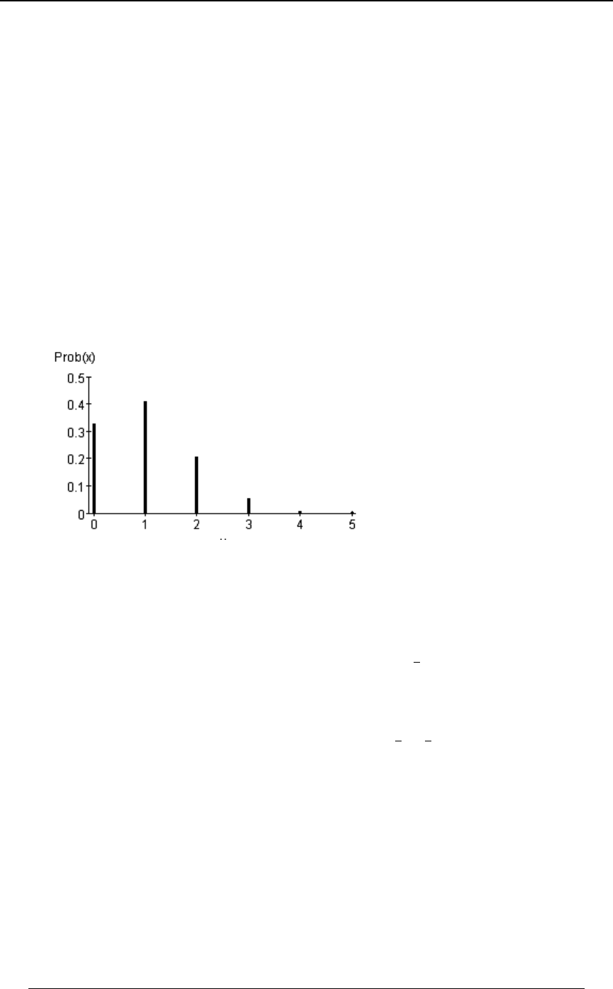
170 SECTION 6 - FREQUENTLY USED DISCRETE DISTRIBUTIONS

Example 6-2 continued

The number of answers Jones gets correct, say , has the same distribution. Then,]

T Ò\ œ ] Ó œ T ÒÐ\ œ !Ñ ∩ Ð] œ !ÑÓ  T ÒÐ\ œ "Ñ ∩ Ð] œ "ÑÓ  â  T ÒÐ\ œ &Ñ ∩ Ð] œ &ÑÓ

œTÒ\ œ!Ó†TÒ] œ!ÓTÒ\ œ"Ó†TÒ] œ"ÓâTÒ\ œ&Ó†TÒ] œ&Ó

(this follows from independence of and ), which is equal to\]

ÐÞ$#(')Ñ  ÐÞ%!*'Ñ  ÐÞ#!%)Ñ  ÐÞ!&"#Ñ  ÐÞ!!'%Ñ  ÐÞ!!!$#Ñ œ Þ$"*)

##### #

(ii) For a particular question, the probability that Jones picks (at random) the same answer as

Smith is .2. Since all 5 questions are answered independently, the probability of both papers

being identical is . ÐÞ#Ñ œ Þ!!!$#

&

The following is a probability plot for the binomial distribution in Example 6-2.

Example 6-3: If is the number of "6"'s that turn up when 72 ordinary dice are independently\

thrown, find the expected value of .\#

Solution: has a binomial distribution with and . Then\8œ(#:œ

IÒ\Óœ8:œ"# Z+<Ò\Óœ8:Ð":Ñœ"! Z+<Ò\ÓœIÒ\ ÓÐIÒ\ÓÑ, and . But ,

so that .IÒ\ Ó œ Z +<Ò\Ó  ÐIÒ\ÓÑ œ "!  "# œ "&%

###

Note that the probability function of is for \ T Ò\ œ 5Ó œ Ð Ñ Ð Ñ 5 œ !ß "ß #ß ÞÞÞß (#Þ

Š‹

5''

5 (#5

Below is a histogram for the distribution of . The probabilities are very small for -values\\

above 20 or so. For instance, , andT Ò\ œ #&Ó œ Þ!!!"!"*& T Ò\ œ $!Ó œ $Þ& ‚ "!(

T Ò\ œ #Ó œ Þ!!!#!$& \ œ "# . The mode of the distribution occurs at , with a probability of

T Ò\ œ "#Ó œ Þ"#&#& \ œ "# 8. is also the mean of the distribution. As gets larger in a binomial

distribution, the histogram takes on more of a bell shape. Later on we will see the normal

approximation applied to a distribution.

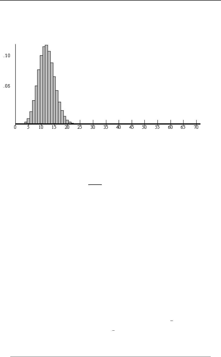
SECTION 6 - FREQUENTLY USED DISCRETE DISTRIBUTIONS 171

Example 6-3 continued

The normal distribution is a continuous random variable with a bell-shaped density that can

sometimes be used to approximate other distributions such as the binomial.



Poisson distribution with parameter ( )--!

This distribution is defined for all integers !ß "ß #ß ÞÞÞ

The probability function is for :ÐBÑ œ B œ !ß "ß #ß $ß ÞÞÞß

B--

- may be referred to as the Poisson parameter for the distribution.

The mean and variance are equal to the Poisson parameter, IÒ\Ó œ Z +<Ò\Ó œ -ß

and the moment generating function is .QÐ>Ñœ/

\Ð/ "Ñ->

The Poisson distribution is often used as a model for counting the number of events of a certain

type that occur in a certain period of time. Suppose that represents the number of customers\

arriving for service at a bank in a one hour period, and that a model for is the Poisson\

distribution with parameter . Under some reasonable assumptions (such as independence of the-

numbers arriving in different time intervals) it is possible to show that the number arriving in any

time period also has a Poisson distribution with the appropriate parameter that is "scaled" from .-

Suppose that , meaning that , the number of bank customers arriving in one hour, has a-œ%! \

mean of . If represents the number of customers arriving in 2 hours, then has a Poisson%! ] ]

distribution with a parameter of 80. For any time interval of length , the number of customers>

arriving in that time interval has a Poisson distribution with parameter (mean) . For-> œ %!>

instance, the number of customers arriving during a 15-minute period hour) will have aÐ> œ "

Poisson distribution with parameter (mean) .%! ‚ œ "!

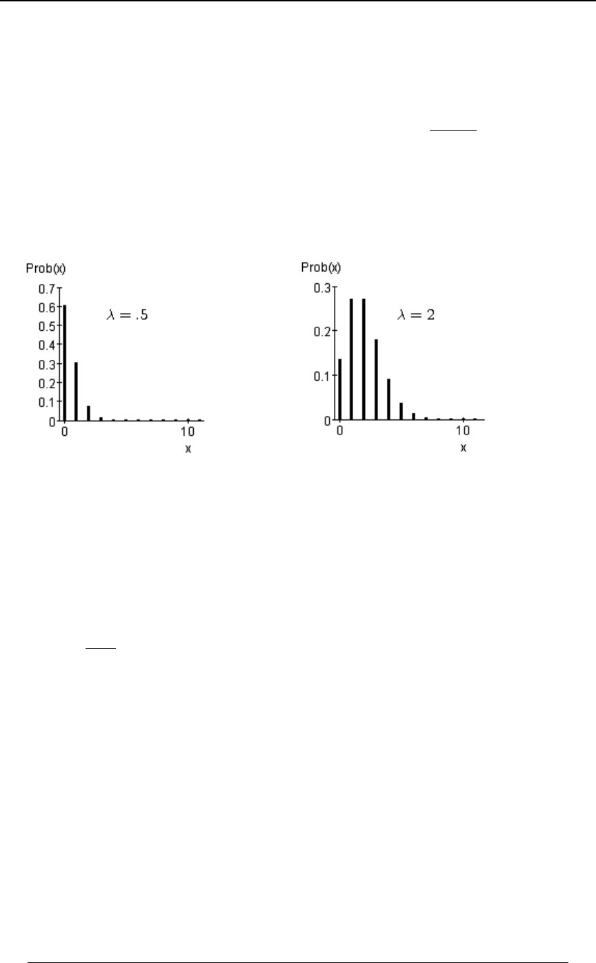
172 SECTION 6 - FREQUENTLY USED DISCRETE DISTRIBUTIONS

As an example, for , the following is a partial description of the Poisson distribution:-œÞ&

\À!"#$%&

:ÐBÑ À Þ'!'& Þ$!$$ Þ!(&) Þ!"#' Þ!!"' Þ!!!# Þ Þ

An example of the calculation of these values is .T Ò\ œ $Ó œ :Ð$Ñ œ œ Þ!"#'$'

/ÐÞ&Ñ

Þ& $

For , the following is a partial description of the Poisson distribution:-œ#

\À!"#$%&ÞÞÞ

:ÐBÑ À Þ"$&$ Þ#(!( Þ#(!( Þ")!% Þ!*!# Þ!$'" Þ Þ

Histograms of these two Poisson distributions are as follows:

Example 6-4: The number of home runs in a baseball game is assumed to have a Poisson

distribution with a mean of 3. As a promotion, a company pledges to donate $10,000 to charity

for each home run hit up to a maximum of 3. Find the expected amount that the company will

donate. Another company pledges to donate $C for each home run over 3 hit during the game,

and C is chosen so that the second company's expected donation is the same as the first. Find C.

Solution: Let be the number of home runs hit in the game and let be the first company's\]

donation, and let be the second company's donation. The probability function for is^\

TÒ\ œ 8Ó œ \

$ 8 . The distribution of is

\À!"#$%& ...

:ÐBÑ À Þ!%*) Þ"%*% Þ##%! Þ##%! Þ"')! Þ"!!)

] À ! "!ß !!! #!ß !!! $!ß !!! $!ß !!! $!ß !!!

^À!!!!G#G

IÒ] Ó œ Ð!ÑÐÞ!%*)Ñ  Ð"!ß !!!ÑÐÞ"%*%Ñ  Ð#!ß !!!ÑÐÞ##%!Ñ  Ð$!ß !!!ÑÐÞ##%!  Þ"')!  âÑ

œ Ð"!ß !!!ÑÐÞ"%*%Ñ  Ð#!ß !!!ÑÐÞ##%!Ñ  Ð$!ß !!!ÑÐ"  :Ð!Ñ  :Ð"Ñ  :Ð#ÑÑ

œ Ð"!ß !!!ÑÐÞ"%*%Ñ  Ð#!ß !!!ÑÐÞ##%!Ñ  Ð$!ß !!!ÑÐ"  Þ!%*)  Þ"%*%  Þ##%!Ñ œ #$ß #() .

To find we look at as the sum of two new random variables and ..IÒ^Ó \ Y [

\À!"#$%&' ÞÞÞBÞÞÞ

YÀ!"#$$$$ ÞÞÞ$ÞÞÞ

[À!!!!"#$ B$ÞÞÞ ...

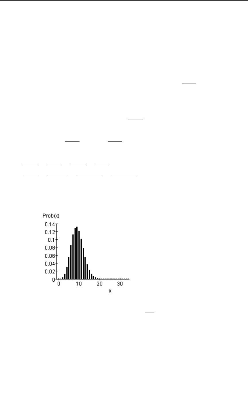
SECTION 6 - FREQUENTLY USED DISCRETE DISTRIBUTIONS 173

Example 6-4 continued

We see that , and therefore, . We can find in the\ œ Y  [ $ œ IÒ\Ó œ IÒY Ó  IÒ[ Ó IÒY Ó

same way we found above,IÒ] Ó

IÒYÓœ!‚:Ð!Ñ"‚:Ð"Ñ#‚:Ð#Ñ$‚Ò":Ð!Ñ:Ð"Ñ:Ð#ÑÓ

œ Þ"%*%  #ÐÞ##%!Ñ  $Ð"  Þ!%*)  Þ"%*%  Þ##%!Ñ œ #Þ$#() (reduced by a factor of 10,000

from ). It follows that Then, since ,] IÒ[ Ó œ IÒ\Ó  IÓY Ó œ $  #Þ$#() œ Þ'(##Þ ^ œ G[

we get . In order for this to be 23,278 we require .IÒ^Ó œ Þ'(##G G œ œ $%ß '$!

#$ß#()

Þ'(## 

Example 6-5: Assume that the number of hits, , per baseball game, has a Poisson\

distribution. If the probability of a no-hit game is , find the probability of having 4 or more

"!ß!!!

hits in a particular game.

Solution: .T Ò\ œ !Ó œ œ / œ p œ 68 "!ß !!!

/† "

!x "!ß!!!

!----

TÒ\  %Ó œ "ÐTÒ\ œ !ÓTÒ\ œ "ÓTÒ\ œ #ÓTÒ\ œ $ÓÑ

œ"ÐÑ

/† /† /† /†

!x "x #x $x

! " # $----

----

œ "  Ð    Ñ œ Þ*)"(

"!ß!!! "!ß!!! #Ð"!ß!!!Ñ 'Ð"!ß!!!Ñ

68"!ß!!! Ð68"!ß!!!Ñ Ð68"!ß!!!Ñ

. 

The mean in Example 6-5 is . The histogram for this Poisson-œ 68Ð"!ß !!!Ñ œ *Þ#"

distribution is given below. As increases, the histogram becomes more bell-shaped.-

Note that for the Poisson distribution with mean , we have the following relationship between-

successive probabilities: .TÐ\œ8"ÑœTÐ\œ8Ñ† -

8"

For Exam P it is very important to be familiar with the binomial and Poisson distributions.

The following distributions have all come up on the exam at one time or another as well, but

not as often as the binomial and Poisson distributions.

174 SECTION 6 - FREQUENTLY USED DISCRETE DISTRIBUTIONS

Geometric distribution with parameter ( ): !Ÿ:Ÿ"

Suppose that a single trial of an experiment results in either success with probability , or failure:

with probability . The experiment is performed with successive independent trials":œ;

until the first success occurs. If represents the number of failures until the first success, then \\

is a discrete random variable that can be . is said to have a !ß "ß #ß $ß ÞÞÞ \ geometric

distribution with parameter The probability function for is:\.

:ÐBÑ œÐ":Ñ : B œ !ß"ß#ß$ßÞÞÞ

Bfor .

The are .mean and variance of \IÒ\Óœ Z+<Ò\Óœ

": ":

œß œ

;;

The moment generating function is .QÐ>Ñœ

"Ð":Ñ/>

The geometric distribution has the lack of memory property, .TÒ\œ85l\8ÓœTÒ\œ5Ó

An equivalent description of the geometric distribution uses the parameter , where .""œ":

Another version of a geometric distribution is the random variable , the number of the]

experiment on which the first success occurs. is related to just defined: and]\ ]œ\"

T Ò] œ CÓ œ T Ò\ œ C  "Ó œ Ð"  :Ñ : C œ "ß #ß $ß ÞÞÞ

C" for An example of this was seen with

tossing a coin until a head turns up. is the toss number of the first head, is the number of]\

tails until the first head: .IÒ] Ó œ IÒ\Ó  " œ ß Z +<Ò] Ó œ Z +<Ò\Ó œ

":

Example 6-6: In tossing a fair die repeatedly (and independently on successive tosses), find the

probability of getting the first "1" on the -th toss. Find the expected number of tosses before the>

first "1" is tossed.

Solution: The probability that the first "1" occurs on the first toss is . The probability that the

first "1" occurs on the second toss is (a toss other than "1" followed by a "1").ÐÑÐÑ

The probability that the first "1" occurs on the -th toss is ( rolls other than "1">ÐÑÐÑ>"

>"

followed by a "1"). If we define tossing a "1" as a success, then the number of failures until the

first success has a geometric distribution described as above, with :\:œ

TÒ\ œ!Óœ ß TÒ\ œ "ÓœÐ ÑÐ Ñß ÞÞÞß TÒ\ œ>ÓœÐ Ñ Ð ÑÞ \

"&" &"

''' ''

>" The mean of is

IÒ\Óœ "œ'"œ&

: . We expect 5 "failures" until the first success.

If the question had asked us to find the expected toss number of the first "1", then this would be

the version of the geometric distribution defined as above, with Then is the toss]:œÞ]

number at which the first "1" occurs. The mean of is . This is reasonable, since]IÒ]Óœœ'

there are six possible outcomes from the die toss, we would expect 6 tosses would be needed on

average to get the first "1". 

SECTION 6 - FREQUENTLY USED DISCRETE DISTRIBUTIONS 175

Negative binomial distribution with parameters and ( and )< : <! !:Ÿ"

The probability function is

for :ÐBÑ œ : Ð"  :Ñ œ : Ð"  :Ñ B œ !ß "ß #ß $ß ÞÞÞß

Š‹ Š‹

<B" <B"

B<"

<B <B

The mean and variance and moment generating function are

.IÒ\Ó œ ß Z +<Ò\Ó œ ß Q Ð>Ñ œ

<Ð":Ñ <Ð":Ñ

: : "Ð":Ñ/

’“

If is an integer, then the negative binomial random variable can be interpreted as follows.<\

Suppose that an experiment ends in either failure or success, and the probability of success for a

particular trial of the experiment is . Suppose further that the experiment is performed repeatedly:

(independent trials) until the -th success occurs. If is the number of failures until the -th<\ <

success occurs, then has a negative binomial distribution with parameters and . The\<:

distribution is defined even if is not an integer. Note that is the total number of trials until<<B

the -th success. If is not an integer then .<< œ

Š‹

<B"

<" Bx

Ð<B"ÑÐ<B#ÑâÐ<"ÑÐ<Ñ

The notation is sometimes used to represent .;":

The geometric distribution is a special case of the negative binomial with .<œ"

We can get some insight into the algebraic form of the negative binomial probability function by

considering an example. Suppose that a fair die is tossed until the 3rd "1" turns up. We will define

"success" to be a "1" turning up on a die toss, and "failure" will be the result that a "1" didn't turn

up on the toss. Suppose that we wish to find the probability that there are (exactly) 2 failures

before the 3rd success. In order for there to be 2 failures before the 3rd success, the 3rd success

must be on the 5th toss, and of the previous 4 tosses there must be 2 failures and 2 successes. The

number of non-"1"'s on the first 4 trials has a binomial distribution, with and probability8œ%

' (we are assuming that the die is fair). Therefore, the probability of 2 failures on the first 4 trials

is . The probability of 2 failures in the first 4 trials followed by a success on the

Š‹

#' '

ÐÑÐÑ

5th trial is (because of independence) . This is the negative

Š‹ Š‹

#' ' ' #' '

&" " &"

ÐÑÐÑ‚ œ ÐÑÐÑ

## #$

binomial probability function for .TÒ\ œ #Ó < œ $ß : œ "

More generally, in order to have failures before the -th success, we must have the th successB< <

occur on trial number failures and successes in the first trials, followed<BÐB <" B<"

by a success on the -th trial). Therefore, we must have failures in the first trials,<BB<"

followed by a success on trial number . The number of failures in the first trialsB< B<"

has a binomial distribution, and the probability of failures in the first trials isB B<"

Š‹

B<"

BÐ"  :Ñ : < :

B<"

. The probability of a success on the -th trial is , so the total probability

of failures before the -th success is .B < Ð":Ñ : ‚:œ Ð":Ñ :

Š‹ Š‹

B<" B<"

B<" B<

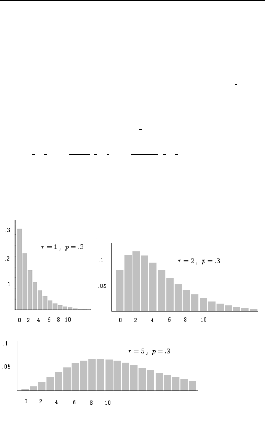
176 SECTION 6 - FREQUENTLY USED DISCRETE DISTRIBUTIONS

Keep in mind the binomial coefficient relationship , which might be useful in

ˆ‰ ˆ ‰

585

some circumstances.

Example 6-7: In tossing a fair die repeatedly (and independently on successive tosses), find the

probability of getting the third "1" on the -th toss.>

Solution: The negative binomial random variable with parameters and is the\<œ$:œ

number of failures (failure means tossing 2,3,4,5 or 6) until the 3rd success. The probability that

the 3rd success (3rd "1") occurs on the -th toss is the same as the probability of >Bœ>$

failures before the 3rd success. Thus, if is the number of failures until the 3rd success, has a\\

negative binomial distribution with and . Then, the probability that is<œ$ :œ \œ>$

TÒ\ œ >$Ó œ :Ð>$Ñ œ : Ð":Ñ œ Ð Ñ Ð Ñ

Š‹ Š ‹

<B" $>$"

B>$''

<B $>$

œ ÐÑÐÑ œ ÐÑÐÑ œ ÐÑÐÑ Þ

Š‹

>"

>$ ' ' Ð>$Ñx†#x ' ' # ' '

"& "& "&

Ð>"Ñx Ð>"ÑÐ>#Ñ

$>$ $>$ $>$



As mentioned above, the geometric distribution is a special case of the negative binomial with

<œ" :œÞ$ . The graphs below show the histogram for negative binomial distributions with

and (i) (geometric) , (ii) , and (iii) .<œ" <œ# <œ&

SECTION 6 - FREQUENTLY USED DISCRETE DISTRIBUTIONS 177

Hypergeometric distribution with integer parameters and Qß O 8

( , and ):Q ! !ŸOŸQ "Ÿ8ŸQ

In a group of objects, suppose that are of Type I and are of Type II.QOQO

If a subset of objects is randomly chosen without replacement from the group of objects, let8Q

\8\ denote the number that are of Type I in the subset of size . is said to have a

hypergeometric distribution. is a non-negative integer that satisfies\

\Ÿ8 \ŸO !Ÿ\ 8ÐQOÑŸ\ , , and .

The probability function for is .\:ÐBÑœ

ˆ‰ˆ ‰

ˆ‰

OQO

B8B

B8OBŸ738Ò8ßOÓ QO can't be larger than or , so , and since there are Type II objects in

total, must be at least .B8ÐQOÑ

The probability function is explained as follows. There are ways of choosing the subset of

Š‹

8Q B objects from the entire group of objects. The number of choices that result in objects of

Type I and objects of Type II is .8B Š‹Š ‹

OQO

B8B

The mean and variance of are , .\IÒ\Óœ Z+<Ò\Óœ

QQ†ÐQ"Ñ

8OÐQ OÑÐQ8Ñ

Example 6-8: An urn contains 6 blue and 4 red balls. 6 balls are chosen at random and

without replacement from the urn. If is the number of red balls chosen, find the standard\

deviation of .\

Solution: This is a hypergeometric distribution with and .Qœ"!ßOœ% 8œ'

The probability function of is , for .\ 0ÐBÑ œ B œ !ß "ß #ß $ß %

ˆ‰ˆ ‰

ˆ‰

B'B

The variance is . Standard deviation is . Z+<Ò\Óœ œÞ'% Þ'%œÞ)

8OÐQ OÑÐQ8Ñ

Q†ÐQ"Ñ

#È

The hypergeometric distribution has rarely come up on the exams that have been publicly

released.

178 SECTION 6 - FREQUENTLY USED DISCRETE DISTRIBUTIONS

Multinomial distribution with parameters (where is a positive8ß : ß : ßÞÞÞß : 8

"# 5

integer and for all and ! Ÿ : Ÿ " 3 œ "ß #ß ÞÞÞß 5 :  :  â  : œ "Ñ

3"#5

Suppose that an experiment has possible outcomes, with probabilities 5 : ß : ß ÞÞÞß :

"# 5

respectively. Each time the experiment is performed, it results in one of the possible outcomes.

If the experiment is performed successive times (independently), let denote the number of8\

experiments that resulted in outcome , so that .3 \ \ â\ œ8

"# 5

The multinomial distribution probability function is

T Ò\ œ B ß \ œ B ß âß \ œ B Ó œ :ÐB ß B ß ÞÞÞß B Ñ œ † : † : â:

""## 55 "# 5 "#

B x†B xâB x

"# 5

"# 5 .

For each from to , is a random variable with a mean and variance similar to the33œ"3œ\k3

binomial mean and variance: .IÒ\Óœ8: ß Z+<Ò\Óœ8:Ð":Ñ

33 333

Also, for and between 1 and , and are related. A little later on in this study guide we34 8\ \

will review joint distributions and relationships between random variables. One measure of the

relationship between random variables is the covariance. For the multinomial distribution, the

covariance between and is .\\G9@Ò\ß\Óœ8::

34 34 34

For example, the toss of a fair die results in one of 6 outcomes, with probabilities5œ

: œ 3 œ "ß #ß $ß %ß &ß ' 8

' for . If the die is tossed times, then with

\ œ 3 \ ß \ ß ÞÞÞß \

3"# '

# of tosses resulting in face " " turning up, the distribution of is a

multinomial distribution. In tosses of the die, the probability that there are exactly8œ"!

2-"1"'s , 1-"2" , 0-"3"'s , 3-"4"'s , 1-"5" and 3-"6"'s is .

"!x """"""

#x†"x†!x†$x†"x†$x''''''

†Ð ÑÐ ÑÐ ÑÐ ÑÐ ÑÐ Ñ

#"!$"$

Recursive relationship for the binomial, Poisson and negative binomial:

The probability function for each these three distributions satisfies the following recursive

relationship for .

5" œ+ 5 œ"ß#ß$ßÞÞÞ

Poisson with parameter : .--

/Î5x

/ ÎÐ5"Ñx

5"

5

5"

œœp+œ!ß,œ

Binomial with parameters and : 8:+œ ß,œ Þ

": ":

Ð8"Ñ:

Negative binomial with parameters and : < : + œ "  : ß , œ Ð<  "ÑÐ"  :Ñ Þ

For instance, for a Poisson distribution with , we have , and-œ# +œ!ß,œ#

:œÐ+ Ñ†: œ † œ

5,#/†#/†#

5 5 Ð5"Ñx 5x

5"

# #

5" 5 .

In the released exams, the binomial, Poisson and geometric have come up regularly. The

negative binomial arises occasionally, and the, multinomial and hypergeometric have rarely

occurred.

SECTION 6 - FREQUENTLY USED DISCRETE DISTRIBUTIONS 179

SUMMARY OF DISCRETE DISTRIBUTIONS

Distribution Parameters Prob. Fn. Mean Variance MGFßßIÒ\ÓßZ+<Ò\ÓßQÐ>Ñ:ÐBÑ \

Uniform , integer R  ! ß B œ "ß #ß ÞÞÞß R

"R"R"

R # "# R Ð/ "Ñ

/Ð/ "Ñ

#>R>

Binomial integer 8  ! ß : Ð"  :Ñ 8: 8:Ð"  :Ñ Ð"  :  :/ Ñ

ˆ‰

BB8B >8

!  :  " B œ !ß "ß ÞÞÞß 8

Poisson ---! ß Bœ!ß"ß#ßÞÞÞ /

B---Ð/ "Ñ

Geometric !:" Ð":Ñ †:ß Bœ!ß"ß#ßÞÞÞ

B": ": :

: : "Ð":Ñ/

Negative

Binomial <!ß!:" :Ð":Ñ ß

Š‹ “

<B"

B : : "Ð":Ñ/

<Ð":Ñ <Ð":Ñ :

<B <

’

B œ !ß "ß #ß ÞÞÞ

Hypergeometric Q!ß!ŸOŸQß ˆ‰ˆ ‰

ˆ‰

OQO

B8B

QQÐQ"Ñ

8OÐQ OÑÐQ8Ñ

integers " Ÿ 8 Ÿ Qß B Ÿ 738Ò8ß OÓ

Multinomial 8ß : ß : ß ÞÞÞß : † : † : â: IÒ\ Ó œ 8: Z +<Ò\ Ó œ 8: Ð"  : Ñ

"# 5 3 3 3 3 3

B x†B xâB x

"# 5

!: " B B âB œ8

3"#5

180

PROBLEM SET 6 181

PROBLEM SET 6

Frequently Used Discrete Distributions

1. has a discrete uniform distribution on the integers and has a discrete\ !ß"ß#ßÞÞÞß8 ]

uniform distribution on the integers . Find ."ß#ß$ßÞÞÞß8 Z+<Ò\ÓZ+<Ò]Ó

A) B) C) D) E)

#8" " " #8"

"# "# "# "#

! 

2. The probability that a particular machine breaks down in any day is .20 and is independent of

the breakdowns on any other day. The machine can break down only once per day. Calculate the

probability that the machine breaks down two or more times in ten days.

A) B) C) D) E) Þ"!(& Þ!%!! Þ#')% Þ'#%# Þ*&*'

3. (SOA) A company prices its hurricane insurance using the following assumptions:

(i) In any calendar year, there can be at most one hurricane.

(ii) In any calendar year, the probability of a hurricane is 0.05 .

(iii) The number of hurricanes in any calendar year is independent

of the number of hurricanes in any other calendar year.

Using the company’s assumptions, calculate the probability that there are fewer than 3 hurricanes

in a 20-year period.

A) 0.06 B) 0.19 C) 0.38 D) 0.62 E) 0.92

4. (SOA) A study is being conducted in which the health of two independent groups of ten

policyholders is being monitored over a one-year period of time. Individual participants in the

study drop out before the end of the study with probability 0.2 (independently of the other

participants). What is the probability that at least 9 participants complete the study in one of the

two groups, but not in both groups?

A) 0.096 B) 0.192 C) 0.235 D) 0.376 E) 0.469

182 PROBLEM SET 6

5. (SOA) A hospital receives 1 5 of its flu vaccine shipments from Company X and theÎ

remainder of its shipments from other companies. Each shipment contains a very large number of

vaccine vials. For Company X’s shipments, 10% of the vials are ineffective. For every other

company, 2% of the vials are ineffective. The hospital tests 30 randomly selected vials from a

shipment and finds that one vial is ineffective. What is the probability that this shipment came

from Company X?

A) 0.10 B) 0.14 C) 0.37 D) 0.63 E) 0.86

6. (SOA) A company establishes a fund of 120 from which it wants to pay an amount, , to anyG

of its 20 employees who achieve a high performance level during the coming year. Each

employee has a 2% chance of achieving a high performance level during the comingyear,

independent of any other employee. Determine the maximum value of for which theG

probability is less than 1% that the fund will be inadequate to cover all payments for high

performance.

A) 24 B) 30 C) 40 D) 60 E) 120

7. Let be a Poisson random variable with . Calculate .\ IÒ\Ó œ 68 # IÒ-9=Ð \ÑÓ1

A) B) C) D) E) !"#68#

8. (SOA) The number of days that elapse between the beginning of a calendar year and the

moment a high-risk driver is considered to be a continuous random variable with pdf . An-/-B

insurance company expects that 30% of high-risk drivers will be involved in an accident during

the first 50 days of a calendar year. What portion of high-risk drivers are expected to be involved

in an accident during the first 80 days of a calendar year?

A) 0.15 B) 0.34 C) 0.43 D) 0.57 E) 0.66

9. (SOA) An actuary has discovered that policyholders are three times as likely to file two claims

as to file four claims. If the number of claims filed has a Poisson distribution, what is the

variance of the number of claims filed?

A) B) C) D) E)

È"##%

PROBLEM SET 6 183

10. (SOA) An insurance policy on an electrical device pays a benefit of 4000 if the device fails

during the first year. The amount of the benefit decreases by 1000 each successive year until it

reaches 0. If the device has not failed by the beginning of any given year, the probability of

failure during that year is 0.4. What is the expected benefit under this policy?

A) 2234 B) 2400 C) 2500 D) 2667 E) 2694

11. (SOA) A tour operator has a bus that can accommodate 20 tourists. The operator knows that

tourists may not show up, so he sells 21 tickets. The probability that an individual tourist will not

show up is 0.02, independent of all other tourists. Each ticket costs 50, and is non-refundable if a

tourist fails to show up. If a tourist shows up and a seat is not available, the tour operator has to

pay to the tourist. What is the expected revenue of the tour"!!Ð>3-5/> -9=>  &! :/8+6>CÑ

operator?

A) 935 B) 950 C) 967 D) 976 E) 985

12. A fair die is tossed until a 2 is obtained. If is the number of trials required to obtain the\

first 2, what is the smallest value of for which ?BTÒ\ŸBÓ

A) B) C) D) E) #$%&'

13. (SOA) A large pool of adults earning their first driver’s license includes 50% low-risk

drivers, 30% moderate-risk drivers, and 20% high-risk drivers. Because these drivers have no

prior driving record, an insurance company considers each driver to be randomly selected from

the pool. This month, the insurance company writes 4 new policies for adults earning their first

driver’s license. What is the probability that these 4 will contain at least two more high-risk

drivers than low-risk drivers?

A) 0.006 B) 0.012 C) 0.018 D) 0.049 E) 0.073

14. A box contains 10 white and 15 black marbles. Let denote the number of white marbles in\

a selection of 10 marbles selected at random and without replacement. Find .

Z+<Ò\Ó

IÒ\Ó

A) B) C) D) E)

"$ &$

)"')"')

184 PROBLEM SET 6

15. A multiple choice test has 10 questions, and each question has 5 answer choices (exactly one

of which is correct). A student taking the test guesses randomly on all questions. Find the

probability that the student will actually get at least as many correct answers as she would expect

to get with the random guessing approach.

A) .624 B) .591 C) .430 D) .322 E) .302

16. An analysis of auto accidents shows that one in four accidents results in an insurance claim.

In a series of independent accidents, find the probability that the first accident resulting in an

insurance claim is one of the first 3 accidents.

A) .50 B) .52 C) .54 D) .56 E) .58

17. An insurer has 5 independent one-year term life insurance policies. The face amount on each

policy is 100,000. The probability of a claim occurring in the year for any given policy is .2.

Find the probability the insurer will have to pay more than the total expected claim for the year.

A) .06 B) .11 C) .16 D) .21 E) .26

18. The number of claims per year from a particular auto insurance policy has a Poisson

distribution with a mean of 1, and probability function . Based on a number of years of:5

experience, the insurer decides to change the distribution, so that the new probability of 0 claims

is .5 , and the new probabilities for are proportional to the old (Poisson):œ : 5"

‡‡

probabilities according to the relationship for . Find the mean of the new:œ-†: 5"

‡5

claim number distribution.

A) .79 B) .63 C) .5 E) .37 E) .21

19. The probability generating function of a discrete non-negative integer valued random

variable is a function of the real variable : .R>TÐ>Ñœ>†TÒRœ5ÓœIÒ>Ó



5œ!

∞5R

Which of the following is the correct expression for the probability generating function of the

Poisson random variable with mean 2?

A) B) C) D) E) // // /

#> "#> #> #>" #Ð>"Ñ

PROBLEM SET 6 185

20. An insurer issues two independent policies to individuals of the same age.

The insurer models the distribution of the completed number of years until death for each

individual, and uses the geometric distribution , where T ÒR œ 5Ó œ ÐÞ**Ñ ÐÞ!"Ñ 5 œ !ß "ß #ß ÞÞÞ

and is the completed number of years until death for each individual.R

Find the probability that the two individuals die in the same year.

A) .001 B) .003 C) .005 D) .007 E) .009

21. An insurer uses the Poisson distribution with mean 4 as the model for the number of warranty

claims per month on a particular product. Each warranty claim results in a payment of 1 by the

insurer. Find the probability that the total payment by the insurer in a given month is less than

one standard deviation above the average monthly payment.

A) .9 B) .8 C) .7 D) .6 E) .5

22. As part of the underwriting process for insurance, each prospective policyholder is tested for

high blood pressure. Let represent the number of tests completed when the first person with\

high blood pressure is found. The expected value of is 12.5.\

Calculate the probability that the sixth person tested is the first one with high blood pressure.

A) 0.000 B) 0.053 C) 0.080 D) 0.316 E) 0.394

23. Let be a random variable with moment generating function\

.QÐ>Ñœ ß ∞>∞

Š‹

#/

Calculate the variance of .\

A) 2 B) 3 C) 8 D) 9 E) 11

24. According to the house statistician, a casino estimates that it has a 51% chance of winning on

any given hand of blackjack. The casino also assumes that blackjack hands are independent of

one another. The casino randomly monitors its blackjack dealers, and as soon as a dealer is found

to lose 5 hands in a row, the casino stops the game at that dealer's table and checks the deck of

cards that the dealer is using. The casino has just started monitoring a dealer. What is the chance

that the game will be stopped at the table sometime within the next 8 hands of blackjack?

A) .07 B) .09 C) .11 D) .13 E) .15

186 PROBLEM SET 6

25. (SOA) A company takes out an insurance policy to cover accidents that occur at its

manufacturing plant. The probability that one or more accidents will occur during any given

month is . The number of accidents that occur in any given month is independent of the number

of accidents that occur in all other months. Calculate the probability that there will be at least

four months in which no accidents occur before the fourth month in which at least one accident

occurs.

A) 0.01 B) 0.12 C) 0.23 D) 0.29 E) 0.41

26. (SOA) Each time a hurricane arrives, a new home has a 0.4 probability of experiencing

damage. The occurrences of damage in different hurricanes are independent. Calculate the mode

of the number of hurricanes it takes for the home to experience damage from two hurricanes.

A) 2 B) 3 C) 4 D) 5 E) 6

27. For a certain discrete random variable on the non-negative integers, the probability function

satisfies the relationships

T Ð!Ñ œ T Ð"Ñ T Ð5  "Ñ œ † T Ð5Ñ 5 œ "ß #ß $ß ÞÞÞ T Ð!Ñ and for Find .

A) B) C) D) E) 68/ /" Ð/"Ñ / Ð/"Ñ

" " "

PROBLEM SET 6 187

PROBLEM SET 6 SOLUTIONS

1. and so thatZ+<Ò\Óœ Z+<Ò]Óœ

Ð8"Ñ "

"# "#

8"

Z+<Ò\ÓZ+<Ò]Óœ #8"

"# . Answer: A

2. Since the breakdowns from one day to another are independent, the number of breakdowns

(successes) in days has a binomial distribution with and ."! ß\ß 8œ"! :œÞ#

TÒ\  #Ó œ "ÐTÒ\ œ !ÓTÒ\ œ "ÓÑ

œ "  ÐÞ#Ñ ÐÞ)Ñ  ÐÞ#Ñ ÐÞ)Ñ œ Þ'#%# Þ

Š‹ Š‹

"! "!

!"! "* Answer: D

3. The number of hurricanes in 20 years will have a binomial distribution withR

8œ#! :œÞ!& (years) and (chance of hurricane in any one year).

TÒR $ÓœTÒR œ!ÓTÒR œ"ÓTÒR œ#Ó

œ ÐÞ!&Ñ ÐÞ*&Ñ  ÐÞ!&Ñ ÐÞ*&Ñ  ÐÞ!&Ñ ÐÞ*&Ñ œ Þ*#%&

Š‹ Š‹ Š‹

#! #! #!

!"#

!#! ""* #") .

Note that Answer: E

ˆ‰

55xÐ85Ñx

œÞ

4. For each group, the number who complete the study is a binomial random variable with

8œ"! :œÞ) trials (10 people in the group, each is a "trial") and probability of any individual

in the group completing the study (probability of success for one trial).

The probability of at least 9 completing the study in group 1 is .T ÒR œ *Ó  T ÒR œ "!Ó

This is .

ˆ‰ ˆ‰

"! "!

*"!

* " "! !

ÐÞ)Ñ ÐÞ#Ñ  ÐÞ)Ñ ÐÞ#Ñ œ Ð"!ÑÐÞ"$%##ÑÐÞ#Ñ  Ð"ÑÐÞ"!($(Ñ œ Þ$('

The probability that less than 9 complete the study in group 1 is ."  Þ$(' œ Þ'#%

The same is true for group 2.

We are asked to find the probability that at least 9 participants complete the study in one of the

two groups, but not in both of the groups. Since the two groups are independent, this will be

TÒ Ó†TÒ Óat least 9 complete study in group 1 less than 9 complete study in group 2

TÒ Ó†TÒ Óless than 9 complete study in group 1 at least 9 complete study in group 2

œ ÐÞ$('ÑÐÞ'#%Ñ  ÐÞ'#%ÑÐÞ$('Ñ œ Þ%'* . Answer: E

188 PROBLEM SET 6

5. Event - vaccine is from company ,\\

\ \ TÐ\Ñ œ ß TÐ\Ñ œ Þ



- vaccine is from a company other than . "%

In a sample of 30 vials from Company , the number of ineffective vials has a binomial\

distribution with trials (vials) and probability of any particular one being8œ$! :œÞ"!

ineffective. In a sample of 30 vials from a Company other than , the number of ineffective\

vials has a binomial distribution with trials (vials) and probability of any8œ$! :œÞ!#

particular one being ineffective.

Therefore, ineffective shipment is from Company ,T Ò" l \Ó œ ÐÞ"Ñ ÐÞ*Ñ œ Þ"%"$

Š‹

""#*

and

T Ò" l \Ó œ ÐÞ!#Ñ ÐÞ*)Ñ œ Þ$$%! Þ ineffective shipment is from Company other than Š‹

""#*

We wish to find shipment is from Company ineffectiveTÒ \l" Ó

œT ÒÐ \Ñ∩Ð" ÑÓ

TÒ" Ó

shipment is from Company ineffective

ineffective .

T ÒÐ \Ñ ∩ Ð" ÑÓshipment is from Company ineffective

œTÒ"l\Ó†TÒ\Ó ineffective shipment is from Company shipment is from Company

œ ÐÞ"%"$ÑÐ Ñ Þ

TÒ"ÓœTÒÐ"Ñ∩\ÓTÒÐ"Ñ∩\Ó



ineffective ineffective ineffective

œ T ÒÐ" Ñl\Ó † T Ò\Ó  T ÒÐ" Ñl\Ó † T Ò\Ó œ ÐÞ"%"$ÑÐ Ñ  ÐÞ$$%!ÑÐ Ñ



ineffective ineffective .

Then, shipment is from Company ineffective .T Ò \l" Ó œ œ Þ!*'

ÐÞ"%"$ÑÐ Ñ

ÐÞ"%"$ÑÐ ÑÐÞ$$%!ÑÐ Ñ

This can be described by the following probability table.

Company Other Companies\

, given T Ò\Ó œ Þ# T Ò\ Ó œ Þ)

1 Ineff 1 Ineff 1 Ineff otherT Ò l\Ó œ Þ"%"$ T Ò l Ó œ Þ$$%!

given (calc. for binomial dist.) given (calc. for binomial dist.)

ÌÌ

1 Ineff 1 Ineff OtherTÒ ∩\Ó TÒ ∩ Ó

œ ÐÞ"%"$ÑÐÞ#Ñ œ ÐÞ$$%!ÑÐÞ)Ñ

I ineffT Ò Ó œ ÐÞ"%"$ÑÐÞ#Ñ  ÐÞ$$%!ÑÐÞ)Ñ

1 ineff . Answer: AT Ò\l Ó œ œ Þ!*'

ÐÞ"%"$ÑÐÞ#Ñ

ÐÞ"%"$ÑÐÞ#ÑÐÞ$$%!ÑÐÞ)Ñ

PROBLEM SET 6 189

6. is the number of people who achieve high performance. has a binomial distribution withRR

8œ#! :œÞ!# G and . We wish to find the largest for which

T ÒRG  "#!Ó  Þ!" . From the binomial distribution, we have

T ÒR œ !Ó œ ÐÞ!#Ñ ÐÞ*)Ñ œ Þ''(' ß

Š‹

!!#!

T ÒR œ "Ó œ ÐÞ!#Ñ ÐÞ*)Ñ œ Þ#(#& ß

Š‹

"""*

T ÒR œ #Ó œ ÐÞ!#Ñ ÐÞ*)Ñ œ Þ!&#)

Š‹

###) .

Therefore, .T ÒR  "Ó œ Þ!&** ß T ÒR  #Ó œ Þ!!("

If then ,

"#! "#!

 # T ÒRG  "#!Ó œ T ÒR  Ó Ÿ T ÒR  #Ó œ Þ!!("  Þ!"

but if then .

"#! "#!

 # T ÒRG  "#!Ó œ T ÒR  Ó Ÿ T ÒR  #Ó œ Þ!&**  Þ!"

In order to satisfy we must have , or equivalently,T ÒRG  "#!Ó  Þ!"  #

"#!

GŸ'! .

An alternative approach to this problem is to look at each possible value of in the answers, andG

find the probability for each. Starting with the largest possible value, we get forT ÒR G  "#!Ó

answer E, T Ò"#!R  "#!Ó œ T ÒR  "Ó œ "  T ÒR œ !Ó  T ÒR œ "Ó

œ "  Þ''('  Þ#(#& œ Þ!&**  Þ!" G œ "#! , so does not satisfy the probability requirement.

Then for answer D, we get

T Ò'!R  "#!Ó œ T ÒR  #Ó œ "  T ÒR œ !Ó  T ÒR œ "Ó  T ÒR œ #Ó

œ "  Þ''('  Þ#(#&  Þ!&#) œ Þ!!("  Þ!" G œ '!, so that does satisfy the requirement.

Answer: D

7. Since has a Poisson distribution, it can take on the non-negative integer values \ !ß"ß#ßÞÞÞ

With the probability function of is IÒ\Ó œ 68Ð#Ñß \ TÒ\ œ BÓ œ œ †

/ Ò68Ð#ÑÓ Ò68Ð#ÑÓ

Bx # Bx

68Ð#Ñ B B

The transformed random variable can take on the values-9=Ð \Ñ1

-9=Ð!Ñ œ "ß -9=Ð Ñ œ  "ß -9=Ð# Ñ œ "ß  " ß " ß  " ß Þ Þ Þ11

Then

IÒ-9=Ð \ÑÓ œ -9=Ð BÑ † † œ † Ð  "Ñ † œ †11



Bœ! Bœ! Bœ!

∞∞∞

"" "

#Bx # Bx # Bx

Ò68Ð#ÑÓ Ò68Ð#ÑÓ Ò68Ð#ÑÓ

BBB

œ†/ œ œ/ÑÞ

"" +

#% Bx

68Ð#Ñ +

Bœ!

∞

(we use the identity, Answer: B

B

190 PROBLEM SET 6

8. We interpret proportion as probability. The statement "30% of high-risk drivers will be

involved in an accident in the first 50 days of the year" is interpreted as

TÒ Ó œ Þ$a high-risk driver is involved in an accident in the first 50 days of the year .

This can be written as , where is the time, in days, until an accident occurs forT ÒX Ÿ &!Ó œ Þ$ X

a high-risk driver. We are told that has an exponential distribution. Suppose that the mean ofX

X X 0Ð>Ñ œ / T ÒX Ÿ &!Ó œ "  / is . Then the density function of is , and .."

.>Î &!Î..

From , we get , and then Þ$ œ T ÒX Ÿ &!Ó œ "  / / œ Þ( œ  Þ

&!Î &!Î.. .&!

68 Þ(

The proportion of high-risk drivers that are expected to have an accident in the first 80 days of the

year is interpreted as a probability,

TÒX Ÿ)!Óœ"/ œ"/ œ"/ œ"ÐÞ(Ñ œÞ%$

)!Î )!ÎÐ&!Î68 Þ(Ñ "Þ' 68 Þ( "Þ'. .

Answer: C

9. has a Poisson distribution with mean . andRTÒRœ#Óœ/†---#

TÒR œ%Óœ/ † TÒRœ#Óœ$TÒR œ%Ó

--%

%x . We are told that , so that

/† œ$/† Ê œ#

--

##%

The variance of the Poisson distribution is equal to the mean, Answer: D-œ#Þ

10. The probability that the device fails in year ,8 œ "ß #ß $ß ÞÞÞ

is ( years of non-failure followed year of failure).ÐÞ'Ñ ÐÞ%Ñ 8  "

8"

This is a version of the geometric distribution.

Year of Failure Prob. Amount Paid

1 .4 4000

2 (.6)(.4) .24 3000œ

3 (.6) (.4) .144 2000

#œ

4 (.6) (.4) .0864 1000

$œ

5 0

The expected amount paid is

Ð%!!!ÑÐÞ%Ñ  Ð$!!!ÑÐÞ#%Ñ  Ð#!!!ÑÐÞ"%%Ñ  Ð"!!!ÑÐÞ!)'%Ñ œ #'*%Þ% .

Answer: E

PROBLEM SET 6 191

11. The tour operator collects 21 fares, . Let denote the number of ticket#" ‚ &! œ "!&! R

holders who show up. The tour operator does not have to make a refund if . If ,RŸ#! Rœ#"

the tour operator must pay 100. The number of ticket holders that show up has a binomial

distribution based on (ticket holders) and (probability of any particular ticket8œ#" :œÞ*)

holder showing up). Then .T ÒR œ #"Ó œ ÐÞ*)Ñ ÐÞ!#Ñ œ Þ'&%#'

Š‹

#" #" !

The expected amount the tour operator must pay in refund and penalty is

Ð!Ñ † T ÒR Ÿ #!Ó  Ð"!!Ñ † T ÒR œ #"Ó œ Ð"!!ÑÐÞ'&%#'Ñ œ '&Þ%$ .

The expected revenue (after refund and penalty) is ."!&!  '&Þ%$ œ *)%Þ&(

Answer: E

12. TÒ\ œ 5Ó œ Ð Ñ Ð ÑÞ

5"

TÒ\ŸBÓœ TÒ\œ5Óœ † œ"ÐÑ pÐÑŸ pB%

’“

5œ"

BBB

"&"&"

'"Î' '#'#

"Ð Ñ

'B.

Note that has a geometric distribution with . Answer: C\" :œ "

13. This problem involves the multinomial distribution. The multinomial distribution with

parameters (where is a positive integer and for all 8ß : ß : ßÞÞÞß : 8 !Ÿ: Ÿ" 3œ"ß#ßÞÞÞß 5

"# 5 3

and is defined in the following way.::â:œ"Ñ

"# 5

Suppose that an experiment has possible outcomes, with probabilities 5 : ß : ß ÞÞÞß :

"# 5

respectively. If the experiment is performed successive times (independently), let denote8\

the number of experiments that resulted in outcome , so that3

\\â\œ8

"# 5 . The multinomial probability function is

0ÐB ß B ß ÞÞÞß B Ñ œ † : † : â:

"# 5 "#

B x†B xâB x

"# 5

"# 5 .

In this problem, the "experiment" outcome is the type of driver, which has three outcomes. These

are "low-risk", with probability , "moderate-risk", with probability , and "high-:œÞ& :œÞ$

risk", with probability . The "experiment" (choosing a driver) is performed times.:œÞ# 8œ%

We want to find the probability that (number of high-risk drivers at least two more\\#

than the number of low-risk drivers). We can look at the outcomes that result in this event:

, number of , number of , number of\\ \

"# $

low-risk drivers moderate-risk rivers high-risk drivers

0 0 4

0 1 3

0 2 2

1 0 3

192 PROBLEM SET 6

13. continued

These are the only outcomes that result in this event.

0Ð!ß !ß %Ñ œ † ÐÞ&Ñ † ÐÞ$Ñ † ÐÞ#Ñ œ Þ!!"' ß

!x†!x†%x !!%

0Ð!ß "ß $Ñ œ † ÐÞ&Ñ † ÐÞ$Ñ † ÐÞ#Ñ œ Þ!!*' ß

!x†"x†$x !"$

0Ð!ß #ß #Ñ œ † ÐÞ&Ñ † ÐÞ$Ñ † ÐÞ#Ñ œ Þ!#"' ß

!x†#x†#x !##

0Ð"ß !ß $Ñ œ † ÐÞ&Ñ † ÐÞ$Ñ † ÐÞ#Ñ œ Þ!"'!

"x†!x†$x "!$ .

The total probability of this event is then . Þ!!"'  Þ!!*'  Þ!#"'  Þ!"'! œ Þ!%))

Answer: D

14. has a hypergeometric distribution with marbles, white marbles,\ Qœ#& Oœ"!

and marbles chosen. Then and8œ"! IÒ\Óœ œ œ%ß

Q#&

Ð"!ÑÐ"!Ñ

Z+<Ò\Óœ œ Ê œ œ

8OÐQ OÑÐQ8Ñ Z +<Ò\Ó ÐQOÑÐQ8Ñ

Q ÐQ"Ñ # IÒ\Ó QÐQ "Ñ )

# . Answer: E

15. The probability of a correct guess is on any particular question. The number of correctÞ#

guesses forms a binomial distribution based on trials (10 questions), with a probability8œ"!

of of success (correct answer) on each trial. The expected number of correct guesses is:œÞ#

8: œ "!ÐÞ#Ñ œ # T Ò\  #Ó . The probability of getting at least 2 correct is . The binomial

distribution probability is . Then,T Ò\ œ 5Ó œ ÐÞ#Ñ ÐÞ)Ñ

Œ 5 "!5

T Ò\  #Ó œ "  ÐT Ò\ œ !Ó  T Ò\ œ "ÓÑ œ "  ÐÞ#Ñ ÐÞ)Ñ  ÐÞ#Ñ ÐÞ)Ñ

"! "!

Œ Œ

!"! "*

œ Þ'#% . Answer: A

16. Out of 3 independent accidents, the number that result in a claim has a binomial distribution

with and . The probability that none of the 3 accidents result in a claim is8œ$ :œ "

Š‹

!% %

ÐÑÐÑœÞ%##

!$ . The probability that there is a least one claim in the 3 accidents is

"  Þ%## œ Þ&() .

Alternatively, the probability that the first accident resulting in a claim is the -th accident is5

ÐÞ(&Ñ ÐÞ#&Ñ

5" (geometric distribution). Thus, the probability is

ÐÞ(&Ñ ÐÞ#&Ñ  ÐÞ(&Ñ ÐÞ#&Ñ  ÐÞ(&Ñ ÐÞ#&Ñ œ Þ&()

!"#

. Answer: E

PROBLEM SET 6 193

17. The expected claim from any one policy is , soÐ"!!ß !!!ÑÐÞ#Ñ œ #!ß !!!

the overall expected claim from all 5 policies is 100,000 . The total claim for the year will be

more than 100,000 if there are 2 or more claims. This probability is

TÒR #Óœ"TÒRœ!ÓTÒRœ"Ó R , where is the number of claims.

R 8œ&ß :œÞ# has a binomial distribution with .

T ÒR œ !Ó  T ÒR œ "Ó œ ÐÞ#Ñ ÐÞ)Ñ  ÐÞ#Ñ ÐÞ)Ñ œ Þ($(#)

Š‹ Š‹

!& "%

Ê T ÒR  #Ó œ "  Þ($(#) œ Þ#'#(# . Answer: E

18. , so that since , we must have ."œ:  : : œÞ& : œ- : œÞ&

!5 ! 5

‡‡ ‡ ‡

5œ" 5œ" 5œ"

∞∞∞



However, ," œ :  : œ /  : p : œ "  / œ Þ'$#"

!5œ" 5œ" 5œ"

∞∞∞

555

" "



so that . Then, the new expectation is- œ œ Þ(*"!

Þ&

Þ'$#"

  

5œ! 5œ" 5œ" 5œ" 5œ!

∞∞∞ ∞ ∞

‡‡ 555

5:œ 5:œ 5-:œ- 5:œ- 5:

old expectation . Answer: Aœ - ‚ œ - † " œ Þ(*"!

19. TÐ>Ñœ>†TÒRœ5ÓœIÒ>Óœ>†/†



5œ! 5œ!

∞∞

5R5#

œ/† œ/† œ//œ/



5œ! 5œ!

∞∞

# # # #> #Ð>"Ñ

Ð#>Ñ Ð#>Ñ

5x 5x

55 . Answer: E

20. death in same year both die after complete yearsTÒ Ó œ TÒ 5 Ó



5œ!

∞

œTÒ5Ó†TÒ5Ó



5œ!

∞person 1 dies after complete years person 2 dies after complete years

œ ÐÞ**Ñ ÐÞ!"ÑÐÞ**Ñ ÐÞ!"Ñ œ ÐÞ!!!"Ñ ÒÐÞ**Ñ Ó œ œ Þ!!&



5œ! 5œ!

∞∞

55 #5

Þ!!!"

"ÐÞ**Ñ# . Answer: C

21. Average monthly payment is 4, variance is 4 (variance of Poisson is equal to mean).

Probability that total payment is less than is%#œ'

TÒRŸ&Óœ/Ò"%ÓœÞ()&

% %%%%

#x $x %x &x

#$%& . Answer: B

194 PROBLEM SET 6

22. This problem makes use of the geometric distribution. The experiment being performed is

the blood pressure test on an individual. We define "success" of the experiment to mean that the

individual has high blood pressure. We denote the probability of a success occurring in a

particular trial by . Since is the number of persons tested until the first person with high:\

blood pressure is found, it is like the version of the geometric distribution described as earlier]

in the study guide, where is the trial number of the first success (the trial number of the first]

success is 1, or 2, or 3, ...). The mean of this form of the geometric distribution is , so that

:œ "#Þ& : œ Þ!) and therefore . The probability that the first success occurs on the 6th trial

(first case of high blood pressure is the 6th individual) is , since there will be 5 failuresÐ"  :Ñ :

and then the first success. This probability is Answer: BÐÞ*#Ñ ÐÞ!)Ñ œ Þ!&#( Þ

23. One of the applications of the moment generating function for the random variable QÐ>Ñ \

is to calculate the moments of - for an integer ,\5"

IÒ\ Ó œ Q Ð>Ñ Z +<Ò\Ó œ IÒ\ Ó  ÐIÒ\ÓÑ œ Q Ð!Ñ  ÒQ Ð!ÑÓ

5##w#

Ð#Ñ

.> >œ!

5¹ . Therefore, .

In this problem, , so that andQÐ>Ñœ* Ð Ñ QÐ!Ñœ$ß

)

Š‹

#/ /

QÐ>Ñœ(#ÐÑ*ÐÑ QÐ!Ñœ""ß

Ð#Ñ Ð#Ñ

()

Š‹ Š‹

#/ / #/ /

$$ $$

>> >>

, so that

and then, .Z+<Ò\Óœ""$ œ#

Alternatively, . In thisZ+<Ò\Óœ Ò68Q Ð>ÑÓ

.> >œ!

#\¹

problem, , so that68 Q Ð>Ñ œ * 68Ð#  / Ñ  * 68 $

.*/.

.> #/ .> Ð#/ Ñ

Ð#/ ÑÐ*/ ÑÐ*/ ÑÐ/ Ñ

Ò68 Q Ð>ÑÓ œ Ò68 Q Ð>ÑÓ œ

># >#

>> >>

, and , and then

Z+<Ò\Óœ œ#

Ð$ÑÐ*ÑÐ*ÑÐ"Ñ

Ð$Ñ# .

A much faster solution is based on the following fact. The moment generating function of the

binomial random variable with parameters (number of trials) and (probability of success) is8:

Ð"::/Ñ 8œ*

. In this case, the mgf corresponds to the binomial distribution with and

: œ 8:Ð"  :Ñ œ *Ð ÑÐ Ñ œ #

""#

$$$

, and therefore the variance is . Answer: A

24. The game will be stopped only under the following circumstances:

L L L L L , W L L L L L , L W L L L L L , W W L L L L L ,

L L W L L L L L , W L W L L L L L , L W W L L L L L , W W W L L L L L ,

where W refers to win and L refers to loss. The sum of the probabilities is

ÐÞ%*Ñ  ÐÞ&"ÑÐÞ%*Ñ  ÐÞ%*ÑÐÞ&"ÑÐÞ%*Ñ  ÐÞ&"Ñ ÐÞ%*Ñ  ÐÞ%*Ñ ÐÞ&"ÑÐÞ%*Ñ

& & &#&# &

 ÐÞ&"ÑÐÞ%*ÑÐÞ&"ÑÐÞ%*Ñ  ÐÞ%*ÑÐÞ&"Ñ ÐÞ%*Ñ  ÐÞ&"Ñ Ð%*Ñ œ Þ!("&

&#&$&

. Answer: A

PROBLEM SET 6 195

25. We define the random variable to be the number of months in which no accidents have\

occurred when the fourth month of accidents has occurred. We wish to find . ThisTÒ\  %Ó

can be written as or ."  T Ò\ œ !ß "ß # $Ó

T Ò\ œ !Ó œ T Ò Ó œ Ð Ñ œ Þ"#*'first 4 months all have accidents .

TÒ\ œ "Ó œ TÒ1 of the first 4 months has no accidents and 3 have accidents

and 5th month has accidents .Ó œ Ð Ñ Ð Ñ Ð Ñ œ %Ð ÑÐ Ñ œ Þ#!(%

ˆ‰

"$ %

#$$ #$

&&& &&

TÒ\ œ #Ó œ TÒ2 of the first 5 months has no accidents and 3 have accidents

and 6th month has accidents .Ó œ Ð Ñ Ð Ñ Ð Ñ œ "!Ð Ñ Ð Ñ œ Þ#!(%

ˆ‰

#$ #%

#$$ #$

&&& &&

TÒ\ œ $Ó œ TÒ3 of the first 6 months has no accidents and 3 have accidents

and 7th month has accidents .Ó œ Ð Ñ Ð Ñ Ð Ñ œ #!Ð Ñ Ð Ñ œ Þ"'&*

ˆ‰

$$ $%

#$$ #$

&&& &&

T Ò\  %Ó œ "  Þ"#*'  Þ#!(%  Þ#!(%  Þ"'&* œ Þ#* .

\<œ%:œ has a negative binomial distribution with and . Answer: D

26. If "failure" refers to a hurricane that results in no damage and "success" refers a hurricane

that causes damage, then the distribution of the number of failures until the 2nd success has a\

negative binomial distribution with probability function

:Ð\ œ BÑ œ : Ð"  :Ñ B œ !ß "ß #ß $ß ÞÞÞß < œ # : œ Þ%

Š‹

<B"

<" <B

for where and

We can also describe this in terms of total number of hurricanes ,8œ<Bœ#B

so that TÐR œ8ÑœTÐ\œ8#Ñœ : Ð":Ñ œ ÐÞ%ÑÐÞ'Ñ

Š‹ Š‹

8" 8"

#" #"

# 8# # 8#

for . We wish find that maximizes this probability.8 œ #  B œ #ß $ß ÞÞÞ 8

T ÐR œ #Ñ œ Þ"' ß T ÐR œ $Ñ œ # ‚ Þ"' ‚ Þ' œ Þ"*# ß T ÐR œ %Ñ œ Þ"(#) .

The probabilities continue to decrease, because for , we have .8$ ‚Þ'"

8"

Answer: B

27. , . . .T Ð#Ñ œ T Ð"Ñ œ T Ð!Ñ ß T Ð$Ñ œ † T Ð#Ñ œ † T Ð!Ñ

##x

TÐ5Ñ œ †TÐ!Ñ

Ð5"Ñx . The probability function must satisfy the requirement



3œ! 3œ"

∞∞

TÐ3Ñ œ " TÐ!Ñ †TÐ!Ñ œ TÐ!ÑÐ"/Ñ œ "so that "

Ð3"Ñx

(this uses the series expansion for at ). Then, . Answer: C/Bœ" TÐ!Ñœ

/"

196 PROBLEM SET 6

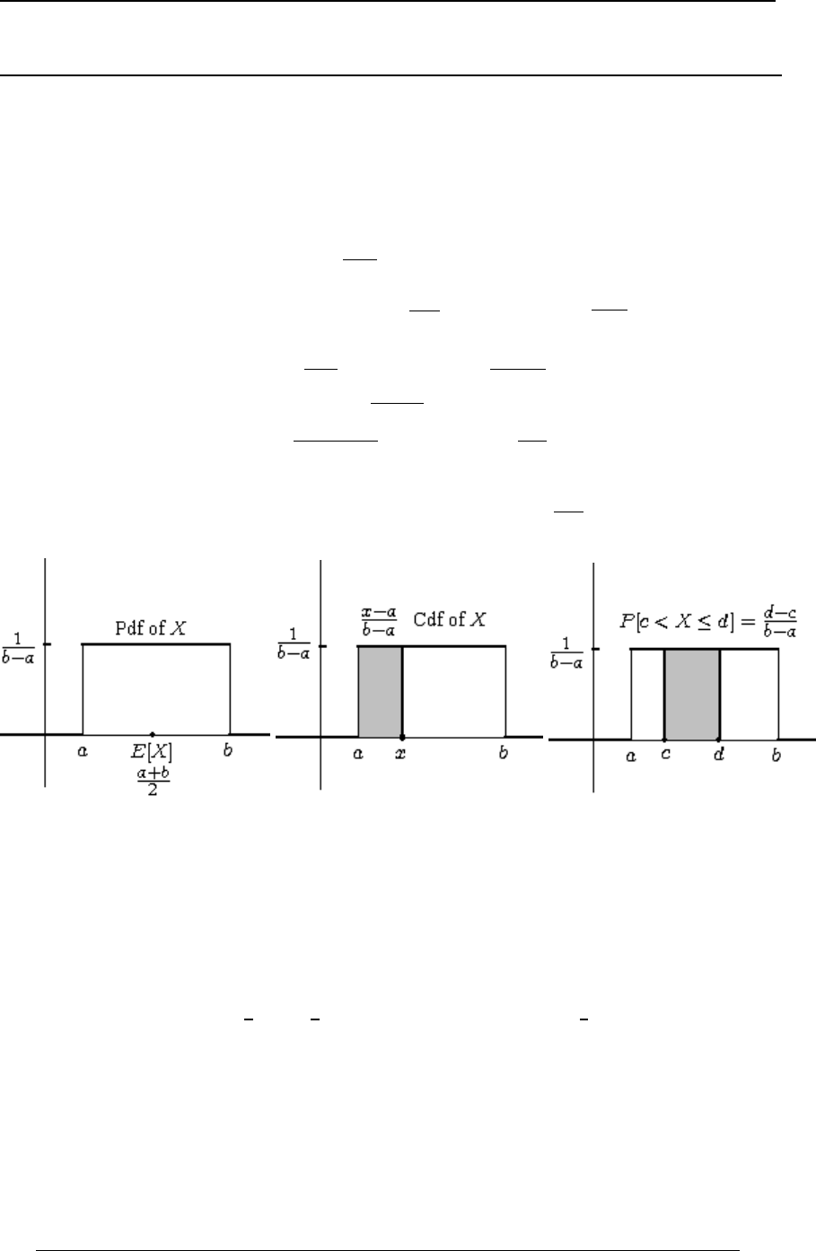
SECTION 7 - FREQUENTLY USED CONTINUOUS DISTRIBUTIONS 197

SECTION 7 - FREQUENTLY USED CONTINUOUS DISTRIBUTIONS

Note that for a continuous random variable , the following probabilities are the same:\

TÒ+  \  ,Ó TÒ+  \ Ÿ ,Ó TÒ+ Ÿ \  ,Ó TÒ+ Ÿ \ Ÿ ,Ó , , , .

Uniform distribution on the interval (where ):Ð+ß ,Ñ  ∞  +  ,  ∞

The density function is constant, and otherwise.0ÐBÑœ +B,

,+ for ß0ÐBÑœ!

The distribution function is , so .JÐBÑ œ 0ÐBÑ.B œ

BB+

,+ JÐBÑœ

!B+

+ŸBŸ,

"B,

B+

,+

The mean and variance are and .IÒ\Ó œ Z +<Ò\Ó œ

+,

#"#

Ð,+Ñ#

The moment generating function is for any real .QÐ>Ñœ >

\//

Ð,+Ñ†>

,> +>

The -th moment of is The median is , the same as the mean.8\IÒ\ÓœÞ

8,+ +,

Ð8"ÑÐ,+Ñ #

8" 8"

This is a symmetric distribution about the mean; the mean is the midpoint of the interval .Ð+ß ,Ñ

The probability of the subinterval of is .Ð-ß .Ñ Ð+ß ,Ñ T Ò-  \ Ÿ .Ó œ .-

,+

Example 7-1: Suppose that has a uniform distribution on the interval , where .\Ð!ß+Ñ+!

Find .TÒ\  \ Ó

Solution: If , then is always true for , so that .+Ÿ" \\ !\+ TÒ\\ Óœ"

If , then only if , which has probability+" \\ \"

T Ò\  "Ó œ 0ÐBÑ .B œ .B œ T Ò\  \ Ó œ 738Ò"ß Ó

"" #

"" "

++ +

. Thus, . 

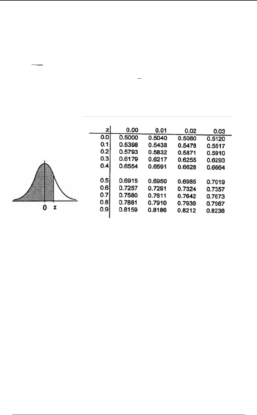
198 SECTION 7 - FREQUENTLY USED CONTINUOUS DISTRIBUTIONS

The Normal Distribution

The distribution, , has a mean of and variance of 1. A table ofstandard normal ^ µ R Ð!ß "Ñ !

probabilities for the standard normal distribution is provided on the exam. The density function

is 9ÐDÑœ †/ ∞D∞ IÒ^Óœ!ß Z+<Ò^Óœ"

È1

D Î#

#for . .

The moment generating function is .QÐ>Ñœ/B:

^’“

The density function has the following bell-shaped graph. The shaded area is the distribution

function , which is denoted . The graph and an excerpt from the standard normalTÒ^ Ÿ DÓ ÐDÑF

distribution table are given on the following page.

A normal distribution table is provided at the exam. The full table can be found just before the

practice exam section later in this study guide. The entries in the table are probabilities of the

form . The 95-th percentile of is 1.645 (sometimes denoted ) sinceFÐDÑ œ T Ò^ Ÿ DÓ ^ DÞ!&

FÐ"Þ'%&Ñ œ Þ*&! D œ "Þ'%& (the shaded region to the left of in the graph above).

We use the symmetry of the standard normal distribution to find for negative values of .FÐDÑ D

For instance, since the two regions have theFFÐ"ÑœTÒ^Ÿ "ÓœTÒ^"Óœ" Ð"Ñ

same area (probability). This is illustrated in the left graph below. The two outside areas are

equal, the left area is and the right area is . Notice also in the right graph belowFFÐ"Ñ " Ð"Ñ

that , since , and this area isT Ò  "Þ*' Ÿ ^ Ÿ "Þ*'Ó œ Þ*& T Ò^  "Þ*'Ó œ "  Ð"Þ*'Ñ œ Þ!#&F

deleted from both ends of the curve.

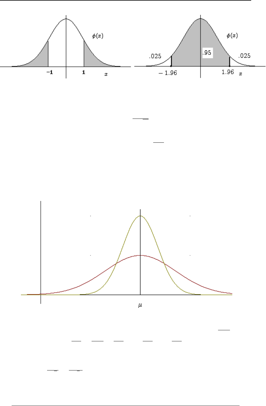
SECTION 7 - FREQUENTLY USED CONTINUOUS DISTRIBUTIONS 199

The general form of the normal distribution has mean and variance . This is a continuous.5

distribution with a "bell-shaped" density function similar to that of the standard normal, but

symmetric around the mean . The pdf is .0ÐBÑ œ †/ ∞  B  ∞

†#51

ÈÐB Ñ Î#.5

for .

and the mean, variance and moment generating function of are\

.IÒ\Ó œ ß Z +<Ò\Ó œ ß Q Ð>Ñ œ /B: > .5 .

#\’“

5##

Note also that for the normal distribution, . is the "center" of mean median modeœœœ..

the distribution, and the variance is a measure of how widely dispersed the distribution is.5#

The graph shows the density functions of two normal distributions with a common mean . The.

distribution with the "flatter" graph has the larger variance, and is more widely dispersed around

the mean.

Given any normal random variable , it is possible to find by first\µRÐ ß Ñ TÒ<\=Ó.5

"standardizing" . This means that we define the random variable as follows: .^^œ

\.

Then .TÒ<  \  =Ó œ TÒ   Ó œ Ð Ñ Ð Ñ

< \ = = <... . .

555 5 5

For example, suppose that has a normal distribution with mean 1 and variance 4. Then\

T Ò\ Ÿ #Þ&Ó œ T Ò Ÿ Ó œ T Ò^ Ÿ Þ(&Ó œ ÐÞ(&Ñ œ Þ(($%

\" #Þ&"

ÈÈ F .

We have found from the standard normal table.FÐÞ(&Ñ

200 SECTION 7 - FREQUENTLY USED CONTINUOUS DISTRIBUTIONS

The 95-th percentile of can be found as follows. Let us denote the 95-th percentile of by .\\-

Then .TÒ\Ÿ-ÓœÞ*& Ê TÒ Ÿ Óœ Ð ÑœÞ*& œ"Þ'%& Ê -œ%Þ#*

\" -" -" -"

%% % %

ÈÈ È È

FÊ

We have used the value 1.645, which is the 95-th percentile of the standard normal.

Example 7-2: If for a certain normal random variable , and\ T Ò\  &!!Ó œ Þ&

T Ò\  '&!Ó œ Þ!##( \ , find the standard deviation of .

Solution: The normal distribution is symmetric about its mean, with forTÒ\  Ó œ Þ&.

any normal random variable. Thus, for this normal we have . Then,\ œ &!!.

T Ò\  '&!Ó œ Þ!##( œ T 

’“

\&!! "&!

. From the standard normal table, we see that

FÐ#Þ!!Ñ œ Þ*(($ Þ Since has a standard normal distribution, it follows from the table for

\&!!

the standard normal distribution that and .

"&!

5œ#Þ!! œ(&5

Approximating a distribution using a normal distribution

Given a random variable with mean and variance , probabilities related to the distribution\.5

of are sometimes approximated by assuming the distribution of is approximately .\\RÐßÑ.5

The SOA/CAS probability exam regularly has questions involving the normal approximation. It

has sometimes been the case that a question asks for the approximate probability for some

interval. This will almost always mean that the normal approximation should be applied, even if it

is not specifically mentioned. Later in the study guide we will see the justification for using the

normal approximation for a sum of random variables. It is in this context that approximate

probabilities have come up on the exam.

Integer correction for the normal approximation to an integer-valued

random variable:

The normal distribution is continuous, but it can be used to approximate a discrete

integer- valued distribution. In such a case (if instructed to do so) we can apply the

following procedure.

If is discrete and integer-valued then an may be applied in the following\"integer correction"

way. If and are integers, the probability is approximated by using a normal87 TÒ8Ÿ\Ÿ7Ó

random variable with the same mean and variance as , and then finding the probability]\

TÒ8 Ÿ] Ÿ7 Ó Ò8ß7Ó Ò8 ß7 Ó

"" ""

## ##

. We extend the interval to . The reasoning

behind this can be seen from the following graphs, in which a normal density function is

superimposed over the histogram of an integer-valued random variable.

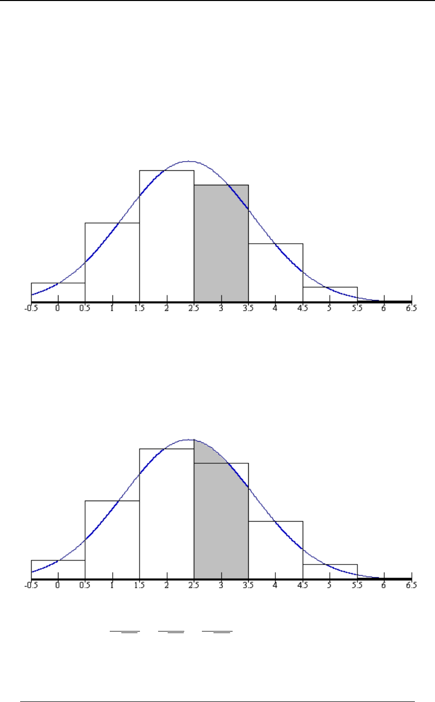
SECTION 7 - FREQUENTLY USED CONTINUOUS DISTRIBUTIONS 201

The integer-valued random variable in the following graphs happens to be a binomial with\

R œ ' : œ Þ% Ð'ÑÐÞ%Ñ œ #Þ% Ð'ÑÐÞ%ÑÐÞ'Ñ œ "Þ%% and , so the mean and variance are and . The

way in which the normal approximation is applied, is to use the normal distribution with the same

mean ( ) and variance ( ) as the original distribution. The density function in the.5œ#Þ% œ"Þ%%

graphs is of that normal distribution. In the first graph, the shaded region is the actual binomial

probability that the outcome of the binomial distribution is 3.

This actual probability is .

Š‹

$ÐÞ%Ñ ÐÞ'Ñ œ Þ#('%)

$'$

Since the normal distribution is a continuous distribution, in order to calculate a probability]

using the normal distribution, we must integrate the density over an interval. In order to use the

normal distribution to approximate the probability that the binomial outcome is 3, we integrate

over an interval of length 1 centered at . This is the integral from 2.5 to 3.5 of the normalBœ$

density, so the normal approximation probability is . This is the shadedT Ò#Þ&  ]  $Þ&Ó

region in the next graph.

For a normal distribution with mean 2.4 and variance 1.44, this probability is:

T Ò#Þ&  ]  $Þ&Ó œ T Ò   Ó œ T ÒÞ!)$$  ^  Þ*"'(Ó

#Þ&#Þ% ] #Þ% $Þ&#Þ%

"Þ%% "Þ%% "Þ%%

ÈÈÈ

œ ÐÞ*#Ñ  ÐÞ!)Ñ œ Þ)")'  Þ&$"* œ Þ#*FF . The exact binomial probability is .27648 .

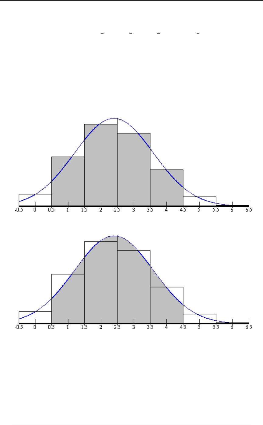
202 SECTION 7 - FREQUENTLY USED CONTINUOUS DISTRIBUTIONS

In general, the normal approximation for an integer value is the normal distribution ( )\œ5 ]

probability on the interval from to ( ). For the probability5 5 TÒ5 ] 5 Ó

""" "

### #

of several successive integer values, we have a series of intervals. For instance, to find the

probability that , we would approximate the probability at 1 , 2 , 3"Ÿ\Ÿ% \œ \œ \œ

and 4 and add them up. This corresponds to finding the normal probability for on the\œ ]

intervals from .5 to 1.5 , from 1.5 to 2.5, from 2.5 to 3.5 and from 3.5 to 4.5. When we combine

these, we get the probability from .5 to 4.5 , . This is illustrated in the followingT ÒÞ&  ]  %Þ&Ó

graphs. The shaded region of the first graph is the actual binomial probability .TÒ" Ÿ \ Ÿ %Ó

The shaded region of the second graph is the normal approximation probability .T ÒÞ&  ]  %Þ&Ó

Note that if we were asked to approximate the probability , then this would beTÒ"  \  %Ó

T Ò\ œ # $Ó T Ò"Þ&  ]  $Þ&Ó or , which we would approximate it as . If we were asked to

approximate , we would approximate it as .T Ò\ Ÿ &Ó T Ò]  &Þ&Ó

SECTION 7 - FREQUENTLY USED CONTINUOUS DISTRIBUTIONS 203

There is a little bit of a vague area regarding the use of the integer correction on the exam and it

may be worthwhile to calculate probabilities both with and without the integer correction. If the

probability corresponding to the integer correction is one of the possible answers, it should be the

correct answer (unless there is an indication that the integer correction should not be used).

We will consider sums of independent random variables in more detail later in this study guide,

but one rule to make a note of now is the following. If and are independent normal\\

random variables with means and , and variances and , respectively, then.. 55

"# ##

[œ\ \  

"# "# ##

is also a normal random variable, and has mean , and variance ... 55

Example 7-3: Suppose that a multiple choice exam has 40 questions, each with 5 possible

answers. A well prepared student feels that he has a probability of . of getting any particular&

question correct, with independence from one question to another. Apply the normal

approximation to , the number of correct answers out of 40, to determine the probability of\

getting at least 25 correct. Find the probability with the integer correction, and then without the

correction.

Solution: The number of questions answered correctly, say , has a binomial distribution with\

mean and variance . Applying the normal approximation toÐ%!ÑÐÞ&Ñ œ #! Ð%!ÑÐÞ&ÑÐÞ&Ñ œ "! ]

\, with integer correction to find the probability of answering at least 25 correct, we get

T Ò\  #&Ó œ T Ò]  #%Þ&Ó œ T Ò  Ó œ T Ò^  "Þ%#Ó œ "  Ð"Þ%#Ñ œ Þ!()

] #! #%Þ&#!

"! "!

ÈÈ F .

Without the integer correction, the probability is

T Ò]  #&Ó œ T Ò  Ó œ T Ò^  "Þ&)Ó œ "  Ð"Þ&)Ñ œ Þ!&(

] #! #&#!

"! "!

ÈÈ F.

There is a noticeable difference between the two approaches. If has a much larger standard\

deviation, then the difference is not so noticeable. 

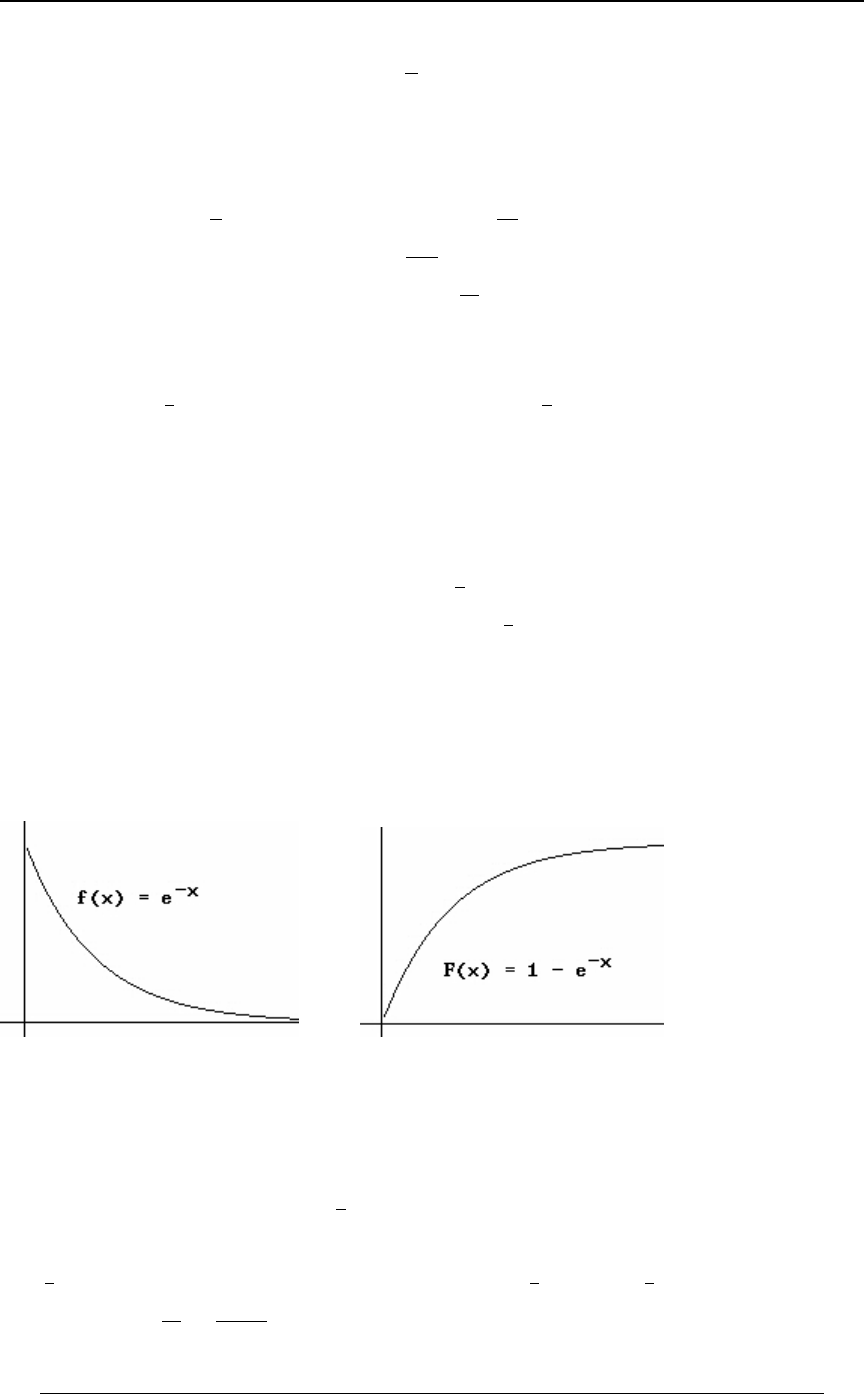
204 SECTION 7 - FREQUENTLY USED CONTINUOUS DISTRIBUTIONS

Exponential distribution with mean "

-!

The density function is and otherwise.0ÐBÑ œ / B  !-B- for , 0ÐBÑ œ !

The distribution function is , andJÐBÑœ"/ B  !

B-for

the survival function is .WÐBÑ œ "  J ÐBÑ œ T Ò\  BÓ œ /B-

The mean is the variance is andIÒ\Ó œ Z +<Ò\Ó œ

ßß #

the moment generating function is for QÐ>Ñœ >

-> -

The -th moment is , 5 IÒ\ Ó œ B † / .B œ 5 œ "ß #ß $ß ÞÞÞ

55B

∞

'--5x

-5

An alternative, but equivalent way to describe the exponential distribution is with the density

function , using the parameter . Then (the mean of ) is the0ÐBÑ œ / œ \

BÎ)))

relationship linking the parameters in these two descriptions of the exponential distribution. Some

probability textbooks use one definition and some use the other. This makes it somewhat

ambiguous if we are told that has an exponential distribution with "parameter 3". Does this\

mean , or does it mean ? It is more precise to be told that has an exponential-)œ$ œ$ \

distribution with 3. Then we know that based on the first definition, and a mean of "

-œ$ œ$)

based on the second. Either way, the density function is .

$/BÎ$

The exponential distribution is often used as a model for the time until some specific event

occurs, say the time until the next earthquake at a certain location.

The graphs of the pdf and cdf for the exponential distribution with mean 1 are

Example 7-4: The random variable has an exponential distribution such thatX

TÒX Ÿ#Óœ#†TÒX %Ó Z+<ÒXÓ . Find .

Solution: Suppose that has mean . Then X T ÒX Ÿ #Ó œ "  / œ #T ÒX  %Ó œ #/

-# %--

Ê#BB"œ! Bœ/

##

, where . Solving the quadratic equation results in

Bœ ß" / œ œ 68#

"""

###

. We ignore the negative root, so that , and .

#--

Then, . Z+<ÒXÓœ œ

Ð68 #Ñ-## 

SECTION 7 - FREQUENTLY USED CONTINUOUS DISTRIBUTIONS 205

Example 7-5: The initial cost of a machine is 3. The lifetime of the machine has an

exponential distribution with a mean of 3 years. The manufacturer is considering offering a

warranty and considers two types of warranties. Warranty 1 pays 3 if the machine fails in the first

year, 2 if the machine fails in the second year, and 1 if the machine fails in the third year, with no

payment if the machine fails after 3 years. Warranty 2 pays if the machine fails at time $/ >

>

years (with no limit on the time of failure). Find the expected warranty payment under each of

the two warranties.

Solution: The pdf of is , and the cdf is .X 0Ð>Ñ œ / J Ð>Ñ œ "  /

$>Î$ >Î$

Let be the amount paid by warranty 1. The distribution of is\\

\À$#"!

:ÐBÑÀ TÒ!X Ÿ"Ó TÒ"X Ÿ#Ó TÒ#X Ÿ$Ó TÒX $Ó

"  / œ Þ#)$& /  / œ Þ#!$" /  / œ Þ"%&& / œ Þ$'(*

    " "

""##

$$$$

IÒ\Ó œ Ð$ÑÐÞ#)$&Ñ  Ð#ÑÐÞ#!$"Ñ  Ð"ÑÐÞ"%&&Ñ œ "Þ%! .

Let be the amount paid by warranty 2. Then .]]œ$/

X

IÒ]Óœ $/ † / .>œ / .>œ

∞∞

> >Î$ %>Î$

. 

There are a few additional properties satisfied by the exponential distribution that are worth

noting.

(i) for ,

Lack of memory property: Bß C  !

TÒ\BCl\BÓœ œ œ œ/ œTÒ\CÓ

TÖ\BC∩\BÓ TÖ\BCÓ

TÒ\BÓ TÒ\BÓ

ÐBCÑ

B

-C- .

We can interpret this as follows. Suppose that represents the time, measured from now, in\

weeks until the next insurance claim filed by a company, and suppose also that has an\

exponential distribution with mean . Suppose that 5 weeks have passed without an insurance

claim, and we want to know the distribution of the time until the next insurance claim as

measured from our new time origin, which is 5 weeks after the previous time origin. According to

the lack of memory property, the fact that there have been no claims in the past 5 weeks is

irrelevant, and measuring time starting from our new time origin, the time until the next claim is

exponential with the same mean . In fact, no matter how many claims have occurred in the past

5 weeks, as measured from now, the time until the next claim has an exponential distribution with

mean ; the distribution has "forgotten" what has happened prior to now and the "clock"

measuring time until the next claim is restarted now..

206 SECTION 7 - FREQUENTLY USED CONTINUOUS DISTRIBUTIONS

(ii) Link between the exponential distribution and Poisson distribution:

Suppose that has an exponential distribution with mean and we regard as the time\\

between successive occurrences of some type of event (say the event is the arrival of a new

insurance claim at an insurance office), where time is measured in some appropriate units

(seconds, minutes, hours or days, etc.). Now, we imagine that we choose some starting time (say

labeled as ), and from now we start recording times between successive events. For>œ!

instance, the first claim may arrive in 2 days, then the next claim arrives 3 days after that, etc.

Let represent the Rnumber of events (claims) that have occurred when one unit of time has

elapsed. Then will be a random variable related to the times of the occurring events. It can beR

shown that the distribution of is Poisson with a mean of .R-

(iii) The minimum of a collection of independent exponential random variables:

Suppose that independent random variables each have exponential distributions] ß ] ß ÞÞÞß ]

"# 8

with means , respectively. Let . Then has an

"" "

-- -

"# 8

ß ß ÞÞÞß ] œ 738Ö] ß ] ß ÞÞÞß ] × ]

"# 8

exponential distribution with mean . An interpretation of this relationship is as

â-- -

"# 8

follows. Suppose that an insurer has two types of insurance policies, basic coverage and extended

coverage. Suppose insurance policies are independent of one another and that the time until a\F

claim from a basic policy is exponential with a mean of 4 weeks, and the time until a claim\I

from an extended policy is exponential with a mean of 2 weeks. The time until the next claim of

any type is . will be exponential with mean weeks. Another\œ738Ö\ ß\ × \ œ

FI "%

$

way of interpreting this is that the average number of claims per week for basic policies is (one

every 4 weeks) and the average number of claims per week for extended policies is , so the

average number of claims per week for the two policy types combined is .

We can descibe the average of claims per weeks an average of weeks between claims.

Example 7-6: Verify algebraically the validity of properties (i) and (iii) of the exponential

distribution described above.

Solution: (i) Suppose that has an exponential distribution with parameter . Then\-

TÒ\BCl\BÓœ œ œ œ/

T ÒÐ\BCÑ∩Ð\BÑÓ T Ò\BCÓ

TÒ\BÓ TÒ\BÓ

ÐBCÑ

B

-C-,

and .TÒ\  CÓ œ /

C-

SECTION 7 - FREQUENTLY USED CONTINUOUS DISTRIBUTIONS 207

Example 7-6 continued

(iii) Suppose that independent random variables have exponential distributions with] ß ] ß ÞÞÞß ]

"# 8

means respectively. Let . Then,

"" "

-- -

"# 8

ß ß ÞÞÞß ] œ 738Ö] ß ] ß ÞÞÞß ] ×

"# 8

T Ò]  CÓ œ T Ò]  C 3 œ "ß #ß ÞÞÞß 8Ó œ T ÒÐ]  CÑ ∩ Ð]  CÑ ∩ â ∩ Ð]  CÑÓ

3"#8

for all

œTÒ] CÓ†TÒ] CÓâTÒ] CÓ ]

"# 8 3

(because of independence of the 's)

œ Ð/ ÑÐ/ ÑâÐ/ Ñ œ / Þ ]

C C C ÐâÑC-- - ---

"# 8 "#8

The cdf of is then

J ÐCÑœTÒ] ŸCÓœ"TÒ] CÓœ"/ ]

]Ð  â ÑC-- -

"# 8

and the pdf of is

0ÐCÑœJÐCÑœÐ  â Ñ/

]"#8

wÐâÑC

]-- - -- -

"# 8

, which is the pdf of an

exponential distribution with parameter . -- -

"# 8

â 

Gamma distribution with parameters and α"! !

The pdf is for , and otherwise.0ÐBÑ œ B  ! 0ÐBÑ œ !

>α

αα "

†B †/

ÐÑ

"  B

>α α >αÐÑ ! ÐÑœ C †/ .C is the , which is defined for to be .gamma function '!

∞" Cα

If is a positive integer it can be shown that .8Ð8ÑœÐ8"Ñx>

The mean, variance and moment generating function of are and\ IÒ\Ó œ ß Z +<Ò\Ó œ ß

αα

QÐ>ÑœÐ Ñ >

">

α for ."

If this distribution was to show up on Exam P, it would likely have the parameter as an integerα

80ÐBÑœ, in which case the density would be .

"α"

†B †/

Ð8"Ñx

8"  B

An alternative, but equivalent parametrization of uses and the same , so the pdf,\œ)α

mean, and variance are written as and .0ÐBÑ œ ß IÒ\Ó œ Z+<Ò\Ó œ

B†/

†ÐÑ

α)

" B/

)>α α) α)#

Note that the exponential distribution with mean is a special case of the gamma distribution

with and . The graphs below illustrate the density functions of a few gammaα"-œ" œ

distributions with various combinations of parameters and .α"

The cdf of the gamma distribution can be complicated. If is an integer then it is possible to findα

the cdf by integration by parts. But this would tend to be quite tedious unless is 1 or 2.α

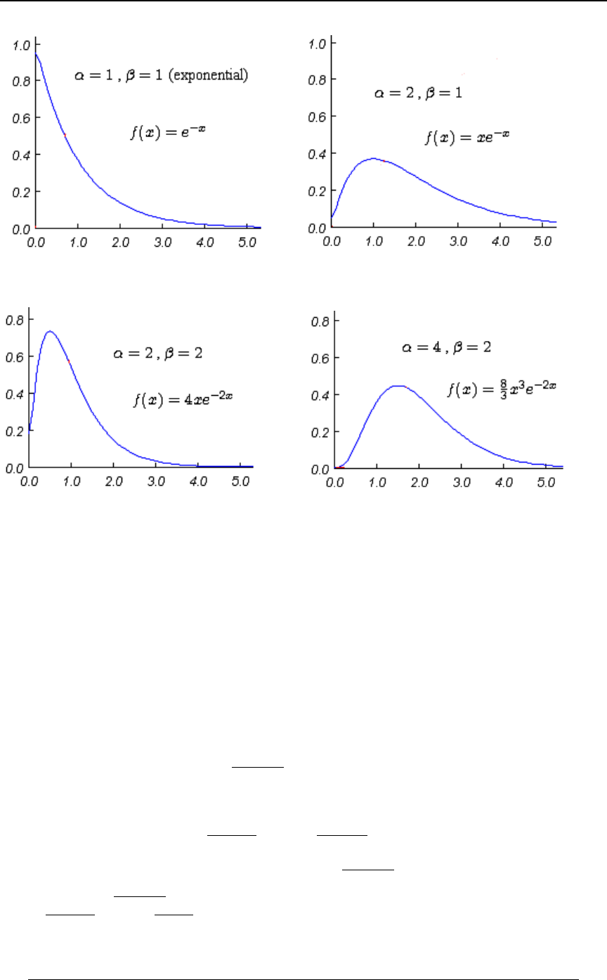
208 SECTION 7 - FREQUENTLY USED CONTINUOUS DISTRIBUTIONS

Gamma distribution density functions

As gets larger, the pdf becomes more weighted to the right and is more spread out. As getsα "

larger, the pdf is more weighted to the left and becomes more peaked.

For Exam P it is very important to be familiar with the uniform, normal and exponential

distributions.

Example 7-7: An insurer will pay 80% of the loss incurred on a loss of amount . The loss\

random variable has pdf for , and for .\ 0ÐBÑ œ B  "!! 0ÐBÑ œ ! B Ÿ "!!

$ß!!!ß!!!

Find the standard deviation of the amount paid by the insurer.

Solution: If is the amount paid by the insurer, then , so that]]œÞ)\

Z +<Ò] Ó œ ÐÞ)Ñ Z +<Ò\Ó Z +<Ò] Ó œ ÐÞ)Ñ Z +<Ò\Ó

# , and .

ÈÈ

Z +<Ò\Ó œ IÒ\ Ó  ÐIÒ\ÓÑ IÒ\Ó œ B † .B œ "&!

## "!!

∞

, where and

'$ß!!!ß!!!

IÒ\ Ó œ B † .B œ $!ß !!! Z +<Ò\Ó œ $!ß !!!  Ð"&!Ñ œ (ß &!!

## #

"!!

∞

'$ß!!!ß!!!

B% . Then ,

and .

ÈÈ

Z +<Ò] Ó œ ÐÞ)Ñ (ß &!! œ '*Þ$ 

209 SECTION 7 - FREQUENTLY USED CONTINUOUS DISTRIBUTION

SUMMARY OF CONTINUOUS DISTRIBUTIONS

Distribution Parameters PDF Mean Variance MGFßßIÒ\ÓßZ+<Ò\ÓßQÐ>Ñ:ÐBÑ \

Uniform +, ß+B,

",+ //

,+ # "# Ð,+Ñ†>

Ð,+Ñ

#,> +>

Normal (any number) ..5.ß†/ /B:>

" >

†# #

ÈÐB Ñ Î# #.5

## ’“

5#! ∞B∞

Exponential

"""

>----

œ! / ßB!)-

B-#

JÐBÑ œ "/

B-

Gamma , , α"! ! B! Ð Ñ

" "

>α " " "

αα

αα "

†B †/

ÐÑ >

"  B

210

PROBLEM SET 7 211

PROBLEM SET 7

Frequently Used Continuous Distributions

1. Let be a random variable with a continuous uniform distribution on the interval \Ð"ß+Ñ

where . If , then +" IÒ\Óœ'†Z+<Ò\Ó +œ

A) B) C) D) E) #$$#()

2. A large wooden floor is laid with strips 2 inches wide and with negligible space between

strips. A uniform circular disk of diameter 2.25 inches is dropped at random on the floor. What

is the probability that the disk touches three of the wooden strips?

A) B) C) D) E)

"""""

È111

3. If has a continuous uniform distribution on the interval from 0 to 10, then what is\

TÒ\   (Ó

\ ?

A) B) C) D) E)

$ $" " $* (

"! (! # (! "!

Problems 4 and 5 relate to the following information. Three individuals are running a one

kilometer race. The completion time for each individual is a random variable. is the\3

completion time, in minutes, for person .3

\ À Ò#Þ* ß $Þ"Ó

" uniform distribution on the interval

\ À Ò#Þ( ß $Þ"Ó

# uniform distribution on the interval

\ À Ò#Þ* ß $Þ$Ó

$ uniform distribution on the interval

The three completion times are independent of one another.

4. Find the probability that the earliest completion time is less than 3 minutes.

A) .89 B) .91 C) .94 D) .96 E) .98

5. Find the probability that the latest completion time is less than 3 minutes (nearest .01).

A) .03 B) .06 C) .09 D) .12 E) .15

212 PROBLEM SET 7

6. A student received a grade of 80 in a math final where the mean grade was 72 and the standard

deviation was . In the statistics final, he received a 90, where the mean grade was 80 and the=

standard deviation was 15. If the standardized scores (i.e., the scores adjusted to a mean of 0 and

standard deviation of 1) were the same in each case, then =œ

A) B) C) D) E) "! "# "' ") #!

7. If has a standard normal distribution and , what is the -th moment of ?\]œ/5]

A) B) C) D) !"/ /

5Î# 5 Î#

E) if and if "5œ#7" / 5œ#7

Ð#7"ÑÐ#7$Ñâ$†"

8. (SOA) For Company A there is a 60% chance that no claim is made during the coming year. If

one or more claims are made, the total claim amount is normally distributed with mean 10,000

and standard deviation 2,000. For Company B there is a 70% chance that no claim is made during

the coming year. If one or more claims are made, the total claim amount is normally distributed

with mean 9,000 and standard deviation 2,000. Assume that the total claim amounts of the two

companies are independent. What is the probability that, in the coming year, Company B’s total

claim amount will exceed Company A’s total claim amount?

A) 0.180 B) 0.185 C) 0.217 D) 0.223 E) 0.240

9. (SOA) The waiting time for the first claim from a good driver and the waiting time for the first

claim from a bad driver are independent and follow exponential distributions with means 6 years

and 3 years, respectively. What is the probability that the first claim from a good driver will be

filed within 3 years and the first claim from a bad driver will be filed within 2 years?

A) B) C)

") ")

"/// / "/ / /

Š‹

#Î$ "Î# (Î' (Î' #Î$ "Î# (Î'

D) E) "/// "///

#Î$ "Î# "Î$ #Î$ "Î# (Î'

"" "

$'")

10. Let be a continuous random variable with density function\

0ÐBÑœ / ∞B∞ IÒ\l\!Ó

È1

B Î#

# for . Calculate .

A) B) C) D) E) !"

"" #

È211

PROBLEM SET 7 213

11. (SOA) Two instruments are used to measure the height, h, of a tower. The error made by the

less accurate instrument is normally distributed with mean 0 and standard deviation 0.0056h . The

error made by the more accurate instrument is normally distributed with mean 0 and standard

deviation 0.0044h . Assuming the two measurements are independent random variables, what is

the probability that their average value is within 0.005h of the height of the tower?

A) 0.38 B) 0.47 C) 0.68 D) 0.84 E) 0.90

12. A new car battery is sold for $100 with a 3-year limited warranty. If the battery fails at time

> !  >  $ "!!Ð"  Ñ ( ), the battery manufacturer will refund $ . After analyzing battery

performance, the battery manufacturer uses the (continuous) uniform distribution on the interval

Ð!ß 8Ñ 8 as the model for time until failure for the battery ( in years). The battery manufacturer

determines that the expected cost of the warranty is $10. Find .8

A) 3 B) 5 C) 10 D) 15 E) 30

13. (SOA) The lifetime of a printer costing 200 is exponentially distributed with mean 2 years.

The manufacturer agrees to pay a full refund to a buyer if the printer fails during the first year

following its purchase, and a one-half refund if it fails during the second year. If the

manufacturer sells 100 printers, how much should it expect to pay in refunds?

A) 6,321 B) 7,358 C) 7,869 D) 10,256 E) 12,642

14. (SOA) A piece of equipment is being insured against early failure. The time from purchase

until failure of the equipment is exponentially distributed with mean 10 years. The insurance will

pay an amount if the equipment fails during the first year, and it will pay if failure occursB!Þ&B

during the second or third year. If failure occurs after the first three years, no payment will be

made. At what level must be set if the expected payment made under this insurance is to beB

1000 ?

A) 3858 B) 4449 C) 5382 D) 5644 E) 7235

15. (SOA) The time to failure of a component in an electronic device has an exponential

distribution with a median of four hours. Calculate the probability that the component will work

without failing for at least five hours.

A) 0.07 B) 0.29 C) 0.38 D) 0.42 E) 0.57

214 PROBLEM SET 7

16. An insurer uses the exponential distribution with mean as the model for the total annual.

claim occurring from a particular insurance policy in the current one year period. The insurer

assumes an inflation factor of 10% for the one year period following the current one year period.

Using the insurer's assumption, find the coefficient of variation ( ) for the

=>+8.+<. ./@3+>398

/B:/->/. @+6?/

annual claim paid on the policy for the one year period following the current one year period.

A) B) C) D) E) "Þ#" "Þ" " ""

"Þ" "Þ#"

17. Average loss size per policy on a portfolio of policies is 100. Actuary 1 assumes that the

distribution of loss size has an exponential distribution with a mean of 100, and Actuary 2

assumes that the distribution of loss size has a pdf of , . If and 0ÐBÑœ B! 7 7

#"#

ÐB Ñ

)

represent the median loss sizes for the two distributions, find .

A) .6 B) 1.0 C) 1.3 D) 1.7 E) 2.0

18. The time until the occurrence of a major hurricane is exponentially distributed. It is found

that it is 1.5 times as likely that a major hurricane will occur in the next ten years as it is that the

next major hurricane will occur in the next five years. Find the expected time until the next major

hurricane.

A) B) C) D) E)&&68# "!68#

&"!

68 # 68 #

PROBLEM SET 7 215

PROBLEM SET 7 SOLUTIONS

1. and , so thatIÒ\Ó œ Z +<Ò\Ó œ

"+

#"#

Ð+"Ñ#

+"

#"#

Ð+"Ñ

œ'† Ê + $+œ! Ê +œ!ß$ Ê +œ$ +!

## (since ). Answer: B

2. Let us focus on the left-most point on the disk. Consider two adjacent strips on the floor.:

Let the interval represent the distance as we move across the left strip from left to right. IfÒ!ß #Ó

: ! "Þ(& is between and , then the disk lies within the two strips.

If is between and , the disk will lie on 3 strips (the first two and the next one to the right).:"Þ(&#

Since any point between and is equally likely as the left most point on the disk (i.e.!# :

uniformly distributed between and ) it follows that the probability that the disk will touch three!#

strips is . Answer: D

Þ#& "

3. Since the density function for is for , we can regard as\0ÐBÑœ !B"! \

being positive. Then

T Ò\   (Ó œ T Ò\  (\  "!  !Ó œ T ÒÐ\  &ÑÐ\  #Ñ  !Ó

œTÒ\&ÓTÒ\#Ó Ð>&ÑÐ>#Ñ! >&ß>#! (since if either both

or both ) . Answer: E>&ß>#! œ  œ

&# (

"! "! "!

4. for for 0 Ð>Ñœ œ& #Þ*Ÿ>Ÿ$Þ"ß J Ð>ÑœTÒ\ Ÿ>Óœ&Ð>#Þ*Ñ #Þ*Ÿ>Ÿ$Þ"Þ

\\"

Þ#

0 Ð>Ñ œ œ & #Þ Ÿ > Ÿ $Þ" ß J Ð>Ñ œ T Ò\ Ÿ >Ó œ #Þ&Ð>  #Þ(Ñ #Þ( Ÿ > Ÿ $Þ" Þ

\\#

Þ42. for 7 for

0 Ð>Ñ œ œ #Þ& #Þ* Ÿ > Ÿ $Þ$ ß J Ð>Ñ œ T Ò\ Ÿ >Ó œ #Þ&Ð>  #Þ*Ñ #Þ* Ÿ > Ÿ $Þ$ Þ

\\$

Þ% for for

TÒ738Ð\ß\ß\Ñ$Óœ"TÒ738Ð\ß\ß\Ñ$Ó

"#$ "#$

œ"TÒÐ\$Ñ∩Ð\$Ñ∩Ð\$ÑÓ

"#$

œ"Ò"J Ð$ÑÓ†Ò"J Ð$ÑÓ†Ò"J Ð$ÑÓ

\\\

"#$

œ "  Ò"  &Ð$  #Þ*ÑÓ † Ò"  #Þ&Ð$  #Þ(ÑÓ † Ò"  #Þ&Ð$  #Þ*ÑÓ œ Þ*!'#& . Answer: B

5. TÒ7+BÐ\ß\ ß\Ñ$ÓœTÒÐ\ $Ñ∩Ð\ $Ñ∩Ð\ $ÑÓ

"#$ " # $

œ J Ð$Ñ † J Ð$Ñ † J Ð$Ñ œ Ò&Ð$  #Þ*ÑÓ † Ò#Þ&Ð$  #Þ(ÑÓ † Ò#Þ&Ð$  #Þ*ÑÓ œ Þ!*$(& Þ

\\\

"#$

Answer: C

216 PROBLEM SET 7

6. The standardized statistics score is . The standardized math score is

*!)! #

"& $

)!(# ) #

==$

œœp=œ"#. Answer: B

7. The -th moment of is (since and ). 5 ] IÒ] ÓœIÒ/ ÓœQ Ð5Ñœ/ œ! œ"

5 5\ 5 Î# #

#.5

Answer: D

8. We denote by and the total claim amount for the coming year for Company A and B,\\

respectively. We are asked to find . is a mixture of two parts.TÒ\  \ Ó \

FEE

There is a discrete part,

TÒ Ó œ TÒ\ œ !Ó œ Þ'Company A has no claims in the coming year ,

and a continuous part

TÒ ÓCompany A has some claims in the coming year

œ T Ò\ Ó œ Þ%

E has a normal distribution with mean 10,000 and standard deviation 2,000 .

\F is similar. There is a discrete part

TÒ Ó œ TÒ\ œ !Ó œ Þ(Company B has no claims in the coming year ,

and a continuous part

TÒ ÓCompany B has some claims in the coming year

œ T Ò\ Ó œ Þ$

F has a normal distribution with mean 9,000 and standard deviation 2,000 .

Therefore, and

prob. .6

, normal, mean 10,000, std. dev. 2000 prob. .4

\œ !

]

\œ !

]

œprob. .7

, normal, mean 9,000, std. dev. 2000 prob. .3 .

We use the following probability rule:

TÒGÓœTÒGlH Ó†TÒH ÓTÒGlH Ó†TÒH ÓâTÒGlH Ó†TÒH Ó

"" ## 88

for any event and any partition of events .G H ß H ß ÞÞÞß H

"# 8

In this case, the event is , and the partition has 4 events,G\\

HÀ

" Company A has no claims and Company B has no claims,

HÀ

# Company A has no claims and Company B has some claims,

HÀ

$ Company A has some claims and Company B has no claims,

HÀ

% Company A has some claims and Company B has some claims.

The companies have independent claim amounts, so we can use the following rule for

independent events: .T ÒY ∩ Z Ó œ T ÒY Ó † T ÒZ Ó

PROBLEM SET 7 217

8. continued

The probabilities of the partition events are

TÒH Ó œ TÒ ∩ Ó

"(no claims for company A) (no claims for company B)

œTÒ Ó†TÒ ÓœÐÞ'ÑÐÞ(ÑœÞ%#no claims for company A no claims for company B .

T ÒH Ó œ Ð'ÞÑÐÞ$Ñ œ Þ") ß T ÒH Ó œ ÐÞ%ÑÐÞ(Ñ œ Þ#) ß T ÒH Ó œ ÐÞ%ÑÐÞ$Ñ œ Þ"#

#$%

Using the partition rule above, we have

TÒ\ \ ÓœTÒ\ \ lH Ó†TÒH ÓTÒ\ \ lH Ó†TÒH Ó

FF""F##

EE E

TÒ\ \ lH Ó†TÒH ÓTÒ\ \ lH Ó†TÒH Ó

F$$F%%

TÒ\\lHÓœ! \œ\œ!

F" F

, since in this case .

TÒ\ \ lH ÓœTÒ] !ÓœTÒ  Ó

F#F

E] *ß!!! !*ß!!!

#ß!!! #ß!!!

œ T Ò^   %Þ&Ó œ Ð%Þ&Ñ œ " \ œ ! \ œ ]F . In this case and has a normal distribution,

EFF

and we can standardize the probability; has a standard normal distribution^

(mean 0, standard deviation 1).

TÒ\ \ lH ÓœTÒ] !ÓœTÒ  Ó

] "!ß!!! !"!ß!!!

#ß!!! #ß!!!

œTÒ^ &Óœ Ð&Ñœ" Ð&Ñœ! \ œ! \ œ]FF . In this case, and has a normal

FEE

distribution, and we can standardize the probability.

TÒ\ \ lH ÓœTÒ] ] ÓœTÒ] ] !Ó

F%F F

EEE

. Since claims from the two companies are

independent, and are independent. The sum or difference of normal random variables is]]

normal, and the mean is the sum or difference of the means. The mean of is]]

*ß !!!  "!ß !!! œ  "ß !!! ] ] . Since and are independent,

Z +<Ò]  ] Ó œ #!!!  #!!! œ )ß !!!ß !!!

FE## .

Then standardizing , we get]]

TÒ\ \ lH ÓœTÒ] ] ÓœTÒ] ] !Ó

F%F F

EEE

œ T Ò  Ó œ T Ò^  Þ$&$'Ó œ "  ÐÞ$&Ñ œ Þ$'$

] ] Ð"ß!!!Ñ !Ð"ß!!!Ñ

)ß!!!ß!!! )ß!!!ß!!!

ÈÈ F

(from the normal distribution table, we get ).FFFÐÞ$&Ñ œ ÐÞ&Ñ ÐÞ$Ñ  ÐÞ&Ñ ÐÞ%Ñ œ Þ'$(

Finally,

T Ò\  \ Ó œ Ð!ÑÐÞ%#Ñ  Ð"ÑÐÞ")Ñ  Ð!ÑÐÞ#)Ñ  ÐÞ$'$ÑÐÞ"#Ñ œ Þ##$

FE .

218 PROBLEM SET 7

8. continued

This solution can be summarized using some "general intuitive reasoning" as follows. The only

way that can be greater than is if Company B has some claims. If Company A has no\\

claims (prob. .6) and Company B has some claims (prob. .3), then the probability that Company

B's claim amount will exceed Company A's claim is 1. If Company A has some claims (prob. .4)

and Company B has some claims (prob. .3), then the probability that Company B's claims exceed

Company A's claims is .363 (as outlined above). The overall probability that Company B's

claims exceed Company A's claims is . ÐÞ'ÑÐÞ$ÑÐ"Ñ  ÐÞ%ÑÐÞ$ÑÐÞ$'$Ñ œ Þ##$

Answer: D

9. Let be the time until a claim from the good driver. Then the pdf of isXX

1 1

0Ð>Ñœ / X

>Î'

' (exponential with a mean of 6). Let be the time until a claim from the bad

driver. Then the pdf of is (exponential with a mean of 3).X0Ð>Ñœ/

,, >Î$

Let be the event that the first claim from a good driver will be filed within 3 years.E

TÒEÓœTÒX $Óœ / .>œ"/

$>Î' "Î#

' .

Let be the event that the first claim from a bad driver will be filed within 2 years.F

TÒFÓœTÒX #Óœ / .>œ"/

#>Î$ #Î$

$ .

The probability that the first claim from a good driver will be filed within 3 years and the first

claim from a bad driver will be filed within 2 years is . Since and areTÒE∩FÓ X X

independent, so are the events and . Therefore,EF

T ÒE ∩ FÓ œ T ÒEÓ † T ÒFÓ œ Ð"  / ÑÐ"  / Ñ œ "  /  /  /

"Î# #Î$ "Î# #Î$ (Î'.

Answer: C

10. has a distribution, so that the density function of the conditional distribution is\RÐ!ß"Ñ

0ÐBl\  !Ñ œ œ œ #0ÐBÑÞ

0ÐBÑ 0ÐBÑ

T Ò\!Ó "Î# The conditional expectation is

'' ¹É

∞∞

B Î# B Î#

B†0ÐBl\!Ñ.Bœ #B† / .Bœ  / œ œ

"###

###

Bœ!

Bœ∞

ÈÈÈ

111

Answer: D

PROBLEM SET 7 219

11. .IÐI Ñ œ IÐI Ñ œ ! ß Z +<ÐI Ñ œ ÐÞ!!&'2Ñ ß Z +<ÐI Ñ œ ÐÞ!!%%2Ñ

"# " #

II IÐIIÑœ! I I

"# "# " #

is normal with , and since and are independent,

Z +<ÐI  I Ñ œ Z +<ÐI Ñ  Z +<ÐI Ñ œ ÐÞ!!&'2Ñ  ÐÞ!!%%2Ñ œ ÐÞ!!("#2Ñ

"# " # ## #

The average of and is , which is also normal with mean andIIEœÐIIÑ !

"# "#

variance .Z +<ÐEÑ œ Z +<ÐI  I Ñ œ ÐÞ!!$&'2Ñ

%"# #

The average height is within of the height of the tower if the absolute error in the averageÞ!!&2

is less than . We wish to find .Þ!!&2 T ÐlEl  Þ!!&2Ñ œ T Ð  Þ!!&2  E  Þ!!&2Ñ

We standardize to getE

T Ð  Þ!!&2  E  Þ!!&2Ñ œ T Ð   Ñ

Þ!!&2IÐEÑ EIÐEÑ Þ!!&2IÐEÑ

Z+<ÐEÑ Z+<ÐEÑ Z+<ÐEÑ

ÈÈÈ

œTÐ ^ ÑœTÐ"Þ%^"Þ%Ñ

Þ!!&2! Þ!!&2!

Þ!!$&'2 Þ!!$&'2 ,

where has a standard normal distribution. From the standard normal table,^

T Ð^  "Þ%Ñ œ Þ*"*# T Ð^   "Þ%Ñ œ T Ð^  "Þ%Ñ œ Þ!)!) , so that ,

and therefore, . Answer: DT Ð  "Þ%  ^  "Þ%Ñ œ Þ*"*#  Þ!)!) œ Þ)$)%

12. The expected payout on the warranty is '!

$"!!Ð"  Ñ † .> œ œ "!

> " $!!

$8 #8

p8œ"& . Answer: D

13. The exponential distribution with a mean of 2 has density function

0ÐBÑ œ / ß B  !

#BÎ# for , and distribution function

TÒ\ŸBÓœJÐBÑœ"/ B!

BÎ# , for .

The probability that a printer will fail in the first year is

T Ò\ Ÿ "Ó œ J Ð"Ñ œ "  / œ Þ$*$%(

"Î# , so that the expected number of failures in the first

year out of 100 printers is 39.347 .

The probability that a printer will fail in the second year is

T Ò"  \ Ÿ #Ó œ J Ð#Ñ  J Ð"Ñ œ /  / œ Þ#$)'&

"Î# #Î# , so that the expected number of

failures in the first year out of 100 printers is 23.865 .

The expected amount the manufacturer will pay in refunds is

Ð#!!ÑÐ$*Þ$%(Ñ  Ð"!!ÑÐ#$Þ)'&Ñ œ "!ß #&' . Answer: D

14. The density function for the time of failure is (exponential with mean 10).X0Ð>ÑœÞ"/

Þ">

The amount paid is . The expected amount paid isTÐ>Ñ œ

B !>Ÿ"

Þ&B ">Ÿ$

!>$



IÒTÐXÑÓ œ TÐ>Ñ†0Ð>Ñ.B œ Þ"B/ .> Þ!&B/ .>

'''

!!"

∞"$

Þ"> Þ">

œ BÒ"  / Ó  Þ&BÒ/  / Ó œ Þ"(("(B

Þ" Þ" Þ$ .

In order for this to be 1000, we must have . Answer: DÞ"(("(B œ "!!! p B œ &'%%

220 PROBLEM SET 7

15. The exponential time until failure random variable has density function of the formX

0Ð>Ñœ / JÐ>ÑœTÒX Ÿ>Óœ"/ >!-> >- -

, and had distribution function for .

The median of the distribution is the time point that satisfies the relationship7

JÐ7Ñ œ Þ& 7 ; in other words, is the time point for which there is a 50% probability of failure by

time . We are given that , and therefore , from which it follows7 7œ% JÐ%Ñœ"/ œÞ&

%-

that . We are asked to find ./œÞ& TÒX&Óœ"JÐ&Ñœ/

% &- -

Using the relationship , we get ./ œ Ð/ Ñ T ÒX  &Ó œ / œ ÐÞ&Ñ œ Þ%#!

& % "Þ#& & "Þ#&-- -

Notice that we could solve for from the equation , but it is not necessary.-/œÞ&

%-

Answer: D

16. The coefficient of variation of a random variable is .\ÈZ+<Ò\Ó

IÒ\Ó

If denotes the claim amount for the current one year period, then .\ IÒ\Ó œ ß Z +<Ò\Ó œ..

The claim amount for the one year period following the current one year period is , with"Þ"\

mean , and varianceIÒ"Þ"\Ó œ Ð"Þ"ÑIÒ\Ó œ "Þ".

Z +<Ò"Þ"\Ó œ Ð"Þ"Ñ Z +<Ò\Ó œ Ð"Þ"Ñ

###

. .

The coefficient of variation in the following period is

ÈÈ ÈÈ

Z +<Ò"Þ"\Ó Z +<Ò\Ó

IÒ"Þ"\Ó Ð"Þ"ÑIÒ\Ó IÒ\Ó

Ð"Þ"Ñ Z +<Ò\Ó

œœœœ"

. . Answer: C

17. The cdf for distribution 1 is . The median must satisfyJÐBÑœ"/ 7

BÎ"!!

Þ& œ J Ð7 Ñ œ "  / p 7 œ '*Þ$

"" "

7 Î"!!

" .

The cdf for distribution 2 is JÐBÑœ 0Ð>Ñ.>œ .>œ" Þ

Ð> Ñ ÐB Ñ

))

The mean of distribution 2 is .IÒ\ Ó œ Ò"  J ÐBÑÓ .B œ .B œ œ "!!

∞∞

)

ÐB Ñ )

Therefore, the cdf of distribution 2 is , and the median satisfiesJÐBÑœ" 7

"!!

ÐB"!!Ñ

Þ&œJ Ð7Ñœ" Ê 7 œ%"Þ% œ œ"Þ'(

## #

"!! '*Þ$

Ð7 "!!Ñ 7 %"Þ%

. Then .

Answer: D

18. time, in years, until next major hurricane, is exponentially distributed with mean . TheXœ .

density function of is , and cumulative distribution function isX0Ð>Ñœ/

.>Î.

JÐ>ÑœTÒX Ÿ>Óœ"/ TÒX Ÿ"!Óœ"Þ&TÒX Ÿ&Ó

>Î. . We are given , so that

"  / œ Ð"Þ&ÑÒ"  / Ó /  "Þ&/  Þ& œ !

"!Î &Î "!Î &Î.. ..

. This can be written as .

With , this becomes the quadratic equation . with rootsB œ / B  "Þ&B  Þ& œ !

&Î #.

Bœ"ßÞ& / / œ" . Therefore, is either 1 or .5 . It is not possible to have ,

&Î &Î..

since that would require . Therefore, , so that ...œ∞ / œÞ& œ œ

&Î.& &

68 68 #

Answer: C

SECTION 8 - JOINT, MARGINAL, AND CONDITIONAL DISTRIBUTIONS 221

SECTION 8 - JOINT, MARGINAL,

AND CONDITIONAL DISTRIBUTIONS

Joint distribution of random variables and \]

A random variable is a numerical outcome that results from some random experiment, such as\

the number that turns up when tossing a die. It is possible that an experiment may result in two or

more numerical outcomes. A simple example would be the numbers that turn up when tossing

two dice. could be the number that turns up on the first die and could be the number on the\]

second die. Another example could be the following experiment. A coin is tossed and if the

outcome is head then toss one die, and if the outcome is tails then toss two dice. We could set

\œ" \œ# ] œ for a head and for a tail and total on the dice thrown. In both of the examples

just described, we have a pair of random variables and , that result from the experiment. \] \

and might be unrelated or independent of one another (as in the example of the toss of two]

independent dice), or they might be related to each other (as in the coin-dice example).

We describe the probability distribution of two or more random variables together as a joint

distribution. As in the case of a single discrete random variable, we still describe probabilities

for each possible pair of outcomes for a pair of discrete random variables. In the case of a pair of

random variables and , there would be probabilities of the form for\ ] TÒÐ\ œ BÑ ∩ Ð] œ CÑÓ

each pair of possible outcomes. For a pair of continuous random variables and , thereÐBß CÑ \ ]

would be a density function to describe density over a two dimensional region.

A joint distribution of two random variables has a probability function or probability density

function that is a function of two variables (sometimes denoted ). It is defined0ÐBß CÑ 0 ÐBß CÑ

\ß]

over a two-dimensional region. For joint distributions of continuous random variables and ,\]

the region of probability (the probability space) is usually a rectangle or triangle in the - plane.BC

If and are discrete random variables, then is the joint\ ] 0ÐBß CÑ œ T ÒÐ\ œ BÑ ∩ Ð] œ CÑÓ

probability function, and it must satisfy

(i) and (ii) .! Ÿ 0ÐBßCÑ Ÿ " 0ÐBßCÑ œ "



If and are continuous random variables, then must satisfy\] 0ÐBßCÑ

(i) and (ii) .0ÐBßCÑ  ! 0ÐBßCÑ.C.B œ "

∞ ∞

∞∞

222 SECTION 8 - JOINT, MARGINAL, AND CONDITIONAL DISTRIBUTIONS

In the two dice example described above, if the two dice are tossed independently of one another

then for each pair0ÐBß CÑ œ T ÒÐ\ œ BÑ ∩ Ð] œ CÑÓ œ T Ò\ œ BÓ ‚ T Ò] œ CÓ œ ‚ œ

"" "

'' $'

with and . The coin-die toss example above is moreB œ "ß #ß $ß %ß &ß ' C œ "ß #ß $ß %ß &ß '

complicated because the number of dice tossed depends on whether the toss is head or tails. If the

coin toss is a head then and so\ œ" ] œ"ß#ß$ß%ß&ß'

0Ð"ß CÑ œ T ÒÐ\ œ "Ñ ∩ Ð] œ CÑÓ œ ‚ œ C œ "ß #ß $ß %ß &ß '

"" "

#' "#

for .

If the coin toss is tail then and with\ œ # ] œ #ß $ß ÞÞÞß "#

0Ð#ß #Ñ œ T ÒÐ\ œ #Ñ ∩ Ð] œ #ÑÓ œ ‚ œ

"" "

#$' (#

0Ð#ß $Ñ œ T ÒÐ\ œ #Ñ ∩ Ð] œ $ÑÓ œ ‚ œ

"# "

#$' $'

, etc.

It is possible to have a joint distribution in which one variable is discrete and one is continuous,

or either has a mixed distribution. The joint distribution of two random variables can be extended

to a joint distribution of any number of random variables.

If is a subset of two-dimensional space, then is the summation (discrete case)ETÒÐ\ß]Ñ−EÓ

or double integral (continuous case) of over the region .0ÐBßCÑ E

Example 8-1: and are discrete random variables which are jointly distributed\]

with the probability function defined in the following table:0ÐBßCÑ

" ! "

From this table we see, for example, that""""

") * '

.] ! ! TÒ\œ!ß] œ "Óœ0Ð!ß"Ñœ

"" "

*' *

" """

'**

Find (i) , (ii) and (iii) .TÒ\ ] œ "Ó TÒ\ œ !Ó TÒ\  ]Ó

Solution: (i) We identify the -points for which , and the probability is theÐBß CÑ \  ] œ "

sum of over those points. The only combinations that sum to 1 are the points 0ÐBß CÑ Bß C Ð!ß "Ñ

and . Therefore, Ð"ß !Ñ T Ò\  ] œ "Ó œ 0Ð!ß "Ñ  0Ð"ß !Ñ œ  œ Þ

"" &

*' ")

(ii) We identify the -points for which . These are and (we omitÐBß CÑ \ œ ! Ð!ß  "Ñ Ð!ß "Ñ

Ð!ß !Ñ T Ò\ œ !Ó œ 0Ð!ß  "Ñ  0Ð!ß "Ñ œ  œ since there is no probability at that point). "" #

** *

(iii) The -points satisfying are and .ÐBß CÑ \  ] Ð  "ß !Ñ ß Ð  "ß "Ñ Ð!ß "Ñ

Then T Ò\  ] Ó œ 0Ð  "ß !Ñ  0Ð  "ß "Ñ  0 Ð!ß "Ñ œ   œ Þ

""" &

*")* ") 

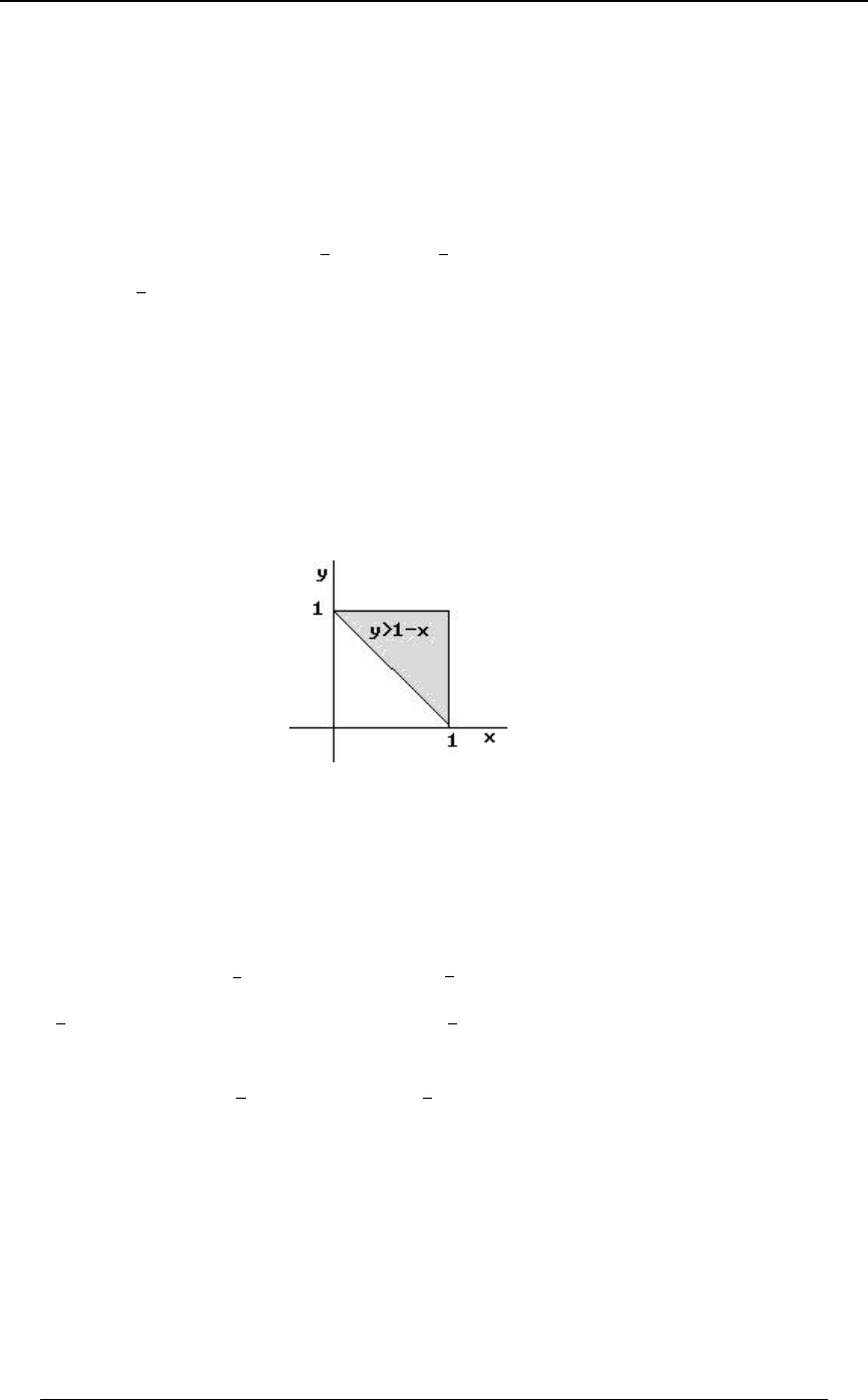
SECTION 8 - JOINT, MARGINAL, AND CONDITIONAL DISTRIBUTIONS 223

Example 8-2: Suppose that is the density function for the joint0ÐBßCÑ œ OÐB  C Ñ

distribution of the continuous random variables and defined over the unit square bounded by\]

the points and , find . Find .Ð!ß !Ñ ß Ð"ß !Ñ ß Ð"ß "Ñ Ð!ß "Ñ O T Ò\  ]  "Ó

Solution: In order for to be a properly defined joint density, the (double) integral of the0ÐBßCÑ

density function over the region of density must be 1, so that

" œ OÐB  C Ñ .C .B œ O † Ê O œ

"" ##

Ê 0ÐBß CÑ œ ÐB  C Ñ ! Ÿ B Ÿ " ! Ÿ C Ÿ " for and .

###

In order to find the probability , we identify the two dimensional regionTÒ\ ]  "Ó

representing . This is generally found by drawing the boundary line for the\] "

inequality, which is (or ) in this case, and then determining which side ofBCœ" Cœ"B

the line is represented in the inequality. We can see that is equivalent to .BC" C"B

This is the shaded region in the graph below.

The probability is found by integrating the joint density over the two-dimensionalTÒ\ ]  "Ó

region. It is possible to represent two-variable integrals in either order of integration. In some

cases one order of integration is more convenient than the other. In this case there is not much

advantage of one direction of integration over the other.

TÒ\  ]  "Ó œ ÐB  C Ñ .C .B œ Ð$B C  C Ñ .B

'' ' ¹

!"B !

"" "

## # $

#Cœ"B

Cœ"

œ Ð$B "$B Ð"BÑÐ"BÑ Ñ.Bœ Þ

"## $

Reversing the order of integration, we have , so thatB"C

TÒ\  ]  "Ó œ ÐB  C Ñ.B .C œ Þ

!"C

"" ##



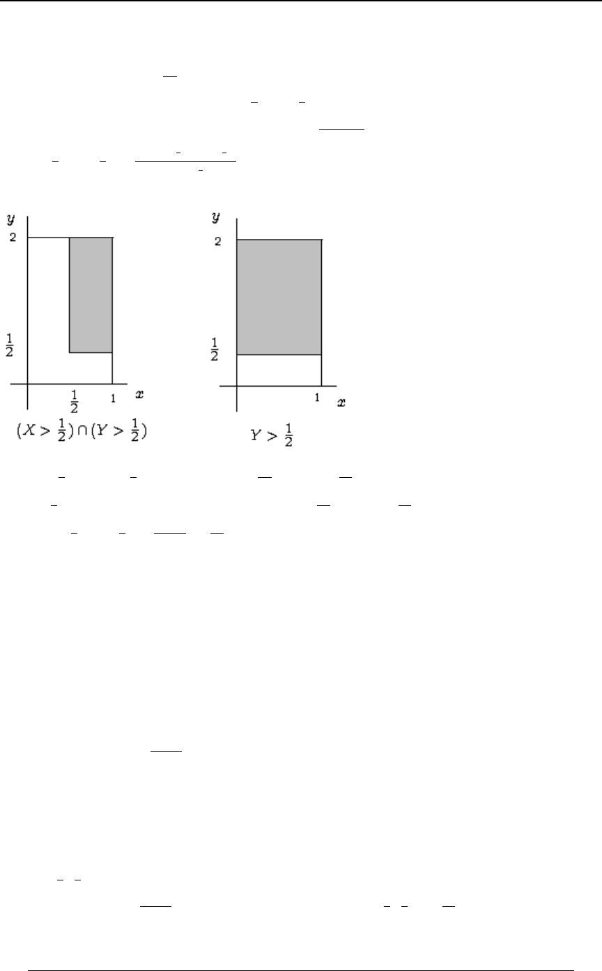
224 SECTION 8 - JOINT, MARGINAL, AND CONDITIONAL DISTRIBUTIONS

Example 8-3: Continuous random variables and have a joint distribution with density\]

function for and .0ÐBßCÑœB  !B" !C#

#BC

Find the conditional probability .TÒ\  l]  Ó

Solution: We use the usual definition .TÒElFÓ œ TÒE∩FÓ

TÒFÓ

TÒ\  l]  Ó œ

T ÒÐ\ Ñ∩Ð]  ÑÓ

TÒ] Ó

These regions are described in the following diagram

T ÒÐ\  Ñ ∩ Ð]  ÑÓ œ ÒB  Ó .C .B œ

"" %$

## $ '%

"Î# "Î#

"# #.

TÒ]  Óœ Ò 0ÐBßCÑ.BÓ.C œ ÒB  Ó.B.C œ

""$

#$"'

'' ''

"Î# ! "Î# !

#" #"

pTÒ\ l]  Óœ œ

"" %$

# # "$Î"' &#

%$Î'% . 

Cumulative distribution function of a joint distribution: If random variables and have\]

a joint distribution, then the cumulative distribution function is

J ÐBß CÑ œ T ÒÐ\ Ÿ BÑ ∩ Ð] Ÿ CÑÓ .

In the continuous case, ,JÐBßCÑ œ 0Ð=ß>Ñ.>.=

∞ ∞

and in the discrete case, .JÐBßCÑ œ 0Ð=ß>Ñ



=œ∞

>œ∞

In the continuous case, .

`B`C

#JÐBßCÑ œ 0ÐBßCÑ

Example 8-4: The cumulative distribution function for the joint distribution of the continuous

random variables and is , for and .\ ] JÐBßCÑœÐÞ#ÑÐ$B C#B C Ñ !ŸBŸ" !ŸCŸ"

$##

Find .0Ð ß Ñ

Solution: 0ÐBß CÑ œ J ÐBß CÑ œ ÐÞ#ÑÐ*B  )BCÑ p 0Ð ß Ñ œ Þ

`"""(

`B`C # # #!

##

SECTION 8 - JOINT, MARGINAL, AND CONDITIONAL DISTRIBUTIONS 225

Expectation of a function of jointly distributed random variables

If is a function of two variables, and and are jointly distributed random variables,2ÐBß CÑ \ ]

then the is defined to beexpected value of 2Ð\ß ] Ñ

IÒ2Ð\ß ] ÑÓ œ 2ÐBß CÑ † 0ÐBß CÑ



in the discrete case, and

IÒ2Ð\ß ] ÑÓ œ 2ÐBß CÑ † 0ÐBß CÑ .C .B

∞ ∞

∞∞ in the continuous case.

Example 8-5: and are discrete random variables which are jointly distributed\]

with the following probability function (from Example 8-1):0ÐBßCÑ

" ! "

""""

") * '

]! !

" """

'**

Find .IÒ\ † ] Ó

Solution: IÒ\] Ó œ BC † 0ÐBß CÑ œ Ð  "ÑÐ"ÑÐ Ñ  Ð  "ÑÐ!ÑÐ Ñ  Ð  "ÑÐ  "ÑÐ Ñ



"" "

") * '

 Ð!ÑÐ"ÑÐ Ñ  Ð!ÑÐ!ÑÐ!Ñ  Ð!ÑÐ  "ÑÐ Ñ

.  Ð"ÑÐ"ÑÐ Ñ  Ð"ÑÐ!ÑÐ Ñ  Ð"ÑÐ  "ÑÐ Ñ œ

"" ""

'' *' 

Example 8-6: Suppose that is the density function for the joint 0ÐBßCÑ œ ÐB C Ñ

distribution of the continuous random variables and defined over the unit square defined on\]

the region and . Find .!ŸBŸ" !ŸCŸ" IÒ\ ] Ó

Solution:

IÒ\  ] Ó œ ÐB  C Ñ † 0ÐBß CÑ .C .B œ ÐB  C ÑÐ ÑÐB  C Ñ .C .B

# # ## ## ##

!! !!

"" ""

'' '' $

œ Ð"Þ&B  B  Þ$Ñ .B œ

"%# "%

"& . 

226 SECTION 8 - JOINT, MARGINAL, AND CONDITIONAL DISTRIBUTIONS

Marginal distribution of found from a joint distribution of and \\]

If and have a joint distribution with joint density or probability function , then the\] 0ÐBßCÑ

marginal distribution of \ has a probability function or density function denoted , which0ÐBÑ

is equal to in the discrete case, and is equal to 0 ÐBÑ œ 0 ÐBß CÑ 0 ÐBÑ œ 0 ÐBß CÑ .C

\ \

C∞

∞

'

in the continuous case. The density function for the marginal distribution of is found in a]

similar way, is equal to either or .0 ÐCÑ 0 ÐCÑ œ 0ÐBß CÑ 0 ÐCÑ œ 0ÐBß CÑ .B

]]]

B∞

∞

'

For instance, in the discrete case. What we are doing is "adding up" the0Ð"Ñœ 0Ð"ßCÑ



probability for all points whose -value is 1 to get the overall probability that is 1. TheB\

marginal distribution of describes the random behavior of as a single random variable.\\

Care must be taken when the probability space is triangular or some other non-rectangular shape.

In this case one must be careful to set the limits of integration properly when finding a marginal

density. This is illustrated in Example 8-9 below.

If the cumulative distribution function of the joint distribution of and is , then the cdf\]JÐBßCÑ

for the marginal distributions of and are\]

J ÐBÑ œ J ÐBß CÑ J ÐCÑ œ J ÐBß CÑ

CÄ∞ BÄ∞

lim lim and .

This concept of marginal distribution can be extended to define the marginal distribution of any

one (or subcollection) variable in a multivariate distribution. Marginal probability functions and

marginal density functions must satisfy all the requirements of probability and density functions.

A marginal probability function must sum to 1 over all points of probability and a marginal

density function must integrate to 1.

Example 8-7: Find the marginal distributions of and for the joint distribution in\]

Example 8-1 .

Solution: The joint distribution was given as

" ! "

""""

") * '

]! !

" """

'**

To find the marginal probability function for , we first note that can be or .\\"ß!"

We wish to find and .0Ð"ÑœTÒ\œ"Óß0Ð!Ñ 0Ð"Ñ

\\\

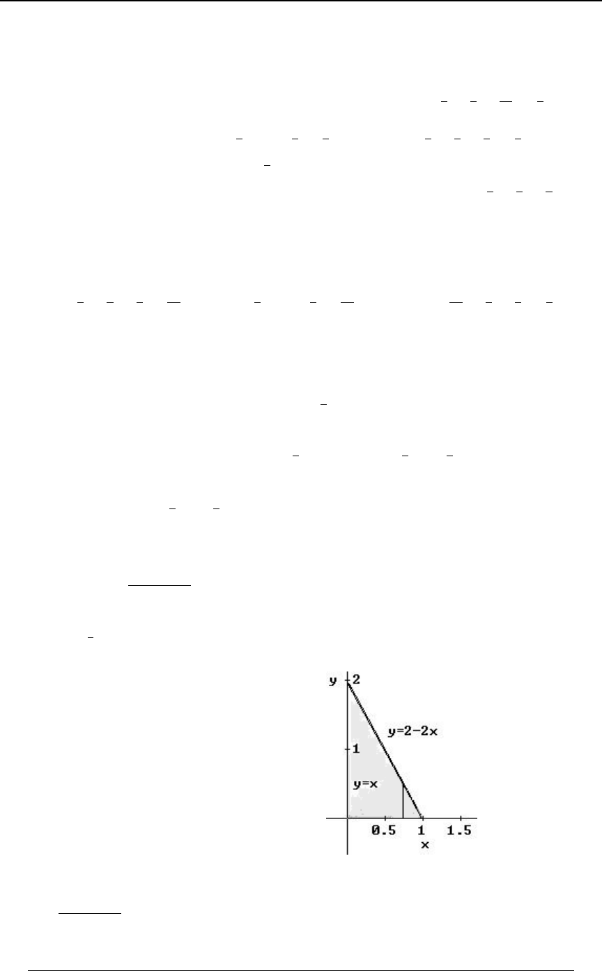
SECTION 8 - JOINT, MARGINAL, AND CONDITIONAL DISTRIBUTIONS 227

Example 8-7 continued

As noted above, to find we sum over the other variable :0ÐBÑ ]

0 Ð"Ñœ 0Ð"ßCÑœ0Ð"ß "Ñ0Ð"ß!Ñ0Ð"ß"Ñœ   œ



all

"" " "

'*") $

and in a similar way we get and .0Ð!Ñœ ! œ 0Ð"Ñœ   œ

" " # """ %

* * * *'' *

In Example 8-1 we saw that . What we were finding was the marginalTÒ\ œ !Ó œ #

probability . Note also that .0Ð!Ñ 0ÐBÑœ0Ð"Ñ0Ð!Ñ0Ð"Ñœ   œ"

\\\\\



all

"#%

$**

This verifies that satisfies the requirements of a probability function.0ÐBÑ

The marginal probability function of is found in the same way, except that sum over (across]B

each row in the table above).

0 Ð"Ñœ   œ 0 Ð!Ñœ ! œ 0 Ð"Ñœ   œ

]]]

""" ( " " & " "" "

'** ") * ' ") ")*' $

, and . 

Example 8-8: Find the marginal distributions of and for the joint distribution in\]

Example 8-2 .

Solution: The joint density function is for and .0ÐBßCÑœ ÐB C Ñ !ŸBŸ" !ŸCŸ"

###

The marginal density function of is found by integrating out the other variable .\C

0 ÐBÑ œ 0ÐBß CÑ .C œ 0ÐBß CÑ .C œ ÐB  C Ñ .C œ B  ! Ÿ B Ÿ "

\C!!

## #

'''

all $$"

###

for .

We can verify that this is a proper density function by checking that .

0ÐBÑ.Bœ"

In a similar way, for . 0 ÐCÑœ C  !ŸCŸ"

## 

Example 8-9: Continuous random variables and have a joint distribution with density\]

function in the region bounded by 0ÐBßCÑœ Cœ!ßBœ!

$Ð##BCÑ

and . Find the density function for the marginal distribution of for .Cœ##B \ !B"

Find and find .TÒ\  Ó TÒ\  ]Ó

Solution: The region of joint density is

illustrated in the graph at the right. Note

that must be in the interval and \ Ð!ß "Ñ ]

must be in the interval and the jointÐ!ß #Ñ

probability space is triangular. Since

0ÐBÑœ 0ÐBßCÑ.C

\∞

∞

' , we note that given

a value of in , the possible values ofB Ð!ß "Ñ

C0ÐBßCÑ (with non-zero density for ) must

satisfy , so that !C##B

0ÐBÑœ 0ÐBßCÑ.C

##B

œ.Cœ$Ð"BÑ

##B #

$Ð##BCÑ

# .

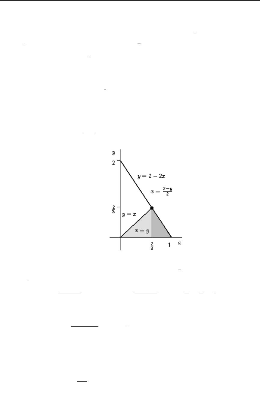
228 SECTION 8 - JOINT, MARGINAL, AND CONDITIONAL DISTRIBUTIONS

Example 8-9 continued

Once we have the marginal density function for , we can find .\TÒ\Ó

TÒ\  Ó œ 0 ÐBÑ.B œ $Ð"BÑ .B œ

#"Î# "Î#

'' 1

) .

Note that we could find by identifying the two-dimensional region and integratingTÒ\  Ó

0ÐBßCÑ 0ÐBßCÑ.C.B œ 0 ÐBÑ.B . This would come out to be ,

'' '

"Î# ! "Î#

"##B "

which is the same as finding the marginal density first. We could also have reversed the order of

integration in and , so that . This involves a little moreB C TÒ\  Ó œ 0ÐBß CÑ .B .C

#! "Î#

" Ð#CÑÎ#

algebra.

The region for which is identified in the graph below. The line intersects with the\] CœB

line at the point . The region we are looking for is , and lies below theCœ##B Ð ß Ñ CB

line .CœB

The probability can be expressed as a double integral. If we set the order of integration with .B

on the outside then we must integrate in two pieces, first from 0 to beneath the line , and

$CœB

then from to beneath the line .

$"Cœ##B

TÒ\  ] Ó œ .C .B  .C .B œ  œ

'' ''

! ! #Î$ !

#Î$ B " ##B

$Ð##BCÑ $Ð##BCÑ

# # #( #( $

)""

The integral can be found in the integration order. In that case,.B .C

TÒ\  ]Ó œ .B.C œ

#Î$ Ð#CÑÎ# "

$Ð##BCÑ

# .

In this case it is more efficient to express the integral with on the outside..C

There is one other note on this example. The probability space was originally described as "the

region bounded by and ". We might also see this region defined inCœ!ßBœ! Cœ##B

the following way: and . The reader can check that this is the same region. !B C!

#C

#

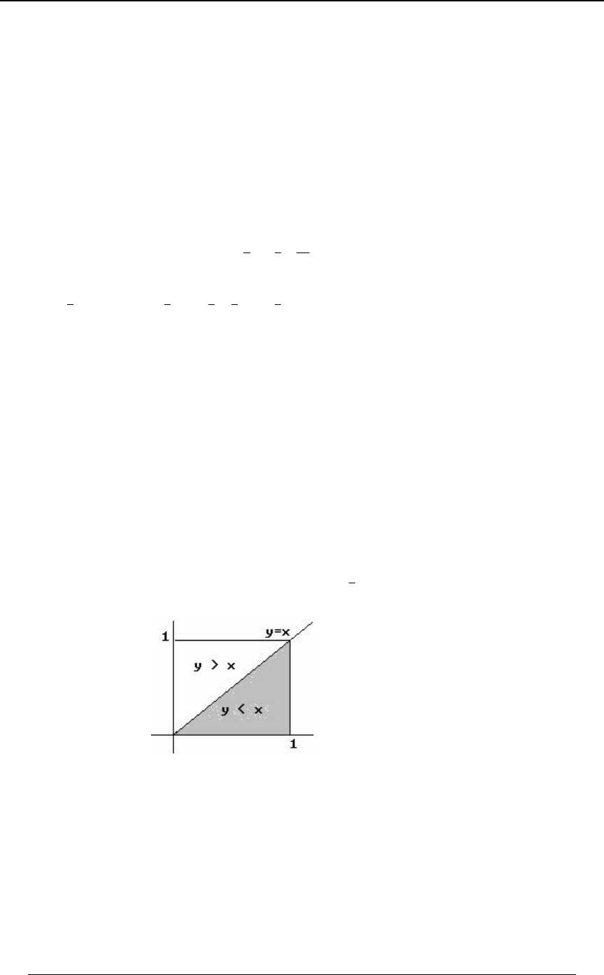
SECTION 8 - JOINT, MARGINAL, AND CONDITIONAL DISTRIBUTIONS 229

Independence of random variables and\]

Random variables and with density functions and are said to be independent\] 0ÐBÑ0ÐCÑ

(or stochastically independent) if the probability space is rectangular ( ,+ŸBŸ,ß -ŸCŸ.

where the endpoints can be infinite) and if the joint density function is of the form

0ÐBß CÑ œ 0 ÐBÑ † 0 ÐCÑ

. Independence of and is also equivalent to the factorization of\]

the cumulative distribution function . for all J ÐBß CÑ œ J ÐBÑ † J ÐCÑ ÐBß CÑ

For the discrete joint distribution in Example 8-1 we can see that and are not independent,\]

because, for instance, . For the continuous0Ð"ß "Ñœ Á † œ0 Ð"Ñ†0 Ð"Ñ

""(

'$") \]

joint distribution of Example 8-8, we see that

0ÐBßCÑœ ÐBCÑÁÐB ÑÐC Ñœ0ÐBÑ†0ÐCÑ \ ]

$$"$"

#####

## # # \]

, so and are not

independent.

Example 8-10: Suppose that and are independent continuous random variables with the\]

following density functions: for and for .0 ÐBÑœ" !B" 0 ÐCÑœ#C !C"

Find .TÒ]  \Ó

Solution: Since and are independent, the density function of the joint distribution of \] \

and is , and is defined on the rectangle created by the intervals] 0ÐBß CÑ œ 0 ÐBÑ † 0 ÐCÑ œ #C

for and , which, in this case, is the unit square. The graph below illustrates the region for the\]

probability in question. .TÒ] \Óœ #C.C.Bœ

"B "



230 SECTION 8 - JOINT, MARGINAL, AND CONDITIONAL DISTRIBUTIONS

Conditional distribution of given ]\œB

The way in which a conditional distribution is defined follows the basic definition of conditional

probability, . In fact, given a discrete joint distribution, this is exactly how aTÒElFÓ œ TÒE∩FÓ

TÒFÓ

conditional distribution is defined. Example 8-1 described a discrete joint distribution of and\

]\], and then Example 8-7 showed how to formulate the marginal distributions of and . We

now wish to formulate a conditional distribution. For instance, for the joint distribution of

Example 8-1, suppose we wish to describe the conditional distribution of given . What\]œ"

we are trying to describe are conditional probabilities of the form .TÒ\ œ Bl] œ "Ó

We find these conditional probabilities in the usual way that conditional probability is defined.

TÒ\ œ "l] œ "Ó œ T ÒÐ\œ"Ñ∩Ð] œ"ÑÓ

TÒ]œ"Ó .

The denominator is the marginal probability that , . The numerator is the joint]œ"0Ð"Ñœ

probability , which is found in the joint probability table. Then,0Ð "ß"Ñ œ "

. We would denote this conditional probabilityTÒ\ œ "l] œ "Ó œ 0 Ð"ß"Ñ "Î")

0 Ð"Ñ "Î$ '

]œœ

0 Ð  "l] œ "Ñ 0 Ð!l] œ "Ñ œ œ

\l] \l]

. In a similar way, we can get , and

0Ð!ß"Ñ "Î*

0 Ð"Ñ "Î$ $

]œ

0 Ð"l] œ "Ñ œ œ

\l]

0Ð"ß"Ñ "Î'

0 Ð"Ñ "Î$ #

]œ . This completely describes the conditional distribution of

\]œ"given . As with any discrete distribution, probabilities for a conditional distribution must

add to 1, and this is the case for this conditional distribution, since

0 Ð"l] œ"Ñ0 Ð!l] œ"Ñ0 Ð"l] œ"Ñœ   œ"

\l] \l] \l] """

'$# .

A conditional distribution satisfies all the same properties of any distribution. We can find a

conditional mean, a conditional variance, etc. For instance, the conditional mean of given\

]œ" in the example we have just been considering is

IÒ\l] œ "Ó œ B † 0 ÐBl] œ "Ñ

+66 B

D\l]

œ Ð  "Ñ0 Ð  "l] œ "Ñ  Ð!Ñ0 Ð!l] œ "Ñ  Ð"Ñ0 Ð"l] œ "Ñ

\l] \l] \l]

œ Ð  "ÑÐ Ñ  Ð!ÑÐ Ñ  Ð"ÑÐ Ñ œ Þ

""""

'$#$

We can find the second conditional moment in a similar way,

IÒ\ l] œ "Ó œ B † 0 ÐBl] œ "Ñ

+66 B

\l]

D . Then the conditional variance would be

Z+<Ò\l]œ"ÓœIÒ\l]œ"ÓÐIÒ\l]œ"ÓÑ

SECTION 8 - JOINT, MARGINAL, AND CONDITIONAL DISTRIBUTIONS 231

The expression for conditional probability that was used above in the discrete case was

0ÐBl]œCÑœ

\l]

0ÐBßCÑ

0ÐCÑ

]. This can be applied to find a conditional distribution of given]

\œB 0 ÐCl\œBÑœ also, so that we define .

]l\

0ÐBßCÑ

0ÐBÑ

We also apply this same algebraic form to define the conditional density in the continuous case,

with being the joint density and being the marginal density. In the continuous case,0 ÐBß CÑ 0 ÐBÑ

the conditional mean of given would be]\œB

,IÒ] l\ œ BÓ œ C † 0 ÐCl\ œ BÑ.C

']l\

where the integral is taken over the appropriate interval for the conditional distribution of ]

given . The conditional density/probability is also written as , or .\ œ B 0 ÐClBÑ 0ÐClBÑ

]l\

If and are independent random variables, then\]

0ÐCl\œBÑœ œ œ0ÐCÑ

]l\ ]

0ÐBßCÑ 0 ÐBÑ†0 ÐCÑ

0ÐBÑ 0ÐBÑ

and in a similar way we have , which indicates that the density of 0ÐBl]œCÑœ0ÐBÑ ]

\l] \

does not depend on and vice-versa.\

The conditional density function must satisfy the usual requirement of a density function, '∞

∞

0 ÐClBÑ .C œ " 0 ÐBÑ \

]l\ \

. Note also that if , the marginal density of is known, and if

0ÐCl\œBÑ ] \œB

]l\ , the conditional density of given , is also known, then the joint density

of and can be formulated as \]

0ÐBßCÑœ0 ÐCl\œBÑ†0 ÐBÑ

]l\ \Þ

Example 8-11: Find the conditional distribution of given for the joint distribution]\œ"

of Example 8-1. Find the conditional expectation of given .]\œ"

Solution: The marginal probability function for was found in Example 8-7, where it was\

found that . The conditional probability function of given is0Ð"Ñœ ] \œ"

0ÐCl\œ"Ñœ œ

]l\

0Ð"ßCÑ 0 Ð"ßCÑ

0 Ð"Ñ "Î$

\ . Then,

0Ð"l\œ"Ñœ œ œß0Ð!l\œ"Ñœ œ œß

]l\ ]l\

0Ð"ß"Ñ "Î' 0 Ð"ß!Ñ "Î*

"Î$ "Î$ # "Î$ "Î$ $

and .0Ð"l\œ"Ñœ œ œ

]l\

0Ð"ß"Ñ "Î")

"Î$ "Î$ '

IÒ]l\œ "Óœ C†0 ÐCl\œ "ÑœÐ"ÑÐ ÑÐ!ÑÐ ÑÐ"ÑÐ Ñœ 



all C

]l\ """"

#$'$

. 

232 SECTION 8 - JOINT, MARGINAL, AND CONDITIONAL DISTRIBUTIONS

Example 8-12: Find the conditional density and conditional expectation and conditional

variance of given for the joint distribution of Example 8-2.\]œÞ$

Solution: .0ÐBl]œÞ$Ñœ œ œ

\l]

0ÐBßÞ$Ñ

0 ÐÞ$Ñ Þ'$&

ÐB Þ$ Ñ ÐB Þ!*Ñ

Þ$ 

]

## #

The conditional expectation is

IÒ\l]œÞ$Óœ B†0 ÐBl]œÞ$Ñ.Bœ B† .BœÞ'*(

\l]

ÐB Þ!*Ñ

Þ'$& .

The conditional second moment of given is\]œÞ$

IÒ\l]œÞ$Óœ B †0 ÐBl]œÞ$Ñ.Bœ B † .BœÞ&%$

## #

\l]

ÐB Þ!*Ñ

Þ'$& .

The conditional variance is

Z +<Ò\l] œ Þ$Ó œ IÒ\ l] œ Þ$Ó  ÐIÒ\l] œ Þ$ÓÑ œ Þ&%$  ÐÞ'*(Ñ œ Þ!&(

###

. 

Example 8-13: Continuous random variables and have a joint distribution with density\]

function for and . Find .0ÐBßCÑœ Ð=38 CÑ/ !B∞ !C" TÒ\"l] œ Ó

B

Solution: .TÒ\  "l] œ Ó œ

T ÒÐ\"Ñ∩Ð] œ ÑÓ

0ÐÑ

T ÒÐ\  "Ñ ∩ Ð] œ ÑÓ œ 0ÐBß Ñ .B œ Ð=38 Ñ/ .B œ † /

###%%

∞∞

B "

11 1È.

0 Ð Ñ œ 0ÐBß Ñ .B œ Ð=38 Ñ/ .B œ Ê T Ò\  "l] œ Ó œ /

]!!

∞∞

B "

"" "

###%% #

11 1È .

Note that , and0 ÐBÑ œ 0ÐBß CÑ .C œ Ð=38 CÑ/ .C œ /

\!!

B B

.0 ÐCÑ œ 0 ÐBß CÑ .B œ Ð=38 CÑ/ .B œ Ð=38 CÑ

]!!

∞∞

B

11 11

## ##

Then we see that and are independent.\]

This follows from .0ÐBß CÑ œ Ð/ ÑÐ † =38 CÑ œ 0 ÐBÑ † 0 ÐCÑ

B

## \]

From independence it follows that (same as the resultTÒ\  "l] œ Ó œ TÒ\  "Ó œ /

"

above)Þ

As a final comment on this example, we could have noticed at the start that since can be0ÐBßCÑ

factored into separate functions in and , we might anticipate that and are independent.BC \]

Since the joint distribution is defined on a rectangular area, it follows that and must be\]

independent if the pdf factors into a function of only multiplied by a function of only.BC

Furthermore, the factor involving is . Since this integrates to 1 over the range for , it mustB/ \

B

be the marginal density of , . Then, because of independence, we have\0ÐBÑœ/

\B

TÒ\  "l] œ Ó œ TÒ\  "Ó / .B œ /

∞B "

, and from the marginal density, this is .

'

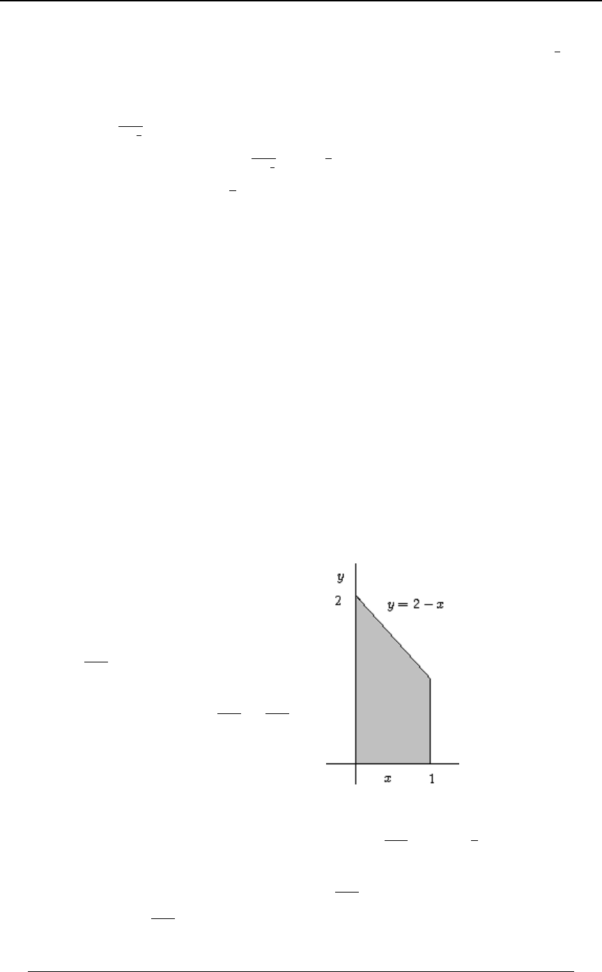
SECTION 8 - JOINT, MARGINAL, AND CONDITIONAL DISTRIBUTIONS 233

Example 8-14: is a continuous random variable with density function for\0ÐBÑœB

!B" \ ] . is also jointly distributed with the continuous random variable , and the

conditional density function of given is]\œB

0 ÐCl\œBÑœ !B" !C" 0 ÐCÑ !C"

]l\ ]

BC

B"

for and . Find for .

Solution: .0ÐBß CÑ œ 0ÐClBÑ † 0 ÐBÑ œ † ÐB  Ñ œ B  C

\BC

B

Then, 0ÐCÑœ 0ÐBßCÑ.BœC Þ

#

As Example 8-14 shows, we can construct the joint density from knowing the conditional0ÐBßCÑ

density and the marginal density using the relationship0 ÐClBÑ 0 ÐBÑ

]l\ \

0ÐBß CÑ œ 0ÐClBÑ † 0 ÐBÑ

\ . When doing this, care must be taken to ensure that proper two-

dimensional region is being formulated for the joint distribution. The following example

illustrates this point.

Example 8-15: A company will experience a loss that is uniformly distributed between 0\

and 1. The company pays a bonus to its employees that is uniformly distributed on the interval

Ð!ß #  \Ñ, which depends on the amount of the loss that occurred. Find the expected amount of

the bonus paid.

Solution: has marginal pdf \0ÐBÑœ"

for . Let be the bonus paid.!B" ]

The conditional distribution of given]

\œB is a uniform distribution on the

interval , with conditional densityÐ!ß #  BÑ

0ÐClBÑœ \

]l\ "

#B . The joint density of

and is]

0ÐBß CÑ œ 0 ÐClBÑ † 0 ÐBÑ œ " † œ

]l\ \""

#B #B

and the two-dimensional region of

probability is the region and!C#B

!B" . This region is the shaded area in

the graph at the right.

The expected value of can be found as .] IÒ] Ó œ C † .C .B œ

"#B "$

#B %

We could have found the marginal density on , and then have found , but that is more]IÒ]Ó

awkward because for we have , and for !CŸ" 0 ÐCÑœ .Bœ68# "CŸ#

#B

we have . 0 ÐCÑ œ .B œ 68 #  68 C

#C

#B 

234 SECTION 8 - JOINT, MARGINAL, AND CONDITIONAL DISTRIBUTIONS

Example 8-16: Suppose that has a continuous distribution with pdf \0ÐBÑœ#B

on the interval , and elsewhere. Suppose that is a continuous randomÐ!ß "Ñ 0 ÐBÑ œ ! ]

variable such that the conditional distribution of given is uniform on the interval .]\œB Ð!ßBÑ

Find the mean and variance of .]

Solution: We find the unconditional (marginal) distribution of . We are given ]0ÐBÑœ#B

for , and for .!B" 0 ÐCl\œBÑœ !CB

]l\ "

Then, for .0ÐBß CÑ œ 0 ÐClBÑ † 0 ÐBÑ œ † #B œ # !  C  B  "

The unconditional (marginal) distribution of has pdf.]

0 ÐCÑœ 0ÐBßCÑ.Bœ #.Bœ#Ð"CÑ !C" 0 ÐCÑ !

] ]

∞ C

∞"

'' for (and is

elsewhere). Then , ,IÒ] Ó œ C † #Ð"  CÑ.C œ IÒ] Ó œ C † #Ð"  CÑ.C œ

and . Z +<Ò] Ó œ IÒ] Ó  ÐIÒ] ÓÑ œ  Ð Ñ œ

## #

"" "

'$ ")



Covariance between random variables and :\] If random variables and are jointly\]

distributed with joint density/probability function , and might not be independent of0ÐBßCÑ \ ]

one another. We have seen some examples in which and are independent, and some in\]

which they are not. There are a couple of numerical measures that describe, in some sense, the

dependence that exists between and . Covariance is one such measure.\]

The covariance between and is\]

G9@Ò\ß ] Ó œ IÒÐ\  IÒ\ÓÑÐ]  IÒ] ÓÑÓ

œ IÒÐ\  ÑÐ]  ÑÓ œ IÒ\] Ó  IÒ\Ó † IÒ] ÓÞ..

A positive covariance between and is an indication that "large" values of (values of \] \ \

that are bigger than ) tend to occur paired with "large" values of , and the same for "small"IÒ\Ó ]

values of and . Negative covariance indicates the opposite relationship. Covariance near or at\]

0 indicates that the "size" of value is not related to the "size" of the values to which they are\]

paired.

Note that . One important application of the covariance is in finding theG9@Ò\ß \Ó œ Z +<Ò\Ó

variance of the sum of and . Suppose that , and are constants. Then it can be shown that\] +,-

Z+<Ò+\,] -Óœ+ Z+<Ò\Ó, Z+<Ò]Ó#+,G9@Ò\ß]Ó

## .

SECTION 8 - JOINT, MARGINAL, AND CONDITIONAL DISTRIBUTIONS 235

Coefficient of correlation between random variables and :\]

The coefficient of correlation between random variables and is\]

33Ð\ß ] Ñ œ œ

\ß] G9@Ò\ß] Ó

\] , where and are the standard deviations of and55

\] \

]"ŸŸ" respectively. Note that always.3\ß]

Example 8-17: Find for the jointly distributed discrete random variables inG9@Ò\ß]Ó

Example 8-1 above.

Solution: . In Example 8-5 it was found that .G9@Ò\ß ] Ó œ IÒ\] Ó  IÒ\Ó † IÒ] Ó IÒ\] Ó œ "

The marginal probability function for is ,\TÒ\œ"Óœœ

""" %

''* *

T Ò\ œ !Ó œ T Ò\ œ  "Ó œ \

and , and the mean of is

IÒ\ÓœÐ"ÑÐ ÑÐ!ÑÐ ÑÐ"ÑÐ Ñœ

%# ""

** $*

In a similar way, the probability function of is found to be ] T Ò] œ "Ó œ ß T Ò] œ !Ó œ ß

$")

and with a mean of .TÒ] œ "Óœ ß IÒ]Óœ 

") ")

Then, . G9@Ò\ß] Ó œ  Ð ÑÐ  Ñ œ

"" " "%

' * ") )" 

Example 8-18: The coefficient of correlation between random variables and is ,\]

and . The random variable is defined to be , and55

œ+ß œ%+ ^ ^œ$\%]

it is found that . Find .5#

^œ ""% +

Solution: .5#

^œ Z +<Ò^Ó œ *Z +<Ò\Ó  "'Z +<Ò] Ó  # † Ð$ÑÐ  %Ñ G9@Ò\ß ] Ó

Since it follows thatG9@Ò\ß ] Ó œ Ò\ß ] Ó † † œ † + † %+ œ ß355

\] "#+

ÈÈ

""% œ œ *+  "'Ð%+Ñ  #%Ð Ñ œ &(+ p + œ #5#

$ . 

236 SECTION 8 - JOINT, MARGINAL, AND CONDITIONAL DISTRIBUTIONS

Moment generating function of a joint distribution: Given jointly distributed random

variables and , the moment generating function of the joint distribution is\]

Q Ð>ß>ÑœIÒ/ Ó

\ß] " # >\>]

. This definition can be extended to the joint distribution of

any number of random variables. It can be shown that is equal to the multiple partialIÒ\ ] Ó

derivative evaluated at 0, .IÒ\] Óœ Q Ð>ß>Ñ

87 \ß] " #

`>` > >œ>œ!

87

"# "#

Example 8-19: Suppose that and are random variables whose joint distribution has\]

moment generating function , for all real and .QÐ>ß>ÑœÐ /  /  Ñ > >

"# " #

>>"!

"$$

%))

Find the covariance between and .\]

Solution: .G9@Ò\ß ] Ó œ IÒ\] Ó  IÒ\Ó † IÒ] Ó

IÒ\]Óœ Q Ð>ß>Ñ

`> `>

"# \ß] " # >œ>œ!

¹"#

œ Ð"!ÑÐ*ÑÐ /  /  Ñ Ð / ÑÐ / Ñ œ

"$$"$ "$&

%))%) "'

>œ>œ!

>>)>>

"# "#

¹"#

IÒ\Óœ Q Ð>ß>Ñ œÐ"!ÑÐ//ÑÐ/Ñ œ ß

` "$$ &

`> %)) #

>œ>œ! >œ>œ!

""# "#

\ß] " # >>*>

¹¹

"# "

IÒ]Óœ Q Ð>ß>Ñ œÐ"!ÑÐ//ÑÐ/Ñ œ ß

` "$$$ "&

`> %))) %

>œ>œ! >œ>œ!

#"# "#

\ß] " # >>*>

¹¹

"# #

ÊG9@Ò\ß]Óœ ÐÑÐ Ñœ .

"$& & "& "&

"' # % "' 

The Bivariate normal distribution:

Suppose that and are normal random variables with means and variances\]

IÒ\Ó œ ß Z +<Ò\Ó œ ß IÒ] Ó œ ß Z +<Ò] Ó œ.5.5 3

\] \]

, and with correlation coefficient .

\] ] and are said to have a bivariate normal distribution. The conditional mean and variance of

given are\œB

IÒ] l\ œ BÓ œ  † † B œ  † B.3 . . .

]\] \ ] \

]

() ()

G9@Ð\ß] Ñ ,

and . Similar relationships apply for the conditionalZ+<Ò]l\œBÓœ † 53

]\]

(1 )

distribution of given .\]œC

If and are independent, then , and vice-versa.\] œ!3\]

The pdf of the bivariate normal distribution is

0ÐBßCÑ œ † /B:  †

#" #Ð" Ñ

B C B C

15 5 3 35 5 55

.. ..

\] ##\] \]

\] \]

ÈÒÓÒÐ Ñ Ð Ñ Ð ÑÐ Ñ

#3Ó .

The bivariate normal has occurred infrequently on Exam P.

SECTION 8 - JOINT, MARGINAL, AND CONDITIONAL DISTRIBUTIONS 237

Some results and formulas related to this section are

(i) If and are independent, then for any functions and ,\] 12

IÒ1Ð\Ñ † 2Ð] ÑÓ œ IÒ1Ð\ÑÓ † IÒ2Ð] ÑÓ IÒ\ † ] Ó œ IÒ\Ó † IÒ] Ó , and in particular, .

(ii) The density/probability function of jointly distributed variables and can be written in\]

the form 0ÐBßCÑœ0 ÐCl\œBÑ†0 ÐBÑœ0 ÐBl] œCÑ†0 ÐCÑ

]l\ \l]

(iii) .G9@Ò\ß]ÓœIÒ\†]Ó † œIÒ\]ÓIÒ\Ó†IÒ]Ó..

G9@Ò\ß ] Ó œ G9@Ò] ß \Ó \ ] IÒ\ † ] Ó œ IÒ\Ó † IÒ] Ó . If and are independent, then

and . For constants and random variables and ,G9@Ò\ß]Óœ! +ß,ß-ß.ß/ß0 \ß]ß^ [

G9@Ò+\,] -ß .^/[ 0Ó

œ +.G9@Ò\ß ^Ó  +/G9@Ò\ß [ Ó  ,.G9@Ò] ß ^Ó  ,/G9@Ò] ß [ Ó

(iv) Z +<Ò\  ] Ó œ IÒÐ\  ] Ñ Ó  ÐIÒ\  ] ÓÑ

œIÒ\ #\] ] ÓÐIÒ\ÓIÒ]ÓÑ

## #

œ IÒ\ Ó  IÒ#\] Ó  IÒ] Ó  ÐIÒ\ÓÑ  #IÒ\ÓIÒ] Ó  ÐIÒ] ÓÑ

### #

œZ+<Ò\ÓZ+<Ò]Ó#†G9@Ò\ß]Ó

If and are independent, then .\ ] Z+<Ò\]ÓœZ+<Ò\ÓZ+<Ò]Ó

For any , \ß ] Z +<Ò+\  ,]  -Ó œ + Z +<Ò\Ó  , Z +<Ò] Ó  #+, † G9@Ò\ß ] Ó

(v) If and have a joint distribution which is uniform (constant density) on the two \]

dimensional region (usually will be a triangle, rectangle or circle in the plane)VV ÐBßCÑ

then the pdf of the joint distribution is inside the region (and the pdf is 0

E</+ 90 V V

outside). The probability of any event (represented by a subset of ) is theEV

proportion Also the conditional distribution of given has a

E</+ 90 E

E</+ 90 V Þ]\œB

uniform distribution on the line segment (or segments) defined by the intersection of the

region with the line .V\œB

The marginal distribution of might or might not be uniform]

(vi) , and in particular,IÒ2 Ð\ß ] Ñ  2 Ð\ß ] ÑÓ œ IÒ2 Ð\ß ] ÑÓ  IÒ2 Ð\ß ] ÑÓ

"# #

IÒ\  ] Ó œ IÒ\Ó  IÒ] Ó IÒ \ Ó œ IÒ\ Ó and 

(vii) lim lim

BÄ∞ CÄ∞

JÐBßCÑ œ JÐBßCÑ œ !

238 SECTION 8 - JOINT, MARGINAL, AND CONDITIONAL DISTRIBUTIONS

(viii) TÒÐB \ŸB Ñ∩ÐC ] ŸCÑÓœJÐB ßC ÑJÐBßC ÑJÐBßC ÑJÐBßC Ñ

" # " # ## #" "# ""

(ix) T ÒÐ\ Ÿ BÑ ∪ Ð] Ÿ CÑÓ œ J ÐBÑ  J ÐCÑ  J ÐBß CÑ Ÿ "

(x) For any jointly distributed random variables and , \]"Ÿ Ÿ"3\]

(xi) and Q Ð>ß!ÑœIÒ/ ÓœQ Ð>Ñ Q Ð!ß>ÑœIÒ/ ÓœQ Ð>Ñ

\ß] " \ " \ß] # ] #

>\ >]

" #

(xii) ,

`> `>

>œ>œ! >œ>œ!

"# "#

Q Ð>ß>Ñ œIÒ\Ó Q Ð>ß>Ñ œIÒ]Ó

\ß] " # \ß] " #

¹¹

`>`> >œ>œ!

<=

"# "#

Q Ð>ß>Ñ œIÒ\ †] Ó

\ß] " # <=

(xiii) If for and in a region about ,QÐ>ß>ÑœQÐ>ß!Ñ†QÐ!ß>Ñ > > Ð!ß!Ñ

"# " # " #

then and are independent.\]

(xiv) If then .] œ +\  , Q Ð>Ñ œ / Q Ð+>Ñ

(xv) If and are jointly distributed, then for any , depends on , say\ ] C IÒ\l] œ CÓ C

IÒ\l] œ CÓ œ 2ÐCÑ IÒ2Ð] ÑÓ œ IÒ\Ó . It can then be shown that ; this is more usually written

in the form .IÒ IÒ\l] Ó Ó œ IÒ\Ó

It can also be shown that .Z +<Ò\Ó œ IÒ Z +<Ò\l] Ó Ó  Z +<Ò IÒ\l] Ó Ó

This relationship has come up on several questions on recent exams.

Example 8-20: For random variables and , you are given that \ß] ^ Z +<Ò\Ó œ Z +<Ò] Ó œ "ß

Z+<Ò^Óœ#ßG9@Ð\ß]Ñœ "ßG9@Ð\ß^Ñœ!ßG9@Ð]ß^Ñœ" .

Find the covariance between and .\  #] ]  #^

Solution:

G9@Ð\  #] ß]  #^Ñ œ G9@Ð\ß] Ñ  G9@Ð\ß#^Ñ  G9@Ð#] ß] Ñ  G9@Ð#] ß#^Ñ

œ  "  #G9@Ð\ß ^Ñ  #G9@Ð] ß ] Ñ  %G9@Ð] ß ^Ñ

œ "#Ð!Ñ#Z+<Ò]Ó%Ð"Ñœ "#Ð"Ñ%œ& . 

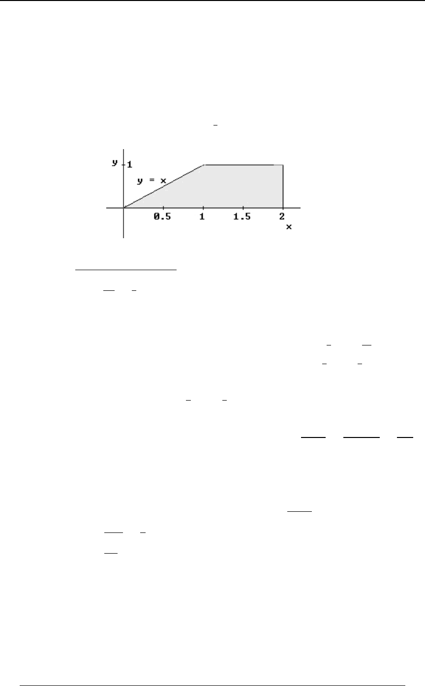
SECTION 8 - JOINT, MARGINAL, AND CONDITIONAL DISTRIBUTIONS 239

Example 8-21: Random variables and are jointly distributed on the region\]

. The joint distribution has a constant density over the entire region.!ŸCŸBß CŸ"ß BŸ#

(i) Find the joint density.

(ii) Find the marginal densities of and .\]

(iii) Find the conditional densities of given , and given .\ ] œC ] \œB

(iv) Find the probabilities , and .TÒ\  "Ó ß TÒ] Ÿ Ó TÒ\ ] Ÿ "Ó

Solution: The region of probability is outlined below.

(i) Since we are told that the joint density is constant on the region of probability that constant

must be equal to . The area of the region of probability is

area of region of probability

1.5 , so that for points in the region of probability.0ÐBßCÑ œ œ ÐBßCÑ

"Þ& $

(ii) The marginal density function of is .\0ÐBÑœ0ÐBßCÑ.C

If the probability region is , so that !ŸBŸ"ß !ŸCŸB 0 ÐBÑœ .Cœ Þ

'##B

If , the probability region is , so that "ŸBŸ# !ŸCŸ" 0 ÐBÑœ .Cœ Þ

'##

The marginal density of is for .]0ÐCÑœ .BœÐ#CÑ !ŸCŸ"

'##

(iii) The conditional density of given is .\]œC0ÐBl]œCÑœ œ œ

\l]

0ÐBßCÑ #Î$

0 ÐCÑ #Ð#CÑÎ$ #C

]

Note that the interval of probability for the conditional distribution of given is\]œC

CŸBŸ# \ ] œC . The conditional density of given is uniform on that interval.

The conditional density of given is .]\œB0ÐCl\œBÑœ

]l\

0ÐBßCÑ

0ÐBÑ

For this is , a uniform distribution for .!ŸBŸ" œ !ŸCŸB

#Î$

#BÎ$ B

For this is 1 , a uniform distribution for ."ŸBŸ# œ !ŸCŸ"

#Î$

Note that in all cases the conditional distributions are uniform. This will always be the case if the

joint distribution is uniform on its probability space.

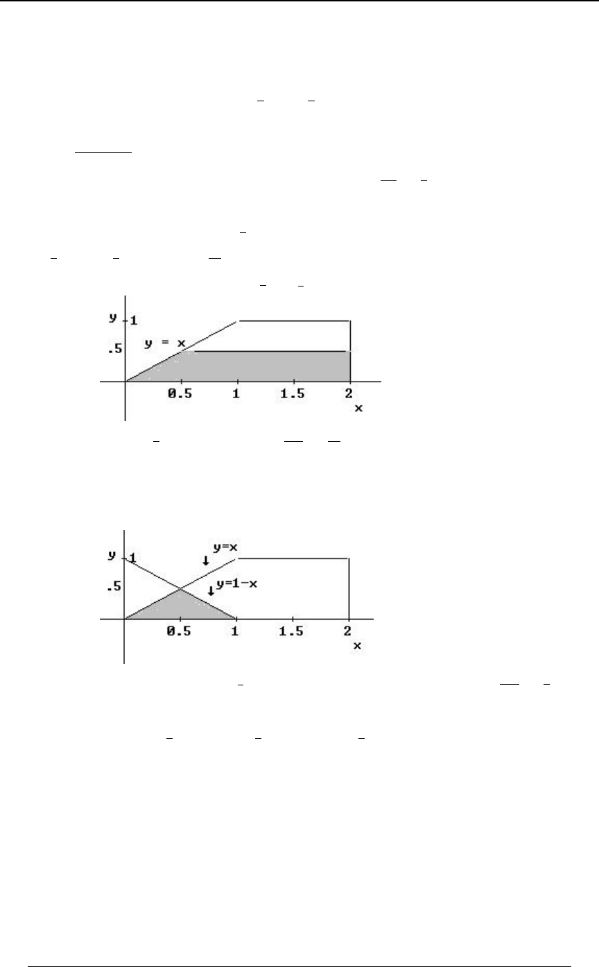
240 SECTION 8 - JOINT, MARGINAL, AND CONDITIONAL DISTRIBUTIONS

Example 8-21 continued

(iv) can be found in two ways. Since we have the marginal density for , we can useTÒ\  "Ó \

it to find .TÒ\  "Ó œ 0 ÐBÑ.B œ .B œ

\##

Alternatively, since the joint distribution is uniform, the probability of any event is theE

proportion The area of the full probability space was already found to be 1.5 . E</+ 90 E

E</+ 90 V ÞV

The area of the region is 1. Therefore, .\" TÒ\"Óœ œ

"Þ& $

The same comment applies to . From the marginal density of we haveTÒ] Ÿ Ó ]

TÒ] Ÿ Ó œ Ð#CÑ.C œ

"# (

#$ "#

"Î# .

Alternatively, the area of the region is (outlined in the diagram below).]Ÿ"

(

)

The probability is the proportion .TÒ] Ÿ Ó œ

# $Î# "#

(Î)

The region is outlined in the diagram below (the region below within\] Ÿ" Cœ"B

the original probability space).

The area of the region is , so the probability is .\] Ÿ" TÒ\] Ÿ"Óœ œ

"Î%

$Î# '

We could also find the probability by integrating the joint density over the appropriate region,

TÒ\ ] Ÿ "Ó œ .B.C œ Ð"#CÑ.C œ

'' '

!C !

Þ& "C Þ&

## "

$$ '

. 

SECTION 8 - JOINT, MARGINAL, AND CONDITIONAL DISTRIBUTIONS 241

Example 8-22: Suppose that is the 3-point discrete uniform random variable , with[ Ö"ß #ß $×

TÒ[ œ"ÓœTÒ[ œ#ÓœTÒ[ œ$Óœ ]

$ , and suppose that the conditional distribution of

given is exponential with mean .[œA A

Find the (unconditional) mean and (unconditional) variance of ]Þ

Solution: The conditional pdf of given is .][œA0ÐCl[œAÑœ/

]l[ CÎA

Also, we are given , so that .

if , prob.

IÒ] l[ œ AÓ œ A IÒ] l[Ó œ

"[œ"

#[œ#

$[œ$

"

We see that is a 3-point random variableIÒ] l[Ó Þ

Let us use the notation for this 3-point random variable.^œIÒ]l[Ó

Then .IÒ^Ó œ IÒ IÒ] l[ Ó Ó œ Ð"ÑÐ Ñ  Ð#ÑÐ Ñ  Ð$ÑÐ Ñ œ #

"""

$$$

This is according to the rule cited above..IÒ] Ó

Also, as a random variable, has a variance:^œIÒ]l[Ó

Z +<Ò^Ó œ Z +<Ò IÒ] l[ Ó Ó œ IÒ^ Ó  ÐIÒ^ÓÑ œ IÒÐIÒ] l[ ÓÑ Ó  ÐIÒ IÒ] l[ Ó ÓÑ

## # #

œ ÒÐ" ÑÐ Ñ  Ð# ÑÐ Ñ  Ð$ ÑÐ ÑÓ  # œ

####

""" #

$$$ $

The variance of an exponential random variable is the square of the mean, so since the

conditional distribution of given is exponential with mean , the conditional variance of ][ A ]

given is . As with the conditional mean of ,[ œ A Z +<Ò] l[ œ AÓ œ A ] l[

# the

conditional variance of is a random variable dependent on the outcome of .]l[ [

Z+<Ò]l[Óœ

Z+<Ò]l[œ"Óœ" [œ"

Z+<Ò]l[œ#Óœ% [œ#

Z+<Ò]l[œ$Óœ* [œ$

 .

if , prob.

Z+<Ò]l[Ó Y œZ+<Ò]l[Ó is a three-point random variable. Let us use the notation .

Then IÒY Ó œ IÒ Z +<Ò] l[ Ó Ó

œ ÐZ +<Ò] lA œ "ÓÑÐ Ñ  ÐZ +<Ò] lA œ #ÓÑÐ Ñ  ÐZ +<Ò] lA œ $ÓÑÐ Ñ

"""

$$$

œ Ð"ÑÐ Ñ  Ð%ÑÐ Ñ  Ð*ÑÐ Ñ œ

""""%

$$$$

Using the variance rule cited above in (xv) above, we have

Z +<Ò] Ó œ IÒ Z +<Ò] l[ Ó Ó  Z +<Ò IÒ] l[ Ó Ó œ IÒY Ó  Z +<Ò^Ó œ  œ

"% # "'

$$ $

. 

242 SECTION 8 - JOINT, MARGINAL, AND CONDITIONAL DISTRIBUTIONS

PROBLEM SET 8 243

PROBLEM SET 8

Joint, Marginal and Conditional Distributions

1. A wheel is spun with the numbers 1, 2 and 3 appearing with equal probability of each. If the

number 1 appears, the player gets a score of 1.0; if the number 2 appears, the player gets a score

of 2.0; if the number 3 appears, the player gets a score of , where is a normal random\\

variable with mean 3 and standard deviation 1. IF represents the player's score on 1 spin of[

the wheel, then what is ?T Ò[ Ÿ "Þ&Ó

A) B) C) D) E) Þ"$ Þ$$ Þ$' Þ%! Þ'%

2. Let and be discrete loss random variables with joint probability function\]

.0ÐBßCÑ œ š for

otherwise

#%B Bœ"ß#ß% à Cœ#ß%ß) à BŸC

!ß

An insurance policy pays the full amount of loss and half of loss . Find the probability that\]

the total paid by the insurer is no more than 5.

A) B) C) D) E)

"($

)#%)

&"(

)#%

3. Let and be continuous random variables with joint density function\]

.0ÐBßCÑ œ š for and

otherwise

Þ(&B !B# !CŸ#B

!ß

What is ?TÒ\  "Ó

A) B) C) D) E)

""$"$

)%)#%

4. Let and be independent random variables with \] œ"ßœ"ßœß.. 5

\] #

and . Calculate .5###

]œ# IÒÐ\"ÑÐ] "Ñ Ó

A) B) C) D) E) ""'"(#(

5. (SOA) Let be the time between a car accident and reporting a claim to the insuranceX"

company. Let be the time between the report of the claim and payment of the claim. The jointX#

density function of and , is constant over the region , ,X X ß0Ð> ß> Ñ ! >  ' !> '

"#"# " #

>>"! IÒXXÓ

"# " #

, and zero otherwise. Determine , the expected time between a car

accident and payment of the claim.

A) 4.9 B) 5.0 C) 5.7 D) 6.0 E) 6.7

244 PROBLEM SET 8

6. (SOA) A diagnostic test for the presence of a disease has two possible outcomes: 1 for disease

present and 0 for disease not present. Let denote the disease state of a patient, and let denote\]

the outcome of the diagnostic test. The joint probability function of and is given by:\]

T Ð\ œ !ß ] œ !Ñ œ !Þ)!! ß T Ð\ œ "ß ] œ !Ñ œ !Þ!&! ß

T Ð\ œ !ß ] œ "Ñ œ !Þ!#& ß T Ð\ œ "ß ] œ "Ñ œ !Þ"#& Þ

Calculate .Z+<Ð]l\œ"Ñ

A) 0.13 B) 0.15 C) 0.20 D) 0.51 E) 0.71

7. (SOA) A car dealership sells 0, 1, or 2 luxury cars on any day. When selling a car, the dealer

also tries to persuade the customer to buy an extended warranty for the car. Let denote the\

number of luxury cars sold in a given day, and let denote the number of extended warranties]

sold.

T Ð\ œ !ß ] œ !Ñ œ ß T Ð\ œ "ß ] œ !Ñ œ ß T Ð\ œ "ß ] œ "Ñ œ ß

"""

'"#'

T Ð\ œ #ß ] œ !Ñ œ ß T Ð\ œ #ß ] œ "Ñ œ ß T Ð\ œ #ß ] œ #Ñ œ

"""

"#$'

What is the variance of ?\

A) 0.47 B) 0.58 C) 0.83 D) 1.42 E) 2.58

8. (SOA) Once a fire is reported to a fire insurance company, the company makes an initial

estimate, , of the amount it will pay to the claimant for the fire loss. When the claimis finally\

settled, the company pays an amount, , to the claimant. Thecompany has determined that and]\

] have the joint density function

0ÐBß CÑ œ C B  "ß C  "Þ

BÐB"Ñ

Ð#B"ÑÎÐB"Ñ

Given that the initial claim estimated by the company is 2, determine the probability that the final

settlement amount is between 1 and 3.

A) B) C) D) E)

"#"# )

**$$ *

9. (SOA) An auto insurance policy will pay for damage to both the policyholder s car and the’

other driver s car in the event that the policyholder is responsible for an accident. The size of the’

payment for damage to the policyholder s car, , has a marginal density function of for’\"

!B" \œB ]. Given , the size of the payment for damage to the other driver s car, , has’

conditional density of 1 for If the policyholder is responsible for an accident,BCB"Þ

what is the probability that the payment for damage to the other driver s car will be greater than 0.5?’

A) B) C) D) E)

$" $ ("&

)# % )"'

PROBLEM SET 8 245

10. (SOA) The future lifetimes (in months) of two components of a machine have the following

joint density function:

for

otherwise.

0ÐBßCÑ œ Ð&!  B  CÑ !  B  &!  C  &!

œ'

"#&ß!!!

What is the probability that both components are still functioning 20 months from now?

A) '

"#&ß!!! ''

#! #!Ð&!  B  CÑ .C .B

B) '

"#&ß!!! ''

#! #!

$! &!BÐ&!  B  CÑ .C .B

C) '

"#&ß!!! ''

#! #!

$! &!BCÐ&!  B  CÑ .C .B

D) '

"#&ß!!! ''

#! #!

&! &!BÐ&!  B  CÑ .C .B

E) '

"#&ß!!! ''

#! #!

&! &!BCÐ&!  B  CÑ .C .B

11. (SOA) Let and be continuous random variables with joint density function\]

for

otherwise.

0ÐBßCÑ œ BC !ŸBŸ"ß BŸCŸ#B

)

Calculate the covariance of and .\]

A) 0.04 B) 0.25 C) 0.67 D) 0.80 E) 1.24

12. (SOA) Let and be continuous random variables with joint density function\]

for

otherwise.

0ÐBßCÑ œ "&C B Ÿ C Ÿ B

#

Let be the marginal density function of . Which of the following represents ?1] 1

A) B)

for

otherwise for

otherwise

1ÐCÑ œ 1ÐCÑ œ

"&C ! Ÿ C Ÿ "

BCB



"&C

C) D)

for

otherwise

for

otherwise

1ÐCÑ œ 1ÐCÑ œ

!C"

"&C Ð"C Ñ B CB



"&C

$Î# "Î# #

E) for

otherwise

1ÐCÑ œ "&C Ð"C Ñ !C"

$Î# "Î#

246 PROBLEM SET 8

13. (SOA) An insurance company insures a large number of drivers. Let X be the random

variable representing the company’s losses under collision insurance, and let Y represent the

company’s losses under liability insurance. X and Y have joint density function

for and

otherwise.

0ÐBßCÑ œ !B" !C#

œ#B#C

What is the probability that the total loss is at least 1 ?

A) 0.33 B) 0.38 C) 0.41 D) 0.71 E) 0.75

14. (SOA) Let and denote the values of two stocks at the end of a five-year period. is\] \

uniformly distributed on the interval (0, 12). Given , is uniformly distributed on the\œB ]

interval . Determine according to this model.Ð!ß BÑ G9@Ð\ß ] Ñ

A) 0B) 4C) 6D) 12E) 24

15. (SOA) Let and be continuous random variables with joint density function\]

for and

otherwise.

0ÐBßCÑ œ #%BC !B" !ŸCŸ"B



Calculate .TÒ]  \l\ œ Ó

A) B) C) D) E)

"#""%

#( #( % $ *

16. (SOA) A joint density function is given by

where is a constant.

for

otherwise

0ÐBßCÑ œ 5

5B !B"ß!C"

!ß

What is Cov ?Ð\ß ] Ñ

A) B) C) D) E)!

"""#

'*'$

PROBLEM SET 8 247

17. (SOA) An actuary determines that the annual numbers of tornadoes in counties P and Q are

jointly distributed as follows:

Annual number of

tornadoes in county Q

0 1 2 3

Annual number 0 0.12 0.06 0.05 0.02

of tornadoes 1 0.13 0.15 0.12 0.03

in county P 2 0.05 0.15 0.10 0.02

Calculate the conditional variance of the annual number of tornadoes in county Q, given

that there are no tornadoes in county P .

A) 0.51 B) 0.84 C) 0.88 D) 0.99 E) 1.76

18. (SOA) A device contains two components. The device fails if either component fails. The

joint density function of the lifetimes of the components, measured in hours, is where0Ð=ß>Ñß

!=" !>"Þand What is the probability that the device fails during the first half hour of

operation?

A) B) C)

'' '' ''

!! !! !Þ&!Þ&

!Þ&!Þ& "!Þ& " "

0Ð=ß >Ñ .= .> 0Ð=ß >Ñ .= .> 0Ð=ß >Ñ .= .>

D) E)

'' '' '' ''

!! !! !!Þ& !!

!Þ&" "!Þ& !Þ&" "!Þ&

0Ð=ß >Ñ .= .>  0Ð=ß >Ñ .= .> 0Ð=ß >Ñ .= .>  0Ð=ß >Ñ .= .>

19. (SOA) A company offers a basic life insurance policy to its employees, as well as a

supplemental life insurance policy. To purchase the supplemental policy, an employee must first

purchase the basic policy. Let denote the proportion of employees who purchase the basic\

policy, and the proportion of employees who purchase the supplemental policy. Let and ]\]

have the joint density function on the region where the density is positive.0ÐBßCÑ œ #ÐB  CÑ

Given that 10% of the employees buy the basic policy, what is the probability that fewer than 5%

buy the supplemental policy?

A) 0.010 B) 0.013 C) 0.108 D) 0.417 E) 0.500

20. (SOA) The stock prices of two companies at the end of any given year are modeled with

random variables and that follow a distribution with joint density function\]

0ÐBßCÑ œ #B !  B  "ß B  C  B  "

!Þ

œfor

otherwise

What is the conditional variance of given that ?]\œB

A) B) C) D) E)

""""

"# # ' $

B B BB

248 PROBLEM SET 8

21. Let and be continuous random variables having a bivariate normal distribution with\]

means and , common variance , and correlation coefficient . Let and be the.. 5 3

\] \] \ ]

#JJ

cumulative distribution functions of and respectively. Determine which of the following is\]

a necessary and sufficient condition for for all .JÐ>ÑJÐ>Ñ >

A) B) C) D) E) .. .. .3. .3. 3

\] \] \\]] \\]] \]

Ÿ Ÿ !

22. If the joint probability density function of is , for\ß\ 0ÐBßBÑœ"

"# "#

!B " !B " !

and , and otherwise, then the moment generating function

QÐ>ß>Ñß>ß> Á!

"# "# of the joint distribution is

A) B) C) D) E)

/" "

>>> >>>>

/"/" /"/"

""# "#"#

>> >>

"# "#

()() ()() /"

>>

23. The moment generating function for the joint distribution of random variables and is\]

Q Ð>ß>Ñœ  / † > " Z+<Ò\Ó

\ß] " # #

"# #

$Ð"> Ñ $ Ð#> Ñ

", for . Find .

A) B) C) D) E)

"""#"

")*'*$

24. (SOA) A company is reviewing tornado damage claims under a farm insurance policy. Let \

be the portion of a claim representing damage to the house and let be the portion of the same]

claim representing damage to the rest of the property. The joint density function of and is\]

0ÐBßCÑ œ 'Ò"ÐBCÑ B!ßC!ßBC"

œ]for

otherwise.

Determine the probability that the portion of a claim representing damage to the house is less than

0.2.

A) 0.360 B) 0.480 C) 0.488 D) 0.512 E) 0.520

25. The distribution of Smith's future lifetime is , an exponential random variable with mean ,\α

and the distribution of Brown's future lifetime is , an exponential random variable with mean .]"

Smith and Brown have future lifetimes that are independent of one another. Find the probability

that Smith outlives Brown.

A) B) C) D) E)

αα

α" α" α " "

"α""α





PROBLEM SET 8 249

26. and are continuous losses with joint distribution\]

0ÐBßCÑ œ š$

%Ð#BCÑ !B#ß !C#ß BC#

!ß

for and

otherwise .

An insurance policy pays the total .\]

Find the expected amount the policy will pay.

A) 0 B) .5 C) 1 D) 1.5 E) 2

27. A pair of loss random variables and have joint density function\]

. Find the probability that the loss is no more than .5 .0ÐBßCÑ œ ]

š'BC$B !BC "

!ß

# for <

otherwise

A) .015625 B) .03125 C) .0625 D) .125 E) .25

28. The joint density function of two random losses and is\]

.0ÐBßCÑ œ šBC !B" !C"

, for and

, elsewhere

Find the probability that loss is less than double the loss .\]

A) B) C) D) E)

("$"*(

$# % % #% )

29. (SOA) A device contains two circuits. The second circuit is a backup for the first, so the

second is used only when the first has failed. The device fails when and only when the second

circuit fails. Let and be the times at which the first and second circuits fail, respectively. \] \

and have joint probability density function ]

for

otherwise.

0ÐBßCÑ œ '/ / !BC∞

œB #C

What is the expected time at which the device fails?

A) 0.33 B) 0.50 C) 0.67 D) 0.83 E) 1.50

30. (SOA) Let represent the age of an insured automobile involved in an accident. Let \]

represent the length of time the owner has insured the automobile at the time of the accident. \

and have joint probability density function]

for and

otherwise.

0ÐBßCÑ œ Ð"!BC Ñ #ŸBŸ"! !ŸCŸ"

"

Calculate the expected age of an insured automobile involved in an accident.

A) 4.9 B) 5.2 C) 5.8 D) 6.0 E) 6.4

250 PROBLEM SET 8

31. A health insurance policy for a family of three covers up to two claims per person during a

year. The joint probability function for the number of claims by the three family members is

0ÐBßCßDÑœ BßCßD !ß" # \ ] ^

'BCD

)" , where can each be or , and , and are the number of

claims for person 1, 2 and 3 in the family. Find the probability that the total number of claims for

the family in the year is 2 given that person 1 has no claims for the year.

A) B) C) D) E)

"""" "

#$'*"#

32. (SOA) Let T and T represent the lifetimes in hours of two linked components in an

electronic device. The joint density function for T and T is uniform over the region defined by

!Ÿ>Ÿ>ŸP

"# where L is a positive constant. Determine the expected value of the sum of the

squares of T and T .

A) B) C) D) E)

PP#P$P

$# $ %

## # #

33. (SOA) Two insurers provide bids on an insurance policy to a large company. The bids must

be between 2000 and 2200. The company decides to accept the lower bid if the two bids differ by

20 or more. Otherwise, the company will consider the two bids further. Assume that the two bids

are independent and are both uniformly distributed on the interval from 2000 to 2200. Determine

the probability that the company considers the two bids further.

A) 0.10 B) 0.19 C) 0.20 D) 0.41 E) 0.60

34. The distribution of loss due to fire damage to a warehouse is:

Amount of Loss Probability

0 0.900

500 0.060

1,000 0.030

10,000 0.008

50,000 0.001

100,000 0.001

Given that a loss is greater than zero, calculate the expected amount of the loss.

A) 290 B) 322 C) 1,704 D) 2,900 E) 32,222

PROBLEM SET 8 251

35. (SOA) A family buys two policies from the same insurance company. Losses under the two

policies are independent and have continuous uniform distributions on the interval from 0 to 10.

One policy has a deductible of 1 and the other has a deductible of 2. The family experiences

exactly one loss under each policy. Calculate the probability that the total benefit paid to the

family does not exceed 5.

A) 0.13 B) 0.25 C) 0.30 D) 0.32 E) 0.42

36. Let and be discrete random variables with joint probability function\]

.:ÐBß CÑ œ #BC

"# for

otherwise

ÐBß CÑ œ Ð!ß "Ñ ß Ð!ß #Ñ ß Ð"ß #Ñ ß Ð"ß $Ñ

Determine the marginal probability function for .\

A) B) :ÐBÑ œ :ÐBÑ œ



for

for for

otherwise

for

otherwise

Bœ!

Bœ" Bœ"

Bœ!

C) D) :ÐBÑ œ :ÐBÑ œ



for

otherwise

for

0otherwise

Bœ!

Bœ"

Bœ#

Bœ$

E) :ÐBÑ œ 

#C

for

otherwise

Bœ!

Bœ"

37. (SOA) An insurance policy pays a total medical benefit consisting of two parts for each

claim. Let represent the part of the benefit that is paid to the surgeon, and let represent the\]

part that is paid to the hospital. The variance of is 5000, the variance of is 10,000, and the\]

variance of the total benefit, , is 17,000. Due to increasing medical costs, the company\]

that issues the policy decides to increase by a flat amount of 100 per claim and to increase \]

by 10% per claim. Calculate the variance of the total benefit after these revisions have been

made.

A) 18,200 B) 18,800 C) 19,300 D) 19,520 E) 20,670

E) The correct answer is not given by A, B, C, or D

252 PROBLEM SET 8

38. (SOA) Let denote the size of a surgical claim and let denote the size of the associated\]

hospital claim. An actuary is using a model in which IÐ\Ñ œ &ß IÐ\ Ñ œ #(Þ%ß IÐ] Ñ œ ( ß

IÐ] Ñœ&"Þ%Þ Z+<Ð\]Ñœ)Þ G œ\]

and Let denote the size of the combined claims

before the application of a 20% surcharge on the hospital portion of the claim, and let denoteG#

the size of the combined claims after the application of that surcharge. Calculate G9@ÐGßGÑÞ

A) 8.80 B) 9.60 C) 9.76 D) 11.52 E) 12.32

39. In reviewing some data on smoking ( , number of packages of cigarettes smoked per year),\

income , in thousands per year and health ( , number of visits to the family physician perÐ] Ñ ^

year) for a sample of males, it is found that

IÒ\Óœ"!ßZ+<Ò\Óœ#&ßIÒ]Óœ&!ßZ+<Ò]Óœ"!!ßIÒ^Óœ'ßZ+<Ò^Óœ% ,

and (covariances).G9@Ð\ß ] Ñ œ  "! ß G9@Ð\ß ^Ñ œ #Þ&

Dr. N.A. Ively, a young statistician, attempts to describe the variable in terms of and by^\]

the relation , where is a constant to be determined . Dr. Ively's methodology for^œ\-] -

determining is to find the value of for which remains equal to 2.5 when is--G9@Ð\ß^Ñ ^

replaced by . What value of does Dr. Ively find?\-] -

A) 2.00 B) 2.25 C) 2.50 D) 2.00 E) 2.25

40. (SOA) An insurance policy is written to cover a loss X where X has density function

for

otherwise.

0ÐBÑ œ B !ŸBŸ#

œ$

)

The time (in hours) to process a claim of size x, where , is uniformly distributed!ŸBŸ#

on the interval from to . Calculate the probability that a randomly chosen claim on thisB#B

policy is processed in three hours or more.

A) 0.17 B) 0.25 C) 0.32 D) 0.58 E) 0.83

41. (SOA) An insurance company sells two types of auto insurance policies: Basic and Deluxe.

The time until the next Basic Policy claim is an exponential random variable with mean two

days. The time until the next Deluxe Policy claim is an independent exponential random variable

with mean three days. What is the probability that the next claim will be a Deluxe Policy claim?

A) 0.172 B) 0.223 C) 0.400 D) 0.487 E) 0.500

PROBLEM SET 8 253

42. (SOA) The joint probability density for and is\]

0ÐBßCÑ œ #/ B  ! ß C  !

ÐB#CÑ for

otherwise.

Calculate the variance of given that and .]\$]$

A) 0.25 B) 0.50 C) 1.00 D) 3.25 E) 3.50

43. (SOA) The definition of , given , is uniform on the interval . The marginal density]\ Ò!ß\Ó

of is \0ÐBÑœ

#B !  B  "

for

otherwise

Determine the conditional density of , given , where positive.\]œC

A) 1 B) 2 C) D) E) #B ""

C"C

44. (SOA) A man purchases a life insurance policy on his 40th birthday, The policy will pay

5000 only if he dies before his 50th birthday and will pay 0 otherwise. The length of lifetime, in

years, of a male born the same year as the insured has the cumulative distribution function

JÐ>Ñ œ !>Ÿ!

"/

for

otherwise .

Ð""Þ" ÑÎ"!!!

Calculate the expected payment to the man under this policy.

A) 333 B) 348 C) 421 D) 549 E) 574

45. (SOA) The number of workplace injuries, , occurring in a factory on any given day isR

Poisson distributed with mean . The parameter is a random variable that is determined my the--

level of activity in the factory, and is uniformly distributed on the interval .Ò!ß $Ó

Calculate Z+<ÒRÓ

A) B) C) 0.75 D) 1.50 E) 2.25--#

46. (SOA) A fair die is rolled repeatedly. Let be the number of rolls neede to obtain a 5 and \]

the number of rolls needed to obtain a 6. Calculate .IÐ\l] œ #Ñ

A) 5.0 B) 5.2 C) 6.0 D) 6.6 E) 6.8

254 PROBLEM SET 8

47. Let and be identically distributed independent random variables such that the moment\]

generating function of is\]

QÐ>Ñ œ !Þ!*/  !Þ#%/  !Þ$%  !Þ#%/  !Þ!*/  ∞  >  ∞

#> > > #> for .

Calculate .TÒ\ Ÿ !Ó

A) .33 B) .34 C) .50 D) .67 E) .70

48. New dental and medical plan options will be offered to state employees next year. An actuary

uses the following density function to model the joint distribution of the proportion of state\

employees who will choose Dental Option 1 and the proportion who will choose Medical]

Option 1 under the new plan options:

0ÐBßCÑ œ !Þ&!ß !  B  !Þ& !  C  !Þ&

"Þ#&ß !  B  !Þ& !Þ&  C  "

"Þ&!ß !Þ&  B  " !  C  !Þ&

!Þ(&ß !Þ&  B  " !Þ&  C  "

for and

Calculate .Z +<Ð] l\ œ !Þ(&Ñ

A) 0.00 B) 0.061 C) 0.076 D) 0.083 E) 0.141

49. The joint density function for the pair of random variables and is\]

0ÐBßCÑœ / †=38Cß !B∞ß !C Þ

#B 1

Find .T ÒÐ\  "Ñ ∩ Ð]  ÑÓ

A) B) C) D) E)

"/ /" # # /

##/""/

"

" 1

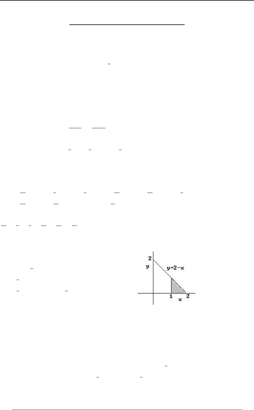
PROBLEM SET 8 255

PROBLEM SET 8 SOLUTIONS

1. Let denote the number that appears on the wheel, so thatR

. Then, conditioning over ,TÒR œ"ÓœTÒRœ#ÓœTÒR œ$Óœ R

T Ò[ Ÿ "Þ&Ó œ T Ò[ Ÿ "Þ&lR œ "Ó † T ÒR œ "Ó  ÓT Ò[ Ÿ "Þ&lR œ #Ó † T ÒR œ #Ó

. T Ò[ Ÿ "Þ&lR œ $Ó † T ÒR œ $Ó

If then , so that andR œ " [ œ " T Ò[ Ÿ "Þ&lR œ "Ó œ " ß

if then , so that .R œ # [ œ # T Ò[ Ÿ "Þ&lR œ #Ó œ !

If then so thatRœ$ [µRÐ$ß"Ñ

T Ò[ Ÿ "Þ&lR œ $Ó œ T Ò Ÿ lR œ $Ó œ T Ò^ Ÿ  "Þ&Ó œ Þ!(

[ $ "Þ&$

( has a standard normal distribution - the probability is found from the table).^

Then, . Answer: CT Ò[ Ÿ "Þ&Ó œ " †  ! †  ÐÞ!(Ñ † œ Þ$&(

"" "

$$ $

2. This discrete distribution has the following 8 points and probabilities:

Ð"ß #Ñ Ð"ß %Ñ Ð"ß )Ñ Ð#ß #Ñ Ð#ß %Ñ Ð#ß )Ñ , ; , ; , ; , ; , ; , ;

"""" ""

"#'$#%"#'

Ð%ß %Ñ Ð%ß )Ñ \  Ÿ & , ; , . The event occurs at the points

"" ]

#% "# #

Ð"ß #Ñ ß Ð"ß %Ñ ß Ð"ß )Ñ ß Ð#ß #Ñ Ð#ß %Ñand . The total probability of this event occurring is

"""" " "(

"#'$#%"# #%

  œ . Answer: E

3. TÒ\  "Ó

œ B .C .B

##B

œBÐ#BÑ.B

œÐ#BBÑ.Bœ

Answer: D

4. It follows from the independence of and that\]

IÒÐ\  "Ñ Ð]  "Ñ Ó œ IÒÐ\  "Ñ Ó † IÒÐ]  "Ñ ÓÞ

## # #

IÒÐ\  "Ñ Ó œ IÒ\  #\  "Ó œ IÒ\ Ó  #IÒ\Ó  " ß

## # and since

## # ## #

œ IÒ\ Ó  ÐIÒ\ÓÑ IÒ\ Ó œ  ÐIÒ\ÓÑ œ, we have , and then

IÒÐ\  "Ñ Ó œ IÒ\  #\  "Ó œ  #Ð"Ñ  " œ

## $*

In a similar way, andIÒ] Ó œ  ÐIÒ] ÓÑ œ $ ß

## #

]

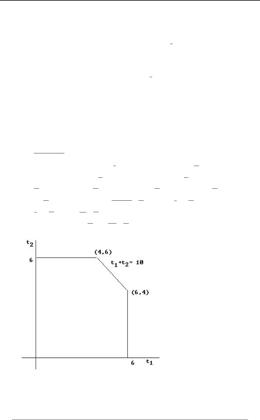
256 PROBLEM SET 8

4. continued

IÒÐ] "Ñ ÓœIÒ] #] "Óœ$#Ð"Ñ"œ'

## ,

so that .IÒÐ\"Ñ Ð] "Ñ ÓœIÒÐ\"Ñ Ó†IÒÐ] "Ñ Óœ †'œ#(

## # #

Note that we could also find in the following way:IÒÐ\  "Ñ Ó

Ð\"Ñ œ\ #\"œ\ #\"%\œÐ\"Ñ %\

## # # , and then

IÒÐ\  "Ñ Ó œ IÒÐ\  "Ñ Ó  %IÒ\Ó œ  % œ

## #

#(since

Z +<Ò\Ó œ IÒÐ\  Ñ Ó ß œ " IÒÐ]  "Ñ Ó..

and ). can be found in a similar way.

Answer: E

5. Since the joint density is a constant, say , over the probability region, and since the total-

probability in the region must be 1, it follows that (Region Area) ,-‚ œ"

so that . The area of the region is the area of the 6 by 6 square minus the area-œ "

V/1398 E</+

of the upper right triangle. This is , so that .$'  ‚ # ‚ # œ $% - œ

#$%

Then, IÒX  X Ó œ Ð>  > ÑÐ Ñ .> .>  Ð>  > ÑÐ Ñ .> .> Þ

" # "# #" "# #"

!! %!

% ' ' "!>

$% $%

'' '' "

"# # " " "

Ð>  > ÑÐ Ñ .> œ Ð'>  ")ÑÐ Ñ Ê Ð'>  ")ÑÐ Ñ .> œ Ð%)  (#ÑÐ Ñ

"" ""

$% $% $% $% .

"!> "# # "" "

"Ð>  > ÑÐ Ñ .> œ ÒÐ"!  > Ñ>  ÓÐ Ñ œ Ð&!  > ÑÐ Ñ

"""

$% # $% $%

Ð"!> Ñ

pÐ&!>ÑÐÑ.>œÐÑÐÑ

'" ##%

$% $% .

Then, . IÒX  X Ó œ Ð%)  (#ÑÐ Ñ  Ð ÑÐ Ñ œ &Þ($

"# " ##% "

$% $ $%

Answer: C

PROBLEM SET 8 257

6. We first find the conditional distribution of given .]\œ"

T Ò] œ !l\ œ "Ó œ œ ß T Ò] œ "l\ œ "Ó œ

T Ò\œ"ß] œ!Ó

TÒ\œ"Ó TÒ\œ"Ó TÒ\œ"Ó

Þ!& Þ"#& ;

this requires .TÒ\ œ "Ó œ T Ò\ œ "ß ] œ !Ó  T Ò\ œ "ß ] œ "Ó œ Þ!&  Þ"#& œ Þ"(&

The conditional distribution of given is]\œ"

T Ò] œ !l\ œ "Ó œ œ œ ß T Ò] œ "l\ œ "Ó œ œ

T Ò\œ"ß] œ!Ó

T Ò\œ"Ó Þ"(& ( Þ"(& (

Þ!& # Þ"#& & .

The conditional variance is , whereZ +<Ò] l\ œ "Ó œ IÒ] l\ œ "Ó  ÐIÒ] l\ œ "ÓÑ

IÒ]l\œ"ÓœÐ!ÑÐÑÐ"ÑÐÑœ ßIÒ]l\œ"ÓœÐ!ÑÐÑÐ"ÑÐÑœ

###

#&& #&&

((( (((

Then . Answer: CZ +<Ò] l\ œ "Ó œ  Ð Ñ œ Þ#!%

((

7. The marginal distribution of is found by summing probabilities over the other variable .\]

TÒ\œ!Óœ TÒ\œ!ß] œCÓœ !!œ



Cœ!

#""

TÒ\œ"Óœ TÒ\œ"ß] œCÓœ  !œ



Cœ!

#"" "

"# ' % ,

TÒ\œ#Óœ TÒ\œ#ß] œCÓœ   œ



Cœ!

#""" (

"#$' "#

IÒ\Ó œ B † T Ò\ œ BÓ œ Ð!ÑÐ Ñ  Ð"ÑÐ Ñ  Ð#ÑÐ Ñ œ



Bœ!

#"" ("(

'%"#"#

IÒ\ Ó œ B † T Ò\ œ BÓ œ Ð! ÑÐ Ñ  Ð" ÑÐ Ñ  Ð# ÑÐ Ñ œ

## ###

Bœ!

"" ($"

'%"#"#

Z +<Ò\Ó œ IÒ\ Ó  ÐIÒ\ÓÑ œ  Ð Ñ œ Þ&('

## #

$" "(

"# "# . Answer: B

8. We wish to find .T Ò"  ]  $l\ œ #Ó œ 0ÐCl\ œ #Ñ .C œ .C

0Ð#ßCÑ

0Ð#Ñ

0Ð#ßCÑ œ †C œ C

# Ð#"Ñ #

#ÒÐ#ÑÐ#Ñ"ÓÎÐ#"Ñ $ ,

0 Ð#Ñœ 0Ð#ßCÑ.Cœ C .Cœ Ê œ#C

\""

∞∞

$ $

%0Ð#Ñ

0Ð#ßCÑ

\ .

TÒ"] $l\ œ#Óœ #C .Cœ C œ  Ð"Ñœ

'¹

$$ #

Cœ"

Cœ$ ")

Answer: E

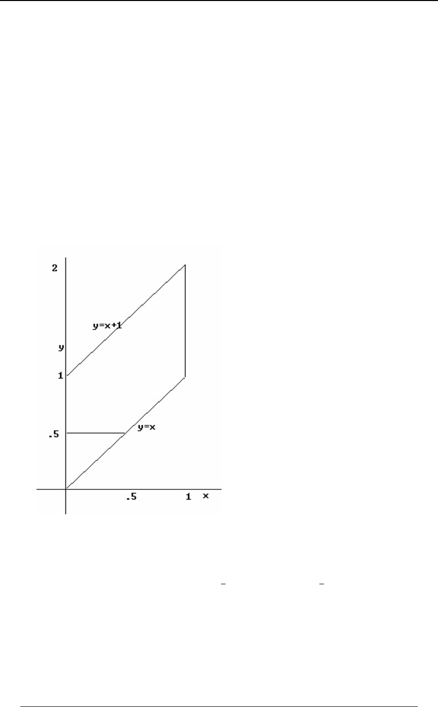
258 PROBLEM SET 8

9. We are given that the marginal distribution of is uniform on the interval ,\ Ð!ß "Ñ

so that for . We are also given that the conditional distribution of 0ÐBÑœ" !B" ]

given is uniform on the interval , so that for\œB BCB" 0 ÐCl\œBÑœ"

]l\

BCB" \ ] . The density function for the joint distribution of and is

0 ÐBßCÑœ0 ÐCl\œBÑ†0 ÐBÑœ" !BCB"#

\ß] \

]l\ on the region ;

this region of probability is the parallelogram in the graph below .

The event "damage to the other driver's car will be greater than .5" when an accident occurs is the

event " " . This is the upper region of the parallelogram below. The probability is the]Þ&

double integral of the joint distribution density on that region. We can also find the probability by

first finding the probability of the lower triangular region and then taking the complement.

TÒ]  Þ&Ó œ "TÒ] Ÿ Þ&Ó .

TÒ] Ÿ Þ&Ó œ ".C.B œ ÐÞ&BÑ.B œ Ê TÒ]  Þ&Ó œ

'' '

!B !

Þ& Þ& Þ& "(

))

. Answer: D

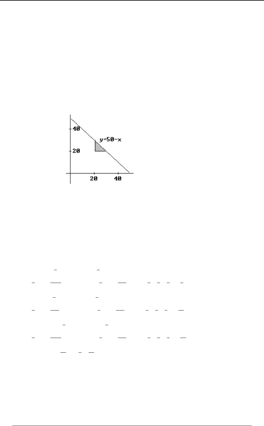
PROBLEM SET 8 259

10. The region of joint density is the region in the first quadrant below the line Cœ&!B

(with horizontal intercept 50 and vertical intercept 50). If and denote the failure time of\]

the two components, then the event that both components are still functioning 20 months from

now has probability . This is the shaded region in the graph at theT ÒÐ\  #!Ñ ∩ Ð]  #!ÑÓ

right. From the graph it can be seen that the region of probability for this event is the triangular

region bounded on the left by and on the right by , and bounded below byBœ#! Bœ$!

C œ #! C œ &!  B, and bounded above by .

The probability of the event is .

#! #!

$! &!B0ÐBß CÑ .C .B

Answer: B

11. .G9@Ð\ß ] Ñ œ IÒ\] Ó  IÒ\Ó † IÒ] Ó

We use the expression to find . Since the region ofIÒ\Ó œ B † 0ÐBß CÑ .C .B IÒ\Ó

probability is defined with , we apply double integration in the order. ItB Ÿ C Ÿ #B .C .B

would be possible to reverse the order, but that would not make the solution any more efficient.

IÒ] Ó IÒ\] Ó and are found in a similar way.

IÒ\Ó œ B † † BC .C .B œ † B C .C .B

'' ''

!B !B

"#B "#B

))

œ†Ò Ó.Bœ†Ò Ó.Bœ††œ Þ

) ) $B )$" %

$ # $ # $#& &

CœB

Cœ#B

## %

IÒ] Ó œ C † † BC .C .B œ † BC .C .B

'' ''

!B !B

"#B "#B #

))

œ†Ò Ó.Bœ†Ò Ó.Bœ††œ Þ

) ) (B ) ( " &'

$ $ $ $ $$& %&

CœB

Cœ#B

IÒ\] Ó œ BC † † BC .C .B œ † B C .C .B

'' ''

!B !B

"#B "#B

))

œ†Ò Ó.Bœ†Ò Ó.Bœ††œ Þ

) ) (B ) ( " #)

$ $ $ $ $$' #(

CœB

Cœ#B

#$ &

Then . Answer: AG9@Ð\ß ] Ñ œ  Ð ÑÐ Ñ œ Þ!%"

#) % &'

#( & %&

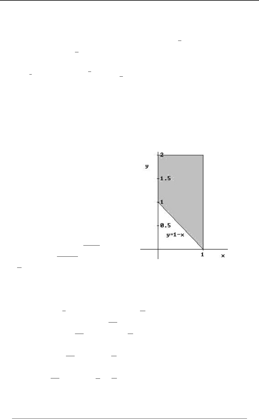
260 PROBLEM SET 8

12. The range is only valid for . This is true since for B ŸCŸB !ŸBŸ" B B B"

# #

and for . Therefore, the range for is , so thatB !B B! C !ŸB ŸCŸBŸ"

# #

!ŸCŸ" B ŸC BŸ C B ŸCŸB . Also, the inequality is equivalent to , so that

is equivalent to . The marginal density function of is found by integrating theCŸBŸ C ]

joint density over the range for the other variable ;B

1ÐCÑ œ "&C .B œ "&CB œ "&CÐ C  CÑ œ "&ÐC  C Ñ ! Ÿ C Ÿ "

'¹È

C$Î# #

ÈBœC

Bœ C

È for .

Note that it is true that for any particular we have . However, since can be anyB B ŸCŸB B

number from 0 to 1, can also be any number from 0 to 1. Answer: EC

13. We are asked to find .TÒ\ ]  "Ó

The joint distribution of and is defined\]

on the rectangle .!\"ß !] #

The region representing the probability in

question is the region on and above the line

BCœ" that is inside the rectangle.

The probability is the double integral of the

joint density function, integrated over the

region of probability. This can be

expressed as

'' ''

!"B !"B

"# "# #B#C

0ÐBß CÑ .C .B œ .C .B

, which becomes '!

"&B 'B"

)

.B œ œ Þ("

#% .

Answer: D

14. for , for 0 ÐCl\œBÑœ !CB 0 ÐBÑœ !B"#Þ

]l\ \

B"#

0 ÐBßCÑœ0 ÐCl\œBÑ†0 ÐBÑœ !CB"#Þ

\ß] \

]l\ "

"#B for

Then .IÒ\] Ó œ BC † .C .B œ .C .B œ #%

'' ''

!! !!

"# B "# B

"#B "#

We are given that has a uniform distribution on , and therefore, .\ Ð!ß "#Ñ IÒ\Ó œ '

Also, (note that if we had used the reverse order ofIÒ] Ó œ C † .C .B œ .B œ $

'' '

!! !

"# B "#

"#B #%

integration then we would have

IÒ] Ó œ C † .B.C œ 68Ð Ñ.C

'' '

!C !

"# "# "# C

""#

"#B C , which would require integration by parts).

Finally, . Answer: CG9@Ð\ß ] Ñ œ #%  Ð'ÑÐ$Ñ œ '

PROBLEM SET 8 261

15. If we find the conditional density function , then0ÐCl\œÑ

]l\ "

TÒ]  \l\ œ Ó œ TÒ]  l\ œ Ó œ 0 ÐCl\ œ Ñ.C

"" "

$$ $

"Î$

]l\

' .

The conditional density is .0ÐCl\œÑœ

]l\ "

0Ð ßCÑ

0ÐÑ

The joint density is ,0Ð ß CÑ œ #%Ð ÑC œ )C ß !  C  " 

"" "

$$ $

and the marginal density of at is \ \ œ 0 Ð Ñ œ #%Ð ÑC .C œ Þ

"" " "'

$$ $ *

#Î$

The conditional density is .0ÐCl\œÑœ œ

]l\ "

)C *C

The conditional probability is . Answer: CTÒ]  \l\ œ Ó œ .C œ

$#%

"Î$

16. We first find the value of the constant that makes a properly defined density50ÐBßCÑ

function for the joint distribution. The requirement that must be met is that the double integral of

0ÐBßCÑ BC BC over the - region of density must be 1. The - region of density is the square

!B"ß !C" . Thus,

'' '

!! !

"" " "

5B.C.Bœ5 B.Bœ5Ð Ñœ" 5œ# 0ÐBßCÑœ#B , from which we get and .

We use following definition of : .G9@Ð\ß]Ñ G9@Ð\ß]ÑœIÒ\]ÓIÒ\Ó†IÒ]Ó

IÒ\] Ó œ ÐBCÑ0ÐBß CÑ .C .B œ ÐBCÑÐ#BÑ .C .B œ

'' ''

!! !!

"" "" "

$ ,

IÒ\Ó œ ÐBÑ0ÐBß CÑ .C .B œ ÐBÑÐ#BÑ .C .B œ

'' ''

!! !!

"" ""

2 ,and

IÒ] Ó œ ÐCÑ0ÐBß CÑ .C .B œ ÐCÑÐ#BÑ .C .B œ

'' ''

!! !!

"" "" "

# .

Then, .G9@Ð\ß] Ñ œ  † œ !

"#"

$$#

There is another way that this covariance of 0 could have been found.

The density function of the marginal distribution of is for\0ÐBÑœ#B.Cœ#B

!B" ], and the density function of the marginal distribution of is

0 ÐCÑœ #B.Bœ" !C"

' for . We can then see that

0ÐBß CÑ œ #B œ Ð#BÑÐ"Ñ œ 0 ÐBÑ † 0 ÐCÑ \ ]

, which indicates that and are independent. If two

random variables are independent, then they have covariance of 0. Answer: B

17. The distribution of the number of tornadoes in county Q given there are none in county P is

TÒUœ8lT œ!Ó œ 8œ!ß"ß#ß$

T ÒÐUœ8Ñ∩ÐT œ!ÑÓ

TÒTœ!Ó , for .

The denominator is T ÒT œ !Ó œ T ÒÐU œ !Ñ ∩ ÐT œ !ÑÓ  T ÒÐU œ "Ñ ∩ ÐT œ !ÑÓ

 T ÒÐU œ #Ñ ∩ ÐT œ !ÑÓ  T ÒÐU œ $Ñ ∩ ÐT œ !ÑÓ œ Þ"#  Þ!'  Þ!&  Þ!# œ Þ#& .

Then, T ÒU œ !lT œ !Ó œ œ œ Þ%) ß T ÒU œ "lT œ !Ó œ Þ#% ß

T ÒÐUœ!Ñ∩ÐT œ!ÑÓ

TÒTœ!Ó Þ#&

Þ"#

T ÒU œ #lT œ !Ó œ Þ#! ß T ÒU œ $lT œ !Ó œ Þ!) .

Then, IÒUlT œ !Ó œ Ð!ÑÐÞ%)Ñ  Ð"ÑÐÞ#%Ñ  Ð#ÑÐÞ#Ñ  Ð$ÑÐÞ!)Ñ œ Þ)) ß

IÒU lT œ !Ó œ Ð! ÑÐÞ%)Ñ  Ð" ÑÐÞ#%Ñ  Ð# ÑÐÞ#Ñ  Ð$ ÑÐÞ!)Ñ œ "Þ(' ß

# #### and

Z +<ÒUlT œ !Ó œ IÒU lT œ !Ó  ÐIÒUlT œ !ÓÑ œ "Þ('  ÐÞ))Ñ œ Þ*)&'

###

. Answer: D

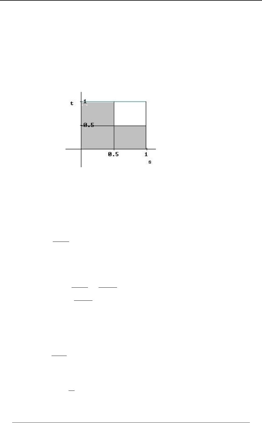
262 PROBLEM SET 8

18. Suppose that the times of failure of the two devices are and .\]

We wish to find the probability that at least one failure occurs by time .5 .

This is . The region of probability is the shaded in the graph below. TheT ÒÐ\  Þ&Ñ ∪ Ð]  Þ&ÑÓ

probability is the double integral over region E (let be the horizontal, vertical).>=

The first integral corresponds to the square . and the second integral&="ß!>Þ&ß

corresponds to the rectangle .!=Þ&ß!>"

Answer: E

19. We must have since no more than proportion buy the supplementary policy. The]Ÿ\ \

region of positive joint density is the triangular region !ŸCŸBŸ"

(below the line , inside the unit square). We wish to find the conditionalCœB

probability . The conditional density for given isT Ò]  Þ!&l\ œ Þ"Ó ] \ œ Þ"

0 ÐCl\ œ Þ"Ñ œ 0 ÐÞ"Ñ

]l\ \

0ÐÞ"ßCÑ

0ÐÞ"Ñ

\ , where is the density function of the marginal distribution of

\0ÐBÑœ0ÐBßCÑ.C at .1 . In general, gives the density of the marginal distribution of

\∞

∞

\ from a joint distribution. In this case, based on where the joint density is non-zero, we have

0 ÐÞ"Ñ œ 0ÐÞ"ß CÑ .C œ #ÐÞ"  CÑ .C œ Þ!$

\!!

Þ" Þ"

'' .

Then, , (since and0 ÐCl\œÞ"Ñœ œ CÞ" ] \Ñß

]l\

0ÐÞ"ßCÑ #ÐÞ"CÑ

0ÐÞ"Ñ Þ!$

T Ò]  Þ!&l\ œ Þ"Ó œ .C œ Þ%"'(

Þ!& #ÐÞ"CÑ

Þ!$ . Answer: D

20. To find the conditional variance of given that , we must find the density]\œB

function of the conditional distribution of given . This is ]\œB

0ÐCl\œBÑœ Þ

]l\

0ÐBßCÑ

0ÐBÑ

\ We must find the density function of the marginal distribution

of . This is found by integrating the joint distribution density with respect to over the\C

appropriate region: for .0ÐBÑœ #B.Cœ#B !B"

B"

Then, and this conditional density is valid for .0 ÐCl\œBÑœ œ" BCB"

]l\ #B

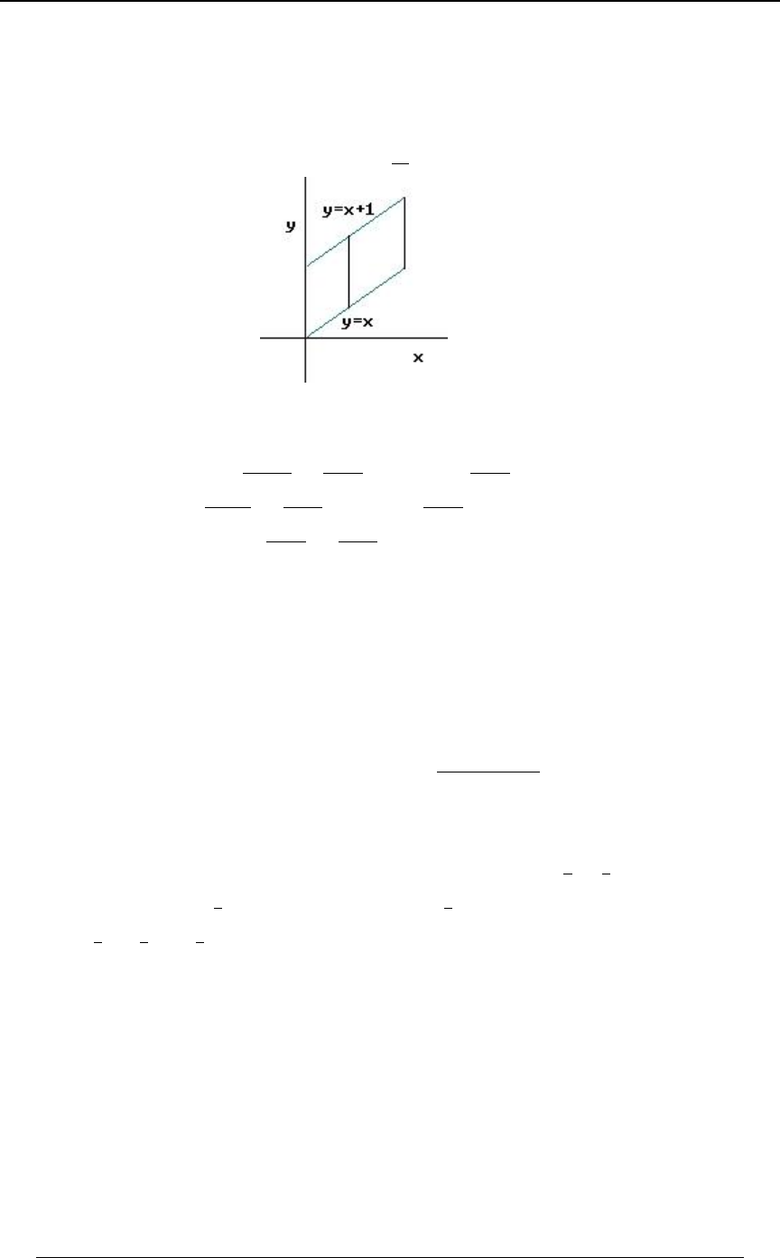
PROBLEM SET 8 263

20. continued

Therefore, the conditional distribution of given is uniform on the interval]\œB

BCB" (a uniform distribution has a constant density). The variance of the continuous

uniform distribution on an interval of length 1 is .

Answer: A

21. , where J Ð>ÑœTÒ\Ÿ>ÓœTÒ Ÿ ÓœTÒ[ Ÿ Ó [ µRÐ!ß"Ñ

\\ > >.. .

55 5

\\ \

, where J Ð>ÑœTÒ] Ÿ>ÓœTÒ Ÿ ÓœTÒZ Ÿ Ó Z µRÐ!ß"ÑÞ

]]  > >.. .

55 5

]] ]

JÐ>ÑJÐ>Ñ  Ÿ Þ

\] \]

is equivalent to , which is equivalent to

> >..

\] ..

Note that the fact the and have a bivariate distribution with correlation coefficient is\] 3\]

irrelevant - we are comparing probabilities of the marginal distributions of and (however,\]

we do use the fact that and have common variance ). Answer: B\] 5#

22. The moment generating function of and is\\

QÐ>ß>ÑœIÒ/ Óœ / .B .B œ

"# " #

>\>\ >B>B

"" ## "" ##

'' ()()/"/"

"# . Answer: B

23. The moment generating function for is \QÐ>ÑœQÐ>ß!Ñœ/Þ

\" " >

Then, , and , so thatIÒ\Ó œ Q Ð!Ñ œ IÒ\ Ó œ Q Ð!Ñ œ

w#ww

Z+<Ò\Óœ Ð Ñ œ

## #

$$ *

# . Answer: D

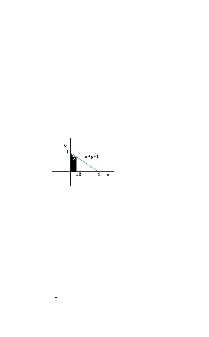
264 PROBLEM SET 8

24. We wish to find . The region of density for the joint distribution is below theTÒ\  Þ#Ó

line . The region of probability for the event in question is shaded below. TheBCœ"

probability is found by integrating the joint density over that region.

T Ò\  Þ#Ó œ 'Ò"  ÐB  CÑÓ .C .B œ $Ð"  BÑ .B œ Þ%))

'' '

!! !

Þ# "B Þ# # .

It would also be possible to solve this problem by first finding the marginal distribution of , and\

then find . The density function of the marginal distribution of isTÒ\  Þ#Ó \

found by integrating the joint density in the " -direction" over the appropriate range.C

Since is equivalent to , the appropriate range for integration over is fromBC" C"B C

Cœ! Cœ"B to . Therefore,

0 ÐBÑ œ 0ÐBß CÑ .C œ 'Ò"  ÐB  CÑÓ .C œ $Ð"  BÑ

\!!

"B "B #

'' .

This is exactly the "inside integral" in the double integration above.

Then, , as before.T Ò\  Þ#Ó œ $Ð"  BÑ .B œ Þ%))

Þ# #

This second approach is essentially identical to the first approach.

Answer: C

25. (since and are independent, the joint densityT Ò]  \Ó œ 0 ÐBÑ0 ÐCÑ .B .C \ ]

∞∞

function of and is the product of the two separate density functions).\]

The density function of is , and of is , so that\/ ] /

α"

BÎ BÎα"

TÒ]\Óœ / /.B.Cœ // .Cœ œ

'' '

!C !

∞∞ ∞

BÎ CÎ CÎ CÎ

"" "

α" " α"

α" "α

α"

Answer: A

26. The marginal density function of is ,\ 0 ÐBÑ œ Ð#  B  CÑ .C œ Ð#  BÑ

#B #

'$$

and then . In a similar way, the marginal density function of IÒ\Ó œ B † Ð#  BÑ .B œ Þ& ]

)

is ,0 ÐCÑ œ Ð#  B  CÑ .B œ Ð#  CÑ

#C #

'$$

and then (this could be anticipated from the symmetry of IÒ] Ó œ C † Ð#  CÑ .C œ Þ& B

)

and in the joint density function). Then, . Alternatively, we can findCIÒ\]Óœ"

IÒ\]Óœ ÐBCÑ† Ð#BCÑ.C.Bœ"

##B $

%. Answer: C

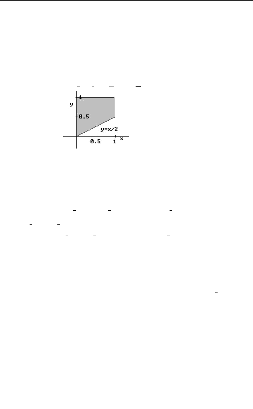
PROBLEM SET 8 265

27. The marginal density function of is , and then] 0 ÐCÑ œ Ð'BC  $B Ñ.B œ %C

C#$

T Ò]  Þ&Ó œ %C .C œ ÐÞ&Ñ

Þ& $%

. Answer: C

28. The shaded region in the graph below corresponds to the event that . The\#]

probability is TÒ\  #]Ó œ TÒ  ]Ó œ ÐBCÑ.C.B

#!BÎ#

.œÒBÐ"ÑÐ"ÑÓ.Bœ

"B" B

## %

#"*

Answer: D

29. The device fails when the second circuit fails, which is at time . We wish to find .]IÒ]Ó

This is .IÒ] Ó œ C † '/ / .C .B œ '/ Ð C † / .C Ñ.B

'' ' '

!B ! B

∞∞ ∞ ∞

B #C B #C

We find by integration by parts :

∞#C

C†/ .C

'' '

BB B

∞∞ ∞

#C #C #C #C

C†/ .Cœ C.Ð / Ñœ  C/  Ð / Ñ.C

"" "

## #

CœB

Cœ∞

œ! B/  /

#B #B .

Then, .IÒ] Ó œ '/ Ð B/  / Ñ .B œ Ð$B/  / Ñ .B

∞∞

B #B #B $B $B

"" $

#% #

From integration by parts, we get .

'' ¹

∞∞

$B $B $B

$B/ .B œ B .Ð  / Ñ œ  B/ œ

Bœ!

Bœ∞

Also, so that

∞$B

$" ""&

## $#'

/ .Bœß IÒ]ÓœœÞ

Alternatively, we can find the pdf of the marginal distribution of first:]

0 ÐCÑ œ 0ÐBß CÑ .B œ '/ / .B œ 'Ð"  / Ñ/ œ 'Ð/  / Ñ !  C  ∞

]!!

B #C C #C #C $C

'' , for .

Then, . After integration by parts, this becomes .IÒ] Ó œ C † 'Ð/  / Ñ.C

∞#C $C &

Answer: D

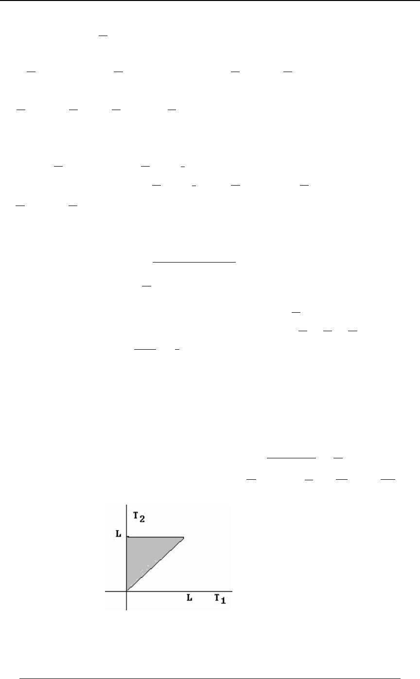
266 PROBLEM SET 8

30. .IÒ\Ó œ B † Ð"!  BC Ñ .C .B

"! " #

The "inside" integral is

###

B † Ð"!  BC Ñ .C œ † Ð"!B  B C Ñ .C œ † Ò"!B  Ó

"" "B

'% '% '% $

# .

The complete integral is

'¹

"! #

"B" B

'% $ '% * Bœ#

Bœ"!

† Ò"!B  Ó .B œ † ÒÐ&B  Ñ Ó œ &Þ)

Note that we could have found , the marginal density function of first and the have found0ÐBÑ \

IÒ\Ó. This would be done as follows:

0 ÐBÑ œ Ð"!  BC Ñ .C œ Ð"!  Ñ

"#B

'""

'% '% , and then

IÒ\Ó œ B † 0 ÐBÑ .B œ B † Ð"!  Ñ .B œ † Ð"!B  Ñ .B

'' '

## #

"! "! "!

""B

'% '% $

œ†Ð&BÑ Óœ&Þ)

'% * Bœ#

Bœ"!

#$¹ (as in the first approach). Answer: C

31. .T Ò\  ]  ^ œ #l\ œ !Ó œ T ÒÐ] ^œ#Ñ∩Ð\œ!ÑÓ

TÒ\œ!Ó

T Ò\ œ !Ó œ 0Ð!ß Cß DÑ œ ÒÐ'  !Ñ  Ð'  "Ñ  Ð'  #Ñ



Cœ! Dœ!

## "

Ð'"ÑÐ'#ÑÐ'$ÑÐ'#ÑÐ'$ÑÐ'%ÑÓœ $'

)" .

T ÒÐ]  ^ œ #Ñ ∩ Ð\ œ !ÑÓ œ 0Ð!ß !ß #Ñ  0Ð!ß "ß "Ñ  0Ð!ß #ß !Ñ œ  

%%%

)" )" )" .

T Ò\  ]  ^ œ #l\ œ !Ó œ œ Þ

"#Î)"

$'Î)" $

" Answer: B

32. The graph at the right indicates the region of non-zero density for the joint distribution of

X X Ð>  > Ñ 0Ð> ß > Ñ .> .>

"# "#"#

and . The expected value is . We are told that the joint

''#

distribution is uniform over the triangular region, and therefore the joint density function

0Ð>ß>Ñ œ

is constant over the region and numerically equal to (half of the

Parea of region #

P‚P Ð>>Ñ† .>.>œ † .>œ square). The expected value is .

'' '

!! !

P> P

## "# #

##P

P$$

Answer: C

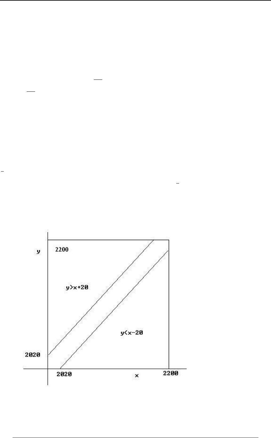
PROBLEM SET 8 267

33. The company considers the two bids further if the two bids are within 20 of one another. If

we let be the amount of the first bid and the amount of the second bid, then the region\] ÐBßCÑ

for which the company will consider the bids further satisfies

B#!CB#! . This is the complement of the union of the two regions

ÐC Ÿ B  #!Ñ ∪ ÐC  B  #!Ñ \ ] . We are told that both and are uniformly distributed between

2000 and 2200, so that for and0 ÐBÑ œ œ Þ!!& #!!! Ÿ B Ÿ ##!! ß

#!!

0 ÐCÑ œ œ Þ!!& #!!! Ÿ C Ÿ ##!! \ ]

#!! for . Since and are independent, the density

function of the joint distribution is for0 ÐBß CÑ œ 0 ÐBÑ † 0 ÐCÑ œ ÐÞ!!&Ñ

\ß] \ ] #

#!!! Ÿ B Ÿ ##!! #!!! Ÿ C Ÿ ##!! and . The probability of a two-dimensional region is the

double integral of the joint density over the region. Since the joint density is constant, the

probability is the region of the area multiplied by that constant.

The region (and inside the square) has probabilityCŸB#!

#‚ ")! ‚ ")! ‚ ÐÞ!!&Ñ œ Þ%!&

# (since the triangular region below the lower line has base 180

and height 180). The region also has probability C  B  #! ‚ ")! ‚ ")! ‚ ÐÞ!!&Ñ œ Þ%!&

(same size triangle). Therefore,

T Ò Ó œ T Ò\#!  ]  \  #!Óthe two bids are within 20 of one another

œ "  Þ%!&  Þ%!& œ Þ"* .

Answer: B

268 PROBLEM SET 8

34. Conditional expectations are usually found as follows.

IÒ[l[  +Ó œ '+

∞[

A0 ÐAÑ.A

TÒ[+Ó (with summation used in the discrete case), with a similar

formulation for or . In the specific case that is a non-IÒ[l[  +Ó IÒ[l+  [  ,Ó [

negative random variable( ), we have (in the discrete case),[  ! IÒ[ l[  !Ó œ DA0ÐAÑ

TÒ[!Ó

and notice that the numerator is (unconditional expectation), so thatIÒ[Ó

IÒ[l[  !Ó œ Þ

IÒ[Ó

TÒ[!Ó In this case,

IÒPÓ œ Ð!ÑÐÞ*Ñ  Ð&!!ÑÐÞ!'Ñ  â  Ð"!!ß !!!ÑÐÞ!!"Ñ œ #*! T ÒP  !Ó œ Þ" , and ,so that

the conditional expectation becomes .IÒPlP  !Ó œ œ #*!!

#*!

Þ"

The problem can be solved in an alternative way. We first determine the conditional distribution

of given that (where denotes that amount of the loss). has a discrete distribution,PP!P P

and the probability function of given that is found from the following relationship.PP!

For , .B  ! T ÒP œ BlP  !Ó œ œ œ "!T ÒP œ BÓ

TÒPœBÓ TÒPœBÓ

TÒP!Ó Þ"

The conditional distribution of given isPP!

BTÒPœBlP!Ó

&!! Þ'!!

"ß !!! Þ$!!

"!ß !!! Þ!)!

&!ß !!! Þ!"!

"!!ß !!! Þ!"!

The expected amount of the loss given that the loss is greater than 0 is the expectation of this

conditional distribution of given that . This expectation isPP!

IÒPlP  !Ó œ Ð&!!ÑÐÞ'Ñ  Ð"ß !!!ÑÐÞ$Ñ  Ð"!ß !!!ÑÐÞ!)Ñ

 Ð&!ß !!!ÑÐÞ!"Ñ  Ð"!!ß !!!ÑÐÞ!"Ñ œ #ß *!! . Answer: D

35. Let and denote the two loss amounts ( payment amounts).\] not

We consider the following combinations of and that result in the total benefit not\] payment

exceeding 5.

Case 1: (so loss results in no payment) and (so that loss results in a!\Ÿ" \ !] Ÿ( ]

maximum payment of 5 after applying the deductible of 2).

Case 2: (so loss results in a maximum payment of 5 after the deductible of 1 is"\Ÿ' \

applied) and (so loss results in no payment).!] Ÿ# ]

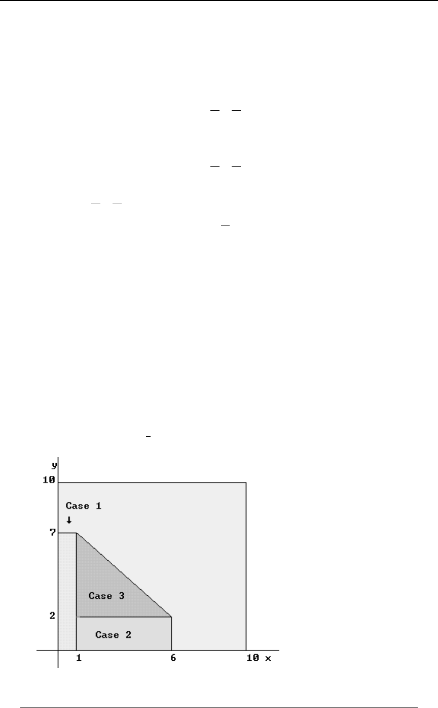
PROBLEM SET 8 269

Case 3: and and ( is paid for loss "\ Ÿ' #Ÿ] Ÿ( Ð\"ÑÐ] #ÑŸ& \" \

and is paid for loss ). The last condition is equivalent to . The probability]# ] \]Ÿ)

that the total benefit paid does not exceed 5 is the sum of the probabilities for Cases 1, 2 and 3.

TÒ ÓœTÒÐ!\Ÿ"Ñ∩Ð!] Ÿ(ÑÓCase 1

œTÒ!\Ÿ"Ó†TÒ!] Ÿ(ÓœÐ ÑÐ ÑœÞ!(

"! "!

(we have used the independence of and to find the probability of the intersection)\]

TÒ ÓœTÒÐ"\Ÿ'Ñ∩Ð!] Ÿ#ÑÓCase 2

.œTÒ"\Ÿ'Ó†TÒ!] Ÿ#ÓœÐ ÑÐ ÑœÞ"!

"! "!

TÒ Ó œ 0ÐBß CÑ .C .B œ 0 ÐBÑ † 0 ÐCÑ .C .BCase 3 '' ''

"# "#

')B ')B

œ Ð ÑÐ Ñ .C .B œ ÐÞ!"Ñ .C .B

'' ''

"# "#

')B ')B

"! "!

œ ÐÞ!"Ñ Ò)  B  #Ó .B œ ÐÞ!"ÑÐ'B  Ñ œ Þ"#&

'¹

#Bœ"

Bœ'

(note that because and are independent).0ÐBß CÑ œ 0 ÐBÑ † 0 ÐCÑ \ ]

The total probability is .Þ!(  Þ"!  Þ"#& œ Þ#*&

Once we have identified Cases 1, 2 and 3, this problem could be approached from a graphical

point of view. Since and are independent and uniform, the joint distribution of and is\] \]

uniform on the square , , with joint density .!  B  "! !  C  "! ÐÞ"ÑÐÞ"Ñ œ Þ!"

Since the joint distribution is uniform, the probability of any event involving and is equal to\]

the constant density (.01 in this case) multiplied by the area of the region representing the event.

The three regions for Cases 1, 2 and 3 are indicated in the graph below.

The 10 10 square is the full region for the joint distribution.‚

The rectangular area for Case 1 is for a probability of ." ‚ ( œ ( ( ‚ Þ!" œ Þ!(

The rectangular area for Case 2 is for a probability of .& ‚ # œ "! "! ‚ Þ!" œ Þ"!

The triangular are for Case 3 is for a probability of .

#‚ & ‚ & œ "#Þ& "#Þ& ‚ Þ!" œ Þ"#&

The total probability for Cases 1, 2 and 3 combined is again . Þ#*&

Answer: C

270 PROBLEM SET 8

36. ,: ÐBÑ œ :ÐBß CÑ Þ : Ð!Ñ œ :Ð!ß "Ñ  :Ð!ß #Ñ œ  œ

D"#"

"# "# %

: Ð"Ñ œ :Ð"ß #Ñ  :Ð"ß $Ñ œ  œ : ÐBÑ œ !

%&$

"# "# % , and , otherwise. Answer: B

37. The new amount paid to the surgeon is , and the new amount of hospital\ œ \  "!!

charges is . We wish to find] œ "Þ"]

Z+<Ò\]ÓœZ+<Ò\ÓZ+<Ò]Ó#G9@Ð\ß]ÑÞ

ww w w ww

Z +<Ò\ Ó œ Z +<Ò\  "!!Ó œ Z +<Ò\Ó œ &ß !!! ß

w and

Z +<Ò] Ó œ Z +<Ò"Þ"] Ó œ Ð"Þ" ÑZ +<Ò] Ó œ Ð"Þ#"ÑÐ"!ß !!!Ñ œ "#ß "!!

w# .

G9@Ð\ ß ] Ñ œ G9@Ð\  "!!ß "Þ"] Ñ œ "Þ"G9@Ð\ß ] Ñ

ww .

We have used the covariance rule .G9@Ð+Y ,ß-[ .Ñ œ+-G9@ÐYß[Ñ

We still must know to complete the problem.G9@Ð\ß]Ñ

We are given , and we use the relationshipZ +<Ò\  ] Ó œ "(ß !!!

"(ß !!! œ Z +<Ò\  ] Ó œ Z +<Ò\Ó  Z +<Ò] Ó  #G9@Ð\ß ] Ñ

œ &ß !!!  "!ß !!!  #G9@Ð\ß ] Ñ p G9@Ð\ß ] Ñ œ "ß !!! .

Then .G9@Ð\ ß] Ñ œ "Þ"G9@Ð\ß]Ñ œ "ß"!!

Finally, Z+<Ò\]ÓœZ+<Ò\ÓZ+<Ò]Ó#G9@Ð\ß]Ñ

ww w w ww

. Answer: Cœ &ß !!!  "#ß "!!  #Ð"ß "!!Ñ œ "*ß $!!

38. .Gœ\]ßGœ\"Þ#]

We use the following rules: ,G9@ÐYßYÑ œ Z+<ÐYÑ

G9@Ð+Y ,Z -ß.W/X 0Ñ

œ +.G9@ÐY ß WÑ  +/G9@ÐY ß XÑ  ,.G9@ÐZ ß WÑ  ,/G9@ÐZ ß X Ñ ,

and .G9@ÐYßZ Ñ œ G9@ÐZ ßYÑ

Then, G9@ÐGßGÑœG9@Ð\]ß\"Þ#]Ñ

œG9@Ð\ß\Ñ"Þ#G9@Ð\ß]ÑG9@Ð]ß\Ñ"Þ#G9@Ð]ß]Ñ

œ Z +<Ð\Ñ  #Þ#G9@Ð\ß ] Ñ  "Þ#Z +<Ð] Ñ .

From the given information, we have Z +<Ð\Ñ œ IÐ\ Ñ  ÒIÐ\ÑÓ œ #Þ% ß

Z +<Ð] Ñ œ IÐ] Ñ  ÒIÐ] ÑÓ œ #Þ%

. Also,

Z+<Ð\]ÑœZ+<Ð\ÑZ+<Ð]Ñ#G9@Ð\ß]Ñ

p ) œ #Þ%  #Þ%  #G9@Ð\ß ] Ñ p "Þ' .

Then, .G9@ÐG ß G Ñ œ #Þ%  #Þ#Ð"Þ'Ñ  "Þ#Ð#Þ%Ñ œ )Þ)

Answer: A

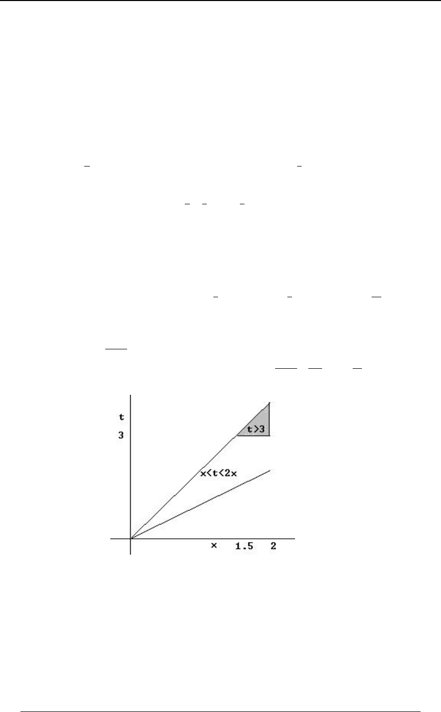
PROBLEM SET 8 271

39. G9@Ð\ß \  -] Ñ œ G9@Ð\ß\Ñ  -G9@Ð\ß ] Ñ œ Z +<Ò\Ó  -G9@Ð\ß ] Ñ

œ#&"!- G9@Ð\ß^Ñœ#Þ& . This is set equal to , so that

#&  "!- œ #Þ& p - œ #Þ#& . Answer: B

40. Distribution of given claim amount is uniform on interval and has pdfX\œB ÐBß#BÑ

0 Ð>l\œBÑœ B>#B \ 0 ÐBÑœ B !ŸBŸ#

Xl\ \#

for . The pdf of is for .

The density function of the joint distribution between and isX\

0 ÐBß>Ñœ0 Ð>l\œBÑ†0 ÐBÑœÐ ÑÐ BÑœ B !ŸB>#BŸ%

\ßX \

Xl\ #

"$ $

B) )

for

(since , it follows that ).BŸ# #BŸ%

The event is illustrated in the graph below. In order to have , it must be trueX$ X$

that , since if then . Thus, the region of probability for the eventB  "Þ& B  "Þ& >  #B  $

X $ "Þ&ŸBŸ# $>#B is , and . The probability is

TÒX $Óœ 0 ÐBß>Ñ.>.Bœ B.>.Bœ BÐ#B$Ñ.Bœ Þ

'' '' '

"Þ& $ "Þ& $ "Þ&

# #B # #B #

\ßX $$ ""

)) '%

Alternatively, we can express the conditional probability asTÒX  $l\ œ BÓ

TÒX  $l\ œ BÓ œ BŸ"Þ& #BŸ$

"Þ&  B Ÿ #

œ!if (since then )

if .

#B$

Then, T ÒX  $Ó œ T ÒX  $l\ œ BÓ † 0 ÐBÑ .B œ † .B œ Þ

"Þ& "Þ&

\#B$ $B ""

B) '%

The graph of the probability region is below.

Answer: A

272 PROBLEM SET 8

41. exponential mean 2 , pdf .Xµ 0Ð=Ñœ/

=Î#

X µ 0 ÐÑœ /

H>Î$

exponential mean 3 , t .

Since and are independent, the joint density isXX

0 Ð=ß >Ñ œ 0 Ð=Ñ † 0 Ð>Ñ œ Ð / ÑÐ / Ñ

FßH F H =Î# >Î$

, and

TÒX  X Ó œ Ð / ÑÐ / Ñ.=.>

HF !>

∞∞ =Î# >Î$

'' ""

œ/.>œÞ%

∞&>Î'

$ .

A more general reasoning approach to the solution is the following.

In the next 6 days we expect 3 Basic claims (one every 2 days) and 2 Deluxe claims

(one every 3 days). Of the next 5 claims, there is a chance that it is from a Deluxe policy

&œÞ%

on average. Answer: C

42. We first note that and are independent. This is true because the joint density can be\]

factored in a function of alone multiplied by a function of alone. Another way to verifyBC

independence is to note that the marginal density of is\

0ÐBÑœ 0ÐBßCÑ.Cœ #/ .Cœ/ B!

\!!

∞∞

ÐB#CÑ B

'' for ,

and the marginal density of is]

0 ÐCÑœ 0ÐBßCÑ.Bœ #/ .Bœ#/ C!

]!!

∞∞

ÐB#CÑ #C

'' for .

Then, since and since the region of density is rectangular (the entire0ÐBß CÑ œ 0 ÐBÑ † 0 ÐCÑ

first quadrant), it follows that and are independent. Since they are independent, the variance\]

of does not depend on , so the conditional variance of given is the same as the variance]\ ]\

of , and the conditional variance of given that and is the same as the]]\$]$

conditional variance of given that . The conditional density of given that is]]$ ]]$

0ÐCl]$Ñœ C$ TÐ]$Ñœ #/ .Cœ/

0ÐCÑ

TÐ]$Ñ

] for . , so

∞#C )

0ÐCl]  $Ñ œ C  $ D œ C $

#C

) for . If we make the change of variable

then this becomes for .0ÐDl^  !Ñ œ œ #/ D  !

#ÐD$Ñ

) #D

This is an exponential density with a mean of . The variance of an exponential distribution is

the square of the mean, which is .

#œ

Another point to note, once we have determined that the marginal distribution of is exponential]

with mean 0.5, because of the "lack-of-memory" property of the exponential distribution, the

conditional distribution of given is still exponential with mean 0.5, for any . ]]+ +!

Answer: A.

PROBLEM SET 8 273

43. The conditional density of given is on the interval (uniform).] \ 0 ÐClBÑ œ Ò!ß BÓ

]l\ "

The region of non-zero joint density of and is on the region , since has\] !CB" ]

non-zero density only on the interval . The joint density of and on that region isÒ!ß BÓ \ ]

0 ÐBß CÑ œ 0 ÐClBÑ † 0 ÐBÑ œ † #B œ # !  B  C  "

\ß] \

]l\ "

B for . We can summarize the joint

density function as if

0ÐBßCÑœ

# !CB"

! !BC"

\ß] œ

(note that we can ignore the region , since it has area 0 in the two-dimensional region ofCœB

probability). This is a (joint) uniform distribution on the triangular region . The!BC"

marginal density of is ,] 0 ÐCÑ œ 0 ÐBß CÑ .B œ ! .B  # .B œ #Ð"  CÑ

]\ß]

!!C

"C"

'''

and this is defined on the region . This is true because for!C" 0ÐBßCÑœ!

!CB" 0ÐBßCÑœ# !BC" and for .

Then the conditional density of given is\]œC

0 ÐBlCÑœ œ œ CB"

\l]

0ÐBßCÑ

0 ÐCÑ #Ð"CÑ "C

] for , and 0 otherwise.

It is also true in general that i the joint distribution of and is uniform (has constant density)\]

on a region, then the conditional density of given , or of given will be uniform on the]\\]

appropriate region of non-zero density. Once we have determined that the joint density of and\

] !CB" is 2 (constant, and therefore uniform) on the region , we know that the

conditional density of given will be constant on the interval of definition. The interval of\]

definition for given is , which has length . Therefore, the conditional\]CB" "C

density of given is the constant (the density of a uniform is )\] ""

"C interval length

Answer: E

44. The key point to note in this problem is that we are given the cdf of survival for someone

born in the same year as the insured. This is not the cdf of survival for a 40-year old, it is the cdf

of survival for a newborn. If we define to be the time until death for the 40-year old, then the\

distribution of is the conditional distribution of (time from birth until death) given that\X

X%! (given survival from birth to age 40). The expected payment is

&!!! ‚ T Ð\  "!Ñ œ &!!! ‚ T ÐX  &!lX  %!Ñ œ &!!! ‚ T Ð%!X &!Ñ

T ÐX %!Ñ

œ &!!! ‚ œ &!!! ‚ Þ!'*' œ $%)

J Ð&!ÑJ Ð%!Ñ

"J Ð%!Ñ

X . Answer: B

274 PROBLEM SET 8

45. We use the conditioning formula for variance.

Z+<ÒRÓœIÒZ+<ÒRl ÓÓ  Z+<ÒIÒRl ÓÓ-- .

Since the distribution of workplace accidents is Poisson with mean , we have-

IÒRl Ó œ Z +<ÒRl Ó œ-- -- - and . Then, since the distribution of is uniform on the

interval , we have , andÒ!ß$Ó IÒZ+<ÒRl ÓÓœIÒ Óœ"Þ&--

Z+<ÒIÒRl ÓÓœZ+<Ò Óœ œÞ(&--

# (the variance of a uniform random variable is the square of

the interval length divided by 12). Then . Answer: EZ+<ÒRÓœ"Þ&Þ(&œ#Þ#&

46. Since , a 5 can be rolled on the first roll or the third or later roll, and also there is no 6]œ#

on the first roll. Given that there is no 6 on the first roll, the probability of a 5 on the first roll

is . The number of rolls until a 5 appears has a geometric distribution with probability function

TÐ\ œ 8Ñ œ Ð ÑÐ Ñ œ '

"& "

' ' "Î'

8" , with mean . If the first 5 does not appear on the first roll,

then it will appear on the third or later roll, so the expected number of rolls needed to roll a 5

given that a 5 did not occur on the first two rolls is The overall expected number of#'œ)Þ

rolls until a 5 given that the first 6 is on the second roll is .Ð"ÑÐÞ#Ñ  Ð)ÑÐÞ)Ñ œ 'Þ'

Answer: D

47. If is a discrete random variable with probability function , then the[TÐ[œ5Ñœ:

moment generating function of is . Also, the moment generating function[QÐ>Ñœ:/

5>

of the sum of independent random variables is the product of the separate moment generating

functions. Then . Since and are identically distributed, weQ Ð>Ñ œ Q Ð>Ñ † Q Ð>Ñ \ ]

\] \ ]

have , so .Q Ð>Ñ œ Q Ð>Ñ Þ!*/  Þ#%/  Þ$%  Þ#%/  Þ!*/ œ ÒQ Ð>ÑÓ

\] \

#> > > #> #

Algebraically, we see that , so that he distribution of (and ) isQÐ>ÑœÞ$/ Þ%Þ$/ \ ]

\> >

TÐ\œ "ÑÞ$ßTÐ\œ!ÑœÞ% TÐ\œ"ÑœÞ$ TÐ\Ÿ!ÑœÞ( , . Then .

Answer: E

PROBLEM SET 8 275

48. The marginal density for at 0,75 is\

0 Ð!Þ(&Ñ œ 0Ð!Þ(&ß CÑ .C œ "Þ& .C  !Þ(& .C œ "Þ"#& Þ

\! ! !Þ&

"!Þ&"

'''

The conditional density of given is then]\œ!Þ(&

0 ÐClB œ Þ(&Ñ œ œ œ !CÞ&

œÞ&C"

]l\

0ÐÞ(&ßCÑ

0 ÐÞ(&Ñ Þ(& #

"Þ& %

"Þ"#& $

\œfor

for

Then, , andIÐ] l\ œ Þ(&Ñ œ C .C  C .C œ œ Þ%"(

!Þ&

Þ& "

IÐ] l\ œ Þ(&Ñ œ C .C  C .C œ Þ#&

###

!Þ&

Þ& "

$$ .

Z +<Ð] l\ œ Þ(&Ñ œ Þ#&  Þ%"( œ Þ!('

# . Answer: C

49. The joint density can be written as .0ÐBß CÑ œ / † Ð =38 CÑ œ 1ÐBÑ † 2ÐCÑ

B "

Since the joint density is defined on a rectangular region and since it factors into the form

1ÐBÑ † 2ÐCÑ \ ], it follows that the marginal distributions of and are independent. Therefore

T ÒÐ\  "Ñ ∩ Ð]  ÑÓ œ T Ò\  "Ó † T Ò]  Ó œ Ð / .BÑÐ =38 C .CÑ

###

"Î#

B 1

œÐ"/ ÑÐ Ñ

" "

# . Answer: A

276 PROBLEM SET 8

SECTION 9 - FUNCTIONS AND TRANSFORMATIONS OF RANDOM VARIABLES 277

SECTION 9 - FUNCTIONS AND TRANSFORMATIONS

OF RANDOM VARIABLES

Distribution of a transformation of a continuous random variable \

Suppose that is a continuous random variable with pdf and cdf , and suppose that\ 0 ÐBÑ J ÐBÑ

?ÐBÑ ? ?ÐBÑ œ / ß B is a one-to-one function (usually is either strictly increasing, such as or

BÈ

68 B ? ?ÐBÑ œ / ?, or is strictly decreasing, such as or ). As a one-to-one function, has an

B "

inverse function , so that . The random variable is referred to as a@ @Ð?ÐBÑÑ œ B ] œ ?Ð\Ñ

transformation of \. The pdf of can be found in one of two ways (they are actually]

equivalent)

(i) ,0 ÐCÑ œ 0 Ð@ÐCÑÑ † l@ ÐCÑl

]\ w

(ii) if is a strictly increasing function, then?

J ÐCÑ œ TÒ] Ÿ CÓ œ TÒ?Ð\Ñ Ÿ CÓ œ T Ò\ Ÿ @ÐCÑÓ œ J Ð@ÐCÑÑ 0 ÐCÑ œ J ÐCÑ

]\]

]

, and .

Distribution of a transformation of a discrete random variable \

Suppose that is a discrete random variable with probability function . If is a function\ 0ÐBÑ ?ÐBÑ

of , and is a random variable defined by the equation , then is a discreteB] ]œ?Ð\Ñ ]

random variable with probability function . Given a value of , find all values1ÐCÑ œ 0ÐBÑ C



Cœ?ÐBÑ

of for which (say , and then is the sum ofB Cœ?ÐBÑ ?ÐB Ñœ?ÐB Ñœâœ?ÐBÑœCÑ 1ÐCÑ

"# >

those probabilities.0ÐB Ñ

If and are independent random variables, and and are functions, then the random\] ?@

variables and are independent.?Ð\Ñ @Ð] Ñ

Example 9-1: The random variable has an exponential distribution with a mean of 1. The\

random variable is defined to be . Find , the pdf of .]]œ#68\0ÐCÑ]

]

Solution: .J ÐCÑœTÒ] ŸCÓœTÒ#68\ ŸCÓœTÒ\Ÿ/ Ó

]CÎ#

We can now use the cdf of , , so that\JÐ>Ñœ"/

\>

J ÐCÑœTÒ\Ÿ/ ÓœJ Ð/ Ñœ"/

CÎ# CÎ# /CÎ# .

Then .0 ÐCÑ œ J ÐCÑ œ Ð"  / Ñ œ / † /

]w/CÎ#/

]."

.C #

CÎ# CÎ#

Alternatively, . We see that is a strictly increasing function of with] œ #68\ C œ#68B B

inverse function and . It follows thatBœ@ÐCÑœ/ \œ/

CÎ# ] Î#

0 ÐCÑ œ 0 Ð@ÐCÑÑ † l@ ÐCÑl œ 0 Ð/ Ñ † / œ / † /

]\ \

w CÎ# CÎ# / CÎ#

¹¹

.C #

CÎ# . 

278 SECTION 9 - FUNCTIONS AND TRANSFORMATIONS OF RANDOM VARIABLES

Transformation of jointly distributed random variables and \]

Suppose that the random variables and are jointly distributed with joint density function\]

0ÐBß CÑ ? @ B C Y œ ?Ð\ß ] Ñ. Suppose also that and are functions of the variables and . Then

and are also random variables with a joint distribution. We wish to find the jointZœ@Ð\ß]Ñ

density function of and , say . This is a two-variable version of the transformationYZ 1Ð?ß@Ñ

procedure outlined on the previous page. In the one variable case we required that the

transformation had an inverse. There is a similar requirement in the two variable case. We must

be able to find inverse functions, and such that , and2Ð?ß @Ñ 5Ð?ß @Ñ B œ 2Ð?ÐBß CÑß @ÐBß CÑÑ

C œ 5Ð?ÐBß CÑß @ÐBß CÑÑ Y Z. The joint density of and is then

1Ð?ß @Ñ œ 0Ð2Ð?ß @Ñß 5Ð?ß @ÑÑ † l †  † l

`2 `5 `2 `5

`? `@ `@ `? .

The factor is referred to as the Jacobian of the transformation.l†  †l

`2 `5 `2 `5

`? `@ `@ `?

This procedure sometimes arises in the context of being given a joint distribution between and\

]Yœ?Ð\ß]Ñ, and being asked to find the pdf of some function . In this case, we try to find a

second function that will simplify the process of finding the joint distribution of and@Ð\ß ] Ñ Y

ZYZ. Then, after we have found the joint distribution of and , we can find the marginal

distribution of .Y

Example 9-2: Suppose that and are independent exponential random variables, each with\]

mean 1. Suppose that and . Find the joint distribution of and and theYœ Zœ\ Y Z

]

marginal distribution of .Y

Solution: and , so that and .Y œ ?Ð\ß ] Ñ œ Z œ @Ð\ß ] Ñ œ \ ?ÐBß CÑ œ @ÐBß CÑ œ B

]

We can invert these transformations in the following way. , andBœ@œ2Ð?ß@Ñ

Cœ †Bœ?†@œ5Ð?ß@Ñ \ ] \ ]

B . Since and are independent, the joint density of and is

0ÐBßCÑœ0 ÐBÑ†0 ÐCÑœ/ †/ œ/

\] B C ÐBCÑ. According to the two-variable transformation

method outlined above, the joint density of and isYZ

1Ð?ß @Ñ œ 0Ð2Ð?ß @Ñß 5Ð?ß @ÑÑ † l †  † l œ 0 Ð@ß ?@Ñ † l! † ?  " † @l

`2 `5 `2 `5

`? `@ `@ `?

œ/ †@œ@/ Ð œ!ß œ?ß œ" œ@

Ð@?@Ñ @Ð?"Ñ since and ).

`2 `5 `2 `5

`? `@ `@ `?

We also note that and are defined on the region and , so and are defined\] B! C!YZ

on the region and . The marginal density of is?! @! Y

1Ð?Ñœ 1Ð?ß@Ñ.@œ

Y!!

∞∞

@/ .@ œ   œ

@Ð?"Ñ @/ / "

Ð?"Ñ Ð?"Ñ Ð?"Ñ

@œ!

@œ∞

@Ð?"Ñ @Ð?"Ñ

¹ .

We used the integration by parts rule , with ,

'@/ .@ œ   + œ ?  "

+@ @/ /

+@ +@

and the fact that . lim

@Ä∞

Ð?"Ñ

@Ð?"Ñ œ! 

SECTION 9 - FUNCTIONS AND TRANSFORMATIONS OF RANDOM VARIABLES 279

The distribution of a sum of random variables:

(i) If and are random variables, and , then\\ ]œ\\

"# "#

IÒ]ÓœIÒ\ÓIÒ\Ó Z+<Ò]ÓœZ+<Ò\ÓZ+<Ò\Ó#G9@Ò\ß\Ó

"# " # "#

and

(ii) If and are discrete non-negative integer-valued random variables with joint\\

probability function , then for an integer ,0ÐBßBÑ 5!

TÒ\ \ œ 5Ó œ 0ÐB ß5 B Ñ \ \

"# " " " #

Bœ!



(this considers all combinations of and whose sum

is ). If and are independent with probability functions and , respectively,5 \ \ 0 ÐB Ñ 0 ÐB Ñ

" # "" ##

then (this is the of finding theTÒ\ \ œ 5Ó œ 0 ÐB Ñ†0 Ð5B Ñ

"# ""# "

Bœ!



convolution method

distribution of the sum of independent discrete random variables).

(iii) If and are continuous random variables with joint density function then the\ \ 0ÐBßBÑ

"# "#

density function of is .]œ\ \ 0 ÐCÑœ 0ÐBßCBÑ.B

"# ] " ""

∞

∞

If and are independent continuous random variables with density functions and\\ 0ÐBÑ

"# ""

0ÐBÑß ]œ\ \ 0 ÐCÑœ 0ÐBÑ†0ÐCBÑ.B

## " # ] "" # " "

∞

∞

then the density function of is .

If and , then .\! \! 0ÐCÑœ 0ÐBßCBÑ.B

"# ] """

This is the continuous version of the convolution method.

(iv) If are random variables, and the random variable is defined to be\ ß \ ß ÞÞÞß \ ]

"# 8

] œ \ IÒ] Ó œ IÒ\ Ó Z +<Ò] Ó œ Z +<Ò\ Ó  # G9@Ò\ ß \ Ó

 

3œ" 3œ" 3œ" 3œ"4œ3"

88 888

33 334

, then and .

If are mutually independent random variables, then\ ß \ ß ÞÞÞß \

"# 8

Z +<Ò] Ó œ Z +<Ò\ Ó Q Ð>Ñ œ Q Ð>Ñ œ Q Ð>Ñ † Q Ð>ÑâQ Ð>Ñ and

#

3œ" 3œ"

3] \ \\\

3"#8

(v) If and are random variables and \ ß \ ß ÞÞÞß \ ] ß ] ß ÞÞÞß ] + ß + ß ÞÞÞß + ß ,ß - ß - ß ÞÞÞß -

"# 8 "# 7 "# 8 "# 7

and are constants, then .G9@Ò+\,ß-].Óœ+-G9@Ò\ß]Ó

 

3œ" 4œ" 3œ" 4œ"

87 87

33 44 34 3 4

280 SECTION 9 - FUNCTIONS AND TRANSFORMATIONS OF RANDOM VARIABLES

(vi) The Central Limit Theorem: Suppose that is a random variable with mean and\.

standard deviation and suppose that are independent random variables with5\ ß \ ß ÞÞÞß \ 8

"# 8

the same distribution as . Let . Then and\ ] œ\ \ â\ IÒ] Óœ8

8"# 8 8.

Z+<Ò] Óœ8 8 ]

5 , and as increases, the distribution of approaches a normal distribution

RÐ8 ß8 Ñ.5

#. This is a justification for using the normal distribution as an approximation to the

distribution of a sum of random variables. When an exam question asks for a probability

involving a sum of a large number of independent random variables, it is usually asking for

the normal approximation to be applied. As mentioned earlier in Section 7 of these notes,

when applying the normal approximation to an integer random variable, we may be asked to use

the integer correction.

(vii) Sums of certain distributions: Suppose that are independent random\ ß \ ß ÞÞÞß \

"# 5

variables and ]œ \



3œ"

distribution of distribution of \ ]

Bernoulli binomial FÐ"ß :Ñ FÐ5ß :Ñ

binomial binomial FÐ8 ß :Ñ FÐ 8 ß :Ñ

Poisson Poisson -D-

geometric negative binomial :5ß:

negative binomial , negative binomial <: <ß:

normal RÐ ß Ñ RÐ ß Ñ. 5 D. D5

exponential with mean gamma with , .α".œ5 œ"Î

gamma with , gamma with , α" Dα"

Chi-square with df Chi-square with df55

Example 9-3: Suppose that and are independent discrete integer-valued random variables\]

with uniformly distributed on the integers to , and having the following probability\"&]

function: , , . Let . Find .0 Ð!ÑœÞ$ 0 Ð"ÑœÞ& 0 Ð$ÑœÞ# ^œ\] TÒ^œ&Ó

]]]

Solution: Using the fact that for , and the convolution method for0 ÐBÑœÞ# Bœ"ß#ß$ß%ß&

independent discrete random variables, we have 0 Ð&Ñ œ 0 Ð3Ñ0 Ð&  3Ñ

^\]

3œ"



œ ÐÞ#ÑÐ!Ñ  ÐÞ#ÑÐÞ#Ñ  ÐÞ#ÑÐ!Ñ  ÐÞ#ÑÐÞ&Ñ  ÐÞ#ÑÐÞ$Ñ œ Þ#! 

SECTION 9 - FUNCTIONS AND TRANSFORMATIONS OF RANDOM VARIABLES 281

Example 9-4: and are independent exponential random variables each with a mean of 1.\\

Find .TÒ\ \  "Ó

Solution: Using the convolution method, the density function of is]œ\ \

0ÐCÑœ0Ð>Ñ†0ÐC>Ñ.>œ/†/ .>œC/

]\\

> ÐC>Ñ C

"# , so that

TÒ\ \ "ÓœTÒ] "Óœ C/ .CœÒC/ / Ó œ"#/

"# !

"C C C "

'¹Cœ!

Cœ"

(the last integral required integration by parts). 

Example 9-5: Given independent random variables each having the same8 \ ß \ ß ÞÞÞß \

"# 8

variance of , and defining and5#"# 8"

Y œ#\ \ â\

Zœ\\â#\ Y Z

#$ 8

, find the coefficient of correlation between and .

Solution: ; .35 555

YZ ####

œ œÐ%""â"Ñ œÐ8#Ñ œ

G9@ÒYßZ Ó

Since the 's are independent, if then . Then, noting that\ 3Á4 G9@Ò\ß\Óœ!

G9@Ò[ß[Ó œZ+<Ò[Ó, we have

G9@ÒYßZÓœG9@Ò#\ß\ÓG9@Ò#\ß\ÓâG9@Ò\ ß#\Ó

"# "$ 8" 8

œZ+<Ò\ ÓZ+<Ò\ ÓâZ+<Ò\ ÓœÐ8#Ñ

#$ 8" #

5 .

Then, 3YZ œœÞ

Ð8#Ñ

Ð8#Ñ 8#

8#

#

Example 9-6: Independent random variables and are identically distributed. Let\ß ] ^

[œ\] [ Q Ð>ÑœÐÞ(Þ$/Ñ. The moment generating function of is .

[>'

Find the moment generating function of .Zœ\]^

Solution: For independent random variables,

Q Ð>Ñ œ Q Ð>Ñ † Q Ð>Ñ œ ÐÞ(  Þ$/ Ñ \ ]

\] \ ] >'

. Since and have identical

distributions, they have the same moment generating function. Thus,

Q Ð>Ñ œ ÐÞ(  Þ$/ Ñ Q Ð>Ñ œ Q Ð>Ñ † Q Ð>Ñ † Q Ð>Ñ œ ÐÞ(  Þ$/ Ñ

\Z\]^

>$ >*

, and then .

Alternatively, note that the moment generating function of the binomial isFÐ8ß :Ñ

Ð"::/Ñ \] FÐ'ßÞ$Ñ \ß] ^

. Thus, has a distribution, and each of and has

a distribution, so that the sum of these independent binomial distributions isFÐ$ß Þ$Ñ

FÐ*ß Þ$Ñ ÐÞ(  Þ$/ Ñ , with mgf .

>* 

282 SECTION 9 - FUNCTIONS AND TRANSFORMATIONS OF RANDOM VARIABLES

Example 9-7: The birth weight of males is normally distributed with mean 6 pounds, 10

ounces, standard deviation 1 pound. For females, the mean weight is 7 pounds, 2 ounces with

standard deviation 12 ounces. Given two independent male/female births, find the probability

that the baby boy outweighs the baby girl.

Solution: Let random variables and denote the boy's weight and girl's weight, respectively.\]

Then, has a normal distribution with mean lb. and variance[œ\] ' ( œ

"! # "

"' "' #

œ"œÞ

*#&

"' "'

Then, ,TÒ\]ÓœTÒ\] !ÓœT  œTÒ^Þ%Ó

’“

[ Ð Ñ Ð Ñ

#&Î"' #&Î"'

ÈÈ

where has standard normal distribution ( was standardized). Referring to the^[

standard normal table, this probability is . Þ$% 

Example 9-8: If the number of typographical errors per page typed by a certain typist follows a

Poisson distribution with a mean of , find the probability that the total number of errors in 10-

randomly selected pages is 10.

Solution: The 10 randomly selected pages have independent distributions of errors per page.

The sum of independent Poisson random variables with parameters has a7 ß ÞÞÞÞß-- -

"# 7

Poisson distribution with parameter . Thus, the total number of errors in the 10 randomlyD-3

selected pages has a Poisson distribution with parameter . The probability of 10 errors in the"!-

10 pages is .

/ Ð"! Ñ

"!x

"! "!--

Example 9-9: Smith estimates his chance of winning a particular hand of blackjack at a casino

is .45, his probability of losing is .5, and his probability of breaking even on a hand is .05. He is

playing at a $10 table, which means that on each play, he either wins $10, loses $10 or breaks

even, with the stated probabilities. Smith plays 100 times. What is the approximate probability

that he has won money on the 100 plays of the game in total?

Solution: Suppose that is the gain on a particular play of the game. Then\

IÒ\Ó œ Ð"!ÑÐÞ%&Ñ  Ð  "!ÑÐÞ&Ñ œ  Þ& is his expected gain on each play, and

IÒ\ Ó œ Ð"!!ÑÐÞ%&Ñ  Ð"!!ÑÐÞ&Ñ œ *& Ê Z +<Ò\Ó œ IÒ\ Ó  ÐIÒ\ÓÑ œ *%Þ(&

###

[ œ \ p IÒ[ Ó œ  &! ß Z +<Ò[ Ó œ *%(&



3œ"

"!!

3 .

The use of "approximate" in the context of the sum of a large number of independent random

variables (the 's) indicates that we are to apply the normal approximation to find the\

probability. . We assume that has an approximateTÒ[  !Ó œ TÒ  Ó [

[IÒ[Ó !IÒ[Ó

Z+<Ò[Ó Z+<Ò[Ó

ÈÈ

normal distribution. Then TÒ[  !Ó œ TÒ  Ó œ TÒ^  Ó

[IÒ[Ó !IÒ[Ó

Z+<Ò[Ó Z+<Ò[Ó

*%(&

ÈÈ È

. œTÒ^Þ&"Óœ"TÒ^ŸÞ&"ÓœÞ$!& 

SECTION 9 - FUNCTIONS AND TRANSFORMATIONS OF RANDOM VARIABLES 283

The distribution of the maximum or minimum of a collection of independent

random variables: Suppose that and are independent random variables. We define two\\

new random variables related to and : and .\ \ Y œ 7+BÖ\ ß \ × Z œ 738Ö\ ß \ ×

" # "# "#

We wish to find the distributions of and . Suppose that we know that the distributionYZ

functions of and are and , respectively.\ \ J ÐBÑœTÒ\ ŸBÓ JÐBÑœTÒ\ ŸBÓ

"#"" ##

We can formulate the distribution functions of and in terms of and as follows.YZ J J

J Ð?ÑœTÒY Ÿ?ÓœTÒ7+BÖ\ ß\×Ÿ?ÓœTÒÐ\ Ÿ?Ñ∩Ð\ Ÿ?ÑÓ

Y"#"#

(if the larger of and is , then so is the smaller one, so both are ).\ \ Ÿ? Ÿ?

Since and are independent, we have\\

TÒÐ\ Ÿ?Ñ∩Ð\ Ÿ?ÑÓœTÒ\ Ÿ?Ó†TÒ\ Ÿ?ÓœJÐ?Ñ†J Ð?Ñ

"# " #"#

Therefore, the distribution function of is .Y J Ð?Ñ œ J Ð?Ñ † J Ð?Ñ

Y"#

J Ð@ÑœTÒZ Ÿ@Óœ"TÒZ @Ó

œ "  T Ò738Ö\ ß \ ×  @Ó œ "  T ÒÐ\  @Ñ ∩ Ð\  @ÑÓ

"# " #

(if the smaller of and is , then so is the larger one, so both are ).\ \ @ @

Since and are independent, we have\\

TÒÐ\ @Ñ∩Ð\ @ÑÓœTÒ\ @Ó†TÒ\ @ÓœÒ"J Ð@ÑÓ†Ò"J Ð@ÑÓ

"# " # " #

Therefore, the distribution function of is .Z J Ð@Ñ œ "  Ò"  J Ð@ÑÓ † Ò"  J Ð@ÑÓ

Z"#

Example 9-10: A homeowner is accepting sealed bids from two prospective buyers on their

offering price to purchase his home. The homeowner assumes that the two bidders will formulate

their bids independently of one another. The homeowner assumes a probability distribution for

the bid that will be offered by each of the two bidders. For one of the bidders, the homeowner

assumes that the bid will be uniformly distributed between 100,000 and 120,000. For the other

bidder, the homeowner assumes that the bid will be uniformly distributed between 90,000 and

140,000. Find the probability that the larger of the two bids is over 110,000.

Solution: Let us denote the two bids as and , so that has a uniform distribution on the\\ \

"# "

interval , and has a uniform distribution on the intervalÐ"!!ß !!! ß "#!ß !!!Ñ \#

Ð*!ß !!! ß "%!ß !!!Ñ \ \. The distribution function of and are

J ÐBÑ œ "!!ß !!!  B  "#!ß !!!

"B"!!ß!!!

#!ß!!! for ,

J ÐBÑ œ *!ß !!!  B  "%!ß !!!

#B*!ß!!!

&!ß!!! for .

The larger of the two bids is . ThenYœ7+BÖ\ ß\×

T ÒY  ""!ß !!!Ó œ "  T ÒY Ÿ ""!ß !!!Ó œ "  T ÒÐ\ Ÿ ""!ß !!!Ñ ∩ Ð\ Ÿ ""!ß !!!ÑÓ

œ "  J Ð""!ß !!!Ñ † J Ð""!ß !!!Ñ œ "  Ð ÑÐ Ñ

"# ""!ß!!!"!!ß!!! ""!ß!!!*!ß!!!

#!ß!!! &!ß!!!

œ"Ð ÑÐ Ñœ

"# %

#& &

. 

284 SECTION 9 - FUNCTIONS AND TRANSFORMATIONS OF RANDOM VARIABLES

It is possible to extend the case of the max or min of two random variables to the max or min of

any collection of independent random variables. For instance, if are independent\ \ ß ÞÞÞß \

"# 8

random variables with cdf's , and if ,J ÐBÑß J ÐBÑß ÞÞÞß J ÐBÑ Y œ7+BÖ\ \ ßÞÞÞß \ ×

"# 8 "#8

then the cdf of is Y J Ð?Ñ œ T ÒY Ÿ ?Ó œ T Ò7+BÖ\ \ ß ÞÞÞß \ × Ÿ ?Ó

Y"#8

.œ T ÒÐ\ Ÿ ?Ñ ∩ Ð\ Ÿ ?Ñ ∩ â ∩ Ð\ Ÿ ?ÑÓ œ J Ð?Ñ † J Ð?ÑâJ Ð?Ñ

"# 8"#8

If , then the cdf of isZ œ 738Ö\ \ ß ÞÞÞß \ × Z

"# 8

J Ð@Ñ œ T ÒZ Ÿ @Ó œ "  T ÒZ  @Ó œ "  T Ò738Ö\ \ ß ÞÞÞß \ ×  @Ó

Z"#8

œ"TÒÐ\ @Ñ∩Ð\ @Ñ∩â∩Ð\ @ÑÓ

"# 8

.œ"Ò"J Ð@ÑÓ†Ò"J Ð@ÑÓâÒ"J Ð@ÑÓ

"# 8

Order statistics

For a random variable , a is a collection of independent 's all\8\random sample of size 83

having the same distribution as . For instance, if is the outcome that results from tossing a\\

fair die, and the die is tossed independently 10 times, then the outcomes form a\ ß \ ß ÞÞÞß \

"# "!

random sample of size 10. We can think of the 's as 10 separate independent random variables\3

(when we actually toss the die, we will have 10 numerical outcomes, but in advance of tossing the

die we can still think of the outcomes as random variables). When we toss the die 10 times, we

will get values between 1 and 6, and they will occur in a random order. For instance, the

outcomes might be 5 , 2 , 4 , 4 , 1 , 5 , 2 , 6 , 3 , 1 .

Suppose in advance of actually tossing the die, we decide that we will summarize the 10

outcomes by placing them in increasing order. So the first actual outcome might not be the\"

smallest numerical outcome, etc. We define 10 new variables , so that the 's] ß ] ß ÞÞÞß ] ]

"# "!

are the same collection of numbers as the 's, but they have been put in increasing order.\

]\] ]

"#"!

is the smallest of the 's, is the next smallest, . . . , is the largest.

In general is the -th from the smallest of the 's.]5 \

We can imagine that we will do this even before the die is actually tossed, so that we can think of

the 's as random variables as well. In fact, is just the minimum of the 's,]]\

] œ 738Ö\ ß \ ß ÞÞÞß \ × ] \ ]

""#"!"!

, and is the maximum of the 's (and we also have the 's that

are in between).

SECTION 9 - FUNCTIONS AND TRANSFORMATIONS OF RANDOM VARIABLES 285

We saw in the previous example and comments how to find the distribution of the max and the

min of a collection of independent random variables, and that would apply to and . The]]

""!

] \

3's that we get in this procedure are called the order statistics of the random sample of 's.

In Example 9-10 we had and with different distributions. We are assuming now that\\

although the 's are independent, they all have the same distribution (such as the outcome of\3

tossing a die), say with density function and distribution function .0ÐBÑ J ÐBÑ

We now wish to describe the distribution of each of the order statistics . The density] ß ] ß ÞÞÞß ]

"# 8

function of can be described in terms and , the density function and distribution] 0 ÐBÑ J ÐBÑ

function of . For each the pdf of is\ 5 œ "ß #ß ÞÞÞß 8 ]5

1Ð>Ñœ

5 1 .

18x

Ð5  ÑxÐ85Ñx J Ð>Ñ  J Ð>Ñ 0 Ð>Ñcdc d

5 851

We will not give the general derivation of this density, but the derivation of the density 1Ð>Ñ

for is not difficult to find. If we consider (the "first order" statistic of the sample of , its]] \=Ñ

pdf according to the expression above with is . We saw on5 œ " 1 Ð>Ñ œ 8Ò"  J Ð>ÑÓ † 0Ð>Ñ

"8"

the previous page that the cdf of the minimum of \ \ ß ÞÞÞß \ Z

"# 8

(it was called ) was

J Ð@Ñ œ "  Ò"  J Ð@ÑÓ † Ò"  J Ð@ÑÓâÒ"  J Ð@ÑÓ Z ] œ Z

Z"#8 "

. Since is the first order statistic,

and J Ð>Ñ œ "  Ò"  J Ð>ÑÓ † Ò"  J Ð>ÑÓâÒ"  J Ð>ÑÓ œ "  Ò"  J Ð>ÑÓ

]"#8 8

(since each is the cdf of ). Then the pdf of isJ\ ]

1 Ð>Ñ œ J Ð>Ñ œ Ð"  Ò"  J Ð>ÑÓ Ñ œ

"] 8

.> .>

"8Ò"  J Ð>ÑÓ † 0 Ð>Ñ

8" .

Since is one of the 's, it takes on the same possible values as , so the probability space for]\ \

each is the same as the probability space for .]\

The largest order statistic is the same as the random variable ]Yœ7+BÖ×

8\ \ ß ÞÞÞß \

"# 8

described on the previous page. The cdf of is , and the pdf is] J Ð>Ñ œ ÒJ Ð>ÑÓ

8] 8

0Ð>Ñœ

.> .>

J Ð>Ñ œ ÒJ Ð>ÑÓ œ 8 ÒJ Ð>ÑÓ 0 Ð>Ñ

]88"

which can be found from the general form of the pdf of noted above.]5

For the other order statistics, , the cdf's tend to be more complicated (but we do] ß ] ß ÞÞÞ]

#$ 8"

have the pdf of of for described above).1 Ð>Ñ ] 5 œ "ß #ß ÞÞÞß 8

55 It is possible to formulate the

joint distribution of the order statistics ] ß ] ß ÞÞÞ]

"# 8

The joint density of is ] ß ] ß ÞÞÞß ] 1ÐC ß C ß ÞÞÞß C Ñ œ 8x0ÐC Ñ0ÐC Ñâ0ÐC ÑÞ

"# 8 "# 8 " # 8

286 SECTION 9 - FUNCTIONS AND TRANSFORMATIONS OF RANDOM VARIABLES

Example 9-11: An airport shuttle service driver is waiting for three passengers to arrive. The

passengers will be arriving on three separate flights. The shuttle driver assumes that the times

until arrival of the three flights are independent of one another, but each time until arrival has an

exponential distribution (as measured from now) with a mean of 1 hour. Find the expected time

until the 2nd arriving flight.

Solution: We let and be the three arrival times. The time until the 2nd arriving\ß\ \

"# $

flight is , the second order statistics of the 3 's. We wish to find the expected value of .]\ ]

# #

The pdf of each is , and the cdf of each is . The pdf of can\0Ð>Ñœ/ \JÐ>Ñœ"/ ]

> > #

be found from the general form described earlier: 8œ$ß5œ#ß

1 Ð>Ñ œ ÒJ Ð>ÑÓ † Ò"  J Ð>ÑÓ † 0 Ð>Ñ

##" $#

Ð#"ÑxÐ$#Ñx

, .œ 'Ð"  / ÑÐ/ ÑÐ/ Ñ œ 'Ð/  / Ñ >  !

> > > #> $>

The expected value of is]#

IÒ] Ó œ > 1 Ð>Ñ .> œ > † 'Ð/  / Ñ .> œ 'Ò >/ .>  >/ .>Ó

!! !!

∞∞ ∞∞

#> $> #> $>

'' ''

œ'      œ'Ð  Ñœ

”•

¹Š ¹‹

>/ / >/ /

#% $*

>œ! >œ!

>œ∞ >œ∞

#> #> $> $> "" &

%* '

The reader might recall that near the end of Section 7 of this study guide there was a summary of

some properties of the exponential distribution. In particular, it was pointed out that the minimum

of a collection of independent exponential random variables is also exponential. In this example,

the order statistic is , the minimum of three independent exponential random variables, each]"

with a mean of 1. According to the comments in Section 7 (and also, using the methods of order

statistics developed in this section) the distribution of will be exponential with a mean of .]""

We can expect the first flight arrival to occur in 20 minutes.

Also, recall the exponential integration formula, for an integer , .5! > †/ .>œ

∞5-> 5x

-5"

This can be used to calculate the integrals above. 

SECTION 9 - FUNCTIONS AND TRANSFORMATIONS OF RANDOM VARIABLES 287

Mixtures of Distributions

Suppose that and are random variables with density (or probability) functions and\\ 0ÐBÑ

"# "

0ÐBÑ + !+" \

#, and suppose is a number with . We define a new random variable by

defining a new density function . This newly defined density0ÐBÑ œ + † 0 ÐBÑ  Ð"  +Ñ † 0 ÐBÑ

function will satisfy the requirements for being a properly defined density function. Furthermore,

all moments, probabilities and the moment generating function of the newly defined random

variable are of the following "weighted-average" form:

IÒ\Ó œ +IÒ\ Ó  Ð"  +ÑIÒ\ Ó ß IÒ\ Ó œ +IÒ\ Ó  Ð"  +ÑIÒ\ Óß

## #

J ÐBÑ œ T Ò\ Ÿ BÓ œ +T Ò\ Ÿ BÓ  Ð"  +ÑT Ò\ Ÿ BÓ œ +J ÐBÑ  Ð"  +ÑJ ÐBÑ ß

\"#"#

Q Ð>Ñ œ +Q Ð>Ñ  Ð"  +ÑQ Ð>Ñ

\\ \

The random variable is called a mixture of and , and and are referred to as\\\+"+

mixing weights. As mentioned in Section 5, this notion of mixture can be extended to a mixture

of any number of random variables.

One place where this "weighted average" relationship is in the formulation of thedoes not work

variance of . , .\ Z +<Ò\Ó œ +Z +<Ò\ Ó  Ð"  +ÑZ +<Ò\ ÓWE DO NOT USE it is incorrect

We must use the earlier relationship above to get the second and first moments of , and then\

Z +<Ò\Ó œ IÒ\ Ó  ÐIÒ\ÓÑ

, and we would find and using the weighted-IÒ\Ó IÒ\ Ó

average approach described above.

Another point to note is the following. It appears that the mixture random variable is equal\

to . is a sum of random variables. is totally+\  Ð"  +Ñ\ \ \

This is incorrect. not

defined by the definition of the pdf .0ÐBÑ œ + † 0 ÐBÑ  Ð"  +Ñ † 0 ÐBÑ

A special case of a mixture occurs when is the constant 0. This situation can be described in\"

the following way. Suppose there is probability that a loss does not occur, and probability+

"+ \that a loss does occur, and if the loss does occur, the loss amount is a random variable .

The overall loss amount is .

if loss does not occur, prob.

if loss does occur, prob.

\œ !+

\"+

œ#

This is a mixture of the constant "random" variable which is always 0, and the loss random\"

variable , with mixing weight applied to and mixing weight applied to .\+!"+\

# #

Then the expected value of will be ,\ +Ð!Ñ  Ð"  +ÑIÒ\ Ó œ Ð"  +ÑIÒ\ Ó

and the second moment of will be .\ +Ð! Ñ  Ð"  +ÑIÒ\ Ó œ Ð"  +ÑIÒ\ Ó

###

288 SECTION 9 - FUNCTIONS AND TRANSFORMATIONS OF RANDOM VARIABLES

Example 9-12: Suppose there are two urns containing balls. Urn I contains 5 red and 5 blue

balls and Urn II contains 8 red and 2 blue balls. A die is tossed, and if the number turning up is

even then a ball is picked from Urn I, and if the number turning up is odd then a ball is picked

from Urn II. is the number of red balls chosen (0 or 1). We can formulate the distribution of\

\\\ \ as a mixture of and , where random variable is the number of red balls chosen from

"# "

Urn I and is the number of red balls chosen from Urn II. Since each urn is equally likely to be\#

chosen, the mixing weights are Then+œÞ&ß"+œÞ&Þ

T Ò\ œ "Ó œ +T Ò\ œ "Ó  Ð"  +ÑT Ò\ œ "Ó œ ÐÞ&ÑÐÞ&Ñ  ÐÞ&ÑÐÞ)Ñ œ Þ'&

"# , and

T Ò\ œ !Ó œ +T Ò\ œ !Ó  Ð"  +ÑT Ò\ œ !Ó œ ÐÞ&ÑÐÞ&Ñ  ÐÞ&ÑÐÞ#Ñ œ Þ$&

"# 

Example 9-13: An insurer has three risk classifications for policies: low, medium and high.

25% of the company's policies are low risk, 70% are medium risk and 5% are high risk. An

individual policy loss is exponentially distributed with the following mean: low risk has mean 1,

medium risk has mean 2 and high risk has mean 5. A policy is chosen from the insurer's portfolio

of policies, but the risk class is not known. Find the expected loss that will be experienced by the

policy, and find the probability that the policy will experience a loss of at least 1.

Solution: We define three loss random variables. (low risk) has an exponential distribution\"

with a mean of 1, (medium risk) has an exponential distribution with a mean of 2, and \\

# $

(high risk) has an exponential distribution with a mean of 5.

Since there is a 25% chance that the chosen policy is low risk, and a 70% chance that it is

medium risk and a 5% chance that it is high risk, the distribution of the loss from the chosen

policy is a mixture of , and , with mixing weights of .25 applied to , .70 applied to\\ \ \

"# $ "

\\\

and .05 applied to . The pdf of is

0ÐBÑ œ Þ#&0 ÐBÑ  Þ(!0 ÐBÑ  Þ!&0 ÐBÑ œ Þ#& ‚ /  Þ(! ‚ /  Þ!& ‚ /

"#$ B BÎ# BÎ&

The expected value of is\

IÒ\Ó œ Þ#& ‚ IÒ\ Ó  Þ(! ‚ IÒ\ Ó  Þ!& ‚ IÒ\ Ó œ ÐÞ#&ÑÐ"Ñ  ÐÞ(!ÑÐ#Ñ  ÐÞ!&ÑÐ&Ñ œ "Þ*!Þ

"#$

The cdf of is \ J ÐBÑ œ Þ#&J ÐBÑ  Þ(!J ÐBÑ  Þ!&J ÐBÑ

\ "#$

œÞ#&‚Ð"/ ÑÞ(!‚Ð"/ ÑÞ!&‚Ð"/ Ñ

B BÎ# BÎ& , so

T Ò\  "Ó œ "  J Ð"Ñ œ "  ÒÞ#& ‚ Ð"  / Ñ  Þ(! ‚ Ð"  / Ñ  Þ!& ‚ Ð"  / ÑÓ

\" "Î# "Î&

. œ"Þ%%œÞ&' 

PROBLEM SET 9 289

PROBLEM SET 9

Functions and Transformations of Random Variables

1. (SOA) The profit for a new product is given by . and are independent^ œ$\] & \ ]

random variables with and .Z+<Ð\Ñœ" Z+<Ð]Ñœ#

What is the variance of ?^

A) 1B) 5C) 7D) 11E) 16

2. Let be independent discrete random variables, with the probability function\ß\ß\

"#$

T Ò\ œ 5Ó œ : Ð"  :Ñ 5 œ !ß "ß ÞÞÞß 8 3 œ "ß #ß $ !  :  "

585

ˆ‰

33for for and .

Determine the probability function of .Wœ\\\ßTÒWœ=Ó

"#$

A) B)

Š‹ ˆ‰

888 8

= 8 8 8 =

"#$ 3

"#$

:Ð":Ñ :Ð":Ñ

= 8 8 8 = = 8 =

3œ"

"#$ 3

C) D)

#

ˆ‰ ˆ‰

3œ" 3œ"

=8= =8=

3 3

:Ð":Ñ :Ð":Ñ

3 3

E) ˆ‰

888

"#$ :Ð":Ñ

= 888=

"#$

3. (SOA) The time, , that a manufacturing system is out of operation has cumulativeX

distribution function for

otherwise.

JÐ>Ñ œ " >#

Š‹

The resulting cost to the company is .]œX

Determine the density function of , for .]C%

A) B) C) D) E)

% ) ) "' "!#%

C CCC

#$ &

$Î#

4. Let and be two independent random variables with moment generating functions\]

, Q Ð>Ñ œ / Q Ð>Ñ œ /

> #> $> >

Determine the moment generating function of .\#]

A) B) C) D) E) /#/ // / #/ /

> #> $> > > #> "#> #> > %> %> $> "$> %>

## ## # # #

5. Let and be random variables with joint moment generating function\\

QÐ> ß > Ñ œ Þ$  Þ"/  Þ#/  Þ%/ IÒ#\  \ Ó

"# " #

>>>>

"#"#

. What is ?

A) B) C) D) E) Þ" Þ% Þ) Þ#/Þ%/ Þ$Þ"/ Þ#/ Þ%/

# $>>$>>

"#"#

290 PROBLEM SET 9

6. (SOA) An investment account earns an annual rate that follows a uniform distribution onV

the interval . The value of a 10,000 initial investment in this account after one yearÐ!Þ!% ß !Þ!)Ñ

is given by . Determine the cumulative distribution function, , of forZ œ "!ß !!!/ J Ð@Ñ Z

values of that satisfy .@!JÐ@Ñ"

A) B) C)

"!ß!!!/ "!ß%!) @"!ß%!)

%#& "!ß)$$"!ß%!)

@Î"!ß!!! #&/  !Þ!%

@Î"!ß!!!

D) E)

#& @

@ "!ß!!!

#& 68Ð Ñ  !Þ!%

’“

7. Let and be discrete random variables with joint probability function given by\] 0ÐBßCÑ

the following table:

!"#

C! !Þ%!Þ#!

"Þ#!Þ#!!

What is the variance of ?]\

A) B) C) D) E) Þ"' Þ'% "Þ!% "Þ#& "Þ%

8. Let and be two independent observations from a normal distribution with mean and\\

variance 1. If , then IÒ-l\  \ lÓ œ " - œ

A) B) C) D) E)

È1"#

ÈÈ

9. Let , and be independent Poisson Random variables with , , and\ ] ^ IÒ\Ó œ $ IÒ] Ó œ "

IÒ^Ó œ % TÒ\  ]  ^ Ÿ "Ó . What is ?

A) B) C) D) E) "#/ */ / */ /

"# ) "Î"# "Î) "Î)

"$ *

"# )

10. (SOA) The monthly profit of Company I can be modeled by a continuous random variable

with density function f . Company II has a monthly profit that is twice that of Company I.

Determine the probability density function of the monthly profit of Company II.

A) B) C) D) E)

"B B B

## # #

0Ð Ñ 0Ð Ñ #0Ð Ñ #0ÐBÑ #0Ð#BÑ

PROBLEM SET 9 291

11. (SOA) An actuary models the lifetime of a device using the random variable ] œ "!\!Þ)

where is an exponential random variable with mean 1 year. Determine the probability density\

function for of the random variable .0ÐCÑß C  !ß ]

A) B) C)"!C / )C / )C /

!Þ) C !#Þ "!C !Þ# Ð!Þ"CÑ

!Þ# !Þ) "Þ#&

D) E)Ð!Þ"CÑ / !Þ"#&Ð!Þ"CÑ /

"Þ#& !Þ"#&Ð!Þ"CÑ !Þ#& Ð!Þ"CÑ

!Þ#& "Þ#&

12. Let and have means and , respectively, and variances and ,\ß ] ^ "ß # $ %ß & *

respectively. The covariance of and is 2, the covariance of and is , and the covariance\] \^$

of and is 1. What are the mean and variance, respectively, of the random variable]^

$\  #]  ^ ?

A) 4 and 31 B) 4 and 65 C) 4 and 67 D) 14 and 13 E) 14 and 65

13. (SOA) A device containing two key components fails when, and only when, both

components fail. The lifetimes, and , of these components are independent with commonXX

density function The cost, , of operating the device until failure is0Ð>Ñœ/ ß>!Þ \

>

#X  X Þ \ B  !

Which of the following is the density function of for ?

A) B) 2 C) D) E) // // B/ / /

##$

BÎ# B BÎ# B # B BÎ# BÎ$

Š‹

14. (SOA) A company has two electric generators. The time until failure for each generator

follows an exponential distribution with mean 10. The company will begin using the second

generator immediately after the first one fails. What is the variance of the total time that the

generators produce electricity?

A) 10 B) 20 C) 50 D) 100 E) 200

15. (SOA) A company offers earthquake insurance. Annual premiums are modeled by an

exponential random variable with mean 2. Annual claims are modeled by an exponential random

variable with a mean of 1. Premiums and claims are independent. Let denote the ratio of claims\

to premiums. What is the density function of ?\

A) B) C) D) E)

#B  " Ð#B  "Ñ /#/ B/

B #B B

292 PROBLEM SET 9

16. (SOA) Let T denote the time in minutes for a customer service representative to respond to 10

telephone inquiries. T is uniformly distributed on the interval with endpoints 8 minutes and 12

minutes. Let R denote the average rate, in customers per minute, at which the representative

responds to inquiries. Which of the following is the density function of the random variable R on

the interval ?

"! "!

"# )

ŸVŸ

A) B) C) D) E)

"# & "! &

&#< #<#<

&68Ð<Ñ

$ $< ##

17. (SOA) A charity receives 2025 contributions. Contributions are assumed to be independent

and identically distributed with mean 3125 and standard deviation 250. Calculate the

approximate 90th percentile for the distribution of the total contributions received.

A) 6,328,000 B) 6,338,000 C) 6,343,000 D) 6,784,000 E) 6,977,000

18. (SOA) An insurance company issues 1250 vision care insurance policies. The number of

claims filed by a policyholder under a vision care insurance policy during one year is a Poisson

random variable with mean 2 . Assume the numbers of claims filed by distinct policyholders are

independent of one another. What is the approximate probability that there is a total of between

2450 and 2600 claims during a one-year period?

A) 0.68 B) 0.82 C) 0.87 D) 0.95 E) 1.00

19. The number of claims received each day by a claims center has a Poisson distribution. On

Mondays, the center expects to receive 2 claims but on other days of the week, the claims center

expects to receive 1 claim per day. The numbers of claims received on separate days are

mutually independent of one another. Find the probability that the claims center receives at least

3 claims in a 5 day week (Monday to Friday).

A) .90 B) .92 C) .94 D) .96 E) .98

20. In analyzing the risk of a catastrophic event, an insurer uses the exponential distribution with

mean as the distribution of the time until the event occurs. The insurer has independentα8

catastrophe policies of this type. Find the expected time until the insurer will have the first

catastrophe claim.

A) B) C) D) E) 8Î8 8Îαα α α α

8 "Î8

PROBLEM SET 9 293

21. (SOA) In an analysis of healthcare data, ages have been rounded to the nearest multipleof 5

years. The difference between the true age and the rounded age is assumed to be uniformly

distributed on the interval from 2.5 years to 2.5 years. The healthcare data are based on a

random sample of 48 people.What is the approximate probability that the mean of the rounded

ages is within 0.25 years of the mean of the true ages?

A) 0.14 B) 0.38 C) 0.57 D) 0.77 E) 0.88

22. (SOA) A city has just added 100 new female recruits to its police force. The city will provide

a pension to each new hire who remains with the force until retirement. In addition, if the new

hire is married at the time of her retirement, a second pension will be provided for her husband. A

consulting actuary makes the following assumptions:

(i) Each new recruit has a 0.4 probability of remaining with the police force until retirement.

(ii) Given that a new recruit reaches retirement with the police force, the probability that she is

not married at the time of retirement is 0.25.

(iii) The number of pensions that the city will provide on behalf of each new hire is independent

of the number of pensions it will provide on behalf of any other new hire.

Determine the probability that the city will provide at most 90 pensions to the 100 new hires and

their husbands.

A) 0.60 B) 0.67 C) 0.75 D) 0.93 E) 0.99

23. An insurer has a portfolio of 1000 independent one-year insurance policies. For any

particular policy there is a probability of .01 of a loss occurring within the year. For any

particular policy, if a loss occurs, the expected loss is $2000 with a standard deviation of $1000.

Find the standard deviation of the insurer's aggregate payout for the year (nearest 1000).

A) 6000 B) 7000 C) 8000 D) 9000 E) 10,000

24. (SOA) Claims filed under auto insurance policies follow a normal distribution with mean

19,400 and standard deviation 5,000 . What is the probability that the average of 25 randomly

selected claims exceeds 20,000 ?

A) 0.01 B) 0.15 C) 0.27 D) 0.33 E) 0.45

294 PROBLEM SET 9

25. (SOA) You are given the following information about N, the annual number of claims for a

randomly selected insured:

TÐR œ !Ñ œ "

TÐR œ "Ñ œ "

TÐR  "Ñ œ "

Let denote the total annual claim amount for an insured. When is exponentiallyWRœ"ßW

distributed with mean 5 . When is exponentially distributed with mean 8.R"ßW

Determine .TÐ%  W  )Ñ

A) 0.04 B) 0.08 C) 0.12 D) 0.24 E) 0.25

26. (SOA) A company manufactures a brand of light bulb with a lifetime in months that is

normally distributed with mean 3 and variance 1. A consumer buys a number of these bulbs with

the intention of replacing them successively as they burn out. The light bulbs have independent

lifetimes. What is the smallest number of bulbs to be purchased so that the succession of light

bulbs, produces light for at least 40 months with probability at least 0.9772?

A) 14 B) 16 C) 20 D) 40 E) 55

27. A financial analyst tracking the price of a particular stock uses the uniform distribution

between 1 and 2 as the model for the distribution of the stock price one year from now. AT

second analyst analyzing the same stock price uses the uniform distribution on the interval from

10 to 100 as the model for the distribution of one year from now ( is the stock price one"! U

year from now). Find , the difference in the median stock price one year from now as77

estimated by the first and second analyst.

A) B) C) D) E) Þ#% Þ"# !  Þ"#  Þ#%

28. An actuary is reviewing a study she performed on the size of claims made ten years ago

under homeowners insurance policies. In her study, she concluded that the size of claims

followed an exponential distribution and that the probability that a claim would be less than

$1,000 was 0.250. The actuary feels that the conclusions she reached in her study are still valid

today with one exception: every claim made today would be twice the size of a similar claim

made ten years ago as a result of inflation. Calculate the probability that the size of a claim made

today is less than $1,000.

A) 0.063 B) 0.125 C) 0.134 D) 0.163 E) 0.250

PROBLEM SET 9 295

29. An automobile insurance company divides its policyholders into two groups: good drivers

and bad drivers. For the good drivers, the amount of an average claim is 1400, with a variance of

40,000. For the bad drivers, the amount of an average claim is 2000, with a variance of 250,000.

Sixty percent of the policyholders are classified as good drivers.

Calculate the variance of the amount of a claim for a policyholder.

A) 124,000 B) 145,000 C) 166,000 D) 210,400 E) 235,000

30. An insurance company designates 10% of its customers as high risk and 90% as low risk.

The number of claims made by a customer in a calendar year is Poisson distributed with mean )

and is independent of the number of claims made by that customer in the previous calendar year.

For high risk customers 0.6, while for low risk customers 0.1. Calculate the probability))œœ

that a customer of unknown risk profile who made exactly one claim in 1997 will make exactly

one claim in 1998.

A) 0.08 B) 0.12 C) 0.16 D) 0.20 E) 0.24

31. (SOA) Let and be the number of hours that a randomly selected person watches movies\]

and sporting events, respectively, during a three-month period. The following information is

known about and :\]

IÐ\Ñ œ &!

IÐ] Ñ œ #!

Z+<Ð\Ñ œ &!

Z+<Ð]Ñ œ $!

G9@Ð\ß] Ñ œ "!

One hundred people are randomly selected and observed for these three months. Let bethe totalX

number of hours that these one hundred people watch movies orsporting events during this three-

month period. Approximate the value of T ÐX  ("!!ÑÞ

A) 0.62 B) 0.84 C) 0.87 D) 0.92 E) 0.97

32. For a certain type of insurance policy, the actual loss amount has an exponential distribution

with a mean of . An insurer will pay 75% of the loss that occurs. Find the moment generating-

function for the random variable representing the amount paid by the insurer.

A) B) C) D) E) .

Þ(& " Þ(& " "

Þ(&= Þ(&Þ(&= "Þ(&= "Þ(&= ""=-----

296 PROBLEM SET 9

33. (SOA) The total claim amount for a health insurance policy follows a distribution with

density function

.0ÐBÑ œ / ß B  !

"!!! BÎ"!!!

The premium for the policy is set at 100 over the expected total claim amount. If 100 policies are

sold, what is the approximate probability that the insurance company will have claims exceeding

the premiums collected?

A) 0.001 B) 0.159 C) 0.333 D) 0.407 E) 0.460

34. A company finds that the time it takes to process a randomly selected insurance claim has a

uniform distribution on the interval from 1 to 2 hours. A claims adjuster has developed a new

method for processing claims such that if the claim processing time under the current method is >

hours, then the claim processing time under his new method is hours. Find the density68 >

function for the claim processing time under the new method.0Ð>Ñ

A) B) C) D) E) 68 > > 68 > > >/ /

35. and are random variables with correlation coefficient .75 , and with\]

IÒ\Ó œ Z +<Ò\Ó œ " IÒ] Ó œ Z +<Ò] Ó œ # Z +<Ò\  #] Ó, and . Find .

A) B) C) D) E) * * # *# # *$ # *% #

ÈÈÈÈ

36. (SOA) Claim amounts for wind damage to insured homes are independent randomvariables

with common density function

0ÐBÑ œ

BB"

%for

otherwise,

where is the amount of a claim in thousands. Suppose 3 such claims will be made. What is theB

expected value of the largest of the three claims?

A) 2025 B) 2700 C) 3232 D) 3375 E) 4500

PROBLEM SET 9 297

37. (SOA) A company agrees to accept the highest of four sealed bids on a property. The four

bids are regarded as four independent random variables with common cumulative distribution

function

J ÐBÑ œ Ð" BÑ Ÿ B Ÿ Þ

"$&

###

sin for 1

Which of the following represents the expected value of the accepted bid?

A) cos B) sin ) C) sin )11 1 1

(( (

$Î# $Î# $Î#

&Î# &Î# &Î#

B B .B Ð" B .B BÐ" B .B

"' "'

D) cos sin ) E) cos sin )

BÐ" B .B B BÐ" B .B111 1 11

((

$Î# $Î#

&Î# &Î#

38. (SOA) A device runs until either of two components fails, at which point the device stops

running. The joint density function of the lifetimes of the two components, both measured in

hours, is

for and .0ÐBßCÑœ !B$ !C$

BC

Calculate the probability that the device fails during its first hour of operation.

A) 0.04 B) 0.41 C) 0.44 D) 0.59 E) 0.96

39. Let be the order statistics of a random sample of size from a uniform]ßáß] 8

distribution on the interval (0, 2). What is ?T] ]

’“

A) B) C) D) E)

$" $" %$" %$" %$"

%% % % %

8 8 88 88 88

88 8 8 8

40. The random variables and are independent and identically distributed.\ß\ß\ß\ß \

"#$% &

The random variable has moment generating function]œ\\\\\

"#$%&

QÐ>Ñœ/ \

"&/ "&

>. Find the variance of .

A) B) C) D) E)

ÈÈ

$ $ "& "& ##&

41. (SOA) and are independent random variables with common moment generating\]

function . Let and .QÐ>Ñœ/ [ œ\] ^œ] \

>Î#

Determine the joint moment generating function of and .QÐ>ß>Ñ [ ^

A) B) C) D) E) // / //

#>#> Ð>>Ñ Ð>>Ñ #>> >>

"# "#

## # # ##

"# "# "#

298 PROBLEM SET 9

PROBLEM SET 9 SOLUTIONS

1. We use the probability rule ,Z+<Ò+\,] -Óœ+ Z+<Ò\Ó, Z+<Ò]Ó#+,G9@Ò\ß]Ó

where are constants and and are random variables.+ß ,ß - \ ]

Since and are independent, we have .\] G9@Ò\ß]Óœ!

Therefore, .Z +<Ò$\  ]  &Ó œ $ Z +<Ò\Ó  Ð  "Ñ Z +<Ò] Ó œ Ð*ÑÐ"Ñ  Ð"ÑÐ#Ñ œ ""

Answer: D

2. and are independent binomial random variables, all with the same value of , and\ß\ \ :

"# $

therefore, has a binomial distribution with parameters andWœ\\\ :

"#$

8œ888Þ W

"#$

The probability function of is

TÒW œ =Ó œ : Ð":Ñ œ : Ð":Ñ Þ

8 8 8 8

Œ Œ 

= 8= = 8 8 8 =

"#$ "#$ Answer: A

3. The density function for is . If we can find , the cumulative distribution] 0 ÐCÑ J ÐCÑ

]]

function for then . We can find from the relationship between and] 0ÐCÑœJÐCÑ JÐCÑ ]

]]

]

X J Ð>Ñ X ÑÞand from (the cdf of

J ÐCÑœTÒ] ŸCÓœTÒX ŸCÓœTÒ!X Ÿ CÓ

]#È

(the description of indicates that is defined for only positive numbers).JÐ>Ñ X

Therefore, .J ÐCÑœJ Ð CÑœ"Ð Ñ œ"

]X #

È#%

The density function for is Answer: A]0ÐCÑœJÐCÑœÞ

]]

4. Q Ð>Ñ œ IÒ/ Ó œ IÒ/ † / Ó œ IÒ/ Ó † IÒ/ Ó œ Q Ð>Ñ † Q Ð#>Ñ

\#] \]

>Ð\#] Ñ >\ #>] >\ #>]

œ /B:Ð>  #>Ñ † /B:Ò$Ð#>Ñ  #>Ó œ /B:Ð"$>  %>Ñ

###

. Note that the equality

IÒ/ † / Ó œ IÒ/ Ó † IÒ/ Ó \ ]

>\ #>] >\ #>] follows from the independence of and . Answer: E

5. and IÒ\Óœ QÐ>ß>Ñ IÒ\Óœ QÐ>ß>Ñ

""# #"#

`> `>

>œ>œ! >œ>œ!

"# "#

¹¹

`>"QÐ>ß>ÑœÞ"/ Þ%/ pIÒ\ÓœÞ&

"# "

>>>

""#

`>#QÐ>ß>ÑœÞ#/ Þ%/ pIÒ\ÓœÞ'

"# #

>>>

#"#

. Answer: BÊ IÒ#\  \ Ó œ #IÒ\ Ó  IÒ\ Ó œ Þ%

"# " #

PROBLEM SET 9 299

6. .JÐ@Ñ œ T ÒZ Ÿ @Ó œ T Ò"!ß !!!/ Ÿ @Ó œ T ÒV Ÿ 68Ð ÑÓ

"!ß!!!

If has a uniform distribution on the interval then if ,\Ð+ß,Ñ+B,

T Ò\ Ÿ BÓ œ V ÐÞ!%ß Þ!)Ñ

B+

,+ . Since is uniform on it follows that

T ÒV Ÿ 68Ð ÑÓ œ œ #&Ò68Ð Ñ  Þ!%Ó Þ!%  68Ð Ñ  Þ!)

@@@

"!ß!!! Þ!)Þ!% "!ß!!! "!ß!!!

68Ð ÑÞ!%

"!ß!!! if .

Answer: E

7. The distribution of is discrete with possible values and .[œ]\ !ß "ß #ß "

The probabilities are (this occurs only if and ),0Ð#ÑœÞ# ]œ! \œ#

[

0 Ð"ÑœÞ% ] œ!ß\œ" 0 Ð!ÑœÞ# ] œ"ß\œ"

[[

( ) , ( ) , and

0 Ð"ÑœÞ# ] œ"ß\œ! IÒ[Óœ Þ' IÒ[ Óœ"Þ%

( ). Then , and , so that

Z+<Ò[Óœ"Þ%ÐÞ'Ñ œ"Þ!%

# . Answer: C

8. has a normal distribution with a mean of , and a variance of[œ\ \ ""œ!

"  " œ # IÒ-l\  \ l Ó œ IÒ-l[ l Ó œ - lAl † 0 ÐAÑ .A. Then, "# [

∞

∞

œ Ð  AÑ0 ÐAÑ .A  A 0 ÐAÑ .A œ #- A 0 ÐAÑ .A

'''

∞ ! !

!∞∞

[[ [

But (from the pdf for ), so that0ÐAÑœ †/ RÐß Ñ

[A Î% #

#† #

ÈÈ1

#.5

'' ¹

∞∞

[A Î% A Î%

A0 ÐAÑ.Aœ A† †/ .Aœ  †/ œ

"""

#† # Aœ!

Aœ∞

ÈÈÈ

È111

Thus, . Answer: E#- † œ " p - œ

ÈÈ

9. As the sum of independent Poisson random variables, has a Poisson[œ\]^

distribution with parameter , so that$"%œ)

TÒ[ Ÿ"ÓœTÒ[ œ!ÓTÒ[ œ"Óœ/  œ*/

) )

/†)

) . Answer: B

10. Let us denote the cumulative distribution function of Company I's monthly profit by

JÐBÑœTÒ\ŸBÓ , and let us denote Company II's density function and cumulative distribution

function of monthly profit by and , respectively.KÐCÑœTÒ] ŸCÓ 1ÐCÑ

Company II's monthly profit is . The cumulative distribution function for Company II's]œ#\

monthly profit is .KÐCÑœTÒ] ŸCÓœTÒ#\ŸCÓœTÒ\Ÿ Óœ 0ÐBÑ.B

CÎ#

The density function for Company II's profit is then KÐCÑœ 0ÐBÑ.Bœ0Ð Ñ†

CÎ#

.C # #

(this uses the differentiation rule ;

.C '+

2ÐCÑ w

5Ð=Ñ .= œ 5Ð2ÐCÑÑ † 2 ÐCÑ

in this case, and ).2ÐCÑ œ 5Ð=Ñ œ 0Ð=Ñ

Looking at the cdf of the new random variable is a standard method for determining the density

function of a random variable that is defined in terms of or as a transformation of another random

variable. Answer: A

300 PROBLEM SET 9

11. We first find the distribution function of , . Then .] J ÐCÑ 0 ÐCÑ œ J ÐCÑ

]]

]

J ÐCÑœTÒ] ŸCÓœTÒ"!\ ŸCÓœTÒ\ŸÐÞ"CÑ Óœ"/

]Þ) "Þ#& ÐÞ"CÑ"Þ#& .

Then, 0 ÐCÑ œ Ò"  / Ó œ  / † Ð  "Þ#&ÐÞ"CÑ ÐÞ"ÑÑ

ÐÞ"CÑ ÐÞ"CÑ Þ#&

"Þ#& "Þ#&

œ Þ"#&ÐÞ"CÑ /

Þ#& ÐÞ"CÑ"Þ#& . Answer: E

12. .IÒ$\  #]  ^Ó œ $IÒ\Ó  #IÒ] Ó  IÒ^Ó œ $Ð"Ñ  #Ð#Ñ  "Ð$Ñ œ %

Z+<Ò$\#] ^Óœ*Z+<Ò\Ó%Z+<Ò]ÓZ+<Ò^Ó

#Ð'G9@Ò\ß]Ó$G9@Ò\ß^Ó#G9@Ò]ß^ÓÑœ'( . Answer: C

13. Let . Then the cdf of is[œ#X [

J ÐAÑœTÒ[ ŸAÓœTÒ#X ŸAÓœTÒX Ÿ ÓœJ Ð Ñœ"/

[""X

AÎ#

Then the pdf of is .[0ÐAÑœJÐAÑœ/

[wAÎ#

The density of can be found by convolution.] œ#X X œ[ X

"# #

0 ÐCÑ œ 0 ÐAÑ † 0 ÐC  AÑ .A œ / † / .A œ / / .A

][X

!! !

CC C

AÎ# ÐCAÑ C AÎ#

'' '

œ / Ð Ñœ/ / ß C!

C CÎ# C

/"

"Î#

CÎ# .

Alternatively, the density function of the joint distribution of and isXX

0 Ð=ß >Ñ œ 0 Ð=Ñ † 0 Ð>Ñ œ / † / ] œ #X  X

XßX X X "#

= >

"# " # (by independence). Then with

TÒ] Ÿ CÓ œ TÒ#X  X Ÿ CÓ œ / † / .> .= œ / † Ð"  / Ñ .=

"# !! !

CÎ# C#= CÎ#

= > = ÐC#=Ñ

'' '

œ / † .= / Ñ.=œ"/ / Ð/ "Ñœ"/ #/

CÎ# CÎ#

= ÐC=Ñ CÎ# C CÎ# C CÎ#

Ê 0 ÐCÑœ Ð"/ #/ Ñœ/ / C!

]C CÎ# CÎ# C

.C , . Answer: A

14. Since the second generator starts after the first one fails, the total time that the generators are

working is the sum of the two separate working times: .XœX X

The length of time the second generator operates is not related to how long the first generated

operated, so and are independent. Therefore,XX

Z+<ÒX X ÓœZ+<ÒX ÓZ+<ÒX Ó

"# " #

(in general, , but if and are independent,Z+<Ò\]ÓœZ+<Ò\ÓZ+<Ò]Ó#G9@Ò\ß]Ó \ ]

then ).G9@Ò\ß] Ó œ !

Each of and has an exponential distribution with mean 10. The variance of an exponentialXX

random variable is the square of the mean, so that each of and has a variance of 100.XX

Therefore, . Answer: EZ +<ÒX Ó œ #!!

PROBLEM SET 9 301

15. The random variable is defined to be , where (claims) has an exponential\\œG

distribution with mean 1, and (premiums) has an exponential distribution with mean 2. If weT

can find , the distribution function of , then the density function is .JÐBÑ \ 0ÐBÑœ JÐBÑ

\\\

J ÐBÑœTÒ\ŸBÓœTÒ ŸBÓœTÒGŸTBÓ

T .

The 2-dimensional region described by this event (with on the horizontal axis and onÐGß T Ñ T G

the vertical axis) is all points ( ) below the line .Ð:ß -Ñ  ! - œ :B

The density function of is (exponential with mean 1) and the density function ofG0Ð-Ñœ/

G-

T0Ð:Ñœ/ T G is (exponential with mean 2). Since and are independent, the density

T:Î#

function of the joint distribution of and isTG

0Ð:ß -Ñ œ 0 Ð:Ñ † 0 Ð-Ñ œ / † / TÒG Ÿ TBÓ

TG :Î# -

# . The probability is

'' '

!! !

∞:B ∞

:Î# - :Î# :B

/†/.-.:œ /†Ð"/Ñ.:

œ / .:  / .: œ " 

∞∞

:Î# :ÐB Ñ

"" "

## #B"

# .

This is , so that the density function of isJÐBÑ \

0ÐBÑœ Ò" Óœ

\." #

.B #B" Ð#B"Ñ# . Answer: B

16. Since has a uniform distribution on the interval from 8 to 12, 's distribution function isXX

J Ð>ÑœTÒX Ÿ>Óœ TÒX >Óœ )Ÿ>Ÿ"#

X>) "#>

"#) "#)

, and , for .

Vœ J Ð<ÑœTÒVŸ<ÓœTÒ Ÿ<ÓœTÒX  Óœ œ$ Þ

"! "! "! #Þ&

X X < "#) <

"#

The density function of is .V 0 Ð<Ñ œ J Ð<Ñ œ J Ð<Ñ œ Ò$  Ó œ

w..#Þ&#Þ&

.< .< < <#

Alternatively, for . 0 Ð>Ñœ )Ÿ>Ÿ"# Vœ œ1ÐXÑpX œ œ2ÐVÑ

X""!"!

%XV

p 0 Ð<Ñ œ 0 Ð2Ð<ÑÑ † l2 Ð<Ñl œ † l l œ

VX w" "! #Þ&

%< <

. Answer: E

17. The standard approximation to the sum (total) of a collection of independent random

variables is the normal approximation. The total contribution is ,XœGGâG

" # #!#&

the sum of the 2025 contributions. is the amount of the -th contribution, the 's are mutuallyG3G

independent, and each has mean and variance .IÒG Ó œ $"#& Z +<ÒG Ó œ Ð#&!Ñ

The mean and variance of are andX IÒX Ó œ IÒG Ó œ Ð#!#&ÑÐ$"#&Ñ œ 'ß $#)ß "#&



3œ"

#!#&

Z +<ÒX Ó œ Z +<ÒG Ó œ Ð#!#&ÑÐ#&! Ñ œ "#'ß &'#ß &!!



3œ"

#!#&

3# .

We will denote the 90th percentile of by . We find the approximate 90th percentile of byX: X

applying the normal approximation to . We wish to find so that .X:TÒXŸ:ÓœÞ*

We standardize the probability: .TÒX Ÿ :Ó œ TÒ Ÿ Ó œ Þ*!

X 'ß$#)ß"#& :'ß$#)ß"#&

"#'ß&'#ß&!! "#'ß&'#ß&!!

ÈÈ

302 PROBLEM SET 9

17. continued

X 'ß$#)ß"#&

"#'ß&'#ß&!!

È is approximately standard normal (mean 0, variance 1), so that

:'ß$#)ß"#&

"#'ß&'#ß&!!

È is the 90-th percentile of the standard normal distribution. From the table for the

standard normal distribution, we see that ( . Therefore we haveF"Þ#)#Ñ œ Þ*!

:'ß$#)ß"#&

"#'ß&'#ß&!!

Èœ "Þ#)# : œ 'ß $%#ß &%(Þ& , from which we get . Answer: C

18. For policyholder , let be the number of claims filed in the year, .3 \ 3 œ "ß #ß ÞÞÞß "#&!

Each is Poisson with a mean of 2, and therefore has variance of 2 also; ,\IÒ\Óœ#

3 3

Z+<Ò\Óœ# X œ \ \

333

3œ"

"#&!

. The total number of claims in the year is . Since the 's are



mutually independent, the distribution of is approximately normal. The mean of isXX

IÒX Ó œ IÒ \ Ó œ IÒ\ Ó œ Ð"#&!ÑÐ#Ñ œ #&!! X



3œ" 3œ"

"#&! "#&!

33 , and the variance of is

Z +<ÒX Ó œ Z +<Ò \ Ó œ Z +<Ò\ Ó œ Ð"#&!ÑÐ#Ñ œ #&!! \



3œ" 3œ"

"#&! "#&!

33 3

(since the 's are independent, there

are no covariances between 's). We wish to find , by using the normal\ T Ò#%&! Ÿ X Ÿ #'!!Ó

approximation for . Applying the normal approximation we getX

T Ò#%&! Ÿ X Ÿ #'!!Ó œ T Ò Ÿ Ÿ Ó

#%&!IÒX Ó X IÒX Ó #'!!IÒX Ó

Z+<ÒXÓ Z+<ÒXÓ Z+<ÒXÓ

ÈÈÈ

œTÒ Ÿ Ÿ ÓœTÒ"Ÿ^Ÿ#Ó

#%&!#&!! X #&!! #'!!#&!!

#&!! #&!! #&!!

ÈÈÈ

œ Ð#Ñ  Ò"  Ð"ÑÓ œ Þ*((#  Ð"  Þ)%"$Ñ œ Þ)")&FF (from the normal the table provided with

the exam). Answer: B

19. The sum of independent Poisson random variables is also Poisson, so that the number of

claims occurring in a 5 day week has a Poisson distribution with 6 claims expected. Then

TÒ\$Óœ"TÒ\œ!ÓTÒ\œ"ÓTÒ\œ#Ó

œ "  /  / †  / † œ "  Þ!'#! œ Þ*$)

' ' '

"x #x

# . Answer: C

20. Let represent the time until a catastrophe occurs on policy , and let represent the timeX3X

until the first catastrophe occurs. Then

TÒX >ÓœTÒ X >ÓœTÒÐX >Ñ∩ÐX >Ñ∩â∩ÐX >ÑÓAll 3"# 8

(this last equality follows from the independence of theœTÒX >Ó†TÒX >ÓâTÒX >Ó

"# 8

XTÒX>Óœ/

>Î

's). From the exponential distribution, we have , so that

TÒX >ÓœÐ/ Ñ œ/ X Î8

>Î 8 >8Îαα

, thus has an exponential distribution with mean . α

Answer: B

PROBLEM SET 9 303

21. For any given round age , the error is uniform between and .\I #Þ&#Þ&

Therefore, and (the variance of the uniform distribution onIÒIÓœ! Z+<ÒIÓœ

the interval from to has a mean of and a variance of ) .+, +,

#"#

Ð,+Ñ#

The total error in 48 independent rounded ages is , which has a mean of , and



3œ"

variance . The mean of the errors in the 48 rounded ages, has%)Ð Ñ œ "!! I œ I



#& "

"# %) 

3œ"

expected value 0 and variance . Using the normal approximation for theZ +<ÒIÓ œ Ð Ñ Ð"!!Ñ

"

distribution of (since it is the sum of a relatively large number of independent and identicallyI

distributed random variables) it follows that has an approximate normal distribution, and thenI



T ÒlIl  Þ#&Ó œ T Ò  Þ#&  I  Þ#&Ó œ T Ò   Ó



Þ#&IÐIÑ IIÐIÑ Þ#&IÐIÑ

 

Z+<ÐIÑ Z+<ÐIÑ Z+<ÐIÑ



ÈÈÈ

œ T Ò  "Þ#  ^  "Þ#Ó ^ , where has a standard normal distribution.

T Ò  "Þ#  ^  "Þ#Ó œ T Ò^  "Þ#Ó  T Ò^  "Þ#Ó œ #T Ò^  "Þ#Ó  "

œ #ÐÞ))%*Ñ  " œ Þ('*) . Answer: D

22. For a given new hire, the number of pensions that the city will provide at retirement isR

either 0, 1 or 2, with probabilities (no longer with the police force)TÒR œ !Ó œ Þ' ß

T ÒR œ "Ó œ ÐÞ%ÑÐÞ#&Ñ œ Þ" ß (stays with police force and is not married)

T ÒR œ #Ó œ ÐÞ%ÑÐÞ(&Ñ œ Þ$ (stays with the force and is married).

The mean of is , and the variance isR Ð"ÑÐÞ"Ñ  Ð#ÑÐÞ$Ñ œ Þ(

IÒR Ó  ÐIÒR ÓÑ œ ÒÐ" ÑÐÞ"Ñ  Ð# ÑÐÞ$ÑÓ  ÐÞ(Ñ œ Þ)"

#### #

The number of pensions provided by the city for 100 (independent) new hires is

XœRRâR X

" # "!! . We can use the normal approximation for .

IÒX Ó œ "!!IÒR Ó œ (! ß Z +<ÒX Ó œ "!!Z +<ÒRÓ œ )" .

T ÒX Ÿ *!Ó œ T Ò Ÿ Ó œ T Ò^ Ÿ #Þ##Ó œ Ð#Þ##Ñ œ Þ*)'(

X (! *!(!

)" )"

ÈÈ F .

Answer: E

23. Let denote the amount paid out on a particular policy. Then\

IÒ\Ó œ IÒ\l ÓTÒ Ó  IÒ\l ÓTÒ Óno claim no claim claim occurs claim

, andœ Ð!ÑÐÞ**Ñ  Ð#!!!ÑÐÞ!"Ñ œ #!

IÒ\ Ó œ IÒ\ l ÓTÒ Ó  IÒ\ l ÓTÒ Ó

## #

no claim no claim claim occurs claim

œ Ð! ÑÐÞ**Ñ  IÒ\ l ÓÐÞ!"Ñ

claim occurs .

However, claim occurs claim occurs claim occurs"!!! œ Z +<Ò\l Ó œ IÒ\ l Ó  ÐIÒ\l ÓÑ

## #

œ IÒ\ l Ó  Ð#!!!Ñ Ê IÒ\ l Ó œ &ß !!!ß !!!

###

claim occurs claim occurs ,

so that ,IÒ\ Ó œ Ð! ÑÐÞ**Ñ  Ð&ß !!!ß !!!ÑÐÞ!"Ñ œ &!ß !!!

and then . The variance on 1000 independent policies isZ +<Ò\Ó œ &!ß !!!  #! œ %*ß '!!

49,600,000, and the standard deviation is . Answer: B

È%*ß '!!ß !!! œ (ß !%$

304 PROBLEM SET 9

24. Suppose the 25 random claim amounts are , where each has a normal\ ß \ ß ÞÞÞß \ \

" # #& 3

distribution with mean 19,400 and standard deviation 5,000 (variance 25,000,000). Since the

claims are randomly chosen, they are independent of one another. The sum of normal random

variables is normal and multiplying a normal random variable by a constant results in a normal

random variable. Therefore the average of the claims has aEœ Ð\ \ â\ Ñ

#& "# #&

normal distribution. Using the basic rules for expected value, we get the mean of ,E

IÒEÓœ IÒ\ \ â\ Óœ ÐIÒ\ ÓIÒ\ ÓâIÒ\ ÓÑ

#& #&

" # #& " # #&

œ Ð ÑÐ#&ÑÐ"*ß %!!Ñ œ "*ß %!!

#& .

Since the 's are mutually independent, they have covariances of 0, and we get the variance of\3

E Z+<ÒEÓœZ+<Ò Ð\ \ â\ ÑÓœÐ Ñ Z+<Ò\ \ â\ Ó, ""

#& #&

"# #& "# #&

œ Ð Ñ ÐZ +<Ò\ Ó  Z +<Ò\ Ó  â  Z +<Ò\ ÓÑ œ Ð Ñ Ð#&ÑÐ#&ß !!!ß !!!Ñ œ "ß !!!ß !!!

#& #&

"# #& .

Therefore, has a normal distribution with mean 19,400 and variance 1,000,000 .E

Then, , where has a standardT ÒE  #!ß !!!Ó œ T Ò  Ó œ T Ò^  Þ'Ó ^

E"*ß%!! #!ß!!!"*ß%!!

"ß!!!ß!!! "ß!!!ß!!!

ÈÈ

normal distribution. From the standard normal table distributed with the exam, we have

T Ò^  Þ'Ó œ "  ÐÞ'Ñ œ "  Þ(#&( œ Þ#(%$F . Answer: C

25. is a mixture of three components:W

(i) the constant 0, with probability ,

(ii) exponential distribution with mean 5, probability , and\""

(iii) exponential distribution with mean 8, probability .\#"

For the exponential distribution with mean , the cdf is ..JÐ>Ñ œ "/

>Î.

Then, T Ò%  W  )Ó œ Ð!Ñ  T Ò%  \  )Ó  T Ò%  \  )Ó

#"#

œÒ//ÓÒ//ÓœÞ"#$

%Î& )Î& %Î) )Î) . Answer: C

26. (SOA) Suppose that bulbs are purchased. Then the total lifetime of the bulbs will be8

X œ\\â\ $8

8"# 8

, which has a normal distribution with mean

and variance . The probability that total lifetime will be at least 40 is8

T ÒX  %!Ó œ T Ò  Ó œ "  Ð Ñ

8X$8

88 8

%!$8 %!$8

ÈÈ È

F .

We want this probability to be at least .9772. Trial and error using the possible answers results in

A) ,8 œ "% p "  Ð Ñ œ "  Ð  Þ&$Ñ œ ÐÞ&$Ñ œ Þ("!(FFF

%!%#

B) .8 œ "' p "  Ð Ñ œ "  Ð  #Þ!Ñ œ Ð#Þ!Ñ œ Þ*((#FFF

%!%)

The probability is reached with . Answer: B8œ"'

PROBLEM SET 9 305

27. The median of is the midpoint of the uniform interval, 1.5 ,T

The median of is , where .U7 TÒUŸ7ÓœÞ&

But T ÒU Ÿ 7 Ó œ T Ò"! Ÿ "! Ó œ œ Þ& p 7 œ "Þ(% Þ

U"! "!

"!!"!

Then, . Answer: E77œÞ#%

28. We assume that the exponential distribution used by the actuary 10 years ago for the claim

amount had a parameter . Then, 10 years ago,\-

T Ò\  "!!!Ó œ "  / œ Þ#& p / œ Þ(& Þ

"!!! "!!!--

If denotes the random variable for a claim amount today, then , since every claim]]œ#\

made today is twice the size of a similar claim made ten years ago. Then

T Ò]  "!!!Ó œ T Ò#\  "!!!Ó œ T Ò\  &!!Ó œ "  /&!!-

œ"Ð/ Ñ œ"ÐÞ(&Ñ œÞ"$%Þ

"!!! "Î# "Î#- Answer: C

29. as a mixture of two distributions, based on the two groups. Good drivers are group 1 withG

claim distribution and bad drivers are group 2 with claim distribution . The mixing factors\\

are (60% of drivers are classified as good) and . Then, moments of are theαα

œÞ' œÞ% G

"weighted" moments of and . Thus,\\

IÒGÓ œ ÐÞ'ÑIÒ\ Ó  ÐÞ%ÑIÒ\ Ó œ ÐÞ'ÑÐ"%!!Ñ  ÐÞ%ÑÐ#!!!Ñ œ "ß '%! Þ

Since , and since we are given andZ +<Ò\ Ó œ IÒ\ Ó  ÐIÒ\ ÓÑ Z +<Ò\ Ó œ %!ß !!!

"" "

IÒ\ Ó œ "%!! IÒ\ Ó œ #ß !!!ß !!!

, it follows that , and in a similar way we get

IÒ\ Ó œ %ß #&!ß !!! IÒG Ó œ ÐÞ'ÑIÒ\ Ó  ÐÞ%ÑIÒ\ Ó œ #ß *!!ß !!!

#"#

####

. Then, .

Finally, . Answer: DZ +<ÒGÓ œ IÒG Ó  ÐIÒGÓÑ œ #ß *!!!ß !!!  Ð"ß '%!Ñ œ #"!ß %!!

## #

30. We wish to find . Using the definition of conditional probability, weTÒRœ"lRœ"Ó

have . We find the numerator and denominator byTÒRœ"lRœ"Óœ

#" TÒRœ"∩Rœ"Ó

TÒR œ"Ó

conditioning on the value of (since we don't know ).))

TÒR œ"ÓœTÒR œ"∩ œÞ'ÓTÒR œ"∩ œÞ"Ó

"" "

))

œTÒR œ"l œÞ'Ó†TÒ œÞ'ÓTÒR œ"l œÞ"Ó†TÒ œÞ"Ó

)) ))

.œ / ÐÞ'Ñ † ÐÞ"Ñ  / ÐÞ"ÑÐÞ*Ñ

Þ' Þ"

306 PROBLEM SET 9

30. continued

TÒRœ"∩Rœ"ÓœTÒRœ"∩Rœ"∩ œÞ'ÓTÒRœ"∩Rœ"∩ œÞ"Ó

"# "# "#

))

œTÒR œ"∩R œ"l œÞ'Ó†TÒ œÞ'ÓTÒR œ"∩R œ"l œÞ"Ó†TÒ œÞ"Ó

"# "#

)) ))

œ T ÒR œ "l œ Þ'Ó † T ÒR œ "l œ Þ'Ó † T Ò œ Þ'Ó

)))

 T ÒR œ "l œ Þ"Ó † T ÒR œ "l œ Þ"Ó † T Ò œ Þ"Ó

)))

.œ / ÐÞ'Ñ † / ÐÞ'Ñ † ÐÞ"Ñ  / ÐÞ"Ñ † / ÐÞ"Ñ † ÐÞ*Ñ

Þ' Þ' Þ" Þ"

Note that we have used independence of and given and also given .RR œÞ' œÞ"

"#))

Then .T ÒR œ "lR œ "Ó œ œ Þ"&*

#" / ÐÞ'Ñ†ÐÞ"Ñ/ ÐÞ"ÑÐÞ*Ñ

/ ÐÞ'Ñ†/ ÐÞ'Ñ†ÐÞ"Ñ/ ÐÞ"Ñ†/ ÐÞ"Ñ†ÐÞ*Ñ/ ÐÞ'Ñ†ÐÞ"Ñ/ ÐÞ"ÑÐÞ*Ñ

Þ' Þ"

Þ' Þ' Þ" Þ" Þ' Þ"

Answer: C

31. .Xœ\]\]â\ ] œXXâX

" " # # "!! "!! " # "!!

Since the individuals are randomly selected, they are independent of one another, the 's areX3

independent of one another. IÒXÓœIÒ\ÓIÒ]Óœ&!#!œ(!ß

Z +<ÒX Ó œ Z +<Ò\Ó  Z +<Ò] Ó  #G9@Ò\ß ] Ó œ &!  $!  #Ð"!Ñ œ "!!

3 .

IÒX Ó œ "!!IÒX Ó œ (!!! ß Z +<ÒX Ó œ "!!Z +<ÒX Ó œ "!ß !!!

We apply the normal approximation to to getX

T ÒX  ("!!Ó œ T Ò  Ó œ T Ò^  "Ó œ Ð"Ñ œ Þ)%"$

X (!!! ("!!(!!!

"!ß!!! "!ß!!!

ÈÈ F . Answer: B

32. If denotes the actual loss, then the pdf of is .\\0Ð>Ñœ/ß>!

\>Î

The moment generating function is

Q Ð<ÑœIÒ/ Óœ / † / .>œ / .>œ œ

\<\ <> >Î Ð <Ñ>

∞∞

"" "

< " <-- -

The amount paid by the insurer is , and the moment generating function of is] œ Þ(&\ ]

Q Ð=Ñ œ IÒ/ Ó œ IÒ/ Ó œ IÒ/ Ó œ Q ÐÞ(&=Ñ œ

=] =ÐÞ(&\Ñ Þ(&=\ "

"Þ(&=- . Answer: D

33. This is the pdf for an exponential distribution with a mean of 1000. The expected

claim per policy is 1000, and the variance is . The premium collected is 1100 per policy."!!!#

For 100 policies, a total of 110,000 is collected in premium. The total claim is

[ œ \  \  â  \ IÒ[ Ó œ "!!IÒ\Ó œ "!!Ð"!!!Ñ œ "!!ß !!!

" # "!! , and ,

and . The central limit theorem suggests that Z +<Ò[ Ó œ "!!Z +<Ò\Ó œ "!! † "!!! [

has an approximately normal distribution. Thus,

T Ò[  ""!ß !!!Ó œ T Ò  Ó œ T Ò^  Ó

[ IÒ[ Ó ""!ß!!!IÒ[ Ó

Z+<Ò[Ó Z+<Ò[Ó

""!ß!!!"!!ß!!!

"!!†"!!!

ÈÈ È

œ T Ò^  "Ó œ "  Þ)%"$ œ Þ"&)( ^ ( has an approximately standard normal distribution).

Answer: B

PROBLEM SET 9 307

34. Current method has pdf for .1Ð>Ñ œ " "  >  #

The cdf of this uniform distribution is for , andKÐ>ÑœTÒX Ÿ>Óœ>" ">#

KÐ>Ñ œ " >  #for .

The new method claim processing time is , where is uniformly distributedYœ68X X

from 1 to 2. The range for is .Y !œ68"Ÿ?Ÿ68#

The cdf of isY

JÐ?ÑœTÒY Ÿ?ÓœTÒ68X Ÿ?ÓœTÒX Ÿ/ Óœ/ " !?68#

??for ,

and for .0Ð?Ñ œ ! ?  68#

The pdf of if for , and otherwise . Y 0Ð?Ñ œ J Ð?Ñ œ / !  ?  68 # 0 Ð?Ñ œ !

Answer: E

35. The correlation coefficient between and is equal to .\] G9@Ò\ß] Ó

Z+<Ò\Ó Z+<Ò]Ó

ÈÈ

Therefore, .Þ(& œ œ Ê G9@Ò\ß ] Ó œ Þ(& #

G9@Ò\ß] Ó G9@Ò\ß] Ó

Z+<Ò\Ó Z+<Ò]Ó "Ó #

ÈÈ È

ÈÈ

Then, Z+<Ò\#]ÓœZ+<Ò\Ó# Z+<Ò]Ó#Ð#ÑG9@Ò\ß]Ó

œ")$ #œ*$ #

ÈÈ

. Answer: D

36. amount of claim , .\ œ 3 3œ"ß#ß$

Largest claim is .]œQ+BÖ\ß\ß\×

"#$

The density function of is the derivative of the distribution function of ,]]

0ÐCÑœJÐCÑ ]

]]

w . The distribution function of can be found as follows.

TÒ] ŸCÓœTÒ \ ß\ ß\ ŸCÓeach of is

"#$

œTÒÐ\ŸCÑ∩Ð\ŸCÑ∩Ð\ŸCÑÓ

"#$

œ T ÒÐ\ Ÿ CÑÓ † T ÒÐ\ Ÿ CÑ † T ÒÐ\ Ÿ CÑÓ C

"#$

. is measured in thousands.

The last is equality follows from the independence of and \ß\ \

"# $

( for independent events).T ÒE ∩ FÓ œ T ÒEÓ † T ÒFÓ

TÒ\ Ÿ CÓ œ .B œ " \  ]

C$"

(since each must be 1, the same is true for ). Then

J ÐCÑœTÒ] ŸCÓœÐ" Ñ

$ , from which we get

0 ÐCÑœ$Ð" Ñ Ð Ñœ*Ò   Ó

]"$ "# "

CC CCC

$% %("!

Then, IÒ] Ó œ C † 0 ÐCÑ.C œ C † *Ò   Ó .C

∞∞

]"# "

CCC

%("!

œ * Ò   Ó .C œ *Ò  #Ð Ñ  Ó œ #Þ!#&

∞"#" " " "

CCC # & )

$'* .

The measurement is in thousands, so the expected value of the largest claim is 2025.

Answer: A

308 PROBLEM SET 9

37. Suppose the bids are and . To find the expected value of the highest bid we\ß\ß\ \

"#$ %

need to find the distribution of the highest bid. Let us call the highest bid . We can find the]

distribution function of as follows. In order for it to be true that , it must be true that]]ŸC

\ŸC \ŸC \ŸC \ŸC

" #$%

and and and . Thus,

TÒ] Ÿ CÓ œ TÒÐ\ Ÿ CÑ ∩ Ð\ Ÿ CÑ ∩ Ð\ Ÿ CÑ ∩ Ð\ Ÿ CÑÓ

"#$%

Since and are mutually independent (we are given that the bids are independent),\ß\ß\ \

"#$ %

it follows that the events and and and\ŸC \ŸC \ŸC \ŸC

" #$%

are mutually independent. Therefore, T ÒÐ\ Ÿ CÑ ∩ Ð\ Ÿ CÑ ∩ Ð\ Ÿ CÑ ∩ Ð\ Ÿ CÑ

"#$%

œTÒÐ\ ŸCÑÓ†TÒÐ\ ŸCÑÓ†TÒÐ\ ŸCÑÓ†TÒÐ\ ŸCÑÓ

"#$%

œ J ÐCÑ † J ÐCÑ † J ÐCÑ † J ÐCÑ œ Ò Ð"  =38 BÑÓ œ T Ò] Ÿ CÓ œ J ÐCÑ

#1%] .

The density function for is then .] 0 ÐCÑ œ J ÐCÑ œ %Ò Ð"  =38 BÑÓ Ð ÑÐ -9= BÑ

]]

#111

The range for is between and since the maximum bid must be one of the 's, and all 's]\\

are in that range. The mean of is then]

IÒ] Ó œ C † 0 ÐCÑ .C œ C † Ð ÑÐ"  =38 CÑÓ ÑÐ -9= CÑ .C

$Î# $Î#

&Î# &Î#

4111

3 . Answer E.

38. The device fails as soon as either component fails. The probability of failure within the first

hour is . There are a couple of ways in which this can be found.T ÒÐ\ Ÿ "Ñ ∪ Ð] Ÿ "ÑÓ

We can use the probability rule

TÒÐ\Ÿ"Ñ∪Ð] Ÿ"ÑÓœTÒ\Ÿ"ÓTÒ] Ÿ"ÓTÒÐ\Ÿ"Ñ∩Ð] Ÿ"ÑÓ ,

but this will require three separate double integrals (although the first two are equal because of

the symmetry of the distribution).

Alternatively, we can use DeMorgan's rule, , so thatTÒE∪FÓ œ "TÒE ∩F Ó

T ÒÐ\ Ÿ "Ñ ∪ Ð] Ÿ "ÑÓ œ "  T ÒÐ\  "Ñ ∩ Ð]  "ÑÓ .

Since both and are between 0 and 3, we get\]

T ÒÐ\  "Ñ ∩ Ð]  "ÑÓ œ Ð Ñ .C .B œ † ÒÐBC  C Ñ Ó .B

'' ' ¹

"" "

$$ $ #

BC

#( #( #

Cœ"

Cœ$

œ†Ð#B%Ñ.Bœ†ÐB%BÑ œÞ

"""'

#( #( #(

Bœ"

Bœ$

'¹

Then, . Answer: BTÒÐ\Ÿ"Ñ∪Ð] Ÿ"ÑÓœ" œ œÞ%!(

"' ""

#( #(

PROBLEM SET 9 309

39. 1 .T ]  ] œ T ] Ÿ T ] 

’“’“’“

111

222

all 's .T]ŸœT]ŸœT]Ÿ œ

’“’ “Š’“‹

1111

2224

Similarly, all 's .T]œT]œT] œÐÑ

’“’ “Š’“‹

1111

2224

Thus, 1 . Answer: CT] ] œ   œ

’“

1113413

2444

888 8

888



40. Since the 's are independent and all 's have the same variance, say . it follow\\ Z+<Ò\Ó

that , so that .Z +<Ò] Ó œ Z +<Ò\ Ó œ &Z +<Ò\Ó Z +<Ò\Ó œ Z +<Ò] Ó



3œ"

From the mgf of we get and .]IÒ]ÓœQÐ!ÑIÒ]ÓœQÐ!Ñ

]]

w#ww

Q Ð>Ñ œ / † Ð"&/ Ñ ß Q Ð>Ñ œ / † Ð"&/ Ñ  / † Ð"&/ Ñ

]]

w "&/ "& > ww "&/ "& > # "&/ "& >

>>>

so that , andIÒ] Ó œ Q Ð!Ñ œ / † Ð"&/ Ñ œ "&

]

w!!

IÒ] Ó œ Q Ð!Ñ œ / Ð"&/ Ñ  / Ð"&/ Ñ œ #%!

#ww !!#!!

Then , and .Z +<Ò] Ó œ IÒ] Ó  ÐIÒ] ÓÑ œ #%!  Ð"&Ñ œ "& Z +<Ò\Ó œ Z +<Ò] Ó œ $

## # "

There are two alternative ways to find the variance of . The first alternative uses the fact that]

Z +<Ò] Ó œ Ð68 Q Ð>ÑÑ 68 Q Ð>Ñ œ "&/  "&

.> ]]

>œ!

#¹ . In this case, ,

and .

.. .

.> .> .> >œ!

## #

Ð68 Q Ð>ÑÑ œ Ð"&/  "&Ñ œ "&/ p Ð68 Q Ð>ÑÑ œ "&/ œ "&

]]

>> !

The second alternative requires making the observation that if has a Poisson distribution with^

mean , then the mgf of is . In this case it can be seen that has a Poisson-^QÐ>Ñœ/ ]

^Ð/ "Ñ->

distribution with . Therefore the variance (and mean) of is 15 and the variance of each-œ"& ]

\ Z +<Ò\Ó œ ‚ Z +<Ò] Ó œ $ is . Answer: B

41. QÐ>ß>ÑœIÒ/ ÓœIÒ/ ÓœIÒ/ Ó

"# > [ > ^ > Ð\] Ñ> Ð] \Ñ Ð> > Ñ\Ð> > Ñ]

" # " # "# "#

œIÒ/ †/ ÓœIÒ/ Ó†IÒ/ Ó

Ð> > Ñ\ Ð> > Ñ] Ð> > Ñ\ Ð> > Ñ]

"# "# "# "#

(this equality follows from the independence of and )\]

œQ Ð> >Ñ†Q Ð> >Ñœ/ †/ œ/ Þ

\" # ] " # Ð>>ÑÎ# Ð>>ÑÎ# >>

"# "#

####

Answer: E

310 PROBLEM SET 9

SECTION 10 - REVIEW OF RISK MANAGEMENT CONCEPTS 311

SECTION 10 - REVIEW OF RISK MANAGEMENT CONCEPTS

LOSS DISTRIBUTIONS AND INSURANCE

Loss and insurance: When someone is subject to the risk of incurring a financial loss, the loss

is generally modeled using a random variable or some combination of random variables. The loss

is often related to a particular time interval. For example, an individual may own property that

might suffer some damage during the following year. Someone who is at risk of a financial loss

may choose some form of protection to reduce the impact of the loss. An insurance insurance

policy policyholder insurer is a contract between the party that is at risk (the ) and an . This

contract generally calls for the policyholder to pay the insurer some specified amount, the

insurance premium claims, and in return, the insurer will reimburse certain to the policyholder.

A claim is all or part of the loss that occurs, depending on the nature of the insurance contract.

Modeling a loss random variable: There are a few ways of modeling a random loss/claim for a

particular insurance policy, depending on the nature of the loss. Unless indicated otherwise, we

will assume the amount paid to the policyholder as a claim is the amount of the loss that occurs.

Once the random variable representing the loss has been determined, the expected value of the\

loss, is referred to as the for the policy. is also the IÒ\Óß IÒ\Ópure premium expected claim

on the insurer. Note that in general, one of the outcomes of might be , since it may be\!

possible that no loss occurs. The following are the basic models used for describing the loss

random variable. For a random variable a measure of the risk is ]. The \œZ+<Ò\5#unitized

risk coefficient of variation or for the random variable is defined to be .\œ

ÈZ+<Ò\Ó

IÒ\Ó

Many insurance policies do not cover the full amount of the loss that occurs, but only provide

partial coverage. There are a few standard types of partial insurance coverage that can be applied

to a basic (full loss) random variable . These are described starting on theground up loss \

following page.

312 SECTION 10 - REVIEW OF RiSK MANAGEMENT CONCEPTS

PARTIAL INSURANCE COVERAGE

(i) deductible amountDeductible insurance: A deductible insurance specifies a , say . If.

a loss of amount occurs, the insurer pays nothing if the loss is less than , and pays the\.

policyholder the amount of the loss in excess of if the loss is greater than . The amount paid..

by the insurer can be described as . This is also]œ œQ+BÖ\.ß!×

š!\Ÿ.

\. \.

denoted . The expected payment made by the insurer when a loss occurs would beÐ\  .Ñ

∞\

ÐB  .Ñ 0 ÐBÑ .B in the continuous case; (this is also called the ).expected cost per loss

With integration by parts, this can be shown to be equal to . This type of

∞\

Ò"J ÐBÑÓ .B

policy is also referred to as an ordinary deductible insurance.

Two variations on deductible insurance are the franchise deductible, and the

disappearing deductible. These are less likely to appear on the exam.

(a) A franchise deductible of amount refers to the situationFranchise deductible: .

in which the insurer pays 0 if the loss is below but pays the full amount of loss if.

the loss is above ; the amount paid by the insurer can be described as ..š!\Ÿ.

\\.

(b) A disappearing deductible with lower limit andDisappearing deductible: .

upper limit (where ) refers to the situation in which the insurer pays 0 if the...

loss is below , the insurer pays the full loss if the loss amount is above , and the..

deductible amount reduces linearly from to 0 as the loss increases from to ; the...

amount paid by the insurer can be described as !\Ÿ.

.† .\Ÿ.

\\.

\.

.. w

Example 10-1: A discrete loss random variable has the following two-point distribution:\

T Ò\ œ $Ó œ T Ò\ œ "#Ó œ !Þ& . An ordinary deductible insurance policy is set up for this loss,

with deductible . It is found that the expected claim on the insurer is . Find ..$.

Solution: The claim on the insurer is .]œ

š if

!\Ÿ.

\. \.

We proceed by "trial-and-error". Suppose our initial "guess" is that ..Ÿ$

Then the claim on the insurer will be either or , each with probability . so that$. "#. !Þ&

the expected claim on the insurer will be , which implies thatÐ$  .ÑÐÞ&Ñ  Ð"#  .ÑÐÞ&Ñ œ $

.œ%Þ& .Ÿ$ . This contradicts our "guess" that .

This indicates that the guess was wrong. Thus, , so that the claim on the insurer will be .$ !

(if ) or , each with probability . The expected claim on the insurer will then be\œ$ "#. !Þ&

Ð"#  .ÑÐÞ&Ñ œ $ p . œ ' . 

SECTION 10 - REVIEW OF RISK MANAGEMENT CONCEPTS 313

Example 10-2: A loss random variable is uniformly distributed between 0 and 1000. A

deductible of 200 is applied before any insurance payment. Find the expected amount paid by the

insurer when a loss occurs.

Solution: Expected insurance payment is

IÒÐ\  #!!Ñ Ó œ ÐB  #!!ÑÐ Ñ .B œ $#! Þ

#!!

"!!!

"!!! 

Example 10-3: A loss random variable is exponentially distributed with a mean of 1000. A

deductible of 200 is applied before any insurance payment. Find the expected amount paid by the

insurer when a loss occurs.

Solution: Expected insurance payment is

IÒÐ\  #!!Ñ Ó œ ÐB  #!!ÑÐ Ñ .B œ Ò"  J ÐBÑÓ .B Þ

\

#!! #!!

∞∞

"!!!

BÎ"!!! .

We can calculate this integral three ways.

(a)

'''

#!! #!! #!!

∞∞∞

ÐB  #!!ÑÐ Ñ .B œ BÐ Ñ .B  #!! Ð Ñ .B Þ

// /

"!!! "!!! "!!!

BÎ"!!! BÎ"!!! BÎ"!!!

œ  B/  "!!!/  #!!/

BÎ"!!! BÎ"!!! BÎ"!!! ∞

¹Bœ#!!

.œ  !  !  #!!/  )!!/ œ )")Þ($

Þ# Þ#

(b) Apply the change of variable . The integral becomesC œ B  #!!

∞∞

8->

C † .C > / .> œ 8

/8x

"!!! -

CÎ"!!!

8"

and we can use the general rule (when is an

integer and ) to get ! -! C† .Cœ † C/ .C

∞∞

CÎ"!!!

"!!! "!!!

ÐC#!!ÑÎ"!!! Þ#

. œ ÐÞ!!!)")(ÑÐ Ñ œ )")Þ($

Ð"Î"!!!Ñ#

#!! #!!

∞∞

\BÎ"!!! Þ#

Ò"  J ÐBÑÓ .B œ / .B œ "!!!/ œ )")Þ($ 

314 SECTION 10 - REVIEW OF RiSK MANAGEMENT CONCEPTS

(ii) policy limit of amount Policy limit: A indicates that the insurer will pay a maximum?

amount of when a loss occurs. Therefore, the amount paid by the insurer is .?š\\Ÿ? if

?\? if

The expected payment made by the insurer per loss would be

?\\

B†0 ÐBÑ.B?†Ò"J Ð?ÑÓ in the continuous case.

This can be shown to be equal to .

Ò"J ÐBÑÓ .B

NOTE: Suppose that is the loss random variable. An insurance policy which pays the loss\

amount in excess of deductible pays ,-]œ

"š!\Ÿ-

\- \-

and an insurance policy which pays the loss up to a limit of pays .-]œ

#š\\Ÿ-

-\-

The combined payment of the two policies is , since covers any loss up to]]œ\ ]

"# #

amount and covers the loss in excess of . If an insurance policy with an ordinary deductible-] -

of is purchased, then the part of the loss not paid by the insurance policy will be algebraically-

the same as the amount paid on a policy with policy limit , and vice versa.-

Questions on ordinary deductible and policy limit have come up regularly on the exam.

Example 10-4: A loss random variable is uniformly distributed between 0 and 1000. An

insurance policy pays the loss up to a maximum of 200. Find the expected amount paid by the

insurer when a loss occurs.

Solution: The expected amount paid by the insurer is

#!! \

B † Ð Ñ .B  #!! † Ò"  J Ð#!!ÑÓ œ #!  Ð#!!ÑÐ"  Þ#Ñ œ ")!

"!!! .

This is the same loss random variable as in Example 10-2. In that example, with a deductible of

200, the expected amount paid by the insurer was 320. As pointed out above in the notes above,

the combination of an insurance with a deductible of 200 and an insurance with a policy limit of

200 is the full loss. Therefore, it is no coincidence that the expected amounts paid by the insurer

on the combination of the policy in this example and the one in Example 10-2 add up to the

overall expected loss of 500. 

It is possible to combine a deductible insurance with a policy limit. If a policy has a deductible of

.?. and a limit of then the claim amount paid by the insurer can be described as

œ!\Ÿ.

\. .\Ÿ?

?. \?

if if

if . Note that "the deductible is applied after the policy limit is applied".

SECTION 10 - REVIEW OF RISK MANAGEMENT CONCEPTS 315

This means that a loss of amount greater than triggers the maximum insurance payment of?

amount . The expected payment made by the insurer per loss would be?.

?\\

ÐB.Ñ†0 ÐBÑ.BÐ?.Ñ†Ò"J Ð?ÑÓ in the continuous case.

This can be shown to be equal to .

Ò"J ÐBÑÓ .B

Example 10-5: A loss random variable is uniformly distributed on .Ð! ß "!!!Ñ

(a) Find the mean and variance of the insurance payment if a deductible of 250 is imposed.

(b) Find the mean and variance of the insurance payment if a policy limit of 500 is imposed.

Solution: Suppose the insurance payment is .]

(i) IÒ] Ó œ ÐB  #&!Ñ † .B œ œ #)"Þ#& ß

'¹

#&!

"!!! "

"!!! #Ð"!!!Ñ

ÐB#&!Ñ

Bœ#&!

Bœ"!!!

IÒ] Ó œ ÐB  #&!Ñ † .B œ œ "%!ß '#& ß

#&!

"!!!

'¹

"!!! $Ð"!!!Ñ

ÐB#&!Ñ

Bœ#&!

Bœ"!!!

Z +<Ò] Ó œ IÒ] Ó  ÐIÒ] ÓÑ œ "%!ß '#&  Ð#)"Þ#&Ñ œ '"ß &#$

## #

(ii) ,IÒ] Ó œ B † .B  &!!Ò"  J Ð&!!ÑÓ œ "#&  &!!Ð"  Ñ œ $(&

&!! ""

"!!! #

IÒ] Ó œ B † .B  Ð&!!Ñ Ò"  J Ð&!!ÑÓ œ %"ß ''(  "#&ß !!! œ "''ß ''(

## #

&!!

"!!! ,

Z +<Ò] Ó œ IÒ] Ó  ÐIÒ] ÓÑ œ #'ß !%#

(iii) The policy limit is , so that . Then?  . œ ?  #&! œ #&! ? œ &!!

IÒ] Ó œ ÐB  #&!Ñ † .B  #&!Ò"  J Ð&!!ÑÓ œ $"Þ#&  Ð#&!ÑÐ Ñ œ "&'Þ#& ß

'#&!

&!! "

"!!!

IÒ] Ó œ ÐB  #&!Ñ † .B  Ð#&!Ñ Ò"  J Ð&!!ÑÓ œ &#!)  $"ß #&! œ $'ß %&) ß

###

#&!

&!! "

"!!!

Z +<Ò] Ó œ IÒ] Ó  ÐIÒ] ÓÑ œ "#ß !%%

. 

(iii) - Proportional insurance specifies a fraction ( ),

Proportional insurance αα! "

and if a loss of amount occurs, the insurer pays the policyholder the specified fraction of\\ßα

the full loss.

316 SECTION 10 - REVIEW OF RiSK MANAGEMENT CONCEPTS

Models for describing a loss random variable :\

Case 1 (most likely): The complete description of is given:\

In this case, if is continuous, the density function or distribution function is given.\ 0 ÐBÑ J ÐBÑ

If is discrete, the probability function (or possibly the distribution function) is given. One\

typical (and simple) example of the discrete case is a loss random variable of the form

\œšO;

!";

with probability

(this might arise in a one- year term life insurance in which the death benefit is , paid if theO

policyholder dies within the year, and probability of death within the year is ).;

Another example of a discrete loss random variable (with more than two points) is the following

example of dental expenses for a family over a one-year period.

Amount of Dental Expense Probability

$ 0 .1

200 .1

400 .3

800 .4

1500 .1

In some problems, all that is needed is the mean and variance of , and sometimes that is the\

only information about that is given (rather than the full description of 's distribution).\\

Case 2 (less likely): The probability of a non-negative loss is given, and the;

conditional given that a loss has occurred distribution of loss amount is given:F

The probability of no loss occurring is , and the loss amount is 0 if no loss occurs; thus,"; \

TÒ\ œ !Ó œ "; F. If a loss does occur, the loss amount is the random variable , so that

\œF F F. The random variable is the loss amount , so that isgiven that a loss has occurred

really the . The randomconditional distribution of the loss amount given that a loss occurs\

variable might be described in detail, or only the mean and variance of might be known.FF

Note that if and are given, then (this is needed in theIÒFÓ Z +<ÒFÓ IÒF Ó œ Z +<ÒFÓ  ÐIÒFÓÑ

formulation of ).Z+<Ò\Ó

We can formulate as a "mixture" of two random variables, and , where is the\[[[œ!

"# "

constant random variable (not really random at all), and , and with mixing weights[œF

αα

œ"; œ; \ and . Then the first two moments of are

IÒ\Ó œ Ð"  ;ÑIÒ[ Ó  ; † IÒ[ Ó œ IÒ[ Ó œ !

"# "

;†IÒFÓ , since , and

SECTION 10 - REVIEW OF RISK MANAGEMENT CONCEPTS 317

IÒ\ Ó œ Ð"  ;ÑIÒ[ Ó  ; † IÒ[ Ó œ

###

;†IÒF Ó

# . Then,

Z+<Ò\Óœ;†IÒF ÓÐ;†IÒFÓÑ

œ ;Z +<ÒFÓ  ;Ð"  ;ÑÐIÒFÓÑ#

(note that ).Z+<Ò\Ó ;†Z+<ÒFÓis not

The mixing weight applies to , which means that there is a probability the"; [ œ! ";

no loss will occur (loss ). The mixing weight (the probability of a loss occurring) is appliedœ! ;

to , the random loss amount when a loss occurs.F

For example, the loss due to fire damaging a particular property might be modeled this way.

Suppose that is the probability that fire damage occurs, and given that fire damage;œÞ!"

occurs, the amount of damage, , has a uniform distribution between $ and $ .F "!ß !!! &!ß !!!

Keep in mind that is the loss amount given that a loss has occurred, whereas is theF\

overall loss amount. Then, $ and (first and secondIÒFÓ œ $!ß !!! IÒF Ó œ

#$ß"!!ß!!!ß!!!

moment of the uniform distribution on . Using the formulas above,Ð"!ß !!! ß &!ß !!!Ñ

IÒ\Ó œ ÐÞ!"ÑÐ$!ß !!!Ñ œ $!!$ , and

Z +<Ò\Ó œ ; † IÒF Ó  Ð; † IÒFÓÑ œ ÐÞ!"ÑÐ Ñ  Ð$!!Ñ œ

## #

$ß"!!ß!!!ß!!! $!ß($!ß!!!

Example 10-6: For a one-year dental insurance policy for a family, we consider the following

two models for annual claims :\

Model 1: Amount of Dental Expense ( ) Probability\

$ 0 .1

200 .1

400 .3

800 .4

1500 .1

Model 2: There is a probability of that no claim occurs , . If a claim doesÞ" T Ò\ œ !Ó œ Þ"

occur, the claim amount random variable , has mean and varianceF IÒFÓ œ '((Þ()

Z +<ÒFÓ œ "$#ß )$*Þ&" .

For each loss model, find and .IÒ\Ó Z +<Ò\Ó

Solution: Model 1: In this case the complete description of is given (Case 1 mentioned\

above). IÒ\Ó œ !ÐÞ"Ñ  #!!ÐÞ"Ñ  %!!ÐÞ$Ñ  )!!ÐÞ%Ñ  "&!!ÐÞ"Ñ œ '"! ß

IÒ\ Ó œ ! ÐÞ"Ñ  #!! ÐÞ"Ñ  %!! ÐÞ$Ñ  )!! ÐÞ%Ñ  "&!! ÐÞ"Ñ œ &$$ß !!!

##### #

Z +<Ò\Ó œ &$$ß !!!  '"! œ "'!ß *!!

318 SECTION 10 - REVIEW OF RiSK MANAGEMENT CONCEPTS

Model 2: In this case, the probability of a claim occurring is given ) along with the meanÐ; œ Þ*

and variance of the conditional distribution of claim amount given that a claim occurs (Case 2F

mentioned above). ,IÒ\Ó œ ; † IÒFÓ œ ÐÞ*ÑÐ'((Þ()Ñ œ '"!

IÒ\ Ó œ ; † IÒF Ó œ ÐÞ*ÑÒZ +<ÒFÓ  ÐIÒFÓÑ Ó œ ÐÞ*ÑÒ"$#ß )$*Þ&"  Ð'((Þ()Ñ Ó œ &$$ß !!$ Þ

## # #

Z +<Ò\Ó œ IÒ\ Ó  ÐIÒ\ÓÑ œ "'!ß *!!

## .

Note that it is not a coincidence that the mean and variance of turned out to be the same for\

Models 1 and 2. This is true because the mean and variance of in Model 2 were chosen as theF

conditional mean and variance of the distribution in Model 1 given that a claim occurs. 

Modeling the aggregate claims in a portfolio of insurance policiesß

The Individual Risk Model

The individual risk model assumes that the portfolio consists of a specific number, say , of8

insurance policies, with the claim for one period on policy being the random variable . 3\\

would be modeled in one of the ways described above for an individual policy loss random

variable. Unless mentioned otherwise, it is assumed that the 's are mutually independent\3

random variables. Then the aggregate claim is the random variable

W œ \ IÒWÓ œ IÒ\ Ó Z +<ÒWÓ œ Z +<Ò\ Ó

 

3œ" 3œ" 3œ"

88 8

33 3

, with and .

If and for each , then the coefficient of variation of theIÒ\ Ó œ Z +<Ò\ Ó œ 3 œ "ß #ß ÞÞÞß 8

aggregate claim distribution is , which goes to 0 as Wœœ 8p∞Þ

ÈÈ È

Z+<ÒWÓ 8Z+<Ò\Ó

IÒWÓ 8IÒ\Ó 8

Example 10-7: An insurer has a portfolio of 1000 one-year term life insurance policies just

issued to 1000 different (independent) individuals. Each policy will pay $1000 in the event that

the policyholder dies within the year. For 500 of the policies, the probability of death is .01 per

policyholder, and for the other 500 policies the probability of death is .02 per policyholder. Find

the expected value and the standard deviation of the aggregate claim that the insurer will pay.

Solution: The aggregate claim random variable is , where is the claim fromWœ \ \



3œ"

"!!!

policy . Then and since the claims are independent, .3 IÒWÓ œ IÒ\ Ó Z +<ÒWÓ œ Z +<Ò\ Ó



3œ" 3œ"

"!!! "!!!

3 3

If is one of the 500 policies with death probability .01, then ]]œÊ

" " š!

"!!!

prob. .99

prob. 01

IÒ] Ó œ "!!!ÐÞ!"Ñ œ "! Z +<Ò] Ó œ IÒ] Ó  ÐIÒ] ÓÑ œ **!!

"""

, .

If is one of the 500 policies with death probability .02, then ] IÒ] Ó œ #!ß Z +<Ò] Ó œ "*ß '!!Þ

###

Thus, IÒWÓ œ &!!Ð"!Ñ  &!!Ð#!Ñ œ "&ß !!! ß

Z +<ÒWÓ œ Z +<Ò\ Ó œ &!!Ð**!!Ñ  &!!Ð"*ß '!!Ñ œ "%ß (&!ß !!! Ê Z +<ÒWÓ œ $ß )%"

È

3œ"

"!!!

3 . 

SECTION 10 - REVIEW OF RISK MANAGEMENT CONCEPTS 319

Example 10-8: Two portfolios of independent insurance policies have the following

characteristics:

Portfolio A:

Number Probability Claim

Class in Classper Policy of Claim Amount

1 2,000 0.05 1

2 500 0.10 2

Portfolio B:

Claim Amount

Number Probability Distribution

Class in Classper Policy of Claim Mean Variance

1 2,000 0.05 1 1

2 500 0.10 2 4

The aggregate claims in the portfolios are denoted by and .WW

Find .

Z+<ÒW Ó

Solution: In this example, Portfolio B information is given in the following form: for policy ,3

the probability of a claim occurring is given, , and the mean and variance of the conditional;3

distribution of claim amount given a claim occurs is given, , .IÒF Ó œ Z +<ÒF Ó œ

33 3#

Note that for each policy in Portfolio , . When the loss random variable isEZ+<ÒFÓœ!

given in this form, we have for policy , , and3IÒ\Óœ;†IÒFÓ

33 3

Z +<Ò\ Ó œ ; Ð"  ; ÑÐIÒF ÓÑ  ; † Z +<ÒF Ó

33 3 3 3 3

# , and

for a portfolio of independent policies, and .IÒWÓ œ IÒ\ Ó Z +<ÒWÓ œ Z +<Ò\ Ó



For Portfolio , any policy in Class 1 hasE

Z +<Ò\ Ó œ ; Ð"  ; ÑÐIÒF ÓÑ  ; † Z +<ÒF Ó œ ÐÞ!&ÑÐÞ*&ÑÐ" Ñ  ÐÞ!&ÑÐ!Ñ œ Þ!%(&

33 3 3 3 3

and any policy in Class 2 has , so thatZ +<Ò\ Ó œ ÐÞ"!ÑÐÞ*!ÑÐ# Ñ  ÐÞ"!ÑÐ!Ñ œ Þ$'

Z +<ÒW Ó œ #!!!ÐÞ!%(&Ñ  &!!ÐÞ$'Ñ œ #(&

E .

For Portfolio , any policy in Class 1 has F Z +<Ò\ Ó œ ÐÞ!&ÑÐÞ*&ÑÐ" Ñ  ÐÞ!&ÑÐ"Ñ œ Þ!*(&

and any policy in Class 2 has , so thatZ +<Ò\ Ó œ ÐÞ"!ÑÐÞ*!ÑÐ# Ñ  ÐÞ"!ÑÐ%Ñ œ Þ('

Z +<ÒW Ó œ #!!!ÐÞ!*(&Ñ  &!!ÐÞ('Ñ œ &(&

F .

Then, .

Z+<ÒW Ó

Fœ Þ%() 

320 SECTION 10 - REVIEW OF RiSK MANAGEMENT CONCEPTS

The normal approximation to aggregate claims: For an aggregate claims distribution ,W

if the mean and variance of are known ( and ), it is possible to approximateW IÒWÓ Z +<ÒWÓ

probabilities for by using the normal distribution. The 95-th percentile of aggregate claims isW

the number for which . If is assumed to have a distribution which isU T ÒW Ÿ UÓ œ Þ*& W

approximately normal, then by standardizing we haveW

TÒW Ÿ UÓ œ TÒ Ÿ Ó œ Þ*&

WIÒWÓ UIÒWÓ UIÒWÓ

Z+<ÒWÓ Z+<ÒWÓ Z+<ÒWÓ

ÈÈ È

, so that is equal to the 95-th

percentile of the standard normal distribution (which is found to be 1.645 when referring to the

standard normal table), so that can be found; . If the insurerU U œ IÒWÓ  "Þ'%& † Z +<ÒWÓ

collects total premium of amount , then (assuming that it is reasonable to use theU

approximation) there is a 95% chance (approximately) that aggregate claims will be less than the

premium collected, and there is a 5% chance that aggregate claims will exceed the premium.

Since is a sum of many independent individual policy loss random variables, the Central LimitW

Theorem suggests that the normal approximation to is not unreasonable. WThe normal

approximation has come up frequently on past exams. The normal approximation and the

integer correction when applied to integer-valued random variables was discussed earlier in

Section 7 of this study guide.

Example 10-9: An insurance company provides insurance to three classes of independent

insureds with the following characteristics:

For Each Insured

Number Probability Expected Variance of

Class in Class of a Claim Claim Amount Claim Amount

1 500 0.05 5 5

2 1000 0.10 10 10

3 500 0.15 5 5

For each class, the amount of premium collected is (expected claims), where is the sameÐ"  Ñ))

for all three classes. Using the normal approximation to aggregate claims, find so that the)

probability that total claims exceed the amount of premium collected is .05 .

Solution: We wish to find , so that ,UœÐ" ÑIÒWÓ TÒWUÓœÞ!&)

or equivalently, .TÒW Ÿ UÓ œ Þ*&

Applying the normal approximation and standardizing , this can be written in the formW

T ÒW Ÿ UÓ œ T Ò Ÿ Ó œ Þ*& œ "Þ'%&

WIÒWÓ UIÒWÓ UIÒWÓ

Z+<ÒWÓ Z+<ÒWÓ Z+<ÒWÓ

ÈÈ È

, so that (the 95-th percentile of

the standard normal distribution). Thus, once and are found, we can findIÒWÓ Z +<ÒWÓ

UœÐ" ÑIÒWÓ)) , and then find .

IÒWÓ œ IÒ\ Ó œ ; † IÒF Ó œ &!!ÐÞ!&ÑÐ&Ñ  "!!!ÐÞ"ÑÐ"!Ñ  &!!ÐÞ"&ÑÐ&Ñ œ "&!!DD

333 ,

SECTION 10 - REVIEW OF RISK MANAGEMENT CONCEPTS 321

Example 10-9 continued

since there are 500 policies in class 1, each with expected claim , and similarly forÐÞ!&ÑÐ&Ñ

classes 2 and 3. The policies are independent so that the variance of the sum of all policy claims

is the sum of the variances (no covariances when independence is assumed). The variance of a

claim for a policy from class 1 is ,;Ð"  ;Ñ † ÐIÒFÓÑ  ; † Z +<ÒFÓ œ ÐÞ!&ÑÐÞ*&ÑÐ& Ñ  ÐÞ!&ÑÐ&Ñ

and there are 500 of those policies, and similarly for classes 2 and 3.

Z +<ÒWÓ œ Z +<Ò\ Ó œ Ò; Ð"  ; Ñ † ÐIÒF ÓÑ  ; † Z +<ÒF Ó ÓDD

333 33 3

œ &!!ÒÐÞ!&ÑÐÞ*&ÑÐ& Ñ  ÐÞ!&ÑÐ&ÑÓ  "!!!ÒÐÞ"ÑÐÞ*ÑÐ"! Ñ  ÐÞ"ÑÐ"!ÑÓ

. &!!ÒÐÞ"&ÑÐÞ)&ÑÐ& Ñ  ÐÞ"&ÑÐ&ÑÓ œ "#ß ')(Þ&

Then, , and . U œ "')&Þ#* œ Þ"#$&)

Example 10-10: Suppose that a multiple choice exam has 40 questions, each with 5 possible

answers. A well prepared student feels that he has a probability of . of getting any particular&

question correct, with independence from question to question. Apply the normal approximation

to , the number of correct answers out of 40 to determine the probability of getting at least 25\

correct. Find the probability with the integer correction, and then without the correction.

Solution: The number of questions answered correctly, say , has a binomial distribution with\

mean and variance . Applying the normal approximation to ,Ð%!ÑÐÞ&Ñ œ #! Ð%!ÑÐÞ&ÑÐÞ&Ñ œ "! \

with integer correction since the binomial distribution is a discrete integer-valued random

variable to find the probability of answering at least 25 correct, we get

T Ò\  #&Ó œ T Ò\  #%Þ&Ó œ T Ò  Ó œ T Ò^  "Þ%#Ó œ "  Ð"Þ%#Ñ œ Þ!()

\#! #%Þ&#!

"! "!

ÈÈ F .

Without the integer correction, the probability is

T Ò\  #&Ó œ T Ò  Ó œ T Ò^  "Þ&)Ó œ "  Ð"Þ&)Ñ œ Þ!&(

\#! #&#!

"! "!

ÈÈ F.

There is a noticeable difference between the two approaches. If has a much larger standard\

deviation, then the difference is no so noticeable. 

322 SECTION 10 - REVIEW OF RiSK MANAGEMENT CONCEPTS

Mixture of Loss Distributions

A portfolio of policies might consist of two or more classes of policyholders, as in the previous

example. In the previous example, the number of policies in each class was known. It may be the

case that the number of policies in each class is not known but the proportion of policies in each

class is known. In such a situation, we might be asked to describe the distribution of the loss for a

randomly chosen policy from the portfolio of policies. This will be a mixture of the distributions

representing the different classes of policyholders. Mixtures of distributions were considered near

the end of Section 9 of the study guide. The following example illustrates this idea.

Example 10-11: The insurer of a portfolio of automobile insurance policies classifies each

policy as either high risk, medium risk or low risk. The portfolio consists of 10% high risk

policies, 30% medium risk and 60% low risk. The claim means and variances for the three risk

classes are

mean variance

high risk 10 16

medium risk 4 4

low risk 1 1

A policy is chosen at random from the portfolio. Find the mean and variance of this policy.

Solution: The distribution of the randomly chosen policy is the mixture of the three risk class

claim distributions, using the percentages as the mixing factors. If denotes the claim for the\

randomly chosen policy, then all moments of (pdf and cdf also) are the weighted averages of\

the moments for the component distributions in the mixture.

IÒ\Ó œ ÐÞ"ÑÐ"!Ñ  ÐÞ$ÑÐ%Ñ  ÐÞ'ÑÐ"Ñ œ #Þ) is the mean.

Since , we need in order to find the variance of .Z +<Ò\Ó œ IÒ\ Ó  ÐIÒ\ÓÑ IÒ\ Ó \

## #

Let denote the claim random variable for a high risk policy. Then\L

"' œ Z +<Ò\ Ó œ IÒ\ Ó  ÐIÒ\ ÓÑ œ IÒ\ Ó  Ð"!Ñ IÒ\ Ó œ ""'Þ

LL L

#### #

, from which we get

In a similar way we get and .IÒ\ Óœ%Ð%Ñ œ#! IÒ\ Óœ"Ð"Ñ œ#

## ##

Then , and .IÒ\ Ó œ ÐÞ"ÑÐ""'Ñ  ÐÞ$ÑÐ#!Ñ  ÐÞ'ÑÐ#Ñ œ ")Þ) Z +<Ò\Ó œ ")Þ)  Ð#Þ)Ñ œ "!Þ*'

# #

Note that the variance of is not the weighted average of the variances of , and \\\\

LQ P

We can use the conditional variance formula Z +<Ò\Ó œ IÒ Z +<Ò\l] Ó Ó  Z +<Ò IÒ\l] Ó Ó

to get the variance of . If we define to be the 3-point random variable with\ ] ] œÖLßQßP×

probabilities (high risk) , and , then fromTÐ] œLÑœÞ" TÐ] œQÑœÞ$ TÐ] œPÑœÞ'

the information given, we have IÐ\l] œ LÑ œ "!ß Z +<Ð\l] œ LÑ œ "' ß

IÐ\l] œQÑœ%ßZ+<Ð\l] œQÑœ%ß IÐ\l] œPÑœ"ßZ+<Ð\l] œPÑœ" and .

Then, from the double expectation rule, we have

IÒ\Ó œ IÒ IÒ\l] Ó Ó œ "! ‚ Þ"  % ‚ Þ$  " ‚ Þ' œ #Þ) .

SECTION 10 - REVIEW OF RISK MANAGEMENT CONCEPTS 323

Example 10-11 continued

We can think of as a 3-point random variableZ+<Ò\l]Ó

prob.

prob. .3

prob. .6

Z+<Ð\l]Ñœ

Z+<Ð\l] œLÑœ"' Þ"

Z+<Ð\l] œQÑœ%

Z+<Ð\l] œPÑœ"



And then we get the expected value of that 3-point random variable

IÒZ+<Ò\l]ÓÓœ"'‚Þ"  %‚Þ$  "‚Þ'œ$Þ% .

To find , we think of as a 3-point random variable,Z+<ÒIÒ\l]ÓÓ IÐ\l]Ñ

prob.

prob. .3

prob. .6

IÐ\l] Ñ œ Þ

IÐ\l] œ LÑ œ "! Þ"

IÐ\l] œ QÑ œ %

IÐ\l] œ PÑ œ "



We then find the variance of this 3-point random variable:

"! ‚ Þ"  % ‚ Þ$  " ‚ Þ'  Ð"! ‚ Þ"  % ‚ Þ$  " ‚ Þ'Ñ œ "&Þ%  #Þ) œ (Þ&'

### # #

This is .Z+<ÒIÒ\l]ÓÓ

Then . Z +<Ò\Ó œ IÒZ +<Ò\l] ÓÓ  Z +<ÒIÒ\l] ÓÓ œ $Þ%  (Þ&' œ "!Þ*' 

Loss Distribution Formulated By Conditioning

A loss distribution may be presented in a conditional format in the following way. We

may be given the conditional distribution of the loss variable given some other\

variable. For instance, in Example 10-11, we were presented with the distribution of

claim for three types of policies, high, medium and low risk. What we are given is

actually the conditional claim given risk type. We are given the conditional mean\

IÐ\l Z +<Ð\lrisk type) and the conditional variance risk type). If we denote "risk type"

as , we can think of a randomly chosen policy as coming from the distribution of ]]

where ] œ ÖLßQßP× with probabilities (high risk) , andTÐ] œLÑœÞ" TÐ] œQÑœÞ$

TÐ] œ PÑ œ Þ' . Then we can use the double expectation rule and the conditional variance rule

to find the overall or total mean claim and overall claim variance .IÐ\Ñ Z +<Ð\Ñ

A special case that arises when a loss distribution is formulated by conditioning in this way is the

following. Suppose that the number of losses, say , in specified period of time has a PoissonR

distribution with mean . Suppose that the severity of each loss is a random variable , and-\

suppose that the number of losses and the amount of each loss are mutually independent. The

mean and variance of the aggregate loss can be found as follows.W

IÒWÓ œ IÒIÒWlRÓÓ œ IÒR ‚ IÒ\ÓÓ œ IÒRÓ ‚ IÒ\Ó œ ‚ IÒ\Ó- , and

Z +<ÒWÓ œ IÒZ +<ÒWlR ÓÓ  Z +<ÒIÒWlRÓÓ œ IÒR ‚ Z +<Ò\ÓÓ  Z +<ÒR ‚ IÒ\ÓÓ

œ IÒR Ó ‚ Z +<Ò\Ó  Z +<ÒRÓ ‚ ÐIÒ\ÓÑ œ ‚ ÐZ +<Ò\Ó  IÒ\Ó Ñ œ ‚ IÒ\ Ó Þ

###

324 SECTION 10 - REVIEW OF RiSK MANAGEMENT CONCEPTS

Example 10-12: 40. (SOA) The number of hurricanes that will hit a certain house in the next

ten years is Poisson distributed with mean 4. Each hurricane results in a loss that is exponentially

distributed with mean 1000. Losses are mutually independent of the number of hurricanes.

Calculate the mean and variance of the total loss due to hurricanes hitting the house in the next

ten years.

Solution: The number of hurricanes in 10 years is , which is Poisson with a mean of 4. TheR

size of each hurricane loss is exponential with mean 1000. The average loss in 10 years is\

IÒWÓ œ IÒRÓ ‚ IÒ\Ó œ % ‚ "!!! œ %!!!. The variance of the loss in 10 years is

Z +<ÒWÓ œ IÒRÓ ‚ Z +<Ò\Ó  Z +<ÒRÓ ‚ ÐIÒ\ÓÑ#

œ % ‚ "!!!  % ‚ "!!! œ )ß !!!ß !!!Þ

Alternatively, since has a Poisson distribution, we also haveR

Z +<ÒWÓ œ IÒR Ò ‚ IÒ\ Ó œ % ‚ Ð# ‚ "!!! Ñ œ )ß !!!ß !!!

. 

PROBLEM SET 10 325

PROBLEM SET 10

Loss Distributions and Insurance

1. (SOA) An insurance policy pays an individual 100 per day for up to 3 days of hospitalization

and 25 per day for each day of hospitalization thereafter. The number of days of hospitalization,

\, is a discrete random variable with probability function

for

otherwise.

TÐ\ œ 5Ñ œ 5 œ "ß #ß $ß %ß &

'5

Calculate the expected payment for hospitalization under this policy.

A) 85 B) 163 C) 168 D) 213 E) 255

2. An insurance company issues insurance contracts to two classes of independent lives, as

shown below.

Class Probability of Death Benefit Amount Number in Class

A 0.01 200,000 500

B 0.05 100,000 300

The company wants to collect an amount, in total, equal to the 95-th percentile of the distribution

of total claims. The company will collect an amount from each life insured that is proportional to

that life's expected claim. That is, the amount for life with expected claim would be4IÒ\Ó

5IÒ\ Ó 5

4. Calculate .

A) 1.30 B) 1.32 C) 1.34 D) 1.36 E) 1.38

3. (SOA) An insurance policy reimburses a loss up to a benefit limit of 10 . The policyholder’s

loss, , follows a distribution with density function:]

for

otherwise.

0ÐCÑ œ C"

œ#

What is the expected value of the benefit paid under the insurance policy?

A) 1.0 B) 1.3 C) 1.8 D) 1.9 E) 2.0

326 PROBLEM SET 10

4. (SOA) A device that continuously measures and records seismic activity is placed in a remote

region. The time, , to failure of this device is exponentially distributed with mean 3 years. SinceX

the device will not be monitored during its first two years of service, the time to discovery of its

failure is max . Determine \ œ ÐX ß #Ñ IÒ\ÓÞ

A) B) C) D) E) # / ##/ &/ $ #$/ &

' #Î$ %Î$ #Î$

5. (SOA) The warranty on a machine specifies that it will be replaced at failure or age 4,

whichever occurs first. The machine’s age at failure, has density function\

0ÐBÑ œ

&!B&

Üfor

otherwise.

Let be the age of the machine at the time of replacement. Determine the variance of .] ]

A) 1.3 B) 1.4 C) 1.7 D) 2.1 E) 7.5

6. (SOA) An insurance policy is written to cover a loss, , where has a uniform distribution\\

on [0, 1000] . At what level must a deductible be set in order for the expected payment to be 25%

of what it would be with no deductible?

A) 250 B) 375 C) 500 D) 625 E) 750

7. A derivative investment speculator identifies certain technical financial conditions which,

when they arise, allow her to place an investment whose return will be normally distributed with

a mean return of $100,000 and a standard deviation of $20,000. Experience indicates that the

number of times per year these specific financial conditions arise has a Poisson distribution with a

mean of 3. Assuming that the financial conditions arise independently of one another and that the

speculator places the investment each time it arises, find the probability that the speculator earns

less than $100,000 in a year in total on her investments.

A) .12 B) .18 C) .24 D) .30 E) .36

PROBLEM SET 10 327

8. (SOA) An insurance company sells a one-year automobile policy with a deductible of 2 The

probability that the insured will incur a loss is 0.05. If there is a loss, the probability of a loss of

amount is , for 5 and a constant. These are the only possible loss amounts andRRœ"ßáßO

no more than one loss can occur. Determine the net premium for this policy.

A) 0.031 B) 0.066 C) 0.072 D) 0.110 E) 0.150

9. A company's dental plan pays the annual dental expenses above a deductible of $100 for each

of 50 employees. The distribution of annual dental expenses for an individual employee is \

, prob. .1

, prob. .2

, prob. .4

, prob. .2

, prob. .1

\œ

"!!

#!!

&!!

"!!!



Using the normal approximation, find the 95th percentile of the aggregate annual claims

distribution that the company pays (nearest $10).

A) 11,640 B) 12,640 C) 13,640 D) 14,640 E) 15,640

10. A portfolio of independent one-year insurance policies has three classes of policies:

Probability

Number of Claim Claim

Class in Class per Policy Amount

1 1000 .01 1

2 2000 .02 1

3 500 .04 2

Find the standard deviation of the aggregate one-year claims distribution.

A) 10.0 B) 10.4 C) 10.8 D) 11.2 E) 11.6

11. A loss random variable has the following (cumulative) distribution function:\

JÐBÑ œ

!B!

Þ#  Þ$B ! Ÿ B  #

B#

œ, if , if

1, if .

An insurer will provide proportional insurance on this loss, covering fraction of the lossα

( ). The expected claim on the insurer is . Find .! " Þ&αα

A) .25 B) .3 C) .45 D) .5 E) .65

328 PROBLEM SET 10

12. If a loss occurs, the amount of loss will be uniform between $1000 and $2,000.

The probability of the loss occurring is .2. An insurance policy pays the total loss, if a loss

occurs. Find the standard deviation of the amount paid by the insurer.

A) 584 B) 614 C) 634 D) 654 E) 674

13. and are random losses with joint density function\]

for and .0ÐBß CÑ œ !  B  "!! !  C  "!!

&!!ß!!!

An insurance policy on the losses pays the total of the two losses to a maximum payment of 100.

Find the expected payment the insurer will make on this policy (nearest 1).

A) 90 B) 92 C) 94 D) 96 E) 98

14. The number of claims that can result from a small group insurance policy is 0, 1 or 2, eachR

with probability . Information about the aggregate loss incurred by the insurer is available in

conditional form: IÒWlR œ !Ó œ ! ß Z +<ÒWlR œ !Ó œ ! ß

IÒWlR œ "Ó œ "! ß Z +<ÒWlR œ "Ó œ & ß IÒWlR œ #Ó œ #! ß Z +<ÒWlR œ #Ó œ ) Þ

Find the unconditional variance of the aggregate loss .W

A) 13/3 B) 6.5 C) 13 D) 200/3 E) 71

15. In modeling the behavior of insurance claims, a risk manager uses an exponential distribution

with mean as the distribution describing the claim size random variable..

The risk manager forecasts that claim sizes will increase next year, with the average claim size

increasing by 10% from this year to next. The risk manager plans to continue using the

exponential distribution as the model for claim amounts next year. The risk manager calculates

the median of the claim size distribution this year, and for next year .QßQ

Find .QÎQ

A) B) C) D) E) ""68"Þ""Þ"/ /

Þ" "Þ"

PROBLEM SET 10 329

16. (SOA) An auto insurance company insures an automobile worth 15,000 for one year under a

policy with a 1,000 deductible. During the policy year there is a 0.04 chance of partial damage to

the car and a 0.02 chance of a total loss of the car. If there is partial damage to the car, the amount

\ of damage (in thousands) follows a distribution with density function

0ÐBÑ œ !Þ&!!$/ !  B  "&

!Þ

œBÎ# for

otherwise

What is the expected claim payment?

A) 320 B) 328 C) 352 D) 380 E) 540

17. An insurer finds that for automobile drivers classified as high risk, the number of accidents in

one year has a binomial distribution with and , and for drivers classified as low8œ# :œÞ!#

risk, the number of accidents in one year has a Bernoulli distribution with 8œ"

and . The insurer's portfolio is made up of 25% policies on high risk drivers and 75% low:œÞ!"

risk drivers. Suppose that a driver has had no accidents in the past year.

Find the probability that the same driver will have no accidents in the next year.

A) .980 B) . 983 C) .986 D) .991 E) .994

18. (SOA) A manufacturer's annual losses follow a distribution with density function

for

otherwise.

0ÐBÑ œ B!Þ'

œ#Þ&ÐÞ'Ñ

#Þ&

$Þ&

To cover its losses, the manufacturer purchases an insurance policy with an annual deductible

of 2 What is the mean of the manufacturer's annual losses not paid by the insurance policy?Þ

A) 0.84 B) 0.88 C) 0.93 D) 0.95 E) 1.00

19. Let and be random variables with joint density function\]

for and .0ÐBßCÑœ#B !B" !C"

An insurance policy is written to cover the loss . The policy has a deductible of 1.\]

Calculate the expected payment under the policy.

A) 1/4 B) 1/3 C) 1/2 D) 7/12 E) 5/6

330 PROBLEM SET 10

20. (SOA) An insurance policy pays for a random loss subject to a deductible of , where\G

!G" . The loss amount is modeled as a continuous random variable with density function

for

otherwise.

0ÐBÑ œ #B !  B  "



Given a random loss , the probability that the insurance payment is less than or equal to 0.5 is\

0.64. Calculate .G

A) .1 B) .3 C) .4 D) .6 E) .8

21. (SOA) The owner of an automobile insures it against damage by purchasing an insurance

policy with a deductible of 250. In the event that the automobile is damaged, repair costs can be

modeled by a uniform random variable on the interval Determine the standardÐ!ß "&!!ÑÞ

deviation of the insurance payment in the event that the automobile is damaged.

A) 361 B) 403 C) 433 D) 464 E) 521

22. An insurer models the claim random variable for a certain insurance policy as follows:\

BTÒ\ œ BÓ

!!Þ$!

&! !Þ"!

#!! !Þ"!

&!! !Þ#!

"ß !!! !Þ#!

"!ß !!! !Þ"!

The insurer wishes to summarize the claim amount distribution with the parameters:

;œprobability a non-zero claim occurs ,

Fœconditional distribution of claim amount given that a claim occurs.

Find the standard deviation of (nearest 100).F

A) 3200 B) 3300 C) 3400 D) 3500 E) 3600

23. (SOA) A company buys a policy to insure its revenue in the event of major snowstorms that

shut down business. The policy pays nothing for the first such snowstorm of the year and 10,000

for each one thereafter, until the end of the year. The number of major snowstorms per year that

shut down business is assumed to have a Poisson distribution with mean 1.5 . What is the

expected amount paid to the company under this policy during a one-year period?

A) 2,769 B) 5,000 C) 7,231 D) 8,347 E) 10,578

PROBLEM SET 10 331

24. A loss random variable has density function for . An insurance policy0ÐBÑœB/ B!

B

on the loss has a deductible of 2. Find the expected insurance payment.

A) .46 B) .50 C) .54 D) .58 E) .62

25. A loss random variable has density function for .0ÐBÑœ##B !ŸBŸ"

At what level should a policy limit be set so that the expected insurer payment is one-half of the

overall expected loss?

A) .11 B) .16 C) .21 D) .26 E) .31

26. (SOA) A baseball team has scheduled its opening game for April 1. If it rains on April l, the

game is postponed and will be played on the next day that it does not rain. The team purchases

insurance against rain. The policy will pay 1000 for each day, up to 2 days, that the opening game

is postponed. The insurance company determines that the number of consecutive days of rain

beginning on April 1 is a Poisson random variable with mean 0.6. What is the standard deviation

of the amount the insurance company will have to pay?

A) 668 B) 699 C) 775 D) 817 E) 904

27. (SOA) An insurance company sells an auto insurance policy that covers losses incurred by a

policyholder, subject to a deductible of 100 . Losses incurred follow an exponential distribution

with mean 300 . What is the 95th percentile of actual losses that exceed the deductible?

A) 600 B) 700 C) 800 D) 900 E) 1000

Problems 28 and 29 are based on the following information.

A portfolio of independent insurance policies is divided into three classes:

Probability

Number of Claim Claim

Class in Class per Policy Amount

" "!!! !Þ!" "

# #!!! !Þ!# "

$ &!! !Þ!% #

28. The insurer charges a premium that is the 95-th percentile of the aggregate claimsU

distribution based on the normal approximation to the aggregate claims distribution.

Find (nearest 5).U

A) 90 B) 95 C) 100 D) 105 E) 110

332 PROBLEM SET 10

29. The insurer calculates the variance of the aggregate claims random variable. The insurer then

changes the assumptions regarding the claims and now supposes that the individual policy claim

amounts are also random variables, and that the claim amount listed in the table above is the

expected claim amount for each of the policies, and the variance of the claim amount per policy is

5#. The insurer recalculates the variance of the aggregate claims and finds that it is 67% larger

than the initial calculation. Find .5#

A) 1.0 B) 1.2 C) 1.4 D) 1.6 E) 1.8

30. An insurer with aggregate claim distribution charges a premium which includes a relativeW

security loading of (i.e., the premium is ). The insurer purchases))UœÐ" ÑIÒWÓ

proportional reinsurance, in which the reinsurer will pay the fraction S of aggregate claims.α†

The reinsurer charges a premium that includes a relative security loading of . After reinsurance,)w

the ceding insurer's resulting effective relative security loading is . Which is the correct)ww

expression for in terms of and ?α)))ßß

www

A) B) C) D) E)

)) )) ) ) ) ) ) )

)) )) )) )) ))

  

  

w ww w www www

ww w w ww ww w ww w

31. (SOA) An insurance policy reimburses dental expense, X, up to a maximum benefit of 250 .

The probability density function for X is:

for

otherwise,

0ÐBÑ œ -/ B  !

œÞ!!%B

where is a constant. Calculate the median benefit for this policy.-

(A) 161 B) 165 C) 173 D) 182 E) 250

32. For a certain insurance, individual losses in 2000 were uniformly distributed over .Ð! ß "!!!Ñ

A deductible of 100 is applied to each loss. In 2001, individual losses have increased 5%, and are

still uniformly distributed. A deductible of 100 is still applied to each loss. Determine the

percentage increase in the standard deviation of amount paid.

A) Less than 5.0% B) At least 5.0% but less than 5.5%

C) At least 5.5% but less than 6.0% D) At least 6.0% but less than 6.5%

E) At least 6.5%

PROBLEM SET 10 333

33. Losses follow a distribution with density function , .0ÐBÑ œ / !  B  ∞

"!!! BÎ"!!!

There is a policy deductible of 500 and 10 losses are expected to exceed the deductible each year.

Determine the expected number of losses that would exceed the deductible each year if all loss

amounts doubled, but the deductible remained at 500.

A) Less than 10 B) At least 10, but less than 12

C) At least 12, but less than 14 D) At least 14, but less than 16

E) At least 16

34. You are given the following:

- the underlying distribution for year 2000 losses is given by , ,0ÐBÑ œ / B  !

B

where losses are expressed in millions of dollars

- inflation of 5% impacts all claims uniformly from 2000 to 2001

- under a basic limits policy, payments on individual losses are capped at 1 million per year

Find the inflation rate from 2000 to 2001 on expected payments.

A) Less than 1.5% B) At least 1.5%, but less than 2.5%

C) At least 2.5%, but less than 3.5% D) At least 3.5%, but less than 4.5%

E) At least 4.5%

35. An insurer issues a one-year malpractice liability insurance policy to a medical clinic. If a

malpractice suit is brought against the clinic, the distribution of the total of legal plus settlement

costs to the clinic is assumed to be uniformly distributed between $100,000 and $1,000,000 . The

number of malpractice suits brought against the clinic in one year, , is assumed to have theR

following distribution . The insurerTÒR œ !Ó œ Þ*' ß T ÒR œ "Ó œ Þ!$ ß T ÒR œ #Ó œ Þ!"

charges a premium which is equal to IÒ] Ó  Z +<Ò] Ó

where is the annual total of the clinic's claims. It is assumed that the number of malpractice]

suits and the costs arising from each suit are mutually independent. Find the premium charged by

the insurer (nearest 25,000).

A) 100,000 B) 125,000 C) 150,000 D) 175,000 E) 200,000

334 PROBLEM SET 10

36. For a certain insurance, individual losses last year were uniformly distributed over the

interval . A deductible of 100 is applied to each loss (the insurer pays the loss in excessÐ!ß "!!!Ñ

of the deductible of 100). This year, individual losses are uniformly distributed over the interval

Ð!ß "!&!Ñ and a deductible of 100 is still applied. Determine the percentage increase in the

expected amount paid by the insurer from last year to this year.

A) 2 B) 4 C) 6 D) 8 E) 10

37. A life insurance company covers 16,000 mutually independent lives for 1-year term life

insurance:

Benefit Number Probability

Class Amount Covered of Claim

1 1 8000 0.025

2 2 3500 0.025

3 4 4500 0.025

The insurance company's retention limit is 2 units per life (the insurer only covers an individual

life up to a payment of 2). Reinsurance is purchased for 0.03 per benefit unit. The ceding insurer

collects a premium of , where denotes the distribution ofU œ IÒWÓ  # Z +<ÒWÓ  V W

retained claims and is the cost of reinsurance. Find .VU

A) Less than 900 B) At least 900 but less than 910 C) At least 910 but less than 920

D) At least 920 but less than 930 E) At least 930

38. (SOA) The cumulative distribution function for health care costs experienced by a

policyholder is modeled by the function JÐBÑ œ "/ B!

BÎ"!! for

otherwise,

The policy has a deductible of 20. An insurer reimburses the policyholder for 100% of health care

costs between 20 and 120 less the deductible. Health care costs above 120 are reimbursed at 50%.

Let be the cumulative distribution function of reimbursements given that the reimbursement isK

positive. Calculate .KÐ""&Ñ

A) 0.683 B) 0.727 C) 0.741 D) 0.757 E) 0.777

39. (SOA) The amount of a claim that a car insurance company pays out follows an exponential

distribution. By imposing a deductible of , the insurance company reduces the expected claim.

payment by 10%. Calculate the percentage reduction on the variance of the claim payment.

A) 1% B) 5% C) 10% D) 20% E) 25%

PROBLEM SET 10 335

40. (SOA) A motorist makes three driving errors, each independently resulting in an accident

with probability 0.25. Each accident results in a loss that is exponentially distributed with

mean 0.80. Losses are mutually independent and independent of the number of accidents. The

motorist's insurer reimburses 70% of each loss due to an accident. Calculate the variance of the

total unreimbursed loss the motorist experiences due to accidents resulting from these driving

errors.

A) 0.0432 B) 0.0756 C) 0.1782 D) 0.2520 E) 0.4116

336 PROBLEM SET 10

PROBLEM SET 10 SOLUTIONS

1. The probability function is

BÀ "#$%&

TÒ\ œ BÓ À

&%$#"

"& "& "& "& "&

Amount paid À "!! #!! $!! $#& $&!

Expected amount paid

œ Ð"!!ÑÐ Ñ  Ð#!!ÑÐ Ñ  Ð$!!ÑÐ Ñ  Ð$#&ÑÐ Ñ  Ð$&!ÑÐ Ñ œ #"$Þ$

&%$#"

"& "& "& "& "& . Answer: D

2. This is an example of the "individual risk model" for total claims. When there are a large

number of policies, it is generally assumed that the distribution of total claims, , can beW

approximated by a normal distribution. The total claim random variable is

Wœ\\â\

" # )!! (there are a total of 800 policies),

where denotes the claim from policy (which may be 0). We wish to find the amount needed,\3

say , so that ( is the 95-th percentile of the distribution of total claims ). IfK T ÒW Ÿ KÓ œ Þ*& K W

we knew the mean and variance of , then we can writeW

TÒW Ÿ KÓ œ T Ÿ œ Þ*&

’“

WIÒWÓ KIÒWÓ

Z+<ÒWÓ Z+<ÒWÓ

ÈÈ .

We have "standardized" , meaning that has a standard normal distribution,WWIÒWÓ

Z+<ÒWÓ

and, therefore is the 95-th percentile of the standard normal, which is 1.645.

KIÒWÓ

Z+<ÒWÓ

Thus, So, if we know the numerical values of and , then we can

KIÒWÓ

Z+<ÒWÓ

Èœ "Þ'%& Þ IÒWÓ Z +<ÒWÓ

find , the 95-th percentile of (under the normal approximation).KW

Since , it follows thatWœ\\â\

" # )!!

IÒWÓ œ IÒ\ Ó Z +<ÒWÓ œ Z +<Ò\ Ó \



3œ" 3œ"

)!! )!!

333

, and (it is assumed that the 's are independent, and

therefore the variance of the sum is the sum of the variances with no covariance factors).

In the notes on risk topics earlier in this study material, the following comments were made.

Suppose that the probability of a non-negative loss occurring is specified (usually denoted , with;

";œ: being the probability no loss occurs), and the conditional distribution of the loss

amount given that a loss occurs is specified, say random variable . The random variable FF

might be described in detail, or only the mean and variance of might be given.F

PROBLEM SET 10 337

2. continued

In this case, if no loss occurs (probability ) and if a loss does occur\œ! : \œF

(probability ). It is possible to use a mixture of distributions formulation;

IÒ\Ó œ ; † IÒFÓ IÒ\ Ó œ ;IÒF Ó Z +<Ò\Ó œ ; † IÒF Ó  Ð; † IÒFÓÑ and , so that .

## # #

In this problem there are 500 policies with and ,; œ Þ!" ß IÒF Ó œ #!!ß !!! IÒF Ó œ #!!ß !!!

and there are 300 policies with and ; œ Þ!& ß IÒF Ó œ "!!ß !!! IÒF Ó œ "!!ß !!! Þ

According to the comments above, for each of the first 500 policies,

IÒ\ Ó œ ; † IÒF Ó œ ÐÞ!"ÑÐ#!!ß !!!Ñ œ #ß !!! ß

Z +<Ò\ Ó œ ÐÞ!"ÑÐ#!!ß !!!Ñ  ÒÐÞ!"ÑÐ#!!ß !!!ÑÓ œ $*'ß !!!ß !!! ß

3##

and for each of the next 300 policies, IÒ\ Ó œ ÐÞ!&ÑÐ"!!ß !!!Ñ œ &ß !!! ß

Z +<Ò\ Ó œ ÐÞ!&ÑÐ"!!ß !!!Ñ  ÒÐÞ!&ÑÐ"!!ß !!!ÑÓ œ %(&ß !!!ß !!! Þ

3##

Then, andIÒWÓ œ Ð&!!ÑÐ#ß !!!Ñ  Ð$!!ÑÐ&ß !!!Ñ œ #ß &!!ß !!!

Z +<ÒWÓ œ Ð&!!ÑÐ$*'ß !!!ß !!!Ñ  Ð$!!ÑÐ%(&ß !!!ß !!!Ñ œ $Þ%!& ‚ "! Þ

Then, (nearest 1,000).K œ IÒWÓ  "Þ'%& Z +<ÒWÓ œ $ß %'!ß !!!

The company wishes to collect from policyholder , for a total amount collected equal to5IÒ\ Ó 3

5IÒWÓ Þ 5Ð#ß &!!ß !!!Ñ œ $ß %'!ß !!! ß 5 œ "Þ$) Thus, so that . Answer: E

3. Amount paid .œœC "CŸ"!

"! C  "!

Expected amount paid .œ C † 0ÐCÑ .C  Ð"!ÑT Ð]  "!Ñ

T Ò]  "!Ó œ 0ÐCÑ .C œ .C œ Þ

"! "!

∞∞

C "!!

Expected amount paid . Answer: Dœ C † .C  Ð"!ÑÐÞ!"Ñ œ "Þ)  Þ" œ "Þ*

"! #

4. The pdf of is for .X0Ð>Ñœ/ >!

$>Î$

\œQ+BÐXß#Ñœ #XŸ#

XX#

œ . This random variablehas a discrete point,

TÒ\œ#ÓœTÒX #Óœ / .>œ"/ Þ

#>Î$ #Î$

IÒ\Ó œ Ð#ÑÐ"  / Ñ  > † / .>

#Î$ >Î$

∞

Integration by parts gives us

'' '

## #

∞∞ ∞

>Î$ >Î$ >Î$ >Î$

>† .>œ >†.Ð/Ñœ>/  /.>

∞

œ#/ $/ œ&/

#Î$ #Î$ #Î$ .

Recall that in general, the antiderivative of is (valid for any ).B/  + Á !

+B B/ /

+B +B

Then, . Answer: DIÒ\ÓœÐ#ÑÐ"/ Ñ&/ œ#$/

#Î$ #Î$ #Î$

338 PROBLEM SET 10

5. ( is the smaller of and 4, since the machine will be replaced at time 4 if]œQ38Ö\ß%× ] \

it is still operating). is a combination of a continuous distribution and one discrete point. The]

density function of is the same as that of for , and the probability that is the]\]% ]œ%

probability that . \% TÒ\%Óœ .Bœ Þ

&""

Therefore, .0ÐCÑœ ]%

]œ%

]œ"

We use the following formulation for variance of , .] Z +<Ò] Ó œ IÒ] Ó  ÐIÒ] ÓÑ

IÒ] Ó œ C † Ð Ñ.C  %Ð Ñ œ IÒ] Ó œ C † Ð Ñ.C  % Ð Ñ œ Þ

## #

" " "# " " ""#

&&& & &"&

Z+<Ò]Óœ Ð Ñ œ"Þ("

""# "#

"& & # . Answer: C

6. Expected payment with no deductible is (mean of a uniform distribution on interval from&!!

0 to 1000). With deductible , the amount paid on a loss of amount is.B

œ!BŸ.

B. B. , and the expected payment is

"!!! #

ÐB  .ÑÐÞ!!"Ñ .B œ ÐÞ!!!&ÑÐ"!!!  .Ñ .

In order for this to be 25% of the expected payment with no deductible, we must have

ÐÞ!!!&ÑÐ"!!!  .Ñ œ ÐÞ#&ÑÐ&!!Ñ p . œ &!!

# . Answer: C

7. Let denote the Poisson random variable, the number of times in one year the financialR

conditions arise for the investment to be made, and let denote the aggregate return on the\

investments for the year. Then

T Ò\  "!!ß !!!Ó œ T Ò\  "!!ß !!!lR œ !Ó † T ÒR œ !Ó

 T Ò\  "!!ß !!!lR œ "Ó † T ÒR œ "Ó  â

If , then no investments were made and , and ifR œ ! TÒ\  "!!ß !!!lR œ !Ó œ "

R œ " "!!ß !!!, then one investment was made whose return is normal with mean so that

T Ò\  "!!ß !!!lR œ "Ó œ Þ& R œ # \ . If , then is the sum of two independent normal random

variables with total mean and variance , so that#!!ß !!! # † #!ß !!! œ #)ß #)%

T Ò\  "!!ß !!!lR œ #Ó œ T Ò  Ó œ T Ò^   $Þ&%Ó

\#!!ß!!! "!!ß!!!#!!ß!!!

#)ß#)% #)ß#)%

where has a standard normal distribution - this probability is essentially , and so will be^!

T Ò\  "!!ß !!!lR œ $ß %ß ÞÞÞÓ T ÒR œ !Ó œ / œ Þ!%*) . Since and

$

T ÒR œ "Ó œ / Ð$Ñ œ Þ"%*%

$ , it follows that

T Ò\  "!!ß !!!Ó œ Ð"ÑÐÞ!%*)Ñ  ÐÞ&ÑÐÞ"%*%Ñ œ Þ"# Þ Answer: A

PROBLEM SET 10 339

8. In order for the loss random variable to be properly defined, the probabilities must add to 1:

OOOOO "

"#$%& #Þ#)$$

œ"pOœ œÞ%$)! .

The net premium for the policy is the expected amount paid by the policy.

The amount paid by the policy can be regarded as a mixture of the outcome 0 (amount paid if no

loss occurs) with probability .95, and the outcome (amount paid after deductible if a loss]

occurs) with probability .05. The expected amount paid by the policy is .Ð!ÑÐÞ*&Ñ  IÐ] Ñ † ÐÞ!&Ñ

] is the amount paid after the deductible is applied, given that a loss has occurred.

Therefore, or T Ð] œ !Ñ œ T ÐR œ " #Ñ œ  œ Þ'&( ß

T Ð] œ "Ñ œ T ÐR œ $Ñ œ œ Þ"%' ß T Ð] œ #Ñ œ T ÐR œ %Ñ œ œ Þ""! ß

T Ð] œ $Ñ œ T ÐR œ &Ñ œ Þ!)) IÐ] Ñ œ Ð"ÑÐÞ"%'Ñ  Ð#ÑÐÞ""!Ñ  Ð$ÑÐÞ!))Ñ œ Þ'$ . Then and

the expected amount paid by the policy is . Answer: AÐÞ!&ÑÐÞ'$Ñ œ Þ!$"&

9. For an individual employee, the distribution of the amount the company pays above the

deductible of $100 is , with and ,

, prob. .3

, prob. .4

, prob. .2

, prob. .1

] œ IÒ] Ó œ #"! IÒ] Ó œ ""(ß !!!

"!!

%!!

*!!

#

so that . If is the aggregate amount paid by the company in one year, thenZ +<Ò] Ó œ (#ß *!! W

IÒWÓ œ &!IÒ] Ó œ "!ß &!! Z +<ÒWÓ œ &!Z +<Ò] Ó œ $ß '%&ß !!! and .

The 95-th percentile if is , where . This probability can be rewritten asW+ TÒWŸ+ÓœÞ*&

TÒ Ÿ Ó œ Þ*& W

WIÒWÓ +IÒWÓ WIÒWÓ

Z+<ÒWÓ Z+<ÒWÓ Z+<ÒWÓ

ÈÈ È

, and then applying the normal approximation to , has

an approximately standard normal distribution.

Then, is equal to the 95-th percentile of the standard normal

+IÒWÓ

Z+<ÒWÓ

+"!ß&!!

$ß'%&ß!!!

ÈÈ

distribution, which is 1.645 . Thus, . Answer: C

+"!ß&!!

$ß'%&ß!!!

Èœ "Þ'%& p + œ "$ß '%"

10. A policy with probability of claim and claim amount has a two-point claim distribution:G

\ œ IÒ\Ó œ G: ß IÒ\ Ó œ G :

š! ß ":

Gß :

prob.

prob. . Then, and

Z +<Ò\Ó œ G :  ÐG:Ñ œ G :Ð"  :Ñ

###

. Since the policies are mutually independent,

the variance of the aggregate claim is the sum of the variances of the individual policy claims:W

Z +<ÒWÓ œ "!!!Ð" ÑÐÞ!"ÑÐÞ**Ñ  #!!!Ð" ÑÐÞ!#ÑÐÞ*)Ñ  &!!Ð# ÑÐÞ!%ÑÐÞ*'Ñ œ "#&Þ* ß

### and the

standard deviation of is . Answer: DW Z +<ÒWÓ œ "#&Þ* œ ""Þ##

ÈÈ

340 PROBLEM SET 10

11. The expected loss is .IÒ\Óœ Ò"JÐBÑÓ.Bœ ÐÞ)Þ$BÑ.Bœ"

∞#

The expected claim on the insurer is . Answer: DÞ& œ IÒ \Ó œ IÒ\Ó œαα α

12. The insurance payout has a mixed distribution - there is a .8 probability that ,]]œ!

and the conditional density of given that a claim has occurred is]

0 ÐCl œ œ Þ!!" "!!! Ÿ C Ÿ #!!!

]claim) for , so that

0ÐCÑ

:<9,Þ -6+37 9--?<=

]

0 ÐCÑ œ Þ!!!# "!!! Ÿ C Ÿ #!!! 0ÐCÑ œ

] for : .

šÞ) ß Cœ!

Þ!!!#ß "!!!ŸCŸ#!!!

Then , andIÒ] Ó œ ÐÞ)ÑÐ!Ñ  ÐÞ!!!#ÑC .C œ $!!

'"!!!

#!!!

IÒ] Ó œ ÐÞ)ÑÐ! Ñ  ÐÞ!!!#ÑC .C œ p Z +<Ò] Ó œ ¸ '"%

## # #

"!!!

#!!!

'"ß%!!ß!!! "ß"$!ß!!!

Alternatively,

IÒ] Ó œ IÒ] l ÓTÒ Ó  IÒ] l ÓTÒ Óno claim occurs no claim claim occurs claim

, andœ Ð!ÑÐÞ)Ñ  Ð"&!!ÑÐÞ#Ñ œ $!!

IÒ] Ó œ IÒ] l ÓTÒ Ó  IÒ] l ÓTÒ Ó

## #

no claim occurs no claim claim occurs claim

. Answer: Bœ Ð! ÑÐÞ)Ñ  Ð ÑÐÞ#Ñ œ

#(ß!!!ß!!! ß !!ß!!!

13. The maximum payment on the policy occurs when . The expected payment is\  ]  "!!

'' ''

ÐB  CÑ .C .B  Ð"!!Ñ .C .B

&!!ß!!! &!!ß!!!

where and are the regions in the square V V ÖÐBß CÑl! Ÿ B Ÿ "!!ß ! Ÿ C Ÿ "!!×

represented in the graph below: , .V œ ÖÐBß CÑlB  C Ÿ "!!× V œ ÖÐBß CÑlB  C  "!!×

The expected payment is

'' ''

! ! ! "!!B

"!! "!!B "!! "!!

ÐB  CÑ .C.B  Ð"!!Ñ .C .B

&!!ß!!! &!!ß!!!

œ ÒB Ð"!!  BÑ  BÐ"!!  BÑ Ó .B  .B œ #&  ''Þ( ¸ *# Þ

&!!ß!!! &!!!

"!! "!!

Answer: B

PROBLEM SET 10 341

14. We use the conditional variance approach:

Z +<ÒWÓ œ IÒZ +<ÒWlR ÓÓ  Z +<ÒIÒWlRÓÓ .

Z+<ÒWlRÓ Z+<ÒWlRÓœ

!Rœ!

&Rœ"

)Rœ#ß

is a 3-point random variable - ,

, if , prob. 1/3

, if prob. 1/3

so that .IÒZ+<ÒWlRÓÓœÐ!&)Ñ† œ

""$

IÒWlRÓ IÒWlRÓ œ

!Rœ!

"! R œ "

#! R œ # ß

is also a 3-point random variable - , so that

, if , prob. 1/3

, if prob. 1/3

IÒIÒWlR ÓÓ œ Ð!  "!  #!Ñ † œ "!

$ , and

IÒ IÒWlRÓ Ó œ Ð!  "!  #! Ñ † œ( ) , and then

###

" &!!

Z +<ÒIÒWlRÓÓ œ IÒ IÒWlRÓ Ó  ÐIÒIÒWlRÓÓÑ œ  "! œ() .

###

&!! #!!

Then, . Answer: EZ+<ÒWÓœ  œ œ("

"$ #!! #"$

$$ $

15. With mean the exponential distribution has parameter , and median which.."Î Q!

satisfies .TÒ\  Q Ó œ œ / p Q œ  68

Q Î

!.."

Next year, with mean , the exponential distribution has parameter , and median "Þ" "Î"Þ" Q..

which satisfies .TÒ\  Q Ó œ œ / p Q œ "Þ" 68

w Q Î"Þ"

"..

Thus, . Answer: CQÎQ œ"Þ"

16. The amount paid by the insurer is a mixture of 3 components.

There is a .94 probability that the damage and claim is 0.

There is a .04 probability of partial damage, and a .02 probability of total loss on the car.

If there is total loss on the car, the insurer pays 14,000 (15,000 minus the deductible of 1,000). If

there is partial damage, then the expected amount paid by the insurer after deductible is

"!!! ÐB  "ÑÐÞ&!!$/ Ñ .B

"& BÎ# . This integral can be simplified by integration by parts:

?ÐBÑ œ B  " ß .@ÐBÑ œ Þ&!!$/ .B p @ÐBÑ œ  "Þ!!!'/ Þ

BÎ# BÎ#

! "

"& "&

BÎ# BÎ# BÎ#

ÐB  "ÑÐÞ&!!$/ Ñ .B œ ÐB  "ÑÐ  "Þ!!!'/ Ñ   "Þ!!!'/ .B

Bœ"

Bœ"&

œ  Þ!!((&  "Þ!!!'/ .B œ  Þ!!((&  "Þ#"#') œ "Þ#!&

"& BÎ# .

Therefore, if there is partial damage, the expected amount paid by the insurer is

"!!!Ð"Þ#!&Ñ œ "#!& . The overall expected amount paid by the insurer is

ÐÞ*%ÑÐ!Ñ  ÐÞ!%ÑÐ"#!&Ñ  ÐÞ!#ÑÐ"%ß !!!Ñ œ $#)Þ#! . Answer: B

342 PROBLEM SET 10

17. - the number of accidents in the first year,E"

E# - the number of accidents in the second year.

We wish to find .TÒEœ!lEœ!Óœ

#" T ÒÐE œ!Ñ∩ÐE œ!ÑÓ

TÒE œ!Ó

We find these probabilities by conditioning over the age of the driver:

TÒE œ !Ó œ TÒE œ !l †TÒ ÓTÒE œ !l †TÒ Ó

"" "

high risk] high risk low risk] low risk

, andœ ÐÞ*)Ñ ÐÞ#&Ñ  ÐÞ**ÑÐÞ(&Ñ œ Þ*)#'

T ÒÐE œ !Ñ ∩ ÐE œ !ÑÓ œ T ÒÐE œ !Ñ ∩ ÐE œ !Ñl † T Ò Ó

"# "#

high risk] high risk

low risk] low riskTÒÐEœ!Ñ∩ÐEœ!Ñl †TÒ Ó

œ ÒÐÞ*)Ñ Ó ÐÞ#&Ñ  ÐÞ**Ñ ÐÞ(&Ñ œ Þ*'&'( p T ÒE œ !lE œ !Ó œ œ Þ*)#)

## # #" Þ*'&'(

Þ*)#' .

Answer: B

18. The losses not paid by the insurance policy can be described in terms of total losses as]\

follows . The expected value of is

]œ ]

\\Ÿ#

#\#

IÒ]ÓœB†0ÐBÑ.B #†0ÐBÑ.BœB† .B #† .B

'' ' '

Þ' # Þ' #

#∞# ∞

#Þ&ÐÞ'Ñ #Þ&ÐÞ'Ñ

#Þ& #Þ&

$Þ& $Þ&

œ.B œ Ð!Ñ

'º

Þ'

##Þ&ÐÞ'Ñ &ÐÞ'Ñ #Þ&ÐÞ'Ñ &ÐÞ'Ñ

B Ð#Þ&ÑB Ð"Þ&ÑB Ð#Þ&Ñ#

Bœ#

Bœ∞

BœÞ'

Bœ#

#Þ& #Þ& "Þ& #Þ&

œ   Þ!*)&* œ Þ*$%

#Þ&ÐÞ'Ñ #Þ&ÐÞ'Ñ

Ð"Þ&Ñ# Ð"Þ&ÑÐÞ'Ñ

#Þ& #Þ&

"Þ& "Þ& . Answer: C

19. Given a function , to find the expectation of that function of the two random variables2ÐBß CÑ

\ ] 0ÐBß CÑ 2ÐBß CÑ † 0ÐBß CÑ .C .B and with joint density function , we calculate the integral ,

where the integral is taken over the two dimensional region of density for the joint distribution.

Any region over which can be ignored. In this problem, is the insurer's2ÐBß CÑ œ ! 2ÐBß CÑ

payment when the random losses are amounts and . What it means to say that the policy has aBC

deductible of 1 is that the insurer pays losses of 1. The insurer pays ifin excess \] "

\] " \] Ÿ" and if , the insurer pays 0. The amount paid by the insurer can also be

described as .2ÐBßCÑœ7+BÖBC"ß !×

The bivariate distribution of and has density only on the unit square, and in the\] BC"

shaded upper triangular region of the unit square (above the line ), so that BCœ" 2ÐBßCÑœ!

on the lower triangular region. Therefore, the expectation can found by integrating over the upper

triangular region. The upper triangular region corresponds to

ÖÐBßCÑÀ!ŸBŸ"ß"BŸCŸ"×Þ

PROBLEM SET 10 343

19. continued

The expectation is '' ''

2ÐBß CÑ † 0 ÐBß CÑ .C .B œ ÐB  C  "Ñ † #B .C .B

!"B

œ ÒÐB  "Ñ † B  Ð"  Ð"  BÑ ÑÓ † #B .B œ B .B œ Þ

Answer: A

20. The insurance payment is .]œ !\Ÿ-

\G G\"

The insurance payment is less than .5 if the , or equivalently, if .\  G  Þ& \  G  Þ&

It must be true that , because if then and then G Ÿ Þ& G  Þ& G  Þ&  " T Ò\  G  Þ&Ó œ "

since .TÒ\  "Ó œ "

T Ò\  G  Þ&Ó œ #B .B œ Ð-  Þ&Ñ

-Þ& # . In order for this to be equal to .64 we must have

Ð-  Þ&Ñ œ Þ'% p -  Þ& œ Þ) \  ! p - œ Þ$

# (we ignore the negative square root since ) .

Answer: B

21. If the repair amount is , then the insurance pays\

]œ ! \ Ÿ #&!

\  #&! \  #&!

œ .

Then ,IÒ] Ó œ ÐB  #&!Ñ † 0 ÐBÑ .B œ ÐB  #&!Ñ † .B œ &#!Þ)$

#&! #&!

"&!! "&!!

"&!!

and .IÒ] Ó œ ÐB  #&!Ñ † 0 ÐBÑ .B œ ÐB  #&!Ñ † .B œ %$%ß !#)

## #

#&! #&!

"&!! "&!!

"&!!

Then , and the standard deviation of isZ +<Ò] Ó œ %$%ß !#)  Ð&#!Þ)$Ñ œ "'#ß ('% ]

ÈZ +<Ò] Ó œ %!$Þ Answer: B

22. The probability of a non-zero claim occurring is .;œ"Þ$œÞ(

F &!ß #!!ß &!!ß "!!! "!ß !!! can take on the values or , with probabilities

T ÒF œ &!Ó œ T Ò\ œ &!l Ó œ œ œ œnon-zero claim occurs ,

T Ò\œ&!Ó

TÒ\!Ó ; Þ( (

Þ" Þ" "

and in a similar way, T ÒF œ #!!Ó œ ß T ÒF œ &!!Ó œ ß T ÒF œ "!!!Ó œ ß

"# #

(( (

T ÒF œ "!ß !!!Ó œ "

(. Then,

Z +<ÒFÓ œ IÒF Ó  ÐIÒFÓÑ œ "%ß '%)ß *)$  Ð")*#Þ)'Ñ œ ""ß !''ß !!!

## # (nearest 1000)

and . Answer: B

ÈZ +<ÒFÓ œ $$#(

344 PROBLEM SET 10

23. We denote by the Poisson random variable representing the number of major snowstormsR

for the year. We are given that . The probability function for this PoissonIÒRÓ œ "Þ&

distribution is .:Ð8ÑœTÒR œ8Óœ / Ð"Þ&Ñ

"Þ& 8

The amount paid to the company is if or , but is if .- œ ! R œ ! " - œ "!ß !!!8 R œ 8  #

RÀ!"#$%ÞÞÞ

Amt. paid to ! ! "!ß !!! #!ß !!! $!ß !!! Þ Þ Þ

company, -R

Loss absorbed ! "!ß !!! "!ß !!! "!ß !!! "!ß !!! Þ Þ Þ

by company

Total loss ! "!ß !!! #!ß !!! $!ß !!! %!ß !!! Þ Þ Þ

Note that Total loss Amt. paid to company Loss absorbed by companyIÒ Ó œ IÒ Ó  IÒ Ó

Total loss Total loss .œ "!ß !!!R Ê IÒ Ó œ IÒ"!ß !!!R Ó œ "!ß !!!IÒRÓ œ "&ß !!!

IÒ ÓLoss absorbed by company

œ ! † :Ð!Ñ  "!ß !!! † Ò:Ð"Ñ  :Ð#Ñ  :Ð$Ñ  :Ð%Ñ  â œ "!ß !!!Ò"  :Ð!ÑÓ

œ "!ß !!! † Ò"  Ó œ (ß ('*

/ Ð"Þ&Ñ

"Þ& ! .

Therefore, Amt. paid to company .IÒ Ó œ "&ß !!!  (ß ('* œ (ß #$"

Note that the amount paid to the company is the total loss above a deductible of 10,000 .

Answer: C

24. The expected insurance payment is .

∞∞

B

ÐB  #Ñ † 0ÐBÑ .B œ ÐB  #Ñ † B/ .B

With the change of variable , this integral becomesCœB#

'''

!!!

∞∞∞

C# # # C C #

CÐC  #Ñ/ .C œ / Ò C / .C  # C/ Ó œ / Ò  #Ð ÑÓ œ Þ&%"$

$# .

Answer: C

25. The overall expected loss is .

"BÐ#  #BÑ .B œ "

With policy limit , the expected insurance payment is .? B † 0 ÐBÑ .B  ? † Ò"  J Ð?ÑÓ

In this case, .J Ð?Ñ œ Ð#  #BÑ .B œ #?  ?

Therefore, the expected insurance payment is

?## #$ #

BÐ##BÑ.B?Ò"#?? Óœ?  ?#? ? œ ? ?

#? ?

In order for this to be one-half of expected total loss we must have .

$? ?œ

We do not solve the cubic equation. We substitute in the possible answers to see which is closest.

We see that with we get , which is the closest to of all? œ Þ#"  ÐÞ#"Ñ  Þ#" œ Þ"'*

ÐÞ#"Ñ

the possible values given in the answers. Answer: C

PROBLEM SET 10 345

26. Let be the number of consecutive days of rain starting on April 1. Then the amount paidR

by insurance is

RÀ ! " #

Amt paid by ins.: ! "!!! #!!!

We are told that has a Poisson distribution with mean .6, so that .RTÒRœ5Óœ

/ÐÞ'Ñ

Þ' 5

We note that or .T ÒR  #Ó œ "  T ÒR œ ! "Ó œ "  /  / ÐÞ'Ñ œ Þ"#"*

Þ' Þ'

The first two moments of are\

IÒ\Ó œ Ð!Ñ/  Ð"!!!Ñ/ ÐÞ'Ñ  Ð#!!!ÑÐÞ"#"*Ñ œ &($

Þ' Þ' and

IÒ\ Ó œ Ð!Ñ/  Ð"!!! Ñ/ ÐÞ'Ñ  Ð#!!! ÑÐÞ"#"*Ñ œ )"'ß )*$

# Þ' # Þ' # .

Then , and the standard deviation isZ +<Ò\Ó œ IÒ\ Ó  ÐIÒ\ÓÑ œ %))ß %'"

È%))ß %'" œ '** . Answer: B

27. The pdf of the exponential distribution with mean 300 is ,0ÐBÑ œ / B  !

$!! BÎ$!!

and the cdf is . "Actual losses that exceed the deductible" refers to lossesJÐBÑ œ "/

BÎ$!!

above 100, given that the loss is above 100. The 95-th percentile is , where-

Þ*& œ œ œ œ Þ

T Ò"!!\Ÿ-Ó J Ð-ÑJ Ð"!!Ñ Ð"/ ÑÐ"/ Ñ

T Ò\"!!Ó "J Ð"!!Ñ "Ð"/ Ñ /

//

-Î$!! "!!Î$!!

"!!Î$!! "Î$

"Î$ -Î$!!

Solving for results in Answer: E- - œ **)Þ(

28. Information is given for individual policies in the form

;œ 3

3probability of a non-zero claim from policy

œ3 3œ!claim amount from policy , given that a claim occurs on policy ,

Let denote the aggregate claims. Then the expected claim from policy is W3;†

and the variance is .;Ð";Ñ†

IÒWÓ œ ; † œ "!!!ÐÞ!"ÑÐ"Ñ  #!!!ÐÞ!#ÑÐ"Ñ  &!!ÐÞ!%ÑÐ#Ñ œ *!

33

., and

Z +<ÒWÓ œ ; Ð"  ; Ñ † œ "!!!ÐÞ!"ÑÐÞ**ÑÐ" Ñ  #!!!ÐÞ!#ÑÐÞ*)ÑÐ" Ñ

33

## #

. &!!ÐÞ!%ÑÐÞ*'ÑÐ# Ñ œ "#&Þ*

The 95-th percentile of is , where . Standardizing results inWU TÒWŸUÓœÞ*& W

TÒ Ÿ Ó œ Þ*&

WIÒWÓ UIÒWÓ

Z+<ÒWÓ Z+<ÒWÓ

ÈÈ . Applying the normal approximation results in

UIÒWÓ

Z+<ÒWÓ

U*!

"#&Þ*

ÈÈ

œ œ "Þ'%& p U œ "!)Þ& (the 95-th percentile of the standard

normal distribution is ). Answer: E"Þ'%&

346 PROBLEM SET 10

29. With the insurer's initial assumption, information is given for individual policies in the form

;œ 3ß

3probability of a non-zero claim from policy

œ3 3ßœ!claim amount from policy , given that a claim occurs on policy

The insurer's revised assumption results in for all .55

3œ3

Under the initial assumption, the variance of a claim from policy is ,3;Ð";Ñ†

so that the variance of aggregate claims is

; Ð"  ; Ñ † œ "!!!ÐÞ!"ÑÐÞ**ÑÐ" Ñ  #!!!ÐÞ!#ÑÐÞ*)ÑÐ" Ñ  &!!ÐÞ!%ÑÐÞ*'ÑÐ# Ñ œ "#&Þ*

## ##

Under the revised assumption, the variance of a claim from policy is3

;Ð";Ñ† ; †

33 3

.5 , so that the variance of aggregate claims is

Ò; Ð"  ; Ñ †  ; † Ó œ "!!!ÒÐÞ!"ÑÐÞ**ÑÐ" Ñ  ÐÞ!"Ñ Ó

33 3

## # #

.5 5

 #!!!ÒÐÞ!#ÑÐÞ*)ÑÐ" Ñ  ÐÞ!#Ñ Ó  &!!ÒÐÞ!%ÑÐÞ*'ÑÐ# Ñ  ÐÞ!%Ñ Ó œ "#&Þ*  (!

## ## #

555.

We are given that . Answer: B"#&Þ*  (! œ "Þ'(Ð"#&Þ*Ñ p œ "Þ#55

30. The ceding insurer' initial premium is . The expected claim on the reinsurerÐ"  Ñ † IÒWÓ)

is , so the premium paid by the ceding insurer to the reinsurer isα†IÒWÓ

Ð"  Ñ † † IÒWÓ)α

w . The retained premium for the ceding insurer is

, and the expected retainedÐ" Ñ†IÒWÓÐ" Ñ† †IÒWÓœÒ"  Ð" ÑÓ†IÒWÓ))α)α)

claim for the ceding insurer is . Thus, the effective relative security loading forÐ"  Ñ † IÒWÓα

the ceding insurer after reinsurance is , where)ww

Ð" Ñ† Ð" Ñ†IÒWÓœÒ"  Ð" ÑÓ†IÒWÓ)α )α)

ww w

, from which we can solve for

α)))α in terms of , and : . Answer: B

www

œ))

))



www

31. The density function for an exponential distribution with mean is , .

--/B!

B-

In order for to be a proper probability density function, we must have .0ÐBÑ - œ Þ!!%

Alternatively, .

∞∞

Þ!!%B

0ÐBÑ.Bœ"p -/ .Bœ œ"p-œÞ!!%

Þ!!%

If is the reimbursed amount and is the actual expense, thenV\

Vœ 5

\ \ Ÿ #&!

#&! \  #&!

œ . The median benefit is the amount for which

TÒV Ÿ 5Ó œ Þ& \ . From the distribution of , we see that

T Ò\ Ÿ <Ó œ 0ÐBÑ .B œ "  / T Ò\ Ÿ <Ó œ Þ&

<Þ!!%< . Solving

results in ."  / œ Þ& p < œ "($Þ#*

Þ!!%<

Therefore, the median of is 173.29 . Answer: CV

PROBLEM SET 10 347

32. In 2000, with no policy limit and with a deductible of 100, the expected amount paid per

loss is , where IÒ] Ó ] œ ! \  "!!

\  "!! \  "!! .

The density function of is for (0 otherwise) and the\ 0 ÐBÑ œ Þ!!" !  B  "!!!

distribution function for .J ÐBÑ œ Þ!!"B !  B  "!!!

The expectation is

(i) orIÒ] Ó œ ÐB  "!!ÑÐÞ!!"Ñ .B œ %!&

'"!!

"!!!

(ii) .

"!! "!!

"!!! "!!!

Ò"  J ÐBÑÓ .B œ Ò"  Þ!!"BÓ .B œ %!&

The variance of amount paid is .IÒ] Ó  ÐIÒ] ÓÑ

IÒ] Ó œ ÐB  "!!Ñ ÐÞ!!"Ñ .B œ #%$ß !!!

"!!

"!!!

' , so that the standard deviation of amount paid

per loss in 2000 is .

È#%$ß !!!  Ð%!&Ñ œ #)"Þ!

In 2001, the loss is uniform on . The amount paid by the insurance is[ Ð ! ß "!&! Ñ

^œ! [  "!!

[  "!! [  "!! ^ , and the variance of is

IÒ^ Ó  ÐIÒ^ÓÑ œ ÐA  "!!Ñ Ð Ñ .A  Ò ÐA  "!!ÑÐ Ñ .BÓ

## # #

"!! "!!

"!&! "!&!

,œ #(#ß ")#  Ð%#*Þ('Ñ œ )(ß %)(

and the standard deviation is . The percentage increase in standard deviation from 2000#*&Þ)

to 2001 is . Answer: B

#*&Þ)

#)"Þ!  " œ Þ!&$

33. The probability of a given loss exceeding 500 is ./ œ / œ Þ'!'&$

&!!Î"!!! "Î#

If there are exposures, then the expected number of losses exceeding the deductible8

will be . We are told that this is 10, so that .8/ œ Þ'!'&$8 8 œ "!/

"Î# "Î#

If all loss amounts doubled, the loss distribution will be exponential with mean 2000, so that

JÐBÑ œ "/

BÎ#!!!, and the expected number of losses exceeding 500 will be

8Ò"  J Ð&!!ÑÓ œ "!/ / œ "!/ œ "#Þ)% Þ

8/A "Î# "Î% "Î% Answer: C

34. In year 2000, payment (million).IÒ Ó œ Ò"  J ÐBÑÓ .B œ / .B œ "  / œ Þ'$#"

B "

After 5% inflation, in year 2001,

TÒ] CÓœTÒ"Þ!&\CÓœTÒ\ Óœ"/

"Þ!&

CÎ"Þ!& , exponential with mean

"Þ!& (million). In year 2001,

IÒ Ó œ Ò"  J ÐBÑÓ .B œ / .B œ "Þ!&  "Þ!&/ œ Þ'%%* Þpayment ''

]BÎ"Þ!& "Î"Þ!&

The inflation rate on expected losses is . Answer: B

Þ'%%*

Þ'$#" œ "Þ!#!#

348 PROBLEM SET 10

35. This is a case in which the single claim amount distribution (severity distribution) is given,\

and the distribution of the number of claims per year (frequency distribution) is given.R

We can regard the total claim amount as a mixture of 3 distributions:

^œ! Rœ!

" when there are suits (prob. .96)

^œ\ Rœ"

# when there is suit (prob. .03) and

^œ\\ Rœ#

$"#

when there are suits (prob. .01) .

Then IÒ] Ó œ ÐÞ*'ÑIÒ^ Ó  ÐÞ!$ÑIÒ^ Ó  ÐÞ!"ÑIÒ^ Ó

"#$

.œ ÐÞ*'ÑÐ!Ñ  ÐÞ!$ÑÐ&&!ß !!!Ñ  ÐÞ!"ÑÐ&&!ß !!!ÑÐ#Ñ œ #(ß &!!

To find note that .IÒ] Ó IÒ^ Ó œ IÒ\ Ó œ B Ð Ñ.B œ $Þ( ‚ "!

#### ""

#"!!ß!!!

"ß!!!ß!!! "

*!!ß!!!

and IÒ^ Ó œ IÒÐ\  \ Ñ Ó œ IÒ\ Ó  #IÒ\ \ Ó  IÒ\ Óß

$"#

### #

"# "#

where by independence .IÒ\ \ Ó œ IÒ\ Ó † IÒ\ Ó œ &&!ß !!!

"# " # #

Then IÒ] Ó œ ÐÞ*'ÑIÒ^ Ó  ÐÞ!$ÑIÒ^ Ó  ÐÞ!"ÑIÒ^ Ó

# ###

"#$

œ ÐÞ*'ÑÐ!Ñ  ÐÞ!$ÑÐ$Þ( ‚ "! Ñ

+ . ÐÞ!"ÑÐ$Þ( ‚ "! # ‚ &&!ß !!!  $Þ( ‚ "! Ñ œ #Þ%&& ‚ "!

"" # "" "!

Z +<Ò] Ó œ IÒ] Ó  ÐIÒ] ÓÑ œ #Þ$) ‚ "!

## "!

The premium charged by the insurer is

1 . Answer: DIÒ] Ó  Z +<Ò] Ó œ #(ß &!!  "&%ß #&! œ )"ß (&!

36. Last year, for a loss of amount , the amount paid by the insurer was\

]œ \

‡š if

! \Ÿ"!!

\"!! \"!! . Last year the pdf of the loss random variable was

0 ÐBÑ œ Ð!ß "!!!Ñ

"!!! (uniform distribution on the interval ). The expected payment by the

insurer last year was '"!!

"!!!ÐB  "!!Ñ † .B œ %!& Þ

"!!!

This year, for a loss of amount , the amount paid by the insurer is still\

]œ \

‡š if

! \Ÿ"!!

\"!! \"!! , but this year the pdf of the loss random variable is

0 ÐBÑ œ Ð!ß "!&!Ñ

"!&! (uniform distribution on the interval ).

The expected payment by the insurer this year is '"!!

"!&!ÐB  "!!Ñ † .B œ %#*Þ('Þ

"!&!

The percentage increase is . Answer: C "!!Ð  "Ñ œ 'Þ""

%#*Þ('

%!&

PROBLEM SET 10 349

37. The ceding insurer will cover all claims from classes 1 and 2, and will cover the first 2 units

of claim from any policy in class 3. The ceding insurer purchases 2 units of reinsurance for each

of the policies with benefit amount 4, for a total of units reinsured. The cost of%&!!Ð#Ñ œ *!!!

the reinsurance is . The retained claim distribution consists of 8000V œ *!!!ÐÞ!$Ñ œ #(! W

(Class 1) policies with and and 8000 policies ( , Classes 2 and; œ Þ!#& IÒF Ó œ " $&!!  %&!!

3 combined) with and . We are using the notation mentioned earlier, is; œ Þ!#& IÒF Ó œ # F

the conditional claim from policy given that a claim occurs. Then, is related to through3\F

the relationships and . In thisIÒ\ Ó œ ; IÒF Ó Z +<Ò\ Ó œ ; Ð"  ; ÑÐIÒF ÓÑ  ; † Z +<ÒF Ó

333 33 3 3 3 3

case for all policies; this is generally assumed for term life insurances. Then,Z+<ÒFÓœ!

IÒWÓ œ IÒ\ Ó œ )!!!ÐÞ!#&ÑÐ"Ñ  )!!!ÐÞ!#&ÑÐ#Ñ œ '!!

3 and

Z +<ÒWÓ œ Z +<Ò\ Ó œ )!!!ÐÞ!#&ÑÐÞ*(&ÑÐ" Ñ  )!!!ÐÞ!#&ÑÐÞ*(&ÑÐ# Ñ œ *(&

3##

Then, . Answer: EU œ '!!  # *(&  #(! œ *$#Þ%&

38. The distribution of costs is exponential with a mean of 100. From the lack-of-memory

property of the exponential distribution, the conditional distribution of costs given cost is greater

than 20 is also exponential with mean 100. Reimbursement is 100 if health care cost is 120 and

reimbursement is 115 if health care cost is 120+30 (since 50% of the additional 30 is reimbursed).

The conditional probability that reimbursement is below 115 given that reimbursement is positive

is the probability that an exponential random variable with mean 100 is less than 130 (conditional

probability that total cost is less than 150 given that it is at least 120). This is

"  / œ (#(

"$!Î"!! . Answer: B

39. Suppose that the mean of the exponential distribution is . Then with deductible amount ,-.

the expected payout is .IÒÐ\.Ñ Óœ Ò"J ÐBÑÓ.Bœ / .Bœ /

\

∞∞

BÎ .Î

Since the expected payout with deductible is 90% of the expected claim payment, it follows that

/œÞ* TÐ\.Ñ

.Î- . This is also for the exponential distribution.

Then . If we apply the change of variableIÒÐ\  .Ñ l\  .Ó œ ÐB  .Ñ .B

∞

'/BÎ-

CœB. C / .Cœ/ ‚# œÞ*‚# œ"Þ) , we get .

∞#.Î .Î # # #--

/CÎ-

----

This is because is the second moment of an exponential distribution

∞##

C.Cœ#

/CÎ-

and was already determined to be .9 ./.Î-

Then .Z +<ÒÐ\  .Ñ Ó œ IÒÐ\  .Ñ l\  .Ó  Ð IÒÐ\  .Ñ ÓÓ œ "Þ)  ÐÞ* Ñ œ Þ**



#####

-- -

This is less (1%) than the variance of . Answer: AÞ!" \-#

350 PROBLEM SET 10

40. The number of accidents has a binomial distribution with and so the mean:œÞ#& 8œ$ß

number of driving errors is and the variance of the number of drivingIÒRÓœ$‚Þ#&œÞ(&

errors is .Z +<ÒRÓ œ $ ‚ Þ#& ‚ Þ(& œ Þ&'#&

If the loss is , then and .\ IÒ\Ó œ Þ) Z +<Ò\Ó œ Þ) œ Þ'%

The unreimbursed loss for a single accident is , with mean ] œ Þ$\ Þ$ ‚ Þ) œ Þ#%

and variance . The variance of the total unreimbursed loss isÞ$ ‚ Þ'% œ Þ!&(' W

Z +<ÒIÒWlR ÓÓ  IÒZ +<ÒWlRÓÓ Þ IÒWlRÓ œ Þ#%R Z +<ÒWlRÓ œ Þ!&('RBut and

since there are independent accidents.R

Then ,IÒZ +<ÒWlRÓÓ œ IÒÞ!&('RÓ œ Þ!&(' ‚ IÒRÓ œ Þ!&(' ‚ Þ(& œ Þ!%$#

and .Z +<ÒIÒWlRÓÓ œ Z +<ÒÞ#%R Ó œ Þ#% ‚ Z +<ÒRÓ œ Þ#% ‚ Þ&'#& œ Þ!$#%

Finally, . Answer: BZ +<ÒWÓ œ Þ!%$#  Þ$#% œ Þ!(&'

TABLE FOR THE

NORMAL DISTRIBUTION

PRACTICE EXAMS

Note that some of the questions on these practice exams are somewhat more challenging than the

typical exam questions.

PRACTICE EXAM 1 351

PRACTICE EXAM 1

1. If and are events for which , then I J TÒI ∪JÓ œ " TÒI ∪J Ó œ

A) B) C) ! T ÒI Ó  T ÒJ Ó  T ÒI Ó † T ÒJ Ó T ÒI Ó  T ÒJ Ó

wwww ww

D) E) 1TÒI ÓTÒJ Ó"

2. Sixty percent of new drivers have had driver education. During their first year, new drivers

without driver education have a probability of .08 of having an accident, but new drivers with

driver education have only a .05 probability of an accident. What is the probability a new driver

has had driver education, given that the driver has had no accidents the first year?

A) B) C)

' ÐÞ*&ÑÐÞ'ÑÐÞ*#ÑÐÞ%Ñ ÐÞ*&ÑÐÞ'ÑÐÞ*#ÑÐÞ%Ñ

ÐÞ*#ÑÐÞ%Ñ ÐÞ*&ÑÐÞ%Ñ

D) E)

ÐÞ*&ÑÐÞ%Ñ ÐÞ*&ÑÐÞ'Ñ

ÐÞ*&ÑÐÞ%ÑÐÞ*#ÑÐÞ'Ñ ÐÞ*&ÑÐÞ'ÑÐÞ*#ÑÐÞ%Ñ

3. A loss distribution random variable has a pdf of \0ÐBÑœ+/,/

B #B

for . If the mean of is 1 , find the probability .B! \ TÒ\"Ó

A) .52 B) .63 C) .74 D) .85 E) .96

4. If for , and , find the density function for .0 ÐBÑœB/ B! ] œ68\ ]

\B Î#

A) B) C) D) E) / Ð68 CÑ/ / C/ /

#C / Ð68 CÑ Î# C / C Î#  /

"""

###

#C # #C # #C

5. An insurer estimates that Smith's time until death is uniformly distributed on the interval Ò!ß &Ó

and Jones' time until death is uniform on the interval . The insurer assumes that the twoÒ!ß "!Ó

times of death are independent of one another. Find the probability that Smith is the first of the

two to die.

A) B) C) D) E)

"""#$

%$#$%

352 PRACTICE EXAM 1

6. If has a normal distribution with mean 1 and variance 4, then ?\TÒ\#\Ÿ)Óœ

A) B) C) D) E) Þ"$ Þ%$ Þ(& Þ)' Þ*$

7. The pdf of is \ . The mean of is .0ÐBÑ œ \

š#B !B"

for

, elsewhere .

Find IÒl\ lÓ

Z+<Ò\Ó

.Þ

A) B) C) D) E)

#! #' $# "* ##

* * * )" )"

8. Two players put one dollar into a pot. They decide to throw a pair of dice alternately. The

first one who throws a total of 5 on both dice wins the pot. How much should the player who

starts add to the pot to make this a fair game?

A) B) C) D) E)

*)"#)

"( "( ) * *

9. An analysis of economic data shows that the annual income of a randomly chosen individual

from country A has a mean of $18,000 and a standard deviation of $6000,

and the annual income of a randomly chosen individual from country B has a mean of $31,000

and a standard deviation of $8000. 100 individuals are chosen at random from Country A and

100 from Country B. Find the approximate probability that the average annual income from the

group chosen from Country B is at least $15,000 larger than the average annual income from the

group chosen from Country A (all amounts are in US$).

A) .9972 B) .8413 C) .5000 D) .1587 E) .0228

10. Three individuals are running a one kilometer race. The completion time for each individual

is a random variable. is the completion time, in minutes, for person .\3

\ À Ò#Þ* ß $Þ"Ó

" uniform distribution on the interval

\ À Ò#Þ( ß $Þ"Ó

# uniform distribution on the interval

\ À Ò#Þ* ß $Þ$Ó

$ uniform distribution on the interval

The three completion times are independent of one another.

Find the expected latest completion time (nearest .1).

A) 2.9 B) 3.0 C) 3.1 D) 3.2 E) 3.3

PRACTICE EXAM 1 353

11. The amount of liability claim in a motor vehicle accident has a uniform distribution on the]

interval , and the amount of property damage in that accident has a uniform distribution onÐ!ß "Ñ

the interval . Find the density function of , the amount of property damage in anÐ!ß CÑ \

accident.

A) B) C) D) E) #Ð"  BÑ #B #Ð"  B Ñ  "

"Î% ""

B#B

ÈÈ

12. A loss random variable has a uniform distribution on the interval .\ Ò!ß "!!!Ó

Find the variance of the insurer payment per loss if there is a deductible of amount 100 and a

policy limit (maximum insurance payment) of amount 400 (nearest 1000).

A) 20,000 B) 21,000 C) 22,000 D) 23,000 E) 24,000

13. Let be independent Poisson random variables with expectations ,\ ß ÞÞÞß \ ß ÞÞÞß

"8 "8

respectively. , where is a constant. Find the moment generating function of .^œ +\ + ^



3œ"

A) B) (e/B: > +  > + /B: +  "Ñ

Š‹Š‹

 

3œ" 3œ" 3œ"

88 8

33 3

## >

-- -

C) D) (e E) /B: > +  > + /B:  "Ñ Ò/  "Ó

Š‹Š‹’“

  #

3œ" 3œ" 3œ" 3œ"

88 8 8

333

### +> +> 8

-- - -

14. Let be a random variable with mean 3 and variance 2, and let be a random variable such\]

that for every , the conditional distribution of given has a mean of and a variance ofB]\œBB

#. What is the variance of the marginal distribution of ?

A) B) C) D) E) # % & "" "$

15. Let and be discrete random variables with joint probabilities given by\]

\ " &

# #)) ) )

"# " #

]

%# )) ))

"# "#

Let the parameters and satisfy the usual assumption associated with a joint probability))

distribution and the additional constraints andÞ#&Ÿ ŸÞ#&)"

!Ÿ ŸÞ$& \ ] Ð ß Ñœ)))

#"#

. If and are independent, then

A) B) C) D) E) Ð!ßÑ Ðß!Ñ ÐßÑ ÐßÑ Ð ßÑ

"""""""

'%$)%"')

354 PRACTICE EXAM 1

16. A machine has two components. The machine will continue to operate as long as at least one

of the two components is working. Measured from when a new machine begins continuous

operation, the time (in years) until failure of component 1 is and the time (in years) until\

failure of component 2 is . The density function of the joint distribution between and is]\]

0ÐBßCÑœBC !B" !C" , , . Find the probability that a new machine is still in

operation 6 months after it began operating.

A) B) C) D) E)

$" "& ( $ "

$# "' ) % #

17. For a Poisson random variable with mean it is found that it is twice as likely for to be\\-

less than 3 as it is for to be greater than or equal to 3. Find (nearest .1).\-

A) 2.0 B) 2.2 C) 2.4 D) 2.6 E) 2.8

18. Let and be discrete random variables with joint probability function\]

0ÐBßCÑ œ IÒ Ó

œ#B"C

*for and

otherwise

Bœ"ß# Cœ"ß#

!ß

]

. Calculate .

A) B) C) D) E)

)&%#&&

*%$")$

19. People passing by a city intersection are asked for the month in which they were born. It is

assumed that the population is uniformly divided by birth month, so that any randomly passing

person has an equally likely chance of being born in any particular month. Find the minimum

number of people needed so that the probability that no two people have the same birth month is

less than .5 .

A) 2 B) 3 C) 4 D) 5 E) 6

PRACTICE EXAM 1 355

20. Under a group insurance policy, an insurer agrees to pay 100% of the medical bills incurred

during the year by employees of a small company, up to a maximum total of one million dollars.

The total amount of bills incurred, , has probability density function\

, where is measured in millions.

otherwise

0ÐBÑ œ B

!B$

BÐ%BÑ

Calculate the total amount, in millions of dollars, the insurer would expect to pay under this

policy.

A) 0.120 B) 0.301 C) 0.935 D) 2.338 E) 3.495

21. Let be a random variable with moment generating function \QÐ>ÑœÐÑ

#/

for . Find the variance of .∞B∞ \

A) B) C) D) E) #$)*""

22. A carnival gambling game involves spinning a wheel and then tossing a coin. The wheel

lands on one of three colors, red, white or blue. There is a 1/2 chance that the wheel lands on red,

and there is a 3/8 chance of white and a 1/8 chance of blue. A coin of the color indicated by the

wheel is then tossed. Red coins have a 50% chance of tossing a head, white coins have a 3/4

chance of tossing a head, and blue coins have a 7/8 chance of tossing a head. If the game player

tosses a head, she wins $100, if she does not toss a head she wins 0. Find the cost to play the

game so that the carnival wins an average of $1 per play of the game.

A) Less than 62 B) At least 62 but less than 64 C) At least 64 but less than 66

D) At least 66 but less than 68 E) At least 68

23. Fred, Ned and Ted each have season tickets to the Toronto Rock (Lacrosse).

Each one of them might, or might not attend any particular game. The probabilities

describing their attendance for any particular game are

TÒ Ó œ Þ*&at least one of them attends the game ,

TÒ Ó œ Þ)!at least two of them attend the game , and

TÒ Ó œ Þ&!all three of them attend the game .

Their attendance pattern is also symmetric in the following way

TÐJÑ œ TÐRÑ œ TÐXÑ TÐJ ∩RÑ œ TÐJ ∩XÑ œ TÐR ∩XÑ and ,

where and denote the events that Fred, Ned and Ted attended the game, respectively. ForJß R X

a particular game, find the probability that Fred and Ned attended.

A) .15 B) .30 C) .45 D) .60 E) .75

356 PRACTICE EXAM 1

24. An insurer will pay the amount of a loss in excess of a deductible amount . Suppose thatα

the loss amount has a continuous uniform distribution between 0 and . When a lossGα

occurs, let the expected payout on the policy be . Find .0Ð Ñ 0 Ð Ñαα

A) B) C) D) E)

ααα α α

GGG G G

"""

25. Coins and are weighted so the probabilities of heads are .3 and .1, respectively. Coin OP O

is tossed 5 times and coin is tossed 10 times. If all the tosses are independent,P

what is the probability that coin will result in heads 3 times and coin will result in heads 6OP

times?

A) B)

Š‹ Š‹ Š‹ Š‹

&"! &"!

$' $'

ÐÞ$Ñ ÐÞ(Ñ  ÐÞ"Ñ ÐÞ*Ñ ÐÞ$Ñ ÐÞ(Ñ ÐÞ"Ñ ÐÞ*Ñ

$# $# $# '%

C) D) E)

Š‹

*ÐÞ%Ñ ÐÞ'Ñ ÐÞ'ÑÐÞ*Ñ

*' ˆ‰ˆ‰

ˆ‰

&"!

26. An insurance policy is written that reimburses the policyholder for all losses incurred up to a

benefit limit of 750 . Let be the benefit paid on a loss of . Which of the following most0ÐBÑ B

closely resembles the graph of the derivative of ?0

PRACTICE EXAM 1 357

27. The value, , of an appliance is based on the number of years since purchase, , as follows:@>

. If the appliance fails within seven years of purchase, a warranty pays the@Ð>Ñ œ /Ð(Þ#>Ñ

owner the value of the appliance. After seven years the warranty pays nothing. The time until

failure of the appliance has an exponential distribution with a mean of 10. Calculate the expected

payment from the warranty.

A) 98.70 B) 109.66 C) 270.43 D) 320.78 E) 352.16

28. A test for a disease correctly diagnoses a diseased person as having the disease with

probability .85. The test incorrectly diagnoses someone without the disease as having the disease

with a probability of .10. If 1% of the people in a population have the disease, what is the chance

that a person from this population who tests positive for the disease actually has the disease?

A) B) C) D) E) Þ!!)& Þ!(*" Þ"!(& Þ"&!! Þ*!!!

29. Let and be discrete random variables with joint probability function given\] 0ÐBßCÑ

by the following table:

#$%&

! Þ!& Þ!& Þ"& Þ!&

C"Þ%!!!!

# Þ!& Þ"& Þ"! !

For this joint distribution, and . Calculate .IÒ\Ó œ #Þ)& IÒ] Ó œ " G9@Ò\ß ] Ó

A) B) C) D) E)  Þ#!  Þ"& Þ*& #Þ(! #Þ)&

30. One of the questions asked by an insurer on an application to purchase a life insurance policy

is whether or not the applicant is a smoker. The insurer knows that the proportion of smokers in

the general population is .30, and assumes that this represents the proportion of applicants who

are smokers. The insurer has also obtained information regarding the honesty of applicants:

• 40% of applicants that are smokers say that they are non-smokers on their applications,

• none of the applicants who are non-smokers lie on their applications.

What proportion of applicants who say they are non-smokers are actually non-smokers?

A) B) C) D) E) !"

'"#$&

%" %" %"

358 PRACTICE EXAM 1

PRACTICE EXAM 1 - SOLUTIONS

1. .TÒI ∪J Ó œTÒI ÓTÒJ ÓTÒI ∩J Ó

ww w w ww

But , so that ,I ∩J œÐI∪JÑ TÒI ∩J ÓœTÒÐI∪JÑÓœ"TÒI∪JÓœ""œ!

ww w ww w

so that . Answer: CTÒI ∪J Ó œ TÒI ÓTÒJ Ó

ww w w

2. We define the following events:

E- the new driver has had driver education

F - the new driver has had an accident in his first year.

We are to find , and we are given ,T ÒElFÓ œ T ÒEÓ œ Þ' ß T ÒFlEÓ œ Þ!)



TÒE∩FÓ



TÒFÓ



and Using rules of probability, ,T ÒFlEÓ œ Þ!& Þ T ÒFlEÓ œ "  T ÒFlEÓ œ Þ*&



and hence, Also, T ÒE ∩ FÓ œ T ÒFlEÓ † T ÒEÓ œ ÐÞ*&ÑÐÞ'Ñ Þ T ÒEÓ œ "  T ÒEÓ œ Þ% Þ

 

But, , and henceT ÒFlEÓ œ "  T ÒFlEÓ œ "  Þ!) œ Þ*#



T ÒE ∩ FÓ œ T ÒFlEÓ † T ÒEÓ œ ÐÞ*#ÑÐÞ%Ñ



 .

Thus, , and thenT ÒFÓ œ T ÒE ∩ FÓ  T ÒE ∩ FÓ œ ÐÞ*&ÑÐÞ'Ñ  ÐÞ*#ÑÐÞ%Ñ





TÒElFÓ œ œ

T ÒE∩FÓ ÐÞ*&ÑÐÞ'Ñ



TÒFÓ

ÐÞ*&ÑÐÞ'ÑÐÞ*#ÑÐÞ%Ñ . Answer: E

3. .0ÐBÑ œ +/  ,/ p 0ÐBÑ.B œ +  , œ "

B #B !

∞

We use the following integral rule for integer and 5! -!

∞5-B

B/ .Bœ 5x

-5" , to get

IÒ\Óœ B0ÐBÑ.Bœ+ ,œ"

∞"

% .

Solving the equations results in . The probability is+œ"ß,œ!

T Ò\  "Ó œ / .B œ "  / œ Þ'$#

"B " . Answer: B

4. The function is strictly increasing (and thus, one-to-one) for all , withC œ ?ÐBÑ œ 68 B B  !

the inverse function being . ThenBœ/ œ@ÐCÑ

0 ÐCÑœ0 Ð@ÐCÑÑ†l@ÐCÑlœ0 Ð/ Ñ†/ œ/ †/ †/ œ/

]\ \

w CCCÐ/ÑÎ#C#C/

C# #C

# .

Alternatively, , andJ ÐCÑœTÒ] ŸCÓœTÒ68\ŸCÓœTÒ\Ÿ/ Ó

J ÐBÑœTÒ\ŸBÓœ >/ .>œ"/

B> Î# B Î#

'##

ÊJÐCÑœTÒ\Ÿ/Óœ >/ .>œ"/

]C>Î# Ð/ÑÎ#

'C#C#

Ê0ÐCÑœJÐCÑœ/

]]

w#C/

##C . Answer: A

PRACTICE EXAM 1 359

5. The joint density of time until death is .0 Ð=ß 4Ñ œ 0 Ð=Ñ † 0 Ð4Ñ œ † œ

WßN W N "" "

&"! &!

The rectangle below is the region of density for the joint distribution and the shaded region

represents the event (Smith's time of death is less than that of Jones). The probabilityWN

is . Alternatively, since both and are uniformly

'' '

!= !

&"! &

" "!=

&! &!

.4 .= œ .= œ Þ(& W N

distributed, and they are independent, it follows that the joint distribution is uniformly distributed

on the rectangle and the probability of any region is the fraction of the region of the full rectangle

on which the joint distribution is defined. The shaded region can be seen to be .75 of area of the

rectangle, and therefore probability of the shaded region is .75.

Answer: E

6. Since , has a standard normal distribution. The probability\ µ RÐ"ß %Ñ ^ œ \"

in question can be written as

T Ò\  #B Ÿ )Ó œ T Ò\  #\  " Ÿ *Ó œ T ÒÐ\  "Ñ Ÿ *Ó œ T Ò  $ Ÿ \  " Ÿ $Ó

## #

œ T Ò  "Þ& Ÿ Ÿ "Þ&Ó œ T Ò  "Þ& Ÿ ^ Ÿ "Þ&Ó œ Ð"Þ&Ñ  Ò"  Ð"Þ&ÑÓ œ Þ)'

\"

#FF

(from the standard normal table). Answer: D

7. IÒ\Ó œ B † Ð#BÑ.B œ Þ IÒ\ Ó œ B † Ð#BÑ.B œ Þ

Z +<Ò\Ó œ IÒ\ Ó  ÐIÒ\ÓÑ œ  Ð Ñ œ Þ

## #

"# "

#$ ")

IÒl\  lÓ œ IÒl\  lÓ œ Ð  BÑÐ#BÑ .B  ÐB  ÑÐ#BÑ .B œ.## # "'

$$ $ )"

! #Î$

#Î$ " .

Then Answer: C

IÒ l\ l Ó "'Î)"

Z +<Ò\Ó "Î") *

.œœ .

360 PRACTICE EXAM 1

8. Player 1 throws the dice on throws 1, 3, 5, . . . and the probability that player wins on throw

#5" Ð Ñ † 5 œ!ß"ß#ß$ßÞÞÞ is for (there is a probability of throwing a total of 5 on any

)

*#5 ""

one throw of the pair of dice). The probability that player 1 wins the pot is

")")" " " *

***** * "(

"Ð Ñ

Ð Ñ † Ð Ñ † âœ † œ Þ

#% )

Player 2 throws the dice on throws 2, 4, 6, . . The probability that player 2 wins the pot on

throw is for and the probability that player 2 wins is#5 Ð Ñ † 5 œ"ß#ß$ßÞÞÞ

)

*#5" "

)) ) ) ) *

** ** ** ** "( "(

†ÐÑ†ÐÑ†âœ†† œ œ" Þ

111 1

$& "

"Ð Ñ

)

If player 1 puts dollars into the pot, then his expected gain is "- "† Ð"-Ñ† Þ

"( "(

and player 2's expected gain is In order for the two players to have theÐ"-Ñ† "†

"( "( .

same expected gain, we must have , so that . Answer: C"† Ð"-Ñ† œ! -œ

*) "

"( "( )

9. Let be the average annual income of the 100 individuals from Country A.Wœ \

"!! 

3œ"

"!!

Then ,IÒWÓ œ Ð Ñ IÒ\ Ó œ Ð ÑÐ"!!ÑÐ")ß !!!Ñ œ ")ß !!!

"!! "!!



3œ"

"!!

and Z +<ÒWÓ œ Ð Ñ Z +<Ò\ Ó œ Ð Ñ Ð"!!ÑÐ'ß !!!Ñ œ $'!ß !!!

"!! "!!

###

3œ"

"!!



(being randomly chosen, the 's are independent, and covariances between any pair is 0). In a\3

similar way, let be the average annual income of the 100 individuals fromXœ ]

"!! 

3œ"

"!!

Country B. Then ,IÒX Ó œ Ð Ñ IÒ] Ó œ Ð ÑÐ"!!ÑÐ$"ß !!!Ñ œ $"ß !!!

"!! "!!



3œ"

"!!

and .Z +<ÒX Ó œ Ð Ñ Z +<Ò] Ó œ Ð Ñ Ð"!!ÑÐ)ß !!!Ñ œ '%!ß !!!

"!! "!!

###

3œ"

"!!



Since the sample sizes are each 100, both and have distributions which are approximatelyWX

normal (sample size 30 is usually the number taken in practice to use the normal approximation to

the sum or mean of a random sample).

We wish to find . has normal distribution with meanT ÒX  W  "&ß !!!Ó [ œ X  W

IÒ[ Ó œ IÒX  WÓ œ IÒX Ó  IÒWÓ œ $"ß !!!  ")ß !!! œ "$ß !!! , and with variance

Z +<Ò[ Ó œ Z +<ÒX  WÓ œ Z +<ÒX Ó  Z +<ÒWÓ œ '%!ß !!!  $'!ß !!! œ "ß !!!ß !!!

( and are independent, since the samples are drawn from two different Countries;XW

therefore there is no covariance between and ). Then,XW

T Ò[  "&ß !!!Ó œ T Ò  Ó œ T Ò^  #Ó

[ "$ß!!! "&ß!!!"$ß!!!

"ß!!!ß!!! "ß!!!ß!!!

ÈÈ

œ "  Ð#Ñ œ "  Þ*((# œ Þ!##) [ ^ œF (we transform to get , which has a

[IÒ[Ó

Z+<Ò[Ó

standard normal distribution). Answer: E

PRACTICE EXAM 1 361

10. , where]œ7+BÐ\ß\ ß\ÑÞ 0ÐCÑœJÐCÑ

"# $ ] w

]

J ÐCÑœTÒ] ŸCÓœTÒ7+BÐ\ ß\ ß\ ÑŸCÓœTÒÐ\ ŸCÑ∩Ð\ ŸCÑ∩Ð\ ŸCÑÓ

]"#$"#$

œTÒ\ ŸCÓ†TÒ\ ŸCÓ†TÒ\ ŸCÓ

"#$

œ&ÐC  #Þ*Ñ † #Þ&ÐC  #Þ(Ñ † #Þ&ÐC  #Þ*Ñ œ $"Þ#&ÐC  )Þ&C  #%Þ!(C  ##Þ(!(Ñ #Þ* Ÿ C Ÿ$Þ"

#Þ&ÐC  #Þ*Ñ $Þ" Ÿ C Ÿ $Þ$

$# for

for

and for .JÐCÑœ! CŸ#Þ*

]

Then, .

for

0ÐCÑœJÐCÑœ $"Þ#&Ð$C  "(C  #%Þ!(Ñ #Þ* Ÿ C Ÿ $Þ"

#Þ& $Þ"ŸCŸ$Þ$

]



Finally, .IÒ] Ó œ C † $"Þ#&Ð$C  "(C  #%Þ!(Ñ .C  C † #Þ& .C œ  "Þ' œ $Þ"#

#Þ* $Þ"

$Þ" $Þ$

#($

An alternative solution uses the fact that for a non-negative random variable, , the mean]!

can be expressed in the form .IÒ] Ó œ Ò"  J ÐCÑÓ.C

∞]

In this case,

IÒ] Ó œ Ò"  !Ó .C  Ò"  $"Þ#&ÐC  )Þ&C  #%Þ!(C  ##Þ(!(ÑÓ .C

!#Þ*

#Þ* $Þ" $#

. Answer: C Ò"  #Þ&ÐC  #Þ*ÑÓ .C œ #Þ*   œ $Þ"#

'$Þ"

$Þ$ %" "

#%! #!

11. The marginal density of is .\0ÐBÑœ0ÐBßCÑ.C

The joint density of and can be constructed from the conditional density of given and\] \ ]

the marginal density of , . Then] 0ÐBß CÑ œ 0ÐBlCÑ † 1ÐCÑ

0ÐBÑ œ 0ÐBßCÑ.C œ 0ÐBlCÑ †1ÐCÑ.C

"" .

But for , or equivalently, for .0ÐBlCÑ œ !  B  C B  C  "

ÈÈ#

Thus, . Answer: A0ÐBÑ œ †".C œ #C œ #Ð" BÑ

'¹

""Î#

CCœB

Cœ"

È#

12. amount paid by insurance]œ œ

! \  "!!

\  "!! "!! Ÿ \  &!!

%!! \  &!!



IÒ] Ó œ ÐB  "!!Ñ † .B  %!!Ò"  J Ð&!!ÑÓ œ )!  %!!Ð"  Ñ œ #)! Þ

'"!!

&!! \

"!!! #

IÒ] Ó œ ÐB  "!!Ñ † .B  %!! Ò"  J Ð&!!ÑÓ œ  %!! Ð"  Ñ œ

### #

"!!

&!! \

'""

"!!! $ # $

'%ß!!! $!%ß!!! .

Z +<Ò] Ó œ IÒ] Ó  ÐIÒ] ÓÑ œ œ ##ß *$$ Þ

')ß)!!

$ Answer: D

13. and since the 'sQ Ð>ÑœIÒ/ ÓœIÒ/B:Ð> +\ÑœIÒ/ †/ â/ Óß \

^3 3

>^ +>\ +>\ +>\

3œ"

"# 8

are independent, and since a Poisson random variable with mean has mgf.]-3

QÐ<Ñœ/ ß

]Ð/ "Ñ-3<this becomes

Answer: DQ Ð>Ñ œ IÒ/ Ó œ Q Ð+>Ñ œ / œ /B:Ò Ð/  "ÑÓ Þ

^\ 3

3œ" 3œ" 3œ" 3œ"

88 8 8

+>\ Ð/ "Ñ +>

### 

362 PRACTICE EXAM 1

14. .Z +<Ò] Ó œ Z +<ÒIÒ] l\ÓÓ  IÒZ +<Ò] l\ÓÓ

We are given and , so thatIÒ]l\œBÓœB Z+<Ò]l\œBÓœB

IÒ]l\Óœ\ Z+<Ò]l\Óœ\and , and then

Z+<Ò]ÓœZ+<Ò\ÓIÒ\ Ó IÒ\Óœ$ Z+<Ò\Óœ#

# . We are given , and ,

so that , and therefore,# œ Z +<Ò\Ó œ IÒ\ Ó  ÐIÒ\ÓÑ p IÒ\ Ó œ ""

###

Z+<Ò]Óœ#""œ"$. Answer: E

15. Since the total probability must be 1, we have .%'œ"))

The marginal distributions of and have\]

TÒ\œ"ÓœTÒ\œ&ÓœTÒ] œ#ÓœTÒ] œ%Óœ# $ œ Þ))

# Then, because

of independence, .TÒ\œ"ß] œ#ÓœTÒ\œ"Ó†TÒ] œ#Óœ œ 

%))

Solving the two equations in and ( and ) results in)))) ))

"#"# "#

%'œ"  œ

))

œœ!

% , . Answer: B

16. The new machine is still operating if at least one component is still working. The machine is

no longer operating if both components have stopped working.

TÒ Óthe new machine is still operating at time 6 months ( -year)

œ"TÒ Ómachine is no longer operating at -year

œ "  T ÒÐ\  Ñ ∩ Ð]  ÑÓ œ "  0ÐBß CÑ .C .B

"Î# "Î#

œ "  ÐB  CÑ.C .B œ "  Ð B  Ñ .B œ "  œ

'' '

!! !

"Î# "Î# "Î# "" "(

#) ))

. Answer: C

17. .TÒ\$Óœ/  /  / œ/ Ð"  Ñ

 -- --

TÒ\$Óœ"TÒ\$Óœ"/ Ð"  Ñ

---#

# .

We are given that T Ò\  $Ó œ #T Ò\  $Ó p / Ð"   Ñ œ #Ò"  / Ð"   ÑÓ

--

.p/ Ð"  Ñœ

---#

It is not possible to solve this equation algebraically, but we can substitute the 5 possible answers

for to see which is closest. For , we get , which turns out to--œ# / Ð"# ÑœÞ'((

# #

be the closest answer. Answer: A

18. Answer: DIÒ Óœ †:Ð\ß]Ñœ"†  † #† "† œ

\#"%##&

]] *#**")



Bœ" Cœ"

33 "

PRACTICE EXAM 1 363

19. event that second person has different birth month from the first.Eœ

T ÐE Ñ œ œ Þ*"'( Þ

#""

Eœ

$event that third person has different birth month from first and second.

Then, the probability that all three have different birthdays is

T ÒE ∩ E Ó œ T ÒE lE Ó † T ÐE Ñ œ Ð ÑÐ Ñ œ Þ('$*

$# $# # "! ""

"# "# .

Eœ

%event that fourth person has different birth month from first three.

Then, the probability that all four have different birthdays is

T ÒE ∩ E ∩ E Ó œ T ÒE lE ∩ E Ó † T ÒE ∩ E Ó

%$# %$# $#

œ T ÒE lE ∩ E Ó † T ÒE lE Ó † T ÐE Ñ œ Ð ÑÐ ÑÐ Ñ œ Þ&(#*

%$ # $# # *"!""

"# "# "# .

Eœ

&event that fifth person has different birth month from first four.

Then, the probability that all five have different birthdays is

TÒE ∩E ∩E ∩E ÓœTÒE lE ∩E ∩E Ó†TÒE ∩E ∩E Ó

&%$# &%$# %$#

œ T ÒE lE ∩ E ∩ E Ó † T ÒE lE ∩ E Ó † T ÒE lE Ó † T ÐE Ñ

&%$# %$# $# #

œ Ð ÑÐ ÑÐ ÑÐ Ñ œ Þ$)"*

) * "! ""

"# "# "# "# . Answer: D

20. The insurer will pay .

if (million)

Pœ BBŸ"

"B"

The expected payment by the insurer will be

IÒPÓœB†0ÐBÑ.B"†0ÐBÑ.BœB† .B .B

''' '

!"! "

"$" $

BÐ%BÑ BÐ%BÑ

œ  œ œ Þ*$&

"$ ## "!"

"!) #( "!) . Answer: C

21. , and .Z +<Ò\Ó œ IÒ\ Ó  ÐIÒ\ÓÑ IÒ\Ó œ Q Ð!Ñ ß IÒ\ Ó œ Q Ð!Ñ

## w#ww

Q Ð>Ñ œ *Ð Ñ † ß Q Ð>Ñ œ * † )Ð Ñ † Ð Ñ  *Ð Ñ †

w)ww (#)

#/ / #/ / #/ /

$$ $ $ $$

>> > > >>

Then, and , so that .QÐ!Ñœ$ Q Ð!Ñœ)$œ"" Z+<Ò\Óœ""$ œ#

www #

Alternatively, . In this case,Z+<Ò\Óœ 68QÐ>Ñ

.> >œ!

#¹

68 QÐ>Ñ œ * 68Ð Ñ œ * Ò68Ð#  / Ñ  68 $Ó

#/

>> ,

so that , and ,

.*/.

.> #/ .> Ð#/ Ñ

Ð#/ ÑÐ*/ ÑÐ*/ ÑÐ/ Ñ

68 QÐ>Ñ œ 68 QÐ>Ñ œ

># >#

>> >>

and then .

.> Ð$Ñ

>œ!

Ð$ÑÐ*ÑÐ*ÑÐ"Ñ

68 QÐ>Ñ œ œ #

A quicker alternative is to recognize that the given MGF is the MGF of a binomial random

variable with and . In general, the MGF of a binomial random variable with8œ* :œ "

parameters and is . Each random variable has its own unique8 : QÐ>Ñ œ Ò:/  Ð"  :ÑÓ

MGF, so must be the MGF for the binomial with and . QÐ>ÑœÐ Ñ 8œ* :œ

#/ "

The variance of is then . Answer: A\ 8:Ð"  :Ñ œ *Ð ÑÐ Ñ œ #

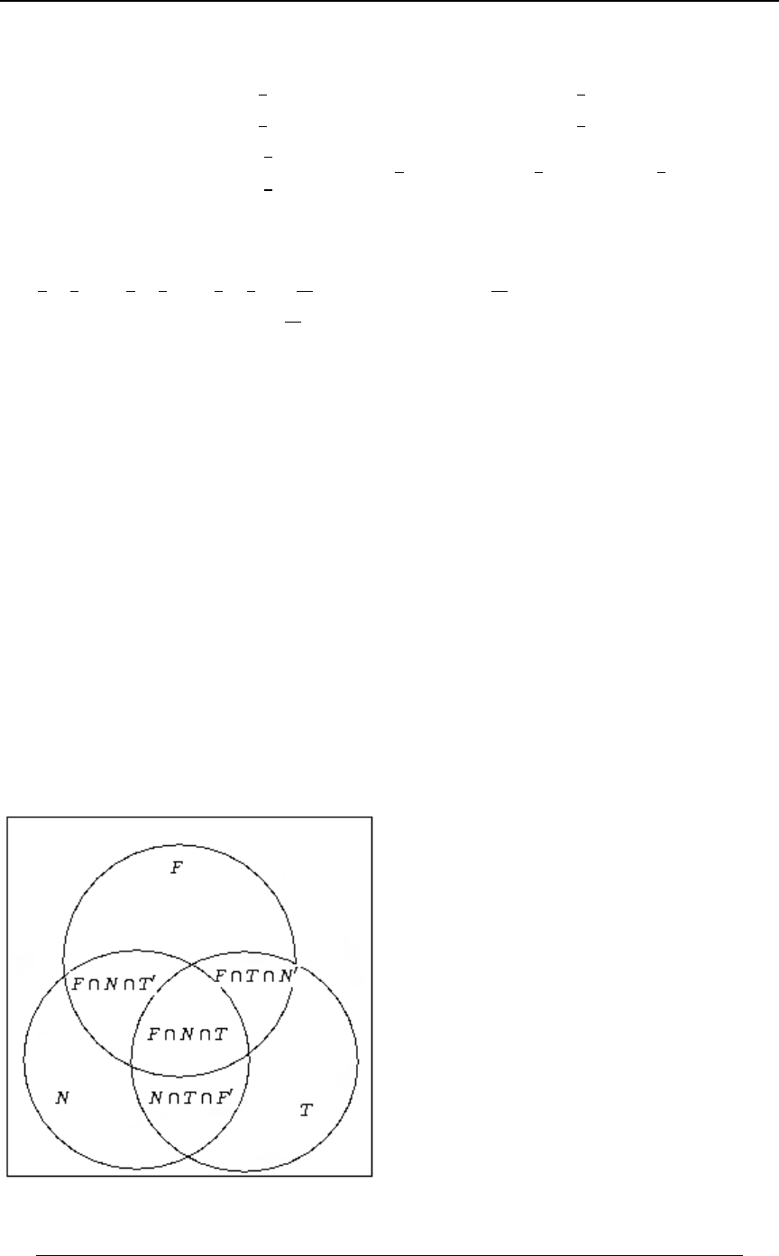
364 PRACTICE EXAM 1

22. The amounts won for each coin type are the component distributions:

Red coin: , White coin: ,

prob. prob.

\œ \ œ

"!! "!!

œœ

Blue coin: . Red , White , Blue .

prob.

\ œ TÐ Ñ œ TÐ Ñ œ TÐ Ñ œ

"!!

Fœ(

)

"$"

#))

]œ \ß\ \amount won is a mixture of and , with the mixing weights above.

V[ F

Then T Ð] œ "!!Ñ

œ T Ð\ œ "!!Ñ † T Ð Ñ  T Ð\ œ "!!Ñ † T Ð Ñ  T Ð\ œ "!!Ñ † T Ð Ñ

V[ F

Red White Blue

œœ TÐ]œ!ÑœÐÑÐÑ ÐÑÐÑ ÐÑÐÑ

"" $$ (" %" #$

## %) )) '% '%

, and .

The expected amount won is on a play of the game, so the carnival should"!! œ '%Þ!'#&ÐÑ

charge the player per play. Answer: C'&Þ!'#&

23. From the given probabilities, it follows that

TÒ Óexactly two of them attend the game

œTÒ ÓTÒ Óat least two of them attend the game all three of them attend the game

œ Þ)!  Þ&! œ Þ$! .

We also know that exactly two of them attend the gameTÒ Ó

œTÐJ ∩R ∩X ÑTÐJ ∩R ∩XÑTÐJ ∩R ∩XÑœÞ$

www .

From the symmetry of the probabilities, the three on the right hand side of the equation are equal,

so that .TÐJ ∩R ∩X ÑœTÐJ ∩R ∩XÑœTÐJ ∩R ∩XÑœÞ"

www

They are equal because andTÐJ ∩R ∩X Ñ œ TÐJ ∩RÑTÐJ ∩R ∩XÑ

TÐJ ∩X ∩R Ñ œ TÐJ ∩XÑTÐJ ∩R ∩XÑ

w and

TÐR ∩X ∩J Ñ œ TÐR ∩XÑTÐJ ∩R ∩XÑ

w , which are all equal.

The probability that Fred and Ned attend is then

TÐJ∩RÑœTÐJ∩R∩XÑTÐJ∩R∩XÑœÞ"Þ&œÞ'

w .

Answer: D

PRACTICE EXAM 1 365

24. . Answer: D0Ð Ñ œ ÐB Ñ † .B œ p 0 Ð Ñ œ "αα α

'α

G#G G

ÐG Ñαα

25. Because of independence, TÒÐOœ$Ñ∩ÐPœ'ÑÓœTÒOœ$Ó†TÒPœ'Ó

œ ÐÞ$Ñ ÐÞ(Ñ ÐÞ"Ñ ÐÞ*Ñ

’Š ‹ “’Š ‹ “

&"!

$# '%

( and both have binomial distributions). Answer: BOP

26. 0ÐBÑ œ œœ

B B Ÿ (&! " B Ÿ (&!

(&! B  (&! ! B  (&!

.p0ÐBÑœ

This is the graph in C. Answer: C

27. The expected value of the warranty is , where is theIÒAÐ7ÑÓ œ AÐ7Ñ † 0Ð7Ñ .7 0Ð7Ñ

∞

density function of the appliance failing at time . We are given that the failure time has an7

exponential distribution with a mean of 10. The mean of an exponential distribution with

parameter is , so that . and the density function is . The--

"Þ"7

-œ"! œÞ" 0Ð7ÑœÞ"/

expected value of the warranty is IÒAÐ7ÑÓ œ @Ð7Ñ † Þ"/ .7 œ / † Þ"/ .7

((

Þ"7 Ð(Þ#7Ñ Þ"7

œ Þ"/ / .7 œ Þ"/ Ò Ó œ $#!Þ() Þ

( Þ$7 (

(

'"/

Þ$

#Þ" Answer: D

28. We define the following events: - a person has the disease ,H

XT TÒXTlHÓ œ Þ)& - a person tests positive for the disease. We are given and

T ÒX T lH Ó œ Þ"! T ÒHÓ œ Þ!" T ÒHlX T Ó

w and . We wish to find .

With a model population of 10,000, there would be # people with"!ß !!! ‚ T ÐHÑ œ "!! œ H

the disease and 9,900 without the disease. The number that have the disease and test positive is

# # and the number that do not have the disease andH ∩ X T œ H ‚ T ÒX T lHÓ œ "!! ‚ Þ)& œ )&

test positive is # # . The total number who testH ∩ X T œ H ‚ T ÒX T lH Ó œ *ß *!! ‚ Þ" œ **!

www

positive is # # # The probability that someoneH œ H ∩ X T  H ∩ X T œ )&  **! œ "!(&Þ

who tests positive actually has the disease is the proportion .

#H∩XT )&

X T "!(&

œ œ Þ!(*"

The conditional probability approach to solving the problem is as follows.

Using the formulation for conditional probability we have .TÒHlXTÓ œ TÒH∩XTÓ

TÒXTÓ

But , andT ÒH ∩ X T Ó œ T ÒX T lHÓ † T ÒHÓ œ ÐÞ)&ÑÐÞ!"Ñ œ Þ!!)&

T ÒH ∩ X T Ó œ T ÒX T lH Ó † T ÒH Ó œ ÐÞ"!ÑÐÞ**Ñ œ Þ!**

www . Then,

T ÒX T Ó œ T ÒH ∩ X T Ó  T ÒH ∩ X T Ó œ Þ"!(& p T ÒHlX T Ó œ œ Þ!(*"

w .

Þ!!)&

Þ"!(&

366 PRACTICE EXAM 1

28. continued

The following table summarizes the calculations.

, given TÒHÓ œ Þ!" Ê TÒH Ó œ "TÒHÓ œ Þ**

ÌÌ

TÒH∩XTÓ TÒH ∩XTÓ

œ T ÒX T lHÓ † T ÒHÓ œ Þ!!)& œ T ÒX T lH Ó † T ÒH Ó œ Þ!**

T ÒX T Ó œ T ÒH ∩ X T Ó  T ÒH ∩ X T Ó œ Þ"!(&

. Answer: BT ÒHlX T Ó œ œ œ Þ!(*"

TÒH∩XTÓ

T ÒX T Ó Þ"!(&

Þ!!)&

29. G9@Ò\ß ] Ó œ IÒ\] Ó  IÒ\Ó † IÒ] Ó œ IÒ\] Ó  #Þ)& Þ

IÒ\]Óœ BC†0ÐBßCÑœ#†!†ÐÞ!&Ñ#†"†ÐÞ%!Ñâ&†"†Ð!Ñ&†#†Ð!Ñ



Bœ# Cœ!

Answer: Bœ #Þ(  #Þ)& œ  Þ"& Þ

30. We identify the following events:

WRW œW - the applicant is a smoker, - the applicant is a non-smoker w

HW - the applicant declares to be a smoker on the application

HR œ HW - the applicant declares to be non-smoker on the application .

The information we are given is .TÒWÓ œ Þ$ß TÒRWÓ œ Þ(ß TÒHRlWÓ œ Þ%ß TÒHWlRWÓ œ !

We wish to find .TÒRWlHRÓ œ TÒRW∩HRÓ

TÒHRÓ

With a model population of 100 there are 30 # smokers and 70 # non-smokers. TheœW œRW

number of smokers who declare that they are non-smokers is

# # and since non-smokers don't lie, the number ofHR ∩ W œ W ‚ T ÒHR lWÓ œ $! ‚ Þ% œ "#

non-smokers who declare that they are non-smokers is equal to the number of non-smokers,

so # . The total number of people who declare that they are non-smokersHR ∩ RW œ RW œ (!

is # # # .HR∩W  HR∩RWœ"#(!œ)#œ HR

Then, the proportion of applicants who say they are non-smokers that are actually non-smokers is

#HR∩RW (! $&

HR )# %"

œœ .

The conditional probability approach to the solution is on the next page.

PRACTICE EXAM 1 367

30. continued

We calculate ,Þ% œ T ÒHRlWÓ œ œ p T ÒHR ∩ WÓ œ Þ"#

TÒHR∩WÓ TÒHR∩WÓ

TÒWÓ Þ$

and .! œ T ÒHWlR WÓ œ œ p T ÒHW ∩ RWÓ œ !

TÒHW∩RWÓ TÒHW∩RWÓ

TÒRWÓ Þ(

Using the rule , and noting that and TÒEÓœTÒE∩FÓTÒE∩FÓ HWœHR WœRW

www

we have , andT ÒHW ∩ WÓ œ T ÒWÓ  T ÒHR ∩ WÓ œ Þ$  Þ"# œ Þ")

T ÒHR ∩ RWÓ œ T ÒRWÓ  T ÒHW ∩ R WÓ œ Þ(  ! œ Þ( , and

T ÒHR Ó œ T ÒHR ∩ RWÓ  T ÒHR ∩ WÓ œ Þ(  Þ"# œ Þ)# .

Then, . TÒRWlHRÓ œ œ œ

TÒRW∩HRÓ

T ÒHR Ó Þ)# %"

Þ( $&

These calculations can be summarized in the order indicated in the following table.

TÐWÑßÞ$ Ê TÐRWÑ œ "TÐWÑ œ Þ(1.

given Ì

6. 5. 2. HW É T ÐHW ∩ WÑ T ÐHWlRWÑ œ ! , given

TÐHWÑ œ TÐWÑTÐHR ∩WÑ TÐHW ∩RWÑ

œ T ÐHW ∩ WÑ œ Þ$  Þ"# œ Þ") œ T ÐHWlRWÑ † T ÐRWÑ

 T ÐHW ∩ RWÑ œ Ð!ÑÐÞ(Ñ œ !

œÞ")!œÞ")

ÌË

7. 4. 3. HR T ÐHRlWÑ œ Þ% T ÐHR ∩ R WÑ œ

TÐHRÑ œ TÐRWÑTÐHW ∩RWÑ given

œ"TÐHWÑ TÐHR∩WÑ œÞ(!œÞ(

œ"Þ") œTÐHRlWÑ†TÐWÑ

œÞ)# œÐÞ%ÑÐÞ$ÑœÞ"#

Then, . Answer: D8. TÒRWlHRÓ œ œ œ

TÒRW∩HRÓ

T ÒHR Ó Þ)# %"

Þ( $&

368 PRACTICE EXAM 1

PRACTICE EXAM 2 369

PRACTICE EXAM 2

1. Let have the density function .\0ÐBÑœ

š#B

5# for

, otherwise

!ŸBŸ5

For what value of is the variance of equal to ?5\#

A) B) C) D) E) # ' * ") $'

2. A life insurer classifies insurance applicants according to the following attributes:

Q - the applicant is male

L - the applicant is a homeowner

Out of a large number of applicants the insurer has identified the following information:

40% of applicants are male, 40% of applicants are homeowners and

20% of applicants are female homeowners.

Find the percentage of applicants who are male and do not own a home.

A) 10% B) 20% C) 30% D) 40% E) 50%

3. Two components in an electrical circuit have continuous failure times and . Both\]

components will fail by time 1, but the circuit is designed so that the combined times until failure

is also less than 1, so that the joint distribution of failure times satisfies the requirements

!BC" . How many of the following joint density functions are consistent with an

expected combined time until failure less than for the two components?

I. II. III. IV. 0ÐBßCÑ œ # 0ÐBßCÑ œ $ÐB  CÑ 0ÐBßCÑ œ 'B 0ÐBßCÑ œ 'C

A) 0 B) 1 C) 2 D) 3 E) 4

4. In a "wheel of fortune" game, the contestant spins a dial and it ends up pointing to a number

uniformly distributed between 0 and 1 (continuous). After 10,000 independent spins of the wheel

find the approximate probability that the average of the 10,000 spins is less than .499.

A) Less than .34 B) At least .34 but less than .35 C) At least .35 but less than .36

D) At least .36 but less than .37 E) At least .37

370 PRACTICE EXAM 2

5. A continuous random variable has density function .Y0Ð?Ñœ

Yš"l?l "?"

for

, otherwise

Which of the pairs of the following events are independent?

I. II. III. ."Y !  Y  !Y "

A) I and II only B) I and III only C) II and III only

D) I and II, II and III only E) No pairs are independent

6. An excess-of-loss insurance policy has a deductible of 1 and pays a maximum amount of 1.

The loss random variable being insured by the policy has an exponential distribution with a mean

of 1. Find the expected claim paid by the insurer on this policy.

A) B) C) D) E) /#/ // #Ð//Ñ / #/

" # " # " # " #

7. If for , find the moment generating function of .0ÐBÑœÐ5"ÑB !B" \

A) B) C)

/ Ð''>$> Ñ / Ð''>$> Ñ / Ð''>$> Ñ

>>>>

># ># >#

$$$$



D) E)

/ Ð''>$> Ñ / Ð''>$> Ñ

>> >>

># >#

$$ $$



8. Urn 1 contains 5 red and 5 blue balls. Urn 2 contains 4 red and 6 blue balls, and Urn 3 contains

3 red balls. A ball is chosen at random from Urn 1 and placed in Urn 2. Then a ball is chosen at

random from Urn 2 and placed in Urn 3. Finally, a ball is chosen at random from Urn 3. Find the

probability that the ball chosen from Urn 3 is red.

A) B) C) D) E)

"& $! %& '! (&

)) )) )) )) ))

9. The amount of time taken by a machine repair person to repair a particular machine is a

random variable with an exponential distribution with a mean of 1 hour. The repair person's

employer pays the repair person a bonus of 2 whenever a repair takes less than hours, and a

bonus of 1 if the repair takes between and hours. Find the average bonus received per

machine repaired.

A) Less than .3 B) At least .3 but less than .4 C) At least .4 but less than .5

D) At least .5 but less than .6 E) At least .6

PRACTICE EXAM 2 371

10. A stock market analyst has recorded the daily sales revenue for two companies

over the last year and displayed them in the histograms below.

The analyst noticed that a daily sales revenue above 100 for Company A was always

accompanied by a daily sales revenue below 100 for Company B, and vice versa. Let denote\

the daily sales revenue for Company A and let denote the daily sales revenue for Company B,]

on some future day. Assuming that for each company the daily sales revenues are independent

and identically distributed, which of the following is true?

(A) Var(X) > Var(Y) and Var(X + Y) > Var(X) + Var(Y) .

(B) Var(X) > Var(Y) and Var(X + Y) < Var(X) + Var(Y) .

(D) Var(X) < Var(Y) and Var(X + Y) > Var(X) + Var(Y) .

(E) Var(X) < Var(Y) and Var(X + Y) < Var(X) + Var(Y) .

11. Bob and Doug are both 100-metre sprinters. Bob's sprint time is normally distributed with a

mean of 10.00 seconds and Doug's sprint time is also normally distributed, but with a mean of

9.90 seconds. Both have the same standard deviation in sprint time of . Assuming that Bob and5

Doug have independent sprint times, and given that there is . chance that Doug beats Bob in*&

any given race, find .5

A) .040 B) .041 C) .042 D) .043 E) .044

12. Let and be continuous random variables with joint cumulative distribution function\]

JÐBßCÑœ Ð#!BCB CBC Ñ !ŸBŸ& !ŸCŸ&

#&! ##

for and .

Determine .TÒ\  #Ó

A) B) C) D) E)

$"""#" "

"#& &! #& #&! #&!

Ð$*C  $C Ñ Ð$'C  #C Ñ

372 PRACTICE EXAM 2

13. In a survey of males over the age of 30, it is found 50% are married, 40% smoke, 30% own a

home and 60% own a car. It is also found that 30% are non-smoking bachelors, 40% are married

car owners, 36% are non-smoking car owners, 25% own both a home and a car and 20% are

married and own a home and a car. Which of the following statements is true regarding

independence among the attributes of being married, being a smoker, being a car owner and being

a home owner?

A) Being single and owning a car are independent

B) Being married and smoking are not independent

C) Being a smoker and owning a car are independent

D) Being a home owner and being a car owner are independent

E) Being married, being a home owner and being a car owner are mutually independent

14. A loss random variable is uniformly distributed on the integers from 0 to 11.

An insurance pays the loss in excess of a deductible of 5.5 . Find the expected amount not

covered by the insurance.

A) 2 B) 3 C) 4 D) 5 E) 6

15. An insurer offers an "all or nothing" policy of the following type. If the loss being insured is

for an amount of or more, then the insurance policy pays the full amount, but if the loss is lessH

than then the policy pays nothing. Assuming that the distribution of the loss has anH

exponential distribution with a mean of 2, and that , find the expected payout on the policy.Hœ#

A) B) C) D) E)

"#%

///

/#/

16. Suppose that is a random variable with moment generating function\

QÐ>Ñ œ TÒ\ œ #Ó



4œ!

∞/

Ð>4"Ñ . Find .

A) B) C) D) E) !"/ /

#/ # # 4x

1

4œ!

∞#4"

PRACTICE EXAM 2 373

17. A supplier of a testing device for a type of component claims that the device is highly

reliable, with , whereT ÒElFÓ œ T ÒE lF Ó œ Þ*&

Eœ Fœdevice indicates component is faulty, and component is faulty .

You plan to use the testing device on a large batch of components of which 5% are faulty.

Find the probability that the component is faulty given that the testing device indicates that the

component is faulty .

A) 0 B) .05 C) .15 D) .25 E) .50

18. Customers arrive randomly and independently at a service window, and the time between

arrivals has an exponential distribution with a mean of 12 minutes. Let equal the number of\

arrivals per hour. What is ?T Ò\ œ "!Ó

A) B) C) D) E)

"!/ "! / " / " / & /

"!x "!x "!x "!x "!x

"# "# "! "! " "! "# "! &

19. Workplace accidents are categorized in three groups: minor, moderate, and severe. The

probability that a given accident is minor is .5, that it is moderate is .4, and that it is severe is .1.

Two accidents occur independently in one month. Calculate the probability that neither accident

is severe and at most one is moderate.

A) B) C) D) E) Þ#& Þ%! Þ%& Þ&' Þ'&

20. Let be a Poisson random variable with mean . If , what is the\ T Ò\ œ "l\ Ÿ "Ó œ Þ)-

value of ?-

A) B) C) D) E) %68#Þ)Þ#&68Þ)

21. Let and be continuous random variables with joint density function\]

0ÐBßCÑ œ š for

otherwise

BC !B" ß !C"

!ß .

What is the marginal density function for where nonzero?\ß

A) B) C) D) E) C #B B B

"BB"

###

22. Let be uniform random variables on the interval with\ß\ß\ Ð!ß"Ñ

"#$

G9@Ò\ß\ Óœ 3ß4 œ"ß#ß$ß 3Á4 \ #\ \

34 "#$

#% for . Calculate the variance of .

A) B) C) D) E)

"" & """

'%"##"#

374 PRACTICE EXAM 2

23. The joint density for liability damage and collision damage when a claim occurs is\]

0ÐBßCÑ !Ÿ\Ÿ$ß !Ÿ] Ÿ" , . Which of the following represents the probability that total

loss will exceed 1?

A) B) C)

'' ' ' ''

!! ! ! !!

" "B "C "B " "C

0ÐBß CÑ .C .B "  0ÐBß CÑ .C .B 0ÐBß CÑ .B .C

D) E) "  0ÐBß CÑ .B .C 0ÐBß CÑ .C .B

'' ''

!! !!

""C "B"

24. Medical researchers have identified three separate genes that individuals may or may not be

born with. The researchers have found that 25% of the population have gene , 20% have geneE

FG E and 10% have gene . Furthermore, in any individual, the presence of gene is independent

of the presence of genes or , but no people can have both genes and . Find theFG F G

probability that a randomly chosen individual has at least one of the three genes.

A. .450 B. .475 C. .500 D. .525 E. .550

25. An insurance contract reimburses a family's automobile accident losses up to a maximum of

two accidents per year. The joint probability distribution for the number of accidents of a three

person family is , whereÐ\ß]ß^Ñ :ÐBßCßDÑœ5ÐB#CDÑ

B œ !ß " ß C œ !ß "ß # ß D œ !ß "ß # ß and

Bß Cß D \ ] ^ are the number of accidents incurred by , and , respectively.

Determine the expected number of unreimbursed accident losses given that is not involved in\

any of the accidents.

A) 5/21 B) 1/3 C) 5/9 D) 4/63 E) 7/9

26. Let be a continuous random variable with density function .\0ÐBÑœ

šB

# for

, otherwise

!ŸBŸ#

Find .IÒ \  IÒ\Ó Ó

¸¸

A) B) C) D) E) !#$#'%%

*)")"$

27. Let and be continuous random variables with joint density function\]

0ÐBßCÑ œ š for and

otherwise

" !C"lBl "BŸ"

!ß .

What is ?Z+<Ò\Ó

A) B) C) D) E)

""#""#

") ' * ") $

PRACTICE EXAM 2 375

28. A pair of fair dice is tossed times. is the number of times a total of 2 occurs. Find#"'! \

the approximate probability that is less than 55 using the continuity correction.\

A) .24 B) .26 C) .28 D) .30 E) .32

29. Suppose the remaining lifetimes of a husband and wife are independent and uniformly

distributed on the interval [0,40]. An insurance company offers two products to married couples:

One which pays when the husband dies; and

One which pays when both the husband and wife have died.

Calculate the covariance of the two payment times.

A) 0.0 B) 44.4 C) 66.7 D) 200.0 E) 466.7

30. The mortality of a certain type of transistor is such that the probability of its breakdown in

the interval is given by: , , . If 10 of these transistors are taken atÐ>ß >  .>Ñ -/ .> >  ! -  !

->

random, then the probability that the 10th transistor that breaks down will do so during time

Ð@ß @  .@Ñ is

A.) B) C) "!-Ð"  / Ñ / .@ "!-/ .@ "!-/ Ð"  / Ñ .@

-@ * -@ "!-@ *-@ -@

D) E. "!-Ð"  / Ñ/ .@ -Ð"  / Ñ / .@

*-@ -@ -@ * -@

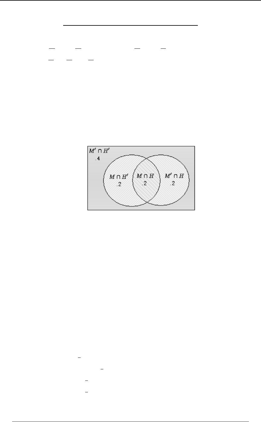
376 PRACTICE EXAM 2

PRACTICE EXAM 2 - SOLUTIONS

1. IÒ\Ó œ B † .B œ ß IÒ\ Ó œ B † .B œ

#B #5 #B 5

5$ 5#

. Answer: BÊ Z+<Ò\Óœ Ð Ñ œ œ# p 5œ'

5#5 5

#$ ")

2. TÒQÓ œ Þ%ß TÒQ Ó œ Þ'ß TÒLÓ œ Þ%ß TÒL Ó œ Þ' ß TÒQ ∩LÓ œ Þ#ß

We wish to find . From probability rules, we haveTÒQ ∩L Ó

Þ' œ T ÒL Ó œ T ÒQ ∩ L Ó  T ÒQ ∩ L Ó

www

w , and

Þ' œ T ÒQ Ó œ T ÒQ ∩ LÓ  T ÒQ ∩ L Ó œ Þ#  T ÒQ ∩ L Ó

ww w ww

Thus, and then . The following diagram identifies theT ÒQ ∩ L Ó œ Þ% T ÒQ ∩ L Ó œ Þ#

www

component probabilities.

The calculations above can also be summarized in the following table. The events across the top

of the table categorize individuals as male( ) or female ( ), and the events down the left sideQQ

of the table categorize individuals as homeowners ( ) or non-homeowners ( ).LL

, given TÐQÑœÞ% TÐQÑœ"Þ%œÞ'

TÐLÑ œ Þ% TÐQ ∩LÑ É TÐQ ∩LÑ œ Þ# , given

given œTÐLÑTÐQ ∩LÑœÞ%Þ#œÞ#

TÐLÑœ"Þ%œÞ' TÐQ∩LÑœTÐQÑTÐQ∩LÑœÞ%Þ#œÞ#

Answer: B

3. IÒ\  ] Ó œ ÐB  CÑ0ÐBß CÑ .C .B

""B

I. Not correct.

""B

#ÐB  CÑ .C .B œ Þ

II. Not correct.

""B

$ÐB  CÑÐB  CÑ .C .B œ Þ

III . Not correct.

""B

'BÐB  CÑ .C .B œ Þ

IV . Not correct.

""B

'CÐB  CÑ .C .B œ Þ

Note that III and IV will have the same outcome by the symmetry of and . Answer: ABC

PRACTICE EXAM 2 377

4. The outcome of a single spin is , which has a uniform distribution on the interval .\ Ð!ß "Ó

The mean and variance of are and . If , then has an approximately\[œ\[

#"# 3œ"

"!ß!!!



normal distribution with mean and variance ."!ß !!!Ð Ñ œ &!!! "!ß !!!Ð Ñ œ )$$Þ$$

#"#

The average of the 10,000 spins is .Eœ [

"!ß!!!

T ÒE  Þ%**Ó œ T Ò[  %**!Ó œ T Ò  Ó

[ &!!! %**!&!!!

)$$Þ$$ )$$Þ$$

ÈÈ

œ Ð Ñ œ Ð  Þ$%'Ñ œ "  ÐÞ$&Ñ œ "  Þ'$( œ Þ$'$

ÞFF F

%**!&!!!

)$$Þ$$

È . Answer: D

5. T ÐMÑ œ Ð"  l?lÑ .? œ Ð"  ?Ñ .? œ

" "

# ,

TÐMMÑœ Ð"l?lÑ.?œ Ð"?Ñ.? Ð"?Ñ.?œ

'''

"Î# "Î# !

"Î# ! "Î# $

% ,

.TÐMMMÑ œ Ð"  l?lÑ.? œ Ð"  ?Ñ.? œ

TÐM∩MMÑœTÐ Y !Ñœ Ð"?Ñ.?œ œÐ ÑÐ ÑœTÐMÑ†TÐMMÑ

#"Î#

'$"$

)#% ,

which shows that I and II are independent.

TÐM ∩ MMMÑ œ TÐgÑ œ ! Á Ð ÑÐ Ñ œ TÐMÑ † TÐMMMÑ

## , which shows that I and III are not

independent.

TÐMM ∩ MMMÑ œ Ð"  l?lÑ.? œ œ Ð ÑÐ Ñ œ TÐMMÑ † TÐMMMÑ

"Î# $$"

)%# , which shows that II and III

are independent. Answer: D

From the density function for we have]

T Ò"!!ß !!!]  %!ß !!!Ó œ T Ò]  Þ%Ó œ 0ÐCÑ .C œ &Ð"  CÑ .C œ ÐÞ'Ñ

Þ% Þ%

, and

T Ò"!!ß !!!]  "!ß !!!Ó œ T Ò]  Þ"Ó œ 0ÐCÑ .C œ &Ð"  CÑ .C œ ÐÞ*Ñ

Þ" Þ"

The conditional probability in question is . Answer: B

ÐÞ'Ñ

ÐÞ*Ñ

&œ Þ"$#

6. The loss random variable is , which has density function for .\0ÐBÑœ/B"

\B

The amount paid by the insurance is .

if if

]œ

!\Ÿ"

\" "\Ÿ#

"\#

Then . IÒ]Óœ ÐB"Ñ/ .B"†TÒ\#Óœ B/ / œ/ /

'¹

#B B # " #

Bœ"

Bœ#

Answer: B

378 PRACTICE EXAM 2

7. Since , it follows that , so that , and .

0ÐBÑ.Bœ" Ð5"Ñ† œ" 5œ# 0ÐBÑœ$B

Then, . Applying integration byQÐ>ÑœIÒ/ Óœ / †$B.B

\>\ >B #

parts, we have

'' '

!! !

"" "

>B # #

/ † $B .B œ $B .Ð Ñ œ  .B / $B / 'B/

>> >

Bœ!

Bœ"

>B # >B >B

œ  .Ð Ñ œ   .B

$/ 'B / $/ 'B/ '/

>>>>> >

Bœ!

Bœ"

> >B > >B >B

’¹ “

œ œ 

$/ '/ '

>> > > >

'Ð/ "Ñ / Ð''>$> Ñ

#$ $ $

>>#

. Answer: E

8. .TÐV ÑœTÐV ∩V ∩V ÑTÐV ∩V ∩F ÑTÐV ∩F ∩V ÑTÐV ∩F ∩F Ñ

$ $#" $#" $#" $#"

TÐV ∩V ∩VÑœTÐVlV ∩VÑ†TÐVlVÑ†TÐVÑœ"† † œ

$#" $#"#"" &" &

"" # ## ß

TÐV ∩V ∩FÑœTÐVlV ∩FÑ†TÐVlFÑ†TÐFÑœ"† † œ

$#" $#"#"" %" #

"" # "" ß

TÐV ∩F ∩VÑœTÐVlF ∩VÑ†TÐFlVÑ†TÐVÑœ † † œ

$#" $#"#""

$'" *

%""# %%

TÐV ∩F ∩FÑœTÐVlF ∩FÑ†TÐFlFÑ†TÐFÑœ † † œ

$#" $#"#""

$(" #"

%""# ))

Finally, . Answer: ETÐVÑœœ

$& # * #" (&

## "" %% )) ))

9. Average bonus œ#†TÒX Ÿ Ó"†TÒ X Ÿ Ó

"""

%%#

œ #Ò"  / Ó  Ò/  / Ó œ Þ'"&

"Î% "Î% "Î# . Answer: E

10. The histogram for Company B is more widely dispersed about its mean than the histogram

for Company A, and therefore . Since daily sales revenue above 100 forZ+<Ð]ÑZ+<Ð\Ñ

Company A is always associated with daily sales revenue below 100 for Company B and vice-

versa, the covariance between and is negative. Therefore,\]

Z+<Ð\]ÑœZ+<Ð\ÑZ+<Ð]Ñ#G9@Ð\ß]ÑZ+<Ð\ÑZ+<Ð]Ñ . Answer: E

11. FHµRÐÞ"ß# ÑÞTÒFHÓœTÒFH!ÓœTÒ  ÓœÞ*&5#FHÞ" !Þ"

##55

ÈÈ

Ê œ  "Þ'%& T Ò^  "Þ'%&Ó œ Þ*& p œ Þ!%$

!Þ"

#5È (since ) . Answer: D5

12. ,J Ð#ÑœTÒ\Ÿ#Óœ JÐ#ßCÑœJÐ#ß&Ñœ œ

\CÄ∞

lim "$! "$

#&! #&

so that Answer: CTÒ\#Óœ"TÒ\Ÿ#Óœ Þ

PRACTICE EXAM 2 379

13. - married, - smoker, - car owner, - home ownerQWG L

We are given, TÒQÓ œ Þ&ß TÒWÓ œ Þ%ß TÒGÓ œ Þ'ß TÒLÓ œ Þ$ß TÒQ ∩W Ó œ Þ$ ß

TÒQ ∩GÓ œ Þ%ß TÒW ∩GÓ œ Þ$'ß TÒL ∩GÓ œ Þ#&ß TÒQ ∩G ∩LÓ œ Þ#

Then, ,TÒQ ∩GÓœTÒGÓTÒQ∩GÓœÞ'Þ%œÞ#

but not independent A is false.T ÒQ Ó † T ÒGÓ œ ÐÞ&ÑÐÞ'Ñ œ Þ$ p Q ß G p

T ÒQ ∩ W Ó œ Þ$ ß T ÒQ Ó † T ÒW Ó œ ÐÞ&ÑÐÞ'Ñ œ Þ$ p Q ß W

ww w

are independent

are independent B is false.pQßW p

TÒW ∩GÓœÞ$'œÐÞ'ÑÐÞ'ÑœTÒWÓ†TÒGÓpWßG

www

are independent

are independent C is true.pWßG p

We can also check TÒL∩GÓœÞ#&ÁÐÞ$ÑÐÞ'ÑœTÒLÓ†TÒGÓ

not independent D is false,pLßG p

T ÒQ ∩ G ∩ LÓ œ Þ# Á ÐÞ&ÑÐÞ'ÑÐÞ$Ñ œ T ÒQ Ó † T ÒGÓ † T ÒLÓ

p QßGßLare not mutually independent. Answer: C

14. The amount not covered is

Loss !"#$%&'(â""

Amt. !"#$%&&Þ&&Þ&â&Þ&

Not Covered

Prob. """""""" "

"# "# "# "# "# "# "# "# "#

The expected amount not covered by the insurance is

Ð ÑÒ!"#$%&&Þ&Ð'ÑÓœ%

"# . Answer: C

15. The expected payment on the policy will be

'º

∞BÎ# BÎ# BÎ# "

B† / .Bœ B/ #/ œ%/ Þ

#Bœ#

Bœ∞ Answer: C

16. The moment generating function for a non-negative discrete integer-valued random variable

\0QÐ>ÑœIÒ/Óœ/†0Ð4Ñ with probability function is defined to be .

>\ >4

4œ!

∞



Since we are given that , and it is known that the distribution of a randomQÐ>Ñ œ 

4œ!

∞/

Ð>4"Ñ

variable is uniquely determined by its moment generating function (i.e., there is precisely one

probability distribution with that specified mgf), it follows that

0Ð4Ñœ œ 0Ð4ÑœTÒ\œ4Ó TÒ\œ#Óœ

/" "

4x /†4x #/

" . Since , it follows that .

Answer: B

380 PRACTICE EXAM 2

17. With a model population of 10,000, we have # faulty componentsF œ "!ß !!! ‚ Þ!& œ &!!

and # working components. We also have # # devicesF œ *ß &!! E ∩ F œ F ‚ T ÒElFÓ œ %(&

that are faulty and that test as faulty, and we have # #E ∩ F œ F ‚ T ÒE lF Ó œ *ß !#&

ww w ww

components that are working and do not test faulty. Therefore, there are

# # # components that are working and testE ∩ F œ F  E ∩ F œ *ß &!!  *ß !#& œ %(&

ww ww

faulty. The total number of components that test faulty is # # # .Eœ E∩F  E∩F œ*&!

The probability that a component is faulty given that it test faulty is the proportion .

#E∩F "

The conditional probability approach to solving the problem is as follows. We can calculate

entries in the following table in the order indicated.

F T ÒElFÓ œ Þ*& (given)

T ÒFÓ œ Þ!& T ÒE ∩ FÓ œ T ÒElFÓ † T ÒFÓ œ Þ!%(& 1.

(given)

F T ÒE ∩ F Ó T ÒE ∩ F Ó

ww ww

3. 2.

T ÒF Ó œ T ÒF Ó  T ÒE ∩ F Ó œ T ÒE lF Ó † T ÒF Ó

wwww www

œ "  T ÒFÓ œ Þ!%(& œ Þ*!#&

œÞ*&

4. TÒEÓ œ TÒE∩FÓTÒE∩F Ó œ Þ!*&

5. TÒFlEÓ œ œ œ Þ&

TÒF∩EÓ

T ÒEÓ Þ!*&

Þ!%(& . Answer: E

18. When the time between successive arrivals has an exponential distribution with mean "

(units of time), then the number of arrivals per unit time has a Poisson distribution with parameter

(mean) . The time between successive arrivals has an exponential distribution with mean α"

hours (12 minutes). Thus, the number of arrivals per hour has a Poisson distribution with

parameter , so that Answer: E& T Ò\ œ "!Ó œ Þ

"!x

& "!

19. denotes the severity of accident and denotes the severity of accident .E"E#

QM denotes the event that an accident is minor,

QS denotes the event that an accident is moderate, and

W denotes the event that an accident is severe.

The probability in question is the probability that either both are minor or exactly one is moderate

(and because of independence, ) :T ÒE ∩ E Ó œ T ÒE Ó † T ÒE Ó

"# " #

T ÒÐE œ QMÑ ∩ ÐE œ QMÑÓ  T ÒÐE œ QMÑ ∩ ÐE œ QSÑÓ

"# "#

Answer: E T ÒÐE œ Q SÑ ∩ ÐE œ QMÑ œ ÐÞ&ÑÐÞ&Ñ  ÐÞ&ÑÐÞ%Ñ  ÐÞ%ÑÐÞ&Ñ œ Þ'&

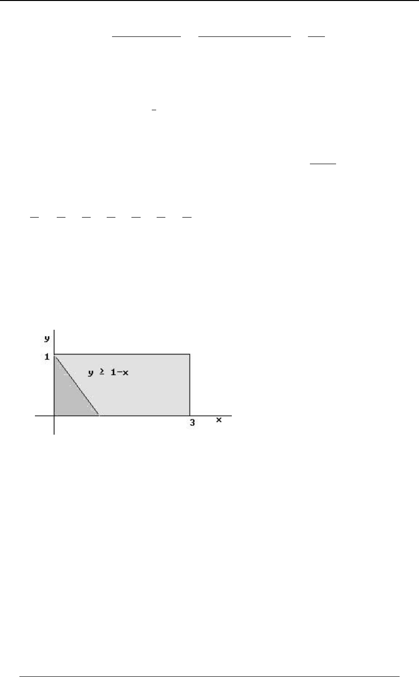
PRACTICE EXAM 2 381

20. TÒ\œ"l\Ÿ"Óœ œ œ œÞ)

T Ò\œ"Ó / † Î"x

T Ò\œ!ÓT Ò\œ"Ó "

Ð/ † Î!xÑÐ/ † Î"xÑ

"

! "

pœ%- . Answer: A

21. . Answer: E0ÐBÑœ ÐBCÑ.CœB

22. The variance of a uniform random variable on the interval is Ò+ß ,Ó Þ

Ð,+Ñ

Z+<Ò\ #\ \ ÓœZ+<Ò\ Ó%Z+<Ò\ ÓZ+<Ò\ Ó

"#$ " # $

#†#G9@Ò\ß\Ó#G9@Ò\ß\Ó#†#G9@Ò\ß\Ó

"# "$ #$

œ œÞ

" %"%#% &

"# "# "# #% #% #% "# Answer: C

23. The region of probability is the lightly shaded region below. It is the complement of the

darkly shaded region. The probability of the darkly shaded region is .

""C

0ÐBß CÑ .B .C

Therefore, the probability of the lighter region is ."  0ÐBß CÑ .B .C

""C

Answer: D

24. We are given , , and fromT ÒEÓ œ Þ#& ß T ÒFÓ œ Þ# ß T ÒGÓ œ Þ" T ÒF ∩ GÓ œ !

independence, we have , T ÒE ∩ FÓ œ ÐÞ#&ÑÐÞ#Ñ œ Þ!& T ÒE ∩ GÓ œ ÐÞ#&ÑÐÞ"Ñ œ Þ!#& Þ

Using the probability rule for the union of events, we have

TÒE∪F ∪GÓ œ TÒEÓTÒFÓTÒGÓ

.TÒE∩FÓTÒE∩GÓTÒF∩GÓTÒE∩F∩GÓ

Since no people have both genes and , it is also true that no one has all three genes.FG

Thus, . Answer: BTÒE∪F∪GÓœÞ#&Þ#Þ"Þ!&Þ!#&!!œÞ%(&

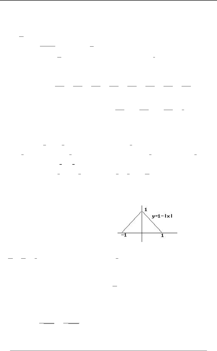
382 PRACTICE EXAM 2

25. In order to be a probability distribution, we must have :DDD:ÐBß Cß DÑ œ "

5Ò!"#$%&"#$%&'#$%&'(Óœ"

p5œ Þ \œ! ] ^

'$ Given that , the conditional distribution of and is

:ÐCß Dl\ œ !Ñ œ Þ :Ð!ß Cß DÑ œ Ð#C  DÑ

:Ð!ßCßDÑ

:Ð!Ñ

\ , and

: Ð!Ñœ :Ð!ßCßDÑœ Ð!#%"$&#%'Ñœ Þ

\"$

'$ (

The conditional probabilities for are]ß^

ÐCß DÑ Ð!ß !Ñ Ð"ß !Ñ Ð#ß !Ñ Ð!ß "Ñ Ð"ß "Ñ Ð#ß "Ñ Ð!ß #Ñ Ð"ß #Ñ Ð#ß #Ñ

:ÐCß Dl\ œ !Ñ !

#Î'$ %Î'$ "Î'$ $Î'$ &Î'$ #Î'$ %Î'$ 'Î'$

$Î( $Î( $Î( $Î( $Î( $Î( $Î( $Î(

Number of unreimbursed

accidents !!!!!"!"#

Expected number of unreimbursed accidents is "† "† #† œ Þ

&Î'$ %Î'$ 'Î'$

$Î( $Î( $Î( *

(

Answer: E

26. . Then, , which is negative forIÒ\Ó œ B † .B œ \  IÒ\Ó œ \ 

#B% %

#$ $

!ŸBŸ Ÿ Ÿ# \IÒ\Ó œ \ !Ÿ\Ÿ

44 44

$$ $$

and is positive for x . Thus, if

¸¸

and if x . Then,

¸¸

\IÒ\Ó œ\ Ÿ Ÿ#

IÒ \  IÒ\Ó Ó œ Ð  BÑ † .B  ÐB  Ñ † .B œ . Answer: C

¸¸

! %Î$

%Î$ #

$# $#)"

BB$#

27. The marginal distribution of is\

0ÐBÑœ 0ÐBßCÑ.C

\∞

∞

"lBl".C œ"lBl " ŸB Ÿ"for .

IÒ\Ó œ BÐ"  lBlÑ.B

'"

œ BÐ"  BÑ .B  BÐ"  BÑ .B œ !

" !

IÒ\ Ó œ B Ð"  lBlÑ .B œ B Ð"  BÑ .B  B Ð"  BÑ .B

## # #

" " !

"!"

'''

œ  œ Z +<Ò\Ó œ IÒ\ Ó  ÐIÒ\ÓÑ œ

""" "

"# "# ' '

. . Answer: B

28. The probability of tossing a total of 2 is (both dice have to turn up "1").:œ "

The number of "2"s occurring in tosses of the dice has a binomial distribution with8 œ #"'!

mean and variance . Applying the normal approximation with8: œ '! 8:Ð"  :Ñ œ &)Þ$$

continuity correction, we have

T Ò\  &&Ó œ T Ò  Ó œ Ð  Þ(#Ñ œ "  ÐÞ(#Ñ œ "  Þ('%# œ Þ#$&)

\'! &%Þ&'!

&)Þ$$ &)Þ$$

ÈÈFF .

Answer: A

PRACTICE EXAM 2 383

29. time of husband's death , time of wife's death , .Xœ Yœ [œ7+BÐXßYÑ

G9@ÐX ß [ Ñ œ IÒX [ Ó  IÒX ÓIÒ[ Ó IÒX Ó œ #! Ò!ß %!Ó . , expectation of uniform .

J Ð>ÑœTÒ[ Ÿ>ÓœTÒÐX Ÿ>Ñ∩ÐY Ÿ>ÑÓœTÒX Ÿ>Ó†TÒY Ÿ>Ó

[

œÐ ÑÐ Ñœ !Ÿ>Ÿ%!

>> >

%! %! "'!!

# for .

The pdf of is , and [0Ð>ÑœJÐ>Ñœ IÒ[Óœ >† .>œÞ

[[

>>)!

)!! )!! $

Alternatively, IÒ[ Ó œ IÒ7+BÐX ß Y ÑÓ œ 7+BÐ>ß ?Ñ Ð ÑÐ Ñ .? .>

%! %! ""

%! %!

œ > † .? .>  ? † .? .> œ  œ Þ

'' ''

!! !>

%! > %! %! "

"'!!

"%!%!)!

"'!! $ $ $

Let . Then,2Ð>ß ?Ñ œ > † 7+BÐ>ß ?Ñ

IÒX[Ó œ IÒ2ÐXßYÑÓ œ > † 7+BÐ>ß?ÑÐ ÑÐ Ñ .?.>

%! %! ""

%! %!

œ > † .? .>  >? † .? .> œ %!!  #!! œ '!! Þ

'' ''

!! !>

%! > %! %!

#""

"'!! "'!!

G9@ÐX ß [ Ñ œ '!!  Ð#!ÑÐ Ñ œ

)! #!!

. Answer: C

30. The density function for the time of breakdown for a particular transistor is for 0.>-/>

->

Thus, the cumulative distribution function for the break down time of transistor is 5TÒXŸ>Ó

œ-/ .=œ / > [

>-= ->

1 for 0. Let denote the break down time of the last (10th)

transistor. Then the event that the 10th transistor breaks down by time is equivalent to the>

event that all transistors break down by time (if the last one breaks down by time then all>>

the others have already broken down by that time). Thus,

()()œ TÒX Ÿ> ∩ X Ÿ> ∩â∩ÐX Ÿ>ÑÓKÐ>Ñ œ T Ò[ Ÿ >Ó 12 10

1.œ T ÒX Ÿ >Ó † T ÒX Ÿ >Ó â T ÒX Ÿ >Ó œ Ð  / Ñ

12 10 10->

The second last equality is a consequence of the assumption of independence of the 's. Thus, X5

the density function of is 10 1 . Answer: A[1Ð>ÑœKÐ>Ñœ Ð/Ñ-/

w->->9

384 PRACTICE EXAM 2

PRACTICE EXAM 3 385

PRACTICE EXAM 3

1. Let and form a random sample from a Poisson distribution. The Poisson distribution\\

has a mean of 1. If , then =] œ 738Ò\ß\Ó TÒ] "Óœ

A) B) C) D) E)

#/" #/$ /" $/ "

///

2. and are random losses with the following joint density function:\]

0ÐBßCÑ œ B !  B  C  # !

% for , and elsewhere. Find the probability that the total loss

\] is no greater than 2.

A) B) C) D) E)

"""""

"#'%$#

3. An insurer classifies flood hazard based on geographical areas, with hazard categorized as

low, medium and high. The probability of a flood occurring in a year in each of the three areas is

Area Hazard low medium high

Prob. of Flood .001 .02 .25

The insurer's portfolio of policies consists of a large number of policies with 80% low hazard

policies, 18% medium hazard policies and 2% high hazard policies. Suppose that a policy had a

flood claim during a year. Find the probability that it is a high hazard policy.

A) .50 B) .53 C) .56 D) .59 E) .62

4. Let and be continuous random variables with joint density function\]

0ÐBßCÑ œ š for

otherwise

'B !BC"

!ß .

Note that and . What is ?IÒ\Ó œ IÒ] Ó œ G9@Ò\ß ] Ó

A) B) C) D) E)

""""

%! #! "! & "

5. A marketing survey indicates that 60% of the population owns an automobile, 30% owns a

house, and 20% owns both an automobile and a house. Calculate the probability that a person

chosen at random owns an automobile or a house, but not both.

A) 0.4 B) 0.5 C) 0.6 D) 0.7 E) 0.9

386 PRACTICE EXAM 3

6. The number of injury claims per month is modeled by a random variable withR

TÒR œ 8Ó œ 8  !Þ

Ð8"ÑÐ8#Ñ, where

Determine the probability of at least one claim during a particular month, giventhat there have

been at most four claims during that month.

A) B) C) D) E)

"#" $&

$& &'

7. A survey of a large number randomly selected males over the age of 50 shows the following

results:

- the proportion found to have diabetes is .02

- the proportion found to have heart disease is .03

- the proportion having neither heart disease nor diabetes is .96 .

Find the proportion that have both diabetes and heart disease.

A) 0 B) .001 C) .006 D) .01 E) .05

8. Customers at Fred's Cafe win a 100 dollar prize if their cash register receipts show a star on

each of the five consecutive days Monday,..., Friday in any one week. The cash

Fred's once each day for four consecutive weeks and the appearance of stars is an independent

process, what is the standard deviation of , where is the number of dollars won by Mark in\\

the four-week period?

A) .61 B) .62 C) .63 D) .64 E) .65

9. Let have joint density function .Ð\ß ] Ñ 0ÐBß CÑ œ š for

otherwise

# !BC"

!ß

For , what is ?!  B  " Z +<Ò] l\ œ BÓ

A) B) C) D)

""B"

") "# # $

Ð"BÑ#

E) Cannot be determined from the given information

PRACTICE EXAM 3 387

10. A health insurer finds that health claims for an individual in a one year period are random

and depend upon whether or not the individual is a smoker. For a smoker, the expected health

claim in a year is $500 with a standard deviation of $200, and for a non-smoker, the expected

health claim is $200 with a standard deviation of $100. The insurer estimates that 30% of the

population are smokers. The insurer accepts a group health insurance policy with a large number

of members in the group. Find the standard deviation for the aggregate claims for a randomly

selected member of the group.

A) 184.1 B) 186.8 C) 189.5 D) 192.1 E) 194.7

11. At a certain large university the weights of male students and female students are

approximately normally distributed with means and standard deviations of (180,20) and (130,15),

respectively. If a male and female are selected at random, what is the probability that the sum of

their weights is less than 280?

A) 0.1587 B) 0.1151 C) 0.0548 D) 0.0359 E) 0.0228

12. A loss distribution is uniformly distributed on the interval from 0 to 100 .

Two insurance policies are being considered to cover part of the loss.

Insurance policy 1 insures 80% of the loss.

Insurance policy 2 covers the loss up to a maximum insurance payment of .P  "!!

Both policies have the same expected payment by the insurer. Find the ratio

Z+<Ò Ó

insurer payment under policy 2

insurer payment under policy 1 (nearest .1).

A) 1.5 B) 1.2 C) .9 D) .6 E) .3

13. The random variable has an exponential distribution with mean . It is found that\"

QÐ,Ñœ!Þ# ,

\# . Find .

A) B) C) D) E) "#$%&

388 PRACTICE EXAM 3

14. An inspector has been informed that a certain gambling casino uses a "fixed" deck of cards

one-quarter of the time in its blackjack games. With a fair deck, the probability of the casino

winning a particular hand of blackjack is .52, but with a fixed deck the probability of the casino

winning a particular hand is .75 . The inspector visits the casino and plays 3 games of blackjack

(from the same deck of cards), losing all of them. Find the conditional probability that the deck

was fixed given that the inspector lost all 3 games.

A) 0 B) .25 C) .50 D) .75 E) 1

15. Let and be continuous random variables with joint density function\]

0ÐBßCÑ œ TÒ Ÿ ] Ÿ \Ó

š for and

otherwise

BC !ŸBŸ# !ŸCŸ"

!ß

. What is ?

A) B) C) D) E)

$""$$

$#)%)%

16. The life (in days) of a certain machine has an exponential distribution with a mean of 1 day.

The machine comes supplied with one spare. Find the density function ( measure in days) of the>

combined life of the machine and its spare if the life of the spare has the same distribution as the

first machine, but is independent of the first machine.

A) B) C) D) E) >/ #/ / Ð>  "Ñ/ #>/

> > > > >

17. An insurer finds that the time until occurrence of a claim from its property insurance division

is exponentially distributed with a mean of 1 unit of time, and the time until occurrence of a claim

from its life insurance division is exponentially distributed with a mean of 2 units of time. Claims

occur independently in the two divisions. Find the expected time until the first claim occurrence,

property or life.

A) B) C) D) E)

"""#&

'$#$'

18. A factory makes three different kinds of bolts: Bolt A, Bolt B and Bolt C. The factory

produces millions of each bolt every year, but makes twice as many of Bolt B as it does Bolt A.

The number of Bolt C made is twice the total of Bolts A and B combined. Four bolts made by the

factory are randomly chosen from all the bolts produced by the factory in a given year. Which of

the following is most nearly equal to the probability that the sample will contain two of Bolt B

and two of Bolt C?

A) B) C) D) E)

) *' $)% $# "

#%$ '#& #%"! #%$ '

PRACTICE EXAM 3 389

19. Events , and satisfy the following relationships:\] ^

\∩] œ ß]∩^ œ ßTÐ\∩]Ñœ+ßTÐ] ∩^Ñœ,ßTÐ^Ñœ-

www w

99 .

Find in terms of , and .TÐ\Ñ + , -

A) B) C) D) E) +,- +,- -,+ -+, -,+

20. Let be independent random variables each with mean and variance , and let^ß^ß^ ! "

"#$

\ œ #^  ^ ] œ #^  ^

"$ #$ \]

and . What is ?3

A) B) C) D) E)"   !

"" $

$& &

21. Suppose that has a binomial distribution based on trials with a probability of success\ "!!

of on any given trial. Find the approximate probability using the integerÞ# T Ò"& Ÿ \ Ÿ #&Ó

correction.

A) .17 B) .34 C) .50 D) .67 E) .83

22. The model for the amount of damage to a particular property during a one-month period is as

follows: there is a .99 probability of no damage, there is a .01 probability that damage will occur,

and if damage does occur, it is uniformly distributed between 1000 and 2000. An insurance

policy pays the amount of damage up to a policy limit of 1500. It is later found that the original

model for damage when damage does occur was incorrect, and should have been uniformly

distributed between 1000 and 5000. Find the amount by which the insurer's expected payment

was understated when comparing the original model with the corrected model.

A) B) C) D) E)

"" "$ "& "( "*

"' "' "' "' "'

23. A coin is twice as likely to turn up tails as heads. If the coin is tossed independently, what is

the probability that the third head occurs on the fifth toss?

A) B) C) D) E)

)%!"')!$

)" #%$ )" #%$ &

390 PRACTICE EXAM 3

24. The repair costs for boats in a marina have the following characteristics:

Number Probability that Mean of repair cost Variance of repair

Boat Type of boats repair is needed given a repair cost given a repair

Power Boats 100 0.3 300 10,000

Sailboats 300 0.1 1000 400,000

Luxury Yachts 50 0.6 5000 2,000,000

At most one repair is required per boat each year. The marina budgets an amount, , equal to the]

aggregate mean repair costs plus the standard deviation of the aggregate repair costs.

Calculate .]

A) 200,000 B) 210,000 C) 220,000 D) 230,000 E) 240,000

25. writes to and does not receive an answer. Assuming that one letter in is lost in theEF 8

mail, find the chance that received the letter. It is to be assumed that would have answeredFF

the letter if he had received it.

A) B) C) D) E)

8 8" " 8" 8 8"

8" 8 8 #8" #8" 8



26. A study is done of people who have been charged by police on a drug-related crime in a large

urban area. A conviction must take place in order for there to be a sentence of jail time.

The following information is determined:

(a) 75% are convicted.

(b) 10% of those convicted actually did not commit the crime.

(d) 2% of those who actually did not commit the crime are jailed.

(e) 20% of those who actually did commit the crime are not jailed.

Find the probability that someone charged with a drug-related crime who is convicted but not

sentenced to jail time actually did not commit the crime.

A) .35 B) .40 C) .45 D) .50 E) .55

PRACTICE EXAM 3 391

27. An insurance policy covers losses incurred by Jim and Bob who work at ABC Company. Jim

and Bob each have a probability of 40% of incurring a loss during a year, and their losses are

independent of one another. Jim is allowed at most one loss per year, and so is Bob. The policy

reimburses the full amount of the total losses of Jim and Bob combined up to an annual maximum

of 8000. If Jim has a loss, the amount is uniformly distributed on [1000, 5000], and the same is

true for Bob. Given that Jim has incurred a loss in excess of 2000, determine the probability

that total losses will exceed reimbursements made by the policy.

A) B) C) D) E)

"""""

#! "& "! ) '

28. Let be a continuous random variable with cumulative distribution function]

JÐCÑ œ + ]

š!CŸ+

"/

for

otherwise

ÐC+Ñ

## , where is a constant. Find the 75th percentile of .

A) B) 2 C) 2 D) 2 2 E) 2JÐÞ(&Ñ + #68 + #68 + 68 +# 68

ÈÈ ÈÈ

29. Let be a continuous random variable with density function .\0ÐBÑœ

š#B B#

!ß

# for

otherwise

Determine the density function of for .]œ !CŸ"

\"

A) B) C) D) E)

"# #

C ÐC"Ñ ÐC"Ñ C" C

CC"

###

#Ð Ñ #Ð Ñ

30. and are loss random variables, with discrete and continuous. The joint density\] \ ]

function of and is for and .\ ] 0ÐBßCÑ œ B œ!ß"ß# ! C ∞

(+1)B/

CÎ#

Find the probability that the total loss, is less than 2.\]

A) B) C)

"""

''$

Ð$#/ / Ñ Ð$/ #/ Ñ Ð$#/ / Ñ

"Î# " "Î# " "Î# "

D) E)

Ð$/ / Ñ Ð$#/ / Ñ

"Î# " "Î# "

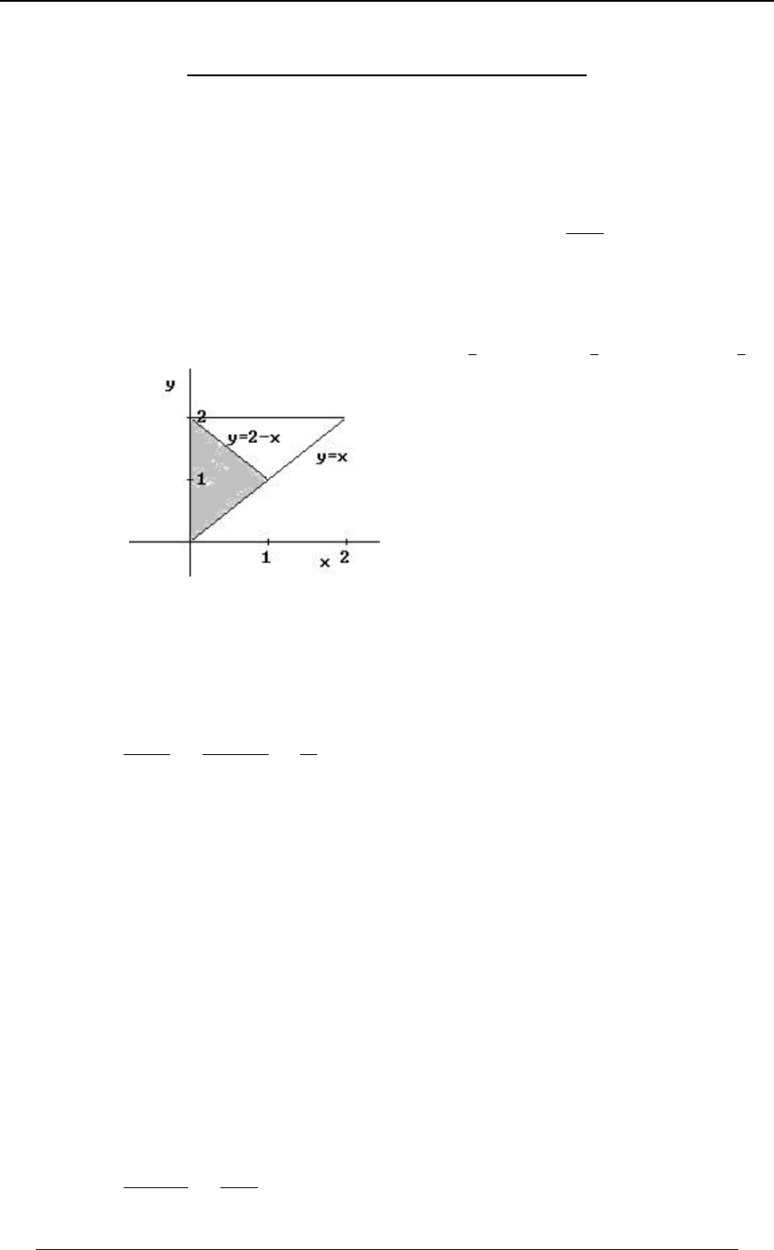
392 PRACTICE EXAM 3

PRACTICE EXAM 3 - SOLUTIONS

1. =1 =1 1 =1 2T Ò] Ó œ T ÒÐ\ Ñ ∩ Ð\  ÑÓ  T ÒÐ\ Ñ ∩ Ð\  ÑÓ

12 21

=1 1 =1 2œ T Ò\ Ó † T Ò\  Ó  T Ò\ Ó † T Ò\  Ó

12 21

=1 1 =0 =1 1 1œ T Ò\ Ó † T Ò\ Ó  T Ò\ Ó † T Ò\ Ÿ Ó

1221

Š‹ Š ‹

1 1 2 2 3 . Answer: Bœ/ Ð/ Ñ/ Ð/ Ñœ /  / œ

  111 1 12

23/

2. The event is equivalent to the event . The region of\] Ÿ# ] Ÿ#\

probability is shaded in the graph at the right. The probability is found by integrating the joint

density function over the two-dimensional region. '' '

!B !

"#B "

$$ "

%% %

B.C.Bœ BÐ##BÑ.Bœ Þ

Answer: C

3. This is a classical Bayesian probability situation. Let denote the event that a flood claimG

occurred. We wish to find . With a model populatiojn of 10,000 we have # ,T ÐLlGÑ P œ )ß !!!

# and # . Also, # # , and similarly,Q œ ")!! L œ #!! G ∩ P œ P ‚ T ÐG ∩ PÑ œ )

# and # . The probability that a policy is high hazard given that thereG∩Qœ$' G∩Lœ&!

was a claim is .

#G∩L &! &!

G )$'&! *%

œ œ œ Þ&$#

The conditional probability approach to solving the problem is as follows.

We can summarize the information in the following table, with the order of calculations

indicated.

PßTÐPÑœÞ) QßTÐQÑœÞ") LßTÐLÑœÞ!#

(given) (given) (given)

G T ÐGlPÑ œ Þ!!"T ÐGlQ Ñ œ Þ!# T ÐGlLÑ œ Þ#&

(given) (given) (given)

1. 2. 3.TÐG ∩PÑ TÐG ∩QÑ TÐG ∩LÑ

œTÐGlPÑ†TÐPÑ œTÐGlQÑ†TÐQÑ œTÐGlLÑ†TÐLÑ

œ Þ!!!) œ Þ!!$' œ Þ!!&

4. T ÐGÑ œ T ÐG ∩ PÑ  T ÐG ∩ Q Ñ  T ÐG ∩ LÑ œ Þ!!*% .

5. . Answer: BT ÐLlGÑ œ œ œ Þ&$#

TÐL∩GÑ

T ÐGÑ Þ!!*%

Þ!!&

PRACTICE EXAM 3 393

4. G9@Ò\ß ] Ó œ IÒ\] Ó  IÒ\Ó † IÒ] Ó

The region of probability is the triangle

above the line in the unit squareCœB

!ŸBŸ" !ŸCŸ" , .

IÒ\]Ó œ BC†'B.B.C œ

"C #

pG9@Ò\ß]Óœ  † œ .

#"$ "

&#% %!

Alternatively,

IÒ\] Ó œ BC † 'B .C .B œ

"" #

Answer: A

5. We identify the events and : a randomly chosen person owns an automobile,ELEœ

Lœ a randomly chosen person owns a house.

We are given .T ÒEÓ œ Þ'! ß T ÒLÓ œ Þ$! ß T ÒE ∩ LÓ œ Þ#!

We wish to find TÒE∩L ÓTÒE ∩LÓ

(the event is the event that a randomly chosen person owns an automobile but does notE∩L

own a house, and the reverse for the event ).E∩L

In a population of 10, 6 would own an automobile, 3 would own a house, and 2 would own at

least one is and the number owning exactly one is , so the probability'$#œ( (#œ&

of owning exactly one is .

"! œÞ&

The event probabliity approach to solving the problem is as follows.

The diagram at the right indicates the

breakdown of the components of the two

events. We can see that TÒE ∩LÓ œ Þ"

and , so the desiredTÒE∩L Ó œ Þ%

probability is .5.

Also, from rules of probability we have ,TÒE∩LÓœTÒEÓTÒE∩LÓœÞ'!Þ#!œÞ%!

and similarly, Therefore, the probabilityTÒE ∩LÓœTÒLÓTÒE∩LÓœÞ$!Þ#!œÞ"!Þ

in question is . An alternative way to consider the problem is to start with theÞ%!  Þ"! œ Þ&!

event , which is the event that a randomly chosen person either owns an automobile, orE∪L

owns a house (or owns both), and then note that this event is the disjoint union of the event in

question and the event , so thatE∩L

"either or or both" "exactly one of or " "both and ".EL œ EL∪ E L

394 PRACTICE EXAM 3

5. continued

It follows that the probability in question is

TÒE L Ó œ TÒE∪LÓTÒE∩LÓ or , but not both

œ T ÒEÓ  T ÒLÓ  T ÒE ∩ LÓ  T ÒE ∩ LÓ œ ÐÞ'!  Þ$!  Þ#!Ñ  Þ#! œ Þ&! Þ

Š‹

The following table also summarizes the calculations in a simple way.

, given TÐEÑ œ Þ' Ê TÐE Ñ œ "Þ' œ Þ%

T ÐLÑ œ Þ$ T ÐE ∩ LÑ œ Þ# Ê T ÐE ∩ LÑ w

given given œTÐLÑTÐE∩LÑ

Ì Ì œÞ$Þ#œÞ"

TÐL Ñ TÐE∩L Ñ

œ"Þ$œÞ( œTÐEÑTÐE∩LÑ

œÞ'Þ#œÞ%

Then . Answer: BTÐE∩LÑTÐE ∩LÑœÞ%Þ"œÞ&

6. We are asked to find .TÒR"lRŸ%ÓœT Ò"ŸR Ÿ%Ó

TÒRŸ%Ó

TÒ"ŸR Ÿ%ÓœTÒRœ"ÓTÒRœ#ÓTÒRœ$ÓTÒRœ%Ó

œœ

"""""

Ð#ÑÐ$Ñ Ð$ÑÐ%Ñ Ð%ÑÐ&Ñ Ð&ÑÐ'Ñ $ .

TÒR Ÿ%ÓœTÒRœ!ÓTÒ"ŸRŸ%Óœ  œ Þ

""&

Ð"ÑÐ#Ñ $ '

TÒR"lRŸ%Óœ œÞ%

"Î$

&Î' . Answer: B

7. We identify events as follows:

HÀ randomly chosen individual has diabetes

LÀ randomly chosen individual has heart disease

We are given T ÒHÓ œ Þ!# ß T ÒLÓ œ Þ!$ ß T ÒH ∩ L Ó œ Þ*' Þ

Using rules of probability, we have

Þ*) œ T ÒH Ó œ T ÒH ∩ LÓ  T ÒH ∩ L Ó p T ÒH ∩ LÓ œ Þ*)  Þ*' œ Þ!#

ww ww w , and

Þ!$ œ T ÒLÓ œ T ÒL ∩ HÓ  T ÒL ∩ H Ó p T ÒL ∩ HÓ œ Þ!$  Þ!# œ Þ!"

w .

These calculations are summarized in the following table.

, given T ÐHÑ œ Þ!# Ê T ÐH Ñ œ "  Þ!# œ Þ*)

TÐLÑ œ Þ!$ TÐL ∩HÑ

given œTÐHÑTÐL ∩HÑœÞ!#Þ!"œÞ!"

ÌË

TÐL Ñ œ Þ*( TÐH∩L Ñ É TÐH ∩L Ñ œ Þ*'

ww ww

, given

œ"Þ!$ œTÐLÑTÐH ∩LÑœÞ*(Þ*'œÞ!" Answer: D

www

PRACTICE EXAM 3 395

8. win in a given week . Then the number of wins in four weeks, , has aTÒ Ó œ ÐÞ"Ñ œ : R

binomial distribution , and dollars is the amount won in 4 weeks. Then,FÐ%ß :Ñ \ œ "!!R

Z +<Ò\Ó œ "!! Z +<ÒR Ó œ "!! Ð%ÑÐ:ÑÐ"  :Ñ Ê \

## the standard deviation of

is . Answer: C#!! :Ð"  :Ñ œ Þ'$

9. .Z +<Ò] l\ œ BÓ œ IÒ] l\ œ BÓ  ÐIÒ] l\ œ BÓÑ

0 ÐCl\ œ BÑ œ 0 ÐBÑ œ # .C œ #Ð"  BÑ Þ

]l\ \B

0ÐBßCÑ

0ÐBÑ

\, where '

Thus, so that0 ÐCl\ œ BÑ œ IÒ] l\ œ BÓ œ C † .C œ

]l\ B

" " "B

"B "B #

and , and thenIÒ] l\ œ BÓ œ C † .C œ

'" "BB

"B $

Z+<Ò]l\Óœ Ò Ó œ

"BB "B

$#"#

Ð"BÑ

# .

Alternatively, note that given any joint uniform distribution, any related conditional distribution

is also uniform. Given , has a uniform distribution on and\œB ] ÐBß"Ñ

thus has a variance of . Answer: B

Ð"BÑ

10. This is an example of a mixture of distributions. is the annual claim amount for a smoker\"

and is the annual claim amount for a non-smoker. We are given\#

IÒ\ Ó œ &!! ß Z +<Ò\ Ó œ #!! ß IÒ\ Ó œ #!! ß Z +<Ò\ Ó œ "!!

""#"

ÈÈ

We are also given the mixing weights (proportion of the population that are smokers),α"œÞ$

and . The distribution of the annual claim amount for a randomly chosen individualα#œÞ(

from the group is , which is a mixture of and .\\\

IÒ\Ó œ ÐÞ$ÑIÒ\ Ó  ÐÞ(ÑIÒ\ Ó œ #*!

IÒ\ Ó œ ÐÞ$ÑIÒ\ Ó  ÐÞ(ÑIÒ\ Ó

###

We know that Z +<Ò\ Ó œ %!ß !!! œ IÒ\ Ó  ÐIÒ\ ÓÑ œ IÒ\ Ó  Ð&!!Ñ

####

, andp IÒ\ Ó œ #*!ß !!!

Z +<Ò\ Ó œ "!ß !!! œ IÒ\ Ó  ÐIÒ\ ÓÑ œ IÒ\ Ó  Ð#!!Ñ p IÒ\ Ó œ &!ß !!!

###

#####

Then, .IÒ\ Ó œ ÐÞ$ÑIÒ\ Ó  ÐÞ(ÑIÒ\ Ó œ "##ß !!!

###

Finally, Z +<Ò\Ó œ IÒ\ Ó  ÐIÒ\ÓÑ œ "##ß !!!  Ð#*!Ñ œ $(ß *!!

## #

and the standard deviation is . Answer: E

È$(ß &!! œ "*%Þ(

396 PRACTICE EXAM 3

11. Let and denote the random variables of the weights of the male and female students\]

respectively. Since the students are chosen at random, and are independent. But then\]

[œ\] œ  œ is normal with mean 310 and variance...

[\]

555

^\]

222

œœ TÒ[ÓœT  œTÒ^ÞÓ625. Thus, 280 1 2 ,

”•

[ 310 280 310

625 625

ÈÈ

(where has a standard normal distribution) 1151. Answer: B^œÞ

12. Expected payment under policy 2 is

P##

CÐÞ!"Ñ.C  P † T Ò\  PÓ œ Þ!!&P  ÐPÑÐ Ñ œ P  Þ!!&P

"!!P

"!! .

This is equal to the expected payment under policy 1, which is

ÐÞ)ÑIÒ\Ó œ ÐÞ)ÑÐ&!Ñ œ %! Þ P  Þ!!&P œ %! Solving results in

P œ &&Þ#) ß "%%Þ(# . We discard 144.72 as a limit since it is larger than the maximum loss

amount. Thus, .P œ &&Þ#)

The variance of insurer payment under policy 1 is

Z +<ÒÞ)\Ó œ Þ'%Z +<Ò\Ó œ ÐÞ'%ÑÐ Ñ œ &$$Þ$$

"!!

# .

Under policy 2,

IÒ Ó œ C ÐÞ!"Ñ.C  Ð&&Þ#)Ñ † T Ò\  &&Þ#)Ó(insurer payment)## #

&&Þ#)

œ &'$Þ"!  Ð&&Þ#)Ñ Ò Ó œ "*#*Þ'*

#"!!&&Þ#)

"!! , and

Z +<Ò Ó œ "*#*Þ'*  Ð%!Ñ œ $#*Þ'*insurer payment .

Z+<Ò Ó

Z +<Ò Ó &$$Þ$$

$#*Þ'*

insurer payment under policy 2

insurer payment under policy 1 œ œ Þ'") . Answer: D

13. .QÐ>Ñœ ÊQÐ,Ñœ œ œ œÞ#Ê,œ%

,,,"

,> ,Ð, Ñ ,, ",

Answer: D

14. Let 'deck is fixed' , number of games lost out of 3 games.Eœ \œ

We wish to find .TÒEl\ œ $Ó

\8œ$: has a binomial distribution with and depends on whether or not the deck is fixed.

We use the usual Bayesian approach.

TÒEl\ œ $Ó œ œ

T Ò\œ$lEÓ†T ÒEÓ T Ò\œ$lEÓ†T ÒEÓ

T Ò\œ$Ó T Ò\œ$lEÓ†T ÒEÓT Ò\œ$lE Ó†T ÒE Ó

We are given that (the casino uses a fixed deck one-quarter the time).TÒEÓ œ Þ#&

Also, if the deck is fixed then , and : œ Þ(& T Ò\ œ $lEÓ œ ÐÞ(&Ñ œ Þ%#")(& Þ

If the deck is fair, then , and : œ Þ&# T Ò\ œ $lE Ó œ ÐÞ&#Ñ œ Þ"%!'!) Þ

Then . Answer: C TÒEl\ œ $Ó œ œ Þ&!

ÐÞ%#")(&ÑÐÞ#&Ñ

ÐÞ%#")(&ÑÐÞ#&ÑÐÞ"%!'!)ÑÐÞ(&Ñ

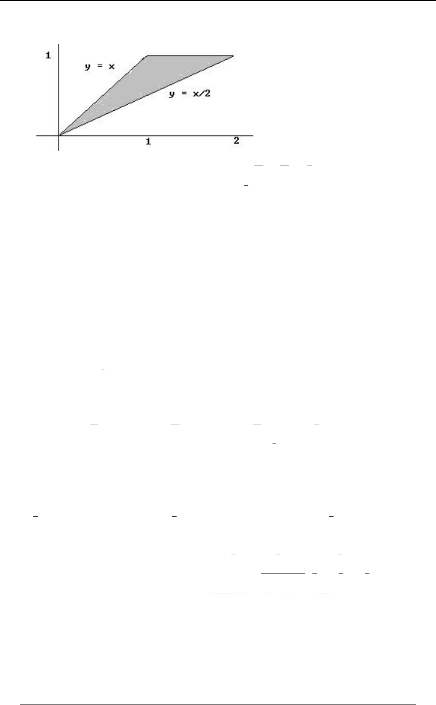
PRACTICE EXAM 3 397

15. The region of probability is shown in the shaded figure below

The probability is .

'' ''

!BÎ# "BÎ#

"B #"

BC .C .B  BC .C .B œ  œ

$*$

$# $# )

Alternatively, the probability is . Answer: D

"#C

BC .B .C œ œ $

)

16. , where is the random lifetime of machine ( days). Since and XœX X X 3 8 X X

"# 3 " #

are independent, the joint density of and is .X X 0Ð>ß>Ñœ/ /

"# "#> >

Applying the convolution method for the sum of random variables results in

0Ð>Ñœ 0Ð=ß>=Ñ.=œ / / .=œ>/

X!!

= Ð>=Ñ >

'' . Answer: A

17. time until property claim, time until life claim.\œ ] œ

0ÐBÑ œ / ß 1ÐCÑ œ /

B CÎ#

# .

X œ œ 738Ð\ß ] Ñtime until next claim .

TÒX >ÓœTÒ\>Ó†TÒ] >Óœ/ †/ œ/

> >Î $>Î#2 .

Pdf of is .X 2Ð>Ñ œ TÒX Ÿ >Ó œ  TÒX  >Ó œ  Ð/ Ñ œ /

...$

.> .> .> #

$>Î# $>Î#

This is the pdf of an exponential random variable with mean . Answer: D

18. Because of the proportions in which the bolts are produced, a randomly selected bolt will

have a chance of being of type A, a chance of being of type B, and a chance of

"# #

** $

being of type C. A random selection of size from the production of bolts will have a8

multinomial distribution with parameters , and , with8:œ ß: œ : œ

EFG

"# #

** $

probability function TÒR œ 8 ßR œ 8 ßR œ 8 Ó œ Ð Ñ Ð Ñ Ð Ñ

F,G- 888

8x " # #

8x8x8x * * $

EFG

With , Answer: D8œ% TÒR œ!ßR œ#ßR œ#Óœ Ð ÑÐ Ñ Ð Ñ œ

EFG !##

%x " # # $#

!x #x #x * * $ #%$

398 PRACTICE EXAM 3

19. \ œ Ð\ ∩ ] Ñ ∪ Ð\ ∩ ] Ñ p \ œ \ ∩ ] p

TÐ]Ñ œ TÐ] ∩\ÑTÐ] ∩\ Ñ œ TÐ\Ñ+Þ

] œ Ð] ∩ ^Ñ ∪ Ð] ∩ ^ Ñ p ] œ ] ∩ ^ p - œ T Ð^Ñ œ T Ð^ ∩ ] Ñ  T Ð^ ∩ ] Ñ œ T Ð] Ñ  ,Þ

w w

Then, It is also true that , so thatTÐ\Ñ+,œ- p TÐ\Ñœ-,+Þ \§] §^ef

- œ TÐ^Ñ œ TÐ\ÑTÐ] \ÑTÐ^ ]Ñ

œTÐ\ÑTÐ] ∩\ÑTÐ^∩] ÑœTÐ\Ñ+,

ww . Answer: E

20. .3\] œœ

G9@Ò\ß] Ó G9@Ò#^ ^ ß#^ ^ Ó

Z +<Ò#^ ^ Ó†Z +<Ò#^ ^ Ó

"$#$

"$ #$

G9@Ò#^  ^ ß#^  ^ Ó

"$#$

œ%G9@Ò^ß^Ó#G9@Ò^ß^Ó#G9@Ò^ß^ÓG9@Ò^ß^Ó

"# "$ $# $$

œ %Ð!Ñ  #Ð!Ñ  #Ð!Ñ  Z +<Ò^ Ó œ  " G9@Ò^ ß ^ Ó œ Z +<Ò^ Ó

$$$$

(since and

independent random variables have covariance of ).!

Z+<Ò#^ ^Óœ%Z+<Ò^ÓZ+<Ò^Ó#Ð#G9@Ò^ß^ÓÑœ&ß

"$ " $ "$

Z+<Ò#^ ^Óœ%Z+<Ò^ÓZ+<Ò^Ó#Ð#G9@Ò^ß^ÓÑœ&

#$ # $ #$ .

Thus, the correlation is . Answer: C3\] "

œœ

"

Ð&Ñ†Ð&Ñ

21. The mean and variance of are .\ IÒ\Ó œ "!!ÐÞ#Ñ œ #! ß Z +<Ò\Ó œ "!!ÐÞ#ÑÐÞ)Ñ œ "'

Using the normal approximation with integer correction, we assume that is approximately\

normal and find

T Ò"%Þ& Ÿ \ Ÿ #&Þ&Ó œ T Ò Ÿ Ÿ Ó œ T Ò  "Þ$(& Ÿ ^ Ÿ "Þ$(&Ó

"%Þ&#! \#! #&Þ&#!

"' "' "'

ÈÈÈ ,

where has a standard normal distribution.^

T Ò  "Þ$(& Ÿ ^ Ÿ "Þ$(&Ó œ Ð"Þ$(&Ñ  Ð  "Þ$(&Ñ œ Ð"Þ$(&Ñ  Ò"  Ð"Þ$(&ÑÓFF F F

œ # Ð"Þ$(&Ñ  "F .

From the standard normal table we have and . Using linearFFÐ"Þ$Ñ œ Þ*!$# Ð"Þ%Ñ œ Þ*"*#

interpolation (since 1.375 is of the way from 1.3 to 1.4) we have

FFFÐ"Þ$(&Ñ œ ÐÞ#&Ñ Ð"Þ$Ñ  ÐÞ(&Ñ Ð"Þ%Ñ œ Þ*"&# , and then the probability in question is

#ÐÞ*"&#Ñ  " œ Þ)$!% . Answer: E

PRACTICE EXAM 3 399

22. When damage occurs, the pdf of the amount of damage is .001 for the uniform distribution

on the interval from 1000 to 2000 .

Expected insurer payment Expected payment given that damage occursœ ÐÞ!"Ñ †

œ ÐÞ!"ÑÒ BÐÞ!!"Ñ .B  "&!! † T Ð ÑÓ

'"!!!

"&!! damage exceeds 1500 when damage occurs

œ ÐÞ!"ÑÒ'#&  Ð"&!!ÑÐ ÑÓ œ "$Þ(&

#!!!"&!!

#!!!"!!! . For the corrected model,

Expected insurer payment Expected payment given that damage occursœ ÐÞ!"Ñ †

œ ÐÞ!"ÑÒ BÐÞ!!!#&Ñ .B  "&!! † T Ð ÑÓ

'"!!!

"&!! damage exceeds 1500 when damage occurs

œ ÐÞ!"ÑÒ"&'Þ#&  Ð"&!!ÑÐ ÑÓ œ "%Þ')(&

&!!!"&!!

&!!!"!!! .

Increase in expected value is .9375 . Answer: C

23. head , tail .TÒ Ó œ TÒ Ó œ

TÒ Ó œ TÒ ∩ Ó3rd head on 5th toss (2 heads in first 4 tosses) (head on 5th toss)

2 heads in first 4 tosses head on 5th tossœTÒ Ó†TÒ Ó

.œ Ð ÑÐ ÑÐ Ñœ

Š‹

#$$$ )"

"#" )

Note that the number of tails, , that are tossed until the 3rd head occurs can also be regarded as\

negative binomial distribution with and , and we are finding . :œ <œ$ TÒ\œ#Ó

Answer: A

24. For each boat type we find the mean and the variance of the repair cost. The mean of the

aggregate repair costs is the sum of the mean repair costs for the 450 boats, and assuming

independence of boat repair costs for all 450 boats, the variance of the aggregate cost is the sum

of the variances for the 450 boats.

For each type of boat, the repair cost is a mixture of 0 (if no repair is needed) and (repair cost\3

variable for boat if a repair is needed). The mean repair cost for boat is33

IÒ\ Ó ‚ 3 3

3prob. repaid is needed for boat , and the second moment of the repair cost for boat is

IÒ\ Ó ‚ 3 IÒ\ Ó œ Z +<Ò\ Ó  ÐIÒ\ ÓÑ

###

prob. repaid is needed for boat (note that ).

The variance of the repaid cost for boat is the second moment minus the square of the first3

moment.

Power boats: Mean repair cost for one boat ,œ $!!ÐÞ$Ñ œ *!

second moment of repair cost for one boat .œ Ò"!ß !!!  $!! ÓÐÞ$Ñ œ $!ß !!!

Variance of repair cost for one power boat .œ $!ß !!!  *! œ #"ß *!!

400 PRACTICE EXAM 3

24. continued

Sailboats: Mean repair cost for one boat ,œ "!!!ÐÞ"Ñ œ "!!

second moment of repair cost for one boat .œ Ò%!!ß !!!  "!!! ÓÐÞ"Ñ œ "%!ß !!!

Variance of repair cost for one power boat .œ "%!ß !!!  "!! œ "$!ß !!!

Luxury Yachts: Mean repair cost for one boat ,œ &!!!ÐÞ'Ñ œ $!!!

second moment of repair cost for one boat .œ Ò#ß !!!ß !!!  &!!! ÓÐÞ'Ñ œ "'ß #!!ß !!!

Variance of repair cost for one power boat .œ "'ß #!!ß !!!  $!!! œ (ß #!!ß !!!

The mean of the aggregate repair cost is ,"!!Ð*!Ñ  $!!Ð"!!Ñ  &!Ð$!!!Ñ œ ")*ß !!!

and the variance is ."!!Ð#"ß *!!Ñ  $!!Ð"$!ß !!!Ñ  &!Ð(ß #!!ß !!!Ñ œ %!"ß "*!ß !!!

The amount budgeted by the marina is . Answer: B")*ß !!!  %!"ß "*!ß !!! œ #!*ß !$!

25. received the letter did not receive an answer after writing to TÒF lE FÓ

œTÒÐF ∩ E F Ó

TÒE FÓ

received the letter) ( did not receive an answer after writing to )

did not receive an answer after writing to .

But, does not receive a reply after writing to ]TÒE F

does not receive a reply after writing to received 's letterœTÒÐE FÑ∩ÐF E ÑÓ

TÒÐE FÑ∩ÐF E ÑÓÞ does not receive a reply after writing to did not receive 's letter

T ÒÐE FÑ ∩ ÐF E ÑÓ does not receive a reply after writing to received 's letter

œTÒE FlF E Ó does not receive a reply after writing to received 's letter

received 's letter , and‚TÒF E Óœ †

"8"

25. continued

T ÒÐE FÑ ∩ ÐF E ÑÓ does not receive a reply after writing to did not receive 's letter

œTÒE FlF E Ó does not receive a reply after writing to did not receive 's letter

did not receive 's letter 1 .‚TÒF E Óœ † "

Therefore,

TÒE F œ †  œ does not receive a reply after writing to ] and

8" " " #8"

888 8

TÒF lE FÓ received the letter did not receive an answer after writing to

œTÒÐF ∩ E F Ó

TÒE FÓ

received the letter) ( did not receive an answer after writing to )

did not receive an answer after writing to

. Answer: Cœœ

Ð8"ÑÎ8

Ð#8"ÑÎ8 #8"

8"

PRACTICE EXAM 3 401

26. Our "probability space" consists of all people who have been charged with a drug-related

offence. We define the following events:

GX - the person is convicted - the person is sentenced to jail time

H - the person did actually commit the crime.

Since jail time is sentenced only to those who are convicted, we have

X§G TÐX∩GÑœTÐXÑ, so that .

We are also given the following information:

T ÐGÑ œ Þ(& ß T ÐH lGÑ œ Þ"! ß T ÐHlG Ñ œ Þ#& ß T ÐX lH Ñ œ Þ!# ß T ÐX lHÑ œ Þ#!

wwww

We wish to find . In the model population approach, .TÐH lG ∩X Ñ TÐH lG ∩X Ñ œ

ww ww

H∩G∩X

G∩X

With a model population of 100,000 we have # and # .G œ (&ß !!! G œ #&ß !!!

From this we get # # so thatH ∩ G œ G ‚ T ÐH lGÑ œ (&ß !!! ‚ Þ" œ (ß &!!

# # # . We also get # .H ∩ G œ G  H ∩ G œ '(ß &!! H ∩ G œ #&ß !!! ‚ Þ#& œ 'ß #&!

Then, # # # and # .H œ H ∩ G  H ∩ G œ '(ß &!!  'ß #&! œ ($ß (&! H œ #'ß #&!

We now get # and # ,X ∩ H œ #'ß #&! ‚ Þ!# œ &#& X ∩ H œ ($ß (&! ‚ Þ# œ "%ß (&!

and then # # # andX ∩ H œ H  X ∩ H œ ($ß (&!  "%ß (&! œ &*ß !!!

# # # and # .X œ X ∩ H  X ∩ H œ &#&  &*ß !!! œ &*ß &#& X œ %!ß %(&

Since we have # # and # # so thatX§G Xœ X∩G H∩G∩Xœ H∩X

#####G∩X œ G  G∩Xœ G Xœ"&ß%(&

and # # .H∩G∩Xœ H∩Xœ&#&

Then # # # .H ∩ G ∩ X œ H ∩ G  H ∩ G ∩ X œ (ß &!!  &#& œ 'ß *(&

www w

Finally, .T ÐH lG ∩ X Ñ œ œ œ Þ%&!(

H∩G∩X

G∩X "&ß%(&

'ß*(&

The conditional probability solution is as follows. From the given information, we get

TÐH ∩GÑœTÐHlGÑ†TÐGÑœÐÞ"ÑÐÞ(&ÑœÞ!(&ß

ww and

T ÐH ∩ G Ñ œ T ÐHlG Ñ † T ÐG Ñ œ ÐÞ#&ÑÐÞ#&Ñ œ Þ!'#&

www .

Since and , we getT ÐGÑ œ Þ(&Ñ T ÐG Ñ  Þ#&

T ÐH ∩ GÑ œ T ÐGÑ  T ÐH ∩ GÑ œ Þ(&  Þ!(& œ Þ'(&

w .

Then , and .T ÐHÑ œ T ÐH ∩ GÑ  T ÐH ∩ G Ñ œ Þ'(&  Þ!'#& œ Þ($(& T ÐH Ñ œ Þ#'#&

Then, andT ÐX ∩ H Ñ œ T ÐX lH Ñ † T ÐH Ñ œ ÐÞ!#ÑÐÞ#'#&Ñ œ Þ!!&#&

www

T ÐX ∩ HÑ œ T ÐX lHÑ † T ÐHÑ œ ÐÞ#!ÑÐÞ($(&Ñ œ Þ"%(&

ww , so that

T ÐX ∩ HÑ œ T ÐHÑ  T ÐX ∩ HÑ œ Þ($(&  Þ"%(& œ Þ&*

w and

T ÐX Ñ œ T ÐX ∩ HÑ  T ÐX ∩ H Ñ œ Þ&*  Þ!!&#& œ Þ&*&#& T ÐX Ñ œ Þ%!%(& Þ

, and

402 PRACTICE EXAM 3

26. continued

Then , andT ÐG ∩ X Ñ œ T ÐGÑ  T ÐG ∩ X Ñ œ T ÐGÑ  T ÐX Ñ œ Þ(&  Þ&*&#& œ Þ"&%(&

T ÐH ∩ G ∩ X Ñ œ T ÐH ∩ GÑ  T ÐH ∩ G ∩ X Ñ œ Þ!(&  Þ!!&#& œ Þ!'*(&

www w

(note that because ).TÐH ∩G∩XÑœTÐH ∩XÑ X §G

Finally, . Answer: CT ÐH lG ∩ X Ñ œ œ œ Þ%&!(

TÐH∩G∩X Ñ

T ÐG∩X Ñ Þ"&%(&

Þ!'*(&

27. Suppose that is the amount of Jim's loss and is Bob's loss. Since there is a .6 chance\\

of no loss for an individual, the pdf of loss amount is ,\0ÐBÑœ

Þ' \ œ !

Þ!!!" "!!! Ÿ \ Ÿ &!!!

œ#

and 0 otherwise. We wish to find . This is equal to0ÐBÑ œ T Ò\  \  )!!!l\  #!!!Ó

"# "

T ÒÐ\ \ )!!!Ñ∩Ð\ #!!!ÑÓ

T Ò\ #!!!Ó

"# "

" . From the pdf for we have\

T Ò\  #!!!Ó œ ÐÞ!!!"ÑÐ&!!!  #!!!Ñ œ Þ$

" .

If , then it is impossible for to be . Then,\ Ÿ $!!! \  \  )!!!

""#

T ÒÐ\  \  )!!!Ñ ∩ Ð\  #!!!ÑÓ œ ÐÞ!!!"Ñ .B .B

"# " #"

$!!! )!!!B

&!!! &!!! #

'' "

'¹

$!!!

&!!! #""

ÐÞ!!!"Ñ ÐB  $!!!Ñ .B œ œ Þ!# Þ

ÐÞ!!!"Ñ ÐB $!!!Ñ

#B œ$!!!

B œ&!!!

The conditional probability in question is then

T ÒÐ\ \ )!!!Ñ∩Ð\ #!!!ÑÓ

T Ò\ #!!!Ó Þ$ "&

Þ!# "

"# "

"œœ . Answer: B

28. Let us denote the 75th percentile of by . Thus, , so that]- JÐ-ÑœÞ(&

"/œÞ(& - /œÞ#&

Ð-+Ñ Ð-+Ñ

" "

# #

. Solving this equation for results in ,

or equivalently, . Answer: E

#Ð-+Ñ œ68% p-œ+ #68%œ+# 68#

#ÈÈ

29. The transformation (for ) is a decreasing function, and therefore]œ?Ð\Ñœ \#

\"

is invertible, . Then using the standard method for finding the\œ? Ð]Ñœ@Ð]Ñœ "

" "

]

density of a transformed random variable, we have the density function of is]

1ÐCÑ œ 0 Ð@ÐCÑÑ † @ÐCÑ œ #Ð  "Ñ †  œ Þ

¹¹ ¹¹

." "#

.C C C ÐC"Ñ

# ##

Alternatively, J ÐCÑœTÒ] ŸCÓœTÒ ŸCÓœTÒ\" Ó

]""

\" C

œ#B.Bœp0ÐCÑœJÐCÑœÞ

'ÐC"ÑÎC

∞# w

]]

C" ÐC"Ñ

## Answer: B

30. T Ò\  ]  #Ó œ T ÒÐ\ œ !Ñ ∩ Ð]  #ÑÓ  T ÒÐ\ œ "Ñ ∩ Ð]  "ÑÓ

T ÒÐ\ œ !Ñ ∩ Ð]  #ÑÓ œ 0Ð!ß CÑ .C œ / .C œ Ò"  / Ó

CÎ# "

"# ' ,

T ÒÐ\ œ "Ñ ∩ Ð]  "ÑÓ œ 0Ð"ß CÑ .C œ / .C œ Ò"  / Ó

CÎ# "Î#

"# $

. Answer: AÊ T Ò\  ]  #Ó œ Ò"  / Ó  Ò"  / Ó œ Ò$  #/  / Ó

"" "

'$ '

" "Î# "Î# "

PRACTICE EXAM 4 403

PRACTICE EXAM 4

1. Event is a subevent of . Which of the following must be true.GE∪F

I. E∪G œF∪G

II. TÐGÑœTÐE∩GÑTÐF∩GÑTÐE∩F∩GÑ

III. E∩G§F

A) All but I B) All but II C) All but III D) II only E) III only

2. A dental insurance policy covers three procedures: orthodontics, fillings and extractions.

During the life of the policy, the probability that the policyholder needs:

· orthodontic work is 1/2

· orthodontic work or a filling is 2/3

· orthodontic work or an extraction is 3/4

· a filling and an extraction is 1/8

The need for orthodontic work is independent of the need for a filling and is also independent of

the need for an extraction. Calculate the probability that the policyholder will need a filling or an

extraction during the life of the policy.

A) 7/24 B) 3/8 C) 2/3 D) 17/24 E) 5/6

3. A loss random variable has a continuous uniform distribution between 0 and $100 .

An insurer will insure the loss amount above a deductible . The variance of the amount that the-

insurer will pay is 69.75 . Find .-

A) 65 B) 70 C) 75 D) 80 E) 85

4. The joint probability of the three discrete random variables is\ß ] ß ^

0 ÐBßCßDÑœ Bœ"ß#ß Cœ"ß#ß Dœ!ß"

\ß] ß^ BCBD

#for .

How many of the following statements are true?

I. and are independent\]

II. and are independent\^

III. and are independent]^

A) 0 B) 1 C) 2 D) 3

404 PRACTICE EXAM 4

5. Let and be events such that and .E F T ÒEÓ œ Þ( T ÒFÓ œ Þ*

Calculate the largest possible value of .TÒE∪FÓTÒE∩FÓ

A) B) C) D) E) Þ#! Þ$% Þ%! Þ'! "Þ'!

6. Bob has a fair die and tosses it until a "1" appears. Doug also has a fair die, and he tosses it

until a "1" appears. Joe also has a fair die and he tosses it until a "1" appears. They each stop

tossing as soon as a "1" turns up on their die. We define the random variable to be the total\

number of tosses that Bob, Doug and Joe made (including the first "1" that each of them tossed).

Find .Z+<Ò\Ó

A) 50 B) 60 D) 70 D) 80 E) 90

7. Let and be independent continuous random variables with common density function \]

.0Ð>Ñ œ š" !>"

!ß

for

otherwise

What is ?TÒ\  ] Ó

A) B) C) D) E)

"#$#

$&&$

8. An auto insurer's portfolio of policies is broken into two classes - low risk, which make up

75% of the policies, and high risk, which make up 25% of the policies. The number of claims per

year that occur from a policy in the low risk group has a Poisson distribution with a mean of .2,

and the number of claims per year that occur from a policy in the high risk group has a Poisson

distribution with a mean of 1.5 . A policy is chosen at random from the insurer's portfolio. Find

the probability that there will be exactly one claim during the year on that policy.

A) .21 B) .25 C) .29 D) .33 E) .37

9. Every member of an insured group has an annual claim amount distribution that is

exponentially distributed. The expected claim amount of a randomly chosen member of the

group is , where is uniformly distributed between 1 and 2. Find the probability that a

randomly chosen member of the group has annual claim less than 1.

A) Less than .4 B) At least .4 but less than .5 C) At least .5 but less than .6

D) At least .6 but less than .7 E) At least .7

PRACTICE EXAM 4 405

10. has pdf for . If and is the event that , find\0ÐBÑœ/B!+!E \+

B

0ÐBlB+Ñ \ \+

\lE the density of the conditional distribution of given that .

A) B) C) D) E) // / / +/

B ÐB+Ñ B+ +B +B

11. A company is planning to begin a production process on a certain day. Government approval

is needed in order to begin production, and it is possible that the approval might not be granted

until after the planned starting day. For each day that the start of the process is delayed the

company will incur a cost of 100,000 . The company has determined that the number of days that

the process will be delayed is a random variable with probability function

:Ð8Ñœ 8œ!ß"ß#ßÞÞÞ

Ð8"ÑÐ8#Ñ for .

The company purchases "delay insurance" which will have the insurer pay the company's cost up

to a maximum of 500,000 . Find the expected cost to the insurer.

A) 100,000 B) 115,000 C) 130,000 D) 145,000 E) 160,000

12. A fair coin is tossed. If a head occurs, 1 fair die is rolled; if a tail occurs, 2 fair dice are

rolled. If is the total on the die or dice, then ]TÒ]œ'Óœ

A) B) C) D) E)

"&"""""

*$'(#'$'

13. Let and be continuous random variables with joint density function\]

0ÐBßCÑ œ š# !BC"

for

, otherwise .

Determine the density function of the conditional distribution of given , where]\œB

!B".

A) for B) for C) for

"B BC" #Ð"BÑ BC" # BC"

D) for E) for

C"C

BC" BC"

14. A carnival sharpshooter game charges $25 for 25 shots at a target. If the shooter hits the

bullseye fewer than 5 times then he gets no prize. If he hits the bullseye 5 times he gets back $10.

For each additional bullseye over 5 he gets back an additional $5. The shooter estimates that he

has a .2 probability of hitting the bullseye on any given shot. What is the shooter's expected gain

if he plays the game (nearest $1)?

A) B) C) D) E) "& "! & ! &

406 PRACTICE EXAM 4

15. Let and be random losses with joint density function\]

for and .0ÐBßCÑœ/ B! C!

ÐBCÑ

An insurance policy is written to reimburse .\]

Calculate the probability that the reimbursement is less than 1.

A) B) C D) E) / / Ñ "/ "#/ "#/

# " " " #

16. A company has annual losses that can be described by the continuous random variable ,\

with density function . The company wishes to obtain insurance coverage that covers0ÐBÑ

annual losses above a deductible. The company is trying to choose between deductible amounts

.. .. .

"# "# "

and , where . With deductible the expected annual losses that would not be

covered by insurance is , and with deductible the expected annual losses that would not beI.

covered by insurance is . Which of the following is the correct expression for ?III

##"

#B†0ÐBÑ.B

B) Ð.  . ÑÒJ Ð. Ñ  J Ð. ÑÓ

#" # "

C) '.

.#" # "

#B†0ÐBÑ.BÐ. .ÑÒJÐ.ÑJÐ.ÑÓ

.#"

#B†0ÐBÑ.B Ð. . Ñ

E) '.

.#" ## ""

#B†0ÐBÑ.BÐ. .ÑÒ.JÐ.Ñ.JÐ.ÑÓ

17. Two components in an electrical circuit have continuous failure times and . Both\]

components will fail by time 1, but the circuit is designed so that the combined times until failure

is also less than 1, so that the joint distribution of failure times satisfies the requirements

!BC" . Suppose that the joint density is constant on the probability space. Find the

probability that both components will fail by time "

#Þ

A) B) C) D) E)

""""

"')%#

18. A discrete integer valued random variable has the following probability function:

TÒ\ œ 8Ó œ + + +

88"

, where the 's are numbers which satisfy the following conditions:

(i) (ii) .+ œ" + + + â+ + â!

! !"# 55"

Find the probability .TÒ\Ÿ&l\"Ó

A) B) C) D) E) ." " + + 

++ +++

++ +++

&& &#'

#" "##

PRACTICE EXAM 4 407

19. In a carnival sharpshooter game the shooter pays $10 and takes successive shots at a target

until he misses. Each time he hits the target he gets back $3. The game is over as soon as he

misses a target. The sharpshooter estimates his probability of hitting the target on any given shot

as . According to this estimate he expects to gain $2 on the game. Find .::

A) .5 B) .6 C) .7 D) .8 E) .9

20. In a model for hospital room charges and hospital surgical charges for a particular type\]

of hospital admission, the region of probability (after scaling units) is !ŸCŸ#B"Ÿ$

and . The joint density function of and is .B  ! \ ] 0 ÐBß CÑ œ Þ$ÐB  CÑ

Find , the expected excess of surgical charges over room charges for an admission.IÒ]  \Ó

A) B) C) D) E) !

$" "$

%% %%

21. Auto claim amounts, in thousands, are modeled by a random variable with density function

0ÐBÑœB/ B!

B for . The company expects to pay 100 claims if there is no deductible.

How many claims does the company expect to pay if the company decides to introduce a

deductible of 1000?

A) 26 B) 37 C) 50 D) 63 E) 74

22. Let have a uniform distribution on the interval . What is the probability that the sum\ Ð"ß $Ñ

of 2 independent observations of is greater than 5?\

A) B) C) D) E)

""""&

"))%#)

23. Let and be three independent continuous random variables each with density\ß\ \

"# $

function .0ÐBÑ œ šÈÈ

#B !B #

for

otherwise

What is the probability that exactly 2 of the 3 random variables exceeds 1?

A) B) C)

 # $# # $Ð #"ÑÐ# #Ñ

ÈÈÈÈ

D) E) Ð  #Ñ Ð #  Ñ $Ð  #Ñ Ð #  Ñ

$"$"

####

ÈÈ ÈÈ

24. An insurer has a portfolio of 1000 independent one-year term insurance policies. For any

one policy, there is a probability of .01 that there will be a claim. Use the normal approximation

to find the probability that the insurer will experience at least 15 claims using the integer

correction.

A) .08 B) .10 C) .12 D) .14 E) .16

408 PRACTICE EXAM 4

25. The number of claims occurring in a period has a Poisson distribution with mean .-

The insurer determines the conditional expectation of expected number of claims in the period

given that at least one claim has occurred, say . Find ./Ð Ñ /Ð Ñ--lim

-Ä!

A) B) C) D) E) !/ "/∞

"

26. An insurer notices that for a particular class of policies, whenever the claim amount is over

1000, the average amount by which the claim exceeds 1000 is 500. The insurer assumes that the

claim amount distribution has a uniform distribution on the interval , where .Ò ! ß - Ó -  "!!!

Find the value of that is consistent with the observation of the insurer.-

A) 1500 B) 2000 C) 2500 D) 4000 E) 5000

27. Let and be discrete random variables with joint probability function\]

.0ÐBßCÑ œ š for

otherwise

ÐB"ÑÐC#Ñ

&% Bœ!ß"ß# à Cœ!ß"ß#

!ß

What is ?IÒ] l\ œ "Ó

A) B) C) D) E)

"" ""

#( * * *

C# C #C

28. The following probabilities of three events in a sample space are given:

T ÒEÓ œ !Þ' ß T ÒFÓ œ !Þ& ß T ÒGÓ œ !Þ% ß

TÒE∪FÓ œ "ß TÒE∪GÓ œ !Þ(ß TÒF∪GÓ œ !Þ( .

Find .T ÒE ∩ F ∩ GlÐE ∩ FÑ ∪ ÐE ∩ GÑ ∪ ÐF ∩ GÑÓ

A) B) C) D) !Þ" !Þ"& !Þ# !Þ#&

E) Cannot be determined from the given information

29. Let be a continuous random variable with density function\

0ÐBÑ œ š"lBl "B"

!ß

for

otherwise .

Determine the density function of where nonzero.]œ\

A) B) C) D) E)

ÈÈ

" # CC # C " C

ÈÈÈ

PRACTICE EXAM 4 409

30. The claim amount random variable has the following distribution functionF

JÐBÑ œ

!B!

BÎ#ß !!! ! Ÿ B  "!!!

Þ(& B œ "!!!

ÐB  ""ß !!!ÑÎ"'ß !!!

Ü"!!!  B  &!!!

" B  &!!!

What is ?IÒFÓ  Z +<ÐFÑ

A) 2400 B) 2450 C) 2500 D) 2550 E) 2600

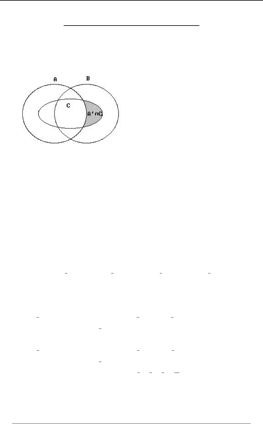
410 PRACTICE EXAM 4

PRACTICE EXAM 4 - SOLUTIONS

1. I. False.

II. . True.G œÐE∩GÑ∪ÐF∩GÑpTÐGÑœTÐE∩GÑTÐF∩GÑTÐE∩F∩GÑ

III. The following diagram explains this situation.

G œÐE∩GÑ∪ÐE ∩GÑ G œÐE∩GÑ∪ÐF∩GÑ

w , and

p ÐE ∩ GÑ § ÐE ∩ GÑ ∪ ÐF ∩ GÑ

p ÐE ∩ GÑ œ Ò ÐE ∩ GÑ ∩ ÐE ∩ GÑÓ ∪ ÒÐE ∩ GÑ ∩ ÐF ∩ GÑÓ ww w

. True. Answer: Aœg∪ÐE ∩F∩GÑ§F

2 We identify the events:Þ

S - orthodontic work will be needed during the lifetime of the policy

J - a filling will be needed during the lifetime of the policy

I - an extraction will be needed during the lifetime of the policy

We wish to find .TÒJ ∪IÓ

We are given: .TÒSÓ œ ß TÒS ∪JÓ œ ß TÒS ∪IÓ œ ß TÒJ ∩IÓ œ

"#$"

#$%)

Using rules of probability, we have ,TÒS∪JÓ œ TÒSÓTÒJÓTÒS ∩JÓ

and since and are independent, we have so thatS J T ÒS ∩ J Ó œ T ÒSÓ † T ÒJ Ó ß

TÒS∪JÓœ œTÒSÓTÒJÓTÒSÓ†TÒJÓœ TÒJÓ †TÒJÓß

#""

$##

from which it follows that TÒJÓ œ Þ

In a similar way, since and are independent,SI

TÒS∪IÓœ œTÒSÓTÒIÓTÒSÓ†TÒIÓœ TÒIÓ †TÒIÓß

$""

%##

from which it follows that TÒIÓ œ Þ

Now, . Answer: DTÒJ ∪IÓ œ TÒJÓTÒIÓTÒJ ∩IÓ œ   œ

""" "(

$#) #%

PRACTICE EXAM 4 411

3. The insurer pays with constant density .01 .]œ

š!B-

B- -BŸ"!!

, if

Then and IÒ] Ó œ .B œ IÒ] Ó œ .B œ

"!! "!!

B-

"!! #!! "!! $!!

Ð"!!-Ñ ÐB-Ñ Ð"!!-Ñ

##$

so that . Substituting the possible answers, we see that withZ+<Ò]Óœ Ò Ó

Ð"!!-Ñ Ð"!!-Ñ

$!! #!!

-œ(! ], the variance of is 69.75 . Answer: B

4. The joint probability table is

B C D 0 ÐBßCßDÑ

\ß] ß^

" " ! "Î#%

" " " #Î#%

" # ! #Î#%

" # " $Î#%

# " ! #Î#%

# " " %Î#%

# # ! %Î#%

# # " 'Î#%

The marginal probability functions are

0Ð"Ñœ œ ß 0Ð#Ñœ œ ß

"##$ " #%%' #

#% $ #% $

0Ð"Ñœ œ ß 0Ð#Ñœ œ ß

]]

"##% $ #$%' &

#% ) #% )

0Ð!Ñœ œ ß 0Ð"Ñœ œ

)

"##% $ #$%'

#% ) #%

The joint distribution of and is\]

0 Ð"ß "Ñ œ œ œ œ 0 Ð"Ñ † 0 Ð"Ñ ß

\ß] \ ]

"# " " $

#% ) $ )

()()

0 Ð"ß #Ñ œ œ œ œ 0 Ð"Ñ † 0 Ð#Ñ ß

\ß] \ ]

#$ & " &

#% #% $ )

()()

0 Ð#ß "Ñ œ œ œ œ 0 Ð#Ñ † 0 Ð"Ñ ß

\ß] \ ]

#% " # $

#% % $ )

()()

0 Ð#ß #Ñ œ œ œ œ 0 Ð#Ñ † 0 Ð#Ñ

\ß] \ ]

%' & # &

#% "# $ )

()() .

Since for all it follows that and are independent.0 ÐBß CÑ œ 0 ÐBÑ † 0 ÐCÑ Bß C \ ]

\ß] \ ]

The joint distribution of and is\^

0 Ð"ß !Ñ œ œ œ 0 Ð"Ñ † 0 Ð!Ñ ß

\ß^ \ ^

""$

)$)

()()

0 Ð"ß "Ñ œ œ œ 0 Ð"Ñ † 0 Ð"Ñ ß

\ß^ \ ^

&"&

#% $ )

()()

0 Ð#ß !Ñ œ œ œ 0 Ð#Ñ † 0 Ð!Ñ ß

\ß^ \ ^

"#$

%$)

()()

0 Ð#ß "Ñ œ œ œ 0 Ð#Ñ † 0 Ð"Ñ

\ß^ \ ^

&#&

"# $ )

()() .

Since for all it follows that and are independent.0 ÐBß DÑ œ 0 ÐBÑ † 0 ÐDÑ BßD \ ^

\ß^ \ ^

For the joint distribution of and we have]^

0 Ð"ß !Ñ œ Á œ 0 Ð"Ñ † 0 Ð!Ñ

]ß^ ] ^

"$$

)))

()() .

It follows that and are not independent. Answer: C]^

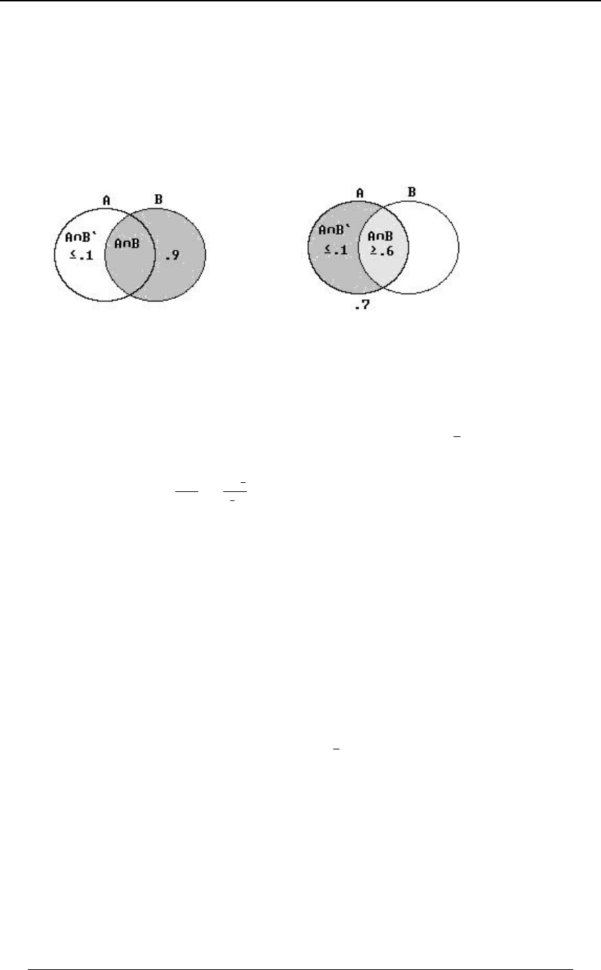
412 PRACTICE EXAM 4

5. T ÒE ∪ FÓ  T ÒE ∩ FÓ œ T ÒEÓ  T ÒFÓ  #T ÒE ∩ FÓ œ "Þ'  #T ÒE ∩ FÓ Þ

This will be maximized if is minimized.TÒE∩FÓ

But and the maximum possible value ofÞ( œ T ÒEÓ œ T ÒE ∩ F Ó  T ÒE ∩ FÓ ß

T ÒE ∩ F Ó Þ" T ÒFÓ Þ* T ÒE ∩ F Ó Ÿ T ÒF Ó œ Þ"

www

is (since is , it follows that ), so that the

minimum possible value for is , and then the maximum of TÒE∩FÓ Þ' TÒE∪FÓTÒE∩FÓ

is . "Þ'  #ÐÞ'Ñ œ Þ%

Answer: C

6. If we consider Doug first and define "success" to be tossing a "1" and "failure" to be a toss that

is not a "1" then the number of tosses Doug makes, say , before his first 1 is the number of\

failures before the first success. has a geometric distribution with ( is the probability\:œ:

of success on a single trial). Doug's total number of tosses is , and\"

Z+<Ð\"ÑœZ+<Ð\Ñœ ":

"

ÐÑ

œœ$! .

Bob and Joe have the same distribution for the number of tosses until a first "1", and since they

toss independently of Doug and each other, the variance of the total number of tosses is just the

sum of the three variances, which is .Answer: E$!  $!  $! œ *!

7. Since both and are between 0 and 1, the event is equivalent to\] \]

\] \ ]

$Î#. Since and are independent, their joint density is

0ÐBß CÑ œ 0 ÐBÑ † 0 ÐCÑ œ "

\] . Then,

TÒ\  ] Ó œ " .B .C œ Ð"  C Ñ .C œ Þ

# $ $Î#

!C !

"" "

'' '

$Î#

& Answer: C

8. low risk low risk high risk high riskTÒR œ"ÓœTÒRœ"l Ó†TÒ ÓTÒR œ"l Ó†TÒ Ó

T ÒR œ "l Ó œ / ÐÞ#Ñ T ÒR œ "l Ó œ / Ð"Þ&Ñ ßlow risk , high risk

Þ# "Þ&

TÒ Ó œ Þ(& TÒ Ó œ Þ#&low risk , high risk

(.75) . Answer: Ap T ÒR œ "Ó œ / ÐÞ#Ñ  ÐÞ#&Ñ/ Ð"Þ&Ñ œ Þ#!'

Þ# "Þ&

PRACTICE EXAM 4 413

9. .TÒ\  "l-Ó œ "/

-

T Ò\  "Ó œ T Ò\  "l-Ó † 0Ð-Ñ .- œ Ð"  / Ñ .- œ Þ('(

- . Answer: E

10. .TÐEÑœTÒ\+Óœ / .Bœ/

∞B +

0 ÐBl\+Ñœ œ œ/ B+ 0 ÐBl\+Ñœ! BŸ+

\lE \lE

ÐB+Ñ

0ÐBÑ

TÐEÑ

B

+ , for , and for .

Answer: B

11. The amount covered by the insurance (in 100,000's) is

Days of delay !"#$%&'â

Insurer Cost !"#$%&&â

The expected insurer cost is

!†:Ð!Ñ"†:Ð"Ñ#†:Ð#Ñ$†:Ð$Ñ%†:Ð%Ñ&†TÒR &Ó

œ!† "† #† $† %† &†Ò"     Óœ"Þ%&

""""" """""

#'"##!$! #'"##!$! .

Answer: D

12. If 1 fair die is rolled, the probability of rolling a 6 is , and if 2 fair dice are rolled, the

probability of rolling a 6 is (of the 36 possible rolls from a pair of dice, the rolls 1-5,

2-4, 3-3, 4-2 and 5-1 result in a total of 6), Since the coin is fair, the probability of rolling a head

or tail is .5. Thus, the probability that is ] œ ' ÐÞ&ÑÐ Ñ  ÐÞ&ÑÐ Ñ œ Þ

"&""

'$'(#

Answer: C

13. The region of joint density is the triangular region above the line and below theCœB

horizontal line for The conditional density of given isCœ" !B"Þ C \œB

0ÐC l \ œ BÑ œ ß 0 ÐBÑ B

0ÐBßCÑ

0ÐBÑ

\ where is the marginal density function of .

0 ÐBÑ œ 0ÐBß CÑ .C œ # .C œ #Ð"  BÑ ß 0ÐC l \ œ BÑ œ œ

\∞ B

∞"

'' so that #"

#Ð"BÑ "B

and the region of density for the conditional distribution of given is ]\œBBC"Þ

It is true in general that if a joint distribution is uniform (has constant density in a region) then

any conditional (though not necessarily marginal) distribution will be uniform on it restricted

region of probability - the conditional distribution of given is uniform on the interval]\œB

BC" , with constant density . Answer: A

"B

414 PRACTICE EXAM 4

14. No. of bullseyes: !"#$%&'(ÞÞÞ#&

Prize: !!!!!"!"&#!ÞÞÞ""!

&\  "& À  "&  "!  & ! & "! "& #! ÞÞÞ ""!

Let number of bullseyes. has a binomial distribution with , , and\œ \ 8œ#& :œÞ#

IÒ\Ó œ & :ÐBÑ œ ÐÞ#Ñ ÐÞ)Ñ Þ . Š‹

BB #&B

Note that for 5 bullseyes or more the prize is .&\  "&

We can find the expected prize by first finding and adjusting for the factorsIÒ&\  "&Ó

corresponding to Therefore,\ œ !ß "ß #ß $ß % Þ

Expected prize

œ IÒ&\  "&Ó  "& † :Ð!Ñ  "! † :Ð"Ñ  & † :Ð#Ñ  ! † :Ð$Ñ  &:Ð%Ñ

œ &IÒ\Ó  "&  "& ÐÞ#Ñ ÐÞ)Ñ  "! ÐÞ#ÑÐÞ)Ñ  & ÐÞ#Ñ ÐÞ)Ñ

Š‹ Š‹ Š‹

#& #& #&

!"#

!#& #% ##$

. Ð!Ñ ÐÞ#Ñ ÐÞ)Ñ  & ÐÞ#Ñ ÐÞ)Ñ œ *Þ("

Š‹ Š‹

#& #&

$## %#"

The expected gain is . Answer: A*Þ("  #& œ  "&Þ#*

15. The probability in question is found by integrating the joint density function over the0ÐBßCÑ

two-dimensional region that represents the event. This two-dimensional region is

ÖÐBßCÑÀBC"ßB!ßC!×œÖÐBßCÑÀC"BßB!ßC!×. This region is

represented in the shaded area in the graph below. The probability is

'' '' ' ¹

!! !! !

""B ""B "

ÐBCÑ B C

0ÐBß CÑ .C .B œ / .C .B œ / Ò  / Ó .B

Cœ!

Cœ"B

œ / Ò"/ Ó.Bœ Ò/ / Ó.B œÒ/ Ó/ œ"#/

'' ¹

B B" B " B " "

Bœ!

Bœ" .

Answer: D

16. ,I œ B † 0ÐBÑ .B  . † 0ÐBÑ .B œ B † 0ÐBÑ .B  . Ò"  J Ð. ÑÓ

"" ""

!. !

.∞ .

'' '

and similarly, . Answer: EI œ B†0ÐBÑ.B. Ò"JÐ. ÑÓ

###

PRACTICE EXAM 4 415

17. The region of probability is the shaded area below.

The joint density is .0ÐBßCÑ œ œ œ #

E</+ 90 :<9,+,363>C =:+-/ "Î#

Since the joint density is constant, the probability that both components will fail by time is

+</+ 90 </1398 E

>9>+6 +</+ 90 :<9,+,363>C =:+-/ , where is the region representing the event that both componentsE

fail by time , . This area is , so that

"" " "

## # %

Ð\  Ñ ∩ Ð]  Ñ

T ÒÐ\  Ñ ∩ Ð]  ÑÓ œ œ Þ

"" "

# # "Î# #

"Î%

Alternatively, we can also formulate the probability as

'' ''

!! !!

"Î# "Î# "Î# "Î#

0ÐBß CÑ .C .B œ # .C .B œ Þ

# Answer: D

18. TÒ\Ÿ&l\"Óœ Þ

T Ò"\Ÿ&Ó

TÒ\"Ó

TÒ\ "Óœ"TÒ\œ!ß"Óœ"Ð"+ ÑÐ+ + Ñœ+

""##

TÒ" \ Ÿ&ÓœTÒ\ œ#ß$ß%ß&Ó

œÐ++ÑÐ++ÑÐ++ÑÐ++Ñœ++

#$ $% %& &' #'

TÒ\Ÿ&l\"Óœ++

# . Answer: E

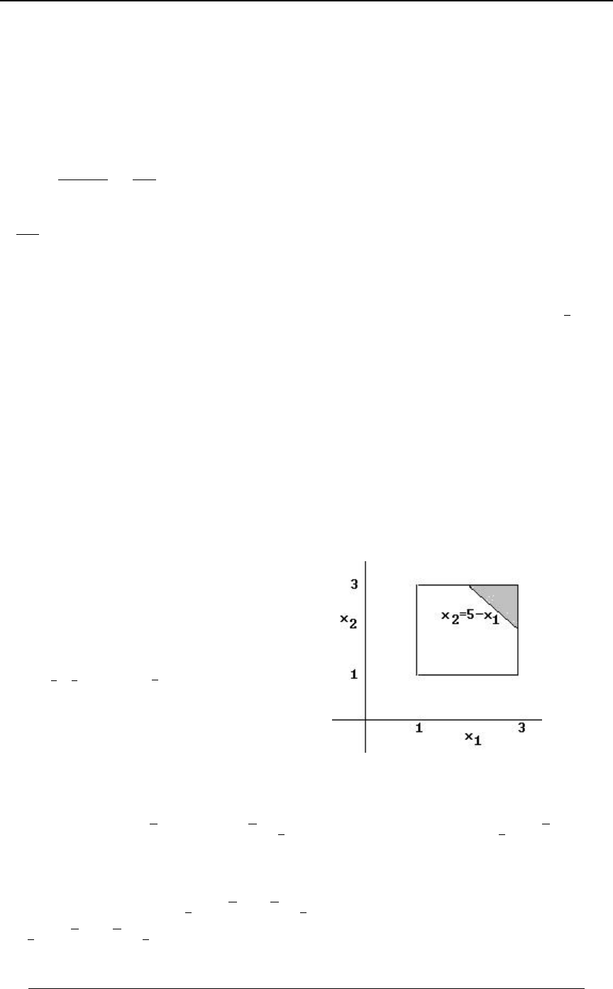
416 PRACTICE EXAM 4

19. Let be the number of targets he hits until the first miss. Then the probability function for\

\TÒ\œ5Óœ:Ð":Ñ is . This is the form of the geometric distribution in which we count

the number of failures until the first success ("failure" in this context means hitting the target, and

"success" means missing the target); however we are using reversing the use of , so in this case:

the probability of success is . Therefore, the expected value of is": \

IÒ\Ó œ œ Þ $IÒ\Ó  "!

"Ð":Ñ

": ":

:The expected gain from the game is

(3 dollars for each hit minus the initial cost). To have an expected gain of 2, we have

$Ð Ñ  "! œ # p : œ Þ)

": . Answer: D

20. IÒ]  \Ó œ ÐC  BÑÐÞ$ÑÐB  CÑ .C .B œ ÐÞ#B  Þ*B  Þ'B  Þ"Ñ .B œ Þ

'' '

!! !

"#B" " $# $

Answer: E

21. There are 100 policies (each claim will result in a payment if there is no deductible).

The probability of a claim being above 1000 (one thousand) is

'¹

∞B B B "

B/ .B œ  B/  / œ #/ œ Þ($&)

Bœ"

∞ . Of the 100 policies, the expected number

that will have claim amounts over 1000 is . Answer: EÐ"!!!ÑÐÞ($&)Ñ œ ($Þ' p (%

22. The probability is theTÒ\ \  &Ó

integral of the joint density of and \\

over the shaded region at the right.

This region is and#ŸB Ÿ$

&BŸBŸ$

"# . The probability is

#&B

$$ ""

## #"

"†.B.Bœ Þ

)

Answer: B

23. .TÒ\ Ÿ "Ó œ Ð #BÑ.B œ # ß TÒ\  "Ó œ "TÒ\ Ÿ "Ó œ  #

'ÈÈ È

""$

With 3 independent random variables, and , there are 3 ways in which exactly 2 of the\ß\ \

"# $

\ \ ß\ \ ß\ \ ß\

3 "#"$#$

's exceed 1 (either or or ). Each way has probability

ÐT Ò\  "ÓÑ † T Ò\ Ÿ "Ó œ Ð  #Ñ Ð #  Ñ

ÈÈ for a total probability of

$†Ð  #Ñ Ð # Ñ

ÈÈ

# . Answer: E

PRACTICE EXAM 4 417

24. The total number of claims follows a binomial distribution with trials and8 œ "!!!

;œÞ!" probability of "success" (claim) for each trial. Since the binomial distribution is the sum

of independent Bernoulli trials, the normal approximation applies to the total number of claims

R IÒRÓ œ "!!!ÐÞ!"Ñ œ "! Z +<ÒRÓ œ "!!!ÐÞ!"ÑÐÞ**Ñ œ *Þ*. and .

Then T ÒR  "&Ó œ T ÒR  "%Þ&Ó œ T Ò  Ó œ T Ò^  "Þ%$Ó

RIÒRÓ

Z+<ÒRÓ

"%Þ&"!

*Þ*

ÈÈ

œ "  Ð"Þ%$Ñ œ "  Þ*#$% œ Þ!('' Ð"Þ%Ñ Ð"Þ&ÑFFF (interpolation between and in the normal

tables provided with the exam). Answer: A

25. IÒRlR"Óœ8†0Ð8lR"Ñœ8† œ8†



8œ" 8œ" 8œ!

∞∞∞

0Ð8Ñ 0Ð8Ñ

"0Ð!Ñ "0 Ð!Ñ

œ†8†0Ð8Ñœœ

"0Ð!Ñ "0 Ð!Ñ

IÒRÓ

"/



8œ!

∞-

- .

(by l'Hospital's rule) . Answer: Clim lim lim

-- -Ä! Ä! Ä!

IÒRlR  "Ó œ œ œ "

"/ /

--

26. If the claim amount is uniform on the interval , then the conditional\Ò!ß-Ó

density , for .0ÐBl\  "!!!Ñ œ œ œ "!!!  B  -

0ÐBÑ "Î-

T Ò\"!!!Ó Ð-"!!!ÑÎ- -"!!!

This conditional density is uniform on the interval , and has a mean ofÒ ! ß -  "!!! Ó

-"!!! -"!!!

Þ œ &!! - œ #!!! In order for this to be 500, we must have , so that .

Answer: B

27. .0 Ð"Ñ œ T Ò\ œ "Ó œ 0Ð"ß CÑ œ 0Ð"ß !Ñ  0 Ð"ß "Ñ  0Ð"ß #Ñ œ

\Cœ∞

∞

"

Then we have conditional probabilities T Ò] œ !l\ œ "Ó œ œ œ ß

0Ð"ß!Ñ %Î&%

T Ò\œ"Ó "Î$ *

and similarly, and .T Ò] œ "l\ œ "Ó œ T Ò] œ #l\ œ "Ó œ

Then, Answer: CIÒ] l\ œ "Ó œ ! †  " †  # † œ Þ

#"%""

*$**

418 PRACTICE EXAM 4

28. .T ÒE ∩ F ∩ GlÐE ∩ FÑ ∪ ÐE ∩ GÑ ∪ ÐF ∩ GÑÓ œ TÒE∩F∩GÓ

T ÒÐE∩FÑ∪ÐE∩GÑ∪ÐF∩GÑÓ

T ÒE ∩ FÓ œ T ÒEÓ  T ÒFÓ  T ÒE ∪ FÓ œ Þ" T ÒE ∩ GÓ œ Þ$ , and similarly, ,

TÒF∩GÓœÞ# TÒE∪FÓœ" TÒE∪F∪GÓœ" . Since , it follows that . Then,

since "œTÒE∪F∪GÓ

œ T ÒEÓ  T ÒFÓ  T ÒGÓ  ÐT ÒE ∩ FÓ  T ÒE ∩ GÓ  T ÒF ∩ GÓÑ  T ÒE ∩ F ∩ GÓ

it follows that . Also,TÒE∩F ∩GÓ œ Þ"

T ÒÐE ∩ FÑ ∪ ÐE ∩ GÑ ∪ ÐF ∩ GÑÓ

œTÒE∩FÓTÒE∩GÓTÒF∩GÓ$TÒE∩F∩GÓTÒE∩F∩GÓœÞ% ,

so that . Answer: D

TÒE∩F∩GÓ

T ÒÐE∩FÑ∪ÐE∩GÑ∪ÐF∩GÑÓ

œÞ#&

29. For , ! Ÿ C  " J ÐCÑ œ T Ò] Ÿ CÓ œ T Ò\ Ÿ CÓ œ T Òl\l Ÿ C Ó

]#È

œ Ð"lBlÑ.Bœ Ð"BÑ.B Ð"BÑ.Bœ# CCÞ

'''

C

ÈÈ

Then, for .0ÐCÑœJÐCÑœ " !ŸC"

]]

Note that in this case the transformation is not one-to-one on the region of probability?ÐBÑ œ B#

of ( ), we cannot use the \  "  B  " 0 ÐCÑ œ 0 Ð@ÐCÑÑ † @ÐCÑ

]\¹¹

approach. Answer: A

30. The pdf of is for and for ,F 0ÐBÑ œ ! B  ! 0ÐBÑ œ ! B  &!!!

it is for , and it is for .0ÐBÑ œ Þ!!!& ! Ÿ B Ÿ "!!! 0ÐBÑ œ Þ!!!!'#& "!!!  B  &!!!

There is a point mass of probability with at ( has a mixed distribution).0ÐBÑ œ Þ#& B œ "!!! F

IÒFÓ œ B † ÐÞ!!!&Ñ.B  Ð"!!!ÑÐÞ#&Ñ B † ÐÞ!!!!'#&Ñ.B œ "#&!

! "!!!

"!!! &!!!

+ ,

IÒF Ó œ B † ÐÞ!!!&Ñ.B  Ð"!!! ÑÐÞ#&Ñ  B † ÐÞ!!!!'#&Ñ.B œ $ß !!!ß !!!

## # #

! "!!!

"!!! &!!!

Z +<ÒFÓ œ IÒF Ó  ÐIÒFÓÑ "ß %$(ß &!! IÒFÓ  Z +<ÒFÓ œ #%%*

= . . Answer: B.

PRACTICE EXAM 5 419

PRACTICE EXAM 5

1. has pdf , defined for , where and are both .\0ÐBÑœ B! !

ÐB Ñ)α" α)

Find for .JÐBÑ B  !

A) B) C) D) E) ÐÑ "ÐÑ ÐÑ "ÐÑ ÐÑ

))) ))

))) ))B B B B B

ααα αα" " "

2. Micro Insurance Company issued insurance policies to 32 independent risks. For each policy,

the probability of a claim is 1/6. The benefit amount given that there is a claim has probability

density function .

, otherwise

0ÐCÑ œ #Ð"  CÑ !  C  "



Calculate the expected value of total benefits paid.

A) B) C) D) E)

"')$#"'$#

*$* $ $

3. Let , and be events such that and are independent, and are mutuallyEF G E F F G

exclusive, , , and . Find .TÒEÓ œ TÒFÓ œ TÒGÓ œ TÒÐE∩FÑ ∪GÓ

"" "

%' # w

A) B) C) D) E)

""$&#$

#%%'#%

4. If the mean and variance of random variable are 2 and 8, find the first three terms inthe\

Taylor series expansion of the moment generating function of about the point .\>œ!

A) B) C) D) E) #>  #> "  #>  '> "  #>  #> "  #>  %> "  #>  "#>

## # # #

5. A small commuter plane has 30 seats. The probability that any particular passenger will not

show up for a flight is 0.10, independent of other passengers. The airline sells 32 tickets for the

flight. Calculate the probability that more passengers show up for the flight than there are seats

available.

A) 0.0042 B) 0.0343 C) 0.0382 D) 0.1221 E) 0.1564

6. The moment generating function for the random variable is .\QÐ>ÑœE/F/

\>#>

You are given that and . Find .Z+<Ò\Óœ E IÒ\Ó

A) B) C) D) E)

"# %&

$$ $$

420 PRACTICE EXAM 5

7. The exponential distribution with mean 1 is being used as the model for a loss distribution.

An actuary attempts to "discretize" the distribution by assigning a probability to for5"

5 œ !ß "ß #ß ÞÞÞ 5  T Ò5  \ Ÿ 5  "Ó \ . The probability assigned to is , where is the

exponential random variable with mean 1. Find the mean of the discretized distribution.

A) 1.00 B) 1.02 C) 1.04 D) 1.06 E) 1.08

8. A casino manager creates a model for the number of customers who play on a particular

gambling machine during a 2-hour period. If (in hours),!Ÿ>Ÿ#

then the probability that people play on the machine during the time interval from time 0 to5

time is (binomial). denotes the time (measured from time 0) at>ÐÞ&>ÑÐ"Þ&>Ñ X

Š‹

55 "!5

which the first person plays on the machine. Find the pdf of .X

A) B) C) "!Ð"  Þ&>Ñ &Ð"  Þ&>Ñ &Þ&Ð"  Þ&>Ñ

** "!

D) E) "!ÐÞ&>Ñ &ÐÞ&>Ñ

* *

9. A loss distribution this year is exponentially distributed with mean 1000. An insurance policy

pays the loss amount up to a maximum of 500. As a result of inflation,

the loss distribution next year will be uniformly distributed between 0 and 1250. The insurer

increases the maximum amount of payment to so that the insurer's expected payment is 25%?

higher next year. Find .?

A) 525 B) 559 C) 673 D) 707 E) 779

10. Of the following statements regarding the sums of independent random variables, how many

are true?

I. The sum of independent Poisson random variables has a Poisson distribution.

II. The sum of independent exponential random variables has an exponential distribution.

III. The sum of independent geometric random variables has a geometric distribution.

IV. The sum of independent normal random variables has a normal distribution.

A) 0 B) 1 C) 2 D) 3 E) 4

PRACTICE EXAM 5 421

11. Among the questions asked in a marketing study were the following:

(i) Are you a member of a group health insurance plan?

(ii) Are you a member of a fitness club?

It was found that 80% of the respondents answered "YES" to at least one of those two questions

and 80% answered "NO" to at least one of those two questions. Find the percentage that

answered "YES" to exactly one of those two questions.

A) .2 B) .3 C) .4 D) .5 E) .6

12. A manufacturing company ships 10,000 units of a product per shipment. In any given

shipment there are a proportion of units that are defective. The company has determined

that 25% of all shipments have a defective proportion of .2 and the other 75% of the shipments

have a defective proportion of .1. A shipment is selected at random and 10 units of the product

are chosen at random from that shipment. Find the probability that at least 2 of the units in that

sample are defective (nearest .05).

A) .30 B) .35 C) .40 D) .45 E) .50

13. A population of insured individuals consists of a% low risk, b% medium risk and c% high

risk. The number of claims in a year for a low risk individual has a Poisson distribution with a

mean of 1 claim, for a medium risk individual the number of claims in a year is Poisson with a

mean of 2, and for a high risk individual the number of annual claims is Poisson with a mean of 3.

An individual is picked at random from the population and it is found that the mean number of

claims for the year is 2.1 and the variance of the number pf claims for the year is 2.59. For a

randomly chosen member of the population find the probability of no claims occurring in the

year.

A) .088 B) .116 C) .156 D) .198 E) .228

14. An insurer is considering taking over a group of policies. The policies in the group are

identically distributed and mutually independent of one another. Each policy in the group has a

claim distribution which is exponentially distributed with mean 100. The premium for each

policy is 120. The insurer wants a probability of at least 95% that the premium received will be

enough to cover the claims. Using the normal approximation, determine the minimum number of

policies needed in the group in order for the insurer's criterion to be met.

A) 60 B) 62 C) 64 D) 66 E) 68

422 PRACTICE EXAM 5

15. has a distribution with pdf .\0ÐBÑœßB!

\α)

)

ÐB Ñ "

]Þ has an exponential distribution with mean "

Which of the following is the correct transformation linking and ?]\

A) B) C) ]œ68Ð\ Ñ ]œ68Ð Ñ ]œ68Ð Ñ)\\

))

)

D) E) ]œ68Ð Ñ ]œ68Ð Ñ

\ \

\\

)

16. Binary digits are transmitted over a communication system. If a 1 is sent, it will be received

as a 1 with probability .95 and as a 0 with probability .05. If a 0 is sent, it will be received as a 0

with probability .99 and as a 1 with probability .01. A series of 0's and 1's is sent in random

order, with 0's and 1's each being equally likely. If a digit is received as a 1 find the probability

that it was sent as a 1.

A) less than .96 B) at least .96 but less than .97 C) at least .97 but less than .98

D) at least .98 but less than .99 E) at least .99

17. The model chosen for a discrete, integer-valued, non-negative random variable with meanR

2 is the binomial distribution with trials and probability of success on each trial. Various8:

combinations of and are considered, and is calculated. Find .8 : TÒR œ !Ó TÒR œ !Ólim

8Ä∞

A) B) C) D) E) //! "

# " "

18. When a fire occurs, the model for fire damage on a particular property is based on the

following joint distribution for (structural damage) and (damage to contents):\]

0ÐBßCÑœ+B,Cß !B#ß!C" (scaled to appropriately sized units). The probability

that is greater than is . Find the total expected damage if a fire occurs, .\] IÒ\]Ó

A) B) C) D) E)

"! "' ## #) $%

*****

19. A machine requires the continual operation of two independent devices in order to keep

functioning. The machine breaks down as soon as the first device stops operating.

The time until failure of Device 1 is uniformly distributed between time 0 and time 1, and the

time until failure of Device 2 has pdf . Find the expected time until the0Ð>Ñ œ #>ß !  >  "

machine breaks down.

A) B) C) D) E)

""""&

"#'%$"#

PRACTICE EXAM 5 423

20. and have a bivariate normal distribution with and .\ ] IÒ\Ó œ ! IÒ] Ó œ "

It is also known that and . Find , the coefficient ofIÒ\l] œ *Ó œ ) IÒ] l\ œ *Ó œ # 3

correlation between and .\]

A) B) C) D) E)!

"" ""

#$ $#

21. Pick the correct relationship:

A) for any events and T ÒE ∩ FÓ Ÿ T ÒEÓ † T ÒFÓ E F

B) for any events andTÒE∪FÓ  TÒEÓTÒFÓ E F

C) for any events and TÒE∩F Ó  TÒEÓTÒFÓ E F

D) for independent events and and any event T ÒE ∪ FlGÓ œ T ÒElGÓ  T ÒFlGÓ E F G

E) for any events and T ÒElFÓ œ T ÒFlEÓ E F

22. A city lotto is held each week. The lotto ticket costs $1, and the lotto prize is $10 and there

is a chance of winning the prize. Smith decides to try his luck at the lotto, and decides to buy

1 ticket each week until he wins, at which time he will stop. Find Smith's expected gain for his

lotto-ticket enterprise.

A) B) C) D) E) #! "& "! & !

23. When a fire occurs, the model for fire damage on a particular property is based on a joint

distribution for (structural damage) and (damage to contents). The marginal distribution of\]

\0ÐBÑœ##B!B" B has density function for . If the amount structural damage is ,

then the distribution of damage to contents is uniform on the interval . Find the expectedÐ!ß Ñ

amount of damage to contents when a fire occurs.

A) B) C) D) E) """" "

#$'"#

24. A loss has a distribution which is uniform between 0 and 1. An insurer issues a policy in this

loss which pays the amount of the loss above a deductible of amount ,.

where . The expected claim on the insurer is , where .!." - !- "

Find the amount of the deductible.

A) B) C) D) E)

ÈÈÈ

#- "  #- "  #-  "  "

#- #-

ÈÈ

424 PRACTICE EXAM 5

25. has an exponential distribution with a mean of 1. is defined to be the conditional\]

distribution of given that , so for instance, for , we have\# \# -!

TÒ] -ÓœTÒ\#-l\#Ó ] . What is the distribution of ?

A) Exponential with mean 1 B) Exponential with mean 2 C) Exponential with mean "

D) Exponential with mean E) Exponential with mean //

26. A die is being loaded so that the probability of tossing a 1 is and the probability of tossing a:

6 is . The probabilities of tossing a 2, 3, 4 or 5 are all . is the outcome from tossing

: \

the die once. Find the value of for which the variance of is maximized.:\

A) B) C) D) E)!""""

"# ' % $

27. The daily high temperature in Toronto in January is normally distributed with a mean of &

degrees Celsius and a standard deviation of 4 degrees Celsius. The daily high temperature in

Winnipeg in January is normally distributed with a mean of degrees Celsius and a standard"!

deviation of degrees Celsius. Assuming that daily high temperatures in Toronto and Winnipeg)

are independent of one another, find the probability that on a given day in January, the high

temperatures for that day in Toronto and Winnipeg are within 1 degree Celsius of each other

(nearest .025).

A) .025 B) .050 C) .075 D) .100 E) .125

28. The joint distribution of random variables and has pdf\]

0ÐBßCÑœBCß !B"ß!C" .

The joint distribution of random variables and has pdf]^

1ÐCßDÑœ$ÐC ÑD ß !C"ß!D"

## .

Which of the following could be the pdf of the joint distribution of and ?\^

A) B D ß !B"ß!D"

B) B $D ß !B"ß!D"

C) $ÐB ÑD ß !B"ß!D"

D) BD ß !B"ß!D"

E) %BD ß !B"ß!D"

PRACTICE EXAM 5 425

29. A small company wishes to insure against losses incurred in the case of a strike by the

company's employees. An insurer agrees to pay $100,000 for each strike that occurs within the

next year, up to a maximum payment of $300,000 . The distribution used to model strike

behavior is strikes within the next year .T Ò8 Ó œ ÐÞ)ÑÐÞ#Ñ ß 8  !

The small company estimates that it will lose $150,000 for each strike that occurs.

For the year, find the company's expected loss that is not covered by the insurance.

A) 12,100 B) 12,300 C) 12,500 D) 12,700 E) 12,900

30. and have a joint distribution with pdf .\ ] 0ÐBßCÑœ/ ß B!ßC!

ÐBCÑ

The random variable is defined to be equal to .YYœ/

ÐBCÑ

Find the pdf of , .Y0Ð?Ñ

A) for B) for 0 Ð?Ñœ" !?" 0 Ð?Ñœ ?"

C) for D) for 0 Ð?Ñœ 68? !?" 0 Ð?Ñœ#? !?"

E) for 0Ð?Ñœ/ ?!

Y?

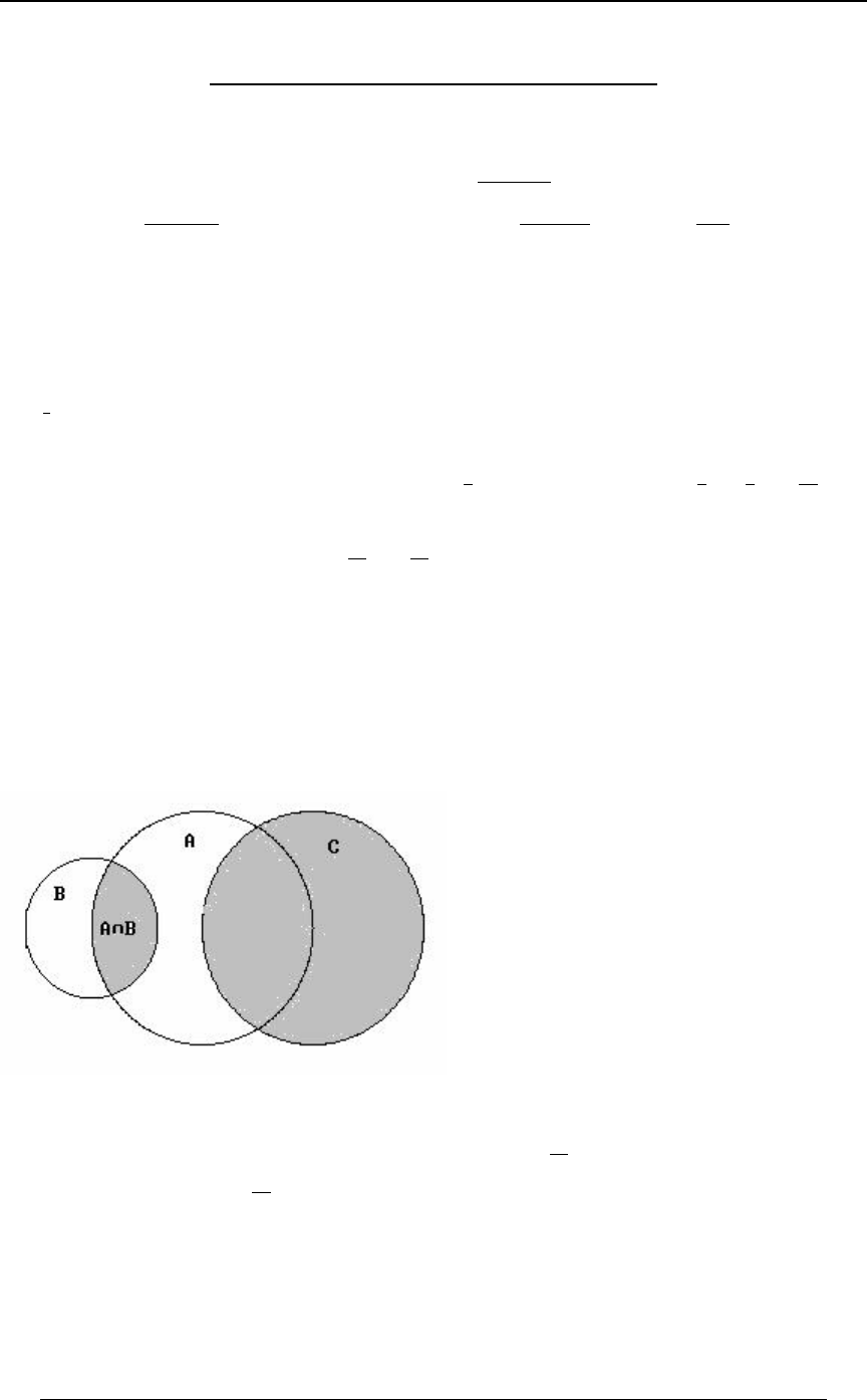
426 PRACTICE EXAM 5

PRACTICE EXAM 5 - SOLUTIONS

1. Since , it follows that ,

∞∞

0ÐBÑ .B œ " - œ "Î .B œ

ÐB Ñ)α" α)α

so that . Then .0ÐBÑ œ JÐBÑ œ 0Ð>Ñ.> œ .> œ "  Ð Ñ

α) α) )

)))

αα

ÐB Ñ Ð> Ñ B

" "

BB α

This is called a Pareto distribution with parameters and . Answer: Bα)

2. In this case, for a particular policy, the probability of a claim occurring is

;œ F

' , and if a claim occurs the (conditional) distribution of the amount of the claim is

defined by the given density function for . Then, the expected0ÐCÑœ#Ð"CÑ !C"

claim from any one policy is IÒ\Óœ;†IÒFÓœÐ Ñ† C†#Ð"CÑ.CœÐ Ñ†Ð Ñœ †

""""

''$")

The expected value of total benefits paid (claims) is the sum of the individual policy expected

values for the 32 policies; this is Answer: AÐ$#ÑÐ Ñ œ Þ

""'

") *

3. and since and are mutually exclusive, is disjoint from .E∩F§F F G E∩F G

It then follows that , and thus .G §ÐE∩FÑ ÐE∩FÑ ∪G œÐE∩FÑ

www

This can be seen in the diagram below.

Then .TÒÐE∩FÑ ∪GÓ œ TÒÐE∩FÑ Ó œ "TÒE∩FÓ

Since and are independent, .E F T ÒE ∩ FÓ œ T ÒEÓ † T ÒFÓ œ "

Thus, . Answer: DTÒÐE∩FÑ ∪GÓ œ

w#$

PRACTICE EXAM 5 427

4. QÐ>Ñ œ IÒ/ Ó œ IÒ"  >\   âÓ œ IÒ"Ó  > † IÒ\Ó  † IÒ\ Ó  â

>\ #

>\ >

## #

IÒ"Ó œ " ß IÒ\Ó # Z +<Ò\Ó œ IÒ\ Ó  ÐIÒ\ÓÑ ) is given as , and is given to be ,

so that . Then the first 3 terms of the expansion of are .IÒ\ Ó œ "# QÐ>Ñ "  #>  '>

# #

Answer: B

5. The number of passengers who show up is a random variable , which has a binomialR

distribution with (each of the 32 ticket holders can be regarded as a trial8œ$#ß:œÞ*

experiment that can end in success - showing up - prob. .9, or failure - not showing up - prob. .1).

In order for more passengers show up for the flight than there are seats available, must be 31R

or 32. Therefore, the probability that more passengers show for the flight than there are seats

available is or .T ÒR œ $" $#Ó œ T ÒR œ $"Ó  T ÒR œ $#Ó

Using the formulation for binomial distribution probabilities we have

T ÒR œ $"Ó œ ÐÞ*Ñ ÐÞ"Ñ œ Þ"##!* ß T ÒR œ $#Ó œ ÐÞ*Ñ ÐÞ"Ñ œ Þ!$%$%

Š‹ Š‹

$# $#

$" $#

$" " $# !

and . The

probability in question is . Answer: ET ÒR œ $"Ó  T ÒR œ $#Ó œ Þ"&'%

6. . For any random variable, Q Ð>ÑœE/ F/ QÐ!Ñœ"pEFœ"

\>#>

p Q Ð>Ñ œ E/  Ð"  EÑ/

\>#>

IÒ\ÓœQ Ð!ÑœE#Ð"EÑœ#E

w .

IÒ\ ÓœQ Ð!ÑœE%Ð"EÑœ%$EÞ

#ww

Z +<Ò\Ó œ IÒ\ Ó  ÐIÒ\ÓÑ œ %  $E  Ð#  EÑ œ E  E œ

## ##

or .pEE œ!pEœ

##"#

*$$

Since we are given that , it follows that and . Answer: EE Eœ IÒ\Óœ# œ

"""&

#$$$

7. is the discretized distribution. ] TÒ] œ5 ÓœTÒ5\Ÿ5"Óœ/ /

#5 5"

for 5 œ !ß "ß #ß ÞÞÞ

IÒ]Óœ Ð5ÑÐ// Ñœ 5Ð// Ñ Ð// Ñ



5œ! 5œ! 5œ!

∞∞∞

5 5" 5 5" 5 5"



5œ!

∞5 5" ! " " #

Ð/  / Ñ œ Ð/  / Ñ  Ð/  / Ñ  â œ "



5œ! 5œ!

∞∞

5 5"

5/ œ ß 5/ œ

Ð"/ Ñ Ð"/ Ñ

" #

" # " #

.p5Ð//Ñœœ



5œ!

∞5 5" ///

Ð"/ Ñ Ð"/ Ñ "/

" # "

" # " # "

IÒ] Ó œ  œ "Þ!)

"/ #

"

" . Answer: E

428 PRACTICE EXAM 5

8. The distribution function of isX

J Ð>ÑœTÒX Ÿ>Óœ"TÒX >Óœ"TÒ >Ó

Xfirst play occurs after time

œ"TÒ >Óœ" ÐÞ&>Ñ Ð"Þ&>Ñ œ"Ð"Þ&>Ñno one plays from time 0 to .

ˆ‰

!"! "!

The pdf of is . Answer: BX 0 Ð>Ñ œ J Ð>Ñ œ &Ð"  Þ&>Ñ

Xw*

9. This year's expected insurance payment is

&!! Þ!!"B

B † ÐÞ!!"/ Ñ .B  &!! † T Ò\  &!!Ó

œ Ð"  J ÐBÑÑ .B œ / .B œ "!!!Ð"  / Ñ œ $*$Þ%(

&!! &!! Þ!!"B Þ& .

Next year's expected insurance payment is

B † ÐÞ!!!)Ñ .B  ? † T Ò\  ?Ó œ Ð"  J ÐBÑÑ .B

œ Ð"  Þ!!!)BÑ .B œ ?  Þ!!!%?

?#.

We want ?  Þ!!!%? œ Ð"Þ#&ÑÐ$*$Þ%(Ñ œ %*"Þ)% Þ

Solving the quadratic equation results in or .? œ '($ ")#(

We ignore the root , since it is above the maximum loss.? œ ")#(

Answer: C

10. I. True.

II. False. The sum of independent exponentials, each with the same mean, has a gamma

distribution.

III. False.

IV. True.

Answer: C

11. "YES" to (i) , "YES" to (ii)Eœ Fœ

TÒE∪FÓœÞ)ß TÒE ∪FÓœÞ)pTÒE∩FÓœTÒÐE ∪FÑÓœ"Þ)œÞ#

ww www

pTÒ ÓœTÒE∩FÓTÒE ∩FÓ"YES' to exactly one ww

. Answer: EœTÒE∪FÓTÒE∩FÓœÞ)Þ#œÞ'

PRACTICE EXAM 5 429

12. , number of defective in a sample of size 10, has a binomial distribution with probabilityR :

of any one being defective.

TÒR #l:Óœ"TÒR! "l:Óœ" Ð":Ñ  Ð":Ñ †: or .

Š‹ Š‹

"! "!

"! *

For shipment with .2 defective,

T ÒR  #l: œ Þ#Ó œ "  ÐÞ)Ñ  Ð"!ÑÐÞ)Ñ ÐÞ#Ñ œ Þ'#%#

"! * .

For shipment with .1 defective,

T ÒR  #l: œ Þ"Ó œ "  ÐÞ*Ñ  Ð"!ÑÐÞ*Ñ ÐÞ"Ñ œ Þ#'$*

"! * .

TÒR #ÓœTÒR #l:œÞ#Ó†TÒ:œÞ#ÓTÒR#l:œÞ"Ó†TÒ:œÞ"Ó

œ ÐÞ'#%#ÑÐÞ#&Ñ  ÐÞ#'$*ÑÐÞ(&Ñ œ Þ$&% . Answer: B

13. With mixing weight applied to the Poisson with mean 1 and mixing weight applied to the+,

Poisson with mean 2, the mean of is .\ IÐ\Ñœ+#,$Ð"+,Ñœ#Þ"

The second moment of is .\ IÐ\ Ñ œ #+  ',  "#Ð"  +  ,Ñ œ #Þ&*  #Þ" œ (Þ!

We get the two equations and .#+  , œ Þ* "!+  ', œ &

Solving these two equations results in and .+ œ Þ# , œ Þ&

Then . Answer: CT Ð\ œ !Ñ œ Þ#/  Þ&/  Þ$/ œ Þ"&'

" # $

14. Claim on policy is . With policies, the aggregate claim is , and3\ 8 Gœ \

3œ"



the mean of the aggregate claim is

IÒGÓ œ IÒ\  \  â  \ Ó œ 8IÒ\Ó œ "!!8

"# 8 , and the variance is

Z +<ÒGÓ œ Z +<Ò\  \  â  \ Ó œ 8Z +<Ò\Ó œ "!ß !!!8 \

"# 8 3

(since the 's are independent,

the variance of the sum is the sum of the variances, and variance of the exponential distribution is

the square of the mean). Total premium collected is ."#!8

Using the normal approximation the probability that total premium exceeds total claims is

T ÒG  "#!8Ó œ T Ò  Ó

GIÒGÓ GIÒGÓ

Z+<ÒGÓ Z+<ÒGÓ

"#!8"!!8

"!ß!!!8

È . is approximately normal, so in order for

this probability to be .95, we must have (from the normal table). This is  "Þ'%&

"#!8"!!8

"!ß!!!8

equivalent to , or equivalently, . Answer: EÞ# 8  "Þ'%& 8  '(Þ(

430 PRACTICE EXAM 5

15. If with inverse function , then .] œ 1Ð\Ñ \ œ 5Ð] Ñ 0 ÐCÑ œ 0 Ð5ÐCÑÑ † l5 ÐCÑl

]\ w

Also, we can think of as a function of , so that .\ ] 0 ÐBÑ œ 0 Ð1ÐBÑÑ † l1 ÐBÑl

\] w

But we are given that is exponential with mean , so that .]0ÐCÑœ/

α]C

αα

Therefore, .0 ÐBÑ œ / † l1 ÐBÑl œ

\1ÐBÑ w

ααα)

)

ÐB Ñ "

We can try each of the transformations to see which one satisfies the relationship.]œ1Ð\Ñ

A) and1ÐBÑ œ 68ÐB  Ñ p 1 ÐBÑ œ)w"

B)

αα/ † l1 ÐBÑl œ / † l l œ

1ÐBÑ w  68ÐBÑαα)

B ÐB Ñ))

α" . Incorrect.

B) and1ÐBÑ œ 68Ð Ñ p 1 ÐBÑ œ

B)w

αα/ † l1 ÐBÑl œ / † l l œ

1ÐBÑ w  68ÐBÎÑαα)

α)α

α" . Incorrect.

C) and1ÐBÑ œ 68Ð Ñ p 1 ÐBÑ œ

B "

B

)

))

αα/ † l1 ÐBÑl œ / † l l œ

1ÐBÑ w 68Ð Ñ

ααB

"

)

B ÐB Ñ))

α) . Correct.

Answer: C

16. 1 was sent , 1 was received .Eœ Fœ

T ÒEÓ œ T ÒE Ó œ Þ& T ÒFlEÓ œ Þ*& ß T ÒFlE Ó œ Þ!" Þ

T ÒFlEÓ œ p T ÒF ∩ EÓ œ ÐÞ*&ÑÐÞ&Ñ œ Þ%(& ß

TÒF∩EÓ

TÒEÓ

T ÒFlE Ó œ p T ÒF ∩ E Ó œ ÐÞ!"ÑÐÞ&Ñ œ Þ!!&

TÒF∩EÓ

TÒEÓ

T ÒFÓ œ T ÒF ∩ EÓ  T ÒF ∩ E Ó œ Þ%(&  Þ!!& œ Þ%) Þ

TÒElFÓ œ œ œ Þ* Þ

TÒE∩FÓ

TÒFÓ

Þ%(&

Þ%) 896 Answer: D

17. . Since , it follows that .TÒRœ!ÓœÐ":Ñ IÒRÓœ8:œ# :œ

Then .lim lim lim

8Ä∞ 8Ä∞ 8Ä∞

TÒRœ!ÓœÐ":ÑœÐ"Ñ

We consider .691ÒÐ"  Ñ Ó œ 8 691Ð"  Ñ œ

691Ð" Ñ

Applying l'Hopital's rule, we get

.lim lim lim

8Ä∞ 8Ä∞ 8Ä∞

691ÒÐ"  Ñ Ó œ œ œ  #

691Ð" Ñ



#Î8#

" #

Therefore, . Answer: Alim lim

8Ä∞ 8Ä∞

8#

Ð" Ñ œ/ œ TÒRœ!Ó

PRACTICE EXAM 5 431

18. In order to be a proper density function, must satisfy the relationship0ÐBßCÑ

Ð+B  ,CÑ .C .B œ " #+  , œ " , so that .

From the given probability, we have ,

Ð+B  ,CÑ .B .C œ &

so that .

Ò Ð%CÑ,Ð#CCÑÓ.Cœ  œ p""+%,œ&

""+ #, &

'$ '

Solving the two equations results in .#+  , œ " ß ""+  %, œ & + œ , œ "

Then, IÒ\]Óœ ÐBCÑÐ B CÑ.C.Bœ ÐB #BCC Ñ.C.B

'' ''

!! !!

#" #" ##

"" "

$$ $

œÐBBÑ.BœÐÑœ

""""'"'

$$$$*

## . Answer: B

19. .0 Ð=Ñœ"ß !="ß 0 Ð>Ñœ#>ß !>"

Time to breakdown is .\œ738ÐWßXÑ

The distribution function of is\

J ÐBÑ œ T Ò\ Ÿ BÓ œ "  T Ò\  BÓ œ "  T ÒÐW  BÑ ∩ ÐX  BÑÓ

\ .

Since and are independent, we haveWX

TÒÐWBÑ∩ÐX BÑÓœTÒWBÓ†TÒX BÓ .

TÒW  BÓ œ ".= œ "B TÒX  BÓ œ #>.> œ "B

, and .

Therefore, , and theJ ÐBÑœ"Ð"BÑÐ"B ÑœBB B

\##$

pdf of is .\0ÐBÑœJÐBÑœ"#B$B

\w#

The mean of is .\ IÒ\Óœ B†0 ÐBÑ.Bœ ÐB#B $B Ñ.Bœ

\#$ &

Note that since , the mean of can be formulated as\! \

IÒ\Ó œ Ò"  J ÐBÑÓ .B œ WÐBÑ † X ÐBÑ .B œ Ð"  BÑÐ"  B Ñ .B œ

'''

!!!

∞∞"

\#&

"# .

Answer: E

20. For a bivariate normal distribution, we have the following.

IÒ\l] œCÓœ  † †ÐC Ñœ! † †ÐC"Ñ p )œ † †)Þ.3 . 3 3

555

\\\

]]]

IÒ]l\œBÓœ  † †ÐB Ñœ" † †ÐB!Ñp#œ" † †*Þ.3 . 3 3

55 5

]] ]

\\ \

Therefore, and , from which we get33†œ" †œ

Ð † ÑÐ † Ñ œ œ Ð"ÑÐ Ñ œ Þ33 3

#""

Since , it follows that (because)œIÒ\l] œ*ÓœIÒ\Ó † †)IÒ\Óœ! !33

]

]! always). Therefore, is the positive square root of , which is . Answer: D3""

21. , since .TÒE∩F Ó œ TÒEÓTÒE∩FÓ  TÒEÓTÒFÓ TÒFÓ  TÒE∩FÓ

Answer: C

432 PRACTICE EXAM 5

22. The probability of first win occurring in week is .8ÐÑÐÑ

#* "

$! $!

8"

If week is Smith's first week then his net gain is dollars (10 dollar prize minus weeks8"!88

with cost of 1 per week). Smith's expected net gain is



8œ" 8œ" 8œ"

∞∞∞

8" 8" 8"

Ð"!8ÑÐÑ ÐÑœ"!ÐÑ ÐÑ 8ÐÑ ÐÑ

#* " #* " #* "

$! $! $! $! $! $!

The week number in which the first win occurs is the form of the geometric distribution on the

integers 1 , 2 , 3 , ... with . The mean is .:œ œ$!œ 8Ð Ñ Ð Ñ

$! 8œ"

∞8"

"#*"

:$!$!



Also, . Smith's net gain is then . Answer: A



8œ"

∞8"

Ð Ñ Ð Ñ œ " "!Ð"Ñ  $! œ  #!

#* "

$! $!

23. for . The joint density of and is0ÐClBÑœ !C \ ]

]l\ #B

0ÐBß CÑ œ 0 ÐClBÑ † 0 ÐBÑ œ † Ð#  #BÑ œ  % ß !  B  " ß !  C 

]l\ \#% B

BB #

IÒ]Óœ C†Ð %Ñ.C.B œ Ð  Ñ.B œ Þ

'' '

!! !

" BÎ# "

%BB"

B##"#

A second approach is somewhat more work. The region of joint density can also be described as

!C ß !#CB"

# .

The density function of the marginal distribution of is]

0 ÐCÑ œ Ð  %Ñ .B œ Ð% 68 B  %BÑ œ Ð  %Ñ  Ð% 68 #C  )CÑ

]#C

BBœ#C

Bœ"

'¹

œ)C%68#C  % !C for .

The mean of is ] IÒ]Óœ C†Ð)C%68#C  %Ñ.C

"Î#

œ Ð)C  %C 68 #C  %CÑ .C

"Î# # . This approach requires finding the antiderivative of

C68#C . This can be done by integration by parts.

'' '

C 68 #C .C œ 68 #C .Ð C Ñ œ C † Ð68 #CÑ  Ð C Ñ .Ð68 #CÑ

"" "

## #

œ C †Ð68#CÑ Ð C ÑÐ Ñ.C œ C †Ð68#CÑ Þ

""""

##C#%

###

' Then,

IÒ] Ó œ Ð)C  %C 68 #C  %CÑ .C œ C  %Ð C † Ð68 #CÑ  Ñ  #C

'¹

"Î# #$##

Cœ!

Cœ"Î#

$# %

œ%Ð68" Ñœ

"" """

$ ) "' # "# . Answer: E

24. The expected amount paid by the insurer is

ÐB  .Ñ 0 ÐBÑ .B œ ÐB  .Ñ .B œ Ð"  .Ñ

# .

Then, . Answer: B

#Ð"  .Ñ œ - p . œ "  #-

#È

PRACTICE EXAM 5 433

25. For we have-!

TÒ] -ÓœTÒ\#-l\#ÓœTÒ\-#l\#Óœ T ÒÐ\-#Ñ∩Ð\#ÑÓ

TÒ\#Ó .

TÒ\  #Ó œ / œ / .B -  ! ß

# B

∞

( ) and since

TÒÐ\-#Ñ∩Ð\#ÑÓœTÒ\-#Óœ/

Ð-#Ñ .

Then, , so that .TÒ] -Óœ"J Ð-Ñœ œ/ 0 Ð-ÑœJ Ð-Ñœ/

]]

- w -

]

-#

#

Therefore, has an exponential distribution with mean 1. Answer: A]

26. .IÒ\Ó œ Ð"ÑÐ:Ñ  Ð#  $  %  &ÑÐ Ñ  Ð'ÑÐ  :Ñ œ  &:

"" "$

'$ $

IÒ\ Ó œ Ð" ÑÐ:Ñ  Ð#  $  %  & ÑÐ Ñ  Ð' ÑÐ  :Ñ œ #"  $&:

# # #### #

'$ .

Z +<Ò\Ó œ IÒ\ Ó  ÐIÒ\ÓÑ œ #"  $&:  Ð  &:Ñ œ  :  #&:

## # #

"$ #! #&

$*$

Z +<Ò\Ó Ð  :  #&: Ñ œ  &!: œ ! is maximized where ,

.#! #& #&

.: * $ $

so that . Answer: C:œ "

27. Toronto high temp. , Winnipeg high temp. .\ œ R Ð  &ß "'Ñ ] œ R Ð  "!ß '%Ñ

High temperature difference is .\  ] µ RÐ&ß )!Ñ

TÒ Ÿ ÓœTÒl\]lŸ"ÓœTÒ"Ÿ\] Ÿ"Óhigh temp. diff. 1

œ T Ò Ÿ ^ Ÿ Ó œ Ð  Þ%&Ñ  Ð  Þ'(Ñ œ Ò"  ÐÞ%&ÑÓ  Ò"  ÐÞ'(ÑÓ

' %

)! )!

ÈÈ

FF F F

œ ÐÞ'(Ñ  ÐÞ%&Ñ œ Þ(%)  Þ'($ œ Þ!(&FF . Answer: C

28. Marginal distribution of has pdf .\0ÐBÑœ0ÐBßCÑ.CœBß!B"

Marginal distribution of has pdf ,]0ÐCÑœ0ÐBßCÑ.BœCß!C"

or 0 ÐCÑœ 1ÐCßDÑ.DœC ß !C"Þ

Marginal distribution of has pdf .^0ÐDÑœ1ÐCßDÑ.Cœ$Dß!D"

Only C has marginal distributions for and that are correct. Answer: C\^

434 PRACTICE EXAM 5

29. The number of strikes in the year has a geometric distribution with mean

Þ#

Þ) œÞ#& . The expected loss to the company in the year (before any insurance coverage) is

"&!ß !!!ÐÞ#&Ñ œ $(ß &!! Þ The expected amount paid by the insurance company in the year is

! † T ÒR œ !Ó  "!!ß !!! † T ÒR œ "Ó  #!!ß !!! † T ÒR œ #Ó  $!!ß !!! † T ÒR  $Ó

œ "!!ß !!!ÒÐÞ)ÑÐÞ#Ñ  #ÐÞ)ÑÐÞ#Ñ  $Ð"  Þ)  ÐÞ)ÑÐÞ#Ñ  ÐÞ)ÑÐÞ#Ñ Ó œ #%ß )!!

The expected loss to the company during the year not covered by insurance is

$(ß &!!  #%ß )!! œ "#ß (!! . Answer: D

30. Using the transformations and , we haveY œ / œ ?Ð\ß] Ñ Z œ \ œ @Ð\ß ] Ñ

Ð\] Ñ

inverse transformations and .\œZ œ2ÐYßZÑ ] œ 68Y Z œ5ÐYßZÑ

Applying the "Jacobian" method to find the joint distribution of transformed random variables Y

and , we haveZ

1Ð?ß @Ñ œ 0Ð2Ð?ß @Ñß 5Ð?ß @ÑÑ † l †  † l

`2 `5 `2 `5

`? `@ `@ `?

œ0Ð@ß 68? @Ñ†l!†Ð"Ñ"†Ð Ñlœ/ † œ"

Ð@68 ? @Ñ .

Since , the region of joint density is and68Y œ\] \œZ !Z  68Y

!Y " Y 0 Ð?Ñœ ".@œ 68? !?" . The marginal pdf of is , on the region .

68 ?

Answer: C

PRACTICE EXAM 6 435

PRACTICE EXAM 6

1. A survey of the public determines the following about the "Lord of the Rings" trilogy

(3 movies).

Have Seen #1 Have Seen #2 Have Seen #3 Percentage of Public

No No No 50%

Yes ? ? 35%

? Yes ? 33%

? ? Yes 31%

Yes No No 8%

Yes Yes No 4%

Yes Yes Yes 20%

Based on this information, determine the percentage of the public that has seen exactly one of the

three "Lord of the Rings" movies.

A) 15 B) 17 C) 19 D) 21 E) 23

following pairs of values is impossible?

A) and B) and T ÐEÑ œ T ÐFÑ œ " T ÐEÑ œ T ÐFÑ œ "

C) and D) and TÐEÑ œ ! TÐFÑ œ TÐEÑ œ TÐFÑ œ

"""

###

E) and TÐEÑ œ " TÐFÑ œ "

$. For a particular disease, it is found that 1% of the population will develop the disease and 2%

of the population has a family history of having the disease. A genetic test is devised to predict

whether or not the individual will develop the disease. For those with a family history of the

disease, 20% of the time the genetic test predicts that the individual will develop the disease and

for those with no family history of the disease, 1% of the time the genetic test predicts that the

individual will develop the disease. The genetic test is not perfect, and individuals are followed to

determine whether or not they actually develop the disease. It is found that for those who have a

family history of the disease and for whom the genetic test predicts the disease will develop, 80%

actually develop the disease. It is also found that for those who have a family history of the

disease and for whom the genetic test does not predict the disease will develop, 10% actually

develop the disease. Find the probability that someone with a family history of the disease will

develop the disease.

A) .20 B) .22 C) .24 D) .26 E) .28

436 PRACTICE EXAM 6

4. You are given the following information:

and TÐElFÑ œ Þ% œ TÐE lF Ñ TÐEÑ œ Þ&

Find .TÐFÑ

A) .4 B) .5 C) .6 D) .7 E) .8

5. If with each new birth, boys and girls are equally likely to be born, find the probability that in

a family with three children, exactly one is a girl.

A) B) C) D) E)

"" $ " &

)% ) # )

6. Six digits from 2 , 3 , 4 , 5 , 6 , 7 , 8 are chosen and arranged in a row without replacement to

create a 6-digit number. Find the probability that the resulting number is divisible by 2.

A) B) C) D) E)

&$ " % *

"% ( # ( "%

7. A bag contains 3 red balls, 2 white balls and 3 blue balls. Three balls are selected randomly

from the bag with replacement. Given that no blue ball has been selected, calculate the

probability that the number of red balls exceeds the number of white balls chosen.

A) B) C) D) E)

$$ ( )" )"

) & "! &"# "#&

8. A student has to sit for an examination consisting of 3 questions selected randomly from a list

of 100 questions (each question has the same chance of being selected). To pass, he needs to

answer at least two questions correctly. What is the probability that the student will pass the

examination if he only knows the answers to 90 questions on the list?

A) Less than .96 B) At least .96 but less than .97 C) At least .97 but less than .98

D) At least .98 but less than .99 E) At least .99

PRACTICE EXAM 6 437

9. A random variable has a probability mass of 0.2 at and a probability mass of 0.1 at\\œ!

\œ" \. For all other values, has the following density function:

, where is a constant.0ÐBÑœ -

!B!

B !B"

#B "  B  -

!B-

\

Find TÐ\"l\Þ&Ñ

A) Less than .6 B) At least .6 but less than .7 C) At least .7 but less than .8

D) At least .8 but less than .9 E) At least .9

10. An ordinary fair die is tossed independently until two consecutive tosses result in the same

face turning up. denotes the toss number on which this happens, so . Which of the\\#

following is , the CDF of for ?JÐBÑ \ B  #

A) B) C) D) E) "ÐÑ "ÐÑ "ÐÑ "ÐÑ ÐÑ

&&""&

'''''

B" B B" B B

11. A discrete random variable has the following probability function\

B À "! #! $! %! &!

0ÐBÑ À !Þ" !Þ" !Þ% !Þ$ !Þ"

Denote by and the mean and the standard deviation of . Find ..5 .5

\\ \\

\TÐl\lŸÑ

A) 1 B) 0.8 C) 0.7 D) 0.5 E) 0.4

12. The continuous random variable has pdf for , where .\0ÐBÑœ !B-5!

Ð5"ÑB

5"

The coefficient of variation of a random variable is defined to be .

ÈZ+<3+8-/

Q/+8

Find the coefficient of variation of .\

A) B) C) D) E)

"" """

Ð5"ÑÐ5#Ñ Ð5#ÑÐ5$Ñ Ð5"ÑÐ5$Ñ 5" 5$

ÈÈ È

13. and are discrete random variables on the integers , with moment generating\ ] Ö!ß "ß #×

functions and . You are given the following:Q Ð>Ñ Q Ð>Ñ

QÐ>ÑQÐ>Ñœ // QÐ>ÑQÐ>Ñœ /

\] \]

>#> >

$$ " ""

%% # %%

and .

Find .TÐ\ œ "Ñ

A) B) C) D) E)

""$"&

)%)#)

438 PRACTICE EXAM 6

14. is a continuous random variable for the density function for ,\ 0ÐBÑœ %ŸBŸ#

lBl

and otherwise. Find , where is the median of .0ÐBÑ œ ! lIÐ\Ñ 7l 7 \

A) Less than .2 B) At least .2 but less than .4 C) At least .4 but less than .6

D) At least .6 but less than .8 E) At least .8

15. Smith plays a gambling game in which his probability of winning on any given play of the

game is .4. If Smith bets 1 and wins, the amount he wins is 1, and if he loses, then he loses the

amount of 1 that he bet. Smith devises the following strategy. If he loses a game, he doubles the

amount that he bets on the next play of the game. He continues this strategy of doubling after

each loss until he wins for the first time. He stops as soon as he wins for the first time. Smith has

a limited amount of money to gamble, say $ . If he loses all $ he goes broke and stops playing--

the game. Find the minimum amount that Smith needs in order for him to have a probability of-

at least .95 of eventually winning before he goes broke.

A) 7 B) 15 C) 31 D) 63 E) 127

16. A production process for electronic components has a followup inspection procedure.

Inspectors assign a rating of high, medium or low to each component inspected. Long run

inspection data have yielded the following probabilities for component ratings:

TÐ Ñ œ Þ& ß TÐ Ñ œ Þ% ß TÐ Ñ œ Þ"high medium low .

Find the probability that in the next batch of 5 components inspected, at least 3 are rated high,

and at most 1 is rated low.

A) Less than .10 B) At least .10 but less than .20 C) At least .20 but less than .30

D) At least .30 but less than .40 E) At least .40

17. A teacher in a high school class of 25 students must pick 5 students from the class for a

school board math test. The students must be chosen randomly from the class. According to the

teacher's assessment, there are 3 exceptional math students in the class and all the rest are

average. Find the probability that at least 2 of the exceptional students are chosen for the test.

A) .01 B) .03 C) .05 D) .07 E) .09

PRACTICE EXAM 6 439

18. Smith is a quality control analyst who uses the exponential distribution with a mean of 10

years as the model for the exact time until failure for a particular machine. Smith is really only

interested in the integer number of years, say , until the machine fails, so if failure is within the\

first year, Smith regards that as 0 (integer) years until failure, and if the machine does not fail

during the first year but fails in the second year, the Smith regards that as 1 (integer) year until

failure, etc. Smith's colleague Jones, who is also a quality control analyst reviews Smith's model

for the random variable and has two comments:\

I. has a geometric distribution.\

II. The mean of is 10.\

Determine which, if any, of the statements made by Jones are true?

A) Neither are true B) Only Statement I is true C) Only Statement II is true

D) Both are true E) None of A, B, C or D is correct

19. and are independent normal random variables with\ß\ß\ß\ \

"#$% &

IÐ\ ÑœZ+<Ð\Ñœ3 3œ"ß#ß$ß%ß&

for .

We define to be . What is the 50th percentile of ?]]œ\ ]$

&

3œ"

A) 0 B) 1.645 C) 3.84 D) 11.07 E) 19.21

20. According to the definition of the beta distribution on the interval (0,1) with integer\

parameters and , the pdf is .+  " ,  " 0ÐBÑ œ † B Ð"  BÑ

Ð+,"Ñx

Ð+"ÑxÐ,"Ñx +" ,"

Which of the following statements are true?

I. If then .+œ, IÐ\Ñœ "

II. If then .+œ, Z+<Ð\Ñœ "

)+"

III. As increases, increases.5IÐ\Ñ

A) I only B) II only C) III only D) All but II E) All but III

21. The joint pdf of and is for and .\ ] 0ÐBßCÑœ5B / "B∞ "C∞

$ CÎ$

Find (the mean of the marginal distribution of ).IÐ\Ñ \

A) 4 B) 2 C) 1 D) E)

440 PRACTICE EXAM 6

22. Smith and Jones are financial analysts who enter a stock picking contest. Smith picks the

stock of Company A and Jones picks the stock of Company B. Over the next week, the gain in the

price of stock A will be and the gain in the price of stock B will be , where and have the\]\]

joint density for and .0ÐBßCÑœ ÐB#CÑ !B" !C"

If the gain in Smith's stock for the week is greater than the gain in Jones' stock, Jones will pay

Smith $1000. How much should Smith pay Jones if the gain in Smith's stock is less than that of

Jones' stock in order that Smith's expected return in this contest is 0?

A) 400 B) 800 C) 1200 D) 1600 E) 2000

23. and are normal random variables with means and , standard deviations and\] .. 5

\] \

]\]

, and correlation coefficient . and denote the cdf's of and respectively.J Ð>Ñ J Ð>Ñ \ ]

If , for what values of is it true that ?55

\] \ ]

œ# > J Ð>ÑJ Ð>Ñ

A) B) C) >Ÿ#  >Ÿ#  >Ÿ Ð  Ñ.. .. 3..

]\ \] \]

D) E) All real numbers >Ÿ Ð  Ñ >3. .

24. and are continuous random variables with pdf for ,\] 0ÐBßCÑœ#!ŸBŸCŸ"

and otherwise. Find the conditional expectation of given .0ÐBßCÑœ! ] \œB

A) B) C) D) E)

"BB" "B

## # # B

25. is a sequence of independent random variables, each with mean 0 and\ ß \ ß \ ß ÞÞÞÞ

"#$

variance 1. We define to be .] \ \ â\

5"# 5

If , what is the coefficient of correlation between and ?54 ] ]

A) B) B) D) E) 54 54

ÈÉ

445

26. has an exponential distribution with mean 1 and . Find .\]œ\"JÐ$Ñ

A) B) C) D) E)

$ # "#/ "/ "/

# # $

PRACTICE EXAM 6 441

27. A financial analyst uses the following model for the daily change in the price of a certain

stock: has a distribution with a mean of .01 and a variance of .0009 ,68Ð Ñ

5"

where is the stock closing price for trading day . Assuming that the daily changes in price are\3

independent from one day to the next, and assuming that the stock price closed at 1 on day 1,

use the normal approximation to find the probability that the stock price is at least 4 at the close

of trading day 101.

A) .05 B) .1 C) .5 D) .9 E) .95

28. An insurance policy has a deductible of 1 and pays a maximum of 1. The underlying loss

random variable being insured by the policy has an exponential distribution with a mean of 1.

Find the expected amount paid by the insurer on this policy.

A) B) C) D) E) #/ / /  / /  #/ #Ð/  / Ñ

# " " # " # " #

29. has a uniform distribution on the interval , and .\ Ð!ß #Ñ ] œ 7+BÖ\ß "×

Find .Z+<Ð]Ñ

A) .05 B) .10 C) .15 D) .20 E) .25

30. has a distribution with the following cdf ,\JÐBÑœ"/

ÐBÎ Ñ)7

where and . The random variable is defined to be .7)! ! ] ] œ1Ð\Ñ

Which of the following transformations results in a distribution of which is exponential with a]

mean of 1?

A) B) C) D) E) 1ÐBÑ œ B 1ÐBÑ œ B 1ÐBÑ œ Ð Ñ 1ÐBÑ œ Ð Ñ 1ÐBÑ œ

77 7 7"Î "Î

B))

)

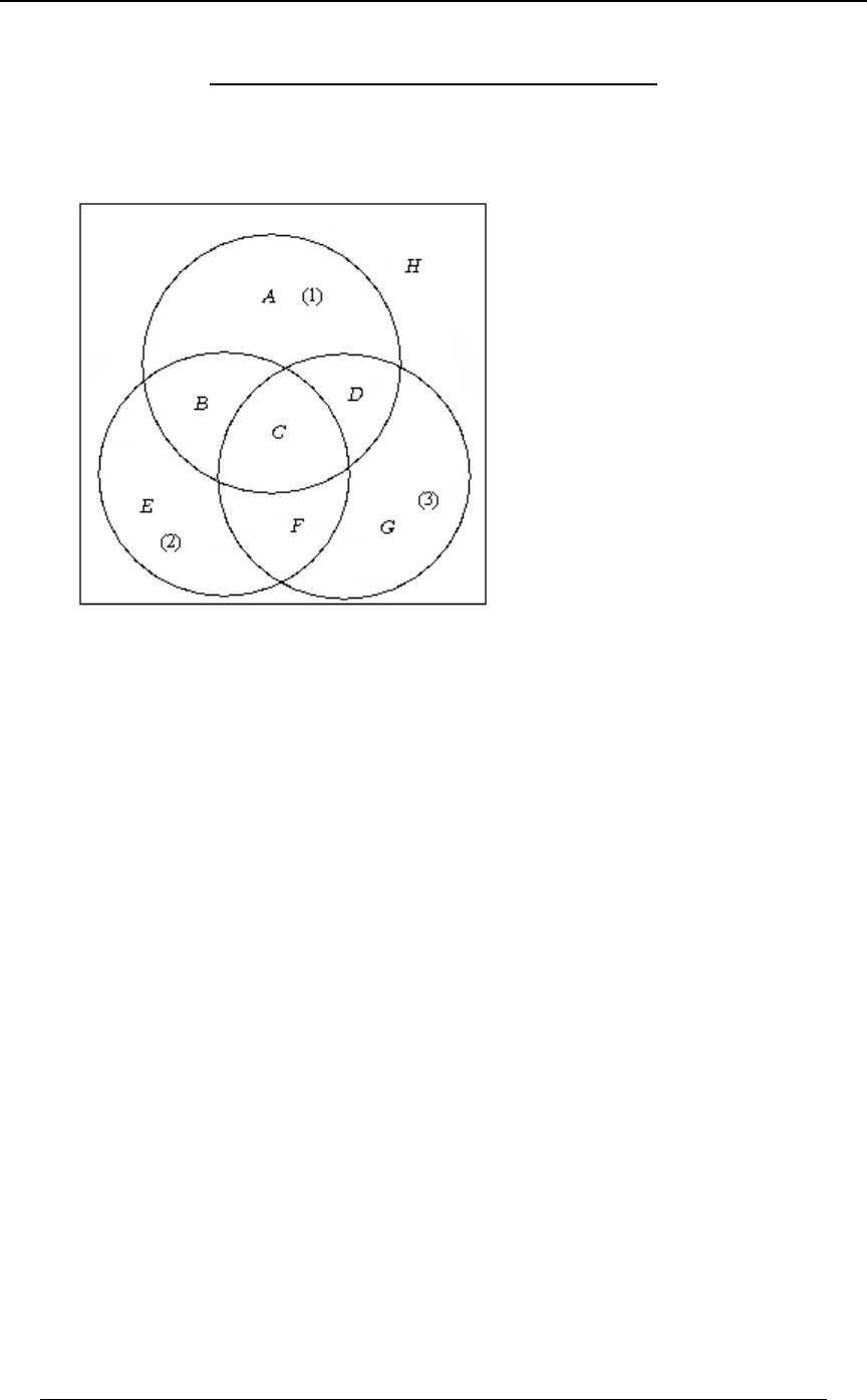
442 PRACTICE EXAM 6

PRACTICE EXAM 6 - SOLUTIONS

1. We can represent the events in the following diagram:

The top circle, represents the event of having seen #1 of the movie series, theE∪F∪G∪H

lower left circle, represents the event of having seen #2 of the movie series, theI∪F∪G∪J

lower right circle, represents the event of having seen #3 of the movie series,K∪J∪G∪H

and represents the event of having seen none of the three movies.L

From the given information, we know that the percentage for event is .L2œ&!

The second line of the information table indicates that 35% of the public has seen movie #1 but

we don't know about movies #2 and #3 for this group. This is interpreted as the percentage for

E∪F∪G∪H +,-.œ$& is .

Similarly, the percentage for is , andI∪F∪G∪J /,-0 œ$$

the percentage for is .K∪J ∪G∪H 10-.œ$"

The 5th line of the table indicates that 8% have seen movie #1 and not movies #2 or #3.

Therefore, the percentage for event is .E+œ)

Event is the event of having seen both #1 and #2 but not #3 and this has percentage ,F,œ%

and event C is the event of have seen all three, and this has percentage .-œ#!

PRACTICE EXAM 6 443

1. continued

The event of having seen exactly one of the three movies is the combination .E∪I∪K

This will be .+/1

We know that percent, since everyone either sees a+  ,  -  .  /  0  1  2 œ "!!

movie or doesn't. This leads to the following 8 equations:

2œ&! ß +,-.œ$& ß /,-0 œ$$ ß 10-.œ$" ß (1) (2) (3) (4)

+œ) ß ,œ% ß -œ#! ß +,-./012œ"(5) (6) (7) (8) .

From equations (3), (6) and (7) we get (9) ./0 œ*

From equations (1), (2) and (8) we get (10) ./01œ"&

From equations (9) and (10) we get (11) .1œ'

From equations (2), (5) and (6) we get (12) .-.œ#$

From equations (11), (12) and (4) we get (13) .0œ#

From equations (9) and (13) we get ./œ(

Then is the percentage that has seen exactly one of the three+/1œ)('œ#"

movies.

Once we have determined the individual values of , we can find the+ß ,ß -ß .ß /ß 0ß 1ß 2

percentage for any combination. For instance, the percentage of people who have seen #1 and #3

but not #2 is . Answer: D.œ$

2. Since and are independent, we must have .E F TÐE∩FÑ œ TÐEÑ†TÐFÑ

Therefore, we must have .TÐEÑ œ TÐEÑ†TÐFÑ

The only way this can be true is if is 0 or 1 , or if is 1.TÐEÑ TÐFÑ

Only D does not satisfy one of these conditions. Answer: D

444 PRACTICE EXAM 6

3. We denote events as follows:

J - an individual has a family history of the disease

X - the genetic test indicates that an individual will develop the disease

H - an individual will develop the disease

We are given the probabilities and .TÐHÑ œ Þ!" TÐJÑ œ Þ!#

The language "for those with a family history of the disease, 20% of the time the genetic test

predicts that the individual will develop the disease" describes the conditional probability

TÐthe genetic test indicates that the individual will develop

the disease the individual has a family history of the disease .l Ñ œ T ÐX lJ Ñ œ Þ#!

In a similar way and .T ÐX lJ Ñ œ Þ!" ß T ÐHlX ∩ J Ñ œ Þ)! T ÐHlX ∩ J Ñ œ Þ"!

We are asked to find .TÐHlJÑ œ TÐH∩JÑ

TÐJÑ

We are given so that .TÐJÑ œ Þ!# TÐJ Ñ œ Þ*)

Then, since ,Þ#! œ T ÐX lJ Ñ œ TÐX∩JÑ

TÐJÑ

we get .TÐX∩JÑœTÐXlJÑ†TÐJÑœÐÞ#ÑÐÞ!#ÑœÞ!!%

Then, since it follows that .T ÐJ Ñ œ T ÐX ∩ J Ñ  T ÐX ∩ J Ñ T ÐX ∩ J Ñ œ Þ!#  Þ!!% œ Þ!"'

Also, .T ÐH ∩ X ∩ J Ñ œ T ÐHlX ∩ J Ñ † T ÐX ∩ J Ñ œ ÐÞ)!ÑÐÞ!!%Ñ œ Þ!!$#

Similarly .T ÐH ∩ X ∩ J Ñ œ T ÐHlX ∩ J Ñ † T ÐX ∩ J Ñ œ ÐÞ"!ÑÐÞ!"'Ñ œ Þ!!"'

www

Then .T ÐH ∩ J Ñ œ T ÐH ∩ X ∩ J Ñ  T ÐH ∩ X ∩ J Ñ œ Þ!!$#  Þ!!"' œ Þ!!%)

Finally, . Answer: CTÐHlJÑ œ œ œ Þ#%

TÐH∩JÑ

TÐJÑ Þ!#

Þ!!%)

4. TÐE∩FÑ œ TÐElFÑ†TÐFÑ œ Þ%‚TÐFÑÞ

T ÐElF Ñ œ "  T ÐE lF Ñ œ Þ' T ÐE ∩ F Ñ œ T ÐElF Ñ † T ÐF Ñ œ Þ' ‚ Ò"  T ÐFÑÓ

www www

and .

Then

Þ& œ T ÐEÑ œ T ÐE ∩ FÑ  T ÐE ∩ F Ñ œ Þ% ‚ T ÐFÑ  Þ' ‚ Ò"  T ÐFÑÓ œ Þ'  Þ# ‚ T ÐFÑ Þ

Solving for results in . Answer: BTÐFÑ TÐFÑ œ Þ&

5. There are 8 possible orderings of births in a family of three children:

GGG , GGB , GBG , GBB , BGG , BGB , BBG , BBB .

# of these orderings result in a family with exactly one girl: GBB , BGB , BBG .

Each of the orderings has a probability of of occurring, so the probability of

""" "

### )

‚‚œ

exactly one girl is . Answer: C

)

PRACTICE EXAM 6 445

6. To find the probability that a certain type of combination or arrangement occurs, the

probability is usually formulated as number of combinations or arrangement of the specific type required

total number of all combinations or arrangements .

For these problems, the denominator is the total number of all 6 digit numbers that can be created

by choosing 6 digits without replacement from 2 , 3 , 4 , 5 , 6 , 7 , 8. The total number of 6-digit

numbers is 7 since the first digit can be any one of the 7 integers,‚'‚&‚%‚$‚#œ&ß!%!

the second digit can be any one of the remaining 6 integers, etc.

The number is even if it ends in 2 , 4 , 6 or 8 . For each of these 4 cases, there are

'‚&‚%‚$‚#œ(#! arrangements of the first 5 digits in the number, since the other 5 digits

are chosen from the 6 remaining integers. The numerator of the probability is

% ‚ (#! œ #))! œ Þ , and the probability is #))! %

&!%! (

An alternative solution is to note that there are 7 possible equally likely final digits for the 6-digit

number, and 4 of them make the number even. The probability is . Answer: D

(

7. We wish to find , whereTÐElFÑ œ TÐE∩FÑ

TÐFÑ

Eœ Fœmore red than white are chosen, and no blue are chosen.

Out of 8 balls in the bag, 5 are not blue, so for each of the three trials, the probability of picking a

ball that is not blue is ; since the ball chosen is always replaced, the probability remains the

)

same on each subsequent choice. Then, .TÐFÑœ‚‚œ

&&& "#&

))) &"#

On any given trial, the probability of a red ball being chosen is and the probability of a white

)

ball being chosen is .

)

E∩Fœno blue are chosen and more red than white are chosen.

The following sequences of choices result in occurring: .E ∩ F VVV ß VV[ ß V[ V ß [ VV

The probabilities of these sequences is

TÐVVVÑ œ ‚ ‚ œ T ÐVV[Ñ œ ‚ ‚ œ

$$$ #( $$# ")

))) &"# ))) &"#

, ,

TÐV[VÑœ‚‚œ TÐ[VVÑœ‚‚œ

$#$ ") #$$ ")

))) &"# ))) &"#

, .

Then, .TÐE∩FÑ œ œ

#(")")") )"

&"# &"#

Finally, . Answer: ETÐElFÑ œ œ

)"Î&"#

"#&Î&"# "#&

446 PRACTICE EXAM 6

8. The student will pass if at least two of the three questions chosen come from the 90 questions

that the student knows. The number of ways of choosing 3 questions from 100 is

Š‹

"!!

$ *(x†$x '

"!!x "!!‚**‚*)

œ œ œ "'"ß (!! .

The student will pass if either

(i) all three questions are chosen from the 90 he knows the answers to, or

(ii) exactly two of the three questions are chosen from the 90 he knows the answers to and the

other is chosen from the other 10.

The number of ways of (i) occurring is , and the number

Š‹

$ )(x†$x '

*!x *!‚)*‚))

œ œ œ ""(ß %)!

of ways of (ii) occurring is Š‹Š‹

*! "!

# " ))x†#x *x†"x #

*!x "!x *!‚)*

‚ œ ‚ œ ‚ "! œ %!ß !&! Þ

The probability that the student gets at least 2 of the 3 questions right is .

""(ß%)!%!ß!&!

"'"ß(!! œ Þ*(%

Answer: C

9. TÐÞ&\"Ñœ B.B œ Þ$(&Þ

'Þ&

TÐ\"l\Þ&ÑœT ÐÞ&\"Ñ

T Ð\Þ&Ñ .

Although we have not determined the value of , we know that-

T Ð\  Þ&Ñ œ "  T Ð\ Ÿ Þ&Ñ œ "  ÒT Ð\ œ !Ñ  T Ð!  \ Ÿ Þ&ÑÓ

œ "  ÒÞ#  B .BÓ œ "  Þ$#& œ Þ'(& Þ

Þ&

Then . Answer: AT Ð\  "l\  Þ&Ñ œ œ œ Þ&&'

T ÐÞ&\"Ñ

T Ð\Þ&Ñ Þ'(&

Þ$(&

10. .JÐBÑœTÐ\ŸBÑ

TÐ\ œ #Ñ œ \ œ #

" "

' '

, since if the second toss is the same as the first, and there is a chance

of that. There is a chance that the 2nd toss is not the same as the first, and then a chance that

the 3rd toss is the same as the 2nd, so . There is a chance that the 3rd tossTÐ\ œ $Ñ œ ‚

&" &

'' '

is not the same as the 2nd, and then a chance that the 4th toss is the same as the 3rd, so

TÐ\ œ %Ñ œ Ð Ñ ‚ TÐ\ œ 8Ñ œ Ð Ñ ‚

&" & "

'' ' '

#8#

. Continuing in this way, we see that .

Then .JÐBÑœ TÐ\œ8Ñœ ÐÑ ‚ œÒ" ÐÑâÐÑ Ó‚



8œ# 8œ#

8# # B#

&" && & "

'' '' ' '

We use the geometric series expression , to get"++ â+ œ

"+

5"

JÐBÑ œ ‚ œ "Ð Ñ

"Ð Ñ

"

'B"

B" . Answer: A

PRACTICE EXAM 6 447

11. ..\œ Ð"! ‚ Þ"Ñ  Ð#! ‚ Þ"Ñ  Ð$! ‚ Þ%Ñ  Ð%! ‚ Þ$Ñ  Ð&! ‚ Þ"Ñ œ $#

œIÒÐ\ Ñ Ó

œ Ð"!  $#Ñ ÐÞ"Ñ  Ð#!  $#Ñ ÐÞ"Ñ  Ð$!  $#Ñ ÐÞ%Ñ  Ð%!  $#Ñ ÐÞ$Ñ  Ð&!  $#Ñ ÐÞ"Ñ

#####

œ ""'

Alternatively, .5\

## #

œ IÐ\ ÑÐIÒ\ÓÑ

IÐ\ Ñ œ Ð"! ‚ Þ"Ñ  Ð#! ‚ Þ"Ñ  Ð$! ‚ Þ%Ñ  Ð%! ‚ Þ$Ñ  Ð&! ‚ Þ"Ñ œ ""%!

###### ,

so that , and .55

## \

œ ""%!  $# œ ""' œ ""' œ "!Þ((

Then, T Ðl\  l Ÿ Ñ œ T Ðl\  $#l Ÿ "!Þ((Ñ œ T Ð  "!Þ(( Ÿ \  $# Ÿ "!Þ((Ñ.5

œ T Ð#"Þ#$ Ÿ \ Ÿ %#Þ((Ñ œ T Ð\ œ $! %!Ñ œ !Þ( or . Answer: C

12. .IÐ\Ñ œ B † 0ÐBÑ.B œ .B œ † -

Ð5"ÑB

5"

5#

5"

IÐ\ Ñ œ B † 0ÐBÑ.B œ .B œ † -

## #

Ð5"ÑB

5"

5$

5#

5" .

Z +<Ð\Ñ œ IÐ\ Ñ  ÐIÒ\ÓÑ œ † -  Ð † -Ñ œ Ò  Ð Ñ Ó-

### # ##

5" 5" 5" 5"

5$ 5# 5$ 5#

.œ†-

5"

Ð5$ÑÐ5#Ñ##

The coefficient of variation of is .\†-Ð†-Ñœ

É‚

5" 5" "

Ð5$ÑÐ5#Ñ 5# Ð5"ÑÐ5$Ñ

##È

Answer: C

13. We denote the probability function of by and\ : œTÐ\œ!Ñß: œTÐ\œ"Ñß

:œTÐ\œ#Ñ ]

\ . With similar notation for .

Then andQÐ>ÑœIÒ/Óœ/†:/†:/†:

\>\ ! \ > \ #> \

!" #

QÐ>ÑœIÒ/Óœ/†:/†:/†:

]>] ! ] > ] #> ]

!" #

Then QÐ>ÑQÐ>Ñœ:/†:/†::/†:/†:

!" #!" #

\>\#>\] >] #>]

,œ: : Ð: : Ñ/ Ð: : Ñ/

!! "" ##

\] \]> \]#>

and it follows that and .: : œ ß : : œ : : œ

!! "" ##

\] \] \]

$$ "

%% #

In a similar way, we have

QÐ>ÑQÐ>Ñœ:/†:/†::/†:/†:

!" #!" #

\>\#>\] >] #>]

,œ: : Ð: : Ñ/ Ð: : Ñ/

!! "" ##

\] \]> \]#>

and it follows that and .::œ ß::œ ::œ!

!! "" ##

\] \] \]

From these equations, we see that ,::::œ#:œ  œ

"" "" "

\] \] \

$" "

%% #

and therefore . Answer: BTÐ\ œ "Ñ œ : œ

448 PRACTICE EXAM 6

14. .IÐ\ÑœB0ÐBÑ.BœB†ÐÑ.BB†ÐÑ.Bœ

'' '

% % !

#! #

B B #)

"! "! "&

The median satisfies the relationship .70ÐBÑ.Bœ

'%

We know that , so we must have

% %

0ÐBÑ.Bœ Ð Ñ.Bœ %Ÿ7Ÿ!Þ

B %

"! &

Then . Setting this equal to , we get (we take the negative

'È

%

7ÐÑ.Bœ 7œ'

B "'7 "

"! #! #

square root because we know that the median is between and 0).%

Then . Answer: ClIÐ\Ñ  7l œ l   Ð  'Ñl œ Þ&)$

"& È

15. We can approach this problem by trial and error.

If Smith has , then Smith will go broke if he loses the first game (prob. .6), so there is a .4-œ"

chance that Smith wins before going broke.

If Smith has , then Smith will go broke if he loses the first two games (prob.-œ"#œ$

Þ' ‚ Þ' œ Þ$'), so there is a .64 chance that Smith wins before going broke.

If Smith has , then Smith will go broke if he loses the first three games (prob.-œ"#%œ(

ÐÞ'Ñ œ Þ#"'

$), so there is a .784 chance that Smith wins before going broke.

If Smith has , then Smith will go broke if he loses the first four games-œ"#%)œ"&

(prob. ), so there is a .8704 chance that Smith wins before going broke.ÐÞ'Ñ œ Þ"#*'

If Smith has , then Smith will go broke if he loses the first five-œ"#%)"'œ$"

games (prob. ), so there is a .9222 chance that Smith wins before going broke.ÐÞ'Ñ œ Þ!(()

If Smith has , then Smith will go broke if he loses the first six-œ"#%)"'$#œ'$

games (prob. ), so there is a .9533 chance that Smith wins before going broke.ÐÞ'Ñ œ Þ!%'(

Answer: D

16. We can use the multinomial distribution. For a batch of components tested, the probability8

that are rated high, are rated medium and are rated low is .+ , - ÐÞ&Ñ ÐÞ%Ñ ÐÞ"Ñ

+x ,x -x +,-

In a batch of 5, in order to have at least 3 high and at most 1 low, the following combinations are

possible 5H , 4H and 1M , 4H and 1L , 3H and 1M and 1L .

The probabilities of these combinations are

T Ð&LÑ œ ÐÞ&Ñ ÐÞ%Ñ ÐÞ"Ñ œ Þ!$"#& ß

&x !x !x &!!

T Ð%L "Q Ñ œ ÐÞ&Ñ ÐÞ%Ñ ÐÞ"Ñ œ Þ"#& ß and &x

%x "x !x %"!

T Ð%L "PÑ œ ÐÞ&Ñ ÐÞ%Ñ ÐÞ"Ñ œ Þ!$"#& ß and &x

%x !x "x %!"

T Ð$L "Q "PÑ œ ÐÞ&Ñ ÐÞ%Ñ ÐÞ"Ñ œ Þ" and and .

$x "x "x $""

T Ð$L #Q Ñ œ ÐÞ&Ñ ÐÞ%Ñ ÐÞ"Ñ œ Þ# and .

$x #x !x $#!

The total probability is . Answer: EÞ!$"#&  Þ"#&  Þ!$"#&  Þ"  Þ# œ Þ%)(&

PRACTICE EXAM 6 449

17. The number of exceptional students chosen, say , can be described as having a\

hypergeometric distribution. For we have 5 œ !ß "ß #ß $ T Ð\ œ 5Ñ œ ˆ‰ˆ ‰

ˆ‰

$##

5&5

( of the 3 exceptional students are chosen, and of the average students are chosen).5##5

Then the probability that at least 2 exceptional students are chosen for the test is

T Ð\ œ # $Ñ œ  œ œ Þ!*"$or . Answer: E

ˆ‰ˆ‰ ˆ‰ˆ‰

ˆ‰ ˆ‰

$## $##

#$ $#

#& #&

Ð$ÑÐ"&%!ÑÐ"ÑÐ#$"Ñ

&$ß"$!

18. We denote by the exponential distribution with a mean of 10,[

so the pdf of is [0ÐAÑœ Þ

AÎ"!

Then the distribution of can be found from the distribution of .\[

\! is a discrete integer-valued random variable .

\œ! ![ Ÿ" if (if failure is in the first year), and the probability is

T Ð\ œ !Ñ œ T Ð!  [ Ÿ "Ñ œ 0 ÐAÑ .A œ Þ"/ .A œ "  / œ Þ!*&"'$ Þ

[Þ"A Þ"

\œ" "[ Ÿ# if (if failure is in the second year), and the probability is

T Ð\ œ "Ñ œ T Ð"  [ Ÿ #Ñ œ Þ"/ .A œ /  / œ Þ!)'"!(

#Þ"A Þ" Þ# .

\œ5 5[ Ÿ5" if (if failure is in the first year), and the probability is

TÐ\œ5ÑœTÐ5[ Ÿ5"Ñœ Þ"/ .A

5" Þ"A

œ/ / œÐ/ Ñ Ð"/ ÑÞ

Þ"5 Þ"Ð5"Ñ Þ" 5 Þ"

The commonly used definition of the geometric distribution is as follows.

Suppose that and suppose that is an integer-valued random variable !:" ^ !

with probability function for .T Ð^ œ 4Ñ œ Ð"  :Ñ † : 4 œ !ß "ß #ß ÞÞÞ

^:^ is said to have a geometric distribution with parameter , and the mean of is

IÒ^Ó œ ^ Z +<Ò^Ó œ

": ":

(and the variance of is ).

From the probability function of described above, if we let , then\:œ"/

Þ"

":œ/ TÐ\œ5ÑœÐ/ Ñ Ð"/ ÑœÐ":Ñ †:

Þ" Þ" 5 Þ" 5

and .

We see that has a geometric distribution, with .\:œ"/

Þ"

The mean of is .\ œ œ *Þ&!)

":

:"/

/Þ"

Þ"

Jones is correct about the distribution of being geometric, but is wrong about the mean of .\\

Answer: B

450 PRACTICE EXAM 6

19. The sum of normal random variables is normal, and a constant multiple of a normal random

variable is normal. Therefore is normal and the mean of is]]

&

3œ"

IÐ\Ñœ Ð"#$%&Ñœ$ ] $ . Then the mean of is 0.

The mean and median (50th percentile) of a normal random variable are the same, so that the

median of is equal to 0. Answer: A]$

20. Since is a pdf, it follows that 0ÐBÑ '!

"BÐ"BÑ.Bœ

+" ," Ð+"ÑxÐ,"Ñx

Ð+,"Ñx ,

and this is valid for any integers and .+,

Then IÐ\Ñ œ B0ÐBÑ.B œ B Ð"  BÑ .B

+,"

Ð+,"Ñx

Ð+"ÑxÐ,"Ñx

œBÐ"BÑ.Bœ‚œ

Ð+,"Ñx Ð+,"Ñx +xÐ,"Ñx

Ð+"ÑxÐ,"Ñx Ð+"ÑxÐ,"Ñx Ð+,Ñx +,

"+,"

(this follows by using instead of for the pdf).+" +

Therefore, if then , so statement I is true.+œ, IÐ\Ñœ "

IÐ\ Ñ œ B Ð"  BÑ .B œ ‚

#+","

'Ð+,"Ñx Ð+,"Ñx Ð+"ÑxÐ,"Ñx

Ð+"ÑxÐ,"Ñx Ð+"ÑxÐ,"Ñx Ð+,"Ñx

œ+œ,IÐ\Ñœœ

+Ð+"Ñ +Ð+"Ñ

Ð+,ÑÐ+,"Ñ Ð#+ÑÐ#+"Ñ #Ð#+"Ñ

+"

. If then .

Then with we have .+œ, Z+<Ð\Ñœ Ð Ñ œ  œ œ

+" " +" " # "

#Ð#+"Ñ # %+# % %Ð%+#Ñ )+%

Statement II is false.

IÐ\ Ñ œ B 0ÐBÑ.B œ B Ð"  BÑ .B

55 +5","

Ð+,"Ñx

Ð+"ÑxÐ,"Ñx .

Since , as increases is raised to a higher power, so becomes smaller!B" 5 B B

+5"

numerically, and so does the integral. Statement III is false.

Answer: A

21. In order to be a properly defined pdf we must have .

∞∞

0ÐBß CÑ .C .B œ "

Therefore

'' '

"" "

∞∞ ∞ "Î$ $ "Î$ "Î$

5B /

$ CÎ$ .C .B œ 5 $/ B .B œ 5 † $/ † œ 5/ œ "

## ,

and it follows that .5œ#/

"Î$

The marginal density of is\

0ÐBÑœ 0ÐBßCÑ.Cœ † .Cœ †

\""

∞∞

#/ #/

"Î$ "Î$

B/ B †$/ œ#B

$ CÎ$ $ "Î$ $

for ."B∞

Then .IÐ\ÑœB0ÐBÑ.BœB†#B.Bœ#B.Bœ#

'''

"""

∞∞∞

\$ #

Answer: B

PRACTICE EXAM 6 451

22. Smith wins 1000 if . The probability of this is\] ''

ÐB  #CÑ .C .B œ .

Therefore, the probability that is .\] &

Suppose that Smith pays Jones $ if .G\]

Then Smith's expected return is ."!!!Ð Ñ  GÐ Ñ œ

% & %!!!&G

** *

In order for this to be 0 we must have . Answer: BG œ )!!

23. Standardizing and , we have has a standard normal distribution, as does .\] \ ] ..

\ ]

Then , and similarly, .J Ð>ÑœTÐ\Ÿ>ÑœTÐ Ÿ Ñœ Ð Ñ J Ð>Ñœ Ð Ñ

\ ]

\ > > >.. . .

55 5 5

\\ \ ]

Then if , which occurs if JÐ>ÑJÐ>Ñ Ð Ñ Ð Ñ  Þ

> > > >.. ..

55 55

\] \]

This inequality can be written as > Ð> Ñ† œ#Ð> Ñ.. .

\] ]

]

(since we were given that ).55

œ#

The inequality can be rewritten as . Answer: A>Ÿ# ..

24. The conditional density of given is , where is the]\œB0ÐClBÑœ 0ÐBÑ

0ÐBßCÑ

0ÐBÑ

marginal density of . The marginal density of is\\

0 ÐBÑ œ 0 ÐBß CÑ .C œ # .C œ #Ð"  BÑ B Ÿ C Ÿ "

\BB

'' on the interval .

The conditional density of given is for .]\œB0ÐClBÑœ œ BŸCŸ"

#Ð"BÑ "B

The conditional mean of given is .]\œBC†.Cœ œ

"" "B "B

"B #Ð"BÑ #

We also could have noted that is a uniform density on the interval .0ÐClBÑœ BŸCŸ"

"B

so the mean is the midpoint of the interval, . Answer: C

B"

25. The coefficient of correlation is .

G9@Ð] ß] Ñ

Z+<Ð] Ñ‚Z+<Ð]Ñ

Z+<Ð] ÑœZ+<Ð \Ñœ Z+<Ð\Ñ œ""â"œ5

533

3œ" 3œ"

 (because of independence) ,

and similarly, .Z+<Ð]Ñœ4

Since , it follows that 54 ] œ] \ â\ œ] Ð] ] Ñ

45 5" 45 45

and therefore .G9@Ð]ß]ÑœG9@Ð]ß]ÑG9@Ð]ß] ]ÑœZ+<Ð]Ñ!œ5

54 55 54 5 5

Since , we see that is independent of , and therefore]] œ\ â\ ]] ]

45 5" 4 45 5

G9@Ð]ß] ]Ñœ!

54 5 .

The coefficient of correlation is . Answer: D

54 4

ÈœÉ

26. .J Ð$ÑœTÐ] Ÿ$ÑœTÐ\ "Ÿ$ÑœTÐ\ Ÿ%ÑœTÐ#Ÿ\Ÿ#ÑœJ Ð#Ñ

] \

The pdf of since is exponential with mean 1. Then,\3=0ÐBÑœ/ \

B

JÐ#Ñœ / .Bœ"/

#B #

' . Answer: D

452 PRACTICE EXAM 6

27. From the properties of natural log, we have

.68Ð Ñ  68Ð Ñ  â  68Ð Ñ œ 68Ð Ñ œ 68Ð\ Ñ

\\ \ \

\\\

"!"

" # "!! "

$ "!" "!"

This is the sum of 100 independent rv's each with mean .01 and variance .0009, so

68Ð\ Ñ "!!ÐÞ!"Ñ œ "

"!" has a distribution which is approximately normal with mean and

variance . The probability that is at least 4 is"!!ÐÞ!!!*Ñ œ Þ!* \"!"

T Ð\  %Ñ œ T Ò68Ð\ Ñ  68%Ó œ T Ò  Ó œ "  Ð"Þ#*Ñ œ Þ"!

"!" "!" 68Ð\ Ñ"

Þ!* Þ!*

68 %"

"!"

ÈÈ F .

Answer: B

28. The maximum payment will occur if the loss is 2 or more, since the deductible would bring

the payment to 1. If is the amount paid by the insurance and is the underlying loss, then]\

.]œ

!\Ÿ"

\" "\Ÿ#

"\#



The pdf of is , so the expected value of is .\ / ] ÐB  "Ñ/ .B  T Ð\  #Ñ

B B

''' ¹

"""

###

B B B B B " #

Bœ"

Bœ#

ÐB  "Ñ/ .B œ B/ .B  / .B œ Ð  B/  / Ñ  Ð/  / Ñ

œ/ #/

" # , and

TÐ\  #Ñ œ / .B œ /

∞B # .

Then . Answer: CIÐ]Ñœ/#//œ//

" # # " #

29. . The pdf of is .]œ \ 0ÐBÑœ

"\Ÿ"

\\"

œ"

IÐ]ÑœTÐ\"Ñ B† .Bœ  œ

#""$&

##%%

and

IÐ] ÑœTÐ\"Ñ B † .Bœ  œ

'""(&

##'$

Z +<Ð] Ñ œ IÐ] Ñ  ÒIÐ] ÑÓ œ  Ð Ñ œ Þ"!%#

## #

$% . Answer: B

30. For the exponential random variable with mean 1, we have .]TÐ]CÑœ/

C

For this distribution, we have .TÐ\  BÑ œ /

ÐBÎ Ñ)7

With transformation A we have

TÐ] CÑœTÐ\ CÑœTÐ\C Ñœ/ œ/ Á/

77))"Î ÐC Î Ñ CÎ C

"Î77 7 .

With transformation B we have

TÐ] CÑœTÐ\ CÑœTÐ\C Ñœ/ œ/ Á/

"Î ÐC Î Ñ C Î C77))

77 77

# .

With transformation C we have

TÐ]  CÑ œ TÐÐ Ñ  CÑ œ T Ð\  C Ñ œ / œ /

\"Î Ð C Î Ñ C

)

77))

)"Î77 . This is the correct

probability for the exponential distribution with mean 1. Answer: C

PRACTICE EXAM 7 453

PRACTICE EXAM 7

1. A study of the relationship between blood pressure and cholesterol level showed the following

results for people who took part in the study:

(a) of those who had high blood pressure, 50% had a high cholesterol level, and

(b) of those who had high cholesterol level, 80% had high blood pressure.

Of those in the study who had at least one of the conditions of high blood pressure or high

cholesterol level, what is the proportion who had both conditions?

A) B) C) D) E)

"% & # (

$* * $ *

2. A study of international athletes shows that of the two performance-enhancing steroids

Dianabol and Winstrol, 5% of athletes use Dianabol and not Winstrol, 2% use Winstrol and not

Dianabol, and 1% use both. A breath test has been developed to test for the presence of the these

drugs in an athlete. Past use of the test has resulted in the following information regarding the

accuracy of the test. Of the athletes that are using both drugs, the test indicates that 75% are using

both drugs, 15% are using Dianabol only and 10% are using Winstrol only. In 80% of the

athletes that are using Dianabol but not Winstrol, the test indicates they are using Dianabol but

not Winstrol, and for the other 20% the test indicates they are using both drugs. In 60% of the

athletes that are using Winstrol but not Dianabol, the test indicates that they are using Winstrol

only, and for the other 40% the test indicates they are using both drugs. For all athletes that are

using neither Dianabol nor Winstrol, the test always indicates that they are using neither drug.

Of those athletes who test positive for Dianabol but not Winstrol, find the percentage that are

using both drugs.

A) 1.2% B) 2.4% C) 3.6% D) 4.8% E) 6.0%

3. The random variable has the following characteristics:R

(i) With probability , has a binomial distribution with and .:R ;œ!Þ& 7œ#

(ii) With probability , has a binomial distribution with and .": R ;œ!Þ& 7œ%

Which of the following is a correct expression for Prob ?ÐR œ #Ñ

A) B) C) !Þ"#&: !Þ$(&  !Þ"#&: !Þ$(&  !Þ"#&:

D) E) !Þ$(&  !Þ"#&: !Þ$(&  !Þ"#&:

454 PRACTICE EXAM 7

4. An insurance company does a study of claims that arrive at a regional office. The study

focuses on the days during which there were at most 2 claims. The study finds that for the days

on which there were at most 2 claims, the average number of claims per day is 1.2 . The company

models the number of claims per day arriving at that office as a Poisson random variable. Based

on this model, find the probability that at most 2 claims arrive at that office on a particular day.

A) .62 B) .64 C) .66 D) .68 E) .70

5. An actuarial trainee working on loss distributions encounters a special distribution. The

student reads a discussion of the distribution and sees that the density of is on\0ÐBÑœ

α)α

B"

the region , where and must both be , and the mean is if .\ ! ")α) α

α)

α"

The student is analyzing loss data that is assumed to follow such a distribution, but the values of

α) ) and are not specified, although it is known that . The data shows that the average loss #!!

for all losses is 180, and the average loss for all losses that are above 200 is 300.

Find the median of the loss distribution.

A) Less than 100 B) At least 100, but less than 120 C) At least 120, but less than 140

D) At least 140, but less than 160 E) At least 160

6. An insurance claims administrator verifies claims for various loss amounts.

For a loss claim of amount , the amount of time spent by the administrator to verify the claim isB

uniformly distributed between 0 and hours. The amount of each claim received by the"B

administrator is uniformly distributed between 1 and 2. Find the average amount of time that an

administrator spends on a randomly arriving claim.

A) 1.125 B) 1.250 C) 1.375 D) 1.500 E) 1.625

7. A husband and wife have a health insurance policy. The insurer models annual losses for the

husband separately from the wife. is the annual loss for the husband and is the annual loss\]

for the wife. has a uniform distribution on the interval and has a uniform distribution\ Ð!ß &Ñ ]

on the interval , and and are independent. The insurer applies a deductible of 2 to theÐ!ß (Ñ \ ]

combined annual losses, and the insurer pays a maximum of 8 per year. Find the expected annual

payment made by the insurer for this policy.

A) 2 B) 3 C) 4 D) 5 E) 6

PRACTICE EXAM 7 455

8. has a Poisson distribution with a mean of .\#

] !"#ÞÞÞ has a geometric distribution on the integers , , , , also with mean 2.

\]and are independent.

Find .TÐ\ œ ]Ñ

A) B) C) D) E)

//"//

$$$$$

#Î$ "Î$ "Î$ #Î$

9. has a uniform distribution on the interval .\ Ð!ß "Ñ

The random variable is defined by , where .]]œ\5!

5

Find the mean of , assuming that it is finite.]

A) B) C) D) E)

"" 5"

5 "5 "5 5"

10. The marginal distributions of and are both normal with mean 0, but has a variance of\] \

1, and has a variance of 4.]

\]and have a bivariate normal distribution with the following joint pdf:

0ÐBßCÑ œ †/ Þ

Þ$"#&

1Þ()"#&ÐB Þ'BCÞ#&C Ñ

Find the coefficient of correlation between and .\] \]

A) Less than B) At least , but less than C) At least , but less than  Þ'  Þ'  Þ#  Þ# Þ#

D) At least , but less than E) At least Þ# Þ' Þ'

11. An insurer is considering insuring two independent risks. The loss for each risk has an

exponential distribution with a mean of 1. The insurer is considering issuing two separate

insurance policies, one for each risk, each of which has a policy limit (maximum payment) of 2.

The insurer is also considering issuing a single policy covering the combined loss on both risks,

with a policy limit of 4. We denote by the expected insurance payment for each of the two seE

prate policies, and we denote by the expected insurance payment for the single policy coveringF

the combined loss. Find .FÎE

A) 1.4 B) 1.8 C) 2.2 D) 2.6 E) 3.0

456 PRACTICE EXAM 7

12. At the start of a year, Smith is presented with an investment proposal. Smith's payoff from

the investment is related to the closing value of an international financial stock index on the last

day of the year. If the closing value of the index on the last day of the year is , Smith's payoff\

will be .] œ Q38ÖQ+BÖ\ß#!×ß &!×

At the start of the year, when Smith is considering this proposal, Smith's model for is that \\

has a continuous uniform distribution on the interval .Ð!ß "!!Ñ

Based on Smith's model, find the expected payoff.

A) Less than 30 B) At least 30, but less than 32 C) At least 32, but less than 34

D) At least 34, but less than 36 E) At least 36

13. In the 2006 World Cup of soccer, according to an online ranking service, Brazil, England and

Germany are the three most highly ranked teams to win the tournament. A survey of soccer fans

asks the fans to rank from most likely to least likely the chance of each those country's teams

winning the world cup. The survey found that 50% of the fans ranked Brazil first, 30% ranked

Brazil second, 30% ranked England second, 50% ranked England third, and 20% ranked Brazil

first and England second. Of the fans surveyed who ranked England first, find the proportion who

ranked Brazil last.

A) B) C) D) E)

"""#$

%$#$%

14. In the 2006 World Cup of soccer, according to an online ranking service, Brazil, England and

Germany are the three most highly ranked teams to win the tournament. A survey of soccer fans

asks the fans to rank from most likely to least likely the chance of each those country's teams

winning the world cup. The survey found the following:

- 2/3 of those who ranked Germany first ranked Brazil second ,

- 1/7 of those who didn't rank Germany first ranked Brazil second ,

- 30% of those surveyed ranked Brazil second.

Of those surveyed who ranked Brazil second, find the proportion that ranked Germany third.

A) B) C) D) E)

"""#$

%$#$%

PRACTICE EXAM 7 457

15. In the Canadian national lottery called "6-49", a ticket consists of 6 distinct numbers from 1

to 49 chosen by the player. The lottery chooses 6 distinct numbers at random from 1 to 49. If a

player's ticket matches at least 3 of the 6 numbers chosen at random, then the player wins a prize.

The next lottery is next Wednesday. A lottery player buys the following two tickets for next

Wednesday's lottery:

Ticket 1 - 1 , 2 , 3 , 4 , 5 , 6 Ticket 2 - 7 , 8 , 9 , 10 , 11 , 12

Find the player's chance of not matching any of the 6 random numbers chosen on either of her

two tickets.

A) Less than .1 B) At least .1, but less than .15 C) At least .15, but less than .2

D) At least .2, but less than .25 E) At least .25

16. A loaded six-sided die has the following probability function:

TÐ\œ"ÑœTÐ\œ$ÑœTÐ\œ&Ñœ ß

TÐ\œ#ÑœTÐ\œ%ÑœTÐ\œ'Ñœ #

The die is tossed repeatedly until the outcome is 1, 2 or 3.

The first 1, 2 or 3 is the random variable . Find the variance of .]]

A) B) C) D) E)

"""#$

%$#$%

17. has a discrete non-negative integer valued distribution with a mean of 5 and a variance\

of 10. Two new distributions are created from .\

] \ ] œ #ß $ß %ß ÞÞÞ T Ð] œ !Ñ œ ! has the same probability function as for , but and

TÐ] œ"ÑœTÐ\œ!ÑTÐ\œ"Ñ .

^ \ ^ œ $ß %ß ÞÞÞ has the same probability function as for , but

TÐ^œ!ÑœTÐ^œ"Ñœ! TÐ^œ#ÑœTÐ\œ!ÑTÐ\œ"ÑTÐ\œ#Ñ and

You are given that the mean of is 5.1 and the mean of is 5.3 . Find the variance of .]^ ^

A) 7.0 B) 7.2 C) 7.4 D) 7.6 E) 7.8

458 PRACTICE EXAM 7

18. The time until failure of a machine is modeled as an exponential distribution with a mean of

3 years. A warranty on the machine provides the following schedule of refunds:

- if the machine fails within 1 year, the full purchase price is refunded,

- if the machine fails after 1 year but before 2 years, 3/4 of the purchase price is refunded,

- if the machine fails after 2 years but before 4 years, 1/2 of the purchase price is refunded, and

- if the machine fails after 4 years, 1/4 of the purchase price is refunded.

Find the expected fraction of the purchase price that will be refunded under the warranty.

A) Less than .2 B) At least .2, but less than .4 C) At least .4, but less than .6

D) At least .6, butt less than .8 E) At least .8

19. A loss random variable is uniformly distributed on the interval .\ Ò! ß "!!!Ó

An insurance policy on the loss pays the following amount:

(i) 0 if the loss is below 200 ,

(ii) one-half of the loss in excess of 200 if the loss is between 200 and 500 , and

(iii) 150 plus one-quarter of the loss in excess of 500 if the loss is at least 500.

] ] is the amount paid by the insurer when a loss occurs. Find the coefficient of variation of .

A) Less than .2 B) At least .2, but less than .4 C) At least .4, but less than .6

D) At least .6, butt less than .8 E) At least .8

20. A fair 6-sided die with faces numbered 1 to 6 is tossed successively and independently until

the total of the faces is at least 14. Find the probability that at least 4 tosses are needed.

A) Less than .2 B) At least .2, but less than .4 C) At least .4, but less than .6

D) At least .6, butt less than .8 E) At least .8

21. A loss random variable has an exponential distribution with mean 800.

If an insurer imposes a policy limit of on the loss, the insurer will pay a maximum of when a??

loss occurs. The expected payment by the insurer with a policy limit of is . If instead the?E

insurer imposes a policy limit of on the loss, the expected payment by the insurer will be#?

"Þ#)'&E ? when a loss occurs. Find .

A) 250 B) 500 C) 1000 D) 2000 E) 4000

PRACTICE EXAM 7 459

22. An insurer is insuring 800 independent losses. 400 of the losses each have an exponential

distribution with mean 1, and the other 400 losses each have an exponential distribution with

mean 2. The insurer applies the normal approximation to find each of the following:

(a) the 95-th percentile of the aggregate of the first 400 losses with mean 1 each, say ,E

(b) the 95-th percentile of the aggregate of the second 400 losses with mean 2 each, say , andF

Find .

EF

A) Less than .2 B) At least .2, but less than .4 C) At least .4, but less than .6

D) At least .6, butt less than .8 E) At least .8

23. A model describes the time until a loss occurs, , and the size of the loss, .\]

\0ÐBÑœB"Þ has pdf for

The conditional distribution of given has pdf for .] \œB 0 ÐCl\œBÑœ BC#B

]l\ "

Find pdf of the marginal distribution of , .]0ÐCÑ

]

A) B) C)

œœœ

"" "" ""

##C #$C ##C

$#$

#C $C #C



#$#

###

"C# "C# "C#

C# C# C#

D) E)

œœ

"" ""

#$C $%C

#C $C



"C# "C#

C# C#

24. and have a bivariate normal distribution, and and each have marginal distributions\] \]

that are standard normal (mean 0, variance 1).

You are given . Find .T Ð\  ]  "Ñ œ Þ#""* T Ð\  ]  #Ñ

A) .050 B) .055 C) .060 D) .065 E) .070

25. The Toronto Blue Jays baseball team holds a Children's Hospital Day. The Blue Jays will

donate $100,000 for each home run hit after the 2nd home run in the game. The team's model for

the number of home runs hit in the game is Poisson with a mean of 4. Find the expected amount

that the Blue Jays will donate.

A) Less than 150,000 B) At least 150,000, but less than 175,000

C) At least 175,000, but less than 200,000 D) At least 200,000, but less than 225,000

E) At least 225,000

460 PRACTICE EXAM 7

26. In the Texas Hold'em poker game. each person is dealt two cards before any betting begins.

For an ordinary deck of cards (spades, hearts, diamonds, clubs, 4 aces, 4 kings, etc), find is the

probability that a randomly chosen player has a pair in the first two cards received.

A) .0188 B) .0288 C) .0388 D) .0488 E) .0588

27. has a mean of 2 and a variance of 4. has a mean of 5 and a variance of 1.\+\,

What is assuming that ?+, +  !

A) 1 B) 2 C) 3 D) 4 E) 5

28. and have the following joint distribution:\]

"- #-

]

#-Î# -

Find .GSZ Ð\ß] Ñ

A) B) C) D) E) !

%# #%

$$ $$

29. and are independent continuous random variables, with uniformly distributed on the\] \

interval and uniformly distributed on the interval . Find .Ò!ß Ó ] Ò!ß # Ó T Ð]  $\Ñ))

A) B) C) D) E)

"""#&

'$#$'

30. An insurance company is considering insuring a loss. The amount of the loss is uniformly

distributed on the interval . The insurer considers two possible insurance policies.Ò! ß "!!!Ó

Policy 1 - The insurer applies a deductible of 100 to the loss, and if the loss is above 100, the

insurer limits the payment to a maximum payment amount of 500.

Policy 2 - If the loss is above 500 the insurer pays 400. If the loss is below 500, there is no

deductible.

Find the ratio .

Expected insurance payment with Policy 1

Expected insurance payment with Policy 2

A) B) C) D) E)

%& '&

&' &%

PRACTICE EXAM 7 461

PRACTICE EXAM 7 - SOLUTIONS

1. We will use to denote the event that a randomly chosen person in the study has high bloodF

pressure, and will denote the event high cholesterol level.G

The information given tells us that and .TÐGlFÑ œ Þ&! TÐGlFÑ œ Þ)!

We wish to find . This isTÐF∩GlF∪GÑ

T ÒÐF∩GÑ∩ÐF∪GÑÓ T ÒF∩GÑÓ

TÐF∪GÑ TÐFÑTÐGÑTÐF∩GÑ

Ò"Ó

œœœT ÐFÑT ÐGÑT ÐF∩G Ñ

TÐF∩GÑ

TÐGlFÑ TÐGlFÑ

œœœ

""%

" #Þ#& *

Þ& Þ)

. Answer: B

2. We define the following events:

H - the athlete uses Dianabol

[- the athlete uses Winstrol

XH - the test indicates that the athlete uses Dianabol

X[ - the test indicates that the athlete uses Winstrol

We are given the following probabilities

TÐH∩[ Ñ œ Þ!& ß TÐH ∩[Ñ œ Þ!# ß TÐH∩[Ñ œ Þ!"

ww ,

TÐXH∩X[lH∩[Ñ œ Þ(&ß TÐXH∩X[ lH∩[ÑœÞ"&ß TÐXH ∩X[lH∩[Ñ œÞ"ß

TÐXH∩X[lH∩[ÑœÞ#ßTÐXH∩X[lH∩[ÑœÞ)ß

www

TÐXH∩X[lH ∩[Ñ œ Þ%ß TÐXH ∩X[lH ∩[Ñ œ Þ'

www

We wish to find TÐH∩[lXH∩X[ Ñ œ

wTÐH∩[∩XH∩X[ Ñ

TÐXH∩X[ Ñ

w .

The numerator is TÐH∩[ ∩XH∩X[ ÑœTÐXH∩X[ lH∩[Ñ†TÐH∩[Ñ

œ ÐÞ"&ÑÐÞ!"Ñ œ Þ!!"& .

The denominator is

TÐXH∩X[ Ñœ TÐXH∩X[ ∩H∩[Ñ TÐXH∩X[ ∩H ∩[Ñ

ww ww

 TÐXH∩X[ ∩H∩[ Ñ TÐXH∩X[ ∩H ∩[ Ñ

ww www

We have used the rule , where TÐEÑœTÐE∩FÑTÐE∩FÑâ FßFßÞÞÞ

"# "#

forms a partition. The partition in this case is FœH∩[ßFœH∩[ß

FœH∩[ßFœH∩[

www

, since an athlete must be using both, one or neither of the drugs.

462 PRACTICE EXAM 7

2. continued

We have just seen that .T ÐX H ∩ X [ ∩ H ∩ [ Ñ œ Þ!!"&

In a similar way, we have

TÐXH∩X[ ∩H ∩[ÑœTÐXH∩X[ lH ∩[Ñ†TÐH ∩[ÑœÐ!ÑÐÞ!#Ñœ!

ww ww w , and

TÐXH∩X[ ∩H∩[ÑœTÐXH∩X[ lH∩[ Ñ†TÐH∩[ ÑœÐÞ)ÑÐÞ!&ÑœÞ!%

wwww

' , and

TÐXH∩X[ ∩H ∩[ ÑœTÐXH∩X[ lH ∩[ Ñ†TÐH ∩[ ÑœÐ!ÑÐÞ*#Ñœ!

www www ww

(note that TÐH ∩[ Ñ œ "TÐH ∪[Ñ

œ "  T ÐH ∩ [ Ñ  T ÐH ∩ [ Ñ  T ÐH ∩ [ Ñ œ Þ*#

ww .

Then, , 3.6% . Answer: CT ÐH ∩ [ lX H ∩ X [ Ñ œ œ Þ!$'

wÞ!!"&

Þ!!"&!Þ!%!

3. .T ÐR œ #Ñ œ :T ÐR œ #Ñ  Ð"  :ÑT ÐR œ #Ñ œ :ÐÞ&Ñ  Ð"  :Ñ'ÐÞ&Ñ œ Þ$(&  Þ"#&:

We have used the binomial probabilities . Answer: E

ˆ‰

575

;Ð";Ñ

4. Suppose that the mean number of claims per day arriving at the office is .-

Let denote the number of claims arriving in one day.\

Then the probability of at most 2 claims in one day is .TÐ\ Ÿ #Ñ œ /  / 

--

--#

The conditional probability of 0 claims arriving on a day given that there are at most 2 for the day

is .TÐ\œ!l\Ÿ#Ñœ œ œ

TÐ\œ!Ñ

TÐ\Ÿ#Ñ

// " 





#

---

The conditional probability of 1 claim arriving on a day given that there are at most 2 for the day

is .TÐ\œ"l\Ÿ#Ñœ œ œ

TÐ\œ"Ñ

TÐ\Ÿ#Ñ

// " 





#

---

The conditional probability of 2 claims arriving on a day given that there are at most 2 for the day

is .TÐ\œ#l\Ÿ#Ñœ œ œ

TÐ\œ#Ñ

TÐ\Ÿ#Ñ // " 

---

# #



#

The expected number of claims per day, given that there were at most 2 claims per day is

Ð!Ñ  Ð"Ñ  Ð#Ñ œÐÑÐÑÐÑ

"

"  "  "  " ----

---

----

####

## .

We are told that this is 1.2 .

Therefore , which becomes the quadratic equation-- - œ Ð"Þ#ÑÐ"   Ñ

#-#

Þ%  Þ#  "Þ# œ ! œ #  "Þ&-- -

# . Solving the equation results in or , but we ignore the

negative root. The probability of at most 2 claims arriving at the office on a particular day is

T Ð\ Ÿ #Ñ œ /  #/  œ Þ'('(

# # #/

## . Answer: D

PRACTICE EXAM 7 463

5. The distribution function will be .JÐCÑ œ 0ÐBÑ.B œ .B œ "

))

α) )

αα

"

The median occurs where . If and were known, we could find the median.7JÐ7Ñœ

#α)

The average loss for all losses is , but both and are not known.

α)

α" œ ")! )α

The conditional distribution of loss amount given that isB \  #!!

0ÐBl\  #!!Ñ œ œ œ

0ÐBÑ

T Ð\#!!Ñ B #!! B

#!!α) ) α

αα α

ααα" "

‚ .

This random variable has a mean of . We are given that this mean is 300,

#!!

"

so , and therefore .

#!!

"

αœ $!! œ $α

Then, from , we get , so that .

α) )

α" #

œ ")! œ ")! œ "#!)

The median satisfies the relation , so that .7 œ J Ð7Ñ œ "  œ "  7 œ "&"Þ#

" "#!

#77

)α

αÐÑ

Answer: D

6. amount of loss claim, uniformly distributed on , so for .\ œ Ð"ß #Ñ 0 ÐBÑ œ " "  B  #

]œamount of time spent verifying claim.

We are given that the conditional distribution of given is uniform on ,]\œB Ð!ß"BÑ

so for .0ÐClBÑœ !C"B

"B

We wish to find The joint density of and isIÒ] ÓÞ \ ]

0ÐBßCÑœ0ÐClBÑ†0 ÐBÑœ !C"B "B#

"B for and .

There are a couple of ways to find :IÒ] Ó

(i) or , with careful setting of theIÒ] Ó œ C 0ÐBß CÑ .C .B IÒ] Ó œ C 0ÐBß CÑ .B .C

'' ''

integral limits, or

(ii) , where is the pdf of the marginal distribution of .IÒ]Óœ C0ÐCÑ.C 0ÐCÑ ]

']]

IÒ] Ó œ C †

#"B

(iii) The double expectation rule, .IÒ] Ó œ IÒ IÒ] l\Ó Ó

If we apply the first approach for method (i), we get

IÒ]Óœ C† .C.Bœ .Cœ .Bœ

'' ' '

"! " "

#"B # #

""B&

"B #Ð"BÑ # %

Ð"BÑ# .

If we apply the second approach for method (i), we must split the double integral into

IÒ] Ó œ C † .B .C  C † .B .C

'' ''

!" #C"

## $#

"B "B

The first integral becomes .

#C68 .C œ#68ÐÑ ÐÑ

The second integral becomes .

C Ò68$  68 CÓ .C œ 68$  C 68 C .C

The integral is found by integration by parts.

$C68C.C

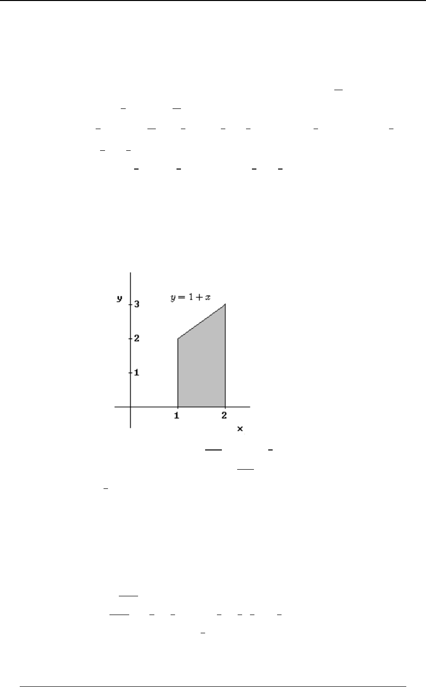
464 PRACTICE EXAM 7

6. continued

Let 'C68C.C œ EÞ

Let and , then (antiderivative of ), and then? œ C .@ œ 68 C .C @ œ C 68C  C 68 C

E œ C68C.C œ CÐC68C  CÑ ÐC68CCÑ.C œ C 68C  C E

# ,

so that .Eœ C68C.Cœ C 68C 

Then .

'¹

C68C.CœC68C œ68$Ð68#"Ñœ68$#68#

"**%*&

#%#%# # %

Finally, IÒ] Ó œ # 68  68$  C 68 C .CÐÑ

## '#

.œ # 68 $  # 68 #  68$  Ð 68$  # 68#  Ñ œ

&* &&

## %%

The first order of integration for method (i) was clearly the more efficient one.

(ii) This method is equivalent to the second approach in method (i), because we find from0ÐCÑ

]

the relationship . The two-dimensional region of probability for the joint0ÐCÑœ 0ÐBßCÑ.B

distribution is and . This is illustrated in the graph below"B# !C"B

For , !C# 0 ÐCÑœ 0ÐBßCÑ.Bœ .Bœ68

]""

"B #

ÐÑ

and for , .#ŸB$ 0 ÐCÑœ 0ÐBßCÑ.Bœ .Bœ68$68C

]C" C"

"B

Then , which is the same as the second part ofIÒ] Ó œ C 68 .C  C Ò68$  68 CÓ .C

ÐÑ

method (i).

(iii) According to the double expectation rule, for any two random variables and , we haveY[

IÒY Ó œ IÒ IÒY l[ Ó Ó IÒ] Ó œ IÒ IÒ] l\Ó Ó . Therefore, .

We are told that the conditional distribution of given is uniform on the interval]\œB

Ð!ß "  BÑ IÒ] l\Ó œ , so .

"\

Then ,IÒIÒ] l\ÓÓ œ IÒ Ó œ  IÒ\Ó œ  œ

"\ " " " " $ &

### ###%

ÐÑ

since is uniform on and has mean . Answer: B\ Ð"ß #Ñ \ $

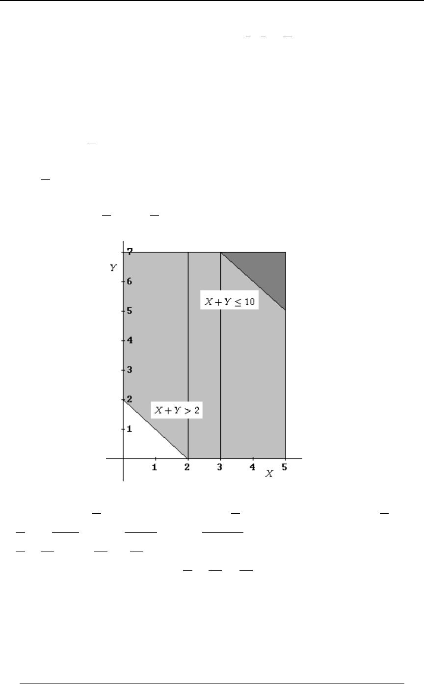
PRACTICE EXAM 7 465

7. The joint distribution of and has pdf on the rectangle\] 0ÐBßCÑœ†œ

"" "

&( $&

!B& !C( \] # \] # and . The insurer pays if the combined loss is .

The maximum payment of 8 is reached if , or equivalently, if .\] #) \] "!

Therefore, the insurer pays if (the lighter shaded region in the\] # #\] Ÿ"!

diagram below) , and the insurer pays if (the darker shaded region in the diagram)\]"!

below). The expected amount paid by the insurer is a combination of two integrals:

, where the integral is taken over the region

''ÐBC#Ñ† .C.B #BCŸ"!

(the lightly shaded region), plus

, where the integral is taken over the region

'') † .C .B \  ]  "!

(the darker region).

The second integral is , since the area of the darkly shaded triangle is 2 (it is a

)"'

$& $&

†Ð#Ñœ

2 right triangle).‚#

The first integral can be broken into three integrals:

'' '' ''

!#B #! $!

#( $( &"!B

ÐBC#Ñ† .C.B  ÐBC#Ñ† .C.B ÐBC#Ñ† .C.B

"" "

$& $& $&

œ†Ò .B .B .BÓ

" '!%BB

$& # # #

ÐB&Ñ (Ð#B$Ñ

'' '

!# $

#$ &

œ†Ò #) Óœ

" "!* "(* "#%

$& $ $ $& .

The total expected insurance payment is . Answer: C

"' "#% "%!

$& $& $&

œœ%

466 PRACTICE EXAM 7

8. The probability function of is .\TÐ\œ5Ñœ

/†#

# 5

The general probability function of a geometric distribution on is of the form!ß "ß #ß ÞÞÞ

TÐ] œ5Ñ œ:Ð":Ñ 5 œ!ß"ß#ßÞÞÞ

5 for and the mean is .

":

Since the mean is 2, we have , from which we get ,

":

œ# :œ

so the probability function of is .]TÐ]œ5ÑœÐÑÐÑ

TÐ\œ]ÑœTÐ\œ] œ!ÑTÐ\œ] œ"Ñâœ TÐ\œ] œ5Ñ



5œ!

∞ .

Since and are independent, we have\]

TÐ\œ] œ5ÑœTÐ\œ5Ñ†TÐ] œ5Ñœ † œ †

/†# " # /

5x $ $ $ 5x

Ð%Î$Ñ

# 5 # 5

ÐÑÐÑ

5 .

Then, .TÐ\œ]Ñœ TÐ\œ] œ5Ñœ † œ †



5œ! 5œ! 5œ!

∞∞ ∞

# Ð%Î$Ñ Ð%Î$Ñ

5x $ 5x

#

The Taylor series expansion for is , so it follows that .//œ œ/

B B %Î$

5œ! 5œ!

∞∞



5x 5x

Ð%Î$Ñ

Then, . Answer: ATÐ\ œ ]Ñ œ †/ œ

# #Î$

%Î$

9. .\œ] œ2Ð]Ñ

"Î5

According to the method by which we find the density of a transformed random variable, the pdf

of is , where is the pdf of .] 1ÐCÑ œ 0Ð2ÐCÑÑ † l2 ÐCÑl 0 \

Since is uniform on , we know that .\ Ð!ß "Ñ 0ÐBÑ œ "

Therefore, . Since , it follows that , since1ÐCÑ œ  œ C œ B C  "

¹¹

Ð5"ÑÎ5 Ð5"ÑÎ5

5

!B" .

The mean of will be .] C†1ÐCÑ.Cœ C† .Cœ .Cœ

'' ' ¹

"" "

∞∞ ∞

Cœ"

Cœ∞

CCC

555"

Ð5"ÑÎ5 "Î5 Ð5"ÑÎ5

This will be if . If , then . Answer: B∞5" 5" IÒ]Óœ œ

5" "5

10. If and have a bivariate normal distribution for which\]

\ has mean and standard deviation , and.5

] has mean and standard deviation , and.5

]]

the coefficient of correlation between and is , then\]3

the general bivariate normal joint pdf is

0ÐBßCÑ œ † /B:Ò †Ò  # Ó

#" #Ð" Ñ

B C B C

15 5 3 35 5 55

.. ..

\] ##

\] \]

ÈÐÑÐÑ ÐÑÐÑ

3 .

We are given that .0ÐBßCÑ œ † /

Þ$"#&

1Þ()"#&ÐB Þ'BCÞ#&C Ñ

PRACTICE EXAM 7 467

10. continued

From the general form of the joint pdf, we see that , so that .

\]œÞ' œÞ'3

The covariance between and is\] \]

G9@Ð\]ß\]ÑœG9@Ð\ß\ÑG9@Ð\ß ]ÑG9@Ð]ß\ÑG9@Ð]ß ]Ñ

œ Z +<Ð\Ñ  G9@Ð\ß ] Ñ  G9@Ð] ß \Ñ  Z +<Ð] Ñ œ Z +<Ð\Ñ  Z +<Ð] Ñ œ "  % œ  $ .

The coefficient of correlation between and is .\] \] G9@Ð\] ß\] Ñ

Z +<Ð\] Ñ†Z +<Ð\] Ñ

Z +<Ð\  ] Ñ œ Z +<Ð\Ñ  Z +<Ð] Ñ  # Z +<Ð\Ñ † Z +<Ð] Ñ œ "  %  #ÐÞ'Ñ Ð"ÑÐ%Ñ œ (Þ%3ÈÈ

and

Z +<Ð\  ] Ñ œ Z +<Ð\Ñ  Z +<Ð] Ñ  # Z +<Ð\Ñ † Z +<Ð] Ñ œ "  %  #ÐÞ'Ñ Ð"ÑÐ%Ñ œ #Þ'3ÈÈ

The coefficient of correlation between and is\] \]

G9@Ð\] ß\] Ñ

Z +<Ð\] Ñ†Z +<Ð\] Ñ Ð(Þ%ÑÐ#Þ'Ñ

$

ÈÈ

œ œ  Þ')% . Answer: A

11. Suppose that is an exponential random variable with mean 1.\

The pdf of is . The insurance policy for a single risk with policy limit 2\0ÐBÑœ/ßB!

\B

will pay if if

œB !BŸ#

#B#

The expected amount paid for one policy is

Eœ B†0 ÐBÑ.B#†TÐ\#Ñœ B†/ .B#†/

\B #

œÐB/ / Ñ #/ œÐ#/ / ÑÐ!"Ñ#/ œ"/

B B # # # # #

Bœ!

Bœ#

¹ .

Note that, for a non-negative random variable , with a policy limit , the expected\! ?

insurance payment is . In the case of the exponential distribution with

Ò"  J ÐBÑÓ .B

mean 1, , so the expected insurance payment with a policy limit of 2 isJÐBÑœ"/

\B

B B #

Ò"Ð"/ ÑÓ.Bœ / .Bœ"/ .

Suppose that and are the independent exponential losses on the two risks. The combined\\

loss is , and the insurance on the combined losses will apply a limit of 4 to .]œ\ \ ]

The sum of two independent exponential random variables, each with a mean of 1, is a gamma

random variable with pdf . This can be verified a couple of ways.0ÐCÑœC/ ßC!

]C

(i) Convolution:

0ÐCÑœ0ÐBÑ†0ÐCBÑ.Bœ/†/ .Bœ/.BœC/

]\\

!!!

CCC

B ÐCBÑ C C

'''

468 PRACTICE EXAM 7

(ii) Transformation of random variables:

Since and are independent, the joint distribution of and has pdf\\ \\

"# "#

0ÐBßBÑœ0 ÐBÑ†0 ÐBÑœ/ †/

"# \" \# B B

Yœ\ß]œ\\p\œYß\œ]Y

""#"#

pdf of is ,p Yß] 1Ð?ßCÑœ0Ð?ßC?Ñ† œ/ †/ †"œ/

?C?

ââ

`? `?

`C `C

? ÐC?Ñ C

and the joint distribution of and is defined on the region Y] !?C

(this is true because ).?œBBBœC

""#

The marginal density of is .] 0 ÐCÑ œ 1Ð?ßCÑ .? œ / .C œ C/

]!!

C C

We impose a limit of 4 for the insurance policy on , the combination of the two exponential]

losses. The amount paid by the insurance is if if

œC !CŸ%

%C%

The expected insurance payment is .

C†0 ÐCÑ.C  %†TÐ] %Ñ

'''

!!!

%%%

]C # C

C†0ÐCÑ.Cœ C†C/.Cœ C†/.C .

Applying integration by parts, this becomes

C /  Ð/ ÑÐ#CÑ.Cœ "'/ # C/ .C

#C C % C

Cœ!

Cœ%

¹''

œ  "'/  # † Ò  C/  / Ó œ  "'/  #Ò  %/  /  Ð!  "ÑÓ œ #  #'/

% C C % % % %

Cœ!

Cœ%

¹ .

TÐ]  %Ñ œ 0 ÐCÑ.C œ C/ .C œ ÐC/ / Ñ

'' ¹

∞∞

]C C C

Cœ%

Cœ∞

œÐ!!ÑÐ%/ / Ñœ&/

% % % .

Expected insurance payment of the combined policy is .##'/ %Ð&/ Ñœ#'/ œF

% % %

The ratio is . Answer: CFÎE œ #Þ")'

#'/

"/

%

#

12. If the index closes below 20, then ,] œ Q+BÖ\ß #!× œ #!

and if the index closes above 50, then .] œ Q38Ö Q+BÖ\ß #!× ß &!× œ &!

If the index closes between 20 and 50, then

] œ Q 38Ö Q +BÖ\ß #!× ß &!× œ Q 38Ö\ß &!× œ \ .

Therefore, .]œ

#! \ Ÿ #!

\#!\Ÿ&!

&! \  &!



IÐ]Ñœ #!†0 ÐBÑ.B B†0 ÐBÑ.B &!†0 ÐBÑ.B

'''

!#!&!

#! &! "!!

\\ \

\0ÐBÑœœÞ!" has pdf , so

"!!

IÐ] Ñ œ #!ÐÞ!"Ñ .B  B † ÐÞ!"Ñ .B  &!ÐÞ!"Ñ .B œ %  "!Þ&  #& œ $*Þ&

'''

!#!&!

#! &! "!! .

Answer: E

PRACTICE EXAM 7 469

13. There are 6 possible rankings that a surveyed fan can choose:

BEG , BGE , EBG , EGB , GEB , GBE

We are given the following:

TÐFIKÑ  T ÐFKIÑ œ Þ& ß T ÐIFKÑ  T ÐKFIÑ œ Þ$ ß TÐFIKÑ  T ÐKIFÑ œ Þ$ ß

TÐFKIÑ  TÐKFIÑ œ Þ& ß T ÐFIKÑ œ Þ# .

We wish to find TÐIKFlIKF ∪ IFKÑ œ Þ

TÐIKFÑ

TÐIKFÑTÐIFKÑ

Since 80% ranked England either second or third, it follows that 20% ranked England first, so

TÐIKF ∪ IFKÑ œ TÐIKFÑ  TÐIFKÑ œ Þ# .

From the given information, we have .Þ#  T ÐFKIÑ œ Þ& p T ÐFKIÑ œ Þ$

Then, .Þ$  T ÐKFIÑ œ Þ& p T ÐKFIÑ œ Þ#

Then, , and then .T ÐIFKÑ  Þ# œ Þ$ p T ÐIFKÑ œ Þ" T ÐIKFÑ  Þ" œ Þ# p T ÐIKFÑ œ Þ"

Finally, . Answer: C

TÐIKFÑ

T ÐIKFÑT ÐIFKÑ Þ"Þ" #

Þ" "

œœ

14. We define the following events:

F# - a surveyed individual ranked Brazil second ,

K" - a surveyed individual ranked Germany first .

We wish to find .TÐK$lF#Ñ œ TÐF#∩K$Ñ

TÐF#Ñ

We are given ,TÐF#Ñ œ Þ$

and we are given the conditional probabilities and .T ÐF#lK"Ñ œ T ÐF#lK" Ñ œ

From we get , and fromTÐF#lK"Ñ œ œ TÐF#∩K"Ñ œ †TÐK"Ñ

TÐF#∩K"Ñ

TÐK"Ñ $ $

T ÐF#lK" Ñ œ T ÐF# ∩ K" Ñ œ † T ÐK" Ñ œ † Ò"  T ÐK"ÑÓ

www

"""

(((

we get .

Therefore Þ$ œ T ÐF#Ñ œ T ÐF# ∩ K"Ñ  T ÐF# ∩ K" Ñ œ † T ÐK"Ñ  † T ÐK" Ñ

(

œ †TÐK"Ñ †Ò"TÐK"ÑÓ TÐK"Ñ œ Þ$

$( , from which we get .

Then, TÐF#∩K$ÑœTÐF#∩K"Ñœ †Ò"TÐK"ÑÓœÞ"

(

and . Answer: BTÐK$lF#Ñ œ œ œ

TÐF#∩K$Ñ

TÐF#Ñ Þ$ $

Þ" "

15. In order to have no matching number on either ticket, the 6 randomly chosen numbers must

come from the 37 other numbers, 13 , 14 , . . . , 49 . The probability in question is the ratio of the

number of random ticket draws that result in the event over the total possible number of random

ticket draws.

TÐEÑ œ œ œ

ˆ‰

# randomly chosen tickets that avoid 1,2,...,12

total number of possible randomly chosen tickets $(xÎÐ $"x 'xÑ

%*xÎÐ%$x 'xÑ œ Þ"''#%) .

Answer: C

470 PRACTICE EXAM 7

16. can be thought of as the conditional distribution of given that is not 4, 5 or 6.]\\

The probability function of is]

TÐ] œ"ÑœTÐ\œ"l\Á%ß&ß'Ñœ œ œ ß

T Ð\œ"Ñ "Î*

T Ð\Á%ß&ß'Ñ %Î* %

TÐ] œ#ÑœTÐ\œ#l\Á%ß&ß'Ñœ œ œ ß

T Ð\œ#Ñ #Î*

T Ð\Á%ß&ß'Ñ %Î* #

TÐ] œ$ÑœTÐ\œ$l\Á%ß&ß'Ñœ œ œ

T Ð\œ$Ñ "Î*

T Ð\Á%ß&ß'Ñ %Î* %

" .

IÒ] Ó œ Ð"Ñ  Ð#Ñ  Ð$Ñ œ # ßÐÑ ÐÑ ÐÑ

"""

%#%

IÒ] ÓœÐ"Ñ Ð#Ñ Ð$Ñ œ

####

ÐÑ ÐÑ ÐÑ

"""*

%#%#

Z +<Ò] Ó œ IÒ] Ó  ÐIÒ] ÓÑ œ  # œ

###

. Answer: C

17. We wish to find .Z +<Ò^Ó œ IÒ^ Ó  ÐIÒ^ÓÑ œ IÒ^ Ó  Ð&Þ$Ñ

####

Let us denote etc.TÐ\œ!Ñœ: ßTÐ\œ"Ñœ: ßTÐ\œ#Ñœ: ß

!"#

Then etc.TÐ] œ!Ñœ!ß TÐ] œ"Ñœ: : ßTÐ] œ#Ñœ: ß

!" #

Then TÐ^œ!ÑœTÐ^œ"Ñœ!ß TÐ^œ#Ñœ: : : ß

!"#

&Þ! œ IÒ\Ó œ :  #:  $:  â

"#$ and

&Þ"œIÒ]ÓœÐ::Ñ#:$:â

!" # $ and

&Þ$œIÒ^Óœ#Ð: : : Ñ$: â

!"# $ .

Therefore, and ,Þ"œIÒ]ÓIÒ\Óœ: Þ#œIÒ^ÓIÒ]Óœ: : œÞ":

!!""

so that .:œÞ"

From , we have"! œ Z +<Ò\Ó œ IÒ\ Ó  ÐIÒ\ÓÑ œ IÒ\ Ó  #&

###

IÒ\Óœ$&œ:%:*:â

#"#$

Then, IÒ^ Óœ%Ð: : : Ñ*: âœ%: $: IÒ\ Ó

!"# $ ! "

œ %ÐÞ"Ñ  $ÐÞ"Ñ  $& œ $&Þ( , and

Z +<Ò^Ó œ $&Þ(  Ð&Þ$Ñ œ (Þ'"

# . Answer: D

18. Suppose that is the time until failure of the machine. .X TÐ+X Ÿ,Ñœ/ /

+Î$ ,Î$

The fraction of the purchase price refunded is a random variable that can be described in the\

following way:

prob.

\œ

" !X Ÿ" "/

$Î% "  X Ÿ # /  /

"Î# #  X Ÿ $ /  /

"Î% X  $ /



"Î$

"Î$ #Î$

#Î$ %Î$

%Î$

Then, IÒ\Óœ"/ Ð/ / ÑÐ/ / Ñ/

"Î$ "Î$ #Î$ #Î$ %Î$ %Î$

$""

%#%

œ"/ / / œÞ'#(

"""

%%%

"Î$ #Î$ %Î$ . Answer: D

PRACTICE EXAM 7 471

19. The coefficient of variation of is .] ÈZ+<Ð]Ñ

IÐ] Ñ

IÐ] Ñ œ ÐB  #!!ÑÐÞ!!"Ñ .B  Ò"&!  ÐB  &!!ÑÓÐÞ!!"Ñ .B œ  œ Þ

#!! &!!

&!! "!!!

" " %& %#& &"&

#%#%%

IÐ] Ñ œ Ò ÐB  #!!ÑÓ ÐÞ!!"Ñ .B  Ò"&!  ÐB  &!!ÑÓ ÐÞ!!"Ñ .B

## #

#!! &!!

&!! "!!!

œ ##&!  œ

"$*ß$(& "&#ß)(&

Z +<Ð] Ñ œ  œ œ )*!#Þ' Þ

"&#ß)(& %#(ß$#&

'% %)

&"&

ÐÑ

The coefficient of variation is . Answer: D

È)*!#Þ'

"#)Þ(& œ Þ($$

20. At least 4 tosses are needed at most 3 tosses are needed .TÒ Ó œ "TÒ Ó

It is not possible to reach the total of 14 on 1 or 2 tosses.

There are possible sets of 3 consecutive tosses.'‚'‚'œ#"'

The following sets of 3 consecutive tosses result in a total of at least 14 on the faces that turn up.

(a) Three 6's (6 on each toss) ; 1 set.

(b) Two 6's and 2 to 5 on the other toss ; sets%‚$œ"#

( 6,6,2 , and 6,2,6 and 2,6,6 , and the same with 3 or 4 or 5 instead of 2).

(6,5,5 or 5,6,5 or 5,5,6, and 6,4,5 in six arrangements, and 6-3-5 in six arrangements).

(d) No 6's, and either three 5's, or two 5's and a 4; sets."$œ%

Total of sets out of 216 possible sets.""#")%œ$&

Probability is At least 4 tosses are needed . Answer: ET Ò Ó œ "  œ Þ)$)

#"'

21. The exponential distribution with mean has pdf and cdf .)0Ð>Ñ œ / JÐBÑ œ "  /

)>Î BÎ))

For a non-negative loss random variable with cdf , if a policy limit of is imposed, thePJÐCÑ ?

expected payment by the insurer when a loss occurs is .

?Ò"  J ÐCÑÓ .C

For the exponential loss random variable with mean 800 and with limit , the expected amount?

paid by the insurer when a loss occurs is .

?BÎ ?Î)!!

/ .B œ )!!Ò"  / Ó

)

If the limit is , the expected payment by the insurer when a loss occurs is .#? )!!Ò"  / Ó

#?Î)!!

We are given that .)!!Ò"  / Ó œ "Þ#)'&Ð)!!Ò"  / ÓÑ

#?Î)!! ?Î)!!

After canceling 800 and factoring the difference of squares

,"  / œ Ð"  / ÑÐ"  / Ñ

#?Î)!! ?Î)!! ?Î)!!

this equation becomes , so that . Answer: C"  / œ "Þ#)'& ? œ "!!!

?Î)!!

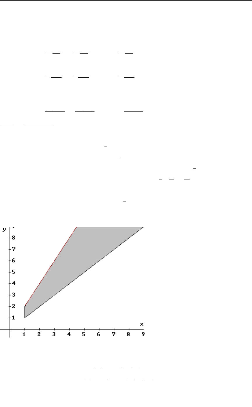
472 PRACTICE EXAM 7

22. The mean and variance of the exponential loss with mean 1 are 1 and 1, and the mean and

variance of the exponential distribution with mean 2 are 2 and 4.

(a) . , .W œ \  â  \ IÒW Ó œ %!!Ð"Ñ œ %!! Z +<ÒW Ó œ %!!Ð"Ñ œ %!!

+ " %!! + +

T ÒW Ÿ EÓ œ T Ò Ÿ Ó œ Þ*& p œ "Þ'%& p E œ %$#Þ*

+W %!!

%!! %!! %!!

E%!! E%!!

ÈÈ È .

(b) . , .W œ ]  â  ] IÒW Ó œ %!!Ð#Ñ œ )!! Z +<ÒW Ó œ %!!Ð%Ñ œ "'!!

, " %!! , ,

T ÒW Ÿ FÓ œ T Ò Ÿ Ó œ Þ*& p œ "Þ'%& p F œ )'&Þ)

,W )!!

"'!! "'!! "'!!

F)!! F)!!

ÈÈ È .

- " %!! " %!!

IÒW Ó œ %!!  )!! œ "#!! Z +<ÒW Ó œ %!!  "'!! œ #!!!

, .

T ÒW Ÿ GÓ œ T Ò Ÿ Ó œ Þ*& p œ "Þ'%& p E œ "#($Þ'

-W "#!!

#!!! #!!! #!!!

G"#!! G"#!!

ÈÈ È

G "#($Þ'

EF %$#Þ*)'&Þ)

œ œ Þ*)!( . Answer: E

23. Since , it follows that .BC#B BC

Also, since it follows that , and .B" B7+BÖ ß"× C"

Therefore, if , it follows that , and if then ."CŸ# B" C# B C

The joint density of and is .\ ] 0 ÐBß CÑ œ 0ÐClBÑ † 0 ÐBÑ œ † œ

\"" "

BB B

If , then this joint pdf is defined for ,"C# "BC

and if , then this joint pdf is defined for .C# BC

The shaded region below is the region of joint density.

The pdf of the marginal distribution of is .]0ÐCÑœ0ÐBßCÑ.B

For , we get ."C# 0 ÐCÑœ .Bœ 

'"""

B##C

For , we get . Answer: AC# 0ÐCÑœ .Bœœ

]CÎ#

'"%"$

B#C#C#C

$###

PRACTICE EXAM 7 473

24. Suppose that the covariance between and is . Then has a normal distribution\]G \]

with mean and variance""œ!

Z+<Ò\]ÓœZ+<Ò\ÓZ+<Ò]Ó#G9@Ð\ß]Ñœ""G œ#G .

Then, .T Ð\  ]  "Ñ œ T Ð  Ñ œ Þ#""*

\] "

#G #G

ÈÈ

^œ \]

#G

È has a standard normal distribution, and from the standard normal table,

we get .

#G

ÈœÞ)!

Then, .TÐ\  ]  #Ñ œ T Ð\  ]   #Ñ œ T Ð  Ñ œ T Ð^  "Þ'Ñ œ Þ!&%)

\] #

#G #G

ÈÈ

Answer: B

25. denotes the number of home runs hit in the game. and has a PoissonRIÒRÓœ%R

distribution. The amount donated (multiples of 100,000) can be summarized as follows:\

Define to be .]]œR\

R!"#$%&ÞÞÞ

\!!!"#$ÞÞÞ

]!"####ÞÞÞ

We know that so that .\  ] œ R IÒ\Ó  IÒ] Ó œ IÒRÓ œ %

But we also can see that can only be 0, 1 or 2, and]

TÐ] œ!ÑœTÐRœ!Ñœ/ TÐ] œ"ÑœTÐR œ"Ñœ%/

% %

and .T Ð] œ #Ñ œ T ÐR  #Ñ œ "  T ÐR œ !ß "Ñ œ "  &/%

Therefore, IÒ\Óœ%IÒ]Óœ%Ð"ÑÐ%/ ÑÐ#ÑÒ"&/ Óœ#Þ""

% %

and the expected amount paid by the Blue Jays is 211,000 . Answer: D

26. There are 6 possible pairs of aces (Spade-Heart, Spade-Diamond, Spade-Club, Heart-

Diamond, Heart-Club, Diamond-Club, and there are 13 possible ranks (ace, king,...),

for a total of 78 possible pairs in the first two cards. There are possible

ˆ‰

#œ œ "$#'

&#†&"

two-card combinations that can be received in the first two cards. The probability of getting a pair

in the first two cards is . Answer: E

()

"$#' œ Þ!&))

27. .Z +<Ð+\  ,Ñ œ + Z +<Ð\Ñ p %+ œ " p + œ

IÐ+\  ,Ñ œ +IÐ\Ñ  , p #+  , œ & p , œ % p +, œ # . Answer: B

474 PRACTICE EXAM 7

28. In order to be a properly defined joint distribution, it must be true that .-#- -œ"

Therefore, .-œ#

Then .IÐ\] Ñ œ Ð"ÑÐ"ÑÐ Ñ  Ð"ÑÐ#ÑÐ Ñ  Ð#ÑÐ"ÑÐ Ñ  Ð#ÑÐ#ÑÐ Ñ œ

#"%##!

*****

The marginal distribution of has , and ,\ TÐ\œ"Ñœœ TÐ\œ#Ñœ

#" " #

** $ $

so .IÐ\Ñ œ &

The marginal distribution of has , and ,] TÐ]œ"Ñœœ TÐ]œ#Ñœ

#% # "

** $ $

so .IÐ] Ñ œ %

The covariance is GSZ Ð\ß ] Ñ œ IÐ\] Ñ  IÐ\ÑIÐ] Ñ œ  Ð ÑÐ Ñ œ ! Þ

#! & %

*$$

An alternative solution follows from the observation that and are independent. Once we\]

have determined the marginal distributions of and , we can check to see if\]

TÐ\œBß] œCÑœTÐ\œBÑ†TÐ] œCÑ ÐBßCÑ for each pair. For instance,

T Ð\ œ "ß ] œ "Ñ œ - œ T Ð\ œ "Ñ † T Ð] œ "Ñ œ † œ

#"##

*$$*

and . This turns out to be true

for all pairs. It follows that and are independent, from which it follows that theÐBß CÑ \ ]

covariance between and is 0. Answer: C\]

29. If , then , so\ # $\]

))

TÐ]$\Ñœ † .C.B .Bœœ

'' '

!! #Î$

#Î$ $B))

)

"" " " " #

#$$$)) ) . Answer: D

30. For Policy 1, the maximum payment amount of 500 is reached if the loss is 600 or more

because the deductible of 100 is applied first.

Expected insurance payment with Policy 1 is

'"!!

'!!ÐB  "!!Ñ † .B &!!T Ð\  '!!Ñ œ "#&  &!! œ $#&

"!!! "!

+ .ÐÑ

Expected insurance payment with Policy 2 is

&!!B † .B %!!T Ð\  &!!Ñ œ "#&  %!! œ $#&

"!!! "!

+ . Answer: CÐÑ

PRACTICE EXAM 8 475

PRACTICE EXAM 8

1. \0ÐBÑœis a continuous random variable with density function .

šlBl "ŸBŸ"

for

, otherwise

Find .IÒ \ Ó

¸¸

A) B) C) D) E) !"

"# %

$$ $

2. As part of the underwriting process for insurance, each prospective policyholder is tested for

diabetes. Let represent the number of tests completed when the first person with diabetes\

pressure is found. The expected value of is 8. Calculate the probability that the fourth person\

tested is the first one with diabetes.

A) 0.000 B) 0.050 C) 0.084 D) 0.166 E) 0.394

3. If has a normal distribution with mean 1 and variance 4, then ?\TÒ\%\Ÿ!Óœ

A) Less than .15 B) At least .15 but less than .35

C) At least .35 but less than .55 D) At least .55 but less than .75

E) At least .75

4. Let and be discrete random variables with joint probability function given\] 0ÐBßCÑ

by the following table:

#$%&

! Þ!& Þ!& Þ"& Þ!&

C"Þ%!!!!

# Þ!& Þ"& Þ"! !

Calculate .G9@Ò\]ß\]Ó

A) Less than B) At least but less than " " !

C) At least but less than D) At least but less than !" "#

E) At least #

476 PRACTICE EXAM 8

5. Let and be continuous random variables with joint density function\]

0ÐBßCÑ œ š for

otherwise

-ÐCBÑ !BC"

!ß .

What is the mean of the marginal distribution of ?\

A) B) C) D) E)

""$"&

)%)#)

6. According to NBA playoff statistics, if a team has won 3 games and lost 1 game out of the

first 4 games during a "best of 7" playoff series, that team has an 80% chance of winning the

series. Statistics also show that if a team has won 3 games and lost 1 game out of the first 4 games

and then loses the 5th game, that team has a 65% chance of winning the series. Find the

probability that a team that has won 3 games and lost 1 game out of the first 4 games will win the

next game.

A) B) C) D) E)

#$%&'

(((((

7. A statistician for the National Hockey League has created a model for the number of goals

scored per 60-minute game by the Ottawa Senators and the Buffalo Sabres. According to the

model, the number of goals scored per game by the Senators has a geometric distribution,

\ œ !ß "ß #ß ÞÞÞ

SX X with a mean of 3.5. The model also has a similar geometric distribution for

the number of goals scored per 60-minute game by the Sabres, , with a mean of 3.0.\FYJ

Assuming that and are independent, find the probability that Buffalo wins the game\\

SX X FY J

in 60 minutes by at least 2 goals.

A) .1 B) .2 C) .3 D) .4 E) .5

8. 8 fair six-sided dice are tossed independently of one another.

Find the probability that the sum is even.

A) B) C)

"""

# '8 # '8 #

Ð8"ÑÐ8#ÑÐ8$Ñ Ð8"ÑÐ8#Ñ



D) E)

#'8 #'8

Ð8"ÑÐ8#ÑÐ8$Ñ Ð8"ÑÐ8#Ñ



9. A fair coin is tossed 100 times. The tosses are independent of one another. The number of

heads tossed is . It is desired to find the smallest integer value which satisfies the probability\5

relationship .TÐ&!5Ÿ\Ÿ&!5ÑÞ*&

Find by applying the normal approximation with integer correction to the distribution of .5 \

A) 6 B) 7 C) 8 D) 9 E) 10

PRACTICE EXAM 8 477

10. The loss random variable has an exponential distribution\

with a mean of . An insurance policy pays , where if

))

)

! ] ] œ \Ÿ

\\

œ\

Find .IÒ] Ó

A) B) C) D) E)

)) ))

## ##

Ð"  / Ñ Ð"  #/ Ñ Ð"  / Ñ Ð"  #/ Ñ Ð"  / Ñ

" " " " "

)

11. has a continuous uniform distribution on the interval and the conditional\ Ò!ß "Ó

distribution of given is a continuous uniform distribution on the interval .]\œB ÒBß#Ó

Find .IÒ] Ó

A) B) 1 C) D) E)

$&$(

%%#%

12. A loss random variable has a continuous uniform distribution on the interval .\ Ð!ß "!!Ñ

An insurance policy on the loss pays the full amount of the loss if the loss is less than or equal

to 40. If the loss is above 40 but less than or equal to 80, then the insurance pays 40 plus one-half

of the loss in excess of 40. If the loss is above 80, the insurance pays 60. If denotes the amount]

paid by the insurance when a loss occurs, find the variance of .]

A) B) C) D) E)

"!#! "!%! "!'! "! ! """!

$$$$$

13. A survey of a large number of adult city dwellers identified two characteristics involving

personal transportation:

• have a driver's licence

• own a bicycle .

The following information was determined.

• 80% of those surveyed had a driver's licence or owned a bicycle, or both

• of those who had a driver's license also owned a bike

• of those who owned a bike also had a driver's license.

Of those surveyed who didn't own a bike, find the fraction that didn't have a driver's license.

A) B) C) D) E)

"%&#(

$**$*

478 PRACTICE EXAM 8

14. A particular large calculus class has two term tests and a final exam.

Students are not allowed to drop the course before the first term test.

Class records for past years show the following:

• 80% of students pass the first test

• 30% of students who fail the first term test drop the course before the second test

• 10% of students who pass the first term test drop the course before the second test

• 90% of students who pass the first term test and take the second test pass the second test

• 80% of students who fail the first term test and take the second test pass the second test

• 50% of students who fail the second term test drop the course before the final exam

• none of students who pass the second term test drop the course before the final exam.

Find the fraction of students who drop the course.

A) Less than B) At least but less than C) At least but less than

""""$

#! #! "! "! #!

D) At least but less than E) At least

$" "

#! & 5

15. The graph below is the pdf of a continuous random variable on the interval .\Ò+ß2Ó

The numerical values represent probabilities for the subintervals.

Find the conditional probability .TÒ,\/lÐ-\1Ñ∩Ð\.ÑÓ

A) Less than .15 B) At least .15 but less than .35 C) At least .35 but less than .55

D) At least .55 but less than .75 E) At least .75

PRACTICE EXAM 8 479

16. An urn has 6 identically shaped balls. 4 of the balls are white and 2 of the balls are blue.

A ball is chosen at random from the urn and replaced with a white ball. The procedure

is done repeatedly. Find the probability that after the -th application of this procedure8

there is exactly one blue ball in the urn.

A) B) C) ÐÑÐÑ ÐÑÐÑ #ÒÐÑÐÑÓ

&# &# &#

'$ '$ '$

88 88 88

D) E) #ÒÐ Ñ  Ð Ñ Ó #Ð Ñ

&# &

'$ "#

88 8

17. has a Poisson distribution with a mean of 1, so the probability function for is\\

for TÐ\ œBÑœ Bœ!ß"ß#ßÞÞÞ

"

] ] is a new random variable on the non-negative integers. The probability function of is related

to that of as follows. A number is given, with .\!"αα

, for T Ð] œ !Ñ œ T Ð] œ BÑ œ - † T Ð\ œ BÑ B œ "ß #ß ÞÞÞα

The number is found so that satisfies the requirement for being a random variable-]



Bœ!

∞

TÐ] œ BÑ œ ".

Find the mean of in terms of and .]/α

A) B) C) D) E)

" " " "

"/ / " "/ /" /"

ααααα

"αα

18. The Toronto Maple Leafs have two suppliers for hockey sticks,

Crosscheck Lumber, and Sticks R Us. The Leafs get equal numbers

of sticks from each supplier, and since the team logo is branded on every

stick, after the sticks are delivered, it is not possible to tell what supplier

provided any particular stick. The team estimates that on average, 10% of the

sticks from Crosscheck lumber are defective and 20% of the sticks from Sticks R Us

are defective. A Leaf player examines 10 sticks from a recent shipment from

a supplier but doesn't know who the supplier was. The player finds 2 defective

sticks out of the 10 sticks. Find the probability that the supplier of those sticks

was Crosscheck Lumber.

A) Less than .11 B) At least .11 but less than .22 C) At least .22 but less than .33

D) At least .33 but less than .44 E) At least .44

480 PRACTICE EXAM 8

19. The Winnipeg Rangers hockey team is considering a one-time charitable program of making

a donation to the Winnipeg Children's Hospital. The donation will be related to how many goals

they score in their next game. The team statistician has determined that the number of goals

scored by the Rangers in a game has a Poisson distribution with a mean of 3.

The Rangers are planning donate $K for each goal they score up to a maximum of 3 goals.

Find the value of K that would make the Rangers' expected donations for game to be $5000..

A) Less than 2000 B) At least 2000 but less than 2100

C) At least 2100 but less than 2200 At least 2200 but less than 2300 E) At least 2300 D)

20. \ has a distribution which is partly continuous and partly discrete.

\ \œ" : !:" has a discrete point of probability at with probability , where .

On the interval has a constant density of ,Ð!ß "Ñ \ ":

and on the interval has a constant density of .Ð"ß #Ñ \ ":

Find the variance of in terms of \:

A) B) C) D) E)

": #: ": #: ":

$$###

21. \0ÐBÑœ

B !BŸ"

B" "B#

has the following pdf: , and 0 otherwise.

œB

The random variable is defined as follows: . Find .]]œ\JÐ#Ñ

A) .33 B) .48 C) .55 D) .67 E) .80

22. You are given the following:

• has a binomial distribution with a mean of 2 and a variance of 1.\"

• has a Poisson distribution with a variance of 2.\#

• and are independent.\\

• .]œ\ \

What is ?TÐ]  $Ñ

A) B) C) D) E)

"" "& "* #$ #(

"' "' "' "' "'

// / //

# # # # #

PRACTICE EXAM 8 481

23. has pdf for .\ 0ÐBÑœB !B"

Also, and , and .TÐ\œ!Ñœ+ TÐ\œ"Ñœ, TÐ\!ÑœTÐ\"Ñœ!

For what value of is maximized?+Z+<Ð\Ñ

A) B) C) D) E) !Ÿ+Þ" Þ"Ÿ+Þ# Þ#Ÿ+Þ$ Þ$Ÿ+Þ% +Þ%

24. You are given the events and satisfy the relationshipsEÁg FÁg

(i) andTÐE∩FÑ  !

(ii) (conditional probabilities) .TÐElFÑ œ TÐFlEÑ

How many of the following statements always must be true?

I. and are independent. II. III. E F TÐEÑœTÐFÑ EœF

A) None B) 1 C) 2 D) All 3 E) None of A,B,C or D is correct

25. A loss random variable is uniformly distributed on the interval .Ð ! ß #!!! Ñ

An insurance policy on this loss has an ordinary deductible of 500 for loss amounts

up to 1000. If the loss is above 1000, the insurance pays half of the loss amount.

Find the standard deviation of the amount paid by the insurance when a loss occurs.

A) Less than 250 B) At least 250, but less than 300 C) At least 300, but less than 350

D) At least 350, but less than 400 E) At least 400

26. Random variables and have a joint distribution with joint pdf\]

for and 0ÐBßCÑœ !ŸBŸ# !ŸCŸ#

#BC

Find the conditional probability .T Ð\  ]  #l\ Ÿ "Ñ

A) B) C) D) E)

""$"&

)%)#)

27. The pdf of is on the interval and the pdf is 0 elsewhere.\0ÐBÑœ+B, Ò!ß#Ó

You are given that the median of is . Find the variance of .\"Þ#& \

A) Less than .05 B) At least .05 but less than .15 C) At least .15 but less than .25

D) At least .25 but less than .35 E) At least .35

482 PRACTICE EXAM 8

28. In the casino game of roulette, a wheel with 38 equally likely spots is spun, and a ball is

dropped at random into one of the 38 spots. The 38 spots are numbers 1 to 36 along with 0 and

00. On a spin of the wheel, a gambler can bet that the ball will drop into a specified spot. If the

ball does drop into that spot, the gamble gets back the amount that he bet plus 36 time the amount

that he bet. If that spot does not turn up, the gambler loses the amount bet. A gambler can also bet

that the outcome of the spin will be even. If the ball drops into an even number spot from 2 to 36,

the gambler gets back his bet plus an amount equal to the amount that he bet (the bet is lost if the

spot is 0 or 00). On every spin, Gambler 1 always bets 1 that the ball will drop in the spot with

the number 1, and Gambler 2 always bets 1 that the ball will drop into an even numbered spot. \"

denotes the net profit of Gambler 1 after spins, and denotes the net profit of Gambler 2 after8\

the spins. Find .8IÐ\\Ñ

A) B) C) D) E) !

88 88

"* $) $) "*

29. A loss random variable has a Poisson distribution with a mean of \-

An insurance policy on the loss has a policy limit of 1.

The expected insurance payment when a loss occurs is .8892 .

Find the expected insurance payment when a loss occurs for a policy on the same loss variable if

the policy limit is 2.

A) Less than .35 B) At least .35 but less than .70 C) At least .70 but less than 1.05

D) At least 1.05 but less than 1.4 E) At least 1.4

30. An insurer has two lines of business: auto insurance and home fire insurance.

People with a home fire insurance policy can add flood insurance coverage, but only if the policy

already has fire coverage. You are given the following information about the insurer's customers:

• 80% of all customers have an auto insurance policy

• 40% of all customers have a fire insurance policy

• 25% of customers with an auto insurance policy also have a fire insurance policy

• 50% of customers with a fire insurance policy also have flood insurance

• 50% of customers with flood insurance coverage also have auto insurance

Of the insurer's customers that have fire insurance, find the fraction that have neither auto

insurance nor flood insurance coverage.

A) .05 B) .10 C) .15 D) .20 E) .25

PRACTICE EXAM 8 483

PRACTICE EXAM 8 - SOLUTIONS

1. .IÒ \ Ó œ lBl 0ÐBÑ .B œ lBl † lBl .B œ lBl .B œ B .B œ

¸¸ ''''

" " " "

""""

Answer: C

2. This problem makes use of the geometric distribution. The experiment being performed is the

diabetes test on an individual. We define "success" of the experiment to mean that the individual

has high diabetes. We denote the probability of a success occurring in a particular trial by .:

Since is the number of persons tested until the first person with diabetes is found, it is a version\

of the geometric distribution, where is the trial number of the first success (the trial number of]

the first success is 1, or 2, or 3, ...).

The probability function if T Ð] œ 5Ñ œ Ð"  :Ñ : ß 5 œ "ß #ß $ß ÞÞÞ

5"

The mean of this form of the geometric distribution is , so that

œ) :œ and therefore . The probability that the first success occurs on the 4th trial (first

case of diabetes is the 4th individual) is , since there will be 3 failures and then the firstÐ"  :Ñ :

success. This probability is Answer: CÐ Ñ Ð Ñ œ Þ!)$(% Þ

))

3. Since , has a standard normal distribution. The probability\ µ RÐ"ß %Ñ ^ œ \"

in question can be written as

T Ò\  %\ Ÿ !Ó œ T Ò\  %\  % Ÿ %Ó œ T ÒÐ\  #Ñ Ÿ %Ó œ T Ò  # Ÿ \  # Ÿ #Ó

## #

œTÒ"Ÿ\"Ÿ$Ó

œ T Ò  Þ& Ÿ Ÿ "Þ&Ó œ T Ò  Þ& Ÿ ^ Ÿ "Þ&Ó œ Ð"Þ&Ñ  Ò"  ÐÞ&ÑÓ

\"

#FF

œ Þ*$$#  Þ$!)& œ Þ'#%( . (from the standard normal table). Answer: D

4. G9@Ò\]ß\]ÓœG9@Ò\ß\ÓG9@Ò\ß]ÓG9@Ò]ß\ÓG9@Ò]ß]Ó

œZ+<Ò\ÓZ+<Ò]Ó

The marginal distribution of has probability function\

T Ð\ œ #Ñ œ Þ& ß T Ð\ œ $Ñ œ Þ# ß T Ð\ œ %Ñ œ Þ#& ß T Ð\ œ &Ñ œ Þ!& .

IÒ\Ó œ Ð#ÑÐÞ&Ñ  Ð$ÑÐÞ#Ñ  Ð%ÑÐÞ#&Ñ  Ð&ÑÐÞ!&Ñ œ #Þ)& .

IÒ\ Ó œ Ð%ÑÐÞ&Ñ  Ð*ÑÐÞ#Ñ  Ð"'ÑÐÞ#&Ñ  Ð#&ÑÐÞ!&Ñ œ *Þ!&

# .

Z +<Ò\Ó œ IÒ\ Ó œ ÐIÒ\ÓÑ œ *Þ!&  #Þ)& œ Þ*#(&

## #

484 PRACTICE EXAM 8

4. continued

The marginal distribution of has probability function]

TÐ] œ !Ñ œ Þ$ß TÐ] œ "Ñ œ Þ%ß TÐ] œ #Ñ œ Þ$ .

IÒ] Ó œ Ð"ÑÐÞ%Ñ  Ð#ÑÐÞ$Ñ œ "Þ! .

IÒ] Ó œ Ð"ÑÐÞ%Ñ  Ð%ÑÐÞ$Ñ œ "Þ'

# .

Z +<Ò] Ó œ IÒ] Ó œ ÐIÒ] ÓÑ œ "Þ'  " œ Þ'

###

G9@Ò\  ] ß \  ] Ó œ Z +<Ò\Ó  Z +<Ò] Ó œ Þ*#(&  Þ' œ Þ$#(& . Answer: C

5. In order for this to be a properly defined joint pdf, we must have

-ÐC  BÑ .C .B œ " .

B !

" "

-ÐC  BÑ .C œ -Ò  BÐ"  BÑÓ œ .B œ

"B -

###'

-Ð"BÑ -Ð"BÑ

###

, and .

Therefore, .-œ'

0 ÐBÑ œ 'ÐC  BÑ .C œ $Ð"  BÑ ß !  B  "

IÒ\Ó œ $BÐ"  BÑ .B œ $ ÒB  #B  B Ó .B œ $Ò  #  Ó œ Þ#&

##$

"""

#$%

ÐÑ .

Answer: B

6. We define the following events and probabilities:

[œteam wins the best-of-7 series,

Kœteam loses game 5,

Xœteam wins 3 of the first 4 games,

;œprobability team wins 5th game given that it has won 3 of the first 4 games.

Our objective is to find .;œTÒKlXÓ

We are given and .T Ò[ lX Ó œ Þ) T Ò[ lX ∩ KÓ œ Þ'&

TÒ[ ∩KlXÓ œ œ

TÒ[∩K∩XÓ TÒ[∩K∩XÓ TÒK∩XÓ

TÒXÓ TÒK∩XÓ TÒXÓ

†

œ T Ò[ lK ∩ X Ó † T ÒKlX Ó œ ÐÞ'&ÑÐ"  ;Ñ .

Þ) œ T Ò[ lX Ó œ T Ò[ ∩ KlX Ó  T Ò[ ∩ K lX Ó œ ÐÞ'&ÑÐ"  ;Ñ  T Ò[ ∩ K lX Ó Þ

TÒ[ ∩K lXÓ œ œ

wTÒ[∩K ∩XÓ TÒ[∩K ∩XÓ TÒK ∩XÓ

TÒXÓ TÒK ∩XÓ TÒXÓ

www

w†

œ T Ò[ lK ∩ X Ó † T ÒK lX Ó œ ;

(this is true, since , because winning 3 out of the first 4 and then winning theTÒ[lK ∩XÓ œ "

5th game results in winning the series) . Therefore, Þ) œ ÐÞ'&ÑÐ"  ;Ñ  ; p ; œ œ

Þ"& $

Þ$& ( .

PRACTICE EXAM 8 485

6. continued

An alternative solution is as follows.

T Ò[ lX Ó œ Þ# T Ò[ lX ∩ KÓ œ Þ$&

w and ' (these are the complement of the given probabilities

T Ò[ lX Ó œ Þ) T Ò[ lX ∩ KÓ œ Þ'& and ).

First note that , because in order to win 3 of the first 4 games andTÒ[ ∩XÓœTÒ[ ∩K∩XÓ

lose the series, it must be true that the team loses the 5th (and all subsequent games). Therefore,

Þ# œ T Ò[ lX Ó œ œ œ'TÒ[ ∩XÓ TÒ[ ∩K∩XÓ TÒ[ ∩K∩XÓ TÒK∩XÓ

TÒXÓ TÒXÓ TÒK∩XÓ TÒXÓ

ww w

†

œ T Ò[ lX ∩ KÓ † T ÒKlX Ó œ ÐÞ$&Ñ † T ÒKlX Ó T ÒKlX Ó œ œ' . It follows that ,

Þ# %

Þ$& (

and then 1 Answer: B;œTÒKlXÓœ  œ

w%$

((

7. The geometric distribution has probability function \ œ !ß "ß #ß ÞÞÞ T Ò\ œ 5Ó œ Ð"  :Ñ :

and has mean For the Senators, we have , so that

":

: . .

":

:%Þ&

SXX

SXX œ$Þ& : œ

SX X

For the Sabres, we have , so that .

":

FYJ

FYJ œ$ : œ

SX X

TÒ\ Óœ5œÐ" ÑÐ ÑœÐÑÐÑ TÒ\ œ5ÓœÐ" ÑÐÑœÐÑÐÑ

SX X FY J

55 55

" " (# "" $"

%Þ&%Þ& ** %% %%

and .

TÒ\  8Ó œ Ð Ñ Ð Ñ œ Ð Ñ

FYJ

5œ8

∞58

$" $

%% %

TÒ\  \ #Ó

FYJ SXX

œTÒ\ #l\ œ!Ó†TÒ\ œ!ÓTÒ\ $l\ œ"Ó†TÒ\ œ"Óâ

FY J SX X SX X FY J SX X SX X

œ T Ò\  8  #l\ œ 8Ó † T Ò\ œ 8Ó



8œ!

∞

FYJ SXX SXX

œ T Ò\  8  #Ó † T Ò\ œ 8Ó \ \



8œ!

∞

FYJ SXX FYJ SXX

(because of independence of and )

œ ÐÑ ÐÑÐÑœÐÑÐÑ Ð † Ñœ † œÞ$!



8œ! 8œ!

∞∞

8# 8 # 8

$(#$#$(""

%**%*%*)

" (

. Answer: C

8. he probability of an even outcome when tossing a single ) die is .TÐ8 œ " "

The probabilities for the sum when tossing two dice are

Sum #$%&'()*"!"""#

Prob "#$%&'&%$#"

$' $' $' $' $' $' $' $' $' $' $'

The probability that the sum is even is .

"$&&$"")"

$' $' $' $' $' $' $' #

œœ

486 PRACTICE EXAM 8

8. continued

To see that the probability is always , suppose that is the event that sum of the first

#I8"

8"

tosses is even. Then in order for the sum of the dice to be even, we must have either 8I

8"

occurring and the -th toss is even, or occurring (complement) and the -th toss is odd.8I 8

8"

Because of independence of the tosses, we get

T Ð 8 Ñ œ T ÐI ÑÐ Ñ  T ÐI ÑÐ Ñ œ Ð ÑÐ Ñ  Ð ÑÐ Ñ œsum of tosses is even .

8" w

8"

" " "" "" "

# # ## ## #

Since , it follows that for any . Answer: CTÐI Ñ œ TÐI Ñ œ 5

9. has a binomial distribution with 100 trials and probability of success. The expected\"

number of heads is and the variance of the number of heads is ."!!Ð Ñ œ &! "!!Ð ÑÐ Ñ œ #&

"""

###

Using the normal approximation with integer correction, we want to satisfy the relationship

TÐ&!5Þ&Ÿ\Ÿ&!5Þ&ÑÞ*& .

Applying the normal approximation, we have

TÐ&!5Þ&Ÿ\Ÿ&!5Þ&ÑœTÐ Ÿ Ÿ ÑœTÐ-Ÿ^ Ÿ-Ñ

5Þ& \&! 5Þ&

#& #& #&

ÈÈÈ ,

where is standard normal. In order for this probability to be at least .95, it must be true that^

F( . This is true because we want to eliminate less than .025 probability from the left-Ñ  Þ*(&

and right side of .^

From the standard normal table, , and therefore, we must have .FÐ"Þ*'Ñ œ Þ*(& -  "Þ*'

Then, . The smallest integer is .

5Þ&

&"Þ*'p5*Þ$ 5œ"!

Using the normal approximation, but .T Ð%! Ÿ \ Ÿ '!Ñ  Þ*& T Ð%" Ÿ \ Ÿ &*Ñ  Þ*&

Answer: E

10. IÒ]Óœ †/.BB†/.B

!BÎ BÎ

∞)))

)

B" "

#))

œ ÐB/  / Ñ  ÐB/  / Ñ

#BÎ BÎ BÎ BÎ

Bœ! Bœ

Bœ Bœ∞

)) ))

)

))

¹¹

œÐ"#/Ñ#/ œÐ"#/Ñ

))

" " "

) Answer: B

PRACTICE EXAM 8 487

11. The pdf of is for , and the conditional pdf of given is\ 0 ÐBÑœ" !ŸBŸ" ] \œB

0 ÐClBÑœ BŸ] Ÿ#

]l\ "

#B for .

The joint density of and is defined on the region\ ] 0 ÐBß CÑ œ 0 ÐClBÑ † 0 ÐBÑ œ

\ß] \

]l\ "

#B

!ŸBŸ" BŸCŸ#and .

IÒ]Óœ C† .C.Bœ .Bœ .Bœ

'' ' '

!B ! !

"# " " &

" %B #B

#B #Ð#BÑ #

# .

An alternative, solution makes use of the rule .IÒ] Ó œ IÒ IÒ] l\Ó Ó

Since the conditional distribution of is uniform on the interval from to 2, it follows]l\ œB B

that . Then,IÒ] l\Ó œ \#

IÒ] Ó œ IÒ IÒ] l\Ó Ó œ IÒ Ó œ IÒ\Ó  "

\# "

## .

Since is uniform on the interval from 0 to 1, .\IÒ\Óœ

Then, . Answer: CIÒ] Ó œ Ð ÑÐ Ñ  " œ

"" &

## %

12. . ] œ %!  ÐB  %!Ñ %!  \ Ÿ )! Z +<Ò] Ó œ IÒ] Ó  ÐIÒ] ÓÑ Þ

\\Ÿ%!

'! \  )!

"

IÒ] Ó œ B † ÐÞ!"Ñ .B  Ð#!  Þ&BÑÐÞ!"Ñ .B  '!ÐÞ!"Ñ .B

'' '

!%! )!

%! )! "!!

œ)#!"#œ%!Þ

IÒ] Ó œ B † ÐÞ!"Ñ .B  Ð#!  Þ&BÑ ÐÞ!"Ñ .B  '! ÐÞ!"Ñ .B

## # #

!%! )!

%! )! "!!

'' '

œ   (#! œ Þ

'%! $!%! &)%!

$$ $

Z+<Ò]Óœ %! œ

&)%! "!%!

# . Answer: B

13. have driver's license own a bikeEœ Fœ

TÐE∪FÑ œ Þ) œ TÐEÑTÐFÑTÐE∩FÑ

TÐFlEÑ œ œ ß TÐElFÑ œ œ Þ

$TÐEÑ #TÐFÑ

TÐE∩FÑ TÐE∩FÑ

TÐE∪FÑ TÐEÑTÐFÑTÐE∩FÑ

TÐE∩FÑ TÐE∩FÑ TÐE∩FÑ "Î$ "Î#

Þ) " "

œœ œ"œ% ,

and it follows that .TÐE∩FÑ œ Þ#

Then and .TÐEÑ œ $TÐE∩FÑ œ Þ' TÐFÑ œ #TÐE∩FÑ œ Þ%

We wish to find .TÐE lF Ñ œ œ œ œ œ

ww TÐE∩F Ñ TÒÐE∪FÑ Ó "TÐE∪FÑ

TÐF Ñ TÐF Ñ "TÐFÑ "Þ% $

"Þ) "

ww w

Answer: A

488 PRACTICE EXAM 8

14. A student can drop the course after the first test but before the second test.

The fraction of the original group of students that drop the course after the first test but before the

second test is

TÒ Ódrop after 1st test but before 2nd test

œTÒ ∩ Ódrop after 1st test but before 2nd test pass 1st test

drop after 1st test but before 2nd test fail 1st testTÒ ∩ Ó

œTÒ l Ó†TÒ Ódrop after 1st test but before 2nd test pass 1st test pass 1st test

drop after 1st test but before 2nd test fail 1st test fail 1st testTÒ l Ó†TÒ Ó

œ ÐÞ"ÑÐÞ)Ñ  ÐÞ$ÑÐÞ#Ñ œ Þ"%

A student can drop the course after the second test but before the final exam.

TÒ Ódrop after 2nd test but before final exam

œTÒ ∩ ∩ ∩ Ódrop after 2nd test but before final exam pass 1st test take 2nd test pass 2nd test

drop after 2nd test but before final exam pass 1st test take 2nd test fail 2nd testTÒ ∩ ∩ ∩ Ó

TÒ ∩ ∩ ∩ Ódrop after 2nd test but before final exam fail 1st test take 2nd test pass 2nd test

drop after 2nd test but before final exam fail 1st test take 2nd test fail 2nd testTÒ ∩ ∩ ∩ Ó

We find these probabilities in the following way:

TÒ ∩ ∩ ∩ Ódrop after 2nd test but before final exam fail 1st test take 2nd test fail 2nd test

œTÒ l ∩ ∩ Ódrop after 2nd test but before final exam fail 1st test take 2nd test fail 2nd test

‚TÒ l ∩ Ó‚TÒ l Ó‚TÒ Ófail 2nd test take 2nd test fail 1st test take 2nd test fail 1st test fail 1st test

œ ÐÞ&ÑÐÞ#ÑÐÞ(ÑÐÞ#Ñ œ Þ!"% .

Similarly,

TÒ ∩ ∩ ∩ Ódrop after 2nd test but before final exam pass 1st test take 2nd test fail 2nd test

œ ÐÞ&ÑÐÞ"ÑÐÞ*ÑÐÞ)Ñ œ Þ!$' Þ

TÒ ∩ ∩ ∩ Ódrop after 2nd test but before final exam fail 1st test take 2nd test pass 2nd test and

TÒ ∩ ∩ ∩ Ódrop after 2nd test but before final exam pass 1st test take 2nd test pass 2nd test

are both 0, since anyone who passes the 2nd test does not drop the course.

The probability of dropping the course is . Answer: DÞ"%  Þ!"%  Þ!$' œ Þ"*

PRACTICE EXAM 8 489

15. The region is , so the probability isÐ-\1Ñ∩Ð\.Ñ -\.

TÒ,\/l-\.Óœ .

T ÒÐ,\/Ñ ∩ Ð-\.ÑÓ

TÒ-\.Ó

The region is , soÐ,\/Ñ ∩ Ð-\.Ñ -\.

TÒ,\/l-\.Óœ œ" . Answer: E

TÒ-\.Ó

16. In order for there to be one blue ball in the urn after the application, it must be true that8

a blue ball was chosen exactly once in the applications of the procedure. The blue ball could8

have been chosen on the 1st, or 2nd, . . . , or -th application.8

TÐ 8"blue ball chosen on 1st application and no blue ball chosen in next applications)

œ†ÐÑ

8" .

TÐ 8#1st blue ball chosen on 2nd application and no blue ball chosen in next applications)

œ††ÐÑ

#" &

$$ '

8# .

TÐ 5 851st blue ball chosen on -th application and no blue ball chosen in next applications)

œÐ Ñ † †Ð Ñ

#"&

$$'

5" 85 .

TÐ 8 œ Ð Ñ †1st blue ball chosen on -th application) .

8"

The probability in question is the sum of these:



5œ" 5œ"

5" 85 " 8 5 5

ÐÑ † †ÐÑ œ †ÐÑ †ÐÑ† ÐÑÐÑ

#"& "#& #&

$$' $$' $'

œ†ÐÑ† Ð Ñœ†ÐÑ† ÐÞ)Ñœ†ÐÑ†ÐÞ)Ñ† ÐÞ)Ñ

"& "& "&

#' &Î' #' #'

#Î$

85858 5"

5œ" 5œ" 5œ"

88 8

 

œÐÞ%Ñ†ÐÑ† œ#ÒÐÑÐÑÓ

&&#

' "Þ) ' $

"ÐÞ)Ñ

888

8 . Answer: D

17. Since , it follows that .



Bœ! Bœ"

∞∞ "

TÐ\œBÑœ" TÐ\œBÑœ"TÐ\œ!Ñœ"/

Then, .



Bœ" Bœ"

∞∞ "

TÐ] œBÑœ-† TÐ\œBÑœ-Ð"/ Ñ

But it is also true that .



Bœ"

∞

TÐ] œBÑœ"TÐ] œ!Ñœ"α

Therefore, , so that .-Ð"  / Ñ œ "  - œ

" α"

"/

"

The mean of is]

IÒ]Óœ B†TÐ] œBÑœ B†TÐ] œBÑœ B†-†TÐ\œBÑœ-† B†TÐ\œBÑ

 

Bœ! Bœ" Bœ"

∞∞∞ ∞

Bœ9

œ-†IÒ\Óœ-œ "

"/

" . Answer: C

490 PRACTICE EXAM 8

18. We define the following events:

G - shipment is from Crosscheck Lumber

W - shipment is from Sticks R Us

#H - 2 sticks are defective

We wish to find . This is .TÐGl#HÑ T ÐG∩#HÑ

T Ð#HÑ

The numerator can be formulated as .TÐ#HlGÑ†TÐGÑ

We are given that . For a shipment from Crosscheck Lumber,TÐGÑ œ Þ&

the number of sticks that are defective in a batch of 10 sticks has a binomial

distribution with and (prob. of a particular stick being defective).8œ"! :œÞ"

Therefore, .T Ð#HlGÑ œ ÐÞ"Ñ ÐÞ*Ñ œ Þ"*$("!

Š‹

##)

The numerator is .T ÐG ∩ #HÑ œ ÐÞ"*$("!ÑÐÞ&Ñ œ Þ!*')&&

The denominator can be formulated as TÐ#HÑ œ TÐG ∩#HÑTÐW ∩#HÑ

since the shipment must be either or . We find in the same wayGW TÐW∩#HÑ

as . .T ÐG ∩ #HÑ T ÐW ∩ #HÑ œ T Ð#HlWÑ † T ÐWÑ œ ÐÞ#Ñ ÐÞ)Ñ † ÐÞ&Ñ œ Þ"&!**&

Š‹

##)

Then, .T ÐGl#HÑ œ œ œ œ Þ$*

TÐG∩#HÑ TÐG∩#HÑ

T Ð#HÑ T ÐG∩#HÑT ÐW∩#HÑ Þ!*')&&Þ"&!**&

Þ!*')&&

Answer: D

19. The donation is

Prob.

!/

O$/

$O "  Ð/  $/  Ñ

$

$ $

$

The expected donation is

O † $/  #O †  $O † Ò "  Ð/  $/  ÑÓ œ #Þ$#)O Þ

$ $ $

*/ */

$ $

Setting this equal to 5000 results in . Answer: CO œ #"%)

20. Since has a symmetric distribution about the point ,\\œ"

it follows that . The second moment of isIÒ\Ó œ " \

IÒ\ Ó œ B † .B  " † :  B † .B

## # #

": ":

œ† :† œ

"(%

$$$$

": ":

The variance of is . Answer: A\ Z +<Ò\Ó œ IÒ\ Ó  ÐIÒ\ÓÑ œ   " œ

$$ $

:":

PRACTICE EXAM 8 491

21. The cdf of is if

\JÐ>Ñœ0ÐBÑ.Bœ  !>Ÿ"

  >" "B#

'œ>>

">">"

$' #

The cdf of is .] J ÐCÑœTÐ] ŸCÑœTÐ\ ŸCÑœTÐ\Ÿ CÑœJ Ð #Ñ

#ÈÈ

Since , we get" ##

JÐ#ÑœJÐ#Ñœ#"œÞ&&

]\ "

ÈÈ

Ð#Ñ" Ð#Ñ"

ÈÈ

$# . Answer: C

22. is binomial with and .\ 8: œ # 8:Ð"  :Ñ œ "

It follows that , and , and .":œ :œ 8œ%

The probability function of is .\ TÐ\œ5Ñœ ÐÑÐÑ œ ÐÑ

"" 5%5 %

Š‹ Š‹

5# # 5#

"" "

The probability function of is .\TÐ\œ4Ñœ

## #/

4#

.TÐ] $ÑœTÐ] œ!ÑTÐ] œ"ÑTÐ] œ#Ñ

TÐ] œ!ÑœTÐ\ œ!∩\ œ!ÑœTÐ\ œ!Ñ‚TÐ\ œ!Ñ

"# " #

œÐÑ‚ œ/

Š‹

! # !x "'

"#/ "

%#

!# .

TÐ] œ"ÑœTÐ\ œ!∩\ œ"ÑTÐ\ œ"∩\ œ!Ñ

"# "#

œTÐ\ œ!Ñ‚TÐ\ œ"ÑTÐ\ œ"Ñ‚TÐ\ œ!Ñ

"#"#

œ ÐÑ‚  ÐÑ‚ œ /  / œ /

Š‹ Š‹

! # "x " # !x "' "' "'

"#/ "#/ # % '

% % # # #

"# !# .

TÐ] œ#ÑœTÐ\ œ!∩\ œ#ÑTÐ\ œ"∩\ œ"ÑTÐ\ œ#∩\ œ!Ñ

"# "# "#

œTÐ\ œ!Ñ‚TÐ\ œ#ÑTÐ\ œ"Ñ‚TÐ\ œ"ÑTÐ\ œ#Ñ‚TÐ\ œ!Ñ

"#"#"#

œ ÐÑ‚  ÐÑ‚  ÐÑ‚

Š‹ Š‹ Š‹

%%%

!# #x "# "x ## !x

"#/ "#/ "#/

%%%

## "# !#

œ///œ/

#)'

"' "' "'

# # # # .

Then, . Answer: DTÐ]$Ñœ///œ/

"' #$

"' "' "'

# # # #

23. In order to be a properly defined random variable, we must have

TÐ\œ!ÑTÐ!\"ÑTÐ\œ"Ñœ" , so that

+ B.B,œ+ ,œ" +,œ

"""

. Therefore, .

Z +<Ð\Ñ œ IÐ\ Ñ  ÒIÐ\ÑÓ

IÐ\Ñœ!‚+  B‚B.B  "‚,œ ,

$ , and

IÐ\ Ñœ!‚+  B ‚B.B  " ‚,œ ,

### #

% .

Then, .Z+<Ð\Ñœ ,Ð ,Ñ œ  ,

"" &,

% $ $' $

Z+<Ð\Ñ  , œ #,œ! will be maximized if .

.& , "

., $' $ $

ÒÓ

This occurs at . Then . Answer: D,œ +œ ,œ

"""

'#$

492 PRACTICE EXAM 8

24. and .TÐElFÑ œ TÐFlEÑ œ

TÐE∩FÑ TÐE∩FÑ

TÐEÑ TÐFÑ

Since it follows that , so II is true.TÐE∩FÑ  ! TÐEÑ œ TÐFÑ

If and when tossing a fair die then the conditions are satisfied, butE œ Ö"ß #ß $× F œ Ö$ß %ß &×

I is false since , and III is false.TÐE∩FÑ œ Á TÐEÑ‚TÐFÑ

Answer: B

25. The amount paid by the insurance is , where .

0if

]]œ

\ Ÿ &!!

\  &!! &!!  \ Ÿ "!!!

"!!!  \  #!!!

\

Z +<Ð] Ñ œ IÐ] ÑÒIÐ] ÑÓ

IÐ] Ñ œ ÐB  &!!Ñ ‚ .B  ‚ .B œ  $(& œ

&!! "!!!

"!!! #!!!

" B " "#& )(&

#!!! # #!!! # # .

IÐ] Ñ œ ÐB  &!!Ñ ‚ .B  Ð Ñ ‚ .B œ  œ

## #

&!! "!!!

"!!! #!!!

"B"

#!!! # #!!! $ $ $

'#ß&!! )(&ß!!! *$(ß&!! .

Z +<Ð] Ñ œ  Ð Ñ œ "#"ß !*$Þ(&

*$(ß&!!

)(& # .

Standard deviation of is . Answer: C] Z +<Ð] Ñ œ "#"ß !*$Þ(& œ $%)

ÈÈ

26. .T Ð\  ]  #l\ Ÿ "Ñ œ TÐ\] #∩\Ÿ"Ñ

TÐ\Ÿ"Ñ

TÐ\ Ÿ "Ñ œ .C.B œ

"##BC

"# $

" .

TÐ\ ]  #∩\ Ÿ "Ñ œ .C.B œ .B œ

'' '

!#B !

"# "#BC

"# #% )

$B %B "

# .

T Ð\  ]  #l\ Ÿ "Ñ œ œ Þ

"Î)

"Î$ )

$ Answer: C

27. Since is a pdf, we know that .0ÐBÑ 0ÐBÑ.B œ #+ #, œ "

JÐBÑ œ 0Ð>Ñ.> œ ,> JÐ Ñ œ  œ

+> #&+ &, "

#$#%#

# , so .

Solving these two equations results in , .+œ ,œ

"& $!

The mean of is \IÐ\ÑœBÐÑ.Bœ

#%B ( &$

"& $! %&

and the second moment of is .\IÐ\ÑœBÐÑ.Bœ

'%B ( ('

"& $! %&

The variance of is . Answer: D\ IÐ\ Ñ  ÒIÐ\ÑÓ œ  œ œ Þ$!#

## #

(' &$ '""

%& %& %&

Š‹ #

PRACTICE EXAM 8 493

28. Let denote the net profit of Gambler 1 for one spin.]

Then is either with probability or is 36 with probability .]" ]

$( "

$) $)

Then .IÐ]Ñœ "‚  $'‚ œ 

$( " "

$) $) $)

The net profit after spins for Gambler 1 is ,8 \ œ] ] â]

""# 8

and the expected profit is

IÐ\ Ñ œ IÐ] Ñ  IÐ] Ñ  â  IÐ] Ñ œ  ‚ 8 œ 

""# 8

$) $) .

Let denote the net profit of Gambler 2 for one spin.^

Then is either with probability or is with probability .^" ^"

#! ")

$) $)

Then .IÐ^Ñ œ  " ‚  " ‚ œ 

#! ") #

$) $) $)

The net profit after spins for Gambler 2 is ,8 \ œ^ ^ â^

#"# 8

and the expected profit is

IÐ\ Ñ œ IÐ^ Ñ  IÐ^ Ñ  â  IÐ^ Ñ œ  ‚ 8 œ 

#"# 8

##8

$) $) .

Then IÐ\  \ Ñ œ IÐ\ Ñ  IÐ\ Ñ œ   Ð  Ñ œ 

#" # " #8 8 8

$) $) $)

Answer: B

29. The expected insurance payment is .T Ð\  "Ñ œ Þ))*#

Therefore , and it follows that .T Ð\ œ !Ñ œ Þ""!) œ / œ  68ÐÞ""!)Ñ œ #Þ#!!

--

The expected insurance payment on a policy with a deductible of 2 is

"†TÐ\œ"Ñ#†TÐ\#Ñ

œ T Ð\ œ "Ñ  # † Ò"  T Ð\ œ ! "ÑÓ or

œ#†Ò"/Ó

/† /†

"x "x

--

-

œ ÐÞ""!)ÑÐ#Þ#Ñ  # † Ò"  Þ""!)  ÐÞ""!)ÑÐ#Þ#ÑÓ œ "Þ&$ . Answer: E

30. We use the following notation:

E - customer has an auto policy

J - customer has a fire insurance policy

P - customer has flood insurance coverage

We are given: T ÐEÑ œ Þ) ß T ÐJ Ñ œ Þ% ß T ÐJ lEÑ œ Þ#& ß T ÐPlJ Ñ œ Þ& ß T ÐElPÑ œ Þ&

We also know that , so from P∩J œP Þ&œTÐPlJÑœ œ œ

TÐP∩JÑ TÐPÑ TÐPÑ

TÐJÑ TÐJÑ Þ%

we get .TÐPÑ œ Þ#

We wish to find .TÐE ∩P lJÑ œ

ww TÐE∩P∩JÑ

TÐJÑ

494 PRACTICE EXAM 8

30. continued

T ÐE ∩ P ∩ J Ñ œ T ÐJ Ñ  T ÒÐE ∪ PÑ ∩ J Ó œ T ÐJ Ñ  T ÒÐE ∩ J Ñ ∪ ÐP ∩ J ÑÓ

œ T ÐJ Ñ  T ÒÐE ∩ J Ñ ∪ PÓ œ T ÐJ Ñ  ÒT ÐE ∩ J Ñ  T ÐPÑ  T ÐE ∩ J ∩ PÑÓ

œ T ÐJ Ñ  ÒT ÐE ∩ J Ñ  T ÐPÑ  T ÐE ∩ PÑÓ

From the given information we have ,Þ#& œ T ÐJ lEÑ œ œ

TÐJ∩EÑ TÐJ∩EÑ

TÐEÑ Þ)

so that , and so that .TÐJ ∩EÑ œ Þ# Þ& œ TÐElPÑ œ œ TÐE∩PÑ œ Þ"

TÐE∩PÑ TÐE∩PÑ

TÐPÑ Þ#

Then, .TÐE ∩P lJÑ œ œ œ œ Þ#&

ww T ÐE ∩P ∩J Ñ T ÐJ ÑÒT ÐE∩J ÑT ÐPÑT ÐE∩PÑÓ Þ%ÒÞ#Þ#Þ"Ó

TÐJÑ TÐJÑ Þ%

Answer: E

Tcon ACTEX P MANUAL NEW 2010 EDITION

Navigation menu

Versions of this User Manual:

Views

Navigation