AC Users Guide
User Manual:
Open the PDF directly: View PDF ![]() .
.
Page Count: 84
- ACYCLE
- 1. Copyrights
- 2. References
- 3. Software Specifications
- 4. Acycle graphical user interface (GUI)
- 4.1 Functions and GUI
- 4.2 File
- 4.3 Edit
- 4.4 Plot
- 4.5 Basic Series
- 4.6 Math
- Sort/Unique/Delete-empty
- Interpolation
- Select Parts
- Merge Series
- Add Gaps
- Remove Parts
- Remove Peaks
- Clipping
- Smoothing:
- Moving Average
- Moving Median
- Bootstrap
- Changepoint
- Standardize
- Principal Component
- Log-transform
- Derivative
- Simple Function
- Utilities
- Find max/min
- Image:
- Show Image
- RGB to Grayscale
- Image Profile
- Plot Digitizer
- 4.7 Time series
- Detrending
- Prewhitening - First Difference
- Spectral Analysis
- Evolutionary Spectral Analysis
- Wavelet transform
- Filtering
- Build Age Model
- Age Scale
- Sedimentary Rate to Age Model
- Power Decomposition Analysis
- Sedimentary Noise Model
- Correlation Coefficient (COCO)
- Evolutionary Correlation Coefficient (eCOCO)
- Track Sedimentation Rates
- TimeOpt
- eTimeOpt
- 4.8 Help
- 4.9 Mini-robot
- 5. DYNOT model Description
- 6. Case Studies
- References

Acycle v1.0 User’s Guide Mingsong Li
- 1 -
Contents
ACYCLE ...................................................................................................................................... - 1 -
1. COPYRIGHTS ........................................................................................................................ - 4 -
2. REFERENCES ........................................................................................................................ - 5 -
3. SOFTWARE SPECIFICATIONS ............................................................................................. - 7 -
3.1 SYSTEM REQUIREMENTS ............................................................................................................... - 7 -
3.2 DOWNLOADING THE ACYCLE SOFTWARE .................................................................................... - 7 -
3.3 MATLAB VERSION .......................................................................................................................... - 9 -
3.3.1 Installation.............................................................................................................................. - 9 -
3.3.2 Startup .................................................................................................................................... - 9 -
3.4 MAC VERSION ............................................................................................................................... - 10 -
3.4.1 Introduction .......................................................................................................................... - 10 -
3.4.2 AcycleX.X-Mac-green .......................................................................................................... - 10 -
3.4.3 AcycleX.X-Mac-Installer ..................................................................................................... - 13 -
3.5 WINDOWS VERSION ...................................................................................................................... - 19 -
3.5.1 Introduction .......................................................................................................................... - 19 -
3.5.2 AcycleX.X-Win-Installer ...................................................................................................... - 19 -
3.5.3 AcycleX.X-Win-green........................................................................................................... - 20 -
3.6 DATA REQUIREMENT ................................................................................................................... - 22 -
4. ACYCLE GRAPHICAL USER INTERFACE (GUI) ............................................................... - 23 -
4.1 FUNCTIONS AND GUI ................................................................................................................... - 23 -
4.2 FILE ............................................................................................................................................... - 25 -
4.3 EDIT ............................................................................................................................................... - 25 -
4.4 PLOT .............................................................................................................................................. - 25 -
4.5 BASIC SERIES ................................................................................................................................ - 27 -
Insolation ....................................................................................................................................... - 27 -
Astronomical Solution .................................................................................................................. - 27 -
LR04 Stack .................................................................................................................................... - 28 -
Sine Wave ...................................................................................................................................... - 29 -
White Noise.................................................................................................................................... - 29 -
Red Noise ....................................................................................................................................... - 29 -
Examples ....................................................................................................................................... - 29 -
4.6 MATH ............................................................................................................................................ - 31 -
Sort/Unique/Delete-empty ............................................................................................................. - 31 -
Interpolation .................................................................................................................................. - 31 -
Select Parts .................................................................................................................................... - 31 -
Merge Series .................................................................................................................................. - 31 -
Add Gaps........................................................................................................................................ - 32 -
Remove Parts ................................................................................................................................. - 32 -
Remove Peaks ................................................................................................................................ - 32 -
Clipping ......................................................................................................................................... - 32 -
Smoothing: .................................................................................................................................... - 32 -
Moving Average ............................................................................................................................ - 32 -
Acycle v1.0 User’s Guide Mingsong Li
- 2 -
Moving Median ............................................................................................................................. - 32 -
Bootstrap ........................................................................................................................................ - 32 -
Changepoint .................................................................................................................................. - 33 -
Standardize .................................................................................................................................... - 33 -
Principal Component .................................................................................................................... - 33 -
Log-transform ............................................................................................................................... - 33 -
Derivative ....................................................................................................................................... - 33 -
Simple Function ............................................................................................................................ - 33 -
Utilities ........................................................................................................................................... - 34 -
Find max/min ................................................................................................................................ - 34 -
Image: ............................................................................................................................................ - 34 -
Show Image ................................................................................................................................... - 34 -
RGB to Grayscale .......................................................................................................................... - 34 -
Image Profile ................................................................................................................................. - 34 -
Plot Digitizer .................................................................................................................................. - 34 -
4.7 TIME SERIES.................................................................................................................................. - 36 -
Detrending ..................................................................................................................................... - 36 -
Prewhitening - First Difference.................................................................................................... - 37 -
Spectral Analysis ........................................................................................................................... - 37 -
Evolutionary Spectral Analysis..................................................................................................... - 38 -
Wavelet transform ......................................................................................................................... - 39 -
Filtering ......................................................................................................................................... - 40 -
Build Age Model ............................................................................................................................ - 41 -
Age Scale ....................................................................................................................................... - 42 -
Sedimentary Rate to Age Model ................................................................................................... - 42 -
Power Decomposition Analysis..................................................................................................... - 43 -
Sedimentary Noise Model ............................................................................................................. - 43 -
Correlation Coefficient (COCO)................................................................................................... - 44 -
Evolutionary Correlation Coefficient (eCOCO) .......................................................................... - 46 -
Track Sedimentation Rates ........................................................................................................... - 46 -
TimeOpt ......................................................................................................................................... - 47 -
eTimeOpt ....................................................................................................................................... - 48 -
4.8 HELP .............................................................................................................................................. - 49 -
Readme .......................................................................................................................................... - 49 -
Manuals ......................................................................................................................................... - 50 -
Find Updates ................................................................................................................................. - 50 -
Copyright ....................................................................................................................................... - 50 -
Contact ........................................................................................................................................... - 50 -
4.9 MINI-ROBOT ................................................................................................................................. - 51 -
5. DYNOT MODEL DESCRIPTION ......................................................................................... - 52 -
5.1 DATA FORMAT .............................................................................................................................. - 52 -
5.2 STARTUP........................................................................................................................................ - 52 -
5.3 SETTINGS ...................................................................................................................................... - 53 -
5.4. RUNNING THE DYNOT MODEL .................................................................................................. - 56 -
5.5. OUTPUT FILES ............................................................................................................................. - 57 -
6. CASE STUDIES ..................................................................................................................... - 58 -
EXAMPLE #1: INSOLATION ................................................................................................................ - 58 -
Acycle v1.0 User’s Guide Mingsong Li
- 3 -
Step 1: Load data ........................................................................................................................... - 58 -
Step 2: Data pre-processing .......................................................................................................... - 59 -
Step 3: Detrending......................................................................................................................... - 59 -
Step 4: Power Spectral Analysis ................................................................................................... - 60 -
Step 4: Evolutionary Spectral Analysis ........................................................................................ - 61 -
EXAMPLE #2: LA2004 ASTRONOMICAL SOLUTION (ETP) .............................................................. - 63 -
Step 1: Load data ........................................................................................................................... - 63 -
Step 2: Data pre-processing .......................................................................................................... - 64 -
Step 3: Detrending......................................................................................................................... - 64 -
Step 4: Power Spectral Analysis ................................................................................................... - 65 -
Step 5: Evolutionary Spectral Analysis ........................................................................................ - 66 -
Step 6: Wavelet transform ............................................................................................................. - 67 -
EXAMPLE #3: CARNIAN CYCLOSTRATIGRAPHY .............................................................................. - 69 -
Step 1. Load Data .......................................................................................................................... - 69 -
Step 2. Data Preparation ............................................................................................................... - 70 -
Step 3. Interpolation ...................................................................................................................... - 70 -
Step 4. Detrending ......................................................................................................................... - 72 -
Step 5. Power spectral analysis ..................................................................................................... - 73 -
Step 6. Evolutionary power spectral analysis ............................................................................... - 74 -
Step 7. Correlation coefficient ...................................................................................................... - 75 -
Step 8. Filtering ............................................................................................................................. - 78 -
Step 9. Age model and tuning ....................................................................................................... - 79 -
Step 10. Repeat steps. .................................................................................................................... - 81 -
REFERENCES ........................................................................................................................... - 82 -

Acycle v1.0 User’s Guide Mingsong Li
- 4 -
1. Copyrights
Copyright (C) Mingsong Li.
This program is a free software; you can redistribute it and/or modify it under the terms of
the GNU GENERAL PUBLIC LICENSE as published by the Free Software Foundation. You
should have received a copy of the GNU General Public License. If not, see
https://www.gnu.org/licenses/.
This program is distributed in the hope that it will be useful, but WITHOUT ANY
WARRANTY; without even the implied warranty of MERCHANTABILITY or FITNESS FOR
A PARTICULAR PURPOSE.
The original author reserves the right to license this program or modified versions of this
program under other licenses at the discretion.
Any questions regarding the license or the operation of this software may be directed to:
Mingsong Li
Research Assistant Professor
Department of Geosciences, Penn State University
410 Deike Bldg, University Park, PA 16802, USA
mul450@psu.edu or limingsonglms@gmail.com
www.mingsongli.com/acycle
github.com/mingsongli/acycle/

Acycle v1.0 User’s Guide Mingsong Li
- 5 -
2. References
Please acknowledge the program author on any publication of scientific results based in part
on use of the program and cite the following article in which the program was described:
Mingsong Li, Linda Hinnov, Lee Kump. 2019. Acycle: time-series analysis software for
paleoclimate projects and education, Computers and Geosciences, in press
If you publish results using correlation coefficient (COCO or eCOCO) method, please also
cite this paper:
• Li, Mingsong, Kump, Lee, Hinnov, Linda, Mann, Michael, 2018. Tracking variable
sedimentation rates and astronomical forcing in Phanerozoic paleoclimate proxy
series with evolutionary correlation coefficients and hypothesis testing. Earth and
Planetary Science Letters 501, 165-179.
Bayesian Changepoint method:
• Ruggieri, E., 2013. A Bayesian approach to detecting change points in climatic
records. International Journal of Climatology 33, 520-528.
Evolutionary fast Fourier Transform (evoFFT) method:
• Kodama, K.P., Hinnov, L., 2015. Rock Magnetic Cyclostratigraphy. Wiley-
Blackwell.
eTimeOpt method:
• Meyers, S.R., 2019. Cyclostratigraphy and the problem of astrochronologic testing.
Earth-Science Reviews 190, 190-223.
Filtering method (Gauss and Taner filter):
• Kodama, K.P., Hinnov, L., 2015. Rock Magnetic Cyclostratigraphy. Wiley-
Blackwell.
Power decomposition analysis (pda.m):
• Li, Mingsong, Huang, Chunju, Hinnov, Linda, Ogg, James, Chen, Zhong-Qiang,
Zhang, Yang, 2016. Obliquity-forced climate during the Early Triassic hothouse in
China. Geology 44, 623-626. doi: 10.1130/G37970.1
Red noise model:
• Mann, M.E., Lees, J.M., 1996. Robust estimation of background noise and signal
detection in climatic time series. Climatic Change 33, 409-445. [Robust AR(1)]
• Husson, D., 2014. MathWorks File Exchange: RedNoise_ConfidenceLevels,
http://www.mathworks.com/matlabcentral/fileexchange/45539-rednoise-
confidencelevels/content/RedNoise_ConfidenceLevels/RedConf.m. [Conventional
AR(1)]
Sedimentary noise model (DYNOT or ρ1 methods):
Acycle v1.0 User’s Guide Mingsong Li
- 6 -
• Li, Mingsong, Hinnov, Linda, Huang, Chunju, Ogg, James, 2018. Sedimentary noise
and sea levels linked to land–ocean water exchange and obliquity forcing. Nature
communications 9, 1004. Doi: 10.1038/s41467-018-03454-y
TimeOpt method:
• Meyers, S.R., 2015. The evaluation of eccentricity‐related amplitude modulation and
bundling in paleoclimate data: An inverse approach for astrochronologic testing and
time scale optimization. Paleoceanography. doi: 10.1002/2015PA002850
Wavelet analysis method:
• Torrence, C., Compo, G.P., 1998. A practical guide to wavelet analysis. Bulletin of
the American Meteorological society 79, 61-78.

Acycle v1.0 User’s Guide Mingsong Li
- 7 -
3. Software Specifications
3.1 System Requirements
This software is developed in MatLab version 2015b and 2017a. It was tested in Mac
OS Mojave system (macOS 10.14) and Windows 7 & 10.
[1. MatLab version]:
The package works with both Mac OS and Windows. MatLab is essential for the Acycle
software package. Specified MatLab toolboxes may be needed.
[2. Mac version]:
This software is a stand-alone program. It was tested in Mac OS Mojave system (macOS
10.14). If the Mac runs with no MatLab, MatLab runtime R2015b is essential for the Acycle
stand-alone software.
Two versions are available:
v1. AcycleX.X-Mac-green
No installation needed.
Size: ~100 Mb.
MatLab runtime R2015b is not included in this package and can be downloaded at:
https://www.mathworks.com/products/compiler/matlab-runtime.html.
v2. AcycleX.X-Mac-Installer
Install Acycle and MatLab runtime R2015b simultaneously.
Size: ~100 Mb
[3. Windows version]:
This software is a stand-alone program. It was tested in Windows 10 & 7.
AcycleX.X-Win-Installer
Size: ~100 Mb.
If the computer runs with no MatLab, MatLab runtime R2017a is essential for the Acycle
stand-alone software.
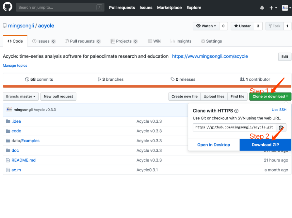
3.2 Downloading the Acycle software
The Acycle software is available for download from:
MatLab version:
GitHub (https://github.com/mingsongli/acycle/),
Acycle v1.0 User’s Guide Mingsong Li
- 9 -
3.3 MatLab version
3.3.1 Installation
Unzip the Acycle software package to your root directory. No installation is needed.
Warning: the working directory and file names contain NO SPACE or no language other
than ENGLISH.
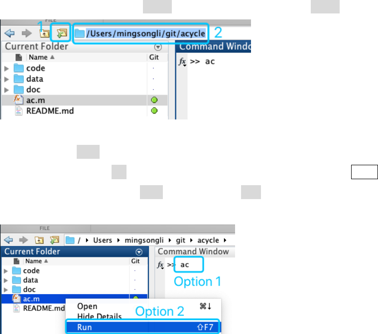
3.3.2 Startup
Step 1: Startup MatLab.
Step 2: Change the MatLab working directory to the Acycle directory.
You may use the icon in blue Box 1 or type the directory in blue Box 2 below.
Step 3: Launch ac.m
Option 1: Type ac in MatLab’s command window, then press the Enter key.
Option 2: Right click ac.m file and choose Run.
Then, all set!
Warning: the working directory and file names contain NO SPACE or no language other
than ENGLISH.
Acycle v1.0 User’s Guide Mingsong Li
- 10 -
3.4 Mac version
3.4.1 Introduction
This version of Acycle is a stand-alone program. It is tested in Mac OS Mojave system
(macOS 10.14). Two versions are available:
Section 3.4.2 AcycleX.X-Mac-green
Section 3.4.3 AcycleX.X-Mac-Installer
3.4.2 AcycleX.X-Mac-green
3.4.2.1 Download AcycleX.X-Mac-green
Dropbox (https://www.dropbox.com/sh/t53vjs539gmixnm/AAC0BqTR0U5xghKwuVc1Iwbma?dl=0), or
Baidu Cloud (https://pan.baidu.com/s/14-xRzV_-BBrE6XfyR_71Nw).
3.4.2.2 Installation of Runtime
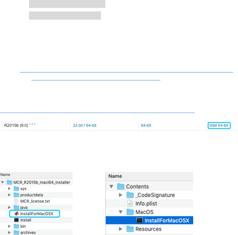
Step 1: Download “MCR_R2015b_maci64_installer.zip” here:
https://www.mathworks.com/products/compiler/matlab-runtime.html
Step 2: Install for mac OS X. Double click the file blue box below (left panel).
Or right-click and select “Show Package Contents”. In the pop-up folder, double
click “InstallForMacOSX”. Then it may ask permission for installation. Follow
instructions of the MatLab Runtime installer, you will install Runtime.
Step 3. Setup Runtime environment (detailed in Box 1).

Acycle v1.0 User’s Guide Mingsong Li
- 11 -
Step 1: Drag “AcyclevX.X-Mac” file to “/Applications” folder.
Box 1 [How to set the MatLab Runtime environment variable DYLD_LIBRARY_PATH?]
Here is a nice answer by Walter Roberson on 14 Jan 2016.
https://www.mathworks.com/matlabcentral/answers/263824-mcr-with-mac-and-environment-variable
Step 1: Go into the Terminal app (it is under /Applications/Utilities).
While you are at the Terminal command window, command
ls ~/.bashrc
If it says that the file does not exist, then in the Terminal window, command
touch ~/.bashrc
to create the file. If the file already exists or you have now created it, then at the terminal
window command
open ~/.bashrc
This will open TextEdit. In TextEdit you can add the line
export
DYLD_LIBRARY_PATH=/Applications/MATLAB/MATLAB_Runtime/v90/runti
me/maci64:/Applications/MATLAB/MATLAB_Runtime/v90/sys/os/maci64
:/Applications/MATLAB/MATLAB_Runtime/v90/bin/maci64
to the end of the file, and then you can use the TextEdit File menu to Save the file.
If your SHELL showed up as csh or tcsh, or in any case if you just want to be more
thorough, then you can use the same kind of steps as just above:
ls ~/.cshrc
and if it does not exist, "touch ~/.cshrc", and then once it exists, "open ~/.cshrc",
and then in TextEdit, add the line they gave in the instructions,
setenv DYLD_LIBRARY_PATH
/Applications/MATLAB/MATLAB_Runtime/v90/runtime/maci64:/Applica
tions/MATLAB/MATLAB_Runtime/v90/sys/os/maci64:/Applications/MAT
LAB/MATLAB_Runtime/v90/bin/maci64
and save.
These changes will not affect your current Terminal session, but they will affect the next time
you start a Terminal session or anything else starts an interactive shell.
Acycle v1.0 User’s Guide Mingsong Li
- 12 -
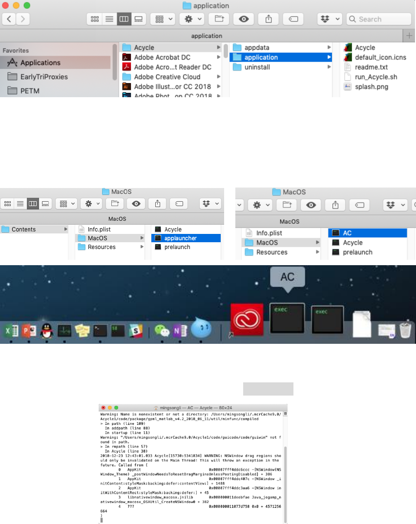
3.4.2.3 Startup AcycleX.X-Mac-green
You only need to do Steps 1-3 for the first time. Then only Step 4 below is need.
Step 1: Drag the AcycleX.X-Mac file to the /Applications folder.
Step 2: Go to the “/Applications” folder. Right click “AcycleX.X-Mac” file, choose
“Show Package Content”.
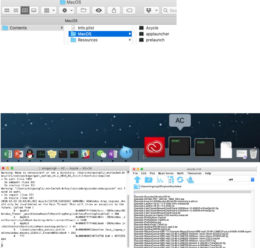
Step 3: Go to “/Contents/MacOS” folder, drag the “applauncher” file to dock (NOT the
“Acycle” file).
Step 4: Click icon of “applauncher” in the dock to start the Acycle software.
Note the first-time run will be very bit slow.
Warning: NEVER close the terminal window (left panel below) when using Acycle. This
will close Acycle.
Warning: the working directory contains no SPACE or no language other than
ENGLISH.
Acycle v1.0 User’s Guide Mingsong Li
- 13 -
3.4.3 AcycleX.X-Mac-Installer
3.4.3.1 Download AcycleX.X-Mac-Installer
Dropbox (https://www.dropbox.com/sh/t53vjs539gmixnm/AAC0BqTR0U5xghKwuVc1Iwbma?dl=0), or
Baidu Cloud (https://pan.baidu.com/s/14-xRzV_-BBrE6XfyR_71Nw).
3.4.3.2 Installation of Acycle and MatLab runtime simultaneously.
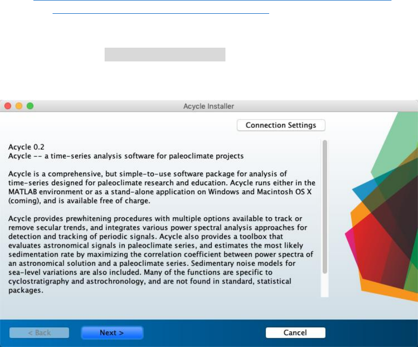
Step 1: Double click “AcycleX.X-Mac-Installer” to start the installation. The admin
permission may be required.
Step 2: Following instructions of Acycle Installer.
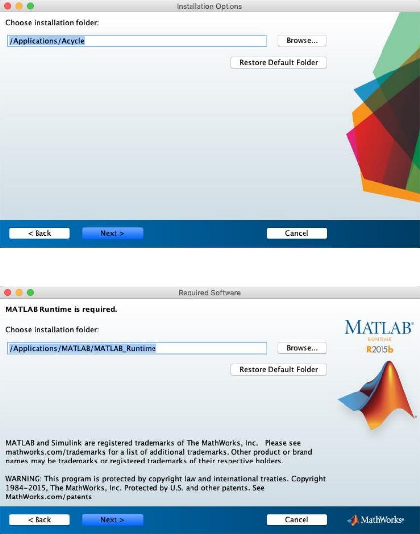
Choose Acycle installation folder (default folder is /Applications/Acycle).
Acycle v1.0 User’s Guide Mingsong Li
- 14 -
Step 3: Choose MATLAB Runtime installation folder (default folder is
/Applications/MATLAB/MATLAB_Runtime).
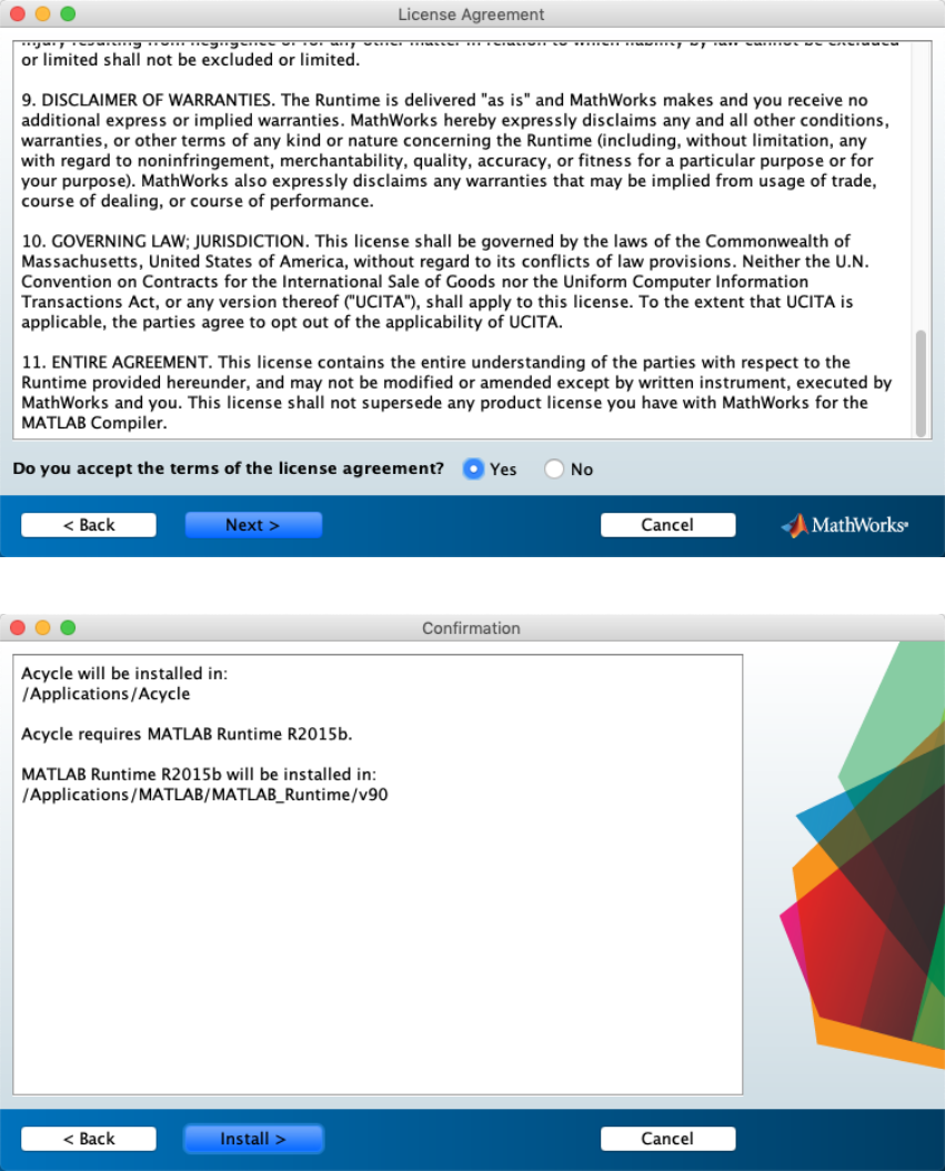
Step 4: License Agreement: Do you accept the terms of the license agreement? You may
select Yes.
Acycle v1.0 User’s Guide Mingsong Li
- 15 -
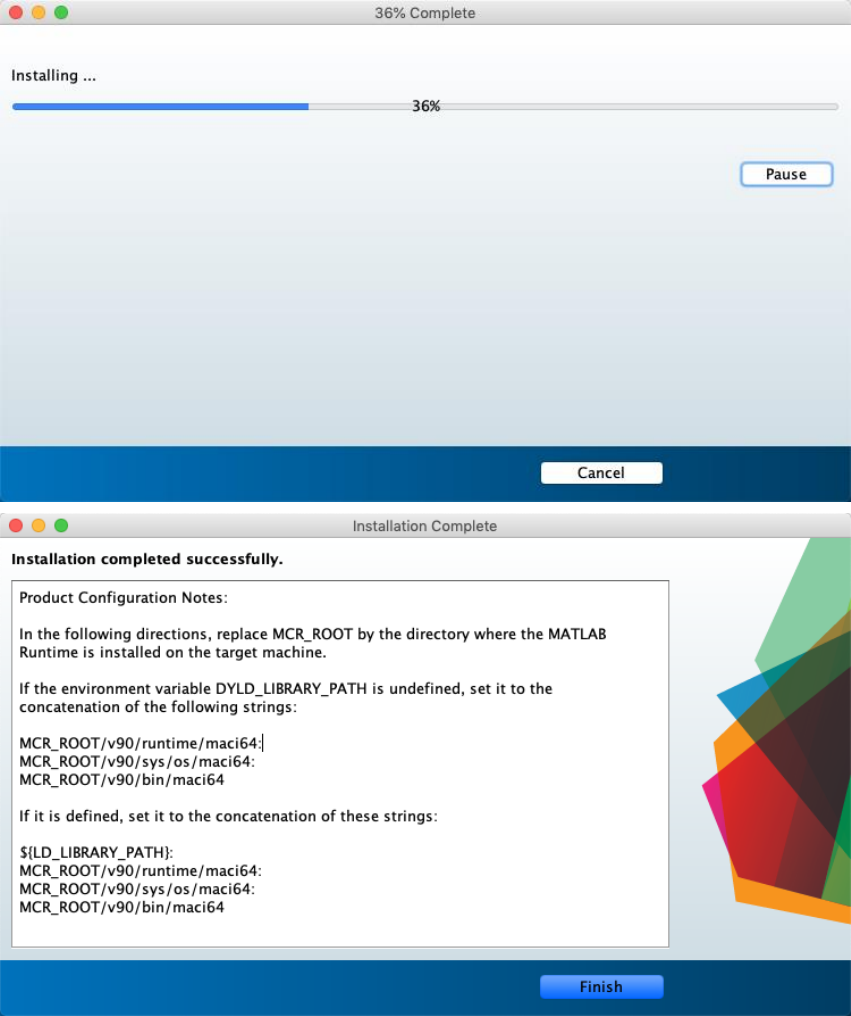
Step 5: Install Acycle.
Acycle v1.0 User’s Guide Mingsong Li
- 16 -
Step 3. Setup Runtime environment (detailed in Box 2).

Acycle v1.0 User’s Guide Mingsong Li
- 17 -
3.3 Startup AcycleX.X-Mac
Box 2 [How to set the MatLab Runtime environment variable DYLD_LIBRARY_PATH?]
Here is a nice answer by Walter Roberson on 14 Jan 2016.
https://www.mathworks.com/matlabcentral/answers/263824-mcr-with-mac-and-environment-variable
Step 1: Go into the Terminal app (it is under /Applications/Utilities).
While you are at the Terminal command window, command
ls ~/.bashrc
If it says that the file does not exist, then in the Terminal window, command
touch ~/.bashrc
to create the file. If the file already exists or you have now created it, then at the terminal
window command
open ~/.bashrc
This will open TextEdit. In TextEdit you can add the line
export
DYLD_LIBRARY_PATH=/Applications/MATLAB/MATLAB_Runtime/v90/runti
me/maci64:/Applications/MATLAB/MATLAB_Runtime/v90/sys/os/maci64
:/Applications/MATLAB/MATLAB_Runtime/v90/bin/maci64
to the end of the file, and then you can use the TextEdit File menu to Save the file.
If your SHELL showed up as csh or tcsh, or in any case if you just want to be more
thorough, then you can use the same kind of steps as just above:
ls ~/.cshrc
and if it does not exist, "touch ~/.cshrc", and then once it exists, "open ~/.cshrc",
and then in TextEdit, add the line they gave in the instructions,
setenv DYLD_LIBRARY_PATH
/Applications/MATLAB/MATLAB_Runtime/v90/runtime/maci64:/Applica
tions/MATLAB/MATLAB_Runtime/v90/sys/os/maci64:/Applications/MAT
LAB/MATLAB_Runtime/v90/bin/maci64
and save.
These changes will not affect your current Terminal session, but they will affect the next time
you start a Terminal session or anything else starts an interactive shell.
Acycle v1.0 User’s Guide Mingsong Li
- 18 -
3.4.3.3 Startup AcycleX.X-Mac
You only need to do Steps 1-3 for the first run. Then only Step 4 below is need.
Step 1: Go to the installation folder (for example: /Applications/Acycle/application).
Step 2: Right click “Acycle” file, choose “Show Package Content”
Step 3: Go to the “Contents/MacOS” folder, drag the applauncher file to dock. Before
that, you may want to change filename of the “applauncher” to “AC” or any other name
except Acycle.
Step 4: Click icon of “applauncher” (or “AC”) above to start the Acycle software.
Warning: NEVER close the terminal window (panel below) when using Acycle. This
will close Acycle either. To kill Acycle software, press CTRL + C keys
Note the first-time run will be very slow. Please ignore various warning messages and
forgive my naïve program skills.
Acycle v1.0 User’s Guide Mingsong Li
- 19 -
Warning: the working directory should contain NO SPACE or no language other than
ENGLISH.
3.5 Windows version
3.5.1 Introduction
This version of Acycle is a stand-alone program. It has been tested in Windows 10 OS. Two
versions are available:
3.5.2 AcycleX.X-Win-Installer
3.5.2.1 Download AcycleX.X-Win-Installer
Dropbox (https://www.dropbox.com/sh/t53vjs539gmixnm/AAC0BqTR0U5xghKwuVc1Iwbma?dl=0), or
Baidu Cloud (https://pan.baidu.com/s/14-xRzV_-BBrE6XfyR_71Nw).
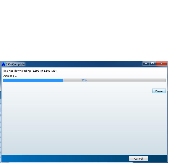
3.5.2.2 Installation
Double click “AcycleInstaller.exe” to install Acycle and MatLab runtime R2017a.
Following the instructions, you will get everything set.
Downloading MatLab runtime R2017a can take a lot of time. The runtime needs 1 GB
space.
3.5.2.3 Start-up
You could just double click the Acycle icon on the desktop to start or start from the
Windows “All Program” menu like any other software.
Acycle v1.0 User’s Guide Mingsong Li
- 20 -
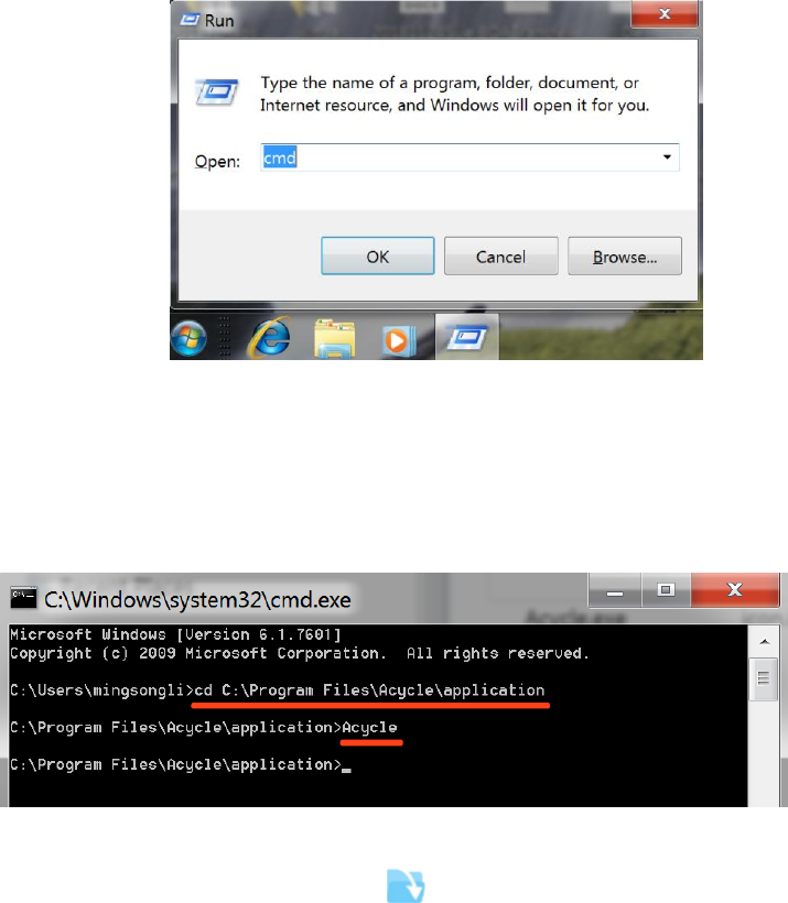
However, I strongly recommend the following start-up method, which will enable a
command window showing a lot of information about many time-consuming steps.
Step 1: Use “Win + R” short-cut keys to start the “RUN” of Windows (figure below). Then in
the pop-up window, type cmd and click OK button.
Step 2: Type following two lines of commend below in the command window. My software was
installed under the directory “ C:\Program Files”, so it should be:
cd C:\Program Files\Acycle\application\
Acycle
The Acycle will start.
Now, you need to change directory ( ) to the working folder.
Warning: the working directory should contain NO SPACE or no language other than
ENGLISH.
Warning: the first-time start-up can be very slow. Never close the command window when
Acycle is running. The commend window will keep on showing information when it runs time-
consuming steps.
3.5.3 AcycleX.X-Win-green
3.5.3.1 Download AcycleX.X-Win-green, unzip the file.

Acycle v1.0 User’s Guide Mingsong Li
- 21 -
Dropbox (https://www.dropbox.com/sh/t53vjs539gmixnm/AAC0BqTR0U5xghKwuVc1Iwbma?dl=0), or
Baidu Cloud (https://pan.baidu.com/s/14-xRzV_-BBrE6XfyR_71Nw).
3.5.3.2 Installation of MatLab runtime 2017a
https://www.mathworks.com/products/compiler/matlab-runtime.html
3.5.3.3 Double click “Acycle.exe” to run Acycle.
3.5.3.4 Now, you need to change directory ( ) to the working folder.
Warning: the working directory should contain NO SPACE or no language other than
ENGLISH.
Acycle v1.0 User’s Guide Mingsong Li
- 22 -
3.6 Data Requirement
The input file of data series can be in a variety of formats, including comma-, table- or
space-delimited text (*.txt), and comma-separated values files (*.csv) from an Excel-type
spreadsheet. No header is permitted.
Most data files should contain two columns of series. The first column must be in depth
or time, and the second column should be value in the corresponding depth or time.
Please make sure there is NO SPACE or language other than ENGLISH in the address line
(above). Or you need to change the directory ( ) to new working folder.
??? Still have no idea, don't worry. Try this, you’ll have a perfect example:
Choose “Basic Series” menu
→
Examples
→
choose any data or image file
The data will be saved in the working directory. All data files, plots, and folders are
displayed in the GUI list box.
Acycle v1.0 User’s Guide Mingsong Li
- 23 -
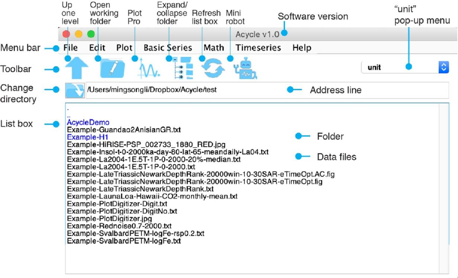
4. Acycle graphical user interface (GUI)
Acycle Graphical User Interface (GUI)
4.1 Functions and GUI
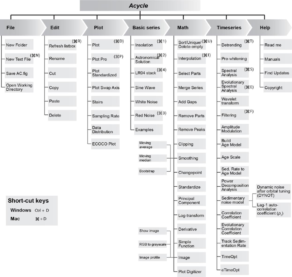
Acycle contains the following functions.
File
New Folder; New Text File; Save *.AC.fig; Open Working Directory; Extract Data
Edit
Refresh; Rename; Cut; Copy; Paste; Delete
Plot
Plot; Plot Pro; Plot Standardized; Plot Swap Axis; Stairs, Sampling Rate; Data Distribution;
ECOCO Plot
Basic Series
Insolation; Astronomical Solution; LR04 Stack; Sine Wave; White Noise; Red Noise; Examples
(a couple of data series of data and images)
Math
Sort/Unique/Delete-empty; Interpolation; Select Parts; Merge Series; Add Gaps; Remove Parts;
Remove Peaks; Clipping; Smoothing[Moving Average, Moving Median, Bootstrap]; Changepoint;
Sampling Rate Sensitivity; Standardize; Principal Component; Log-transform; Derivative; Simple
Acycle v1.0 User’s Guide Mingsong Li
- 24 -
Function; Utilities[Find Max/Min]; Image[Show Image, RGB to Grayscale; Image Profile]; Plot
Digitizer
Time series
Detrending; Pre-whitening [First Difference]; Spectral Analysis; Evolutionary Spectral Analysis;
Wavelet transform; Filtering; Amplitude Modulation; Build Age Model; Age Scale; Sedimentary
Rate to Age Model; Power Decomposition Analysis; Sedimentary noise model (DYNOT; ρ1 method);
Correlation Coefficient; Evolutionary Correlation Coefficient; Track Sedimentation Rates; TimeOpt
method; eTimeOpt method
Help
Readme; Manuals; Find Updates; Copyright; Contact
The structure of the Acycle program
Acycle v1.0 User’s Guide Mingsong Li
- 25 -
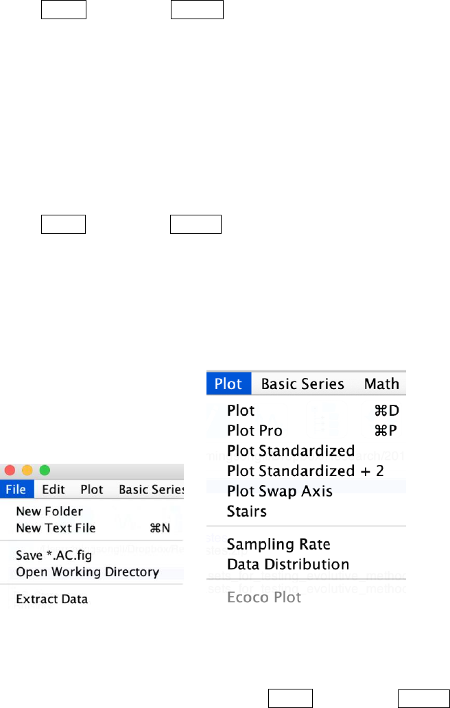
4.2 File
New Folder:
make a new empty folder with a user-defined folder name.
New Text File:
make a new empty *.txt file with a user-defined file name.
Shortcut keys [Mac]:
⌘
+ N; [Windows]: Ctrl + N
Save *.AC.fig file:
Save the current figure as an *.ac.fig file. This file enable users continue a suspended project.
For example, after running the eCOCO (evolutionary correlation coefficient), users may want to
plot the eCOCO results anytime. One can save the current figure as an *.AC.fig file, then double click
this *.AC.fig file and show “ECOCO plot” anytime.
4.3 Edit
Refresh: refresh the main listbox.
Shortcut keys [Mac]:
⌘
+ R; [Windows]: Ctrl + R
Rename:
Select one file, the “rename” function enable changing the name of the selected file.
Cut/Copy/Paste/Delete:
4.4 Plot
Plot:
A quick plot of the selected data file. Shortcut keys [Mac]:
⌘
+ D; [Windows]: Ctrl + D
Plot Pro:
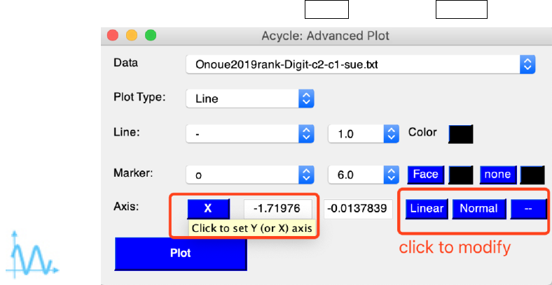
Acycle v1.0 User’s Guide Mingsong Li
- 26 -
An advanced plot of the selected data file (GUI below). One can change plot type, line, and
marker styles, and control the axis. Shortcut keys [Mac]:
⌘
+ P; [Windows]: Ctrl + P
Plot Standardized:
A quick plot of the standardized data file. Useful if one wants to compare 2 or more series.
Plot Standardized +2:
A quick plot of the standardized data file. Useful if one wants to compare 2 or more series.
Plot Swap Axis:
A quick plot, swap axis.
Stairs:
Stairs plot.
Sampling Rate:
A quick plot showing the distribution of the 1st column (time/depth) of the selected data file.
Data Distribution:
A quick plot showing the distribution of the 2nd column (data) of the selected data file.
ECOCO Plot:
Plot eCOCO results from a *.AC.fig, or after running the eCOCO (Timeseries-eCOCO).
Acycle v1.0 User’s Guide Mingsong Li
- 27 -
4.5 Basic Series
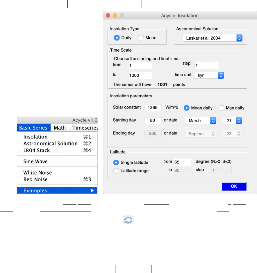
Insolation
A GUI calculates the insolation using various astronomical solutions. Based on the MatLab code
inso.m by Jonathan Levine (2001), UC Berkeley. This code was modified by Peter Huybers
(Harvard) and edited by Mingsong Li (Penn State, 2018) for the Acycle software.
Only insolation series younger than 249,000 k.a. are available.
Shortcut keys [Mac]:
⌘
+ 1; [Windows]: Ctrl + 1
This GUI generates mean daily insolation series on March 21 for the past 1000 kyr (1-1000) at
65°N using the Laskar et al. (2004) solutions. The calculate uses a solar constant of 1365 w/m2.
[NOTE: one has to click the Refresh button in the main window to see the generated
insolation series]
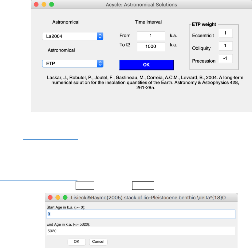
Astronomical Solution
A GUI generates astronomical solutions of Laskar et al. (2004); Laskar et al. (2011), and
Zeebe (2017). Shortcut keys [Mac]:
⌘
+ 2; [Windows]: Ctrl + 2
Acycle v1.0 User’s Guide Mingsong Li
- 28 -
This GUI generates ETP series (standardized eccentricity, tilt, and precession, weights are 1, 1,
and -1, respectively) for the past 1 million years from 1 k.a. throughout 1000 k.a. using the La2004
solution (Laskar et al., 2004).
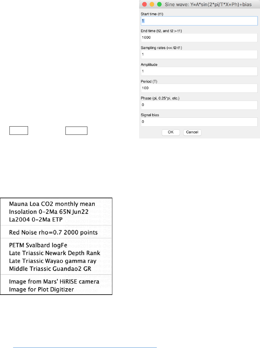
LR04 Stack
This function generates the classical LR04 stack of the Plio-Pleistocene benthic d18O record
(Lisiecki and Raymo, 2005). The input time (below) should be within the interval of 0 and 5320
(k.a.). Shortcut keys [Mac]:
⌘
+ 4; [Windows]: Ctrl + 4
This GUI generates LR04 stack from 0 to 5320 k.a.
Acycle v1.0 User’s Guide Mingsong Li
- 29 -
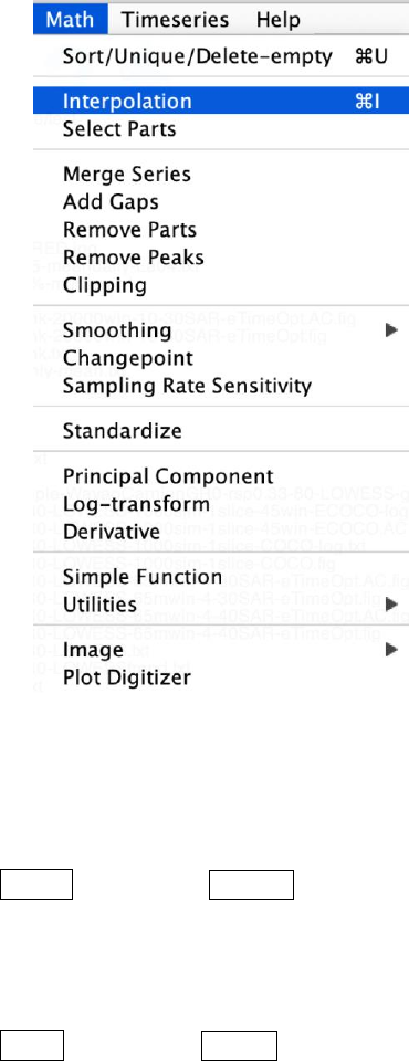
Sine Wave
Generate a sine wave using user-defined
parameters and the following equation:
Y = A * sin(2π / T * X + Ph) + bias
Where A is amplitude, T is period, X is a time
series ranges from t1 to t2 and a sampling rate of dt,
Ph is the phase, and bias is signal bias.
White Noise
This function generates the white noise.
Red Noise
This function generates the red noise using user-
defined standard deviation, and autocorrelation
coefficient (RHO-1, from 0 to 1). Shortcut keys
[Mac]:
⌘
+ 3; [Windows]: Ctrl + 3
This GUI generates a sine wave from 1 to 1000 unit with a sampling rate of 1 unit. Its amplitude
is 1, with a period of 100 unit and zero phase shift and 0 signal bias.
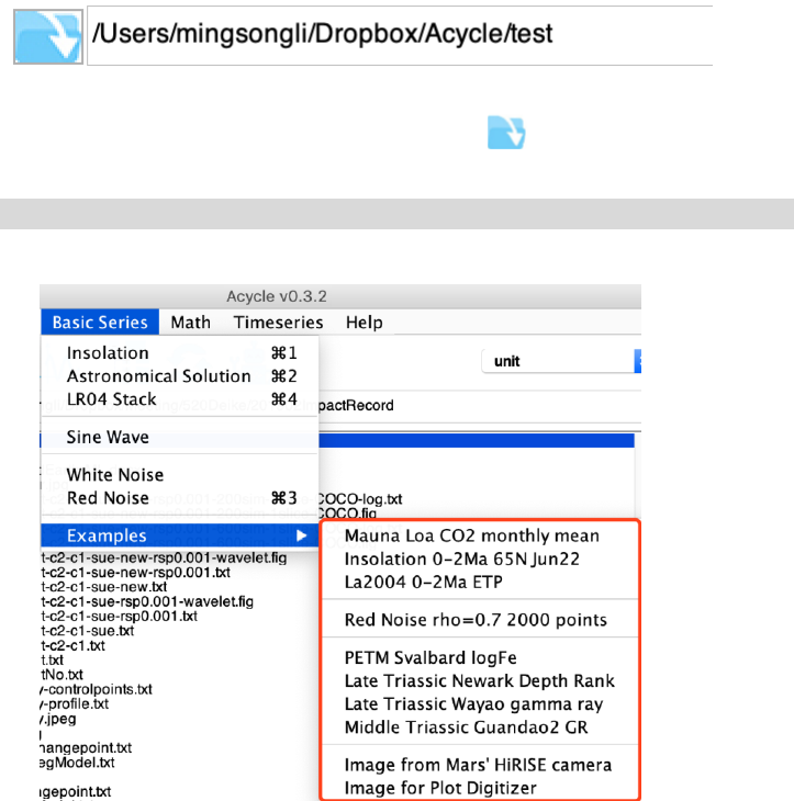
Examples
This function load various example data file to the working folder and show the data
simultaneously. The example data includes:
(1) Mauna Loa CO2 monthly mean:
This data set includes carbon dioxide measurements (monthly mean value) at the Mauna Loa
Observatory, Hawaii from 1958 to 2018.
It will load and save a text file entitled: “Example-LaunaLoa-Hawaii-CO2-monthly-mean.txt”.
Ref: https://www.esrl.noaa.gov/gmd/ccgg/trends/data.html
(2) Insolation 0-2Ma 65N Jun22:
This data set includes insolation intensity data at latitude of 65 ° N on June 22 of each year over
the past 2 million years, with a step of 1 kyr.

Acycle v1.0 User’s Guide Mingsong Li
- 30 -
It will load and save a text file entitled: “Example-Insol-t-0-2000ka-day-80-lat-65-meandaily-
La04.txt”.
(3) La2004 0-2Ma ETP:
This data set includes La2004 (Laskar et al., 2004) ETP (eccentricity, tilt, and precession) data
over the past 2 million years, with a step of 1 kyr.
It will load and save a text file entitled: “Example-La2004-1E.5T-1P-0-2000.txt”.
(4) Red Noise rho=0.7 2000 points:
This data set includes a red noise time series with 2000 datapoints and a lag-1 autocorrelation
coefficient of 0.7.
It will load and save a text file entitled: “Example-Rednoise0.7-2000.txt”.
(5) PETM Svalbard logFe:
This data set includes log-transformed iron series for the Paleocene-Eocene thermal maximum
event in the Svalbard (Charles et al., 2011).
It will load and save a text file entitled: “Example-SvalbardPETM-logFe.txt”.
(6) Late Triassic Newark Depth Rank:
This data set includes depth rank series from the Late Triassic in the Newark Basin of the USA
(Olsen and Kent, 1996).
It will load and save a text file entitled: “Example-LateTriassicNewarkDepthRank.txt”.
(7) Late Triassic Wayao gamma ray:
This data set includes gamma ray series from the Late Triassic (middle Carnian) Wayao section
of South China (Zhang et al., 2015).
It will load and save a text file entitled: “Example-WayaoCarnianGR0.txt”.
(8) Middle Triassic Guandao2 gamma ray:
This data set includes gamma ray series from the Middle Triassic Guandao section of South
China (Li et al., 2018b).
It will load and save a text file entitled: “Example-Guandao2AnisianGR.txt”.
(9) Image from Mars’ HiRISE camera:
This data set includes an image from Mars’ HiRISE camera.
It will show and save an image file entitled: “Example-HiRISE-PSP_002733_1880_RED.jpg”.
Ref: https://www.uahirise.org/PSP_002878_1880
(10) Image for Plot Digitizer:
This includes an image for the demonstration of the “Plot Digitizer” function.
It will show and save an image file entitled: “Example-PlotDigitizer.jpg”.
Acycle v1.0 User’s Guide Mingsong Li
- 31 -
4.6 Math
Sort/Unique/Delete-empty
This function will sort the selected data file like MS Excel’s SORT function. If a dataset contains
2 or more data points with the same time/depth, then these data points will be replaced by their mean
values.
Shortcut keys [Mac]:
⌘
+ U; [Windows]: Ctrl + U
New file name: *-sue.txt or *-s.txt or *-u.txt
Interpolation
Linear interpolation using MatLab’s interp1 function.
Shortcut keys [Mac]:
⌘
+ I; [Windows]: Ctrl + I
New file name: *-rsp0.3.txt, where 0.3 is user-defined interpolation sampling rate. Default value
is the median of the sampling rate.
Select Parts
This function generates a new series from the selected data using user-defined ‘start’ and ‘end’ of
the interval.
New file name: *-a-b.txt, where a is the “start” and b is the “end”.
Merge Series
Two selected series may be merged if their first columns are exactly the same.
New file name: mergedseries.txt.
Acycle v1.0 User’s Guide Mingsong Li
- 32 -
Add Gaps
This function generates a new series based on the selected data file via adding a gap or gaps using
user-defined location and duration of the gap(s). Format, comma delimited:
10.5, 3.2
Add a 3.2-unit gap at the depth/time of 10.5 unit, or
10.5, 3.2, 13.3, 1.5
Add a 3.2-unit gap at the depth/time of 10.5 unit and add the second 1.5-unit gap at the
depth/time of 13.3 unit.
Remove Parts
This function generates a new series based on the selected data file via removing an user-defined
interval(s). Format, comma delimited
15, 3, 20.2, 4
Remove a 3-unit data at the 15 unit (remove 15-18-unit data), and remove the second interval of
20.2-24.2-unit.
Remove Peaks
This function generates a new series based on the selected data file via converting any (2nd
column) data higher than the user-defined Maximum value to that value and any data smaller than
Minimum value to that value.
Clipping
This function generates a new series based on the selected data file via clipping data higher or
smaller than the user-defined threshold value.
Smoothing:
Moving Average
This function generates a new series based on selected data file using n-points smoothing, where
n is a user-defined parameter.
New file name: *-3ptsm.txt, means 3 points smoothing output.
Moving Median
This function generates a new series based on selected data file using x% median smoothing,
where x is a user-defined parameter. The default value is 0.2 (20%).
New file name: *-20%-median.txt, means a 20% median smoothing output.
Bootstrap
This function generates two new series based on selected data file using user-defined smoothing
window, smoothing method, and number of bootstrap sampling.
New file name: *-WINDOW-METHOD-NUMBER-bootstp-meanstd.txt, mean and standard
deviation data, and
*-WINDOW-METHOD-NUMBER-bootstp-percentile.txt, 0.5%, 2.275%, 15.865%, 50%,
84.135%, 97.725%, and 99.5% percentiles.
Acycle v1.0 User’s Guide Mingsong Li
- 33 -
Changepoint
The Bayesian Change Point algorithm - A program to calculate the posterior probability of a
change point in a time series.
Please acknowledge the program author on any publication of scientific results based in part on
use of the program and cite the following article in which the program was described
E. Ruggieri (2013) "A Bayesian Approach to Detecting Change Points in Climatic Records,"
International Journal of Climatology, 33: 520-528. doi: 10.1002/joc.3447
Program Author: Eric Ruggieri
College of the Holy Cross
Worcester, MA 01610
Email: eruggier@holycross.edu
Standardize
Using MatLab’s zscore function.
Z = (X-u)/σ, where X is the second column data, u is the mean of X, and σ is the standard
deviation of X.
New file name: *-stand.txt
Principal Component
This function has different requirements of the data inputs. All column (including the first
column) of data should be value, not depth or time.
Log-transform
This function generates a new data file based on selected data file using log10 transformation of
the second column of the selected data.
Xi = log10(Xi)
New file name: *-log10.txt
Derivative
Approximate derivatives (first, second, third, …).
New file name: *-1derv.txt
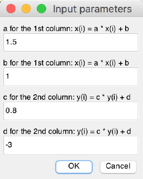
Simple Function
This function is very useful. It generates a new data file based
on the selected data file. Both columns (1st or X column and 2nd or
Y column) can be modified. See below case study.
X(i) = a * X(i) + b
Y(i) = c * Y(i) + d
Acycle v1.0 User’s Guide Mingsong Li
- 34 -
The selected data: all value in the first column data will be transformed using the equation X(i) =
1.5 * X(i) + 1; and all value in the second column data will be transformed using the equation Y(i) =
0.8 * Y(i) + (-3).
New file name: *-new.txt
Utilities
Find max/min
Find max/min value within a user-defined interval. Output
will be displayed in command window only.
Image:
Show Image
Plot selected image file.
RGB to Grayscale
Convert a image file in RGB format to a grayscale format,
save new image .
New image name: *-gray.tif
Image Profile
Get the grayscale profile from a line constrained by two
user-selected dots.
New file name: *-profile.txt % grayscale
profile
New file name: *-controlpoints.txt % location of two
control points
Step 1: Choose the image file, select “Math - Image – Image Profile” function.
Step 2: Click data cursor tool (1), press ALT key and click 2 points.
Step 3: Press Enter key. Grayscale profile data will be picked up and saved along the green line.
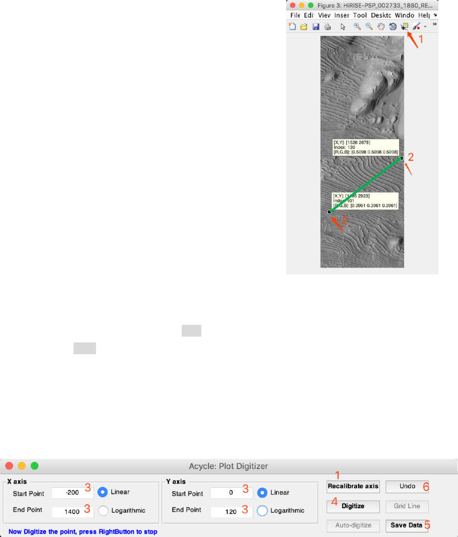
Plot Digitizer
Digitize data points from an image file. Example:
Load “Example-PlotDigitizer.jpg” and run “Plot Digitizer”
“Basic Series” → “Examples” → “Image for Plot Digitizer”.
Left click to select the image file (or your own image -- a plot with data points) in the Acycle main
window, select “Math” → “Plot Digitizer” to run this GUI (see figures below).
Acycle v1.0 User’s Guide Mingsong Li
- 35 -
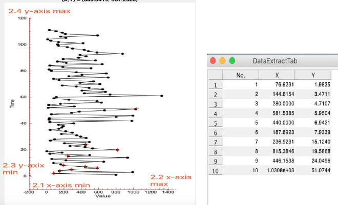
You will see the pop-up window of “Acycle: Plot Digitizer” (top panel). Follow the instructions in
blue text (bottom left corner):
1) Click the “Calibrate axis” button
2) Pick-up axes limits
In the image plot figure, click four points in the correct order: minimum limit of x-axis (2.1),
maximum limit of x-axis (2.2), minimum limit of y-axis (2.3), and maximum limit of y-axis (2.4).
3) Set axes limit values
Return the window of “Acycle: Plot Digitizer”, type the value of x- and y- axis limits. And select
“Linear” or “Log” model.
4) Digitize
Click “Digitize” button, you are able to click in the image figure to select data points.
Data points will be recorded and displayed in “Data Extra Tab” GUI.
Right click to terminate the digitizer; press “Digitize” to continue.
5) Save Data
Click “Save Data” button to save digitized data points in text files.
6) Undo
Press “Undo” to remove the last data point(s).
Acycle v1.0 User’s Guide Mingsong Li
- 36 -
4.7 Time series
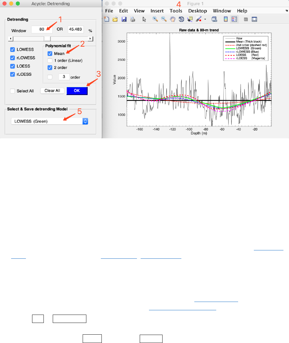
Detrending
This detrending function generates 2 new data files based on the selected data file and user-
defined parameters: window length and detrending method. Steps:
(0) Select a data file in the Main Window; Select Timeseries → Detrending menu
(1) Type a window length or a percentage or move the slider. Default value is 35% of the total
length, that is, if a data length is 100 m, then a window is 35 m.
(2) Tick one or more detrending method
(3) Click OK button, wait for several seconds (up to a minute, depending on the length of the
dataset and the speed of your machine). A new window (4) will popup showing the data and its 35%
trend(s).
(5) In the “Select & Save detrending Model” panel, select the preferred trend. The trend and
detrended file will be displayed in the Main Window.
(Tips) Change window sizes, the trend lines in the right panel will be updated automatically.
Shortcut keys [Mac]:
⌘
+ T; [Windows]: Ctrl + T
New file names: *-80-LOWESS.txt AND *-80-LOWESStrend.txt
Acycle v1.0 User’s Guide Mingsong Li
- 37 -
Prewhitening - First Difference
Differences using MatLab’s diff function.
Y = diff(X), calculates differences between adjacent elements of X.
New file name: *-1stdiff.txt
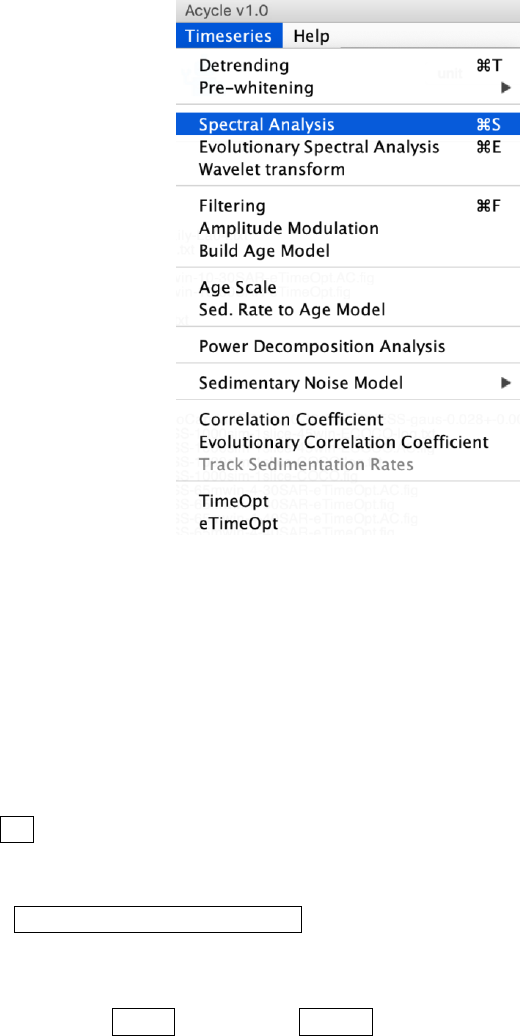
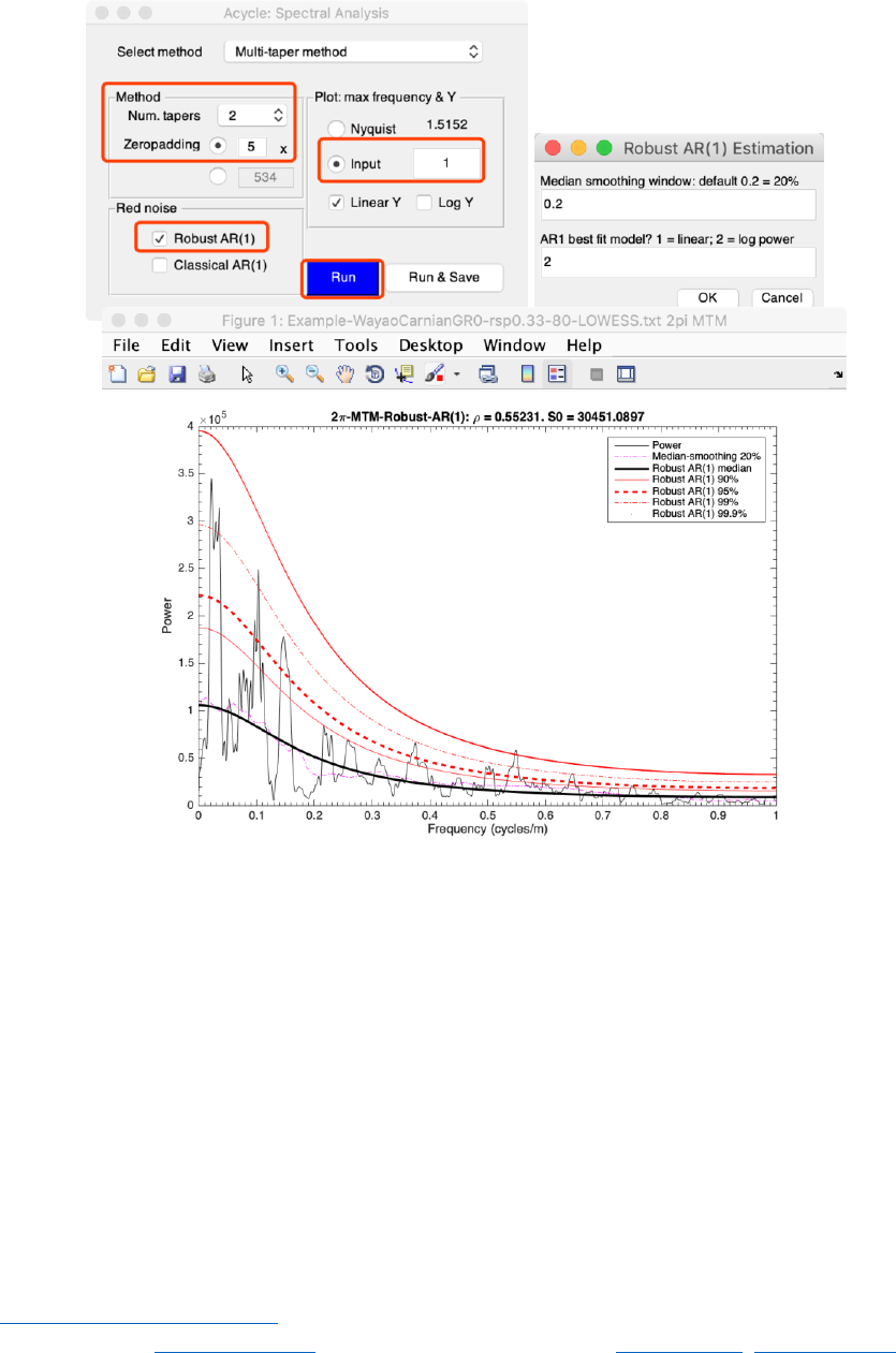
Spectral Analysis
This function conducts spectral analysis with user-defined parameters. Steps:
(1) Select a data file in the Main Window
(2) Select Timeseries → Spectral Analysis menu
(3) Select one method for spectral analysis. Options are Multi-taper method (MTM) (Thomson,
1982), Lomb-Scargle spectrum (Lomb, 1976; Scargle, 1982), and MatLab’s periodogram.
(4) If Multi-taper method (MTM) is selected, then the Method panel may be changed. The default
value is using 2π MTM, with a no zero-padding.
(5) Plot panel: set the max frequency in the coming figure.
(6) Red Noise panel: AR(1) noise model using RedNoise.m by Husson (2014) and modified by
Linda Hinnov. Robust AR(1) noise model follows Mann and Lees (1996).
(7) Run or Run & Save button, generates power spectrum (and save power spectrum data and
AR(1) series)
Shortcut keys [Mac]:
⌘
+ S; [Windows]: Ctrl + S
Acycle v1.0 User’s Guide Mingsong Li
- 38 -
2π MTM power sepctrum of the Wayao Carnian gamma ray data (interpolation = 0.33;
detrend 80-m lowess trend)
New file name: *-2piMTM-CL.txt, means 2π MTM and confidence level series.
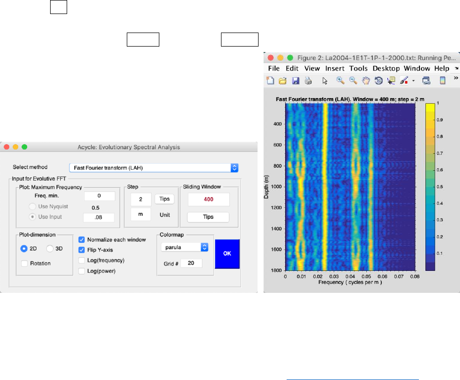
Evolutionary Spectral Analysis
This function conducts evolutionary spectral analysis with user-defined parameters. Steps:
(1) Select a data file in the Main Window.
Warning: The data file must be an evenly spaced depth/time series.
(2) Select Timeseries → Evolutionary Spectral Analysis menu
(3) Select Method. The default method is Fast Fourier transform (LAH) by Linda A. Hinnov
(Kodama and Hinnov, 2015). Other options are MatLab’s Fast Fourier transform, multi-taper
method (MTM) (Thomson, 1982), and Lomb-Scargle spectrum (Lomb, 1976; Scargle, 1982).
Acycle v1.0 User’s Guide Mingsong Li
- 39 -
(4) Input for evolutionary spectral analysis panel includes settings for plot frequencies. Default
values from 0 to Nyquist (fnyq = 1 / (N * Δt)), where N is the total number of data, and Δt is the
sampling rate.
(5) Step of sliding windows. The default value should be sufficient for most paleoclimate
projects. The unit may be m, kyr, etc.
(6) Sliding Window: very important! The length of the sliding window. The default value is
35% of the total length of the selected data. You may need to change this based on following tips.
Tips: assuming the data series is dominated by 35 m cycles, the window may be 2-4 times of 35
m, that is, 70 to 140 m. A large window can smooth out the higher frequencies signals while a small
window cannot detect low-frequency signals.
(7) Plot-dimension: 2D or 3D with rotation option.
(8) Flip Y-axis: give me a try.
(9) Colormap style can be modified and grid levels can be set (empty value results in a smoothed
figure).
(10) OK button: generates a new figure showing the evolutionary spectral analysis results. No
new files generated automatically.
Shortcut keys [Mac]:
⌘
+ E; [Windows]: Ctrl + E
Evolutionary FFT of the La2004 astronomical solutions using a 400 kyr sliding window and 2
kyr step
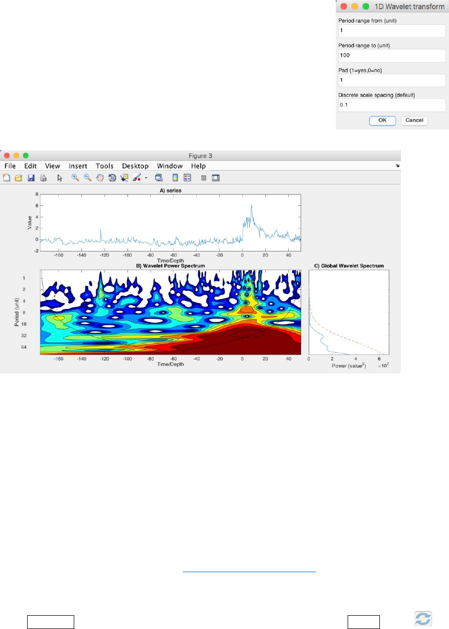
Wavelet transform
This wavelet analysis function conducts wavelet analysis (Torrence and Compo, 1998) with
user-defined parameters. Steps:
Acycle v1.0 User’s Guide Mingsong Li
- 40 -
(1) Select a data file in the Main Window.
Warning: The data file must be an evenly spaced depth/time series.
(2) Select Timeseries → Wavelet Transform menu
(3) Modify parameters
Period ranges from [the first line] to [the second line] unit. Default
values for all lines works well with the program. Users may need to modify
the period range in the 2nd line using a smaller number (e.g., halved value).
[Issue: stand-alone versions of Acycle may have bugs in the wavelet
transform.]
Wavelet analysis of the Wayao gamma ray series. The series has been interpolated using a 0.3 m
sampling rate.
Filtering
This function generates a filter output series based on the selected data file with user-defined
parameters. Steps:
(1) Select a data file in the Main Window.
Warning: The data file must be an evenly spaced depth/time series.
(2) Select Timeseries → Filtering menu
(3) Bandpass filter panel: very important! Type min and center frequencies of the passband, the
max frequency will be set automatically. The bandpass filters are MatLab’s Butter, Cheby1, and Ellip
filters and Gaussian, and Taner-Hilbert filters. The recommended filters are Gaussian filter and
Taner-Hilbert filters code by Linda Hinnov (Kodama and Hinnov, 2015).
Tips: The Taner-Hilbert filter generates both filtered output series and the amplitude modulation
of the filtered output series.
Click Save Data button, the filter outputs will be displayed after clicking the refresh button
in the Main Window.
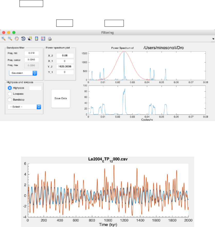
Acycle v1.0 User’s Guide Mingsong Li
- 41 -
(4) Highpass and lowpass panel: Two options are MatLab’s Butter and Ellip filter. Type cutoff
frequency in the text box and select a filter.
Click Save Data button, the filter outputs will be displayed.
(5) Power spectrum plot: give options for display the power spectrum in the right of the GUI.
Shortcut keys [Mac]:
⌘
+ F; [Windows]: Ctrl + F
New file name: *-gaus-0.0243+-0.0053.csv, means filtered output series using gauss filter and a
0.0243 ± 0.0053 cycles/unit bandpass.
*-Tan-0.03+-0007.csv and *-Tan-0.03+-0007-AM.csv, mean filtered output series using Taner-
Hilbert filter and a 0.03 ± 0.007 cycles/unit bandpass, with its amplitude modulation file saved.
Original La2004 solutions and filtered 41 kyr cycles
Build Age Model
This function generates an age model file from a filter output data file. Steps:
(1) Assuming the filtering wavelength generates a filtered 35 m cycle series. The 35 m cycles are
assumed to be 405 kyr long eccentricity cycles. This filtered data file should be selected.
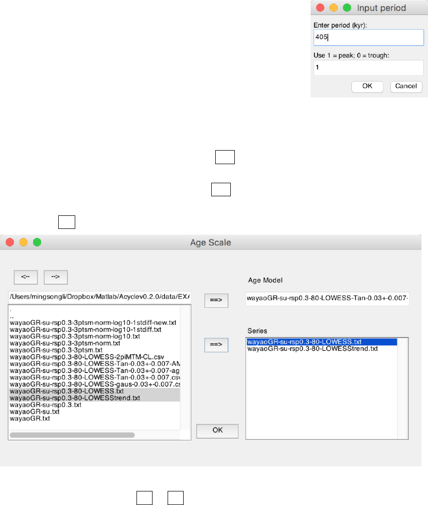
Acycle v1.0 User’s Guide Mingsong Li
- 42 -
(2) Select Timeseries → Build Age Model menu
(3) In the pop-up window, enter 405 and 1, and click OK button.
This generates a new age model series via assigning every peak of 35 m
cycles as peaks of the 405 kyr cycles.
New file name: *-agemodel-405-max.csv,
means an age model file using filtered wavelength peaks as 405 kyr
anchors.
Age Scale
This function conducts depth-to-time transformation in a new standalone GUI. Steps:
(1) Select 1 (ONE) age model file, click the top ==> button to record this file as an age model
file.
(2) Select 1 or more data files, click the bottom ==> button to record this file (these files) as
series needs to be transformed.
(3) Click the OK button. The transformed series can be displayed and saved.
New file name(s): *-TD-name-of-agemodel-file.csv
(Tips) Change directory using <-- or --> button
Sedimentary Rate to Age Model
Assuming you want to generate an age model file from a sedimentary rates file (2 columns: depth
and sedimentation rate), this function generates the age model working well with acycle software.
Acycle v1.0 User’s Guide Mingsong Li
- 43 -
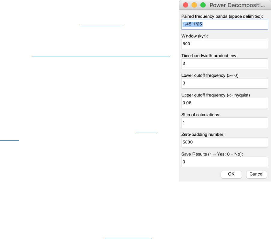
Power Decomposition Analysis
This function subtracts power/variance within a user-defined
frequency band. The code written by Mingsong Li and Linda
Hinnov has been published in Li et al. (2016). Time-dependent
amplitude modulations in the obliquity component were obtained
from 2π multi-taper variance (power) spectra calculated along a
sliding time window using the Matlab script pda.m (also
available at https://doi.pangaea.de/10.1594/PANGAEA.859147).
Steps:
(1) Select the original data file.
Warning: The data must be evenly spaced data in the first
column. And the unit must be in kyr.
(1) Type paired frequency bands; space delimited. If a
dominated frequency is 1/33, then a 1/45 1/25 frequency band is
used
(2) Sliding window in kyr, a 500 kyr is used in Li et al.
(2016)
(3) Time-bandwidth product, ‘2’ means 2π MTM method
will be used.
(4) cutoff frequencies, min = 0, max should cover all
Milankovitch frequencies.
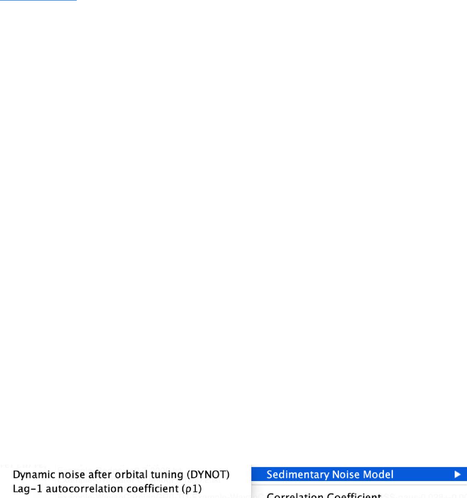
Sedimentary Noise Model
Dynamic noise after orbital tuning (DYNOT)
Dynamic noise after orbital tuning. Detect non-orbital variances from a tuned series. See Chapter
5. DYNOT model Description. See Li et al. (2018a) for details about this method.
Acycle v1.0 User’s Guide Mingsong Li
- 44 -
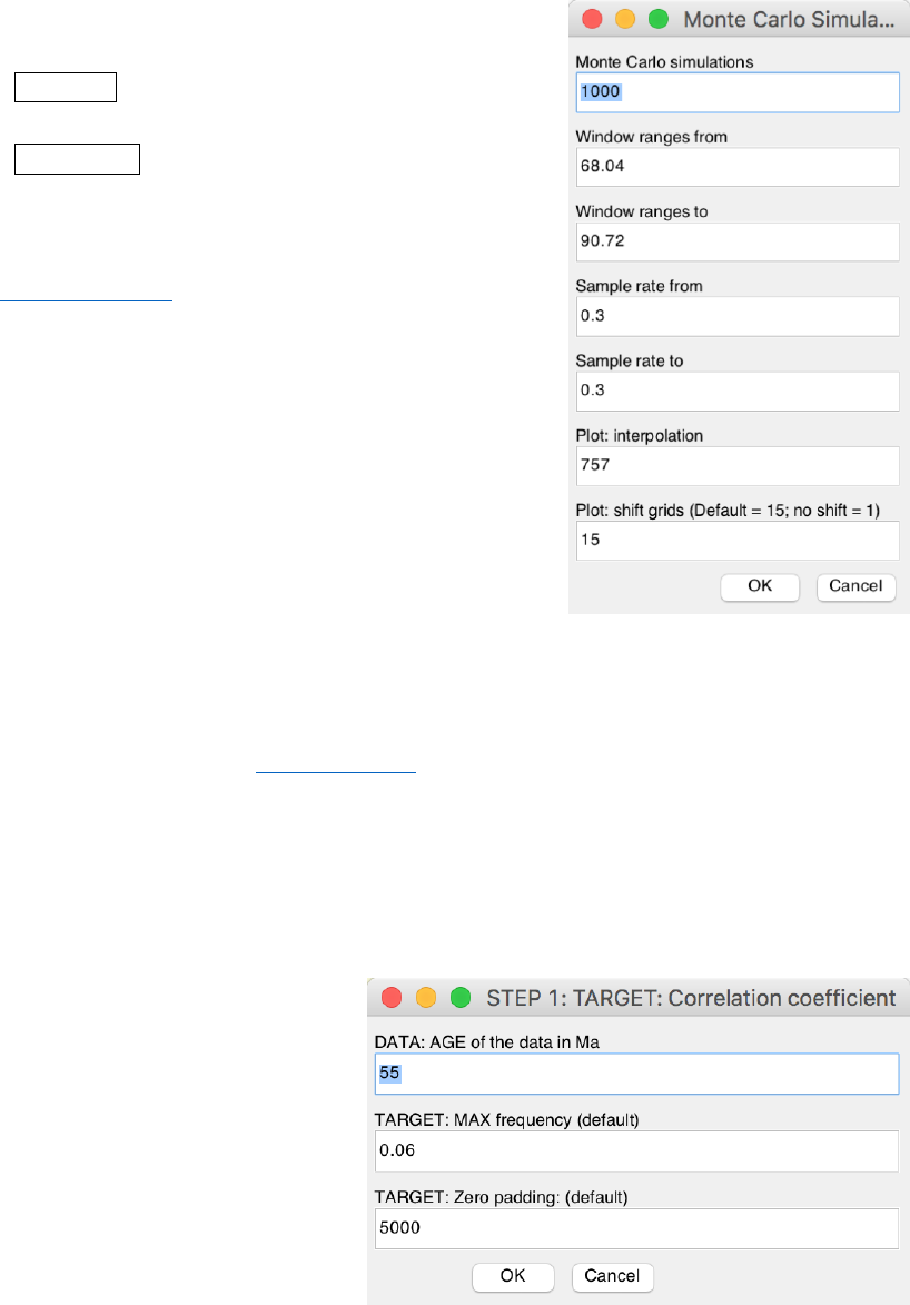
Lag-1 autocorrelation coefficient (ρ1)
This function conducts either single run or Monte Carlo
simulations of lag-1 autocorrelation coefficient (ρ1) using a
sliding window. It works with both depth series and time series.
The “Single run” requires the input of “window” and
“interpolation sampling rate”.
The “Monte Carlo” requires several parameters: Number of
Monte Carlo simulations (default is 1000), sliding window
ranges from win1 to win2, and a sampling rates from sr1 to sr2,
and plot settings (interpolation and shift grid).
See Li et al. (2018a) for details about the parameters and
significance of this method.
Correlation Coefficient (COCO)
This function addresses two fundamental issues in
cyclostratigraphy and paleoclimatology: identification of
astronomical forcing in sequences of stratigraphic cycles, and
accurate evaluation of sedimentation rates. The technique
considers these issues part of an inverse problem and estimates
the product-moment correlation coefficient between the power
spectra of astronomical solutions and paleoclimate proxy series across a range of test sedimentation
rates. The number of contributing astronomical parameters in the estimate is also considered. Our
estimation procedure tests the hypothesis that astronomical forcing had a significant impact on proxy
records. The null hypothesis of no astronomical forcing is evaluated using a Monte Carlo simulation
approach. Details are included in (Li et al., 2018c).
Step 1: settings for generating target power spectrum
Select a depth series (interpolated, detrended), select Timeseries --> Correlation Coefficient
menu
Note: the data series must have a unit in meter.
Type the approximate age for the depth
series, the unit is million years ago (Ma).
Target frequency ranges from 0
cycle/kyr to the given “MAX frequency”.
Default values are recommended for the
depth series with age less than 250 Ma.
For the depth series older than 250 Ma,
the MAX frequency may be set to 0.08.
This is because the precession cycle can be
very short than 16 kyr.
Acycle v1.0 User’s Guide Mingsong Li
- 45 -
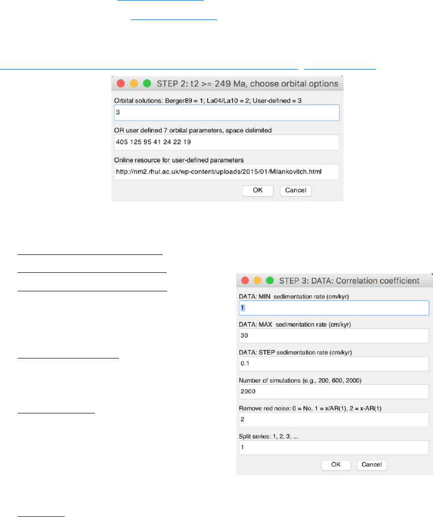
Step 2: astronomical solution [optional]
If the age of the data in Ma is larger than 249 Ma, users need to select which astronomical
solution should be used.
1 = Berger89 solution (Berger et al., 1989),
2 = Laskar 2004 solution (Laskar et al., 2004),
3 = user-defined solution and the second box should be filled by 7 astronomical periods.
Online resource for user-defined astronomical parameters may be found at
http://nm2.rhul.ac.uk/wp-content/uploads/2015/01/Milankovitch.html (Waltham, 2015).
Step 3: settings for generating data power spectrum
MIN sedimentation rate (cm/kyr):
MAX sedimentation rate (cm/kyr):
STEP sedimentation rate (cm/kyr): tested
sedimentation rates range from MIN to MAX, with a
step of STEP cm/kyr. In the following example, the
tested sed. rates are 1, 1.5, 2, 2.5, 3, …, 29.5, and 30
cm/kyr.
Number of simulations: 200-600 simulations are
suggested for an initial run. And 2000 simulations
generate publication quality results, however, 5000,
or 10000 simulations are even better.
Remove red noise: 0 = no removing
(recommended if the power spectrum is not “red”);
else removing red noise:
1 = power spectrum / AR(1) series and those
less than AR(1) series are set to 0;
2 = power spectrum - AR(1) series and those
less than 0 are set to 0 (Default, the best option for the time series with a “red” spectrum).
Split series: 1 (default), 2, 3. If a number of “2” is used, the series will be split into 2 or more
slices.
Acycle v1.0 User’s Guide Mingsong Li
- 46 -
Click the OK button, Monte Carlo simulation steps can be displayed in the Command Window of
MatLab. A log file will be generated recording all parameters used in the correlation coefficient
analysis.
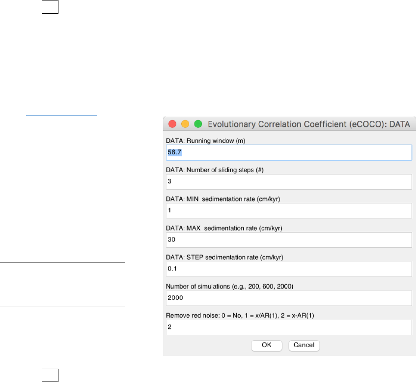
Evolutionary Correlation Coefficient (eCOCO)
The method is applied using a sliding stratigraphic window to track variable sedimentation rates
along the proxy series, in a procedure termed “eCOCO” (evolutionary correlation coefficient)
analysis. (Li et al., 2018c)
Waning: the data series must have
a unit in meter.
Step 1: same as that in COCO.
Step 2: same as that in COCO.
Step 3: most parameters are the
same as those in COCO (see above).
Two new parameters:
DATA: running window (m):
default window is 35% of the total
length of the data series.
DATA: Number of steps (#):
sliding steps. The default value will
give about ~300 sliding windows for
publication quality results.
Click the OK button, Monte Carlo simulation steps can be displayed in the Command Window of
MatLab. A log file and the related *.AC.fig file will be generated recording all parameters used in the
evolutionary correlation coefficient analysis. The user needs to decide which figure output should be
saved or not.
Tips: Users may save the main window using “File” → “save ac.fig” menu anytime. This will
save the data stored in the main window figure, and the user doesn’t have to re-run the eCOCO using
the same parameters.
Tips: User can plot eCOCO results anytime at “Plot” → “ECOCO plot” menu.
Q: Which window should I use?
A: A window that covers 1.5-2 * long eccentricity cycles will give a reliable result. If your series
is dominated by 35 m cycles (405 kyr), then a 70 m window (= 35 * 2) may be good to keep the
balance: A large window eCOCO losses resolution of variable sedimentation rates, and a small
window may not give correct results.
Track Sedimentation Rates
Not finish yet…

Acycle v1.0 User’s Guide Mingsong Li
- 47 -
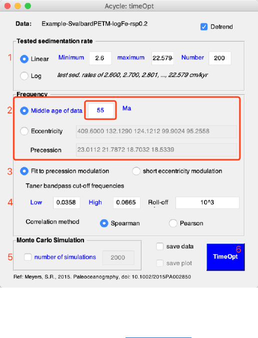
TimeOpt
The method is to determine the optimal sedimentation rates of the proxy series, in a procedure
termed “TimeOpt” analysis (Meyers, 2015). For a “test” sedimentation rate, the TimeOpt method
extracts the precession-band amplitude envelope from the proxy data and evaluates the first
correlation coefficient (r2envolope) between this envelope and reconstructed eccentricity model.
It also evaluates a second correlation coefficient (r2power) between the reconstructed
astronomical (eccentricity and precession) model series and the time-calibrated proxy series.
Finally, a measure of fit (r2opt) combine both correlation coefficients using an equation: r2opt =
r2envolope * r2power. Monte Carlo simulation with a first-order autoregressive model is used to
determine the statistical significance of the observed r2opt value.
This function is largely based on the TimeOpt R script in Astrochron by Steve Meyers.
Step 0: Select a time series in depth domain (interpolation may be needed if the sampling rate is
uneven).
Warning: the unit of depth-series should be in “meter”.
Step 1: In the pop-up window, set the test sedimentation rate:
linear or log model?
Minimum, maximum, and the step of sedimentation rates. (Default values are usually
okay)
Step 2: Set the middle age of data OR type frequencies of eccentricity and precession.
You’ll only need to give the middle age of the data; the frequencies will be calculated
automatically from an astronomical solution of La2004.
The Taner bandpass cut-off frequencies are also adjusted automatically.
If the middle age is > 249 Ma, you may type the frequencies.
Step 3: Fit to precession modulations (default), and short-eccentricity modulation may not be
reliable.
Step 4: If you have typed the frequencies in Step 2, you will also need to adjust frequencies here.
Step 5: Simulations are to evaluate the null hypothesis of the optimal sedimentation rate. This can
be very time-consuming.
Acycle v1.0 User’s Guide Mingsong Li
- 48 -
eTimeOpt
evolutive TimeOpt method (Meyers, 2019).
Step 0: Select a time series in depth domain (interpolation may be needed if the sampling rate is
un-even). For an example, select “Basic Series” → “Examples” → “Late Triassic Newark Depth
Rank” → select generated text file entitled “Example-LateTriassicNewarkDepthRank.txt” in the
Acycle main window.
Step 1: In the pop-up window, set the test sedimentation rate:
linear or log model?
Minimum, maximum, and the step of sedimentation rates.
Step 2: Set the middle age of data OR type frequencies of eccentricity and precession.
You’ll only need to give the middle age of the data; the frequencies will be calculated
automatically from an astronomical solution of La2004.
If the middle age is > 249 Ma, you may type the frequencies.
Step 3: Set filter. Fit to precession modulations (default), and short-eccentricity modulation may
not be reliable.
The Taner bandpass cut-off frequencies are also adjusted automatically.
Step 4: Set the sliding window and step. Default window size is 35% of total range of depth. This
should be adjusted, a window size of 1.5 - 2 x (405-kyr related wavelength) is usually good enough.
Default step size usually generate ~200 sliding window, this is sufficient to generate a publication
quality eTimeOpt result.
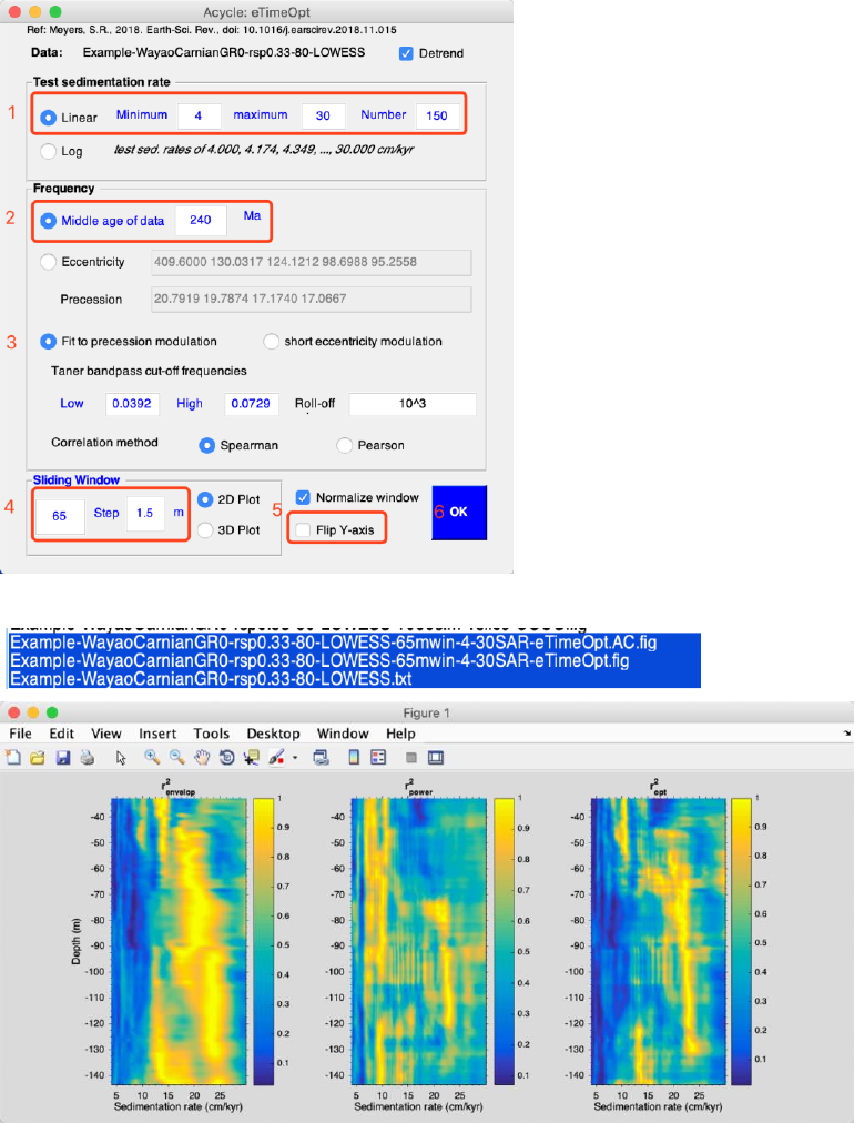
Acycle v1.0 User’s Guide Mingsong Li
- 49 -
Step 5: You may select to normalize each sliding window (forcing the maxima values of each
window to 1). Ticking “Flip Y-axis” checkbox will flip y-axis.
Step 6: Click OK button to run the eTimeOpt.
You will have following two new MatLab figure file, and eTimeOpt plot.
4.8 Help
Readme
Show update log file / online document

Acycle v1.0 User’s Guide Mingsong Li
- 51 -
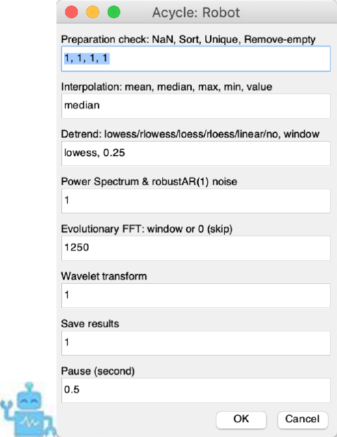
4.9 Mini-robot
This tiny tool can do some work automatically with default settings.
Step 1: Click to select one data file (see 3.6 Data Requirement) in Acycle main window.
Step 2: Click the mini-robot button.
Step 3: review parameters and click the “OK” button.
It will do:
1. Data preparation - check selected data: remove NaN numbers, sort data (based on the first
column), remove duplicated numbers (replace with their mean value), remove empty values
2. Interpolation: using the median sampling rate
3. Detrending: removing a 25% LOWESS trend
4. Power spectral analysis: to show significant frequencies; aided with a robust AR(1) red
noise model using a log best-fit to the 20% median-smoothed spectrum.
5. Evolutionary FFT: using an adjusted sliding window.
6. Wavelet transform: using default settings.
7. Save results
8. Pause 0.5 seconds after each above step.
Acycle v1.0 User’s Guide Mingsong Li
- 52 -
5. DYNOT model Description
Li et al. (2018a) developed a dynamic noise after orbital tuning, or DYNOT model for the
sea-level changes based on the dynamic non-orbital signal in climate proxy records after
subtracting orbital, i.e., astronomically forced climate signal. The DYNOT model is
supplemented by a second, independent lag-1 autocorrelation coefficient, or ρ1 model, which
forms the basis of a statistical method for red noise estimation of time series. DYNOT and ρ1
modeling of a GR series of ODP Site 1119 over the past 1.4 myr correlates with the classic low-
passed δ18O sea-level curve, demonstrating the efficacy of the sedimentary noise model.
5.1 Data format
data for the DYNOT model (support data in *.csv and *.txt format)
Name: data
Length: m × 2 % must be a 2-column dataset
Column 1: time % unit must be in ka;
Column 2: value
Notes:
#1: Proxy data is assumed to be sensitive to water-depth related noise at your section/core.
#2: There is no requirement for interpolation, normalization, or removing long-term trend
(i.e., pre-whitening) of the dataset.
#3: Extreme values should be removed.
#4: Both increasing-upward and decreasing-upward time series are valid.
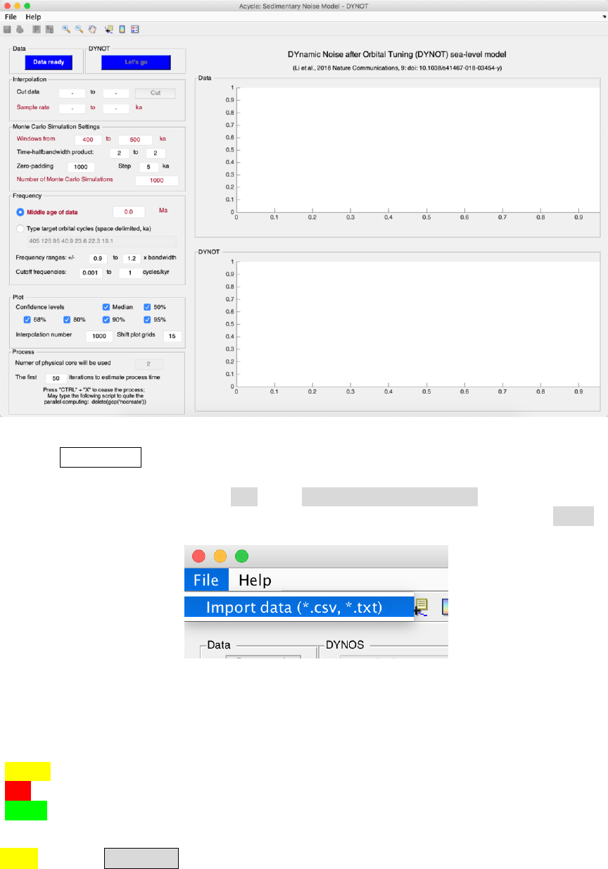
5.2 Startup
1. Left click to select a dataset file in Acycle main window.
2. Select “Timeseries” – “Sedimentary Noise Model” – “DYNOT”
3. The DYNOT sea-level model GUI (Fig. 2) is below.
Fig. 1. MatLab workspace for the DYNOT model.
Acycle v1.0 User’s Guide Mingsong Li
- 53 -
Fig. 2. The DYNOT model
4. Click Data ready button load data or load data from *.txt or *.csv file
In the DYNOT menu: Select “File” → “Import Data (*.txt, *.csv) ” → Select data (chose
“1119_gr_1400de_finetuned.txt” or “1119_gr_1400de_finetuned.csv”) → Click “Open ”
Fig. 3. Load data to DYNOT model.
5.3 Settings
Yellow: load data and run the model.
Red: Key settings. Check before running the model.
Green: Optional settings. Default values are okay for most running.
5.3.0. Click on Data ready (button) to load data into the DYNOT model.

Acycle v1.0 User’s Guide Mingsong Li
- 54 -
5.3.1. Cut data (optional): These settings automatically show the beginning and the end of
the time series, i.e., time span of dataset. Unit is ka. If you want to choose a different
interval, just type two new ages and click Cut button.
5.3.2. Sampling rates (optional): These show a range of sample rates covering 90% of sample
rates (Green Box 20 in Fig. 4). Unit is ka. A Monte Carlo method of hypothesis testing
and the multi-taper method (MTM) of power spectral analysis are to be undertaken,
and so resampling must be applied. Sampling rates of proxy datasets in time are
always greater than zero and so are non-normally distributed. Therefore, the Weibull
distribution is used to represent sampling rate distributions for uncertainty analysis in
the DYNOT model. To avoid an ultra-low or ultra-high, unrealistic sampling rate
created by the Weibull distribution algorithm, we set the 5th and 95th percentiles of
sampling rates of of the data as default, lower and upper limits of the generated,
Weibull-distributed sampling rates.
5.3.3. Windows: These values set sliding window range. Moving window length in units of
time (<< total data length). Unit is ka.
Different windows in the DYNOT model can affect results in two ways.
(1) The DYNOT model with a large window will shorten DYNOT results, and the model
with a small window will generate longer DYNOT results, Nr = Ndata – window + 1,
where Nr is total number of DYNOT values of each simulation, Ndata is total number
of interpolated data points, and window is the running window employed.
(2) The DYNOT model with a small running window generates higher resolution results,
however, the variance of low-frequency cycles and total variance diminish
simultaneously, which leads to increased uncertainty in non-orbital signal ratio
estimation.
The DYNOT model with a small running window also increases the MTM power
spectrum bandwidth (i.e., reduces frequency resolution). The expected sea-level
variations of interest in the Early Triassic are 104 to 106 year-scale, i.e., the fifth to
third-order sequences, therefore a comparable or shorter time window (e.g., 300-500
kyr, 400 kyr or shorter) should be adopted for DYNOT modeling.
5.3.4. Time-bandwidth product (optional): Time-bandwidth product of discrete prolate
spheroidal sequences used for window. Typical choices are 2, 5/2, 3, 7/2, 4.
5.3.5. Zero-padding (optional). zero-padding number, e.g., 1000.
5.3.6. Step (optional). step of calculations; default is 5 ka.
5.3.7. Number of Monte Carlo Simulations: default is 1000. Maybe use 100 or 300 for a
trial running. Recommended value for publication is >5000.
5.3.8. Age of the time series: The age in Ma will be used to estimated target orbital cycles in
5.3.9. You can use either 5.3.8 or 5.3.9 to tell the DYNOT model the target cycles.
5.3.9. Target orbital cycles (space delimited, in ka): 6 orbital cycles of long-eccentricity
(405), short-eccentricity (125 and 95), obliquity (40.9 or shorter), precession (23.6,
22.3, and 19.1 or shorter). This is age dependent (see 7.8). The 405, 125, and 95 kyr
cycles are assumed to be invariant through time. While the obliquity = 41-0.0332*age;
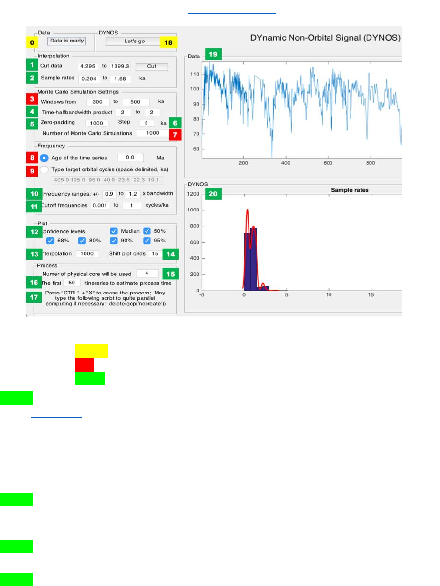
Acycle v1.0 User’s Guide Mingsong Li
- 55 -
precession 1 = 23.75-0.0121*age; precession 2 = 22.43-0.0121*age; precession
3=19.18-0.0079*age. These calculations are from Yao et al. (2015), and are based on
the La2004 astronomical model (Laskar et al., 2004).
Fig. 4. Settings of the DYNOT model.
Yellow: load data and run the model.
Red: Key settings. Check before running the model.
Green: Optional settings. Default values are okay for most running.
5.3.10. Frequency ranges (optional): For the definition of the non-orbital signal ratio by Li et
al. (2018a), cutoff frequencies and their bandwidths are crucial for estimation of
variances of eccentricity, obliquity and precession signals. We vary each cutoff
frequency assuming a uniform distribution with cutoff frequency ranges at ± 90% to ±
120% bandwidth. Here the bandwidth (bw) equals nw/window, where nw is time-
bandwidth product of discrete prolate spheroidal sequences, and window is the running
window.
5.3.11. Cutoff frequencies (optional): lower cutoff frequency (> 0) for estimation of total
variance and upper cutoff frequency (< Nyquist frequency) for estimation of total
variance.
5.3.12. Confidence levels (optional): default values show median and confidence levels (e.g.,
50%, 68%, 80%, 90%, and 95%) of the DYNOT results.
5.3.13. Interpolation (optional): In 5.3.3, a smaller Nr compared to Ndata leads to a “no data”
effect at the very beginning and/or very end of the DYNOT results. To avoid this
problem and to provide a better constraint for noise estimation, technically, the

Acycle v1.0 User’s Guide Mingsong Li
- 56 -
DYNOT model is interpolated and randomly shifts and plots simulation results of a
single iteration at the same time scale of the dataset, although the plots also generate
relatively smoothed DYNOT spectra when a gap is shorter than 2 × window. Here
1000 is adequate for the DYNOT model.
5.3.14 Shift plot grids (optional): See 5.3.13 for interpretation. Default is 15. One can also
use 15-30 for the better shape of the beginning and the end of the DYNOT spectra.
5.3.15. Number of physical cores (optional): This detects the physical cores of the CPU of
the computer.
5.3.16. Number of itineraries to estimate the process time (optional): To estimate process
time of the time-consuming DYNOT model, the model will run some itineraries.
Default is 50.
5.3.17. Emergency note: Press “Ctrl” + “C” to cease the DYNOT process before the parallel
computing. Press “Ctrl” + “X” to cease the DYNOT process during the parallel
computing. You may need to type the following script in the command window to
quite parallel computing.
>> delete(gcp(‘nocreate’))
5.3.18. Click the button to run the model.
5.3.19. A window shows the dataset.
5.3.20. A window shows sample rates of the dataset OR the DYNOT spectrum of the dataset.
5.4. Running the DYNOT model
Click the Let’s go button to run the DYNOT code. In the command window, the estimated
running time will appear:
16:21:20 Begin the process ...
16:22:54 First 50 iterations suggest: remain >= 0h:7m:27sec
% The model runs the first 50 iterations to estimate that the total running time
will last ca. 7 minutes 27 seconds. The real run-time may be 10s seconds to
several minutes longer than this estimate.
Starting parallel pool (parpool) using the 'local' profile ... connected to 4 workers.
16:23:07 Current iteration takes 1.11 seconds
16:23:08 Current iteration takes 1.21 seconds
16:23:15 Current iteration takes 1.19 seconds
16:26:26 Current iteration takes 1.38 seconds
% Start parallel computing and show time of each iteration.
Parallel pool using the 'local' profile is shutting down.
>> Done. % Stop parallel computing and display the DYNOT result (Fig. 5).
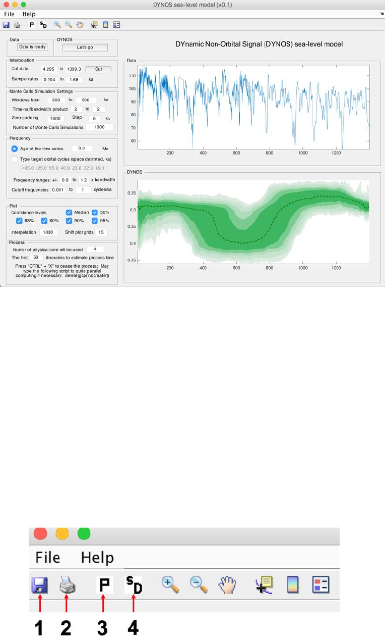
Acycle v1.0 User’s Guide Mingsong Li
- 57 -
Fig. 5. DYNOT sea-level model of the gamma-ray series at ODP site 1119 from 0 to 1.4 Ma.
5.5. Output Files
After running the DYNOT model, the median value of noise and percentiles of the outputs
will be saved as text files.
The GUI menu (Fig. 6) can be used to:
#1: save a MatLab-fig in the working directory entitled “plots_.fig”.
#2: save a PDF file of the plots in the working directory entitled “plots_.pdf”
#3: pop-up display the DYNOT spectrum in a new window.
#4: save DYNOT output data in the working directory entitled “result_handles.mat”.
Caution: Change names of output files, or they will be overwritten by new files.
Fig. 6. Output files
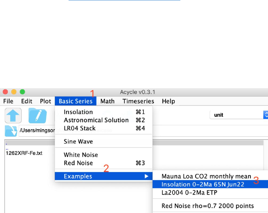
Acycle v1.0 User’s Guide Mingsong Li
- 58 -
6. Case Studies
Example #1: Insolation
Data: Insolation at 65°N on June 22 over the past 2 million years
Age: 0-2000 ka
Proxy: Insolation.
Target:
Dominated cycles of insolation series
Tool:
Acycle software v0.3 (https://github.com/mingsongli/acycle)
Reference:
Berger, A., 1978. Long-term variations of daily insolation and Quaternary climatic
changes. Journal of the atmospheric sciences 35, 2362-2367.
Laskar, J., Robutel, P., Joutel, F., Gastineau, M., Correia, A.C.M., Levrard, B., 2004. A
long-term numerical solution for the insolation quantities of the Earth. Astronomy &
Astrophysics 428, 261-285.
Step 1: Load data
You will have the following data and figure.
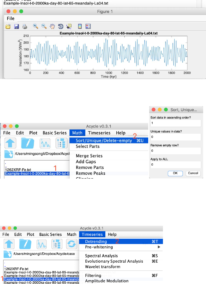
Acycle v1.0 User’s Guide Mingsong Li
- 59 -
Step 2: Data pre-processing
Since the data is not in ascending order. Here we’ll need sort data first.
Step 3: Detrending
Remove the mean value of the insolation series.
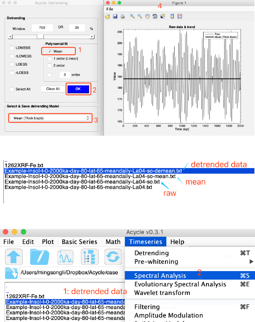
Acycle v1.0 User’s Guide Mingsong Li
- 60 -
You will have:
Step 4: Power Spectral Analysis
Using the following settings:
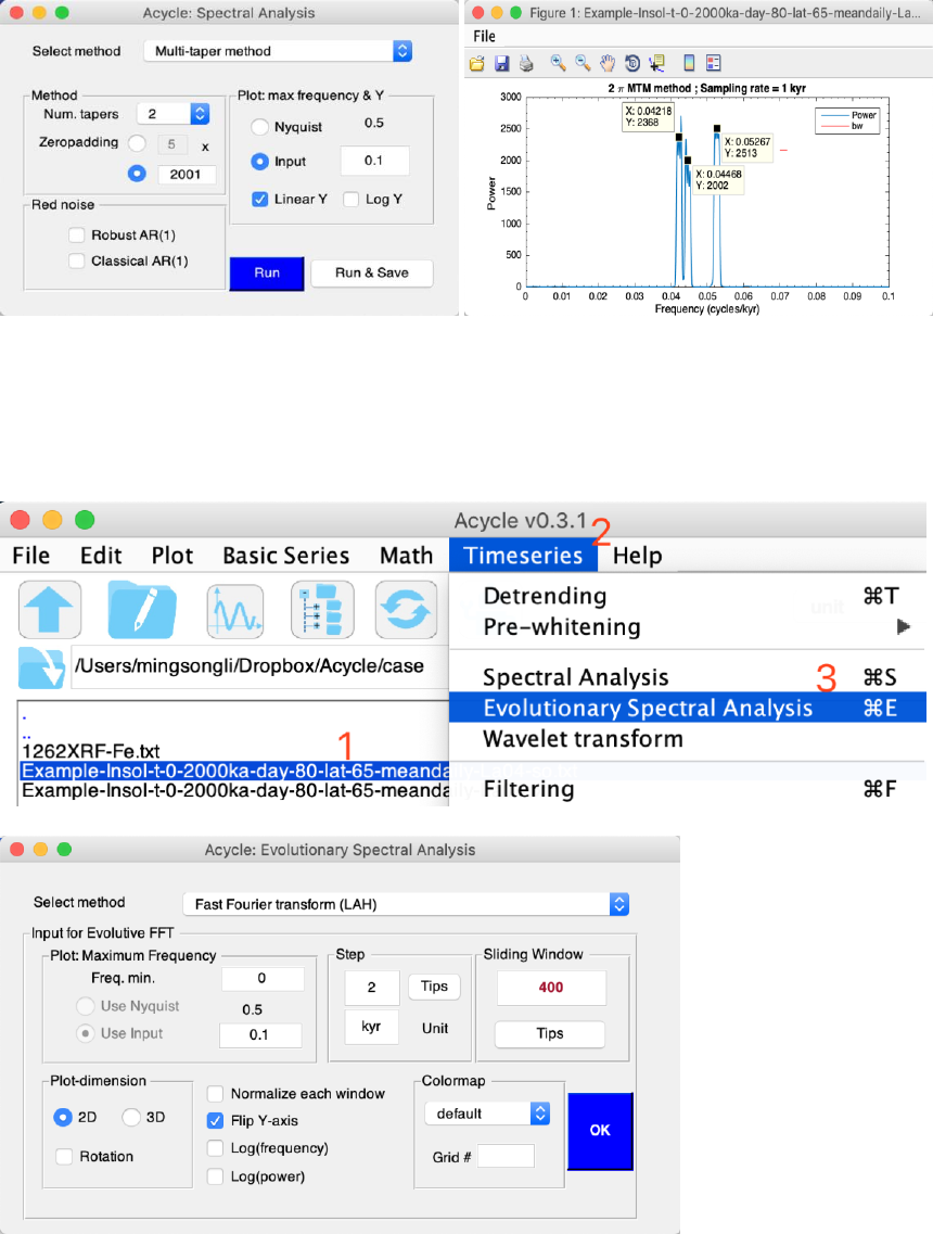
Acycle v1.0 User’s Guide Mingsong Li
- 61 -
Three peaks in the 2 (@Num.tapers) MTM (multi-taper method) power spectrum are
1/0.04218 = 23.7 kyr, 1/0.04468 = 22.4 kyr, and 1/0.05267 = 19.0 kyr.
Step 4: Evolutionary Spectral Analysis
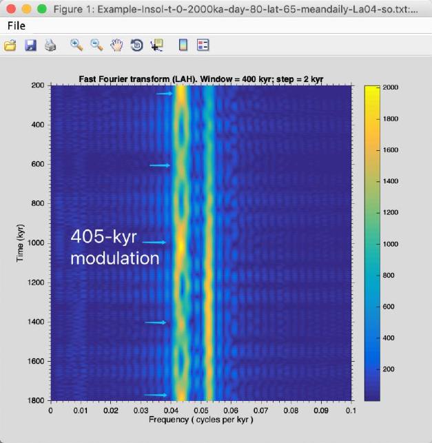
Acycle v1.0 User’s Guide Mingsong Li
- 62 -
This series is dominated by precession cycles. And clearly 405-kyr modulation can be seen
in the evolutionary fast Fourier transform (blue arrows).
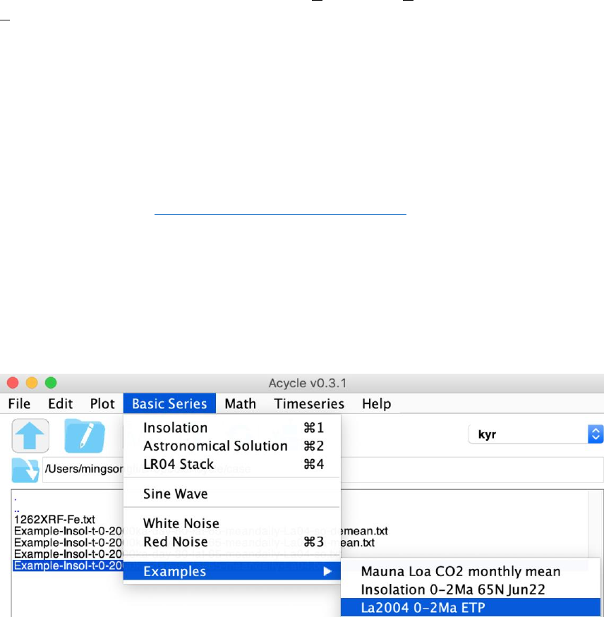
Acycle v1.0 User’s Guide Mingsong Li
- 63 -
Example #2: La2004 astronomical solution (ETP)
Data: La2004 ETP over the past 2 million years
Age: 0-2000 ka
Proxy:
Laskar et al. (2004) astronomical solutions of Eccentricity, Tilt (obliquity), and
Precession, or ETP is defined as:
ETP = standardized E + standardized T - standardized P
, where standardized E = (E – mean(E))/ standard deviation of E
Target:
Dominated cycles of ETP series
Tool:
Acycle software v0.3 (https://github.com/mingsongli/acycle)
Reference:
Laskar, J., Robutel, P., Joutel, F., Gastineau, M., Correia, A.C.M., Levrard, B., 2004. A
long-term numerical solution for the insolation quantities of the Earth. Astronomy &
Astrophysics 428, 261-285.
Step 1: Load data
You will have:
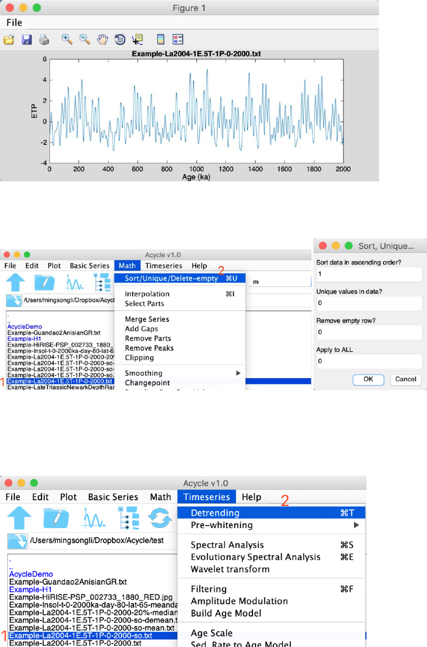
Acycle v1.0 User’s Guide Mingsong Li
- 64 -
Step 2: Data pre-processing
Since the data is not in ascending order. Here we’ll need sort data first.
Step 3: Detrending
Remove the mean value of the insolation series.
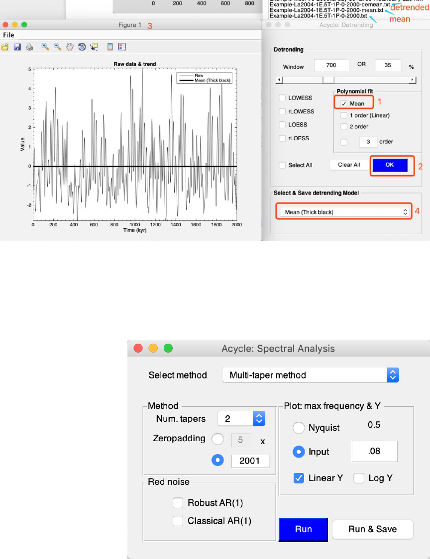
Acycle v1.0 User’s Guide Mingsong Li
- 65 -
Step 4: Power Spectral Analysis
Using the following settings:
Seven peaks in the 2 (@Num.tapers) MTM (multi-taper method) power spectrum are 405
kyr, 125 kyr, 95 kyr, 41 kyr, 23.7 kyr, 22.4 kyr, and 19.0 kyr.
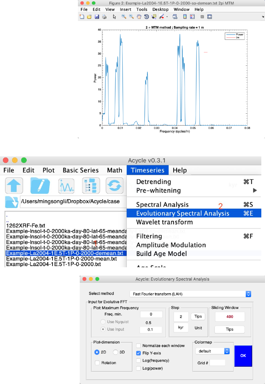
Acycle v1.0 User’s Guide Mingsong Li
- 66 -
Step 5: Evolutionary Spectral Analysis
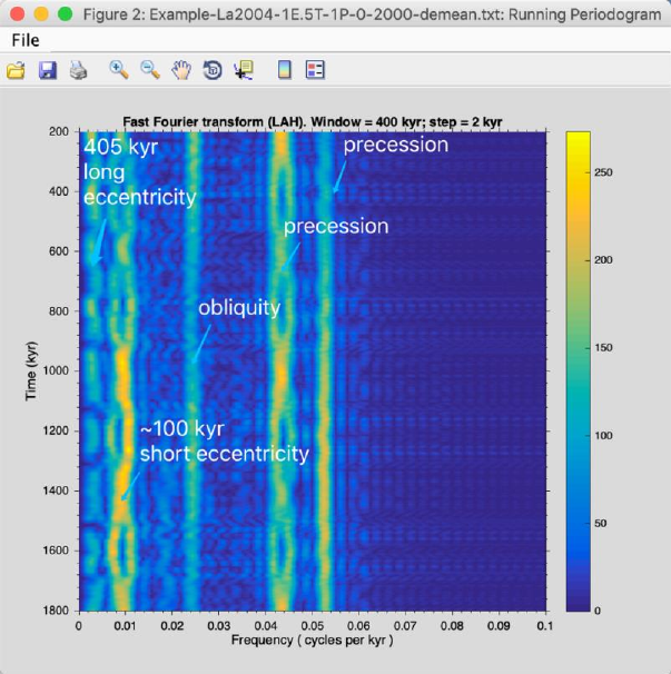
Acycle v1.0 User’s Guide Mingsong Li
- 67 -
This series is dominated by 405 kyr long eccentricity, ~100 kyr short eccentricity, 41 kyr
obliquity, 22 kyr and 19 kyr precession cycles.
Step 6: Wavelet transform
Using the following settings:
Seven peaks in the 2 (@Num.tapers) MTM (multi-taper method) power spectrum are 405
kyr, 125 kyr, 95 kyr, 41 kyr, 23.7 kyr, 22.4 kyr, and 19.0 kyr.
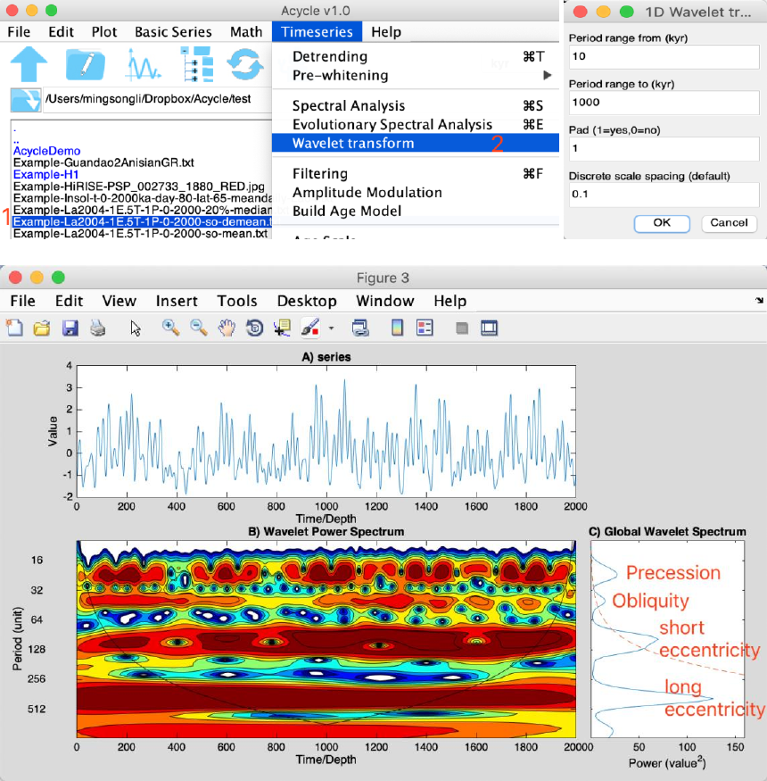
Acycle v1.0 User’s Guide Mingsong Li
- 68 -
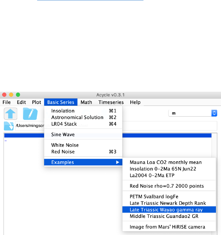
Acycle v1.0 User’s Guide Mingsong Li
- 69 -
Example #3: Carnian cyclostratigraphy
Section: Wayao section, Guizhou, South China
Age: middle Carnian
Lithology: The limestone beds of the Zhuganpo Formation displays patterns of variable
bed thicknesses and changing clay content within the limestones as reflected in relative
weathering resistance.
Proxy: These factors influence the natural gamma-ray signal with higher intensities
indicating higher average clay contents.
Target:
Cyclostratigraphic analysis of gamma ray series
Tool:
Acycle v0.3 (https://github.com/mingsongli/acycle).
Reference:
Zhang, Y., Li, M., Ogg, J.G., Montgomery, P., Huang, C., Chen, Z.-Q., Shi, Z., Enos, P.,
Lehrmann, D.J., 2015. Cycle-calibrated Magnetostratigraphy of middle Carnian from
South China: Implications for Late Triassic Time Scale and Termination of the Yangtze
Platform. Palaeogeography, Palaeoclimatology, Palaeoecology 436, 135-166.
Step 1. Load Data
Select: Basic Series → Examples → Late Triassic Wayao gamma ray.
The gamma ray data entitled “Example-WayaoCarnianGR0.txt” will be loaded and
displayed in the Acycle main window.
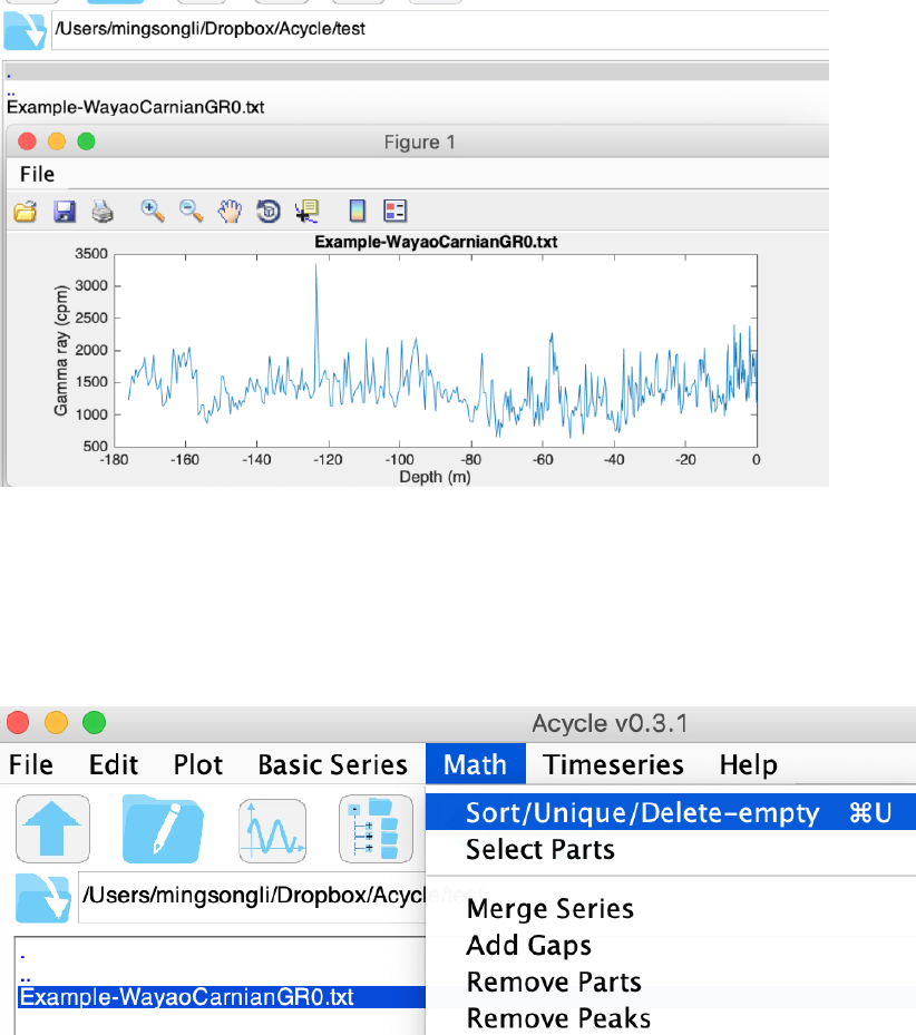
Acycle v1.0 User’s Guide Mingsong Li
- 70 -
Left click to select the data file and select Plot → Plot to plot the data. Double click the
data file to see the accepted format of Acycle software.
Step 2. Data Preparation
Acycle includes several toolboxes to facilitate data preparation. Users can sort data in
ascending order. Two or more values for the same time (or depth) may be averaged with
the "Unique" function.
Step 3. Interpolation
Stratigraphic depth or time series are typically irregularly spaced due to uncertain
timescales or difficulty in data collection. This necessitates interpolation to generate
uniformly spaced time (or depth) series.
Let’s look at the sampling rate plot first.
Select Plot → Sampling Rate.
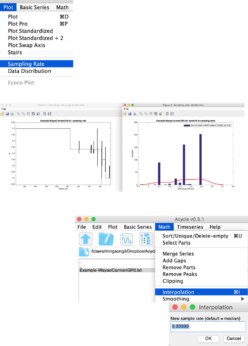
Acycle v1.0 User’s Guide Mingsong Li
- 71 -
You’ll see the sampling intervals of gamma ray data are irregularly spaced with a median
of 0.3333 and mean of 0.35341 (right up corner of figures below).
Math → Interpolation (or Ctrl + I). Then type the new sampling rate to interpolate.
I use a 0.33 m as a new sampling rate, Acycle will generate a uniformly-spaced file
entitled:
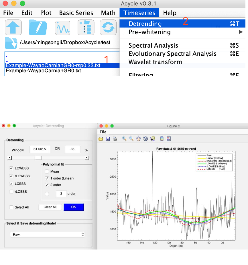
Acycle v1.0 User’s Guide Mingsong Li
- 72 -
“Example-WayaoCarnianGR0-rsp0.33.txt”.
Step 4. Detrending
Detrending is a key step in time series analysis. Removal of these long-term trends, or
detrending, is a critical step for power spectral analysis to ensure that data variability
oscillates about a zero mean, and to avoid power leakage from very low-frequency
components into higher frequencies of the spectrum.
Select the file; then select Timeseries → Detrending (or CTRL + T).
In the pop-up window, select window size, detrending method. Then click OK to see the
various trending.
Don’t close “Acycle: Detrending” window or “New figure” window. Now change
window size in the left panel, you will see the response in the right panel.
You will need to Select & Save detrending Model. I will choose an 80-m LOWESS trend
for the best fit of the data without removing too many cycles.
The Acycle main window now displays an “Example-WayaoCarnianGR0-rsp0.33-80-
LOWESS.txt” detrended file and a “***-LOWESStrend.txt” trend file.
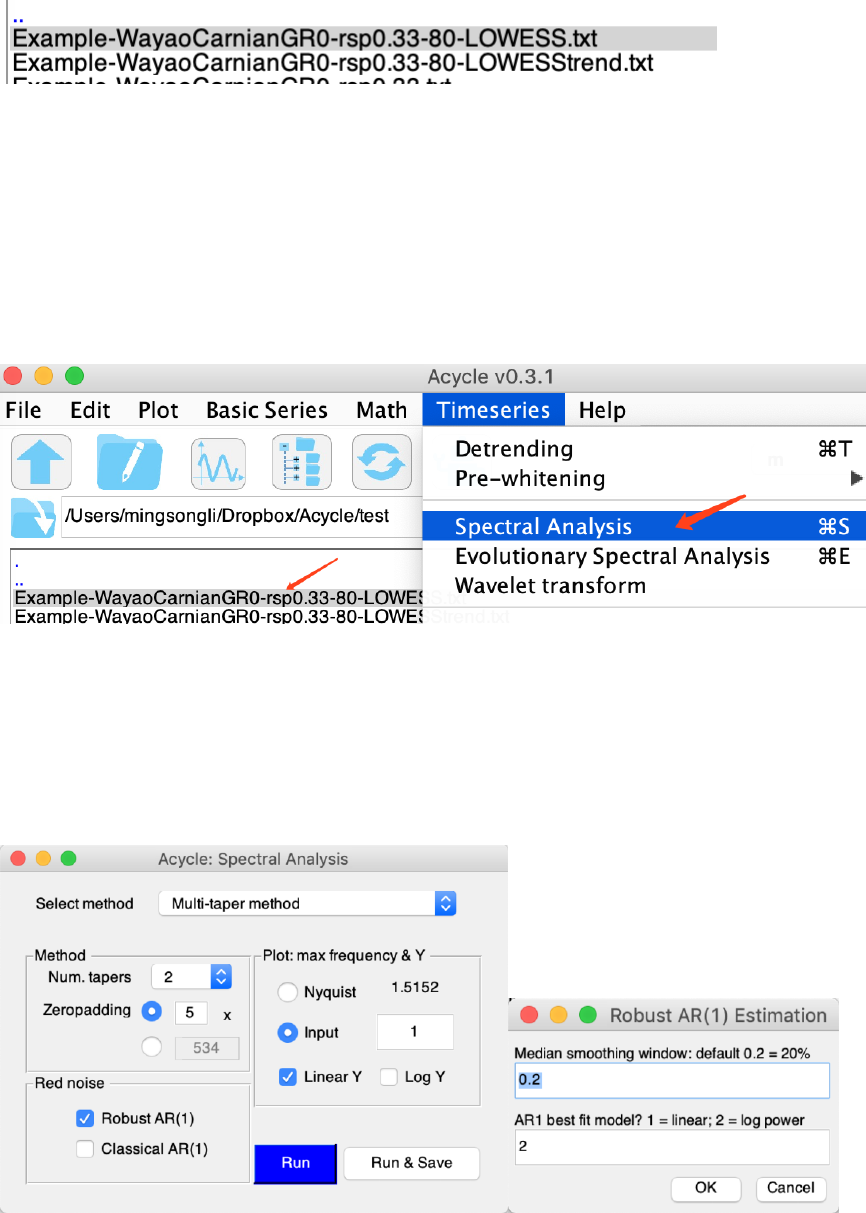
Acycle v1.0 User’s Guide Mingsong Li
- 73 -
Step 5. Power spectral analysis
Power spectral analysis has become a cornerstone in paleoclimatology and
cyclostratigraphy. Power spectral analysis evaluates the distribution of time series
variance (power) as a function of frequency. The primary use of power spectral analysis
is for the recognition of periodic or quasi-periodic components in a data series
Select the detrended file and choose “TimeSeries” → “Spectral Analysis”
Then choose Multi-taper method (MTM) with robust AR (1) red noise models.
Use the following setting:
2 pi MTM with a 5 times zero-padding (to increase frequency resolution).
The maximum frequency set to 1 cycle/m and use a linear Y plot.
Testing with a robust AR1 red noise model, then (right panel) using a 20% median
smoothing window and fitting to a log power of spectrum power.
You will have the MTM power spectrum with red noise models.
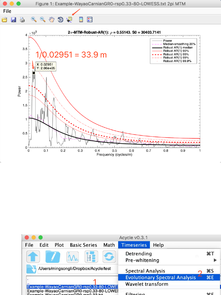
Acycle v1.0 User’s Guide Mingsong Li
- 74 -
Remember the period of a given cycle (frequency peak) is 1/frequency. For example, the
highest frequency peak (middle value) is 0.02951 cycles/m. The corresponding cycle is
1/0.02951 = 33.9 m.
2π MTM power spectrum of the gamma ray series is shown with 20% median-smoothed
spectrum, background AR(1) model, and 90%, 95%, 99%, and 99.9% confidence levels.
[If you count all peaks higher than 95% confidence levels, you will find the 33.9 m, 10 m,
7 m, 2.6 m, and 1.8 m cycles. The ratios of these cycles are 405 kyr, 119 kyr, 83 kyr, 31
kyr, and 21.5 kyr cycles].
Step 6. Evolutionary power spectral analysis
Select data and then select “TimeSeries” → Evolutionary Spectral Analysis
Use the following settings.
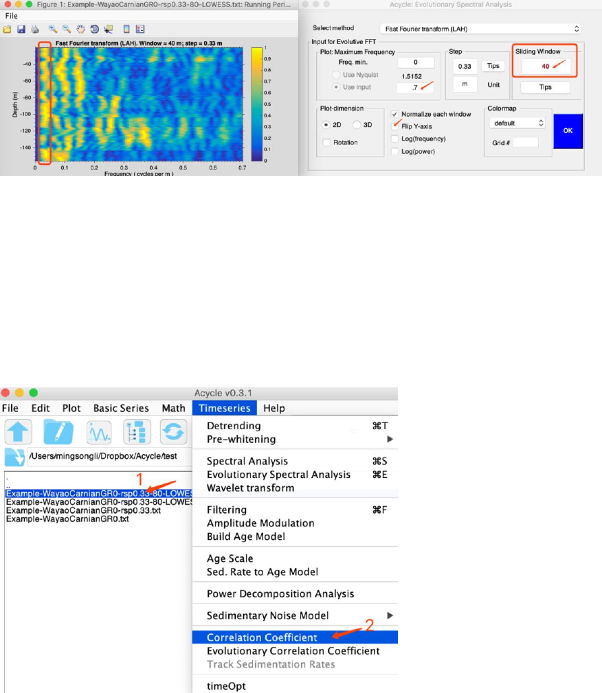
Acycle v1.0 User’s Guide Mingsong Li
- 75 -
A sliding window of 40 m (Why? The longest cycle is 33.9 m, this window should
be larger than 33.9 m. A 1.5-2 times of 33.9 m is good enough).
The maximum frequency is 0.7, this is to highlight low-frequency power.
Normalize each window: make spectral peaks in each window to be 1.
Flip Y-axis: because the first column of this data is increasing upward.
Then click ok to show results.
Don’t close these two windows. Now, you may change frequency limit, flip Y-axis,
change colormap to change the left window.
This figure tells me the dominated cycles of ~34 m is stable in frequency (period).
Therefore, the sedimentation rate is probably not variable (too much).
Step 7. Correlation coefficient
To estimate the most likely sedimentation rate. Select the detrended data, then click
“Timeseries” → Correlation coefficient.
Tell COCO the middle age of your data (~235 Ma). It doesn’t matter if this age has an
uncertainty, an uncertainty less than 2-5 Myr can be okay.
Tell the testing sedimentation rate range: from 1 to 30 cm/kyr, with a step of 0.1
It will test: 1, 1.1, 1.2, 1.3, ……. 29.8, 29.9, 30 cm/kyr.
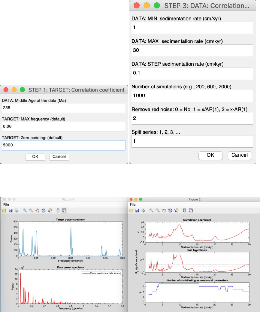
Acycle v1.0 User’s Guide Mingsong Li
- 76 -
Monte Carlo simulation: the number is 1000 (or 500) for an initial test. A 2000 (or more)
number is recommended for a publication purpose.
Split series: If the data set is very long, split series may use 2 or 3.
You will have the following figure and a log file saving all settings:
It tells the most likely sedimentation rate is ~10 cm/kyr, with a significance level of
0.1%. All seven orbital parameters are used in the estimation.
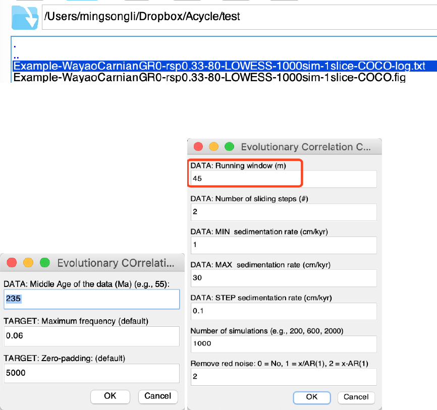
Acycle v1.0 User’s Guide Mingsong Li
- 77 -
Now using a 45 m window eCOCO analysis to track variable sedimentation rate.
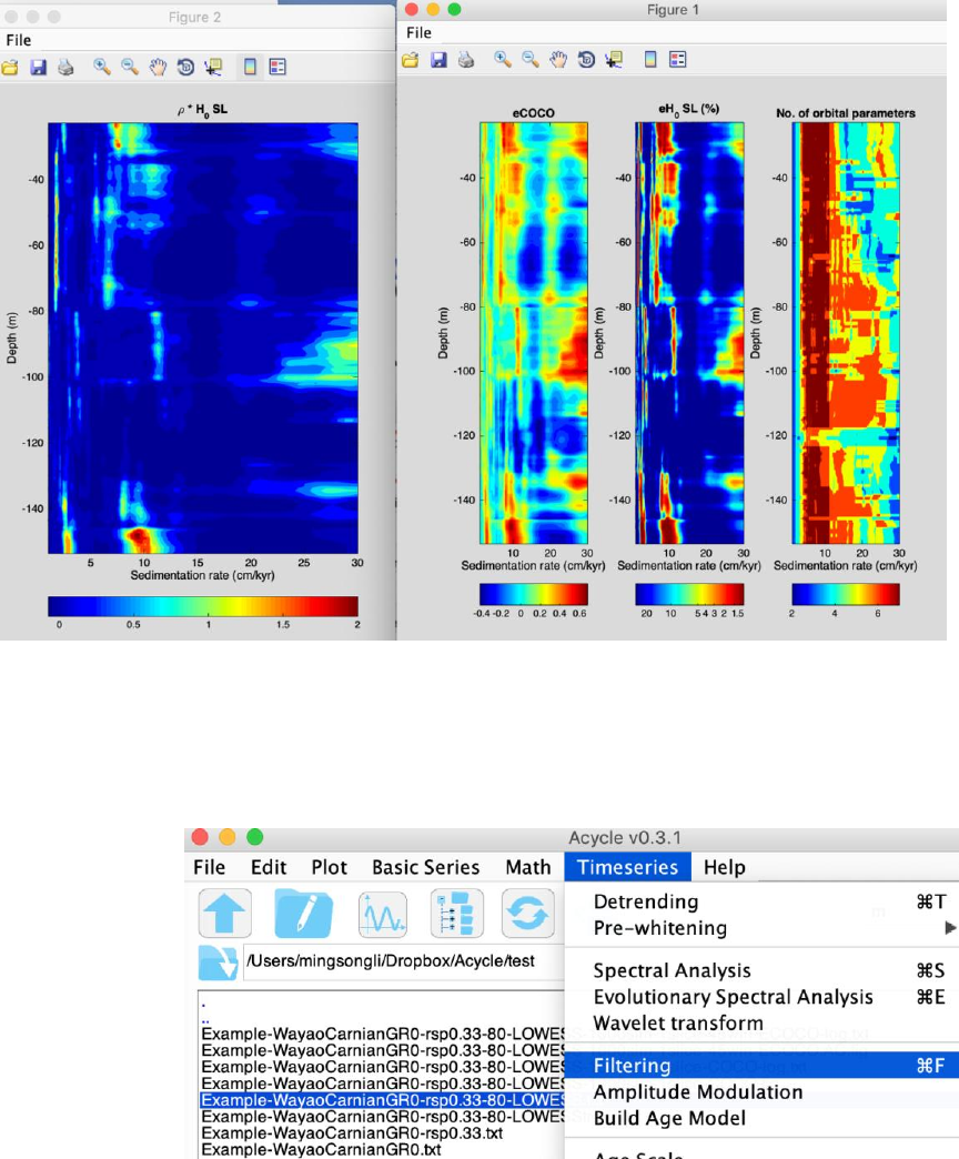
Acycle v1.0 User’s Guide Mingsong Li
- 78 -
Step 8. Filtering
Filters are also essential tools to aid in the isolation of specific frequency components in
the paleoclimate data series.
Select data, then “Timeseries” → Filtering
In the pop-up window
Select the center frequency, low frequency. Then select the Gaussian method. And “save
data” button.
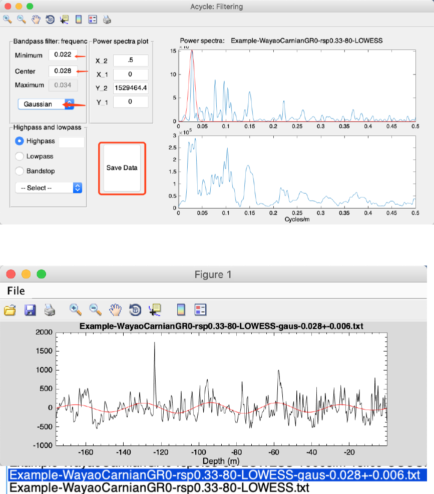
Acycle v1.0 User’s Guide Mingsong Li
- 79 -
You will see the filtered series and data in the Acycle main window.
Step 9. Age model and tuning
“Age Scale” toolbox in Acycle is useful to transform original data (usually in the depth
domain) to tuned data (usually in the time domain) when an age model file is available.
Assuming these 33.4 m cycles are 405 kyr cycles
Select “Example-WayaoCarnianGR0-rsp0.33-80-LOWESS-gaus-0.028+-0.006.txt”
And then Timeseries → Build Age Model
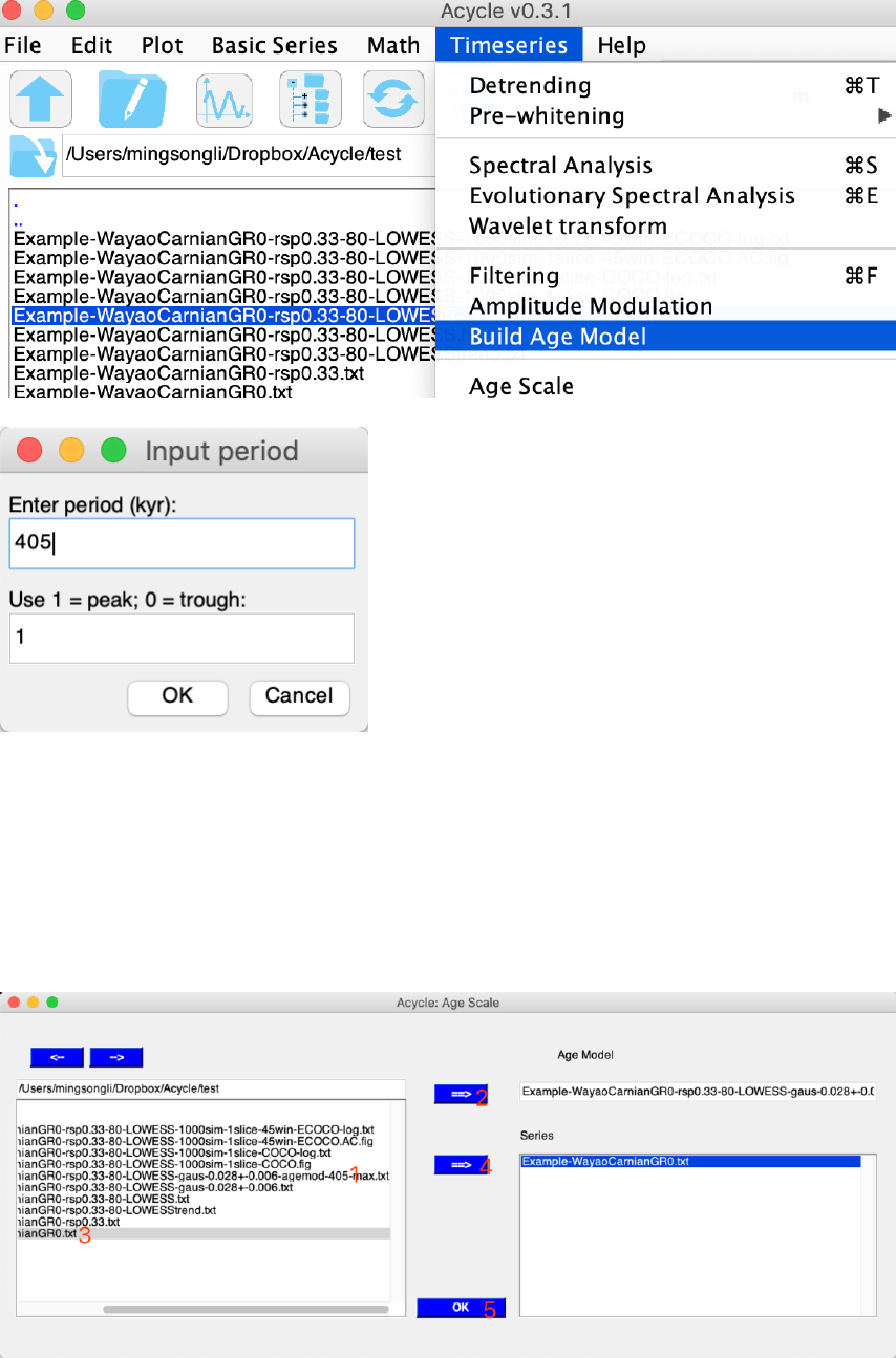
Acycle v1.0 User’s Guide Mingsong Li
- 80 -
Click OK, you will have an Age Model file:
Example-WayaoCarnianGR0-rsp0.33-80-LOWESS-gaus-0.028+-0.006-agemod-405-
max.txt
Timeseries → Age Scale
Select the age model file
And select files to be tuned, click OK.
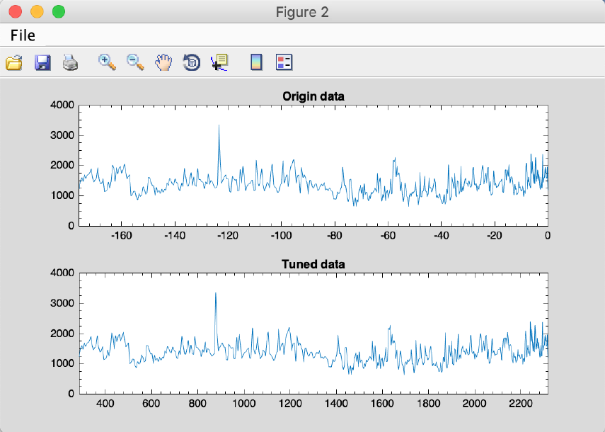
Acycle v1.0 User’s Guide Mingsong Li
- 81 -
Tuned data will be ready.
“Example-WayaoCarnianGR0-TD-Example-WayaoCarnianGR0-rsp0.33-80-LOWESS-
gaus-0.028+-0.006-agemod-405-max.txt”
Step 10. Repeat steps.
You can repeat Steps 3-6 and Step 8.

References
Berger, A., Loutre, M., Dehant, V., 1989. Influence of the changing lunar orbit on the
astronomical frequencies of pre‐Quaternary insolation patterns. Paleoceanography 4, 555-
564.
Charles, A.J., Condon, D.J., Harding, I.C., Pälike, H., Marshall, J.E.A., Cui, Y., Kump, L.,
Croudace, I.W., 2011. Constraints on the numerical age of the Paleocene-Eocene
boundary. Geochemistry, Geophysics, Geosystems 12.
Husson, D., 2014. MathWorks File Exchange: RedNoise_ConfidenceLevels,
http://www.mathworks.com/matlabcentral/fileexchange/45539-rednoise-
confidencelevels/content/RedNoise_ConfidenceLevels/RedConf.m.
Kodama, K.P., Hinnov, L., 2015. Rock Magnetic Cyclostratigraphy. Wiley-Blackwell.
Laskar, J., Fienga, A., Gastineau, M., Manche, H., 2011. La2010: a new orbital solution for the
long-term motion of the Earth. Astronomy & Astrophysics 532.
Laskar, J., Robutel, P., Joutel, F., Gastineau, M., Correia, A.C.M., Levrard, B., 2004. A long-
term numerical solution for the insolation quantities of the Earth. Astronomy &
Astrophysics 428, 261-285.
Li, M., Hinnov, L.A., Huang, C., Ogg, J.G., 2018a. Sedimentary noise and sea levels linked to
land–ocean water exchange and obliquity forcing. Nature communications 9, 1004.
Li, M., Huang, C., Hinnov, L., Chen, W., Ogg, J., Tian, W., 2018b. Astrochronology of the
Anisian stage (Middle Triassic) at the Guandao reference section, South China. Earth and
Planetary Science Letters 482, 591-606.
Li, M., Huang, C., Hinnov, L., Ogg, J., Chen, Z.-Q., Zhang, Y., 2016. Obliquity-forced climate
during the Early Triassic hothouse in China. Geology 44, 623-626.
Li, M., Kump, L.R., Hinnov, L.A., Mann, M.E., 2018c. Tracking variable sedimentation rates
and astronomical forcing in Phanerozoic paleoclimate proxy series with evolutionary
correlation coefficients and hypothesis testing. Earth and Planetary Science Letters 501,
165-179.
Lisiecki, L.E., Raymo, M.E., 2005. A Pliocene‐Pleistocene stack of 57 globally distributed
benthic δ18O records. Paleoceanography 20.
Lomb, N.R., 1976. Least-squares frequency analysis of unequally spaced data. Astrophysics and
Space Science 39, 447-462.
Mann, M.E., Lees, J.M., 1996. Robust estimation of background noise and signal detection in
climatic time series. Climatic Change 33, 409-445.
Meyers, S.R., 2015. The evaluation of eccentricity‐related amplitude modulation and bundling in
paleoclimate data: An inverse approach for astrochronologic testing and time scale
optimization. Paleoceanography.
Meyers, S.R., 2019. Cyclostratigraphy and the problem of astrochronologic testing. Earth-
Science Reviews 190, 190-223.
Olsen, P.E., Kent, D.V., 1996. Milankovitch climate forcing in the tropics of Pangaea during the
Late Triassic. Palaeogeography, Palaeoclimatology, Palaeoecology 122, 1-26.
Scargle, J.D., 1982. Studies in astronomical time series analysis. II-Statistical aspects of spectral
analysis of unevenly spaced data. The Astrophysical Journal 263, 835-853.
Thomson, D.J., 1982. Spectrum estimation and harmonic analysis. Proceedings of the IEEE 70,
1055-1096.
Acycle v1.0 User’s Guide Mingsong Li
- 83 -
Torrence, C., Compo, G.P., 1998. A practical guide to wavelet analysis. Bulletin of the American
Meteorological society 79, 61-78.
Waltham, D., 2015. Milankovitch Period Uncertainties and Their Impact On Cyclostratigraphy.
Journal of Sedimentary Research 85, 990-998.
Yao, X., Zhou, Y., Hinnov, L.A., 2015. Astronomical forcing of a Middle Permian chert
sequence in Chaohu, South China. Earth and Planetary Science Letters 422, 206-221.
Zeebe, R.E., 2017. Numerical Solutions for the orbital motion of the Solar System over the Past
100 Myr: Limits and new results. The Astronomical Journal 154, 193.
Zhang, Y., Li, M., Ogg, J.G., Montgomery, P., Huang, C., Chen, Z.-Q., Shi, Z., Enos, P.,
Lehrmann, D.J., 2015. Cycle-calibrated Magnetostratigraphy of middle Carnian from
South China: Implications for Late Triassic Time Scale and Termination of the Yangtze
Platform. Palaeogeography, Palaeoclimatology, Palaeoecology 436, 135-166.
