AGEPRO_V42_Reference_Manual AGEPRO V4.2 Reference Manual
User Manual:
Open the PDF directly: View PDF ![]() .
.
Page Count: 71

i
AGEPRO Reference Manual
Jon Brodziak
NOAA Fisheries
Pacific Islands Fisheries Science Center
Email: Jon.Brodziak@NOAA.GOV
Version 4.2
March 2018
Abstract
The AGEPRO reference manual describes the new version 4.2 model and software to
perform stochastic age-structured projections for an exploited age-structured fish stock.
The AGEPRO model can be used to quantify the probable effects of alternative harvest
scenarios by multiple fleets on an age-structured population over a given time horizon.
Primary outputs include the projected distribution of spawning biomass, fishing mortality,
recruitment, and landings by time period. This new version allows for multiple
recruitment models to account for alternative hypotheses about recruitment dynamics and
applies model-averaging to predict the distribution of realized recruitment given
estimates of recruitment model probabilities. The reference manual also describes the
logical structure of the projection model, including program inputs, outputs, structure and
usage. This includes three examples, which illustrate standard projection analyses,
projection analyses for stock rebuilding, and projection analyses to calculate annual catch
limits with specific probabilities of exceeding an overfishing level. Although all
reasonable efforts have been taken to ensure the accuracy and reliability of the AGEPRO
software and data, the National Oceanic and Atmospheric Administration and the U.S.
Government do not and cannot warrant the performance or results that may be obtained
by using this software or data.
1
Introduction
The AGEPRO model was initially developed in 1994 to determine optimal strategies to
rebuild a depleted fish stock. The model was reviewed at the May 1994 meeting of the
Northeast Fisheries Science Center Methods Working Group (Brodziak and Rago, 1994;
Brodziak et al. 1998). Subsequently, the model was applied to groundfish stocks at the
18th SARC (NEFSC 1994) to evaluate Amendment 5 harvest scenarios (NEFMC 1994)
and was applied again in 1995 to assist with Amendment 7 (NEFMC 1996). The
reference manual was prepared in 1997 to provide documentation and has been updated
since then to describe modifications to the model and software. The current program is
written in the C language to allow for dynamic array allocation and to achieve rapid
processing speeds.
The AGEPRO program can be used to perform stochastic projections of the abundance of
an exploited age-structured population over a given time horizon. The primary purpose of
the AGEPRO model is to produce management strategy projections that characterize the
sampling distribution of key fishery system outputs such as landings, spawning stock
biomass, population age structure, and fishing mortality from one or more fleets,
accounting for uncertainty in initial population estimates, future recruitment, and natural
mortality (Figure 1). The acronym “AGEPRO” derives from age-structured projections,
in contrast to size- or biomass-based projections for size- or biomass-structured models.
The user can evaluate alternative harvest scenarios by setting quotas or fishing mortality
rates in each year of the time horizon.
Three elements of uncertainty can be included in an AGEPRO projection: recruitment,
initial population size, and process error for population and fishery processes.
Recruitment is the primary stochastic element in the population model, where recruitment
is typically defined as the number of age-0 or age-1 fish entering the modeled population
at the beginning of each year in the time horizon. There are a total of fifteen stochastic
recruitment models that can be used for population projection. It is also possible to
simulate a deterministic recruitment trajectory (see recruitment model 3 below).
Initial population size is the second potential element of uncertainty for population
projection (Figure 1). To include this element, a distribution of initial population sizes
must be calculated a priori. This is typically done using bootstrapping, Markov chain
Monte carlo simulation, or other techniques in most age-structured assessments.
Alternatively, projections can be based on a single best point estimate with no uncertainty
in the initial population size.
The third element of uncertainty is process error in population and fishery processes. The
user can choose to simulate the following population and fishery processes at age through
time with a multiplicative lognormal process error with mean value equal to unity and a
constant coefficient of variation:
1. Natural mortality at age
2. Maturation fraction at age
3. Stock weight on January 1st at age
4. Spawning stock weight at age

2
5. Mean population weight at age
6. Fishery selectivity at age
7. Discard fraction at age
8. Catch weight at age
9. Discard weight at age
The simulated values of each of these processes can be stored in auxiliary data files for
the purpose of documenting projection results.
Age-Structured Population Model
A pooled-sex, age-structured population model is the basis for the AGEPRO model and
software. This model represents an iteroparous fish population whose abundance changes
due to fluctuations in recruitment and natural mortality as well as fishing mortality from
one or more fishing fleets. Population size at age changes continuously throughout the
year due to the concurrent forces of natural and fishing mortality. Recruitment (
R
,
number of age-r fish) to the population occurs at the beginning of each year (January 1st)
and is the first element in the population size at age vector (Table 1).
Population Abundance, Survival, and Spawning Biomass
The AGEPRO model calculates the number of fish alive within each age class of the
population through time. Let Y denote the number of years in a projection where t
indexes time for 1,2,...tY. The maximum number of years in the projection is a
dynamic variable specified by the user and constrained by the amount of computer
memory. The minimum or youngest age class comprises the recruits and the age of
recruitment is age 0r. The oldest age class is a plus-group which consists of all fish
that are at least as old as the plus group age ( A). The maximum number of age classes is
100, including the plus group. For each age class, the number of fish alive at the
beginning of each calendar year (January 1st) is
j
Nt where j indexes age class and t
indexes year. The number of fish in the plus group is
A
Nt
which accounts for the
number of fish that are age-A or older at the beginning of year t. Given this, the
population abundance at the beginning of year t is the vector
Nt with
R
t used as an
alternate notation to emphasize that a recruitment submodel is needed to stochastically
generate recruitment through time horizon
(1)
1
2
r
r
A
Rt
Nt
Nt N t
Nt

3
Population survival at age from year 1t to year t is calculated using instantaneous
fishing and mortality rates at age. To describe annual survival through mortality, let
a
M
t denote the instantaneous natural mortality rate on age group a and let
a
Ft
denote the instantaneous fishing mortality rate for age-a fish in year t where
a
Ft is the
sum of fleet-specific fishing mortalities at age a. Population size at age in year t for age
classes indexed by 1artoA is given by
(2)
-1 -1
11
11aa
M
tFt
aa
Nt N t e
Similarly, population size at age in year t for the plus group of fish age-A and older is
given by
(3)
11
11 1 1
1
11
AA A A
M
tFt MtFt
AA A
Nt Nt e N t e
where survival for the plus-group involves an age-A and an age-(A-1) component.
Incoming recruitment is determined through a stochastic process that is either dependent
or independent of spawning biomass in year t (see Stock-Recruitment Relationship
below).
Annual spawning biomass
S
B
t is calculated from the population size vector
Nt and total mortality rates as well as information on sexual maturity and weight at
age. The age-specific natural mortality rate is
a
M
t. To describe annual survival, let
a
F
t be the instantaneous fishing mortality rate for age-a fish in year t where
a
F
t is
the sum of fleet-specific fishing mortalities at age
,ava
v
Ft F t. Further, let
,mature a
Pt denote the average fraction of age-a fish that are sexually mature in year t and
let
,Sa
Wt
denote the average spawning weight of an age-a fish in year t. Last, let
Frac
Z
t denote the proportion of total mortality that occurs from January 1st to the mid-
point of the spawning season in year t. Given this, population size at the midpoint of the
spawning season in year t
S
Nt is obtained by applying instantaneous natural and
fishing mortality rates that occur prior to the spawning season to the population vector at
the beginning of the year,
Nt.
(4)
22
33
() () ()
() () ()
1
() () ()
2
() () ()
Frac r r
Frac
Frac
Frac A A
ZtMtFt
r
ZtMtFt
r
ZtMtFt
Sr
ZtMtFt
A
Nte
Nte
Nt Nte
Nte

4
As a result, the amount of spawning biomass in year t is the sum of the weight of the
mature fish alive at the midpoint of the spawning season
(5)
() () ()
,, Frac a a
A
Z
tM t Ft
S S a mature a a
ar
Bt W tP tNte
Catch, Landings, and Discards
The fishery catch depends on the fraction of the population that is vulnerable to harvest
or the exploitable stock size. Catch at age by fleet (fleets are indexed by v) is determined
by the Baranov catch equation (e.g., Quinn and Deriso 1999). The catch of age-a fish in
year t by fleet v is
,va
Ct
(6)
,
,
,
,
1ava
Mt F t
va
va a
ava
Ft
Ct e Nt
Mt F t
To account for age-specific discarding of fish, let
,,vDa
Pt
be the proportion of age-a fish
that are discarded by fleet v in year t, and let
,,vLa
Wt and
,,vDa
Wt be the average
weight at age-a in year t for landed and discarded fish, respectively. Then, if discarding is
included in the projections, the total landed weight of fish caught by fleet v in year t,
denoted by
v
Lt, is
(7)
,,,,,
1
A
vvavDavLa
ar
Lt C t P t W t
Similarly, the total weight of discarded fish in year t, denoted by
v
Dt, is
(8)
,,, ,,
A
vvavDavDa
ar
Dt C tP tW t
Population Harvest
Population harvest is set in each year in the projection time horizon by setting the harvest
index
I
t. There are two options for determining the level of population harvest in each
year of the time horizon: these are the fishing mortality and the quota options. Under the
fishing mortality option, the user-input fishing mortality rate determines the harvest level
(i.e., effort-based management). Under the quota option, the user-input landings quota
(i.e., catch-based management). These two harvest options can be combined in any order
within a given projection time horizon where, for example, effort-based management is
applied in some years and quota-based management in the other years. In this case, the
user sets a binary harvest index
I
t to determine the harvest option for each year in the

5
projection time horizon. If
I
t=1, quota-based harvest control is applied in year t; else
if
I
t=0, effort-based harvest control is applied. A mixture of quotas and effort-based
harvest can be useful when projecting forward from a previous assessment to the present
when only catch is available for the intervening years.
When effort-based management is applied, catch at age is determined by setting
,va
Ft
by fleet for each age class. In this case, the fishing mortality rate on age-a fish in year t is
the product of the fully-selected fishing mortality rate by fleet, denoted by
v
Ft, and the
fleet- and age-specific fishery selectivity of age-a fish, denoted by
,va
St
as
(9)
,,va v v a
Ft FtS t
Landings and discards, if applicable, are then determined from
,va
Ft. When quota-
based management is applied, however, the
v
F
t that would yield the landings quota
must be determined numerically.
Under quota-based management, the landings quota by fleet in year t, denoted by
v
Qt,
will translate into a variety of effective fishing mortality rates depending on population
size, fishery selectivity, and discarding, if applicable.
Ignoring the fleet index and time dimension for simplicity, a landings quota Q can be
expressed as a function of F,
QLF, where F is the fully-selected fishing mortality
and L is the landings expressed as a function of F. To see this result, observe that the
catch of age-a fish can be expressed as a function of F
(10)
1aa
Mt FSt
a
a a
aa
FS t
CF e Nt
Mt FSt
As a result, landings can also be expressed as a function of F
(11)
,,
1
A
aDaLa
ar
LF C F P t W t
The fully-selected fishing mortality which satisfies the equation
QLFcan be found
using a robust root-finding algorithm and we apply the bisection method, that previous
versions applied Newton’s method. Quotas which exceed the exploitable biomass of the
population are defined as being infeasible and simulations with infeasible quotas are also
infeasible.

6
Initial Population Abundance
There are two ways to set the initial population abundance, defined as the vector of the
absolute number of fish alive on January 1st of the first year (t=1) of the projection time
horizon
1N. The primary option is to use a set of samples from the distribution of the
estimator of
1N. This approach explicitly incorporates uncertainty in the estimate of
initial population abundance into the projections. Under this option, either frequentist
methods such as bootstrapping or Bayesian methods such as Markov Chain Monte Carlo
simulation can be applied to determine the sampling distribution of the estimator of
1N. The secondary option is to ignore uncertainty in the estimator of initial population
abundance and use a single best estimate for the value of
1N. In this case, there is no
uncertainty in the point estimate of
1Nused in the projections.
The primary option uses a set of B initial population vectors, denoted by
(*) (1) (2) ( )
1 1 , 1 ,..., 1
B
NNN N, for stochastic projections. In this case, the set of
B values are random samples from the distribution of the estimator of
1Ngenerated by
the assessment model or other means. Given this, stochastic projection can be used to
characterize the sampling distribution of key fishery outputs accounting for the
uncertainty in the estimate of the initial population size. For each initial condition
() 1
b
N, a set of simulations will be performed using the specified harvest strategy. Since
dynamic array allocation is used to dimension the set of initial population vectors, the
user may choose to input a large number of initial population vectors (B>103) within the
practical constraint of available computer memory.
The secondary option is to use a single point estimate of
1Nfor projection. In this case,
one estimate of population abundance is assumed to characterize the initial state of the
population. Since there is no uncertainty in the initial state of the population this option
allows one to characterize the sampling distribution of key fishery outputs due to
uncertainty in recruitment or other variables subject to process errors.
Regardless of which initial population abundance option is used, the user must also
specify the units of the initial population size vector taken from the assessment model. In
particular, the initial population abundance vector is specified and input in relative
abundance units along with a conversion coefficient N
k to compute from relative units to
absolute numbers, where the initial population abundance replicate is calculated as the
conversion coefficient times the relative abundance vector via
() ()
() () () ()
1 1 ,..., 1 1 1 ,..., 1
bb
bb b b
rAN NrNA
NN Nknknkn
Retrospective Adjustment
One can adjust the initial population numbers at age vector N(1) to reflect a retrospective
pattern in calculating these estimates. In this case, the user must determine an appropriate
vector of retrospective bias-correction coefficients, denoted by C, to apply to the vector

7
N(1). These multiplicative bias-correction coefficients may be age-specific or constant
across age classes. The bias-corrected initial population vector N*(1) is calculated from
the element-wise product of N(1) and C as
(12)
*1 (1),..., (1),..., (1) T
rr aa AA
NCNCNCN
Note that the bias-correction coefficients are applied to all initial population vectors. If
the bias-correction coefficients are determined to be constant across age classes then C =
(C, C, ..., C)T and the bias-corrected initial population vector is
(13)
*1 (1),..., (1),..., (1) 1
T
raA
NCNCNCN CN
The bias-correction coefficients are only applied in the first time period of the projection
time horizon to reflect uncertainty in the estimated population size at age. Mohn (1999)
provides an informative presentation of the retrospective problem in sequential
population analysis.
Stock-Recruitment Relationship
In general, the relationship between spawning stock
S
B
and recruitment R is highly
variable owing to intrinsic variability in factors governing early life history survival and
to measurement error in the estimates of recruitment and the spawning biomass that
generated it. The stock-recruitment relationship ultimately defines the sustainable yield
curve and its expected variability assuming that the stochastic processes of growth,
maturation, and natural mortality are density-independent and stationary throughout the
time horizon. Quinn and Deriso (1999) provide a useful discussion of stock-recruitment
models, renewal processes, and sustainable yield. Note that the assumed stock-
recruitment relationship does not affect the initial population abundance at the beginning
of the time horizon (see Initial Population Abundance).
A total of twenty stochastic recruitment models are available for population projection in
the AGEPRO software. Thirteen of the recruitment models are functionally dependent on
BS while seven do not depend on spawning biomass. Five of the recruitment models have
time-dependent parameters, eleven are time-invariant, and four may include time as a
predictor, or not. The user is responsible for the choice and parameterization of the
recruitment models. A description of each of the recruitment models follows. Important:
note that the absolute units for recruitment R are numbers of age-r fish, while for
spawning biomass S
B
, the absolute units are kilograms of spawning biomass in each of
the recruitment models below.

8
Model 1. Markov Matrix
A Markov matrix approach to modeling recruitment may be useful when there is
uncertainty about the functional form of the stock-recruitment relationship. A Markov
matrix contains transition probabilities that define the probability of obtaining a given
level of recruitment given that S
B
was within a defined interval range. In particular, the
distribution of recruitment is assumed to follow a multinomial distribution conditioned on
the spawning biomass interval or spawning state of the stock. The Markov matrix model
depends on spawning biomass and is time-invariant.
An empirical approach to estimate a Markov matrix uses stock-recruitment data to
determine the parameters of a multinomial distribution for each spawning biomass state.
In this case, matrix elements can be empirically determined by counting the number of
times that a recruitment observation interval lies within a given spawning biomass state,
defined by an interval of spawning biomass, and normalizing over all spawning states. To
do this, assume that there are K recruitment values and J spawning biomass states. The
spawning biomass states are defined by disjoint intervals on the spawning biomass axis
(14)
1,1 ,1, ,1
0, 1,..., 2 , ,
S j Sj Sj J SJ
I B and for j J I B B and I B
where the spawning biomass values ,Sj
B are the input endpoints of the disjoint intervals
of categories of spawning biomass (e.g., high, medium, low). Note that the spawning
biomass intervals are defined by the cut points ,Sj
B. The conditional probability of
realizing the kth recruitment value given that observed spawning biomass ,S Observed
B is in
the jth interval is ,
j
k
P
. Here ,
j
k
P
is the element in the jth row and kth column of the Markov
matrix ,
j
k
PP
of conditional recruitment probabilities with elements
(15)
,,
Pr |
j
k k S Observed j
PRBI
These individual conditional probabilities can be estimated by the computing the number
of points in the stock recruitment data set that fall within a selected recruitment
1,
kk
OO
range conditioned on the spawning biomass interval
j
I
. If ,
j
k
x
represents the number of
stock-recruitment observations in cell
j
k
I
O and there is at least one observation in
spawning state j, then the empirical maximum likelihood estimate of ,
j
k
P
is
(16)
,
,
Pr | jk
kSj
j
k
k
x
RO B I
x
Here ,0
jk
P and ,
1
1
jk
k
P
.

9
Up to 25 recruitment values and up to 10 spawning biomass states can be used in the
Markov matrix model. For each spawning biomass interval, the user needs to specify the
conditional probabilities of realizing the expected recruitment level, e.g., the ,
j
k
P
. Given
the conditional probabilities ,
j
k
P
, simulated values of
Rare generated by randomly
sampling the conditional distribution
Pr |
kS j
R
tROBtI through time.
Model 2. Empirical Recruits Per Spawning Biomass Distribution
For some stocks, the distribution of recruits per spawner may be independent of the
number of spawners over the range of observed data. The recruitment per spawning
biomass
/S
R
B model randomly generates recruitment under the assumption that the
distribution of the / S
R
B ratio is stationary and independent of stock size. The empirical
recruits per spawning biomass distribution model depends on spawning biomass and is
time-invariant.
To describe this nonparametric approach, let t
S be the / S
R
B ratio for the tth stock
recruitment data point assuming age-1 recruitment
(17)
1
t
S
Rt
SBt
and let
S
R
be the th
S element in the ordered set of t
S. The empirical probability density
function for
S
R
, denoted as
S
gR , assigns a probability of 1/T to each value of / S
R
B
where T is the number of stock-recruitment data points. Let
S
GR denote the
cumulative distribution function (cdf) for
S
R
. Set the values of G at the minimum and
maximum observed
S
R
to be
min 0GR and
max 0GR so that the cdf of
S
R
can be
written as
(18)
1
1
S
s
GR T
Random values of
S
R
can be generated by applying the probability integral
transform to the empirical cdf. To do this, let U be a uniformly distributed random
variable on the interval [0,1]. The value of
S
R
corresponding to a randomly chosen value
of Uis determined by applying the inverse function of the cdf
S
GR . In particular, if U
is an integer multiple of
1/ 1T so that
/1UsT then
1
S
RGU
. Otherwise
S
R
can be obtained by linear interpolation when Uis not a multiple of
1/ 1T.

10
In particular, if
1/ 1 / 1sTUsT
, then
S
R
is interpolated between S
R
and
1S
R
as
(19)
1
11
11 1
SS
SS
ss s
TT
URR
RR T
Solving for
S
R
as a function of Uyields
(20)
1
1
11
SSS S
s
RTRRU R
T
where the interpolation index s is determined as the greatest integer in
11UT
. Given the value of
S
R
, recruitment is generated as
(21)
11
SS
Rt N t B t R
The AGEPRO program can generate stochastic recruitments using model 2 with up to
100 stock-recruitment data points.
Model 3. Empirical Recruitment Distribution
Another simple model for generating recruitment is to draw randomly from the
observed set of recruitments
1 , 2 ,...,RR R RT .This may be a useful approach
when the recruitment has randomly fluctuated about its mean and appears to be
independent of spawning biomass over the observed range of data. In this case, the
recruitment distribution may be modeled as a multinomial random variable where the
probability of randomly choosing a particular recruitment is 1/T given T observed
recruitments. The empirical recruitment distribution model does not depend on spawning
biomass and is time-invariant.
In this model, realized recruitment
R is simulated from the empirical recruitment
distribution as
(22)
1
Pr , 1,2,...,
R
Rt fort T
T
The empirical recruitment distribution approach is nonparametric and assumes that future
recruitment is totally independent of spawning stock biomass. When current levels of
S
B
are near the midrange of historical values this assumption seems reasonable. However, if
contemporary S
B
values are near the bottom of the range, then this approach could be
overly optimistic, for it assumes that all historically observed recruitment levels are

11
possible, regardless of
S
B
. The AGEPRO program allows up to 100 observed
recruitments for random sampling. Note that the empirical recruitment distribution model
can be used to make deterministic projections by specifying a single observed recruitment.
Model 4. Two-Stage Empirical Recruits Per Spawning Biomass Distribution
The two-stage recruits per spawning biomass model is a direct generalization of the R/BS
model where the spawning stock of the population is categorized into “low” and “high”
states. The two-stage empirical recruits per spawning biomass distribution model depends
on spawning biomass and is time-invariant.
In this model, there is an / S
R
Bdistribution for the low spawning biomass state and an
/S
R
Bdistribution for the high spawning biomass state. Let Low
G be the cdf and let Low
T
be the number of / S
R
Bvalues for the low S
B
state. Similarly, let High
G be the cdf and let
High
T be the number of / S
R
Bvalues for the high
S
B
state. Further, let *
S
B denote the
cutoff level of
S
B
such that, if *
SS
BB, then
S
B
falls in the high state. Conversely if
*
SS
BBthen S
B
falls in the low state. Recruitment is stochastically generated from Low
G
or High
Gusing equations (20) and (21) dependent on the S
B
state. The AGEPRO program
can generate stochastic recruitments using the two-stage model with up to 100 stock-
recruitment data points per
S
B
state.
Model 5. Beverton-Holt Curve with Lognormal Error
The Beverton-Holt curve (Beverton and Holt 1957) with lognormal errors is a parametric
model of recruitment generation where survival to recruitment age is density dependent
and subject to stochastic variation. The Beverton-Holt curve with lognormal error model
depends on spawning biomass and is time-invariant.
The Beverton-Holt curve with lognormal error generates recruitment as
(23)
2
1
(1)
~0,, ,
w
S
S
wR SBS
bt
rt e
bt
where w N R t c r t and B t c b t
The stock-recruitment parameters
,
, and 2
w
and the conversion coefficients for
recruitment R
c and spawning stock biomass B
c are specified by the user. Here it is
assumed that the parameter estimates for the Beverton-Holt curve have been estimated in
relative units of recruitment
rt and spawning biomass
S
bt which are converted to
absolute values using the conversion coefficients. Note that the absolute value of
recruitment is expressed as numbers of fish, while for spawning biomass, the absolute
value is expressed as kilograms of
S
B
. For example, if the stock-recruitment curve was

12
estimated with stock-recruitment data that were measured in millions of fish and
thousands of metric tons of
S
B
, then R
c =106 and B
c =106. It may be important to
estimate the parameters of the stock-recruitment curve in relative units to reduce the
potential effects of roundoff error on parameter estimates. It is important to note that the
expected value of the lognormal error term is not unity but is 2
1
exp 2w
. Therefore, in
order to generate a recruitment model that has a lognormal error term that is equal to 1,
one needs to multiply the parameter
by 2
1
exp 2w
. This bias correction applies
when the lognormal error used to fit the Beverton-Holt curve has a log-scale error term
w with zero mean.
The Beverton-Holt curve is often reparameterized in a modified form with parameters for
steepness h, unfished recruitment 0
R
, and unfished spawning biomass 0
B
. The
modified Beverton-Holt curve produces 0
hR recruits when 0
0.2
S
B
B and has the
form
(24)
0
0
4
151
S
S
hR B
RBhBh
The parameters
and
can be expressed as functions of the parameters of the
modified Beverton-Holt curve as
(25)
00
0
0
44
51 51
hR h
B
hBh
R
and
(26)
1
0
00
1
1
51 4
Bh
R
Bh
h
Thus, parameter estimates for the modified curve can be used to determine the Beverton-
Holt parameters for the AGEPRO program.
Model 6. Ricker Curve with Lognormal Error
The Ricker curve (Ricker 1954) with lognormal error is a parametric model of
recruitment generation where survival to recruitment age is density dependent and subject
to stochastic variation. The Ricker curve with lognormal error model depends on
spawning biomass and is time invariant.
The Ricker curve with lognormal error generates recruitment as

13
(27)
1
2
1
~0,, ,
S
bt w
S
wR SBS
rt b t e e
where w N R t c r t and B t c b t
The stock-recruitment parameters
,
, and 2
w
and the conversion coefficients for
recruitment R
c and spawning stock biomass B
c are specified by the user. Here it is
assumed that the parameter estimates for the Beverton-Holt curve have been estimated in
relative units of recruitment
rt and spawning biomass
S
bt which are converted to
absolute values using the conversion coefficients. It is important to note that the expected
value of the lognormal error term is not unity but is 2
1
exp 2w
. To generate a
recruitment model that has a lognormal error term that is equal to 1, premultiply the
parameter
by 2
1
exp 2w
; this mean correction applies when the lognormal error
used to fit the Ricker curve has a log-scale error term w with zero mean.
Model 7. Shepherd Curve with Lognormal Error
The Shepherd curve (Shepherd 1982) with lognormal error is a parametric model of
recruitment generation where survival to recruitment age is density dependent and subject
to stochastic variation. The Shepherd curve with lognormal error model depends on
spawning biomass and is time-invariant.
The Shepherd curve with lognormal error generates recruitment as
(28)
2
1
1
1
~0,, ,
w
S
S
wR SBS
bt
rt e
bt
k
where w N R t c r t and B t c b t
The stock-recruitment parameters
,
, k, and 2
w
and the conversion coefficients for
recruitment R
c and spawning stock biomass B
c are specified by the user. Here it is
assumed that the parameter estimates for the Beverton-Holt curve have been estimated in
relative units of recruitment
rt and spawning biomass
S
bt
which are converted to
absolute values using the conversion coefficients. It is important to note that the expected
value of the lognormal error term is not unity but is 2
1
exp 2w
. To generate a
recruitment model that has a lognormal error term that is equal to 1, premultiply the

14
parameter
by 2
1
exp 2w
; this mean correction applies when the lognormal error
used to fit the Ricker curve has a log-scale error term w with zero mean.
Model 8. Lognormal Distribution
The lognormal distribution provides a parametric model for stochastic recruitment
generation. The lognormal distribution model does not depend on spawning biomass and
is time-invariant.
The lognormal distribution generates recruitment as
(29)
2
log( ) log( )
~,
w
rr R
rt e
where w N and R t c r t
The lognormal distribution parameters
log r
and
2
log r
as well as the conversion
coefficient for recruitment R
c are specified by the user. It is assumed that the parameters
of the lognormal distribution have been estimated in relative units
rt and then
converted to absolute values with the conversion coefficients.
Model 9. Time-Varying Empirical Recruitment Distribution
This model has been deprecated. The time-varying empirical recruitment can be fully
implemented using model 3.
Model 10. Beverton-Holt Curve with Autocorrelated Lognormal Error
The Beverton-Holt curve with autocorrelated lognormal errors is a parametric model of
recruitment generation where survival to recruitment age is density dependent and subject
to serially-correlated stochastic variation. The Beverton-Holt curve with autocorrelated
lognormal error model depends on spawning biomass and is time-dependent.
The Beverton-Holt curve with autocorrelated lognormal error generates recruitment as
(30)
2
1
1
(1)
~0,,
,
t
S
S
tt t t w
RSBS
bt
rt e
bt
where w with w N
R
t c r t and B t c b t

15
The stock-recruitment parameters
,
,
, 0
, and 2
w
and the conversion coefficients
for recruitment R
c and spawning stock biomass B
c are specified by the user. The
parameter 0
is the log-scale residual for the stock-recruitment fit in the time period prior
to the projection. If this value is not known, the default is to set 0
=0.
Model 11. Ricker Curve with Autocorrelated Lognormal Error
The Ricker curve with autocorrelated lognormal error is a parametric model of
recruitment generation where survival to recruitment age is density dependent and subject
to serially correlated stochastic variation. The Ricker curve with autocorrelated
lognormal error model depends on spawning biomass and is time-dependent.
The Ricker curve with autocorrelated lognormal error generates recruitment as
(31)
(1)
2
1
(1)
~0,,
,
St
bt
S
tt t t w
RSBS
rt b t e e
where w with w N
R
t c r t and B t c b t
The stock-recruitment parameters
,
,
, 0
, and 2
w
and the conversion coefficients
for recruitment R
c and spawning stock biomass B
c are specified by the user. The
parameter 0
is the log-scale residual for the stock-recruitment fit in the time period prior
to the projection. If this value is not known, the default is to set 0
=0.
Model 12. Shepherd Curve with Autocorrelated Lognormal Error
The Shepherd curve with autocorrelated lognormal error is a parametric model of
recruitment generation where survival to recruitment age is density dependent and subject
to serially-correlated stochastic variation. The Shepherd curve with autocorrelated
lognormal error model depends on spawning biomass and is time-dependent.
The Shepherd curve with autocorrelated lognormal error generates recruitment as
(32)
2
1
1
1
1
~0,,
,
t
S
S
tt t t w
RSBS
bt
rt e
bt
k
where w with w N
R
t c r t and B t c b t

16
The stock-recruitment parameters
,
,k,
, 0
, and 2
w
and the conversion
coefficients for recruitment R
c and spawning stock biomass B
c are specified by the user.
The parameter 0
is the log-scale residual for the stock-recruitment fit in the time period
prior to the projection. If this value is not known, the default is to set 0
=0.
Model 13. Autocorrelated Lognormal Distribution
The autocorrelated lognormal distribution provides a parametric model for stochastic
recruitment generation with serial correlation. The autocorrelated lognormal distribution
model does not depend on spawning biomass and is time-dependent.
The autocorrelated lognormal distribution is
(33)
2
1 log( ) log( )
~,,
t
r
tt t t rr
Rr
nt e
where w with w N
and R t c n t
The lognormal distribution parameters
log r
,
2
log r
,
, and 0
as well as the conversion
coefficient for recruitment R
c are specified by the user. It is assumed that the parameters
of the lognormal distribution have been estimated in relative units
rt and then
converted to absolute values with the conversion coefficient.
Model 14. Empirical Cumulative Distribution Function of Recruitment
The empirical cumulative distribution function of recruitment can be used to
randomly generates recruitment under the assumption that the distribution of R is
stationary and independent of stock size. The empirical cumulative distribution function
of recruitment model does not depend on spawning biomass and is time-invariant.
To describe this nonparametric approach, let
S
R
denote the th
S element in the ordered set
of observed recruitment values. The empirical probability density function for
S
R
,
denoted as
S
gR , assigns a probability of 1/T to each value of
R
twhere T is the
number of stock-recruitment data points. Let
S
GR denote the cumulative distribution
function (cdf) for
S
R
. Set the values of G at the minimum and maximum observed
S
R
to
be
min 0GR and
max 0GR so that the cdf of
S
R
can be written as
(34)
1
1
S
s
GR T

17
Random values of
S
R
can be generated by applying the probability integral
transform to the empirical cdf. To do this, let U be a uniformly distributed random
variable on the interval [0,1]. The value of
S
R
corresponding to a randomly chosen value
of Uis determined by applying the inverse function of the cdf
S
GR . In particular, if U
is an integer multiple of
1/ 1T so that
/1UsT then
1
S
RGU
. Otherwise
S
R
can be obtained by linear interpolation when Uis not a multiple of
1/ 1T.
In particular, if
1/ 1 / 1sTUsT
, then
S
R
is interpolated between S
R
and
1S
R
as
(35)
1
11
11 1
SS
SS
ss s
TT
URR
RR T
Solving for
S
R
as a function of Uyields
(36)
1
1
11
SSS S
s
RTRRU R
T
where the interpolation index s is determined as the greatest integer in
11UT
. Given the value of
S
R
, recruitment is set to be
(37)
S
Rt R
The AGEPRO program can generate stochastic recruitments using model 14 with up to
100 recruitment data points.
Model 15. Two-Stage Empirical Cumulative Distribution Function of Recruitment
The two-stage empirical cumulative distribution function of recruitment model is an
extension of Model 14 where the spawning stock of the population is categorized into
low and high states. The two-stage empirical cumulative distribution function of
recruitment model depends on spawning biomass and is time-invariant.
In this model, there is an empirical recruitment distribution Low
R for the low spawning
biomass state and an empirical recruitment distribution
H
igh
R for the high spawning
biomass state. Let Low
G be the cdf and let Low
T be the number of Rvalues for the low S
B
state. Similarly, let
H
igh
G be the cdf and let
H
igh
T be the number of Rvalues for the high
S
B
state. Further, let *
S
B denote the cutoff level of
S
B
such that, if *
SS
BB, then S
B

18
falls in the high state. Conversely if *
SS
BBthen S
B
falls in the low state. Recruitment is
stochastically generated from Low
Gor
H
igh
Gusing equations (36) and (37) dependent on
the
S
B
state. The AGEPRO program can generate stochastic recruitments using model 15
with up to 100 stock-recruitment data points.
Model 16. Linear Recruits Per Spawning Biomass Predictor with Normal Error
The linear recruits per spawning biomass predictor with normal error is a parametric
model to simulate random values of recruits per spawning biomass
S
R
B
and realized
recruitment values. The predictors in the linear model
p
X
t can be any continuous
variable and may typically be survey indices of cohort abundance or environmental
covariates that are correlated with recruitment strength. Input values of each predictor are
required for each time period. If a value of a predictor is missing or not known for one or
more periods, the missing values can be imputed using appropriate measures of central
tendency, e.g., mean or median values. Similarly, if this model has zero probability in a
given time period (e.g., is not a member of the set of probable models), then dummy
values can be input for each predictor. For each time period and simulation, a random
value of
S
R
B
is generated using the linear model
(38)
01
p
N
pp
p
S
RXt
B
where p
N is the number of predictors, 0
is the intercept, p
is the linear coefficient of
the pth predictor and
is a normal distribution with zero mean and constant variance 2
.
It is possible negative values of
S
R
B
to be generated using this formulation; such values
are excluded from the set of simulated values of
S
R
B
from equation (35) by testing if
0
S
R
B repeating the random sampling until an feasible positive value of
S
R
B
is obtained.
This model randomly generates
S
R
B
values under the assumption that the linear predictor
of the
S
R
B
ratio is stationary and independent of stock size. Random values of
S
R
B
are
multiplied by realized spawning biomass to generate recruitment in each time period. The
linear recruits per spawning biomass predictor with normal error depends on spawning
biomass and is time-invariant unless time is used as a predictor.

19
Model 17. Loglinear Recruits Per Spawning Biomass Predictor with Lognormal
Error
The loglinear recruits per spawning biomass predictor with lognormal error is a
parametric model to simulate random values of recruits per spawning biomass
S
R
B
and
associated random recruitments. Predictors for the loglinear model
p
X
tcan be any
continuous variable and could include survey indices of cohort abundance or
environmental covariates that are correlated with recruitment strength. Input values of
each predictor are required for each time period. If a value of a predictor is missing or not
known for one or more periods, the missing values can be imputed using appropriate
measures of central tendency, e.g., mean or median values. If this model has zero
probability in a given time period (e.g., is not a member of the set of probable models),
then dummy values can be input for each predictor. For each time period and simulation,
a random value of the natural logarithm of
S
R
B
is generated using the loglinear model
(39)
01
log p
N
pp
p
S
RXt
B
where p
N is the number of predictors, 0
is the intercept, p
is the linear coefficient of
the pth predictor and
is a normal distribution with constant variance 2
and mean equal
to 2
0.5
. In this case, the mean of
implies that the expected value of the lognormal
error term is unity. This model generates positive random values of
S
R
B
under the
assumption that the linear predictor of the
S
R
B
ratio is stationary and independent of stock
size. Simulated values of
S
R
B
are multiplied by realized spawning biomass to generate
recruitment in each time period. The loglinear recruits per spawning biomass predictor
with lognormal error depends on spawning biomass and is time-invariant unless time is
used as a predictor.
Model 18. Linear Recruitment Predictor with Normal Error
The linear recruitment predictor with normal error is a parametric model to simulate
representative random values of recruitment. The predictors in the linear model
p
X
t
can be any continuous variable and could represent survey indices of cohort abundance or
environmental covariates correlated with recruitment strength. Input values of each
predictor are required for each time period. If a value of a predictor is missing or not
known for one or more periods, the missing values can be imputed using appropriate
measures of central tendency, e.g., mean or median values. Similarly, if this model has
zero probability in a given time period (e.g., is not a member of the set of probable

20
models), then dummy values can be input for each predictor. For each time period and
simulation, a random value of R is generated using the linear model
(40)
01
p
N
rpp
p
Rr
nt X t
with R t c n t
here p
N is the number of predictors, 0
is the intercept, p
is the linear coefficient of
the pth predictor and
is a normal distribution with zero mean and constant variance 2
and the conversion coefficients for recruitment is R
c. It is possible that negative values
of R can be generated using this formulation; such values are excluded from the set of
simulated values of R from equation (37) by testing if R repeating the random sampling
until an feasible positive value of R is obtained. This model randomly generates R values
under the assumption that the linear predictor of R is stationary and independent of stock
size. The linear recruitment predictor with normal error does not depend on spawning
biomass and is time-invariant unless time is used as a predictor.
Model 19. Loglinear Recruitment Predictor with Lognormal Error
The loglinear recruitment predictor with lognormal error is a parametric model to
simulate random values of recruitment R. Predictors for the loglinear model
p
X
tcan
be any continuous variable such as survey indices of cohort abundance or environmental
covariates that are correlated with recruitment strength. Input values of each predictor are
required for each time period. If a value of a predictor is missing or not known for one or
more periods, the missing values can be imputed using appropriate measures of central
tendency, e.g., mean or median values. If this model has zero probability in a given time
period (e.g., is not a member of the set of probable models), then dummy values can be
input for each predictor. For each time period and simulation, a random value of the
natural logarithm of R is generated using the loglinear model
(41)
01
log p
N
rpp
p
Rr
nt X t
with R t c n t
where p
N is the number of predictors, 0
is the intercept, p
is the linear coefficient of
the pth predictor and
is a normal distribution with constant variance 2
and mean equal
to 2
0.5
, and the conversion coefficients for recruitment is R
c. In this case, the mean of
implies that the expected value of the lognormal error term is unity. This model
generates positive random values of R under the assumption that the linear predictor of
the R is stationary and independent of stock size. The loglinear recruitment predictor with
lognormal error does not depend on spawning biomass and is time-invariant unless time
is used as a predictor.

21
Model 20. Fixed Recruitment
The fixed recruitment predictor applies a specified value of recruitment for each year of
the time horizon. The vector of input recruitment values in relative units is
1 , 2 , ...,
rrr r
nnn nY
for projections years 1 through Y. The fixed recruitment
model predicts recruitment as
(42)
Rr
R
tcnt
where the conversion coefficient for input recruitment to absolute numbers is R
c.
The fixed recruitment model does not depend on spawning biomass and is time-invariant.
Model 21. Empirical Cumulative Distribution Function of Recruitment with Linear
Decline to Zero
The empirical cumulative distribution function of recruitment with linear decline to zero
model is an extension of the empirical cumulative distribution function of recruitment
(Model 14) in which recruitment strength declines when the spawning stock biomass falls
below a threshold *
S
B. The decline in recruitment randomly generated from the empirical
cdf of the observed recruitment is proportional to the ratio of current spawning stock
biomass to the threshold *
S
S
B
B
when *
SS
BB. In particular, predicted recruitment values
are randomly generated using equation (37) given the input time series of observed
recruitment. That is, if the current spawning biomass is at or above the threshold with
*
SS
BB then the predicted recruitment is
(43)
1
1
11
RSS S
s
R
cT R RU R
T
where the conversion coefficient for input recruitment to absolute numbers is R
c.
Otherwise, if the current spawning biomass falls below the threshold with *
SS
BBthen
the predicted recruitment is reduced to be
(44)
1
*
1
11
S
RSS S
S
Bs
R
cTRRU R
BT
where the conversion coefficient for input recruitment to absolute numbers is R
c.
The empirical cumulative distribution function of recruitment with linear decline to zero
model depends on spawning biomass and is time-invariant.
22
Recruitment Model Probabilities
Model uncertainty about the appropriate stock-recruitment model can be directly
incorporated into AGEPRO projections. Using a set of recruitment models may be
appropriate when each model provides a similar statistical fit to a set of stock-recruitment
data, where similarity can be measured using Akaike information criterion, deviance
information criterion, widely applicable information criterion, or other goodness-of-fit
measures. Given a measure of a stock-recruitment model’s relative likelihood compared
to a set of alternative models, one can use information criteria to calculate an individual
model’s probability of best representing the true state of nature. Alternatively, one can
assign model probabilities based on judgment of other measures of goodness of fit or use
the principle of indifference to assign equal probabilities in the absence of compelling
information.
Regardless of the approach used to estimate them, the recruitment model probabilities are
used to generate stochastic recruitment dynamics in a straightforward manner. Suppose
there are a total of
M
N
probable recruitment models, as determined by the user. The
probability that recruitment model m is realized in year t is denoted by
,0
Rm
Pt.
Conservation of total probability implies that the sum of model probabilities over the set
of probable models in each year is unity
(45)
,
1
1
M
N
Rm
m
Pt
This gives a conditional probability distribution for randomly sampling recruitment
submodels in each year of the projection time horizon. As in previous versions of
AGEPRO, a single recruitment model can be used for the entire projection time horizon
by setting 1
M
N.
One advantage of including multiple recruitment models with time-varying probabilities
is that one can use auxiliary information on recruitment strength, such as environmental
covariates, to make short-term recruitment predictions (1-2 years) and then change to a
less informative set of medium-term recruitment models for medium-term recruitment
predictions (3-5 years). Another advantage of including multiple recruitment models is to
account for model selection uncertainty, which can be a substantial source of uncertainty
for some fishery systems.
Process Errors for Population and Fishery Processes
Process errors to generate time-varying dynamics of population and fishery processes can
be included in stock projections using AGEPRO. These process errors are defined as
independent multiplicative lognormal error distributions for each life history and fishery
process.

23
The general form for a lognormal multiplicative process error term in year t, denoted by
t
, is
(46)
22
~exp
~0.5,
tw
where w N
And where the user specifies the coefficient of variation of the lognormal process error as
2
exp 1CV
which sets the value of
as
2
log 1CV
.
The five population processes and four fishery processes that can include process error
along with the input file keyword to specify the process are (keyword):
Natural mortality at age (NATMORT)
a
M
t
Maturation fraction at age (MATURITY)
,mature a
Pt
Stock weight on January 1st at age (STOCK_WEIGHT)
,Pa
Wt
Spawning stock weight at age (SSB_WEIGHT)
,Sa
Wt
Midyear mean population weight at age (MEAN_WEIGHT)
,midyear a
Wt
Fishery selectivity at age by fleet (FISHERY)
,va
St
Discard fraction at age by fleet (DISCARD)
,,vDa
Pt
Landed catch weight at age by fleet (CATCH_WEIGHT)
,,vLa
Wt
Discard weight at age by fleet (DISC_WEIGHT)
,,vDa
Wt
For detailed documentation of projection results, the user can choose to store individual
simulated values of these processes through time in auxiliary data files by setting the
value of the DataFlag=1 under the keyword OPTIONS (Table 3). The auxiliary file
names are constructed from the AGEPRO input filename with file extensions ranging
from .xxx1 to .xxx9 for the nine processes in the bullet list above, noting that not all
processes may be used in a given projection, e.g., discarding. For processes that are used,
the auxiliary file names are assigned in the order in which the process parameters are set
in the AGEPRO input file. For example, if the spawning stock weight at age process
parameters appeared fifth in the ordering of keywords to specify these nine processes in
the AGEPRO input file, then the time series of simulated spawning stock weights at age
would be store in the auxiliary output file name “input_filename.xxx5”. Each row in this
file would be the spawning weights at age for one year, in sequence, for each bootstrap
replicate and simulation.
Total Stock Biomass
Total stock biomass
T
B
is the sum over the recruitment age (r) to the plus-group age
(A) of stock biomass at age on January 1st. The computational formula for
T
B
in year t is
(47)
,
A
TPaa
ar
B
tWtNt

24
where
,Pa
Wt is the population mean weight of age-a fish on January 1st in year t.
Mean Biomass
Mean stock biomass
B
is the average biomass of the stock over a given year. In
particular, mean stock biomass depends on the total mortality rate experienced by the
stock in each year. In the AGEPRO model, the user selects the range of ages to be used
for calculating mean biomass. One can choose the full range of ages in the model (age-r
through age-A) or alternatively select a smaller age range if desired. In this case, the
upper age
U
A for mean biomass calculations must be less than or equal to the plus group
age A. Similarly the lower age L
A must be greater than or equal to the recruitment age r.
If
,midyear a
Wt denotes the mean weight of age-a fish at the mid-point of year t then the
computational formula for
B
in year t is
(48)
,
1exp
U
L
Aaa
midyear a a
aA aa
M
tFt
Bt W t N t Mt Ft
where
a
F
t is the total fishing mortality on age-a fish calculated across all fleets.
Fishing Mortality Weighted by Mean Biomass
Fishing mortality weighted by mean biomass
B
Ft in year t is the mean-biomass
weighted sum of fishing mortality at age over the age range of L
Ato U
A (see Mean
Biomass above). This quantity may be useful for equilibrium comparisons with fishing
mortality reference points developed from surplus production models. The computational
formula for fishing mortality weighted by mean biomass is
(49)
,
1 exp () ()
() ()
U
L
A
aa
aA
B
aa
amidyear a a
aa
BtFt
Ft Bt
M
tFt
where B t W t N t Mt Ft
where
a
F
t is the total fishing mortality on age-a fish calculated across all fleets.
Feasible Simulations
A feasible simulation is defined as one where the all landings quotas by fleet can be
harvested in each year of the projection time horizon. An infeasible simulation is one
where the exploitable biomass is insufficient to harvest at least one landings quota in one
or more years of the time horizon. All simulations are feasible for projections where
population harvest is based solely on fishing mortality values. For projections that specify
landings quotas by fleet in one or more years, the feasibility of harvesting the landings

25
quota is evaluated using an upper bound on F that defines infeasible quotas relative to the
exploitable biomass (Appendix). For purposes of summarizing projection results, the total
number of simulations is denoted as TOTAL
K and the total number of feasible simulations
is denoted as FEASIBLE
K.
Biomass Thresholds
The user can specify biomass thresholds for spawning biomass
,S THRESHOLD
B , mean
biomass
THRESHOLD
B, and total stock biomass
,T THRESHOLD
Bfor Sustainable Fisheries
Act (SFA) policy evaluation. These biomass thresholds can be specified using the input
keyword REFPOINT (Tables 2 and 3). If the REFPOINT keyword is used in an
AGEPRO model, then projected biomass values are compared to the input thresholds
through time. Probabilities that biomasses meet or exceed threshold values are computed
for each year. In addition, the probability that biomass thresholds were exceeded in at
least one year within a single simulated population trajectory is computed. If the user
specifies fishing mortality-based harvesting with no landings quotas, then the SFA-
threshold probabilities are computed over the entire set of simulations. Let
B
Kt be the
number of times that projected biomass
B
t meets or exceeds a threshold biomass
THRESHOLD
B in year t. The counter
B
Kt
is evaluated for each year and biomass series
(spawning, mean, or total stock). Given that TOTAL
Kis the total number of feasible
simulation runs, the estimate of the annual probability that THRESHOLD
Bwould be met or
exceeded in year t is
(50)
Pr B
THRESHOLD
TOTAL
Kt
Bt B K
Note that this also provides an estimate of the probability of the complementary event
that biomass does not exceed the threshold via
(51)
()
Pr ( ) 1 Pr ( ) 1 B
THRESHOLD THRESHOLD
TOTAL
Kt
Bt B Bt B K
Next, if THRESHOLD
K denotes the number of simulations where biomass exceeded its
threshold at least once, then the probability that THRESHOLD
Bwould be met or exceeded at
least
(52)
Pr 1,2,..., THRESHOLD
THRESHOLD
TOTAL
K
tYsuchthatBtB K
If the user specifies landings quota-based harvesting in one or more years, then the

26
SFA-threshold probabilities can be computed over the set of feasible simulations. In this
case, the year-specific conditional probability that THRESHOLD
Bwould be met or exceeded
for feasible simulations is
(53)
Pr B
THRESHOLD
FEASIBLE
Kt
Bt B K
Note that the counter
B
Ktcan only be incremented in a feasible simulation. In contrast,
the joint probability that THRESHOLD
Bwould be met or exceeded for the entire set of
simulations is given by Equation 54 and the probability that THRESHOLD
Bwould be met or
exceeded at least once during the projection time horizon is given by Equation 55.
Fishing Mortality Thresholds
The user can specify the fishing mortality rate threshold for annual total fishing mortality
THRESHOLD
F calculated across all fleets using the keyword REFPOINT. In this case,
projected total F values are compared to the THRESHOLD
Fthrough time. Probabilities that
fishing mortalities exceed threshold values are computed for each year in the same
manner as for biomass thresholds (see Biomass Thresholds above). In particular,
if
F
Kt is the number of times that fishing mortality
Ft exceeds the threshold
fishing mortality THRESHOLD
Fin year t, then the annual probability that the fishing mortality
threshold is exceeded is
(54)
Pr F
THRESHOLD
TOTAL
Kt
Ft F K
and the complementary probability that the fishing mortality threshold is not exceeded is
(55)
()
Pr ( ) 1 F
THRESHOLD
TOTAL
Kt
Ft F K
Types of Projection Analyses
The AGEPRO module can perform three types of projection analyses. These are:
standard, rebuilding and PStar projection analyses.
Standard Projection
The standard projection analysis is the most flexible and can be used to apply mixtures of
quota and fishing mortality based harvest by multiple fleets to the age-structured
population. For a standard projection, alternative models can be setup and evaluated
using any of the keyword options (Tables 2 and 3) except the REBUILD keyword.
27
Rebuilding Projection
The rebuilding type of projection analysis is focused on the calculation of the constant
total fishing mortality calculated across all fleets that will rebuild the population, denoted
as REBUILD
F. In this case, the user needs to specify the target year (TargetYear, see
keyword REBUILD in Table 3) in which the population is to be rebuilt, the target
biomass value (TargetType), the type of biomass being rebuilt (TargetType, e.g.,
spawning stock biomass), and the target percentage for achieving the rebuilding target
expressed in terms of the fraction of simulations that achieve the rebuilding target
(TargetPercent). Note that in cases where the rebuilding target is not achievable, the
summary output of the rebuilding analysis will report that the combined catch, total
fishing mortality and landings distributions are zero throughout the projection time
horizon. For a rebuilding projection, the user needs to specify an initial harvest scenario
of total fishing mortality values by year using the keyword HARVEST. The value of
REBUILD
F will then be iteratively calculated and the model results will be reported for the
projection using the calculated value of REBUILD
F. For a rebuilding projection, the model
can be setup and evaluated using any of the keyword options (Tables 2 and 3) except the
PSTAR keyword.
PStar Projection
The acronym PStar stands for the probability of exceeding the overfishing threshold in a
target year. The PStar type of projection analysis is focused on the calculation of the total
allowable catch
P
Star
TAC that will achieve the specified probability of overfishing in the
target year. In this case, the user needs to specify the target year (TargetYear, see
keyword PSTAR in Table 3) in which the total annual catch to achieve PStar is calculated,
the number of PStar values to be evaluated (KPStar), the vector of probabilities of
overfishing or PStar values to be used (PStar), and the fishing mortality rate that defines
the overfishing level (PStarF). For a PSTAR projection, the model can be setup and
evaluated using any of the keyword options (Tables 2 and 3) except the REBUILD
keyword.
Age-Structured Projection Software
This section covers operational details for using the AGEPRO software and is organized
into four sections. First, input data requirements and projection options are covered and
the structure of an input file is described. Second, projection model outputs are described
in relation to keywords in the input file and the structure of the standard output file is
described. Third, a set of examples are provided to illustrate projection options and
features of the software.
Input Data
There are four categories of input data for an AGEPRO projection run: system,
simulation, biological, and fishery (Figure 2). The system data consists of the input
filename and this information is read from standard input (e.g., from the command line or
via the AGEPRO GUI). The simulation, biological and fishery data are read from the text
input file and the associated text bootstrap file containing the initial population numbers
at age data.
28
The AGEPRO input file is structured by keywords. Each keyword identifies a set of
related inputs for the projection run in a single section of the input file (Table 2). The
table of AGEPRO input keywords below lists the 23 possible keywords in the sequential
order that the information is read into the program.
Each keyword specifies a projection model attribute and the associated set of inputs that
are required to implement it (Table 3). This includes a detailed listing of the AGEPRO
input file structure showing the sequence of inputs by keyword. Here the input data type
is shown in parentheses, where the types are: I=integer, S=string, F=floating point (Table
3). For data that are input as an array, the array dimensions are listed in order as [0:
Dimension1] [0: Dimension2] and so on (Table 3).
The system data consists of the input file name for the projection run (Figure 2). The
input file name can be any text string with the file extension “inp”. For example, a valid
input file name is “GB cod 2017 FMSY projection.inp”.
Within the input file, the simulation data are specified (Tables 2 and 3) within the
keyword sections named: GENERAL, CASEID, BOOTSTRAP, RETROADJUST,
BOUNDS, OPTIONS, SCALE, PERC, REFPOINT, REBUILD, and PSTAR.
The biological data are specified (Tables 2 and 3) within the keyword sections of the
input file named: NATMORT, BIOLOGICAL, MATURITY, STOCK_WEIGHT,
SSB_WEIGHT, MEAN_WEIGHT, and RECRUIT. The recruitment models are specified
in the RECRUIT keyword section and the specific inputs needed for each recruitment
model are listed in Table 4.
The fishery data are specified (Tables 2 and 3) within the keyword sections of the input
file named: HARVEST, FISHERY, DISCARD, CATCH_WEIGHT, and
DISC_WEIGHT.
To run the AGEPRO program using the AGEPRO GUI, do the following:
Start the AGEPRO program (double left click on the program icon)
Under the File menu tab, select either “Create a New Case” or “Select Existing
AGEPRO Input Data File” to set the input data file
For the selected input file, click on the Run menu tab and select “Launch
AGEPRO model …”.
When the projection run is completed, the AGEPRO output files are written to a
new folder. The new folder is created in the folder
~/Username/Documents/AGEPRO/New_Folder_Name
where the New_Folder_Name is the input data file name with the time stamp of
the run appended to it.
To run the AGEPRO program from the DOS command line, enter “agepro42.exe
inputfilename”. The software first checks whether the input file exists and will stop if the
29
input file does not exist. If the input file exists and is successfully read, you will see the
following output in the command line screen:
>agepro42.exe inputfilename
> Bootstrap Iteration: 1
> Bootstrap Iteration: 2
...
> Bootstrap Iteration: NBootstrap
> Summary Reports …
Model Outputs
An AGEPRO model run creates a standard output file that summarizes the projection
analysis results (Figure 2). The model will also create a set of files containing the raw
output results for key quantities of interest. The user also has the option of creating output
files for the simulated process error data for documentation and the option of creating an
R export file that stores the projections results in an R language dataframe.
There are nine categories of output in the standard output file. The first output describes
the setup of the AGEPRO model and lists the input and bootstrap file names and the
recruitment models and associated model probabilities. The second output shows the
input harvest scenario in terms of quotas or fishing mortality rates by year and fleet. The
third output shows the realized distribution of recruitment through time. The fourth output
shows the realized distribution of spawning stock biomass through time. The fifth output
shows the realized distribution of total stock biomass on January 1st through time. The
sixth output shows the realized distribution of mean biomass through time. The seventh
output shows the realized distribution of combined catch biomass across fleets through
time. The eighth output shows the realized distribution of landings through time. The
ninth output shows the realized distribution of total fishing mortality through time. In
addition, if the user has setup REBUILD or PSTAR projection analyses, then the results
of those analyses will also be listed in the standard output file.
The user may also select to produce summaries of the distribution of population size at
age by year. This is done by setting the StockSummaryFlag=1 under the keyword
OPTIONS in the input file (Table 3). The summaries are output to a new file with the
name inputfilename.xx1, where inputfilename is the name of the AGEPRO input file for
the model. Note choosing this option will typically produce a large file inputfilename.xx1
requiring on the order of 100Mb of storage.
The user may also select to produce a percentile summary of the key results in the
outputfile. This is done by using the keyword PERC in the input file (Tables 2 and 3).
The user may also select to store age-specific population and fisheries process error
simulation results in auxiliary output files. This is done by setting the DataFlag=1 under
the keyword OPTIONS in the input file (Table 3). The simulated process error data can
include the following age-specific information, depending on the projection model setup:
30
natural mortality at age, maturity fraction at age, stock weight on January 1st at age,
spawning stock weight at age, mean population weight at age, fishery selectivity at age,
discard fraction at age, catch weight at age and discard weight at age
The AGEPRO model will automatically create auxiliary raw output data files to record
simulated trajectories of recruitment, spawning biomass, total stock biomass on January
1st, mean biomass, combined catch biomass, landings, discards, and fishing mortality.
This raw output data can be used to characterize the distribution of these key outputs
through time. One auxiliary file is created for each the outputs used in the projection
model. The raw output data file names are:
1. Stock numbers at age summary: inputfilename.xx1 (Note that this file is created
only if StockSummaryFlag=1)
2. Recruitment: inputfilename.xx2
3. Spawning Stock Biomass: inputfilename.xx3
4. Total Stock Biomass on January 1st: inputfilename.xx4
5. Mean Biomass: inputfilename.xx5
6. Combined Catch Biomass: inputfilename.xx6
7. Landings: inputfilename.xx7
8. Discards: inputfilename.xx8
9. Fishing Mortality: inputfilename.xx9
The raw output data files have the same structure. In each output file, a single row
represents a single simulated time trajectory with Y entries ordered from time t=1 to time
t=Y. Within the file, trajectories are ordered by initial population vector (bootstrap) and
then simulation for that initial vector. For example, if
,bk
S
B
t denotes the spawning
biomass in year t simulated from the bth initial population vector and the kth simulation
for that vector, then the output file for spawning biomass with B initial vectors and K
simulations would have BK rows that were ordered as
(56)
1,1 1,1 1,1
1,2 1,2 1,2
,, ,
(1) (2) ( )
(1) (2) ( )
(1) (2) ( )
SS S
SS S
BK BK BK
SS S
B
BBY
B
BBY
B
BBY
The output units of recruitment are numbers of fish. The output units of spawning
biomass, total stock biomass, mean biomass, combined catch biomass, landings, and
discards are kilograms. The units of F are the total annual fishing mortality rate
calculated across all fleets.

31
AGEPRO Projection Examples
The following set of examples is provided to illustrate projection options and features of
the software. These projections use actual fishery data but are for the purposes of
illustration only.
Example 1: The first example is a fishing mortality and landings quota projection for
Acadian redfish. The time horizon is 2004-2009. The fishery is comprised of two fleets
that have identical fishing mortality rates in 2004, identical quotas in 2005, and fishing
mortality rates that differ by 2-fold during 2006-2009. This is standard projection
analysis with 1000 bootstraps and 100 simulations per bootstrap based on an ADAPT-
VPA stock assessment analysis. The model also outputs an R dataframe.
Running example 1 (see Appendix for input file) produces the following output:
-----------------------------------------------------------------------------------------------------------
AGEPRO VERSION 4.2
REDFISH - RECRUITMENT MODEL 14
Date & Time of Run: 29 Dec 2017 13:59
Input File Name: C:\Users\Jon.Brodziak\Documents\AGEPRO\Example1_2017-12-29_13-58-58\Example1.INP
First Age Class: 1
Number of Age Classes: 26
Number of Years in Projection: 6
Number of Fleets: 2
Number of Recruitment Models: 1
Number of Bootstraps: 1000
Number of Simulations: 100
Bootstrap File Name: C:\Users\Jon.Brodziak\Documents\AGEPRO\Example1_2017-12-29_13-58-58\Example1.BSN
Number of Feasible Solutions: 100000 of 100000 Realizations
Input Harvest Scenario
Year Type Fleet-1 Fleet-2
2004 F-Mult 0.0024 0.0024
2005 Landings 350 350
2006 F-Mult 0.0100 0.0200
2007 F-Mult 0.0100 0.0200
2008 F-Mult 0.0100 0.0200
2009 F-Mult 0.0100 0.0200
Recruits 1000000 Fish
Year Class Average StdDev
2004 40.1044 48.2427
2005 39.9399 48.4981
2006 40.2597 48.6950
2007 39.9988 48.2832
2008 39.7856 47.8594
2009 39.9688 48.3182
Recruits Distribution
Year Class 1% 5% 10% 25% 50% 75% 90% 95% 99%
2004 1.6349 2.0914 2.5542 6.4615 29.3437 62.2498 77.8929 90.2558 286.7976
2005 1.6336 2.0901 2.5512 6.4411 29.2167 60.7815 77.8458 90.3986 287.6837
2006 1.6339 2.0818 2.5503 6.4087 29.2849 62.5382 78.0184 90.7273 288.0993
2007 1.6350 2.0884 2.5535 6.4762 29.2302 61.9145 77.9858 90.5247 286.4707
2008 1.6291 2.0739 2.5581 6.5566 29.2446 60.6213 77.7622 89.1439 285.0904
32
2009 1.6344 2.0814 2.5486 6.3915 29.2240 61.4137 77.9242 90.3276 286.2365
Spawning Stock Biomass x 1000 MT
Year Average StdDev
2004 175.6964 4.2235
2005 192.3968 5.2539
2006 201.4634 6.0700
2007 207.9323 6.4531
2008 213.1455 6.8011
2009 215.0860 7.3413
Spawning Stock Biomass Distribution
Year 1% 5% 10% 25% 50% 75% 90% 95% 99%
2004 165.8676 168.7638 170.1585 172.7614 175.8218 178.5690 180.8508 182.8573 185.5046
2005 179.8766 183.7197 185.6327 188.7590 192.5027 195.8383 198.9160 201.2237 204.6554
2006 187.0135 191.4990 193.8062 197.3170 201.4796 205.3871 209.1779 211.8179 215.7972
2007 192.7856 197.3545 199.8073 203.5527 207.8812 212.1478 216.2523 218.9945 223.3188
2008 197.3263 201.9852 204.6063 208.5499 213.0613 217.5741 221.9399 224.8047 229.3702
2009 198.4668 203.2224 205.9017 210.1353 214.9276 219.7958 224.6939 227.6763 232.7305
JAN-1 Stock Biomass x 1000 MT
Year Average StdDev
2004 200.4105 5.4728
2005 211.6190 6.0268
2006 219.0101 6.6628
2007 224.8245 7.3809
2008 230.5534 8.6653
2009 233.1329 10.5266
JAN-1 Stock Biomass Distribution
Year 1% 5% 10% 25% 50% 75% 90% 95% 99%
2004 187.3186 191.4205 193.6011 196.6419 200.3894 203.9891 207.4034 209.8751 213.3976
2005 197.4892 201.7822 204.0521 207.4953 211.5906 215.5423 219.3350 222.0173 226.0517
2006 203.4717 208.0624 210.6302 214.5143 218.9420 223.3492 227.6193 230.4027 234.8197
2007 208.3844 213.0947 215.5979 219.8570 224.5975 229.4958 234.4669 237.6307 242.8859
2008 212.2717 217.3223 220.0521 224.7293 230.0136 235.7004 241.6218 245.6423 254.4127
2009 212.1537 217.8630 220.8943 226.1200 232.1722 238.8682 246.3096 251.9540 265.1036
Mean Biomass x 1000 MT
Year Average StdDev
2004 195.1458 5.3333
2005 206.0696 5.8806
2006 211.4024 6.4287
2007 216.9493 7.1218
2008 222.4861 8.3790
2009 225.0471 10.1991
Mean Biomass Distribution
Year 1% 5% 10% 25% 50% 75% 90% 95% 99%
2004 182.4411 186.3680 188.4693 191.4729 195.1343 198.6408 201.9259 204.3602 207.8469
2005 192.2976 196.4658 198.6699 202.0527 206.0414 209.8959 213.5926 216.1956 220.1596
2006 196.4374 200.8584 203.3081 207.0736 211.3400 215.5932 219.6988 222.4009 226.6468
2007 201.0939 205.6560 208.0465 212.1518 216.7343 221.4392 226.2450 229.2876 234.3949
2008 204.8011 209.7117 212.3378 216.8668 221.9600 227.4532 233.1969 237.0978 245.6776
2009 204.7867 210.2699 213.1971 218.2598 224.1077 230.5910 237.8015 243.2913 256.1328
Combined Catch Biomass x 1000 MT
Year Average StdDev
2004 0.6798 0.0165
2005 0.7000 0.0000
2006 4.4690 0.1527
2007 4.7193 0.1773
2008 4.8199 0.1837
33
2009 4.7281 0.1781
Combined Catch Distribution
Year 1% 5% 10% 25% 50% 75% 90% 95% 99%
2004 0.6412 0.6528 0.6582 0.6686 0.6804 0.6910 0.6998 0.7076 0.7181
2005 0.7000 0.7000 0.7000 0.7000 0.7000 0.7000 0.7000 0.7000 0.7000
2006 4.1055 4.2163 4.2773 4.3641 4.4707 4.5678 4.6673 4.7226 4.8303
2007 4.2937 4.4271 4.4985 4.5986 4.7187 4.8331 4.9489 5.0200 5.1365
2008 4.4001 4.5202 4.5918 4.6971 4.8173 4.9389 5.0572 5.1349 5.2584
2009 4.3327 4.4380 4.5063 4.6087 4.7229 4.8433 4.9632 5.0356 5.1588
Landings x 1000 MT
Year Average StdDev
2004 0.6798 0.0165
2005 0.7000 0.0000
2006 4.4690 0.1527
2007 4.7193 0.1773
2008 4.8199 0.1837
2009 4.7281 0.1781
Landings Distribution
Year 1% 5% 10% 25% 50% 75% 90% 95% 99%
2004 0.6412 0.6528 0.6582 0.6686 0.6804 0.6910 0.6998 0.7076 0.7181
2005 0.7000 0.7000 0.7000 0.7000 0.7000 0.7000 0.7000 0.7000 0.7000
2006 4.1055 4.2163 4.2773 4.3641 4.4707 4.5678 4.6673 4.7226 4.8303
2007 4.2937 4.4271 4.4985 4.5986 4.7187 4.8331 4.9489 5.0200 5.1365
2008 4.4001 4.5202 4.5918 4.6971 4.8173 4.9389 5.0572 5.1349 5.2584
2009 4.3327 4.4380 4.5063 4.6087 4.7229 4.8433 4.9632 5.0356 5.1588
Total Fishing Mortality
Year Average StdDev
2004 0.0048 0.0000
2005 0.0048 0.0001
2006 0.0300 0.0000
2007 0.0300 0.0000
2008 0.0300 0.0000
2009 0.0300 0.0000
Total Fishing Mortality Distribution
Year 1% 5% 10% 25% 50% 75% 90% 95% 99%
2004 0.0048 0.0048 0.0048 0.0048 0.0048 0.0048 0.0048 0.0048 0.0048
2005 0.0045 0.0046 0.0047 0.0047 0.0048 0.0049 0.0050 0.0051 0.0052
2006 0.0300 0.0300 0.0300 0.0300 0.0300 0.0300 0.0300 0.0300 0.0300
2007 0.0300 0.0300 0.0300 0.0300 0.0300 0.0300 0.0300 0.0300 0.0300
2008 0.0300 0.0300 0.0300 0.0300 0.0300 0.0300 0.0300 0.0300 0.0300
2009 0.0300 0.0300 0.0300 0.0300 0.0300 0.0300 0.0300 0.0300 0.0300
Probability Spawning Stock Biomass Exceeds Threshold 236.700 (1000 MT)
Year Probability
2004 0.000000
2005 0.000000
2006 0.000000
2007 0.000000
2008 0.000010
2009 0.001950
Probability Threshold Exceeded at Least Once = 0.0019
Probability Total Fishing Mortality Exceeds Threshold 0.0400
Year Probability
2004 0.000000

34
2005 0.000000
2006 0.000000
2007 0.000000
2008 0.000000
2009 0.000000
Probability Threshold Exceeded at Least Once = 0.0000
-----------------------------------------------------------------------------------------------------------
Example 2: The second example is a fishing mortality and landings quota projection for
Gulf of Maine haddock with a PStar analysis in 2018. The time horizon is 2014-2020.
The fishery is comprised of one fleet. This is PStar projection analysis with 1000
bootstraps and 10 simulations per bootstrap based on an ASAP stock assessment analysis.
The model output shows that total allowable catch amounts in 2018 to produce
probabilities of overfishing of 10%, 20%, 30%, 40% and 50% at the overfishing level of
F=0.35. The total allowable catches to produce overfishing probabilities of 10%, 20%,
30%, 40% and 50% are calculated to be 1780, 1998, 2176, 2332, and 2497 mt,
respectively. The model output includes a stock summary of numbers at age and also
outputs a percentile analysis for key outputs at the 90th percentile.
Running example 2 (see Appendix for input file) produces the following output:
-----------------------------------------------------------------------------------------------------------
AGEPRO VERSION 4.2
GoM haddock ASAP_final (1977-2011 recruitment)
Date & Time of Run: 29 Dec 2017 14:19
Input File Name: C:\Users\Jon.Brodziak\Documents\AGEPRO\Example2_2017-12-29_14-19-44\Example2.INP
First Age Class: 1
Number of Age Classes: 9
Number of Years in Projection: 7
Number of Fleets: 1
Number of Recruitment Models: 1
Number of Bootstraps: 1000
Number of Simulations: 10
Bootstrap File Name: C:\Users\Jon.Brodziak\Documents\AGEPRO\Example2_2017-12-29_14-19-44\Example2.BSN
Number of Feasible Solutions: 10000 of 10000 Realizations
Input Harvest Scenario
Year Type Value
2014 Landings 500
2015 F-Mult 0.2000
2016 F-Mult 0.2000
2017 F-Mult 0.2000
2018 Removals 2497
2019 F-Mult 0.2000
2020 F-Mult 0.2000
Recruits 1000 Fish
Year Class Average StdDev
2014 2113.8225 2387.2409
2015 2095.2435 2388.6322
2016 2161.9981 2415.4853
2017 2154.6634 2430.4964
35
2018 2141.7581 2406.3266
2019 2156.4185 2450.1039
2020 2183.0481 2465.0965
Recruits Distribution
Year Class 1% 5% 10% 25% 50% 75% 90% 95% 99%
2014 150.1671 205.1791 227.5903 331.1452 1120.8200 2542.1990 6162.8810 6484.1110 11028.6100
2015 149.3512 204.6887 228.6934 334.4683 1120.1820 2541.2640 6152.7080 6487.6110 11048.1000
2016 154.2960 203.8387 225.7294 361.4124 1129.3905 2545.1890 6212.6520 6501.7350 10886.1000
2017 152.0371 210.7372 232.7332 359.0538 1129.9945 2544.1510 6190.1710 6506.0160 11309.1700
2018 153.6666 204.7484 227.5898 349.5553 1122.8935 2544.3130 6203.1390 6499.2570 11243.7600
2019 152.0957 209.2503 231.1399 342.5836 1125.1445 2543.9000 6212.2790 6536.6520 11337.6800
2020 150.5870 206.1237 230.0479 360.4650 1132.4435 2544.9890 6226.1050 6535.5360 11422.0900
Spawning Stock Biomass x 1000 MT
Year Average StdDev
2014 6.6153 1.5860
2015 11.0899 2.9220
2016 12.8636 3.4163
2017 12.6038 3.2662
2018 11.3916 3.0953
2019 9.7421 3.0356
2020 9.0292 2.7831
Spawning Stock Biomass Distribution
Year 1% 5% 10% 25% 50% 75% 90% 95% 99%
2014 3.5200 4.3275 4.7137 5.4851 6.4722 7.5894 8.7222 9.4729 10.9446
2015 5.4666 6.9514 7.6632 8.9364 10.7412 12.9279 14.9858 16.4572 19.3031
2016 6.4490 8.0138 8.8712 10.3627 12.4238 15.0340 17.4631 19.0611 22.6196
2017 6.5380 7.9215 8.7276 10.2139 12.2223 14.6496 17.0540 18.4992 21.5570
2018 5.6092 6.9035 7.6665 9.1293 11.0387 13.3430 15.5845 16.9557 19.8974
2019 4.0236 5.3269 6.0556 7.5435 9.4281 11.6586 13.8259 15.2291 17.8403
2020 3.8158 4.9913 5.6425 6.9951 8.7759 10.8012 12.7350 14.0313 16.5065
JAN-1 Stock Biomass x 1000 MT
Year Average StdDev
2014 11.4167 2.9021
2015 13.9657 3.6246
2016 14.8968 3.8103
2017 14.6414 3.6817
2018 13.7025 3.4096
2019 11.6265 3.4733
2020 10.8758 3.2285
JAN-1 Stock Biomass Distribution
Year 1% 5% 10% 25% 50% 75% 90% 95% 99%
2014 5.8387 7.3015 8.0296 9.3083 11.0600 13.2142 15.2749 16.6707 19.5190
2015 7.1894 8.8204 9.7234 11.2971 13.5244 16.2526 18.8028 20.6046 24.1617
2016 7.7881 9.4605 10.4082 12.1233 14.4212 17.2943 20.0188 21.8708 25.6910
2017 7.7478 9.3316 10.2328 11.9419 14.2320 16.9148 19.6778 21.2949 24.6684
2018 7.2064 8.7307 9.5603 11.2420 13.3875 15.8500 18.2481 19.8581 22.8287
2019 4.9782 6.5211 7.4069 9.0983 11.3092 13.8388 16.3219 17.7958 20.9340
2020 4.7593 6.1337 6.9781 8.5232 10.5738 12.9143 15.2091 16.6590 19.4733
Mean Biomass x 1000 MT
Year Average StdDev
2014 13.5594 3.5654
2015 15.0921 4.0054
2016 15.3716 3.9588
2017 14.6866 3.7276
2018 12.9499 3.5927
2019 11.4205 3.4391
2020 10.7213 3.2607
36
Mean Biomass Distribution
Year 1% 5% 10% 25% 50% 75% 90% 95% 99%
2014 6.7743 8.5594 9.4054 10.9301 13.1275 15.7951 18.3751 20.0235 23.4287
2015 7.5738 9.4465 10.3652 12.1587 14.5926 17.5658 20.4590 22.3897 26.2371
2016 7.9903 9.7496 10.6488 12.4953 14.9115 17.8132 20.7241 22.5648 26.2661
2017 7.6799 9.2810 10.1779 11.9493 14.2831 17.0375 19.6923 21.2855 24.9087
2018 6.1034 7.6719 8.5812 10.3214 12.6155 15.2101 17.6818 19.3861 22.5858
2019 4.9062 6.3754 7.2373 8.9247 11.0836 13.6122 15.9977 17.5320 20.7117
2020 4.6255 5.9719 6.7819 8.3407 10.4020 12.7506 15.0877 16.4991 19.5794
Combined Catch Biomass x 1000 MT
Year Average StdDev
2014 0.5000 0.0000
2015 0.8803 0.2338
2016 1.1420 0.3043
2017 1.4560 0.3947
2018 2.4966 0.0000
2019 1.3033 0.4176
2020 1.2978 0.4060
Combined Catch Distribution
Year 1% 5% 10% 25% 50% 75% 90% 95% 99%
2014 0.5000 0.5000 0.5000 0.5000 0.5000 0.5000 0.5000 0.5000 0.5000
2015 0.4340 0.5427 0.6046 0.7113 0.8555 1.0264 1.1884 1.3045 1.5357
2016 0.5651 0.7098 0.7834 0.9215 1.1052 1.3265 1.5480 1.6929 1.9909
2017 0.7298 0.9039 0.9911 1.1700 1.4071 1.6944 1.9823 2.1726 2.6016
2018 2.4966 2.4966 2.4966 2.4966 2.4966 2.4966 2.4966 2.4966 2.4966
2019 0.5368 0.7012 0.8076 0.9984 1.2549 1.5584 1.8669 2.0601 2.4484
2020 0.5392 0.7114 0.8088 1.0025 1.2569 1.5518 1.8438 2.0309 2.3896
Landings x 1000 MT
Year Average StdDev
2014 0.5000 0.0000
2015 0.8803 0.2338
2016 1.1420 0.3043
2017 1.4560 0.3947
2018 2.4966 0.0000
2019 1.3033 0.4176
2020 1.2978 0.4060
Landings Distribution
Year 1% 5% 10% 25% 50% 75% 90% 95% 99%
2014 0.5000 0.5000 0.5000 0.5000 0.5000 0.5000 0.5000 0.5000 0.5000
2015 0.4340 0.5427 0.6046 0.7113 0.8555 1.0264 1.1884 1.3045 1.5357
2016 0.5651 0.7098 0.7834 0.9215 1.1052 1.3265 1.5480 1.6929 1.9909
2017 0.7298 0.9039 0.9911 1.1700 1.4071 1.6944 1.9823 2.1726 2.6016
2018 2.4966 2.4966 2.4966 2.4966 2.4966 2.4966 2.4966 2.4966 2.4966
2019 0.5368 0.7012 0.8076 0.9984 1.2549 1.5584 1.8669 2.0601 2.4484
2020 0.5392 0.7114 0.8088 1.0025 1.2569 1.5518 1.8438 2.0309 2.3896
Total Fishing Mortality
Year Average StdDev
2014 0.2105 0.0583
2015 0.2000 0.0000
2016 0.2000 0.0000
2017 0.2000 0.0000
2018 0.3687 0.1159
2019 0.2000 0.0000
2020 0.2000 0.0000
Total Fishing Mortality Distribution
Year 1% 5% 10% 25% 50% 75% 90% 95% 99%
2014 0.1148 0.1340 0.1461 0.1696 0.2014 0.2412 0.2857 0.3139 0.3952
37
2015 0.2000 0.2000 0.2000 0.2000 0.2000 0.2000 0.2000 0.2000 0.2000
2016 0.2000 0.2000 0.2000 0.2000 0.2000 0.2000 0.2000 0.2000 0.2000
2017 0.2000 0.2000 0.2000 0.2000 0.2000 0.2000 0.2000 0.2000 0.2000
2018 0.1825 0.2189 0.2408 0.2860 0.3500 0.4296 0.5190 0.5799 0.7405
2019 0.2000 0.2000 0.2000 0.2000 0.2000 0.2000 0.2000 0.2000 0.2000
2020 0.2000 0.2000 0.2000 0.2000 0.2000 0.2000 0.2000 0.2000 0.2000
JAN-1 Stock Numbers at Age - 1000 Fish
2014
Age 1% 5% 10% 25% 50% 75% 90% 95% 99%
1 1095.7400 1126.8200 1157.6700 1199.9000 1247.3900 1293.2100 1339.0500 1360.0600 1404.8700
2 5815.7300 7232.0700 8377.4700 10215.8000 12906.8500 16274.7000 19489.5000 22076.3000 26764.3000
3 605.2860 742.5500 868.7790 1068.1800 1346.6300 1645.2400 2021.1100 2259.3700 2788.3600
4 1901.0200 2180.2500 2400.8400 2791.0000 3321.5800 3853.1700 4463.8300 4836.6200 5563.4700
5 176.1790 213.9540 241.0530 284.5670 342.7900 418.2160 477.3430 529.6300 634.5340
6 32.9855 41.5396 46.7232 56.6142 69.9137 88.1928 104.1120 118.6870 136.1660
7 12.9987 16.9683 19.9008 24.6551 31.1685 38.9058 47.6952 55.4722 66.0063
8 50.5496 64.3146 72.2744 89.3943 110.0280 133.9590 157.0870 170.5340 207.6260
9+ 103.9710 159.1740 182.0530 225.6940 284.1005 356.5180 433.8950 482.1760 567.9220
2015
Age 1% 5% 10% 25% 50% 75% 90% 95% 99%
1 150.1671 205.1791 227.5903 331.1452 1120.8200 2542.1990 6162.8810 6484.1110 11028.6100
2 887.8562 922.5597 942.9964 979.3431 1019.9400 1061.2890 1100.2170 1123.0770 1160.5660
3 4724.3670 5884.9600 6798.6190 8276.9970 10469.3300 13189.7300 15985.8800 18030.0100 21786.0300
4 458.6349 579.8621 677.1247 832.9786 1056.4355 1303.7760 1602.3610 1814.0020 2236.2140
5 1388.8850 1636.0870 1812.6300 2132.5230 2555.2555 2996.3000 3495.6230 3824.3460 4417.0360
6 120.7904 150.2547 172.1194 206.6085 252.4803 312.3292 361.4383 400.4779 498.4812
7 21.3308 27.8132 31.8572 39.5234 50.0190 63.7509 76.3860 88.3243 102.9572
8 8.1611 11.0643 12.9375 16.8231 21.5830 27.4805 34.0739 39.6238 48.4185
9+ 99.1900 142.4742 166.3174 212.3172 272.2853 345.9320 425.8746 468.2724 564.1196
2016
Age 1% 5% 10% 25% 50% 75% 90% 95% 99%
1 149.3512 204.6887 228.6934 334.4683 1120.1820 2541.2640 6152.7080 6487.6110 11048.1000
2 122.6079 167.5320 186.7238 270.6380 932.5010 2086.0260 5051.1580 5326.5060 9020.4290
3 710.6238 743.4937 762.5140 792.6984 826.6821 862.4630 895.3975 913.9427 949.1091
4 3699.5560 4632.8560 5342.0500 6523.0780 8265.4655 10393.9500 12573.6900 14252.8300 17146.8600
5 353.6407 447.9320 522.2761 642.1836 814.4617 1004.5240 1234.6130 1397.6710 1723.4520
6 1022.0040 1210.2630 1332.3580 1574.6600 1884.6520 2212.1540 2583.8580 2825.5160 3269.6370
7 85.6311 107.2060 122.3344 147.0802 180.6755 222.8392 258.5840 286.6373 358.1803
8 14.7620 19.2894 22.1592 27.4605 34.8072 44.3394 53.2656 61.4762 71.9711
9+ 76.3752 107.4038 125.3629 160.6426 205.1725 259.9684 318.5978 352.4900 422.2210
2017
Age 1% 5% 10% 25% 50% 75% 90% 95% 99%
1 154.2960 203.8387 225.7294 361.4124 1129.3905 2545.1890 6212.6520 6501.7350 10886.1000
2 122.4453 166.9060 186.5583 273.5268 924.9599 2074.8450 5058.8330 5326.8450 9059.0880
3 98.6721 135.7598 151.5422 218.5243 758.2042 1695.3800 4090.3880 4320.9590 7276.3590
4 555.9447 583.0513 598.1129 623.8630 651.9622 681.2245 708.2104 724.4374 754.6333
5 2851.8990 3580.1050 4117.6850 5024.5930 6371.6070 8004.3590 9689.6580 10972.1000 13239.3800
6 261.0618 330.7912 384.8489 473.6005 600.6945 742.7213 913.8329 1037.5410 1277.2900
7 726.6373 861.8317 950.5333 1123.4050 1341.5895 1577.9470 1845.7470 2020.5990 2342.8860
8 59.3449 74.6039 85.0226 102.4041 125.6241 155.1049 180.6077 200.1796 252.7425
9+ 65.8990 89.2369 103.3606 131.8739 167.2694 209.3213 257.1538 283.2395 341.7310
2018
Age 1% 5% 10% 25% 50% 75% 90% 95% 99%
1 152.0371 210.7372 232.7332 359.0538 1129.9945 2544.1510 6190.1710 6506.0160 11309.1700
2 125.9985 167.1557 185.6035 295.5600 935.4454 2097.9120 5084.9840 5334.7680 8852.2650
3 99.7584 134.7766 152.1943 222.3991 751.9013 1685.2500 4105.3300 4336.8570 7370.9580
4 78.4004 106.8737 119.8788 172.1859 597.7342 1338.5740 3226.9110 3417.3480 5798.7450
5 424.1483 447.3210 459.3271 479.6160 502.7516 526.7769 548.9252 561.7752 586.3748
6 2089.6800 2644.4020 3036.4550 3710.9630 4707.0140 5923.2100 7170.1380 8083.2790 9706.0750
38
7 187.2364 235.6444 273.3657 337.6416 428.3732 530.8136 653.5985 742.1140 910.3953
8 502.6856 601.8133 660.8785 780.8261 935.3516 1100.4240 1284.5000 1409.9500 1644.4540
9+ 88.7375 117.2458 132.9764 162.7726 203.1062 248.8700 296.8760 328.0390 390.5430
2019
Age 1% 5% 10% 25% 50% 75% 90% 95% 99%
1 153.6666 204.7484 227.5898 349.5553 1122.8935 2544.3130 6203.1390 6499.2570 11243.7600
2 125.6385 171.2869 191.4572 293.4845 936.8988 2101.1120 5065.3120 5337.1690 9282.9010
3 100.6454 133.9611 149.4112 239.4418 755.7065 1695.1120 4083.9320 4302.3260 7124.3410
4 75.9471 101.6247 116.3168 169.1645 576.0969 1288.6220 3151.6090 3347.2970 5651.9420
5 56.9325 77.0244 87.8735 126.1823 438.8362 990.5278 2389.8910 2567.0220 4265.1580
6 241.0660 274.4351 290.0872 315.9705 342.6452 368.9478 392.5774 405.1795 430.8668
7 1088.2510 1459.0940 1752.8150 2264.1170 3022.4015 3969.4200 4952.0780 5644.7680 6985.5020
8 92.5160 126.7009 153.4395 200.6431 262.7260 334.9452 427.0272 493.7872 614.5672
9+ 249.7404 360.1757 416.3782 521.9749 661.7476 821.6150 987.4303 1108.2670 1319.1460
2020
Age 1% 5% 10% 25% 50% 75% 90% 95% 99%
1 152.0957 209.2503 231.1399 342.5836 1125.1445 2543.9000 6212.2790 6536.6520 11337.6800
2 125.4417 168.1045 186.3815 286.0352 934.1904 2103.3390 5072.6260 5335.4040 9113.0580
3 101.2067 138.5952 155.5509 238.0804 764.2864 1702.1790 4113.1280 4342.2010 7582.7920
4 79.8333 105.2166 118.2490 189.0875 597.1814 1343.2180 3222.5690 3401.1950 5652.6620
5 58.6316 78.3392 90.1692 130.4061 445.5383 997.0890 2427.3970 2591.6970 4376.1830
6 41.8457 56.4963 64.9800 93.3839 324.2153 733.5625 1763.0560 1905.3330 3168.3210
7 171.4524 195.2795 206.3613 224.8976 244.1048 263.1188 280.4399 289.7867 308.1276
8 749.8229 1020.1310 1215.3620 1577.0540 2104.9460 2770.4520 3463.9650 3924.7230 4854.7490
9+ 244.0270 346.8155 405.7743 507.1333 642.8957 794.1324 959.9258 1070.2010 1260.2230
Requested Percentile Report
Percentile = 90.00 %
2014 2015 2016 2017 2018 2019 2020
Recruits 6162.8810 6152.7080 6212.6520 6190.1710 6203.1390 6212.2790 6226.1050
Spawning Stock Biomass 8.7222 14.9858 17.4631 17.0540 15.5845 13.8259 12.7350
Jan-1 Stock Biomass 15.2749 18.8028 20.0188 19.6778 18.2481 16.3219 15.2091
Mean Biomass 18.3751 20.4590 20.7241 19.6923 17.6818 15.9977 15.0877
Combined Catch Biomass 0.5000 1.1884 1.5480 1.9823 2.4966 1.8669 1.8438
Landings 0.5000 1.1884 1.5480 1.9823 2.4966 1.8669 1.8438
FMort 0.2857 0.2000 0.2000 0.2000 0.5190 0.2000 0.2000
Stock Numbers at Age
Age 1 1339.0500 6162.8810 6152.7080 6212.6520 6190.1710 6203.1390 6212.2790
Age 2 19489.5000 1100.2170 5051.1580 5058.8330 5084.9840 5065.3120 5072.6260
Age 3 2021.1100 15985.8800 895.3975 4090.3880 4105.3300 4083.9320 4113.1280
Age 4 4463.8300 1602.3610 12573.6900 708.2104 3226.9110 3151.6090 3222.5690
Age 5 477.3430 3495.6230 1234.6130 9689.6580 548.9252 2389.8910 2427.3970
Age 6 104.1120 361.4383 2583.8580 913.8329 7170.1380 392.5774 1763.0560
Age 7 47.6952 76.3860 258.5840 1845.7470 653.5985 4952.0780 280.4399
Age 8 157.0870 34.0739 53.2656 180.6077 1284.5000 427.0272 3463.9650
Age 9 433.8950 425.8746 318.5978 257.1538 296.8760 987.4303 959.9258
PStar Summary Report
Overfishing F = 0.3500 Target Year = 2018
PStar TAC
0.1000 1780
0.2000 1998
0.3000 2176
0.4000 2332
0.5000 2497
-----------------------------------------------------------------------------------------------------------

39
Example 3: The third example is a fishing mortality and landings quota projection for
Gulf of Maine haddock with a rebuilding analysis for 2014-2020. The fishery is
comprised of one fleet with process error in fishery selectivity. This is rebuilding
projection with 1000 bootstraps and 10 simulations per bootstrap based on an ASAP
stock assessment analysis. The model output shows the constant fishing mortality to
rebuild the stock is 0.045
REBUILD
F. The model output includes a stock summary of
numbers at age and also outputs a percentile analysis for key outputs at the 90th percentile.
Running example 3 (see Appendix for input file) produces the following output:
-----------------------------------------------------------------------------------------------------------
AGEPRO VERSION 4.2
GoM haddock ASAP_final FREBUILD Projection
Date & Time of Run: 29 Dec 2017 14:49
Input File Name: C:\Users\Jon.Brodziak\Documents\AGEPRO\Example3_2017-12-29_14-49-07\Example3.INP
First Age Class: 1
Number of Age Classes: 9
Number of Years in Projection: 7
Number of Fleets: 1
Number of Recruitment Models: 1
Number of Bootstraps: 1000
Number of Simulations: 10
Bootstrap File Name: C:\Users\Jon.Brodziak\Documents\AGEPRO\Example3_2017-12-29_14-49-07\Example3.BSN
Number of Feasible Solutions: 10000 of 10000 Realizations
Input Harvest Scenario
Year Type Value
2014 Landings 500
2015 F-Mult 0.3000
2016 F-Mult 0.3000
2017 F-Mult 0.3000
2018 F-Mult 0.3000
2019 F-Mult 0.3000
2020 F-Mult 0.3000
Recruits 1000 Fish
Year Class Average StdDev
2014 2170.8200 2441.8617
2015 2144.2492 2416.6899
2016 2150.4373 2418.5021
2017 2077.7020 2359.7104
2018 2169.2781 2458.9123
2019 2146.2591 2453.9399
2020 2109.8574 2409.5591
Recruits Distribution
Year Class 1% 5% 10% 25% 50% 75% 90% 95% 99%
2014 153.7521 208.0085 229.3621 347.0616 1132.0955 2545.3470 6225.6320 6522.2980 11133.4100
2015 152.8537 207.5118 228.9794 352.4027 1126.1215 2542.6540 6181.5870 6500.1300 11200.0900
2016 152.0864 205.9702 227.0639 334.5421 1120.9140 2544.0470 6196.3710 6505.2510 10864.6400
2017 153.9306 204.6065 223.9934 335.6253 1120.2075 2541.6660 6154.7360 6491.9800 10947.3800
2018 151.7663 206.4086 227.8564 353.3611 1136.3925 2544.5000 6227.9310 6534.0640 11412.9500
2019 150.6260 205.4969 229.0507 342.5477 1120.8380 2543.5260 6205.1600 6521.0480 11515.9200
2020 152.6280 209.8481 230.9342 348.8617 1120.4415 2541.6850 6179.7760 6495.6550 11322.8800
40
Spawning Stock Biomass x 1000 MT
Year Average StdDev
2014 6.6170 1.5864
2015 11.2472 2.9734
2016 13.6893 3.6225
2017 14.2545 3.6743
2018 14.2000 3.5843
2019 13.8474 3.4929
2020 13.5056 3.3958
Spawning Stock Biomass Distribution
Year 1% 5% 10% 25% 50% 75% 90% 95% 99%
2014 3.5078 4.3130 4.7139 5.4741 6.4677 7.5996 8.7246 9.5079 10.8959
2015 5.5792 7.0419 7.7295 9.0558 10.8637 13.1038 15.2164 16.6561 19.6792
2016 6.8389 8.5537 9.4430 11.0420 13.2202 15.9565 18.5612 20.2245 23.9665
2017 7.3671 8.9936 9.9199 11.6008 13.8159 16.5604 19.2488 20.9204 24.5266
2018 7.4340 9.0080 9.8747 11.5974 13.8368 16.4445 18.9478 20.6655 24.1175
2019 7.2135 8.7442 9.6034 11.3116 13.5319 16.0556 18.4609 20.0106 23.2609
2020 7.1247 8.5118 9.3369 11.0000 13.2158 15.6735 18.0730 19.5799 22.4662
JAN-1 Stock Biomass x 1000 MT
Year Average StdDev
2014 11.4174 2.8996
2015 13.9853 3.6385
2016 15.5776 3.9671
2017 16.1162 4.0252
2018 16.0743 3.9486
2019 15.7028 3.8651
2020 15.3638 3.7809
JAN-1 Stock Biomass Distribution
Year 1% 5% 10% 25% 50% 75% 90% 95% 99%
2014 5.9561 7.3305 8.0160 9.3127 11.0570 13.2145 15.2783 16.6890 19.4895
2015 7.0768 8.8151 9.7325 11.3215 13.5287 16.2558 18.8747 20.6014 24.4138
2016 8.1564 9.8810 10.8909 12.7070 15.0950 18.1127 20.8555 22.7520 26.5054
2017 8.5564 10.2829 11.2717 13.1921 15.6896 18.6290 21.5091 23.3583 27.0562
2018 8.5860 10.3039 11.2642 13.1568 15.7288 18.5593 21.3129 23.1065 26.8372
2019 8.3366 10.0510 10.9747 12.8914 15.3734 18.1349 20.8302 22.5606 26.1722
2020 8.1237 9.7586 10.7283 12.5950 15.0481 17.7564 20.3938 22.0870 25.1322
Mean Biomass x 1000 MT
Year Average StdDev
2014 13.5499 3.5542
2015 15.4331 4.0737
2016 16.4904 4.2029
2017 16.6939 4.1849
2018 16.3128 4.0289
2019 15.7412 3.9122
2020 15.4252 3.8993
Mean Biomass Distribution
Year 1% 5% 10% 25% 50% 75% 90% 95% 99%
2014 6.8296 8.5113 9.3948 10.9509 13.0968 15.7592 18.2887 20.0230 23.4237
2015 7.8519 9.6342 10.6250 12.5018 14.9013 17.9378 20.8969 22.8972 27.2031
2016 8.6093 10.4184 11.4735 13.4336 16.0525 19.1332 22.1543 24.0733 28.1761
2017 8.7683 10.6194 11.6720 13.6335 16.2788 19.3000 22.2328 24.2065 28.2042
2018 8.6469 10.3838 11.3612 13.3676 15.9913 18.8559 21.6646 23.4338 27.1640
2019 8.3179 9.9544 10.9414 12.8538 15.4182 18.2748 20.9306 22.6906 26.1512
2020 7.9700 9.6937 10.6649 12.5609 15.0972 17.9037 20.6399 22.3327 25.8592
Combined Catch Biomass x 1000 MT
Year Average StdDev
41
2014 0.5000 0.0000
2015 0.2016 0.0530
2016 0.2789 0.0737
2017 0.3796 0.1018
2018 0.4419 0.1161
2019 0.4422 0.1156
2020 0.4748 0.1232
Combined Catch Distribution
Year 1% 5% 10% 25% 50% 75% 90% 95% 99%
2014 0.5000 0.5000 0.5000 0.5000 0.5000 0.5000 0.5000 0.5000 0.5000
2015 0.1003 0.1249 0.1392 0.1633 0.1963 0.2339 0.2728 0.2977 0.3469
2016 0.1394 0.1741 0.1925 0.2250 0.2708 0.3237 0.3775 0.4135 0.4824
2017 0.1914 0.2364 0.2608 0.3046 0.3669 0.4417 0.5168 0.5646 0.6686
2018 0.2283 0.2769 0.3047 0.3575 0.4290 0.5124 0.5971 0.6567 0.7565
2019 0.2287 0.2767 0.3051 0.3569 0.4295 0.5137 0.5978 0.6517 0.7612
2020 0.2444 0.2973 0.3263 0.3852 0.4629 0.5511 0.6407 0.6968 0.8046
Landings x 1000 MT
Year Average StdDev
2014 0.5000 0.0000
2015 0.2016 0.0530
2016 0.2789 0.0737
2017 0.3796 0.1018
2018 0.4419 0.1161
2019 0.4422 0.1156
2020 0.4748 0.1232
Landings Distribution
Year 1% 5% 10% 25% 50% 75% 90% 95% 99%
2014 0.5000 0.5000 0.5000 0.5000 0.5000 0.5000 0.5000 0.5000 0.5000
2015 0.1003 0.1249 0.1392 0.1633 0.1963 0.2339 0.2728 0.2977 0.3469
2016 0.1394 0.1741 0.1925 0.2250 0.2708 0.3237 0.3775 0.4135 0.4824
2017 0.1914 0.2364 0.2608 0.3046 0.3669 0.4417 0.5168 0.5646 0.6686
2018 0.2283 0.2769 0.3047 0.3575 0.4290 0.5124 0.5971 0.6567 0.7565
2019 0.2287 0.2767 0.3051 0.3569 0.4295 0.5137 0.5978 0.6517 0.7612
2020 0.2444 0.2973 0.3263 0.3852 0.4629 0.5511 0.6407 0.6968 0.8046
Total Fishing Mortality
Year Average StdDev
2014 0.2102 0.0578
2015 0.0445 0.0000
2016 0.0445 0.0000
2017 0.0445 0.0000
2018 0.0445 0.0000
2019 0.0445 0.0000
2020 0.0445 0.0000
Total Fishing Mortality Distribution
Year 1% 5% 10% 25% 50% 75% 90% 95% 99%
2014 0.1162 0.1334 0.1462 0.1696 0.2015 0.2408 0.2839 0.3145 0.3851
2015 0.0445 0.0445 0.0445 0.0445 0.0445 0.0445 0.0445 0.0445 0.0445
2016 0.0445 0.0445 0.0445 0.0445 0.0445 0.0445 0.0445 0.0445 0.0445
2017 0.0445 0.0445 0.0445 0.0445 0.0445 0.0445 0.0445 0.0445 0.0445
2018 0.0445 0.0445 0.0445 0.0445 0.0445 0.0445 0.0445 0.0445 0.0445
2019 0.0445 0.0445 0.0445 0.0445 0.0445 0.0445 0.0445 0.0445 0.0445
2020 0.0445 0.0445 0.0445 0.0445 0.0445 0.0445 0.0445 0.0445 0.0445
JAN-1 Stock Numbers at Age - 1000 Fish
2014
Age 1% 5% 10% 25% 50% 75% 90% 95% 99%
1 1095.7400 1126.8200 1157.6700 1199.9000 1247.3900 1293.2100 1339.0500 1360.0600 1404.8700
2 5815.7300 7232.0700 8377.4700 10215.8000 12906.8500 16274.7000 19489.5000 22076.3000 26764.3000
42
3 605.2860 742.5500 868.7790 1068.1800 1346.6300 1645.2400 2021.1100 2259.3700 2788.3600
4 1901.0200 2180.2500 2400.8400 2791.0000 3321.5800 3853.1700 4463.8300 4836.6200 5563.4700
5 176.1790 213.9540 241.0530 284.5670 342.7900 418.2160 477.3430 529.6300 634.5340
6 32.9855 41.5396 46.7232 56.6142 69.9137 88.1928 104.1120 118.6870 136.1660
7 12.9987 16.9683 19.9008 24.6551 31.1685 38.9058 47.6952 55.4722 66.0063
8 50.5496 64.3146 72.2744 89.3943 110.0280 133.9590 157.0870 170.5340 207.6260
9+ 103.9710 159.1740 182.0530 225.6940 284.1005 356.5180 433.8950 482.1760 567.9220
2015
Age 1% 5% 10% 25% 50% 75% 90% 95% 99%
1 153.7521 208.0085 229.3621 347.0616 1132.0955 2545.3470 6225.6320 6522.2980 11133.4100
2 886.9999 920.9055 944.3435 979.9522 1020.1620 1060.7430 1100.8560 1122.0680 1162.0630
3 4740.6350 5881.5180 6788.0890 8280.2530 10437.9000 13190.6000 15924.2900 17940.1300 21772.2100
4 462.1501 579.5480 678.5247 836.1118 1057.6295 1300.8420 1601.9910 1805.4510 2228.2810
5 1402.6870 1632.0730 1811.3860 2130.7570 2557.1140 3001.1490 3490.7850 3797.3750 4431.1560
6 121.0333 150.3102 172.2205 206.2701 252.2545 312.3252 361.8990 399.4688 500.4583
7 21.2549 27.8869 31.7288 39.5810 50.0350 63.4947 76.4838 88.1371 102.7191
8 8.1178 11.0340 12.9066 16.8518 21.5642 27.4360 34.0090 39.6686 48.5591
9+ 99.6480 143.0746 165.8811 212.3056 272.7287 345.4891 426.8521 469.6036 565.7290
2016
Age 1% 5% 10% 25% 50% 75% 90% 95% 99%
1 152.8537 207.5118 228.9794 352.4027 1126.1215 2542.6540 6181.5870 6500.1300 11200.0900
2 125.6120 169.9832 187.3362 285.8009 935.7087 2106.8640 5088.4640 5358.8910 9065.7230
3 717.8408 749.2020 767.2159 798.8983 833.9748 868.6385 901.6998 920.6849 957.7862
4 3849.5580 4772.2030 5517.5350 6713.5670 8486.4350 10724.0600 12954.9300 14583.3900 17684.0800
5 368.8452 470.1688 546.3981 674.9982 854.9253 1053.6940 1296.1080 1465.7940 1812.3090
6 1112.4340 1304.3160 1447.6410 1703.7200 2044.2600 2402.5000 2796.6280 3037.7140 3551.5220
7 95.8425 119.3594 136.5312 163.6895 200.5233 247.8007 287.8207 317.0682 397.7311
8 16.6931 22.0278 25.0771 31.2594 39.5369 50.2574 60.4657 69.4576 81.1850
9+ 87.9257 122.3541 142.6734 181.7372 232.7070 294.7329 361.5172 399.8996 479.7186
2017
Age 1% 5% 10% 25% 50% 75% 90% 95% 99%
1 152.0864 205.9702 227.0639 334.5421 1120.9140 2544.0470 6196.3710 6505.2510 10864.6400
2 124.9328 169.5370 187.5875 289.2126 936.7591 2082.4200 5059.7310 5330.1260 9139.4520
3 102.7604 138.0878 153.3027 233.9465 767.8980 1732.9510 4159.4080 4386.5270 7358.2990
4 578.2827 604.7967 621.0119 646.7345 676.8689 707.3514 734.5654 751.9041 781.6806
5 3091.6750 3845.1700 4440.2080 5421.1320 6866.7700 8644.6120 10492.0100 11781.0100 14283.2900
6 296.0683 374.3265 437.9340 540.8164 682.1429 842.5300 1037.5380 1173.8450 1454.1730
7 879.9575 1036.5260 1146.0000 1352.4100 1621.8885 1915.9780 2223.3420 2419.6970 2822.7990
8 75.7144 94.2965 107.6556 129.2856 158.5479 195.8338 227.5058 250.5553 316.8310
9+ 86.1764 115.7229 134.3767 170.3536 216.4243 270.1949 329.6626 363.0636 442.1880
2018
Age 1% 5% 10% 25% 50% 75% 90% 95% 99%
1 153.9306 204.6065 223.9934 335.6253 1120.2075 2541.6660 6154.7360 6491.9800 10947.3800
2 124.3599 168.1019 186.5384 274.1155 933.7431 2097.5150 5068.9150 5351.9300 8980.8960
3 102.6584 138.0619 153.2109 234.4648 768.2888 1705.2570 4137.6920 4376.4240 7491.3740
4 83.0630 111.7923 125.1747 190.0386 624.9189 1406.8860 3375.8670 3580.8130 5996.0150
5 463.1497 486.4656 499.5535 521.4975 546.8899 572.8059 596.2554 610.6294 636.2804
6 2458.2110 3074.0040 3543.9720 4341.7510 5493.7480 6912.7910 8409.3140 9431.2870 11449.5100
7 232.8949 297.6859 348.1032 429.2734 541.3385 669.5108 824.7090 932.7457 1149.7860
8 693.9673 815.9270 903.8471 1069.8840 1279.5850 1510.4820 1752.6630 1913.4760 2242.3930
9+ 131.7504 172.7009 195.3063 239.6761 298.3704 363.7684 430.1583 479.6413 576.7128
2019
Age 1% 5% 10% 25% 50% 75% 90% 95% 99%
1 151.7663 206.4086 227.8564 353.3611 1136.3925 2544.5000 6227.9310 6534.0640 11412.9500
2 126.1664 166.8946 184.0337 273.6497 926.2880 2074.8740 5060.7700 5321.2440 9009.6770
3 101.1790 137.3052 152.7485 223.9679 764.1367 1718.8710 4145.2170 4387.6230 7300.6000
4 83.1064 111.7158 124.8275 190.8343 624.4940 1389.5640 3365.4510 3567.1850 6061.0810
5 67.4937 90.0772 101.2675 154.1486 505.3076 1142.8570 2726.6630 2894.6220 4833.3090
6 367.9427 387.4575 398.0623 416.4294 437.2194 459.0043 478.4960 491.2420 512.2461
7 1965.4640 2431.6780 2821.0370 3445.3130 4364.2560 5494.9360 6693.2650 7529.1950 9091.8490
43
8 183.2299 234.7869 274.1439 339.3622 427.2745 529.8703 651.1502 737.6687 912.8956
9+ 645.5298 785.3057 869.6136 1034.7050 1242.1625 1464.2670 1703.0170 1862.6330 2167.4780
2020
Age 1% 5% 10% 25% 50% 75% 90% 95% 99%
1 150.6260 205.4969 229.0507 342.5477 1120.8380 2543.5260 6205.1600 6521.0480 11515.9200
2 123.8571 167.9808 187.1525 289.8989 937.2894 2106.1880 5097.7430 5374.9480 9313.5090
3 102.3573 135.9500 150.7452 222.9596 759.5409 1692.0840 4135.9360 4364.2630 7376.7490
4 81.7678 111.0348 123.6390 182.1238 620.7917 1400.0710 3356.1290 3576.1200 5956.0300
5 67.0329 89.8906 100.9146 154.5096 504.2604 1124.6640 2720.8110 2890.6500 4865.1570
6 54.1054 71.9035 81.1756 123.2250 405.4597 915.6747 2177.4730 2329.5830 3886.8050
7 290.4778 305.5871 315.3789 330.0894 347.1659 365.1161 381.6304 391.7124 410.2046
8 1534.5130 1921.6320 2227.5890 2721.7010 3447.9955 4331.5540 5284.6800 5929.2270 7222.0580
9+ 695.9149 838.0460 934.9111 1101.1280 1328.9345 1555.9650 1818.6410 1978.0690 2310.0400
Requested Percentile Report
Percentile = 90.00 %
2014 2015 2016 2017 2018 2019 2020
Recruits 6225.6320 6181.5870 6196.3710 6154.7360 6227.9310 6205.1600 6179.7760
Spawning Stock Biomass 8.7246 15.2164 18.5612 19.2488 18.9478 18.4609 18.0730
Jan-1 Stock Biomass 15.2783 18.8747 20.8555 21.5091 21.3129 20.8302 20.3938
Mean Biomass 18.2887 20.8969 22.1543 22.2328 21.6646 20.9306 20.6399
Combined Catch Biomass 0.5000 0.2728 0.3775 0.5168 0.5971 0.5978 0.6407
Landings 0.5000 0.2728 0.3775 0.5168 0.5971 0.5978 0.6407
FMort 0.2839 0.0445 0.0445 0.0445 0.0445 0.0445 0.0445
Stock Numbers at Age
Age 1 1339.0500 6225.6320 6181.5870 6196.3710 6154.7360 6227.9310 6205.1600
Age 2 19489.5000 1100.8560 5088.4640 5059.7310 5068.9150 5060.7700 5097.7430
Age 3 2021.1100 15924.2900 901.6998 4159.4080 4137.6920 4145.2170 4135.9360
Age 4 4463.8300 1601.9910 12954.9300 734.5654 3375.8670 3365.4510 3356.1290
Age 5 477.3430 3490.7850 1296.1080 10492.0100 596.2554 2726.6630 2720.8110
Age 6 104.1120 361.8990 2796.6280 1037.5380 8409.3140 478.4960 2177.4730
Age 7 47.6952 76.4838 287.8207 2223.3420 824.7090 6693.2650 381.6304
Age 8 157.0870 34.0090 60.4657 227.5058 1752.6630 651.1502 5284.6800
Age 9 433.8950 426.8521 361.5172 329.6626 430.1583 1703.0170 1818.6410
-----------------------------------------------------------------------------------------------------------
Acknowledgments
Special thanks to Paul Rago and Chris Legault for their help in developing this modeling
framework and software. Thanks also to Eric Fletcher for programming the graphical
user interface, Alan Seaver for rewriting the AGEPRO module in the C language, and
Laura Shulman for Fortran support.

44
References
Beverton, R.J.H., and Holt, S.J. 1957. On the dynamics of exploited fish populations.
Chapman and Hall, London. Fascimile reprint, 1993.
Brodziak, J. and P. Rago. Manuscript 1994. A general approach for short-term
stochastic projections in age-structured fisheries assessment models. Methods
working group, Population dynamics branch. Northeast Fisheries Science Center.
Woods Hole, Massachusetts, 02543.
Brodziak, J., P. Rago, and R. Conser. 1998. A general approach for making short-term
stochastic projections from an age-structured fisheries assessment model. In F.
Funk, T. Quinn II, J. Heifetz, J. Ianelli, J. Powers, J. Schweigert, P. Sullivan, and
C.-I. Zhang (Eds.), Proceedings of the International Symposium on Fishery Stock
Assessment Models for the 21st Century. Alaska Sea Grant College Program, Univ.
of Alaska, Fairbanks.
Brodziak, J., Traver, M., Col, L., and Sutherland, S. 2006. Stock assessment of
Georges Bank haddock, 1931-2004. NEFSC Ref. Doc. 06-11. Available at:
http://www.nefsc.noaa.gov/nefsc/publications/crd/crd0611/
Mayo, R.K. and Terceiro, M., editors. 2005. Assessment of 19 Northeast groundfish
stocks through 2004. 2005 Groundfish Assessment Review Meeting (2005
GARM), Northeast Fisheries Science Center, Woods Hole, Massachusetts, 15-19
August 2005. U.S. Dep. Commer., Northeast Fish. Sci. Cent. Ref. Doc. 05-13,
499 p.
Mohn, R. 1999. The retrospective problem in sequential population analysis: An
investigation using cod fishery and simulated data. ICES J. Mar. Sci. 56,473–488.
New England Fishery Management Council [NEFMC]. 1994. Amendment 5 to the
Northeast Multispecies Fishery Management Plan. NEFMC, Newburyport, MA.
NEFMC. 1996. Amendment 7 to the Northeast Multispecies Fishery Management Plan.
NEFMC, Newburyport, MA.
Northeast Fisheries Science Center [NEFSC]. 1994. Report of the 18th Northeast
Regional Stock Assessment Workshop: Stock Assessment Review Committee
Consensus Summary of Assessments. NEFSC Ref. Doc. 94-22, Woods Hole, MA
02543, 199 p.
NEFSC. 2002. Final Report of the Working Group on Re Evaluation of Biological
Reference Points for New England Groundfish. NEFSC Ref. Doc. 02 04, p. 254.
Available at: http://www.nefsc.noaa.gov/nefsc/publications/crd/crd0204/
NEFSC. 2008a. Assessment of 19 Northeast Groundfish Stocks through 2007: Report of
the 3rd Groundfish Assessment Review Meeting (GARM III), Northeast Fisheries
45
Science Center, Woods Hole, Massachusetts, August 4-8, 2008. US Dep Commer,
NOAA Fisheries, Northeast Fish Sci Cent Ref Doc. 08-15; 884 p + xvii.
NEFSC. 2008b. Appendix to the Report of the 3rd Groundfish Assessment Review
Meeting (GARM III): Assessment of 19 Northeast Groundfish Stocks through
2007, Northeast Fisheries Science Center, Woods Hole, Massachusetts, August 4-
8, 2008. US Dep Commer, NOAA Fisheries, Northeast Fish Sci Cent Ref Doc.
08-16; 1056 p.
Quinn, T.J., II, and R. B. Deriso. 1999. Quantitative fish dynamics. Oxford University
Press, New York, 542 p.
Ricker, W.E. 1954. Stock and recruitment. J. Fish. Res. Board. Can. 11:559-623.
Shepherd, J.G. 1982. A versatile new stock-recruitment relationship for fisheries and the
construction of sustainable yield curves. J. Cons. Int. Explor. Mer 40:67-75.

46
Table 1. Glossary of variables in the AGEPRO module.
_______________________________________________________________________
Variable Description
_______________________________________________________________________
A Age of plus-group (fish age-A and older) and last index value for N
S
B
t Spawning biomass in year t
B
t Mean stock biomass in year t
T
B
t Total stock biomass on January 1st of year t
B Number of input initial population vectors
Nt
a
Ct Total catch number of age-a fish that are caught in year t
,va
Ct
Number of age-a fish caught by fleet v in year t
Dt Total weight of fish discarded fish in year t
Ft Instantaneous fully-selected fishing mortality rate in year t
a
F
t Total fishing mortality rate for age-a fish in year t
,va
Ft Fishing mortality rate on age-a fish by fleet v in year t
B
Ft Instantaneous fishing mortality weighted by mean biomass in year t
I
t Harvest index for year t.
If the harvest index has value
I
t= 1, then fishery harvest is based on a
specified landings quota
Qt
Else if
I
t= 0, then fishery harvest is based on a fishing mortality rate
Ft
Lt Total weight of fish landed in year t
a
M
t Instantaneous natural mortality rate of age-a fish in year t
a
Nt Number of age-a fish alive on January 1st of year t
M
N Number of recruitment models used in the projection
,,vDa
Pt Proportion of age-a fish caught and discarded in year t
,va
St
Fishery selectivity for age-a fish by fleet v in year t
,Ri
Pt Probability that the ith recruitment model is applied in year t
,mature a
Pt Proportion of age-a fish that are sexually mature in year t
Frac
Z
t Proportion of total mortality occurring prior to spawning in year t
v
Qt Landings quota for fleet v in year t
R
t Recruitment (number of age-1 fish on January 1st) in year t
,Pa
Wt
Average population weight of an age-a fish on January 1st in year t
_______________________________________________________________________
47
Table 1. Glossary, continued.
_______________________________________________________________________
Variable Description
_______________________________________________________________________
,,vLa
Wt Average landed (catch) weight of an age-a fish by fleet v in year t
.Sa
Wt
Average spawning weight of an age-a fish in year t
,midyear a
Wt Average mid-year, or mean population weight of an age-a fish in year t
,,vDa
Wt Average weight of an age-a fish discarded by fleet v in year t
Y Number of years in projection time horizon where t = 1, 2, ..., Y
_______________________________________________________________________

48
Table 2. Table of AGEPRO input keywords.
KEYWORD PURPOSE
GENERAL Input general model parameters
CASEID Input title identifying model attributes
BOOTSTRAP Input information for bootstrap numbers at age file
HARVEST Input information for harvest intensity (F or Q) by fleet
RETROADJUST Input information for retrospective bias adjustment
NATMORT Input information for natural mortality rate (M) at age
BIOLOGICAL Input information on seasonal spawning timing
for F and M
MATURITY Input information on maturity at age
STOCK_WEIGHT Input information on stock weights (Jan 1st) at age
SSB_WEIGHT Input information on spawning biomass weights at age
MEAN_WEIGHT Input information on mean weights at age
FISHERY Input information on fishery selectivity at age by fleet
DISCARD Input information on discard fraction of numbers at age
CATCH_WEIGHT Input information on catch weights at age
DISC_WEIGHT Input information on discard weights at age
RECRUIT Input information on recruitment model
BOUNDS Input bounds on simulated fish weights and natural
mortality rates
OPTIONS Input information on projection output

49
Table 2. Table of AGEPRO input keywords, continued.
KEYWORD PURPOSE
SCALE Input information on scaling factors for biomass,
recruitment, and stock size
PERC Input information for setting a specific percentile for
the distributions of outputs
REFPOINT Input information for reference points
REBUILD Input information for calculating F to rebuild spawning
biomass
PSTAR Input information for calculating TAC to produce P*
which is the probability of overfishing in the target
projection year

50
Table 3. Structure of an AGEPRO version 4.2 input file by keyword. Inputs are space
delimited.
KEYWORD INPUT VARIABLE
GENERAL
1. NFyear (I) – this is the first year of the projection
2. NXYear (I) – this is the last year of the projection
3. NFAge (I) – this is the first age in the population
model
4. NXAge (I) – this is the plus-group age in the
population model
5. NSims (I) – this is the number of simulations to
conduct for each bootstrap replicate of initial
population size
6. NFleet (I) – this is the number of fleets in the harvest
model
7. NRecModel (I) – this is the number of recruitment
submodels in the population model
8. DiscFlag (I) – this is a logical flag to indicate whether
discards are included in the harvest model (1=true,
0=false)
9. ISeed (I) – this is a positive integer seed to initialize
the random number generator
CASEID 1. Model (S) – this is a string that describes the
projection model run
BOOTSTRAP
1. NBoot (I)- this is the number of bootstrap replicates of
initial population size
2. BootFac (F) – this is the multiplicative factor to
convert the relative bootstrap population numbers at
age to absolute numbers at age
3. BootFile (S) – this is the name of the bootstrap
filename including the file path
HARVEST
1. HarvestSpec[0:NYears-1] (F) – this is the harvest
specification by year vector where an input of zero
indicates an F-based harvest rate and any positive
input indicates a quota-based harvest rate (that is,
input=0 for F and input>0 for catch biomass)
2. HarvestValue[0:NYears-1][0:Nfleet-1] (F) – this is
the harvest amount by year and fleet array where an
input row is the set of annual F values or catches (in
metric tons) depending on the harvest specification by
year.

51
Table 3. Structure of an AGEPRO version 4.2 input file by keyword, continued.
KEYWORD INPUT VARIABLE
RETROADJUST
1. RetroAdjust[0:NAges-1] (F) – this is the vector of
age-specific numbers at age multipliers for an initial
population size at age vector if retrospective bias
adjustment is applied
NATMORT
1. NatMortFlag (I) – this is the logical flag that
indicates if the average natural mortality rate at age
vector is to be read from an existing data file (input
=1) or not (input !=1)
2. NatMortTimeFlag (I) – this is the logical flag that
indicates if the average natural mortality rate at age
vector is a time-varying array (input =1) ordered by
year (row) and age (column); otherwise the average
natural mortality rate at age vector does not vary by
year
3. If (NatMortFlag = 1) then read DataFiles[*] (S)
Else if (NatMortTimeFlag = 1) then
Read AvgNatMort[0:NAges-1][0:NYears-1] (F)
Else Read AvgNatMort[0:NAges-1][0] (F) – this is
the logic for the average natural mortality rate at age
vector inputs
4. NatMortErr[0:NAges-1] (F) – this is the vector of
age-specific CVs for sampling the natural mortality
rate at age vector with lognormal process error
BIOLOGICAL
1. ZFracTimeFlag (I) – this is the logical flag that
indicates if the fractions of fishing and natural
mortality that occur before spawning are a time-
varying array (input =1) or constant values
2. If (ZFracTimeFlag = 1) then read TF[0:NYears-1]
(F) and read TM[0:NYears-1] (F)
Else read TF[0] (F) and read TM[0] (F) – this is the
logic for the fractions of fishing and natural mortality
that occur before spawning

52
Table 3. Structure of an AGEPRO version 4.2 input file by keyword, continued.
KEYWORD INPUT VARIABLE
MATURITY
1. MaturityFlag (I) – this is the logical flag that
indicates if the average fraction mature at age vector is
to be read from an existing data file (input =1) or not
(input !=1)
2. MaturityTimeFlag (I) – this is the logical flag that
indicates if the average fraction mature at age vector is
a time-varying array (input =1) ordered by year (row)
and age (column); otherwise the average fraction
mature at age vector does not vary by year
3. If (MaturityFlag = 1) then read DataFiles[*] (S)
Else if (MaturityTimeFlag = 1) then read
AvgMaturity [0:NAges-1][0:NYears-1] (F)
Else read AvgMaturity[0:NAges-1][0] (F) ) – this is
the logic for the average fraction mature at age vector
inputs
4. MaturityErr[0:NAges-1] (F) – this is the vector of
age-specific CVs for sampling the fraction mature at
age vector with lognormal process error
STOCK_WEIGHT
1. StockWtFlag (I) – this is the logical flag that indicates
if the average stock weight at age vector is to be read
from an existing data file (input =1) or not (input !=1)
2. StockWtTimeFlag (I) – this is the logical flag that
indicates if the average stock weight at age vector is a
time-varying array (input =1) ordered by year (row)
and age (column); otherwise the average stock weight
at age vector does not vary by year
3. If (StockWtFlag = 1) then read DataFiles[*] (S)
Else if (StockWtTimeFlag = 1) then read
AvgStockWeight [0:NAges-1][0:NYears-1] (F)
Else read AvgStockWeight [0:NAges-1][0] (F) ) –
this is the logic for the average stock weight at age
vector inputs
4. StockWtErr[0:NAges-1] (F) – this is the vector of
age-specific CVs for sampling the stock weight at age
vector with lognormal process error

53
Table 3. Structure of an AGEPRO version 4.2 input file by keyword, continued.
KEYWORD INPUT VARIABLE
SSB_WEIGHT
1. SpawnWtFlag (I) – this is the logical flag that
indicates if the average spawning weight at age vector
is to be read from an existing data file (input >0) or to
be read from the input file (input =0) or to be set equal
to the average stock weight at age vector (input=-1)
2. SpawnWtTimeFlag (I) – this is the logical flag that
indicates if the average spawning weight at age vector
is a time-varying array (input =1) ordered by year
(row) and age (column); otherwise the average
spawning weight at age vector does not vary by year
3. If (SpawnWtFlag >0) then read DataFiles[*] (S)
Else if (SpawnWtFlag = -1) then set average
spawning weight at age vector to equal the average
stock weight at age vector
Else if (SpawnWtTimeFlag = 1) then read
AvgSpawnWeight [0:NAges-1][0:NYears-1] (F)
Else read AvgSpawnWeight [0:NAges-1][0] (F) –
this is the logic for the average spawning weight at age
vector inputs
4. SpawnWtErr[0:NAges-1] (F) – this is the vector of
age-specific CVs for sampling the spawning weight at
age vector with lognormal process error
MEAN_WEIGHT
1. MeanStockWtFlag (I) – this is the logical flag that
indicates if the average mean weight at age vector is to
be read from an existing data file (input >0) or not
(input =0)
2. MeanStockWtTimeFlag (I) – this is the logical flag
that indicates if the average mean weight at age vector
is a time-varying array (input =1) ordered by year
(row) and age (column); otherwise the average mean
weight at age vector does not vary by year
3. If (MeanStockWtFlag >0) then read DataFiles[*] (S)
Else if (MeanStockWtTimeFlag = 0) then read
AvgMeanStockWeight [0:NAges-1][0:NYears-1] (F)
Else read AvgMeanStockWeight [0:NAges-1][0] (F)
– this is the logic for the average mean weight at age
vector inputs
4. MeanStockWtErr[0:NAges-1] (F) – this is the vector
of age-specific CVs for sampling the mean weight at
age vector with lognormal process error

54
Table 3. Structure of an AGEPRO version 4.2 input file by keyword, continued.
KEYWORD INPUT VARIABLE
FISHERY
1. FSelecFlag (I) – this is the logical flag that indicates if
the average fishery selectivity at age vectors by fleet
are to be read from an existing data file (input =1) or
not (input !=1)
2. FSelecTimeFlag (I) – this is the logical flag that
indicates if the average fishery selectivity at age
vectors by fleet are a time-varying array (input =1)
ordered by fleet (index 1), year (index 2), and age
(index 3); otherwise the average fishery selectivity at
age vectors by fleet do not vary by year
3. If (FSelecFlag = 1) then read DataFiles[*] (S)
Else if (FSelecTimeFlag = 1) then read AvgFSelec
[0:NAges-1][0:NYears-1][0:NFleets-1] (F)
Else read AvgFSelec[0:NAges-1][0][0:NFleets-1] (F)
– this is the logic for the average fishery selectivity at
age vectors by fleet inputs
4. FSelecErr[0:NAges-1][0:NFleets-1] (F) – this is the
array of age-specific and fleet-specific CVs for
sampling the fishery selectivity at age vectors by fleet
with lognormal process error
DISCARD
1. DiscFracFlag (I) – this is the logical flag that
indicates if the average discard fraction at age vectors
by fleet are to be read from an existing data file (input
=1) or not (input !=1)
2. DiscFracTimeFlag (I) – this is the logical flag that
indicates if the average discard fraction at age vectors
by fleet are a time-varying array (input =1) ordered by
fleet (index 1), year (index 2), and age (index 3);
otherwise the average discard fraction at age vectors
by fleet do not vary by year
3. If (DiscFracFlag = 1) then read DataFiles[*] (S)
Else if (DiscFracTimeFlag = 1) then read
AvgDiscFrac [0:NAges-1][0:NYears-1][0:NFleets-1]
(F)
Else read AvgDiscFrac[0:NAges-1][0][0:NFleets-1]
(F) – this is the logic for the average discard fraction at
age vectors by fleet inputs
4. DiscFracErr[0:NAges-1][0:NFleets-1] (F) – this is
the array of age-specific and fleet-specific CVs for
sampling the discard fraction at age vectors by fleet
with lognormal process error

55
Table 3. Structure of an AGEPRO version 4.2 input file by keyword, continued.
KEYWORD INPUT VARIABLE
CATCH_WEIGHT
1. CatchWtFlag (I) – this is the logical flag that
indicates if the average catch weight at age vectors by
fleet are to be read from an existing data file (input >0)
or to be read from the input file (input =0) or to be set
equal to the average stock weight at age vector
(input=-1) or to be set equal to the average spawning
weight at age vector (input=-2) or to be set equal to the
average mean weight at age vector (input=-3)
2. CatchWtTimeFlag (I) – this is the logical flag that
indicates if the average catch weight at age vectors by
fleet are a time-varying array (input =1) ordered by
fleet (index 1), year (index 2), and age (index 3);
otherwise the average catch weight at age vectors by
fleet do not vary by year
3. If (CatchWtFlag >0) then read DataFiles[*] (S)
Else if (CatchWtFlag = -1) then set average catch
weight at age vector to equal the average stock weight
at age vector
Else if (CatchWtFlag = -2) then set average catch
weight at age vector to equal the average spawning
weight at age vector
Else if (CatchWtFlag = -3) then set average catch
weight at age vector to equal the average mean weight
at age vector
Else if (CatchWtTimeFlag = 0) then read
AvgCatchWeight [0:NAges-1][0:NYears-
1][0:NFleets-1] (F)
Else read AvgCatchWeight[0:NAges-
1][0][0:NFleets-1] (F) – this is the logic for the
average catch weight at age vector inputs
4. CatchWtErr[0:NAges-1][0:NFleets-1] (F) – this is
the array of age-specific and fleet-specific CVs for
sampling the catch weight at age vectors by fleet with
lognormal process error

56
Table 3. Structure of an AGEPRO version 4.2 input file by keyword, continued.
KEYWORD INPUT VARIABLE
DISC_WEIGHT
1. DiscWtFlag (I) – this is the logical flag that indicates
if the average discard weight at age vectors by fleet are
to be read from an existing data file (input >0) or to be
read from the input file (input =0) or to be set equal to
the average stock weight at age vector (input=-1) or to
be set equal to the average spawning weight at age
vector (input=-2) or to be set equal to the average
mean weight at age vector (input=-3) or to be set equal
to the average catch weight at age vector (input=-4)
2. DiscWtTimeFlag (I) ) – this is the logical flag that
indicates if the average discard weight at age vectors
by fleet are a time-varying array (input =1) ordered by
fleet (index 1), year (index 2), and age (index 3);
otherwise the average discard weight at age vectors by
fleet do not vary by year
3. If (DiscWtFlag = 1) then read DataFiles[*] (S)
Else if (DiscWtFlag = -1) then set average discard
weight at age vector to equal the average stock weight
at age vector
Else if (DiscWtFlag = -2) then set average discard
weight at age vector to equal the average spawning
weight at age vector
Else if (DiscWtFlag = -3) then set average discard
weight at age vector to equal the average mean weight
at age vector
Else if (DiscWtFlag = -4) then set average discard
weight at age vector to equal the average catch weight
at age vector
Else if (DiscWtTimeFlag = 1) then read
AvgDiscWeight [0:NAges-1][0:NYears-1][0:NFleets-
1] (F)
Else read AvgDiscWeight[0:NAges-1][0][0:NFleets-
1] (F) – this is the logic for the average discard weight
at age vector inputs
4. DiscWtErr[0:NAges-1][0:NFleets-1] (F) – this is the
array of age-specific and fleet-specific CVs for
sampling the discard weight at age vectors by fleet
with lognormal process error

57
Table 3. Structure of an AGEPRO version 4.2 input file by keyword, continued.
KEYWORD INPUT VARIABLE
RECRUIT
1. RecFac (F) – this is the multiplier to convert
recruitment submodel units for recruitment to absolute
numbers of fish
2. SSBFac (F) – this is the multiplier to convert
recruitment submodel units for spawning biomass to
absolute spawning weight of fish in kilograms
3. MaxRecObs (I) – this is the maximum number of
recruitment observations for an empirical recruitment
submodel
4. RecruitType[0:NRecModel-1] (I) – this is the vector
of recruitment submodel types included in the
projection
5. RecruitProb[0:NYears-1][0:NRecModel-1] (F) – this
is the array of recruitment submodel probabilities
ordered by year (row) and submodel (column) with
row sums equal to unity
6. For J=0 to (NRecModel – 1)
Call ReadRecruitModelInput(J,[RecruitType[J]) –
this is the set of function calls to read in the input data
needed for each recruitment submodel in the order
they are specified in RecruitType where the required
input data for each submodel are listed in Table 4.
BOUNDS
1. MaxWeight (F) – this is the maximum value of an
fish weight, noting that there is lognormal sampling
variation for weight at age values
2. MaxNatMort (F) – this is the maximum natural
mortality rate, noting that there is lognormal sampling
variation for natural mortality at age values
OPTIONS
1. StockSummaryFlag (I) – this is the logical flag to
output stock summary information
2. DataFlag (I) – this is the logical flag to output
population and fishery processes simulated with
lognormal process error to auxiliary output files
3. ExportRFlag (I) – this is the logical flag to output
projection results to an R dataframe
SCALE
1. scalebio (F) – the output units of biomass expressed in
thousand metric tons
2. scalerec (F) – the output units of recruitment numbers
3. scalestk (F) – the output units of stock size numbers

58
Table 3. Structure of an AGEPRO version 4.2 input file by keyword, continued.
KEYWORD INPUT VARIABLE
PERC
1. PercReportValue (F) – this is the user-selected
percentile for reporting the percentile of the projected
distribution of the following quantities of interest by
year: spawning stock biomass, stock biomass on
January 1st, mean biomass, combined catch biomass,
landings, fishing mortality, and stock numbers at age
REFPOINT
1. SSBThresh (F) – this is the spawning biomass
threshold expressed in biomass output units
2. StockBioThresh (F) – this is the stock biomass
threshold expressed in biomass output units
3. MeanBioThresh (F) – this is the mean biomass
threshold expressed in biomass output units
4. FMortThresh (F) – this is the fishing mortality
threshold
REBUILD
1. TargetYear (I) – this is the user-selected target year
for rebuilding to the target value
2. TargetValue (F) – this is the target biomass value in
units of thousands of metric tons
3. TargetType (I) – this is the index for the type of
population biomass as the target where 0=spawning
stock biomass, 1= stock biomass on January 1st, else =
mean biomass
4. TargetPercent (F) – this is the percent frequency of
achieving the target value by the target year where the
percent frequency is a value between 0 (indicating
zero chance of achieving target) and 100 (indicating
100 percent chance of achieving target).
PSTAR
1. KPStar (I) – this is the user-selected number of PStar
values to be evaluated in the target year
2. PStar[0:KPStar-1] (F) – these are the PStar values to
evaluate where PStar is the probability of exceeding
the overfishing level
3. PStarF (F) – this is the fishing mortality rate that
defines the overfishing level
4. TargetYear (I) – this is the user-selected target year
for which the total annual catch to produce the user-
selected PStar values is calculated

59
Table 4. Required input data for AGEPRO recruitment models, where spawning biomass and recruitment inputs are measured in units of the
conversion factors SSBFac and RecFac respectively, which typically have units of SSBFac=RecFac=1000.
Model
Number
Recruitment
Model
Recruitment Model
Input Description
1
Markov Matrix Input the number of recruitment states: K
On the next line input the recruitment values: 12
, ,...,
K
R
RR
On the next line input number of spawning biomass states: J
On the next line input 1J cut points: ,1 ,2 , 1
, ,...,
SS SJ
BB B
On the next J lines input the conditional recruitment probabilities for the spawning biomass states:
1,1 1,2 1,
2,1 2,2 2,
,1 ,2 ,
, ,...,
, ,...,
, ,...,
K
K
J
JJK
pp p
p
pp
p
pp
2
Empirical Recruits Per
Spawning Biomass
Distribution
Input the number of stock recruitment data points:T
On the next line input the recruitments: 12
, ,..., T
R
RR
On the next line input the spawning biomasses: ,1 ,2 ,
, ,...,
SS ST
B
BB
3
Empirical Recruitment
Distribution
Input the number of recruitment data points:T
On the next line input the recruitments: 12
, ,..., T
R
RR
4
Two-Stage Empirical
Recruits Per Spawning
Biomass Distribution
Input the number of low and high recruits per spawning biomass data points: ,
Low High
TT
On the next line input the cutoff level of spawning biomass: *
S
B
On the next line input the low state recruitments: 12
, ,...,
L
ow
T
R
RR
On the next line input the low state spawning biomasses: ,1 ,2 ,
, ,...,
L
ow
SS ST
BB B
On the next line input the high state recruitments: 12
, ,...,
H
igh
T
R
RR
On the next line input the high state spawning biomasses: ,1 ,2 ,
, ,...,
H
igh
SS ST
BB B

60
Table 4. Required input data for AGEPRO recruitment models, continued.
Model
Number
Recruitment
Model
Recruitment Model
Input Description
5
Beverton-Holt Curve with
Lognormal Error
Input the stock-recruitment parameters: 2
,,w
6
Ricker Curve with
Lognormal Error
Input the stock-recruitment parameters: 2
,,w
7
Shepherd Curve with
Lognormal Error
Input the stock-recruitment parameters: 2
,,,w
k
8
Lognormal Distribution Input the log-scale mean and standard deviation: log( ) log( )
,
rr
10
Beverton-Holt Curve with
Autocorrelated Lognormal
Error
Input the stock-recruitment parameters: 2
,,w
On the next line input the autoregressive parameters: 0
,
11
Ricker Curve with
Autocorrelated Lognormal
Error
Input the stock-recruitment parameters: 2
,,w
On the next line input the autoregressive parameters: 0
,
12
Shepherd Curve with
Autocorrelated Lognormal
Error
Input the stock-recruitment parameters: 2
,,,w
k
On the next line input the autoregressive parameters: 0
,

61
Table 4. Required input data for AGEPRO recruitment models, continued.
Model
Number
Recruitment
Model
Recruitment Model
Input Description
13
Autocorrelated Lognormal
Distribution
Input the log-scale mean and standard deviation: log( ) log( )
,
rr
On the next line input the autoregressive parameters: 0
,
14
Empirical Cumulative
Distribution Function of
Recruitment
Input the number of recruitment data points:T
On the next line input the recruitments: 12
, ,..., T
R
RR
15
Two-Stage Empirical
Cumulative Distribution
Function of Recruitment
Input the number of low and high recruits per spawning biomass data points: ,
Low High
TT
On the next line input the cutoff level of spawning biomass: *
S
B
On the next line input the low state recruitments: 12
, ,...,
L
ow
T
R
RR
On the next line input the high state recruitments: 12
, ,...,
H
igh
T
R
RR
16
Linear Recruits Per
Spawning Biomass
Predictor with Normal Error
Input the number of predictors: p
N
On the next line input the intercept coefficient: 0
On the next line input the slope coefficient for each predictor: 12
, ,...,
p
N
On the next line input the error variance: 2
On the next p
N lines input the expected value of the predictor through the projection time horizon:
11
22
1 ,...,
1 ,...,
1 ,...,
pp
X
XY
X
XY
X
XY

62
Table 4. Required input data for AGEPRO recruitment models, continued.
Model
Number
Recruitment
Model
Recruitment Model
Input Description
17
Linear Recruits Per
Spawning Biomass
Predictor with Lognormal
Error
Input the number of predictors: p
N
On the next line input the intercept: 0
On the next line input the linear coefficient for each predictor: 12
, ,...,
p
N
On the next line input the log-scale error variance: 2
And on the next p
Nlines input the expected predictor values over the forecast time horizon 1,…,Y:
11 1
22 2
12
12
12
pp p
X
XXY
X
XXY
X
XXY
18
Linear Recruitment
Predictor with Normal Error
Input the number of predictors: p
N
On the next line input the intercept: 0
On the next line input the linear coefficient for each predictor: 12
, ,...,
p
N
On the next line input the error variance: 2
And on the next p
Nlines input the expected predictor values over the forecast time horizon 1,…,Y:
11 1
22 2
12
12
12
pp p
X
XXY
X
XXY
X
XXY

63
Table 4. Required input data for AGEPRO recruitment models, continued.
Model
Number
Recruitment
Model
Recruitment Model
Input Description
19
Loglinear Recruitment
Predictor with Lognormal
Error
Input the number of predictors: p
N
On the next line input the intercept: 0
On the next line input the linear coefficient for each predictor: 12
, ,...,
p
N
On the next line input the log-scale error variance: 2
And on the next p
Nlines input the expected predictor values over the forecast time horizon 1,…,Y:
11 1
22 2
12
12
12
pp p
X
XXY
X
XXY
X
XXY
20
Fixed Recruitment Input the number of recruitment data points:Y
On the next line input the recruitments: 12
, ,..., Y
R
RR
21
Empirical Cumulative
Distribution Function of
Recruitment with Linear
Decline to Zero
Input the number of observed recruitment values: T
On the next line input the recruitment values: 12
, ,..., T
R
RR
And on the next line input spawning biomass threshold: *
S
B
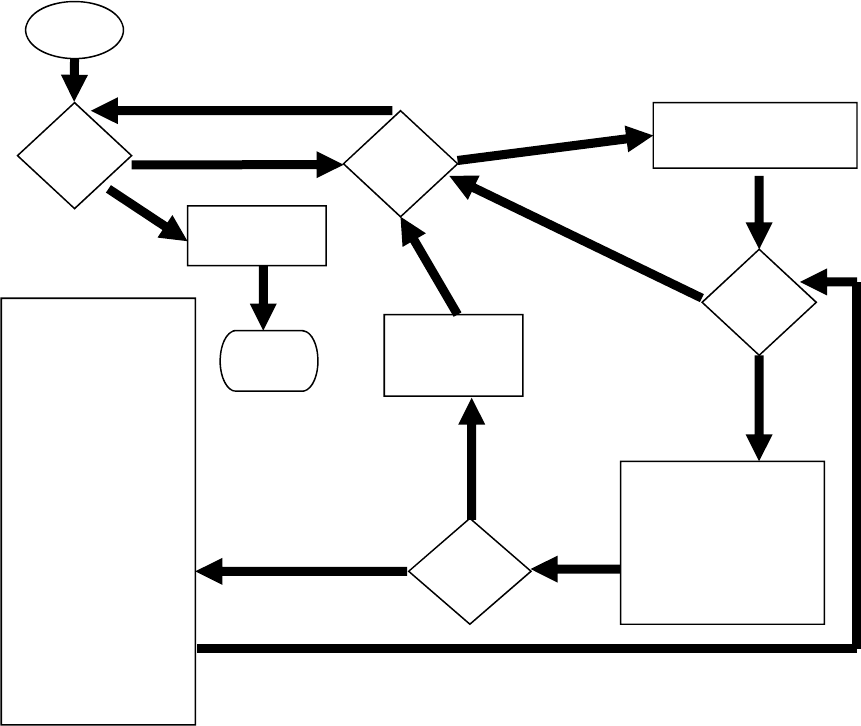
64
NO
YES
NO
YES
NO
NO
YES
BEGIN
END
Figure 1. Flowchart for AGEPRO
DONE
WITH IC
LOOP?
DONE
WITH SIM
LOOP?
SET INITIAL
POPULATION VECTOR
DONE
WITH TIME
LOOP?
SET VARIABLES THAT
VARY BY TIME PERIOD
COMPUTE
CATCH AT AGE
CALCULATE
TOTAL F
IS
QUOTA
FEASIBLE
?
RECORD THAT
SIMULATION IS
INFEASIBLE
COMPUTE LANDINGS
COMPUTE BS
GENERATE RANDOM
RECRUITMENT
COMPUTE FUTURE
POPULATION VECTOR
FOR NEXT TIME PERIOD
COPY CURRENT BS
TO
PREVIOUS BS
COPY FUTURE
POPULATION VECTOR
TO CURRENT
CALCULATE OUTPUTS
OUTPUT
RESULTS
YES
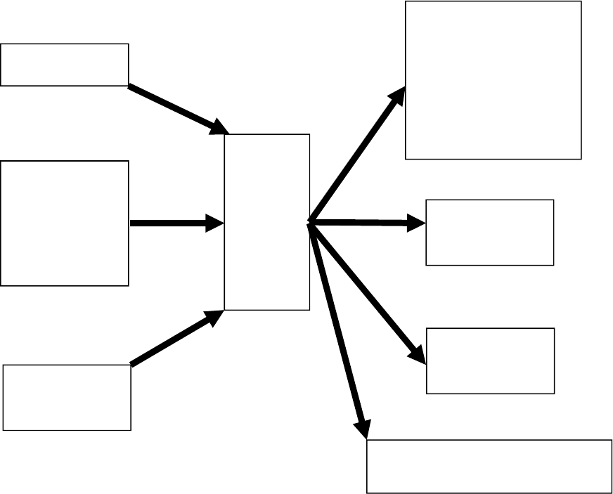
65
Figure 2. AGEPRO input/output diagram
INPUT FILENAME
SYSTEM DATA
AGEPRO
KEYWORDS FOR
SIMULATION DATA,
POPULATION DATA
AND FISHERY DATA
INPUT FILE
PROJECTION
DESCRIPTION
SUMMARY OF PROJECTION
RESULTS
*FREBUILD ANALYSIS
RESULTS
*PSTAR ANALYSIS
RESULTS
OUTPUT FILE
R DATAFRAME WITH
PROJECTION RESULTS
*IF APPLICABLE
INITIAL POPULATION
NUMBERS AT AGE
DATA
BOOTSTRAP FILE
RAW OUTPUT
RESULTS
AUXILIARY
POPULATION AND
FISHERY
PROCESS ERROR
RESULTS
*SIMULATED
DATA FILES
*R EXPORT FILE

66
Appendix
Example 1 Input File
AGEPRO VERSION 4.0
[CASEID]
REDFISH - RECRUITMENT MODEL 14
[GENERAL]
2004 2009 1 26 100 2 1 0 49667890
[BOOTSTRAP]
1000 1000
C:\Users\Jon.Brodziak\Documents\AGEPRO\Example1_2017-12-29_13-58-58\Example1.BSN
[STOCK_WEIGHT]
0 1
0.01 0.02 0.059 0.099 0.145 0.178 0.201 0.25 0.272 0.31 0.348 0.391 0.423 0.429 0.463 0.495 0.503 0.508 0.548 0.558
0.565 0.581 0.595 0.583 0.582 0.637
0.01 0.02 0.059 0.099 0.145 0.178 0.201 0.25 0.272 0.31 0.348 0.391 0.423 0.429 0.463 0.495 0.503 0.508 0.548 0.558
0.565 0.581 0.595 0.583 0.582 0.637
0.01 0.02 0.059 0.099 0.145 0.178 0.201 0.25 0.272 0.31 0.348 0.391 0.423 0.429 0.463 0.495 0.503 0.508 0.548 0.558
0.565 0.581 0.595 0.583 0.582 0.637
0.01 0.02 0.059 0.099 0.145 0.178 0.201 0.25 0.272 0.31 0.348 0.391 0.423 0.429 0.463 0.495 0.503 0.508 0.548 0.558
0.565 0.581 0.595 0.583 0.582 0.637
0.01 0.02 0.059 0.099 0.145 0.178 0.201 0.25 0.272 0.31 0.348 0.391 0.423 0.429 0.463 0.495 0.503 0.508 0.548 0.558
0.565 0.581 0.595 0.583 0.582 0.637
0.01 0.02 0.059 0.099 0.145 0.178 0.201 0.25 0.272 0.31 0.348 0.391 0.423 0.429 0.463 0.495 0.503 0.508 0.548 0.558
0.565 0.581 0.595 0.583 0.582 0.637
0.001 0.001 0.001 0.001 0.001 0.001 0.001 0.001 0.001 0.001 0.001 0.001 0.001 0.001 0.001 0 0.001 0.001 0.001 0.001
0.001 0.001 0.001 0.001 0.001 0.001
[SSB_WEIGHT]
0 1
0.01 0.02 0.059 0.099 0.145 0.178 0.201 0.25 0.272 0.31 0.348 0.391 0.423 0.429 0.463 0.495 0.503 0.508 0.548 0.558
0.565 0.581 0.595 0.583 0.582 0.637
0.01 0.02 0.059 0.099 0.145 0.178 0.201 0.25 0.272 0.31 0.348 0.391 0.423 0.429 0.463 0.495 0.503 0.508 0.548 0.558
0.565 0.581 0.595 0.583 0.582 0.637
0.01 0.02 0.059 0.099 0.145 0.178 0.201 0.25 0.272 0.31 0.348 0.391 0.423 0.429 0.463 0.495 0.503 0.508 0.548 0.558
0.565 0.581 0.595 0.583 0.582 0.637
0.01 0.02 0.059 0.099 0.145 0.178 0.201 0.25 0.272 0.31 0.348 0.391 0.423 0.429 0.463 0.495 0.503 0.508 0.548 0.558
0.565 0.581 0.595 0.583 0.582 0.637
0.01 0.02 0.059 0.099 0.145 0.178 0.201 0.25 0.272 0.31 0.348 0.391 0.423 0.429 0.463 0.495 0.503 0.508 0.548 0.558
0.565 0.581 0.595 0.583 0.582 0.637
0.01 0.02 0.059 0.099 0.145 0.178 0.201 0.25 0.272 0.31 0.348 0.391 0.423 0.429 0.463 0.495 0.503 0.508 0.548 0.558
0.565 0.581 0.595 0.583 0.582 0.637
0.001 0.001 0.001 0.001 0.001 0.001 0.001 0.001 0.001 0.001 0.001 0.001 0.001 0.001 0.001 0 0.001 0.001 0.001 0.001
0.001 0.001 0.001 0.001 0.001 0.001
[MEAN_WEIGHT]
0 1
0.01 0.02 0.059 0.099 0.145 0.178 0.201 0.25 0.272 0.31 0.348 0.391 0.423 0.429 0.463 0.495 0.503 0.508 0.548 0.558
0.565 0.581 0.595 0.583 0.582 0.637
0.01 0.02 0.059 0.099 0.145 0.178 0.201 0.25 0.272 0.31 0.348 0.391 0.423 0.429 0.463 0.495 0.503 0.508 0.548 0.558
0.565 0.581 0.595 0.583 0.582 0.637
0.01 0.02 0.059 0.099 0.145 0.178 0.201 0.25 0.272 0.31 0.348 0.391 0.423 0.429 0.463 0.495 0.503 0.508 0.548 0.558
0.565 0.581 0.595 0.583 0.582 0.637
0.01 0.02 0.059 0.099 0.145 0.178 0.201 0.25 0.272 0.31 0.348 0.391 0.423 0.429 0.463 0.495 0.503 0.508 0.548 0.558
0.565 0.581 0.595 0.583 0.582 0.637
0.01 0.02 0.059 0.099 0.145 0.178 0.201 0.25 0.272 0.31 0.348 0.391 0.423 0.429 0.463 0.495 0.503 0.508 0.548 0.558
0.565 0.581 0.595 0.583 0.582 0.637
0.01 0.02 0.059 0.099 0.145 0.178 0.201 0.25 0.272 0.31 0.348 0.391 0.423 0.429 0.463 0.495 0.503 0.508 0.548 0.558
0.565 0.581 0.595 0.583 0.582 0.637
0.001 0.001 0.001 0.001 0.001 0.001 0.001 0.001 0.001 0.001 0.001 0.001 0.001 0.001 0.001 0 0.001 0.001 0.001 0.001
0.001 0.001 0.001 0.001 0.001 0.001
[CATCH_WEIGHT]
0 1
0.01 0.02 0.059 0.099 0.145 0.178 0.201 0.25 0.272 0.31 0.348 0.391 0.423 0.429 0.463 0.495 0.503 0.508 0.548 0.558
0.565 0.581 0.595 0.583 0.582 0.637
0.01 0.02 0.059 0.099 0.145 0.178 0.201 0.25 0.272 0.31 0.348 0.391 0.423 0.429 0.463 0.495 0.503 0.508 0.548 0.558
0.565 0.581 0.595 0.583 0.582 0.637
0.01 0.02 0.059 0.099 0.145 0.178 0.201 0.25 0.272 0.31 0.348 0.391 0.423 0.429 0.463 0.495 0.503 0.508 0.548 0.558
0.565 0.581 0.595 0.583 0.582 0.637
67
0.01 0.02 0.059 0.099 0.145 0.178 0.201 0.25 0.272 0.31 0.348 0.391 0.423 0.429 0.463 0.495 0.503 0.508 0.548 0.558
0.565 0.581 0.595 0.583 0.582 0.637
0.01 0.02 0.059 0.099 0.145 0.178 0.201 0.25 0.272 0.31 0.348 0.391 0.423 0.429 0.463 0.495 0.503 0.508 0.548 0.558
0.565 0.581 0.595 0.583 0.582 0.637
0.01 0.02 0.059 0.099 0.145 0.178 0.201 0.25 0.272 0.31 0.348 0.391 0.423 0.429 0.463 0.495 0.503 0.508 0.548 0.558
0.565 0.581 0.595 0.583 0.582 0.637
0.01 0.02 0.059 0.099 0.145 0.178 0.201 0.25 0.272 0.31 0.348 0.391 0.423 0.429 0.463 0.495 0.503 0.508 0.548 0.558
0.565 0.581 0.595 0.583 0.582 0.637
0.01 0.02 0.059 0.099 0.145 0.178 0.201 0.25 0.272 0.31 0.348 0.391 0.423 0.429 0.463 0.495 0.503 0.508 0.548 0.558
0.565 0.581 0.595 0.583 0.582 0.637
0.01 0.02 0.059 0.099 0.145 0.178 0.201 0.25 0.272 0.31 0.348 0.391 0.423 0.429 0.463 0.495 0.503 0.508 0.548 0.558
0.565 0.581 0.595 0.583 0.582 0.637
0.01 0.02 0.059 0.099 0.145 0.178 0.201 0.25 0.272 0.31 0.348 0.391 0.423 0.429 0.463 0.495 0.503 0.508 0.548 0.558
0.565 0.581 0.595 0.583 0.582 0.637
0.01 0.02 0.059 0.099 0.145 0.178 0.201 0.25 0.272 0.31 0.348 0.391 0.423 0.429 0.463 0.495 0.503 0.508 0.548 0.558
0.565 0.581 0.595 0.583 0.582 0.637
0.01 0.02 0.059 0.099 0.145 0.178 0.201 0.25 0.272 0.31 0.348 0.391 0.423 0.429 0.463 0.495 0.503 0.508 0.548 0.558
0.565 0.581 0.595 0.583 0.582 0.637
0.001 0.001 0.001 0.001 0.001 0.001 0.001 0.001 0.001 0.001 0.001 0.001 0.001 0.001 0.001 0 0.001 0.001 0.001 0.001
0.001 0.001 0.001 0.001 0.001 0.001
0.001 0.001 0.001 0.001 0.001 0.001 0.001 0.001 0.001 0.001 0.001 0.001 0.001 0.001 0.001 0 0.001 0.001 0.001 0.001
0.001 0.001 0.001 0.001 0.001 0.001
[NATMORT]
0 1
0.05 0.05 0.05 0.05 0.05 0.05 0.05 0.05 0.05 0.05 0.05 0.05 0.05 0.05 0.05 0.05 0.05 0.05 0.05 0.05 0.05 0.05 0.05 0.05
0.05 0.05
0.05 0.05 0.05 0.05 0.05 0.05 0.05 0.05 0.05 0.05 0.05 0.05 0.05 0.05 0.05 0.05 0.05 0.05 0.05 0.05 0.05 0.05 0.05 0.05
0.05 0.05
0.05 0.05 0.05 0.05 0.05 0.05 0.05 0.05 0.05 0.05 0.05 0.05 0.05 0.05 0.05 0.05 0.05 0.05 0.05 0.05 0.05 0.05 0.05 0.05
0.05 0.05
0.05 0.05 0.05 0.05 0.05 0.05 0.05 0.05 0.05 0.05 0.05 0.05 0.05 0.05 0.05 0.05 0.05 0.05 0.05 0.05 0.05 0.05 0.05 0.05
0.05 0.05
0.05 0.05 0.05 0.05 0.05 0.05 0.05 0.05 0.05 0.05 0.05 0.05 0.05 0.05 0.05 0.05 0.05 0.05 0.05 0.05 0.05 0.05 0.05 0.05
0.05 0.05
0.05 0.05 0.05 0.05 0.05 0.05 0.05 0.05 0.05 0.05 0.05 0.05 0.05 0.05 0.05 0.05 0.05 0.05 0.05 0.05 0.05 0.05 0.05 0.05
0.05 0.05
0.1 0.1 0.1 0.1 0.1 0.1 0.1 0.1 0.1 0.1 0.1 0.1 0.1 0.1 0.1 0.1 0.1 0.1 0.1 0.1 0.1 0.1 0.1 0.1 0.1 0.1
[BIOLOGICAL]
0
0.4
0.4
[MATURITY]
0 1
0.01 0.02 0.05 0.15 0.36 0.64 0.85 0.95 0.98 0.99 1 1 1 1 1 1 1 1 1 1 1 1 1 1 1 1
0.01 0.02 0.05 0.15 0.36 0.64 0.85 0.95 0.98 0.99 1 1 1 1 1 1 1 1 1 1 1 1 1 1 1 1
0.01 0.02 0.05 0.15 0.36 0.64 0.85 0.95 0.98 0.99 1 1 1 1 1 1 1 1 1 1 1 1 1 1 1 1
0.01 0.02 0.05 0.15 0.36 0.64 0.85 0.95 0.98 0.99 1 1 1 1 1 1 1 1 1 1 1 1 1 1 1 1
0.01 0.02 0.05 0.15 0.36 0.64 0.85 0.95 0.98 0.99 1 1 1 1 1 1 1 1 1 1 1 1 1 1 1 1
0.01 0.02 0.05 0.15 0.36 0.64 0.85 0.95 0.98 0.99 1 1 1 1 1 1 1 1 1 1 1 1 1 1 1 1
0.001 0.001 0.001 0.001 0.001 0.001 0.001 0.001 0.001 0.001 0.001 0.001 0.001 0.001 0.001 0.001 0.001 0.001 0.001
0.001 0.001 0.001 0.001 0.001 0.001 0.001
[FISHERY]
0 1
0 0.002 0.011 0.054 0.223 0.522 0.656 0.783 1 1 1 1 1 1 1 1 1 1 1 1 1 1 1 1 1 1
0 0.002 0.011 0.054 0.223 0.522 0.656 0.783 1 1 1 1 1 1 1 1 1 1 1 1 1 1 1 1 1 1
0 0.002 0.011 0.054 0.223 0.522 0.656 0.783 1 1 1 1 1 1 1 1 1 1 1 1 1 1 1 1 1 1
0 0.002 0.011 0.054 0.223 0.522 0.656 0.783 1 1 1 1 1 1 1 1 1 1 1 1 1 1 1 1 1 1
0 0.002 0.011 0.054 0.223 0.522 0.656 0.783 1 1 1 1 1 1 1 1 1 1 1 1 1 1 1 1 1 1
0 0.002 0.011 0.054 0.223 0.522 0.656 0.783 1 1 1 1 1 1 1 1 1 1 1 1 1 1 1 1 1 1
0 0.002 0.011 0.054 0.223 0.522 0.656 0.783 1 1 0.783 0.656 0.522 0.5 0.5 0.5 0.5 0.5 0.5 0.5 0.5 0.5 0.5 0.5 0.5 0.5
0 0.002 0.011 0.054 0.223 0.522 0.656 0.783 1 1 0.783 0.656 0.522 0.5 0.5 0.5 0.5 0.5 0.5 0.5 0.5 0.5 0.5 0.5 0.5 0.5
0 0.002 0.011 0.054 0.223 0.522 0.656 0.783 1 1 0.783 0.656 0.522 0.5 0.5 0.5 0.5 0.5 0.5 0.5 0.5 0.5 0.5 0.5 0.5 0.5
0 0.002 0.011 0.054 0.223 0.522 0.656 0.783 1 1 0.783 0.656 0.522 0.5 0.5 0.5 0.5 0.5 0.5 0.5 0.5 0.5 0.5 0.5 0.5 0.5
0 0.002 0.011 0.054 0.223 0.522 0.656 0.783 1 1 0.783 0.656 0.522 0.5 0.5 0.5 0.5 0.5 0.5 0.5 0.5 0.5 0.5 0.5 0.5 0.5
0 0.002 0.011 0.054 0.223 0.522 0.656 0.783 1 1 0.783 0.656 0.522 0.5 0.5 0.5 0.5 0.5 0.5 0.5 0.5 0.5 0.5 0.5 0.5 0.5
0.001 0.001 0.001 0.001 0.001 0.001 0.001 0.001 0.001 0.001 0.001 0.001 0.001 0.001 0.001 0.001 0.001 0.001 0.001
0.001 0.001 0.001 0.001 0.001 0.001 0.001
0.001 0.001 0.001 0.001 0.001 0.001 0.001 0.001 0.001 0.001 0.001 0.001 0.001 0.001 0.001 0.001 0.001 0.001 0.001
0.001 0.001 0.001 0.001 0.001 0.001 0.001
[RECRUIT]
68
1000000 1 75
14
1
1
1
1
1
1
53
73.5939 78.1845 70.6004 62.1267 66.0886 69.9814 49.9445 70.4022 42.6731 85.2977 48.2887 98.1364 76.867 33.8211
7.8195 4.3288 2.6275 2.7917 4.2174 249.227 6.5051 2.5329 1.9038 1.7011 1.5596 2.2002 52.7585 2.4754 2.8037 10.179
21.2349 8.6637 20.0313 11.1925 5.0913 4.3675 28.9894 51.3917 8.7334 35.7165 327.489 73.3318 35.0047 22.4337 24.9481
32.1726 34.4703 29.245 81.7098 30.5807 25.3895 26.28 30.1793
[HARVEST]
0 1 0 0 0 0
0.00239 350 0.01 0.01 0.01 0.01
0.00239 350 0.02 0.02 0.02 0.02
[REFPOINT]
236700 0 0 0.04
[OPTIONS]
0 0 1

69
Example 2 Input File
AGEPRO VERSION 4.0
[CASEID]
GoM haddock ASAP_final (1977-2011 recruitment)
[GENERAL]
2014 2020 1 9 10 1 1 0 854236
[BOOTSTRAP]
1000 1000
C:\Users\Jon.Brodziak\Documents\AGEPRO\Example2_2017-12-29_14-19-44\Example2.BSN
[STOCK_WEIGHT]
0 0
0.15 0.4 0.71 1 1.24 1.43 1.59 1.82 2.04
0.14 0.13 0.07 0.05 0.03 0.03 0.08 0.03 0.04
[SSB_WEIGHT]
-1 0
[MEAN_WEIGHT]
0 0
0.3 0.6 0.89 1.17 1.4 1.55 1.7 1.96 2.04
0.14 0.11 0.11 0.06 0.05 0.05 0.05 0.07 0.04
[CATCH_WEIGHT]
-3 0
[NATMORT]
0 0
0.2 0.2 0.2 0.2 0.2 0.2 0.2 0.2 0.2
0.1 0.1 0.1 0.1 0.1 0.1 0.1 0.1 0.1
[BIOLOGICAL]
0
0.25
0.25
[MATURITY]
0 0
0.04 0.28 0.81 0.98 1 1 1 1 1
0.23 0.08 0.02 0.001 0.001 0.001 0.001 0.001 0.001
[FISHERY]
0 0
0 0.05 0.19 0.3 0.52 0.69 0.82 1 0.83
0.36 0.19 0.14 0.15 0.13 0.13 0.12 0.001 0.16
[RECRUIT]
1000 1000 50
14
1
1
1
1
1
1
1
35
5997 1476 6048 6435 4612 774 2445 1043 282 265 134 443 187 244 267 711 1318 2903 2540 1080 2179 2276 13429
2547 1121 1216 219 6281 386 1118 1218 215 301 966 6659
[HARVEST]
1 0 0 0 2 0 0
500 0.2 0.2 0.2 500 0.2 0.2
[PSTAR]
5
0.1 0.2 0.3 0.4 0.5
0.35
2018
[BOUNDS]
10 0.6
[OPTIONS]
1 0 0
[SCALE]
1000 1000 1000
[PERC]
90

70
Example 3 Input File
AGEPRO VERSION 4.0
[CASEID]
GoM haddock ASAP_final FREBUILD Projection
[GENERAL]
2014 2020 1 9 10 1 1 0 30076
[BOOTSTRAP]
1000 1000
C:\Users\Jon.Brodziak\Documents\AGEPRO\Example3_2017-12-29_14-49-07\Example3.BSN
[STOCK_WEIGHT]
0 0
0.15 0.4 0.71 1 1.24 1.43 1.59 1.82 2.04
0.14 0.13 0.07 0.05 0.03 0.03 0.08 0.03 0.04
[SSB_WEIGHT]
-1 0
[MEAN_WEIGHT]
0 0
0.3 0.6 0.89 1.17 1.4 1.55 1.7 1.96 2.04
0.14 0.11 0.11 0.06 0.05 0.05 0.05 0.07 0.04
[CATCH_WEIGHT]
-3 0
[NATMORT]
0 0
0.2 0.2 0.2 0.2 0.2 0.2 0.2 0.2 0.2
0.1 0.1 0.1 0.1 0.1 0.1 0.1 0.1 0.1
[BIOLOGICAL]
0
0.25
0.25
[MATURITY]
0 0
0.04 0.28 0.81 0.98 1 1 1 1 1
0.23 0.08 0.02 0.001 0.001 0.001 0.001 0.001 0.001
[FISHERY]
0 0
0 0.05 0.19 0.3 0.52 0.69 0.82 1 0.83
0.36 0.19 0.14 0.15 0.13 0.13 0.12 0.001 0.16
[RECRUIT]
1000 1000 50
14
1
1
1
1
1
1
1
35
5997 1476 6048 6435 4612 774 2445 1043 282 265 134 443 187 244 267 711 1318 2903 2540 1080 2179 2276 13429
2547 1121 1216 219 6281 386 1118 1218 215 301 966 6659
[HARVEST]
1 0 0 0 0 0 0
500 0.3 0.3 0.3 0.3 0.3 0.3
[REBUILD]
2020 11000 0 75
[BOUNDS]
10 0.6
[OPTIONS]
1 0 0
[SCALE]
1000 1000 1000
[PERC]
90
