ALCD User Manual
User Manual:
Open the PDF directly: View PDF ![]() .
.
Page Count: 35
Active Learning for Cloud Detection &
Processing Chains Comparator
User Manual
Louis Baetens
October 11, 2018
Contents
1 General instructions 2
1.1 Requirements...................................... 2
1.2 Filestructure...................................... 2
1.3 Configurationfile.................................... 3
1.4 Inputdataorganisation ................................ 3
2 Active Learning for Cloud Detection (ALCD) 7
2.1 Dataorganisation.................................... 7
2.2 Configurationfile.................................... 7
2.3 Code workflow and overview . . . . . . . . . . . . . . . . . . . . . . . . . . . . . . 8
2.4 Tutorial ......................................... 10
3 Processing Chains Comparator (PCC) 28
3.1 Dataorganisation.................................... 28
3.2 Configurationfile.................................... 28
3.3 Code workflow and overview . . . . . . . . . . . . . . . . . . . . . . . . . . . . . . 29
3.4 Possible variations for the comparison . . . . . . . . . . . . . . . . . . . . . . . . 32
3.5 Tutorial ......................................... 32
1
1 General instructions
This is the current user manual for the Active Learning Cloud Detection (ALCD) and the
Processing Chains Comparator (PCC) codes. For a quick start, you can directly go to the
Tutorial parts (sections 2.4 and 3.5). This section describes the requirements, the file structure
and the configuration files.
1.1 Requirements
These code requires OTB 6.0 and GDAL. It runs with Python 2.7. QGIS should be installed
as well.
The Python dependencies are listed below:
otbApplication gdal ogr PIL
numpy matplotlib pandas
Note: before running ALCD or PCC, check that the libraries are present in the PYTHON-
PATH, especially the otbApplication. If this is not the case, you will get this error message:
Im portE rror : No module named o t b A p p l i c a t i o n
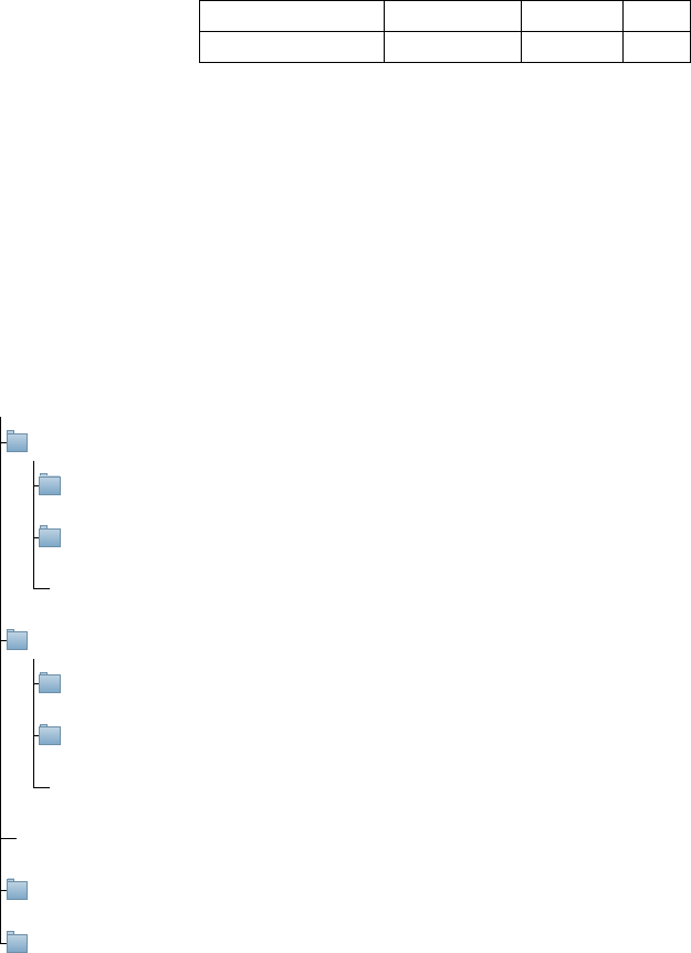
1.2 File structure
The general structure of the folders and files we use in this work should be as follows.
NB: root_dir is the directory where you want to have all the ALCD and PCC codes. Data_ALCD
and Data_PCC can be at another place.
root_dir
ALCD : contains the codes and parameters for the ALCD algorithm
parameters_files : contains the configuration files for the ALCD code
color_table : contains various files for the color scheme to use
ALCD python files
PCC : contains the codes and parameters for the PCC algorithm
parameters_files : contains the configuration files for the PCC code
color_table : contains various files for the color scheme to use
PCC python files
paths_configuration.json : general configuration file
Data_ALCD : contains the input and output for ALCD codes
Data_PCC : contains the input and output for PCC codes
The two Data directories could be renamed or placed in another place. The configuration
files should be modified accordingly.
2
1.3 Configuration file
The file paths_configuration.json should be modified according to your preferences. See the
default one as an example.
global_chains_paths : contains the main paths concerning the output of the processing
chains
L1C : the L1C products, subsequently designated as L1C product root dir
maja : directory where the MAJA files are, subsequently designated as MAJA output
root dir
sen2cor : directory where the Sen2cor files are, subsequently designated as Sen2cor
output root dir
fmask : directory where the Fmask files are, subsequently designated as Fmask output
root dir
DTM_input : directory where the Digital Terrain Model files are, subsequently desig-
nated as DTM product root dir
DTM_resized : directory where the resized Digital Terrain Model files will be stored
data_paths : in case the Data_ALCD and Data_PCC are moved or renamed, this should
be modified
tile_location : specification of the tile code linked to a named place. You could add other
locations here.
1.4 Input data organisation
The data organisation of each of the programs outputs is defined below, with the example of
Arles on the 2nd of October, 2017. If your structure is different, you need to change
some variables in the code. For each directory or file, the pattern to describe it follows the
syntax: "General name : ExampleForArles". The *in a path indicates that the path has been
truncated at this place.
1.4.1 Required for the ALCD
•L1C product structure:
3
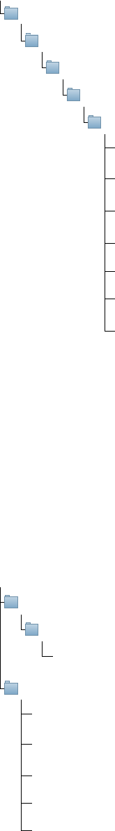
L1C product root dir : /mnt/data/SENTINEL2/L1C_PDGS/
location : Arles
date and tile folder : S2B_MSIL1C_20171002T103009_N0205_R108*.SAFE
granule folder : GRANULE
L1C product : L1C_T31TFJ_A002994_20171002T103209
image data : IMG_data
bands files :
T31TFJ_20171002T103009_B01.jp2
T31TFJ_20171002T103009_B02.jp2
T31TFJ_20171002T103009_B03.jp2
...
T31TFJ_20171002T103009_B11.jp2
T31TFJ_20171002T103009_B12.jp2
The full path of the first band is therefore, in this example: /mnt/data/SENTINEL2/L1C_
PDGS/Arles/S2B_MSIL1C_20171002T103009_N0205_R108_T31TFJ_20171002T103209.SAFE/
GRANULE/L1C_T31TFJ_A002994_20171002T103209/IMG_DATA/T31TFJ_20171002T103009_
B01.jp2
•DTM product structure:
The Digital Terrain Model is specific to a tile. Therefore, there is no need to have a
copy of the DTM for each date. The original DTM should be placed in the DTM_input
directory. After the first time the ALCD is run on one location, its resized DTM will be
created in the DTM_resized directory, so as to avoid generating it each time. The format
has to be an unpacked DTM folder (.DBL).
Original DTM folder: /mnt/data/home/baetensl/DTM/original
Tile folder (must contain the tile ref): S2_*_T31TFJ*
Unpacked .DBL folder: S2_*T31TFJ_*.DBL.DIR
Altitude file: S2__TEST_AUX_REFDE2_T31TFJ_0001_ALT_R2.TIF
Resized DTM folder: /mnt/data/home/baetensl/DTM/resized
Generated DTMs :
Arles_31TFJ_DTM_60m.tif
Gobabeb_33KWP_DTM_60m.tif
...
RailroadValley_11SPC_DTM_60m.tif
The full path of the original DTM is therefore, in this example: /mnt/data/home/
baetensl/DTM/original/S2__TEST_AUX_REFDE2_Arles_T31TFJ_0002/S2__TEST_AUX_REFDE2_
T31TFJ_0001.DBL.DIR/S2__TEST_AUX_REFDE2_T31TFJ_0001_ALT_R2.TIF. After the ALCD
4
is run once on Arles, the resized DTM will be in /mnt/data/home/baetensl/DTM/resized/
Arles_31TFJ_DTM_60m.tif.
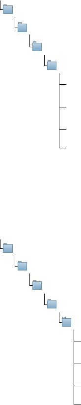
1.4.2 Required for the PCC
•MAJA v1 and v2 output structure:
MAJA output root dir : /mnt/data/SENTINEL2/L2A_MAJA/
location : Arles
tile : 31TFJ
MAJA natif output : MAJA_1_0_S2AS2B_NATIF
date folder : S2B_OPER_SSC_L2VALD_31TFJ____20171002.DBL.DIR
output files :
Cloud mask : S2B_OPER_*_L2VALD_31TFJ____20171002_CLD_R2.DBL.TIF
Geo mask : S2B_OPER_SSC_*_L2VALD_31TFJ____20171002_MSK_R1.DBL.TIF
...
The full path of the cloud mask is therefore, in this example: /mnt/data/SENTINEL2/L2A_
MAJA/Arles/31TFJ/MAJA_1_0_S2AS2B_NATIF/S2B_OPER_SSC_L2VALD_31TFJ____20171002.
DBL.DIR/S2B_OPER_SSC_PDTANX_L2VALD_31TFJ____20171002_MSK_R2.DBL.TIF
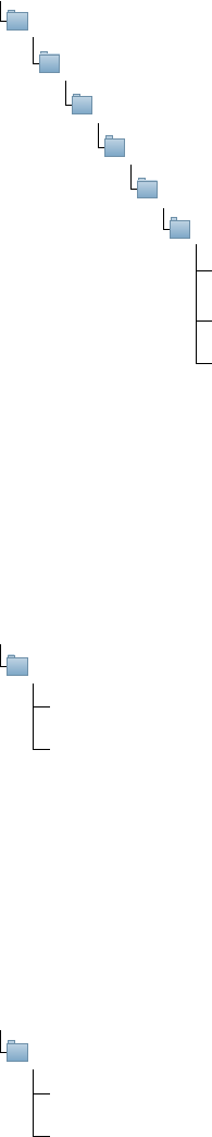
•MAJA v3 output structure:
MAJA output root dir : /mnt/data/SENTINEL2/L2A_MAJA/
location : Arles
tile : 31TFJ
MAJA natif output : MAJA_3_1_S2AS2B
date folder : SENTINEL2B_20171002-103209-123_L2A_T31TFJ_C_V1-0
masks folder : MASKS
output files :
Cloud mask : SENTINEL*CLM_R2.tif
Geo mask : SENTINEL*MG2_R2.tif
...
The full path of the cloud mask is therefore, in this example: /mnt/data/SENTINEL2/L2A_
MAJA/Arles/31TFJ/MAJA_3_1_S2AS2B_HOT016/SENTINEL2B_20171002-103209-123_L2A_
T31TFJ_C_V1-0/MASKS/SENTINEL2B_20171002-103209-123_L2A_T31TFJ_C_V1-0_CLM_R2.
tif
•Sen2cor output structure:
5
Sen2cor output root dir : /mnt/data/SENTINEL2/L2A_SEN2COR/
location : Arles
date and tile : S2B_MSIL2A_20171002T103009_N0205_R108_T31TFJ_*.SAFE
granule folder : GRANULE
sub folder : L2A_T31TFJ_A002994_20171002T103209
image data : IMG_DATA
resolution : R20m
output files :
Cloud mask : L2A_T31TFJ_20171002T103009_SCL_20m.jp2
...
The full path of the cloud mask is therefore, in this example: /mnt/data/SENTINEL2/L2A_
SEN2COR/Arles/S2B_MSIL2A_20171002T103009_N0205_R108_T31TFJ_20171002T103209.
SAFE/GRANULE/L2A_T31TFJ_A002994_20171002T103209/IMG_DATA/R20m/ L2A_T31TFJ_
20171002T103009_SCL_20m.jp2
•Fmask v4 output structure:
For Fmask version 4, which is the last one, the data structure is the following.
Fmask output root dir : /mnt/data/home/baetensl/Programs/Fmask4_output/
location tile and date : Arles_31TFJ_20171002
Cloud mask : L1C_T31TFJ_A002994_20171002T103209_Fmask4.tif
...
The full path of the cloud mask is therefore, in this example: /mnt/data/home/baetensl/
Programs/Fmask4_output//Arles_31TFJ_20171002/L1C_T31TFJ_A002994_20171002T103209_
Fmask4.tif
•Fmask v3 output structure:
For the previous version of Fmask, the structure is similar, only the file name of the cloud
mask changes.
Fmask output root dir : /mnt/data/home/baetensl/Programs/Output_fmask/
location tile and date : Arles_31TFJ_20171002
Cloud mask : Arles_20171002_cloud_mask.img
...
The full path of the cloud mask is therefore, in this example: /mnt/data/home/baetensl/
Programs/Output_fmask/Arles_31TFJ_20171002/Arles_20171002_cloud_mask.img
6
2 Active Learning for Cloud Detection (ALCD)
This part deals with the utilisation of the ALCD code. This code produces classification ref-
erence masks from a Sentinel-2 L1C product, and is particularly designed to detect clouds and
cloud shadows. In order to get the best results as possible, while still minimizing the amount
of manual work to get reference pixels, this method is only applicable to dates in a time series
for which one of the next dates is cloud free.
2.1 Data organisation
For the input data, refer to the section 1.4.1.
The output structure of the code is the following, for a given location and date:
location and date dir : main directory; e.g. Arles_31TFJ_20171002
In_data : contains the input data
Image : contains the different GeoTIFF files
Masks : inside are the asks files for each class which need to be modified
Intermediate : intermediate files needed for the ALCD to run smoothly
Models : output models created by the OTB software
Other : can contain miscellaneous files
Out : main output directory
classification map and the superimposed contours on the original TIF in true colors
Previous_iterations : saves of the previous iterations
Samples : reorganisation of the masks into readable format for OTB training
Statistics : various statistics such as the confusion matrix
2.2 Configuration file
A granule is defined as a set of data specified in space and time, i.e. a location and a date. For
example, a granule could be associated with Orleans, tile 31UDP, and the 13th of April 2018. In
all the environment, a date is in format YYYYMMDD (the previous date becoming 20180413).
Some parameters can be tweaked in the configuration files (located in the parameters_files
directory).
•In the global_parameters.json, the different parameters are described below. The
ones with a star (∗) are the ones you could consider worth changing.
∗classification : classification parameters
method : which method is used (could be rf, svm, ...)
general : output names for the files. Not necessary to change anything. The different
files will be referred to with their default names afterwards
∗local_paths : specific to your environment. It is used if you run the ALCD on a
distant machine, and want to modify the masks on your local machine with QGIS.
Useful if the distant machine does not have a graphic card.
7
copy_folder : on your local machine, where you want to edit the files
current_server : the adress of the distant machine
masks : naming and attribution of a number to each class
postprocessing : global naming for post-processing files
automatically_generated : references to the specific case you are working on. This
will be modified when running ALCD, so you do not need (and should not) change
it manually
∗training_parameters : parameters used for the training and classification of the
algorithm. The default ones are good, but you can change them.
training_proportion : the proportion of samples that will become training sam-
ples (between 0 and 1). The other part (1-training_proportion) will become
validating samples.
expansion_distance : in meters, the size of the buffer zone around each sample.
This buffer zone will be used to augment the data, i.e. take the neighboring
pixels
regularization_radius : in pixels (should be an integer), the radius for the regu-
larization of the classification map. Typical values are between 1 and 5.
dilatation_radius : in pixels (should be an integer), the radius for the dilatation
of the contours for the visualisation. Typical values are between 1 and 5.
Kfold : for the K-fold cross-validation, which k to use (usually 5 or 10).
∗features : which features will be used for the classification.
original_bands : list of the bands from the cloudy date to use. It is recommended
to use all of them.
time_difference_bands : list of the bands from which the difference will be made,
between the cloudy and clear date. It is recommended to use all of them apart
the band 10, which is noisy.
special_indices : list of peculiar indices. Can be composed of NDVI, NDWI, NDSI
for the moment.
ratios : list of ratios. Each item should have the format "a_b", where aand bare
bands numbers (e.g. "2_4" will produce the ratio B2/B4).
DTM : boolean, whether you want to use the Digital Elevation Model or not.
textures : boolean, whether you want to create the two texture features (coefficient
of variation and contours density are available for the moment).
•The specific model parameters can be modified in the model_parameters.json file. They
are directly referring to the OTB ones, and you can therefore see the OTB documenta-
tion for this purpose (https://www.orfeo-toolbox.org/CookBook/Applications/app_
TrainVectorClassifier.html)
2.3 Code workflow and overview
The ALCD framework is based on multi-spectral and multi-temporal features. The user will
have to choose two images separated by a few days: a reference cloud free image, it usually
happens from time to time in a time series, and an image to classify. The latter should have
been acquired before the reference image, otherwise MAJA, which is also multi-temporal will
be favoured as it uses cloud free pixels in the past to classify the pixels. The user should select
an image which is as cloud-free as possible, along the cloudy image which he wishes to classify.
The closer the two dates, the better.
Firstly, the different features are compiled into two GeoTIFF. The features described below
8
are the one created if you use the recommended parameters.
•The main TIF contains all the 12 bands of the cloudy date, the NDVI and NDWI computed
from them, the difference between the bands of the cloudy date and the cloud-free date,
and the Digital Terrain Model (DTM) of the area, with a coarse resolution (60 meters).
•The second TIF, so-called ’heavy’, contains the bands 2, 3, 4, 10, the NDVI and the
NDWI of the cloudy image, with a full resolution (10 or 20 meters). This allows the user
to conveniently select the samples.
Then, the user is asked to put some points in a vector format, such that it labels the image.
Then, the user is asked to manually add reference points with QGIS. Each wanted class
should have at least 3 references points. One empty layer per class is created in the previous
step, such that the user needs to populate them, or leave some of them empty if the class is not
present in the image (e.g. with snow).
The OTB workflow is then put into motion, training a model and classifying the image. The
classification is the output of the ALCD algorithm.
The user can afterwards add new vector points to refined the model, in an iterative way.
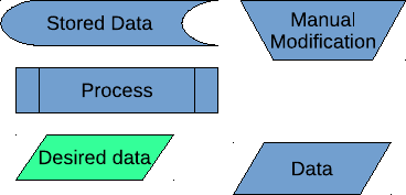
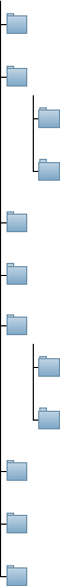
The flowchart is exposed in figure 2.2, with the nomenclature being in figure 2.1.
Figure 2.1: Flowcharts nomenclature
9
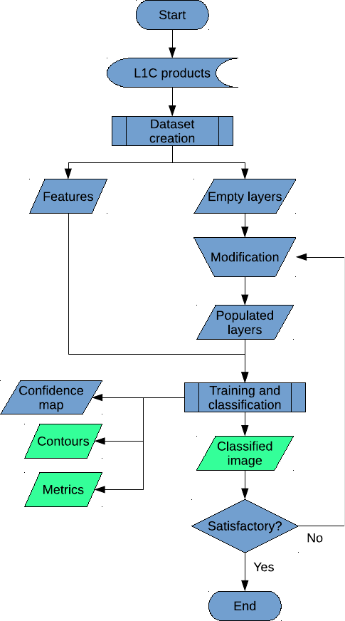
Figure 2.2: ALCD flowchart
2.4 Tutorial
This is a step-by-step tutorial, to help you use the ALCD algorithm. Here, we will classify the
clouds on the image of Arles, on the 2nd of October, 2017.
The expected result is the following:
10
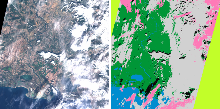
(a) Image to classify (b) Final classification
Figure 2.3: Classification of Arles, 20171002
Change to the ALCD directory. The program that you should use is all_run_alcd.py. You
can display the help with
python a ll_run_alcd . py −h
The available options are:
-l : the location. The spelling should be consistent with the names in the L1C directory
(e.g. Pretoria or Orleans)
-d : the (cloudy) date that you want to classify (e.g. 20180319)
-c : the clear date that will help the classification (e.g. 20180321)
-f : if this is the first iteration or not. If set to True, it will compute and create all
the features, and create the empty class layers. Set it to True for the first iteration, and
thereafter to False.
-s : the step you want to do, the choice is between 0 and 1. 0 will create all the needed
files if this is the first iteration, otherwise it will save the previous iteration. 1 will run the
ALCD algorithm, i.e train a model and classify the image. For each iteration, you should
set it to 0, modify the masks, and then set it to 1.
-kfold : boolean. If set to True, ALCD will perform a k-fold cross-validation with the
available samples.
-dates : boolean. If set to True, ALCD will display the available dates for the given
location.
2.4.1 Summary of the commands
The detailed steps are given after this part. We give here the summary of the commands to
use, so you can come back here if you forget how to use ALCD.
See the available dates.
python a ll_run_alcd . py −l Ar l e s −d a t e s True
11
Initialisation and creation of the features.
python a ll_run_alcd . py −f True −s 0 −l Ar l e s −d 20171002 −c 20171005
Edit the shapefiles to populate them with manually labeled samples. Then run the algorithm.
python a ll_run_alcd . py −f True −s 1
While the results are not satisfactory:
Visualize the results. Save the current iteration.
python a ll_run_alcd . py −f Fal s e −s 0
Edit the shapefiles to your convenience. Run the algorithm again.
python a ll_run_alcd . py −f Fal s e −s 1
2.4.2 Paths preparation
Before running anything, you need to set the correct paths and parameters.
In the paths_configuration.json:
•Add the tile code linked to the location you want to add
•Create the output directory for ALCD, and set its path in the "data_alcd" variable
•Set the correct paths for the L1C directory and the DTM_input
In the global_parameters.json, if you use a distant and a local machine, set the local_
paths variables accordingly.
2.4.3 Step 1
First of all, you must pick the date you are interested in. As the code will run on the L1C
product, you can list all the available dates with the command
python a ll_run_alcd . py −l A r le s −d a t e s True
You should get a list like
[ ’ 2 0 1 5 1 2 0 2 ’ , ’ 2 01 5 1 23 0 ’ , . . . , ’ 2 0 18 0 3 19 ’ , ’ 2 0 1 8 0 3 2 1 ’ ]
A good practice is to visualise the two dates we want to use beforehand. This can be facil-
itated by the code quicklook_generator.py, which generates quicklooks for a given location.
The user can therefore make sure that the cloud-free image is indeed cloud-free, and that the
image to be classified is interesting.
As stated above, the date we will use here is 20171002. This date was acquired just before
a cloud free date: 20171005.
Therefore, initialize the environment by running
python a ll_run_alcd . py −f True −s 0 −l A r l e s −d 20171002 −c 20171005
This will create the concatenated .tif with all the bands, and empty shapefiles for each class,
among other things.
It invites you to copy those created files to your local machine, to accelerate the process
in QGIS (on our processing computer, visualisation is slow, so we use QGIS on a different
computer). You can also modify the files directly, in this case, you can skip the manual copy
of the files and go to Step 2. Otherwise, copy the files on your machine with QGIS, and go to
Step 2.
12
2.4.4 Step 2
You can now open QGIS. Open the raster In_data/Image/Arles_bands_H.tif (H stands for
Heavy, as it is in full resolution of 20m per pixel), and In_data/Image/Arles_bands.tif.
The Arles_bands_H.tif bands refer to the band 2 (blue), 3 (green), 4 (red), 10 (the band at
1375nm), the NDVI and the NDWI. The bands for the Arles_bands.tif are quite numerous,
but the content of each band is documented in the .txt file corresponding to each .tif.
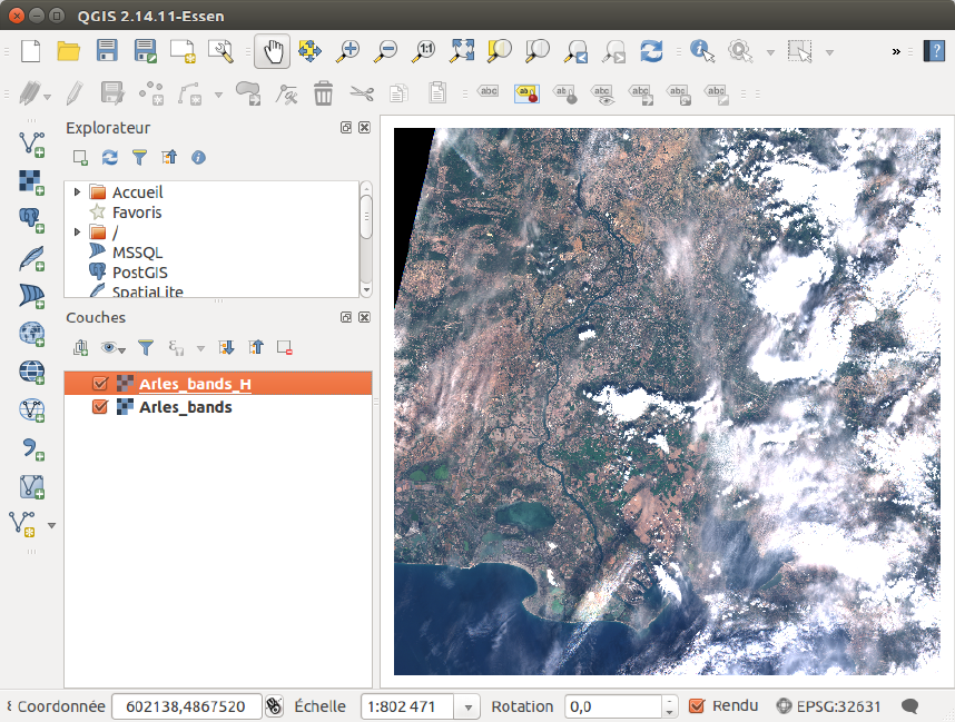
Now, adjust the style in QGIS such that you see the image in true colors. For that, you
can load the file color_tables/heavy_tif_true_colors_style.qml on the Heavy .tif. You
should get :
Figure 2.4: QGIS window with the scene displayed in true colors
Now, load all the empty shapefiles from the directory In_data/Masks.
If you display a band being a time difference (for example the 20th band of Arles_bands.
tif), you will observe that there was no data on the bottom-right corner for the clear date.
The same is true with the top-left corner for the cloudy date.
Thus, the no_data file already has some data (which is the case if one or both of the original
images have no_data pixels). As you can see, on figure 2.4 the top-left and bottom-right corners
are covered by the no-data mask. If you are not satisfied with the mask, you can edit it manually.
You should get something along the lines of the following :
13
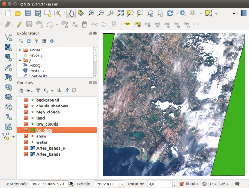
Figure 2.5: No-data areas are automatically computed
This no-data layer is used to discard the areas under it, be it for the classification, or if the
user add samples in these areas by mistake.
2.4.5 Step 3
It is now time to edit the masks layers. For each class (land,low clouds, etc), edit the corre-
sponding layer. Add the points that you want to take as samples, by clicking on the image and
pressing Enter for each point. We have found more efficient to use points rather than polygons,
we later dilate the points by 3 pixels assuming the neighbourhood is homogeneous in terms of
class, so you should avoid to use a pixel just at the edge of a feature (cloud,land).
The high clouds can be visible with the 1375nm band (i.e. the band number 4 of the heavy
.tif). You can load the style heavy_tif_clouds_green_style.qml to see them quickly.
The figure 2.6 shows the image with the high clouds highlighted, and the steps to add points.
14
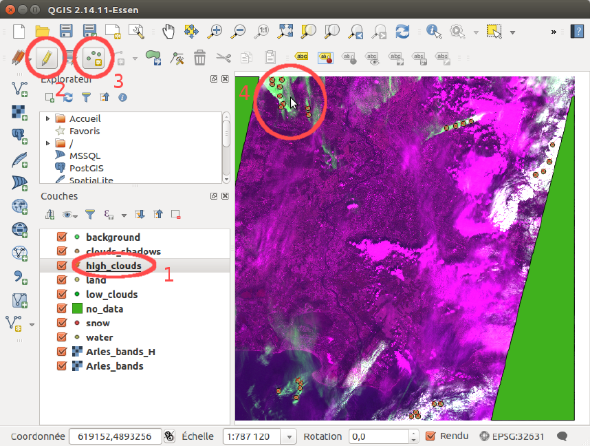
Figure 2.6: Steps to add data points with QGIS
Note: the 1375nm band is not to be trusted blindly. The principle of this band is that the
water vapour in the atmosphere usually absorbs the photons in this wavelength. However, in
dry conditions, or with high altitudes terrains (such as mountains), the photons can be reflected
back. This can be misleading, so the user should take precautions. A typical way to detect such
artefacts is to see if the potential cirrus shape is strongly correlated with that of the underlying
terrain.
You can now go back to true colors, and continue by editing all the wanted classes. The
background class can be used if you do not want to discriminate between land and water for
example, but its use is not recommended.
At the end, you obtain figure 2.7
15
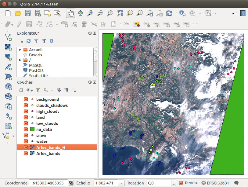
Figure 2.7: Samples placed manually after the first iteration
2.4.6 Step 4
Now, copy back the edited masks to the distant machine, or skip this if you work on one machine.
It is time to train the model, and classify the image! Do it with
python a ll_run_alcd . py −f True −s 1
The results can be seen in the Out directory. The regularized classification map is labeled_
img_regular.tif. You can also see the contingency table in the Statistics directory.
As you can see on the classification map, figure 2.8, some pixels are not well classified.
Moreover, the confidence is low in numerous places, as seen on figure 2.9 (more information
about it in part 2.4.9). Therefore, we will take part of the advantage of this program: the active
learning.
16
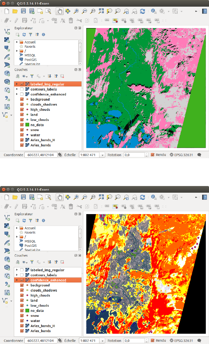
Figure 2.8: Result of the first classification
Figure 2.9: Confidence map of the first classification
2.4.7 Step 5
Do an new iteration, by running
17

python a ll_run_alcd . py −f Fal s e −s 0
It will save the previous iteration, and you can now edit the class layers, by adding new
points (and also remove some if you made an error previously). You can copy on your local
machine the outputs of the previous iteration (the bash command is given when you run the
command above).
We suggest to open the files Out/contours_labels.tif and Out/labeled_img_regular.
tif, and to apply to them the contours_labeled_contrasted_style.qml and the labeled_
img_regular_style.qml styles respectively. It gives each class a recognisable color, which are
given in table 2.1.
Color for the Color for the Class # Class name
classification contours
0 null value
1 background
2 low clouds
3 high clouds
4 clouds shadows
Transparent 5 land
6 water
7 snow
Table 2.1: Available classes and colors
For example, you can display the contours of the classes to see were the classifier was wrong.
Here, we obtained a false detection of clouds shadows on the left of the image, which can be
seen with the yellow contours:
18
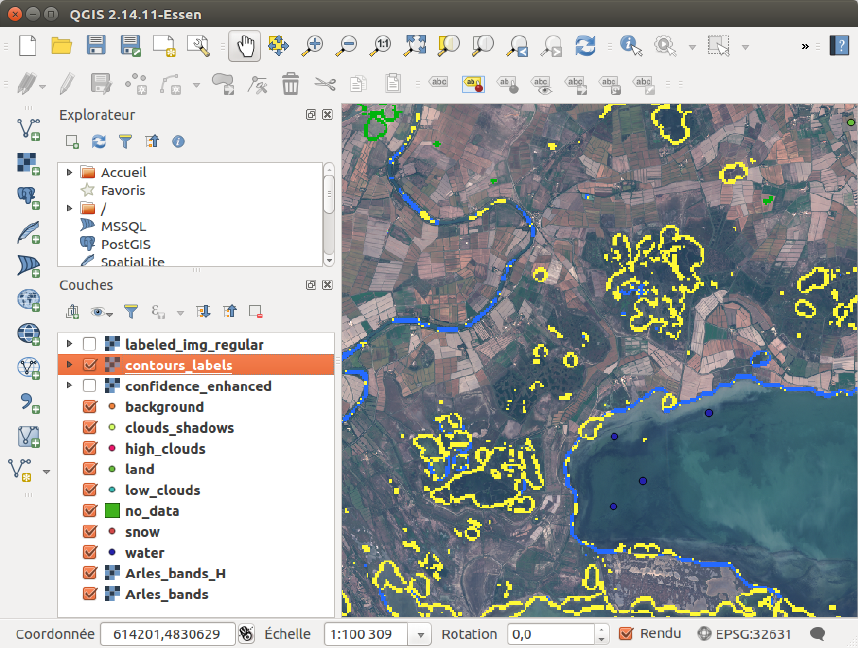
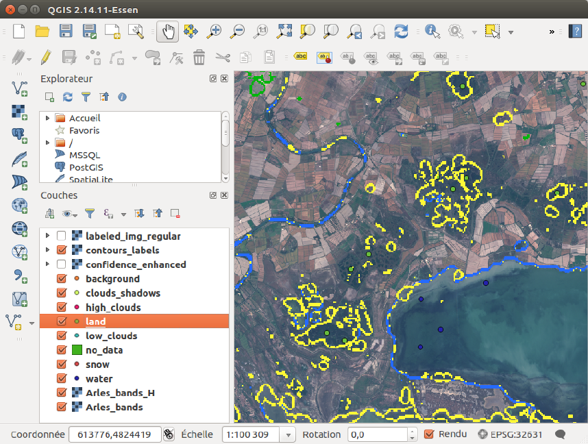
Figure 2.11: Some land samples are added where the wrong classification is visible
Do this for the areas where a misclassification is visible.
Once the wanted points in each class have been added, you can copy back the layers to the
distant machine with the appropriate command.
Finally, you run once again the training and the classification with
python a ll_run_alcd . py −f Fal s e −s 1
2.4.8 Step 6
Repeat the Step 5 until you are satisfied with the classification the ALCD algorithm returns.
Quick tip: some data (30% by default) are used for the validation of the model, i.e. just
to compute statistics. If you want to have more samples that you add manually to be taken
into account for the training part, you can increase the training_proportion in the global_
parameters.json.
Here is an example of the classification that you could obtain after each iteration. The 6th
one is considered to be good (by myself), so you can stop there.
20
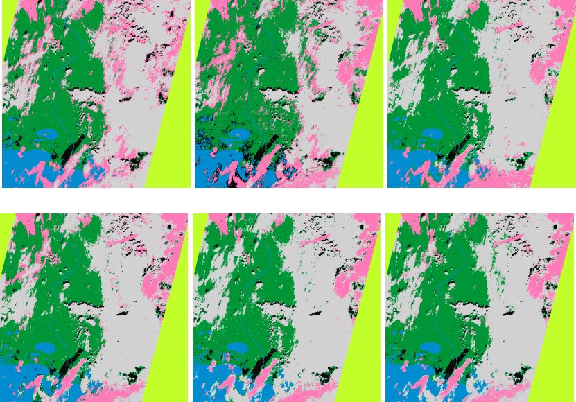
(a) Iteration 1 (b) Iteration 2 (c) Iteration 3
(d) Iteration 4 (e) Iteration 5 (f) Iteration 6
Figure 2.12: Evolution of the classification
As a reference, the QGIS windows at the last iteration with all the samples, with the labeled
classification, and with the confidence map, are given in figures 2.13, 2.14 and 2.15.
21
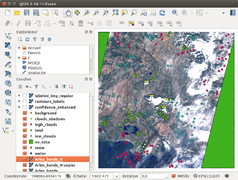
Figure 2.13: All samples present for the last iteration
22

Figure 2.14: Labeled classification as seen in QGIS window for the last iteration
23
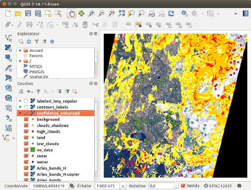
Figure 2.15: Confidence map as seen in QGIS for the last iteration
2.4.9 Tips and advice
Here are some advice that you could consider to achieve a better and faster classification.
A. Samples positioning
If you want to achieve a great classification, a good thing to do is to have a wide variety
of samples. This means samples that are well distributed spatially (do not take all your
samples in a radius of 1km), but also from a feature point of view, especially for the land
class. If your image contains grass, forests, sand and mountains, place samples on all these
classes, and not just on the grass one. For the low clouds and the high clouds classes, put
samples on the centre of the clouds, but also where they are thin. For the clouds shadows,
select shadows over the land, over the water, and so on.
B. Proportion between classes
It is a good practice to keep a balanced number of samples between classes. Therefore,
you should try not to put 10 times more land samples than water ones, or vice versa. It
is sometimes difficult to find enough samples that are well distributed spatially (see point
above), especially for water and snow. In this case, you can add points not far apart, so
as to increase their number, even if it could lead to redundant information.
C. Confidence map
Generally speaking, the user wants to add relevant points at each iteration. The rec-
ommendation is to check on the files Out/contours_labels.tif and Out/labeled_img_
regular.tif if the classification seems correct.
24
However, the confidence map is also provided. It allows to see where the classifier experi-
ences difficulties to make a clear choice between two classes. For the Random Forest (the
default classifier), the confidence of a pixel is the proportion of votes for the majority class.
For other classifiers, see the OTB Cookbook 1. The confidence map has values between 0
and 1, 1 being the best confidence. The user will therefore try to add samples in the low
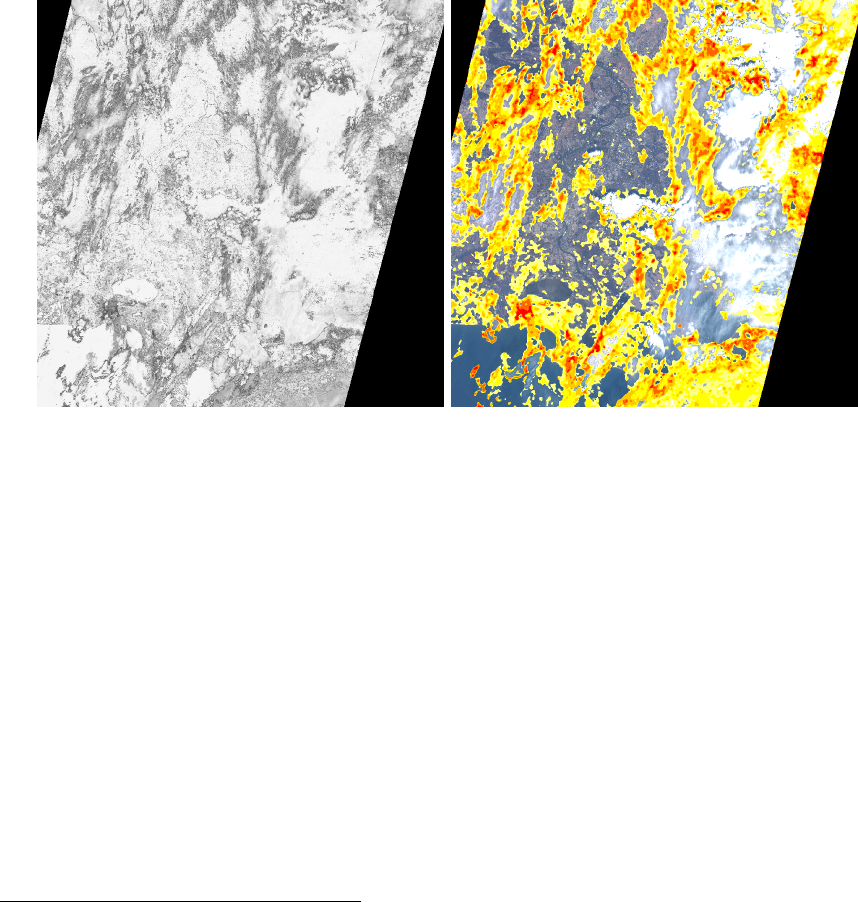
confidence zones. The original confidence map can be a bit difficult to read at first, mostly
due to the fact that isolated pixels of low confidence are often hard to classify even for a
human observer. Therefore, a modified confidence map is provided, consisting of zones of
low confidence, rather than pixels. To do so, a median filter is simply applied to the orig-
inal confidence map. The result are given in figure 2.16. To obtain the same result, apply
the style confidence_enhanced_style.qml on the Out/confidence_enhanced.tif file.
Warning: is it important to note that a high confidence does not imply a good classification.
Therefore, the classification should be checked visually first. However, a low confidence
often implies a bad classification, or at least an unstable one.
(a) Initial Confidence map (b) Modified Confidence map
Figure 2.16: Enhancement of the confidence map
2.4.10 Complementary information
Some information about the performed classification can be retrieved.
A. Samples and confidence evolutions
You can run the confidence_map_exploitation.py easily with
python co nfide nce _m ap_ ex plo ita ti on . py
It will generates two files in the Statistics directory.
The first one is the evolution of samples you manually placed at each iteration (example in
figure 2.17). As you can see here, the evolution is almost linear, and it is a good practice
to follow to obtain quick results. Of course, in some difficult cases, the last iterations will
have less added points, to finely tune the classification.
1https://www.orfeo-toolbox.org/CookBook/Applications/app_TrainVectorClassifier.html
25
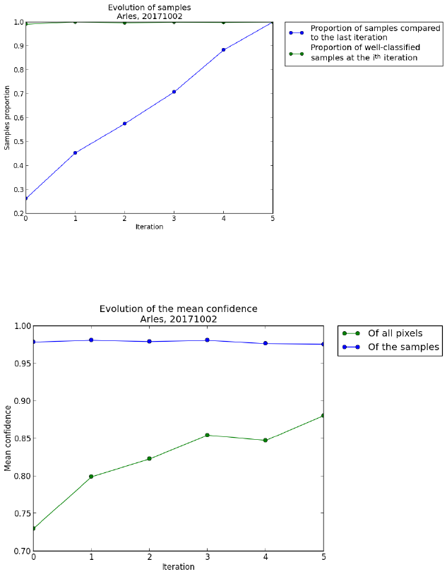
The second one is the confidence evolution. The mean confidence of all the pixels should
generally increase. The confidence of the samples you placed will probably slightly de-
crease, as you will place more difficult points at each iteration.
Figure 2.17
Figure 2.18
B. K-fold cross-validation
At any point, you can perform a K-fold cross-validation with the samples you placed, by
running
python a ll_run_alcd . py −ff a l s e −s 0 −kfold true
Go to the Statistics directory to see the result, notably the k_fold_summary.json file,
or the more eloquent kfold_metrics.png figure, an example of which is shown in figure
2.19. To have a stable classification, the four scores should be as close to 1 as possible,
for each fold.
26
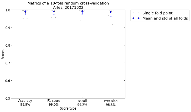
Figure 2.19
27
3 Processing Chains Comparator (PCC)
This part deals with the utilisation of the PCC code. In the following, PC stands for Processing
Chain, i.e. MAJA, Sen2Cor or Fmask.
3.1 Data organisation
For the input data, refer to the section 1.4.2.
The output structure of the code is the following, for a given location and date:
location and date dir : main directory; e.g. Arles_31TFJ_20171002
Binary_classif : conversion of the masks to binary classification
Binary_difference : binary difference between a reference mask and a PC mask
ALCD_dilated : the reference mask is with the dilation of the cloud masks
ALCD_initial : the reference mask is the initial ALCD output
Intermediate : intermediate files needed for the PCC to run smoothly
Multi_classif : conversion of the masks to multi-class classification
Multi_difference : multi-class difference between a reference mask and a PC mask
ALCD_dilated : the reference mask is with the dilation of the cloud masks
ALCD_initial : the reference mask is the initial ALCD output
Original_data : contains the original masks of the different PC
Out : png conversion of the binary differences and quicklook of the site
Statistics : various statistics such as the metrics about the binary differences
3.2 Configuration file
Some parameters can be tweaked in the configuration files (located in the parameters_files
directory).
•In the comparison_parameters.json, the different parameters are described below. There
should be no need to change them, as it is mostly definitions for the output
names. Exception is made for the ones with an ∗.
general : parameters regarding the output names of the ALCD code. They should be the
same as the ones in root_dir/ALCD/parameters_files/global_parameters.json
processing : various definitions for the different processing chains.
automatically_generated : references to the specific case you are working on. This
will be modified when running PCC, so you do not need (and should not) change it
manually
∗alcd_output dilatation_radius_meters : the radius, in meters, for the dilatation
of the clouds masks in the Dilate mode. See 3.4.
erosion_radius_meters : the radius, in meters, for the erosion of the clouds
masks in the Erode mode. See 3.4.
28

labeled_img_name : should be the output name of the ALCD program.
resolution : the output resolution, in meters.
maja_parameters : name of the MAJA sub directory and the MAJA version. They
are automatically changed when running the code, so you should not modify them
here.
3.3 Code workflow and overview
The PCC framework is mostly a comparator of georeferenced data. Therefore, its main steps
are to convert the data such that they can be compared, and then to compare them.
3.3.1 Equivalences between processing chains outputs
First, the framework converts the outputs of the different processing chains to a standard format,
namely that of ALCD, i.e. it changes the class numbers or flags of the original program output
to the ALCD standard. The equivalence between the original classes and the ALCD ones is
given in the following.
It should be noted that this conversion is necessary so as to produce a multi-class classifi-
cation, and not just a valid / not-valid one. However, the interpretation and the philosophy
of each program being different, one could argue about the pertinence of the equivalences. For
example, should a pixel labeled as ’cloud_low_probability’ by Sen2Cor translate into a land or
a low cloud class? Luckily, one can change them directly in the code.
A. Sen2Cor and ALCD equivalence
For Sen2Cor, a direct conversion can be applied between the classes, as shown in table
3.1.
ALCD Sen2Cor
Label Classification Label Classification
0 null value 0 NO_DATA
0 null value 1 SATURATED_OR_DEFECTIVE
5 land 2 DARK_AREA_PIXELS
4 clouds shadows 3 CLOUD_SHADOWS
5 land 4 VEGETATION
5 land 5 BARE_SOILS
6 water 6 WATER
5 land 7 CLOUD_LOW_PROBABILITY
2 low clouds 8 CLOUD_MEDIUM_PROBABILITY
2 low clouds 9 CLOUD_HIGH_PROBABILITY
3 high clouds 10 THIN_CIRRUS
7 snow 11 SNOW
Table 3.1: Sen2cor equivalence
B. MAJA and ALCD equivalence
MAJA works with a flag system. Therefore, one pixel can be flagged in different categories,
for example in ALL CLOUDS and in CIRRUS. Each flag is encoded on one bit. The
description of each bit can be found in the MAJA ATBD 2. Therefore, to have a direct
2MAJA’s ATBD, O Hagolle, M. Huc, C. Desjardins; S. Auer; R. Richter, https://doi.org/10.5281/zenodo.
1209633
29

relation between the MAJA and the ALCD output, each class corresponds to a set of
valid and invalid bits. Moreover, two files produced by MAJA are actually used: a Cloud
mask (thereafter referred to as C) and a Geophysical mask (thereafter referred to as G).
The classification conversion is based on both. The condition C5 means that the 5th bit
of the Cloud mask is 1. The combination C1 ∧¬ G6 means that the 1st bit of the cloud
mask is 1, and the 6th bit of the Geophysical mask is 0. The summary is in table 3.2.
To make it clearer, the condition ’this pixel is cloudy’ is noted C_any. It is formally
noted: C_any = (C1 ∨C2 ∨C3 ∨C4 ∨C5 ∨C6 ∨C7 ∨C8)
ALCD MAJA
Label Classification Bits logic rules
0 null value If it belongs to no other class
1 background Not available
2 low clouds (C5 ∨C6 ∨C7) ∧¬ (C8)
3 high clouds C8
4 clouds shadows (C3 ∨C4) ∧¬ (C5 ∨C6 ∨C7 ∨C8)
5 land ¬C_any ∧ ¬ (G6 ∨G7)
6 water ¬C_any ∧G1
7 snow ¬C_any ∧G6
Table 3.2: MAJA equivalence
C. Fmask and ALCD equivalence
Fmask equivalence is pretty straight-forward. However, it does not make the difference
between the low clouds and the high clouds classes.
ALCD Fmask
Label Classification Label Classification
0 null value 0 null value
5 land 1 clear land
2 low clouds 2 cloud
4 clouds shadows 3 cloud shadow
7 snow 4 snow
6 water 5 water
Table 3.3: Fmask equivalence
D. Multiclass and binary-class equivalence
As seen above, the different programs do not make the same distinction between the
classes. To alleviate this problem, and make a fair comparison, the multiclass classification
can be transformed into a binary classification.
The standard ALCD multi-class equivalence to the binary classification is in table 3.4.
30

ALCD multiclass classification Binary classification
Label Classification Label Classification
0 null value 0 null value
1 background 1 background
2 low clouds 2 cloud
3 high clouds 2 cloud
4 clouds shadows 2 cloud
5 land 1 background
6 water 1 background
7 snow 1 background
Table 3.4: Multiclass and binary classification equivalence
3.3.2 Comparison between the masks
Once the chain masks are converted, it is possible to compare them to the ALCD output. Two
modes are available: the multiclass and the binary-class classification.
Each of them is performed (firstly the multiclass, and then the binary one). The multiclass
difference returns poor results in most of the cases, and for every chain. This is due to the fact
that there is not a bijective relation for the various equivalence, as seen in 3.3.1. Therefore,
statistics (Statistics directory) and quicklook of the differences (in the Out directory) are
only computed for the binary difference. However, the multiclass differences GeoTIFF can be
found in the Multi_difference directory.
3.3.3 Flowchart
The summary of the flowchart is given in figure 3.1, with the legend from the figure 2.1.
31
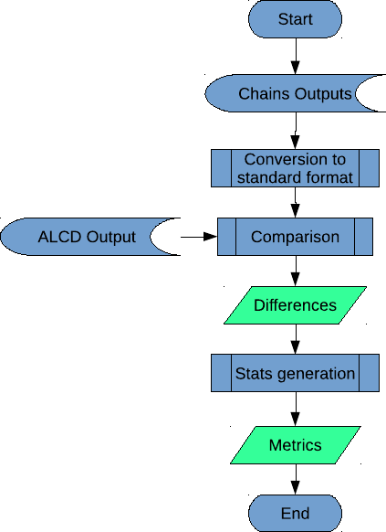
Figure 3.1: PCC flowchart
3.4 Possible variations for the comparison
The traditional way to compare is with the output of the ALCD framework. However, it is
possible to use different modes.
3.4.1 ALCD Original
The original, or ’initial’ mode. The chains can be compared to it on a multiclass and binary
classification fashion.
3.4.2 ALCD Dilation mode
The MAJA cloud mask being dilated, it can be interesting to see what the comparison would
be with the ALCD output being dilated as well. In this case, only the binary comparison makes
sense and is provided.
3.5 Tutorial
The Processing Chains Comparator is pretty straight-forward. We will use the output of the
ALCD code, and therefore use the classification of Arles previously obtained as a reference.
Change to the PCC directory. The program that you should use is all_run_pcc.py. You
can display the help with
python all_run_pcc . py −h
The available options are:
32
-l : the location. The spelling should be consistent with the names in the L1C directory
(e.g. Pretoria or Orleans)
-d : the (cloudy) date that you want to classify (e.g. 20180319)
-s : if you want to output your data to a sub-directory, add this option with a name, e.g.
MAJA_v3. This will put the results in Data_PCC/MAJA_v3/location_tile_date instead
of Data_PCC/location_tile_date. Useful to run multiple version of the same processing
chain and compare the results afterwards.
-m : if the masks from MAJA, Sen2Cor and Fmask have already been converted to a
standard format. If you ran the algorithm once, it should be the case. Thus, you can set
it to True to reduce the computation time
-r : which mode you want to set as a reference. It is a combination of the letter ’i’ (initial,
the original ALCD output) and ’d’ (for a dilation of the cloud masks). Can be ’i’ or ’id’
for example. Several letters will compare with each mode subsequently.
-b : if you only want the binary and not the multi-class comparison, you can set it to
True. It will save some computation time.
-mdir : the name of the MAJA natif output directory you want to use, e.g. MAJA_3_1_S2AS2B_HOT016.
See 1.4.2 to understand the MAJA data structure.
-mver : the version of MAJA you use, which has to be coherent with the -mdir option.
It is needed to automatically fetch the good files, and apply the suitable bits-to-class
equivalence
3.5.1 Step 1
Run the different processing chains on the original image. Their different outputs should be in
a structured way. At the moment, three chains are taken into account: MAJA, Sen2cor, Fmask.
The paths of the output should be well-defined in the root_dir/paths_configuration.
json. As a reminder, by default, the main paths for each chain are:
•L1C product root dir: /mnt/data/SENTINEL2/L1C_PDGS
•MAJA output root dir: /mnt/data/SENTINEL2/L2A_MAJA
•Sen2cor output root dir: /mnt/data/SENTINEL2/L2A_SEN2COR
•Fmask output root dir: /mnt/data/home/baetensl/Programs/Output_fmask
3.5.2 Step 2
Simply run the PCC code, with the command
python all_run_pcc . py −l Ar l e s −d 20171002
You now have the outputs in the Data_PCC directory.
33
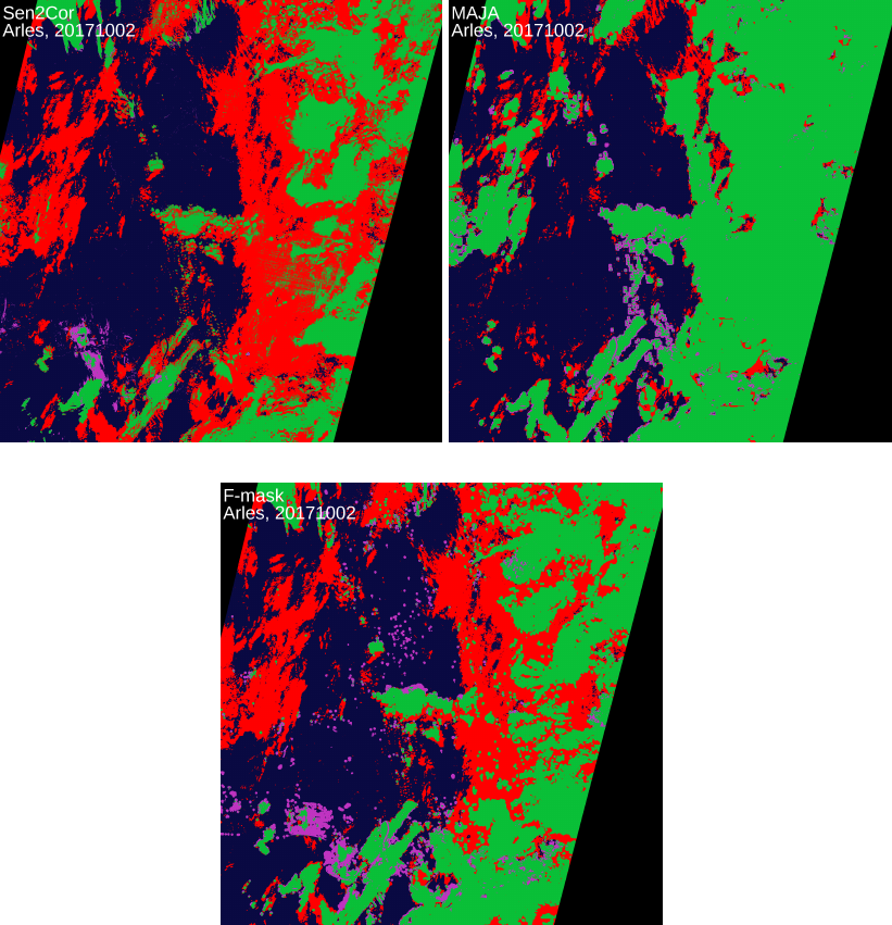
3.5.3 Step 3
You can now analyse the results. For example, in the Out/ALCD_initial directory, are the
quicklooks of the binary differences. You should obtain something along the lines of the figure
3.2. You can also open the GeoTIFF directly in QGIS, and apply the style color_tables/
diff_processes_style.qml to get the same results.
(a) Sen2Cor difference (b) MAJA difference
(c) Fmask difference
Figure 3.2
The legend is given in table 3.5.
34
Color Class # Class name Predicted class Actual class Meaning
0 null value - - -
1 True Positive cloud cloud Good cloud detection
2 False Negative ¬cloud cloud Cloud Sub-detection
3 False Positive cloud ¬cloud Cloud Over-detection
4 True Negative ¬cloud ¬cloud Good background detection
Table 3.5: Available classes and colors
Therefore, it is possible to visually see where the main difference are for each chain output.
From these results, statistics are computed.
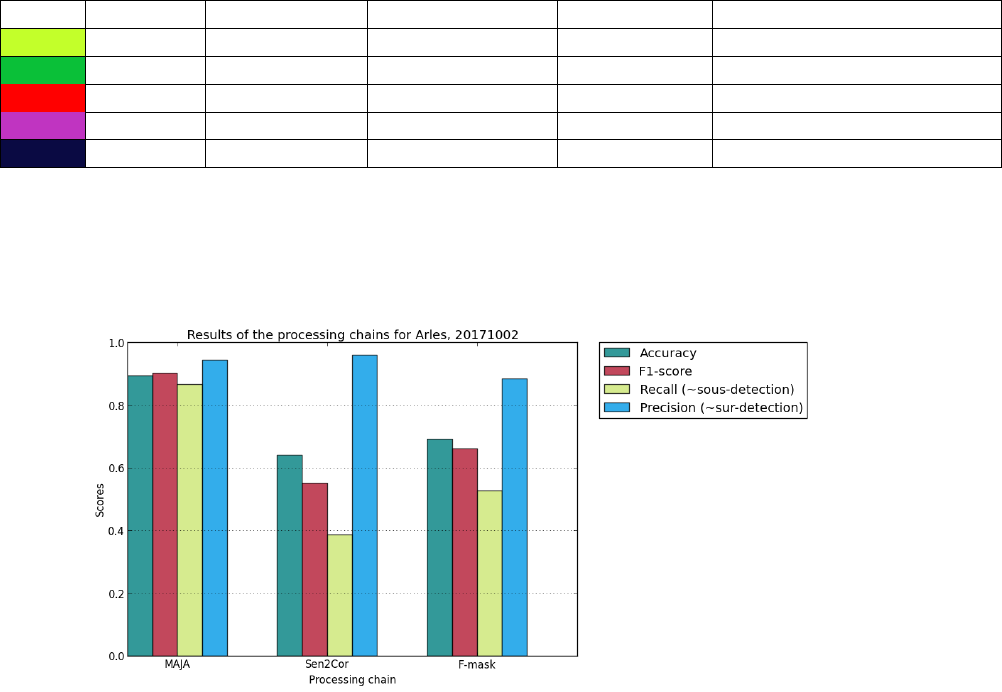
Figure 3.3: Statistics for each chain on Arles, 20171002
35
